Signal Reconstruction by Phase Retrieval and Optical Backpropagation in Phase-Diverse Photonic...

JOURNAL OF LIGHTWAVE TECHNOLOGY, VOL. 25, NO. 10, OCTOBER 2007 3017

Signal Reconstruction by Phase Retrieval and OpticalBackpropagation in Phase-Diverse Photonic

Time-Stretch SystemsJohan Stigwall and Sheila Galt

Abstract—The signal-to-noise ratio and bandwidth of photonictime-stretch (PTS) systems have previously been limited due to thenonlinear distortion caused by modulator response and dispersivepropagation. In this paper, we present a novel method for thereconstruction of the input signal from two phase-diverse intensitymeasurements. The method consists of optical phase retrieval atthe measurement point followed by simulated optical backpropa-gation to the modulation point. By numerical simulation of a PTSsystem with realistic parameters, we analyze the proposed methodand compare it with the previously suggested maximum ratiocombining (MRC) method. We show that the proposed opticalbackpropagation method, unlike the MRC method that treatsthe system as being linear from electrical input to output, canreconstruct the signal even at a large modulation depth and thatthe method is insensitive to biasing error or drift and not overlysensitive to misestimation of system parameters. Furthermore, toreduce the computational effort associated with the simulationof PTS systems, we present a numerical propagation methodwhereby the required number of sampling points is reduced byseveral orders of magnitude.

Index Terms—Analog-to-digital (A–D) conversion, fiber optics,microwave photonics, optical propagation in dispersive media,optical signal processing, photonic A–D converter, photonic sam-pling, time stretch.

I. INTRODUCTION

THE USE of extremely wide-band signals has increasedtremendously during the last decades. Not only has the

bit rate of digital communication links increased, but also, newwide-band techniques such as ultrawideband radio links andnoise radar have emerged. As the bandwidth increases, theproblem of analyzing the systems in the time domain gets moredelicate. In the case of periodic signals, it is possible to employequivalent time sampling techniques to perform time-resolvedultrawide-bandwidth measurements, but to analyze aperiodic ortransient signals, a truly real-time measurement is required.

Bridging the gap between continuous real-time digitization(tens of gigasamples per second, a few gigahertz bandwidth,and “unlimited” temporal window) and methods based on opti-

Manuscript received August 24, 2006; revised June 1, 2007. This workwas supported in part by the Chalmers Center for High-Speed Electronicsand Photonics (Swedish Foundation for Strategic Research, SSF) and by theSwedish Research Council.

The authors are with the Photonics Laboratory, Chalmers University ofTechnology, 412 96 Göteborg, Sweden (e-mail: [email protected];[email protected]).

Color versions of one or more of the figures in this paper are available onlineat http://ieeexplore.ieee.org.

Digital Object Identifier 10.1109/JLT.2007.905893

cal cross correlation or autocorrelation [1], [2] (tens of terahertzbandwidth, a few picosecond window), there is a group ofmethods that employ optical chirping and chromatic dispersionto stretch a signal in time prior to digitization. In direct analogyto how a convex lens creates a magnified image of an object,these methods use a quadratic phase temporal modulation (i.e.,a linear chirp) in place of the lens to magnify a short signalin time by carefully cascading chromatic dispersion, chirpmodulation, and more dispersion [3]–[6].

To simplify the setup when the input signal is electrical,systems analogous to free-space optical shadow projection havealso been studied [7]–[12]. In this case, the amplitude of astrongly prechirped optical pulse is modulated by the electricalsignal, which effectively creates a time-to-wavelength mappingso that the input signal can be measured directly from the wave-length spectrum of the optical pulse. One way of performing thespectral measurement is to temporally disperse the wavelengthspectrum by propagation through a dispersive medium, i.e., awavelength-to-time mapping. The output signal will then be atime-stretched copy of the input signal, and the method is thusoften referred to as “photonic time stretch” (PTS). A thoroughtreatment of such systems can be found in [9]. Equivalentsystems, but with optical input signals onto which the chirp isinduced electrooptically, have also been demonstrated [10].

Similar to how certain frequencies are “faded” in radio-over-fiber links due to chromatic group velocity dispersion, thereis also a fading effect in PTS systems. By using a single-electrode dual-output “phase-diverse” Mach–Zehnder modu-lator, it is, however, possible to obtain two time-stretchedsignals with complementary fading characteristics [11], [12].The question of how to retrieve the input signal from these twocomplementary measurements has, however, not been solvedin a manner that takes nonlinear distortion into account. Thisdistortion is caused by the sinusoidal modulator response aswell as the dispersive propagation itself. The latter is analogousto distortion due to diffraction in a free-space coherent shadowprojection magnifier, which is a result of the fact that coherentoptical propagation is not linear in optical intensity.

In this paper, we will show how the optical phase of thepulses at the measurement point can be retrieved from the twocomplementary phase-diverse measurements. Then, the inputsignal is recovered by numerical optical backward propagation(OBP) of the optical field back to the modulation point.

By numerical simulations, we demonstrate the effectivenessof the proposed signal retrieval method at large modulation

0733-8724/$25.00 © 2007 IEEE

3018 JOURNAL OF LIGHTWAVE TECHNOLOGY, VOL. 25, NO. 10, OCTOBER 2007

Fig. 1. Overview of a phase-diverse PTS system.

depths under the influence of measurement noise, relative in-tensity noise (RIN), and errors in modulator biasing, and in theestimation of system parameters. We also compare the proposedmethod with the previously published maximum ratio combin-ing (MRC) method [12], and under the condition that higher-order dispersion is minimized, we show how the numericalback-propagation can be carried out in a particularly efficientmanner.

II. BASIC PRINCIPLE OF OPERATION

The basic operation of a typical phase-diverse PTS systemis shown in Fig. 1. An electrical input signal is modulatedonto a chirped optical pulse using a single-electrode dual-outputMach–Zehnder modulator, which results in the two modulatedchirped pulses C1 and C2. Then, the pulses are stretched intime by chromatic group velocity dispersion and are finallydetected and digitized using a high-speed electronic real-timeoscilloscope at point D. As shown in the figure, the two outputsfrom the modulator can be combined into one single stretchfiber by delaying one of the outputs by half the pulse repetitionperiod ∆t/2 and then using the same detector and analog-to-digital converter (the stretch fiber is assumed to be muchlonger than the delay fiber). The reason for using a “phase-diverse” single-electrode “Z-cut” dual-output modulator is thatthe frequency-fading characteristics of the two channels arethen complementary.

Often, the initial chirped optical pulse [(B) in Fig. 1] is gen-erated by dispersing a very short nonchirped pulse (A) througha preceding spool of fiber. The stretch factor then equals thequotient of the total dispersion and the initial dispersion, i.e.,just like the magnification of an optical shadow equals thequotient of the distance from the light source to the screen andthe distance from the light source to the object.

The method proposed here for recovering the input sig-nal consists of two steps. First, the optical phase at themeasurement point (D) is calculated by comparing the twophase-diverse intensity measurements. Then, the optical field isnumerically propagated back to the phase modulation pointinside the Mach–Zehnder interferometer, where the input signalvoltage was directly proportional to the optical phase.

III. THEORY

A. Modulation

To achieve “phase diversity” between the two outputs of themodulator, we assume that a single-electrode Mach–Zehnder

modulator is used. The optical field at the output ports with amodulation voltage V is then [12]

AC1 = iAB

2

(exp

[i

(ϕ0 +

πV

Vπ

)]+ 1

)(1)

AC2 =AB

2

(exp

[i

(ϕ0 +

πV

Vπ

)]− 1

)(2)

where AB is the field incident to the modulator (point B inFig. 1), ϕ0 is the zero-voltage phase offset, and Vπ is the voltagethat corresponds to π radians of modulation. That is, the fieldat each output is a superposition of a constant background(i(AB/2) and −(AB/2), respectively) coming from the lightthat goes through the nonmodulated arm of the interferometerand of the modulated light going through the active arm. Tosimplify the notation, we make the substitutions A0 = AB/2and AM = (AB/2) exp[i(ϕ0 + (πV/Vπ))] as

AC1 = iA0 + iAM (3)

AC2 = −A0 +AM . (4)

B. Dispersive Propagation

In this paper, we assume that the power levels are low enoughthat nonlinear optical effects can be neglected, and we alsoneglect polarization mode dispersion since the propagation dis-tance is relatively short. Thus, the propagation operator is linearin optical complex amplitude, and using the notion of a slowlyvarying amplitude A(z, t) with a copropagating reference timeframe (t), we can write

A(z, t) = F−1 [F [A(0, t)]H(z,∆ω)] (5)

where F is the Fourier transform, z is the propagation distance,∆ω is the relative angular frequency, and H is the transferfunction for propagation, which can be expanded into [13]

H(z,∆ω) = exp(i

2β2z(∆ω)2 +

i

6β3z(∆ω)3 + · · ·

)(6)

which defines the group velocity dispersion parameter β2 andthe third-order dispersion parameter β3.

Note that although the optical system is assumed to belinear in optical amplitude, it is not assumed to be linear inoptical intensity or electrical amplitude. As we will see, thePTS system introduces substantial nonlinear distortion whenconsidering the whole system from the electrical input signalto the electrical detector output signal. In this paper, we willshow how the input signal can be retrieved from two phase-diverse nonlinearly distorted measurements by first calculatingthe phase at the measurement point and then numerically back-propagating the field using the expression above.

C. Chirp-Free Equivalent Distance Propagation

An issue when performing numerical simulations of PTSsystems is that the optical bandwidth can be very large due tothe strong chirping (several terahertz), which necessitates a high

STIGWALL AND GALT: SIGNAL RECONSTRUCTION BY PHASE RETRIEVAL AND OPTICAL BACKPROPAGATION 3019

numerical temporal resolution. At the same time, the temporalwindow needs to be rather large at the measurement point toaccommodate the stretched signal (tens of nanoseconds), whichresults in a huge number of sampling points. However, the inputsignal usually has a bandwidth that is one or two orders ofmagnitude smaller than the optical bandwidth.

In this section, we will show that the propagation of amodulated strongly chirped pulse over a long distance z isequivalent to the propagation of a nonchirped pulse with thesame modulation over a shorter distance z′. Using this method,the numerical temporal resolution can be chosen to just resolvethe input signal. Also, the nonchirped pulse will fit perfectlyinto the numerical window both before and after propagationsince it does not significantly broaden during the propagation.So, instead of high numerical temporal resolution and a largetemporal window, one can use lower resolution and a smallwindow. Hence, compared to direct simulation over the full op-tical chirp bandwidth, the number of required sampling pointsis reduced by the square of the ratio between signal and opticalbandwidths when chirp-free equivalent distance propagation isused.

It is a well-known fact that narrow-band dispersive propa-gation and paraxial diffractive propagation result in identicalmathematical equations [3]. We will start by rewriting theFresnel approximation equation for the paraxial diffractivepropagation found in [14, Sec. 4.2] to its narrow-band disper-sion equivalent. In its one-dimensional diffractive form, it iswritten as

U(x)=ejkzz

√jλzz

ejkx2z x2

∞∫−∞

{U(ξ)ej

kx2z ξ2

}e−j 2π

λzz xξdξ (7)

where U(ξ) is the initial field phasor distribution at z = 0,and U(x) is the field in a parallel plane at distance z. Whenrewriting this equation into its narrow-band dispersion equiv-alent, we will first substitute the spatial dimension x for thetemporal dimension t having a reference frame copropagatingwith the pulse. Corresponding to ξ in (7), we will use τ forthe time variable of the initial pulse. The propagation distancevariable z is kept as a spatial dimension, so the value of k willbe unchanged in the z-direction. However, the lateral k-numberhas to be exchanged into its temporally dispersive counterpartin accordance with [3]

kx ⇔ −1/d2β

dω2= − 1

β2. (8)

By making these substitutions, we end up with the followingequation for the Fresnel-approximated propagation of narrow-band pulses in linearly dispersive media:

U(t) =ejkzz− j

2zβ2t2

√jλzz

∞∫−∞

{U(τ)e

−j2zβ2

τ2}e−j 2π

λzz tτdτ. (9)

It is assumed that the propagation distance in the PTS systemis large enough for the Fresnel approximation to be valid. In

fact, the propagation distance in such a system is usually largeenough to be in the Fraunhofer region (the far field), where theterm e(−j/2zβ2)τ

2can be neglected, and the propagated field

is simply the Fourier transform of the initial field. We will,however, still use the Fresnel approximation for now since,as we will soon see, the far-field propagation of the chirpedmodulated pulse is equivalent to a near-field propagation of anonchirped modulated pulse.

We will assume the initial pulse to be composed of a chirpterm with chirp rate ∂ω/∂t and a more slowly varying termI(τ), i.e.,

U(τ) = I(τ)e−j2

∂ω∂τ τ2

. (10)

Putting this into (9), we get

U(t) =ejkzz− j

2zβ2t2

√jλzz

∞∫−∞

{I(τ)e−

j2

∂ω∂τ τ2

e−j

2zβ2τ2

}e−j 2π

λzz tτdτ

(11)

and if we make the substitutions

z′ = z(

1 + zβ2∂ω

∂τ

)−1(12)

t′ = t(

1 + zβ2∂ω

∂τ

)−1(13)

it becomes

U(t) =ejkzz− j

2zβ2t2

√jλzz

∞∫−∞

{I(τ)e−j 1

2z′β2τ2}

e−j 2π

λzz′ t′τdτ

(14)

where the factors before the integral do not affect the intensityenvelope of U(t), apart from a distance-dependent attenuation.The integral part is now identical to the one in the originalpropagation equation (9), so the propagation of a pulse withlinear frequency chirp ∂ω/∂τ and modulation I(τ) is appar-ently equivalent to the propagation of a nonchirped pulse withthe same modulation but to an effective distance z′ = z/M andwith a time stretch ofM = t/t′ = 1 + zβ2(∂ω/∂τ).

If the linear chirp is prepared by dispersing an ultrashortpulse through a preceding fiber length z0, then the chirp will be∂ω/∂τ = 1/z0β2 (assuming that z0β2 is large compared to thesquare of the initial pulse length) [13], and M = 1 + z/z0 =(z + z0)/z0.

Note that the analogy between free-space diffraction andnarrow-band dispersion is only valid in a system with no higher-order dispersion (i.e., pure β2 dispersion). Since the opticalbandwidth can be large in a PTS system, this implies thatβ3-compensating fibers or custom-made chirped fibergratings may have to be employed. For instance, a dispersion-compensating fiber could be combined with a dispersion-shifted fiber to obtain a strong negative dispersion and zerodispersion slope. As will be shown in Section V-E, a fairamount of higher order dispersion can actually be handled bythe chirp-free equivalent distance propagation method. If avery strong higher-order dispersion cannot be avoided, it is still


possible to use the signal retrieval method presented in thispaper but then without the benefit of the chirp-free equivalentdistance propagation method.

In the following numerical simulations, we will use the chirp-free equivalent distance method and simply perform the propa-gation as in (5) but with a nonchirped initial pulse and over thedistance z′. It is also assumed that all higher-order dispersionterms are zero, but by studying the effect of a misestimatedβ2, we will also deduce the limits on higher-order dispersion.With the same parameters as in the following simulations, wehave compared the chirp-free equivalent distance propagationmethod with a full optical bandwidth propagation accordingto (6). The relative deviation in optical intensity was less than10−6, even at 100% modulation depth and a signal frequencyabove the first fading frequencies.

D. Phase and Signal Retrieval

The optical field at the detector can be written as a superpo-sition of the propagated A0 and AM fields as

AD1 = iF−1 [F [A0]H] + iF−1 [F [AM ]H]

= i(P0 + PM ) (15)

AD2 = −F−1 [F [A0]H] + F−1 [F [AM ]H]

= −(P0 − PM ) (16)

whereH = H(L,∆ω) to simplify the notation, and P0 and PM

are the propagated A0 and AM fields. Since the absolute phasecannot be measured, we will ignore the constant factors i and−1 in the following calculations.

Now, with measured intensities ID1 = |AD1 |2 and ID2 =|AD2 |2, and with the full complex P0 known a priori, we willcalculate PM and then propagate it back to the modulationpoint to get the phase of AM , which is assumed to be directlyproportional to the input signal voltage (it has been shown thatelectrooptical phase modulators have excellent linearity [15]).In an experiment, the magnitude of P0 is easily measured, andusing the chirp-free equivalent distance propagation methoddescribed above, the phase of P0 can be approximated as beingconstant.

The magnitude and phase of PM relative to P0 are given bysolving

ID1 = |P0|2 + |PM |2 + 2|P0||PM | cos(ϕP ) (17)

ID2 = |P0|2 + |PM |2 − 2|P0||PM | cos(ϕP ) (18)

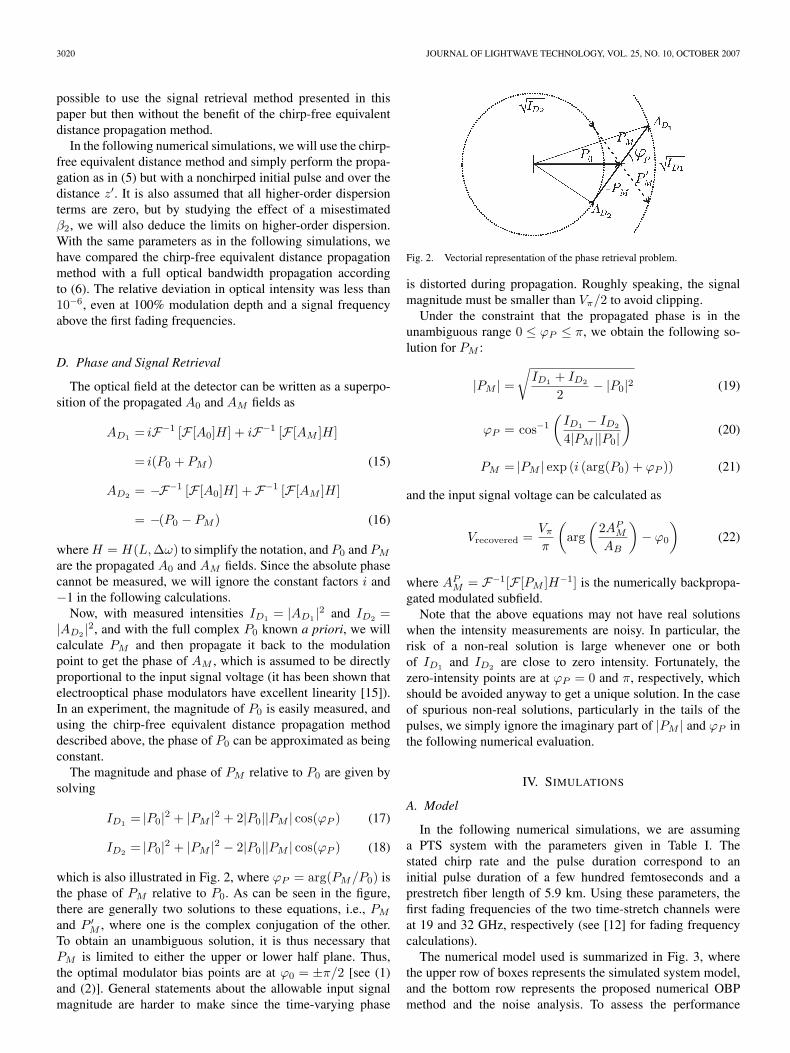
which is also illustrated in Fig. 2, where ϕP = arg(PM/P0) isthe phase of PM relative to P0. As can be seen in the figure,there are generally two solutions to these equations, i.e., PM

and P ′M , where one is the complex conjugation of the other.

To obtain an unambiguous solution, it is thus necessary thatPM is limited to either the upper or lower half plane. Thus,the optimal modulator bias points are at ϕ0 = ±π/2 [see (1)and (2)]. General statements about the allowable input signalmagnitude are harder to make since the time-varying phase

Fig. 2. Vectorial representation of the phase retrieval problem.

is distorted during propagation. Roughly speaking, the signalmagnitude must be smaller than Vπ/2 to avoid clipping.

Under the constraint that the propagated phase is in theunambiguous range 0 ≤ ϕP ≤ π, we obtain the following so-lution for PM :

|PM | =

√ID1 + ID2

2− |P0|2 (19)

ϕP = cos−1(ID1 − ID2

4|PM ||P0|

)(20)

PM = |PM | exp (i (arg(P0) + ϕP )) (21)

and the input signal voltage can be calculated as

Vrecovered =Vπ

π

(arg

(2AP

M

AB

)− ϕ0

)(22)

where APM = F−1[F [PM ]H−1] is the numerically backpropa-

gated modulated subfield.Note that the above equations may not have real solutions

when the intensity measurements are noisy. In particular, therisk of a non-real solution is large whenever one or bothof ID1 and ID2 are close to zero intensity. Fortunately, thezero-intensity points are at ϕP = 0 and π, respectively, whichshould be avoided anyway to get a unique solution. In the caseof spurious non-real solutions, particularly in the tails of thepulses, we simply ignore the imaginary part of |PM | and ϕP inthe following numerical evaluation.

IV. SIMULATIONS

A. Model

In the following numerical simulations, we are assuminga PTS system with the parameters given in Table I. Thestated chirp rate and the pulse duration correspond to aninitial pulse duration of a few hundred femtoseconds and aprestretch fiber length of 5.9 km. Using these parameters, thefirst fading frequencies of the two time-stretch channels wereat 19 and 32 GHz, respectively (see [12] for fading frequencycalculations).

The numerical model used is summarized in Fig. 3, wherethe upper row of boxes represents the simulated system model,and the bottom row represents the proposed numerical OBPmethod and the noise analysis. To assess the performance


TABLE ISYSTEM PARAMETERS

Fig. 3. Simulation model.

of the proposed method, we simulate the system using anonreturn-to-zero (NRZ) binary random bit sequence (RBS) atdata rates of 25, 50, and 100 Gb/s as the input signal (middleleft box in Fig. 3). This input signal was used since it is wideband yet has well-known properties, and by using a randombinary data stream as the input signal in a real experiment, itwill be possible to tweak the estimated z′ by comparing theeye diagram from the PTS system with the one recorded bya sampling oscilloscope. In our simulations, we also use eyediagrams to provide an intuitive way of assessing the distortionscaused by the PTS system.

The optical pulse incident to the modulator was a super-Gaussian with exponent eight and a constant chirp rate of−1.25 GHz/ps. The spectrum of the RBS input signal wasfurther shaped by a Gaussian filter with 1/e intensity point at50 GHz, and “zeros” and “ones” were encoded symmetricallyaround zero voltage as −V and +V volts, respectively.

The chirp rate of the pulse determined the chirp-free equiva-lent propagation distance (Section III-C) was

z′ = L/M = 5.3 km (23)

and the chirp-free pulse envelope was

AB(t) = exp

[−1

2

(t

TB

)8]

[V] (24)

where TB = FWHMB(ln(2))−1/8.This pulse was modulated into two phase-diverse ports ac-

cording to (1) and (2) and then propagated to the measurementpoint using the chirp-free equivalent distance method. Then, thesignals were converted into the electrical domain by taking theabsolute squared optical amplitude. Following the addition ofsimulated measurement noise and low-pass filtering to simulate

the finite bandwidth of the receiver, we retrieved the opticalphase from the two simulated intensity measurements accord-ing to the proposed method (19)–(21). Finally, the optical fieldwas numerically propagated back to the modulation point, andthe input signal voltage was recovered according to (22).

In our model, the correlated noise was simulated by theaddition of a RIN component to the optical pulse before themodulator, and the uncorrelated noise was simulated by addingindependent noise to the two detector signals. Both types ofnoise sources were normally distributed (in amplitude) whitenoise that was low-pass filtered with a cutoff frequency of50 GHz. The spectral shape of the low-pass filter was super-Gaussian with exponent of 16.

B. Analysis

The main analysis consisted of a set of Monte-Carlo simu-lations carried out to obtain a statistical average of the randomnoise (correlated as well as uncorrelated) and distortion ratios,as well as the signal-to-noise ratio (SNR) and distortion ratioof the recovered signal (SINAD, [16]). These quantities wereanalyzed as functions of the modulation depth, noise level,deviation from ideal biasing point, and misestimation of stretchfiber dispersion.

As a comparison, the same analysis was also carried outusing two less complex signal processing methods. The firstmethod consisted of a balanced measurement Vbal = ID1 −ID2 , and the second method was the MRC method [12], wherethe input voltage was recovered from the measured opticalintensities as

VMRC = −F−1[F [ID1 ] cos

(φDIP − π

4

)+ F [ID2 ] cos

(φDIP +

π

4

)](25)

with φDIP = β2zω2/2M . The scaling factors of these two

methods were omitted since only the signal relative noise anddistortion levels were of interest and since SINAD is scalinginvariant [16].

The balanced detection and the MRC method are obviouslylinear in optical intensity (or equivalently in electrical voltage),and neglecting nonlinear effects, the MRC method is “ideal,”i.e., fully eliminating frequency fading [12]. Thus, we believethat the results achieved by the MRC method are representativefor all methods that treat the system as being linear in electricalamplitude. The proposed OBP method, on the other hand,is linear in optical complex amplitude but is nonlinear andhas “memory” in electrical amplitude. Consequently, the OBPmethod is able to recover the signal with higher accuracythan the two former methods, particularly at large modula-tion depth.

All SNR, SINAD, and similar power ratios in the followingrefer to electrical power and were calculated in the temporaldomain. DC offsets and constant scaling factors were com-pensated for, and only the central part containing 65% of thepulse energy was taken into account. Random noise and signaldistortions are included in SINAD, whereas the “measurement


SNR” measures the signal and distortion to random noise ratioat either of the two detectors.

When using the input signal as the reference for SINADcalculations, it was first low-pass filtered to avoid the inclusionof high-frequency roll-off as a signal distortion. The filter wasmatched to give the same frequency response as the filter usedto simulate the finite receiver bandwidth.

The number of symbols that fit into the analysis windowwas 16, 32, and 64 for data rates of 25, 50, and 100 Gb/s,respectively, and every data point in the following section wascalculated as an average from 100 random simulation runs.

V. RESULTS AND DISCUSSION

Eye diagrams from the simulations are shown in Fig. 4 for adirect time-domain comparison of the performance of the threemethods under study. The MRC method and the proposed OBPmethod are clearly able to retrieve the signal with high fidelityin the lower bit rate (25 Gb/s) and small modulation depth(V/Vπ = 1/20) simulation (subfigures a, c, and e). At this rate,the signal itself is not above the first fading frequencies, and theharmonics are weak thanks to the small modulation depth. At50 Gb/s and a modulation depth of V/Vπ = 1/8 (subfigures b,d, and f), there is, however, a considerable nonlinear distortionthat causes a reduction in the fidelity of the signal recovered us-ing the MRC method. The signal recovered using the proposedOBP method (f) is, however, still free of distortion and does notexhibit any amplification of random noise.

A. Measurement Noise

The impact of measurement noise was studied to see howrandom noise is affected by the application of the proposedmethod. Fig. 5 shows the recovered SINAD as a function ofmeasurement noise level in a simulation at 25-Gb/s data rateand a modulation depth of V/Vπ = 1/20. At this modulationdepth, the nonlinear signal distortion is still relatively small,and the maximum bit change frequency is 12.5 GHz, which islower than the fading frequencies of both channels. Therefore,it is still possible to use balanced detection with some success,with a maximum SINAD of around 9 dB. The MRC methodperforms considerably better but is limited to a SINAD of about28 dB due to nonlinear distortion.

Using the proposed OBP method, the SINAD of the retrievedsignal appears to be limited only by measurement noise at leastup to an SNR or SINAD of 60 dB (Fig. 5). Thanks to thefact that two measurements with independent noise componentsare made, there is even a 3-dB improvement over the mea-surement SNR, and as it seems, the method is “transparent”to the measurement noise level, i.e., the recovered SINAD isdirectly proportional to the measurement SNR. At very highmeasurement SNR, there is, however, a slight rolloff due todistortion (compare with Fig. 8). This rolloff vanishes whenlow-pass filtering is turned off in the simulations.

To study the effect of measurement noise at large modulationdepths, we separated the noise from nonrandom distortions byusing an identical but noise-free simulation as reference. Then,the resulting noise level was put in relation to the single mea-

Fig. 4. Simulated eye diagrams with a measurement SNR of 30 dB. Time ison the horizontal axis and recovered signal voltage on the vertical axis.

Fig. 5. SINAD as a function of measurement noise level at 25 Gb/s andV/Vπ = 1/20 using balanced detection (points), the MRC method (dia-monds), and the proposed OBP method (stars). The SINAD equals the mea-surement SNR on the dotted line.

surement noise level to determine if the noise was suppressedor amplified in the signal processing.

In Fig. 6, the gain (or suppression) in noise to signal-and-distortion ratio is shown as a function of modulation depth. Justas was observed in Fig. 5, the noise is suppressed by 3 dB atsmall modulation depths, but Fig. 6 also shows that there is anamplification of random noise at modulation depths of aboveV/Vπ ∼ 0.2. Furthermore, it can be seen in Fig. 6 that the gain


Fig. 6. Relative amplification of measurement noise as a function of modula-tion depth using balanced detection (points), the MRC method (diamonds), andthe proposed OBP method (stars) at three different measurement SNR levelsand a data rate of 50 Gb/s.

in random noise increases at higher measurement SNR but ata considerably slower rate than the increase in measurementSNR, i.e., it is still possible to improve the results by increasingthe measurement SNR.

It is no surprise that the random noise ratio is not affectedvery much by a change in modulation depth when using the twolinear methods, but it is interesting to see that balanced detec-tion only gives a ∼2-dB suppression while the MRC methodreaches ∼4 dB. When using balanced detection, this can beexplained by the fact that the signal cancels in frequency bandswhere the two channels are in-phase. For the MRC method, itis, however, more difficult to explain the improvement, but thefiltering of noise close to fading frequencies is very likely acontributing factor.

The OBP method was found to give very similar results at100 Gb/s below V/Vπ ∼ 0.2. At large modulation depth anda measurement SNR of 40 dB, the 100-Gb/s results were forsome reason slightly better than those at 50 Gb/s.

B. Common-Mode RIN

At low frequencies, it is clear that the phase-diverse setupprovides for a balanced measurement where the signal is out-of-phase while the common-mode RIN noise is in-phase so thatthe common-mode noise will be cancelled by subtraction of thetwo measured signals. The signal phase in a phase-diverse PTSsystem is, however, reversed at each fading frequency so thatthe two channels in some frequency bands are in-phase, whichcauses a coherent addition instead of cancellation of common-mode noise.

The results from a 50-Gb/s simulation run with no measure-ment noise and a premodulation RIN of −20 dB (measuredin the electrical domain) are shown in Fig. 7. Along withthe three studied signal processing methods, we have alsoplotted the single-channel noise ratio (dashed), which is directlycomparable to the measurement SNR in the previous section.

Since balanced detection does not compensate fordispersion-induced signal phase reversal, it also managesto cancel correlated noise throughout the whole spectrum. Thisresults in a noise ratio that does not depend on the modulation

Fig. 7. Common-mode noise to signal-and-distortion ratio for a fixed RINlevel of 20 dB using balanced detection (points), the MRC method (diamonds),and the proposed OBP method (stars) at a data rate of 50 Gb/s. The single-channel noise ratio is also shown for comparison (dashed).

depth (Fig. 7), and weak signals that are severely buried underRIN noise can thus be recovered thanks to the near-perfectnoise cancellation.

When using the more advanced methods that compensate forfading, common-mode noise is no longer cancelled in somefrequency bands. Thus, there is a strong increase in the rela-tive noise level as the modulation depth is reduced. However,comparing the results with those of the single-channel measure-ment, the OBP and MRC methods still suppress common-modeRIN by 8–9 dB up to a modulation depth of V/Vπ ∼ 0.18.

Further simulations show that a suppression of 8–9 dB ismaintained at lower noise levels but that the suppression isreduced at higher noise levels. The common-mode noise sup-pression at a RIN of −10 dB was reduced to ∼6 dB. Doublingthe data rate to 100 Gb/s resulted in less than 1-dB reduction innoise suppression.

C. Distortion Suppression

When the modulation depth (V/Vπ) is increased, so doesalso the strength of the high-frequency harmonics due to thesinusoidal modulator response and the nonlinear (in optical in-tensity) harmonic distortion caused by dispersive propagation.Thus, at large modulation depths, it is no longer possible toretrieve the optical phase perfectly since many overtones areattenuated in the receiver. After backpropagation, the lack ofthese overtones may also affect the signal at the fundamentalfrequencies.

Another effect that occurs when the modulation frequency ishigh is that the range of optical phases at the measurement pointis increased beyond the range imposed at the modulation point.At large modulation depths, the phase at the measurement pointmay thus occasionally exceed the 0 ≤ ϕP ≤ π bound that weestablished in Section III-D, which causes severe distortion ofthe recovered signal.

To test the ability of the proposed OBP method to suppressnonlinear distortion, we calculated the distortion-to-signal ratioby comparing the recovered signal in a noise-free simulationwith the input signal. The results are shown in Fig. 8, where


Fig. 8. Distortion-to-signal ratio as a function of modulation depth usingbalanced detection (points), the MRC method (diamonds), and the proposedOBP method (stars) at a data rate of 50 Gb/s.

this quantity is shown as a function of modulation depth fora data rate of 50 Gb/s. From these data, it is evident that thedistortion as compared to the MRC method is suppressed by atleast 25 dB up to a modulation depth of V/Vπ = 0.2.

Obviously, the amount of attenuated high-frequency har-monics and the risk of having phase values outside the range0 ≤ ϕP ≤ π increase with the input bandwidth. Simulations at100 Gb/s (not shown in figure) showed that there was a verysmall (less than 1 dB) reduction in distortion suppression whenusing the MRC method. The impact on the OBP method was,however, stronger—the distortion suppression was reduced by∼7 dB at 100 Gb/s, which makes the relative improvementover the MRC method 18 dB at V/Vπ = 0.2 and 24 dB atV/Vπ = 0.075.

D. Sensitivity to Misestimation of System Parameters

An error in the estimation of the stretch fiber dispersion orin the chirp rate of the incoming pulse will be manifested asan error in z′ when chirp-free equivalent distance propagationis used. From (12), we see that a change in z does not affectz′ very much when z is large. The chirp rate however affectsz′ more strongly in an inversely proportional manner. Thus,the tolerances on the initial chirp rate ∂ω/∂t or equivalentlythe prechirp fiber length z0 are much more narrow than thetolerances for the estimation of the stretch fiber length z. Forthe MRC method, the relative error in φDIP is equal to theerror in z′ since z′ = z/M , which is a factor in the expressionfor φDIP.

In Fig. 9, it is shown how the misestimation-induced distor-tion depends on the error in z′ for a set of modulation depthswith a 50-Gb/s input data stream. This distortion ratio wascalculated by using an identical simulation but with perfectlyestimated parameters as a reference.

The distortion increases with modulation depth as well aswith the error in z′, and the MRC and OBP methods followvery closely with about 1-dB less distortion when using theOBP method. As an example, an error margin below ±3% isrequired to keep the misestimation-induced distortion below

Fig. 9. Excessive distortion due to misestimation of z′ as a function of errorin z′ at 50 Gb/s and three different modulation depths using the MRC method(diamonds) and the OBP method (stars).

−40 dB. This should, however, be compared with the meanerror amplitude at 40-dB SINAD, which is only 1%.

At 100 Gb/s, the distortion is increased over the whole errorspectrum by ∼3 dB for both methods.

E. Impact of Higher-Order Dispersion

As shown in Fig. 4, in [9], or in the expression for thestretch factor M in Section III-C, higher order dispersiondoes not affect the stretch factor if dispersive elements withidentical dispersion characteristics are used for prechirp andtime-stretch dispersion. The dispersive distortion of the signal,however, depends strongly on the dispersion parameter. Thiscan be accounted for by including higher order dispersionin the simulation of optical backpropagation, but to be ableto use the numerically efficient chirp-free equivalent distancepropagation method (Section III-C), it is essential that higherorder dispersion be minimized.

The acceptable deviation in β2 can be deduced from Fig. 9,which shows the impact of a misestimated value of z′. z′ isapproximately inversely proportional to β2 when the stretchfactor is large, so the acceptable relative deviation in β2 issimilar to the relative deviation in z′ (around 3% at a distortionratio of −40 dB). To keep β2 within this limit at the edgesof the optical spectrum with a third-order dispersion termβ3 = dβ2/dω, we thus have

|β3| <2

2π∆ν|β2|δ

where δ is the acceptable relative deviation in β2, and ∆νis the spectral width of the optical pulses. In the exampleabove, ∆ν = 1.25 THz (10 nm), and β2 = −λ2D/2πc0 =21.7 · 10−26 s2/m, which gives |β3| < 5.52 · 10−39δ s3/m.Considering the standard single-mode fiber, which has β2 ofthe same magnitude but with opposite sign and a slope ofabout 0.09 ps/(km nm2), the third-order dispersion term isβSMF3 = 1.82 · 10−40 s3/m [13]. Thus, the deviation in β2

at the edge of the spectrum for the example above would be


Fig. 10. Excessive distortion due to bias offset error (relative to ϕ0 = π/2)using balanced detection (points), the MRC method (diamonds), and proposedOBP method (stars) at a data rate of 50 Gb/s.

δ < 1.8/55 ≈ 3% and would thus only be limiting if a SINADclose to 40 dB is required.

F. Biasing Error Sensitivity

Linear methods such as the MRC method rely on an exactbiasing of the modulator at ϕ0 = ±π/2, where second-orderdistortion is minimized. With a nonideal bias point causedby, for instance, the signal-induced heating of the modulatoror slow drifts in environmental temperature or humidity, thefidelity is drastically reduced, as shown in Fig. 10.

The OBP method, on the other hand, will simply carrythrough the bias offset as the dc component of the recoveredsignal. For small drifts, the offset can then be removed in thepostprocessing, but the measured bias offset could also be usedto stabilize a system with much larger phase drift online byadjusting the modulator bias voltage in a closed-loop setup.

The bias-error-induced distortion ratio was calculated bycomparing it with an identical simulation but with ideal biasingand is shown as a function of bias offset in Fig. 10. Thetwo simpler methods cause severe distortion, even at smallbias offset errors, but seem to be unaffected by a change inmodulation depth. Using the OBP method, the distortion ismuch smaller and is ∼40 dB below that of the MRC methodfor a modulation depth of V/Vπ = 0.1.

Compared with Fig. 8, it appears that the actual signaldistortion in many cases is stronger than the bias-error-induceddistortion both for the OBP and for the simpler methods. A∼7-dB increase in bias-error-induced distortion was observedfor the OBP method, and a ∼2-dB increase was observed forthe two simpler methods when the data rate was increasedto 100 Gb/s.

G. Impact of Nonideal Modulation

In deriving (1) and (2), it was assumed that the output couplerof the Mach–Zehnder interferometer is ideal. That is, the lightin the modulated and nonmodulated arms of the interferometercouple equally strongly to the two output ports, and the relativephase between the forward- and cross-coupled modulated lightrelative to the nonmodulated light differs by exactly π radians.

In Fig. 2, this means that the vectors “Pm” and “−Pm” are ofequal length and have opposite direction. If these constraintsare not met, (1) and (2) have to be altered. Assuming that thesecond port signal is first normalized with respect to |P0|2, wecan write

ID1 =|P0|2+|PM |2+2|P0||PM | cos(ϕP ) (26)

ID2 =|P0|2+c2m|PM |2−2cm|P0||PM | cos(ϕP +∆ϕ) (27)

where cm is a relative amplitude-coupling factor (from themodulated arm to the second port), and ∆ϕ is the deviationin relative phase from the ideal π radians. When ∆ϕ = 0, theequation system is still analytically solvable, and (19) and (20)should be replaced by

|PM |=

√ID1 + ID2/cmcm + 1

− 1cm

|P0|2 (28)

ϕP =cos−1(c2mID1−ID2 +(1−c2m)|P0|2

2cm(cm+1)|PM ||P0|

). (29)

If ∆ϕ = 0, numerical methods may have to be used to solvethe equation system.

H. Power Requirements

As for any analog optical link, the SNR in a PTS system islimited by RIN noise from the laser source, optical shot noise,and thermal electrical noise in the detector and in the presenceof an optical amplifier—amplified spontaneous emission (ASE)noise. In [9], it was argued that the ASE noise in an amplifiedsystem will often dominate over shot and thermal noise and thatthe maximum SNR with a single amplifier in this regime is

SNRASE ≈ m2/2 · Ps,in

4nsphνBe(30)

where Ps,in is the average optical power input to the amplifier(the average only extends over the pulses and not over thesilence between pulses), Be is the electrical bandwidth (aftertime stretch), and nsp is the population inversion parameter thathas a value close to 2 for a typical erbium-doped fiber amplifier.m is the modulation depth, which is defined as m = πVRF/Vπ

for sinusoidal signals, where VRF is the voltage amplitude ofthe signal. Compared with the modulation depth as definedin this paper, we note that m ≈ πV/Vπ, which results in anunderestimation of SNRASE since a binary NRZ data signalcontains more power than a sinusoid of the same amplitude.

In the previous sections, we have seen that the distortionsbecome drastically worse at modulation depths above V/Vπ =0.2. To provide for a margin of bias offset error, V/Vπ = 0.15(m ≈ 0.47) may be a good conservative choice, and withBe =10 GHz as in the above simulations, nsp = 2, and λ = 1.55 µm,it turns out that Ps,in = 92 µW for SNRASE = 30 dB, 0.92 mWfor 40 dB, 9.2 mW for 50 dB, etc.

Note that the power requirements when using the MRCmethod (or any other linear method) would be much higher.For example, the modulation depth would have to be reduced toV/Vπ = 0.01 or m = 0.03 (the left-most data point in Fig. 8)


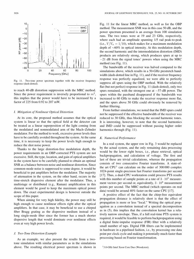
Fig. 11. Two-tone power spectrum together with the receiver frequencyresponse (dash-dotted).

to reach 40-dB distortion suppression with the MRC method.Since the power requirement is inversely proportional to m2,this implies that the power would have to be increased by afactor of 225 from 0.92 to 207 mW.

I. Mitigation of Nonlinear Optical Distortion

At its core, the proposed method assumes that the opticalsystem is linear so that the optical field at the detector canbe treated as a linear superposition of the light coming fromthe modulated and nonmodulated arm of the Mach–Zehndermodulator. For the method to work, excessive power levels thushave to be carefully avoided throughout the system. At the sametime, it is necessary to keep the power levels high enough toreduce the shot noise power.

Thanks to the large distortion-free modulation depth, thepower requirements in an OBP-corrected PTS system are notexcessive. Still, the type, location, and gain of optical amplifiersin the system have to be carefully planned to obtain an optimalSNR as a balance between noise and nonlinear distortion. Sincecommon-mode noise is suppressed to some degree, it would bebeneficial to put amplifiers before the modulator. The majorityof attenuation in the system, on the other hand, occurs in thetime-stretch dispersive element after the modulator. Thus, amultistage or distributed (e.g., Raman) amplification in thiselement would be good to keep the maximum optical powerdown. The exact experimental design is however outside thescope of this paper.

When aiming for very high fidelity, the power may still behigh enough to cause nonlinear effects right after the opticalamplifiers. In that case, it may be beneficial to use a chirpedfiber Bragg grating as the dispersive medium instead of along single-mode fiber since the former has a much shorterdispersive length that would dominate over nonlinear effectseven at very high power levels.

J. Two-Tone Distortion Example

As an example, we also present the results from a two-tone simulation with similar parameters as in the simulationsabove. The resulting electrical power spectrum is shown in

Fig. 11 for the linear MRC method, as well as for the OBPmethod. The measurement SNR was in this case 50 dB, and thepower spectrum presented is an average from 100 simulationruns. The two tones were at 19 and 23 GHz, respectively,where each had an amplitude spanning 1/5 rad peak-to-peak(i.e., V/Vπ = 1/10), which makes for a maximum modulationdepth of ∼60% in optical intensity. At this modulation depth,the second harmonic and the intermodulation distortion (IMD)products are relatively strong, which produces spurs at up to−21 dB from the signal tones’ powers when using the MRCmethod (see Fig. 11).

The bandwidth of the receiver was halved compared to thesimulations above, which results in a 50-GHz prestretch band-width (dash-dotted line in Fig. 11), and if the receiver frequencyresponse was perfectly equalized, we were able to perfectlysuppress all spurs using the OBP method. With the relativelyflat (but not perfect) response in Fig. 11 (dash-dotted), only twospurs remained, with the strongest one at −57-dB power. Thespurs within the passband disappeared if the bandwidth wasincreased to 60 GHz to make the receiver response more flat,and the spurs above 50 GHz could obviously be removed byfurther filtering.

From further simulations, we noted that the IMD spurs couldnot be suppressed if the effective bandwidth of the receiver wasreduced to 30 GHz, thus blocking the second harmonic tones.It is interesting, however, to note that the second harmonicsand IMD could be suppressed without passing higher orderharmonics through (Fig. 11).

K. Numerical Performance

In a real system, the upper row in Fig. 3 would be replacedby the actual system, and the only remaining data processingwould be the lower right boxes, i.e., phase retrieval, opticalbackpropagation, and calculation of voltage. The first andlast of these are trivial calculations, whereas the propagationconsists of two consecutive Fourier transforms. A state-of-the art CPU1 can calculate on the order of 300 000 complex1024-point single-precision fast Fourier transforms per second[17]. Thus, a dual-CPU workstation could process PTS resultswith this number of sample points at a rate of 3 · 105 measure-ment vectors per second or, equivalently, 3 · 108 measurementpoints per second. The MRC method (which operates on realdata) would be around 40% faster on the same CPU [17].

A positive effect of the fact that the chirp-free equivalentpropagation distance is relatively short is that the effect ofpropagation is more or less “local.” Writing the optical prop-agation as a convolution instead of a spectral decompositionas in (5), this implies that the convolution kernel has a rela-tively narrow envelope. Thus, if a full real-time PTS system isrequired, it would be feasible to perform backpropagation usinga digital finite-impulse response (FIR) filter with a relativelysmall number of taps. Digital FIR filters can be implementedin hardware in a pipelined fashion, i.e., by processing one datapoint per clock cycle and making it potentially much faster thanprocessing based on Fourier transformation.

13.0-GHz Intel Xeon Core Duo (Woodcrest).


VI. CONCLUSION

In summary, we have presented a novel method for signalreconstruction in phase-diverse PTS systems. The method isbased on the numerical OBP of the optical field after retrievalof the optical phase from two intensity measurements and isshown to provide a large reduction of signal distortions overmethods that treat the system as being linear from electricalinput to output. As an example of such a method, we studiedthe previously presented MRC method, which, when neglectingnonlinear effects, fully eliminates frequency fading [12].

By numerical simulations, we have shown that the proposedOBP method is able to successfully suppress the nonlinear dis-tortion due to modulator response and dispersive distortion. TheMRC method, on the other hand, only provides a distortion-free reconstruction of the input signal when the modulationdepth is very small. Using the proposed OBP method, themodulation depth can be up to about 60% in optical intensity(V/Vπ = 0.2) before the fidelity degrades, and the suppressionof signal distortion up to this point was 25–30 dB, compared tothe MRC method.

Analyzing the noise properties, we have seen that the OBPmethod, just like the MRC method, is able to suppress thecommon-mode noise by 8–9 dB and the uncorrelated mea-surement noise by 3 dB. Only at modulation depths aboveV/Vπ ≈ 0.2 was there an amplification of random noise.

We have furthermore shown that the proposed OBP method,unlike the MRC method, is insensitive to biasing errors and thatit is no more sensitive to errors in the estimation of system pa-rameters than is the MRC method. Generally, the error marginwhen estimating the propagation lengths is a few times widerthan the amplitude error margin at the desired SINAD.

To enable fast execution of the OBP method, we showedthat the propagation of a modulated chirped pulse over a longdistance is equivalent to a short distance propagation of anonchirped pulse modulated by the same signal. Based on this,the “chirp-free equivalent distance propagation” method waspresented. Since the optical chirp is removed, it suffices to re-solve the signal bandwidth, and the numerical window further-more fits perfectly both before and after propagation since thechirp-free pulse does not significantly broaden during propa-gation. The number of numerical sampling points could thus bereduced by several orders of magnitude in a typical PTS system.

In addition to the main analysis with a random binary datatest signal, we have also shown that the proposed OBP methodsuccessfully suppresses the intermodulation and harmonic dis-tortion products in a two-tone simulation. In this simulation, thedistortion suppression was mainly limited by receiver equaliza-tion accuracy, and it was noted that it is sufficient to detect thesecond harmonic tones to suppress both the second harmonicsthemselves and the IMD tones.

REFERENCES

[1] T. Konishi and Y. Ichioka, “Optical spectrogram scope using time-to-two-dimensional space conversion and interferometric time-of-flight crosscorrelation,” Opt. Rev., vol. 6, no. 6, pp. 507–512, 1999.

[2] P. O’Shea, M. Kimmel, X. Gu, and R. Trebino, “Highly simplified devicefor ultrashort-pulse measurement,” Opt. Lett., vol. 26, no. 12, pp. 932–934, Jun. 2001.

[3] B. H. Kolner, “Space-time duality and the theory of temporal imaging,”IEEE J. Quantum Electron., vol. 30, no. 8, pp. 1951–1963, Aug. 1994.

[4] C. Bennett and B. Kolner, “Upconversion time microscope demonstrat-ing 103×-magnification of femtosecond waveforms,” Opt. Lett., vol. 24,no. 11, pp. 783–785, Jun. 1999.

[5] C. Bennett and B. Kolner, “Principles of parametric temporal imaging—Part I: System configurations,” IEEE J. Quantum Electron., vol. 36, no. 4,pp. 430–437, Apr. 2000.

[6] C. Bennett and B. Kolner, “Principles of parametric temporal imaging—Part II: System performance,” IEEE J. Quantum Electron., vol. 36, no. 6,pp. 649–655, Jun. 2000.

[7] F. Coppinger, A. Bhushan, and B. Jalali, “Time magnification of electri-cal signals using chirped optical pulses,” Electron. Lett., vol. 34, no. 4,pp. 399–400, Feb. 1998.

[8] D. Chang, H. Fetterman, H. Erlig, M. Oh, C. Zhang, W. Steier, andL. Dalton, “Time stretching of 102-GHz millimeter waves using novel1.55-µm polymer electrooptic modulator,” IEEE Photon. Technol. Lett.,vol. 12, no. 5, pp. 537–539, May 2000.

[9] Y. Han and B. Jalali, “Photonic time-stretched analog-to-digital converter:Fundamental concepts and practical considerations,” J. Lightw. Technol.,vol. 21, no. 12, pp. 3085–3103, Dec. 2003.

[10] J. Azana, N. Berger, B. Levit, and B. Fischer, “Spectro-temporal imagingof optical pulses with a single time lens,” IEEE Photon. Technol. Lett.,vol. 16, no. 3, pp. 882–884, Mar. 2004.

[11] Y. Han, O. Boyraz, and B. Jalali, “Real-time A/D conversion at480 Gsample/s using the phase-diversity photonic time-stretch system,”in IEEE Int. Topical MWP Tech. Dig., 2004, pp. 186–189.

[12] Y. Han, O. Boyraz, and B. Jalali, “Ultrawide-band photonic time-stretchA/D converter employing phase diversity,” IEEE Trans. Microw. TheoryTech., vol. 53, no. 4, pt. I, pp. 1404–1408, 2005.

[13] G. Agrawal, Fiber-Optic Communication Systems. New York: Wiley,2002.

[14] J. W. Goodman, Introduction to Fourier Optics, 2nd ed. Singapore:McGraw-Hill, 1996.

[15] P. Juodawlkis, J. Twichell, G. Betts, J. Hargreaves, R. Younger,J. Wasserman, F. O’Donnell, K. Ray, and R. Williamson, “Opticallysampled analog-to-digital converters,” IEEE Trans. Microw. Theory Tech.,vol. 49, no. 10, pp. 1840–1853, Oct. 2001.

[16] IEEE Standard for Terminology and Test Methods for Analog-to-DigitalConverters, IEEE Std. 1241–2000, 2001.

[17] Retrieved on 7 Aug. 2006. [Online]. Available: http: www.fftw.com

Johan Stigwall received the M.Sc. degree in appliedphysics and electrical engineering from the Univer-sity of Linköping, Linköping, Sweden, in 2002 andthe Licentiate and Ph.D. degrees from Chalmers Uni-versity of Technology, Göteborg, Sweden, in 2004and 2006, respectively.

He has recently been a Post Doctoral Researcherwith Chalmers University of Technology. His currentmain research foci are on photonic techniques forreal-time analog-to-digital conversion and on mi-crowave photonics with an interest in both free-space

diffraction optics and dispersive fiber-optical systems. He is now employed atthe Imego Institute, Göteborg.

Sheila Galt received the Ph.D. degree fromChalmers University of Technology, Göteborg,Sweden, in 1990.

She is currently an Associate Professor with thePhotonics Laboratory, Department of Microtechnol-ogy and Nanoscience (MC2), Chalmers Universityof Technology. She leads the Optics Research Groupand is the Coordinator for the microwave photonicsactivities at the Photonics Laboratory. Her researchprofile is broad, including microwave technology,nonlinear fiber optics, biological effects of electro-

magnetic fields, diffractive optics, and photonic signal processing.

Signal Reconstruction by Phase Retrieval and Optical Backpropagation in Phase-Diverse Photonic...

Documents

Transcript of Signal Reconstruction by Phase Retrieval and Optical Backpropagation in Phase-Diverse Photonic...