Shape control of 3D lemniscates

Gabriel Arcos a, Guillermo Montilla b, Jose Ortega c,Marco Paluszny a

aLaboratorio de Computacion Grafica y Geometrıa Aplicada. Universidad Central

de Venezuela. Apartado 47809. Los Chaguaramos, Caracas 1041-A, Venezuela.

bCentro de Procesamiento de Imagenes, Facultad de Ingenierıa, Universidad de

Carabobo, Valencia, Venezuela.

cDepartamento de Matematicas, Facultad de Ciencias y Tecnologıa, Universidad

de Carabobo, Valencia, Venezuela.

Abstract

A 3D lemniscate is the set of points whose product of squared distance to a givenfinite family of fixed points is constant. 3D lemniscates are the space analogs ofthe classical lemniscates in the plane studied in [5]. They are bounded algebraicsurfaces whose degree is twice the number of foci. Within the field of computeraided geometric design (CAGD), 3D lemniscates have been considered in [3] onlyin the case of three foci, this case is simpler than the general case because most ofthe parameters that control connectedness and the deformation may be computedanalytically. We introduce the singularities as shapes handles for the control oflemniscate deformation and pay special attention to the case of four foci.

1 Preliminary remarks.

Given the set {�1, . . . ,�

n} ⊂ �3 of fixed points define the function W :

�3 →�

by

W (�) =n∏

i=1

‖� − �i‖2

A level set of this function Wρ = {� ∈ �3 : W (�) = ρ} will be called 3D lem-

niscate, of foci �1, . . . , �n and radius ρ. 3D lemniscates are implicit boundedalgebraic surfaces, whose degree is twice the number of foci. In general the

? This work was partially supported by Grant G97 000651 of Fonacit, Venezuela.E-mail addresses: gabrielarcos@cantv.net, gmontilla@netuno.net.ve,jortega@uc.edu.ve and marcopaluszny@cantv.net.

Preprint submitted to Elsevier Science 27th August 2004

lemniscate surface does not have to be connected, although each focus is con-tained in one connected component. The number of connected componentsdepends on the position of the foci and the radius ρ.

Figure 1. Some interesting 3D lemnisctes.

Assume that ρ and �1, . . . ,

�n determine a connected lemniscate then

• if we move away one of the foci then the lemniscate stretches in that direc-tion and eventually splits into two connected components

• if ρ increases then the lemniscate swells and tends to a spherical shape• if ρ decreases then the surface tightens towards its foci and eventually splits

into two or more components

Figure 2 shows a sequence of connected lemniscates as one of the foci moves.The surfaces interpolate three given points. See [4].

Figure 2. Focus motion preserving connectivity and the interpolation of three points.

If we start with a lemniscate which consists of several components then

• as ρ increases the components tend to coalesce• the motion of one of the foci affects the shape of each of the components of

the surface

As an example consider a focus � and C a connected component of the lem-

2

niscate which does not contains this focus. Then Figure 3 illustrate how thefocus affects the shape of this connected component.

Figure 3. The component C affected by the position of focus .

2 Singularities and features.

When modelling with lemniscatic surfaces (i.e. connected components of a 3Dlemniscate) it is important, besides of foci and ρ, to be aware of the behaviorof the surface at the singularities.

A singularity is a zero of the lemniscate gradient, i.e., a point such that

∇W (�) = 2W (�)n∑

i=1

� − �i

‖� − �i‖2

= 0

Clearly at the foci �1, . . . ,�

n the gradient vanishes because W (�i) = 0. Thezeros of the sum part of ∇W will be called non trivial singularities.

The behavior near a non trivial singularity is closely related to the signatureof the Hessian of W . It follows from the Taylor expansion of W at a non trivialsingularity � that the shape of the lemniscate W (�) = ρ near �, for ρ not toodifferent of W (�), is approximated by the shape of a quadratic surface.

A singularity � of W can be of four types according to the signature of theHessian: + + +, + + −, + + 0 and + 0 0. The corresponding quadratic ap-proximations are a sphere, a cone, a cylinder and a plane, which means thatthe lemniscate W (�) = ρ, for ρ near W (�), looks locally like each of thesequadrics. Figures 4(a), 4(b), 4(c) and 4(d) illustrate the local behavior of thelemniscate in each case. The table in Figure 5 summarizes the relationshipbetween the Hessian and the local features.

For example if the signature of the Hessian matrix at � is + + + and ρ >

W (�) but smaller than any other singular value greater than W (�), then thelemniscate W (�) = ρ has a component containing � which does not containany of the foci. If we consider the family of lemnicatic surfaces W (�) = ρ fora < ρ < b, such that a < W (�) < b, it can be seen that a new component is

3

(a) (b)

(c) (d)

Figure 4. Local behavior of the lemniscate near a singularity.

Hessian signature Feature

+ + + lobe

+ + − tip

+ + 0 leg

+ 0 0 flat region

Figure 5. Features corresponding to the signatures of the Hessian.

created as ρ grows from a to b. If the signature of the Hessian matrix is ++−at the singularity � then the lemniscate W (�) = ρ looks locally as a two orone sheeted hyperboloid as ρ is smaller or greater that W (�), respectively. Inboth cases ρ must be near W (�).

Given a set of foci �1, . . . ,�

n the non trivial singularities satisfy

n∑

i=1

� − �i

‖� − �i‖2

= 0

In general it is difficult to guess initial points required to apply Newton’s

4

method, but for each �k, the previous equation may be rewritten as

� − �k +

ωk

‖ωk‖2= 0, where ωk =

∑

i6=k

� − �i

‖� − �i‖2

for k = 1, 2, . . . , n. In most cases, Newton’s method converges in few steps(4-8 iterations) using �

k as initial guess.

Note that this recursion will not work in the exceptional case that ωk(�

k) =0. For some configurations of the foci there are convergence problems, forexample, in the neighborhood of a degenerate singularity the step size goesto zero very fast, and Matlab’s implementation of Newton’s method reportsconvergence to a non stationary point.

Knowing the position of the singularities for the given foci is useful for mo-delling purposes since using singular value curves we may define parameterregions for lemniscate deformation so that the connectivity of the surface iskept invariant. For example, if we know all the singular points for a given con-figuration of foci and decide to move one of them along a curve segment pa-rameterized by t ∈ [0, 1] then for each t the singularities �j(t) can be computednumerically using Newton’s method. Hence the graphs of the correspondingsingular value curves partition the plane into regions. Any two points of agiven region determine lemniscates with the same number of components. See[4] for further details.

It is also convenient to be able to construct lemniscates with a singularityprescribed at a given position. This will produce a feature at this point, whosetype will depend on the signature of the Hessian at the singularity. Recall thatthe non trivial singularities of W (�) =

∏ni=1‖� − �

i‖2 are the zeros of

ω(�) =n∑

i=1

� − �i

‖� − �i‖2

If a singularity is wanted at a particular point �0, we use the formula

n+1∑

i=1

� − �i

‖� − �i‖2

= 0

and solve for �n+1. In fact, using

�0 − �n+1

‖�0 − �n+1‖2

+n∑

i=1

�0 − �i

‖�0 − �i‖2

= 0

and1

‖�0 − �n+1‖2

=∥∥∥∥

n∑

i=1

�0 − �i

‖�0 − �i‖2

∥∥∥∥2

5

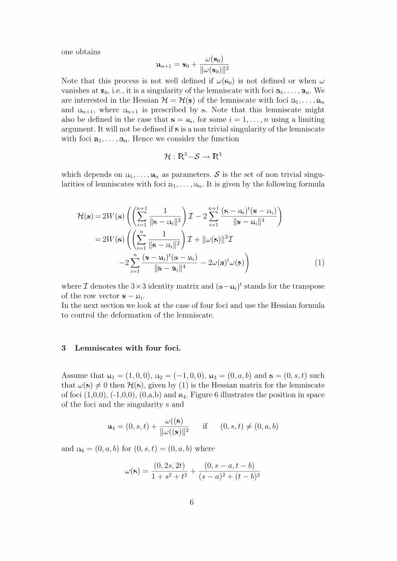
one obtains�

n+1 = �0 +ω(�0)

‖ω(�0)‖2

Note that this process is not well defined if ω(�0) is not defined or when ω

vanishes at �0, i.e., it is a singularity of the lemniscate with foci �1, . . . ,�

n. Weare interested in the Hessian H = H(�) of the lemniscate with foci �1, . . . ,

�n

and �n+1, where �

n+1 is prescribed by �. Note that this lemniscate mightalso be defined in the case that � = �

i, for some i = 1, . . . , n using a limitingargument. It will not be defined if � is a non trivial singularity of the lemniscatewith foci �1, . . . ,

�n. Hence we consider the function

H :�

3−S → �3

which depends on �1, . . . ,

�n as parameters. S is the set of non trivial singu-

larities of lemniscates with foci �1, . . . ,�

n. It is given by the following formula

H(�) = 2W (�)

((n+1∑

i=1

1

‖� − �i‖2

)I − 2

n+1∑

i=1

(� − �i)

t(� − �i)

‖� − �i‖4

)

= 2W (�)

((n∑

i=1

1

‖� − �i‖2

)I + ‖ω(�)‖2I

−2n∑

i=1

(� − �i)

t(� − �i)

‖� − �i‖4

− 2ω(�)tω(�)

)(1)

where I denotes the 3×3 identity matrix and (�−�i)

t stands for the transposeof the row vector � − �

i.In the next section we look at the case of four foci and use the Hessian formulato control the deformation of the lemniscate.

3 Lemniscates with four foci.

Assume that �1 = (1, 0, 0), �2 = (−1, 0, 0), �3 = (0, a, b) and � = (0, s, t) suchthat ω(�) 6= 0 then H(�), given by (1) is the Hessian matrix for the lemniscateof foci (1,0,0), (-1,0,0), (0,a,b) and �

4. Figure 6 illustrates the position in spaceof the foci and the singularity s and

�4 = (0, s, t) +

ω((�)

‖ω((�)‖2if (0, s, t) 6= (0, a, b)

and �4 = (0, a, b) for (0, s, t) = (0, a, b) where

ω(�) =(0, 2s, 2t)

1 + s2 + t2+

(0, s − a, t − b)

(s − a)2 + (t − b)2

6

Figure 6. The singularity moves in the plane x = 0.

In other words, on the plane x = 0, H(�) fails to be defined only at the twozeros (counting multiplicities) of ω(0, s, t) = 0. Without loss of generality wemay assume that (0, a, b) lies on the y axes, namely �

3 = (0, a, 0) then thesolutions of ω(�) = 0 are

(0,

a

3+

√a2 − 3

3, 0

)and

(0,

a

3−

√a2 − 3

3, 0

)if a ≥

√3

These are the points of the plane x = 0 where H(�) is not defined. Next werewrite the Hessian H(�)

H(�) = 2W (�)H(�)

where

W (�) =4∏

i=1

‖� − �i‖2

and

H(�) = (4∑

i=1

1

‖� − �i‖2

)I − 24∑

i=1

(� − �i)

t(� − �i)

‖� − �i‖4

Hence the zeros of det(H(�)) on the plane x = 0 coincide with the zeros ofdet(H(�)) except for � = �

3, but H(�3) = 0. Figure 7, illustrates the graph ofdet(H(�)) = 0 for �

3 = (0, 2, 0). This curve is useful to understand the typesof 3D shapes that can be modelled with 3D lemniscates. For,

• if we prescribe � on the curve we obtain a configuration of foci whose singu-larity � has degenerated Hessian. This means that the lemniscates for ρ nearbut greater that W (�) have a flat or a leg like feature near �. See Figure4(c) and 4(d).

• if � lies off the curve then it determines a position for �4 such that the

lemniscates (with foci �1,�

2,�

3,�

4), W (�) = ρ for ρ near and greater thanW (�) have an isolated spherelike component near �, see Figure 4(a) or hasa splitting/coalescing behavior, see Figure 4(b) and Figure ??.

7

−0.4 −0.2 0 0.2 0.4 0.6 0.8 1 1.2−1

−0.8

−0.6

−0.4

−0.2

0

0.2

0.4

0.6

0.8

1

Figure 7. Graph of detH( ) = 0 for = (0, 2, 0)).

Figure 8 shows a family of nearly singular lemniscates as � moves along asegment that cuts the curve of Figure 7. Figure 9 is a zoom view of Figure8(c). The above works for any choice of �1 and �

2 as long as we choose �3 and

(a) (b) (c)

Figure 8. Nearly singular lemniscates.

Figure 9. Detailed view of singularity of Fig. 8(c).

� on the bisector plane of �1 and �2 because lemniscates are invariant under

rigid motions and scaling [2].If we break the symmetry by positioning �

3, � or both outside the bisectorplane the situation gets much more complicated but one can use the singular-ity following techniques developed in [4] to deform any particular symmetriclemniscatic shape.

8

Acknowledgements

The authors wish to thank FONACIT (Proyecto G97-000651) for the financialsupport of this research.

References

[1] M. Marden, Geometry of Polynomials, Mathematical Surveys, AMS,Providence RI. 1966.

[2] J.R. Ortega, Lemniscatas 3D, Trabajo de Ascenso, Universidad de Carabobo,Valencia, 2003.

[3] J.R. Ortega and M. Paluszny, Lemniscatas 3D, Revista de Matematica: Teorıay Aplicaciones (9) 2, 2002, 7–14.

[4] M. Paluszny, G. Montilla and J.R. Ortega, Lemniscates 3D: A CAGDprimitive?, to appear in Numerical Algorithms.

[5] Markushevich, A., Teorıa de las Funciones Analıticas, Tomo I, Editorial Mir,Moscu, 1970.

9