M. Gobien, F. Garisto, E. Kremer, and C. Medri

Nuclear Waste Management Organization

Seventh Case Study: Reference Data and Codes

NWMO-TR-2018-10 December 2018

Nuclear Waste Management Organization 22 St. Clair Avenue East, 6th Floor Toronto, Ontario M4T 2S3 Canada Tel: 416-934-9814 Web: www.nwmo.ca

- i -

All copyright and intellectual property rights belong to NWMO.

Seventh Case Study: Reference Data and Codes NWMO-TR-2018-10 December 2018

M. Gobien, F. Garisto, E. Kremer, and C. Medri Nuclear Waste Management Organization

- ii -

Document History

Title: Seventh Case Study: Reference Data and Codes

Report Number: NWMO-TR-2018-10

Revision: R000 Date: December 2018

Nuclear Waste Management Organization

Authored by: M. Gobien, F. Garisto, E. Kremer, and C. Medri

Verified by: C. Medri, J. Chen, and T. Yang

Reviewed by: N. Hunt

Approved by: P. Gierszewski

- iii -

ABSTRACT Title: Seventh Case Study: Reference Data and Codes Report No.: NWMO-TR-2018-10 Author(s): M. Gobien, F. Garisto, E. Kremer and C. Medri Company: Nuclear Waste Management Organization Date: December 2018 Abstract The Seventh Case Study is an illustrative postclosure safety assessment of a conceptual repository for used nuclear fuel located at 500 m depth at a hypothetical site in the Michigan Basin. The conceptual design is similar to the Sixth Case Study (NWMO 2017) in that it considers horizontal in-room placement of 48-bundle copper coated used fuel containers. However, the repository design has been updated for suitability in sedimentary rock. Furthermore, the repository layout is now based on a multi-armed geometry with central shafts and services. The hypothetical site where the repository is excavated is the same as in the Fifth Case Study (NWMO 2013) and the repository remains at 500 m below ground surface (mBGS). The main safety assessment codes used in the Seventh Case Study are:

FRAC3DVS-OPG – for modelling 3D groundwater flow and radionuclide transport;

RSM – a simple screening model used to identify the key radionuclides;

SYVAC3-CC4 – the reference system model for calculating radionuclide transport across the repository system and resulting dose consequences;

HIM – for calculating dose consequences for the inadvertent human intrusion scenario.

NHB – for calculating dose consequences to non-human biota

T2GGM – for modelling 3D two-phase flow and gas transport These codes and their datasets are maintained under a software quality assurance system at NWMO. The codes are described briefly in this report. The reference datasets are based on a combination of the site conceptual model information and the repository design description, with most of the general material properties and other input parameters adopted from previous work. Updated data were used when available from more recent studies. This report provides a summary of all the data selected and indicates the references where more details about the derivation of the data may be found.

- iv -

- v -

TABLE OF CONTENTS

Page

ABSTRACT ................................................................................................................................ v

1. INTRODUCTION ................................................................................................. 1

1.1 BACKGROUND................................................................................................... 1 1.2 REPORT OUTLINE ............................................................................................. 1

2. OVERVIEW ......................................................................................................... 3

2.1 REPOSITORY CONCEPT ................................................................................... 3 2.2 SCENARIOS ....................................................................................................... 3 2.3 DATA ................................................................................................................... 4 2.3.1 Data Sources ....................................................................................................... 4 2.3.2 Parameter Variability ............................................................................................ 4

3. COMPUTER MODELS ........................................................................................ 6

3.1 COMPUTER MODEL DESCRIPTIONS ............................................................... 8 3.1.1 SYVAC3-CC4 ...................................................................................................... 8 3.1.2 FRAC3DVS-OPG ................................................................................................. 8 3.1.3 RSM..................................................................................................................... 8 3.1.4 HIM ...................................................................................................................... 8 3.1.5 NHB ..................................................................................................................... 9 3.1.6 TOUGH2-GGM .................................................................................................... 9 3.1.7 Specialized Supporting Codes ............................................................................. 9 3.1.8 Software Tools ................................................................................................... 14 3.1.9 Reference Data .................................................................................................. 14 3.2 SOFTWARE QUALITY ASSURANCE .............................................................. 15

4. USED FUEL DATA ............................................................................................ 17

4.1 USED FUEL WASTEFORM .............................................................................. 17 4.2 USED FUEL COMPOSITION ............................................................................ 19 4.3 NUCLIDE AND ELEMENT INVENTORIES OF UO2 FUEL AND ZIRCALOY .... 21 4.4 CONTAMINATION ON EXTERNAL BUNDLE SURFACES .............................. 29 4.5 INSTANT RELEASE ......................................................................................... 30 4.5.1 UO2 Instant Release .......................................................................................... 30 4.5.2 Zircaloy Instant Release ..................................................................................... 39 4.6 CONGRUENT RELEASE .................................................................................. 40 4.6.1 UO2 Fuel Dissolution .......................................................................................... 40 4.6.2 Zircaloy Corrosion .............................................................................................. 43

5. CONTAINER ..................................................................................................... 44

5.1 CONTAINER DIMENSIONS .............................................................................. 44 5.2 DEFECTIVE CONTAINER ................................................................................. 45 5.3 FREE WATER DIFFUSION COEFFICIENT ....................................................... 46 5.4 WATER COMPOSITION ................................................................................... 47 5.5 SOLUBILITY LIMITS ......................................................................................... 48

6. REPOSITORY DATA ........................................................................................ 51

- vi -

6.1 PHYSICAL LAYOUT ......................................................................................... 51 6.2 BUFFER ............................................................................................................ 61 6.3 BACKFILL ......................................................................................................... 62 6.4 CONCRETE ....................................................................................................... 62 6.5 ASPHALT .......................................................................................................... 63 6.6 DIFFUSION COEFFICIENTS ............................................................................. 63 6.6.1 Buffer ................................................................................................................. 63 6.6.2 Backfill ............................................................................................................... 64 6.6.3 Concrete ............................................................................................................ 65 6.6.4 Asphalt ............................................................................................................... 65 6.7 SORPTION COEFFICIENTS AND CAPACITY FACTORS ............................... 65 6.7.1 Buffer ................................................................................................................. 65 6.7.2 Backfill ............................................................................................................... 68 6.7.3 Concrete ............................................................................................................ 68 6.7.4 Asphalt ............................................................................................................... 68 6.8 EFFECT OF INCREASED TEMPERATURE ON BENTONITE .......................... 68 6.8.1 Physical Properties ............................................................................................ 68 6.8.2 Hydraulic Conductivity ....................................................................................... 68 6.8.3 Diffusion Coefficients ......................................................................................... 69 6.8.4 Sorption Coefficients .......................................................................................... 69 6.9 EXCAVATION DAMAGE ZONE TRANSPORT PARAMETERS ....................... 69 6.9.1 Excavation Damage Zone Thickness ................................................................. 69 6.9.2 Excavation Damage Zone Permeability ............................................................. 70 6.9.3 Excavation Damage Zone Dispersion Length .................................................... 71 6.9.4 Excavation Damage Zone Porosity .................................................................... 72 6.9.5 EDZ Tortuosity ................................................................................................... 72 6.10 NEAR FIELD TWO-PHASE FLOW PARAMETERS .......................................... 74

7. GEOSPHERE DATA ......................................................................................... 78

7.1 GENERAL SITE DESCRIPTION ....................................................................... 78 7.2 PHYSICAL CHARACTERISTICS OF THE GEOSPHERE ................................. 79 7.2.1 Stratigraphic Units .............................................................................................. 79 7.2.2 Hydraulic Conductivity ....................................................................................... 80 7.2.3 Rock Density ...................................................................................................... 81 7.2.4 Porosity .............................................................................................................. 82 7.2.5 Tortuosity ........................................................................................................... 83 7.2.6 Geomechanical Parameters ............................................................................... 83 7.2.7 Fluid Density ...................................................................................................... 84 7.3 CHEMICAL CHARACTERISTICS OF THE GEOSPHERE ................................ 87 7.3.1 Salinity ............................................................................................................... 87 7.3.2 Redox Divide ..................................................................................................... 87 7.3.3 Colloids .............................................................................................................. 87 7.3.4 Temperature ...................................................................................................... 87 7.4 GEOSPHERE TRANSPORT PARAMETERS ................................................... 88 7.4.1 Effective Diffusivity ............................................................................................. 88 7.4.2 Geosphere Dispersion Length............................................................................ 90 7.4.3 Geosphere Sorption ........................................................................................... 91 7.5 TWO PHASE FLOW PARAMETERS ................................................................ 95 7.6 WELL LOCATION AND DEPTH ....................................................................... 97 7.7 OTHER GEOSPHERE PARAMETERS ............................................................. 99 7.8 GEOSPHERE NODE DATA ............................................................................ 100

- vii -

8. BIOSPHERE DATA ......................................................................................... 101

8.1 SITE AND SURFACE WATER ........................................................................ 101 8.2 DISCHARGE ZONES AND WATERSHED AREAS ........................................ 101 8.2.1 Watershed Areas ............................................................................................. 101 8.2.2 Surface discharge area .................................................................................... 103 8.3 CLIMATE AND ATMOSPHERE ...................................................................... 104 8.4 SOILS AND SEDIMENT .................................................................................. 106 8.4.1 Soil Physical Characteristics ............................................................................ 106 8.4.2 Plant/Soil Concentration Ratio ......................................................................... 108 8.4.3 Soil Distribution Coefficient (Kd) ....................................................................... 109 8.4.4 River and Lake Sedimentation Rates ............................................................... 111 8.5 FARMING YIELDS .......................................................................................... 113

9. DOSE PATHWAYS DATA .............................................................................. 114

9.1 HUMAN LIFESTYLE CHARACTERISTICS ..................................................... 114 9.2 HUMAN PHYSICAL CHARACTERISTICS ...................................................... 119 9.3 AIR CONCENTRATION PARAMETERS ......................................................... 119 9.4 MISCELLANEOUS PHYSICAL PARAMETERS ............................................. 121 9.5 ANIMAL CHARACTERISTICS ........................................................................ 123 9.6 DOSE COEFFICIENTS.................................................................................... 126 9.6.1 Adult Ingestion Dose Coefficients .................................................................... 127 9.6.2 Adult Inhalation Dose Coefficients ................................................................... 127 9.6.3 Adult Ground Exposure and Air Immersion Dose Coefficients.......................... 127 9.6.4 Adult Water Immersion Dose Coefficients ........................................................ 127 9.6.5 Adult Building Exposure Dose Coefficients ...................................................... 128 9.7 No-Effect Concentrations for Non-Human Biota ......................................... 131 9.8 Chemical Hazard ............................................................................................ 131

10. SUMMARY ...................................................................................................... 131

11. REFERENCES ................................................................................................ 132

APPENDIX A: USED FUEL INVENTORY UNCERTAINTY ................................................... 146

A.2.1 NPD Reactor Fuel ............................................................................................ 147 A.2.2 Bruce Reactor Fuel .......................................................................................... 148 A.2.3 Pickering Reactor Fuel ..................................................................................... 148 A.2.4 NEA Benchmark on Pressurized Water Reactor Isotopic Prediction ................ 150 A.2.5 More Recent Comparisons of ORIGEN with Measurements for Pressurized Water Reactor Fuel ........................................................................................................... 151 A.2.6 ORIGEN-S Uncertainties for CANDU Fuel ....................................................... 153

APPENDIX B: USED FUEL DISSOLUTION MODEL ............................................................ 157

APPENDIX C: SYVAC3-CC4 GEOSPHERE MODEL DATA ................................................. 169

- viii -

LIST OF TABLES

Page Table 2-1: Parameter Probability Density Function Types and Attributes .................................... 5 Table 3-1: SYVAC3-CC4, Version SCC4.09.3 .......................................................................... 10 Table 3-2: FRAC3DVS-OPG, Version 1.3 ................................................................................. 11 Table 3-3: RSM, Version 1.1 ..................................................................................................... 12 Table 3-4: HIM, Version 2.1 ...................................................................................................... 13 Table 3-5: NHB, Version 1.0 ..................................................................................................... 13 Table 3-6: T2GGM Version 3.2 ................................................................................................. 14 Table 3-7: Description of Software Tools................................................................................... 14 Table 4-1: Used Fuel Parameters ............................................................................................. 18 Table 4-2: Potentially Significant Radionuclides Included in the Assessment ............................ 20 Table 4-3: Potentially Hazardous Elements Included in the Assessment................................... 20 Table 4-4: Discharge Burnup Percentiles on a Per Station Basis .............................................. 22 Table 4-5: Inventories of Potentially Hazardous Radionuclides in UO2 Fuel .............................. 26 Table 4-6: Inventories of Potentially Hazardous Radionuclides of Interest in Zircaloy for

30 Years Decay Time ........................................................................................................ 27 Table 4-7: Inventories of Potentially Hazardous Elements for 30 Year Decay Time .................. 28 Table 4-8: Instant Release Fractions for CANDU Fuel .............................................................. 31 Table 4-9: Rationale for Selection of Instant Release Fractions for Elements without Measured

Data .................................................................................................................................. 37 Table 4-10: Instant Release Fractions for Zircaloy Cladding ..................................................... 40 Table 4-11: Radiation Doses at Fuel Surface (220 MWh/kgU)# ................................................. 41 Table 4-12: Radiation Doses at Fuel Surface (280 MWh/kgU)# ................................................. 42 Table 4-13: Used Fuel Dissolution Rate Parameters (see Appendix B) ..................................... 42 Table 5-1: Container Internal Parameters ................................................................................. 44 Table 5-2: Defective Container Scenario Parameters................................................................ 46 Table 5-3: Free Water Diffusivity ............................................................................................... 47 Table 5-4: Contact Water Composition ..................................................................................... 48 Table 5-5: Element Solubilities1 ................................................................................................. 50 Table 6-1: Placement Room Parameters .................................................................................. 56 Table 6-2: Access Tunnels, Ramps, and Shafts Parameters ..................................................... 59 Table 6-3: Proposed Sealing System for Shafts ........................................................................ 60 Table 6-4: Properties of As-Placed Materials in the Repository ................................................. 60 Table 6-5: Properties of Highly Compacted Bentonite in the Buffer Box and Spacer Blocks at

Saturation .......................................................................................................................... 61 Table 6-6: Properties of Gap Fill at Saturation........................................................................... 61 Table 6-7: Homogenized Bentonite Properties at Saturation ..................................................... 61 Table 6-8: Properties of Dense Backfill at Saturation ................................................................ 62 Table 6-9: Properties of 70% Bentonite / 30% Sand at Saturation............................................. 62 Table 6-10: Properties of Concrete at Saturation ...................................................................... 63 Table 6-11: Properties of Asphalt at Saturation ......................................................................... 63 Table 6-12: Buffer Effective Diffusion Coefficients at 25ºC ........................................................ 64 Table 6-13: Backfill Effective Diffusion Coefficients at 25ºC ...................................................... 64 Table 6-14: Bentonite Sorption Coefficients [m3/kg] .................................................................. 66 Table 6-15: Bentonite Capacity Factors .................................................................................... 67 Table 6-16: Excavation Damage Zone Properties ..................................................................... 73 Table 6-17: Transverse, Radial, and Axial Excavation Damage Zone Properties ...................... 74

- ix -

Table 6-18: Two Phase Flow Properties of the Sealing Materials and Excavation Damaged Zones ................................................................................................................................ 76

Table 6-19: Thermal Properties of the Sealing Materials ........................................................... 77 Table 7-1: Formation Thickness at the Hypothetical Site ........................................................... 80 Table 7-2: Hydrogeologic Parameters1,2 .................................................................................... 86 Table 7-3: Formation-Averaged Salinity at the Seventh Case Study Site .................................. 88 Table 7-4: Geosphere Effective Diffusivities1 [m2/s] ................................................................... 90 Table 7-5: Values of [s(1-expt)/expt] for Several Geological Materials ....................................... 92 Table 7-6: Shale Kd Values [m3/kg] ........................................................................................... 93 Table 7-7: Limestone Kd Values [m3/kg] .................................................................................... 94 Table 7-8: Two Phase Flow Parameters1,2 ................................................................................ 95 Table 7-9: Thermal Properties of the Geosphere ...................................................................... 96 Table 7-10: Well Model Geosphere Parameters ........................................................................ 99 Table 7-11: Other Geosphere Properties ................................................................................ 100 Table 8-1: Surface water properties ........................................................................................ 103 Table 8-2: Surface Discharge Areas ....................................................................................... 104 Table 8-3: Climate and atmosphere parameters ..................................................................... 105 Table 8-4: Soil properties ........................................................................................................ 107 Table 8-5: Plant/Soil Concentration Ratios1,2 ........................................................................... 109 Table 8-6: Soil Kd Values [L/kg] ............................................................................................... 110 Table 8-7: Lake Sedimentation Rates ..................................................................................... 112 Table 8-8: Farming yield data .................................................................................................. 113 Table 9-1: Human lifestyle characteristics for farm household ................................................. 115 Table 9-2: Timing parameters ................................................................................................. 118 Table 9-3: Human physical characteristics .............................................................................. 119 Table 9-4: Volatilization parameters ........................................................................................ 121 Table 9-5: Physical parameters ............................................................................................... 122 Table 9-6: Food energy and water content .............................................................................. 122 Table 9-7: Nutrient Content of Foods1 ..................................................................................... 123 Table 9-8: Domestic Animal Data1 .......................................................................................... 124 Table 9-9: Animal Ingestion Transfer Coefficients1 .................................................................. 125 Table 9-10: Animal inhalation transfer coefficients1 ................................................................. 126 Table 9-11: Adult Human Dose Coefficients1 .......................................................................... 129 Table 9-12: Parameters for human specific activity models ..................................................... 130 Table A-1: Measured and Calculated Atom Ratios for NDP Fuel Study .................................. 147 Table A-2: Measured and Calculated Atom Ratios for Bruce Fuel Study ................................. 148 Table A-3: Measured and Calculated Inventories for Pickering-A Fuel Study .......................... 149 Table A-4: Measured and Calculated Inventories for NEA ATM-104 Study ............................. 151 Table B-1: Alpha, Beta and Gamma Dose Rates (Gy/a) for 220 MWh/kgU and 280 MWh/kgU

Burnups ........................................................................................................................... 160 Table C-1: SYVAC3-CC4 Geosphere Network – Node Properties .......................................... 171 Table C-2: SYVAC3-CC4 Geosphere Network – Segment Properties .................................... 173 Table C-3: SYVAC3-CC4 Geosphere Network – Slope Value ................................................. 175 Table C-4: SYVAC3-CC4 Geosphere Network – Input Data File ............................................. 177

- x -

LIST OF FIGURES

Page Figure 1-1: Illustration of the Geological Repository Concept Considered in the Seventh Case

Study ................................................................................................................................... 2 Figure 3-1: Illustration of Relationship between the Computer Models Used in the Seventh Case

Study and Supporting Data ................................................................................................. 7 Figure 4-1: Typical CANDU Fuel Bundle ................................................................................... 19 Figure 4-2: Distribution of Burnups and Cumulative Distribution for all Fuel Bundles ................ 23 Figure 4-3: Radioactivity of Used Fuel (220 MWh/kgU burnup) as a Function of Time after

Discharge from the Reactor ............................................................................................... 29 Figure 4-4: Distribution of Maximum Linear Power Ratings and Cumulative Distribution for all

Commercial Fuel Bundles (discharged up to 2012) ........................................................... 32 Figure 4-5: Fission Gas (gap) Release as a Function of Peak Linear Power Rating for CANDU

Fuels with Burnups Less than 400 MWh/kgU .................................................................... 34 Figure 4-6: Total Instant Release Fractions (gap + grain boundary inventories) for Iodine and

Cesium .............................................................................................................................. 34 Figure 4-7: Cl-36 Releases from CANDU Fuel .......................................................................... 35 Figure 5-1: Container Design Showing Copper Coating, Inner Steel Vessel, and Inside Support

Tubes ................................................................................................................................ 45 Figure 6-1: Plan View of Underground Repository .................................................................... 53 Figure 6-2: Placement Room Longitudinal Section .................................................................... 54 Figure 6-3: Placement Room Geometry .................................................................................... 55 Figure 6-4: Longitudinal View of a Tunnel Seal ......................................................................... 57 Figure 6-5: Access Tunnels Cross Sections .............................................................................. 57 Figure 6-6: Ramps Cross sections ............................................................................................ 58 Figure 7-1: FRAC3DVS-OPG Model Domains and Basic Features at the Hypothetical Site...... 78 Figure 7-2: Site Scale Model Cross Section .............................................................................. 79 Figure 7-3 Profile of Test Interval Hydraulic Conductivity Estimates Determined from Field

Straddle-Packer Testing in L&ILW DGR Boreholes ........................................................... 81 Figure 7-4: Grain and Bulk Dry Density, Measured Data and Formation Averages. .................. 82 Figure 7-5: Liquid Porosity Profile for DGR Cores Showing Point Data and Arithmetic Formation

Averages ........................................................................................................................... 83 Figure 7-6: Plot of Groundwater Density and Total Dissolved Solids Concentrations Data ........ 85 Figure 7-7: Effective Diffusion Coefficient (De) Profile as Determined by X-ray Radiography and

Through-Diffusion Testing of L&ILW DGR Cores Showing Point Data and Formation Averages ........................................................................................................................... 89

Figure 7-8: Survey of Ontario Well Depths ................................................................................ 98 Figure 7-9: Survey of Southern Ontario Well Depths ................................................................. 98 Figure 8-1: Watershed Boundaries.......................................................................................... 102 Figure A-1: Comparison of Calculated and Experimental Inventories for Actinide (left) and

Fission Product (right) Using ENDF/B-V and ENDF/B-VII Libraries ................................. 152 Figure B-1: Corrosion Rates Measured as a Function of Specific Alpha Activity ..................... 161 Figure B-2: UO2 (fuel) Corrosion Rates (calculated at 100°C) Plotted Logarithmically as a

Function of the Gamma or Beta Radiation Dose Rate ..................................................... 163 Figure B-3: UO2 Corrosion Rates from Various Literature Sources ......................................... 165 Figure B-4: Radiation Dose Rate in Water at the Fuel Surface (220 MWh/kgU burnup) .......... 166 Figure B-5: Calculated Total Fuel Dissolution Rate ................................................................. 166 Figure C-1: SYVAC3-CC4 GEONET Model: Transport Network Connectivity ......................... 170

- 1 -

1. INTRODUCTION

1.1 BACKGROUND

The Seventh Case Study is a postclosure safety assessment of a deep geological repository in sedimentary rock in the Michigan Basin as shown in Figure 1.1 (NWMO 2018). The main objective of the Seventh Case Study is to assess key aspects of the postclosure safety of a deep geological repository based on a more recent Canadian design concept for sedimentary rock. Similar to the Sixth Case Study, the Seventh Case Study assumes 48-bundle copper coated containers. However, the repository design has been updated for suitability in sedimentary rock. Furthermore, the repository layout is now based on a multi-armed geometry with central shafts and services. The hypothetical site where the repository is excavated is the same as in the Fifth Case Study (NWMO 2013) and the repository remains at 500 m Below Ground Surface (mBGS). This information should be considered within the following context.

The Study focusses on key scenarios, including the expected or Normal Evolution Scenario and a variety of Disruptive Event Scenarios, but is not a complete postclosure safety assessment.

The Study is based on a specific conceptual repository design The site is hypothetical. It is assumed that a sufficient volume of competent rock is available

for the repository. The depth of 500 m was assumed for this illustrative assessment, and would be optimized for a real site. There is no site-specific data and, hence, no Geosynthesis, i.e., a geoscientific explanation of the overall understanding of site characteristics and evolution (past and future) as they relate to demonstrating long-term repository performance and safety.

1.2 REPORT OUTLINE

This report describes the main computer codes and data used in the postclosure safety assessment calculations for the Seventh Case Study. It is organized as follows:

Section 2 provides an overview of the repository design, scenarios and general data selection principles;

Section 3 summarizes the computer codes used and their main features, and the software quality assurance approach;

Section 4 provides the used fuel wasteform data;

Section 5 provides the container data;

Section 6 provides the placement room and repository data;

Section 7 provides the geosphere data;

Section 8 provides the local surface biosphere data; and

Section 9 provides the biosphere data, specifically the data used for calculating dose rates to a critical human group assumed to be living at the site in the future.

- 2 -

Figure 1-1: Illustration of the Geological Repository Concept Considered in the Seventh Case Study

- 3 -

2. OVERVIEW

2.1 REPOSITORY CONCEPT

The main features of the conceptual repository are as follows (see also Figure 1.1):

The repository is located at a depth of 500 m below surface in the sedimentary rock of the Michigan Basin formation comprised of shale and limestone lithologies.

The repository is located in a region in which there are no known mineral deposits, other economically exploitable geological resources, or potable groundwater at or near the repository level.

The repository is constructed by the room-and-pillar method, with the repository excavated at a single level.

The repository contains approximately 5.2 million bundles of used CANDU fuel.

At the time of placement, the used-fuel bundles have been discharged from the reactor for a minimum of 30 years.

Prior to placement, used-fuel bundles are sealed inside durable copper and steel containers.

The used fuel containers are placed horizontally in an in-room configuration.

The outer surface temperature of the container after placement is constrained (by design) to a maximum value of 100°C.

Each container is surrounded by a 100% bentonite clay buffer material.

As container placement proceeds, the open space in each room is filled with compacted bentonite, and the filled rooms are closed off by composite seals made of clay-based and cement-based materials.

At the end of a postclosure monitoring period, all tunnels, shafts, and exploration boreholes in the vicinity of the repository are sealed using backfill and a combination of clay-based and cement-based materials.

2.2 SCENARIOS

Five scenarios are considered in the Seventh Case Study:

1. The Normal Evolution Scenario is based on a reasonable extrapolation of present day site features and receptor lifestyles. It includes the expected evolution of the site and expected degradation of the disposal system. It illustrates the anticipated effects of the repository on people and on the environment. The Normal Evolution Scenario is described in terms of a “Reference Case” and a series of associated sensitivity studies. The Reference Case represents the situation in which all repository components meet their design specification and function as anticipated. As such, the used fuel containers remain intact essentially indefinitely and no contaminant releases occur in the one million year time period of interest to the safety assessment. The associated sensitivity studies illustrate repository performance for a range of reasonably foreseeable deviations from key Reference Case assumptions. These deviations arise as a result of components unknowingly placed in the repository that either (a) do not meet their design specification or (b) do not fully function as anticipated.

- 4 -

The most important sensitivity case is the Base Case. The “Base Case” sensitivity study assumes a small number of containers are fabricated with defects in their copper coating, and that a smaller number of these off-specification containers escape detection by the quality assurance program and are unknowingly placed in the repository.

2. An Inadvertent Human Intrusion Scenario, in which the engineered and natural

repository barriers are bypassed by a borehole that is inadvertently drilled through a container, bringing used fuel material directly to the surface.

3. An All Containers Fail Scenario, in which all containers are assumed to fail at 60,000 years, the time of the first major ice-sheet advance over the repository site in the glacial cycle defined by NWMO (2018, Chapter 5).

A sensitivity case where all the containers are assumed to fail at 10,000 years is also assessed.

4. A Repository Seals Failure Scenario, in which there is rapid and extensive degradation of (1) the shaft seals and /or (2) the seals around the fracture passing through the repository footprint.

5. The Undetected Fault Scenario, in which there is an undetected or seismically activated transmissive fault in close proximity to the repository that extends from about the repository level up into the shallow groundwater system. Such a fault could provide an enhanced permeability pathway that bypasses the natural geological barrier.

2.3 DATA

2.3.1 Data Sources For analyses of the Normal Evolution Scenario, the starting point for the data used in the Seventh Case Study was that used in the Fifth Case Study (NWMO 2013). The data needed for the Seventh Case Study were compared with those used in the Fifth Case Study (Gobien et al. 2013), and many of the latter values were judged to be reasonable and kept without change. Parameter values used in the Seventh Case Study are defined in Sections 4 to 9 of this report. This includes all design, inventory, material, geosphere, biosphere, and dose conversion data. Exposure-specific parameters for the Inadvertent Human Intrusion scenario are described in Medri (2015a). 2.3.2 Parameter Variability For some model input parameters, there is a clearly appropriate value. However, for many parameters, a range of values may be possible because of natural variability or measurement uncertainties or uncertainties arising from the modelling basis. An example of natural variability is human diet - the amount that people eat is naturally variable from person to person, and from time to time. An example of model-based uncertainty is the sorption kd parameter, since this is an effective parameter that represents the net effect of possibly several processes that may be occurring at the microscopic scale.

- 5 -

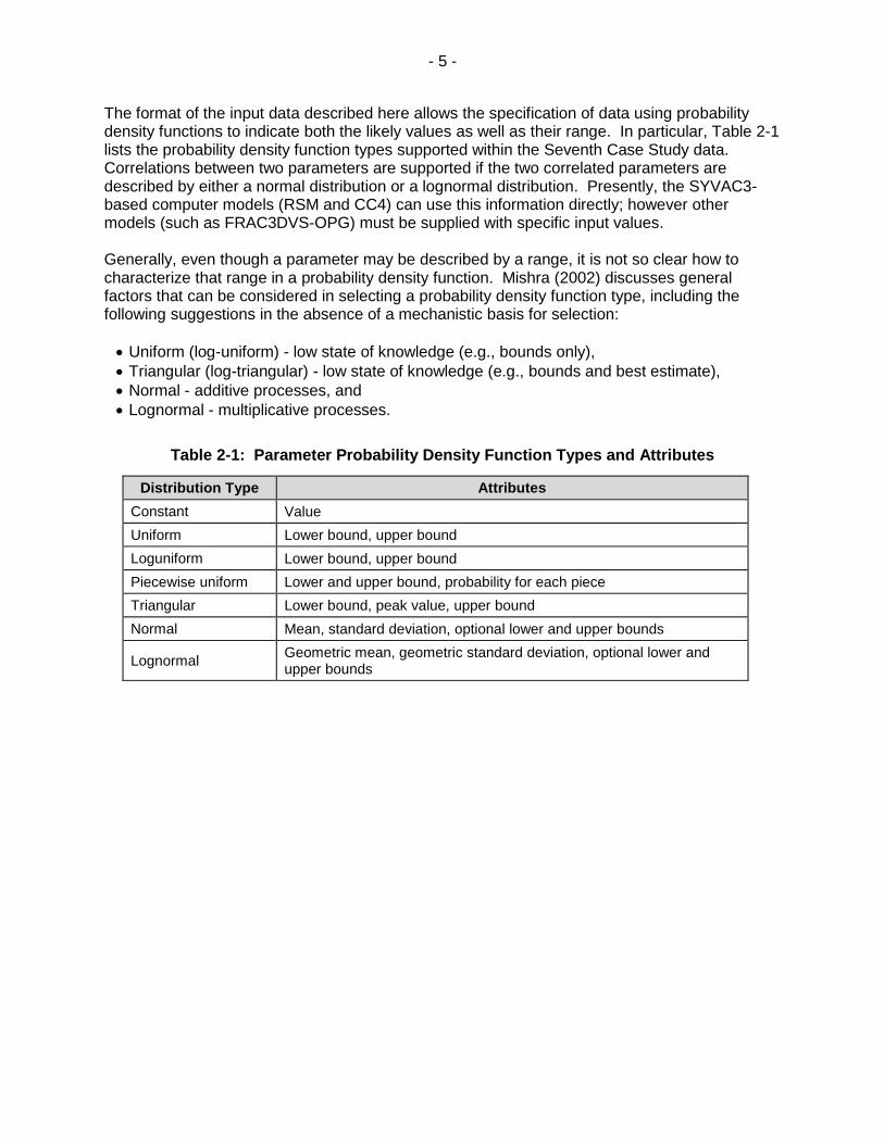
The format of the input data described here allows the specification of data using probability density functions to indicate both the likely values as well as their range. In particular, Table 2-1 lists the probability density function types supported within the Seventh Case Study data. Correlations between two parameters are supported if the two correlated parameters are described by either a normal distribution or a lognormal distribution. Presently, the SYVAC3-based computer models (RSM and CC4) can use this information directly; however other models (such as FRAC3DVS-OPG) must be supplied with specific input values. Generally, even though a parameter may be described by a range, it is not so clear how to characterize that range in a probability density function. Mishra (2002) discusses general factors that can be considered in selecting a probability density function type, including the following suggestions in the absence of a mechanistic basis for selection:

Uniform (log-uniform) - low state of knowledge (e.g., bounds only),

Triangular (log-triangular) - low state of knowledge (e.g., bounds and best estimate),

Normal - additive processes, and

Lognormal - multiplicative processes.

Table 2-1: Parameter Probability Density Function Types and Attributes

Distribution Type Attributes

Constant Value

Uniform Lower bound, upper bound

Loguniform Lower bound, upper bound

Piecewise uniform Lower and upper bound, probability for each piece

Triangular Lower bound, peak value, upper bound

Normal Mean, standard deviation, optional lower and upper bounds

Lognormal Geometric mean, geometric standard deviation, optional lower and upper bounds

- 6 -

3. COMPUTER MODELS The Seventh Case Study uses computer models (or "codes") to numerically represent the repository system. In this section, the computer models used are briefly described, as well as the general software quality assurance system supporting these codes. There are two categories of computer models - detailed (or "process") models and integrated system models. In general, the detailed models address specific topics, usually with the inclusion of mechanistic effects or with greater resolution in space or time. These detailed models either provide supporting data or validation tests, or else identify the important parameters and processes for use in the integrated system models. The latter system models incorporate the most important features, events and processes describing the behaviour of the repository, from waste form to dose consequences. Figure 3-1 identifies the codes used in the Seventh Case Study assessment, and their interrelationship. Initially, information from used fuel characteristics, engineering design, and site characterization are used in conjunction with specialized codes to develop a site-specific system description. For example, the initial inventory is determined using ORIGEN-S, while the site characterization information is collected into a detailed groundwater flow model under FRAC3DVS-OPG. The results from the RSM model are used to screen the initial inventories of radionuclides in the fuel in order to identify a short list of most concern. Detailed transport calculations for scenarios involving groundwater transport of contaminants are then undertaken with the FRAC3DVS-OPG transport model and the SYVAC3-CC4 system model. FRAC3DVS-OPG calculates advective-dispersive transport through the repository and geosphere using a detailed 3-D model, and interfaces with SYVAC3-CC4 for source terms and biosphere consequence calculations. SYVAC3-CC4 contains a set of submodels that represent the whole repository, including the repository (used fuel, defective containers, etc.), the geosphere (advective and diffusive transport, well, etc.) and the biosphere (food chain model, surface waters, etc.). The FRAC3DVS-OPG and SYVAC3-CC4 models are complementary since they use very different numerical approaches and have different strengths. The Inadvertent Human Intrusion scenario is separately analyzed using the Human Intrusion Model (Medri 2015a), which is built on the AMBER software platform (Quintessa 2016). AMBER is a graphical-user interface based software tool that allows users to build dynamic compartment models to represent, for example, the migration and fate of radioactive and non-radioactive contaminants in environmental systems. In addition, the assessment is supported by detailed models, notably PHREEQC for solubilities.

- 7 -

Figure 3-1: Illustration of Relationship between the Computer Models Used in the Seventh Case Study and Supporting Data

- 8 -

3.1 COMPUTER MODEL DESCRIPTIONS

This section provides a brief description of the computer models, model features and associated documentation. The main documentation associated with each computer model is a theory manual, user manual and testing reports. Documentation and key features for the individual codes are specified in Table 3-1 through Table 3-6. 3.1.1 SYVAC3-CC4 The system code for the Seventh Case Study is referred to as SYVAC3-CC4, Version SCC409.3 (NWMO 2012, Table 3-1). It is a system model for assessment of groundwater transport of contaminants from the repository to the biosphere, as in the Normal Evolution Scenario. It was designed for the postclosure safety assessment of a deep geological repository for used CANDU fuel placed in durable containers. It calculates the rate of contaminant releases from used fuel in contact with water, their transport out of defective containers, through the engineered barriers and host rock, and into the biosphere. Dose consequences are calculated for a critical group – a farming household, living in the vicinity of the repository and exposed to contaminants released from the repository. 3.1.2 FRAC3DVS-OPG The reference groundwater flow and transport code used in the Seventh Case Study is FRAC3DVS-OPG, a 3-D finite-element/finite-difference code (Therrien et al. 2010, Table 3-2). FRAC3DVS-OPG is a version of a commercially available code. FRAC3DVS-OPG supports both equivalent-porous-medium and dual-porosity representations of the geologic media. The FRAC3DVS-OPG groundwater flow results are used to derive the parameters for the CC4 geosphere groundwater transport model (GEONET). Furthermore, the results of the FRAC3DVS-OPG radionuclide transport calculations can be compared to the corresponding CC4 calculations, allowing verification of the CC4 geosphere transport model. 3.1.3 RSM One of the simpler models used in the Seventh Case Study analysis is called the Radionuclide Screening Model (Goodwin et al. 2001, Table 3-3) It models groundwater transport of radionuclides via a simple contaminant transport pathway from the defective containers to humans via a well. By conservative choice of input parameters, it can be used to screen radionuclides so as to objectively identify which are potentially important and should be included in more detailed models. 3.1.4 HIM The Inadvertent Human Intrusion Model for the Seventh Case Study (HIMv2.1) assesses an inadvertent human intrusion scenario (Medri 2015a, Table 3-4). The model considers an exposure scenario where a nuclear waste container is unknowingly intersected by a drilled borehole, and used fuel is brought directly to surface, bypassing all the repository barriers. The dose consequences are estimated for the drill crew and a resident of a home built on the contaminated area.

- 9 -

3.1.5 NHB

Non-Human Biota, NHBv1.0, calculates the dose to non-human biota given radionuclide concentrations in water, soil, sediment and air as a function of time. NHBv1.0 is similar to the publicly available ERICA Tool software (Brown et al. 2008), except that it considers both Transfer Factors and Concentration Ratios to model radionuclide partitioning, and is thus able to generate results for both methods. It is based on the equations and data described in Medri and Bird (2015). 3.1.6 TOUGH2-GGM The generation and transport of gases and groundwater in a deep geological repository is modelled using T2GGM v3.2 (Suckling 2015). T2GGM is comprised of two coupled models: a Gas Generation Model (GGM) used to model the generation of gas within a repository due to corrosion and microbial degradation of the various materials present, and a TOUGH2 model for gas-water transport from the repository through the geosphere. Key results include the gas pressure and water saturation levels within a repository, as well as flow rates of water and gas within the geosphere. T2GGM does not include radionuclide transport and decay. 3.1.7 Specialized Supporting Codes Various specialized codes are used to address specific topics or processes. ORIGEN-S is a CANDU-industry standard code that was used to calculate the radionuclide inventories in the used fuel and Zircaloy cladding at time of placement, based on a defined reactor exposure scenario (Tait et al. 2000, Tait and Hanna 2001). The ORIGEN-S code is not part of the Seventh Case Study safety assessment codes, but the results from ORIGEN-S were used to derive a reference used fuel inventory, as described in Section 4. PHREEQC is a widely used computer code that performs aqueous geochemical calculations (Parkhurst and Appelo 1999). The program is based on equilibrium chemistry (i.e., chemical thermodynamics) of aqueous solutions interacting with minerals, gases, solid solutions and sorption surfaces. PHREEQC was used to calculate the solubilities of various elements within the defective containers (Duro et al. 2010).

- 10 -

Table 3-1: SYVAC3-CC4, Version SCC4.09.3

Parameter Comments

Components:

SYVAC3 Executive module, Version SV3.12.1

CC4 System model, Version CC4.09.2

ML3

SLATEC

SYVAC3 math library, Version ML3.03

SLATEC Common Mathematical Library, Version 4.1

Main

Documents

SYVAC3-CC4 Theory Manual (NWMO 2012)

SYVAC3-CC4 User Manual (Kitson et al. 2012)

SYVAC3-CC4 Verification and Validation Summary (Garisto and Gobien 2013)

Main Features - Linear decay chains

- Radionuclide release by instant release and by congruent dissolution

- UO2 dissolution rate calculated using radiation dose-rate based model

- Precipitation in container when user-supplied solubility limits exceeded

- Durable container, but some fail due to small defects

- Cylindrical buffer and backfill layer that surrounds the container and inhibits groundwater flow and radionuclide transport

- Multiple sector repository connected to the geosphere at sector-specific nodes chosen considering the local groundwater flow

- Geosphere network of 1D transport segments that connect the repository to various surface discharge locations, including a well

- Transport considers diffusion, advection / dispersion and sorption

- Biosphere model that calculates field soil concentrations, well water concentrations, and uses a surface water body as a final collection point

- Dose impacts to a self-sufficient human household that uses water body or well water, locally grown crops and food animals, local building materials and heating fuel

- Flow-based models in repository and geosphere, concentration-based models in biosphere

- Generally time-independent material properties and characteristics for the biosphere and geosphere model. Transitions from one geosphere (or biosphere) state to another at specific times can be accommodated

- Ability to represent all input parameters with a probability density function and to run Monte-Carlo type simulations

- 11 -

Table 3-2: FRAC3DVS-OPG, Version 1.3

Parameter Comments

Components:

FRAC3DVS-OPG Main code, Version 1.3

Main

Documents

A Three-dimensional Numerical Model Describing Subsurface Flow and Solute Transport (Therrien et al. 2010)

Verification and validation described in Therrien et al. (2010)

Main Features - Linear decay chains

- 3 D groundwater flow and solute transport in saturated and unsaturated media

- Variable density (salinity) fluid

- 1D hydromechanical coupling

- Equivalent porous medium or dual-continuum model; fractures may be represented as discrete 2D elements

- Finite-element and finite-difference numerical solutions

- Mixed element types suitable for simulating flow and transport in fractures (2D rectangular or triangular elements) and pumping / injection wells, streams or tile drains (1D line elements)

- External flow boundary conditions can include specified rainfall, hydraulic head and flux, infiltration and evapotranspiration, drains, wells, streams and seepage faces

- External transport boundary conditions can include specified concentration and mass flux and the dissolution of immiscible substances

- Options for adaptive time-stepping and sub-gridding

- 12 -

Table 3-3: RSM, Version 1.1

Parameter Comments

Components:

SYVAC3 Executive module, Version SV3.10.1

RSM System model, Version RSM 1.1

Main

Documents

RSM Version 1.1 - Theory (Goodwin et al. 2001)

RSM Version 1.1 Verification and Validation (Garisto 2001)

Main Features - Linear decay chains

- Radionuclide release by instant release and by congruent dissolution

- UO2 dissolution calculated from user-supplied time-dependent data

- Precipitation in container when user-supplied solubility limits exceeded

- Durable containers, some fail with small defects

- 1D buffer and backfill layer that surrounds the container and inhibits groundwater flow and radionuclide transport

- Repository model based on one room containing failed container(s)

- Linear sequence of 1D transport segments that connect the repository to a well. Transport segments are user-supplied; transport is solved considering diffusion, advection/dispersion and sorption

- Dose impacts to a self-sufficient human household that uses well water, based on conservative model for drinking, immersion, inhalation and ground exposure. Effect of other ingestion pathways is included through a user-input multiplier

- Ability to represent all input parameters with a probability density function and to run Monte-Carlo type simulations

- Time-independent material properties and biosphere characteristics

- Database of all radionuclides with half-lives longer than 0.1 years as well as radionuclides with half-lives longer than one day if they have a parent with a half-life longer than 0.1 years

- 13 -

Table 3-4: HIM, Version 2.1

Parameter Comments

Components:

AMBER Executive Code, developed using version 5.5

HIMv2.1 Main Model Version

Main

Documents

Human Intrusion Model for the Mark II Container in Crystalline and Sedimentary Rock Environments: HIMv2.1 (Medri 2015a)

Verification and validation of HIMv2.1 are described in Medri (2015a)

Main Features - Linear decay chains

- Dose consequences by external, inhalation and ingestion pathways to drill crew and site resident

- Surface contamination decreases with time due to radioactive decay and soil leaching

- Time-independent material properties and biosphere characteristics

- Includes data for potentially relevant radionuclides

Table 3-5: NHB, Version 1.0

Parameter Comments

Components:

AMBER Executive Code, developed using version 5.7.1

NHBv1.0 Main Model Version

Main

Documents

Non-Human Biota Dose Assessment Equations and Data (Medri and Bird 2015)

Verification and validation of NHBv1.0 are described in the “Software Quality Assurance Documentation for NHBv1.0”

Main Features - Linear decay chains

- Inputs include water, soil, sediment and air concentrations as a function of time from SYVAC3-CC4 system model

- Calculates dose consequences to Non-Human Biota using Transfer Factor approach

- Calculates dose consequences to Non-Human Biota using Concentration Ratio approach

- 14 -

Table 3-6: T2GGM Version 3.2

Parameter Comments

Components:

TOUGH2 Core Code Version 2.0

EOS3 TOUGH2 Equation of State Module 3 (ideal gas – air and water) Version 1.01

GGM Gas Generation Component of T2GGM Version 3.2

Main Documents: T2GGM Version 3.2: Gas Generation and Transport Code (Suckling et al. 2015)

Verification and validation of T2GGM are described in Suckling et al. (2015)

TOUGH2 User Guide (Pruess et al. 1999)

Main Features: - Corrosion product and hydrogen gas generation from corrosion of steels and other alloys under aerobic and anaerobic conditions; - CO2 and CH4 gas generation from degradation of organic materials under aerobic and anaerobic conditions; - H2 gas reactions, including methanogenesis with CO2; - Biomass generation, decay and recycling; - Exchange of gas and water between the repository and the surrounding geosphere; and - Two-phase flow of water and gas within the geosphere.

3.1.8 Software Tools The safety assessment codes and system models are supported by software tools as listed in Table 3-7. They support the codes in various capacities such as post-processing the raw output, pre-processing input data, and improving software quality. Continuing effort on improving coding, data and documentation of the safety assessment models has led to the development of several software quality assurance support tools. The coding tools, for example, ensure consistency between source code and coding standards, automate certain coding tasks, provide checking that units are balanced in coded equations, and help with the code documentation.

Table 3-7: Description of Software Tools

Output Analysis

SyView, Version 1.3 mView, Version 4.10

A post-processor for SYVAC3-based codes, based on the mView graphical framework Geofirma Engineering Ltd.'s pre- and post-processor for FRAC3DVS-OPG

Prepare Reference Datasets and Input Files for SYVAC3-based Codes

SINGEN, Version 3.2 An application for generating input files for SYVAC3-based codes

3.1.9 Reference Data The main system model – SYVAC3-CC4 – has reference datasets associated with it. These are also maintained under a software configuration management system. Specific reference datasets are prepared as required; for example, for major safety assessments or major

- 15 -

database updates. These reference datasets and their documentation are maintained under control of the NWMO. All data are stored as text files, one for each parameter, in a XML format that is readable by the input file generation software. The data file format allows the description and storage of parameters as probability density functions and stores other information such as: parameter definition, data contributor, date data were entered, distribution bounds, any correlation, justification and references for the data, and information on when the data were checked and who checked it. This latter information is important for quality assurance. The reference datasets are placed in controlled access directories. For example, the SYVAC3-CC4 dataset used in Seventh Case Study Base Case is “7CS XML Dataset”. The main purpose of this report is to describe the source of data in this SYVAC3-CC4 dataset. The RSM dataset used in the Seventh Case Study is “7CS RSM Dataset”. The RSM dataset is described by Gobien and Garisto (2012). It contains data on many more radionuclides and chemical elements than does the SYVAC3-CC4 dataset. Only part of the repository, geosphere and biosphere data required by the FRAC3DVS-OPG model are described in detail in this report. For example, the hydraulic conductivities of the buffer material and geosphere are described, but the detailed data describing the fracture locations and the surface topography are not provided here. These are however available in electronic format in the NWMO archives. Finally, the data used by the Inadvertent Human Intrusion model HIMv2.1 and the Non-Human Biota models NHBv1.0 are embedded directly within the AMBER code describing the model. These data are provided in Medri (2015a) and Medri and Bird (2015) respectively.

3.2 SOFTWARE QUALITY ASSURANCE

The Nuclear Waste Management Organization (NWMO) supports the management principles of CSA N286.7, and has defined a managed system that meets this commitment through a hierarchy of governing documents and procedures. These procedures include quality assurance requirements. Software for use in postclosure safety assessments of a deep geological repository is being developed and maintained by the NWMO consistent with these governing documents and procedures, notably NWMO-PROC-EN-0002. For the main system codes and reference datasets used for the Seventh Case Study (SYVAC3-CC4, RSM, HIM, FRAC3DVS-OPG, T2GGM), this procedure identifies CSA N286.7-16 (CSA 2016) as the relevant software standard. The CSA N286.7-16 software standard identifies requirements for:

configuration management and change control;

documentation; and

verification.

- 16 -

The configuration management approach selected for the NWMO postclosure safety assessment software is based on controlled access, defined releases, and a formal change request system. The CSA N286.7-16 standard distinguishes between verification and validation testing. Verification is the process of ensuring that each phase of the software development is consistent with the previous phase. For example, it ensures that the source code is consistent with the code design, or that the installed version on a new system is consistent with the archived version. Validation is the process of demonstrating that a model adequately represents the physical system that it is meant to describe. A model is validated when it provides a sufficiently good representation of the actual processes occurring in a real system, consistent with the intended use of the model. The types of approaches and tests include:

comparison with field or experimental data (e.g., short term or accelerated experiments or experiments involving specific processes);

comparison with natural analogs;

comparison with independently developed codes and models;

peer review and acceptance; and

use of conservative models and parameters. Validation is best achieved by comparing model predictions with field or experimental observations. However, full validation of models for long-term assessment of nuclear fuel disposal is not possible for several reasons, notably the long time periods involved. Also, there is no firm criterion for determining what constitutes an acceptable level of validation or confidence in the results (CNSC 2006). Consequently, validation is approached through a range of tests that collectively provide confidence in the model results, and through an ongoing testing effort to continuously improve confidence in the long-term models.

- 17 -

4. USED FUEL DATA

This section describes the used fuel data for the Seventh Case Study. It provides a reference to the source(s) of the data, and a brief justification.

4.1 USED FUEL WASTEFORM

The inventory of used fuel in interim storage consists primarily of 28-element and 37-element natural uranium CANDU fuel bundles and their variants. Variants include the 37-element long length bundle and the 37m bundle1, while additionally there are some older bundles that do not have the CANLUB coating (i.e., a thin graphite layer between the fuel pellet and the fuel sheath). Other fuel bundles in storage include small quantities of 18-element bundles2, 19-element bundles3, and 43-element CANFLEX LVRF bundles4. The storage inventory also includes very small quantities of more experimental fuel types (including some enriched in U-235) developed by AECL in prior decades. This fuel is currently the subject of ongoing characterization studies. Given the overwhelming predominance of CANDU fuel in interim storage, the used fuel waste form adopted for this assessment is a post-discharge natural uranium UO2 CANDU fuel bundle. The AECL experimental fuel types mentioned above are not included due to the lack of data describing the fuel characteristics. These will be included in future work as the characterization studies come to fruition. The conceptual repository is assumed to contain 5,224,000 used bundles (Garamszeghy 2016). This number of fuel bundles is based on the announced life plans for the reactor fleet (i.e. refurbishment or not), i.e., future refurbishment of Darlington, Bruce A Units 3 and 4 and Bruce B; past refurbishment of Bruce A Units 1 and 2, and Point Lepreau; and no refurbishment of the Pickering reactors, which are assumed to run until 2020. Refurbished reactors are assumed to operate until the new pressure tubes have accumulated 25 effective full power years. Because the inventory projections indicate there will be 4.4x106 37-element bundles, 7.8x105 28-element bundles, and 3.3x104 other bundle types (e.g. 18 or 19 element bundles), the standard 37-element (Bruce) fuel bundle is selected as the reference fuel bundle for this assessment. Sensitivity studies in Tait et al. (2000) show the differences in radionuclide inventories between the 28-element and 37-element designs are small enough to be ignored. Specifically:

1 A modified 37-element bundle (37m) has entered service in some stations; however, the changes are minor and do

not significantly affect inventory. 2 A small quantity of 18-element fuel is currently in dry storage after use in the Gentilly 1 CANDU-BLW boiling water

reactor prototype. 3 A small quantity of the 19-element fuel is currently in dry storage after use in the Douglas Point CANDU PHWR

reactor prototype. 4 A 43-element bundle with a central element composed of Dysprosium used in a limited fashion in Bruce B reactors

and is an option for use in EC-6 reactors.

- 18 -

Radionuclide inventories calculated for a discharge burnup of 250 MWh/kgU differ by less than 3%, with the most significant differences occurring for Ra-225, Ac-225, Ra-225, Th-229, U-233, Np-237, Pu-239, Pu-242, and Cm-244.

For most fission products, inventories for the 37-element bundles are greater those for the 28-element bundles.

For most actinides, inventories for the 37-element bundles are generally less than those for the 28-element bundles.

Note that the age of the fuel when placed in the repository will vary. Because the earliest bundles date back to 1970 and because the repository is unlikely to open before 2035, some fuel will be over 60 years old at the time of placement. For this assessment, all fuel bundles are assumed to have an out-of-reactor decay time of 30 years. The used fuel irradiation history can be characterized by its power rating and burnup. These are discussed in more detail in Sections 4.2 and 4.3. The characteristics of the reference used fuel are summarized in Table 4-1. A typical CANDU fuel bundle is shown in Figure 4-1.

Table 4-1: Used Fuel Parameters

Parameter Value Comment

Waste Form 37-element

UO2 fuel bundle

Standard fuel bundle from Bruce and Darlington stations

Mass U/bundle 19.25 kg Initial mass (before irradiation); 37r bundle

Mass Zircaloy/ bundle 2.2 kg Includes cladding, spacers, end plates

Initial U-235 0.72 wt% Natural uranium is used in all CANDU fuel, except a small number of research or test bundles

Burnup

220 MWh/kgU For events affecting a large number of containers (such as the All Containers Fail Disruptive Event Scenario)

280 MWh/kgU For events affecting a small number of containers (such as the Normal Evolution Scenario)

Power Rating 455 kW/bundle Nominal mid-range value

Fuel Age (when placed in repository)

30 years e.g., 10 years in pools, 20 years in dry storage

Fuel Pellet Geometric Surface Area

8.47 cm2 Surface area of undamaged pellet (37 element design)

- 19 -

Figure 4-1: Typical CANDU Fuel Bundle

4.2 USED FUEL COMPOSITION

Freshly discharged used fuel could contain a few hundred different radionuclides, as well as over 80 stable elements. However, most of these will be present in negligible amounts or will rapidly decay, so they are not a concern for postclosure safety assessment. The reference screening dataset used for the Seventh Case Study contains inventory, half-lives, dose coefficients and related data for over 300 radionuclides. All radionuclides with half-lives greater than 0.1 years are included in the dataset. A radionuclide with a half-life longer than 1 day is also included in the dataset, if any parent has a half-life longer than 0.1 years. The dose impacts of radionuclides with half-lives shorter than 1 day are incorporated through the dose coefficients of the parents. The analyses for the scenarios discussed in Section 2 start with this full list of radionuclides and chemical elements. However, screening studies are used to reduce the number of nuclides and chemical elements examined in more detail. For clarity, data are not listed in this report for all the nuclides and chemical elements in the full dataset. Instead, data are presented for only the radionuclides and chemical elements that have been identified as of potential interest for the Normal Evolution Scenario (and its variants) and the All Containers Fail Scenario, based on the screening results for the Seventh Case Study (NWMO 2018). The screening analysis identified 26 radionuclides from the UO2 fuel and 2 radionuclides from the Zircaloy sheath as potentially important. Eleven additional radionuclides are included to ensure ingrowth is properly accounted for so that a total of 39 radionuclides are represented in the detailed assessment. Table 4-2 shows the included radionuclides and their associated decay chains.

- 20 -

Table 4-2: Potentially Significant Radionuclides Included in the Assessment

Fuel

Single Nuclides I-129, Cl-36, Cs-135, Pd-107, Se-79, Sm-147, Tc-99, C-14

Chain Nuclides Pu-239 U-235 = Th-231 Pa-231 = Ac-227 = Th-227 = Ra-223

Pu-240 U-236 Th-232 = Ra-228 = Th-228 = Ra-224

Pu-242 U-238 = Th-234 U-234 Th-230 Ra-226 = Rn-222 = Pb-210 = Bi-210 = Po-210

Am-241 Np-237 = Pa-233 U-233 Th-229 = Ra-225 = Ac-225

Zircaloy

Single Nuclides Cl-36, C-14

Note: Red shows the screened-in radionuclides. The indicates decay is modelled while the = indicates the species will be modelled in secular equilibrium with the parent. Radionuclides in black are added to account for ingrowth.

At the time of discharge the used fuel also contains essentially the entire periodic table of elements ranging from hydrogen to californium; however, only a small fraction of these could potentially pose a non-radiological hazard to humans or to the environment. As is the case for radionuclides, the subset of chemical elements of potential concern is identified via a screening analysis. This screening analysis identified 21 elements of potential concern arising from the fuel and Zircaloy, where multiple isotopes of an element (i.e., U, Pb, and Ba) are considered as one element. To ensure that ingrowth is properly accounted for (leading to formation of these elements), 30 radionuclides are also included in the chemical hazard analysis. Table 4-3 shows the included chemical elements and their associated decay chains.

Table 4-3: Potentially Hazardous Elements Included in the Assessment

Fuel

Elements Hg, Mo, Nd, Pd, Rh, Ru

Misc

Pd-107 Ag

Sm-147 Nd

Sm-148 Nd

Note: Red shows the screened-in isotopes. The indicates decay is modelled while the = indicates the species is modelled in secular equilibrium with the parent. Radionuclides in black are added to account for ingrowth.

The data used in the postclosure safety assessment for the radionuclides and chemical elements in Table 4-2 and Table 4-3 are presented in this report.

- 21 -

4.3 NUCLIDE AND ELEMENT INVENTORIES OF UO2 FUEL AND ZIRCALOY

The radionuclide and chemical element inventories in the fuel, at time of placement, will depend on how long it has been since the fuel was discharged from the reactor. In particular, there is significant decay of short-lived radionuclides during this initial period after discharge. Based on system schedule considerations (notably the projected start-up of the repository) as well as engineering design considerations (older fuel produces less thermal power), a minimum fuel age of 30 years has been selected as a design basis. Since the fuel age distribution is unknown at present, for safety assessment purposes it is conservatively assumed that all fuel is 30-years old at the time of placement. The used fuel radionuclide and chemical element inventories for CANDU fuel of various burnups were calculated by Tait et al. (2000, 2001) using ORIGEN-S. The data of Tait et al. are used to calculate the average radionuclide and chemical element inventories in a container with 48 fuel bundles. The uncertainties in these inventories are discussed below. It should be noted that what is important is the uncertainties in the average inventories in a container. These uncertainties are much smaller than the uncertainties in the inventories of a single fuel bundle, based on the central limit theorem and the number of fuel bundles in a container. The total uncertainty in the average inventories in a container is the sum of

1) OR, the uncertainties/errors in the inventories calculated by ORIGEN-S for a fuel bundle with a specified burnup and power history, which arise due ORIGEN-S model and input data uncertainties, and

2) PR, the uncertainties in the inventories arising from the uncertainty in average fuel burnup and fuel power rating of the bundles in container (see below).

The validation of the ORIGEN-S code for predicting radionuclide inventories in CANDU fuel is discussed in Appendix A. Generally, the ORIGEN-S calculated inventories agree well with the measured values, with differences generally well within the measurement uncertainties.

Consequently, the uncertainties/errors in the inventories calculated by ORIGEN-S, OR, for a fuel bundle with a specified burnup and power history, are set equal to the measurement uncertainties, as discussed in Appendix A. Nuclide inventories generally increase with fuel burnup (Tait et al. 2000). The distribution of fuel burnups for existing fuel bundles (up to 2012) from all Canadian CANDU reactors is shown in Figure 4-2. This distribution was obtained using data from Wilk (2013). Table 4-4 shows the corresponding discharge burnup percentiles on a per station basis for burnup values of 220 MWh/kgU and 280 MWh/kgU, where detailed radionuclide inventories are available (Tait et al. 2000).

- 22 -

Table 4-4: Discharge Burnup Percentiles on a Per Station Basis

Reactor Median Burnup [MWh/kgU]

Burnup Percentile for 220 MWh/kgU

Burnup Percentile for 280 MWh/kgU

Bruce A 195 62.9 96.7

Bruce B 188 92.3 99.7

Darlington A 201 75.3 99.7

Gentilly-2 174 93.3 99.9

Point Lepreau 170 93.0 99.9

Pickering A 202 71.5 95.0

Pickering B 191 87.3 99.8

Aggregate 192 80.7 98.8

Note: Based on Data from Wilk (2013)

The used fuel disposal container in the Seventh Case Study holds 48 fuel bundles. Each bundle inventory depends on its burnup. The total nuclide inventory in a container can be calculated from the average burnup of the bundles inside it. On average, across the entire repository, the average "container burnup" is the same as the average fuel bundle burnup, or 190 MWh/kgU, and the standard deviation in the average container burnup is about 42/(48)1/2 or 6.1 MWh/kgU, where 42 MWh/kgU is the standard deviation of the burnup distribution in Figure 4.1. The aggregate 95th percentile value is 254 MWh/kgU, with some exceptional fuel elements experiencing burnups as high as 706 MWh/kgU. On a per station per decade basis, the 95th percentile values vary between 224 MWh/kgU and 286 MWh/kgU. At these burnups, about 2% of the initial uranium is converted into other elements. For the Seventh Case Study, the reference container inventories are conservatively calculated for a fuel burnup of 220 MWh/kgU and 280 MWh/kgU (Tait et al. 2000). When only a few containers fail in a scenario the fuel inventories are calculated assuming a burnup of 280 MWh/kgU; whereas when most containers in the repository fail the fuel inventories are calculated assuming a burnup of 220 MWh/kgU. Because these burnups are significantly larger than the median burnup (see Figure 4.1), there is no need to account for the uncertainty in the total inventories in a container due to the small uncertainty in the average container burnup.

- 23 -

Note: The vertical dashed and solid black lines correspond to burnups of 220 MWh/kgU and 280 MWh/kgU, while the red line represents the cumulative distribution. The figure is based on data in Wilk (2013) and includes data on bundles discharged up to 2012.

Figure 4-2: Distribution of Burnups and Cumulative Distribution for all Fuel Bundles

Although the calculated inventories are for a fuel power rating of 455 kW/bundle, Tait et al. (2000) show that the inventories of important radionuclides (i.e., the most significant contributors to radiological dose, decay heat or gamma radiation) are not sensitive to this value. In general, the differences in the concentrations of the important radionuclides at the minimum (200 kW/bundle), average (455 kW/bundle) and maximum (900 kW/bundle) powers were less than ≈ 2%. Thus, based on the central limit theorem, the uncertainty in the total inventory in a container due to the uncertainty in the average fuel power rating (of all bundles in a container),

PR, would be much smaller.

The radionuclide Cs-135, however, exhibited a substantial inverse dependence on concentration with power. The concentration of Cs-135 at the average power is about 2-fold lower than at the minimum power and about 1.8 times greater than at the maximum power. Since the distribution of bundle power ratings has a standard deviation of approximately 140

kW/bundle (see Figure 4.3), the uncertainty (PR in %) in the total inventory of Cs-135 in a container due to the uncertainty in the average power rating of the fuel bundles in the container is conservatively estimated to be 140/(48)1/2 100%/(455-200) = 7.9% (see Appendix A). This uncertainty is included in the calculation of the total uncertainty in the Cs-135 inventory in a container, as indicated in Table 4-5.

- 24 -

Finally, Tait et al. (2000) calculated inventories using an average bundle burnup calculation. However, elements in each ring of the fuel bundle will see a different neutron flux due to shielding of the surrounding elements, the burnup for each ring will be different. Hence, Tait et al. (2000) examined the differences between the fuel inventories calculated assuming an average fuel bundle burnup and those calculated by summing inventories produced in the individual rings of the fuel bundle. The latter are referred to as the “ring sum” inventories. The analysis indicated that most actinide inventories were under-predicted by the bundle average calculation (Tait et al. 2000, Appendix A). For the actinide radionuclides of most interest (i.e., the most significant contributors to radiological dose, decay heat or gamma radiation), the differences were: Cm-244 (≈10%), Am-243 (≈5%), Np-239 (≈5%), Pu-242 (≈2%) and less than 1% higher for the remaining actinides of interest. The analysis also indicated that for the majority of fission products there was no consistent trend to either under- or over-prediction, and absolute differences between the bundle average and the “ring sum” inventories were < 1%. For the Seventh Case Study, corrections to the inventories calculated by Tait et al. (2000) were made to account for the difference in the bundle average and “ring sum” inventories only if differences exceeded +1%. That is, corrections were not made if the bundle average calculation over-predicted the inventory. Corrections were required for the radionuclides Ac-227 (1%), Pa-231 (1.2%), Pu-242 (1.9%) and U-235 (1.7%). A correction was also required for the element Cd (1%). Table 4-5 and Table 4-6 list the radionuclides of interest, their half-lives and their inventories in the fuel and Zircaloy respectively. Table 4-7 lists the chemical elements of interest and their inventories in the fuel. Table 4-5 through Table 4-7 also show the estimated uncertainties in the average inventories in a container arising from the potential differences between ORIGEN-S and measured

concentrations, OR, which are dominated by the measurement uncertainty, as well as

uncertainties arising from the assumptions made by Tait et al. (2000), i.e., PR. Thus, for most nuclides, the overall inventory is modelled as a normal probability density function with standard

deviation Total, and upper and lower bounds set to 5 standard deviations higher and lower than the mean (see Appendix A). The concentrations of some radionuclides and chemical elements in fuel are affected by the

decay of short-lived precursors with relatively large inventories (e.g., Pu-241 Am-241 and Pu-238 → U-234). Since these precursors are not modelled directly in the simulations carried out for the Seventh Case Study, their influence is accounted for by adding the inventory of the precursor to that of the progeny. This affects the inventory of the radionuclides Am-241 and U-234. Short-lived precursors such as Cm-245 and Am-243 with relatively small inventories are neglected in the simulations. The inventories of C-14 and Cl-36 in Table 4-5 are not directly from Tait et al. (2000). The inventory of the activation product C-14 in used fuel was calculated using an N impurity

level of 15 g/g (Tait et al. 2000). Based on data in Stroes-Gascoyne et al. (1994), the range of measured C-14 concentrations in seven fuels is about 0.43 to 1.21 times the ORIGEN-S predicted values, with most values less than 55% of the ORIGEN-S values. Therefore, the C-14

- 25 -

inventory in fuel is described using a uniform distribution with lower and upper bounds equal to 0.45 times and 1.25 times the predicted inventory, respectively. The median value is 0.85 times the ORIGEN-S value, or 5.21x10-6 mol/kgU for a fuel burnup of 220 MWh/kgU and 6.73x10-6 mol/kgU for a fuel burnup of 280 MWh/kgU. The inventory of the activation product Cl-36 was calculated using a conservative Cl impurity

level of 5 g/g in used fuel (Tait et al. 2000). This leads to an overestimate of the Cl-36

inventory in fuel given that measured Cl impurity levels in fuel range from 1.6 to 3.0 g/g (Tait et al. 1997). Thus, the Cl-36 inventory is described as a uniform distribution with an upper bound equal to the ORIGEN-S prediction and a lower bound 10 times smaller. The median value is 0.55 times the ORIGEN-S values, or 5.42x10-6 mol/kgU for a fuel burnup of 220 MWh/kgU and 6.89x10-6 mol/kgU for a fuel burnup of 280 MWh/kgU. Two radionuclides from the Zircaloy cladding (C-14 and Cl-36) were identified as significant in the screening analysis. The inventory for these species (Table 4-6) are assumed to be constant and are based on conservatively high impurity levels from Tait et al. 2000.

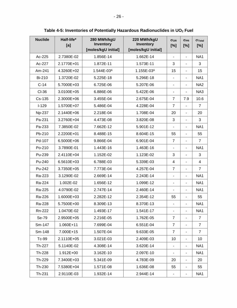
- 26 -

Table 4-5: Inventories of Potentially Hazardous Radionuclides in UO2 Fuel

Nuclide Half-life*

[a]

280 MWh/kgU Inventory

[moles/kgU initial]

220 MWh/kgU Inventory

[moles/kgU initial]

OR

[%]

PR

[%]

Total

[%]

Ac-225 2.7380E-02 1.856E-14 1.662E-14 - - NA1

Ac-227 2.1770E+01 1.872E-11 1.573E-11 3 - 3

Am-241 4.3260E+02 1.544E-03& 1.155E-03& 15 - 15

Bi-210 1.3720E-02 5.225E-18 5.296E-18 - - NA1

C-14 5.7000E+03 6.725E-06 5.207E-06 - - NA2

Cl-36 3.0100E+05 6.886E-06 5.422E-06 - - NA3

Cs-135 2.3000E+06 3.455E-04 2.675E-04 7 7.9 10.6

I-129 1.5700E+07 5.486E-04 4.228E-04 7 - 7

Np-237 2.1440E+06 2.218E-04 1.708E-04 20 - 20

Pa-231 3.2760E+04 4.473E-08 3.820E-08 3 - 3

Pa-233 7.3850E-02 7.662E-12 5.901E-12 - - NA1

Pb-210 2.2200E+01 8.488E-15 8.604E-15 55 - 55

Pd-107 6.5000E+06 9.866E-04 6.901E-04 7 - 7

Po-210 3.7890E-01 1.443E-16 1.463E-16 - - NA1

Pu-239 2.4110E+04 1.152E-02 1.123E-02 3 - 3

Pu-240 6.5610E+03 6.788E-03 5.339E-03 4 - 4

Pu-242 3.7350E+05 7.773E-04 4.257E-04 7 - 7

Ra-223 3.1290E-02 2.669E-14 2.243E-14 - - NA1

Ra-224 1.002E-02 1.656E-12 1.099E-12 - - NA1

Ra-225 4.0790E-02 2.747E-14 2.460E-14 - - NA1

Ra-226 1.6000E+03 2.282E-12 2.354E-12 55 - 55

Ra-228 5.7500E+00 8.309E-13 8.370E-13 - - NA1

Rn-222 1.0470E-02 1.493E-17 1.541E-17 - - NA1

Se-79 2.9500E+05 2.216E-05 1.762E-05 7 - 7

Sm-147 1.060E+11 7.699E-04 6.551E-04 7 - 7

Sm-148 7.000E+15 1.507E-04 9.633E-05 7 - 7

Tc-99 2.1110E+05 3.021E-03 2.409E-03 10 - 10

Th-227 5.1140E-02 4.308E-14 3.620E-14 - - NA1

Th-228 1.912E+00 3.162E-10 2.097E-10 - - NA1

Th-229 7.3400E+03 5.341E-09 4.783E-09 20 - 20

Th-230 7.5380E+04 1.571E-08 1.636E-08 55 - 55

Th-231 2.9110E-03 1.932E-14 2.944E-14 - - NA1

- 27 -

Nuclide Half-life*

[a]

280 MWh/kgU Inventory

[moles/kgU initial]

220 MWh/kgU Inventory

[moles/kgU initial]

OR

[%]

PR

[%]

Total

[%]

Th-232 1.4050E+10 2.078E-03 2.095E-03 4 - 4

Th-234 6.5980E-02 6.074E-11 6.091E-11 - - NA1

U-233 1.5920E+05 4.004E-05 3.608E-05 20 - 20

U-234& 2.4550E+05 2.166E-04& 2.089E-04& 50 - 50

U-235 7.0380E+08 4.748E-03 7.238E-03 3 - 3

U-236 2.3420E+07 3.845E-03 3.501E-03 4 - 4

U-238 4.4680E+09 4.114E+00 4.125E+00 0 - 0

Notes: NA1 = Nuclide assigned a constant inventory because it has a short half-life. NA2 = Nuclide inventory calculated by ORIGEN-S is based on a N impurity level of 15 µg/gU. Inventory is assigned

a uniform distribution with maximum value 1.25x the ORIGEN-S predicted inventory and minimum value equal to 0.45x the ORIGEN-S predicted inventory. Limits are based on measured C-14 values from Stroes-Gascoyne et al. 1994.

NA3 = Nuclide inventory is assigned a uniform distribution with maximum value equal to ORIGEN-S predicted value based on the Cl impurity level of 5µg/gU from Tait et al. (2000). The minimum value is set equal to maximum/10. Table shows the median value.

*Half-life from ENDF/B VII.1 (Chadwick et al. 2011) and converted as required using 365.25 days = 1 year. #Median value from Tait et al. (2000) increased to account for “ring sum” correction: Ac-227 (1%), Pa-231 (1.2%),

Pu-242 (1.9%) and U-235 (1.7%) (Appendix A, Tait et al. 2000) &Includes inventory of short-lived precursor: Am-241 (Pu-241, 2.737E-4 mol/kgU) and U-234 (Pu-238, 2.259E-5

mol/kgU).

Table 4-6: Inventories of Potentially Hazardous Radionuclides of Interest in Zircaloy for 30 Years Decay Time

Nuclide Half-life*

[a]

280 MWh/kgU Inventory

[moles/kgZr initial]

220 MWh/kgU Inventory

[moles/kgZr initial]

OR

[%]

PR

[%]

Total

[%]

C-14 5.7000E+03 2.457E-05 2.180E-06 - - NA1

Cl-36 3.0100E+05 1.489E-05 9.860E-06 - - NA1

Notes: NA1 = Nuclide assigned a constant inventory because it is formed by activation of impurity in the fuel, and

impurity levels were assigned high values in Tait et al. (2000).

*Half-life from ENDF/B VII.1 (Chadwick et al. 2011) and converted as required using 365.25 days = 1 year.

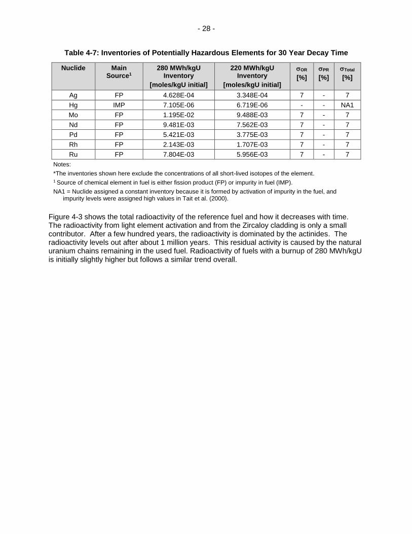
- 28 -

Table 4-7: Inventories of Potentially Hazardous Elements for 30 Year Decay Time

Nuclide Main Source1

280 MWh/kgU Inventory

[moles/kgU initial]

220 MWh/kgU Inventory

[moles/kgU initial]

OR

[%]

PR

[%]

Total

[%]

Ag FP 4.628E-04 3.348E-04 7 - 7

Hg IMP 7.105E-06 6.719E-06 - - NA1

Mo FP 1.195E-02 9.488E-03 7 - 7

Nd FP 9.481E-03 7.562E-03 7 - 7

Pd FP 5.421E-03 3.775E-03 7 - 7

Rh FP 2.143E-03 1.707E-03 7 - 7

Ru FP 7.804E-03 5.956E-03 7 - 7

Notes:

*The inventories shown here exclude the concentrations of all short-lived isotopes of the element. 1 Source of chemical element in fuel is either fission product (FP) or impurity in fuel (IMP).

NA1 = Nuclide assigned a constant inventory because it is formed by activation of impurity in the fuel, and impurity levels were assigned high values in Tait et al. (2000).

Figure 4-3 shows the total radioactivity of the reference fuel and how it decreases with time. The radioactivity from light element activation and from the Zircaloy cladding is only a small contributor. After a few hundred years, the radioactivity is dominated by the actinides. The radioactivity levels out after about 1 million years. This residual activity is caused by the natural uranium chains remaining in the used fuel. Radioactivity of fuels with a burnup of 280 MWh/kgU is initially slightly higher but follows a similar trend overall.

- 29 -

Note: The blue line (Actinides – U Chains) shows the radioactivity of all actinides, except the U-238, U-235 and U-234 actinides and their progeny

Figure 4-3: Radioactivity of Used Fuel (220 MWh/kgU burnup) as a Function of Time after Discharge from the Reactor

4.4 CONTAMINATION ON EXTERNAL BUNDLE SURFACES

Corrosion products formed within the primary coolant circuit of a reactor can deposit on the surfaces of fuel bundles in the reactor core. Neutron activation of some of these corrosion products can generate radioactive isotopes. In addition, fission products and UO2 fuel particulates released from defective fuel bundles can also deposit on the surfaces of fuel bundles. In the context of a geological repository for used fuel, these surface deposits provide a small additional source of radionuclides and potentially chemically toxic elements. Fission product and uranium inventories in surface deposits are very low compared to the corresponding inventories within the fuel bundle itself (i.e., < 0.001%) (Chen et al. 1986, and recent unpublished NWMO work) and, therefore, can be neglected in the Seventh Case Study postclosure safety assessment. Data on metal (Fe, Ni, Cu, Cr and Co) concentrations in fuel surface deposits (Chen et al. 1986) indicate that, for these elements, the metal inventories in the surface deposit are a small fraction (up to 2.3%) of the corresponding metal inventory in the fuel. However, none of these 5 metals are included in the detailed safety assessment calculations carried out for the Seventh Case Study because they were screened out by the chemical hazard screening analyses. Hence, the inventories of these 5 metals on the external bundle surfaces are not included in the Seventh Case Study.

- 30 -

4.5 INSTANT RELEASE

4.5.1 UO2 Instant Release

Radionuclides are released from used fuel by two processes - instant release and congruent dissolution release. Instant release is the rapid release of nuclides on contact of the used fuel with water. Congruent dissolution is the slower release of nuclides as the matrix material itself (either the UO2 fuel or the Zircaloy cladding) dissolves. The instant release process considers any radionuclide (or chemical element) inventory in the fuel-cladding gap or in the UO2 fuel grain boundaries to be quickly exposed to water and to dissolve into the water. The degree of segregation of the various radionuclides (or chemical elements) is highly dependent on fuel operating parameters such as linear power rating and burnup, as well as on the properties of the radionuclides (or chemical elements). The amount of a chemical element (or radionuclide) that is susceptible to instant release is defined as a fraction of the total inventory of that chemical element (or radionuclide) within the fuel. The instant release fraction data are given in Table 4-8. The range of values in the data allow for uncertainties. Radionuclides of the same element are all assumed to have the same instant release fraction. The sources of the instant release fraction data are described below. The instant release fraction data for key elements such as I and Cs are based on the work of Stroes-Gascoyne (1996). The instant release fractions of these key elements were reviewed for the previous Case Study, including the possible implications of newer non-CANDU data (Johnson et al. 2004, 2005; SKB 2010). However, for CANDU fuel, Stroes-Gascoyne (1996) remains the best data source. Stroes-Gascoyne (1996) found that the instant release fraction for Cs can be described using a normal distribution with mean 0.039 and standard deviation 0.019. The instant release fraction for I can be described using a normal distribution with mean 0.036 and standard deviation 0.024. This is higher than the instant release fraction used by SKB for light-water reactor fuel (SKB 2010). The fuels used in the experiments of Stroes-Gascoyne (1996) had burnups and (peak) linear power ratings that were generally higher than those expected for typical CANDU fuel. For example, about 14% of CANDU fuel bundles have peak linear power ratings greater than 42 kW/m (see Figure 4-4, data from Wilk 2013), whereas in the work of Stroes-Gascoyne 57% of the fuels had peak linear power ratings greater than 42 kW/m. Thus, the measured instant release fractions from Stroes-Gascoyne should be conservative, based on the relationship between fission gas releases and linear power rating, as described below. Generally fission (noble) gas releases from CANDU fuel bundles are low if the peak linear power rating of the fuel is less than about 42 kW/m, and increases with linear power rating for linear power rating values above 42 kW/m (Floyd et al. 1992), as illustrated in Figure 4-4. A threshold for fission gas release has also been found for BWR fuel (Kamimura 1992). For light-water reactor fuel, fission gas releases are independent of fuel burnup for burnups less than about 1000 MWh/kgU and then increase with burnup (Johnson et al. 2004). Since CANDU burnups are much lower than 1000 MWh/kgU and there is no correlation between fuel burnup and linear power rating, fission gas releases from CANDU fuels are not correlated to fuel burnup.

- 31 -

Table 4-8: Instant Release Fractions for CANDU Fuel

Element PDF Type PDF Attributes* Lower Limit Upper Limit

Ac constant 0 - -

Ag uniform - 0 0.001

Am constant 0 - -

Bi normal (0.006, 0.0015) 0.0023 0.03

C normal (0.027, 0.016) 0.0005 0.075

Cl normal (0.06, 0.01) 0.01 0.2

Cs normal (0.04, 0.01) 0.015 0.20

Hg normal (0.04, 0.01) 0.015 0.20

I normal (0.04, 0.01) 0.015 0.20

Mo lognormal (0.01, 2) 0.0005 0.05

Nd constant 0 - -

Np constant 0 - -

Pa constant 0 - -

Pb normal (0.006, 0.0015) 0.0023 0.03

Pd lognormal (0.01, 2) 0.0005 0.05

Po normal (0.04, 0.01) 0.015 0.20

Pu constant 0 - -

Ra normal (0.025, 0.008) 0.001 0.05

Rh lognormal (0.01, 2) 0.0005 0.05

Rn normal (0.04, 0.01) 0.015 0.20

Ru lognormal (0.01, 2) 0.0005 0.05

Se normal (0.006, 0.0015) 0.0023 0.03

Sm constant 0 - -

Tc lognormal (0.01, 2) 0.0005 0.05

Th constant 0 - -

U constant 0 - -

*PDF attributes are (mean, standard deviation) for the normal PDF, and (geometric mean, geometric standard deviation) for the lognormal PDF.

- 32 -

Figure 4-4: Distribution of Maximum Linear Power Ratings and Cumulative Distribution for all Commercial Fuel Bundles (discharged up to 2012)

Since iodine and cesium behave like noble gases (Iglesias et al. 2011), the I and Cs gap inventories should depend similarly on the fuel linear power rating. This is illustrated by plotting the instant release fractions for I and Cs (i.e., the sum of the gap and grain boundary inventories) versus the peak linear power rating, as shown in Figure 4.5. Because of the scarcity of data at low linear power ratings, no attempt was made to calculate an average Cs (or I) instant release fraction for the 48 fuel bundles in a fuel container from the distribution of bundle linear powers. Rather, the mean instant release fractions derived by Stroes-Gascoyne (1996), i.e., using unweighted averages, are used in the assessment. These are expected to be conservative given the relatively large number of high peak linear power rating fuels used by Stroes-Gascoyne (compare Figures 4.3 and 4.5).

The standard deviations in the instant release fractions found by Stroes-Gascoyne (1996) reflect mainly the differences between the 14 different fuels used in her experiments. For a larger quantity of fuel (i.e., the 48 fuel bundles in a used fuel container), the standard deviation for the average instant release fraction would be much smaller. For example, the standard deviation for the instant release fraction of I associated with having 48 bundles in a container, assuming that the measured variability is randomly distributed between fuel bundles, is 0.024/(48)1/2 = 0.0035. However, the measured variability may include systematic biases and not just random measurement uncertainty; therefore, the standard deviation for the average instant release fraction for the fuel in a container has been set to a nominal value of 0.01.

- 33 -

In summary, for the Seventh Case Study, it is assumed that the instant release fraction for Cs and I are described by a normal distribution with mean 0.04 and standard deviation 0.01. The limits of the distribution are set at 0.015 to 0.20. The minimum value corresponds approximately to the smallest instant release fraction measured by Stroes-Gascoyne (1996) and the maximum value corresponds approximately to the calculated fission gas release from a high power rating/high burnup fuel (Iglesias et al. 2011). The instant release fraction for Cl is derived from the Cl-36 release data of Tait et al. (1997), who suggest that most of the Cl-36 in the fuel originates from the fuel-cladding gap and that little is present in the grain boundaries. The instant release fraction for Cl increases with both the peak linear power rating and burnup of the fuel (see Figure 4-7). Thus, one could in theory use the relationship in Figure 4-7 along with the distribution of peak linear power ratings (Figure 4-4) to obtain the average expected Cl-36 instant release fraction from all fuel bundles. However, the data of Tait et al. (1997) are limited (i.e., most data are for low linear power rating, low burnups or for high linear power rating, high burnup fuels) and so the relationship shown in Figure 4-7 may not be generally applicable. Hence, a conservative estimate of the Cl-36 instant release fraction was made assuming, based on Tait et al. (1997), that fuels with low peak linear power rating (< 40 kW/m), low burnup (<190 MWh/kgU); intermediate linear power rating, intermediate burnup; and high linear power rating (> 43 kW/m) or high burnup (> 230 MWh/kgU) have Cl-36 instant release fractions of 0.7%, 4.5% and 15%, respectively. Using the distribution of fuel linear power rating and burnup data for the Pickering Nuclear Generating Station (for which linear power ratings and, hence, instant release fractions are the highest), the calculated Cl-36 instant release fraction is 0.06. Therefore, the instant release fraction for Cl-36 is described as a normal distribution with mean 0.06 and standard deviation of 0.01. This standard deviation accounts for the large quantity of fuel in a used fuel container, as discussed above for I and Cs. The limits of the distribution are set at 0.01 to 0.2, the approximate limits of the instant release fraction data measured by Tait et al. (1997). For CANDU fuel, Stroes-Gascoyne et al. (1994) measured C-14 releases from crushed fuel samples. No correlation of total C-14 release with fuel burnup or power rating was observed. The mean release from the fifteen fuel samples was 0.027, with a standard deviation of 0.016. Technetium is not soluble in the UO2 fuel and is present in used fuel in metallic form, typically in alloy inclusions (Kleykamp 1985). The results of leaching studies indicate that Tc gap and grain boundary releases are generally small, i.e., < 0.002 (Johnson and Tait 1997, Garisto and Gierszewski 2002). This may be due to the insolubility of the alloy inclusions in which Tc is found. The highest Tc releases, up to 5%, were observed in studies involving leaching of CANDU fuel that was oxidized in air to U3O8 powder (Stroes-Gascoyne and Sellinger 1986). Although such conditions are not representative of fuel under repository conditions, they may provide a better estimate of the total grain boundary inventory of Tc.

- 34 -

Figure 4-5: Fission Gas (gap) Release as a Function of Peak Linear Power Rating for CANDU Fuels with Burnups Less than 400 MWh/kgU

Figure 4-6: Total Instant Release Fractions (gap + grain boundary inventories) for Iodine and Cesium

0

2

4

6

8

10

12

0 10 20 30 40 50 60 70

Fis

sio

n G

as

Re

lea

se

(%

of

To

tal I

nve

nto

ry)

Peak Linear Power Rating (kW/m)

Bruce

Pickering

Darlington

Non-OPG

0

0.02

0.04

0.06

0.08

0.1

0.12

0 10 20 30 40 50 60

To

tal I

ns

tan

t R

ele

as

e F

rac

tio

n

Peak Linear Power Rating (kW/m)

Cs

I

- 35 -

Figure 4-7: Cl-36 Releases from CANDU Fuel

The Tc instant release fraction is taken from the review of Garisto and Gierszewski (2002). The Tc instant release fraction is lognormally distributed with a geometric mean of 0.01 and a geometric standard deviation of 2. This instant release fraction is larger than that used by SKB in their SR-Site safety assessment (SKB 2010) since it is based on results of leaching experiments with both slightly preoxidized (UO2+x, x < 0.25) and non-oxidized CANDU fuels. This larger value was selected to account for the uncertainty in the amount of Tc that could be leached from the fuel grain boundaries over hundreds of years. The instant release fractions of all actinides and lanthanides are taken to be zero, as in other studies (Johnson et al. 2004), since they form non-volatile oxides that are dissolved within the UO2 fuel matrix. The instant release fraction for Se have not been measured for CANDU fuels. Wilson (1990a, 1990b) attempted to measure the instant release fractions of Se-79 for light-water reactor fuels. However, the amount leached was less than the detection limit. From the “less than” data reported by Wilson, it is possible to infer maximum instant release fractions (Johnson et al. 2004, SKB 2010). For Se, a semi-volatile element that is non-soluble in the UO2 fuel, the maximum instant release fraction is less than 15% of the fission gas release. Such a low instant release fraction suggests that Se is not volatile in the fuel. Perhaps Se forms alloys in the fuel, e.g., BaSe, as suggested by Iglesias et al. (2011). For the Seventh Case Study, the instant release fraction of Se is set equal to 15% of the instant release fraction of I and Cs (following SKB 2010). Thus, the instant release fraction for Se is described by a normal distribution with mean 0.006 and standard deviation 0.0015. The limits of the distribution are set at 0.0023 to 0.03.

0.001

0.01

0.1

1

0 10 20 30 40 50 60

Fra

cti

on

al

Cl-

36

Re

lea

se

s

Peak Linear Power Rating (kW/m)

- 36 -

For the many chemical elements for which leaching measurements are not available, the only basis for estimating the instant release fractions are the diffusion coefficients of the elements in fuel and the chemistry of the elements in fuel. For example, an understanding of which elements form solid solutions with UO2 and which elements form metallic or oxide precipitates in fuel would be important (Kleykamp 1985). This methodology is used to conservatively estimate the instant release fractions of elements for which measured data are not available. Generally, fission products can be classified into 4 groups (Kleykamp 1985):

1. Gases and other volatiles: Kr, Xe, Br, I

2. Fission products forming metallic precipitates:

Mo, Tc, Ru, Rh, Pd, Ag, Cd, In, Sn, Sb, Te

3. Fission products forming oxide precipitates (often referred to as the “grey phase”): Rb, Cs, Ba, Zr, Nb, Mo, Te

4. Fission products dissolved in the fuel matrix: Sr, Zr, Nb, Rare Earths, Y, La, Ce, Pr, Nd, Pm, Sm

Some elements fall into two categories. There is a continuous transition between categories 2 and 3 due to the similar oxygen potential of some fission product oxides and fuel, which changes composition during irradiation. Transitions can also occur between categories 3 and 4 due to the burnup dependent distribution of cations in both oxide phases. Furthermore, some fission products can react without participation of oxygen (e.g., Cs2Te, CsI, etc.). The key thermodynamic factor that influences the chemical state of the fission products in fuel is the oxygen potential, which in turn depends on the stoichiometry of the fuel, the temperature and burnup. The fuel is initially stoichiometric, i.e., the oxygen potential is very low (Lindemer and Besmann 1985), but burnup raises the ratio of oxygen to uranium because the O2 released by fission of uranium cannot be completely bonded by the generated fission products (Cordfunke and Konings 1988). For near-stoichiometric fuels, the oxidation potential in the fuel may be buffered by the Mo/MoO2 couple (Kleykamp 1985, Cubicciotti and Sanecki 1978), since this couple has an oxidation potential that is similar to that of slightly hyperstoichiometric fuel and the fission yield of Mo is relatively high. The oxidation potential for formation of the oxide of each element, relative to the oxidation potential of the fuel, was used to assess the chemical state of the elements in fuel (Kleykamp 1985) and, thence, to estimate the instant release fractions of the elements for which no measured values are available. For an element for which measured instant release fractions are not available, the rationale for the selected instant release fraction is provided in Table 4-9.

- 37 -

Table 4-9: Rationale for Selection of Instant Release Fractions for Elements without Measured Data

Element Chemical State of Element in Fuel

Element Boiling

Point [K]

Rationale for Selected Instant Release Fraction

Ac, Am, Np, Pa,

Pu, Th, U

Oxides dissolved in the fuel matrix

----- Actinides are present in solid solution in the fuel matrix. Assume instant release fraction=0 for all actinides (Johnson and Tait 1997).

Nd, Sm Oxides dissolved in the fuel matrix

----- Lanthanides are present in solid solution in the fuel matrix. The instant release fraction for all lanthanides are assumed to be zero.

Ag Metallic precipitate alloyed with other noble metals such as Cd and Sn (Kleykamp 1985).

2435 Boiling point of Ag is similar to that of Sn (2875 K). Since Ag is likely alloyed with Sn and other similar metals in fuel, assume instant release fraction for Ag is the same as that for Sn.

Bi Metallic precipitate in fuel 1837 Boiling point of Bi is lower than that of Sn (2875 K) and higher than that of Se (958 K). For conservatism, assume instant release fraction is same as that of Se.

C Gaseous oxide (CO or CO2).

----- Measured value (see text).

Cl Volatile, reactive gas ----- Measured value (see text).

Cs Found in various forms in fuel – dissolved in fuel, as Cs urinates, in grey phase and reacted with other fission products such as I and Te (Kleykamp 1985)

----- Measure (see text).

Hg Metallic precipitate in fuel, alloyed with other elements

630 The volatility of Hg is quite high at the temperature of fuel in the reactor; therefore, assume instant release fraction is similar to that of noble gases such as Rn.

I Volatile, reactive gas ----- Measured (see text).

Mo Metallic precipitate alloyed with Tc, Ru, Rh and Pd, and dissolved in fuel matrix as oxide.

4912 Found in grain boundaries of fuel alloyed with Tc in epsilon particles. Assume instant release fraction of Mo is the same as for Tc.

Pb Metallic precipitate in fuel 2022 Boiling point of Pb is lower than that of Sn (2875 K) and higher than that of Se (958 K). For conservatism, assume instant release fraction is same as that of Se.

Pd Metallic precipitate alloyed with a wide variety of metals in fuel, e.g., found in epsilon particles with Tc, Ru, Rh and Mo.

3236 Assume same instant release fraction of Pd is the same as for Tc, since found in grain boundaries of fuel alloyed with Tc in epsilon particles.

- 38 -

Element Chemical State of Element in Fuel

Element Boiling

Point [K]

Rationale for Selected Instant Release Fraction

Po Chemistry is similar to that of Bi and Te.

----- Po has only short-lived isotopes, so for conservatism assume that instant release fraction of Po is the same as for noble gases such as Rn.

Ra Oxide in fuel. ----- Ra is likely dissolved in the fuel matrix. However, for conservatism, assume Ra behaves like Sr in fuel, since both are alkaline earth elements. Thus, assume instant release fraction of Ra is the same as that of Sr.

Rh Metallic precipitate alloyed with Tc, Ru, Mo, and Pd (Kleykamp, 1985)

3968 Rh is found in grain boundaries of fuel alloyed with Tc in epsilon particles. Assumed the instant release fraction of Rh is equal to that of Tc.

Rn Non-reactive gas ----- Rn is a noble gas. The instant release fractions of the Cs, I and the noble gases are similar. Therefore, instant release fraction for Rn is set equal to that of Cs or I.

Ru Metallic precipitate alloyed with Tc, Rh, Mo, and Pd (Kleykamp 1985)

4423 Ru is found in grain boundaries of fuel alloyed with Tc in epsilon particles. Assumed the instant release fraction of Rh is equal to that of Tc.

Se Likely in elemental form in fuel, alloyed with other fission products

958 Measured value (see text). Note that although boiling point of Se is relatively low, the measured values of the instant release fraction are not high. Perhaps alloys or compounds formed by Se are stable.

Tc Oxide in fuel ----- Measured value (see text).

- 39 -

4.5.2 Zircaloy Instant Release

Because the impurities in the Zircaloy of the fuel bundles are likely uniformly distributed and the temperature of the cladding during reactor operation is relatively low, the activation products and impurities in the Zircaloy would be expected to be likewise uniformly distributed. Hence, for the Zircaloy wasteform, the instant release fractions should be zero and contaminants are released congruently as the Zircaloy corrodes. However, leaching experiments indicate that the C-14 within the oxide film on the Zircaloy is released relatively rapidly compared to the C-14 within the metal itself (Gras 2014, Yamaguichi et al. 1999, Smith and Baldwin 1993). The same leaching experiments suggest that the C-14 instant release fraction for the Zircaloy metal is zero. Consequently, the fraction of the C-14 within the oxide layer can be assumed to be instantly released after water breaches a used fuel container and contacts the fuel bundles and so the instant release fraction of C-14 from the Zircaloy wasteform is non-zero. In previous safety assessments, the instant release fraction for C-14 in the Zircaloy was based on pressurized water reactor data. This turns out to be very conservative since the oxide layer on the Zircaloy cladding of a CANDU fuel bundle is much thinner than for pressurized water reactor fuel and the thickness of the Zircaloy claddings is similar in the two fuel types. The derivation of the instant release fraction for C-14 for the Zircaloy wasteform in a CANDU used fuel bundle is described below. The concentration of C-14 in the Zircaloy oxide layer is higher than in the metal itself. Data from Tanabe et al. (2009) indicate that the concentration in the oxide layer is 1.5 to 1.7 times higher (on a weight basis) than in the metal. Thus, if Ω is the concentration of C-14 in the Zircaloy metal (in Bq/kg Zr) then the concentration of C-14 in the oxide layer is approximately 1.6 Ω. Based on information in the literature (Wasywich 1993, 1992), the thickness of the continuous oxide layer on the outer surface of the Zircaloy cladding of used CANDU fuel is less than 5 µm. This oxide thickness is somewhat larger than the value determined using the correlation between the oxide thickness and the burnup of the fuel given in Gras (2014). For a burnup of 280 MWh/kgU (or 11.7 GWd/tU), this correlation gives an oxide thickness of 3.4 μm. The oxide layer on the inner surface of the Zircaloy cladding of CANDU fuel is generally patchy (Wasywich 1992) or non-existent. The patchy oxide layers were generally thicker in used fuel from early test reactors (e.g., Douglas Point) compared to used fuel from later power reactors (e.g. Pickering). The inner oxide layer was absent or patchy and thin (< 2 μm) in fuels from and later power reactors was coated with CANLUB graphite. Thus, the amount of C-14 in the inner oxide layer is small and is approximated by assuming that the inner oxide layer has a thickness of 1 μm. If all the C-14 within the inner and outer oxide layers of the Zircaloy is released upon contact with water, the instant release fraction for C-14 in the Zircaloy wasteform, IRFC14,Zr, would be given by the following equation

𝐼𝑅𝐹𝐶14,𝑍𝑟 =1.6𝛺𝜋𝑑𝛿𝜌𝑍𝑟𝑂2

𝛺𝜋𝑑𝜔𝜌𝑍𝑟 (4.1)

Where δ is the total thickness of the inner and outer oxide layers (6 μm), d is the outer diameter of the cladding, w is the thickness of the cladding (400 μm), ρZrO2 is the density of zirconium

- 40 -

dioxide (5680 kg/m3) and ρZr is the density of Zircaloy (6550 kg/m3). Substituting the values of the parameters in Equation 1, one finds that IRFC14,Zr = 0.021. This value of the instant release fraction for C-14 from the Zircaloy wasteform is approximately 10-fold smaller than the previous value of 0.20 which was based on data for high burnup pressurized water reactor fuel. This large difference is understandable given that the thickness of the Zircaloy oxide layer on the cladding of the higher burnup pressurized water reactor fuel is approximately 10-fold larger than the corresponding value for CANDU used fuel. A summary of Zircaloy instant release fractions used in the Seventh Case Study are shown in Table 4-10.

Table 4-10: Instant Release Fractions for Zircaloy Cladding

Element Value [-]

C 0.021

All other elements 0

4.6 CONGRUENT RELEASE

4.6.1 UO2 Fuel Dissolution

The UO2 ceramic fuel matrix is durable, and dissolves slowly in water. The most important factor in the rate of dissolution of UO2 in water is the redox conditions in the surrounding groundwater. Reducing conditions are expected to prevail in and around the container under the influence of the reducing groundwater, and consumption of any residual oxygen by reaction with the copper and steel container materials or with ferrous and organic material in the sealing materials. Under these reducing conditions, the UO2 fuel would dissolve very slowly. However, the conditions at the used fuel surface are likely to be oxidizing for a long time due to the production of oxidants in the water from radiolysis (Poinssot et al. 2005, Shoesmith 2007,

He et al. 2012). Radiolysis of the groundwater would be caused by the -, -, and -radiations emitted by the used fuel, at rates that depend on the radiation type and that generally decrease with time as the radiation field strengths decrease (Garisto et al. 2009). For the Seventh Case Study, an empirical model for radiolysis-driven dissolution is used. In this

approach, the rates of dissolution of the used fuel matrix due to -, - and -radiolysis are assumed proportional to the corresponding dose rates, i.e.,

R = Acont G f [ D(t+tC) ]aα (4.2)

R = Acont G f [ D(t+tC) ]aβ (4.3)

R = Acont G f [ D(t+tC) ]a (4.4)

with the exponents a = a = a =1. The total matrix dissolution rate, RTOT, is given by

RTOT = R + R + R + Rch* Acont (4.5) where,

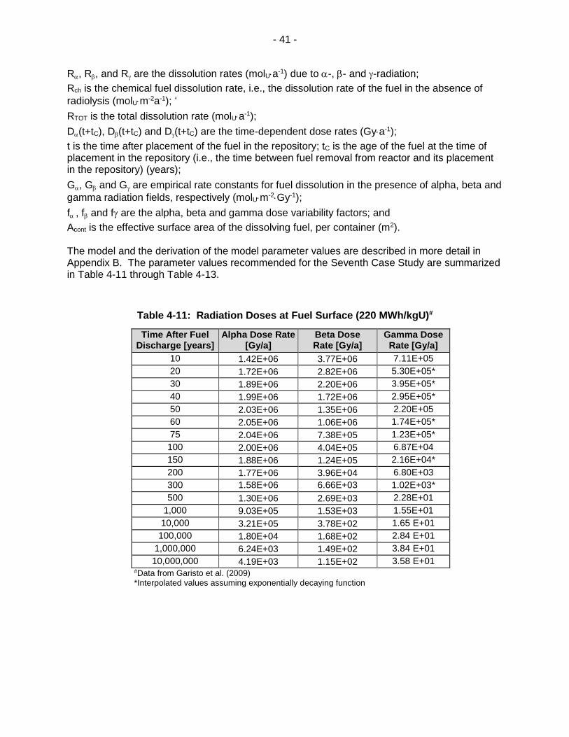
- 41 -

R, R, and R are the dissolution rates (molUa-1) due to -, - and -radiation;

Rch is the chemical fuel dissolution rate, i.e., the dissolution rate of the fuel in the absence of

radiolysis (molUm-2a-1); ‘

RTOT is the total dissolution rate (molUa-1);

D(t+tC), D(t+tC) and D(t+tC) are the time-dependent dose rates (Gya-1);

t is the time after placement of the fuel in the repository; tC is the age of the fuel at the time of placement in the repository (i.e., the time between fuel removal from reactor and its placement in the repository) (years);

G, G and G are empirical rate constants for fuel dissolution in the presence of alpha, beta and

gamma radiation fields, respectively (molUm-2Gy-1);

f , f and f are the alpha, beta and gamma dose variability factors; and

Acont is the effective surface area of the dissolving fuel, per container (m2). The model and the derivation of the model parameter values are described in more detail in Appendix B. The parameter values recommended for the Seventh Case Study are summarized in Table 4-11 through Table 4-13.

Table 4-11: Radiation Doses at Fuel Surface (220 MWh/kgU)#

Time After Fuel Discharge [years]

Alpha Dose Rate [Gy/a]

Beta Dose Rate [Gy/a]

Gamma Dose Rate [Gy/a]

10 1.42E+06 3.77E+06 7.11E+05

20 1.72E+06 2.82E+06 5.30E+05*

30 1.89E+06 2.20E+06 3.95E+05*

40 1.99E+06 1.72E+06 2.95E+05*

50 2.03E+06 1.35E+06 2.20E+05

60 2.05E+06 1.06E+06 1.74E+05*

75 2.04E+06 7.38E+05 1.23E+05*

100 2.00E+06 4.04E+05 6.87E+04

150 1.88E+06 1.24E+05 2.16E+04*

200 1.77E+06 3.96E+04 6.80E+03

300 1.58E+06 6.66E+03 1.02E+03*

500 1.30E+06 2.69E+03 2.28E+01

1,000 9.03E+05 1.53E+03 1.55E+01

10,000 3.21E+05 3.78E+02 1.65 E+01

100,000 1.80E+04 1.68E+02 2.84 E+01

1,000,000 6.24E+03 1.49E+02 3.84 E+01

10,000,000 4.19E+03 1.15E+02 3.58 E+01 #Data from Garisto et al. (2009) *Interpolated values assuming exponentially decaying function

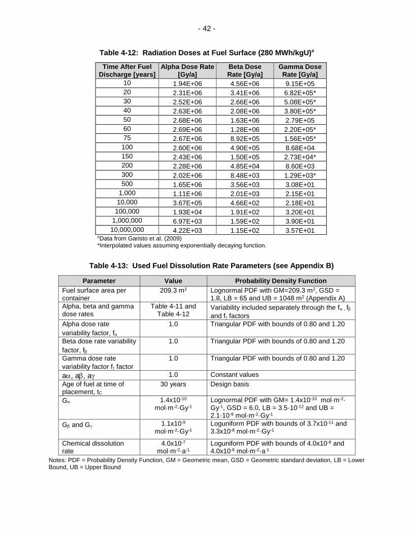
- 42 -

Table 4-12: Radiation Doses at Fuel Surface (280 MWh/kgU)#

Time After Fuel Discharge [years]

Alpha Dose Rate [Gy/a]

Beta Dose Rate [Gy/a]

Gamma Dose Rate [Gy/a]

10 1.94E+06 4.56E+06 9.15E+05

20 2.31E+06 3.41E+06 6.82E+05*

30 2.52E+06 2.66E+06 5.08E+05*

40 2.63E+06 2.08E+06 3.80E+05*

50 2.68E+06 1.63E+06 2.79E+05

60 2.69E+06 1.28E+06 2.20E+05*

75 2.67E+06 8.92E+05 1.56E+05*

100 2.60E+06 4.90E+05 8.68E+04

150 2.43E+06 1.50E+05 2.73E+04*

200 2.28E+06 4.85E+04 8.60E+03

300 2.02E+06 8.48E+03 1.29E+03*

500 1.65E+06 3.56E+03 3.08E+01

1,000 1.11E+06 2.01E+03 2.15E+01

10,000 3.67E+05 4.66E+02 2.18E+01

100,000 1.93E+04 1.91E+02 3.20E+01

1,000,000 6.97E+03 1.59E+02 3.90E+01

10,000,000 4.22E+03 1.15E+02 3.57E+01 #Data from Garisto et al. (2009) *Interpolated values assuming exponentially decaying function.

Table 4-13: Used Fuel Dissolution Rate Parameters (see Appendix B)

Parameter Value Probability Density Function

Fuel surface area per container

209.3 m2 Lognormal PDF with GM=209.3 m2, GSD = 1.8, LB = 65 and UB = 1048 m2 (Appendix A)

Alpha, beta and gamma dose rates

Table 4-11 and Table 4-12

Variability included separately through the f , f

and f factors

Alpha dose rate

variability factor, f

1.0 Triangular PDF with bounds of 0.80 and 1.20

Beta dose rate variability

factor, f

1.0 Triangular PDF with bounds of 0.80 and 1.20

Gamma dose rate

variability factor f factor

1.0 Triangular PDF with bounds of 0.80 and 1.20

a, a, a 1.0 Constant values

Age of fuel at time of placement, tC

30 years Design basis

G 1.4x10-10 mol·m-2·Gy-1

Lognormal PDF with GM= 1.4x10-10 mol·m-2· Gy-1, GSD = 6.0, LB = 3.5·10-12 and UB = 2.1·10-9 mol·m-2·Gy-1

G and G 1.1x10-9 mol·m-2·Gy-1

Loguniform PDF with bounds of 3.7x10-11 and 3.3x10-8 mol·m-2·Gy-1

Chemical dissolution rate

4.0x10-7 mol·m-2·a-1

Loguniform PDF with bounds of 4.0x10-8 and 4.0x10-6 mol·m-2·a-1

Notes: PDF = Probability Density Function, GM = Geometric mean, GSD = Geometric standard deviation, LB = Lower Bound, UB = Upper Bound

- 43 -

4.6.2 Zircaloy Corrosion

The Zircaloy sheath surrounding the fuel pellets in a CANDU fuel bundle naturally forms a thin layer of protective ZrO2 on its surface when in contact with air or water. This oxide layer greatly inhibits the Zircaloy dissolution rate in the postclosure period in the event water gains access to the used fuel container (Shoesmith and Zagidulin 2010). Because the inventory of certain isotopes such as Cl-36 and C-14 within the fuel sheath can be significant relative to the amount present in the fuel (Tait et al. 2000), dissolution of the Zircaloy is modelled in RSM and SYVAC3-CC4.

A kinetic dissolution model is used in which the zirconium dissolves at a rate proportional to the corrosion rate of Zircaloy in water and the surface area of the Zircaloy in contact with water. During corrosion, species trapped in the Zircaloy matrix are released. In the kinetic (corrosion) model, the dissolution rate, Rcor, of the Zircaloy is given by the following equation (4.6)

Rcor=kZrAzrρ (4.6)

where,

kZr is the corrosion rate of ZrO2 in water estimated to be approximately 5 nm/a (Shoesmith and Zagidulin 2010);

AZr is the area of the Zircaloy exposed to water (0.75 m2 per bundle or 36 m2 for a 48 bundle container); and

ρ is the density of the Zircaloy (6550 kg/m3)

Using the values specified above, Rcor is estimated to be 1.18x10-3 kg/a. Each container holds 105.6 kg of Zr (see Table 5-1) resulting in a complete dissolution of the Zircaloy in approximately 89,500 years.

- 44 -

5. CONTAINER

5.1 CONTAINER DIMENSIONS

The used fuel container design is illustrated in Figure 5.1. The main properties needed here are summarized in Table 5.1. The Seventh Case Study reference container design is the copper coated container which holds 48 bundles. The inner steel container provides structural support and is coated with copper for corrosion resistance. Inside this vessel are steel baskets holding the used fuel bundles.

Table 5-1: Container Internal Parameters

Parameter Value Comments

Total Number of Fuel Bundles in the Container

48 Nominal Design

Mass of Uranium in the Container

924 kg 48 bundles x 19.25 kgU/bundle (pre-irradiation value) (Tait et al. 2000)

Mass of Zirconium in the Container

105.6 kg 48 bundles x 2.2 kgZr/bundle (pre-irradiation value) (Tait et al. 2000)

Steel Vessel Outer Diameter

556 mm Nominal Dimension

Steel Vessel Thickness

Body 46.2 mm Nominal Dimension

Head 30 mm Nominal Dimension

Inner Vessel Length 1950 mm 2506 mm

Length of cylindrical shell Overall length, apex head-to-head

Steel Vessel Mass 1343 kg Nominal Mass

Steel Vessel Inner Surface Area

3.613 m2 Nominal Dimension

Inner Vessel Internal Volume

0.393 m3 Calculated using CAD model

Internal Void Volume 0.266 m3 Assumes basket (0.013 m3 = calculated using CAD model) and 37 Standard Element Bruce Bundle (0.114 m3 = 48 x 0.00238 m3 from Tait et al. 2000)

Internal Porosity Fraction

0.677 (Internal void volume)/(Internal volume)

Copper Cladding Thickness

3 mm Minimum Dimension

Copper Coating Mass 157 kg 118 kg

Maximum Mass (Nominal) Minimum Mass

Overall Container Length

2514 mm Nominal Dimension

Overall Container Diameter

564 mm Nominal Dimension

Loaded Container Total Mass

2815 kg Nominal Mass

Probability of a Container Failure in 1 Million Years

0 Base assumption (probabilistic failure analysis program underway)

- 45 -

Figure 5-1: Container Design Showing Copper Coating, Inner Steel Vessel, and Inside Support Tubes

5.2 DEFECTIVE CONTAINER

The “Base Case” sensitivity study assumes a small number of containers are fabricated with defects in their copper coating, and that a smaller number of these off-specification containers escape detection by the quality assurance program and are unknowingly placed in the repository. Studies are underway to determine the likelihood and number of off-specification containers that could potentially be present; however, the results of this work will not be available for quite some time. In the meantime, 10 containers with large undetected voids in the copper coating are assumed to be unknowingly placed in the repository. Postclosure safety studies with 10 defective containers are sufficient to illustrate repository performance and to provide a measure of the consequences that could be expected should such an event (or a similar one) actually occur. The undetected voids in the copper coatings are assumed sufficiently large to cause each of the 10 containers to be breached within the first one million years. Because it is highly unlikely that all 10 containers would fail simultaneously, the failure times are assumed to be evenly spread over the one million year time period of interest, with the first failure occurring at 1000 years and subsequent failures occurring at a rate of one container every 100,000 years thereafter.

- 46 -

For the probabilistic case in which the number of defective containers is varied, the number of defective containers is described by a binomial distribution with the individual container failure probability selected such that 16 failed containers is the 95th percentile value. The parameters used to describe this failure mode are listed in Table 5-2, and discussed further below.

Table 5-2: Defective Container Scenario Parameters

Parameter Value Comment

Instant Failure Fraction

9.18836x10-6 per container

GSD = 4

LB = 9.18835x10-6 UB = 1

Assumes a binomial distribution with the probability of failure set to a constant value and assumes 108,833 “trials” i.e. number of containers (see Section 2.3.2 of NWMO 2012). The probability of failure is set such that the probability of 16 containers failing is the 95th percentile.

Instant Container Failure Quantile

Varies by repository sector

Assumed to be one for all sectors in the Base Case

Container Failure Time, Deterministic Simulations

1000 a

100,000 a

200,000 a

…

900,000 a

For the Base Case the first failure occurs at 1,000 years and subsequent failures occur at a rate of one container every 100,000 years thereafter

Container Failure Time, Probabilistic Simulations

1,000-1,000,000 a Loguniform distribution with a lower bound of 1,000a and an upper bound of 1,000,000a.

Defect Radius 5.623 m Based on complete failure of container from Gobien and Garisto (2013). Although this is a non-physical defect radius, this value makes the calculated contaminant release rates agree with COMSOL model results.

Defect Length 49.23 mm Radial thickness of steel (46.23 mm) and copper (3 mm) container.

Porosity of the Defect

1.0 Assumed to be an open defect

Near Field Temperature

85°C Normal probability density function with mean of 85oC, standard deviation of 10°C, and bounds of 30°C and 100°C

5.3 FREE WATER DIFFUSION COEFFICIENT

Contaminants will escape the breached container by diffusion. The free water diffusivity of ions in a 1 molar strong electrolyte NaI solution is calculated to be 0.0262 m2/a at 25oC using the Nernst equation (Weast 1983). To account for the effect of surface diffusion, HTO is used as a proxy for cations such as Cs and the free-water diffusivity is assumed to be a factor of 2 higher than for ions in 1 molar NaI (Intera, 2011). In reality, free water diffusion coefficients are not influenced by surface diffusion or anion exclusion because the diffusion of a given specifies is not constrained in a porous medium.

- 47 -

However, the geosphere porosity and tortuosity parameters are not element dependent in SYVAC3-CC4 and changes to those parameters to account for surface diffusion would also impact the other elements for which this effect is not observed. Consequently, the free water diffusion coefficient in SYVAC3-CC4 was modified to account for this phenomenon. Changes to the free water diffusion coefficient for Cs will overestimate transport in the container but this conservatism is intended. All other species, including anions which may experience some anion exclusion (reduction diffusivity) in the geosphere are conservatively assumed to have a free-water diffusion coefficient equal to that of a neutral species. Diffusivities would increase by a factor of about 3.4 at 85oC (assuming that the diffusivity can be scaled by the temperature/viscosity ratio, according to Rohsenow and Choi 1961, p.383). The free-water diffusivity therefore ranges from 0.0524 m2/a to 0.356 m2/a, depending on the species and on the container temperature when the release occurs.

Table 5-3: Free Water Diffusivity

Element Value (at 25oC)1,2 [m2/a]

Value (at 85oC) [m2/a]

Cs 0.1048 0.356

Other Species 0.0524 0.178 1Values are assumed to be triangularly distributed with upper and lower bounds a factor of 10 higher and lower.

5.4 WATER COMPOSITION

The groundwater composition around the repository would need to be determined for any specific site. The range of measured groundwater compositions in Michigan Basin sedimentary rocks are described in (NWMO 2011b). A reference sedimentary rock groundwater, SR-270, has been defined for the Seventh Case Study host rock based on the groundwaters found at a depth of around 500 m. Its composition is listed in Table 5-4 (Duro et al. 2010). It is a reducing Na-Ca-Cl type groundwater, with total dissolved solids of about 275 g/L. The composition of the water actually reaching the used fuel will be that of the surrounding host rock groundwater but conditioned by passage through the backfill, buffer and container. In particular, the concentrations of the species in the water reaching the used fuel will be affected by ion exchange with the bentonite buffer (e.g., calcium ions in the groundwater may be exchanged for sodium ions in the bentonite as the groundwater passes through the bentonite), the presence of the iron-container insert, as well as the dissolution of the minor mineral components of the buffer, such as gypsum and calcite, which could lead to higher carbonate and sulphate concentrations in the contact water (Duro et al. 2010). The composition of this contact water is shown in Table 5-5. This was calculated by Duro et al. (2010) by equilibrating the selected SR-270 reference groundwater (see Table 5-5) for the Seventh Case Study site with the bentonite buffer minerals and the steel container. The assumed initial Eh of the groundwater is approximately -200 mV but this is expected to decrease to approximately-535 mV after equilibration of the groundwater with the carbon steel container insert.

- 48 -

Table 5-4: Contact Water Composition

Composition SR-270 Equilibrated SR-270 Bentonite-Iron Equilibration

pH 6.3 8.7

Environment Reducing Reducing

Eh (mV) -200 -535

Ionic Strength (mol/kgw)

5.78 5.88

Density 1.192 1.192

Element Solutes (mg/L)

Na 50,025 48,673

K 12,486 3,482

Ca 32,494 37,285

Mg 8,173 9,940

HCO3 135 3

SO4 1,784 1,813

Cl 168,058 168,744

Br 1,698 1,703

Sr 1,198 1,200

Li 5 5

F 1 1

I 3 3

B 80 80

Si 4 10

Fe 30 579

NO3 10 10

PO4 - -

Total Dissolved Solids

276,184 273,531

5.5 SOLUBILITY LIMITS

After container failure, water can contact the fuel, and cause the release of contaminants. The rate at which contaminants are released from the fuel is determined by the used fuel dissolution model. In theory, the concentrations of a contaminant in the water in the container could reach the solubility limit for that element. Consequently, precipitation of contaminants could occur, especially within or near the container where concentrations are highest. The element solubilities are listed in Table 5-5. These solubilities were calculated for the reference water compositions in Table 5-4 at 25oC. Many solubility limits are temperature sensitive and the vault temperature is expected to be higher than 25oC (approximately 85oC) for thousands of years after repository closure. Despite this, solubility limits were calculated at 25oC since very little thermodynamic data exists for temperatures outside of 25oC. The solubility limits can also be quite sensitive to the groundwater composition which is also likely to vary somewhat throughout the repository due to non-homogeneities in mineral composition of the granitic rock and perhaps the buffer material. To account for uncertainties in the solubility due to the higher temperatures in the repository and the groundwater composition, the solubility values listed in Table 5-5 are increased by a factor of 10 from their original references for use in the safety assessment calculations.

- 49 -

For several elements, i.e., Am, Bi, C, Mo, Np, Pa, Pb, Pd, Pu, Ra, Se, Tc, Th, and U the solubilities were calculated by Duro et al. (2010) using PHREEQC and the ThermoChimie v7b database. ThermoChimie includes the thermodynamic data compiled by the NEA, when available, and uses the specific ion theory (SIT) activity corrections (Guillaumont et al. 2003). Due to uncertainty in the thermodynamic data as well as variability in the geochemical conditions at repository depth, the solubility limit is described using a lognormal distribution. For elements in which the thermodynamic data are well defined or the solubility limit is relatively insensitive to repository conditions, a lognormal distribution with a geometric standard deviation of 3.2 is assumed. This geometric standard deviation corresponds to the 95% confidence bounds being with a factor of 10 of the geometric mean. Conversely for Pa, for which the solubility is highly uncertain due to scarcity of its thermodynamic data, a geometric standard deviation of 10 is used. The remaining elements (Ac, Ag, Cl, Cs, Hg, I, Nd, Po, Rh, Rn, Ru, Sm) are assigned a very high constant solubility (2 mol/kg) to ensure that precipitation does not occur. These elements are either expected to be highly soluble, or to have a low inventory in the fuel, or to exist only as short-lived radionuclides, or to be gaseous (i.e., they do not precipitate), or to have complex chemistries so that their solubility limit is highly uncertain or to have very limited thermodynamic data for conditions of interest.

- 50 -

Table 5-5: Element Solubilities1

Element Value2 (mol/kg)

GSD Distribution Type

Comments

Ac 2.0 - Constant No solubility limit (nominal conservative value)

Ag 2.0 - Constant No solubility limit (nominal conservative value)

Am 2.0 - Constant No solubility limit (Duro et al. 2010)

Bi 2.0 - Constant No solubility limit (Duro et al. 2010)

C 2.2x10-2 3.2 Lognormal Duro et al. (2010)

Cl 2.0 - Constant No solubility limit (nominal conservative value)

Cs 2.0 - Constant No solubility limit (nominal conservative value)

Hg 2.0 - Constant No solubility limit (nominal conservative value)

I 2.0 - Constant No solubility limit (nominal conservative value)

Mo 2.3x10-12 3.2 Lognormal Duro et al. (2010)

Nd 2.0 - Constant No solubility limit (nominal conservative value)

Np 1.7x10-8 3.2 Lognormal Duro et al. (2010)

Pa 3.2x10-7 10 Lognormal Duro et al. (2010)

Pb 2.0 - Constant No solubility limit (Duro et al. 2010)

Pd 2.0 - Constant No solubility limit (Duro et al. 2010)

Po 2.0 - Constant No solubility limit (nominal conservative value)

Pu 2.0 - Constant No solubility limit (Duro et al. 2010)

Ra 1.7x10-4 3.2 Lognormal Duro et al. (2010)

Rh 2.0 - Constant No solubility limit (nominal conservative value)

Rn 2.0 - Constant No solubility limit (nominal conservative value)

Ru 2.0 - Constant No solubility limit (nominal conservative value)

Se 3.4x10-8 3.2 Lognormal Duro et al. (2010)

Sm 2.0 - Constant No solubility limit (nominal conservative value)

Tc 4.4x10-8 3.2 Lognormal Duro et al. (2010)

Th 1.4x10-6 3.2 Lognormal Duro et al. (2010)

U 4.5x10-8 3.2 Lognormal Duro et al. (2010) 1The solubility values in this table are 10-fold larger than those listed in the original references to account for

uncertainties, as discussed in the text. 2Constant value for the constant distribution function, and geometric mean for the lognormal distribution function.

- 51 -

6. REPOSITORY DATA

This section of the report describes the design of the deep geological repository, comprising the excavations for underground placement of the used fuel containers. Dimensions and parameters presented here are consistent with the current repository design (NWMO 2018, Chapter 4).

6.1 PHYSICAL LAYOUT

The deep geological repository consists of a system of access tunnels and placement rooms arranged in distinct panels. Figure 6-1 presents the design for the repository layout. The design consists of 10 panels a total of 318 placement rooms, arranged in 3 repository arms. Placement rooms will be spaced a minimum of 25 m between centre-lines; the 25 m spacing is to prevent used fuel containers from reaching surface temperatures of over 100°C. The repository is designed for a total capacity of 108,833 used fuel containers or 5.224x106 used fuel bundles. Assuming an ideal site, the minimum footprint of the underground repository would be approximately 1.7 km by 1.9 km (Figure 6-1). These dimensions do not account for any adaptations that may be required at an actual site to accommodate local conditions (e.g., specific rock structures, faults, or stress anomalies). Each placement room will contain, on average, 342 buffer boxes. Buffer boxes will be placed in the placement room in two levels and separated by blocks of highly compacted bentonite. The placement room is designed with a rectangular cross-section, as shown in Figure 6-2 and Figure 6-3 (NWMO 2018, Chapter 4). Placement room parameters are listed in Table 6-1. The sealing materials used in placement rooms consist of:

A floor smoothing treatment composed of gap fill;

A 0.15 m thick highly compacted bentonite tablet which is placed on the floor smoothing treatment before start of placement activities;

highly compacted bentonite blocks which surround the used fuel containers inside the buffer boxes;

highly compacted bentonite blocks which act as 0.7 m thick spacers between the buffer boxes; and

0.15 m to 0.3 m layer of gap fill between the buffer boxes and spacer blocks and the rock wall and roof.

During the excavation process, drilled blast holes at the placement room perimeter are angled out by about 15 cm. This results in additional room volume or “lookouts” which effectively increases the average placement room cross-sectional area by about 0.86 m2. The excavation process will also create a ring of damaged rock surrounding all the placement rooms. This Excavation Damage Zone (EDZ) is more porous and has a higher hydraulic conductivity than the surrounding host rock. To minimize hydraulic flow in the placement rooms and access tunnels along the EDZ, bentonite clay will be keyed into the rock to interrupt the EDZ transport path (see Figure 6-4 for an example of the tunnel sealing system). The excavation damaged zone is explicitly accounted for in the detailed FRAC3DVS-OPG models.

- 52 -

After closure of the repository, the access tunnels, perimeter tunnels, and panel access tunnels connecting the placement rooms would be backfilled with dense backfill blocks and light backfill, and tunnel bentonite seals with associated concrete bulkheads would be installed at strategic locations. Tunnel dimensions are shown in Figure 6-5 and tunnel parameters are listed in Table 6-2. The repository design includes three shafts: main shaft, service shaft and ventilation shaft (see Figure 6-1). The excavated diameters of the main shaft, service shaft and ventilation shaft are 7.0 m. However, removal of the excavation damage zone, which will take place during decommissioning of the repository, will result in a nominal postclosure diameter of 9 m for all the shafts. The proposed design for a shaft seal system is described in Table 6-3. As-placed material properties of the engineered sealing materials used in the placement rooms, access tunnels, perimeter tunnels, panel access tunnels and shafts are listed in Table 6-4.

- 53 -

Note: Placement room spacing is 25 m centre to centre

Figure 6-1: Plan View of Underground Repository

- 54 -

Figure 6-2: Placement Room Longitudinal Section

- 55 -

Figure 6-3: Placement Room Geometry

- 56 -

Table 6-1: Placement Room Parameters

Parameter Value Comment

Axial spacing between containers 1.7 m NWMO (2018), Chapter 4

Placement room spacing 25 m NWMO (2018), Chapter 4

Total number of containers 108,833 5.224x106 fuel bundles, 48 bundles per container

Number of placement rooms 318 Arranged in ten panels as shown in Figure 6-1. Two panels with 35 placement rooms, six panels with 36 placement rooms and two panels with 16 placement rooms.

Average number of Buffer Boxes (with containers) per placement room

342.2 108,833 Buffer Boxes (with containers) distributed across 318 placement rooms means an average of 342.2 Buffer Boxes per room. There are 376 Buffer Box positions per room available. It is assumed that 34 Buffer Box positions in each room (about 10% of the positions) are unsuitable and that this space is filled with 34 highly compacted bentonite dummy buffer boxes which occupies 98.6 m3. The total volume occupied by 342 buffer boxes is 991.8 m3.

Placement room Nominal (minimum) width Nominal (minimum) height (including floor leveling layer) Cross-sectional area Maximum cross-sectional area with lookout Average cross sectional lookout Room length Useable room length

3.20 m 2.40 m 7.68 m2 9.45 m2 8.54 m2 341.6 m 324.6 m

Figure 6-3 Because the drilled blast holes at room perimeter are angled out by about 15 cm, there is additional room volume which effectively increases the average cross-section area by about 0.86 m2. Distance from room end to room entrance Distance from room end to inside surface of room seal

Length of concrete bulkhead Volume of concrete

10 m 85.4 m3

- 57 -

Figure 6-4: Longitudinal View of a Tunnel Seal

Note: Ventilation ducts and services will be removed prior to final sealing of tunnels

Figure 6-5: Access Tunnels Cross Sections

- 58 -

Note: Ramps are utilized to provide access from the repository level to the shaft bottom of the Service and Ventilation Shafts

Figure 6-6: Ramps Cross sections

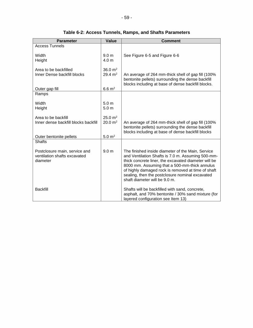
- 59 -

Table 6-2: Access Tunnels, Ramps, and Shafts Parameters

Parameter Value Comment

Access Tunnels Width Height Area to be backfilled Inner Dense backfill blocks Outer gap fill

9.0 m 4.0 m 36.0 m2 29.4 m2 6.6 m2

See Figure 6-5 and Figure 6-6 An average of 264 mm-thick shell of gap fill (100% bentonite pellets) surrounding the dense backfill blocks including at base of dense backfill blocks.

Ramps Width Height Area to be backfill Inner dense backfill blocks backfill Outer bentonite pellets

5.0 m 5.0 m 25.0 m2 20.0 m2

5.0 m2

An average of 264 mm-thick shell of gap fill (100% bentonite pellets) surrounding the dense backfill blocks including at base of dense backfill blocks

Shafts Postclosure main, service and ventilation shafts excavated diameter Backfill

9.0 m

The finished inside diameter of the Main, Service and Ventilation Shafts is 7.0 m. Assuming 500-mm-thick concrete liner, the excavated diameter will be 8000 mm. Assuming that a 500-mm-thick annulus of highly damaged rock is removed at time of shaft sealing, then the postclosure nominal excavated shaft diameter will be 9.0 m. Shafts will be backfilled with sand, concrete, asphalt, and 70% bentonite / 30% sand mixture (for layered configuration see Item 13)

- 60 -

Table 6-3: Proposed Sealing System for Shafts

Depth from Surface

Material

0 – 20 m Low-heat high-performance concrete – concrete cap at surface

20 – 150 m Shaft backfill - 70/30 bentonite-sand mixture compacted in-situ

150 – 170 m Low-heat high-performance concrete for concrete bulkhead keyed into rock to a depth of 0.5 times the original radius of the shaft

170 – 330 m Shaft backfill - 70/30 bentonite-sand mixture shaft seal

330 – 380 m Asphalt seal

380 – 480 m Shaft backfill - 70/30 bentonite-sand shaft seal compacted in-situ

480 – 500 m Concrete monolith – Low-heat high-performance concrete

Table 6-4: Properties of As-Placed Materials in the Repository

Material1 Dry

Density2,3 [kg/m3]

Saturation3 [%]

Porosity [%]

Bulk Density [kg/m3]

Thermal Conductivity4

[W/m·K]

Heat Capacity4 [J/kg·K]

Highly compacted bentonite (100%

bentonite) 1700 67 38.2 1955 1.0 1240

Gap fill (100% bentonite) 1410 6 48.6 1439 0.37 870

70% bentonite (70:30 bentonite: silica sand)

1700 73 37.5 1972 N/A N/A

Dense backfill (5:25:70 bentonite:clay:aggregate)

2120 80 19.4 2276 2.0 1060

Concrete5 N/A 50 5 2425 1.67 900

Asphalt6 N/A N/A 2 1960 N/A N/A

Notes: 1. Actual backfill compositions and their engineered physical properties will depend on the site-specific design

requirements for a repository. 2. These data assume relative solid densities of 2750 kg/m3, 2670 kg/m3, 2650 kg/m3, and 2620 kg/m3 for MX-80

bentonite (80% montmorillonite), non-montmorillonite clay, silica sand, and granite (aggregate), respectively. 3. Dry densities and saturations of the clay-based sealing materials are taken from SNC Lavalin (2014). 4. Material thermal conductivity and heat capacity are determined using calculations illustrated in

Baumgartner (2006). 5. Most concrete properties are from NWMO (2011a). Concrete thermal conductivity and heat capacity are based on

Didry et al. (2000). 6. Asphalt properties are from NWMO (2011a).

- 61 -

6.2 BUFFER

The containers are placed in buffer boxes comprised of highly compacted 100% bentonite. Upon placement, the buffer box surrounding the containers consists of a 1.0 m x 1.0 m x 2.8 m block of highly compacted bentonite, plus an additional 0.1 m of 100% bentonite pellets and gap fill between the buffer box and placement room walls (see Figure 6-3). Spaces between the buffer boxes are filled with highly compacted bentonite spacer blocks. The properties of the saturated buffer box and spacer block are listed in Table 6-5 and Table 6-6.

Table 6-5: Properties of Highly Compacted Bentonite in the Buffer Box and Spacer Blocks at Saturation

Property Value Comment

Dry density 1700 kg/m3

Porosity 38.2%

Hydraulic conductivity 2x10-12 m/s 20C value Intrinsic permeability 2x10-19 m2

Swelling pressure 2 MPa Note: Hydraulic conductivity, intrinsic permeability, and swelling pressure based on Dixon et al. (2016). It assumes that no volume change takes place for the material contained within the buffer box. Assumes SR-270 groundwater from Duro et al. (2010).

Table 6-6: Properties of Gap Fill at Saturation

Property Value Comment

Dry density 1410 kg/m3

Porosity 48.6%

Hydraulic conductivity 5x10-11 m/s 20C value Intrinsic permeability 5x10-18 m2

Swelling pressure 0.3 MPa Note: Hydraulic conductivity, intrinsic permeability, and swelling pressure based on Dixon et al. (2016). Assumes SR-270 groundwater from Duro et al. (2010).

With saturation, the highly compacted bentonite will swell and expand into the gap fill region, and the buffer layers will equilibrate to a uniform density. The properties of the homogenized bentonite at saturation are listed in Table 6-7.

Table 6-7: Homogenized Bentonite Properties at Saturation

Parameter Value Comment

Dry density 1600 kg/m3 The highly compacted bentonite and bentonite Gap Fill pellets have equilibrated at saturation.

Porosity 41.6% Averaged

Hydraulic conductivity 1.5x10-12 m/s 20°C value

Intrinsic permeability 5x10-19 m2

Swelling pressure 1 MPa Saturated

Note: Weighted average combined highly compacted bentonite and gap fill material. Hydraulic conductivity, intrinsic permeability, and swelling pressure based on Dixon et al. (2016). Assumes SR-270 groundwater from Duro et al. (2010).

- 62 -

6.3 BACKFILL

Access tunnels will be backfilled with dense backfill blocks during the closure of the repository. The dense backfill blocks are composed of 5 wt% bentonite, 25 wt% glacial clay, 70 wt% crushed granite aggregate (Dixon et al. 2001). The saturated properties of the backfilling materials are given in Table 6-8. Light backfill material is not used to backfill and seal the access tunnels because the estimated swelling pressure is lower than the required 100 kPa. Gap Fill will be used to fill the gap between the stack of dense backfill blocks and the rock walls of the access tunnels (see Table 6-6).

Table 6-8: Properties of Dense Backfill at Saturation

Property Value Comment

Dry density 2120 kg/m3

Porosity 19.5%

Hydraulic conductivity 1x10-10 m/s 20oC Baumgartner (2006) does not apply for DBF hydraulic conductivity, so a permeability value as noted in Freeze and Cherry (1979) and representing a till-like material is provided.

Intrinsic permeability 1x10-17 m2

Swelling pressure 2 kPa Note: Data listed are derived using calculations illustrated in Baumgartner (2006).

The shaft seal design calls for a sealing backfill material comprised of 70% bentonite and 30% sand. Its properties at saturation are provided in Table 6-9.

Table 6-9: Properties of 70% Bentonite / 30% Sand at Saturation

Property Value Comment

Dry density 1700 kg/m3

Design provisions may be required to

ensure that density does not fall below

this absolute minimum value

Porosity 37.5%

Hydraulic conductivity 4x10-11 m/s 20C value

Intrinsic permeability 4x10-18 m2

Swelling pressure 0.3 MPa

Note: Hydraulic conductivity, intrinsic permeability, and swelling pressure based on Dixon et al. (2016). Assumes SR-270 groundwater from Duro et al. (2010).

6.4 CONCRETE

The reference concrete is a Low-Heat High-Performance Concrete that is designed to minimize effects on the adjacent clay (Dixon et al. 2001). Transport modelling assumes degraded concrete properties from the time of closure, to account for degradation of concrete over tens of thousands of years (Quintessa and Geofirma 2011). The relevant properties of this concrete are summarized in Table 6-10.

- 63 -

Table 6-10: Properties of Concrete at Saturation

Property Value Comment

Dry density 2390 kg/m3

Porosity 10%

Hydraulic conductivity 1x10-10 m/s 20C value Concrete bulkheads, especially those situated near the centre of the repository, are expected to be subjected to elevated temperature.

Intrinsic permeability 1x10-17 m2 Note: Data listed are provided in NWMO (2011a).

6.5 ASPHALT

The shaft seal design concept includes a 50 m thick asphalt layer, as shown in Table 6-3. This provides a redundant low-permeable seal material. The reference asphalt mastic mix is the same as proposed for use in the Waste Isolation Pilot Plant (WIPP 2009). It contains 70% (by weight) silica sand, 20% asphalt and 10% hydrated lime. The high sand content provides a mechanical framework, the high asphalt content relative to conventional (road) asphalt provides this mixture with more plasticity, and the hydrated lime helps to stabilize the mixture and minimize microbial activity. The relevant properties of the asphalt layer are provided in Table 6-11.

Table 6-11: Properties of Asphalt at Saturation

Property Value Comment

Bulk density 1960 kg/m3

Porosity 2%

Hydraulic conductivity 1x10-12 m/s 20C value Intrinsic permeability 1x10-19 m/s

Note: Data listed are provided in NWMO (2011a).

6.6 DIFFUSION COEFFICIENTS

The diffusive transport of contaminants is described, in part, by their effective (or intrinsic) diffusivity in the medium (De).

6.6.1 Buffer

The measured effective diffusivity of contaminants in dense buffer materials under reducing saline conditions varies from about 3x10-5 to 3x10-3 m2/a (Oscarson et al. 1995, Yu and Neretnieks 1997, JNC 2000). Some nuclides are expected to be present in the buffer as anionic species, notably I, Cl, Se and Po. For these species, repulsion by the nominally negative surface charge on the clay particles results a lower effective porosity and, consequently, a lower effective diffusivity than for neutral or cationic species (Wersin and Schwyn 2004, Yu and Neretnieks 1997, JNC 2000). However, the high salinity of the sedimentary groundwater may

- 64 -

mute this anion exclusion effect. Consequently, anionic species are conservatively treated as neutral species. Effective diffusivities for the engineered clay-based sealing materials are listed in Table 6-12 and are described by a triangular probability density function. These values are taken from SKB (2010), in which different elements are sorted into three categories: anionic elements, non-charged and hydrolyzable cationic elements, and cesium. Due to the high salinity of the sedimentary groundwater the anion exclusion effects are ignored and the anions (I, Cl, Se, and Po) are assigned effective diffusivities representative of neutral species. The values listed for bentonite are sufficiently representative of all clay-based sealants in the repository design, except for dense backfill.

Table 6-12: Buffer Effective Diffusion Coefficients at 25ºC

Element Effective Diffusivity [m2/a]

Peak Value Lower Bound Upper Bound

Anions, Neutral and hydrolysable cations

(i.e., all other elements)

4.4x10-3 2.9x10-3 6.6x10-3

Cs 1.3x10-2 3.0x10-3 1.3x10-2

Note: Effective diffusivities are defined using triangular probability density functions. Data are based on SR-Site data report (SKB 2010, Table 5-15); data are sufficiently representative of all clay-based sealants included in the repository design, except for dense backfill.

6.6.2 Backfill

The backfill material are not explicitly modelled in SYVAC3-CC4. The effective diffusivities used in the FRAC3DVS-OPG simulations are listed in Table 6-13 and assumed to be constant values. As in the buffer materials, anion exclusion effects are ignored due to the high salinity in the sedimentary groundwaters. These values, which account for the possible effects of ion exclusion or surface diffusion on diffusive transport, are taken from Table A-18 in SKB (2006), in which elements are sorted into three categories: anionic elements, non-charged and hydrolysable cationic elements and cesium.

Table 6-13: Backfill Effective Diffusion Coefficients at 25ºC

Element Effective Diffusivity [m2/a]

Anions, neutral and hydrolysable cations

(i.e., all other elements)

1.6x10-3

Cs 4.1x10-2

Note: Backfill materials are not explicitly modelled in SYVAC3-CC4 and these values are only used in the FRAC3DVS-OPG simulations.

For the 70% bentonite 30% sand shaft backfill the effective diffusion coefficient is assumed to be 9.46x10-3 m2/a for all species (Quintessa and Geofirma 2011).

- 65 -

6.6.3 Concrete

The effective diffusivity of all contaminants in concrete is taken to be 3.9x10-3 m2/a (Quintessa and Geofirma 2011).

6.6.4 Asphalt

The effective diffusivity of all contaminants in asphalt is 3.16x10-6 m2/a (Quintessa and Geofirma 2011).

6.7 SORPTION COEFFICIENTS AND CAPACITY FACTORS

Radionuclides can become attached to minerals found in the engineering sealing materials. This can be due to a number of physical or chemical processes. The net effect of these processes can be approximated through use of an adsorption coefficient. Adsorption coefficients are listed in Table 6-14 and are described by a lognormal probability density function over the indicated range.

The sorption properties of the buffer can also be described by a capacity factor, CF = + ·Kd,

where is the porosity of the buffer or backfill, is the dry bulk density, and Kd is the sorption coefficient. Buffer and backfill porosity and dry bulk densities are listed in Table 6-7 and Table 6-8 respectively. Buffer capacity factors are listed in Table 6-15.

6.7.1 Buffer

Where available, sorption coefficients are taken from Vilks and Yang (2018) and Vilks and Miller (2018). Sorption data are described by lognormal distributions and include values for Am, Bi, Cs, Np, Pb, Pd, Se, and Th. The geometric mean, geometric standard deviation, lower and upper limit are listed in Table 6-14. Sorption data for Pa, Po, and Ra are taken from Baeyens et al. (2014). Data from Baeyens et al. (2014) does not include a distribution for the recommended sorption values and they are therefore treated as constants. Sorption Data for Pu, Se and Tc are from Bertetti (2016). Data for Pu, Se and Tc are described by lognormal distributions as detailed in Table 6-14. Several sorption values are defined by use of chemical analogs: Ac by Am (trivalent actinides); Sm by Eu (Eu sorption data from Vilks and Yang (2018) and Vilks et al. (2011)) and U by Th (both tetravalent actinides). The sorption coefficients for the remaining elements Ag, C, Cl, Hg, I, Mo, Nd, Rh, Rn and Ru are set to zero for conservatism. Sorption coefficients are listed in Table 6-14 and capacity factors are listed in Table 6-15. The sorption coefficients are described by a lognormal probability density function with exceptions as noted. The values listed for bentonite are sufficiently representative of all clay-based sealants in the repository design, except for dense backfill which is described in next section.

- 66 -

Table 6-14: Bentonite Sorption Coefficients [m3/kg]

Element GM1 GSD Lower Bound

Upper Bound

Reference / Notes

Ac 6.8 6.6 0.23 78 Analogue of Am

Ag 0 - - - Assumed to be zero aAm 6.8 6.6 0.23 78 Recommended value in Vilks and Yang (2018)

Bi 4.4 7.1 1.1 18 Data are based on sorption modelling on montmorillonite in SR-270-PW brine by Vilks and Yang (2018)

C 0 - - - Assumed to be zero

Cl 0 - - - Assumed to be zero

Cs 0.43 3.3 0.14 1.43 Data are measurements in SR-270-PW brine by Vilks and Miller (2018)

Hg 0 - - - Assumed to be zero

aI 0 - - - Assumed to be zero, sensitivity case with a value of 1.3x10-3 m3/kg

Mo 0 - - - Assumed to be zero

Nd 0 - - - Assumed to be zero

aNp 48.1 4.1 17.8 130

Lower range data are based on sorption modelling by Vilks and Yang (2018), upper range data are measurements in SR-270-PW brine by Nagasaki et al. (2017)

Pa 4 - - - Constant value based on bentonite measurement by Baeyens et al. (2014)

Pb 0.003 5 0 0.011 Data are measurements in SR-270-PW brine by Vilks and Miller (2018), values are recommended by Vilks and Yang (2018)

aPd 0.68 9.1 0.03 14.5 Data are measurements in SR-270-PW brine by Vilks and Miller (2014) and in 4 M Na-Cl-Cl brine by Riddoch and Nagasaki (2016)

Po 0.1 - - - Constant value based on bentonite measurements in Baeyens et al. (2014)

Pu 3.91 2.6 1.5 10 Data are measurements in SR-270-PW brine by Bertetti (2016), data are similar to simulated results by Vilks and Yang (2018)

Ra 0.00009 - - - Constant value based on bentonite measurements in by Baeyens et al. (2014)

Rh 0 - - - Assumed to be zero

Rn 0 - - - Assumed to be zero

Ru 0 - - - Assumed to be zero

aSe 0.099 1.1 0.09 0.11 Data considers both recommendations in Vilks and Yang (2018) and measurements in SR-270-PW brine by Bertetti (2016)

Sm 1.3 4.6 0.10 6.7 Analogue of Eu, Eu data from Vilks and Yang (2018) and Vilks et al. (2011)

Tc 5 - - - Data are measurements in SR-270-PW brine by Bertetti (2016)

Th 8.9 1.8 3.4 15.9 Data are measurements in SR-270-PW brine by Vilks and Miller (2018)

U 8.9 1.8 3.4 15.9 Analogue of Th

Note: 1Bentonite Kd values are lognormal with the exception of the Ag, C, Cl, Hg, I, Mo, Nd, Pa, Po, Ra, Rh, Rn, Ru, and Tc which are assumed to be constants. (GM = Geometric Mean, GSD = Geometric Standard Deviation).

aData from a draft version of Vilks (2018) data has been revised in the final version of Vilks (2018).

- 67 -

Table 6-15: Bentonite Capacity Factors

Element GM1 GSD Lower Bound

Upper Bound

Reference

Ac 1.09x104 6.6 3.68x102 1.25x105 Analogue of Am

Ag 0.416 - - - Assumed to be zero

Am 1.09x104 6.6 3.68x102 1.25x105 Recommended value in Vilks and Yang (2018)

Bi 7.04x103 7.1 1.76x103 2.88x104 Data are based on sorption modelling on montmorillonite in SR-270-PW brine by Vilks and Yang (2018)

C 0.416 - - - Assumed to be zero

Cl 0.416 - - - Assumed to be zero

Cs 6.88x102 3.3 2.24x102 2.29x103 Data are measurements in SR-270-PW brine by Vilks and Miller (2018)

Hg 0.416 - - - Assumed to be zero

I 0.416 - - - Assumed to be zero

Mo 0.416 - - - Assumed to be zero

Nd 0.416 - - - Assumed to be zero

Np 7.70x104 4.1 2.85x104 2.08x105

Lower range data are based on sorption modelling by Vilks and Yang (2018), upper range data are measurements in SR-270-PW brine by Nagasaki et al. (2017)

Pa 6.40x103 - - - Constant value based on bentonite measurement by Baeyens et al. (2014)

Pb 5.216 5 0.416 18 Data are measurements in SR-270-PW brine by Vilks and Miller (2018), values are recommended by Vilks and Yang (2018)

Pd 1.09x103 9.1 4.84x101 2.32x104 Data are measurements in SR-270-PW brine by Vilks and Miller (2018) and in 4 M Na-Ca-Cl brine by Riddoch and Nagasaki (2016)

Po 1.60x102 - - - Constant value based on bentonite measurements in Baeyens et al. (2014)

Pu 6.26x103 2.6 2.40x103 1.60x104 Data are measurements in SR-270-PW brine by Bertetti (2016), data are similar to simulated results by Vilks and Yang (2018)

Ra 0.56 - - - Constant value based on bentonite measurements in by Baeyens et al. (2014)

Rh 0.416 - - - Assumed to be zero

Rn 0.416 - - - Assumed to be zero

Ru 0.416 - - - Assumed to be zero

Se 1.59x102 1.1 1.44x102 1.76x102 Data considers both recommendations in Vilks and Yang (2018) and measurements in SR-270-PW brine by Bertetti (2016)

Sm 2.08x103 4.6 1.60x102 1.07x104 Analogue of Eu, Eu data from Vilks and Yang (2018) and Vilks et al. (2011)

Tc 8.00x103 - - - Data are measurements in SR-270-PW brine by Bertetti (2016)

Th 1.42x104 1.8 5.44x103 2.54x104 Data are measurements in SR-270-PW brine by Vilks and Miller (2018)

U 1.42x104 1.8 5.44x103 2.54x104 Analogue of Th

Note: 1Bentonite Capacity Factor values are assumed to be lognormal with the exception of the Ag, C, Cl, Hg, Mo, Nd, Pa, Po, Ra, Rh, Rn, Ru, and Tc which are assumed to be constants. (GM = Geometric Mean, GSD = Geometric Standard Deviation)

- 68 -

6.7.2 Backfill

Backfill sorption coefficients are assumed to be the same as those for the bentonite (see Table 6.14) with the Kd scaled with the clay fraction. This assumption results in a Dense Backfill Kd equal to 5% of the Kd shown in Table 6-14 for access tunnels and ramps and a Shaft Backfill Kd equal to 70% of the Kd shown in Table 6-14.

6.7.3 Concrete

Sorption Coefficients for concrete are conservatively assumed to be zero given the high salinity of the groundwater and lack of sorption data on concrete in these conditions.

6.7.4 Asphalt

Owing to a lack of sorption data, and due to the small porosity and small physical extent of this material, all sorption coefficients for the asphalt shaft seal are conservatively taken to be zero.

6.8 EFFECT OF INCREASED TEMPERATURE ON BENTONITE

As discussed in Section 5.2 it is anticipated that the sealing materials around the containers will experience an increase in temperature. The reference temperature in the highly compacted bentonite around the containers is assumed to be 85oC over the postclosure period. Backfilling materials used in the access tunnels and shafts as well as the host rock do not experience such a high increase, and temperatures are assumed to remain at ambient temperature at these locations.

6.8.1 Physical Properties

Density and porosity of the engineered sealing materials are not expected to be significantly affected by increased temperature. No correction is applied to these data.

6.8.2 Hydraulic Conductivity

Hydraulic conductivity (and correspondingly permeability) increases with increased temperature. Table 6-7 lists the homogenized buffer hydraulic conductivity as 5x10-12 m/s at 20oC. An increase in temperature to 85oC corresponds to a factor 2.9 times increase in the buffer hydraulic conductivity based on the relationship below.

𝐾85

𝐾20=

𝜇20

𝜇85

𝜌85

𝜌20

Where K is the hydraulic conductivity, 𝜇 is the water viscosity at a given temperature and 𝜌 is the water density at a given temperature (see Table 7-11 for temperature dependent water viscosity and density relationships). Despite this increased hydraulic conductivity, groundwater velocities in the buffer are still expected to be extremely small and transport should remain diffusion dominant.

- 69 -

6.8.3 Diffusion Coefficients

Diffusivity increases with increased temperature. Assuming the diffusivity scales with temperature T and porewater viscosity µ(T) as described below (Rohsenow and Choi 1961, p.383), the resulting diffusivity is a factor 3.4 times higher at 85ºC than at room temperature.

𝐷𝑖 = 𝐷𝑖298𝑘

𝑇

298𝐾

𝜇298𝐾

𝜇(𝑇)

Viscosity values are discussed in Table 7-11

6.8.4 Sorption Coefficients

Elemental sorption coefficients on buffer materials are not assumed to be significantly affected by increased temperature. No correction is applied to these data.

6.9 EXCAVATION DAMAGE ZONE TRANSPORT PARAMETERS

In the Seventh Case Study, the excavation of the shafts, tunnels, placement rooms and boreholes will create zones of disturbed rock in which there is significantly increased porosity and flow permeability. These zones are referred to as excavation damage zones (EDZ). The extent and severity of the EDZ is dependent on the excavation method, size of the excavation, localized rock stress and residual heat generated by the fuel. Beyond the EDZ, the rock may be disturbed with respect to stress redistribution, but no significant change to the flow and transport properties of the rock is expected. The selected EDZ parameters used in the Seventh Case Study are summarized in Table 6-16 and Table 6-17, and are described below.

6.9.1 Excavation Damage Zone Thickness

The shafts, placement rooms, and tunnels are assumed to be excavated by a controlled drill-and-blast technique resulting in an EDZ in the rock around the periphery of the shafts and tunnels. However, by considering the stress state in the host rock the extent of the EDZ can be minimized. Radakovic-Guzina et al. (2015) assessed the long-term stability of a repository for the Mark II container design in both the sedimentary and crystalline geological settings. The results of the study indicate some development of EDZ extending few meters from the boundary of the placement rooms into the surrounding rock mass under extreme loading conditions and for bounding (unfavorable from the perspective of stress and damage in the rock) assumptions regarding mechanical properties of the rock mass. Thermo-hydro-mechanical (THM) coupled analysis was conducted. However, some simplifications that resulted in overestimation of the deformation and damage were used. For example, the effect of temperature change and fluid pressure dissipation due to flow were not rigorously simulated.

- 70 -

More recent studies (Radakovic-Guzina and Damjanac 2017) have since refined the models from Radakovic-Guzina et al. (2015). The main difference between Radakovic-Guzina and Damjanac (2017) and the analyses documented in Radakovic-Guzina et al. (2015) is that the pore pressure fields as calculated by the coupled Thermal-Hydro-Mechanical analyses (accounting for the thermally-induced pore pressure changes and pore pressure dissipation due to fluid flow) are imported into the model and used in the effective stress analyses. In the previous study, the hydrostatic pore pressures were assumed with subsequent uniform undrained pore pressure changes during glacially-induced total stress changes. Radakovic-Guzina and Damjanac (2017) concludes that the extent of the EDZ after 1 Ma is localized and contained within 1-m distance from the room walls for the reference case. Sensitivity analysis of the model indicate that variability could result in additional dispersed damage extending few meters from the placement room. For the Seventh Case Study the inner EDZ is assumed to extend 1 m from the tunnel surfaces and the outer EDZ is assumed to extend 3 m from the tunnel surfaces. At the end of each placement room, a bentonite seal will be keyed into the rock with the intent of restricted slow through the EDZ. The room seal will be carefully excavated to reduce the likelihood of an additional EDZ forming. However, the EDZ at the placement room seal locations is conservatively assumed to extend beyond the keyed-in depth of the seal by an additional depth of approximately 10% of the inner EDZ thickness (Table 6-16). Shafts in the Seventh Case Study are roughly circular and the shafts are perpendicular to the bedding planes. Therefore for the shaft EDZ, hydraulic conductivity enhancement factors are applied to the rock vertical hydraulic conductivity. The shaft EDZ is divided into three regions to better represent the large variation in properties across this region. The regions include a highly damaged zone, which is expected to be removed prior to closure of the repository, an inner EDZ of higher hydraulic conductivity, and finally an outer EDZ of lesser permeability. NWMO (2011a) states that significant stress changes occur within approximately one shaft radius of the shaft wall (i.e., out to two tunnel radii from the center). As a result, the shaft EDZ is assumed to have an inner EDZ extending 0.5 shaft radii into the rock and an outer EDZ extending an additional 0.5 shaft radii into the rock (Table 6-16). The shaft design includes several bulkheads that serve the same purpose as the room seals. The bulkheads are designed to interrupt any continuous flow paths along the shaft EDZ with an impermeable layer. However, as is the case for the room seals, a thin inner EDZ is assumed to form around these bulkheads. As in the placement room seals, the EDZ in the shaft bulkheads is conservatively assumed to extend beyond the keyed-in depth of the seal by an additional depth of approximately 10% of the EDZ thickness.

6.9.2 Excavation Damage Zone Permeability

The transport properties within the EDZ strongly depend on the effective axial transmissivity of the whole system, which is controlled by factors such as the interconnectivity of individual micro fractures. Blümling et al. (2007) report that although effective axial permeability measurements within the EDZ at length scales in excess of several metres have been successful, in situ evidence indicates that such permeabilities are much lower than estimates obtained from point scale measurements. Tsang et al. (2005) showed that the key factors that influence excavated damage zone are:

- 71 -

stress magnitude (relative to the strength of the rock);

stress orientation and ratio (for anisotropic stresses);

excavation shape;

excavation method; and

types of rock response (brittle or plastic). Rocks that exhibit a more plastic response typically have a continuous and gradational EDZ that can be identified in modelling by the identification of yield stresses. For these plastic rocks, a well-defined highly damaged zone is not often apparent even at very high levels of yielding. However, for rocks that display a brittle/strain-weakening response changes in volumetric strain is a good indicator of the development of the damage zone. For this study, the reference values for the EDZ permeabilities are based on properties from L&ILW DGR Data (NWMO 2011a), Geosynthesis (NWMO 2011b) and Golder (2012) and are listed in Table 6-16. The reference permeabilities selected for the inner excavation damaged zones surrounding the placement room is selected to be 1000 times that of the host rock. Since values in NWMO 2011b range from 100 to 10,000 times the intact rock permeability, the placement room permeability is defined by a lognormal PDF with a geometric mean of 1,000 times the intact rock permeability, lower and upper bounds of 100 and 10,000 times the host rock permeability, and a geometric standard deviation of 3.2 so that 95% of the values of the distribution are within the bounds of the distribution. In CC4, only the inner EDZ in the placement room is modelled. In the FRAC3VDS-OPG simulations both the inner and outer EDZ is represented. The outer EDZ is assumed to have a 100 fold increased permeability relative to the intact host rock (Table 6-16). The shaft inner and outer EDZs are also included in the FRAC3DVS-OPG models and are assumed to have a 100 times and 10 times increased permeability relative to the intact host rock (Table 6-16). These assumptions are consistent with those made in NWMO (2011a). In the CC4 model, a radial flow component is separately modelled and assigned its own permeability. These are set to 10% of the corresponding axial permeability (Table 6-17).

6.9.3 Excavation Damage Zone Dispersion Length

The axial-flow EDZ dispersion length is defined parallel (longitudinal) or transverse to the room axis direction. Although the room length is 341.6 m, it is expected that the contaminant path length through the EDZ will normally be less than 100 m, considering that the failed container location can vary and that contaminants can also move radially. Johnson et al. 1996 (p.181) uses a fit of dispersion data from a range of laboratory and field studies that gives a 14 m (best estimate) to 45 m (95% confidence bound) dispersion length for axial transport along a 100 m path (i.e., 14% to 45% of the path length). Flow measurements in the EDZ in the Mine-by Tunnel indicated a dispersion length of 0.60 m for a test region of 1.5 m, i.e., 40% of the scale length. Results from the TRUE tracer tests on a 3-m scale implied a 10% dispersion length (SKB 2001, p.99, p.161). In the Seventh Case Study CC4 models, the longitudinal dispersion length for axial transport in the EDZ is described by a uniform probability density function from 10 m to 40 m, corresponding to 10% to 40% of a 100 m path length. In the FRAC3DVS-OPG calculations, the longitudinal dispersion coefficient in the EDZ is selected to be 10 m based on Quintessa and Geofirma

- 72 -

(2011) to avoid unrealistic transport results, i.e., large upstream dispersion. Upstream dispersion does not occur in the CC4 geosphere transport model (NWMO 2012). The transverse dispersion can be as low as about 1% of the longitudinal dispersion (Johnson et al. 1996, p.181), whereas more typical values are around 10% of the longitudinal dispersion length (Chan et al. 1999). For the Seventh Case Study, the transverse dispersion length was selected to be 10% of the longitudinal dispersion length. Thus, in the CC4 model calculations, the EDZ transverse dispersion length is described by a uniform probability density function from 1 to 4 m. The transverse dispersion length in the FRAC3DVS-OPG calculations was also set to 10% of the longitudinal dispersivity. In the CC4 model, a radial flow component is separately modelled and assigned its own longitudinal and transverse dispersion lengths. These are set to 1% of the corresponding longitudinal and transverse dispersion lengths for axial flow.

6.9.4 Excavation Damage Zone Porosity

In addition to an increase in hydraulic conductivity within the EDZs, there is anticipated to be an increase in porosity. Previous studies in Canadian Shield Granite (Gobien et al. 2016) and in Opalinus Clay (NAGRA 2004) have suggested an increase of about a factor of two over the inner EDZ volume. For the Seventh Case Study, the porosity of the intact Cobourg rock is 1.5% (see Section 7.2.4). For regions of inner EDZ, the porosity is assumed to increase by a factor of two relative to the intact rock porosity resulting in an inner EDZ porosity of 3%. The porosity of the regions of outer EDZ are assumed to be the same as those for the intact rock or 1.5%. In CC4, only the inner EDZ is modelled. To account for this, the EDZ porosity is described by a lognormal probability density function with a geometric mean of 3%, a geometric standard deviation of 3.2, and bounding values of 1.5% and 15%. Furthermore, the EDZ porosity is positively correlated with the EDZ permeability, so that the porosities are large when the permeability is large. Although there is no specific data, it is judged that this should be a fairly tight correlation - a correlation coefficient of 0.8 is used.

6.9.5 EDZ Tortuosity

The tortuosity, , used in the Seventh Case Study is defined so that the effective diffusivity is

given by De = Do. For the Seventh Case Study, the inner and outer EDZ tortuosity is set such that the total effective diffusivity in the inner EDZ is increased by a factor of 4 relative to the host rock and increased by a factor of 2 relative to the host rock for the outer EDZ. This approach is consistent with that of NWMO (2011a) and results in a two fold increase in the tortuosity for both the inner and outer EDZ.

- 73 -

Table 6-16: Excavation Damage Zone Properties

EDZ ZONE Description Extent of EDZ from Tunnel / Shaft Surface

Porosity

[-] Tortuosity

[-] Permeability2

[m2]

Placement Rooms (3.2 m x 2.2 m)4

Inner EDZ1

Tunnel Top & Bottom

1 m 2 x Rock 2 x Rock

1000 x Rock

Tunnel Sides 1 m

Outer EDZ

Tunnel Top & Bottom

3 m 1 x Rock 2 x Rock

100 x Rock

Tunnel Sides 3 m

Seal EDZ1

Tunnel Top & Bottom

1.1 2 x Rock 2 x Rock 1000 x Rock

Tunnel Sides 1.1

Seal Outer EDZ

Tunnel Top & Bottom

3 1 x Rock 2 x Rock 100 x Rock

Tunnel Sides 3

Main, Service, and Vent Shafts (R = shaft radius in meters)3

Inner EDZ - 0.5 x R 2 x Rock 2 x Rock 100 x Rock

Outer EDZ - 1.0 x R 1 x Rock 2 x Rock 10 x Rock

Bulkhead Inner EDZ - 0.55 x R 2 x Rock 2 x Rock 100 x Rock

Bulkhead Outer EDZ

- 1.0 x R 1 x Rock 2 x Rock 10 x Rock

1The Highly Damaged Zone (or HDZ) has been incorporated within the inner EDZ zone. The extent of the seal EDZ is measured from the excavation surfaces of placement rooms and shafts, not from the keyed-in excavations of the seals. The EDZ at placement room and shaft seal locations is conservatively assumed to extend beyond the keyed-in depth of the seal by an additional depth of approximately 10% of the inner EDZ thickness. For the purpose of this study only the permeability of seal inner EDZ is equal to that of inner EDZ (i.e., 1000 x Rock). 2Properties from L&ILW DGR Data (NWMO 2011a), Geosynthesis (NWMO 2011b) and Golder (2012). 3The distance from the rock face for the shaft EDZ is specified as a function of the shaft radius and based on data from Itasca (2017). 4The EDZ extent around the placement rooms is also assumed for the central access, panel access and perimeter tunnels.

- 74 -

Table 6-17: Transverse, Radial, and Axial Excavation Damage Zone Properties

Parameter Value Comment

Axial flow, axial dispersion length 25 m Uniform probability density function from 10 m to 40 m. (In FRAC3DVS-OPG, the axial dispersion length is set at 10 m to avoid unrealistic transport, i.e., upstream dispersion.)

Axial flow, transverse dispersion length

2.5 m Uniform probability density function from 1 m to 4 m. (In FRAC3DVS-OPG, transverse dispersion length is set to 10% of longitudinal value or 1 m.)

Radial flow, ratio of radial to axial dispersion length

0.01 Assumed to be 1%

Radial flow, ratio of radial to axial transverse dispersion length

0.01 Assumed to be 1%

Ratio of radial EDZ permeability to axial EDZ permeability

0.1 Assumed to be 10%

6.10 NEAR FIELD TWO-PHASE FLOW PARAMETERS

Gas migration is modelled in T2GGM (Suckling et al. 2015) and can occur through (1) dissolution, (2) two-phase flow and (3) dilational process through clay or bentonite-based materials. Simulating how gas and liquid interact within the engineered sealing materials requires two-phase flow modelling which, in the T2GGM modelling, is based on the van Genuchten model for water retention (describing the relationship between the water content of a capillaceous matrix and the net potential energy of its constituent capillaries). The van Genuchten equations for capillary pressure as a function of liquid saturation are as follows (van Genuchten, 1980).

nm

ecc SP/1/1 1

1

(6.1)

lrc

lrclec

S

SSS

1

(6.2)

‘where:

Pc is the capillary pressure, Pa;

is a van Genuchten fitting parameter, Pa-1. The inverse of is analogous to the air entry pressure, but is often larger than the actual air entry pressure;

Sec is the effective saturation for the capillary pressure relationship (volume ratio); Sl is the liquid saturation (volume ratio); Slrc is the residual liquid saturation for capillary pressure (volume ratio), the liquid

saturation below which liquid does not flow, and capillary pressure is confined; m is a van Genuchten fitting parameter (unitless); and n is a van Genuchten fitting parameter (unitless).

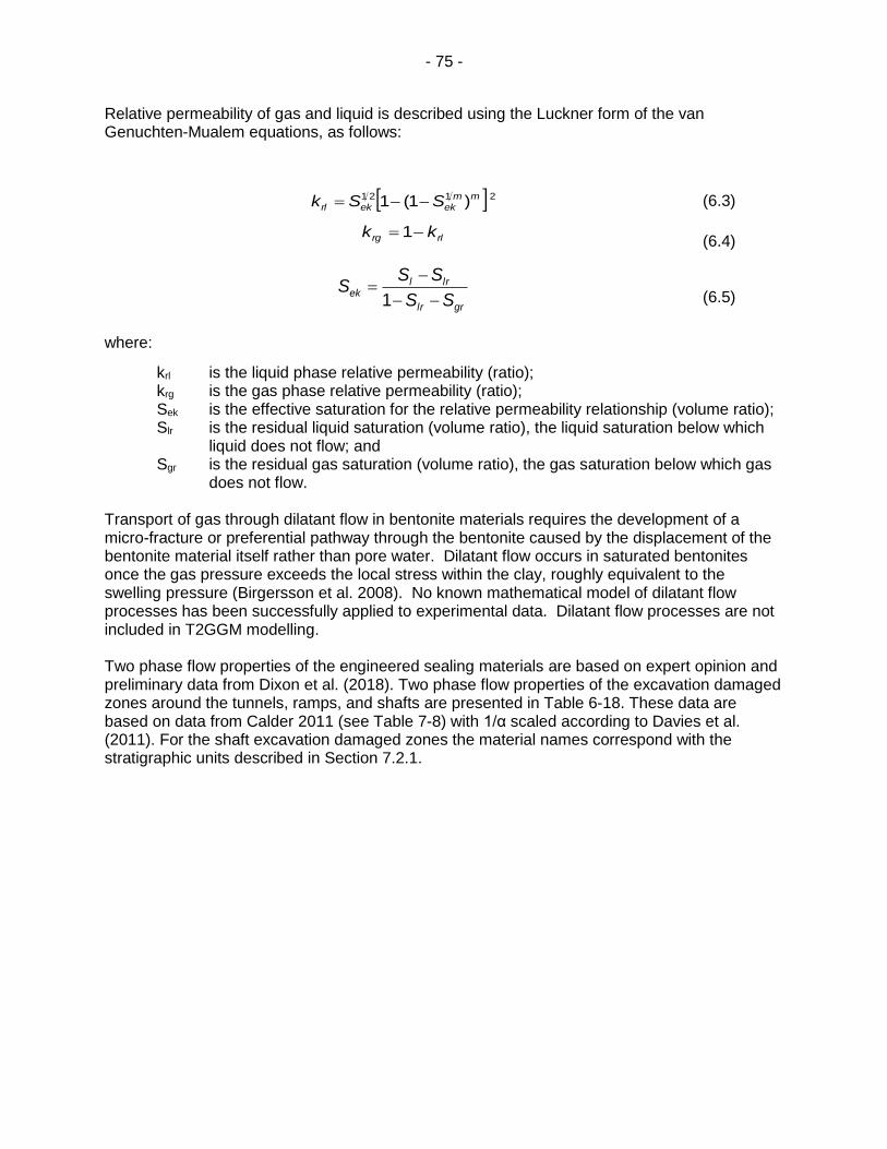
- 75 -

Relative permeability of gas and liquid is described using the Luckner form of the van Genuchten-Mualem equations, as follows:

2121 )1(1 mm

ekekrl SSk (6.3)

rlrg kk 1 (6.4)

grlr

lrlek

SS

SSS

1

(6.5)

where:

krl is the liquid phase relative permeability (ratio); krg is the gas phase relative permeability (ratio); Sek is the effective saturation for the relative permeability relationship (volume ratio); Slr is the residual liquid saturation (volume ratio), the liquid saturation below which

liquid does not flow; and Sgr is the residual gas saturation (volume ratio), the gas saturation below which gas

does not flow. Transport of gas through dilatant flow in bentonite materials requires the development of a micro-fracture or preferential pathway through the bentonite caused by the displacement of the bentonite material itself rather than pore water. Dilatant flow occurs in saturated bentonites once the gas pressure exceeds the local stress within the clay, roughly equivalent to the swelling pressure (Birgersson et al. 2008). No known mathematical model of dilatant flow processes has been successfully applied to experimental data. Dilatant flow processes are not included in T2GGM modelling. Two phase flow properties of the engineered sealing materials are based on expert opinion and preliminary data from Dixon et al. (2018). Two phase flow properties of the excavation damaged zones around the tunnels, ramps, and shafts are presented in Table 6-18. These data are based on data from Calder 2011 (see Table 7-8) with 1/α scaled according to Davies et al. (2011). For the shaft excavation damaged zones the material names correspond with the stratigraphic units described in Section 7.2.1.

- 76 -

Table 6-18: Two Phase Flow Properties of the Sealing Materials and Excavation Damaged Zones

Material 1/α [MPa] M [-] n [-] Slrc [-] Slr [-] Sgr [-]

Homogenized Bentonite1

108 1.21 2.71 0.01 0.01 0.10 Bentonite Gap Fill1

HCB in Placement Room Seals1

Dense Backfill1 10 0.40 1.80 0.09 0.10 0.01

Concrete (LHHPC), degraded2 1 0.50 2.00 0.19 0.20 0.10

Asphalt2,3 - - - - 0.00 0.00

Shaft Seal1 285 4.80 1.94 0.00 0.01 0.12

Placement Room Inner EDZ4 2.48 1.69 3.13 0.06 0.07 0.03

Placement Room Outer EDZ4 6.20 1.69 3.13 0.06 0.07 0.03

Cobourg EDZ (Shaft) 4 1.24 1.69 3.13 0.06 0.07 0.03

Georgian Bay / Blue Mountain EDZ (Shaft) 4

6.00 1.10 3.82 0.17 0.18 0.04

Queenston EDZ (Shaft) 4 7.20 1.13 4.45 0.09 0.10 0.06

Manitoulin EDZ (Shaft) 4 8.20 1.31 3.65 0.11 0.12 0.05

Cabot Head EDZ (Shaft) 4 3.00 0.24 6.82 0.00 0.01 0.05

Fossil Hill EDZ (Shaft) 4 5.60 0.68 6.11 0.03 0.04 0.00 1Based on preliminary data from Dixon (2018) and expert opinion 2Derived using calculations illustrated by Baumgartner (2006) 3Asphalt is assumed to have zero capillary pressure 4Based on Data from Calder (2011) with 1/α scaled according to Davies (1991)

Thermal effects from the fuel shortly after placement can influence gas transport properties, corrosion and resaturation of the repository. In T2GGM the thermal gradient from the fuel is modelled in the placement rooms and its impact on gas transport assessed. Thermal conductivity and heat capacity of the sealing materials are presented in Table 6-19 (Baumgartner 2006). Table 6-19 also includes the thermal properties of the excavation damaged zones around the tunnels, ramps and shafts. These data were taken from SNC (2011).

- 77 -

Table 6-19: Thermal Properties of the Sealing Materials

1Concrete properties are taken from and Didry et al. (2000).

Material Thermal

Conductivity [W/m·K]

Heat Capacity [kJ/kg·K]

Homogenized Bentonite fully saturated: 1

dry: 0.4 920

Bentonite Gap Fill fully saturated: 1

dry: 0.4 920

HCB in Pedestal fully saturated: 1

dry: 0.4 920

HCB in Placement Room Seals

fully saturated: 1 dry: 0.4

1280

Dense Backfill 2.00 1360

Concrete (LHHPC), degraded1 1.67 900

Asphalt N/A N/A

Shaft Seal 0.94 1360

Placement Room Inner EDZ 2.3 900

Placement Room Outer EDZ 2.3 900

Cobourg EDZ (Shaft) 2.3 900

Georgian Bay / Blue Mountain EDZ (Shaft)

2.1 975

Queenston EDZ (Shaft) 2.1 975

Manitoulin EDZ (Shaft) 2.3 830

Cabot Head EDZ (Shaft) 2.3 830

Fossil Hill EDZ (Shaft) 2.3 830

- 78 -

7. GEOSPHERE DATA

7.1 GENERAL SITE DESCRIPTION

The repository in the Seventh Case Study is located at a hypothetical but plausible sedimentary site in the Michigan Basin. Given the hypothetical nature of this assessment site-specific data are not available for a number of parameters. However, a number of exploratory boreholes and site specific data are available for Ontario Power Generation’s Deep Geological Repository for Low and Intermediate Level Waste (L&ILW) also located in the Michigan Basin (NWMO, 2011b). As a result, the majority of the Seventh Case Study rock properties and site data are taken from the corresponding layers at the L&ILW DGR site. Where site-specific data are not available, data have been drawn from a wider range of sources. These data sources can be described as a hierarchy of decreasing confidence:

Data from analogous geological formations at the L&ILW DGR site;

Data from the same geological formations and comparable hydrogeochemical environments across the wider region, e.g., oil and gas wells;

Literature data for equivalent material types, often selected to be cautiously realistic; and

Reasonable values that have been adopted in the absence of the above. Figure 7-1 shows the hypothetical Seventh Case Study site area. Many of the physical and chemical properties of the geosphere are directly correlated with lithology and hence the stratigraphy. Therefore, the stratigraphy has generally been used as the basis for presenting the geosphere properties.

Figure 7-1: FRAC3DVS-OPG Model Domains and Basic Features at the Hypothetical Site

- 79 -

7.2 PHYSICAL CHARACTERISTICS OF THE GEOSPHERE

This section describes the physical characteristics of the host rock.

7.2.1 Stratigraphic Units

Figure 7-2 shows the geological stratigraphy and the lithologies of the different geological formations, members and units present at the Seventh Case Study site. The average unit thickness and the depth of the top of a unit are given in Table 7-1.

Note: Property assignment on vertical cross-section through the entire model domain

Figure 7-2: Site Scale Model Cross Section

- 80 -

Table 7-1: Formation Thickness at the Hypothetical Site

Formation1 Average Unit Thickness2 [m]

Unit Top Depth [mbgs]

Sediment3 10 0.0

Drift / Overburden3 29.4 0

Unit B and C 52.3 29.4

Unit A-2 Carbonate 27 81.7

Unit A-1 Upper Carbonate

3.0 108.7

Unit A-1 Carbonate 22.1 111.7

Unit A-1 Evaporite 2.0 133.8

Unit A0 2.3 135.8

Guelph 71.4 138.1

Reynales / Fossil Hill 6.8 209.5

Cabot Head 15.8 216.3

Manitoulin 15.6 232.1

Queenston 77.6 247.7

Georgian Bay / Blue Mountain

154.3 325.3

Cobourg 46.4 479.6

Sherman Fall 47.3 526.0

Kirkfield 39.5 573.3

Cobokonk 8.0 612.8

Gull River 53.4 620.8

Shadow Lake4 7.6 674.2 1Only geological units present at the Seventh Case Study site is included here and elsewhere in the report 2Formation thicknesses will vary across the hypothetical site. The average thickness represents the median thickness of a given geological unit over the regional modelling area. 3Overburden is present over the entire model domain except for surface water features which have a layer of sediment present. SYVAC3-CC4 model assumes the overburden and sediment thicknesses are uniformly distributed. 4Seventh Case Study Model boundary exists at the bottom of the Shadow Lake formation, Upper Precambrian and Precambrian formations would be present but are not included.

7.2.2 Hydraulic Conductivity

The estimated hydraulic conductivities used in the Seventh Case Study are based on data from the boreholes at the L&ILW DGR site. The collected hydraulic conductivity data are plotted versus depth in Figure 7-3 (Intera 2011). The horizontal to vertical hydraulic conductivity values for each formation used in the Seventh Case Study are given in Table 7-2.

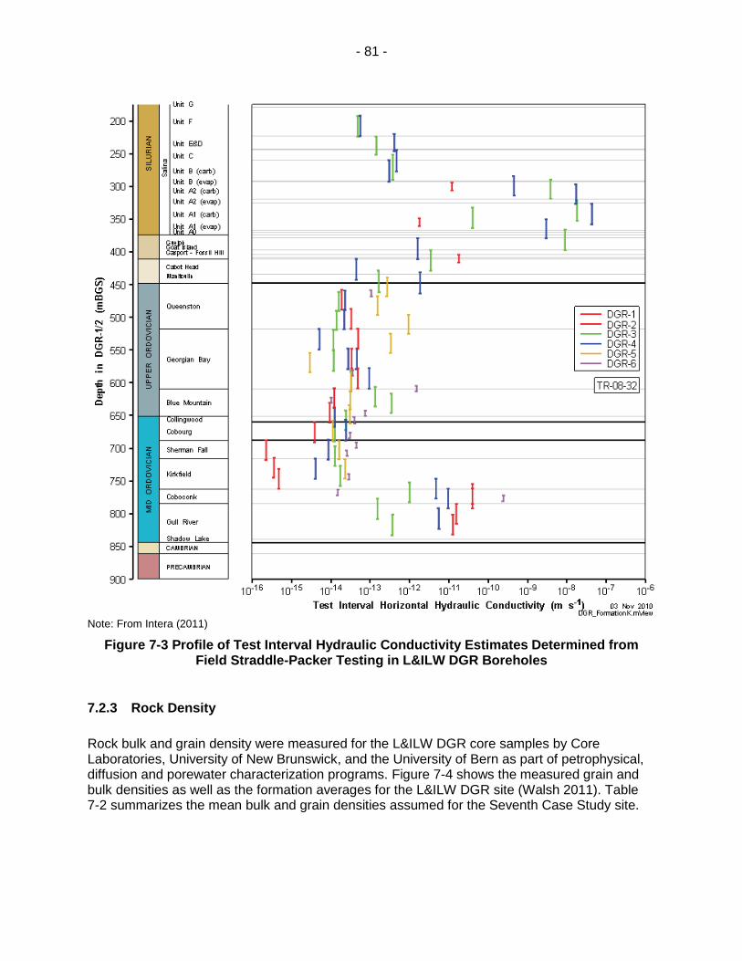
- 81 -

Note: From Intera (2011)

Figure 7-3 Profile of Test Interval Hydraulic Conductivity Estimates Determined from Field Straddle-Packer Testing in L&ILW DGR Boreholes

7.2.3 Rock Density

Rock bulk and grain density were measured for the L&ILW DGR core samples by Core Laboratories, University of New Brunswick, and the University of Bern as part of petrophysical, diffusion and porewater characterization programs. Figure 7-4 shows the measured grain and bulk densities as well as the formation averages for the L&ILW DGR site (Walsh 2011). Table 7-2 summarizes the mean bulk and grain densities assumed for the Seventh Case Study site.

- 82 -

Note: from Walsh (2011)

Figure 7-4: Grain and Bulk Dry Density, Measured Data and Formation Averages.

7.2.4 Porosity

The estimated liquid porosity for the various stratigraphic layers at the L&ILW DGR site are presented graphically in Figure 7-5 (Intera 2011). The porosity values that are used as the basis for the numerical models used in the Seventh Case Study are given in Table 7-2.

- 83 -

Note: From Intera (2011)

Figure 7-5: Liquid Porosity Profile for DGR Cores Showing Point Data and Arithmetic Formation Averages

7.2.5 Tortuosity

The tortuosity parameter varies by layer (see Table 7-2) and is calculated from the sodium iodide effective diffusion coefficient De (see Table 7-4), the porosity θ (see Table 7-2), the free solution diffusion coefficient for sodium iodide at 1.0 mol/L of 1.662x10-9 m2/s (Weast 1983, p. F-46), and assuming a diffusion accessible porosity factor of 0.5 for sodium iodide (Intera 2011).

7.2.6 Geomechanical Parameters

The specific storage (Ss) and one-dimensional loading efficiency (ζ) in Table 7-2 are calculated based on the Young’s Modulus E (Table 2.12 from Sykes et al. 2011), Poisson’s Ratio ν (Table 2.13 from Sykes et al. 2011), the mineral grain modulus Ks for the rock formations, the coefficient of vertical compressibility β′ for the drift, and the fluid density ρ. The mineral grain modulus Ks was chosen as being incompressible (Ks = ∞) for all layers except for the drift due to

- 84 -

a lack of available site specific data. The coefficient of vertical compressibility β′ for the drift was set to 1.0x10-8 Pa-1.

7.2.7 Fluid Density

A relationship between Total Dissolved Solid concentration and density was developed for the Michigan Basin by Lampe (2009) using data compiled by Gupta (1993). The relationship is given by:

𝜌 = 0.000725𝐶𝑇𝐷𝑆 − 0.999 in which CTDS is the Total Dissolved Solid concentration in g/L solution and ρ is fluid density expressed as kg/L. The relationship was used by Lampe (2009) to model three-dimensional density-dependent flow in the Michigan Basin. The data and regression equation for the analysis are presented in Figure 7-6. Intera (2011) used the average groundwater density of the Guelph Formation of 1,234 kg/m3

and average Total Dissolved Solids concentration of 451.8 g/kg of water (equivalent to 384 g/L of solution) for the Guelph Formation to determine the relationship between Total Dissolved Solid concentration and density as:

𝜌 = 0.000609𝐶𝑇𝐷𝑆 − 1.0 For the hypothetical Seventh Case Study modelling the Total Dissolved Solid concentration versus density reflects both the DGR site data and the saline waters elsewhere in the Michigan Basin. This study therefore used an average of the models of Gupta (1993) and Intera (2011), yielding:

𝜌 = 0.000667𝐶𝑇𝐷𝑆 − 1.0 An important consideration in the use of this relationship is the fact that the TDS concentrations have an uncertainty associated with them. The densities are also uncertain. The three relationships between Total Dissolved Solid concentration and density can be compared in Figure 7-6 (Sykes et al. 2011). In the plot, the lower line is from Lampe (2009) and Gupta (1993), the upper line is used by Intera (2011) while the middle line is used in this study. Fluid density numbers listed in Table 7-2 reflect the average approach documented here and in Sykes et al. (2011).

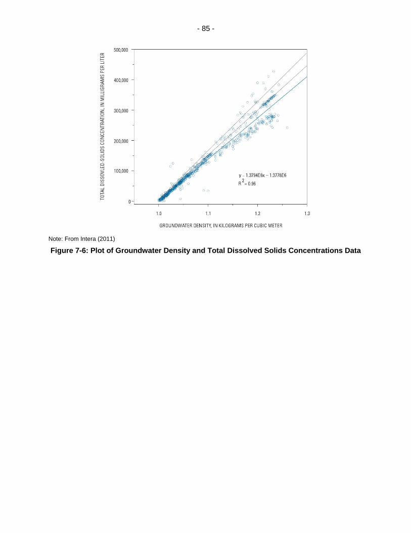
- 85 -

Note: From Intera (2011)

Figure 7-6: Plot of Groundwater Density and Total Dissolved Solids Concentrations Data

- 86 -

Table 7-2: Hydrogeologic Parameters1,2

Formation Kh [m/s]

Kv [m/s]

Kh : Kv Dry Bulk Density3 [kg/m3]

Grain Density3 [kg/m3]

Porosity [-]

Τ4 Ss [m-1]

ζ Fluid Density [kg/m3]

Initial TDS [g/L]

5Overburden 1x10-8 1x10-8 1 : 1 1250 3660 0.42 1 1x10-7 0.99 1000 0.0 5Sediment 1x10-5 1x10-5 1 : 1 1537 2500 0.5 0.75 1x10-7 0.99 1000 0.0

Drift 1x10-7 5x10-8 2 : 1 2620 2840 0.200 4.00x10-1 1x10-4 0.99 1000 0.0 6Unit B and C 4x10-13 4x10-14 10 : 1 2310 2810 0.165 8.75x10-2 1x10-6 0.38 1198 296.7

Unit A-2 Carbonate 3x10-10 3x10-11 10 : 1 2420 2860 0.120 1.20x10-2 7x10-7 0.46 1091 136.0

Unit A-1 Upper Carbonate

2x10-7 2x10-7 1 : 1 2740 2930 0.070 1.17x10-1 5x10-7 0.59 1019 28.6

Unit A-1 Carbonate 9x10-12 9x10-13 10 : 1 2640 2730 0.019 1.14x10-2 4x10-7 0.84 1128 192.0

Unit A-1 Evaporite 3x10-13 3x10-14 10 : 1 2890 2930 0.007 5.16x10-3 4x10-7 0.94 1217 325

Unit A0 3x10-13 3x10-14 10 : 1 2710 2790 0.032 1.13x10-3 5x10-7 0.76 1240 360.0

Guelph 3x10-8 3x10-8 1 : 1 2580 2810 0.057 6.12x10-1 4x10-7 0.47 1247 370.0 6Reynales / Fossil

Hill 5x10-12 5x10-13 10 : 1 2720 2730 0.031 1.67x10-3 3x10-7 0.62 1200 300.0

Cabot Head 9x10-14 9x10-15 10 : 1 2520 2790 0.116 3.22x10-2 1x10-6 0.60 1204 306.0

Manitoulin 9x10-14 9x10-15 10 : 1 2650 2720 0.028 6.45x10-3 8x10-7 0.86 1233 350.0

Queenston 2x10-14 2x10-15 10 : 1 2570 2770 0.073 1.65x10-2 9x10-7 0.71 1207 310.0 6Georgian Bay / Blue Mountain

4x10-14 3x10-15 13 : 1 2610 2760 0.070 1.41x10-2 1x10-6 0.79 1200 299.4

7Cobourg 2x10-14 2x10-15 10 : 1 2660 2710 0.015 2.97x10-2 3x10-7 0.80 1181 272.0

Sherman Fall 1x10-14 1x10-15 10 : 1 2660 2720 0.016 1.65x10-2 5x10-7 0.88 1180 270.0

Kirkfield 8x10-15 8x10-16 10 : 1 2630 2710 0.021 2.41x10-2 5x10-7 0.85 1156 234.0

Coboconk 4x10-12 4x10-15 1000 : 1 2670 2690 0.009 3.61x10-2 5x10-7 0.93 1170 255.0

Gull River 7x10-13 7x10-16 1000 : 1 2670 2730 0.022 1.42x10-2 5x10-7 0.85 1135 203.0

Shadow Lake 1x10-9 1x10-12 1000 : 1 2580 2760 0.097 1.61x10-2 7x10-7 0.56 1133 200.0 1unless otherwise noted, hydrogeologic parameters are from Table 4.2 in Sykes et al. (2011). 2For the purposes of the Seventh Case Study, the permeability of the upper 50m of the reference geosphere domain will be set to 1.0x10-7 m/s in order to reflect weathering of the geologic units when they are near surface. 3Based on data from Table 8 of Walsh (2011). 4The estimated tortuosities for formations below the drift are based upon a free solution diffusion coefficient for NaI of 1.662x10-9 m2/s (Weast 1983), the porosity values specified above, the effective diffusion coefficients (Dev) for NaI in Table 7-4, and assuming a diffusion accessible porosity factor of 0.5 for NaI (Intera 2011). The tortuosity for the drift was adopted from Sykes et al (2011). 5Sediment and overburden data taken from Gobien et al. (2016) 6In the case of grouped lithology, the grouped properties are averages weighted by formation thickness. 7Two sensitivity cases will be considered for the Cobourg limestone, in which hydraulic conductivity will be set to one order of magnitude above and below the value given here.

- 87 -

7.3 CHEMICAL CHARACTERISTICS OF THE GEOSPHERE

This section describes the chemical characteristics of the host rock.

7.3.1 Salinity

Salinity plays an important role with regard to fluid flow as discussed in Section 7.2.7 and as shown in Figure 7-6, an increase in the concentration of Total Dissolved Solids will result in an increase in the fluid density. The increase in density of the deeper fluids will then act as an inhibiter of active flow at depth (Park et al. 2009). The methodology for developing a solution for regional-scale density-dependent flow is described in Sykes et al. (2011). For the purposes of the Seventh Case Study the salinity profile used in the assessment is listed in Table 7-3 and based on the formation average total dissolved solids values calculated for a synthetic borehole at the Seventh Case Study site after system evolution over a period of one million years.

7.3.2 Redox Divide

The redox divide in the Seventh Case Study is assumed to occur at the bottom of the Reynales / Fossil Hill formation (216.3 mBGS). Below this layer the salinity increases dramatically and indicates a stagnant region that has not had contact with fresh water or oxygen. Table 7-3 summarizes the most likely oxidation conditions in the formations at the Seventh Case Study site.

7.3.3 Colloids

In previous safety assessments transport of colloids was considered; however, given the lack of fractures and the small pore size of the Seventh Case Study sedimentary formations it is unlikely that colloids will be able form and travel appreciable distances in the geosphere. Consequently colloids are not considered in the Seventh Case Study and their concentration is set to zero.

7.3.4 Temperature

Thermal models of the repository indicate that the thermal loading from the used fuel would create a region of somewhat elevated temperature around the repository, with a somewhat higher hydraulic conductivity, for around 10,000 years (NWMO 2018 Chapter 8). This transient temperature pulse is not expected to greatly affect the contaminant transport results, given that for I-129 (a mobile radionuclide that is the dominant contributor to the total dose rate) the peak mass flux to the surface biosphere occurs beyond 10 million years after repository closure, i.e., well after dissipation of the thermal pulse. Thus, the transient temperature pulse is neglected in the Seventh Case Study. The majority of the measured data for the Seventh Case Study site was measured at 25oC which is higher than the anticipated ambient temperatures at the repository horizon. These values are likely conservative relative to those at actual temperatures at depth.

- 88 -

Table 7-3: Formation-Averaged Salinity at the Seventh Case Study Site

Formation Average Total Dissolved Solids [g/L]

Oxidation State

Overburden1 0.1 Oxidizing

Sediment1 0.1 Oxidizing

Drift 0.1 Oxidizing

Unit B and C 0.3 Oxidizing

Unit A-2 Carbonate 0.6 Oxidizing

Unit A-1 Upper Carbonate

0.8 Oxidizing

Unit A-1 Carbonite 1.9 Oxidizing

Unit A-1 Evaporite 3.0 Oxidizing

Unit A0 3.1 Oxidizing

Guelph 3.2 Oxidizing

Reynales / Fossil Hill 3.8 Reducing 1Cabot Head 11.6 Reducing

Manitoulin 141.5 Reducing

Queenston 293.7 Reducing

Georgian Bay / Blue Mountain

297.8 Reducing

4Cobourg 279.0 Reducing

Sherman Fall 260.9 Reducing

Kirkfield 243.5 Reducing

Coboconk 235.3 Reducing

Gull River 218.9 Reducing

Shadow Lake 204.3 Reducing 1Sediment and Overburden data assumed to be the same as the drift

7.4 GEOSPHERE TRANSPORT PARAMETERS

7.4.1 Effective Diffusivity

The measured effective or intrinsic diffusivity of contaminants in groundwater in saturated rock is shown in Figure 7-7 (Intera 2011) and values for formations present at the Seventh Case Study site are summarized in Table 7-4. Table 7-4 lists effective diffusivities in the vertical (perpendicular to the bedding planes) and horizontal (parallel to the bedding planes) directions for NaI. These values are assumed to be reasonable for neutral and anions species (anion exclusion is conservatively neglected due to the high salinity). Effective Diffusion Coefficients for cationic species (e.g., Cs) are assumed to two times the NaI values (Intera 2011). The majority of the De values are in the range of 10-13 to 10-11 m2/s, with the Lower Silurian and Upper Ordovician shale samples representing the higher end of this range due to their relatively high porosity (~10%). Fifteen diffusion measurements have been made on samples of the Lower Member of the Cobourg Formation, which is the proposed Deep Geological Repository host rock; the results indicate consistently low De values of 10-13 to 10-12 m2/s. No temperature scaling is applied in the Seventh Case Study effective diffusion coefficients (see Section 7.3.4).

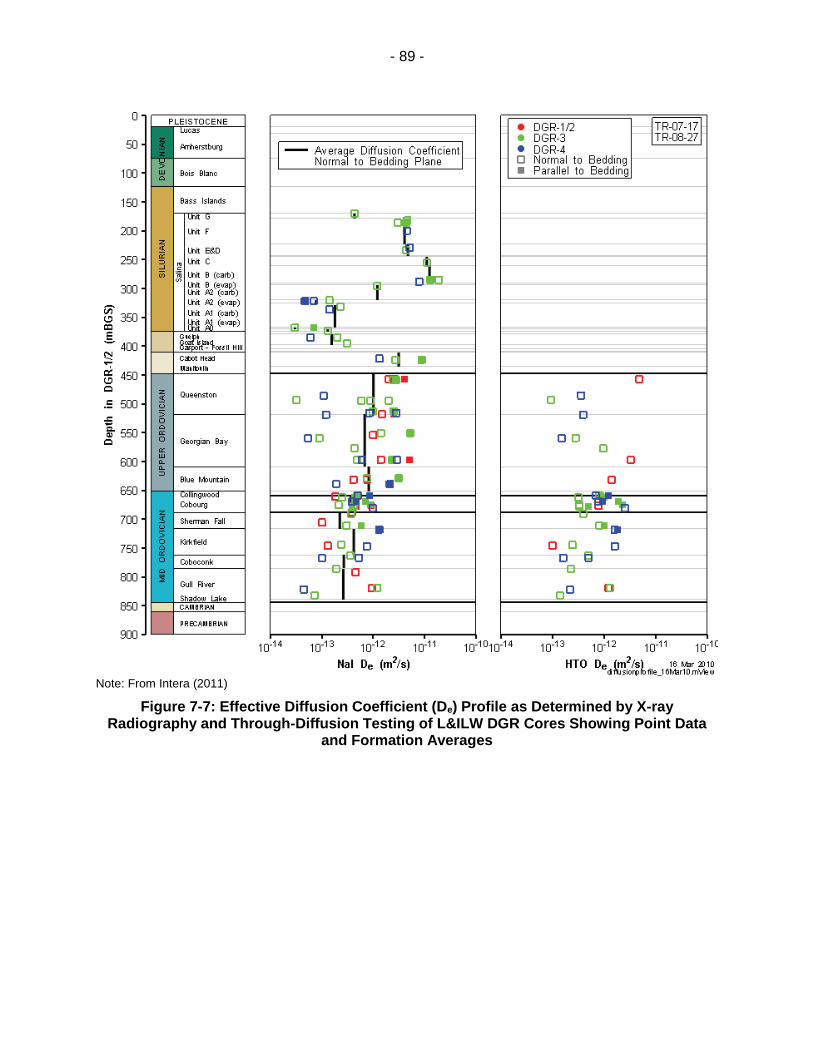
- 89 -

Note: From Intera (2011)

Figure 7-7: Effective Diffusion Coefficient (De) Profile as Determined by X-ray Radiography and Through-Diffusion Testing of L&ILW DGR Cores Showing Point Data

and Formation Averages

- 90 -

Table 7-4: Geosphere Effective Diffusivities1 [m2/s]

Formation De,V Anions / Neutral Species

De,H Anions / Neutral Species

De,v Cationic Species

De,H Cationic Species

Overburden2 7.0x10-10 7.0x10-10 1.4x10-9 1.4x10-9

Sediment2 6.2x10-10 6.2x10-10 1.2x10-9 1.2x10-9

Drift 6.0x10-10 6.0x10-10 1.2x10-9 1.2x10-9

Unit B and C 1.2x10-11 2.4x10-11 2.4x10-11 4.8x10-11

Unit A-2 Carbonate 1.2x10-12 2.4x10-12 2.4x10-12 4.8x10-12

Unit A-1 Upper Carbonate 6.8x10-12 6.8x10-12 1.4x10-11 1.4x10-11

Unit A-1 Carbonate 1.8x10-13 3.6x10-13 3.6x10-13 7.2x10-13

Unit A-1 Evaporite 3.0x10-14 6.0x10-14 6.0x10-14 1.2x10-13

Unit A0 3.0x10-14 6.0x10-14 6.0x10-14 1.2x10-13

Guelph 2.9x10-11 2.9x10-11 5.8x10-11 5.8x10-11

Reynales / Fossil Hill 4.3x10-14 8.6x10-14 8.6x10-14 1.7x10-13

Cabot Head 3.1x10-12 6.2x10-12 6.2x10-12 1.2x10-11

Manitoulin 1.5x10-13 3.0x10-13 3.0x10-13 6.0x10-13

Queenston 1.0x10-12 2.0x10-12 2.0x10-12 4.0x10-12

Georgian Bay / Blue Mountain3

8.2x10-13 1.6x10-12 1.6x10-12 3.2x10-12

Cobourg 3.7x10-13 7.4x10-13 7.4x10-13 1.5x10-12

Sherman Fall 2.2x10-13 4.4x10-13 4.4x10-13 8.8x10-13

Kirkfield 4.2x10-13 8.4x10-13 8.4x10-13 1.7x10-12

Cobokonk 2.7x10-13 5.4x10-13 5.4x10-13 1.1x10-12

Gull River 2.6x10-13 5.2x10-13 5.2x10-13 1.0x10-12

Shadow Lake 1.3x10-12 2.6x10-12 2.6x10-12 5.2x10-12 1unless otherwise noted, effective diffusion values are from Table A6 in Intera (2011). 2Anionic and Neutral species effective diffusion coefficients are based on a NaI free water diffusion coefficient of 1.662x10-9 m2/s (Weast 1983) and porosity and tortuosity data from Table 7-2. Cationic effective diffusion coefficients are assumed to be two times those for anionic and neutral species. 3Based on data for the Blue Mountain formation

7.4.2 Geosphere Dispersion Length

The dispersion length is a parameter that approximates the spreading of a contaminant plume due to inherent variability in the local rock permeability. As a general rule of thumb, a dispersion length is roughly 5-10% of the total path length. For the present repository, the path length of interest for the contaminant plume (i.e., when it reaches the surface) ranges from approximately 280 m (the shortest direct distance from the repository to the bottom of the well) to 500 m (shortest direct distance from repository to the surface). Since a lower dispersion is conservative, results in less spreading of the contaminant plume, the current study assumes a constant longitudinal dispersion length of 20 m or 7% of the 280 m path length to the well. The

- 91 -

transverse dispersion length is assumed to be 10% of the longitudinal dispersion length or 2 m (uniform distribution with a lower bound of 1.6 m and an upper bound of 2.4 m). Dispersivities in the permeable units (the Guelph, the Upper Salina A1 Carbonate, and the drift) were set to higher values (100 m) to avoid numeric issues with the much longer transport distances in the Guelph formation for the no well and all container fail cases.

7.4.3 Geosphere Sorption

Chemical species will, to different degrees, interact with the mineral surfaces surrounding the pores in the rock. Sorption of a radionuclide in the geosphere may be modelled using a linear relation (justified by the expected low radionuclide concentrations) between the concentration of the sorbed species and the aqueous concentration. The proportionality constant is called the sorption coefficient Kd (m3/kg) Sorption properties of the rock depend on a number of factors, such as groundwater chemical composition, groundwater redox potential, rock type, degree of fracturing, etc. Many of the factors controlling radionuclide sorption onto the host rock are site-specific, and experimental data obtained for other conditions may not be applicable or may need to be adapted. At present, many of the site-specific conditions are unknown and, therefore, the sorption data used are partly generic. Radionuclide sorption during transport through the geosphere is incorporated in SYVAC-CC4 using a retardation factor R given by

R = 1 + [s(1-)/] Kd,in (7.1)

where s is the material grain density, is the porosity of the geological material and Kd,in is the radionuclide sorption coefficient for intact rock. Kd,in and R are element dependent. To correct from experimentally measured sorption data on crushed rock samples to those for intact rock, a normalization factor is applied to the experimental sorption coefficient Kd (Vandergraaf 1997, Vandergraaf and Ticknor 1994) to account for the larger sorption area of the crushed rock, i.e.,

Kd,in = [(1-expt)/expt] [(1-)/]-1 Kd (7.2)

where expt is the porosity of the unconsolidated material used in the experimental measurement of Kd. SKB also uses such a normalization factor (Crawford et al. 2006), but that used in Equation 7.2 (Vandergraaf and Ticknor 1994) is more conservative, i.e., generates smaller Kd,in values. Substituting Equation (7.2) into Equation (7.1) leads to the following expression for the retardation factor

R = 1 + [s(1-expt)/expt] Kd (7.3)

Table 7-5 lists values of [s(1-expt)/expt] for various geological materials and units as well as the rock type for each. In general, the geosphere includes an overburden on top of the bedrock, and the compacted (deep) sediment layer at the bottom of lakes. The normalization factors for the overburden materials were calculated with Equation 7.2 assuming a grain density of 2650 kg/m3 and a porosity of 0.42 (Davison et al. 1994, p.366). For the compacted sediment, a density of 2500

- 92 -

kg/m3 (Davis et al. 1993, p. 82) and a porosity of 0.5 (Davison et al. 1994, p. 366) were used. For the sedimentary units, the grain densities density from Table 7-2 and an experimental porosity of 0.5 (Davison et al. 1994) were used.

Table 7-5: Values of [s(1-expt)/expt] for Several Geological Materials

Geological Material s(1-expt)/expt [kg/m3]

Rock Type

Sand 3660

Overburden1 Silt / loam 3660

Clay 3660

Sediment 2500 Sediment2

Drift 2840 Limestone

Unit B and C 2810 Limestone

Unit A-2 Carbonate 2860 Limestone

Unit A-1 Upper Carbonate

2930 Limestone

Unit A-1 Carbonate 2730 Limestone

Unit A-1 Evaporite 2930 Limestone

Unit A0 2790 Limestone

Guelph 2810 Limestone

Reynales / Fossil Hill 2730 Limestone

Cabot Head 2790 Shale

Manitoulin 2720 Limestone

Queenston 2770 Shale

Georgian Bay / Blue Mountain

2760 Shale

Cobourg 2710 Limestone

Sherman Fall 2720 Limestone

Kirkfield 2710 Limestone

Coboconk 2690 Limestone

Gull River 2730 Limestone

Shadow Lake 2760 Limestone 1Mineral composition of the overburden is assumed to be 70% clay, 20% silt/loam and 10% sand. The mineral fractions are normally distributed with standard deviation of 0.28, 0.3, and 0.5 for the clay, silt/loam and sand respectively. Distribution bounds range from 0 to 1. 2Sediment mineral fraction is assumed to be composed of 100% organics.

In the CC4 model, the experimental Kd values are input into the code and then the normalization factor is applied within the model. A complete list of shale and limestone Kd values are shown in Table 7-6 and Table 7-7 respectively. The Kd values are generally described using a lognormal probability density function with exceptions noted in the table. In general, priority is given to measured or modelled sorption coefficients for saline conditions specific to the Canadian shales and limestones. Consequently, the bulk of the Kd values are taken from Vilks and Yang (2018) and Vilks and Miller (2018), when available. Other sources of Kd data include Baeyens et al. (2014), Bertetti (2016), Vilks and Miller (2014), Nagasaki et al. (2017) and Nagasaki et al. (2016). Non-sorbing elements and elements for which there is limited or no sorption data in Canadian shales and limestones are conservatively assumed to have Kd values equal to zero.

- 93 -

Table 7-6: Shale Kd Values [m3/kg]

Element GM1 GSD1 Lower Bound

Upper Bound

Reference / Note

Ac 2.4 13 0.20 53 Analogue of Am

Ag 0 - - - Assumed to be zero aAm 2.4 13 0.20 53 Recommended value in Vilks and Yang (2018)

Bi 2.9 5.8 0.84 10 Data are based on sorption modelling on montmorillonite in SR-270-PW brine by Vilks and Yang (2018)

C 0 - - - Assumed to be zero

Cl 0 - - - Assumed to be zero

Cs 0.2 2.8 0.069 0.63 Data are measured in SR-270-PW brine by Vilks and Miller (2018)

Hg 0 - - - Assumed to be zero aI 0 - - - Assumed to be zero

Mo 0 - - - Assumed to be zero

Nd 0 - - - Assumed to be zero

Np (IV) 32.8 4.6 11 98 Reducing conditions, Lower range data from Vilks and Yang (2018), higher range data Nagasaki et al. (2017)

aNp (V) 0.038 2.2 0.0078 0.12 Oxidizing conditions, data from Vilks and Yang (2018), measured data from Nagasaki et al. (2016) was considered

Pa 2 - - - Constant Value from Baeyens et al. (2014) similar to Vilks and Yang (2018)

Pb 0.001

6 10 0 0.009

Data are measurements in SR-270-PW brine by Vilks and Miller (2018), values recommended in Vilks and Yang (2018)

aPd 2.2 11 0.04 14.3 Data are measurements in SR-270-PW brine by Vilks and Miller (2018) and 4M Na-Ca-Cl brine by Riddoch and Nagasaki et al. (2016)

Po 0.05 - - - Constant value from Baeyens et al. (2014)

Pu (III) 2.45 2.0 1.5 4.0 Reducing conditions, data are measurements in SR-270-PW brine by Bertetti (2016), Kd values are close to simulated results by Vilks and Yang (2018)

Pu (IV, V)

2.2 1.5 1.4 3.2 Oxidizing conditions, data recommended by Vilks and Yang (2018)

Ra 0 - - - Constant value from Baeyens et al. (2014)

Rh 0 - - - Assumed to be zero

Rn 0 - - - Assumed to be zero

Ru 0 - - - Assumed to be zero

Se (-II) 0.021 4.8 0.003 0.1 Reducing Conditions, based on data from Vilks and Yang (2018) and Bertetti (2016)

Se (IV, VI)

0.010 1.2 0.008 0.011 Oxidizing conditions data recommended by Vilks and Yang (2018)

Sm 0.16 1.6 0.11 0.22 Analogue of Eu, Eu data from Vilks and Yang (2018) and Vilks et al. (2011)

Tc (IV) 0.02 - - - Reducing conditions, data are measurements in SR-270-PW brine by Bertetti (2016)

Tc (VI) 0.002

4 140 7.3x10-5 0.079 Oxidizing Conditions, data from Vilks and Yang (2018)

- 94 -

Th 4.6 1.8 1.7 6.8 Data from measurements in SR-270-PW from Vilks and Miller (2018)

U (IV) 4.6 1.8 1.7 6.8 Reducing conditions, analogue of Th

U (VI) 0.027 2.0 0.016 0.044 Oxidizing conditions, data are measurements in SR-270-PW brine by Vilks and Miller (2014)

Note: 1GM = Geometric Mean, GSD = Geometric Standard Deviation aData from a draft version of Vilks (2018) data has been revised in the final version of Vilks (2018).

Table 7-7: Limestone Kd Values [m3/kg]

Element GM1 GSD1 Lower Bound

Upper Bound

Reference / Note

Ac 0.16 1.6 0.09 0.29 Analogue of Am

Ag 0 - - - Assumed to be zero

Am 0.16 1.6 0.09 0.29 Recommended value in Vilks and Yang (2018)

Bi 0.16 1.6 0.09 0.29 Analogue of Eu, Eu data from Vilks and Yang (2018) and Vilks et al. (2011)

C 0 - - - Assumed to be zero

Cl 0 - - - Assumed to be zero

Cs 0.14 4 0.032 0.69 Data are measured in SR-270-PW brine by Vilks and Miller (2018)

Hg 0 - - - Assumed to be zero aI 0 - - - Assumed to be zero

Mo 0 - - - Assumed to be zero

Nd 0 - - - Assumed to be zero

Np (IV) 2.1 1.9 0.6 2.7 Reducing conditions, analogue of Th

Np (V) 0.014 42 0.001 0.2 Oxidizing conditions, data from Vilks and Yang (2018), measured data from Nagasaki et al. (2016) was considered

Pa 0.09 - - - Data based on LFER relationship by Vilks and Yang (2018)

Pb 0.0004 14 0 0.004 Data are measurements in SR-270-PW brine by Vilks and Miller (2018), values recommended in Vilks and Yang (2018)

aPd 1.94 5.7 0.1 22 Data are measurements in SR-270-PW brine by Vilks and Miller (2018)

Po 0 - - - Assumed to be zero

Pu (III) 2.45 2.0 1.5 4.0

Reducing conditions, data are measurements in SR-270-PW brine by Bertetti (2016), Kd values are close to simulated results by Vilks and Yang (2018)

Pu (IV, V) 0.49 7.3 0.069 3.7 Oxidizing conditions, data recommended by Vilks and Yang (2018)

Ra 0 - - - Assumed to be zero

Rh 0 - - - Assumed to be zero

Rn 0 - - - Assumed to be zero

Ru 0 - - - Assumed to be zero

Se (-II) 0.013 5.8 0.0037 0.1 Reducing Conditions, based on data from Vilks and Yang (2018) and Bertetti (2016)

Se (IV, VI) 0.0013 - - - Oxidizing conditions data recommended by Vilks and Yang (2018)

- 95 -

Sm 0.16 1.6 0.09 0.29 Analogue of Eu, Eu data from Vilks and Yang (2018) and Vilks et al. (2011)

Tc (IV) 10 - - - Reducing conditions, data are measurements in SR-270-PW brine by Bertetti (2016)

Tc (VI) 0.015 9.7 0.003 0.075 Oxidizing Conditions, data from Vilks and Yang (2018)

aTh 2.1 1.9 0.6 2.7 Data from measurements in SR-270-PW from Vilks and Miller (2018)

aU (IV) 2.1 1.9 0.6 2.7 Reducing conditions, analogue of Th

U (VI) 0.011 1.6 0.008 0.015 Oxidizing conditions, data are measurements in SR-270-PW brine by Vilks and Miller (2014)

Note: 1GM = Geometric Mean, GSD = Geometric Standard Deviation, aData from a draft version of Vilks (2018) data has been revised in the final version of Vilks (2018).

7.5 TWO PHASE FLOW PARAMETERS

Two-phase flow processes in the geosphere are modelled using TOUGH2-GGM and utilize the Van-Genuchten equations as described in Section 6.10. Geosphere two phase flow properties are presented in Table 7-8 (Calder 2011).

Table 7-8: Two Phase Flow Parameters1,2

Formation 1/α [MPa] m [-] n [-] 9Slrc [-] 9Sir [-] Sgr [-]

Drift2 - - - - - -

Unit B and C3 0.31 0.35 4.22 0.55 0.56 0.00

Unit A-2 Carbonate4 0.76 0.50 3.06 0.00 0.01 0.00

Unit A-1 Upper Carbonate5

39 0.99 2.41 0.00 0.01 0.00

Unit A-1 Carbonate5 39 0.99 2.41 0.00 0.01 0.00

Unit A-1 Evaporate6 2.1 0.99 2.28 0.01 0.02 0.10

Unit A0 5.9 1.13 2.25 0.00 0.01 0.14

Guelph7 0.04 0.15 4.89 0.25 0.26 0.00

Reynales / Fossil Hill 28 0.68 6.11 0.03 0.04 0.00

Cabot Head 15 0.24 6.82 0.00 0.01 0.05

Manitoulin 41 1.31 3.65 0.11 0.12 0.05

Queenston 36 1.13 4.45 0.09 0.10 0.06

Georgian Bay / Blue Mountain

30 1.10 3.82 0.17 0.18 0.04

Cobourg 62 1.69 3.13 0.06 0.07 0.03

Sherman Fall 28 1.00 2.33 0.17 0.18 0.11

Kirkfield 173 7.22 2.17 0.00 0.01 0.15

Coboconk 66 1.73 1.82 0.00 0.01 0.03

Gull River 40 0.78 4.06 0.21 0.22 0.11

Shadow Lake 0.23 0.58 1.20 0.04 0.05 0.00

Precambrian8 0.23 0.58 1.20 0.04 0.05 0.00 1The van Genuchten equations (van Genuchten, 1980; see below) were used to produce the two-phase flow parameter values. 2The drift is not represented in the TOUGH2-GGM two-phase flow model. 3Assumed to have the same properties as the Salina C from Table 6 in Calder (2011). 4Assumed to have the same properties as the Salina A-2 from Table 5 in Calder (2011). 5Assumed to have the same properties as the Salina A-1 from Table 5 in Calder (2011). 6Assumed to have the same properties as the Salina A-2 Evaporate from Table 5 in Calder (2011). 7Assumed to have the same properties as the Salina A-0 (lower) from Table 4 in Calder (2011). 8Precambrian values are assumed to be the same as the shadow lake formation 9Slrc values are assumed to be 0.01 less than Sir.

- 96 -

In 2011, AECL conducted thermal testing of samples obtained from select unit in the L&ILW DGR-4 borehole to obtain thermal properties. These results are published in Golder (2013), and form the basis of the recommended properties for the Seventh Case Study, outlined in Table 7-9. Each sample location was tested using samples oriented parallel and perpendicular to the bedding plane and across the bedding plane. Each sample was tested for saturated, air-dried and oven-dried thermal properties. Note that only 24 hours was allowed for each desaturation process. Given the extremely low permeability of many of these samples, neither of these drying processes are likely to completely remove resident porewater. Parameters suggested for use in this study are the average of these different samples and tests for each geological unit. For geological units without measurements of thermal properties, values were estimated based on the measurements available for similar geological units and expert opinion.

Table 7-9: Thermal Properties of the Geosphere

Formation Thermal Conductivity

[kW/m•K]

Heat Capacity [MJ/m3•K]

Comment

Drift1 4.47 3.36 No new measurements, value from Gobien (2013)

Unit B and C 3.56 2.60 Value determined by expert opinion

Unit A-2 Carbonate

2.68 2.47 Average values from measurements in Golder (2013)

Unit A-1 Upper Carbonate3

2.68 2.47 Average value from Golder (2013) applied to a similar formation

Unit A-1 Carbonate

2.68 2.47 Average value from Golder (2013) applied to a similar formation

Unit A-1 Evaporate

5.21 3.11 Value determined by expert opinion

Unit A04 2.68 2.47 Average value from Golder (2013) applied to a similar formation

Guelph 2.68 2.47 Average value from Golder (2013) applied to a similar formation

Reynales / Fossil Hill

2.68 2.47 Average value from Golder (2013) applied to a similar formation

Cabot Head 1.97 2.10 Average value from Golder (2013) applied to a similar formation

Manitoulin 3.44 2.60 Average value from Golder (2013) applied to a similar formation

Queenston 1.97 2.10 Average values from measurements in Golder (2013)

Georgian Bay / Blue Mountain

1.91 1.66 Average values from measurements in Golder (2013)

Cobourg 2.48 2.01 Average values from measurements in Golder (2013)

Sherman Fall 2.10 1.94 Average values from measurements in Golder (2013)

Kirkfield 2.10 1.94 Average value from Golder (2013) applied to a similar formation

Coboconk 2.10 1.94 Average value from Golder (2013) applied to a similar formation

Gull River 2.10 1.94 Average value from Golder (2013) applied to a similar formation

Shadow Lake 3.00 2.02 No new measurements, value from Gobien (2013) 1The drift is not represented in the TOUGH2-GGM two phase flow model

- 97 -

7.6 WELL LOCATION AND DEPTH

An important pathway for human exposure to contaminants released from the repository is through a well, which can supply water for drinking, domestic use and irrigation. As a conservative assumption for safety assessment, the location and depth of the well are selected so as to maximize the possibility that the well water becomes contaminated. However, this must be tempered with the knowledge that some well locations would be unrealistic. For instance, the water could be unacceptably saline or the rock might not be sufficiently permeable to provide the amount of water required. A survey of 218,518 wells from Open Ontario Data Directive Catalogue and the Land Information Ontario shows the median well depth across Ontario is 8.5 m and the 95th percentile depth is 78 m. Figure 7-8 shows the distribution of well depths across Ontario. The subset of data for wells in southern Ontario includes 48,269 wells. The southern Ontario wells have a median depth of 9.1 m and a 95th percentile depth of 64.4 m. Figure 7-9 shows to distribution of well in southern Ontario. The data indicated that the vast majority in wells in Ontario were relatively shallow and intercept meteoric waters in the upper fractured layers of rock. It is not clear from the data whether these represent shallower wells used primarily for irrigation or potable drinking water wells. For the Seventh Case Study the drinking water well is assumed to be much deeper than a typical southern Ontario well and intercept the Guelph aquifer. A reference (bottom) well depth is 219 m and was chosen to intercept the contaminant plume in the Guelph aquifer and capture the maximum amount of the plume. It should be noted that approximately 0.1% of the wells included in the survey of southern Ontario extended to depths beyond 200 m. The well was analytically tested to be capable of supplying a range of well demands of interest. If the well is not capable of supplying all the water needed by the critical group, then it is assumed that the water demand that cannot be satisfied by the well is taken from surface water. More information on the well location, and on the groundwater flow around the well, is provided in NWMO (2018). Table 7-10 summarizes the reference well properties.

- 98 -

Figure 7-8: Survey of Ontario Well Depths

Figure 7-9: Survey of Southern Ontario Well Depths

- 99 -

Table 7-10: Well Model Geosphere Parameters

Parameter Value Comment

Well depth 219 m Bottom of well, relative to ground surface.

Well casing radius 0.0508 m 75% of wells in Davis et al. 1994 are 0.0508 m radius while 25% are 0.0762 m radius (4 or 6 inches diameter). (Davison et al. 1994, p.416).

Well bypass discharge minimum fraction

1.0 Minimum fraction for the reduction of the discharge area associated with the well bypass. Set to one representing no reduction of the discharge area due to well demand.

Well divergent break point A

Well divergent break point B

Well divergent break point C

420 m3/a

840 m3/a

1261 m3/a

Break Points A, B, and C (BPa, BPb, and BPc) are used for segments leading away from divergent nodes in the SYVAC3-CC4 geosphere model that exhibit changes in flow amounts due to different well demands. The break point values are used in combination with the change of the fractional flow per unit well demand for the three ranges (Appendix C).

Well demand maximum

3500 m3/a If the water demand exceeds this value surface water will be used as a secondary water source.

Distance to the first and second well drawdown

5 m , 20 m Nominal values used for the SYVAC3-CC4 well model

7.7 OTHER GEOSPHERE PARAMETERS

Table 7-11 lists values of other miscellaneous parameters used by the CC4 geosphere model.

- 100 -

Table 7-11: Other Geosphere Properties

Parameter Value Comment

Water density 0 for density equation

997.0470 kg/m3 Value used in calculation of density at other temperatures. (CRC 2016)

Reference temperature for density equation

25.0°C CRC (2016) water density value is for 25°C

Compressibility of water

water at 25oC for the density equation

4.524×10-10 Pa-1 CRC (2016)

Coefficient a for density equation

-2.406×10-4 K-1 Based on data from CRC (2016)1

Coefficient b for density equation

-3.857×10-6 K-2 Based on data from CRC (2016)1

Coefficient a for viscosity equation

1.858×10-6 Pa·s Based on data from CRC (2016)2

Coefficient b for viscosity equation

1.850×103 K Based on data from CRC (2016)2

0oC 273.15 K Used in °C to K conversion

1Density of water = 0 (1+ water p + a(T) + b(T)2), where T = T[°C] – 25°C and p = head difference from hydrostatic [Pa]. Calculated densities match values in CRC (2016) within 0.08% over the range 10–90°C.

2Viscosity of water = ae(b/T[K]). Calculated viscosities match values in CRC (2016) within 4.8% over the range 10–90°C.

7.8 GEOSPHERE NODE DATA

The geosphere is represented by either 3D finite-element models in FRAC3DVS-OPG, or as a network of 1-D transport paths in SYVAC3-CC4. The FRAC3DVS-OPG representations typically involve several million nodes, and are not included here. Further details about these detailed models are given in NWMO (2018). The SYVAC3-CC4 geosphere transport model uses a simplified representation of the FRAC3DVS-OPG groundwater flow field. The input parameters used in this latter model are described in Appendix C of this report.

- 101 -

8. BIOSPHERE DATA

The Seventh Case Study repository is located in the same area of the Michigan Basin as the repository in the Fifth Case Study (NWMO 2013). Thus, many of the biosphere parameter values are unchanged from those used in the Fifth Case Study, although some values have been updated where more appropriate data were available. The following sections summarize the biosphere parameter values used in the Seventh Case Study and provide links to the original sources of the data.

8.1 SITE AND SURFACE WATER

The Seventh Case Study is based on a hypothetical but plausible Michigan Basin site. The surface topography of this site is relatively flat. The sub-regional watershed containing the repository is bounded by topographic highs to the north and south with a series of rivers and streams crossing through the sub-regional watershed area (Figure 7-1). The surface water feature closest to the repository is the river to the west of the repository. The biosphere characteristics and data are typical of southern Ontario when available however, due to the lack of site specific data, much of the biosphere data remains generic.

8.2 DISCHARGE ZONES AND WATERSHED AREAS

Contaminants released from the repository can eventually move through the geosphere and, if they do not decay first, reach the biosphere. In general, they will reach the biosphere at specific discharge zones that will depend upon details of the repository location, geosphere properties, and surface topography. Typically, these discharge zones are topographic low areas and often are associated with bodies of water.

8.2.1 Watershed Areas

The surface area around the repository can be divided into multiple small watersheds, each defined by the topography of the region. For this hypothetical case study, 4 relevant watersheds A, B, C, and D were defined that feed into one another; with each featuring various tributaries collecting eventually into a primary river (see Figure 8-1). The watershed areas listed in Table 8-1, are assumed to be constant in time and are used to calculate the water flow rate through each river system based on the precipitation and runoff values defined in the next section. The characteristics of the watershed system are summarized in Table 8-1.

- 102 -

Figure 8-1: Watershed Boundaries

- 103 -

Table 8-1: Surface water properties

Parameter Value Comment

Watershed areas 2.29x107 m2

2.20x106 m2

4.94x107 m2

6.46x107 m2

Watershed A (18.4% aquatic area)

Watershed B (26.2% aquatic area)

Watershed C (29.7% aquatic area)

Watershed D (16.8% aquatic area)

Aquatic surface area 4.21x106 m2

5.76x105 m2

1.47x107 m2

1.08x107 m2

Watershed A

Watershed B

Watershed C

Watershed D

River Surface Area Scaling Factor

0 a / m3 The river surface area is scaled in SYVAC3-CC4 using the factor F = exQ, where x is the area scaling factor listed here and Q is the well demand. Value of x set to zero so no scaling for this study (ie. river flow is not dependent on well pumping rate).

Mean river depth 4.6 m Value is geometric mean, geometric standard deviation is 2.0 with lower and upper bounds of 1 m and 10 m respectively (Davis et al. 1993, p. 97, except for the upper bound which is limited by the site topography)

Lake sedimentation rate 0.4

kgdry sed./m2a

CSA (2014) value for Canadian Shield Lakes. Lognormal PDF with GSD=2.5, and bounds of 0.01 and 15 kg/(m2.a) (Davis et al. 1993, p.99).

Mixed sediment thickness 0.01-0.1 m Uniform PDF over 0.01-0.1 m (Davis et al. 1993, p. 99).

Thickness of sediment removed for use in fields

0.3 m Set to soil layer thickness

8.2.2 Surface discharge area

Discharge areas used in the Seventh Case Study were estimated as areas in which the cumulative 10 million year I-129 discharge from the repository exceeded background levels of I-129. These areas were determined using FRAC3DVS-OPG. Table 8-2 shows the resulting discharge areas as well as aquatic and terrestrial fractions of said discharge areas for each of the watersheds. Ultimately, contaminants released into the biosphere are either trapped in deep sediments under these water bodies, or transported out of the local watershed through the river system. People living downstream from the repository could be exposed to contaminants that reach the surface. However, the levels would be low because of the slow discharge from the underground and also due to dilution because the river system drains a large watershed area.

- 104 -

Table 8-2: Surface Discharge Areas

Watershed Total Discharge

Area1

[m2]

Aquatic Discharge2

[m2]

Terrestrial Discharge3

[m2]

Watershed A 1.08x106 5.27x105 5.50x105

Watershed B 1.34x105 6.16x104 7.26x104

Watershed C 0 0 0

Watershed D 5.67x106 2.32x106 3.35x106 1Discharge areas equal to 4.7%, 6.1%, 0% and 8.8% of the watershed area for watersheds A, B, C, and D, respectively 2Aquatic fraction based on areas equal to 2.3%, 2.8%, 0%, and 3.6% of the watershed area for watersheds A, B, C and D, respectively. 3 terrestrial fraction set to total discharge area minus the aquatic discharge

8.3 CLIMATE AND ATMOSPHERE

The climate and atmospheric parameters are summarized in Table 8-3. These values reflect CSA (2014) values when available for a Southern Ontario site; otherwise the values are taken from Davis et al. (1993). The variation in these parameter values represents the natural variation across the Michigan Basin for present-day climate conditions.

- 105 -

Table 8-3: Climate and atmosphere parameters

Parameter Value Comment Annual total precipitation

1.02 m/a Normal PDF with a SD of 0.16 and bounds of 0.3 and 3.0 m/a. Calculated using historical records between 1965 and 2006 in Owen Sound, which is assumed to be representative of a sedimentary site in Southern Ontario. The bounds represent half the minimum and twice the maximum recorded rainfall (Government of Canada, 2015).

Annual surface average runoff

0.42 m/a Average value for the region defined as “Great Lakes” in Statistics Canada (2017). Variation coefficient is 0.72, which is the ratio of the monthly mean to the standard deviation. Conservatively assume variation on an annual basis is the same; thus, standard deviation is 0.58. Bounds are taken as the range of Ontario runoff values in Statistics Canada (2017), thus 0.1 to 0.8 m/a.

Average wind speed1

2.36 m/s Normal PDF with mean of 2.36 m/s (8.5 km/h), standard deviation of 0.64 m/s, and bounds of 0.44 and 6 m/s. (Davis et al. 1993, p.196).

Average temperature1

7 oC Calculated using historical records between 1965 and 2006 at the Owen Sound weather station, which is assumed to represent the location of a sedimentary site in Ontario. The monthly average range is from -15 oC in the winter to 23 oC in the summer. (Government of Canada, 2015).

Climate state Temperate Current climate.

Dry deposition velocity

0.0014 m/s CSA (2014) dry deposition velocity for all radionuclides except for noble gases and N-13(0 m/s), Cl-36 (0.02 m/s), particular iodine (0.0036 m/s), elemental iodine (0.0075 m/s) and organic iodine (9.2×10-6 m/s). Geometric standard deviation of 2 is adopted from Amiro (1992).

Atmospheric dust load1

3.2x10-8 kgdrysoil/ m3

air Lognormal PDF with GM calculated from suspended particulate matter concentrations in ON, NB, QC and SK during years 1996 to 2002. GSD of 1.7 with bounds of 7.0x10-9 and 7.5x10-8 kgdrysoil/m3air. (NAPS, 1996 to 2002)

Atmospheric aerosol load1

2.9x10-10 m3water/

m3air

Lognormal PDF with geometric mean of 2.9x10-10 m3water/m3

air, and geometric standard deviation of 1.41. Based on estimate for sea salt aerosol over oceans (Davis et al. 1993, p.191).

Washout Ratio 5 500 000 CSA (2014) washout ratio for deposition to soil for all elements other than noble gases and iodine. This value is conservative for iodine. CSA (2014) recommends 160 000 for elemental iodine and 74 000 for organic iodine.

1Values for these parameters are not available in CSA (2014).

- 106 -

8.4 SOILS AND SEDIMENT

8.4.1 Soil Physical Characteristics

The physical characteristics of the soil at the hypothetical site are described in Table 8.4. These reflect mostly the values in CSA (2014), where available. In SYVAC3-CC4, two soil models are considered: an upland soil and a shallow soil. For the upland soil, which is more typical, the water table is a reasonable distance below the ground surface. For the shallow soil, the water table extends into the surface soil on a regular and extended basis. The distinction between these two cases is important in determining how readily contaminated groundwater can reach the surface. In the upland soil case, it must be transported by processes such as capillary action. In the shallow soil case, the groundwater is directly discharged into the soil layer. For the upland soil model, a simple approach is used to account for upward movement of contaminated groundwater into the surface soil. Specifically, the model requires information on the surface soil moisture content, and parameters describing the downward flow rate of surface water (precipitation and irrigation) and upward flow rate of groundwater. The water leaching fraction is the fraction of net precipitation or irrigation, after evapotranspiration, which penetrates deep into the soil rather than running off along the surface. On exposed bedrock, the fraction would be small. However, it is assumed that any farming would be on locations with suitable soil, and so a higher fraction would be expected. Since the specific value is uncertain, a large range from 0.1 to 1 is assumed. Other soil model characteristics are also shown in Table 8-4.

- 107 -

Table 8-4: Soil properties

Parameter Value Comment Soil types Sandy

Using soil type from Western Ontario, as identified in CSA (2014).

Surface soil bulk density

1500 kg dry soil/m3 soil (sandy soil)

The densities of the four soil types are as follows: 1500, 1300, 1400 and 400 kg dry soil/m3 soil for sand, loam, clay and organic soils, respectively (CSA 2014).

Active surface soil depth

0.2 m This is the active or root zone layer for which nuclide concentrations in the soil are determined (CSA 2014).

Soil Depth to water table

1.5 m The depth of soils vary considerably, from very shallow soils to 5 m or more. However, most soils cannot exert sufficient matric potential to pull groundwater up through the profile to the root zone if the water table lies more than 2.5 m below the surface. To ensure that the critical group and other biota are always exposed to groundwater contamination, we conservatively adopted a maximum soil depth of 2.5 m and a minimum depth of 0.01 m. We treat this value as an upper truncation limit to a normal distribution with a mean of 1.5 m and an SD of 0.5 (Davis et al. 1993).

Minimum soil depth to water table for upland soil model

0.5 m This is the minimum depth-to-water-table at which the upland soil model is used. For smaller depths, a shallow soil model is used that allows for flooding of the surface soil by contaminated groundwater. (Davis et al. 1993, p.137.)

Upland soil leach rate fraction

0.55 Fraction of net precipitation (precipitation + irrigation – evapotranspiration) that infiltrates into soil. Uniform PDF from 0.1 to 1.

Fraction of runoff entering the overburden

0.10 Uniform distribution with a lower bound of 0.03 and an upper bound of 0.17 (Singer and Cheng 2002).

Surface soil moisture content fraction

0.1 (0.03-0.2) sand 0.2 (0.1-0.3) loam 0.3 (0.2-0.5) clay 0.6 (0.3-0.8) organic

Triangular PDF assumed, with the bracketed numbers

correspond to the upper and lower bounds. The most

probable values for sand, loam and clay are from CSA

(2014). The lower bound is the average wilting point

and the upper bound is the average field capacity from

Beals (1985), converted to volume fraction. The most probable value for organic soil corresponds to the average field capacity from Beals (1985), converted to volume fraction. The lower bound corresponds to the wilting point from Beals (1985), converted to volume fraction. The upper bound corresponds to the CSA (2014) value and also the value calculated using equation (1) of Appendix D in Beals (1985), for a bulk dry density of 400 kg/m3. These values correspond approximately to the water content (and range) shown in Figure D-5 of Beals (1985).

Surface soil summer water deficit

0.20 m/a Climate-based parameter. Value is based on water budget summaries (Coligado et al. 1968, 1969a-e). Value selected is the amount of water needed to eliminate the deficit yet not deplete the soil moisture. It is assumed to represent the maximum amount of water would flow upward from a shallow water table.

- 108 -

Groundwater upflow exponent

3 Value is based on data for a fine sandy loam (Hillel 1980), and so likely overestimates upward flow for other soil types.

Bioturbation rate 0 /a Not significant in Michigan Basin soils.

Soil Contamination of Plants

0.0005 Sheppard (1985) Section 5.8.9

Soil Compartment Concentration Limit

1x10-4 mol/kg Warning flag for all soil types in the SYVAC3-CC4 model, not a hard coded limit.

8.4.2 Plant/Soil Concentration Ratio

Table 8-5 lists the plant/soil concentration ratios for the different radiologically hazardous elements and the source of the data. The SYVAC3-CC4 biosphere model distinguishes between "garden" plants grown for human consumption, and "forage" plants which are used for animal consumption. Specifically, the model allows for different plant/soil concentration ratios for these different plants. Plant/soil concentration ratios are inconsistently recorded on a dry or fresh weight basis. Conversion between the two is inaccurate unless the dry/fresh weight ratio is known. For consistency in the values reported herein, a dry/fresh weight ratio of 0.54 and 0.36 are used for forage and garden crops, respectively. These values were calculated from the dry/fresh weight ratios given in CSA (2014). The dry/fresh weight ratio for forage crops is the average the dry/fresh weight ratio of 0.20 for forage (e.g., fresh grass) and 0.87 for feed (e.g., grains), and assumes that animals eat 50% forage and 50% feed over the year. Similarly, the dry/fresh weight ratio for garden crops is calculated assuming that the critical group plant intake is 1/3 grain (dry/fresh weight ratio of 0.87) and 2/3 fruits and vegetables (dry/fresh weight ratio of 0.1). Plant / soil concentration ratios for Cl, I, Np, Ra and U are preferentially selected from Sheppard et al. (2002), Sheppard et al. (2004a), Sheppard et al. (2004b) and Sheppard et al. (2010) where direct measurements are made. For elements not measured in the Sheppard reports data are selected from the more generic CSA (2014) and Davis et al. (1993) sources. The CSA (2014) plant/soil concentration ratios represent the geometric mean of several sources, unless there are data from the international union of radioecologists (Sheppard, 1995b). CSA (2014) values are expressed on a dry weight basis, were converted to a fresh weight basis using the dry/fresh weights shown above. The plant/soil concentration data in Davis et al. (1993) are expressed in a plant fresh-weight basis, and were obtained from the original data using a plant dry/fresh weight ratio of 0.25. For consistency, the Davis et al. (1993) values were converted to a fresh weight basis using the dry/fresh weight ratios selected for this study. The plant/soil concentration ratio is described using a lognormal PDF with the geometric mean given in Table 8-5 and a geometric standard deviation (GSD) of 5.7 for most elements (unless otherwise specified), as recommended by BEAK (2002).

- 109 -

Table 8-5: Plant/Soil Concentration Ratios1,2

Element Garden

[(Bq/kgfw)/ (Bq/kg dw)]

GSD Forage

(Bq/kgfw)/ (Bq/kgdw)

GSD Reference

Ac 1.3E-03 10 1.9E-03 10 Davis et al. (1993)

Am 2.2E-04 5.7 3.4E-04 5.7 CSA (2014)

Bi 4.6E-03 2 7.0E-03 2 Sheppard et al. (2010)

C 7.8E+00 10 1.2E+01 10 Davis et al. (1993)

Cl 3.7E+00 5.7 9.1E+00 5.7 Sheppard et al. (2004a)

Cs 1.9E-02 5.7 2.8E-02 5.7 CSA (2014)

I 5.0E-03 10 2.7E-02 10 Sheppard et al. (2002).

Np 6.0E-04 6.67 4.6E-03 10.4 Sheppard et al. (2004b)

Pa 1.4E-02 5.7 2.0E-02 5.7 CSA (2014)

Pb 8.6E-04 2.5 1.3E-03 2.5 Sheppard et al. (2010)

Pd 5.4E-02 10 3.8E-02 10 Davis et al. (1993)

Po 9.0E-04 10 1.3E-03 10 Davis et al. (1993)

Pu 5.0E-05 5.7 7.5E-05 5.7 CSA (2014)

Ra 4.1E-03 11 1.7E-02 11 Sheppard et al. (2005a)

Rn 0.0E+00 0 0.0E+00 0 Davis et al. (1993)

Se 1.6E-01 5.7 2.4E-01 5.7 CSA (2014)

Sm 1.5E-04 5.1 2.2E-04 5.1 Sheppard et al. (2010)

Tc 1.3E+00 5.7 2.0E+00 5.7 CSA (2014)

Th 1.2E-03 5.7 1.8E-03 5.7 CSA (2014)

U 7.9E-04 5.7 2.7E-03 5.7 Sheppard et al. (2005b) 1Data for exclusively chemically hazardous elements (Ag, Hg, Mo, Nd, Rh and Ru), have been excluded from

the dose model data. 2Values are lognormally distributed

8.4.3 Soil Distribution Coefficient (Kd)

Table 8-6 provides the soil Kd values. The Kd values are taken from CSA (2014) when available. Note that CSA (2014) are preferentially taken from IAEA (2010). The geometric mean values for Cl, I, Np, Ra and U are from Sheppard et al. (2002, 2004a, 2004b, 2005a and 2005b, respectively). The soil Kd values for Rn is assumed to be zero (Sheppard and Thibault 1990). Most soil Kd values are assumed to be lognormally distributed with a geometric standard deviation of 10 as per Davis et al (1993). Notable exceptions include I in organic soil for which the GSD = 22 (Sheppard et al. 2002), Ra in all soils for which the GSD = 4.9 (Sheppard et al. 2005a), and U in all soils for which the GSD = 20 (Sheppard et al. 2005b). Rn is somewhat unique in that it is conservatively assumed to be constant and zero for all soil types. There is a strong inverse correlation between plant uptake of elements and the soil Kd values. Therefore, the Kd values are correlated to the plant/soil concentration ratio values (Table 8-6) with a correlation coefficient of -0.7 (Sheppard et al. 2010).

- 110 -

Table 8-6: Soil Kd Values [L/kg]

Element Sand Loam Clay Organic Reference Ac 450 1500 2400 5400 Davis et al. (1993, p.155)

Ag 90 120 180 15000 CSA (2014), Table G.2

Am 1000 4300 4300 2500 CSA (2014), Table G.2

Bi 100 450 600 1500 Davis et al. (1993, p.155)

C 5 20 1 70 CSA (2014), Table G.2

Cl 0.1 0.1 0.1 2200 Sheppard et al. (2002). CSA (2014) values are 2, 6, 8 and 20 for sand, loam, clay and organic soil, respectively.

Cs 530 370 370 270 CSA (2014), Table G.2

Hg 16 55 84 194 CSA (2014), Table G.2

I 8 18 12 76 Sheppard et al. (2002). CSA (2014) values are 2, 6, 8 and 20 for sand, loam, clay and organic soil, respectively.

Mo 10 125 90 25 CSA (2014), Table G.2

Nd 0 0 0 0 No Data

Np 2.5 13 21 530 Sheppard et al. (2004b). CSA (2014) values are 4, 25, 55 and 1200 for sand, loam, clay and organic soils, respectively.

Pa 540 1800 2700 6600 CSA (2014), Table G.2

Pb 270 16000 550 22000 Davis et al. (1993, p.155)

Pd 55 180 270 670 Davis et al. (1993, p.155)

Po 150 400 3000 7300 Davis et al. (1993, p.155)

Pu 400 1100 1100 760 CSA (2014), Table G.2

Ra 47 47 47 47 Sheppard et al. (2005a). CSA (2014) values are 1900, 1900, 38000 and 1300 for sand, loam, clay and organic soils, respectively.

Rh 43 149 226 524 CSA (2014), Table G.2

Rn 0 0 0 0 Rn soil Kd assumed to be constant and zero for all soil types.

Ru 36 40 40 66000 CSA (2014), Table G.2

Se 56 220 220 1000 CSA (2014), Table G.2

Sm 245 800 1300 3000 Davis et al. (1993, p.155)

Tc 0.04 0.07 0.09 3.1 CSA (2014), Table G.2

Th 700 18000 4500 730 CSA (2014), Table G.2

U 42 220 180 2200 Sheppard et al. (2005b). CSA (2014) values are 110, 310, 280 and 1200 for sand, loam, clay and organic soils, respectively.

- 111 -

8.4.4 River and Lake Sedimentation Rates

Table 8-6 provides data for the sedimentation rate of the different chemical elements in rivers and lakes. This parameter is defined as the fraction of the element in the water column that is lost to the lake or river sediments per unit time. It is the net rate of sedimentation, accounting for any resuspension of sediments back into the water column. The CSA (2014) states that there is a lack of adequate data to describe the sedimentation rate in rivers, and that it should therefore have a default value of zero, which is conservative with respect to radionuclide concentration in the water column. The sedimentation rate for lakes were calculated from the following equation (CSA 2014):

𝜆𝑠 =𝐷𝑅 ∙ 𝜌 ∙ 𝐴 ∙ 𝐾𝑑

𝑉

where:

𝜆𝑠 is the lake sedimentation rate (1/a); 𝐷𝑅 is the lake sediment accumulation rate (1 mm/a) 𝜌 is the sediment density, 400 kgdw/m3 (CSA 2014);

𝐴𝑤 is the area of the lake , m2 (see Table 8-1) 𝐾𝑑 is the solid-to-liquid partition coefficient, m3/kgdw; and

𝑉𝑤 is the volume of the lake (m3) (see Table 8-1). Sediment soil-to-liquid partition coefficient originate from CSA (2014). Values that are not available in CSA (2014) are taken to be 10 times the Kd of sandy soil, which follows the methodology used by CSA (2014) to define missing sediment Kd values. Values of the lake sedimentation rate are lognormally distributed with GM values shown in Table 8-7 and the GSD equal to that for the sandy soil Kd values. Namely, a GSD of 10 except for Ra (GSD=4.9), U (GSD=20) and Rn (constant parameter).

- 112 -

Table 8-7: Lake Sedimentation Rates

Element Sediment1 Kd [m3/kg]

Sedimentation Rate for

Watershed A [1/a]

Sedimentation Rate for

Watershed B [1/a]

Sedimentation Rate for

Watershed C [1/a]

Sedimentation Rate for

Watershed D [1/a]

Ac 4.5 3.9E-01 4.7E-03 1.4E-03 3.2E-04

Ag 95 8.3E+00 9.8E-02 3.0E-02 6.7E-03

Am 210 1.8E+01 2.2E-01 6.6E-02 1.5E-02

Bi 1 8.7E-02 1.0E-03 3.1E-04 7.0E-05

C 0.05 4.3E-03 5.2E-05 1.6E-05 3.5E-06

Cl 0.02 1.7E-03 2.1E-05 6.3E-06 1.4E-06

Cs 9.5 8.3E-01 9.8E-03 3.0E-03 6.7E-04

Hg 0.16 1.4E-02 1.7E-04 5.0E-05 1.1E-05

I 4.4 3.8E-01 4.6E-03 1.4E-03 3.1E-04

Mo 0.1 8.7E-03 1.0E-04 3.1E-05 7.0E-06

Nd 0 0.0E+00 0.0E+00 0.0E+00 0.0E+00

Np 0.01 8.7E-04 1.0E-05 3.1E-06 7.0E-07

Pa 5.4 4.7E-01 5.6E-03 1.7E-03 3.8E-04

Pb 2.7 2.3E-01 2.8E-03 8.5E-04 1.9E-04

Pd 0.55 4.8E-02 5.7E-04 1.7E-04 3.9E-05

Po 1.5 1.3E-01 1.6E-03 4.7E-04 1.1E-04

Pu 240 2.1E+01 2.5E-01 7.5E-02 1.7E-02

Ra 7.4 6.4E-01 7.7E-03 2.3E-03 5.2E-04

Rh 0.43 3.7E-02 4.4E-04 1.4E-04 3.0E-05

Rn 0 0.0E+00 0.0E+00 0.0E+00 0.0E+00

Ru 32 2.8E+00 3.3E-02 1.0E-02 2.2E-03

Se 0.56 4.9E-02 5.8E-04 1.8E-04 3.9E-05

Sm 2.45 2.1E-01 2.5E-03 7.7E-04 1.7E-04

Tc 0.005 4.3E-04 5.2E-06 1.6E-06 3.5E-07

Th 190 1.7E+01 2.0E-01 6.0E-02 1.3E-02

U 0.05 4.3E-03 5.2E-05 1.6E-05 3.5E-06 1Values are lognormally distributed with GM as stated and GSD=10, except Ra with GSD=4.9 and U with GSD=20. 2Rn sediment Kd assumed to be constant and zero.

- 113 -

8.5 FARMING YIELDS

Table 8-8 summarizes the properties relevant for determining the productivity of the area used for farming and building purposes. The data are from CSA (2014), if available; otherwise the data are from Davis et al. (1993).

Table 8-8: Farming yield data

Parameter Value Comment

Forest renewal time

50 a This is the average time for a forest to regenerate, used in estimating woodlot size. Normal PDF with mean 50 a (Davis et al. 1993), assumed standard deviation 10 a, and bounds of 25 and 100 a.

Forest yield in fire

2.2 kg/m2 Lognormal PDF with geometric mean of 2.2 kg/m2 and geometric standard deviation of 1.6 (Davis et al. 1993, p.260). Note only small fraction of the forest mass is consumed in a fire.

Plant yield for wood

10.5 kg/m2 Fixed value (Davis et al. 1993, p.260).

Soil contamination of plants

5x10-4 kgdrysoil/kgwetbio

Fixed value (Davis et al. 1993, p.258).

Plant yield (plant)

0.8 kgfw/m2 The yield per harvest of plant used to feed people. Corresponds to a plant human diet of 2/3 fruits and vegetables and 1/3 grain as per CSA (2014, Table G.5). Normal PDF with bounds 0.1 to 8 and standard deviation of 1, calculated using grain (winter wheat, spring wheat, fall rye, buckwheat, oats, barley, mixed grain, canola and coloured beans) data from OMAFRA (2012) and fruits and vegetable data from OMAFRA (2011a, 2011b).

Plant yield (milk) 0.6 kgfw/m2 The yield per harvest of plants used to feed milk and meat producing animals, such as dairy cattle, beef cattle and chicken. Assume all animals eat generic feed crop (CSA 2014, Table G.5). Normal PDF with bounds of 0.1 to 4 and standard deviation of 1.3, where bounds and standard deviation were determined using the yield from 2001 to 2011 for grain corn, soybeans, dry white beans, fodder corn from OMAFRA (2012).

Plant yield (meat)

0.6 kgfw/m2

Plant yield (bird) 0.6 kgfw/m2

- 114 -

9. DOSE PATHWAYS DATA

9.1 HUMAN LIFESTYLE CHARACTERISTICS

For the present-day temperate climate, the reference human group or "critical group" for dose assessment purposes is defined as a self-sufficient farm household living near the repository. According to Statistics Canada (2009), approximately one third of rural or small town residents in Canada use wells. Davis et al. (1993, p.274) indicates that this value may be closer to 50%, because the official data do not include shallow wells dug by hand. Therefore, lakes and wells are assumed to be equally likely sources of water within the probabilistic safety analyses. In the Seventh Case Study, the critical group is conservatively assumed to use a well, since contaminant concentrations should be higher in well water than in surface waters due to lower dilution. According to the 2011 Canadian census (Statistics Canada), the average Canadian farm had 2.9 people. Since the models are to be applied for long time frames, it is judged that a piece-wise distribution, with a best-estimate of 3 persons per household, and a large PDF range (1-12 people), is a reasonable estimate for the critical group size. In general, there is a balance between the number of people in the household, the domestic water demand and the dilution in the well water. Smaller households typically result in higher dose consequences. The 2011 Canadian census data (Statistics Canada 2011) lumps households of 6 people or more into the same count. Therefore, for households of 6 to 12 people, the piecewise distribution given by the 1987 census data (Smith 1987), which is distributed up to 36 people per household, was prorated to match the probability of 6 people or more given by the 2011 census data. Table 9-1 summarizes the lifestyle characteristics that describe the reference farm household. As noted in Table 9-1, vegetable crops in general would be more likely to be irrigated than forage crops. Furthermore, they are also likely to receive a larger amount of water. The amount of irrigation water required also depends on the soil type - sandy soils in particular are distinctly different in terms of the amount of water they can store for crop use. The recommended irrigation amounts are listed in Table 9-1. These were largely based on 30-year irrigation data from northern Ontario as summarized in Sheppard (1985). The data is represented by a normal PDF, where the standard deviation was calculated using the 95th percentile from Coligado (1968). The lower limit of 0.02 m/a is recommended based on the argument that, when irrigation is invoked, this represents the minimum amount of water that would be applied. The upper bound was set at approximately three standard deviations beyond the mean. The amount of irrigation water will be strongly inversely correlated to the amount of precipitation. The preferred measure would be the effective precipitation, the amount that actually infiltrates the soil. However, total precipitation is the input parameter in SYVAC3-CC4. Therefore, the irrigation rate is correlated to total annual precipitation with a negative correlation coefficient of -0.9.

- 115 -

Table 9-1: Human lifestyle characteristics for farm household

Parameter Value Comment People per household

PPH % Piece-wise uniform PDF from 1 to 12 people per household, with average number of 3 people per household (Statistics Canada 2011; Smith 1987). The 2011 Canadian census data (Statistics Canada 2011) lumps households of 6 people or more into the same count. Therefore, for households of 6 to 12 people, the piecewise distribution given by the 1987 census data (Smith 1987), which is distributed up to 36 people per household, was prorated to match the probability of 6 people or more given by the 2011 census data.

1 11.1

2 43.5

3 14.7

4 15.7

5 9.2

6 2.1

7 1.4

8 0.9

9 0.6

10 0.4

11 0.3

12 0.1

Domestic Water Source

2 1 = Surface Water, 2 = Well

Domestic water demand per person

100 m3/a Lognormal PDF with geometric mean 100 m3/a, GSD of 46 and bounds of 7 and 690 m3/a. Calculated from data in Environment Canada (2011).

Man’s air inhalation rate

8400 m3/a 95th percentile from CSA (2014).

Man’s water ingestion rate

1080 L/a 95th percentile from CSA (2014).

Man’s total energy need

17490 kJ/d 95th percentile from CSA (2014).

Man’s meat ingestion rate

289 gfw/d 95th percentile intakes for male adult (CSA 2014, Table G.9c). The model only assumes the consumption of beef meat, but the meat ingestion about is assumed to equal the sum of beef meat, beef offal, veal, pork, lamb, deer, deer and rabbit, as provided by the CSA (2014). Defined as a constant PDF.

Man’s milk ingestion rate

516 gfw/d 95th percentile intakes for male adult (CSA 2014, Table G.9c). Defined as a constant PDF.

Man’s plant ingestion rate

1824 gfw/d 95th percentile intakes for male adult (CSA 2014, Table G.9c). Sum of grain, fruits and berries, vegetables, musrhooms, potatoes, dulse and honey. Defined as a constant PDF.

Man’s poultry ingestion rate

239 gfw/d 95th percentile intakes for male adult (CSA 2014, Table G.9c). Sum of poultry and egg. Defined as a constant PDF.

Man’s fish ingestion rate

34 gfw/d 95th percentile intakes for male adult (CSA 2014, Table G.9c). Sum of fish and shellfish. Defined as a constant PDF.

Soil ingestion rate 0.0073 kgdw/a Based on 95th percentile value of 0.02 gdw/day from CSA (2014).

Probability of irrigation

0.9 garden 0.02 forage 0 Woodlot 0 Peat Bog

Fixed value (Davis et al. 1993, p.157). Probability of irrigating woodlot and peat bog are set to zero.

Irrigation period 100 a Lognormal PDF with GM = 100 a, GSD = 4, and bounds of 50 and 10000 a (Davis et al. 1993, p.158).

Irrigation rate Mean=0.35 m/a SD = 0.17 m/a

LB = 0 m/a UB = 0.65 m/a

The CSA (2014) states that irrigation rate is difficult to quantify and that it should be determined by site-specific surveys. In the absence of site-specific data, the CSA (2014) recommends an average irrigation rate of 350 mm/a. This value originates from Hart (2013), which states that the irrigation rate should be normally distributed with bounds of 0 and 650 mm/a. No standard deviation is provided in Hart (2013), and is assumed

- 116 -

Parameter Value Comment (170 mm/a). The irrigation rate applies to the forage field and garden fields. The woodlot and peat bog fields are not irrigated.

Probability of using sediments on fields

0.01 Fixed value. This is assumed to be uncommon. Infilled lakes are not included in this category, but are considered normal organic-soil fields (Davis et al. 1993, p.158).

Cropping frequency 1/a garden 1/a forage

1/50 a woodlot 0 peat bog

Assumes gardens and forage are cropped once a year and that woodlots are cropped everyone 50 years.

Cropping period, non-irrigated fields

50 a Fixed value (Davis et al. 1993, p. 137). Period over which non-irrigated fields are farmed.

Cropping soil contaminant loss fraction

0.05 Fixed value (Davis et al. 1993, p.157).

Annual energy consumption per household

1.2x105 MJ/a Normal PDF with GM of 1.2×105MJ/a, standard deviation of 8×103 MJ/a and bounds of 105MJ/a and 1.3×105 MJ/a (Natural Resources Canada 2011).

Probability of burning peat for energy

1% Fixed value (Davis et al. 1993, p.196). Burning peat as a fuel is not common in Canada.

Household lifetime 50 a Fixed value (Gobien 2016). Average duration for household to farm a particular area. Only used to estimate peat fuel requirements.

Building width 9.7 m Lognormal PDF with GM = 9.7 m, GSD = 1.2, bounds of 8.4 and 24 m (Davis et al. 1993, p.197).

Building height 2.4 m Fixed value for single-story house (Davis et al. 1993, p.197).

Building occupancy factor

0.8 Fixed value (CSA 2014).

Building air infiltration rate

9.722x10-5 s-1 Fixed value (CSA 1989), minimum recommendation for tightly-sealed house (0.35 / hr).

Building wake plume entrainment factor

2 Fixed value (Davis et al. 1993, p.198). Value is conservatively set to maximize entrainment.

Probability plants or humans are downwind from fires

0.25 Fixed value (Davis et al. 1993). This factor represents the probability that humans or a crop will be in the path of atmospheric nuclides generated by energy fires

Outdoor or ground exposure factor

0.2 Fixed value (CSA 2014)

Water immersion occupancy factor

0.056 Fixed value (CSA 2014). Sum of occupancy factors in surface water bodies, pools and baths.

Frequency of agricultural fires

1/a Fixed value (Davis et al. 1993, p.180).

Frequency of land-clearing fires

1/(50 a) Fixed value (Davis et al. 1993, p.183).

- 117 -

Table 9-2 summarizes various timing-related parameters. For example, the fish holdup time is the time between catching a fish and consuming the fish. Davis et al. (1993) state that locally caught fish are generally consumed within one day, while commercially processed fish are stored for an average of 10 days. A self-sufficient farmer would furthermore store food for the winter, so one might further expect that some of the fish consumed would be 3 to 6 months old. A shorter time minimizes decay, while a longer time maximizes ingrowth. Thus, a holdup time of 0.5 d is recommended. Similarly, the building holdup time allows for any decay of radionuclides from soil or tree equilibrium levels till occupancy of the building. The values used in Davis et al. (1993) for these holdups were set to 1 or 6 months for soil and wood, respectively. Since buildings would likely have lifetimes on the order of 100 years, during which the radionuclides would be decaying, the decay is minimized. Whether decay or ingrowth is more important, and so whether a shorter or longer time is more conservative, depends on the nuclide. For the long-lived radionuclides that tend to dominate the postclosure safety assessments, for example, a holdup of even 100 years is not an important factor. On the other hand, many biosphere models do not take credit for these holdup delays at all (e.g., CSA 2014). Since these holdups are likely to be of low importance, we set these values to those recommended by Davis et al. (1993).

- 118 -

Table 9-2: Timing parameters

Parameter Value Comment Fish holdup time 0.5 d

Time between catching and eating fish (Davis et al. 1993, p.249). Conservatively assume that the critical group eats local fish which is eaten within a day of being caught.

Plant holdup time 1 d

Time between plant absorbing nuclides and being consumed by man (Davis et al. 1993, p.248). Conservatively assume that the critical group eats local produce which is consumed 1 day after harvesting.

Animal feed holdup time 1 d milk

1 d bird 5 d meat

Time between removal of feed or forage from a field and the consumption of animal food types by man. (Davis et al. 1993, p.249). Conservatively assume that, in addition to the plant hold-up time (1d), the critical group consumes fresh milk and birds (0 d) and that they age their meat slightly (4d).

Animal drinking water holdup time

0 milk 0 bird

4 d meat

Time between water being consumed by animal, and animal (or milk) being consumed by man (Davis et al. 1993, p.249). Because animals drink fresh water from the lake or well, there is no delay between consumption of water and slaughter/milking of animals. Conservatively assume that the critical group consumes fresh milk and birds (0 d) and that they age their meat slightly (4d).

Animal air holdup time 0 milk

0 bird 4 d meat

Time between air inhaled by animal and animal (or milk) being consumed by man (Zach et al. 1996, p.36). Because animals inhale fresh air, there is no delay between inhalation and slaughter/milking of animals. Conservatively assume that the critical group consumes fresh milk and birds (0 d) and that they age their meat slightly (4d).

Animal soil holdup time

0 milk 0 bird

4 d meat

Time between soil being consumed by animal and animal (or milk) being consumed by man (Davis et al. 1993, p.249). Because animals ingest soil while grazing, there is no delay between ingestion of soil and slaughter/milking of animals. Conservatively assume that the critical group consumes fresh milk and birds (0 d) and that they age their meat slightly (4d).

Food exposure time

100 d plant 50 d milk

100 d bird 50 d meat

Time that plants consumed by people or by domestic animals are exposed to possible contamination (Davis et al. 1993, p.250).

Man's water holdup time

0 d Time between removing water from source and its consumption by man (Davis et al. 1993, p.250).

Inorganic building material holdup time

30 d

Time between inorganic material (e.g. sand, clay, rock) being removed from ground and placed into building occupied by man (Davis et al. 1993, p.250). Conservatively assume that these materials are handled relatively rapidly.

Wood building material holdup time

180 d

Time between wood being harvested from woodlot and placed into building occupied by man (Davis et al. 1993, p.250). Normal holdup time is approximate half a year (for harvesting, processing, transporting, storing and building).

Exposure time to wood building materials

60 a

Time from seedling to mature tree. Mean rotation ages for Canadian spruces and firs (typical trees for building materials) from Bowles and Prickett (2001).

Plant Environment Half Life

28 d Half-life for physical loss of an element from plant material, other than radioactive decay from CSA (2014). Statistical distribution is adopted from Davis et al (1993), p251. (i.e., GSD=2, Bounds 0.01 and 400 d)

Longest Daughter Half-life

22.2 a Pb-210 value from Table 4-5

- 119 -

9.2 HUMAN PHYSICAL CHARACTERISTICS

Table 9-3 summarizes the physical characteristics of the reference (adult) human used for dose calculations.

Table 9-3: Human physical characteristics

Parameter Value Comment

Hydrogen concentration in tissue

105 g/kg Hydrogen content of bulk soft tissue is 10.5% by mass (ICRP 2002, Table 13.2).

Carbon content of soft tissue

16.0 kg Carbon content of bulk soft tissue is 25.6% by mass (ICRP 2002, Table 13.2)

Chlorine content of soft tissue

0.13 kg Chorine content of bulk soft tissue is 0.2% by mass (ICRP 2002, Table 13.2).

Mass of soft tissue 62.5 kg Difference between mass of reference man and mass of skeletal system (ICRP 2002).

Mass of thyroid 0.020 kg Fixed value (ICRP 2002).

Stable iodine content of thyroid

1.2x10-5 kg Fixed value (Sheppard et al. 2002).

9.3 AIR CONCENTRATION PARAMETERS

The dispersion of contaminants into the atmosphere is characterized by several parameters. For contaminants that become airborne as fine particulates, the air concentration due to

suspension of particulates from water bodies (i.e., aerosols) is calculated from wwDL

w

air CAC , ,

and the air concentration due to suspension of dust particulates from land is calculated from

stDL

t

air CAC , , where wDLA , is the aerosol load (m3 water/m3 air), tDLA , is the atmospheric

dust load (kg/m3), and Cw and Cs are the radionuclide concentrations in water (mol/m3) and surface soil (mol/kg) (see Table 8-3). In addition, for potentially gaseous nuclides (e.g., Rn-222, I-129, and C-14), additional volatilization terms are considered from both terrestrial sources (soils) and surface waters. The contributions of these sources to the nuclide concentrations in air are calculated as the product of the flux of the radionuclide from the source (i.e., a soil layer or a water body) and an atmospheric dispersion factor. These atmospheric dispersion factors are dependent on the source type (i.e., soil or water). Aquatic degassing for all nuclides is defined by the following equation:

Cair,AGi =

λvoli

3.15×107s/aCL

i ZLDL (8.1)

- 120 -

Where

𝜆𝑣𝑜𝑙𝑖 is the water-to-air loss rate constant for nuclide i for surface water [a-1],

𝐶𝐿𝑖 is the concentration of the nuclide i in river water [mol m-3],

𝑍𝐿 is the depth of the river [m] (see Table 8-1), and 𝐷𝐿 is the semi-empirical dispersion parameter over water described by equation (8.4) [s

m2water m-3

air]

No empirical data is available for values of 𝜆𝑣𝑜𝑙𝑖 for Rn and I. Therefore, the following equations

were used to determine values of 𝜆𝑣𝑜𝑙𝑖 for I and Rn:

𝜆𝑣𝑜𝑙𝑅𝑛 =

𝐾𝑤𝑎𝑡𝑒𝑟𝑅𝑛 3.15×107𝑠/𝑎

𝑍𝐿 (8.2)

𝜆𝑣𝑜𝑙𝐼129 =

𝐼𝑀𝐿𝐴 3.15×107𝑠/𝑎

𝑍𝐿𝐷𝐿 (8.3)

Where

𝐾𝑤𝑎𝑡𝑒𝑟𝑅𝑛 is the radon transfer coefficient from fresh water to air, 6.7x10-6 (mol/m2s)/(mol/m3)

(Sheppard et al. 2002), 𝐼𝑀𝐿𝐴 is the iodine aquatic mass-loading parameter described by equation (8.5) [m3

water m-3air],

and 𝐷𝐿 and 𝐼𝑀𝐿𝐴 are calculated as follows:

𝐷𝐿 =𝑢𝑠

𝑢𝑟𝑒𝑓𝑒5 ln(𝑙𝑛𝐴𝐿)−9 [

𝑠

𝑚] (8.4)

𝐼𝑀𝐿𝐴 =𝐹𝑖𝑘𝑣√𝐴𝐿

𝑢𝑠𝑍𝑎 [−] (8.5)

where 𝑢𝑟𝑒𝑓 is the annual wind speed (m/s) (see Table 8-3),

𝑢𝑠 is the annual wind speed at the repository site, assumed to be the same as 𝑢𝑟𝑒𝑓(m/s),

𝐴𝐿 is the area of the river (m2) (see Table 8-1),

𝐹𝑖 is a correction factor (=0.80) to account for ice and lower temperatures in the winter months

𝑘𝑣 is the iodine volatilization constant = 8.8x10-3 m/a (Connan et al. 2008), and

𝑍𝑎 is the height of the air compartment = 2 m. The values for these and other dispersion parameters are listed in Table 9-4.

- 121 -

Table 9-4: Volatilization parameters

Parameter Value Comment

Degassing rate from river water

0.92/a for C 1.34x10-2/a for I 45.9/a for Rn 0 for others

Value for C from Davis et al. (1993). Value for I is calculated from Equation 8.3 using parameter values described in the text. Value for Rn is calculated from Equation 8.2 using parameter values described in the text.

Gas evasion (degassing) rate from soil

13.6/a for C 9.47x10-4 /a for Cl 2.1x10-2 /a for I 3.2x10-2/s for Se 0 for others

Only C, I, Cl and Se are considered volatile. Rn is treated separately. Lognormal PDF with GM as given on left and GSD of 3.3 for C (Zach et al. 1996) and GSD of 10 for Cl (Sheppard et al. 2004a), I (Sheppard et al. 2002) and Se (Davis et al. 1993). Values for C, I and Se are supported by CSA (2014).

Radon emission rate from soil

2.7x10-9 (mol/m2.s)/(mol/kg)

Lognormal PDF with GM=2.7x10-9 (molRn222/m2.s ) / (molRa226/kgdry soil), GSD = 2.16 (Sheppard et al. 2005b).

Radon indoor transfer coefficient

1.0x10-5

(mol/m3)/(mol/kg)

Lognormal PDF with GM =1.0x10-5 (molRn222/m3air ) /

(molRa226/kgdry soil), GSD = 2.6 (Sheppard et al. 2005b).

Release fraction from indoor water use

Varies by element Most elements are not volatile under domestic water conditions of Eh and pH (particularly Cl and I). Values are as follows (Zach et al. 1996, p.14):

Rn, Xe, Ar, Kr - Triangular PDF with most probable value of 0.52 and range from 0.3 to 0.9

C - uniform PDF from 0.25 to 1.0

All others - loguniform PDF from 0.00052 to 0.052

Release fraction from agricultural fires

Varies by element Set to 0.2 for all elements, except for C, Cl, H, I, Rn, and Xe for which value is 1 and Ar and Kr for which the value is 0. (Davis et al. 1993, p.195).

Release fraction from energy fires

Varies by element Set to 0.2 for all elements, except for C, Cl, H, I, Rn, and Xe for which value is 1 and Ar and Kr for which the value is 0. (Davis et al. 1993, p.195).

Release fraction from land clearing (or forest) fires

1 for all elements except Ar and Kr

0 for Ar and Kr

These fires can burn hotter than energy and agricultural fires (Davis et al. 1993, p.195).

9.4 MISCELLANEOUS PHYSICAL PARAMETERS

The miscellaneous physical parameters used in the biosphere model are listed in Table 9-5. The physical properties of the various human foods are given in Table 9-6 and Table 9-7.

- 122 -

Table 9-5: Physical parameters

Parameter Value Comment

Hydrogen content of water

125,871 g/m3 Mass H = 1.00794 g/mol, mass O = 15.9994 g/mol, density of water at 16oC = 999 kg/m3.

Energy content of peat

5 MJ/kg Fixed value. Based on average 10 MJ/kg for milled peat, used in wood stove with 50% efficiency (Davis et al. 1993, p.194).

Energy content of wood

5.5 MJ/kg Fixed value. Based on average 11 MJ/kg for Canadian wood, used in wood stove with 50% efficiency (Davis et al. 1993, p.194).

Hydrogen content of wood

63 g/kg Average for hardwoods and softwoods in Table 3 of Ragland and Aerts (1991)

Plant interception fractions for food

0.05 irrigation, 1.0 atmospheric

Fraction of the aerial nuclide deposition (wet or dry) that is retained on exposed plant parts and consumed by humans or animals. Corresponds to maximum fraction in CSA (2014), which corresponds to forage crops, grains and wild plants.

Plant interception fractions for wood

1.0 This is the fraction of the aerial nuclide deposition that is retained on wood used for building material (Davis et al. 1993, p.259)

Soil to inorganic building material conversion factor

1 No change in density of inorganic materials between natural form and as used in building materials (Davis et al. 1993, p.264).

Dry/wet soil conversion factor

0.95 kgdry / kgwet (Davis et al. 1993, p.263)

Wet/dry wood weight ratio

1.7 (Davis et al. 1993, p.264)

Table 9-6: Food energy and water content

Parameter Value Comment

Carbohydrate fuel value 15.7 kJ/g CSA (2014) discontinues the reporting of food energy values and instead provides ingestion rates that are adequately proportioned to account of food energy requirement. However, since the SYVAC3-CC4 model requires food energy values as input, the carbohydrate value has been modified to ensure that the total energy requirements from carbohydrate, fat and protein, as reported in CSA (2014), have been met. This value is adjusted slightly from the value in CSA (2008) (16.3 kJ/g).

Fat fuel value 37.7 kJ/g CSA (2008) Table G.8

Protein fuel value 16.7 kJ/g CSA (2008) Table G.8

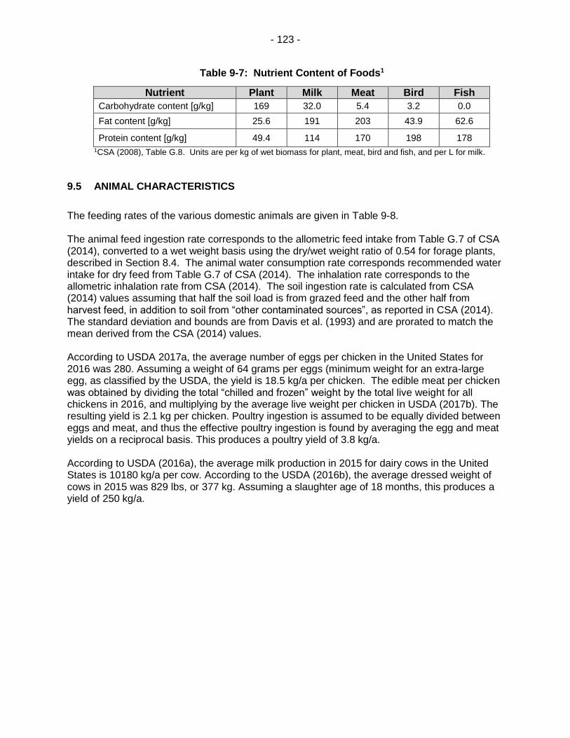
- 123 -

Table 9-7: Nutrient Content of Foods1

Nutrient Plant Milk Meat Bird Fish

Carbohydrate content [g/kg] 169 32.0 5.4 3.2 0.0

Fat content [g/kg] 25.6 191 203 43.9 62.6

Protein content [g/kg] 49.4 114 170 198 178

1CSA (2008), Table G.8. Units are per kg of wet biomass for plant, meat, bird and fish, and per L for milk.

9.5 ANIMAL CHARACTERISTICS

The feeding rates of the various domestic animals are given in Table 9-8. The animal feed ingestion rate corresponds to the allometric feed intake from Table G.7 of CSA (2014), converted to a wet weight basis using the dry/wet weight ratio of 0.54 for forage plants, described in Section 8.4. The animal water consumption rate corresponds recommended water intake for dry feed from Table G.7 of CSA (2014). The inhalation rate corresponds to the allometric inhalation rate from CSA (2014). The soil ingestion rate is calculated from CSA (2014) values assuming that half the soil load is from grazed feed and the other half from harvest feed, in addition to soil from “other contaminated sources”, as reported in CSA (2014). The standard deviation and bounds are from Davis et al. (1993) and are prorated to match the mean derived from the CSA (2014) values. According to USDA 2017a, the average number of eggs per chicken in the United States for 2016 was 280. Assuming a weight of 64 grams per eggs (minimum weight for an extra-large egg, as classified by the USDA, the yield is 18.5 kg/a per chicken. The edible meat per chicken was obtained by dividing the total “chilled and frozen” weight by the total live weight for all chickens in 2016, and multiplying by the average live weight per chicken in USDA (2017b). The resulting yield is 2.1 kg per chicken. Poultry ingestion is assumed to be equally divided between eggs and meat, and thus the effective poultry ingestion is found by averaging the egg and meat yields on a reciprocal basis. This produces a poultry yield of 3.8 kg/a. According to USDA (2016a), the average milk production in 2015 for dairy cows in the United States is 10180 kg/a per cow. According to the USDA (2016b), the average dressed weight of cows in 2015 was 829 lbs, or 377 kg. Assuming a slaughter age of 18 months, this produces a yield of 250 kg/a.

- 124 -

Table 9-8: Domestic Animal Data1

Parameter Bird Dairy cow Beef cow Animal food yield [Quantity/a/animal]

3.8 kg/a 10200 L/a 250 kg/a

Animal feed consumption rate [kgwet weight/d]

Normal PDF m=0.19 sd=0.044 min=0.044 max=0.39

Normal PDF m=37 sd=9.2 min=9.2 max=83

Normal PDF m=24 sd=6.1 min=6.1 max=55

Animal water consumption rate [L/d], with 0.75 correlation with animal feed consumption

Normal PDF m=0.25 sd=0.075 min=0.075 max=0.45

Normal PDF m=115 sd=29 min=29 max=200

Normal PDF m=52 sd=13 min=13 max=91

Animal soil ingestion rate [kg/d], with 0.75 correlation with animal feed consumption

Normal PDF m=0.005 sd=0.0012 min=0.0012 max=0.011

Normal PDF m=1.3 sd=0.32 min=0.32 max=2.9

Normal PDF m=0.83 sd=0.21 min=0.21 max=1.9

Animal air inhalation rate [m3

air/d], with 0.75 correlation with animal feed consumption

Normal PDF m=0.7 sd=0.21 min=0.21 max=1.6

Normal PDF m=91 sd=23 min=22 max=210

Normal PDF m=91 sd=23 min=23 max=210

1m=mean, sd=standard deviation.

Table 9-9 summarizes the mean values for the animal food ingestion transfer coefficients. These values describe the amount of a contaminant in the animal's daily food intake that appears in their produce as used for human food. For example, in the case of dairy cattle, it is the amount of contaminant (mol/kg) in the cow food intake (kg/d) that appears in the milk (mol/L) and has units of (mol/L)/(mol/kg * kg/d) = (d/L).

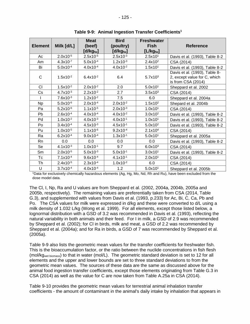
- 125 -

Table 9-9: Animal Ingestion Transfer Coefficients1

Element Milk [d/L] Meat (beef)

[d/kgfw]

Bird (poultry) [d/kgfw]

Freshwater Fish

[L/kgfw] Reference

Ac 2.0x10-5 2.5x10-5 2.5x10-3 2.5x101 Davis et al. (1993), Table 8-2

Am 4.3x10-7 5.0x10-4 1.2x10-3 2.4x102 CSA (2014)

Bi 5.0x10-4 4.0x10-4 4.0x10-2 1.5x101 Davis et al. (1993), Table 8-2

C 1.5x10-2 6.4x10-2 6.4 5.7x103 Davis et al. (1993), Table 8-2, except value for C, which is from CSA (2014)

Cl 1.5x10-2 2.0x10-2 2.0 5.0x101 Sheppard et al. 2002

Cs 4.7x10-3 2.2x10-2 2.7 3.5x103 CSA (2014)

I 7.6x10-3 1.2x10-2 7.5 6.0 Sheppard et al. 2004a

Np 5.0x10-6 2.0x10-4 2.0x10-2 1.5x102 Shepard et al. 2004b

Pa 5.2x10-6 1.1x10-5 2.0x10-3 1.0x101 CSA (2014)

Pb 2.6x10-4 4.0x10-4 4.0x10-2 3.0x102 Davis et al. (1993), Table 8-2

Pd 1.0x10-2 4.0x10-3 4.0x10-1 1.0x101 Davis et al. (1993), Table 8-2

Po 3.4x10-4 4.5x10-3 4.5x10-1 5.0x102 Davis et al. (1993), Table 8-2

Pu 1.0x10-5 1.1x10-6 9.2x10-4 2.1x104 CSA (2014)

Ra 6.2x10-4 9.0x10-4 1.3x10-1 5.0x101 Sheppard et al. 2005a

Rn 0.0 0.0 0.0 0.0 Davis et al. (1993), Table 8-2

Se 4.1x10-3 1.0x10-1 9.7 6.0x103 CSA (2014)

Sm 2.0x10-5 5.0x10-3 5.0x10-1 3.0x101 Davis et al. (1993), Table 8-2

Tc 7.1x10-4 9.6x10-4 4.1x10-1 2.0x101 CSA (2014)

Th 2.4x10-5 2.3x10-4 1.0x10-2 6.0 CSA (2014)

U 3.7x10-4 4.0x10-4 1.2 5.0x101 Sheppard et al. 2005b 1Data for exclusively chemically hazardous elements (Ag, Hg, Mo, Nd, Rh and Ru), have been excluded from the

dose model data.

The Cl, I, Np, Ra and U values are from Sheppard et al. (2002, 2004a, 2004b, 2005a and 2005b, respectively). The remaining values are preferentially taken from CSA (2014, Table G.3), and supplemented with values from Davis et al. (1993, p.233) for Ac, Bi, C, Ca, Pb and Po. The CSA values for milk were expressed in d/kg and these were converted to d/L using a milk density of 1.032 L/kg (Wong et al. 1999). For all elements, except those listed below, a lognormal distribution with a GSD of 3.2 was recommended in Davis et al. (1993), reflecting the natural variability in both animals and their feed. For I in milk, a GSD of 2.9 was recommended by Sheppard et al. (2002); for Cl in birds, milk and meat, a GSD of 2.2 was recommended by Sheppard et al. (2004a); and for Ra in birds, a GSD of 7 was recommended by Sheppard et al. (2005a). Table 9-9 also lists the geometric mean values for the transfer coefficients for freshwater fish. This is the bioaccumulation factor, or the ratio between the nuclide concentrations in fish flesh (mol/kgwet biomass) to that in water (mol/L). The geometric standard deviation is set to 12 for all elements and the upper and lower bounds are set to three standard deviations to from the geometric mean values. The sources of these data are the same as discussed above for the animal food ingestion transfer coefficients, except those elements originating from Table G.3 in CSA (2014) as well as the value for C are now taken from Table A.25a in CSA (2014). Table 9-10 provides the geometric mean values for terrestrial animal inhalation transfer coefficients - the amount of contaminant in the animal's daily intake by inhalation that appears in

- 126 -

the animal produce used by humans for food. A GSD of 5.2 is used for all elements (Zach et al. 1996). The Cl, I, Np, Ra and U values are from Sheppard et al. (2002, 2004a, 2004b, 2005a and 2005b, respectively). The remaining values are preferentially those from Table G.3 in CSA (2014) multiplied by the inhalation/ingestion ratios given in Table G.7 from CSA (2014), and supplemented with values from Zach et al. (1996, p. 27) for Ac, Bi, C, Ca, Pb and Po.

Table 9-10: Animal inhalation transfer coefficients1

Element Milk [d/L] Meat (beef)

[d/kgfw]

Bird (poultry) [d/kgfw]

Reference

Ac 1.0x10-2 1.3x10-2 1.3 Zach et al.(1996), Table 6-2

Am 1.0x10-4 1.2x10-1 2.9x10-1 CSA (2014), Table G.3 and G.7

Bi 5.5x10-3 4.4x10-3 4.4x10-1 Zach et al.(1996), Table 6-2

C 1.5x10-2 6.4x10-2 6.4 Zach et al.(1996), Table 6-2

Cl 1.7x10-2 8.0x10-2 8.0 Sheppard et al. 2002

Cs 2.9x10-3 1.4x10-2 1.7 CSA (2014), Table G.3 and G.7

I 0.0 0.0 0.0 Sheppard et al. 2004a

Np 7.5x10-5 8.3x10-4 8.3x10-2 Sheppard et al. 2004b

Pa 1.2x10-3 2.7x10-3 4.8x10-1 CSA (2014), Table G.3 and G.7

Pb 7.8x10-4 1.2x10-3 1.2x10-1 Zach et al.(1996), Table 6-2

Pd 1.0 4.0x10-1 4.0x101 Zach et al.(1996), Table 6-2

Po 1.9x10-3 2.5x10-2 2.5 Zach et al.(1996), Table 6-2

Pu 2.4x10-3 2.7x10-4 2.2x10-1 CSA (2014), Table G.3 and G.7

Ra 5.6x10-4 1.3x10-3 1.3x10-1 Sheppard et al. 2005a

Rn 0.0 0.0 0.0 Zach et al.(1996), Table 6-2

Se 3.0x10-3 7.5x10-2 7.3 CSA (2014), Table G.3 and G.7

Sm 9.6x10-3 2.4 2.4x102 Zach et al.(1996), Table 6-2

Tc 5.2x10-4 7.2x10-4 3.1x10-1 CSA (2014), Table G.3 and G.7

Th 2.3x10-3 2.3x10-2 1.0 CSA (2014), Table G.3 and G.7

U 4.1x10-3 2.2x10-3 1.3x10-1 Sheppard et al. 2005b 1Data for exclusively chemically hazardous elements (Ag, Hg, Mo, Nd, Rh and Ru), have been excluded from the dose model data.

9.6 DOSE COEFFICIENTS

The International Commission on Radiological Protection (ICRP) 2007 recommendations are considered to be the best estimate of dose response for humans (ICRP 2007) and replace the 1990 recommendations (ICRP 1991). The new recommendations do not lead to changes in dose limits. The recommendations are based on the Linear No-Threshold model, although account was taken of dose and dose-rate effects in their derivation. In the Seventh Case Study, radiological exposures to humans are converted to dose rates using dose coefficients based on the 1990 ICRP recommendations (ICRP 1991), since dose coefficients based on the 2007 recommendations are not yet available. However, dose coefficients are not expected to change substantially (Wrixon 2008).

- 127 -

9.6.1 Adult Ingestion Dose Coefficients

The adult human ingestion dose coefficients are presented in Table 9-11. They are based on ICRP 72 (ICRP 1996). The dose coefficients of parent radionuclides include the contributions from progeny with half-lives less than 1-day. That is, the dose coefficients assume that an amount of progeny in secular equilibrium with the parent is eaten (the ICRP values only account for ingrowth of progeny within the body). Since the present study does not explicitly model radionuclides with half-lives less than one day, this ensures that doses from these short-lived nuclides are fully included in any dose calculations involving their parent. The biosphere model also includes a groundwater limit to the internal I-129, Cl-36 and C-14 human doses (NWMO 2012, Section 5.6). The groundwater dose limit for I-129 is attained when the ratio of I-129 to total iodine in the thyroid is equal to that in groundwater (well water or water discharging into the lake). For Cl-36 (or C-14), the groundwater dose limits are attained when the ratio of Cl-36 to stable chlorine (or C-14 to stable carbon) in the soft tissue of man’s body is equal to that in groundwater. These limits reflect that the human body does not distinguish between isotopes when incorporating these elements into its tissue, and in particular will not concentrate the radioisotopes. The calculation of the groundwater internal dose limits requires data on the concentration of stable I, Cl and C in groundwater and on the human internal dose conversion factors for I-129, Cl-36 and C-14. The values for these parameters are listed in Table 9-12. For I-129, the internal dose conversion factor is based on the thyroid specific-activity model described above; for Cl-36 and C-14, the internal dose conversion factors are on a soft tissue specific activity model.

9.6.2 Adult Inhalation Dose Coefficients

The adult inhalation doses coefficients are presented in Table 9-11. These were based on the values in ICRP 72 (ICRP 1996). The dose coefficients of parent nuclides include contributions from daughters with half-lives less than 1-day, so that doses from these short-lived nuclides are included in any dose calculations involving their parent.

9.6.3 Adult Ground Exposure and Air Immersion Dose Coefficients

The adult ground exposure and air immersion dose coefficients are presented in Table 9-11. These were based on the values in Eckerman and Leggett (1996), which are consistent with ICRP 60 (ICRP 1991). The dose coefficient of parent nuclides include contributions from any progeny with half-lives less than 1 day.

9.6.4 Adult Water Immersion Dose Coefficients

Eckerman and Leggett (1996) calculate adult water immersion dose coefficients based on the recommendations in ICRP 60 (ICRP 1991). These data were selected for use in the Seventh Case Study unless otherwise stated. The values are presented in Table 9-11. The dose coefficients in Eckerman and Leggett (1996) do not include any contributions from progeny. Although radionuclides with half-lives less than one day are not explicitly modelled in

- 128 -

the Seventh Case Study, their contribution to the total water immersion dose is accounted for by adding their water immersion dose coefficient or a fraction thereof (depending on the decay scheme) to that of the parent radionuclide, to derive effective water immersion dose coefficients for the parent, as was done for other dose coefficients.

9.6.5 Adult Building Exposure Dose Coefficients

Whole body building dose coefficients were derived from Holford (1989), who lists building dose coefficients, in units of (Sv/a)/(Bq/kg), for three building types: concrete, wood-log and wood-frame house. The building dose coefficients in Holford (1989) are based on ICRP26/28 recommendations. However, MacDonald and Laverock (1996) compare air, water and soil external dose coefficients based on the ICRP26/28 and ICRP60 recommendations. Thus, the ICRP60 whole body building dose coefficients, for each building type, were estimated by dividing the ICRP26/28 dose coefficients from Holford (1989) for a nuclide by the smallest value of the ICRP26/28-to-ICRP60 dose coefficient ratio listed in MacDonald and Laverock (1996) for that particular nuclide. Radionuclides with half-lives less than one day are not explicitly modelled in the Seventh Case Study assessment. Instead, their contribution to the total building exposure dose rate is accounted for by adding their building dose coefficient or a fraction thereof (depending on the decay scheme) to that of the parent radionuclide to derive an effective building dose coefficient for the parent. However, the CC4 biosphere model does not simulate the ingrowth of radionuclides in building materials. This may be a non-conservative approximation if the building dose coefficient of the progeny is higher than that of the parent and ingrowth contributes significantly to the progeny concentration in building materials. Hence, radionuclides with half-lives less than 2 years are assumed to be in secular equilibrium with their parents in all building materials, and their contribution to the total building exposure dose rate is accounted for by adding their effective building dose coefficient to that of the parent radionuclide. In this case, the building dose coefficient of the short-lived progeny is set to zero (see Table 9-11). For each nuclide, the largest of the building dose coefficients for the three building types was conservatively chosen for use in the Seventh Case Study. The effective building dose coefficients are presented in Table 9-11.

- 129 -

Table 9-11: Adult Human Dose Coefficients1

Nuclide

Ground-Exposure

(Sv/a)/ (Bq/kg)

Air Immersion

(Sv/a)/ (Bq/m3)

Air Inhalation

(Sv/Bq)

Ingestion (Sv/Bq)

Water immersion (Sv/a)/(Bq/

m3)

Building Material (Sv/a)/

(Bq/kgdry

material) Ac-225* 3.18E-07 3.23E-07 8.53E-06 2.43E-08 6.96E-10 0.00E+00#

Ac-227* 7.97E-10 1.12E-09 5.50E-04 1.10E-06 2.39E-12 1.17E-06

Am-241 1.00E-08 2.13E-08 9.60E-05 2.00E-07 4.86E-11 4.70E-08

Bi-210 1.47E-09 8.14E-09 9.30E-08 1.30E-09 9.40E-12 0.00E+00#

C-14 2.97E-12 8.20E-11 5.80E-09 5.80E-10 9.09E-14 0.00E+00

Cl-36 6.72E-10 5.24E-09 7.30E-09 9.30E-10 6.15E-12 5.70E-10

Cs-135 8.68E-12 3.00E-10 8.60E-09 2.00E-09 3.28E-13 0.00E+00

I-129 2.58E-09 8.87E-09 3.60E-08 1.10E-07 2.07E-11 2.00E-08

Np-237 1.88E-08 2.80E-08 5.00E-05 1.10E-07 6.28E-11 6.47E-07

Pa-231 4.77E-08 4.95E-08 1.40E-04 7.10E-07 1.08E-10 1.10E-07

Pa-233 2.54E-07 2.70E-07 3.90E-09 8.70E-10 5.90E-10 0.00E+00#

Pb-210 5.35E-10 1.41E-09 5.60E-06 6.90E-07 3.28E-12 4.05E-09

Pd-107 0.00E+00 0.00E+00 5.90E-10 3.70E-11 0.00E+00 0.00E+00

Po-210 1.33E-11 1.23E-11 4.30E-06 1.20E-06 2.66E-14 0.00E+00#

Pu-239 7.12E-11 1.10E-10 1.20E-04 2.50E-07 2.47E-13 2.40E-10

Pu-240 3.04E-11 1.08E-10 1.20E-04 2.50E-07 2.52E-13 2.60E-10

Pu-242 2.68E-11 9.15E-11 1.10E-04 2.40E-07 2.13E-13 2.20E-10

Ra-223* 3.76E-07 4.11E-07 8.71E-06 1.00E-07 8.76E-10 0.00E+00#

Ra-224* 2.62E-06 2.41E-06 3.62E-06 7.13E-08 5.24E-23 2.40E-04

Ra-225 2.33E-09 7.57E-09 7.70E-06 9.90E-08 1.66E-11 0.00E+00#

Ra-226 7.88E-09 8.96E-09 9.50E-06 2.80E-07 1.97E-11 6.32E-06

Ra-228* 1.53E-06 1.42E-06 1.60E-05 6.90E-07 3.06E-09 3.97E-06

Rn-222* 2.86E-06 2.63E-06 4.00E-09 2.50E-10 5.71E-09 0.00E+00#

Se-79 4.14E-12 1.24E-10 6.80E-09 2.90E-09 1.37E-13 0.00E+00

Sm-147 0.00E+00 0.00E+00 9.60E-06 4.90E-08 0.00E+00 0.00E+00

Sm-148 6.06E-06 5.46E-06 5.50E-04 1.20E-06 0.00E+00 N/A

Tc-99 2.93E-11 9.06E-10 1.30E-08 6.40E-10 9.96E-28 0.00E+00

Th-227 1.30E-07 1.40E-07 1.00E-05 8.80E-09 3.06E-10 0.00E+00#

Th-228 1.94E-09 2.56E-09 4.00E-05 7.20E-08 5.83E-27 4.88E-09

Th-229 7.83E-08 1.06E-07 2.40E-04 4.90E-07 2.36E-10 9.67E-07

Th-230 2.89E-10 4.67E-10 1.00E-04 2.10E-07 1.05E-12 1.00E-09

Th-231 8.68E-09 1.45E-08 3.30E-10 3.40E-10 3.19E-11 2.90E-08

Th-232 1.23E-10 2.28E-10 1.10E-04 2.30E-07 5.18E-13 5.20E-10

Th-234* 3.71E-08 5.19E-08 7.70E-09 3.40E-09 1.03E-10 9.50E-08

U-233 3.42E-10 4.48E-10 9.60E-06 5.10E-08 9.94E-13 8.90E-10

U-234 9.29E-11 1.93E-10 9.40E-06 4.90E-08 4.39E-13 4.60E-10

U-235 1.78E-07 2.04E-07 8.50E-06 4.70E-08 4.51E-10 4.40E-07

U-236 4.80E-11 1.22E-10 8.70E-06 4.70E-08 2.81E-13 3.00E-10

U-238 2.15E-11 7.89E-11 8.00E-06 4.50E-08 1.85E-13 1.90E-10 *Identifies radionuclides whose dose coefficients include contributions from secular-equilibrium progeny with half-lives less than one day.

#The building dose coefficient is set to zero for short-lived nuclides for which the building dose coefficient is added to the building dose coefficient of a longer lived parent.

- 130 -

Table 9-12: Parameters for human specific activity models

Parameter Units Value Comment

Stable iodine concentration in groundwater

kg/L 7.0x10-9

GM of lognormal PDF with GSD of 8.0 and bounds of 1.0x10-10 to 4.0x10-7 (Sheppard and Gascoyne 1997).

Stable chlorine concentration in groundwater

kg/L 3.0x10-5

GM of lognormal PDF with GSD of 6.0 and bounds of 8.0x10-7 to 1.0x10-3 (Sheppard and Gascoyne 1997).

Stable carbon concentration in groundwater

kg/L 4.0x10-5

GM of lognormal PDF with GSD of 3.0 and bounds of 4.0x10-6 to 2.0x10-4 (Sheppard and Gascoyne 1997). Upper bound set to maximum observed concentration.

129l internal dose conversion factor (based on thyroid specific activity model)

(Sv/a)/ (Bq/kg thyroid)

1.6x10-8 Zach et al. (1996, p.32)

36Cl internal dose conversion factor (based on specific activity model)

(Sv/a)/ (Bq/kg soft tissue)

1.38x10-6 Zach et al. (1996, p.31)

14C internal dose conversion factor (based on specific activity model)

(Sv/a)/ (Bq/kg soft tissue)

2.50x10-7 Davis et al. (1993)

3H internal dose conversion factor (based on specific activity model)

(Sv/a)/ (Bq/kg soft tissue)

2.9x10-8 Davis et al. (1993)

- 131 -

9.7 No-Effect Concentrations for Non-Human Biota

Potential radiological impacts on non-human biota will be assessed using the equations and data from Medri and Bird (2015) and are documented in NWMO (2018).

9.8 Chemical Hazard

The proposed values for protection of humans and non-human biota from potentially chemically hazardous elements are listed in Medri (2015b) and are based on Canadian guideline values for concentrations in environmental media relevant to human health and environmental protection, supplemented as needed.

10. SUMMARY

For the Seventh Case Study, several codes were used to support the safety assessment. The data and codes used for this project have been maintained under configuration management and have been documented according to the NWMO software procedure. This report briefly describes the codes and data. For further details, references to the original documentation are provided. Most of the model parameters are the same as the Canadian dataset developed as part of the Fifth Case Study (NWMO 2013). The notable model parameters changes are:

new repository site location;

new MKII container with a 48 bundle capacity;

new adaptive repository design to accommodate the new MKII container design, with three arms and in-room container placement and 25 m room spacing;

revised geosphere transport network, based on the new site geosphere model;

changes in groundwater discharge areas, resulting from new site geosphere model and new repository location;

main groundwater discharge from repository is to a river rather than a lake;

new Zr corrosion rate model and data; and

additional data for bundles with 280 MWh/kgU burnup.

- 132 -

11. REFERENCES

Amiro, B.D. 1992. The atmosphere submodel for the assessment of Canada’s nuclear fuel waste management concept. Atomic Energy of Canada Limited Report, AECL-9889, COG-91-199. Pinawa, Canada.

Baeyens, B., T. Thoen, M.H. Bradbury, M. Marques Fernandes. 2014. Sorption Data Bases for Argillaceous Rocks and Bentonite for the Provisional Safety Analyses for SGT-E2. Nagra Technical Report 12-04.

Baumgartner, P. 2006. Generic thermal-mechanical-hydraulic (THM) data for sealing materials – Volume 1: Soil-water relationships. Ontario Power Generation Report 06819-REP-01300-10122-R00. Toronto, Canada.

BEAK International. 2002. Guidance for calculation of Derived Release Limits for radionuclides in airborne and liquid effluents from Ontario Power Generation Nuclear Facilities - Appendices. Ontario Power Generation Report N-REP-03482-10000-R00. Toronto, Canada.

Beals, D.I. 1985. Soil and climate parameters for post-closure biosphere assessment of nuclear fuel waste disposal. Atomic Energy of Canada Limited Technical Record, TR-285. Pinawa, Canada.

Bertetti, F.P. 2016. Determination of Sorption Properties for Sedimentary Rocks under Saline, Reducing Conditions – Key Radionuclides. Nuclear Waste Management Organization Technical Report NWMO-TR-2016-08, Toronto, Canada.

Birgersson M., M. Akesson M. and H. Hökmark H. 2008. Gas intrusion in saturated bentonite – A thermodynamic approach. Physics and Chemistry of Earth, 33, S248-S251.

Blümling. P., F. Bernier, P. Lebon and C.D. Martin. 2007. The excavation damaged zone in clay formations time-dependent behaviour and influence on performance assessment. Physics and Chemistry of the Earth 32(8-14), 588-599.

Bowles, I.A. and G.T. Prickett. 2001. Footprints in the Jungle. Oxford University Press. NY, USA. p137

Brown, J.E., B. Alfonso, R. Avila, N.A. Beresford, D. Copplestone, G. Pröhl and A. Ulanovsky. 2008. The ERICA Tool. J. Environ. Radioactivity 99: 1371-1383.

Calder, N. 2011. Two-Phased Flow Parameters Determined from DGR-2, DGR-3 and DGR-4 Laboratory Petrophysical Data. Nuclear Waste Management Organization Technical Report DGR-TR-08-33.

Chadwick, M.B., M. Herman, P. Obložinský, M.E. Dunn, Y. Danon, A.C. Kahler, D.L. Smith, B. Pritychenko, G. Arbanas, R. Arcilla, R. Brewer, D.A. Brown, R. Capote, A.D. Carlson, Y.S. Cho, H. Derrien, K. Guber, G.M. Hale, S. Hoblit, S. Holloway, T.D. Johnson, T. Kawano, B.C. Kiedrowski, H. Kim, S. Kunieda, N.M. Larson, L. Leal, J.P. Lestone, R.C. Little, E.A. McCutchan, R.E. MacFarlane, M. MacInnes, C.M. Mattoon, R.D. McKnight, S.F. Mughabghab, G.P.A. Nobre, G. Palmiotti, A. Palumbo, M.T. Pigni, V.G. Pronyaev, R.O. Sayer, A.A. Sonzogni, N.C. Summers, P. Talou, I.J. Thompson, A. Trkov, R.L. Vogt, S.C. van der Marck, A. Wallner, M.C. White, D.

- 133 -

Wiarda, P.G. Young. 2011. ENDF/B-VII.1 Nuclear data for science and technology: Cross section, covariances, fission product yields, and decay data. Nuclear Data Sheets: 112-12, 2887-2996 (2011).

Chan, T., M. Kolar, P.A. O'Connor, N.W. Scheier and F.W. Stanchell. 1999. Finite-element

sensitivity analysis of effects of an excavation damage zone on 129I transport from a used CANDU fuel waste disposal repository. Ontario Hydro Report 06819-REP-01200-0022-R00. Toronto, Canada.

Chen, J.D., P.A. Seeley, R. Taylor, D.C. Hartrick, N.L. Pshhyshlak, K.H. Wasywich, A. Rochon and K.I. Burns. 1986. Characterization of corrosion deposits and the assessment of fission products released from used CANDU fuel. Proceedings 2nd International Conference on Radioactive Waste Management. Winnipeg, Canada, 7-11 September 1986. Canadian Nuclear Society, Canada.

CNSC (Canadian Nuclear Safety Commission). 2006. Assessing the Long Term Safety of

Radioactive Waste Management. CNSC Regulatory Guide G-320. Ottawa, Canada.

Coligado, M.C., W. Baier and W.K. Sly. 1968. Risk Analyses of Weekly Climatic Data for Agricultural and Irrigation Planning, Kapuskasing, Ontario, Technical Bulletin 31, Canada Land Inventory, Dept of Forestry and Rural Development, Agriculture Canada, p8.

Coligado, M.C., W. Baier and W.K. Sly. 1968. Risk Analyses of Weekly Climatic Data for Agricultural and Irrigation Planning, Kapuskasing, Ontario, Technical Bulletin 31, Canada Land Inventory, Dept of Forestry and Rural Development, Agriculture Canada, p8.

Coligado, M.C., W. Baier and W.K. Sly. 1969a. Risk Analyses of Weekly Climatic Data for Agricultural and Irrigation Planning, Armstrong, Ontario, Technical Bulletin 64, Canada Land Inventory, Dept of Forestry and Rural Development, Agriculture Canada. 8 pp.

Coligado, M.C., W. Baier and W.K. Sly. 1969b. Risk Analyses of Weekly Climatic Data for Agricultural and Irrigation Planning, Fort Frances, Ontario, Technical Bulletin 65, Canada Land Inventory, Dept of Forestry and Rural Development, Agriculture Canada. 8 pp.

Coligado, M.C., W. Baier and W.K. Sly. 1969c. Risk Analyses of Weekly Climatic Data for Agricultural and Irrigation Planning, Guelph, Ontario, Technical Bulletin 66, Canada Land Inventory, Dept of Forestry and Rural Development, Agriculture Canada. 8 pp.

Coligado, M.C., W. Baier and W.K. Sly. 19694. Risk Analyses of Weekly Climatic Data for Agricultural and Irrigation Planning, North Bay, Ontario, Technical Bulletin 67, Canada Land Inventory, Dept of Forestry and Rural Development, Agriculture Canada. 8 pp.

Coligado, M.C., W. Baier and W.K. Sly. 1969e. Risk Analyses of Weekly Climatic Data forAgricultural and Irrigation Planning, White River, Ontario, Technical Bulletin 68, Canada Land Inventory, Dept of Forestry and Rural Development, Agriculture Canada. 8 pp.

Connan, O., E. Tessier, D. Maro, D. Amouroux, D. Hebert, M. Rozet, C. Vaiseux and L. Solier. 2008. Water to atmosphere fluxes of 131I in relation with alkyl-iodide compounds from the Sein Estuary (France). J. Environ. Radioactivity 99, 1102-1110.

- 134 -

Cordfunke, E.H.P. and R.J.M. Konings. 1988. Chemical interactions in water-cooled nuclear fuel: A thermodynamic approach. J. Nucl. Mat. 152, 301-309.

Crawford, J., I. Neretnieks and M. Malmström. 2006. Data and uncertainty assessment for radionuclide Kd partitioning coefficients in granitic rock for use in SR-Can calculations. SKB Research Report R-06-75. Stockholm, Sweden.

CRC. 2016. CRC Handbook of chemistry and physics, 96th ed. CRC Press, Ann Arbor, USA

CSA (Canadian Standards Association). 2016. Quality assurance of analytical, scientific, and design computer programs. CSA Standard CSA N286.7-16. Toronto, Canada.

CSA (Canadian Standard Association). 2014. Guidelines for calculating derived release limits for radioactive material in airborne and liquid effluents for normal operation of nuclear facilities. Canadian Standards Association Report CSA-N288.1-14. Toronto, Canada.

CSA (Canadian Standards Association). 2008. Guidelines for calculating derived release limits for radioactive material in airborne and liquid effluents for normal operation of nuclear facilities. Canadian Standards Association Report CSA-N288.1-08. Toronto, Canada.

CSA (Canadian Standards Association). 1989. Residential mechanical ventilation requirements. Canadian Standards Association Preliminary Standard F326.1-M1989. Toronto, Canada.

Cubicciotti, D. And J.E. Sanecki. 1978. Characterization of deposits on inside surfaces of LWR cladding. J. Nucl. Mat. 78, 96-111.

Davies, P.B. 1991. Evaluation of the Role of Threshold Pressure in Controlling Flow of Waste Generated Gas into Bedded Salt at the Waste Isolation Pilot Plant (WIPP). Sandia Report SAND 90-3246. Albuquerque, USA.

Davis, P.A., R. Zach, M.E. Stephens, B.D. Amiro, G.A. Bird, J.A.K. Reid, M.I. Sheppard and M. Stephenson. 1993. The disposal of Canada’s nuclear fuel waste: The biosphere model, BIOTRAC, for postclosure assessment. Atomic Energy of Canada Limited Report AECL-10720. Pinawa, Canada.

Davison, C.C., T. Chan, A. Brown, M. Gascoyne, D. Kamineni, G. Lodha, T. Melnyk, B.W. Nakka, P. O'Connor, D. Ophori, N. Scheier, N. Soonawala, F. Stanchell, D. Stevenson, G. Thorne, T. Vandergraaf, P. Vilks and S. Whitaker. 1994. The disposal of Canada’s nuclear fuel waste: The geosphere model for postclosure assessment. Atomic Energy of Canada Limited Report AECL-10719, COG-93-9. Pinawa, Canada.

Didry, O., M.N. Gray, A. Cournut and J. Graham. 2000. Modelling the early age behaviour of a low heat concrete bulkhead sealing an underground tunnel. Canadian Journal of Civil Engineering 27. 112-124.

Dixon, D., Man, A., Rimal, S., Stone, J. and Siemens, G. 2018. Bentonite Seal Properties in Saline Water. Nuclear Waste Management Organization Technical Report NWMO TR-2018-20 (in preparation). Toronto, Canada.

- 135 -

Dixon, D.A., A. Man, J. Stone, S. Rimal, G. Siemens, P. Abootalebi, and K. Birch. 2016. Backfilling and Sealing materials for a Deep Geological Repository. Presented at the 3rd Canadian Conference on Nuclear Waste Management, Decommissioning and Environmental Restoration. September, 2016.

Dixon, D.A., N.A. Chandler and P.M. Thompson. 2001. The selection of sealing system components in AECL’s 1994 Environmental Impact Statement. Ontario Power Generation Report 06819-REP-01200-10074-R00. Toronto, Canada.

Duro, L., V. Montoya, E. Colàs and D. García. 2010. Groundwater equilibration and radionuclide solubility calculations. Nuclear Waste Management Organization Technical Report NWMO TR-2010-02. Toronto, Canada.

Eckerman, K.F. and R.W. Leggett. 1996. DCFPAK: Dose Coefficients Data File Package for Sandia National Laboratory. Oak Ridge National Laboratory Report ORNL/TM-13347. Oak Ridge, US. (http://homer.hsr.ornl.gov/vlab/VLcodeDF.html)

Environment Canada. 2011. 2011 Municipal Water Use Report, Municipal Water Use 2009 Statistics. Environment Canada. Cat. No.: En11-2/2009E-PDF. Canada.

Floyd, M.R., J. Novak and P.T. Truant. 1992. Fission-gas release in fuel performing to extended burnups in Ontario Hydro Nuclear Generating Stations. Proceedings of a Technical Commitee Meeting on Fission Gas Release and Fuel Rod Chemistry Related to Extended Burnup, Pembroke, Ontario, Canada, 28 April – 1 May1991. IAEA-TECDOC-697, p. 53. Vienna, Austria.

Freeze and Cherry. 1979. Groundwater. Englewood Cliffs, NJ, Prentice-Hall.

Garamszeghy, M. 2016. Nuclear Fuel Waste Projections in Canada - 2016 Update. Nuclear Waste Management Organization Report NWMO-TR-2016-09. Toronto, Canada.

Garisto, F. 2001. Radionuclide Screening Model (RSM) version 1.1 verification and validation.

Ontario Power Generation Report 06819-REP-01300-10029-R00. Toronto, Canada.

Garisto, F. and P. Gierszewski. 2002. Technetium-99: Review of properties relevant to a Canadian geologic repository. Ontario Power Generation Report 06819-REP-01200-10081-R00. Toronto, Canada.

Garisto, F., D.H. Barber, E. Chen, A. Inglot and C.A. Morrison. 2009. Alpha, beta and gamma dose rates in water in contact with used CANDU fuel. Nuclear Waste Management Organization Technical Report NWMO TR-2009-27. Toronto, Canada.

Garisto, F., M. Gobien, E. Kremer and C. Medri. 2012. Fourth Case Study: Reference Data and Codes. Nuclear Waste Management Organization Technical Report NWMO TR-2012-08. Toronto, Canada.

Garisto, F. and M. Gobien. 2013. SYVAC3-CC4 Verification and Validation Summary. Nuclear Waste Management Organization Technical Report NWMO TR-2015-14. Toronto, Canada.

- 136 -

Gascoyne, M. 2004. Hydrogeochemistry, groundwater ages and sources of salts in a granitic batholith on the Canadian Shield, southeastern Manitoba. Appl. Geochem. 19, 519-560.

Gobien, M. and F. Garisto. 2012. Data for radionuclide and chemical element screening. Nuclear Waste Management Organization Technical Report NWMO TR-2012-11. Toronto, Canada.

Gobien, M. and F. Garisto. 2013. Modelling Container Failure in a Deep Geologic Repository. In Proceedings of the 14th International High-Level Radioactive Waste Management Conference, Albuquerque, New Mexico, USA.

Gobien, M., F. Garisto, E. Kremer, C. Medri. 2016. Sixth Case Study: Reference Data and Codes. Nuclear Waste Management Organization Technical Report. NWMO-TR-2016-10. Toronto, Canada.

Golder. 2012. Waste Emplacement Rooms and Access Tunnels Shape Optimization. NWMO DGR Document Number 1011170042-TM-G2070-0003-00 R00

Golder. 2013. OPG’s deep geological repository for low and intermediate level waste factual report- Borehole DGR-7 and DGR-8, Geotechnical Logging. OPG 1011170042-REP-G2040-0004-01.

Goodwin, B.W., P. Gierszewski and F. Garisto. 2001. Radionuclide Screening Model (RSM) Version 1.1 - Theory. Ontario Power Generation Report 06819-REP-01200-10045-R00. Toronto, Canada.

Government of Canada. 2015. Owen Sound MOE Station Results, Historical Data. Posted of Government of Canada Website. Available at: http://climate.weather.gc.ca/historical_data/search_historic_data_stations_e.html?searchType=stnName&timeframe=1&txtStationName=Owen+Sound+MOE&searchMethod=contains&optLimit=yearRange&StartYear=1840&EndYear=2017&Year=2006&Month=10&Day=30&selRowPerPage=25

Gras, J.-M. 1996. Corrosion Assessment of Metal Containers for the Geological Disposal of HLW. Part 1: Carbon Steels, Low Alloy Steels, Cast Iron. EDF Report No. HT/40/96/002/A, Electricité de France, Moret-sur-Loing, France

Gras, J.-M.. 2014. State of the art of 14C in Zircaloy and Zr alloys – 14C release from zirconium alloy hulls. Carbon-14 Source Term (CAST) Report CAST-2014-D.3.1.

Guillaumont, R., J. Fanghänel, V. Neck, J. Fuger, D.A, Palmer, I. Grenthe, and M.H. Ran.

2003. Chemical Thermodynamics 5. Update on the Chemical Thermodynamics of Uranium, Neptunium, Plutonium, Americium and Technetium. NEA OECD, Elsevier, Amsterdam.

Gupta, N. 1993. Geologic and Fluid-density Controls on the Hydrodynamics of the Mt. Simon

Sandstone and Overlying Geologic Units in Ohio and the Surrounding States. Ph.D. Thesis, The Ohio State University, Columbus, Ohio.

- 137 -

Hart,D. 2013 Derived Release Limits Guidance. COG-06-3090R3-I. Candu Owners Group Inc. Toronto, Canada.

He, H., M. Broczkowski, K. O’Neil, D. Ofori, O. Semenikhin and D. Showsmith. 2012. Corrosion of nuclear fuel (UO2) inside a failed nuclear waste container. Nuclear Waste Management Organization Technical Report NWMO TR-2012-09. Toronto, Canada.

Hillel, D. 1980. Application of Soil Physics. Academic Press, Toronto, Canada.

Holford, R.M. 1989. Supplement to dose conversion factors for air, water, soil and building materials. Atomic Energy of Canada Limited Report AECL-9825-1. Pinawa, Canada.

ICRP (International Commission on Radiological Protection). 1991. 1990 recommendations of the International Commission on Radiological Protection. Annals of the ICRP 21 (1-3), ICRP Publication 60. Pergamon Press, Oxford, UK.

ICRP (International Commission on Radiological Protection). 1996. Age-dependent doses to members of the public from intake of radionuclides: Part 5, Compilation of ingestion and inhalation dose coefficients. Annals of the ICRP 26 (1), ICRP Publication 72. Pergamon Press, Oxford, UK.

ICRP (International Commission on Radiological Protection). 2002. Basic Anatomical and Physiological Data for Use in Radiological Protection Reference Values. ICRP Publication 89. Ann. ICRP 89 (3-4), 2002. Vienna, Austria.

ICRP (International Commission on Radiological Protection). 2007. The 2007

recommendations of the International Commission on Radiological Protection. Annals of the ICRP 37(2-4), ICRP Publication 103. Pergamon Press, Oxford, UK.

Iglesias, F., M. Kaye and B. Lewis. 2011. Estimate of instant release fractions using

ORIGEN-S and FEMAXI. Nuclear Waste Management Organization Technical Report NWMO TR-2011-19. Toronto, Canada.

Intera. 2011. Descriptive Geosphere Site Model. Intera Engineering Ltd. Report for the Nuclear

Waste Management Organization, NWMO DGR-TR-2011-24 R000. Toronto, Canada. JNC. 2000. H12: Project to establish the scientific and technical basis for HLW disposal in

Japan; Supporting Report 3; Safety assessment of the geological disposal system. Japan Nuclear Cycle Development Institute Report JNC TN1410 2000-004. Tokai, Japan.

Johnson, L., C. Ferry, C. Poinssot and P. Lovera. 2005. Spent fuel radionuclide source-term model for assessing spent fuel performance in geological disposal. Part I: Assessment of the instant release fraction. J. Nucl. Mat. 346, 56-65.

Johnson, L., C. Poinssot, C. Ferry and P. Lovera. 2004. Estimates of the instant release fractions for UO2 and MOX fuel at t=0. NAGRA Technical Report NTB 04-08. Wettingen, Switzerland.

Johnson, L.H. and J.C. Tait. 1997. Release of segregated nuclides from spent fuel. SKB Technical Report SKB TR 97-18. Stockholm, Sweden.

- 138 -

Johnson, L.H., D.M. LeNeveu, F. King, D.W. Shoesmith, M. Kolar, D.W. Oscarson, S. Sunder, C. Onofrei, and J.L. Crosthwaite. 1996. The disposal of Canada's nuclear fuel waste: A study of postclosure safety of in-room placement of used CANDU fuel in copper containers in permeable plutonic rock, Volume 2: Vault model. Atomic Energy of Canada Limited Report AECL-11494-2. Pinawa, Canada.

Kamimura, K. 1992. FP gas release behaviour of high burn-up MOX fuels for thermal reactors. Proceedings of a Technical Commitee Meeting on Fission Gas Release and Fuel Rod Chemistry Releated to Extended Burnup, Pembroke, Ontario, Canada, 28 April – 1 May1991. IAEA-TECDOC-697, p. 82. Vienna, Austria.

Kitson, C., T. Melnyk, P. Gierszewski and L. Wojciechowski. 2012. SYVAC3-CC4 User Manual. Nuclear Waste Management Organization Technical Report NWMO TR-2012-21. Toronto, Canada.

Kleykamp, H. 1985, The chemical state of the fission products in oxide fuels. J. Nucl. Mat. 131, 221-246.

Lampe, D.C. 2009. Hydrogeologic Framework of Bedrock Units and Initial Salinity Distribution for a Simulation of Groundwater Flow for the Lake Michigan Basin. United States Geological Survey, Technical Report 5060. Reston, Virginia.

Lindemer, T.B. and T.M. Besmann. 1985. Chemical thermodynamic representation of

<UO2±x>. J. Nucl. Mat. 130, 473-488.

Macdonald, C.R. and M. Laverock. 1996. External ICRP 60 dose conversion factors for air and water immersion, groundshine and soil. Atomic Energy of Canada Limited Report TR-739. Pinawa, Canada.

Medri, C. and G. Bird. 2015. Non-human Biota Dose Assessment Equations and Data. Nuclear Waste Management Organization Technical Report NWMO TR-2014-02 R001. Toronto, Canada.

Medri, C. 2015a. Human Intrusion Model for the Mark II Container in Crystalline and Sedimentary Rock Environments: HIMv2.1. Nuclear Waste Management Organization Technical Report NWMO TR-2015-04. Toronto, Canada.

Medri, C. 2015b. Non-Radiological Interim Acceptance Criteria for the Protection of Persons and the Environment. Nuclear Waste Management Organization Technical Report NWMO TR-2015-03. Toronto, Canada.

Mishra, S. 2002. Assigning probability distributions to input parameters of performance assessment models. SKB Technical Report TR-02-11. Stockholm, Sweden.

NAGRA. 2004. Project Opalinus Clay – Integrated approach for the development of geochemical databases used for safety assessment. NAGRA Technical Report 03-06. Wettingen, Switzerland.

NAPS (National Air Pollution Surveillance). 1996-2002. NAPS network annual data summaries. Retrieved online at: http://www.etc-cte.ec.gc.ca/publications/naps/naps_lib_e.html

- 139 -

Natural Resources Canada. 2011. Office of Energy Efficiency Comprehensive Energy Use Database Table. Retrieved online at:http://oee.nrcan.gc.ca/corporate/statistics/neud/dpa/tablestrends2/res_ca_2_e_3.cfm?attr=0

Nagasaki, S., T. Saito, J. Riddoch and T. Yang. 2017. Sorption behavior of Np(IV) on illite, shale and MX-80 in high Ionic Strength Solutions, Journal of Radioanalytical and Nuclear Chemistry 313(1), 1-11.

Nagasaki. S., T. Saito and T. Yang. 2016. Sorption Behavior of Np(V) on Illite, Shale and MX-80 in High Ionic Strength Solutions, Journal of Radioanalytical and Nuclear Chemistry 308 (1), 143-153.

NWMO (Nuclear Waste Management Organization). 2011a. OPG’s Deep Geologic Repository for Low and Intermediate Level Waste: Postclosure Safety Assessment Data. Nuclear Waste Management Organization Technical Report NWMO DGR-TR-2011-32.

NWMO (Nuclear Waste Management Organization). 2011b. Geosynthesis. OPG’s Deep Geologic Repository for Low & Intermediate Level Waste. NWMO DGR-TR-2011-11. Toronto, Canada.

NWMO (Nuclear Waste Management Organization). 2012. SYVAC3-CC4 Theory Manual. Nuclear Waste Management Organization Technical Report NWMO TR-2012-22. Toronto, Canada.

NWMO (Nuclear Waste Management Organization). 2013. Adaptive Phased Management Postclosure Safety Assessment of a Used Fuel Repository in Sedimentary Rock. Nuclear Waste Management Organization Technical Report NWMO TR-2013-07. Toronto, Canada.

NWMO (Nuclear Waste Management Organization). 2017. Postclosure Safety Assessment of a Used Fuel Repository in Crystalline Rock. Nuclear Waste Management Organization Technical Report NWMO-TR-2017-02 Toronto, Canada.

NWMO (Nuclear Waste Management Organization). 2018. Postclosure Safety Assessment of a Used Fuel Repository in Sedimentary Rock. Nuclear Waste Management Organization Technical Report NWMO-TR-2018-08 Toronto, Canada.

OMAFRA (Ontario Ministry of Agriculture, Food and Rural Affairs). 2011a. Area, production and farm value of specified commercial fruit crops, Ontario, 2009 - 2010. Retrieved online at: http://www.omafra.gov.on.ca/english/stats/hort/fruit_all09-10.htm

OMAFRA (Ontario Ministry of Agriculture, Food and Rural Affairs). 2011b. Area, production and farm value of specified commercial vegetable crops, Ontario, 2009 - 2010. Retrieved online at: http://www.omafra.gov.on.ca/english/stats/hort/veg_all09-10.htm

OMAFRA (Ontario Ministry of Agriculture, Food and Rural Affairs). 2012. Estimated area, yield, production and farm value of specified field crops, Ontario, 2001-2011. (Metric Units). Retrieved online at: http://www.omafra.gov.on.ca/english/stats/crops/estimate_metric.htm.

- 140 -

Oscarson, D.W., N.G. Sawatsky, W.-J. Cho and J.-W. Choi. 1995. Compacted clays as barriers to radionuclide transport. In 5th Inter. Conf. on Radioactive Waste Management and Environmental Remediation, Berlin Germany, p.751-754.

Park, Y.J., E.A. Sudicky, and J.F. Sykes. 2009. Effects of Shield brine on the safe disposal of waste in deep geologic environments. Advances in Water Resources 32, 1352–1358.

Parkhurst, D.L. and C.A.J. Appelo. 1999. User’s guide to PHREEQC (version 2). A computer program for speciation, batch reaction, one dimensional transport and inverse geochemical calculations. U. S. Department of the Interior. U. S. Geological Survey, Water Resources Investigations. Reston, Virginia, USA.

Poinssot, C., C. Ferry, M. Kelm, B.Grambow, A. Martinez-Esparza, L. Johnson, Z.Andriambololona, J. Bruno, C. Cachoir, J-M. Cavendon, H. Christensen, C.Corbel, C. Jegou, K.Lemmens, A. Loida, P. Lovera, F. Miserque, J. de Pablo, A. Poulesquen, J. Quinones, V. Rondinella, K. Spahiu and D.Wegen. 2005. Final report of the European project spent fuel stability under repository conditions. European Commission Report CEA-R-6093. Brussels, Belgium.

Pruess, K., C. Oldenburg and G. Moridis. 1999. TOUGH2 User’s Guide, Version 2.0. Lawrence

Berkeley National Laboratory LBNL-43134. Berkeley, USA. Quintessa. 2016. AMBER 6.1 User Guide. Henley-On-Thames, UK.

Quintessa Ltd. and Geofirma Engineering Ltd. 2011. Postclosure safety assessment: Data. Nuclear Waste Management Organization Report NWMO DGR-TR-2011-32 R000. Toronto, Canada.

Radakovic-Guzina, Z., A. Riahi, and B. Damjanic. 2015. Long-Term Stability Analysis of APM Conceptual Repository Design in Sedimentary and Crystalline Rock Settings. Nuclear Waste Management Organization Technical Report NWMO-TR-2015-27.

Radakovic-Guzina, Z., and B. Damjanac. 2017. Sensitivity Analysis of Long-Term Stability of APM Conceptual Repository Designs in Sedimentary and Crystalline Rock Settings. Nuclear Waste Management Organization Technical Report NWMO-TR-2018-17 (in preparation). Toronto, Canada.

Ragland, K.W. and D.J.Aerts. 1991. Properties of wood for combustion analysis. Bioresource Technology 37, 161-168.

Riddoch J. and S. Nagasaki. 2016. Sorption and Speciation of Palladium under High Ionic Strength Conditions. Proceedings of 3rd Canadian Conference on Nuclear Waste Management, Decommissioning and Environmental Restoration, Ottawa, Canada, September 11-14, 2016.

Rohsenow, W. and H. Choi. 1961. Heat, mass and momentum transfer. Prentice-Hall,

Englewood Cliffs, USA.

Sheppard, M.I., and D.H. Thibault. 1990. Default soil solid/liquid partition coefficients, Kds, for four major soil types: A compendium. Health Physics 59, 471-482.

- 141 -

Sheppard, S.C. 1995b. Application of the International Union of Radioecologists Soil-to-Plant Database to Canadian Settings. Atomic Energy of Canada Limited, Report No. AECL-11474.

Sheppard, M.I., S.C. Sheppard and B. Sanipelli. 2002. Recommended biosphere model values for iodine. Ontario Power Generation Report 06819-REP-01200-10090. Toronto, Canada.

Sheppard, M.I., S.C. Sheppard and B. Sanipelli. 2004a. Recommended biosphere model values for chlorine. Ontario Power Generation Report 06819-REP-01200-10119-R00. Toronto, Canada.

Sheppard, M.I., S.C. Sheppard and B. Sanipelli. 2004b. Recommended biosphere model values for neptunium. Ontario Power Generation Report 06819-REP-01200-10120-R00. Toronto, Canada.

Sheppard, M.I., S.C. Sheppard and B. Sanipelli. 2005a. Recommended biosphere model values for uranium. Ontario Power Generation Report 06819-REP-01200-10088-R00. Toronto, Canada.

Sheppard, M.I.,J.C. Tait, B.L. Sanipelli and S.C. Sheppard. 2005b. Recommended biosphere model values for radium and radon. Ontario Power Generation Report 06819-REP-01200-10144-R00. Toronto, Canada.

Sheppard, S. 1985. Use of the food chain model FOOD III and the soil model SCEMR to assess irrigation as a biosphere pathway. Atomic Energy of Canada Limited Report AECL-8380. Pinawa, Canada.

Sheppard, S.C. and M. Gascoyne. 1997. Supplement to the database of groundwater iodine, chlorine and carbon concentrations. Ontario Hydro Report 06819-REP-01200-0005. Toronto, Canada.

Sheppard, S.C., J.M.Long, B.Sanipelli. 2010. Plant/soil concentration ratios for paired field and garden crops, with emphasis on iodine and the role of soil adhesion. Journal of Environmental Radioactivity 101, 1032-1037.

Shoesmith, D.W. 2007. Used fuel and uranium dioxide dissolution studies – A review. Nuclear Waste Management Organization Technical Report NWMO TR-2007-03. Toronto, Canada.

Shoesmith. S. and D. Zagidulin. 2010. The corrosion of Zirconium Under Deep Geolodical Repository Conditions. Nuclear Waste Management Organization Technical Report NWMO TR-2010-09. Toronto, Canada.

Singer, S.N. and C.K. Cheng. 2002. An assessment of the groundwater resources of Northern Ontario. Ontario Ministry of the Environment, Environmental Monitoring and Reporting Branch, Report: Hydrogeology of Ontario Series (Report 2). Toronto, Ontario.

SKB (Svensk Kärnbränslehantering AB). 2001. First TRUE stage - Transport of solutes in an interpreted single fracture. Proc. 4th Inter. Seminar Aspo, September 2000. Swedish

- 142 -

Nuclear and Waste Management Company Technical Report SKB TR-01-24. Stockholm, Sweden.

SKB (Svensk Kärnbränslehantering AB). 2006. Data report for the safety assessment SR-Can. SKB Technical Report TR-06-25. Stockholm, Sweden.

SKB (Svensk Kärnbränslehantering AB). 2010. Data report for the safety assessment SR-Site. SKB Technical Report SKB TR-10-52. Stockholm, Sweden.

Smith, H.D. and D.L. Baldwin. 1993. An investigation of thermal release of carbon-14 from PWR Zircaloy spent fuel cladding. J. Nucl. Mat. 200, 128-137.

Smith, M.1987. Canada Year Book, 1988: A Review of Economic, Social and Political

Developments in Canada. Supply and Services Canada. Ottawa, Canada. SNC Lavalin. 2011. APM Conceptual Design and Cost Estimate Update, Deep Geological

Repository Design Report, Sedimentary Rock Environment, Copper Used Fuel Container, NWMO Report APM-REP-00440-0002. Toronto, Canada.

SNC Lavalin. 2014. 2014 APM Conceptual Design and Cost Estimate Update, Conceptual

Design for Mark II Underground Repository in Crystalline and Sedimentary Rock, APM-TDM-22100-003-R000. Toronto, Canada.

Statistics Canada. 2017.Human Activity and the Environment 2016. Statistics Canada.

Catalogue no. 16-201-X. ISSN 1923-6751. Canada.

Statistics Canada. 2011. 2011 Census of Agriculture, Highlights and Analysis. Statistics Canada. Available at: http://www.statcan.gc.ca/eng/ca2011/ha

Statistics Canada. 2009. Rural and Small Town Canada Analysis Bulletin. Vol 7. No.5. Statistics Canada. Canada. Available at: http://www.statcan.gc.ca/pub/21-006-x/21-006-x2007005-eng.pdf

Stroes-Gascoyne, S. 1996. Measurements of instant release source terms for Cs-137, Sr-90, I-129, Tc-99 and C-14 in used CANDU fuel. J. Nucl. Mat. 238, 264-277.

Stroes-Gascoyne, S. and D.M. Sellinger. 1986. The effect of fuel power on the leaching of cesium and iodine from used CANDU fuel. In Proceedings of the International Conference on CANDU Fuel, Chalk River, Canada, p. 383.

Stroes-Gascoyne, S., J.C. Tait, R.J. Porth, J.L. McConnell and W.J. Lincoln. 1994. Release of 14C from the gap and grain-boundary regions of used CANDU fuels to aqueous solutions. Waste Management 15, 385-392.

Suckling, P., J. Avis, N, Calder, O. Nasir, P. Humphreys, F. King and R. Walsh. 2015. T2GGM Version 3.2: Gas Generation and Transport Code. NWMO-TR-2015-13. Toronto, Canada.

Sykes, J.F., S.D. Normani and Y. Yin. 2011. Hydrogeologic Modelling. Nuclear Waste Management Organization Report NWMO DGR-TR-2011-16 R000. Toronto, Canada.

- 143 -

Tait, J.C. and S. Hanna. 2001. Characteristics and radionuclide inventories of used fuel from OPG Nuclear Generating Stations, Volume 3 - Radionuclide inventory data. Decay times 10 to 300 years. Ontario Power Generation Report 06819-REP-01200-10029-R00. Toronto, Canada.

Tait, J.C., H. Roman and C.A. Morrison. 2000. Characteristics and radionuclide inventories of used fuel from OPG Nuclear Generating Stations. Volume 1 - Main report; and Volume 2 – Radionuclide inventory data. Ontario Power Generation Report 06819-REP-01200-10029-R00. Toronto, Canada.

Tait, J.C., R.J.J. Cornett, L.A. Chant, J. Jirovec, J. McConnell and D.L. Wilkin. 1997. Determination of Cl impurities and 36Cl instant release from used CANDU fuels. Mat. Res. Soc. Symp. Proc. 465, 503-510.

Tanabe H., T. Nishimura, M. Kaneko, T. Sakuragi, Y. Nasu and H. Asano. 2009. Characterization of hull waste in underground condition. In Mobile Fission and Activation Products in Nuclear Waste Disposal, Workshop Proceedings, La Baule, France, 16-19 January 2007. Nuclear Energy Agency Report NEA No. 6310. Paris, France.

Therrien, R., R. G. McLaren, E. A. Sudicky, S.M. Panday, and, V. Guvanasen. 2010.

FRAC3DVS-OPG: A three-dimensional numerical model describing subsurface flow and solute transport. User’s guide. Groundwater Simulations Group, University of Waterloo. Waterloo, Canada.

Tsang, C.F., F. Bernier and C. Davies. 2005. Geohydromechanical processes in the Excavation Damaged Zone in Crystalline Rock, Rock Salt, and Indurated and Plastic Clays – in the context of radioactive waste disposal. International Journal of Rock Mechanics and Mining Sciences 42(1), 109-125.

USDA. 2017a. Chickens and Eggs 2016 Summary. United States Department of Agriculture. National Agricultural Statistics Service. USA.

USDA. 2017b. Poultry Slaughter 2016 Summary. United States Department of Agriculture. National Agricultural Statistics Service. USA

USDA. 2016a. Milk Production, Disposition and Income 2015 Summary. USDA, National Agricultural Statistics Service. USA.

USDA. 2016b. Livestock Slaughter 2015 Summary. USDA, National Agricultural Statistics Service. USA.

Van Genuchten, M., 1980. A Closed Form Equation for Predicting the Hydraulic Conductivity of Unsaturated Soils. Soil Science of America Vol 44-5. Sept-Oct. Madison, Wi, USA.

Vandergraaf, T.T. 1997. The sorptive capacity of sparsely and moderately fractured rock. Atomic Energy of Canada Limited Technical Record TR-752. Pinawa, Canada.

Vandergraaf, T.T. and K.V. Ticknor. 1994. A compilation and evaluation of sorption coefficients used in the geosphere model of SYVAC for the 1990 assessment of the

- 144 -

Whiteshell Research Area. Atomic Energy of Canada Limited Report AECL-10546, COG-92-59. Pinawa, Canada.

Vilks. P., and T. Yang. 2018. Sorption of Selected Radionuclides on Sedimentary Rocks in Saline Conditions – Updated Sorption Values. Nuclear Waste Management Organization Technical Report NWMO-TR-2018-03. Toronto, Canada.

Vilks. P., N.H. Miller and K. Felushko. 2011. Sorption Experiments in Brine Solutions with Sedimentary Rock and Bentonite. Nuclear Waste Management Organization Technical Report NWMO-TR-2011-11.

Vilks, P. and N.H. Miller. 2018. Sorption Experiments with Sedimentary Rocks under Saline Conditions. Nuclear Waste Management Organization Technical Report NWMO-TR-2018-16 (in preparation), Toronto, Canada.

Vilks, P. and N.H. Miller. 2014. Sorption Studies with Sedimentary Rocks in Saline Conditions. Nuclear Waste Management Organization Technical Report NWMO TR-2013-22, Toronto, Canada.

Walsh, R. 2011. Compilation and Consolidation of Field and Laboratory data for Hydrogeological Properties. Geofirma Technical Report TR-08-10. Ottawa, Canada.

Wasywich, K.M. 1993. Characteristics of used CANDU fuel relevant to the Canadian Nuclear Fuel Waste Management Program. Atomic Energy of Canada Limited Report AECL-10463, COG-91-340. Pinawa, Canada.

Wasywich, K.M. 1992. Examination of spent CANDU fuel following 27 years of pool storage. Electric Power Research Institute Report TR-100674. Palo Alto, USA.

Weast, R.C. (Ed.). 1983. CRC Handbook of Chemistry and Physics. 64th edition. CRC Press, Inc., Boca Raton, Florida, USA.

Wersin, P. and B. Schwyn. 2004. Project Opalinus Clay - Integrated approach for the development of geochemical databases used for safety assessment. NAGRA Technical Report 03-06. Wettingen, Switzerland.

Wilk, L. 2013. CANDU Fuel Burnup and Power Rating 2012 Update. Nuclear Waste Management Organization Technical Report NWMO TR-2013-02. Toronto, Canada.

Wilson, C.N. 1990a. Results from NNWSI series 2 bare fuel dissolution tests. Pacific Northwest Laboratory Report PNL-7169. Richland, USA.

Wilson, C.N. 1990b. Results from NNWSI series 3 spent fuel dissolution tests. Pacific Northwest Laboratory Report PNL-7170. Richland, USA.

WIPP. 2009. Waste isolation pilot plant hazardous waste facility permit renewal application September 2009: Appendix I2, Appendix A, Material specification shaft sealing system compliance submittal design report. Waste Isolation Pilot Plant, U.S. Department of Energy, Carlsbad, USA.

- 145 -

Wong, N.P., R. Jenness, M. Keeney, and E.H. Marth. 1999. Fundamentals of Dairy Chemistry (3rd Edition). Spinger-Verlag.

Wrixon, A.D. 2008. New ICRP recommendations. J. Radiol. Prot. 28, 161-168. Yamaguchi, I., S. Tanuma, I. Yasutomi, T. Nakayama, H. Tanabe, K. Katsurai, W. Kawamura,

K. Maeda, H. Katao, and M. Saigusa. 1999. A study on chemical forms and migration behaviour of radionuclides in hull wastes. In ICEM’99 Conference Proceedings, Nagoya, Japan, Sept. 26-30. American Society of Mechanical Engineers. New York, USA.

Yu, J.-W. and I. Neretnieks. 1997. Diffusion and sorption properties of radionuclides in

compacted bentonite. SKB Technical Report TR 97-12. Stockholm, Sweden.

Zach, R., B.D. Amiro, G.A. Bird, C.R. Macdonald, M.I. Sheppard, S.C. Sheppard and J.G. Szekely. 1996. The disposal of Canada's nuclear fuel waste: A study of postclosure safety of in-room placement of used CANDU fuel in copper containers in permeable plutonic rock, Volume 4: Biosphere model. Atomic Energy of Canada Limited Report AECL-11494-4. Pinawa, Canada.

- 146 -

APPENDIX A: USED FUEL INVENTORY UNCERTAINTY

A.1 INTRODUCTION

The radionuclide and chemical inventories in CANDU used fuel, as calculated by ORIGEN-S (Tait et al. 2000), are presented in Table 4-5, Table 4-6, and Table 4-7 in Section 4.3. The uncertainties in these inventories are discussed below. As noted in Section 4.3, the safety assessment calculations require the total radionuclide and chemical element inventories in a loaded container. The inventories in the container are uncertain due to:

Uncertainties in the ORIGEN-S inventory calculations due to uncertainties in the data used by ORIGEN-S (e.g., nuclear cross-sections, fission product yields, decay constants, impurity levels, etc.) and perhaps model approximations.

Variation in the average age of the fuel in each container.

Variation in the average burnup and power rating of the fuel in each container. In the sections below, the uncertainties in the nuclide inventories arising from these three sources are discussed.

A.2 VALIDATION OF ORIGEN-S FOR CANDU REACTORS AND ORIGEN-S UNCERTAINTIES

The used fuel radionuclide and chemical element inventories for CANDU fuel of various burnups were calculated by Tait et al. (2000) and Tait and Hanna (2001) using the ORIGEN-S code. The ORIGEN series of codes are internationally recognized point depletion codes that have been widely used for predicting the characteristics of used reactor fuel, including radionuclide inventories, based on the irradiation history of the fuel. Following discharge of the fuel from the reactor, the code calculates radionuclide inventories as a function of decay time, accounting only for changes in nuclide inventory as a result of radionuclide decay and ingrowth. Tait et al. (2000) used the ORIGEN-S (version SCALE 4.2) code together with a burnup dependent library developed for the CANDU 37-element natural UO2 fuel bundle by Gauld et al. (1995) and Gauld and Litwin (1995). Burnup dependent CANDU cross-sections were compiled from two sources of multigroup data: (1) the AMPX-formatted ENDF/B-IV 27 group neutron library used in SCALE 4.2 and (2) the WIMS-AECL 89 group library (Griffths 1994). Cross-sections for nuclides and reaction types not available from WIMS-AECL were obtained from the AMPX library. Validation of the CANDU reactor 37-element and 28-element fuel cross-section libraries used with ORIGEN-S code are described in detail in Gauld et al. (1995) and Gauld and Litwin (1995). The CANDU reactor libraries were validated through a series of benchmark problems that included comparisons of code and library predictions against measured isotopes in depleted CANDU fuel, measured isotopes in depleted pressurized water reactor fuel in the Nuclear Energy Agency (NEA) ATM-104 benchmark test, measured decay heat from CANDU fuel bundles and comparison against the ANSI/ANS-5.1 decay heat standard. The validation studies demonstrated that the CANDU cross-section libraries could be used by ORIGEN-S code to accurately predict the properties and behaviour of irradiated CANDU fuel.

- 147 -

Here, only the validation tests in which the ORIGEN-S code and associated nuclear data libraries were benchmarked against experimental measurements of used fuel isotopic inventories are described. The ORIGEN-S code results were compared to experimental measurements of used fuel isotopic inventories for three CANDU reactor designs, including the Nuclear Power Demonstration (NPD), Bruce and Pickering reactors; and, the NEA ATM-104 benchmark on pressurized water reactor isotopic prediction. All of the ORIGEN-S inventory calculations were performed with cross-section libraries created specifically for the benchmark problems, using a power history that reflected the actual history of the assemblies used in the studies as closely as possible. Details of the computational methods and nuclear databases used in these benchmark tests are provided in Gauld and Litwin (1995) and Tait et al. (1995).

A.2.1 NPD Reactor Fuel

NPD fuel consists of a 19-element fuel bundle with natural uranium. Measurements were made on a fuel bundle with a burnup of about 6200 MWd/MgU (= 149 MWh/kgU). Measurements consisted of total plutonium and uranium mass and isotopic ratios. Samples were taken from each fuel element in the fuel bundle and the samples were combined in such a way to give representative sample of the outer ring, the middle ring and the central ring. From these measured values, bundle average inventories were calculated. The ORIGEN-S depletion calculation, which directly provides the bundle averaged fuel composition, was ended when the U-235/U-238 ratio, an indicator of the burnup, equalled the experimentally measured U-235/U-238 ratio for the fuel bundle. The calculated and measured (bundle averaged) atom ratios for the NPD fuel study are compared in Table A.1.

Table A-1: Measured and Calculated Atom Ratios for NDP Fuel Study

Atom Ratio Measured ORIGEN-S C/E* U-235/U-238 2.849E-3 0.3% 2.849E-3# 1.00

Pu/U 3.13E-3 0.7% 3.17E-3 1.01

Pu-239/Pu 7.334E-1 0.1% 7.364E-1 1.00

Pu-240/Pu 2.204E-1 0.3% 2.165E-1 0.98

Pu-241/Pu 3.815E-2 0.2% 3.872E-2 1.01

Pu-242/Pu 8.12E-3 0.3% 7.587E-3 0.93

*Ratio of calculated to experimental measured values. #U-235/U-238 ratio used as an indicator of burnup (see text).

The ORIGEN-S results show good agreement with the measured ratios. The total plutonium production is within 1% of the measurement, while individual plutonium atom ratios are generally within about 2% with the exception of Pu-242 which was under predicted by about 7%.

- 148 -

A.2.2 Bruce Reactor Fuel

Bruce CANDU fuel consists of a 37-element fuel bundle with natural uranium. Measurements (isotopic analyses) were made on fuel bundle F21037C from the Bruce-A Nuclear Generating Station with an approximate burnup of 7800 MWd/MgU (= 187 MWh/kgU). Fuel assays were taken from several fuel pins at different radial positions within the bundle. These measurements were combined to generate averaged bundle inventories for use in the benchmark. Measurements consisted of plutonium and uranium atom ratios, measured primarily using mass spectroscopy. Pu-242 data were based on alpha-spectrometric counting. The ORIGEN-S depletion calculation, which directly provides the bundle averaged fuel composition, was ended when the U-235/U atom ratio, an indicator of the burnup, equalled the experimentally measured U-235/U ratio for the fuel bundle. The calculated and measured results for the average bundle values of the atom ratios for the Bruce fuel study are compared in Table A.2.

Table A-2: Measured and Calculated Atom Ratios for Bruce Fuel Study

Atom Ratio Measured ORIGEN-S C/E* U-235/U 0.213 2% 0.2121# 1.00

U-236/U 0.080 6% 0.0784 0.98

U-238/U 99.707 0.05% 99.705 1.00

Pu-239/Pu 65.82 1% 65.218 0.99

Pu-240/Pu 27.46 1% 27.798 1.01

Pu-241/Pu 4.96 3% 5.109 1.03

Pu-242/Pu 1.76 5% 1.757 1.00

*Ratio of calculated to experimentally measured values. #U-235/U ratio used as indicator for burnup (see text).

The ORIGEN-S results show good agreement with the measured values. The ORIGEN-S results lie within the experimental uncertainty for all quantities measured.

A.2.3 Pickering Reactor Fuel

ORIGEN-S was also verified using measured radionuclide inventories for a single outer element of a Pickering A non-CANLUB fuel bundle (Tait et al. 1995). These measurements are the most comprehensive published data for irradiated CANDU fuel. The bundle received uniform axial neutron flux as verified by high resolution gamma scans. The outer elements were irradiated at a linear power of about 40 kW/m and reached a burnup of 9208 MWd/MgU (= 221 MWh/kgU) based on the U-235/U-238 ratio. Chemical analyses for actinides and fission products were performed on three samples from the middle of a single outer fuel element. Each sample consisted of an entire fuel pellet, with its Zircaloy cladding intact. Details of the analytical methods are provided in Tait et al. (1995). ORIGEN-S was used to calculate the final discharge composition of the fuel using a series of burnup steps derived from the detailed power history of the fuel. Some special ORIGEN-S modelling was required to accurately represent just the outer element environment, rather than

- 149 -

the bundle average environment simulated for the NPD and Bruce reactor fuels described above. The details of the calculation method used to predict the inventories of the outer fuel element are described in Tait et al. (1995) and Gauld and Litwin (1995). The ORIGEN-S calculated inventories are compared to the measured radionuclide concentrations in Table A.3. The ORIGEN-S predictions agree reasonably well with measured actinide and fission product inventories; the residual uncertainty is in many cases related more to the accuracy of the measured nuclide concentrations as shown in Table A.3.

Table A-3: Measured and Calculated Inventories for Pickering-A Fuel Study

Isotope Measured1,2

(Bq/kgU) ORIGEN-S (Bq/kg U)

C/E3

Cm-244 7.12E+08 ± 15% 7.44E+08 1.05

Am-241 1.86E+10 ± 20% 1.92E+10 1.03

Np-237 1.00E+06 ± 20% 8.51E+05 0.85

H-3 2.07E+09 ± 7% 2.23E+09 1.08

Sr-90 4.86E+11 ± 4% 5.03E+11 1.03

Tc-99 1.08E+08 ± 10% 1.50E+08 1.39

Ru-106 8.72E+07 ± 5% 2.52E+08 2.89

Sb-125 2.20E+09 ± 18% 2.56E+09 1.16

I-129 2.44E+05 3.62E+05 1.48

Cs-134 4.16E+09 ± 7% 4.03E+09 0.97

Cs-137 8.05E+11 ± 5% 7.88E+11 0.98

Eu-154 8.14E+09 ± 5% 9.07E+09 1.11

Eu-155 3.35E+09 ± 8% 3.13E+09 0.93

Isotope Measured1,2

(g/kg U) ORIGEN-S (g/ kg U)

C/E

U-233 < 0.01 2.22E-07 --

U-234 0.0339 ± 55% 0.0423 1.25

U-235 1.64 ± 2.4% 1.64 1.00

U-236 0.802 ± 3.7% 0.813 1.01

U-238 983.5 ± 0.01% 983.5 1.00

Pu-238 0.0058 ± 5.6% 0.0053 0.91

Pu-239 2.69 ± 2.5% 2.72 1.01

Pu-240 1.22 ± 37% 1.25 1.03

Pu-241 0.134 ± 9% 0.142 1.06

Pu-242 0.094 ± 6.8% 0.0972 1.03 1Data from Tait et al. (1995) 2Analytical or measurement uncertainty, meas, expressed as a percentage. 3Ratio of calculated to experimentally measured value.

Large deviations are observed between the calculated and measured concentrations for I-129, Tc-99 and Ru-106 (see Table A.3). In each case, the calculated concentrations are significantly larger than the measured concentrations. The discrepancies for these isotopes, which are outside the analytical uncertainty, are attributed to: I-129, losses due to incomplete capture in

- 150 -

the off-gas stream; Tc-99, incomplete recovery due to its association with the undissolved metallic residue; and, Ru-106, poor counting (gamma) geometry for the solid metallic residue, as essentially all the Ru-106 is associated with this undissolved residue.

A.2.4 NEA Benchmark on Pressurized Water Reactor Isotopic Prediction

The NEA adopted one of a series of experiments designed to characterize irradiated fuel from light water reactors as a benchmark for validating isotopic predictions by depletion codes. The fuel used in these experiments was designated as an Approved Testing Material (ATM) and designated ATM-104 (Guenther et al. 1991). The fuel assembly was a standard 14 x 14 assembly with 176 uranium oxide fuel rods. The fuel achieved a moderately high burnup of about 42 MWd/kgU (= 1008 MWh/kgU). The benchmark specified history parameters for three fuel samples, corresponding to exit burnup values of 27.35, 37.12 and 44.34 MWd/kgU. Only the 27.35 MWd/kgU (= 656 MWh/kgU) burnup sample was used in the validation test for the ORIGEN-S code and nuclear data libraries used for CANDU reactors (Gauld and Litwin 1995). Chemical and radiochemical assays are available for the ATM-104 fuel pins for a number of actinide and fission product isotopes (Guenther et al. 1991). Burnup was determined by

measured Nd-148 content, with a quoted uncertainty of about 2.5%. The ORIGEN-S calculated results are compared in Table A.4 with experimentally measured values from the NEA ATM-104 benchmark. The uranium and plutonium inventories are in good agreement, i.e., within the standard deviation of the measurements, except for U-234 and Pu-238. For U-234, one possible explanation is uncertainty in the initial concentration of U-234 in fresh fuel which is very low (typically < 0.05 wt%). Gauld and Litwin (1995) indicate that the underprediction for Pu-238 is likely due to missing alpha decay chain information for Cm-244 in WIMS-AECL. Neptunium, americium and fission product inventories are generally within 10% of the measurements. However, large deviations are observed for Se-79 and Sn-126 which are overpredicted by about a factor of 10 and 3, respectively. These discrepancies were also observed in the calculations cited in the ATM-104 study (Guenther et al. 1991) and their cause was unresolved at that time, but is presumably due to uncertainties in the nuclear data for these isotopes. For example, since the time of this work, the half-lives of Se-79 and Sn-126 have been revised significantly to 2.95x105 years and 2.30x105 years, respectively, from the values of 3.3x104 years (Se-79) and 1.0x105 (Sn-126) used in ORIGEN-S (SCALE 4.2) (Tait et al. 2000, Appendix C).

- 151 -

Table A-4: Measured and Calculated Inventories for NEA ATM-104 Study

Isotope Measured1,2 (Ci/kgUO2)

ORIGEN-S (Ci/kg UO2)

C/E3

Am-241 0.856 ± 4.9% 0.8279 0.97

Np-237 1.89E-04 ± 1.9% 1.696E-04 0.90

Se-79 4.55E-5 ± 4.9% 4.950E-4 10.8

Sr-90 45.9 ± 5.7% 49.84 1.09

Tc-99 9.59E-3 ± 3.9% 1.011E-02 1.05

Sn-126 1.25E-4 ± 10.2% 3.773E-4 3.02

Cs-135 4.16E-04 ± 14% 4.308E-04 1.04

Cs-137 67.1 ± 3.5% 68.11 1.02

Isotope Measured1,2

(g/kg U) ORIGEN-S (g/ kg U)

Ratio (C/E)

U-234 0.16 ± 1.6% 0.1758 1.09

U-235 8.47 ± 1.6% 8.114 0.96

U-236 3.14 ± 1.6% 3.282 1.05

U-238 842.5 ± 1.6% 837.2 0.99

Pu-238 0.1012 ± 1.6% 0.08165 0.81

Pu-239 4.264 ± 1.6% 4.271 1.00

Pu-240 1.719 ± 1.6% 1.700 0.99

Pu-241 0.6812 ± 1.6% 0.6777 0.99

Pu-242 0.2886 ± 1.6% 0.2948 1.02 1Data from Gauld and Litwin (1995) 2Analytical or measurement uncertainty, meas, expressed as a percentage. 3Ratio of calculated to experimentally measured value.

A.2.5 More Recent Comparisons of ORIGEN with Measurements for Pressurized Water Reactor Fuel

More recent comparisons by SKB (2010) for pressurized water reactor fuel indicate that the ratio of measured to ORIGEN-S calculated inventories is 1.01 for U and Pu isotopes; 1.01 for fission products and 1.11 for actinides other than U and Pu. The agreement is good and within the uncertainty of the measured data. However, the details of these comparisons are unpublished (SKB 2010). Recently, new isotopic capabilities have been implemented in release 6.1 of SCALE, which is the latest release of the modelling suite for nuclear safety analysis and design that includes ORIGEN, and is maintained by Oak Ridge National Laboratories (ORNL) (Bowman 2011, ORNL 2011). The SCALE 6.1 release includes updates to the data for ORIGEN, including improved ENDF/B-VII cross-section data, ENDF/B-VII nuclear decay data, and energy dependent fission product yields (Gauld et al. 2011). An assessment of the effect of these developments on the performance of ORIGEN was carried out by Ilas et al. (2012, and references therein). The analyses were focussed on evaluating the predictions for isotopic compositions using an extensive database of measured radionuclide

- 152 -

concentrations in pressurized water reactor spent nuclear fuel compiled by ORNL (Ilas et al. 2012). Overall, the radionuclide inventories predicted by SCALE 6.1 showed good agreement with measured data, as shown in Figure A.1 which shows the average values of the calculated to experimental ratios for all spent fuels in the ORNL database for both the SCALE 5.1-ENDF/B-V and SCALE 6.1-ENDF/B-VII calculations (Ilas et al. 2012). Moreover, the comparison shows that the use of SCALE 6.1 and the new nuclear data from ENDF/B-VII leads to significant improvements in the estimation of the inventories of some fission product (particularly Cs-134, Sm-151, Sm-152, Eu-155 and Gd-155) and some minor actinides (Cm-245 and Cm-246). Note that the calculated average C/E values were not weighted by the measurement uncertainties because of the observed large variation in data reported by different laboratories. In some cases, reported uncertainties refer only to instrument precision whereas the total uncertainty, which includes all sources of uncertainty along the analytical process (i.e., dissolution and separation yields, etc.), is required. Evaluation of the measurement data is an ongoing task being performed by members of the OECD/NEA Expert Group on Assay Data of Spent Nuclear Fuel (Ilas et al. 2012). The results presented above indicate that SCALE 6.1 (and the new nuclear data libraries) provides an improved prediction of the used fuel concentrations of the isotopes of interest to criticality safety, reactor physics and radiation source terms. Additional studies are needed to determine if this is also the case for the isotopes of interest to nuclear waste management (e.g., C-14, Cl-36, I-129, Cs-135 and Se-79).

Note: (C/E)avg is the average of the calculated to experimental values for all fuels in the ORNL database

Figure A-1: Comparison of Calculated and Experimental Inventories for Actinide (left) and Fission Product (right) Using ENDF/B-V and ENDF/B-VII Libraries

- 153 -

A.2.6 ORIGEN-S Uncertainties for CANDU Fuel

As discussed above, the ORIGEN-S calculated inventories for CANDU fuel agree reasonably well with measured values. In most cases, the residual uncertainty is related more to the accuracy of the measured nuclide concentrations as shown in Tables A.1 to A.4.

Consequently, the uncertainty in the ORIGEN calculated inventories, OR, for most radionuclides and chemical elements, was estimated as a normal probability density function with the predicted inventory as the mean value and the largest measurement (or analytical) uncertainty

(meas, see Table A.3 and Table A.4) as the standard deviation. If measurement uncertainties were not available then: (1) for progeny of well characterized parents, the standard deviation of the parent was used; or (2) a standard deviation of 7% was used, which is a typical uncertainty for fission products (Tait et al. 1995). Upper and lower bounds were chosen to be 5 standard deviations higher and lower than the mean. If the lower bound was not meaningful, i.e., less than zero, then the lower bound was set to 10 times smaller than the mean. For short lived radionuclides, i.e., half-life < 2 years, the initial inventory is assigned a constant value because, soon after repository closure, the inventory of such short-lived nuclides would be determined by ingrowth from a long-lived parent nuclide.

A.3 INVENTORY UNCERTAINTY DUE TO AVERAGE AGE OF FUEL IN CONTAINERS

The design basis for the used fuel specifies a minimum fuel age of 30 years at time of placement. However, the Seventh Case Study assumes that fuel placed in the repository has cooled for exactly 30 years. This assumption is conservative for short-lived radionuclides such as Sr-90, and does not affect the inventory of the potentially most important dose contributors such as I-129 and Cl-36 because of their long half-lives. Therefore, uncertainty in the nuclide inventories arising from the uncertainty in the average fuel age is small and is neglected.

A.4 INVENTORY UNCERTAINTY DUE TO VARIATION IN AVERAGE BURNUP AND POWER RATING OF FUEL IN EACH CONTAINER

Uncertainly in average contaminant inventories in a container also arise due to the uncertainty in the average burnup and average power rating of the fuel bundles in the container. As discussed in the main text, the burnup uncertainty is conservatively treated in most safety assessment calculations by using calculated inventories for a reference burnup of 280 MWh/kgU, which represents, approximately, the 99th percentile of the fuel burnups for all CANDU fuel (Wilk 2013). The reference burnup is also much larger than the median burnup on a station-specific basis, which is relevant as fuel bundles would likely be received and processed in the container encapsulation plant in groups from a particular station. The largest median burnup on a station-specific basis is 218 MWh/kgU for Bruce A for the years 2010 to 2012 (Wilk 2013). However, perhaps of more relevance to this discussion, is the fact that the distribution of bundle burnups for the Bruce A station is bimodal with peaks at approximately 130 and 246 MWh/kgU (Wilk 2013). The reference burnup of 280 MWh/kgU is also larger than 246 MWh/kgU. The use of the reference burnup of 280 MWh/kgU is conservative because radionuclide inventories generally increase with burnup. Furthermore, given that the standard deviation in the distribution of bundle burnups (see Figure 4-1) is approximately 38 MWh/kgU, the standard

- 154 -

deviation in the average container burnup is about 38/(48)1/2 MWh/kgU = 5.5 MWh/kgU for a container with 48 fuel bundles. This standard deviation is much less than 34 MWh/kgU (= 280 – 246 MWh/kgU); thus, the likelihood of having a container with an average container burnup greater than 280 MWh/kgU is less than 0.01%. For the All Containers Fail scenario, all fuel bundles are eventually exposed to water and radionuclides are released from all fuel bundles in the repository. For this case, the inventories are calculated for a fuel burnup of 220 MWh/kgU, which represents the 80th percentile of the fuel burnups for all CANDU fuel bundles and is about 15% larger than the median burnup value of 192 MWh.kgU for all fuel bundles (Wilk 2013). This is considered to be sufficiently conservative for this scenario whereas use of the 280 MWh/kgU inventories would be overly conservative. Nuclide inventories in used fuel bundles could also depend on the power rating of the fuel bundle (Tait et al. 2000). The inventories in Tait et al. (2000) were calculated for a reference bundle power rating of 455 kW/bundle and a screening analysis was done to determine the effect on the calculated inventories of lower and higher power ratings. These results were used to estimate inventory uncertainties arising from uncertainties in the average power rating of the bundles in a container as described below. The distribution of Bruce fuel bundle power ratings has a standard deviation of approximately 140 kW/bundle (see Figure 4-3). However, if bundles are selected randomly, the standard deviation in the average power rating for the 48 bundles in a container would be about 140/481/2

or 20.2 kW/bundle. The uncertainty in the nuclide inventory in a container, PR, arising from the uncertainty in the average power rating of the bundles in the container was estimated as the maximum of the values calculated using Equations A.1a and A.1b

455

200455100/200455

/2.20(%)

PR

PRPRPR

I

II

bundlekW

bundlekW (A.1a)

455

455900100/455900

/2.20(%)

PR

PRPRPR

I

II

bundlekW

bundlekW (A.1b)

where in Equation A.1a, for example, the term in square brackets is the percentage difference in the nuclide inventories for bundle power ratings of 455 and 200 kW/bundle.

This analysis of inventory uncertainty due to bundle power rating found that the values of PR

are generally small (i.e., < 0.5%) for the radionuclides of interest, except for Cs-135 (7.4%).

A.5 SUMMARY OF INVENTORY UNCERTAINTIES

The uncertainty in the total contaminant inventories in a used fuel container is the sum of the following: (1) the uncertainties in the ORIGEN-S calculations, (2) the variation in the average age of the fuel in the container and (3) the variation in the average burnup and power rating of the fuel in the container. These uncertainties have been estimated in Sections A.2, A.3 and A.4 above.

- 155 -

For all radionuclides and chemical elements except Cs-135, it is found that the total uncertainty in the container inventory is dominated by the estimated uncertainty in the calculated ORIGEN

inventory of the radionuclide (or chemical element), OR,, as shown in Table 4-5, Table 4-6, and Table 4-7. For Cs-135, the uncertainty due to variation in the fuel power rating is also important. The inventory uncertainties of the different radionuclides (or chemical elements) are assumed to be uncorrelated given that the uncertainties arising from the variation in the average properties of the fuel in a container (i.e., age, burnup, and power rating) do not contribute significantly to the total uncertainty except for Cs-135.

REFERENCES

Bowman, S.M. 2011. SCALE 6: Comprehensive nuclear safety analysis code system. Nucl.

Tech. 174, 126-148. Gauld, I.C. and K.A. Litwin. 1995. Verification and validation of the ORIGEN-S code and

nuclear data libraries. Atomic Energy of Canada Limited Report RC-1429, COG-I-95-150. Pinawa, Canada.

Gauld, I.C., P.A. Carlson and K.A. Litwin. 1995. Production and validation of ORIGEN-S cross-

section libraries for CANDU reactor fuel studies. Atomic Energy of Canada Limited Report RC-1442, COG-I-95-200. Pinawa, Canada.

Gauld, I.C., G. Radulescu, G. Ilas, B.D. Murphy, M.L. Williams and D. Wiarda. 2011. Isotopic

depletion and decay methods and analysis capabilities in SCALE. Nucl. Tech. 174, 169-195.

Griffiths, J. 1994. WIMS-AECL users manual. Atomic Energy of Canada Limited Report RC-

1176, COG-94-52. Chalk River, Canada. Guenther, R.J., D.E. Blahnik, U.P. Jenquin, J.E. Mendel, L.E. Thomas and C.K. Thornhill. 1991.

Characterization of spent fuel approved testing material ATM-104. Pacific Northwest Laboratory Report PNL-5109-104/UC-802. Richland, Washington, USA.

Ilas, G., I.C. Gauld and G. Radulescu. 2012. Validation of new depletion capabilities and

ENDF/B-VII data libraries in SCALE. Ann. Nucl. Energy 46, 43-55. ORNL (Oak Ridge National Laboratory). 2011. SCALE: A comprehensive modeling and

simulation suite for nuclear safety analysis and design. ORNL/TM-2005/39, Version 6.1. Available from Radiation Safety Information Computational Center at Oak Ridge National Laboratory as CCC-785. Oak Ridge, USA.

SKB (Svensk Kärnbränslehantering AB). 2010. Spent nuclear fuel for disposal in the KBS-3

repository. SKB Technical Report SKB TR-10-13. Stockholm, Sweden. Tait, J.C., I.C. Gauld and A.H. Kerr. 1995. Validation of the ORIGEN-S code for predicting

radionuclide inventories in used CANDU fuel. J. Nucl. Mat. 223, 109-121 (Also AECL-10891, COG-93-346, 1994).

- 156 -

Tait, J.C., H. Roman and C.A. Morrison. 2000. Characteristics and radionuclide inventories of used fuel from OPG Nuclear Generating Stations. Volume 1 – Main report. Volume 2 – Radionuclide inventory data. Ontario Power Generation Report 06819-REP-01200-10029-R00. Toronto, Canada.

Tait, J.C. and S. Hanna. 2001. Characteristics and radionuclide inventories of used fuel from

OPG Nuclear Generating Stations, Volume 3 - Radionuclide inventory data. Decay times 10 to 300 years. Ontario Power Generation Report 06819-REP-01200-10029-R00. Toronto, Canada.

Wilk, L. 2013. CANDU fuel burnup and power rating 2012 update. Nuclear Waste Management Organization Technical Report NWMO TR-2013-02. Toronto, Canada.

- 157 -

APPENDIX B: USED FUEL DISSOLUTION MODEL

B.1 UO2 DISSOLUTION MODEL

The UO2 ceramic fuel matrix is durable, and dissolves slowly in water. However, due to the radionuclides trapped within it, the rate of fuel dissolution is important. The most important factor in the rate of dissolution of UO2 in water is the redox conditions in the surrounding groundwater. Reducing conditions are expected to prevail in and around the container under the influence of the reducing groundwater, and consumption of any residual oxygen by reaction with the copper and steel container materials or with ferrous and organic material in the sealing materials. Under these reducing conditions, the UO2 would dissolve very slowly. However, the conditions at the used fuel surface are likely to be oxidizing for long time due to the production of oxidants in the water from radiolysis (Poinssot et al. 2005). (This water would have reached the fuel only after failure of the container and fuel cladding.) Radiolysis of the

groundwater would be caused by the -, -, and -radiations emitted by the used fuel, at rates that depend on the radiation type and that decrease with time as the radiation fields decrease.

Shoesmith and Sunder (1991) used an electrochemical approach to predict the effect of -, -

and -radiolysis on fuel dissolution. In this model, corrosion potential (ECORR) measurements as a function of radiation source strength were combined with independent measurements of the fuel dissolution rate as a function of corrosion potential. This model formed the basis of the dissolution model for the Second Case Study (Johnson et al. 1996). However, this approach requires long extrapolations of the measurements at high doses to the low dose conditions expected at the fuel surface. For this Case Study, an empirical model for radiolysis-driven dissolution is used. In this

approach, the rates of dissolution of the used fuel matrix due to -, - and -radiolysis are assumed linear to the corresponding dose rates, i.e., Rα = AcontGαFα[Dα(t+tc)]aα (B.1) Rβ = AcontGβFβ [Dβ (t+tc)]aβ (B.2) Rγ = AcontGγFγ [Dγ (t+tc)]aγ (B.3)

with a = a = a =1; and the total matrix dissolution rate is given by RTOT = Rα + Rβ + Rγ + Rch* Acont (B.4) where

Rα, Rβ, and Rγ are the dissolution rates (molUa-1) due to -, - and -radiation, respectively;

Rch is the chemical fuel dissolution rate, i.e., the dissolution rate of the fuel in the absence of

radiolysis (molUm-2a-1);

D(t+tC), D(t+tC) and D(t+tC) are the time-dependent dose rates (Gya-1);

- 158 -

t is the time after placement of the fuel in the repository; tC is the age of the fuel at the time of placement in the repository (i.e., the time between fuel removal from reactor and its placement in the repository) (years);

Gα, Gβ, and Gγ are empirical rate constants for fuel dissolution in the presence of alpha, beta

and gamma radiation fields, respectively (molUm-2Gy-1);

fα, fβ, and fγ are the alpha, beta and gamma dose variability factors; and

Acont is the effective surface area of the dissolving fuel, per container (m2). The remainder of this Appendix provides the basis for the values recommended for these parameters in this Case Study

B.2 FUEL SURFACE AREA IN A CONTAINER

The surface area of the fuel depends on the fragment size. The minimum possible surface area is that of the intact fuel pellets (about 12 mm diameter), or 0.043 m2/kg. After irradiation, the fuel pellets are fragmented. Thus, the surface area of irradiated fuel would be greater than 0.043 m2/kg. For example, the surface area would increase to about 0.062 m2/kg if each fuel pellet had two radial cracks. This is selected to be the minimum fuel surface area. The geometric surface area of used fuel has been estimated to be about 0.2 m2/kg, based on the size of fuel fragments from a Bruce bundle (Johnson 1982). In comparison, if the fuel were to be completely broken into small particles of about 0.6 mm, the surface area would be 1 m2/kg. The fuel surface area can be also be estimated from the observation that the number of radial cracks in CANDU fuel is approximately equal to one-half of the linear heat rating expressed in kW/m (Lewis et al. 2009). The fuel pellets may also have circumferential and/or transversal cracks but these are rarer (Bain 1963, Hastings 1983). The surface area of a cracked Bruce fuel pellet, which has a nominal diameter of 12.2 mm and length of 16 mm (Tait et al . 2000), was estimated assuming the following:

1. The fuel experienced a power rating of 38 kW/m (see Section 4), suggesting that the

pellet has 19 radial cracks. The radial cracks are assumed to extend from the outer

surface of the pellet to the fuel centreline, even though cracks at the fuel centre could

heal if the centreline temperature was sufficiently high for the UO2 to become plastic

(Bain 1963).

2. The fuel pellet has one circumferential crack that is located at R/2 where R is the radius

of the fuel pellet.

3. The fuel pellet has one transversal crack.

Based on these assumptions, the surface area of Bruce fuel is about 0.27 m2/kg. This is in fair agreement with the measured and selected value of 0.20 m2/kg. Note that Bruce fuel would have a larger surface area per unit mass than Pickering fuel because the Bruce fuel pellets are smaller, i.e., the S/V ratio is larger. The mass of UO2 fuel in a container is 1048 kg, based on the 21.84 kg UO2 per bundle and 48 bundles. Therefore, based on the range of geometric surface areas given above, Acont is described using a lognormal distribution with a geometric mean of 209.3 m2, a geometric standard deviation of 1.8, and lower and upper bounds of 65 and 1048 m2, respectively.

- 159 -

Note that the effective surface area undergoing dissolution could be somewhat higher than the geometric surface area if the surface is rough. A typical value of the surface roughness factor is 3 (Grambow et al. 2000, p.27; Forsyth 1997 p.77). However, geometric surface areas are used

here because the Gm (m = , or ) values in Equation (B.1) to (B.3) are derived based on experimental dissolution rates calculated using the geometric surface area of the fuel.

B.3 FUEL RADIATION FIELDS

The alpha, beta and gamma radiation fields near the surface of a used fuel bundle within a water filled used fuel container have been calculated by Garisto et al. (2009) for the reference fuel burnup of 220 MWh/kg U and 280 MWh/kg U. These radiation field strengths are presented in Table B.1. Based on the variability in alpha stopping power and nuclide inventories, the alpha dose rate

variability factor f is described using a triangular probability density function with a most probable value of 1 and bounds of 0.8 to 1.2 (Garisto et al. 2009). Based on the variability in beta stopping power and nuclide inventories, the beta dose rate

variability factor f is described using a triangular probability density function with a most probable value of 1 and bounds of 0.8 to 1.2 (Garisto et al. 2009).

Based on the variability in nuclide inventories, the gamma dose rate variability factor f is described using a triangular probability density function with a most probable value of 1 and bounds of 0.8 to 1.2 (Garisto et al. 2009).

- 160 -

Table B-1: Alpha, Beta and Gamma Dose Rates (Gy/a) for 220 MWh/kgU and 280 MWh/kgU Burnups

Time [a]

Alpha Dose Rate (Gy/a) Beta Dose Rate (Gy/a) Gamma Dose Rate (Gy/a)

220 MWh/kgU

280 MWh/kgU

220 MWh/kgU

280 MWh/kgU

220 MWh/kgU

280 MWh/kgU

10 1.42x106 1.94x106 4.56x106 4.56x106 7.11x105 9.15x105

20 1.72x106 2.31x106 3.41x106 3.41x106 5.30x105 6.82x105

30 1.89x106 2.52x106 2.66x106 2.66x106 3.95x105 5.08x105

40 1.99x106 2.63x106 2.08x106 2.08x106 2.95x105 3.80x105

50 2.03x106 2.68x106 1.63x106 1.63x106 2.20x105 2.79x105

60 2.05x106 2.69x106 1.28x106 1.28x106 1.74x105 2.20x105

75 2.04x106 2.67x106 8.92x105 8.92x105 1.23x105 1.56x105

100 2.00x106 2.60x106 4.90x105 4.90x105 6.87x104 8.68x104

150 1.88x106 2.43x106 1.50x105 1.50x105 2.16x104 2.73x104

200 1.77x106 2.28x106 4.85x104 4.85x104 6.80x103 8.60x103

300 1.58x106 2.02x106 8.48x103 8.48x103 1.02x103 1.29x103

500 1.30x106 1.65x106 3.56x103 3.56x103 2.28x101 3.08x101

1,000 9.03x105 1.11x106 2.01x103 2.01x103 1.55x101 2.15x101

10,000 3.21x105 3.67x105 4.66x102 4.66x102 1.65x101 2.18x101

100,000 1.80x104 1.93x104 1.91x102 1.91x102 2.84x101 3.20x101

1,000,000 6.24x103 6.97x103 1.59x102 1.59x102 3.84x101 3.90x101

10,000,000 4.19x103 4.22x103 1.15x102 1.15x102 3.58x101 3.57x101

B.4 Gα, Gβ, and Gγ VALUES

The value of Gα is based on the experimental corrosion rate data compiled by Poinssot et al. (2005) (see also Shoesmith 2007) and plotted in Figure B.1. These corrosion rates are for

-doped UO2, non-doped UO2 (0.01 MBq/g) and used fuel. Search of the literature indicates that only a few additional experiments have been done since the compilation of Poinssot et al. (2005). The additional data from Muzeau et al. (2009) are also plotted in Figure B.1. The results in Figure B.1 show a clear trend of increasing corrosion rates with increasing alpha activity. It also seems to show that there is a threshold activity below which no effect of alpha activity is observed (at approximately 1 MBq/g(UO2)). Below the threshold activity, the corrosion rate of used UO2 fuel is determined by the chemical dissolution rate Rch (see Equation B.4). A line with a slope of one (i.e., the corrosion rate is assumed to vary linearly with the alpha activity) was fitted through the experimental points, as shown in Figure B.1. This line describes the fuel dissolution rate as a function of alpha activity in fuel. The dashed lines show rates that are one order of magnitude lower and higher than the best estimate value. About 80% of the points fall within the two dashed lines.

- 161 -

Notes: The red lines show the selected chemical fuel dissolution rate and its bounds New data are identified using the symbol

Figure B-1: Corrosion Rates Measured as a Function of Specific Alpha Activity

Based on the fit of the data in Figure B.1, it is found that

Corrosion Rate (mgUO2/m2/d) = 4.35x10-3 * Activity (MBq/g(UO2)) (B.5)

The activity in used fuel (which can be calculated from the radionuclide inventory in Tait et al. (2000)) can be approximately expressed in terms of the alpha dose rate at the fuel surface, i.e.,

Alpha Dose Rate (Gy/a) = 4.2x104 Activity (MBq/g(UO2)) (B.6)

This relationship can be used to express the corrosion in Equation B.5 in terms of the alpha dose rate at the fuel surface.

Corrosion Rate (molUO2/m2/a) = (4.35x10-3/4.2x104) x 365(d/a) x 3.7x10-6(mol/mg) x D (Gy/a)

= 1.4x10-10 x D (Gy/a) (B.7)

Comparing Equations B.7 and B.1 it can be determined that Gα = 1.4x10-10 mol/m2/Gy.

1.E-5

1.E-4

1.E-3

1.E-2

1.E-1

1.E+0

1.E+1

1.E+2

1.E+3

1.E+4

1.E-2 1.E-1 1.E+0 1.E+1 1.E+2 1.E+3 1.E+4 1.E+5

Dis

so

luti

on

Ra

te in

mg

(UO

2)/

(m2

d)

Alpha Activity in MBq / g(UO2)

- 162 -

Based on the variation of the experimental data in Figure B.1, Gα is described by a lognormal probability density function with geometric mean equal to 1.4x10-10 mol/m2/Gy, a geometric standard deviation of 6.0 and bounds of 3.5x10-12 to 2.1x10-9 mol/m2/Gy.

This selected value of Gα agrees well with the value 8.3x10-11 mol/m2/a for Geff() used in the Third Case Study even though these two values were obtained using very different sets of experimental data.

As in previous assessments, it is assumed that G = G because beta and gamma radiation are both low linear energy (LET) radiation. Low LET radiation produces more radicals (e.g., H, O2

-)

than high LET radiation, such as -radiation, which results predominantly in the formation of molecular radiolysis products (e.g., H2O2).

The values of G and G are obtained using the data in the Second Case Study (SCS) (Johnson et al. 1996). For convenience, Figure 5.6 of Johnson et al. (1996) is shown in Figure B.2 below.

Based on the data in Table 5.2 of Johnson et al. (1996), for 100°C, G = G.= 10-8.543

(mol/m2/Gy) or 2.86x10-9 mol/m2/Gy. The uncertainty in this value is about 0.74 log units (GSD = 5.5). For the Seventh Case Study, the temperature in the vault is assumed to be 85°C throughout the

simulation time. Using the activation energy of 33.5 kJ/mole (Johnson et al. 1996), G = G.= 1.82x10-9 mol/m2/Gy at 85°C. However, the temperature will only remain at 85oC briefly and rapidly cool as short lived radionuclides decay. Given the large range of temperature

fluctuations over the time frames of interest, the Seventh Case Study assumes G and G are described by loguniform probability density functions with bounds of 3.7x10-11 to 3.3x10-8 mol/m2/Gy. A value of 1.1x10-9 mol/m2/Gy is conservatively used for the Base Case and corresponds with a temperature of 70oC.

The selected value of G can be compared to the value 4.6x10-10 mol/m2/a for Geff() used in the Third Case Study. Again, the two values are similar.

- 163 -

Notes: The solid line is a fitted line and the dashed lines the 1 values of this fit. The horizontal lines show the range of dose rates between the fuel ages of 10a and 1000a for beta and gamma radiation. Figure 5.6 from Johnson et al. 1996

Figure B-2: UO2 (fuel) Corrosion Rates (calculated at 100°C) Plotted Logarithmically as a Function of the Gamma or Beta Radiation Dose Rate

B.5 CHEMICAL FUEL DISSOLUTION RATE

When the alpha-radiation field from used fuel becomes sufficiently low, chemical processes will drive fuel dissolution rather than the oxidative dissolution processes resulting from alpha-radiolysis of water. Under the reducing conditions expected in the repository, the chemical dissolution rate is low. As defined, the chemical dissolution rate, Rch, represents the intrinsic rate of UO2 dissolution, i.e., the dissolution rate in the absence of solubility constraints and radiolysis. However, as the uranium concentration in solution approaches the solubility of UO2, it is expected that the net fuel dissolution rate would decrease. In this case, the dissolution of the fuel can be described using a solubility limited dissolution model (Lemire and Garisto 1989, Grambow et al. 2010). Since the solubility of UO2 is low under reducing conditions, the solubility limited dissolution rate can be substantially lower than the intrinsic chemical dissolution rate, if the rate of transport of uranium away from the container is constrained (e.g., small defect in the container). Thus, use of the intrinsic fuel dissolution rate is conservative. Data on the chemical dissolution rate have been compiled from the literature. In many cases, these data actually represent the minimum observed fuel corrosion rate, which is taken here to be representative of the chemical dissolution rate. (The data may include radiolysis effects or be at measurement accuracy limits, and thus overestimate the true chemical dissolution rate.) The compiled chemical dissolution data are shown in Figure B.3. The data are from the following sources:

- 164 -

1. One of the first studies under reducing conditions was performed by Bruno et al. (1991).

Using a continuous flow-through reactor, they found dissolution rates of (6 2.5) x 10-5 mol/(m2 a)m, for neutral to alkaline conditions.

2. Grambow and Giffaut (2006) state that the dissolution rate of spent fuel under reducing conditions is less than 0.01 mg(UO2)/(m2 d), equivalent to 1.4x10-5 mol/(m2 a).

3. The static dissolution tests of Ollila et al. (2003) using U-233 doped UO2. 4. The data of Ollila (2007) from the NF-PRO project. 5. The dynamic tests under reducing conditions performed by SCK•CEN for the SFS

project with alpha-doped UO2 in Boom Clay water (Poinssot et al. 2005). Dissolution rates were independent of alpha activity. This is thought to be due to the reducing conditions imposed by the organic reductants in Boom Clay. If this is the case, then chemical dissolution would be expected to prevail.

6. The static dissolution tests of Saleh et al. (2006) using alpha-doped UO2 in Boom clay suspensions suggest a dissolution rate of 9.7x10-6 mol/(m2 a), independent of alpha activity. In these tests, the chemical dissolution rate may have been increased by sorption onto the suspended clay particles.

As noted above, the data in Figure B.3 are expected to overestimate the chemical dissolution rate. This is taken into account in selecting the value of the chemical dissolution rate to be used in the Seventh Case Study. The UO2 chemical dissolution rate under reducing conditions (i.e., with no radiolysis effects) is selected to be loguniformly distributed with bounds of 4.0x10-8 to 4.0x10-6 mol/(m2 a) and a median value of 4.0x10-7 mol/(m2 a), which is about an order of magnitude higher than the median value used in the Third Case Study. The fuel dissolution rate at long times is expected to be much lower than this median value if the fuel is in equilibrium with the water in the defective container and the chemical dissolution rate is controlled by the diffusion of uranium out of the container. Given the selected values of Rch and Gα, and the alpha dose rate at the fuel surface, the dissolution rate due to alpha radiolysis will exceed the chemical dissolution rate for more than 10 million years. With the selected median value of the chemical dissolution rate and the selected surface area of the fuel (0.2 m2/kg), all the fuel in a defective container would dissolve in about 13 million years. In comparison, SKB (2010) selects a (best-estimate) fractional fuel dissolution rate of 1.0x10-7/year, based on the work of Werme et al. (2004); in which case all the fuel dissolves in 10 million years.

- 165 -

Figure B-3: UO2 Corrosion Rates from Various Literature Sources

B.6 TOTAL FUEL DISSOLUTION RATE

Table B.1 summarizes the radiation dose rates at the used fuel surface as a function of time after discharge for 220 MWh/kgU and 280 MWh/kgU fuel. Figure B.4 shows the same data in a graphical form. After a few hundred years, the alpha contribution dominates. Figure B.5 shows the total used fuel dissolution rate calculated using Equation B.4 and the data given above.

1.E-08

1.E-07

1.E-06

1.E-05

1.E-04

0 1 2 3 4 5 6 7

Dis

so

luto

n R

ate

in m

ol/(m

2a

)

Bruno et al. (1991) Grambow and Giffaut (2006) Ollila et al. (2003)

Ollila (2007) Poinssot et al. (2005) Salah et al. (2006)

- 166 -

Figure B-4: Radiation Dose Rate in Water at the Fuel Surface (220 MWh/kgU burnup)

Figure B-5: Calculated Total Fuel Dissolution Rate

- 167 -

REFERENCES Bain, A.S. 1963. Cracking and bulk movement in irradiated uranium oxide fuel elements.

Atomic Energy of Canada Limited Report AECL-1827. Chalk River, Canada. Bruno J., I. Casas and I. Puigdomènech. 1991. The kinetics of dissolution of UO2 under

reducing conditions and the influence of an oxidized surface layer (UO2+x): Application of a continuous flow-through reactor. Geochimica et Cosmochimica Acta, 55, 647-658.

Forsyth, R. 1997. The SKB spent fuel corrosion programmed. An evaluation of results from

the experimental programme performed in the Studsvik Hot Cell Laboratory. SKB Technical Report TR 97-25. Stockholm, Sweden.

Garisto, F., D.H. Barber, E. Chen, A. Inglot and C.A. Morrison. 2009. Alpha, beta and

gamma dose rates in water in contact with used CANDU fuel. Nuclear Waste Management Organization Technical Report NWMO TR-2009-27. Toronto, Canada.

Grambow, B.G. and E. Giffaut. 2006. Coupling of chemical processes in the near field. Mat.

Res. Soc. Symp. Proc. Vol. 932, 55-66. Grambow, B., A. Loida, A. Martinez-Esparza, P. Diaz-Arocas, J. de Pablo, J.-L. Paul, G.

Marx, J.-P. Glatz, K. Lemmens, K. Ollila and H. Christensen. 2000. Source term for performance assessment of spent fuel as a waste form. European Commission Report EUR 19140. Brussels, Belgium.

Grambow, B., J. Bruno, L. Duro, J. Merino, A. Tamayo, C. Martin, G. Pepin, S.

Schumacher, O. Smidt, C. Ferry, C. Jegou, J. Quiñones, E. Iglesias, N. Rodriguez Villagra, J. M. Nieto, A. Martínez-Esparza, A. Loida, V. Metz, B. Kienzler, G. Bracke (GRS), D. Pellegrini, G. Mathieu, V. Wasselin-Trupin, C. Serres, D. Wegen, M. Jonsson, L. Johnson, K. Lemmens, J. Liu, K. Spahiu, E. Ekeroth, I. Casas, J. de Pablo, C. Watson, P. Robinson, and D. Hodgkinson. 2010. MICADO model uncertainty for the mechanism of dissolution of spent fuel in nuclear waste repository. European Commission Report EUR 24597 EN. Brussels, Belgium.

Hastings, I.J. 1983. Structure in irradiated UO2 fuel from Canadian reactors. Atomic Energy of

Canada Limited Report AECL-MISC-249. Chalk River, Canada. Johnson, L.H. 1982. The dissolution of irradiated UO2 fuel in groundwater. Atomic Energy of

Canada Limited Report AECL-6837. Pinawa, Canada. Johnson, L.H., D.M. LeNeveu, F. King, D.W. Shoesmith, M. Kolar, D.W. Oscarson, S.

Sunder, C. Onofrei, and J.L. Crosthwaite. 1996. The disposal of Canada's nuclear fuel waste: A study of postclosure safety of in-room placement of used CANDU fuel in copper containers in permeable plutonic rock, Volume 2: Vault model. Atomic Energy of Canada Limited Report AECL-11494-2. Pinawa, Canada.

Lemire, R.J. and F. Garisto. 1989. The solubility of U, Np, Pu, Th and Tc in a geological

disposal vault for used nuclear fuel. Atomic Energy of Canada Limited Report AECL-10009. Pinawa, Canada.

- 168 -

Lewis, B.J., F.C. Iglesias, R.S. Dickson and A. Williams. 2009. Overview of high-temperature fuel behaviour with relevance to CANDU fuel. J. Nucl. Mater. 394, 67-86.

Muzeau, B., C. Jegou, F. Delaunay, V. Brodic, A. Brevet, H. Catalette, E. Simoni and C.

Corbel. 2009. Radiolytic oxidation of UO2 pellets doped with alpha–emitters (238/239Pu). J. Alloys and Comps. 467, 578-589.

Ollila, K. 2007. Dissolution of unirradiated UO2 and UO2 doped with 233U in low and high ionic

strength NaCl under anoxic and reducing conditions. European Commission NF-PRO Report D.1.5.11. Brussels, Belgium.

Ollila, K. Y. Albinsson, V. Oversby and M. Cowper. 2003. Dissolution rates of unirradiated

UO2, UO2 doped with 233U, and spent fuel under normal atmospheric conditions and under reducing conditions using an isotope dilution method. SKB Technical Report TR 03-13. Stockholm, Sweden.

Poinssot, C., C. Ferry, M. Kelm, B.Grambow, A. Martinez-Esparza, L. Johnson,

Z.Andriambololona, J. Bruno, C. Cachoir, J-M. Cavendon, H. Christensen, C.Corbel, C. Jegou, K.Lemmens, A. Loida, P. Lovera, F. Miserque, J. de Pablo, A. Poulesquen, J. Quinones, V. Rondinella, K. Spahiu and D.Wegen. 2005. Final report of the European project spent fuel stability under repository conditions. European Commission Report CEA-R-6093. Brussels, Belgium.

Saleh, S., C. Cachoir, K. Lemmens and N. Maes. Static dissolution tests of alpha-doped UO2

under repository relevant conditions: Influence of Boom Clay and alpha activity on fuel dissolution rates. Mat. Res. Soc. Symp. Proc. Vol. 932, 481-488.

Shoesmith, D.W. 2007. Used fuel and uranium dioxide dissolution studies – A review. Nuclear

Waste Management Organization Technical Report NWMO TR-2007-03. Toronto, Canada.

Shoesmith, D.W. and S. Sunder. 1991. An electrochemistry-based model for the dissolution

of UO2. Atomic Energy of Canada Limited Report AECL-10488. Pinawa, Canada. SKB (Svensk Kärnbränslehantering AB). 2010. Fuel and canister process report for the safety

assessment SR-Site. SKB Technical Report SKB TR-10-46. Stockholm, Sweden. Tait, J.C., H. Roman and C.A. Morrison. 2000. Characteristics and Radionuclide Inventories

of Used Fuel from OPG Nuclear Generating Stations, Volume 2 – Radionuclide Inventory Data. Ontario Power Generation Report 06819-REP-01200-10029-R00. Toronto, Canada.

Werme, L., L.H. Johnson, V.M. Oversby, F. King, K. Spahiu, B.Grambow and D.W.

Shoesmith. 2004. Spent fuel performance under repository conditions: a model for use in SR-Can. SKB Technical Report TR-04-19. Stockholm, Sweden.

- 169 -

APPENDIX C: SYVAC3-CC4 GEOSPHERE MODEL DATA The SYVAC3-CC4 geosphere transport model (also called GEONET) uses a simplified representation of the groundwater flow results from FRAC3DVS-OPG. It uses a network of interconnected 1-D transport path segments to represent the transport of nuclides through the geosphere, from the repository to surface discharge points (see NWMO 2012 and Davison et al. 1994 for a description of the features of this model). The input data for the network model used to represent the Seventh Case Study is listed in this appendix. The geosphere network model is derived from detailed groundwater flow modelling carried out using the FRAC3DVS-OPG code, and described in NWMO (2018). In particular, a detailed FRAC3DVS-OPG groundwater flow model was developed in which the entire subregional area was represented. The transport pathways were then approximated by a network of 1-D segments to form the geosphere transport network described below, taking into account of direct paths for diffusion transport. Figure C.1 illustrates the transport network interconnections for the GEONET model. Segments in the GEONET model have constant properties, characterized by a permeability, temperature (constant 20oC), groundwater flow rate, diffusivity and dispersivity. All transport paths end at the surface, either in the well or at a surface water discharge point. At the surface discharge locations the transport is further divided into a component that enters beneath the water body through sediments (aquatic discharge), and a portion that enters along the edge of the water body (terrestrial discharge). Depending on the well pumping rate, contaminants that would otherwise go to the river discharges may be captured by the well. This pumping-rate dependent branching occurs at several nodes across the larger GEONET model. The model data are listed the following tables. Table C.1 lists the nodes and the nodal input data. Table C.2 lists the segments and the segment input data. Table C.3 lists slope values only for segments with variable source fractions indicated in Table C2. Table C.4 lists the data in the SYVAC3-CC4 Geosphere Network Input Files for the simple model.

- 170 -

Notes: Only nodes (ellipses) with a particular function are colour coded. The line segments, representing the 1D transport pathways, are colour coded (see legend) to indicate the geosphere zone through which they pass.

Figure C-1: SYVAC3-CC4 GEONET Model: Transport Network Connectivity

- 171 -

Table C-1: SYVAC3-CC4 Geosphere Network – Node Properties

Node # X Position Y Position Z Position NAQDA1

1 -3.61E+01 1.70E+02 -2.38E+02 5.48E-03

2 -3.61E+01 1.70E+02 -2.19E+02 5.68E-03

3 -3.81E+01 1.70E+02 -2.38E+02 5.48E-03

4 -3.81E+01 1.70E+02 -2.19E+02 5.68E-03

5 -4.01E+01 1.70E+02 -2.38E+02 5.48E-03

6 -4.01E+01 1.70E+02 -2.19E+02 5.68E-03

7 -4.21E+01 1.70E+02 -2.38E+02 5.48E-03

8 -4.21E+01 1.70E+02 -2.19E+02 5.68E-03

9 -4.41E+01 1.70E+02 -2.38E+02 5.48E-03

10 -4.41E+01 1.70E+02 -2.19E+02 5.68E-03

11 -4.61E+01 1.70E+02 -2.38E+02 5.48E-03

12 -4.61E+01 1.70E+02 -2.19E+02 5.68E-03

13 -4.81E+01 1.70E+02 -2.38E+02 5.48E-03

14 -4.81E+01 1.70E+02 -2.19E+02 5.68E-03

15 -5.01E+01 1.70E+02 -2.38E+02 5.48E-03

16 -5.01E+01 1.70E+02 -2.19E+02 5.68E-03

17 -5.21E+01 1.70E+02 -2.38E+02 5.48E-03

18 -5.21E+01 1.70E+02 -2.19E+02 5.68E-03

19 -5.41E+01 1.70E+02 -2.38E+02 5.48E-03

20 -5.41E+01 1.70E+02 -2.19E+02 5.68E-03

21 -3.41E+01 1.70E+02 -2.19E+02 5.68E-03

22 -3.41E+01 1.70E+02 -6.42E+01 7.56E-03

23 -3.41E+01 1.70E+02 1.37E+01 1.00E-02

24 -3.41E+01 1.70E+02 2.92E+01 1.05E-02

25 -3.41E+01 1.70E+02 4.51E+01 1.09E-02

26 -3.41E+01 1.70E+02 5.22E+01 1.12E-02

27 9.10E+00 1.81E+02 -2.33E+02 5.45E-03

28 9.10E+00 1.81E+02 -2.09E+02 5.76E-03

29 9.10E+00 1.81E+02 -1.20E+02 6.69E-03

30 9.10E+00 1.81E+02 -7.99E+01 7.28E-03

31 9.10E+00 1.81E+02 6.40E+01 1.08E-02

32 9.10E+00 1.81E+02 7.05E+01 1.08E-02

33 -3.41E+01 1.60E+02 5.77E+01 1.14E-02

34 -3.41E+01 1.65E+02 1.03E+02 1.46E-02

35 -3.41E+01 1.67E+02 1.18E+02 1.46E-02

36 -3.41E+01 1.68E+02 1.23E+02 1.46E-02

37 -3.41E+01 1.68E+02 2.70E+02 0.00E+00

38 -3.41E+01 -8.07E+04 5.09E+01 0.00E+00

39 -3.41E+01 -8.07E+04 1.16E+02 0.00E+00

- 172 -

40 -3.41E+01 -8.07E+04 1.16E+02 0.00E+00

41 -3.41E+01 -8.07E+04 1.21E+02 0.00E+00

42 -3.41E+01 -8.07E+04 1.06E+02 0.00E+00

43 -3.41E+01 -8.07E+04 1.21E+02 0.00E+00

44 -3.41E+01 -8.07E+04 1.21E+02 0.00E+00

45 -3.41E+01 1.68E+02 1.23E+02 0.00E+00

46 -1.03E+02 1.70E+02 -1.42E+02 6.62E-03

47 -3.91E+01 1.70E+02 -8.09E+01 2.44E-03

48 0.00E+00 0.00E+00 0.00E+00 0.00E+00

49 0.00E+00 0.00E+00 0.00E+00 0.00E+00

50 0.00E+00 0.00E+00 0.00E+00 0.00E+00

198 0.00E+00 0.00E+00 0.00E+00 0.00E+00

199 0.00E+00 0.00E+00 0.00E+00 0.00E+00

200 0.00E+00 0.00E+00 0.00E+00 0.00E+00

- 173 -

Table C-2: SYVAC3-CC4 Geosphere Network – Segment Properties

Segment # Segment Hydraulic

Conductivity [SGHYCO]

Segment Axial Dispersion

Length [SGDSPF]

Source Fraction [SGSFRI]

1 6.31E-08 1.04E+00 1.00E+00

2 6.31E-08 1.00E+02 1.00E+00

3 6.31E-08 1.04E+00 1.00E+00

4 6.31E-08 5.00E+00 1.00E+00

5 6.31E-08 1.04E+00 1.00E+00

6 6.31E-08 3.33E+00 1.00E+00

7 6.31E-08 1.04E+00 1.00E+00

8 6.31E-08 2.50E+00 1.00E+00

9 6.31E-08 1.04E+00 1.00E+00

10 6.31E-08 2.00E+00 1.00E+00

11 6.31E-08 1.04E+00 1.00E+00

12 6.31E-08 1.67E+00 1.00E+00

13 6.31E-08 1.04E+00 1.00E+00

14 6.31E-08 1.43E+00 1.00E+00

15 6.31E-08 1.04E+00 1.00E+00

16 6.31E-08 1.25E+00 1.00E+00

17 6.31E-08 1.04E+00 1.00E+00

18 6.31E-08 1.11E+00 1.00E+00

19 6.31E-08 1.04E+00 1.00E+00

20 6.31E-08 1.00E+00 1.00E+00

21 9.46E-08 4.27E-01 5.00E-04

22 3.15E-03 8.50E-01 1.00E+00

23 1.26E-03 2.23E-01 1.00E+00

24 3.15E-05 5.00E-01 1.00E+00

25 1.26E-03 1.39E-01 1.00E+00

26 3.15E-03 3.07E+00 1.00E+00

27 0.00E+00 0.00E+00 1.00E+00

28 9.46E-08 1.30E-01 4.95E-02

29 6.31E-08 2.57E-01 1.00E-01

30 2.84E-07 1.29E+00 1.00E+00

31 2.84E-07 1.26E+00 1.00E+00

32 1.58E-05 2.82E+00 1.00E+00

33 9.46E-01 2.47E-04 0.00E+00

34 9.46E-01 2.86E-01 1.00E+00

35 3.15E-01 2.00E+00 1.00E+00

36 3.15E+02 0.00E+00 1.00E+00

37 9.46E-01 2.81E-01 1.00E+00

- 174 -

38 3.15E-01 0.00E+00 1.00E+00

39 3.15E+02 0.00E+00 1.00E+00

40 0.00E+00 2.81E-01 1.00E+00

41 9.46E-01 2.70E-01 1.00E+00

42 9.46E-01 0.00E+00 1.00E+00

43 9.46E-01 0.00E+00 1.00E+00

44 0.00E+00 1.35E-01 1.00E+00

45 0.00E+00 1.35E-01 0.00E+00

46 9.46E-08 1.93E-01 9.50E-01

47 9.46E-08 1.93E-01 1.00E+00

48 6.31E-08 2.11E-01 9.00E-01

49 6.31E-08 2.11E-01 1.00E+00

50 0.00E+00 0.00E+00 0.00E+00

… 0.00E+00 0.00E+00 0.00E+00

198 0.00E+00 0.00E+00 0.00E+00

199 0.00E+00 0.00E+00 0.00E+00

200 0.00E+00 0.00E+00 0.00E+00

- 175 -

Table C-3: SYVAC3-CC4 Geosphere Network – Slope Value

Segment # Slope Values [a/m3]

Well Demand Lower than

BPA

Well Demand Higher than BPA but Lower than

BPB

Well Demand Higher than BPB but Lower than

BPC

1 0.00E+00 0.00E+00 0.00E+00

2 0.00E+00 0.00E+00 0.00E+00

3 0.00E+00 0.00E+00 0.00E+00

4 0.00E+00 0.00E+00 0.00E+00

5 0.00E+00 0.00E+00 0.00E+00

6 0.00E+00 0.00E+00 0.00E+00

7 0.00E+00 0.00E+00 0.00E+00

8 0.00E+00 0.00E+00 0.00E+00

9 0.00E+00 0.00E+00 0.00E+00

10 0.00E+00 0.00E+00 0.00E+00

11 0.00E+00 0.00E+00 0.00E+00

12 0.00E+00 0.00E+00 0.00E+00

13 0.00E+00 0.00E+00 0.00E+00

14 0.00E+00 0.00E+00 0.00E+00

15 0.00E+00 0.00E+00 0.00E+00

16 0.00E+00 0.00E+00 0.00E+00

17 0.00E+00 0.00E+00 0.00E+00

18 0.00E+00 0.00E+00 0.00E+00

19 0.00E+00 0.00E+00 0.00E+00

20 0.00E+00 0.00E+00 0.00E+00

21 0.00E+00 0.00E+00 0.00E+00

22 0.00E+00 0.00E+00 0.00E+00

23 0.00E+00 0.00E+00 0.00E+00

24 0.00E+00 0.00E+00 0.00E+00

25 0.00E+00 0.00E+00 0.00E+00

26 0.00E+00 0.00E+00 0.00E+00

27 0.00E+00 0.00E+00 0.00E+00

28 0.00E+00 0.00E+00 0.00E+00

29 0.00E+00 0.00E+00 0.00E+00

30 0.00E+00 0.00E+00 0.00E+00

31 0.00E+00 0.00E+00 0.00E+00

32 0.00E+00 0.00E+00 0.00E+00

33 0.00E+00 0.00E+00 0.00E+00

34 0.00E+00 0.00E+00 0.00E+00

35 0.00E+00 0.00E+00 0.00E+00

- 176 -

36 0.00E+00 0.00E+00 0.00E+00

37 0.00E+00 0.00E+00 0.00E+00

38 0.00E+00 0.00E+00 0.00E+00

39 0.00E+00 0.00E+00 0.00E+00

40 0.00E+00 0.00E+00 0.00E+00

41 0.00E+00 0.00E+00 0.00E+00

42 0.00E+00 0.00E+00 0.00E+00

43 0.00E+00 0.00E+00 0.00E+00

44 0.00E+00 0.00E+00 0.00E+00

45 0.00E+00 0.00E+00 0.00E+00

46 0.00E+00 0.00E+00 0.00E+00

47 0.00E+00 0.00E+00 0.00E+00

48 0.00E+00 0.00E+00 0.00E+00

49 0.00E+00 0.00E+00 0.00E+00

50 0.00E+00 0.00E+00 0.00E+00

… 0.00E+00 0.00E+00 0.00E+00

198 0.00E+00 0.00E+00 0.00E+00

199 0.00E+00 0.00E+00 0.00E+00

200 0.00E+00 0.00E+00 0.00E+00

- 177 -

Table C-4: SYVAC3-CC4 Geosphere Network – Input Data File

! 2017-May-30 VERSION 1 R. Guo

! new network file for 7CS Flex Geonet

! Finalized nodes for determination of geosphere consequences for reference case

! List includes:

! - Total nodes: 45; Total segments: 45; Number of sectors: 10 ! - Number of source nodes: 10

! - Well node 37, ! - Lake discharge nodes (Aquatic 41) (Terrestrial 44),

! INPUT FILE FOR SYVAC3-CC409

! Dimensions of 25 sectors (50 source nodes)

! 200 nodes

! 200 segments

! 10 discharges

! 10 unique glaciation states

! groundwater velocity function indicator []

! 1 = velocity input

! 2 = darcy velocity input

! 3 = hydraulic conductivity and head input and

! velocity calculated

! 4 = permeability and head input

! both hydraulic conductivity and

! velocity calculated from reference water properties

! 5 = permeability and temperature and head input

! both hydraulic conductivity and

! velocity calculated from variable water properties

! 6 = permeability and temperature and head input

- 178 -

! both hydraulic conductivity and

! velocity calculated from variable water properties

! with gravitational buoyancy term

3 &! geosphere fixed parameters for segments

&!response function flags []

&!1 =RSMINF, semi-infinite b.c. response function

&!2 =RMSTFR, mass transfer b.c. response function

&!3 =RZROCO, zero concentration b.c. response function

&!4 =pass without change, no response function

&!5 =MULTIC, compartment model mimic a semi-infinite b.c.

&!6 =MULTIC, compartment model mimic a zero concentration b.c.

& 1 1 1 1 1 1 1 1 1 1 !10 & 1 1 1 1 1 1 1 1 1 1 !20 & 1 1 1 1 1 1 4 1 1 1 !30 & 1 1 1 1 1 1 1 1 1 1 !40 & 1 1 1 4 4 1 1 1 1 0 !50 & 0 0 0 0 0 0 0 0 0 0 !60 & 0 0 0 0 0 0 0 0 0 0 !70 & 0 0 0 0 0 0 0 0 0 0 !80 & 0 0 0 0 0 0 0 0 0 0 !90 & 0 0 0 0 0 0 0 0 0 0 !100 & 0 0 0 0 0 0 0 0 0 0 !110 & 0 0 0 0 0 0 0 0 0 0 !120 & 0 0 0 0 0 0 0 0 0 0 !130 & 0 0 0 0 0 0 0 0 0 0 !140 & 0 0 0 0 0 0 0 0 0 0 !150 & 0 0 0 0 0 0 0 0 0 0 !160 & 0 0 0 0 0 0 0 0 0 0 !170 & 0 0 0 0 0 0 0 0 0 0 !180 & 0 0 0 0 0 0 0 0 0 0 !190 & 0 0 0 0 0 0 0 0 0 0 !200

&! chemical property class

& 1 1 1 1 1 1 1 1 1 1 !10 & 1 1 1 1 1 1 1 1 1 1 !20 & 2 10 11 12 11 10 20 2 3 4 !30 & 5 6 7 7 8 9 7 8 9 7 !40 & 7 7 7 20 20 2 2 3 3 0 !50 & 0 0 0 0 0 0 0 0 0 0 !60

- 179 -

& 0 0 0 0 0 0 0 0 0 0 !70 & 0 0 0 0 0 0 0 0 0 0 !80 & 0 0 0 0 0 0 0 0 0 0 !90 & 0 0 0 0 0 0 0 0 0 0 !100 & 0 0 0 0 0 0 0 0 0 0 !110 & 0 0 0 0 0 0 0 0 0 0 !120 & 0 0 0 0 0 0 0 0 0 0 !130 & 0 0 0 0 0 0 0 0 0 0 !140 & 0 0 0 0 0 0 0 0 0 0 !150 & 0 0 0 0 0 0 0 0 0 0 !160 & 0 0 0 0 0 0 0 0 0 0 !170 & 0 0 0 0 0 0 0 0 0 0 !180 & 0 0 0 0 0 0 0 0 0 0 !190 & 0 0 0 0 0 0 0 0 0 0 !200

&! physical property class

& 1 1 1 1 1 1 1 1 1 1 !10 & 1 1 1 1 1 1 1 1 1 1 !20 & 2 10 11 12 11 10 20 2 3 4 !30 & 5 6 7 7 8 9 7 8 9 7 !40 & 7 7 7 20 20 2 2 3 3 0 !50 & 0 0 0 0 0 0 0 0 0 0 !60 & 0 0 0 0 0 0 0 0 0 0 !70 & 0 0 0 0 0 0 0 0 0 0 !80 & 0 0 0 0 0 0 0 0 0 0 !90 & 0 0 0 0 0 0 0 0 0 0 !100 & 0 0 0 0 0 0 0 0 0 0 !110 & 0 0 0 0 0 0 0 0 0 0 !120 & 0 0 0 0 0 0 0 0 0 0 !130 & 0 0 0 0 0 0 0 0 0 0 !140 & 0 0 0 0 0 0 0 0 0 0 !150 & 0 0 0 0 0 0 0 0 0 0 !160 & 0 0 0 0 0 0 0 0 0 0 !170 & 0 0 0 0 0 0 0 0 0 0 !180 & 0 0 0 0 0 0 0 0 0 0 !190 & 0 0 0 0 0 0 0 0 0 0 !200

&!node index number for node at inlet of segment

& 1 2 3 4 5 6 7 8 9 10 !10 & 11 12 13 14 15 16 17 18 19 20 !20 & 21 27 28 29 30 31 32 21 22 23 !30 & 24 25 26 38 39 40 38 42 43 26 !40 & 33 34 35 36 33 21 46 22 47 0 !50 & 0 0 0 0 0 0 0 0 0 0 !60 & 0 0 0 0 0 0 0 0 0 0 !70 & 0 0 0 0 0 0 0 0 0 0 !80 & 0 0 0 0 0 0 0 0 0 0 !90 & 0 0 0 0 0 0 0 0 0 0 !100 & 0 0 0 0 0 0 0 0 0 0 !110 & 0 0 0 0 0 0 0 0 0 0 !120 & 0 0 0 0 0 0 0 0 0 0 !130

- 180 -

& 0 0 0 0 0 0 0 0 0 0 !140 & 0 0 0 0 0 0 0 0 0 0 !150 & 0 0 0 0 0 0 0 0 0 0 !160 & 0 0 0 0 0 0 0 0 0 0 !170 & 0 0 0 0 0 0 0 0 0 0 !180 & 0 0 0 0 0 0 0 0 0 0 !190 & 0 0 0 0 0 0 0 0 0 0 !200

&!node index number for node at outlet of segment

& 2 21 4 21 6 21 8 21 10 21 !10 & 12 21 14 21 16 21 18 21 20 21 !20 & 27 28 29 30 31 32 33 22 23 24 !30 & 25 26 38 39 40 41 42 43 44 33 !40 & 34 35 36 37 38 46 22 47 23 0 !50 & 0 0 0 0 0 0 0 0 0 0 !60 & 0 0 0 0 0 0 0 0 0 0 !70 & 0 0 0 0 0 0 0 0 0 0 !80 & 0 0 0 0 0 0 0 0 0 0 !90 & 0 0 0 0 0 0 0 0 0 0 !100 & 0 0 0 0 0 0 0 0 0 0 !110 & 0 0 0 0 0 0 0 0 0 0 !120 & 0 0 0 0 0 0 0 0 0 0 !130 & 0 0 0 0 0 0 0 0 0 0 !140 & 0 0 0 0 0 0 0 0 0 0 !150 & 0 0 0 0 0 0 0 0 0 0 !160 & 0 0 0 0 0 0 0 0 0 0 !170 & 0 0 0 0 0 0 0 0 0 0 !180 & 0 0 0 0 0 0 0 0 0 0 !190 & 0 0 0 0 0 0 0 0 0 0 !200

&!unique glaciation states

&! 1 Bora1 !Normal Boreal

&! 2 PrmT1 !Permafrost Talik

&! 3 IceC1 !Icesheet Coldbase

&! 4 PrmT0 !Permafrost No Talik

&! 5 IceW1 !Icesheet Warmbase

&! 6 ProL1 !Proglacial Lake

&! 7 Bora2 !Normal Boreal 2

&! 8 sta08 !state 8

&! 9 sta09 !state 9

&! 10 sta10 !state 10

- 181 -

&!identification of states with impermeable zone and pathway through

&! 0 = no impermeable zone

&! 1 = impermeable zone but no open pathway

&! 2 = impermeable zone with open pathway

& 0 0 0 0 0 0 0 0 0 0 !10 &!list of segments in open pathway passing through impermeable zone

& 0 0 0 0 0 0 0 0 0 0 !10 & 0 0 0 0 0 0 0 0 0 0 !20 & 0 0 0 0 0 0 0 0 0 0 !30 & 0 0 0 0 0 0 0 0 0 0 !40 & 0 0 0 0 0 0 0 0 0 0 !50 & 0 0 0 0 0 0 0 0 0 0 !60 & 0 0 0 0 0 0 0 0 0 0 !70 & 0 0 0 0 0 0 0 0 0 0 !80 & 0 0 0 0 0 0 0 0 0 0 !90 & 0 0 0 0 0 0 0 0 0 0 !100 & 0 0 0 0 0 0 0 0 0 0 !110 & 0 0 0 0 0 0 0 0 0 0 !120 & 0 0 0 0 0 0 0 0 0 0 !130 & 0 0 0 0 0 0 0 0 0 0 !140 & 0 0 0 0 0 0 0 0 0 0 !150 & 0 0 0 0 0 0 0 0 0 0 !160 & 0 0 0 0 0 0 0 0 0 0 !170 & 0 0 0 0 0 0 0 0 0 0 !180 & 0 0 0 0 0 0 0 0 0 0 !190 & 0 0 0 0 0 0 0 0 0 0 !200

&!lists of nodes

&!list of source nodes, last entry zero

& 1 3 5 7 9 11 13 15 17 19 !10 & 0 0 0 0 0 0 0 0 0 0 !20 & 0 0 0 0 0 0 0 0 0 0 !30 & 0 0 0 0 0 0 0 0 0 0 !40 & 0 0 0 0 0 0 0 0 0 0 !50

&!list of vault sector numbers connected to source nodes

& 1 2 3 4 5 6 7 8 9 10 !10 & 0 0 0 0 0 0 0 0 0 0 !20

& 0 0 0 0 0 0 0 0 0 0 !30 & 0 0 0 0 0 0 0 0 0 0 !40 & 0 0 0 0 0 0 0 0 0 0 !50

&!code number for vault release types

&!1 = AQUA (aqueous release)

- 182 -

&!2 = GAS (gaseous release)

& 1 1 1 1 1 1 1 1 1 1 !10 & 0 0 0 0 0 0 0 0 0 0 !20 & 0 0 0 0 0 0 0 0 0 0 !30 & 0 0 0 0 0 0 0 0 0 0 !40 & 0 0 0 0 0 0 0 0 0 0 !50

&!list of nodes in well aquifer

& 33 34 35 36 0 0 0 0 0 0 !10 & 0 0 0 0 0 0 0 0 0 0 !20 & 0 0 0 0 0 0 0 0 0 0 !30 & 0 0 0 0 0 0 0 0 0 0 !40 & 0 0 0 0 0 0 0 0 0 0 !50 & 0 0 0 0 0 0 0 0 0 0 !60 & 0 0 0 0 0 0 0 0 0 0 !70 & 0 0 0 0 0 0 0 0 0 0 !80 & 0 0 0 0 0 0 0 0 0 0 !90 & 0 0 0 0 0 0 0 0 0 0 !100 & 0 0 0 0 0 0 0 0 0 0 !110 & 0 0 0 0 0 0 0 0 0 0 !120 & 0 0 0 0 0 0 0 0 0 0 !130 & 0 0 0 0 0 0 0 0 0 0 !140 & 0 0 0 0 0 0 0 0 0 0 !150 & 0 0 0 0 0 0 0 0 0 0 !160 & 0 0 0 0 0 0 0 0 0 0 !170 & 0 0 0 0 0 0 0 0 0 0 !180 & 0 0 0 0 0 0 0 0 0 0 !190 & 0 0 0 0 0 0 0 0 0 0 !200

&!list of nonaquifer nodes for drawdown calculation

& 1 2 3 4 5 6 7 8 9 10 !10 & 11 12 13 14 15 16 17 18 19 20 !20 & 21 22 23 24 25 26 27 28 29 30 !30 & 31 32 38 0 0 0 0 0 0 0 !40 & 0 0 0 0 0 0 0 0 0 0 !50 & 0 0 0 0 0 0 0 0 0 0 !60 & 0 0 0 0 0 0 0 0 0 0 !70 & 0 0 0 0 0 0 0 0 0 0 !80 & 0 0 0 0 0 0 0 0 0 0 !90 & 0 0 0 0 0 0 0 0 0 0 !100 & 0 0 0 0 0 0 0 0 0 0 !110 & 0 0 0 0 0 0 0 0 0 0 !120 & 0 0 0 0 0 0 0 0 0 0 !130 & 0 0 0 0 0 0 0 0 0 0 !140 & 0 0 0 0 0 0 0 0 0 0 !150 & 0 0 0 0 0 0 0 0 0 0 !160 & 0 0 0 0 0 0 0 0 0 0 !170 & 0 0 0 0 0 0 0 0 0 0 !180 & 0 0 0 0 0 0 0 0 0 0 !190 & 0 0 0 0 0 0 0 0 0 0 !200

- 183 -

&!nodes in well aquifer bounding well position, upper then lower

& 45 33 &!list of biosphere discharge nodes

& 37 41 44 0 0 0 0 0 0 0 !10

&!code number for biosphere discharge

&!1 = AQUA (aquatic discharge)

&!2 = WELL (well discharge)

&!3 = TERR (terrestrial discharge)

&!4 = BOG (swamp or bog discharge)

&!5 = GAS (gaseous discharge)

&!9 = TOTL (a total discharge)

& 2 1 3 0 0 0 0 0 0 0 !10 &!list of nodes for determination of geosphere consequences

& 21 27 22 37 0 0 0 0 0 0 !10 & 0 0 0 0 0 0 0 0 0 0 !20 & 0 0 0 0 0 0 0 0 0 0 !30 & 0 0 0 0 0 0 0 0 0 0 !40 & 0 0 0 0 0 0 0 0 0 0 !50 & 0 0 0 0 0 0 0 0 0 0 !60 & 0 0 0 0 0 0 0 0 0 0 !70 & 0 0 0 0 0 0 0 0 0 0 !80 & 0 0 0 0 0 0 0 0 0 0 !90 & 0 0 0 0 0 0 0 0 0 0 !100 & 0 0 0 0 0 0 0 0 0 0 !110 & 0 0 0 0 0 0 0 0 0 0 !120 & 0 0 0 0 0 0 0 0 0 0 !130 & 0 0 0 0 0 0 0 0 0 0 !140 & 0 0 0 0 0 0 0 0 0 0 !150 & 0 0 0 0 0 0 0 0 0 0 !160 & 0 0 0 0 0 0 0 0 0 0 !170 & 0 0 0 0 0 0 0 0 0 0 !180 & 0 0 0 0 0 0 0 0 0 0 !190 & 0 0 0 0 0 0 0 0 0 0 !200

&!Number of divergent segments affected by well demand

& 0 0 0 0 0 0 0 0 0 0 !10 & 0 0 0 0 0 0 0 0 0 0 !20 & 0 0 0 0 0 0 0 0 0 0 !30 & 0 0 0 0 0 0 0 0 0 0 !40 & 0 0 0 0 0 0 0 0 0 0 !50 & 0 0 0 0 0 0 0 0 0 0 !60

- 184 -

& 0 0 0 0 0 0 0 0 0 0 !70 & 0 0 0 0 0 0 0 0 0 0 !80 & 0 0 0 0 0 0 0 0 0 0 !90 & 0 0 0 0 0 0 0 0 0 0 !100 & 0 0 0 0 0 0 0 0 0 0 !110 & 0 0 0 0 0 0 0 0 0 0 !120 & 0 0 0 0 0 0 0 0 0 0 !130 & 0 0 0 0 0 0 0 0 0 0 !140 & 0 0 0 0 0 0 0 0 0 0 !150 & 0 0 0 0 0 0 0 0 0 0 !160 & 0 0 0 0 0 0 0 0 0 0 !170 & 0 0 0 0 0 0 0 0 0 0 !180 & 0 0 0 0 0 0 0 0 0 0 !190 & 0 0 0 0 0 0 0 0 0 0 !200

REFERENCES Davison, C.C., T. Chan, A. Brown, M. Gascoyne, D. Kamineni, G. Lodha, T. Melnyk, B.W.

Nakka, P. O’Connor, D. Ophori, N. Scheier, N. Soonawala, F. Stanchell, D. Stevenson, G. Thorne, T. Vandergraaf, P. Vilks and S. Whitaker. 1994. The disposal of Canada’s nuclear fuel waste: The geosphere model for postclosure assessment. Atomic Energy of Canada Limited Report AECL-10719, COG-93-9. Pinawa, Canada.

NWMO (Nuclear Waste Management Organization). 2018. Postclosure Safety Assessment of a

Used Fuel Repository in Sedimentary Rock. Nuclear Waste Management Organization Technical Report NWMO-TR-2018-08. Toronto, Canada.

NWMO (Nuclear Waste Management Organization). 2012. SYVAC3-CC4 Theory Manual.

Nuclear Waste Management Organization Technical Report NWMO TR-2012-22. Toronto, Canada.