
Seven Databases in Seven Weeks, Second Edition - Index of
354
Prepared exclusively for Shohei Tanaka
-
Upload
khangminh22 -
Category
Documents
-
view
0 -
download
0
Transcript of Seven Databases in Seven Weeks, Second Edition - Index of
Prepared exclusively for Shohei Tanaka

Prepared exclusively for Shohei Tanaka
What Readers Are Saying AboutSeven Databases in Seven Weeks, Second Edition
Choosing a database is perhaps one of the most important architectural decisionsa developer can make. Seven Databases in Seven Weeks provides a fantastic tourof different technologies and makes it easy to add each to your engineering toolbox.
➤ Dave ParfittSenior Site Reliability Engineer, Mozilla
By comparing each database technology to a tool you’d find in any workshop, theauthors of Seven Databases in Seven Weeks provide a practical and well-balancedsurvey of a very diverse and highly varied datastore landscape. Anyone lookingto get a handle on the database options available to them as a data platformshould read this book and consider the trade-offs presented for each option.
➤ Matthew OldhamDirector of Data Architecture, Graphium Health
Reading this book felt like some of my best pair-programming experiences. Itshowed me how to get started, kept me engaged, and encouraged me to experimenton my own.
➤ Jesse HallettOpen Source Mentor
This book will really give you an overview of what’s out there so you can choosethe best tool for the job.
➤ Jesse AndersonManaging Director, Big Data Institute
Prepared exclusively for Shohei Tanaka

We've left this page blank tomake the page numbers thesame in the electronic and
paper books.
We tried just leaving it out,but then people wrote us toask about the missing pages.
Anyway, Eddy the Gerbilwanted to say “hello.”
Prepared exclusively for Shohei Tanaka
Seven Databases in Seven Weeks,Second Edition
A Guide to Modern Databases and the NoSQL Movement
Luc Perkinswith Eric Redmond
and Jim R. Wilson
The Pragmatic BookshelfRaleigh, North Carolina
Prepared exclusively for Shohei Tanaka

Many of the designations used by manufacturers and sellers to distinguish their productsare claimed as trademarks. Where those designations appear in this book, and The PragmaticProgrammers, LLC was aware of a trademark claim, the designations have been printed ininitial capital letters or in all capitals. The Pragmatic Starter Kit, The Pragmatic Programmer,Pragmatic Programming, Pragmatic Bookshelf, PragProg and the linking g device are trade-marks of The Pragmatic Programmers, LLC.
Every precaution was taken in the preparation of this book. However, the publisher assumesno responsibility for errors or omissions, or for damages that may result from the use ofinformation (including program listings) contained herein.
Our Pragmatic books, screencasts, and audio books can help you and your team createbetter software and have more fun. Visit us at https://pragprog.com.
The team that produced this book includes:
Publisher: Andy HuntVP of Operations: Janet FurlowManaging Editor: Brian MacDonaldSupervising Editor: Jacquelyn CarterSeries Editor: Bruce A. TateCopy Editor: Nancy RapoportIndexing: Potomac Indexing, LLCLayout: Gilson Graphics
For sales, volume licensing, and support, please contact [email protected].
For international rights, please contact [email protected].
Copyright © 2018 The Pragmatic Programmers, LLC.All rights reserved.
No part of this publication may be reproduced, stored in a retrieval system, or transmitted,in any form, or by any means, electronic, mechanical, photocopying, recording, or otherwise,without the prior consent of the publisher.
Printed in the United States of America.ISBN-13: 978-1-68050-253-4Encoded using the finest acid-free high-entropy binary digits.Book version: P1.0—April 2018
Prepared exclusively for Shohei Tanaka

Contents
Acknowledgments . . . . . . . . . . . viiPreface . . . . . . . . . . . . . . ix
1. Introduction . . . . . . . . . . . . . 1It Starts with a Question 2The Genres 3Onward and Upward 8
2. PostgreSQL . . . . . . . . . . . . . 9That’s Post-greS-Q-L 9Day 1: Relations, CRUD, and Joins 10Day 2: Advanced Queries, Code, and Rules 21Day 3: Full Text and Multidimensions 36Wrap-Up 50
3. HBase . . . . . . . . . . . . . . 53Introducing HBase 54Day 1: CRUD and Table Administration 55Day 2: Working with Big Data 67Day 3: Taking It to the Cloud 82Wrap-Up 88
4. MongoDB . . . . . . . . . . . . . 93Hu(mongo)us 93Day 1: CRUD and Nesting 94Day 2: Indexing, Aggregating, Mapreduce 110Day 3: Replica Sets, Sharding, GeoSpatial, and GridFS 124Wrap-Up 132
5. CouchDB . . . . . . . . . . . . . 135Relaxing on the Couch 135
Prepared exclusively for Shohei Tanaka
Day 1: CRUD, Fauxton, and cURL Redux 137Day 2: Creating and Querying Views 145Day 3: Advanced Views, Changes API, and Replicating Data 158Wrap-Up 174
6. Neo4J . . . . . . . . . . . . . . 177Neo4j Is Whiteboard Friendly 177Day 1: Graphs, Cypher, and CRUD 179Day 2: REST, Indexes, and Algorithms 189Day 3: Distributed High Availability 202Wrap-Up 207
7. DynamoDB . . . . . . . . . . . . . 211DynamoDB: The “Big Easy” of NoSQL 211Day 1: Let’s Go Shopping! 216Day 2: Building a Streaming Data Pipeline 233Day 3: Building an “Internet of Things” SystemAround DynamoDB 246Wrap-Up 255
8. Redis . . . . . . . . . . . . . . 259Data Structure Server Store 259Day 1: CRUD and Datatypes 260Day 2: Advanced Usage, Distribution 274Day 3: Playing with Other Databases 289Wrap-Up 303
9. Wrapping Up . . . . . . . . . . . . 305Genres Redux 305Making a Choice 309Where Do We Go from Here? 309
A1. Database Overview Tables . . . . . . . . . 311A2. The CAP Theorem . . . . . . . . . . . 315
Eventual Consistency 316CAP in the Wild 317The Latency Trade-Off 317
Bibliography . . . . . . . . . . . . 319Index . . . . . . . . . . . . . . 321
Contents • vi
Prepared exclusively for Shohei Tanaka
AcknowledgmentsA book with the size and scope of this one is never the work of just the authors,even if there are three of them. It requires the effort of many very smart peoplewith superhuman eyes spotting as many mistakes as possible and providingvaluable insights into the details of these technologies.
We’d like to thank, in no particular order, all of the folks who provided theirtime and expertise:
Jesse HallettJerry SievertDave Parfitt
Nick CapitoBen RadyMatthew Oldham
Sean MoubryJesse Anderson
Finally, thanks to Bruce Tate for his experience and guidance.
We’d also like to sincerely thank the entire team at the Pragmatic Bookshelf.Thanks for entertaining this audacious project and seeing us through it. We’reespecially grateful to our editor, Jackie Carter. Your patient feedback madethis book what it is today. Thanks to the whole team who worked so hard topolish this book and find all of our mistakes.
For anyone we missed, we hope you’ll accept our apologies. Any omissionswere certainly not intentional.
From Eric: Dear Noelle, you’re not special; you’re unique, and that’s so muchbetter. Thanks for living through another book. Thanks also to the databasecreators and committers for providing us something to write about and makea living at.
From Luc: First, I have to thank my wonderful family and friends for makingmy life a charmed one from the very beginning. Second, I have to thank ahandful of people who believed in me and gave me a chance in the tech industryat different stages of my career: Lucas Carlson, Marko and Saša Gargenta,Troy Howard, and my co-author Eric Redmond for inviting me on board to
report erratum • discussPrepared exclusively for Shohei Tanaka

prepare the most recent edition of this book. My journey in this industry haschanged my life and I thank all of you for crucial breakthroughs.
From Jim: First, I want to thank my family: Ruthy, your boundless patienceand encouragement have been heartwarming. Emma and Jimmy, you’re twosmart cookies, and your daddy loves you always. Also, a special thanks to allthe unsung heroes who monitor IRC, message boards, mailing lists, and bugsystems ready to help anyone who needs you. Your dedication to open sourcekeeps these projects kicking.
Acknowledgments • viii
report erratum • discussPrepared exclusively for Shohei Tanaka
PrefaceIf we use oil extraction as a metaphor for understanding data in the contem-porary world, then databases flat-out constitute—or are deeply intertwinedwith—all aspects of the extraction chain, from the fields to the refineries,drills, and pumps. If you want to harness the potential of data—which hasperhaps become as vital to our way of life as oil—then you need to understanddatabases because they are quite simply the most important piece of moderndata equipment.
Databases are tools, a means to an end. But like any complex tool, databasesalso harbor their own stories and embody their own ways of looking at theworld. The better you understand databases, the more capable you’ll be oftapping into the ever-growing corpus of data at our disposal. That enhancedunderstanding could lead to anything from undertaking fun side projects toembarking on a career change or starting your own data-driven company.
Why a NoSQL BookWhat exactly does the term NoSQL even mean? Which types of systems doesthe term include? How will NoSQL impact the practice of making great soft-ware? These were questions we wanted to answer—as much for ourselves asfor others.
Looking back more than a half-decade later, the rise of NoSQL isn’t so muchbuzzworthy as it is an accepted fact. You can still read plenty of articles aboutNoSQL technologies on HackerNews, TechCrunch, or even WIRED, but thetenor of those articles has changed from starry-eyed prophecy (“NoSQL willchange everything!”) to more standard reporting (“check out this new Redisfeature!”). NoSQL is now a mainstay and a steadily maturing one at that.
But don’t write a eulogy for relational databases—the “SQL” in “NoSQL”—justyet. Although NoSQL databases have gained significant traction in the tech-nological landscape, it’s still far too early to declare “traditional” relationaldatabase models as dead or even dying. From the release of Google’s BigQuery
report erratum • discussPrepared exclusively for Shohei Tanaka
and Spanner to continued rapid development of MySQL, PostgreSQL, andothers, relational databases are showing no signs of slowing down. NoSQLhasn’t killed SQL; instead, the galaxy of uses for data has expanded, andboth paradigms continue to grow and evolve to keep up with the demand.
So read this book as a guide to powerful, compelling databases with similarworldviews—not as a guide to the “new” way of doing things or as a nail in thecoffin of SQL. We’re writing a second edition so that a new generation of dataengineers, application developers, and others can get a high-level understand-ing and deep dive into specific databases in one place.
Why Seven DatabasesThis book’s format originally came to us when we read Bruce Tate’s exemplarySeven Languages in Seven Weeks [Tat10] many years ago. That book’s style ofprogressively introducing languages struck a chord with us. We felt teachingdatabases in the same manner would provide a smooth medium for tacklingsome of these tough NoSQL questions while also creating conceptual bridgesacross chapters.
What’s in This BookThis book is aimed at experienced application developers, data engineers,tech enthusiasts, and others who are seeking a well-rounded understandingof the modern database landscape. Prior database experience is not strictlyrequired, but it helps.
After a brief introduction, this book tackles a series of seven databaseschapter by chapter. The databases were chosen to span five different databasegenres or styles, which are discussed in Chapter 1, Introduction, on page 1.In order, the databases covered are PostgreSQL, Apache HBase, MongoDB,Apache CouchDB, Neo4J, DynamoDB, and Redis.
Each chapter is designed to be taken as a long weekend’s worth of work, splitup into three days. Each day ends with exercises that expand on the topicsand concepts just introduced, and each chapter culminates in a wrap-updiscussion that summarizes the good and bad points about the database.You may choose to move a little faster or slower, but it’s important to graspeach day’s concepts before continuing. We’ve tried to craft examples thatexplore each database’s distinguishing features. To really understand whatthese databases have to offer, you have to spend some time using them, andthat means rolling up your sleeves and doing some work.
Preface • x
report erratum • discussPrepared exclusively for Shohei Tanaka
Although you may be tempted to skip chapters, we designed this book to beread linearly. Some concepts, such as mapreduce, are introduced in depthin earlier chapters and then skimmed over in later ones. The goal of this bookis to attain a solid understanding of the modern database field, so we recom-mend you read them all.
What This Book Is NotBefore reading this book, you should know what it won’t cover.
This Is Not an Installation GuideInstalling the databases in this book is sometimes easy, sometimes a bit ofa challenge, and sometimes downright frustrating. For some databases, you’llbe able to use stock packages or tools such as apt-get (on many Linux systems)or Homebrew (if you’re a Mac OS user) and for others you may need to compilefrom source. We’ll point out some useful tips here and there, but by and largeyou’re on your own. Cutting out installation steps allows us to pack in moreuseful examples and a discussion of concepts, which is what you really camefor anyway, right?
Administration Manual? We Think NotIn addition to installation, this book will also not cover everything you’d findin an administration manual. Each of these databases offers myriad options,settings, switches, and configuration details, most of which are well coveredonline in each database’s official documentation and on forums such asStackOverflow. We’re much more interested in teaching you useful conceptsand providing full immersion than we are in focusing on the day-to-dayoperations. Though the characteristics of the databases can change basedon operational settings—and we discuss these characteristics in some chapters—we won’t be able to go into all the nitty-gritty details of all possible configu-rations. There simply isn’t space!
A Note to Windows UsersThis book is inherently about choices, predominantly open source softwareon *nix platforms. Microsoft environments tend to strive for an integratedenvironment, which limits many choices to a smaller predefined set. As such,the databases we cover are open source and are developed by (and largelyfor) users of *nix systems. This is not our own bias so much as a reflectionof the current state of affairs.
report erratum • discuss
What This Book Is Not • xi
Prepared exclusively for Shohei Tanaka
Consequently, our tutorial-esque examples are presumed to be run in a *nixshell. If you run Windows and want to give it a try anyway, we recommendsetting up Bash on Windows1 or Cygwin2 to give you the best shot at success.You may also want to consider running a Linux virtual machine.
Code Examples and ConventionsThis book contains code in a variety of languages. In part, this is a conse-quence of the databases that we cover. We’ve attempted to limit our choiceof languages to Ruby/JRuby and JavaScript. We prefer command-line toolsto scripts, but we will introduce other languages to get the job done—suchas PL/pgSQL (Postgres) and Cypher (Neo4J). We’ll also explore writing someserver-side JavaScript applications with Node.js.
Except where noted, code listings are provided in full, usually ready to beexecuted at your leisure. Samples and snippets are syntax highlighted accord-ing to the rules of the language involved. Shell commands are prefixed by $for *nix shells or by a different token for database-specific shells (such as >in MongoDB).
CreditsApache, Apache HBase, Apache CouchDB, HBase, CouchDB, and the HBaseand CouchDB logos are trademarks of The Apache Software Foundation. Usedwith permission. No endorsement by The Apache Software Foundation isimplied by the use of these marks.
Online ResourcesThe Pragmatic Bookshelf’s page for this book3 is a great resource. There you’llfind downloads for all the source code presented in this book. You’ll also findfeedback tools such as a community forum and an errata submission formwhere you can recommend changes to future releases of the book.
Thanks for coming along with us on this journey through the modern databaselandscape.
Luc Perkins, Eric Redmond, and Jim R. WilsonApril 2018
1. https://msdn.microsoft.com/en-us/commandline/wsl/about2. http://www.cygwin.com/3. http://pragprog.com/book/pwrdata/seven-databases-in-seven-weeks
Preface • xii
report erratum • discussPrepared exclusively for Shohei Tanaka
CHAPTER 1
IntroductionThe non-relational database paradigm—we’ll call it NoSQL throughout thisbook, following now-standard usage—is no longer the fledgling upstart thatit once was. When the NoSQL alternative to relational databases came on thescene, the “old” model was the de facto option for problems big and small.Today, that relational model is still going strong and for many reasons:
• Databases such as PostgreSQL, MySQL, Microsoft SQL Server, and Oracle,amongst many others, are still widely used, discussed, and activelydeveloped.
• Knowing how to run SQL queries remains a highly sought-after skill forsoftware engineers, data analysts, and others.
• There remains a vast universe of use cases for which a relational databaseis still beyond any reasonable doubt the way to go.
But at the same time, NoSQL has risen far beyond its initial upstart statusand is now a fixture in the technology world. The concepts surrounding it,such as the CAP theorem, are widely discussed at programming conferences,on Hacker News, on StackOverflow, and beyond. Schemaless design, massivehorizontal scaling capabilities, simple replication, new query methods thatdon’t feel like SQL at all—these hallmarks of NoSQL have all gone mainstream.Not long ago, a Fortune 500 CTO may have looked at NoSQL solutions withbemusement if not horror; now, a CTO would be crazy not to at least considerthem for some of their workloads.
In this book, we explore seven databases across a wide spectrum of databasestyles. We start with a relational database, PostgreSQL, largely for the sake ofcomparison (though Postgres is quite interesting in its own right). From there,things get a lot stranger as we wade into a world of databases united aboveall by what they aren’t. In the process of reading this book, you will learn the
report erratum • discussPrepared exclusively for Shohei Tanaka
various capabilities that each database presents along with some inevitabletrade-offs—rich vs. fast queryability, absolute vs. eventual consistency, andso on—and how to make deeply informed decisions for your use cases.
It Starts with a QuestionThe central question of Seven Databases in Seven Weeks is this: what databaseor combination of databases best resolves your problem? If you walk awayunderstanding how to make that choice, given your particular needs andresources at hand, we’re happy.
But to answer that question, you’ll need to understand your options. To thatend, we’ll take you on a deep dive—one that is both conceptual and practical—into each of seven databases. We’ll uncover the good parts and point outthe not so good. You’ll get your hands dirty with everything from basic CRUDoperations to fine-grained schema design to running distributed systems infar-away datacenters, all in the name of finding answers to these questions:
• What type of database is this? Databases come in a variety of genres, suchas relational, key-value, columnar, document-oriented, and graph. Populardatabases—including those covered in this book—can generally be groupedinto one of these broad categories. You’ll learn about each type and thekinds of problems for which they’re best suited. We’ve specifically chosendatabases to span these categories, including one relational database(Postgres), a key-value store (Redis), a column-oriented database (HBase),two document-oriented databases (MongoDB, CouchDB), a graph database(Neo4J), and a cloud-based database that’s a difficult-to-classify hybrid(DynamoDB).
• What was the driving force? Databases are not created in a vacuum. Theyare designed to solve problems presented by real use cases. RDBMSdatabases arose in a world where query flexibility was more importantthan flexible schemas. On the other hand, column-oriented databaseswere built to be well suited for storing large amounts of data across sev-eral machines, while data relationships took a backseat. We’ll cover usecases for each database, along with related examples.
• How do you talk to it? Databases often support a variety of connectionoptions. Whenever a database has an interactive command-line interface,we’ll start with that before moving on to other means. Where programmingis needed, we’ve stuck mostly to Ruby and JavaScript, though a few otherlanguages sneak in from time to time—such as PL/pgSQL (Postgres) andCypher (Neo4J). At a lower level, we’ll discuss protocols such as REST
Chapter 1. Introduction • 2
report erratum • discussPrepared exclusively for Shohei Tanaka
(CouchDB) and Thrift (HBase). In the final chapter, we present a more complexdatabase setup tied together by a Node.js JavaScript implementation.
• What makes it unique? Any database will support writing data and readingit back out again. What else it does varies greatly from one database tothe next. Some allow querying on arbitrary fields. Some provide indexingfor rapid lookup. Some support ad hoc queries, while queries must beplanned for others. Is the data schema a rigid framework enforced by thedatabase or merely a set of guidelines to be renegotiated at will? Under-standing capabilities and constraints will help you pick the right databasefor the job.
• How does it perform? How does this database function and at what cost?Does it support sharding? How about replication? Does it distribute dataevenly using consistent hashing, or does it keep like data together? Isthis database tuned for reading, writing, or some other operation? Howmuch control do you have over its tuning, if any?
• How does it scale? Scalability is related to performance. Talking aboutscalability without the context of what you want to scale to is generallyfruitless. This book will give you the background you need to ask the rightquestions to establish that context. While the discussion on how to scaleeach database will be intentionally light, in these pages you’ll find outwhether each database is geared more for horizontal scaling (MongoDB,HBase, DynamoDB), traditional vertical scaling (Postgres, Neo4J, Redis),or something in between.
Our goal is not to guide a novice to mastery of any of these databases. A fulltreatment of any one of them could (and does) fill entire books. But by theend of this book, you should have a firm grasp of the strengths of each, aswell as how they differ.
The GenresLike music, databases can be broadly classified into one or more styles. Anindividual song may share all of the same notes with other songs, but someare more appropriate for certain uses. Not many people blast Bach’s Mass inB Minor from an open convertible speeding down the 405. Similarly, somedatabases are better than others for certain situations. The question youmust always ask yourself is not “Can I use this database to store and refinethis data?” but rather, “Should I?”
In this section, we’re going to explore five main database genres. We’ll alsotake a look at the databases we’re going to focus on for each genre.
report erratum • discuss
The Genres • 3
Prepared exclusively for Shohei Tanaka
It’s important to remember most of the data problems you’ll face could be solvedby most or all of the databases in this book, not to mention other databases.The question is less about whether a given database style could be shoehornedto model your data and more about whether it’s the best fit for your problemspace, your usage patterns, and your available resources. You’ll learn the artof divining whether a database is intrinsically useful to you.
RelationalThe relational model is generally what comes to mind for most people withdatabase experience. Relational database management systems (RDBMSs)are set-theory-based systems implemented as two-dimensional tables withrows and columns. The canonical means of interacting with an RDBMS is towrite queries in Structured Query Language (SQL). Data values are typed andmay be numeric, strings, dates, uninterpreted blobs, or other types. The typesare enforced by the system. Importantly, tables can join and morph into new,more complex tables because of their mathematical basis in relational (set)theory.
There are lots of open source relational databases to choose from, includingMySQL, H2, HSQLDB, SQLite, and many others. The one we cover is inChapter 2, PostgreSQL, on page 9.
PostgreSQL
Battle-hardened PostgreSQL is by far the oldest and most robust databasewe cover. With its adherence to the SQL standard, it will feel familiar to anyonewho has worked with relational databases before, and it provides a solid pointof comparison to the other databases we’ll work with. We’ll also explore someof SQL’s unsung features and Postgres’s specific advantages. There’s some-thing for everyone here, from SQL novice to expert.
Key-ValueThe key-value (KV) store is the simplest model we cover. As the name implies,a KV store pairs keys to values in much the same way that a map (orhashtable) would in any popular programming language. Some KV implemen-tations permit complex value types such as hashes or lists, but this is notrequired. Some KV implementations provide a means of iterating through thekeys, but this again is an added bonus. A file system could be considered akey-value store if you think of the file path as the key and the file contentsas the value. Because the KV moniker demands so little, databases of thistype can be incredibly performant in a number of scenarios but generallywon’t be helpful when you have complex query and aggregation needs.
Chapter 1. Introduction • 4
report erratum • discussPrepared exclusively for Shohei Tanaka
As with relational databases, many open source options are available. Someof the more popular offerings include memcached, Voldemort, Riak, and twothat we cover in this book: Redis and DynamoDB.
Redis
Redis provides for complex datatypes such as sorted sets and hashes, as wellas basic message patterns such as publish-subscribe and blocking queues.It also has one of the most robust query mechanisms for a KV store. And bycaching writes in memory before committing to disk, Redis gains amazingperformance in exchange for increased risk of data loss in the case of ahardware failure. This characteristic makes it a good fit for caching noncriticaldata and for acting as a message broker. We leave it until the end so we canbuild a multidatabase application with Redis and others working together inharmony.
DynamoDB
DynamoDB is the only database in this book that is both not open sourceand available only as a managed cloud service.
No More Riak?
The first edition of Seven Databases in Seven Weeks had a chapter on Riak. For thesecond edition, we made the difficult decision to retire that chapter and replace itwith the chapter on DynamoDB that you see here. There are a number of reasonsfor this choice:
• Cloud-hosted databases are being used more and more frequently. We would bedoing the current NoSQL landscape a disservice by not including a public clouddatabase service. We chose DynamoDB for reasons that we’ll go over in thatchapter.
• Because we wanted to include DynamoDB (a key-value store) and stick with the“seven” theme, something had to give. With Redis, we already had a key-valuestore covered.
• Somewhat more somberly, for commercial reasons that we won’t discuss here,the future of Riak as an actively developed database and open source projectis now fundamentally in doubt in ways that are true of no other database inthis book.
Riak is an extremely unique, intriguing, and technologically impressive database,and we strongly urge you to explore it in other venues. The official docs are a goodplace to start.a
a. http://docs.basho.com
report erratum • discuss
The Genres • 5
Prepared exclusively for Shohei Tanaka
ColumnarColumnar, or column-oriented, databases are so named because the importantaspect of their design is that data from a given column (in the two-dimensionaltable sense) is stored together. By contrast, a row-oriented database (like anRDBMS) keeps information about a row together. The difference may seeminconsequential, but the impact of this design decision runs deep. In column-oriented databases, adding columns is quite inexpensive and is done on arow-by-row basis. Each row can have a different set of columns, or none atall, allowing tables to remain sparse without incurring a storage cost for nullvalues. With respect to structure, columnar is about midway between rela-tional and key-value.
In the columnar database market, there’s somewhat less competition thanin relational databases or key-value stores. The two most popular are HBase(which we cover in Chapter 3, HBase, on page 53) and Cassandra.
HBase
This column-oriented database shares the most similarities with the relationalmodel of all the nonrelational databases we cover (though DynamoDB comesclose). Using Google’s BigTable paper as a blueprint, HBase is built on Hadoopand the Hadoop Distributed File System (HDFS) and designed for scalinghorizontally on clusters of commodity hardware. HBase makes strong consis-tency guarantees and features tables with rows and columns—which shouldmake SQL fans feel right at home. Out-of-the-box support for versioning andcompression sets this database apart in the “Big Data” space.
DocumentDocument-oriented databases store, well, documents. In short, a documentis like a hash, with a unique ID field and values that may be any of a varietyof types, including more hashes. Documents can contain nested structures,and so they exhibit a high degree of flexibility, allowing for variable domains.The system imposes few restrictions on incoming data, as long as it meetsthe basic requirement of being expressible as a document. Different documentdatabases take different approaches with respect to indexing, ad hoc querying,replication, consistency, and other design decisions. Choosing wisely betweenthem requires that you understand these differences and how they impactyour particular use cases.
The two major open source players in the document database market areMongoDB, which we cover in Chapter 4, MongoDB, on page 93, and CouchDB,covered in Chapter 5, CouchDB, on page 135.
Chapter 1. Introduction • 6
report erratum • discussPrepared exclusively for Shohei Tanaka

MongoDB
MongoDB is designed to be huge (the name mongo is extracted from the wordhumongous). Mongo server configurations attempt to remain consistent—ifyou write something, subsequent reads will receive the same value (until thenext update). This feature makes it attractive to those coming from an RDBMSbackground. It also offers atomic read-write operations such as incrementinga value and deep querying of nested document structures. Using JavaScriptfor its query language, MongoDB supports both simple queries and complexmapreduce jobs.
CouchDB
CouchDB targets a wide variety of deployment scenarios, from the datacenterto the desktop, on down to the smartphone. Written in Erlang, CouchDB hasa distinct ruggedness largely lacking in other databases. With nearly incor-ruptible data files, CouchDB remains highly available even in the face of inter-mittent connectivity loss or hardware failure. Like Mongo, CouchDB’s nativequery language is JavaScript. Views consist of mapreduce functions, which arestored as documents and replicated between nodes like any other data.
GraphOne of the less commonly used database styles, graph databases excel atdealing with highly interconnected data. A graph database consists of nodesand relationships between nodes. Both nodes and relationships can haveproperties—key-value pairs—that store data. The real strength of graphdatabases is traversing through the nodes by following relationships.
In Chapter 6, Neo4J, on page 177, we discuss the most popular graph databasetoday.
Neo4J
One operation where other databases often fall flat is crawling through self-referential or otherwise intricately linked data. This is exactly where Neo4Jshines. The benefit of using a graph database is the ability to quickly traversenodes and relationships to find relevant data. Often found in social networkingapplications, graph databases are gaining traction for their flexibility, withNeo4j as a pinnacle implementation.
PolyglotIn the wild, databases are often used alongside other databases. It’s stillcommon to find a lone relational database, but over time it is becoming popular
report erratum • discuss
The Genres • 7
Prepared exclusively for Shohei Tanaka
to use several databases together, leveraging their strengths to create anecosystem that is more powerful, capable, and robust than the sum of itsparts. This practice, known as polyglot persistence, is covered in Chapter 9,Wrapping Up, on page 305.
Onward and UpwardFive years after the initial edition of this book, we’re still in the midst of aCambrian explosion of data storage options. It’s hard to predict exactly whatwill evolve out of this explosion in the coming years but we can be fairly certainthat the pure domination of any particular strategy (relational or otherwise)is unlikely. Instead, we’ll see increasingly specialized databases, each suitedto a particular (but certainly overlapping) set of ideal problem spaces. Andjust as there are jobs today that call for expertise specifically in administratingrelational databases (DBAs), we are going to see the rise of their nonrelationalcounterparts.
Databases, like programming languages and libraries, are another set of toolsthat every developer should know. Every good carpenter must understandwhat’s in their tool belt. And like any good builder, you can never hope to bea master without a familiarity of the many options at your disposal.
Consider this a crash course in the workshop. In this book, you’ll swing somehammers, spin some power drills, play with some nail guns, and in the endbe able to build so much more than a birdhouse. So, without further ado,let’s wield our first database: PostgreSQL.
Chapter 1. Introduction • 8
report erratum • discussPrepared exclusively for Shohei Tanaka
CHAPTER 2
PostgreSQLPostgreSQL is the hammer of the database world. It’s commonly understood,often readily available, and sturdy, and it solves a surprising number ofproblems if you swing hard enough. No one can hope to be an expert builderwithout understanding this most common of tools.
PostgreSQL (or just “Postgres”) is a relational database management system(or RDBMS for short). Relational databases are set-theory-based systems inwhich data is stored in two-dimensional tables consisting of data rows andstrictly enforced column types. Despite the growing interest in newer databasetrends, the relational style remains the most popular and probably will forquite some time. Even in a book that focuses on non-relational “NoSQL”systems, a solid grounding in RDBMS remains essential. PostgreSQL is quitepossibly the finest open source RDBMS available, and in this chapter you’llsee that it provides a great introduction to this paradigm.
While the prevalence of relational databases can be partially attributed totheir vast toolkits (triggers, stored procedures, views, advanced indexes), theirdata safety (via ACID compliance), or their mind share (many programmersspeak and think relationally), query pliancy plays a central role as well. Unlikesome other databases, you don’t need to know in advance how you plan touse the data. If a relational schema is normalized, queries are flexible. Youcan start storing data and worrying about how exactly you’ll use it later on,even changing your entire querying model over time as your needs change.
That’s Post-greS-Q-LPostgreSQL is by far the oldest and most battle-tested database in this book.It has domain-specific plug-ins for things like natural language parsing,multidimensional indexing, geographic queries, custom datatypes, and muchmore. It has sophisticated transaction handling and built-in stored procedures
report erratum • discussPrepared exclusively for Shohei Tanaka
So, What’s with the Name?
PostgreSQL has existed in the current project incarnation since 1995, but its rootsgo back much further. The project was originally created at UC Berkeley in the early1970s and called the Interactive Graphics and Retrieval System, or “Ingres” for short.In the 1980s, an improved version was launched post-Ingres—shortened to “Postgres.”The project ended at Berkeley proper in 1993 but was picked up again by the opensource community as Postgres95. It was later renamed to PostgreSQL in 1996 todenote its rather new SQL support and has retained the name ever since.
for a dozen languages, and it runs on a variety of platforms. PostgreSQL hasbuilt-in Unicode support, sequences, table inheritance, and subselects, andit is one of the most ANSI SQL-compliant relational databases on the market.It’s fast and reliable, can handle terabytes of data, and has been proven torun in high-profile production projects such as Skype, Yahoo!, France’s CaisseNationale d’Allocations Familiales (CNAF), Brazil’s Caixa Bank, and theUnited States’ Federal Aviation Administration (FAA).
You can install PostgreSQL in many ways, depending on your operating sys-tem.1 Once you have Postgres installed, create a schema called 7dbs using thefollowing command:
$ createdb 7dbs
We’ll be using the 7dbs schema for the remainder of this chapter.
Day 1: Relations, CRUD, and JoinsWhile we won’t assume that you’re a relational database expert, we do assumethat you’ve confronted a database or two in the past. If so, odds are good thatthe database was relational. We’ll start with creating our own schemas andpopulating them. Then we’ll take a look at querying for values and finallyexplore what makes relational databases so special: the table join.
Like most databases you’ll read about, Postgres provides a back-end serverthat does all of the work and a command-line shell to connect to the runningserver. The server communicates through port 5432 by default, which youcan connect to the shell using the psql command. Let’s connect to our 7dbsschema now:
$ psql 7dbs
1. http://www.postgresql.org/download/
Chapter 2. PostgreSQL • 10
report erratum • discussPrepared exclusively for Shohei Tanaka
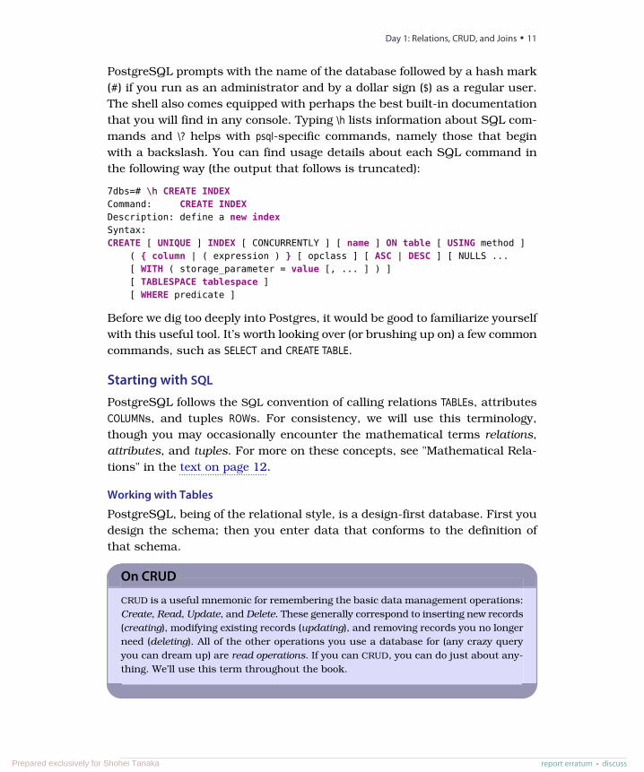
PostgreSQL prompts with the name of the database followed by a hash mark(#) if you run as an administrator and by a dollar sign ($) as a regular user.The shell also comes equipped with perhaps the best built-in documentationthat you will find in any console. Typing \h lists information about SQL com-mands and \? helps with psql-specific commands, namely those that beginwith a backslash. You can find usage details about each SQL command inthe following way (the output that follows is truncated):
7dbs=# \h CREATE INDEXCommand: CREATE INDEXDescription: define a new indexSyntax:CREATE [ UNIQUE ] INDEX [ CONCURRENTLY ] [ name ] ON table [ USING method ]
( { column | ( expression ) } [ opclass ] [ ASC | DESC ] [ NULLS ...[ WITH ( storage_parameter = value [, ... ] ) ][ TABLESPACE tablespace ][ WHERE predicate ]
Before we dig too deeply into Postgres, it would be good to familiarize yourselfwith this useful tool. It’s worth looking over (or brushing up on) a few commoncommands, such as SELECT and CREATE TABLE.
Starting with SQL
PostgreSQL follows the SQL convention of calling relations TABLEs, attributesCOLUMNs, and tuples ROWs. For consistency, we will use this terminology,though you may occasionally encounter the mathematical terms relations,attributes, and tuples. For more on these concepts, see "Mathematical Rela-tions" in the text on page 12.
Working with Tables
PostgreSQL, being of the relational style, is a design-first database. First youdesign the schema; then you enter data that conforms to the definition ofthat schema.
On CRUD
CRUD is a useful mnemonic for remembering the basic data management operations:Create, Read, Update, and Delete. These generally correspond to inserting new records(creating), modifying existing records (updating), and removing records you no longerneed (deleting). All of the other operations you use a database for (any crazy queryyou can dream up) are read operations. If you can CRUD, you can do just about any-thing. We’ll use this term throughout the book.
report erratum • discuss
Day 1: Relations, CRUD, and Joins • 11
Prepared exclusively for Shohei Tanaka
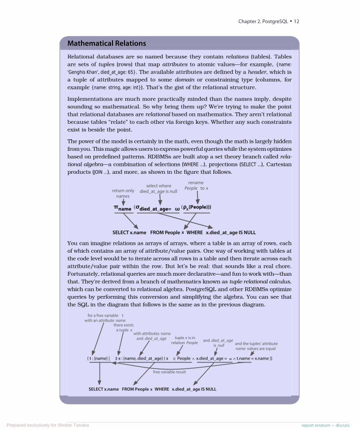
Mathematical Relations
Relational databases are so named because they contain relations (tables). Tablesare sets of tuples (rows) that map attributes to atomic values—for example, {name:'Genghis Khan', died_at_age: 65}. The available attributes are defined by a header, which isa tuple of attributes mapped to some domain or constraining type (columns, forexample {name: string, age: int}). That’s the gist of the relational structure.
Implementations are much more practically minded than the names imply, despitesounding so mathematical. So why bring them up? We’re trying to make the pointthat relational databases are relational based on mathematics. They aren’t relationalbecause tables “relate” to each other via foreign keys. Whether any such constraintsexist is beside the point.
The power of the model is certainly in the math, even though the math is largely hiddenfrom you. This magic allows users to express powerful queries while the system optimizesbased on predefined patterns. RDBMSs are built atop a set theory branch called rela-tional algebra—a combination of selections (WHERE ...), projections (SELECT ...), Cartesianproducts (JOIN ...), and more, as shown in the figure that follows.
WHERESELECT x.name FROM People x.died_at_age IS NULLx
( ( (People)))name died_at_age= x
renamePeople to xselect where
died_at_age is nullreturn onlynames
You can imagine relations as arrays of arrays, where a table is an array of rows, eachof which contains an array of attribute/value pairs. One way of working with tables atthe code level would be to iterate across all rows in a table and then iterate across eachattribute/value pair within the row. But let’s be real: that sounds like a real chore.Fortunately, relational queries are much more declarative—and fun to work with—thanthat. They’re derived from a branch of mathematics known as tuple relational calculus,which can be converted to relational algebra. PostgreSQL and other RDBMSs optimizequeries by performing this conversion and simplifying the algebra. You can see thatthe SQL in the diagram that follows is the same as in the previous diagram.
{ t : {name} | x : {name, died_at_age} ( x People x.died_at_age = t.name = x.name )}
free variable result
WHERESELECT x.name FROM People x.died_at_age IS NULLx
with attributes nameand died_at_age tuple x is in
relation People and died_at_ageis null and the tuples' attribute
name values are equal
there existsa tuple x
for a free variable twith an attribute name
Chapter 2. PostgreSQL • 12
report erratum • discussPrepared exclusively for Shohei Tanaka
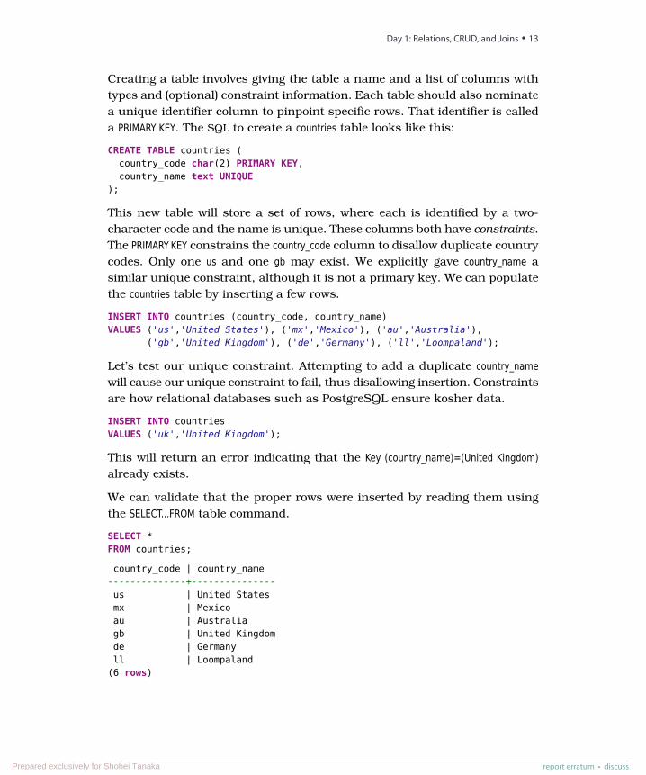
Creating a table involves giving the table a name and a list of columns withtypes and (optional) constraint information. Each table should also nominatea unique identifier column to pinpoint specific rows. That identifier is calleda PRIMARY KEY. The SQL to create a countries table looks like this:
CREATE TABLE countries (country_code char(2) PRIMARY KEY,country_name text UNIQUE
);
This new table will store a set of rows, where each is identified by a two-character code and the name is unique. These columns both have constraints.The PRIMARY KEY constrains the country_code column to disallow duplicate countrycodes. Only one us and one gb may exist. We explicitly gave country_name asimilar unique constraint, although it is not a primary key. We can populatethe countries table by inserting a few rows.
INSERT INTO countries (country_code, country_name)VALUES ('us','United States'), ('mx','Mexico'), ('au','Australia'),
('gb','United Kingdom'), ('de','Germany'), ('ll','Loompaland');
Let’s test our unique constraint. Attempting to add a duplicate country_namewill cause our unique constraint to fail, thus disallowing insertion. Constraintsare how relational databases such as PostgreSQL ensure kosher data.
INSERT INTO countriesVALUES ('uk','United Kingdom');
This will return an error indicating that the Key (country_name)=(United Kingdom)already exists.
We can validate that the proper rows were inserted by reading them usingthe SELECT...FROM table command.
SELECT *FROM countries;
country_code | country_name--------------+---------------us | United Statesmx | Mexicoau | Australiagb | United Kingdomde | Germanyll | Loompaland
(6 rows)
report erratum • discuss
Day 1: Relations, CRUD, and Joins • 13
Prepared exclusively for Shohei Tanaka
According to any respectable map, Loompaland isn’t a real place, so let’sremove it from the table. You specify which row to remove using the WHEREclause. The row whose country_code equals ll will be removed.
DELETE FROM countriesWHERE country_code = 'll';
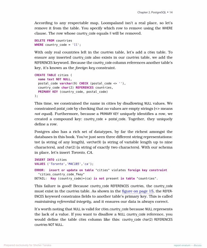
With only real countries left in the countries table, let’s add a cities table. Toensure any inserted country_code also exists in our countries table, we add theREFERENCES keyword. Because the country_code column references another table’skey, it’s known as the foreign key constraint.
CREATE TABLE cities (name text NOT NULL,postal_code varchar(9) CHECK (postal_code <> ''),country_code char(2) REFERENCES countries,PRIMARY KEY (country_code, postal_code)
);
This time, we constrained the name in cities by disallowing NULL values. Weconstrained postal_code by checking that no values are empty strings (<> meansnot equal). Furthermore, because a PRIMARY KEY uniquely identifies a row, wecreated a compound key: country_code + postal_code. Together, they uniquelydefine a row.
Postgres also has a rich set of datatypes, by far the richest amongst thedatabases in this book. You’ve just seen three different string representations:text (a string of any length), varchar(9) (a string of variable length up to ninecharacters), and char(2) (a string of exactly two characters). With our schemain place, let’s insert Toronto, CA.
INSERT INTO citiesVALUES ('Toronto','M4C1B5','ca');
ERROR: insert or update on table "cities" violates foreign key constraint"cities_country_code_fkey"
DETAIL: Key (country_code)=(ca) is not present in table "countries".
This failure is good! Because country_code REFERENCES countries, the country_codemust exist in the countries table. As shown in the figure on page 15, the REFER-ENCES keyword constrains fields to another table’s primary key. This is calledmaintaining referential integrity, and it ensures our data is always correct.
It’s worth noting that NULL is valid for cities.country_code because NULL representsthe lack of a value. If you want to disallow a NULL country_code reference, youwould define the table cities column like this: country_code char(2) REFERENCEScountries NOT NULL.
Chapter 2. PostgreSQL • 14
report erratum • discussPrepared exclusively for Shohei Tanaka
country_code | country_name
--------------+---------------
us | United States
mx | Mexico
au | Australia
uk | United Kingdom
de | Germany
name | postal_code | country_code
----------+-------------+--------------
Portland | 97205 | us
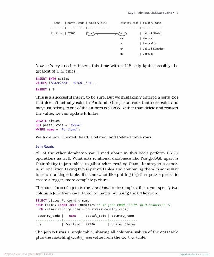
Now let’s try another insert, this time with a U.S. city (quite possibly thegreatest of U.S. cities).
INSERT INTO citiesVALUES ('Portland','87200','us');
INSERT 0 1
This is a successful insert, to be sure. But we mistakenly entered a postal_codethat doesn’t actually exist in Portland. One postal code that does exist andmay just belong to one of the authors is 97206. Rather than delete and reinsertthe value, we can update it inline.
UPDATE citiesSET postal_code = '97206'WHERE name = 'Portland';
We have now Created, Read, Updated, and Deleted table rows.
Join Reads
All of the other databases you’ll read about in this book perform CRUDoperations as well. What sets relational databases like PostgreSQL apart istheir ability to join tables together when reading them. Joining, in essence,is an operation taking two separate tables and combining them in some wayto return a single table. It’s somewhat like putting together puzzle pieces tocreate a bigger, more complete picture.
The basic form of a join is the inner join. In the simplest form, you specify twocolumns (one from each table) to match by, using the ON keyword.
SELECT cities.*, country_nameFROM cities INNER JOIN countries /* or just FROM cities JOIN countries */
ON cities.country_code = countries.country_code;
country_code | name | postal_code | country_name--------------+----------+-------------+---------------us | Portland | 97206 | United States
The join returns a single table, sharing all columns’ values of the cities tableplus the matching country_name value from the countries table.
report erratum • discuss
Day 1: Relations, CRUD, and Joins • 15
Prepared exclusively for Shohei Tanaka
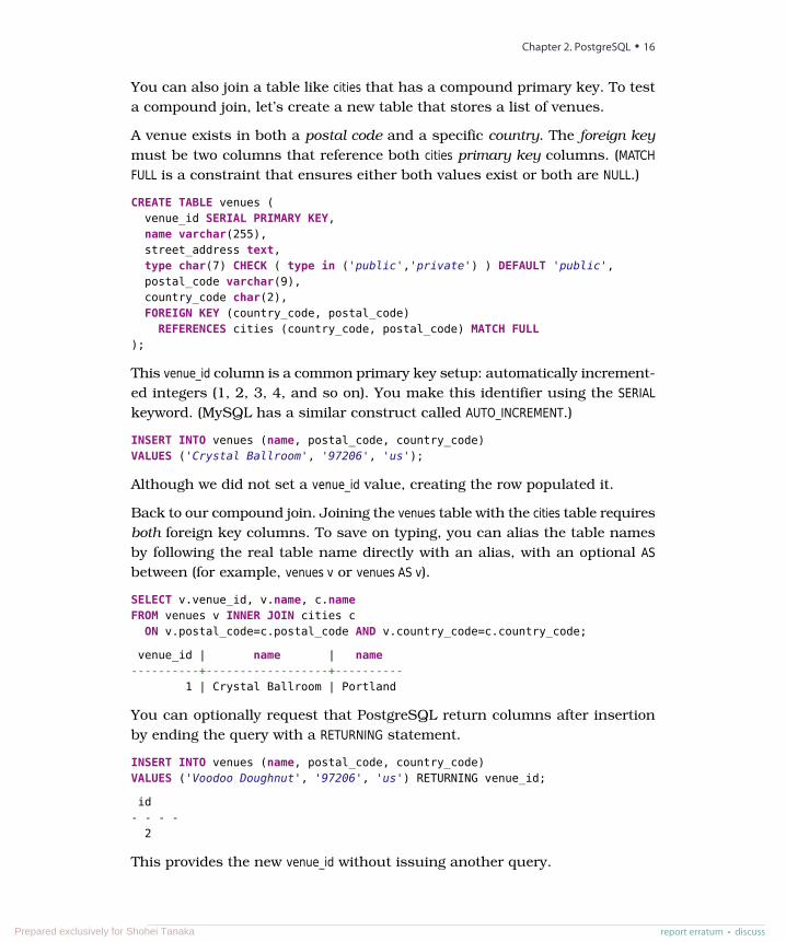
You can also join a table like cities that has a compound primary key. To testa compound join, let’s create a new table that stores a list of venues.
A venue exists in both a postal code and a specific country. The foreign keymust be two columns that reference both cities primary key columns. (MATCHFULL is a constraint that ensures either both values exist or both are NULL.)
CREATE TABLE venues (venue_id SERIAL PRIMARY KEY,name varchar(255),street_address text,type char(7) CHECK ( type in ('public','private') ) DEFAULT 'public',postal_code varchar(9),country_code char(2),FOREIGN KEY (country_code, postal_code)
REFERENCES cities (country_code, postal_code) MATCH FULL);
This venue_id column is a common primary key setup: automatically increment-ed integers (1, 2, 3, 4, and so on). You make this identifier using the SERIALkeyword. (MySQL has a similar construct called AUTO_INCREMENT.)
INSERT INTO venues (name, postal_code, country_code)VALUES ('Crystal Ballroom', '97206', 'us');
Although we did not set a venue_id value, creating the row populated it.
Back to our compound join. Joining the venues table with the cities table requiresboth foreign key columns. To save on typing, you can alias the table namesby following the real table name directly with an alias, with an optional ASbetween (for example, venues v or venues AS v).
SELECT v.venue_id, v.name, c.nameFROM venues v INNER JOIN cities c
ON v.postal_code=c.postal_code AND v.country_code=c.country_code;
venue_id | name | name----------+------------------+----------
1 | Crystal Ballroom | Portland
You can optionally request that PostgreSQL return columns after insertionby ending the query with a RETURNING statement.
INSERT INTO venues (name, postal_code, country_code)VALUES ('Voodoo Doughnut', '97206', 'us') RETURNING venue_id;
id- - - -
2
This provides the new venue_id without issuing another query.
Chapter 2. PostgreSQL • 16
report erratum • discussPrepared exclusively for Shohei Tanaka
The Outer Limits
In addition to inner joins, PostgreSQL can also perform outer joins. Outer joinsare a way of merging two tables when the results of one table must always bereturned, whether or not any matching column values exist on the other table.
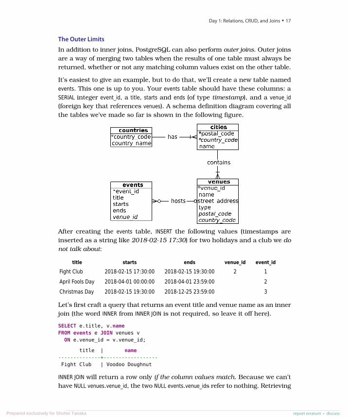
It’s easiest to give an example, but to do that, we’ll create a new table namedevents. This one is up to you. Your events table should have these columns: aSERIAL integer event_id, a title, starts and ends (of type timestamp), and a venue_id(foreign key that references venues). A schema definition diagram covering allthe tables we’ve made so far is shown in the following figure.
After creating the events table, INSERT the following values (timestamps areinserted as a string like 2018-02-15 17:30) for two holidays and a club we donot talk about:
event_idvenue_idendsstartstitle
122018-02-15 19:30:002018-02-15 17:30:00Fight Club22018-04-01 23:59:002018-04-01 00:00:00April Fools Day32018-12-25 23:59:002018-02-15 19:30:00Christmas Day
Let’s first craft a query that returns an event title and venue name as an innerjoin (the word INNER from INNER JOIN is not required, so leave it off here).
SELECT e.title, v.nameFROM events e JOIN venues v
ON e.venue_id = v.venue_id;
title | name--------------+------------------Fight Club | Voodoo Doughnut
INNER JOIN will return a row only if the column values match. Because we can’thave NULL venues.venue_id, the two NULL events.venue_ids refer to nothing. Retrieving
report erratum • discuss
Day 1: Relations, CRUD, and Joins • 17
Prepared exclusively for Shohei Tanaka
all of the events, whether or not they have a venue, requires a LEFT OUTER JOIN(shortened to LEFT JOIN).
SELECT e.title, v.nameFROM events e LEFT JOIN venues vON e.venue_id = v.venue_id;
title | name------------------+----------------Fight Club | Voodoo DoughnutApril Fools Day |Christmas Day |
If you require the inverse, all venues and only matching events, use a RIGHTJOIN. Finally, there’s the FULL JOIN, which is the union of LEFT and RIGHT; you’reguaranteed all values from each table, joined wherever columns match.
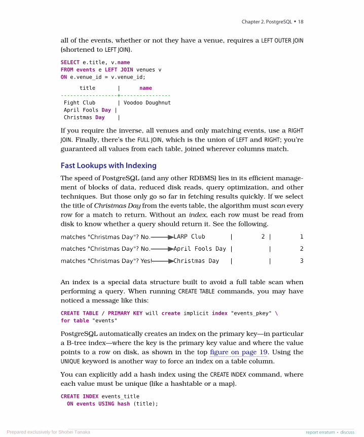
Fast Lookups with IndexingThe speed of PostgreSQL (and any other RDBMS) lies in its efficient manage-ment of blocks of data, reduced disk reads, query optimization, and othertechniques. But those only go so far in fetching results quickly. If we selectthe title of Christmas Day from the events table, the algorithm must scan everyrow for a match to return. Without an index, each row must be read fromdisk to know whether a query should return it. See the following.
An index is a special data structure built to avoid a full table scan whenperforming a query. When running CREATE TABLE commands, you may havenoticed a message like this:
CREATE TABLE / PRIMARY KEY will create implicit index "events_pkey" \for table "events"
PostgreSQL automatically creates an index on the primary key—in particulara B-tree index—where the key is the primary key value and where the valuepoints to a row on disk, as shown in the top figure on page 19. Using theUNIQUE keyword is another way to force an index on a table column.
You can explicitly add a hash index using the CREATE INDEX command, whereeach value must be unique (like a hashtable or a map).
CREATE INDEX events_titleON events USING hash (title);
Chapter 2. PostgreSQL • 18
report erratum • discussPrepared exclusively for Shohei Tanaka
LARP Club | 2 | 1
April Fools Day | | 2
Christmas Day | | 3
1
2
3
"events" Table"events.id" hash Index
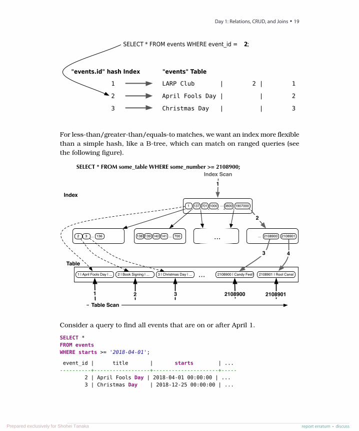
SELECT * FROM events WHERE event_id = 2;
For less-than/greater-than/equals-to matches, we want an index more flexiblethan a simple hash, like a B-tree, which can match on ranged queries (seethe following figure).
1 137 701 1000 1907000... 3600
2 3 ... 136 138 139 ... 700140 141 ... 2108901
< < < < > < < >
...
Table
Index
1 | April Fools Day | ... 2 | Book Signing | ... 3 | Christmas Day | ... ... 2108901 | Root Canal
1
2
4
1 2 3 2108901
Table Scan
Index Scan
2108900 | Candy Fest!
2108900
3
2108900
SELECT * FROM some_table WHERE some_number >= 2108900;
Consider a query to find all events that are on or after April 1.
SELECT *FROM eventsWHERE starts >= '2018-04-01';
event_id | title | starts | ...----------+------------------+---------------------+-----
2 | April Fools Day | 2018-04-01 00:00:00 | ...3 | Christmas Day | 2018-12-25 00:00:00 | ...
report erratum • discuss
Day 1: Relations, CRUD, and Joins • 19
Prepared exclusively for Shohei Tanaka
For this, a tree is the perfect data structure. To index the starts column witha B-tree, use this:
CREATE INDEX events_startsON events USING btree (starts);
Now our query over a range of dates will avoid a full table scan. It makes ahuge difference when scanning millions or billions of rows.
We can inspect our work with this command to list all indexes in the schema:
7dbs=# \di
It’s worth noting that when you set a FOREIGN KEY constraint, PostgreSQL willnot automatically create an index on the targeted column(s). You’ll need tocreate an index on the targeted column(s) yourself. Even if you don’t like usingdatabase constraints (that’s right, we’re looking at you, Ruby on Rails devel-opers), you will often find yourself creating indexes on columns you plan tojoin against in order to help speed up foreign key joins.
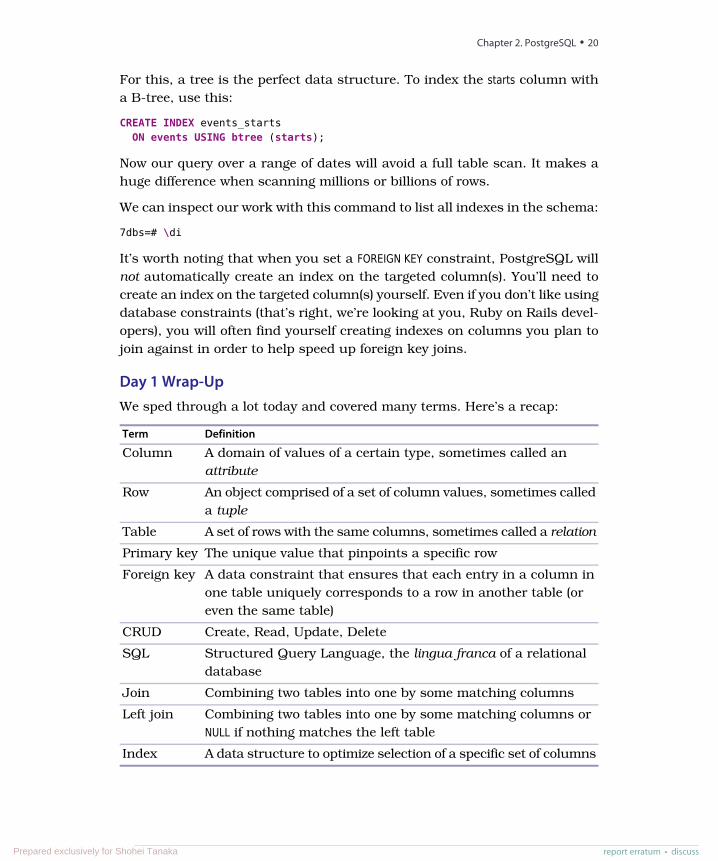
Day 1 Wrap-UpWe sped through a lot today and covered many terms. Here’s a recap:
DefinitionTerm
A domain of values of a certain type, sometimes called anattribute
Column
An object comprised of a set of column values, sometimes calleda tuple
Row
A set of rows with the same columns, sometimes called a relationTable
The unique value that pinpoints a specific rowPrimary key
A data constraint that ensures that each entry in a column inone table uniquely corresponds to a row in another table (oreven the same table)
Foreign key
Create, Read, Update, DeleteCRUD
Structured Query Language, the lingua franca of a relationaldatabase
SQL
Combining two tables into one by some matching columnsJoin
Combining two tables into one by some matching columns orNULL if nothing matches the left table
Left join
A data structure to optimize selection of a specific set of columnsIndex
Chapter 2. PostgreSQL • 20
report erratum • discussPrepared exclusively for Shohei Tanaka
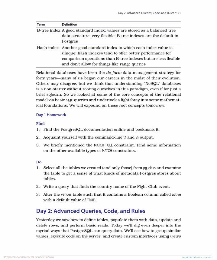
DefinitionTerm
A good standard index; values are stored as a balanced treedata structure; very flexible; B-tree indexes are the default inPostgres
B-tree index
Another good standard index in which each index value isunique; hash indexes tend to offer better performance for
Hash index
comparison operations than B-tree indexes but are less flexibleand don’t allow for things like range queries
Relational databases have been the de facto data management strategy forforty years—many of us began our careers in the midst of their evolution.Others may disagree, but we think that understanding “NoSQL” databasesis a non-starter without rooting ourselves in this paradigm, even if for just abrief sojourn. So we looked at some of the core concepts of the relationalmodel via basic SQL queries and undertook a light foray into some mathemat-ical foundations. We will expound on these root concepts tomorrow.
Day 1 Homework
Find
1. Find the PostgreSQL documentation online and bookmark it.
2. Acquaint yourself with the command-line \? and \h output.
3. We briefly mentioned the MATCH FULL constraint. Find some informationon the other available types of MATCH constraints.
Do
1. Select all the tables we created (and only those) from pg_class and examinethe table to get a sense of what kinds of metadata Postgres stores abouttables.
2. Write a query that finds the country name of the Fight Club event.
3. Alter the venues table such that it contains a Boolean column called activewith a default value of TRUE.
Day 2: Advanced Queries, Code, and RulesYesterday we saw how to define tables, populate them with data, update anddelete rows, and perform basic reads. Today we’ll dig even deeper into themyriad ways that PostgreSQL can query data. We’ll see how to group similarvalues, execute code on the server, and create custom interfaces using views
report erratum • discuss
Day 2: Advanced Queries, Code, and Rules • 21
Prepared exclusively for Shohei Tanaka
and rules. We’ll finish the day by using one of PostgreSQL’s contributedpackages to flip tables on their heads.
Aggregate FunctionsAn aggregate query groups results from several rows by some common criteria.It can be as simple as counting the number of rows in a table or calculatingthe average of some numerical column. They’re powerful SQL tools and alsoa lot of fun.
Let’s try some aggregate functions, but first we’ll need some more data in ourdatabase. Enter your own country into the countries table, your own city intothe cities table, and your own address as a venue (which we just named MyPlace). Then add a few records to the events table.
Here’s a quick SQL tip: Rather than setting the venue_id explicitly, you cansub-SELECT it using a more human-readable title. If Moby is playing at theCrystal Ballroom, set the venue_id like this:
INSERT INTO events (title, starts, ends, venue_id)VALUES ('Moby', '2018-02-06 21:00', '2018-02-06 23:00', (
SELECT venue_idFROM venuesWHERE name = 'Crystal Ballroom'
));
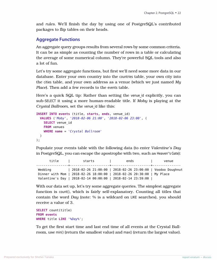
Populate your events table with the following data (to enter Valentine’s Dayin PostgreSQL, you can escape the apostrophe with two, such as Heaven''s Gate):
title | starts | ends | venue-----------------+---------------------+---------------------+---------------Wedding | 2018-02-26 21:00:00 | 2018-02-26 23:00:00 | Voodoo DoughnutDinner with Mom | 2018-02-26 18:00:00 | 2018-02-26 20:30:00 | My PlaceValentine's Day | 2018-02-14 00:00:00 | 2018-02-14 23:59:00 |
With our data set up, let’s try some aggregate queries. The simplest aggregatefunction is count(), which is fairly self-explanatory. Counting all titles thatcontain the word Day (note: % is a wildcard on LIKE searches), you shouldreceive a value of 3.
SELECT count(title)FROM eventsWHERE title LIKE '%Day%';
To get the first start time and last end time of all events at the Crystal Ball-room, use min() (return the smallest value) and max() (return the largest value).
Chapter 2. PostgreSQL • 22
report erratum • discussPrepared exclusively for Shohei Tanaka
SELECT min(starts), max(ends)FROM events INNER JOIN venues
ON events.venue_id = venues.venue_idWHERE venues.name = 'Crystal Ballroom';
min | max---------------------+---------------------2018-02-06 21:00:00 | 2018-02-06 23:00:00
Aggregate functions are useful but limited on their own. If we wanted to countall events at each venue, we could write the following for each venue ID:
SELECT count(*) FROM events WHERE venue_id = 1;SELECT count(*) FROM events WHERE venue_id = 2;SELECT count(*) FROM events WHERE venue_id = 3;SELECT count(*) FROM events WHERE venue_id IS NULL;
This would be tedious (intractable even) as the number of venues grows. Thisis where the GROUP BY command comes in handy.
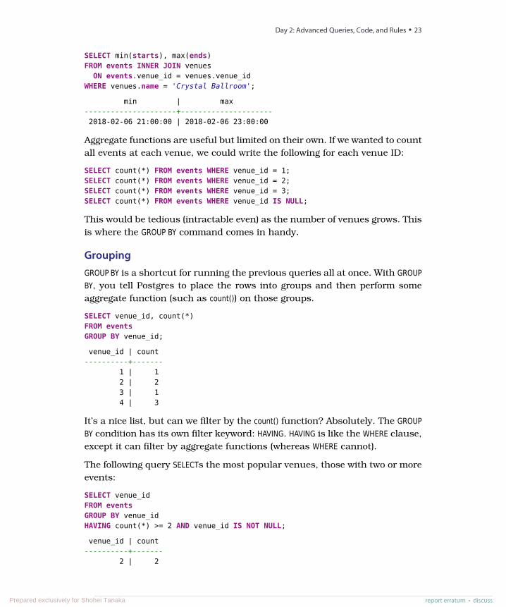
GroupingGROUP BY is a shortcut for running the previous queries all at once. With GROUPBY, you tell Postgres to place the rows into groups and then perform someaggregate function (such as count()) on those groups.
SELECT venue_id, count(*)FROM eventsGROUP BY venue_id;
venue_id | count----------+-------
1 | 12 | 23 | 14 | 3
It’s a nice list, but can we filter by the count() function? Absolutely. The GROUPBY condition has its own filter keyword: HAVING. HAVING is like the WHERE clause,except it can filter by aggregate functions (whereas WHERE cannot).
The following query SELECTs the most popular venues, those with two or moreevents:
SELECT venue_idFROM eventsGROUP BY venue_idHAVING count(*) >= 2 AND venue_id IS NOT NULL;
venue_id | count----------+-------
2 | 2
report erratum • discuss
Day 2: Advanced Queries, Code, and Rules • 23
Prepared exclusively for Shohei Tanaka
You can use GROUP BY without any aggregate functions. If you call SELECT...FROM...GROUP BY on one column, you get only unique values.
SELECT venue_id FROM events GROUP BY venue_id;
This kind of grouping is so common that SQL has a shortcut for it in theDISTINCT keyword.
SELECT DISTINCT venue_id FROM events;
The results of both queries will be identical.
GROUP BY in MySQL
If you tried to run a SELECT statement with columns not defined under a GROUP BY inMySQL, you would be shocked to see that it works. This originally made us questionthe necessity of window functions. But when we inspected the data MySQL returnsmore closely, we found it will return only a random row of data along with the count,not all relevant results. Generally, that’s not useful (and quite potentially dangerous).
Window FunctionsIf you’ve done any sort of production work with a relational database in thepast, you are likely familiar with aggregate queries. They are a common SQL
staple. Window functions, on the other hand, are not quite so common (Post-greSQL is one of the few open source databases to implement them).
Window functions are similar to GROUP BY queries in that they allow you torun aggregate functions across multiple rows. The difference is that they allowyou to use built-in aggregate functions without requiring every single field tobe grouped to a single row.
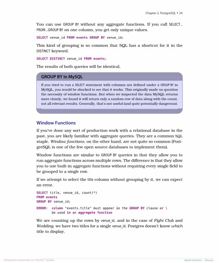
If we attempt to select the title column without grouping by it, we can expectan error.
SELECT title, venue_id, count(*)FROM eventsGROUP BY venue_id;
ERROR: column "events.title" must appear in the GROUP BY clause or \be used in an aggregate function
We are counting up the rows by venue_id, and in the case of Fight Club andWedding, we have two titles for a single venue_id. Postgres doesn’t know whichtitle to display.
Chapter 2. PostgreSQL • 24
report erratum • discussPrepared exclusively for Shohei Tanaka
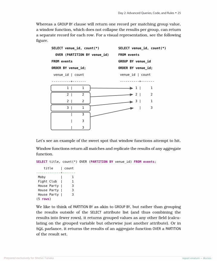
Whereas a GROUP BY clause will return one record per matching group value,a window function, which does not collapse the results per group, can returna separate record for each row. For a visual representation, see the followingfigure.
venue_id | count
----------+-------
1 | 1
2 | 2
2 | 2
3 | 1
| 3
| 3
| 3
SELECT venue_id, count(*)
OVER (PARTITION BY venue_id)
FROM events
ORDER BY venue_id;
SELECT venue_id, count(*)
FROM events
GROUP BY venue_id
ORDER BY venue_id;
venue_id | count
----------+-------
1 | 1
2 | 2
3 | 1
| 3
Let’s see an example of the sweet spot that window functions attempt to hit.
Window functions return all matches and replicate the results of any aggregatefunction.
SELECT title, count(*) OVER (PARTITION BY venue_id) FROM events;
title | count-------------+-------Moby | 1Fight Club | 1House Party | 3House Party | 3House Party | 3
(5 rows)
We like to think of PARTITION BY as akin to GROUP BY, but rather than groupingthe results outside of the SELECT attribute list (and thus combining theresults into fewer rows), it returns grouped values as any other field (calcu-lating on the grouped variable but otherwise just another attribute). Or inSQL parlance, it returns the results of an aggregate function OVER a PARTITIONof the result set.
report erratum • discuss
Day 2: Advanced Queries, Code, and Rules • 25
Prepared exclusively for Shohei Tanaka
TransactionsTransactions are the bulwark of relational database consistency. All or nothing,that’s the transaction motto. Transactions ensure that every command of aset is executed. If anything fails along the way, all of the commands are rolledback as if they never happened.
PostgreSQL transactions follow ACID compliance, which stands for:
• Atomic (either all operations succeed or none do)
• Consistent (the data will always be in a good state and never in an incon-sistent state)
• Isolated (transactions don’t interfere with one another)
• Durable (a committed transaction is safe, even after a server crash)
We should note here that consistency in ACID is different from consistencyin CAP (covered in Appendix 2, The CAP Theorem, on page 315).
Unavoidable Transactions
Up until now, every command we’ve executed in psql has been implicitly wrapped ina transaction. If you executed a command, such as DELETE FROM account WHERE total < 20;and the database crashed halfway through the delete, you wouldn’t be stuck withhalf a table. When you restart the database server, that command will be rolled back.
We can wrap any transaction within a BEGIN TRANSACTION block. To verifyatomicity, we’ll kill the transaction with the ROLLBACK command.
BEGIN TRANSACTION;DELETE FROM events;
ROLLBACK;SELECT * FROM events;
The events all remain. Transactions are useful when you’re modifying twotables that you don’t want out of sync. The classic example is a debit/creditsystem for a bank, where money is moved from one account to another:
BEGIN TRANSACTION;UPDATE account SET total=total+5000.0 WHERE account_id=1337;UPDATE account SET total=total-5000.0 WHERE account_id=45887;
END;
If something happened between the two updates, this bank just lost fivegrand. But when wrapped in a transaction block, the initial update is rolledback, even if the server explodes.
Chapter 2. PostgreSQL • 26
report erratum • discussPrepared exclusively for Shohei Tanaka
Stored ProceduresEvery command we’ve seen until now has been declarative in the sense thatwe‘ve been able to get our desired result set using just SQL (which is quitepowerful in itself). But sometimes the database doesn‘t give us everything weneed natively and we need to run some code to fill in the gaps. At that point,though, you need to decide where the code is going to run. Should it run inPostgres or should it run on the application side?
If you decide you want the database to do the heavy lifting, Postgres offersstored procedures. Stored procedures are extremely powerful and can be usedto do an enormous range of tasks, from performing complex mathematicaloperations that aren’t supported in SQL to triggering cascading series ofevents to pre-validating data before it‘s written to tables and far beyond. Onthe one hand, stored procedures can offer huge performance advantages. Butthe architectural costs can be high (and sometimes not worth it). You mayavoid streaming thousands of rows to a client application, but you have alsobound your application code to this database. And so the decision to usestored procedures should not be made lightly.
Caveats aside, let’s create a procedure (or FUNCTION) that simplifies INSERTinga new event at a venue without needing the venue_id. Here‘s what the procedurewill accomplish: if the venue doesn’t exist, it will be created first and thenreferenced in the new event. The procedure will also return a Boolean indicat-ing whether a new venue was added as a helpful bonus.
What About Vendor Lock-in?
When relational databases hit their heyday, they were the Swiss Army knife of tech-nologies. You could store nearly anything—even programming entire projects inthem (for example, Microsoft Access). The few companies that provided this softwarepromoted use of proprietary differences and then took advantage of this corporatereliance by charging enormous license and consulting fees. This was the dreadedvendor lock-in that newer programming methodologies tried to mitigate in the 1990sand early 2000s.
The zeal to neuter the vendors, however, birthed maxims such as no logic in thedatabase. This is a shame because relational databases are capable of so many varieddata management options. Vendor lock-in has not disappeared. Many actions weinvestigate in this book are highly implementation-specific. However, it’s worthknowing how to use databases to their fullest extent before deciding to skip toolssuch as stored procedures solely because they’re implementation-specific.
report erratum • discuss
Day 2: Advanced Queries, Code, and Rules • 27
Prepared exclusively for Shohei Tanaka
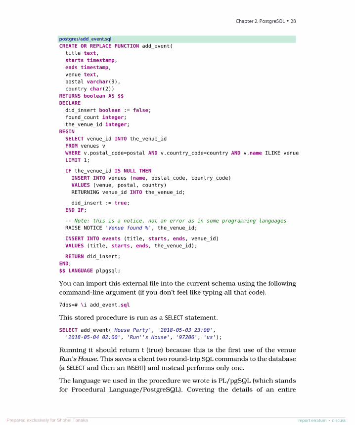
postgres/add_event.sqlCREATE OR REPLACE FUNCTION add_event(
title text,starts timestamp,ends timestamp,venue text,postal varchar(9),country char(2))
RETURNS boolean AS $$DECLARE
did_insert boolean := false;found_count integer;the_venue_id integer;
BEGINSELECT venue_id INTO the_venue_idFROM venues vWHERE v.postal_code=postal AND v.country_code=country AND v.name ILIKE venueLIMIT 1;
IF the_venue_id IS NULL THENINSERT INTO venues (name, postal_code, country_code)VALUES (venue, postal, country)RETURNING venue_id INTO the_venue_id;
did_insert := true;END IF;
-- Note: this is a notice, not an error as in some programming languagesRAISE NOTICE 'Venue found %', the_venue_id;
INSERT INTO events (title, starts, ends, venue_id)VALUES (title, starts, ends, the_venue_id);
RETURN did_insert;END;$$ LANGUAGE plpgsql;
You can import this external file into the current schema using the followingcommand-line argument (if you don’t feel like typing all that code).
7dbs=# \i add_event.sql
This stored procedure is run as a SELECT statement.
SELECT add_event('House Party', '2018-05-03 23:00','2018-05-04 02:00', 'Run''s House', '97206', 'us');
Running it should return t (true) because this is the first use of the venueRun’s House. This saves a client two round-trip SQL commands to the database(a SELECT and then an INSERT) and instead performs only one.
The language we used in the procedure we wrote is PL/pgSQL (which standsfor Procedural Language/PostgreSQL). Covering the details of an entire
Chapter 2. PostgreSQL • 28
report erratum • discussPrepared exclusively for Shohei Tanaka
Choosing to Execute Database Code
This is the first of a number of places where you’ll see this theme in this book: Doesthe code belong in your application or in the database? It’s often a difficult decision,one that you’ll have to answer uniquely for every application.
In many cases, you’ll improve performance by as much as an order of magnitude.For example, you might have a complex application-specific calculation that requirescustom code. If the calculation involves many rows, a stored procedure will save youfrom moving thousands of rows instead of a single result. The cost is splitting yourapplication, your code, and your tests across two different programming paradigms.
programming language is beyond the scope of this book, but you can readmuch more about it in the online PostgreSQL documentation.2
In addition to PL/pgSQL, Postgres supports three more core languages forwriting procedures: Tcl (PL/Tcl), Perl (PL/Perl), and Python (PL/Python). Peoplehave written extensions for a dozen more, including Ruby, Java, PHP, Scheme,and others listed in the public documentation. Try this shell command:
$ createlang 7dbs --list
It will list the languages installed in your database. The createlang commandis also used to add new languages, which you can find online.3
Pull the TriggersTriggers automatically fire stored procedures when some event happens, suchas an insert or update. They allow the database to enforce some requiredbehavior in response to changing data.
Let’s create a new PL/pgSQL function that logs whenever an event is updated(we want to be sure no one changes an event and tries to deny it later). First,create a logs table to store event changes. A primary key isn’t necessary herebecause it’s just a log.
CREATE TABLE logs (event_id integer,old_title varchar(255),old_starts timestamp,old_ends timestamp,logged_at timestamp DEFAULT current_timestamp
);
2. http://www.postgresql.org/docs/9.0/static/plpgsql.html3. http://www.postgresql.org/docs/9.0/static/app-createlang.html
report erratum • discuss
Day 2: Advanced Queries, Code, and Rules • 29
Prepared exclusively for Shohei Tanaka
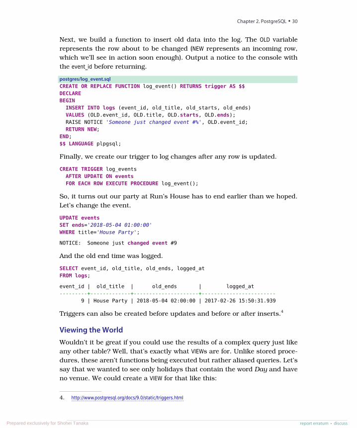
Next, we build a function to insert old data into the log. The OLD variablerepresents the row about to be changed (NEW represents an incoming row,which we’ll see in action soon enough). Output a notice to the console withthe event_id before returning.
postgres/log_event.sqlCREATE OR REPLACE FUNCTION log_event() RETURNS trigger AS $$DECLAREBEGIN
INSERT INTO logs (event_id, old_title, old_starts, old_ends)VALUES (OLD.event_id, OLD.title, OLD.starts, OLD.ends);RAISE NOTICE 'Someone just changed event #%', OLD.event_id;RETURN NEW;
END;$$ LANGUAGE plpgsql;
Finally, we create our trigger to log changes after any row is updated.
CREATE TRIGGER log_eventsAFTER UPDATE ON eventsFOR EACH ROW EXECUTE PROCEDURE log_event();
So, it turns out our party at Run’s House has to end earlier than we hoped.Let’s change the event.
UPDATE eventsSET ends='2018-05-04 01:00:00'WHERE title='House Party';
NOTICE: Someone just changed event #9
And the old end time was logged.
SELECT event_id, old_title, old_ends, logged_atFROM logs;
event_id | old_title | old_ends | logged_at---------+-------------+---------------------+------------------------
9 | House Party | 2018-05-04 02:00:00 | 2017-02-26 15:50:31.939
Triggers can also be created before updates and before or after inserts.4
Viewing the WorldWouldn’t it be great if you could use the results of a complex query just likeany other table? Well, that’s exactly what VIEWs are for. Unlike stored proce-dures, these aren’t functions being executed but rather aliased queries. Let’ssay that we wanted to see only holidays that contain the word Day and haveno venue. We could create a VIEW for that like this:
4. http://www.postgresql.org/docs/9.0/static/triggers.html
Chapter 2. PostgreSQL • 30
report erratum • discussPrepared exclusively for Shohei Tanaka
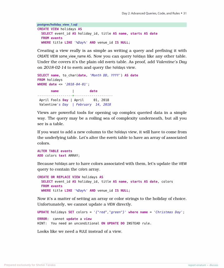
postgres/holiday_view_1.sqlCREATE VIEW holidays AS
SELECT event_id AS holiday_id, title AS name, starts AS dateFROM eventsWHERE title LIKE '%Day%' AND venue_id IS NULL;
Creating a view really is as simple as writing a query and prefixing it withCREATE VIEW some_view_name AS. Now you can query holidays like any other table.Under the covers it’s the plain old events table. As proof, add Valentine’s Dayon 2018-02-14 to events and query the holidays view.
SELECT name, to_char(date, 'Month DD, YYYY') AS dateFROM holidaysWHERE date <= '2018-04-01';
name | date------------------+--------------------April Fools Day | April 01, 2018Valentine's Day | February 14, 2018
Views are powerful tools for opening up complex queried data in a simpleway. The query may be a roiling sea of complexity underneath, but all yousee is a table.
If you want to add a new column to the holidays view, it will have to come fromthe underlying table. Let’s alter the events table to have an array of associatedcolors.
ALTER TABLE eventsADD colors text ARRAY;
Because holidays are to have colors associated with them, let’s update the VIEWquery to contain the colors array.
CREATE OR REPLACE VIEW holidays ASSELECT event_id AS holiday_id, title AS name, starts AS date, colorsFROM eventsWHERE title LIKE '%Day%' AND venue_id IS NULL;
Now it’s a matter of setting an array or color strings to the holiday of choice.Unfortunately, we cannot update a VIEW directly.
UPDATE holidays SET colors = '{"red","green"}' where name = 'Christmas Day';
ERROR: cannot update a viewHINT: You need an unconditional ON UPDATE DO INSTEAD rule.
Looks like we need a RULE instead of a view.
report erratum • discuss
Day 2: Advanced Queries, Code, and Rules • 31
Prepared exclusively for Shohei Tanaka
Storing Views on Disk with Materialized Views
Though VIEWs like the holidays view mentioned previously are a convenient abstraction,they don’t yield any performance gains over the SELECT queries that they alias. If youwant VIEWs that do offer such gains, you should consider creating materialized views,which are different because they’re stored on disk in a “real” table and thus yieldperformance gains because they restrict the number of tables that must be accessedto exactly one.
You can create materialized views just like ordinary views, except with a CREATE MATE-RIALIZED VIEW rather than CREATE VIEW statement. Materialized view tables are populatedwhenever you run the REFRESH command for them, which you can automate to runat defined intervals or in response to triggers. You can also create indexes on materi-alized views the same way that you can on regular tables.
The downside of materialized views is that they do increase disk space usage. But inmany cases, the performance gains are worth it. In general, the more complex thequery and the more tables it spans, the more performance gains you’re likely to getvis-à-vis plain old SELECT queries or VIEWs.
What RULEs the School?A RULE is a description of how to alter the parsed query tree. Every time Post-gres runs an SQL statement, it parses the statement into a query tree (gener-ally called an abstract syntax tree).
Operators and values become branches and leaves in the tree, and the treeis walked, pruned, and in other ways edited before execution. This tree isoptionally rewritten by Postgres rules, before being sent on to the queryplanner (which also rewrites the tree to run optimally), and sends this finalcommand to be executed. See how SQL gets executed in PostgreSQL in thefigure on page 33.
In fact, a VIEW such as holidays is a RULE. We can prove this by taking a look atthe execution plan of the holidays view using the EXPLAIN command (notice Filteris the WHERE clause, and Output is the column list).
EXPLAIN VERBOSESELECT *FROM holidays;
QUERY PLAN-----------------------------------------------------------------------------Seq Scan on public.events (cost=0.00..1.01 rows=1 width=44)
Output: events.event_id, events.title, events.starts, events.colorsFilter: ((events.venue_id IS NULL) AND
((events.title)::text ~~ '%Day%'::text))
Chapter 2. PostgreSQL • 32
report erratum • discussPrepared exclusively for Shohei Tanaka
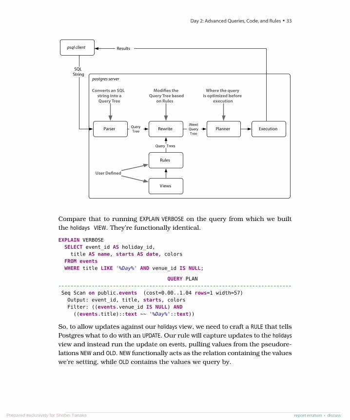
postgres server
Parser Rewrite Planner
Rules
Views
Query Trees
QueryTree
Where the queryis optimized before
execution
Converts an SQLstring into aQuery Tree
Modi�es theQuery Tree based
on Rules
(New)QueryTree
User De�ned
psql client
SQLString
Results
Execution
Compare that to running EXPLAIN VERBOSE on the query from which we builtthe holidays VIEW. They’re functionally identical.
EXPLAIN VERBOSESELECT event_id AS holiday_id,
title AS name, starts AS date, colorsFROM eventsWHERE title LIKE '%Day%' AND venue_id IS NULL;
QUERY PLAN-----------------------------------------------------------------------------Seq Scan on public.events (cost=0.00..1.04 rows=1 width=57)
Output: event_id, title, starts, colorsFilter: ((events.venue_id IS NULL) AND
((events.title)::text ~~ '%Day%'::text))
So, to allow updates against our holidays view, we need to craft a RULE that tellsPostgres what to do with an UPDATE. Our rule will capture updates to the holidaysview and instead run the update on events, pulling values from the pseudore-lations NEW and OLD. NEW functionally acts as the relation containing the valueswe’re setting, while OLD contains the values we query by.
report erratum • discuss
Day 2: Advanced Queries, Code, and Rules • 33
Prepared exclusively for Shohei Tanaka
postgres/create_rule.sqlCREATE RULE update_holidays AS ON UPDATE TO holidays DO INSTEAD
UPDATE eventsSET title = NEW.name,
starts = NEW.date,colors = NEW.colors
WHERE title = OLD.name;
With this rule in place, now we can update holidays directly.
UPDATE holidays SET colors = '{"red","green"}' where name = 'Christmas Day';
Next, let’s insert New Years Day on 2013-01-01 into holidays. As expected, weneed a rule for that too. No problem.
CREATE RULE insert_holidays AS ON INSERT TO holidays DO INSTEADINSERT INTO ...
We’re going to move on from here, but if you’d like to play more with RULEs,try to add a DELETE RULE.
I’ll Meet You at the CrosstabFor our last exercise of the day, we’re going to build a monthly calendar ofevents, where each month in the calendar year counts the number of eventsin that month. This kind of operation is commonly done by a pivot table. Theseconstructs “pivot” grouped data around some other output, in our case a listof months. We’ll build our pivot table using the crosstab() function.
Start by crafting a query to count the number of events per month each year.PostgreSQL provides an extract() function that returns some subfield from adate or timestamp, which aids in our grouping.
SELECT extract(year from starts) as year,extract(month from starts) as month, count(*)
FROM eventsGROUP BY year, monthORDER BY year, month;
To use crosstab(), the query must return three columns: rowid, category, and value.We’ll be using the year as an ID, which means the other fields are category (themonth) and value (the count).
The crosstab() function needs another set of values to represent months. Thisis how the function knows how many columns we need. These are the valuesthat become the columns (the table to pivot against). So let’s create a tableto store a list of numbers. Because we‘ll only need the table for a few opera-tions, we‘ll create an ephemeral table, which lasts only as long as the currentPostgres session, using the CREATE TEMPORARY TABLE command.
Chapter 2. PostgreSQL • 34
report erratum • discussPrepared exclusively for Shohei Tanaka
CREATE TEMPORARY TABLE month_count(month INT);INSERT INTO month_count VALUES (1),(2),(3),(4),(5),
(6),(7),(8),(9),(10),(11),(12);
Now we’re ready to call crosstab() with our two queries.
SELECT * FROM crosstab('SELECT extract(year from starts) as year,
extract(month from starts) as month, count(*)FROM eventsGROUP BY year, monthORDER BY year, month',
'SELECT * FROM month_count');
ERROR: a column definition list is required for functions returning "record"
Oops. An error occurred. This cryptic error is basically saying that the functionis returning a set of records (rows) but it doesn’t know how to label them. Infact, it doesn’t even know what datatypes they are.
Remember, the pivot table is using our months as categories, but thosemonths are just integers. So, we define them like this:
SELECT * FROM crosstab('SELECT extract(year from starts) as year,
extract(month from starts) as month, count(*)FROM eventsGROUP BY year, monthORDER BY year, month',
'SELECT * FROM month_count') AS (
year int,jan int, feb int, mar int, apr int, may int, jun int,jul int, aug int, sep int, oct int, nov int, dec int
) ORDER BY YEAR;
We have one column year (which is the row ID) and twelve more columnsrepresenting the months.
year | jan | feb | mar | apr | may | jun | jul | aug | sep | oct | nov | dec-----+-----+-----+-----+-----+-----+-----+-----+-----+-----+-----+-----+-----2018 | | 5 | | 1 | 1 | | | | | | | 1
Go ahead and add a couple more events on another year just to see nextyear’s event counts. Run the crosstab() function again, and enjoy the calendar.
Day 2 Wrap-UpToday finalized the basics of PostgreSQL. What we’re starting to see is thatPostgres is more than just a server for storing vanilla datatypes and querying
report erratum • discuss
Day 2: Advanced Queries, Code, and Rules • 35
Prepared exclusively for Shohei Tanaka
them. Instead, it’s a powerful data management engine that can reformatoutput data, store weird datatypes such as arrays, execute logic, and provideenough power to rewrite incoming queries.
Day 2 Homework
Find
1. Find the list of aggregate functions in the PostgreSQL docs.
2. Find a GUI program to interact with PostgreSQL, such as pgAdmin,Datagrip, or Navicat.
Do
1. Create a rule that captures DELETEs on venues and instead sets the activeflag (created in the Day 1 homework) to FALSE.
2. A temporary table was not the best way to implement our event calendarpivot table. The generate_series(a, b) function returns a set of records, froma to b. Replace the month_count table SELECT with this.
3. Build a pivot table that displays every day in a single month, where eachweek of the month is a row and each day name forms a column acrossthe top (seven days, starting with Sunday and ending with Saturday) like astandard month calendar. Each day should contain a count of the numberof events for that date or should remain blank if no event occurs.
Day 3: Full Text and MultidimensionsWe’ll spend Day 3 investigating the many tools at our disposal to build amovie query system. We’ll begin with the many ways PostgreSQL can searchactor/movie names using fuzzy string matching. Then we’ll discover the cubepackage by creating a movie suggestion system based on similar genres ofmovies we already like. Because these are all contributed packages, theimplementations are special to PostgreSQL and not part of the SQL standard.
Often, when designing a relational database schema, you’ll start with an entitydiagram. We’ll be writing a personal movie suggestion system that keeps trackof movies, their genres, and their actors, as modeled in the figure on page 37.
Before we begin the Day 3 exercises, we’ll need to extend Postgres by installingthe following contributed packages: tablefunc, dict_xsyn, fuzzystrmatch, pg_trgm, andcube. You can refer to the website for installation instructions.5
5. http://www.postgresql.org/docs/current/static/contrib.html
Chapter 2. PostgreSQL • 36
report erratum • discussPrepared exclusively for Shohei Tanaka
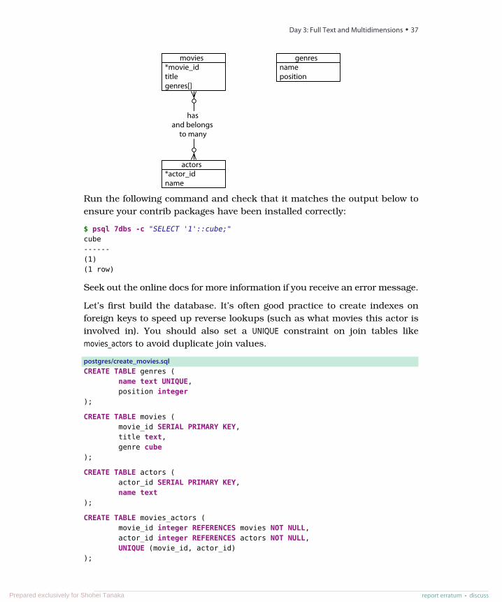
*movie_idtitlegenres[]
moviesnameposition
genres
*actor_idname
actors
hasand belongs
to many
Run the following command and check that it matches the output below toensure your contrib packages have been installed correctly:
$ psql 7dbs -c "SELECT '1'::cube;"cube------(1)(1 row)
Seek out the online docs for more information if you receive an error message.
Let’s first build the database. It’s often good practice to create indexes onforeign keys to speed up reverse lookups (such as what movies this actor isinvolved in). You should also set a UNIQUE constraint on join tables likemovies_actors to avoid duplicate join values.
postgres/create_movies.sqlCREATE TABLE genres (
name text UNIQUE,position integer
);
CREATE TABLE movies (movie_id SERIAL PRIMARY KEY,title text,genre cube
);
CREATE TABLE actors (actor_id SERIAL PRIMARY KEY,name text
);
CREATE TABLE movies_actors (movie_id integer REFERENCES movies NOT NULL,actor_id integer REFERENCES actors NOT NULL,UNIQUE (movie_id, actor_id)
);
report erratum • discuss
Day 3: Full Text and Multidimensions • 37
Prepared exclusively for Shohei Tanaka
CREATE INDEX movies_actors_movie_id ON movies_actors (movie_id);CREATE INDEX movies_actors_actor_id ON movies_actors (actor_id);CREATE INDEX movies_genres_cube ON movies USING gist (genre);
You can download the movies_data.sql file as a file alongside the book and pop-ulate the tables by piping the file into the database. Any questions you mayhave about the genre cube will be covered later today.
Fuzzy SearchingOpening up a system to text searches means opening your system to inaccu-rate inputs. You have to expect typos like “Brid of Frankstein.” Sometimes,users can’t remember the full name of “J. Roberts.” In other cases, we justplain don’t know how to spell “Benn Aflek.“ We’ll look into a few PostgreSQLpackages that make text searching easy.
It’s worth noting that as we progress, this kind of string matching blurs thelines between relational queries and searching frameworks such as Lucene6
and Elasticsearch.7 Although some may feel that features like full-text searchbelong with the application code, there can be performance and administrativebenefits of pushing these packages to the database, where the data lives.
SQL Standard String Matches
PostgreSQL has many ways of performing text matches but the two majordefault methods are LIKE and regular expressions.
I Like LIKE and ILIKE
LIKE and ILIKE are the simplest forms of text search (ILIKE is a case-insensitiveversion of LIKE). They are fairly universal in relational databases. LIKE comparescolumn values against a given pattern string. The % and _ characters arewildcards: % matches any number of any characters while _ matches exactlyone character.
SELECT title FROM movies WHERE title ILIKE 'stardust%';
title-------------------StardustStardust Memories
If we want to be sure the substring stardust is not at the end of the string,we can use the underscore (_) character as a little trick.
6. http://lucene.apache.org/7. https://www.elastic.co/products/elasticsearch
Chapter 2. PostgreSQL • 38
report erratum • discussPrepared exclusively for Shohei Tanaka
SELECT title FROM movies WHERE title ILIKE 'stardust_%';
title-------------------Stardust Memories
This is useful in basic cases, but LIKE is limited to simple wildcards.
Regex
A more powerful string-matching syntax is a regular expression (regex).Regexes appear often throughout this book because many databases supportthem. There are entire books dedicated to writing powerful expressions—thetopic is far too wide and complex to cover in depth here. Postgres conforms(mostly) to the POSIX style.
In Postgres, a regular expression match is led by the ~ operator, with theoptional ! (meaning not matching) and * (meaning case insensitive). To countall movies that do not begin with the, the following case-insensitive query willwork. The characters inside the string are the regular expression.
SELECT COUNT(*) FROM movies WHERE title !~* '^the.*';
You can index strings for pattern matching the previous queries by creatinga text_pattern_ops operator class index, as long as the values are indexed inlowercase.
CREATE INDEX movies_title_pattern ON movies (lower(title) text_pattern_ops);
We used the text_pattern_ops because the title is of type text. If you need to indexvarchars, chars, or names, use the related ops: varchar_pattern_ops, bpchar_pat-tern_ops, and name_pattern_ops.
Bride of Levenshtein
Levenshtein is a string comparison algorithm that compares how similar twostrings are by how many steps are required to change one string into another.Each replaced, missing, or added character counts as a step. The distanceis the total number of steps away. In PostgreSQL, the levenshtein() function isprovided by the fuzzystrmatch contrib package. Say we have the string bat andthe string fads.
SELECT levenshtein('bat', 'fads');
The Levenshtein distance is 3 because in order to go from bat to fads, wereplaced two letters (b=>f, t=>d) and added a letter (+s). Each change incre-ments the distance. We can watch the distance close as we step closer (so tospeak). The total goes down until we get zero (the two strings are equal).
report erratum • discuss
Day 3: Full Text and Multidimensions • 39
Prepared exclusively for Shohei Tanaka
SELECT levenshtein('bat', 'fad') fad,levenshtein('bat', 'fat') fat,levenshtein('bat', 'bat') bat;
fad | fat | bat-----+-----+-----
2 | 1 | 0
Changes in case cost a point, too, so you may find it best to convert all stringsto the same case when querying.
SELECT movie_id, title FROM moviesWHERE levenshtein(lower(title), lower('a hard day nght')) <= 3;
movie_id | title----------+--------------------
245 | A Hard Day's Night
This ensures minor differences won’t over-inflate the distance.
Try a Trigram
A trigram is a group of three consecutive characters taken from a string. Thepg_trgm contrib module breaks a string into as many trigrams as it can.
SELECT show_trgm('Avatar');
show_trgm-------------------------------------{" a"," av","ar ",ata,ava,tar,vat}
Finding a matching string is as simple as counting the number of matchingtrigrams. The strings with the most matches are the most similar. It’s usefulfor doing a search where you’re okay with either slight misspellings or evenminor words missing. The longer the string, the more trigrams and the morelikely a match—they’re great for something like movie titles because they haverelatively similar lengths. We’ll create a trigram index against movie namesto start, using Generalized Index Search Tree (GIST), a generic index API madeavailable by the PostgreSQL engine.
CREATE INDEX movies_title_trigram ON moviesUSING gist (title gist_trgm_ops);
Now you can query with a few misspellings and still get decent results.
SELECT titleFROM moviesWHERE title % 'Avatre';
title---------Avatar
Chapter 2. PostgreSQL • 40
report erratum • discussPrepared exclusively for Shohei Tanaka
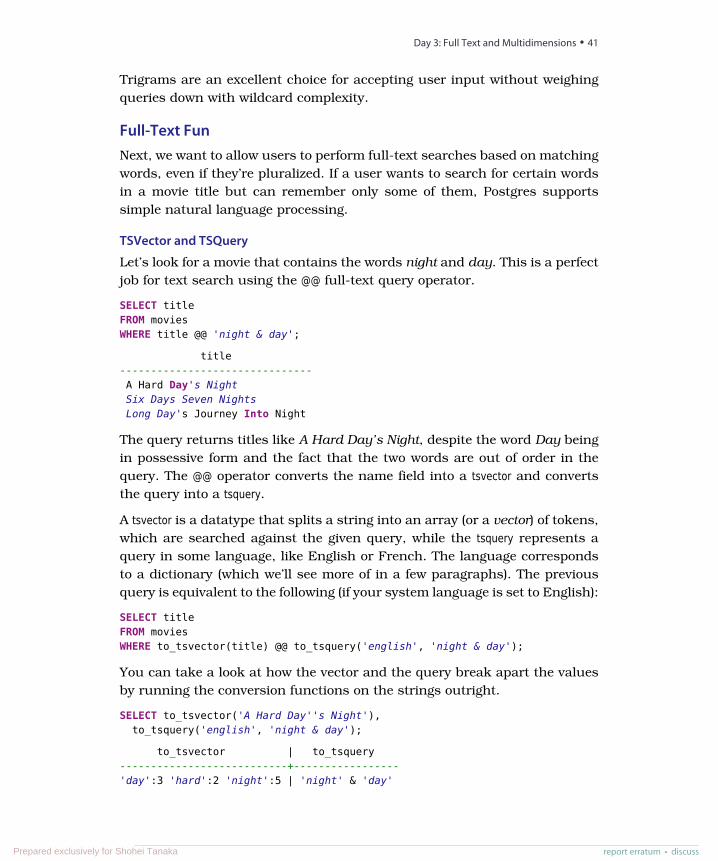
Trigrams are an excellent choice for accepting user input without weighingqueries down with wildcard complexity.
Full-Text FunNext, we want to allow users to perform full-text searches based on matchingwords, even if they’re pluralized. If a user wants to search for certain wordsin a movie title but can remember only some of them, Postgres supportssimple natural language processing.
TSVector and TSQuery
Let’s look for a movie that contains the words night and day. This is a perfectjob for text search using the @@ full-text query operator.
SELECT titleFROM moviesWHERE title @@ 'night & day';
title-------------------------------A Hard Day's NightSix Days Seven NightsLong Day's Journey Into Night
The query returns titles like A Hard Day’s Night, despite the word Day beingin possessive form and the fact that the two words are out of order in thequery. The @@ operator converts the name field into a tsvector and convertsthe query into a tsquery.
A tsvector is a datatype that splits a string into an array (or a vector) of tokens,which are searched against the given query, while the tsquery represents aquery in some language, like English or French. The language correspondsto a dictionary (which we’ll see more of in a few paragraphs). The previousquery is equivalent to the following (if your system language is set to English):
SELECT titleFROM moviesWHERE to_tsvector(title) @@ to_tsquery('english', 'night & day');
You can take a look at how the vector and the query break apart the valuesby running the conversion functions on the strings outright.
SELECT to_tsvector('A Hard Day''s Night'),to_tsquery('english', 'night & day');
to_tsvector | to_tsquery---------------------------+-----------------'day':3 'hard':2 'night':5 | 'night' & 'day'
report erratum • discuss
Day 3: Full Text and Multidimensions • 41
Prepared exclusively for Shohei Tanaka
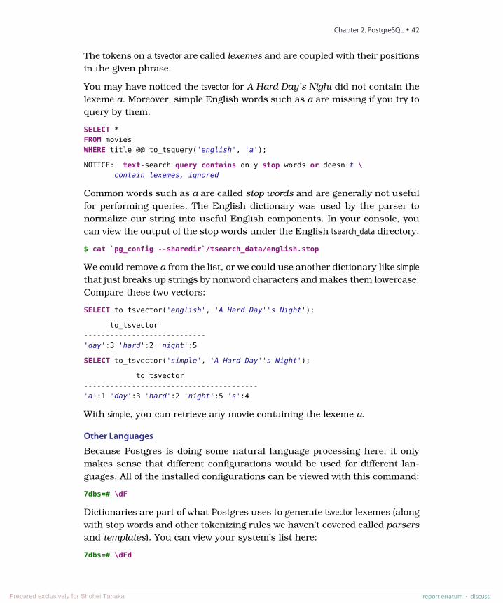
The tokens on a tsvector are called lexemes and are coupled with their positionsin the given phrase.
You may have noticed the tsvector for A Hard Day’s Night did not contain thelexeme a. Moreover, simple English words such as a are missing if you try toquery by them.
SELECT *FROM moviesWHERE title @@ to_tsquery('english', 'a');
NOTICE: text-search query contains only stop words or doesn't \contain lexemes, ignored
Common words such as a are called stop words and are generally not usefulfor performing queries. The English dictionary was used by the parser tonormalize our string into useful English components. In your console, youcan view the output of the stop words under the English tsearch_data directory.
$ cat `pg_config --sharedir`/tsearch_data/english.stop
We could remove a from the list, or we could use another dictionary like simplethat just breaks up strings by nonword characters and makes them lowercase.Compare these two vectors:
SELECT to_tsvector('english', 'A Hard Day''s Night');
to_tsvector----------------------------'day':3 'hard':2 'night':5
SELECT to_tsvector('simple', 'A Hard Day''s Night');
to_tsvector----------------------------------------'a':1 'day':3 'hard':2 'night':5 's':4
With simple, you can retrieve any movie containing the lexeme a.
Other Languages
Because Postgres is doing some natural language processing here, it onlymakes sense that different configurations would be used for different lan-guages. All of the installed configurations can be viewed with this command:
7dbs=# \dF
Dictionaries are part of what Postgres uses to generate tsvector lexemes (alongwith stop words and other tokenizing rules we haven’t covered called parsersand templates). You can view your system’s list here:
7dbs=# \dFd
Chapter 2. PostgreSQL • 42
report erratum • discussPrepared exclusively for Shohei Tanaka
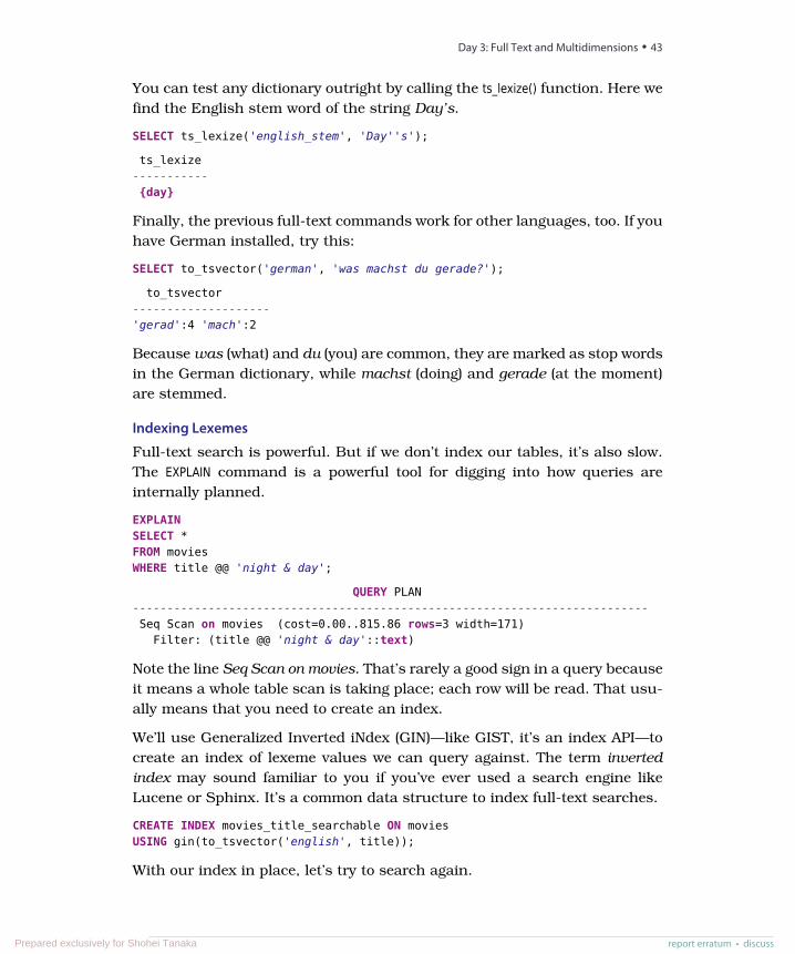
You can test any dictionary outright by calling the ts_lexize() function. Here wefind the English stem word of the string Day’s.
SELECT ts_lexize('english_stem', 'Day''s');
ts_lexize-----------{day}
Finally, the previous full-text commands work for other languages, too. If youhave German installed, try this:
SELECT to_tsvector('german', 'was machst du gerade?');
to_tsvector--------------------'gerad':4 'mach':2
Because was (what) and du (you) are common, they are marked as stop wordsin the German dictionary, while machst (doing) and gerade (at the moment)are stemmed.
Indexing Lexemes
Full-text search is powerful. But if we don’t index our tables, it’s also slow.The EXPLAIN command is a powerful tool for digging into how queries areinternally planned.
EXPLAINSELECT *FROM moviesWHERE title @@ 'night & day';
QUERY PLAN---------------------------------------------------------------------------Seq Scan on movies (cost=0.00..815.86 rows=3 width=171)
Filter: (title @@ 'night & day'::text)
Note the line Seq Scan on movies. That’s rarely a good sign in a query becauseit means a whole table scan is taking place; each row will be read. That usu-ally means that you need to create an index.
We’ll use Generalized Inverted iNdex (GIN)—like GIST, it’s an index API—tocreate an index of lexeme values we can query against. The term invertedindex may sound familiar to you if you’ve ever used a search engine likeLucene or Sphinx. It’s a common data structure to index full-text searches.
CREATE INDEX movies_title_searchable ON moviesUSING gin(to_tsvector('english', title));
With our index in place, let’s try to search again.
report erratum • discuss
Day 3: Full Text and Multidimensions • 43
Prepared exclusively for Shohei Tanaka
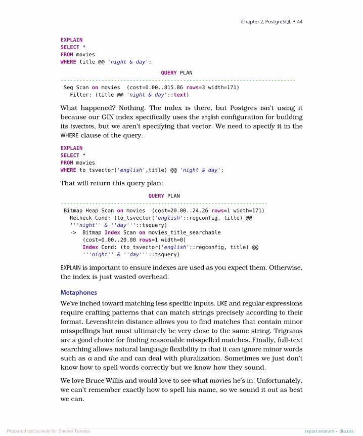
EXPLAINSELECT *FROM moviesWHERE title @@ 'night & day';
QUERY PLAN---------------------------------------------------------------------------Seq Scan on movies (cost=0.00..815.86 rows=3 width=171)
Filter: (title @@ 'night & day'::text)
What happened? Nothing. The index is there, but Postgres isn’t using itbecause our GIN index specifically uses the english configuration for buildingits tsvectors, but we aren’t specifying that vector. We need to specify it in theWHERE clause of the query.
EXPLAINSELECT *FROM moviesWHERE to_tsvector('english',title) @@ 'night & day';
That will return this query plan:
QUERY PLAN------------------------------------------------------------------Bitmap Heap Scan on movies (cost=20.00..24.26 rows=1 width=171)
Recheck Cond: (to_tsvector('english'::regconfig, title) @@'''night'' & ''day'''::tsquery)-> Bitmap Index Scan on movies_title_searchable
(cost=0.00..20.00 rows=1 width=0)Index Cond: (to_tsvector('english'::regconfig, title) @@'''night'' & ''day'''::tsquery)
EXPLAIN is important to ensure indexes are used as you expect them. Otherwise,the index is just wasted overhead.
Metaphones
We’ve inched toward matching less specific inputs. LIKE and regular expressionsrequire crafting patterns that can match strings precisely according to theirformat. Levenshtein distance allows you to find matches that contain minormisspellings but must ultimately be very close to the same string. Trigramsare a good choice for finding reasonable misspelled matches. Finally, full-textsearching allows natural language flexibility in that it can ignore minor wordssuch as a and the and can deal with pluralization. Sometimes we just don’tknow how to spell words correctly but we know how they sound.
We love Bruce Willis and would love to see what movies he’s in. Unfortunately,we can’t remember exactly how to spell his name, so we sound it out as bestwe can.
Chapter 2. PostgreSQL • 44
report erratum • discussPrepared exclusively for Shohei Tanaka
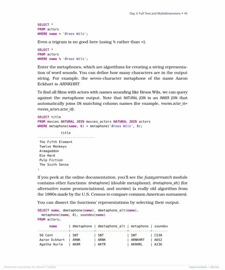
SELECT *FROM actorsWHERE name = 'Broos Wils';
Even a trigram is no good here (using % rather than =).
SELECT *FROM actorsWHERE name % 'Broos Wils';
Enter the metaphones, which are algorithms for creating a string representa-tion of word sounds. You can define how many characters are in the outputstring. For example, the seven-character metaphone of the name AaronEckhart is ARNKHRT.
To find all films with actors with names sounding like Broos Wils, we can queryagainst the metaphone output. Note that NATURAL JOIN is an INNER JOIN thatautomatically joins ON matching column names (for example, movies.actor_id=movies_actors.actor_id).
SELECT titleFROM movies NATURAL JOIN movies_actors NATURAL JOIN actorsWHERE metaphone(name, 6) = metaphone('Broos Wils', 6);
title-----------------------------The Fifth ElementTwelve MonkeysArmageddonDie HardPulp FictionThe Sixth Sense
:
If you peek at the online documentation, you’ll see the fuzzystrmatch modulecontains other functions: dmetaphone() (double metaphone), dmetaphone_alt() (foralternative name pronunciations), and soundex() (a really old algorithm fromthe 1880s made by the U.S. Census to compare common American surnames).
You can dissect the functions’ representations by selecting their output.
SELECT name, dmetaphone(name), dmetaphone_alt(name),metaphone(name, 8), soundex(name)
FROM actors;
name | dmetaphone | dmetaphone_alt | metaphone | soundex----------------+------------+----------------+-----------+--------50 Cent | SNT | SNT | SNT | C530Aaron Eckhart | ARNK | ARNK | ARNKHRT | A652Agatha Hurle | AK0R | AKTR | AK0HRL | A236
report erratum • discuss
Day 3: Full Text and Multidimensions • 45
Prepared exclusively for Shohei Tanaka
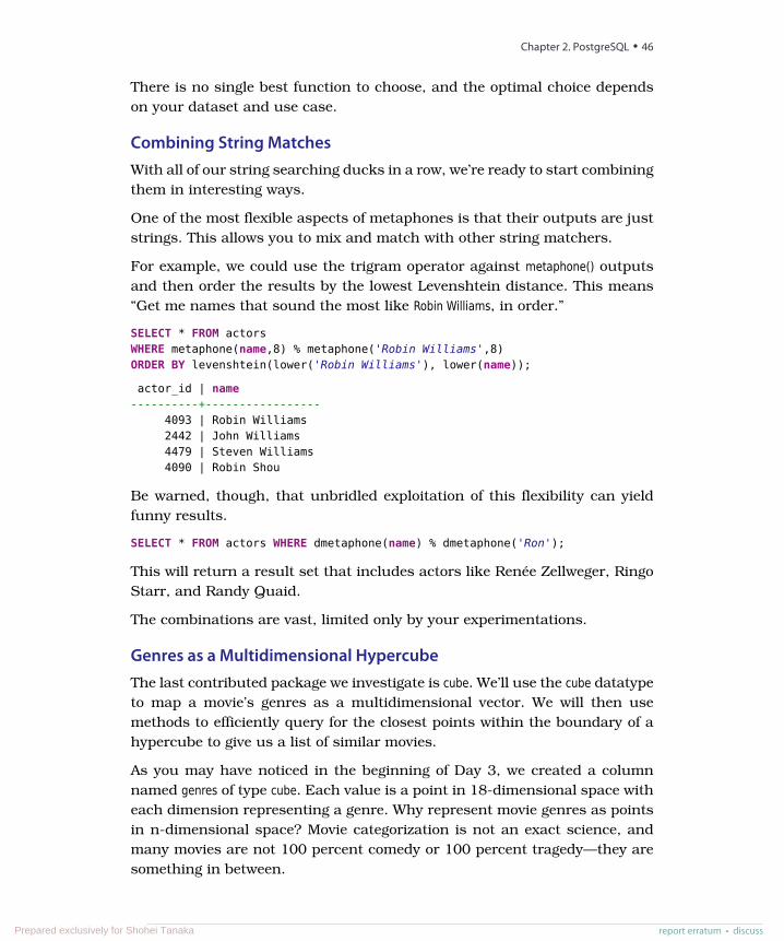
There is no single best function to choose, and the optimal choice dependson your dataset and use case.
Combining String MatchesWith all of our string searching ducks in a row, we’re ready to start combiningthem in interesting ways.
One of the most flexible aspects of metaphones is that their outputs are juststrings. This allows you to mix and match with other string matchers.
For example, we could use the trigram operator against metaphone() outputsand then order the results by the lowest Levenshtein distance. This means“Get me names that sound the most like Robin Williams, in order.”
SELECT * FROM actorsWHERE metaphone(name,8) % metaphone('Robin Williams',8)ORDER BY levenshtein(lower('Robin Williams'), lower(name));
actor_id | name----------+-----------------
4093 | Robin Williams2442 | John Williams4479 | Steven Williams4090 | Robin Shou
Be warned, though, that unbridled exploitation of this flexibility can yieldfunny results.
SELECT * FROM actors WHERE dmetaphone(name) % dmetaphone('Ron');
This will return a result set that includes actors like Renée Zellweger, RingoStarr, and Randy Quaid.
The combinations are vast, limited only by your experimentations.
Genres as a Multidimensional HypercubeThe last contributed package we investigate is cube. We’ll use the cube datatypeto map a movie’s genres as a multidimensional vector. We will then usemethods to efficiently query for the closest points within the boundary of ahypercube to give us a list of similar movies.
As you may have noticed in the beginning of Day 3, we created a columnnamed genres of type cube. Each value is a point in 18-dimensional space witheach dimension representing a genre. Why represent movie genres as pointsin n-dimensional space? Movie categorization is not an exact science, andmany movies are not 100 percent comedy or 100 percent tragedy—they aresomething in between.
Chapter 2. PostgreSQL • 46
report erratum • discussPrepared exclusively for Shohei Tanaka
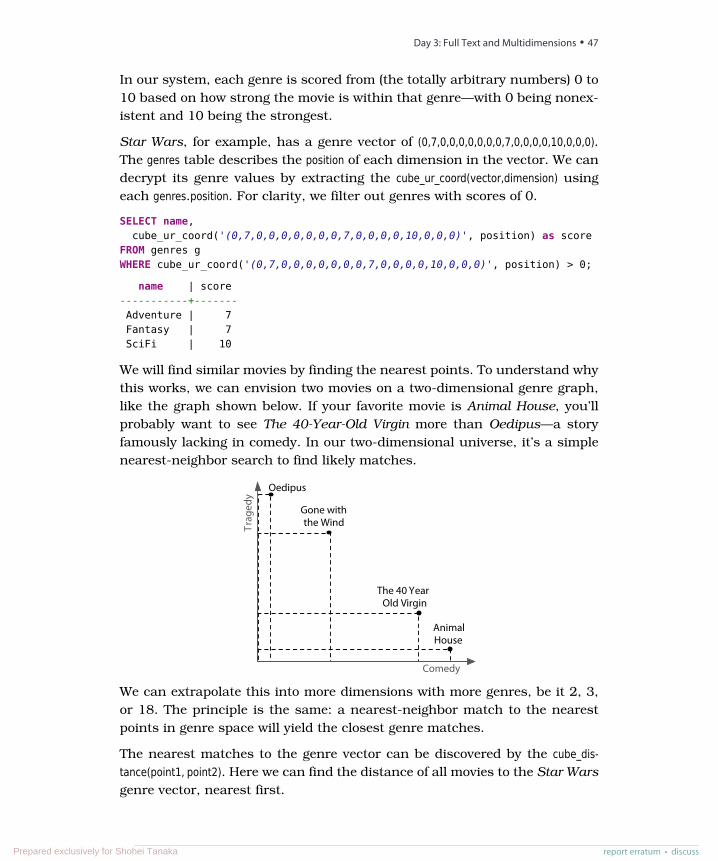
In our system, each genre is scored from (the totally arbitrary numbers) 0 to10 based on how strong the movie is within that genre—with 0 being nonex-istent and 10 being the strongest.
Star Wars, for example, has a genre vector of (0,7,0,0,0,0,0,0,0,7,0,0,0,0,10,0,0,0).The genres table describes the position of each dimension in the vector. We candecrypt its genre values by extracting the cube_ur_coord(vector,dimension) usingeach genres.position. For clarity, we filter out genres with scores of 0.
SELECT name,cube_ur_coord('(0,7,0,0,0,0,0,0,0,7,0,0,0,0,10,0,0,0)', position) as score
FROM genres gWHERE cube_ur_coord('(0,7,0,0,0,0,0,0,0,7,0,0,0,0,10,0,0,0)', position) > 0;
name | score-----------+-------Adventure | 7Fantasy | 7SciFi | 10
We will find similar movies by finding the nearest points. To understand whythis works, we can envision two movies on a two-dimensional genre graph,like the graph shown below. If your favorite movie is Animal House, you’llprobably want to see The 40-Year-Old Virgin more than Oedipus—a storyfamously lacking in comedy. In our two-dimensional universe, it’s a simplenearest-neighbor search to find likely matches.
Trag
edy
Comedy
Oedipus
The 40 YearOld Virgin
Gone withthe Wind
AnimalHouse
We can extrapolate this into more dimensions with more genres, be it 2, 3,or 18. The principle is the same: a nearest-neighbor match to the nearestpoints in genre space will yield the closest genre matches.
The nearest matches to the genre vector can be discovered by the cube_dis-tance(point1, point2). Here we can find the distance of all movies to the Star Warsgenre vector, nearest first.
report erratum • discuss
Day 3: Full Text and Multidimensions • 47
Prepared exclusively for Shohei Tanaka
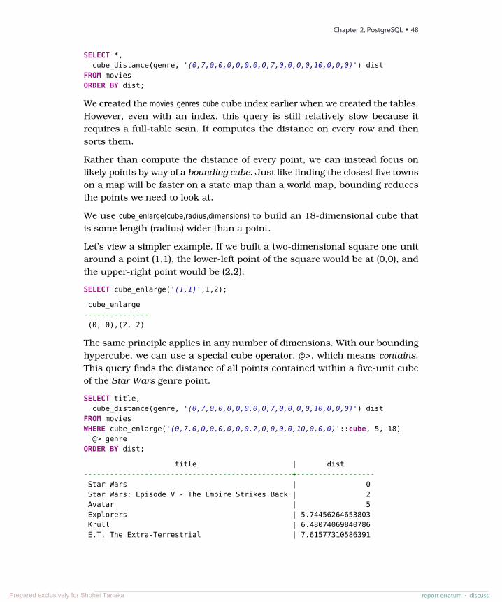
SELECT *,cube_distance(genre, '(0,7,0,0,0,0,0,0,0,7,0,0,0,0,10,0,0,0)') dist
FROM moviesORDER BY dist;
We created the movies_genres_cube cube index earlier when we created the tables.However, even with an index, this query is still relatively slow because itrequires a full-table scan. It computes the distance on every row and thensorts them.
Rather than compute the distance of every point, we can instead focus onlikely points by way of a bounding cube. Just like finding the closest five townson a map will be faster on a state map than a world map, bounding reducesthe points we need to look at.
We use cube_enlarge(cube,radius,dimensions) to build an 18-dimensional cube thatis some length (radius) wider than a point.
Let’s view a simpler example. If we built a two-dimensional square one unitaround a point (1,1), the lower-left point of the square would be at (0,0), andthe upper-right point would be (2,2).
SELECT cube_enlarge('(1,1)',1,2);
cube_enlarge---------------(0, 0),(2, 2)
The same principle applies in any number of dimensions. With our boundinghypercube, we can use a special cube operator, @>, which means contains.This query finds the distance of all points contained within a five-unit cubeof the Star Wars genre point.
SELECT title,cube_distance(genre, '(0,7,0,0,0,0,0,0,0,7,0,0,0,0,10,0,0,0)') dist
FROM moviesWHERE cube_enlarge('(0,7,0,0,0,0,0,0,0,7,0,0,0,0,10,0,0,0)'::cube, 5, 18)
@> genreORDER BY dist;
title | dist------------------------------------------------+------------------Star Wars | 0Star Wars: Episode V - The Empire Strikes Back | 2Avatar | 5Explorers | 5.74456264653803Krull | 6.48074069840786E.T. The Extra-Terrestrial | 7.61577310586391
Chapter 2. PostgreSQL • 48
report erratum • discussPrepared exclusively for Shohei Tanaka
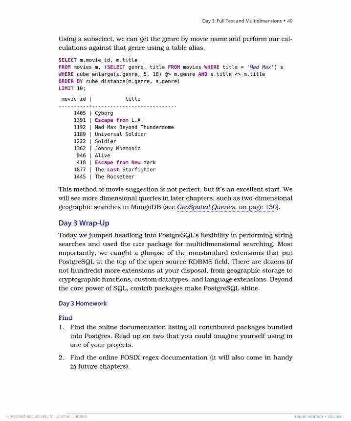
Using a subselect, we can get the genre by movie name and perform our cal-culations against that genre using a table alias.
SELECT m.movie_id, m.titleFROM movies m, (SELECT genre, title FROM movies WHERE title = 'Mad Max') sWHERE cube_enlarge(s.genre, 5, 18) @> m.genre AND s.title <> m.titleORDER BY cube_distance(m.genre, s.genre)LIMIT 10;
movie_id | title----------+----------------------------
1405 | Cyborg1391 | Escape from L.A.1192 | Mad Max Beyond Thunderdome1189 | Universal Soldier1222 | Soldier1362 | Johnny Mnemonic946 | Alive418 | Escape from New York
1877 | The Last Starfighter1445 | The Rocketeer
This method of movie suggestion is not perfect, but it’s an excellent start. Wewill see more dimensional queries in later chapters, such as two-dimensionalgeographic searches in MongoDB (see GeoSpatial Queries, on page 130).
Day 3 Wrap-UpToday we jumped headlong into PostgreSQL’s flexibility in performing stringsearches and used the cube package for multidimensional searching. Mostimportantly, we caught a glimpse of the nonstandard extensions that putPostgreSQL at the top of the open source RDBMS field. There are dozens (ifnot hundreds) more extensions at your disposal, from geographic storage tocryptographic functions, custom datatypes, and language extensions. Beyondthe core power of SQL, contrib packages make PostgreSQL shine.
Day 3 Homework
Find
1. Find the online documentation listing all contributed packages bundledinto Postgres. Read up on two that you could imagine yourself using inone of your projects.
2. Find the online POSIX regex documentation (it will also come in handyin future chapters).
report erratum • discuss
Day 3: Full Text and Multidimensions • 49
Prepared exclusively for Shohei Tanaka
Do
1. Create a stored procedure that enables you to input a movie title or anactor’s name and then receive the top five suggestions based on eithermovies the actor has starred in or films with similar genres.
2. Expand the movies database to track user comments and extract keywords(minus English stopwords). Cross-reference these keywords with actors’last names and try to find the most talked-about actors.
Wrap-UpIf you haven’t spent much time with relational databases, we highly recom-mend digging deeper into PostgreSQL, or another relational database, beforedeciding to scrap it for a newer variety. Relational databases have been thefocus of intense academic research and industrial improvements for morethan forty years, and PostgreSQL is one of the top open source relationaldatabases to benefit from these advancements.
PostgreSQL’s StrengthsPostgreSQL’s strengths are as numerous as any relational model: years ofresearch and production use across nearly every field of computing, flexiblequeryability, and very consistent and durable data. Most programming lan-guages have battle-tested driver support for Postgres, and many programmingmodels, like object-relational mapping (ORM), assume an underlying relationaldatabase.
But the real crux of the matter is the flexibility of the join. You don’t need toknow how you plan to actually query your model because you can alwaysperform some joins, filters, views, and indexes—odds are good that you willalways have the ability to extract the data you want. In the other chapters ofthis book that assumption will more or less fly out the window.
Chapter 2. PostgreSQL • 50
report erratum • discussPrepared exclusively for Shohei Tanaka
PostgreSQL is fantastic for what we call “Stepford data” (named for TheStepford Wives, a story about a neighborhood where nearly everyone wasconsistent in style and substance), which is data that is fairly homogeneousand conforms well to a structured schema.
Furthermore, PostgreSQL goes beyond the normal open source RDBMSofferings, such as powerful schema constraint mechanisms. You can writeyour own language extensions, customize indexes, create custom datatypes,and even overwrite the parsing of incoming queries. And where other opensource databases may have complex licensing agreements, PostgreSQL isopen source in its purest form. No one owns the code. Anyone can do prettymuch anything they want with the project (other than hold authors liable).The development and distribution are completely community supported. Ifyou are a fan of free(dom) software, you have to respect their general resistanceto cashing in on an amazing product.
PostgreSQL’s WeaknessesAlthough relational databases have been undeniably the most successfulstyle of database over the years, there are cases where it may not be a great fit.
Postgres and JSON
Although we won‘t delve too deeply into it here given that we cover two other databasesin this book that were explicitly created to handle unstructured data, we‘d be remissin not mentioning that Postgres has offered support for JSON since version 9.3.Postgres offers two different formats for this: JSON and JSONB (the json and jsonbtypes, respectively). The crucial difference between them is that the json type storesJSON as text while jsonb stores JSON using a decomposed binary format; json is opti-mized for faster data input while jsonb is optimized for faster processing.
With Postgres, you can perform operations like this:
CREATE TABLE users (username TEXT,data JSON
);INSERT INTO users VALUES ('wadeboggs107', '{ "AVG": 0.328, "HR": 118, "H": 3010 }');SELECT data->>'AVG' AS lifetime_batting_average FROM users;
lifetime_batting_average--------------------------0.328
If your use case requires a mixture of structured and unstructured (or less structured)datatypes—or even requires only unstructured datatypes—then Postgres may providea solution.
report erratum • discuss
Wrap-Up • 51
Prepared exclusively for Shohei Tanaka
Partitioning is not one of the strengths of relational databases such as Post-greSQL. If you need to scale out rather than up—multiple parallel databasesrather than a single beefy machine or cluster—you may be better servedlooking elsewhere (although clustering capabilities have improved in recentreleases). Another database might be a better fit if:
• You don’t truly require the overhead of a full database (perhaps you onlyneed a cache like Redis).
• You require very high-volume reads and writes as key values.
• You need to store only large BLOBs of data.
Parting ThoughtsA relational database is an excellent choice for query flexibility. While Post-greSQL requires you to design your data up front, it makes no assumptionsabout how you use that data. As long as your schema is designed in a fairlynormalized way, without duplication or storage of computable values, youshould generally be all set for any queries you might need to create. And ifyou include the correct modules, tune your engine, and index well, it willperform amazingly well for multiple terabytes of data with very small resourceconsumption. Finally, to those for whom data safety is paramount, Post-greSQL’s ACID-compliant transactions ensure your commits are completelyatomic, consistent, isolated, and durable.
Chapter 2. PostgreSQL • 52
report erratum • discussPrepared exclusively for Shohei Tanaka
CHAPTER 3
HBaseApache HBase is made for big jobs, like a nail gun. You would never useHBase to catalog your corporate sales list or build a to-do list app for fun,just like you’d never use a nail gun to build a doll house. If the size of yourdataset isn’t many, many gigabytes at the very least then you should probablyuse a less heavy-duty tool.
At first glance, HBase looks a lot like a relational database, so much so thatif you didn’t know any better, you might think that it is one. In fact, the mostchallenging part of learning HBase isn’t the technology; it’s that many of thewords used in HBase are deceptively familiar. For example, HBase stores datain buckets it calls tables, which contain cells that appear at the intersectionof rows and columns. Sounds like a relational database, right?
Wrong! In HBase, tables don’t behave like relations, rows don’t act like records,and columns are completely variable and not enforced by any predefinedschema. Schema design is still important, of course, because it informs theperformance characteristics of the system, but it won’t keep your house inorder—that task falls to you and how your applications use HBase. In general,trying to shoehorn HBase into an RDBMS-style system is fraught with nothingbut peril and a certain path to frustration and failure. HBase is the evil twin,the bizarro doppelgänger, if you will, of RDBMS.
On top of that, unlike relational databases, which sometimes have troublescaling out, HBase doesn’t scale down. If your production HBase cluster hasfewer than five nodes, then, quite frankly, you’re doing it wrong. HBase is notthe right database for some problems, particularly those where the amountof data is measured in megabytes, or even in the low gigabytes.
So why would you use HBase? Aside from scalability, there are a few reasons.To begin with, HBase has some built-in features that other databases lack,
report erratum • discussPrepared exclusively for Shohei Tanaka
such as versioning, compression, garbage collection (for expired data), andin-memory tables. Having these features available right out of the box meansless code that you have to write when your requirements demand them. HBasealso makes strong consistency guarantees, making it easier to transition fromrelational databases for some use cases. Finally, HBase guarantees atomicityat the row level, which means that you can have strong consistency guaranteesat a crucial level of HBase’s data model.
For all of these reasons, HBase really shines as the cornerstone of a large-scale online analytics processing system. While individual operations maysometimes be slower than equivalent operations in other databases, scanningthrough enormous datasets is an area where HBase truly excels. For genuinelybig queries, HBase often outpaces other databases, which helps to explainwhy HBase is often used at big companies to back heavy-duty logging andsearch systems.
Introducing HBaseHBase is a column-oriented database that prides itself on its ability to provideboth consistency and scalability. It is based on Bigtable, a high-performance,proprietary database developed by Google and described in the 2006 whitepaper “Bigtable: A Distributed Storage System for Structured Data.”1 Initiallycreated for natural language processing, HBase started life as a contribpackage for Apache Hadoop. Since then, it has become a top-level Apacheproject.
Luc says:
Hosted HBase with Google Cloud BigtableAs you’ll see later in this chapter, HBase can be tricky to administer. Fortunately,there’s now a compelling option for those who want to utilize the power of HBase withvery little operational burden: Google’s Cloud Bigtable, which is part of its CloudPlatform suite of products. Cloud Bigtable isn’t 100% compatible with HBase but asof early 2018 it’s very close—close enough that you may be able to migrate manyexisting HBase applications over.
If you find the basic value proposition of, for example, Amazon’s cloud-basedDynamoDB compelling and you think HBase is a good fit for a project, then CloudBigtable might be worth checking out. You can at least be assured that it’s run bythe same company that crafted the concepts behind HBase (and the folks at Googledo seem to know a thing or two about scale).
1. http://research.google.com/archive/bigtable.html
Chapter 3. HBase • 54
report erratum • discussPrepared exclusively for Shohei Tanaka
On the architecture front, HBase is designed to be fault tolerant. Hardwarefailures may be uncommon in individual machines but, in large clusters,node failure is the norm (as are network issues). HBase can gracefullyrecover from individual server failures because it uses both write-ahead log-ging, which writes data to an in-memory log before it’s written (so that nodescan use the log for recovery rather than disk), and distributed configuration,which means that nodes can rely on each other for configuration rather thanon a centralized source.
Additionally, HBase lives in the Hadoop ecosystem, where it benefits from itsproximity to other related tools. Hadoop is a sturdy, scalable computing platformthat provides a distributed file system and MapReduce capabilities. Whereveryou find HBase, you’ll find Hadoop and other infrastructural components thatyou can use in your own applications, such as Apache Hive, a data warehousingtool, and Apache Pig, a parallel processing tool (and many others).
Finally, HBase is actively used and developed by a number of high-profilecompanies for their “Big Data” problems. Notably, Facebook uses HBase fora variety of purposes, including for Messages, search indexing, and streamanalysis. Twitter uses it to power its people search capability, for monitoringand performance data, and more. Airbnb uses it as part of their realtimestream processing stack. Apple uses it for...something, though they won‘tpublicly say what. The parade of companies using HBase also includes thelikes of eBay, Meetup, Ning, Yahoo!, and many others.
With all of this activity, new versions of HBase are coming out at a fairly rapidclip. At the time of this writing, the current stable version is 1.2.1, so that’swhat you’ll be using. Go ahead and download HBase, and we’ll get started.
Day 1: CRUD and Table AdministrationToday’s goal is to learn the nuts and bolts of working with HBase. You’ll geta local instance of HBase running in standalone mode (rather than in dis-tributed mode), and then you’ll use the HBase shell to create and alter tablesand to insert and modify data using basic CRUD-style commands. After that,you’ll explore how to perform some of those operations programmatically byusing the HBase Java API in JRuby. Along the way, you’ll uncover some HBasearchitectural concepts, such as the relationship between rows, column fami-lies, columns, and values in a table. Just bear in mind that these conceptsin HBase are subtly different from their counterparts in relational databases.
According to most HBase admins out there, a fully operational, production-quality HBase cluster should really consist of no fewer than five nodes. But
report erratum • discuss
Day 1: CRUD and Table Administration • 55
Prepared exclusively for Shohei Tanaka

this bulky of a setup would be overkill for our needs (and for our laptops).Fortunately, HBase supports three running modes:
• Standalone mode is a single machine acting alone.• Pseudo-distributed mode is a single node pretending to be a cluster.• Fully distributed mode is a cluster of nodes working together.
For most of this chapter, you’ll be running HBase in standalone mode. Yeteven that can be a bit of a challenge, especially compared to other databasesin this book, such as Redis or MongoDB. So although we won’t cover everyaspect of installation and administration, we’ll give some relevant troubleshoot-ing tips where appropriate.
Configuring HBaseBefore you can use HBase, you need to provide it with some configuration,as HBase doesn’t really have an “out-of-the-box” mode. Configuration settingsfor HBase are kept in a file called hbase-site.xml, which can be found in the${HBASE_HOME}/ conf directory. Note that HBASE_HOME is an environment variablepointing to the directory where you’ve installed HBase. Make sure to set thisvariable now, preferably in your .bash_profile or similar file so that it persistsacross shell sessions.
Initially, this hbase-site.xml file contains just an empty <configuration> tag. You canadd any number of property definitions to your configuration using this format:
<property><name>some.property.name</name><value>A property value</value>
</property>
The hbase-default.xml File
Another way of installing HBase is to clone the project directory locally using Git,either from the Apache repository at http://git.apache.org/hbase.git or from the mirrorrepository on GitHub at https://github.com/apache/hbase.
If you install HBase this way, you’ll find an hbase-default.xml file in the hbase-com-mon/src/main/resources subdirectory. This is a very handy file that lists all of the availableconfigurable parameters for HBase—and there are many!—along with default valuesand descriptions for each parameter.
You can also see the contents of this file in your browser on GitHub.a
a. https://github.com/apache/hbase/blob/master/hbase-common/src/main/resources/hbase-default.xml
Chapter 3. HBase • 56
report erratum • discussPrepared exclusively for Shohei Tanaka
By default, HBase uses a temporary directory to store its data files. Thismeans you’ll lose all your data whenever the operating system decides toreclaim the disk space. To keep your data around, you should specify a non-ephemeral storage location. Set the hbase.rootdir property to an appropriatepath like so:
<property><name>hbase.rootdir</name><value>file:///path/to/hbase</value>
</property>
Here’s an example configuration:
<property><name>hbase.rootdir</name><value>file://</value>
</property>
To start HBase, open a terminal (command prompt) and run this command:
$ ${HBASE_HOME}/bin/start-hbase.sh
To shut down HBase at any time, use the stop-hbase.sh command in the samedirectory.
If anything goes wrong, take a look at the most recently modified files in the${HBASE_HOME}/logs directory. On *nix-based systems, the following commandwill pipe the latest log data to the console as it’s written:
$ cd ${HBASE_HOME}$ find ./logs -name "hbase-*.log" -exec tail -f {} \;
The HBase ShellThe HBase shell is a JRuby-based command-line program you can use to interactwith HBase. In the shell, you can add and remove tables, alter table schemas,add or delete data, and perform a bunch of other tasks. Later, we’ll exploreother means of connecting to HBase, but for now the shell will be our home.
With HBase running, open a terminal and fire up the HBase shell:
$ ${HBASE_HOME}/bin/hbase shell
To confirm that it’s working properly, try asking it for version information.That should output a version number and hash, and a timestamp for whenthe version was released.
hbase> version1.2.1, r8d8a7107dc4ccbf36a92f64675dc60392f85c015, Wed Mar 30 11:19:21 CDT 2016
report erratum • discuss
Day 1: CRUD and Table Administration • 57
Prepared exclusively for Shohei Tanaka
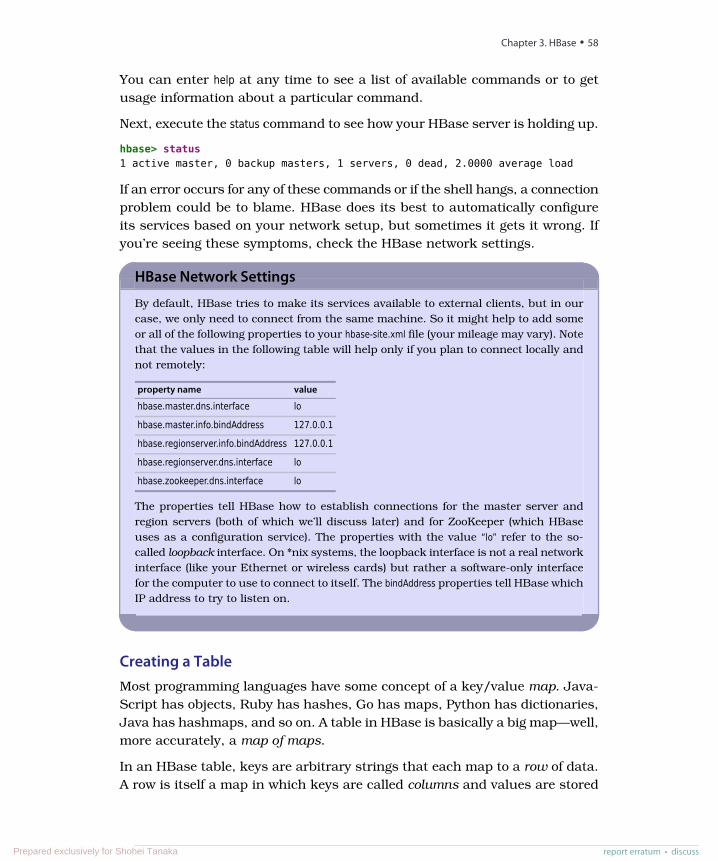
You can enter help at any time to see a list of available commands or to getusage information about a particular command.
Next, execute the status command to see how your HBase server is holding up.
hbase> status1 active master, 0 backup masters, 1 servers, 0 dead, 2.0000 average load
If an error occurs for any of these commands or if the shell hangs, a connectionproblem could be to blame. HBase does its best to automatically configureits services based on your network setup, but sometimes it gets it wrong. Ifyou’re seeing these symptoms, check the HBase network settings.
HBase Network Settings
By default, HBase tries to make its services available to external clients, but in ourcase, we only need to connect from the same machine. So it might help to add someor all of the following properties to your hbase-site.xml file (your mileage may vary). Notethat the values in the following table will help only if you plan to connect locally andnot remotely:
valueproperty name
lohbase.master.dns.interface
127.0.0.1hbase.master.info.bindAddress
127.0.0.1hbase.regionserver.info.bindAddress
lohbase.regionserver.dns.interface
lohbase.zookeeper.dns.interface
The properties tell HBase how to establish connections for the master server andregion servers (both of which we’ll discuss later) and for ZooKeeper (which HBaseuses as a configuration service). The properties with the value “lo” refer to the so-called loopback interface. On *nix systems, the loopback interface is not a real networkinterface (like your Ethernet or wireless cards) but rather a software-only interfacefor the computer to use to connect to itself. The bindAddress properties tell HBase whichIP address to try to listen on.
Creating a TableMost programming languages have some concept of a key/value map. Java-Script has objects, Ruby has hashes, Go has maps, Python has dictionaries,Java has hashmaps, and so on. A table in HBase is basically a big map—well,more accurately, a map of maps.
In an HBase table, keys are arbitrary strings that each map to a row of data.A row is itself a map in which keys are called columns and values are stored
Chapter 3. HBase • 58
report erratum • discussPrepared exclusively for Shohei Tanaka
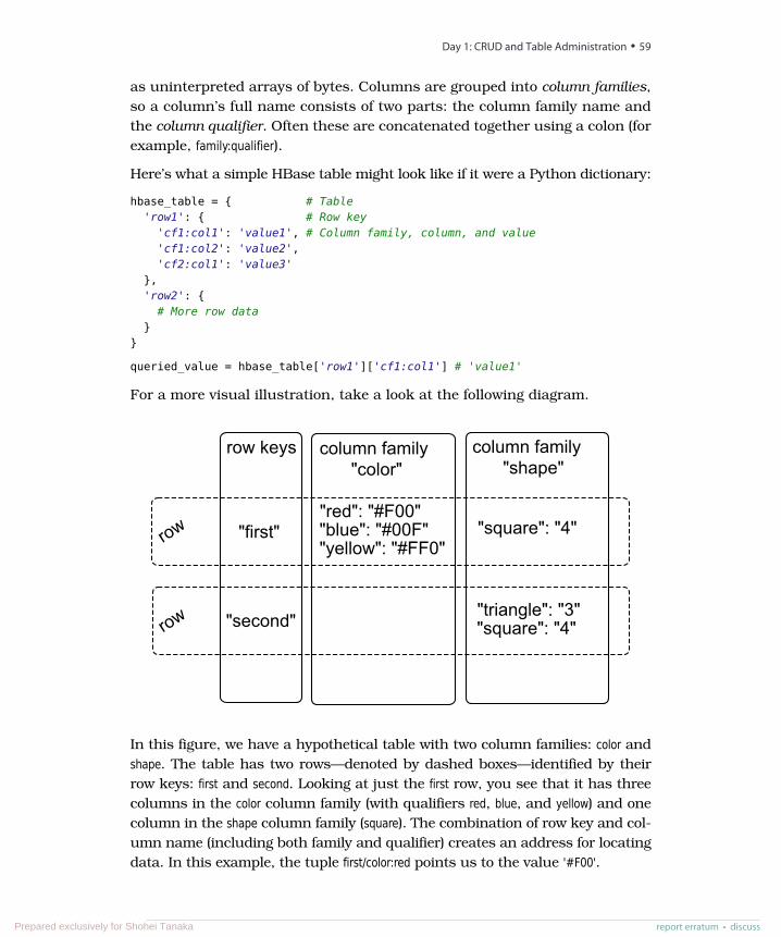
as uninterpreted arrays of bytes. Columns are grouped into column families,so a column’s full name consists of two parts: the column family name andthe column qualifier. Often these are concatenated together using a colon (forexample, family:qualifier).
Here’s what a simple HBase table might look like if it were a Python dictionary:
hbase_table = { # Table'row1': { # Row key
'cf1:col1': 'value1', # Column family, column, and value'cf1:col2': 'value2','cf2:col1': 'value3'
},'row2': {
# More row data}
}
queried_value = hbase_table['row1']['cf1:col1'] # 'value1'
For a more visual illustration, take a look at the following diagram.
row keys column family column family
"first""red": "#F00""blue": "#00F""yellow": "#FF0"
"square": "4"
"second""triangle": "3""square": "4"
row
row
"color" "shape"
In this figure, we have a hypothetical table with two column families: color andshape. The table has two rows—denoted by dashed boxes—identified by theirrow keys: first and second. Looking at just the first row, you see that it has threecolumns in the color column family (with qualifiers red, blue, and yellow) and onecolumn in the shape column family (square). The combination of row key and col-umn name (including both family and qualifier) creates an address for locatingdata. In this example, the tuple first/color:red points us to the value '#F00'.
report erratum • discuss
Day 1: CRUD and Table Administration • 59
Prepared exclusively for Shohei Tanaka
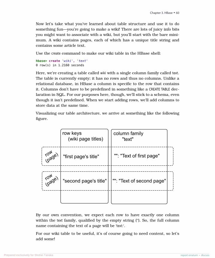
Now let’s take what you’ve learned about table structure and use it to dosomething fun—you’re going to make a wiki! There are lots of juicy info bitsyou might want to associate with a wiki, but you’ll start with the bare mini-mum. A wiki contains pages, each of which has a unique title string andcontains some article text.
Use the create command to make our wiki table in the HBase shell:
hbase> create 'wiki', 'text'0 row(s) in 1.2160 seconds
Here, we’re creating a table called wiki with a single column family called text.The table is currently empty; it has no rows and thus no columns. Unlike arelational database, in HBase a column is specific to the row that containsit. Columns don’t have to be predefined in something like a CREATE TABLE dec-laration in SQL. For our purposes here, though, we’ll stick to a schema, eventhough it isn’t predefined. When we start adding rows, we’ll add columns tostore data at the same time.
Visualizing our table architecture, we arrive at something like the followingfigure.
row keys column family
"first page's title" "": "Text of first page"
"second page's title"
row
"text"(wiki page titles)
(page)
row
(page)"": "Text of second page"
By our own convention, we expect each row to have exactly one columnwithin the text family, qualified by the empty string (''). So, the full columnname containing the text of a page will be 'text:'.
For our wiki table to be useful, it’s of course going to need content, so let’sadd some!
Chapter 3. HBase • 60
report erratum • discussPrepared exclusively for Shohei Tanaka

Inserting, Updating, and Retrieving DataOur wiki needs a Home page, so we’ll start with that. To add data to an HBasetable, use the put command:
hbase> put 'wiki', 'Home', 'text:', 'Welcome to the wiki!'
This command inserts a new row into the wiki table with the key 'Home', adding'Welcome to the wiki!' to the column called 'text:'. Note the colon at the end of thecolumn name. This is actually a requirement in HBase if you don’t specifya column family in addition to a column (in this case, you’re specifying nocolumn family).
We can query the data for the 'Home' row using get, which requires two param-eters: the table name and the row key. You can optionally specify a list ofcolumns to return. Here, we’ll fetch the value of the text: column:
hbase> get 'wiki', 'Home', 'text:'COLUMN CELLtext: timestamp=1295774833226, value=Welcome to the wiki!
1 row(s) in 0.0590 seconds
Notice the timestamp field in the output. HBase stores an integer timestampfor all data values, representing time in milliseconds since the epoch (00:00:00UTC on January 1, 1970). When a new value is written to the same cell, theold value hangs around, indexed by its timestamp. This is a pretty awesomefeature, and one that is unique to HBase amongst the databases in this book.Most databases require you to specifically handle historical data yourself,but in HBase, versioning is baked right in!
Finally, let’s perform a scan operation:
hbase> scan 'wiki'
Scan operations simply return all rows in the entire table. Scans are powerfuland great for development purposes but they are also a very blunt instrument,so use them with care. We don’t have much data in our wiki table so it’s per-fectly fine, but if you’re running HBase in production, stick to more precisereads or you’ll put a lot of undue strain on your tables.
Putting and GettingThe put and get commands allow you to specify a timestamp explicitly. If usingmilliseconds since the epoch doesn’t strike your fancy, you can specify anotherinteger value of your choice. This gives you an extra dimension to work with ifyou need it. If you don’t specify a timestamp, HBase will use the current timewhen inserting, and it will return the most recent version when reading.
report erratum • discuss
Day 1: CRUD and Table Administration • 61
Prepared exclusively for Shohei Tanaka
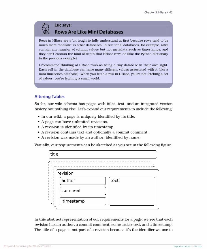
Luc says:
Rows Are Like Mini DatabasesRows in HBase are a bit tough to fully understand at first because rows tend to bemuch more “shallow” in other databases. In relational databases, for example, rowscontain any number of column values but not metadata such as timestamps, andthey don’t contain the kind of depth that HBase rows do (like the Python dictionaryin the previous example).
I recommend thinking of HBase rows as being a tiny database in their own right.Each cell in the database can have many different values associated with it (like amini timeseries database). When you fetch a row in HBase, you’re not fetching a setof values; you’re fetching a small world.
Altering TablesSo far, our wiki schema has pages with titles, text, and an integrated versionhistory but nothing else. Let’s expand our requirements to include the following:
• In our wiki, a page is uniquely identified by its title.• A page can have unlimited revisions.• A revision is identified by its timestamp.• A revision contains text and optionally a commit comment.• A revision was made by an author, identified by name.
Visually, our requirements can be sketched as you see in the following figure.
In this abstract representation of our requirements for a page, we see that eachrevision has an author, a commit comment, some article text, and a timestamp.The title of a page is not part of a revision because it’s the identifier we use to
Chapter 3. HBase • 62
report erratum • discussPrepared exclusively for Shohei Tanaka
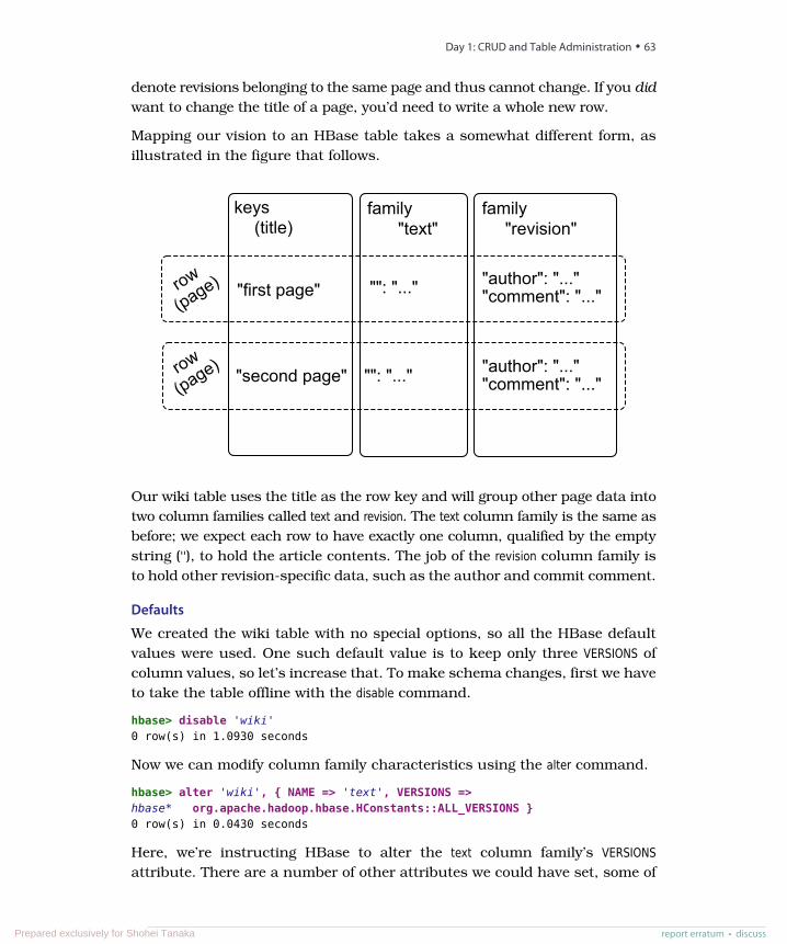
denote revisions belonging to the same page and thus cannot change. If you didwant to change the title of a page, you’d need to write a whole new row.
Mapping our vision to an HBase table takes a somewhat different form, asillustrated in the figure that follows.
keys family
"first page" "": "..."
"second page"
row
"text"(title)
(page)
row
(page)"": "..."
family
"author": "..."
"revision"
"comment": "..."
"author": "...""comment": "..."
Our wiki table uses the title as the row key and will group other page data intotwo column families called text and revision. The text column family is the same asbefore; we expect each row to have exactly one column, qualified by the emptystring (''), to hold the article contents. The job of the revision column family isto hold other revision-specific data, such as the author and commit comment.
Defaults
We created the wiki table with no special options, so all the HBase defaultvalues were used. One such default value is to keep only three VERSIONS ofcolumn values, so let’s increase that. To make schema changes, first we haveto take the table offline with the disable command.
hbase> disable 'wiki'0 row(s) in 1.0930 seconds
Now we can modify column family characteristics using the alter command.
hbase> alter 'wiki', { NAME => 'text', VERSIONS =>hbase* org.apache.hadoop.hbase.HConstants::ALL_VERSIONS }0 row(s) in 0.0430 seconds
Here, we’re instructing HBase to alter the text column family’s VERSIONSattribute. There are a number of other attributes we could have set, some of
report erratum • discuss
Day 1: CRUD and Table Administration • 63
Prepared exclusively for Shohei Tanaka
which we’ll discuss in Day 2. The hbase* line means that it’s a continuationof the previous line.
Altering a Table
Operations that alter column family characteristics can be very expensivebecause HBase has to create a new column family with the chosen specifica-tions and then copy all the data over. In a production system, this may incursignificant downtime. For this reason, the sooner you settle on column familyoptions the better.
With the wiki table still disabled, let’s add the revision column family, againusing the alter command:
hbase> alter 'wiki', { NAME => 'revision', VERSIONS =>hbase* org.apache.hadoop.hbase.HConstants::ALL_VERSIONS }0 row(s) in 0.0660 seconds
Just as before, with the text family, we’re only adding a revision column familyto the table schema, not individual columns. Though we expect each row toeventually contain a revision:author and revision:comment, it’s up to the client tohonor this expectation; it’s not written into any formal schema. If someonewants to add a revision:foo for a page, HBase won’t stop them.
Moving On
With these additions in place, let’s reenable our wiki:
hbase> enable 'wiki'0 row(s) in 0.0550 seconds
Now that our wiki table has been modified to support our growing require-ments list, we can start adding data to columns in the revision column family.
Adding Data ProgrammaticallyAs you’ve seen, the HBase shell is great for tasks such as manipulating tables.Sadly, the shell’s data insertion support isn’t the best. The put commandallows you to set only one column value at a time, and in our newly updatedschema, we need to add multiple column values simultaneously so they allshare the same timestamp. We’re going to need to start scripting.
The following script can be executed directly in the HBase shell because theshell is also a JRuby interpreter. When run, it adds a new version of the textfor the Home page, setting the author and comment fields at the same time.JRuby runs on the Java virtual machine (JVM), giving it access to the HBaseJava code. These examples will not work with non-JVM Ruby.
Chapter 3. HBase • 64
report erratum • discussPrepared exclusively for Shohei Tanaka
hbase/put_multiple_columns.rbimport 'org.apache.hadoop.hbase.client.HTable'import 'org.apache.hadoop.hbase.client.Put'
def jbytes(*args)args.map {|arg| arg.to_s.to_java_bytes}
end
table = HTable.new(@hbase.configuration, "wiki")
p = Put.new(*jbytes("Home"))
p.add(*jbytes("text", "", "Hello world"))p.add(*jbytes("revision", "author", "jimbo"))p.add(*jbytes("revision", "comment", "my first edit"))
table.put(p)
The import lines bring references to useful HBase classes into the shell. Thissaves us from having to write out the full namespace later. Next, the jbytes()function takes any number of arguments and returns an array converted toJava byte arrays, as the HBase API methods demand.
After that, we create a local variable (table) pointing to our wiki table, usingthe @hbase administration object for configuration information.
Next, we stage a commit operation by creating and preparing a new instanceof a Put object, which takes the row to be modified. In this case, we’re stickingwith the Home page we’ve been working with thus far. Finally, we add() propertiesto our Put instance and then call on the table object to execute the put operationwe’ve prepared. The add() method has several forms; in our case, we used thethree-argument version: add(column_family, column_qualifier, value).
Why Column Families?
You may be tempted to build your whole structure without column families.Why not just store all of a row’s data in a single column family? That solutionwould be simpler to implement. But there are downsides to avoiding columnfamilies. One of them is that you’d miss out on fine-grained performancetuning. Each column family’s performance options are configured indepen-dently. These settings affect things such as read and write speed and diskspace consumption.
The other advantage to keep in mind is that column families are stored indifferent directories. When reading row data in HBase, you can potentiallytarget your reads to specific column families within the row and thus avoidunnecessary cross-directory lookups, which can provide a speed boost,especially in read-heavy workloads.
report erratum • discuss
Day 1: CRUD and Table Administration • 65
Prepared exclusively for Shohei Tanaka
All operations in HBase are atomic at the row level. No matter how manycolumns are affected, the operation will have a consistent view of the partic-ular row being accessed or modified. This design decision helps clients reasonintelligently about the data.
Our put operation affects several columns and doesn’t specify a timestamp,so all column values will have the same timestamp (the current time in mil-liseconds). Let’s verify by invoking get.
hbase> get 'wiki', 'Home'COLUMN CELLrevision:author timestamp=1296462042029, value=jimborevision:comment timestamp=1296462042029, value=my first edittext: timestamp=1296462042029, value=Hello world
3 row(s) in 0.0300 seconds
As you can see, each column value listed previously has the same timestamp.
Day 1 Wrap-UpToday, you got a firsthand look at a running HBase server. You learned howto configure it and monitor log files for troubleshooting. And using the HBaseshell you performed basic administration and data manipulation tasks.
In providing a basic data model for a wiki storage engine, you explored schemadesign in HBase. You learned how to create tables and manipulate columnfamilies. Designing an HBase schema means making choices about columnfamily options and, just as important, our semantic interpretation of featuressuch as timestamps and row keys.
You also started poking around in the HBase Java API by executing JRubycode in the shell. In Day 2, you’ll take this a step further, using the shell torun custom scripts for big jobs such as data import.
At this point, we hope you’ve been able to uncouple your thinking from rela-tional database terms such as table, row, and column. By all means, don’t forgetthose terms; just suspend their meaning in your head for a while longer, as thedifference between how HBase uses these terms and what they mean in othersystems will become even starker as we delve deeper into HBase’s features.
Day 1 HomeworkHBase documentation online generally comes in two flavors: extremely tech-nical and nonexistent. There are some decent “getting started” guides outthere, but there’s a chance you may need to spend some time trawling throughJavadoc or source code to find answers.
Chapter 3. HBase • 66
report erratum • discussPrepared exclusively for Shohei Tanaka
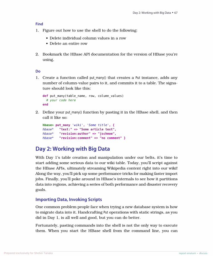
Find
1. Figure out how to use the shell to do the following:
• Delete individual column values in a row• Delete an entire row
2. Bookmark the HBase API documentation for the version of HBase you’reusing.
Do
1. Create a function called put_many() that creates a Put instance, adds anynumber of column-value pairs to it, and commits it to a table. The signa-ture should look like this:
def put_many(table_name, row, column_values)# your code here
end
2. Define your put_many() function by pasting it in the HBase shell, and thencall it like so:
hbase> put_many 'wiki', 'Some title', {hbase* "text:" => "Some article text",hbase* "revision:author" => "jschmoe",hbase* "revision:comment" => "no comment" }
Day 2: Working with Big DataWith Day 1’s table creation and manipulation under our belts, it’s time tostart adding some serious data to our wiki table. Today, you’ll script againstthe HBase APIs, ultimately streaming Wikipedia content right into our wiki!Along the way, you’ll pick up some performance tricks for making faster importjobs. Finally, you’ll poke around in HBase’s internals to see how it partitionsdata into regions, achieving a series of both performance and disaster recoverygoals.
Importing Data, Invoking ScriptsOne common problem people face when trying a new database system is howto migrate data into it. Handcrafting Put operations with static strings, as youdid in Day 1, is all well and good, but you can do better.
Fortunately, pasting commands into the shell is not the only way to executethem. When you start the HBase shell from the command line, you can
report erratum • discuss
Day 2: Working with Big Data • 67
Prepared exclusively for Shohei Tanaka
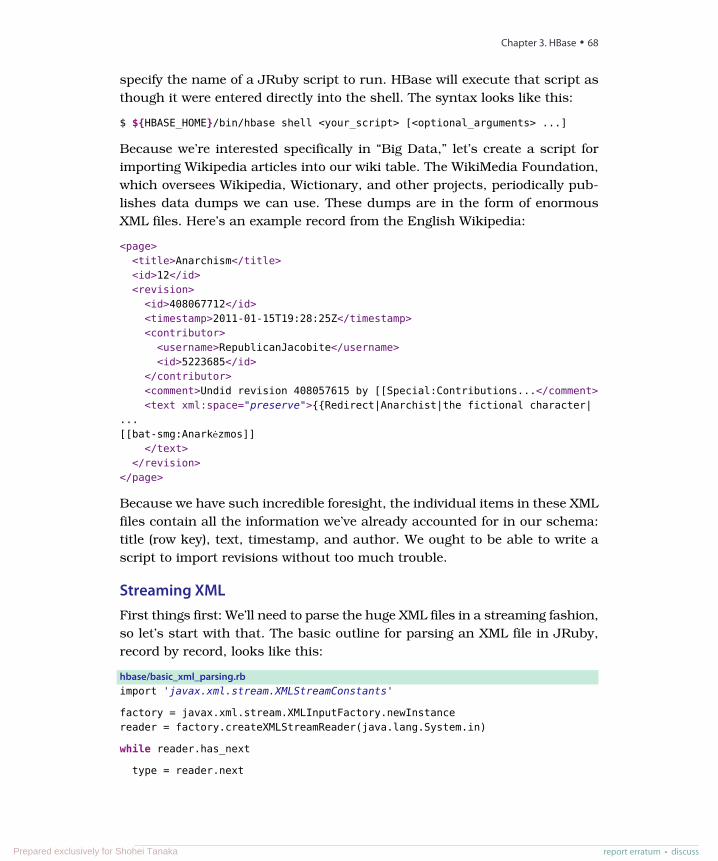
specify the name of a JRuby script to run. HBase will execute that script asthough it were entered directly into the shell. The syntax looks like this:
$ ${HBASE_HOME}/bin/hbase shell <your_script> [<optional_arguments> ...]
Because we’re interested specifically in “Big Data,” let’s create a script forimporting Wikipedia articles into our wiki table. The WikiMedia Foundation,which oversees Wikipedia, Wictionary, and other projects, periodically pub-lishes data dumps we can use. These dumps are in the form of enormousXML files. Here’s an example record from the English Wikipedia:
<page><title>Anarchism</title><id>12</id><revision>
<id>408067712</id><timestamp>2011-01-15T19:28:25Z</timestamp><contributor><username>RepublicanJacobite</username><id>5223685</id>
</contributor><comment>Undid revision 408057615 by [[Special:Contributions...</comment><text xml:space="preserve">{{Redirect|Anarchist|the fictional character|
...[[bat-smg:Anarkėzmos]]
</text></revision>
</page>
Because we have such incredible foresight, the individual items in these XMLfiles contain all the information we’ve already accounted for in our schema:title (row key), text, timestamp, and author. We ought to be able to write ascript to import revisions without too much trouble.
Streaming XMLFirst things first: We’ll need to parse the huge XML files in a streaming fashion,so let’s start with that. The basic outline for parsing an XML file in JRuby,record by record, looks like this:
hbase/basic_xml_parsing.rbimport 'javax.xml.stream.XMLStreamConstants'
factory = javax.xml.stream.XMLInputFactory.newInstancereader = factory.createXMLStreamReader(java.lang.System.in)
while reader.has_next
type = reader.next
Chapter 3. HBase • 68
report erratum • discussPrepared exclusively for Shohei Tanaka
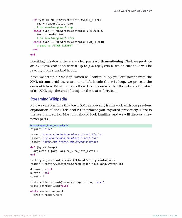
if type == XMLStreamConstants::START_ELEMENTtag = reader.local_name# do something with tag
elsif type == XMLStreamConstants::CHARACTERStext = reader.text# do something with text
elsif type == XMLStreamConstants::END_ELEMENT# same as START_ELEMENT
end
end
Breaking this down, there are a few parts worth mentioning. First, we producean XMLStreamReader and wire it up to java.lang.System.in, which means it will bereading from standard input.
Next, we set up a while loop, which will continuously pull out tokens from theXML stream until there are none left. Inside the while loop, we process thecurrent token. What happens then depends on whether the token is the startof an XML tag, the end of a tag, or the text in between.
Streaming WikipediaNow we can combine this basic XML processing framework with our previousexploration of the HTable and Put interfaces you explored previously. Here isthe resultant script. Most of it should look familiar, and we will discuss a fewnovel parts.
hbase/import_from_wikipedia.rbrequire 'time'
import 'org.apache.hadoop.hbase.client.HTable'import 'org.apache.hadoop.hbase.client.Put'import 'javax.xml.stream.XMLStreamConstants'
def jbytes(*args)args.map { |arg| arg.to_s.to_java_bytes }
end
factory = javax.xml.stream.XMLInputFactory.newInstancereader = factory.createXMLStreamReader(java.lang.System.in)
document = nilbuffer = nilcount = 0
table = HTable.new(@hbase.configuration, 'wiki')table.setAutoFlush(false)
while reader.has_nexttype = reader.next
report erratum • discuss
Day 2: Working with Big Data • 69
Prepared exclusively for Shohei Tanaka
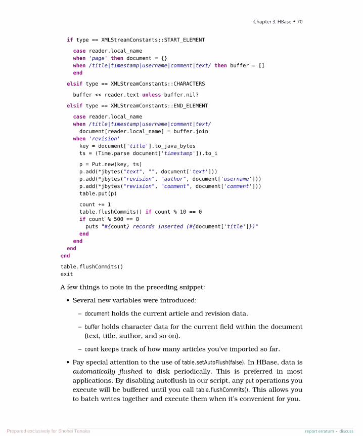
if type == XMLStreamConstants::START_ELEMENT
case reader.local_namewhen 'page' then document = {}when /title|timestamp|username|comment|text/ then buffer = []end
elsif type == XMLStreamConstants::CHARACTERS
buffer << reader.text unless buffer.nil?
elsif type == XMLStreamConstants::END_ELEMENT
case reader.local_namewhen /title|timestamp|username|comment|text/document[reader.local_name] = buffer.join
when 'revision'key = document['title'].to_java_bytests = (Time.parse document['timestamp']).to_i
p = Put.new(key, ts)p.add(*jbytes("text", "", document['text']))p.add(*jbytes("revision", "author", document['username']))p.add(*jbytes("revision", "comment", document['comment']))table.put(p)
count += 1table.flushCommits() if count % 10 == 0if count % 500 == 0
puts "#{count} records inserted (#{document['title']})"end
endend
end
table.flushCommits()exit
A few things to note in the preceding snippet:
• Several new variables were introduced:
– document holds the current article and revision data.
– buffer holds character data for the current field within the document(text, title, author, and so on).
– count keeps track of how many articles you’ve imported so far.
• Pay special attention to the use of table.setAutoFlush(false). In HBase, data isautomatically flushed to disk periodically. This is preferred in mostapplications. By disabling autoflush in our script, any put operations youexecute will be buffered until you call table.flushCommits(). This allows youto batch writes together and execute them when it’s convenient for you.
Chapter 3. HBase • 70
report erratum • discussPrepared exclusively for Shohei Tanaka
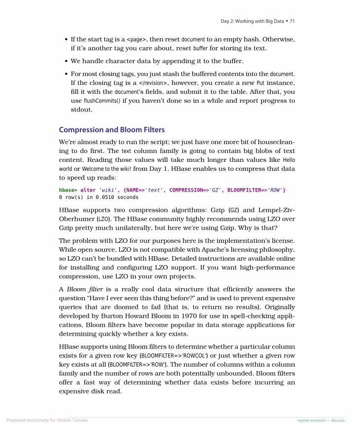
• If the start tag is a <page>, then reset document to an empty hash. Otherwise,if it’s another tag you care about, reset buffer for storing its text.
• We handle character data by appending it to the buffer.
• For most closing tags, you just stash the buffered contents into the document.If the closing tag is a </revision>, however, you create a new Put instance,fill it with the document’s fields, and submit it to the table. After that, youuse flushCommits() if you haven’t done so in a while and report progress tostdout.
Compression and Bloom FiltersWe’re almost ready to run the script; we just have one more bit of houseclean-ing to do first. The text column family is going to contain big blobs of textcontent. Reading those values will take much longer than values like Helloworld or Welcome to the wiki! from Day 1. HBase enables us to compress that datato speed up reads:
hbase> alter 'wiki', {NAME=>'text', COMPRESSION=>'GZ', BLOOMFILTER=>'ROW'}0 row(s) in 0.0510 seconds
HBase supports two compression algorithms: Gzip (GZ) and Lempel-Ziv-Oberhumer (LZO). The HBase community highly recommends using LZO overGzip pretty much unilaterally, but here we’re using Gzip. Why is that?
The problem with LZO for our purposes here is the implementation’s license.While open source, LZO is not compatible with Apache’s licensing philosophy,so LZO can’t be bundled with HBase. Detailed instructions are available onlinefor installing and configuring LZO support. If you want high-performancecompression, use LZO in your own projects.
A Bloom filter is a really cool data structure that efficiently answers thequestion “Have I ever seen this thing before?” and is used to prevent expensivequeries that are doomed to fail (that is, to return no results). Originallydeveloped by Burton Howard Bloom in 1970 for use in spell-checking appli-cations, Bloom filters have become popular in data storage applications fordetermining quickly whether a key exists.
HBase supports using Bloom filters to determine whether a particular columnexists for a given row key (BLOOMFILTER=>'ROWCOL') or just whether a given rowkey exists at all (BLOOMFILTER=>'ROW'). The number of columns within a columnfamily and the number of rows are both potentially unbounded. Bloom filtersoffer a fast way of determining whether data exists before incurring anexpensive disk read.
report erratum • discuss
Day 2: Working with Big Data • 71
Prepared exclusively for Shohei Tanaka
How Do Bloom Filters Work?
Without going too deep into implementation details, a Bloom filter manages a stati-cally sized array of bits initially set to 0. Each time a new blob of data is presentedto the filter, some of the bits are flipped to 1. Determining which bits to flip dependson generating a hash from the data and turning that hash into a set of bit positions.
Later, to test whether the filter has been presented with a particular blob in the past,the filter figures out which bits would have to be 1 and checks them. If any are 0,then the filter can unequivocally say “no.” If all of the bits are 1, then it reports “yes.”Chances are it has been presented with that blob before, but false positives areincreasingly likely as more blobs are entered.
This is the trade-off of using a Bloom filter as opposed to a simple hash. A hash willnever produce a false positive, but the space needed to store that data is unbounded.Bloom filters use a constant amount of space but will occasionally produce falsepositives at a predictable rate based on saturation. False positives aren’t a huge deal,though; they just mean that the filter says a value is likely to be there, but you willeventually find out that it isn’t.
Engage!Now that we’ve dissected the script a bit and added some powerful capabilitiesto our table, we’re ready to kick off the script. Remember that these files areenormous, so downloading and unzipping them is pretty much out of thequestion. So, what are we going to do?
Fortunately, through the magic of *nix pipes, we can download, extract, andfeed the XML into the script all at once. The command looks like this:
$ curl https://url-for-the-data-dump.com | bzcat | \${HBASE_HOME}/bin/hbase shell import_from_wikipedia.rb
Note that you should replace the preceding dummy URL with the URL of aWikiMedia Foundation dump file of some kind.2 You should use [project]-latest-pages-articles.xml.bz2 for either the English Wikipedia (~12.7 GB)3 or the EnglishWiktionary (~566 MB).4 These files contain all of the most recent revisions ofpages in the Main namespace. That is, they omit user pages, discussion pages,and so on.
Plug in the URL and run it! You should start seeing output like this shortly:
2. https://dumps.wikimedia.org/enwiki/latest3. https://dumps.wikimedia.org/enwiki/latest/enwiki-latest-pages-articles.xml.bz24. https://dumps.wikimedia.org/enwiktionary/latest/enwiktionary-latest-pages-articles.xml.bz2
Chapter 3. HBase • 72
report erratum • discussPrepared exclusively for Shohei Tanaka
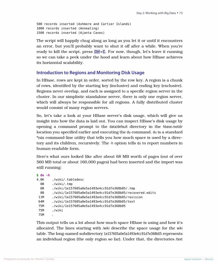
500 records inserted (Ashmore and Cartier Islands)1000 records inserted (Annealing)1500 records inserted (Ajanta Caves)
The script will happily chug along as long as you let it or until it encountersan error, but you’ll probably want to shut it off after a while. When you’reready to kill the script, press Ctrl+C . For now, though, let’s leave it runningso we can take a peek under the hood and learn about how HBase achievesits horizontal scalability.
Introduction to Regions and Monitoring Disk UsageIn HBase, rows are kept in order, sorted by the row key. A region is a chunkof rows, identified by the starting key (inclusive) and ending key (exclusive).Regions never overlap, and each is assigned to a specific region server in thecluster. In our simplistic standalone server, there is only one region server,which will always be responsible for all regions. A fully distributed clusterwould consist of many region servers.
So, let’s take a look at your HBase server’s disk usage, which will give usinsight into how the data is laid out. You can inspect HBase’s disk usage byopening a command prompt to the data/default directory in the hbase.rootdirlocation you specified earlier and executing the du command. du is a standard*nix command-line utility that tells you how much space is used by a direc-tory and its children, recursively. The -h option tells du to report numbers inhuman-readable form.
Here’s what ours looked like after about 68 MB worth of pages (out of over560 MB total or about 160,000 pages) had been inserted and the import wasstill running:
$ du -h4.0K ./wiki/.tabledesc
0B ./wiki/.tmp0B ./wiki/1e157605a0e5a1493e4cc91d7e368b05/.tmp0B ./wiki/1e157605a0e5a1493e4cc91d7e368b05/recovered.edits
11M ./wiki/1e157605a0e5a1493e4cc91d7e368b05/revision64M ./wiki/1e157605a0e5a1493e4cc91d7e368b05/text75M ./wiki/1e157605a0e5a1493e4cc91d7e368b0575M ./wiki75M .
This output tells us a lot about how much space HBase is using and how it’sallocated. The lines starting with /wiki describe the space usage for the wikitable. The long-named subdirectory 1e157605a0e5a1493e4cc91d7e368b05 representsan individual region (the only region so far). Under that, the directories /text
report erratum • discuss
Day 2: Working with Big Data • 73
Prepared exclusively for Shohei Tanaka
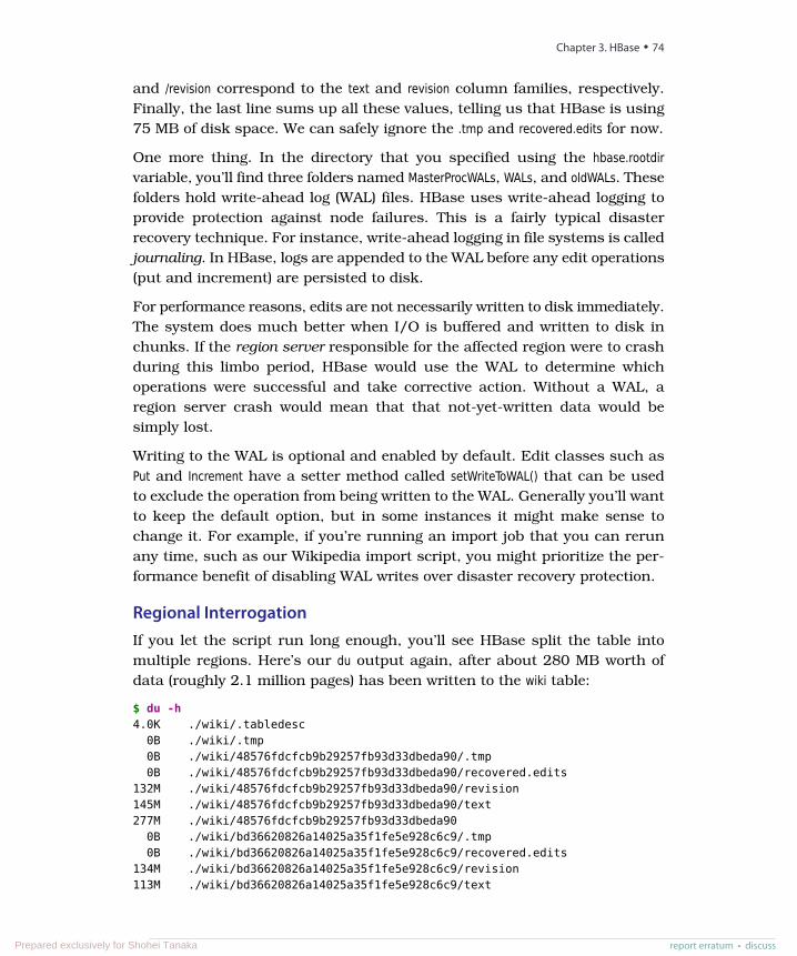
and /revision correspond to the text and revision column families, respectively.Finally, the last line sums up all these values, telling us that HBase is using75 MB of disk space. We can safely ignore the .tmp and recovered.edits for now.
One more thing. In the directory that you specified using the hbase.rootdirvariable, you’ll find three folders named MasterProcWALs, WALs, and oldWALs. Thesefolders hold write-ahead log (WAL) files. HBase uses write-ahead logging toprovide protection against node failures. This is a fairly typical disasterrecovery technique. For instance, write-ahead logging in file systems is calledjournaling. In HBase, logs are appended to the WAL before any edit operations(put and increment) are persisted to disk.
For performance reasons, edits are not necessarily written to disk immediately.The system does much better when I/O is buffered and written to disk inchunks. If the region server responsible for the affected region were to crashduring this limbo period, HBase would use the WAL to determine whichoperations were successful and take corrective action. Without a WAL, aregion server crash would mean that that not-yet-written data would besimply lost.
Writing to the WAL is optional and enabled by default. Edit classes such asPut and Increment have a setter method called setWriteToWAL() that can be usedto exclude the operation from being written to the WAL. Generally you’ll wantto keep the default option, but in some instances it might make sense tochange it. For example, if you’re running an import job that you can rerunany time, such as our Wikipedia import script, you might prioritize the per-formance benefit of disabling WAL writes over disaster recovery protection.
Regional InterrogationIf you let the script run long enough, you’ll see HBase split the table intomultiple regions. Here’s our du output again, after about 280 MB worth ofdata (roughly 2.1 million pages) has been written to the wiki table:
$ du -h4.0K ./wiki/.tabledesc
0B ./wiki/.tmp0B ./wiki/48576fdcfcb9b29257fb93d33dbeda90/.tmp0B ./wiki/48576fdcfcb9b29257fb93d33dbeda90/recovered.edits
132M ./wiki/48576fdcfcb9b29257fb93d33dbeda90/revision145M ./wiki/48576fdcfcb9b29257fb93d33dbeda90/text277M ./wiki/48576fdcfcb9b29257fb93d33dbeda90
0B ./wiki/bd36620826a14025a35f1fe5e928c6c9/.tmp0B ./wiki/bd36620826a14025a35f1fe5e928c6c9/recovered.edits
134M ./wiki/bd36620826a14025a35f1fe5e928c6c9/revision113M ./wiki/bd36620826a14025a35f1fe5e928c6c9/text
Chapter 3. HBase • 74
report erratum • discussPrepared exclusively for Shohei Tanaka
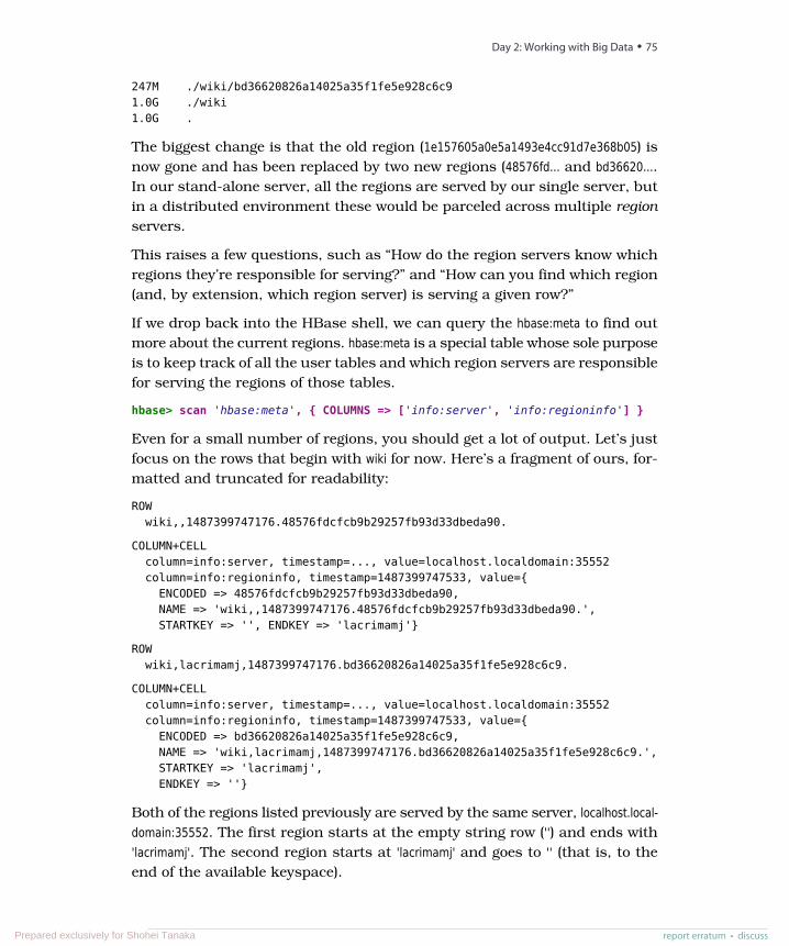
247M ./wiki/bd36620826a14025a35f1fe5e928c6c91.0G ./wiki1.0G .
The biggest change is that the old region (1e157605a0e5a1493e4cc91d7e368b05) isnow gone and has been replaced by two new regions (48576fd... and bd36620....In our stand-alone server, all the regions are served by our single server, butin a distributed environment these would be parceled across multiple regionservers.
This raises a few questions, such as “How do the region servers know whichregions they’re responsible for serving?” and “How can you find which region(and, by extension, which region server) is serving a given row?”
If we drop back into the HBase shell, we can query the hbase:meta to find outmore about the current regions. hbase:meta is a special table whose sole purposeis to keep track of all the user tables and which region servers are responsiblefor serving the regions of those tables.
hbase> scan 'hbase:meta', { COLUMNS => ['info:server', 'info:regioninfo'] }
Even for a small number of regions, you should get a lot of output. Let’s justfocus on the rows that begin with wiki for now. Here’s a fragment of ours, for-matted and truncated for readability:
ROWwiki,,1487399747176.48576fdcfcb9b29257fb93d33dbeda90.
COLUMN+CELLcolumn=info:server, timestamp=..., value=localhost.localdomain:35552column=info:regioninfo, timestamp=1487399747533, value={
ENCODED => 48576fdcfcb9b29257fb93d33dbeda90,NAME => 'wiki,,1487399747176.48576fdcfcb9b29257fb93d33dbeda90.',STARTKEY => '', ENDKEY => 'lacrimamj'}
ROWwiki,lacrimamj,1487399747176.bd36620826a14025a35f1fe5e928c6c9.
COLUMN+CELLcolumn=info:server, timestamp=..., value=localhost.localdomain:35552column=info:regioninfo, timestamp=1487399747533, value={
ENCODED => bd36620826a14025a35f1fe5e928c6c9,NAME => 'wiki,lacrimamj,1487399747176.bd36620826a14025a35f1fe5e928c6c9.',STARTKEY => 'lacrimamj',ENDKEY => ''}
Both of the regions listed previously are served by the same server, localhost.local-domain:35552. The first region starts at the empty string row ('') and ends with'lacrimamj'. The second region starts at 'lacrimamj' and goes to '' (that is, to theend of the available keyspace).
report erratum • discuss
Day 2: Working with Big Data • 75
Prepared exclusively for Shohei Tanaka
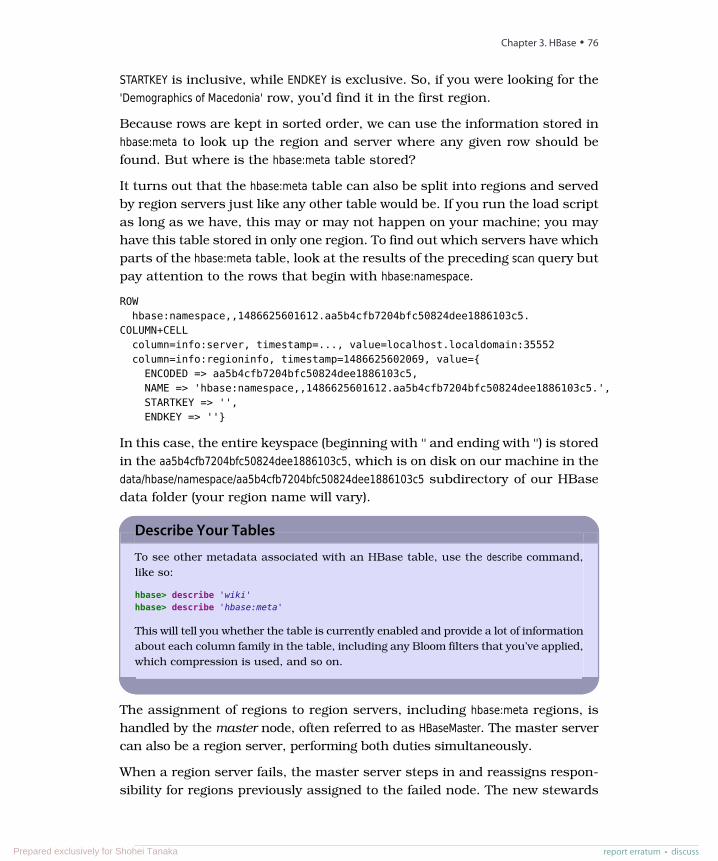
STARTKEY is inclusive, while ENDKEY is exclusive. So, if you were looking for the'Demographics of Macedonia' row, you’d find it in the first region.
Because rows are kept in sorted order, we can use the information stored inhbase:meta to look up the region and server where any given row should befound. But where is the hbase:meta table stored?
It turns out that the hbase:meta table can also be split into regions and servedby region servers just like any other table would be. If you run the load scriptas long as we have, this may or may not happen on your machine; you mayhave this table stored in only one region. To find out which servers have whichparts of the hbase:meta table, look at the results of the preceding scan query butpay attention to the rows that begin with hbase:namespace.
ROWhbase:namespace,,1486625601612.aa5b4cfb7204bfc50824dee1886103c5.
COLUMN+CELLcolumn=info:server, timestamp=..., value=localhost.localdomain:35552column=info:regioninfo, timestamp=1486625602069, value={
ENCODED => aa5b4cfb7204bfc50824dee1886103c5,NAME => 'hbase:namespace,,1486625601612.aa5b4cfb7204bfc50824dee1886103c5.',STARTKEY => '',ENDKEY => ''}
In this case, the entire keyspace (beginning with '' and ending with '') is storedin the aa5b4cfb7204bfc50824dee1886103c5, which is on disk on our machine in thedata/hbase/namespace/aa5b4cfb7204bfc50824dee1886103c5 subdirectory of our HBasedata folder (your region name will vary).
Describe Your Tables
To see other metadata associated with an HBase table, use the describe command,like so:
hbase> describe 'wiki'hbase> describe 'hbase:meta'
This will tell you whether the table is currently enabled and provide a lot of informationabout each column family in the table, including any Bloom filters that you’ve applied,which compression is used, and so on.
The assignment of regions to region servers, including hbase:meta regions, ishandled by the master node, often referred to as HBaseMaster. The master servercan also be a region server, performing both duties simultaneously.
When a region server fails, the master server steps in and reassigns respon-sibility for regions previously assigned to the failed node. The new stewards
Chapter 3. HBase • 76
report erratum • discussPrepared exclusively for Shohei Tanaka
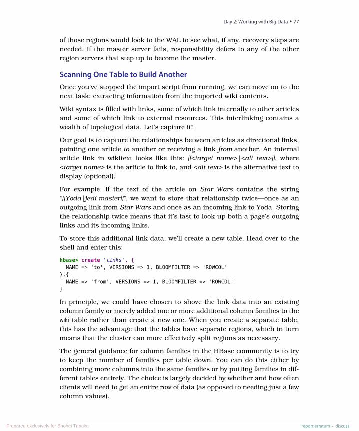
of those regions would look to the WAL to see what, if any, recovery steps areneeded. If the master server fails, responsibility defers to any of the otherregion servers that step up to become the master.
Scanning One Table to Build AnotherOnce you’ve stopped the import script from running, we can move on to thenext task: extracting information from the imported wiki contents.
Wiki syntax is filled with links, some of which link internally to other articlesand some of which link to external resources. This interlinking contains awealth of topological data. Let’s capture it!
Our goal is to capture the relationships between articles as directional links,pointing one article to another or receiving a link from another. An internalarticle link in wikitext looks like this: [[<target name>|<alt text>]], where<target name> is the article to link to, and <alt text> is the alternative text todisplay (optional).
For example, if the text of the article on Star Wars contains the string"[[Yoda|jedi master]]", we want to store that relationship twice—once as anoutgoing link from Star Wars and once as an incoming link to Yoda. Storingthe relationship twice means that it’s fast to look up both a page’s outgoinglinks and its incoming links.
To store this additional link data, we’ll create a new table. Head over to theshell and enter this:
hbase> create 'links', {NAME => 'to', VERSIONS => 1, BLOOMFILTER => 'ROWCOL'
},{NAME => 'from', VERSIONS => 1, BLOOMFILTER => 'ROWCOL'
}
In principle, we could have chosen to shove the link data into an existingcolumn family or merely added one or more additional column families to thewiki table rather than create a new one. When you create a separate table,this has the advantage that the tables have separate regions, which in turnmeans that the cluster can more effectively split regions as necessary.
The general guidance for column families in the HBase community is to tryto keep the number of families per table down. You can do this either bycombining more columns into the same families or by putting families in dif-ferent tables entirely. The choice is largely decided by whether and how oftenclients will need to get an entire row of data (as opposed to needing just a fewcolumn values).
report erratum • discuss
Day 2: Working with Big Data • 77
Prepared exclusively for Shohei Tanaka
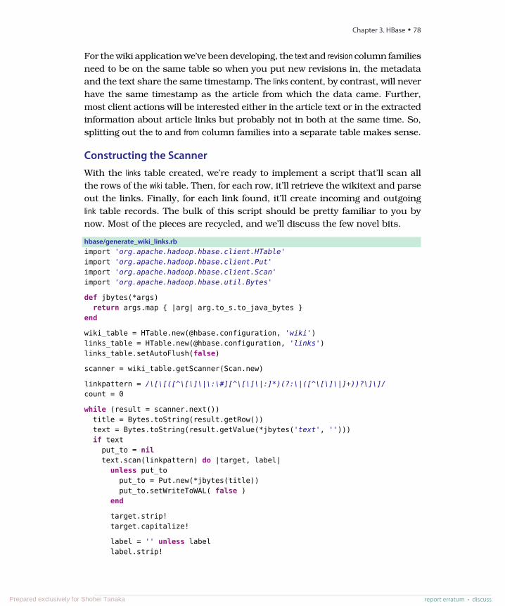
For the wiki application we’ve been developing, the text and revision column familiesneed to be on the same table so when you put new revisions in, the metadataand the text share the same timestamp. The links content, by contrast, will neverhave the same timestamp as the article from which the data came. Further,most client actions will be interested either in the article text or in the extractedinformation about article links but probably not in both at the same time. So,splitting out the to and from column families into a separate table makes sense.
Constructing the ScannerWith the links table created, we’re ready to implement a script that’ll scan allthe rows of the wiki table. Then, for each row, it’ll retrieve the wikitext and parseout the links. Finally, for each link found, it’ll create incoming and outgoinglink table records. The bulk of this script should be pretty familiar to you bynow. Most of the pieces are recycled, and we’ll discuss the few novel bits.
hbase/generate_wiki_links.rbimport 'org.apache.hadoop.hbase.client.HTable'import 'org.apache.hadoop.hbase.client.Put'import 'org.apache.hadoop.hbase.client.Scan'import 'org.apache.hadoop.hbase.util.Bytes'
def jbytes(*args)return args.map { |arg| arg.to_s.to_java_bytes }
end
wiki_table = HTable.new(@hbase.configuration, 'wiki')links_table = HTable.new(@hbase.configuration, 'links')links_table.setAutoFlush(false)
scanner = wiki_table.getScanner(Scan.new)
linkpattern = /\[\[([^\[\]\|\:\#][^\[\]\|:]*)(?:\|([^\[\]\|]+))?\]\]/count = 0
while (result = scanner.next())title = Bytes.toString(result.getRow())text = Bytes.toString(result.getValue(*jbytes('text', '')))if text
put_to = niltext.scan(linkpattern) do |target, label|unless put_to
put_to = Put.new(*jbytes(title))put_to.setWriteToWAL( false )
end
target.strip!target.capitalize!
label = '' unless labellabel.strip!
Chapter 3. HBase • 78
report erratum • discussPrepared exclusively for Shohei Tanaka
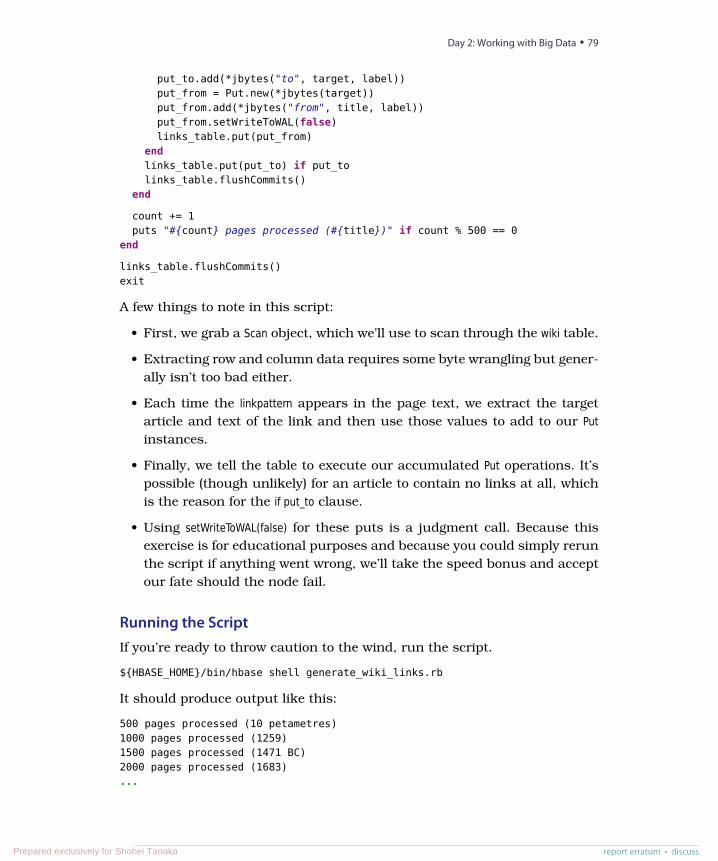
put_to.add(*jbytes("to", target, label))put_from = Put.new(*jbytes(target))put_from.add(*jbytes("from", title, label))put_from.setWriteToWAL(false)links_table.put(put_from)
endlinks_table.put(put_to) if put_tolinks_table.flushCommits()
end
count += 1puts "#{count} pages processed (#{title})" if count % 500 == 0
end
links_table.flushCommits()exit
A few things to note in this script:
• First, we grab a Scan object, which we’ll use to scan through the wiki table.
• Extracting row and column data requires some byte wrangling but gener-ally isn’t too bad either.
• Each time the linkpattern appears in the page text, we extract the targetarticle and text of the link and then use those values to add to our Putinstances.
• Finally, we tell the table to execute our accumulated Put operations. It’spossible (though unlikely) for an article to contain no links at all, whichis the reason for the if put_to clause.
• Using setWriteToWAL(false) for these puts is a judgment call. Because thisexercise is for educational purposes and because you could simply rerunthe script if anything went wrong, we’ll take the speed bonus and acceptour fate should the node fail.
Running the ScriptIf you’re ready to throw caution to the wind, run the script.
${HBASE_HOME}/bin/hbase shell generate_wiki_links.rb
It should produce output like this:
500 pages processed (10 petametres)1000 pages processed (1259)1500 pages processed (1471 BC)2000 pages processed (1683)...
report erratum • discuss
Day 2: Working with Big Data • 79
Prepared exclusively for Shohei Tanaka
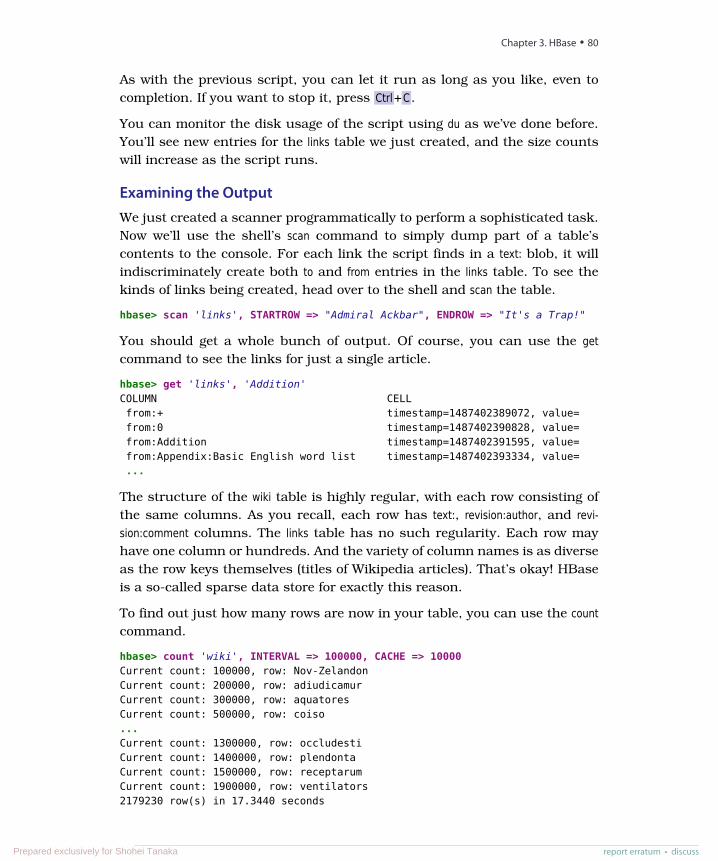
As with the previous script, you can let it run as long as you like, even tocompletion. If you want to stop it, press Ctrl+C .
You can monitor the disk usage of the script using du as we’ve done before.You’ll see new entries for the links table we just created, and the size countswill increase as the script runs.
Examining the OutputWe just created a scanner programmatically to perform a sophisticated task.Now we’ll use the shell’s scan command to simply dump part of a table’scontents to the console. For each link the script finds in a text: blob, it willindiscriminately create both to and from entries in the links table. To see thekinds of links being created, head over to the shell and scan the table.
hbase> scan 'links', STARTROW => "Admiral Ackbar", ENDROW => "It's a Trap!"
You should get a whole bunch of output. Of course, you can use the getcommand to see the links for just a single article.
hbase> get 'links', 'Addition'COLUMN CELLfrom:+ timestamp=1487402389072, value=from:0 timestamp=1487402390828, value=from:Addition timestamp=1487402391595, value=from:Appendix:Basic English word list timestamp=1487402393334, value=...
The structure of the wiki table is highly regular, with each row consisting ofthe same columns. As you recall, each row has text:, revision:author, and revi-sion:comment columns. The links table has no such regularity. Each row mayhave one column or hundreds. And the variety of column names is as diverseas the row keys themselves (titles of Wikipedia articles). That’s okay! HBaseis a so-called sparse data store for exactly this reason.
To find out just how many rows are now in your table, you can use the countcommand.
hbase> count 'wiki', INTERVAL => 100000, CACHE => 10000Current count: 100000, row: Nov-ZelandonCurrent count: 200000, row: adiudicamurCurrent count: 300000, row: aquatoresCurrent count: 500000, row: coiso...Current count: 1300000, row: occludestiCurrent count: 1400000, row: plendontaCurrent count: 1500000, row: receptarumCurrent count: 1900000, row: ventilators2179230 row(s) in 17.3440 seconds
Chapter 3. HBase • 80
report erratum • discussPrepared exclusively for Shohei Tanaka
Because of its distributed architecture, HBase doesn’t immediately know howmany rows are in each table. To find out, it has to count them (by performinga table scan). Fortunately, HBase’s region-based storage architecture lendsitself to fast distributed scanning. So, even if the operation at hand requiresa table scan, we don’t have to worry quite as much as we would with otherdatabases.
Day 2 Wrap-UpWhew, that was a pretty big day! You learned how to write an import scriptfor HBase that parses data out of a stream of XML. Then you used thosetechniques to stream Wikipedia dumps directly into your wiki table.
You learned more of the HBase API, including some client-controllable perfor-mance levers such as setAutoFlush(), flushCommits(), and setWriteToWAL(). Along thoselines, we discussed some HBase architectural features such as disasterrecovery, provided via the write-ahead log.
Speaking of architecture, you discovered table regions and how HBase divviesup responsibility for them among the region servers in the cluster. We scannedthe hbase:meta table to get a feel for HBase internals.
Finally, we discussed some of the performance implications of HBase’s sparsedesign. In so doing, we touched on some community best practices regardingthe use of columns, families, and tables.
Day 2 Homework
Find
1. Find a discussion or article describing the pros and cons of compressionin HBase.
2. Find an article explaining how Bloom filters work in general and how theybenefit HBase.
3. Aside from the algorithm, what other column family options relate tocompression?
4. How does the type of data and expected usage patterns inform columnfamily compression options?
Do
Expanding on the idea of data import, let’s build a database containingnutrition facts.
report erratum • discuss
Day 2: Working with Big Data • 81
Prepared exclusively for Shohei Tanaka
Download the MyPyramid Raw Food Data set from Data.gov5 and extract thezipped contents to Food_Display_Table.xml.
This data consists of many pairs of <Food_Display_Row> tags. Inside these, eachrow has a <Food_Code> (integer value), <Display_Name> (string), and other factsabout the food in appropriately named tags.
1. Create a new table called foods with a single column family to store thefacts. What should you use for the row key? What column family optionsmake sense for this data?
2. Create a new JRuby script for importing the food data. Use the streamingXML parsing style we used earlier for the Wikipedia import script andtailor it to the food data. Pipe the food data into your import script on thecommand line to populate the table.
3. Using the HBase shell, query the foods table for information about yourfavorite foods.
Day 3: Taking It to the CloudOn Days 1 and 2, you got quite a lot of hands-on experience using HBase instandalone mode. Our experimentation so far has focused on accessing asingle local server. But in reality, if you choose to use HBase, you’ll want tohave a good-sized cluster in order to realize the performance benefits of itsdistributed architecture. And nowadays, there’s also an increasingly highchance that you’ll want to run it in the cloud.
Here on Day 3, let’s turn our attention toward operating and interacting witha remote HBase cluster. First, you’ll deploy an HBase cluster on Amazon WebServices’ Elastic MapReduce platform (more commonly known as AWS andEMR, respectively) using AWS’s command-line tool, appropriately named aws.Then, you’ll connect directly to our remote HBase cluster using Secure Shell(SSH) and perform some basic operations.
Initial AWS and EMR SetupEMR is a managed Hadoop platform for AWS. It enables you to run a widevariety of servers in the Hadoop ecosystem—Hive, Pig, HBase, and manyothers—on EC2 without having to engage in a lot of the nitty-gritty detailsusually associated with managing those systems.
5. https://www.cnpp.usda.gov/Innovations/DataSource/MyFoodapediaData.zip
Chapter 3. HBase • 82
report erratum • discussPrepared exclusively for Shohei Tanaka
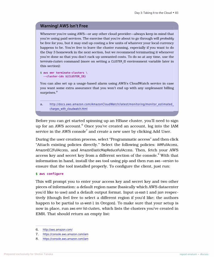
Warning! AWS Isn’t Free
Whenever you’re using AWS—or any other cloud provider—always keep in mind thatyou’re using paid services. The exercise that you’re about to go through will probablybe free for you, but it may end up costing a few units of whatever your local currencyhappens to be. You’re free to leave the cluster running, especially if you want to dothe Day 3 homework in the next section, but we recommend terminating it wheneveryou’re done so that you don’t rack up unwanted costs. To do so at any time, use theterminate-clusters command (more on setting a CLUSTER_ID environment variable later inthis section):
$ aws emr terminate-clusters \--cluster-ids ${CLUSTER_ID}
You can also set up a usage-based alarm using AWS’s CloudWatch service in caseyou want some extra assurance that you won’t end up with any unpleasant billingsurprises.a
a. http://docs.aws.amazon.com/AmazonCloudWatch/latest/monitoring/monitor_estimated_charges_with_cloudwatch.html
Before you can get started spinning up an HBase cluster, you’ll need to signup for an AWS account.6 Once you’ve created an account, log into the IAMservice in the AWS console7 and create a new user by clicking Add User.
During the user creation process, select “Programmatic access” and then click“Attach existing policies directly.” Select the following policies: IAMFullAccess,AmazonEC2FullAccess, and AmazonElasticMapReduceFullAccess. Then, fetch your AWSaccess key and secret key from a different section of the console.8 With thatinformation in hand, install the aws tool using pip and then run aws --version toensure that the tool installed properly. To configure the client, just run:
$ aws configure
This will prompt you to enter your access key and secret key and two otherpieces of information: a default region name (basically which AWS datacenteryou’d like to use) and a default output format. Input us-east-1 and json respec-tively (though feel free to select a different region if you’d like; the authorshappen to be partial to us-west-1 in Oregon). To make sure that your setup isnow in place, run aws emr list-clusters, which lists the clusters you’ve created inEMR. That should return an empty list:
6. http://aws.amazon.com/7. https://console.aws.amazon.com/iam8. https://console.aws.amazon.com/iam
report erratum • discuss
Day 3: Taking It to the Cloud • 83
Prepared exclusively for Shohei Tanaka
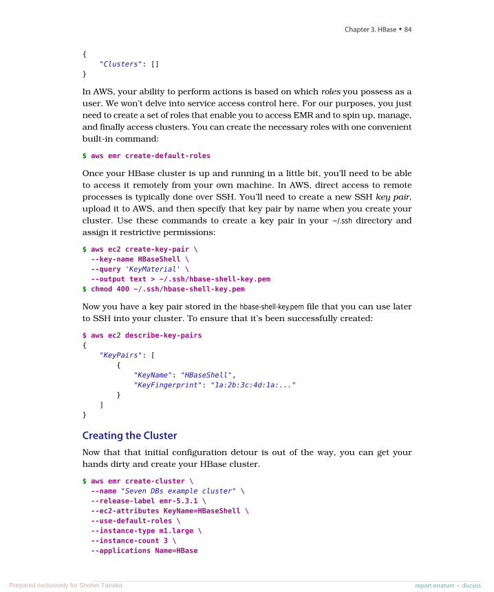
{"Clusters": []
}
In AWS, your ability to perform actions is based on which roles you possess as auser. We won’t delve into service access control here. For our purposes, you justneed to create a set of roles that enable you to access EMR and to spin up, manage,and finally access clusters. You can create the necessary roles with one convenientbuilt-in command:
$ aws emr create-default-roles
Once your HBase cluster is up and running in a little bit, you’ll need to be ableto access it remotely from your own machine. In AWS, direct access to remoteprocesses is typically done over SSH. You’ll need to create a new SSH key pair,upload it to AWS, and then specify that key pair by name when you create yourcluster. Use these commands to create a key pair in your ~/.ssh directory andassign it restrictive permissions:
$ aws ec2 create-key-pair \--key-name HBaseShell \--query 'KeyMaterial' \--output text > ~/.ssh/hbase-shell-key.pem
$ chmod 400 ~/.ssh/hbase-shell-key.pem
Now you have a key pair stored in the hbase-shell-key.pem file that you can use laterto SSH into your cluster. To ensure that it’s been successfully created:
$ aws ec2 describe-key-pairs{
"KeyPairs": [{
"KeyName": "HBaseShell","KeyFingerprint": "1a:2b:3c:4d:1a:..."
}]
}
Creating the ClusterNow that that initial configuration detour is out of the way, you can get yourhands dirty and create your HBase cluster.
$ aws emr create-cluster \--name "Seven DBs example cluster" \--release-label emr-5.3.1 \--ec2-attributes KeyName=HBaseShell \--use-default-roles \--instance-type m1.large \--instance-count 3 \--applications Name=HBase
Chapter 3. HBase • 84
report erratum • discussPrepared exclusively for Shohei Tanaka
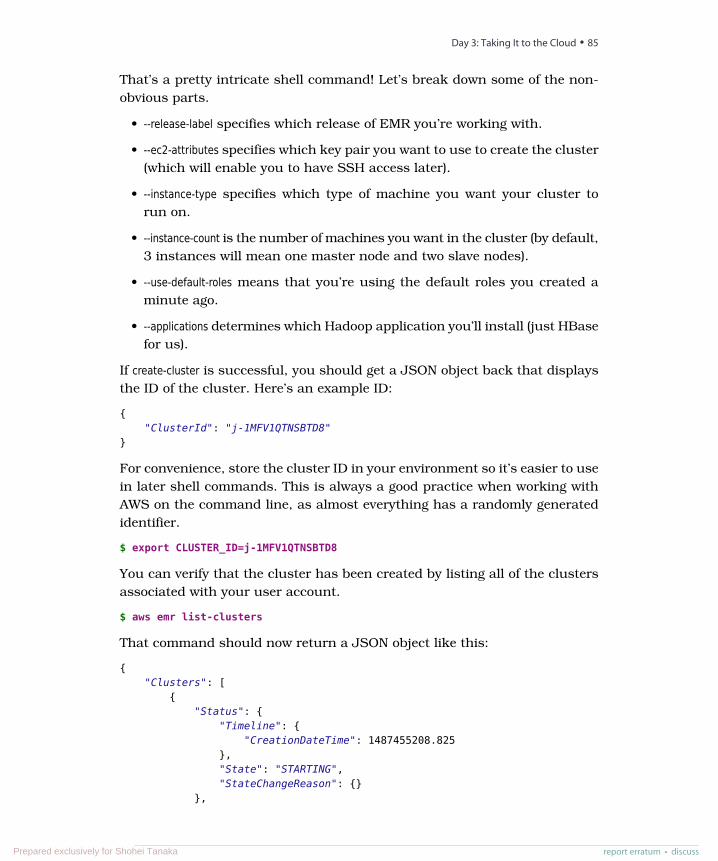
That’s a pretty intricate shell command! Let’s break down some of the non-obvious parts.
• --release-label specifies which release of EMR you’re working with.
• --ec2-attributes specifies which key pair you want to use to create the cluster(which will enable you to have SSH access later).
• --instance-type specifies which type of machine you want your cluster torun on.
• --instance-count is the number of machines you want in the cluster (by default,3 instances will mean one master node and two slave nodes).
• --use-default-roles means that you’re using the default roles you created aminute ago.
• --applications determines which Hadoop application you’ll install (just HBasefor us).
If create-cluster is successful, you should get a JSON object back that displaysthe ID of the cluster. Here’s an example ID:
{"ClusterId": "j-1MFV1QTNSBTD8"
}
For convenience, store the cluster ID in your environment so it’s easier to usein later shell commands. This is always a good practice when working withAWS on the command line, as almost everything has a randomly generatedidentifier.
$ export CLUSTER_ID=j-1MFV1QTNSBTD8
You can verify that the cluster has been created by listing all of the clustersassociated with your user account.
$ aws emr list-clusters
That command should now return a JSON object like this:
{"Clusters": [
{"Status": {
"Timeline": {"CreationDateTime": 1487455208.825
},"State": "STARTING","StateChangeReason": {}
},
report erratum • discuss
Day 3: Taking It to the Cloud • 85
Prepared exclusively for Shohei Tanaka
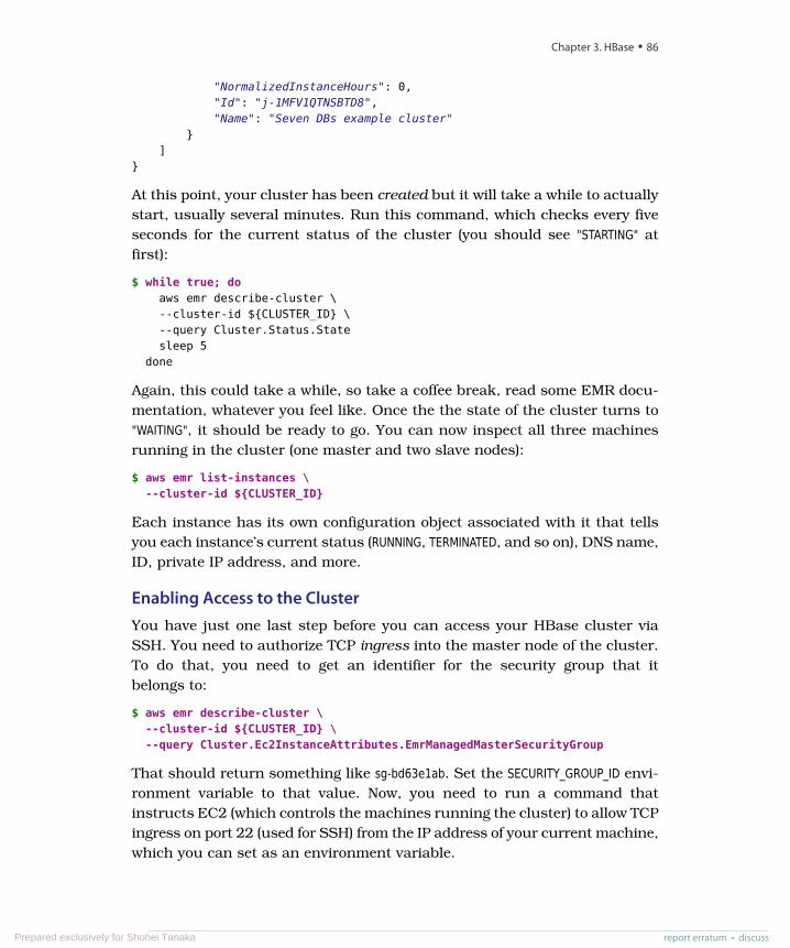
"NormalizedInstanceHours": 0,"Id": "j-1MFV1QTNSBTD8","Name": "Seven DBs example cluster"
}]
}
At this point, your cluster has been created but it will take a while to actuallystart, usually several minutes. Run this command, which checks every fiveseconds for the current status of the cluster (you should see "STARTING" atfirst):
$ while true; doaws emr describe-cluster \--cluster-id ${CLUSTER_ID} \--query Cluster.Status.Statesleep 5
done
Again, this could take a while, so take a coffee break, read some EMR docu-mentation, whatever you feel like. Once the the state of the cluster turns to"WAITING", it should be ready to go. You can now inspect all three machinesrunning in the cluster (one master and two slave nodes):
$ aws emr list-instances \--cluster-id ${CLUSTER_ID}
Each instance has its own configuration object associated with it that tellsyou each instance’s current status (RUNNING, TERMINATED, and so on), DNS name,ID, private IP address, and more.
Enabling Access to the ClusterYou have just one last step before you can access your HBase cluster viaSSH. You need to authorize TCP ingress into the master node of the cluster.To do that, you need to get an identifier for the security group that itbelongs to:
$ aws emr describe-cluster \--cluster-id ${CLUSTER_ID} \--query Cluster.Ec2InstanceAttributes.EmrManagedMasterSecurityGroup
That should return something like sg-bd63e1ab. Set the SECURITY_GROUP_ID envi-ronment variable to that value. Now, you need to run a command thatinstructs EC2 (which controls the machines running the cluster) to allow TCPingress on port 22 (used for SSH) from the IP address of your current machine,which you can set as an environment variable.
Chapter 3. HBase • 86
report erratum • discussPrepared exclusively for Shohei Tanaka
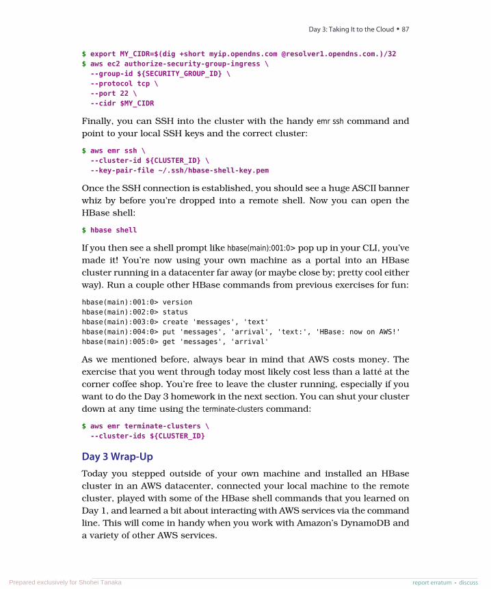
$ export MY_CIDR=$(dig +short myip.opendns.com @resolver1.opendns.com.)/32$ aws ec2 authorize-security-group-ingress \
--group-id ${SECURITY_GROUP_ID} \--protocol tcp \--port 22 \--cidr $MY_CIDR
Finally, you can SSH into the cluster with the handy emr ssh command andpoint to your local SSH keys and the correct cluster:
$ aws emr ssh \--cluster-id ${CLUSTER_ID} \--key-pair-file ~/.ssh/hbase-shell-key.pem
Once the SSH connection is established, you should see a huge ASCII bannerwhiz by before you’re dropped into a remote shell. Now you can open theHBase shell:
$ hbase shell
If you then see a shell prompt like hbase(main):001:0> pop up in your CLI, you’vemade it! You’re now using your own machine as a portal into an HBasecluster running in a datacenter far away (or maybe close by; pretty cool eitherway). Run a couple other HBase commands from previous exercises for fun:
hbase(main):001:0> versionhbase(main):002:0> statushbase(main):003:0> create 'messages', 'text'hbase(main):004:0> put 'messages', 'arrival', 'text:', 'HBase: now on AWS!'hbase(main):005:0> get 'messages', 'arrival'
As we mentioned before, always bear in mind that AWS costs money. Theexercise that you went through today most likely cost less than a latté at thecorner coffee shop. You’re free to leave the cluster running, especially if youwant to do the Day 3 homework in the next section. You can shut your clusterdown at any time using the terminate-clusters command:
$ aws emr terminate-clusters \--cluster-ids ${CLUSTER_ID}
Day 3 Wrap-UpToday you stepped outside of your own machine and installed an HBasecluster in an AWS datacenter, connected your local machine to the remotecluster, played with some of the HBase shell commands that you learned onDay 1, and learned a bit about interacting with AWS services via the commandline. This will come in handy when you work with Amazon’s DynamoDB anda variety of other AWS services.
report erratum • discuss
Day 3: Taking It to the Cloud • 87
Prepared exclusively for Shohei Tanaka
Day 3 Homework
For today’s homework, open up the AWS documentation for the Find section.For the Do section, leave your HBase cluster running on EMR with the HBaseshell open. Just remember to terminate the cluster when you’re done!
Find
1. Use the help interface aws for the CLI tool to see which commands areavailable for the emr subcommand. Read through the help material forsome of these commands to get a sense of some of the capabilities offeredby EMR that we didn’t cover in today’s cluster building exercise. Payspecial attention to scaling-related commands.
2. Go to the EMR documentation at https://aws.amazon.com/documentation/emr andread up on how to use Simple Storage Service (S3) as a data store forHBase clusters.
Do
1. In your HBase shell that you’re accessing via SSH, run some of the clustermetadata commands we explored on Day 2, such as scan 'hbase:meta'. Makenote of anything that’s fundamentally different from what you saw whenrunning HBase locally in standalone mode.
2. Navigate around the EMR section of your AWS browser console9 and findthe console specific to your running HBase cluster. Resize your clusterdown to just two machines by removing one of the slave nodes (knownas core nodes). Then increase the cluster size back to three (with twoslave/core nodes).
3. Resizing a cluster in the AWS console is nice, but that’s not an automat-able approach. The aws CLI tool enables you to resize a cluster program-matically. Consult the docs for the emr modify-instance-groups command byrunning aws emrmodify-instance-groups help to find out how this works. Removea machine from your cluster using that command.
Wrap-UpHBase is a juxtaposition of simplicity and complexity. Its data storage modelis pretty straightforward, with a lot of flexibility and just a few built-in schemaconstraints. A major barrier to understanding HBase, though, stems from the
9. https://console.aws.amazon.com/elasticmapreduce
Chapter 3. HBase • 88
report erratum • discussPrepared exclusively for Shohei Tanaka
fact that many terms are overloaded with baggage from the relational world(such as table and column). Schema design in HBase typically boils down todeciding on the performance characteristics that you want to apply to yourtables and columns, which is pretty far afield from the relational world, wherethings usually hinge upon table design.
HBase’s StrengthsNoteworthy features of HBase include a robust scale-out architecture andbuilt-in versioning and compression capabilities. HBase’s built-in versioningcapability can be a compelling feature for certain use cases. Keeping the ver-sion history of wiki pages is a crucial feature for policing and maintenance,for instance. By choosing HBase, you don’t have to take any special steps toimplement page history—you get it for free. No other database in this bookoffers that out of the box.
On the performance front, HBase is meant to scale out. If you have hugeamounts of data, measured in many terabytes or more, HBase may be foryou. HBase is rack aware, replicating data within and between datacenterracks so that node failures can be handled gracefully and quickly.
The HBase community is pretty awesome. There’s almost always somebodyon the #hbase IRC channel,10 on HBase’s dedicated Slack channel,11 or onthe mailing list12 ready to help with questions and get you pointed in the rightdirection.
HBase’s WeaknessesAlthough HBase is designed to scale out, it doesn’t scale down. The HBasecommunity seems to agree that five nodes is the minimum number you’llwant to use. Because it’s designed to be big, it can also be harder to adminis-trate (though platforms like EMR, which you saw in Day 3, do provide somegood managed options). Solving small problems isn’t what HBase is about,and nonexpert documentation is tough to come by, which steepens thelearning curve.
Additionally, HBase is almost never deployed alone. Instead, it is usuallyused in conjunction with other scale-ready infrastructure piece. These include
10. irc://irc.freenode.net/#hbase11. https://apache-hbase.slack.com/12. http://hbase.apache.org/mail-lists.html
report erratum • discuss
Wrap-Up • 89
Prepared exclusively for Shohei Tanaka
Hadoop (an implementation of Google’s MapReduce), the Hadoop distributedfile system (HDFS), Zookeeper (a headless service that aids internode coordi-nation), and Apache Spark (a popular cluster computing platform). Thisecosystem is both a strength and a weakness; it simultaneously provides anever-expanding set of powerful tools, but making them all work in conjunctionwith one another across many machines—sometimes in the thousands—canbe quite cumbersome.
One noteworthy characteristic of HBase is that it doesn’t offer any sorting orindexing capabilities aside from the row keys. Rows are kept in sorted orderby their row keys, but no such sorting is done on any other field, such ascolumn names and values. So, if you want to find rows by something otherthan their key, you need to either scan the table or maintain your own index(perhaps in a separate HBase table or in an external system).
Another missing concept is datatypes. All field values in HBase are treatedas uninterpreted arrays of bytes. There is no distinction between, say, aninteger value, a string, and a date. They’re all bytes to HBase, so it’s up toyour application to interpret the bytes, which can be tricky, especially if you’reused to relational access patterns like object-relational mappers (ORMs).
HBase on CAPWith respect to CAP, HBase is decidedly CP (for more information on the CAPtheorem, see Appendix 2, The CAP Theorem, on page 315). HBase makes strongconsistency guarantees. If a client succeeds in writing a value, other clientswill receive the updated value on the next request. Some databases allow youto tweak the CAP equation on a per-operation basis. Not so with HBase. Inthe face of reasonable amounts of partitioning—for example, a node failing—HBase will remain available, shunting the responsibility off to other nodes inthe cluster. However, in the pathological case, where only one node is leftalive, HBase has no choice but to refuse requests.
The CAP discussion gets a little more complex when you introduce cluster-to-cluster replication, an advanced feature we didn’t cover in this chapter. Atypical multicluster setup could have clusters separated geographically bysome distance. In this case, for a given column family, one cluster is thesystem of record, while the other clusters merely provide access to the repli-cated data. This system is eventually consistent because the replicationclusters will serve up the most recent values they’re aware of, which may notbe the most recent values in the master cluster.
Chapter 3. HBase • 90
report erratum • discussPrepared exclusively for Shohei Tanaka
Parting ThoughtsHBase can be quite a challenge at first. The terminology is often deceptivelyreassuring, and the installation and configuration are not for the faint ofheart. On the plus side, some of the features HBase offers, such as versioningand compression, are quite unique. These aspects can make HBase quiteappealing for solving certain problems. And of course, it scales out to manynodes of commodity hardware quite well. All in all, HBase—like a nail gun—is a pretty big tool, so watch your thumbs.
report erratum • discuss
Wrap-Up • 91
Prepared exclusively for Shohei Tanaka
CHAPTER 4
MongoDBMongoDB is in many ways like a power drill. Your ability to complete a taskis framed largely by the components you choose to use (from drill bits ofvarying size to sander adapters). MongoDB’s strength lies in its versatility,power, ease of use, and ability to handle jobs both large and small. Althoughit’s a much newer invention than the hammer, it is a tool that builders reachfor more and more often.
First publicly released in 2009, MongoDB (often just called Mongo) quicklybecame one of the most widely used NoSQL databases in existence, andremains somewhere very close to the top—if not right at the top—of that listtoday. MongoDB was designed as a scalable database—the name Mongocomes from “humongous”—with performance and easy data access as coredesign goals. It is a document database, which allows you to store objectsnested to whichever depth you’d like, and you can query that nested data inan ad hoc fashion. It enforces no schema (similar to HBase but unlike Post-gres), so documents can contain fields or types that no other document inthe collection contains (whether that’s advisable is another matter).
But don’t think that MongoDB’s flexibility makes it a toy. There are somehuge production MongoDB deployments out there, such as Foursquare,Comcast, Adobe, and CERN, where it’s used to collect data from the LargeHadron Collider.
Hu(mongo)usMongo hits a sweet spot between the powerful queryability of a relationaldatabase and the distributed nature of other databases, like HBase. Projectfounder Dwight Merriman has said that MongoDB is the database he wisheshe’d had at DoubleClick, where as the CTO he had to house large-scale datawhile still being able to satisfy ad hoc queries.
report erratum • discussPrepared exclusively for Shohei Tanaka
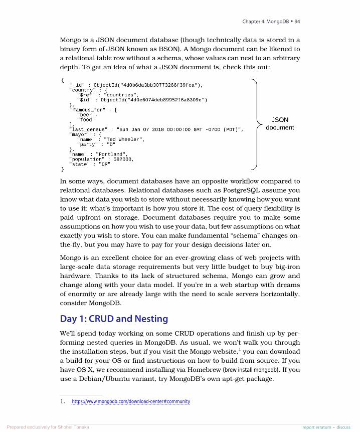
Mongo is a JSON document database (though technically data is stored in abinary form of JSON known as BSON). A Mongo document can be likened toa relational table row without a schema, whose values can nest to an arbitrarydepth. To get an idea of what a JSON document is, check this out:
In some ways, document databases have an opposite workflow compared torelational databases. Relational databases such as PostgreSQL assume youknow what data you wish to store without necessarily knowing how you wantto use it; what’s important is how you store it. The cost of query flexibility ispaid upfront on storage. Document databases require you to make someassumptions on how you wish to use your data, but few assumptions on whatexactly you wish to store. You can make fundamental “schema” changes on-the-fly, but you may have to pay for your design decisions later on.
Mongo is an excellent choice for an ever-growing class of web projects withlarge-scale data storage requirements but very little budget to buy big-ironhardware. Thanks to its lack of structured schema, Mongo can grow andchange along with your data model. If you’re in a web startup with dreamsof enormity or are already large with the need to scale servers horizontally,consider MongoDB.
Day 1: CRUD and NestingWe’ll spend today working on some CRUD operations and finish up by per-forming nested queries in MongoDB. As usual, we won’t walk you throughthe installation steps, but if you visit the Mongo website,1 you can downloada build for your OS or find instructions on how to build from source. If youhave OS X, we recommend installing via Homebrew (brew install mongodb). If youuse a Debian/Ubuntu variant, try MongoDB’s own apt-get package.
1. https://www.mongodb.com/download-center#community
Chapter 4. MongoDB • 94
report erratum • discussPrepared exclusively for Shohei Tanaka
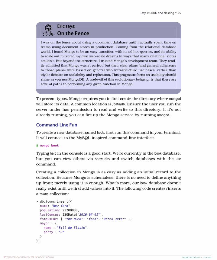
Eric says:
On the FenceI was on the fence about using a document database until I actually spent time onteams using document stores in production. Coming from the relational databaseworld, I found Mongo to be an easy transition with its ad hoc queries, and its abilityto scale out mirrored my own web-scale dreams in ways that many relational storescouldn’t. But beyond the structure, I trusted Mongo’s development team. They read-ily admitted that Mongo wasn’t perfect, but their clear plans (and general adherenceto those plans) were based on general web infrastructure use cases, rather thanidyllic debates on scalability and replication. This pragmatic focus on usability shouldshine as you use MongoDB. A trade-off of this evolutionary behavior is that there areseveral paths to performing any given function in Mongo.
To prevent typos, Mongo requires you to first create the directory where mongodwill store its data. A common location is /data/db. Ensure the user you run theserver under has permission to read and write to this directory. If it’s notalready running, you can fire up the Mongo service by running mongod.
Command-Line FunTo create a new database named book, first run this command in your terminal.It will connect to the MySQL-inspired command-line interface.
$ mongo book
Typing help in the console is a good start. We’re currently in the book database,but you can view others via show dbs and switch databases with the usecommand.
Creating a collection in Mongo is as easy as adding an initial record to thecollection. Because Mongo is schemaless, there is no need to define anythingup front; merely using it is enough. What’s more, our book database doesn’treally exist until we first add values into it. The following code creates/insertsa towns collection:
> db.towns.insert({name: "New York",population: 22200000,lastCensus: ISODate("2016-07-01"),famousFor: [ "the MOMA", "food", "Derek Jeter" ],mayor : {
name : "Bill de Blasio",party : "D"
}})
report erratum • discuss
Day 1: CRUD and Nesting • 95
Prepared exclusively for Shohei Tanaka
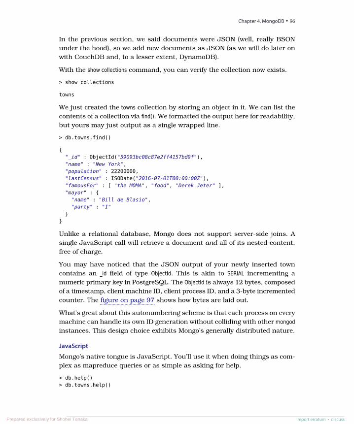
In the previous section, we said documents were JSON (well, really BSONunder the hood), so we add new documents as JSON (as we will do later onwith CouchDB and, to a lesser extent, DynamoDB).
With the show collections command, you can verify the collection now exists.
> show collections
towns
We just created the towns collection by storing an object in it. We can list thecontents of a collection via find(). We formatted the output here for readability,but yours may just output as a single wrapped line.
> db.towns.find()
{"_id" : ObjectId("59093bc08c87e2ff4157bd9f"),"name" : "New York","population" : 22200000,"lastCensus" : ISODate("2016-07-01T00:00:00Z"),"famousFor" : [ "the MOMA", "food", "Derek Jeter" ],"mayor" : {
"name" : "Bill de Blasio","party" : "I"
}}
Unlike a relational database, Mongo does not support server-side joins. Asingle JavaScript call will retrieve a document and all of its nested content,free of charge.
You may have noticed that the JSON output of your newly inserted towncontains an _id field of type ObjectId. This is akin to SERIAL incrementing anumeric primary key in PostgreSQL. The ObjectId is always 12 bytes, composedof a timestamp, client machine ID, client process ID, and a 3-byte incrementedcounter. The figure on page 97 shows how bytes are laid out.
What’s great about this autonumbering scheme is that each process on everymachine can handle its own ID generation without colliding with other mongodinstances. This design choice exhibits Mongo’s generally distributed nature.
JavaScript
Mongo’s native tongue is JavaScript. You’ll use it when doing things as com-plex as mapreduce queries or as simple as asking for help.
> db.help()> db.towns.help()
Chapter 4. MongoDB • 96
report erratum • discussPrepared exclusively for Shohei Tanaka
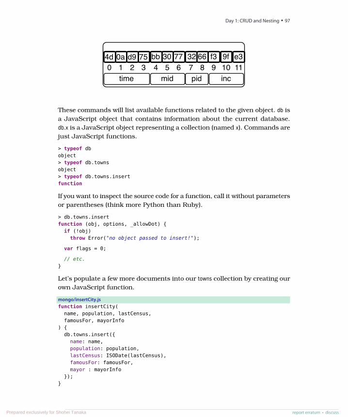
0 1 2 3time
4 5 6mid
7 8pid
9 10 11inc
4d 0a d9 75 e3bb 30 77 32 66 f3 9f
These commands will list available functions related to the given object. db isa JavaScript object that contains information about the current database.db.x is a JavaScript object representing a collection (named x). Commands arejust JavaScript functions.
> typeof dbobject> typeof db.townsobject> typeof db.towns.insertfunction
If you want to inspect the source code for a function, call it without parametersor parentheses (think more Python than Ruby).
> db.towns.insertfunction (obj, options, _allowDot) {
if (!obj)throw Error("no object passed to insert!");
var flags = 0;
// etc.}
Let’s populate a few more documents into our towns collection by creating ourown JavaScript function.
mongo/insertCity.jsfunction insertCity(
name, population, lastCensus,famousFor, mayorInfo
) {db.towns.insert({
name: name,population: population,lastCensus: ISODate(lastCensus),famousFor: famousFor,mayor : mayorInfo
});}
report erratum • discuss
Day 1: CRUD and Nesting • 97
Prepared exclusively for Shohei Tanaka
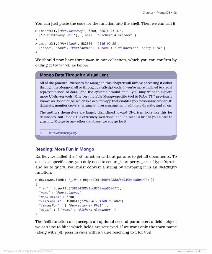
You can just paste the code for the function into the shell. Then we can call it.
> insertCity("Punxsutawney", 6200, '2016-01-31',["Punxsutawney Phil"], { name : "Richard Alexander" }
)> insertCity("Portland", 582000, '2016-09-20',
["beer", "food", "Portlandia"], { name : "Ted Wheeler", party : "D" })
We should now have three towns in our collection, which you can confirm bycalling db.towns.find() as before.
Mongo Data Through a Visual Lens
All of the practical exercises for Mongo in this chapter will involve accessing it eitherthrough the Mongo shell or through JavaScript code. If you’re more inclined to visualrepresentations of data—and the systems around data—you may want to exploremore UI-driven tools. One very notable Mongo-specific tool is Robo 3T,a previouslyknown as Robomongo, which is a desktop app that enables you to visualize MongoDBdatasets, monitor servers, engage in user management, edit data directly, and so on.
The authors themselves are largely disinclined toward UI-driven tools like this fordatabases, but Robo 3T is extremely well done, and if a nice UI brings you closer tograsping Mongo or any other database, we say go for it.
a. https://robomongo.org/
Reading: More Fun in MongoEarlier, we called the find() function without params to get all documents. Toaccess a specific one, you only need to set an _id property. _id is of type ObjectId,and so to query, you must convert a string by wrapping it in an ObjectId(str)function.
> db.towns.find({ "_id" : ObjectId("59094288afbc9350ada6b807") }){
"_id" : ObjectId("59094288afbc9350ada6b807"),"name" : "Punxsutawney","population" : 6200,"lastCensus" : ISODate("2016-01-31T00:00:00Z"),"famousFor" : [ "Punxsutawney Phil" ],"mayor" : { "name" : "Richard Alexander" }
}
The find() function also accepts an optional second parameter: a fields objectwe can use to filter which fields are retrieved. If we want only the town name(along with _id), pass in name with a value resolving to 1 (or true).
Chapter 4. MongoDB • 98
report erratum • discussPrepared exclusively for Shohei Tanaka
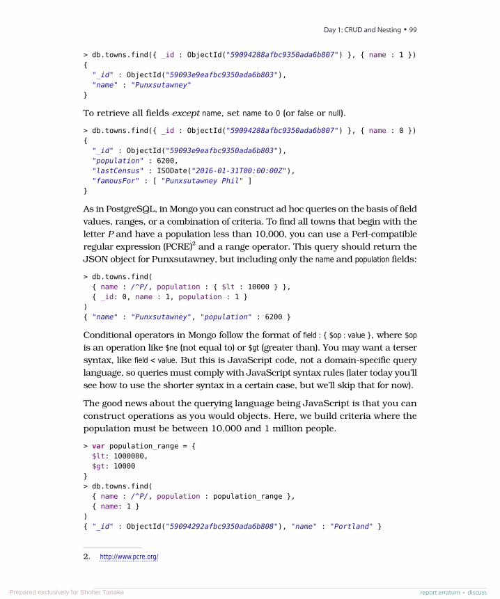
> db.towns.find({ _id : ObjectId("59094288afbc9350ada6b807") }, { name : 1 }){
"_id" : ObjectId("59093e9eafbc9350ada6b803"),"name" : "Punxsutawney"
}
To retrieve all fields except name, set name to 0 (or false or null).
> db.towns.find({ _id : ObjectId("59094288afbc9350ada6b807") }, { name : 0 }){
"_id" : ObjectId("59093e9eafbc9350ada6b803"),"population" : 6200,"lastCensus" : ISODate("2016-01-31T00:00:00Z"),"famousFor" : [ "Punxsutawney Phil" ]
}
As in PostgreSQL, in Mongo you can construct ad hoc queries on the basis of fieldvalues, ranges, or a combination of criteria. To find all towns that begin with theletter P and have a population less than 10,000, you can use a Perl-compatibleregular expression (PCRE)2 and a range operator. This query should return theJSON object for Punxsutawney, but including only the name and population fields:
> db.towns.find({ name : /^P/, population : { $lt : 10000 } },{ _id: 0, name : 1, population : 1 }
){ "name" : "Punxsutawney", "population" : 6200 }
Conditional operators in Mongo follow the format of field : { $op : value }, where $opis an operation like $ne (not equal to) or $gt (greater than). You may want a tersersyntax, like field < value. But this is JavaScript code, not a domain-specific querylanguage, so queries must comply with JavaScript syntax rules (later today you’llsee how to use the shorter syntax in a certain case, but we’ll skip that for now).
The good news about the querying language being JavaScript is that you canconstruct operations as you would objects. Here, we build criteria where thepopulation must be between 10,000 and 1 million people.
> var population_range = {$lt: 1000000,$gt: 10000
}> db.towns.find(
{ name : /^P/, population : population_range },{ name: 1 }
){ "_id" : ObjectId("59094292afbc9350ada6b808"), "name" : "Portland" }
2. http://www.pcre.org/
report erratum • discuss
Day 1: CRUD and Nesting • 99
Prepared exclusively for Shohei Tanaka
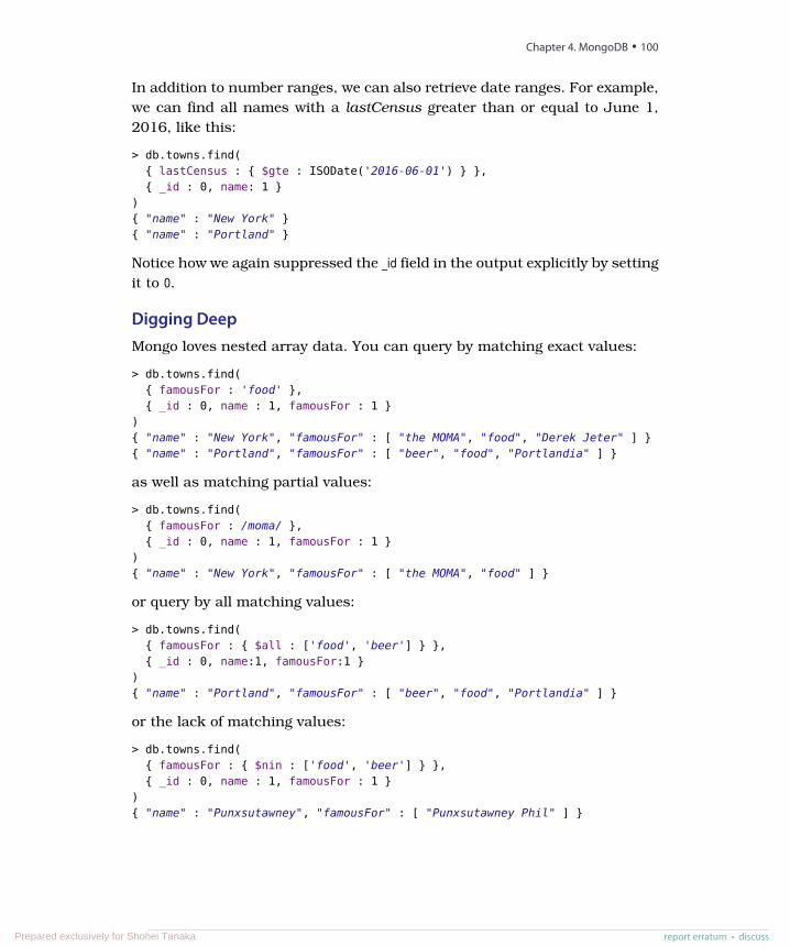
In addition to number ranges, we can also retrieve date ranges. For example,we can find all names with a lastCensus greater than or equal to June 1,2016, like this:
> db.towns.find({ lastCensus : { $gte : ISODate('2016-06-01') } },{ _id : 0, name: 1 }
){ "name" : "New York" }{ "name" : "Portland" }
Notice how we again suppressed the _id field in the output explicitly by settingit to 0.
Digging DeepMongo loves nested array data. You can query by matching exact values:
> db.towns.find({ famousFor : 'food' },{ _id : 0, name : 1, famousFor : 1 }
){ "name" : "New York", "famousFor" : [ "the MOMA", "food", "Derek Jeter" ] }{ "name" : "Portland", "famousFor" : [ "beer", "food", "Portlandia" ] }
as well as matching partial values:
> db.towns.find({ famousFor : /moma/ },{ _id : 0, name : 1, famousFor : 1 }
){ "name" : "New York", "famousFor" : [ "the MOMA", "food" ] }
or query by all matching values:
> db.towns.find({ famousFor : { $all : ['food', 'beer'] } },{ _id : 0, name:1, famousFor:1 }
){ "name" : "Portland", "famousFor" : [ "beer", "food", "Portlandia" ] }
or the lack of matching values:
> db.towns.find({ famousFor : { $nin : ['food', 'beer'] } },{ _id : 0, name : 1, famousFor : 1 }
){ "name" : "Punxsutawney", "famousFor" : [ "Punxsutawney Phil" ] }
Chapter 4. MongoDB • 100
report erratum • discussPrepared exclusively for Shohei Tanaka
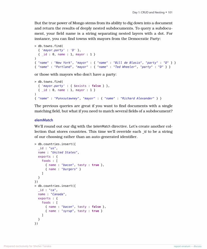
But the true power of Mongo stems from its ability to dig down into a documentand return the results of deeply nested subdocuments. To query a subdocu-ment, your field name is a string separating nested layers with a dot. Forinstance, you can find towns with mayors from the Democratic Party:
> db.towns.find({ 'mayor.party' : 'D' },{ _id : 0, name : 1, mayor : 1 }
){ "name" : "New York", "mayor" : { "name" : "Bill de Blasio", "party" : "D" } }{ "name" : "Portland", "mayor" : { "name" : "Ted Wheeler", "party" : "D" } }
or those with mayors who don’t have a party:
> db.towns.find({ 'mayor.party' : { $exists : false } },{ _id : 0, name : 1, mayor : 1 }
){ "name" : "Punxsutawney", "mayor" : { "name" : "Richard Alexander" } }
The previous queries are great if you want to find documents with a singlematching field, but what if you need to match several fields of a subdocument?
elemMatch
We’ll round out our dig with the $elemMatch directive. Let’s create another col-lection that stores countries. This time we’ll override each _id to be a stringof our choosing rather than an auto-generated identifier.
> db.countries.insert({_id : "us",name : "United States",exports : {
foods : [{ name : "bacon", tasty : true },{ name : "burgers" }
]}
})> db.countries.insert({
_id : "ca",name : "Canada",exports : {
foods : [{ name : "bacon", tasty : false },{ name : "syrup", tasty : true }
]}
})
report erratum • discuss
Day 1: CRUD and Nesting • 101
Prepared exclusively for Shohei Tanaka
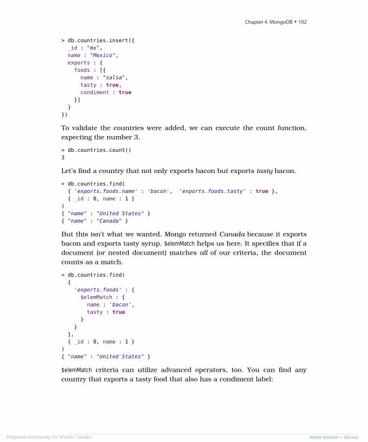
> db.countries.insert({_id : "mx",name : "Mexico",exports : {
foods : [{name : "salsa",tasty : true,condiment : true
}]}
})
To validate the countries were added, we can execute the count function,expecting the number 3.
> db.countries.count()3
Let’s find a country that not only exports bacon but exports tasty bacon.
> db.countries.find({ 'exports.foods.name' : 'bacon', 'exports.foods.tasty' : true },{ _id : 0, name : 1 }
){ "name" : "United States" }{ "name" : "Canada" }
But this isn’t what we wanted. Mongo returned Canada because it exportsbacon and exports tasty syrup. $elemMatch helps us here. It specifies that if adocument (or nested document) matches all of our criteria, the documentcounts as a match.
> db.countries.find({
'exports.foods' : {$elemMatch : {
name : 'bacon',tasty : true
}}
},{ _id : 0, name : 1 }
){ "name" : "United States" }
$elemMatch criteria can utilize advanced operators, too. You can find anycountry that exports a tasty food that also has a condiment label:
Chapter 4. MongoDB • 102
report erratum • discussPrepared exclusively for Shohei Tanaka
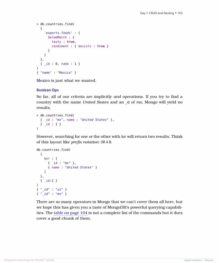
> db.countries.find({
'exports.foods' : {$elemMatch : {
tasty : true,condiment : { $exists : true }
}}
},{ _id : 0, name : 1 }
){ "name" : "Mexico" }
Mexico is just what we wanted.
Boolean Ops
So far, all of our criteria are implicitly and operations. If you try to find acountry with the name United States and an _id of mx, Mongo will yield noresults.
> db.countries.find({ _id : "mx", name : "United States" },{ _id : 1 }
)
However, searching for one or the other with $or will return two results. Thinkof this layout like prefix notation: OR A B.
db.countries.find({
$or : [{ _id : "mx" },{ name : "United States" }
]},{ _id:1 }
){ "_id" : "us" }{ "_id" : "mx" }
There are so many operators in Mongo that we can’t cover them all here, butwe hope this has given you a taste of MongoDB’s powerful querying capabili-ties. The table on page 104 is not a complete list of the commands but it doescover a good chunk of them.
report erratum • discuss
Day 1: CRUD and Nesting • 103
Prepared exclusively for Shohei Tanaka
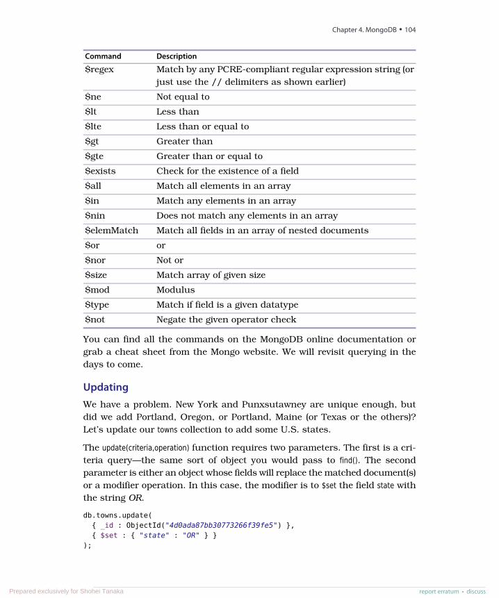
DescriptionCommand
Match by any PCRE-compliant regular expression string (orjust use the // delimiters as shown earlier)
$regex
Not equal to$ne
Less than$lt
Less than or equal to$lte
Greater than$gt
Greater than or equal to$gte
Check for the existence of a field$exists
Match all elements in an array$all
Match any elements in an array$in
Does not match any elements in an array$nin
Match all fields in an array of nested documents$elemMatch
or$or
Not or$nor
Match array of given size$size
Modulus$mod
Match if field is a given datatype$type
Negate the given operator check$not
You can find all the commands on the MongoDB online documentation orgrab a cheat sheet from the Mongo website. We will revisit querying in thedays to come.
UpdatingWe have a problem. New York and Punxsutawney are unique enough, butdid we add Portland, Oregon, or Portland, Maine (or Texas or the others)?Let’s update our towns collection to add some U.S. states.
The update(criteria,operation) function requires two parameters. The first is a cri-teria query—the same sort of object you would pass to find(). The secondparameter is either an object whose fields will replace the matched document(s)or a modifier operation. In this case, the modifier is to $set the field state withthe string OR.
db.towns.update({ _id : ObjectId("4d0ada87bb30773266f39fe5") },{ $set : { "state" : "OR" } }
);
Chapter 4. MongoDB • 104
report erratum • discussPrepared exclusively for Shohei Tanaka
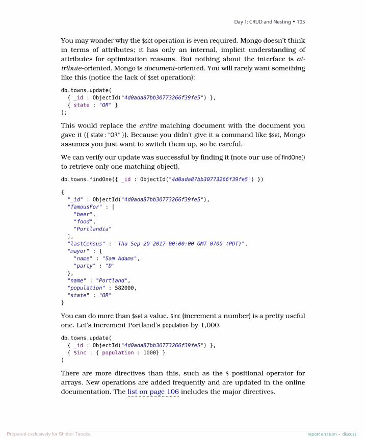
You may wonder why the $set operation is even required. Mongo doesn’t thinkin terms of attributes; it has only an internal, implicit understanding ofattributes for optimization reasons. But nothing about the interface is at-tribute-oriented. Mongo is document-oriented. You will rarely want somethinglike this (notice the lack of $set operation):
db.towns.update({ _id : ObjectId("4d0ada87bb30773266f39fe5") },{ state : "OR" }
);
This would replace the entire matching document with the document yougave it ({ state : "OR" }). Because you didn’t give it a command like $set, Mongoassumes you just want to switch them up, so be careful.
We can verify our update was successful by finding it (note our use of findOne()to retrieve only one matching object).
db.towns.findOne({ _id : ObjectId("4d0ada87bb30773266f39fe5") })
{"_id" : ObjectId("4d0ada87bb30773266f39fe5"),"famousFor" : [
"beer","food","Portlandia"
],"lastCensus" : "Thu Sep 20 2017 00:00:00 GMT-0700 (PDT)","mayor" : {
"name" : "Sam Adams","party" : "D"
},"name" : "Portland","population" : 582000,"state" : "OR"
}
You can do more than $set a value. $inc (increment a number) is a pretty usefulone. Let’s increment Portland’s population by 1,000.
db.towns.update({ _id : ObjectId("4d0ada87bb30773266f39fe5") },{ $inc : { population : 1000} }
)
There are more directives than this, such as the $ positional operator forarrays. New operations are added frequently and are updated in the onlinedocumentation. The list on page 106 includes the major directives.
report erratum • discuss
Day 1: CRUD and Nesting • 105
Prepared exclusively for Shohei Tanaka
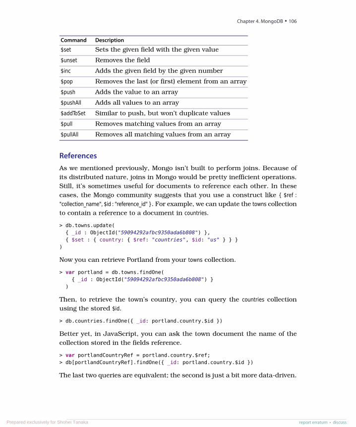
DescriptionCommand
Sets the given field with the given value$set
Removes the field$unset
Adds the given field by the given number$inc
Removes the last (or first) element from an array$pop
Adds the value to an array$push
Adds all values to an array$pushAll
Similar to push, but won’t duplicate values$addToSet
Removes matching values from an array$pull
Removes all matching values from an array$pullAll
ReferencesAs we mentioned previously, Mongo isn’t built to perform joins. Because ofits distributed nature, joins in Mongo would be pretty inefficient operations.Still, it’s sometimes useful for documents to reference each other. In thesecases, the Mongo community suggests that you use a construct like { $ref :"collection_name", $id : "reference_id" }. For example, we can update the towns collectionto contain a reference to a document in countries.
> db.towns.update({ _id : ObjectId("59094292afbc9350ada6b808") },{ $set : { country: { $ref: "countries", $id: "us" } } }
)
Now you can retrieve Portland from your towns collection.
> var portland = db.towns.findOne({ _id : ObjectId("59094292afbc9350ada6b808") }
)
Then, to retrieve the town’s country, you can query the countries collectionusing the stored $id.
> db.countries.findOne({ _id: portland.country.$id })
Better yet, in JavaScript, you can ask the town document the name of thecollection stored in the fields reference.
> var portlandCountryRef = portland.country.$ref;> db[portlandCountryRef].findOne({ _id: portland.country.$id })
The last two queries are equivalent; the second is just a bit more data-driven.
Chapter 4. MongoDB • 106
report erratum • discussPrepared exclusively for Shohei Tanaka
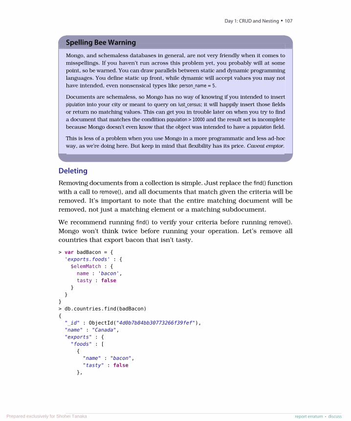
Spelling Bee Warning
Mongo, and schemaless databases in general, are not very friendly when it comes tomisspellings. If you haven’t run across this problem yet, you probably will at somepoint, so be warned. You can draw parallels between static and dynamic programminglanguages. You define static up front, while dynamic will accept values you may nothave intended, even nonsensical types like person_name = 5.
Documents are schemaless, so Mongo has no way of knowing if you intended to insertpipulation into your city or meant to query on lust_census; it will happily insert those fieldsor return no matching values. This can get you in trouble later on when you try to finda document that matches the condition population > 10000 and the result set is incompletebecause Mongo doesn’t even know that the object was intended to have a population field.
This is less of a problem when you use Mongo in a more programmatic and less ad-hocway, as we’re doing here. But keep in mind that flexibility has its price. Caveat emptor.
DeletingRemoving documents from a collection is simple. Just replace the find() functionwith a call to remove(), and all documents that match given the criteria will beremoved. It’s important to note that the entire matching document will beremoved, not just a matching element or a matching subdocument.
We recommend running find() to verify your criteria before running remove().Mongo won’t think twice before running your operation. Let’s remove allcountries that export bacon that isn’t tasty.
> var badBacon = {'exports.foods' : {
$elemMatch : {name : 'bacon',tasty : false
}}
}> db.countries.find(badBacon){
"_id" : ObjectId("4d0b7b84bb30773266f39fef"),"name" : "Canada","exports" : {
"foods" : [{
"name" : "bacon","tasty" : false
},
report erratum • discuss
Day 1: CRUD and Nesting • 107
Prepared exclusively for Shohei Tanaka
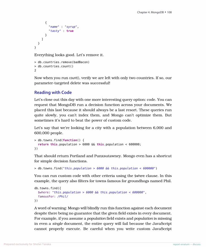
{"name" : "syrup","tasty" : true
}]
}}
Everything looks good. Let’s remove it.
> db.countries.remove(badBacon)> db.countries.count()2
Now when you run count(), verify we are left with only two countries. If so, ourparameter-targeted delete was successful!
Reading with CodeLet’s close out this day with one more interesting query option: code. You canrequest that MongoDB run a decision function across your documents. Weplaced this last because it should always be a last resort. These queries runquite slowly, you can’t index them, and Mongo can’t optimize them. Butsometimes it’s hard to beat the power of custom code.
Let’s say that we’re looking for a city with a population between 6,000 and600,000 people.
> db.towns.find(function() {return this.population > 6000 && this.population < 600000;
})
That should return Portland and Punxsutawney. Mongo even has a shortcutfor simple decision functions.
> db.towns.find("this.population > 6000 && this.population < 600000")
You can run custom code with other criteria using the $where clause. In thisexample, the query also filters for towns famous for groundhogs named Phil.
db.towns.find({$where: "this.population > 6000 && this.population < 600000",famousFor: /Phil/
})
A word of warning: Mongo will blindly run this function against each documentdespite there being no guarantee that the given field exists in every document.For example, if you assume a population field exists and population is missingin even a single document, the entire query will fail because the JavaScriptcannot properly execute. Be careful when you write custom JavaScript
Chapter 4. MongoDB • 108
report erratum • discussPrepared exclusively for Shohei Tanaka
functions, be comfortable using JavaScript before attempting custom code,and in general avoid these sorts of operations in production.
Day 1 Wrap-UpToday we took a peek at our first document database, MongoDB. We saw howwe can store nested structured data as JSON objects and query that data toany depth. You learned that a document can be envisioned as a schemalessrow in the relational model, keyed by a generated _id. A set of documents iscalled a collection in Mongo, similar to a table in PostgreSQL but also quitedifferent.
Unlike the previous styles we’ve encountered, with collections of sets of simpledatatypes, Mongo stores complex, denormalized documents, stored andretrieved as collections of arbitrary JSON structures. Mongo tops off thisflexible storage strategy with a powerful query mechanism unconstrained byany predefined schema.
Its denormalized nature makes a document database a superb choice forstoring data with unknown qualities, while other styles (such as relational orcolumnar) prefer, or sometimes even demand, that you know your datamodels in advance and require schema migrations to add or edit fields.
Day 1 Homework
Find
1. Bookmark the online MongoDB documentation and read up on somethingyou found intriguing today.
2. Look up how to construct regular expressions in Mongo.
3. Acquaint yourself with command-line db.help() and db.collections.help() output.
4. Find a Mongo driver in your programming language of choice (Ruby, Java,PHP, Go, Elixir, and so on).
Do
1. Print a JSON document containing { "hello" : "world" }.
2. Select a town via a case-insensitive regular expression containing theword new.
3. Find all cities whose names contain an e and are famous for food or beer.
4. Create a new database named blogger with a collection named articles. Inserta new article with an author name and email, creation date, and text.
report erratum • discuss
Day 1: CRUD and Nesting • 109
Prepared exclusively for Shohei Tanaka
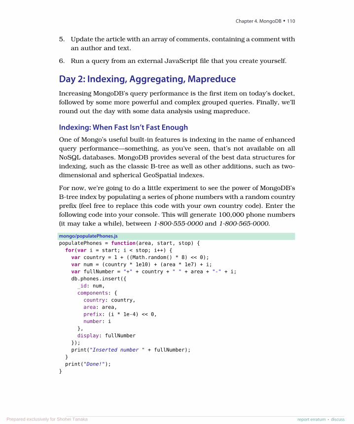
5. Update the article with an array of comments, containing a comment withan author and text.
6. Run a query from an external JavaScript file that you create yourself.
Day 2: Indexing, Aggregating, MapreduceIncreasing MongoDB’s query performance is the first item on today’s docket,followed by some more powerful and complex grouped queries. Finally, we’llround out the day with some data analysis using mapreduce.
Indexing: When Fast Isn’t Fast EnoughOne of Mongo’s useful built-in features is indexing in the name of enhancedquery performance—something, as you’ve seen, that’s not available on allNoSQL databases. MongoDB provides several of the best data structures forindexing, such as the classic B-tree as well as other additions, such as two-dimensional and spherical GeoSpatial indexes.
For now, we’re going to do a little experiment to see the power of MongoDB’sB-tree index by populating a series of phone numbers with a random countryprefix (feel free to replace this code with your own country code). Enter thefollowing code into your console. This will generate 100,000 phone numbers(it may take a while), between 1-800-555-0000 and 1-800-565-0000.
mongo/populatePhones.jspopulatePhones = function(area, start, stop) {
for(var i = start; i < stop; i++) {var country = 1 + ((Math.random() * 8) << 0);var num = (country * 1e10) + (area * 1e7) + i;var fullNumber = "+" + country + " " + area + "-" + i;db.phones.insert({_id: num,components: {
country: country,area: area,prefix: (i * 1e-4) << 0,number: i
},display: fullNumber
});print("Inserted number " + fullNumber);
}print("Done!");
}
Chapter 4. MongoDB • 110
report erratum • discussPrepared exclusively for Shohei Tanaka
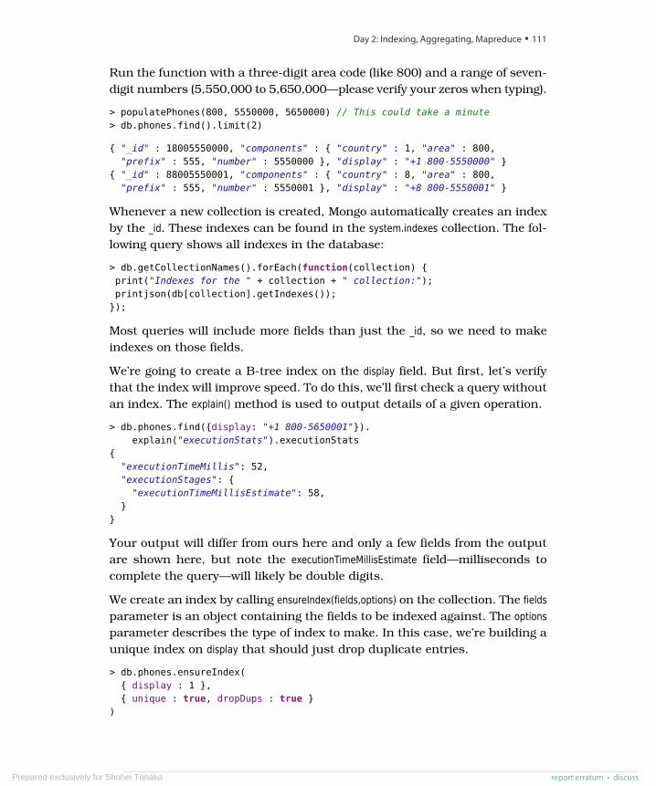
Run the function with a three-digit area code (like 800) and a range of seven-digit numbers (5,550,000 to 5,650,000—please verify your zeros when typing).
> populatePhones(800, 5550000, 5650000) // This could take a minute> db.phones.find().limit(2)
{ "_id" : 18005550000, "components" : { "country" : 1, "area" : 800,"prefix" : 555, "number" : 5550000 }, "display" : "+1 800-5550000" }
{ "_id" : 88005550001, "components" : { "country" : 8, "area" : 800,"prefix" : 555, "number" : 5550001 }, "display" : "+8 800-5550001" }
Whenever a new collection is created, Mongo automatically creates an indexby the _id. These indexes can be found in the system.indexes collection. The fol-lowing query shows all indexes in the database:
> db.getCollectionNames().forEach(function(collection) {print("Indexes for the " + collection + " collection:");printjson(db[collection].getIndexes());
});
Most queries will include more fields than just the _id, so we need to makeindexes on those fields.
We’re going to create a B-tree index on the display field. But first, let’s verifythat the index will improve speed. To do this, we’ll first check a query withoutan index. The explain() method is used to output details of a given operation.
> db.phones.find({display: "+1 800-5650001"}).explain("executionStats").executionStats
{"executionTimeMillis": 52,"executionStages": {
"executionTimeMillisEstimate": 58,}
}
Your output will differ from ours here and only a few fields from the outputare shown here, but note the executionTimeMillisEstimate field—milliseconds tocomplete the query—will likely be double digits.
We create an index by calling ensureIndex(fields,options) on the collection. The fieldsparameter is an object containing the fields to be indexed against. The optionsparameter describes the type of index to make. In this case, we’re building aunique index on display that should just drop duplicate entries.
> db.phones.ensureIndex({ display : 1 },{ unique : true, dropDups : true }
)
report erratum • discuss
Day 2: Indexing, Aggregating, Mapreduce • 111
Prepared exclusively for Shohei Tanaka
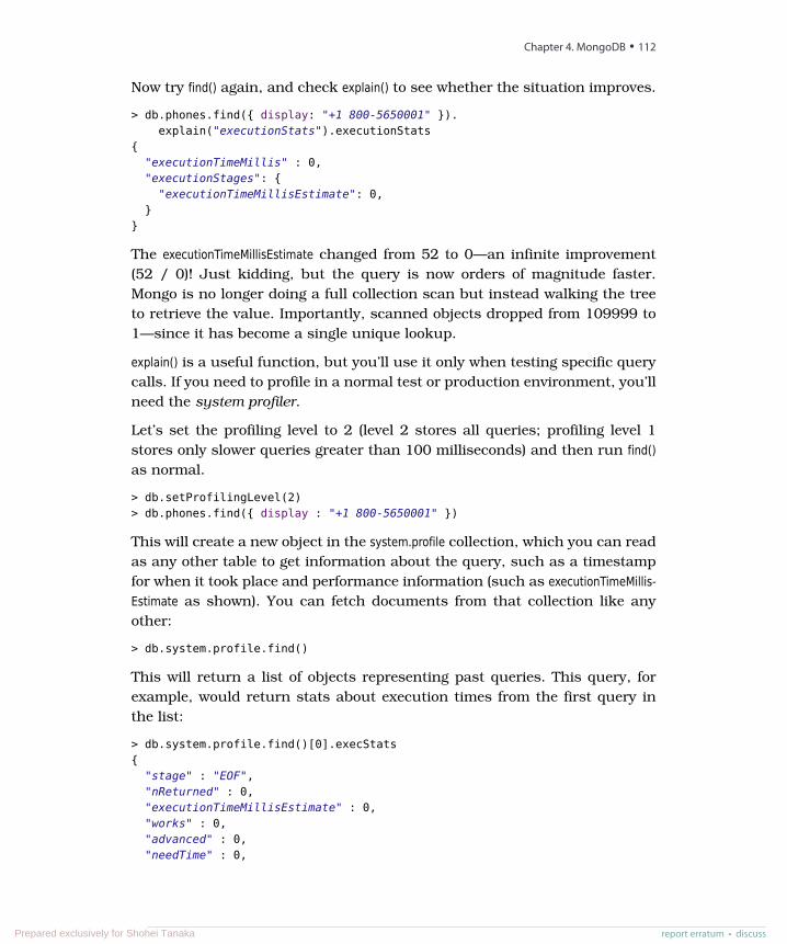
Now try find() again, and check explain() to see whether the situation improves.
> db.phones.find({ display: "+1 800-5650001" }).explain("executionStats").executionStats
{"executionTimeMillis" : 0,"executionStages": {
"executionTimeMillisEstimate": 0,}
}
The executionTimeMillisEstimate changed from 52 to 0—an infinite improvement(52 / 0)! Just kidding, but the query is now orders of magnitude faster.Mongo is no longer doing a full collection scan but instead walking the treeto retrieve the value. Importantly, scanned objects dropped from 109999 to1—since it has become a single unique lookup.
explain() is a useful function, but you’ll use it only when testing specific querycalls. If you need to profile in a normal test or production environment, you’llneed the system profiler.
Let’s set the profiling level to 2 (level 2 stores all queries; profiling level 1stores only slower queries greater than 100 milliseconds) and then run find()as normal.
> db.setProfilingLevel(2)> db.phones.find({ display : "+1 800-5650001" })
This will create a new object in the system.profile collection, which you can readas any other table to get information about the query, such as a timestampfor when it took place and performance information (such as executionTimeMillis-Estimate as shown). You can fetch documents from that collection like anyother:
> db.system.profile.find()
This will return a list of objects representing past queries. This query, forexample, would return stats about execution times from the first query inthe list:
> db.system.profile.find()[0].execStats{
"stage" : "EOF","nReturned" : 0,"executionTimeMillisEstimate" : 0,"works" : 0,"advanced" : 0,"needTime" : 0,
Chapter 4. MongoDB • 112
report erratum • discussPrepared exclusively for Shohei Tanaka
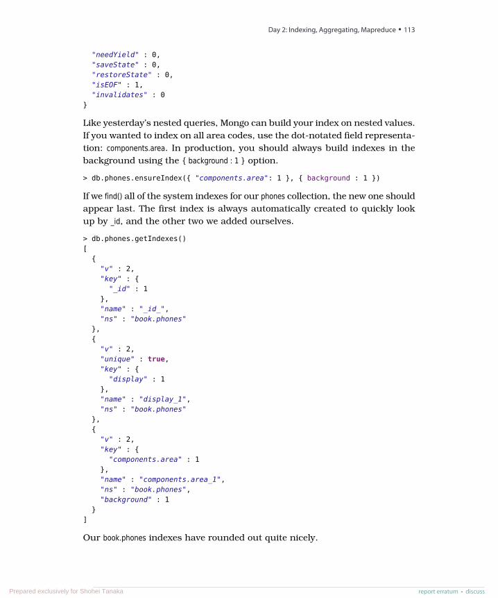
"needYield" : 0,"saveState" : 0,"restoreState" : 0,"isEOF" : 1,"invalidates" : 0
}
Like yesterday’s nested queries, Mongo can build your index on nested values.If you wanted to index on all area codes, use the dot-notated field representa-tion: components.area. In production, you should always build indexes in thebackground using the { background : 1 } option.
> db.phones.ensureIndex({ "components.area": 1 }, { background : 1 })
If we find() all of the system indexes for our phones collection, the new one shouldappear last. The first index is always automatically created to quickly lookup by _id, and the other two we added ourselves.
> db.phones.getIndexes()[
{"v" : 2,"key" : {
"_id" : 1},"name" : "_id_","ns" : "book.phones"
},{
"v" : 2,"unique" : true,"key" : {
"display" : 1},"name" : "display_1","ns" : "book.phones"
},{
"v" : 2,"key" : {
"components.area" : 1},"name" : "components.area_1","ns" : "book.phones","background" : 1
}]
Our book.phones indexes have rounded out quite nicely.
report erratum • discuss
Day 2: Indexing, Aggregating, Mapreduce • 113
Prepared exclusively for Shohei Tanaka
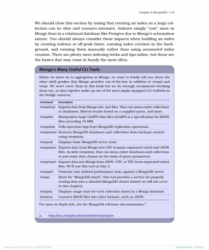
We should close this section by noting that creating an index on a large col-lection can be slow and resource-intensive. Indexes simply “cost” more inMongo than in a relational database like Postgres due to Mongo’s schemalessnature. You should always consider these impacts when building an indexby creating indexes at off-peak times, running index creation in the back-ground, and running them manually rather than using automated indexcreation. There are plenty more indexing tricks and tips online, but these arethe basics that may come in handy the most often.
Mongo’s Many Useful CLI Tools
Before we move on to aggregation in Mongo, we want to briefly tell you about theother shell goodies that Mongo provides out-of-the-box in addition to mongod andmongo. We won’t cover them in this book but we do strongly recommend checkingthem out, as they together make up one of the most amply equipped CLI toolbelts inthe NoSQL universe.
DescriptionCommand
Exports data from Mongo into .bson files. That can mean entire collectionsor databases, filtered results based on a supplied query, and more.
mongodump
Manipulates large GridFS data files (GridFS is a specification for BSONfiles exceeding 16 MB).
mongofiles
Polls operation logs from MongoDB replication operations.mongooplog
Restores MongoDB databases and collections from backups createdusing mongodump.
mongorestore
Displays basic MongoDB server stats.mongostat
Exports data from Mongo into CSV (comma-separated value) and JSONfiles. As with mongodump, that can mean entire databases and collectionsor just some data chosen on the basis of query parameters.
mongoexport
Imports data into Mongo from JSON, CSV, or TSV (term-separated value)files. We’ll use this tool on Day 3.
mongoimport
Performs user-defined performance tests against a MongoDB server.mongoperf
Short for “MongoDB shard,” this tool provides a service for properlyrouting data into a sharded MongoDB cluster (which we will not coverin this chapter).
mongos
Displays usage stats for each collection stored in a Mongo database.mongotop
Converts BSON files into other formats, such as JSON.bsondump
For more in-depth info, see the MongoDB reference documentation.a
a. https://docs.mongodb.com/manual/reference/program
Chapter 4. MongoDB • 114
report erratum • discussPrepared exclusively for Shohei Tanaka
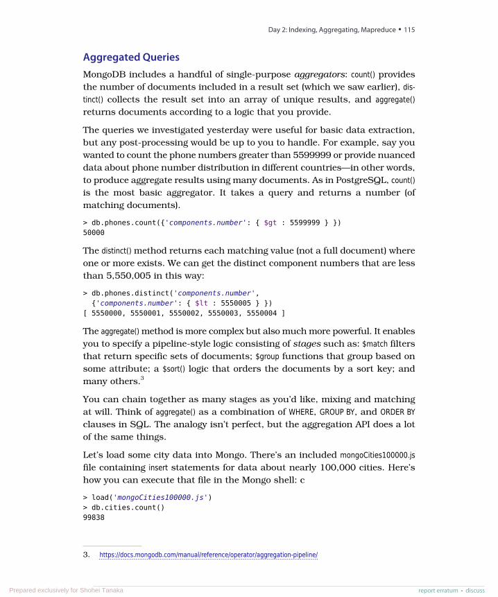
Aggregated QueriesMongoDB includes a handful of single-purpose aggregators: count() providesthe number of documents included in a result set (which we saw earlier), dis-tinct() collects the result set into an array of unique results, and aggregate()returns documents according to a logic that you provide.
The queries we investigated yesterday were useful for basic data extraction,but any post-processing would be up to you to handle. For example, say youwanted to count the phone numbers greater than 5599999 or provide nuanceddata about phone number distribution in different countries—in other words,to produce aggregate results using many documents. As in PostgreSQL, count()is the most basic aggregator. It takes a query and returns a number (ofmatching documents).
> db.phones.count({'components.number': { $gt : 5599999 } })50000
The distinct() method returns each matching value (not a full document) whereone or more exists. We can get the distinct component numbers that are lessthan 5,550,005 in this way:
> db.phones.distinct('components.number',{'components.number': { $lt : 5550005 } })
[ 5550000, 5550001, 5550002, 5550003, 5550004 ]
The aggregate() method is more complex but also much more powerful. It enablesyou to specify a pipeline-style logic consisting of stages such as: $match filtersthat return specific sets of documents; $group functions that group based onsome attribute; a $sort() logic that orders the documents by a sort key; andmany others.3
You can chain together as many stages as you’d like, mixing and matchingat will. Think of aggregate() as a combination of WHERE, GROUP BY, and ORDER BYclauses in SQL. The analogy isn’t perfect, but the aggregation API does a lotof the same things.
Let’s load some city data into Mongo. There’s an included mongoCities100000.jsfile containing insert statements for data about nearly 100,000 cities. Here’show you can execute that file in the Mongo shell: c
> load('mongoCities100000.js')> db.cities.count()99838
3. https://docs.mongodb.com/manual/reference/operator/aggregation-pipeline/
report erratum • discuss
Day 2: Indexing, Aggregating, Mapreduce • 115
Prepared exclusively for Shohei Tanaka
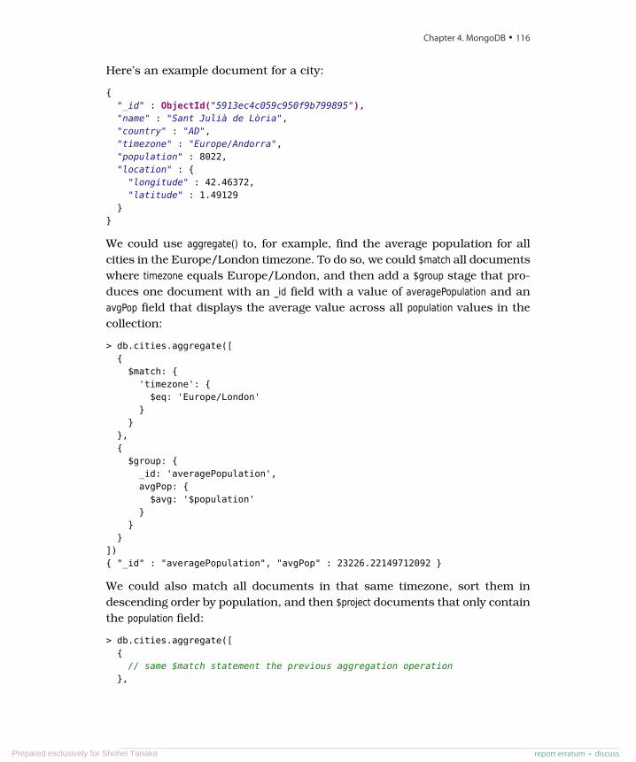
Here’s an example document for a city:
{"_id" : ObjectId("5913ec4c059c950f9b799895"),"name" : "Sant Julià de Lòria","country" : "AD","timezone" : "Europe/Andorra","population" : 8022,"location" : {
"longitude" : 42.46372,"latitude" : 1.49129
}}
We could use aggregate() to, for example, find the average population for allcities in the Europe/London timezone. To do so, we could $match all documentswhere timezone equals Europe/London, and then add a $group stage that pro-duces one document with an _id field with a value of averagePopulation and anavgPop field that displays the average value across all population values in thecollection:
> db.cities.aggregate([{
$match: {'timezone': {
$eq: 'Europe/London'}
}},{
$group: {_id: 'averagePopulation',avgPop: {
$avg: '$population'}
}}
]){ "_id" : "averagePopulation", "avgPop" : 23226.22149712092 }
We could also match all documents in that same timezone, sort them indescending order by population, and then $project documents that only containthe population field:
> db.cities.aggregate([{
// same $match statement the previous aggregation operation},
Chapter 4. MongoDB • 116
report erratum • discussPrepared exclusively for Shohei Tanaka

{$sort: {population: -1
}},{
$project: {_id: 0,name: 1,population: 1
}}
])
You should see results like this:
{ "name" : "City of London", "population" : 7556900 }{ "name" : "London", "population" : 7556900 }{ "name" : "Birmingham", "population" : 984333 }// many others
Experiment with it a bit—try combining some of the stage types we’ve alreadycovered in new ways—and then delete the collection when you’re done, aswe’ll add the same data back into the database using a different method onDay 3.
> db.cities.drop()
This provides a very small taste of Mongo’s aggregation capabilities. Thepossibilities are really endless, and we encourage you to explore other stagetypes. Be forewarned that aggregations can be quite slow if you add a lot ofstages and/or perform them on very large collections. There are limits to howwell Mongo, as a schemaless database, can optimize these sorts of operations.But if you’re careful to keep your collections reasonably sized and, even better,structure your data to not require bold transformations to get the outputsyou want, then aggregate() can be a powerful and even speedy tool.
Server-Side CommandsIn addition to evaluating JavaScript functions, there are several pre-builtcommands in Mongo, most of which are executed on the server, althoughsome require executing only under the admin database (which you can accessby entering use admin). The top command, for example, will output access detailsabout all collections on the server.
report erratum • discuss
Day 2: Indexing, Aggregating, Mapreduce • 117
Prepared exclusively for Shohei Tanaka

> use admin> db.runCommand("top"){
"totals" : {"note" : "all times in microseconds","admin.system.roles" : {
"total" : {"time" : 3666,"count" : 1
},// etc}
}
You can also list all commands that are currently available (let’s switch back to thebook database first because the admin database provides a different set of commands):
> use book> db.listCommands()
When you run listCommands(), you may notice a lot of commands we’ve usedalready. In fact, you can execute many common commands through the run-Command() method, such as counting the number of phones. However, youmay notice a slightly different output.
> db.runCommand({ "find" : "someCollection" }){
"cursor" : {"id" : NumberLong(0),"ns" : "book.someCollection","firstBatch" : [ ]
},"ok" : 1
}
Here, we see that this function returns an object containing a cursor and anok field. That’s because db.phones.find() is a wrapper function created for ourconvenience by the shell’s JavaScript interface, whereas runCommand() is anoperation executed on the server. Remember that we can play detective onhow a function such as find() works by leaving off the calling parentheses.
> db.phones.findfunction (query, fields, limit, skip, batchSize, options) {
var cursor = new DBQuery(this._mongo,// other query parametersoptions || this.getQueryOptions());
// some cursor-building logic
return cursor;}
Chapter 4. MongoDB • 118
report erratum • discussPrepared exclusively for Shohei Tanaka
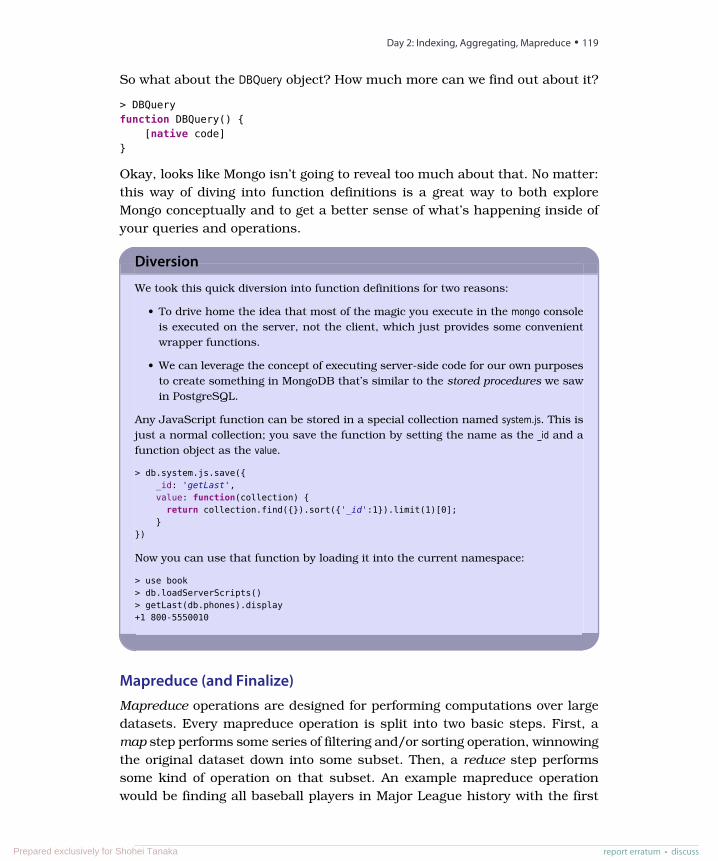
So what about the DBQuery object? How much more can we find out about it?
> DBQueryfunction DBQuery() {
[native code]}
Okay, looks like Mongo isn’t going to reveal too much about that. No matter:this way of diving into function definitions is a great way to both exploreMongo conceptually and to get a better sense of what’s happening inside ofyour queries and operations.
Diversion
We took this quick diversion into function definitions for two reasons:
• To drive home the idea that most of the magic you execute in the mongo consoleis executed on the server, not the client, which just provides some convenientwrapper functions.
• We can leverage the concept of executing server-side code for our own purposesto create something in MongoDB that’s similar to the stored procedures we sawin PostgreSQL.
Any JavaScript function can be stored in a special collection named system.js. This isjust a normal collection; you save the function by setting the name as the _id and afunction object as the value.
> db.system.js.save({_id: 'getLast',value: function(collection) {
return collection.find({}).sort({'_id':1}).limit(1)[0];}
})
Now you can use that function by loading it into the current namespace:
> use book> db.loadServerScripts()> getLast(db.phones).display+1 800-5550010
Mapreduce (and Finalize)Mapreduce operations are designed for performing computations over largedatasets. Every mapreduce operation is split into two basic steps. First, amap step performs some series of filtering and/or sorting operation, winnowingthe original dataset down into some subset. Then, a reduce step performssome kind of operation on that subset. An example mapreduce operationwould be finding all baseball players in Major League history with the first
report erratum • discuss
Day 2: Indexing, Aggregating, Mapreduce • 119
Prepared exclusively for Shohei Tanaka
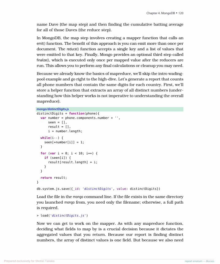
name Dave (the map step) and then finding the cumulative batting averagefor all of those Daves (the reduce step).
In MongoDB, the map step involves creating a mapper function that calls anemit() function. The benefit of this approach is you can emit more than once perdocument. The reduce() function accepts a single key and a list of values thatwere emitted to that key. Finally, Mongo provides an optional third step calledfinalize(), which is executed only once per mapped value after the reducers arerun. This allows you to perform any final calculations or cleanup you may need.
Because we already know the basics of mapreduce, we’ll skip the intro wading-pool example and go right to the high-dive. Let’s generate a report that countsall phone numbers that contain the same digits for each country. First, we’llstore a helper function that extracts an array of all distinct numbers (under-standing how this helper works is not imperative to understanding the overallmapreduce).
mongo/distinctDigits.jsdistinctDigits = function(phone){
var number = phone.components.number + '',seen = [],result = [],i = number.length;
while(i--) {seen[+number[i]] = 1;
}
for (var i = 0; i < 10; i++) {if (seen[i]) {result[result.length] = i;
}}
return result;}
db.system.js.save({_id: 'distinctDigits', value: distinctDigits})
Load the file in the mongo command line. If the file exists in the same directoryyou launched mongo from, you need only the filename; otherwise, a full pathis required.
> load('distinctDigits.js')
Now we can get to work on the mapper. As with any mapreduce function,deciding what fields to map by is a crucial decision because it dictates theaggregated values that you return. Because our report is finding distinctnumbers, the array of distinct values is one field. But because we also need
Chapter 4. MongoDB • 120
report erratum • discussPrepared exclusively for Shohei Tanaka
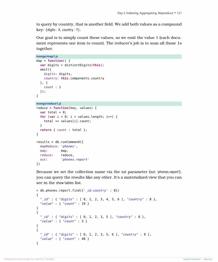
to query by country, that is another field. We add both values as a compoundkey: {digits : X, country : Y}.
Our goal is to simply count these values, so we emit the value 1 (each docu-ment represents one item to count). The reducer’s job is to sum all those 1stogether.
mongo/map1.jsmap = function() {
var digits = distinctDigits(this);emit({
digits: digits,country: this.components.country
}, {count : 1
});}
mongo/reduce1.jsreduce = function(key, values) {
var total = 0;for (var i = 0; i < values.length; i++) {
total += values[i].count;}return { count : total };
}
results = db.runCommand({mapReduce: 'phones',map: map,reduce: reduce,out: 'phones.report'
})
Because we set the collection name via the out parameter (out: 'phones.report'),you can query the results like any other. It’s a materialized view that you cansee in the show tables list.
> db.phones.report.find({'_id.country' : 8}){
"_id" : { "digits" : [ 0, 1, 2, 3, 4, 5, 6 ], "country" : 8 },"value" : { "count" : 19 }
}{
"_id" : { "digits" : [ 0, 1, 2, 3, 5 ], "country" : 8 },"value" : { "count" : 3 }
}{
"_id" : { "digits" : [ 0, 1, 2, 3, 5, 6 ], "country" : 8 },"value" : { "count" : 48 }
}
report erratum • discuss
Day 2: Indexing, Aggregating, Mapreduce • 121
Prepared exclusively for Shohei Tanaka
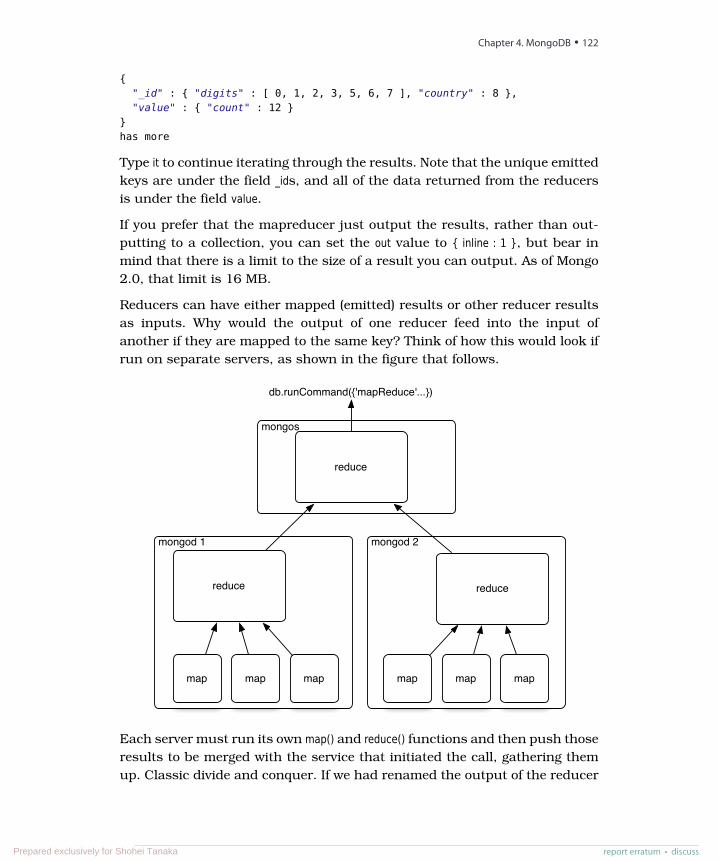
{"_id" : { "digits" : [ 0, 1, 2, 3, 5, 6, 7 ], "country" : 8 },"value" : { "count" : 12 }
}has more
Type it to continue iterating through the results. Note that the unique emittedkeys are under the field _ids, and all of the data returned from the reducersis under the field value.
If you prefer that the mapreducer just output the results, rather than out-putting to a collection, you can set the out value to { inline : 1 }, but bear inmind that there is a limit to the size of a result you can output. As of Mongo2.0, that limit is 16 MB.
Reducers can have either mapped (emitted) results or other reducer resultsas inputs. Why would the output of one reducer feed into the input ofanother if they are mapped to the same key? Think of how this would look ifrun on separate servers, as shown in the figure that follows.
mongos
mongod 1 mongod 2
map map map
reduce
map map map
reduce
reduce
db.runCommand({'mapReduce'...})
Each server must run its own map() and reduce() functions and then push thoseresults to be merged with the service that initiated the call, gathering themup. Classic divide and conquer. If we had renamed the output of the reducer
Chapter 4. MongoDB • 122
report erratum • discussPrepared exclusively for Shohei Tanaka
to total instead of count, we would have needed to handle both cases in theloop, as shown here:
mongo/reduce2.jsreduce = function(key, values) {
var total = 0;for(var i = 0; i < values.length; i++) {
var data = values[i];if('total' in data) {total += data.total;
} else {total += data.count;
}}return { total : total };
}
However, Mongo predicted that you might need to perform some final changes,such as renaming a field or some other calculations. If you really need theoutput field to be total, you can implement a finalize() function, which worksthe same way as the finalize function under group().
Day 2 Wrap-UpOn Day 2, we’ve expanded our query power by including several aggregatequeries: count(), distinct(), and topped off by aggregate(). To speed up the responsetime of these queries, we used MongoDB’s indexing options. When morepower is required, the ever-present mapReduce() is available.
Day 2 Homework
Find
1. Find a shortcut for admin commands.
2. Find the online documentation for queries and cursors.
3. Find the MongoDB documentation for mapreduce.
4. Through the JavaScript interface, investigate the code for three collectionsfunctions: help(), findOne(), and stats().
Do
1. Implement a finalize method to output the count as the total.
2. Install a Mongo driver for a language of your choice, and connect to thedatabase. Populate a collection through it, and index one of the fields.
report erratum • discuss
Day 2: Indexing, Aggregating, Mapreduce • 123
Prepared exclusively for Shohei Tanaka
Day 3: Replica Sets, Sharding, GeoSpatial, and GridFSMongo has a powerful ability to store and query data in a variety of ways. Butthen again, other databases can do those things, too. What makes documentdatabases unique is their ability to efficiently handle arbitrarily nested,schemaless data documents. Thus far, we’ve run Mongo as a single server.But if you were to run Mongo in production, you’d want to run it as a clusterof machines, which would provide for much higher availability and enableyou to replicate data across servers, shard collections into many pieces, andperform queries in parallel.
Replica SetsMongo was meant to scale out, not to run in standalone mode. It was builtfor data consistency and partition tolerance, but sharding data has a cost: Ifone part of a collection is lost, the whole thing is compromised. What good isquerying against a collection of countries that contains only the WesternHemisphere or only Asia? Mongo deals with this implicit sharding weaknessin a simple manner: duplication. You should rarely run a single Mongoinstance in production and instead replicate the stored data across multipleservices.
Rather than muck with our existing database, today we’ll start from scratchand spawn a few new servers. Mongo’s default port is 27017, so we’ll startup each server on other ports. Remember that you must create the datadirectories first, so create three of them:
$ mkdir ./mongo1 ./mongo2 ./mongo3
Next, we’ll fire up the Mongo servers. This time we’ll add the replSet flag withthe name book and specify the ports.
$ mongod --replSet book --dbpath ./mongo1 --port 27011
Chapter 4. MongoDB • 124
report erratum • discussPrepared exclusively for Shohei Tanaka
Open another terminal window and run the next command, which launchesanother server, pointing to a different directory, available on another port.Then open a third terminal to start the third server.
$ mongod --replSet book --dbpath ./mongo2 --port 27012$ mongod --replSet book --dbpath ./mongo3 --port 27013
Notice that you get lots of this noise on the output, with error messages like this:
[initandlisten] Did not find local voted for document at startup
That’s a good thing because we haven’t yet initialized our replica set andMongo is letting us know that. Fire up a mongo shell to one of the servers, andexecute the rs.initiate() function.
$ mongo localhost:27011> rs.initiate({
_id: 'book',members: [
{_id: 1, host: 'localhost:27011'},{_id: 2, host: 'localhost:27012'},{_id: 3, host: 'localhost:27013'}
]})> rs.status().ok1
Notice we’re using a new object called rs (replica set) instead of db (database).Like other objects, it has a help() method you can call. Running the status()command will let us know when our replica set is running, so just keepchecking the status for completion before continuing. If you watch the threeserver outputs, you should see that one server outputs this line:
Member ... is now in state PRIMARY
And two servers will have the following output:
Member ... is now in state SECONDARY
PRIMARY will be the master server. Chances are, this will be the server on port27011 (because it started first); however, if it’s not, go ahead and fire up aconsole to the primary. Just insert any old thing on the command line, andwe’ll try an experiment.
> db.echo.insert({ say : 'HELLO!' })
After the insert, exit the console, and then let’s test that our change has beenreplicated by shutting down the master node; pressing Ctrl+C is sufficient. Ifyou watch the logs of the remaining two servers, you should see that one ofthe two has now been promoted to master (it will output the Member ... is now in
report erratum • discuss
Day 3: Replica Sets, Sharding, GeoSpatial, and GridFS • 125
Prepared exclusively for Shohei Tanaka
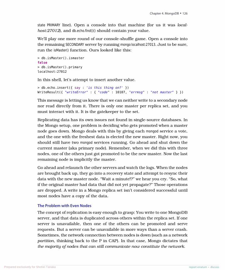
state PRIMARY line). Open a console into that machine (for us it was local-host:27012), and db.echo.find()() should contain your value.
We’ll play one more round of our console-shuffle game. Open a console intothe remaining SECONDARY server by running mongo localhost:27013. Just to be sure,run the isMaster() function. Ours looked like this:
> db.isMaster().ismasterfalse> db.isMaster().primarylocalhost:27012
In this shell, let’s attempt to insert another value.
> db.echo.insert({ say : 'is this thing on?' })WriteResult({ "writeError" : { "code" : 10107, "errmsg" : "not master" } })
This message is letting us know that we can neither write to a secondary nodenor read directly from it. There is only one master per replica set, and youmust interact with it. It is the gatekeeper to the set.
Replicating data has its own issues not found in single-source databases. Inthe Mongo setup, one problem is deciding who gets promoted when a masternode goes down. Mongo deals with this by giving each mongod service a vote,and the one with the freshest data is elected the new master. Right now, youshould still have two mongod services running. Go ahead and shut down thecurrent master (aka primary node). Remember, when we did this with threenodes, one of the others just got promoted to be the new master. Now the lastremaining node is implicitly the master.
Go ahead and relaunch the other servers and watch the logs. When the nodesare brought back up, they go into a recovery state and attempt to resync theirdata with the new master node. “Wait a minute!?” we hear you cry. “So, whatif the original master had data that did not yet propagate?” Those operationsare dropped. A write in a Mongo replica set isn’t considered successful untilmost nodes have a copy of the data.
The Problem with Even Nodes
The concept of replication is easy enough to grasp: You write to one MongoDBserver, and that data is duplicated across others within the replica set. If oneserver is unavailable, then one of the others can be promoted and serverequests. But a server can be unavailable in more ways than a server crash.Sometimes, the network connection between nodes is down (such as a networkpartition, thinking back to the P in CAP). In that case, Mongo dictates thatthe majority of nodes that can still communicate now constitute the network.
Chapter 4. MongoDB • 126
report erratum • discussPrepared exclusively for Shohei Tanaka
MongoDB expects an odd number of total nodes in the replica set. Considera five-node network, for example. If connection issues split it into a three-node fragment and a two-node fragment, the larger fragment has a clearmajority and can elect a master and continue servicing requests. With noclear majority, a quorum couldn’t be reached.
To see why an odd number of nodes is preferred, consider what might happento a four-node replica set. Say a network partition causes two of the serversto lose connectivity from the other two. One set will have the original master,but because it can’t see a clear majority of the network, the master stepsdown. The other set will similarly be unable to elect a master because it, too,can’t communicate with a clear majority of nodes. Both sets are now unableto process requests and the system is effectively down. Having an odd numberof total nodes would have made this particular scenario—a fragmented networkwhere each fragment has less than a clear majority—less likely to occur.
Some databases (such as CouchDB) are built to allow multiple masters, butMongo is not, and so it isn’t prepared to resolve data updates between them.MongoDB deals with conflicts between multiple masters by simply notallowing them.
Because it’s a CP system, Mongo always knows the most recent value; theclient needn’t decide. Mongo’s concern is strong consistency on writes, andpreventing a multimaster scenario is not a bad method for achieving it.
Voting and Arbiters
You may not always want to have an odd number of servers replicating data. In thatcase, you can either launch an arbiter (generally recommended) or increase votingrights on your servers (generally not recommended). In Mongo, an arbiter is a votingbut nonreplicating server in the replica set. You launch it just like any other serverbut on configuration set a flag, like this: {_id: 3, host: 'localhost:27013', arbiterOnly : true}.Arbiters are useful for breaking ties, like the U.S. Vice President in the Senate. Bydefault, each mongod instance has a single vote.
ShardingOne of the core goals of Mongo is to provide safe and quick handling of verylarge datasets. The clearest method of achieving this is through horizontalsharding by value ranges—or just sharding for brevity. Rather than a singleserver hosting all values in a collection, some range of values is split, orsharded, onto other servers. For example, in our phone numbers collection,we may put all phone numbers less than 1-500-000-0000 onto Mongo server
report erratum • discuss
Day 3: Replica Sets, Sharding, GeoSpatial, and GridFS • 127
Prepared exclusively for Shohei Tanaka
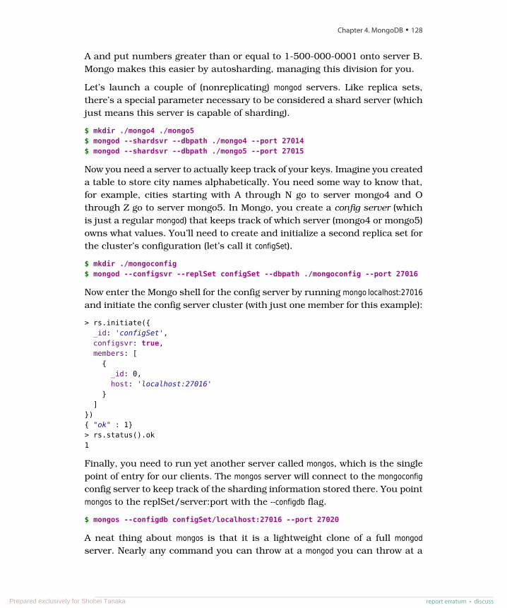
A and put numbers greater than or equal to 1-500-000-0001 onto server B.Mongo makes this easier by autosharding, managing this division for you.
Let’s launch a couple of (nonreplicating) mongod servers. Like replica sets,there’s a special parameter necessary to be considered a shard server (whichjust means this server is capable of sharding).
$ mkdir ./mongo4 ./mongo5$ mongod --shardsvr --dbpath ./mongo4 --port 27014$ mongod --shardsvr --dbpath ./mongo5 --port 27015
Now you need a server to actually keep track of your keys. Imagine you createda table to store city names alphabetically. You need some way to know that,for example, cities starting with A through N go to server mongo4 and Othrough Z go to server mongo5. In Mongo, you create a config server (whichis just a regular mongod) that keeps track of which server (mongo4 or mongo5)owns what values. You’ll need to create and initialize a second replica set forthe cluster’s configuration (let’s call it configSet).
$ mkdir ./mongoconfig$ mongod --configsvr --replSet configSet --dbpath ./mongoconfig --port 27016
Now enter the Mongo shell for the config server by running mongo localhost:27016and initiate the config server cluster (with just one member for this example):
> rs.initiate({_id: 'configSet',configsvr: true,members: [
{_id: 0,host: 'localhost:27016'
}]
}){ "ok" : 1}> rs.status().ok1
Finally, you need to run yet another server called mongos, which is the singlepoint of entry for our clients. The mongos server will connect to the mongoconfigconfig server to keep track of the sharding information stored there. You pointmongos to the replSet/server:port with the --configdb flag.
$ mongos --configdb configSet/localhost:27016 --port 27020
A neat thing about mongos is that it is a lightweight clone of a full mongodserver. Nearly any command you can throw at a mongod you can throw at a
Chapter 4. MongoDB • 128
report erratum • discussPrepared exclusively for Shohei Tanaka
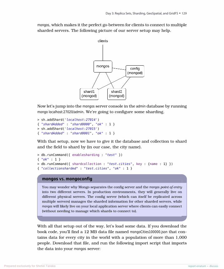
mongos, which makes it the perfect go-between for clients to connect to multiplesharded servers. The following picture of our server setup may help.
Now let’s jump into the mongos server console in the admin database by runningmongo localhost:27020/admin. We’re going to configure some sharding.
> sh.addShard('localhost:27014'){ "shardAdded" : "shard0000", "ok" : 1 }> sh.addShard('localhost:27015'){ "shardAdded" : "shard0001", "ok" : 1 }
With that setup, now we have to give it the database and collection to shardand the field to shard by (in our case, the city name).
> db.runCommand({ enablesharding : "test" }){ "ok" : 1 }> db.runCommand({ shardcollection : "test.cities", key : {name : 1} }){ "collectionsharded" : "test.cities", "ok" : 1 }
mongos vs. mongoconfigYou may wonder why Mongo separates the config server and the mongos point of entryinto two different servers. In production environments, they will generally live ondifferent physical servers. The config server (which can itself be replicated acrossmultiple servers) manages the sharded information for other sharded servers, whilemongos will likely live on your local application server where clients can easily connect(without needing to manage which shards to connect to).
With all that setup out of the way, let’s load some data. If you download thebook code, you’ll find a 12 MB data file named mongoCities100000.json that con-tains data for every city in the world with a population of more than 1,000people. Download that file, and run the following import script that importsthe data into your mongos server:
report erratum • discuss
Day 3: Replica Sets, Sharding, GeoSpatial, and GridFS • 129
Prepared exclusively for Shohei Tanaka
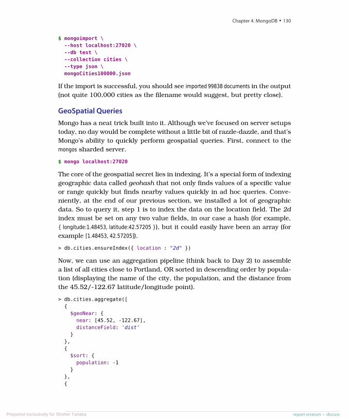
$ mongoimport \--host localhost:27020 \--db test \--collection cities \--type json \mongoCities100000.json
If the import is successful, you should see imported 99838 documents in the output(not quite 100,000 cities as the filename would suggest, but pretty close).
GeoSpatial QueriesMongo has a neat trick built into it. Although we’ve focused on server setupstoday, no day would be complete without a little bit of razzle-dazzle, and that’sMongo’s ability to quickly perform geospatial queries. First, connect to themongos sharded server.
$ mongo localhost:27020
The core of the geospatial secret lies in indexing. It’s a special form of indexinggeographic data called geohash that not only finds values of a specific valueor range quickly but finds nearby values quickly in ad hoc queries. Conve-niently, at the end of our previous section, we installed a lot of geographicdata. So to query it, step 1 is to index the data on the location field. The 2dindex must be set on any two value fields, in our case a hash (for example,{ longitude:1.48453, latitude:42.57205 }), but it could easily have been an array (forexample [1.48453, 42.57205]).
> db.cities.ensureIndex({ location : "2d" })
Now, we can use an aggregation pipeline (think back to Day 2) to assemblea list of all cities close to Portland, OR sorted in descending order by popula-tion (displaying the name of the city, the population, and the distance fromthe 45.52/-122.67 latitude/longitude point).
> db.cities.aggregate([{
$geoNear: {near: [45.52, -122.67],distanceField: 'dist'
}},{
$sort: {population: -1
}},{
Chapter 4. MongoDB • 130
report erratum • discussPrepared exclusively for Shohei Tanaka
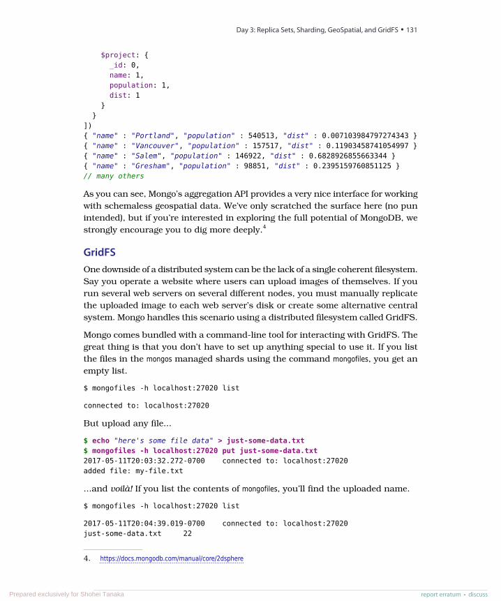
$project: {_id: 0,name: 1,population: 1,dist: 1
}}
]){ "name" : "Portland", "population" : 540513, "dist" : 0.007103984797274343 }{ "name" : "Vancouver", "population" : 157517, "dist" : 0.11903458741054997 }{ "name" : "Salem", "population" : 146922, "dist" : 0.6828926855663344 }{ "name" : "Gresham", "population" : 98851, "dist" : 0.2395159760851125 }// many others
As you can see, Mongo’s aggregation API provides a very nice interface for workingwith schemaless geospatial data. We’ve only scratched the surface here (no punintended), but if you’re interested in exploring the full potential of MongoDB, westrongly encourage you to dig more deeply.4
GridFSOne downside of a distributed system can be the lack of a single coherent filesystem.Say you operate a website where users can upload images of themselves. If yourun several web servers on several different nodes, you must manually replicatethe uploaded image to each web server’s disk or create some alternative centralsystem. Mongo handles this scenario using a distributed filesystem called GridFS.
Mongo comes bundled with a command-line tool for interacting with GridFS. Thegreat thing is that you don’t have to set up anything special to use it. If you listthe files in the mongos managed shards using the command mongofiles, you get anempty list.
$ mongofiles -h localhost:27020 list
connected to: localhost:27020
But upload any file...
$ echo "here's some file data" > just-some-data.txt$ mongofiles -h localhost:27020 put just-some-data.txt2017-05-11T20:03:32.272-0700 connected to: localhost:27020added file: my-file.txt
...and voilà! If you list the contents of mongofiles, you’ll find the uploaded name.
$ mongofiles -h localhost:27020 list
2017-05-11T20:04:39.019-0700 connected to: localhost:27020just-some-data.txt 22
4. https://docs.mongodb.com/manual/core/2dsphere
report erratum • discuss
Day 3: Replica Sets, Sharding, GeoSpatial, and GridFS • 131
Prepared exclusively for Shohei Tanaka
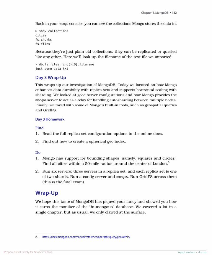
Back in your mongo console, you can see the collections Mongo stores the data in.
> show collectionscitiesfs.chunksfs.files
Because they’re just plain old collections, they can be replicated or queriedlike any other. Here we’ll look up the filename of the text file we imported.
> db.fs.files.find()[0].filenamejust-some-data.txt
Day 3 Wrap-UpThis wraps up our investigation of MongoDB. Today we focused on how Mongoenhances data durability with replica sets and supports horizontal scaling withsharding. We looked at good server configurations and how Mongo provides themongos server to act as a relay for handling autosharding between multiple nodes.Finally, we toyed with some of Mongo’s built-in tools, such as geospatial queriesand GridFS.
Day 3 Homework
Find
1. Read the full replica set configuration options in the online docs.
2. Find out how to create a spherical geo index.
Do
1. Mongo has support for bounding shapes (namely, squares and circles).Find all cities within a 50-mile radius around the center of London.5
2. Run six servers: three servers in a replica set, and each replica set is oneof two shards. Run a config server and mongos. Run GridFS across them(this is the final exam).
Wrap-UpWe hope this taste of MongoDB has piqued your fancy and showed you howit earns the moniker of the “humongous” database. We covered a lot in asingle chapter, but as usual, we only clawed at the surface.
5. https://docs.mongodb.com/manual/reference/operator/query/geoWithin/
Chapter 4. MongoDB • 132
report erratum • discussPrepared exclusively for Shohei Tanaka
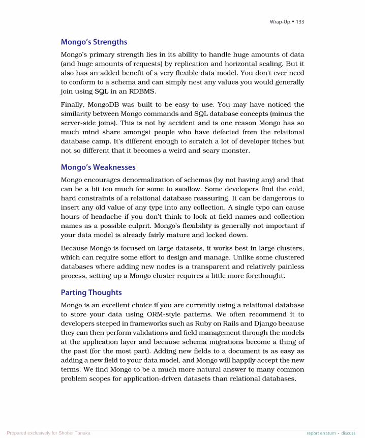
Mongo’s StrengthsMongo’s primary strength lies in its ability to handle huge amounts of data(and huge amounts of requests) by replication and horizontal scaling. But italso has an added benefit of a very flexible data model. You don’t ever needto conform to a schema and can simply nest any values you would generallyjoin using SQL in an RDBMS.
Finally, MongoDB was built to be easy to use. You may have noticed thesimilarity between Mongo commands and SQL database concepts (minus theserver-side joins). This is not by accident and is one reason Mongo has somuch mind share amongst people who have defected from the relationaldatabase camp. It’s different enough to scratch a lot of developer itches butnot so different that it becomes a weird and scary monster.
Mongo’s WeaknessesMongo encourages denormalization of schemas (by not having any) and thatcan be a bit too much for some to swallow. Some developers find the cold,hard constraints of a relational database reassuring. It can be dangerous toinsert any old value of any type into any collection. A single typo can causehours of headache if you don’t think to look at field names and collectionnames as a possible culprit. Mongo’s flexibility is generally not important ifyour data model is already fairly mature and locked down.
Because Mongo is focused on large datasets, it works best in large clusters,which can require some effort to design and manage. Unlike some clustereddatabases where adding new nodes is a transparent and relatively painlessprocess, setting up a Mongo cluster requires a little more forethought.
Parting ThoughtsMongo is an excellent choice if you are currently using a relational databaseto store your data using ORM-style patterns. We often recommend it todevelopers steeped in frameworks such as Ruby on Rails and Django becausethey can then perform validations and field management through the modelsat the application layer and because schema migrations become a thing ofthe past (for the most part). Adding new fields to a document is as easy asadding a new field to your data model, and Mongo will happily accept the newterms. We find Mongo to be a much more natural answer to many commonproblem scopes for application-driven datasets than relational databases.
report erratum • discuss
Wrap-Up • 133
Prepared exclusively for Shohei Tanaka
CHAPTER 5
CouchDBRatchet wrenches are light and convenient tools you carry around for a rangeof jobs, big and small. As with power drills, you can swap out variously sizedbits like sockets or screws. Unlike a power drill that needs to be plugged into120 volts of AC power, however, a wrench is happy to rest in your pocket andrun on elbow grease. Apache CouchDB is like that. Able to scale down as wellas up, it fits problem spaces of varying size and complexity with ease.
CouchDB is the quintessential JSON- and REST-based document-orienteddatabase. First released all the way back in 2005, CouchDB was designedwith the web in mind and all the innumerable flaws, faults, failures, andglitches that come with it. Consequently, CouchDB offers a robustnessunmatched by most other databases. Whereas other systems tolerate occa-sional network drops, CouchDB thrives even when connectivity is only rarelyavailable.
Like MongoDB, CouchDB stores documents—JSON objects consisting of key-value pairs where values may be any of several types, including other objectsnested to any depth. What you don’t get, though, is ad hoc querying. Instead,indexed views produced by incremental mapreduce operations are the principalway you discover documents.
Relaxing on the CouchCouchDB lives up to its tag line: relax. Instead of focusing on working wellonly in massive clusters running on hundreds of nodes, CouchDB aims tosupport a variety of deployment scenarios from the datacenter down to thesmartphone. You can run CouchDB on your Android phone, on your MacBook,and in your datacenter. Written in Erlang, CouchDB is built tough—the onlyway to shut it down is to kill the process! With its append-only storage model,your data is virtually incorruptible and easy to replicate, back up, and restore.
report erratum • discussPrepared exclusively for Shohei Tanaka
CouchDB is document oriented, using JSON as its storage and communicationlanguage. All calls to CouchDB happen through its REST interface. Replicationcan be one way (from one database to another) or bidirectional (back andforth between databases), and ad hoc (triggered at will) or continuous (triggeredat periodic intervals). CouchDB gives you a lot of flexibility to decide how tostructure, protect, and distribute your data.
Frontend-to-Backend Syncing with PouchDB
The past few years have seen a dramatic increase in interest in web apps that remainusable even when the user is offline. One of the core difficulties behind building suchoffline-friendly applications is the data synchronization problem. If a user uses anapp offline for an hour and makes a wide variety of changes, what happens whentheir connection comes back and the discrepancy between client and server stateneeds to be resolved?
PouchDB is a very interesting tool that has emerged from the CouchDB ecosystemto address this problem. PouchDB is an open source database created in JavaScriptthat acts as a client-side, in-browser data store that automatically synchronizes datawith CouchDB on the backend.
We won‘t cover PouchDB in this book, but we do find it to be a compelling solutionto a problem that‘s widely encountered but has very few ready-made solutions. Ifyou‘re looking to use CouchDB as a backend for web apps, you‘d be remiss not totake a look.
Comparing CouchDB and MongoDBOne of the big questions we wanted to address in this book is “What’s thedifference between CouchDB and MongoDB?” On the surface, CouchDB andMongoDB—which we covered in Chapter 4, MongoDB, on page 93—can seemquite similar. They’re both document-oriented databases with an affinity forJavaScript that use JSON for data transport. There are many differences,though, ranging from project philosophy to implementation to scalabilitycharacteristics. We’ll cover many of these as we explore the beautiful simplic-ity of CouchDB.
During our three-day tour, we’ll explore many of CouchDB’s compelling fea-tures and design choices. We’ll start, as always, with individual CRUD com-mands and then move on to indexing through mapreduce views. As we’vedone with other databases, we’ll import some structured data and then useit to explore some advanced concepts. Finally, we’ll develop some simple event-driven client-side applications using Node.js and learn how CouchDB’s master-master replication strategy deals with conflicting updates. Let’s get to it!
Chapter 5. CouchDB • 136
report erratum • discussPrepared exclusively for Shohei Tanaka
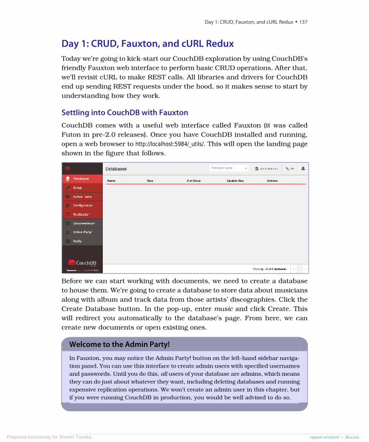
Day 1: CRUD, Fauxton, and cURL ReduxToday we’re going to kick-start our CouchDB exploration by using CouchDB’sfriendly Fauxton web interface to perform basic CRUD operations. After that,we’ll revisit cURL to make REST calls. All libraries and drivers for CouchDBend up sending REST requests under the hood, so it makes sense to start byunderstanding how they work.
Settling into CouchDB with FauxtonCouchDB comes with a useful web interface called Fauxton (it was calledFuton in pre-2.0 releases). Once you have CouchDB installed and running,open a web browser to http://localhost:5984/_utils/. This will open the landing pageshown in the figure that follows.
Before we can start working with documents, we need to create a databaseto house them. We’re going to create a database to store data about musiciansalong with album and track data from those artists’ discographies. Click theCreate Database button. In the pop-up, enter music and click Create. Thiswill redirect you automatically to the database’s page. From here, we cancreate new documents or open existing ones.
Welcome to the Admin Party!
In Fauxton, you may notice the Admin Party! button on the left-hand sidebar naviga-tion panel. You can use this interface to create admin users with specified usernamesand passwords. Until you do this, all users of your database are admins, which meansthey can do just about whatever they want, including deleting databases and runningexpensive replication operations. We won’t create an admin user in this chapter, butif you were running CouchDB in production, you would be well advised to do so.
report erratum • discuss
Day 1: CRUD, Fauxton, and cURL Redux • 137
Prepared exclusively for Shohei Tanaka
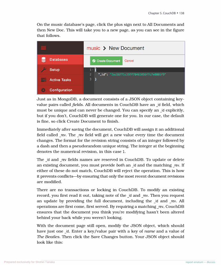
On the music database’s page, click the plus sign next to All Documents andthen New Doc. This will take you to a new page, as you can see in the figurethat follows.
Just as in MongoDB, a document consists of a JSON object containing key-value pairs called fields. All documents in CouchDB have an _id field, whichmust be unique and can never be changed. You can specify an _id explicitly,but if you don’t, CouchDB will generate one for you. In our case, the defaultis fine, so click Create Document to finish.
Immediately after saving the document, CouchDB will assign it an additionalfield called _rev. The _rev field will get a new value every time the documentchanges. The format for the revision string consists of an integer followed bya dash and then a pseudorandom unique string. The integer at the beginningdenotes the numerical revision, in this case 1.
The _id and _rev fields names are reserved in CouchDB. To update or deletean existing document, you must provide both an _id and the matching _rev. Ifeither of these do not match, CouchDB will reject the operation. This is howit prevents conflicts—by ensuring that only the most recent document revisionsare modified.
There are no transactions or locking in CouchDB. To modify an existingrecord, you first read it out, taking note of the _id and _rev. Then you requestan update by providing the full document, including the _id and _rev. Alloperations are first come, first served. By requiring a matching _rev, CouchDBensures that the document you think you’re modifying hasn’t been alteredbehind your back while you weren’t looking.
With the document page still open, modify the JSON object, which shouldhave just one _id. Enter a key/value pair with a key of name and a value ofThe Beatles. Then click the Save Changes button. Your JSON object shouldlook like this:
Chapter 5. CouchDB • 138
report erratum • discussPrepared exclusively for Shohei Tanaka
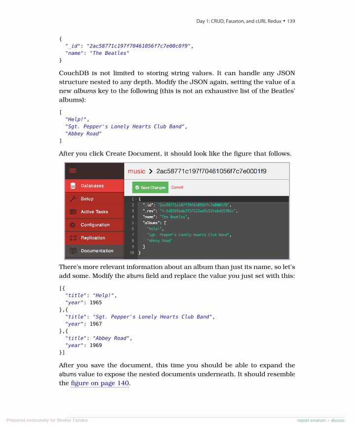
{"_id": "2ac58771c197f70461056f7c7e00c0f9","name": "The Beatles"
}
CouchDB is not limited to storing string values. It can handle any JSONstructure nested to any depth. Modify the JSON again, setting the value of anew albums key to the following (this is not an exhaustive list of the Beatles’albums):
["Help!","Sgt. Pepper's Lonely Hearts Club Band","Abbey Road"
]
After you click Create Document, it should look like the figure that follows.
There’s more relevant information about an album than just its name, so let’sadd some. Modify the albums field and replace the value you just set with this:
[{"title": "Help!","year": 1965
},{"title": "Sgt. Pepper's Lonely Hearts Club Band","year": 1967
},{"title": "Abbey Road","year": 1969
}]
After you save the document, this time you should be able to expand thealbums value to expose the nested documents underneath. It should resemblethe figure on page 140.
report erratum • discuss
Day 1: CRUD, Fauxton, and cURL Redux • 139
Prepared exclusively for Shohei Tanaka
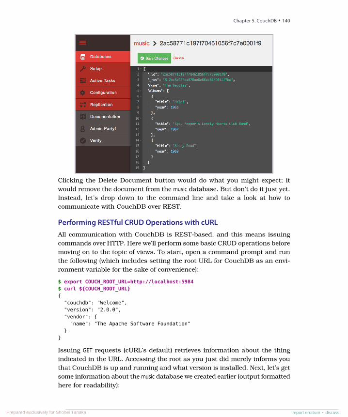
Clicking the Delete Document button would do what you might expect; itwould remove the document from the music database. But don’t do it just yet.Instead, let’s drop down to the command line and take a look at how tocommunicate with CouchDB over REST.
Performing RESTful CRUD Operations with cURLAll communication with CouchDB is REST-based, and this means issuingcommands over HTTP. Here we’ll perform some basic CRUD operations beforemoving on to the topic of views. To start, open a command prompt and runthe following (which includes setting the root URL for CouchDB as an envi-ronment variable for the sake of convenience):
$ export COUCH_ROOT_URL=http://localhost:5984$ curl ${COUCH_ROOT_URL}{
"couchdb": "Welcome","version": "2.0.0","vendor": {
"name": "The Apache Software Foundation"}
}
Issuing GET requests (cURL’s default) retrieves information about the thingindicated in the URL. Accessing the root as you just did merely informs youthat CouchDB is up and running and what version is installed. Next, let’s getsome information about the music database we created earlier (output formattedhere for readability):
Chapter 5. CouchDB • 140
report erratum • discussPrepared exclusively for Shohei Tanaka
$ curl "${COUCH_ROOT_URL}/music/"{
"db_name": "music","update_seq": "4-g1AA...aZxxw","sizes": {
"file": 24907,"external": 193,"active": 968
},"purge_seq": 0,"other": {
"data_size": 193},"doc_del_count": 0,"doc_count": 1,"disk_size": 24907,"disk_format_version": 6,"data_size": 968,"compact_running": false,"instance_start_time": "0"
}
This returns some information about how many documents are in thedatabase, how long the server has been up, how many operations have beenperformed, disk size, and more.
Reading a Document with GETTo retrieve a specific document, append its _id to the database URL like so:
$ curl "${COUCH_ROOT_URL}/music/2ac58771c197f70461056f7c7e0001f9"{
"_id": "2ac58771c197f70461056f7c7e0001f9","_rev": "8-e1b7281f6adcd82910c6473be2d4e2ec","name": "The Beatles","albums": [
{"title": "Help!","year": 1965
},{"title": "Sgt. Pepper's Lonely Hearts Club Band","year": 1967
},{"title": "Abbey Road","year": 1969
}]
}
report erratum • discuss
Day 1: CRUD, Fauxton, and cURL Redux • 141
Prepared exclusively for Shohei Tanaka
In CouchDB, issuing GET requests is always safe. CouchDB won’t make anychanges to documents as the result of a GET. To make changes, you have touse other HTTP commands such as PUT, POST, and DELETE.
Creating a Document with POSTTo create a new document, use POST. Make sure to specify a Content-Typeheader with the value application/json; otherwise, CouchDB will refuse the request.
$ curl -i -XPOST "${COUCH_ROOT_URL}/music/" \-H "Content-Type: application/json" \-d '{ "name": "Wings" }'
HTTP/1.1 201 CreatedCache-Control: must-revalidateContent-Length: 95Content-Type: application/jsonDate: Sun, 30 Apr 2017 23:15:42 GMTLocation: http://localhost:5984/music/2ac58771c197f70461056f7c7e002edaServer: CouchDB/2.0.0 (Erlang OTP/19)X-Couch-Request-ID: 92885ae1d3X-CouchDB-Body-Time: 0
{"ok": true,"id": "2ac58771c197f70461056f7c7e002eda","rev": "1-2fe1dd1911153eb9df8460747dfe75a0"
}
The HTTP response code 201 Created tells us that our creation request wassuccessful. The body of the response contains a JSON object with usefulinformation, such as the _id and _rev values.
Updating a Document with PUTThe PUT command is used to update an existing document or create a newone with a specific _id. Just like GET, the URL for a PUT URL consists of thedatabase URL followed by the document’s _id.
$ curl -i -XPUT \"${COUCH_ROOT_URL}/music/2ac58771c197f70461056f7c7e002eda" \-H "Content-Type: application/json" \-d '{
"_id": "74c7a8d2a8548c8b97da748f43000f1b","_rev": "1-2fe1dd1911153eb9df8460747dfe75a0","name": "Wings","albums": ["Wild Life", "Band on the Run", "London Town"]
}'HTTP/1.1 201 CreatedCache-Control: must-revalidateContent-Length: 95
Chapter 5. CouchDB • 142
report erratum • discussPrepared exclusively for Shohei Tanaka
Content-Type: application/jsonDate: Sun, 30 Apr 2017 23:25:13 GMTETag: "2-17e4ce41cd33d6a38f04a8452d5a860b"Location: http://localhost:5984/music/2ac58771c197f70461056f7c7e002edaServer: CouchDB/2.0.0 (Erlang OTP/19)X-Couch-Request-ID: 6c0bdfffa5X-CouchDB-Body-Time: 0
{"ok": true,"id": "2ac58771c197f70461056f7c7e002eda","rev": "2-17e4ce41cd33d6a38f04a8452d5a860b"
}
Unlike MongoDB, in which you modify documents in place, with CouchDByou always overwrite the entire document to make any change. The Fauxtonweb interface you saw earlier may have made it look like you could modify asingle field in isolation, but behind the scenes it was rerecording the wholedocument when you hit Save Changes.
As we mentioned earlier, both the _id and _rev fields must exactly match thedocument being updated, or the operation will fail. To see how, try executingthe same PUT operation again.
HTTP/1.1 409 ConflictCache-Control: must-revalidateContent-Length: 58Content-Type: application/jsonDate: Sun, 30 Apr 2017 23:25:52 GMTServer: CouchDB/2.0.0 (Erlang OTP/19)X-Couch-Request-ID: 5b626b9060X-CouchDB-Body-Time: 0
{"error":"conflict","reason":"Document update conflict."}
You’ll get an HTTP 409 Conflict response with a JSON object describing theproblem. This is how CouchDB enforces consistency.
Removing a Document with DELETEFinally, you can use the DELETE operation to remove a document from thedatabase.
$ curl -i -XDELETE \"${COUCH_ROOT_URL}/music/2ac58771c197f70461056f7c7e002eda" \-H "If-Match: 2-17e4ce41cd33d6a38f04a8452d5a860b"
HTTP/1.1 200 OKCache-Control: must-revalidateContent-Length: 95Content-Type: application/jsonDate: Sun, 30 Apr 2017 23:26:40 GMT
report erratum • discuss
Day 1: CRUD, Fauxton, and cURL Redux • 143
Prepared exclusively for Shohei Tanaka
ETag: "3-42aafb7411c092614ce7c9f4ab79dc8b"Server: CouchDB/2.0.0 (Erlang OTP/19)X-Couch-Request-ID: c4dcb91db2X-CouchDB-Body-Time: 0
{"ok": true,"id": "2ac58771c197f70461056f7c7e002eda","rev": "3-42aafb7411c092614ce7c9f4ab79dc8b"
}
The DELETE operation will supply a new revision number, even though thedocument is gone. It’s worth noting that the document wasn’t really removedfrom disk, but rather a new empty document was appended, flagging thedocument as deleted. Just like with an update, CouchDB does not modifydocuments in place. But for all intents and purposes, it’s deleted.
Day 1 Wrap-UpNow that you’ve learned how to do basic CRUD operations in Fauxton andcURL, you’re ready to move on to more advanced topics. On Day 2, we’ll diginto creating indexed views, which will provide other avenues for retrievingdocuments than just specifying them by their _id values.
Day 1 Homework
Find
1. Find the CouchDB HTTP API reference documentation online.
2. We’ve already used GET, POST, PUT, and DELETE. What other HTTP methodsare supported?
Do
1. Use cURL to PUT a new document into the music database with a specific_id of your choice.
2. Use cURL to create a new database with a name of your choice, and thendelete that database also via cURL.
3. CouchDB supports attachments, which are arbitrary files that you cansave with documents (similar to email attachments). Again using cURL,create a new document that contains a text document as an attachment.Lastly, craft and execute a cURL request that will return just that docu-ment’s attachment.
Chapter 5. CouchDB • 144
report erratum • discussPrepared exclusively for Shohei Tanaka
Day 2: Creating and Querying ViewsIn CouchDB, a view is a window into the documents contained in a database.Views are the principal way that documents are accessed in all but trivialcases, such as those individual CRUD operations you saw on Day 1. Today,you’ll discover how to create the functions that make up a view. You’ll alsolearn how to perform ad hoc queries against views using cURL. Finally, you’llimport music data, which will make the views more salient and demonstratehow to use couchrest, a popular Ruby library for working with CouchDB.
Accessing Documents Through ViewsA view consists of mapper and reducer functions that are used to generatean ordered list of key-value pairs. Both keys and values can be any validJSON. The simplest view is called _all_docs. It is provided out-of-the-box for alldatabases and contains an entry for each document in the database, keyedby its string _id.
To retrieve all of the things in the database, issue a GET request for the _all_docs view.
$ curl "${COUCH_ROOT_URL}/music/_all_docs"{
"total_rows": 1,"offset": 0,"rows": [
{"id": "2ac58771c197f70461056f7c7e0001f9","key": "2ac58771c197f70461056f7c7e0001f9","value": {
"rev": "7-d37c47883f4d30913c6a38644410685d"}
}]
}
You can see in the previous output the one document we’ve created so far.The response is a JSON object that contains an array of rows. Each row is anobject with three fields:
• id is the document’s _id.• key is the JSON key produced by the mapreduce functions.• value is the associated JSON value, also produced through mapreduce.
In the case of _all_docs, the id and key fields match, but for custom views thiswill almost never be the case.
report erratum • discuss
Day 2: Creating and Querying Views • 145
Prepared exclusively for Shohei Tanaka

By default, views will include only metadata for documents in the value fieldrather than each document’s content. To retrieve all of the document’s fields,add the include_docs=true URL parameter.
$ curl "${COUCH_ROOT_URL}/music/_all_docs?include_docs=true"{
"total_rows": 1,"offset": 0,"rows": [
{"id": "2ac58771c197f70461056f7c7e0001f9","key": "2ac58771c197f70461056f7c7e0001f9","value": {
"rev": "7-d37c47883f4d30913c6a38644410685d"},"doc": {
"_id": "2ac58771c197f70461056f7c7e0001f9","_rev": "7-d37c47883f4d30913c6a38644410685d","name": "The Beatles","albums": [
{"title": "Help!","year": 1965
},{"title": "Sgt. Pepper's Lonely Hearts Club Band","year": 1967
},{"title": "Abbey Road","year": 1969
}]
}}
]}
Here you can see that the other properties, name and albums, have been addedto the value object in the output. With this basic structure in mind, let’s makeour own views.
Writing Your First ViewNow that we’ve gotten a rough overview of how views work, let’s try creatingour own views. To start, we’ll reproduce the behavior of the _all_docs view, andafter that, we’ll make increasingly complex views to extract deeper informationfrom our documents for indexing.
Chapter 5. CouchDB • 146
report erratum • discussPrepared exclusively for Shohei Tanaka
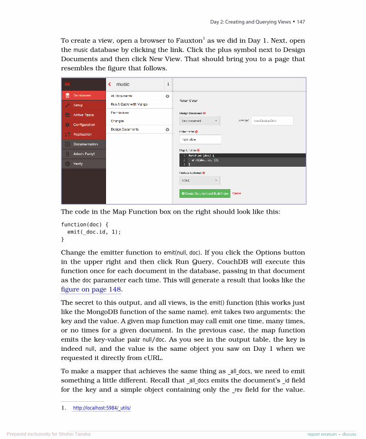
To create a view, open a browser to Fauxton1 as we did in Day 1. Next, openthe music database by clicking the link. Click the plus symbol next to DesignDocuments and then click New View. That should bring you to a page thatresembles the figure that follows.
The code in the Map Function box on the right should look like this:
function(doc) {emit(_doc.id, 1);
}
Change the emitter function to emit(null, doc). If you click the Options buttonin the upper right and then click Run Query, CouchDB will execute thisfunction once for each document in the database, passing in that documentas the doc parameter each time. This will generate a result that looks like thefigure on page 148.
The secret to this output, and all views, is the emit() function (this works justlike the MongoDB function of the same name). emit takes two arguments: thekey and the value. A given map function may call emit one time, many times,or no times for a given document. In the previous case, the map functionemits the key-value pair null/doc. As you see in the output table, the key isindeed null, and the value is the same object you saw on Day 1 when werequested it directly from cURL.
To make a mapper that achieves the same thing as _all_docs, we need to emitsomething a little different. Recall that _all_docs emits the document’s _id fieldfor the key and a simple object containing only the _rev field for the value.
1. http://localhost:5984/_utils/
report erratum • discuss
Day 2: Creating and Querying Views • 147
Prepared exclusively for Shohei Tanaka
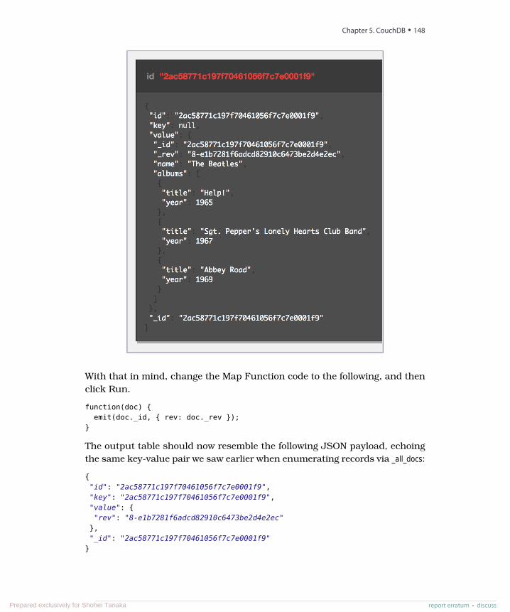
With that in mind, change the Map Function code to the following, and thenclick Run.
function(doc) {emit(doc._id, { rev: doc._rev });
}
The output table should now resemble the following JSON payload, echoingthe same key-value pair we saw earlier when enumerating records via _all_docs:
{"id": "2ac58771c197f70461056f7c7e0001f9","key": "2ac58771c197f70461056f7c7e0001f9","value": {"rev": "8-e1b7281f6adcd82910c6473be2d4e2ec"
},"_id": "2ac58771c197f70461056f7c7e0001f9"
}
Chapter 5. CouchDB • 148
report erratum • discussPrepared exclusively for Shohei Tanaka
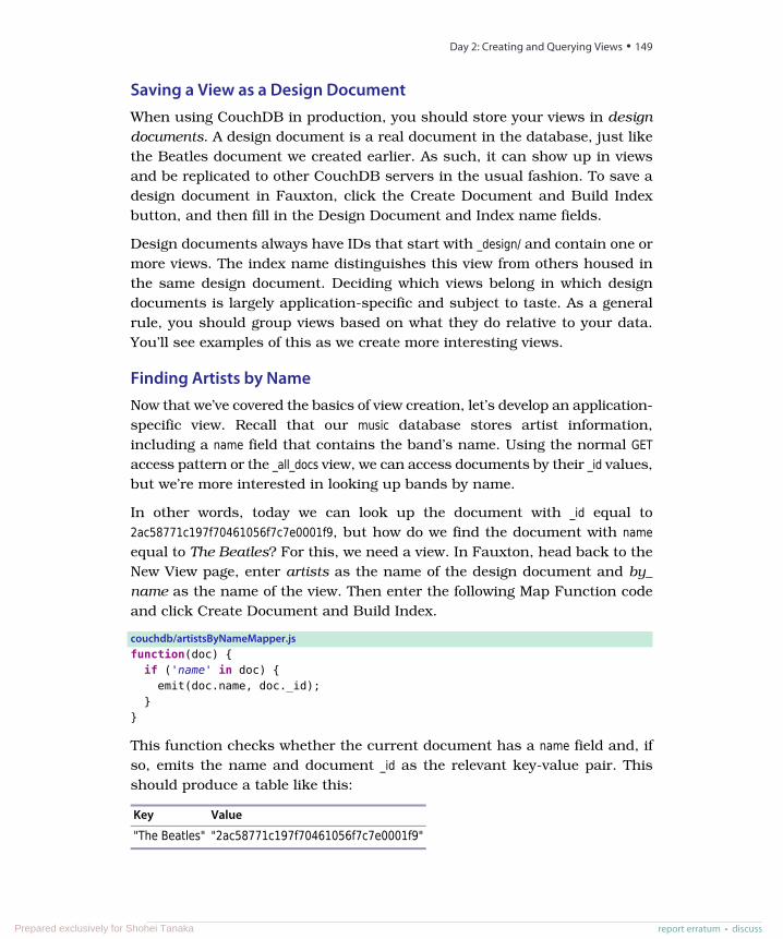
Saving a View as a Design DocumentWhen using CouchDB in production, you should store your views in designdocuments. A design document is a real document in the database, just likethe Beatles document we created earlier. As such, it can show up in viewsand be replicated to other CouchDB servers in the usual fashion. To save adesign document in Fauxton, click the Create Document and Build Indexbutton, and then fill in the Design Document and Index name fields.
Design documents always have IDs that start with _design/ and contain one ormore views. The index name distinguishes this view from others housed inthe same design document. Deciding which views belong in which designdocuments is largely application-specific and subject to taste. As a generalrule, you should group views based on what they do relative to your data.You’ll see examples of this as we create more interesting views.
Finding Artists by NameNow that we’ve covered the basics of view creation, let’s develop an application-specific view. Recall that our music database stores artist information,including a name field that contains the band’s name. Using the normal GETaccess pattern or the _all_docs view, we can access documents by their _id values,but we’re more interested in looking up bands by name.
In other words, today we can look up the document with _id equal to2ac58771c197f70461056f7c7e0001f9, but how do we find the document with nameequal to The Beatles? For this, we need a view. In Fauxton, head back to theNew View page, enter artists as the name of the design document and by_name as the name of the view. Then enter the following Map Function codeand click Create Document and Build Index.
couchdb/artistsByNameMapper.jsfunction(doc) {
if ('name' in doc) {emit(doc.name, doc._id);
}}
This function checks whether the current document has a name field and, ifso, emits the name and document _id as the relevant key-value pair. Thisshould produce a table like this:
ValueKey
"2ac58771c197f70461056f7c7e0001f9""The Beatles"
report erratum • discuss
Day 2: Creating and Querying Views • 149
Prepared exclusively for Shohei Tanaka
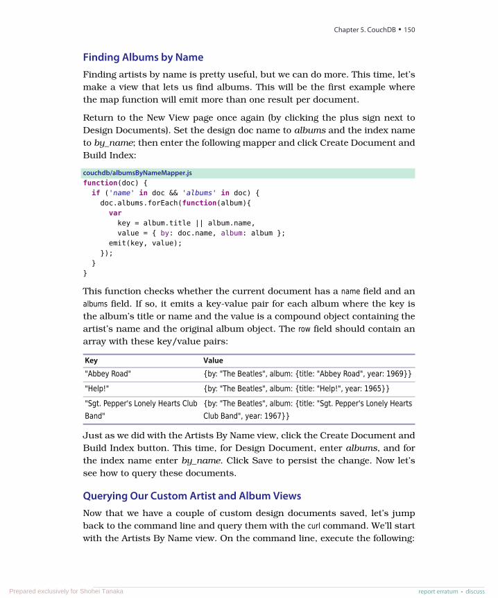
Finding Albums by NameFinding artists by name is pretty useful, but we can do more. This time, let’smake a view that lets us find albums. This will be the first example wherethe map function will emit more than one result per document.
Return to the New View page once again (by clicking the plus sign next toDesign Documents). Set the design doc name to albums and the index nameto by_name; then enter the following mapper and click Create Document andBuild Index:
couchdb/albumsByNameMapper.jsfunction(doc) {
if ('name' in doc && 'albums' in doc) {doc.albums.forEach(function(album){var
key = album.title || album.name,value = { by: doc.name, album: album };
emit(key, value);});
}}
This function checks whether the current document has a name field and analbums field. If so, it emits a key-value pair for each album where the key isthe album’s title or name and the value is a compound object containing theartist’s name and the original album object. The row field should contain anarray with these key/value pairs:
ValueKey
{by: "The Beatles", album: {title: "Abbey Road", year: 1969}}"Abbey Road"
{by: "The Beatles", album: {title: "Help!", year: 1965}}"Help!"
{by: "The Beatles", album: {title: "Sgt. Pepper's Lonely HeartsClub Band", year: 1967}}
"Sgt. Pepper's Lonely Hearts ClubBand"
Just as we did with the Artists By Name view, click the Create Document andBuild Index button. This time, for Design Document, enter albums, and forthe index name enter by_name. Click Save to persist the change. Now let’ssee how to query these documents.
Querying Our Custom Artist and Album ViewsNow that we have a couple of custom design documents saved, let’s jumpback to the command line and query them with the curl command. We’ll startwith the Artists By Name view. On the command line, execute the following:
Chapter 5. CouchDB • 150
report erratum • discussPrepared exclusively for Shohei Tanaka
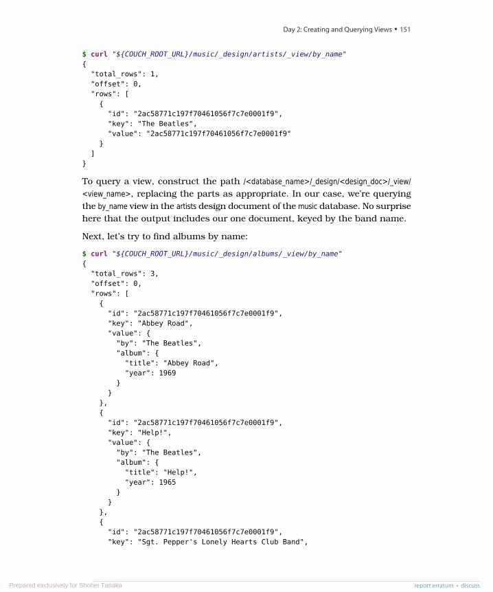
$ curl "${COUCH_ROOT_URL}/music/_design/artists/_view/by_name"{
"total_rows": 1,"offset": 0,"rows": [
{"id": "2ac58771c197f70461056f7c7e0001f9","key": "The Beatles","value": "2ac58771c197f70461056f7c7e0001f9"
}]
}
To query a view, construct the path /<database_name>/_design/<design_doc>/_view/<view_name>, replacing the parts as appropriate. In our case, we’re queryingthe by_name view in the artists design document of the music database. No surprisehere that the output includes our one document, keyed by the band name.
Next, let’s try to find albums by name:
$ curl "${COUCH_ROOT_URL}/music/_design/albums/_view/by_name"{
"total_rows": 3,"offset": 0,"rows": [
{"id": "2ac58771c197f70461056f7c7e0001f9","key": "Abbey Road","value": {
"by": "The Beatles","album": {
"title": "Abbey Road","year": 1969
}}
},{"id": "2ac58771c197f70461056f7c7e0001f9","key": "Help!","value": {
"by": "The Beatles","album": {
"title": "Help!","year": 1965
}}
},{"id": "2ac58771c197f70461056f7c7e0001f9","key": "Sgt. Pepper's Lonely Hearts Club Band",
report erratum • discuss
Day 2: Creating and Querying Views • 151
Prepared exclusively for Shohei Tanaka
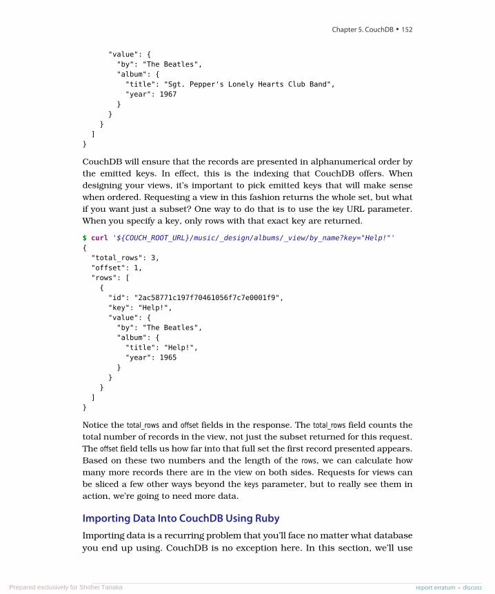
"value": {"by": "The Beatles","album": {
"title": "Sgt. Pepper's Lonely Hearts Club Band","year": 1967
}}
}]
}
CouchDB will ensure that the records are presented in alphanumerical order bythe emitted keys. In effect, this is the indexing that CouchDB offers. Whendesigning your views, it’s important to pick emitted keys that will make sensewhen ordered. Requesting a view in this fashion returns the whole set, but whatif you want just a subset? One way to do that is to use the key URL parameter.When you specify a key, only rows with that exact key are returned.
$ curl '${COUCH_ROOT_URL}/music/_design/albums/_view/by_name?key="Help!"'{
"total_rows": 3,"offset": 1,"rows": [
{"id": "2ac58771c197f70461056f7c7e0001f9","key": "Help!","value": {
"by": "The Beatles","album": {
"title": "Help!","year": 1965
}}
}]
}
Notice the total_rows and offset fields in the response. The total_rows field counts thetotal number of records in the view, not just the subset returned for this request.The offset field tells us how far into that full set the first record presented appears.Based on these two numbers and the length of the rows, we can calculate howmany more records there are in the view on both sides. Requests for views canbe sliced a few other ways beyond the keys parameter, but to really see them inaction, we’re going to need more data.
Importing Data Into CouchDB Using RubyImporting data is a recurring problem that you’ll face no matter what databaseyou end up using. CouchDB is no exception here. In this section, we’ll use
Chapter 5. CouchDB • 152
report erratum • discussPrepared exclusively for Shohei Tanaka
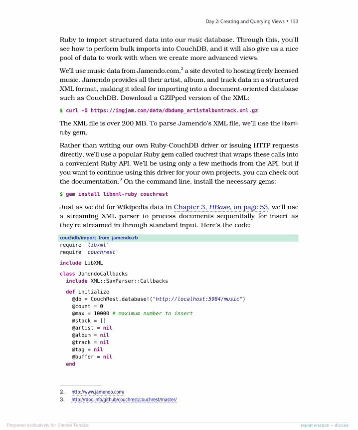
Ruby to import structured data into our music database. Through this, you’llsee how to perform bulk imports into CouchDB, and it will also give us a nicepool of data to work with when we create more advanced views.
We’ll use music data from Jamendo.com,2 a site devoted to hosting freely licensedmusic. Jamendo provides all their artist, album, and track data in a structuredXML format, making it ideal for importing into a document-oriented databasesuch as CouchDB. Download a GZIPped version of the XML:
$ curl -O https://imgjam.com/data/dbdump_artistalbumtrack.xml.gz
The XML file is over 200 MB. To parse Jamendo’s XML file, we’ll use the libxml-ruby gem.
Rather than writing our own Ruby-CouchDB driver or issuing HTTP requestsdirectly, we’ll use a popular Ruby gem called couchrest that wraps these calls intoa convenient Ruby API. We’ll be using only a few methods from the API, but ifyou want to continue using this driver for your own projects, you can check outthe documentation.3 On the command line, install the necessary gems:
$ gem install libxml-ruby couchrest
Just as we did for Wikipedia data in Chapter 3, HBase, on page 53, we’ll usea streaming XML parser to process documents sequentially for insert asthey’re streamed in through standard input. Here’s the code:
couchdb/import_from_jamendo.rbrequire 'libxml'require 'couchrest'
include LibXML
class JamendoCallbacksinclude XML::SaxParser::Callbacks
def initialize@db = CouchRest.database!("http://localhost:5984/music")@count = 0@max = 10000 # maximum number to insert@stack = []@artist = nil@album = nil@track = nil@tag = nil@buffer = nil
end
2. http://www.jamendo.com/3. http://rdoc.info/github/couchrest/couchrest/master/
report erratum • discuss
Day 2: Creating and Querying Views • 153
Prepared exclusively for Shohei Tanaka
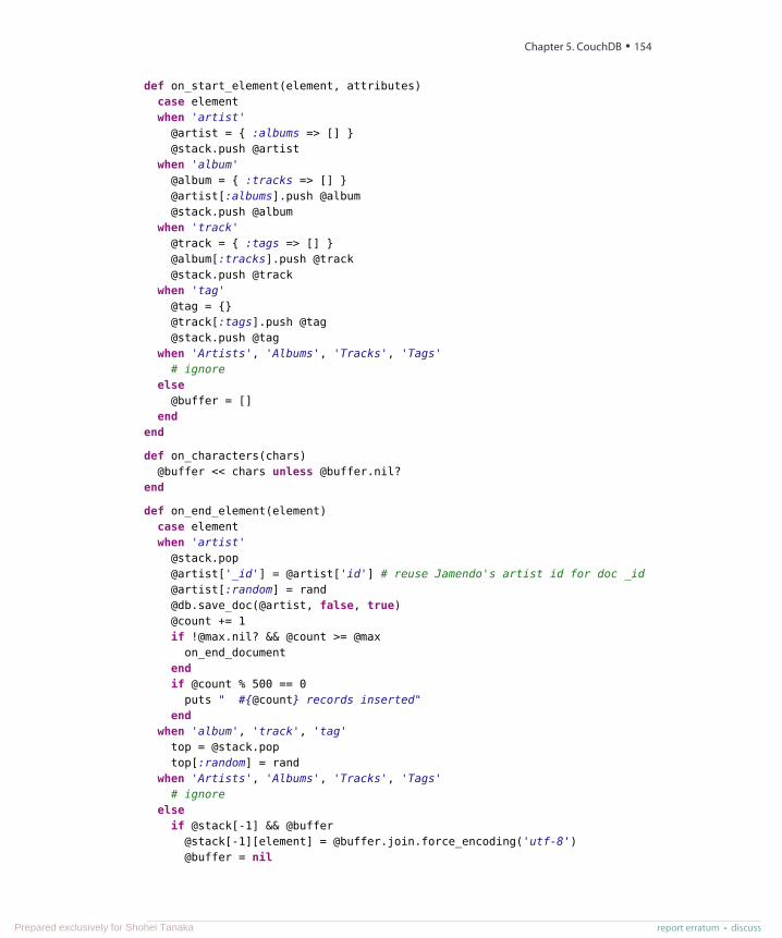
def on_start_element(element, attributes)case elementwhen 'artist'@artist = { :albums => [] }@stack.push @artist
when 'album'@album = { :tracks => [] }@artist[:albums].push @[email protected] @album
when 'track'@track = { :tags => [] }@album[:tracks].push @[email protected] @track
when 'tag'@tag = {}@track[:tags].push @[email protected] @tag
when 'Artists', 'Albums', 'Tracks', 'Tags'# ignore
else@buffer = []
endend
def on_characters(chars)@buffer << chars unless @buffer.nil?
end
def on_end_element(element)case elementwhen 'artist'@stack.pop@artist['_id'] = @artist['id'] # reuse Jamendo's artist id for doc _id@artist[:random] = [email protected]_doc(@artist, false, true)@count += 1if [email protected]? && @count >= @max
on_end_documentendif @count % 500 == 0
puts " #{@count} records inserted"end
when 'album', 'track', 'tag'top = @stack.poptop[:random] = rand
when 'Artists', 'Albums', 'Tracks', 'Tags'# ignore
elseif @stack[-1] && @buffer
@stack[-1][element] = @buffer.join.force_encoding('utf-8')@buffer = nil
Chapter 5. CouchDB • 154
report erratum • discussPrepared exclusively for Shohei Tanaka
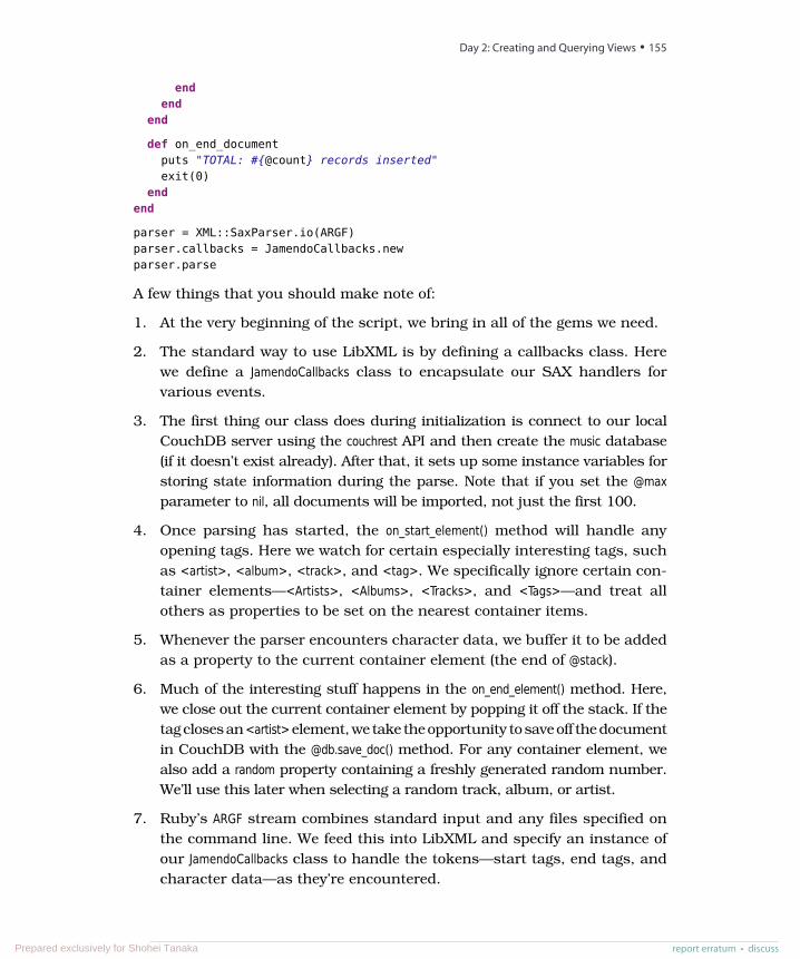
endend
end
def on_end_documentputs "TOTAL: #{@count} records inserted"exit(0)
endend
parser = XML::SaxParser.io(ARGF)parser.callbacks = JamendoCallbacks.newparser.parse
A few things that you should make note of:
1. At the very beginning of the script, we bring in all of the gems we need.
2. The standard way to use LibXML is by defining a callbacks class. Herewe define a JamendoCallbacks class to encapsulate our SAX handlers forvarious events.
3. The first thing our class does during initialization is connect to our localCouchDB server using the couchrest API and then create the music database(if it doesn’t exist already). After that, it sets up some instance variables forstoring state information during the parse. Note that if you set the @maxparameter to nil, all documents will be imported, not just the first 100.
4. Once parsing has started, the on_start_element() method will handle anyopening tags. Here we watch for certain especially interesting tags, suchas <artist>, <album>, <track>, and <tag>. We specifically ignore certain con-tainer elements—<Artists>, <Albums>, <Tracks>, and <Tags>—and treat allothers as properties to be set on the nearest container items.
5. Whenever the parser encounters character data, we buffer it to be addedas a property to the current container element (the end of @stack).
6. Much of the interesting stuff happens in the on_end_element() method. Here,we close out the current container element by popping it off the stack. If thetag closes an <artist> element, we take the opportunity to save off the documentin CouchDB with the @db.save_doc() method. For any container element, wealso add a random property containing a freshly generated random number.We’ll use this later when selecting a random track, album, or artist.
7. Ruby’s ARGF stream combines standard input and any files specified onthe command line. We feed this into LibXML and specify an instance ofour JamendoCallbacks class to handle the tokens—start tags, end tags, andcharacter data—as they’re encountered.
report erratum • discuss
Day 2: Creating and Querying Views • 155
Prepared exclusively for Shohei Tanaka
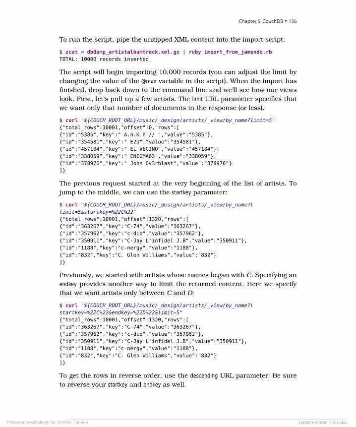
To run the script, pipe the unzipped XML content into the import script:
$ zcat < dbdump_artistalbumtrack.xml.gz | ruby import_from_jamendo.rbTOTAL: 10000 records inserted
The script will begin importing 10,000 records (you can adjust the limit bychanging the value of the @max variable in the script). When the import hasfinished, drop back down to the command line and we’ll see how our viewslook. First, let’s pull up a few artists. The limit URL parameter specifies thatwe want only that number of documents in the response (or less).
$ curl "${COUCH_ROOT_URL}/music/_design/artists/_view/by_name?limit=5"{"total_rows":10001,"offset":0,"rows":[{"id":"5385","key":" A.n.K.h // ","value":"5385"},{"id":"354581","key":" E2U","value":"354581"},{"id":"457184","key":" EL VECINO","value":"457184"},{"id":"338059","key":" ENIGMA63","value":"338059"},{"id":"378976","key":" John Ov3rblast","value":"378976"}]}
The previous request started at the very beginning of the list of artists. Tojump to the middle, we can use the startkey parameter:
$ curl "${COUCH_ROOT_URL}/music/_design/artists/_view/by_name?\limit=5&startkey=%22C%22"{"total_rows":10001,"offset":1320,"rows":[{"id":"363267","key":"C-74","value":"363267"},{"id":"357962","key":"c-dio","value":"357962"},{"id":"350911","key":"C-Jay L'infidel J.B","value":"350911"},{"id":"1188","key":"c-nergy","value":"1188"},{"id":"832","key":"C. Glen Williams","value":"832"}]}
Previously, we started with artists whose names began with C. Specifying anendkey provides another way to limit the returned content. Here we specifythat we want artists only between C and D:
$ curl "${COUCH_ROOT_URL}/music/_design/artists/_view/by_name?\startkey=%22C%22&endkey=%22D%22&limit=5"{"total_rows":10001,"offset":1320,"rows":[{"id":"363267","key":"C-74","value":"363267"},{"id":"357962","key":"c-dio","value":"357962"},{"id":"350911","key":"C-Jay L'infidel J.B","value":"350911"},{"id":"1188","key":"c-nergy","value":"1188"},{"id":"832","key":"C. Glen Williams","value":"832"}]}
To get the rows in reverse order, use the descending URL parameter. Be sureto reverse your startkey and endkey as well.
Chapter 5. CouchDB • 156
report erratum • discussPrepared exclusively for Shohei Tanaka
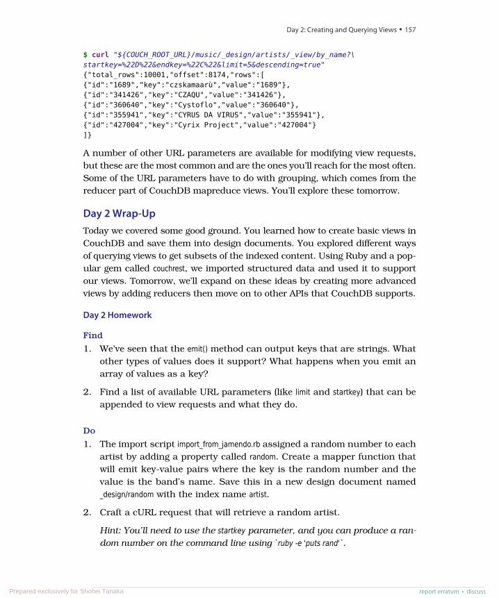
$ curl "${COUCH_ROOT_URL}/music/_design/artists/_view/by_name?\startkey=%22D%22&endkey=%22C%22&limit=5&descending=true"{"total_rows":10001,"offset":8174,"rows":[{"id":"1689","key":"czskamaarù","value":"1689"},{"id":"341426","key":"CZAQU","value":"341426"},{"id":"360640","key":"Cystoflo","value":"360640"},{"id":"355941","key":"CYRUS DA VIRUS","value":"355941"},{"id":"427004","key":"Cyrix Project","value":"427004"}]}
A number of other URL parameters are available for modifying view requests,but these are the most common and are the ones you’ll reach for the most often.Some of the URL parameters have to do with grouping, which comes from thereducer part of CouchDB mapreduce views. You’ll explore these tomorrow.
Day 2 Wrap-UpToday we covered some good ground. You learned how to create basic views inCouchDB and save them into design documents. You explored different waysof querying views to get subsets of the indexed content. Using Ruby and a pop-ular gem called couchrest, we imported structured data and used it to supportour views. Tomorrow, we’ll expand on these ideas by creating more advancedviews by adding reducers then move on to other APIs that CouchDB supports.
Day 2 Homework
Find
1. We’ve seen that the emit() method can output keys that are strings. Whatother types of values does it support? What happens when you emit anarray of values as a key?
2. Find a list of available URL parameters (like limit and startkey) that can beappended to view requests and what they do.
Do
1. The import script import_from_jamendo.rb assigned a random number to eachartist by adding a property called random. Create a mapper function thatwill emit key-value pairs where the key is the random number and thevalue is the band’s name. Save this in a new design document named_design/random with the index name artist.
2. Craft a cURL request that will retrieve a random artist.
Hint: You’ll need to use the startkey parameter, and you can produce a ran-dom number on the command line using `ruby -e 'puts rand'`.
report erratum • discuss
Day 2: Creating and Querying Views • 157
Prepared exclusively for Shohei Tanaka
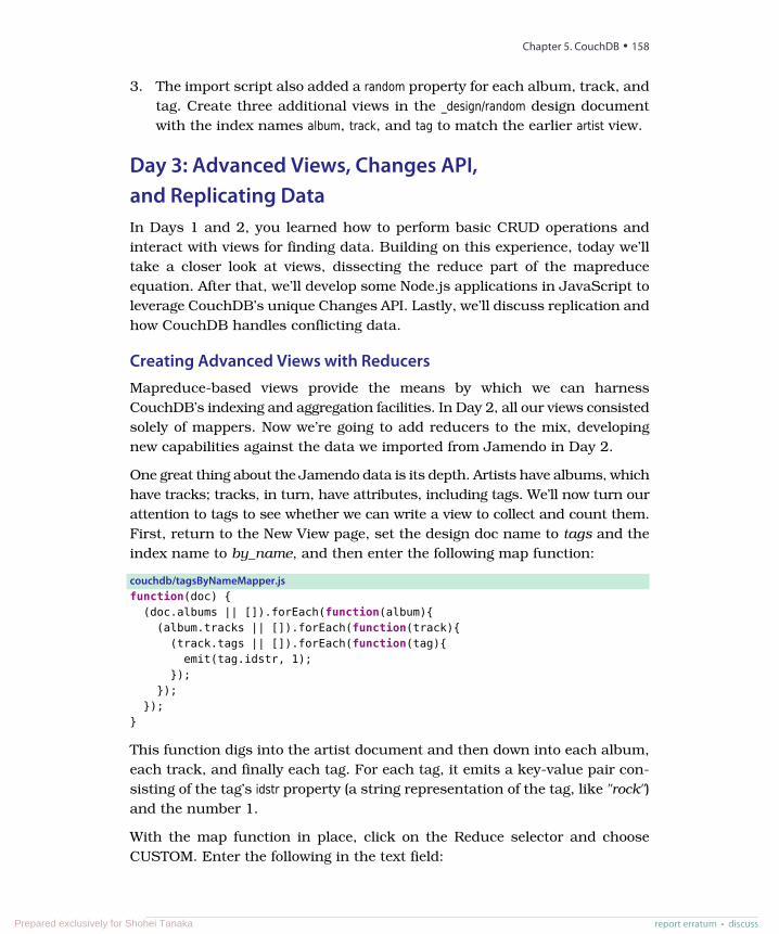
3. The import script also added a random property for each album, track, andtag. Create three additional views in the _design/random design documentwith the index names album, track, and tag to match the earlier artist view.
Day 3: Advanced Views, Changes API,and Replicating DataIn Days 1 and 2, you learned how to perform basic CRUD operations andinteract with views for finding data. Building on this experience, today we’lltake a closer look at views, dissecting the reduce part of the mapreduceequation. After that, we’ll develop some Node.js applications in JavaScript toleverage CouchDB’s unique Changes API. Lastly, we’ll discuss replication andhow CouchDB handles conflicting data.
Creating Advanced Views with ReducersMapreduce-based views provide the means by which we can harnessCouchDB’s indexing and aggregation facilities. In Day 2, all our views consistedsolely of mappers. Now we’re going to add reducers to the mix, developingnew capabilities against the data we imported from Jamendo in Day 2.
One great thing about the Jamendo data is its depth. Artists have albums, whichhave tracks; tracks, in turn, have attributes, including tags. We’ll now turn ourattention to tags to see whether we can write a view to collect and count them.First, return to the New View page, set the design doc name to tags and theindex name to by_name, and then enter the following map function:
couchdb/tagsByNameMapper.jsfunction(doc) {
(doc.albums || []).forEach(function(album){(album.tracks || []).forEach(function(track){(track.tags || []).forEach(function(tag){
emit(tag.idstr, 1);});
});});
}
This function digs into the artist document and then down into each album,each track, and finally each tag. For each tag, it emits a key-value pair con-sisting of the tag’s idstr property (a string representation of the tag, like "rock")and the number 1.
With the map function in place, click on the Reduce selector and chooseCUSTOM. Enter the following in the text field:
Chapter 5. CouchDB • 158
report erratum • discussPrepared exclusively for Shohei Tanaka
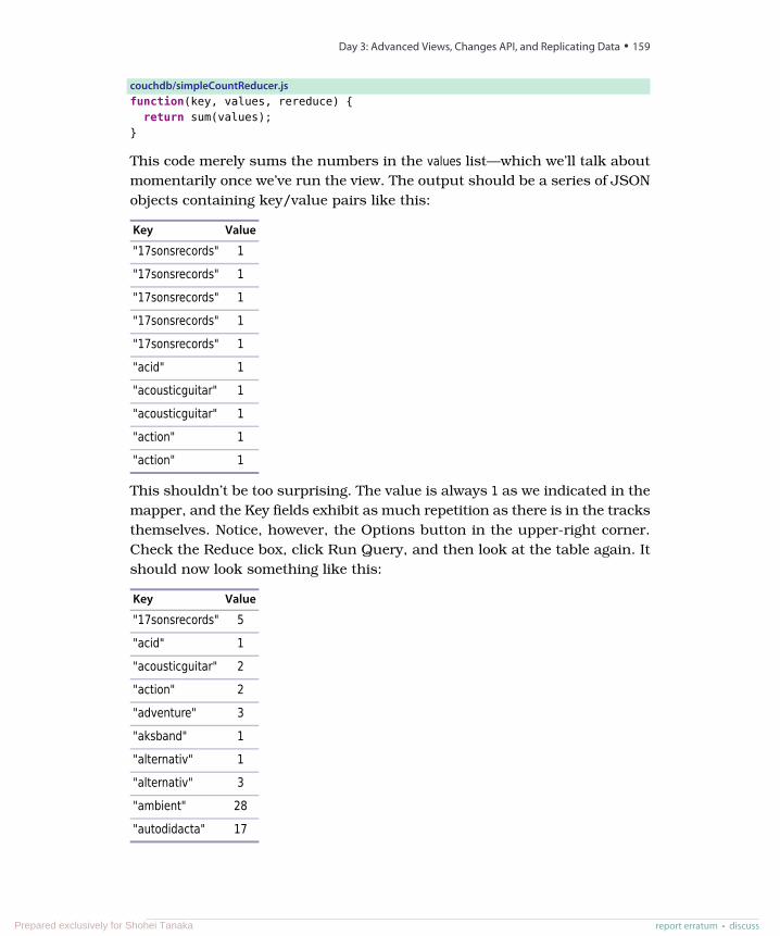
couchdb/simpleCountReducer.jsfunction(key, values, rereduce) {
return sum(values);}
This code merely sums the numbers in the values list—which we’ll talk aboutmomentarily once we’ve run the view. The output should be a series of JSONobjects containing key/value pairs like this:
ValueKey
1"17sonsrecords"
1"17sonsrecords"
1"17sonsrecords"
1"17sonsrecords"
1"17sonsrecords"
1"acid"
1"acousticguitar"
1"acousticguitar"
1"action"
1"action"
This shouldn’t be too surprising. The value is always 1 as we indicated in themapper, and the Key fields exhibit as much repetition as there is in the tracksthemselves. Notice, however, the Options button in the upper-right corner.Check the Reduce box, click Run Query, and then look at the table again. Itshould now look something like this:
ValueKey
5"17sonsrecords"
1"acid"
2"acousticguitar"
2"action"
3"adventure"
1"aksband"
1"alternativ"
3"alternativ"
28"ambient"
17"autodidacta"
report erratum • discuss
Day 3: Advanced Views, Changes API, and Replicating Data • 159
Prepared exclusively for Shohei Tanaka
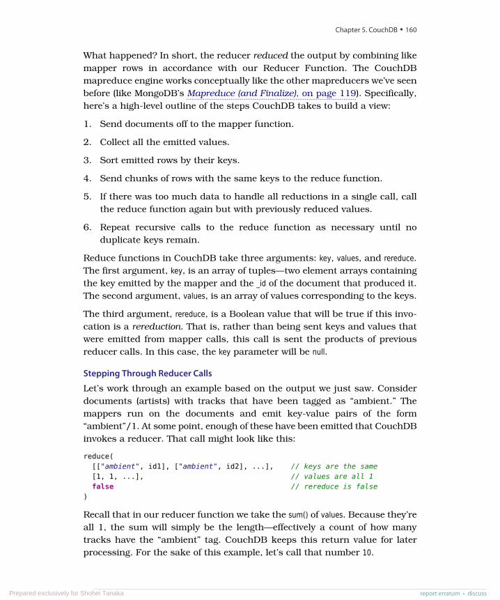
What happened? In short, the reducer reduced the output by combining likemapper rows in accordance with our Reducer Function. The CouchDBmapreduce engine works conceptually like the other mapreducers we’ve seenbefore (like MongoDB’s Mapreduce (and Finalize), on page 119). Specifically,here’s a high-level outline of the steps CouchDB takes to build a view:
1. Send documents off to the mapper function.
2. Collect all the emitted values.
3. Sort emitted rows by their keys.
4. Send chunks of rows with the same keys to the reduce function.
5. If there was too much data to handle all reductions in a single call, callthe reduce function again but with previously reduced values.
6. Repeat recursive calls to the reduce function as necessary until noduplicate keys remain.
Reduce functions in CouchDB take three arguments: key, values, and rereduce.The first argument, key, is an array of tuples—two element arrays containingthe key emitted by the mapper and the _id of the document that produced it.The second argument, values, is an array of values corresponding to the keys.
The third argument, rereduce, is a Boolean value that will be true if this invo-cation is a rereduction. That is, rather than being sent keys and values thatwere emitted from mapper calls, this call is sent the products of previousreducer calls. In this case, the key parameter will be null.
Stepping Through Reducer Calls
Let’s work through an example based on the output we just saw. Considerdocuments (artists) with tracks that have been tagged as “ambient.” Themappers run on the documents and emit key-value pairs of the form“ambient”/1. At some point, enough of these have been emitted that CouchDBinvokes a reducer. That call might look like this:
reduce([["ambient", id1], ["ambient", id2], ...], // keys are the same[1, 1, ...], // values are all 1false // rereduce is false
)
Recall that in our reducer function we take the sum() of values. Because they’reall 1, the sum will simply be the length—effectively a count of how manytracks have the “ambient” tag. CouchDB keeps this return value for laterprocessing. For the sake of this example, let’s call that number 10.
Chapter 5. CouchDB • 160
report erratum • discussPrepared exclusively for Shohei Tanaka
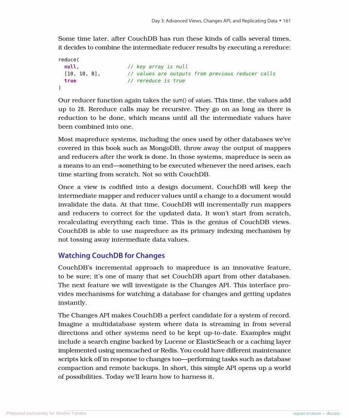
Some time later, after CouchDB has run these kinds of calls several times,it decides to combine the intermediate reducer results by executing a rereduce:
reduce(null, // key array is null[10, 10, 8], // values are outputs from previous reducer callstrue // rereduce is true
)
Our reducer function again takes the sum() of values. This time, the values addup to 28. Rereduce calls may be recursive. They go on as long as there isreduction to be done, which means until all the intermediate values havebeen combined into one.
Most mapreduce systems, including the ones used by other databases we’vecovered in this book such as MongoDB, throw away the output of mappersand reducers after the work is done. In those systems, mapreduce is seen asa means to an end—something to be executed whenever the need arises, eachtime starting from scratch. Not so with CouchDB.
Once a view is codified into a design document, CouchDB will keep theintermediate mapper and reducer values until a change to a document wouldinvalidate the data. At that time, CouchDB will incrementally run mappersand reducers to correct for the updated data. It won’t start from scratch,recalculating everything each time. This is the genius of CouchDB views.CouchDB is able to use mapreduce as its primary indexing mechanism bynot tossing away intermediate data values.
Watching CouchDB for ChangesCouchDB’s incremental approach to mapreduce is an innovative feature,to be sure; it’s one of many that set CouchDB apart from other databases.The next feature we will investigate is the Changes API. This interface pro-vides mechanisms for watching a database for changes and getting updatesinstantly.
The Changes API makes CouchDB a perfect candidate for a system of record.Imagine a multidatabase system where data is streaming in from severaldirections and other systems need to be kept up-to-date. Examples mightinclude a search engine backed by Lucene or ElasticSeach or a caching layerimplemented using memcached or Redis. You could have different maintenancescripts kick off in response to changes too—performing tasks such as databasecompaction and remote backups. In short, this simple API opens up a worldof possibilities. Today we’ll learn how to harness it.
report erratum • discuss
Day 3: Advanced Views, Changes API, and Replicating Data • 161
Prepared exclusively for Shohei Tanaka
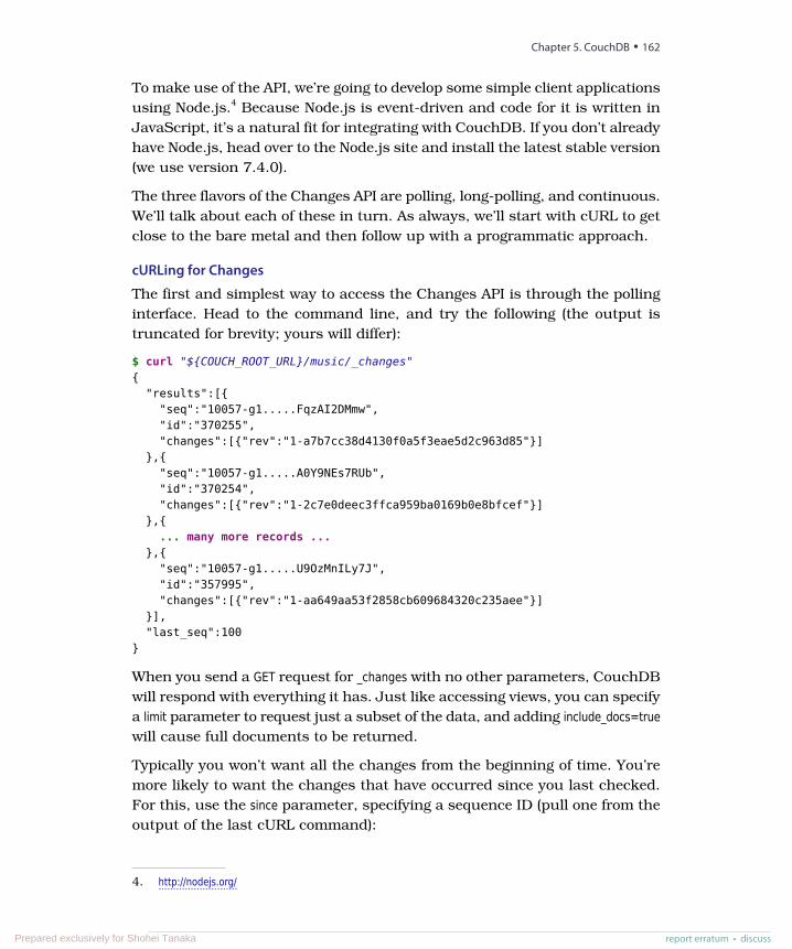
To make use of the API, we’re going to develop some simple client applicationsusing Node.js.4 Because Node.js is event-driven and code for it is written inJavaScript, it’s a natural fit for integrating with CouchDB. If you don’t alreadyhave Node.js, head over to the Node.js site and install the latest stable version(we use version 7.4.0).
The three flavors of the Changes API are polling, long-polling, and continuous.We’ll talk about each of these in turn. As always, we’ll start with cURL to getclose to the bare metal and then follow up with a programmatic approach.
cURLing for Changes
The first and simplest way to access the Changes API is through the pollinginterface. Head to the command line, and try the following (the output istruncated for brevity; yours will differ):
$ curl "${COUCH_ROOT_URL}/music/_changes"{
"results":[{"seq":"10057-g1.....FqzAI2DMmw","id":"370255","changes":[{"rev":"1-a7b7cc38d4130f0a5f3eae5d2c963d85"}]
},{"seq":"10057-g1.....A0Y9NEs7RUb","id":"370254","changes":[{"rev":"1-2c7e0deec3ffca959ba0169b0e8bfcef"}]
},{... many more records ...
},{"seq":"10057-g1.....U9OzMnILy7J","id":"357995","changes":[{"rev":"1-aa649aa53f2858cb609684320c235aee"}]
}],"last_seq":100
}
When you send a GET request for _changes with no other parameters, CouchDBwill respond with everything it has. Just like accessing views, you can specifya limit parameter to request just a subset of the data, and adding include_docs=truewill cause full documents to be returned.
Typically you won’t want all the changes from the beginning of time. You’remore likely to want the changes that have occurred since you last checked.For this, use the since parameter, specifying a sequence ID (pull one from theoutput of the last cURL command):
4. http://nodejs.org/
Chapter 5. CouchDB • 162
report erratum • discussPrepared exclusively for Shohei Tanaka
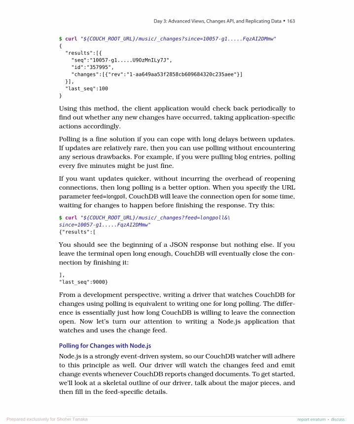
$ curl "${COUCH_ROOT_URL}/music/_changes?since=10057-g1.....FqzAI2DMmw"{
"results":[{"seq":"10057-g1.....U9OzMnILy7J","id":"357995","changes":[{"rev":"1-aa649aa53f2858cb609684320c235aee"}]
}],"last_seq":100
}
Using this method, the client application would check back periodically tofind out whether any new changes have occurred, taking application-specificactions accordingly.
Polling is a fine solution if you can cope with long delays between updates.If updates are relatively rare, then you can use polling without encounteringany serious drawbacks. For example, if you were pulling blog entries, pollingevery five minutes might be just fine.
If you want updates quicker, without incurring the overhead of reopeningconnections, then long polling is a better option. When you specify the URLparameter feed=longpoll, CouchDB will leave the connection open for some time,waiting for changes to happen before finishing the response. Try this:
$ curl "${COUCH_ROOT_URL}/music/_changes?feed=longpoll&\since=10057-g1.....FqzAI2DMmw"{"results":[
You should see the beginning of a JSON response but nothing else. If youleave the terminal open long enough, CouchDB will eventually close the con-nection by finishing it:
],"last_seq":9000}
From a development perspective, writing a driver that watches CouchDB forchanges using polling is equivalent to writing one for long polling. The differ-ence is essentially just how long CouchDB is willing to leave the connectionopen. Now let’s turn our attention to writing a Node.js application thatwatches and uses the change feed.
Polling for Changes with Node.js
Node.js is a strongly event-driven system, so our CouchDB watcher will adhereto this principle as well. Our driver will watch the changes feed and emitchange events whenever CouchDB reports changed documents. To get started,we’ll look at a skeletal outline of our driver, talk about the major pieces, andthen fill in the feed-specific details.
report erratum • discuss
Day 3: Advanced Views, Changes API, and Replicating Data • 163
Prepared exclusively for Shohei Tanaka
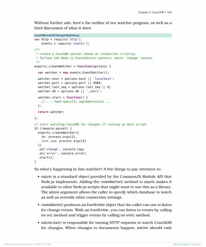
Without further ado, here’s the outline of our watcher program, as well as abrief discussion of what it does:
couchdb/watchChangesSkeleton.jsvar http = require('http'),
events = require('events');
/*** create a CouchDB watcher based on connection criteria;* follows the Node.js EventEmitter pattern, emits 'change' events.*/
exports.createWatcher = function(options) {
var watcher = new events.EventEmitter();
watcher.host = options.host || 'localhost';watcher.port = options.port || 5984;watcher.last_seq = options.last_seq || 0;watcher.db = options.db || '_users';
watcher.start = function() {// ... feed-specific implementation ...
};
return watcher;
};
// start watching CouchDB for changes if running as main scriptif (!module.parent) {
exports.createWatcher({db: process.argv[2],last_seq: process.argv[3]
}).on('change', console.log).on('error', console.error).start();
}
So what’s happening in this watcher? A few things to pay attention to:
• exports is a standard object provided by the CommonJS Module API thatNode.js implements. Adding the createWatcher() method to exports makes itavailable to other Node.js scripts that might want to use this as a library.The options argument allows the caller to specify which database to watchas well as override other connection settings.
• createWatcher() produces an EventEmitter object that the caller can use to listenfor change events. With an EventEmitter, you can listen to events by callingits on() method and trigger events by calling its emit() method.
• watcher.start() is responsible for issuing HTTP requests to watch CouchDBfor changes. When changes to documents happen, watcher should emit
Chapter 5. CouchDB • 164
report erratum • discussPrepared exclusively for Shohei Tanaka
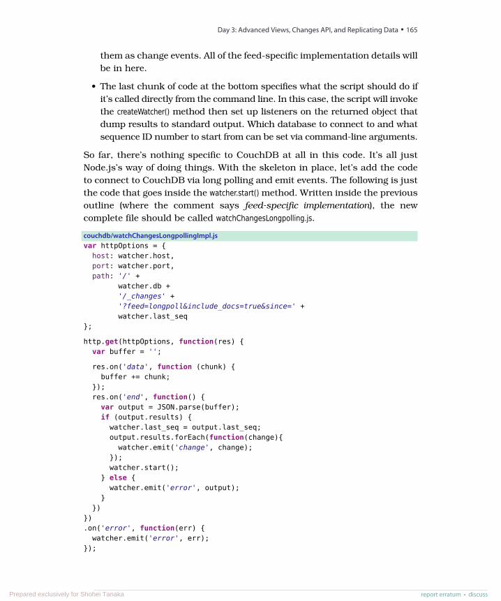
them as change events. All of the feed-specific implementation details willbe in here.
• The last chunk of code at the bottom specifies what the script should do ifit’s called directly from the command line. In this case, the script will invokethe createWatcher() method then set up listeners on the returned object thatdump results to standard output. Which database to connect to and whatsequence ID number to start from can be set via command-line arguments.
So far, there’s nothing specific to CouchDB at all in this code. It’s all justNode.js’s way of doing things. With the skeleton in place, let’s add the codeto connect to CouchDB via long polling and emit events. The following is justthe code that goes inside the watcher.start() method. Written inside the previousoutline (where the comment says feed-specific implementation), the newcomplete file should be called watchChangesLongpolling.js.
couchdb/watchChangesLongpollingImpl.jsvar httpOptions = {
host: watcher.host,port: watcher.port,path: '/' +
watcher.db +'/_changes' +'?feed=longpoll&include_docs=true&since=' +watcher.last_seq
};
http.get(httpOptions, function(res) {var buffer = '';
res.on('data', function (chunk) {buffer += chunk;
});res.on('end', function() {
var output = JSON.parse(buffer);if (output.results) {watcher.last_seq = output.last_seq;output.results.forEach(function(change){
watcher.emit('change', change);});watcher.start();
} else {watcher.emit('error', output);
}})
}).on('error', function(err) {
watcher.emit('error', err);});
report erratum • discuss
Day 3: Advanced Views, Changes API, and Replicating Data • 165
Prepared exclusively for Shohei Tanaka
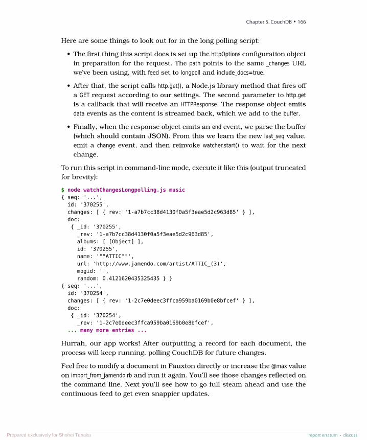
Here are some things to look out for in the long polling script:
• The first thing this script does is set up the httpOptions configuration objectin preparation for the request. The path points to the same _changes URLwe’ve been using, with feed set to longpoll and include_docs=true.
• After that, the script calls http.get(), a Node.js library method that fires offa GET request according to our settings. The second parameter to http.getis a callback that will receive an HTTPResponse. The response object emitsdata events as the content is streamed back, which we add to the buffer.
• Finally, when the response object emits an end event, we parse the buffer(which should contain JSON). From this we learn the new last_seq value,emit a change event, and then reinvoke watcher.start() to wait for the nextchange.
To run this script in command-line mode, execute it like this (output truncatedfor brevity):
$ node watchChangesLongpolling.js music{ seq: '...',
id: '370255',changes: [ { rev: '1-a7b7cc38d4130f0a5f3eae5d2c963d85' } ],doc:{ _id: '370255',
_rev: '1-a7b7cc38d4130f0a5f3eae5d2c963d85',albums: [ [Object] ],id: '370255',name: '""ATTIC""',url: 'http://www.jamendo.com/artist/ATTIC_(3)',mbgid: '',random: 0.4121620435325435 } }
{ seq: '...',id: '370254',changes: [ { rev: '1-2c7e0deec3ffca959ba0169b0e8bfcef' } ],doc:{ _id: '370254',
_rev: '1-2c7e0deec3ffca959ba0169b0e8bfcef',... many more entries ...
Hurrah, our app works! After outputting a record for each document, theprocess will keep running, polling CouchDB for future changes.
Feel free to modify a document in Fauxton directly or increase the @max valueon import_from_jamendo.rb and run it again. You’ll see those changes reflected onthe command line. Next you’ll see how to go full steam ahead and use thecontinuous feed to get even snappier updates.
Chapter 5. CouchDB • 166
report erratum • discussPrepared exclusively for Shohei Tanaka
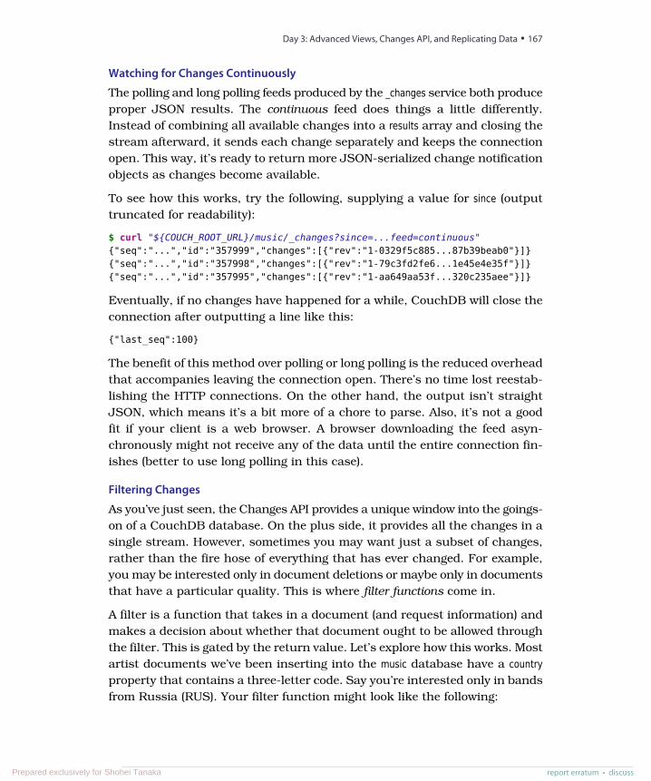
Watching for Changes Continuously
The polling and long polling feeds produced by the _changes service both produceproper JSON results. The continuous feed does things a little differently.Instead of combining all available changes into a results array and closing thestream afterward, it sends each change separately and keeps the connectionopen. This way, it’s ready to return more JSON-serialized change notificationobjects as changes become available.
To see how this works, try the following, supplying a value for since (outputtruncated for readability):
$ curl "${COUCH_ROOT_URL}/music/_changes?since=...feed=continuous"{"seq":"...","id":"357999","changes":[{"rev":"1-0329f5c885...87b39beab0"}]}{"seq":"...","id":"357998","changes":[{"rev":"1-79c3fd2fe6...1e45e4e35f"}]}{"seq":"...","id":"357995","changes":[{"rev":"1-aa649aa53f...320c235aee"}]}
Eventually, if no changes have happened for a while, CouchDB will close theconnection after outputting a line like this:
{"last_seq":100}
The benefit of this method over polling or long polling is the reduced overheadthat accompanies leaving the connection open. There’s no time lost reestab-lishing the HTTP connections. On the other hand, the output isn’t straightJSON, which means it’s a bit more of a chore to parse. Also, it’s not a goodfit if your client is a web browser. A browser downloading the feed asyn-chronously might not receive any of the data until the entire connection fin-ishes (better to use long polling in this case).
Filtering Changes
As you’ve just seen, the Changes API provides a unique window into the goings-on of a CouchDB database. On the plus side, it provides all the changes in asingle stream. However, sometimes you may want just a subset of changes,rather than the fire hose of everything that has ever changed. For example,you may be interested only in document deletions or maybe only in documentsthat have a particular quality. This is where filter functions come in.
A filter is a function that takes in a document (and request information) andmakes a decision about whether that document ought to be allowed throughthe filter. This is gated by the return value. Let’s explore how this works. Mostartist documents we’ve been inserting into the music database have a countryproperty that contains a three-letter code. Say you’re interested only in bandsfrom Russia (RUS). Your filter function might look like the following:
report erratum • discuss
Day 3: Advanced Views, Changes API, and Replicating Data • 167
Prepared exclusively for Shohei Tanaka
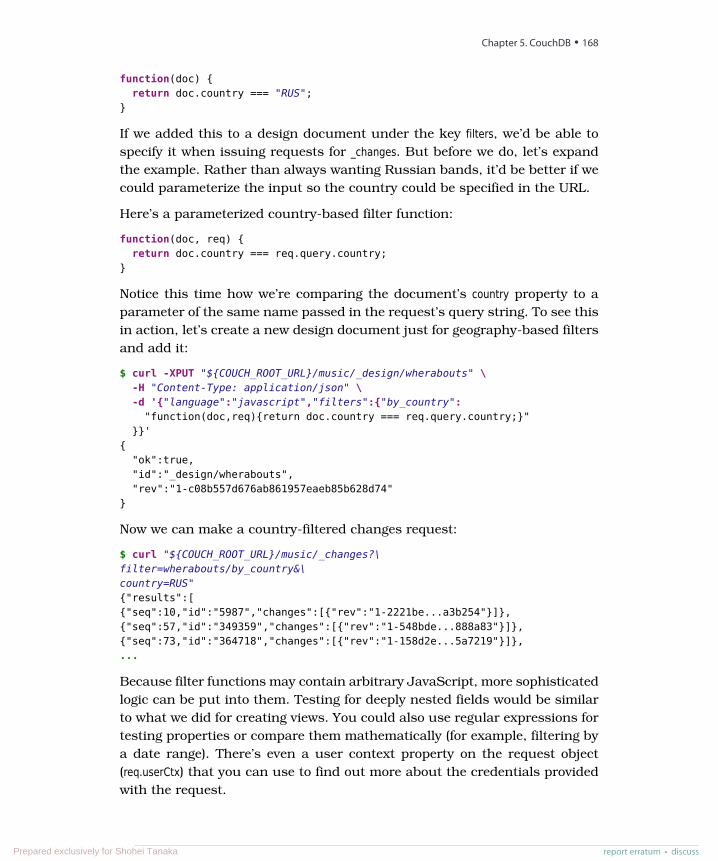
function(doc) {return doc.country === "RUS";
}
If we added this to a design document under the key filters, we’d be able tospecify it when issuing requests for _changes. But before we do, let’s expandthe example. Rather than always wanting Russian bands, it’d be better if wecould parameterize the input so the country could be specified in the URL.
Here’s a parameterized country-based filter function:
function(doc, req) {return doc.country === req.query.country;
}
Notice this time how we’re comparing the document’s country property to aparameter of the same name passed in the request’s query string. To see thisin action, let’s create a new design document just for geography-based filtersand add it:
$ curl -XPUT "${COUCH_ROOT_URL}/music/_design/wherabouts" \-H "Content-Type: application/json" \-d '{"language":"javascript","filters":{"by_country":
"function(doc,req){return doc.country === req.query.country;}"}}'
{"ok":true,"id":"_design/wherabouts","rev":"1-c08b557d676ab861957eaeb85b628d74"
}
Now we can make a country-filtered changes request:
$ curl "${COUCH_ROOT_URL}/music/_changes?\filter=wherabouts/by_country&\country=RUS"{"results":[{"seq":10,"id":"5987","changes":[{"rev":"1-2221be...a3b254"}]},{"seq":57,"id":"349359","changes":[{"rev":"1-548bde...888a83"}]},{"seq":73,"id":"364718","changes":[{"rev":"1-158d2e...5a7219"}]},...
Because filter functions may contain arbitrary JavaScript, more sophisticatedlogic can be put into them. Testing for deeply nested fields would be similarto what we did for creating views. You could also use regular expressions fortesting properties or compare them mathematically (for example, filtering bya date range). There’s even a user context property on the request object(req.userCtx) that you can use to find out more about the credentials providedwith the request.
Chapter 5. CouchDB • 168
report erratum • discussPrepared exclusively for Shohei Tanaka
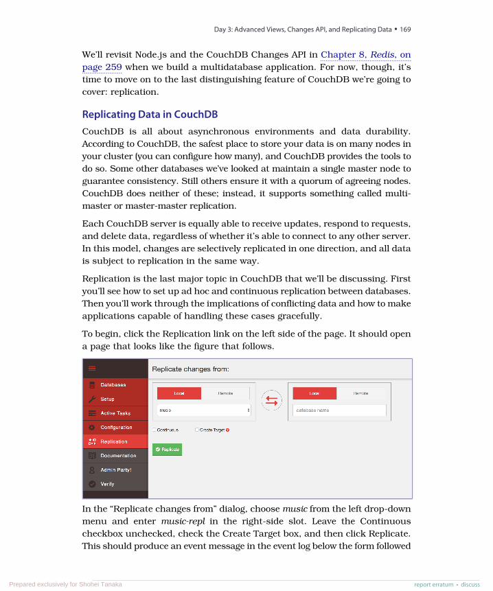
We’ll revisit Node.js and the CouchDB Changes API in Chapter 8, Redis, onpage 259 when we build a multidatabase application. For now, though, it’stime to move on to the last distinguishing feature of CouchDB we’re going tocover: replication.
Replicating Data in CouchDBCouchDB is all about asynchronous environments and data durability.According to CouchDB, the safest place to store your data is on many nodes inyour cluster (you can configure how many), and CouchDB provides the tools todo so. Some other databases we’ve looked at maintain a single master node toguarantee consistency. Still others ensure it with a quorum of agreeing nodes.CouchDB does neither of these; instead, it supports something called multi-master or master-master replication.
Each CouchDB server is equally able to receive updates, respond to requests,and delete data, regardless of whether it’s able to connect to any other server.In this model, changes are selectively replicated in one direction, and all datais subject to replication in the same way.
Replication is the last major topic in CouchDB that we’ll be discussing. Firstyou’ll see how to set up ad hoc and continuous replication between databases.Then you’ll work through the implications of conflicting data and how to makeapplications capable of handling these cases gracefully.
To begin, click the Replication link on the left side of the page. It should opena page that looks like the figure that follows.
In the “Replicate changes from” dialog, choose music from the left drop-downmenu and enter music-repl in the right-side slot. Leave the Continuouscheckbox unchecked, check the Create Target box, and then click Replicate.This should produce an event message in the event log below the form followed
report erratum • discuss
Day 3: Advanced Views, Changes API, and Replicating Data • 169
Prepared exclusively for Shohei Tanaka

by a big green banner at the top of the page saying that the replication oper-ation has begun.
To confirm that the replication request worked, go back to the FauxtonDatabases page. There should now be a new database called music-repl withthe same number of documents as the music database. If it has fewer, give itsome time and refresh the page—CouchDB may be in the process of catchingup. Don’t be concerned if the Update Seq values don’t match. That’s becausethe original music database had deletions and updates to documents, whereasthe music-repl database had only insertions to bring it up to speed.
Creating Conflicts
Next, we’ll create a conflict and then explore how to deal with it. Keep theReplicator page handy because we’re going to be triggering ad hoc replicationbetween music and music-repl frequently. Drop back to the command line, andenter this to create a document in the music database:
$ curl -XPUT "${COUCH_ROOT_URL}/music/theconflicts" \-H "Content-Type: application/json" \-d '{ "name": "The Conflicts" }'
{"ok":true,"id":"theconflicts","rev":"1-e007498c59e95d23912be35545049174"
}
On the Replication page, click Replicate to trigger another synchronization.We can confirm that the document was successfully replicated by retrievingit from the music-repl database.
$ curl "${COUCH_ROOT_URL}/music-repl/theconflicts"{
"_id":"theconflicts","_rev":"1-e007498c59e95d23912be35545049174","name":"The Conflicts"
}
Next, let’s update it in music-repl by adding an album called Conflicts of Interest.
$ curl -XPUT "${COUCH_ROOT_URL}/music-repl/theconflicts" \-H "Content-Type: application/json" \-d '{
"_id": "theconflicts","_rev": "1-e007498c59e95d23912be35545049174","name": "The Conflicts","albums": ["Conflicts of Interest"]
}'
Chapter 5. CouchDB • 170
report erratum • discussPrepared exclusively for Shohei Tanaka
{"ok":true,"id":"theconflicts","rev":"2-0c969fbfa76eb7fcdf6412ef219fcac5"
}
And create a conflicting update in music proper by adding a different album:Conflicting Opinions.
$ curl -XPUT "${COUCH_ROOT_URL}/music/theconflicts" \-H "Content-Type: application/json" \-d '{
"_id": "theconflicts","_rev": "1-e007498c59e95d23912be35545049174","name": "The Conflicts","albums": ["Conflicting Opinions"]
}'{
"ok":true,"id":"theconflicts","rev":"2-cab47bf4444a20d6a2d2204330fdce2a"
}
At this point, both the music and music-repl databases have a document with an_id value of theconflicts. Both documents are at version 2 and derived from thesame base revision (1-e007498c59e95d23912be35545049174). Now the question is,what happens when we try to replicate between them?
Fine-Grained Data Replication in CouchDB 2.0
With early versions of CouchDB, if you set up a multi-node CouchDB cluster, alldocuments were stored on all nodes in the cluster. CouchDB 2.0 brought a nativeclustering capability that enables you to store documents on only some nodes in thecluster and to determine, at write time, how many nodes should store the document,enabling you to choose a replication factor for data.
We won’t cover this or related issues such as sharding, but if you plan on usingCouchDB in production, you should check out some theoretical documentationa tosee how it works and receive guidance in making intelligent decisions about replication.
a. http://docs.couchdb.org/en/latest/cluster/theory.html
Resolving Conflicts
With our document now in a conflicting state between the two databases,head back to the Replication page and kick off another replication. If you were
report erratum • discuss
Day 3: Advanced Views, Changes API, and Replicating Data • 171
Prepared exclusively for Shohei Tanaka
expecting this to fail, you may be shocked to learn that the operation succeedsjust fine. So how did CouchDB deal with the discrepancy?
It turns out that CouchDB basically just picks one and calls that one thewinner. Using a deterministic algorithm, all CouchDB nodes will pick thesame winner when a conflict is detected. However, the story doesn’t end there.CouchDB stores the unselected “loser” documents as well so that a clientapplication can review the situation and resolve it at a later date.
To find out which version of our document won during the last replication,we can request it using the normal GET request channel. By adding the conflicts=true URL parameter, CouchDB will also include information about the conflict-ing revisions.
$ curl "${COUCH_ROOT_URL}/music-repl/theconflicts?conflicts=true"{
"_id":"theconflicts","_rev":"2-cab47bf4444a20d6a2d2204330fdce2a","name":"The Conflicts","albums":["Conflicting Opinions"],"_conflicts":[
"2-0c969fbfa76eb7fcdf6412ef219fcac5"]
}
So, we see that the second update won. Notice the _conflicts field in the response.It contains a list of other revisions that conflicted with the chosen one. Byadding a rev parameter to a GET request, we can pull down those conflictingrevisions and decide what to do about them.
$ curl "${COUCH_ROOT_URL}/music-repl/theconflicts?rev=2-0c969f..."{
"_id":"theconflicts","_rev":"2-0c969fbfa76eb7fcdf6412ef219fcac5","name":"The Conflicts","albums":["Conflicts of Interest"]
}
The takeaway here is that CouchDB does not try to intelligently merge con-flicting changes. How you should merge two documents is highly applicationspecific, and a general solution isn’t practical. In our case, combining the twoalbums arrays by concatenating them makes sense, but one could easily thinkof scenarios where the appropriate action is not obvious.
For example, imagine you’re maintaining a database of calendar events. Onecopy is on your smartphone; another is on your laptop. You get a text messagefrom a party planner specifying the venue for the party you’re hosting, so you
Chapter 5. CouchDB • 172
report erratum • discussPrepared exclusively for Shohei Tanaka
update your phone database accordingly. Later, back at the office, you receiveanother email from the planner specifying a different venue. So you updateyour laptop database and then replicate between them.
CouchDB has no way of knowing which of the two venues is "correct." Thebest it can do is make them consistent, keeping the old value around so youcan verify which of the conflicting values should be kept. It would be up tothe application to determine the right user interface for presenting this situ-ation and asking for a decision.
Day 3 Wrap-UpAnd so ends our tour of CouchDB. Here in Day 3, you started out by learninghow to add reducer functions to your mapreduce-generated views. After that,we took a deep dive into the Changes API, including a jaunt into the world ofevent-driven server-side JavaScript development with Node.js. Lastly, we tooka brief look at how you can trigger replication between databases and howclient applications can detect and correct for conflicts.
Day 3 Homework
Find
1. What native reducers are available in CouchDB? What are the benefitsof using native reducers over custom JavaScript reducers?
2. How can you filter the changes coming out of the _changes API on theserver side?
3. Like everything in CouchDB, the tasks of initializing and canceling repli-cation are controlled by HTTP commands under the hood. What are theREST commands to set up and remove replication relationships betweenservers?
4. How can you use the _replicator database to persist replication relationships?
Do
1. Create a new module called watchChangesContinuous.js based on the skeletalNode.js module described in the section Polling for Changes with Node.js,on page 163.
2. Implement watcher.start() such that it monitors the continuous _changes feed.Confirm that it produces the same output as watchChangesLongpolling.js.
Hint: If you get stuck, you can find an example implementation in thedownloads that accompany this book.
report erratum • discuss
Day 3: Advanced Views, Changes API, and Replicating Data • 173
Prepared exclusively for Shohei Tanaka
3. Documents with conflicting revisions have a _conflicts property. Create aview that emits conflicting revisions and maps them to the doc _id.
Wrap-UpThroughout this chapter, you’ve seen how to do a pretty wide range of taskswith CouchDB, from performing basic CRUD operations to building views outof mapreduce functions. You saw how to watch for changes, and you exploredhow to develop nonblocking event-driven client applications. Finally, youlearned how to perform ad-hoc replication between databases and how todetect and resolve conflicts. Despite all of this content, there’s still a lot wedidn’t cover, but now it’s time to wrap things up before heading off to ournext database.
CouchDB’s StrengthsCouchDB is a robust and stable member of the NoSQL community. Built onthe philosophy that networks are unreliable and hardware failure is imminent,CouchDB offers a heartily decentralized approach to data storage. Smallenough to live in your smartphone and big enough to support the enterprise,CouchDB affords a variety of deployment situations.
CouchDB’s WeaknessesOf course, CouchDB isn’t well suited for everything. CouchDB’s mapreduce-based views, while novel, can’t perform all the fancy data slicing you’d expectfrom a relational database. In fact, you shouldn’t be running ad-hoc queriesat all in production. As with many other NoSQL databases, CouchDB alwaysworks best when you have a very good sense of what you’re going to need inadvance. In some databases, that means knowing the key or “address” of anobject; in CouchDB, that means knowing all of your queries in advance. Ifyour use case doesn’t allow for that kind of foreknowledge, then you maywant to look elsewhere.
Parting ThoughtsCouchDB’s attention to robustness in the face of uncertainty makes it a greatchoice if your system must stand up to the harsh realities of the wild Internet.By leveraging standard “webisms” like HTTP/REST and JSON, CouchDB fitsin easily wherever web technologies are prevalent, which is increasinglyeverywhere. Inside the walled garden of a datacenter, CouchDB can still makesense if you commit to managing conflicts when they arise or if you utilizesome more recently added clustering features.
Chapter 5. CouchDB • 174
report erratum • discussPrepared exclusively for Shohei Tanaka

There are plenty of other features that make CouchDB unique and specialthat we didn’t have time to cover. A short list would include ease of backups,binary attachments to documents, and CouchApps, a system for developingand deploying web apps directly through CouchDB with no other middleware.Having said that, we hope we’ve provided enough of an overview to whet yourappetite for more. Try CouchDB for your next data-driven web app; you won’tbe disappointed!
report erratum • discuss
Wrap-Up • 175
Prepared exclusively for Shohei Tanaka
CHAPTER 6
Neo4JA bungee cord is a helpful tool because you can use it to tie together the mostdisparate of things, no matter how awkwardly shaped or ill fitting they maybe. In a lot of ways, Neo4j is the bungee cord of databases, a system intendednot so much to store information about things as to tie them together andrecord their connections with each other.
Neo4j is a member of a family of databases known as graph databases becauseit stores data as a graph (in the mathematical sense). Neo4j is known forbeing “whiteboard friendly” because virtually any diagram that you can drawusing boxes and lines on a whiteboard can be stored in Neo4j.
Neo4j focuses more on the relationships between values than on the common-alities among sets of values (such as collections of documents or tables ofrows). In this way, it can store highly variable data in a natural and straight-forward way.
On one side of the scale spectrum, Neo4j is small enough to be embeddedinto nearly any application; on the other side of the spectrum, Neo4j can runin large clusters of servers using master-slave replication and store tens ofbillions of nodes and as many relationships. In other words, Neo4j can handlejust about any size problem that you can throw at it.
Neo4j Is Whiteboard FriendlyImagine you need to create a wine suggestion engine in which wines are catego-rized by different varieties, regions, wineries, vintages, and designations. Imaginethat you also need to keep track of things like articles describing those wineswritten by various authors and to enable users to track their favorite wines.
If you were using a relational model, you might create a category table anda many-to-many relationship between a single winery’s wine and some
report erratum • discussPrepared exclusively for Shohei Tanaka
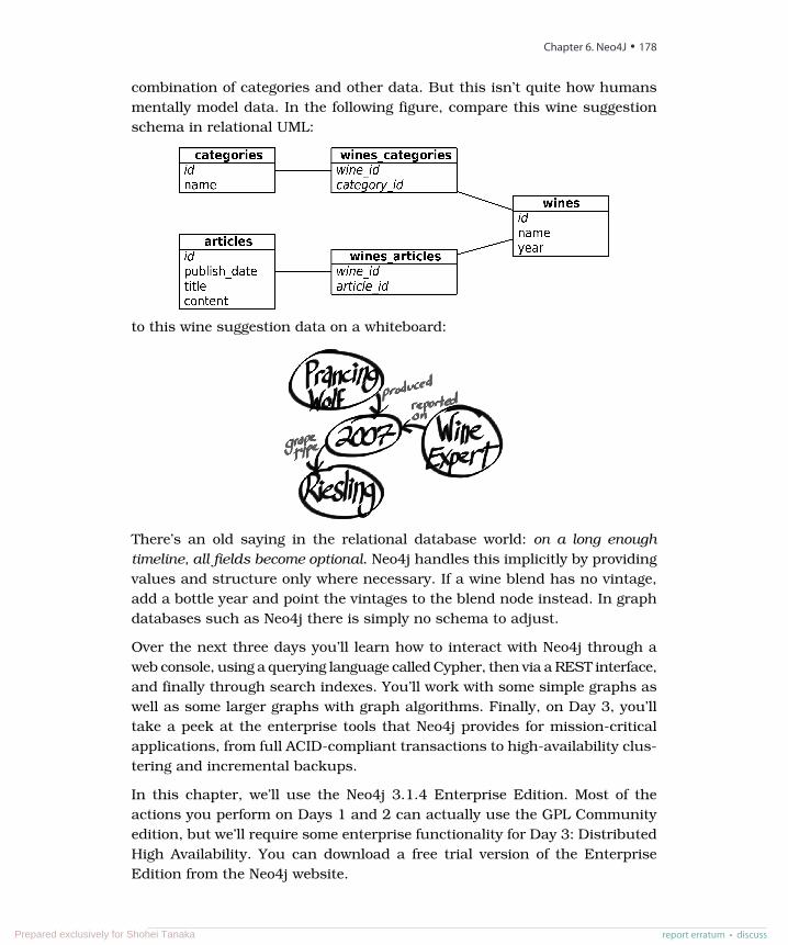
combination of categories and other data. But this isn’t quite how humansmentally model data. In the following figure, compare this wine suggestionschema in relational UML:
to this wine suggestion data on a whiteboard:
There’s an old saying in the relational database world: on a long enoughtimeline, all fields become optional. Neo4j handles this implicitly by providingvalues and structure only where necessary. If a wine blend has no vintage,add a bottle year and point the vintages to the blend node instead. In graphdatabases such as Neo4j there is simply no schema to adjust.
Over the next three days you’ll learn how to interact with Neo4j through aweb console, using a querying language called Cypher, then via a REST interface,and finally through search indexes. You’ll work with some simple graphs aswell as some larger graphs with graph algorithms. Finally, on Day 3, you’lltake a peek at the enterprise tools that Neo4j provides for mission-criticalapplications, from full ACID-compliant transactions to high-availability clus-tering and incremental backups.
In this chapter, we’ll use the Neo4j 3.1.4 Enterprise Edition. Most of theactions you perform on Days 1 and 2 can actually use the GPL Communityedition, but we’ll require some enterprise functionality for Day 3: DistributedHigh Availability. You can download a free trial version of the EnterpriseEdition from the Neo4j website.
Chapter 6. Neo4J • 178
report erratum • discussPrepared exclusively for Shohei Tanaka
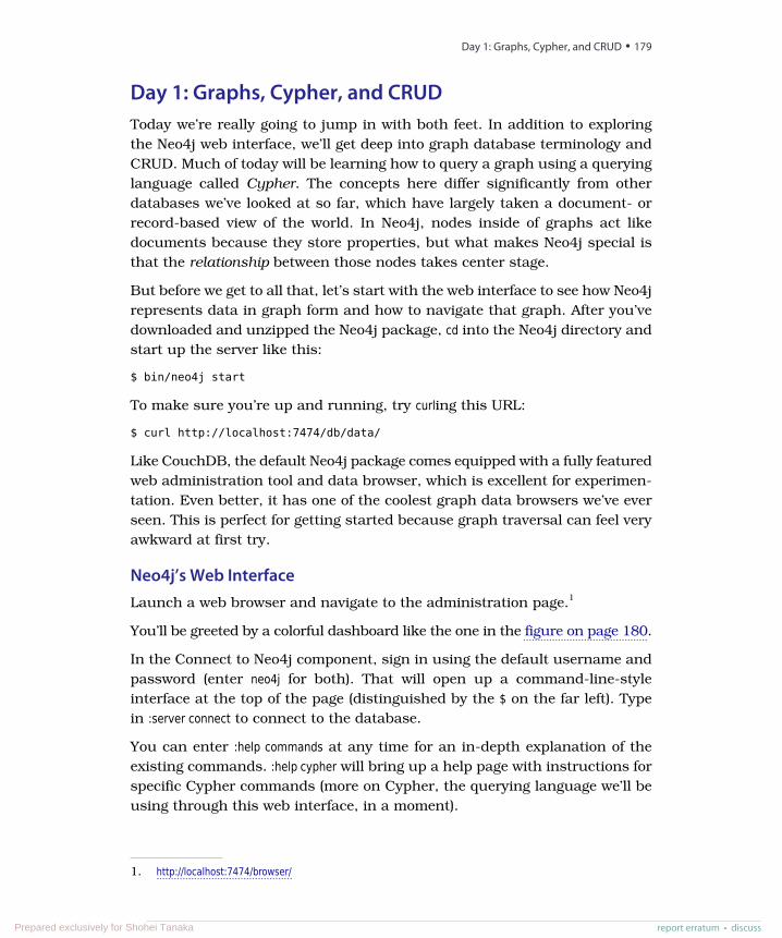
Day 1: Graphs, Cypher, and CRUDToday we’re really going to jump in with both feet. In addition to exploringthe Neo4j web interface, we’ll get deep into graph database terminology andCRUD. Much of today will be learning how to query a graph using a queryinglanguage called Cypher. The concepts here differ significantly from otherdatabases we’ve looked at so far, which have largely taken a document- orrecord-based view of the world. In Neo4j, nodes inside of graphs act likedocuments because they store properties, but what makes Neo4j special isthat the relationship between those nodes takes center stage.
But before we get to all that, let’s start with the web interface to see how Neo4jrepresents data in graph form and how to navigate that graph. After you’vedownloaded and unzipped the Neo4j package, cd into the Neo4j directory andstart up the server like this:
$ bin/neo4j start
To make sure you’re up and running, try curling this URL:
$ curl http://localhost:7474/db/data/
Like CouchDB, the default Neo4j package comes equipped with a fully featuredweb administration tool and data browser, which is excellent for experimen-tation. Even better, it has one of the coolest graph data browsers we’ve everseen. This is perfect for getting started because graph traversal can feel veryawkward at first try.
Neo4j’s Web InterfaceLaunch a web browser and navigate to the administration page.1
You’ll be greeted by a colorful dashboard like the one in the figure on page 180.
In the Connect to Neo4j component, sign in using the default username andpassword (enter neo4j for both). That will open up a command-line-styleinterface at the top of the page (distinguished by the $ on the far left). Typein :server connect to connect to the database.
You can enter :help commands at any time for an in-depth explanation of theexisting commands. :help cypher will bring up a help page with instructions forspecific Cypher commands (more on Cypher, the querying language we’ll beusing through this web interface, in a moment).
1. http://localhost:7474/browser/
report erratum • discuss
Day 1: Graphs, Cypher, and CRUD • 179
Prepared exclusively for Shohei Tanaka
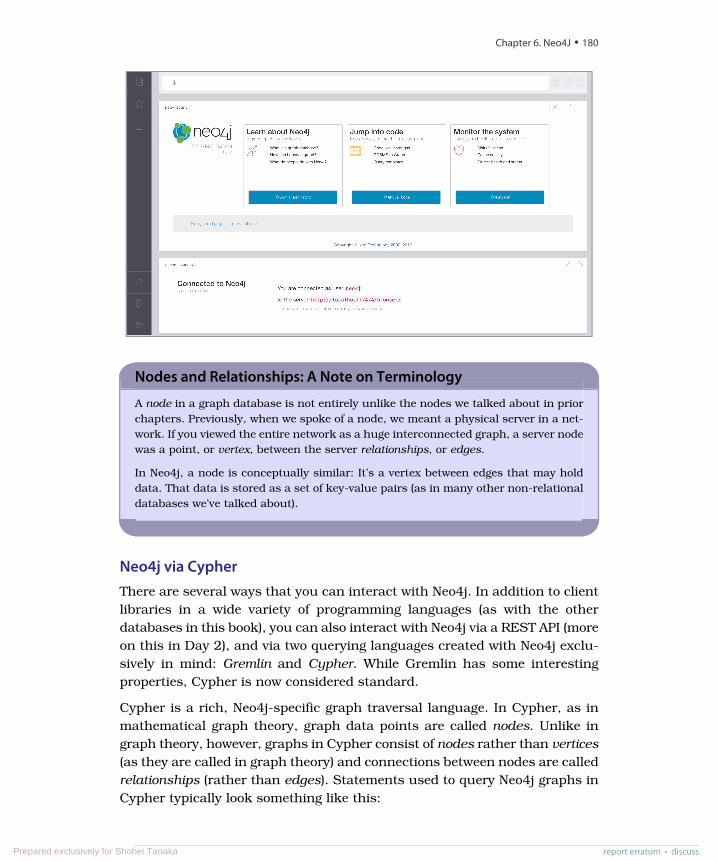
Nodes and Relationships: A Note on Terminology
A node in a graph database is not entirely unlike the nodes we talked about in priorchapters. Previously, when we spoke of a node, we meant a physical server in a net-work. If you viewed the entire network as a huge interconnected graph, a server nodewas a point, or vertex, between the server relationships, or edges.
In Neo4j, a node is conceptually similar: It’s a vertex between edges that may holddata. That data is stored as a set of key-value pairs (as in many other non-relationaldatabases we’ve talked about).
Neo4j via CypherThere are several ways that you can interact with Neo4j. In addition to clientlibraries in a wide variety of programming languages (as with the otherdatabases in this book), you can also interact with Neo4j via a REST API (moreon this in Day 2), and via two querying languages created with Neo4j exclu-sively in mind: Gremlin and Cypher. While Gremlin has some interestingproperties, Cypher is now considered standard.
Cypher is a rich, Neo4j-specific graph traversal language. In Cypher, as inmathematical graph theory, graph data points are called nodes. Unlike ingraph theory, however, graphs in Cypher consist of nodes rather than vertices(as they are called in graph theory) and connections between nodes are calledrelationships (rather than edges). Statements used to query Neo4j graphs inCypher typically look something like this:
Chapter 6. Neo4J • 180
report erratum • discussPrepared exclusively for Shohei Tanaka
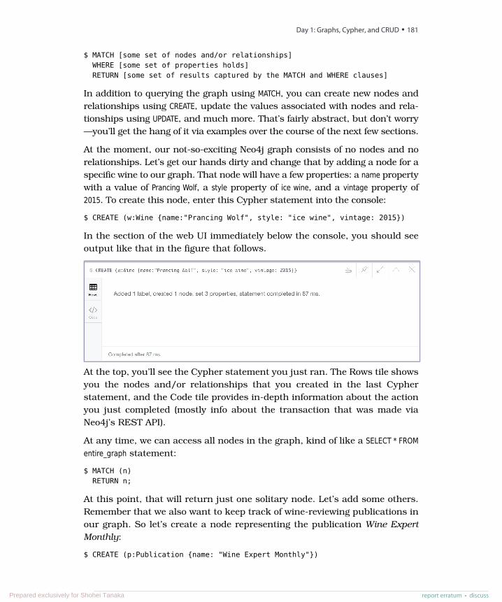
$ MATCH [some set of nodes and/or relationships]WHERE [some set of properties holds]RETURN [some set of results captured by the MATCH and WHERE clauses]
In addition to querying the graph using MATCH, you can create new nodes andrelationships using CREATE, update the values associated with nodes and rela-tionships using UPDATE, and much more. That’s fairly abstract, but don’t worry—you’ll get the hang of it via examples over the course of the next few sections.
At the moment, our not-so-exciting Neo4j graph consists of no nodes and norelationships. Let’s get our hands dirty and change that by adding a node for aspecific wine to our graph. That node will have a few properties: a name propertywith a value of Prancing Wolf, a style property of ice wine, and a vintage property of2015. To create this node, enter this Cypher statement into the console:
$ CREATE (w:Wine {name:"Prancing Wolf", style: "ice wine", vintage: 2015})
In the section of the web UI immediately below the console, you should seeoutput like that in the figure that follows.
At the top, you’ll see the Cypher statement you just ran. The Rows tile showsyou the nodes and/or relationships that you created in the last Cypherstatement, and the Code tile provides in-depth information about the actionyou just completed (mostly info about the transaction that was made viaNeo4j’s REST API).
At any time, we can access all nodes in the graph, kind of like a SELECT * FROMentire_graph statement:
$ MATCH (n)RETURN n;
At this point, that will return just one solitary node. Let’s add some others.Remember that we also want to keep track of wine-reviewing publications inour graph. So let’s create a node representing the publication Wine ExpertMonthly:
$ CREATE (p:Publication {name: "Wine Expert Monthly"})
report erratum • discuss
Day 1: Graphs, Cypher, and CRUD • 181
Prepared exclusively for Shohei Tanaka
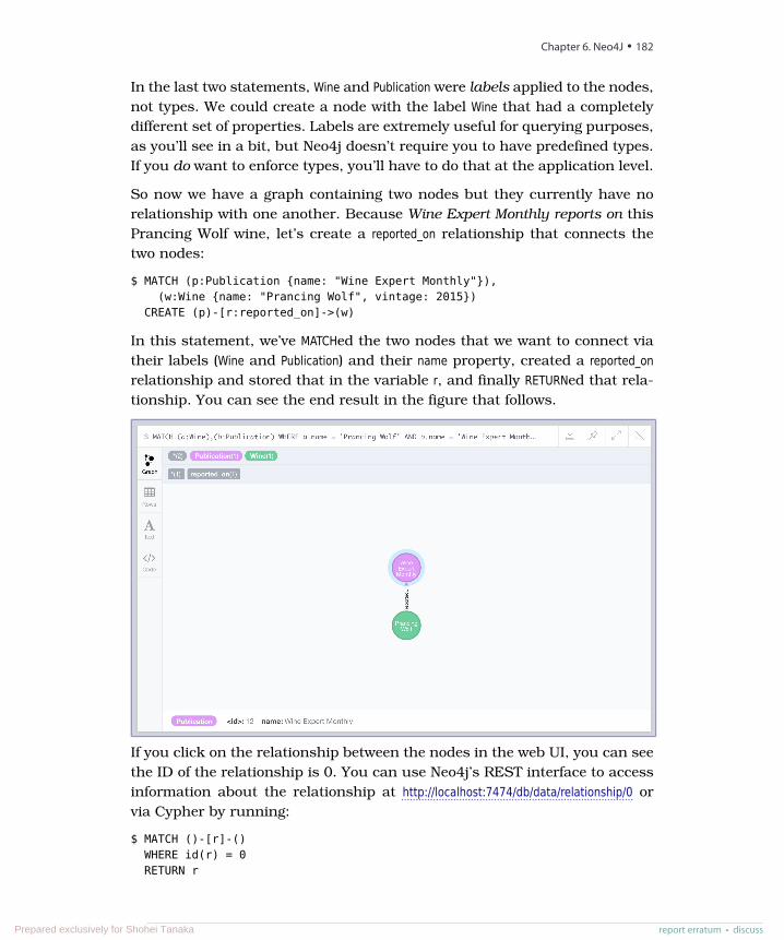
In the last two statements, Wine and Publication were labels applied to the nodes,not types. We could create a node with the label Wine that had a completelydifferent set of properties. Labels are extremely useful for querying purposes,as you’ll see in a bit, but Neo4j doesn’t require you to have predefined types.If you do want to enforce types, you’ll have to do that at the application level.
So now we have a graph containing two nodes but they currently have norelationship with one another. Because Wine Expert Monthly reports on thisPrancing Wolf wine, let’s create a reported_on relationship that connects thetwo nodes:
$ MATCH (p:Publication {name: "Wine Expert Monthly"}),(w:Wine {name: "Prancing Wolf", vintage: 2015})
CREATE (p)-[r:reported_on]->(w)
In this statement, we’ve MATCHed the two nodes that we want to connect viatheir labels (Wine and Publication) and their name property, created a reported_onrelationship and stored that in the variable r, and finally RETURNed that rela-tionship. You can see the end result in the figure that follows.
If you click on the relationship between the nodes in the web UI, you can seethe ID of the relationship is 0. You can use Neo4j’s REST interface to accessinformation about the relationship at http://localhost:7474/db/data/relationship/0 orvia Cypher by running:
$ MATCH ()-[r]-()WHERE id(r) = 0RETURN r
Chapter 6. Neo4J • 182
report erratum • discussPrepared exclusively for Shohei Tanaka
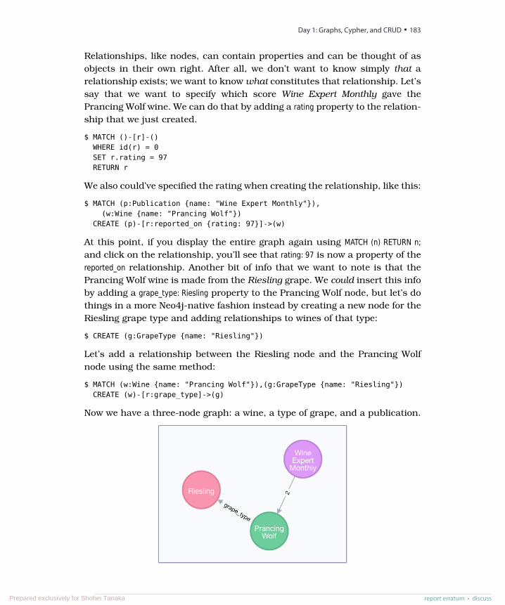
Relationships, like nodes, can contain properties and can be thought of asobjects in their own right. After all, we don’t want to know simply that arelationship exists; we want to know what constitutes that relationship. Let’ssay that we want to specify which score Wine Expert Monthly gave thePrancing Wolf wine. We can do that by adding a rating property to the relation-ship that we just created.
$ MATCH ()-[r]-()WHERE id(r) = 0SET r.rating = 97RETURN r
We also could’ve specified the rating when creating the relationship, like this:
$ MATCH (p:Publication {name: "Wine Expert Monthly"}),(w:Wine {name: "Prancing Wolf"})
CREATE (p)-[r:reported_on {rating: 97}]->(w)
At this point, if you display the entire graph again using MATCH (n) RETURN n;and click on the relationship, you’ll see that rating: 97 is now a property of thereported_on relationship. Another bit of info that we want to note is that thePrancing Wolf wine is made from the Riesling grape. We could insert this infoby adding a grape_type: Riesling property to the Prancing Wolf node, but let’s dothings in a more Neo4j-native fashion instead by creating a new node for theRiesling grape type and adding relationships to wines of that type:
$ CREATE (g:GrapeType {name: "Riesling"})
Let’s add a relationship between the Riesling node and the Prancing Wolfnode using the same method:
$ MATCH (w:Wine {name: "Prancing Wolf"}),(g:GrapeType {name: "Riesling"})CREATE (w)-[r:grape_type]->(g)
Now we have a three-node graph: a wine, a type of grape, and a publication.
report erratum • discuss
Day 1: Graphs, Cypher, and CRUD • 183
Prepared exclusively for Shohei Tanaka
So far, we’ve created and updated both nodes and relationships. You can alsodelete both from a graph. The following are three Cypher statements that willcreate a new node, establish a relationship between that node and one of ourexisting nodes, delete the relationship, and then delete the node (you can’t deletea node that still has relationships associated with it):
$ CREATE (e: EphemeralNode {name: "short lived"})$ MATCH (w:Wine {name: "Prancing Wolf"}),
(e:EphemeralNode {name: "short lived"})CREATE (w)-[r:short_lived_relationship]->(e)
$ MATCH ()-[r:short_lived_relationship]-()DELETE r
$ MATCH (e:EphemeralNode)DELETE e
Our wine graph is now back to where it was before creating the short lived node.Speaking of deletion, if you ever want to burn it all down and start from scratchwith an empty graph, you can use the following command at any time to deleteall nodes and relationships. But beware! This command will delete the entiregraph that you’re working with, so run it only if you’re sure that you’re ready tomove on from a graph’s worth of data for good.
$ MATCH (n)OPTIONAL MATCH (n)-[r]-()DELETE n, r
Now that you know how to start from scratch, let’s continue building out our winegraph. Wineries typically produce more than one wine. To express that relationshipin an RDBMS, we might create a separate table for each winery and store wines thatthey produce as rows. The most natural way to express this in Neo4j would be—youguessed it—to represent wineries as nodes in the graph and create relationshipsbetween wineries and wines. Let’s create a node for Prancing Wolf Winery and adda relationship with the Prancing Wolf wine node that we created earlier:
$ CREATE (wr:Winery {name: "Prancing Wolf Winery"})$ MATCH (w:Wine {name: "Prancing Wolf"}),
(wr:Winery {name: "Prancing Wolf Winery"})CREATE (wr)-[r:produced]->(w)
We’ll also add two more wines produced by Prancing Wolf Winery—a Kabinettand a Spätlese—and also create produced relationships and specify that all of thePrancing Wolf wines are Rieslings.
$ CREATE (w:Wine {name:"Prancing Wolf", style: "Kabinett", vintage: 2002})$ CREATE (w:Wine {name: "Prancing Wolf", style: "Spätlese", vintage: 2010})$ MATCH (wr:Winery {name: "Prancing Wolf"}),(w:Wine {name: "Prancing Wolf"})
CREATE (wr)-[r:produced]->(w)$ MATCH (w:Wine),(g:GrapeType {name: "Riesling"})
CREATE (w)-[r:grape_type]->(g)
Chapter 6. Neo4J • 184
report erratum • discussPrepared exclusively for Shohei Tanaka
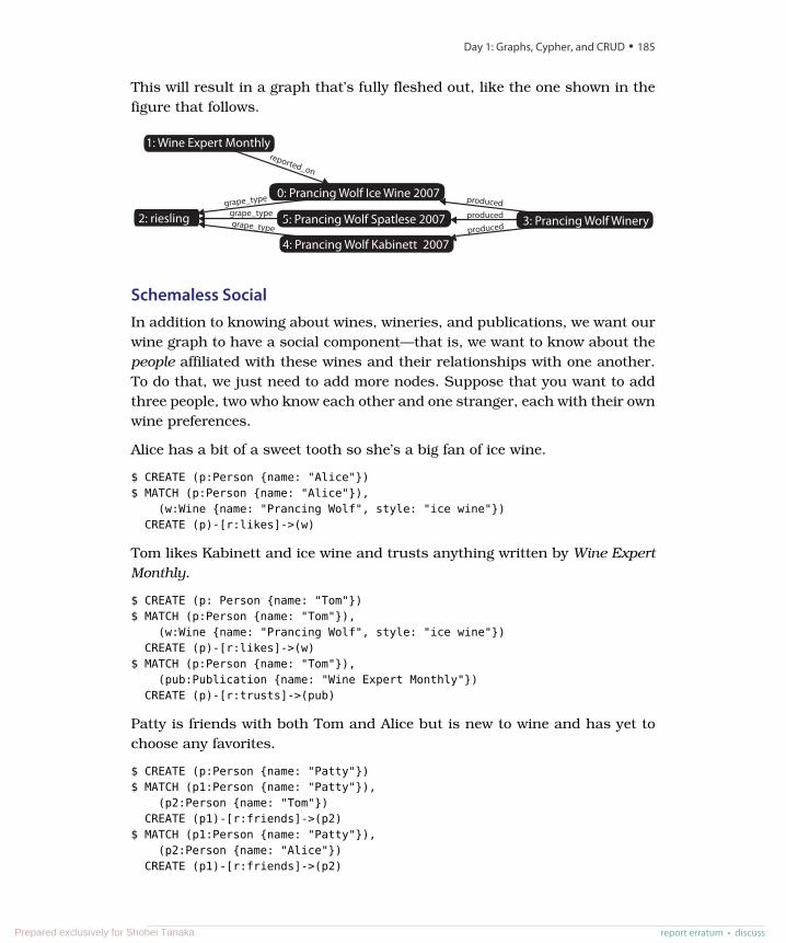
This will result in a graph that’s fully fleshed out, like the one shown in thefigure that follows.
1: Wine Expert Monthly
0: Prancing Wolf Ice Wine 2007
5: Prancing Wolf Spatlese 2007
4: Prancing Wolf Kabinett 2007
2: riesling grape_typegrape_type
grape_typeproduced
produced
produced
reported_on
3: Prancing Wolf Winery
Schemaless SocialIn addition to knowing about wines, wineries, and publications, we want ourwine graph to have a social component—that is, we want to know about thepeople affiliated with these wines and their relationships with one another.To do that, we just need to add more nodes. Suppose that you want to addthree people, two who know each other and one stranger, each with their ownwine preferences.
Alice has a bit of a sweet tooth so she’s a big fan of ice wine.
$ CREATE (p:Person {name: "Alice"})$ MATCH (p:Person {name: "Alice"}),
(w:Wine {name: "Prancing Wolf", style: "ice wine"})CREATE (p)-[r:likes]->(w)
Tom likes Kabinett and ice wine and trusts anything written by Wine ExpertMonthly.
$ CREATE (p: Person {name: "Tom"})$ MATCH (p:Person {name: "Tom"}),
(w:Wine {name: "Prancing Wolf", style: "ice wine"})CREATE (p)-[r:likes]->(w)
$ MATCH (p:Person {name: "Tom"}),(pub:Publication {name: "Wine Expert Monthly"})
CREATE (p)-[r:trusts]->(pub)
Patty is friends with both Tom and Alice but is new to wine and has yet tochoose any favorites.
$ CREATE (p:Person {name: "Patty"})$ MATCH (p1:Person {name: "Patty"}),
(p2:Person {name: "Tom"})CREATE (p1)-[r:friends]->(p2)
$ MATCH (p1:Person {name: "Patty"}),(p2:Person {name: "Alice"})
CREATE (p1)-[r:friends]->(p2)
report erratum • discuss
Day 1: Graphs, Cypher, and CRUD • 185
Prepared exclusively for Shohei Tanaka
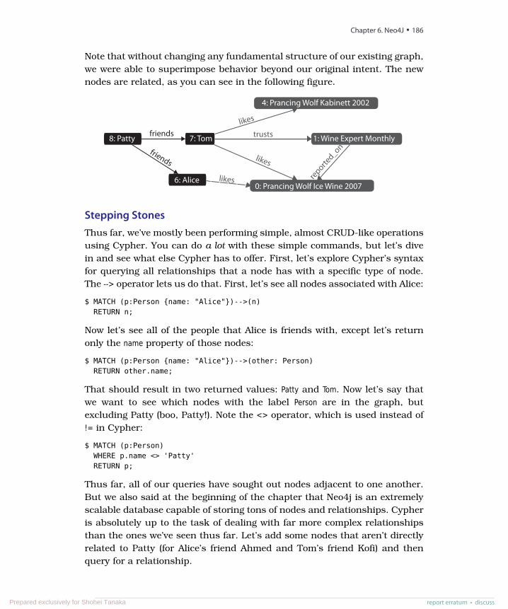
Note that without changing any fundamental structure of our existing graph,we were able to superimpose behavior beyond our original intent. The newnodes are related, as you can see in the following figure.
8: Patty trustsfriends
friends
likes
likes
likes
reporte
d_on
4: Prancing Wolf Kabinett 2002
0: Prancing Wolf Ice Wine 2007
1: Wine Expert Monthly7: Tom
6: Alice
Stepping StonesThus far, we’ve mostly been performing simple, almost CRUD-like operationsusing Cypher. You can do a lot with these simple commands, but let’s divein and see what else Cypher has to offer. First, let’s explore Cypher’s syntaxfor querying all relationships that a node has with a specific type of node.The --> operator lets us do that. First, let’s see all nodes associated with Alice:
$ MATCH (p:Person {name: "Alice"})-->(n)RETURN n;
Now let’s see all of the people that Alice is friends with, except let’s returnonly the name property of those nodes:
$ MATCH (p:Person {name: "Alice"})-->(other: Person)RETURN other.name;
That should result in two returned values: Patty and Tom. Now let’s say thatwe want to see which nodes with the label Person are in the graph, butexcluding Patty (boo, Patty!). Note the <> operator, which is used instead of!= in Cypher:
$ MATCH (p:Person)WHERE p.name <> 'Patty'RETURN p;
Thus far, all of our queries have sought out nodes adjacent to one another.But we also said at the beginning of the chapter that Neo4j is an extremelyscalable database capable of storing tons of nodes and relationships. Cypheris absolutely up to the task of dealing with far more complex relationshipsthan the ones we’ve seen thus far. Let’s add some nodes that aren’t directlyrelated to Patty (for Alice’s friend Ahmed and Tom’s friend Kofi) and thenquery for a relationship.
Chapter 6. Neo4J • 186
report erratum • discussPrepared exclusively for Shohei Tanaka
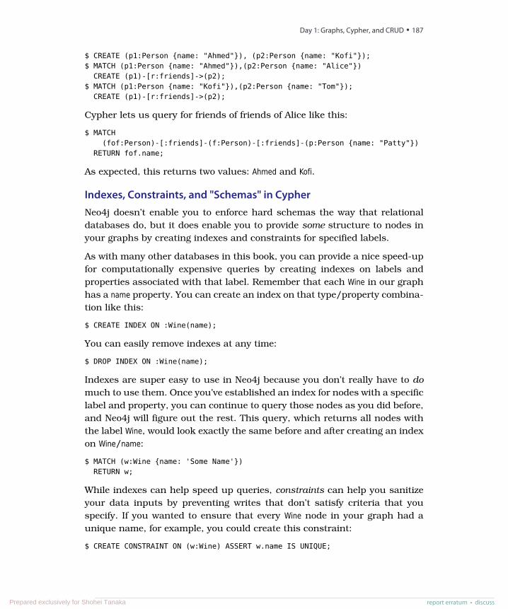
$ CREATE (p1:Person {name: "Ahmed"}), (p2:Person {name: "Kofi"});$ MATCH (p1:Person {name: "Ahmed"}),(p2:Person {name: "Alice"})
CREATE (p1)-[r:friends]->(p2);$ MATCH (p1:Person {name: "Kofi"}),(p2:Person {name: "Tom"});
CREATE (p1)-[r:friends]->(p2);
Cypher lets us query for friends of friends of Alice like this:
$ MATCH(fof:Person)-[:friends]-(f:Person)-[:friends]-(p:Person {name: "Patty"})
RETURN fof.name;
As expected, this returns two values: Ahmed and Kofi.
Indexes, Constraints, and "Schemas" in CypherNeo4j doesn’t enable you to enforce hard schemas the way that relationaldatabases do, but it does enable you to provide some structure to nodes inyour graphs by creating indexes and constraints for specified labels.
As with many other databases in this book, you can provide a nice speed-upfor computationally expensive queries by creating indexes on labels andproperties associated with that label. Remember that each Wine in our graphhas a name property. You can create an index on that type/property combina-tion like this:
$ CREATE INDEX ON :Wine(name);
You can easily remove indexes at any time:
$ DROP INDEX ON :Wine(name);
Indexes are super easy to use in Neo4j because you don’t really have to domuch to use them. Once you’ve established an index for nodes with a specificlabel and property, you can continue to query those nodes as you did before,and Neo4j will figure out the rest. This query, which returns all nodes withthe label Wine, would look exactly the same before and after creating an indexon Wine/name:
$ MATCH (w:Wine {name: 'Some Name'})RETURN w;
While indexes can help speed up queries, constraints can help you sanitizeyour data inputs by preventing writes that don’t satisfy criteria that youspecify. If you wanted to ensure that every Wine node in your graph had aunique name, for example, you could create this constraint:
$ CREATE CONSTRAINT ON (w:Wine) ASSERT w.name IS UNIQUE;
report erratum • discuss
Day 1: Graphs, Cypher, and CRUD • 187
Prepared exclusively for Shohei Tanaka
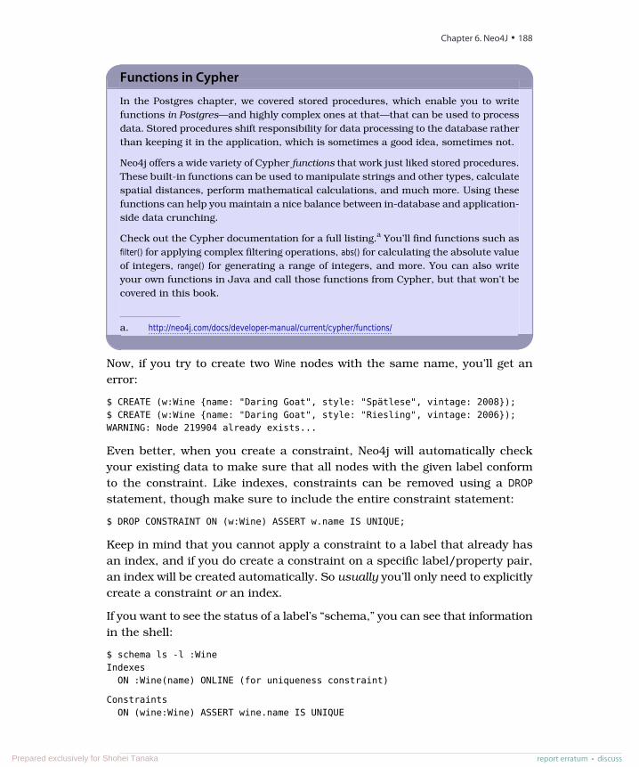
Functions in Cypher
In the Postgres chapter, we covered stored procedures, which enable you to writefunctions in Postgres—and highly complex ones at that—that can be used to processdata. Stored procedures shift responsibility for data processing to the database ratherthan keeping it in the application, which is sometimes a good idea, sometimes not.
Neo4j offers a wide variety of Cypher functions that work just liked stored procedures.These built-in functions can be used to manipulate strings and other types, calculatespatial distances, perform mathematical calculations, and much more. Using thesefunctions can help you maintain a nice balance between in-database and application-side data crunching.
Check out the Cypher documentation for a full listing.a You’ll find functions such asfilter() for applying complex filtering operations, abs() for calculating the absolute valueof integers, range() for generating a range of integers, and more. You can also writeyour own functions in Java and call those functions from Cypher, but that won’t becovered in this book.
a. http://neo4j.com/docs/developer-manual/current/cypher/functions/
Now, if you try to create two Wine nodes with the same name, you’ll get anerror:
$ CREATE (w:Wine {name: "Daring Goat", style: "Spätlese", vintage: 2008});$ CREATE (w:Wine {name: "Daring Goat", style: "Riesling", vintage: 2006});WARNING: Node 219904 already exists...
Even better, when you create a constraint, Neo4j will automatically checkyour existing data to make sure that all nodes with the given label conformto the constraint. Like indexes, constraints can be removed using a DROPstatement, though make sure to include the entire constraint statement:
$ DROP CONSTRAINT ON (w:Wine) ASSERT w.name IS UNIQUE;
Keep in mind that you cannot apply a constraint to a label that already hasan index, and if you do create a constraint on a specific label/property pair,an index will be created automatically. So usually you’ll only need to explicitlycreate a constraint or an index.
If you want to see the status of a label’s “schema,” you can see that informationin the shell:
$ schema ls -l :WineIndexes
ON :Wine(name) ONLINE (for uniqueness constraint)
ConstraintsON (wine:Wine) ASSERT wine.name IS UNIQUE
Chapter 6. Neo4J • 188
report erratum • discussPrepared exclusively for Shohei Tanaka
Although Neo4j isn’t fundamentally schema-driven the way that relationaldatabases are, indexes and constraints will help keep your queries nice andfast and your graph sane. They are an absolute must if you want to run Neo4jin production.
Day 1 Wrap-UpToday we began digging into the graph database Neo4j and the Cyper queryinglanguage—and what a different beast we’ve encountered! Although we didn’tcover specific design patterns per se, our brains are now buzzing with thestrange and beautiful possibilities opened up by the graph database worldview.Remember that if you can draw it on a whiteboard, you can store it in a graphdatabase.
Day 1 Homework
Find
1. Browse through the Neo4j docs at https://neo4j.com/docs and read more aboutCypher syntax. Find some Cypher features mentioned in those docs thatwe didn’t have a chance to use here and pick your favorite.
2. Experiment with an example graph consisting of movie-related data bygoing back to the browser console at http://localhost:7474/browser, typing :playmovie-graph into the web console, and following the instructions.
Do
1. Create a simple graph describing some of your closest friends, your rela-tionships with them, and even some relationships between your friends.Start with three nodes, including one for yourself, and create five relation-ships.
Day 2: REST, Indexes, and AlgorithmsToday we’ll start with Neo4j’s REST interface. First, we’ll use the REST inter-face to create and index nodes and relationships, and to execute full-textsearch. Then we’ll look at a plugin that lets us execute Cypher queries on theserver via REST, freeing our code from the confines of the web console.
Taking a RESTJust like HBase, Mongo, and CouchDB, Neo4j ships with a REST interface.One reason all of these databases support REST is that it allows language-agnostic interactions in a standard connection interface. You can connect to
report erratum • discuss
Day 2: REST, Indexes, and Algorithms • 189
Prepared exclusively for Shohei Tanaka
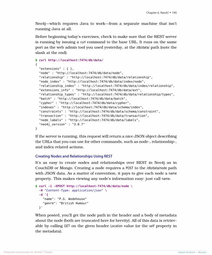
Neo4j—which requires Java to work—from a separate machine that isn’trunning Java at all.
Before beginning today’s exercises, check to make sure that the REST serveris running by issuing a curl command to the base URL. It runs on the sameport as the web admin tool you used yesterday, at the /db/data/ path (note theslash at the end).
$ curl http://localhost:7474/db/data/{
"extensions" : { },"node" : "http://localhost:7474/db/data/node","relationship" : "http://localhost:7474/db/data/relationship","node_index" : "http://localhost:7474/db/data/index/node","relationship_index" : "http://localhost:7474/db/data/index/relationship","extensions_info" : "http://localhost:7474/db/data/ext","relationship_types" : "http://localhost:7474/db/data/relationship/types","batch" : "http://localhost:7474/db/data/batch","cypher" : "http://localhost:7474/db/data/cypher","indexes" : "http://localhost:7474/db/data/schema/index","constraints" : "http://localhost:7474/db/data/schema/constraint","transaction" : "http://localhost:7474/db/data/transaction","node_labels" : "http://localhost:7474/db/data/labels","neo4j_version" : "3.0.7"
}
If the server is running, this request will return a nice JSON object describingthe URLs that you can use for other commands, such as node-, relationship-,and index-related actions.
Creating Nodes and Relationships Using REST
It’s as easy to create nodes and relationships over REST in Neo4j as inCouchDB or Mongo. Creating a node requires a POST to the /db/data/node pathwith JSON data. As a matter of convention, it pays to give each node a nameproperty. This makes viewing any node’s information easy: just call name.
$ curl -i -XPOST http://localhost:7474/db/data/node \-H "Content-Type: application/json" \-d '{
"name": "P.G. Wodehouse""genre": "British Humour"
}'
When posted, you’ll get the node path in the header and a body of metadataabout the node (both are truncated here for brevity). All of this data is retriev-able by calling GET on the given header Location value (or the self property inthe metadata).
Chapter 6. Neo4J • 190
report erratum • discussPrepared exclusively for Shohei Tanaka
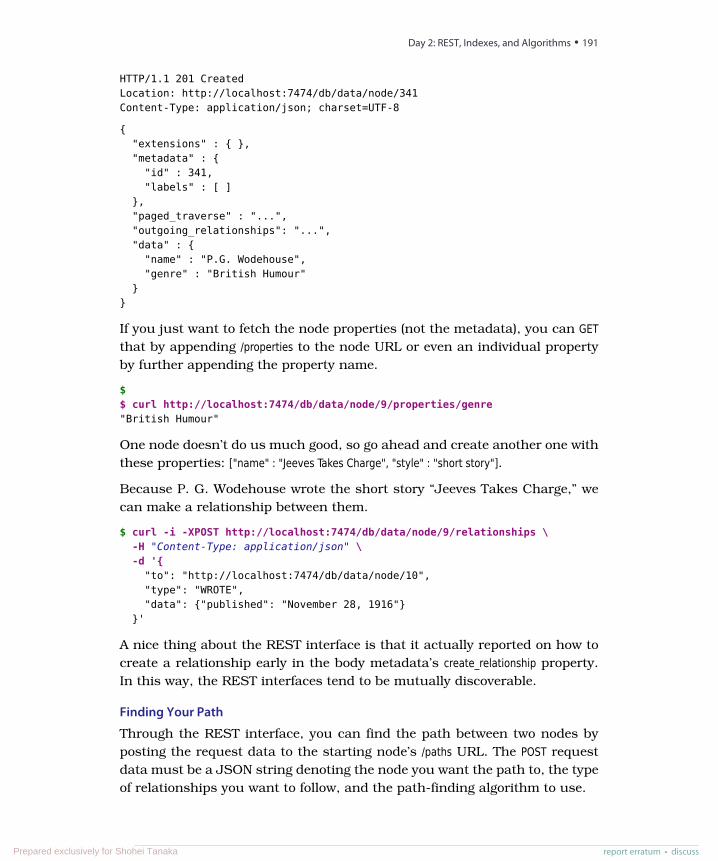
HTTP/1.1 201 CreatedLocation: http://localhost:7474/db/data/node/341Content-Type: application/json; charset=UTF-8
{"extensions" : { },"metadata" : {
"id" : 341,"labels" : [ ]
},"paged_traverse" : "...","outgoing_relationships": "...","data" : {
"name" : "P.G. Wodehouse","genre" : "British Humour"
}}
If you just want to fetch the node properties (not the metadata), you can GETthat by appending /properties to the node URL or even an individual propertyby further appending the property name.
$$ curl http://localhost:7474/db/data/node/9/properties/genre"British Humour"
One node doesn’t do us much good, so go ahead and create another one withthese properties: ["name" : "Jeeves Takes Charge", "style" : "short story"].
Because P. G. Wodehouse wrote the short story “Jeeves Takes Charge,” wecan make a relationship between them.
$ curl -i -XPOST http://localhost:7474/db/data/node/9/relationships \-H "Content-Type: application/json" \-d '{
"to": "http://localhost:7474/db/data/node/10","type": "WROTE","data": {"published": "November 28, 1916"}
}'
A nice thing about the REST interface is that it actually reported on how tocreate a relationship early in the body metadata’s create_relationship property.In this way, the REST interfaces tend to be mutually discoverable.
Finding Your Path
Through the REST interface, you can find the path between two nodes byposting the request data to the starting node’s /paths URL. The POST requestdata must be a JSON string denoting the node you want the path to, the typeof relationships you want to follow, and the path-finding algorithm to use.
report erratum • discuss
Day 2: REST, Indexes, and Algorithms • 191
Prepared exclusively for Shohei Tanaka
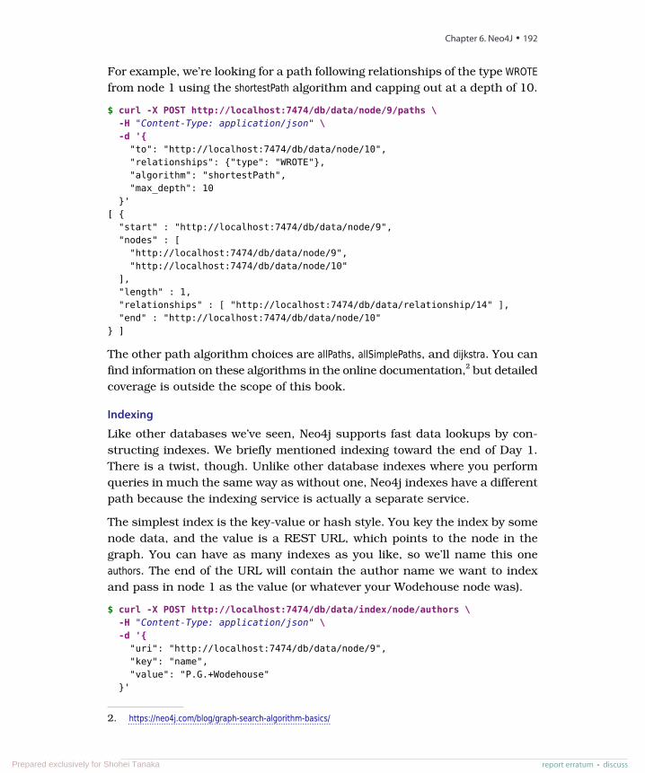
For example, we’re looking for a path following relationships of the type WROTEfrom node 1 using the shortestPath algorithm and capping out at a depth of 10.
$ curl -X POST http://localhost:7474/db/data/node/9/paths \-H "Content-Type: application/json" \-d '{
"to": "http://localhost:7474/db/data/node/10","relationships": {"type": "WROTE"},"algorithm": "shortestPath","max_depth": 10
}'[ {
"start" : "http://localhost:7474/db/data/node/9","nodes" : [
"http://localhost:7474/db/data/node/9","http://localhost:7474/db/data/node/10"
],"length" : 1,"relationships" : [ "http://localhost:7474/db/data/relationship/14" ],"end" : "http://localhost:7474/db/data/node/10"
} ]
The other path algorithm choices are allPaths, allSimplePaths, and dijkstra. You canfind information on these algorithms in the online documentation,2 but detailedcoverage is outside the scope of this book.
Indexing
Like other databases we’ve seen, Neo4j supports fast data lookups by con-structing indexes. We briefly mentioned indexing toward the end of Day 1.There is a twist, though. Unlike other database indexes where you performqueries in much the same way as without one, Neo4j indexes have a differentpath because the indexing service is actually a separate service.
The simplest index is the key-value or hash style. You key the index by somenode data, and the value is a REST URL, which points to the node in thegraph. You can have as many indexes as you like, so we’ll name this oneauthors. The end of the URL will contain the author name we want to indexand pass in node 1 as the value (or whatever your Wodehouse node was).
$ curl -X POST http://localhost:7474/db/data/index/node/authors \-H "Content-Type: application/json" \-d '{
"uri": "http://localhost:7474/db/data/node/9","key": "name","value": "P.G.+Wodehouse"
}'
2. https://neo4j.com/blog/graph-search-algorithm-basics/
Chapter 6. Neo4J • 192
report erratum • discussPrepared exclusively for Shohei Tanaka
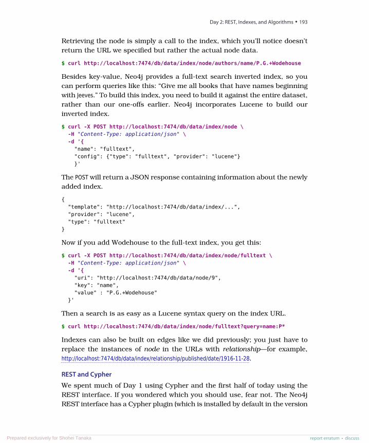
Retrieving the node is simply a call to the index, which you’ll notice doesn’treturn the URL we specified but rather the actual node data.
$ curl http://localhost:7474/db/data/index/node/authors/name/P.G.+Wodehouse
Besides key-value, Neo4j provides a full-text search inverted index, so youcan perform queries like this: “Give me all books that have names beginningwith Jeeves.” To build this index, you need to build it against the entire dataset,rather than our one-offs earlier. Neo4j incorporates Lucene to build ourinverted index.
$ curl -X POST http://localhost:7474/db/data/index/node \-H "Content-Type: application/json" \-d '{
"name": "fulltext","config": {"type": "fulltext", "provider": "lucene"}}'
The POST will return a JSON response containing information about the newlyadded index.
{"template": "http://localhost:7474/db/data/index/...","provider": "lucene","type": "fulltext"
}
Now if you add Wodehouse to the full-text index, you get this:
$ curl -X POST http://localhost:7474/db/data/index/node/fulltext \-H "Content-Type: application/json" \-d '{
"uri": "http://localhost:7474/db/data/node/9","key": "name","value" : "P.G.+Wodehouse"
}'
Then a search is as easy as a Lucene syntax query on the index URL.
$ curl http://localhost:7474/db/data/index/node/fulltext?query=name:P*
Indexes can also be built on edges like we did previously; you just have toreplace the instances of node in the URLs with relationship—for example,http://localhost:7474/db/data/index/relationship/published/date/1916-11-28.
REST and Cypher
We spent much of Day 1 using Cypher and the first half of today using theREST interface. If you wondered which you should use, fear not. The Neo4jREST interface has a Cypher plugin (which is installed by default in the version
report erratum • discuss
Day 2: REST, Indexes, and Algorithms • 193
Prepared exclusively for Shohei Tanaka
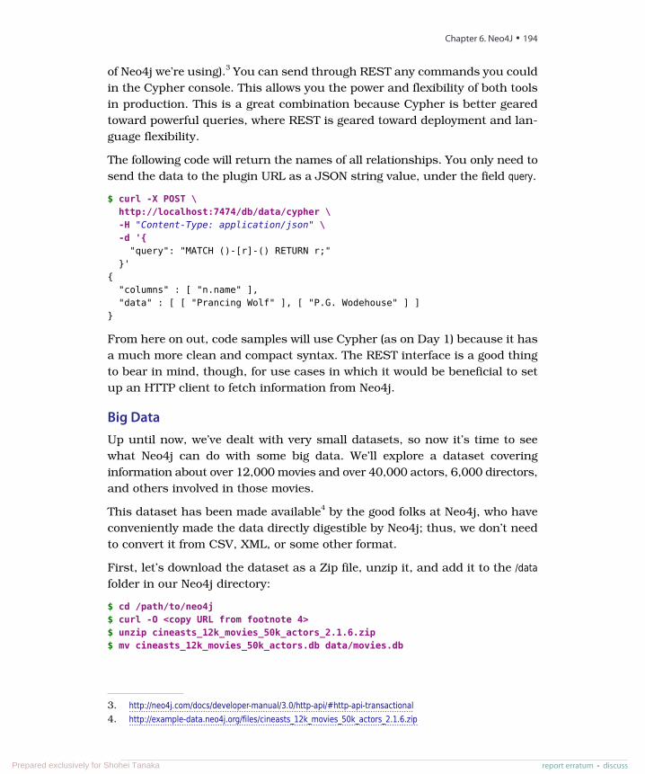
of Neo4j we’re using).3 You can send through REST any commands you couldin the Cypher console. This allows you the power and flexibility of both toolsin production. This is a great combination because Cypher is better gearedtoward powerful queries, where REST is geared toward deployment and lan-guage flexibility.
The following code will return the names of all relationships. You only need tosend the data to the plugin URL as a JSON string value, under the field query.
$ curl -X POST \http://localhost:7474/db/data/cypher \-H "Content-Type: application/json" \-d '{
"query": "MATCH ()-[r]-() RETURN r;"}'
{"columns" : [ "n.name" ],"data" : [ [ "Prancing Wolf" ], [ "P.G. Wodehouse" ] ]
}
From here on out, code samples will use Cypher (as on Day 1) because it hasa much more clean and compact syntax. The REST interface is a good thingto bear in mind, though, for use cases in which it would be beneficial to setup an HTTP client to fetch information from Neo4j.
Big DataUp until now, we’ve dealt with very small datasets, so now it’s time to seewhat Neo4j can do with some big data. We’ll explore a dataset coveringinformation about over 12,000 movies and over 40,000 actors, 6,000 directors,and others involved in those movies.
This dataset has been made available4 by the good folks at Neo4j, who haveconveniently made the data directly digestible by Neo4j; thus, we don’t needto convert it from CSV, XML, or some other format.
First, let’s download the dataset as a Zip file, unzip it, and add it to the /datafolder in our Neo4j directory:
$ cd /path/to/neo4j$ curl -O <copy URL from footnote 4>$ unzip cineasts_12k_movies_50k_actors_2.1.6.zip$ mv cineasts_12k_movies_50k_actors.db data/movies.db
3. http://neo4j.com/docs/developer-manual/3.0/http-api/#http-api-transactional4. http://example-data.neo4j.org/files/cineasts_12k_movies_50k_actors_2.1.6.zip
Chapter 6. Neo4J • 194
report erratum • discussPrepared exclusively for Shohei Tanaka
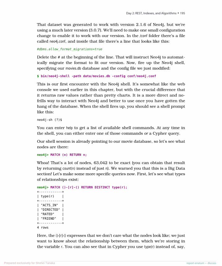
That dataset was generated to work with version 2.1.6 of Neo4j, but we’reusing a much later version (3.0.7). We’ll need to make one small configurationchange to enable it to work with our version. In the /conf folder there’s a filecalled neo4j.conf, and inside that file there’s a line that looks like this:
#dbms.allow_format_migrations=true
Delete the # at the beginning of the line. That will instruct Neo4j to automat-ically migrate the format to fit our version. Now, fire up the Neo4j shell,specifying our movies.db database and the config file we just modified:
$ bin/neo4j-shell -path data/movies.db -config conf/neo4j.conf
This is our first encounter with the Neo4j shell. It’s somewhat like the webconsole we used earlier in this chapter, but with the crucial difference thatit returns raw values rather than pretty charts. It is a more direct and no-frills way to interact with Neo4j and better to use once you have gotten thehang of the database. When the shell fires up, you should see a shell promptlike this:
neo4j-sh (?)$
You can enter help to get a list of available shell commands. At any time inthe shell, you can either enter one of those commands or a Cypher query.
Our shell session is already pointing to our movie database, so let’s see whatnodes are there:
neo4j> MATCH (n) RETURN n;
Whoa! That’s a lot of nodes, 63,042 to be exact (you can obtain that resultby returning count(n) instead of just n). We warned you that this is a Big Datasection! Let’s make some more specific queries now. First, let’s see what typesof relationships exist:
neo4j> MATCH ()-[r]-() RETURN DISTINCT type(r);+------------+| type(r) |+------------+| "ACTS_IN" || "DIRECTED" || "RATED" || "FRIEND" |+------------+4 rows
Here, the ()-[r]-() expresses that we don’t care what the nodes look like; we justwant to know about the relationship between them, which we’re storing inthe variable r. You can also see that in Cypher you use type(r) instead of, say,
report erratum • discuss
Day 2: REST, Indexes, and Algorithms • 195
Prepared exclusively for Shohei Tanaka
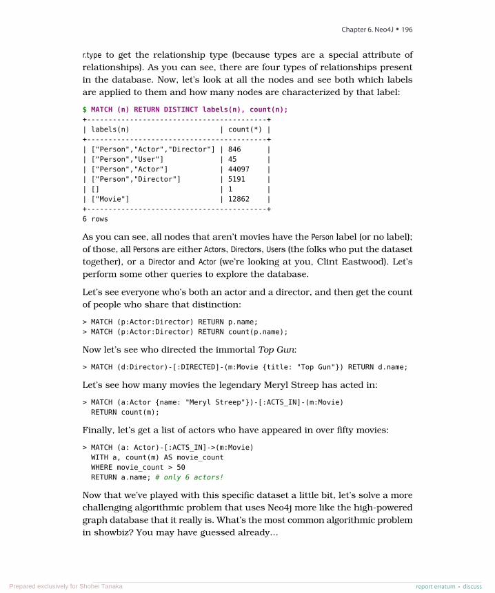
r.type to get the relationship type (because types are a special attribute ofrelationships). As you can see, there are four types of relationships presentin the database. Now, let’s look at all the nodes and see both which labelsare applied to them and how many nodes are characterized by that label:
$ MATCH (n) RETURN DISTINCT labels(n), count(n);+------------------------------------------+| labels(n) | count(*) |+------------------------------------------+| ["Person","Actor","Director"] | 846 || ["Person","User"] | 45 || ["Person","Actor"] | 44097 || ["Person","Director"] | 5191 || [] | 1 || ["Movie"] | 12862 |+------------------------------------------+6 rows
As you can see, all nodes that aren’t movies have the Person label (or no label);of those, all Persons are either Actors, Directors, Users (the folks who put the datasettogether), or a Director and Actor (we’re looking at you, Clint Eastwood). Let’sperform some other queries to explore the database.
Let’s see everyone who’s both an actor and a director, and then get the countof people who share that distinction:
> MATCH (p:Actor:Director) RETURN p.name;> MATCH (p:Actor:Director) RETURN count(p.name);
Now let’s see who directed the immortal Top Gun:
> MATCH (d:Director)-[:DIRECTED]-(m:Movie {title: "Top Gun"}) RETURN d.name;
Let’s see how many movies the legendary Meryl Streep has acted in:
> MATCH (a:Actor {name: "Meryl Streep"})-[:ACTS_IN]-(m:Movie)RETURN count(m);
Finally, let’s get a list of actors who have appeared in over fifty movies:
> MATCH (a: Actor)-[:ACTS_IN]->(m:Movie)WITH a, count(m) AS movie_countWHERE movie_count > 50RETURN a.name; # only 6 actors!
Now that we’ve played with this specific dataset a little bit, let’s solve a morechallenging algorithmic problem that uses Neo4j more like the high-poweredgraph database that it really is. What’s the most common algorithmic problemin showbiz? You may have guessed already...
Chapter 6. Neo4J • 196
report erratum • discussPrepared exclusively for Shohei Tanaka
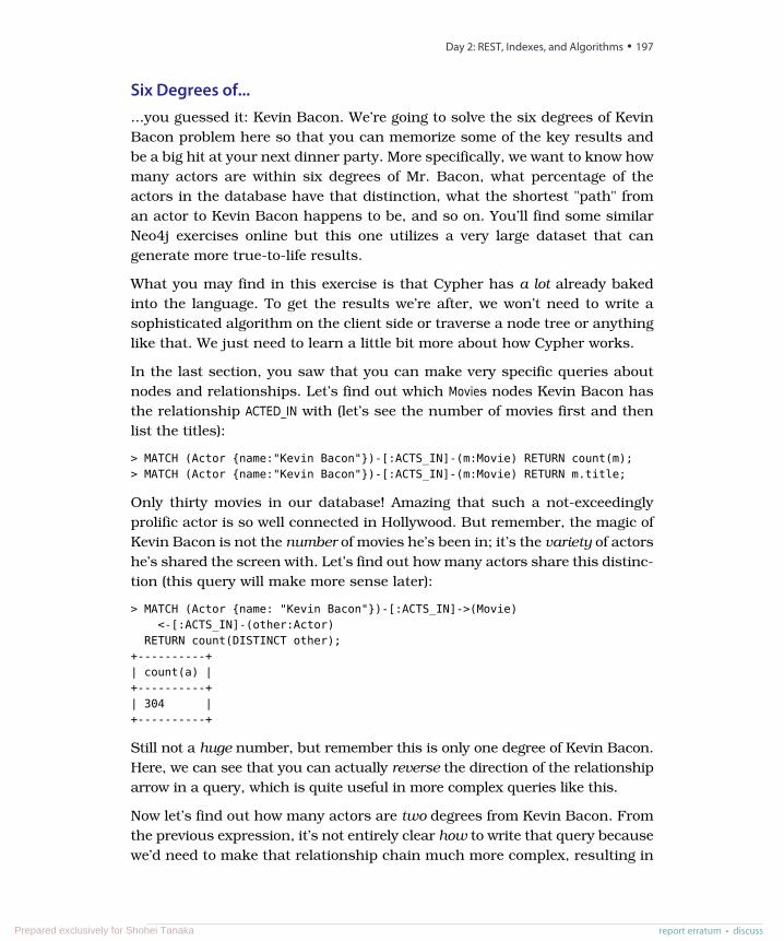
Six Degrees of......you guessed it: Kevin Bacon. We’re going to solve the six degrees of KevinBacon problem here so that you can memorize some of the key results andbe a big hit at your next dinner party. More specifically, we want to know howmany actors are within six degrees of Mr. Bacon, what percentage of theactors in the database have that distinction, what the shortest "path" froman actor to Kevin Bacon happens to be, and so on. You’ll find some similarNeo4j exercises online but this one utilizes a very large dataset that cangenerate more true-to-life results.
What you may find in this exercise is that Cypher has a lot already bakedinto the language. To get the results we’re after, we won’t need to write asophisticated algorithm on the client side or traverse a node tree or anythinglike that. We just need to learn a little bit more about how Cypher works.
In the last section, you saw that you can make very specific queries aboutnodes and relationships. Let’s find out which Movies nodes Kevin Bacon hasthe relationship ACTED_IN with (let’s see the number of movies first and thenlist the titles):
> MATCH (Actor {name:"Kevin Bacon"})-[:ACTS_IN]-(m:Movie) RETURN count(m);> MATCH (Actor {name:"Kevin Bacon"})-[:ACTS_IN]-(m:Movie) RETURN m.title;
Only thirty movies in our database! Amazing that such a not-exceedinglyprolific actor is so well connected in Hollywood. But remember, the magic ofKevin Bacon is not the number of movies he’s been in; it’s the variety of actorshe’s shared the screen with. Let’s find out how many actors share this distinc-tion (this query will make more sense later):
> MATCH (Actor {name: "Kevin Bacon"})-[:ACTS_IN]->(Movie)<-[:ACTS_IN]-(other:Actor)
RETURN count(DISTINCT other);+----------+| count(a) |+----------+| 304 |+----------+
Still not a huge number, but remember this is only one degree of Kevin Bacon.Here, we can see that you can actually reverse the direction of the relationshiparrow in a query, which is quite useful in more complex queries like this.
Now let’s find out how many actors are two degrees from Kevin Bacon. Fromthe previous expression, it’s not entirely clear how to write that query becausewe’d need to make that relationship chain much more complex, resulting in
report erratum • discuss
Day 2: REST, Indexes, and Algorithms • 197
Prepared exclusively for Shohei Tanaka
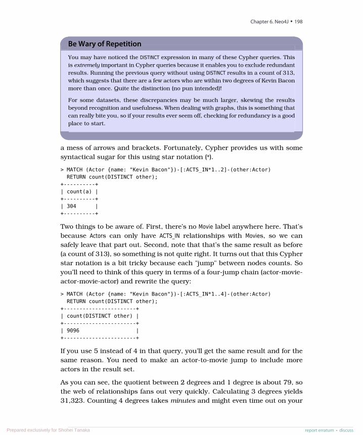
Be Wary of Repetition
You may have noticed the DISTINCT expression in many of these Cypher queries. Thisis extremely important in Cypher queries because it enables you to exclude redundantresults. Running the previous query without using DISTINCT results in a count of 313,which suggests that there are a few actors who are within two degrees of Kevin Baconmore than once. Quite the distinction (no pun intended)!
For some datasets, these discrepancies may be much larger, skewing the resultsbeyond recognition and usefulness. When dealing with graphs, this is something thatcan really bite you, so if your results ever seem off, checking for redundancy is a goodplace to start.
a mess of arrows and brackets. Fortunately, Cypher provides us with somesyntactical sugar for this using star notation (*).
> MATCH (Actor {name: "Kevin Bacon"})-[:ACTS_IN*1..2]-(other:Actor)RETURN count(DISTINCT other);
+----------+| count(a) |+----------+| 304 |+----------+
Two things to be aware of. First, there’s no Movie label anywhere here. That’sbecause Actors can only have ACTS_IN relationships with Movies, so we cansafely leave that part out. Second, note that that’s the same result as before(a count of 313), so something is not quite right. It turns out that this Cypherstar notation is a bit tricky because each "jump" between nodes counts. Soyou’ll need to think of this query in terms of a four-jump chain (actor-movie-actor-movie-actor) and rewrite the query:
> MATCH (Actor {name: "Kevin Bacon"})-[:ACTS_IN*1..4]-(other:Actor)RETURN count(DISTINCT other);
+-----------------------+| count(DISTINCT other) |+-----------------------+| 9096 |+-----------------------+
If you use 5 instead of 4 in that query, you’ll get the same result and for thesame reason. You need to make an actor-to-movie jump to include moreactors in the result set.
As you can see, the quotient between 2 degrees and 1 degree is about 79, sothe web of relationships fans out very quickly. Calculating 3 degrees yields31,323. Counting 4 degrees takes minutes and might even time out on your
Chapter 6. Neo4J • 198
report erratum • discussPrepared exclusively for Shohei Tanaka
machine, so we don’t recommend running that query unless you need a (long)hot chocolate break.
Thus far, we’ve only really been counting nodes that share some trait, thoughour ability to describe those traits has been enhanced. We’re still not equippedto answer any of our initial questions, such as how many degrees lie betweenKevin Bacon and other actors, what percentage of actors lie within N degrees,and so on.
To get traction into those questions, we need to begin querying for path data,as we did in the REST exercises. Once again, Cypher comes through in theclutch for us with its shortestPath function, which enables you to easily calculatethe distance between two nodes. You can specify the relationship type you’reinterested in specifically or just use * if the relationship type doesn’t matter.
We can use the shortestPath function to find the number of degrees separatingKevin Bacon and another dashing actor, Sean Penn, using this query:
> MATCH (bacon:Actor {name: "Kevin Bacon"}),(penn:Actor {name: "Sean Penn"}
),p=shortestPath((bacon)-[:ACTS_IN*]-(penn))RETURN length(p);
+---------------+| length(p) / 2 |+---------------+| 2 |+---------------+
But wait a second. According to IMDB, Messieurs Bacon and Penn starredtogether in Mystic River. So why does it take 2 degrees to connect these twowhen it should be one? Well, it turns out that Mystic River isn’t in ourdatabase.
> MATCH (m:Movie {name: "Mystic River"})RETURN count(DISTINCT m);
+-------------------+| count(DISTINCT m) |+-------------------+| 0 |+-------------------+
Looks like our database is lacking some crucial bits of cinema. So maybedon’t use these results to show off at your next dinner party just yet; youmight want to find a more complete database for that. But for now, you knowhow to calculate shortest paths, so that’s a good start. Try finding the numberof degrees between some of your favorite actors.
report erratum • discuss
Day 2: REST, Indexes, and Algorithms • 199
Prepared exclusively for Shohei Tanaka
Another thing we’re interested in beyond the shortest path between any two actorsis the percentage of actors that lie within N degrees. We can do that by using ageneric other node with the Actor label and counting the number of shortest pathsthat are found within a number of degrees. We’ll start with 2 degrees and dividethe result by the total number of actors, making sure to specify that we don’tinclude the original Kevin Bacon node in the shortest path calculation (or we’llget a nasty and long-winded error message).
> MATCH p=shortestPath((bacon:Actor {name: "Kevin Bacon"})-[:ACTS_IN*1..2]-(other:Actor)
)WHERE bacon <> otherRETURN count(p);
+----------+| count(p) |+----------+| 304 |+----------+
Just as expected, the same result as before. What happened there is that Neo4jtraversed every relationship within 1 degree of Kevin Bacon and found the numberthat had shortest paths. So in this case, p returns a list of many shortest pathsbetween Kevin Bacon and many actors rather than just a single shortest path toone actor. Now let’s divide by the total number of actors (44,943) and add anextra decimal place to make sure we get a float:
> MATCH p=shortestPath((bacon:Actor {name: "Kevin Bacon"})-[:ACTS_IN*1..2]-(other:Actor)
)WHERE bacon <> otherRETURN count(p) / 44943.0;
+----------------------+| count(p) / 44943.0 |+----------------------+| 0.006764123445252876 |+----------------------+
That’s a pretty small percentage of actors. But now re-run that query using 4instead of 2 (to symbolize 2 degrees rather than 1):
> MATCH p=shortestPath((bacon:Actor {name: "Kevin Bacon"})-[:ACTS_IN*1..4]-(other:Actor)
)WHERE bacon <> otherRETURN count(p) / 44943.0;
+--------------------+| count(p) / 44943.0 |+--------------------+| 0.2023674432058385 |+--------------------+
Chapter 6. Neo4J • 200
report erratum • discussPrepared exclusively for Shohei Tanaka
Already up to 20 percent within just 1 extra degree. Running the same querygets you almost 70 percent for 3 degrees, a little over 90 percent for 4 degrees,93 percent for 5, and about 93.4 percent for a full 6 degrees. So how manyactors have no relationship with Kevin Bacon whatsoever in our database? Wecan find that out by not specifying an N for degrees and just using any degree:
> MATCH p=shortestPath((bacon:Actor {name: "Kevin Bacon"})-[:ACTS_IN*]-(other:Actor)
)WHERE bacon <> otherRETURN count(p) / 44943.0;
+--------------------+| count(p) / 44943.0 |+--------------------+| 0.9354960728033287 |+--------------------+
Just a little bit higher than the percentage of actors within 6 degrees, so ifyou’re related to Kevin Bacon at all in our database, then you’re almost cer-tainly within 6 degrees.
Day 2 Wrap-UpOn Day 2, we broadened our ability to interact with Neo4j by taking a lookat the REST interface. You saw how, using the Cypher plugin, you can executeCypher code on the server and have the REST interface return results. Weplayed around with a larger dataset and finally finished up with a handful ofalgorithms for diving into that data.
Day 2 Homework
Find
1. Bookmark the documentation for the Neo4j REST API.
2. Bookmark the API for the JUNG project and the algorithms it implements.
3. Find a binding or REST interface for your favorite programming language.
Do
1. Turn the path-finding portion of the Kevin Bacon algorithm into its ownstep. Then implement a general-purpose Groovy function (for example,def actor_path(g, name1, name2) {...}) that accepts the graph and two names andcompares the distance.
2. Choose and run one of the many JUNG algorithms on a node (or thedataset, if the API demands it).
report erratum • discuss
Day 2: REST, Indexes, and Algorithms • 201
Prepared exclusively for Shohei Tanaka

3. Install your driver of choice, and use it to manage your company graphwith the people and the roles they play, with edges describing theirinteractions (reports to, works with). If your company is huge, just tryyour close teams; if you’re with a small organization, try including somecustomers. Find the most well-connected person in the organization byclosest distance to all other nodes.
Day 3: Distributed High AvailabilityLet’s wrap up our Neo4j investigation by learning how to make Neo4j moresuitable for mission-critical, production uses. We’ll see how Neo4j keeps datastable via ACID-compliant transactions. Then we’ll install and configure aNeo4j high availability (HA) cluster to improve availability when serving high-read traffic. Then we’re going to look into backup strategies to ensure thatour data remains safe.
Transactions and Only Transactions with Cypher
Neo4j is an Atomic, Consistent, Isolated, Durable (ACID) transaction database, similarto PostgreSQL. This makes it a good option for important data that you may haveotherwise picked a relational database for. Just like transactions you’ve seen before,Neo4j transactions are all-or-nothing operations. When a transaction starts, everyfollowing operation will succeed or fail as an atomic unit—failure of one means failureof all. Much like specifying BEGIN and COMMIT delimiters as in Postgres, Cypher enablesyou to do the same thing in the Cypher shell using :begin and :commit (the debts to theSQL world should be quite clear here!).
If you’re using Cypher from a non-shell client, all queries are automatically treatedas transactions and thus completely succeed or completely fail. Explicit transactionlogic is necessary only in the shell.
Chapter 6. Neo4J • 202
report erratum • discussPrepared exclusively for Shohei Tanaka
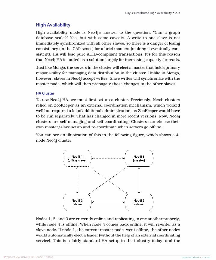
High AvailabilityHigh availability mode is Neo4j’s answer to the question, “Can a graphdatabase scale?” Yes, but with some caveats. A write to one slave is notimmediately synchronized with all other slaves, so there is a danger of losingconsistency (in the CAP sense) for a brief moment (making it eventually con-sistent). HA will lose pure ACID-compliant transactions. It’s for this reasonthat Neo4j HA is touted as a solution largely for increasing capacity for reads.
Just like Mongo, the servers in the cluster will elect a master that holds primaryresponsibility for managing data distribution in the cluster. Unlike in Mongo,however, slaves in Neo4j accept writes. Slave writes will synchronize with themaster node, which will then propagate those changes to the other slaves.
HA Cluster
To use Neo4j HA, we must first set up a cluster. Previously, Neo4j clustersrelied on ZooKeeper as an external coordination mechanism, which workedwell but required a lot of additional administration, as ZooKeeper would haveto be run separately. That has changed in more recent versions. Now, Neo4jclusters are self-managing and self-coordinating. Clusters can choose theirown master/slave setup and re-coordinate when servers go offline.
You can see an illustration of this in the following figure, which shows a 4-node Neo4j cluster.
Nodes 1, 2, and 3 are currently online and replicating to one another properly,while node 4 is offline. When node 4 comes back online, it will re-enter as aslave node. If node 1, the current master node, went offline, the other nodeswould automatically elect a leader (without the help of an external coordinatingservice). This is a fairly standard HA setup in the industry today, and the
report erratum • discuss
Day 3: Distributed High Availability • 203
Prepared exclusively for Shohei Tanaka
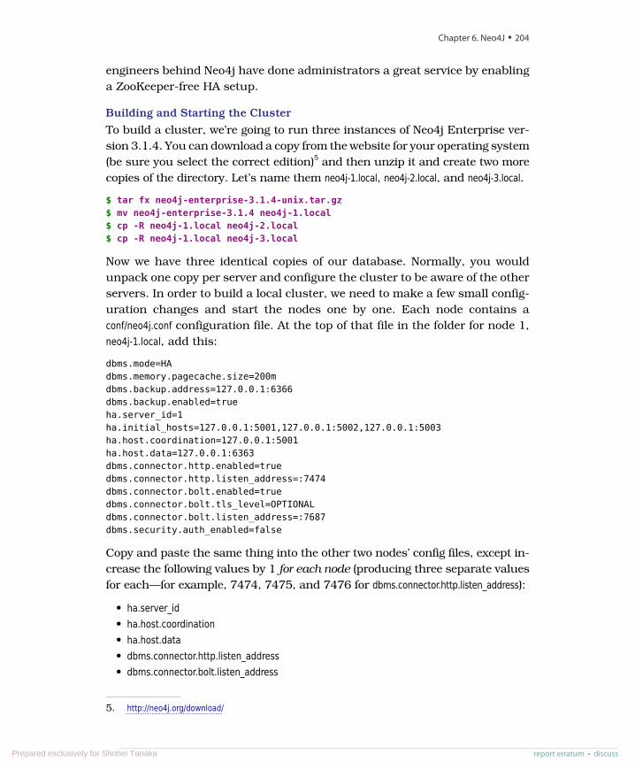
engineers behind Neo4j have done administrators a great service by enablinga ZooKeeper-free HA setup.
Building and Starting the Cluster
To build a cluster, we’re going to run three instances of Neo4j Enterprise ver-sion 3.1.4. You can download a copy from the website for your operating system(be sure you select the correct edition)5 and then unzip it and create two morecopies of the directory. Let’s name them neo4j-1.local, neo4j-2.local, and neo4j-3.local.
$ tar fx neo4j-enterprise-3.1.4-unix.tar.gz$ mv neo4j-enterprise-3.1.4 neo4j-1.local$ cp -R neo4j-1.local neo4j-2.local$ cp -R neo4j-1.local neo4j-3.local
Now we have three identical copies of our database. Normally, you wouldunpack one copy per server and configure the cluster to be aware of the otherservers. In order to build a local cluster, we need to make a few small config-uration changes and start the nodes one by one. Each node contains aconf/neo4j.conf configuration file. At the top of that file in the folder for node 1,neo4j-1.local, add this:
dbms.mode=HAdbms.memory.pagecache.size=200mdbms.backup.address=127.0.0.1:6366dbms.backup.enabled=trueha.server_id=1ha.initial_hosts=127.0.0.1:5001,127.0.0.1:5002,127.0.0.1:5003ha.host.coordination=127.0.0.1:5001ha.host.data=127.0.0.1:6363dbms.connector.http.enabled=truedbms.connector.http.listen_address=:7474dbms.connector.bolt.enabled=truedbms.connector.bolt.tls_level=OPTIONALdbms.connector.bolt.listen_address=:7687dbms.security.auth_enabled=false
Copy and paste the same thing into the other two nodes’ config files, except in-crease the following values by 1 for each node (producing three separate valuesfor each—for example, 7474, 7475, and 7476 for dbms.connector.http.listen_address):
• ha.server_id• ha.host.coordination• ha.host.data• dbms.connector.http.listen_address• dbms.connector.bolt.listen_address
5. http://neo4j.org/download/
Chapter 6. Neo4J • 204
report erratum • discussPrepared exclusively for Shohei Tanaka
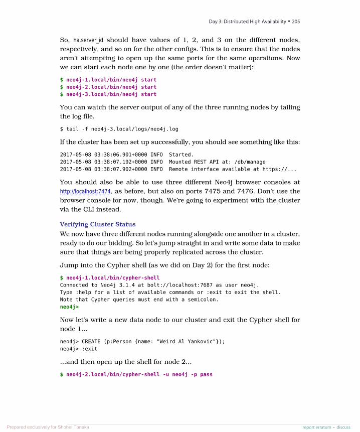
So, ha.server_id should have values of 1, 2, and 3 on the different nodes,respectively, and so on for the other configs. This is to ensure that the nodesaren’t attempting to open up the same ports for the same operations. Nowwe can start each node one by one (the order doesn’t matter):
$ neo4j-1.local/bin/neo4j start$ neo4j-2.local/bin/neo4j start$ neo4j-3.local/bin/neo4j start
You can watch the server output of any of the three running nodes by tailingthe log file.
$ tail -f neo4j-3.local/logs/neo4j.log
If the cluster has been set up successfully, you should see something like this:
2017-05-08 03:38:06.901+0000 INFO Started.2017-05-08 03:38:07.192+0000 INFO Mounted REST API at: /db/manage2017-05-08 03:38:07.902+0000 INFO Remote interface available at https://...
You should also be able to use three different Neo4j browser consoles athttp://localhost:7474, as before, but also on ports 7475 and 7476. Don’t use thebrowser console for now, though. We’re going to experiment with the clustervia the CLI instead.
Verifying Cluster Status
We now have three different nodes running alongside one another in a cluster,ready to do our bidding. So let’s jump straight in and write some data to makesure that things are being properly replicated across the cluster.
Jump into the Cypher shell (as we did on Day 2) for the first node:
$ neo4j-1.local/bin/cypher-shellConnected to Neo4j 3.1.4 at bolt://localhost:7687 as user neo4j.Type :help for a list of available commands or :exit to exit the shell.Note that Cypher queries must end with a semicolon.neo4j>
Now let’s write a new data node to our cluster and exit the Cypher shell fornode 1...
neo4j> CREATE (p:Person {name: "Weird Al Yankovic"});neo4j> :exit
...and then open up the shell for node 2...
$ neo4j-2.local/bin/cypher-shell -u neo4j -p pass
report erratum • discuss
Day 3: Distributed High Availability • 205
Prepared exclusively for Shohei Tanaka
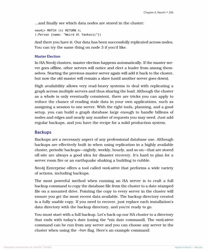
...and finally see which data nodes are stored in the cluster:
neo4j> MATCH (n) RETURN n;(:Person {name: "Weird Al Yankovic"})
And there you have it: Our data has been successfully replicated across nodes.You can try the same thing on node 3 if you’d like.
Master Election
In HA Neo4j clusters, master election happens automatically. If the master ser-ver goes offline, other servers will notice and elect a leader from among them-selves. Starting the previous master server again will add it back to the cluster,but now the old master will remain a slave (until another server goes down).
High availability allows very read-heavy systems to deal with replicating agraph across multiple servers and thus sharing the load. Although the clusteras a whole is only eventually consistent, there are tricks you can apply toreduce the chance of reading stale data in your own applications, such asassigning a session to one server. With the right tools, planning, and a goodsetup, you can build a graph database large enough to handle billions ofnodes and edges and nearly any number of requests you may need. Just addregular backups, and you have the recipe for a solid production system.
BackupsBackups are a necessary aspect of any professional database use. Althoughbackups are effectively built in when using replication in a highly availablecluster, periodic backups—nightly, weekly, hourly, and so on—that are storedoff-site are always a good idea for disaster recovery. It’s hard to plan for aserver room fire or an earthquake shaking a building to rubble.
Neo4j Enterprise offers a tool called neo4j-admin that performs a wide varietyof actions, including backups.
The most powerful method when running an HA server is to craft a fullbackup command to copy the database file from the cluster to a date-stampedfile on a mounted drive. Pointing the copy to every server in the cluster willensure you get the most recent data available. The backup directory createdis a fully usable copy. If you need to recover, just replace each installation’sdata directory with the backup directory, and you’re ready to go.
You must start with a full backup. Let’s back up our HA cluster to a directorythat ends with today’s date (using the *nix date command). The neo4j-admincommand can be run from any server and you can choose any server in thecluster when using the --from flag. Here’s an example command:
Chapter 6. Neo4J • 206
report erratum • discussPrepared exclusively for Shohei Tanaka
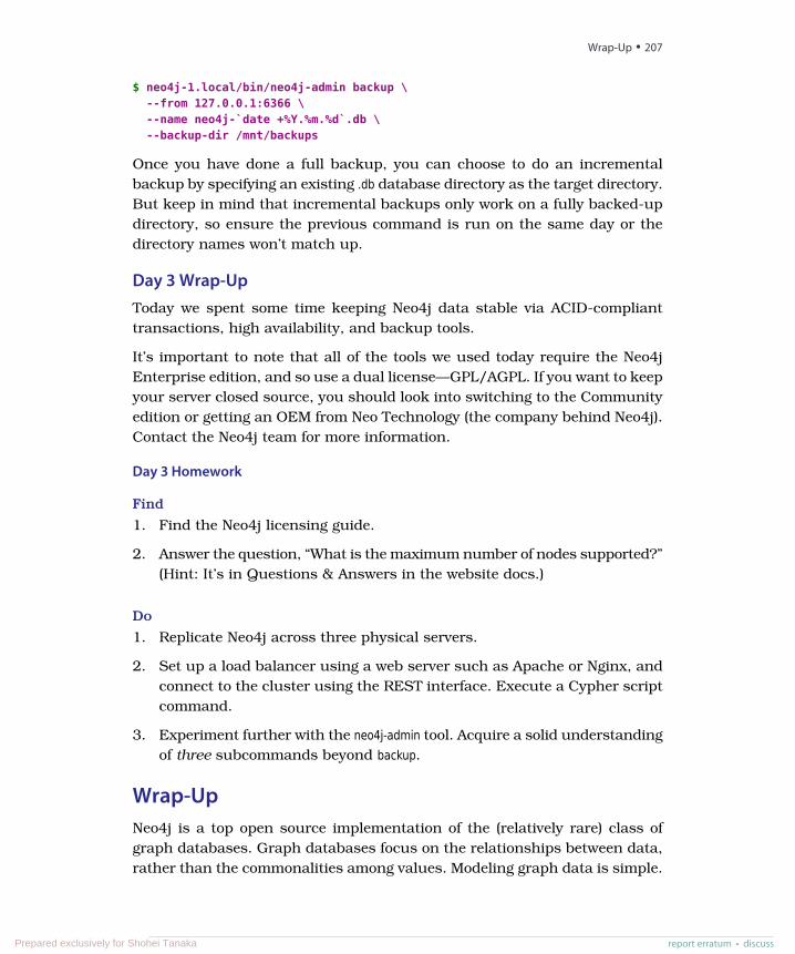
$ neo4j-1.local/bin/neo4j-admin backup \--from 127.0.0.1:6366 \--name neo4j-`date +%Y.%m.%d`.db \--backup-dir /mnt/backups
Once you have done a full backup, you can choose to do an incrementalbackup by specifying an existing .db database directory as the target directory.But keep in mind that incremental backups only work on a fully backed-updirectory, so ensure the previous command is run on the same day or thedirectory names won’t match up.
Day 3 Wrap-UpToday we spent some time keeping Neo4j data stable via ACID-complianttransactions, high availability, and backup tools.
It’s important to note that all of the tools we used today require the Neo4jEnterprise edition, and so use a dual license—GPL/AGPL. If you want to keepyour server closed source, you should look into switching to the Communityedition or getting an OEM from Neo Technology (the company behind Neo4j).Contact the Neo4j team for more information.
Day 3 Homework
Find
1. Find the Neo4j licensing guide.
2. Answer the question, “What is the maximum number of nodes supported?”(Hint: It’s in Questions & Answers in the website docs.)
Do
1. Replicate Neo4j across three physical servers.
2. Set up a load balancer using a web server such as Apache or Nginx, andconnect to the cluster using the REST interface. Execute a Cypher scriptcommand.
3. Experiment further with the neo4j-admin tool. Acquire a solid understandingof three subcommands beyond backup.
Wrap-UpNeo4j is a top open source implementation of the (relatively rare) class ofgraph databases. Graph databases focus on the relationships between data,rather than the commonalities among values. Modeling graph data is simple.
report erratum • discuss
Wrap-Up • 207
Prepared exclusively for Shohei Tanaka
You just create nodes and relationships between them and optionally hangkey-value pairs from them. Querying is as easy as declaring how to walk thegraph from a starting node.
Neo4j’s StrengthsNeo4j is one of the finest examples of open source graph databases. Graphdatabases are perfect for unstructured data, in many ways even more so thandocument databases. Not only is Neo4j typeless and schemaless, but it putsno constraints on how data is related. It is, in the best sense, a free-for-all.Currently, Neo4j can support 34.4 billion nodes and 34.4 billion relationships,which is more than enough for most use cases. (Neo4j could hold more than15 nodes for each of Facebook’s 2.2 billion users in a single graph.)
The Neo4j distributions provide several tools for fast lookups with Lucene,the Cypher querying language, and the REST interface. Beyond ease of use,Neo4j is fast. Unlike join operations in relational databases or map-reduceoperations in other databases, graph traversals are constant time. Like datais only a node step away, rather than joining values in bulk and filtering thedesired results, which is how most of the databases we’ve seen operate. Itdoesn’t matter how large the graph becomes; moving from node A to node Bis always one step if they share a relationship. Finally, the Enterprise editionprovides for highly available and high read-traffic sites by way of Neo4j HA.
Neo4j’s WeaknessesNeo4j does have a few shortcomings. We found its choice of nomenclature(node rather than vertex and relationship rather than edge) to add complexitywhen communicating. Although HA is excellent at replication, it can onlyreplicate a full graph to other servers. It cannot currently shard subgraphs,which still places a limit on graph size (though, to be fair, that limit measuresin the tens of billions). Finally, if you are looking for a business-friendly opensource license (like MIT), Neo4j may not be for you. Although the Communityedition (everything we used in the first two days) is GPL, you’ll probably needto purchase a license if you want to run a production environment using theEnterprise tools (which includes HA and backups).
Neo4j on CAPThe term “high availability cluster" should be enough to give away Neo4j’sstrategy. Neo4j HA is available and partition tolerant (AP). Each slave willreturn only what it currently has, which may be out of sync with the masternode temporarily. Although you can reduce the update latency by increasing
Chapter 6. Neo4J • 208
report erratum • discussPrepared exclusively for Shohei Tanaka
a slave’s pull interval, it’s still technically eventually consistent. This is whyNeo4j HA is recommended for read-mostly requirements.
Parting ThoughtsNeo4j’s simplicity can be off-putting if you’re not used to modeling graph data.It provides a powerful open-source API with years of production use and yetit hasn’t gotten the same traction as other databases in this book. We chalkthis up to lack of knowledge because graph databases mesh so naturally withhow humans tend to conceptualize data. We imagine our families as trees,or our friends as graphs; most of us don’t imagine personal relationships asself-referential datatypes. For certain classes of problems, such as socialnetworks, Neo4j is an obvious choice. But you should give it some seriousconsideration for non-obvious problems as well—it just may surprise youhow powerful and easy it is.
report erratum • discuss
Wrap-Up • 209
Prepared exclusively for Shohei Tanaka
CHAPTER 7
DynamoDBEarth movers are epic pieces of machinery, able to shuffle around massivebits of dirt and other materials with great ease. DynamoDB is a bit like therented earth mover of NoSQL databases. You don’t have to build it yourselfor fix it when it’s broken; you just have to drive it and pay for your usage.But it’s complex to handle so you’ll need to make very intelligent decisionsabout how to use it lest you end up incurring unexpected costs or jammingthe engine.
DynamoDB is a cloud-based database available through Amazon Web Services(AWS), the cloud computing division of e-commerce giant Amazon (the sameAmazon from which you may have purchased this book). You may know AWSas the creator of a dizzying, ever-expanding array of widely used cloud services,from the Simple Storage Service (S3) to the Elastic Compute Cloud (EC2) andfar beyond (there could be over 100 services by the time you read this).
Despite the emergence of serious competitors, such as Microsoft Azure andGoogle Cloud Platform, AWS remains the leader of the Infrastructure-as-a-Service (IaaS) paradigm that has brought cloud computing to the masses,and DynamoDB is AWS’s most significant contribution—thus far—to theworld of NoSQL. The cloud has opened vast new horizons for everyone fromlone-wolf developers to Fortune 500 companies, and any book on the NoSQLparadigm would be incomplete without this pioneering cloud database.
DynamoDB: The “Big Easy” of NoSQLSix out of the seven databases that we cover in this book are easy enough torun on your laptop. But running systems such as HBase, CouchDB, andothers in production—and using them for applications handling massiveworkloads—is a much different matter. Even databases that are a famouslyeasy to operate at smaller scale, such as Redis, present major challenges in
report erratum • discussPrepared exclusively for Shohei Tanaka
production environments, usually requiring skilled (and expensive!) adminsand operations specialists on hand.
DynamoDB is a different story—and an outlier in this book. You don’t haveto install it, start it, or maintain it. You can sign up for an AWS account,create a DynamoDB table, and just go. As you’ll see, DynamoDB does requiresome operations-style thinking and preparation, but you’ll never need toprovide it an XML configuration à la HBase or set up a complex cluster à laMongo. DynamoDB is a database that runs itself and yet is capable of fulfillingsome of your most ambitious “webscale” dreams, offering consistently fastperformance no matter how much data you’re storing.
So just how “webscale” are we talking here? Some facts:
• You can store as many items as you want in any DynamoDB table (moreon tables and items later).
• Each item (the equivalent of a row in an SQL database) can hold as manyattributes as you want, although there is a hard size limit of 400 KB peritem (that limit will likely grow in the future).
• If you get data modeling right, which will occupy a decent chunk of thischapter, you should experience very little performance degradation evenwhen your tables store petabytes of data.
• Over 100,000 AWS customers currently use DynamoDB.
• DynamoDB handles well over a trillion total requests a day (across allAWS customers).
But DynamoDB isn’t interesting just because it’s big and cloud-based andmanaged by experts you don’t have to hire and fire. It’s also a system verymuch worth learning in its own right, providing a familiar yet unique datamodel and an array of features you won’t find in any of the other databasesin this book. While some folks may be reticent to trust a cloud database that’smanaged by someone else, a variety of forward-thinking tech companies,including Airbnb, Adobe, Siemens, and Comcast, have taken the plunge anduse DynamoDB as one of the core databases driving their platforms.
DynamoDB and the (Almost) Ops-Free LifestyleIf you’re running a database yourself or as part of a team, you can expectmany of the following to keep you awake at night: ensuring speedy, predictableperformance; handling unforeseeable hardware outages and network failures;scaling out disk capacity to meet unexpected spikes in demand; and enablingapplication developers to quickly get up and running using your database.
Chapter 7. DynamoDB • 212
report erratum • discussPrepared exclusively for Shohei Tanaka
On top of that, DBAs with a background in NoSQL aren’t exactly a dime adozen, so hiring, training, and scaling out a team of DBAs for Mongo, HBase,or another NoSQL database is nothing to sneeze at. DynamoDB doesn’tcompletely rid your life of these kinds of issues, but if you use it right it cantake an enormous bite out of them.
There are also a number of secondary reasons why you might want to considerDynamoDB:
• You can use it in any of AWS’s many datacenters across the entire globe.As of July 2017, AWS offers DynamoDB in forty-two Availability Zones(AZs) in sixteen geographic regions, with plans to expand into at leasteight more AZs in three additional regions.
• All data in DynamoDB is stored on high-performing Solid State Disks(SSDs) and automatically replicated across multiple availability zoneswithin an AWS region (which guarantees redundancy even within a singleregion).
• You can expect genuine downtime out of DynamoDB only in the rare eventthat an entire AWS datacenter goes down.
Datacenter outages are the Achilles heel of the cloud, and a very real riskthat you should keep in mind. We’ve all experienced Netflix, Instagram, andother widely used services going down for hours at a time due to outages inAmazon’s massive us-east-1 datacenter in Northern Virginia. AWS andDynamoDB aren’t perfect, but their track record is exceedingly good, if notdownright pristine. Using a database like DynamoDB won’t grant you acompletely ops-free lifestyle, but it may just enable you to refocus a hugechunk of your attention and resources onto other things, and for that reasonalone it’s worth a look.
The Core Storage Concepts: Tables, Items, and MoreDynamoDB’s data model is a bit tricky to define using standard “NoSQL”categories. It strongly resembles the data model of a key-value store such asRedis in that it wasn’t really built to provide the rich queryability of an RDBMSsuch as Postgres. Although DynamoDB does have some interesting queryingfeatures, which we’ll learn about shortly, it really soars when you know whatyou’re looking for in advance, which is a hallmark of key-value stores. If you’rebuilding an application that uses DynamoDB, you should always strive toarchitect it so that your data is associated with certain “natural” keys thatallow for easy discoverability—for example, the ability to find user data onthe basis of unique usernames.
report erratum • discuss
DynamoDB: The “Big Easy” of NoSQL • 213
Prepared exclusively for Shohei Tanaka
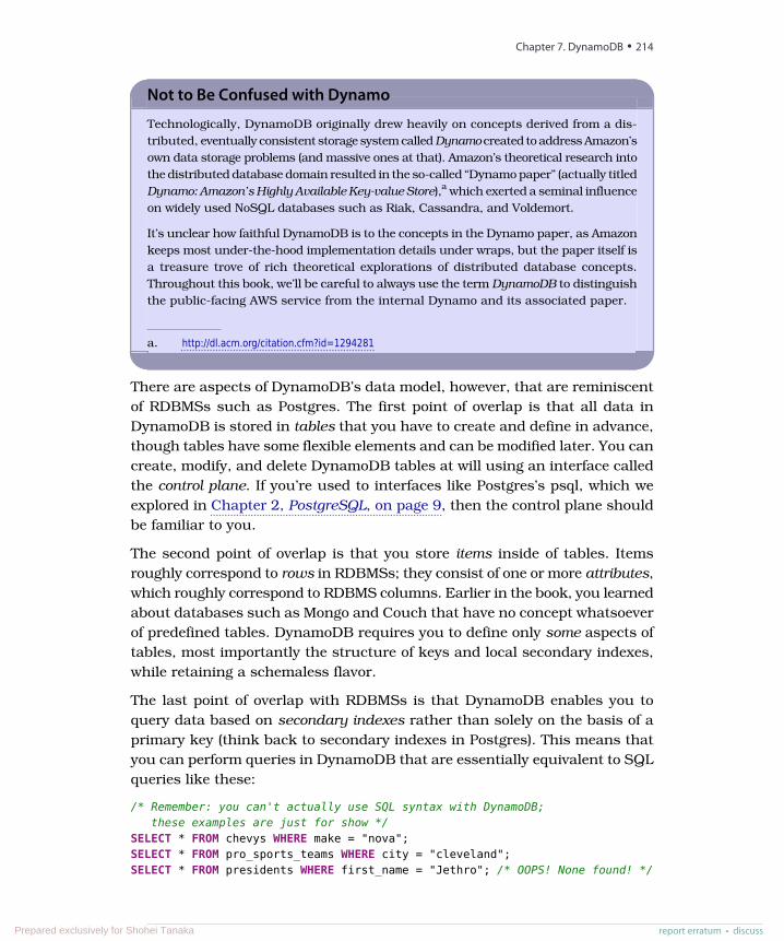
Not to Be Confused with Dynamo
Technologically, DynamoDB originally drew heavily on concepts derived from a dis-tributed, eventually consistent storage system called Dynamo created to address Amazon’sown data storage problems (and massive ones at that). Amazon’s theoretical research intothe distributed database domain resulted in the so-called “Dynamo paper” (actually titledDynamo: Amazon’s Highly Available Key-value Store),a which exerted a seminal influenceon widely used NoSQL databases such as Riak, Cassandra, and Voldemort.
It’s unclear how faithful DynamoDB is to the concepts in the Dynamo paper, as Amazonkeeps most under-the-hood implementation details under wraps, but the paper itself isa treasure trove of rich theoretical explorations of distributed database concepts.Throughout this book, we’ll be careful to always use the term DynamoDB to distinguishthe public-facing AWS service from the internal Dynamo and its associated paper.
a. http://dl.acm.org/citation.cfm?id=1294281
There are aspects of DynamoDB’s data model, however, that are reminiscentof RDBMSs such as Postgres. The first point of overlap is that all data inDynamoDB is stored in tables that you have to create and define in advance,though tables have some flexible elements and can be modified later. You cancreate, modify, and delete DynamoDB tables at will using an interface calledthe control plane. If you’re used to interfaces like Postgres’s psql, which weexplored in Chapter 2, PostgreSQL, on page 9, then the control plane shouldbe familiar to you.
The second point of overlap is that you store items inside of tables. Itemsroughly correspond to rows in RDBMSs; they consist of one or more attributes,which roughly correspond to RDBMS columns. Earlier in the book, you learnedabout databases such as Mongo and Couch that have no concept whatsoeverof predefined tables. DynamoDB requires you to define only some aspects oftables, most importantly the structure of keys and local secondary indexes,while retaining a schemaless flavor.
The last point of overlap with RDBMSs is that DynamoDB enables you toquery data based on secondary indexes rather than solely on the basis of aprimary key (think back to secondary indexes in Postgres). This means thatyou can perform queries in DynamoDB that are essentially equivalent to SQLqueries like these:
/* Remember: you can't actually use SQL syntax with DynamoDB;these examples are just for show */
SELECT * FROM chevys WHERE make = "nova";SELECT * FROM pro_sports_teams WHERE city = "cleveland";SELECT * FROM presidents WHERE first_name = "Jethro"; /* OOPS! None found! */
Chapter 7. DynamoDB • 214
report erratum • discussPrepared exclusively for Shohei Tanaka
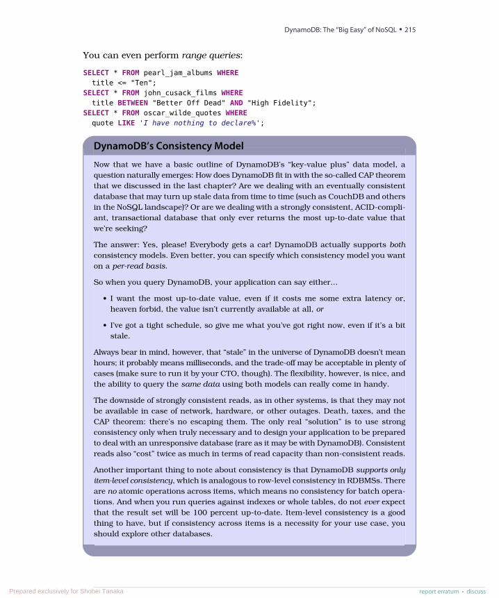
You can even perform range queries:
SELECT * FROM pearl_jam_albums WHEREtitle <= "Ten";
SELECT * FROM john_cusack_films WHEREtitle BETWEEN "Better Off Dead" AND "High Fidelity";
SELECT * FROM oscar_wilde_quotes WHEREquote LIKE 'I have nothing to declare%';
DynamoDB’s Consistency Model
Now that we have a basic outline of DynamoDB’s “key-value plus” data model, aquestion naturally emerges: How does DynamoDB fit in with the so-called CAP theoremthat we discussed in the last chapter? Are we dealing with an eventually consistentdatabase that may turn up stale data from time to time (such as CouchDB and othersin the NoSQL landscape)? Or are we dealing with a strongly consistent, ACID-compli-ant, transactional database that only ever returns the most up-to-date value thatwe’re seeking?
The answer: Yes, please! Everybody gets a car! DynamoDB actually supports bothconsistency models. Even better, you can specify which consistency model you wanton a per-read basis.
So when you query DynamoDB, your application can say either...
• I want the most up-to-date value, even if it costs me some extra latency or,heaven forbid, the value isn’t currently available at all, or
• I’ve got a tight schedule, so give me what you’ve got right now, even if it’s a bitstale.
Always bear in mind, however, that “stale” in the universe of DynamoDB doesn’t meanhours; it probably means milliseconds, and the trade-off may be acceptable in plenty ofcases (make sure to run it by your CTO, though). The flexibility, however, is nice, andthe ability to query the same data using both models can really come in handy.
The downside of strongly consistent reads, as in other systems, is that they may notbe available in case of network, hardware, or other outages. Death, taxes, and theCAP theorem: there’s no escaping them. The only real “solution” is to use strongconsistency only when truly necessary and to design your application to be preparedto deal with an unresponsive database (rare as it may be with DynamoDB). Consistentreads also “cost” twice as much in terms of read capacity than non-consistent reads.
Another important thing to note about consistency is that DynamoDB supports onlyitem-level consistency, which is analogous to row-level consistency in RDBMSs. Thereare no atomic operations across items, which means no consistency for batch opera-tions. And when you run queries against indexes or whole tables, do not ever expectthat the result set will be 100 percent up-to-date. Item-level consistency is a goodthing to have, but if consistency across items is a necessity for your use case, youshould explore other databases.
report erratum • discuss
DynamoDB: The “Big Easy” of NoSQL • 215
Prepared exclusively for Shohei Tanaka
As you can see, these kinds of querying capabilities take DynamoDB beyondwhat you’d find in a more straightforward key-value store (like the one you’llsee in the next chapter, on Redis). So we’ll call DynamoDB’s data model key-value plus for short to account for these borrowings from the relationalparadigm.
In spite of these SQL-flavored capabilities, though, there are firm limits tothe DynamoDB/RDBMS parallels. Most importantly, if you need queryingcapabilities that go beyond the simple ones in the previous example, you’llhave to implement them on the application side, or just use a differentdatabase (or use other cloud services in conjunction with DynamoDB, as we’lldo on Day 3). Furthermore, DynamoDB has no concept of things like joinsbetween tables; the table is the highest level at which data can be groupedand manipulated, and any join-style capabilities that you need will have tobe implemented on the application side, which has its own downsides.
So that provides a little bit of background, historical and technological, forDynamoDB. It’s time to dig much deeper using real interactions with thedatabase.
Day 1: Let’s Go Shopping!Fun fact: Dynamo—the database that inspired the later DynamoDB—wasoriginally built with the very specific purpose of serving as the storage systemfor Amazon’s famous shopping cart. When you’re building a shopping cartapplication, the absolute, unbreakable categorical imperative guiding yourdatabase should be this: do not lose data under any circumstances. Losingshopping cart data means losing money directly. If a user puts a $2,500mattress in their Amazon shopping cart and the database suddenly forgetsthat, then that’s money potentially lost, especially if the data is lost just beforecheckout.
Multiply a mistake like that times thousands or even millions and you get aclear sense of why Amazon needed to build a fault-tolerant, highly availabledatabase that never loses data. The good news is that you get to reap thebenefits of Amazon’s efforts and use DynamoDB to your own ends in yourown applications.
As a first practical taste of DynamoDB, we’ll set up a DynamoDB table thatcould act as the database for a simple shopping cart application. This tablewill be able to store shopping cart items (it looks like Amazon’s use of the“item” terminology was no accident). We’ll perform basic CRUD operationsagainst this table via the command line.
Chapter 7. DynamoDB • 216
report erratum • discussPrepared exclusively for Shohei Tanaka
But first, a stern warning: DynamoDB is not free! It is a paid service. AWSoffers a free tier for virtually all of its services so that you can kick the tireswithout immediately incurring costs, but make sure to check the pricingguide1 before you start going through the examples in this book. We won’tmake super intensive use of AWS services, so it should cost you at most afew dollars, but due diligence may just save you from an unpleasant end-of-the-month surprise.
Before you can get started with this section, you’ll need to create an AWSaccount for yourself using the AWS console.2 That part is pretty self-explanatory. Don’t worry about familiarizing yourself with the AWS consolefor now, as most of the examples in this chapter will use the command line.Once you’ve signed up with AWS and can access your user console (whichshows you all of AWS’s currently available services on the landing page),download the official AWS CLI tool using pip, the Python package manager:
$ sudo pip install aws
If you run aws --version and get a version string like aws-cli/1.11.51 Python/2.7.10Darwin/16.1.0 botocore/1.5.14, you should be ready to go. All of the aws tool’s com-mands are of the form aws [service] [command], where service can be dynamodb, s3,ec2, and so on. To see the commands and options available for DynamoDBspecifically, run aws dynamodb help.
Once the CLI tool is installed, you’ll need to configure it by running the following:
$ aws configure
Running DynamoDB Locally
If you ever decide to develop a full-fledged application of your own using DynamoDB,you might want to check out DynamoDB Local,a which is a version of DynamoDBthat you can run on your own machine that’s fully API compatible with hostedDynamoDB. It’s available as a Java JAR and works on Windows, Mac OS, and Linux.
We won’t use DynamoDB Local for the exercises here because we’ll need to use thehosted version in conjunction with other AWS services, but it’s a very nice thing tohave in your development toolbelt.
a. https://aws.amazon.com/blogs/aws/dynamodb-local-for-desktop-development
1. https://aws.amazon.com/pricing2. https://console.aws.amazon.com
report erratum • discuss
Day 1: Let’s Go Shopping! • 217
Prepared exclusively for Shohei Tanaka
That will prompt you to input the AWS access key ID and secret access keyfor your account and enable you to choose a default AWS region when usingthe tool (us-east-1 is the default) and output format for CLI commands (json isthe default).
The DynamoDB control plane is the set of commands used to manage tables.Our first action using the control plane will be to see which tables are associ-ated with our account:
$ aws dynamodb list-tables{
"TableNames": []}
As expected, there are no tables associated with our account, so let’s makea very simple shopping cart table in which each item has just one attribute:an item name stored as a string.
$ aws dynamodb create-table \--table-name ShoppingCart \--attribute-definitions AttributeName=ItemName,AttributeType=S \--key-schema AttributeName=ItemName,KeyType=HASH \--provisioned-throughput ReadCapacityUnits=1,WriteCapacityUnits=1
DynamoDB’s Almost Schemaless Data Model
In the create-table operation, it seems like the ShoppingCart table is being created with astrict schema according to which items in the table can have only an ItemName attribute.But DynamoDB doesn’t work that way. Whenever you create a table, you only haveto define attributes that function as keys (sometimes referred to as key attributes).
So we could store items in our shopping cart table that have any number of otherproperties (brand name, year manufactured, ISBN, whatever) if we wanted to, withouthaving to specify those attributes when we create the table. The only restriction onour ShoppingCart table is that each item must have an ItemName.
But there’s a catch here: although schema restraints apply only to key attributes, youcan’t query for attributes that aren’t specified as keys or indexes when you create thetable (more on indexes later). So if you started storing items with a brand name attributein the ShoppingCart table, you wouldn’t be able to discover items by brand name. If youwanted to do that, you’d have to create a new table and add the brand name as a keyor index. And so even though schema design doesn’t force you into a straitjacket, youshould make that decision very carefully.
This is in contrast to a database like Mongo, which is schemaless but allows you toquery for whatever fields you want at any time.
Chapter 7. DynamoDB • 218
report erratum • discussPrepared exclusively for Shohei Tanaka
The output of that command should be a JSON object describing our newlycreated table:
{"TableDescription": {
"TableArn": "arn:aws:dynamodb:...:table/ShoppingCart","AttributeDefinitions": [
{"AttributeName": "ItemName","AttributeType": "S"
}],"ProvisionedThroughput": {
"NumberOfDecreasesToday": 0,"WriteCapacityUnits": 1,"ReadCapacityUnits": 1
},"TableSizeBytes": 0,
"TableName": "ShoppingCart","TableStatus": "CREATING","KeySchema": [
{"KeyType": "HASH","AttributeName": "ItemName"
}],"ItemCount": 0,"CreationDateTime": 1475032237.808
}}
We could get that same output using the describe-table command at any time(except that the TableStatus parameter will change to ACTIVE very quickly aftercreation):
$ aws dynamodb describe-table \--table-name ShoppingCart
So now we’ve reserved a little nook and cranny in an AWS datacenter to holdour shopping cart data. But that create-table command is probably still a bitcryptic because there are some core concepts we haven’t gone over yet. Let’sstart with supported data types.
DynamoDB’s Data TypesDynamoDB’s type system is, in essence, a stripped-down version of the typesystem that you’d find in a relational database. DynamoDB offers simpletypes such as Booleans, strings, and binary strings, but none of the morepurpose-specific types that you’d find in, say, Postgres (such as currency
report erratum • discuss
Day 1: Let’s Go Shopping! • 219
Prepared exclusively for Shohei Tanaka
values or geometric types). DynamoDB offers these five scalar types, whichcan be thought of as its atomic types:
JSON ExampleDescriptionSymbol Type
"S": "this is a string"A typical string like you’d find inmost programming languages.
SString
"N": "98", "N":"3.141592"Any integer or float. Sent as astring for the sake of compatibilitybetween client libraries.
NNumber
"B": "4SrNYKrcv4wjJczEf6u+TgaT2YaWGgU76YPhF"
Base64-encoded binary data ofany length (within item size limits).
BBinary
"BOOL": falsetrue or false.BOOLBoolean
"NULL": trueA null value. Useful for missingvalues.
NULLNull
Warning! No Empty Strings
String values cannot be empty in DynamoDB. You must provide some kind of place-holder when using strings, perhaps something like "nil" or "empty". This is frankly oneof the oddest things about DynamoDB and something to always bear in mind whenbuilding applications using it.
In addition to the scalar types, DynamoDB also supports a handful of settypes and document types (list and map):
JSON ExampleDescriptionSymbol Type
"SS": ["Larry", "Moe"]A set of strings.SSString set
"NS": ["42", "137"]A set of numbers.NSNumber set
"BS": ["TGFycnkK","TW9lCg=="]
A set of binary strings.BSBinary set
"L": [{"S": "totchos"},{"N": "741"}]
A list that can consist of data ofany scalar type, like a JSON array. You can mix scalar types as well.
LList
"M": {"FavoriteBook":{"S": "Old Yeller"}}
A key-value structure with stringsas keys and values of any type,including sets, lists, and maps.
MMap
Chapter 7. DynamoDB • 220
report erratum • discussPrepared exclusively for Shohei Tanaka
Set types act just like sets in most programming languages. All items in a setmust be unique, which means that attempting to add the string "totchos" to astring set that already included it would result in no change to the set.
JSON in DynamoDB
And last but certainly not least, DynamoDB also allows you to store any valid JSONas an item attribute. So if your application’s data model uses data types that areJSON serializable/deserializable, then you can store those types directly rather thanwrangling them into the supported types you just saw. Keep two things in mind,though: Individual items can’t be larger than 400 KB, so don’t go too crazy usingDynamoDB as a store for large JSON objects or BLOBs; and you can’t query insideof JSON objects (your application will need to supply that logic).
DynamoDB’s set of supported data types is fairly limited compared to what you wouldfind in an RDBMS such as Postgres but quite rich in comparison with something likeHBase, which only holds binary data and makes the application responsible for allserialization and deserialization.
Here’s an example put operation that uses JSON:
$ aws dynamodb put-item --table-name Books \--item '{"Title": {"S": "Moby Dick"},"PublishYear": {"N": "2012"},"ISBN": {"N": "98765"},"PublisherInfo": {
"Name": "Something"}
}'
Basic Read/Write OperationsNow that you have a better sense of what actually goes on in tables and insideof items, you can begin actually working with data. Let’s add a few items toour shopping cart using the put-item command:
$ aws dynamodb put-item --table-name ShoppingCart \--item '{"ItemName": {"S": "Tickle Me Elmo"}}'
$ aws dynamodb put-item --table-name ShoppingCart \--item '{"ItemName": {"S": "1975 Buick LeSabre"}}'
$ aws dynamodb put-item --table-name ShoppingCart \--item '{"ItemName": {"S": "Ken Burns: the Complete Box Set"}}'
As you can see, when we need to add data using the command line we needto send it across the wire as JSON. We now have three items in our shopping
report erratum • discuss
Day 1: Let’s Go Shopping! • 221
Prepared exclusively for Shohei Tanaka
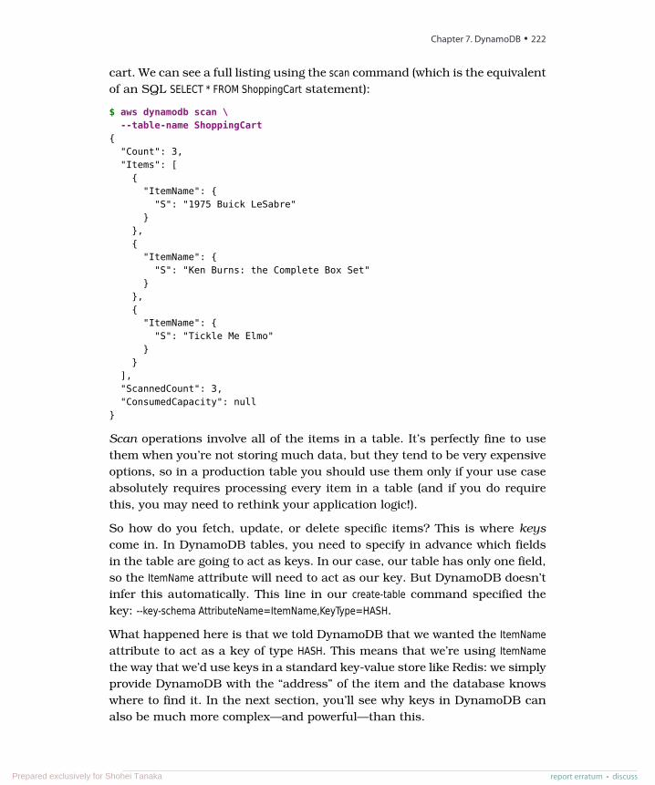
cart. We can see a full listing using the scan command (which is the equivalentof an SQL SELECT * FROM ShoppingCart statement):
$ aws dynamodb scan \--table-name ShoppingCart
{"Count": 3,"Items": [
{"ItemName": {
"S": "1975 Buick LeSabre"}
},{"ItemName": {
"S": "Ken Burns: the Complete Box Set"}
},{"ItemName": {
"S": "Tickle Me Elmo"}
}],"ScannedCount": 3,"ConsumedCapacity": null
}
Scan operations involve all of the items in a table. It’s perfectly fine to usethem when you’re not storing much data, but they tend to be very expensiveoptions, so in a production table you should use them only if your use caseabsolutely requires processing every item in a table (and if you do requirethis, you may need to rethink your application logic!).
So how do you fetch, update, or delete specific items? This is where keyscome in. In DynamoDB tables, you need to specify in advance which fieldsin the table are going to act as keys. In our case, our table has only one field,so the ItemName attribute will need to act as our key. But DynamoDB doesn’tinfer this automatically. This line in our create-table command specified thekey: --key-schema AttributeName=ItemName,KeyType=HASH.
What happened here is that we told DynamoDB that we wanted the ItemNameattribute to act as a key of type HASH. This means that we’re using ItemNamethe way that we’d use keys in a standard key-value store like Redis: we simplyprovide DynamoDB with the “address” of the item and the database knowswhere to find it. In the next section, you’ll see why keys in DynamoDB canalso be much more complex—and powerful—than this.
Chapter 7. DynamoDB • 222
report erratum • discussPrepared exclusively for Shohei Tanaka
For now, we can fetch specific items from our shopping cart, by key, usingthe --key flag:
$ aws dynamodb get-item --table-name ShoppingCart \--key '{"ItemName": {"S": "Tickle Me Elmo"}}'
{"Item": {
"ItemName": {"S": "Tickle Me Elmo"
}}
}
As discussed in the intro to this chapter, DynamoDB enables you to specifywhether or not you want to perform a consistent read on every request usingthe --consistent-read flag when you make a get-item request. This GET requestwould guarantee item-level consistency:
$ aws dynamodb get-item --table-name ShoppingCart \--key '{"ItemName": {"S": "Tickle Me Elmo"}}' \--consistent-read
But let’s be honest: Tickle Me Elmo isn’t exactly all the rage these days solet’s eliminate that from our cart (though we may regret it if Tickle Me Elmosexperience a spike in resale value). We can do that on the basis of the hashkey as well:
$ aws dynamodb delete-item --table-name ShoppingCart \--key '{"ItemName": {"S": "Tickle Me Elmo"}}'
If we run the same scan operation as before, the Count field in the returnedJSON will indicate that we now only have two items in our shopping cart.
Two Key Types, Many PossibilitiesDynamoDB is, at root, a key-value store. But it’s a special key-value store inthat it provides two types of key that you can choose on a table-by-table basis.You can use either a hash key (aka partition key) by itself or you can use acomposite key that combines a hash key and a range key (aka sort key), asshown in the figure on page 224.
A hash key can be used to find items the same way you perform lookups inkey-value databases such as HBase and Redis. You provide DynamoDB witha key and it checks the table to see if there’s an item associated with the key.Imagine fetching information about NFL teams that have won the Super Bowlusing the year as the hash key. Or imagine retrieving information about an
report erratum • discuss
Day 1: Let’s Go Shopping! • 223
Prepared exclusively for Shohei Tanaka
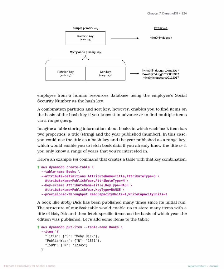
employee from a human resources database using the employee’s SocialSecurity Number as the hash key.
A combination partition and sort key, however, enables you to find items onthe basis of the hash key if you know it in advance or to find multiple itemsvia a range query.
Imagine a table storing information about books in which each book item hastwo properties: a title (string) and the year published (number). In this case,you could use the title as a hash key and the year published as a range key,which would enable you to fetch book data if you already know the title or ifyou only know a range of years that you’re interested in.
Here’s an example aws command that creates a table with that key combination:
$ aws dynamodb create-table \--table-name Books \--attribute-definitions AttributeName=Title,AttributeType=S \
AttributeName=PublishYear,AttributeType=N \--key-schema AttributeName=Title,KeyType=HASH \
AttributeName=PublishYear,KeyType=RANGE \--provisioned-throughput ReadCapacityUnits=1,WriteCapacityUnits=1
A book like Moby Dick has been published many times since its initial run.The structure of our Book table would enable us to store many items with atitle of Moby Dick and then fetch specific items on the basis of which year theedition was published. Let’s add some items to the table:
$ aws dynamodb put-item --table-name Books \--item '{
"Title": {"S": "Moby Dick"},"PublishYear": {"N": "1851"},"ISBN": {"N": "12345"}
}'
Chapter 7. DynamoDB • 224
report erratum • discussPrepared exclusively for Shohei Tanaka
$ aws dynamodb put-item --table-name Books \--item '{
"Title": {"S": "Moby Dick"},"PublishYear": {"N": "1971"},"ISBN": {"N": "23456"},"Note": {"S": "Out of print"}
}'$ aws dynamodb put-item --table-name Books \
--item '{"Title": {"S": "Moby Dick"},"PublishYear": {"N": "2008"},"ISBN": {"N": "34567"}
}'
You may have noticed that we supplied an ISBN attribute for each item withoutspecifying that in the table definition. That’s okay because remember that weonly need to specify key attributes when creating tables. This gives DynamoDBits relative schemalessness, which you can also see at work in the seconditem we created, which has a Note attribute while the others do not.
To see which books were published after the year 1980, for example, we coulduse a range query:
$ aws dynamodb query --table-name Books \--expression-attribute-values '{
":title": {"S": "Moby Dick"},":year": {"N": "1980"}
}' \--key-condition-expression 'Title = :title AND PublishYear > :year'
{"Count": 1,"Items": [
{"PublishYear": {
"N": "2008"},"ISBN": {
"N": "34567"},"Title": {
"S": "Moby Dick"}
}],"ScannedCount": 1,"ConsumedCapacity": null
}
With the query command, the --expression-attribute-values flag enables us to providevalues for variables that we want to use as JSON. The --key-condition-expression
report erratum • discuss
Day 1: Let’s Go Shopping! • 225
Prepared exclusively for Shohei Tanaka
flag enables us to provide an actual query string strongly reminiscent of SQL,in this case Title = :title AND PublishYear > :year (which becomes Title = "Moby Dick" ANDPublishYear > 1900 via interpolation).
If you’ve used a SQL driver for a specific programming language, then you’veprobably constructed parameterized queries like this. As output, we got oneof three books currently in the Books table, as expected.
Whenever you provide key condition expressions, you must match directlyon the hash key (in this case Title = :title) and then you can optionally providea query for the range key using one of these operators: =, >, <, >=, <=, BETWEEN,or begins_with. A BETWEEN a AND b expression is the direct equivalent of >= a AND<= b and begins_with enables you to create an expression like begins_with(Title, :str)where :str could be a string.
But what if we wanted our result set to include only, say, ISBN data? Afterall, we know that all the books are titled Moby Dick, so we may not need thatas part of our result set. We can tailor that result set using attribute projection.On the command line, you can perform attribute projection using the --projection-expression flag, which enables you to specify a list of attributes that you wantreturned for each item. This query would return only the ISBN for each editionof Moby Dick published after 1900:
$ aws dynamodb query --table-name Books \--expression-attribute-values \
'{":title": {"S": "Moby Dick"},":year": {"N": "1900"}}' \--key-condition-expression \
'Title = :title AND PublishYear > :year' \--projection-expression 'ISBN'
{"Count": 2,"Items": [
{"ISBN": {
"N": "23456"}
},{
"ISBN": {"N": "34567"
}}
],"ScannedCount": 2,"ConsumedCapacity": null
}
Chapter 7. DynamoDB • 226
report erratum • discussPrepared exclusively for Shohei Tanaka
If the attribute isn’t defined for a specific item, then an empty object will bereturned. Remember that only one of our book items has a Note attribute.Here’s the result set when projecting for that attribute:
$ aws dynamodb query --table-name Books \--expression-attribute-values \
'{":title": {"S": "Moby Dick"},":year": {"N": "1900"}}' \--key-condition-expression \
'Title = :title AND PublishYear > :year' \--projection-expression 'Note'
{"Count": 2,"Items": [
{"Note": {
"S": "Out of print"}
},{}
],"ScannedCount": 2,"ConsumedCapacity": null
}
Note the empty object, {}, returned for one of the Items.
As you can see in this section, choosing the right key setup for any DynamoDBtable is extremely important because that will determine how your applicationis able to discover the items it’s looking for. A good rule of thumb is this: Ifyour application is built to know in advance where an item lives, then usejust a hash key. An example here would be a user info database where youfind items based on usernames already known to the application.
Spreading the Data Around: Partitioning in DynamoDBBehind the scenes, DynamoDB’s system for distributing item data acrossservers—partitions in DynamoDB parlance—is likely very complex. But fromyour perspective as a user it’s really fairly simple. You can see a basic visualillustration of data partitioning in the figure on page 228.
When you start writing data to a DynamoDB table, it begins filling in a firstpartition (partition 1 in the diagram). Eventually, that partition will fill upand data will start being distributed to partition 2, then at some point topartition 3, and so on out to N partitions. That N can be pretty much as largeas you want; AWS provides no guidelines for limits to the number of partitions.The logic will simply repeat itself until you stop feeding data to the table.
report erratum • discuss
Day 1: Let’s Go Shopping! • 227
Prepared exclusively for Shohei Tanaka
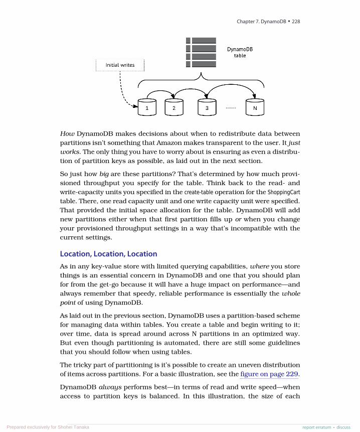
How DynamoDB makes decisions about when to redistribute data betweenpartitions isn’t something that Amazon makes transparent to the user. It justworks. The only thing you have to worry about is ensuring as even a distribu-tion of partition keys as possible, as laid out in the next section.
So just how big are these partitions? That’s determined by how much provi-sioned throughput you specify for the table. Think back to the read- andwrite-capacity units you specified in the create-table operation for the ShoppingCarttable. There, one read capacity unit and one write capacity unit were specified.That provided the initial space allocation for the table. DynamoDB will addnew partitions either when that first partition fills up or when you changeyour provisioned throughput settings in a way that’s incompatible with thecurrent settings.
Location, Location, LocationAs in any key-value store with limited querying capabilities, where you storethings is an essential concern in DynamoDB and one that you should planfor from the get-go because it will have a huge impact on performance—andalways remember that speedy, reliable performance is essentially the wholepoint of using DynamoDB.
As laid out in the previous section, DynamoDB uses a partition-based schemefor managing data within tables. You create a table and begin writing to it;over time, data is spread around across N partitions in an optimized way.But even though partitioning is automated, there are still some guidelinesthat you should follow when using tables.
The tricky part of partitioning is it’s possible to create an uneven distributionof items across partitions. For a basic illustration, see the figure on page 229.
DynamoDB always performs best—in terms of read and write speed—whenaccess to partition keys is balanced. In this illustration, the size of each
Chapter 7. DynamoDB • 228
report erratum • discussPrepared exclusively for Shohei Tanaka
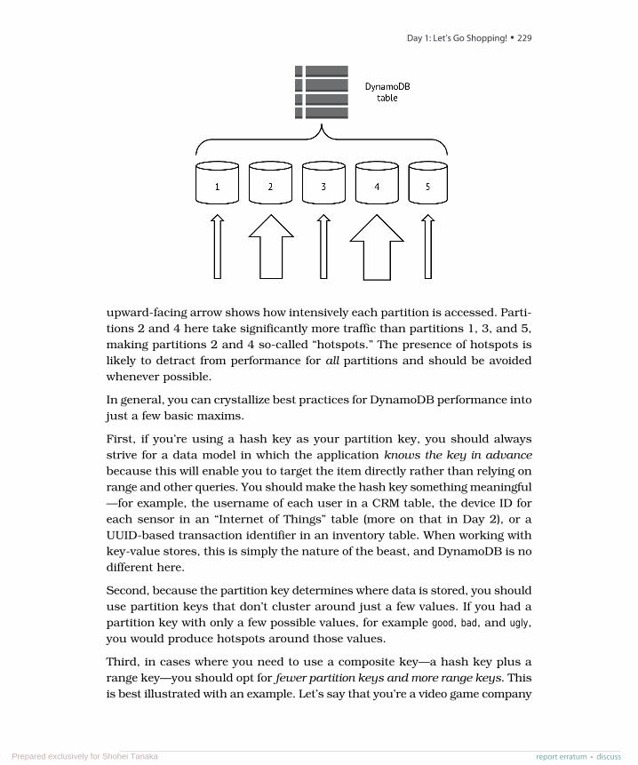
upward-facing arrow shows how intensively each partition is accessed. Parti-tions 2 and 4 here take significantly more traffic than partitions 1, 3, and 5,making partitions 2 and 4 so-called “hotspots.” The presence of hotspots islikely to detract from performance for all partitions and should be avoidedwhenever possible.
In general, you can crystallize best practices for DynamoDB performance intojust a few basic maxims.
First, if you’re using a hash key as your partition key, you should alwaysstrive for a data model in which the application knows the key in advancebecause this will enable you to target the item directly rather than relying onrange and other queries. You should make the hash key something meaningful—for example, the username of each user in a CRM table, the device ID foreach sensor in an “Internet of Things” table (more on that in Day 2), or aUUID-based transaction identifier in an inventory table. When working withkey-value stores, this is simply the nature of the beast, and DynamoDB is nodifferent here.
Second, because the partition key determines where data is stored, you shoulduse partition keys that don’t cluster around just a few values. If you had apartition key with only a few possible values, for example good, bad, and ugly,you would produce hotspots around those values.
Third, in cases where you need to use a composite key—a hash key plus arange key—you should opt for fewer partition keys and more range keys. Thisis best illustrated with an example. Let’s say that you’re a video game company
report erratum • discuss
Day 1: Let’s Go Shopping! • 229
Prepared exclusively for Shohei Tanaka
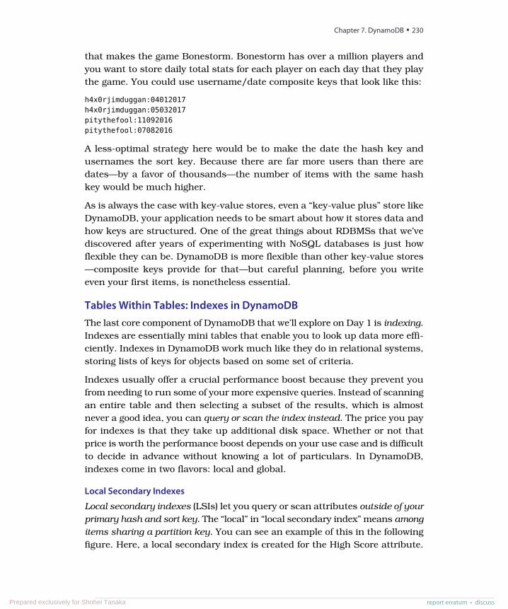
that makes the game Bonestorm. Bonestorm has over a million players andyou want to store daily total stats for each player on each day that they playthe game. You could use username/date composite keys that look like this:
h4x0rjimduggan:04012017h4x0rjimduggan:05032017pitythefool:11092016pitythefool:07082016
A less-optimal strategy here would be to make the date the hash key andusernames the sort key. Because there are far more users than there aredates—by a favor of thousands—the number of items with the same hashkey would be much higher.
As is always the case with key-value stores, even a “key-value plus” store likeDynamoDB, your application needs to be smart about how it stores data andhow keys are structured. One of the great things about RDBMSs that we’vediscovered after years of experimenting with NoSQL databases is just howflexible they can be. DynamoDB is more flexible than other key-value stores—composite keys provide for that—but careful planning, before you writeeven your first items, is nonetheless essential.
Tables Within Tables: Indexes in DynamoDBThe last core component of DynamoDB that we’ll explore on Day 1 is indexing.Indexes are essentially mini tables that enable you to look up data more effi-ciently. Indexes in DynamoDB work much like they do in relational systems,storing lists of keys for objects based on some set of criteria.
Indexes usually offer a crucial performance boost because they prevent youfrom needing to run some of your more expensive queries. Instead of scanningan entire table and then selecting a subset of the results, which is almostnever a good idea, you can query or scan the index instead. The price you payfor indexes is that they take up additional disk space. Whether or not thatprice is worth the performance boost depends on your use case and is difficultto decide in advance without knowing a lot of particulars. In DynamoDB,indexes come in two flavors: local and global.
Local Secondary Indexes
Local secondary indexes (LSIs) let you query or scan attributes outside of yourprimary hash and sort key. The “local” in “local secondary index” means amongitems sharing a partition key. You can see an example of this in the followingfigure. Here, a local secondary index is created for the High Score attribute.
Chapter 7. DynamoDB • 230
report erratum • discussPrepared exclusively for Shohei Tanaka

The LSI on the High Score attribute here means that we can perform scans orqueries related to high scores for a specific user.
Here’s an example range query for the HighScore attribute that shows all of thedates on which the player h4x0rjimduggan scored over 800 points:
$ aws dynamodb query --table-name BonestormData \--expression-attribute-values \
'{":user": {"S": "h4x0rjimduggan"},":score": {"N": "800"}}' \--key-condition-expression \
'Username = :user AND HighScore > :score' \--projection-expression 'Date'
Always bear in mind that LSIs can’t be modified after a table has been created,so be extra careful to plan for them in advance (or, even better, thoroughlytest different indexing models in development).
Global Secondary Indexes
Global secondary indexes (GSIs) are indexes that aren’t restricted to itemswith the same partition key. The “global” here essentially means “any attributein the table.” See the figure on page 232 for an example. You can find anyitems in the table using the Avatar attribute.
Here’s an example query that finds all items for which the Avatar field equalsLion and returns the Username and Date for each of those items:
$ aws dynamodb query --table-name BonestormData \--expression-attribute-values \
'{":avatar": {"S": "Lion"}}' \--key-condition-expression \
'Avatar = :avatar' \--projection-expression 'Username, Date'
report erratum • discuss
Day 1: Let’s Go Shopping! • 231
Prepared exclusively for Shohei Tanaka
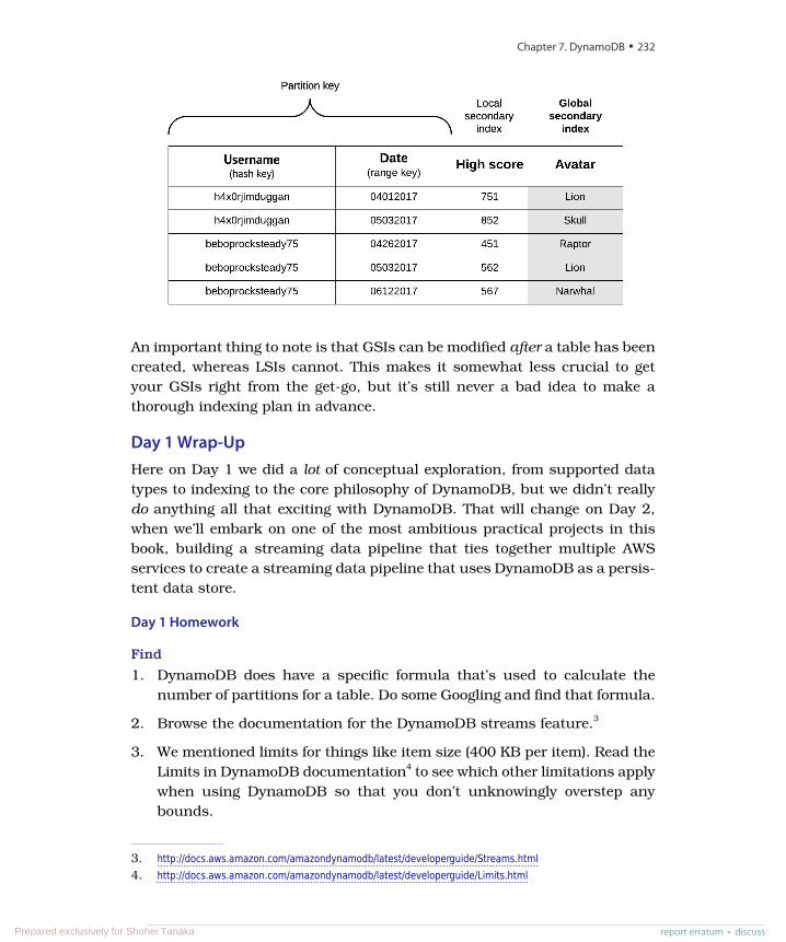
An important thing to note is that GSIs can be modified after a table has beencreated, whereas LSIs cannot. This makes it somewhat less crucial to getyour GSIs right from the get-go, but it’s still never a bad idea to make athorough indexing plan in advance.
Day 1 Wrap-UpHere on Day 1 we did a lot of conceptual exploration, from supported datatypes to indexing to the core philosophy of DynamoDB, but we didn’t reallydo anything all that exciting with DynamoDB. That will change on Day 2,when we’ll embark on one of the most ambitious practical projects in thisbook, building a streaming data pipeline that ties together multiple AWSservices to create a streaming data pipeline that uses DynamoDB as a persis-tent data store.
Day 1 Homework
Find
1. DynamoDB does have a specific formula that’s used to calculate thenumber of partitions for a table. Do some Googling and find that formula.
2. Browse the documentation for the DynamoDB streams feature.3
3. We mentioned limits for things like item size (400 KB per item). Read theLimits in DynamoDB documentation4 to see which other limitations applywhen using DynamoDB so that you don’t unknowingly overstep anybounds.
3. http://docs.aws.amazon.com/amazondynamodb/latest/developerguide/Streams.html4. http://docs.aws.amazon.com/amazondynamodb/latest/developerguide/Limits.html
Chapter 7. DynamoDB • 232
report erratum • discussPrepared exclusively for Shohei Tanaka
Do
1. Using the formula you found for calculating the number of partitions usedfor a table, calculate how many partitions would be used for a tableholding 100 GB of data and assigned 2000 RCUs and 3000 WCUs.
2. If you were storing tweets in DynamoDB, how would you do so usingDynamoDB’s supported data types?
3. In addition to PutItem operations, DynamoDB also offers update item opera-tions that enable you to modify an item if a conditional expression is satis-fied. Take a look at the documentation for conditional expressions5 andperform a conditional update operation on an item in the ShoppingCart table.
Day 2: Building a Streaming Data PipelineOn Day 1, we made some solid progress on understanding the core conceptsof DynamoDB, from how DynamoDB partitions data to the data types that itsupports to secondary indexes. We worked through some simple table man-agement commands and some basic CRUD operations on that table to seethe concepts in action.
We were exposed to some features that set DynamoDB apart from other, morestrict key-value stores, but those features are mostly garnishes. The maindish is DynamoDB’s unique blend of extreme scalability, predictably solidperformance as you scale out, and freedom from operational burdens.
On Day 2, we’ll build something that can take full advantage of those featuresin a way that we couldn’t in our Day 1 CRUD exercises. We’ll build astreaming data pipeline that pumps sensor data into DynamoDB (we’ll use aRuby script to act as mock sensors). Those mock sensors will populate ourtable with three pieces of data per “reading”:
• An identifier for the sensor—for example, sensor-1 or temp-a1b2c3• A timestamp for the reading in Unix time (this will allow for easier sorting)• The current temperature picked up by the sensor—for example, 81.4 or 73.2
But instead of writing to DynamoDB directly, we’ll use a streaming data servicecalled Kinesis that’s built for handling massive write throughput; messagespassing through Kinesis will be written to DynamoDB using functions deployedto AWS’s Lambda service.
It may seem a bit odd to focus on connecting AWS services in a chapterdevoted to DynamoDB. But it’s important to note that cloud databases are
5. http://docs.aws.amazon.com/amazondynamodb/latest/developerguide/Expressions.ConditionExpressions.html
report erratum • discuss
Day 2: Building a Streaming Data Pipeline • 233
Prepared exclusively for Shohei Tanaka
rarely used as standalone tools. Cloud providers typically offer lots and lotsof services that can run in the same datacenter as your database, built tosupplement one another. To use multiple services together is to go with thegrain of cloud computing.
A Data Model for Sensor DataThe data pipeline that we build later today will be capable of handling lots ofstreaming data, to the tune of many megabytes per second. But before weopen up that pipeline, we need to make some big choices about our datamodel. For reasons we went over on Day 1, getting data modeling right iseverything in DynamoDB and any missteps can get you into trouble, especiallyin a big production system.
Getting Our Keys Right
Keys are extremely important in DynamoDB because they not only act as“addresses” for items, as in systems like Redis, in DynamoDB they alsodetermine how your data is distributed between partitions, which in turnaffects the write/read performance of the table.
We’ll call our DynamoDB table SensorData, and it will consist of the followingcolumns:
• The hash key will be a ReadingId attribute that will be randomly generated.This will ensure that our partition keys are evenly distributed acrosspartitions. There will be no range key, as each item will have a differentpartition key; range keys can only sort across items with the same partitionkey, and in this case a range key for a single partition key would benonsensical.
• The ID of the device emitting the data (sensor1, factory-sensor-1337, and so on).
• A timestamp number expressing the current Unix time.
• The temperature for the reading.
When creating DynamoDB tables via the command line, you can either useflags (as for the previous ShoppingCart table) or you can use a JSON specification.The spec for our SensorData table will be complex enough that using CLI flagswill be too unwieldy. So we’ll do it this way instead:
$ aws dynamodb create-table \--cli-input-json file://sensor-data-table.json
And here’s the JSON spec itself:
Chapter 7. DynamoDB • 234
report erratum • discussPrepared exclusively for Shohei Tanaka
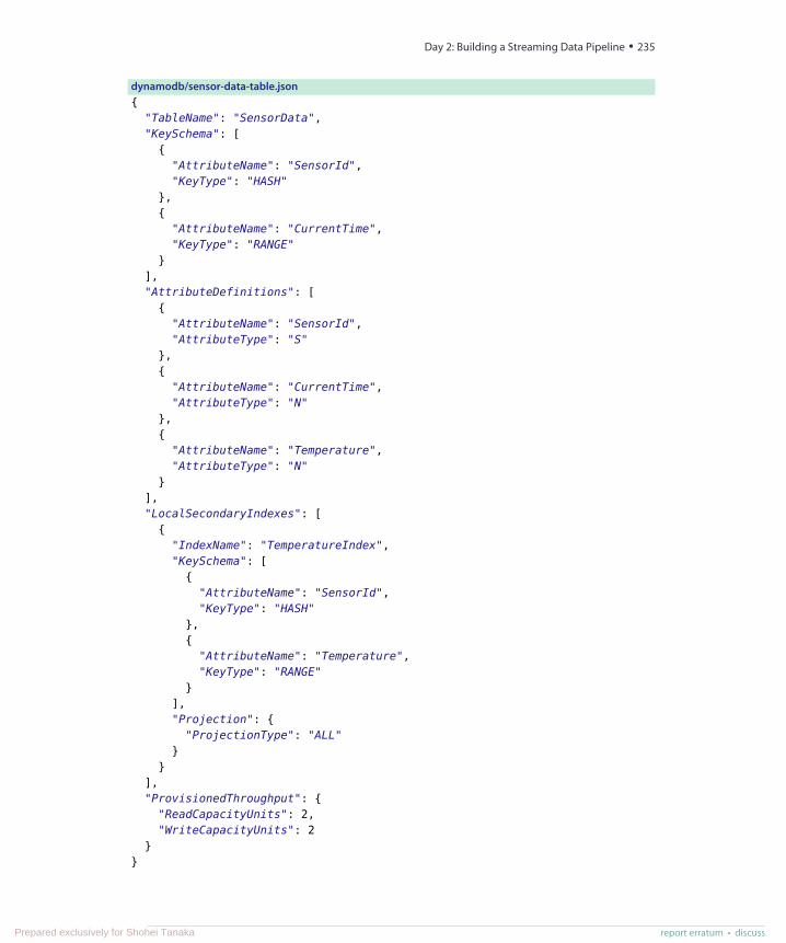
dynamodb/sensor-data-table.json{
"TableName": "SensorData","KeySchema": [
{"AttributeName": "SensorId","KeyType": "HASH"
},{
"AttributeName": "CurrentTime","KeyType": "RANGE"
}],"AttributeDefinitions": [
{"AttributeName": "SensorId","AttributeType": "S"
},{
"AttributeName": "CurrentTime","AttributeType": "N"
},{
"AttributeName": "Temperature","AttributeType": "N"
}],"LocalSecondaryIndexes": [
{"IndexName": "TemperatureIndex","KeySchema": [
{"AttributeName": "SensorId","KeyType": "HASH"
},{
"AttributeName": "Temperature","KeyType": "RANGE"
}],"Projection": {
"ProjectionType": "ALL"}
}],"ProvisionedThroughput": {
"ReadCapacityUnits": 2,"WriteCapacityUnits": 2
}}
report erratum • discuss
Day 2: Building a Streaming Data Pipeline • 235
Prepared exclusively for Shohei Tanaka
Keep in mind that this data model is highly specific to our use case. Many usecases may involve more complex column structures, more secondary indexes,more attributes, and so on. The important thing is making sure that you gothrough a similar decision-making process whenever you use DynamoDB;missteps here will cost you, and we do mean actual money.
Navigating Trade-offs in Performance Tuning
As we’ve stressed before, you simply shouldn’t use DynamoDB if you’re afteranything but extremely good performance at massive scale. But as with anycomplex system, performance and scalability in DynamoDB are not guaran-teed. There’s a wide variety of missteps that will ensure that you have a deeplysub-optimal experience, spend too much money, or both.
On Day 1, we talked about performance optimization from the standpoint ofdata modeling and how the distribution of primary keys is very important. Inthis section, the focus will be more operational. DynamoDB provides a smallhandful of knobs you can adjust that can have a big impact on performance.These knobs are the closest thing you get to “ops” in DynamoDB, but theyaren’t terribly complex. You just need to keep a few basic principles in view.
Throughput is the central concept here. When we created the ShoppingCart tableon Day 1, we used this command but didn’t provide much explanation of the--provisioned-throughput flag:
$ aws dynamodb create-table --table-name ShoppingCart \--attribute-definitions AttributeName=ItemName,AttributeType=S \--key-schema AttributeName=ItemName,KeyType=HASH \--provisioned-throughput ReadCapacityUnits=1,WriteCapacityUnits=1
Read capacity and write capacity units are handled differently in DynamoDB.Write capacity units (WCUs) are measured in units of 1 KB per second whileread capacity units (RCUs) are measured in units of 4 KB per second. Youcan set both read and write throughput on a per-table basis. For workloadsthat are more write heavy, you could provision just one RCU and many WCUs,or vice versa for read-heavy workloads.
We won’t delve too far into DynamoDB throughput tuning here. Just keep afew things in mind:
• Strive to match the RCUs and WCUs in a table to balance between read andwrite intensity. Perform regular checks—Amazon offers numerous servicesto help with this, such as CloudWatch—to ensure that you haven’t over-or under-provisioned throughput on either the read or the write side.Perhaps even set up an automated system to re-provision when necessary.
Chapter 7. DynamoDB • 236
report erratum • discussPrepared exclusively for Shohei Tanaka
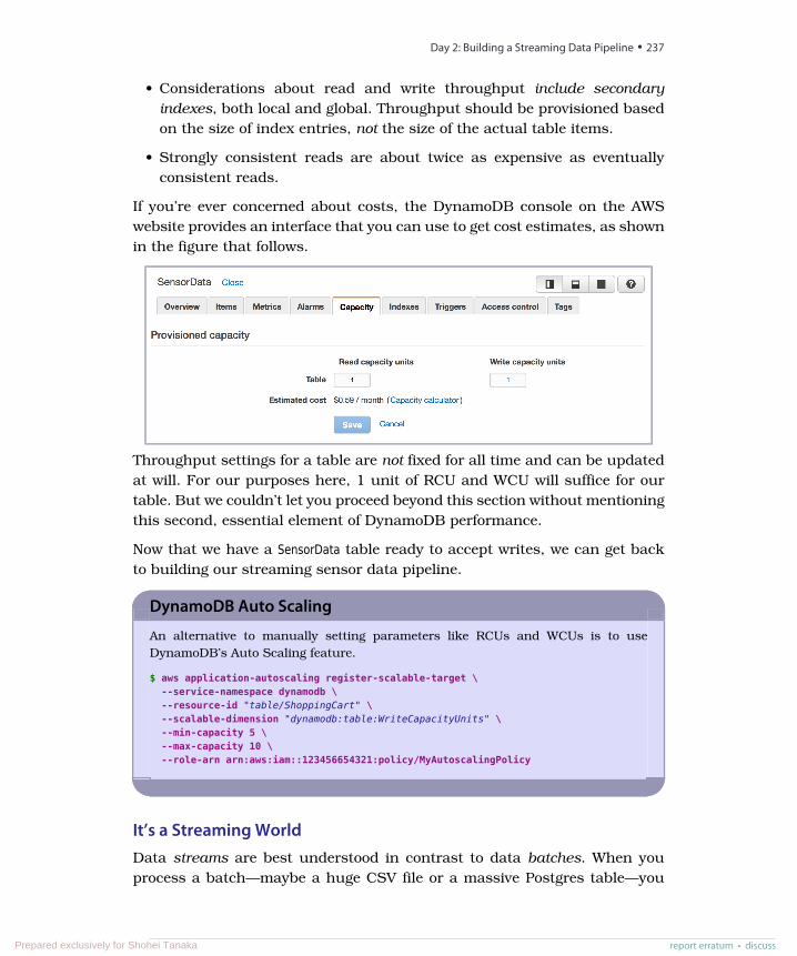
• Considerations about read and write throughput include secondaryindexes, both local and global. Throughput should be provisioned basedon the size of index entries, not the size of the actual table items.
• Strongly consistent reads are about twice as expensive as eventuallyconsistent reads.
If you’re ever concerned about costs, the DynamoDB console on the AWSwebsite provides an interface that you can use to get cost estimates, as shownin the figure that follows.
Throughput settings for a table are not fixed for all time and can be updatedat will. For our purposes here, 1 unit of RCU and WCU will suffice for ourtable. But we couldn’t let you proceed beyond this section without mentioningthis second, essential element of DynamoDB performance.
Now that we have a SensorData table ready to accept writes, we can get backto building our streaming sensor data pipeline.
DynamoDB Auto Scaling
An alternative to manually setting parameters like RCUs and WCUs is to useDynamoDB’s Auto Scaling feature.
$ aws application-autoscaling register-scalable-target \--service-namespace dynamodb \--resource-id "table/ShoppingCart" \--scalable-dimension "dynamodb:table:WriteCapacityUnits" \--min-capacity 5 \--max-capacity 10 \--role-arn arn:aws:iam::123456654321:policy/MyAutoscalingPolicy
It’s a Streaming WorldData streams are best understood in contrast to data batches. When youprocess a batch—maybe a huge CSV file or a massive Postgres table—you
report erratum • discuss
Day 2: Building a Streaming Data Pipeline • 237
Prepared exclusively for Shohei Tanaka
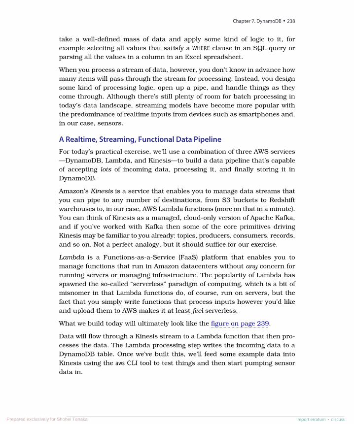
take a well-defined mass of data and apply some kind of logic to it, forexample selecting all values that satisfy a WHERE clause in an SQL query orparsing all the values in a column in an Excel spreadsheet.
When you process a stream of data, however, you don’t know in advance howmany items will pass through the stream for processing. Instead, you designsome kind of processing logic, open up a pipe, and handle things as theycome through. Although there’s still plenty of room for batch processing intoday’s data landscape, streaming models have become more popular withthe predominance of realtime inputs from devices such as smartphones and,in our case, sensors.
A Realtime, Streaming, Functional Data PipelineFor today’s practical exercise, we’ll use a combination of three AWS services—DynamoDB, Lambda, and Kinesis—to build a data pipeline that’s capableof accepting lots of incoming data, processing it, and finally storing it inDynamoDB.
Amazon’s Kinesis is a service that enables you to manage data streams thatyou can pipe to any number of destinations, from S3 buckets to Redshiftwarehouses to, in our case, AWS Lambda functions (more on that in a minute).You can think of Kinesis as a managed, cloud-only version of Apache Kafka,and if you’ve worked with Kafka then some of the core primitives drivingKinesis may be familiar to you already: topics, producers, consumers, records,and so on. Not a perfect analogy, but it should suffice for our exercise.
Lambda is a Functions-as-a-Service (FaaS) platform that enables you tomanage functions that run in Amazon datacenters without any concern forrunning servers or managing infrastructure. The popularity of Lambda hasspawned the so-called “serverless” paradigm of computing, which is a bit ofmisnomer in that Lambda functions do, of course, run on servers, but thefact that you simply write functions that process inputs however you’d likeand upload them to AWS makes it at least feel serverless.
What we build today will ultimately look like the figure on page 239.
Data will flow through a Kinesis stream to a Lambda function that then pro-cesses the data. The Lambda processing step writes the incoming data to aDynamoDB table. Once we’ve built this, we’ll feed some example data intoKinesis using the aws CLI tool to test things and then start pumping sensordata in.
Chapter 7. DynamoDB • 238
report erratum • discussPrepared exclusively for Shohei Tanaka
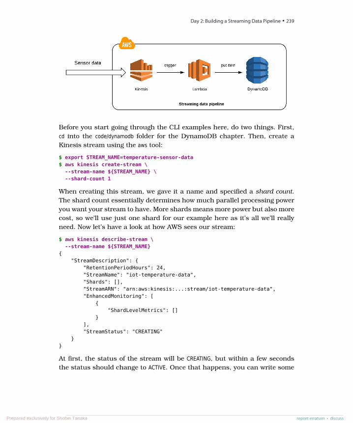
Before you start going through the CLI examples here, do two things. First,cd into the code/dynamodb folder for the DynamoDB chapter. Then, create aKinesis stream using the aws tool:
$ export STREAM_NAME=temperature-sensor-data$ aws kinesis create-stream \
--stream-name ${STREAM_NAME} \--shard-count 1
When creating this stream, we gave it a name and specified a shard count.The shard count essentially determines how much parallel processing poweryou want your stream to have. More shards means more power but also morecost, so we’ll use just one shard for our example here as it’s all we’ll reallyneed. Now let’s have a look at how AWS sees our stream:
$ aws kinesis describe-stream \--stream-name ${STREAM_NAME}
{"StreamDescription": {
"RetentionPeriodHours": 24,"StreamName": "iot-temperature-data","Shards": [],"StreamARN": "arn:aws:kinesis:...:stream/iot-temperature-data","EnhancedMonitoring": [
{"ShardLevelMetrics": []
}],"StreamStatus": "CREATING"
}}
At first, the status of the stream will be CREATING, but within a few secondsthe status should change to ACTIVE. Once that happens, you can write some
report erratum • discuss
Day 2: Building a Streaming Data Pipeline • 239
Prepared exclusively for Shohei Tanaka
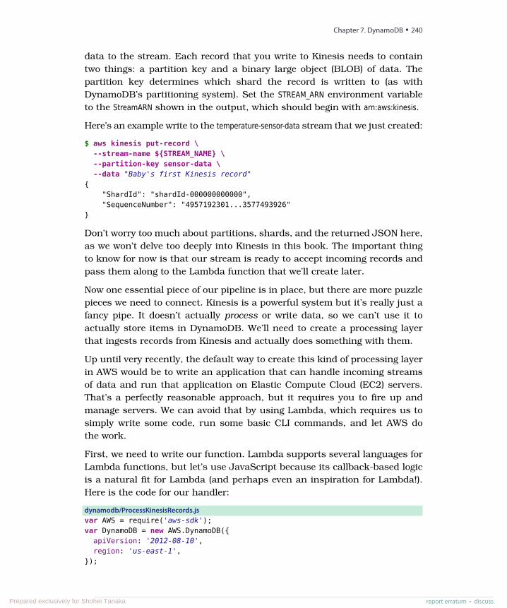
data to the stream. Each record that you write to Kinesis needs to containtwo things: a partition key and a binary large object (BLOB) of data. Thepartition key determines which shard the record is written to (as withDynamoDB’s partitioning system). Set the STREAM_ARN environment variableto the StreamARN shown in the output, which should begin with arn:aws:kinesis.
Here’s an example write to the temperature-sensor-data stream that we just created:
$ aws kinesis put-record \--stream-name ${STREAM_NAME} \--partition-key sensor-data \--data "Baby's first Kinesis record"
{"ShardId": "shardId-000000000000","SequenceNumber": "4957192301...3577493926"
}
Don’t worry too much about partitions, shards, and the returned JSON here,as we won’t delve too deeply into Kinesis in this book. The important thingto know for now is that our stream is ready to accept incoming records andpass them along to the Lambda function that we’ll create later.
Now one essential piece of our pipeline is in place, but there are more puzzlepieces we need to connect. Kinesis is a powerful system but it’s really just afancy pipe. It doesn’t actually process or write data, so we can’t use it toactually store items in DynamoDB. We’ll need to create a processing layerthat ingests records from Kinesis and actually does something with them.
Up until very recently, the default way to create this kind of processing layerin AWS would be to write an application that can handle incoming streamsof data and run that application on Elastic Compute Cloud (EC2) servers.That’s a perfectly reasonable approach, but it requires you to fire up andmanage servers. We can avoid that by using Lambda, which requires us tosimply write some code, run some basic CLI commands, and let AWS dothe work.
First, we need to write our function. Lambda supports several languages forLambda functions, but let’s use JavaScript because its callback-based logicis a natural fit for Lambda (and perhaps even an inspiration for Lambda!).Here is the code for our handler:
dynamodb/ProcessKinesisRecords.jsvar AWS = require('aws-sdk');var DynamoDB = new AWS.DynamoDB({
apiVersion: '2012-08-10',region: 'us-east-1',
});
Chapter 7. DynamoDB • 240
report erratum • discussPrepared exclusively for Shohei Tanaka
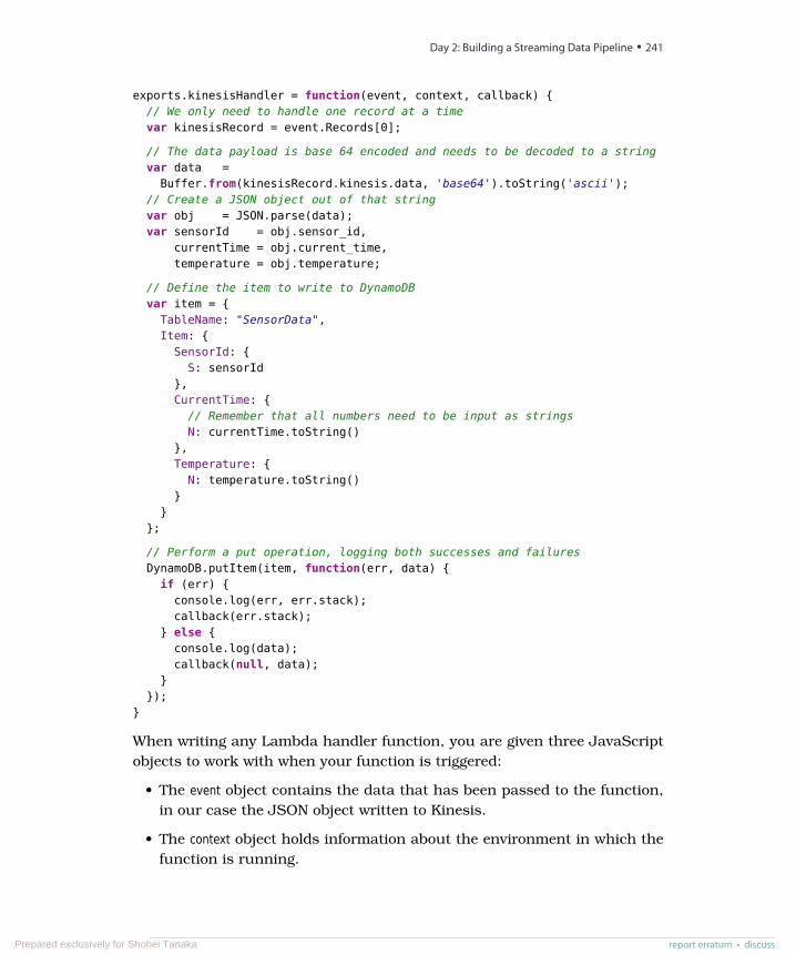
exports.kinesisHandler = function(event, context, callback) {// We only need to handle one record at a timevar kinesisRecord = event.Records[0];
// The data payload is base 64 encoded and needs to be decoded to a stringvar data =
Buffer.from(kinesisRecord.kinesis.data, 'base64').toString('ascii');// Create a JSON object out of that stringvar obj = JSON.parse(data);var sensorId = obj.sensor_id,
currentTime = obj.current_time,temperature = obj.temperature;
// Define the item to write to DynamoDBvar item = {
TableName: "SensorData",Item: {SensorId: {
S: sensorId},CurrentTime: {
// Remember that all numbers need to be input as stringsN: currentTime.toString()
},Temperature: {
N: temperature.toString()}
}};
// Perform a put operation, logging both successes and failuresDynamoDB.putItem(item, function(err, data) {
if (err) {console.log(err, err.stack);callback(err.stack);
} else {console.log(data);callback(null, data);
}});
}
When writing any Lambda handler function, you are given three JavaScriptobjects to work with when your function is triggered:
• The event object contains the data that has been passed to the function,in our case the JSON object written to Kinesis.
• The context object holds information about the environment in which thefunction is running.
report erratum • discuss
Day 2: Building a Streaming Data Pipeline • 241
Prepared exclusively for Shohei Tanaka
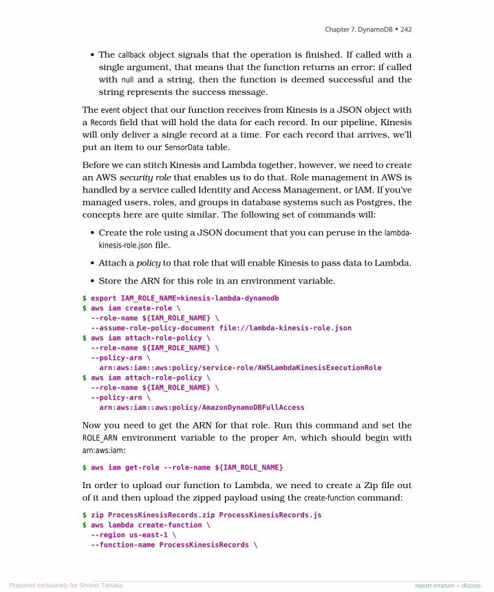
• The callback object signals that the operation is finished. If called with asingle argument, that means that the function returns an error; if calledwith null and a string, then the function is deemed successful and thestring represents the success message.
The event object that our function receives from Kinesis is a JSON object witha Records field that will hold the data for each record. In our pipeline, Kinesiswill only deliver a single record at a time. For each record that arrives, we’llput an item to our SensorData table.
Before we can stitch Kinesis and Lambda together, however, we need to createan AWS security role that enables us to do that. Role management in AWS ishandled by a service called Identity and Access Management, or IAM. If you’vemanaged users, roles, and groups in database systems such as Postgres, theconcepts here are quite similar. The following set of commands will:
• Create the role using a JSON document that you can peruse in the lambda-kinesis-role.json file.
• Attach a policy to that role that will enable Kinesis to pass data to Lambda.
• Store the ARN for this role in an environment variable.
$ export IAM_ROLE_NAME=kinesis-lambda-dynamodb$ aws iam create-role \
--role-name ${IAM_ROLE_NAME} \--assume-role-policy-document file://lambda-kinesis-role.json
$ aws iam attach-role-policy \--role-name ${IAM_ROLE_NAME} \--policy-arn \
arn:aws:iam::aws:policy/service-role/AWSLambdaKinesisExecutionRole$ aws iam attach-role-policy \
--role-name ${IAM_ROLE_NAME} \--policy-arn \
arn:aws:iam::aws:policy/AmazonDynamoDBFullAccess
Now you need to get the ARN for that role. Run this command and set theROLE_ARN environment variable to the proper Arn, which should begin witharn:aws:iam:
$ aws iam get-role --role-name ${IAM_ROLE_NAME}
In order to upload our function to Lambda, we need to create a Zip file outof it and then upload the zipped payload using the create-function command:
$ zip ProcessKinesisRecords.zip ProcessKinesisRecords.js$ aws lambda create-function \
--region us-east-1 \--function-name ProcessKinesisRecords \
Chapter 7. DynamoDB • 242
report erratum • discussPrepared exclusively for Shohei Tanaka
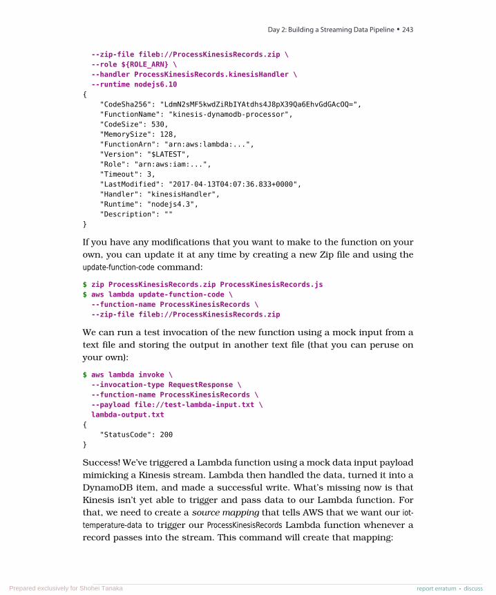
--zip-file fileb://ProcessKinesisRecords.zip \--role ${ROLE_ARN} \--handler ProcessKinesisRecords.kinesisHandler \--runtime nodejs6.10
{"CodeSha256": "LdmN2sMF5kwdZiRbIYAtdhs4J8pX39Qa6EhvGdGAcOQ=","FunctionName": "kinesis-dynamodb-processor","CodeSize": 530,"MemorySize": 128,"FunctionArn": "arn:aws:lambda:...","Version": "$LATEST","Role": "arn:aws:iam:...","Timeout": 3,"LastModified": "2017-04-13T04:07:36.833+0000","Handler": "kinesisHandler","Runtime": "nodejs4.3","Description": ""
}
If you have any modifications that you want to make to the function on yourown, you can update it at any time by creating a new Zip file and using theupdate-function-code command:
$ zip ProcessKinesisRecords.zip ProcessKinesisRecords.js$ aws lambda update-function-code \
--function-name ProcessKinesisRecords \--zip-file fileb://ProcessKinesisRecords.zip
We can run a test invocation of the new function using a mock input from atext file and storing the output in another text file (that you can peruse onyour own):
$ aws lambda invoke \--invocation-type RequestResponse \--function-name ProcessKinesisRecords \--payload file://test-lambda-input.txt \lambda-output.txt
{"StatusCode": 200
}
Success! We’ve triggered a Lambda function using a mock data input payloadmimicking a Kinesis stream. Lambda then handled the data, turned it into aDynamoDB item, and made a successful write. What’s missing now is thatKinesis isn’t yet able to trigger and pass data to our Lambda function. Forthat, we need to create a source mapping that tells AWS that we want our iot-temperature-data to trigger our ProcessKinesisRecords Lambda function whenever arecord passes into the stream. This command will create that mapping:
report erratum • discuss
Day 2: Building a Streaming Data Pipeline • 243
Prepared exclusively for Shohei Tanaka
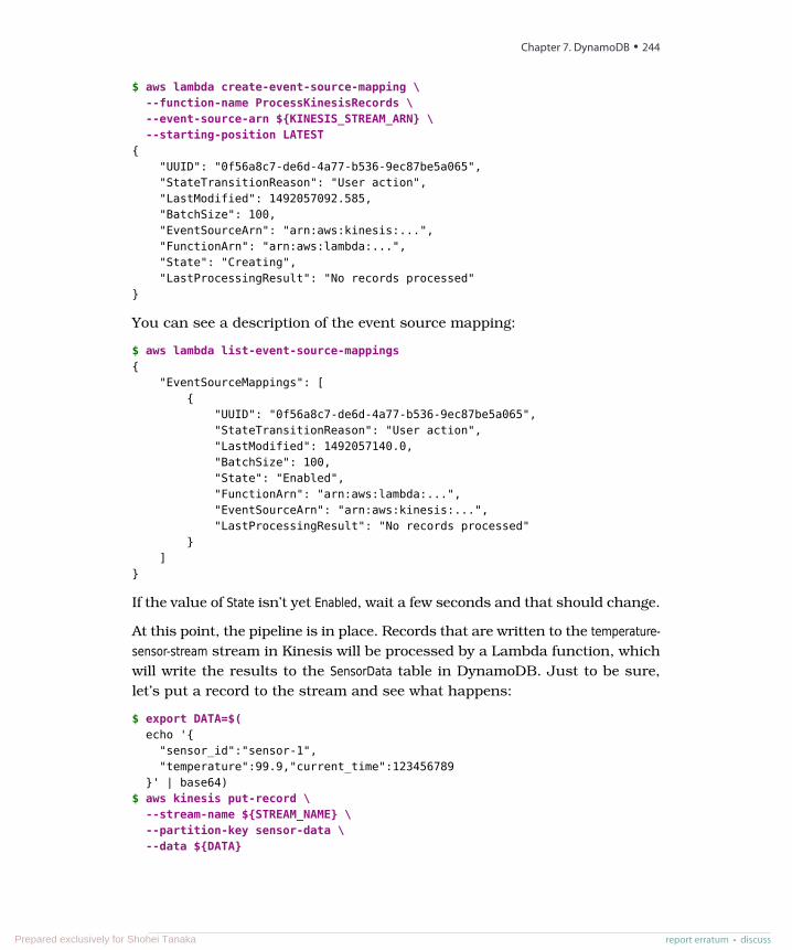
$ aws lambda create-event-source-mapping \--function-name ProcessKinesisRecords \--event-source-arn ${KINESIS_STREAM_ARN} \--starting-position LATEST
{"UUID": "0f56a8c7-de6d-4a77-b536-9ec87be5a065","StateTransitionReason": "User action","LastModified": 1492057092.585,"BatchSize": 100,"EventSourceArn": "arn:aws:kinesis:...","FunctionArn": "arn:aws:lambda:...","State": "Creating","LastProcessingResult": "No records processed"
}
You can see a description of the event source mapping:
$ aws lambda list-event-source-mappings{
"EventSourceMappings": [{
"UUID": "0f56a8c7-de6d-4a77-b536-9ec87be5a065","StateTransitionReason": "User action","LastModified": 1492057140.0,"BatchSize": 100,"State": "Enabled","FunctionArn": "arn:aws:lambda:...","EventSourceArn": "arn:aws:kinesis:...","LastProcessingResult": "No records processed"
}]
}
If the value of State isn’t yet Enabled, wait a few seconds and that should change.
At this point, the pipeline is in place. Records that are written to the temperature-sensor-stream stream in Kinesis will be processed by a Lambda function, whichwill write the results to the SensorData table in DynamoDB. Just to be sure,let’s put a record to the stream and see what happens:
$ export DATA=$(echo '{
"sensor_id":"sensor-1","temperature":99.9,"current_time":123456789
}' | base64)$ aws kinesis put-record \
--stream-name ${STREAM_NAME} \--partition-key sensor-data \--data ${DATA}
Chapter 7. DynamoDB • 244
report erratum • discussPrepared exclusively for Shohei Tanaka
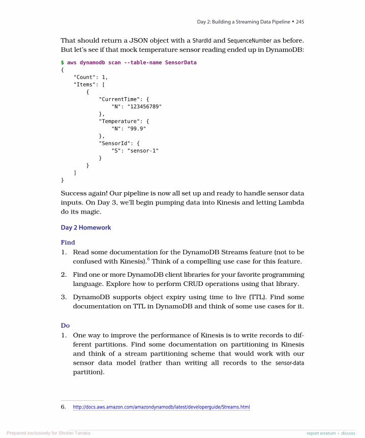
That should return a JSON object with a ShardId and SequenceNumber as before.But let’s see if that mock temperature sensor reading ended up in DynamoDB:
$ aws dynamodb scan --table-name SensorData{
"Count": 1,"Items": [
{"CurrentTime": {
"N": "123456789"},"Temperature": {
"N": "99.9"},"SensorId": {
"S": "sensor-1"}
}]
}
Success again! Our pipeline is now all set up and ready to handle sensor datainputs. On Day 3, we’ll begin pumping data into Kinesis and letting Lambdado its magic.
Day 2 Homework
Find
1. Read some documentation for the DynamoDB Streams feature (not to beconfused with Kinesis).6 Think of a compelling use case for this feature.
2. Find one or more DynamoDB client libraries for your favorite programminglanguage. Explore how to perform CRUD operations using that library.
3. DynamoDB supports object expiry using time to live (TTL). Find somedocumentation on TTL in DynamoDB and think of some use cases for it.
Do
1. One way to improve the performance of Kinesis is to write records to dif-ferent partitions. Find some documentation on partitioning in Kinesisand think of a stream partitioning scheme that would work with oursensor data model (rather than writing all records to the sensor-datapartition).
6. http://docs.aws.amazon.com/amazondynamodb/latest/developerguide/Streams.html
report erratum • discuss
Day 2: Building a Streaming Data Pipeline • 245
Prepared exclusively for Shohei Tanaka
2. Modify various elements of our data pipeline—the SensorData table definition,the Lambda function, and so on—to enable sensors to write humidity-related data to the pipeline (as a percentage). Make sure that all of thesecomponents line up properly!
Day 3: Building an “Internet of Things” SystemAround DynamoDBOn Day 2, we delved into DynamoDB‘s streaming feature and turned ourDynamoDB database from a fairly standard cloud storage mechanism into amuch more dynamic processing system consisting of a Kinesis-Lambda-DynamoDB system. What we didn’t do on Day 2 was provide any data inputsbeyond some CLI test runs. On Day 3, we’ll provide some “Internet of Things”-style data from mock sensors.
The term “Internet of Things” (aka IoT) is kind of like “Big Data” or “the Cloud.”Its use is controversial because there’s a lot of buzz surrounding it, and whatit points to isn’t so much something that already exists as much as it is a setof emerging technological possibilities. The “things” in the expression canrefer to everything from moisture sensors in your refrigerator to a heart-ratemonitor you wear on your wrist—essentially anything that isn‘t a “normal”computer (laptop, smartphone, cloud server) and is capable of producing dataand transmitting it to some part of the Internet.
The interesting thing about the IoT from the perspective of this book is thatthings like sensors can produce tons of data, especially when aggregatingacross many data-producing devices. Imagine a 50-acre vineyard with moistureand temperature sensors hooked up every few feet along the rows of vines, ora high-tech manufacturing facility where each machine in an assembly line isfeeding all kinds of data to some centralized source. In both cases, these devicesmight be sending data every few hours or they might be sending it more thanonce a second. IoT data usually comes in small chunks (maybe just a fewsensor readings at a time), but those small chunks can really add up.
DynamoDB is a good choice for an IoT database because it’s built to handle notjust huge data sets but data sets whose size can’t be determined in advanced.The downside of DynamoDB, as we discussed before, is that it isn’t built forcomplex queries of the type you’d be able to run on a relational database. Forour needs here, though, DynamoDB’s “key-value plus” querying system will dojust fine. Our tables will be fairly simple, and range queries will enable us to useDynamoDB as a powerful timeseries database. Any processing logic we needto apply beyond this can happen on the application side if we need it to.
Chapter 7. DynamoDB • 246
report erratum • discussPrepared exclusively for Shohei Tanaka
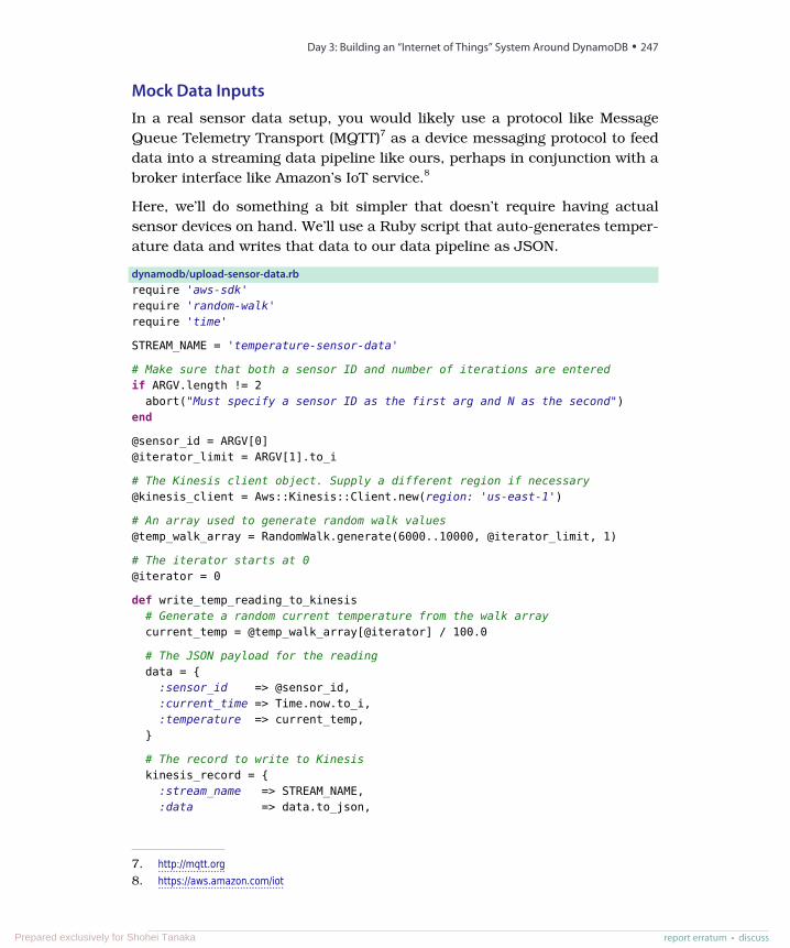
Mock Data InputsIn a real sensor data setup, you would likely use a protocol like MessageQueue Telemetry Transport (MQTT)7 as a device messaging protocol to feeddata into a streaming data pipeline like ours, perhaps in conjunction with abroker interface like Amazon’s IoT service.8
Here, we’ll do something a bit simpler that doesn’t require having actualsensor devices on hand. We’ll use a Ruby script that auto-generates temper-ature data and writes that data to our data pipeline as JSON.
dynamodb/upload-sensor-data.rbrequire 'aws-sdk'require 'random-walk'require 'time'
STREAM_NAME = 'temperature-sensor-data'
# Make sure that both a sensor ID and number of iterations are enteredif ARGV.length != 2
abort("Must specify a sensor ID as the first arg and N as the second")end
@sensor_id = ARGV[0]@iterator_limit = ARGV[1].to_i
# The Kinesis client object. Supply a different region if necessary@kinesis_client = Aws::Kinesis::Client.new(region: 'us-east-1')
# An array used to generate random walk values@temp_walk_array = RandomWalk.generate(6000..10000, @iterator_limit, 1)
# The iterator starts at 0@iterator = 0
def write_temp_reading_to_kinesis# Generate a random current temperature from the walk arraycurrent_temp = @temp_walk_array[@iterator] / 100.0
# The JSON payload for the readingdata = {
:sensor_id => @sensor_id,:current_time => Time.now.to_i,:temperature => current_temp,
}
# The record to write to Kinesiskinesis_record = {
:stream_name => STREAM_NAME,:data => data.to_json,
7. http://mqtt.org8. https://aws.amazon.com/iot
report erratum • discuss
Day 3: Building an “Internet of Things” System Around DynamoDB • 247
Prepared exclusively for Shohei Tanaka
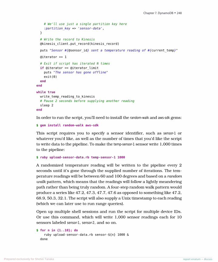
# We'll use just a single partition key here:partition_key => 'sensor-data',
}
# Write the record to Kinesis@kinesis_client.put_record(kinesis_record)
puts "Sensor #{@sensor_id} sent a temperature reading of #{current_temp}"
@iterator += 1
# Exit if script has iterated N timesif @iterator == @iterator_limit
puts "The sensor has gone offline"exit(0)
endend
while truewrite_temp_reading_to_kinesis# Pause 2 seconds before supplying another readingsleep 2
end
In order to run the script, you’ll need to install the random-walk and aws-sdk gems:
$ gem install random-walk aws-sdk
This script requires you to specify a sensor identifier, such as sensor-1 orwhatever you’d like, as well as the number of times that you’d like the scriptto write data to the pipeline. To make the temp-sensor-1 sensor write 1,000 timesto the pipeline:
$ ruby upload-sensor-data.rb temp-sensor-1 1000
A randomized temperature reading will be written to the pipeline every 2seconds until it’s gone through the supplied number of iterations. The tem-perature readings will be between 60 and 100 degrees and based on a randomwalk pattern, which means that the readings will follow a lightly meanderingpath rather than being truly random. A four-step random walk pattern wouldproduce a series like 47.2, 47.3, 47.7, 47.6 as opposed to something like 47.2,68.9, 50.3, 32.1. The script will also supply a Unix timestamp to each reading(which we can later use to run range queries).
Open up multiple shell sessions and run the script for multiple device IDs.Or use this command, which will write 1,000 sensor readings each for 10sensors labeled sensor-1, sensor-2, and so on.
$ for n in {1..10}; doruby upload-sensor-data.rb sensor-${n} 1000 &
done
Chapter 7. DynamoDB • 248
report erratum • discussPrepared exclusively for Shohei Tanaka
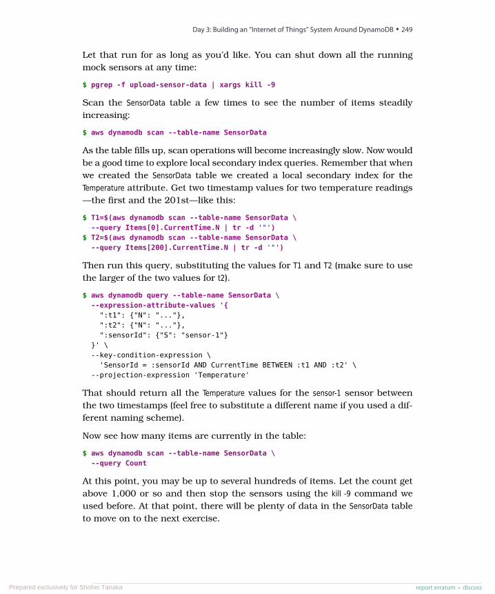
Let that run for as long as you’d like. You can shut down all the runningmock sensors at any time:
$ pgrep -f upload-sensor-data | xargs kill -9
Scan the SensorData table a few times to see the number of items steadilyincreasing:
$ aws dynamodb scan --table-name SensorData
As the table fills up, scan operations will become increasingly slow. Now wouldbe a good time to explore local secondary index queries. Remember that whenwe created the SensorData table we created a local secondary index for theTemperature attribute. Get two timestamp values for two temperature readings—the first and the 201st—like this:
$ T1=$(aws dynamodb scan --table-name SensorData \--query Items[0].CurrentTime.N | tr -d '"')
$ T2=$(aws dynamodb scan --table-name SensorData \--query Items[200].CurrentTime.N | tr -d '"')
Then run this query, substituting the values for T1 and T2 (make sure to usethe larger of the two values for t2).
$ aws dynamodb query --table-name SensorData \--expression-attribute-values '{
":t1": {"N": "..."},":t2": {"N": "..."},":sensorId": {"S": "sensor-1"}
}' \--key-condition-expression \
'SensorId = :sensorId AND CurrentTime BETWEEN :t1 AND :t2' \--projection-expression 'Temperature'
That should return all the Temperature values for the sensor-1 sensor betweenthe two timestamps (feel free to substitute a different name if you used a dif-ferent naming scheme).
Now see how many items are currently in the table:
$ aws dynamodb scan --table-name SensorData \--query Count
At this point, you may be up to several hundreds of items. Let the count getabove 1,000 or so and then stop the sensors using the kill -9 command weused before. At that point, there will be plenty of data in the SensorData tableto move on to the next exercise.
report erratum • discuss
Day 3: Building an “Internet of Things” System Around DynamoDB • 249
Prepared exclusively for Shohei Tanaka
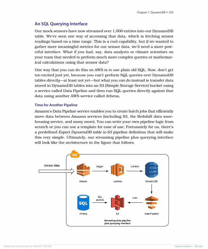
An SQL Querying InterfaceOur mock sensors have now streamed over 1,000 entries into our DynamoDBtable. We’ve seen one way of accessing that data, which is fetching sensorreadings based on a time range. This is a cool capability, but if we wanted togather more meaningful metrics for our sensor data, we’d need a more pow-erful interface. What if you had, say, data analysts or climate scientists onyour team that needed to perform much more complex queries or mathemat-ical calculations using that sensor data?
One way that you can do this on AWS is to use plain old SQL. Now, don’t gettoo excited just yet, because you can’t perform SQL queries over DynamoDBtables directly—at least not yet—but what you can do instead is transfer datastored in DynamoDB tables into an S3 (Simple Storage Service) bucket usinga service called Data Pipeline and then run SQL queries directly against thatdata using another AWS service called Athena.
Time for Another Pipeline
Amazon’s Data Pipeline service enables you to create batch jobs that efficientlymove data between Amazon services (including S3, the Redshift data ware-housing service, and many more). You can write your own pipeline logic fromscratch or you can use a template for ease of use. Fortunately for us, there’sa predefined Export DynamoDB table to S3 pipeline definition that will makethis very simple. Ultimately, our streaming pipeline plus querying interfacewill look like the architecture in the figure that follows.
Chapter 7. DynamoDB • 250
report erratum • discussPrepared exclusively for Shohei Tanaka
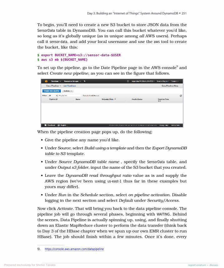
To begin, you’ll need to create a new S3 bucket to store JSON data from theSensorData table in DynamoDB. You can call this bucket whatever you’d like,so long as it’s globally unique (as in unique among all AWS users). Perhapscall it sensor-data, and add your local username and use the aws tool to createthe bucket, like this:
$ export BUCKET_NAME=s3://sensor-data-$USER$ aws s3 mb ${BUCKET_NAME}
To set up the pipeline, go to the Date Pipeline page in the AWS console9 andselect Create new pipeline, as you can see in the figure that follows.
When the pipeline creation page pops up, do the following:
• Give the pipeline any name you’d like.
• Under Source, select Build using a template and then the Export DynamoDBtable to S3 template.
• Under Source DynamoDB table name , specify the SensorData table, andunder Output s3 folder, input the name of the S3 bucket that you created.
• Leave the DynamoDB read throughput ratio value as is and supply theAWS region (we’ve been using us-east-1 thus far in these examples butyours may differ).
• Under Run in the Schedule section, select on pipeline activation. Disablelogging in the next section and select Default under Security/Access.
Now click Activate. That will bring you back to the data pipeline console. Thepipeline job will go through several phases, beginning with WAITING. Behindthe scenes, Data Pipeline is actually spinning up, using, and finally shuttingdown an Elastic MapReduce cluster to perform the data transfer (think backto Day 3 of the HBase chapter when we spun up our own EMR cluster to runHBase). The job should finish within a few minutes. Once it’s done, every
9. https://console.aws.amazon.com/datapipeline
report erratum • discuss
Day 3: Building an “Internet of Things” System Around DynamoDB • 251
Prepared exclusively for Shohei Tanaka
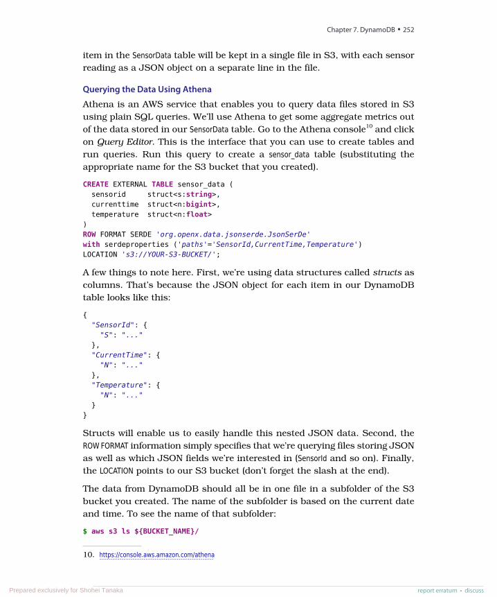
item in the SensorData table will be kept in a single file in S3, with each sensorreading as a JSON object on a separate line in the file.
Querying the Data Using Athena
Athena is an AWS service that enables you to query data files stored in S3using plain SQL queries. We’ll use Athena to get some aggregate metrics outof the data stored in our SensorData table. Go to the Athena console10 and clickon Query Editor. This is the interface that you can use to create tables andrun queries. Run this query to create a sensor_data table (substituting theappropriate name for the S3 bucket that you created).
CREATE EXTERNAL TABLE sensor_data (sensorid struct<s:string>,currenttime struct<n:bigint>,temperature struct<n:float>
)ROW FORMAT SERDE 'org.openx.data.jsonserde.JsonSerDe'with serdeproperties ('paths'='SensorId,CurrentTime,Temperature')LOCATION 's3://YOUR-S3-BUCKET/';
A few things to note here. First, we’re using data structures called structs ascolumns. That’s because the JSON object for each item in our DynamoDBtable looks like this:
{"SensorId": {
"S": "..."},"CurrentTime": {
"N": "..."},"Temperature": {
"N": "..."}
}
Structs will enable us to easily handle this nested JSON data. Second, theROW FORMAT information simply specifies that we’re querying files storing JSONas well as which JSON fields we’re interested in (SensorId and so on). Finally,the LOCATION points to our S3 bucket (don’t forget the slash at the end).
The data from DynamoDB should all be in one file in a subfolder of the S3bucket you created. The name of the subfolder is based on the current dateand time. To see the name of that subfolder:
$ aws s3 ls ${BUCKET_NAME}/
10. https://console.aws.amazon.com/athena
Chapter 7. DynamoDB • 252
report erratum • discussPrepared exclusively for Shohei Tanaka
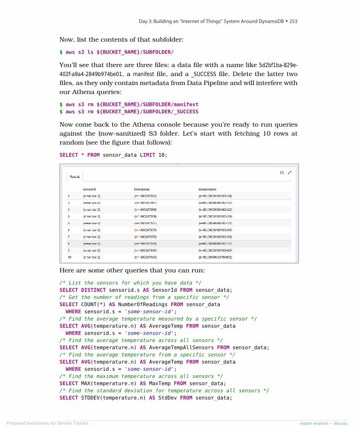
Now, list the contents of that subfolder:
$ aws s3 ls ${BUCKET_NAME}/SUBFOLDER/
You’ll see that there are three files: a data file with a name like 5d2bf1ba-829e-402f-a9a4-2849b974be01, a manifest file, and a _SUCCESS file. Delete the latter twofiles, as they only contain metadata from Data Pipeline and will interfere withour Athena queries:
$ aws s3 rm ${BUCKET_NAME}/SUBFOLDER/manifest$ aws s3 rm ${BUCKET_NAME}/SUBFOLDER/_SUCCESS
Now come back to the Athena console because you’re ready to run queriesagainst the (now-sanitized) S3 folder. Let’s start with fetching 10 rows atrandom (see the figure that follows):
SELECT * FROM sensor_data LIMIT 10;
Here are some other queries that you can run:
/* List the sensors for which you have data */SELECT DISTINCT sensorid.s AS SensorId FROM sensor_data;/* Get the number of readings from a specific sensor */SELECT COUNT(*) AS NumberOfReadings FROM sensor_data
WHERE sensorid.s = 'some-sensor-id';/* Find the average temperature measured by a specific sensor */SELECT AVG(temperature.n) AS AverageTemp FROM sensor_data
WHERE sensorid.s = 'some-sensor-id';/* Find the average temperature across all sensors */SELECT AVG(temperature.n) AS AverageTempAllSensors FROM sensor_data;/* Find the average temperature from a specific sensor */SELECT AVG(temperature.n) AS AverageTemp FROM sensor_data
WHERE sensorid.s = 'some-sensor-id';/* Find the maximum temperature across all sensors */SELECT MAX(temperature.n) AS MaxTemp FROM sensor_data;/* Find the standard deviation for temperature across all sensors */SELECT STDDEV(temperature.n) AS StdDev FROM sensor_data;
report erratum • discuss
Day 3: Building an “Internet of Things” System Around DynamoDB • 253
Prepared exclusively for Shohei Tanaka
Production Ready? Not Quite
The system that we’ve built here—the Kinesis/Lambda/DynamoDB pipelineplus Athena querying layer—has served us well in exploring these services,but you wouldn’t want to use it as a production system. Why? Because it’sbuilt on the assumption that there’s only one table.
In reality, data in DynamoDB is often spread across many tables, whilequerying that data involves knowing in which tables the right data lives (onecould call this tertiary indexing but the authors are unaware of this usage inthe wild!). For our sensor data use case, that may involve, for example, storingdata from different days in different tables and automatically writing newsensor data to the correct table.
To make a setup like that work, you could auto-infer the table name from thecurrent date in the Lambda function, like this:
var date = new Date().toJSON().slice(0,10).replace(/-/g, '-');var tableName = `sensor-data-${date}`;var item = {
TableName: tableName,Item: {
// item data}
}
The name of each table in this setup would be of the form sensor-data-YYYY-MM-DD. You could create DynamoDB tables for specific dates in advance, alongwith S3 buckets for holding JSON data and Athena external table definitionsfor those different buckets. This would, in turn, enable you to run queriesacross DynamoDB tables and thus to gather metrics across days. A querylike this, for example, would find the average temperature for all sensorsacross two days’ worth of readings:
SELECT ((SELECT SUM(temperature.n) FROM sensor_data_05_01_2017) +
(SELECT SUM(temperature.n) FROM sensor_data_05_02_2017)) / ((SELECT COUNT(temperature.n) FROM sensor_data_05_01_2017) +
(SELECT COUNT(temperature.n) FROM sensor_data_05_02_2017));
What a ride! We just combined five AWS services—DynamoDB, Kinesis,Lambda, DataPipeline, and Athena, plus some helper services like IAM—intoa cohesive platform for sensor data.
Chapter 7. DynamoDB • 254
report erratum • discussPrepared exclusively for Shohei Tanaka
Day 3 Homework
Find
1. We added a global secondary index to our SensorData table, which increasedour disk space usage. Read some documentation11 to see how much spaceGSIs use.
2. The Athena service enables you to use a broad palette of SQL commandsfor running queries against S3 buckets—but not all the commands youmay be used to. Do some Googling and find out which commands are andaren’t supported.
Do
1. Exercise 1 in the homework for Day 2 called for modifying the data pipelineto handle humidity readings from our mock sensors. Modify the sensordata input script from Day 3 so that each sensor reading contains ahumidity reading. Make sure to use a random walk logic to keep thosereadings relatively un-volatile. Then create a new external table in Athenathat can run queries against that new data model.
2. In the last section of Day 3, we stated that the data pipeline we built isn’tquite production ready because we have only one table and that a bettersystem would store data from different days in different tables. Beginbuilding that system to the best of your ability, given what you’ve learnedso far.
Wrap-UpThis chapter has been quite a ride! We explored not just the very interestingand powerful DynamoDB but also a broad swathe of AWS offerings, and webuilt a pretty darned scalable data pipeline for use in a far-away datacenter.DynamoDB presents us not just with a relatively ops-free experience butalways with a data model that sits in a nice middle point between the granu-larity of SQL and the minimalism of most NoSQL data models.
DynamoDB’s StrengthsThe strengths of DynamoDB have been on display throughout this chapter. Itenables you to skip all the installation and setup steps and get started buildingimmediately. And if you build something small, there are few intrinsic limits to
11. http://docs.aws.amazon.com/amazondynamodb/latest/developerguide/GSI.html
report erratum • discuss
Wrap-Up • 255
Prepared exclusively for Shohei Tanaka
how big it can get (if, of course, you have the budget for it). DynamoDB canbe tricky in places, especially when it comes to things like capacity provision-ing, planning for indexes, and coming up with a data model that enables youto take advantage of DynamoDB’s performance and scalability. But gettingpast the tricky parts unlocks a lot of possibilities.
Although DynamoDB requires you to give up some of the querying power ofrelational databases, its data and querying models provide some powerfulconstructs, such as indexes and range queries, that you won’t find in a lotof NoSQL databases. And if you run into barriers, such as the inability towrite SQL-style queries for tables, you may be able to use an external serviceto fill in the gaps, as we did on Day 3. Beyond all of this, DynamoDB’s featureset continues to expand, as does the constellation of services surroundingDynamoDB in the AWS ecosystem.
DynamoDB’s WeaknessesThe drawbacks presented by DynamoDB are directly reminiscent of otherNoSQL databases. Despite some interesting querying and modeling constructs,you’re probably better off using Postgres or another relational database unlessyou know for sure that you’re dealing with a DynamoDB-shaped problem (ormaybe an HBase-shaped problem, or Mongo, and so on). Even if you have ause case that truly calls for a big NoSQL database, you may have troublegetting your data model to mesh well with DynamoDB’s partitioning system.And as always, there’s the cost. Any database you use is going to cost moneysomehow, but DynamoDB and others don’t always make financial sense.There may be times when it makes sense to run databases yourself, maybeon your own hardware and maybe in the cloud. Caveat emptor.
Parting ThoughtsCloud databases aren’t everyone’s cup of tea. They require a lot of trust—trustin massive systems whose internals you can’t see and trust in the futureeconomic prospects of cloud providers themselves. These and other drawbacksare real, but there are some major upsides, as we hope to have shown in thischapter. We urge anybody with a strong interest in databases to give them atry. Even if you don’t ever have a use case that requires a database likeDynamoDB, we think that they’re greatly empowering for developers and justdownright fun. They turn your humble little laptop into a very powerfulorchestration platform.
Chapter 7. DynamoDB • 256
report erratum • discussPrepared exclusively for Shohei Tanaka
DynamoDB is a good place to start but we focused on it here mostly due toits influence and market share. There are many other options. If you wanta DynamoDB-style experience with a SQL favor, have a look at Google’sBigQuery or Amazon’s Redshift. For globally distributed databases, try GoogleCloud Spanner, CockroachDB, or FaunaDB. We reckon that the databaselandscape is starting to lean strongly in the direction of the cloud and theops-free lifestyle. The next edition of this book may even feature several clouddatabases.
report erratum • discuss
Wrap-Up • 257
Prepared exclusively for Shohei Tanaka
CHAPTER 8
RedisRedis is like grease. It’s most often used to lubricate moving parts and keepthem working smoothly by reducing friction and speeding up their overallfunction. Whatever the machinery of your system, it could very well beimproved with a bit poured over it. Sometimes the answer to your problemis simply a judicious use of more Redis.
First released in 2009, Redis (REmote DIctionary Service) is a simple-to-usekey-value store with a sophisticated set of commands. And when it comes tospeed, Redis is hard to beat. Reads are fast and writes are even faster, han-dling upwards of 100,000 SET operations per second by some benchmarks.Redis creator Salvatore Sanfilippo (aka antirez) refers to his project as a “datastructure server” to capture its nuanced handling of complex datatypes andother features. Exploring this super-fast, more-than-just-a-key-value-storewill round out our view of the modern database landscape.
Data Structure Server StoreIt can be a bit difficult to classify exactly what Redis is. At a basic level, it’sa key-value store, of course, but that simple label doesn’t really do it justice.Redis supports advanced data structures, though not to the degree that adocument-oriented database would. It supports set-based query operationsbut not with the granularity or type support you’d find in a relational database.And, of course, it’s fast, trading durability for raw speed.
In addition to being an advanced data structure server, Redis can also beused as a blocking queue (or stack) and a publish-subscribe system. It featuresconfigurable expiry policies, durability levels, and replication options. All ofthis makes Redis more of a toolkit of useful data structure algorithms andprocesses than a member of any specific database genre.
report erratum • discussPrepared exclusively for Shohei Tanaka
Redis’s expansive list of client libraries makes it a drop-in option for manyprogramming languages. It’s not simply easy to use; it’s a joy. If an API is UXfor programmers, then Redis should be in the Museum of Modern Art alongsidethe Mac Cube.
In Days 1 and 2, we’ll explore Redis’s features, conventions, and configuration.Starting with simple CRUD operations, like always, we’ll quickly move on tomore advanced operations involving more powerful data structures: lists,hashes, sets, and sorted sets. We’ll create transactions and manipulate dataexpiry characteristics. We’ll use Redis to create a simple message queue andexplore its publish-subscribe functionality. Then we’ll dive into Redis’sconfiguration and replication options, learning how to strike an application-appropriate balance between data durability and speed.
Databases are often and increasingly used in concert with each other. Redisis introduced last in this book so that we can use it in just such a manner.In Day 3, we’ll build our capstone system, a rich multidatabase music solutionincluding Redis, CouchDB, Neo4J, and Postgres—using Node.js to cement ittogether.
Day 1: CRUD and DatatypesBecause the command-line interface (CLI) is of such primary importance tothe Redis development team—and loved by users everywhere—we’re going tospend Day 1 looking at many of the 160+ commands available. Of primaryimportance are Redis’s sophisticated datatypes and how they can query inways that go far beyond simply “retrieve the value of this key.”
Getting StartedRedis is available through a few package builders such as Homebrew for Macbut is also rather painless to build from source.1 We’ll be working off version3.2.8. Once you have it installed, you can start up the server by calling this:
$ redis-server
It won’t run in the background by default, but you can make that happen byappending &, or you can just open another terminal. Next, run the command-line tool, which should connect to the default port 6379 automatically.
$ redis-cli
After you connect, let’s try to ping the server.
1. http://redis.io
Chapter 8. Redis • 260
report erratum • discussPrepared exclusively for Shohei Tanaka
redis 127.0.0.1:6379> PINGPONG
If you cannot connect, you’ll receive an error message. Typing help will displaya list of help options. Type help followed by a space and then start typing anycommand. If you don’t know any Redis commands, just start pressing Tabto cycle through your options.
redis 127.0.0.1:6379> helpredis-cli 3.2.8To get help about Redis commands type:
"help @<group>" to get a list of commands in <group>"help <command>" for help on <command>"help <tab>" to get a list of possible help topics"quit" to exit
Today we’re going to use Redis to build the back end for a URL shortener,such as tinyurl.com or bit.ly. A URL shortener is a service that takes a reallylong URL and maps it to a shorter version on their own domain—like mappinghttp://supercalifragilisticexpialidocious.com to http://bit.ly/VLD. Visiting that short URLredirects users to the longer, mapped URL, which saves the visitors from textmessaging long strings and also provides the short URL creator with somestatistics, such as a count of visits.
In Redis, we can use SET to key a shortcode like 7wks to a value likehttp://www.sevenweeks.org. SET always requires two parameters: a key and a value.Retrieving the value just needs GET and the key name.
redis 127.0.0.1:6379> SET 7wks http://www.sevenweeks.org/OKredis 127.0.0.1:6379> GET 7wks"http://www.sevenweeks.org/"
To reduce traffic, we can also set multiple values with MSET, like any numberof key-value pairs. Here we map Google.com to gog and Yahoo.com to yah.
redis 127.0.0.1:6379> MSET gog http://www.google.com yah http://www.yahoo.comOK
Correlatively, MGET grabs multiple keys and returns values as an ordered list.
redis 127.0.0.1:6379> MGET gog yah1) "http://www.google.com/"2) "http://www.yahoo.com/"
Although Redis stores strings, it recognizes integers and provides some simpleoperations for them. If we want to keep a running total of how many shortkeys are in our dataset, we can create a count and then increment it with theINCR command.
report erratum • discuss
Day 1: CRUD and Datatypes • 261
Prepared exclusively for Shohei Tanaka
redis 127.0.0.1:6379> SET count 2OKredis 127.0.0.1:6379> INCR count(integer) 3redis 127.0.0.1:6379> GET count"3"
Although GET returns count as a string, INCR recognized it as an integer andadded one to it. Any attempt to increment a non-integer ends poorly.
redis 127.0.0.1:6379> SET bad_count "a"OKredis 127.0.0.1:6379> INCR bad_count(error) ERR value is not an integer or out of range
If the value can’t be resolved to an integer, Redis rightly complains. You canalso increment by any integer (INCRBY) or decrement (DECR, DECRBY).
TransactionsYou’ve seen transactions in previous databases (Postgres and Neo4j), andRedis’s MULTI block atomic commands are a similar concept. Wrapping twooperations like SET and INCR in a single block will complete either successfullyor not at all. But you will never end up with a partial operation.
Let’s key another shortcode to a URL and also increment the count all in onetransaction. We begin the transaction with the MULTI command and executeit with EXEC.
redis 127.0.0.1:6379> MULTIOKredis 127.0.0.1:6379> SET prag http://pragprog.comQUEUEDredis 127.0.0.1:6379> INCR countQUEUEDredis 127.0.0.1:6379> EXEC1) OK2) (integer) 4
When using MULTI, the commands aren’t actually executed when we definethem (similar to Postgres transactions). Instead, they are queued and thenexecuted in sequence.
Similar to ROLLBACK in SQL, you can stop a transaction with the DISCARD com-mand, which will clear the transaction queue. Unlike ROLLBACK, it won’t revertthe database; it will simply not run the transaction at all. The effect is identi-cal, although the underlying concept is a different mechanism (transactionrollback vs. operation cancellation).
Chapter 8. Redis • 262
report erratum • discussPrepared exclusively for Shohei Tanaka
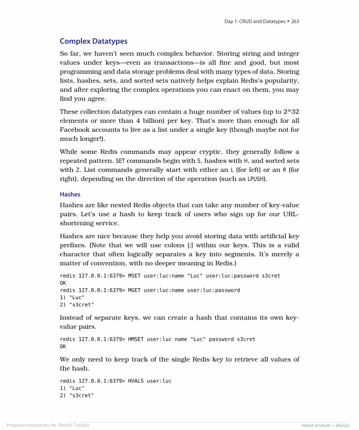
Complex DatatypesSo far, we haven’t seen much complex behavior. Storing string and integervalues under keys—even as transactions—is all fine and good, but mostprogramming and data storage problems deal with many types of data. Storinglists, hashes, sets, and sorted sets natively helps explain Redis’s popularity,and after exploring the complex operations you can enact on them, you mayfind you agree.
These collection datatypes can contain a huge number of values (up to 2^32elements or more than 4 billion) per key. That’s more than enough for allFacebook accounts to live as a list under a single key (though maybe not formuch longer!).
While some Redis commands may appear cryptic, they generally follow arepeated pattern. SET commands begin with S, hashes with H, and sorted setswith Z. List commands generally start with either an L (for left) or an R (forright), depending on the direction of the operation (such as LPUSH).
Hashes
Hashes are like nested Redis objects that can take any number of key-valuepairs. Let’s use a hash to keep track of users who sign up for our URL-shortening service.
Hashes are nice because they help you avoid storing data with artificial keyprefixes. (Note that we will use colons [:] within our keys. This is a validcharacter that often logically separates a key into segments. It’s merely amatter of convention, with no deeper meaning in Redis.)
redis 127.0.0.1:6379> MSET user:luc:name "Luc" user:luc:password s3cretOKredis 127.0.0.1:6379> MGET user:luc:name user:luc:password1) "Luc"2) "s3cret"
Instead of separate keys, we can create a hash that contains its own key-value pairs.
redis 127.0.0.1:6379> HMSET user:luc name "Luc" password s3cretOK
We only need to keep track of the single Redis key to retrieve all values ofthe hash.
redis 127.0.0.1:6379> HVALS user:luc1) "Luc"2) "s3cret"
report erratum • discuss
Day 1: CRUD and Datatypes • 263
Prepared exclusively for Shohei Tanaka
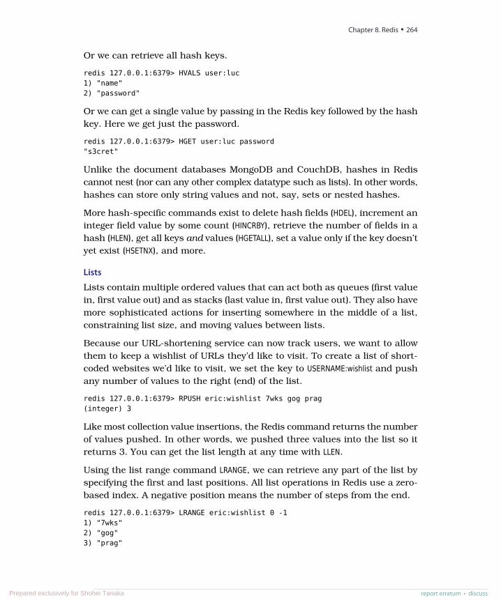
Or we can retrieve all hash keys.
redis 127.0.0.1:6379> HVALS user:luc1) "name"2) "password"
Or we can get a single value by passing in the Redis key followed by the hashkey. Here we get just the password.
redis 127.0.0.1:6379> HGET user:luc password"s3cret"
Unlike the document databases MongoDB and CouchDB, hashes in Rediscannot nest (nor can any other complex datatype such as lists). In other words,hashes can store only string values and not, say, sets or nested hashes.
More hash-specific commands exist to delete hash fields (HDEL), increment aninteger field value by some count (HINCRBY), retrieve the number of fields in ahash (HLEN), get all keys and values (HGETALL), set a value only if the key doesn’tyet exist (HSETNX), and more.
Lists
Lists contain multiple ordered values that can act both as queues (first valuein, first value out) and as stacks (last value in, first value out). They also havemore sophisticated actions for inserting somewhere in the middle of a list,constraining list size, and moving values between lists.
Because our URL-shortening service can now track users, we want to allowthem to keep a wishlist of URLs they’d like to visit. To create a list of short-coded websites we’d like to visit, we set the key to USERNAME:wishlist and pushany number of values to the right (end) of the list.
redis 127.0.0.1:6379> RPUSH eric:wishlist 7wks gog prag(integer) 3
Like most collection value insertions, the Redis command returns the numberof values pushed. In other words, we pushed three values into the list so itreturns 3. You can get the list length at any time with LLEN.
Using the list range command LRANGE, we can retrieve any part of the list byspecifying the first and last positions. All list operations in Redis use a zero-based index. A negative position means the number of steps from the end.
redis 127.0.0.1:6379> LRANGE eric:wishlist 0 -11) "7wks"2) "gog"3) "prag"
Chapter 8. Redis • 264
report erratum • discussPrepared exclusively for Shohei Tanaka
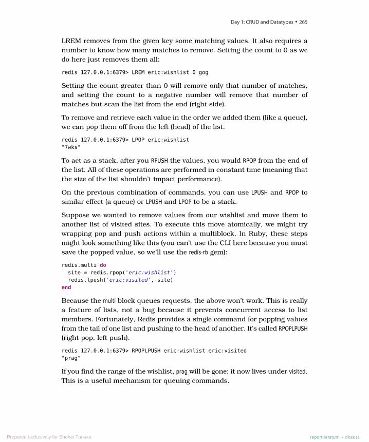
LREM removes from the given key some matching values. It also requires anumber to know how many matches to remove. Setting the count to 0 as wedo here just removes them all:
redis 127.0.0.1:6379> LREM eric:wishlist 0 gog
Setting the count greater than 0 will remove only that number of matches,and setting the count to a negative number will remove that number ofmatches but scan the list from the end (right side).
To remove and retrieve each value in the order we added them (like a queue),we can pop them off from the left (head) of the list.
redis 127.0.0.1:6379> LPOP eric:wishlist"7wks"
To act as a stack, after you RPUSH the values, you would RPOP from the end ofthe list. All of these operations are performed in constant time (meaning thatthe size of the list shouldn’t impact performance).
On the previous combination of commands, you can use LPUSH and RPOP tosimilar effect (a queue) or LPUSH and LPOP to be a stack.
Suppose we wanted to remove values from our wishlist and move them toanother list of visited sites. To execute this move atomically, we might trywrapping pop and push actions within a multiblock. In Ruby, these stepsmight look something like this (you can’t use the CLI here because you mustsave the popped value, so we’ll use the redis-rb gem):
redis.multi dosite = redis.rpop('eric:wishlist')redis.lpush('eric:visited', site)
end
Because the multi block queues requests, the above won’t work. This is reallya feature of lists, not a bug because it prevents concurrent access to listmembers. Fortunately, Redis provides a single command for popping valuesfrom the tail of one list and pushing to the head of another. It’s called RPOPLPUSH(right pop, left push).
redis 127.0.0.1:6379> RPOPLPUSH eric:wishlist eric:visited"prag"
If you find the range of the wishlist, prag will be gone; it now lives under visited.This is a useful mechanism for queuing commands.
report erratum • discuss
Day 1: CRUD and Datatypes • 265
Prepared exclusively for Shohei Tanaka
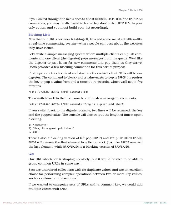
If you looked through the Redis docs to find RPOPRPUSH, LPOPLPUSH, and LPOPRPUSHcommands, you may be dismayed to learn they don’t exist. RPOPLPUSH is youronly option, and you must build your list accordingly.
Blocking Lists
Now that our URL shortener is taking off, let’s add some social activities—likea real-time commenting system—where people can post about the websitesthey have visited.
Let’s write a simple messaging system where multiple clients can push com-ments and one client (the digester) pops messages from the queue. We’d likethe digester to just listen for new comments and pop them as they arrive.Redis provides a few blocking commands for this sort of purpose.
First, open another terminal and start another redis-cli client. This will be ourdigester. The command to block until a value exists to pop is BRPOP. It requiresthe key to pop a value from and a timeout in seconds, which we’ll set to fiveminutes.
redis 127.0.0.1:6379> BRPOP comments 300
Then switch back to the first console and push a message to comments.
redis 127.0.0.1:6379> LPUSH comments "Prag is a great publisher!"
If you switch back to the digester console, two lines will be returned: the keyand the popped value. The console will also output the length of time it spentblocking.
1) "comments"2) "Prag is a great publisher!"(7.88s)
There’s also a blocking version of left pop (BLPOP) and left push (BRPOPLPUSH).BLPOP will remove the first element in a list or block (just like BRPOP removedthe last element) while BRPOPLPUSH is a blocking version of RPOPLPUSH.
Sets
Our URL shortener is shaping up nicely, but it would be nice to be able togroup common URLs in some way.
Sets are unordered collections with no duplicate values and are an excellentchoice for performing complex operations between two or more key values,such as unions or intersections.
If we wanted to categorize sets of URLs with a common key, we could addmultiple values with SADD.
Chapter 8. Redis • 266
report erratum • discussPrepared exclusively for Shohei Tanaka
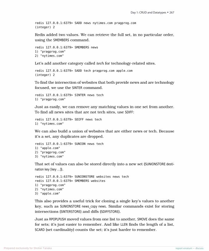
redis 127.0.0.1:6379> SADD news nytimes.com pragprog.com(integer) 2
Redis added two values. We can retrieve the full set, in no particular order,using the SMEMBERS command.
redis 127.0.0.1:6379> SMEMBERS news1) "pragprog.com"2) "nytimes.com"
Let’s add another category called tech for technology-related sites.
redis 127.0.0.1:6379> SADD tech pragprog.com apple.com(integer) 2
To find the intersection of websites that both provide news and are technologyfocused, we use the SINTER command.
redis 127.0.0.1:6379> SINTER news tech1) "pragprog.com"
Just as easily, we can remove any matching values in one set from another.To find all news sites that are not tech sites, use SDIFF:
redis 127.0.0.1:6379> SDIFF news tech1) "nytimes.com"
We can also build a union of websites that are either news or tech. Becauseit’s a set, any duplicates are dropped.
redis 127.0.0.1:6379> SUNION news tech1) "apple.com"2) "pragprog.com"3) "nytimes.com"
That set of values can also be stored directly into a new set (SUNIONSTORE desti-nation key [key ...]).
redis 127.0.0.1:6379> SUNIONSTORE websites news techredis 127.0.0.1:6379> SMEMBERS websites1) "pragprog.com"2) "nytimes.com"3) "apple.com"
This also provides a useful trick for cloning a single key’s values to anotherkey, such as SUNIONSTORE news_copy news. Similar commands exist for storingintersections (SINTERSTORE) and diffs (SDIFFSTORE).
Just as RPOPLPUSH moved values from one list to another, SMOVE does the samefor sets; it’s just easier to remember. And like LLEN finds the length of a list,SCARD (set cardinality) counts the set; it’s just harder to remember.
report erratum • discuss
Day 1: CRUD and Datatypes • 267
Prepared exclusively for Shohei Tanaka
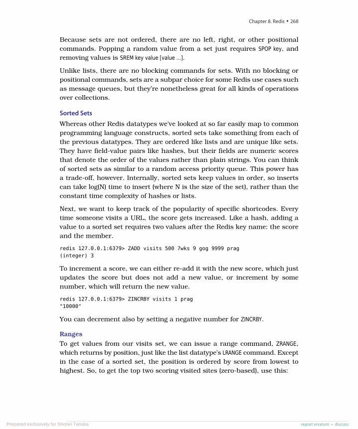
Because sets are not ordered, there are no left, right, or other positionalcommands. Popping a random value from a set just requires SPOP key, andremoving values is SREM key value [value ...].
Unlike lists, there are no blocking commands for sets. With no blocking orpositional commands, sets are a subpar choice for some Redis use cases suchas message queues, but they’re nonetheless great for all kinds of operationsover collections.
Sorted Sets
Whereas other Redis datatypes we’ve looked at so far easily map to commonprogramming language constructs, sorted sets take something from each ofthe previous datatypes. They are ordered like lists and are unique like sets.They have field-value pairs like hashes, but their fields are numeric scoresthat denote the order of the values rather than plain strings. You can thinkof sorted sets as similar to a random access priority queue. This power hasa trade-off, however. Internally, sorted sets keep values in order, so insertscan take log(N) time to insert (where N is the size of the set), rather than theconstant time complexity of hashes or lists.
Next, we want to keep track of the popularity of specific shortcodes. Everytime someone visits a URL, the score gets increased. Like a hash, adding avalue to a sorted set requires two values after the Redis key name: the scoreand the member.
redis 127.0.0.1:6379> ZADD visits 500 7wks 9 gog 9999 prag(integer) 3
To increment a score, we can either re-add it with the new score, which justupdates the score but does not add a new value, or increment by somenumber, which will return the new value.
redis 127.0.0.1:6379> ZINCRBY visits 1 prag"10000"
You can decrement also by setting a negative number for ZINCRBY.
Ranges
To get values from our visits set, we can issue a range command, ZRANGE,which returns by position, just like the list datatype’s LRANGE command. Exceptin the case of a sorted set, the position is ordered by score from lowest tohighest. So, to get the top two scoring visited sites (zero-based), use this:
Chapter 8. Redis • 268
report erratum • discussPrepared exclusively for Shohei Tanaka
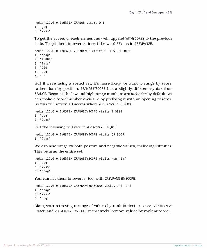
redis 127.0.0.1:6379> ZRANGE visits 0 11) "gog"2) "7wks"
To get the scores of each element as well, append WITHSCORES to the previouscode. To get them in reverse, insert the word REV, as in ZREVRANGE.
redis 127.0.0.1:6379> ZREVRANGE visits 0 -1 WITHSCORES1) "prag"2) "10000"3) "7wks"4) "500"5) "gog"6) "9"
But if we’re using a sorted set, it’s more likely we want to range by score,rather than by position. ZRANGEBYSCORE has a slightly different syntax fromZRANGE. Because the low and high range numbers are inclusive by default, wecan make a score number exclusive by prefixing it with an opening paren: (.So this will return all scores where 9 <= score <= 10,000:
redis 127.0.0.1:6379> ZRANGEBYSCORE visits 9 99991) "gog"2) "7wks"
But the following will return 9 < score <= 10,000:
redis 127.0.0.1:6379> ZRANGEBYSCORE visits (9 99991) "7wks"
We can also range by both positive and negative values, including infinities.This returns the entire set.
redis 127.0.0.1:6379> ZRANGEBYSCORE visits -inf inf1) "gog"2) "7wks"3) "prag"
You can list them in reverse, too, with ZREVRANGEBYSCORE.
redis 127.0.0.1:6379> ZREVRANGEBYSCORE visits inf -inf1) "prag"2) "7wks"3) "gog"
Along with retrieving a range of values by rank (index) or score, ZREMRANGE-BYRANK and ZREMRANGEBYSCORE, respectively, remove values by rank or score.
report erratum • discuss
Day 1: CRUD and Datatypes • 269
Prepared exclusively for Shohei Tanaka
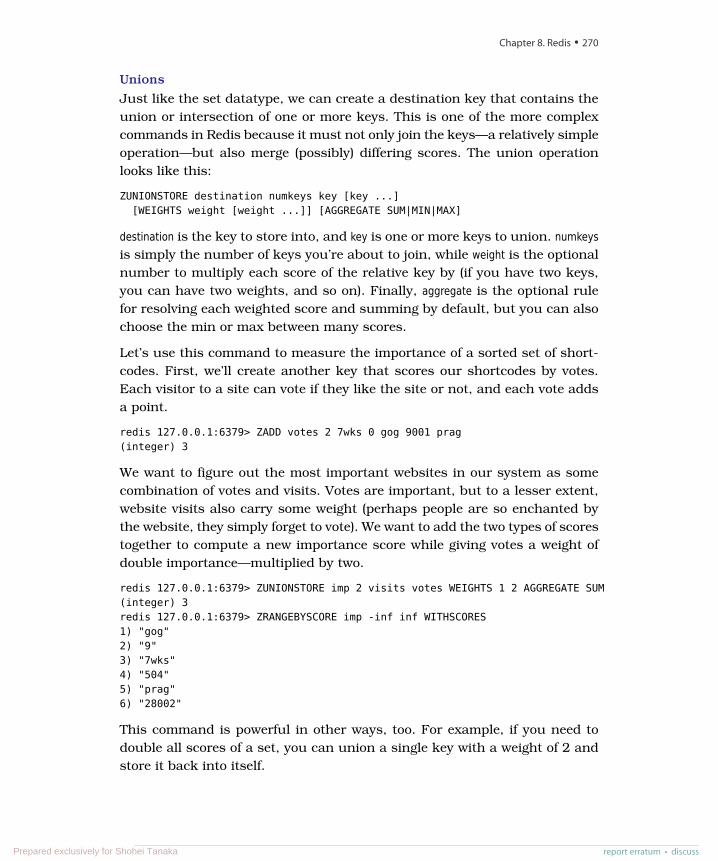
Unions
Just like the set datatype, we can create a destination key that contains theunion or intersection of one or more keys. This is one of the more complexcommands in Redis because it must not only join the keys—a relatively simpleoperation—but also merge (possibly) differing scores. The union operationlooks like this:
ZUNIONSTORE destination numkeys key [key ...][WEIGHTS weight [weight ...]] [AGGREGATE SUM|MIN|MAX]
destination is the key to store into, and key is one or more keys to union. numkeysis simply the number of keys you’re about to join, while weight is the optionalnumber to multiply each score of the relative key by (if you have two keys,you can have two weights, and so on). Finally, aggregate is the optional rulefor resolving each weighted score and summing by default, but you can alsochoose the min or max between many scores.
Let’s use this command to measure the importance of a sorted set of short-codes. First, we’ll create another key that scores our shortcodes by votes.Each visitor to a site can vote if they like the site or not, and each vote addsa point.
redis 127.0.0.1:6379> ZADD votes 2 7wks 0 gog 9001 prag(integer) 3
We want to figure out the most important websites in our system as somecombination of votes and visits. Votes are important, but to a lesser extent,website visits also carry some weight (perhaps people are so enchanted bythe website, they simply forget to vote). We want to add the two types of scorestogether to compute a new importance score while giving votes a weight ofdouble importance—multiplied by two.
redis 127.0.0.1:6379> ZUNIONSTORE imp 2 visits votes WEIGHTS 1 2 AGGREGATE SUM(integer) 3redis 127.0.0.1:6379> ZRANGEBYSCORE imp -inf inf WITHSCORES1) "gog"2) "9"3) "7wks"4) "504"5) "prag"6) "28002"
This command is powerful in other ways, too. For example, if you need todouble all scores of a set, you can union a single key with a weight of 2 andstore it back into itself.
Chapter 8. Redis • 270
report erratum • discussPrepared exclusively for Shohei Tanaka
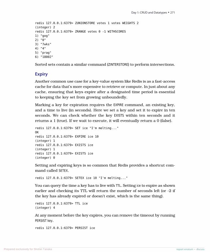
redis 127.0.0.1:6379> ZUNIONSTORE votes 1 votes WEIGHTS 2(integer) 2redis 127.0.0.1:6379> ZRANGE votes 0 -1 WITHSCORES1) "gog"2) "0"3) "7wks"4) "4"5) "prag"6) "18002"
Sorted sets contain a similar command (ZINTERSTORE) to perform intersections.
ExpiryAnother common use case for a key-value system like Redis is as a fast-accesscache for data that’s more expensive to retrieve or compute. In just about anycache, ensuring that keys expire after a designated time period is essentialto keeping the key set from growing unboundedly.
Marking a key for expiration requires the EXPIRE command, an existing key,and a time to live (in seconds). Here we set a key and set it to expire in tenseconds. We can check whether the key EXISTS within ten seconds and itreturns a 1 (true). If we wait to execute, it will eventually return a 0 (false).
redis 127.0.0.1:6379> SET ice "I'm melting..."OKredis 127.0.0.1:6379> EXPIRE ice 10(integer) 1redis 127.0.0.1:6379> EXISTS ice(integer) 1redis 127.0.0.1:6379> EXISTS ice(integer) 0
Setting and expiring keys is so common that Redis provides a shortcut com-mand called SETEX.
redis 127.0.0.1:6379> SETEX ice 10 "I'm melting..."
You can query the time a key has to live with TTL. Setting ice to expire as shownearlier and checking its TTL will return the number of seconds left (or -2 ifthe key has already expired or doesn’t exist, which is the same thing).
redis 127.0.0.1:6379> TTL ice(integer) 4
At any moment before the key expires, you can remove the timeout by runningPERSIST key.
redis 127.0.0.1:6379> PERSIST ice
report erratum • discuss
Day 1: CRUD and Datatypes • 271
Prepared exclusively for Shohei Tanaka
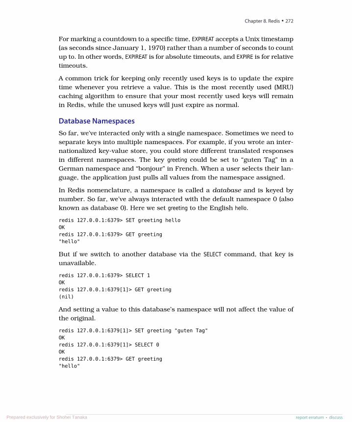
For marking a countdown to a specific time, EXPIREAT accepts a Unix timestamp(as seconds since January 1, 1970) rather than a number of seconds to countup to. In other words, EXPIREAT is for absolute timeouts, and EXPIRE is for relativetimeouts.
A common trick for keeping only recently used keys is to update the expiretime whenever you retrieve a value. This is the most recently used (MRU)caching algorithm to ensure that your most recently used keys will remainin Redis, while the unused keys will just expire as normal.
Database NamespacesSo far, we’ve interacted only with a single namespace. Sometimes we need toseparate keys into multiple namespaces. For example, if you wrote an inter-nationalized key-value store, you could store different translated responsesin different namespaces. The key greeting could be set to “guten Tag” in aGerman namespace and “bonjour” in French. When a user selects their lan-guage, the application just pulls all values from the namespace assigned.
In Redis nomenclature, a namespace is called a database and is keyed bynumber. So far, we’ve always interacted with the default namespace 0 (alsoknown as database 0). Here we set greeting to the English hello.
redis 127.0.0.1:6379> SET greeting helloOKredis 127.0.0.1:6379> GET greeting"hello"
But if we switch to another database via the SELECT command, that key isunavailable.
redis 127.0.0.1:6379> SELECT 1OKredis 127.0.0.1:6379[1]> GET greeting(nil)
And setting a value to this database’s namespace will not affect the value ofthe original.
redis 127.0.0.1:6379[1]> SET greeting "guten Tag"OKredis 127.0.0.1:6379[1]> SELECT 0OKredis 127.0.0.1:6379> GET greeting"hello"
Chapter 8. Redis • 272
report erratum • discussPrepared exclusively for Shohei Tanaka
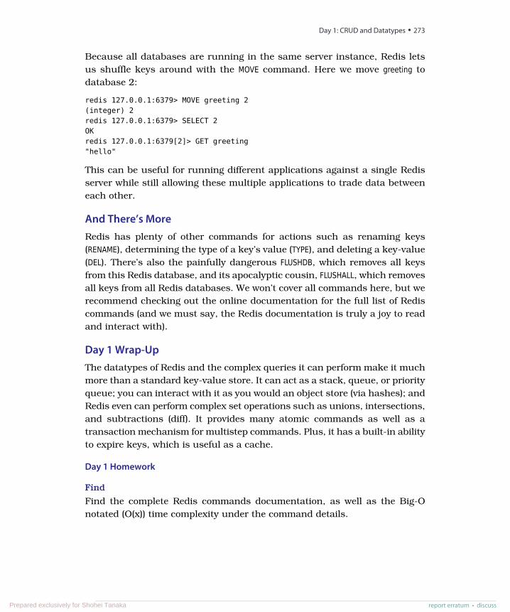
Because all databases are running in the same server instance, Redis letsus shuffle keys around with the MOVE command. Here we move greeting todatabase 2:
redis 127.0.0.1:6379> MOVE greeting 2(integer) 2redis 127.0.0.1:6379> SELECT 2OKredis 127.0.0.1:6379[2]> GET greeting"hello"
This can be useful for running different applications against a single Redisserver while still allowing these multiple applications to trade data betweeneach other.
And There’s MoreRedis has plenty of other commands for actions such as renaming keys(RENAME), determining the type of a key’s value (TYPE), and deleting a key-value(DEL). There’s also the painfully dangerous FLUSHDB, which removes all keysfrom this Redis database, and its apocalyptic cousin, FLUSHALL, which removesall keys from all Redis databases. We won’t cover all commands here, but werecommend checking out the online documentation for the full list of Rediscommands (and we must say, the Redis documentation is truly a joy to readand interact with).
Day 1 Wrap-UpThe datatypes of Redis and the complex queries it can perform make it muchmore than a standard key-value store. It can act as a stack, queue, or priorityqueue; you can interact with it as you would an object store (via hashes); andRedis even can perform complex set operations such as unions, intersections,and subtractions (diff). It provides many atomic commands as well as atransaction mechanism for multistep commands. Plus, it has a built-in abilityto expire keys, which is useful as a cache.
Day 1 Homework
Find
Find the complete Redis commands documentation, as well as the Big-Onotated (O(x)) time complexity under the command details.
report erratum • discuss
Day 1: CRUD and Datatypes • 273
Prepared exclusively for Shohei Tanaka

Do
1. Install your favorite programming language driver and connect to theRedis server. Insert and increment a value within a transaction.
2. Using your driver of choice, create a program that reads a blocking listand outputs somewhere (console, file, Socket.io, and so on) and anotherthat writes to the same list.
Day 2: Advanced Usage, DistributionDay 1 introduced us to Redis as a data structure server. Today, we’ll buildon that foundation by looking at some of the advanced functions provided byRedis, such as pipelining, the publish-subscribe model, system configuration,and replication. Beyond that, we’ll look at how to create a Redis cluster, storea lot of data quickly, and use an advanced technique involving Bloom filters.
A Simple InterfaceAt 80,000 lines of source code, Redis is a fairly small project compared tomost databases. But beyond code size, it has a simple interface that acceptsthe very strings we have been writing in the console.
Telnet
We can interact without the command-line interface by streaming commandsthrough TCP on our own via telnet and terminating the command with acarriage return line feed (CRLF, or \r\n). Run Ctrl+ ] at any time to exit.
redis/telnet.sh$ telnet localhost 6379Trying 127.0.0.1...Connected to localhost.Escape character is '^]'.SET test hello+OKGET test
Chapter 8. Redis • 274
report erratum • discussPrepared exclusively for Shohei Tanaka
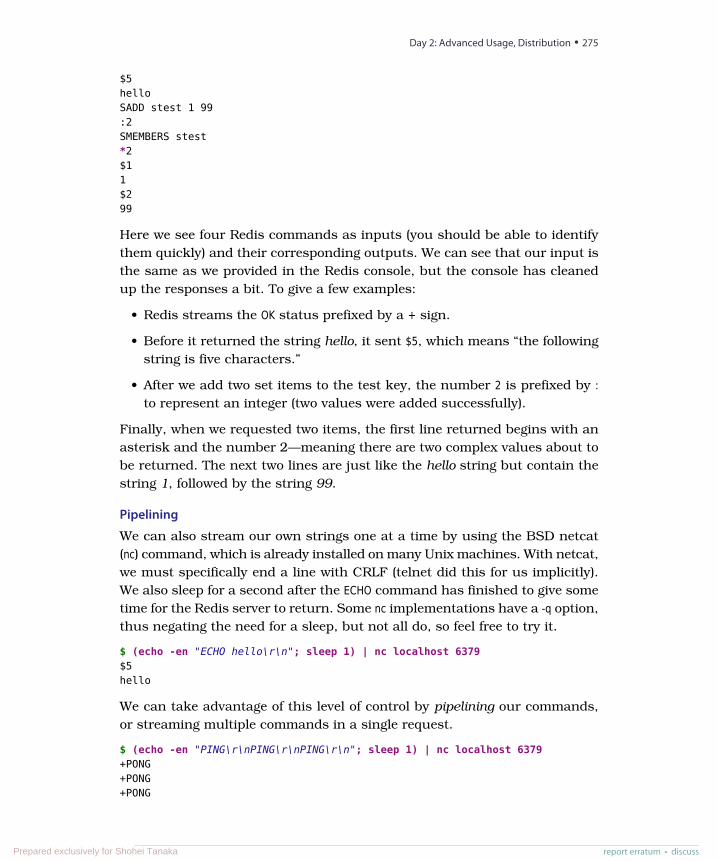
$5helloSADD stest 1 99:2SMEMBERS stest*2$11$299
Here we see four Redis commands as inputs (you should be able to identifythem quickly) and their corresponding outputs. We can see that our input isthe same as we provided in the Redis console, but the console has cleanedup the responses a bit. To give a few examples:
• Redis streams the OK status prefixed by a + sign.
• Before it returned the string hello, it sent $5, which means “the followingstring is five characters.”
• After we add two set items to the test key, the number 2 is prefixed by :to represent an integer (two values were added successfully).
Finally, when we requested two items, the first line returned begins with anasterisk and the number 2—meaning there are two complex values about tobe returned. The next two lines are just like the hello string but contain thestring 1, followed by the string 99.
Pipelining
We can also stream our own strings one at a time by using the BSD netcat(nc) command, which is already installed on many Unix machines. With netcat,we must specifically end a line with CRLF (telnet did this for us implicitly).We also sleep for a second after the ECHO command has finished to give sometime for the Redis server to return. Some nc implementations have a -q option,thus negating the need for a sleep, but not all do, so feel free to try it.
$ (echo -en "ECHO hello\r\n"; sleep 1) | nc localhost 6379$5hello
We can take advantage of this level of control by pipelining our commands,or streaming multiple commands in a single request.
$ (echo -en "PING\r\nPING\r\nPING\r\n"; sleep 1) | nc localhost 6379+PONG+PONG+PONG
report erratum • discuss
Day 2: Advanced Usage, Distribution • 275
Prepared exclusively for Shohei Tanaka
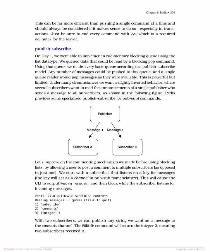
This can be far more efficient than pushing a single command at a time andshould always be considered if it makes sense to do so—especially in trans-actions. Just be sure to end every command with \r\n, which is a requireddelimiter for the server.
publish-subscribeOn Day 1, we were able to implement a rudimentary blocking queue using thelist datatype. We queued data that could be read by a blocking pop command.Using that queue, we made a very basic queue according to a publish-subscribemodel. Any number of messages could be pushed to this queue, and a singlequeue reader would pop messages as they were available. This is powerful butlimited. Under many circumstances we want a slightly inverted behavior, whereseveral subscribers want to read the announcements of a single publisher whosends a message to all subscribers, as shown in the following figure. Redisprovides some specialized publish-subscribe (or pub-sub) commands.
Publisher
Subscriber A Subscriber B
Message 1 Message 1
Let’s improve on the commenting mechanism we made before using blockinglists, by allowing a user to post a comment to multiple subscribers (as opposedto just one). We start with a subscriber that listens on a key for messages(the key will act as a channel in pub-sub nomenclature). This will cause theCLI to output Reading messages... and then block while the subscriber listens forincoming messages.
redis 127.0.0.1:6379> SUBSCRIBE commentsReading messages... (press Ctrl-C to quit)1) "subscribe"2) "comments"3) (integer) 1
With two subscribers, we can publish any string we want as a message tothe comments channel. The PUBLISH command will return the integer 2, meaningtwo subscribers received it.
Chapter 8. Redis • 276
report erratum • discussPrepared exclusively for Shohei Tanaka
redis 127.0.0.1:6379> PUBLISH comments "Check out this shortcoded site! 7wks"(integer) 2
Both of the subscribers will receive a multibulk reply (a list) of three items:the string “message,” the channel name, and the published message value.
1) "message"2) "comments"3) "Check out this shortcoded site! 7wks"
When your clients no longer want to receive correspondence, they can executethe UNSUBSCRIBE comments command to disconnect from the comments channelor simply UNSUBSCRIBE alone to disconnect from all channels. However, notethat in the redis-cli console you will have to press Ctrl+C to break the connection.
Server InfoBefore getting into changing Redis’s system settings, it’s worth taking a quicklook at the INFO command because changing settings values will alter someof these values as well. INFO outputs a list of server data, including version,process ID, memory used, and uptime.
redis 127.0.0.1:6379> INFO# Serverredis_version:3.2.8redis_git_sha1:00000000redis_git_dirty:0redis_build_id:b533f811ec736a0credis_mode:standalone...
You may want to revisit this command again in this chapter because it pro-vides a useful snapshot of this server’s global information and settings. Iteven provides information on durability, memory fragmentation, and replica-tion server status.
Redis ConfigurationSo far, we’ve only used Redis with its out-of-the-box configuration. But muchof Redis’s power comes from its configurability, allowing you to tailor settingsto your use case. The redis.conf file that comes with the distribution—found in/etc/redis on *nix systems or /usr/local/etc on Mac OS—is fairly self-explanatory,so we’re going to cover only a portion of the file. We’ll go through a few of thecommon settings in order.
report erratum • discuss
Day 2: Advanced Usage, Distribution • 277
Prepared exclusively for Shohei Tanaka
daemonize noport 6379loglevel verboselogfile stdoutdatabase 16
By default, daemonize is set to no, which is why the server always starts up inthe foreground. This is nice for testing but not very production friendly.Changing this value to yes will run the server in the background while settingthe server’s process ID in a pid file.
The next line is the default port number for this server, port 6379. This canbe especially useful when running multiple Redis servers on a single machine.
loglevel defaults to verbose, but it’s good to set it to notice or warning in productionto cut down on the number of log events. logfile outputs to stdout (standardoutput, the console), but a filename is necessary if you run in daemonize mode.
database sets the number of Redis databases we have available. We saw howto switch between databases. If you plan to only ever use a single databasenamespace, it’s not a bad idea to set this to 1 to prevent unwanted databasesfrom being accidentally created.
Durability
Redis has a few persistence options. First is no persistence at all, which willsimply keep all values in main memory. If you’re running a basic cachingserver, this is a reasonable choice since durability always increases latency.
One of the things that sets Redis apart from other fast-access caches likememcached2 is its built-in support for storing values to disk. By default, key-value pairs are only occasionally saved. You can run the LASTSAVE commandto get a Unix timestamp of the last time a Redis disk write succeeded, or youcan read the last_save_time field from the server INFO output.
You can force durability by executing the SAVE command (or BGSAVE, to asyn-chronously save in the background).
redis 127.0.0.1:6379> SAVE
If you read the redis-server log, you will see lines similar to this:
[46421] 10 Oct 19:11:50 * Background saving started by pid 52123[52123] 10 Oct 19:11:50 * DB saved on disk[46421] 10 Oct 19:11:50 * Background saving terminated with success
2. http://www.memcached.org/
Chapter 8. Redis • 278
report erratum • discussPrepared exclusively for Shohei Tanaka
Another durability method is to alter the snapshotting settings in the config-uration file.
Snapshotting
We can alter the rate of storage to disk by adding, removing, or altering oneof the save fields. By default, there are three, prefixed by the save keywordfollowed by a time in seconds and a minimum number of keys that mustchange before a write to disk occurs. For example, to trigger a save every 5minutes (300 seconds) if any keys change at all, you would write the following:
save 300 1
The configuration has a good set of defaults. The set means if 10,000 keyschange, save in 60 seconds; if 10 keys change, save in 300 seconds, and anykey changes will be saved in at least 900 seconds (15 minutes).
save 900 1save 300 10save 60 10000
You can add as many or as few save lines as necessary to specify precisethresholds.
Append-Only File
Redis is eventually durable by default, in that it asynchronously writes valuesto disk in intervals defined by our save settings, or it is forced to write byclient-initiated commands. This is acceptable for a second-level cache orsession server but is insufficient for storing data that you need to be durable,like financial data. If a Redis server crashes, our users might not appreciatehaving lost money.
Redis provides an append-only file (appendonly.aof) that keeps a record of allwrite commands. This is like the write-ahead logging we saw in Chapter 3,HBase, on page 53. If the server crashes before a value is saved, it executesthe commands on startup, restoring its state; appendonly must be enabled bysetting it to yes in the redis.conf file.
appendonly yes
Then we must decide how often a command is appended to the file. Settingalways is the more durable because every command is saved. It’s also slow,which often negates the reason people have for using Redis. By default,everysec is enabled, which saves up and writes commands only once a second.This is a decent trade-off because it’s fast enough, and worst case you’ll loseonly the last one second of data. Finally, no is an option, which just lets the
report erratum • discuss
Day 2: Advanced Usage, Distribution • 279
Prepared exclusively for Shohei Tanaka

OS handle flushing. It can be fairly infrequent, and you’re often better offskipping the append-only file altogether rather than choosing it.
# appendfsync alwaysappendfsync everysec# appendfsync no
Append-only has more detailed parameters, which may be worth readingabout in the config file when you need to respond to specific production issues.
Security
Although Redis is not natively built to be a fully secure server, you may runacross the requirepass setting and AUTH command in the Redis documentation.These can be safely ignored because they are merely a scheme for setting aplaintext password. Because a client can try nearly 100,000 passwords asecond, it’s almost a moot point, beyond the fact that plaintext passwordsare inherently unsafe anyway. If you want Redis security, you’re better offwith a good firewall and SSH security.
Interestingly, Redis provides command-level security through obscurity, byallowing you to hide or suppress commands. Adding this to your config willrename the FLUSHALL command (remove all keys from the system) into somehard-to-guess value like c283d93ac9528f986023793b411e4ba2:
rename-command FLUSHALL c283d93ac9528f986023793b411e4ba2
If you attempt to execute FLUSHALL against this server, you’ll be hit with anerror. The secret command works instead.
redis 127.0.0.1:6379> FLUSHALL(error) ERR unknown command 'FLUSHALL'redis 127.0.0.1:6379> c283d93ac9528f986023793b411e4ba2OK
Or better yet, we can disable the command entirely by setting it to a blankstring in the configuration.
rename-command FLUSHALL ""
You can set any number of commands to a blank string, allowing you amodicum of customization over your command environment.
Tweaking Parameters
There are several more advanced settings for speeding up slow query logs,encoding details, making latency tweaks, and importing external config files.Keep in mind, though, if you run across some documentation about Redisvirtual memory, simply ignore it, as that feature was removed in version 2.6.
Chapter 8. Redis • 280
report erratum • discussPrepared exclusively for Shohei Tanaka
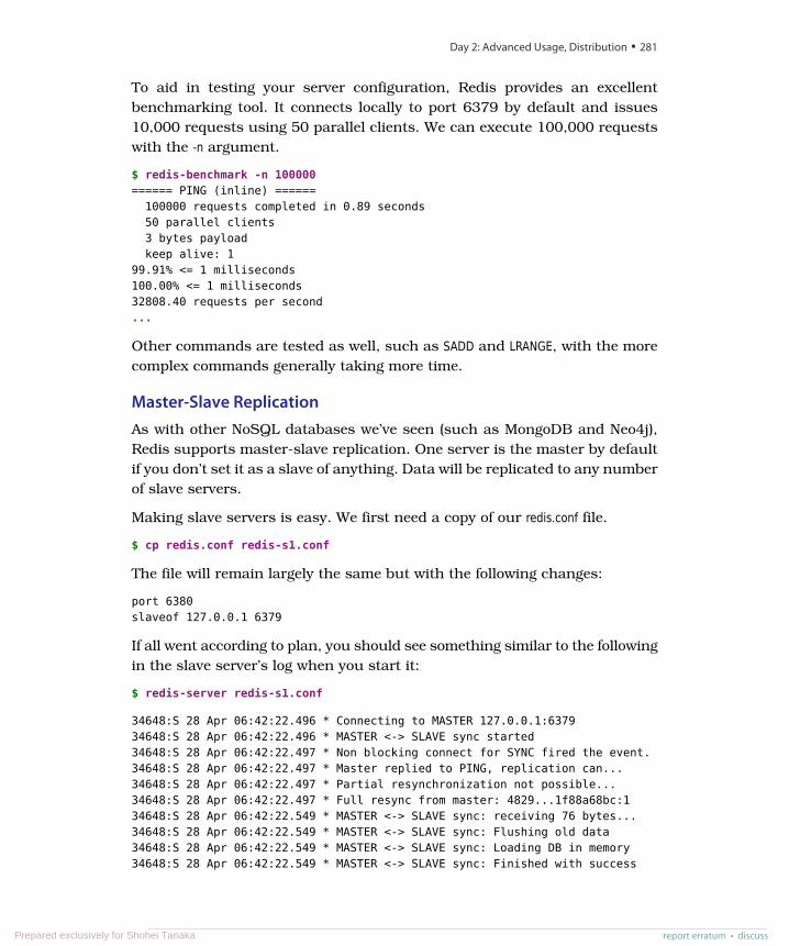
To aid in testing your server configuration, Redis provides an excellentbenchmarking tool. It connects locally to port 6379 by default and issues10,000 requests using 50 parallel clients. We can execute 100,000 requestswith the -n argument.
$ redis-benchmark -n 100000====== PING (inline) ======
100000 requests completed in 0.89 seconds50 parallel clients3 bytes payloadkeep alive: 1
99.91% <= 1 milliseconds100.00% <= 1 milliseconds32808.40 requests per second...
Other commands are tested as well, such as SADD and LRANGE, with the morecomplex commands generally taking more time.
Master-Slave ReplicationAs with other NoSQL databases we’ve seen (such as MongoDB and Neo4j),Redis supports master-slave replication. One server is the master by defaultif you don’t set it as a slave of anything. Data will be replicated to any numberof slave servers.
Making slave servers is easy. We first need a copy of our redis.conf file.
$ cp redis.conf redis-s1.conf
The file will remain largely the same but with the following changes:
port 6380slaveof 127.0.0.1 6379
If all went according to plan, you should see something similar to the followingin the slave server’s log when you start it:
$ redis-server redis-s1.conf
34648:S 28 Apr 06:42:22.496 * Connecting to MASTER 127.0.0.1:637934648:S 28 Apr 06:42:22.496 * MASTER <-> SLAVE sync started34648:S 28 Apr 06:42:22.497 * Non blocking connect for SYNC fired the event.34648:S 28 Apr 06:42:22.497 * Master replied to PING, replication can...34648:S 28 Apr 06:42:22.497 * Partial resynchronization not possible...34648:S 28 Apr 06:42:22.497 * Full resync from master: 4829...1f88a68bc:134648:S 28 Apr 06:42:22.549 * MASTER <-> SLAVE sync: receiving 76 bytes...34648:S 28 Apr 06:42:22.549 * MASTER <-> SLAVE sync: Flushing old data34648:S 28 Apr 06:42:22.549 * MASTER <-> SLAVE sync: Loading DB in memory34648:S 28 Apr 06:42:22.549 * MASTER <-> SLAVE sync: Finished with success
report erratum • discuss
Day 2: Advanced Usage, Distribution • 281
Prepared exclusively for Shohei Tanaka
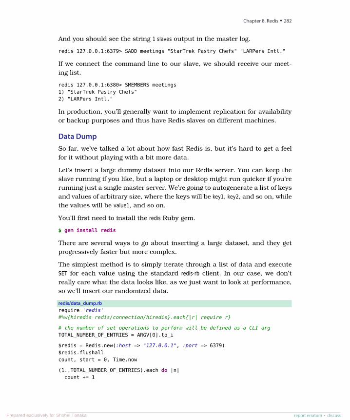
And you should see the string 1 slaves output in the master log.
redis 127.0.0.1:6379> SADD meetings "StarTrek Pastry Chefs" "LARPers Intl."
If we connect the command line to our slave, we should receive our meet-ing list.
redis 127.0.0.1:6380> SMEMBERS meetings1) "StarTrek Pastry Chefs"2) "LARPers Intl."
In production, you’ll generally want to implement replication for availabilityor backup purposes and thus have Redis slaves on different machines.
Data DumpSo far, we’ve talked a lot about how fast Redis is, but it’s hard to get a feelfor it without playing with a bit more data.
Let’s insert a large dummy dataset into our Redis server. You can keep theslave running if you like, but a laptop or desktop might run quicker if you’rerunning just a single master server. We’re going to autogenerate a list of keysand values of arbitrary size, where the keys will be key1, key2, and so on, whilethe values will be value1, and so on.
You’ll first need to install the redis Ruby gem.
$ gem install redis
There are several ways to go about inserting a large dataset, and they getprogressively faster but more complex.
The simplest method is to simply iterate through a list of data and executeSET for each value using the standard redis-rb client. In our case, we don’treally care what the data looks like, as we just want to look at performance,so we’ll insert our randomized data.
redis/data_dump.rbrequire 'redis'#%w{hiredis redis/connection/hiredis}.each{|r| require r}
# the number of set operations to perform will be defined as a CLI argTOTAL_NUMBER_OF_ENTRIES = ARGV[0].to_i
$redis = Redis.new(:host => "127.0.0.1", :port => 6379)$redis.flushallcount, start = 0, Time.now
(1..TOTAL_NUMBER_OF_ENTRIES).each do |n|count += 1
Chapter 8. Redis • 282
report erratum • discussPrepared exclusively for Shohei Tanaka
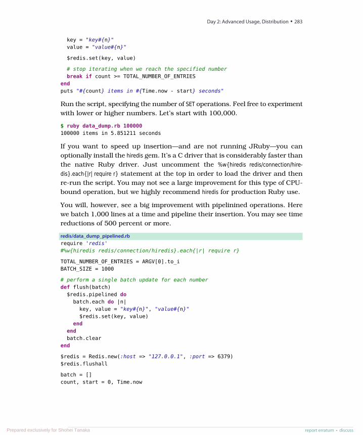
key = "key#{n}"value = "value#{n}"
$redis.set(key, value)
# stop iterating when we reach the specified numberbreak if count >= TOTAL_NUMBER_OF_ENTRIES
endputs "#{count} items in #{Time.now - start} seconds"
Run the script, specifying the number of SET operations. Feel free to experimentwith lower or higher numbers. Let’s start with 100,000.
$ ruby data_dump.rb 100000100000 items in 5.851211 seconds
If you want to speed up insertion—and are not running JRuby—you canoptionally install the hiredis gem. It’s a C driver that is considerably faster thanthe native Ruby driver. Just uncomment the %w{hiredis redis/connection/hire-dis}.each{|r| require r} statement at the top in order to load the driver and thenre-run the script. You may not see a large improvement for this type of CPU-bound operation, but we highly recommend hiredis for production Ruby use.
You will, however, see a big improvement with pipelinined operations. Herewe batch 1,000 lines at a time and pipeline their insertion. You may see timereductions of 500 percent or more.
redis/data_dump_pipelined.rbrequire 'redis'#%w{hiredis redis/connection/hiredis}.each{|r| require r}
TOTAL_NUMBER_OF_ENTRIES = ARGV[0].to_iBATCH_SIZE = 1000
# perform a single batch update for each numberdef flush(batch)
$redis.pipelined dobatch.each do |n|key, value = "key#{n}", "value#{n}"$redis.set(key, value)
endendbatch.clear
end
$redis = Redis.new(:host => "127.0.0.1", :port => 6379)$redis.flushall
batch = []count, start = 0, Time.now
report erratum • discuss
Day 2: Advanced Usage, Distribution • 283
Prepared exclusively for Shohei Tanaka
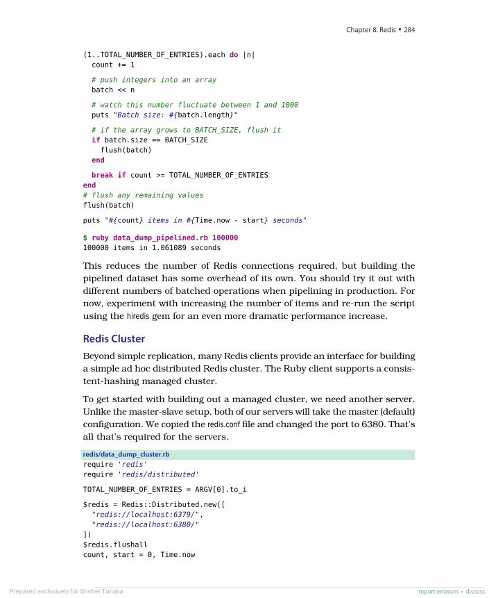
(1..TOTAL_NUMBER_OF_ENTRIES).each do |n|count += 1
# push integers into an arraybatch << n
# watch this number fluctuate between 1 and 1000puts "Batch size: #{batch.length}"
# if the array grows to BATCH_SIZE, flush itif batch.size == BATCH_SIZE
flush(batch)end
break if count >= TOTAL_NUMBER_OF_ENTRIESend# flush any remaining valuesflush(batch)
puts "#{count} items in #{Time.now - start} seconds"
$ ruby data_dump_pipelined.rb 100000100000 items in 1.061089 seconds
This reduces the number of Redis connections required, but building thepipelined dataset has some overhead of its own. You should try it out withdifferent numbers of batched operations when pipelining in production. Fornow, experiment with increasing the number of items and re-run the scriptusing the hiredis gem for an even more dramatic performance increase.
Redis ClusterBeyond simple replication, many Redis clients provide an interface for buildinga simple ad hoc distributed Redis cluster. The Ruby client supports a consis-tent-hashing managed cluster.
To get started with building out a managed cluster, we need another server.Unlike the master-slave setup, both of our servers will take the master (default)configuration. We copied the redis.conf file and changed the port to 6380. That’sall that’s required for the servers.
redis/data_dump_cluster.rbrequire 'redis'require 'redis/distributed'
TOTAL_NUMBER_OF_ENTRIES = ARGV[0].to_i
$redis = Redis::Distributed.new(["redis://localhost:6379/","redis://localhost:6380/"
])$redis.flushallcount, start = 0, Time.now
Chapter 8. Redis • 284
report erratum • discussPrepared exclusively for Shohei Tanaka
(1..TOTAL_NUMBER_OF_ENTRIES).each do |n|count += 1
key = "key#{n}"value = "value#{n}"
$redis.set(key, value)
break if count >= TOTAL_NUMBER_OF_ENTRIESendputs "#{count} items in #{Time.now - start} seconds"
Bridging between two or more servers requires only some minor changes toour existing data dump client. First, we need to require the redis/distributed filefrom the redis gem.
require 'redis/distributed'
Then replace the Redis client with Redis::Distributed and pass in an array ofserver URIs. Each URI requires the redis scheme, server (localhost in our case),and port.
$redis = Redis::Distributed.new(["redis://localhost:6379/","redis://localhost:6380/"
])
Running the client is the same as before.
$ ruby data_dump_cluster.rb 10000100000 items in 6.614907 seconds
We do see a performance decrease here because a lot more work is being doneby the client, since it handles computing which keys are stored on whichservers. You can validate that keys are stored on separate servers byattempting to retrieve the same key from each server through the CLI.
$ redis-cli -p 6379 --raw GET key537$ redis-cli -p 6380 --raw GET key537
Only one client will be able to GET the value of value537. But as long as youretrieve keys set through the same Redis::Distributed configuration, the clientwill access the values from the correct servers.
Bloom FiltersA good way to improve the performance of just about any data retrieval systemis to simply never perform queries that you know are doomed to fail and findno data. If you know that you dropped your car keys in your house, it’ssenseless to scour your neighbor’s house in search of them. You should start
report erratum • discuss
Day 2: Advanced Usage, Distribution • 285
Prepared exclusively for Shohei Tanaka
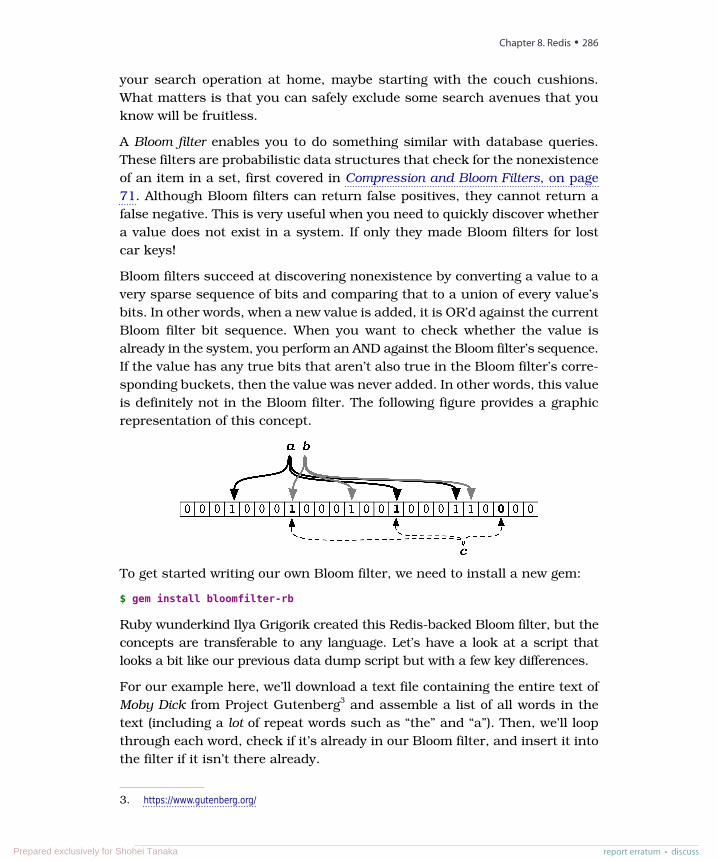
your search operation at home, maybe starting with the couch cushions.What matters is that you can safely exclude some search avenues that youknow will be fruitless.
A Bloom filter enables you to do something similar with database queries.These filters are probabilistic data structures that check for the nonexistenceof an item in a set, first covered in Compression and Bloom Filters, on page71. Although Bloom filters can return false positives, they cannot return afalse negative. This is very useful when you need to quickly discover whethera value does not exist in a system. If only they made Bloom filters for lostcar keys!
Bloom filters succeed at discovering nonexistence by converting a value to avery sparse sequence of bits and comparing that to a union of every value’sbits. In other words, when a new value is added, it is OR’d against the currentBloom filter bit sequence. When you want to check whether the value isalready in the system, you perform an AND against the Bloom filter’s sequence.If the value has any true bits that aren’t also true in the Bloom filter’s corre-sponding buckets, then the value was never added. In other words, this valueis definitely not in the Bloom filter. The following figure provides a graphicrepresentation of this concept.
To get started writing our own Bloom filter, we need to install a new gem:
$ gem install bloomfilter-rb
Ruby wunderkind Ilya Grigorik created this Redis-backed Bloom filter, but theconcepts are transferable to any language. Let’s have a look at a script thatlooks a bit like our previous data dump script but with a few key differences.
For our example here, we’ll download a text file containing the entire text ofMoby Dick from Project Gutenberg3 and assemble a list of all words in thetext (including a lot of repeat words such as “the” and “a”). Then, we’ll loopthrough each word, check if it’s already in our Bloom filter, and insert it intothe filter if it isn’t there already.
3. https://www.gutenberg.org/
Chapter 8. Redis • 286
report erratum • discussPrepared exclusively for Shohei Tanaka
redis/bloom_filter.rbrequire 'bloomfilter-rb'
bloomfilter = BloomFilter::Redis.new(:size => 1000000)bloomfilter.clear
# we'll read the file data and strip out all the non-word materialtext_data = File.read(ARGV[0])clean_text = text_data.gsub(/\n/, ' ').gsub(/[,-.;'?"()!*]/, '')
clean_text.split(' ').each do |word|word = word.downcase
next if bloomfilter.include?(word)puts wordbloomfilter.insert(word)
end
puts "Total number of words: #{text_data.length}"puts "Number of words in filter: #{bloomfilter.size}"
Let’s download the text using cURL and run the script:
$ curl -o moby-dick.txt https://www.gutenberg.org/files/2701/old/moby10b.txt$ ruby bloom_filter.rb moby-dick.txt > output.txt
Open up the output.txt and scroll through the contents. Each word in this filehas not yet been added to the filter. At the top of the list, you’ll find a lot ofcommon words like the, a, and but. At the bottom of the list, you’ll see theword “orphan,” which is the very last word in the Epilogue, which explainswhy it hadn’t been added to the filter yet! Some other fairly esoteric wordstoward the end include “ixion,” “sheathed,” “dirgelike,” and “intermixingly.”
What essentially happened here is that the more frequently used words weremore likely to get filtered out early, whereas less common words or wordsused only once were filtered out later. The upside with this approach is theability to detect duplicate words. The downside is that a few false positiveswill seep through—the Bloom filter may flag a word we have never seen before.This is why in a real-world use case you would perform some secondary check,such as a slower database query to a system of record, which should happenonly a small percentage of the time, presuming a large enough filter size,which is computable.4
SETBIT and GETBIT
As mentioned earlier, Bloom filters function by flipping certain bits in a sparsebinary field. The Redis Bloom filter implementation we just used takes advantageof two Redis commands that perform just such actions: SETBIT and GETBIT.
4. http://en.wikipedia.org/wiki/Bloom_filter
report erratum • discuss
Day 2: Advanced Usage, Distribution • 287
Prepared exclusively for Shohei Tanaka
Like all Redis commands, SETBIT is fairly descriptive. The command sets asingle bit (either 1 or 0) at a certain location in a bit sequence, starting fromzero. It’s a common use case for high-performance multivariate flagging—it’sfaster to flip a few bits than write a set of descriptive strings.
If we want to keep track of the toppings on a hamburger, we can assign eachtype of topping to a bit position, such as ketchup = 0, mustard = 1, onion =2, lettuce = 3. So, a hamburger with only mustard and onion could be repre-sented as 0110 and set in the command line:
redis 127.0.0.1:6379> SETBIT my_burger 1 1(integer) 0redis 127.0.0.1:6379> SETBIT my_burger 2 1(integer) 0
Later, a process can check whether my burger should have lettuce or mustard.If zero is returned, the answer is false—one if true.
redis 127.0.0.1:6379> GETBIT my_burger 3(integer) 0redis 127.0.0.1:6379> GETBIT my_burger 1(integer) 1
The Bloom filter implementation takes advantage of this behavior by hashinga value as a multibit value. It calls SETBIT X 1 for each on position in an insert()(where X is the bit position) and verifies existence by calling GETBIT X on theinclude?() method—returning false if any GETBIT position returns 0.
Bloom filters are excellent for reducing unnecessary traffic to a slower under-lying system, be it a slower database, limited resource, or network request.If you have a slower database of IP addresses and you want to track all newusers to your site, you can use a Bloom filter to first check whether the IPaddress exists in your system. If the Bloom filter returns false, you know theIP address has yet to be added and can respond accordingly. If the Bloomfilter returns true, this IP address may or may not exist on the back end andrequires a secondary lookup to be sure. This is why computing the correctsize is important—a well-sized Bloom filter can reduce (but not eliminate) theerror rate or the likelihood of a false positive.
Day 2 Wrap-UpToday we rounded out our Redis investigation by moving beyond simpleoperations into squeezing every last bit of speed out of an already very fastsystem. Redis provides for fast and flexible data structure storage and simplemanipulations as we saw in Day 1, but it’s equally adept at more complexbehaviors by way of built-in publish-subscribe functions and bit operations.
Chapter 8. Redis • 288
report erratum • discussPrepared exclusively for Shohei Tanaka
It’s also highly configurable, with many durability and replication settingsthat conform to whatever your needs may be. Finally, Redis also supportssome nice third-party enhancements, such as Bloom filters and clustering.
This concludes major operations for the Redis data structure store. Tomorrowwe’re going to do something a bit different, by using Redis as the cornerstoneof a polyglot persistence setup along with CouchDB and Neo4j.
Day 2 Homework
Find
1. Find out what messaging patterns are, and discover how many Redis canimplement.
2. Read some documentation on Sentinel,5 a system used to manage high-availability Redis clusters.
Do
1. Run the data dump script with all snapshotting and the append-only fileturned off. Then try running with appendfsync set to always, noting the speeddifference.
2. Using your favorite programming language’s web framework, try to builda simple URL-shortening service backed by Redis with an input box forthe URL and a simple redirect based on the URL. Back it up with a Redismaster-slave replicated cluster across multiple nodes as your back end.
Day 3: Playing with Other DatabasesToday we’re wrapping up our final database chapter by inviting some otherdatabases from the book to the Redis party. Amongst the databases we’vegone over in this book, Redis is the most lightweight and modular, capableof enhancing just about any complex data setup without imposing a ton ofengineering and ops overhead. Redis will hold a starring role in today’s exerciseby making our interaction with other databases faster and easier.
We’ve learned throughout this book that different databases have differentstrengths, so many modern systems have moved toward a polyglot persistencemodel, where many databases each play a role in the system. You will learnhow to build one of these projects using CouchDB as the system of record(the canonical data source), Neo4j to handle data relationships, and Redis
5. http://objectrocket.com/blog/how-to/introduction-to-redis-sentinel
report erratum • discuss
Day 3: Playing with Other Databases • 289
Prepared exclusively for Shohei Tanaka
to help with data population and caching. Consider this your final exam forthe book.
Note that our choice of databases for this last project should not be seen as theauthors’ endorsement of any specific set of databases, languages, or frame-works over another but rather a showcase of how multiple databases canwork together, leveraging the capabilities of each in pursuit of a single goal.
A Polyglot, Persistent ServiceOur polyglot persistence service will act as the backend for a web interfacethat provides information about bands. We want to store a list of musicalband names, the artists who performed in those bands, and any number ofroles each artist played in the band, from lead singer to backup keytar playerto people who just dance (like the guy in Mighty Mighty Bosstones). Each ofthe three databases—Redis, CouchDB, and Neo4j—will handle a differentaspect of our band data management system.
Redis plays three important roles in our system: It assists in populating datato CouchDB, it acts as a cache for recent Neo4j changes, and it enables quicklookup for partial value searches. Its speed and ability to store multiple dataformats make it well suited for data population, and its built-in expiry policiesare perfect for handling cached data.
CouchDB is our system of record (SOR), or authoritative data source.CouchDB’s document structure is an easy way to store band data becauseit allows for nested artist and role information, and we will take advantage ofthe changes API6 in CouchDB to keep our third data source in sync.
Neo4j is our relationship store. Although querying the CouchDB SOR directlyis perfectly reasonable, a graph database affords us a simplicity and speedin walking node relationships that other databases have a difficult timematching. We’ll store relationships between bands, band members, and theroles the members play.
Each database has a specific role to play in our system, but they don’t nativelycommunicate with another, which means that we need to build a translationlayer between them. We’ll use Node.js to populate the databases, communicatebetween them, and act as a simple front-end server. Because gluing multipledatabases together requires a bit of code, this last day will include much morecode than we have seen so far in this book.
6. http://docs.couchdb.org/en/latest/api/database/changes.html
Chapter 8. Redis • 290
report erratum • discussPrepared exclusively for Shohei Tanaka
The Rise of Polyglot Persistence
Like the growing phenomenon of polyglot programming, polyglot persistence is nowwell established in most corners of the database universe.
If you are unfamiliar with the practice, polyglot programming is what happens whena team uses more than one programming language in a single project. Contrast thiswith the convention of using one general-purpose language throughout a project oreven an entire company (you may have heard of “Java shops” or “Ruby shops”).Polyglot programming is useful because each language has different inherentstrengths. A language like Scala may be better suited for large “Big Data” processingtasks, whereas a language like Ruby may be friendlier for shell scripts. Used together,they create a synergy. The rise of so-called microservice architectures, in which serviceswritten in different languages interact with each other to form complex, unified sys-tems, is a logical outcome of polyglot programming.
Similar to its language-centric cousin, polyglot persistence happens when you usethe strengths of many kinds of database in the same system, as opposed to relyingon a single database (often a relational database). A basic variant of this is alreadyquite common: using a key-value store (such as Redis) that acts as a cache for queriesagainst a relatively slower relational database (such as PostgreSQL). Relationalmodels, as we’ve seen in previous chapters, are ill-suited for a growing host of prob-lems, such as graph traversal. But even these new databases shine only as a fewstars in the full galaxy of requirements.
Why the sudden interest in polyglot everything? Nearly a decade ago, Martin Fowlernoteda that having a single central database that multiple applications could use as asource of truth was a common pattern in software design. This once-popular databaseintegration pattern has given way to a middleware layer pattern, where multiple appli-cations instead communicate to a service layer over HTTP or a lighter protocol, suchas Thrift or Protocol Buffers. This frees up the middleware service itself to rely on anynumber of databases or, in the case of polyglot persistence, many types of database.
a. http://martinfowler.com/bliki/DatabaseThaw.html
PopulationThe first item of business is to populate our databases with the necessarydata. We take a two-phased approach here, by first populating Redis andthen populating our CouchDB SOR. We’ll be using a large dataset holdinginformation about bands, including the names of those bands, band members,which role each band member played, and more. This dataset contains a lotof information, but we’re interested only in extracting the member or artistname, the group or band name, and their roles in that band stored as a comma-separated list. For example, John Cooper played in the band Skillet as theLead vocalist, Acoustic guitar player, and Bassist.
report erratum • discuss
Day 3: Playing with Other Databases • 291
Prepared exclusively for Shohei Tanaka

First, download the file holding the dataset:
$ curl -O [data-file-url]
Replace [data-file-url] with the URL in the footnote below.7
This file contains a lot of information, but we are interested only in extractingthe member or artist name, the group or band name, and their roles in that bandstored as a comma-separated list. For example, John Cooper played in theband Skillet as the Lead vocalist, Acoustic guitar player, and Bassist.
/m/0654bxy John Cooper Skillet Lead vocalist,Acoustic guitar,Bass 1996
Ultimately we want to structure John Cooper and the other members ofSkillet into a single CouchDB document like the following, stored at the URLhttp://localhost:5984/bands/Skillet:
{"_id": "Skillet","name": "Skillet""artists": [
{"name": "John Cooper","role": [
"Acoustic guitar","Lead vocalist","Bass"
]},...{"name": "Korey Cooper","role": [
"backing vocals","Synthesizer","Guitar","Keyboard instrument"
]}
]}
This file contains well over 100,000 band members and more than 30,000bands. That’s not many, but it’s a good starting point to build your own sys-tem. Note that not all roles are documented for each artist. This is anincomplete dataset, but we can deal with that later.
7. https://raw.githubusercontent.com/coderoshi/NCNRCSBuzzSpec/master/group_membership.tsv
Chapter 8. Redis • 292
report erratum • discussPrepared exclusively for Shohei Tanaka
Phase 1: Data Transformation
You may wonder why we bother populating Redis and don’t just dive rightinto populating CouchDB. Acting as an intermediary, Redis adds structureto the flat TSV data so that subsequent insertion into another database isfast. Because our plan is to create a single record per band name, Redis allowsus to make a single pass through our TSV file (which lists the same band foreach band member—each band member is represented in a line). Addingsingle members directly to CouchDB for each line in the file can cause updatethrashing, where two band member lines attempt to create/update the sameband document at the same time, forcing the system to reinsert when one ofthem fails CouchDB’s version check.
The catch with this strategy is that you’re limited to the constraints of Redisto hold an entire dataset in RAM—though this limit could be overcome by thesimple consistent-hashing cluster you saw on Day 2.
With our data file in hand, ensure you have Node.js installed as well as theNode Package Manager (npm). Once that’s all done, we need to install threeNPM projects: redis, csv, and hiredis (the optional Redis C-driver you learnedabout on Day 2 that can greatly speed up Redis interactions).
$ npm install hiredis redis csv-parser cradle
Then, check that your Redis server is running on the default port 6379, oralter each script’s createClient() function to point to your Redis port.
You can populate Redis by running the following Node.js script in the samedirectory as your TSV file, which we assume is named group_membership.tsv. (Allof the JavaScript files we’ll look at are fairly verbose, so we don’t show themin their entirety. All of the code can be downloaded from the PragmaticBookshelf website. Here we’ll just stick to the meat of each file.) Downloadand run the following file:
$ node prePopulate.js
This script basically iterates through each line of the TSV and extracts theartist name, the band name, and the roles they play in that band. Then itadds those values to Redis (skipping any blank values).
The format of each Redis band key is "band:Band Name". The script will add thisartist name to the set of artist names. So, the key "band:Beatles" will containthe set of values ["John Lennon", "Paul McCartney", "George Harrison", "Ringo Starr"]. Theartist keys will also contain the band name and similarly contain a set ofroles. "artist:Beatles:Ringo Starr" will contain the set ["Drums"].
report erratum • discuss
Day 3: Playing with Other Databases • 293
Prepared exclusively for Shohei Tanaka
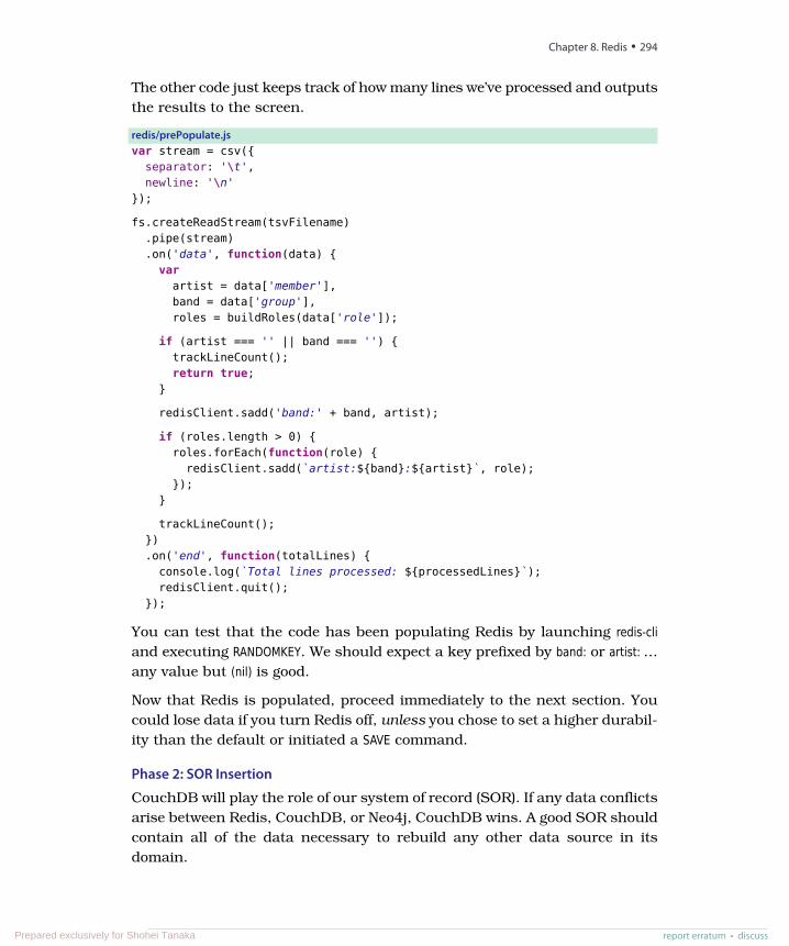
The other code just keeps track of how many lines we’ve processed and outputsthe results to the screen.
redis/prePopulate.jsvar stream = csv({
separator: '\t',newline: '\n'
});
fs.createReadStream(tsvFilename).pipe(stream).on('data', function(data) {
varartist = data['member'],band = data['group'],roles = buildRoles(data['role']);
if (artist === '' || band === '') {trackLineCount();return true;
}
redisClient.sadd('band:' + band, artist);
if (roles.length > 0) {roles.forEach(function(role) {
redisClient.sadd(`artist:${band}:${artist}`, role);});
}
trackLineCount();}).on('end', function(totalLines) {
console.log(`Total lines processed: ${processedLines}`);redisClient.quit();
});
You can test that the code has been populating Redis by launching redis-cliand executing RANDOMKEY. We should expect a key prefixed by band: or artist:…any value but (nil) is good.
Now that Redis is populated, proceed immediately to the next section. Youcould lose data if you turn Redis off, unless you chose to set a higher durabil-ity than the default or initiated a SAVE command.
Phase 2: SOR Insertion
CouchDB will play the role of our system of record (SOR). If any data conflictsarise between Redis, CouchDB, or Neo4j, CouchDB wins. A good SOR shouldcontain all of the data necessary to rebuild any other data source in itsdomain.
Chapter 8. Redis • 294
report erratum • discussPrepared exclusively for Shohei Tanaka
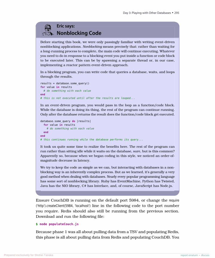
Eric says:
Nonblocking CodeBefore starting this book, we were only passingly familiar with writing event-drivennonblocking applications. Nonblocking means precisely that: rather than waiting fora long-running process to complete, the main code will continue executing. Whateveryou need to do in response to a blocking event you put inside a function or code blockto be executed later. This can be by spawning a separate thread or, in our case,implementing a reactor pattern event-driven approach.
In a blocking program, you can write code that queries a database, waits, and loopsthrough the results.
results = database.some_query()for value in results
# do something with each valueend# this is not executed until after the results are looped...
In an event-driven program, you would pass in the loop as a function/code block.While the database is doing its thing, the rest of the program can continue running.Only after the database returns the result does the function/code block get executed.
database.some_query do |results|for value in results
# do something with each valueend
end# this continues running while the database performs its query...
It took us quite some time to realize the benefits here. The rest of the program canrun rather than sitting idle while it waits on the database, sure, but is this common?Apparently so, because when we began coding in this style, we noticed an order-of-magnitude decrease in latency.
We try to keep the code as simple as we can, but interacting with databases in a non-blocking way is an inherently complex process. But as we learned, it’s generally a verygood method when dealing with databases. Nearly every popular programming languagehas some sort of nonblocking library. Ruby has EventMachine, Python has Twisted,Java has the NIO library, C# has Interlace, and, of course, JavaScript has Node.js.
Ensure CouchDB is running on the default port 5984, or change the require('http').createClient(5984, 'localhost') line in the following code to the port numberyou require. Redis should also still be running from the previous section.Download and run the following file:
$ node populateCouch.js
Because phase 1 was all about pulling data from a TSV and populating Redis,this phase is all about pulling data from Redis and populating CouchDB. You
report erratum • discuss
Day 3: Playing with Other Databases • 295
Prepared exclusively for Shohei Tanaka
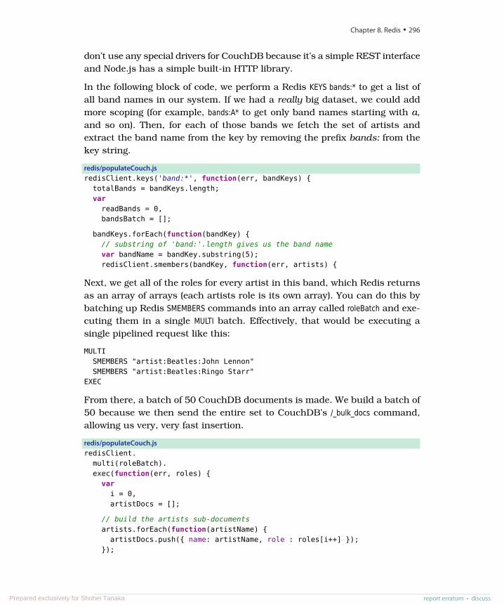
don’t use any special drivers for CouchDB because it’s a simple REST interfaceand Node.js has a simple built-in HTTP library.
In the following block of code, we perform a Redis KEYS bands:* to get a list ofall band names in our system. If we had a really big dataset, we could addmore scoping (for example, bands:A* to get only band names starting with a,and so on). Then, for each of those bands we fetch the set of artists andextract the band name from the key by removing the prefix bands: from thekey string.
redis/populateCouch.jsredisClient.keys('band:*', function(err, bandKeys) {
totalBands = bandKeys.length;var
readBands = 0,bandsBatch = [];
bandKeys.forEach(function(bandKey) {// substring of 'band:'.length gives us the band namevar bandName = bandKey.substring(5);redisClient.smembers(bandKey, function(err, artists) {
Next, we get all of the roles for every artist in this band, which Redis returnsas an array of arrays (each artists role is its own array). You can do this bybatching up Redis SMEMBERS commands into an array called roleBatch and exe-cuting them in a single MULTI batch. Effectively, that would be executing asingle pipelined request like this:
MULTISMEMBERS "artist:Beatles:John Lennon"SMEMBERS "artist:Beatles:Ringo Starr"
EXEC
From there, a batch of 50 CouchDB documents is made. We build a batch of50 because we then send the entire set to CouchDB’s /_bulk_docs command,allowing us very, very fast insertion.
redis/populateCouch.jsredisClient.
multi(roleBatch).exec(function(err, roles) {
vari = 0,artistDocs = [];
// build the artists sub-documentsartists.forEach(function(artistName) {artistDocs.push({ name: artistName, role : roles[i++] });
});
Chapter 8. Redis • 296
report erratum • discussPrepared exclusively for Shohei Tanaka
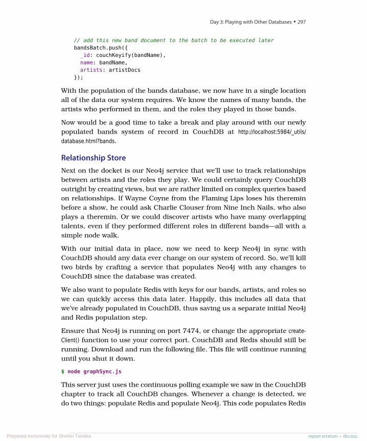
// add this new band document to the batch to be executed laterbandsBatch.push({_id: couchKeyify(bandName),name: bandName,artists: artistDocs
});
With the population of the bands database, we now have in a single locationall of the data our system requires. We know the names of many bands, theartists who performed in them, and the roles they played in those bands.
Now would be a good time to take a break and play around with our newlypopulated bands system of record in CouchDB at http://localhost:5984/_utils/database.html?bands.
Relationship StoreNext on the docket is our Neo4j service that we’ll use to track relationshipsbetween artists and the roles they play. We could certainly query CouchDBoutright by creating views, but we are rather limited on complex queries basedon relationships. If Wayne Coyne from the Flaming Lips loses his thereminbefore a show, he could ask Charlie Clouser from Nine Inch Nails, who alsoplays a theremin. Or we could discover artists who have many overlappingtalents, even if they performed different roles in different bands—all with asimple node walk.
With our initial data in place, now we need to keep Neo4j in sync withCouchDB should any data ever change on our system of record. So, we’ll killtwo birds by crafting a service that populates Neo4j with any changes toCouchDB since the database was created.
We also want to populate Redis with keys for our bands, artists, and roles sowe can quickly access this data later. Happily, this includes all data thatwe’ve already populated in CouchDB, thus saving us a separate initial Neo4jand Redis population step.
Ensure that Neo4j is running on port 7474, or change the appropriate create-Client() function to use your correct port. CouchDB and Redis should still berunning. Download and run the following file. This file will continue runninguntil you shut it down.
$ node graphSync.js
This server just uses the continuous polling example we saw in the CouchDBchapter to track all CouchDB changes. Whenever a change is detected, wedo two things: populate Redis and populate Neo4j. This code populates Redis
report erratum • discuss
Day 3: Playing with Other Databases • 297
Prepared exclusively for Shohei Tanaka
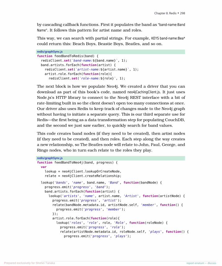
by cascading callback functions. First it populates the band as "band-name:BandName". It follows this pattern for artist name and roles.
This way, we can search with partial strings. For example, KEYS band-name:Bea*could return this: Beach Boys, Beastie Boys, Beatles, and so on.
redis/graphSync.jsfunction feedBandToRedis(band) {
redisClient.set(`band-name:${band.name}`, 1);band.artists.forEach(function(artist) {
redisClient.set(`artist-name:${artist.name}`, 1);artist.role.forEach(function(role){redisClient.set(`role-name:${role}`, 1);
The next block is how we populate Neo4j. We created a driver that you candownload as part of this book’s code, named neo4jCachingClient.js. It just usesNode.js’s HTTP library to connect to the Neo4j REST interface with a bit ofrate-limiting built in so the client doesn’t open too many connections at once.Our driver also uses Redis to keep track of changes made to the Neo4j graphwithout having to initiate a separate query. This is our third separate use forRedis—the first being as a data transformation step for populating CouchDB,and the second we just saw earlier, to quickly search for band values.
This code creates band nodes (if they need to be created), then artist nodes(if they need to be created), and then roles. Each step along the way createsa new relationship, so The Beatles node will relate to John, Paul, George, andRingo nodes, who in turn each relate to the roles they play.
redis/graphSync.jsfunction feedBandToNeo4j(band, progress) {
varlookup = neo4jClient.lookupOrCreateNode,relate = neo4jClient.createRelationship;
lookup('bands', 'name', band.name, 'Band', function(bandNode) {progress.emit('progress', 'band');band.artists.forEach(function(artist) {lookup('artists', 'name', artist.name, 'Artist', function(artistNode) {
progress.emit('progress', 'artist');relate(bandNode.metadata.id, artistNode.self, 'member', function() {
progress.emit('progress', 'member');});artist.role.forEach(function(role){
lookup('roles', 'role', role, 'Role', function(roleNode) {progress.emit('progress', 'role');relate(artistNode.metadata.id, roleNode.self, 'plays', function() {
progress.emit('progress', 'plays');
Chapter 8. Redis • 298
report erratum • discussPrepared exclusively for Shohei Tanaka
Let this service keep running in its own window. Every update to CouchDBthat adds a new artist or role to an existing artist will trigger a new relationshipin Neo4j and potentially new keys in Redis. As long as this service runs, theyshould be in sync.
Open your CouchDB web console and open a band. Make any data changeyou want to the database: add a new band member (make yourself a memberof the Beatles!), or add a new role to an artist. Keep an eye on the graphSyncoutput. Then fire up the Neo4j console and try finding any new connectionsin the graph. If you added a new band member, they should now have arelationship with the band node or new role if that was altered. The currentimplementation does not remove relationships—though it would not be acomplete modification to add a Neo4j DELETE operation to the script.
The ServiceThis is the part we’ve been building up to. We’re going to create a simple webapplication that allows users to search for a band. Any band in the systemwill list all of the band members as links, and any clicked band member linkwill list some information about the artist—namely, the roles they play. Inaddition, each role the artist plays will list every other artist in the systemwho also plays that role.
For example, searching for Led Zeppelin would give you Jimmy Page, JohnPaul Jones, John Bonham, and Robert Plant. Clicking Jimmy Page will listthat he plays guitar and also many other artists who play guitar, like TheEdge from U2.
To simplify our web app creation a bit, we’ll need two more node packages:bricks (a simple web framework) and mustache (a templating library).
$ npm install bricks mustache neo4j-driver
As in the previous sections, ensure you have all of the databases running,and then start up the server. Download and run the following code:
$ node band.js
The server is set to run on port 8080, so if you point your browser tohttp://localhost:8080/, you should see a simple search form.
Let’s take a look at the code that will build a web page that lists band infor-mation. Each URL performs a separate function in our little HTTP server. Thefirst is at http://localhost:8080/band and accepts any band name as a parameter.
report erratum • discuss
Day 3: Playing with Other Databases • 299
Prepared exclusively for Shohei Tanaka
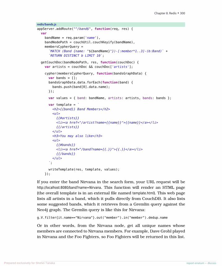
redis/bands.jsappServer.addRoute("^/band$", function(req, res) {
varbandName = req.param('name'),bandNodePath = couchUtil.couchKeyify(bandName),membersCypherQuery =
`MATCH (Band {name: "${bandName}"})-[:member*1..3]-(b:Band)` +`RETURN DISTINCT b LIMIT 10`;
getCouchDoc(bandNodePath, res, function(couchDoc) {var artists = couchDoc && couchDoc['artists'];
cypher(membersCypherQuery, function(bandsGraphData) {var bands = [];bandsGraphData.data.forEach(function(band) {
bands.push(band[0].data.name);});
var values = { band: bandName, artists: artists, bands: bands };
var template = `<h2>{{band}} Band Members</h2><ul>
{{#artists}}<li><a href="/artist?name={{name}}">{{name}}</a></li>{{/artists}}
</ul><h3>You may also like</h3><ul>
{{#bands}}<li><a href="/band?name={{.}}">{{.}}</a></li>{{/bands}}
</ul>`;
writeTemplate(res, template, values);});
If you enter the band Nirvana in the search form, your URL request will behttp://localhost:8080/band?name=Nirvana. This function will render an HTML page(the overall template is in an external file named template.html). This web pagelists all artists in a band, which it pulls directly from CouchDB. It also listssome suggested bands, which it retrieves from a Gremlin query against theNeo4j graph. The Gremlin query is like this for Nirvana:
g.V.filter{it.name=="Nirvana"}.out("member").in("member").dedup.name
Or in other words, from the Nirvana node, get all unique names whosemembers are connected to Nirvana members. For example, Dave Grohl playedin Nirvana and the Foo Fighters, so Foo Fighters will be returned in this list.
Chapter 8. Redis • 300
report erratum • discussPrepared exclusively for Shohei Tanaka
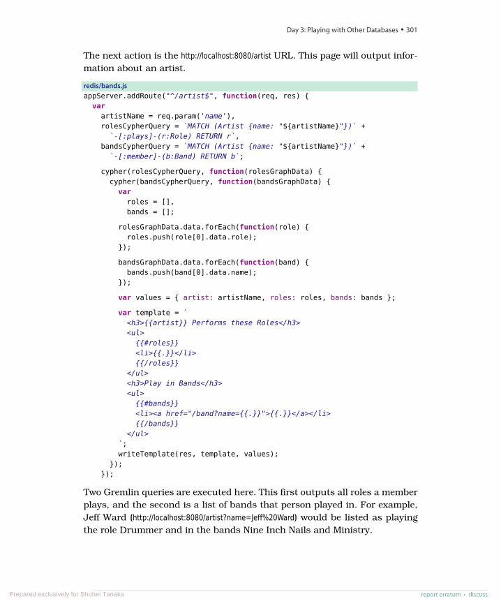
The next action is the http://localhost:8080/artist URL. This page will output infor-mation about an artist.
redis/bands.jsappServer.addRoute("^/artist$", function(req, res) {
varartistName = req.param('name'),rolesCypherQuery = `MATCH (Artist {name: "${artistName}"})` +
`-[:plays]-(r:Role) RETURN r`,bandsCypherQuery = `MATCH (Artist {name: "${artistName}"})` +
`-[:member]-(b:Band) RETURN b`;
cypher(rolesCypherQuery, function(rolesGraphData) {cypher(bandsCypherQuery, function(bandsGraphData) {
varroles = [],bands = [];
rolesGraphData.data.forEach(function(role) {roles.push(role[0].data.role);
});
bandsGraphData.data.forEach(function(band) {bands.push(band[0].data.name);
});
var values = { artist: artistName, roles: roles, bands: bands };
var template = `<h3>{{artist}} Performs these Roles</h3><ul>
{{#roles}}<li>{{.}}</li>{{/roles}}
</ul><h3>Play in Bands</h3><ul>
{{#bands}}<li><a href="/band?name={{.}}">{{.}}</a></li>{{/bands}}
</ul>`;writeTemplate(res, template, values);
});});
Two Gremlin queries are executed here. This first outputs all roles a memberplays, and the second is a list of bands that person played in. For example,Jeff Ward (http://localhost:8080/artist?name=Jeff%20Ward) would be listed as playingthe role Drummer and in the bands Nine Inch Nails and Ministry.
report erratum • discuss
Day 3: Playing with Other Databases • 301
Prepared exclusively for Shohei Tanaka
A cool feature of the previous two pages is that we render links between thesevalues. The artist list in the /bands page links to the chosen /artist page, andvice versa. But we could make searching a bit easier.
redis/bands.jsappServer.addRoute("^/search$", function(req, res) {
var query = req.param('term');
redisClient.keys(`band-name:${query}*`, function(error, keys) {var bands = [];keys.forEach(function(key){bands.push(key.replace("band-name:", ''));
});res.write(JSON.stringify(bands));res.end();
Here we just pull all keys from Redis that match the first part of the string,such as "Bea*" as described previously. The function then outputs the data asJSON. The template.html file links to the jQuery code necessary to make thisfunction as an autocomplete feature on the rendered search box.
Expanding the Service
This is a fairly little script for all of the bare-bones work we’re doing here. Youmay find many places you want to extend. Notice that the band suggestionis only first-order bands (bands the current band’s members have performedin); you can get interesting results by writing a query to traverse second-orderbands, like this: g.V.filter{it.name=='Nine Inch Nails'}.out('member').in('member').dedup.loop(3){ it.loops <= 2 }.name.
You may also note that we do not have a form where someone can updateband information. Adding this functionality could be fairly simple becausewe already wrote CouchDB population code in the populateCouch.js script, andpopulating CouchDB will automatically keep Neo4j and Redis eventuallyconsistent as long as the graph_sync.js service is running.
If you enjoy playing with this kind of polyglot persistence, you could take thiseven further. You could add a PostgreSQL data warehouse8 to transform thisdata into a star schema—allowing for different dimensions of analysis, such asmost commonly played instrument or average numbers of total members in aband vs. total instruments. You could add a CouchDB server to store informationabout the music associated with each band, an HBase server to build a messag-ing system that enables users to keep track of their historical likes/dislikes,or a MongoDB extension to add a geographic element to this service.
8. http://en.wikipedia.org/wiki/Data_warehouse
Chapter 8. Redis • 302
report erratum • discussPrepared exclusively for Shohei Tanaka
Or, redesign this project entirely with a different language, web framework,or dataset. There are as many opportunities to extend this project as thereare combinations of databases and technologies to create it—a Cartesianproduct of all open source.
Day 3 Wrap-UpToday was a big day—so big, in fact, we wouldn’t be surprised if it took severaldays to complete. But this is a little taste of the future of data managementsystems, as the world strolls away from the one large relational database modelto a several specialized databases model. We also glued these databases togetherwith some nonblocking code, which, though not a focus of this book, alsoseems to be where database interaction is headed in the development space.
The importance of Redis in this model should not be missed. Redis certainlydoesn’t provide any functionality these databases don’t supply individually, butit does supply speedy data structures. We were able to organize a flat file intoa series of meaningful data structures, which is an integral part of both datapopulation and transportation. And it did this in a fast and simple-to-use way.
Even if you’re not sold on the whole polyglot persistence model, you shouldcertainly consider Redis for any system.
Day 3 Homework
Do
1. Alter the importer steps to also track a band member’s start and enddates with the band. Track that data in the artist’s CouchDB subdocu-ment. Display this information on the artist’s page.
2. Add MongoDB into the mix by storing a few music samples into GridFS,whereby users can hear a song or two related to a band. If any song existsfor a band, add a link to the web app.
Wrap-UpThe Redis key-value (or data structure) store is light and compact, with avariety of uses. It’s akin to one of those multitools composed of a knife, canopener, and other bits and bobs like a corkscrew—Redis is good to havearound for solving a variety of odd tasks. Above all, Redis is fast, simple, andas durable as you choose. While rarely a standalone database, Redis is aperfect complement to any polyglot ecosystem as an ever-present helper fortransforming data, caching requests, or managing messages by way of itsblocking commands.
report erratum • discuss
Wrap-Up • 303
Prepared exclusively for Shohei Tanaka
Redis’s StrengthsThe obvious strength of Redis is speed, like so many key-value stores of itsilk. But more than most key-value stores, Redis provides the ability to storecomplex values such as lists, hashes, and sets, and retrieve them based onoperations specific to those datatypes. Beyond even a data structure store,however, Redis’s durability options allow you to trade speed for data safetyup to a fairly fine point. Built-in master-slave replication is another nice wayof ensuring better durability without requiring the slowness of syncing anappend-only file to disk on every operation. Additionally, replication is greatfor very high-read systems.
Redis’s WeaknessesRedis is fast largely because it resides in memory. Some may consider thischeating because, of course, a database that never hits the disk will be fast.A main memory database has an inherent durability problem; namely, if youshut down the database before a snapshot occurs, you can lose data. Evenif you set the append-only file to disk sync on every operation, you run a riskwith playing back expiry values because time-based events can never becounted on to replay in exactly the same manner—though, in fairness, thiscase is more hypothetical than practical.
Redis also does not support datasets larger than your available RAM (Redisis removing virtual memory support), so its size has a practical limitation.Although there is a Redis Cluster currently in development to grow beyonda single machine’s RAM requirements, anyone wanting to cluster Redis mustcurrently roll their own with a client that supports it (like the Ruby driver weused in Day 2).
Parting ThoughtsRedis is chock-full of commands—more than 120 of them. Most commands arestraightforward enough to understand by their names alone, once you get usedto the idea that seemingly random letters will be removed (for example, INCRBY)or that mathematical precision can sometimes be more confusing than helpful(for example, ZCOUNT, or sorted set count, vs. SCARD, or set cardinality).
Redis is already becoming an integral part of many systems. Several opensource projects rely on Redis, from Resque, a Ruby-based asynchronous jobqueueing service, to session management in the Node.js project SocketStream.Regardless of the database you choose as your SOR, you should certainlyadd Redis to the mix.
Chapter 8. Redis • 304
report erratum • discussPrepared exclusively for Shohei Tanaka
CHAPTER 9
Wrapping UpNow that we’ve made it through the databases, congratulations are in order!We hope that you’ve gained an appreciation for these seven challengingdatabases and their unique worldviews. If you use one in a project, we’ll behappy. And if you decide to use multiple databases, as you saw at the end ofthe Redis chapter, we’ll be ecstatic. We believe that the future of data man-agement lies in the polyglot persistence model (using more than one databasein a project), while the approach that sees a single general-purpose RDBMSas the only available design pattern slowly drifts away.
Let’s take this opportunity to see where our seven databases fit together inthe greater database ecosystem. By this point, we have explored the detailsof each and mentioned a few commonalities and differences. You’ll see howthey contribute to the vast and expanding landscape of data storage options.
Genres ReduxYou’ve seen that how databases store their data can be largely divided intofive genres: relational, key-value, columnar, document, and graph. Let’s takea moment and recap their differences and see what each style is good for andnot so good for—when you’d want to use them and when to avoid them.
RelationalThis is the most common classic database pattern. Relational databasemanagement systems (RDBMSs) are set-theory-based systems implementedas two-dimensional tables with rows and columns. Relational databasesstrictly enforce type and are generally numeric, strings, dates, and uninter-preted blobs, but as you saw, PostgreSQL provides extensions such as arrayor cube.
report erratum • discussPrepared exclusively for Shohei Tanaka

Good For:
Because of the structured nature of relational databases, they make sensewhen the layout of the data is known in advance but how you plan to usethat data later may not be. Or, in other words, you pay the organizationalcomplexity up front to achieve query flexibility later. Many business problemsare aptly modeled this way, from orders to shipments and from inventory toshopping carts. You may not know in advance how you’ll want to query thedata later—how many orders did we process in February?—but the data isquite regular in nature, so enforcing that regularity is helpful.
Not-So-Good For:
When your data is highly variable or deeply hierarchical, relational databasesaren’t the best fit. Because you must specify a schema up front, data problemsthat exhibit a high degree of record-to-record variation will be problematic.Consider developing a database to describe all the creatures in nature. Creat-ing a full list of all features to account for (hasHair, numLegs, laysEggs, andso on) would be intractable. In such a case, you’d want a database that placesfewer restrictions in advance on what you can put into it.
Key-ValueThe key-value (KV) store was the simplest model we covered. KV maps simplekeys—sometimes to simple values like strings, and sometimes to more complexvalues, like a huge hashtable. Because of their relative simplicity, this genreof database has the most flexibility of implementation. Hash lookups are fast,so in the case of Redis, speed was its primary concern. Hash lookups are alsoeasily distributed, and so DynamoDB took advantage of this in its partitioningscheme. Of course, its simplicity can be a downside for any data with strictor complex modeling requirements.
Good For:
With little or no need to maintain indexes, key-value stores are often designedto be horizontally scalable, extremely fast, or both. They’re particularly suitedfor problems where the data are not highly related. For example, in a webapplication, users’ session data meet this criteria; each user’s session activitywill be different and largely unrelated to the activity of other users.
Not-So-Good For:
Often lacking indexes and scanning capabilities, KV stores won’t help you ifyou need to be able to perform queries on your data, other than basic CRUDoperations (Create, Read, Update, Delete).
Chapter 9. Wrapping Up • 306
report erratum • discussPrepared exclusively for Shohei Tanaka
ColumnarColumnar databases (aka column-oriented or column family) share manysimilarities with both KV and RDBMS stores. As with a key-value database,values are queried by matching keys. Like relational, their values are groupsof zero or more columns, though each row is capable of populating howevermany it wants. Unlike either, columnar databases store like data by columns,rather than keeping data together by rows. Columns are inexpensive to add,versioning is trivial, and there is no real storage cost for unpopulated values.You saw how HBase is a classic implementation of this genre.
Good For:
Columnar databases have been traditionally developed with horizontal scala-bility as a primary design goal. As such, they’re particularly suited to “BigData” problems, living on clusters of tens, hundreds, or thousands of nodes.They also tend to have built-in support for features such as compression andversioning. The canonical example of a good columnar data storage problemis indexing web pages. Pages on the web are highly textual (which means thatthey benefit from compression), they tend to be somewhat interrelated, andthey change over time (which means that they benefit from versioning).
Not-So-Good For:
Different columnar databases have different features and therefore differentdrawbacks. But one thing they have in common is that it’s best to designyour schema based on how you plan to query the data. This means you shouldhave some idea in advance of how your data will be used, not just what it’llconsist of. If data usage patterns can’t be defined in advance—for example,fast ad hoc reporting—then a columnar database may not be the best fit.
DocumentDocument databases allow for any number of fields per object and even allowobjects to be nested to any depth as values of other fields. The common rep-resentation of these objects is as JavaScript Object Notation (JSON), adheredto by both MongoDB and CouchDB—though this is by no means a conceptualrequirement. Because documents don’t relate to each other like relationaldatabases, they are relatively easy to shard and replicate across severalservers, making distributed implementations fairly common. MongoHQ tendsto tackle availability by supporting the creation of datacenters that managehuge datasets for the web. Meanwhile, CouchDB focuses on being simple anddurable, where availability is achieved by master-master replication of fairlyautonomous nodes. There is high overlap between these projects.
report erratum • discuss
Genres Redux • 307
Prepared exclusively for Shohei Tanaka
Good For:
Document databases are suited to problems involving highly variable domains.When you don’t know in advance what exactly your data will look like, docu-ment databases are a good bet. Also, because of the nature of documents,they often map well to object-oriented programming models. This means lessimpedance mismatch when moving data between the database model andapplication model.
Not-So-Good For:
If you’re used to performing elaborate join queries on highly normalized rela-tional database schemas, you’ll find the capabilities of document databaseslacking. A document should generally contain most or all of the relevantinformation required for normal use. So while in a relational database you’dnaturally normalize your data to reduce or eliminate copies that can get outof sync, with document databases, denormalized data is the norm.
GraphGraph databases are an emerging class of database that focuses more on theinterrelation between data nodes than on the actual values stored in thosenodes. Neo4j, our open source example, is growing in popularity for manysocial network applications. Unlike other database styles that group collectionsof like objects into common buckets, graph databases are more free-form—queries consist of following edges shared by two nodes or, aka traversing nodes.As more projects use them, graph databases are growing the straightforwardsocial examples to occupy more nuanced use cases, such as recommendationengines, access control lists, and geographic data.
Good For:
Graph databases seem to be tailor-made for networking applications. The pro-totypical example is a social network, where nodes represent users who havevarious kinds of relationships to each other. Modeling this kind of data usingany of the other styles is often a tough fit, but a graph database would acceptit with relish. They are also perfect matches for an object-oriented system. Ifyou can model your data on a whiteboard, you can model it in a graph.
Not-So-Good For:
Because of the high degree of interconnectedness between nodes, graphdatabases are generally not suitable for network partitioning. Spidering thegraph quickly means you can’t afford network hops to other database nodes,so graph databases don’t scale out well. It’s likely that if you use a graph
Chapter 9. Wrapping Up • 308
report erratum • discussPrepared exclusively for Shohei Tanaka
database, it’ll be one piece of a larger system, with the bulk of the data storedelsewhere and only the relationships maintained in the graph.
Making a ChoiceAs we said at the beginning, data is like oil. We sit upon a vast ocean of data,yet until it’s refined into information, it’s unusable (and with a more crudecomparison, no pun intended, there’s a lot of money in data these days). Theease of collecting and ultimately storing, mining, and refining the data outthere starts with the database you choose.
Deciding which database to choose is often more complex than merely consid-ering which genre maps best to a given domain’s data. Though a social graphmay seem to clearly function best with a graph database, if you’re Facebook,you simply have far too much data to choose one. You are more likely goingto choose a “Big Data” implementation, such as HBase or DynamoDB. Thiswill force your hand into choosing a columnar or key-value store. In othercases, though you may believe a relational database is clearly the best optionfor bank transactions, it’s worth knowing that Neo4j also supports ACIDtransactions, expanding your options.
These examples serve to point out that there are other avenues beyond genreto consider when choosing which database—or databases—best serve yourproblem scope. As a general rule, as the size of data increases, the capacityof certain database styles wane. Column-oriented database implementationsare often built to scale across datacenters and support the largest “Big Data”sets, while graphs generally support the smallest. This is not always the case,however. DynamoDB is a large-scale key-value store meant to automaticallyshard data across hundreds or thousands of nodes without any need for useradministration, while Redis was built to run on one—with the possibility ofa few master-slave replicas or client-managed shards.
There are several more dimensions to consider when choosing a database, suchas durability, availability, consistency, scalability, and security. You have todecide whether ad hoc queryability is important or if mapreduce will suffice.Do you prefer to use an HTTP/REST interface, or are you willing to requirea driver for a custom binary protocol? Even smaller scope concerns, such asthe existence of bulk data loaders, might be important for you to think about.
Where Do We Go from Here?Scaling problems associated with modern applications now fall largely in therealm of data management. We have reached a point in the evolution of
report erratum • discuss
Making a Choice • 309
Prepared exclusively for Shohei Tanaka
applications where the choice of framework, operating system, programminglanguage, and so on matters less than ever. Hardware and storage getcheaper by the day and tools like virtual machines, the cloud, and containersmake interoperation between servers and runtime operations ever moreseamless, to the point where once-epochal decisions about languages andplatforms are often driven as much by preference as by necessity.
But for reasons we‘ve laid out throughout this book, database choices aredifferent. Someday those choices may revolve around whims and preferences,but we won‘t get there for quite some time. If you want to scale your applica-tion in this day and age, you should think long and hard about whichdatabase, or databases, you choose, as that aspect of your application couldend up being more of a bottleneck and break point than the languages, plat-forms, operating systems, and other tools you use. One of the core purposesof this book was to help you make this choice wisely.
Although the book has come to a close, we trust your interest in polyglotpersistence and the world of non-relational databases is wide open. The nextsteps from here are to pursue in detail the databases that piqued your interestor continue learning about other NoSQL options, such as Cassandra,ArangoDB, Titan, or Google Cloud Datastore.
It’s time to get your hands dirty.
Chapter 9. Wrapping Up • 310
report erratum • discussPrepared exclusively for Shohei Tanaka
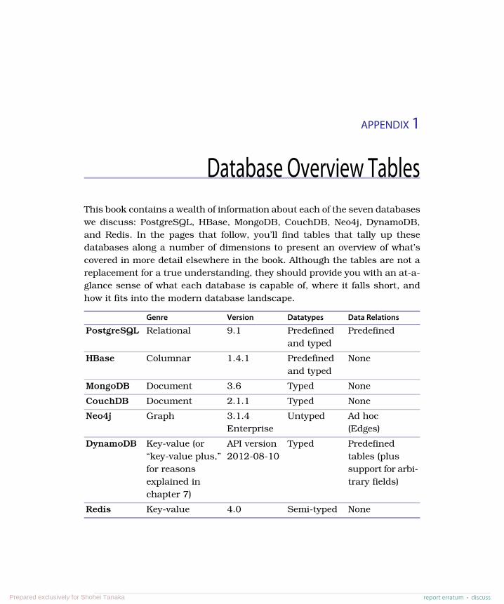
APPENDIX 1
Database Overview TablesThis book contains a wealth of information about each of the seven databaseswe discuss: PostgreSQL, HBase, MongoDB, CouchDB, Neo4j, DynamoDB,and Redis. In the pages that follow, you’ll find tables that tally up thesedatabases along a number of dimensions to present an overview of what’scovered in more detail elsewhere in the book. Although the tables are not areplacement for a true understanding, they should provide you with an at-a-glance sense of what each database is capable of, where it falls short, andhow it fits into the modern database landscape.
Data RelationsDatatypesVersionGenre
PredefinedPredefinedand typed
9.1RelationalPostgreSQL
NonePredefinedand typed
1.4.1ColumnarHBase
NoneTyped3.6DocumentMongoDB
NoneTyped2.1.1DocumentCouchDB
Ad hoc(Edges)
Untyped3.1.4Enterprise
GraphNeo4j
Predefinedtables (plus
TypedAPI version2012-08-10
Key-value (or“key-value plus,”
DynamoDB
support for arbi-trary fields)
for reasonsexplained inchapter 7)
NoneSemi-typed4.0Key-valueRedis
report erratum • discussPrepared exclusively for Shohei Tanaka

HTTP/RESTInterfaceProtocol
Written inLanguage
StandardObject
NoCustom overTCP
CTablePostgreSQL
YesThrift, HTTPJavaColumnsHBase
SimpleCustom overTCP
C++JSONMongoDB
YesHTTPErlangJSONCouchDB
YesHTTPJavaHashNeo4j
YesJSON overHTTP
UnknownTableDynamoDB
NoSimple textover TCP
C/C++StringRedis
DurabilityScalableMapreduceAd Hoc Query
ACIDCluster (viaadd-ons)
NoSQLPostgreSQL
Write-aheadlogging
DatacenterHadoopWeakHBase
Write-aheadjournaling,Safe mode
DatacenterJavaScriptCommands,mapreduce
MongoDB
Crash-onlyDatacenter(via BigCouch)
JavaScriptTemporaryviews
CouchDB
ACIDCluster (viaHA)
No (in thedistributedsense)
Graph walk-ing, Cypher,search
Neo4j
ACIDMulti-datacen-ter
NoLimited rangeof SQL-stylequeries
DynamoDB
Append-onlylog
Cluster (viamaster-slave)
NoCommandsRedis
Appendix 1. Database Overview Tables • 312
report erratum • discussPrepared exclusively for Shohei Tanaka
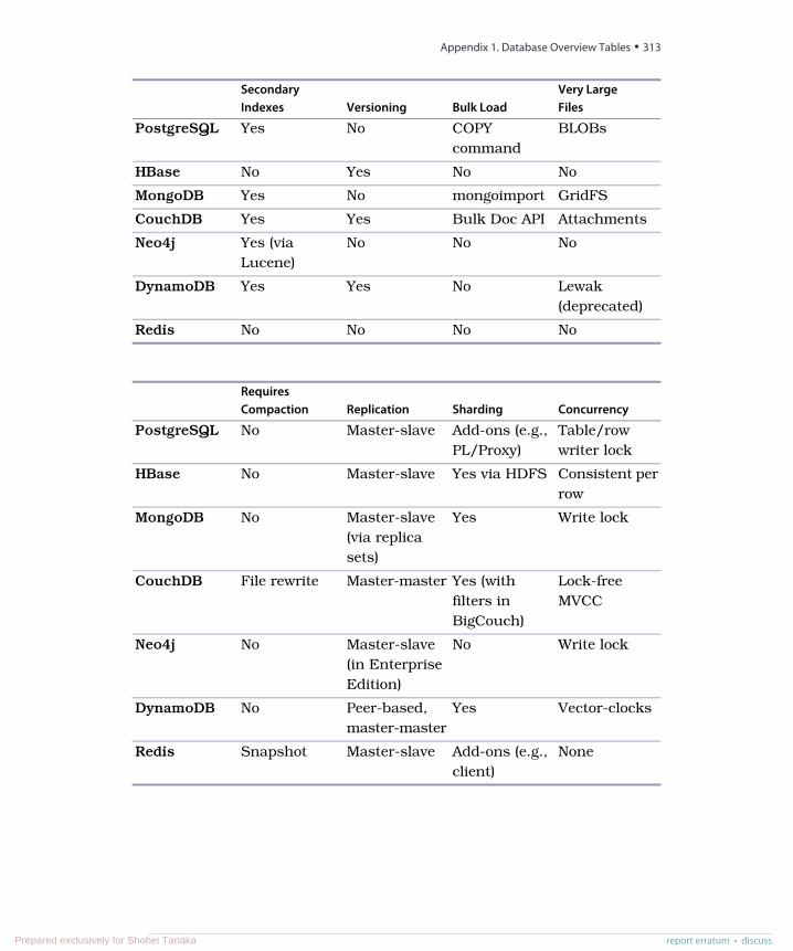
Very LargeFilesBulk LoadVersioning
SecondaryIndexes
BLOBsCOPYcommand
NoYesPostgreSQL
NoNoYesNoHBase
GridFSmongoimportNoYesMongoDB
AttachmentsBulk Doc APIYesYesCouchDB
NoNoNoYes (viaLucene)
Neo4j
Lewak(deprecated)
NoYesYesDynamoDB
NoNoNoNoRedis
ConcurrencyShardingReplicationRequiresCompaction
Table/rowwriter lock
Add-ons (e.g.,PL/Proxy)
Master-slaveNoPostgreSQL
Consistent perrow
Yes via HDFSMaster-slaveNoHBase
Write lockYesMaster-slave(via replicasets)
NoMongoDB
Lock-freeMVCC
Yes (withfilters inBigCouch)
Master-masterFile rewriteCouchDB
Write lockNoMaster-slave(in EnterpriseEdition)
NoNeo4j
Vector-clocksYesPeer-based,master-master
NoDynamoDB
NoneAdd-ons (e.g.,client)
Master-slaveSnapshotRedis
report erratum • discuss
Appendix 1. Database Overview Tables • 313
Prepared exclusively for Shohei Tanaka
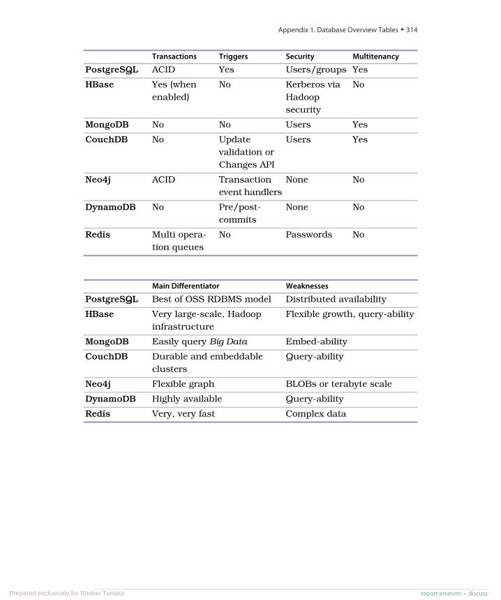
MultitenancySecurityTriggersTransactions
YesUsers/groupsYesACIDPostgreSQL
NoKerberos viaHadoopsecurity
NoYes (whenenabled)
HBase
YesUsersNoNoMongoDB
YesUsersUpdatevalidation orChanges API
NoCouchDB
NoNoneTransactionevent handlers
ACIDNeo4j
NoNonePre/post-commits
NoDynamoDB
NoPasswordsNoMulti opera-tion queues
Redis
WeaknessesMain Differentiator
Distributed availabilityBest of OSS RDBMS modelPostgreSQL
Flexible growth, query-abilityVery large-scale, Hadoopinfrastructure
HBase
Embed-abilityEasily query Big DataMongoDB
Query-abilityDurable and embeddableclusters
CouchDB
BLOBs or terabyte scaleFlexible graphNeo4j
Query-abilityHighly availableDynamoDB
Complex dataVery, very fastRedis
Appendix 1. Database Overview Tables • 314
report erratum • discussPrepared exclusively for Shohei Tanaka
APPENDIX 2
The CAP TheoremUnderstanding the five database genres is important when deciding on whichdatabase to use in a particular case, but there’s one other major thing thatyou should always bear in mind. A recurring theme in this book has beenthe CAP theorem, which lays bare an unsettling truth about how distributeddatabase systems behave in the face of network instability.
CAP proves that you can create a distributed database that can have one ormore of the following qualities: It can be consistent (writes are atomic and allsubsequent requests retrieve the new value), available (the database willalways return a value as long as a single server is running), and/or partitiontolerant (the system will still function even if server communication is tem-porarily lost—that is, a network partition). But the catch is that any givensystem can be at most two of these things at once, and never all three.
In other words, you can create a distributed database system that is consistentand partition tolerant (a “CP” system), a system that is available and partitiontolerant (an “AP” system), or a system that is consistent and available (themuch more rare CA system that is not partition tolerant—which basicallymeans not distributed). Or a system can have only one of those qualities (thisbook doesn’t cover any databases like that, and you’re unlikely to encountersuch a database in wide use). But at the end of the day it simply isn’t possibleto create a distributed database that is consistent and available and partitiontolerant at the same time, and anyone who says that they’ve “solved CAP” issaying that they’ve defied the laws of physics and thus should not be trusted.
The CAP theorem is pertinent when considering a distributed database becauseit forces you to decide what you are willing to give up. The database you choosewill lose either availability or consistency. Partition tolerance is strictly anarchitectural decision (depending on whether you want a distributed database).It’s important to understand the CAP theorem to fully grok your options. The
report erratum • discussPrepared exclusively for Shohei Tanaka
trade-offs made by the database implementations in this book are largelyinfluenced by it.
A CAP Adventure, Part I: CAP
Imagine the world as a giant distributed database system. All of the land in the worldcontains information about certain topics, and as long as you’re somewhere nearpeople or technology, you can find an answer to your questions.
Now, for the sake of argument, imagine you are a passionate Beyoncé fan and thedate is September 5, 2016. Suddenly, while at your friend’s beach house party cele-brating the release of Beyoncé’s hot new studio album, a freak tidal wave sweepsacross the dock and drags you out to sea. You fashion a makeshift raft and wash upon a desert island days later. Without any means of communication, you are effectivelypartitioned from the rest of the system (the world). There you wait for five long years...
One morning in 2021, you are awakened by shouts from the sea. A salty old schoonercaptain has discovered you! After five years alone, the captain leans over the bowand bellows: “How many studio albums does Beyoncé have?”
You now have a decision to make. You can answer the question with the most recentvalue you have (which is now five years old). If you answer his query, you are available.Or, you can decline to answer the question, knowing that because you are partitioned,your answer may not be consistent with the current state of the world. The captainwon’t get his answer, but the state of the world remains consistent (if he sails backhome, he can get the correct answer). In your role of queried node, you can eitherhelp keep the world’s data consistent or be available, but not both.
Eventual ConsistencyDistributed databases must be partition tolerant, so the choice betweenavailability and consistency can be difficult. However, while CAP dictates thatif you pick availability you cannot have true consistency, you can still provideeventual consistency.
The idea behind eventual consistency is that each node is always availableto serve requests. As a trade-off, data modifications are propagated in thebackground to other nodes. This means that at any time the system may beinconsistent, but the data is still largely accurate.
The Internet’s Domain Name Service (DNS) is a prime example of an eventuallyconsistent system. You register a domain, and it may take a few days topropagate to all DNS servers across the Internet. But at no time is any partic-ular DNS server unavailable (assuming you can connect to it, that is).
Appendix 2. The CAP Theorem • 316
report erratum • discussPrepared exclusively for Shohei Tanaka
A CAP Adventure, Part II: Eventual Consistency
Let’s rewind two years, back to 2009. You’ve been on the island for three years atthis point, and you spot a bottle in the sand—precious contact with the outside world.You uncork it and rejoice! You’ve just received an integral piece of knowledge…
The number of studio albums Beyoncé has is of utmost importance to the world’saggregate knowledge. It’s so important, in fact, that every time she releases a newalbum, someone writes the current date and the number on a piece of paper. Theyplace that paper in a bottle and throw it out to sea. If someone, like yourself, is par-titioned from the rest of the world on a desert island, they can eventually have thecorrect answer.
Skip forward to the present. When the ship captain asks, “How many studio albumsdoes Beyoncé have?” you remain available and answer “three.” You may be inconsistentwith the rest of the world, but you are reasonably certain of your answer, having notyet received another bottle.
The story ends with the captain rescuing you, and you return home to find her newalbum and live happily ever after. As long as you remain on land, you needn’t bepartition tolerant and can remain consistent and available until the end of your days.
CAP in the WildThe databases in this book largely occupy one corner or another of the CAPtrade-off triangle. Redis, PostgreSQL, and Neo4J are consistent and available(CA); they don’t distribute data and so partitioning is not an issue (thougharguably, CAP doesn’t make much sense in non-distributed systems). MongoDBand HBase are generally consistent and partition tolerant (CP). In the event ofa network partition, they can become unable to respond to certain types ofqueries (for example, in a Mongo replica set you flag slaveok to false for reads).In practice, hardware failure is handled gracefully—other still-networked nodescan cover for the downed server—but strictly speaking, in the CAP theoremsense, they are unavailable. Finally, CouchDB is available and partition tolerant(AP). Even though two or more CouchDB servers can replicate data betweenthem, CouchDB doesn’t guarantee consistency between any two servers.
It’s worth noting that most of these databases can be configured to changeCAP type (Mongo can be CA, CouchDB can be CP), but here we’ve noted theirdefault or common behaviors.
The Latency Trade-OffThere is more to distributed database system design than CAP, however. Forexample, low latency (speed) is a chief concern for many architects. If you read
report erratum • discuss
CAP in the Wild • 317
Prepared exclusively for Shohei Tanaka

the Amazon Dynamo1 paper, you’ll notice a lot of talk about availability butalso Amazon’s latency requirements. For a certain class of applications, evena small latency change can translate to a large costs. Yahoo’s PNUTS databasefamously gives up both availability on normal operation and consistency onpartitions in order to squeeze a lower latency out of its design.2 It’s importantto consider CAP when dealing with distributed databases, but it’s equallyimportant to be aware that distributed database theory does not stop there.
1. http://allthingsdistributed.com/files/amazon-dynamo-sosp2007.pdf2. http://dbmsmusings.blogspot.com/2010/04/problems-with-cap-and-yahoos-little.html
Appendix 2. The CAP Theorem • 318
report erratum • discussPrepared exclusively for Shohei Tanaka

Bibliography
[Tat10] Bruce A. Tate. Seven Languages in Seven Weeks. The Pragmatic Bookshelf,Raleigh, NC, 2010.
report erratum • discussPrepared exclusively for Shohei Tanaka
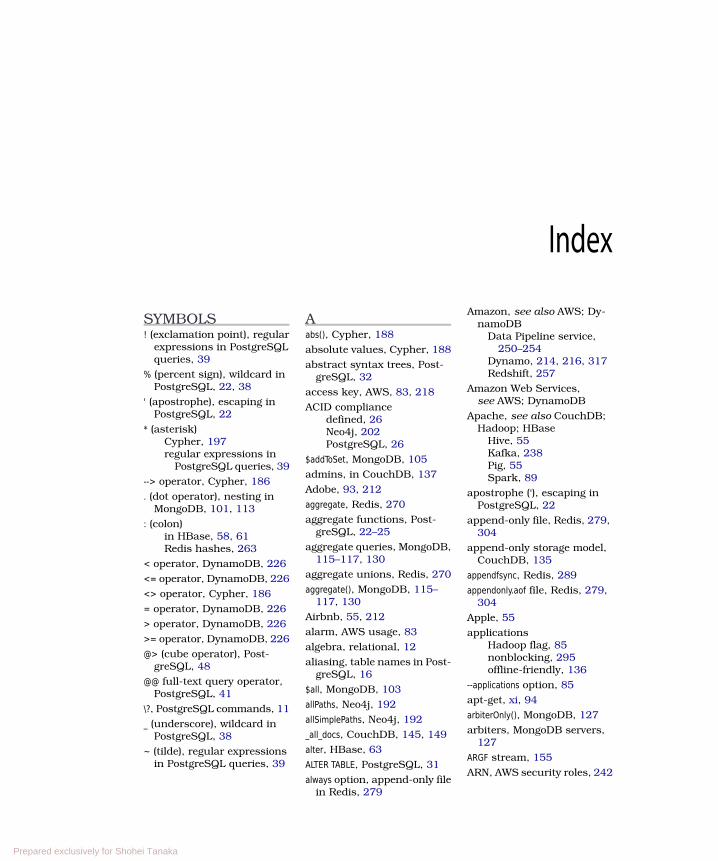
Index
SYMBOLS! (exclamation point), regular
expressions in PostgreSQLqueries, 39
% (percent sign), wildcard inPostgreSQL, 22, 38
' (apostrophe), escaping inPostgreSQL, 22
* (asterisk)Cypher, 197regular expressions in
PostgreSQL queries, 39
--> operator, Cypher, 186
. (dot operator), nesting inMongoDB, 101, 113
: (colon)in HBase, 58, 61Redis hashes, 263
< operator, DynamoDB, 226
<= operator, DynamoDB, 226
<> operator, Cypher, 186
= operator, DynamoDB, 226
> operator, DynamoDB, 226
>= operator, DynamoDB, 226
@> (cube operator), Post-greSQL, 48
@@ full-text query operator,PostgreSQL, 41
\?, PostgreSQL commands, 11
_ (underscore), wildcard inPostgreSQL, 38
~ (tilde), regular expressionsin PostgreSQL queries, 39
Aabs(), Cypher, 188
absolute values, Cypher, 188
abstract syntax trees, Post-greSQL, 32
access key, AWS, 83, 218
ACID compliancedefined, 26Neo4j, 202PostgreSQL, 26
$addToSet, MongoDB, 105
admins, in CouchDB, 137
Adobe, 93, 212
aggregate, Redis, 270
aggregate functions, Post-greSQL, 22–25
aggregate queries, MongoDB,115–117, 130
aggregate unions, Redis, 270
aggregate(), MongoDB, 115–117, 130
Airbnb, 55, 212
alarm, AWS usage, 83
algebra, relational, 12
aliasing, table names in Post-greSQL, 16
$all, MongoDB, 103
allPaths, Neo4j, 192
allSimplePaths, Neo4j, 192
_all_docs, CouchDB, 145, 149
alter, HBase, 63
ALTER TABLE, PostgreSQL, 31
always option, append-only filein Redis, 279
Amazon, see also AWS; Dy-namoDB
Data Pipeline service,250–254
Dynamo, 214, 216, 317Redshift, 257
Amazon Web Services,see AWS; DynamoDB
Apache, see also CouchDB;Hadoop; HBase
Hive, 55Kafka, 238Pig, 55Spark, 89
apostrophe ('), escaping inPostgreSQL, 22
append-only file, Redis, 279, 304
append-only storage model,CouchDB, 135
appendfsync, Redis, 289
appendonly.aof file, Redis, 279, 304
Apple, 55
applicationsHadoop flag, 85nonblocking, 295offline-friendly, 136
--applications option, 85
apt-get, xi, 94
arbiterOnly(), MongoDB, 127
arbiters, MongoDB servers,127
ARGF stream, 155
ARN, AWS security roles, 242
Prepared exclusively for Shohei Tanaka
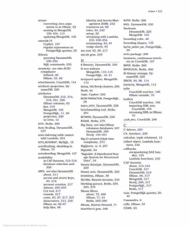
arraysconverting Java argu-
ments to in HBase, 65nesting in MongoDB,
100–104, 113updating MongoDB, 105
asterisk (*)Cypher, 197regular expressions in
PostgreSQL queries, 39
Athenaquerying DynamoDB,
250–254SQL commands, 255
atomicity, see also ACIDcompliance
defined, 26HBase, 53, 66
attachments, CouchDB, 144
attribute projection, Dy-namoDB, 226
attributesDynamoDB, 212, 214,
218, 221, 226HBase columns, 63key, 218MongoDB, 105PostgreSQL, 11, 20projection, 226as term, 12
AUTH, Redis, 280
Auto Scaling, DynamoDB,237
auto-inferring table nameswith Lambda, 254
AUTO_INCREMENT, MySQL, 16
autoflushing, disabling inHBase, 70
autosharding, MongoDB, 127
availabilityin CAP theorem, 315–318database selection and,
309
AWS, see also DynamoDBabout, 211access and secret keys,
83, 218account creation, 217Athena, 250–255CLI tool, 217console, 217costs, 83, 87, 217, 237datacenters, 213, 238HBase on, 82–87help files, 88
Identity and Access Man-agement (IAM), 242
resources on, 88roles, 84, 242setup, 82streaming with Lambda,
233, 238–254terminating, 83, 87usage alarm, 83
aws tool, 82, 88, 217
aws-sdk gem, 248
BB (binary), DynamoDB, 220
B-tree indexesMongoDB, 110–115PostgreSQL, 18, 21
background option, MongoDB,113
backup, HA Neo4j clusters, 206
Bash, xii
:begin, Cypher, 202
BEGIN TRANSACTION, PostgreSQL,26
begins_with(), DynamoDB, 226
benchmarking tool, Redis,281
BETWEEN, DynamoDB, 226
BGSAVE, Redis, 278
Big Data, see also HBasecolumnar databases, 307DynamoDB, 309Neo4j, 194–201
Big-O notated (O(x)) timecomplexity, 273
BigQuery, ix, 6, 257
Bigtable, 54
“Bigtable: A Distributed Stor-age System for StructuredData”, 54
binary datatype, DynamoDB,220
binary sets, DynamoDB, 220
bindAddress, HBase, 58
BLOBs, Kinesis streams, 239
blocking queues, Redis, 259, 265, 276
Bloom filtersabout, 72, 286HBase, 71, 81Redis, 285–288
Bloom, Burton Howard, 71
bloomfilter-rb gem, 286
BLPOP, Redis, 266
BOOL, DynamoDB, 220
BooleansDynamoDB, 220MongoDB, 103
bounding cube, 48
bounding shapes, 132
bpchar_pattern_ops, PostgreSQL,39
bricks package, 299
browsers, continuous watch-ers in CouchDB, 167
BRPOP, Redis, 266
BRPOPLPUSH, Redis, 266
BS (binary strings), Dy-namoDB, 220
BSON, 94, 96, 114
bsondump, MongoDB, 114
bufferCouchDB watcher, 166HBase variable, 70
buffersCouchDB watcher, 166importing XML into
CouchDB, 155streaming XML in HBase,
70
/_bulk_docs, CouchDB, 296
CC drivers, 283
C#, Interlace, 295
calculus, tuple relational, 12
callback object, Lambda func-tions, 242
callbacksencapsulating SAX han-
dler, 155Lambda functions, 242
CAP theoremabout, 315–318CouchDB, 317DynamoDB, 215HBase, 90, 317MongoDB, 317Neo4j, 208, 317PostgreSQL, 317Redis, 317
case, PostgreSQL queries, 39–40
Cassandra, 6
cells, HBase, 53
CERN, 93
Index • 322
Prepared exclusively for Shohei Tanaka
Changes API, CouchDB, 161–169, 290
_changes field, CouchDB, 162, 166, 168
channels, publish-subscribewith Redis, 276
chars, indexing in Post-greSQL, 39
--cli-input-json flag, 234
cloning, key values in Redis,267
Cloud Spanner, 257
cloud-based databases, seealso DynamoDB
Cloud Bigtable, 54costs, 83as genre, 2HBase example, 82–87increase in, 5multiple services and,
233trade-offs, 256
CloudWatch, 83, 236
clustersCouchDB replication, 171HBase, 55, 83–88, 90MongoDB, 114Neo4j high availability
mode, 203–208Redis, 284–285, 289, 304
CockroachDB, 257
codefor this book, xii, 293executing fuzzy search in
database, 38executing in PostgreSQL
database, 27–30executing in database,
reasons to, 29nonblocking applications,
295reading in MongoDB, 108
collections, MongoDBCRUD operations, 94–
109indexing, 110–115listing, 96vs. Postgres tables, 109verifying, 96
colon (:)in HBase, 58, 61Redis hashes, 263
column families, HBaseadvantages, 65compression, 81defined, 58
modifying, 63number per table, 77
column qualifier, HBase, 58
columnar databases, see al-so HBase
about, 6, 307, 309as genre, 2, 6, 307
columnsHBase, 53, 58–60, 63, 79PostgreSQL, 11, 20
Comcast, 93, 212
:commit, Cypher, 202
CommonJS Module API, 164
composite key, DynamoDB,223, 229–230, 234
compound keys, PostgreSQL,14, 16
compressioncolumnar databases, 307HBase, 71, 81, 89
conditionalsDynamoDB, 233MongoDB, 99
--configdb flag, MongoDB, 128
conflicts, CouchDB, 138, 170–174
_conflicts field, CouchDB, 172, 174
connectionsbreaking Redis, 277CouchDB fault tolerance,
135HBase, 58PostgreSQL schema, 10Redis, 260, 277as selection criteria, 2
consistency, see also ACIDcompliance
in CAP theorem, 315–318CouchDB, 143database selection and,
309defined, 26DynamoDB, 215, 237eventual, 316HBase, 53, 90MongoDB, 127Neo4j, 203PostgreSQL, 14, 26
--consistent-read flag, Dy-namoDB, 223
constraintsforeign key, 14, 16, 20,
37Neo4j, 187
PostgreSQL, 13, 16, 20, 37
Redis, 264
Content-Type header, CouchDBdocuments, 142
context object, Lambda func-tions, 241
continuous pollingCouchDB, 162, 167polyglot persistence ser-
vice example, 297
control plane, DynamoDB,214, 218
core nodes, HBase clusters,88
CouchDB, 135–175about, 2, 7, 135, 307attachments, 144CAP theorem, 317Changes API, 161–169,
290CRUD, 137–149design documents, 149Fauxton interface, 137–
140, 147, 149filtering changes, 167–
169homework, 144, 157, 173importing data using Ru-
by, 152–157indexes, 135, 149, 152,
161mapreduce, 145, 158–
161, 174vs. MongoDB, 136offline-friendly applica-
tions, 136polyglot persistence ser-
vice example, 289–303querying, 149–152, 157replication, 169–173, 307resources on, 171REST, 135–136, 140–
144, 173strengths, 174views, 135, 145–161watchers, 161–169, 173weaknesses, 174
couchrest gem, 153–156
count, HBase, 70, 80
count()MongoDB, 102, 115PostgreSQL, 22
CREATE, Neo4j with Cypher,181–186
create, HBase, 60
Index • 323
Prepared exclusively for Shohei Tanaka
CREATE INDEXNeo4j, 187PostgreSQL, 18, 37
CREATE MATERIALIZED VIEWS, Post-greSQL, 32
CREATE TABLE, PostgreSQL, 37
CREATE TEMPORARY TABLE, Post-greSQL, 34
CREATE VIEW, PostgreSQL, 31
create-cluster, HBase, 84
create-default-roles, AWS, 84
create-function, Lambda, 242
create-stream, Kinesis, 239
create-table, DynamoDB, 218, 222
createClient(), polyglot persis-tence service example, 293, 297
createWatcher(), Node.js, 164
createlang, PostgreSQL, 29
creating, see also CRUDCouchDB, 137–142, 145–
149DynamoDB, 218–219,
234HBase, 58–60indexes in MongoDB, 111indexes in Neo4j, 187indexes in PostgreSQL,
18Kinesis streams, 239materialized views, 32MongoDB, 95–98, 111Neo4j, 181–187, 190pipelines, 251PostgreSQL, 10–13, 18,
31
CRLF (\r\n), Redis streaming,274–275
crosstab(), PostgreSQL, 34–35
CRUDCouchDB, 137–149defined, 13, 20DynamoDB, 214, 216,
218–219, 221, 234HBase, 58–66MongoDB, 94–109Neo4j, 179–186, 190PostgreSQL, 10–15Redis, 260–262
CSV, exporting MongoDB,114
csv gem, 293
Ctrl+Cbreaking connection in
Redis, 277killing scripts in HBase,
73, 80
Ctrl - ] , terminating telnet, 274
cube, 36, 46–49
cube operator (@>), Post-greSQL, 48
cube_distance(), 47
cube_enlarge(), 48
cubesbounding, 48querying PostgreSQL
with, 46–49
cURLchecking REST server is
running, 190CouchDB changes
watcher, 162CouchDB CRUD opera-
tions, 140–144CouchDB queries, 150–
152, 157Neo4j REST interface,
189–194
Cygwin, xii
CypherCRUD, 179–186excluding redundancies,
198functions, 188help files, 179, 195querying with, 180–189,
195–201resources on, 188REST and, 193shell, 202terminology, 180transactions, 202
D/dF, PostgreSQL, 42
daemonize, Redis, 278
dataadding to HBase with
scripts, 64–73importing into CouchDB
with Ruby, 152–157inserting large dataset
into Redis, 282–285population for polyglot
persistence service ex-ample, 291–297
replicating in CouchDB,169–173
size and database selec-tion, 309
transforming TSV in Re-dis, 293–294
warehousing, 302
Data Pipeline service, 250–254
data warehousing, 302
Data.gov, 82
database setting, Redis, 278
databases, see also CouchDB;DynamoDB; HBase; Mon-goDB; Neo4j; NoSQL; Post-greSQL; Redis; relationaldatabases
genres, 2–8, 305–309HBase rows as, 62multiple namespaces in
Redis, 272selection and genres, 2–
3, 305selection criteria, 309selection questions, 2
datatypesDynamoDB, 219key-value stores, 4lack of in HBase, 90PostgreSQL, 14Redis, 5, 260, 263–271relational databases, 4
@db.save_doc(), CouchDB, 155
DECR, Redis, 262
DECRBY, Redis, 262
DEL, Redis, 273
DELETECouchDB CRUD opera-
tions, 143Neo4j, 184, 299PostgreSQL, 14, 36
delete-item, DynamoDB, 223
deleting, see also CRUDCouchDB, 138, 140, 143DynamoDB, 214, 222MongoDB, 105, 107Neo4j, 184, 188, 299PostgreSQL, 14, 34, 36Redis, 264, 268, 273
descending parameter, import-ing XML into CouchDB,156
describe, HBase, 76
describe-table, DynamoDB, 219
design documents, CouchDB,149
destination, Redis, 270
Index • 324
Prepared exclusively for Shohei Tanaka
dict_xsyn package, 36
dictionarieslisting in PostgreSQL, 42tsvector and tsvector, 41
diffs, Redis sets, 267
dijkstra, Neo4j, 192
dimensional queries with cube,46–49
directoriesHBase, 57, 65MongoDB, 95
disable, HBase, 63
disablingcommands in Redis, 280tables in HBase, 63
disaster recoverybackups for HA Neo4j
clusters, 206write-ahead logging in
HBase, 74, 76
DISCARD, Redis, 262
disk usage, HBase, 73, 80
DISTINCT, Cypher, 198
distinct(), MongoDB, 115
distributed configuration,HBase, 55
dmetaphone(), PostgreSQL, 45
dmetaphone_alt(), PostgreSQL,45
DNS (Domain Name Service)and eventual consistency,316
document types, DynamoDB,220
document variable, HBase, 70
document-oriented databas-es, see also CouchDB;MongoDB
about, 6, 307advantages, 95, 124as genre, 2, 6, 307workflow, 94
domain, relational databases,12
dot operator (.), nesting inMongoDB, 101, 113
double metaphones, 45
DoubleClick, 93
driverschanges watcher in
CouchDB, 163graph databases exercise,
202MongoDB, 109, 123
for Neo4j in polyglot per-sistence service exam-ple, 298
performance, 283Redis, replacing, 283
driving force, as selection cri-teria, 2
DROP CONSTRAINT, Neo4j, 188
DROP INDEX, Neo4j, 187
du, HBase, 73
duplicate words, Bloom fil-ters, 287
durability, see also ACIDcompliance
database selection and,309
defined, 26DynamoDB, 213HBase, 55Redis, 259, 278–280, 304
Dynamo, 214, 216, 317, seealso DynamoDB
Dynamo: Amazon’s HighlyAvailable Key-value Store,214
DynamoDB, 211–257about, 2, 5, 211, 309Auto Scaling, 237AWS datacenters, 213,
238control plane, 214, 218costs, 217, 237, 256CRUD, 214, 216, 218–
219, 221, 234data model, 213–216,
218data model for sensor ex-
ample, 234–236datatypes, 219exporting to S3, 250–252help files, 217homework, 232, 245, 255indexes, 214, 218, 230–
233, 249, 255Internet of Things, 246–
254keys, 213, 222–228, 230,
234Local version, 217partitions, 227–230, 232performance, 212, 222,
228, 230, 236querying, 213, 215, 218,
221, 224–227, 230, 249–254
resources on, 232streaming, 232–254
Streams, 245strengths, 212, 255throughput, 236, 251weaknesses, 256
DynamoDB Streams, 245
E--ec2-attributes, HBase cloud ex-
ample, 85
Elastic MapReduce, see EMR
Elasticsearch, 38
$elemMatch, MongoDB, 101, 103
emit()CouchDB, 147, 149–152,
157–161, 164MongoDB, 120–123
EMRabout, 82exporting DynamoDB,
251HBase on cloud example,
82–87resources on, 88setup, 82
emr command, 88
enable, HBase, 64
encapsulating, SAX handler,155
ENDKEY, HBase, 76
endkey parameter, importingXML into CouchDB, 156
ensureIndex, MongoDB, 111
entity diagrams, 36
Erlang, 7, 135
escaping, apostrophe (') inPostgreSQL, 22
event object, Lambda func-tions, 241
event source mapping, AWS,243
EventEmitter, Node.js, 164
EventMachine, 295
eventual consistency, 316
everysec option, append-onlyfile in Redis, 279
exclamation point (!), regularexpressions in PostgreSQLqueries, 39
EXEC, Redis, 262
EXISTS, Redis, 271
$exists, MongoDB, 103
EXPIRE, Redis, 271
Index • 325
Prepared exclusively for Shohei Tanaka
EXPIREAT, Redis, 272
expiryDynamoDB, 245Redis, 259, 271
EXPLAIN, PostgreSQL, 32, 43
EXPLAIN VERBOSE, PostgreSQL,33
explain(), MongoDB, 111
exportingDynamoDB to S3, 250–
252MongoDB, 114Node.js scripts, 164
exports object, Node.js, 164
--expression-attribute-values flag,DynamoDB, 225
extract(), PostgreSQL, 34
FFaaS (Functions-as-a-Ser-
vice), Lambda as, 238
Facebook, 55
false positives, Bloom filters,72, 286–287
FaunaDB, 257
Fauxton interface, CouchDB,137–140, 147, 149
feed, CouchDB watcher, 166
fieldsCouchDB, 138creating indexes in Mon-
goDB, 111setting in MongoDB, 105
fields parameter, creating in-dexes in MongoDB, 111
filesfile system as key-value
store, 4listing in MongoDB, 131loading in MongoDB, 120S3 buckets, 252storing in HBase, 57
filter functions, CouchDB,167–169
filter(), Cypher, 188
filteringaggregate functions in
PostgreSQL, 23Bloom filters, 71–72, 81,
285–288CouchDB, 167–169Cypher, 188
filters key, CouchDB, 168
finalize(), MongoDB, 120, 122
find()MongoDB, 96, 98, 107,
125MongoDB replica sets,
125
findOne(), MongoDB, 105
floats, DynamoDB, 220
flushCommits, HBase, 70
FLUSHALL, Redis, 273, 280
FLUSHDB, Redis, 273
flushingdisabling autoflush in
HBase, 70Redis, 273, 280
foreign key constraints, Post-greSQL, 14, 16, 20, 37
Foursquare, 93
Fowler, Martin, 291
--from flag, HA Neo4j clustersbackup, 206
FULL JOIN, PostgreSQL, 18
full-text searchesNeo4j, 193PostgreSQL, 41–46
FUNCTION, PostgreSQL storedprocedures, 27–30
functionsaggregate functions, 22–
25custom JavaScript func-
tions, 108Cypher, 188definitions in MongoDB,
97, 118–119filter functions, 167–169Lambda, 240–242, 254storing JavaScript func-
tions in system.js, 119window functions, Post-
greSQL, 24–25
Functions-as-a-Service(FaaS), Lambda as, 238
fuzzy string matching inPostgreSQL, 36–46
fuzzystrmatch package, 36, 39, 45
GGeneralized Index Search
Tree (GIST), 40
Generalized Inverted iNdex(GIN), 43
generate_series(a, b) function,PostgreSQL, 36
geohashes, 130
geospatial queries, MongoDB,130
GETCouchDB change watch-
er, 162CouchDB conflicts, 172CouchDB CRUD opera-
tions, 140CouchDB watcher, 166Neo4j nodes and relation-
ships, 190Redis, 261, 275
get, HBase, 61, 66, 80
get(), CouchDB watcher, 166
get-item, DynamoDB, 223
GETBIT, Bloom filters, 287
GIN (Generalized Inverted iN-dex), 43
GIST (Generalized IndexSearch Tree), 40
Git, creating HBase directly,56
global secondary indexes(GSIs), 231, 237, 255
GoogleBigQuery, ix, 6, 257Bigtable, 54Cloud Spanner, 257
graph databases, see al-so Neo4j
about, 7, 308advantages, 208as genre, 2, 7, 308nodes, 180, 208
graphSync.js, 297
Gremlin, 180, 300
GridFS, MongoDB, 114, 131–132, 303
Grigorik, Ilya, 286
Groovy, 201
$group, MongoDB, 115–116
GROUP BY, PostgreSQL, 23–24
groupingqueries in MySQL, 24queries in PostgreSQL, 23views in CouchDB, 149
GSIs (global secondary index-es), 231, 237, 255
$gt, MongoDB, 103
$gte, MongoDB, 103
GZ compression, HBase, 71
Gzip compression, HBase, 71
Index • 326
Prepared exclusively for Shohei Tanaka
H/h, PostgreSQL commands, 11
-h option for du in HBase, 73
H2, 4
Hadoopabout, 55--applications flag, 85EMR, 82HBase and, 6, 54, 89
Hadoop Distributed File Sys-tem (HDFS), 6, 89
hash datatype, Redis, 263
hash indexesNeo4j, 192PostgreSQL, 18, 21
hash key, DynamoDB, 223, 226, 229–230, 234, 239
HAVING, PostgreSQL, 23
HBase, 53–91about, 2, 6, 53, 309adding data with scripts,
64–73Bloom filters, 71, 81CAP theorem, 90, 317cloud based example, 82–
87cluster-to-cluster replica-
tion, 90community support for,
55, 89compression, 71, 81, 89CRUD, 58–66defaults, 63disabling tables, 63disk usage, 73, 80help files, 58homework, 66, 81, 88indexes, 61, 90installation, 56killing, 57killing scripts, 73, 80modes, 55performance, 61, 64–65,
71, 74, 89polyglot persistence ser-
vice example, 302regions, 58, 73–77resources on, 66scans, 61, 76–81shell, 57starting, 57strengths, 89terminology, 53, 55, 66,
88version, 55, 57weaknesses, 89
@hbase administration object,65
hbase*, 63
hbase-default.xml file, 56
hbase-site.xml file, 56, 58
hbase.rootdir property, 57, 73
hbase:meta table, 75
HBASE_HOME environment vari-able, 56
HBaseMaster, 76
HDEL, Redis, 264
HDFS (Hadoop DistributedFile System), 6, 89
headersCouchDB documents,
142relational databases, 12
helpCypher, 195DynamoDB, 217HBase, 58MongoDB, 95Neo4j, 195PostgreSQL, 11Redis, 261
:help commands, Neo4j, 179
:help cypher, Neo4j, 179
help filesaws tool, 88Cypher, 179, 195DynamoDB, 217emr command, 88HBase, 58MongoDB, 95–96, 109MongoDB replica sets,
125Neo4j, 179, 195PostgreSQL, 11Redis, 261
help()MongoDB, 96, 109MongoDB replica sets,
125
HGETALL, Redis, 264
hiding commands in Redis,280
high availability mode, Neo4j,203–208
high-performance multivari-ate flagging, 288
HINCRBY, Redis, 264
hiredis gem, 283, 293
Hive, 55
HLEN, Redis, 264
Homebrew, xi, 94, 260
homeworkCouchDB, 144, 157, 173DynamoDB, 232, 245,
255HBase, 66, 81, 88MongoDB, 109, 123, 132Neo4j, 189, 201, 207PostgreSQL, 21, 36, 49Redis, 273, 289, 303
horizontal sharding,see sharding
hotspots, 228
HSETNX, Redis, 264
HSQLDB, 4
HTML, polyglot persistenceservice example, 300
HTTPResponse, CouchDBwatcher, 166
IIAM (Identity and Access
Management), 242
_id field, CouchDB, 138, 143
_id property, MongoDB, 98
idstr property, CouchDB, 158
if put_to, HBase, 79
ILIKE, PostgreSQL, 38
import, HBase, 65
importingdata in HBase with
scripts, 65, 67–73data into CouchDB using
Ruby, 152–157MongoDB, 114
$in, MongoDB, 103
$inc, MongoDB, 105
include?(), Bloom filters, 288
include_docs parameter,CouchDB watcher, 162, 166
INCR, Redis, 261
INCRBY, Redis, 262
incrementing in Redishashes, 264sorted sets, 268strings, 261values within transac-
tions, 274
indexesB-tree indexes, 18, 21,
110–115CouchDB, 135, 149,
152, 161
Index • 327
Prepared exclusively for Shohei Tanaka
creating MongoDB, 111defined, 18, 20design documents, 149DynamoDB, 214, 218,
230–233, 237, 249, 255
global secondary indexes,231, 237, 255
hash indexes, 18, 21, 192HBase, 61, 90inverted, 43, 193key-value, 192lexemes in PostgreSQL,
43listing in MongoDB, 111listing in PostgreSQL, 20local secondary indexes,
214, 230, 237, 249materialized views, 32MongoDB, 110–115, 130Neo4j, 187, 192nested values in Mon-
goDB, 113performance in Dy-
namoDB, 230performance in Mon-
goDB, 110, 114PostgreSQL, 18–20, 32,
37, 39–40, 43reverse lookups, 37trigrams, 40
infinite ranges, Redis, 269
INFO, Redis, 277
Ingres, 9
initialize(), MongoDB replicasets, 125
INNER JOIN, PostgreSQL, 15–18
inner joins, 15–18, 45
INSERT INTO, PostgreSQL, 13, 15
insert(), Bloom filters, 288
insertingCouchDB bulk insertion,
296HBase, 61PostgreSQL, 13, 15Redis lists, 264Redis, large datasets,
282–285
installationabout, xiaws tool, 83, 217cube, 36HBase, 56MongoDB, 94PostgreSQL, 10PostgreSQL packages, 36
--instance-count, HBase cloudexample, 85
--instance-type, HBase cloud ex-ample, 85
integersDynamoDB datatype, 220Redis, 261, 264
Interactive Graphics and Re-trieval System, 9
Interlace, 295
Internet of Thingsabout, 246streaming DynamoDB
example, 246–254
intersectionsRedis keys, 270Redis sets, 267
inverted indexes, 43, 193
isMaster(), MongoDB replicasets, 126
isolation, defined, 26, see al-so ACID compliance
items, DynamoDBconsistency, 215data model, 212, 214,
218JSON and, 221
JJamendo.com, 153, 155
JamendoCallbacks class, 155
Javaconverting arguments to
HBase, 65custom functions in
Cypher, 188NIO library, 295
JavaScript, see also Node.jscustom functions, 108filter functions, 168Lambda functions, 240–
242MongoDB and, 96nonblocking code, 295storing functions in sys-tem.js, 119
syntax rules, 99
jbytes(), HBase, 65
JOIN, PostgreSQL, 17
joinscompound, 16inner joins, 15–18, 45natural joins, 45outer joins, 17
PostgreSQL, 15–18, 20, 45, 50
relational databases, 4
journaling, see write-aheadlogging
jQuery, polyglot persistenceservice example, 302
JRubyHBase shell as inter-
preter, 64streaming XML in HBase,
68
JSON, see also CouchDB;MongoDB
document-orienteddatabases, 307
in DynamoDB, 221, 234, 252
PostgreSQL support, 51
JSONB, PostgreSQL support,51
JUNG project, 201
KKafka, 238
Kevin Bacon example, 197–201
--key flagDynamoDB, 223Redis, 270
key argument, CouchDB re-duce functions, 160
key attributes, DynamoDB,218
key condition expressions,DynamoDB, 225
key pair, SSH, 84
--key-condition-expression flag, Dy-namoDB, 225
key-value indexes, Neo4j, 192
key-value pairsmapreduce in CouchDB,
158–161querying CouchDB, 149–
152
key-value stores, see also Re-dis
about, 4, 306, 309DynamoDB as, 216, 223as genre, 2, 4, 306performance, 306
KEYS, Redis, 296
keysAWS access and secret,
83, 218
Index • 328
Prepared exclusively for Shohei Tanaka
cloning key values in Re-dis, 267
composite, 223, 229–230, 234
compound, 14, 16CouchDB mapreduce,
158–161CouchDB views, 145,
147, 152DynamoDB, 213, 222–
228, 230, 234, 239foreign key constraints,
14, 16, 20, 37hash, 223, 226, 229–
230, 234, 239HBase, 58, 73, 90MongoDB mapreduce,
120, 122MongoDB sharding, 128PostgreSQL, 13, 16, 18,
20, 37primary, 13, 16, 18, 20range, 223, 229–230, 234Redis, 261, 263, 265,
267, 270–273row key in HBase, 73, 90SET (Redis), 261
killingAWS, 83, 87HBase, 57scripts in HBase, 73, 80telnet in Redis, 274transactions in Post-
greSQL, 26
Kinesisperformance, 245streaming DynamoDB,
233, 238–254
KV stores, see key-valuestores; Redis
LL (list datatype), DynamoDB,
220
labels, Neo4j constraints, 187
Lambdaauto-inferring table
names, 254functions, 240–242, 254streaming DynamoDB,
233, 238–254
languagespolyglot programming,
291PostgreSQL support, 28,
42Redis support, 260
last_seq, CouchDB watcher,166
LASTSAVE, Redis, 278
latencyCAP theorem, 317nonblocking code, 295
LEFT JOIN, PostgreSQL, 17, 20
LEFT OUTER JOIN, PostgreSQL, 17
Lempel-Ziv-Oberhumer com-pression, HBase, 71
Levenshtein distance, 39
levenshtein() function, 39
lexemes, 42–43
libxml-ruby gem, 153–156
licenses, Neo4j, 207–208
LIKE, PostgreSQL, 22, 38
limit parameterCouchDB watcher, 162importing XML into
CouchDB, 156
list datatypeDynamoDB, 220Redis, 263–266
listCommands(), MongoDB, 118
listingblocking lists in Redis,
266collections in MongoDB,
96databases in MongoDB,
95dictionaries in Post-
greSQL, 42files in MongoDB, 131functions in MongoDB,
97HBase clusters, 83, 85indexes in MongoDB, 111indexes in PostgreSQL,
20languages in PostgreSQL,
29list length in Redis, 264popping lists in Redis,
265server-side commands in
MongoDB, 118tables in DynamoDB, 218
LLEN, Redis, 264
load balancer exercise, 207
local secondary indexes, Dy-namoDB, 214, 230, 237, 249
lock-in, vendor, 27
logfile, Redis, 278
loglevel, Redis, 278
logsHBase, 55, 57, 74, 76, 79MongoDB, 114PostgreSQL, 29Redis options, 278tailing Neo4j HA cluster,
205write-ahead logging in
HBase, 55, 74, 76, 79
logs table, creating in Post-greSQL, 29
longpolling, CouchDB, 162–163, 165, 167
loopback interface, HBase, 58
LPOP, Redis, 265
LPUSH, Redis, 265
LRANGE, Redis, 264
LREM, Redis, 265
LSIs, see local secondary in-dexes
$lt, MongoDB, 103
$lte, MongoDB, 103
Lucene, 38, 193
LZO compression, HBase, 71
MM (map datatype), DynamoDB,
220
map datatype, DynamoDB,220
map function, CouchDB,147, 149–152, 158–161
mapReduce() function, Mon-goDB, 119–123
mapreduceCouchDB, 145, 158–161,
174database selection and,
309defined, 119DynamoDB exporting
and, 251MongoDB, 119–123
master election, HA Neo4jclusters, 206
master node, HBase, 76
master-master replication,CouchDB, 169–173, 307
master-slave replication, Re-dis, 281
MasterProcWALs folder, HBase,74
Index • 329
Prepared exclusively for Shohei Tanaka
mastersCouchDB, 169–173, 307HBase, 58, 76MongoDB replica sets,
125–127multiple in Redis, 284Neo4j high availability
mode, 203–207Redis, 281, 284
MATCHNeo4j, 181–189, 195–201PostgreSQL, 21
$match, MongoDB, 115–116
MATCH FULL, PostgreSQL, 16, 21
materialized views, 32
mathematical relations andrelational databases, 12
@max parameter, importingXML into CouchDB, 155
max(), PostgreSQL, 22
memcached, 278
memory, Redis, 278, 280, 304
Merriman, Dwight, 93
Message Queue TelemetryTransport (MQTT), 247
messaging patterns, Redis,289
metadataCouchDB views, 146HBase, 75–76, 88Neo4j nodes, 190PostgreSQL, 21
metaphones, 44–46
MGET, Redis, 261
microservices, polyglot pro-gramming and, 291
middleware layer pattern andpolyglot persistence, 291
min(), PostgreSQL, 22
misspellingsMongoDB, 107PostgreSQL, 40
Moby Dick example, 286
$mod, MongoDB, 103
modify-instance-groups, EMR, 88
mongoconfig, 129
mongod, 95, 126–127
MongoDB, 93–133about, 2, 7, 93, 307aggregate queries, 115–
117, 130CAP theorem, 317CLI tools list, 114
clusters, 114commands, listing, 105,
118conventions, 99vs. CouchDB, 136CRUD, 94–109databases, listing, 95databases, switching, 95files, listing, 131functions, 97geospatial queries, 130GridFS, 114, 131–132,
303help files, 95–96, 109,
125homework, 109, 123, 132indexes, 110–115, 130installation, 94mapreduce, 119–123misspellings, 107nesting, 100–104, 113performance, 108, 110,
114, 117polyglot persistence ser-
vice example, 302–303query command list, 103querying, 98–104, 106,
108, 112, 115–117, 121, 130
reading code in, 108references, 106replica sets, 124–128,
132resources on, 104, 109server-side commands,
117–119sharding, 114, 127–131starting, 95strengths, 95, 133UI tools, 98weaknesses, 133
mongodump, 114
mongoexport, 114
mongofiles, 114, 131
MongoHQ, 307
mongoimport, 114
mongooplog, 114
mongoperf, 114
mongorestore, 114
mongos, 114, 128–130
mongostat, 114
mongotop, 114
most recently used (MRU)caching algorithm, 272
MOVE, Redis, 273
MQTT (Message QueueTelemetry Transport), 247
MRU (most recently used)caching algorithm, 272
MSET, Redis, 261
MULTI, Redis, 262, 296
multi-master replication,CouchDB, 169–173, 307
multibulk reply, Redis, 277
multivariate flagging, high-performance, 288
mustache package, 299
MyPyramid Raw Food Data,82
MySQLabout, ix, 4AUTO_INCREMENT, 16grouping queries, 24
NN (number), DynamoDB, 220
name property, nodes in Neo4j,190
name_pattern_ops, PostgreSQL,39
namesaliasing table names in
PostgreSQL, 16auto-inferring table
names, 254indexing in PostgreSQL,
39nodes in Neo4j, 190
NATURAL JOIN, PostgreSQL, 45
natural language processing,PostgreSQL, 41–46
nc, netcat, 275
$ne, MongoDB, 103
nearest neighbor matches,with cube, 47
Neo Technology, 207
Neo4j, 177–209, see al-so Cypher
about, 2, 7, 177, 308CAP theorem, 208, 317constraints, 187CRUD, 179–186, 190Enterprise Edition, 178,
204, 207–208GPL Community Edition,
178, 207help files, 179, 195high availability mode,
203–208homework, 189, 201, 207
Index • 330
Prepared exclusively for Shohei Tanaka
indexes, 187, 192licenses, 207–208performance, 208polyglot persistence ser-
vice example, 289–290, 297–303
querying, 180–189, 193, 195–201
resources on, 189, 192REST, 189–194shell, 195strengths, 208terminology, 180, 208tools, 208version, 178, 207–208weaknesses, 208web interface, 179
neo4j-admin tool, 206
nestingCouchDB, 139document-oriented
databases, 307filter functions, 168JSON in streaming in
DynamoDB, 252lack of in Redis, 264MongoDB, 100–104, 113
netcat, 275
network settings, HBase, 58
networksCouchDB fault tolerance,
135HBase settings, 58
$nin, MongoDB, 103
NIO library, 295
*nix platforms, Windowsusers, xi
no option, append-only file inRedis, 279
Node Package Manager (npm),293
node path, Neo4j, 190–192, 199–201
node walking, 297
Node.jsabout, 162change watcher for
CouchDB, 162–169checking installation, 293nonblocking code, 295polyglot persistence ser-
vice example, 290SocketStream, 304
nodesCouchDB master-master
replication, 169–173
Cypher, 180eventual consistency, 316graph databases, 180,
208HBase, 55, 76, 88MongoDB, 126Neo4j, 180–186, 190,
195–201, 203–207Neo4j high availability
mode, 203–207
non-relational databases,see CouchDB; DynamoDB;HBase; MongoDB; Neo4j;NoSQL; Redis
nonblocking applications, 295
$nor, MongoDB, 103
NoSQL, see also CouchDB;DynamoDB; HBase; Mon-goDB; Neo4j; Redis
vs. relational databases,1
as term, ix
$not, MongoDB, 103
notice setting, Redis log, 278
npm (Node Package Manager),293
NS (number set), DynamoDB,220
NULLDynamoDB, 220PostgreSQL, 14
null valuesdisallowing in Post-
greSQL, 14DynamoDB, 220
number datatype, Dy-namoDB, 220
number sets, DynamoDB,220
Oobject expiry, DynamoDB,
245
ObjectId, MongoDB, 96, 98
offline-friendly applications,136
offset files, CouchDB, 152
oldWALs folder, HBase, 74
ON, joining tables in Post-greSQL, 15
on_end_element(), importing XMLinto CouchDB, 155
on_start_element(), importingXML into CouchDB, 155
options parameter, creating in-dexes in MongoDB, 111
$or, MongoDB, 103
orderreversing row order when
importing XML intoCouchDB, 156
sorted sets in Redis, 268
outer joins, 17
Pparsing
PostgreSQL parsers, 42XML for CouchDB, 153–
156XML for HBase, 68
partial values, matching inMongoDB, 100
PARTITION BY, PostgreSQL, 25
partition key, see hash key
partition tolerance, in CAPtheorem, 315–318
partitionsin CAP theorem, 315–318DynamoDB, 227–230,
232graph databases, 308Kinesis, 245PostgreSQL, 52
passwords, Redis, 280
path, CouchDB watcher, 166
pathsCouchDB watcher, 166counting number of
shortest paths inNeo4j, 200
querying in Neo4j, 190–192, 199–201
querying views inCouchDB, 151
pattern matching, Post-greSQL, 39
PCRE (Perl-compatible regu-lar expression), 99, 103
percent sign (%), wildcard inPostgreSQL, 22, 38
performanceaggregate queries in
MongoDB, 117append-only file in Redis,
279Bloom filters, 71, 288CAP theorem, 317column families, HBase,
65drivers, 283
Index • 331
Prepared exclusively for Shohei Tanaka
DynamoDB, 212, 222, 228, 230, 236
executing database code,29
HBase, 61, 64–65, 71, 74, 89
indexes in DynamoDB,230
indexes in MongoDB,110, 114
key-value stores, 306Kinesis, 245MongoDB, 108, 110,
114, 117Neo4j, 208nonblocking code, 295PostgreSQL, 27, 32Redis, 5, 259, 279, 283,
285, 304scans, 61, 222as selection criteria, 3stored procedures, 27write-ahead logging in
HBase, 74
Perl, 29
Perl-compatible regular ex-pression (PCRE), 99, 103
PERSIST, Redis, 271
persistencepolyglot persistence ser-
vice example, 289–303Redis, 271, 278–280
pg_trgm package, 36, 40
Pig, 55
pipelinescreating, 251replacing Redis driver,
283streaming DynamoDB,
233–254streaming with Redis,
275, 283
pivot tables, PostgreSQL, 34–35
PL/Perl, 29
PL/pgSQL, 28
PL/Python, 29
PL/Tcl, 29
PNUTS, 317
point of entry, MongoDB, 129
policies, AWS security roles,242
polling, CouchDB, 162–166, 297
polyglot persistenceabout, 7, 289rise of, 291service example, 289–303
polyglot programming, 291
$pop, MongoDB, 105
poppingelements from MongoDB
arrays, 105sets in Redis, 268values in Redis lists, 265
populateCouch.js, 295
portsCouchDB, 295MongoDB, 124Neo4j, 205, 297Redis, 260, 278, 284, 293
POSIX style, regular expres-sions, 39, 49
POSTCouchDB CRUD opera-
tions, 142Neo4j indexes, 193Neo4j nodes and relation-
ships, 190
Postgres95, 9
PostgreSQL, 9–52about, ix, 1, 4, 9aggregate functions, 22–
25CAP theorem, 317community support for,
51core languages, 28CRUD, 10–15full-text searches, 41–46fuzzy string matching,
36–46help menus, 11homework, 21, 36, 49indexes, 18–20, 32, 37,
39–40, 43installation, 10joins, 15–18, 20, 45, 50JSON and, 51materialized views, 32natural language process-
ing, 41–46performance, 27, 32pivot tables, 34–35polyglot persistence ser-
vice example, 302querying, 9, 18–20, 22–
25, 32–49querying full-text, 41–46querying with cube, 46–49resources on, 11, 28, 45
RULEs, 32–35schema, 9–11, 17, 51stored procedures, 27–
30, 50, 188strengths, 50transactions, 26views, 30–34weaknesses, 51window functions, 24–25
PouchDB, 136
prefix notation, 103
PRIMARY KEY, PostgreSQL, 13
primary keys, PostgreSQL,13, 16, 18, 20
PRIMARY server, MongoDBreplica sets, 125–127
Procedural Language/Post-greSQL, 28
procedures, stored (Post-greSQL), 27–30, 50, 188
$project, MongoDB, 116
--projection-expression flag, Dy-namoDB, 226
properties, Neo4j nodes, 191
pseudo-distributed mode,HBase, 55
PUBLISH, Redis, 276
publish-subscribe with Redis,259, 276
$pull, MongoDB, 105
$pullAll, MongoDB, 105
$push, MongoDB, 105
$pushAll, MongoDB, 105
PUT, cURL CouchDB CRUDoperations, 142
put, HBase, 61, 64–66, 70
PUT instances, HBase, 64, 67, 69, 79
put-item, DynamoDB, 221
PythonPostgreSQL support, 29Twisted, 295
Q-q option, netcat, 275
query, DynamoDB, 225
query planner, PostgreSQL,32
query trees, PostgreSQL, 32
queryingaggregate functions in
PostgreSQL, 22–25
Index • 332
Prepared exclusively for Shohei Tanaka
aggregate queries inMongoDB, 115–117, 130
columnar databases, 307CouchDB, 149–152, 157database selection and,
309DynamoDB, 213, 215,
218, 221, 224–227, 230, 249–254
full-text searches in Post-greSQL, 41–46
fuzzy string matching inPostgreSQL, 36–46
geospatial queries inMongoDB, 130
graph databases, 308grouping queries in
MySQL, 24grouping queries in Post-
greSQL, 23HBase regions, 75key-value stores, 306MongoDB, 98–104, 106,
108, 112, 115–117, 121, 130
MongoDB commands list,103
MySQL, 24Neo4j, 180–189, 193,
195–201polyglot persistence ser-
vice example, 298–303PostgreSQL, 9, 18–20,
22–25, 32–49PostgreSQL full-text, 41–
46PostgreSQL fuzzy string
matching in, 36–46PostgreSQL with cube, 46–
49Redis, 285–288relational databases, 9,
12, 306reverse querying in Neo4j,
197RULEs, 32–35
queues, Redis, 259, 262, 264, 276
R\r\n (CRLF), Redis streaming,
274–275
random property, CouchDB,155, 157
random walk pattern, 248
random-walk gem, 248
RANDOMKEY, Redis, 294
range key, DynamoDB, 223, 229–230, 234
range(), Cypher, 188
rangesCypher, 188DynamoDB, 215, 224–
227MongoDB, 99Redis, 264, 268
RDBMS databases, see Post-greSQL; relational databas-es
read capacity, DynamoDB,236
reading, see also CRUDCouchDB, 141DynamoDB, 214, 221,
236MongoDB, 98–104, 108Neo4j high availability
mode, 203–207operations, defined, 13PostgreSQL, 13
Redis, 259–304about, 2, 5, 259, 309append-only file, 279,
304benchmarking tool, 281blocking queues, 259,
265, 276Bloom filters, 285–288CAP theorem, 317client libraries, 260clusters, 284–285, 289,
304command conventions,
263command-line interface,
260–273configuration, 277–281CRUD, 260–262datatypes, 5, 260, 263–
271expiry, 259, 271help files, 261hiding or disabling com-
mands, 280homework, 273, 289, 303inserting large dataset,
282–285limits on size, 304master-slave replication,
281multiple namespaces,
272performance, 5, 259,
279, 283, 285, 304
polyglot persistence ser-vice example, 289–303
preventing unwanteddatabases, 278
publish-subscribe with,259, 276
querying, 285–288resources on, 273running in background,
260, 278security, 280server information, 277snapshotting, 279stacks, 259, 264–265starting, 260storage options, 261,
267, 278–280streaming with pipelines,
275, 283streaming with telnet,
274strengths, 303–304transactions, 262, 274,
276tweaking parameters,
280version, 260weaknesses, 304
Redis Cluster, 304
redis gem, 282, 285, 293
redis-rb client, 282
redis-rb gem, 265
redis-server command, 260
redis.conf file, 277–281
Redshift, 257
reduce() function, MongoDB,120–123
reducers, CouchDB, 158–161, 173
redundancyDynamoDB, 213excluding in Cypher, 198
references, MongoDB, 106
REFERENCES keyword, Post-greSQL, 14
referential integrity, Post-greSQL, 14
REFRESH, materialized views inPostgreSQL, 32
$regex, MongoDB, 103
region servers, HBase, 58, 73–77
regular expressionsfilter functions, 168MongoDB, 103, 109
Index • 333
Prepared exclusively for Shohei Tanaka
PCRE-compliant, 99, 103POSIX style, 39, 49PostgreSQL queries, 39
relational algebra, 12
relational databases, see al-so PostgreSQL
about, 4, 9, 305, 309continued use of, ix, 1, 9as genre, 4, 305mathematical relations,
12vs. NoSQL, 1querying, 9, 12, 306set theory, 4, 9, 12, 305workflow, 94
relationsPostgreSQL, 11, 20as term, 12
relationship store, polyglotpersistence service exam-ple, 290, 297–303
relationships, Neo4jcreating, 181–186, 190deleting, 184getting information on,
182indexes, 193querying, 186, 195–201returning names, 194reversing, 197terminology, 180, 208
--release-label, HBase cloud ex-ample, 85
Remote Dictionary Service,see Redis
remove, MongoDB, 107
RENAME, Redis, 273
replSet, MongoDB, 124
replica sets, MongoDB, 124–128, 132
replicationCouchDB, 169–173, 307document-oriented
databases, 307HBase cluster-to-cluster
replication, 90Redis, 259
Representational StateTransfer, see REST
requirepass, Redis, 280
rereduce, CouchDB, 160
resourcesAWS, 88for this book, xiiCouchDB, 171couchrest gem, 153
Cypher, 188DynamoDB, 232EMR, 88fuzzy matching in Post-
greSQL, 45HBase, 66MongoDB, 104, 109Neo4j, 189, 192PostgreSQL, 11, 28, 45Redis, 273S3 (Simple Storage Ser-
vice), 88
Resque, 304
RESTCouchDB, 135–136, 140–
144, 173Cypher and, 193Neo4j, 189–194
restoring, MongoDB, 114
RETURN, Neo4j, 183
return values, filter functions,167
RETURNING, PostgreSQL, 16
_rev field, CouchDB, 138, 143, 172
reverse lookups, PostgreSQL,37
reverse querying, Neo4j, 197
reverse ranges, Redis, 269
revision strings, CouchDB,138, 143
Riak, 5
RIGHT JOIN, PostgreSQL, 18
Robo 3T, 98
Robomongo, 98
ROLE_ARN environment vari-able, 242
roles, AWS, 84, 242
ROLLBACKPostgreSQL, 26SQL, 262
root directory, HBase, 57, 73
ROW FORMAT, DynamoDB, 252
row key, HBase, 73, 90
rowsCouchDB, 145, 156counting, 80HBase, 53, 58, 61–62,
73, 79–80, 90PostgreSQL, 11, 20reversing order when im-
porting XML intoCouchDB, 156
RPOP, Redis, 265
RPOPLPUSH, Redis, 265
RPUSH, Redis, 264
rs object, MongoDB, 125
RubyARGF stream, 155EventMachine, 295importing data into
CouchDB, 152–157redis gem, 282script for streaming Dy-
namoDB, 247–249
RULEs, PostgreSQL, 32–35
runCommand(), MongoDB, 118
SS (string), DynamoDB, 220
S3 (Simple Storage Service)exporting DynamoDB to,
250–252querying DynamoDB,
250–254resources on, 88
SADD, Redis, 266, 275
Sanfilippo, Salvatore, 259
SAVE, Redis, 278
save keyword, Redis snapshot-ting, 279
savingdocuments in CouchDB,
155Redis options, 278–280views in CouchDB as de-
sign documents, 149
SAX handler, encapsulating,155
scalabilitycolumnar databases,
307, 309database selection and,
3, 309DynamoDB, 212, 237,
309HBase, 6, 53, 89key-value stores, 306MongoDB, 93, 133Neo4j, 177, 203PostgreSQL, 52Redis, 309
scalar types, DynamoDB, 219
scanDynamoDB, 221HBase, 61, 76, 80
Scan object, HBase, 79
scansDynamoDB, 221, 248
Index • 334
Prepared exclusively for Shohei Tanaka
HBase, 61, 76–81performance, 61, 222
SCARD, Redis, 267
schemasdefinition diagrams, 17DynamoDB data model,
214, 218entity diagrams, 36HBase, 53, 60, 88lack of enforcement in
MongoDB, 93, 133lack of in Neo4j, 178, 187misspellings in Mon-
goDB, 107PostgreSQL, 9–11, 17, 51selection decisions, 2,
306–308
scriptsadding data in HBase,
64–73changes watcher for
CouchDB, 165data transformation for
polyglot persistenceservice example, 293–294
disabling autoflush inHBase, 70
disk usage in HBase, 80importing data into
CouchDB with Ruby,152–157
killing in HBase, 73, 80querying polyglot persis-
tence service example,299–303
scanning one table tobuild another inHBase, 77–81
streaming DynamoDBexample, 247–249
SDIFF, Redis, 267
SDIFFSTORE, Redis, 267
secondary indexes, Dy-namoDB, 214, 230, 237, 249
SECONDARY server, MongoDBreplica sets, 126
secret key, AWS, 83, 218
securityAWS security roles, 242database selection and,
309Redis, 280
SECURITY_GROUP_ID environmentvariable, 86
SELECTPostgreSQL, 22–25, 28Redis, 272
SELECT * FROM, DynamoDB,214, 253
SELECT AVG, DynamoDB, 253
SELECT COUNT, DynamoDB, 253
SELECT DISTINCTDynamoDB, 253PostgreSQL, 24
SELECT MAX, DynamoDB, 253
SELECT STDDEV, DynamoDB,253
SELECT...FROM, PostgreSQL, 13, 24
self property, Neo4j, 190
sensor example of streamingDynamoDB, 234–254
Sentinel, 289
SERIAL, PostgreSQL, 16
serversHBase region servers,
58, 73–77MongoDB replica sets,
125–127MongoDB, server-side
commands, 117–119MongoDB, shard servers,
128Redis master-slave repli-
cation, 281Redis server information,
277Redis, bridging, 285Redis, multiple masters,
284voting rights, 127
SET, Redis, 261, 263, 275, 282
$set, MongoDB, 104–105
set theory, relationaldatabases, 4, 9, 12, 305
set types, DynamoDB, 220
setWriteToWAL(), HBase, 74, 79
SETBIT, Bloom filters, 287
SETEX, Redis, 271
setsRedis, 261, 263, 266–269sorted sets in Redis, 263,
268–269
Seven Languages in SevenWeeks, x
shard counts, streaming withKinesis, 239
sharding, see also replica setsdocument-oriented
databases, 307MongoDB, 114, 127–131streaming DynamoDB
with Kinesis, 239
shortestPath, Neo4j, 192, 199
show collections, MongoDB, 96
show dbs, MongoDB, 95
Siemens, 212
Simple Storage Service (S3),see S3 (Simple Storage Ser-vice)
since parameter, CouchDBwatcher, 162
SINTER, Redis, 267
SINTERSTORE, Redis, 267
$size, MongoDB, 103
slave nodes, HBase clusters,88
slavesNeo4j high availability
mode, 203–207Redis, 281
SMEMBERS, Redis, 267, 275, 296
SMOVE, Redis, 267
snapshotting, Redis, 279
social networks, graphdatabases, 7, 209, 308
SocketStream, 304
$sort, MongoDB, 115
sort key, see range key
sorted sets, Redis, 263, 268–269
soundex() algorithm, 45
source mapping, AWS, 243
Spanner, ix
Spark, 89
SPOP, Redis, 268
SQLabout, 20commands in Athena,
255conventions, 11help for commands in
PostgreSQL, 11querying DynamoDB,
250–254relational databases, 4ROLLBACK, 262
SQLite, 4
SREM, Redis, 268
Index • 335
Prepared exclusively for Shohei Tanaka
SS (string set), DynamoDB,220
SSHkey pair, 84running HBase on AWS,
84, 86
ssh command, 87
stacks, Redis as, 259, 264–265
stages, aggregate queries inMongoDB, 115–117
standalone mode, HBase, 55
star notation, Cypher, 197
STARTKEY, HBase, 76
startkey parameter, importingXML into CouchDB, 156
statistics, MongoDB, 114
status, HBase, 58
status(), MongoDB replica sets,125
stop words, 42
stop-hbase.sh, 57
stored procedures, Post-greSQL, 27–30, 50
storingCouchDB append-only
storage model, 135DynamoDB tables, 214JavaScript functions, 119materialized views, 32Redis intersections, 267Redis options, 261, 267,
278–280Redis strings, 261
STREAM_ARN environment vari-able, 239
streamingDynamoDB, 232–254Kinesis streams, creating,
239Redis with pipelines,
275, 283Redis with telnet, 274understanding, 237XML in HBase, 68
string sets, DynamoDB, 220
stringschecking for empty in
PostgreSQL, 14CouchDB, 138, 143DynamoDB, 220fuzzy string matching in
PostgreSQL, 36–46incrementing in Redis,
261
indexing for patternmatching in Post-greSQL, 39
Levenshtein distance, 39metaphones, 44–46natural language process-
ing, 41–46PostgreSQL, 14, 39, 41–
46publish-subscribe with
Redis, 276querying partial strings
in polyglot persistenceservice example, 298
Redis, 261, 274–275, 283regular expressions in
PostgreSQL queries, 39storage in Redis, 261streaming in Redis with
pipelines, 275, 283streaming in Redis with
telnet, 274trigrams, 40tsvector, 41–44
structs, 252
Structured Query Language,see PostgreSQL; SQL
subdocuments, querying inMongoDB, 101
subfolders, S3 buckets, 252
SUBSCRIBE, Redis, 276
subsetsCouchDB watcher, 162filtering changes in
CouchDB, 167–169querying CouchDB views,
152
sum(), CouchDB reducer func-tions, 160
SUNION, Redis, 267
SUNIONSTORE, Redis, 267
system of recordCouchDB, 161, 290, 294polyglot persistence ser-
vice example, 290, 294
system profiler, MongoDB,112
Ttablefunc package, 36
tablesaliasing table names in
PostgreSQL, 16auto-inferring table
names with Lambda,254
DynamoDB, 214HBase, 53, 58–60, 63–
64, 77–81join tables in PostgreSQL,
15–18, 20joins in relational
databases, 4metadata, 21pivot tables in Post-
greSQL, 34–35PostgreSQL, 11, 15–18,
20–21, 34–35temporary tables in Post-
greSQL, 34as term, 12
tags, CouchDB, 158
Tate, Bruce, x
Tcl, 29
TCPauthoring ingress, 86Redis, 274
telnet, Redis streaming, 274
templatespolyglot persistence ser-
vice example, 300PostgreSQL, 42
temporary tables, Post-greSQL, 34
term-separated value,see TSV
terminate-clusters, AWS, 83, 87
text_pattern_ops, PostgreSQL, 39
thrashing, 293
throughputexporting DynamoDB,
251tuning in DynamoDB,
236
tilde (~), regular expressionsin PostgreSQL queries, 39
time to live (TTL)DynamoDB, 245Redis, 271
timeouts, Redis, 271
timestampsHBase, 61PostgreSQL, 17Redis, 272, 278
top, MongoDB, 117
total_rows files, CouchDB, 152
transactionsCypher, 202PostgreSQL, 26Redis, 262, 274, 276
trees, abstract syntax, 32
Index • 336
Prepared exclusively for Shohei Tanaka
triggersmaterialized views, 32stored procedures, 29
trigrams, 40
ts_lexize(), PostgreSQL, 43
tsearch_data directory, 42
tsquery datatype, 41
TSVimporting into MongoDB,
114transforming in Redis,
293–294
tsvector datatype, 41–44
TTL, see time to live (TTL)
TTL command, Redis, 271
tuple relational calculus, 12
tuplesPostgreSQL, 11, 20as term, 12
Twisted, 295
Twitter, 55
TYPE, Redis, 273
$type, MongoDB, 103
UUI tools, MongoDB, 98
underscore (_), wildcard inPostgreSQL, 38
unions, Redis, 267, 270
UNIQUE, PostgreSQL, 18, 37
uniqueness, as selection crite-ria, 3
$unset, MongoDB, 105
UNSUBSCRIBE, Redis, 277
UPDATENeo4j with Cypher, 181PostgreSQL, 15
update(), MongoDB, 104
updating, see also CRUDCouchDB, 138, 142, 161–
169, 173, 293DynamoDB, 214, 222,
233HBase, 61–66Lambda functions, 243MongoDB, 104–106MongoDB commands list,
105Neo4j with Cypher, 181PostgreSQL, 13, 15, 31–
34thrashing, 293
URL shortener with Redis,261–273
use, MongoDB, 95
--use-default-roles, HBase cloudexample, 85
user context property, filterfunctions, 168
Vvalue types, key-value stores,
4
valuescloning key values in Re-
dis, 267CouchDB mapreduce,
158–161CouchDB views, 145, 147incrementing in Redis,
274linking in polyglot persis-
tence service example,302
MongoDB, matching in,100–104, 113
MongoDB, updating, 105partial, 100popping lists in Redis,
265popping sets in Redis,
268Redis, 261, 264–268SET (Redis), 261sets in Redis, 267sorted sets in Redis, 268
values argument, CouchDB re-duce functions, 160
varchar_pattern_ops, PostgreSQL,39
varchars, indexing in Post-greSQL, 39
vendor lock-in, 27
verbose setting, Redis log, 278
version, HBase, 57
versioningcolumnar databases, 307in HBase, 61, 89
VERSIONS, HBase columns, 63
vertexes, graph databases,180, 208
VIEW, PostgreSQL, 30–34
viewsCouchDB, 135, 145–161,
174creating in CouchDB,
145–149creating in CouchDB with
mapreduce, 158–161, 174
creating in PostgreSQL,31
defined, 145grouping in CouchDB,
149materialized views, 32metadata in CouchDB
views, 146PostgreSQL, 30–34querying CouchDB, 149–
152, 157saving in CouchDB, 149
Voldemort, 5
voting rights, MongoDBservers, 127
WWALs folder, HBase, 74
warehousing, data, 302
warning setting, Redis log, 278
watcherscontinuous, 167CouchDB, 161–169, 173
WHERE, PostgreSQL, 14
$where, MongoDB, 108
while, loop for streaming XMLin HBase, 69
WikiMedia Foundation, 68, 72
wildcards, PostgreSQL, 22
window functions, Post-greSQL, 24–25
Windows, shell setup, xi
write-ahead loggingexcluding, 74HBase, 55, 74, 76, 79
writingappend-only file in Redis,
279DynamoDB, 221, 236DynamoDB write capaci-
ty, 236
XXML
importing into CouchDBwith Ruby, 153–157
streaming in HBase, 68
XMLStreamReader, 69
YYahoo, PNUTS, 317
Index • 337
Prepared exclusively for Shohei Tanaka

ZZADD, Redis, 270
ZINCRBY, Redis, 268
ZooKeeper, 58, 89, 203
ZRANGE, Redis, 268
ZRANGEBYSCORE, Redis, 269
ZREMRANGEBYRANK, Redis, 269
ZREMRANGEBYSCORE, Redis, 269
ZREVRANGE, Redis, 269
ZREVRANGEBYSCORE, Redis, 269
ZUNIONSTORE, Redis, 270
Index • 338
Prepared exclusively for Shohei Tanaka

Thank you!How did you enjoy this book? Please let us know. Take a moment and emailus at [email protected] with your feedback. Tell us your story and youcould win free ebooks. Please use the subject line “Book Feedback.”
Ready for your next great Pragmatic Bookshelf book? Come on over tohttps://pragprog.com and use the coupon code BUYANOTHER2018 to save 30%on your next ebook.
Void where prohibited, restricted, or otherwise unwelcome. Do not useebooks near water. If rash persists, see a doctor. Doesn’t apply to ThePragmatic Programmer ebook because it’s older than the Pragmatic Bookshelfitself. Side effects may include increased knowledge and skill, increasedmarketability, and deep satisfaction. Increase dosage regularly.
And thank you for your continued support,
Andy Hunt, Publisher
SAVE 30%!Use coupon codeBUYANOTHER2018
Prepared exclusively for Shohei Tanaka
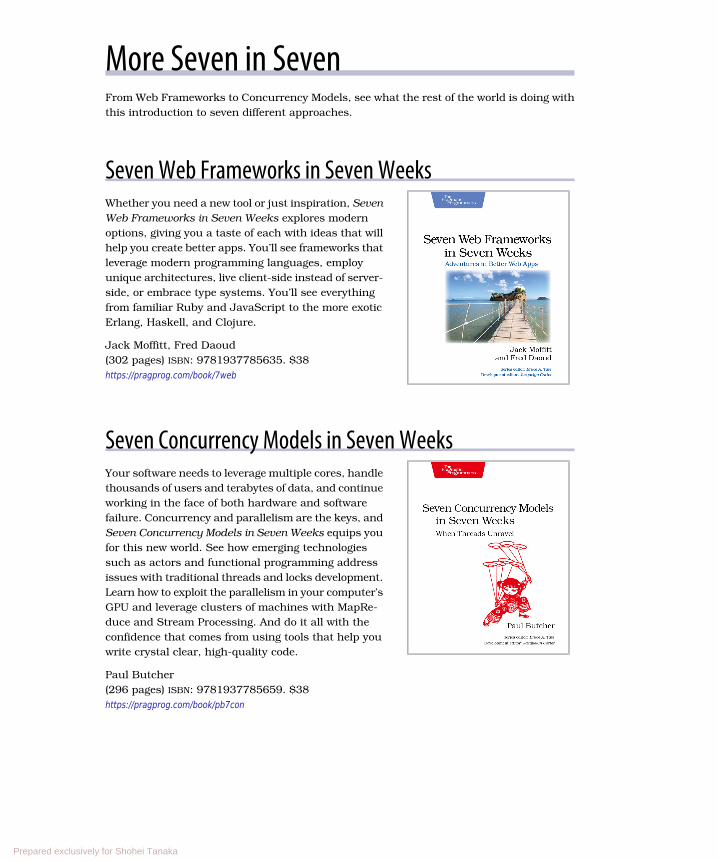
More Seven in SevenFrom Web Frameworks to Concurrency Models, see what the rest of the world is doing withthis introduction to seven different approaches.
Seven Web Frameworks in Seven WeeksWhether you need a new tool or just inspiration, SevenWeb Frameworks in Seven Weeks explores modernoptions, giving you a taste of each with ideas that willhelp you create better apps. You’ll see frameworks thatleverage modern programming languages, employunique architectures, live client-side instead of server-side, or embrace type systems. You’ll see everythingfrom familiar Ruby and JavaScript to the more exoticErlang, Haskell, and Clojure.
Jack Moffitt, Fred Daoud(302 pages) ISBN: 9781937785635. $38https://pragprog.com/book/7web
Seven Concurrency Models in Seven WeeksYour software needs to leverage multiple cores, handlethousands of users and terabytes of data, and continueworking in the face of both hardware and softwarefailure. Concurrency and parallelism are the keys, andSeven Concurrency Models in Seven Weeks equips youfor this new world. See how emerging technologiessuch as actors and functional programming addressissues with traditional threads and locks development.Learn how to exploit the parallelism in your computer’sGPU and leverage clusters of machines with MapRe-duce and Stream Processing. And do it all with theconfidence that comes from using tools that help youwrite crystal clear, high-quality code.
Paul Butcher(296 pages) ISBN: 9781937785659. $38https://pragprog.com/book/pb7con
Prepared exclusively for Shohei Tanaka
Learn Why, Then Learn HowGet started on your Elixir journey today.
Adopting ElixirAdoption is more than programming. Elixir is an excit-ing new language, but to successfully get your applica-tion from start to finish, you’re going to need to knowmore than just the language. You need the case studiesand strategies in this book. Learn the best practicesfor the whole life of your application, from design andteam-building, to managing stakeholders, to deploy-ment and monitoring. Go beyond the syntax and thetools to learn the techniques you need to develop yourElixir application from concept to production.
Ben Marx, José Valim, Bruce Tate(242 pages) ISBN: 9781680502527. $42.95https://pragprog.com/book/tvmelixir
Programming Elixir ≥ 1.6This book is the introduction to Elixir for experiencedprogrammers, completely updated for Elixir 1.6 andbeyond. Explore functional programming without theacademic overtones (tell me about monads just onemore time). Create concurrent applications, but getthem right without all the locking and consistencyheadaches. Meet Elixir, a modern, functional, concur-rent language built on the rock-solid Erlang VM. Elixir’spragmatic syntax and built-in support for metaprogram-ming will make you productive and keep you interestedfor the long haul. Maybe the time is right for the NextBig Thing. Maybe it’s Elixir.
Dave Thomas(398 pages) ISBN: 9781680502992. $47.95https://pragprog.com/book/elixir16
Prepared exclusively for Shohei Tanaka
A Better Web with Phoenix and ElmElixir and Phoenix on the server side with Elm on the front end gets you the best of bothworlds in both worlds!
Programming Phoenix ≥ 1.4Don’t accept the compromise between fast and beauti-ful: you can have it all. Phoenix creator Chris McCord,Elixir creator José Valim, and award-winning authorBruce Tate walk you through building an applicationthat’s fast and reliable. At every step, you’ll learn fromthe Phoenix creators not just what to do, but why.Packed with insider insights and completely updatedfor Phoenix 1.4, this definitive guide will be your con-stant companion in your journey from Phoenix noviceto expert, as you build the next generation of web ap-plications.
Chris McCord, Bruce Tate and José Valim(325 pages) ISBN: 9781680502268. $45.95https://pragprog.com/book/phoenix14
Programming ElmElm brings the safety and stability of functional pro-graming to front-end development, making it one ofthe most popular new languages. Elm’s functional na-ture and static typing means that run-time errors arenearly impossible, and it compiles to JavaScript foreasy web deployment. This book helps you take advan-tage of this new language in your web site development.Learn how the Elm Architecture will help you createfast applications. Discover how to integrate Elm withJavaScript so you can update legacy applications. Seehow Elm tooling makes deployment quicker and easier.
Jeremy Fairbank(250 pages) ISBN: 9781680502855. $40.95https://pragprog.com/book/jfelm
Prepared exclusively for Shohei Tanaka

Better by DesignFrom architecture and design to deployment in the harsh realities of the real world, makeyour software better by design.
Design It!Don’t engineer by coincidence—design it like you meanit! Grounded by fundamentals and filled with practicaldesign methods, this is the perfect introduction tosoftware architecture for programmers who are readyto grow their design skills. Ask the right stakeholdersthe right questions, explore design options, share yourdesign decisions, and facilitate collaborative workshopsthat are fast, effective, and fun. Become a better pro-grammer, leader, and designer. Use your new skills tolead your team in implementing software with the rightcapabilities—and develop awesome software!
Michael Keeling(358 pages) ISBN: 9781680502091. $41.95https://pragprog.com/book/mkdsa
Release It! Second EditionA single dramatic software failure can cost a companymillions of dollars—but can be avoided with simplechanges to design and architecture. This new editionof the best-selling industry standard shows you howto create systems that run longer, with fewer failures,and recover better when bad things happen. New cov-erage includes DevOps, microservices, and cloud-nativearchitecture. Stability antipatterns have grown to in-clude systemic problems in large-scale systems. Thisis a must-have pragmatic guide to engineering forproduction systems.
Michael Nygard(376 pages) ISBN: 9781680502398. $47.95https://pragprog.com/book/mnee2
Prepared exclusively for Shohei Tanaka
Java in DepthGet up to date on the latest Java 8 features, and take an in-depth look at concurrency op-tions.
Functional Programming in JavaGet ready to program in a whole new way. FunctionalProgramming in Java will help you quickly get on topof the new, essential Java 8 language features and thefunctional style that will change and improve yourcode. This short, targeted book will help you make theparadigm shift from the old imperative way to a lesserror-prone, more elegant, and concise coding stylethat’s also a breeze to parallelize. You’ll explore thesyntax and semantics of lambda expressions, methodand constructor references, and functional interfaces.You’ll design and write applications better using thenew standards in Java 8 and the JDK.
Venkat Subramaniam(196 pages) ISBN: 9781937785468. $33https://pragprog.com/book/vsjava8
Programming Concurrency on the JVMStop dreading concurrency hassles and start reapingthe pure power of modern multicore hardware. Learnhow to avoid shared mutable state and how to writesafe, elegant, explicit synchronization-free programsin Java or other JVM languages including Clojure,JRuby, Groovy, or Scala.
Venkat Subramaniam(280 pages) ISBN: 9781934356760. $35https://pragprog.com/book/vspcon
Prepared exclusively for Shohei Tanaka
Python and Data ScienceFor data science and basic science, for you and anyone else on your team.
Data Science Essentials in PythonGo from messy, unstructured artifacts stored in SQLand NoSQL databases to a neat, well-organized datasetwith this quick reference for the busy data scientist.Understand text mining, machine learning, and net-work analysis; process numeric data with the NumPyand Pandas modules; describe and analyze data usingstatistical and network-theoretical methods; and seeactual examples of data analysis at work. This one-stop solution covers the essential data science youneed in Python.
Dmitry Zinoviev(224 pages) ISBN: 9781680501841. $29https://pragprog.com/book/dzpyds
Practical Programming, Third EditionClassroom-tested by tens of thousands of students,this new edition of the best-selling intro to program-ming book is for anyone who wants to understandcomputer science. Learn about design, algorithms,testing, and debugging. Discover the fundamentals ofprogramming with Python 3.6—a language that’s usedin millions of devices. Write programs to solve real-world problems, and come away with everything youneed to produce quality code. This edition has beenupdated to use the new language features in Python3.6.
Paul Gries, Jennifer Campbell, Jason Montojo(410 pages) ISBN: 9781680502688. $49.95https://pragprog.com/book/gwpy3
Prepared exclusively for Shohei Tanaka

The Pragmatic BookshelfThe Pragmatic Bookshelf features books written by developers for developers. The titlescontinue the well-known Pragmatic Programmer style and continue to garner awards andrave reviews. As development gets more and more difficult, the Pragmatic Programmers willbe there with more titles and products to help you stay on top of your game.
Visit Us OnlineThis Book’s Home Pagehttps://pragprog.com/book/pwrdataSource code from this book, errata, and other resources. Come give us feedback, too!
Register for Updateshttps://pragprog.com/updatesBe notified when updates and new books become available.
Join the Communityhttps://pragprog.com/communityRead our weblogs, join our online discussions, participate in our mailing list, interact withour wiki, and benefit from the experience of other Pragmatic Programmers.
New and Noteworthyhttps://pragprog.com/newsCheck out the latest pragmatic developments, new titles and other offerings.
Buy the BookIf you liked this eBook, perhaps you’d like to have a paper copy of the book. It’s availablefor purchase at our store: https://pragprog.com/book/pwrdata
Contact Ushttps://pragprog.com/catalogOnline Orders:
[email protected] Service:
[email protected] Rights:
[email protected] Use:
http://write-for-us.pragprog.comWrite for Us:
+1 800-699-7764Or Call:
Prepared exclusively for Shohei Tanaka