Service District Optimization: Usage of Facility Location Methods and Geographic Information Systems...
71
Service District Optimization Usage of facility location methods and geographic information systems to analyze and optimize urban food retail distribution Holger Johann [email protected] Margeret Hall [email protected] Steven O. Kimbrough [email protected] Nicholas Quintus [email protected] Christof Weinhardt [email protected] This document was a Bachelor’s Thesis by Holger Johann submitted to the Department of Economics and Management of Karlsruhe Institute of Technology (KIT) on March 10, 2014. The thesis was supervised by Margeret Hall from the Karlsruhe Service Research Institute (KSRI) at Karlsruhe Institute of Technology and Steven Kimbrough from the Operations and Information Management Department at the Wharton School of the Uni- versity of Pennsylvania. Abstract With the surge of obesity in the United States, improving urban food environ- ments has gained in importance. Research on food deserts focuses mainly on assessing the food environment but lacks methods of generating good solutions for the placement of food stores. This work uses a maximum covering location problem in combination with census block group GIS data from the City of Philadelphia to find optimal locations for future food store openings. A socioeconomic index of vulnerability is computed to weigh regions based on their residents’ sensitivity to food access limitations. The analy- sis found that supermarkets in Philadelphia are relatively unequally distributed and that there are many viable locations which could satisfy both the public interest of improv- ing food access as well as the private interest of being profitable. Going forward, this joint approach of GIS data and operations research can be used to highlight locations for possible policy interventions in urban areas.
-
Upload
independent -
Category
Documents
-
view
4 -
download
0
Transcript of Service District Optimization: Usage of Facility Location Methods and Geographic Information Systems...

Service District OptimizationUsage of facility location methods and geographic information systems to
analyze and optimize urban food retail distribution
Holger [email protected]
Margeret [email protected]
Steven O. [email protected]
Nicholas [email protected]
Christof [email protected]
This document was a Bachelor’s Thesis by Holger Johann submitted to the Departmentof Economics and Management of Karlsruhe Institute of Technology (KIT) on March 10,2014. The thesis was supervised by Margeret Hall from the Karlsruhe Service ResearchInstitute (KSRI) at Karlsruhe Institute of Technology and Steven Kimbrough from theOperations and Information Management Department at the Wharton School of the Uni-versity of Pennsylvania.
Abstract With the surge of obesity in the United States, improving urban food environ-ments has gained in importance. Research on food deserts focuses mainly on assessingthe food environment but lacks methods of generating good solutions for the placementof food stores. This work uses a maximum covering location problem in combinationwith census block group GIS data from the City of Philadelphia to find optimal locationsfor future food store openings. A socioeconomic index of vulnerability is computed toweigh regions based on their residents’ sensitivity to food access limitations. The analy-sis found that supermarkets in Philadelphia are relatively unequally distributed and thatthere are many viable locations which could satisfy both the public interest of improv-ing food access as well as the private interest of being profitable. Going forward, thisjoint approach of GIS data and operations research can be used to highlight locations forpossible policy interventions in urban areas.

Contents
List of Figures iv
List of Tables v
1. Introduction 1
2. Background 32.1. Towards a definition of food deserts . . . . . . . . . . . . . . . . . . . . . . 3
2.1.1. Food availability . . . . . . . . . . . . . . . . . . . . . . . . . . . . . 32.1.2. Food affordability . . . . . . . . . . . . . . . . . . . . . . . . . . . . 42.1.3. Food access . . . . . . . . . . . . . . . . . . . . . . . . . . . . . . . . 52.1.4. Characteristics of Vulnerability . . . . . . . . . . . . . . . . . . . . . 6
2.2. Consequences of food deserts . . . . . . . . . . . . . . . . . . . . . . . . . . 72.3. The urban food environment . . . . . . . . . . . . . . . . . . . . . . . . . . 10
2.3.1. Historical development of the food retail environment . . . . . . . . 102.3.2. Economic theory of retail facility location . . . . . . . . . . . . . . . 122.3.3. The importance of urban planning . . . . . . . . . . . . . . . . . . . 152.3.4. The food environment in Philadelphia . . . . . . . . . . . . . . . . . 152.3.5. Community initiatives to improve urban food access . . . . . . . . . 16
2.4. Facility location models and defining an optimization problem . . . . . . . . 182.4.1. Geometric principles . . . . . . . . . . . . . . . . . . . . . . . . . . . 18
2.4.1.1. Point-polygon location problem . . . . . . . . . . . . . . . 192.4.1.2. Point-point location problem . . . . . . . . . . . . . . . . . 19
2.4.2. Objective functions . . . . . . . . . . . . . . . . . . . . . . . . . . . . 192.4.2.1. Total or average distance problems . . . . . . . . . . . . . . 202.4.2.2. Maximum distance models . . . . . . . . . . . . . . . . . . 20
2.4.3. Computational strategies . . . . . . . . . . . . . . . . . . . . . . . . 212.4.3.1. Problem formulation . . . . . . . . . . . . . . . . . . . . . . 212.4.3.2. Solution techniques . . . . . . . . . . . . . . . . . . . . . . 22
3. Methodology 253.1. Form and acquisition of necessary data . . . . . . . . . . . . . . . . . . . . . 25
3.1.1. Study area . . . . . . . . . . . . . . . . . . . . . . . . . . . . . . . . 253.1.2. Spatial data . . . . . . . . . . . . . . . . . . . . . . . . . . . . . . . . 263.1.3. Demand point aggregation . . . . . . . . . . . . . . . . . . . . . . . . 263.1.4. Socioeconomic data . . . . . . . . . . . . . . . . . . . . . . . . . . . 263.1.5. Retail outlets . . . . . . . . . . . . . . . . . . . . . . . . . . . . . . . 26
3.2. Underlying assumptions . . . . . . . . . . . . . . . . . . . . . . . . . . . . . 273.2.1. Definition of coverage and access . . . . . . . . . . . . . . . . . . . . 27
3.3. Vulnerability Index . . . . . . . . . . . . . . . . . . . . . . . . . . . . . . . . 273.3.1. Variable selection . . . . . . . . . . . . . . . . . . . . . . . . . . . . . 273.3.2. Data reduction . . . . . . . . . . . . . . . . . . . . . . . . . . . . . . 27
ii

Contents
3.3.3. Constructing the Index . . . . . . . . . . . . . . . . . . . . . . . . . 303.4. Input and Output parameters . . . . . . . . . . . . . . . . . . . . . . . . . . 303.5. Implementation of the algorithm . . . . . . . . . . . . . . . . . . . . . . . . 32
3.5.1. Computation of initial coverage . . . . . . . . . . . . . . . . . . . . . 323.5.2. Greedy-Adding Heuristic . . . . . . . . . . . . . . . . . . . . . . . . 323.5.3. Substitution Heuristic . . . . . . . . . . . . . . . . . . . . . . . . . . 323.5.4. Output of results . . . . . . . . . . . . . . . . . . . . . . . . . . . . . 33
4. Results 344.1. Status quo: Limited access and deprivation in Philadelphia . . . . . . . . . 34
4.1.1. Mapping population distribution and retail outlets . . . . . . . . . . 344.1.2. Mapping low access and vulnerability characteristics . . . . . . . . . 34
4.2. Results of algorithms . . . . . . . . . . . . . . . . . . . . . . . . . . . . . . . 374.2.1. MCLP: Supermarket location . . . . . . . . . . . . . . . . . . . . . . 374.2.2. MCLP: Farmers’ Market location . . . . . . . . . . . . . . . . . . . . 39
4.3. Performance and sensitivity analysis . . . . . . . . . . . . . . . . . . . . . . 44
5. Evaluation 465.1. Discussion . . . . . . . . . . . . . . . . . . . . . . . . . . . . . . . . . . . . . 465.2. Limitations and Recommendations . . . . . . . . . . . . . . . . . . . . . . . 48
5.2.1. Level of demand aggregation . . . . . . . . . . . . . . . . . . . . . . 495.2.2. Definition of coverage . . . . . . . . . . . . . . . . . . . . . . . . . . 495.2.3. Adequateness of vulnerability measure . . . . . . . . . . . . . . . . . 505.2.4. Implementation and software interoperability . . . . . . . . . . . . . 50
6. Conclusion 52
Bibliography 54
Appendix 61A. List of considered supermarkets . . . . . . . . . . . . . . . . . . . . . . . . . 61B. MCLP results . . . . . . . . . . . . . . . . . . . . . . . . . . . . . . . . . . . 62
iii

List of Figures
2.1. Prevalence of obesity among adults aged 20 years and over, by povertyincome ratio and sex: United States, 1988-1994 and 2005-2008 (Ogden et al.,2010) . . . . . . . . . . . . . . . . . . . . . . . . . . . . . . . . . . . . . . . . 8
3.1. Scree plot from eigenvalues of factors . . . . . . . . . . . . . . . . . . . . . . 29
4.1. Population density and food retail locations in Philadelphia . . . . . . . . . 354.2. Star Map of nearest supermarket per Block Group centroid . . . . . . . . . 364.3. Map of Block Group level Vulnerability and supermarket coverage areas . . 384.4. Map of Combinations of Vulnerability characteristics . . . . . . . . . . . . . 394.5. 40-MCLP of supermarket placement coverage graph . . . . . . . . . . . . . 404.6. Map of optimal 14 MCLP locations (placement: Supermarkets, p=40, initial
coverage: supermarkets (S=12 mile) . . . . . . . . . . . . . . . . . . . . . . . 40
4.7. 20-wMCLP of supermarket placement coverage graph . . . . . . . . . . . . 414.8. Map of optimal 14 wMCLP locations in comparison to MCLP locations
(placement: Supermarkets, p=40, initial coverage: supermarkets (S=12 mile) 41
4.9. 80-MCLP of farmers’ market placement coverage graph . . . . . . . . . . . 424.10. Map of optimal 67 MCLP locations (placement: Farmers’ markets, p=80,
initial coverage: supermarkets (S=12 mile), Farmers’ Markets (S=1
4 mile) . . 434.11. Performance comparison of GA and GAS heuristic for a supermarket MCLP
and Sensitivity of the GAS algorithm towards maximum service distance . . 44
iv

List of Tables
3.1. Socioeconomic variables of neighborhood vulnerability . . . . . . . . . . . . 283.2. Descriptive statistics of vulnerability variables in block groups of Philadelphia 283.3. Pearson correlations of vulnerability variables in block groups of Philadelphia 293.4. Principal Factor Analysis component matrix . . . . . . . . . . . . . . . . . . 30
4.1. Performance and Sensitivities of algorithms for a MCLPs . . . . . . . . . . 454.2. Performance and Sensitivities of algorithms for SCLPs . . . . . . . . . . . . 45
5.1. Economic Feasibility of supermarket placement: vulnerability-weighted andunweighted coverage from weighted 20-MCLP solution . . . . . . . . . . . . 48
A.1. List of considered supermarket chains in Philadelphia . . . . . . . . . . . . 61A.2. List of considered supermarkets in Philadelphia . . . . . . . . . . . . . . . . 63B.3. MCLP solution - placement: Supermarkets, p=40, initial coverage: super-
markets (S=12 mile) . . . . . . . . . . . . . . . . . . . . . . . . . . . . . . . 64
B.4. weighted MCLP solution - placement: Supermarkets, p=40, initial coverage:supermarkets (S=1
2 mile) . . . . . . . . . . . . . . . . . . . . . . . . . . . . 65B.5. MCLP solution - placement: Farmers’ Markets, p=80, initial coverage: su-
permarkets (S=12 mile) and Farmers’ Markets (S=1
4 mile . . . . . . . . . . . 66
v

1. Introduction
Over the past two decades, research in the field of health and nutrition has focused ondefining and identifying urban food deserts through empirical research on individual shop-ping behavior and spatial mapping solutions using geographic information systems (GIS).However, the derivation of appropriate action plans that benefit public and private stake-holders is still a challenging task and specific to the study area. This lack of attention issignificant because the misuse of incentives to shape the food environment can compoundthe disadvantages faced by the population in food deserts and waste taxpayer money andcompany resources. In order to address this problem, this study combines a GIS approachwith a facility location model in order to identify food deserts and generate good solutionsfor possible facility placements in the city of Philadelphia, PA.
Over the last three decades, obesity in the United States has increased at an alarming rate.In 2009-2010, 35.7 percent of the US population were obese (Ogden et al., 2012), puttingstrain on the national health-care budget through costs associated with obesity and diet-related diseases. Studies have explored different environmental conditions that supportregional health disparities and that these adverse health outcomes might be subject tosocioeconomic factors such as income or ethnicity. Furthermore, studies on economic andgeographic access to food find that poor populations in urban areas encounter food pricesthat are higher than middle-class families and that the development of the local food en-vironment disadvantages people living in areas of high deprivation.In his hierarchy of needs that shapes human motivation, Maslow (1943) describes phys-iological needs as the physical requirements for human survival. In comparison to waterand housing, two goods that underlie strong regulations, the distribution mechanism offood is often neglected by local and federal governments and left to the private sector,leading to issues of inequal and inadequate food access. In the The Food, Conservation,and Energy Act of 2008, the United States government formally recognized the notionof “food deserts” and issued a large-scale study on the food desert problem (Ploeg et al.,2009), which provided a formal foundation for this study.As a means of tackling this problem, empirical studies examined behavioral and economicaspects of food shopping by monitoring the local food environment and the buying pat-terns. Geographic access studies have undertaken several approaches with geographicinformation systems (GIS) to analyze the access to food on a spatial basis. These em-ployed approaches help understand the problem and find problem areas, however, theylack the generation of distinct recommendations for policy interventions.
1

Public-private partnerships have been successfully applied to have an impact on the localfood environment. In order for those to be effective, it is crucial to ensure incentive com-patibility between public goals (such as welfare maximization and equality) and privatesector imperatives (such as economic viability and long-term sustainability).Modern facility location theory originally stems from private-sector applications based onprofit maximization and has been amply employed in the optimization of the site selec-tion processes. Especially in the retail environment, covering problems such as the oneby ReVelle et al. (1970) provide means of maximizing revenue by maximizing populationreach given constrained resources. The goal formulations of such problems can be fit toalign with public and private interest. This study employs a combination of GIS and fa-cility location models. Its aim is to unite easily accessible visual representation of a GISwith a quantitative approach. It helps overcoming market failures in the food sector byreducing demand information asymmetry through the identification of key locations of in-terest. Several urban areas in North America have been studied in regards to the existenceof food deserts. Philadelphia has been cited as a city that lacks a significant amount ofsupermarkets and an adequate access to healthy and nutritious food and the relevant areaof this study.
Throughout the course of this study, the following questions were examined:
1. Do food deserts in Philadelphia exist and if yes, where?
2. How can one take advantage of the possibilities offered by both a GIS and a mathe-matical optimization software?
3. How could a possible implementation of a facility location problem look like and howcan it be solved?
4. What set of locations for possible facility sites are optimal from a public or privatestandpoint (neediness vs. profitability)?
5. Do identified locations satisfy the goals of both stakeholders?
6. Can this implementation be applied to different problem sets, such as other urbanareas?
The thesis will be structured as follows: First, the background section will give a briefintroduction on the definition of food deserts and its consequences. A review of the historyand characteristics of urban food environments in the United States aims to provide anunderstanding of the interaction between food retail and the community. Following anintroduction of the environment of this study - Philadelphia, PA in the United States -the importance of urban planning for tackling the problem of food deserts is depicted andrecent undertakings in this area are presented. The section ends with a review of facilitylocation problems that have been applied for retail site selection and might be applicableto this particular problem. The methodology section describes the means of collectingspatial data, the combination of vulnerability characteristics in a vulnerability index andlastly, the design, implementation and solution of the optimization problem. The results ofthe optimization are then presented in a map and table form and discussed on the groundsof feasibility, sensitivity, performance and incentive compatibility.
2

2. Background
2.1. Towards a definition of food deserts
The terminology Food Desert was reportedly first used by Scottish public sector housingresidents in the early 1990s. It first appeared in a government publication in 1995 as partof a Nutrition Task Force of the Conservative UK Government (Cummins and Macintyre,2002, pg. 1). Since then, it has been used differently by different researchers. The leastcommon denominator of all definitions is the literal absence of retail food resource in adefined area. In light of obesity having reached “nationwide epidemic proportions” (Of-fice Of The Surgeon General, 2001, pg. XIII), the local food environment becomes anincreasingly pressing public health concern. A more advanced conceptual definition thatincorporates nutritious value of different foods was given by the Department of Health(1996), decscribing food deserts as “areas of relative exclusion where people experiencephysical and economic barriers to accessing healthy food”.Studies have shown that people living in low-income and minority areas tend to have pooraccess to varied healthy food (Beaulac et al., 2009, pg. 4). Policy-makers and most studiestherefore do not only consider access to food in general but focus on an unequal access tohealthy and nutritious food. This is emphasized in the Food, Conservation, and EnergyAct of 2008 (U.S. Government Printing Office, 2008, sec. 7527), also known as the 2008Farm Bill, in which a food desert is defined as “an area in the United States with limitedaccess to affordable and nutritious food, particularly such an area composed of predomi-nantly lower income neighborhoods and communities”.From these definitions we can derive four important elements for the definition of a fooddesert (adapted from (Leete et al., 2012, pg. 205): (1) Availability: a definition of asufficiently wide range of nutritious foods items; (2) Affordability: a definition whereand at which price those food items can be attained; (3) Access: a measurement of geo-graphic access and a threshold for determining low access; (4) Vulnerability:a thresholdfor determining which populations with low food access will lack the resources to accessfood from more distant retail outlets geographical access and social deprivation. Thesefour factors will now be examined in detail.
2.1.1. Food availability
Defining a healthy diet
In order to examine whether the food environment imposes a constraint on a healthy andnutritious diet, one has to define what a healthy and nutritious diet consists of. While
3

2.1. Towards a definition of food deserts
total fat intake over the last 30 years has decreased, a trend towards a energy-dense dietshas evolved and the intake of calories and carbohydrates has risen (Austin et al., 2011,pg. 839). This may be applicable to increasing portion sizes, marketing and pricing aswell as changes in food production and higher rates of pre-processing and pre-packaging(Morland et al., 2006, pg. 334). (Swinburn et al., 2004, pg. 126) have shown that a dietfilled with processed foods often leads to poorer health outcomes compared to a diet highin complex carbohydrates and fiber.Whereas a pairwise comparison of similar foods can help attribute some foods as morenutritious than others, no one food can fulfill the recommendations for a healthy diet(Ploeg et al., 2009, pg. 2). Furthermore, nutritious food may come in various formsand packaging types. What is perceived as a healthy diet also varies between ethnicgroups and might have differing acceptance rates among those (Donkin et al., 1999, pg.556). Empirical researchers therefore use a more conceptual definition of insufficient fooddiversity: The lack of reasonable access to fresh fruits and vegetables and foods from allthe major food groups required for a “modest but adequate diet” (Sparks et al., 2009, pg.8).
Food sources
Food is sold in a wide range of retail outlets. Because of various forms of nutritious diets,research that studies the quality and availability uses food categories (e.g., fruits) or indi-cator items (e.g., ground beef, skim milk) to compare food variety between different typesof these outlets (Glanz et al., 2007, pg. 283).Grocery stores were found to have greater quality of those healthier food options comparedto convenience stores and these differences may be large enough to have substantial effectson consumer purchasing and health (Glanz et al., 2007, pg. 287). In a cross-sectional studyof 10,763 Atherosclerosis Risk in Communities participants, the presence of supermarketswas associated with a lower prevalence of obesity and overweight, and the presence ofconvenience stores was associated with a higher prevalence of obesity and overweight. Anationally representative sample of 2,400 stores accepting food stamps by SupplementalNutrition Assistance Program (SNAP) showed that availability as well as variety of marketbasket items did not vary by poverty level for large grocery stores(Mantovani, 1997, pg.98ff).We can conclude that supermarkets and large grocery stores offer more variety and avail-ability of food than other store types and can be used as proxies for food retailers thatoffer a variety of nutritious, affordable retail food (Ploeg et al., 2009, pg. 15).
2.1.2. Food affordability
A key concern for areas of limited economic access (see section 2.1.3) is not only whether anutritious variety of food is available but whether it is affordable. Studies have examinedfood prices and have found that the types of stores that are available as well as individualshopping habits are key factors for the incurred costs of food.Market-basket studies measure the price of a particular food or the relative price of a sub-stitute or alternative good. Just like in variety and availability, studies have found thatthere are distinct differences between different types of food outlets. Firstly, Kaufmanet al. (1997) point out that supermarket tend to have significantly lower prices than thoseof smaller foodstores (about ten percent on average) because they are able to capitalizeon economies of scale and to withstand lower margins. Secondly, a study by Chung andMyers (1999) demonstrates that people in non-chain stores pay a premium to customers ofchain stores. The net impact of chains on the price of a Thrifty food plan (TFP) marketbasket by the United States Department of Agriculture (USDA) was found to be as highas $15.94 (non-chain market price: $109.90).
4

2.1. Towards a definition of food deserts
These two food price factors put low-income neighbourhoods at a disadvantage. In theseareas non-chain supermarkets and grocery stores are more prevalent than larger chain-supermarkets (Powell et al., 2007, pg. 189). The non-placement of large chain stores,where prices tend to be lower is a key factor contributing to higher grocery costs in poorareas. Kaufman et al. (1997) illustrates that low-income households tend to select moreeconomical foods such as generic items or larger package sizes. In contrast, those peo-ple pay a premium to the average price of an identical market basket. They lack accessto large-scale supermarkets that utilitze economies of scale to generate lower prices. Inanother study by Hendrickson et al. (2006), a significant number of foods in urban neigh-borhoods of Minnesota, USA were significantly more expensive than the TFP market price.One could argue that growing popularity of supercenters in suburban areas (see section2.3.1) could have increased competitiveness in metropolitan statistical areas (MSA) thatthey are placed in. However, recent research provides evidence that this may not be thecase and entry of supercenters does not have a significant effect on food prices within theMSA (Stiegert and Sharkey, 2007). The placement of supercenters in mostly suburbanareas and only marginal procompetitive effects on the MSA food prices help explain theexisting disparities in food prices among city limits.It is apparent that policy motions to promote the placement of chain stores or super-centers could provide affordable food in communities that experience high food prices andvulnerability to food access.
2.1.3. Food access
Three barriers of access
After establishing a joint understanding of food options and prices, it should given consid-eration to measuring the way people access food. Following the topology of (McEntee andAgyeman, 2010, pg. 167), barriers of food access may be divided into three groups: infor-mational, economic and geographical access . Informational access comprises the analysisof how and why certain types of food are consumed (knowledge of sources). Studies ofEconomic access examine the financial situation of consumers and the total cost incurredin the acquisition of food, such as food prices transportation costs.The focus of this research is the measurement and optimization of Geographic access,which is defined in the following paragraph. However, it is important to notice that lack offood access is a multifaceted problem that has more dimensions than spatial and financialcharacteristics.
Defining and measuring geographic access
Geographic access specifies the physical accessibility of food and has a variety of repre-sentational frameworks for its attribution and measurement. It might be conceived as anattribute of either locations (place accessibility) or individuals personal accessibility (Kwanet al., 2003, pg. 130). In the example of grocery store placement, place or personal ac-cessibility differentiates between a supply-driven (Does the outlet have access to a certaingroup of people?) or a demand-driven approach (Do individuals have access to sufficientfood?). Hence, research employs individual-based measures and area-based measures offood access (Ploeg et al., 2009, pg. 11).Individual-based measures examine access for individuals directly, regardless of their loca-tion. For example, an annual national representative food security survey by the USDAhas found that 5.7 percent were experiencing access problems and more than half of themstated that insufficient money was the main reason for this (Ploeg et al., 2009, pg. 13).This gives an understanding of the general extent of the food desert problem and howmany people are negatively affected on a national scale. It does not, however, help in
5

2.1. Towards a definition of food deserts
identifying who is affected and where policy interventions would be fruitful.Area-based measures of access use aggregate spatial frameworks (e.g. block groups) to mapgeographic access as distance to the nearest retail outlet, such as a supermarket. Mostcommonly, the distance is measured in straight-line distance by the creation of circularbuffers. The buffer size works as a proxy for an access range, representing a certain maxi-mal distance to a store or a related time necessary to reach a store. Straight-line distanceis not an exact measurement of distance or travel time because of unique road networks.Access-related studies such as (McEntee and Agyeman, 2010, pg. 170) have therefore madeuse of network measurement tools that calculate travel distances on a given road network.The majority of research however, has employed straight-line distance buffers because ofits ease of use and representation.
Geographic access in urban and rural areas
Urban food access studies seek to identify areas outside of a walkability range. Commonunderstandings of walkability ranges reach from a quarter mile up to one mile. Based onan average walking speed of 88m/minute for a male and 74m/minute for a female respec-tively (Donkin et al., 1999, pg. 558), these buffers represent a walking distance of fiveto six minutes (quarter mile) up until nineteen to twenty-two minutes (one mile). (Ploeget al., 2009, pg. 17) employs a categorization of walkability, in which walkability is definedas 1) high (within 1
2 mile); 2) medium (12 mile to one mile); and 3) low (more than a mile).Access studies in rural areas require different access measures. Urban distance limit arenot applicable here as most people live further from a food retailer and do heavily relyon an automobile for grocery shopping (McEntee and Agyeman, 2010, pg. 168). Thefocus lies on drivability more so than walkability. There have been several approachestowards rural access measurement, such as increasing the buffer to a drivability range of10 miles or comparing potential spending from households to sales data from food stores.Rural areas are more error-prone to skewing of travel distances through metrics becausethe road network is usually less extensive than in urban areas. Additionally, zone-basedaggregation of population in rural areas leads to much larger areas as in urban areas (e.g.census tracts). The geographic center may not accurately represent the population center(Sharkey and Horel, 2008, pg. 622). Hence, the more broken-down block groups are usedto calculate population-weighted centers instead of geographic centers. Similarly, (McEn-tee and Agyeman, 2010, pg. 170) derive mean distances to supermarkets within an censustract using a network distance tool for residential units.As this research is focusing on geographic access in the urban area of Philadelphia, astraight-line distance measure has been used. Appropriate access was defined as a maxi-mum distance to the nearest store below 1
2 mile, which is in line with the USDA definitionof high walkability.
2.1.4. Characteristics of Vulnerability
After a variety of healthy and nutritious food has been defined and measures of geographicaccess has been established, it is of interest which subpopulations may experience particu-lar challenges in accessing nutritious food sources from more distant retail outlets. Not allpeople experience access barriers in the same way. In order to relate geographic accessibil-ity and access limitation vulnerability, different proxies for disadvantage have been used.These are based on the assumption that socioeconomically deprived residents are mostlikely to face transportation and time–cost barriers in seeking out more-distant shoppingoptions (Leete et al., 2012, pg. 206). Examples are poverty rate, unemployment rate, per-centage of residents with low levels of education, or presence of single-parent or immigranthouseholds.
6

2.2. Consequences of food deserts
Measurement of disadvantage
To account for more than one characteristic and facilitate visual representation, existingsocioeconomic indices are computed. Examples are “The Indices of Deprivation 2007” bythe British Department for Communities and Local Government (made up of seven dimen-sions of deprivation: Income, Employment, Health and Disability, Education, Skills andTraining, Barriers to Housing and Services, Living Environment, Crime) or the CarstairsIndex (based on four census indicators: low social class, lack of car ownership, overcrowdingand male unemployment) used by Clarke et al. (2002). On other occasions, a compositeindex of socioeconomic distress or deprivation was calculated with given socioeconomicdata. Apparicio et al. (2007) computes a linear combination of five deprivation measures:1) low-income population; 2) lone-parent families; 3) unemployment rate; 4) adults withlow level schooling 4) recent immigrants. The exact same approach except for an omissionof recent immigrants was used by Larsen and Gilliland (2008). Sharkey and Horel (2008)neglect recent immigrant and lone-parent family figures but include household crowding,public assistance, vehicle availability and telephone service. Unfortunately, there is littlereasoning about why certain measures are included. The variety of deprivation indicesshows that there is no “one right measure” for deprivation for this type of research, whichshows the multitude of food desert definitions and compound effects of deprivation.
2.2. Consequences of food deserts
Obesity in the United States
Overweight and obesity in the United States have reached epidemic proportions. TheUnited States have seen a dramatic increase in obesity (Body Mass Index greater than 30)from 1990 through 2010. According to the National Center for Health Statistics (Ogdenet al., 2012), more than 35 percent of adults and almost 17 percent of youth in the U.S.were obese in 2009-2010. Both the prevention and treatment of overweight and obesityand their associated health problems are important public health goals.Individuals who are obese have a 50 to 100 percent increased risk of premature death fromall causes (most importantly type 2 diabetes and heart disease) compared to individualswith a BMI in the range of 20 to 25. An estimated 300,000 deaths a year may be at-tributable to obesity. In June of 2013, the American Medical Association announced achange in its recognition of obesity from a “major public health problem” to a “disease re-quiring a range of medical interventions for treatment and prevention” (American MedicalAssociation, 2013).
Economic impact of obesity
Rising rates of overweight and obesity pose an economic burden on both private payersand public authorities. Medical costs associated with obesity can be broken down to directand indirect costs. Direct medical costs may include preventive, diagnostic, and treatmentservices related to obesity. Indirect costs relate to morbidity and mortality costs (Wolf andColditz, 1998, pg. 98f). Finkelstein et al. (2009) state that the connection between risingrates of obesity and rising medical spending is undeniable. In the study, it is estimatedthat the medical costs of obesity through increased health care use and expenditure couldamount to $147 billion per year by 2008 (up 87 percent from 1998). The per capita medicalspending for obese people in 2006 was estimated to be 41.5 percent higher compared tonormal weight people (a difference of $1,400).Roughly half of those costs are borne by Medicare or Medicaid. These are public socialinsurance programs targeted at elderly people over 65 and people with low-income respec-tively. Elderly and low-income subpopulations also happen to be especially vulnerable to
7

2.2. Consequences of food deserts
food access barriers. The Patient Protection and Affordable Care Act by the U.S. gov-ernment, effective in 2014, is aimed to improve the rights and benefits of obese peoplethrough equal access (Roddenberry and Fleming, 2013). Whereas adults with obesity willbe protected from losing coverage due to pre-existing conditions (Manchikanti et al., 2011,pg. E55), it is still noteworthy that so-called “wellness benefits” dramatically expand theability of companies to penalize employees for lifestyle issues, including being overweightor smoking. While the wellness benefits tend to be described as discriminatory towardspoor and obese people (Roddenberry and Fleming, 2013), tackling the problem of obesityhas clearly become a focus of recent US federal policy.
Health disparities
Obesity is a problem that affects some more than others. A National Health and NutritionExamination Survey among adults aged twenty years and older between 2005 and 2008 hasshown that there are relationships between socioeconomics, educational status and obesityprevalence (Ogden et al., 2010). The results differ by sex, race and ethnicity. Among men,the relationships seems to be less distinct. With the exception of non-Hispanic Black andMexican-American men, who are more likely to be obese with rising income, obesity preva-lence is generally similar among all income levels. Women, however, seem to be far moreaffected by socioeconomic status and educational attainment. Lower income of women isrelated to an increased likelihood of obesity, and obesity prevalence increases as educationdecreases.A multi-level study surveyed 15,358 inhabitants of 327 zip code tabulation areas in Mas-sachusetts, USA between 1998 and 2002 (Lopez, 2007). The presence of a supermarketwas negatively associated with obesity risk. In a multiple regression model, having onesupermarket in a zip code tabulation area decreased the risk of obesity by 10.7 percent.As median income (+$1000), population density (+1000 per square mile), and retail es-tablishment density (+100 per square mile) increased, the risk of obesity declined by 0.8%,2%, and 1.9%.
Figure 2.1.: Prevalence of obesity among adults aged 20 years and over, by poverty incomeratio and sex: United States, 1988-1994 and 2005-2008 (Ogden et al., 2010)
These relationships between different factors of increased obesity prevalence are limited toonly being observational. The current understanding of underlying complex causes of dis-parities are still very limited and do not allow a causal interpretation of the relationships.
8

2.2. Consequences of food deserts
It is apparent that obesity may be caused by many factors. In many cases though, weightgain can be backtracked to excess calorie consumption and inadequate physical activity.Dietary and physical activity choices are influenced by one’s individual characteristics andinteraction with the social and physical environment. Differential rates of available lo-cal physical fitness facilities and types of food stores by neighborhood characteristics areexamples for factors of the physical environment that might help explain disparities inobesity prevalence. Population-based policies and programs that focus on environmentalchanges are most likely to be successful and crucial to promoting healthful eating as wellas physical activity (Wang and Beydoun, 2007, pg. 24).While the United States have traditionally relied on markets rather than social policiesto distribute wealth (Swinburn, 2009, pg. 510), the federal government and many statesare undertaking various policy initiatives to address the obesity crisis. For example, Pres-ident Barack Obama has created a new White House Task Force on Childhood Obesityto create a new national obesity strategy and implement concrete measures and roles. By2010, twenty states had introduced nutritional standards for school lunches, breakfastsand snacks that are stricter than USDA requirements, whereas only four states had in-troduced these standards by 2005 (Levi et al., 2011, pg. 43). First lady Michelle Obamahas also started the “Let’s Move!” initiative in 2010, an attempt to improve childhoodobesity on a city-level. The initiative is aimed towards pooling the expertise and efforts ofpublic officials, advocacy groups and the food industry (Levi et al., 2011, pg. 71f). Thisis just a small excerpt of the federal and state-level policies and programs that addressthe growing prevalence of obesity. A plurality of initiatives is necessary, because healthychoices can only be effectively supported if policies on every level cover all aspects of access- informational, economic and geographic.
Linkages between food access and a healthy diet
After delineating the consequences of obesity in the United States in its extent and show-ing distinctive disparities between socioeconomic, ethnic and geographic groups, the directimpact of food deserts on an unhealthy lifestyle needs to be assessed.Dietary decisions are formed through individual characteristics and interdependencies withthe physical and social environment (Ploeg et al., 2009, pg. 52). Food deserts describeareas where people with vulnerable individual characteristics are accumulated and experi-ence a limitation of physical access to food. It should not come as a surprise that researchshows linkages between food deserts and a less healthy dietary intake. In general, betteraccess to a supermarket is associated with a healthier diet, while the opposite can besaid about greater availability and lower prices of fast food items (Ploeg et al., 2009, pg.52). Hendrickson et al. (2006) studied fruit and vegetable access in selected low-incomefood desert communities in Minnesota, USA. Focus group surveys showed that the lack ofquality, affordable food for low-income residents in these four communities impedes theirability to choose food that helps maintaining a healthy lifestyle. A study of less affluentareas with a high share of African-American residents by Lewis et al. (2005) posted simi-lar results. It also reported another common finding in food deserts, that restaurants andfast-food outlets in deprived areas heavily promote unhealthy food options to residents.This shows that not only access limitations of healthy food alone is the main causes for thedevelopment of obesity but the substitution effects through savvily-advertised, low-pricedfast food with a high energy density . A study of fast food marketing focusing on youngercustomers in 2010 found that only 12 of 3,039 possible kids’ meal combinations meet nu-trition criteria for preschoolers and that black children and teens see at least 50 percentmore fast food advertising than white ones (Levi et al., 2011, pg. 62). A lack of options fornutritious food is intensified through early exposure to fast food in food deserts. Researchof overweight schoolchildren in Pennsylvania, USA by Schafft et al. (2009) also finds apositive relationship between increased rates of child overweight and the percentage of the
9

2.3. The urban food environment
district population residing in a food desert. A proposed “Healthy Food Financing Ini-tiative” is geared towards bringing affordable healthy foods to under-served communities,particularly through building new retail food stores in these neighborhoods.The US state of New York has also asked the USDA in 2011 to rule on a proposed ban ofsoda and sugar-sweetened beverages (SSB) for people using the Supplementary NutritionAssistance Program (SNAP formerly known as the Food Stamp Program). On the con-trary, fast food lobbying groups are campaigning for allowing SNAP recipients to buy foodat fast food restaurants. This would incentivize a variety of new unhealthy food choicesfor a group that shows signs of vulnerability, such as individuals with disabilities, elderly,and homeless (Levi et al., 2011, pg. 58).
2.3. The urban food environment
Eating habits are shaped by the food environment that individuals are exposed to. Thissection describes what major changes the urban food environments in the United Stateshave gone through over time and gives an explanation to the economic forces at work.Subsequently, the food retail situation in Philadelphia is depicted, followed by an overviewof initiatives that show how change can be brought to urban food environments.
2.3.1. Historical development of the food retail environment
Over the last century, the retail environment in the U.S. has undergone several majorchanges that have formed the way people use and access food, with some of them beingexternally driven (e.g. by a geographic shift of demand) and others internally driven (e.g.by economies of scale). Mainly, the evolution of communities is the origin for changes inthe retail environment. It is to be noted that the retail environment changes considerablylag behind influencing external factors, which could be attributed to a slow or conservativeobserve-and-adapt process of retailers to newly created demands.
Auto-mobility and suburban sprawl
The first and probably the most far-reaching change was the introduction of automobiles.Rising prevalence of auto-mobility in affluent households and highway construction madeit easier for people to move more freely and cover greater distances. The establishment ofa car-centered infrastructure however put poorer families that could not afford a car at adisadvantage - mobility is a luxury good and is unequally distributed (Larsen and Gilliland,2008, pg. 2). The availability of motorized individual transportation opened up thepossibility to escape the larger cities. Overpopulated centers of “walking cities” (Jackson,1985, pg. 14) with increased levels of pollution and congestion were mostly perceived asunhealthy places. Suburbs offered domesticity, privacy, and isolation at relatively lowerland costs (Ploeg et al., 2009, pg. 87). Antidromic to the urbanization, the move ofaffluent households to the suburbs fueled the urban sprawl of the cityscape. As moreand more people of the customer base and workforce moved outside of the city centers,retailers and businesses followed suit and opened suburban establishments. Studies byMieszkowski and Mills (1993) show the decreasing relevant of central cities: In 1950, 57percent of metropolitan statistical area (MSA) residents in the and 70 percent of MSAjobs were located in central cities; in 1990, the percentages were about 37 and 45.
Economies of scale and Standardization
Another trend in food retail during the 20th century was the expulsion of independently-owned markets by chain stores, pioneered by The Great American Tea Company, thepredecessor of A&P Inc. (Stiegert and Sharkey, 2007, pg. 295). The organization of
10

2.3. The urban food environment
chains offered lower operating costs through standardization of marketing and sophisti-cated inventory systems. The pooling of demand and the cutting of middlemen ensuredlower per-unit prices through stronger bargaining power with suppliers.As a means of enabling economies of scale and catering to more demanding customer base,especially in the suburban areas with low land prices, average grocery stores began togrow larger in size. Through new outlet placement techniques, grocery stores were able toserve a larger number of customers. Full-line supermarkets (floor design > 5,000 squarefeet) that could offer a larger variety of goods in comparison to more specialized mar-kets with less offering. As these smaller independent stores were superseded, the averagenumber of stores per capita decreased (Larsen and Gilliland, 2008, pg. 2). Additionally,supermarkets started moving away from urban areas, which became especially apparentin the 1980s, when cities experienced a net loss of supermarkets even as, nationally, storeopenings exceeded closings, often referred to as “supermarket redlining” (Eisenhauer, 2001,pg. 127).The two developments peaked in a trend towards fewer, bigger supercenters since the endof the 20th century. These outlets combine food retailing with general merchandising andpharmacy under one roof to cater to all routine shopping needs of their customers. Dueto the “one-stop-shop” business model, supercenters rely almost exclusively on car accessby their customers and require large parking facilities. Because of the large store size andcoverage area, supercenters are mostly located in suburban or out-of-town locations thatare well connected to major road networks.
Recent niche retail stores
Changes in the demographic and geographic environment of metropolitan areas and grow-ing competition by supercenters have put traditional supermarkets in need of searching fornew business models, of which two are most notable: Specialty stores and hard discountstores.
Specialty storesAs a response to no longer being able to compete for price-leadership with supercenters,certain stores have focused on a premium approach. It involves carrying specialty prod-ucts, own premium store brands, an emphasis on organic products or local sourcing offood. Due to higher relative prices, premium products are primarily aimed at the moreaffluent population. Supermarkets that specialize on these premium products provide aniche of food retail that is capable of providing healthy and nutritious food. Whole Foods,one of the pioneers of the organic food movement, has recently targeted low-income neigh-borhoods in Detroit (Buss, 2013) and Chicago (Munshi, 2013). However, it remains to beseen whether a business model for upscale food retail in deprived areas can be sustainableand, more importantly, whether it will yield prices low enough to be affordable in areas ofdeprivation.
Hard discount storesAnother trend in food retail that goes the opposite direction of specialty stores are harddiscount stores (e.g. Save-a-Lot or ALDI). Instead of providing a premium product of-fering above the price level of the competition, the stores employ a low-variety strategyto keep stock and lease costs down. This and the introduction of own-store-brands offeran affordable full-line grocery option, especially within low-income areas. There has alsobeen a “channel blurring” effect among retailers traditionally carrying non-food items suchas pharmacies and dollar stores (Ploeg et al., 2009, pg. 88), although they can not beexpected to carry a full line of foods that comprise a healthy diet (Hillier et al., 2011, pg.717).Wholesale clubs offer discounts on a small variety of products that are either larger in size
11

2.3. The urban food environment
or bulk. They require an annual membership fee (basic annual memberships costs in Jan-uary 2014: $45 (Sam’s Club); $50 (BJ’s Wholesale Club); $55 (Costco)) and are often notincluded in food desert studies. This is firstly due to the industry not considering whole-sale club stores as supermarkets and secondly due to only few of these stores acceptingSNAP benefits. SNAP is an important means of food payment in vulnerable low-incomeneighborhoods (Ploeg et al., 2009, pg. 16). Hence, due to reasons stated above, discountstores were used as a means of providing adequate nutritious food in this study, whilepharmacies, dollar stores and wholesale clubs were not.
2.3.2. Economic theory of retail facility location
The history of the food environment has shown significant changes in store types andespecially store location that have led to the disparities in food access today. To improvethe placement of food retail facilities, it is essential to understand the economic drivers andforces behind it. A framework by Bitler and Haider (2011) provides an economic analysis ofrelevant products (omitted here as it is covered in 2.1.1), demand- and supply-side factorsof food access, the market environment and market failures leading to inefficient outcomes.The next part addresses causes of retail outlet agglomeration and discusses consequencesof market failures on food access.
Demand-side issues
Basic determinants for consumer choice in an economic context are income, price andpersonal preferences (Bitler and Haider, 2011, pg. 156). In general, healthy food is assumedto be a normal good, meaning that demand increases with increasing income. Hence, high-income areas should see a higher prevalence of healthy food retail options than low-incomeareas. To cater to income discrepancies on the demand-side, government programs focuson increasing the spendable income through temporary assistance or supplemental income.Direct food assistance (e.g. SNAP) works similarly, it provides an increase in the incometo be spent on food where necessary. Another approach is substituting food purchasesthrough direct provision (e.g. Seniors Farmers Market Nutrition Program).Regarding the price of food, it is important to note that indirect costs of food supply exist.The time cost of obtaining ingredients and preparing meals add up to the total price ofunprepared food. One also has to account for disparities in consumer preferences. Peoplewith different ethnic and social backgrounds tend to demand different foods and diets.Heterogeneous preferences do affect the supply of food but might cloud the real issues.Additionally, customers are not perfectly rational concerning the health of food due toinadequate information about food choices (a lack of informational access) and behavioralfactors (lack of self-control, time-inconsistent preferences, effects of habituation).
Supply-side issues
Supply of food retail is determined by the input costs to running an outlet. The fixedinput costs include labor, land and equipment; transportation, stocking, inventory, andwholesale product costs are examples of variable input costs as they are sensitive to achange in quantity of outputs (Bitler and Haider, 2011, pg. 157). When consideringserving urban food deserts, there is a controversy about land and labor costs: Generally,land prices in densely populated areas tend to be higher than in less densely populatedareas. But as deprivation increases, land and labor costs decrease. However, the prevalenceof food deserts shows that placement of large-scale retailers in those areas is rare. Researchon the existence of food deserts from the supply-side is far from complex. One possibleexplanation for this anomaly could be stricter zoning requirements or higher security costsin poor areas. Another reason for high access disparity and certain areas being underserved
12

2.3. The urban food environment
are economic effects such as economies of scale, scope and agglomeration that support theclustering of food outlets and create areas of low and high food availability. Agglomerationis addressed in further detail later in this chapter.
The market
From an economic standpoint, the market is the place where supply-side and demandfactors interact. Basic determinants for market interaction are market power, fixed costsand transportation, differentiation as well as endogenous fixed costs. In places where thereis a shortage of firms serving a market (monopoly, duopoly or oligopoly), firms are able toexercise market power. Hence, consumers in underserved areas have little market powerdue to a deficit of competition. Market power is influenced by demand-side factors (suchas transportation cost for consumers) as well as supply-side factors (such as fixed costs).As local market power is a determinant for price development, higher price levels couldbe sustained in food deserts where high market power and low store density is prevalent.Another theory states that the use of endogenous fixed costs to constrain or keep outcompetitors is a means of controlling market power, which could provide an explanationto the small number of large chains and a multitude of smaller stores (Bitler and Haider,2011, pg. 159).Another dimension of strategic decision making in the market is the level of productdifferentiation. Economic theory suggests that vendors selling indifferentiated productswill enter a sequential price undercutting (Hotelling, 1929, pg. 43), hence companies thatare not able to differentiate by location should differentiate by the range of products offered.The economic analysis shows that either supply-side factors or demand-side factors couldlead to disparities across areas in location, type of store available and the products offeredwithin stores. However, it is difficult to determine which factors affect location and thetype of available products because they are interdependent and determined simultaneously(Ploeg et al., 2009, pg. 86).
Market failures
Food deserts constitute as an area where demand for certain products can not be satisfiedshows signs of market inefficiencies. A deviation from an a perfectly competitive market(called a market failure) may lead to inefficient outcomes. Economists are concerned withcauses of market failure and possible means of correction. If necessary, market inefficienciesmay be grounds for policy interventions to restore or improve allocative efficiency. Theproblem with economic analysis in the public sector is that policymakers have to bear atrade-off between market efficiency and social equity; economic theory does not make astatement about how to weigh these factors.To model appropriate public policy changes, it is important to note the reasons for marketfailure and ultimately understand the causes of inefficiencies. First, barriers to entryimpede de novo entry of competitors, which is a valid regulatory mechanism to punish orlimit the exercise of market power. In food retail, barriers to entry may include substantialfixed costs of operation in areas with a lack of competitors. Second, imperfect informationamong consumers as well as suppliers constitutes a market failure. A lack of informationalaccess among consumers may yield a socially inefficient outcome, such as unhealthy eatinghabits resulting in rising health care costs. But also among retailers, imperfect informationmay lead to market inefficiency. This is closely related to the concept of bounded rationalityproposed by Simon (1972). For example, inexact demand forecasts through incompleteconsumer information may result in retail placements that are not efficient. Companiesmake use of learning effects for lack of a sufficient data or sophisticated analysis methodsby adopting strategies from competitors.One example is the placement technique of the fast food chains. Toivanen and Waterson
13

2.3. The urban food environment
(2005) has found that the probability of opening a new fast food outlet in the UK between1991 and 1995 increases with the stock of outlets belonging to a rival chain - the placementof a rival updates one’s own market expectations in light of uncertain forecasts. A thirdexample of market failures are externalities - situations, in which the consequences ofactions are experienced by unrelated third parties. An unhealthy lifestyle may ensuehealth care costs that are only partly borne by the individual (Bitler and Haider, 2011,pg. 160), an issue that is magnified through the widespread introduction of public healthcare in the United States.
Outlet agglomeration
Store location is one of the most long-term and costly strategic decisions for food retailers.The (short-term) irreversible nature of location choice makes economic theory on facilitylocation crucial for the placement of stores (Fox et al., 2007, pg. 3). A phenomenon thathas been extensively studied and of utter importance for the formation of food deserts isagglomeration. Agglomeration is one of the reasons why most new grocery superstores,along with other ’big box’ outlets, are found in expansive retail centers. These retailcenters are almost always built in excess of a 500 meter walk of residential land uses(Larsen and Gilliland, 2008), constituting access barriers for people without access toindividual transportation.
Agglomeration through proximity of stores to customers
Economic models of spatial competition seek to include the total costs incurred by cus-tomers as a function of actual product price and transportation costs. Hotelling firstdescribed the competitive effects in a market based on sheer proximity to customers(Hotelling, 1929). In models of spatial competition, being “closer” to the customer meansexperiencing a higher degree of price competition while catering to a larger customer base.The model has several limitations to actual facility location problems (such as inelasticdemand, restriction of goods to one, constant economies of scale) but provides an simpleanalytic explanation why states of agglomeration are stable. Gravitational models offeranother explanation to agglomeration as well as supermarket floor size growth by differ-entiating between outlets with different characteristics. Huffs measure of attractiveness isbased on the notion that the larger a store, the farther a customer is willing to travel (Foxet al., 2007, pg. 6f).
Agglomeration through inter-store externalities
Other causes of agglomeration are externalities that arise between stores close to eachother. One can differentiate between facilitated consumer search and multipurpose shop-ping opportunities (Fox et al., 2007, pg. 7).Studies about consumer search have shown that consumers search for prices among prod-ucts in outlets of the same type and visit different grocery stores in one trip, althoughevidence about the extent of aggressive price search shows mixed results at best (Urbanyet al., 2000, pg. 244). Agglomeration of several similar store might increase attraction ofretail centers for customers who exercise price search and and increase profits of all storesinvolved.A second dimension of externalities are spillover effects between retail stores that are of adifferent type. Expectedly, evidence suggests that inter-type externalities are more benefi-cial than intra-type externalities because of less competitive pressure (Fox et al., 2007, pg.8). Arentze et al. (2005) provide evidence that agglomerations of stores selling differentgoods experience agglomeration effects even beyond its effect of multipurpose shopping.Different store types add to the attraction of a retail location and draw both multi-purposeand single-purpose shopping trips, even if no purchases are made from these stores.
14

2.3. The urban food environment
2.3.3. The importance of urban planning
The historical development century of food retail until the beginning of the 21st has ren-dered increasingly unequal food access. However, profound intervention in the food envi-ronment has often been and still is neglected by urban planning and government policy.The logic in policy was that food, in contrast to air and water, was not a public good,although it constitutes a basic human need (Eckert and Shetty, 2011, pg. 1218). Hence,the adequate supply of food was left to the private sector and balanced by market forces.From a welfare standpoint, this might provide evidence that the liberal approach towardsfood supply was flawed. Urban food system have a lower visibility than the main systemsin urban planning such as transportation, housing, employment or the environment Thereasons for lower visibility of food systems in urban areas are 1) the population takesfood for granted; 2) food issues are perceived as an agricultural and therefore rural issue;3) technology has geographically decoupled food production and food consumption and4) policymakers in the United States follow a strict separation between urban and ruralissues, which is why food programs tend to focus on the rural issues (Pothukuchi andKaufman, 1999, pg. 213f).Urban planning for effective and policy interventions could improve equity in food accessand tackle the market failures that have arisen. It is apparent that a comprehensive so-lution must include several fields of planning and should cover all dimensions of access(Eckert and Shetty, 2011, pg. 1218). An optimization of geographic access for economicdevelopment planning alone, as covered in this research, can only be fully effective whencombined with measures to improve economic and informational access as well.
2.3.4. The food environment in Philadelphia
With 29.1 percent self-reported obesity prevalence according to a national study by theCenters for Disease Control and Prevention (2013) in 2012, Pennsylvania shows a mediumlevel of obesity on a national scale. However, among the states with the 20 highest adultobesity rates, Pennsylvania is the only one not located in the South or Midwest of theUnited States (Levi et al., 2011). Obesity rates of Pennsylvania also lie above the averageand population-weighted average of neighboring states 1.As the largest city of Pennsylvania, making up more than 12 percent of the total popula-tion, Philadelphia’s health status has a considerable effect on those numbers. PhiladelphiaCounty shows the highest prevalence of adult obesity (35.1 percent) and diabetes (11.9percent) and the second highest prevalence of heart disease (4.5 percent) among countiesthat contain the 10 largest U.S. cities (Gilewicz, 2011).Philadelphia is commonly used as an example for a city that lacks general supermarketaccess. While Philadelphia does not stand out in characteristics of poverty status whencompared to other large urban areas, the lack of access to healthy foods due to a shortageof supermarkets is remarkable (Giang et al., 2008, pg. 272). A national study of supermar-ket density in 20 metropolitan areas from the University of Connecticut Food MarketingPolicy Center found that Philadelphia had the second lowest number of supermarkets percapita of any major city in the United States in 1990, second only to Boston (Cotterill andFranklin, 1995, pg. 15). According to (Duane Perry, 2001, pg. 2), the Greater Philadel-phia region has 70 too few supermarkets in low-income neighborhoods.In addition to a sheer lack in numbers, access to food in Philadelphia was found to behighly uneven. Instead of being dispersed throughout the metropolitan area in relationto the population, supermarket sales in Philadelphia were observed as concentrated in
1Obesity prevalence of neighboring states in 2012: New York 23.6 %, New Jersey 24.6 %, Maryland 27.6%, Ohio 30.1 %, West Virginia 33.8 %: Mean: 26.8 %, population-weighted Mean: 27.8 %Sources: Centers for Disease Control and Prevention (2013), United States Census Bureau (2013),Author’s own calculation.
15

2.3. The urban food environment
certain areas, indicating that many people lack geographic access and shoulder notabledistances to buy food at supermarkets. Furthermore, low-income residents seem to bedisproportionally affected by lack of geographic access. In the poorest parts of town thereare fewer supermarkets (Weinberg, 2000, pg. 23). In Philadelphia, the disparity in su-permarket density in the lowest-income neighborhoods compared to the highest-incomeneighborhoods was five times worse than the average of all 20 metropolitan areas. Thenumber of supermarkets in the lowest-income neighborhoods was 38 percent less than inthe highest-income neighborhoods, in contrast to 30 percent less on average (Cotterill andFranklin, 1995, pg. 57). Unsurprisingly, in a block-group-level study by Giang et al. (2008)low-income Philadelphia residents were more likely to incur deaths believed to be relatedto diet, such as deaths from heart disease, cancer, and diabetes.
2.3.5. Community initiatives to improve urban food access
Research has shown that Philadelphia’s lack of supermarkets and an uneven distributionthereof puts low-income areas at a disadvantage and might negatively affect the health ofcommunities. Across the country, there has been a vast array of public policy and privatesector efforts to tackle this problem. The most far-reaching and relevant to this researchtopic are discussed in the following section.
Incentivizing urban super market establishment
Private sector efforts
An obvious solution to improving urban food access is the endorsement of new supermarket facilities in areas of need. According to (Cotterill and Franklin, 1995, pg. 9f) anexplicit campaign by the First National Stores chain to re-enter urban city areas seems tohave solved the grocery gap problem in Cleveland, Ohio. The two zip code groups with thehighest quintiles of households on public assistance have a higher number of grocery storesper capita than the lower three groups. This could still be accounted to larger grocerystores serving suburban areas with higher car densities (Cotterill and Franklin, 1995, pg.45). However, those two groups also have the highest square foor per capita than any otherzip group (Cotterill and Franklin, 1995, pg. 14). This is a unique observation among the 21metropolitan areas studied and shows that efforts towards urban grocery store relocationcan have impact on the urban food landscape.
Public policy efforts
Public/private partnerships between local government and private sector organizations canbe used to bring supermarkets into food deserts and provide access to a populaton thathas been overlooked by the retail food industry.Pothukuchi (2005) studied whether cities have addressed the lack of access to supermarketsthrough supermarket development initiatives in low-income, underserved neighborhoods.Only three cities (Dallas, Rochester and Chicago) were found to have succeeded throughsystematic and city-wide efforts to attract supermarkets in urban areas. These citieshave leveraged public/private partnerships with supermarket business leaders to buildand maintain infrastructure and necessary community facilities (Walker et al. (2010), pg.882; Pothukuchi and Kaufman (1999)).The city of Dallas negotiated the development of five sites in the city’s EmpowermentZones with Fiesta Mart, a supermarket chain that caters to mixed-income and ethnic mi-nority communities. In total, three supermarkets were built and the incentives that wereoffered attracted the settling of another supermarket chain, which, at the time of thisstudy, had opened three additional stores.Another partnership that has revived urban food retail was between the city of Rochester
16

2.3. The urban food environment
and a local nonprofit citizens group (Partners Through Food). After a decline from 42supermarkets within city limits in 1970 to five in 1995 (Pothukuchi, 2005, pg. 238), a ma-jor supermarket chain (Tops) committed to build four new stores and expand an existingone in exchange for public funding and a plan to improve areas of the newly built stores(Brunett and Pothukuchi, 2002).The city of Chicago introduced the Chicago Retail program in 1994, which streamlined theprocess of retail development for potential developers. Apart from a range of financial in-centives, it provided analyses of retail environments and guidance for facilitating approval,assembly and community involvement opportunities. The program helped one supermar-ket chain to stay competitive and open four new stores, among other new supermarkets.The evidence suggests that collaboration between the public and the private sector canyield win-win situations because it combines welfare- and profit-maximizing principles.Unfortunately, it is rare to see city planners taking on a “proactive” role in developing theurban food retail environment because they tend to overstate its attraction towards busi-nesses. On the contrary, the market conditions are perceived as poor and out of their locusof control by developers, tampering the design new development proposals (Pothukuchi,2005, pg. 241f).In 2004, the state of Pennsylvania took on this proactive role by introducing the nation’sfirst statewide financing program for supermarket establishment. It provides financing forunderserved communities where infrastructure costs and credit needs cannot be filled byconventional financial institutions alone. As a private/public partnership, it has attractedmore than $190 million in private funding for supermarkets throughout the state. Pennsyl-vania appropriated $30 million to the program and the Reinvestment Fund, a CommunityDevelopment Financial Institution (CDFI), leveraged the investment to create a $120 mil-lion initiative. As of June 2010, it has provided funding for 88 fresh food retail projectsin 34 Pennsylvania counties, ranging from large, full-service urban-area supermarkets tosmall grocery stores in rural areas (The Reinvestment Fund, 2012).
Get Healthy Philly - a comprehensive Philadelphia health initiative
Get Healthy Philly is a comprehensive, equity-oriented approach to healthy eating andactive living program that was started the Philadelphia Department of Public Health in2004 and a fundamental component of Philadelphia2035 (Bell et al., 2013, pg. 19). It isfunded by the “Communities Putting Prevention to Work” Initiative from the Centers forDisease Control and Prevention (Kimberly, 2011). Its aim is the reduction and preventionof obesity and diet-related diseases through three specific objectives: 1) improving accessto healthy and affordable food; 2) decrease the consumption of high-sugar drinks and junkfoods and 3) establish spaces for physical activities in communities, such as walk- andbike-friendly neighborhoods. Food retail related programs of Get Healthy Philly includethe Healthy Corner Store initiative, the addition of Farmers’ Markets and the Philly FoodBucks Program, both of which are introduced in the following section.
Healthy Corner Store Initiative
In contrast to opening new supermarkets, Philadelphia has introduced the Healthy CornerStore Initiative in 2004 to improve the offering of corner stores in underserved communities.Instead of building a new facility, this strategy builds on the existing infrastructure toincentivize a healthier product offering. Corner stores in Philadelphia sell only a smallselection of foods and its owners lack resources to advertise, stock and sell healthy food(Ploeg et al., 2009, pg. 99). Because they tend to be willing to make a transition to ahealthy inventory (The Food Trust, 2012, pg. 3), the city provided corner stores in targetneighborhoods with a phased framework to facilitate the process.Each corner store in the network was required to add a minimum of four new products
17

2.4. Facility location models and defining an optimization problem
with at least two healthy products in at least two food categories including: fruits andvegetables, low-fat dairy, lean meats and whole grains. As an incentive, stores in thenetwork have received marketing materials and training. A subset of corner stores receivesinvestments between $1,000 and $5,000 in form of equipment to stock and display freshproduce and healthy products, transforming the businesses into health-promoting foodretail outlets (The Food Trust, 2012, pg. 6f). By December 2012, 640 corner storeswithin Philadelphia added at least four new required products; 200 qualified for one-on-one training and infrastructural investments as an“Enhanced Healthy Corner Store”(OpenData Philly, 2012).
Farmers’ Markets
Recently, Farmers’ Markets have seen growing popularity as components of urban revital-ization. The number of Farmers’ Markets throughout the United States has been growingsteadily over the last decade, from 3,137 in 2002 to 7,864 in 2012 (United States De-partment of Health Agricultural Marketing Service, 2013). In Philadelphia the seasonaloffering of local and fresh food was perceived as affordable (Get Healthy Philly, 2011, pg.3), leading to a city-wide initiative to expand the Farmers’ Market network and stim-ulate attraction among the low-income population. As part of a two-year $15 milliongrant through the U.S. Department of Health and Human Services’, the city of Philadel-phia has set a target of 10 new Farmers’ Markets in addition to the roughly 40 stores in2010. By January 2013, this goal has far been exceeded: 62 Farmers’ Markets operate inPhiladelphia (Open Data Philly, 2013). The funding also piloted the Philly Food Buckscoupon incentive program for SNAP participants at more than 25 Farmers’ Market sitesin Philadelphia. For each spending of $5 SNAP benefits, individuals receive a $2 dollarcoupon that can only be redeemed for fresh fruits and vegetables. SNAP benefits at Farm-ers’ Markets increased by 97 percent within one year after the introduction. Philly FoodBucks users have reported higher consumption of fruits and vegetables and show greaterloyalty as compared to non-users (Get Healthy Philly, 2011, pg. 11f). Furthermore, anevaluation of Farmers’ Market showed that the primary methods of customer transporta-tion are walking or biking, suggesting that Farmers’ Markets are mostly used by peoplefrom the direct vicinity of a Farmers’ Market. Hence, the location of Farmers’ Market inurban areas is even more crucial for its social and economic impact.
2.4. Facility location models and defining an optimizationproblem
As this research is concerned with the observation and optimization of food access throughthe search for appropriate locations of new facilities, the possible approaches from anoperations research standpoints must be introduced and evaluated. ReVelle et al. (1970)classify location models into two broad classes of problems: continuous space and discretenetwork-based models. Location model development has focused on the latter of these twoclasses (Church, 2002, pg. 552). This section features a typology and existing formulationsof discrete facility location problems. These are differentiated by geometric principles (thetype of supply and demand objects and the type of measurement), objective function,constraints and solution techniques.
2.4.1. Geometric principles
The definition of a location model involves the decision of how a demand and how a fa-cility is defined, based on what kind of spatial relationships between them exist. Eventhough demand is often continuously spread across an area, it is often aggregated as asingle point. Geographic Information Systems (GIS ) offer the opportunity of displaying
18

2.4. Facility location models and defining an optimization problem
and storing a space of demand as spatial data. But most of the existing facility locationmodels are based upon the assumption of point representation of demands. Facility sitescan be defined as points, lines, or areas (Longley et al., 1999, pg. 296ff).Miller (1996) has introduced a typology of location models based on the geometric rep-resentation of demand and the geometric representation of facilities. The drawback ofdifferent representations of demand is that they may provoke aggregation errors. Anyspatial aggregation of dispersed demand propagates error to the value of the objectivefunction and optimality of the results (Drezner and Hamacher, 2002, pg. 208). Millerstates that the use of GIS allows for better representation of object features, such as facil-ity size and shape, potentially to increase the relevance and flexibility of facility locationmodels. Albeit, as the demand data in the case of food retail in an urban environment ispolygon-based (e.g. in form of population per area respectively shape), the two manifestrepresentations of demand are polygons or points of aggregation. While food outlets alsocover a geographic space (the outlet’s footprint), the discrepancy between the service areaand the facility size is rather large, therefore a polygon representation may be neglected infavor of a point representation. Hence, the two types of location models most appropriatefor further use in this study are point-point location problems and point-polygon locationproblems and are covered in the following section.
2.4.1.1. Point-polygon location problem
Point-polygon problems locate a set of facility points to serve a set of weighted polygons.They are based on the assumption that demand characteristics are almost evenly dispersedover a specific geographic area and can be represented as areal demands. The assumptionthat people living in close proximity or in a certain area (e.g. census tracts, planningdistricts) share similar characteristics is often a necessary trade-off between aggregationerrors and the computational cost to obtain and implement individual data (Drezner andHamacher, 2002, pg. 215). Furthermore, institutions that have the means to gatherand publish individual information (such as the U.S. Census Bureau) often underlie strictprivacy guidelines and use aggregation to sanitize personal data. Common usage for point-polygon location problems with demand data spatially aggregated as polygons is retail orservice facility location (Miller, 1996, pg. 795).
2.4.1.2. Point-point location problem
A common simplifying assumption in location models is that both demand and facilitysites are represented as a collection of discrete points (“site points to serve points”). Theobjective of a point-point location problem is locating a set of points in order to servea subset of this collection of (weighted) demand points . The aggregation of client datain point form allows for easier solution techniques, as the complexity and the amount ofinformation is reduced.However, since most solution algorithms have been developed for such cases (Longleyet al., 1999, pg. 297), a point-point based model is used more often than not, especiallyfor applications such as retail or service facility location with disaggregate client data oraggregate client data represented by centroids (Miller, 1996, pg. 795).
2.4.2. Objective functions
Four basic models of deterministic discrete facility location problems are center problems,covering problems, median problems and warehouse location problems (Vahrenkamp andMattfeld, 2007, pg. 144). Several abstractions are needed for modeling and solving theseproblems. First, the optimization needs to be based on a fixed network, meaning thatuser demands are represented as a finite set of discrete points that are fully or partly
19

2.4. Facility location models and defining an optimization problem
interconnected and that the potential locations are also a finite set of points. Second, adistance measure is required and the distances from demand points to potential facilitiesis known. Third, the set of demand nodes constitutes the potential locations for facilities,meaning that facilities may only be placed on points of demand (Toregas et al., 1971, pg.1364).
2.4.2.1. Total or average distance problems
Median problems
A median problem involves locating a fixed number of facilities in such a manner thatthe average distance from any user to their closest facility is minimized. Classic medianmodels are based upon the assumption that there are enough resources at each facility tohandle whatever demand needs to be served. Thus, everyone is assumed to be served bytheir closest facility.
P-Median Extension: Warehouse location problem
The warehouse location problem, often referred to as Simple Plant Location Problem(SPLP) or uncapacitated facility location problem (UFL), is a particular version of a p-median problem that has been adapted for the distribution of consumption goods. Itsgoal is the cost-optimal placement of warehouses on nodes of a network in order to sat-isfy the consumer demands, while the nodes represent aggregated points of demand andpossible locations for warehouses. The total costs incurred consists of two antidromic costtypes: 1) variable transportation costs that increase with distance and weight of the de-mand points, and 2) fixed costs of opening a facility (Vahrenkamp and Mattfeld, 2007, pg.165f). Because the opening of facilities is dependent on whether it yields a decrease intotal costs, the number of facilities to be located is endogenous to the problem (ReVelleand Eiselt, 2005, pg. 8), in contrast to the fixed amount of facilities to be opened in aregular p-median problem.In real life, companies encounter limits on what can be accomplished at each facility (e.g.the number of units that can be manufactured, the amount of demand that can be servedor assigned, the volume of garbage that can be handled per day etc.). To account forthis, warehouse location problem are commonly extended by warehouse (supplier) capac-ity constraints. The resulting problem is commonly referred to as a capacitated plantlocation problem (CPLP). These additional constraints destroy the binary property of ser-vice; all demand of a customer might not be satisfied from a single facility because supplyis prone to running out. This complicates the allocation rule, making the capacitatedplant location problem much more difficult to solve than the corresponding uncapacitatedproblem (ReVelle and Eiselt, 2005, pg. 8f), where just the assignment of demand pointto the nearest facility normally does not underlie further constraints (Vahrenkamp andMattfeld, 2007, pg. 164). The CPLP is strongly NP-hard (Farahani and Hekmatfar, 2009,pg. 180).
2.4.2.2. Maximum distance models
Center problems
A p-center problem seeks p (1<=p<n) facility locations that minimize the maximumdistance to the demand points, where the distance from one point to the facilities is thedistance from the point to its nearest facility. The problem seeks to minimize the maximumdistance from a site to any demand point, so to speak the worst case distance scenario,and is therefore often referred to as the minimax facility location problem. Rather thantaking a given input coverage distance, this problem class determines a minimal coveragedistance associated with the placement of p facilities(Owen and Daskin, 1998, pg. 429).
20

2.4. Facility location models and defining an optimization problem
Covering problems
Minimizing average distance using a median problem can still leave individual demandpoints far from their closest facility, sometimes too far for ensuring the adequacy of theservice (Longley et al., 1999, pg. 299). This issue is especially pressing for services that areperceived as “public”, as the amount of stakeholders involved is rather large and an equal,adequate service level is generally expected. Therefore, a different measure of locationefficiency is needed (Owen and Daskin, 1998, pg. 427). For example, in food retail, aver-age distance to healthy and nutritious food does not capture the extent of inequalities inaccess. Covering models use a different measure of service. They involve locating facilitiesin order to cover all or most demand within some desired service distance or response timestandard (often referred to as the maximum service distance). The idea is that the moreusers who are relatively close to a facility, the better the service. One key issue of coveringmodels is the definition of coverage.An acceptable upper limit for the service distance should best represents a point of indif-ference between costs of travel and individual demand for a product. This is especiallyimportant when considering a basic assumption of “binary coverage” in almost all coveringmodels up to date: demand points are covered completely if located within the criticaldistance of the facility and not covered at all outside of the critical distance (althoughthere have been approaches to account for “partial coverage” in relation to distance from afacility such as Karasakal and Karasakal (2004)). In this application, the service distanceof a food retail outlet should resemble a barrier after which it is no longer practicable tobear the periodic travel to and from the outlet based on a means of transportation.
Maximal covering location and location set covering problems
The maximal covering location problem (MCLP) and the location set location problem(LSCP) form the basis of a large class of location models.The location set covering models determine the cost-minimal spatial arrangement of fa-cilities needed to cover all demand nodes. If costs are identical for all possible facilitylocations, then an equivalent goal formulation would be minimizing the total number offacilities necessary to meet all demand. The solution will provide the locations as well asthe number of facilities that offer the required service (Toregas et al., 1971, pg. 1363f).The definition of the location set covering model implies a guaranteed coverage, as ev-ery demand point must be within the maximal service distance to a facility. In planningsituations there may exist a budget constraint, setting an upper limit on the number offacilities. The maximal covering location problem assumes that there is an abundance ofdemand and there may not be enough facilities to cover all demand nodes. Subsequently,the goal of the MCLP is locating a fixed number of facilities in a manner that coverage ismaximized (Drezner and Hamacher, 2002, pg. 86ff).Median models can address many different types of application, which may explain thewide array of extensions that have been added over time. However, in light of limitedlimited food access being defined on a binary basis (located within a certain range to afood retail store), covering problems offer a direct representation of geographic access. Themaximum covering location problem is used to determine what levels of coverage can beprovided given a specific levels of investment, which might be one of the first questionsasked in the stages of retail coverage modeling. To lay the foundation for this research,the following paragraph addresses the solving process of large covering problems throughexact and heuristic methods.
2.4.3. Computational strategies
2.4.3.1. Problem formulation
To formulate the covering problems, the following notation will be used:
21
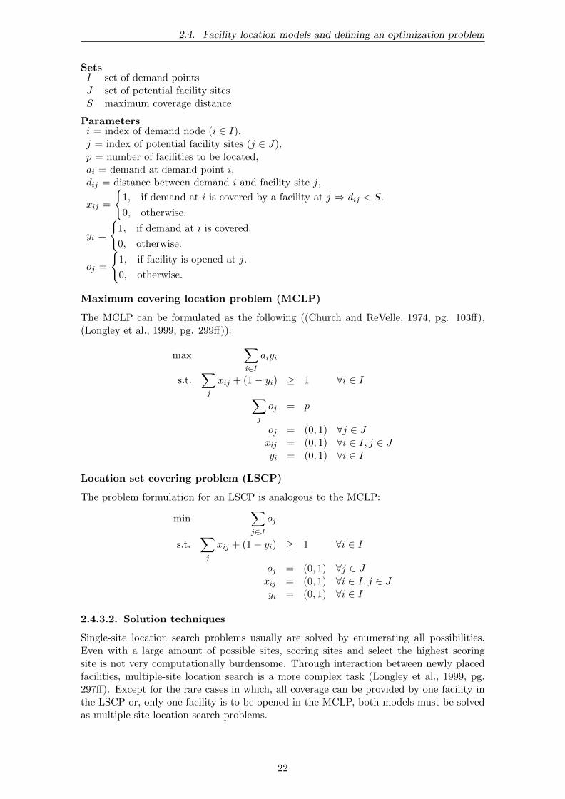
2.4. Facility location models and defining an optimization problem
SetsI set of demand pointsJ set of potential facility sitesS maximum coverage distance
Parametersi = index of demand node (i ∈ I),j = index of potential facility sites (j ∈ J),p = number of facilities to be located,ai = demand at demand point i,dij = distance between demand i and facility site j,
xij =
{1, if demand at i is covered by a facility at j ⇒ dij < S.
0, otherwise.
yi =
{1, if demand at i is covered.
0, otherwise.
oj =
{1, if facility is opened at j.
0, otherwise.
Maximum covering location problem (MCLP)
The MCLP can be formulated as the following ((Church and ReVelle, 1974, pg. 103ff),(Longley et al., 1999, pg. 299ff)):
max∑i∈I
aiyi
s.t.∑j
xij + (1− yi) ≥ 1 ∀i ∈ I∑j
oj = p
oj = (0, 1) ∀j ∈ Jxij = (0, 1) ∀i ∈ I, j ∈ Jyi = (0, 1) ∀i ∈ I
Location set covering problem (LSCP)
The problem formulation for an LSCP is analogous to the MCLP:
min∑j∈J
oj
s.t.∑j
xij + (1− yi) ≥ 1 ∀i ∈ I
oj = (0, 1) ∀j ∈ Jxij = (0, 1) ∀i ∈ I, j ∈ Jyi = (0, 1) ∀i ∈ I
2.4.3.2. Solution techniques
Single-site location search problems usually are solved by enumerating all possibilities.Even with a large amount of possible sites, scoring sites and select the highest scoringsite is not very computationally burdensome. Through interaction between newly placedfacilities, multiple-site location search is a more complex task (Longley et al., 1999, pg.297ff). Except for the rare cases in which, all coverage can be provided by one facility inthe LSCP or, only one facility is to be opened in the MCLP, both models must be solvedas multiple-site location search problems.
22

2.4. Facility location models and defining an optimization problem
Links between p-median and covering problems
(Church and ReVelle, 2010, pg. 409ff) noted that there are theoretical links between thep-Median and covering problems. The MCLP as well as the LSCP can both be defined as aspecial class of general p-median problem by transforming the real distances of a p-medianproblem into binary values representing coverage or no coverage:
d′ij =
{0, if dij ≤ S.1, if dij > S.
(2.1)
A value of one indicates that a demand at node i can not be covered by a facility at nodej and vice versa because the distance exceeds the maximum service distance. Therefore,in addition to being able to solve the MCLP using the LP approach or the heuristics de-veloped by (Church and ReVelle, 1974, pg. 105), any covering problem structured in ap-median format may be solved with approaches for a p-median problem.
Lagrangian Relaxation
There are two prevalent solution techniques for the p-median problem: Lagrangian Relax-ation with limited branch and bound and heuristics. Special purpose Lagrangian Relax-ation with branch and bound has been used to identify an exact optimum or a solutionwithin a known percentage of optimality. A Lagrangian Relaxation with subgradient op-timization has been employed to solve problems of up to 800-900 nodes (Beasley, 1993)but can be quite sensitive to parameter changes(Longley et al., 1999, pg. 300f).Maximal covering (Longley et al., 1999, pg. 300) and set covering (ReVelle and Eiselt,2005, pg. 9) problems are non-deterministic polynomial (NP)-hard. This means that spe-cific instances of this problem might not be solvable through branch and bound withina reasonable amount of processing time. Since covering problems can be represented bythousands of nodes, it is virtually impossible to consider solving problems of these propor-tions optimally. This is where heuristics offer techniques that provide a solution which isnot guaranteed to be optimal in mostly a much shorter amount of computing time.
Heuristics
Because of the high degree of interoperability between the generic p-median problem andother location problems, it is not surprising that several types of heuristic for the problemhave been developed.One of the first heuristic methods for the p-median problem is a location–allocation heuris-tic by Maranzana (1964). The method “approaches the p-median by finding successivesingle vertex medians of p subsets of destination vertices each associated with one source,and then adjusting the subsets before repeating the process” (Teitz and Bart, 1968, pg.957f). In other words, it partitions the customers by facility and then finds centers of grav-ity within each partition. If any facility location changes, the re-partitioning of customersand the search for new optimal locations are iterated until no further improvement in thesolution can be found (Farahani and Hekmatfar, 2009, pg. 497).Another one of the older but more common heuristics for the p-median problem is the ver-tex substitution technique of Teitz and Bart (1968). The procedure starts with a patternof p facilities. At each step of the heuristic, a candidate site is selected and tested to see ifa substitution with other already sited facilities is possible. If any such substitution yieldsan improvement in the target function, a substitution is made. The heuristic was one ofthe first to work with a 1-opt search space, for the number of items being simultaneously
23

2.4. Facility location models and defining an optimization problem
exchanged (ReVelle and Eiselt, 2005, pg. 8). Until now, it has received the widest recog-nition and is recognized as fairly robust at finding good, if not optimal, solutions. Themain drawback of the vertex substitution technique is that its performance is restrainedby the potential existence of a multitude of many local optima resulting from differentstarting solutions (Church and Sorensen, 1994, pg. 12). However, assuming there is aunique location with the best improvement in the iterations of the Greedy algorithm, theresulting solutions are unique and deterministic.In their proceedings on the MCLP, Church and ReVelle (1974) posted two solution tech-niques, Greedy Adding Algorithm (GA) and Greedy Adding with Substitution Algorithm.In a performance analysis of a 55-node network by (Church and ReVelle, 2010, pg. 412),both heuristics usually provided good solutions to a given MCLP and the GAS algorithmoutperforming both the Maranzana and the GA algorithm. The solutions were optimalbetween 30 percent for the GA and 50 percent of the time for the GAS algorithm. Thebetter performance of the GAS algorithm can be led back to the “piggybacking” approachof the GAS algorithm by initiating a second solution technique with the final results fromthe first (GA). Essentially, the GA algorithm is a method of finding a starting solutionfor the vertex substitution procedure of Teitz and Bart used subsequently in the GASalgorithm. The only difference between GAS and Teitz and Bart is that GAS iterativelydevelops solution, whereas the algorithm Teitz and Bart relies on an initial start from theuser (Church and ReVelle, 2010, pg. 411).Following Maranzana (1964) and Teitz and Bart (1968), a number of other heuristictechniques have evolved (including genetic algorithm simulated annealing, TABU search,GRASP, and hybrids like Global- Regional Interchange Approach). Church and Sorensen(1994) described these techniques in detail and compared them in robustness as well asapplicability in problem sets arising from geographic information systems. The algorithmof Teitz and Bart was favored due to its speed, robustness and ease of integration andshould provide a good solution for the application in this study.
24

3. Methodology
The goal of this study was to assess the city-wide geographic access to supermarketsof Philadelphia and design a general facility location problem to identify possible newlocations of supermarkets that bring a maximal improvement in supermarket accessibility,especially in areas that could be classified as food deserts. This analysis could help policymakers to not only become aware of deserted areas but provide resources for future businessinitiatives to effectively incentivize urban supermarket placements.
3.1. Form and acquisition of necessary data
To identify areas that lack supermarkets, a spatial representation of food access was createdby mapping the locations of supermarkets and farmers markets combined with character-istics of increased vulnerability to food deserts. An initial series of maps was generatedusing the open source geographic information system software QGIS 2.0.1 (formerly Quan-tum GIS). Food demand was aggregated in geometric centroids (points of gravity)of Cen-sus Block Groups, the smallest geographical unit for which the Census Bureau publishessample data. The distances between the demand points and existing supermarkets wereextracted using QGIS functionalities. Available socioeconomic data was used to determinea measure of vulnerability. Finally, a covering location problem was defined and a GreedyAdding and a Greedy Adding & Substitution heuristic was programmed to solve the prob-lem. The robustness of the heuristics was tested in a sensitivity analysis and the solutionswere mapped and analyzed to propose feasible locations for urban supermarket openings.
3.1.1. Study area
This study focuses on the city of Philadelphia, which is the only consolidated city-countyof Pennsylvania and has a population of 1,526,006 as of the 2010 Census. The city encom-passes an area of 141.6 square miles (367 square kilometers) and is divided into 384 Censustracts and 1336 Census block groups. In comparison to the national average, Philadel-phia shows signs of high relative deprivation 1. Additionally, Philadelphia has the highestprevalence of obesity among the largest ten cities in the United States (Get Healthy Philly,2013, pg. 4) and is home to a large black and Hispanic population2, two ethnic groups that
126.2% of the population ranks below poverty level, a percentage twice as large as in the state of Penn-sylvania (13.1%) (United States Census Bureau, 2014b)
2Black or African American alone, 2012: Philadelphia 44.3%, Pennsylvania 11.4%Hispanic or Latino, 2012: Philadelphia 13.0%, Pennsylvania 6.1%(United States Census Bureau, 2014b)
25

3.1. Form and acquisition of necessary data
have shown above-average obesity rates among lower-income levels (Ogden et al., 2010).Because of the combination of poverty and obesity in an urban area, access to food is animportant social concern for public policy.
3.1.2. Spatial data
Mapping data of the city boundaries and statistical subdivisions of interest (block grouplevel and census tract level) were drawn from 2010 Census TIGER/Line3 Shapefiles pro-vided by the United States Census Bureau (United States Census Bureau, 2010a). TheShapefile is a vector data format for the use in GIS which describes vector features suchas points, lines and polygons and the attributes describing these features. The shapefilesprovided describes outlines of the statistical subdivisions (Block groups in this case) andincludes attributes about size (land/water area), population, location and various socioe-conomic sample data.
3.1.3. Demand point aggregation
As a means of minimizing complexity for the solution of the problem, the subdivisions werediscreticized. Because aggregation error increases with the subdivision size, the smallestsubdivisions for which demographic data was available - block groups - were aggregatedas geographic centroids, representing population-weighted points of demand in the opti-mization problem later on.
3.1.4. Socioeconomic data
The use of the shapefiles by the Census Bureau however, is restricted to mapping purposesas they do not include demographic data. This type of data was only offered in form ofpre-joined Shapefiles with Geodatabases, which are not directly compatible with QGIS.Therefore it had to be resorted to the proprietary commercial GIS software ArcGIS 10.2 foran export of the demographic data to Comma-Separated-Value tables. The tables couldthen be re-joined with the subdivisions in QGIS using unique identifiers. Population datawas taken from the 2010 Census, whereas the 2007-2011 American Community Survey5-year estimates Summary File (United States Census Bureau, 2014a) served as a data setfor other socioeconomic data. The most finely granulated representation of demographicdata available are the block group level data sets, due to smallest subdivision size andtherefore the smallest aggregation error.
3.1.5. Retail outlets
Farmers’ Markets and supermarkets were used as existing facilities that can serve as sourcesfor healthy food. Farmers’ Market locations are made accessible by the City of Philadelphiaon (Open Data Philly, 2013) as Shapefiles. Supermarket locations were identified by onlinelocation listings of chain stores serving the Philadelphia area and Google Maps. Foodoutlets had to have a full-line grocery offering, including a produce and fresh meat section,in order to be considered (e.g. Walmart supercenters were considered whereas WalmartDiscount Stores were not because they lack fresh produce). This is also the reason why,although available on Open Data Philly (2012), Healthy Corner Store locations were notconsidered. Even though the initiative has been highly successful (see section 2.3.5), thevery small selection of fresh produce rules out Healthy Corner Stores from full-line grocerystores. Hence, they were not considered an option for ensuring an adequate and full supply
3“TIGER = Topologically Integrated Geographic Encoding and Referencing.TIGER products are spatial extracts from the Census Bureau’s MAF/TIGER database, containingfeatures such as roads, railroads, rivers, as well as legal and statistical geographic areas.” (UnitedStates Census Bureau, 2010b)
26

3.2. Underlying assumptions
of healthy food in the course of this study. After the addresses of eligible supermarketswere obtained, the WGS 84 (GPS) coordinates of the supermarkets were queried using aGoogle Geocode API XML request in an Excel VBA macro and joined with the Censuslayers in QGIS. In addition to 62 listed Farmers’ Markets, 81 supermarkets within the citylimits could be identified. The complete list of supermarkets can be found in the Appendixsection A.
3.2. Underlying assumptions
3.2.1. Definition of coverage and access
Two different types of optimization about food access were made for the facility locationproblem. The first type models a supply pattern during the “farmers’ market low season”with only supermarkets providing adequate access, whereas the second type represents asituation where farmers’ markets can provide adequate access as well, but within a smallerrange.
1. Supermarkets and supercenters can provide adequate healthy food access within anarea of 1/2 mile (2640 feet).
2. Supermarkets and supercenters can provide adequate healthy food access to an areaof 1/2 mile (2640 feet) and Farmers’ Markets can provide adequate healthy foodaccess to an area of 1/4 mile (1320 feet).
The service areas are in line with the service areas use in an access study by the (GetHealthy Philly, 2013, pg. 5). It should be noted that supermarket and farmers’ mar-ket access was measured using the straight-line distance metric. The distances betweeneach demand point and food retail stores was calculated using the QGIS Distance Matrixfunction.
3.3. Vulnerability Index
3.3.1. Variable selection
Socioeconomic variables can represent how communities are composed and the social con-ditions that prevail. To give a measure of how vulnerable some subdivisions are from astatistical standpoint, this index was based on composite deprivation indices that havebeen used in geographic access studies by Apparicio et al. (2007) and Larsen and Gilliland(2008) and are described in 2.1.4. Figures of recent immigration, however, could not beobtained from the Census Bureau and are not included in this study. To specially ac-count for lack of physical mobility, two economic variables were added, vehicle access andshare of elderly people. This measure included seven variables, computed from the 2007-2011 American Community Survey 5-year estimates: Three poverty, one employment, oneeducation and two mobility variables (see the detailed variable description in3.1 and itsdescriptive statistics in 3.2).
3.3.2. Data reduction
The individual vulnerability of a subdivision to a geographic access barrier was measuredusing a composite Vulnerability Index, whose inputs are comparable to the ones used inindices by Apparicio et al. (2007), Larsen and Gilliland (2008). These studies computea linear combination of five social indices. However, it is apparent deprivation variablescan be strongly interdependent, skewing the composite index by over-representing certaincausal links. Our data set showed significant correlations between all variable pairs except
27

3.3. Vulnerability Index
Table 3.1.: Socioeconomic variables of neighborhood vulnerability
Domain Variable Description
Poverty Low-Income population Share of households with income oflast 12 months below poverty level
Public assistance Share of households on public assis-tance
Lone-parent families Share of Lone-Parent-families of inrelation to all households
Employment Unemployment Unemployment rate of labor force
Education Low-level education Share of population 25 years andover with with no no more thangrade 8 education
Mobility Elderly population Share of population 65 years andolder
No vehicle access Share of housing units with no vehi-cle access
Table 3.2.: Descriptive statistics of vulnerability variables in block groups of Philadelphia
Low-Income population [%]
Public assistance [%]
Lone-parent families [%]
Unemploy-ment [%]
Low-level education [%]
Elderly population [%]
No vehicle access [%]
MeanStd. DeviationSkewnessKurtosisMinimumMaximumPercentiles 25
5075
25.09 8.64 27.98 14.57 5.49 12.48 34.6217.49 9.52 17.29 11.36 6.52 8.75 21.06
.81 1.45 .37 1.05 1.89 1.49 .28
.29 2.18 -.47 1.07 4.68 3.84 -.81
.00 .00 .00 .00 .00 .00 .0091.18 60.00 87.04 66.24 48.26 63.96 100.0010.97 .00 14.25 6.20 .00 6.36 17.1622.13 5.75 26.32 12.21 3.42 10.89 33.4835.17 12.95 40.13 20.69 8.11 16.86 50.84
Page 1
the one involving elderly population (see 3.3), which is unsurprising but stresses the im-portance of reducing linear combinations.To merge the data and reduce the number of linear combinations in an overall index ofneighborhood vulnerability, a factor extraction through a Principal Component Analysis(PCA) was constructed in IBM SPSS Statistics Version 21 following the method of LaerdStatistics (2014). The PCA procedure has also been used for similar composite deprivationindices such as the one computed by (Sharkey and Horel, 2008, pg. 622).It is apparent that the share of elderly population is negatively correlated with variablesthat generally characterize socioeconomic deprivation. It should be included in the measureof vulnerability because it corresponds to a individual mobility dimension of vulnerabilitythat is, in contrast to car accessibility, independent to the economic circumstances. Dueto the negative correlations, including the elderly population variable in the PCA resultsin a negative component loading - a higher share of elderly people would lead to a lowervulnerability index. To avoid this misrepresentation of the elderly population, only the“deprivation-related” variables (excluding the elderly population share) underwent a PCAand combined with the elderly population later on (see 3.3.3).
Before conducting a factor analysis, the variables were tested on multicollinearity using aKaiser-Meyer-Ohlin (KMO) measure of Sampling Adequacy (MSA). This test resulted ina KMO value of .793, ranking between a “middling” value of 0.70 and a “meritous” valueof 0.80. The Bartlett’s Test of Sphericity tests the null hypothesis of uncorrelation amongthe variables and showed a significance level of 0.00, a value that justifies the rejection of
28
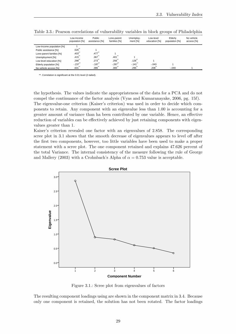
3.3. Vulnerability Index
Table 3.3.: Pearson correlations of vulnerability variables in block groups of Philadelphia
Low-Income population [%]
Public assistance [%]
Lone-parent families [%]
Unemploy-ment [%]
Low-level education [%]
Elderly population [%]
No vehicle access [%]
Low-Income population [%]
Public assistance [%]
Lone-parent families [%]
Unemployment [%]
Low-level education [%]
Elderly population [%]
No vehicle access [%]
1 .526** .433** .415** .298** -.237** .631**
.526** 1 .477** .367** .273** -.187** .386**
.433** .477** 1 .401** .256** -.267** .300**
.415** .367** .401** 1 .128** -.141** .295**
.298** .273** .256** .128** 1 -.043 .208**
-.237** -.187** -.267** -.141** -.043 1 -.040
.631** .386** .300** .295** .208** -.040 1
Correlation is significant at the 0.01 level (2-tailed).**.
Page 1
the hypothesis. The values indicate the appropriateness of the data for a PCA and do notcompel the continuance of the factor analysis (Vyas and Kumaranayake, 2006, pg. 15f).The eigenvalue-one criterion (Kaiser’s criterion) was used in order to decide which com-ponents to retain. Any component with an eigenvalue less than 1.00 is accounting for agreater amount of variance than ha been contributed by one variable. Hence, an effectivereduction of variables can be effectively achieved by just retaining components with eigen-values greater than 1.Kaiser’s criterion revealed one factor with an eigenvalues of 2.858. The correspondingscree plot in 3.1 shows that the smooth decrease of eigenvalues appears to level off afterthe first two components, however, too little variables have been used to make a properstatement with a scree plot. The one component retained and explains 47.626 percent ofthe total Variance. The internal consistency of the measure following the rule of Georgeand Mallery (2003) with a Crohnbach’s Alpha of α = 0.753 value is acceptable.
Component Number
654321
Eig
enva
lue
3.0
2.5
2.0
1.5
1.0
0.5
0.0
Scree Plot
Page 1
Figure 3.1.: Scree plot from eigenvalues of factors
The resulting component loadings using are shown in the component matrix in 3.4. Becauseonly one component is retained, the solution has not been rotated. The factor loadings
29

3.4. Input and Output parameters
represent both the weighting of variables for each factor but also the correlation betweenthe variables and the factor.
Table 3.4.: Principal Factor Analysis component matrix
Component
1Low-Income population [%]
Public assistance [%]
No vehicle access [%]
Lone-parent families [%]
Unemployment [%]
Low-level education [%]
.831
.754
.704
.701
.630
.463
Extraction Method: Principal Component Analysis.
Page 1
3.3.3. Constructing the Index
The resulting factor from the Principal Component Analysis was then normalized sothat it ranges between zero and one, representing a Deprivation index ID (Vyas andKumaranayake, 2006, pg. 19).
ID =f1 − f1,min
f1,max − f1,min(3.1)
To get to the final Vulnerability Index the elderly population share needs to be included.For weighting purposes, the assumption that being aged over 65 poses a similar vulnera-bility to access barriers than not having access to a vehicle in the household was necessary.Hence, the contribution of both variables to the composite Vulnerability Index should beequal. Solving the equation for the weighting leaves us with a weighting of the elderlyshare we of 14.71 percent. 4
Hence, the Vulnerability Index IV for each block group is combined from the DeprivationIndex ID and the normalized5 elderly population share Ie in the following way:
IV = (1− we) ∗ ID + we ∗ Ie = (1− .1471) ∗ ID + .1471 ∗ Ie (3.2)
3.4. Input and Output parameters
Inputs
The inputs for the optimization program are drawn directly from the spatial data usingQGIS. Given the nature of covering problems, the following matrices are inputs to theoptimization model:
• Number of facilities to be opened (p) - this only applies to the MCLP
• Population vector: provides populations per block group
4The no-vehicle-access-share had a loading for the deprivation index of .704. The sum of all loadingsis (.831 + .754 + .704 + .701 + .630 + .463) = 4.083, therefore the contribution to the deprivationindex is .704
4.083= 17.24%. Solving for the contribution of the elderly population share to the composite
Vulnerability Index (under the assumption stated above) results in x = frac.7044.083 ∗ (1− x)⇔ x =.7044.787
≈ 14.71%5The normalization of the elderly population share is done analogous to the Deprivation index:Ie =
Se−Se,min
Se,max−Se,min
30
3.4. Input and Output parameters
• Vulnerability Index vector: provides Vulnerability scores per block group
• Inter-block-group-centroid-distance matrix: necessary for determining distances be-tween demand points and possible new supermarkets
• Block group to facility distance matrices
• Maximum service distances for supermarkets and Farmers’ Markets: the distancerelates to the coverage area per facility type
The number of facilities to be opened as well as the service distances are the only param-eters that are not exogenous and could be chosen arbitrarily. As mentioned in 2.1.3, thisstudy used service distances of 1
2 mile (2640 feet) for supermarkets and 14 mile (1320 feet)
for Farmers’ Markets. The initial amount of facilities to be placed was ten but adaptedbased on the iterative coverage results later on. Both parameters were adjusted in asensitivity analysis to test the robustness of the algorithm.
Outputs
As MATLAB operates on matrices, a comma-separated output file is a matrix with thedifferent pieces of information saved in columns. The matrix is converted to a comma-separated-value (CSV) file, whose naming scheme makes it possible to differentiate betweenthe following parameters: 1) MCLP or SCLP; 2) Vulnerability-weighting of population; 3)Type of initial stores included; 3) buffer size; 4) Heuristic (GA or GAS); and, 5) type ofplaced facilities. The resulting output file includes the following information:
• Iteration in which facility was placed as an integer values from one to p
• Location of facility as an integer ID of block group centroid
• Sum of newly covered population per facility
• Sum of newly covered weighted population per facility
• Sum of newly covered demand nodes per facility
• Average distance of demand nodes to facilities
• Improvement of average distance per iteration
The sum of newly covered (weighted) population represents the MCLP objective function,whereas the newly covered (weighted) population values are the basis for the selectionfunction in each iteration of the Greedy-Adding algorithm. The newly covered demandnodes are the basis for the Greedy-Adding selection function in each iteration to solve theSCLP. Hence, using a Greedy-Adding algorithm, the values of new coverage per iteration(both in the MCLP and SCLP) is a concave function as new facilities will either havean equal or lower amount of new coverage. Solving the MCLP with a GA heuristic fora certain value of p therefore also reveals the GA solutions for all MCLP with a smallervalue of p.Adding a substitution heuristic in each iteration takes away the concavity of the new cov-erage, meaning that the first p− k, 1 <= k < p opened facilities of a MCLP solved with aGAS heuristic do not necessarily represent the solutions of the p− k MCLP. Whereas theGAS heuristic guarantees a globally better or at least equal objective value, it increasescomputational complexity per iteration through the piggybacking of another heuristic. Italso needs to be recomputed for different values of p in case there are additional substitu-tions in between the pnew and pold.
31

3.5. Implementation of the algorithm
3.5. Implementation of the algorithm
The following section describes the how the different steps in creating necessary inputvariables, solving the actual problem and presenting the output were implemented. Thealgorithm programmed to solve the MCLP for the food retail application was implementedin four steps:
1. Computation of initial coverage and construction of input variables
2. Subsequent Greedy-Adding of facilities
3. Substitution of facilities
4. Output of results
3.5.1. Computation of initial coverage
The main difference in this algorithm to the GAS prototype from Church and ReVelle(1974) are already existing facilities which are able to cover a certain amount of nodes. Soafter a creation of initial variables in MATLAB, the imported locations of existing facilitieshad to be imported and the present level of coverage had to be computed. This was done bytransforming the facility-to-block-group-centroids distance matrix to an adjacency matrix.A logical comparison of all distances to the corresponding maximal service distance resultsin values of one if the block group lies within the maximal service distance to a facilityand zero if not. By summing these binary variables of supply, a vector of the amountof facilities supplying each demand node was extracted. This vector can then be furthertransformed to a vector of supply by checking whether each block group is covered by zero(no coverage) or at least one facility (coverage). The vector can now be used as a vectorof initial coverage to not include already covered nodes in the heuristic.
3.5.2. Greedy-Adding Heuristic
The Greedy-Adding algorithm is a well-established heuristic which solution procedure isdescribed in detail by (Daskin, 2013, pg. 146ff). The implementation of the Greedy Addingheuristic in MATLAB draws heavily from the Pseudo-Code provided by (Vahrenkamp andMattfeld, 2007, pg. 160), with a differing initialization phase, as described in the sectionabove. In each of the p iterations, the possible additional coverage provided from a facilityat each demand node is calculated. The location with the maximum new coverage (ofpopulation, weighted population or demand nodes, respectively) is selected for a facilityplacement at that location. The ID and improvement is stored and the entries of newlycovered nodes in the coverage vector are adjusted.
3.5.3. Substitution Heuristic
In each of the p iterations (or an unknown number of iterations in the SCLP), the Substi-tution heuristic works downstream the Greedy-Adding heuristic to improve the coverageto a 1-optimal solution (Church and ReVelle, 1974, pg. 106). For all already openedfacilities, the heuristic calculates the effect of a swap of that facility to a “free” site onthe objective total coverage function. If an improvement through such a replacement ispossible, the opened facility is closed, all “unique” coverage (nodes that are only coveredby that one facility alone) is eliminated from the coverage vector. Subsequently, a newfacility is opened at the identified location with newly covered demand nodes. Becausefurther opportunities for improvement might arise through the swap, all opened facilitieshave to be examined on possible substitutions again, which explains the greatly largercomputation time with an additional Substitution heuristic. The Substitution heuristicwas implemented using a while-loop which uses a counter that resets each time a substi-tution is made and terminates if all locations have been checked for substitutions withoutfinding a possible improvement.
32

3.5. Implementation of the algorithm
3.5.4. Output of results
Both the GAS and GA algorithm create a comma-separated-value output file that includesthe values mentioned in 3.4. Because frequent changes of the solution during runtime ofthe GAS algorithm (which can be attributed to the nature of the Substitution heuristic),the output matrix only includes the bare minimum of information during the iterations(iteration number, facility ID and new coverage) and is filled with the other values at thevery end. In order to estimate how much of an effect the heuristic would have on theobjective function of a SCLP or a p-Median problem, the development of the average dis-tance (p-Median) and the amount of newly covered demand nodes is also included. Bothunweighted and weighted values of new population coverage help analyze the influence ofa Vulnerability weighting on the objective value of the unweighted problem and vice versa.For improved error backtracking, several other output matrices were created in MATLABbut exported in the solution table. This included substitution iterations including infor-mation such as the swaps made and the possible improvement for each facility. However,these are not necessary pieces of information when considering the final solution of thealgorithm and meant for development uses only.
33

4. Results
4.1. Status quo: Limited access and deprivation in Philadel-phia
4.1.1. Mapping population distribution and retail outlets
The map population density and food retail locations (see Figure 4.1) reveals that the mostdensely populated areas in Philadelphia are located in and south of the Center City district.Two areas that also show relatively high density levels are the University city district westof Schuylkill River and the Upper North area. The predominantly suburban areas ofNortheast and Northwest Philadelphia are among the least populated areas, consideringthat large parts of the Southernmost part of Philadelphia and the Riverfront are non-residential areas. Especially in South Philadeplhia and northeast of the City Center, anagglomeration of supermarkets is apparent.
The Star Map in (see Figure 4.2) gives a visual representation of the straight-line distancesfrom each Block Group centroid to a supermarket. Although the distances to the nearestsupermarket seem to increase the further from the city center, the stars from supermarketin the city center still reveal that many block group centroids are still out of walkingdistance (distances greater than 1
2 mile, colored red) from a supermarket. Furthermore,assuming each customer visits the closest supermarket, there are several supermarkets thatseem to be serving an abnormally large amount of customers, such as two facilities westand south of the City Center District. One could presume that the area is undersaturatedwith food retail opportunities or the supermarket is oversaturated and might be workingat or above capacity limit.
4.1.2. Mapping low access and vulnerability characteristics
After analyzing the concentration of people living in Philadelphia and the food retailenvironment, it is of importance to examine if there are areas that show signs of highvulnerability and low access. Figure 4.3 represents the Block Group level VulnerabilityIndex values and the coverage areas of the existing supermarkets. Generally, vulnerabilityseems to be higher in the core areas that are heavily populated and decreases with thedistance from the city core. An exception is the City Center district, which shows thehighest levels of population but low vulnerability.Four areas can be made out that show relatively high Vulnerability scores. First, Kensing-ton/Upper North (located northeast of the City Center District) shows the highest levels
34
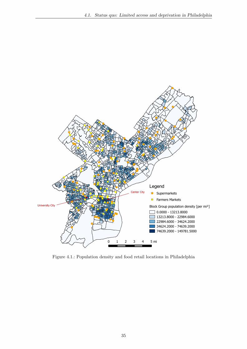
4.1. Status quo: Limited access and deprivation in Philadelphia
University City
Center City Supermarkets
Farmers Markets
Block Group population density [per mi²]
0.0000 - 13213.800013213.8000 - 22984.600022984.6000 - 34624.200034624.2000 - 74639.200074639.2000 - 149781.5000
Legend
0 1 2 3 4 5 mi
Figure 4.1.: Population density and food retail locations in Philadelphia
35
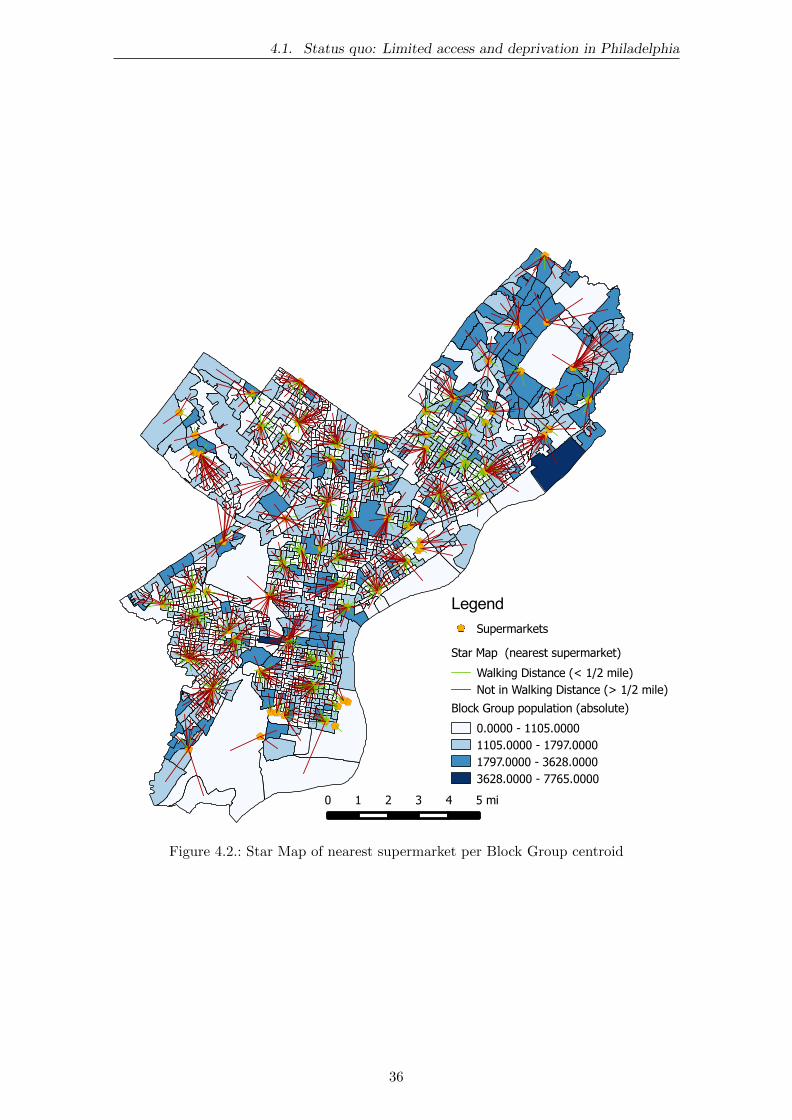
4.1. Status quo: Limited access and deprivation in Philadelphia
Supermarkets
Star Map (nearest supermarket)
Walking Distance (< 1/2 mile)Not in Walking Distance (> 1/2 mile)
Block Group population (absolute)
0.0000 - 1105.00001105.0000 - 1797.00001797.0000 - 3628.00003628.0000 - 7765.0000
Legend
0 1 2 3 4 5 mi
Figure 4.2.: Star Map of nearest supermarket per Block Group centroid
36
4.2. Results of algorithms
of vulnerability at a relatively high population density and many block groups withoutwalking accessibility to a supermarket. Areas that share similar characteristics are thesurrounding areas of University City, the western part of South Philadelphia as well asLower North Philadelphia (bordering the City Center to the Northwest).Figure 4.4 depicts the combination of several Vulnerability characteristics to show areasthat are vulnerable to access limitations on several dimensions. Again, the four areasmentioned above stand out as potential food deserts. Although socioeconomic deprivationis negatively correlated with the share of elders, there are several areas north of the CityCenter District and west of University City that show signs of deprivation and a relativelylarge concentration of seniors. The combination both characteristics might justify the in-clusion of the elderly people share in the Vulnerability Index.It should be noted that in contrast to the Vulnerability Index, the characteristics weredefined on a relative basis (attributes in highest Block Group quartile). This means thatthis visual measure represents relative but not absolute vulnerability and does not allowfor comparisons among different study areas.
4.2. Results of algorithms
Before the optimization, the 81 supermarkets with a maximum service distance of 12 mile
were able to cover a total of 605 demand points (about 45 percent of the demand points)and a population of 700,606 (46 percent of the total population). The average populationthat each supermarket provides coverage for is 8,649. This number can provide a roughestimate for the minimum covered population necessary for a new feasible supermarketto operate, as this is a measure of the uncontested market within walking distance of thefacility.
4.2.1. MCLP: Supermarket location
Unweighted population
After running the GAS algorithm for the MCLP of supermarket location (12 mile supermar-ket service distance and existing supermarket locations considered) with different values ofp, it became apparent that the Substitution heuristic was not able to find a swap yieldingin an improvement until the 46th iteration. Therefore, the results of the Greedy-Addingand the Greedy Adding with Substitution are identical every value of p <= 45. Butalready after 34 opened facilities, the newly covered population falls below the averagepopulation coverage of 8,649. This would mean that facilities added after 33 iterationsmight have a below-average spatial market (except for iterations with substitutions, butthat would decrease the coverage of a previously opened facility so that the total coveredpopulation per iteration would still fall below the average).The GA/GAS solution for the 40-MCLP of supermarket location can be found in the Ap-pendix (see B.3). The development of the newly covered population is depicted in Figure4.5. There is a visible break in coverage after 14 facilities (coverage roughly 2,000 peopleless). The top 14 facility locations were added to the existing supermarkets in Philadelphiaand plotted in Figure 4.6.
Vulnerability-weighted population
The Vulnerability Index as a weighting influenced the algorithm procedure so that Substi-tutions were made earlier on (at the 21st iteration). This means that the iteration counts tothe 40-wMCLP (vulnerability-weighted MCLP) in Table B.4 no longer match the “ranks”of contribution to the objective function. Decreasing p to a value of 20 and examiningthe development of the new coverage per iteration, a break is visible after nine iterations
37

4.2. Results of algorithms
Supermarkets
Supermarkets (2640 ft Buffer)
Block Group Vulnerability Index
0.0000 - 0.17610.1761 - 0.35230.3523 - 0.52840.5284 - 0.70460.7046 - 0.8807
Legend
0 1 2 3 4 5 mi
Figure 4.3.: Map of Block Group level Vulnerability and supermarket coverage areas
38

4.2. Results of algorithms
Low access: Centroid further than 1/2 mile from a supermarketLow Income: Within the high quartile of people with income below poverty levelNo vehicle: Within the high quartile of households with no access to a carSeniors: Within the high quartile of people above 65 years
Supermarkets
Supermarkets (2640ft Buffer)
Block Group characteristics
Low Access + Low IncomeLow Access + Low Income + No VehicleLow Access + Low Income + No Vehicle + Seniors
Legend
0 1 2 3 4 5 mi
Figure 4.4.: Map of Combinations of Vulnerability characteristics
(see Figure 4.7). To improve comparability, a map of both the 14 optimal locations fromunweighted and vulnerability-weighted optimization shows the effect of the weighting onthe spatial placement (Figure 4.8).
4.2.2. MCLP: Farmers’ Market location
The first model assumes that outside of the Farmers’ Market season supermarkets do notface competition in the market of fresh produce and meat. Therefore, it models the out-of-season food retail environment. The second model is based on the fact that Farmers’Markets have to compete with supermarkets for customers during Farmers’ Market seasonand a public authority should not promote Farmers’ Markets that are in direct competitionwith a full-line supermarket. In this model, additional Farmers’ Markets optimal locationsare computed based on the existing supermarkets and Farmers’ Markets. The Farmers’Markets’ service distance was set to 1
4 mile, whereas the supermarkets’ larger productoffering appeal is represented in a 1
2 mile service distance that has also been used above.When not taking the existing supermarkets into account, the 62 existing Farmers’ Marketscover a total population of 201,533 people. Again, the average coverage per facility of 3,250is used as an indicator of when the addition of new facilities becomes not economicallyviable.The GAS algorithm does not substitute facilities up until a p of 80, meaning that the
39

4.2. Results of algorithms
y = 22406e-0.029x
R² = 0.9614
0.00%
0.50%
1.00%
1.50%
2.00%
2.50%
3.00%
3.50%
4.00%
4.50%
0
5000
10000
15000
20000
25000
30000
1 6 11 16 21 26 31 36
Ad
dit
ion
al
cov
ere
d p
op
ula
tio
n
Iteration
MCLP GA/GAS (Supermarket locations, S=2640ft): Additional
coverage
Additional Coverage
Average coverage (existing supermarkets)
Expon. (Additional Coverage)
Figure 4.5.: 40-MCLP of supermarket placement coverage graph
Figure 4.6.: Map of optimal 14 MCLP locations (placement: Supermarkets, p=40, initialcoverage: supermarkets (S=1
2 mile)
40

4.2. Results of algorithms
y = 10741e-0.06x
R² = 0.8656
0.00%
1.00%
2.00%
3.00%
4.00%
5.00%
6.00%
7.00%
8.00%
0
2000
4000
6000
8000
10000
12000
14000
16000
1 6 11 16
Ad
dit
ion
al
cov
ere
d w
eig
hte
d p
op
ula
tio
n
Iteration
wMCLP GA/GAS (Supermarket locations, S=2640ft): Additional
coverage
Additional weighted coverage
Average weighted coverage (existing
supermarkets)
Expon. (Additional weighted coverage)
Figure 4.7.: 20-wMCLP of supermarket placement coverage graph
Figure 4.8.: Map of optimal 14 wMCLP locations in comparison to MCLP locations (place-ment: Supermarkets, p=40, initial coverage: supermarkets (S=1
2 mile)
41

4.2. Results of algorithms
resulting list of facilities is ranked by contribution to the objective function and that theobjective value of the GA heuristic solution is identical to value of the GAS heuristicsolution. The coverage graph in Figure 4.9 reveals that openings of 67 Farmers’ Marketswould yield above-average coverage. That is surprising, considering that the coverage ofexisting Farmers’ Markets was calculated based on a no competition from supermarkets,while the new located Farmers’ Markets’ coverage only consists of areas that are leftuncovered by existing Farmers’ Markets as well as supermarkets. Reasons for this anomalycould include the inefficient placement of existing Farmers’ Markets, a too small buffer incorrespondence to too large subdivisions (Block Groups) or the aggregation of severalFarmers’ Markets in the city center, leading to overlapping areas of coverage. A map ofthe above-mentioned 67 Farmers’ Markets is another sign for the amount of demand forfood that is not satisfied in high-density areas, as new facility proposals concentrate onareas with high relative density (see Figure 4.10).
y = 7431.4e-0.013x
R² = 0.9799
0.00%
0.20%
0.40%
0.60%
0.80%
1.00%
1.20%
1.40%
0
2000
4000
6000
8000
10000
1 6 11 16 21 26 31 36 41 46 51 56 61 66 71 76
Ad
dit
ion
al
cov
ere
d p
op
ula
tio
n
Iteration
MCLP GA/GAS (Farmers' Market locations,
S(FM)=1320ft, S(SM)=2640ft: Additional coverage
Additional Coverage
Average coverage (existing farmers'
markets)
Expon. (Additional Coverage)
Figure 4.9.: 80-MCLP of farmers’ market placement coverage graph
42

4.2. Results of algorithms
Figure 4.10.: Map of optimal 67 MCLP locations (placement: Farmers’ markets, p=80,initial coverage: supermarkets (S=1
2 mile), Farmers’ Markets (S=14 mile)
43

4.3. Performance and sensitivity analysis
4.3. Performance and sensitivity analysis
Performance
The Substition heuristic was implemented on top of the Greedy-Adding heuristic in orderto find better solutions for the location problems at hand than a normal Greedy-Addingalgorithm would find. Both algorithms were written parametric, such that they allowedfor quick change of input parameters. The trade-off is a higher computation time for theSubstitution heuristic, as the amount of pairwise combinations of locations to be checkedincreases with the iterations (set by the value of p). The values of p (possible facility open-ings) that were relevant for this application were fairly small, because certain feasibilityconstraints for new store openings were applied (such as above-average new coverage).The algorithms were run in MATLAB R2013b on a 2.0 GHz Intel Core 2 Duo laptop with3GB of memory running Windows 7 (64 Bit) with service pack 1. Tables 4.1 and 4.2depict several runs of both algorithms. In the MCLP, the first swap of locations was onlydone in the 46th iteration. Hence, only for values higher than 46 would the GAS yield animprovement but overall takes much longer computing time (e.g. increasing the value of pby the factor five from 20 to 100 lead to a computing time increase by the factor of five forthe GA heuristic and a computing time increase by the factor of 31 for the GAS heuristic.For the performance test of the SCLP algorithm, the buffer sizes were varied. This had twoeffects: First, the amount of necessary facilities increases because of the smaller coveragearea and second, the amount nodes to be covered increases as well. Higher values of presult in more opportunities for Substitutions, so the GAS solutions need a smaller amountof facilities to cover the whole demand point set (2.2 percent and 4.7 percent respectively).However, the general computing time of the GAS algorithm is higher and furthermoreincreases more strongly with decreasing buffer size. A maximal service distance of 1
2 , tech-nically inducing the problem of trying to cover all demand points by placing supermarkets,takes a computing time of over five minutes. Cutting the service distance in half took morethan ten times the computing time.In theory, the GAS algorithm yields better objective function values in exchange for morecomputing time. For this application, the improvement through substitution did not mat-ter for the values of p that were constrained by the minimum coverage constraints. Hence,the GAS heuristic could only be used as an affirmation of the good solution provided bythe Greedy-Adding algorithm.
0
5000
10000
15000
20000
25000
10 20 40 70 100
Ave
rag
e a
dd
itio
na
l co
ve
rag
e
p
Service Distance Sensitivity
for the GAS algorithm solving the MCLP
of supermarket placement
1320 ft service distance 2640 ft service distance 5280 ft service distance
0.10
1.00
10.00
100.00
1000.00
10 20 40 70 100
Tim
e e
lap
sed
[s]
p
Performance comparison of GA and GAS heuristic
solving the MCLP of supermarket placement
GA, 1320 ft service distance GAS, 1320 ft service distance
GA, 2640 ft service distance GAS 2640 ft service distance
GA, 5280 ft service distance GAS, 5280 ft service distance
Figure 4.11.: Performance comparison of GA and GAS heuristic for a supermarket MCLPand Sensitivity of the GAS algorithm towards maximum service distance
Sensitivity towards service distance and facility placements
Along with the performance, the algorithms for solving the supermarket placement MCLPand SCLP were tested on its robustness in a sensitivity analysis. The varied parameters
44

4.3. Performance and sensitivity analysis
included the maximum service distance (buffer sizes of 14 mile, 1
2 mile and one mile - 1320,2640 and 5280 feet, respectively) and the amount of facilities placed p.The analysis revealed that the fit of the algorithm is dependent on the maximum servicedistance employed. First, the average additional coverage is decreasing with the numberof facilities placed, which is in line with the expectation of a greedy heuristic. The decayof average coverage in relation to p increases with the maximum service distance.A potential explanation for this observation is the quadratically increasing coverage areawhen varying the service distance. Smaller buffers lead to more uncovered subdivisionsand more gaps to be filled by new facilities. For a 1
4 -mile service distance, the averageadditional coverage per facility exceeds the average coverage of existing facilities in allcases (even in the case of p = 100), which could be attributed to the level of aggregation:Because in contrast to the possible locations for new facilities, the existing facilities arenot located directly on the block group centroids, hence, the level coverage is prone tocoverage gaps resulting from a small service distance. Additionally, some block groups areheavily populated (larger population than the average existing coverage), which even putsone-block-group-covering facilities on an above-average population coverage. The one-mileservice distance could be assumed as exceedingly large, as new facilities employing thisdistance are only barely competitive, whereas the quarter-mile service distance could beassumed as too small for the level of aggregation in the given data.
Table 4.1.: Performance and Sensitivities of algorithms for a MCLPs
MCLP GA algorithm GAS algorithm
Buffer size[ft]
Nodesavg.
existingcoverage
pNew
coverageaverage
Timeelapsed [s]
Newcoverage
averageTime
elapsed [s]
1320 1172 2368 10 94991 9499 0.57 94991 9499 1.771320 1172 2368 20 170149 8507 1.40 170149 8507 5.811320 1172 2368 40 297139 7428 2.55 298441 7461 20.921320 1172 2368 70 460348 6576 4.24 461650 6595 98.59
1320 1172 2368 100 598479 5985 5.81 600305 6003 199.41
2640 745 8649 10 199783 19978 1.11 199783 19978 1.662640 745 8649 20 339083 16954 2.14 339083 16954 5.862640 745 8649 40 525278 13132 3.82 525278 13132 18.572640 745 8649 70 698272 9975 4.42 711176 10160 100.30
2640 745 8649 100 780316 7803 10.01 788645 7886 180.91
5280 93 17330 10 99290 9929 0.70 99290 9929 2.355280 93 17330 20 122268 6113 1.12 122268 6113 7.275280 93 17330 40 122311 3058 2.33 122311 3058 18.585280 93 17330 70 122311 1747 3.98 122311 1747 34.54
5280 93 17330 100 122311 1223 6.18 122311 1223 56.22
Table 4.2.: Performance and Sensitivities of algorithms for SCLPs
SCLP GA algorithm GAS algorithm
Buffer size [ft] Nodes Facilities Time elapsed [s] Facilities Time elapsed [s]
1320 1172 514 31.07 503 3815.752640 745 148 5.16 141 309.865280 93 23 0.64 23 7.07
45

5. Evaluation
5.1. Discussion
Inadequacy of city-wide food access
The results of this study reveal that, in 2014 the inner-city supermarket coverage inPhiladelphia in most cases is still inadequate. Taking supermarkets and supercenters thatoffer a full range of nutritious food into account, with 2866.9 feet the average distance fromrepresentational block group centroids to a supermarket is still above the widely used walk-ability distance of 1
2 mile (2640 feet). 46.9 percent of the population does not fall withinwalkability range to a supermarket, and within the block groups in the highest quantile ofthe Vulnerability Index (measuring vulnerability towards food access limitations), roughly55.5 percent of the population is confronted with limited access to supermarkets.
Deprivation and food access
On first glance, no systematic link can be drawn between deprivation and low food access.The data reveals that the level of vulnerability towards food access barriers (consisting ofcharacteristics of deprivation and the share of elderly population) shows a weak negativePearson correlation (% = −0.278) to the distance to a supermarket offering a full rangeof nutritious food. Higher vulnerability shows a Pearson correlation to population den-sity (% = +0.203). The goodness of the fit is poor in both cases (R = 0.078 and 0.042,respectively), however. But taking the visual representations on the generated maps intoaccount, this shows that subpopulations with elevated levels of vulnerability seem to con-centrate in the old core area of Philadelphia.Walkable supermarket access across the city limits is limited to a minority of the exam-ined population. In total, 54.1 percent of the population (825,400 of 1.52 million) are notserviced by a supermarket in walkability range. The share for the areas with the highestlevels of vulnerability is larger; 55.5 percent of the population living in the highest quantilevulnerability block groups face non-walkable distances to supermarkets.The average distance from the highest quantile vulnerability block groups to supermarketswas found to be smaller than the average of all block groups, but only by a small margin(2866 vs. 2967 feet). This means however, that on average, the most vulnerable blockgroups (that also tend to have relatively low levels of car ownership) do not offer walkablesupermarket access.Although no systematical discrimination of vulnerable areas could be detected, two ma-jor clusters (Lower North/Northeast Philadelphia and the surrounding areas of University
46
5.1. Discussion
City) of low access and high vulnerability were found. Considering the existence of co-herent areas that are not only susceptible to access barriers but also densely populated,firstly, deprivation is a factor of food deserts that should be incorporated and secondly,public policy incentives for the private market might prove efficient in these singled-outareas.The share of elderly population has mostly been neglected in vulnerability, as mostly vul-nerability was measured in socioeconomic deprivation. Areas with a large elderly popula-tion however tend to be less deprived and in our case, the share of elderly people showeda strong negative correlation with socioeconomic deprivation. Figure 4.4 indicates thatPhiladelphia is scattered with block groups that show a combination of deprivation char-acteristics and a high share of elderly people. The amount of high-risk areas with anotherfactor of vulnerability provides a means of justification for the inclusion of disadvantagesin food access through elevated shares of elderly population.
Marginal utility of new supermarket placement
The marginal utility from new supermarket openings at the locations found with the algo-rithm from both the supply- as well as the demand-side can be measured in the marginalcoverage per store opening. The marginal coverage per facility decreases monotonously fora large range of p. In general, marginal coverage showed a pattern of exponential decay.The first 40 supermarket locations exhibit an exponential decay of λ = 0.29, whereas thefirst 40 farmers’ markets exhibited a decay of λ = 0.13. This means that the marginalcoverage per facility with a smaller service distance (farmers’ market: 1
4 mile) decreasesby a smaller margin than the marginal coverage per facility with a larger service distance(supermarket: 1
2 mile). Hence, this indicates that a possible point of saturation for theopening of larger, further-servicing stores is reached earlier. Additionally, the existing foodenvironment seems to not feature a multitude of equally large coverage gaps in which newsupermarkets could garner a large new customer base. This is relatively speaking though,it should be noted that the absolute numbers of marginal coverage for these stores arestill above average for more than 30 facilities. However, the placement of farmers’ marketsshould provide coverage for areas where new supermarkets are not economically viable.Due to this insensitivity of farmers’ markets to new store openings and its weakly decreas-ing marginal utility could lead a recommendation of city-wide initiatives stores offering anextensive choice of healthy and nutritious foods but with a smaller service area. AlthoughHealthy Corner Stores were not considered in this study because of the restricted freshproduce offering, this result indicates that Corner Stores are a quick way of improving thefood retail situation partially by providing a small share of nutritious food retail in citycore areas. However, the relatively higher prices are a burden for equal food access. Poorpeople are more price-sensitive and tend to shoulder longer distances to food retail forthese reasons. The existence of (Healthy) Corner Stores might hint at well-serviced areasthrough short shopping distances whereas in reality the majority of the population incursmuch longer routes for food shopping. Corner Stores might also embrace people to makemore short-term and impulsive, thus less rational purchases.The marginal vulnerability-weighted populations from the corresponding vulnerability-weighted MCLP for supermarket openings showed an exponential decay of λ = 0.42. Thestronger decreasing marginal utility based on the weighted population compared to theunweighted MCLP could be partially explained due to the variance in the distribution of(relative) vulnerability index values. On the other hand, this might also provide evidencethat vulnerable subpopulations are concentrated in a small amount of certain densely pop-ulated areas; the “right” placement of a small amount of stores is very effective in tacklingthe problem of limited food access in these areas.
47

5.2. Limitations and Recommendations
Unifying equality and profitability
Because the weighted population is only an absolute abstract measure of population andvulnerability of the people, the goal value is less meaningful in an economic, supply-sidecontext. In order for local government to support the placement of new food retail facilitiesin food deserts of high vulnerability and low access, the profitability of proposed locationsneeds to be assessed. This comparison of the newly covered vulnerability-weighted popu-lation and the total covered weighted population allows for identifying the feasibility of apossible project. Table number 5.1 shows both measurement for the optimal locations ofthe weighted 20-MCLP of supermarket placement. The results show that the public questfor equal food access is not necessarily antagonistic to the private sector constraints throughprofitability and a large enough market area. In fact, each of the optimal vulnerability-weighted locations combines the goal of welfare optimization with above-average exclusivecustomer coverage resulting from a placement. Although effects from lower income levelsin socially deprived areas have to be taken into account, the competitive advantage fromopening a larger store with relatively low prices in areas with high price elasticity mighteven outweigh the income effect.
Table 5.1.: Economic Feasibility of supermarket placement: vulnerability-weighted andunweighted coverage from weighted 20-MCLP solution
Iteration IDWeightedcoverage
improvement
Relative toaverage
weightedcoverage [%]
Unweightedcoverage
improvement
Relative toaverage
unweighted
coverage [%]
1 120 14381 540.3% 22722 262.7%2 538 10871 408.5% 20042 231.7%3 508 10220 384.0% 26842 310.3%4 239 8347.1 313.6% 18962 219.2%5 193 7443.6 279.7% 19016 219.9%6 867 6825.3 256.4% 17314 200.2%7 1098 6583.9 247.4% 16026 185.3%8 973 5839.7 219.4% 20305 234.8%9 1199 5045.6 189.6% 16938 195.8%10 1176 5005.5 188.1% 10746 124.2%11 76 4837.5 181.8% 10468 121.0%12 693 4831.7 181.5% 16928 195.7%13 172 4622.8 173.7% 12464 144.1%14 338 4614.7 173.4% 10310 119.2%15 1250 4393.9 165.1% 16610 192.0%16 457 4188 157.4% 13501 156.1%17 834 4026.1 151.3% 16248 187.8%18 139 4011.4 150.7% 9570 110.6%19 27 4000 150.3% 15996 184.9%
20 102 3928.5 147.6% 10800 124.9%
5.2. Limitations and Recommendations
A distributed use of facility location problem solution among different areas sometimesproves to be problematic. The results are subject to type and quality of inputs, whichmight differ due to regional differences in market environment, such as supply and demandfactors, level of competition or prevalent public policy. However, many cities in the United
48
5.2. Limitations and Recommendations
States face similar problems of food access and deprivation as Philadelphia. A transfer ofthis solution approach might bring substantial informational benefit to public and privateefforts tackling urban food deserts. As there is no general consensus about the adequacyof certain service levels for food retail and types of demand aggregation, the applicabilityof this model stems from a strong set of (objective) assumptions. Further enhancement ofthis parametric problem and an increased level of automation should provide a foundationfor extended use in different urban areas plagued to identify and, more importantly, helpin managing efforts and funding.
5.2.1. Level of demand aggregation
The discretization of demand was driven by limitations in computing power, a lack ofsophisticated solution algorithms and poor interoperability between QGIS’ spatial andMATLAB’s matrix data structures. It is to be noted that this procedure produces aggre-gation errors, mainly stemming from two sources.Firstly, the population and socioeconomic data on a level of spatial subdivisions assumesan evenly distributed population among the area. This is rather unproblematic in areasthat are homogenously populated, such as city centers with a high population density,leading to relatively small subdivisions. As block groups are supposed to contain between600 and 3,000 people (United States Census Bureau, 2013), areas that are not populatedenough to make up a block group on their own might be merged. Thus, this leads to anaveraging of population density and socioeconomic characteristics and a lossy represen-tation of the communities’ characteristics. However, the most populous block group notonly strongly exceeds the the target populations with 7,765 inhabitants but also is the15th largest block group (GEOID 421019891001). The break-up of this block group wouldinherently improve population as well as size parity among block groups. This providesevidence that the Census subdivisions leave much room for improvement. An explanationfor this anomaly might be historical consistency among Census surveys for comparabilityreasons. The usage of block level data could reduce aggregation error in exchange for in-creased computation time. The drawback of this is that on on block level, only populationdata is available while socioeconomic data is omitted in the data sets provided by the USCensus Bureau.Secondly, the discretization itself is another source of aggregation errors. While the cov-ering problems optimize point-based coverage or, in case of the SCLP, guarantee it, thearea represented by the centroids may not be fully covered, which is problematic as heav-ily populated parts of block groups might be assumed as covered while they truly aren’t.The reduction in subdivision size as a means of reducing spacing between utilized pointsshould decrease the possibility of coverage gaps while again increasing the problem sizeand computational complexity beyond the capabilities of available algorithms or heuristics(Murray et al., 2008, pg. 342). However, employing population-weighted centroids couldimprove the representational qualities of demand points.Lastly, the aggregation of demand point also has an effect on the feasibility of the proposedstore openings. As in the algorithm employed here, every demand point is a possible loca-tion for a facility, meaning that new openings should optimally take place in the centroidsof the corresponding block groups. Obviously, the feasibility of this undertaking can notbe guaranteed due to zoning laws, housing structures, parks or recreational areas or pricesof land.
5.2.2. Definition of coverage
Types of retail facilities and store data
Due to limited means of data acquisition and time, the considered facility types werenarrowed down to supermarket-plus-sized facilities and Farmers’ Markets. The binary
49

5.2. Limitations and Recommendations
definition of coverage required by the MCLP and SCLP models forces strong assumptionsto be made among store types, and in fact might misrepresent actual shopping behaviors.Further research in this field is necessary and could involve a median problem that focuseson optimizing coverage as a linear combination of food availability scores provided by fa-cilities in reach, with different scores per type and size of facility such as in (Get HealthyPhilly, 2011, pg. 5) and a decay of service level relating to the distance.Because of the data collection methods employed (such as using an “advertisement-biased”source like Google Maps or a public list on Wikipedia) and a lack of local presence orknowledge, the exhaustiveness of the supermarket set can neither be guaranteed nor mea-sured. Professional collections of food retail obtainable from ACNielsen’s TradeDimensionsRetail Database employed by Duane Perry (2001) should provide a more complete set ofexisting facilities and further data of interest, allowing for more detailed classification ofdifferent stores by size or sale.
Distance Functions
The use of straight-line distances is prone to measurement errors. While the straight-linedistance should provide good estimates of travel times in street-dense areas like the city ofPhiladelphia, the transfer of this algorithm to another environment should be evaluatedcarefully. Especially for areas with heterogeneous street patterns and natural barriers suchas rivers or lakes, a network distance measurement based on the actual transportationinfrastructure should yield better results. Lopez (2007) employs a different accessibilityand safety measure by calculating an “Intersection density” value from the 2000 Censusstreet shape files. Furthermore, Google Maps could provide accurate travel times bydifferent means of travel (foot, bike, public transportation, car) and can be accessed byXML or JSON requests Google Developers (2014). Another possible extension is a measureof public infrastructure accessibility per demand point, such as amount of walkable busstops or LRT stations. Additionally, the measurement of distances from residences foodstores does not take into account that food shopping may be integrated into regular daytimetrips, such as the commute to work or child care locations (Sparks et al., 2009, pg. 26).
5.2.3. Adequateness of vulnerability measure
The vast array of Deprivation Indices described in section 2.1.4 shows that measurementsof socioeconomic status are based on an objective choice of input characteristics and mostlyrelative to the environment. Hence, the calculated Vulnerability Index can only representa fraction of the characteristics related to nutritious limitations following geographicalaccess barriers. Extensions might include obesity-related data (obesity rates could not beobtained on block group level) or public transit accessibility measures mentioned above.It is also relative to the population of Philadelphia, hence, the values are not comparableto calculations for other cities and the distribution might be skewed by outliers.
5.2.4. Implementation and software interoperability
A tedious component of the study was the exchange of raw data and results between thegeographic representation in QGIS and the optimization in MATLAB. Both programs of-fer interfaces for importing comma separated value files (CSV) that can be converted tomatrices (MATLAB) or joined with layers (QGIS). A block group ID was used for refer-encing purposes so that distance matrices and optimization output files were compatible.Thanks to a table join of block group centroids and the output tables, this also allowedfor examining proposed facility openings in QGIS for output variable values.The manual import and export of data put a constraint on the time associated with eachoptimization run and hence, the amount of runs executed. Further research could utilize
50

5.2. Limitations and Recommendations
the QGIS’ Python interface (QGIS Development Team, 2014) to offer a turn-key solutionof objective values and a visual representation of the results in map form. It providesthe necessary commands for loading layers, geometric operations (such as the creation ofdistance buffers), and map rendering. Thus, a better connectivity of a GIS system and anumerical computing environment could be achieved.Another approach that might allow for more sophisticated problem definitions is the useof a dedicated optimization software package such as IBM ILOG CPLEX. Murray et al.(2008) combined CPLEX and ArcView for a service coverage modeling problem, however,the data exchange between the GIS and CPLEX was still done manually with text files.The advantage of a dedicated optimization software in contrast to more general mathe-matical programming software is the array of integrated solution techniques for commonoptimization problems. This shifts the workload from programming a solution algorithmtowards defining more elaborate problem sets while still remaining flexible about the ac-tual means of solving the problem. Further research would benefit from easier problemdefinition and visual representation through the combination of two fairly specialized pro-grams.
51

6. Conclusion
Food is a basic need, whose means of distribution has recently become a more and morepressing public concern. The allocation of food distribution responsibilities to the privatesector has formed a market structure that focuses on demand patterns and segmentationthrough demographic characteristics instead of population distress through limited foodaccess.Especially in North America, rising rates of obesity and cardiovascular diseases not onlythreaten general healthiness but more importantly strain national health care budgets.Observed disparities in diet-related health issues among different ethnic subpopulationsor levels of individual socioeconomic deprivation have raised the question as to what thecauses and driving forces for these disparities are. Individuals’ food choices are shapedby the food environment that they are surrounded by. Hence, “food deserts” as area thatexhibit geographic limitations in adequate food access and whose population is especiallyvulnerable to these limitations has garnered scientific attention.With empirical studies indicating that the food environment in urban areas of high de-privation hampers the people’s upkeep of a healthy and nutritious diet due to issues ofaffordability and limited access, the systematic identification of such areas constitutes acornerstone of efforts to tackle the food desert problem. There have been several ap-proaches in identifying food deserts, the majority employing a geographic informationsystem (GIS) for the spatial analysis of food retail facilities and socioeconomic charac-teristic of urban geographic subdivisions. However, the multi-dimensional definitions ofadequate food access and socioeconomic deprivation have led to a multitude of differentcity-based approaches that account for local specifics and thus, are not directly transfer-able to other study areas.This study introduces a joint approach to not only identifying food deserts but generatinggood solutions for possible policy interventions - in this case in the city of Philadelphia,PA. The first step consisted of an analysis of typical socioeconomic characteristics of fooddeserts and combinations of these characteristics that pose a high risk of food access barri-ers. In the second step, a maximal covering optimization problem was defined and solved,based on maximizing the newly covered population or minimizing the population with lowaccess to food retail facilities, respectively. A novelty of this study is the merging of a(visual and quantitative) analysis of the status quo with a constrained optimization algo-rithm to generate solutions for future policy implementations meant to shape the urbanfood environment.Firstly, the map-based analysis of the existing food environment revealed that supermar-ket access in Philadelphia is unequally distributed. Two distinct problem areas could be
52

identified (Lower North/Northeast Philadelphia and the surroundings of University City)which share common characteristics of food deserts and should receive urgent attentionby the local government for food access interventions. Secondly, the application of avulnerability-weighted maximum covering location problem exposed that there are a mul-titude of viable options for the placement of new food retail facilities. Considering the aimof satisfying both the public as well as private-sector interests, almost all of the proposedwelfare-optimal locations should offer yield above-average market reach. Another pointof interest is that stores with a smaller coverage area are less sensitive to the amount ofnew openings at locations that are considered “good”. For the city of Philadelphia, onecould derive two recommendations for food retail policies from this: The placement of largestores such as full-line supermarkets in food deserts should undergo individual assessmentsin order to maximize the population reach and the contribution to the additional welfaregenerated. On the other hand, the placement of smaller stores contributing to the servicelevel of the food environment (such as farmers’ markets, fruit and vegetable stores or eth-nic specialty stores) should be more liberal and far-reaching in order to take advantage ofthe smaller decay in marginal utility.Food access varies greatly from city to city, let alone from country to country. This ex-amination of food access should readily be applicable to other cities in the United States,considering the employed spatial data is standardized and publicly accessible. However,current and future food desert research stresses the interconnectedness of a plurality ofpossible food sources, especially in an urban setting. Additionally , the sensitivity analysisshowed the vulnerability to a under- or overestimation of assumed service distances asproxies for the ease of geographic access. A combination of further empirical studies ofconsumer behavior over time (especially pertaining to deprivation and type of food retailfacility) and more sophisticated optimization problems that assess and optimize level ofservice for consumers is needed to increase understanding of food deserts and to providebetter solutions for appropriate policy.
53
Bibliography
American Medical Association (2013). AMA Adopts New Policies on Second Day of Vot-ing at Annual Meeting. URL: http://www.ama-assn.org/ama/pub/news/news/2013/2013-06-18-new-ama-policies-annual-meeting.page (accessed January 12, 2014).
Apparicio, P., M.-S. Cloutier, and R. Shearmur (2007, January). The case of Montreal’smissing food deserts: evaluation of accessibility to food supermarkets. InternationalJournal of Health Geographics 6, 1–13.
Arentze, T., H. Oppewal, and H. Timmermans (2005). A multipurpose shopping trip modelto assess retail agglomeration effects. Journal of Marketing Research 42 (1), 109–115.
Austin, G. L., L. G. Ogden, and J. O. Hill (2011). Trends in carbohydrate, fat, andprotein intakes and association with energy intake in normal-weight, overweight, andobese individuals: 1971-2006. The American Journal of Clinical Nutrition 93, 836–843.
Beasley, J. (1993). Lagrangean heuristics for location problems. European Journal ofOperational Research 65, 383–399.
Beaulac, J., E. Kristjansson, and S. Cummins (2009). A systematic review of food deserts,1966-2007. Preventing Chronic Disease 6, A105.
Bell, J., G. Mora, E. Hagan, V. Rubin, and A. Karpyn (2013). Access to Healthy Foodand Why It Matters: A Review of the Research. Technical report, The Food Trust,Philadelphia.
Bitler, M. and S. J. Haider (2011, December). An economic view of food deserts in theunited states. Journal of Policy Analysis and Management 30 (1), 153–176.
Brunett, D. and K. Pothukuchi (2002). Supermarket Access in Low-Income Communities.Technical report, Prevention Institute for the Center for Health Improvement, Oakland,CA.
Buss, D. (2013). Whole Foods Opens In Detroit, But Don’t Get MaudlinOver It. URL: http://www.forbes.com/sites/dalebuss/2013/06/05/
whole-foods-opens-in-detroit-but-dont-get-maudlin-over-it/ (accessedJanuary 20, 2014).
Centers for Disease Control and Prevention (2013). BRFSS 2012 Survey Data and Doc-umentation. URL: http://www.cdc.gov/brfss/annual_data/annual_2012.html (ac-cessed January 26, 2014).
Chung, C. and S. L. Myers (1999). Do the Poor Pay More for Food? An Analysis ofGrocery Store Availability and Food Price Disparities. Journal of Consumer Affairs 33,276–296.
Church, R. and C. ReVelle (1974, January). The maximal covering location problem.Papers in Regional Science 32 (1), 101–118.
54
Bibliography
Church, R. L. (2002). Geographical information systems and location science. Computers& Operations Research 29 (6), 541–562.
Church, R. L. and C. S. ReVelle (2010, September). Theoretical and ComputationalLinks between the p-Median, Location Set-covering, and the Maximal Covering LocationProblem. Geographical Analysis 8 (4), 406–415.
Church, R. L. and P. Sorensen (1994). Integrating Normative Location Models into GIS:Problems and Prospects with the p-median Model. Technical Report 94-5. Technicalreport, NCGIA, Santa Barbara.
Clarke, G., H. Eyre, and C. Guy (2002). Deriving indicators of access to food retailprovision in British cities: studies of Cardiff, Leeds and Bradford. Urban Studies 39 (11),2041–2060.
Cotterill, R. W. and A. W. Franklin (1995). The urban grocery store gap. Technical report,University of Connecticut, Department of Agricultural and Resource Economics, CharlesJ. Zwick Center for Food and Resource Policy, Storrs, CT.
Cummins, S. and S. Macintyre (2002). ”Food deserts”–evidence and assumption in healthpolicy making. BMJ 325, 436–438.
Daskin, M. S. (2013, September). Network and Discrete Location: Models, Algorithms,and Applications (Second Edi ed.). Hoboken, New Jersey: John Wiley & Sons, Inc.
Department of Health (1996). Low income, food, nutrition and health: strategies forimprovement. A Report from the Low Income Project Team to the Nutrition TaskForce. Technical report, Department of Health, London.
Donkin, A. J., E. A. Dowler, S. J. Stevenson, and S. A. Turner (1999, January). Mappingaccess to food at a local level. British Food Journal 101 (7), 554–564.
Drezner, Z. and H. W. Hamacher (2002). Facility location: applications and theory. Berlin;Heidelberg; New York: Springer.
Duane Perry (2001). The Need for More Supermarkets in Philadelphia. Technical report,The Food Trust, Philadelphia.
Eckert, J. and S. Shetty (2011, October). Food systems, planning and quantifying access:Using GIS to plan for food retail. Applied Geography 31 (4), 1216–1223.
Eisenhauer, E. (2001, February). In poor health: Supermarket redlining and urban nutri-tion. GeoJournal 53 (2), 125–133.
Farahani, R. and M. Hekmatfar (2009). Facility location: concepts, models, algorithmsand case studies. Berlin Heidelberg: Springer-Verlag.
FindTheData (2014). SNAP Retailers | Food Stamp Locations. URL: http://
snap-retailers.findthedata.org (accessed February 17, 2014).
Finkelstein, E., J. Trogdon, J. Cohen, and W. Dietz (2009). Annual medical spendingattributable to obesity: payer-and service-specific estimates. Health Affairs 28 (5), 822–831.
Fox, E., S. Postrel, and A. McLaughlin (2007). The impact of retail location on retailerrevenues: An Empirical investigation. Technical report, Southern Methodist University,Dallas, TX.
George, D. and P. Mallery (2003). SPSS for Windows step by step: A simple guide andreference. 11.0 update (4th editio ed.), Volume 11.0 updat. Boston: Pearson Education,Inc.
55
Bibliography
Get Healthy Philly (2011). Farmers’ Market and Philly Food Bucks 2010 Report. Technicalreport, Philadelphia Department of Public Health, Philadelphia, PA.
Get Healthy Philly (2013). Walkable Access to Healthy Food in Philadelphia, 2010-2012.Technical report, Philadelphia Department of Public Health, Philadelphia, PA.
Giang, T., A. Karpyn, H. B. Laurison, A. Hillier, and R. D. Perry (2008). Closing thegrocery gap in underserved communities: the creation of the Pennsylvania Fresh FoodFinancing Initiative. Journal of Public Health Management Practice 14 (3), 272–279.
Gilewicz, N. (2011). Zoning. URL: http://www.nextgreatcity.com/taxonomy/term/14(accessed January 26, 2014).
Glanz, K., J. F. Sallis, B. E. Saelens, and L. D. Frank (2007). Nutrition EnvironmentMeasures Survey in stores (NEMS-S): development and evaluation. American Journalof Preventive Medicine 32, 282–289.
Google Developers (2014). The Google Directions API - Google Maps API Web Services.URL: https://developers.google.com/maps/documentation/directions (accessedFebruary 27, 2014).
Hendrickson, D., C. Smith, and N. Eikenberry (2006). Fruit and vegetable access in fourlow-income food deserts communities in Minnesota. Agriculture and Human Values 23,371–383.
Hillier, A., C. C. Cannuscio, A. Karpyn, J. McLaughlin, M. Chilton, and K. Glanz (2011).How Far Do Low-Income Parents Travel to Shop for Food? Empirical Evidence fromTwo Urban Neighborhoods. Urban Geography 32, 712–729.
Hotelling, H. (1929). Stability in competition. The Economic Journal 39, 41–57.
Jackson, K. (1985). Crabgrass frontier: The suburbanization of the United States. NewYork: Oxford University Press.
Karasakal, O. and E. K. Karasakal (2004). A maximal covering location model in thepresence of partial coverage. Computers & Operations Research 31 (9), 1515–1526.
Kaufman, P. R., J. M. MacDonald, S. M. Lutz, and D. M. Smallwood (1997). Do the PoorPay More for Food? Item Selection and Price Differences Affect Low-Income HouseholdFood Costs. Technical report, Food and Rural Economics Division, Economic ResearchService, U.S. Department of Agriculture.
Kimberly, L. (2011). Get Healthy Philly: Policy Change to Promote Healthy Eating,Active Living, and Tobacco Control. Population Health Matters (Formerly Health PolicyNewsletter) 24 (1), 1.
Kwan, M.-P., A. T. Murray, M. E. O’Kelly, and M. Tiefelsdorf (2003, May). Recent ad-vances in accessibility research: Representation, methodology and applications. Journalof Geographical Systems 5 (1), 129–138.
Laerd Statistics (2014). How to perform a principal components analysis(PCA) in SPSS. URL: https://statistics.laerd.com/spss-tutorials/
principal-components-analysis-pca-using-spss-statistics.php (accessedFebruary 10, 2014).
Larsen, K. and J. Gilliland (2008). Mapping the evolution of ’food deserts’ in a Canadiancity: supermarket accessibility in London, Ontario, 1961-2005. International Journal ofHealth Geographics 7, 16.
56

Bibliography
Leete, L., N. Bania, and A. Sparks-Ibanga (2012). Congruence and Coverage: Alterna-tive Approaches to Identifying Urban Food Deserts and Food Hinterlands. Journal ofPlanning Education and Research 32, 204–218.
Levi, J., L. M. Segal, R. S. Laurent, and D. Kohn (2011). F as in Fat : How obesitythreatens America’s future. Technical report, Trust for America’s Health, Washington,DC.
Lewis, L. B., D. C. Sloane, L. M. Nascimento, A. L. Diamant, J. J. Guinyard, A. K.Yancey, and G. Flynn (2005). African Americans’ access to healthy food options inSouth Los Angeles restaurants. American Journal of Public Health 95, 668–673.
Longley, P. A., M. F. Goodchild, D. J. Maguire, and D. W. Rhind (1999). Geographicalinformation systems: principles, techniques, applications and management (2nd unabried.). New York: John Wiley & Sons, Inc.
Lopez, R. P. (2007). Neighborhood risk factors for obesity. Obesity 15, 2111–2119.
Manchikanti, L., D. L. Caraway, A. T. Parr, B. Fellows, and J. a. Hirsch (2011). PatientProtection and Affordable Care Act of 2010: reforming the health care reform for thenew decade. Pain Physician 14, E35–67.
Mantovani, R. E. (1997). Authorized Food Retailer Characteristics Study: TechnicalReport IV : Authorized Food Retailers’ Characteristics and Access Study. Technicalreport, U.S. Dept. of Agriculture, Food and Consumer Service, Office of Analysis andEvaluation, Alexandria, VA.
Maranzana, F. (1964). On the location of supply points to minimize transport costs.OR 15 (3), 261–270.
Maslow, A. H. (1943). A theory of human motivation. Psychological Review 50 (4), 370–396.
McEntee, J. and J. Agyeman (2010, January). Towards the development of a GIS methodfor identifying rural food deserts: Geographic access in Vermont, USA. Applied Geog-raphy 30 (1), 165–176.
Mieszkowski, P. and E. Mills (1993). The causes of metropolitan suburbanization. TheJournal of Economic Perspectives 7 (3), 135–147.
Miller, H. J. (1996). GIS and geometric representation in facility location problems. Geo-graphical Information Systems 10 (7), 791–816.
Morland, K., A. V. Diez Roux, and S. Wing (2006). Supermarkets, Other Food Stores,and Obesity. American Journal of Preventive Medicine 30 (4), 333–339.
Munshi, N. (2013). Whole Foods targets low-income market inChicago’s mean streets. URL: http://www.ft.com/intl/cms/s/0/
1c3375e6-1b36-11e3-b781-00144feab7de.html (accessed January 20, 2014).
Murray, A. T., M. E. O. Kelly, and R. L. Church (2008). Regional service coveragemodeling. Computers & Operations Research 35, 339–355.
Office Of The Surgeon General (2001). The Surgeon General’s Call to Action To Preventand Decrease Overweight and Obesity: Overweight in Children and Adolescents. HealthSan Francisco 2007, 1–39.
Ogden, C. L., M. D. Carroll, B. K. Kit, and K. M. Flegal (2012). Prevalence of obesity inthe United States, 2009-2010. Technical report, National Center for Health Statistics,Hyattsville, MD.
57

Bibliography
Ogden, C. L., M. M. Lamb, M. D. Carroll, and K. M. Flegal (2010). Obesity and socioe-conomic status in adults: United States, 2005-2008. Technical report, National Centerfor Health Statistics, Hyattsville, MD.
Open Data Philly (2012). Healthy Corner Store Locations. URL: http://www.
opendataphilly.org/opendata/resource/216/healthy-corner-store-locations/
(accessed January 28, 2014).
Open Data Philly (2013). Farmers Markets Locations. URL: http://www.
opendataphilly.org/opendata/resource/217/farmers-markets-locations/
(accessed January 28, 2014).
Owen, S. H. and M. S. Daskin (1998, December). Strategic facility location: A review.European Journal of Operational Research 111 (3), 423–447.
Ploeg, M. V., V. Breneman, T. Farrigan, K. Hamrick, D. Hopkins, P. Kaufman, B.-h. Lin,M. Nord, T. Smith, R. Williams, K. Kinnison, C. Olander, A. Singh, E. Tuckermanty,R. Krantz-kent, C. Polen, H. Mcgowan, and S. Kim (2009). Access to Affordable andNutritious Food : Measuring and Understanding Food Deserts and Their ConsequencesReport to Congress. Technical Report June, United States Department of Agriculture.
Pothukuchi, K. (2005, August). Attracting Supermarkets to Inner-City Neighborhoods:Economic Development Outside the Box. Economic Development Quarterly 19 (3), 232–244.
Pothukuchi, K. and J. Kaufman (1999). Placing the food system on the urban agenda:The role of municipal institutions in food systems planning. Agriculture and HumanValues 16, 213–224.
Powell, L. M., S. Slater, D. Mirtcheva, Y. Bao, and F. J. Chaloupka (2007). Foodstore availability and neighborhood characteristics in the United States. PreventiveMedicine 44, 189–195.
QGIS Development Team (2014). PyQGIS Developer Cookbook. URL: http://www.
qgis.org/en/docs/pyqgis_developer_cookbook/intro.html (accessed February 28,2014).
ReVelle, C. and H. Eiselt (2005). Location analysis: A synthesis and survey. EuropeanJournal of Operational Research 165, 1–19.
ReVelle, C., D. Marks, and J. C. Liebman (1970, July). An Analysis of Private and PublicSector Location Models. Management Science 16 (11), 692–707.
Roddenberry, D. and J. Fleming (2013). Do Obamacare wellness incentives penal-ize the poor and overweight? URL: http://ebn.benefitnews.com/blog/ebviews/
do-obamacare-wellness-incentives-penalize-the-poor-and-overweight-2738050-1.
html (accessed January 12, 2014).
Schafft, K. a., E. B. Jensen, and C. C. Hinrichs (2009). Food Deserts and OverweightSchoolchildren: Evidence from Pennsylvania. Rural Sociology 74, 153–177.
Sharkey, J. R. and S. Horel (2008). Neighborhood socioeconomic deprivation and minoritycomposition are associated with better potential spatial access to the ground-truthedfood environment in a large rural area. The Journal of Nutrition 138, 620–627.
Simon, H. (1972). Theories of Bounded Rationality. In C. B. McGuire and R. Radner(Eds.), Decision and Organization, pp. 161–176. Amsterdam: North-Holland PublishingCompany.
58

Bibliography
Sparks, A., N. Bania, and L. Leete (2009). Finding Food Deserts: Methodology andMeasurement of Food Access in Portland , Oregon. In National Poverty Center/USDAEconomic Research Service research conference “Understanding the Economic Conceptsand Characteristics of Food Access”, Washington, DC, pp. 54. University of Oregon.
Stiegert, K. W. and T. Sharkey (2007, January). Food pricing, competition, and theemerging supercenter format. Agribusiness 23 (3), 295–312.
Swinburn, B. A. (2009, April). Commentary: Closing the disparity gaps in obesity. Inter-national Journal of Epidemiology 38 (2), 509–11.
Swinburn, B. A., I. Caterson, J. C. Seidell, and W. P. T. James (2004). Diet, nutrition andthe prevention of excess weight gain and obesity. Public Health nutrition 7, 123–146.
Teitz, M. B. and P. Bart (1968). Heuristic Methods for Estimating the Generalized VertexMedian of a Weighted Graph. Operations Research 16, 955–961.
The Food Trust (2012). Philadelphia’s Healthy Corner Store Initiative 2010-2012. Tech-nical report, The Food Trust, Philadelphia.
The Reinvestment Fund (2012). Searching for Markets: The Geography of InequitableAccess to Healthy & Affordable Food in the United States. Technical report, CDFIFund, Philadelphia, PA.
Toivanen, O. and M. Waterson (2005). Market Structure and Entry: Where’s the Beef?RAND Journal of Economics 36 (3), 680–699.
Toregas, C., R. Swain, C. ReVelle, and L. Bergman (1971, October). The Location ofEmergency Service Facilities. Operations Research 19 (6), 1363–1373.
United States Census Bureau (2010a). TIGER Products. URL: http://www.census.gov/geo/maps-data/data/tiger.html (accessed February 8, 2014).
United States Census Bureau (2010b). TIGER/Line R© with Demographic Data. URL:http://www.census.gov/geo/maps-data/data/tiger-data.html (accessed February8, 2014).
United States Census Bureau (2013). Population Estimates. URL: http://www.census.gov/popest/data/state/totals/2013/index.html (accessed January 26, 2014).
United States Census Bureau (2014a). American Community Survey Summary File.URL: http://www.census.gov/acs/www/data_documentation/summary_file/ (ac-cessed February 10, 2014).
United States Census Bureau (2014b). Philadelphia County QuickFacts from the USCensus Bureau. URL: http://quickfacts.census.gov/qfd/states/42/42101.html(accessed February 8, 2014).
United States Department of Agriculture (2014). SNAP Retailer Locator | Food andNutrition Service. URL: http://www.fns.usda.gov/snap/retailerlocator (accessedFebruary 17, 2014).
United States Department of Health Agricultural Marketing Service (2013). Farmers Mar-ket Growth. URL: http://www.ams.usda.gov/AMSv1.0/ams.fetchTemplateData.
do?template=TemplateS&navID=WholesaleandFarmersMarkets&leftNav=
WholesaleandFarmersMarkets&page=WFMFarmersMarketGrowth&description=
Farmers%20Market%20Growth&acct=frmrdirmkt (accessed January 28, 2014).
Urbany, J. E., P. R. Dickson, and A. G. Sawyer (2000). Insights into cross- and within-storeprice search: retailer estimates vs. consumer self-reports. Journal of Retailing 76 (2),243–258.
59

Bibliography
U.S. Government Printing Office (2008). Food, Conservation, and EnergyAct of 2008. URL: http://www.gpo.gov/fdsys/pkg/PLAW-110publ234/pdf/
PLAW-110publ234.pdf (accessed December 27, 2013).
Vahrenkamp, R. and D. Mattfeld (2007). Logistiknetzwerke: Modelle fur Standortwahl undTourenplanung (1. Auflage ed.). Wiesbaden: Springer Gabler.
Vyas, S. and L. Kumaranayake (2006, November). Constructing socio-economic statusindices: how to use principal components analysis. Health Policy and Planning 21 (6),459–68.
Walker, R. E., C. R. Keane, and J. G. Burke (2010). Disparities and access to healthy foodin the United States: A review of food deserts literature. Health & Place 16, 876–884.
Wang, Y. and M. A. Beydoun (2007). The obesity epidemic in the United States–gender,age, socioeconomic, racial/ethnic, and geographic characteristics: a systematic reviewand meta-regression analysis. Epidemiologic Reviews 29, 6–28.
Weinberg, Z. (2000). No place to shop: food access lacking in the inner city. Race, Poverty& the Environment 7 (2), 22–24.
Wikipedia Contributors (2014). List of supermarket chains in the United States. URL:http://en.wikipedia.org/w/index.php?title=List_of_supermarket_chains_in_
the_United_States&oldid=594929611 (accessed February 17, 2014).
Wolf, A. M. and G. A. Colditz (1998). Current estimates of the economic cost of obesityin the United States. Obesity Research 6, 97–106.
60

Appendix
A. List of considered supermarkets
Table A.1.: List of considered supermarket chains in Philadelphia
Store Locations 1 SNAP 2
GIANT 1 YesTrader Joe’s 1 YesShopRite 14 YesPathmark 9 YesSuper Fresh 5 YesFood Basics 2 YesAcme 10 YesWalmart Supercenter 2 YesALDI 4 YesBottom Dollar Food 7 YesShop n Bag 3 YesThriftway 3 YesSupreme Food Market 1 YesSave-A-Lot 13 YesCousins Supermarket 2 Yes∑
81
Sources
• Chains: Google Maps, Wikipedia Contributors (2014)
• Store locations: Store locators of correspondent retailer websites
• SNAP: FindTheData (2014), United States Department of Agriculture (2014)
61

B. MCLP results
B. MCLP results
62

B. MCLP results
Table A.2.: List of considered supermarkets in PhiladelphiaID X Y NAME ADDRESS SNAP ZIP
1 -75.0264552 40.0791841 GIANT 2550 Grant Ave, 19114 Yes 191142 -75.1761220 39.9542770 Trader Joe’s 2121 Market St, 19103 Yes 191033 -75.0937467 39.9949708 ShopRite 3745 Aramingo Avenue Yes 191374 -75.1641307 40.0773099 ShopRite 2385 Cheltenham Avenue Yes 191505 -75.1200327 40.0351153 ShopRite 101 E. Olney Avenue Yes 191206 -75.2535227 39.9724547 ShopRite 6710 Haverford Avenue Yes 191517 -75.2399895 39.9029486 ShopRite 2946 Island Avenue Yes 191538 -75.0513320 40.0316280 ShopRite 6725 Frankford Avenue Yes 191359 -74.9848140 40.0645440 ShopRite 9910 Frankford Avenue Yes 1911410 -75.1883675 39.9196722 ShopRite 24th St at Oregon Ave Yes 1914511 -75.0872612 40.0436409 ShopRite 6301 Oxford Avenue Yes 1911112 -75.2260450 39.9782212 ShopRite 1575 N 52nd Street Yes 1913113 -75.0094850 40.1021610 ShopRite 11000 Roosevelt Blvd. Yes 1911614 -75.2275630 40.0440210 ShopRite 6901 Ridge Avenue Yes 1912815 -75.1465950 39.9214073 ShopRite 29 Snyder Avenue Yes 1914816 -75.1759520 40.0119930 ShopRite Fox St at Roberts Ave. Yes 1912917 -75.1940453 39.9391875 Pathmark 3021 Grays Ferry Ave. Yes 1914618 -75.1547092 39.9143351 Pathmark 330 Oregon Ave. Yes 1914819 -75.1540189 39.9972711 Pathmark 2900 North Broad St. Yes 1913220 -75.1013173 39.9898654 Pathmark 3399 Aramingo Ave. Yes 1913421 -75.2150200 40.0018130 Pathmark 4160 Monument Ave. Yes 1913122 -75.1779090 40.0316380 Pathmark 176-82 West Chelten Ave Yes 1914423 -75.1944800 40.0724870 Pathmark 7700 Crittenden St. Yes 1911824 -75.0864740 40.0614769 Pathmark 840 Cottman Ave. Yes 1911125 -75.0616622 40.0505382 Pathmark 2101-41 Cottman Ave Yes 1914926 -75.0132206 40.0481391 Pathmark 8700 Frankford Ave. Yes 1913627 -75.0097148 40.0509782 Food Basics 8920 Frankford Ave Yes 1913628 -75.0091308 40.1341236 Food Basics 15501 Bustleton Ave Yes 1911629 -75.1593730 39.9431040 Super Fresh 1001 South St Yes 1914730 -75.1499340 39.9444880 Super Fresh 309 S Fifth St. Yes 1910631 -75.1390650 39.9686990 Super Fresh 180 West Girard Avenue Yes 1912332 -75.1403901 39.9234256 Super Fresh 1851 South Columbus Boulevard Yes 1914833 -75.2315647 40.0450892 Super Fresh 7162 Ridge Ave Yes 1912834 -75.1613800 39.9317359 Acme 1400 East Passyunk Avenue Yes 1914735 -75.1802329 39.9178652 Acme 1901 Johnston Street Yes 1914536 -75.2304038 40.0532987 Acme 5927-59 Ridge Avenue Yes 1912837 -75.1894020 40.0567270 Acme 7010 Germantown Avenue Yes 1911938 -75.0629150 40.0358760 Acme 6601 Roosevelt Blvd Yes 1914939 -75.2400011 40.0643746 Acme 8600 Ridge Avenue Yes 1912840 -75.0861146 40.0503161 Acme 6640 Oxford Avenue Yes 1911141 -75.0449660 40.0603520 Acme 8200 Roosevelt Blvd Yes 1915242 -74.9937500 40.0801580 Acme 3200-09 Red Lion Road Yes 1911443 -75.0272786 40.1010882 Acme 920 Red Lion Road Yes 1911544 -75.1431726 39.9243039 Walmart Supercenter 1675 S Christopher Columbus Bl Yes 1914845 -75.0923540 39.9988830 Walmart Supercenter 2200 Wheatsheaf Ln Yes 1913746 -75.1487007 39.9120596 ALDI 2603 S. Front Street Yes 1914847 -75.2130154 39.9593055 ALDI 4421 Market St. Yes 1910448 -75.1124952 40.0105759 ALDI 4104 G. Street Yes 1912449 -75.0066768 40.0688217 ALDI 3320 Grant Avenue Yes 1911450 -75.1422270 40.0466660 Bottom Dollar Food 6119 N Broad St Yes 1914151 -75.0466760 40.0847760 Bottom Dollar Food 9303 Krewstown Road Yes 1911552 -75.1457820 40.0397682 Bottom Dollar Food 7627 Lindbergh Blvd. Yes 1915353 -75.0495920 40.0551850 Bottom Dollar Food 7900 Roosevelt Blvd Yes 1915254 -75.0984430 40.0068830 Bottom Dollar Food 3975 Castor Avenue Yes 1912455 -75.1871991 39.9751004 Bottom Dollar Food 3101 West Girard Avenue Yes 1913056 -75.1733040 40.0510040 Bottom Dollar Food 6301 Chew Ave. Yes 1913857 -75.1495960 40.0189970 Shop n Bag 4424 North Broad Street Yes 1914058 -75.0687944 40.0673073 Shop n Bag 7938 Dungan Road Yes 1911159 -75.0552739 40.0203813 Shop n Bag 6499 Sackett Street Yes 1913560 -75.0787779 40.0218504 Thriftway 5147 Frankford Ave Yes 1912461 -75.1665820 39.9963229 Thriftway 2101 W Lehigh Ave Yes 1913262 -75.1197180 39.9762952 Thriftway 2497 Aramingo Avenue Yes 1912563 -75.2092340 39.9552229 Supreme Food Market 4301 Walnut Street Yes 1910464 -75.1660331 40.0576520 Save-A-Lot 1300 Washington Ave Yes 1914565 -75.1824430 40.0314480 Save-A-Lot 5834 Pulaski Ave Yes 1914466 -75.1953934 39.9080850 Save-A-Lot 2132 E Lehigh Ave Yes 1912567 -75.1848119 39.9192630 Save-A-Lot 2201 W Oregon Ave Yes 1914568 -75.1782972 39.9907760 Save-A-Lot 2801 W Dauphin St Yes 1913269 -75.0766840 40.0402329 Save-A-Lot 6422 Castor Ave Yes 1914970 -75.0920920 39.9959408 Save-A-Lot 3801-03 Aramingo Ave Yes 1913771 -75.2385229 39.9461913 Save-A-Lot 5740 Baltimore Ave Yes 1914372 -75.2328090 39.9665700 Save-A-Lot 5601 Vine St Yes 1913973 -75.2244090 39.9316760 Save-A-Lot 5800 Woodland Ave Yes 1914374 -75.0999400 40.0064380 Save-A-Lot 3901-29 M Street Yes 1912475 -75.1187770 40.0292780 Save-A-Lot 5201 Rising Sun Ave Yes 1912076 -75.2347780 39.9802990 Save-A-Lot 5610 Lancaster Ave Yes 1912577 -75.1444137 39.9927606 Save-A-Lot 701 West Lehigh Yes 1913378 -75.1186445 40.0511816 Save-A-Lot 101 West Cheltenham Ave Yes 1901279 -75.0501880 40.0320630 Save-A-Lot 6801 Frankford Yes 1913580 -75.1430777 39.9801746 Cousin’s Supermarket 1900 North 5th St Yes 1912281 -75.1356815 40.0126873 Cousin’s Supermarket 4037 North 5th St Yes 19140
63

B. MCLP results
Table B.3.: MCLP solution - placement: Supermarkets, p=40, initial coverage: supermar-kets (S=1
2 mile)Iteration Index ID Additional Coverage Covered nodes Nearest supermarket [ft] Improvement
1 508 508 26842 28 2923.8 43.2562 120 120 22722 18 2875.5 51.5433 973 973 20305 22 2840.7 34.8364 538 538 20042 16 2817.6 23.0785 253 253 19716 14 2785.7 53.0156 158 158 19620 18 2744.6 21.7277 193 193 19016 17 2720.3 25.1878 867 867 17314 15 2682.8 26.6619 691 691 17268 14 2662.6 35.61410 1199 1199 16938 14 2636.1 17.53311 324 324 16731 17 2611.3 26.54812 834 834 16248 15 2565.2 24.83513 1098 1098 16026 17 2542.6 46.12814 27 27 15996 17 2505.2 22.6515 660 660 13939 13 2484.2 33.27816 460 460 12744 10 2465 20.67717 893 893 12743 15 2398.8 11.87418 172 172 12464 15 2376.1 14.11219 1067 1067 11329 10 2358.3 47.66120 106 106 11080 9 2346.3 17.80821 59 59 10991 5 2328.1 12.06522 378 378 10955 7 2315 18.15123 1176 1176 10746 12 2291.3 12.71324 76 76 10468 10 2276.6 19.53925 338 338 10310 10 2262.3 21.64226 1072 1072 10300 9 2249.4 23.70327 1316 1316 10098 6 2201.1 43.9228 364 364 10091 10 2179.2 21.72329 1127 1127 9219 10 2162.1 17.14230 240 240 9144 10 2146.3 13.57731 987 987 8999 10 2128.8 17.60532 1184 1184 8849 7 2119.6 9.18133 1225 1225 8770 9 2103.4 9.713934 540 540 8574 8 2094.2 10.53535 1313 1313 8548 4 2083.7 14.13936 46 46 8344 6 2072.8 14.62537 264 264 8141 6 2065.9 15.75238 1078 1078 8084 7 2046.7 7.896739 920 920 7799 7 2038.5 19.19640 762 762 7765 1 2034.5 8.1638
64

B. MCLP results
Table B.4.: weighted MCLP solution - placement: Supermarkets, p=40, initial coverage:supermarkets (S=1
2 mile)Iteration Index ID Coverage Newly covered nodes Nearest supermarket [ft] improvement Weighted coverage
1 120 120 22722 18 2918.8 48.309 143812 538 538 20042 16 2895.7 23.077 108713 508 508 26842 28 2852.5 43.256 102204 1261 1261 17741 17 2807.7 44.757 7340.85 193 193 19016 17 2783.4 24.329 7443.66 868 868 15438 14 2747.8 35.612 6195.87 1098 1098 16026 17 2725.1 22.7 6583.98 1026 1026 18802 21 2690.7 34.337 5721.49 1199 1199 16938 14 2664.2 26.548 5045.610 1176 1176 10746 12 2640.5 23.702 5005.511 796 796 9326 9 2627.6 12.921 4816.612 693 693 16928 13 2608.1 19.49 4831.713 172 172 12464 15 2581.1 27.012 4622.814 338 338 10310 10 2566.8 14.261 4614.715 155 155 14497 11 2542 24.8 3810.216 457 457 13501 13 2521.2 20.831 418817 834 834 16248 15 2475.2 46.003 4026.118 139 139 9570 10 2453.6 21.58 4011.419 27 27 15996 17 2420.5 33.065 400020 102 102 10800 9 2408.2 12.264 3928.521 253 253 15777 12 2391.6 16.605 637722 460 460 12744 10 2372.4 19.231 3747.123 1126 1126 11138 12 2353.3 19.093 4138.324 1067 1067 11329 10 2335.5 17.809 3716.525 324 324 16731 17 2310.7 24.836 3252.126 263 263 7284 6 2301.3 9.3904 3224.227 805 805 9166 9 2288.1 13.203 3819.128 540 540 8574 8 2278.9 9.2232 2625.729 1274 1274 7123 7 2268.2 10.672 2542.630 1134 1134 8235 9 2253.4 14.788 3407.331 893 893 12743 15 2187.3 66.131 2086.132 1252 1252 5938 7 2176.2 11.115 2499.433 865 865 9455 8 2162.6 13.6 2975.734 59 59 10991 5 2144.4 18.151 1953.435 355 355 5866 4 2138.2 6.1627 1939.236 987 987 8999 10 2120.7 17.531 1851.537 1225 1225 8770 9 2104.5 16.188 1806.538 1086 1086 7209 4 2094.9 9.6508 1778.839 130 130 8252 4 2087.1 7.8033 2042.640 180 180 4913 5 2079.1 7.919 1733.1
65

B. MCLP results
Table B.5.: MCLP solution - placement: Farmers’ Markets, p=80, initial coverage: super-markets (S=1
2 mile) and Farmers’ Markets (S=14 mile
Iteration ID Coverage Newly covered nodes Nearest supermarket [ft] improvement Weighted coverage
1 504 8839 9 5590.5 9.2862 3480.52 533 8629 7 5465 125.56 5061.83 762 7765 1 4708.7 756.28 12354 700 7446 5 4686.2 22.469 2148.35 723 7389 5 4671.3 14.916 4047.26 381 7160 5 4617.4 53.933 2546.17 534 6984 6 4591 26.401 3627.48 253 6697 4 4583 7.9718 26849 905 6439 7 4291.3 291.68 1413.710 1043 6340 6 4250.2 41.089 177411 942 6326 6 4244.1 6.1655 1035.512 141 6105 4 4214.3 29.791 3304.813 60 6098 5 4155.6 58.64 2552.314 295 6085 7 4114.8 40.843 2013.215 568 6076 6 4097.9 16.91 1937.216 863 6008 5 4007.6 90.244 1910.917 1100 5993 7 3998 9.5945 2399.818 1265 5945 4 3974.9 23.129 1164.319 103 5756 4 3919 55.88 197720 78 5730 5 3912.5 6.506 4005.721 338 5590 4 3907.7 4.8005 2086.622 1310 5583 5 3902.1 5.5937 1631.923 617 5528 5 3884.6 17.514 1393.424 828 5448 5 3854.8 29.77 1395.325 463 5412 3 3824.5 30.302 172526 1156 5373 3 3378.5 446 1137.727 803 5202 5 3351.7 26.829 2380.628 262 5192 4 3334.3 17.374 2449.129 1016 5010 6 3327.8 6.5469 1820.530 413 4966 5 3321.4 6.4436 1307.131 189 4904 6 3310.9 10.428 1841.732 868 4854 5 3294.5 16.461 2371.133 360 4715 5 3248.1 46.387 1728.134 1138 4578 6 3234.8 13.247 1884.735 965 4550 5 3226.4 8.456 1664.536 139 4405 4 3203.2 23.201 1762.437 1281 4382 4 3186.9 16.228 2158.538 516 4341 4 3182.3 4.6085 1780.939 1036 4277 4 3178.6 3.754 783.140 397 4268 5 3174.2 4.3552 1343.441 683 4257 3 3166.9 7.2803 2647.242 351 4243 5 3158.6 8.3025 1905.443 1262 4238 5 3131.4 27.279 1754.744 528 4196 4 3128.2 3.1227 2931.145 170 4136 4 3123.4 4.8413 1644.146 1232 4122 5 3103.6 19.799 87747 1289 4112 3 3101 2.5562 1007.448 671 4102 3 3098.6 2.4061 680.2949 921 4086 3 2876.5 222.14 684.4150 169 4043 4 2872 4.537 2212.951 749 4017 4 2856.6 15.317 926.4952 899 3944 5 2839.8 16.89 639.2853 805 3937 5 2830.5 9.2758 1571.454 74 3745 3 2822.3 8.2219 2169.655 271 3745 3 2796.5 25.752 1357.556 226 3708 3 2787.9 8.6465 137357 23 3631 3 2761.3 26.607 1020.958 459 3624 3 2750.8 10.421 836.2459 108 3504 3 2745.8 5.0777 1507.460 997 3472 3 2636.9 108.9 752.4661 565 3399 2 2594.9 41.93 669.5562 597 3380 2 2586.9 8.0591 847.9863 1299 3358 4 2583.9 2.9246 802.4664 110 3306 3 2580.8 3.1622 113465 883 3294 4 2572.2 8.5868 482.4266 646 3275 3 2527.5 44.671 693.8167 36 3253 4 2515.2 12.323 853.8468 840 3214 2 2500.5 14.682 859.8369 604 3104 2 2301.7 198.8 467.4970 894 3093 4 2295.9 5.8203 444.0171 909 3091 3 2284.8 11.13 445.9772 85 3080 3 2266 18.803 516.1973 1178 3061 4 2261.5 4.4196 1339.374 90 3047 3 2249.6 11.96 649.6475 447 3022 3 2233.1 16.49 745.7976 497 2957 2 2229.5 3.5759 1235.177 588 2946 3 2208.1 21.469 771.9178 50 2873 2 2162 46.022 297.9779 490 2852 1 2036.9 125.14 351.1180 1236 2847 1 2012.3 24.544 502.15
66