Electronic copy of this paper is available at: http://ssrn.com/abstract=968263

Sentiment and Price Formation: The Impact of Non-linearity

Nektaria Karakatsani and Mark Salmon1

Financial Econometrics Research Centre Warwick Business School

University of Warwick Abstract: In this paper, two non-linear hypotheses are tested on the controversial time-series relationship between investor sentiment and market returns: i) an interaction, subject to abrupt regime shifts, and ii) a gradual sentiment effect, which alters the influences of other factors, such as the volatility premium, as a sentiment threshold is exceeded. Both hypotheses are supported by the data (vs. the corresponding linear alternatives) for the SP500 index and institutional (but not individual) sentiment over the period 1965-2003, and after controlling for various risk factors. A mutual influence, significant both in statistical and economic terms, exists between monthly returns and institutional sentiment, during a dominant market regime with occurrence probability 80%. Instead, individual sentiment exerts no significant effect on SP500 returns, although it responds positively to them. Institutional and individual investors are influenced by each others’ sentiment, but they interpret these as opposite signals, contrarian and momentum respectively. Similarly, they perceive past volatility as a source of optimism / pessimism. Interestingly, aggregate idiosyncratic volatility, a proxy for total arbitrage cost, exerts a positive impact on both subsequent returns and institutional sentiment, indicating that institutions correctly predict higher returns as this cost increases (e.g. due to an anticipated correction of a mispricing) or possibly, that they partially contribute to this pattern via their own trading. A smooth-transition regression specification reveals that, in a similar way that sentiment alters, at the individual stock level, the effects of firm characteristics on returns (Baker and Wurgler, 2006), institutional sentiment alters, at the market level, the sign and magnitude of the volatility effect. This indicates a compensation for sentiment risk, as implied by De Long et al. (1990). Accounting for regime shifts seems critical for return prediction over month-ahead horizons. JEL: G12, G14 Keywords: Investor sentiment, Noise trading, Regime switching, Smooth transitions 1 Contact details - Warwick Business School, University of Warwick, Scarman Road, Coventry, CV47AL, Mark.Salmon@wbs.ac.uk and Nektaria.Karakatsani@wbs.ac.uk .Tel: 0044 2476574168. The authors would like to thank Denys Glushkov for kindly providing sentiment data.

Electronic copy of this paper is available at: http://ssrn.com/abstract=968263

1 Introduction The formation process of investor sentiment and the exact form of its impact on aggregate market returns are two critical issues in behavioural finance -strongly related to noise trading, price distortions and even, economic policy- but yet, only partially understood. This paper focuses on the following aspects of sentiment risk, which remain still unresolved: i) What influences investors’ expectations about short-term movements of the stock market? To what extent their optimism or pessimism reflects financial and macroeconomic risks or, behavioural patterns unrelated to fundamentals, and how these responses vary across individual and institutional investors? ii) How the “irrational” component of sentiment, i.e. its part orthogonal to conventional risk factors, impacts on subsequent market returns and volatility, and conversely, how is sentiment affected by the past realizations of these moments? iii) Is the formation of “irrational” sentiment and returns a linear process, or does it exhibit shifts, abrupt or gradual, over time? If the sentiment effect is non-linear, what is the exact form of non-linearity? iv) What are the implications of the underlying non-linearities for return predictability in the short term? These questions become even more challenging, as theoretical models imply that sentiment can distort asset prices for prolonged periods (De Long et al., 1990; Dumas et al., 2005), but empirical findings on the time-series2 relationship between sentiment and market returns diverge substantially in terms of the direction, significance, sign and magnitude of the effects (e.g. Solt and Statman, 1988; Neal and Wheatly, 1998; Wang, 2003; Qiu and Welch, 2005; Brown and Cliff, 2005). As opposed to the ambiguous impact of sentiment on aggregate market returns, its cross-sectional effects appear much more clear (Baker and Wurgler, 2006; Glushkov, 2005). Nevertheless, price exposure to sentiment would be expected to be more pronounced at the market rather than the firm level. Several studies conclude that innovations to stock index returns are largely transitory, with a large fraction of price variation not being accounted by fundamental factors (e.g. Cutler et al. (1989), Campbell (1991)), while innovations to idiosyncratic firm-level returns are largely permanent, with most of the variation driven by cashflow news (e.g. Vuolteenaho (2002)). Consistently with this view of micro efficiency vs. macro inefficiency, expressed by Samuelson (1990), Lamont and Stein (2005) find that corporate activities attributed to sentiment to a large extent, such as corporate equity issuance and mergers, are substantially more sensitive to stock indices than firm-level returns. As the aggregate market appears to be more sentiment-prone than individual stocks, the impact of “irrational” sentiment components on aggregate stock indices, such as the SP500, would be expected to be substantial and less ambiguous. One subtle issue, potentially critical for the interpretation of such diverse results, is that the assumption of linearity about sentiment and price formation, implicit in existing studies, is likely to be restrictive. Instead, the underlying relationships would be expected to exhibit non-linearities (as implied by Campbell and Kyle, 1993; He and Modest, 1995; Baker and Stein, 2004; Lux and Marchesi, 2000 among others), manifested in the form of abrupt regime changes or alternatively, more smooth transitions. These asymmetries could reflect the interaction of rational and noise traders, the relative presence of which varies over time, learning effects, or temporal economic shocks. Motivated by the asymmetries implied by theoretical models as well as diverse empirical findings, this paper investigates non-linearities in the formation of institutional and individual sentiment, aggregate market returns (SP500 index) and realised volatility, over an extensive time period of almost forty years, controlling for a rich set of risk factors, some of which were identified in recent studies. This adjustment, which tends to be disregarded in previous studies, is critical, as predictable movements in returns may just as well be a result of compensation for risks as a consequence of biases in investors’ expectations3 (e.g. Chordia and Shivakumar, 2002). Two, non-nested, hypotheses 2 As opposed to the ambiguous impact of sentiment on aggregate market returns, its cross-sectional effects appear much more clear (Baker and Wurgler, 2006; Glushkov, 2005). 3 Chordia and Shivakumar (2002) find that the returns of momentum strategies can be well attributed to the business cycle rather than behavioural theories of over- or under-reaction.

are tested on the time-series relationship between sentiment and market returns: i) an interaction (as in Otoo (1999), Schmitz et al. (2005)), which is allowed however to exhibit abrupt regime shifts and, ii) an implicit sentiment effect which alters gradually the influences of other factors, such as the impact of volatility, on returns, as a sentiment threshold is exceeded. The second specification is to some extent an adaptation at the market level of the result derived by Baker and Wurgler (2006) that sentiment alters the effects of firm characteristics on returns. Both types of transition dynamics could arise due to heterogeneous expectations or exogenous shocks, depending on whether the adjustment occurs instantaneously (e.g. Vigfusson, 1997; Ahrens and Reitz, 2003) or more gradually (Black and McMillan, 2004). Another critical issue is that in the former hypothesis sentiment is perceived as an endogenous variable, which influences returns and is influenced by them, while in the latter, sentiment is viewed as a transition variable, which drives changes in the price formation process. Finally, we evaluate the implications of the regime-switching sentiment effect for out-of-sample return forecasting over month-ahead horizons. Theoretically, the impact of sentiment on asset prices arises in the presence of limits to arbitrage (e.g. Shleifer and Vishny, 1997) and departures from classical rationality assumptions about investor behaviour4 (e.g. Kahnemann and Tversky, 1979). Reflecting upon evidence from psychology, behavioural finance models allow investors to exhibit cognitive biases in their beliefs, preferences and investment choices. In this context, sentiment reflects, in non-technical terms, the extent to which investors’ expectations about market movements deviate from a norm, i.e. an intrinsic value justified by market fundamentals. Intuitively, investors who rely on sentiment to some degree, being excessively optimism or pessimism than the fundamentals would dictate, are termed as “noise traders”. By definition, these investors misperceive elements of the expected price distribution, compared to the unbiased expectations of “rational” investors, or trade upon non-fundamental signals, emerging from technical analysis or heuristic rules (e.g. trend extrapolation). To the extent that the activities of noise traders are systematically and sufficiently correlated (e.g. Dorn, 2005)5, and rational investors are constrained by limits to arbitrage, noise trading can distort asset prices. Both conditions hold in practice quite often. As shown by De Long et al. (1990), noise traders create an additional source of risk, which reflects the unpredictability of their beliefs. As it is uncertain whether their expectations will converge quickly to their long-term average level or become even more extreme, it is always possible that a temporal mispricing will be amplified further instead of being eliminated. This risk, often termed as “sentiment risk”, reduces the size of the positions that arbitrageurs can take against mispricings - given their finite investment horizons- and hence, prevents prices from reverting to fundamental values. In equilibrium therefore, prices are determined not solely by fundamentals, but also by sentiment. Similarly, Dumas et al. (2005) conclude that rational investors cannot eliminate noise traders apart from the very long run. The exact form and magnitude of the sentiment impact on market returns are critical for trading strategies as well as economic policy. De Long et al. (1990) note that, if sentiment is mean-reverting, then the optimal strategy for rational investors dictates increased exposure to stocks when noise traders are pessimistic and decreased exposure when they are optimistic. As this strategy requires a long time horizon, an alternative indicated by the authors would be a market-timing strategy based on sentiment shifts. Such strategies presuppose an adequate specification of sentiment dynamics. In addition, Basu et al. (2006) find that sentiment improves dramatically dynamic asset allocation over and above business cycle indicators, when added to the set of predictive instruments. Apart from

4 Asset returns exhibit various irregularities, such as persistent deviations from fundamental values, continuation in the short-term vs. reversal in the long-run, under-reaction to earnings announcements, or over-reaction to private signals(e.g. Shleifer and Vishny, 1997; Daniel et al., 1998; Lamont and Thaler, 2003). These indicate that agents may update their beliefs incorrectly, or make choices which are inconsistent with Savage’s notion of subjective expected utility. 5 Dorn et al. (2005) document that retail clients at a major German discount broker tend to be on the same side of the market in a given stock during a given day, week, month, and quarter. Correlated speculative trades perturb markets enough to make returns predictable over a short horizon.

portfolio design, sentiment may implicitly affect policy decisions. For instance, to the extent that sentiment distorts the value of the risk premium, it can invoke government interventions on interest rates and hence, exert an impact even on household prices. Nevertheless, as previously noted, this impact remains ambiguous to a large extent. In this paper, two non-linear hypotheses are postulated on the controversial time-series relationship between sentiment and market returns: i) an interaction subject to discontinuities and ii) a smoother, implicit effect on return formation. The first is tested via a multivariate Markov-switching VAR model for our four response variables, while the second via a smooth-transition regression model for market returns, in which sentiment appears as the transition variable. These specifications reveal new insights on price and sentiment formation, verifying to some extent the predictions of theoretical behavioural models. Furthermore, the representation of such non-linearities, regime shifts in particular, appears to have a significant impact on predictive accuracy over month-ahead horizons. More specifically, this paper adds four new elements to the existing empirical literature on investor sentiment. Firstly, we investigate the extent to which aggregate returns, realised volatility, individual and institutional sentiment- more specifically, their components orthogonal to fundamentals- respond jointly to financial and macroeconomic risks or, behavioural patterns unrelated to fundamentals. In this multivariate context, a rich set of control variables is specified. These factors are theoretically motivated -which reduces spurious regression or data mining concerns- and have been identified, individually or jointly to some extent, to influence asset returns. Still, the incremental effects of these factors on aggregate returns, if simultaneously included in the same specification, as well as their impacts on volatility and sentiment have not been previously investigated. These variables include: i) the aggregate Idiosyncratic Volatility in the market, which can be interpreted as the total cost of arbitrage (Ali, 2003) – being strongly correlated to other accepted measures of limits of arbitrage like the extent of institutional holding, analyst coverage, and stock price level (Brav and Heaton, 2006) - or alternatively as a proxy for loadings on discount-rate shocks in the ICAPM (Guo and Savickas, 2006), ii) the Volatility of the Value Premium, which can be perceived as a proxy for the volatility of shocks to investment opportunities (Guo et al., 2005), iii) changes in the size and value premium, which represent systematic risk factors, and iv) the cumulative return of the stock index over the previous 11 months, as a proxy for Momentum (Baker and Wugler, 2006). The impacts on the response variables of idiosyncratic volatility are expected to be particularly interesting. Unhedged volatility is the limit to arbitrage most commonly assumed in the behavioural finance literature and was recently documented to exert aggregate as well as cross-sectional effects. Nevertheless, the sign and significance of the former are still controversial6. In general, as arbitrageurs are often underdiversified (Shleifer and Vishny, 1997; Pontiff, 2006), unhedged volatility increases the risks of arbitrage by raising the probability of severe poor performance and capital withdrawal by arbitrageurs’ investors (e.g. Shleifer and Vishny, 1997). In addition, residual volatility increases margin requirements and limits the extent to which arbitrageurs can borrow to leverage their capital 6 Goyal and Santa-Clara (2003) report that the equal-weighted idiosyncratic volatility is positively and significantly related to future stock market returns using monthly U.S. data over the period July 1962 to December 1999, although stock market volatility has negligible predictive power. However, subsequent studies, such as Bali et al. (2005) and Wei and Zhang (2005), show that neither idiosyncratic volatility nor stock market volatility forecasts stock market returns in an extended sample ending in 2001.

and take larger positions against perceived mispricing (e.g. Mordecai, 2004). Interestingly, Brav and Heaton (2006) find that anomalies such as the value and momentum premium are strongest when the limits of arbitrage are lowest. Still, how such mechanisms influence the optimism of institutional and individual investors as well as their trading patterns is an open issue that remains to be investigated. Secondly, we account for non-linearities in the formation mechanisms of investors’ beliefs and asset prices. Such asymmetries are expected to arise naturally given the interaction of rational and noise traders, the relative presence of which varies over time. For instance, in the Lux and Marchesi (2000) model of heterogeneous agents, investors switch among three categories, namely fundamentalists and chartists (momentum or contrarian), influenced by profit comparisons as well as the relative optimism in the market, i.e. sentiment. These transitions lead to a non-linear return process with volatility clustering and leptokurtosis. In the context of exchange rates, the presence of rational traders tends to become more intense when deviations from equilibrium are sufficiently large to make arbitrage trade profitable (He and Modest, 1995). Hence, the speed of reversion to equilibrium increases with the size of the deviation (Campbell and Kyle, 1993). Another source of non-linearity, in the context of financial markets, is implied by Baker and Stein (2004). The authors argue that, in the presence of short-sales constraints, irrational investors, characterised by overconfidence, underreact to order flow information and are only active in the market when their valuations are higher than those of rational investors, i.e. when their sentiment is positive and the market is overvalued, as a result. In contrast, when their sentiment is negative, irrational investors withdraw collectively from the market. Hence, theoretical models imply non-linearities in both sentiment and price formation. While such non-linearities have been tested extensively for market returns and portfolios (e.g. Schaller and Norden, 1997, Black and McMillan, 2004, Guidolin and Timmermann, 2006), they have not been investigated for the dynamics of investor sentiment and in particular its comovement with returns and volatility, while the set of predictive variables had been rather restricted. In this paper, having adjusted for various risk factors, we test for two, non-nested, hypotheses on the time-series sentiment-return relationship vs. their corresponding linear alternatives. These non-linearities correspond to discontinuous regime shifts or, more smooth transitions in the dynamics of the processes. Thirdly, we allow the sentiments of institutional and individual investors to be formed through distinct processes, as the two categories are dissimilar in terms of profile, exposure to biases, and trading strategies. In general, due to their size and sophistication, institutions represent informed investors who collect and interpret fundamental information to calculate fair asset prices, sometimes enjoy privileged access to company-specific information (selective disclosure), and are less prone to cognitive biases and overreactions (Lakonishok et al., 1994). This view is consistent with trading data (e.g. Chakravarty, 2001), although there is also evidence on non-sophisticated behaviour by institutions like herding. While the literature provides mixed results on whether institutions have a larger price impact than individual investors, there is evidence that the two categories tend to take opposite trading positions (e.g. Kaniel et al., 2005, Griffin et al., 2005). Schmeling (2006) verifies that institutional sentiment correctly predicts market returns over longer horizons, as opposed to individual sentiment which functions systematically as a contrarian indicator. In addition, institutional investors take into account individual sentiment when forming their beliefs and interpret this as a contrarian indicator, while individuals neglect the information contained in institutional sentiment. These interesting conclusions are derived however, from the Sentix survey which covers a very brief and recent period; 2001-2005. In this paper, we extend these findings using forty years of data and two robust measures of sentiment; the Investors Intelligence (II) survey index, as reflective of institutional sentiment, and the Glushkov (2005) composite index, extracted from eight sentiment proxies, as a proxy for individual sentiment. In both cases, we derive the irrational components of sentiment; i.e. those orthogonal to fundamentals.

In terms of inferences, this paper elucidates new aspects of sentiment risk. Firstly, an interaction, significant both in statistical and economic terms, exists between returns and institutional sentiment (changes) in monthly data, even after controlling for various risk factors. This feedback relationship holds during a dominant market regime, which occurs with probability 80% in the forty-year sample. More specifically, institutional sentiment has a positive impact on returns, which indicates that institutions predict correctly on average, or possibly, that they influence the stock index via their own activities (e.g. by contributing to the continuation of an overvaluation or the correction of a previous undervaluation). Their sentiment responds negatively to returns, consistently with a contrarian paradigm previously documented in the literature. Interestingly, the reaction of institutional sentiment is “asymmetric” towards positive and negative returns, a finding similar to the implications of prosperity theory, in the sense that institutions become less optimistic as positive returns increase, which indicates a reversal fear, but less pessimistic as negative returns decline, which indicates reversal anticipation. Instead, individual sentiment exerts no significant effect on returns, although it reacts positively to them. Secondly, the formation of sentiment exhibits substantial dissimilarities across institutional and individual investors, which reflect differences in risk attitudes or level of sophistication. More specifically, both categories are influenced by the others’ sentiment, but they interpret these as opposite signals, contrarian and momentum respectively. The same divergence applies to past volatility, which institutions perceive as a source of optimism while individuals as an indication of pessimism. Interestingly, aggregate idiosyncratic volatility, a proxy for total arbitrage cost, exerts a positive impact on both subsequent returns and institutional sentiment, indicating that institutions correctly predict higher returns as this cost increases (e.g. due to an anticipated correction of a mispricing) or even, that they partially contribute to this pattern via their own trading. The above sensitivities, in addition to the presence of two regimes, imply that “irrational” institutional sentiment can potentially induce price distortions, as opposed to individual sentiment, the impact of which is more constrained. Hence, while Verma and Soydemir (2006) find that the response of the U.S. equity market to individual sentiment is relatively erratic and to institutional sentiment smoother, the latter appears here to be more influential. Thirdly, the formation of sentiment and returns are subject to regime shifts, which, if accounted for, can increase substantially predictive accuracy. In the alternative regime, which captures extreme negative returns and occurs with a frequency 20% in the sample, the relationships summarised above are altered to a large extent. Market returns and institutional sentiment exhibit fast mean-reversal and their mutual influence is disrupted, while individual sentiment continues to be positively influenced by past returns. Volatility, which, under regular conditions, creates excitement amongst institutions, becomes now a source of pessimism. In contrast, recessions are interpreted by individuals as temporal events creating optimism for a reversal in the following period. The presence of multiple regimes appears to be potentially critical for out-of-sample return prediction. Conventional error statistics -such as the RMSE, which corresponds to a quadratic and hence, symmetric loss function- confirm better forecasting performance for the regime-switching model with the entire set of predictive instruments over a period of ten years. The Anatolyev-Gerco (2005) statistic, which can be interpreted as the excess profitability of a trading strategy over a benchmark, indicates substantial gains from both the specification of regimes and the set of predictive instruments (which refrain froms the econometric biases implicit in the aggregate financial ratios conventionally used in the literature). The substantial impact of non-linearity on predictability arises in other contexts. For instance, Tu (2007) shows that the incorporation of regime-switching is economically important from an investment perspective, even in the presence of mispricing uncertainty and parameter uncertainty. Finally, a smooth-transition regression specification for market returns reveals that as institutional sentiment increases, the compensation for risk implicit in returns –more precisely, the volatility premium- increases as well according to an S-shape pattern. One interpretation is that as institutions’ optimism intensifies, this premium contains an additional component: a compensation for noise trader risk, as implied by DeLong et al. (1990). A similar interpretation is that sentiment, apart from increasing the relative presence of noise traders, reduces the risk-aversion of investors and increases

their risk exposures creating a higher risk compensation. This effect of sentiment through discount rates, which is indicated here at the market level, is consistent with previous results at the stock level. Barberis and Huang (2001) propose a model inspired by the concept of “loss aversion” which predicts that high stock returns, apart from increasing the relative demand of positive feedback traders, are followed by a decrease in investors’ risk aversion due to the feeling that they are “gambling with the house money” (Benartzi and Thaler, 1995). This yields a reduction in the discount rates of individual stocks after a period of continuing high returns. Our empirical model verifies a compensation for sentiment risk expressed in a specific functional form. This finding also relates to the cross-sectional results of Baker and Wugler (2006). The authors find that sentiment is a conditioning variable which alters the otherwise insignificant effects of firm-specific factors on individual stock returns. In an analogous way, we document that, at the market level, sentiment alters, in a non-linear way, the sign and magnitude of the volatility effect. The paper is structured as follows. Section 2 reviews measures and empirical studies of investor sentiment. Section 3 describes the data. Section 4 tests the first non-linear hypothesis on the time-series relationship between market returns and sentiment: the existence of a direct interaction, possibly subject to regime shifts. Section 5 tests our second hypothesis: a gradual sentiment effect which alters the influences of other factors, such as the volatility premium, on returns. Section 6 discusses the implications of such non-linearities for out-of-sample return forecasting. Section 7 concludes. 2 Empirical Sentiment Literature 2.1 Sentiment Measures Intuitively, sentiment is the degree of excessive optimism or pessimism in the subjective return distribution of noise traders relatively to the unbiased expectations of rational investors. This misperception is typically expressed as a divergence in the means of the two distributions. Shefrin (2005) redefines sentiment as the aggregate distortion of beliefs in the market, and decomposes the stochastic discount factor, at least theoretically, into two components, relating to fundamentals and the sentiment distortion. In this context, zero sentiment is a condition under which markets aggregate heterogeneous beliefs in a manner that leads to efficient prices. Alternatively, Baker and Wurgler (2006) define sentiment as the propensity to speculation, which drives the relative demand for speculative investments, and hence causes cross-sectional effects, even if arbitrage forces are the same across stocks. While sentiment predominantly arises due to misperception of information by noise traders, its exact source, i.e. cognitive mechanism, varies across models16. As there are no definitive or uncontroversial measures of investor sentiment, various proxies have appeared in the literature. These can be classified into two main categories; indirect indicators, extracted from financial markets and direct measures, derived from surveys of investors’ expectations. The former can be subdivided into a) market-wide indicators7, which mainly employ proxies from fund markets (closed-end fund discounts, mutual fund redemptions), derivatives (put/call ratio, volatility index), IPO activity (IPO number or returns) as well as recent market performance (e.g. liquidity, momentum) and, b) clientele-specific indicators8, reflective of the

7 See Kaniel et al. (2004), Kumar and Lee (2006), Rath et al. (2004), Wang et al. (2006), Baker and Wugler (2005), and Baker and Stein (2004). 8 For instance, Schmitz et al. (2005) derive a sentiment indicator from the transactions of warrant traders. 9 Brown and Cliff (2005) create a composite index based on a set of technical variables which relate to recent market performance (e.g. the advance–decline ratio, the ratio of new highs to new lows), short selling (e.g. the ratio of specialists’ to total short sales, the ratio of odd lot to total sales) and derivatives trading (e.g. net trading positions in S&P futures). Baker and Wurgler (2004) include in their index the closed-end fund discount (Zweig, 1973; Lee et al. 1991), market turnover (Baker and Stein, 2004; Jones, 2001), number of IPOs and average first-day return (Ritter, 1991), equity share (Baker and Wurgler, 2000) and dividend premium. These

behaviour of individual or institutional investors (e.g. transactions and portfolio holdings). In addition, composite sentiment indices can be derived based on the common variation of several proxies9, generally defined as their first principal component (Brown and Cliff, 2005; Baker and Wugler, 2006). Glushkov (2005) introduce a potentially more representative index by adding a survey measure of institutional sentiment, the Bull-Bear Spread, to a rigorous set of financial indicators. The variables appear in a contemporaneous or lagged form depending on whether they reflect investor demand or supply reactions by firms. Still, the synthesis of sentiment proxies entails some complications. Specific indicators may have predictive power at specific points in the market cycle and aggregating them into an overall index could dilute or obscure their individual information content. In addition, principal components are linear combinations of the constituent variables and the underlying assumption of normality is often violated for the sentiment proxies used in the literature. Finally, the first principal component defined as the composite index tends to capture a relatively low fraction of data variation (less than 30%). The extent to which financial indicators truly reflect investor sentiment remains ambiguous. For instance, there are various non-sentiment10 explanations for why CEF discounts as well as IPO volume and under-pricing vary over time. In a seminal study, Lee et al. (1991) interpret the fund discount as an indicator of individual investors’ sentiment and document its predictive ability for returns, especially for stocks predominantly held and traded by individual investors, such as small firms. This study has been controversial however, with the main objection focused on the economic significance of the sentiment-return relationships. Elton, Gruber and Busse (1998) argue that these could be attributed to sampling error and that, if properly measured, the reported comovements are neither strong enough, nor robust enough to support a sentiment interpretation. Doukas and Milonas (2002) find that the fund discount does not exist in the Greek stock market, the environment of which at the time was expected to be more prone to sentiment than other mature markets. Swaminathan (1996) concludes that the discount contains fundamental economic information about growth rates and future inflation of small firms. Thus, instead of being a sentiment measure, it may well be a proxy of individual investors’ rational expectations about future economic conditions and/or risk aversion to macroeconomic risks. Still, as Neal and Wheatly (1998) state, evidence that fund discounts predict macroeconomic aggregates would not be inconsistent with the sentiment hypothesis, since changes in sentiment can have real effects. The second category of sentiment measures, i.e. those derived from surveys, are characterised by more clarity and transparency as well as a richer information content. Instead of being inferred from market data, investor beliefs and levels of optimism or confidence are quantified directly from investors’ responses. Qiu and Welch (2005) find that only survey-based measures can robustly explain the return spreads relating to firm size as well as retail vs. institutional ownership. Interestingly, these measures do not correlate with the closed-end fund discount (CEFD), the IPO issuing activity, IPO returns or market trading volume. Their potential to predict future market performance is clearly manifested in the context of inflation prediction, where survey measures of investor expectations outperform various conventional methods (Ang, Bekaert and Wei, 2006). Among survey measures, the Investors Intelligence (II) index, defined as the percentage of optimistic variables appear in a contemporaneous or lagged form depending on whether they reflect investor demand or supply reactions by firms.

minus pessimistic recommendations11, often quoted as the Bull-Bear Spread, is perceived as a representative indicator of institutional sentiment (Brown and Cliff, 2005; Glushkov, 2005), as the writers of the newsletters are active or retired professionals, of substantial sophistication and intense engagement into the market. Its predictive power for market returns was document fairly early (Siegel, 1992). Other survey indices include the AAII (American Association of Individual Investors), a proxy for individual investor sentiment, the Michigan Consumers Confidence index, which focuses more on individuals’ own financial conditions, the Conference Board index, which focuses on macroeconomic conditions, and the UBS/Gallup index of investor optimism, which was introduced only recently (1996). 2.2 Sentiment Effects on Returns Empirical research on investor sentiment can be classified into three categories according to their focus on time-series effects (aggregate market level), cross-sectional effects (stock level) and individual behaviour (investor level). The first category has primarily intended to clarify the nature of the linkage between sentiment and aggregate quantities, i.e. market returns or volatility, and mainly, to assess the existence of interactions or one-direction causalities. The second category investigates the impact of sentiment on the cross-sectional dispersion of stock returns. The third focuses on cognitive biases in individual behaviour or systematic trading behaviour in certain types of investors. This study belongs to the first category, i.e. shares a time-series, aggregate prospective and postulates, for the first time, two non-linear (non-nested) hypotheses on the time-series relationship between sentiment and market returns. This relationship remains ambiguous and is often assessed without adjustment for other risk factors. Studies that employ survey-based measures document a strong finding; the endogeneity of sentiment, as this appears to be influenced significantly by lagged returns and to a lesser extent by technical indicators. This effect, often consistent with positive feedback trading, implies that recent strong market performance is associated with a tendency of survey respondents to become more optimistic, and the reverse. Still, the evidence on the reverse effect, i.e. the impact of sentiment on market returns is diverse. More specifically, Solt and Statman (1988) and Clarke and Statman (1998) find that a bullish indicator of institutional sentiment (defined as the percentage of optimistic newsletters) does not influence Dow Jones returns over 4, 26 and 52 week horizons in the periods 1963-1985 and 1963-1995 respectively. However, sentiment is influenced by lagged returns over these horizons. Based on the same survey, Brown and Cliff (2005) find that the Bull-Bear Spread (percentage of optimistic minus pessimistic newsletters) does affect asset values and their deviations from fundamental values in the long-run (6, 12, 24 and 36 month horizons) but not in the short-term. Similarly, Fisher and Statman (2000) find that indicators of institutional and individual sentiment, derived from the II and AAII surveys, are both positively influenced by prior market returns, and, while the latter is a reliable contrarian indicator for SP500 returns, the former does not have a significant predictive ability. Qiu and Welch (2005) identify a negative, although not statistically significant, relationship between the expectations component of two consumer confidence measures (the Michigan and the Conference Board indices) and SP500 returns in the following month. Contrary to the previous studies, Neal and Wheatly (1998) find that two measures of individual sentiment, one compiled from closed-end fund discounts and the other from mutual fund redemptions, predict equity returns and in particular, the size premium. Based on the net positions of three investor categories, Wang (2003) concludes that in the short-term, speculator sentiment can act as a price continuation indicator, hedger sentiment as a contrary indicator, while small investor sentiment has no predictive ability. Simon and Wiggins (2001) conclude that three financial sentiment proxies – the

11 This index reflects the outlook of over 100 independent advisory services and has been compiled since 1964. Every Friday, the submitted newsletters are classified as “bullish”, when the writer recommends stock purchases or predicts a market rise, and “bearish”, when the writer recommends closing long positions or opening short ones due to a predicted market decline.

volatility index, the put–call ratio, and the trading index, are statistically and economically significant predictors, of a contrarian nature, for SP500 returns in the short-term (10, 20, and 30-day horizons). Apart from one-directional relationships, evidence of a mutual influence between sentiment and returns has also emerged. Otoo (1999) documents an interaction between the Michigan Consumer Confidence Index and the Wilshire 5000 index at the monthly level in the period 1980-1999, in which the effect of sentiment on returns is much weaker than the converse. Deriving a sentiment measure from bank-issued warrants, Schmitz et al. (2005) also find a significant mutual influence but only in the very-short run (one and two trading days). This rigorous study is however constrained to a period of four years. Based on a VAR model, Verma and Soydemir (2006) find that individual and institutional sentiment reflect both rational and irrational factors, with distinct effects on domestic and international stock market returns. For instance, the response of the U.S. equity market to individual sentiment is relatively erratic, while its response to institutional sentiment is smoother. While the sentiment relationship to aggregate market returns remains ambiguous, findings at the stock level are more homogeneous. In general, stocks with higher sensitivity to sentiment-driven demand, i.e. stocks with highly subjective valuations, tend to incur higher idiosyncratic risk and arbitrage costs. Given the substantial cross-sectional variation of these two elements, sentiment should have differential impacts on stock returns instead of affecting all of them in a similar direction. In general, stocks with high exposure to sentiment deliver lower future returns, as their mispricing is being corrected. Baker and Wurgler (2006) find that sentiment is a conditioning variable which alters the effects of firm characteristics on returns, á la Daniel & Titman (1997). When sentiment is low, smaller, more volatile, unprofitable, non-dividend-paying, extreme growth and distressed stocks earn higher subsequent returns, as these stocks were initially under-valued, whereas the patterns largely reverse when sentiment is high, in which cases the stocks were initially over-valued. Gluskov (2005) derive similar findings specifying sentiment as an additional factor, orthogonal to fundamentals (the Fama-French factors and liquidity risk), which influences stock returns. This time-series approach allows exploring whether or not sentiment exposure is priced at the stock level. Hvidkjaer (2005) finds that stocks favoured by retail investors become overvalued and subsequently experience prolonged underperformance relative to stocks out of favour with retail investors. The relationship between sentiment and volatility is also unclear. The seminal work of De Long et al (1990) implies that more noise trading is associated with increased price volatility but the precise form of this relationship remains to be identified. Brown (1999) shows that deviations from the mean level of sentiment, as proxied by survey indicators or the closed-end fund discount, are positively and significantly related to the volatility of closed-end fund returns. However, this relationship is contemporaneous and forecasting aspects are not addressed. Lee et al (2002) estimate a GARCH-in-mean model, which includes contemporaneous sentiment changes in the mean equation and lagged sentiment changes in the conditional volatility equation. They find that bullish (bearish) changes in sentiment, proxied by a survey indicator, result in downward (upward) adjustments in the volatility of stock indices (DJIA, S&P 500, and NASDAQ) but the significance tends to be low. Wang et al. (2006) find that various sentiment indicators, such as survey measures and put-call ratios, are Granger caused by the realized volatility of market returns rather than the reverse, except for the ratio of volume of advancing versus declining issues. Still, the predictive power of this measure for realized volatility becomes negligible once lagged returns are included.

3 Data Description In this paper, the following definitions are employed. tR is the monthly log return of the composite SP 500 Index. tVol is the realised return volatility (st.deviation), derived as the square root of the sum of squared daily returns over a month. Similarly to Andersen et al. (2003) and Chen et al. (2006), the lagged value of tVol can be interpreted as a proxy of the conditional standard deviation and is a more robust measure than realised variance, although similar inferences were derived for both. tSentInst , is a measure of institutional sentiment, defined as the percentage of optimistic minus pessimistic recommendations submitted for the Investors Intelligence survey on the last Friday of month t. This measure, quoted as the Bull-Bear Spread and adopted by Brown and Cliff (2005) and Glushkov (2005), is perceived as a representative proxy of institutions’ expectations, as the newsletters’s writers are active or retired market professionals. In order to reduce the likelihood that variation in sentiment is related to systematic macroeconomic risks, the sentiment measure is orthogonalised with respect to several contemporaneous factors12 which are perceived to reflect business cycle fluctuations and varying macroeconomic conditions. As Glushkov (2005) notes, this orthogonalisation to macro variables is a second-order issue, as the correlation between raw and residual or “irrational” sentiment is very high (0.86 in our sample). ΔSentInst is the monthly change in institutional sentiment, orthogonalised w.r.t. to changes in the nine economic factors previously mentioned. Similarly, ΔSentInd is the monthly change in the composite sentiment index proposed by Glushkov (2005), which is interpreted as a proxy of individual sentiment. This index is derived as the first principal component of eight (differenced) sentiment proxies, each of which is first orthogonalised as above. Its interpretation as individual sentiment is motivated by three facts. Firstly, this indicator involves activities in which individual investors are engaged to a large extent (IPO issuing and trading, closed-end fund discount and mutual fund redemptions), while institutional sentiment is involved in a lagged form, consistently with the view that individual investors would incorporate this sentiment in their beliefs. Secondly, stocks with high exposure to this index tend to underperform relatively to those with low exposure; this contrarian behaviour is indicative of the sentiment of individual investors rather than institutions, as found by Schmeling (2006). Finally, the correlation between ΔSentInst and ΔSentInd is relatively low and negative (-0.19), suggesting that the two proxies represent fairly distinct aspects. For individual sentiment, we cannot adopt a survey measure, such as the American Association of Individual Investors index, as these cover more recent periods. Instead, the selected index is available since 1964. Figure 1 displays the proxies of institutional and individual sentiment, ΔSentInst and ΔSentInd, across the sample. The control variables involve risk, behavioural and economic factors. Aggregate idiosyncratic Volatility (IdVol) can be interpreted as a measure of total arbitrage cost (Ali, 2003) - being strongly correlated to other accepted measures of limits of arbitrage like the extent of institutional holding, analyst coverage, and stock price level (Brav and Heaton, 2006) - or alternatively, as a proxy for

12 Following Glushkov (2005), these factors include the growth in the industrial production index (IP), growth in consumption of durables (DUR), non-durables (NONDUR) and services (SERV), employment (SERV, from the Federal Reserve Statistical Release G.17 and BEA National Income Accounts Table 2.10) and a dummy for NBER recessions (RECESS). As Glushkov notes most macroeconomic variables are moving slowly over time and the simple adjustment with respect to growth rates may not be sufficient to account for the rational variation in sentiment. Therefore, sentiment is also orthogonalised with respect to contemporaneous term (TS) and credit spreads (CS) as well as returns of the long-short factor-mimicking portfolio which is constructed to have the highest exposure to the fluctuations in aggregate consumption growth (CAY). 13 Other authors, e.g., Bali et al. (2005), Wei and Zhang (2005), and Guo and Savickas (2006), use CAPM or the Fama and French 3-factor model to adjust for systematic risk. In general, the results are not sensitive to any particular measure of idiosyncratic volatility, possibly because, as shown by Goyal and Santa-Clara (2003), total stock price volatility is predominantly composed of idiosyncratic volatility.

loadings on discount-rate shocks in the ICAPM (Guo and Savickas, 2006). It is constructed13 as in Campbell et al. (2001) by decomposing daily excess stock returns into three components: a market-wide return (the CRSP value-weighted index), an industry-specific residual, and a firm-specific residual, and subsequently computing the monthly averages of these residual variances or idiosyncratic risks. HMLVol, a proxy for the volatility of shocks to investment opportunities (Guo et al., 2005), is defined as the logged volatility of the value premium (measured as the sum of squared daily observations over a month). Momentum (MOM) is defined as the cumulative return of the SP500 index over the eleventh month period between 12 and two months prior to the observation return, similarly to Baker and Wugler (2006). The change in the size (SMB) and the value premium (HML) over the previous month are included as systematic risk factors that are being priced, although their exact interpretation remains an open issue in the literature. Economic variables include i) the change in the Credit Spread (CS) over the previous month, defined as the difference between the yields of Baa- and Aaa-rated corporate bonds, which relates to long-term business cycle conditions, ii) the change in the Term Spread over the previous month (TS), defined as the difference in yield on the 10-year and 3-month Treasure bonds, which relates to short-term business cycle conditions (Fama and French 1988), iii) an NBER recession indicator (REC), and iv) a January indicator (JAN). The sample period is May 1965 to December 2003. Variables that proved to be insignificant and hence excluded from the analysis were: i) the highest level of the stock index in the previous month, intended to capture level-dependent investor reactions similar to those documented by George and Hwang (2004), and ii) the short-term interest rate. Variables such as the dividend yield, aggregate consumption growth (CAY) and aggregate financial ratios were intentionally avoided, due to the econometric problems caused by persistent variables, and the strong correlation between the regression residuals and innovations in these ratios. Interestingly, Park (2006) provides evidence that the US dividend-price ratio has undergone a change in persistence from I(0) to I(1) and hence, its predictive power for returns due to its cointegration relationship with prices, does not hold any more. In the context of a multivariate, non-linear model, spurious regression results are even more difficult to assess and address. While financial ratios were considered for consistency with previous studies, their contribution to the models was either insignificant or deemed to be marginal compared to the econometric biases induced. Such results are available from the authors upon request. 4 Regime Shifts in Sentiment – Return Interaction In this section, we investigate the interactions or one-direction causalities that exist between four processes: monthly returns of the SP500 index, their realised volatility, and the sentiments of institutional and individual investors. Hence, a Vector Autoregressive (VAR) model is specified for these processes while controlling for a set of lagged factors, associated with financial / economic risks and behavioural effects, as described above. The test of Davies (1987) indicates that a linear VAR model would lead to inappropriate inferences due to the presence of multiple regimes.14 Ignoring these discontinuities would lead to misleading values for the coefficients as well as the error correlation structure, as both elements appear to be time-varying. The misspecification of the linear VAR model is also reflected in the GARCH effects present in the residuals, a phenomenon which is typical when the presence of multiple regimes is ignored (Lamoreaux and Lastrapes, 1990; Rich et al., 1992). More specifically, the hypothesis of a linear (one-regime) specification is rejected against the alternative of a two-regime formulation with Markov switching, as the Davies (1987) bound test

14 Testing for the presence of Markov switching as well as identifying the number of underlying regimes are two issues of substantial theoretical complexity. This arises because certain parameters, such as the regime transition probabilities, are not identified under the null hypothesis of a linear (one-regime) model and the scores are identically zero. This invalidates regularity conditions, under which likelihood ratio statistics follow standard asymptotic distributions. In our case, if regularity conditions were satisfied, under the null hypothesis of linearity, the LR statistic (481.682) would follow asymptotically a Chi-square distribution with 66 df and yield a p-value of zero. The non-standard Likelihood Ratio bounds test of Davies (1987) yields also a p-value of zero indicating the rejection of the linear model.

yields a p-value of zero. The Cheung and Erlandsson15 (2004) test for adequacy of the number of regimes and the Andrews (1993) test for remaining non-linearities suggest that two regimes are present and sufficient to capture the underlying non-linearities. In addition, if a third regime is allowed, this isolates only a few data points, which intuitively suggests that a third regime does not capture any systematic structure. A Markov-switching VAR model with two regimes is specified as follows:

, ~ (0, )tt tt S S t t t t SY X S Nμ ε ε= + Φ + Σ , 1Pr( ) , ,t t ijS i S j p i j S−= = = ∀ ∈ (1)

where ( , , , )t t t t tY R Vol SentInst SentInd ′= Δ Δ is the vector of dependent variables, tX the vector of intercepts, first lags of the responses and the nine predetermined variables defined in the previous section, tS the latent regime at time t, {1,2,}S = the set of possible states,

tSΦ a 4x14

matrix of regression coefficients in regime tS , tSΣ the error covariance matrix of the innovations in

regime tS , and ijp the transition probability between states i and j. Following Hamilton (1990), the above model assumes that the market at each time point is in one of two possible states, indexed by an unobservable discrete variable, tS , which alternates stochastically according to a first-order Markovian process. St is as an additional endogenous variable in the model and exogenous to the included fundamentals. Each market regime is characterised by a distinct VAR model, i.e. the model parameters are a function of the prevailing state at each time point. A regime shift occurs whenever the underlying market framework changes. The changes are not restricted to shifts in the coefficients but could also be shifts in the residual variances and cross-correlations. The regimes are not apriori defined but determined endogenously with Kalman filtering. The above Markov-switching specification reveals two regimes; a dominant, denoted as regime 1, which occurs with probability 80% in the sample, and a less frequent, denoted as regime 2, with probability 20%. The latter is associated with higher return volatility and tends to coincide with times of extreme negative returns or excess pessimism, as shown in Figure 2, which depicts smoothed, filtered and predicted probabilities for this state. More specifically, the irregular regime captures the collapse of the bubble which was developed in 1967-68, the oil crisis in 1973 -74, the Persian Gulf war in 1990, the collapse of the internet bubble in 2001, and the war in Iraq in 2003. Given the complex dynamics of the four stochastic processes, this non-linear model explains a quite substantial proportion of their variation equal to 15% for market returns, 25% for institutional sentiment changes, 51% for individual sentiment changes and 45% for realised volatility. Standard diagnostic tests indicate no misspecification problems, e.g. the residuals of the model do not exhibit autocorrelation or GARCH effects, as opposed to the linear VAR model. Parameter estimates are displayed in Table 2. The main results are summarised as follows. i) An interaction, significant both in statistical and economic terms, exists between returns and institutional sentiment (changes) in the most frequent state (regime 1). This feedback relationship clarifies to some extent the trading patterns of institutions. More specifically, institutional sentiment has a positive impact on the subsequent monthly return in both regimes, although the effect is statistically insignificant in regime 2. This implies that as institutions’ optimism intensifies, market

15 Regime-switching models with 2 and 3 states are estimated and the empirical likelihood ratio statistic, denoted by m, is computed. To test the adequacy of 2 regimes and specifically, the hypothesis Ho: 2 states vs. HA: 3 states, M time-series are generated under the assumption that Ho is true. On these simulated data, the two competing models are estimated and corresponding simulated likelihood ratio statistics are computed. The p-value of the test is obtain from the number of simulated statistics that exceed the empirical value m and the statistic is computed as (m+1)/(M+1). For our data, a simulation of 1000 time-series yields a p-value of 0.38, which indicates that two regimes are sufficient.

returns tend to increase, and conversely. If a mispricing was present, this increase would indicate the continuation of an overvaluation or, the correction of a previous undervaluation of the index, which was anticipated by institutions or supported by their activity to some extent. The interpretation that institutions induce some overvaluation is plausible and consistent with evidence for positive feedback / momentum trading documented in previous studies. DeLong et al. (1990) and Jegadeesh and Titman (1993) note that positive feedback traders tend to force prices to overreact, even in the absence of fundamental information, and yield temporal deviations from long-run values. There is also evidence that institutions have participated in irrational pricing in an obvious way, as they took long positions in overvalued stocks during the internet bubble (Brunnermeier and Nagel, 2004, and Griffin et al. 2005). An alternative conjecture is that institutional investors are simply correct, on average, in their expectations for the following period. Simultaneously, market returns exert a negative impact on the adjustment of institutional sentiment over the following month, which is significant and intense (Coefficient: -70) under the regular regime. This implies that the higher the return, the less the subsequent change in sentiment (in numerical, not absolute value), while lower returns are followed higher adjustments. This effect, also documented in previous studies and interpreted as contrarian behaviour, indicates that as returns increase, the prospective of a market reversal is perceived as more eminent. Some more subtle inferences can be drawn, if unconditional patterns of the sign of returns and sentiment are analysed. More specifically, an asymmetry is implied in the change of institutions’ beliefs in the case of positive and negative returns. In general, investors have diverse beliefs about future returns as well as the correction horizons of mispricings and this heterogeneity is manifested in the simultaneous presence of momentum and contrarian trading in the market. In the case of positive returns, as these become more extreme, the scepticism over a short-term continuation vs. reversal tends to be augmented. This is reflected in the following pattern: if sentiment increases over the next month (a scenario with sample frequency of 47%, without conditioning on other factors), then this adjustment is lower than after the occurrence of lower (positive) returns; alternatively, if sentiment declines (a scenario with a frequency of 53%), then the sentiment change, in absolute value, is more abrupt compared to a scenario of lower past returns. In contrast, in the case of negative returns, as these become lower, the expectation of a market reversal tends to prevail and what follows is either a higher increase in optimism (a scenario with a frequency of 60%) or alternatively, a smaller decrease in optimism (frequency 40%) compared to the case of less negative preceding returns. This pattern, compatible with loss aversion, could indicate an asymmetry between the concavity of aggregate risk aversion and convexity of loss aversion. In the irregular regime, the effect of returns on institutional sentiment is positive but insignificant. ii) Both returns and institutional sentiment exhibit significant negative autocorrelation after controlling for other factors. The speed of mean reversion is higher in the irregular regime compared to the regular one for both process (autoregressive parameters: -0.23, -0.26 for returns and -0.09, -0.47 for sentiment), which is consistent with the view that severe corrections occur when deviations from equilibrium are substantial. Individual sentiment is also mean-reverting but only in regime 1 (Coef: -0.05). In general, sentiment appears to be a mean-reverting process but with different reversion rates across regimes. This non-linearity in addition to its sensitivity to certain market factors augments the unpredictability of sentiment. iii) As opposed to institutional sentiment, individual sentiment exerts no significant effect on market returns, although it responds positively to their past values. Still, individuals incorporate institutions’ beliefs into their expectations, perceiving their optimism as a positive signal. In contrast, the individuals’ optimism is interpreted by institutions as a contrarian indicator. This implies that when individuals are optimistic (pessimistic), institutions become more pessimistic (optimistic), since they fear that noise trading may force prices away from intrinsic values. This finding indicates that more sophisticated investors take into account noise trader risk, as implied by DeLong et al. (1990). iv) Volatility exhibits high positive autocorrelation across months in the dominant regime (Coef: 0.61), which vanishes however, in the irregular regime. Consistently with a leverage interpretation,

volatility is influenced negatively by the lagged return in both regimes. The negative, although insignificant effect of institutional sentiment in regime 1, indicates that higher adjustments of sentiment are followed by less volatility. This stabilising effect of optimism is consistent with Lee et al. (2002) who find that bullish (bearish) changes in sentiment result in downward (upward) adjustments in volatility, although the statistical significance tends to be low. During the irregular regime, institutional sentiment exerts a significant positive impact on volatility, indicating that, at these times, as optimism escalates, trading positions become more dispersed and this induces some instability. v) Volatility exerts significant effects on subsequent returns and the sentiment of both institutional and individual investors during the dominant regime. In the irregular regime, some of these effects exhibit interesting sign reversals. More specifically, in regime 1, the former effect is positive (Coef: 0.56) , consistent with the conventional interpretation of the volatility premium as a compensation for risk. In regime 2 however, the effect becomes negative (Coef: -0.45) and this sign reversal is consistent with the volatility premium literature, discussed in section 5. The positive effect of lagged volatility on institutional sentiment is equally interesting (Coef: 104). One interpretation, verified by communication with institutional investors, is that market instability, although expected to increase the dispersion of beliefs, signifies profit opportunities and creates excitement among institutions. As a result, their optimism intensifies. In recession times however, this effect is reversed. Volatility is perceived negatively and tends to create pessimism, although the effect is statistical insignificant. While past volatility is perceived as a positive signal by institutions, it is interpreted as a negative signal by individuals (Coef: -8.34). This is reflective of the different risk attitudes or level of sophistication of the two categories. vi) Aggregate idiosyncratic volatility, a proxy for arbitrage cost, exerts a positive impact on both subsequent returns and institutional sentiment. The positive sign of the former is consistent with the interpretation of IdVol as the variance of an omitted risk factor. Still, the interpretation of these effects is non-trivial. While it can be assumed that as the cost of arbitrage increases, mispricings tend to occur, it is not evident if these are over- or under- valuations of the index. The former appear more likely, when the sign of price deviation from fundamental value, computed as in Sharpe (2002), is regressed against contemporaneous and lagged IdVol (in a logistic regression model). The exchange rate literature suggests that fundamentalists become more active when prices deviate substantially from fundamental value (because their potential profit becomes significant), and hence, eliminate mispricings when these become extreme. In the case of the financial market, it is not evident how institutions’ or individuals’ trading depends on cost of arbitrage and how strongly this is related to potential arbitrage profit. Still, the result of these complex investor interactions appears to be higher market returns. It is notable that institutional sentiment increases simultaneously, which indicates either that institutions correctly predict higher returns as this cost increases (e.g. by expecting persistence of an overvaluation, more intense noise trading, or correction of a pricing.) or, that they partially contribute to these, and hence simply anticipate the results of their own behaviour. This interpretation would be consistent with previous findings on institutions exacerbating sentiment-driven mispricing instead of countering the actions of noise traders (e.g. Glushkov, 2005). Overall, institutions may contribute to mispricings via their positive feedback trading as well as active arbitrage when this becomes profitable.

vii) The volatility of the value premium, HMLVol, which represents the volatility of shocks to investment opportunities, exerts an insignificant effect on returns with a negative sign in the regular regime. The negativity and insignificance of this coefficient is consistent with Guo et al. (2005), who find that HMLVol is closely related to the aggregate consumption-wealth ratio and that its effect becomes insignificant in the presence of CAY or IdVol. Regarding the size and value anomalies, an increase in the size premium tends to be followed by higher market returns as well as individual sentiment. viii) Regarding macroeconomic factors, these influence the response variables to a small extent. In the regular regime, the term spread, reflective of short-term business cycle conditions, has a positive effect on subsequent returns and institutional sentiment, while the credit spread, indicative of long-term business cycle fluctuations, has a positive effect only on returns. It is notable that institutional investors appear more pessimistic during a recession, as opposed to individual investors who seem to expect a market reversal. 5 Smooth-Transitions and an Indirect Sentiment Effect The previous section suggests that institutional sentiment and SP500 returns are influenced by each other and that these effects, as well as the responses of the two processes to other factors, are subject to abrupt regime shifts. In contrast, individual sentiment exerts no significant influence on the stock index returns, although it responds positively to them. The impacts of individual and institutional sentiment on market returns are particularly interesting, as they relate to price distortions. While in the regime-switching model, investor sentiment, as any other factor, was assumed to influence directly market returns, and both were assumed to adjust instantaneously to sudden market transitions, in this section we test an alternative hypothesis: that sentiment has a more gradual and indirect influence. More specifically, our second hypothesis posits that the price formation process may exhibit smoother changes over time, less abrupt than instantaneous regime transitions, which are driven by investor sentiment. This hypothesis is motivated by Baker and Wurgler (2006). The authors find that sentiment is a conditioning variable which alters the otherwise insignificant effects of firm-specific factors on individual stock returns. In an analogous way, we investigate whether, at the market level, sentiment alters, in a non-linear way, the sign and magnitude of other effects on aggregate returns. In addition, Black and McMillan (2004) conclude that such gradual changes are present in the value premium, as the effects of macroeconomic variables relate to its lagged value. To assess the existence of a more gradual and indirect sentiment effect, a smooth-transition regression model is specified for market returns with lagged sentiment, institutional or individual, as a transition variable. Before discussing the model specification, we should note that both regime-switching and smooth-transition models represent a natural approach to modelling non-linearities in time series. Both formalise the concept of different underlying states or regimes, and allow for the possibility that the dynamic behaviour of the series depends on the regime that occurs at any given point in time (Franses and van Dijk, 2000). Markov-switching models, introduced by Hamilton (1989), assume that regime changes are governed by the outcome of an unobserved Markov chain. This implies that one cannot be certain that a particular regime has occurred at a particular point in time, but can assign probabilities to the occurrence of the different regimes. These models imply a sharp regime switch, and therefore a small number of regimes, often reduced to two or three. A different approach is to allow the regime transition to be a function of a past value of an observable variable, such as the response or a control variable. In this context, Teräsvirta and Anderson (1992) introduced the smooth-

transition autoregressive (STAR) class of models. These can be interpreted in two ways: as regime-switching models that allow for two states and a smooth transition among them, or alternatively, as allowing for a continuum of states between these two extremes. The concept behind these models is that changes in economic aggregates are influenced by changes in the behaviour of various heterogeneous agents and it is highly unlikely that all of them react simultaneously to a given economic signal. Hence, the time path of a structural change is liable to be better captured by a model the dynamics of which undergo gradual, rather than instantaneous adjustment between regimes. While the STAR models allow for this kind of gradual change, they are still flexible enough in the sense that discontinuous changes arise as a special case. The Smooth-Transition Regression (STR) model for SP500 returns is specified as follows:

21 ; 0,( ) ( , ) ,{ } ~ . . ( )t o t t t t tR W W F Z c u u i i d σφ φ γ′ ′= + + (2)

where 1 1 1 1 1 1{1, , , , , , , , , }t t t t t t t tW R Vol MOM IdVol SMBD JAN REC TS CS− − − − − −= is a vector of explanatory variables (lagged returns and predetermined variables), tZ is the transition variable, defined as the change in institutional sentiment over the previous month, orthogonalised w.r.t. to macroeconomic factors (i.e. 1tSENT −Δ ), and ;( , )tF Z cγ is the transition function bounded by zero and unity. The parameter γ defines the slope of the transition function and indicates how rapid the transition is from states 0 to 1 as a function of tZ , while c is a threshold which specifies the location of the transition. Monotonic transitions are appealing in our context, as one would expect optimism and pessimism to create different agent reactions. Hence, the transition is assumed to evolve

according to the logistic function: 1( ; , ) (1 exp( ( ))) , 0t tF Z c Z cγ γ γ−= + − − > (3), which is monotonically increasing in tZ with ;( , ) 0tF Z cγ → as tZ c− → −∞ and ;( , ) 1tF Z cγ → as

tZ c− → +∞ . When ,γ → ∞ F becomes a step function and the transition between regimes is abrupt. Equations (2) and (3) yield a logistic STR model, denoted as Model 2. The null hypothesis of a linear model vs. the LSTR model is rejected with a p-value 0.07. Some insignificant variables, such as ΔSentInd, HML and HMLVol were excluded to avoid converge complications. The only non-linear effect, apart from the intercept, is this of contemporaneous volatility, and statistical tests indicate no remaining non-linearities. Parameter estimates are displayed in Table 3 and the values of the transition function across the sample in Figure 3. The transitions are less smooth than in macroeconomic contexts, very similar to those derived from the multivariate regime-switching model, and this indicates that the formation of returns changes fast in response to sentiment changes. The threshold c of the transition function is estimated as 16.16. When this value of institutional sentiment is exceeded, the intercept term and the pricing of volatility change towards the values relating to state 1. In particular, the intercept term, positive in state 0, becomes negative in state 1, while the contemporaneous volatility effect, significantly negative in state 0 (-0.63), attains a significant positive value (1.30). Regarding the linear (time-invariant) effects in the STR model, returns exhibit a negative autocorrelation, and a positive response to IdVol, SMB and CS, consistently with the inferences from the regime-switching VAR model. The effects of January, recession and term spread display the correct signs but appear insignificant in this specification. The substantial variation of the volatility effect between the bounds -0.63 and 1.30 is consistent with sign reversals of the volatility premium documented in the literature. Standard asset pricing theory, e.g. the capital asset pricing model (CAPM), predicts that investors demand an ex ante risk premium for bearing the systematic risk that they cannot diversify. While a positive relation between the expected market return and its conditional variance is intuitively appealing and represents the “first fundamental law of finance” according to Ghysels et al. (2005), empirical evidence on this relation has been mixed. Several authors, including French et al. (1987), and Ghysels et al. (2005), find that, consistently with CAPM, the conditional excess stock market return is positively related to the conditional stock market variance, while many others document a significantly negative risk-return

trade-off (e.g. Campbell, 1987; Glosten et al., 1993; Lettau and Ludvigson, 2003; Brandt and Kang, 2004). It is beyond the scope of this paper to comment explicitly on this literature. Instead, we are interested in interpreting the non-linearity that arises in the context of sentiment risk. The non-linear volatility effect reveals that as institutional sentiment increases, the compensation for risk implicit in returns (i.e. the volatility premium) increases as well according to the S-shape pattern implied by the logistic function. One interpretation is that as sentiment intensifies and possibly the presence of noise traders, the risk premium contains an additional component: a compensation for noise trader risk, as implied by DeLong et al. (1990), which is reflected instantaneously upon monthly returns. A similar interpretation is that sentiment reduces the risk-aversion16 of investors and increases their risk exposures creating a higher risk compensation. This effect of sentiment through discount rates, which is indicated here at the market level, is consistent with previous results at the stock level. Barberis and Huang (2001) propose a model inspired by the concept of “loss aversion” which predicts that high stock returns, apart from increasing the relative demand of positive feedback traders, are followed by a decrease in investors’ risk aversion due to the feeling that they are “gambling with the house money” (Benartzi and Thaler, 1995). This yields a reduction17 in the discount rates of individual stocks after a period of continuing high returns. In this context, our empirical model indicates a compensation for sentiment risk, which is expressed in terms of lagged institutional sentiment via a specific functional form. This finding relates also to the conditioning effect of sentiment on cross-sectional returns identified by Baker and Wurgler (2006). Motivated by the previous paper, we document that at the market level, institutional sentiment alters, in a non-linear way, the sign and magnitude of the volatility effect on aggregate returns. Instead, when individual sentiment was defined as a transition variable, convergence was not attained under none of various formulations. This finding, consistent with the insignificant impact of individual sentiment inferred from the regime-switching model, indicates that only institutional sentiment relates to non-linearities in the return formation process. 6 Out-of-Sample Return Forecasting As the regime-switching regression model for sentiment and price formation, specified in section 4, was deemed to be adequate in-sample, according to standard diagnostics, in this section, we evaluate the implications of this model for out-of-sample, short-term forecasting. More specifically, we assess the effects on month-ahead predictability of two particular aspects of the model: firstly, the predictive instruments used, particularly as some of these appeared recently in the literature and their role in asset pricing has not been clarified yet; secondly, the representation of non-linearities in the sentiment - return interaction in the form of discontinuous regime-shifts. To address these issues, the month-ahead return forecasts derived from the regime-switching model of section 4 were compared to a regime-switching model with an elementary set of predictors (the January and recession indicators), a linear VAR model with the entire set of predictors, and a naïve model, which assumes that the predicted return equals its value in the previous period. A recursive estimation procedure was followed. All models were initially estimated from May 1965 to December 1993 and predicted returns were computed for January 1994. The models were then re-estimated recursively on a monthly basis up to December 2003, updating accordingly the set of predictors. The ten-year period involved both irregular and irregular states, including the internet bubble. This procedure yielded a sequence of 120 return forecasts which were compared on conventional statistical metrics, the MSE, MAE, Max AE as well as the Excess Profitability (EP) statistic, proposed by

16 Time-varying relative risk aversion arises also in the context of habit formation models (e.g. Campbell and Cochrane (1999)). 17 As Glushkov (2005) notes, the discount rate channel is also consistent with the phenomenon called “individual stock accounting”, where prior outcomes of individual stocks (e.g. those most prone to sentiment movements) can affect the risk-aversion of the investors.

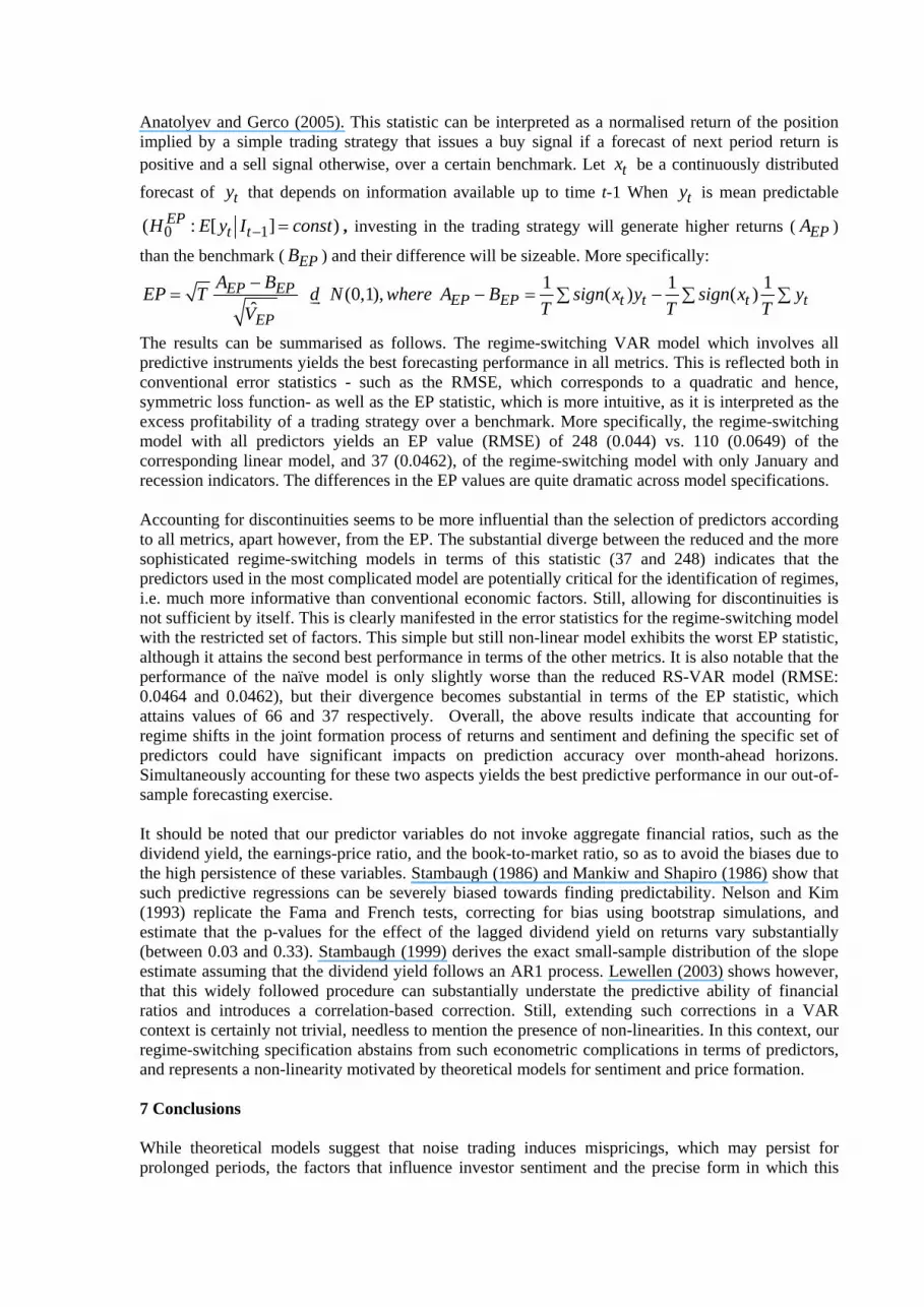
Anatolyev and Gerco (2005). This statistic can be interpreted as a normalised return of the position implied by a simple trading strategy that issues a buy signal if a forecast of next period return is positive and a sell signal otherwise, over a certain benchmark. Let tx be a continuously distributed forecast of ty that depends on information available up to time t-1 When ty is mean predictable

0 1( : [ ] )EPt tH E y I const− = , investing in the trading strategy will generate higher returns ( EPA )

than the benchmark ( EPB ) and their difference will be sizeable. More specifically: 1 1 1(0,1), ( ) ( )

ˆEP EP

EP EP t t t tEP

A BEP T d N where A B sign x y sign x yT T TV

−= − = −∑ ∑ ∑

The results can be summarised as follows. The regime-switching VAR model which involves all predictive instruments yields the best forecasting performance in all metrics. This is reflected both in conventional error statistics - such as the RMSE, which corresponds to a quadratic and hence, symmetric loss function- as well as the EP statistic, which is more intuitive, as it is interpreted as the excess profitability of a trading strategy over a benchmark. More specifically, the regime-switching model with all predictors yields an EP value (RMSE) of 248 (0.044) vs. 110 (0.0649) of the corresponding linear model, and 37 (0.0462), of the regime-switching model with only January and recession indicators. The differences in the EP values are quite dramatic across model specifications. Accounting for discontinuities seems to be more influential than the selection of predictors according to all metrics, apart however, from the EP. The substantial diverge between the reduced and the more sophisticated regime-switching models in terms of this statistic (37 and 248) indicates that the predictors used in the most complicated model are potentially critical for the identification of regimes, i.e. much more informative than conventional economic factors. Still, allowing for discontinuities is not sufficient by itself. This is clearly manifested in the error statistics for the regime-switching model with the restricted set of factors. This simple but still non-linear model exhibits the worst EP statistic, although it attains the second best performance in terms of the other metrics. It is also notable that the performance of the naïve model is only slightly worse than the reduced RS-VAR model (RMSE: 0.0464 and 0.0462), but their divergence becomes substantial in terms of the EP statistic, which attains values of 66 and 37 respectively. Overall, the above results indicate that accounting for regime shifts in the joint formation process of returns and sentiment and defining the specific set of predictors could have significant impacts on prediction accuracy over month-ahead horizons. Simultaneously accounting for these two aspects yields the best predictive performance in our out-of-sample forecasting exercise. It should be noted that our predictor variables do not invoke aggregate financial ratios, such as the dividend yield, the earnings-price ratio, and the book-to-market ratio, so as to avoid the biases due to the high persistence of these variables. Stambaugh (1986) and Mankiw and Shapiro (1986) show that such predictive regressions can be severely biased towards finding predictability. Nelson and Kim (1993) replicate the Fama and French tests, correcting for bias using bootstrap simulations, and estimate that the p-values for the effect of the lagged dividend yield on returns vary substantially (between 0.03 and 0.33). Stambaugh (1999) derives the exact small-sample distribution of the slope estimate assuming that the dividend yield follows an AR1 process. Lewellen (2003) shows however, that this widely followed procedure can substantially understate the predictive ability of financial ratios and introduces a correlation-based correction. Still, extending such corrections in a VAR context is certainly not trivial, needless to mention the presence of non-linearities. In this context, our regime-switching specification abstains from such econometric complications in terms of predictors, and represents a non-linearity motivated by theoretical models for sentiment and price formation. 7 Conclusions While theoretical models suggest that noise trading induces mispricings, which may persist for prolonged periods, the factors that influence investor sentiment and the precise form in which this

impacts on aggregate market returns and volatility remain an open issue. Motivated by diverse empirical findings and theoretical models that imply non-linearities, in this paper, two non-linear hypotheses are tested on the controversial time-series relationship between investor sentiment and market returns: i) an interaction, subject to abrupt regime shifts, and ii) a gradual sentiment effect, which alters the influences of other factors, such as the volatility premium, as a sentiment threshold is exceeded. Both hypotheses are supported by the data (vs. the corresponding linear alternatives) for the SP500 index and institutional (but not individual) sentiment over the period 1965-2003, and after controlling for various risk factors. This adjustment, which tends to be disregarded in previous studies, is critical, as predictable movements in returns may just as well be a result of compensation for risks as a consequence of biases in investors’ expectations. The former hypothesis is tested via a multivariate Markov-switching VAR model, while the latter via a smooth-transition regression model for market returns in which sentiment is defined as a transition variable. The common element in these specifications is that investors’ beliefs and prices are perceived as non-linear processes which exhibit shifts, other instantaneous or more gradual. Such non-linearities can arise for instance due to learning, heterogeneous expectations (e.g. fundamentalists and chartists) or simply, reactions to temporal shocks in the economic or trading environment. A significant inference is that institutional sentiment can be viewed either as an endogenous variable, the determinants and impact of which are subject to discontinuities, for instance at times of extreme negative returns or extreme pessimism, or alternatively, as a transition variable which affects more smoothly and indirectly the price formation process. Instead, individual sentiment exerts no significant impact on SP 500 returns. Some results are summarised as follows. Firstly, an interaction, significant both in statistical and economic terms, exists between returns and institutional sentiment in monthly data, even after controlling for various risk factors. This feedback relationship holds during a dominant market regime, which occurs with probability 80% in the sample. More specifically, institutional sentiment has a positive impact on returns, which indicates that institutions predict correctly on average, or possibly, that they influence the stock index via their own activities (e.g. by contributing to the continuation of an overvaluation or the correction of a previous undervaluation). Their sentiment responds negatively to returns, consistently with a contrarian paradigm previously documented. Interestingly, the reaction of institutional sentiment is “asymmetric” towards positive and negative returns, a finding similar to the implications of prosperity theory, in the sense that institutions become less optimistic as positive returns increase, which indicates a reversal fear, but less pessimistic as negative returns decline, which indicates reversal anticipation. Instead, individual sentiment exerts no significant effect on returns, although it reacts positively to them. Secondly, the formation process of sentiment exhibits dissimilarities across institutional and individual investors, which reflect differences in risk attitudes or level of sophistication. More specifically, both categories are influenced by the other’s sentiment, but they interpret these as opposite signals, contrarian and momentum respectively. The same divergence applies to past volatility, which institutions perceive as a source of optimism while individuals as an indication of pessimism. Interestingly, aggregate idiosyncratic volatility, a proxy for total arbitrage cost, exerts a positive impact on both subsequent returns and institutional sentiment, indicating that institutions correctly predict higher returns as this cost increases (e.g. due to an anticipated correction of a mispricing) or even, that they partially contribute to this pattern via their own trading. The above sensitivities, in addition to the presence of two regimes, imply that institutional sentiment can be perceived as a source of noise trading risk, and potentially induce price distortions, while the impact of individual sentiment is more constrained. Overall, institutions appear likely to contribute to mispricings via their positive effect on returns as well as active arbitrage when this becomes profitable. This interpretation would be consistent with previous findings on institutions exacerbating sentiment-driven mispricing instead of countering the actions of noise traders. Thirdly, as institutional sentiment increases, the compensation for risk implicit in returns (i.e. the pricing of realised volatility) increases as well according to the S-shape pattern. One interpretation is

that as sentiment intensifies, the risk premium contains an additional component: a compensation for noise trading risk, as implied by DeLong et al. (1990), which is reflected instantaneously upon monthly returns. This finding also relates to the cross-sectional results of Baker and Wurgler (2006). The authors find that sentiment is a conditioning variable which alters the otherwise insignificant effects of firm-specific factors on individual stock returns. In an analogous way, we document that at the market level, institutional sentiment alters, in a non-linear way, the sign and magnitude of the volatility effect on aggregate returns. Finally, accounting for regime shifts in the joint formation process of returns and sentiment and defining the specific set of predictors could have significant implications for return prediction over month-ahead horizons. Simultaneously accounting for these two aspects yields the best predictive performance in an out-of-sample forecasting exercise over a ten year period. In addition, this regime-switching specification abstains from econometric complications associated with the use of financial ratios as predictors. Overall, this study verifies that non-linearities in sentiment and price formation indeed arise and may appear in either of two forms: instantaneous regime shifts or relatively more smooth transitions. The representation of these non-linearities appears critical for out-of-sample prediction of returns. It should be emphasised that the sentiment effect on returns, in either of the two forms, proves to be statistically and economically significant only in the case of institutional sentiment, as measured in the Investors Intelligence survey. This effect does not apply to none of the various financial indicators employed, including the closed-end fund discount, IPO issues, dividend premium, mutual fund redemptions, margin borrowing and ratio of specialists’ to total short sales. This finding possibly indicates that these sentiment proxies reflect primarily individual sentiment, which was found in this paper to have no significant impact on SP 500 returns. Alternatively, it may reflect the quality and information content of the survey-based measure of sentiment as opposed to the noisy measures extracted from the markets, consistently with Qiu and Welch (2005). Investigating the implications of the non-linear sentiment effect on asset allocation and detection of speculative bubbles are appealing topics for future research.

References

Ali, A., L-S. Hwang, and M. Trombley, 2003, Arbitrage risk and the book-to-market anomaly, Journal of Financial Economics 69, 355-373. Anatolyev, S., and A., Gerco (2005), A trading approach to testing for predictability, Journal of Business and Economic Statistics 23, 455-461. Ang, A., G. Bekaert , and M.Wei, 2006, Do macro variables, asset markets or surveys forecast inflation better?, NBER Working Paper. Baker, M., and J. Stein, 2004, Market liquidity as a sentiment indicator, Journal of Financial Markets 7, 271-299. Baker, M., and J. Wurgler, 2000, The Equity Share in New issues and Aggregate Stock Returns, Journal of Finance 55, 2219-2257. Baker, M. and J. Wurgler, 2006, Investor sentiment and the cross-section of stock returns, Journal of Finance, 61, 1645–1680. Bali, T., N. Cakici, X. Yan, and Z. Zhang, 2005, Does Idiosyncratic Risk Really Matter? Journal of Finance 60, 905-929. Barber, B.M., and T. Odean, 2005, “All that glitters: The effect of attention and news on the buying behaviour of individual and institutional investors”, Working Paper, University of California, Berkeley. Barberis, N., and M. Huang, 2001, Mental accounting, loss aversion and individual stock returns, Journal of Finance Barberis, N., A. Shleifer, and R. Vishny, 1998, A model of investor sentiment, Journal of Financial Economics 49, 307-343. Barberis, N., and R. Thaler, 2003, A Survey of Behavioural Finance, in: Handbook of the Economics of Finance, edited by G.M. Constantinides, M. Harris and R.Stulz, Elsevier Science B. V. Basu, D., Hung, C-H., Oomen, R. and Stremme, A., 2006, “When to Pick the Losers: Do Sentiment Indicators Improve Dynamic Asset Allocation?” EFA 2006 Zurich Meetings Paper. Benartzi, S., and R. H. Thaler, 1995, Myopic loss aversion and the equity premium puzzle, The Quarterly Journal of Economics 110, 73-92.

Black, A., and D. McMillan, 2004, Non-linear predictability of Value and Growth Stocks and Economic Activity, Journal of Business Finance and Accounting 31, 439-474

Brandt, M. W., Brav, A. and Graham, J. R., 2005, The idiosyncratic volatility puzzle: Time trend or speculative episodes? Working Paper, Duke University. Brandt, M.W., and Q. Kang, 2004, On the relationship between the conditional mean and volatility of stock returns: A latent VAR approach, Journal of Financial Economics 72, 217-257.

Brown, G., and M. Cliff, 2004, Investor sentiment and the near-term stock market, Journal of Empirical Finance 11, 1-27. Brown, G., and M. Cliff, 2005, Investor sentiment and asset valuation, Journal of Business 78, 405-440. Brunnermeier, M., and S. Nagel, 2004, Hedge funds and the technology bubble, Journal of Finance 59, 2013-2040. Campbell, J.Y, 1991, A variance decomposition for stock returns, Economic Journal 101, 157-179. Campbell, J.Y., 1987, Stock Returns and the Term Structure, Journal of Financial Economics 18, 373-399. Campbell, J.Y., and J. Cochrane, 1999, By force of habit. A consumption-based explanation of aggregate stock market behaviour, Journal of Political Economy 107, 205-251. Campbell, J.Y., and A.S. Kyle, 1993, Smart money, noise trading and stock price behaviour, Review of Economic Studies 60, 1-34. Campbell, J., M. Lettau, B. Malkiel, and Y. Xu, 2001, Have Individual Stocks Become More Volatile? An Empirical Exploration of Idiosyncratic Risk, Journal of Finance 56, 1-43. Chakravarty, S., 2001, Stealth-trading: Which traders’ trades move stock prices?, Journal of

Financial Economics 61, 289-307.

Chen, N., R. Kan, and M. Miller, 1993, Are the discounts on closed-end funds a sentiment index?, Journal of Finance, 48, 795-800. Chordia, T., and L. Shivakumar, 2002, Momentum, business cycle and time-varying expected returns, Journal of Finance, 985-1019. Clarke, R., and M. Statman, 1998, Bullish or bearish? Financial Analysts Journal, 63-72. Cutler, D., J. Poterba and L. Summers, 1989, What Moves Stock Prices?, Journal of Portfolio Management 15, 4-12. Daniel, K., M. Grinblatt, S. Titman, and R. Wermers, 1997, Measuring mutual fund performance with characteristic-based benchmarks, Journal of Finance 52, 1035–1058. Daniel, K., D. Hirshleifer, and A. Subrahmanyam, 1998, Investor psychology and security market over- and underreactions, Journal of Finance 53, 1839-1885. Daniel, K., and S. Titman, 1997. Evidence on the characteristics of cross sectional variation in stock returns, Journal of Finance 51, 1-33 De Long, J.B., A. Shleifer, L.H. Summers, and R.J. Waldmann, 1990, Noise trader risk in financial markets, Journal of Political Economy 98, 703-738. Dorn, D., G. Huberman, and P. Sengmueller, 2005, Correlated trading and returns, Working Paper, Drexel University. Doukas, J., and Milonas, N., 2004, Investor sentiment and the closed-end fund puzzle: Out-of-sample evidence, European Financial Management 10, 235-266.

Dumas, B., A. Kurshev and R.Uppal, 2005, What Can Rational Investors Do About Excessive Volatility and Sentiment Fluctuations?, Working Paper, London Business School. Elton, E.J., M. J. Gruber, and J.A. Busse, 1998, Do investors care about sentiment?, Journal of Business 71, 477-500. Fama, E. F. and K. R. French, 1993, Common Risk Factors in the Returns on Stocks and Bonds, Journal of Financial Economics 33, 3-56. French, K., G.W. Schwert, and R.F. Stambaugh, 1987, Expected stock returns and volatility," Journal of Financial Economics 19, 3-30. Fisher, K.L., and M. Statman, 2000, Investor sentiment and stock returns, Financial Analysts Journal 56, 16–23. George, T.J., and C. Hwang, 2004, The 52-week high and momentum investing, Journal of Finance 59, 2145-2176. Gerber, A., T. Hens, and B. Vogt, 2005, Coordination in a repeated stochastic game with imperfect monitoring, Working Paper, University of Zurich. Glosten, L.R., R. Jagannathan, and D. Runkle, 1993, On the relation between the expected value and the volatility of the nominal excess return on stocks, Journal of Finance, 48, 1779-1801. Ghysels, E., P. Santa-Clara, and R.Valkanov, 2005, There is a risk-return trade off after all!, Journal of Financial Economics 76, 509-548. Glushkov, D., 2005, Sentiment beta, Working Paper, University of Texas at Austin. Griffin, J., H. Harris and S. Topaloglu, 2005, The Dynamics of institutional and individual trading,

Journal of Finance 58, 2285-2320.

Guidolin, M., and Timmermann, A. G., 2006, Asset allocation under multivariate regime

switching, Working Paper, Federal Reserve Bank of St. Louis;

Guo, H., and R. Savickas, 2006, Idiosyncratic volatility, stock market volatility, and expected stock returns, Journal of Business and Economic Statistics 24, 43-56. Guo, H., R. Savickas, Z. Wang, and J. Yang, 2005, Is the value premium a proxy for time- varying investment opportunities: Some time series evidence, Working Paper, the Federal Reserve Bank of St. Louis. He, H., and D. Modest, 1995, Market Frictions and Consumption-based Asset Pricing, Journal of Political Economy 103, 94-117. Hirshleifer, D., 2001, Investor psychology and asset pricing, Journal of Finance 56, 1533 1598. Hong, H., and J. Stein. 2002, A unified theory of underraction, momentum trading and overreaction in asset markets, Journal of Finance 54, 2143-2184. Hvidkjaer, S., 2005, Small trades and the cross-section of stock returns, Working Paper, University of Maryland.

Jegadeesh, N., and S. Titman, 1993, Returns to buying winners and selling losers: Implications for stock market efficiency, Journal of Finance 48, 65–91. Jones, C. 2001, A century of stock market liquidity and trading costs, Working Paper, Columbia University. Kaniel, R., G. Saar, and S. Titman, 2004, Individual investor sentiment and stock returns, Working paper, Duke University. Kumar, A., and C.M.C. Lee, 2006, Retail investor sentiment and return comovements, Journal of Finance 61, 2451–2486.

Lakonishok, J., A. Shleifer, and R. Vishny, 1994, Contrarian investment, extrapolation and risk, Journal of Finance 49, 1541-1578. Lamont, O, and J., Stein, 2005, Investor sentiment and corporate finance: Micro and macro, Working Paper, National Bureau of Economic Research Lamont, O. and R. Thaler, 2003. Can the market add and subtract? Mispricing in tech stock carve-outs, Journal of Political Economy Lamoreaux, C.G, and Lastrapes, W.D. (1990) “Persistence in variance, structural change and the GARCH model”, Journal of Business and Economic Statistics 8, 225-234. Lee, C., A. Shleifer, and R. H. Thaler, Investor sentiment and the closed-end fund puzzle, Journal of Finance 46, 75-109. Lettau, M., and S. Ludvigson (2003), Measuring and modelling variation in the risk-return trade-off, Handbook of Financial Econometrics, Elsevier Science B.V. Amsterdam. Lewellen, J., 2003, “Predicting returns with financial ratios,” Journal of Financial Economics 74,

209-235.

Liu, N. and Zhang, L., 2005, The value spread is not a useful predictor of returns, Working Paper, University of Pennsylvania. Lux, T., and M. Marchesi, 1999, Scaling and criticality in a stochastic multi-agent model of a financial market, Nature 397, 498-500. Mankiw, N.G., and M. Shapiro, 1986, Do we reject too often? Small sample properties of tests of rational expectations models, Economic Letters 20, 139-145. McMillan, D.G., 2001, Nonlinear Predictability of stock market returns: Evidence from Parametric and Threshold Models, International Review of Economics and Finance 10, 353-368. Nagel, S., 2005, Short sales, institutional investors, and the book-to-market effect, Journal of

Financial Economics, forthcoming.

Neal, R., with S. Wheatley, 1998, Do measures of investor sentiment predict stock returns, Journal of Financial and Quantitative Analysis 34, 523-547.

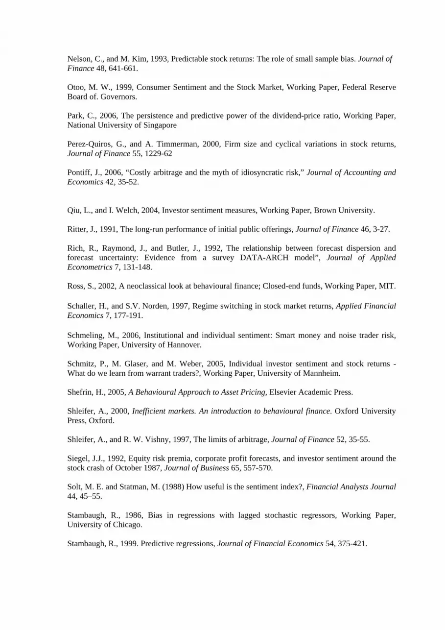
Nelson, C., and M. Kim, 1993, Predictable stock returns: The role of small sample bias. Journal of Finance 48, 641-661. Otoo, M. W., 1999, Consumer Sentiment and the Stock Market, Working Paper, Federal Reserve Board of. Governors. Park, C., 2006, The persistence and predictive power of the dividend-price ratio, Working Paper, National University of Singapore Perez-Quiros, G., and A. Timmerman, 2000, Firm size and cyclical variations in stock returns, Journal of Finance 55, 1229-62 Pontiff, J., 2006, “Costly arbitrage and the myth of idiosyncratic risk,” Journal of Accounting and Economics 42, 35-52. Qiu, L., and I. Welch, 2004, Investor sentiment measures, Working Paper, Brown University. Ritter, J., 1991, The long-run performance of initial public offerings, Journal of Finance 46, 3-27. Rich, R., Raymond, J., and Butler, J., 1992, The relationship between forecast dispersion and forecast uncertainty: Evidence from a survey DATA-ARCH model”, Journal of Applied Econometrics 7, 131-148. Ross, S., 2002, A neoclassical look at behavioural finance; Closed-end funds, Working Paper, MIT.

Schaller, H., and S.V. Norden, 1997, Regime switching in stock market returns, Applied Financial Economics 7, 177-191.

Schmeling, M., 2006, Institutional and individual sentiment: Smart money and noise trader risk, Working Paper, University of Hannover. Schmitz, P., M. Glaser, and M. Weber, 2005, Individual investor sentiment and stock returns - What do we learn from warrant traders?, Working Paper, University of Mannheim. Shefrin, H., 2005, A Behavioural Approach to Asset Pricing, Elsevier Academic Press. Shleifer, A., 2000, Inefficient markets. An introduction to behavioural finance. Oxford University Press, Oxford. Shleifer, A., and R. W. Vishny, 1997, The limits of arbitrage, Journal of Finance 52, 35-55. Siegel, J.J., 1992, Equity risk premia, corporate profit forecasts, and investor sentiment around the stock crash of October 1987, Journal of Business 65, 557-570. Solt, M. E. and Statman, M. (1988) How useful is the sentiment index?, Financial Analysts Journal 44, 45–55. Stambaugh, R., 1986, Bias in regressions with lagged stochastic regressors, Working Paper, University of Chicago. Stambaugh, R., 1999. Predictive regressions, Journal of Financial Economics 54, 375-421.

Swaminathan, B., 1996, Time-varying expected small firm returns and closed-end fund discounts, Review of Financial Studies 9, 845–887.

Teräsvirta, T., and H.M. Anderson, 1992, Characterising nonlinearities in business cycles using Smooth -Transition Autoregressive models, Journal of Applied Econometrics 7, 119-136. Terrasrvita, T., 1994, Specification, estimation and evaluation of Smooth-Transition Autoregressive models, Journal of the American Statistical Association 89, 208-218. Tu, J., 2007, Analyzing regime switching in stock returns: An investment perspective, Working Paper, Singapore Management University. Vuolteenaho, T., 2002, “What Drives Firm-Level Stock Returns?”Journal of Finance 57, 233–264. Wang, Y-H., A. Keswani and S.J. Taylor, 2006, The relationships between sentiment, returns and volatility, International Journal of Forecasting 22, 109-123. Wei, S. and C. Zhang, 2005, Idiosyncratic Volatility Does Not Matter: A Re-Examination of the Relation between Average Returns and Average Volatilities, Journal of Banking and Finance 29, 603-621. Zweig, M. E., 1973, An investor expectations stock price predictive model using closed-end fund premiums, Journal of Finance 28, 67-87.

Table 1 Linear VAR Model Return ΔSentInst ΔSentInd Vol Intercept -0.0059 -3.49 -0.10 0.023*** Return(-1) -0.09 -45.84** 10.40*** -0.03 ΔSentInst(-1) 0.0005*** -0.22*** 0.03*** -0.0001 ΔSentInd(-1) -0.0028 -3.12*** 0.02** 0.0007 Vol(-1) -0.23* -15.15 -5.99** 0.25*** MOM 0.004 15.34 2.54*** -0.039** HMLVol(-1) -0.001 -2.32 0.16 -0.0013 IdVol(-1) 0.0014** 0.32* 0.017 0.0002 ΔSMB(-1) -0.0002 -0.35 0.02 -0.0004 ΔHML(-1) 0.0003 -0.14 -0.025* 0.0001 CS(-1) -0.01 12.3* -0.20 0.002 TS(-1) 0.006 -1.14 0.09 0.002 JAN 0.01 -2.98 -0.92*** 0.003 REC -0.007 -1.46 0.26* 0.011*** SE 0.043 15.80 0.88 0.019

Table 2 Markov-Switching VAR Model

Panel A: Coefficients Regime 1 Return ΔSentInst ΔSentInd Vol Intercept -0.0019*** -6.17** 0.003 0.011*** Return(-1) -0.23*** -70*** 10.47*** -0.06*** ΔSentInst(-1) 0.0005*** -0.09* 0.03*** -0.00003 ΔSentInd(-1) 0.0015 -1.42** -0.05** 0.00036 Vol(-1) 0.56*** 104* -8.34** 0.61*** MOM -0.005 1.24 2.62*** 0.012 HMLVol(-1) -0.009 -2.47 0.31* -0.0004 IdVol(-1) 0.001** 0.28* 0.012 0.00015 ΔSMB(-1) 0.001** 0.21 0.06*** 0.00004 ΔHML(-1) -0.00014 0.047 0.017 -0.00026* CS(-1) 0.03* -8.50 -0.26 -0.002 TS(-1) 0.011** 3.93** -0.03 -0.0016 JAN 0.005 -2.06 -1.10*** 0.005*** REC -0.011** -2.31 0.28* 0.0038*** SE 0.034 13.49 0.87 0.009 Regime 2 Return ΔSentInst ΔSentInd Vol Intercept 0.031 -4.83 0.13 0.006 Return(-1) -0.26** 50 7.94*** -0.11 ΔSentInst(-1) 0.0003 -0.47*** 0.05 0.00008** ΔSentInd(-1) -0.005 -7.31*** 0.08 0.0016 Vol(-1) -0.45** -31 -3.00 -0.07 MOM 0.05 52 1.79 -0.11* HMLVol(-1) -0.0005 -11.32* -0.85 -0.013 IdVol(-1) -0.0017 0.53 0.013 0.003** ΔSMB(-1) -0.001 -0.23 0.042 ** 0.0001 ΔHML(-1) 0.001 0.43 0.056** 0.001 CS(-1) 0.06 -7.34 -0.27* -0.02 TS(-1) -0.014 -6.04 0.44 0.003 JAN 0.007 6.65 -0.02 0.0006 REC -0.058*** -1.94 0.47* 0.01 SE 0.044 14.68 0.72 0.031

Panel B: Transition and Ergodic Regime Probabilities. Ergodic Probabilities Duration Number of Observations Regime 1 0.80 15.09 368 Regime 2 0.20 3.77 94 Transition Probabilities Regime 1 Regime 2 Regime 1 0.93 0.07 Regime 2 0.73 0.26

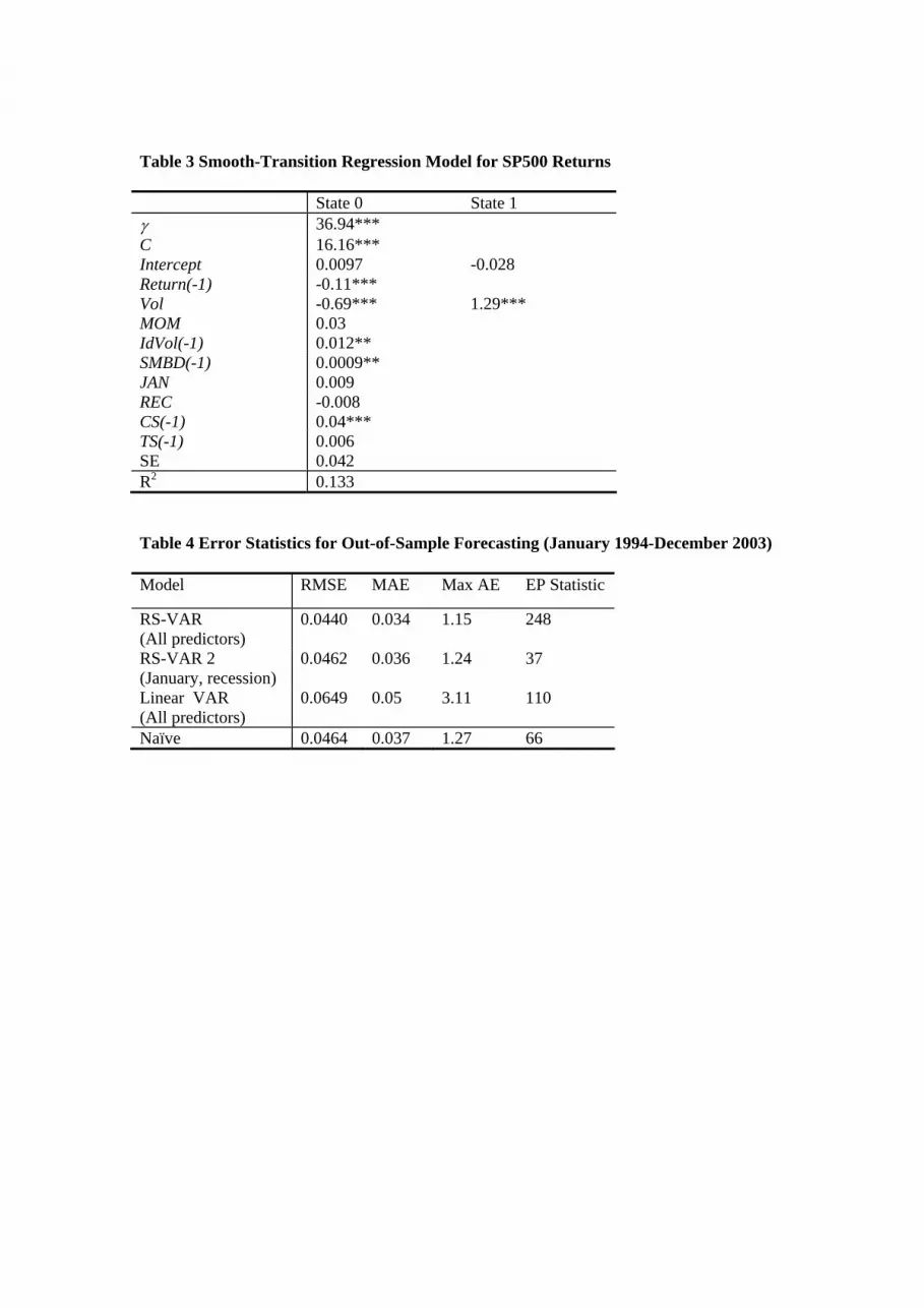
Table 3 Smooth-Transition Regression Model for SP500 Returns State 0 State 1 γ 36.94*** C 16.16*** Intercept 0.0097 -0.028 Return(-1) -0.11*** Vol -0.69*** 1.29*** MOM 0.03 IdVol(-1) 0.012** SMBD(-1) 0.0009** JAN 0.009 REC -0.008 CS(-1) 0.04*** TS(-1) 0.006 SE 0.042 R2 0.133 Table 4 Error Statistics for Out-of-Sample Forecasting (January 1994-December 2003) Model RMSE MAE Max AE EP Statistic

RS-VAR (All predictors)

0.0440 0.034 1.15 248

RS-VAR 2 (January, recession)

0.0462 0.036 1.24 37

Linear VAR (All predictors)

0.0649

0.05 3.11 110

Naïve 0.0464 0.037 1.27 66

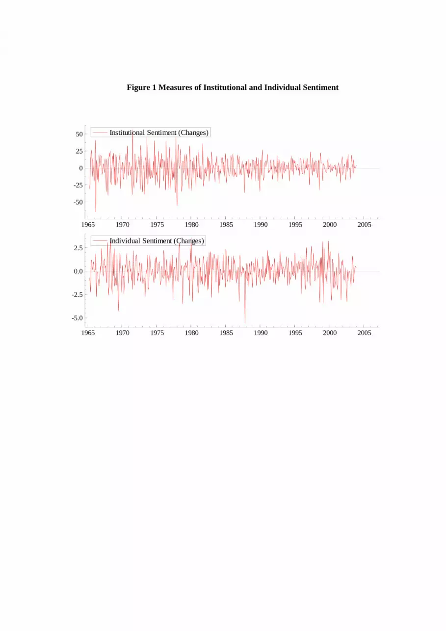
Figure 1 Measures of Institutional and Individual Sentiment

1965 1970 1975 1980 1985 1990 1995 2000 2005

-50

-25

0

25

50 Institutional Sentiment (Changes)

1965 1970 1975 1980 1985 1990 1995 2000 2005

-5.0

-2.5

0.0

2.5Individual Sentiment (Changes)

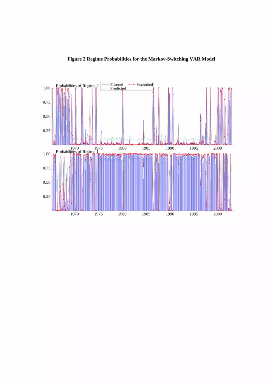
Figure 2 Regime Probabilities for the Markov-Switching VAR Model

1970 1975 1980 1985 1990 1995 2000

0.25

0.50

0.75

1.00 Probabilities of Regime 2 Filtered Predicted

Smoothed

1970 1975 1980 1985 1990 1995 2000

0.25

0.50

0.75

1.00 Probabilities of Regime 1

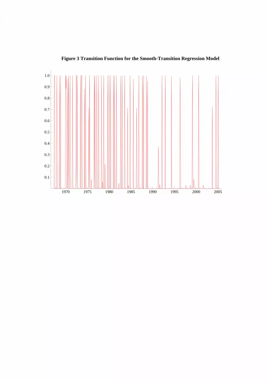
Figure 3 Transition Function for the Smooth-Transition Regression Model

1970 1975 1980 1985 1990 1995 2000 2005

0.1

0.2

0.3

0.4

0.5

0.6

0.7

0.8

0.9

1.0