Semi-Huber potential function for image segmentation

Semi-Huber potential function for imagesegmentation

Osvaldo Gutierrez,∗ Ismael de la Rosa, Jesus Villa,Efren Gonzalez, and Nivia Escalante

Doctorado en Ciencias de la IngenierıaUnidad Academica de Ingenierıa Electrica

Universidad Autonoma de ZacatecasAv. Lopez Velarde 801, Col. Centro, C. P. 98000, Zacatecas, Zacatecas, Mexico

∗osvaldo gtz [email protected]

Abstract: In this work, a novel model of Markov Random Field (MRF)is introduced. Such a model is based on a proposed Semi-Huber potentialfunction and it is applied successfully to image segmentation in presenceof noise. The main difference with respect to other half-quadratic modelsthat have been taken as a reference is, that the number of parameters to betuned in the proposed model is smaller and simpler. The idea is then, tochoose adequate parameter values heuristically for a good segmentation ofthe image. In that sense, some experimental results show that the proposedmodel allows an easier parameter adjustment with reasonable computationtimes.

© 2012 Optical Society of America

OCIS codes: (100.0100) Image processing; (100.2000) Digital image processing.

References and links1. R. C. Gonzalez, R. E. Woods, and S. L. Eddins, Digital Image Processing Using MATLAB, (Prentice Hall, 2004).2. X. Cufı, X. Munoz, J. Freixenet, and J. Martı, “A review on image segmentation thechniques integrating region

and boundary information,” Adv. Imag. Elect. Phys. 120, 1–39 (Elsevier, 2003).3. M. M. Fernandez, “Contribuciones al analisis automatico y semiautomatico de ecografıa fetal tridimensional

mediante campos aleatorios de Markov y contornos activos. Ayudas al diagnostico precoz de malformaciones,”PhD Thesis, Escuela Tecnica Superior de Ingenieros de Telecomunicacion, Universidad de Valladolid, November2001.

4. K. Sauer and C. Bouman, “Bayesian estimation of transmission tomograms using segmentation based optimiza-tion,” IEEE Trans. Nucl. Sci. 39(4), 1144–1152 (1992).

5. C. Bouman and K. Sauer, “A generalized Gaussian image model for edge-preserving MAP estimation,” IEEETrans. Image Process. 2(3), 296–310 (1993).

6. K. Held, E. R. Kops, B. J. Krause, W. M. Wells III, R. Kikinis, and H. W. Muller-Gartner, “Markov random fieldsegmentation of brain MR images,” IEEE Trans. Med. Imaging 16(6), 878–886 (1997).

7. L. Cordero-Grande, P. Casaseca-de-la-Higuera, M. Martın-Fernandez, and C. Alberola-Lopez, “Endocardiumand epicardium contour modeling based on Markov random fields and active contours,” in Proc. of IEEE EMBSAnnu. Int. Conf., 928–931 (2006).

8. Y. Zhang, M. Brady, and S. Smith, “Segmentation of brain MR images through a hidden Markov random fieldmodel and the expectation-maximization algorithm,” IEEE Trans. Med. Imaging 20(1), 45–57 (2001).

9. S. Krishnamachari and R. Chellappa, “Multiresolution Gauss-Markov random field models for texture segmen-tation,” IEEE Trans. Image Process. 6(2), 251–267 (1997).

10. D. A. Clausi and B. Yue, “Comparing cooccurrence probabilities and Markov random fields for texture analysisof SAR sea ice imagery,” IEEE Trans. Geosci. Remote Sens. 42(1), 215–228 (2004).

11. Y. Li and P. Gong, “An efficient texture image segmentation algorithm based on the GMRF model for classifica-tion of remotely sensed imagery,” Int. J. Remote Sens. 26(22), 5149–5159 (2005).

12. S. Geman and C. Geman, “Stochastic relaxation, Gibbs distribution, and the Bayesian restoration of images,”IEEE Trans. Pattern Anal. Mach. Intell. 6, 721–741 (1984).

#155220 - $15.00 USD Received 23 Sep 2011; revised 24 Dec 2011; accepted 27 Feb 2012; published 6 Mar 2012(C) 2012 OSA 12 March 2012 / Vol. 20, No. 6 / OPTICS EXPRESS 6542

13. J. E. Besag, “On the statistical analysis of dirty pictures,” J. Roy. Stat. Soc. B 48, 259–302 (1986).14. S. Z. Li, “MAP image restoration and segmentation by constrained optimization,” IEEE Trans. Image Process.

7(12), 1730–1735 (1998).15. R. Pan and S. J. Reeves, “Efficient Huber-Markov edge-preserving image restoration,” IEEE Trans. Image Pro-

cess. 15(12), 3728–3735 (2006).16. M. Rivera and J. L. Marroquin, “Efficent half-quadratic regularization with granularity control,” Image Vision

Comput. 21, 345–357 (2003).17. M. Rivera, O. Ocegueda, and J. L. Marroquin, “Entropy-controlled quadratic Markov measure field models for

efficient image segmentation,” IEEE Trans. Image Process. 16(12), 3047–3057 (2007).18. M. Mignotte, “A segmentation-based regularization term for image deconvolution,” IEEE Trans. Image Process.

15(7), 1973–1984 (2006).19. H. Deng and D. A. Clausi, “Unsupervised image segmentation using a simple MRF model with a new imple-

mentation scheme,” Pattern Recogn. 37, 2323–2335 (2004).20. O. Lankoande, M. M. Hayat, and B. Santhanam, “Segmentation of SAR images based on Markov random field

model,” in Proc. of IEEE Int. Conf. on Systems, Man, and Cybernetics, 2956–2961 (2005).21. X. Lei, Y. Li, N. Zhao, and Y. Zhang, “Fast segmentation approach for SAR image based on simple Markov

random field,” J. Syst. Eng. Electron. 21(1), 31–36 (2010).22. J. Marroquin, S. Mitter, and t. Poggio, “Probabilistic solution of ill-posed problems in computational vision,” J.

Amer. Statist. Assoc. 82(397), 76–89 (1987).23. R. Szeliski, “Bayesian modeling of uncertainty in low-level vision,” Int. J. Comput. Vision 5(3), 271–301 (1990).24. J. I. de la Rosa, J. J. Villa, and Ma. A. Araiza, “Markovian random fields and comparison between different

convex criteria optimization in image restoration,” in Proc. XVII Int. Conf. on Electronics, Communications andComputers, 9 (CONIELECOMP, 2007).

25. S. Z. Li, Markov Random Field Modeling in Image Analysis (Springer-Verlag, 2009).26. J. E. Besag, “Spatial interaction and the statistical analysis of lattice systems,” J. Roy. Stat. Soc. B 36, 192–236

(1974).27. J. I. de la Rosa and G. Fleury, “Bootstrap methods for a measurement estimation problem,” IEEE Trans. Instrum.

Meas. 55(3), 820–827 (2006).28. M. Nikolova and R. Chan, “The equivalence of half-quadratic minimization and the gradient linearization itera-

tion,” IEEE Trans. Image Process. 16(6), 1623–1627 (2007).29. T. F. Chan, S. Esedoglu, and M. Nikolova, “Algorithms for finding global minimizers of image segmentation and

denoising models,” SIAM J. Appl. Math. 66(5), 1632–1648 (2006).30. M. Nikolova, “Functionals for signal and image reconstruction: properties of their minimizers and applications,”

Research report to obtain the Habilitation a diriger des recherches, Centre de Mathematiques et de Leurs Appli-cations (CMLA), Ecole Normale Superieure de Cachan (2006).

1. Introduction

Segmentation can be considered the first step and essential part in object recognition, scene andimage understanding. Some of its applications comprise industrial quality control, medicine,robot navigation, geophysical exploration, military applications, agriculture, among others. Im-age segmentation is an image processing method that subdivides an image into its constitutiveregions or objects. The level until which this process is carried out depends on the problem to besolved. This means, segmentation stops once the objects of interest in an application have beenisolated. For example, in automated inspection in electronic assemblies is of particular interestto analyze images with the purpose of determining the presence or absence of anomalies suchas missing components or broken paths. In this case, segmentation process is carried out untilthe required level to identify these elements.

On the other hand, digital images are usually affected by some degrading factors as blurringor noise coming from image acquisition systems or during the transmission-reception process,resulting in degraded or distorted images of the real world and, as a consequence, yielding inad-equate segmentation results. A degradation process can be described as a degradation functionH that, together with an additive noise term n, it operates on an input image x and produces adegraded image y:

y = Hx+n. (1)

Given y, some previous knowledge about the degradation function and some knowledge about


the additive noise term, the aim is to obtain an estimation x of the original image x for a goodsegmentation of the regions or objects into it. The more we know about H and n, the closer xwill be to x [1]. The simplest case is when the degradation function H is modeled as a linearfunction, but it could be non linear in many cases and then the problem becomes more complex.In this work it will be assumed that H is the identity operator and we consider only degradationdue to Gaussian noise.

In general, segmentation methods are based on two basic properties of the pixels in relationto their local neighborhood, discontinuity and similarity [2, 3]. Methods based on discontinuityproperty of the pixels are called boundary-based methods, while methods based on similarityproperty are called region-based methods. Unfortunately, these both techniques often fail toproduce accurate segmentation. For example, in boundary-based methods, if an image is noisyor if its region attributes differ by only a small amount between regions, edge detection mayresult in spurious and broken edges. On the other hand, region-based methods always provideclosed contour regions and make use of relatively large neighborhoods in order to obtain suf-ficient information to decide the aggregation of a pixel into a region. This tends to sacrificeresolution and detail in the image, which can result in segmentation errors at the boundaries ofthe regions, and in failure to distinguish regions that would be small in comparison with theblock size used [2].

To overcome these difficulties, the use of Markov random fields (MRF) within a Bayesianframework has become a powerful method and has been used in different works and differentareas such as medicine [4–8], texture modeling [9–11], image segmentation and restoration[12–18] and SAR imagery classification [10], [19–21]. This is because enables posing thisproblem, and many others in image processing, as statistical estimation problems [9] wherethe solution is going to be estimated from the degraded image. Prior distributions of images,which encode contextual constraints [14], can be modeled with MRF. The basic premise is thatneighborhood pixels are expected to have similar characteristics [10]. Because MRF modelsstate global statistics in terms of local neighborhood, all computations are restricted to a localwindow. Typical MRF algorithms visit all sites in the image in a specific order and execute alocal computation at each site; this is repeated until some convergence criterion is reached [9].

Usually, information data (input image) is not enough for an accurate estimation of the orig-inal image, so the regularization of the problem is necessary. This means that a priori infor-mation or assumptions about the structure of x need to be introduced in the estimation process[16]. The a priori knowledge is given in terms of a probability distribution. This distribution,together with a probabilistic description of the noise that corrupts the observations, allows theuse of Bayes theory to compute the posterior distribution which represents the likelihood of asolution x given the observations y [22].

Statistical methods look for the solution that best matches the probabilistic behavior ofthe data. Maximum likelihood (ML) estimation selects the reconstruction which most closelymatches the data available. Maximum a posteriori (MAP) estimation allows the introduction ofa prior distribution that reflects knowledge or beliefs concerning the types of images acceptableas estimates of the original one [4]. There is a wide variety of MRF models; the differencebetween them lies on the choice of a potential function. Each of them characterizes the inter-actions between pixels in the same local group by assigning a larger cost to configurations ofpixels which are less likely to occur. The main idea is to avoid excessive penalties extracted,for instance, by the Gaussian’s quadratic potential function, which tends to blur edges due tothe high cost of abrupt transitions [5].

In this work, we introduce a novel potential function named semi Huber MRF as a pro-posal of a new algorithm for image segmentation. The main advantage of this model lies in thefact that the hyperparameters to be tuned for an adequate result are less than those needed by


other models that were taken as a reference to verify the results of the proposed one. Section2 provides an overview about the Bayesian approach. Section 3 includes a theoretical basis ofMarkov random fields and describes the MAP estimators used in this work as a reference. Adescription of the proposed model and its corresponding MAP estimator is provided in section4. Some results and comments for image segmentation experiments are presented in section 5.Finally, in section 6 some conclusions are given.

2. The Bayesian approach

Problems consisting on finding the solution of the model to restore some or all features of theobjects in an image using assumptions about the real world are called inverse problems. A com-mon approach to solve this kind of problems is the Bayesian modeling. A Bayesian model isa statistical description of an estimation problem that consists of three components. The firstcomponent, the prior model p(x) that is a probabilistic description of the real world or its prop-erties, that we are trying to estimate, before collecting data. The second component, the sensormodel p(y|x), is a description of the behavior of noise or stochastic characteristics that relatethe original state x to the sampled input image or sensor values y. These two components canbe combined to obtain the third component, the posterior model p(x|y), which is a probabilisticdescription of the current estimation of the original scene x, given the observed data y. Themodel is obtained using the Bayes rule:

p(x|y) = p(y|x)p(x)p(y)

, (2)

where p(y) is the density function of y and is constant if the observed image is provided [21].To use Bayesian modeling in image processing, it is necessary to encode somehow the

smoothness inherent in the image. This can be done by describing the correlation between adja-cent pixels of the image in the prior model, and a simple method for modeling such correlationare the Markov random fields [23].

In its usual application [12], Bayesian modeling is used to find the maximum a posteriori(MAP) estimate, that is, the value of x that maximizes the conditional probability p(x|y). It isone of the more efficient and most used estimators [4, 5, 8, 9, 18] defined by:

xMAP = argmaxx∈X

{p(x|y)}= argmax

x∈X{log p(y|x)+ logg(x)}, (3)

where g(x) is a MRF function that models prior information of the phenomena to be estimatedas a probability distribution, X is the set of pixels capable to maximize p(x|y) and p(y|x) is thelikelihood function from y given x [24].

3. Markov random fields and MAP estimators

In this section, some previous concepts about Markov random fields are given. Then we presentand describe some existing MRF models that were taken as a reference in order to evaluate theperformance of our proposal. Finally, the corresponding MAP estimators for each model aredefined.

Let S= {(i, j)|1 ≤ i ≤ m,1 ≤ j ≤ n} be the set of sites of a rectangular lattice for a 2D imageof m×n size. Its elements correspond to the locations where an image is sampled. The sites inS are related to one another via a neighborhood system defined as

N= {Ni|i ∈ S},


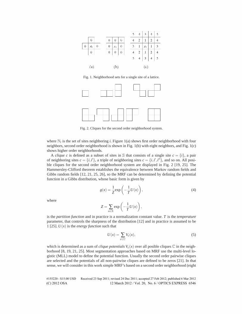
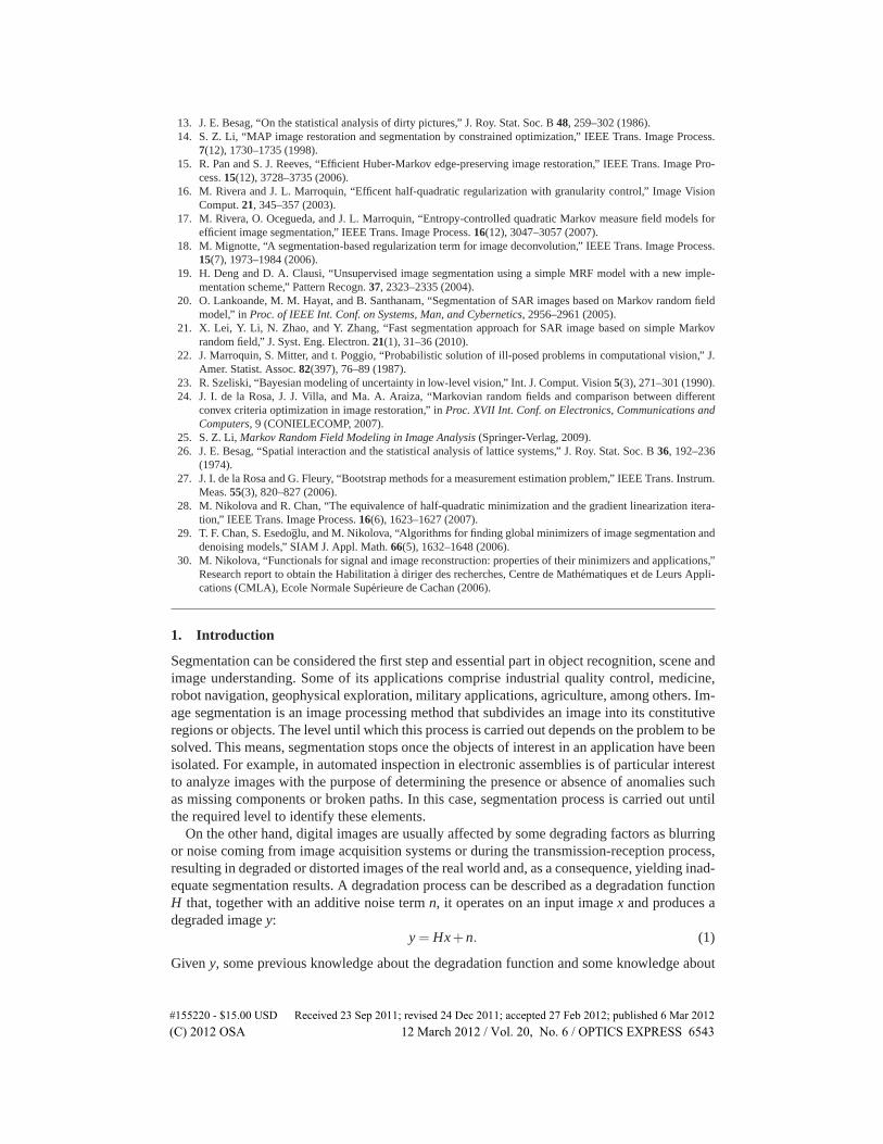
Fig. 1. Neighborhood sets for a single site of a lattice.

Fig. 2. Cliques for the second order neighborhood system.

where Ni is the set of sites neighboring i. Figure 1(a) shows first order neighborhood with fourneighbors, second order neighborhood is shown in Fig. 1(b) with eight neighbors, and Fig. 1(c)shows higher order neighborhoods.

A clique c is defined as a subset of sites in S that consists of a single site c = {i}, a pairof neighboring sites c = {i, i′}, a triple of neighboring sites c = {i, i′, i′′}, and so on. All posi-ble cliques for the second order neighborhood system are displayed in Fig. 2 [19, 25]. TheHammersley-Clifford theorem establishes the equivalence between Markov random fields andGibbs random fields [12, 21, 25, 26], so the MRF can be determined by defining the potentialfunction in a Gibbs distribution, whose basic form is given by

g(x) =1Z

exp

(

− 1T

U(x)

)

, (4)

where

Z = ∑x∈X

exp

(

− 1T

U(x)

)

,

is the partition function and in practice is a normalization constant value. T is the temperatureparameter, that controls the sharpness of the distribution [12] and in practice is assumed to be1 [25]. U(x) is the energy function such that

U(x) = ∑c∈C

Vc(x), (5)

which is determined as a sum of clique potentials Vc(x) over all posible cliques C in the neigh-borhood [8, 19, 21, 25]. Most segmentation approaches based on MRF use the multi-level lo-gistic (MLL) model to define the potential function. Usually the second order pairwise cliquesare selected and the potentials of all non-pairwise cliques are defined to be zeros [21]. In thatsense, we will consider in this work simple MRF’s based on a second order neighborhood (eight


sites) and potential functions of the form ρ(λ (xi − x j)) which act on pairs of sites, where λ isa constant that scales the difference between pixel values.

3.1. Generalized Gaussian MRF (GGMRF)

A common choice for the prior model is a Gaussian Markov random field (GMRF). The dis-tribution for a random field of this kind has the form

g(x) =λ√

2

(2π)N/2|B|1/2 exp(−λ 2xtBx),

where B is a symmetric positive definite matrix, named the precision matrix, λ is a constantand xt is the transpose of x. To make this to correspond to a Gibbs distribution with neighbor-hood system ∂ s, it is imposed the constraint that Bsr = 0 when s is not in ∂ r and s �= r. Thisdistribution may then be rewritten, to form the log likelihood, as

logg(x) =−λ 2

(

∑s∈S

asx2s + ∑

{s,r}∈Cbsr|xs − xr|2

)

,

where as = ∑r∈S Bsr and bsr =−Bsr.The generalization of the GMRF is made by replacing the power 2 by p, where 1 ≤ p ≤ 2

and λ is a parameter inversely proportional to the scale of x [5]. The potential function for aGGMRF is then

logg(x) =−λ p

(

∑s∈S

asxps + ∑

{s,r}∈Cbsr|xs − xr|p

)

+ c, (6)

where as ≥ 0 and bsr > 0, s is the site of interest, r corresponds to the local neighbors and c isa constant term. In practice it is recommended to take as = 0 for Gaussian noise assumption,thus the unicity of the MAP estimator can be assured, resulting in

logg(x) =−λ p

(

∑{s,r}∈C

bsr|xs − xr|p)

+ c. (7)

Here, bsr is a constant that depends on the distance between pixels s and r. The selected valuefor power p is determinant, since it constrains the convergence speed of the local or globalestimator and the quality of the estimated image [24].

3.2. Welsh’s potential function.

The Welsh’s potential function, proposed by Rivera [16] as a hard redescender potential func-tion with granularity control, is defined as

logg(x) =−λ

(

μ ∑{s,r}∈C

bsrϕ1(x)+(1−μ) ∑{s,r}∈C

bsrρ2(x)

)

+ c, (8)

where μ is the granularity control parameter, ϕ1(x) = e2 with e = (xs − xr),

ρ2(x) = 1− 12k

exp(−kϕ1(x)), (9)

and k is a positive scale parameter for edge preservation.


3.3. Tukey’s potential function.

Another hard redescender potential function also proposed by Rivera [16] is the Tukey’s poten-tial function with granularity control, given by

logg(x) =−λ

(

μ ∑{s,r}∈C

bsrϕ1(x)+(1−μ) ∑{s,r}∈C

bsrρ3(x)

)

+ c, (10)

where, in this case

ρ3(x) =

{

1− (

1− (2e/k)2)3, for |e/k|< 1/2,

1, in other case,(11)

k is also a scale parameter and μ provides the granularity control too.

3.4. MAP estimators

With Eq. (3) and the MRF’s previously defined, the corresponding MAP estimators are de-duced. The MAP estimator for a GGMRF [5] is given by

xMAPgg = argminx∈X

{

∑s∈S

|ys − xs|q +σqλ p ∑{s,r}∈C

bsr |xs − xr|p}

, (12)

where the term ∑s∈S |ys−xs|q stands for the term log p(y|x), and the term σqλ p ∑{s,r}∈C bsr|xs−xr|p corresponds to the term logg(x) of Eq. (3). This applies for the other models. The mini-mization problem can be solved from a global or local point of view considering various meth-ods [16, 28, 29, 30]. As global iterative techniques we have the descendent gradient, the conju-gate gradient, the Gauss-Seidel, among others. Local minimization techniques work minimizingat each pixel xs. In this work the Levenberg-Marquardt algorithm was used for local minimiza-tion, because all the parameters included into the potential functions were chosen heuristicallyor according to values proposed in references [24]. Thus, local estimation is implemented withthe expression

xs gg = argminx∈X

{

|ys − xs|q +σqλ p ∑r∈∂ s

bsr|xs − xr|p}

, (13)

where the subset ∂ s stands for the sites in the neighborhood. Estimator performance dependson the chosen values for parameters p and q. For example if p = q = 2, we have the Gaussiancondition for the potential function and the obtained estimator is similar to the least-square onesince the likelihood function is quadratic. Moreover, when p = q = 1, the criterion is absoluteand the estimator converges to the median one; nevertheless, this criterion is not differentiableat zero and it causes instability in the minimization process [24]. The form of the first termin Eq. (12) depends on the type of noise regarded. For all experiments made in this work weassumed that noise has a Gaussian distribution with mean value μn and variance σ2

n . From thisidea, the corresponding value for parameter q was set at 2.

As a second MAP estimator we introduce in the second term of Eq. (3) the Welsh’s potentialfunction [16]

xMAPwel = argminx∈X

{

∑s∈S

|ys − xs|2 +λ

(

μ ∑{s,r}∈C

bsrϕ1(x)+(1−μ) ∑{s,r}∈C

bsrρ2(x)

)}

. (14)

In the same context, local estimation for this model is given by

xs wel = argminx∈X

{

|ys − xs|2 +λ

(

μ ∑r∈∂ s

bsrϕ1(x)+(1−μ) ∑r∈∂ s

bsrρ2(x)

)}

. (15)


Fig. 3. Semi-Huber cost function.

Finally, the last MAP estimator used as a reference, corresponds to the Tukey’s potentialfunction [16], which is given by the expression

xMAPtuk = argminx∈X

{

∑s∈S

|ys − xs|2 +λ

(

μ ∑{s,r}∈C

bsrϕ1(x)+(1−μ) ∑{s,r}∈C

bsrρ3(x)

)}

, (16)

where the local estimation is obtained by

xs tuk = argminx∈X

{

|ys − xs|2 +λ

(

μ ∑r∈∂ s

bsrϕ1(x)+(1−μ) ∑r∈∂ s

bsrρ3(x)

)}

. (17)

4. Semi-Huber proposal

For logg(x) in Eq. (3), we introduce the Huber-like norm or semi-Huber potential function,which has been used in one dimensional robust estimation problems [27] for the case of non-linear regression. This function has been modified for the two dimensional case according tothe following equation:

logg(x) =−λ

(

∑{s,r}∈C

bsrρ1(x)

)

+ c, (18)

where s is the site of interest, r corresponds to the local neighbors, c is a constant term and

ρ1(x) =Δ2

0

2

(√

1+4ϕ1(x)

Δ20

−1

)

. (19)

Here Δ0 > 0 is a constant value and ϕ1(x) = e2 with e = (xs − xr).Semi-Huber potential function is shown in Fig. 3 for Δ0 = 1. Near zero the function is

quadratic and for values beyond ±1, the function is almost linear. This linear region of thefunction allows sharp edges, while convexity makes MAP estimate efficient to compute.

The MAP estimator corresponding to the proposed semi-Hubber potential function, Eq. (18)[24, 27], is given by:

xMAPqh = argminx∈X

{

∑s∈S

|ys − xs|2 +λ ∑{s,r}∈C

bsrρ1(x)

}

. (20)


Fig. 4. Top row: original brain image, brain image corrupted by Gaussian noise and thesegmentation result using the semi-Huber MRF. Bottom row: segmentation result using theGGMRF, segmentation result using the Welsh’s MRF and segmentation result using theTukey’s MRF.

Equation (20) is simplified to obtain:

xs qh = argminx∈X

{

|ys − xs|2 +λ ∑r∈∂ s

bsrρ1(x)

}

, (21)

for local MAP estimation in a single site.

5. Experiments and results

In this section, we present a set of experiments to show the performance of the proposed modelin the segmentation of some images. In all cases, we used the Levenberg-Marquardt algorithmprovided in the optimization toolbox of MATLAB R2009a for the local minimization stage.For this algorithm, we need to introduce the initial value, X0, to start the search of the solution.It was observed that the final result depended on the choice of this value, which adds oneadditional hyperparameter to the segmentation process.

All the tests was executed on a Mac Pro computer with a 2×2.8 GHz Quad-Core Intel Xeonprocessor and 2 GB at 800 MHz DDR2 RAM. The first experiment was carried out with an im-age of the brain, trying to segment in three tissues: gray matter, white matter and cerebrospinalfluid. Figure 4 shows segmentation results of the brain image corrupted by centered Gaussiannoise, n ∼ N(0, Iσ2

n ). In top row from left to right we have the original brain image, brain im-age with noise (σ2

n = 10), and segmentation result using the semi-Huber MRF. In the bottomrow we have the segmentation result using the GGMRF, segmentation result using the Welsh’sMRF and segmentation result using the Tukey’s MRF. Table 1 shows computation times takenby each model, and Table 2 shows the list of hyperparameters to be tuned.

It can be seen that visual result obtained with the proposed model is good enough with respectto those obtained with the others and difference in computation times is not significant. Whatmatters here is the fact that, from the original semi-Huber MRF model, we only had to adjustone hyperparameter value, Δ0 in this case, keeping λ = 1 (two if one takes into account theinitial value in the optimization stage). Therefore, the number of times that it was necessary torun the segmentation process was significantly lower than with other models.


Table 1. Computation times taken by each model of MRF for segmentation of brain image.

Image Model Time (s)

brain slice Semi-Huber 339.1406(187×161) GGMRF 339.0461

Welsh 334.0902Tukey 332.3922

Table 2. List of parameter values for segmentation results in Fig. 4.

Semi-Huber GGMRF Welsh Tukey

Δ0 = 150 σ = 0.3 λ = 10 λ = 10X0 = 80 λ = 40 k = 10 k = 10

p = 1.5 μ = 0.5 μ = 0.5X0 = 80 X0 = 58 X0 = 58

Fig. 5. Top row: original dike image, dike image corrupted by Gaussian noise and thesegmentation result using the semi-Huber MRF. Bottom row: segmentation result using theGGMRF, segmentation result using the Welsh’s MRF and segmentation result using theTukey’s MRF.

A second experiment was made with a geographical image of Paso de las Piedras dam,located in Argentina, taken from Google Earth. In this case, the main interest is on segmentwater from no water in spite of the noise present. Figure 5 shows segmentation results of thedike image. In top row from left to right we have the original dike image, dike image corruptedby Gaussian noise with σ2

n = 20, and segmentation result using the semi-Huber MRF. In thebottom row we have the segmentation result using the GGMRF, segmentation result using theWelsh’s MRF and segmentation result using the Tukey’s MRF. Table 3 shows times taken byeach model and Table 4 shows the list of hyperparameters values by which results presented inFig. 5 were obtained.

Here, it can be seen that with the semi-Huber proposed model, noise reduction looks moresatisfactory than GGMRF model for example, where we can see in the water region, bigger graypoints than the others. Even though the semi-Huber model took the longest time, the relativedifference is negligible.

From a third experiment, we show segmentation results for a geographical image of Villaher-mosa Tabasco city, from the German Spatial Agency, taken by the german satellite TerraSAR-X


Table 3. Computation times taken by each model of MRF for segmentation of dike image.

Image Model Time (s)

dike image Semi-Huber 713.5470(310×208) GGMRF 704.3832

Welsh 704.6216Tukey 697.2369

Table 4. List of parameter values for segmentation results in Fig. 5.

Semi-Huber GGMRF Welsh Tukey

Δ0 = 60 σ = 0.4 λ = 10 λ = 10X0 = 90 λ = 200 k = 10 k = 10

p = 1.4 μ = 0.5 μ = 0.5X0 = 80 X0 = 128 X0 = 128

Fig. 6. Top row: original satellite image of Villahermosa, Tabasco, image corrupted byGaussian noise and the segmentation result using the semi-Huber MRF. Bottom row: seg-mentation result using the GGMRF, segmentation result using the Welsh’s MRF and seg-mentation result using the Tukey’s MRF.

in november 13th 2007. Figure 6 shows in top row from left to right: original image, image cor-rupted by Gaussian noise with σ2

n = 20, and segmentation result using the semi-Huber MRF. Inthe bottom row we have the segmentation result using the GGMRF, segmentation result usingthe Welsh’s MRF and segmentation result using the Tukey’s MRF.

In this case, computation times during the segmentation process for each model had a similarbehavior than in the previous cases. It means, there was not a significant difference betweenthem, being about 575 s on average for a 282×190 image size. Again, we remark the advantagethat using semi-Huber potential function, fewer parameters have to be tuned according to thetype of image, which allows faster segmentation results.

In order to construct a more objective assessment of the results in numeric form, we alsoincluded an experiment performed with a synthetic image of the chessboard type, which wasdegraded with Gaussian noise and then segmented, applying the three models of reference andthe proposed one. Two error measures were considered, from segmented images with respectto the original, namely the mean square error (MSE) and the mean absolute error (MAE).

Figure 7 shows the synthetic image to the left, and to the right, we have the same imagedegraded by Gaussian noise with σ2

n = 20. Figure 8 contains the segmentation results obtained


Fig. 7. Synthetic image, original and degraded by noise.

Fig. 8. Segmentation results of the chessboard synthetic image corresponding to eachmodel.

with each model. From left to right we have the segmentation result using the semi-HuberMRF, segmentation result using the GGMRF, segmentation result using the Welsh’s MRF andsegmentation result using the Tukey’s MRF. Numerical results of the error measures are shownin Table 5, where it can be seen that the proposed model presents another advantage, the smallererror measures.

Table 5. Numerical results of the error measures for the segmentation of the synthetic imagewith each model.

Model MSE MAE

Semi-Huber 0.0416 0.2014GGMRF 0.0514 0.2271

Welsh 0.1476 0.5046Tukey 0.1475 0.5044

6. Conclusion

It was proposed the semi-Huber MRF model to construct a novel algorithm for image segmen-tation. We verified that this proposal has a satisfactory performance. Times in execution weresimilar and visual segmentation results were agree with those obtained from models reportedin other works. In the case of the Generalized Gaussian, Welsh’s and Tukey’s Markov randomfields, several tests had to be made to find adequate parameter values for each kind of image,since one has more degrees of freedom. While, for the semi-Huber MRF we obtained good re-sults with fewer tests because the parameter adjustment is less complicated. On the other hand,the proposed model produced very good results concerning to error measures. Some of the ex-periments presented were made on geographical images because we pretend an application onthe analysis of this kind of images, properly that concerning to hydrographic resources.


Acknowledgments

The authors would like to thank the FOMIX-CONACyT Gobierno del Estado de Zacatecasof Mexico under project number ZAC-2007-CO1-82136 for the invaluable support that madepossible to achieve this research. Osvaldo Gutierrez wants to thank to Instituto TecnologicoSuperior de Fresnillo authorities for all the support provided for the realization of this work,and also the support received from PIFI 2010.


Semi-Huber potential function for image segmentation

Documents

Transcript of Semi-Huber potential function for image segmentation