c o m p u t e r m e t h o d s a n d p r o g r a m s i n b i o m e d i c i n e 8 4 ( 2 0 0 6 ) 124–134

journa l homepage: www. int l .e lsev ierhea l th .com/ journa ls /cmpb

Semi-automated CT segmentation using opticflow and Fourier interpolation techniques

Tzung-Chi Huanga, Geoffrey Zhanga,∗, Thomas Guerrerob,George Starkschall b, Kan-Ping Linc, Ken Forstera

a Department of Radiation Oncology, The University of Texas Southwestern Medical Center,5801 Forest Park Road, Dallas, TX 75390-9183, United Statesb U.T.MD Anderson Cancer Center, Houston, TX, United Statesc Chung-Yuan University, Taipei, Taiwan

a r t i c l e i n f o

Article history:

Received 28 April 2006

Received in revised form

7 September 2006

Accepted 8 September 2006

Keywords:

CT contouring

Deformable image registration

a b s t r a c t

In radiotherapy treatment planning, tumor volumes and anatomical structures are manu-

ally contoured for dose calculation, which takes time for clinicians. This study examines

the use of semi-automated segmentation of CT images. A few high curvature points are

manually drawn on a CT slice. Then Fourier interpolation is used to complete the con-

tour. Consequently, optical flow, a deformable image registration method, is used to map

the original contour to other slices. This technique has been applied successfully to contour

anatomical structures and tumors. The maximum difference between the mapped contours

and manually drawn contours was 6 pixels, which is similar in magnitude to difference one

would see in manually drawn contours by different clinicians. The technique fails when the

Optical flow

Fourier interpolation

region to contour is topologically different between two slices. A solution is recommended

to manually delineate contours on a sparse subset of slices and then map in both directions

to fill the remaining slices.

1. Introduction

The outlining of anatomic structures from computed tomog-raphy (CT) images, as part of the process of radiationtreatment planning has become an issue with the adventof 3D conformal radiotherapy (RT) and intensity modulatedradiotherapy (IMRT). Manual CT image segmentation of bothtumor and normal anatomy has become an essential compo-nent of treatment planning. In both three-dimensional (3D)conformal treatment planning and IMRT treatment planning,anatomic structures need to be visualized in order to assist the

treatment planner in determining beam geometries and treat-ment portals that provide target coverage while minimizingthe irradiation of the normal anatomic structure. Normally,anatomic structures surrounded by tissue of similar density

∗ Corresponding author. Tel.: +1 214 645 7640; fax: +1 214 645 7622.E-mail address: Geoffrey.zhang@utsouthwestern.org (G. Zhang).

0169-2607/$ – see front matter © 2006 Elsevier Ireland Ltd. All rights resdoi:10.1016/j.cmpb.2006.09.003

© 2006 Elsevier Ireland Ltd. All rights reserved.

cannot be visualized on projection radiographs. However,these anatomic structures may be outlined on CT images,because the contrast afforded on CT images better delineatesthe features of the structures. Once segmented on the CTimages anatomic structures are projected onto a digitallyreconstructed radiograph (DRR). The delineated boundariesare also used to formulate dose-volume histograms (DVH), animportant measure by which radiation treatment plans areevaluated.

2. Background

A major problem with outlining anatomic structures on CTimages is that the procedure is done manually and is repet-

erved.

i n b

c o m p u t e r m e t h o d s a n d p r o g r a m s

itive, tedious, and time-consuming. Outlines are drawn on aslice-by-slice basis, and a skilled dosimetrist may spend anhour or longer on each case. Efficient algorithms are neededto automate this task. Although current commercial radiationtreatment planning systems offer auto-contouring optionsand contour interpolation between slices, these tools havesignificant limitations. The auto-contouring algorithms usedare typically based on histogram segmentation, which is alsoreferred to as thresholding of CT voxel values. In one suchalgorithm, the treatment planner selects a pair of thresholdCT voxel values that form boundaries for the CT values thatcomprise the region of interest. A point is found on the bound-ary of the region of interest where the threshold is crossed,and the boundary is traced all the way back to the initial point.This approach works well for anatomic structures that haveCT numbers that are significantly different from the CT num-bers of their surroundings and are completely surroundedby CT numbers outside of the threshold values. Examples ofsuch structures are lungs, bones, and the exterior contourof the patient, although each of these structures may haveregions for which this approach to image segmentation doesnot work well. This approach however does not work well forstructures bordered by tissue of similar density with similarCT numbers. Contour interpolation techniques assume asimilarity between the contours drawn at the bounding endimages and the images between them and make no use ofimage content information. What is needed for the practicalclinical cases is an accurate and robust automatic method ofdelineating soft tissue anatomy on CT images.

3. Design considerations

The purpose of the present paper is to demonstrate proof-of-concept for a semi-automated method of delineating regionsof interest based on the techniques applied in deformableimage registration. The new approach recognizes that theaxial CT images used in radiation treatment planning areacquired at small intervals in the superior–inferior direction,typically 3–5 mm. The patient’s anatomical features do notvary in large amounts over these distances. An anatomicstructure delineated on one axial CT image has a similar rela-tionship with surrounding organs to the same anatomic struc-ture on an adjacent slice. Consequently, a deformable imageregistration matrix can be generated to describe the regis-tration of one axial CT image with the adjacent image. Theelements of this matrix are two-dimensional vectors with rel-atively small magnitudes relating the computed displacementor flow of pixels from one image to the next.

Once this deformation matrix has been determined, thematrix can be applied to a contour of an anatomic structuredelineated on one axial slice to deform the contour to an adja-cent slice. This procedure can be repeated for the entire CTimage data set to generate a complete set of contours for radi-ation treatment planning.

For the original contour, the Fourier interpolation (FI) tech-nique is used to make this task easier and faster. Only a fewcritical points are needed instead of tracing the whole bound-ary of the region of interest.

i o m e d i c i n e 8 4 ( 2 0 0 6 ) 124–134 125

4. System description

4.1. Image data sets

Twelve different patient 3D CT data sets of entire body orpelvis, thoracic region with either 3- or 5-mm slice spacing areused for several segmentation experiments to generate lung,esophagus, heart, kidney, spinal cord, prostate, rectum, blad-der, and gross tumor volumes (GTV).

4.2. Fourier interpolation

FI [1,2] is used in the first contour delineation. Instead of draw-ing the whole contour of a structure of interest on an axial CTslice, the user needs to pick only a few critical points that usu-ally have high curvature along the boundary of the anatomicalstructure. The critical point sampling method gives a bettercontour fit than the equal-space sampling and other samplingmethods. The equal-space sampling method selects pointswith equal intervals in space.

The Cartesian coordinates of the critical points, X(n), Y(n),are changed into complex coordinate a(n),

a(n) = X(n) + jY(n), n = 0, 1, 2, . . . , N − 1, (1)

where n is the sequential number of a point.The complex coordinates a(n) are transferred to frequency

domain by applying discrete Fourier transformation (DFT),

a(n) =N−1∑n=0

A(u) exp{

j2�un

N

}. (2)

where u means the uth spectrum in frequency domain and Nis the total number of points, and

A(u) = 1n

N−1∑n=0

a(n) exp{−j2�un

N

}(3)

is called Fourier descriptor.The zero-padding technique is used to increase the

original N points to M points (M > N) on the frequencyspectrum by adding nil energy points between the Npoints. In the frequency domain, the zero-padding Xd

i[k] is

expressed as

Xdi [k] =

⎧⎪⎪⎨⎪⎪⎩

LXd[k], 0 ≤ k ≤ N − 12

LXd[K − M + N], M − N − 12

≤ k ≤ M − 1

0, otherwise

⎫⎪⎪⎬⎪⎪⎭

(4)

where M = LN, L > 0 is called interpolation factor. M is an integermultiple of N in the current version of the FI program.

Subsequently, the original points and the interpolated

points in the frequency domain are transferred back to theCartesian system using the inverse discrete Fourier trans-formation. The Cartesian resulting points then define thecontour.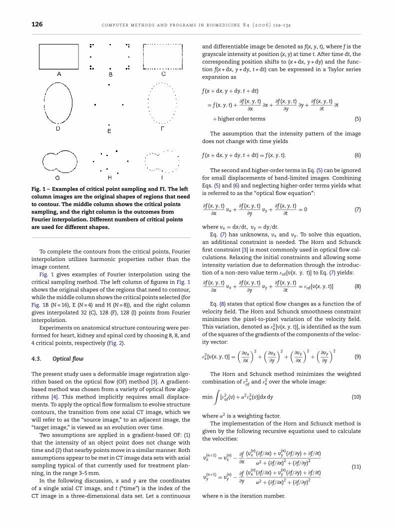

126 c o m p u t e r m e t h o d s a n d p r o g r a m s i n

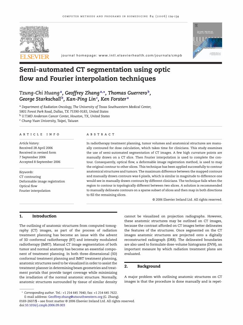
Fig. 1 – Examples of critical point sampling and FI. The leftcolumn images are the original shapes of regions that needto contour. The middle column shows the critical pointssampling, and the right column is the outcomes from

(11)

Fourier interpolation. Different numbers of critical pointsare used for different shapes.

To complete the contours from the critical points, Fourierinterpolation utilizes harmonic properties rather than theimage content.

Fig. 1 gives examples of Fourier interpolation using thecritical sampling method. The left column of figures in Fig. 1shows the original shapes of the regions that need to contour,while the middle column shows the critical points selected (forFig. 1B (N = 16), E (N = 4) and H (N = 8)), and the right columngives interpolated 32 (C), 128 (F), 128 (I) points from Fourierinterpolation.

Experiments on anatomical structure contouring were per-formed for heart, kidney and spinal cord by choosing 8, 8, and4 critical points, respectively (Fig. 2).

4.3. Optical flow

The present study uses a deformable image registration algo-rithm based on the optical flow (OF) method [3]. A gradient-based method was chosen from a variety of optical flow algo-rithms [4]. This method implicitly requires small displace-ments. To apply the optical flow formalism to evolve structurecontours, the transition from one axial CT image, which wewill refer to as the “source image,” to an adjacent image, the“target image,” is viewed as an evolution over time.

Two assumptions are applied in a gradient-based OF: (1)that the intensity of an object point does not change withtime and (2) that nearby points move in a similar manner. Bothassumptions appear to be met in CT image data sets with axialsampling typical of that currently used for treatment plan-

ning, in the range 3–5 mm.

In the following discussion, x and y are the coordinatesof a single axial CT image, and t (“time”) is the index of theCT image in a three-dimensional data set. Let a continuous

b i o m e d i c i n e 8 4 ( 2 0 0 6 ) 124–134

and differentiable image be denoted as f(x, y, t), where f is thegrayscale intensity at position (x, y) at time t. After time dt, thecorresponding position shifts to (x + dx, y + dy) and the func-tion f(x + dx, y + dy, t + dt) can be expressed in a Taylor seriesexpansion as

f (x + dx, y + dy, t + dt)

= f (x, y, t) + ∂f (x, y, t)∂x

∂x + ∂f (x, y, t)∂y

∂y + ∂f (x, y, t)∂t

∂t

+ higher order terms (5)

The assumption that the intensity pattern of the imagedoes not change with time yields

f (x + dx, y + dy, t + dt) = f (x, y, t). (6)

The second and higher-order terms in Eq. (5) can be ignoredfor small displacements of band-limited images. CombiningEqs. (5) and (6) and neglecting higher-order terms yields whatis referred to as the “optical flow equation”:

∂f (x, y, t)∂x

vx + ∂f (x, y, t)∂y

vy + ∂f (x, y, t)∂t

= 0 (7)

where vx = dx/dt, vy = dy/dt.

Eq. (7) has unknowns, vx and vy. To solve this equation,an additional constraint is needed. The Horn and Schunckfirst constraint [3] is most commonly used in optical flow cal-culations. Relaxing the initial constraints and allowing someintensity variation due to deformation through the introduc-tion of a non-zero value term εof[v(x, y, t)] to Eq. (7) yields:

∂f (x, y, t)∂x

vx + ∂f (x, y, t)∂y

vy + ∂f (x, y, t)∂t

= εof[v(x, y, t)] (8)

Eq. (8) states that optical flow changes as a function the ofvelocity field. The Horn and Schunck smoothness constraintminimizes the pixel-to-pixel variation of the velocity field.This variation, denoted as ε2

s[v(x, y, t)], is identified as the sumof the squares of the gradients of the components of the veloc-ity vector:

ε2s[v(x, y, t)] =

(∂vx

∂x

)2+

(∂vx

∂y

)2+

(∂vy

∂x

)2

+(

∂vy

∂y

)2

(9)

The Horn and Schunck method minimizes the weightedcombination of ε2

of and ε2s over the whole image:

min

∫[ε2

of(v) + ˛2ε2s(v)]dx dy (10)

where ˛2 is a weighting factor.The implementation of the Horn and Schunck method is

given by the following recursive equations used to calculatethe velocities:

v(n+1)x = v

(n)x − ∂f

∂x

(v(n)x (∂f/∂x) + v

(n)y (∂f/∂y) + ∂f/∂t)

˛2 + (∂f/∂x)2 + (∂f/∂y)2

v(n+1)y = v

(n)y − ∂f

∂y

(v(n)x (∂f/∂x) + v

(n)y (∂f/∂y) + ∂f/∂t)

˛2 + (∂f/∂x)2 + (∂f/∂y)2

where n is the iteration number.

c o m p u t e r m e t h o d s a n d p r o g r a m s i n b i o m e d i c i n e 8 4 ( 2 0 0 6 ) 124–134 127

Fig. 2 – Examples of the use of the FI for contours of various anatomical structures: the left column is an example of theapplication for heart contouring, while the middle for spinal cord and the right for kidney. Contrast has been enhanced inimages (E) and (F) to permit visualization of the edges of the organ of interest.

tTse

4

Atmvcaaagomtctecg

The optical flow software was originally designed to regis-er two-dimensional (2D) images acquired at different times.his study extends the concept of time frames to neighboringlices of three-dimensional (3D) CT image data sets to allowlastic registration between adjacent slices.

.4. Image registration and contour mapping

n original contour was delineated by selecting some ini-ial critical points and employing the Fourier interpolation

ethod. Next, the images from adjacent slices in each imageolume were registered utilizing the 2D optical flow softwarereating a pixel-by-pixel displacement vector field for eachdjacent image. The registration requires a source image andtarget image with the same numbers of pixels in both the x

nd y directions. As the source image was registered to the tar-et image, a pixel-by-pixel velocity matrix was created basedn the registration between two adjacent slices. This velocityatrix was used to deform the contour of the anatomic struc-

ure of interest on the source image to the target image. Theontour points were re-sampled to provide equal spacing of

he points around the contour set at one point per three pix-ls. Fig. 3 illustrates the flow diagram required to transformontour points from a source 2D CT image to the adjacent tar-et image.

The deformed contour was then used as the source con-tour for the next round of registration to the next adjacentimage, which became the new target image. This procedurewas repeated for as many slices as long as no topological lim-itations were reached.

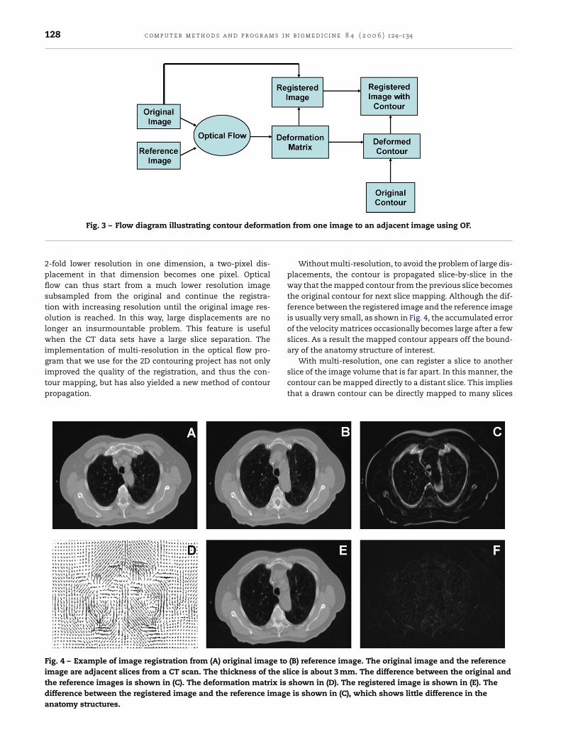
Fig. 4 demonstrates an example of OF image registration,where (A) was the source image, (B) target image, (C) givesthe difference between the source and the target images, (D)displays a velocity matrix from the source image to the target,(E) was the deformed image applied by velocity matrix and (F)shows the difference between estimated image and the targetimage.

4.5. Multi-resolution

Originally, one limitation of the optical flow method was thatlarge variations in images on adjacent slices would cause prob-lems in the deformable image registration. As a consequence,the separation of the CT slices used in the registration couldnot be too large. For the thoracic CT image data sets with astandard slice separation of 3 mm, slice-by-slice registration

usually does not encounter problems of large image changesbetween adjacent slices.

However, multi-resolution is the solution to larger dis-placement problems. If the image size is subsampled to a

128 c o m p u t e r m e t h o d s a n d p r o g r a m s i n b i o m e d i c i n e 8 4 ( 2 0 0 6 ) 124–134

ation

Fig. 3 – Flow diagram illustrating contour deform

2-fold lower resolution in one dimension, a two-pixel dis-placement in that dimension becomes one pixel. Opticalflow can thus start from a much lower resolution imagesubsampled from the original and continue the registra-tion with increasing resolution until the original image res-olution is reached. In this way, large displacements are nolonger an insurmountable problem. This feature is usefulwhen the CT data sets have a large slice separation. Theimplementation of multi-resolution in the optical flow pro-

gram that we use for the 2D contouring project has not onlyimproved the quality of the registration, and thus the con-tour mapping, but has also yielded a new method of contourpropagation.

Fig. 4 – Example of image registration from (A) original image toimage are adjacent slices from a CT scan. The thickness of the slthe reference images is shown in (C). The deformation matrix isdifference between the registered image and the reference imageanatomy structures.

from one image to an adjacent image using OF.

Without multi-resolution, to avoid the problem of large dis-placements, the contour is propagated slice-by-slice in theway that the mapped contour from the previous slice becomesthe original contour for next slice mapping. Although the dif-ference between the registered image and the reference imageis usually very small, as shown in Fig. 4, the accumulated errorof the velocity matrices occasionally becomes large after a fewslices. As a result the mapped contour appears off the bound-ary of the anatomy structure of interest.

With multi-resolution, one can register a slice to anotherslice of the image volume that is far apart. In this manner, thecontour can be mapped directly to a distant slice. This impliesthat a drawn contour can be directly mapped to many slices

(B) reference image. The original image and the referenceice is about 3 mm. The difference between the original andshown in (D). The registered image is shown in (E). Theis shown in (C), which shows little difference in the

c o m p u t e r m e t h o d s a n d p r o g r a m s i n b i o m e d i c i n e 8 4 ( 2 0 0 6 ) 124–134 129

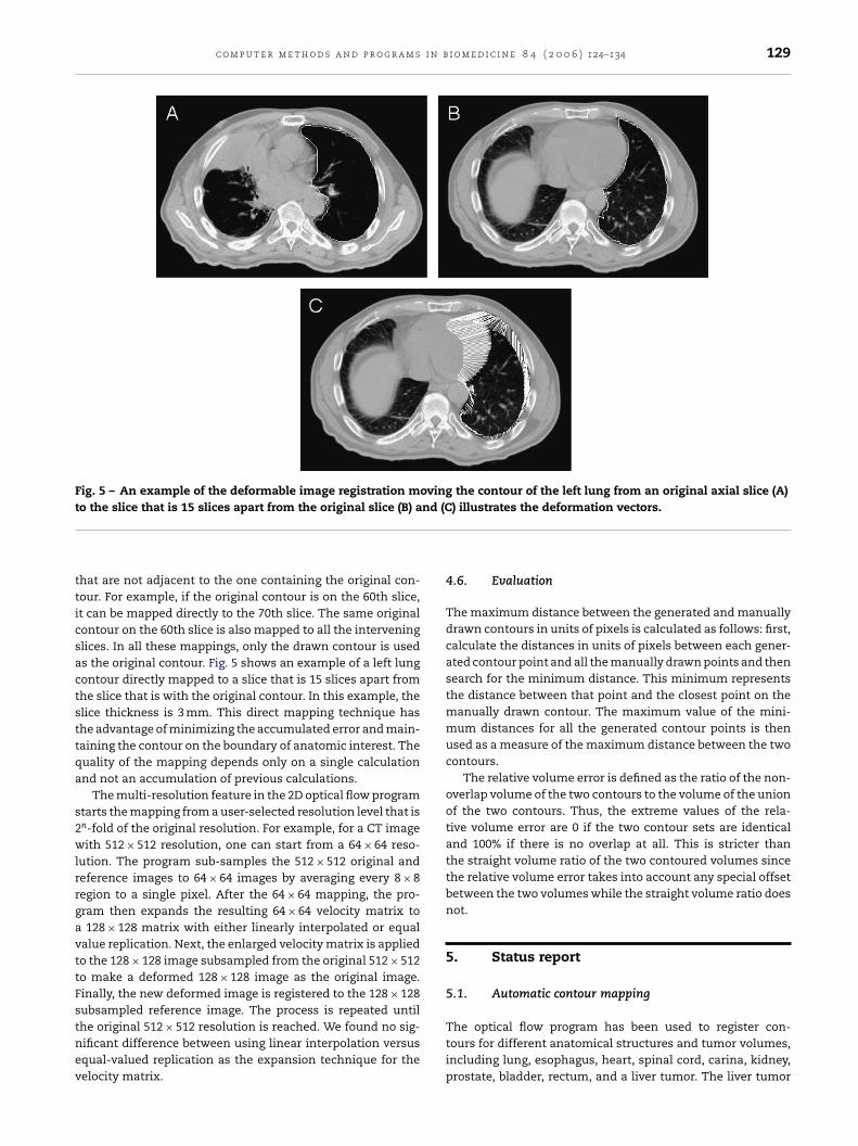
Fig. 5 – An example of the deformable image registration moving the contour of the left lung from an original axial slice (A)t nd (C

tticsactsttqa

s2wlrrgavttFstnev

o the slice that is 15 slices apart from the original slice (B) a

hat are not adjacent to the one containing the original con-our. For example, if the original contour is on the 60th slice,t can be mapped directly to the 70th slice. The same originalontour on the 60th slice is also mapped to all the interveninglices. In all these mappings, only the drawn contour is useds the original contour. Fig. 5 shows an example of a left lungontour directly mapped to a slice that is 15 slices apart fromhe slice that is with the original contour. In this example, thelice thickness is 3 mm. This direct mapping technique hashe advantage of minimizing the accumulated error and main-aining the contour on the boundary of anatomic interest. Theuality of the mapping depends only on a single calculationnd not an accumulation of previous calculations.

The multi-resolution feature in the 2D optical flow programtarts the mapping from a user-selected resolution level that isn-fold of the original resolution. For example, for a CT imageith 512 × 512 resolution, one can start from a 64 × 64 reso-

ution. The program sub-samples the 512 × 512 original andeference images to 64 × 64 images by averaging every 8 × 8egion to a single pixel. After the 64 × 64 mapping, the pro-ram then expands the resulting 64 × 64 velocity matrix to128 × 128 matrix with either linearly interpolated or equal

alue replication. Next, the enlarged velocity matrix is appliedo the 128 × 128 image subsampled from the original 512 × 512o make a deformed 128 × 128 image as the original image.inally, the new deformed image is registered to the 128 × 128ubsampled reference image. The process is repeated until

he original 512 × 512 resolution is reached. We found no sig-ificant difference between using linear interpolation versusqual-valued replication as the expansion technique for theelocity matrix.

) illustrates the deformation vectors.

4.6. Evaluation

The maximum distance between the generated and manuallydrawn contours in units of pixels is calculated as follows: first,calculate the distances in units of pixels between each gener-ated contour point and all the manually drawn points and thensearch for the minimum distance. This minimum representsthe distance between that point and the closest point on themanually drawn contour. The maximum value of the mini-mum distances for all the generated contour points is thenused as a measure of the maximum distance between the twocontours.

The relative volume error is defined as the ratio of the non-overlap volume of the two contours to the volume of the unionof the two contours. Thus, the extreme values of the rela-tive volume error are 0 if the two contour sets are identicaland 100% if there is no overlap at all. This is stricter thanthe straight volume ratio of the two contoured volumes sincethe relative volume error takes into account any special offsetbetween the two volumes while the straight volume ratio doesnot.

5. Status report

5.1. Automatic contour mapping

The optical flow program has been used to register con-tours for different anatomical structures and tumor volumes,including lung, esophagus, heart, spinal cord, carina, kidney,prostate, bladder, rectum, and a liver tumor. The liver tumor

130 c o m p u t e r m e t h o d s a n d p r o g r a m s i n b i o m e d i c i n e 8 4 ( 2 0 0 6 ) 124–134

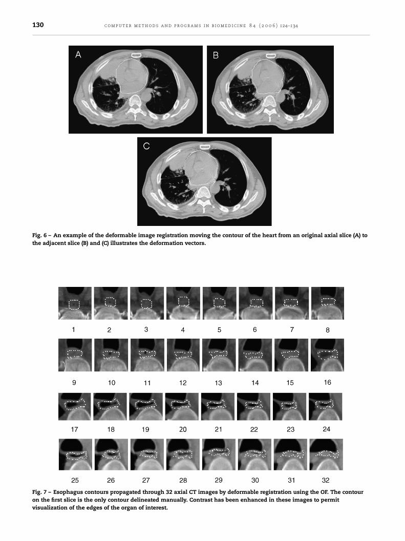
Fig. 6 – An example of the deformable image registration moving the contour of the heart from an original axial slice (A) tothe adjacent slice (B) and (C) illustrates the deformation vectors.

Fig. 7 – Esophagus contours propagated through 32 axial CT images by deformable registration using the OF. The contouron the first slice is the only contour delineated manually. Contrast has been enhanced in these images to permitvisualization of the edges of the organ of interest.

i n b

wttofidrciFcl

pCofi

Fgpo

c o m p u t e r m e t h o d s a n d p r o g r a m s

as chosen because of its difficulty for other automatic con-ouring methods due to the low density contrast between theumor and the normal liver tissue. Fig. 5 displays an examplef the contour mapping using deformable image registrationor the left lung from an original axial slice (A) to the slice thats 15 slices apart from the original (B), and (C) illustrates theeformation vectors. Fig. 6 shows an example of heart contouregistration on a patient’s CT data set. Qualitative review of theontour in Fig. 6B indicates a good fit of the contour to the CTmage of the heart. It is noticeable that the contour change inig. 6 is much smaller than that in Fig. 5. In Fig. 6, the heartontour is mapped to an adjacent CT slice while in Fig. 5 theeft lung contour is mapped to a slice that is 15 slices apart.

Fig. 7 illustrates a set of esophagus images with contours

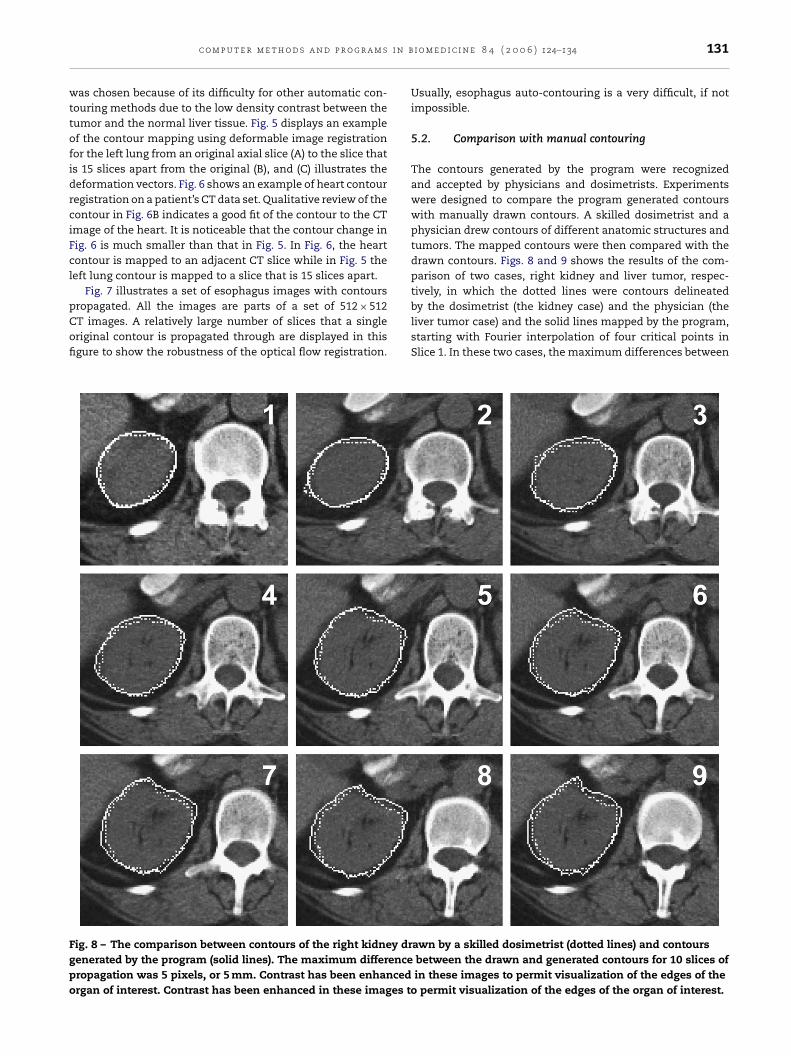
ropagated. All the images are parts of a set of 512 × 512T images. A relatively large number of slices that a singleriginal contour is propagated through are displayed in thisgure to show the robustness of the optical flow registration.

ig. 8 – The comparison between contours of the right kidney drenerated by the program (solid lines). The maximum differenceropagation was 5 pixels, or 5 mm. Contrast has been enhancedrgan of interest. Contrast has been enhanced in these images to

i o m e d i c i n e 8 4 ( 2 0 0 6 ) 124–134 131

Usually, esophagus auto-contouring is a very difficult, if notimpossible.

5.2. Comparison with manual contouring

The contours generated by the program were recognizedand accepted by physicians and dosimetrists. Experimentswere designed to compare the program generated contourswith manually drawn contours. A skilled dosimetrist and aphysician drew contours of different anatomic structures andtumors. The mapped contours were then compared with thedrawn contours. Figs. 8 and 9 shows the results of the com-parison of two cases, right kidney and liver tumor, respec-tively, in which the dotted lines were contours delineated

by the dosimetrist (the kidney case) and the physician (theliver tumor case) and the solid lines mapped by the program,starting with Fourier interpolation of four critical points inSlice 1. In these two cases, the maximum differences between

awn by a skilled dosimetrist (dotted lines) and contoursbetween the drawn and generated contours for 10 slices ofin these images to permit visualization of the edges of thepermit visualization of the edges of the organ of interest.

132 c o m p u t e r m e t h o d s a n d p r o g r a m s i n b i o m e d i c i n e 8 4 ( 2 0 0 6 ) 124–134

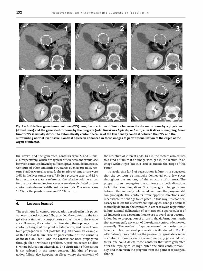
Fig. 9 – In this liver gross tumor volume (GTV) case, the maximum difference between the drawn contours by a physician(dotted lines) and the generated contours by the program (solid lines) was 6 pixels, or 6 mm, after 6 slices of mapping. Livertumor GTV is usually difficult to automatically contour because of the low density contrast between the GTV and thesurrounding normal liver tissue. Contrast has been enhanced in these images to permit visualization of the edges of the

organ of interest.

the drawn and the generated contours were 5 and 6 pix-els, respectively, which are typical differences one would seebetween contours drawn by different physicians/dosimetrists.Contours of other anatomic structures, such as prostate, rec-tum, bladder, were also tested. The relative volume errors were2.6% in the liver tumor case, 7.5% in a prostate case, and 8.5%in a rectum case. As a reference, the relative volume errorsfor the prostate and rectum cases were also calculated on twocontour sets drawn by different dosimetrists. The errors were18.6% for the prostate case and 16.1% rectum.

6. Lessons learned

The technique for contour propagation described in this paperappears to work successfully, provided the contour in the tar-get slice is similar in compositions as the image in the sourceslice. However, if a contour is bifurcated, the topology of thecontour changes at the point of bifurcation, and correct con-tour propagation is not possible. Fig. 10 shows an exampleof this kind of failure. The original contour of the carina isdelineated on Slice 1, and the contour has been propagated

through Slice 4 without a problem. A problem occurs at Slice5, where bifurcation takes place. The bifurcation of the carinais not reflected in the target contour. This kind of propa-gation failure also happens on slices where the anatomy of

the structure of interest ends. Gas in the rectum also causesthis kind of failure if an image with gas in the rectum to animage without gas, but this issue is outside the scope of thispaper.

To avoid this kind of registration failure, it is suggestedthat the contours be manually delineated on a few slicesthroughout the anatomy of the structure of interest. Theprogram then propagates the contours on both directionsto fill the remaining slices. If a topological change occursbetween the manually delineated contours, the program stillcan propagate the contours from opposite directions andmeet where the change takes place. In this way, it is not nec-essary to select the slices where topological changes occur tomanually delineate the contours in order to avoid registrationfailure. Manual delineation of contours on a sparse subset ofCT images is also a good method to use to avoid error accumu-lation due to propagation of errors in the deformation matrixthat may magnify any error of the original contours delineatedmanually. The method of sparse manual contouring com-bined with bi-directional propagation is illustrated in Fig. 11.Alternatively, one could use the program to generate a seriesof contours. Upon review of the automatically generated con-

tours, one could delete those contours that were generatedafter the topological change, enter one such contour manu-ally, and then rerun the program from the point of topologicalchange.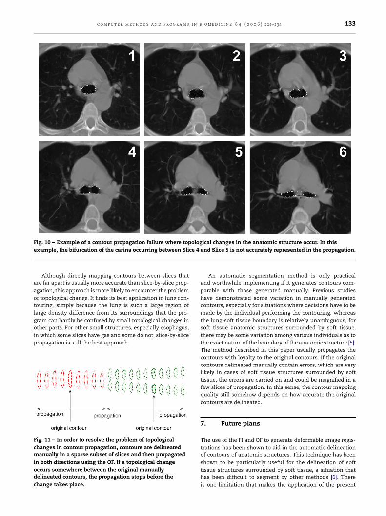

c o m p u t e r m e t h o d s a n d p r o g r a m s i n b i o m e d i c i n e 8 4 ( 2 0 0 6 ) 124–134 133

Fig. 10 – Example of a contour propagation failure where topological changes in the anatomic structure occur. In thise ce 4

aaotlgoip

Fcmiodc

xample, the bifurcation of the carina occurring between Sli

Although directly mapping contours between slices thatre far apart is usually more accurate than slice-by-slice prop-gation, this approach is more likely to encounter the problemf topological change. It finds its best application in lung con-ouring, simply because the lung is such a large region ofarge density difference from its surroundings that the pro-ram can hardly be confused by small topological changes in

ther parts. For other small structures, especially esophagus,

n which some slices have gas and some do not, slice-by-sliceropagation is still the best approach.

ig. 11 – In order to resolve the problem of topologicalhanges in contour propagation, contours are delineatedanually in a sparse subset of slices and then propagated

n both directions using the OF. If a topological changeccurs somewhere between the original manuallyelineated contours, the propagation stops before thehange takes place.

and Slice 5 is not accurately represented in the propagation.

An automatic segmentation method is only practicaland worthwhile implementing if it generates contours com-parable with those generated manually. Previous studieshave demonstrated some variation in manually generatedcontours, especially for situations where decisions have to bemade by the individual performing the contouring. Whereasthe lung-soft tissue boundary is relatively unambiguous, forsoft tissue anatomic structures surrounded by soft tissue,there may be some variation among various individuals as tothe exact nature of the boundary of the anatomic structure [5].The method described in this paper usually propagates thecontours with loyalty to the original contours. If the originalcontours delineated manually contain errors, which are verylikely in cases of soft tissue structures surrounded by softtissue, the errors are carried on and could be magnified in afew slices of propagation. In this sense, the contour mappingquality still somehow depends on how accurate the originalcontours are delineated.

7. Future plans

The use of the FI and OF to generate deformable image regis-trations has been shown to aid in the automatic delineationof contours of anatomic structures. This technique has been

shown to be particularly useful for the delineation of softtissue structures surrounded by soft tissue, a situation thathas been difficult to segment by other methods [6]. Thereis one limitation that makes the application of the present

s i n

r

[

[

[

[

[

structures, J. Appl. Clin. Med. Phys. 4 (2003) 17–24.[6] S.S.C. Burnett, G. Starkschall, C.W. Stevens, Z. Liao, A

134 c o m p u t e r m e t h o d s a n d p r o g r a m

method difficult to be completely automatic: contours mustbe topologically similar to each other for accurate progressionfrom CT slice to CT slice. Currently the solution to bifurcatedcontours is to map in both directions. To eliminate thisproblem and make this technique completely automatic, anew version of the software that can handle such topologicalchange between slices is in the future plan.

e f e r e n c e s

1] P.-C. Wang, Fourier descriptor analysis and medical imageapplication, Thesis, CYCU, Taipei, 1999.

b i o m e d i c i n e 8 4 ( 2 0 0 6 ) 124–134

2] C. Zahn, R. Roskies, Fourier descriptors for plane closedcurves, IEEE Trans. Comput. 21 (3) (1972) 269–281.

3] B.K.P. Horn, B.G. Schunck, Determining optical flow, Artif.Intell. Med. 17 (1981) 185–203.

4] S.S. Beauchemin, J.L. Barron, The computation of optical flow,ACM Comput. Surv. 27 (1995) 433–466.

5] D.C. Collier, S.S. Burnett, M. Amin, et al., Assessment ofconsistency in contouring of normal-tissue anatomic

deformable-model approach to semi-automatic segmentationof CT images demonstrated by application to the spinal canal,Med. Phys. 31 (2004) 251–263.