
Selective Darkening Filter and Welding Arc Observation for ...
153
Doctoral Thesis Selective Darkening Filter and Welding Arc Observation for the Manual Welding Process Bernd Hillers University Bremen
-
Upload
khangminh22 -
Category
Documents
-
view
1 -
download
0
Transcript of Selective Darkening Filter and Welding Arc Observation for ...

Doctoral Thesis
Selective Darkening Filterand Welding Arc Observation
for the Manual Welding Process
Bernd HillersUniversity Bremen

doctoral thesis
Selective Darkening Filter and Welding ArcObservation for the Manual Welding Process
Bernd Hillers
15th March 2012
1. Gutachter: Prof. Dr.-Ing. Axel Graser2. Gutachter: Prof. Dr.-Ing. Kai Michels


Zusammenfassung
Der Schutz des Schweißers wahrend des Schweißens stellt die Grundmotivation dieser Arbeitdar. Die heutzutage verfugbaren, automatisch abdunkelnden Schweißfilter (Automatic Dar-kening Filter (ADF)) verbessern die Sicht des Schweißers, indem diese vor dem Zunden desLichtbogen und wahrend des Schweißen die Lichtdurchlassigkeit dynamisch anpassen. Ermo-glicht wird dies durch Flussigkristalldisplays (LCDs), bestehend aus einem einzigen Pixel zurAbdunkelung der Sicht. Die ADFs sind verbesserungsfahig, indem die Sicht des Nutzers nurdort abgedunkelt wird, wo der helle Lichtbogen im Blickfeld erscheint. Ein grafisches LCD(GLCD) mit einer Auflosung von n × m Pixeln ermoglicht die selektive Abdunkelung imSichtbereich des Schweißers. Der Aufbau eines solchen selektiven, automatisch abdunkeln-den Filters (Selective Auto Darkening Filter (SADF)) wird als Gesamtsystem entwickelt undseine Anwendbarkeit getestet. Unter anderem besteht der Aufbau zur korrekten Detektionder Lichtbogenposition aus der Integration einer Kamera in den Schweißprozess. Anstelleeines LCDs mit einem Pixel wird ein speziell fur den Einsatz beim Schweißen angepassterPrototyp eines GLCD in den Sichtbereich des Schweißers integriert. Ein Kalibrierungsver-fahren sichert die korrekte Projektion der Lichtbogenposition aus der Sicht der Kamera indie Sicht des Schweißers.
Wie eingefuhrt ist zur Detektion der Lichtbogenposition die Entwicklung eines angepasstenVideosystems zur Beobachtung wahrend des Schweißens notwendig. Die Videobeobachtungvon Szenen mit hoher Kontrastdynamik tritt bei sehr großen Unterschieden zwischen demhellsten und dunkelsten Bildpunkt auf. Spezielle Kamerachips sind in der Lage, solcheanspruchsvollen hohen Kontrastdynamiken abzubilden. Solch eine hochdynamische Ka-mera wird zur Integration im Schweißschutzhelm eingesetzt. Die gewahlte Anwendung, dasSchweißen, mit ihren rauen Umgebungsbedingungen, macht die Entwicklung weiterer Hard-ware notwendig. So sind ein Problem die zumeist flackernden Lichtverhaltnisse wahrend derunterschiedlichen Phasen der Schweißprozesse. Die optische Synchronisation der Bildauf-nahme auf den Schweißprozess stabilisiert die Videoaufnahme und ermoglicht weiterhin einegezielte gepulste Beleuchtung durch kompakte Leuchtdioden hochster Leuchtdichte. DerBildaufnahmeprozess wird weiterhin verbessert, indem zwei mit unterschiedlichen Kamera-parametern aufgenommene Bilder als Datengrundlage genutzt werden. Hierbei werden einunterbelichtetes und ein uberbelichtetes Bild zu einem neuen Bild mit hoherem Kontrastum-fang, als es durch eine Einzelaufnahme moglich ist, zusammengefuhrt.
Die Grundannahme gangiger histogrammbasierter Kontrastaufbereitungsalgorithmen, dassHistogrammklassen von Farbwerten mit geringer Haufigkeitsdichte auch geringe und damitunwichtige Informationen enthalten, ist bei der Videobeobachtung von Schweißprozessennicht zutreffend. Der Lichtbogen und das helle Schweißbad als Interessenfokus und hell-ste Bereiche besitzen zumeist nur einen geringen Flachenanteil am Gesamtbild und bildendabei Klassen geringer Haufigkeitsdichten. Um fur die Kontrastverbesserung eine Losungzu erhalten, werden unterschiedliche Standardalgorithmen getestet bzw. von diesen aus-gehend ein neues Verfahren entwickelt. Dieses Verfahren segmentiert das Bild in Bereicheahnlichen Inhalts, bereitet diese unabhangig auf und fuhrt sie zu einem neuen Gesamtbildwieder zusammen. Diese Arbeit entwickelt somit alle Aspekte eines SADF System mit derProblematik der Abdunkelung der Sicht, Kalibrierung, Bildakquise und Bildaufbereitung.
6

7

Abstract
The protection of the welder during arc-time is the source of motivation for this thesis.Automatic Darkening Filter (ADF) enhance the welder’s protection by giving him a goodview of the welding scene before and during welding by driving automatically darken aone pixel LCD when the welding starts. These ADFs may be enhanced by darkening thewelders view partially where it is necessary to protect him from glaring light. A GraphicalLCD (GLCD) with a resolution of n × m pixels gives the ability to selectively control thedarkening in the welders view. The setup of such a Selective Auto Darkening Filter isdeveloped and its applicability tested. The setup is done by integrating a camera into thewelding operation for extracting the welding arc position properly. Instead of the ADF aprototype of a GLCD taylored for welding is mounted in the welder’s view. A calibrationprocess assures the correct projection of the extracted arc position from the camera viewonto the welders view.
The extraction of the welding arc position requires an enhanced video acquisition duringwelding. The observation of scenes with high dynamic contrast is an outstanding problemwhich occurs if very high differences between the darkest and the brightest spot in a sceneoccur. Special camera chips which map a high range of lighting conditions at once to an imagecan improve the image acquisition. Such a high dynamic range camera is used for the helmetintegration. The application to welding with its harsh conditions needs the development ofsupporting hardware. The synchronization of the camera with the flickering light conditionsof pulsed welding processes in Gas Metal Arc Welding stabilizes the acquisition process andallows the scene to be flashed precisely if required by compact high power LEDs. The imageacquisition is enhanced by merging two different exposed images for the resulting sourceimage. These source images cover a wider histogram range than it is possible by usingonly a single shot image with optimal camera parameters. For a welding scene the basicassumption that the bin of an histogram with the lowest number of pixels does not containimportant information does not apply, because the arc, the brightest and most importantspot in the image, is covers mostly a small area. After testing different standard contrastenhancement algorithm a novel more content based algorithm is developed. It segments theimage into areas with similar content related to the used colour space and enhances theseindependently. So this thesis covers all aspects of a SADF system with darkening the view,calibration, image acquisition and image enhancement.


” Cuando una puerta se cierra, otra se abre ”” When one door closes, another one opens ”
” Wenn sich eine Tur schließt, offnet sich eine andere ”
(Miguel de Cervantes Saavedra *1547 - †1616)
11

12

Contents
Glossary 15
1. Introduction 191.1. Organization of the thesis . . . . . . . . . . . . . . . . . . . . . . . . . . . . . 201.2. Overview of the Welding Process . . . . . . . . . . . . . . . . . . . . . . . . . 21
1.2.1. Gas Metal Arc Welding . . . . . . . . . . . . . . . . . . . . . . . . . . 211.2.2. Shielded Metal Arc Welding . . . . . . . . . . . . . . . . . . . . . . . . 251.2.3. Laser Welding . . . . . . . . . . . . . . . . . . . . . . . . . . . . . . . 26
1.3. Welding Observation . . . . . . . . . . . . . . . . . . . . . . . . . . . . . . . . 261.3.1. Quality Assessment . . . . . . . . . . . . . . . . . . . . . . . . . . . . 271.3.2. Process Control . . . . . . . . . . . . . . . . . . . . . . . . . . . . . . . 29
1.4. Personal Protection Equipment . . . . . . . . . . . . . . . . . . . . . . . . . . 301.4.1. Passive Filters . . . . . . . . . . . . . . . . . . . . . . . . . . . . . . . 301.4.2. Automatic Darkening Filter . . . . . . . . . . . . . . . . . . . . . . . . 311.4.3. Selective Auto Darkening Filter . . . . . . . . . . . . . . . . . . . . . . 311.4.4. Mixed Reality . . . . . . . . . . . . . . . . . . . . . . . . . . . . . . . . 32
2. State of the Art 352.1. Welding Protection . . . . . . . . . . . . . . . . . . . . . . . . . . . . . . . . . 35
2.1.1. Sensitivities of the Human Eye . . . . . . . . . . . . . . . . . . . . . . 352.1.2. Regulations for Welding Protection . . . . . . . . . . . . . . . . . . . . 392.1.3. Automatic Darkening Filter . . . . . . . . . . . . . . . . . . . . . . . . 40
2.2. Welding Process Observation . . . . . . . . . . . . . . . . . . . . . . . . . . . 422.2.1. Process Parameter . . . . . . . . . . . . . . . . . . . . . . . . . . . . . 422.2.2. Visual Observation . . . . . . . . . . . . . . . . . . . . . . . . . . . . . 42
2.3. Image Processing . . . . . . . . . . . . . . . . . . . . . . . . . . . . . . . . . . 492.3.1. Spatially Uniform Enhancement . . . . . . . . . . . . . . . . . . . . . 502.3.2. Spatially Varying Enhancement . . . . . . . . . . . . . . . . . . . . . . 502.3.3. Noise Filtering . . . . . . . . . . . . . . . . . . . . . . . . . . . . . . . 51
2.4. High Dynamic Range Increase . . . . . . . . . . . . . . . . . . . . . . . . . . . 512.4.1. Recovering Radiance Map . . . . . . . . . . . . . . . . . . . . . . . . . 53
3. IntARWeld system 573.1. Image Acquisition . . . . . . . . . . . . . . . . . . . . . . . . . . . . . . . . . 58
3.1.1. High Dynamic Range Camera System . . . . . . . . . . . . . . . . . . 583.1.2. Optical Camera Trigger . . . . . . . . . . . . . . . . . . . . . . . . . . 603.1.3. Active LED Lighting . . . . . . . . . . . . . . . . . . . . . . . . . . . . 65
13
Contents
3.1.4. Toggle Merging for High Dynamic Range Increase . . . . . . . . . . . 693.2. Image Enhancement . . . . . . . . . . . . . . . . . . . . . . . . . . . . . . . . 73
3.2.1. Using Histogram Equalization . . . . . . . . . . . . . . . . . . . . . . . 743.2.2. Using Grey Level Grouping . . . . . . . . . . . . . . . . . . . . . . . . 753.2.3. Using Contrast Limited Histogram Equalization . . . . . . . . . . . . 813.2.4. Variable Block Shape Adaptive Histogram Equalization . . . . . . . . 863.2.5. Stripe denoising . . . . . . . . . . . . . . . . . . . . . . . . . . . . . . 94
3.3. Selective Automatic Darkening Filter . . . . . . . . . . . . . . . . . . . . . . . 953.3.1. Graphical Liquid Crystal Display . . . . . . . . . . . . . . . . . . . . . 973.3.2. Calibration of a GLCD to the Camera . . . . . . . . . . . . . . . . . . 98
4. Results 1034.1. Pulsed MAG process . . . . . . . . . . . . . . . . . . . . . . . . . . . . . . . . 104
4.1.1. Raw Data . . . . . . . . . . . . . . . . . . . . . . . . . . . . . . . . . . 1044.1.2. Comparing Different Image Enhancement Algorithms . . . . . . . . . 1084.1.3. Comparing Results of VBSAHE Processing with LED Lighting . . . . 1154.1.4. Merging two Different Exposed Images . . . . . . . . . . . . . . . . . . 116
4.2. Pulsed MIG process . . . . . . . . . . . . . . . . . . . . . . . . . . . . . . . . 1234.3. Pulsed TIG Process . . . . . . . . . . . . . . . . . . . . . . . . . . . . . . . . 1244.4. The Selective Automatic Darkening Filter . . . . . . . . . . . . . . . . . . . . 1264.5. Conclusions . . . . . . . . . . . . . . . . . . . . . . . . . . . . . . . . . . . . . 128
A. Appendix 131A.1. Mathematical Conventions . . . . . . . . . . . . . . . . . . . . . . . . . . . . . 131A.2. Linear Algebra . . . . . . . . . . . . . . . . . . . . . . . . . . . . . . . . . . . 131A.3. 2D Projection of the 3D World . . . . . . . . . . . . . . . . . . . . . . . . . . 133
A.3.1. Finite projective camera . . . . . . . . . . . . . . . . . . . . . . . . . . 133A.4. Schematics . . . . . . . . . . . . . . . . . . . . . . . . . . . . . . . . . . . . . 136A.5. Results of different image processing algorithms . . . . . . . . . . . . . . . . . 137
Bibliography 143
List of Figures 149
List of Tables 153
14

Glossary
Abbreviations
ADF (Automatic Darkening Filters) An Automatic Darkening Filter is welding filter whichdarkens the view automatically if a welding arc is in the welders view. So thewelder can see the scene through the filter while not welding and is protected bythe automatic shading against the bright glaring from the welding arc.
AR (Augmented Reality) Augmented reality is a part of a virtuality continuum calledMixed Reality, which was introduced by Paul Milgram [1]. It describes theinterstages of this continuum ranging from the real environment, to augmentedreality over augmented virtuality to a pure virtual environment.
CCD (Charged Coupled Device) Type of a camera chip which integrates the incomingphotons by transforming the collected charge caused by the photo current toa voltage. Too high charges may flood neighboured regions where they distortthe voltage measurement of the neighboured cell. This effect is called bloomingwhere white areas bloom from a spot of high brightness intensity to neighbouredregions.
CLAHE (Contrast Limited Adpative Histogram Eqaualization) The CLAHE algorithm di-vides the images into n×n squares, which are enhanced independently but limitedrelated to contrast. The resulting image is produced by merging the enhancedtiles to the complete image.
DOF (degree of freedom) One degree of freedom is the ability either to move along a lineor to rotate around a line.
EMC (Electromagnetic compatibility) A branch of electrical sciences which studies theunintentional generation, propagation and reception of electromagnetic energywith reference to the unwanted effects (Electromagnetic interference, or EMI)that such energy may induce. The goal of EMC is the correct operation, in thesame electromagnetic environment, of different equipment which use electroma-gnetic phenomena, and the avoidance of any interference effects.
FPN (Fixed Pattern Noise) An uncalibrated C-MOS camera chip does not supply equalpixel values for single-coloured areas. So before using the camera the camera is
15
GLOSSARY
calibrated by holding a single coloured surface in front of the lense and storingfor every single pixel its deviation to the mean value of all pixel. Now duringgrabbing images this deviation is subtracted from every single image, with theresult that single- coloured surfaces occur with nearly constant values for all itspixels. The matrix with the subtractions for every single camera pixel is calledthe fixed pattern noise. It is a noise which is related to the pixel position andnot to time as it is constant over time.
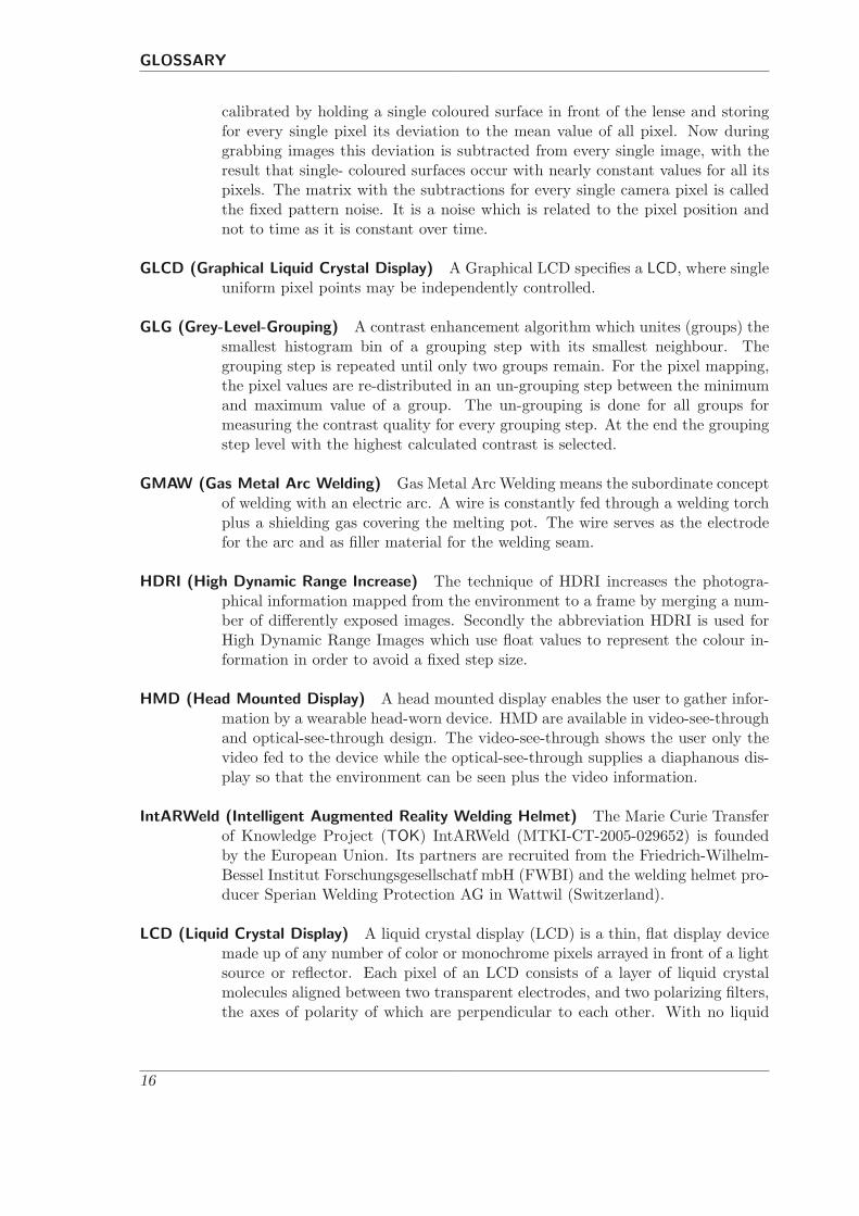
GLCD (Graphical Liquid Crystal Display) A Graphical LCD specifies a LCD, where singleuniform pixel points may be independently controlled.
GLG (Grey-Level-Grouping) A contrast enhancement algorithm which unites (groups) thesmallest histogram bin of a grouping step with its smallest neighbour. Thegrouping step is repeated until only two groups remain. For the pixel mapping,the pixel values are re-distributed in an un-grouping step between the minimumand maximum value of a group. The un-grouping is done for all groups formeasuring the contrast quality for every grouping step. At the end the groupingstep level with the highest calculated contrast is selected.
GMAW (Gas Metal Arc Welding) Gas Metal Arc Welding means the subordinate conceptof welding with an electric arc. A wire is constantly fed through a welding torchplus a shielding gas covering the melting pot. The wire serves as the electrodefor the arc and as filler material for the welding seam.
HDRI (High Dynamic Range Increase) The technique of HDRI increases the photogra-phical information mapped from the environment to a frame by merging a num-ber of differently exposed images. Secondly the abbreviation HDRI is used forHigh Dynamic Range Images which use float values to represent the colour in-formation in order to avoid a fixed step size.
HMD (Head Mounted Display) A head mounted display enables the user to gather infor-mation by a wearable head-worn device. HMD are available in video-see-throughand optical-see-through design. The video-see-through shows the user only thevideo fed to the device while the optical-see-through supplies a diaphanous dis-play so that the environment can be seen plus the video information.
IntARWeld (Intelligent Augmented Reality Welding Helmet) The Marie Curie Transferof Knowledge Project (TOK) IntARWeld (MTKI-CT-2005-029652) is foundedby the European Union. Its partners are recruited from the Friedrich-Wilhelm-Bessel Institut Forschungsgesellschatf mbH (FWBI) and the welding helmet pro-ducer Sperian Welding Protection AG in Wattwil (Switzerland).
LCD (Liquid Crystal Display) A liquid crystal display (LCD) is a thin, flat display devicemade up of any number of color or monochrome pixels arrayed in front of a lightsource or reflector. Each pixel of an LCD consists of a layer of liquid crystalmolecules aligned between two transparent electrodes, and two polarizing filters,the axes of polarity of which are perpendicular to each other. With no liquid
16

GLOSSARY
crystal between the polarizing filters, light passing through one filter would beblocked by the other. If a voltage is applied between the electrodes, the liquidcrystals are aligned parallel to the electrode with a torsion so that the preferredorientation of the polarized light from the one side is shifted to the orientationof the opposite polarizer.
MAG (Metal Active Gas Welding) Process where an active gas is used to improve the arcstability. It may supply carbon -dissolved from carbon dioxide- for to burn upforeign matters in the melting pool. A very common active gas is a mixture of82% argon with 18% carbon dioxide.
MIG (Metal Inert Gas Welding) The Metal Inert Gas Welding means the concept of usedshielding gas. The used gas shall protect the melting pot from oxidizing, whatwould change the temperature and the material in the metal pool e.g. Alumi-nium, with its hard aluminiumoxide phase, is welded with argon as inert gas.
MISE (Mean integrated squared error) An optimum criterion used in density estimationis given by summing up all deviations of an estimated value based on a samplefrom the real value (groundtruth).
PDF (Probability Density Function) The Probability density function of a multidimen-sional random variable is a function that describes the relative likelihood in theobservation space. It can be estimated by a so called density estimator. Theestimator uses a finite number of samples of the process.
PPE (Personal Protection Equipment) Equipment related to all aspects of personal pro-tection for working like ear, eye, hand and foot protection.
SADF (Selective Automatic Darkening Filter) Optical filter which darkens selectively au-tomatically when the welding arc starts by identifying glaring light sources anddarkens selected pixels of a Graphical Liquid Crystal Display (GLCD) where thelight source occur in the view of the welder.
SMAW (Shield Metal Arc Welding) One of the oldest manual welding processes develo-ped in 1908. A massive rod coated with a material which produce during weldingshielding gases and light slag on the seam, is clamped to a rod holder. The wel-der holds this rod which is used like in GMAW processes as electrode and fillermaterial.
SVD (Singular Value Decomposition) Algorithm to decompose a n × m matrix into itsEigenvalues and Eigenvector. It can be used to retrieve an optimal solution foran overdetermined system based on unprecise data.
TIG (Tungsten Inert Gas Welding) Process as well known as Gas Tungsten Arc Weldingwhich uses a nonconsumable (tungsten-) electrode for the welding arc. If fillermaterial is needed for the welding process, it is applied from outside. Mostly a
17

GLOSSARY
rod is fed by the welder to the weld pool. This process can produce filigree arcsto weld thin materials.
TN (Twisted Nematic) A type of LCD where the liquid crystal fluid rotates the plane ofpolarization about 90◦.
TOK (Transfer of Knowledge Program) A Transfer of Knowledge program aims for theknowledge exchange between business and academic institutions. The knowledgetransfer is based on interchange of people working form the business unit at theacademic institute and vice versa.
VBSAHE (Variable Block Size Adaptive Histogram Equalization) The VBSAHE algorithmsegments the image related to its content. The segments are enhanced indepen-dently but limited to its contrast. The resulting image is produced by mergingthe enhanced tiles to the complete image.
18

1Introduction
The first experiments in the modern arc welding were made by the Russian engineer NikolaiGawrilowitsch Slawjanow in 1891 when he used a metal electrode instead of a carbon one.Hence the electrode was used to invoke an electric arc and to be transferred as filler metal.From these first experiment until the present time about 156 different welding processeshave been developed for over 2000 different types of metal materials and the number is stillgrowing. The welding process now has wide application in the value creation chain likeautomotive, shipyards, building construction, chemical industry et cetera. The process ofwelding, cutting and screwing produced in the year 2008 about 6% of value of germany’sgross domestic product.
The welding process is one that still relies heavily on the skill of the welder, because theprocess is sensitive to slight changes of its numerous parameters, so automation of the weldingprocess is generally limited to specific recurring tasks. Robustness of any process can beimproved by sensing and monitoring it. In welding the sensing is mostly done at a distancefrom the place where the welding process takes place. The harsh conditions of an electricalarc with a pool of melted metal, flying metal drip and splatters of the process cause glaringlight, harmful ultraviolet rays, unhealthy smoke, dirty conditions, high temperature andhigh electromagnetic distortions which make direct measurement very challenging. Hencethe available sensors concentrate on measuring parameters such as voltage, current or wirefeed speed, light and acoustic emissions to calculate or estimate physical quantities. Forautomated seam tracking and quality measurement the seam is measured online in front andbehind the welding torch as the weld is made.
The human visual system with the eyes protected by a welding helmet with an opticaldarkening filter is still considered to be superior to common electronic sensor systems becauseof its higher dynamic contrast range. The only disadvantage of this approach is that the
19
1. Introduction
area around the weld becomes less visible because the welding helmet darkens the wholevisible scene not just the weld itself. Current available auto darkening filters (ADF) use aone pixel LCD to darken the view at the exact moment of arc occurrence. New developmentsof graphical LCDs (GLCD), may offer a 2D matrix with independently shadable pixels. Onecan imagine that if such a GLCD is placed between the eye and the welding arc, it only hasto darken the view where the arc occurs and can leave the surrounding view unaffected. Theapplication of a GLCD for selectively auto darken the view of the welder, is one of the aimsof this thesis. The welder shall be supplied with a running prototype of a selective autodarkening welding helmet.
To extract the right position of the glaring lights as it occurs with the arc, a sensor systemhas to be used. Trials have been done to photograph or film the seam using standard CCDcameras, but the results gave little usable visible information because of the low contrastdynamics of CCD or standard C-MOS camera chips. Blooming effects of a single brightspot cause saturation over a large area resulting in barely visible surrounding or a poorflickering image. For some years video sensor chips are available with the ability to map ahigh dynamic range of contrast ratio to a digital image. They potentially provide the abilityto setup a system for the observation of the electrical arc in the welding process and weldpool. To provide an effective technical setup it is not sufficient to have the right sensor. It isalso necessary to understand and minimize the effect of other process phenomena that reducethe quality of the image. This states the second aim of the thesis, which is the examinationof the problem of extracting a proper video view of the welding process. The resulting videoquality depends on the welding process, the camera system and the final image processingthat enhances the information contained in the captured images.
1.1. Organization of the thesis
During reading of the different chapters, the reader will gain knowledge about the boundaryconditions as given by the welding applications and state-of-the-art for eye protection duringwelding. In order to understand the environment given by a welding arc, the most importantissues of gas metal arc welding (GMAW) are introduced in the sections that follow. Themotivation for a welding protection system with a SADF technique using a GLCD is presentedas well as applications for a welding observation system.
Chapter 2 will start with the human eye and its perception for light and contrast, which willbe the next issue on the track to the complete boundaries for a SADF system. Especiallythe medical considerations in accordance to the emitted radiance of the welding, introducethe need for a safe eye shield.
After introducing the human eye and its need for welding protection, the norm for workingsafety which represent the condensed experience about protection, will be presented. Thefocus will be on the European Norms, to have beside the academic access as well the practicalknowledge with the focus onto the human user. Coming from the human perception of theprocess, the machine vision part will be examined. Especially the image acquisition and
20

1.2. Overview of the Welding Process
image pre-processing for direct welding observation is a central subject related to the state-of-the-art. Here the process and the camera must be jointly reviewed. The chapter 2 endswith the introduction to the high dynamic range increase (HDRI) by merging multiple shotsof the identical scene but different camera parameters in order to give the idea of raising thecameras contrast dynamics.
Chapter 3 focusses on the direct development of the SADF. The different issues presented inthe preceding chapter will be further developed. So the image acquisition and improvementfollowed by a deep view onto the mathematical description for the mapping between theworlds from 3D to 2D will be elaborated. The selective shading needs to cope with glaringlight sources of varying brightness and reflections due to different process parameters (e.g.welding current, type of wire electrode), different material (e.g. construction steel, alumi-nium), different surfaces (e.g. polished, untreated, painted, rusty) and the geometrical setupof the environment for reflections (e.g. plain surfaces, closed space). After developing theapplication from the theoretical point of view, the real world results will be measured andevaluated in chapter 4.
1.2. Overview of the Welding Process
The huge amount of about 156 different welding processes and 2000 different sorts of materialfor welding, urge to constraint the SADF system to the most important welding applications.The MIG and MAG processes are presented uniquely although they use a similar technique.The reason are the different conditions they produce for image acquisition.
1.2.1. Gas Metal Arc Welding
The Gas Metal Arc Welding (GMAW) is a class of welding which uses an electrical weldingarc and a covering gas. The arc is produced by a metal electrode which serves also as fillermaterial. The function of the gas is to cover the melting pool for either protect it completelyfrom oxidation or supply the process with active gas components to control the metallurgyprocess. The shielding gas and its flow rate also have a pronounced effect on aspects of thewelding process like [2]:
• Arc characteristic: (e.g. length, shape, stability)
• Mode of metal transfer: (e.g. globular transfer, spray transfer, droplet transfer fre-quency, size of drops)
• Penetration and weld bead profile
• Undercutting tendency
• Cleaning Action: (e.g. burning impurities)
21

1. Introduction
• Mechanical properties after welding
Normally a wire is fed through a welding torch and acts as the melting electrode, with themelted material filling the welding seam as shown in figure 1.1. The gas flow encloses thewire electrode and the area of the melting pool. Below a distinction of the GMAW will bemade concerning the implementation of the welding arc with its connected metal transfermodes and the used gas for the process.
Figure 1.1.: Technical Concept of GMAW. (source:[3])
The welding arc and its connected metal transfer exists in four different major forms: glo-bular, short circuit, spray and pulsed spray.
Short Circuiting Transfer The short circuit arc can use the lowest range of welding cur-rents. When starting the process, the wire electrode is constantly fed through the torch andtouches the workpiece causing a short circuit as it can be seen in figure 1.2 [A]. Due to theshort circuit, the current rises [B,C] rapidly and heats the wire until it is melted [D]. Theliquid metal pinches off the electrode [E] and the short circuit is interrupted causing an arc.Electromagnetical forces transport the liquid metal to the weld pool[F]. The welding arcburns until the wire contacts the workpiece again, causing the short circuit [G,H,I] and theprocess repeats. This happens with a frequency of 20 to 200 Hz and depends on a variety ofparameters like current, gas and electrode material.
Globular Metal Transfer Globular metal transfer produces metal drops at the end of theelectrode with a size bigger than then the diameter of the wire. It takes place at low currents,if the force of the welding is not sufficient to pinch off metal drops from the electrode, sothat either gravity or a short circuit detaches them. Globular transfer has a high depositionrate and thus high welding speeds maybe reached. The disadvantage is that the huge drops
22

1.2. Overview of the Welding Process
Figure 1.2.: Phases of the short circuit welding arc (source:[2])
causes a high sputter rate, an uneven surface and is limited to flat and horizontal positions[4].
Spray Transfer In the spray transfer mode the welding arc has such a high energy, that themetal drop pinches off the electrode by magnetic effects before the electrode contacts theworkpiece. For this mode of operation a stable electric arc with a higher average current isneeded. The stability of an arc can be boosted by using a gas mixture of mostly argon pluscarbon dioxide as an active component. Argon is an inert gas more than 1.4 times denserthan air and provides an inert blanket against oxidation of the melting pool. The carbondioxide in the mixture provides a better ionisation of the arc path and thus improves the arcstability. The presence of carbon dioxide constraints the use of this exemplary gas mixtureto carbon and low alloy steel. The spray transfer mode results in a highly focussed streamof tiny drops (spray) onto the work piece, which are merely influenced by gravity forces.
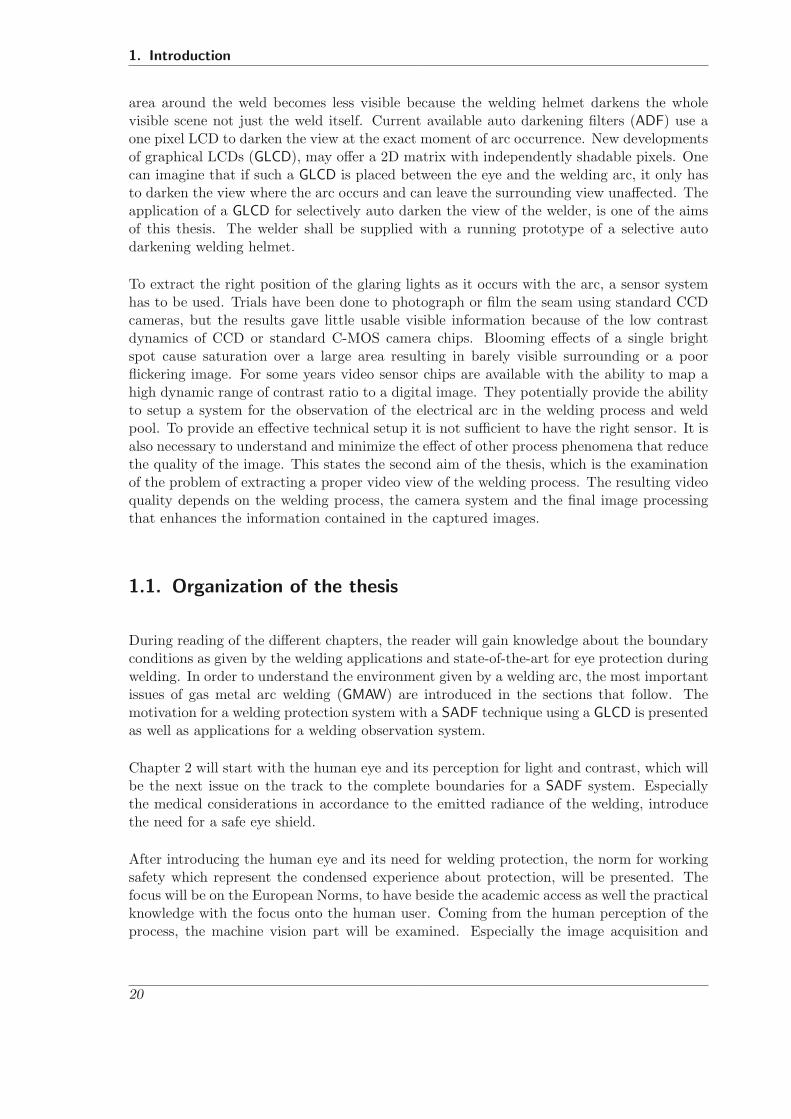
Pulsed Spray Transfer The pulsed spray transfer mode is made possible by current control-led welding sources, which can produce a high current signal of nearly any shape. The basicsignal for pulsed spray transfer consists of a positive Alternating Current (AC) superim-posed on a low constant (DC) current (see figure 1.3). The DC signal (see figure 1.3 (A))keeps the arc burning on a level without forming metal drops on the wire tip. The positiveAC-signal does the job of metal transfer. At the moment the welding current is forced torise by the welding source, a metal drop begins to pinch off the electrode (B) and acceleratestowards the work piece with its positive polarity. In order not to accelerate too much, thewelding source lowers the current, but still keeps it high to enforce a straight trajectory(backpack current) (C). In ideal case the arc current returns to the DC-level, when the droptouches the work pieces(D). Depending on the welding parameters this process runs with arecurrence rate of 20− 200Hz for the described sequence. Beside this basic form of a pulsedwelding arc, a huge variety of different arc-signals exists for different applications.
23
1. Introduction
Figure 1.3.: Qualitative example of measured spray transfer
Metal Inert Gas Welding
After describing the different types of metal transfer modes a concise explanations of thedifferent welding processes are given.
The Metal Inert Gas (MIG) process uses mostly argon, helium or a mixture of both. Thepurpose of the inert gases is to cover the welding process against reactions with oxidizingatmospheric gases. One of the most utilized materials for MIG welding is aluminium. It issensitive to oxidation and aluminium-oxide is a hard and resistant shell which melt at hightemperature. Its melting point is at about 2050◦C while pure aluminium melts at 660◦C.This is one reason why aluminium welding is more complicated, as the for high temperatureresistant aluminium-oxide skin must be breached, while the pure aluminium body is alreadymelting some thousand grades Celsius below.
Metal Active Gas Welding
Adding an active gas like oxygen or carbon oxide gives the Metal Active Gas (MAG) weldingthe effect of improving the arc stability due to better ionization in the arc track. For carbonsteel and low alloy steels carbon dioxide deepens the penetration of the material but increasesthe sputter loss. Adding oxygen grows the weld pool, the penetration and arc stability but ahigher oxidation of the welding material occurs, with a loss of silicon and manganese, whichcan change the metallurgy of alloyed steel.
Tungsten Inert Gas Welding
The Tungsten Inert Gas (TIG) is a process in which the filler material is not used as the arcproducing electrode. Commonly a DC arc is produced between the work piece and a non-
24

1.2. Overview of the Welding Process
consumable tungsten electrode. This electrode is covered by an inert shielding gas like argonor helium to protect it and to cover the weld pool from oxidation (see figure 1.4). A fillermaterial is often used but is not compulsory as it can be omitted at thin butt joints. Thefeeding of the filler material to an arc, which burns constantly from the tungsten electrode,does not splatter which allows a smooth seam to be laid. On the other hand the quality ofthe process is as only as good as the skill of the welder in handling the welding torch. If theelectrode touches the work piece, then beside some wolfram inclusions in the seam, the conicform of the electrode is destroyed by metal that attaches to it, resulting in the shape andquality of the welding arc becoming poor. An additional issue is that the tungsten electrodeneeds some special protection against oxygen. Especially if the arc is turned off the electrodehas to be cooled and protected by the shielding gas down to 300◦C. High quality professionalTIG welding machines turn off the arc smoothly to avoid shrinkage cavities, enable craterfilling and electrode cooling at once.
Figure 1.4.: Technical principle of a TIG process (source:[3])
The TIG-process can cause significant electromagnetic compatibility (EMC) problems, whenthe arc is started. For example one non-contacting technique to start the arc uses a highfrequency (HF) starter which causes high current surges and by that high electromagneticradiations. This may cause computing boards like microcontrollers (μC), interface chipsor Personal Computers (PC) to crash or to be damaged. An alternative approach usesa technique called lift-arc. Here the welder first touches the workpiece with the tungstenelectrode, while the welding source measures the voltage between electrode and workpieceand does not raise the current from a low level until the electrode is lifted off the workpieceand the arc starts at an insignificant distance between electrode and workpiece.
1.2.2. Shielded Metal Arc Welding
This process is also known as stick welding. In comparison to processes where some shieldinggas is used to protect the weld pool from oxidation, the stick welding uses a glass like filmcalled slag, produced during the process for weld metal protection. No wire is constantly
25

1. Introduction
fed through a welding torch. A coated thick rod electrode is clamped into a holder and thefeeding is done by the user with the rod holder in his hand. This process was one of the firstbeing commercially used. It is the most sensitive and most robust process one in a kind. Itis the most sensitive, because the welder does not really see the process as clear like a GMAWprocess and must fed manually the electrode. The manual feeding means another degree offreedom to be handled by the welder, so that a good welding seam expects higher weldingskills. On the other hand it is the most robust process, because in comparison to the GMAWprocess, which is quite sensitive to air draught, the Shielded Metal Arc Welding (SMAW)process is less sensitive because the coating of the rod electrode produces during welding ashielding gas and the remaining light slag covers the seam and forces a slow cool down of theprocess. These properties are helpful on open air construction sites, where adverse weathercondition make welding more complicated.
1.2.3. Laser Welding
Beside drilling and cutting, a laser can be used for welding. It is a process with brings highlyfocussed energy to the workpiece whereby the heat affected zone is small. Laser weldingis usually used without any filler material and the laser produce a weld pool to a depthdepending on the focus point of the laser beam. Pure laser beam welding can be dividedinto the heat transfer and keyhole melting. The first uses a laser with ”low” energy, whichimpinges on the metal surface and heats it until it melts. The keyhole technique uses alaser with higher power which forms a small channel of vaporised metal and thus a smallerweld pool. Due to the high but very focussed energy, this method is suitable for high speedwelding.
1.3. Welding Observation
Welding observation is normally done by a person looking through a darkening filter. Thehuman eye is able to perceive a huge variety of contrast dynamics. So if the welder usesa darkening filter he is able to see the bright welding arc and also the surrounding of thisscene. Using a passive or automatic filter in front of a commercial CCD video camera hasdisappointing results. The welding arc is mapped to appear as a white area, due to theblooming effect of the CCD technology. This effect is produced by very bright spots ina scene whose brightness exceeds the maximum abilities of the pixel cell (see figure 1.5).Welding videos of the welding process with all its details as seen by the human observerthrough a darkening filter is not available and opens a new field of application in qualityassessment, process control, human interaction and personal protection equipment. But theterm ”observation” can be interpreted to a wider area, if it is seen independent from visualimpressions. The following paragraphs do give an overview about the varieties of observationapplicable to welding results related to different purposes.
26

1.3. Welding Observation
Figure 1.5.: CCD camera image of MAG process with bloomed view on arc
1.3.1. Quality Assessment
To ensure a reliable quality assessment of a desired welding process a variety of differentmeasurement approaches are used. Starting from classical paper sheets where the usedwelding machine parameter and used material are documented, the bandwidth includes non-destructive method in online and post analysis. During welding the process parameters likecurrent and voltage may be recorded or tracking sensors which work by tactile probes orlaser triangulation in front or behind the welding torch keep the track. In the post processphase measurements can be done by using
• x-ray photoThe most commonly and widely used technique available for quality assessment isx-ray photography of the welding seam. On one side of the seam the photographicfilm is placed while on the other side a γ-ray source ”exposures” the film. The 3Ddetails information of the seam is thereby mapped to 2D image which integrates theinformation in depth of the material.
• ultrasonicAn ultrasonic transmitter in contact to the workpiece transmits a directed wave intoit, which is distorted and reflected by the imperfections in the material. The echo ofthe ultrasonic signal give information about the inner structure of the material.
• pyrometerA pyrometer gives information about the temperature of the work piece without contac-ting it. Spatial resolving pyrometer or IR-cameras supply information about the workpiece and weld pool.
27
1. Introduction
• dye penetrationThis method makes surface defects like cracks visible. A high capillary ink is appliedby spraying or painting it onto the produced seam. The ink dissolves into the finestcracks. After cleaning a developer is used to drive the ink out of the cracks so that itbecomes visible on the surface, making the cracks clearly identifiable. The ink is oftenfluorescent so that it can be easily seen using ultraviolet light
• magnetic powderWith ferromagnetical materials the magnetic powder method can be used. In thismethod the material is covered with fine metal powder and a pattern is induced inthe metal powder that follows the magnetic flux in the metal. Defects or inclusion inthe metal deflect the magnetic flux lines so that the metal powder pattern maps theinformation from inside the material onto its surface.
• eddy currentThe eddy current method is applicable for automated testing. A primary coil inducesby electro magnetic induction a local field to the metal piece. This field can be sensedby a secondary coil. If a defect in the material deflects the eddy current lines then itoverlays with the primary magnetic field resulting in an attenuated field sensed by thesecondary coil.
• acoustic emissionTwo different methods exist for acoustic testing. The first method acoustic emission isan intrusive method which measures the emissions during tension or pressure testing.Cracks in the material produce a crackle sound if the material is impinged on pressureor tension. Using several microphones may give information about the position of thedefect. This method gives a simple applicable approach for testing huge structures bystressing them without harming.
The second method is related to process supervision during automated welding. Theautomated process is taught by a self learning system and deviation after learningimply possible error during the production [5] (see i3tech 1).
This short list of non-destructive measurements related to welding is not comprehensive [6],but it shows that all testing modes avoid directly contacting the location where and whenthe real process takes place that is where the metal melts while the arc burns.
Welding observation may enhance these approaches to an in situ observation of the runningprocess.
1http://www.i3tech-gmbh.com/ seen on 27.3.2009
28

1.3. Welding Observation
1.3.2. Process Control
The application to use a proper welding process visualization is inherent to apply this newdata domain of welding observation for process control in automated and semi-automatedprocesses. Achieving a high quality video opens the field of application to several newopportunities.
Remote View
Processes like tractor automata, semi-automated production using positioners, roller bedsor portal system for stringer joining, often need a manual supervisor to make adjustmentsduring welding. The torch distance or the position relative to the prepared welding seammay change which results in inappropriate joints. A remote view on the process includingthe arc and environment may facilitate a remote control of the production by one personwith more than one process being supervised at once.
Seam Tracking
Seam tracking during automated welding is used to either rise the precision of a welding taskby avoiding misalignment or to weld fuzzy taught production. Tactile sensors exist with ametal finger gliding at an edge of the workpiece and the torch is guided along one axis. Theguidance of the process cannot be done directly at the position of the welding arc and needsto be guided either by an edge parallel to the seam.
Another approach is to use laser light section where a camera is heading on a projectedlaser line. On a plain surface the laser line is straight visible. Aberrations by unevennessdo deform the straight line depending on the height of the asperity. A laser triangulationsensor supplies 2D information of the surface. The sensor cannot be used directly at theposition of the welding arc, as either the camera is blended by the light or the laser line isnot visible. The average minimum distance from relative to the welding arc depends highlyon the available contrast dynamic of the used camera.
A stereo camera system which can grab good images of the process may extracts a 2.5Dview of the process and may supply precise information about the welding process at theweld pool for seam tracking.
Arc Length and Torch Distance Measurement
The length of the welding arc defines significantly the produced heat power and its disse-mination. Low profile metal sheets are more sensitive to deviations from optimal powerdistribution, The arc length measurement is a task which is roughly done by the welding
29

1. Introduction
power source by measuring the voltage at the arc path. The drawback to be coped with,is the unknown chain of contact resistors of the setup between the two connector (poles)of the welding source. They differ from setup to setup and as well during the process asthe conductance of the arc and workpiece change with its temperature, working positionand distance. Especially in MIG and MAG processes the resistors between the contact tip inthe welding torch and the wire electrode are not stable and cause imprecision in arc-lengthextraction. For GMAW in the specialization of very short (0.5 − 5 mm) TIG arcs a precisionof about ±0.1 mm is needed to ensure a proper welding.
1.4. Personal Protection Equipment
The welding process causes high radiances over a variety of wavelength from infrared overvisible light to ultraviolet rays with wavelengths from 350-800 nm. The spectral irradiance -an example is shown in figure 1.6- highly depends on the used process, material and gas asthe light is produce like in an electric discharge lamp. The visible light of a welding arc ismuch too bright for the eye and causes flash burns. The infrared radiance causes burns dueto overheating the skin and eye with the danger of coagulation causing tissue injury. Thelast and most dangerous radiance is the UV spectrum which causes skin cancer, painful sunburns on the skin and horny skin (cornea) of the eye [7].
Figure 1.6.: Example of spectral irradiance for MAG welding of mild steel with a mixture ofargon and carbon dioxyde (18%) at 100 A
1.4.1. Passive Filters
During the welding process the welder has to be protected from these hazards by covering thebody with opaque and heat resistant material like cotton or leather equipment. Everythingbut the eyes must be opaquely covered. The eyes need a special protection as they are neededfor observation during welding. Observation situations occur for manual, semi-automated orfully automated welding. If only a short glance is taken for inspection of a running welding
30
1.4. Personal Protection Equipment
process a simple black glass with a very low transmission will be sufficient from the protectionand ergonomic point of view. Some very high professional manual welder prefer passive filteras they claim to have a better view through a one layer passive than through a three to fivelayer automatic darkening filter.
1.4.2. Automatic Darkening Filter
For the manual welding process where a welder needs to be precise in welding torch handlingover a whole working day of eight hours or more, an Automatic Darkening Filter (ADF), is amore ergonomic and thus quality assurance choice. This type of filter darkens automaticallya see-through window, if a welding process starts in the surrounding. With an ADF thewelder does not have the problem of a permanent merely diaphanous view, like he has witha passive filter. Now a correct aiming to the starting point of the welding seam is easy tofind. With an ADF the welder has a good view onto the scene by the inactive shading ofthe filter. During welding process a safe observance is assured due to the ADF activatedshading at an adequate shading level [8]. By shading the complete view by one constantshading level, the limited dynamic range of the eye cannot picture low lighted details of thesurrounding, as the arc must be shaded at an high level.
1.4.3. Selective Auto Darkening Filter
The European Union - Marie Curie Transfer of Knowledge Program (TOK) grants underthe number MTKI-CT-2005-029652 the project IntARWeld. The IntARWeld project yields,from the point of research, to the improvement of current ADF technique as it is widelyused in high-end welding protection. The research activities at Optrel AG 2 in Switzerlandand the Friedrich-Wilhelm-Bessel-Institut Forschungsgesellschaft mbH (FWBI3) in Bremen(Germany) follow the idea of a Selective Auto Darkening Filter (SADF). This filter shalldynamically darkens the users view only there, where a glaring light source occurs and keepthe low lighted regions clear. Such a SADF will protect the welder during welding fromflash-burn by shading the areas which overexposes the eye and remains a good view ontothe environment by less shading the surrounding. In order to achieve the functionality ofa dynamic selective shading one idea is to place a partial shadable filter between the userand the light sources as it can be done with a GLCD. A light source detecting device needsto extract the bright areas in the welders view as they occur in the welders line of sight. Adigital camera can sense the view of the welder and thus the bright areas occurring duringwelding. These cores of the technique give an approach for a SADF setup integrated in awelding helmet. They have to be embedded into the SADF application where they inducethe adjacent problems, which will be investigated in the following chapters.
One big issue is the proper extraction of a camera image. The welding process causes anharsh environment with high electromagnetic radiations. The scene has very high contrast
2formerly know as Sperian Welding Protection3http://www.fwbi-bremen.de/
31

1. Introduction
ratio which is the ratio of the darkest to the brightest area and a fast changing light conditiondue to the unstable light source produced by the electric arc of the most welding process.Theses boundaries urge the active control of the camera parameters during welding and anadapted image processing to receive a good view onto the process. Another issue is to buildan algorithm for controlling the GLCD for each eye while the camera with its monoscopicview does not have the same stereoscopic view of the user. Additionally the relative posebetween the user and camera is not constant between different uses. That is why the issueof precise system calibration needs to be considered. Especially the projective geometry willhelp to regard the context of mapping the world from 3D to a 2D camera chip and fromthere to a 2D GLCD which is in the line of sight of the second ”camera” called human eye.
1.4.4. Mixed Reality
The SADF concept enables a better access to the welding by supplying a better view. TheMixed Reality paradigm can be seen as the next logical step after improving the user view.The mixed reality paradigm enriches the user view by adding new information. The MixedReality continuum (see figure 1.7) as introduced by Paul Milgram [1] gives the opportunityto add any amount of artificial content to the users view . It starts with the pure reality andadds on his way to the virtual reality more and more additional data to the users view.
Figure 1.7.: Mixed Reality continuum
The blending of information is mostly done by using a head-mounted display (HMD) widelyknown as video goggles. These displays do either blend the additional data to the users viewwhile he sees the environment pure naturally. This approach is called optical see-throughHMD. The second more simple mode of adding information is to grab the view by camera,add some content and display this video stream to the user, which is called video-see-throughmode. If the portion of real view is bigger than the added virtual information, then this iscalled Augmented Reality (AR). For this video see-through AR can be used to form a newparadigm for Personal Protection Equipment (PPE). A stereo camera system integrated ina welding helmet records the scene and feeds the images to a stereo HMD. The connection ismade with a computer system in between the camera and HMD which gives the opportunityto enrich the images with additional data. Here the image acquisition and enhancementplays a central role for the view impression of the user. For the field of welding applicationthe project TEREBES uses this approach. It integrates two cameras in a welding helmetwith an intercamera distance similar to the human eye distance (see figure 1.8). These twoview channels are processed by two independent computers and shown on a stereo HMD [9],[10], [11], [12]. One problem of this system was the limitation to spray transfer processesdue to a limited adaptation of the video system onto other welding processes.
32

1.4. Personal Protection Equipment
Figure 1.8.: Conceptional Setup of the TEREBES welding helmet
Instead of using this paradigm during welding it can be used for a pure virtual welding. Thewelding piece and the welding torch need to be tracked in order to know the relative poseof these two objects. The relative pose is fed to an welding seam model, which produces apure virtual graphical rendered welding seam. The seam can be overlaid for the user ontothe real physical object by blending it into the HMD [13].
33

1. Introduction
34

2State of the Art
In this chapter the problem of welding observation and protection is re-defined by introducingthe single aspects of the problem and confining it from other works. It starts with the issueof the human visual system and its sensitivities and regulations. In the next step the aspectsof the state of the art related to extract data about the welding process and the visualobservation are described. A special section takes care about the image processing problemwhich consists of noise filtering, image enhancement and high dynamic range increase bymerging several shots of the scene.
2.1. Welding Protection
As presented, the welding process produces emission as glaring visible light, infrared andultraviolet rays. The visible light, which has the wavelength from 400 to 700nm is the one tobe dynamically shaded. First the sensitivities of the human eye is taken into account fromthe physiology point of view. After introducing the functionality of the human eye receptors,a look onto the regulations for welding protection is taken. These regulations, which are thecondensed experience for eye protection during welding, give a good impression about whata SADF has to cope with.
2.1.1. Sensitivities of the Human Eye
The human eye with its ability to adjust to different lighting conditions covers the dynamicrange of 1 : 104 from the darkest to the brightest point in the scene. Different mechanism
35
2. State of the Art
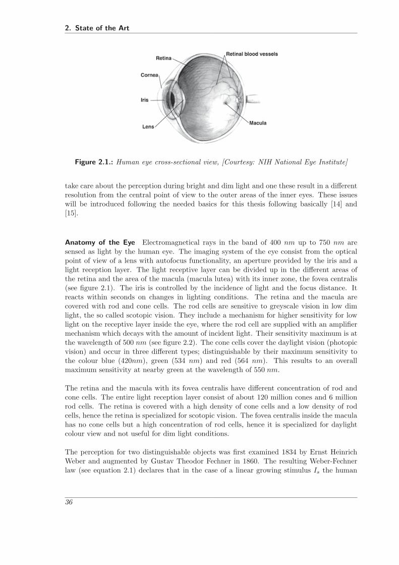
Figure 2.1.: Human eye cross-sectional view, [Courtesy: NIH National Eye Institute]
take care about the perception during bright and dim light and one these result in a differentresolution from the central point of view to the outer areas of the inner eyes. These issueswill be introduced following the needed basics for this thesis following basically [14] and[15].
Anatomy of the Eye Electromagnetical rays in the band of 400 nm up to 750 nm aresensed as light by the human eye. The imaging system of the eye consist from the opticalpoint of view of a lens with autofocus functionality, an aperture provided by the iris and alight reception layer. The light receptive layer can be divided up in the different areas ofthe retina and the area of the macula (macula lutea) with its inner zone, the fovea centralis(see figure 2.1). The iris is controlled by the incidence of light and the focus distance. Itreacts within seconds on changes in lighting conditions. The retina and the macula arecovered with rod and cone cells. The rod cells are sensitive to greyscale vision in low dimlight, the so called scotopic vision. They include a mechanism for higher sensitivity for lowlight on the receptive layer inside the eye, where the rod cell are supplied with an amplifiermechanism which decays with the amount of incident light. Their sensitivity maximum is atthe wavelength of 500 nm (see figure 2.2). The cone cells cover the daylight vision (photopicvision) and occur in three different types; distinguishable by their maximum sensitivity tothe colour blue (420nm), green (534 nm) and red (564 nm). This results to an overallmaximum sensitivity at nearby green at the wavelength of 550 nm.
The retina and the macula with its fovea centralis have different concentration of rod andcone cells. The entire light reception layer consist of about 120 million cones and 6 millionrod cells. The retina is covered with a high density of cone cells and a low density of rodcells, hence the retina is specialized for scotopic vision. The fovea centralis inside the maculahas no cone cells but a high concentration of rod cells, hence it is specialized for daylightcolour view and not useful for dim light conditions.
The perception for two distinguishable objects was first examined 1834 by Ernst HeinrichWeber and augmented by Gustav Theodor Fechner in 1860. The resulting Weber-Fechnerlaw (see equation 2.1) declares that in the case of a linear growing stimulus Is the human
36

2.1. Welding Protection
Figure 2.2.: Scotopic and Photopic Vision [source:[17]]
sensing organ like the eye percepts a resulting sensing signal (A) by the logarithm of thestimulus.
A = k · log(
Is
I0
)(2.1)
with k depends on the individual eye. I0 is a critical value for two distinguishable impressionsand depends on the adaptation of the eye system. This law results, that the sensing systemlike the eye uses a logarithmic compression for the signal.
Equipped with these most important mechanisms the eye is able to adapt to light conditionswith a ratio of 1 : 1011 between the darkest and brightest condition. If the illumination iskept constant, the most everyday life situation supply a ratio of 1:40 for the darkest to thebrightest object reflectance [16].
Contrast perception The contrast perception of the human eye can be formulated fordifferent boundary conditions. Two neighboured areas, form a border if they differ withthe smallest distinguishable difference in brightness. This smallest distinguishable differencedepends on the size of the two areas. The smaller the areas are, the bigger must be thedifference. But this is not the only variable for the contrast. The problem here is, that itdiffers with the used colour and slope at the border in between, as well. Another access tothis problem is to use different 2D patterns like a sinus with different frequencies f and tomeasure the perception level of the test person in comparison to a rising pattern amplitudeof time (see equation 2.2).
P (u, v) = sin (2πfv) with u, v : row, column of the image (2.2)
The resulting function is called the modulation transfer function (MDF) of the eye anddepends on the age, pupil diameter and eye colour [18]. As an example the MDF is shownin figure 2.3 for a 25 year old blue eyed human with a pupil diameter of 3,8 mm.
Hazarderous effects The hazardous effects of optical radiation on the eye vary significantlywith the irradiated wavelength. The discussion about the hazarderous effects can be divided
37

2. State of the Art
Figure 2.3.: Modulation Transfer Function
up into three main parts: The ultraviolet, the viewable light and infrared radiation [19]. Thehazards from electromagnetic and magnetic fields related to cancer [20] are not considered,as they are not part of the welders protection using a SADF or ADF.
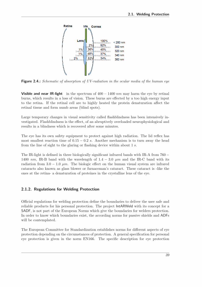
UV-rays with the distinction of UV-A (315 − 400 nm), UV-B(280 − 315 nm) and UV-C(100 − 280 nm) radiation are absorbed for about 96% by the cornea and the eye-lens. Thelonger the wavelength of the UV-ray is, the more they penetrate the eye (see figure 2.4). Onthe cornea mostly the UV-B and UV-C cause photochemical effects which result in a actinickeratosis- that painful effect known as snow blindless or welder’s flesh, which is like a sunburn on the cornea surface. After exposure the discomfort come with a latency between 6 and12 hours. Symptons are the reddening on the conjunctiva (conjunctivitis) within the areabetween the eye lids, a heavy tear flow, high sensitivity to light with a painful uncontrolledexcessive blinking and the feeling of having ”sand” in the eye. The recovery takes one or twodays.
The UV-A and UV-B rays are transmitted by the cornea and conjunctiva into the lens. Apigment in the lens which is itself a photodegradation product from an UV-B photochemicalreaction, absorbs and therefore protects the retina from these rays. Inside the lens thisbrownish pigment can be accumulated and turn the lens almost black. This process isreversal, so that the opacity may last for some days and disappears if the exposure of theeye to UV-A and UV-B is sufficiently low.
The UV-B and UV-C ray can be easily blocked by a clear plastic or glass panel, so that thehazardeous effect can be minimized without loosing the access to the visual reception of ascene.
38
2.1. Welding Protection
Figure 2.4.: Schematic of absorption of UV-radiation in the ocular media of the human eye
Visible and near IR-light in the spectrum of 400 − 1400 nm may harm the eye by retinalburns, which results in a loss of vision. These burns are effected by a too high energy inputto the retina. If the retinal cell are to highly heated the protein denaturation affect theretinal tissue and form numb areas (blind spots).
Large temporary changes in visual sensitivity called flashblindness has been intensively in-vestigated. Flashblindness is the effect, of an abruptively overloaded neurophysiological andresults in a blindness which is recovered after some minutes.
The eye has its own safety equipment to protect against high radiation. The lid reflex hasmost smallest reaction time of 0.15 − 0.2 s. Another mechanism is to turn away the headfrom the line of sight to the glaring or flashing device within about 1 s.
The IR-light is defined in three biologically significant infrared bands with IR-A from 760−1400 nm, IR-B band with the wavelength of 1.4 − 3.0 μm and the IR-C band with itsradiation from 3.0 − 1.0 μm. The biologic effect on the human visual system are infraredcataracts also known as glass blower or furnaceman’s cataract. These cataract is -like theones at the retina- a denaturation of proteines in the crystalline lens of the eye.
2.1.2. Regulations for Welding Protection
Official regulations for welding protection define the boundaries to deliver the user safe andreliable products for his personal protection. The project IntARWeld with its concept for aSADF, is not part of the European Norms which give the boundaries for welders protection.In order to know which boundaries exist, the according norms for passive shields and ADFswill be contemplated.
The European Committee for Standardization establishes norms for different aspects of eyeprotection depending on the circumstances of protection. A general specification for personaleye protection is given in the norm EN166. The specific description for eye protection
39

2. State of the Art
Norm TitleEN165 Glossar for used termsEN166 SpecificationsEN167 Optical test methodsEN168 Non-Optical test methodsEN169 Filters for welding and related techniques:
Transmittance requirements and recommended useEN170 Ultraviolet filters. Transmittance requirements and recommended useEN171 Infrared filters. Transmittance requirements and recommended useEN172 Specification for sunglare filters used
in personal eye-protectors for industrial useEN175 Equipment for eye and face protection during welding and allied processesEN379 Automatic welding filters
Table 2.1.: Overview about European Norms [EN] for personal eye protection
while welding, against an UV-, IR-source or sun-light are explicitly described in separatenorms (EN169, EN170, EN171). With respect to welding an additional norm describes the”Equipment for eye and face protection during welding and allied processes (EN 175). InEN379 the boundaries for ”Automatic welding filters” are described for ADFs. For definingthe used terms for personal eye protection the norm EN165 consists only of a glossar witha description of the terms. Another two norms declare the testing methods for the opticaland non-optical test methods (EN167, EN168). An overview about the European Norms forpersonal eye protection is given in table 2.1.
The level of shading depends on the brightness of the welding arc, which can be seen by thewelder. The different welding processes with its material, used gas and the current affectthe brightness of the arc. The environmental properties like the material surface (grinded orpolished) and the geometrical shape affect the amount of light which is reflected or absorbed.The recommendations given by EN169 consider solely the process and the used current forthe arc. In figure 2.5 the reference guidelines from EN169 are sketched in a diagram.
2.1.3. Automatic Darkening Filter
An ADF is like a LCD with one single huge pixel. A compound consisting of an IR-filter plusone or two LCDs gives the basic setup of the optical part. This optical block is connectedto an arc detecting device, which darkens the optical block by connecting the LCDs to anelectrical AC-signal. Depending on the functionalities of the control unit, the shading levelof the ADF can be adjusted manually or automatically. The EN379 enjoins a maximumshading level difference between the open and close state of the ADF which must not exceednine shading levels.
The technique used in LCDs is based on polarized light. Imagine two polarizers with per-pendicular planes of polarizations. In between these two polarizers mostly produced as athin plastic film, another two glass sheet with a filling of special liquid crystals is set up (see
40

2.1. Welding Protection
Figure 2.5.: Transmission requirements for shading level
figure 2.6). The surfaces of the glass sheets which are in contact with the liquid crystal arecoated with a transparent electrode. If no voltage source is connected, the liquid crystals arearranged in parallel to the electrode planes and smoothly twisted about 90o from the one tothe other electrode. This smooth twist guides the polarized light from the upper polarizerto the lower polarizer (analyzer) by changing the direction of polarization of 90o (see figure2.6-A). If a voltage source is connected to these electrodes, an electro-magnetical field isformed and distorts the smooth twist by changing the alignment (e.g. twist and tilt)of theliquid crystals (see figure 2.6-B). For a deep understanding of liquid crystals and polarizedlight see [21] and [22].
Figure 2.6.: Principles of LCD using TN technique
41
2. State of the Art
2.2. Welding Process Observation
The welding process observation includes the general documentation or abstraction of datafrom the welding process. This can be 1D-signals like the current, voltage, wire feed speed,brightness, point temperatures or acoustic. Visual imaging provides a 2D signal which isdone by sensing light in a selected spectrum from visble to infrared. Active and passivedirect sensing give the two branches of approaches for visual sensing. Active visual sensinguses external light sources like bulbs, lasers or flashing units. The passive direct sensing usesonly a camera without any additional light. Using X-rays for documentation is widely usedfor after process documentation but can be used as well during the process. A good overviewabout this topic is given in [23].
2.2.1. Process Parameter
The process parameters may give information about the status of the process. In MIG/ MAG short-arc welding the voltage to current evaluation may characterize if the arc ismelting a metal drop from the electrode or if the liquid metal is detached after the shortcutand travels in direction of the workpiece.For pulsed MIG/MAG process the extraction isharder as the machine and not the process controls the signal. By that it happens thatirregularly the energy during one pulse is not sufficient to detach a metal drop. The voltagechange during detaching is not robustly visible in the impulse signal. The wire feed speedis directly mapped to the current. A so called synergy diagram defines the best current forthe selected process related to wire feed speed.
The measured temperature of the weld pool may give information about the penetrationdepth of the welding process. Sensing the temperature with an IR point sensor and modellingthe heat transfer in the work piece, makes a control of a gas tungsten arc welding andsubmerged arc welding feasible [24].
Sensing the spectral optical emissions of the process is used in [25] to control the energyin the process. By sensing the spectral lines of the light emissions caused by the gas andthe metal vapour the difference of these two signals give information about the heat in theprocess. The control lowers the energy, if the metal vapour emissions gets dominant whilethe gas light emissions gets low.
2.2.2. Visual Observation
The visual observation can be subdivided related to the setup into active - with externallight- and direct passive -without external light- observation. Applicable used sensors aresensor based on the Charged-Coupled-Device (CCD) or C-MOS technique.
42
2.2. Welding Process Observation
Active Observation
Active video observation uses external illumination to extract scene information. It doesnot need to be automatically a light source which lights the entire scene as it is used for 3Dextraction for seam tracking by laser triangulation.
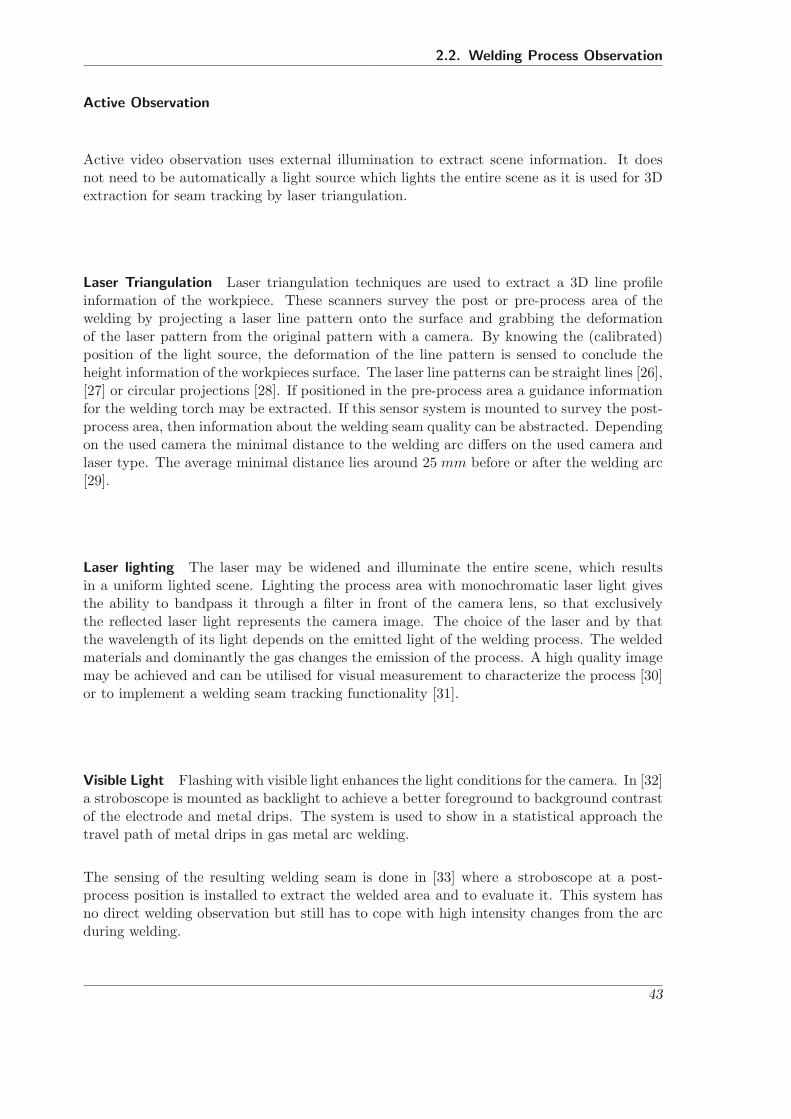
Laser Triangulation Laser triangulation techniques are used to extract a 3D line profileinformation of the workpiece. These scanners survey the post or pre-process area of thewelding by projecting a laser line pattern onto the surface and grabbing the deformationof the laser pattern from the original pattern with a camera. By knowing the (calibrated)position of the light source, the deformation of the line pattern is sensed to conclude theheight information of the workpieces surface. The laser line patterns can be straight lines [26],[27] or circular projections [28]. If positioned in the pre-process area a guidance informationfor the welding torch may be extracted. If this sensor system is mounted to survey the post-process area, then information about the welding seam quality can be abstracted. Dependingon the used camera the minimal distance to the welding arc differs on the used camera andlaser type. The average minimal distance lies around 25 mm before or after the welding arc[29].
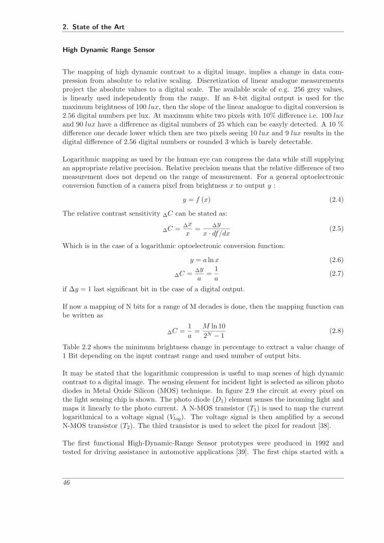
Laser lighting The laser may be widened and illuminate the entire scene, which resultsin a uniform lighted scene. Lighting the process area with monochromatic laser light givesthe ability to bandpass it through a filter in front of the camera lens, so that exclusivelythe reflected laser light represents the camera image. The choice of the laser and by thatthe wavelength of its light depends on the emitted light of the welding process. The weldedmaterials and dominantly the gas changes the emission of the process. A high quality imagemay be achieved and can be utilised for visual measurement to characterize the process [30]or to implement a welding seam tracking functionality [31].
Visible Light Flashing with visible light enhances the light conditions for the camera. In [32]a stroboscope is mounted as backlight to achieve a better foreground to background contrastof the electrode and metal drips. The system is used to show in a statistical approach thetravel path of metal drips in gas metal arc welding.
The sensing of the resulting welding seam is done in [33] where a stroboscope at a post-process position is installed to extract the welded area and to evaluate it. This system hasno direct welding observation but still has to cope with high intensity changes from the arcduring welding.
43
2. State of the Art
Passive Direct Observation
For a passive direct observation of the weld pool without any external lighting, differentapproaches exist. In [34] a CCD camera inspects the weld pool from the top through thewelding torch with the wire electrode in the middle. This coaxial view onto the weld poolsuppresses the direct view onto the welding arc. The contrast dynamics in the scene areminimized and can be recorded by the CCD sensor.
Meanwhile the extinction of the welding arc in a short arc welding, the contrast dynamic isthe lowest during the process. At that moment it can be used to acquire an image of thewelding pool and achieve good quality images [35].
The idea of bandpassing specific wavelengths as done with a laser lighting, can be transferredto avoid too high contrast dynamics on the camera chip. An IR filter in front of the cameralens filters the visible light and remains the important information from the high temperaturewelding pool. An implementation of this technique is described in [36] where it is appliedto a TIG process to control the weld pool size. The same idea is applied in [37] where itextracts information about the weld pool size with for aluminium alloy welding. A generaloverview about this topic with the focus of work on Chinese research is given in [23, chapter1].
Charge-Coupled-Device Cameras
The basic principal of a Charged Coupled Device (CCD) camera is the collection of photoninduced electrons in a bounded area within a predefined time. An array of light sensitivecells integrates the amount of light, which falls onto every single picture cell [pixel] of thesensor. By that an optical image projected by a lens system is converted to a digital image,which can be processed with the computer. The single pixels use the inner photovoltaiceffect. This effect produces free electrons by pushing an electron from the valence band tothe conduction band in silicon. The probability of a photon to be dissolved rises with itsenergy, which depends on its wavelength (see equation 2.3).
EPhoton = h f Frequency : f
= h cλ Wavelength : λ
P lanck′sconstant : h := 6.626 ∗ 10−34JsLightSpeed : c := 2.997 ∗ 108m/s
(2.3)
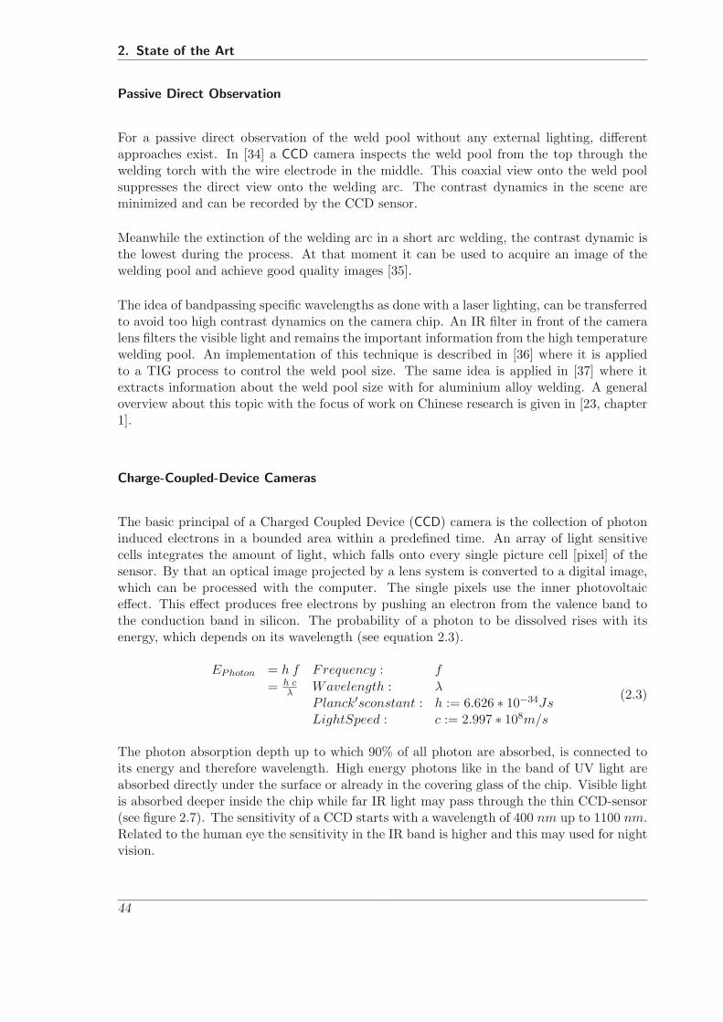
The photon absorption depth up to which 90% of all photon are absorbed, is connected toits energy and therefore wavelength. High energy photons like in the band of UV light areabsorbed directly under the surface or already in the covering glass of the chip. Visible lightis absorbed deeper inside the chip while far IR light may pass through the thin CCD-sensor(see figure 2.7). The sensitivity of a CCD starts with a wavelength of 400 nm up to 1100 nm.Related to the human eye the sensitivity in the IR band is higher and this may used for nightvision.
44
2.2. Welding Process Observation
0
250
500
750
1000
350 450 550 650 750 850 950 1050
wavelength [nm]
pen
etra
tio
n d
epth
[u
m]
Figure 2.7.: Depth up to which 90% of Photons are absorbed depending on wavelength
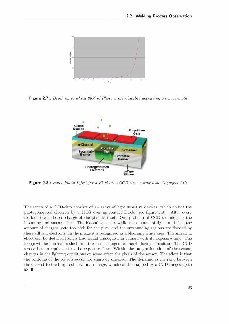
Figure 2.8.: Inner Photo Effect for a Pixel on a CCD-sensor [courtesy: Olympus AG]
The setup of a CCD-chip consists of an array of light sensitive devices, which collect thephotogenerated electron by a MOS over np-contact Diode (see figure 2.8). After everyreadout the collected charge of the pixel is reset. One problem of CCD technique is theblooming and smear effect. The blooming occurs while the amount of light -and thus theamount of charges- gets too high for the pixel and the surrounding regions are flooded bythese affluent electrons. In the image it is recognized as a blooming white area. The smearingeffect can be deduced from a traditional analogue film camera with its exposure time. Theimage will be blurred on the film if the scene changed too much during exposition. The CCDsensor has an equivalent to the exposure time. Within the integration time of the sensor,changes in the lighting conditions or scene effect the pixels of the sensor. The effect is thatthe contours of the objects occur not sharp or smeared. The dynamic as the ratio betweenthe darkest to the brightest area in an image, which can be mapped by a CCD ranges up to58 db.
45
2. State of the Art
High Dynamic Range Sensor
The mapping of high dynamic contrast to a digital image, implies a change in data com-pression from absolute to relative scaling. Discretization of linear analogue measurementsproject the absolute values to a digital scale. The available scale of e.g. 256 grey values,is linearly used independently from the range. If an 8-bit digital output is used for themaximum brightness of 100 lux, then the slope of the linear analogue to digital conversion is2.56 digital numbers per lux. At maximum white two pixels with 10% difference i.e. 100 luxand 90 lux have a difference as digital numbers of 25 which can be easyly detected. A 10 %difference one decade lower which then are two pixels seeing 10 lux and 9 lux results in thedigital difference of 2.56 digital numbers or rounded 3 which is barely detectable.
Logarithmic mapping as used by the human eye can compress the data while still supplyingan appropriate relative precision. Relative precision means that the relative difference of twomeasurement does not depend on the range of measurement. For a general optoelectronicconversion function of a camera pixel from brightness x to output y :
y = f (x) (2.4)
The relative contrast sensitivity ΔC can be stated as:
ΔC = Δx
x= Δy
x · df/dx(2.5)
Which is in the case of a logarithmic optoelectronic conversion function:
y = a lnx (2.6)
ΔC = Δy
a=
1a
(2.7)
if Δy = 1 last significant bit in the case of a digital output.
If now a mapping of N bits for a range of M decades is done, then the mapping function canbe written as
ΔC =1a
=M ln 102N − 1
(2.8)
Table 2.2 shows the minimum brightness change in percentage to extract a value change of1 Bit depending on the input contrast range and used number of output bits.
It may be stated that the logarithmic compression is useful to map scenes of high dynamiccontrast to a digital image. The sensing element for incident light is selected as silicon photodiodes in Metal Oxide Silicon (MOS) technique. In figure 2.9 the circuit at every pixel onthe light sensing chip is shown. The photo diode (D1) element senses the incoming light andmaps it linearly to the photo current. A N-MOS transistor (T1) is used to map the currentlogarithmical to a voltage signal (Vlog). The voltage signal is then amplified by a secondN-MOS transistor (T2). The third transistor is used to select the pixel for readout [38].
The first functional High-Dynamic-Range Sensor prototypes were produced in 1992 andtested for driving assistance in automotive applications [39]. The first chips started with a
46

2.2. Welding Process Observation
Output N Bit 8 bit 9 bit 10 bitInput M decades3 dec 2.7 1.35 0.6754 dec 3.6 1.8 0.95 dec 4.5 2.25 1.1756 dec 5.4 2.7 1.357 dec 6.3 3.15 1.575
Table 2.2.: Contrast sensitivity of the last significant bit in percentage for logarithmic map-ping [38]
Figure 2.9.: Circuit for one HDRC Pixel
47

2. State of the Art
resolution of 64 by 64 pixel and reached a resolution of 1024 by 1024 pixels. For the imagereadout a rolling shutter is mostly available. This means that one pixel line is connectedto a sample and hold block before readout. As the photo diode reacts instantly to scenechanges, this line by line readout may introduce wrong impressions of the scene. Criticalsituations exist if rotating or moving objects are observed by the camera. Depending on theirrelative movement to the camera translated objects are stretched or compressed. High globalillumination changes during readout generate an average brightness change of an entire pixelline.
Specific for the high dynamic range C-MOS camera pixels is the fixed pattern noise (FPN),which effects every pixel individually. The FPN depends on the two independent pheno-mena:
1. Distribution of dark currents for low light levels
2. Distribution at bright levels by the individual transistor parameter like its thresholdvoltage
The FPN correction can be assumed to be constant in a wide range of illumination. To achievea good FPN correction during welding, it is sufficient to have a static offset subtraction forevery single pixel. The calibration of the FPN correction is done by grabbing a frame of aunicoloured white surface at a bright illumination level. The deviation of every pixel fromthe mean value of the image is subtracted for FPN correction (see figure 2.10 and figure2.11).
Figure 2.10.: Image of the automatic teststand without FPN correction
Figure 2.11.: Image of the automatic teststand with FPN correction
Optics
As the High dynamic range camera chip senses relative brightness information already at alow minimum brightness level, the lenses used for CCD camera do have negative effects on
48
2.3. Image Processing
Figure 2.12.: Spectral response of Gevilux lenses [40]
the image quality. The reflection at the annealed glass-air surface are the source for refleximage. The intensity of the reflex images is below the lower bound to be sensed by a CCDcamera but are recorded by the logarithmic high dynamic range sensor as ghost images.Lenses for CCD sensor lead to a setup of numerous free-standing lenses where every glass-airsurface is a source for ghost images visible for high dynamic range sensors. Theses newboundary lead to a new setup for specialized optics with a minimized number of lenses andhigh quality reflective coatings [40].
A second change for the boundary conditions is the different sensitivity for near-IR light sothat a correct focus for this bandwith is needed and a lower cut-off frequency is implemented.The figure 2.12 and figure 2.13 show the spectral response of a specialized high dynamic rangelense type ”Gevilux” from the company gevitec1 and a standard CCD tube lense from thecompany QIOPTICS 2. The differences in the spectral response can be clearly seen. TheGevilux lense has its cut-off wavelength of 550 nm at the bottom and a sharp fall-off at830 nm for the upper bound, while the CCD lense starts at 400 nm and has a smooth upperblocking.
2.3. Image Processing
The enhancement of images cover the fields of denoising distorted images as it occurs for dimscenes, deblurring of unsharp images e.g. due to movement and enhancing the contrast forcompressed scene data. Basic techniques for image processing can be found in recomendedbooks like [41], [14], [42] or [43]. Here the issues for contrast enhancement for low contrastimages is visited for global and local operators.
1GeViTec, Ettlingen, Germany: http://www.gevitec.de/2QIOPTIQ, Asslar, Germany: http://www.qioptiq.de/
49

2. State of the Art
Figure 2.13.: Spectral response of standard tube lense system
2.3.1. Spatially Uniform Enhancement
Spatially uniform enhancement normally has the property of being a monotonic mapping.It means that a mapping of a pixel value of the input image to a new pixel value in theoutput image does not depend on the position in the image. The most classical approach isusing the gamma correction for compensating the non-linear luminance response of the eye.Other approaches uses logarithmic, sigmoid or bezier function. If the input image does notuse the entire available range of pixel values then a histogram stretching to redistribute thepixels among the available values is the basic approach. This kind of image enhancementdoes not take care about the content of the image. It just redistributes the values either tofit a model (as done with the gamma correction) or to statistically re-distribute the valuesfor a better use of the available range.
The approach called grey-level-grouping by Chen et al. [44] merges the histogram bin withthe lowest number of pixels with its smallest direct neighbour and redistributes them to theresulting gap. The contrast is measured by a contrast measurement function. Measuringthe contrast of an image is not clearly defined. The used contrast measurement function(Tenengrad criteria) is approved only for grey-level-grouping or other histogram based ap-proaches. The upcoming step takes the resulting image and merges the next bin with thesmallest amount of pixel with its smallest direct neighbour, redistributes it and measures thecontrast. This is done until a minimum amount of bin remains. At the end the grey-level-grouping assignment is used for the image which maximises the contrast measurement.
2.3.2. Spatially Varying Enhancement
Algorithms which do not apply global mapping functions to an image take care about thelocal luminance changes. They are based on the widely accepted assumption that the human
50

2.4. High Dynamic Range Increase
visual system extracts information by local and not global illumination changes [45]. Thisassumption cannot be used for machine vision as it changes the information of the image.The algorithm introduced by [46] refers to the technique of overlapped sub-block histogramequalization, where the neighbourhood of every single pixel is used to calculate the histogramequalization mapping function and to map the single pixel to a new value.
Tiling the image in a predefined number of squared areas which are enhanced indepen-dently and merged in a succeeding step, is an approach which integrates a family of similaralgorithms [47]. A special implementation is the contrast limited adaptive histogram equali-zation, which constricts the intensity of the contrast improvement for every tile [48].[49]. Allthese algorithms are not content based, as they do not consider about the objects, shape,areas etc. included in the image.
2.3.3. Noise Filtering
Existing noise in images is mostly amplified if the image is enhanced. Kernel based filteringtechniques often use a gaussian kernel, which filters noise and blurs existing edges. Usingthe median instead of the weighted mean is popular to be used for salt and pepper noise[14]. The 2D Wiener filter described by the cybernetician Norbert Wiener in [50] -an optimalfilter- uses an a priori know noise model. Although its optimization approach minimizes thestill existing blurring of the image, the precise real noise is seldom known.
An edge preserving techniques exist with the bilateral filtering. which is a combination oftwo filters. The influence of a neighbourhood pixel is weighted by its distance similar to thegaussian filter and second its colour difference to the center pixel [51], [52]. Another edgepreserving and robust approach is the mean shift filter, which calculates for every singlepixel the governing mean shift using a kernel density estimator, shifts the kernel by thisvalue, until it converges to a local extreme point where the mean shift equals zero [53]. Thisalgorithm will be introduced and applied more deeply in the following chapter 3.
2.4. High Dynamic Range Increase
The abbreviation HDRI has two denotations. One is the meaning of High Dynamic RangeIncrease as a technique to merge a number of differently exposed images in order to retrievea higher dynamic image and secondly has the meaning of a High Dynamic Range Image.
Before going into deep into the subject of High Dynamic Range Increase [HDRI], the basicand concept of High Dynamic Range Images shall be introduced:The dynamics of images is connected to a set of techniques for representing, displaying andbuilding images without the boundary of a fixed amount of available colours. Very commonfor representing images is here the storage of either 8 Bit grey scale, which gives 256 grey
51

2. State of the Art
level or a palette of three channel coding using the colour channels red, green and blue(RGB)3.
Using here 8 Bits for each channel, results in 16.777.216 different countable colours. Thisparadigm of clearly discriminable countable colours, is abolished or at least abated in thefield of high dynamic range images by using floating point numbers -or any other adequatetype. By that the opportunity to calculate pixel values covering a range of values4 and nota predefined set of values [15].
It is comparable with the step made from the set of natural number N to the set of rationalnumbers R from number theory.Instead of using integer values with their fixed step size between different colours or greyvalues, a floating point value is used in order to allocate the abilities for a more precise imagemapping. By providing such a data domain, an infinite number of colour steps is available.If we take the dynamic of an image as the number of available steps, an infinite number ofdynamic can be mapped to the image. As an example a grey value image with 256 greylevels has an maximum light dynamic between the minimum and maximum value of 1 : 256.Now assuming the minimum value defines the smallest step size and expand the data to afloating point with any desired precision, then the light dynamic is enhanced to an infiniteavailable dynamic.
This representation of an image as the fundament of the new paradigm has to be aligned tothe opportunities of the available display devices. Looking at a high dynamic floating pointgreyscale image, with the unlimited ratio between the smallest (darkest) and brightest pixelvalue produces a theoretical unlimited contrast ratio that can be stored. Normal technicallimitations, as every technical system is limited, makes it impossible to fully display thiscontrast. This means a mapping between the unlimited representation with its undeterminedminimum and maximum values and its display device is an immanent need for the HDRItechnique. Additionally for this ”tone mapping” called operation, the human eye needs to becomprised. Its response curve, following the Weber-Fechner law describing the relationshipbetween the physical magnitudes of stimuli and the perceived intensity of the stimuli for theeye (see equation 2.1 take non-linear mapping into account for maximizing the sensation ofviewing.
Nevertheless the term High Dynamic Range Increase (HDRI) is widely used in photographyfor merging a number of differently exposed images. Images are taken from an identicalviewport and each one covers a specific bandwidth of light dynamic. The widely used ideafrom Debevec [54] calculates the camera chip response function in order to remap the pixels ofthe different shots to the radiance map of the environment. The knowledge of the exposuretime is here indispensable for the algorithm. The resulting image contains the completebandwidth of light dynamic covered by the single shots.
3The RGB colour space is only one of many. It is presented exemplary for the available colour spaces4It may be stated that a variable of type floating point represents a set of countable values due to its binary
representation in the computer
52

2.4. High Dynamic Range Increase
2.4.1. Recovering Radiance Map
For merging the single differently exposed images their radiance map needs to be recovered.Following [54] the exposure time of a single image j is chosen by Δtj and it is assumed tohave a static scene and the film irradiance values Ei for each pixel i are constant. The pixeli.e. the grey level values can be denoted by Zij where i is the spatial index of the pixel andj is the index over the exposure time Δtj . The film reciprocity equation may be stated as:
Zij = f (EiΔtj) (2.9)
with Ei as the radiance value on the film (chip).
The assumption of its monotonical behaviour give the existence of the inverting function:
f−1 (Zij) = EiΔtj (2.10)ln f−1 (Zij) = lnEi + lnΔ tj | g ( ) := ln f−1 (2.11)
g (Zij) = lnEi + lnΔ tj (2.12)
The values of Zij are known, as are the Δtj while the irradiances Ei and the set of functionsg ( ) are unknown.
The recovering process includes these two issues Ei and g ( ) that best satisfy the set ofequations arising from equation 2.10. in a least-squared error sense. The recoverage of g ( )only requires recovering the finite number of values that g ( ) can take, as the domain ofavailable pixel values is finite. Let Zmin and Zmax be the minimum and maximum occurringinteger pixel values, then the problem can be formulated as to find the Zmax−Zmin+1 valuesfor the function g ( ) for the N selected spatial distributed pixels with its correspondingirradiance Ei.
This problem can be written as the least square minimization problem of N equations forthe P different images:
0 ≈N∑
i=1
P∑j=1
[g (Zij) − lnEi − lnΔ tj ]2 + λ
Zmax−1∑z=Zmin+1
g′′ (z)2
︸ ︷︷ ︸smothness term
(2.13)
The smoothness term to emphasize a low curvature is choosen as:
g′′ (z) = g (z − 1) − 2g (z) + g (z + 1) (2.14)
The smoothness has to be chosen appropriately for the amount of noise expected in themeasured pixel valus Zij .
53
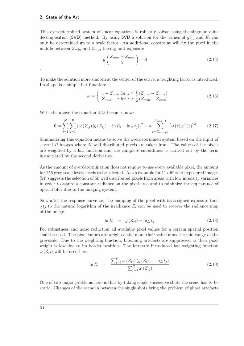
2. State of the Art
This overdetermined system of linear equations is robustly solved using the singular valuedecomposition (SVD) method. By using SVD a solution for the values of g ( ) and Ei canonly be determined up to a scale factor. An additional constraint will fix the pixel in themiddle between Zmin and Zmax having unit exposure
g
(Zmin + Zmax
2
)= 0 (2.15)
.
To make the solution more smooth at the center of the curve, a weighting factor is introduced.Its shape is a simple hat function:
ω ={
z − Zmin for z ≤ 12 (Zmin + Zmax)
Zmax − z for z > 12 (Zmin + Zmax)
(2.16)
With the above the equation 2.13 becomes now:
0 ≈N∑
i=1
P∑j=1
{ω (Zij) [g (Zij) − lnEi − lnΔ tj ]}2 + λ
Zmax−1∑z=Zmin+1
[ω (z) g′′ (z)
]2 (2.17)
Summarizing this equation means to solve the overdetermined system based on the input ofseveral P images where N well distributed pixels are taken from. The values of the pixelsare weighted by a hat function and the complete smoothness is carried out by the terminstantiated by the second derivative.
As the amount of overdetermination does not require to use every available pixel, the amountfor 256 grey scale levels needs to be selected. As an example for 11 different exposured images[54] suggests the selection of 50 well distributed pixels from areas with low intensity variancesin order to assure a constant radiance on the pixel area and to minimize the appearance ofoptical blur due to the imaging system.
Now after the response curve i.e. the mapping of the pixel with its assigned exposure timeΔtj to the natural logarithm of the irradiance Ei can be used to recover the radiance mapof the image.
lnEi = g (Zij) − lnΔ tj (2.18)
For robustness and noise reduction all available pixel values for a certain spatial positionshall be used. The pixel values are weighted the more their value aims the mid-range of thegreyscale. Due to the weighting function, blooming artefacts are suppressed as their pixelweight is low due to its border position. The formerly introduced hat weighting functionω (Zij) will be used here.
lnEi =
∑Pj=1 ω (Zij) (g (Zij) − lnΔ tj)∑P
j=1 ω (Zij)(2.19)
One of two major problems here is that by taking single successive shots the scene has to bestatic. Changes of the scene in between the single shots bring the problem of ghost artefacts
54

2.4. High Dynamic Range Increase
if objects move and occur at different positions in the images (like moving people or treeleaves do). One approach as presented in [55] tries to warp pixels for successive frames bydividing up the successive images into corresponding regions. For these corresponding regionthe homographies are calculated. This technique fails if the movements are too big betweenthe single shots. A more simple and reliable technique is described in [15]. The detectionof ghost is based on the fact that each single shot is self-consistent, which means that allinformation appear more or less in every image and that in regions of ghost the calculation ofpixel merged from different exposure is turned off and the image with the best quality in thatregion supplies the pixel. It is done by computing the variance based on a weighted averagefrom the already merged and low scaled image. Now all regions where the variance exceedsa threshold and area are defined as regions with a ghost. For these regions the substitutingoriginal data is taken individually from the best available single shot.
The second problem are the global movements of the camera system, which can be easilyaligned for translation by using a pyramidal approach to align the image from coarse to fineas suggested in [56]. Movement with complete 6 degree of freedom (DOF) can be done bycalculating the homography between the images.
So, more information of the real scene is stored in an image than before by a single shot fromthe camera. The new problem arising is how to display this information enhanced data, duenormal available displays like LCD/TFT have a maximum contrast ratio of 1 : 103, which ismuch lower than a contrast ratio of 1 : 106 as it occurs in the natural world. If a HDRI shall bedisplayed it needs to have a dynamic as much as the monitor can display and as distributedas the human eye can perceive. For that different tone mapping algorithms are suggested tokeep the stored information available for the human viewer [57], [58], [59]. These algorithmscan be divided up into fast global approaches and cost intensive local operators.
In figure 2.14 the content of the thesis is shown on a high abstraction level using a mindmap.The two aims of welding protection and observation form the two main branches. The greensub-branches emphasize the subjects beyond the State-of-the-Art. The new application ofSADF and by that the use of a GLCD has not been done yet. The problem of synchronizingthe camera onto the welding arc without depending on the welding machine or process hasnot been solved yet. All solutions used the measured voltage or are directly connected by wireto the welding machine [32]. The trigger drives the camera and a supporting miniaturizedlight sources like they are newly available by high power LEDs. The contrast enhancementfor an image where the most important information is stored in the minority of the pixels likethe welding arc, contradicts one of the most basic assumption that the image information isstored in the majority of occurring grey values. So here a deeper investigation is needed.
Figure 2.14.: Subjects of the thesis beyond the State-of-the-Art (with green background)
55

2. State of the Art
56

3IntARWeld system
In this chapter 3 the setup for achieving valuable high contrast welding images and the Se-lective Automatic Darkening Filter (SADF) system for the IntARWeld project, as introducedin chapter 1.4.3, is presented.
Figure 3.1.: Top-down approach for a SADF setup
The conceptual design of a SADF system can be built up by using a top-down approach wherethe view onto the system starts on the highest level of abstraction of the entire system. It goesdown to a finer granularity for modularizing to subsystems (see figure 3.1). This approachstarts by dividing the problem up into a sensing and actor unit for the glaring light detectionand view shading on the highest abstraction layer. A sensor needs to detect the position ofthe glaring lights from the welding process and the actor shades the corresponding point in
57

3. IntARWeld system
the welders view. By selecting a specific sensor, the sensing task needs to be split up into asensing hardware part and an algorithmic arc detection. As well as the view shading may besubdivided into a proper projective transformation from the glaring light detecting deviceto the shading device and the shading itself by a physical device. Choosing the devices byusing an high dynamic range camera for sensing and a graphical LCD (GLCD) for shading,other additional tasks have to be defined for a proper use of the hardware. The camerahardware needs a synchronization to the welding process and the glaring light detectionneeds the extraction of the glaring light. In order to know the constant transformationbetween the camera and users view through the GLCD, it is needed to calculate a proper apriori calibrated transformation. The transformation for compensation of the parallax erroris needed in every case as the camera cannot be in the same line of sight as the welderseyes.
For the welding observation of the IntARWeld system, a high dynamic grey scale camerais used. Two approaches to receive a good image are implemented. One approach usesthe sensed camera image and applies image enhancement techniques to make all availableinformation visible for the user. A second approach uses an alternating acquisition of imagestaken with different camera parameters. These are merged for the resulting image. Themerged image contains already an higher amount of information than displayable by standardmonitors and that is why a basic linear tone mapping operation is applied before displaying.Both approaches need a synchronization of the camera to the welding process if others thanMIG/MAG spray transfer arc or DC-TIG processes shall be recorded.
3.1. Image Acquisition
The image acquisition is related to the use of the FuGa1000 camera chip and its imple-mentation in the camera system as provided by the company Falldorf GmbH 1 (Bremen).However, the eight bit A/D converter used in the implementation and the so called rollingshutter cause problems which will be explained in the following sections.
3.1.1. High Dynamic Range Camera System
The selected Falldorf FuGa1000 camera does not directly supply the complete available dataas digital data. In a first step an offset is added to the analogue signal and amplified bytwo independent analogue amplifiers. The analogue signal is then converted by an 8 bitanalogue/digital converter (see figure 3.2). The range of the A/D converter is fixed to therange of 2 Volts. Pixel values which exceed this upper border are clipped to the maximumpixel value of 255 and pixels which undershoot due to the applied offset the value of 0 voltare clipped to the pixel value of zero.
1http://www.falldorfsensor.de/
58

3.1. Image Acquisition
The selection of the amplification and offset has to be chosen as a trade-off between goodstepping and covering the range of the pixel signals without clipping any important informa-tion to the pixel value of 255 (white) or 0 (black). This means if a high dynamic scene withits broad signal range will be amplified with an high analogue gain, then the upper voltagepixels containing the welding arc information may be clipped to the maximum digital valueof 255.The limitations of the A/D converter urge to adjust the camera parameters during weldingdepending on the image data. The offset is selected to have an overall pixel mean value ofthe image data of 128.
Lenses Another usually unconsidered issue is the fact that a high dynamic contrast rangecamera needs lenses which may be used for high contrast with high luminous flux. The lensesapplied for CCD or photographic film camera do not have to cope with such highly changingirradiances at once as their field of application does not contain such scenes.The boundary conditions for a typical CCD camera are
• a relative low lens contrast of maximum 1 : 103 or 60dB,
• no low intensities of light,
• an equal or smooth illumination in the image field,
• a system immanent linear response curve of the grey tone conversion.
The boundaries for a CCD camera application contradict the new field of high dynamiccontrast range cameras. The boundary conditions for the lenses change significantly as thecase of high dynamic contrast range the remaining stray light of the annealed glass can besensed by the camera. Especially by the glass to air surfaces or at the lens edges, reflectionsof the scene content are spread as ghost images over the acquired image. A CCD camerachip with its lower sensitivity does not sense these low lighted reflections but with a moresensitive high dynamic contrast range camera they are now sensed and by that visible in theacquired image. An improvement with less ghosts e.g from glaring light sources, is achievedby improving the design boundaries for the lenses. Minimizing the number of free-standinglenses, which minimizes the amount of glass air surfaces, causes less reflections. Maximum
Figure 3.2.: Signal diagram for a single pixel of the used Falldorf FuGa1000 camera
59

3. IntARWeld system
blackening and matting of all surfaces outside the optical path (e.g. lens holder and frames)as well as using high quality deflective back side coatings, does absorb prospective ghostsbefore reaching the camera chip [60]. In the IntARWeld system specialized lenses fromGevitec2 (Esslingen) of the type Gevilux are used. These lenses lens covers all the presentedboundaries for an high dynamic contrast scene.
3.1.2. Optical Camera Trigger
The used high dynamic C-MOS camera chip FuGa1000 from FillFactory3 reacts instantlyto the brightness changes during the welding process. This chip does not have an electronicglobal shutter which may freeze all pixel values before readout and by that maps the lightingconditions and scene view of a single moment. Instead of the global shutter this chip has aso called rolling shutter, which alternates in freezing one single line, does a readout of thisline before going further to the next line.
Figure 3.3.: Impulse Arc: 23 V,122 A, Gas with 82% Argon and 18% CO2, mild steel
Using an impulse or short circuit arc (as introduced in section 1.2) the brightness change ofthe process is a process immanent characteristic. During every pulse or short circuit the arcbecomes brighter and darker, up to a complete extinction of a short circuit arc. In figure 3.3and figure 3.4 the characteristic voltage Uw, current Iw and optical brightness signal Uopt
during the welding process for two different arc characteristics are shown. It can be seen thatthe impulse arc does not extinct but the short circuit arc does. The short circuit arc has aphase of complete darkness before it re-ignites while the pulsed process remains a minimumburning arc over time.
2http://www.gevitec.de/3The company Fillfactory from Belgium is now part of Cypress semiconductors
60
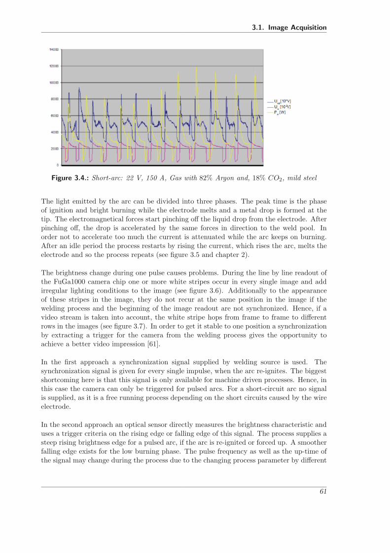
3.1. Image Acquisition
Figure 3.4.: Short-arc: 22 V, 150 A, Gas with 82% Argon and, 18% CO2, mild steel
The light emitted by the arc can be divided into three phases. The peak time is the phaseof ignition and bright burning while the electrode melts and a metal drop is formed at thetip. The electromagnetical forces start pinching off the liquid drop from the electrode. Afterpinching off, the drop is accelerated by the same forces in direction to the weld pool. Inorder not to accelerate too much the current is attenuated while the arc keeps on burning.After an idle period the process restarts by rising the current, which rises the arc, melts theelectrode and so the process repeats (see figure 3.5 and chapter 2).
The brightness change during one pulse causes problems. During the line by line readout ofthe FuGa1000 camera chip one or more white stripes occur in every single image and addirregular lighting conditions to the image (see figure 3.6). Additionally to the appearanceof these stripes in the image, they do not recur at the same position in the image if thewelding process and the beginning of the image readout are not synchronized. Hence, if avideo stream is taken into account, the white stripe hops from frame to frame to differentrows in the images (see figure 3.7). In order to get it stable to one position a synchronizationby extracting a trigger for the camera from the welding process gives the opportunity toachieve a better video impression [61].
In the first approach a synchronization signal supplied by welding source is used. Thesynchronization signal is given for every single impulse, when the arc re-ignites. The biggestshortcoming here is that this signal is only available for machine driven processes. Hence, inthis case the camera can only be triggered for pulsed arcs. For a short-circuit arc no signalis supplied, as it is a free running process depending on the short circuits caused by the wireelectrode.
In the second approach an optical sensor directly measures the brightness characteristic anduses a trigger criteria on the rising edge or falling edge of this signal. The process supplies asteep rising brightness edge for a pulsed arc, if the arc is re-ignited or forced up. A smootherfalling edge exists for the low burning phase. The pulse frequency as well as the up-time ofthe signal may change during the process due to the changing process parameter by different
61
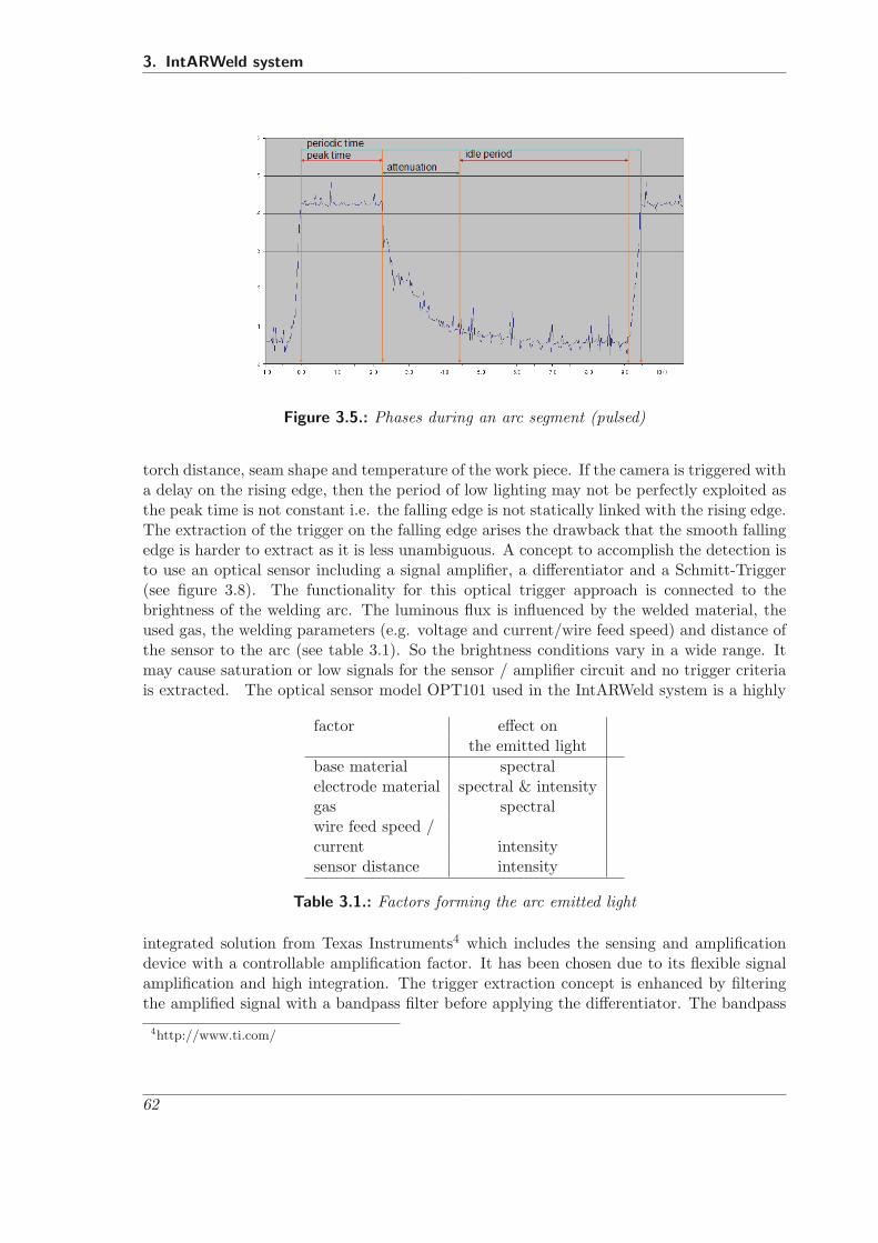
3. IntARWeld system
Figure 3.5.: Phases during an arc segment (pulsed)
torch distance, seam shape and temperature of the work piece. If the camera is triggered witha delay on the rising edge, then the period of low lighting may not be perfectly exploited asthe peak time is not constant i.e. the falling edge is not statically linked with the rising edge.The extraction of the trigger on the falling edge arises the drawback that the smooth fallingedge is harder to extract as it is less unambiguous. A concept to accomplish the detection isto use an optical sensor including a signal amplifier, a differentiator and a Schmitt-Trigger(see figure 3.8). The functionality for this optical trigger approach is connected to thebrightness of the welding arc. The luminous flux is influenced by the welded material, theused gas, the welding parameters (e.g. voltage and current/wire feed speed) and distance ofthe sensor to the arc (see table 3.1). So the brightness conditions vary in a wide range. Itmay cause saturation or low signals for the sensor / amplifier circuit and no trigger criteriais extracted. The optical sensor model OPT101 used in the IntARWeld system is a highly
factor effect onthe emitted light
base material spectralelectrode material spectral & intensitygas spectralwire feed speed /current intensitysensor distance intensity
Table 3.1.: Factors forming the arc emitted light
integrated solution from Texas Instruments4 which includes the sensing and amplificationdevice with a controllable amplification factor. It has been chosen due to its flexible signalamplification and high integration. The trigger extraction concept is enhanced by filteringthe amplified signal with a bandpass filter before applying the differentiator. The bandpass
4http://www.ti.com/
62

3.1. Image Acquisition
Figure 3.6.: White stripe in camera image caused by brightness change
Figure 3.7.: Sequence with hopping white stripe
of 28-4000 Hz is used to reject noise from electromagnetic distortions and suppress constant(DC) voltage components (see figure 3.9). A customized inverting Schmitt-Trigger maps thesignal to a rectangle logical signal with Uup = 4.1 V and Ulow = 3.3 V for the upper andlower boundary of the Schmitt Trigger hysteresis (see figure 3.10).
Beside the filtering of the signal from the optical sensor, its amplification factor is dynamicallyadjusted if no trigger signal is sensed. This may happen if either no welding is done or if theamplification of the optical sensor needs to be adjusted. An additional microcontroller (μC)is connected to the output of the Schmitt-Trigger. If no trigger signal is detected, then theμC produces a default trigger signal to avoid a freezing video. By the start of the defaulttrigger the amplification of the optical sensor (OPT101) is changed by the μC and a countdown is started. If now again no trigger signal is detected and the count down expires thenthe amplification of the sensor is changed again. If all values for the signal amplificationhave been set one after another the search restarts at the lowest value. But, if a trigger
Figure 3.8.: Simple optical trigger on the welding process
63

3. IntARWeld system
Figure 3.9.: a.) noisy signal from optical sensor, b.) bandpass filtered signal
Figure 3.10.: Schmitt-Trigger signal of optical sensor signal
64

3.1. Image Acquisition
is detected due to the new amplification factor, then the countdown is reset every time atrigger occurs and the amplification is not changed (see figure 3.11).
Figure 3.11.: Sensor amplification control
3.1.3. Active LED Lighting
In order to enhance the abilities of the camera system, the image acquisition is augmentedwith an active illumination part. High power LEDs flash the process scene and by thatreduce the occurring contrast dynamic of the scene by lighting significantly the low lightedregions. The contrast dynamic d of a scene is the ratio between the darkest areas with itsradiance Edark and the brightest area Ebright. If additional light is added with the amountEadd then the contrast ratio changes to:
dadd =Ebright + Eadd
Edark + Eadd(3.1)
For the welding scene it can be assumed that the arc as the brightest spot has no reflectivity,so that the equation simplifies to:
dadd =Ebright
Edark + Eadd(3.2)
Accordingly the contrast dynamic characteristic changes depending on the light reflectionof the surface. An example how the contrast dynamic changes if additional reflected lightis added to the scene is given for Edark = 10 lux and Ebright = 107 lux. In figure 3.12 thecontrast ratio of a scene is shown as a function of the added light Eadd. It shows that thecontrast ratio may be lowered by one order of magnitude or 20 dB from 1 : 106 to 1 : 105 ifthe irradiance of the darkest area is enhanced with 90 lux of reflected light.
65
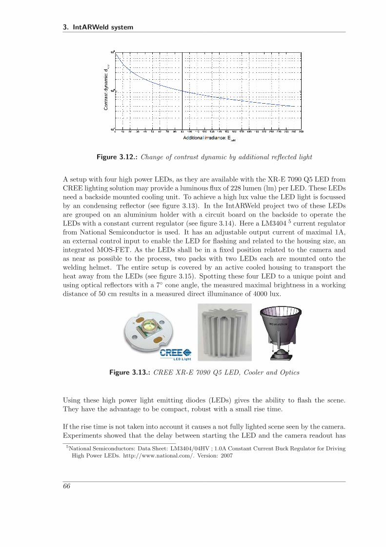
3. IntARWeld system
Figure 3.12.: Change of contrast dynamic by additional reflected light
A setup with four high power LEDs, as they are available with the XR-E 7090 Q5 LED fromCREE lighting solution may provide a luminous flux of 228 lumen (lm) per LED. These LEDsneed a backside mounted cooling unit. To achieve a high lux value the LED light is focussedby an condensing reflector (see figure 3.13). In the IntARWeld project two of these LEDsare grouped on an aluminium holder with a circuit board on the backside to operate theLEDs with a constant current regulator (see figure 3.14). Here a LM3404 5 current regulatorfrom National Semiconductor is used. It has an adjustable output current of maximal 1A,an external control input to enable the LED for flashing and related to the housing size, anintegrated MOS-FET. As the LEDs shall be in a fixed position related to the camera andas near as possible to the process, two packs with two LEDs each are mounted onto thewelding helmet. The entire setup is covered by an active cooled housing to transport theheat away from the LEDs (see figure 3.15). Spotting these four LED to a unique point andusing optical reflectors with a 7◦ cone angle, the measured maximal brightness in a workingdistance of 50 cm results in a measured direct illuminance of 4000 lux.
Figure 3.13.: CREE XR-E 7090 Q5 LED, Cooler and Optics
Using these high power light emitting diodes (LEDs) gives the ability to flash the scene.They have the advantage to be compact, robust with a small rise time.
If the rise time is not taken into account it causes a not fully lighted scene seen by the camera.Experiments showed that the delay between starting the LED and the camera readout has
5National Semiconductors: Data Sheet: LM3404/04HV ; 1.0A Constant Current Buck Regulator for DrivingHigh Power LEDs. http://www.national.com/. Version: 2007
66

3.1. Image Acquisition
Figure 3.14.: Lighting unit with two CREE Q5 LEDs
Figure 3.15.: Mounting four CREE Q5 LEDs with active cooled housing on a welding helmet
67

3. IntARWeld system
Figure 3.16.: Rise-time of the CREE Q5 setup
to be 16μs for the used setup with the Cree XR-E 7090 Q5 LEDs and a constant currentregulator LM3404. In figure 3.16 can be seen the delay between the input signal and theLED start-up.
Figure 3.17.: Setup for measuring the delay between the triggersignal and the first line read-out
In the moment of extinction or during the low burning phase of the impulse arc, the leastappearing brightness difference and consequently contrast ratio is available in the scene. Bytriggering the camera and LEDs on this low contrast phase, this moment can be used toacquire an image with less hard mapping boundaries for the used camera. If done so, thisratio can be minimized twice: Firstly by the active lighting and secondly by the right cameratrigger.
The camera readout-time depends on the pixel resolution selected on the chip. For a singlepixel using a FuGa1000 chip driven with 25 MHz the readout time of 40 ns is needed. So thereadout time for a single image with a resolution of 300x400 Pixel is accumulated to 4.8ms.This read-out does not include the transfer from the camera chip via the ethernet stack tothe computer. The bottleneck here is the ethernet interface with its upper limit of 100 MBit
68
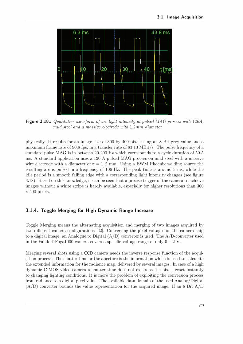
3.1. Image Acquisition
Figure 3.18.: Qualitative waveform of arc light intensity at pulsed MAG process with 120A,mild steel and a massive electrode with 1.2mm diameter
physically. It results for an image size of 300 by 400 pixel using an 8 Bit grey value and amaximum frame rate of 90,8 fps, in a transfer rate of 83,13 MBit/s. The pulse frequency of astandard pulse MAG is in between 20-200 Hz which corresponds to a cycle duration of 50-5ms. A standard application uses a 120 A pulsed MAG process on mild steel with a massivewire electrode with a diameter of ∅ = 1, 2 mm. Using a EWM Phoenix welding source theresulting arc is pulsed in a frequency of 106 Hz. The peak time is around 3 ms, while theidle period is a smooth falling edge with a corresponding light intensity changes (see figure3.18). Based on this knowledge, it can be seen that a precise trigger of the camera to achieveimages without a white stripe is hardly available, especially for higher resolutions than 300x 400 pixels.
3.1.4. Toggle Merging for High Dynamic Range Increase
Toggle Merging means the alternating acquisition and merging of two images acquired bytwo different camera configurations [62]. Converting the pixel voltages on the camera chipto a digital image, an Analogue to Digital (A/D) converter is used. The A/D-converter usedin the Falldorf Fuga1000 camera covers a specific voltage range of only 0 − 2 V.
Merging several shots using a CCD camera needs the inverse response function of the acqui-sition process. The shutter time or the aperture is the information which is used to calculatethe extended information for the radiance map, delivered by several images. In case of a highdynamic C-MOS video camera a shutter time does not exists as the pixels react instantlyto changing lighting conditions. It is more the problem of exploiting the conversion processfrom radiance to a digital pixel value. The available data domain of the used Analog/Digital(A/D) converter bounds the value representation for the acquired image. If an 8 Bit A/D
69

3. IntARWeld system
converter is used, the huge contrast ratio of 1 : 106 is mapped to only 28 = 256 grey levelsfor the pixel value.Between the light sensitive pixel and the A/D converter an offset control and amplifier ad-justs the output of the pixel to the input range of the A/D converter (see figure 3.2).
Figure 3.19.: Histogram clipping by saturation of A/D converter
If the highest voltages delivered by the brightest pixels exceed the upper input range of theA/D-converter
(UA/Dmax
), then these values saturate the digital output to its maximum
value. In case of an 8 Bit A/D converter the values are saturated to 255 (see figure 3.19).
Figure 3.20.: Histogram clipping for dark pixels
In order to cover the complete range of voltages delivered by the pixels, a gain factor andoffset can be chosen in order not to exceed the limits of the A/D converter. In this case thescenery will be mostly mapped to much less than 256 grey values.To increase the amount of available pixel range for maximising the available informationin the image, is the idea to compose an image by merging two acquisitions. The firstmeasurement covers the low voltages while saturating the upper pixel voltages. The secondmeasurement with an offset subtraction converts the higher voltages while too low values areclipped to zero. In order to distinguish the pixel values from the first measurement to thesecond measurement the formerly subtracted voltage has to be re-added as a digital offset(see figure 3.20).
By comparing the two measurements it can be clearly seen, that parts of the image infor-mation are complementary, so that the fusion of both image result in an image with moreinformation. The information exceeds the maximum of 255 because the negative offset wasre-added. Optimally the ranges of these two measurements do not overlap but are directlyneighboured. But if overlapping exists these mid-range areas with data from both imagesare fused by taking the mean i.e. average of both measurements I1 and I2 (see figure 3.21).The resulting image is calculated:
I ′ (u, v) =
⎧⎨⎩
I2 if I1 (u, v) = 255I1 + δpOffset if I2 (u, v) = 0I1+I2
2 else
(3.3)
70
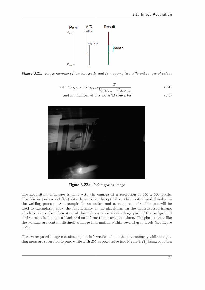
3.1. Image Acquisition
Figure 3.21.: Image merging of two images I1 and I2 mapping two different ranges of values
with δpOffset = UOffset2n
UA/Dmax− UA/Dmin
(3.4)
and n : number of bits for A/D converter (3.5)
Figure 3.22.: Underexposed image
The acquisition of images is done with the camera at a resolution of 450 x 600 pixels.The frames per second (fps) rate depends on the optical synchronization and thereby onthe welding process. An example for an under- and overexposed pair of images will beused to exemplarily show the functionality of the algorithm. In the underexposed image,which contains the information of the high radiance areas a huge part of the backgroundenvironment is clipped to black and no information is available there. The glaring areas likethe welding arc contain distinctive image information within several grey levels (see figure3.22).
The overexposed image contains explicit information about the environment, while the gla-ring areas are saturated to pure white with 255 as pixel value (see Figure 3.23) Using equation
71

3. IntARWeld system
Figure 3.23.: Overexposed image
Figure 3.24.: Composition from high (red), mid (green) and low (blue) radiance informationfrom images in figure 3.22 and figure 3.23
72
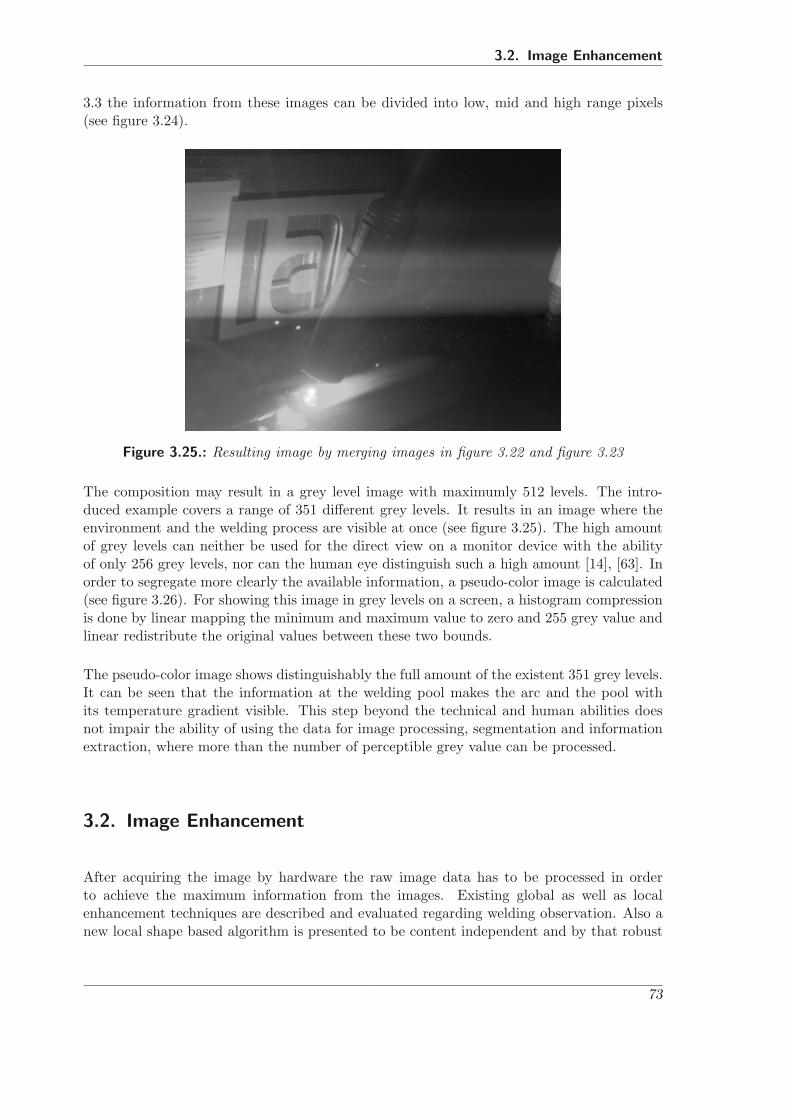
3.2. Image Enhancement
3.3 the information from these images can be divided into low, mid and high range pixels(see figure 3.24).
Figure 3.25.: Resulting image by merging images in figure 3.22 and figure 3.23
The composition may result in a grey level image with maximumly 512 levels. The intro-duced example covers a range of 351 different grey levels. It results in an image where theenvironment and the welding process are visible at once (see figure 3.25). The high amountof grey levels can neither be used for the direct view on a monitor device with the abilityof only 256 grey levels, nor can the human eye distinguish such a high amount [14], [63]. Inorder to segregate more clearly the available information, a pseudo-color image is calculated(see figure 3.26). For showing this image in grey levels on a screen, a histogram compressionis done by linear mapping the minimum and maximum value to zero and 255 grey value andlinear redistribute the original values between these two bounds.
The pseudo-color image shows distinguishably the full amount of the existent 351 grey levels.It can be seen that the information at the welding pool makes the arc and the pool withits temperature gradient visible. This step beyond the technical and human abilities doesnot impair the ability of using the data for image processing, segmentation and informationextraction, where more than the number of perceptible grey value can be processed.
3.2. Image Enhancement
After acquiring the image by hardware the raw image data has to be processed in orderto achieve the maximum information from the images. Existing global as well as localenhancement techniques are described and evaluated regarding welding observation. Also anew local shape based algorithm is presented to be content independent and by that robust
73
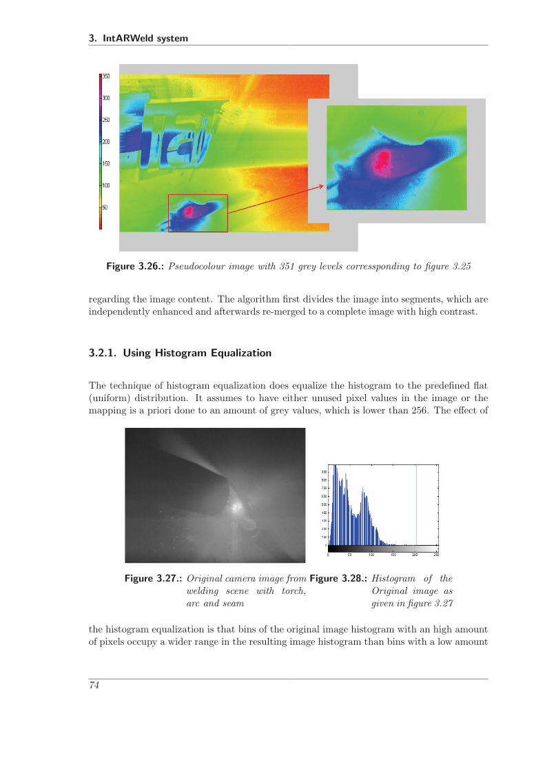
3. IntARWeld system
Figure 3.26.: Pseudocolour image with 351 grey levels corressponding to figure 3.25
regarding the image content. The algorithm first divides the image into segments, which areindependently enhanced and afterwards re-merged to a complete image with high contrast.
3.2.1. Using Histogram Equalization
The technique of histogram equalization does equalize the histogram to the predefined flat(uniform) distribution. It assumes to have either unused pixel values in the image or themapping is a priori done to an amount of grey values, which is lower than 256. The effect of
Figure 3.27.: Original camera image fromwelding scene with torch,arc and seam
Figure 3.28.: Histogram of theOriginal image asgiven in figure 3.27
the histogram equalization is that bins of the original image histogram with an high amountof pixels occupy a wider range in the resulting image histogram than bins with a low amount
74

3.2. Image Enhancement
of pixels. This reciprocally proportional distribution does depend on the amount of freeunused grey values and number of bins in the destination image histogram [14].
Figure 3.29.: (top) Resulting grey level images of Histogram Equalization for 8, 16, 32 and256 different resulting bins. (bottom) Corresponding histograms
An example of the histogram equalization applied to the original image in figure 3.27 is givenin figure 3.29 for 8, 16, 32 and 256 bins in the resulting image histogram.It can be seen that the higher the number of destination bins is, the more similar is thequalitative shape of the resulting histogram related to the original image. Also it can beseen that the higher the amount of pixels in a bin is, the wider is the distance to theneighboured bin. It is the basic assumption of histogram equalization that bins with an highamount of pixels contain an high amount of information. For welding the special problemoccurs, that the high specific information of the welding arc is contained in bins with smallamounts of pixels. These very bright bins are mostly automatically merged to one bin andtheir assigned width in the histogram is narrow in contrast to the huge background pixelwhich are not merged and mapped to a wider bin. Hence, the global histogram equalizationis not useful for image enhancement related to welding observation.
3.2.2. Using Grey Level Grouping
Grey-Level Grouping (GLG) tries to overcome the drawback of classical global histogramequalization by realigning the used histogram bins to the available number of grey values. Itdoes not change the interregional information in the sense of smaller and larger grey valuesof two pixels in the entire image. The basic GLG techniques enumerates the used grey valuesinto bins or so called groups. One after another, it merges the bin with the smallest amountof pixels with its smallest direct neighbour. The borders of the groups are updated andthe number of groups are equally distributed by assigning each group a constant division ofthe entire grey scale. If a group was composed by merging different grey levels, then thesegrey levels are un-grouped and equally distributed over the available division. The resulting
75
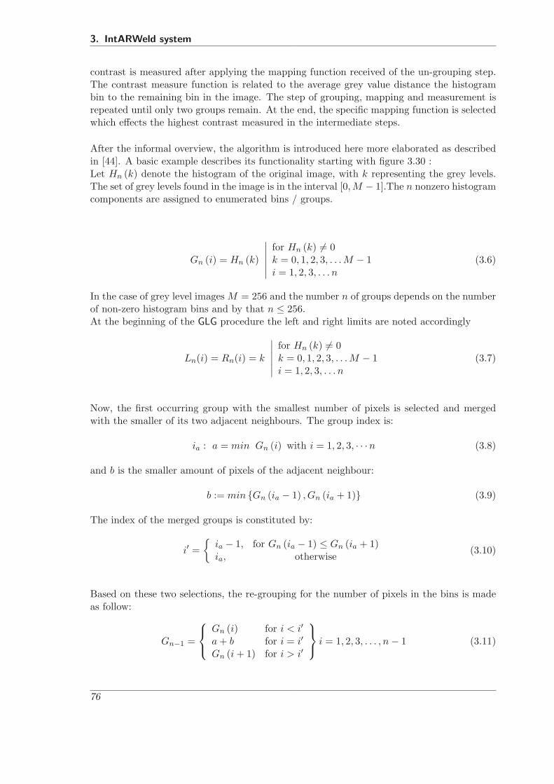
3. IntARWeld system
contrast is measured after applying the mapping function received of the un-grouping step.The contrast measure function is related to the average grey value distance the histogrambin to the remaining bin in the image. The step of grouping, mapping and measurement isrepeated until only two groups remain. At the end, the specific mapping function is selectedwhich effects the highest contrast measured in the intermediate steps.
After the informal overview, the algorithm is introduced here more elaborated as describedin [44]. A basic example describes its functionality starting with figure 3.30 :Let Hn (k) denote the histogram of the original image, with k representing the grey levels.The set of grey levels found in the image is in the interval [0, M − 1].The n nonzero histogramcomponents are assigned to enumerated bins / groups.
Gn (i) = Hn (k)
∣∣∣∣∣∣for Hn (k) �= 0k = 0, 1, 2, 3, . . . M − 1i = 1, 2, 3, . . . n
(3.6)
In the case of grey level images M = 256 and the number n of groups depends on the numberof non-zero histogram bins and by that n ≤ 256.At the beginning of the GLG procedure the left and right limits are noted accordingly
Ln(i) = Rn(i) = k
∣∣∣∣∣∣for Hn (k) �= 0k = 0, 1, 2, 3, . . . M − 1i = 1, 2, 3, . . . n
(3.7)
Now, the first occurring group with the smallest number of pixels is selected and mergedwith the smaller of its two adjacent neighbours. The group index is:
ia : a = min Gn (i) with i = 1, 2, 3, · · ·n (3.8)
and b is the smaller amount of pixels of the adjacent neighbour:
b := min {Gn (ia − 1) , Gn (ia + 1)} (3.9)
The index of the merged groups is constituted by:
i′ ={
ia − 1, for Gn (ia − 1) ≤ Gn (ia + 1)ia, otherwise
(3.10)
Based on these two selections, the re-grouping for the number of pixels in the bins is madeas follow:
Gn−1 =
⎧⎨⎩
Gn (i) for i < i′
a + b for i = i′
Gn (i + 1) for i > i′
⎫⎬⎭ i = 1, 2, 3, . . . , n − 1 (3.11)
76

3.2. Image Enhancement
Figure 3.30.: Histogram example for the grouping and ungrouping process
The respective group related limits are updated by:
Ln−1 ={
Ln (i) for i ≤ i′
Ln (i + 1) for i > i′
}i = 1, 2, 3, . . . , n − 1 (3.12)
Rn−1 ={
Rn (i) for i < i′
Rn (i + 1) for i ≥ i′
}i = 1, 2, 3, . . . , n − 1 (3.13)
An example histogram with 5 initial groups is given in figure 3.30. Group G5 (2) is mergedwith G5 (3) and results in the successive step to group G4 (2). The updated border to L4 andR4 is shown in table 3.2
Group G5 (1) G5 (2) G5 (3) G5 (4) G5 (5)Number of pixels 400 100 100 300 600Left border, L5 1 3 4 5 7Right border, R5 1 3 4 5 7New groupingGroup G4 (1) G4 (2) G4 (3) G4 (4)Number of pixels 400 200 300 600Left borders, L4 1 3 5 7Right border R4 1 4 5 7
Table 3.2.: Groups and borders of the example given in figure 3.30
Next, the calculation of the contrast is performed. For that the consolidated bins are ungrou-ped by linearly redistributing the grey levels within the average section available for a bin.The resulting transformation function Tn−1 (k) will be applied to the image and the resultingcontrast is measured. Every bin will occupy an average number of Nn−1 grey levels as theproportion of the available number of grey values divided by the number of used bins.
Nn−1 =M − 1n − 1
(3.14)
The background, which is the first bin of the lowest grey level, may occupy many grey levelalthough only one grey level is assigned to it Ln−1 (1) = Rn−1 (1). In that case to prevent
77

3. IntARWeld system
this occupation the first bin is mapped to 0 and an heuristic alignment is introduced forNn−1:
Nn−1 =M − 1
n − 1 − α| with α ≈ 0.8 (3.15)
The first group of the example fulffills the condition of identical values of the left and rightborder. So the α will be considered in the calculation of the ungrouping and mapping for thegreyscale transformation.
While constructing the transformation function Tn−1 (k) four different cases have to be consi-dered:
1. The grey level k falls inside a grey level bin Gn−1 (i) which is attached to more thanone grey level with Ln−1 (1) �= Rn−1 (1). So the grey level k as a part of the bin islinearly re-mapped to the section assigned to the bin using the equation 3.16. Thisequation is split into the two cases of a monovalued background bin and the generalcase as introduced:
Tn−1 (k) =
⎧⎨⎩
(i − α − Rn−1(i)−k
Rn−1(i)−Ln−1(i)
)Nn−1 + 1, for Ln−1 (1) = Rn−1 (1)(
i − Rn−1(i)−kRn−1(i)−Ln−1(i)
)Nn−1 + 1, for Ln−1 (1) �= Rn−1 (1)
(3.16)
If the bin occupies only one grey value then the transformation differentiate betweena background group o and others
Tn−1 (k) ={
(i − α) Nn−1, for Ln−1 (1) = Rn−1 (1)iNn−1, for Ln−1 (1) �= Rn−1 (1) with i > 1
(3.17)
2. If the grey level k falls between two grey level bins Gn−1 (i) and Gn−1 (i + 1), sothat this grey level is not used in the image, then for the sake of completeness, itstransformation function is identical to equation 3.17. This ensures that Tn−1 (k) ismonotonically increasing.
3. The grey level k is below the lowest used grey level bin, then it is mapped to zero
If k ≤ L1 (1) , then Tn−1 (k) = 0 (3.18)
4. The grey level k is above the highest used grey level bin, then it is mapped to thehighest grey value:
If k ≥ Rn−1 (1) , then Tn−1 (k) = M − 1 (3.19)
The resulting grey level transformation for the first and second grouping can be seen in figure3.31.
78

3.2. Image Enhancement
Figure 3.31.: Histogram after first grouping and ungrouping process
This constructed grey level transformation Tn−1 (k) needs to be stored for eventual lateruse. Its use depends on the resulting contrast which is calculated as the average distanceDn−1 between pixels on the grey scale for the entire image. The calculation is done bysumming up all products of available pairing of bins and weighting these pairing by theirgrey level distance. If a histogram transformation produces in the final rating of all Hn−1 (i)the maximum contrast, then this transformation will be selected as the final to achieve thebest result:
Dn−1 =1
Npix (Npix − 1)
M−2∑i=0
M−1∑j=i+1
Hn−1 (i) Hn−1 (j) (j − i) (3.20)
; |for i, j ∈ [0, M − 1] (3.21)
where Npix is the total number of pixels in the image.
Now the process continues just after the first binning, by searching the bin with the smallestamount of pixels and merge it with its smallest adjacent neighbour. Then ungroup everythingby constructing the transformation function Tn−2 and calculate the contrast Dn−2. Continueby binning the residual bins, ungroup, calculate contrast....until only two bins/groups areleft. At the end the transformation is selected for the best image transformation with thehighest average pixel distance.
In figure 3.32 the result for different selected transformation is given. The original imagestarts with 206 occurring grey values and by that 206 groups. The contrast measure is shownin figure 3.33. The algorithm starts with the maximum number of groups which is here 206groups. Then the number of groups is decreased by merging two neighboured groups andthe contrast is measured again until a minimum amount of groups is reached As it can beseen the lower bound was set to a minimum of two groups. After merging and contrastmeasure the grouping and its transformation /mapping function is selected which results inthe highest contrast. The example supplies the highest contrast measure for 102 groups.
79

3. IntARWeld system
Figure 3.32.: Mapping for a different amount of selected groups
Figure 3.33.: Contrast measure for different amount of groups
80
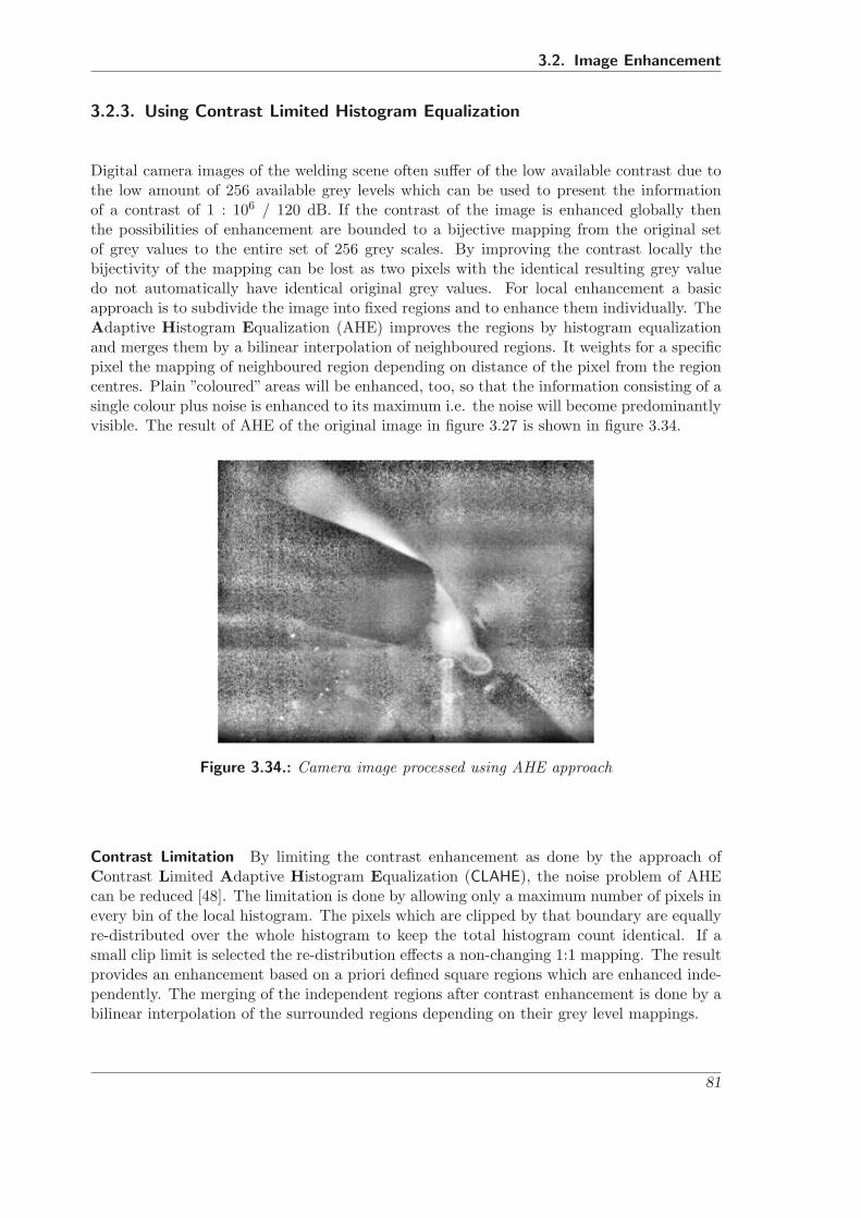
3.2. Image Enhancement
3.2.3. Using Contrast Limited Histogram Equalization
Digital camera images of the welding scene often suffer of the low available contrast due tothe low amount of 256 available grey levels which can be used to present the informationof a contrast of 1 : 106 / 120 dB. If the contrast of the image is enhanced globally thenthe possibilities of enhancement are bounded to a bijective mapping from the original setof grey values to the entire set of 256 grey scales. By improving the contrast locally thebijectivity of the mapping can be lost as two pixels with the identical resulting grey valuedo not automatically have identical original grey values. For local enhancement a basicapproach is to subdivide the image into fixed regions and to enhance them individually. TheAdaptive Histogram Equalization (AHE) improves the regions by histogram equalizationand merges them by a bilinear interpolation of neighboured regions. It weights for a specificpixel the mapping of neighboured region depending on distance of the pixel from the regioncentres. Plain ”coloured” areas will be enhanced, too, so that the information consisting of asingle colour plus noise is enhanced to its maximum i.e. the noise will become predominantlyvisible. The result of AHE of the original image in figure 3.27 is shown in figure 3.34.
Figure 3.34.: Camera image processed using AHE approach
Contrast Limitation By limiting the contrast enhancement as done by the approach ofContrast Limited Adaptive Histogram Equalization (CLAHE), the noise problem of AHEcan be reduced [48]. The limitation is done by allowing only a maximum number of pixels inevery bin of the local histogram. The pixels which are clipped by that boundary are equallyre-distributed over the whole histogram to keep the total histogram count identical. If asmall clip limit is selected the re-distribution effects a non-changing 1:1 mapping. The resultprovides an enhancement based on a priori defined square regions which are enhanced inde-pendently. The merging of the independent regions after contrast enhancement is done by abilinear interpolation of the surrounded regions depending on their grey level mappings.
81

3. IntARWeld system
Figure 3.35.: Bilinear merging of contextual regions A, B, C, D
Let the grey level mappings of the contextual regions {A, B, C, D} be denoted as gA(p),gB(p), gC(p) and gD(p). Each region has a center point named with the regions letter(see figure 3.35). The distance between two horizontal or vertical neighboured region isnormalized to one. The new grey level value p′ of the pixel p is calculated by weightedsum of the surrounding mappings. The weighting is done based on the portion of the pixeldistance to the center of the contextual regions (see equation 3.22).
p′ (u, v) = (1 − y) ((1 − x) gA (p) + x gB (p)) + y ((1 − x) gC (p) + x gD (p)) (3.22)
Figure 3.36.: Camera image with an 8x8 gridof tiles (red lines)
Figure 3.37.: Camera image processed by theCLAHE algorithm
In figure 3.36 the grid for the squared tiles is sketched with red lines. The grid approachcauses artefacts in the resulting image in figure 3.37, where new horizontal and vertical softlines can be seen in between the tile borders. This algorithm keeps plain areas plain, butimproves where image information is available (see figure 3.37). The predefined size andshape of the contextual regions does not consider the content of the image. Hence, it is notrobust for different image scenes as the achieved contrast enhancement differs for differentobject size.
82

3.2. Image Enhancement
Figure 3.38.: Noise supression in the image processing queue using a Wiener Filter
Adaptive Wiener Filter Filtering the time relevant Gaussian noise by an optimal filternamed by its author Wiener filter, as suggested in [50], can improve the content of a signal byminimizing the noise. This filter can be used in the image processing queue as a preparativestep before using the CLAHE algorithm as shown in figure 3.38).
Wiener approached the problem to be a least square minimization problem. Assuming adistortion model of the camera image being the sum of the signal s (u, v) plus additive noisen (u, v):
i (u, v) = s (u, v) + n (u, v) (3.23)
The Wiener filter can be understood in the frequency domain as a filter H (ωx, ωy) whichrestores the image I (ωx, ωy) to the original data I ′ (ωu, ωv) without noise:
i (u, v) � � I (ωu, ωv) (3.24)I ′ (ωu, ωv) = H (ωu, ωv) I (ωu, ωv) (3.25)
The filter H (ωu, ωv) can be choosen so that the error function E [ ] is minimized:
min ( E [S (ωu, ωv) − H (ωu, ωv) I (ωu, ωv)] ) (3.26)
The Wiener filter function for a two dimensional case can be stated using the power spec-trum Ps (ωu, ωv) of the signal representing the image and power spectrum of the noisePn (ωu, ωv):
H (ωu, ωv) =Ps (ωu, ωv)
Ps (ωu, ωv) + Pn (ωu, ωv)(3.27)
The power spectrum of the image is assumed to be globally constant over the entire image.An improved version applicable to image processing is the Adaptive Wiener Filter, whichdoes not use a fixed filter for the entire image [64], [65]. But here no proper informationabout the local noise is available, so that the assumption of a constant global noise is used.The power spectrum of the noise Pn is widely assumed as white noise with zero mean mn = 0,so that it simplifies down to the constant of variance Pn = σ2
n. If now locally the signal canbe modelled by a white noise process w (u, v) independent of the distortion with its ownmean ms(u, v) and variance σs(u, v), then it can be modelled as:
f (u, v) = ms (u, v) + σs (u, v) w (u, v) (3.28)
83
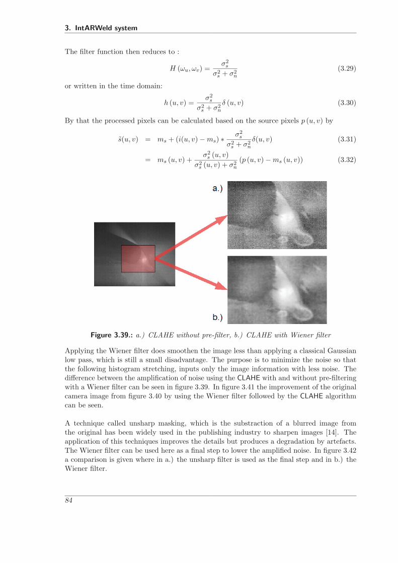
3. IntARWeld system
The filter function then reduces to :
H (ωu, ωv) =σ2
s
σ2s + σ2
n
(3.29)
or written in the time domain:
h (u, v) =σ2
s
σ2s + σ2
n
δ (u, v) (3.30)
By that the processed pixels can be calculated based on the source pixels p (u, v) by
s(u, v) = ms + (i(u, v) − ms) ∗ σ2s
σ2s + σ2
n
δ(u, v) (3.31)
= ms (u, v) +σ2
s (u, v)σ2
s (u, v) + σ2n
(p (u, v) − ms (u, v)) (3.32)
Figure 3.39.: a.) CLAHE without pre-filter, b.) CLAHE with Wiener filter
Applying the Wiener filter does smoothen the image less than applying a classical Gaussianlow pass, which is still a small disadvantage. The purpose is to minimize the noise so thatthe following histogram stretching, inputs only the image information with less noise. Thedifference between the amplification of noise using the CLAHE with and without pre-filteringwith a Wiener filter can be seen in figure 3.39. In figure 3.41 the improvement of the originalcamera image from figure 3.40 by using the Wiener filter followed by the CLAHE algorithmcan be seen.
A technique called unsharp masking, which is the substraction of a blurred image fromthe original has been widely used in the publishing industry to sharpen images [14]. Theapplication of this techniques improves the details but produces a degradation by artefacts.The Wiener filter can be used here as a final step to lower the amplified noise. In figure 3.42a comparison is given where in a.) the unsharp filter is used as the final step and in b.) theWiener filter.
84
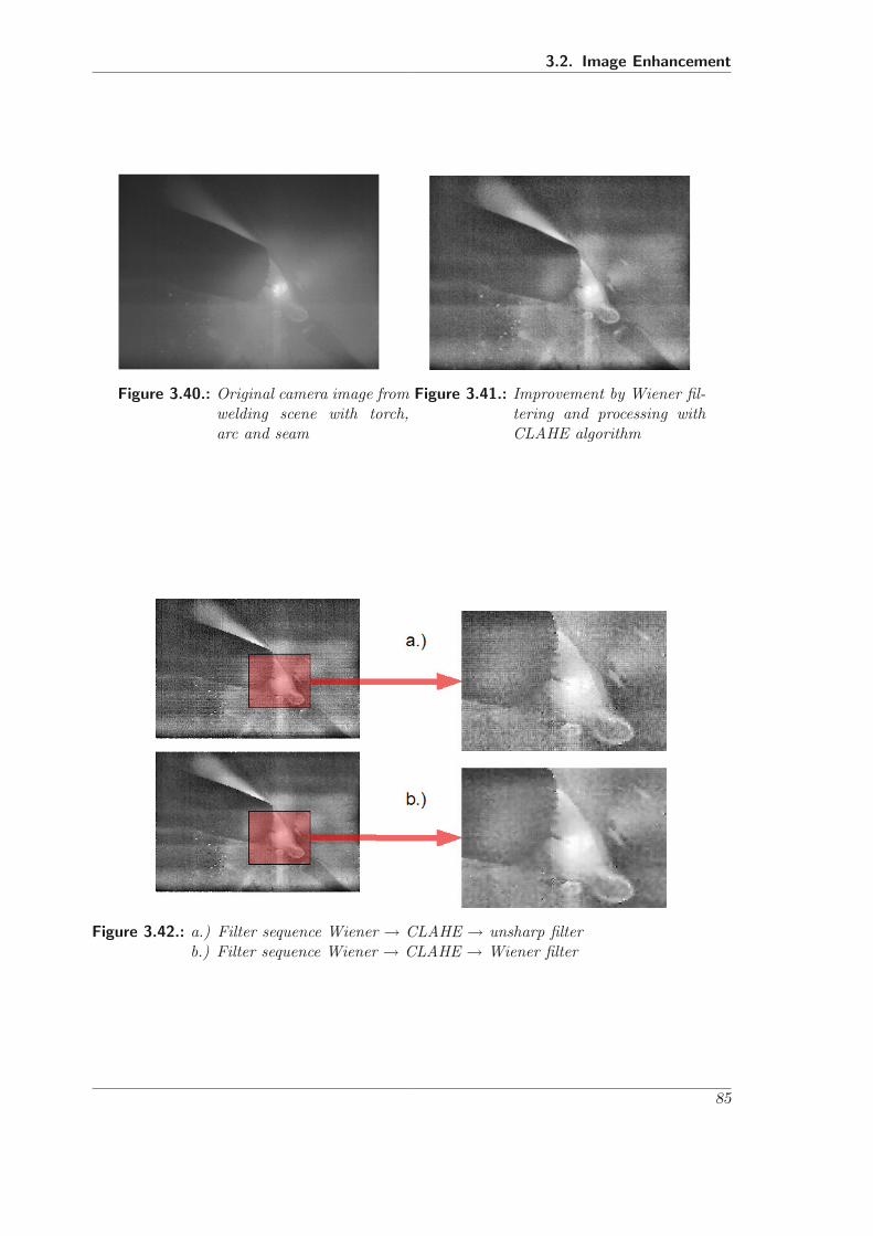
3.2. Image Enhancement
Figure 3.40.: Original camera image fromwelding scene with torch,arc and seam
Figure 3.41.: Improvement by Wiener fil-tering and processing withCLAHE algorithm
Figure 3.42.: a.) Filter sequence Wiener → CLAHE → unsharp filterb.) Filter sequence Wiener → CLAHE → Wiener filter
85

3. IntARWeld system
3.2.4. Variable Block Shape Adaptive Histogram Equalization
The Variable Block Shape Adaptive Histogram Equalization (VBSAHE) [66] is developedin this thesis as an improvement of the classical CLAHE algorithm. As said, the CLAHEalgorithm enhances independently a predefined number of n × m tiles of a tiled originalimage, which are consolidated by an interpolation process. The area and the shape of thetiles are fixed so that the content of the image does not allow an individual subdivision ofthe image. By abolishing the fixed size and shape by a concept with segments depending onthe content with individual size and shape, the enhancement does not statically depend onthe a priori selection of n × m tiles.
The basic mathematical concept of the VBSAHE is to compute for every pixel an assignedconvergence point where the probability density function attains its maximum in a featurespace i.e. mode of the probability density function (PDF). The feature space consists ofthe position and pixel value so that in the case of a grey image, a probability functionis calculated for the feature space given by the row, column and grey value of the pixel.The feature space can be clustered into regions by searching the local maxima, where thegradient of the PDF is zero, for the starting position x1. Now all starting points/ pixels whichconverge to similar local maxima are clustered together. Clustering the pixels into segmentsis done by using a flood fill approach where all modes which deviate from an initially setboundary are clustered together with their corresponding pixels. The retrieved segments areindividually enhanced and in a succeeding step the re-composition to a complete image isdone (see figure 3.43).
Figure 3.43.: Basic Variable Block Shape Adaptive Histogram Equalization setup
So the Mean Shift algorithm does segment the image based on a statistical approach for afeature space. The Mean Shift states, that it points in the direction of the gradient of thePDF. For the feature space the position and the value of a pixel can be used, whereby thevalue can be one of the various available colour spaces like greyscale, RGB, HSV, L∗u∗v∗
depending on the application. For a deeper understanding the reader is recommended to anintroduction to colour spaces and colour image processing as given in [67].The Mean Shift is defined as the difference with respect to the local mean E ( ) regardingthe proximity
{Δ
X}
at the position x [53].
m (x) = EΔ
�X (x) − x (3.33)
86

3.2. Image Enhancement
The question that arises is wether the mean shift vector converges from a starting point toa local maximum. If we regard the feature space to be described by an empirical densityfunction of the represented parameters, then the PDF can be estimated by a kernel densityestimation, as well known as Parzen window techniques.
Kernel Density Estimator An image gives n data points xi with i = 1, . . . , n in a d-dimensional feature space Rd. As introduced the dimension of the feature consists of thelocation (row, column) of the pixel and the used colour space (grey, RGB, HSV etc.). Themultivariate density estimator is given by
f (x) =1n
n∑i=1
KH (x − xi) . (3.34)
Where KH uses a kernel function K (Δx) like the Gaussian or Epanechnikov kernel to weightthe input data depending on its difference Δx = x − xi.
KH (Δx) = |H|−1/2 K(H−1/2
Δx)
(3.35)
While H is a symmetric positive definite d × d bandwidth matrix. The scalar result ofequation 3.34 gives the probability density at the point x of the feature space. The numberof n data points may include all available data as given by an entire image but the kerneltruncates to points in the proximity Δ
X of x. The weighting of the dimensions and theirinteraction for the density estimation is configured by the bandwidth matrix H. It scalesthe input data so that by up- or down scaling of the input data a smaller or wider regionis covered by the kernel function K ( ). This matrix H can be simplified by choosing asa constant diagonal matrix with the bandwidth factor h. This simplification does equallyweight the dimensions of the feature space:
H = h2 I | where I is the identity matrix (3.36)
=
⎡⎢⎢⎢⎢⎢⎣
h2
h2 0h2
0. . .
h2
⎤⎥⎥⎥⎥⎥⎦ (3.37)
= diag(h2)
(3.38)
The d-variate symmetric kernel K (Δx) is a bounded function which integrates to 1:∫Rd
K (Δx) dΔx = 1 (3.39)
is symmetrical with every positive value being compensated by its negative counterpart:∫Rd
Δx K (Δx) dΔx = 0 (3.40)
and has finite support by infinite values multiplied with the kernel value result to zero:
limΔx→∞ ‖Δx‖K (Δx) = 0 (3.41)
87

3. IntARWeld system
Using the density estimator given by equation 3.34 with the simplified bandwidth matrix Hfrom equation 3.36 leads to:
f (x) =1
nhd
n∑i=1
K
(x − xi
h
)(3.42)
Which gives the result of the kernel density estimator at the position x using the entire data(of the image) by xi.
For image processing, a radial symmetric kernel is mostly produced by using a profile functionk(r2)
with r ≥ 0 as the euclidian distance r = ‖Δx‖ from the origin. A normalizationconstant ck multiplied with k
(r2)
norms the integration of the function to one as demandedby the boundary conditions of equation 3.39 - 3.41.
K (Δx) = ck k(‖Δx‖2
)(3.43)
As a profile the Epanechnikov profile is often used for the kernel density estimation, as itoptimizes the mean integrated squared error [MISE] for the density estimation. This optimalcriteria is calculated as the expectation value E () for the difference between the probabilitydensity f and the estimated density f .
E(∥∥∥f − f
∥∥∥) = E
∫ (f (x) − f (x)
)2dx (3.44)
Fulfilling the MISE optimum criteria give no assumption about the error distribution. It mayhappen that the error function has a peak at the maximum and by that a huge deviationbetween the estimated density and real value may occur at that point. This issue is notinvestigated in the research community up to now.
The Epanechnikov profile which minimizes the preceeding equation 3.44 is given by
kE
(‖Δx‖2
)={
1 − ‖Δx‖2 0 ≤ ‖x‖2 ≤ 10 else
(3.45)
Another advantage of the Epanechnikov profile is its limited expansion and the fact thatit does not need to be cut off like a normal (Gaussian) profile with its infinite support. Infigure 3.44 the Epanechnikov profile is zero at the border of the kernel, instead of the normalGaussian kernel in figure 3.45 which is unequal to zero at the border of the kernel matrix(see figure 3.44 - 3.45).
The density estimator in equation 3.42 can be written with the Epanechnikov profile as
fh,K (x) =ck
nhd
n∑i=1
kE
(∥∥∥∥x − xi
h
∥∥∥∥2)
(3.46)
After setting up the kernel estimation, the next step is to find the gradient of the estimatedPDF with the aim to calculate the maxima where the gradient equals zero.
88
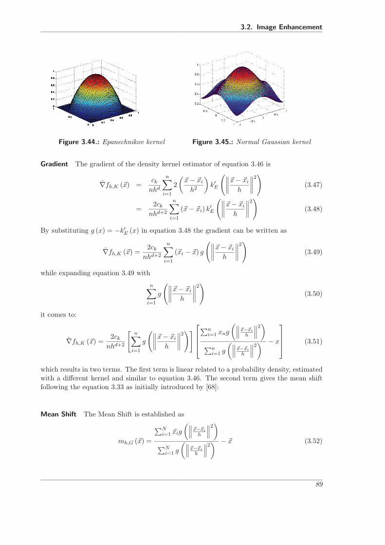
3.2. Image Enhancement
Figure 3.44.: Epanechnikov kernel Figure 3.45.: Normal Gaussian kernel
Gradient The gradient of the density kernel estimator of equation 3.46 is
∇fh,K (x) =ck
nhd
n∑i=1
2(
x − xi
h2
)k′
E
(∥∥∥∥x − xi
h
∥∥∥∥2)
(3.47)
=2ck
nhd+2
n∑i=1
(x − xi) k′E
(∥∥∥∥x − xi
h
∥∥∥∥2)
(3.48)
By substituting g (x) = −k′E (x) in equation 3.48 the gradient can be written as
∇fh,K (x) =2ck
nhd+2
n∑i=1
(xi − x) g
(∥∥∥∥x − xi
h
∥∥∥∥2)
(3.49)
while expanding equation 3.49 with
n∑i=1
g
(∥∥∥∥x − xi
h
∥∥∥∥2)
(3.50)
it comes to:
∇fh,K (x) =2ck
nhd+2
[n∑
i=1
g
(∥∥∥∥x − xi
h
∥∥∥∥2)]⎡⎢⎢⎣
∑ni=1 xng
(∥∥∥�x−�xih
∥∥∥2)
∑ni=1 g
(∥∥∥�x−�xih
∥∥∥2) − x
⎤⎥⎥⎦ (3.51)
which results in two terms. The first term is linear related to a probability density, estimatedwith a different kernel and similar to equation 3.46. The second term gives the mean shiftfollowing the equation 3.33 as initially introduced by [68]:
Mean Shift The Mean Shift is established as
mh,G (x) =
∑Ni=1 xig
(∥∥∥�x−�xih
∥∥∥2)
∑Ni=1 g
(∥∥∥�x−�xih
∥∥∥2) − x (3.52)
89
3. IntARWeld system
The Mean Shift uses a kernel profile g (x). To recall the kernel profile kE (x) in equation3.45 results in scalar values as it is a simplification due to the Epanechnikov kernel.The first term of equation 3.51 can be seen as corresponding to a kernel density estimatorfh,G (x). If so, then the kernel
G (x) = cg g (x) (3.53)
needs to fulfil the condition of a bounded symmetrical function with finite supports as statedin equations 3.39.
The proof that the mean shift points in the direction of the local density maximum can begiven by reinserting the density estimator fh,G (x) and the mean shift mh,G(�x)in equation3.51:
∇fh,K (x) =2ck
h2cg
cg
nhd
n∑i=1
g
(∥∥∥∥x − xi
h
∥∥∥∥2)
mh,G(�x) (3.54)
= fh,G (x)2ck
h2cgmh,G(�x) (3.55)
�→ mh,G(�x) =12h2c
∇fh,K (x)
fh,G (x)(3.56)
It can be seen that the mean shift points in the direction of the density gradient and soin the direction of the maximum increase of the density. The step size is controlled by thePDF in the denominator. Regions with low density are not of interest for the feature spaceanalysis. Nearby local maxima with high densities in the proximity refine the step size ofthe mean shift and by that the Mean Shift is an adaptive gradient ascent method.
Up to here it is described that the Mean Shift leads from a starting point to the densitymaximum or so called mode with a zero gradient. If all neighboured starting points whichlead to the similar modes are clustered to a segment, then the segmentation of the image isdone. A simple floodfill algorithm is used starting at the upper left corner and clustering allconnected pixel in the neighbourhood within the colour distance cd related to the startingpixel xi.The segments can be defined by
Si ={xn ∈ Sl
∣∣∣ ‖xi − xn‖ ≤ cd, xi ∈ Rd}
(3.57)
In figure 3.47 the mean shift algorithm is applied to the original camera image from figure3.27. The pixel values of the resulting image show the grey value of the assigned maximumand by that give only one dimension of the 3D feature space consisting of the pixel positionu and v plus the grey value. It can be seen that the mean shift algorithm is edge preservingfor object larger than the used bandwith of 16 pixel.
In figure 3.48 a segmentation of figure 3.47 is done using the floodfill algorithm to cluster thepixels. Here it has to be mentioned that the number of segments can be controlled choosingdifferent colour distances. Segments with a minimum number of pixels smaller than 50 aremerged to the nearest mode.
90

3.2. Image Enhancement
Figure 3.46.: Original camera imageidentical to figure 3.27
Figure 3.47.: Mean shift applied to figure3.46
Figure 3.48.: Floodfill clustering of figure 3.47 with colour distance cd = 20
91

3. IntARWeld system
The Mean Shift algorithm is computational costly but robust, as it clusters the data basedon its statistical occurrence of a multidimensional feature vector and by that is based on theimage content.
Enhancing the Segmented Image After segmenting the image using the non-parametricadaptive gradient ascent method Mean Shift, the segments are individually enhanced by acontrast limited histogram equalization as it is used in the CLAHE (section 3.2.3). For everysegment with the mode at position xn an individual histogram mapping function si,�xn () iscalculated which maps the original pixel value to a new one. The contrast limitation avoidsthe amplification of noise in flat areas which contain low information, as mentioned in section3.2.1.
Interpolation After the individual enhancement of the segments, they need to be reunitedto a new image. As known from the CLAHE section 3.2.3, an interpolation process is neededto avoid rough edges between the segments. The CLAHE uses an interpolation scheme basedon the distance of the pixel to the three nearest neighboured tiles (see figure 3.35). As thetiles are replaced by segments, which are individual in shape and size, this approach will fail.In this thesis it is suggested to use a kernel based approach, where the mapping function fora pixel is a weighted sum of the surrounding histogram mapping functions of segments. Theproximity can be weighted by a kernel function such as radial kernels based on the normal(Gaussian) or Epanechnikov profile.
Let the image I consist of a set of positions X = {x |x ∈ I } and the assigned pixel valuesp (x).After segmentation the image consists of k ∈ N segments
S = {S1, S2, . . . , Sk} (3.58)
and the set of segments includes all positions of the image X =⋃k
i=1 Si.
For a pixel value p at position x = (u, v) ∈ Si, i ∈ {1 . . . k}, a histogram mapping functionsi(p) is surjectively assigned for this position.
p (u, v) = si (p (u, v)) (3.59)
so that si,�xn () designates the assigned histogram mapping function at position xn.
To avoid harsh edges due to the segments border a new interpolation approach is used.The new improved and interpolated pixel value p (u, v) for the composed image is calculatedby an interpolation of the histogram mapping functions in the kernel bounded proximity
ΔX (x) ={
xm| |xm − xn|2 ≤ ε}
.
92

3.2. Image Enhancement
Analogously to the kernel density estimator a radial kernel (such as Epanechnikov, normalor unit kernel) with its centre at the position x0 (u0, v0) is used.The weighting value at the position xn with the kernel at position x0 is given by
K (x0, xn) = ck,dk
(∥∥∥∥x0 − xn
h
∥∥∥∥2)
(3.60)
The new pixel value pi (x0) is interpolated as a weighted sum depending on the distance andthe participating histogram mapping functions si,�xn for the proximity positions xn.
p (x0) =ck,d
N hD
N∑n=1
si,�xn (p (x0)) k
(∥∥∥∥x0 − xn
h
∥∥∥∥2)
(3.61)
The summation in equation 3.61 is influenced only by the limited amount of different histo-gram mapping functions and the weighting kernel K ( ).
Figure 3.49.: Interpolating the pixel value by histogram mapping functions of the proximity
An example is given in figure 3.49 with three participating segments S1, S2 and S3. Thekernel is a radial kernel with the diameter of 2R pixels. The new pixel value for p (x0)iscalculated as:
p1 (x0) =ck,d
3 · 4R2
⎛⎝ ∑
∀xn∈S1
s1 (p1 (x0)) k
(∥∥∥∥x0 − xn
2R
∥∥∥∥2)
(3.62)
+∑
∀xn∈S2
s2 (p1 (x0)) k
(∥∥∥∥x0 − xn
2R
∥∥∥∥2)
(3.63)
+∑
∀xn∈S3
s3 (p1 (x0)) k
(∥∥∥∥x0 − xn
2R
∥∥∥∥2)⎞⎠ (3.64)
93
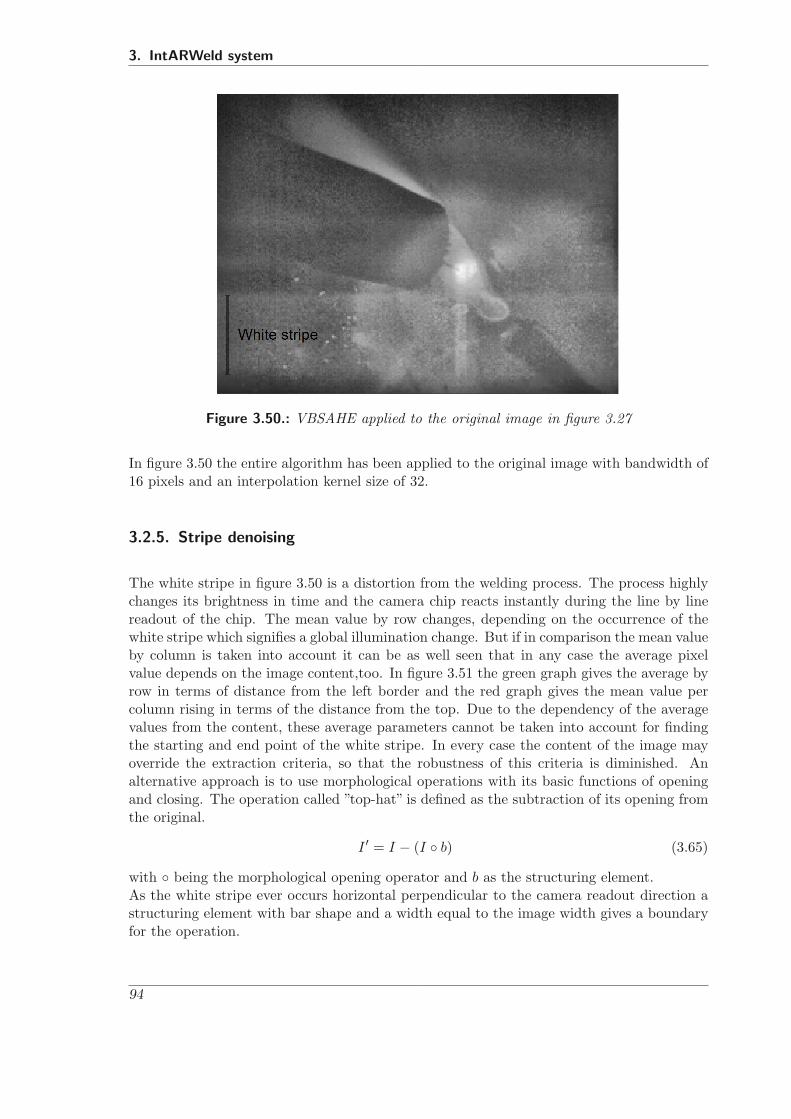
3. IntARWeld system
Figure 3.50.: VBSAHE applied to the original image in figure 3.27
In figure 3.50 the entire algorithm has been applied to the original image with bandwidth of16 pixels and an interpolation kernel size of 32.
3.2.5. Stripe denoising
The white stripe in figure 3.50 is a distortion from the welding process. The process highlychanges its brightness in time and the camera chip reacts instantly during the line by linereadout of the chip. The mean value by row changes, depending on the occurrence of thewhite stripe which signifies a global illumination change. But if in comparison the mean valueby column is taken into account it can be as well seen that in any case the average pixelvalue depends on the image content,too. In figure 3.51 the green graph gives the average byrow in terms of distance from the left border and the red graph gives the mean value percolumn rising in terms of the distance from the top. Due to the dependency of the averagevalues from the content, these average parameters cannot be taken into account for findingthe starting and end point of the white stripe. In every case the content of the image mayoverride the extraction criteria, so that the robustness of this criteria is diminished. Analternative approach is to use morphological operations with its basic functions of openingand closing. The operation called ”top-hat” is defined as the subtraction of its opening fromthe original.
I ′ = I − (I ◦ b) (3.65)
with ◦ being the morphological opening operator and b as the structuring element.As the white stripe ever occurs horizontal perpendicular to the camera readout direction astructuring element with bar shape and a width equal to the image width gives a boundaryfor the operation.
94

3.3. Selective Automatic Darkening Filter
Figure 3.51.: Mean value by row and column as the distance from left or from the top of theimage
Tests done with different height structuring elements effect in different amount of minimizingthe white stripe (see figure 3.52). For a resolution of 600×450 pixel the best result is achievedby using the height of 40 pixel for the structuring element. This filtering can be applied beforeenhancing any contrast so that the white stripes -meaning distortion- will not be amplifiedby contrast enhancement algorithms for welding observation.
3.3. Selective Automatic Darkening Filter
The aim of the SADF is to darken the users view where glaring lights occur. A graphicalliquide crystal display (GLCD) is mounted in front of the users eyes. Those pixels of the GLCDshall be darkened, which cover the users line of sight to a glaring light. The sensor for such asystem needs to extract the 3D position of the glaring light and the transformation from thecamera coordinate system to the users view needs to be known. The system consisting ofthe users eye and the GLCD may be modelled as a second camera system. The plane of theGLCD can be seen as the image plane where the extracted glaring light position is mapped.So if the position of the glaring light on the GLCD is known then the position of the pixel tobe darkened is identical.
The GLCD and a camera is integrated in a welding helmet. In figure 3.53 the setup of thesystem is shown. The GLCD substitutes the Automatic Darkening filter with its single pixel.The electronic for the GLCD is situated in the area nearby the welders chin. The camera issplit into two pieces. One is the pure camera chip with the lense and second the interfacingelectronic device, which is integrated in a housing under the top shell of the helmet.
95
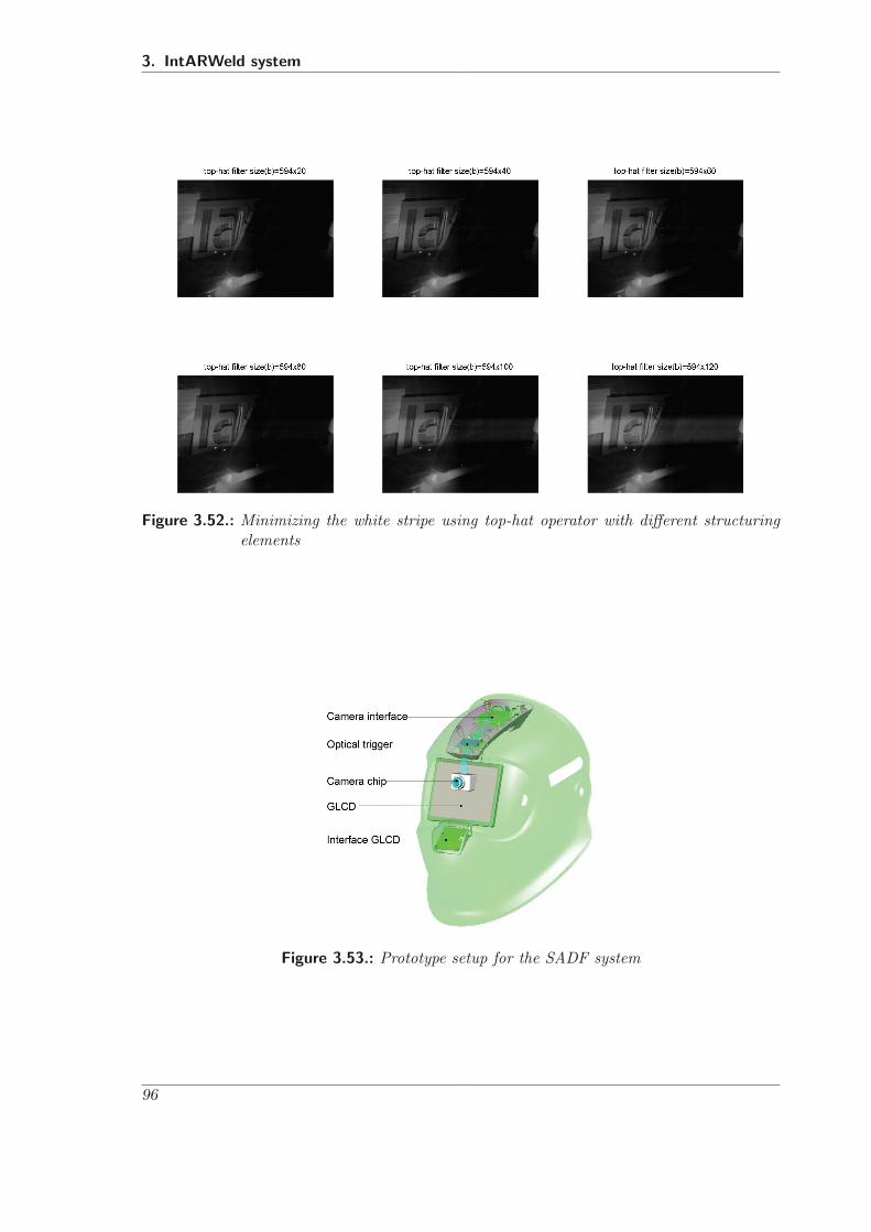
3. IntARWeld system
Figure 3.52.: Minimizing the white stripe using top-hat operator with different structuringelements
Figure 3.53.: Prototype setup for the SADF system
96
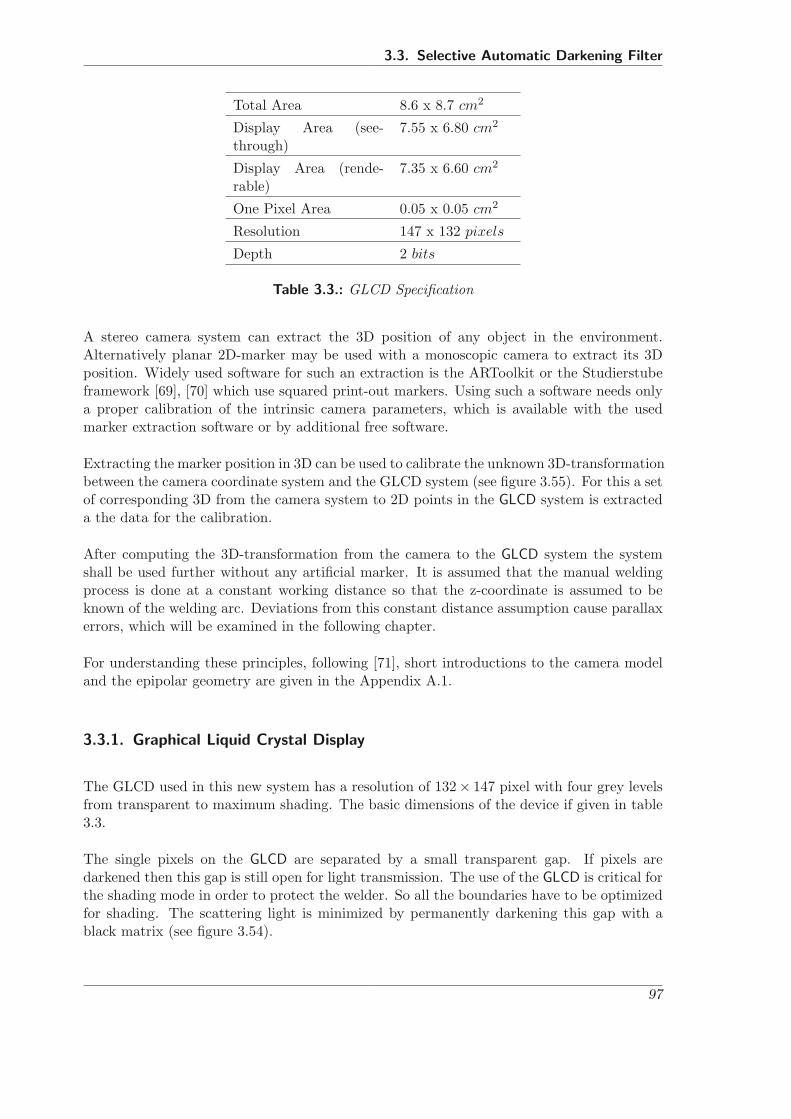
3.3. Selective Automatic Darkening Filter
Total Area 8.6 x 8.7 cm2
Display Area (see-through)
7.55 x 6.80 cm2
Display Area (rende-rable)
7.35 x 6.60 cm2
One Pixel Area 0.05 x 0.05 cm2
Resolution 147 x 132 pixels
Depth 2 bits
Table 3.3.: GLCD Specification
A stereo camera system can extract the 3D position of any object in the environment.Alternatively planar 2D-marker may be used with a monoscopic camera to extract its 3Dposition. Widely used software for such an extraction is the ARToolkit or the Studierstubeframework [69], [70] which use squared print-out markers. Using such a software needs onlya proper calibration of the intrinsic camera parameters, which is available with the usedmarker extraction software or by additional free software.
Extracting the marker position in 3D can be used to calibrate the unknown 3D-transformationbetween the camera coordinate system and the GLCD system (see figure 3.55). For this a setof corresponding 3D from the camera system to 2D points in the GLCD system is extracteda the data for the calibration.
After computing the 3D-transformation from the camera to the GLCD system the systemshall be used further without any artificial marker. It is assumed that the manual weldingprocess is done at a constant working distance so that the z-coordinate is assumed to beknown of the welding arc. Deviations from this constant distance assumption cause parallaxerrors, which will be examined in the following chapter.
For understanding these principles, following [71], short introductions to the camera modeland the epipolar geometry are given in the Appendix A.1.
3.3.1. Graphical Liquid Crystal Display
The GLCD used in this new system has a resolution of 132× 147 pixel with four grey levelsfrom transparent to maximum shading. The basic dimensions of the device if given in table3.3.
The single pixels on the GLCD are separated by a small transparent gap. If pixels aredarkened then this gap is still open for light transmission. The use of the GLCD is critical forthe shading mode in order to protect the welder. So all the boundaries have to be optimizedfor shading. The scattering light is minimized by permanently darkening this gap with ablack matrix (see figure 3.54).
97

3. IntARWeld system
Figure 3.54.: Black matrix on the GLCD to minimize the scattering light
Measurement without any controller attached to this GLCD result in a shading equivalentto a protection level of 7.8 which corresponds to 0.0085% transmission. If a controller isused which sets the pixel by alternating through every row and column, then the shadingis getting less to a protection level of 4.2 which corresponds to a light transmission rate of0.8% and a protection level for the transparent mode of 2.6 which corresponds to a lighttransmission of 29%.
3.3.2. Calibration of a GLCD to the Camera
The system of the GLCD with the user’s eye behind form a system similar to a camera. TheGLCD form the image plane and together with the eye the lens system and camera center isdefined. In figure 3.55 the principal setup of such a system is shown. It consists of a camerasystem with the optical axis nearby the users optical axis to achieve a similar viewport sothat the parallax error is as minimal as possible.The calibration of the GLCD system to the camera is needed in order to darken the cameraextracted glaring light for the user on the GLCD.
The principle is to have the 3D Information of specific points in the camera coordinatesystem and to retrieve its 2D correspondence on the GLCD [72]. For that the user has towear the system on his head and to overlay a square or crosshair blended on the GLCD with apredefined point in 3D. The proper overlay is done by head movement of the user. With thecorrespondences of the 3D marker position and its 2D equivalent on the GLCD, the mappingof 3D points in the camera coordinates to the 2D points on the GLCD can be calculated.The 3D information can be supplied by a stereo-rig or, as it is done here, by using artificialmarkers [69]. The coordinate system of the 3D data points extracting device needs to betransformed by an euclidian transformation compounded by a rotation and translation.
This transformation will be covered by the calibration and needs to be done for the left andright eye independently. In figure 3.56 the setup with the different coordinate systems isshown.
98
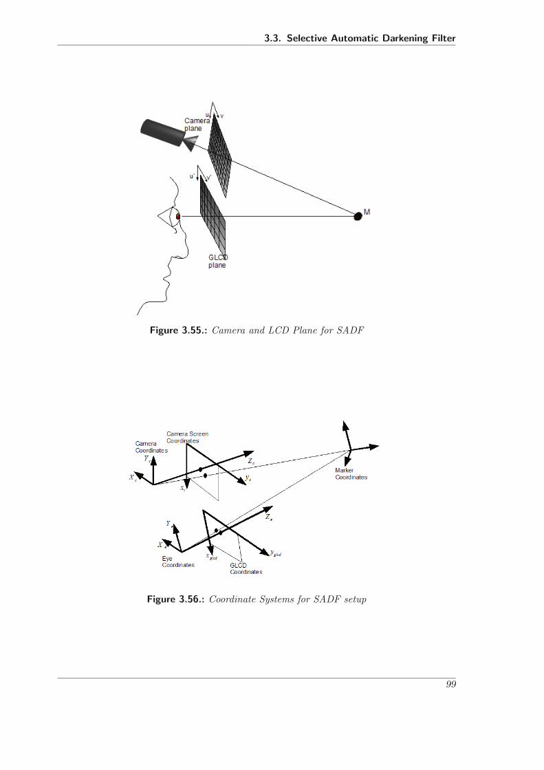
3.3. Selective Automatic Darkening Filter
Figure 3.55.: Camera and LCD Plane for SADF
Figure 3.56.: Coordinate Systems for SADF setup
99
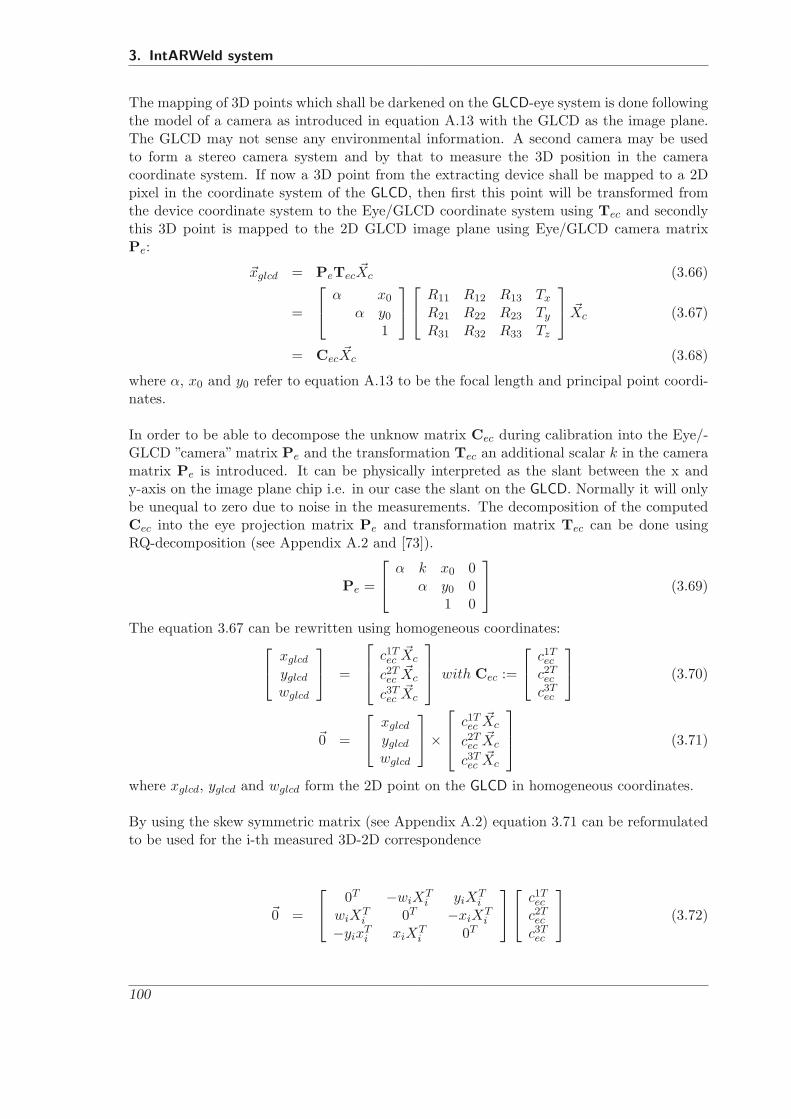
3. IntARWeld system
The mapping of 3D points which shall be darkened on the GLCD-eye system is done followingthe model of a camera as introduced in equation A.13 with the GLCD as the image plane.The GLCD may not sense any environmental information. A second camera may be usedto form a stereo camera system and by that to measure the 3D position in the cameracoordinate system. If now a 3D point from the extracting device shall be mapped to a 2Dpixel in the coordinate system of the GLCD, then first this point will be transformed fromthe device coordinate system to the Eye/GLCD coordinate system using Tec and secondlythis 3D point is mapped to the 2D GLCD image plane using Eye/GLCD camera matrixPe:
xglcd = PeTecXc (3.66)
=
⎡⎣ α x0
α y0
1
⎤⎦⎡⎣ R11 R12 R13 Tx
R21 R22 R23 Ty
R31 R32 R33 Tz
⎤⎦ Xc (3.67)
= CecXc (3.68)
where α, x0 and y0 refer to equation A.13 to be the focal length and principal point coordi-nates.
In order to be able to decompose the unknow matrix Cec during calibration into the Eye/-GLCD ”camera” matrix Pe and the transformation Tec an additional scalar k in the cameramatrix Pe is introduced. It can be physically interpreted as the slant between the x andy-axis on the image plane chip i.e. in our case the slant on the GLCD. Normally it will onlybe unequal to zero due to noise in the measurements. The decomposition of the computedCec into the eye projection matrix Pe and transformation matrix Tec can be done usingRQ-decomposition (see Appendix A.2 and [73]).
Pe =
⎡⎣ α k x0 0
α y0 01 0
⎤⎦ (3.69)
The equation 3.67 can be rewritten using homogeneous coordinates:⎡⎣ xglcd
yglcd
wglcd
⎤⎦ =
⎡⎢⎣ c1T
ecXc
c2Tec
Xc
c3Tec
Xc
⎤⎥⎦ with Cec :=
⎡⎣ c1T
ec
c2Tec
c3Tec
⎤⎦ (3.70)
0 =
⎡⎣ xglcd
yglcd
wglcd
⎤⎦×
⎡⎢⎣ c1T
ecXc
c2Tec
Xc
c3Tec
Xc
⎤⎥⎦ (3.71)
where xglcd, yglcd and wglcd form the 2D point on the GLCD in homogeneous coordinates.
By using the skew symmetric matrix (see Appendix A.2) equation 3.71 can be reformulatedto be used for the i-th measured 3D-2D correspondence
0 =
⎡⎣ 0T −wiX
Ti yiX
Ti
wiXTi 0T −xiX
Ti
−yixTi xiX
Ti 0T
⎤⎦⎡⎣ c1T
ec
c2Tec
c3Tec
⎤⎦ (3.72)
100

3.3. Selective Automatic Darkening Filter
The equation 3.72 forms a homogeneous linear system. A solution can be retrieved bystacking the first and second line for the measured n correspondences to a [2n × 12] matrix.This overdetermined system can be computed by using the singular value decomposition ofthe stacked matrix, where the unit singular vector v corresponding to the smallest singularvalue supplies the solution for cec.
cec =
⎡⎣ c1T
ec
c2Tec
c3Tec
⎤⎦ =
⎡⎢⎢⎢⎣
v1
v2...
v12
⎤⎥⎥⎥⎦ (3.73)
One problem which occurs while computing numerical solutions is the error of the solution.If the problem is ill-conditioned caused by the input data, the result implies raised errorsdue to rounding errors. The conditioning of the problem to be solved can be enhanced bynormalizing the input data using a scaling and translation to a new centroid with the origin0 and an average distance to the origin of
√2. The normalization T3D for the 3D point and
the transformation T2D for the 2D points are calculated independently. After calculatingthe solution Cec for the transformed data, the solution needs to be back transformed to Cec
by:Cec = TT−1
2D CecT3D (3.74)
Although the normalization is introduced at the end of the calibration it is an essential stepand must not be considered optional [71].After introducing the algorithmic part of the calibration the question arises how to implementit into a program and how a user will be prompted during calibration. If points in 3D andthe correspondent 2D points on the GLCD are measured then the solution for Cec can becalculated. The measurement can be done by actively requesting the user to do the followingtask repeatedly.
• On the GLCD a cross-hair will be shown at a random position and the user has toalign his head, and consequently the GLCD and camera, until the cross-hair seen byone eye covers the 3D point / marker.
• At the moment, when the 3D point and the cross-hair are aligned, the user presses abutton to save the 3D position of the point and its image in the camera view.
• The covering of the cross-hair with the marker is repeated for several times to receivesufficient correspondences between the camera image and the GLCD.
• The complete procedure is done once for each eye separately
After computing the calibration, the mapping of 3D points onto the GLCD plane is known.This means that in the application during welding the 3D position of the glaring lightwhich is the welding arc respectively, needs to be extracted. The welding arc has not theinformation like a planar ARToolkit marker has, so that only the pixel position on the cameraimage plane can be extracted. For simple application and according to that simple weldingsituations, it is assumed that the working distance between the welders eye and the torch is
101

3. IntARWeld system
fixed during welding. So that the 2D position can be used to calculate the 3D position underthe assumption of the constant working distance i.e. the z-coordinate. For more complexscenarios with changing working distances, a 3D tracking of the welding arc or torch isneeded.
102

4Results
This chapter presents the evaluation of three different aspects of the SADF system. Thefirst and most important section evaluates the performances of the different image enhance-ment algorithms as introduced in chapter 3. The global histogram equalization, grey-level-grouping, CLAHE and the new VBSAHE are evaluated for different welding processes. Thehigh dynamic range improvement by merging two different shots of the image is includedas well. The merging approach does not cover the subject of contrast enhancement like thepreceding algorithms. Its results is presented in relation to the additional extracted amountof data, which covers better the available grey scale space.
Secondly in this chapter the LED lighting is compared with different bright welding arcs forstandard welding processes to demonstrate the abilities of this setup. At last, a view is takenonto the SADF idea. Due to the lack of a GLCD, which darkens the arc sufficiently, only oneprocess, the MAG process, is used.
The evaluation of the different image processing algorithms focusses on the GMAW processeswith its subtypes of MAG and MIG welding. For these processes a range of three differentcurrents are considered. The result of the VBSAHE algorithm is rated for the different weldingcurrent. The comparison of the histogram equalization, the grey-level-grouping (GLG), theCLAHE and the VBSAHE algorithm is done for one common welding current.
In order to evaluate the LED lighting, records are done with the LEDs turned ”ON” and”OFF”. The image merging technique needs a toggling camera parameter setup for under-and overexposed images. The raw data consist of a video with images of the alternatingcamera setup. Hence, for each welding current three recordings are made to retrieve the rawdata for evaluation: LED on, LED off and the toggle video.
103
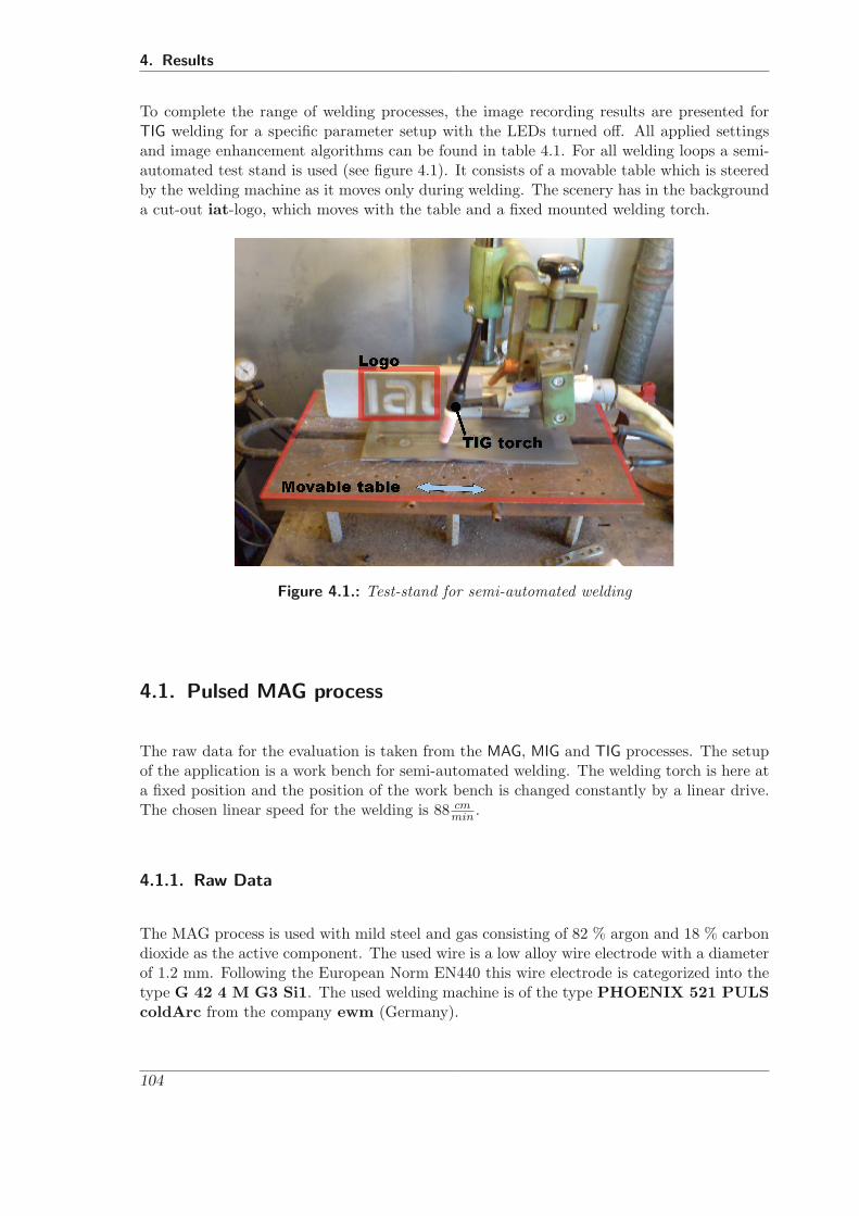
4. Results
To complete the range of welding processes, the image recording results are presented forTIG welding for a specific parameter setup with the LEDs turned off. All applied settingsand image enhancement algorithms can be found in table 4.1. For all welding loops a semi-automated test stand is used (see figure 4.1). It consists of a movable table which is steeredby the welding machine as it moves only during welding. The scenery has in the backgrounda cut-out iat-logo, which moves with the table and a fixed mounted welding torch.
Figure 4.1.: Test-stand for semi-automated welding
4.1. Pulsed MAG process
The raw data for the evaluation is taken from the MAG, MIG and TIG processes. The setupof the application is a work bench for semi-automated welding. The welding torch is here ata fixed position and the position of the work bench is changed constantly by a linear drive.The chosen linear speed for the welding is 88 cm
min .
4.1.1. Raw Data
The MAG process is used with mild steel and gas consisting of 82 % argon and 18 % carbondioxide as the active component. The used wire is a low alloy wire electrode with a diameterof 1.2 mm. Following the European Norm EN440 this wire electrode is categorized into thetype G 42 4 M G3 Si1. The used welding machine is of the type PHOENIX 521 PULScoldArc from the company ewm (Germany).
104

4.1. Pulsed MAG process
Lighting Process Current [A] AlgorithmLED Off MAG 85 VBSAHELED ON MAG 85 VBSAHEToggle MAG 85 ToggleMergeLED Off MAG 120 Histogram equ., GLG, CLAHE, VBSAHELED ON MAG 120 VBSAHEToggle MAG 120 ToggleMergeLED Off MAG 220 VBSAHELED ON MAG 220 VBSAHEToggle MAG 220 ToggleMergeLED Off MIG 80 VBSAHELED ON MIG 80 VBSAHEToggle MIG 80 ToggleMergeLED Off MIG 180 Histogram equ., GLG, CLAHE, VBSAHELED ON MIG 180 VBSAHEToggle MIG 180 ToggleMergeLED Off MIG 240 VBSAHELED ON MIG 240 VBSAHEToggle MIG 240 ToggleMergeLED Off TIG 230 Histogram equ., GLG, CLAHE, VBSAHE
Table 4.1.: Series of measurements to evaluate different image enhancement algorithms
Single images
Different welding currents of 85 A, 120 A and 220 A are selected in order to cover the midand upper range of occurring brightness conditions. The images taken at 85A differ in thelighting by the LEDs, which are focussed onto the boundary area around the welding arc.It can be seen in figure 4.2 and figure 4.3 that the difference with and without lighting issmall. Parts of the metal grid (B), the front edge of the metal plate (A) and the weldingtorch (C) are lighted by the LEDs . A difference with or without lighting by the LED canbe merely seen but will be made visible by the enhancement algorithms.
The brightness of the arc differs over a wide range from 1.5 · 103 Lux for 85 A over 2.4 · 103
Lux at 120 A up to 8.13 · 103 Lux at 220 (see table 4.2). The measurement is done at adistance of 1 m at the height level of the welding torch and can be rated only as a qualitativevalue as it depends on the physical setup of the work bench, welding torch inclination anddistance to the work piece. Differences caused by the LED lighting remain visible for thewelding arc with 120 A and 220 A but get less the higher the arc current is (see figure 4.4 -4.7).
As it can be seen, the white stripes on the images, which are caused by the instant brightnesschanges in connection with the rolling shutter of the used FuGa1000 camera chip, occurmore often in the case of higher currents used. They depend on the pulse frequency of the
105
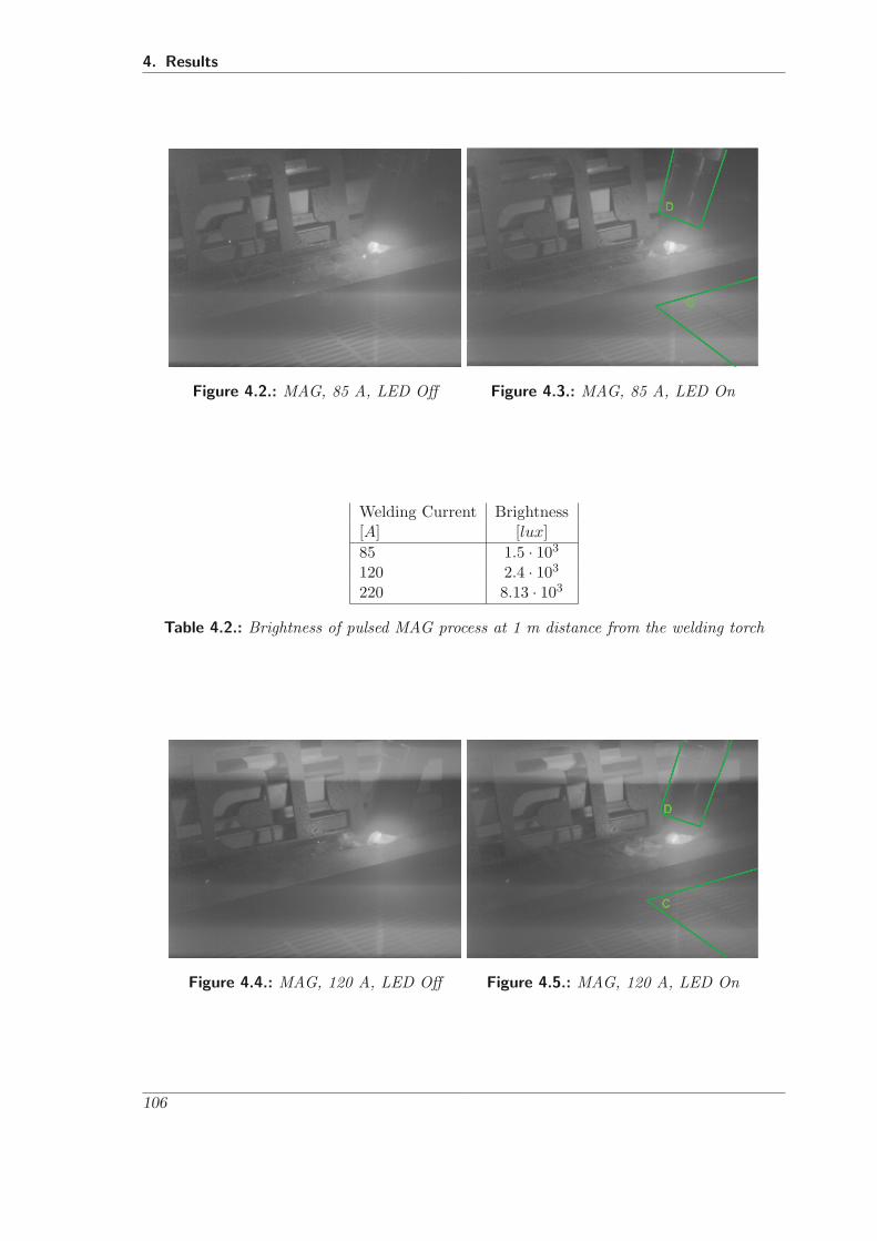
4. Results
Figure 4.2.: MAG, 85 A, LED Off Figure 4.3.: MAG, 85 A, LED On
Welding Current Brightness[A] [lux]85 1.5 · 103
120 2.4 · 103
220 8.13 · 103
Table 4.2.: Brightness of pulsed MAG process at 1 m distance from the welding torch
Figure 4.4.: MAG, 120 A, LED Off Figure 4.5.: MAG, 120 A, LED On
106
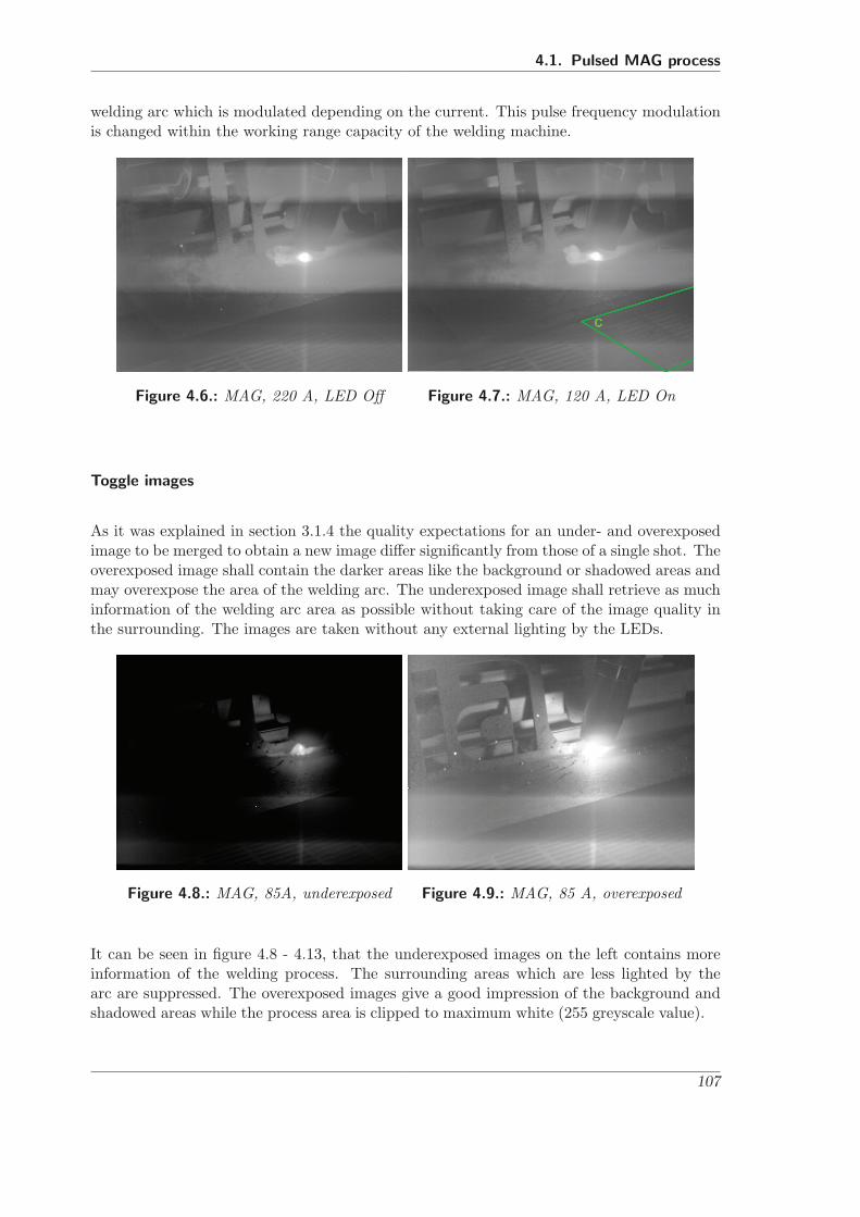
4.1. Pulsed MAG process
welding arc which is modulated depending on the current. This pulse frequency modulationis changed within the working range capacity of the welding machine.
Figure 4.6.: MAG, 220 A, LED Off Figure 4.7.: MAG, 120 A, LED On
Toggle images
As it was explained in section 3.1.4 the quality expectations for an under- and overexposedimage to be merged to obtain a new image differ significantly from those of a single shot. Theoverexposed image shall contain the darker areas like the background or shadowed areas andmay overexpose the area of the welding arc. The underexposed image shall retrieve as muchinformation of the welding arc area as possible without taking care of the image quality inthe surrounding. The images are taken without any external lighting by the LEDs.
Figure 4.8.: MAG, 85A, underexposed Figure 4.9.: MAG, 85 A, overexposed
It can be seen in figure 4.8 - 4.13, that the underexposed images on the left contains moreinformation of the welding process. The surrounding areas which are less lighted by thearc are suppressed. The overexposed images give a good impression of the background andshadowed areas while the process area is clipped to maximum white (255 greyscale value).
107

4. Results
Figure 4.10.: MAG, 120 A, underexposed Figure 4.11.: MAG, 120 A, overexposed
The specific properties of the C-MOS camera chip technique can be seen in the overexposedareas. A CCD camera chip tends to bloom from the point of high brightness. A hugerarea than the real optical bright area appears in the saved digital image as maximum white.The electrons at the bright spot cause by means of the incoming photons, a flooding of theneighboured areas on the chip, so that they are measured as white, too.
Figure 4.12.: MAG, 220 A, underexposed Figure 4.13.: MAG, 220 A, overexposed
4.1.2. Comparing Different Image Enhancement Algorithms
In this section the raw images shown in section 4.1.1 are processed by different image en-hancement algorithms. The classical histogram equalization, the GLG, the CLAHE and theVBSAHE algorithms are used to compare their usefulness for welding images. The threedifferent welding current of 85 A, 120 A and 220 A are used with the external LED lightingturned on.
108

4.1. Pulsed MAG process
MAG, 85 A The results for 85 A welding current are given in figure 4.15. The histogramequalization in subfigure a.) destroys the information in the process area by clipping itto maximum white. The background is over-amplified which means that the more brightregions are good visible while the darker regions occur more darkened and by that are lessvisible. This can be seen in figure 4.15 a.) nearby the iat logo on the left side. The sameeffect occurs for the difference at the white stripe which becomes more perturbing than inthe original raw image of figure 4.3.
The GLG with its result in sub-figure b.) processes the background to darkness but doesnot bloom the welding process area which remains precise without loosing image informa-tion. However the overall effect of enhancement is negative as the image details become lessvisible.
Enhancing the raw image with the CLAHE algorithm does change the welding process regionto be less visible by lowering the contrast and adding brightness. As it can be seen in figure4.15 c.), the background becomes highly structured, as single metal drips on the logos surfaceare now visible. The enhancement of the metal grid at the bottom of the image is improvedwithout getting blended by an amplification of the white stripe.
The VBSAHE algorithm has been introduced in chapter 3. It segments the image by usingthe mean shift filter approach as presented in [53] with a succeeding floodfill segmentation.The single segments are individually enhanced by histogram stretching. In a final step theenhanced segments are merged for the resulting image. In figure 4.14 the segmentation of theraw input image in figure 4.2 is shown. Every edge is part of the border of a mono-colouredsegment. Especially the area around the welding arc is divided into small segments and bythat enhanced individually.
Figure 4.14.: MAG, 85 A, LED On, Segmentation by Mean Shift approach
109
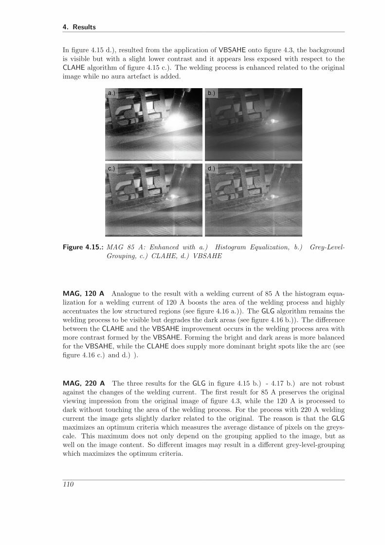
4. Results
In figure 4.15 d.), resulted from the application of VBSAHE onto figure 4.3, the backgroundis visible but with a slight lower contrast and it appears less exposed with respect to theCLAHE algorithm of figure 4.15 c.). The welding process is enhanced related to the originalimage while no aura artefact is added.
Figure 4.15.: MAG 85 A: Enhanced with a.) Histogram Equalization, b.) Grey-Level-Grouping, c.) CLAHE, d.) VBSAHE
MAG, 120 A Analogue to the result with a welding current of 85 A the histogram equa-lization for a welding current of 120 A boosts the area of the welding process and highlyaccentuates the low structured regions (see figure 4.16 a.)). The GLG algorithm remains thewelding process to be visible but degrades the dark areas (see figure 4.16 b.)). The differencebetween the CLAHE and the VBSAHE improvement occurs in the welding process area withmore contrast formed by the VBSAHE. Forming the bright and dark areas is more balancedfor the VBSAHE, while the CLAHE does supply more dominant bright spots like the arc (seefigure 4.16 c.) and d.) ).
MAG, 220 A The three results for the GLG in figure 4.15 b.) - 4.17 b.) are not robustagainst the changes of the welding current. The first result for 85 A preserves the originalviewing impression from the original image of figure 4.3, while the 120 A is processed todark without touching the area of the welding process. For the process with 220 A weldingcurrent the image gets slightly darker related to the original. The reason is that the GLGmaximizes an optimum criteria which measures the average distance of pixels on the greys-cale. This maximum does not only depend on the grouping applied to the image, but aswell on the image content. So different images may result in a different grey-level-groupingwhich maximizes the optimum criteria.
110
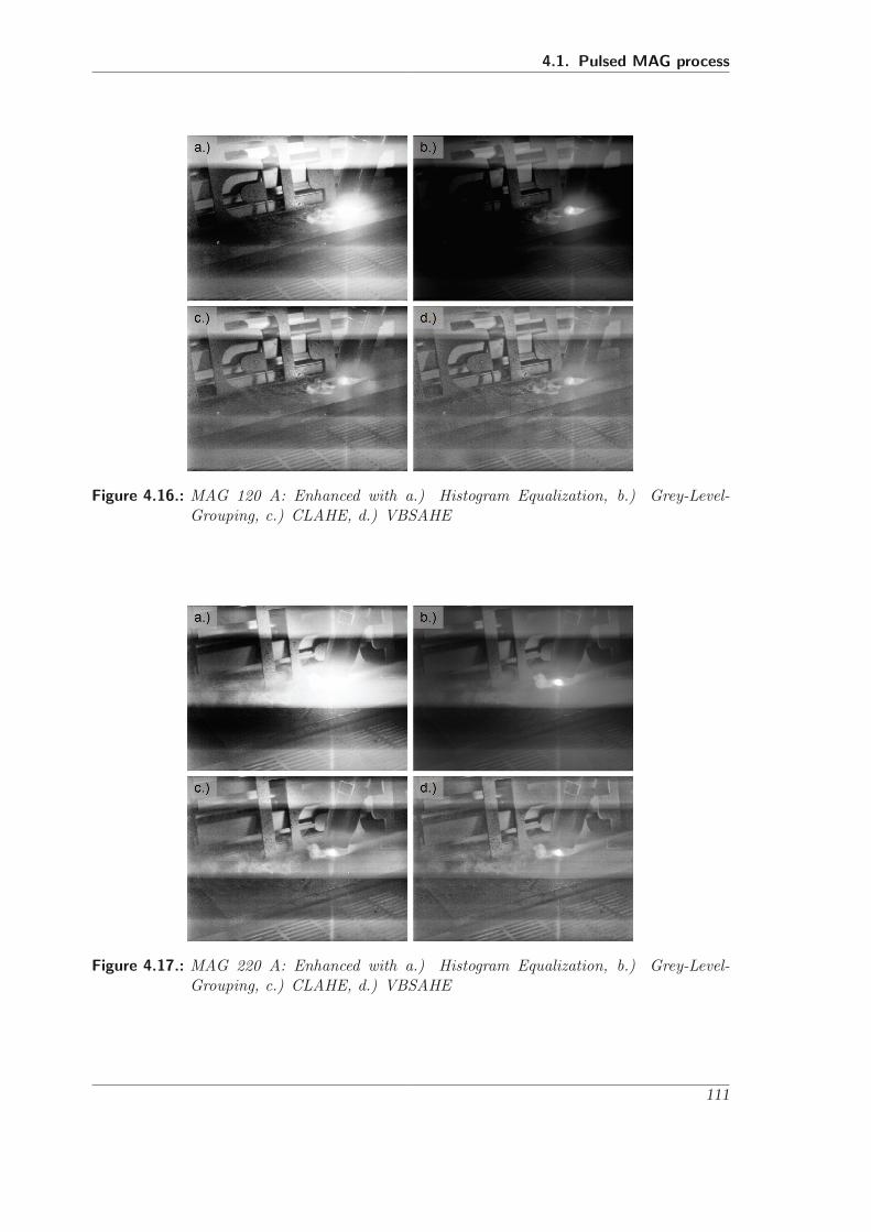
4.1. Pulsed MAG process
Figure 4.16.: MAG 120 A: Enhanced with a.) Histogram Equalization, b.) Grey-Level-Grouping, c.) CLAHE, d.) VBSAHE
Figure 4.17.: MAG 220 A: Enhanced with a.) Histogram Equalization, b.) Grey-Level-Grouping, c.) CLAHE, d.) VBSAHE
111
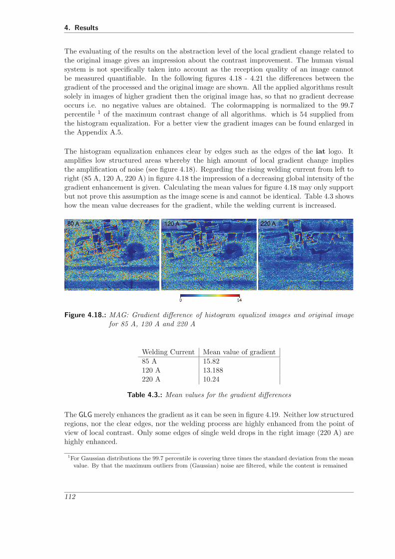
4. Results
The evaluating of the results on the abstraction level of the local gradient change related tothe original image gives an impression about the contrast improvement. The human visualsystem is not specifically taken into account as the reception quality of an image cannotbe measured quantifiable. In the following figures 4.18 - 4.21 the differences between thegradient of the processed and the original image are shown. All the applied algorithms resultsolely in images of higher gradient then the original image has, so that no gradient decreaseoccurs i.e. no negative values are obtained. The colormapping is normalized to the 99.7percentile 1 of the maximum contrast change of all algorithms. which is 54 supplied fromthe histogram equalization. For a better view the gradient images can be found enlarged inthe Appendix A.5.
The histogram equalization enhances clear by edges such as the edges of the iat logo. Itamplifies low structured areas whereby the high amount of local gradient change impliesthe amplification of noise (see figure 4.18). Regarding the rising welding current from left toright (85 A, 120 A, 220 A) in figure 4.18 the impression of a decreasing global intensity of thegradient enhancement is given. Calculating the mean values for figure 4.18 may only supportbut not prove this assumption as the image scene is and cannot be identical. Table 4.3 showshow the mean value decreases for the gradient, while the welding current is increased.
Figure 4.18.: MAG: Gradient difference of histogram equalized images and original imagefor 85 A, 120 A and 220 A
Welding Current Mean value of gradient85 A 15.82120 A 13.188220 A 10.24
Table 4.3.: Mean values for the gradient differences
The GLG merely enhances the gradient as it can be seen in figure 4.19. Neither low structuredregions, nor the clear edges, nor the welding process are highly enhanced from the point ofview of local contrast. Only some edges of single weld drops in the right image (220 A) arehighly enhanced.
1For Gaussian distributions the 99.7 percentile is covering three times the standard deviation from the meanvalue. By that the maximum outliers from (Gaussian) noise are filtered, while the content is remained
112
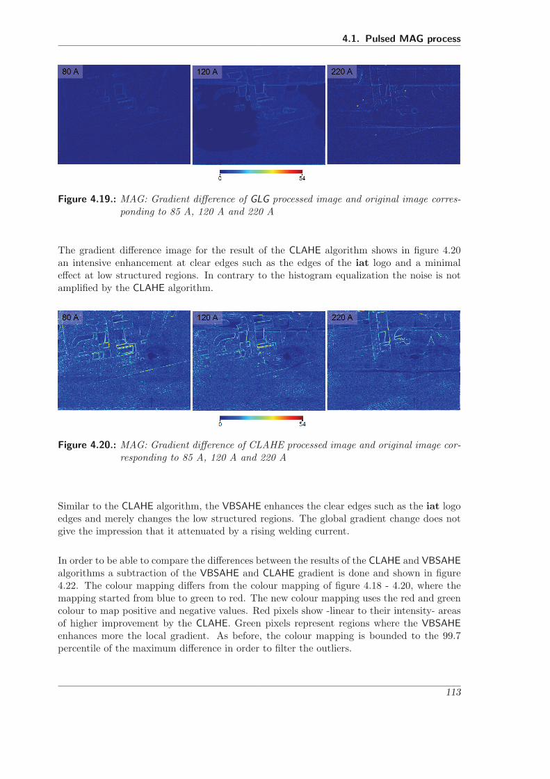
4.1. Pulsed MAG process
Figure 4.19.: MAG: Gradient difference of GLG processed image and original image corres-ponding to 85 A, 120 A and 220 A
The gradient difference image for the result of the CLAHE algorithm shows in figure 4.20an intensive enhancement at clear edges such as the edges of the iat logo and a minimaleffect at low structured regions. In contrary to the histogram equalization the noise is notamplified by the CLAHE algorithm.
Figure 4.20.: MAG: Gradient difference of CLAHE processed image and original image cor-responding to 85 A, 120 A and 220 A
Similar to the CLAHE algorithm, the VBSAHE enhances the clear edges such as the iat logoedges and merely changes the low structured regions. The global gradient change does notgive the impression that it attenuated by a rising welding current.
In order to be able to compare the differences between the results of the CLAHE and VBSAHEalgorithms a subtraction of the VBSAHE and CLAHE gradient is done and shown in figure4.22. The colour mapping differs from the colour mapping of figure 4.18 - 4.20, where themapping started from blue to green to red. The new colour mapping uses the red and greencolour to map positive and negative values. Red pixels show -linear to their intensity- areasof higher improvement by the CLAHE. Green pixels represent regions where the VBSAHEenhances more the local gradient. As before, the colour mapping is bounded to the 99.7percentile of the maximum difference in order to filter the outliers.
113

4. Results
Figure 4.21.: MAG: Gradient difference of VBSAHE processed image and original imagecorresponding to 85 A, 120 A and 220A
Figure 4.22.: MAG: Gradient difference of VBSAHE and CLAHE results corresponding to85 A, 120 A and 220A
114

4.1. Pulsed MAG process
All three images give the same viewing impression independent of the welding current. TheCLAHE algorithm improves more the clear edges while the VBSAHE amplifies more the lowstructured areas. Along with the view onto the real images resulting in figure 4.15 - 4.17,the gradient images of figure 4.22 support the well balanced impression for the VBSAHE incomparison to the CLAHE results.
4.1.3. Comparing Results of VBSAHE Processing with LED Lighting
In figure 4.23, the result of applying the VBSAHE algorithm on the raw image of figure 4.2is given. In both cases with the LED on and off the image is enhanced from a smooth imagewith insignificant local contrast to an image with high local contrast and sharp edges. Themetal grid in the foreground of figure 4.2 supplies a structured object which now becomesvisible. The background with the iat logo is transformed from a dark area with low localstructure to a surface with weld sputter on the metal and good visibility.
Figure 4.23.: MAG, 85 A, VBSAHE Applied with LED Off (Left), LED On (Right)
The comparison between the left and right image in figure 4.23 supplies the differences of theexternal lighting turned on and off. High power LEDs are used to highlight the surrounding.In region A the texture of the iat logo has a higher contrast as the LED have enoughbrightness to override slightly the welding arc light. In region B and C the LEDs highlightareas which are shadowed by the geometrical setup. In region B the far side from thewelding torch can be seen after enhancement as well as the metal grid in region B where theshadowed edges of the grid are lighted. In region D reflections of the LED light source arevisible. If the result of the contrast enhanced image is compared with the raw image in figure4.3, then it can be seen that in the raw image the regions A and B where not identified tobe highlighted by the LED although the contrast enhancement result of figure 4.23 makes itvisible.
The more light is produced by the welding arc the less improvement is made by the LEDsas it can be seen in the regions B, C and D. No improvement is visible in the backgroundat the iat logo of figure 4.24, which is highlighted in figure 4.23 as region A.
115
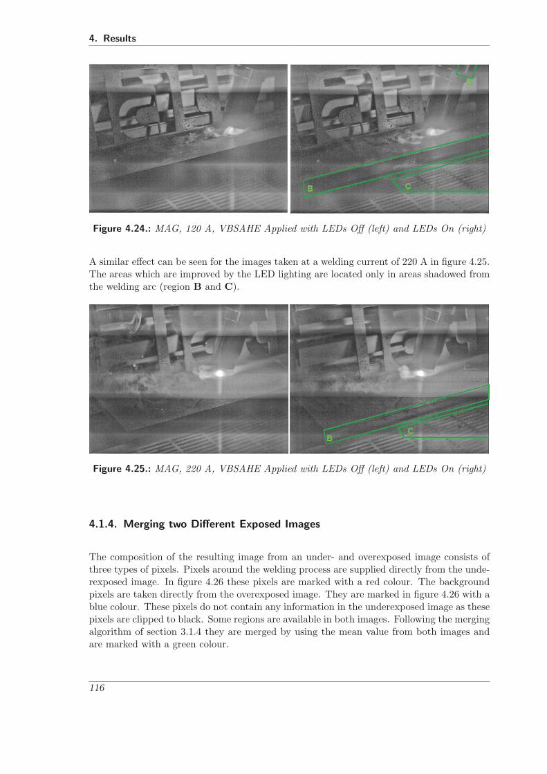
4. Results
Figure 4.24.: MAG, 120 A, VBSAHE Applied with LEDs Off (left) and LEDs On (right)
A similar effect can be seen for the images taken at a welding current of 220 A in figure 4.25.The areas which are improved by the LED lighting are located only in areas shadowed fromthe welding arc (region B and C).
Figure 4.25.: MAG, 220 A, VBSAHE Applied with LEDs Off (left) and LEDs On (right)
4.1.4. Merging two Different Exposed Images
The composition of the resulting image from an under- and overexposed image consists ofthree types of pixels. Pixels around the welding process are supplied directly from the unde-rexposed image. In figure 4.26 these pixels are marked with a red colour. The backgroundpixels are taken directly from the overexposed image. They are marked in figure 4.26 with ablue colour. These pixels do not contain any information in the underexposed image as thesepixels are clipped to black. Some regions are available in both images. Following the mergingalgorithm of section 3.1.4 they are merged by using the mean value from both images andare marked with a green colour.
116

4.1. Pulsed MAG process
Figure 4.26.: MAG process at 85 A: Merge composition of the resulting image from theunderexposed (red), both (green) and overexposed (blue) image
Merging the images results in data with exceeding the value range of a standard grey scaleimage of a computer. More than 256 different grey scales values are not available on thescreen and nor the human eye can perceive all. One way to make it visible is to use falsecolours which map a high amount of different grey scale values to a colour map. The colourmap is deviated from the hue-saturation-value colour model, where the hue component isvaried (see [74]). The colour map begins with red, passes through yellow, green, cyan, blue,magenta and returns to red.
MAG, 85 A In figure 4.27 such a mapping is made to show the enhanced informationcontained in the merging result. The magnified area of the welding process shows that theimage information contains a higher number of different grey values. If only the data takenfrom the underexposed image is taken into account (marked with red in figure 4.26) then 98different grey values form the information of the welding process. By contrast the amountof an adequate area from a direct single shot as presented in section 4.1.1, covers 62 greyvalues. This measurement can only be used qualitatively as the region borders of the weldingprocess are not clearly defined in the single shot image.
The resulting grey scale image in figure 4.28 is the linear transformation of the false colourimage (figure 4.27) with 389 grey values to a 256 greyscale image. The transformationis equal to a histogram stretching where it is used for image improvement with the onlydifference that it is now done from a large data domain to a smaller one.
By applying the VBSAHE algorithm the source image needs to be segmented before enhan-cing. The result of the detailed segmentation of figure 4.28 is shown in figure 4.29. It givesan impression about the amount and individual shape of the regions. After enhancing, themerged regions form a new image enriched in details as given in figure 4.30.
117
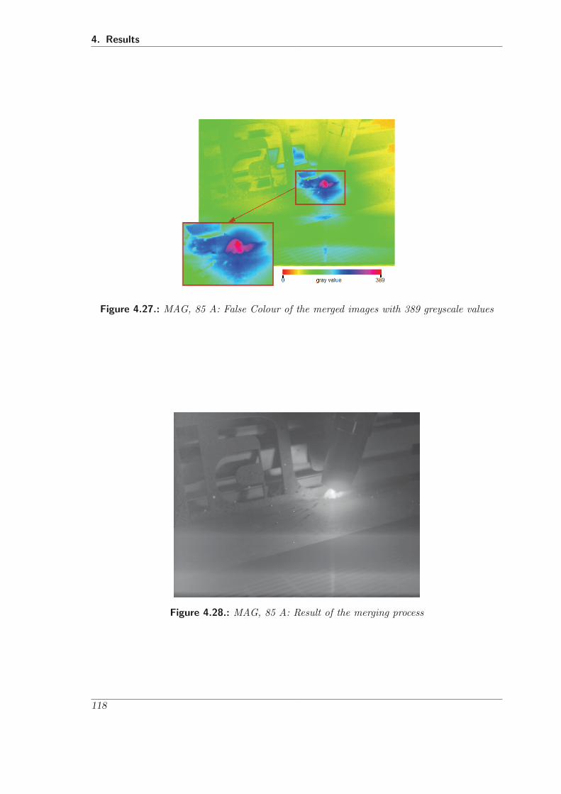
4. Results
Figure 4.27.: MAG, 85 A: False Colour of the merged images with 389 greyscale values
Figure 4.28.: MAG, 85 A: Result of the merging process
118
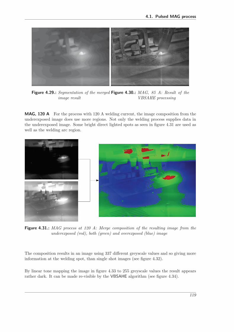
4.1. Pulsed MAG process
Figure 4.29.: Segmentation of the mergedimage result
Figure 4.30.: MAG, 85 A: Result of theVBSAHE processing
MAG, 120 A For the process with 120 A welding current, the image composition from theunderexposed image does use more regions. Not only the welding process supplies data inthe underexposed image. Some bright direct lighted spots as seen in figure 4.31 are used aswell as the welding arc region.
Figure 4.31.: MAG process at 120 A: Merge composition of the resulting image from theunderexposed (red), both (green) and overexposed (blue) image
The composition results in an image using 337 different greyscale values and so giving moreinformation at the welding spot, than single shot images (see figure 4.32).
By linear tone mapping the image in figure 4.33 to 255 greyscale values the result appearsrather dark. It can be made re-visible by the VBSAHE algorithm (see figure 4.34).
119
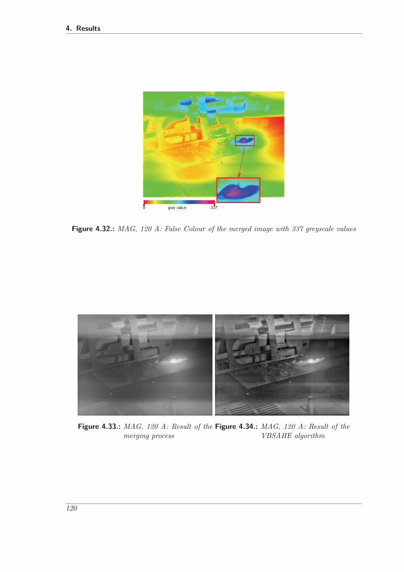
4. Results
Figure 4.32.: MAG, 120 A: False Colour of the merged image with 337 greyscale values
Figure 4.33.: MAG, 120 A: Result of themerging process
Figure 4.34.: MAG, 120 A: Result of theVBSAHE algorithm
120
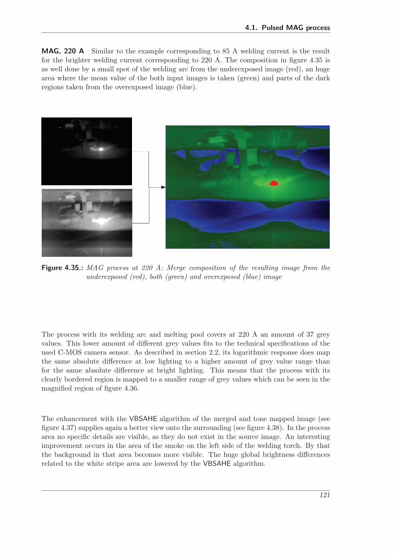
4.1. Pulsed MAG process
MAG, 220 A Similar to the example corresponding to 85 A welding current is the resultfor the brighter welding current corresponding to 220 A. The composition in figure 4.35 isas well done by a small spot of the welding arc from the underexposed image (red), an hugearea where the mean value of the both input images is taken (green) and parts of the darkregions taken from the overexposed image (blue).
Figure 4.35.: MAG process at 220 A: Merge composition of the resulting image from theunderexposed (red), both (green) and overexposed (blue) image
The process with its welding arc and melting pool covers at 220 A an amount of 37 greyvalues. This lower amount of different grey values fits to the technical specifications of theused C-MOS camera sensor. As described in section 2.2, its logarithmic response does mapthe same absolute difference at low lighting to a higher amount of grey value range thanfor the same absolute difference at bright lighting. This means that the process with itsclearly bordered region is mapped to a smaller range of grey values which can be seen in themagnified region of figure 4.36.
The enhancement with the VBSAHE algorithm of the merged and tone mapped image (seefigure 4.37) supplies again a better view onto the surrounding (see figure 4.38). In the processarea no specific details are visible, as they do not exist in the source image. An interestingimprovement occurs in the area of the smoke on the left side of the welding torch. By thatthe background in that area becomes more visible. The huge global brightness differencesrelated to the white stripe area are lowered by the VBSAHE algorithm.
121

4. Results
Figure 4.36.: MAG, 220 A: False Colour of the merged image with 321 greyscale values
Figure 4.37.: MAG, 220 A: Result of themerging process
Figure 4.38.: MAG, 220 A: Result of ap-plying the VBSAHE algo-rithm
122
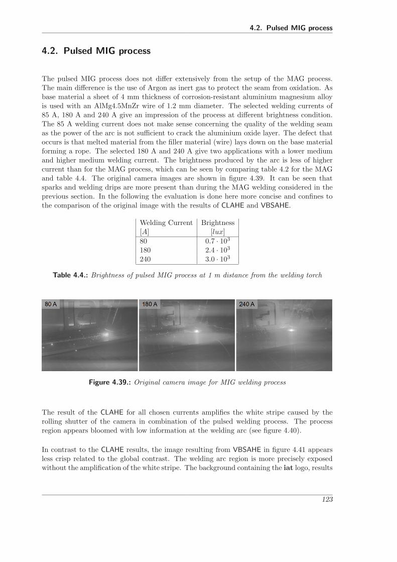
4.2. Pulsed MIG process
4.2. Pulsed MIG process
The pulsed MIG process does not differ extensively from the setup of the MAG process.The main difference is the use of Argon as inert gas to protect the seam from oxidation. Asbase material a sheet of 4 mm thickness of corrosion-resistant aluminium magnesium alloyis used with an AlMg4.5MnZr wire of 1.2 mm diameter. The selected welding currents of85 A, 180 A and 240 A give an impression of the process at different brightness condition.The 85 A welding current does not make sense concerning the quality of the welding seamas the power of the arc is not sufficient to crack the aluminium oxide layer. The defect thatoccurs is that melted material from the filler material (wire) lays down on the base materialforming a rope. The selected 180 A and 240 A give two applications with a lower mediumand higher medium welding current. The brightness produced by the arc is less of highercurrent than for the MAG process, which can be seen by comparing table 4.2 for the MAGand table 4.4. The original camera images are shown in figure 4.39. It can be seen thatsparks and welding drips are more present than during the MAG welding considered in theprevious section. In the following the evaluation is done here more concise and confines tothe comparison of the original image with the results of CLAHE and VBSAHE.
Welding Current Brightness[A] [lux]80 0.7 · 103
180 2.4 · 103
240 3.0 · 103
Table 4.4.: Brightness of pulsed MIG process at 1 m distance from the welding torch
Figure 4.39.: Original camera image for MIG welding process
The result of the CLAHE for all chosen currents amplifies the white stripe caused by therolling shutter of the camera in combination of the pulsed welding process. The processregion appears bloomed with low information at the welding arc (see figure 4.40).
In contrast to the CLAHE results, the image resulting from VBSAHE in figure 4.41 appearsless crisp related to the global contrast. The welding arc region is more precisely exposedwithout the amplification of the white stripe. The background containing the iat logo, results
123
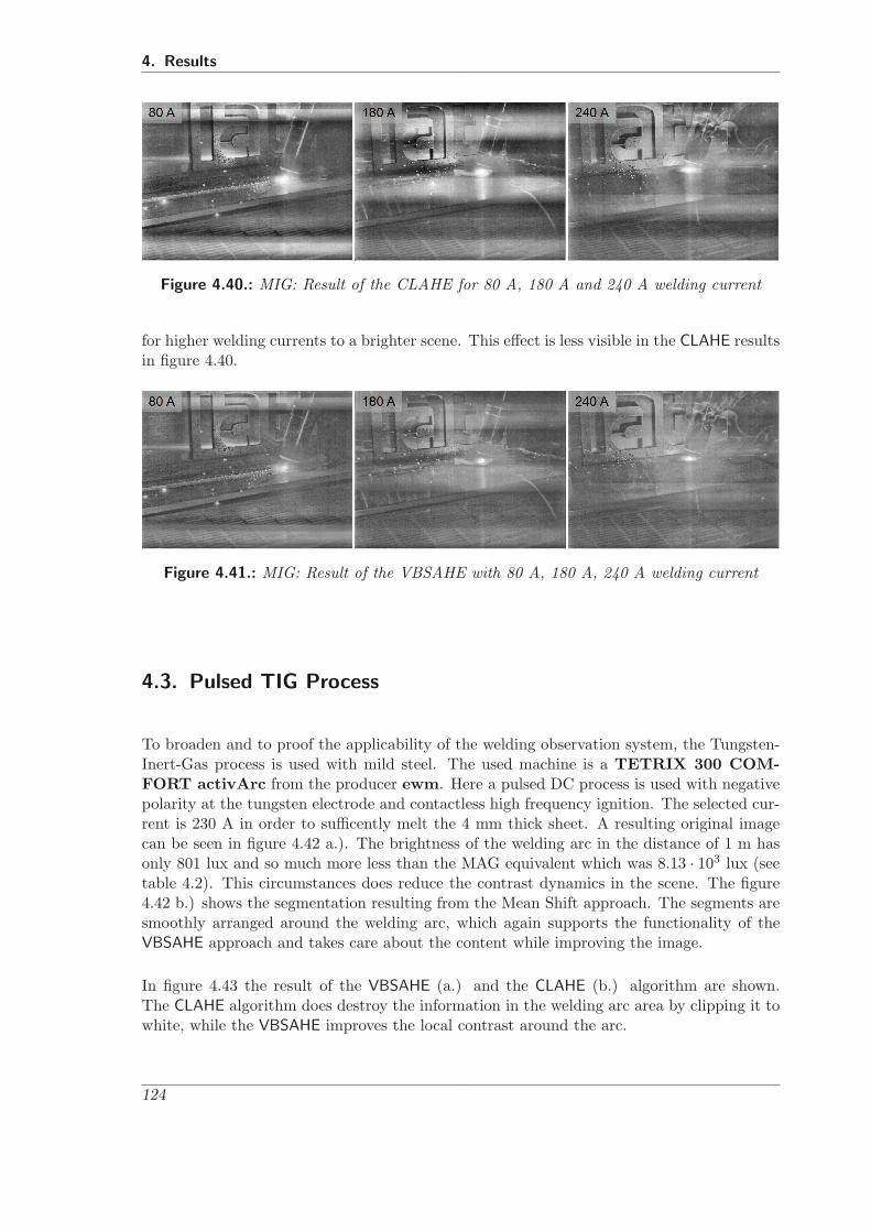
4. Results
Figure 4.40.: MIG: Result of the CLAHE for 80 A, 180 A and 240 A welding current
for higher welding currents to a brighter scene. This effect is less visible in the CLAHE resultsin figure 4.40.
Figure 4.41.: MIG: Result of the VBSAHE with 80 A, 180 A, 240 A welding current
4.3. Pulsed TIG Process
To broaden and to proof the applicability of the welding observation system, the Tungsten-Inert-Gas process is used with mild steel. The used machine is a TETRIX 300 COM-FORT activArc from the producer ewm. Here a pulsed DC process is used with negativepolarity at the tungsten electrode and contactless high frequency ignition. The selected cur-rent is 230 A in order to sufficently melt the 4 mm thick sheet. A resulting original imagecan be seen in figure 4.42 a.). The brightness of the welding arc in the distance of 1 m hasonly 801 lux and so much more less than the MAG equivalent which was 8.13 · 103 lux (seetable 4.2). This circumstances does reduce the contrast dynamics in the scene. The figure4.42 b.) shows the segmentation resulting from the Mean Shift approach. The segments aresmoothly arranged around the welding arc, which again supports the functionality of theVBSAHE approach and takes care about the content while improving the image.
In figure 4.43 the result of the VBSAHE (a.) and the CLAHE (b.) algorithm are shown.The CLAHE algorithm does destroy the information in the welding arc area by clipping it towhite, while the VBSAHE improves the local contrast around the arc.
124
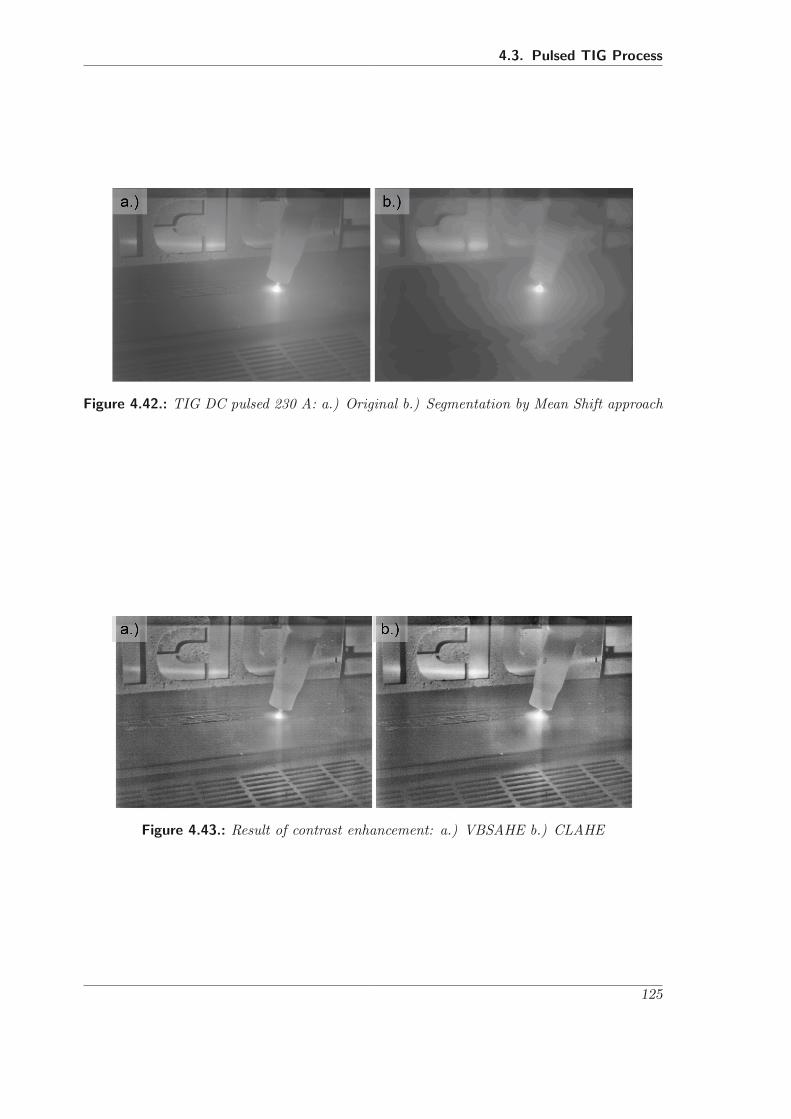
4.3. Pulsed TIG Process
Figure 4.42.: TIG DC pulsed 230 A: a.) Original b.) Segmentation by Mean Shift approach
Figure 4.43.: Result of contrast enhancement: a.) VBSAHE b.) CLAHE
125

4. Results
These results are supported by the difference in the gradient of the results in figure 4.44. Asin the previous sections the differences of the VBSAHE and the CLAHE are coded in greencolour for a stronger VBSAHE gradient, while red shows a stronger gradient resulted by theCLAHE algorithm. The region around the welding arc is coloured green, which means that
Figure 4.44.: Difference of image gradient for VBSAHE and CLAHE results
the local contrast is higher for the image enhanced by the VBSAHE algorithm. Other regionslike clear edges at the iat logo in the background are more enhanced by the CLAHE, whilesmooth areas are more enhanced by the VBSAHE.
4.4. The Selective Automatic Darkening Filter
The prototype helmet (see chapter 3) is used with a mannequin head. It gives the opportunityto place an external camera at the eye position (see figure 4.45). After starting the systemit has to be calibrated by using optical markers of the ARToolkit. Theses markers haveto be placed around the working distance of the welder, who may then use the system atthis specific distance. The calibration and the running system is done with the mannequincamera instead of a human user to document the results. For human user the calibrationcan be reduced to around 25 s after some time of practice by repetition. One drawback ishere that the calibration needs to be done every time the user puts the helmet on as well asafter raising it up. It must be done as the position of the camera and GLCD related to theeye is changed every time of moving the helmet.
The response time of the GLCD is about 150-175 ms as the pixels of the GLCD are setby serial access. The frame rate of the GLCD is lower than the detection threshold ofthe human eye for fluent movements. The abilities of the GLCD are restricted to squaredshapes. Implementing other shapes than squares by building an entire Graphics DeviceInterface (GDI) would go along with a lower frame rate as for the square the most effective
126
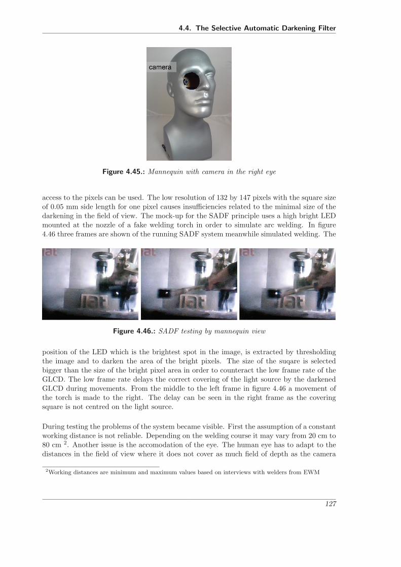
4.4. The Selective Automatic Darkening Filter
Figure 4.45.: Mannequin with camera in the right eye
access to the pixels can be used. The low resolution of 132 by 147 pixels with the square sizeof 0.05 mm side length for one pixel causes insufficiencies related to the minimal size of thedarkening in the field of view. The mock-up for the SADF principle uses a high bright LEDmounted at the nozzle of a fake welding torch in order to simulate arc welding. In figure4.46 three frames are shown of the running SADF system meanwhile simulated welding. The
Figure 4.46.: SADF testing by mannequin view
position of the LED which is the brightest spot in the image, is extracted by thresholdingthe image and to darken the area of the bright pixels. The size of the suqare is selectedbigger than the size of the bright pixel area in order to counteract the low frame rate of theGLCD. The low frame rate delays the correct covering of the light source by the darkenedGLCD during movements. From the middle to the left frame in figure 4.46 a movement ofthe torch is made to the right. The delay can be seen in the right frame as the coveringsquare is not centred on the light source.
During testing the problems of the system became visible. First the assumption of a constantworking distance is not reliable. Depending on the welding course it may vary from 20 cm to80 cm 2. Another issue is the accomodation of the eye. The human eye has to adapt to thedistances in the field of view where it does not cover as much field of depth as the camera
2Working distances are minimum and maximum values based on interviews with welders from EWM
127

4. Results
lenses may do, so that the black square covering the glaring light may not be seen sharp butblurred by the human observer.
In figure 4.46 the background and the black squares of the GLCD are good viewable. Al-though the background is better visible the black square is precisely noticeable. If a humanuses the system, he does not recognize a black square. The darkening of the GLCD is seenas an fluent smooth darkening around the square center. Different results are made with anoptical-see-through HMD, where the optics are well aligned to the users view, but the dar-kening abilities of such an HMD is very low and by that not useful for welding protection.
4.5. Conclusions
This thesis elaborates a system for the video observation of high dynamic contrast sceneswith the application of welding. The development of a SADF system was achievable onlyby a feasibility study due to non-existent adequate hardware. The lack of a 2D GLCD onlygives the opportunity to build a mock-up system, which keeps the idea of a SADF systemalive (see section 3.3 and section 4.4).
The problems of having on the one side a camera for high dynamic contrast but only eight bitsto record the greyscale is a drawback which bounds the quality of the raw image. One stepto overcome with such limitations is to use the toggle merging with two images containinginformation of two different brightness ranges. It ends up in an image with more than 256greyscale values, which has to be tone mapped to eight bits information for displaying on amonitor. This technique assured to use all the available 256 steps of greyscale as the inputfor the next algorithmic step of contrast enhancement (see section 3.1.4).
After widening the input data range of the image, the second most important question aroserelated to enhancing the image information. The question of what is the information ofthe image and how can it be enhanced ended up at the VBSAHE algorithm after exami-ning different contrast enhancement approaches. This algorithm individually enhances thesegmented information of the image. It takes the eight bit greyscale and enhances the lo-cal contrast, so that globally seen, the information becomes better visible as informationby small greyscale differences can be enhanced without overrunning the limitations of 256greyscale values of the output image (see section 3.2.4).
Related to the application of welding the problem of synchronizing the camera onto thewelding process gave a milestone in video quality for the human observer. The flickering wasnot abolished but stabilized to a fixed position without depending on any machine interface.The optical trigger with automatic alignment of the sensor system to the brightness conditionmakes this system robust for a wide range of applications related to welding method, workingdistance and conditions (see section 3.1.2).
With the integration of the trigger, the flashing of the scene with high power LED becamefeasible. Although the effect of this technique is limited to widely used medium welding
128

4.5. Conclusions
currents, it produces a lighted areas which are lying in the shadow of the glaring welding arc(section 3.1.3).
In the future the aspects of a SADF system need to be observed regarding available GLCDswhich may darken sufficiently the bright spots and follow movements with an adequate framerate. An alternative suggestion is to re-think the idea of a video see-through welding helmet[9] were the user sees the scene by a video see-through HMD while the scene is captured bya camera system; a camera system as it is researched here.
Side effects of this research are the examination of the morphological top-hat operator (seesection 3.2.5) and the application of the Wiener filter for denoising the image (see section3.2.3). The lack of a defined helmet fixation on the user’s head to preserve a valid cali-bration, needs further investigation for an alternative approach in order to avoid tediouscalibrations.
129

4. Results
130

AAppendix
A.1. Mathematical Conventions
x, X : scalarx(. . .), X(. . .) : functionx, X : vectors in 2D (lowercase) and 3D (capital)X : matrix
A.2. Linear Algebra
A small introduction taken from [71] about important equations is given here
determinants The determinant of the product of two quadratic matrices A and B is thesame as the product of their single determinants
det (A · B) = det (A) · det (B) (A.1)
Transposed product The transposed matrix of matrix product is equal to the product ofthe two transposed matrices:
(A · B)T = AT · BT (A.2)
131
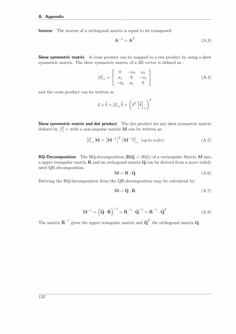
A. Appendix
Inverse The inverse of a orthogonal matrix is equal to its transposed
A−1 = AT (A.3)
Skew symmetric matrix A cross product can be mapped to a dot product by using a skewsymmetric matrix. The skew symmetric matrix of a 3D vector is defined as :
[a]× =
⎡⎣ 0 −a3 a2
a3 0 −a1
−a2 a1 0
⎤⎦ (A.4)
and the cross product can be written as
a ×b = [a]×b =(
aT[b]×
)T
Skew symmetric matrix and dot product The dot product for any skew symmetric matrixdefined by
[t]× with a non-singular matrix M can be written as:
[t]× M =
[M−1
]T [M−1t]× (up to scale) (A.5)
RQ-Decomposition The RQ-decomposition [RQ] = RQ() of a rectangular Matrix M intoa upper triangular matrix R and an orthogonal matrix Q can be derived from a more widelyused QR-decomposition.
M = R · Q (A.6)
Deriving the RQ-decomposition from the QR-decomposition may be calculated by:
M = Q · R (A.7)
M−1 =(Q · R
)−1= R
−1 · Q−1= R
−1 · QT(A.8)
The matrix R−1
gives the upper triangular matrix and QT
the orthogonal matrix Q.
132
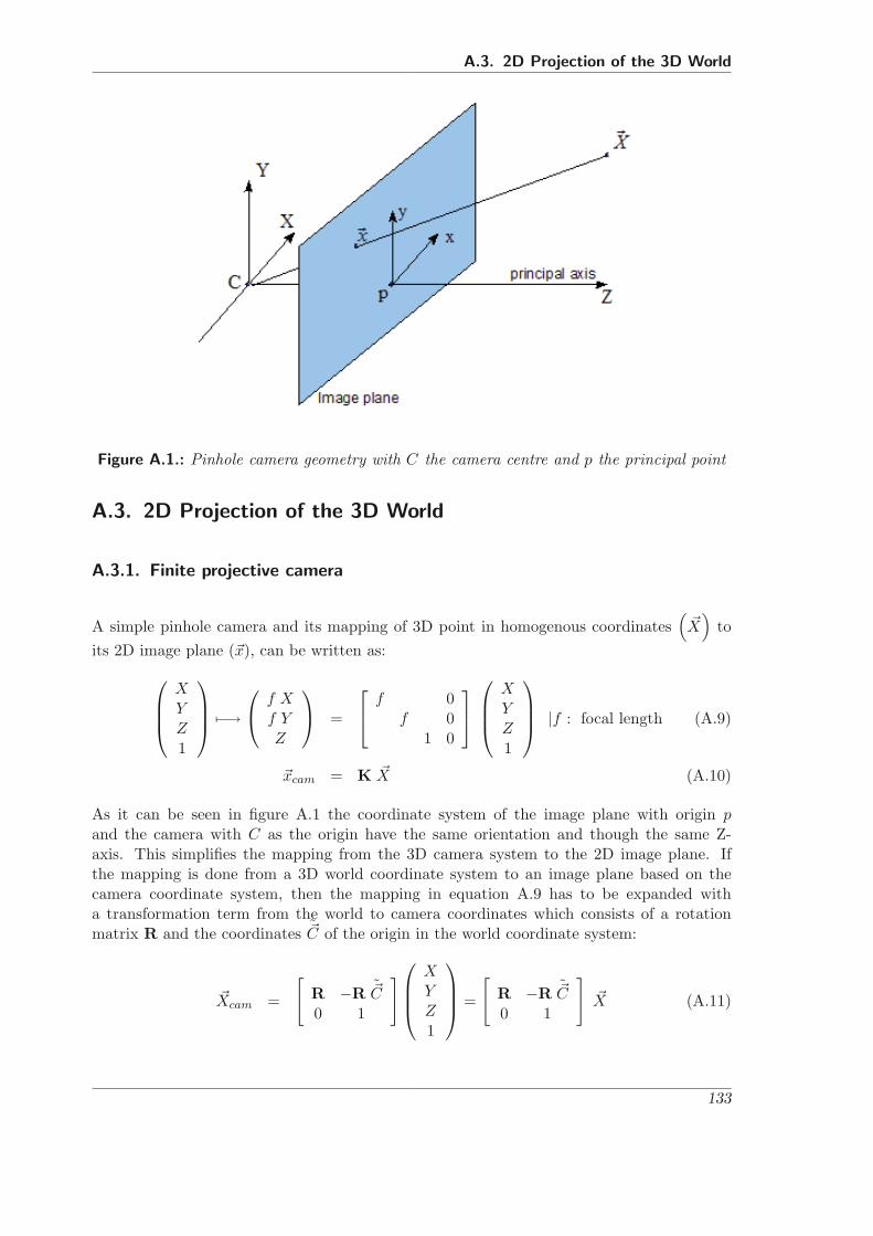
A.3. 2D Projection of the 3D World
Figure A.1.: Pinhole camera geometry with C the camera centre and p the principal point
A.3. 2D Projection of the 3D World
A.3.1. Finite projective camera
A simple pinhole camera and its mapping of 3D point in homogenous coordinates(
X)
toits 2D image plane (x), can be written as:⎛
⎜⎜⎝XYZ1
⎞⎟⎟⎠ �−→
⎛⎝ f X
f YZ
⎞⎠ =
⎡⎣ f 0
f 01 0
⎤⎦⎛⎜⎜⎝
XYZ1
⎞⎟⎟⎠ |f : focal length (A.9)
xcam = K X (A.10)
As it can be seen in figure A.1 the coordinate system of the image plane with origin pand the camera with C as the origin have the same orientation and though the same Z-axis. This simplifies the mapping from the 3D camera system to the 2D image plane. Ifthe mapping is done from a 3D world coordinate system to an image plane based on thecamera coordinate system, then the mapping in equation A.9 has to be expanded witha transformation term from the world to camera coordinates which consists of a rotationmatrix R and the coordinates C of the origin in the world coordinate system:
Xcam =
[R −R C0 1
]⎛⎜⎜⎝XYZ1
⎞⎟⎟⎠ =
[R −R C0 1
]X (A.11)
133

A. Appendix
Which leads together with equation A.9 to
x = K R[I∣∣∣− C
]X (A.12)
= P X (A.13)
with X in world coordinate frame.
Up to yet the mapping to the image plane is still measured in distance units like meter orinches, but a digital camera uses pixels. For this the number of pixels per unit distance min image coordinates is introduced and changes the use of the focal length f by mapping toa focal length in pixel coordinates α = f m. The used C-MOS camera has squared pixelswith identical dimension in x and y direction. This is why only one variable m is used. 1
The camera Matrix K changes for a mapping to pixel coordinates to:
K =
⎡⎣ α x0 0
α y0 01 0
⎤⎦ (A.14)
With x0 and y0 as the principal point derived from the pixel coordinates p0 = (px, py) withx0 = m px and y0 = m py.
Back projection The ray back-projected from x on the image plane by the camera systemformed with P is given by a one parameter family of solutions, which forms a 3D line
X (λ) = P−1x + λ C (A.15)
Camera Calibration
To calibrate a camera, the unknown P can be calculated by using sufficient known 3D pointsXi and their projection xi onto the image plane as used in A.13. For an exact solution sixprecise pairs of 3D to 2D corresponding points are needed to solve the problem. But allmeasurements include measurement errors and so noise. An exact solution for the cameramatrix P is not achievable and can be iteratively solved by minimizing an optimum criterion.In this case a bigger number of measured correspondences Xi → xi is used for a more precisesolution. For such an approximated solution the Gold Standard algorithm is used [71].It needs an initial estimate using a linear method to be calculated before minimizing theprojection error using an iterative algorithm such as Levenberg-Marquardt [75], [76]. Beforestarting to find any solution the image points and the space points need to be normalizedby a translation and scaling so that the centroid of the points is in the coordinate origin andtheir average distance from the origin is
√2.
xi = Txi (A.16)Xi = U Xi (A.17)
1If a camera has non-squared pixel, as some CCD cameras have, two different value for the number of pixelper unit distance in x and y direction has to be used and effect two different (pixel based) focal length inx and y direction.
134

A.3. 2D Projection of the 3D World
Linear solution The inhomogeneous camera projection equation A.13 can be changed toan homogenous problem by applying the cross product from the left with x to both sides:
xi = P Xi (A.18)
xi × xi = xi ×[P Xi
](A.19)
Now the cross product can be realigned by using instead a skew symmetric matrix. The wayto use the skew symmetric matrix is sketched as follows with pT
i denoted as the i-th row ofthe matrix P and xi = (xi, yi, wi)
T
0 = xi ×
⎛⎜⎝ pT
1Xi
pT2
Xi
pT3
Xi
⎞⎟⎠ (A.20)
=
⎡⎢⎣ 0T −wi
XTi yi
XTi
wiXT
i 0T −xiXT
i
−yiXT
i xiXT
i 0T
⎤⎥⎦⎛⎝ p 1
p 2
p 3
⎞⎠ (A.21)
0 := A · p (A.22)
The overdetermined system is received by stacking for each of the n normalized correspondingpairs Xi → xi equation A.22, to a 2n × 12 matrix A. Only two equations of A.22 can beused for each correspondence Xi → xi as the third is not linearly independent. In order toachieve an optimal solution for p for the 2n×12 matrix A the Singular Value Decomposition(SVD) will be used. The unit singular vector corresponding to the smallest singular values isthe optimal solution for p. Especially if A = UDVT with D diagonal matrix with positivediagonal entries, arranged in descending order, then an optimal solution for p is the lastcolumn of V.
So the matrix P is determined from the last column of V as:
P =
⎡⎣ v1,12 v2,12 v3,12 v4,12
v5,12 v6,12 v7,12 v8,12
v9,12 v10,12 v11,12 v12,12
⎤⎦ (A.23)
Following the camera model as used in equation A.13, the minimization of∑
i d(xi, P Xi
)which is the projection error between the measured 2D points and the projection of their 3Dcorrespondences, gives the optimization criteria. The Levenberg-Marquardt Algorithm maybe used to retrieve a first approximation for the preceeding SVD.
Denormalization The camera matrix for the original coordinates is obtained from P bydenormalization of P (see A.17) by
P = T−1PU (A.24)
135
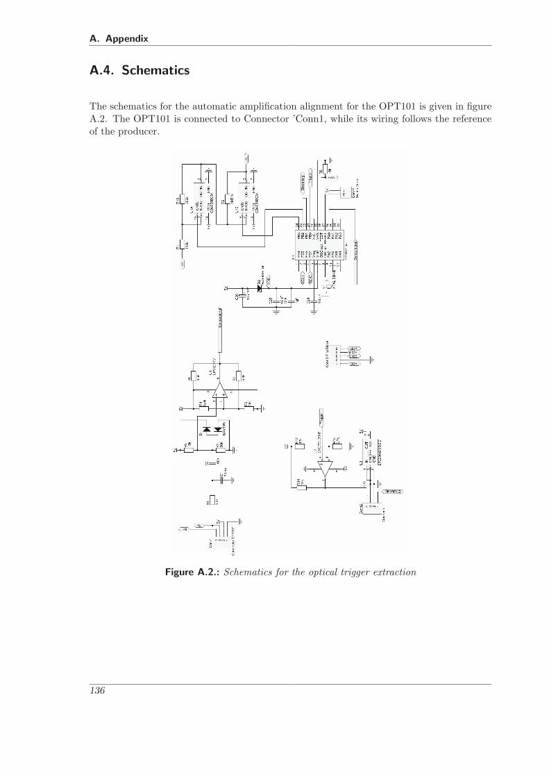
A. Appendix
A.4. Schematics
The schematics for the automatic amplification alignment for the OPT101 is given in figureA.2. The OPT101 is connected to Connector ’Conn1, while its wiring follows the referenceof the producer.
Figure A.2.: Schematics for the optical trigger extraction
136

A.5. Results of different image processing algorithms
A.5. Results of different image processing algorithms
The visibility of the result in section 4.1.2 is not optimal for precise inspection. Due tospace limitation for a good readable text the single images are repeated here upscaled onthe following pages.
137

A. Appendix
Figure A.3.: MAG: Gradient difference of Histogram equalization and original image for 80A, 120 A and 220A
138

A.5. Results of different image processing algorithms
Figure A.4.: MAG: Gradient difference of GLG and original image for 80 A, 120 A and220A
139
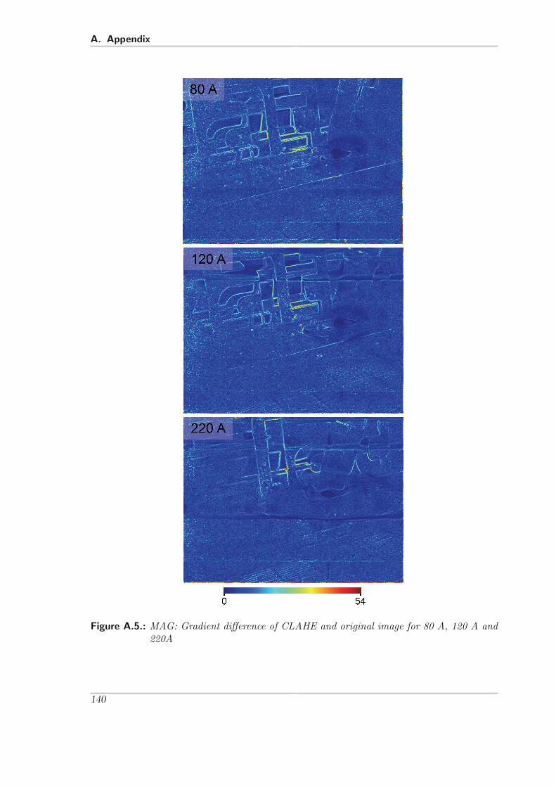
A. Appendix
Figure A.5.: MAG: Gradient difference of CLAHE and original image for 80 A, 120 A and220A
140

A.5. Results of different image processing algorithms
Figure A.6.: MAG: Gradient difference of VBSAHE and original image for 80 A, 120 A and220A
141
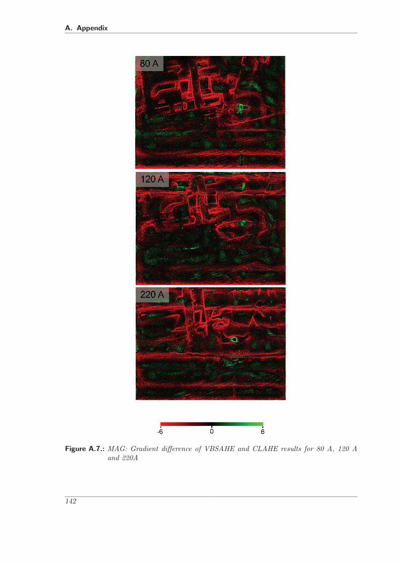
A. Appendix
Figure A.7.: MAG: Gradient difference of VBSAHE and CLAHE results for 80 A, 120 Aand 220A
142
Bibliography
[1] P. Milgram, H. Takemura, A. Utsumi, and F. Kishino, “Augmented Reality: A class ofdisplays on the reality-virtuality continuum,” in SPIE Proceedings of Telemanipulatorand Telepresence Technologies, no. 2351, 1994, pp. 282–292.
[2] R. L. O’Brien, Welding processes, 8th ed., ser. Welding handbook. Miami, Fla, USA:American Welding Society, 1995, vol. Vol. 2.
[3] K.-J. Matthes and E. Richter, Schweißtechnik - Schweißen von metallischen Konstruk-tionswerkstoffen, 4th ed. Munchen: Fachbuchverlag Leipzig, 2008.
[4] K. Weman, Welding processes handbook, vii ed. Boca Raton, Fla., USA: CRC PressInc, 2003.
[5] D. Saini and S. Floy, “An investigation of gas metal arc welding sound signature foron-line quality control,” Welding Journal, vol. 4, pp. 172–179, 1998.
[6] S. Steeb, Zerstorungsfreie Werkstuck- und Werkstoffprufung - Die gebrauchlichsten Ver-fahren im Uberblick, 3rd ed., ser. Kontakt und Studium. Renningen: expert Verlag,2005, vol. 243.
[7] E. Sutter, A. Schirmacher, I. Decker, and G. Ott, Elektrooptische Schweisserschutz-filter und Abschirmungen an Schweisserarbeitsplatzen - Sicherheitsanalyse und Mess-verfahren, ser. Schriftenreihe der Bundesanstalt fur Arbeitsschutz und Arbeitsmedizin.Bremerhaven: Wirtschaftsverlag NW, 1997, vol. 756.
[8] W. Koschinski, A. Schirmacher, E. Sutter, G. Ott, and M. Janssen, AutomatischeSchutzstufeneinstellung elektrooptischer Schweißerschutzfilter, ser. Schriftenreihe derBundesanstalt fur Arbeitsschutz und Arbeitsmedizin,. Bremerhaven: Wirtschaftsverl.NW, Verl. fur neue Wiss, 1999, vol. 859.
[9] B. Hillers, D. Aiteanu, and A. Graeser, “Augmented-Reality Helmet for the manualwelding process,” in Virtual and Augmented Reality applications in manufacturing, S. K.Ong and A. Y. C. Nee, Eds. London: Springer, 2004, pp. 361–381.
[10] D. Aiteanu, B. Hillers, and A. Graeser, “A Step Forward in Manual Welding: Demons-tration of Augmented Reality Helmet,” in The Second IEEE and ACM InternationalSymposium on Mixed and Augmented Reality (ISMAR), Tokyo, Japan, Oct., 7.-10. 2003.
143
Bibliography
[11] ——, “Improvement of the welding seam quality and minimizing the production costs inassembly process by using an Augmented-Reality helmet,” in The second InternationalConference on Economical Engineering and Manufacturing Systems (ICEEMS), Brasov,Romania, Oct., 23.-25. 2003.
[12] P. Tschirner, B. Hillers, and A. Graeser, “A concept for the application of augmentedreality in manual gas metal arc welding,” in International Symposium on Mixed andAugmented Reality (ISMAR), Darmstadt, Germany, 2002.
[13] B. Hillers and A. Graeser, “Augmented Reality- The Third Way for New Technologiesin Welding Education,” in Technical Conference: Welding Trainer 2010 - The Future ofEducation. Duisburg: GSI SLV Ruhr, September, 08.-09. 2010.
[14] R. C. Gonzalez and R. E. Woods, Digital image processing, 3rd ed. Reading, Massa-chusetts: Addison-Wesley Publishing Company, 2007.
[15] E. Reinhard, G. Ward, S. Pattanaik, and P. Debevec, High Dynamic Range Imaging -Acquisition, Display and Image-based Lighting, 1st ed. Elsevier, 2006.
[16] R. F. Schmidt, G. Thews, and F. Lang, Physiologie des Menschen, 28th ed., ser.Springer-Lehrbuch. Berlin: Springer, 2000.
[17] Wikipedia, The Free Encyclopedia - http://www.wikipedia.org/, 2007.
[18] J. K. Ijspeert, T. J. P. Vandenberg, and H. Spekreisje, “A mathematical description ofthe foveal visual point spread function with parameters for age, pupil size and pigmen-tation,” Vision Research, vol. 33, no. 1, pp. 15–20, 15-20.1.1993 1993.
[19] D. Sliney and M. Wolbarsht, Safety with lasers and other optical sources - a compre-hensive handbook, 4th ed. New York [u.a.]: Plenum Press, 1985.
[20] K. Hug, M. Roosli, and R. Rapp, “Magnetic field exposure and neurodegenerative di-seases in recent epidemiological studies,”Social and Preventive Medicine, vol. V51, no. 4,pp. 210 – 220, 2006/07/19/ 2006.
[21] V. G. Chigrinov, Liquid crystal devices - physics and applications, ser. Artech Houseoptoelectronics library. Boston: Artech House, 1999.
[22] T. Scharf, Polarized light in liquid crystals and polymers. Hoboken, N.J, USA: Wiley,2007.
[23] S.-B. Chen and J. Wu, Intelligentized Methodology for Arc Welding Dynamical Process- Visual Information Acquiring, Knowledge Modeling and Intelligent Control of ArcWelding Dynamical Process, 1st ed., ser. Lecture Notes in Electrical Engineering Vol.29.Heidelberg: Springer, 2009.
144
Bibliography
[24] H. C. Wikle, S. Kottilingam, R. H. Zee, and B. A. Chin, “Infrared sensing techniques forpenetration depth control of the submergege arc welding process,” Journal of MaterialsProcessing Technology, vol. 113, pp. 228–233, 2001.
[25] T. U. Berlin, “Verfahren und Vorrichtung zum Regeln eines Energieertrags bei einemFugeprozeß - Patent: DE102004015553A1,” Patent, March, 30., 2004.
[26] G. Saeed, Y. M. Zhang, and S. Cook, “A compact vision sensor for weld pool surfacesensing,” International Journal of Modelling, Identification and Control, vol. 1, no. 2,pp. 94–100, 2006.
[27] Z. Yan, D. Xu, Y. Li, and M. Tan, “A Vision-Based Seam Tracking System for Sub-merged Arc Welding,” in Lecture Notes in Control and Information Sciences, Springer,Ed., 2007, vol. 362, pp. 349–357.
[28] P. Xu, G. Xu, X. Tang, and S. Yao, “A visual seam tracking system for robotic arcwelding,” International journal of advanced manufacturing technology, vol. 37, no. 1-2,pp. 70–75, 2008.
[29] D. Xu, L. Wang, and M. Tan, “Image Processing and Visual Control Method for ArcWelding Robot,” in IEEE International Conference on Robotics and Biomimetics (RO-BIO), Shenyang, China, Aug. 2004, pp. 727–732.
[30] Y. M. Zhang, R. Kovacevic, and L. Li, “Characterization and real-time measurement ofgeometrical appearance of the weld pool,” International Journal of Machine Tools andManufacture, vol. 36, no. 7, pp. 799 – 816, 1996.
[31] H. Fennander, V. Kyrki, A. Fellman, A. Salminen, and H. Kalviainen, “Visual measure-ment and tracking in laser hybrid welding,” Machine Vision and Applications, vol. 20,no. 2, p. 103, 2009.
[32] S. Nordbruch, “Procedure for the optimization of PGMAW using visual and electricalinformation,” Ph.D. dissertation, Universtitat Bremen, Germany, 2005.
[33] D. Schreiber, L. Cambrini, J. Biber, and B. Sardy, “Online visual quality inspection forweld seams,”The International Journal of Advanced Manufacturing Technology, vol. 42,no. 5, p. 497, 2009.
[34] B. Brzakovic and D. T. Khani, “Weld Pool Edge Detection for Automated Control ofWelding,” IEEE Transactions on Robotics and Automation, vol. 7, no. 3, pp. 397–403,1991.
[35] K. Y. Bae, T. H. Lee, and K. C. Ahn, “An optical sensing system for seam tracking andweld pool control in gas metal arc welding of steel pipe,”Journal of Materials ProcessingTechnology, vol. 120, no. 1-3, pp. 458 – 465, 2002.
145

Bibliography
[36] J. S. Smith and C. Balfour, “Real-time top-face vision based control of weld pool size,”Industrial Robot: An International Journal, vol. 32, no. 4, pp. 334–340, 2005.
[37] F. Chongjian, S. B. Chen, and T. Lin, “Visual Sensing and Image Processing in Alu-minum Alloy Welding,” Robotic Welding, Intelligence and Automation, vol. 262, p. 275,2007.
[38] B. Hoefflinger and V. Schneider, “The High-Dynamic-Range Sensor,” in High-Dynamic-Range (HDR) Vision Microelectronics, Image Processing, Computer Graphics’, 1st ed.,B. Hoefflinger, Ed. Springer, 2007, vol. 26, pp. 13–56.
[39] U. Seger, H.-G. Graf, and M. E. Landgraf, “Vision assistance in scenes with extremecontrast,” IEEE Micro, vol. 13, no. 1, pp. 50–56, Feb 1993.
[40] H.-J. Schoenherr, “Lenses for HDR Imaging,” in High dynamic range (HDR) vision,B. Hofflinger, Ed. Springer, 2007, vol. 26, pp. 99–105.
[41] A. K. Jain, Fundamentals of digital image processing. Prentice-Hall, Inc. Upper SaddleRiver, NJ, USA, 1989.
[42] J. C. Russ, The image processing handbook. Boca Raton, FL: CRC Press, 2002.
[43] B. Jaehne, Digital Image Processing, 6th ed. Berlin, Heidelberg: Springer-Verlag, 2005.
[44] Z. Y. Chen, B. Abidi R., P. D. L., and M. A. Abidi, “Gray-level grouping (GLG): anautomatic method for optimized image contrast Enhancement-part I: the basic method,”IEEE Transactions on Image Processing, vol. 15, no. 8, pp. 2290–2302, Aug. 2006.
[45] J. DiCarlo and B. Wandell, “Rendering high dynamic range images,” in Proceedings ofthe SPIE: Image Sensors, vol. 3965. SPIE, 2000, pp. 392–401.
[46] J. Y. Kim, L. S. Kim, and S. H. Hwang, “An advanced contrast enhancement usingpartially overlapped sub-block histogram equalization,” IEEE Transactions on Circuitsand Systems for Video Technology, vol. 11, no. 4, pp. 475–484, 2001.
[47] S. M. Pizer, E. P. Amburn, J. D. Austin, R. Cromartie, A. Geselowitz, T. Greer, B. T. H.Romeny, and J. B. Zimmerman, “Adaptive histogram equalization and its variations,”Computer Vision, Graphics and Image Processing, vol. 39, no. 3, pp. 355–368, 1987.
[48] K. Zuiderveld, “Contrast Limited Adaptive Histogram Equalization,” in Graphics GemsIV. Boston: Academic Press, 1994, pp. 474–485.
[49] A. M. Reza, “Realization of the Contrast Limited Adaptive Histogram Equalization(CLAHE) for Real-Time Image Enhancement,” The Journal of VLSI Signal Processing,vol. 38, no. 1, pp. 35 – 44, 2004/08/01/ 2004.
146
Bibliography
[50] N. Wiener, Extrapolation, Interpolation and Smoothing of Stationary Times Series:With Engineering Applications, 5th ed. Cambridge: MIT Press, 1964, vol. 9.
[51] C. Tomasi and R. Manduchi, “Bilateral filtering for gray and color images,” in Procee-dings of the Sixth International Conference on Computer Vision, vol. 846. Citeseer,1998.
[52] F. Durand and J. Dorsey, “Fast bilateral filtering for the display of high-dynamic-rangeimages,” in Proceedings of the 29th annual conference on Computer graphics and inter-active techniques. ACM New York, NY, USA, 2002, pp. 257–266.
[53] D. Comaniciu and P. Meer, “Mean Shift: A Robust Approach Towards Feature SpaceAnalysis - dobe,” IEEE Transaction on Pattern Analysis and Machine Intelligence,vol. 24, no. 5, pp. 603–619, May 2002.
[54] P. E. Debevec and J. Malik, “Recovering high dynamic range radiance maps from pho-tographs,” in SIGGRAPH ’97: Proceedings of the 24th annual conference on Computergraphics and interactive techniques. New York, NY, USA: ACM Press/Addison-WesleyPublishing Co., 1997, pp. 369–378.
[55] S. B. Kang, M. Uyttendaele, S. Winder, and R. Szeliski, “High dynamic range video,”in ACM SIGGRAPH 2003. New York, NY, USA: ACM Press, 2003, pp. 319–325.
[56] G. Ward, “Fast, Rrobust Image registration for compositing high dynamice range pho-tographs from handheld exposures,” Journal of Graphics Tools, vol. 8, no. 2, pp. 17–30,2003.
[57] K. Devlin, A Review of Tone Reproduction Techniques, ser. Technical report: CSTR-02-005. Department of Computer Science; University of Bristol, 2002.
[58] F. Drago, K. Myszkowski, T. Annen, and N. Chiba, “Adaptive logarithmic mapping fordisplaying high contrast scenes,” Computer Graphics Forum, vol. 22, no. 3, pp. 419 –426, 2003.
[59] E. Reinhard and K. Devlin, “Dynamic Range Reduction Inspired by PhotoreceptorPhysiology,” IEEE Transactions on Visualization and Computer Graphics, vol. 11, no. 1,pp. 13–24, 2005.
[60] B. Hoefflinger, High-Dynamic-Range (HDR) Vision - Microelectronics, Image Proces-sing, Computer Graphics, 1st ed., ser. Springer Series in Advanced Microelectronics.Springer, 2007.
[61] B. Hillers and A. Graeser, “Direct welding arc observation without harsh flicker,” inAWS welding show, Chicago, Nov., 11.-14. 2007.
[62] ——, “Real time Arc Welding Video Observation System,” in 62nd International Confe-rence of the IIW, Singapore, July, 12.-17. 2009, pp. 65–69.
147
Bibliography
[63] S. Zeki, A vision of the brain, 6th ed. Oxford: Blackwell Scientific Publications, 1993.
[64] J. S. Lee, “Digital image enhancement and noise filtering by use of local statistics,”IEEE Transactions on Pattern Analysis and Machine Intelligence, no. 2, pp. 165–168,1980.
[65] J. S. Lim, Two-dimensional signal and image processing. Englewood Cliffs. NJ: PrenticeHall, 1990.
[66] B. Hillers, V. Gui, and A. Graser, “Contrast Enhancement in Video Sequences UsingVariable Block Shape Adaptive Histogram Equalization,” in 31st IAT Colloquium ofAutomation. Leer: Institute of Automation, November, 05.-06. 2009.
[67] A. Koschan and M. A. Abidi, Digital color image processing. Hoboken, NJ: Wiley-Interscience, 2008.
[68] K. Fukunaga and L. D. Hostetler, “The Estimation of the Gradient of a Density Func-tion, with Application in Pattern Recognition,” IEEE Transactions on InformationTheory, vol. 21, pp. 32–40, 1975.
[69] H. Kato and M. Billinghurst, “Marker Tracking and HMD Calibration for a video-based Augmented Reality Conferencing System,” in Proceedings of the 2nd InternationalWorkshop on Augmented Reality (IWAR 99), San Francisco, USA, 1999.
[70] D. Schmalstieg, H. Fuhrmann A. G., Z. Szalavari, M. Encarnacao L. M. Gervautz, andW. Purgathofer, “The Studierstube Augmented Reality Project,” Presence: Teleopera-tors and Virtual Environments, vol. 11, no. 1, pp. 32–54, 2002.
[71] R. Hartley and A. Zisserman, Multiple View Geometry in Computer Vision, 1st ed.Cambridge, UK: Cambridge University Press, 2000.
[72] M. Tuceryan, Y. Genc, and N. Navab, “Single-Point active alignment method (SPAAM)for optical see-through HMD calibration for augmented reality,”Presence: Teleoperatorsand Virtual Environments, vol. 11, no. 3, pp. 259–276, 2002.
[73] W. H. Press, S. A. Teukolsky, and W. T. Vetterling, Numerical recipes in C - the art ofscientific computing. Cambridge University Press, 1992.
[74] M. D. Fairchild, Color appearance models, 2nd ed. Hoboken, NJ: Wiley, 2006.
[75] K. Levenberg, “A Method for the Solution of Certain Problems in Least Squares,”Quart.Appl. Math, vol. 2, pp. 164–168, 1944.
[76] D. Marquardt, “An Algorithm for Least-Squares Estimation of Nonlinear Parameters,”Journal of the Society for Industrial and Applied Mathematics, vol. 11, no. 2, pp. 431–441, 1963.
148
List of Figures
1.1. Technical Concept of GMAW. (source:[3]) . . . . . . . . . . . . . . . . . . . . 221.2. Phases of the short circuit welding arc (source:[2]) . . . . . . . . . . . . . . . 231.3. Qualitative example of measured spray transfer . . . . . . . . . . . . . . . . . 241.4. Technical principle of a TIG process (source:[3]) . . . . . . . . . . . . . . . . . 251.5. CCD camera image of MAG process with bloomed view on arc . . . . . . . . 271.6. Example of spectral irradiance for MAG welding of mild steel with a mixture
of argon and carbon dioxyde (18%) at 100 A . . . . . . . . . . . . . . . . . . 301.7. Mixed Reality continuum . . . . . . . . . . . . . . . . . . . . . . . . . . . . . 321.8. Conceptional Setup of the TEREBES welding helmet . . . . . . . . . . . . . 33
2.1. Human eye cross-sectional view, [Courtesy: NIH National Eye Institute] . . . 362.2. Scotopic and Photopic Vision [source:[17]] . . . . . . . . . . . . . . . . . . . . 372.3. Modulation Transfer Function . . . . . . . . . . . . . . . . . . . . . . . . . . . 382.4. Schematic of absorption of UV-radiation in the ocular media of the human eye 392.5. Transmission requirements for shading level . . . . . . . . . . . . . . . . . . . 412.6. Principles of LCD using TN technique . . . . . . . . . . . . . . . . . . . . . . 412.7. Depth up to which 90% of Photons are absorbed depending on wavelength . . 452.8. Inner Photo Effect for a Pixel on a CCD-sensor [courtesy: Olympus AG] . . . 452.9. Circuit for one HDRC Pixel . . . . . . . . . . . . . . . . . . . . . . . . . . . . 472.10. Image of the automatic test stand without FPN correction . . . . . . . . . . . 482.11. Image of the automatic test stand with FPN correction . . . . . . . . . . . . 482.12. Spectral response of Gevilux lenses [40] . . . . . . . . . . . . . . . . . . . . . 492.13. Spectral response of standard tube lense system . . . . . . . . . . . . . . . . . 502.14. Subjects of the thesis beyond the State-of-the-Art (with green background) . 55
3.1. Top-down approach for a SADF setup . . . . . . . . . . . . . . . . . . . . . . 573.2. Signal diagram for a single pixel of the used Falldorf FuGa1000 camera . . . . 593.3. Impulse Arc: 23 V,122 A, Gas with 82% Argon and 18% CO2, mild steel . . 603.4. Short-arc: 22 V, 150 A, Gas with 82% Argon and, 18% CO2, mild steel . . . 613.5. Phases during an arc segment (pulsed) . . . . . . . . . . . . . . . . . . . . . . 623.6. White stripe in camera image caused by brightness change . . . . . . . . . . . 633.7. Sequence with hopping white stripe . . . . . . . . . . . . . . . . . . . . . . . . 633.8. Simple optical trigger on the welding process . . . . . . . . . . . . . . . . . . 633.9. a.) noisy signal from optical sensor, b.) bandpass filtered signal . . . . . . . . 643.10. Schmitt-Trigger signal of optical sensor signal . . . . . . . . . . . . . . . . . . 643.11. Sensor amplification control . . . . . . . . . . . . . . . . . . . . . . . . . . . . 653.12. Change of contrast dynamic by additional reflected light . . . . . . . . . . . . 66
149

List of Figures
3.13. CREE XR-E 7090 Q5 LED, Cooler and Optics . . . . . . . . . . . . . . . . . 663.14. Lighting unit with two CREE Q5 LEDs . . . . . . . . . . . . . . . . . . . . . 673.15. Mounting four CREE Q5 LEDs with active cooled housing on a welding helmet 673.16. Rise-time of the CREE Q5 setup . . . . . . . . . . . . . . . . . . . . . . . . . 683.17. Setup for measuring the delay between the triggersignal and the first line
read-out . . . . . . . . . . . . . . . . . . . . . . . . . . . . . . . . . . . . . . . 683.18. Qualitative waveform of arc light intensity at pulsed MAG process with 120A,
mild steel and a massive electrode with 1.2mm diameter . . . . . . . . . . . . 693.19. Histogram clipping by saturation of A/D converter . . . . . . . . . . . . . . . 703.20. Histogram clipping for dark pixels . . . . . . . . . . . . . . . . . . . . . . . . 703.21. Image merging of two images I1 and I2 mapping two different ranges of values 713.22. Underexposed image . . . . . . . . . . . . . . . . . . . . . . . . . . . . . . . . 713.23. Overexposed image . . . . . . . . . . . . . . . . . . . . . . . . . . . . . . . . . 723.24. Composition from high (red), mid (green) and low (blue) radiance information
from images in figure 3.22 and figure 3.23 . . . . . . . . . . . . . . . . . . . . 723.25. Resulting image by merging images in figure 3.22 and figure 3.23 . . . . . . . 733.26. Pseudocolour image with 351 grey levels corressponding to figure 3.25 . . . . 743.27. Original camera image from welding scene with torch, arc and seam . . . . . 743.28. Histogram of the Original image as given in figure 3.27 . . . . . . . . . . . . . 743.29. (top) Resulting grey level images of Histogram Equalization for 8, 16, 32 and
256 different resulting bins. (bottom) Corresponding histograms . . . . . . . 753.30. Histogram example for the grouping and ungrouping process . . . . . . . . . 773.31. Histogram after first grouping and ungrouping process . . . . . . . . . . . . . 793.32. Mapping for a different amount of selected groups . . . . . . . . . . . . . . . 803.33. Contrast measure for different amount of groups . . . . . . . . . . . . . . . . 803.34. Camera image processed using AHE approach . . . . . . . . . . . . . . . . . . 813.35. Bilinear merging of contextual regions A, B, C, D . . . . . . . . . . . . . . . 823.36. Camera image with an 8x8 grid of tiles (red lines) . . . . . . . . . . . . . . . 823.37. Camera image processed by the CLAHE algorithm . . . . . . . . . . . . . . . 823.38. Noise supression in the image processing queue using a Wiener Filter . . . . . 833.39. a.) CLAHE without pre-filter, b.) CLAHE with Wiener filter . . . . . . . . . 843.40. Original camera image from welding scene with torch, arc and seam . . . . . 853.41. Improvement by Wiener filtering and processing with CLAHE algorithm . . . 853.42. a.) Filter sequence Wiener → CLAHE → unsharp filter b.) Filter sequence
Wiener → CLAHE → Wiener filter . . . . . . . . . . . . . . . . . . . . . . . . 853.43. Basic Variable Block Shape Adaptive Histogram Equalization setup . . . . . 863.44. Epanechnikov kernel . . . . . . . . . . . . . . . . . . . . . . . . . . . . . . . . 893.45. Normal Gaussian kernel . . . . . . . . . . . . . . . . . . . . . . . . . . . . . . 893.46. Original camera image identical to figure 3.27 . . . . . . . . . . . . . . . . . . 913.47. Mean shift applied to figure 3.46 . . . . . . . . . . . . . . . . . . . . . . . . . 913.48. Floodfill clustering of figure 3.47 with colour distance cd = 20 . . . . . . . . . 913.49. Interpolating the pixel value by histogram mapping functions of the proximity 933.50. VBSAHE applied to the original image in figure 3.27 . . . . . . . . . . . . . . 943.51. Mean value by row and column as the distance from left or from the top of
the image . . . . . . . . . . . . . . . . . . . . . . . . . . . . . . . . . . . . . . 953.52. Minimizing the white stripe using top-hat operator with different structuring
elements . . . . . . . . . . . . . . . . . . . . . . . . . . . . . . . . . . . . . . . 96
150
List of Figures
3.53. Prototype setup for the SADF system . . . . . . . . . . . . . . . . . . . . . . 963.54. Black matrix on the GLCD to minimize the scattering light . . . . . . . . . . 983.55. Camera and LCD Plane for SADF . . . . . . . . . . . . . . . . . . . . . . . . 993.56. Coordinate Systems for SADF setup . . . . . . . . . . . . . . . . . . . . . . . 99
4.1. Test-stand for semi-automated welding . . . . . . . . . . . . . . . . . . . . . . 1044.2. MAG, 85 A, LED Off . . . . . . . . . . . . . . . . . . . . . . . . . . . . . . . 1064.3. MAG, 85 A, LED On . . . . . . . . . . . . . . . . . . . . . . . . . . . . . . . 1064.4. MAG, 120 A, LED Off . . . . . . . . . . . . . . . . . . . . . . . . . . . . . . . 1064.5. MAG, 120 A, LED On . . . . . . . . . . . . . . . . . . . . . . . . . . . . . . . 1064.6. MAG, 220 A, LED Off . . . . . . . . . . . . . . . . . . . . . . . . . . . . . . . 1074.7. MAG, 120 A, LED On . . . . . . . . . . . . . . . . . . . . . . . . . . . . . . . 1074.8. MAG, 85A, underexposed . . . . . . . . . . . . . . . . . . . . . . . . . . . . . 1074.9. MAG, 85 A, overexposed . . . . . . . . . . . . . . . . . . . . . . . . . . . . . 1074.10. MAG, 120 A, underexposed . . . . . . . . . . . . . . . . . . . . . . . . . . . . 1084.11. MAG, 120 A, overexposed . . . . . . . . . . . . . . . . . . . . . . . . . . . . . 1084.12. MAG, 220 A, underexposed . . . . . . . . . . . . . . . . . . . . . . . . . . . . 1084.13. MAG, 220 A, overexposed . . . . . . . . . . . . . . . . . . . . . . . . . . . . . 1084.14. MAG, 85 A, LED On, Segmentation by Mean Shift approach . . . . . . . . . 1094.15. MAG 85 A: Enhanced with a.) Histogram Equalization, b.) Grey-Level-
Grouping, c.) CLAHE, d.) VBSAHE . . . . . . . . . . . . . . . . . . . . . . . 1104.16. MAG 120 A: Enhanced with a.) Histogram Equalization, b.) Grey-Level-
Grouping, c.) CLAHE, d.) VBSAHE . . . . . . . . . . . . . . . . . . . . . . . 1114.17. MAG 220 A: Enhanced with a.) Histogram Equalization, b.) Grey-Level-
Grouping, c.) CLAHE, d.) VBSAHE . . . . . . . . . . . . . . . . . . . . . . . 1114.18. MAG: Gradient difference of histogram equalized images and original image
for 85 A, 120 A and 220 A . . . . . . . . . . . . . . . . . . . . . . . . . . . . . 1124.19. MAG: Gradient difference of GLG processed image and original image corres-
ponding to 85 A, 120 A and 220 A . . . . . . . . . . . . . . . . . . . . . . . . 1134.20. MAG: Gradient difference of CLAHE processed image and original image
corresponding to 85 A, 120 A and 220 A . . . . . . . . . . . . . . . . . . . . . 1134.21. MAG: Gradient difference of VBSAHE processed image and original image
corresponding to 85 A, 120 A and 220A . . . . . . . . . . . . . . . . . . . . . 1144.22. MAG: Gradient difference of VBSAHE and CLAHE results corresponding to
85 A, 120 A and 220A . . . . . . . . . . . . . . . . . . . . . . . . . . . . . . . 1144.23. MAG, 85 A, VBSAHE Applied with LED Off (Left), LED On (Right) . . . . 1154.24. MAG, 120 A, VBSAHE Applied with LEDs Off (left) and LEDs On (right) . 1164.25. MAG, 220 A, VBSAHE Applied with LEDs Off (left) and LEDs On (right) . 1164.26. MAG process at 85 A: Merge composition of the resulting image from the
underexposed (red), both (green) and overexposed (blue) image . . . . . . . . 1174.27. MAG, 85 A: False Colour of the merged images with 389 greyscale values . . 1184.28. MAG, 85 A: Result of the merging process . . . . . . . . . . . . . . . . . . . . 1184.29. Segmentation of the merged image result . . . . . . . . . . . . . . . . . . . . . 1194.30. MAG, 85 A: Result of the VBSAHE processing . . . . . . . . . . . . . . . . . 1194.31. MAG process at 120 A: Merge composition of the resulting image from the
underexposed (red), both (green) and overexposed (blue) image . . . . . . . . 1194.32. MAG, 120 A: False Colour of the merged image with 337 greyscale values . . 120
151
List of Figures
4.33. MAG, 120 A: Result of the merging process . . . . . . . . . . . . . . . . . . . 1204.34. MAG, 120 A: Result of the VBSAHE algorithm . . . . . . . . . . . . . . . . . 1204.35. MAG process at 220 A: Merge composition of the resulting image from the
underexposed (red), both (green) and overexposed (blue) image . . . . . . . . 1214.36. MAG, 220 A: False Colour of the merged image with 321 greyscale values . . 1224.37. MAG, 220 A: Result of the merging process . . . . . . . . . . . . . . . . . . . 1224.38. MAG, 220 A: Result of applying the VBSAHE algorithm . . . . . . . . . . . 1224.39. Original camera image for MIG welding process . . . . . . . . . . . . . . . . . 1234.40. MIG: Result of the CLAHE for 80 A, 180 A and 240 A welding current . . . 1244.41. MIG: Result of the VBSAHE with 80 A, 180 A, 240 A welding current . . . . 1244.42. TIG DC pulsed 230 A: a.) Original b.) Segmentation by Mean Shift approach 1254.43. Result of contrast enhancement: a.) VBSAHE b.) CLAHE . . . . . . . . . . 1254.44. Difference of image gradient for VBSAHE and CLAHE results . . . . . . . . 1264.45. Mannequin with camera in the right eye . . . . . . . . . . . . . . . . . . . . . 1274.46. SADF testing by mannequin view . . . . . . . . . . . . . . . . . . . . . . . . . 127
A.1. Pinhole camera geometry with C the camera centre and p the principal point 133A.2. Schematics for the optical trigger extraction . . . . . . . . . . . . . . . . . . . 136A.3. MAG: Gradient difference of Histogram equalization and original image for
80 A, 120 A and 220A . . . . . . . . . . . . . . . . . . . . . . . . . . . . . . . 138A.4. MAG: Gradient difference of GLG and original image for 80 A, 120 A and 220A139A.5. MAG: Gradient difference of CLAHE and original image for 80 A, 120 A and
220A . . . . . . . . . . . . . . . . . . . . . . . . . . . . . . . . . . . . . . . . . 140A.6. MAG: Gradient difference of VBSAHE and original image for 80 A, 120 A
and 220A . . . . . . . . . . . . . . . . . . . . . . . . . . . . . . . . . . . . . . 141A.7. MAG: Gradient difference of VBSAHE and CLAHE results for 80 A, 120 A
and 220A . . . . . . . . . . . . . . . . . . . . . . . . . . . . . . . . . . . . . . 142
152

List of Tables
2.1. Overview about European Norms [EN] for personal eye protection . . . . . . 402.2. Contrast sensitivity of the last significant bit in percentage for logarithmic
mapping [38] . . . . . . . . . . . . . . . . . . . . . . . . . . . . . . . . . . . . 47
3.1. Factors forming the arc emitted light . . . . . . . . . . . . . . . . . . . . . . . 623.2. Groups and borders of the example given in figure 3.30 . . . . . . . . . . . . . 773.3. GLCD Specification . . . . . . . . . . . . . . . . . . . . . . . . . . . . . . . . 97
4.1. Series of measurements to evaluate different image enhancement algorithms . 1054.2. Brightness of pulsed MAG process at 1 m distance from the welding torch . . 1064.3. Mean values for the gradient differences . . . . . . . . . . . . . . . . . . . . . 1124.4. Brightness of pulsed MIG process at 1 m distance from the welding torch . . 123
153