Selection in Massively Parallel Genetic

Algorithms

�

Robert J. Collins

David R. Je�erson

Arti�cial Life Laboratory

Department of Computer Science

University of California, Los Angeles

Los Angeles, CA 90024

Abstract

The availability of massively parallel computers makes it possible to apply

genetic algorithms to large populations and very complex applications. Among

these applications are studies of natural evolution in the emerging �eld of arti-

�cial life, which place special demands on the genetic algorithm. In this paper,

we characterize the di�erence between panmictic and local selection/mating

schemes in terms of diversity of alleles, diversity of genotypes, the inbreeding

coe�cient, and the speed and robustness of the genetic algorithm. Based on

these metrics, local mating appears to not only be superior to panmictic for

arti�cial evolutionary simulations, but also for more traditional applications of

genetic algorithms.

�

In Proceedings of the Fourth International Conference on Genetic Algorithms. Morgan Kauf-

mann, 1991.

1

1 Introduction

The availability of powerful supercomputers such as the Connection Machine (Hillis 1985)

means that genetic algorithms are now applied to larger and more di�cult optimiza-

tion problems (e.g. (Collins and Je�erson 1991a), where the search space consists of

2

25590

points). Some of our recent arti�cial life work (Je�erson et al. 1991; Collins

and Je�erson 1991b; Collins and Je�erson 1991c; Collins and Je�erson 1991a) has

involved massively parallel genetic algorithms characterized by large populations,

enormous search spaces, and �tness functions that change through time.

These simulated evolution applications place special demands on the genetic al-

gorithm. The simulations generally attempt to model the evolution of populations

of tens of thousands of arti�cial organisms in a simulated environment over a period

of thousands of generations. The ecosystem in which the �tness of each individual

is evaluated can potentially include both direct and indirect interactions with other

members of the population, members of coevolving populations, the background en-

vironment, etc. In addition, the environment and selection criteria may change both

during a generation and over a period of many generations (and may be di�erent in

di�erent parts of the simulated world). Such applications require a genetic algorithm

that is able to simultaneously explore a wide range of genotypes and can maintain

enough genetic diversity to respond to changing conditions.

Genetic algorithms that use panmictic selection and mating (where any individual

can potentially mate with any other) typically converge on a single peak of multimodal

functions, even when several solutions of equal quality exist (Deb and Goldberg 1989).

Genetic convergence is a serious problem when the adaptive landscape is constantly

changing as it does in both natural and arti�cial ecosystems. Crowding, sharing, and

restrictive mating are modi�cations to panmictic selection schemes that have been

proposed to deal with the problem of convergence, and thus allow the population

to simultaneously contain individuals on more than one peak in the adaptive land-

scape (De Jong 1975; Goldberg and Richardson 1987; Deb and Goldberg 1989). These

modi�cations are motivated by the natural phenomena of niches, species, and assor-

tative mating, but they make use of global knowledge of the population, phenotypic

distance measures, and global selection and mating, and thus are not well suited for

parallel implementation. Rather than attempting to directly implement these natural

phenomena, we exploit the fact that they are emergent properties of local mating.

In this paper, we introduce several metrics for evolving populations, and use them

to characterize the di�erences between local and panmictic selection/mating schemes.

Although our target applications involve the evolution of arti�cial organisms, for

computational convenience we have performed this study using the optimization of

graph partitions as the evolutionary task.

The results of this empirical study indicate that local mating is more appropriate

for arti�cial evolution than the panmictic mating schemes that are usually used in

genetic algorithms. In addition, local mating appears to be superior to panmictic

mating, even when considering traditional applications. Local mating (a) �nds op-

timal solutions in faster; (b) typically �nds multiple optimal solutions in the same

run; and (c) is much more robust. These results are encouraging, but are based on

2

a single optimization problem, a single recombination rate, a single mutation rate,

one local mating algorithm, and large populations. Further investigation seems both

appropriate and necessary.

2 Graph Partitioning

The graph partitioning problem (Ackley 1987) is to �nd two subsets V

0

and V

1

of the

set V of vertices of a �xed graph G such that V = V

0

[ V

1

, V

0

\ V

1

= ;, jV

0

j = jV

1

j

(which assumes that jV j is even), and the cut size (the number of edges with one

endpoint in V

0

and the other in V

1

) is minimized. We represent a partition of G by a

string S of jV j bits, such that vertex i 2 V

S[i]

(the value of each bit indicates to which

subset the corresponding vertex belongs).

In order to incorporate this problem statement into a genetic algorithm, we use

the �tness function de�ned by Ackley (Ackley 1987), which has a penalty that is

quadratic in the imbalance of a partition:

f(x) = �cutsize(x)� 0:1(Z(x)�O(x))

2

where x is an arbitrary bit string, Z(x) is the number of 0's in x, and O(x) is the

number of 1's in x. The cutsize and penalty term are given negative signs to make

this a function maximization problem (with maximum value of 0).

There is little structure in small random graphs, so good partitions are relatively

easy to �nd by simple hill climbing methods (Ackley 1987). To make the problem

harder, a \clumpy" or multilevel graph is used (a clump is a strongly connected group

of vertices). We adopt Ackley's multilevel graphs, where a clump consists of four fully

connected vertices, and each graph consists of two identical, disconnected pieces (so

the optimal partition has �tness 0). Each of the connected components of the graph

connects its clumps in a hypercube. For example, a 64 vertex multilevel graph consists

of 16 clumps. Each of the two connected components is cube with a clump in each

of the 8 corners.

We place the vertices within each clump and each connected component consec-

utively on the string S. This means that there are two optimal solutions to the

multilevel graph partitioning problem:

jV j

2

0's followed by

jV j

2

1's, and the bitwise

complement.

To the genetic algorithm, the clumps act as short, low{order and highly �t schemata,

thus the search is quickly focused on partitions that do not cut clumps. In order to

continue the search for an optimal partition, it is necessary to move clumps across

the partition via recombination. Recombination is necessary because moving a clump

across the cut one vertex at a time (i.e. by point mutations) results in a dramatic

decrease in �tness. The result is that the multilevel graph partitioning problem is

di�cult for genetic algorithms, unless convergence can be avoided (recombination re-

quires diversity in order to have an impact, and convergence implies little diversity).

3

3 Evolution Metrics

In this section, we introduce four metrics that we use to characterize evolving popu-

lations. These particular metrics were chosen in order to measure and highlight the

di�erences in the evolutionary dynamics of structured (locally mating) and panmictic

(globally mating) populations.

3.1 Diversity of Alleles

We measure the allele diversity of a population by comparing the observed allele

frequencies to the expected allele frequencies of a maximally diverse population. In

this paper, we consider loci with exactly 2 alleles, so the maximum diversity occurs

when each allele frequency is 0.5. We de�ne the diversity of alleles of a population at

locus (bit position) i as

D

i

= 1 � 4(0:5� observed freq

i

)

2

where observed freq

i

is the frequency of the 0 allele at locus i. D

i

can range from 0,

which indicates complete �xation (convergence), to 1 which indicates the maximum

possible genetic diversity. D, the genetic diversity of the population for the entire

genome S, is

D =

P

D

i

jSj

which also ranges from 0 (�xation) to 1 (maximal diversity).

3.2 Diversity of Genotypes

We measure genotypic diversity by choosing a random sample (without replacement)

of 10 loci and count the number of unique genotypes (with respect to these loci)

represented in the population. A new set of loci is sampled each generation. This

provides a measure of the breadth of the genetic search.

3.3 Inbreeding Coe�cient

We de�ne inbreeding to be the mating of two individuals who are more similar to

each other than would be expected if mates were chosen randomly. The primary

e�ect of inbreeding is to decrease the frequency of heterozygous genotypes (Hartl and

Clark 1989). A (diploid) genotype is heterozygous at a locus if the two haplotypes

contain di�erent alleles at that locus. The inbreeding coe�cient F is calculated by

comparing the actual proportion of heterozygous genotypes in the population with

the proportion that would occur under random mating. Heterozygosity (and thus

the inbreeding coe�cient) is de�ned in terms of diploid organisms, but with few

exceptions genetic algorithms use haploid strings. Only during sexual reproduction

are our individuals diploid, so this is when we measure F .

4

Let H be the observed proportion of heterozygous genotypes, and H

0

be the

expected heterozygosity in a randomly mating population with the same allele fre-

quencies. The standard form for F is

F =

H

0

�H

H

0

In this paper, there are two alleles (0 and 1) at each locus, so (from the Hardy{

Weinberg principle) H

0

= 2p(1 � p), where p is the frequency of the 0 allele.

3.4 Speed and Robustness

We measure the speed of evolution achieved by a genetic algorithm in two ways.

� Number of generations required to discover an acceptable solution. This mea-

sure allows implementation independent comparisons.

� Computational time required to discover an acceptable solution. This measure

takes into account the varying computational costs of the reproduction portion

of the genetic algorithm.

We de�ne the robustness to be the fraction of runs that �nd at least one acceptable

solution. In this paper, we de�ne an acceptable solution as either of the two optimal

graph partitions. Since we do not always discover acceptable solutions, we stop such

runs at 1000 generations. We report speed in terms of the median run (of all runs,

including those that do not �nd optimal partitions).

4 Selection Schemes

4.1 Local Selection

One of the basic assumptions of Wright's shifting balance theory of evolution is that

spatial structure exists in large populations (Wright 1969; Crow 1986). The structure

is in the form of demes, or semi{isolated subpopulations, with relatively thorough

gene mixing within a deme, but restricted gene ow between demes. One way that

demes can form in a continuous population and environment is isolation by distance:

the probability that a given parent will produce an o�spring at a given location is a

fast{declining function of the geographical distance between the parent and o�spring

locations. Wright's theory of evolution has played a role in the design of several

parallel genetic algorithms (M�uhlenbein 1989; Gorges-Schleuter 1989; Manderick and

Spiessens 1989; Collins and Je�erson 1991a).

To simulate isolation by distance in the selection and mating process, we place

the individuals on a toroidal, 1 or 2 dimensional grid, with one organism per grid

location. Selection and mating take place locally on this grid, with each individual

competing and mating with its nearby neighbors. In our local mating scheme, the two

parents of each o�spring are the highest scoring individual encountered during two

5

random walks that begin at the o�spring location, one parent per walk. The parents

are chosen with replacement, so it possible for the same high{scoring individual to be

encountered during both random walks, in which case it would act as both parents

for the o�spring. Deme size (and thus the rate of gene ow) is a function of R, the

length of the random walks.

4.2 Stochastic Selection

The most typical panmictic selection strategy that is used in genetic algorithms is

known as stochastic selection with replacement (or roulette wheel selection) (Gold-

berg 1989). We de�ne the probability that individual x is chosen as a parent as

P (x) =

f

x

P

f

i

The stochastic selection algorithm assumes that all �tness values are non{negative.

Because f

x

� 0 for the graph partitioning problem, we adjust the �tness scores for

the stochastic selection algorithm

f

0

x

= f

x

+ jminf

i

j

where f

x

is the �tness of partition x.

4.3 Linear Rank Selection

Another panmictic selection algorithm is the linear rank method (Grefenstette and

Baker 1989). The linear rank selection algorithm de�nes the target sampling rate

(TSR) of an individual x as

TSR(x) = Min+ (Max�Min)

rank(x)

N � 1

where rank(x) is the index of x when the population is sorted in increasing order

based on �tness, and N is the population size. Also, the constraints that 0 � TSR(x),

P

TSR(x) = N , 1 �Max � 2, and Min+Max = 2 are imposed. The TSR is the

number of times an individual should be chosen as a parent for every N sampling

operations.

5 Empirical Results

We have compared various genetic algorithms on the multilevel graph partitioning

problem. The selection algorithms that we used were local mating in both 1 and 2 di-

mensional geometries (for R = f1, 2, 3, 5, 10, 20, 30g), linear rank selection (with

Min = 0:0 and Max = 2:0), and stochastic selection with replacement. The opti-

mization problem is the partitioning of the 64{vertex multilevel graph. The popula-

tion size N varies over a range from 2

13

= 8; 192 to 2

19

= 524; 288 individuals in each

6

generation. In this section, we present only a representative sample of our results,

because space constraints prevent us from presenting all of our data here.

The genetic operators include both recombination and mutation. During recom-

bination, crossovers occur with a constant probability of 0.02 between each pair of

consecutive bits, so most matings (64%) will result in zero or one crossovers, but some

matings may result in many crossovers. In a similar way, point mutations (bit ips)

occur with a constant probability of 0.001 per bit, with only 6% of the individuals

experiencing one or more mutations.

5.1 Diversity of Alleles

The diversity of alleles over time that is maintained by the four selection algorithms is

plotted in Figure 1. Both of the panmictic selection algorithms quickly lose diversity,

while both of the local selection schemesmaintain a high degree of variation. Although

the 1 dimensional local scheme maintains nearly perfect variation, the 2 dimensional

algorithm loses a small amount over time. Of the two panmictic selection algorithms,

linear ranking loses diversity sooner, and stabilizes at a lower level.

0

.2

.4

.6

.8

1

0 200 400 600 800 1000

D

Generation

1D (R = 1)

2D (R = 1)

Stochastic

Rank

Figure 1: The diversity of alleles D maintained by the four selection algorithms.

N = 2

16

= 65; 536 and the task is the 64 vertex multilevel graph. Each curve is the

average of 7 runs.

5.2 Diversity of Genotypes

The genotypic diversity for the four selection algorithms is plotted in Figure 2. This

data is based on a random sample (with a new sample each generation) of 10 of the 64

loci in the genome. In all four cases, the genotypic diversity begins to fall after only

a few generations. Both of the local mating schemes maintain a count of about 150

7

genotypes (out of a possible 1024), while stochastic selection remains around 40, and

linear rank selection around 15. With the exception of 1 dimensional local mating,

all of the algorithms quickly reach their stable values.

0

200

400

600

800

1000

0 200 400 600 800 1000

G

e

n

o

t

y

p

e

s

Generation

1D (R = 1)

2D (R = 1)

Stochastic

Rank

Figure 2: The genotypic diversity for the four selection algorithms, based on sampling

10 loci per generation. N = 2

16

= 65; 536 and the task is the 64 vertex multilevel

graph. Each curve is the average of 7 runs.

5.3 Inbreeding Coe�cient

The inbreeding coe�cient for the four selection algorithms is plotted in Figure 3.

In the early generations, both of the panmictic selection algorithms show no excess

homozygosity (F near 0), while both local algorithms immediately show signi�cant

and increasing excess homozygosity. A signi�cant degree of inbreeding is observed in

later generations with both panmictic algorithms, and throughout the experiments for

both local selection schemes. In later generations, stochastic selection is characterized

by a much lower inbreeding coe�cient than the others.

5.4 Speed and Robustness

The �rst speed comparison is based on the number of generations to the �rst ap-

pearance of an optimal partitioning of the 64 vertex graph (Table 1). Of the two

panmictic selection algorithms, linear rank selection �nds solutions nearly twice as

fast as stochastic selection. We also note that both panmictic algorithms do not re-

liably �nd optimal solutions when applied to the smaller populations. For both local

mating algorithms, longer random walks result in faster evolution, and for the same

R value, 2 dimensional local mating is faster than 1 dimensional local mating. With

the exception of the most constrained local mating (1 dimensional with R = 1), local

mating always beats panmictic, and in some cases by about a factor of 7.

8

0

.2

.4

.6

.8

1

0 200 400 600 800 1000

F

Generation

1D (R = 1)

2D (R = 1)

Stochastic

Rank

Figure 3: The inbreeding coe�cient F for the four selection algorithms.

N = 2

16

= 65; 536 and the task is the 64 vertex multilevel graph. Each curve is

the average of 7 runs.

log

2

Population Size

Algorithm 13 14 15 16 17 18 19

Stochastic y y 151 137 119 y 136

Linear Rank y 57 66 52 35 32 31

1D (R = 1) 156 148 142 124 126 108 114

1D (R = 5) 85 79 59 63 57 49 50

1D (R = 10) 56 50 47 50 43 40 41

1D (R = 20) 42 40 37 37 34 30 27

1D (R = 30) 41 39 32 32 29 26 24

2D (R = 1) 48 43 41 42 40 40 38

2D (R = 5) 23 20 16 17 16 16 15

2D (R = 10) 14 13 13 12 12 11 11

2D (R = 20) 13 11 10 11 9 9 9

2D (R = 30) 11 8 9 9 8 8 8

Table 1: Generation of �rst appearance of an optimal partition (median of 11 runs)

on the 64 vertex multilevel graph problem. y indicates that the median run did not

�nd an optimal solution within 1000 generations.

9

log

2

Population Size

Algorithm 14 15 16 17 18 19

Stochastic y (0.57) 165 (1.09) 285 (2.08) 552 (4.64) y (9.47) 2652 (19.50)

Linear Rank 40 (0.70) 83 (1.26) 132 (2.54) 200 (5.72) 379 (11.84) 755 (24.34)

1D (R = 1) 24 (0.16) 41 (0.29) 70 (0.56) 139 (1.10) 264 (2.44) 540 (4.74)

1D (R = 5) 15 (0.19) 21 (0.35) 42 (0.67) 81 (1.42) 133 (2.72) 265 (5.29)

1D (R = 10) 13 (0.25) 20 (0.42) 37 (0.74) 65 (1.50) 122 (3.06) 252 (6.15)

1D (R = 20) 16 (0.39) 20 (0.54) 35 (0.95) 72 (2.13) 116 (3.85) 199 (7.38)

1D (R = 30) 16 (0.42) 22 (0.69) 38 (1.18) 71 (2.44) 120 (4.61) 216 (9.00)

2D (R = 1) 7 (0.16) 12 (0.29) 25 (0.59) 51 (1.28) 98 (2.46) 185 (4.87)

2D (R = 5) 4 (0.22) 6 (0.38) 12 (0.73) 26 (1.62) 48 (3.01) 86 (5.72)

2D (R = 10) 3 (0.26) 6 (0.47) 10 (0.87) 22 (1.86) 39 (3.54) 75 (6.86)

2D (R = 20) 4 (0.39) 7 (0.67) 13 (1.22) 23 (2.58) 43 (4.82) 83 (9.27)

2D (R = 30) 4 (0.53) 8 (0.91) 14 (1.60) 26 (3.29) 49 (6.14) 93 (11.67)

Table 2: Computation time (seconds) to the �rst appearance of an optimal partition

(median of 11 runs) on the 64 vertex multilevel graph problem. The time (seconds)

per generation is shown in parentheses. y indicates that the median run did not �nd

an optimal solution within 1000 generations.

Across all of the genetic algorithms, increasing the population size causes only

slight speed improvements (in terms of number of generations to an optimal solution).

In addition, we found that an optimal solution is either found within a couple hundred

generations, or the run times out (across all selection algorithms). We never observed

a run that �rst discovered an optimal solution between generation 200 and 1000.

The second speed comparison is based on the actual time required to �nd an

optimal solution (Table 2). The run{time measurements reported here are based on

implementations in C++/CM++ (Collins 1990) that di�er only in the selection/mate

choice code. The data was gathered on an 16K processor Connection Machine{2

equipped with 64K bits of memory per processor and 32-bit oating point accelerators,

with a Sun 4/330 front end running SunOS 4.1.1 and Connection Machine software

version 6.0.

Although the run time per generation for stochastic selection is less than linear

rank selection, it still requires more than twice as much time to �nd optimal solutions.

For local mating, although long random walks require signi�cant computation, the

fastest evolution occurs when R is in the range 5 < R < 20. Even with long random

walks, the local mating algorithms run signi�cantly faster (per generation) than the

panmictic algorithms, which accentuates the fact that local mating optimizes in fewer

generations.

When we compare the fastest panmictic algorithm that we implemented (linear

rank) to our slowest local mating algorithm (1 dimensional with R = 1), we �nd that

local mating is faster by about a factor of 2. When compared to the fastest local

mating algorithm (2 dimensional with R = 10), linear rank is slower by more than

an order of magnitude and stochastic selection is slower by about a factor of 25.

We measure the robustness of the various genetic algorithms in terms of the frac-

tion of runs that �nd one of the two optimal solutions within 1000 generations. None

of the local mating runs, across all population sizes and R values, failed to �nd an

optimal solution. Unlike the local algorithms, the panmictic algorithms are not 100%

robust (Table 3). Of the two panmictic algorithms, linear rank selection is more

10

log

2

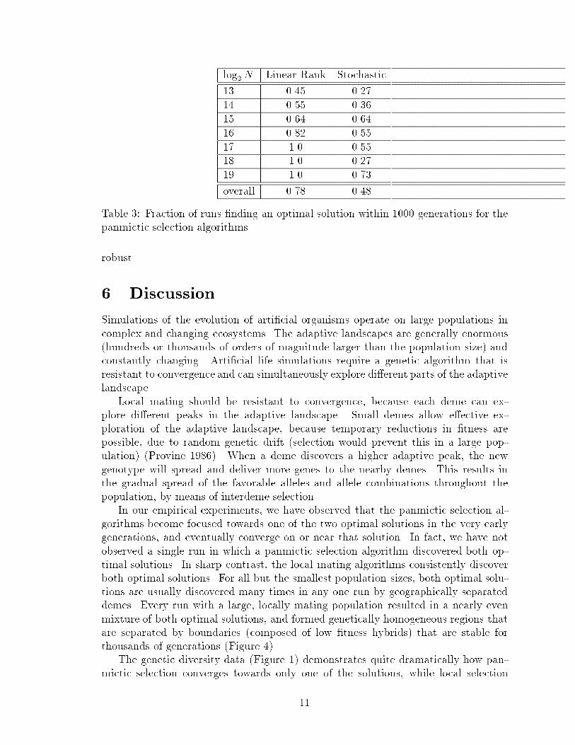
N Linear Rank Stochastic

13 0.45 0.27

14 0.55 0.36

15 0.64 0.64

16 0.82 0.55

17 1.0 0.55

18 1.0 0.27

19 1.0 0.73

overall 0.78 0.48

Table 3: Fraction of runs �nding an optimal solution within 1000 generations for the

panmictic selection algorithms.

robust.

6 Discussion

Simulations of the evolution of arti�cial organisms operate on large populations in

complex and changing ecosystems. The adaptive landscapes are generally enormous

(hundreds or thousands of orders of magnitude larger than the population size) and

constantly changing. Arti�cial life simulations require a genetic algorithm that is

resistant to convergence and can simultaneously explore di�erent parts of the adaptive

landscape.

Local mating should be resistant to convergence, because each deme can ex-

plore di�erent peaks in the adaptive landscape. Small demes allow e�ective ex-

ploration of the adaptive landscape, because temporary reductions in �tness are

possible, due to random genetic drift (selection would prevent this in a large pop-

ulation) (Provine 1986). When a deme discovers a higher adaptive peak, the new

genotype will spread and deliver more genes to the nearby demes. This results in

the gradual spread of the favorable alleles and allele combinations throughout the

population, by means of interdeme selection.

In our empirical experiments, we have observed that the panmictic selection al-

gorithms become focused towards one of the two optimal solutions in the very early

generations, and eventually converge on or near that solution. In fact, we have not

observed a single run in which a panmictic selection algorithm discovered both op-

timal solutions. In sharp contrast, the local mating algorithms consistently discover

both optimal solutions. For all but the smallest population sizes, both optimal solu-

tions are usually discovered many times in any one run by geographically separated

demes. Every run with a large, locally mating population resulted in a nearly even

mixture of both optimal solutions, and formed genetically homogeneous regions that

are separated by boundaries (composed of low{�tness hybrids) that are stable for

thousands of generations (Figure 4).

The genetic diversity data (Figure 1) demonstrates quite dramatically how pan-

mictic selection converges towards only one of the solutions, while local selection

11

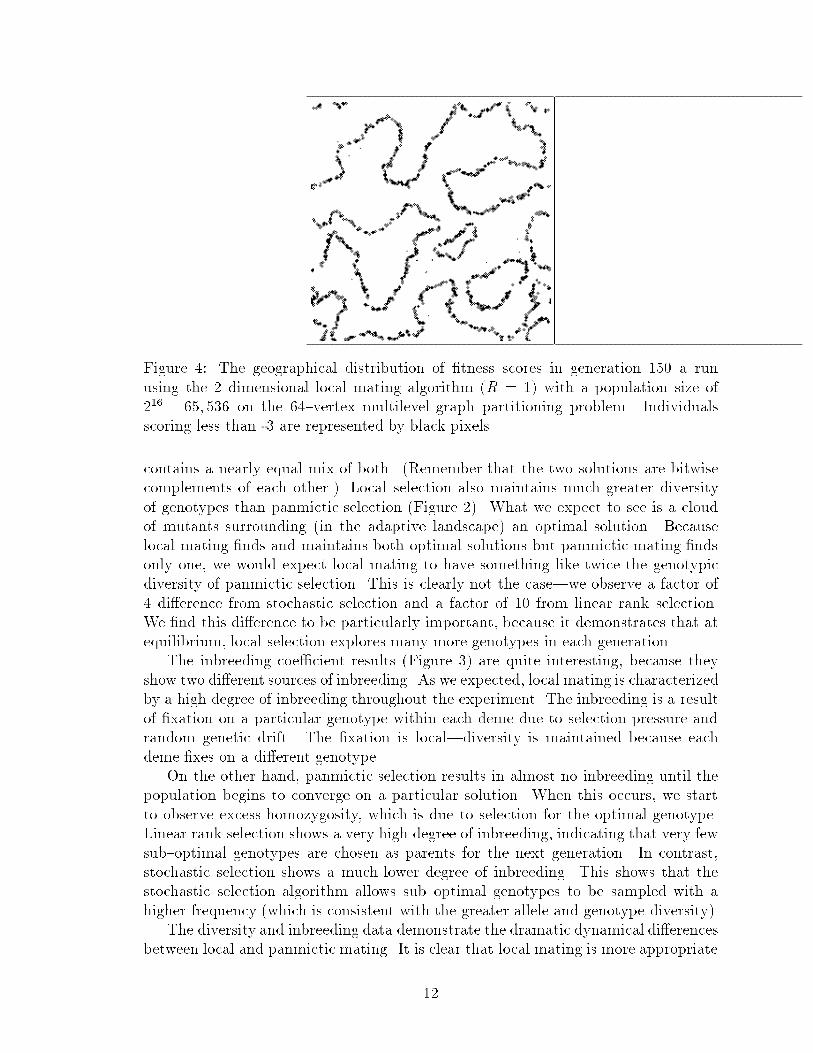
Figure 4: The geographical distribution of �tness scores in generation 150 a run

using the 2 dimensional local mating algorithm (R = 1) with a population size of

2

16

= 65; 536 on the 64{vertex multilevel graph partitioning problem. Individuals

scoring less than -3 are represented by black pixels.

contains a nearly equal mix of both. (Remember that the two solutions are bitwise

complements of each other.) Local selection also maintains much greater diversity

of genotypes than panmictic selection (Figure 2). What we expect to see is a cloud

of mutants surrounding (in the adaptive landscape) an optimal solution. Because

local mating �nds and maintains both optimal solutions but panmictic mating �nds

only one, we would expect local mating to have something like twice the genotypic

diversity of panmictic selection. This is clearly not the case|we observe a factor of

4 di�erence from stochastic selection and a factor of 10 from linear rank selection.

We �nd this di�erence to be particularly important, because it demonstrates that at

equilibrium, local selection explores many more genotypes in each generation.

The inbreeding coe�cient results (Figure 3) are quite interesting, because they

show two di�erent sources of inbreeding. As we expected, local mating is characterized

by a high degree of inbreeding throughout the experiment. The inbreeding is a result

of �xation on a particular genotype within each deme due to selection pressure and

random genetic drift. The �xation is local|diversity is maintained because each

deme �xes on a di�erent genotype.

On the other hand, panmictic selection results in almost no inbreeding until the

population begins to converge on a particular solution. When this occurs, we start

to observe excess homozygosity, which is due to selection for the optimal genotype.

Linear rank selection shows a very high degree of inbreeding, indicating that very few

sub{optimal genotypes are chosen as parents for the next generation. In contrast,

stochastic selection shows a much lower degree of inbreeding. This shows that the

stochastic selection algorithm allows sub{optimal genotypes to be sampled with a

higher frequency (which is consistent with the greater allele and genotype diversity).

The diversity and inbreeding data demonstrate the dramatic dynamical di�erences

between local and panmictic mating. It is clear that local mating is more appropriate

12

for arti�cial evolution, because it maintains a broad genetic search for thousands of

generations. If the adaptive landscape or �tness function were changing over time,

this diversity would allow the population to exploit the genotypes which suddenly

have higher relative �tness values. Local mating would be more appropriate than

panmictic mating for arti�cial life applications, even if local mating results in slower

evolution. Fortunately, this is not the case.

The data on the speed of evolution shows that the dynamics of local mating

results in a faster and more robust genetic algorithm. Local mating is characterized

by faster evolution both in terms of the number of �tness function evaluations and

time required to �nd an optimal solution. The robustness of local mating is rather

surprising: across all population sizes, both 1 and 2 dimensional geometries, and all

R values, local mating never failed to �nd an optimal solution, while both of the

panmictic algorithms had a signi�cant fraction of their runs \time out" (no optimal

solution found within 1000 generations).

The fact genetic algorithms that use local mating can be signi�cantly faster and

more robust than traditional genetic algorithms is an important result, and suggests

that further investigation is in order. While many important theoretical results have

been developed for panmictic mating algorithms, it is not clear that any of these

results can be applied directly to local mating. Also, it is not at all clear how local

mating will perform with small populations, although the di�erence in robustness

between local and panmictic mating is greatest for the smaller population sizes that

we examined. In addition, we have only examined one very simple local mating

algorithm, and it is almost certainly not the best that can be (or has been) found.

Acknowledgments

We would like to thank Ernst Mayr, Joe Pemberton, Chuck Taylor, Greg Werner, and

Alexis Wieland for their valuable input. We also acknowledge the three anonymous

reviewers for their helpful comments. This work is supported in part by W. M. Keck

Foundation grant number W880615, University of California Los Alamos National

Laboratory award number CNLS/89{427, and University of California Los Alamos

National Laboratory award number UC{90{4{A{88. The empirical data was gath-

ered in part on a CM-2 computer at UCLA under the auspices of National Science

Foundation Biological Facilities, grant number BBS 87 14206, and a CM-2 computer

at the Advanced Computing Laboratory of Los Alamos National Laboratory under

the auspices of the U.S. Department of Energy, contract W{7405{ENG{36.

References

Ackley, David H. (1987). Stochastic Iterated Genetic Hillclimbing. PhD thesis,

Carnegie Mellon Univeristy.

13

Collins, Robert J. (1990). CM++: A C++ interface to the Connection Machine.

In Proceedings of the Symposium on Object Oriented Programming Emphasizing

Practical Applications. Marist College.

Collins, Robert J. and David R. Je�erson (1991a). AntFarm: Towards simulated evo-

lution. In Langton, Christopher G., Charles Taylor, J. Doyne Farmer, and Steen

Rasmussen, editors, Arti�cial Life II, volume 10 of Santa Fe Institute Studies in

the Sciences of Complexity, pages 579{601. Santa Fe Institute, Addison{Wesley.

Collins, Robert J. and David R. Je�erson (1991b). An arti�cial neural network repre-

sentation for arti�cial organisms. In Schwefel, Hans-Paul and Reinhard M�anner,

editors, Proceedings of the First Workshop on Parallel Problem Solving, number

496 in Lecture Notes in Computer Science, pages 259{263, Berlin. Springer{

Verlag.

Collins, Robert J. and David R. Je�erson (1991c). Representations for arti�cial or-

ganisms. In Meyer, Jean-Arcady and Stewart W. Wilson, editors, Proceedings

of the First International Conference on Simulation of Adaptive Behavior: From

Animals to Animats, pages 382{390. The MIT Press/Bradford Books.

Crow, James F. (1986). Basic Concepts in Population, Quantitative, and Evolutionary

Genetics. W. H. Freeman and Company, New York.

De Jong, Kenneth A. (1975). An Analysis of the Behavior of a Class of Genetic

Adaptive Systems. PhD thesis, University of Michigan.

Deb, Kalyanmoy and David E. Goldberg (1989). An investigation of niche and species

formation in genetic function optimization. In Proceedings of the Third Interna-

tional Conference on Genetic Algorithms, pages 42{50. Morgan Kaufmann.

Goldberg, David E. (1989). Genetic Algorithms in Search, Optimization and Machine

Learning. Addison{Wesley Publishing Company, Inc.

Goldberg, David E. and Jon T. Richardson (1987). Genetic algorithms with sharing

for multimodal function optimization. In Genetic Algorithms and Their Applica-

tions: Proceedings of the Second International Conference on Genetic Algorithms,

pages 41{49. Lawrence Erlbaum Associates.

Gorges-Schleuter, Martina (1989). ASPARAGOS an asynchronous parallel genetic

optimization strategy. In Proceedings of the Third International Conference on

Genetic Algorithms, pages 422{427. Morgan Kaufmann.

Grefenstette, John J. and James E. Baker (1989). How genetic algorithms work: A

critical look at implicit parallelism. In Proceedings of the Third International

Conference on Genetic Algorithms, pages 20{27. Morgan Kaufmann.

Hartl, Daniel L. and Andrew G. Clark (1989). Principles of Population Genetics.

Sinauer Associates, Inc., Sunderland, Massachusetts.

14

Hillis, W. Daniel (1985). The Connection Machine. The MIT Press, Cambridge,

Massachusetts.

Je�erson, David, Robert Collins, Claus Cooper, Michael Dyer, Margot Flowers,

Richard Korf, Charles Taylor, and Alan Wang (1991). The Genesys System:

Evolution as a theme in arti�cial life. In Langton, Christopher G., Charles Tay-

lor, J. Doyne Farmer, and Steen Rasmussen, editors, Arti�cial Life II, volume 10

of Santa Fe Institute Studies in the Sciences of Complexity, pages 549{578. Santa

Fe Institute, Addison{Wesley.

Manderick, Bernard and Piet Spiessens (1989). Fine{grained parallel genetic algo-

rithms. In Proceedings of the Third International Conference on Genetic Algo-

rithms, pages 428{433. Morgan Kaufmann.

M�uhlenbein, Heinz (1989). Parallel genetic algorithms, population genetics and com-

binatorial optimization. In Proceedings of the Third International Conference on

Genetic Algorithms, pages 416{421. Morgan Kaufmann.

Provine, William B. (1986). Sewall Wright and Evolutionary Biology. University of

Chicago Press.

Wright, Sewall (1969). Evolution and the Genetics of Populations. Volume 2: The

Theory of Gene Frequencies. University of Chicago Press.

15