Selected deterministic models for lot sizing of growing items ...

Selected deterministic models for lot sizingof growing items inventory

by

Makoena Sebatjane

Submitted in partial fulfillment of the requirements for the degree

Master of Engineering (Industrial Engineering)

in the Faculty of Engineering, Built Environment and Information Technology

University of Pretoria

November 12, 2018

Selected deterministic models for lot sizing of

growing items inventory

by

Makoena Sebatjane

Supervisor : Dr. O AdetunjiDepartment : Industrial and Systems EngineeringDegree : Master of Engineering (Industrial Engineering)

Abstract

One of the more recent advances in inventory management is the modelling of inventorysystems consisting of items which are capable of growing during the course of the replen-ishment cycle. These items, such as livestock, are a vital part of life because most ofthem serve as saleable food items downstream in supply chains.

In the context of this study, growth is defined as achieving an increase in weight.This increase in weight is what differentiates growing items from conventional items. Atypical inventory system for growing items has two distinct periods, namely growing andconsumption periods. The growth period starts when a shipment of live newborn arrives.The live items are fed so that they can grow. All the items in each lot are assumedto grow at the same rate. Once the weight of the items reaches a specific target, theyare slaughtered. This marks the end of the growth period and thus the start of theconsumption period. The slaughtered items are kept in stock and consumed continuouslyat a given demand rate. At the instant that the consumption period ends, items in thenext cycle would have completed their growth period and they will be ready for slaughterand consumption. A feeding cost is incurred for feeding the live items during the growthperiod whereas holding costs are incurred for keeping the slaughtered items in stockduring the consumption period.

This study is aimed at developing lot sizing models for growing items under threedifferent conditions which might occur in food supply chains. These selected conditionsare used to develop three Economic Order Quantity (EOQ) models for growing items. Inaddition to item growth, these three models assume, respectively, that a certain fractionof the items is of imperfect quality due to errors in one of the processing stages; theavailable growing and storage facilities have limited capacities; and the vendor of theitems offers incremental quantity discounts. These models are aimed at answering two ofthe most important questions facing inventory managers, namely “how much to order?”and “when to place order?”. A third question, which is specific to growing items, arises,namely “when should the items be slaughtered?”.

In the imperfect quality model, it is assumed that the poor quality items are alsosold, but at a discounted price. Furthermore, there is a screening process, conductedon all the items before they are sold, to separate the poor quality items from those ofgood quality. For the limited capacity model, it is assumed that if the order quantityexceeds the available capacity, additional growing and storage capacities are rented froman external service provider, but this comes at a cost as the rented warehouse has higher

i

holding costs. The final model assumes that the supplier of the newborn items offers thepurchasing company incremental quantity discounts.

For all three model presented in this study, the proposed inventory systems are givenvivid descriptions which are used to formulate corresponding mathematical models. So-lution procedures for solving the proposed mathematical models are also presented. Nu-merical examples are provided to demonstrate the solution procedures and to conductsensitivity analyses on the major input parameters.

The presence of poor quality items means that more items need to be ordered in or-der to meet a specific demand for good quality items. The effect worsens as the fractionof imperfect quality items increases. Having capacity constraints on the growing andstorage facilities increases total costs mainly because of the higher holding costs in therented facility. As the capacity increases, the total costs decrease, but increasing capacityis capital intensive and poses financial risks if market conditions change for the worst.Quantity discounts were shown to reduce the purchasing cost of the newborn items, how-ever ordering very large quantities has downsides as well. The biggest downsides are therisk of running out of storage capacity, the increased holding costs and item deteriorationsince larger order quantities result in increased cycle times. Through sensitivity analysesconducted for all three models, the target slaughter weight was shown to have the greatesteffect on the EOQ than any other input parameter.

The inventory models presented in this study can be used by procurement and in-ventory managers, working in industries which stock growing items, as a guideline whenmaking purchasing decisions. This can result in sizable reductions in inventory-relatedcosts. Seeing that growing items are an integral part of food supply chains, the result-ing cost savings can be used to cushion consumers against rising food prices or from afinancial stand point, the savings can be used to boost profit margins.

ii

Contents

Abstract i

1 Introduction 11.1 Background . . . . . . . . . . . . . . . . . . . . . . . . . . . . . . . . . . 11.2 Motivation and significance . . . . . . . . . . . . . . . . . . . . . . . . . 21.3 Problem statement, objectives and research questions. . . . . . . . . . . . 3

1.3.1 Problem statement . . . . . . . . . . . . . . . . . . . . . . . . . . 31.3.2 Objectives . . . . . . . . . . . . . . . . . . . . . . . . . . . . . . . 31.3.3 Research questions . . . . . . . . . . . . . . . . . . . . . . . . . . 4

1.4 Scope of the study . . . . . . . . . . . . . . . . . . . . . . . . . . . . . . 41.5 Research methodology . . . . . . . . . . . . . . . . . . . . . . . . . . . . 41.6 Dissertation outline . . . . . . . . . . . . . . . . . . . . . . . . . . . . . . 5

2 Literature Review 62.1 Introduction . . . . . . . . . . . . . . . . . . . . . . . . . . . . . . . . . . 62.2 The classic EOQ model and major extensions . . . . . . . . . . . . . . . 7

2.2.1 The classic EOQ model . . . . . . . . . . . . . . . . . . . . . . . . 72.2.2 Significant extensions made to the classic EOQ model . . . . . . . 8

2.3 Growing inventory . . . . . . . . . . . . . . . . . . . . . . . . . . . . . . 102.3.1 EOQ model for growing items . . . . . . . . . . . . . . . . . . . . 102.3.2 Extensions made to the EOQ model for growing items . . . . . . 12

2.4 Imperfect quality inventory . . . . . . . . . . . . . . . . . . . . . . . . . 132.4.1 EOQ model for items with imperfect quality . . . . . . . . . . . . 132.4.2 Extensions made to the EOQ model for items with imperfect quality 14

2.5 Inventory with two levels of storage . . . . . . . . . . . . . . . . . . . . . 182.5.1 EOQ model for items with two levels of storage . . . . . . . . . . 182.5.2 Extensions made to the two-warehouse EOQ model . . . . . . . . 19

2.6 Inventory purchased under incremental quantity discounts . . . . . . . . 222.6.1 EOQ model with incremental quantity discounts . . . . . . . . . . 222.6.2 Extensions made to the EOQ model with incremental quantity dis-

counts . . . . . . . . . . . . . . . . . . . . . . . . . . . . . . . . . 232.7 Conclusion . . . . . . . . . . . . . . . . . . . . . . . . . . . . . . . . . . . 24

3 Economic order quantity model for growing items with imperfect qual-ity 253.1 Introduction . . . . . . . . . . . . . . . . . . . . . . . . . . . . . . . . . . 253.2 Problem definition . . . . . . . . . . . . . . . . . . . . . . . . . . . . . . 273.3 Notations and assumptions . . . . . . . . . . . . . . . . . . . . . . . . . . 28

iii

3.3.1 Notations . . . . . . . . . . . . . . . . . . . . . . . . . . . . . . . 283.3.2 Assumptions . . . . . . . . . . . . . . . . . . . . . . . . . . . . . . 28

3.4 Model development . . . . . . . . . . . . . . . . . . . . . . . . . . . . . . 293.4.1 General mathematical model . . . . . . . . . . . . . . . . . . . . . 293.4.2 Specific mathematical model: Case of items with a linear growth

function . . . . . . . . . . . . . . . . . . . . . . . . . . . . . . . . 313.4.3 Solution . . . . . . . . . . . . . . . . . . . . . . . . . . . . . . . . 34

3.5 Numerical results . . . . . . . . . . . . . . . . . . . . . . . . . . . . . . . 363.5.1 Numerical example . . . . . . . . . . . . . . . . . . . . . . . . . . 363.5.2 The effect of poor quality on the lot size . . . . . . . . . . . . . . 383.5.3 Sensitivity analysis . . . . . . . . . . . . . . . . . . . . . . . . . . 39

3.6 Conclusion . . . . . . . . . . . . . . . . . . . . . . . . . . . . . . . . . . . 41

4 Economic order quantity model for growing items with two growing andstorage facilities 424.1 Introduction . . . . . . . . . . . . . . . . . . . . . . . . . . . . . . . . . . 424.2 Problem definition . . . . . . . . . . . . . . . . . . . . . . . . . . . . . . 444.3 Notations and assumptions . . . . . . . . . . . . . . . . . . . . . . . . . . 45


4.4 Model formulation . . . . . . . . . . . . . . . . . . . . . . . . . . . . . . 464.4.1 General mathematical model . . . . . . . . . . . . . . . . . . . . . 464.4.2 Specific mathematical model: Case of a linear growth function . . 494.4.3 Solution . . . . . . . . . . . . . . . . . . . . . . . . . . . . . . . . 51

4.5 Numerical results . . . . . . . . . . . . . . . . . . . . . . . . . . . . . . . 534.5.1 Numerical example . . . . . . . . . . . . . . . . . . . . . . . . . . 534.5.2 The effect of limited growing and storage capacity of the owned

facility . . . . . . . . . . . . . . . . . . . . . . . . . . . . . . . . . 554.5.3 Sensitivity analysis . . . . . . . . . . . . . . . . . . . . . . . . . . 56

4.6 Conclusion . . . . . . . . . . . . . . . . . . . . . . . . . . . . . . . . . . . 59

5 Economic order quantity model for growing items with incrementalquantity discounts 615.1 Introduction . . . . . . . . . . . . . . . . . . . . . . . . . . . . . . . . . . 615.2 Problem definition . . . . . . . . . . . . . . . . . . . . . . . . . . . . . . 635.3 Notations and assumptions . . . . . . . . . . . . . . . . . . . . . . . . . . 64


5.4 Model development . . . . . . . . . . . . . . . . . . . . . . . . . . . . . . 655.4.1 General mathematical model . . . . . . . . . . . . . . . . . . . . . 655.4.2 Specific mathematical model: Case of a linear growth function . . 675.4.3 Solution . . . . . . . . . . . . . . . . . . . . . . . . . . . . . . . . 70

5.5 Numerical results . . . . . . . . . . . . . . . . . . . . . . . . . . . . . . . 715.5.1 Numerical example . . . . . . . . . . . . . . . . . . . . . . . . . . 715.5.2 Sensitivity analysis . . . . . . . . . . . . . . . . . . . . . . . . . . 74

5.6 Conclusion . . . . . . . . . . . . . . . . . . . . . . . . . . . . . . . . . . . 77

iv

6 Conclusion 786.1 Summary of findings . . . . . . . . . . . . . . . . . . . . . . . . . . . . . 786.2 Possible practical applications of findings . . . . . . . . . . . . . . . . . . 796.3 Contributions . . . . . . . . . . . . . . . . . . . . . . . . . . . . . . . . . 796.4 Possible areas for future research . . . . . . . . . . . . . . . . . . . . . . 79

References 81

v

List of Figures

2.1 Holding cost, ordering cost and total cost as functions of order quantity . 72.2 Typical inventory system behaviour for the classic EOQ model . . . . . . 82.3 Timeline showing some of the major developments in inventory theory . . 92.4 Behaviour of typical inventory systems for conventional and growing items 102.5 Inventory system behaviour for growing items . . . . . . . . . . . . . . . 112.6 Inventory system behaviour for items with imperfect quality . . . . . . . 132.7 Inventory system behaviour for items with two levels of storage . . . . . 19

3.1 Inventory system behaviour for growing items with imperfect quality . . 273.2 Inventory system behaviour for growing items with imperfect quality under

the assumption of linear growth function . . . . . . . . . . . . . . . . . . 323.3 Graph of expected total profit per unit time, cycle time and order quantity 383.4 The impact of the presence of poor quality items on the order quantity . 38

4.1 Inventory system behaviour for growing items with two growing and stor-age facilities . . . . . . . . . . . . . . . . . . . . . . . . . . . . . . . . . . 44

4.2 Inventory system behaviour for growing items with two growing and stor-age facilities and a linear growth function . . . . . . . . . . . . . . . . . . 49

4.3 Graph of total cost per unit time, cycle time and order quantity . . . . . 554.4 The effect of limited growing and storage capacity on the lot size . . . . . 55

5.1 Behaviour of an inventory system for growing items . . . . . . . . . . . . 635.2 Inventory system behaviour for growing items under the assumption of

linear growth function . . . . . . . . . . . . . . . . . . . . . . . . . . . . 685.3 Average total cost under incremental quantity discounts . . . . . . . . . 74

vi

List of Tables

3.1 Gap analysis of related works in literature . . . . . . . . . . . . . . . . . 263.2 Notations used in the formulation of the mathematical model . . . . . . . 283.3 Summary of the results from the numerical example . . . . . . . . . . . . 373.4 Changes to y∗ and E[TPU ]∗ due to changes in c . . . . . . . . . . . . . . 393.5 Changes to y∗ and E[TPU ]∗ due to changes in K . . . . . . . . . . . . . 393.6 Changes to y∗ and E[TPU ]∗ due to changes in h . . . . . . . . . . . . . . 403.7 Changes to y∗ and E[TPU ]∗ due to changes in w1 . . . . . . . . . . . . . 40

4.1 Gap analysis of related works in literature . . . . . . . . . . . . . . . . . 444.2 Notations used in the formulation of the mathematical model . . . . . . . 454.3 Summary of the results from the numerical example . . . . . . . . . . . . 544.4 Changes to y∗ and TCU∗ due to changes in c . . . . . . . . . . . . . . . 564.5 Changes to y∗ and TCU∗ due to changes in K . . . . . . . . . . . . . . . 574.6 Changes to y∗ and TCU∗ due to changes in hm . . . . . . . . . . . . . . 574.7 Changes to y∗ and TCU∗ due to changes in hr . . . . . . . . . . . . . . . 584.8 Changes to y∗ and TCU∗ due to changes in m . . . . . . . . . . . . . . . 584.9 Changes to y∗ and TCU∗ due to changes in w1 . . . . . . . . . . . . . . . 59

5.1 Gap analysis of related works in literature . . . . . . . . . . . . . . . . . 625.2 Notations used in the formulation of the mathematical model . . . . . . . 645.3 Purchase cost structure under incremental quantity discounts . . . . . . . 725.4 Summary of the results from the numerical example . . . . . . . . . . . . 735.5 Changes to Y ∗ and ATCU∗ due to changes in K . . . . . . . . . . . . . . 745.6 Changes to Y ∗ and ATCU∗ due to changes in i . . . . . . . . . . . . . . 755.7 Changes to Y ∗ and ATCU∗ due to changes in c . . . . . . . . . . . . . . 755.8 Changes to Y ∗ and ATCU∗ due to changes in w1 . . . . . . . . . . . . . 765.9 Changes to Y ∗ and ATCU∗ due to changes in yj . . . . . . . . . . . . . . 765.10 Changes to Y ∗ and ATCU∗ due to changes in pj . . . . . . . . . . . . . . 77

vii

List of Abbreviations and Acronyms

AM-GM Arithmetic Mean-Geometric MeanDEL Dynamic Economic LotEOQ Economic Order QuantityEPQ Economic Production QuantityFIFO First-In-First-OutLIFO Last-In-Last-OutOM Operations ManagementOR Operations ResearchVAT Value-Added TaxVMI Vendor-Managed InventoryWIP Work-In-ProcessZAR South African Rand

viii

Chapter 1

Introduction

1.1 Background

Inventories are an important part of organisations, regardless of whether they are for-profit or non-profit. Having the right levels and mix of inventories ensures that operationsrun smoothly and customer demands are satisfied. Furthermore, inventories representa sizable portion of assets on the balance sheet. High inventory levels might reducethe possibility of stock-outs and contribute to higher customer satisfaction, but theyincrease operating costs. On the other hand, low inventory levels reduce the operatingcosts and increase the possibility of running out of stock. Inventory management isconcerned with balancing these contradictory objectives (Stevenson, 2018). Inventorymanagement affects multiple functions or departments (such as production, marketingand sales, finance and procurement) within the primary organisation and across the entiresupply chain.

Inventory management is a well-studied area that has been researched for over a cen-tury. Since the publication of the seminal model by Harris (1913), various researcheshave modified and extended the model in order to represent different and more realisticinventory systems. An area that seems to be receiving attention lately is the modellingof growing items inventory. The first work dealing with inventory management for grow-ing items was presented by Rezaei (2014) and there seems to still be opportunities forfurther research in this area. Growing items can be considered as a distinct class of itemswithin inventory theory, similar to perishable, ameliorating or repairable items, to namea few. These items, unlike conventional items, experience an increase in weight duringthe inventory planning period as a result of being fed. These items are fed (or raised) fora certain period of time and after growing to a specific weight, they are slaughtered andthen sold to market.

The aim of this study is to extend the basic inventory model for growing items byrelaxing three implicit assumptions made in Rezaei (2014)’s model. The first assumptionis that all the ordered inventory is of acceptable quality. This is not true for all situationsbecause prior to selling the items, they need to be prepared (in the form of slaughtering,cutting and packaging, among other processes) for sale. Like most production systems,the preparation processes are subject to variation and human error and thus it is highlyunlikely that all the items produced from the process will be of perfect quality. Thesecond assumption is that all the ordered items are grown in one facility and stored inone facility regardless of the size of the order. This implies that the capacity of the growingand storage facilities are unlimited. In reality, these facilities, just like all assets, have

1

limited capacities. The third assumption is that quantity discounts are not permitted.Sometimes suppliers offer customers discounts for purchasing larger quantities as a meansof reducing their transportation costs (i.e. by incentivising customers to buy highervolumes of stock, the supplier has to make fewer shipments of larger order quantities) orto stimulate demand in response to difficult market conditions or competitor pricing.

1.2 Motivation and significance

The research presented in this dissertation is motivated by perceived lack of sufficientresearch in the area of inventory management for growing items. While growing items(which includes livestock and fish, among others) are only recently receiving attentionin inventory management research, they are a very important part of daily life. Mostgrowing inventory items serve as food downstream in most supply chains, and as suchhaving a better understanding of this class of inventory items will enrich the knowledgecurrently available in this relatively new and important subarea of inventory theory.

Growing items are an important part of food supply chains. Typical food supplychains have producers, processors, distributors, retailers and consumers. The producersare typically farmers who are involved in the production of fruits, vegetables, grains orlivestock, among others. Processors transform the items from the producers into varioussaleable food items which meet consumer needs. Logistics providers ensure that thesaleable food items reach consumers, who typically purchase these food items throughretailers, in an acceptable condition (Dani, 2015). The business of food producers istypically the production (in the form of rearing and eventually slaughtering) of growingitems. Food supply chains are faced with a number of issues, three of which are thesubject of this study. These are quality, outsourcing due to capacity limits and costreduction through better procurement practices.

There a number of processes in food supply chains that can compromise the qualityof the items. Growing items are often processed into various customer-preferred variants,for example chickens reach consumers in various forms such as fillets, burgers, sausages,etc., and these processing stages, like most production systems, seldom produce perfectquality items. This reason makes quality screening a vital part of inventory managementin food supply chains. Slaughtering is an important aspect of a growing items inventorysystem and errors might occurs during this stage, resulting in improperly slaughteredpieces which might not be appreciated by aesthetically-conscious customers. For thisreason, the imperfect quality items are removed from the lot and sold as a single batchat a reduced price to a bulk-purchasing and value-oriented customer. Imperfect qualityitems are not necessarily defective or unhealthy, they just don’t meet all the aspects of aquality inspection process and hence, they are sold as a single batch to a different typeof customer.

Capacity planning is another important decision which affects inventory managementin supply chains. When facilities are set up, companies need to make decisions about thequantity of items their facilities can accommodate. Changing macro-economic conditionsor the departure of a competitor, among other reasons, might increase customer demandand the result is that the capacity of the company-owned facilities can not keep up withdemand. In this situation, it might be necessary for the company to outsource some of itsactivities, such as rearing and warehousing in the case of growing items, from an externalservice provider.

2

Suppliers often offer quantity discounts as a means of encouraging customers to pur-chase higher volumes of stock. In an effort to reduce costs, procurement managers oftenbuy larger quantities of stock in order to take advantage of quantity discounts. However,the right quantity of stock needs to be ordered because if too much is ordered then theholding costs will increase and this might negate the effects of quantity discounts.

The role that growing items play in the food supply chain, which is mainly to serveas saleable food items, makes them important because food consumption is an essentialpart of daily life. Likewise, the management of inventoried growing items is significant.Recently, South Africa has experienced a number of events which have led to increases inthe price of food. These events include increases in the Value-Added Tax (VAT) and thefuel levy as well as unfavourable weather conditions (BusinessTech, 2018), among others.South Africa, has high levels of poverty which can be attributed to, among other things,the high unemployment rate. Consequently, basic food items are unaffordable to mostpeople. This makes effective inventory management in food supply chains even moreimportant because through effective inventory management, food producers can achievesignificant cost savings which they can use to either absorb some of the increases in theprice of food (and thus making food more affordable to a larger customer base) or froma financial standpoint, to improve their profit margins.

1.3 Problem statement, objectives and research ques-

tions.

1.3.1 Problem statement

Certain inventory items are living organisms and hence they are capable of growingduring the course of the replenishment cycle. These items are purchased soon afterbirth as as newborn items. The items are fed and this leads to growth. In the contextof this dissertation, growth is quantified only through an increase in weight. Feedingcontinues until the items reach a certain target weight, after which they are slaughteredand consumed (i.e. put on sale). A number of issues might arise in such inventorysystems, three of which are considered in this dissertation. Firstly, between the growthand consumption period, the quality of some of the items might deteriorate and at thetime of consumption it is discovered that a certain fraction of the items is of unacceptablequality. Secondly, the space used for raising the live items and the space used for stockingthe slaughtered items might have limited capacities. Lastly, the supplier of the newbornitems might offer discounts for purchasing larger quantities.

1.3.2 Objectives

Based on the problem statement, the following objectives are identified:

• To develop an Economic Order Quantity (EOQ) model for an inventory systemconsisting of growing items when a certain fraction of the items is of poor quality.

• To develop an EOQ model for growing items reared (or grown) and stored in twofacilities because the first facilities, which are company-owned, have limited capac-ities.

3

• To formulate an EOQ model for growing items when incremental discounts aregranted by the supplier of the newborn items.

1.3.3 Research questions

The following research questions, which apply to all three models, are formulated:

How many newborn items should be ordered at the beginning of a growing cycle?

Given a target slaughter weight for the items, when (i.e. how long after receivingthem as newborn items) should they be slaughtered?

How much time should elapse between successive order replenishments?

1.4 Scope of the study

The common themes among the three models presented in this study are item growth anddeterministic demand. The first theme implies that the live inventory items purchasedat the beginning of a replenishment cycle experience an increase in weight for a certainperiod of time during the course of the replenishment cycle. The second theme impliesthat customer demand rate for the slaughtered inventory items is assumed to be knownwith certainty.

With regards to the first theme, a number of additional assumptions are made. Firstly,a uniform growth rate is assumed for all the ordered items in each lot. This means thatall the live items received grow at the same rate and consequently, they complete theirgrowth period at the same time and they are slaughtered at the same time since theywould have reached the target weight at the same time. Secondly, sickness and mortalityas a result of sickness are not accounted for in the models presented. Nonetheless, thesetwo factors are important and they present an opportunity for further development ofthe models presnted in this work.

1.5 Research methodology

Bertrand and Fransoo (2002) proposed various methodologies for conducting quantitativeresearch in Operations Management (OM) and Operations Research (OR). The follow-ing methodology, which is adapted from Bertrand and Fransoo (2002), was used whenconducting the research presented in this dissertation:

Theoretical model of the problem or process: Vivid descriptions of the pro-posed inventory systems are provided. The descriptions are based on real life situ-ations that might arise in firms stocking growing items.

Scientific model of the problem or process: Mathematical models are formu-lated based on the worded problem definitions. Since the mathematical models areintended to mimic real life situations as closely are possible, it is necessary to makea number of assumptions which aid in bridging the gap between reality and themathematical formulations of the problems.

4

Solution to the scientific model: Solution procedures for solving the proposedmathematical models are presented. The solution algorithms are then applied tonumerical examples in order to illustrate their use in finding solutions to the pro-posed inventory systems.

Proof of the solution: It is then shown that unique solutions to the mathematicalmodels representing the proposed inventory systems exist.

Observations on the theoretical model: Sensitivity analyses are conducted todetermine the most significant inputs. The results are used to make recommenda-tions on real life inventory systems for growing items.

1.6 Dissertation outline

The remainder of this dissertation is structured as follows:Chapter 2 documents a review of literature related to the classic EOQ model as well

as EOQ models for growing items, items with imperfect quality, items with two storagefacilities and items purchased under incremental quantity discounts.

Chapter 3 addresses one the three main objectives of the work presented in this dis-sertation, which is to develop an EOQ model for growing items with imperfect quality.The proposed inventory system considers a situation where a company orders a certainnumber of items which are capable of growing during the course of the inventory replen-ishment cycle. Growth is facilitated by the company through feeding the items. Theseitems are then slaughtered after growing to a certain weight. A certain fraction of theitems is not of acceptable quality. Prior to being sold, the items are screened to separatethe good quality items from the poor quality items. Good quality items are sold at agiven price while poor quality items are salvaged as a single batch at the end of thescreening period.

An EOQ model for growing items with two growing and storage facilities is presentedin Chapter 4. The inventory system under study considers a company which purchasesnewborn items. The company’s growing and storage facilities have limited capacities. Ifthe order size exceeds the capacities of the company-owned facilities, the company leasesa second growing facility and a second storage facility. These facilities can raise or storeas many items as possible, but they charge higher holding costs. For this reason, theitems in the rented facility are consumed first.

In Chapter 5, incremental quantity discounts are incorporated to the basic EOQ modelfor growing items. Incremental quantity discounts are one of two quantity discounts of-ten offered by suppliers as a way of encouraging customers to purchase larger volumesof stock, the other being all-units quantity discounts. The difference between them isthat incremental quantity discounts result in reduced purchasing cost for the entire or-der if larger volumes are ordered whereas if incremental quantity discounts are offered,the reduced purchasing cost only applies to items bought above a certain quantity. Theinventory system studied in this chapter considers a company whose supplier offers dis-counts for purchasing larger quantities of newborn items which are capable of growingduring the replenishment cycle.

Chapter 6 concludes the dissertation by providing a summary of the findings, con-tributions, limitations and possible areas for future research in the area of inventorymanagement for growing items.

5

Chapter 2

Literature Review

2.1 Introduction

Any resource stocked or stored by an entity, with the intention of using the resource,is termed inventory (Jacobs and Chase, 2018). Entities hold inventories for a varietyof reasons, Simchi-Levi et al. (2008) stated four major reasons. The first reason is tohedge against unanticipated changes in customer demands. Secondly, inventory acts as abuffer which cushions the entity against the effects of various forms of uncertainty. An-other reason for keeping inventory is to take advantage of economies of scale brought bypurchasing large quantities or incentives given by transportation companies. Lastly, hold-ing inventory safeguards against the possibility of stock-outs during supply lead times.While maintaining high inventory levels has business benefits, such as high customerservice levels and smooth running operations, there are potential disadvantages. Thebiggest of which is the excessive costs associated with holding inventory (Mentzer et al.,2007; Simchi-Levi et al., 2008; Jaber et al., 2008; Muckstadt and Sapra, 2010; Stevenson,2018). These include all costs incurred as a result of storage, handling, taxes, insurance,depreciation, deterioration and obsolescence, among others, and most importantly inter-est or the opportunity cost of capital had the money been invested elsewhere (Jacobs andChase, 2018).

Inventory can be categorised into one of five groups depending on the reason forkeeping it (Muckstadt and Sapra, 2010), namely cycle, safety, pipeline, decoupling andanticipation inventories. Cycle stock is held for the purpose of satisfying customer demandbetween replenishment periods. Companies hold safety stocks as a buffer to absorb theeffects of uncertainties in lead time, supply and demand. Items in transit, or in the caseof manufacturing systems Work-In-Process (WIP) inventories, are classified as pipelineinventories. Decoupling stock is a specific type of safety stock in manufacturing systemswhich ensures that manufacturing operations run smoothly in the presence of variation insetup times or breakdowns. Anticipation inventories are held by companies in anticipationof certain events which might occur in the future such as price increases or buildingup inventory prior to a selling period in the case of seasonal products or new productintroductions.

Successful management of inventory not only ensures that operations run smoothly,but it also improves cash flow and profitability in the case of commercial entities. Forthese reasons, inventory management is one of the most important activities in productionand operations management (Stevenson, 2018). Poor inventory management results inover- or under-stocking of resources, both of which are undesirable and can have major

6

cost repercussions across the entire supply chain. On the other hand, good inventorymanagement not only reduces the possibility of stock-outs or overstocking but it alsoresults in improved customer satisfaction while keeping inventory costs as low as possible.The two major decisions in inventory management are the order quantity and the cycletime, i.e. how much to order and when to place an order (Stevenson, 2018). Thesedecisions are addressed through lot sizing models of which the EOQ is the classic model.

2.2 The classic EOQ model and major extensions

The EOQ model works out the optimal order size which minimises certain inventoryrelated costs. These costs vary with the order size and the frequency of ordering. In theEOQ’s most basic form, these costs are those associated with placing an order and keepingthe order in storage. While the model was made famous by Wilson (1934), its foundationslie in Harris (1913)’s work. Harris (1913) proposed a formulation for determining the orderquantity while balancing the purchasing cost, setup cost and inventory holding cost. Theresulting formulation, which would later morph into what is now referred to as the classicEOQ model, makes a number of unrealistic assumptions. These assumptions limit themodel’s application to most real-life inventory systems. In attempts to make the modelmore realistic, various researchers have made extensions to the model by considering newassumptions, in addition to relaxing some of the assumptions made when the originalmodel was formulated (Andriolo et al., 2014).

2.2.1 The classic EOQ model

The classic EOQ model is the simplest inventory control model. It is used to determinea fixed order order quantity which minimises the sum of the inventory holding costs andthe ordering costs. The purchasing cost can also be included, but it is often excludedbecause it has no effect on the optimal order quantity except when quantity discounts aretaken into account. In essence, the EOQ model finds a balance between the holding andordering costs because as the order quantity increases the holding costs increase and theordering costs decrease. The reverse is also true. These trade-offs are shown in Figures2.1 and 2.2 which demonstrate how the total costs change with order quantity and thechanges to the inventory level with time respectively.

Figure 2.1: Holding cost, ordering cost and total cost as functions of order quantity

7

(a) Fewer large orders result in higher inventoryholding costs and lower setup costs

(b) Numerous small orders result in lower in-ventory holding costs and higher setup costs

Figure 2.2: Typical inventory system behaviour for the classic EOQ model

The inventory system depicted in Figure 2.2 considers only one type of item and it isassumed that there is no lead time. An order for Q items is received, in one shipment, atthe beginning of each inventory planning cycle. Each time an order for Q items is placed,a ordering cost of K is incurred. The items are consumed at a constant annual rate Duntil they are used up at the end of period T . A new order for Q items is received at theinstant the previous order finishes up. The items are kept in stock at an annual holdingcost of h per item. Additional assumptions made when developing the model are thatquantity discounts and shortages are not permitted. The total cost per unit time, TCU ,is given by

TCU = h

(Q

2

)+K

(D

Q

). (2.1)

The value of Q which minimises Equation (2.1), denoted by Q∗ and referred to as theEOQ, is determined using differential calculus as

Q∗ =

√2KD

h. (2.2)

2.2.2 Significant extensions made to the classic EOQ model

Following the publication of Harris (1913)’s paper, a multitude of inventory models havebeen developed based on that particular model (Andriolo et al., 2014). Some of the mostsignificant extensions made to Harris’ model are depicted in Figure 2.3, which also showshow research in the area of inventory theory has evolved since the publication of Harris’pioneering work over a century ago.

The first major extension to the classic EOQ model, courtesy of Taft (1918), camein the form of what is now widely known as the Economic Production Quantity (EPQ)model. In the EPQ model, two major events take place simultaneously, namely continuousconsumption and periodic production. The consumption rate of items is assumed to beless than the capacity to produce the items, i.e. the production rate exceeds the demandrate.

Inventory models presented inn the first half of the 20th century made the assumptionthat the demand rate is static. Wagner and Whitin (1958) relaxed this assumptionthrough the development of the Dynamic Economic Lot (DEL) model.The difference

8

between the DEL model and earlier lot sizing models is that the demand rate is assumedto be changing over a set number of periods.

As a way of persuading customers to order larger quantities, a supplier might offerprice reductions for large orders (Stevenson, 2018). Quantity discounts were taken intoconsideration when modelling inventory systems for the first time by Hadley and Whitin(1963). Two types of quantity discounts were modelled, namely all unit and incrementalquantity discounts. The models considered different price breaks which are a result ofstep changes in the prices of predetermined order quantities.

Subsequently, Hadley and Whitin (1963) studied inventory systems where shortagesare permitted. When shortages are taken into account in inventory theory, they are eitherfully or partially backordered. Full backordering of shortages means that all customers arewilling to wait until the next shipment arrives. When shortages are partially backordered,some customers are willing to wait while others are not, resulting in lost sales.

Figure 2.3: Timeline showing some of the major developments in inventory theory

Harris (1913)’ model assumes that items can be stored indefinitely without a change tothe item’s integrity, utility or value. However, this is not true for certain items like fruits,vegetables, dairy products and eggs, to name a few. Such items are called perishableor deteriorating items. Deterioration is an umbrella term which emcompasses any formof damage, pilferage, evaporation, loss of usefulness or spoilage of the item (Palaniveland Uthayakumar, 2016). Ghare and Schrader (1963) presented an inventory model foritems which deteriorate while in stock. The items’ deterioration rate was modelled by adecaying exponential function.

An implicit assumption of most inventory models is that costs remain constant overtime. However, this is not true in practice as inflation and the time value of moneyinfluence costs. Buzacott (1975) investigated the impact that cost increases, brought byinflation, had on the order quantity by taking into account a rate of inflation on thevarious cost components. Gurnani (1983) studied, under discounted cash flow analysis, afew inventory models in order to determine the effect that the time value of money hadon the EOQ and total costs.

Goyal (1985) presented an EOQ model in which delays in payments (from the buyer

9

to the vendor) are allowed. The motivation behind the model was that in most situationsordered items are not paid for at the instant the vendor delivers them to the customer.The delay in payment can be because the buyer wants to inspect the order after receiptto ensure that it is in the agreed upon state, or it can be due to the supplier giving buyersa grace period to settle their bills.

Salameh and Jaber (2000) extended the basic EOQ model by relaxing the assumptionthat all items are of good quality. They studied an inventory system where a certainfraction of items is assumed to be of imperfect quality. Both perfect and imperfectquality items are then sold, but the imperfect quality items are sold at a discount.

Stringent environmental policies legislated in some jurisdictions around the world as ameans of reducing carbon emissions, such as the cap and trade emissions trading schemein the European Union, motivated Hua et al. (2011) to incorporate carbon emissions tothe classic EOQ model. They assumed that a company incurs a cost associated with itsemissions, released as a result of its production and logistics activities, based on the capand trade emissions trading scheme.

Rezaei (2014) used the growth rate and feeding functions of broiler chickens to developan EOQ model for a new class of inventory items called growing items. These are itemswhich grow, through gaining weight, during the course of a replenishment cycle.

In order to model specific and realistic inventory systems, some of the features of clas-sic EOQ model and its extensions are combined, either together or with new assumptions.This study is concerned with the management of growing inventory items under a set ofrealistic conditions, namely, imperfect quality, limited capacity and quantity discounts,which might arise in food supply chains.

2.3 Growing inventory

2.3.1 EOQ model for growing items

The classic EOQ model makes the assumption that the weight of the inventory remainsconstant throughout the replenishment cycle. This is not true for items like livestockwhich grow, and thus their weight varies over the course of an inventory planning cy-cle. Item growth in inventory theory was first addressed by Rezaei (2014). Growingitems are defined as items whose weight increases over time. This does not happen withconventional items. Figures 2.4a and 2.4b depict typical inventory system behaviour forconventional items and growing items respectively.

(a) Conventional items (b) Growing items

Figure 2.4: Behaviour of typical inventory systems for conventional and growing items

The weight of conventional inventory items, such as books or car parts, remainsconstant over time if they are not consumed (i.e. period t in Figure 2.4a). A change to

10

the weight of the inventory level is only brought by consumption (i.e. period T in Figure2.4a). However, the weight of growing items, such as poultry or livestock, increases overtime as they are fed (i.e. period t in Figure 2.4b) until the point of slaughter. Theweight of the items then decreases continuously as a result of consumption as indicatedby period T . Although the model developed by Rezaei (2014) is generalised, it depends onthe growth rate of the items under study because different growing items have differentgrowth rates. Rezaei considered an inventory situation in which newborn animals, ofa certain initial weight, are purchased. The animals are then fed (or raised) until theyreach a specific weight. Following this, the animals are slaughtered and sold to the market.Rezaei developed a model that determined the optimal quantity of newborn animals toorder and the optimal day to slaughter them following the growth period. The modelcould not be solved in closed form. The optimal slaughter age was determined using abisection method.

The series of events taking place in the inventory system studied by Rezaei (2014)can be summarized as follows:

• A company orders a lot size of y newborn animals at a cost of p each at the beginningof each cycle. At the time of receiving the order, the newborn animals each weighw0.

• It costs the company K to setup for a new growth cycle. This is a fixed cost and itis incurred at the beginning of each cycle.

• In order for the animals to grow, they are fed at a unit cost c. However, the animalsconsume different quantities of feed stock based on their age. The relationshipbetween the animals’ age and the quantity of feed stock they consume is given bythe feeding function f(t).

• After growing to a target weight wt, the animals are slaughtered and kept in storage.The company pays a annual holding cost of h per weight unit.

• The slaughtered animals are sold at a price of s per weight unit. The annual demandfor the slaughtered animals is a deterministic constant D.

Figure 2.5: Inventory system behaviour for growing items

The behaviour of the inventory system over time is depicted in Figure 2.5, where t isthe slaughter age and T is the duration of consumption period or the cycle time. The

11

total profit per cycle is defined as the difference between the revenue from the sales ofthe slaughtered animals minus the total costs. The total costs is the sum of the purchase,setup, production (i.e. feeding) and holding costs. The total profit per cycle, denoted byTP , is given by:

TP = sywt − pyw0 − cy∫ t

o

f(t)dt− hT(ywt

2

)−K (2.3)

An expression for the total profit per unit time, TPU , is determined by dividing TPby the length of the sales period, T , which equals ywt/D. In order to make the modelspecific, an assumption was made that the animals in the inventory system under studyare broiler chickens. Hence, the feeding function, f(t), and the growth function, f(wt|w0),were replaced by functions developed for broiler chickens and proposed by (Goliomytiset al., 2003) and Richards (1959) respectively. The feeding and the growth functions aregiven by the following expressions respectively:

f(t) = b0 + b1t+ b2t2 + b3t

3 (2.4)

wt = A(1 + le−gt

)−1/n(2.5)

The order quantity is determined by equating the derivative of the expression for thetotal profit per unit time, TPU , with respect to y to zero and the result is

y =

√√√√ 2KD

h[A2(1 + le−gt

)−2/n] (2.6)

The model’s decision variables, namely the optimal order quantity (y∗) and optimalslaughter age (t∗), could not be determined in closed form. Rezaei (2014) used a bisectionmethod, in particular the Newton-Raphson method, to work out the optimal value of t∗.This value was then used to determine the EOQ from Equation (2.6).

2.3.2 Extensions made to the EOQ model for growing items

Zhang et al. (2016) formulated an inventory model for growing items in a carbon-constrained environment. Their model used the same basic assumptions, including thegrowth and feeding functions, as Rezaei (2014)’s model. They extended Rezaei’s modelby assuming that the company under study operates in a country where carbon taxesare legislated. The carbon tax is based on the amount of emissions released into theatmosphere as a result of the company’s inventory holding, ordering and transportationactivities. As was the case with Rezaei’s model, the total profit was the objective func-tion and the decision variables were the optimal order quantity and optimal slaughterage. The optimal solution to the problem was determined through an algorithm.

Nobil et al. (2018) developed an EOQ model for growing items with shortages. Themodel presented by Nobil et al. (2018) differed from Rezaei (2014)’s model in two ways.Firstly, in the former model shortages are allowed and fully backordered and secondly,the growth function of the items was approximated by a linear function in former modelas opposed to using Richards (1959)’s growth curve as was the case in the latter model.Earlier inventory models for growing items, namely those by Rezaei (2014) and Zhang

12

et al. (2016), utilised the feeding function proposed by Goliomytis et al. (2003), whichincreased the computational complexity when determining optimal solutions. By as-suming a linear growth function, Nobil et al. (2018) drastically reduced the complexityof computing the feeding cost. Consequently, the optimal solution to the problem wasdetermined using a relatively simple heuristic.

2.4 Imperfect quality inventory

2.4.1 EOQ model for items with imperfect quality

Item quality was incorporated to inventory management research by Salameh and Jaber(2000). They relaxed the assumption that all the items received in each order are of goodquality. They proposed an inventory situation in which a certain fraction of the ordereditems is of poor quality. Before the items are sold, they are all subjected to a screeningprocess so as to separate the items of good quality from those of poor quality. Both goodand poor items are then sold. While good quality items are sold continuously during theinventory replenishment cycle, poor quality items are salvaged (i.e. sold at a price lowerthan that charged for good quality items) as a single batch at the end of the screeningprocess. The model’s optimal solution was determined in closed form.

Figure 2.6: Inventory system behaviour for items with imperfect quality

The series of events taking place in inventory system for items with imperfect quality,as proposed by Salameh and Jaber (2000) and depicted in Figure 2.6, can be summarisedas follows:

• A lot size of Q items is ordered by a company at cost of p per item.

• Each time the company places an order, an ordering cost of K is charged.

• Not all of the items received in each lot are of good quality. A fraction of the items,x, is of poor quality. The fraction of poor quality items, x, is random and has aknown probability density function g(x).

• Before selling the items, they are subjected to a 100% screening process, whichseparates the good quality items from those of poor quality. Unit screening cost

13

is z and the items are screened at a rate r per unit time. The screening processoccurs for the duration τ .

• The company keeps all the items in stock. The cost associated with keeping oneunit in stock for a year is h.

• Good quality items are sold at a price of s per unit and are demanded at an annualrate of D. Poor quality items are sold as a single batch at a price v per unit, whichis lower than the price charged for good quality items, at the end of the screeningperiod.

The total profit per cycle is given by

TP = sy(1− x) + vyx− py −K − zy − h(y(1− x)2

2D+xy2

r

). (2.7)

Since x is a random variable with a known probability density function, the expectedvalue of the total profit per unit time, E[TPU ], is computed by dividing Equation (2.7)by the expected value of the cycle time. This approach was suggested by Maddah andJaber (2008) when they presented a corrected version of Salameh and Jaber (2000)’smodel. The EOQ is determined, through the use of differential calculus, as

Q∗ =

√√√√ 2KD

h[E[(1− x)2

]+ 2E[x]D/r

] . (2.8)

2.4.2 Extensions made to the EOQ model for items with im-perfect quality

Goyal and Cardenas-Barron (2002) proposed a simpler approach for arriving at the opti-mal solution to Salameh and Jaber (2000). They achieved this by changing the expressionfor the expected value of the total profit per unit time. They determined the expectedvalues of the revenue and total cost separately, unlike Salameh and Jaber who first de-fined an expression for the total profit before finding an expression for the expected valueof that quantity. The result was that Goyal and Cardenas-Barron’s approach requiredless computational effort compared to Salameh and Jaber’s approach. Like Salameh andJaber, they found a solution to the problem in closed form. The difference between theirmodel and Salameh and Jaber’s model was negligible (i.e. in the region of 0.0002%)(Goyal and Cardenas-Barron, 2002). While Goyal and Cardenas-Barron made no newmajor contributions to the literature on inventory models for imperfect quality items,they found a simpler method which yielded almost the same results.

Huang (2002) extended Salameh and Jaber (2000)’s model by considering a vendor-buyer cooperative supply chain relationship. Instead of only optimising the cost on thebuyer’s side, Huang optimised the total costs incurred by both the buyer and the vendor.In the model, the vendor supplies items to the buyer who screens them before puttingthem up for sale. The buyer only sells good quality items and the vendor incurs a warrantycost for the fraction of poor quality items they supply to the buyer.

Chan et al. (2003) developed an inventory model for a situation where there mightbe lower pricing, rework and reject of some of the items. The biggest difference betweentheir work and Salameh and Jaber (2000)’s work is that in their model the screening

14

process separates the items into three distinct groups as opposed to two in the latter.These groups are good quality items (which are sold at the regular price), poor qualityitems (which are either sold at a price lower than the regular price or reworked) anddefective items (which are rejected and not sold).

Chang (2004) applied fuzzy sets theory to the basic EOQ model with imperfect qualityitems. The objective was to determine the optimal order quantity which maximises totalprofit provided that some of the inputs to the model exhibited fuzzy behaviour. Inapplying fuzzy theory to the model, Chang considered two cases. In the first case, thefraction of imperfect quality items was considered to be a fuzzy variable. The secondcase assumed that both the fraction of imperfect quality items and the demand rate ratewere fuzzy variables.

Yu et al. (2005) extended Salameh and Jaber (2000)’s work along two dimensions,namely the incorporation of item deterioration and partial backordering. They assumedthat the items deteriorate while in stock and that shortages are partially backordered forcustomers who are willing to wait. A lost sales charge was incurred for customers whoare not willing to wait for the stock on backorder.

Wee et al. (2007) relaxed the assumption in Salameh and Jaber (2000)’s model thatshortages are not allowed. They developed an inventory model, for items with a fractionof imperfect quality items, where shortages are allowed and fully backordered. This meantthat the company did not incur a lost sales cost because all the customers are willing towait for the backordered stock (i.e. the company only incurred a backorder cost).

Jaber et al. (2008) extended the imperfect quality EOQ model by taking into accountlearning effects. The only difference between their model and Salameh and Jaber (2000)’swas that they assumed that the fraction of imperfect quality items decreases according toa learning curve. The logic behind the assumption is that in most repetitive operationsthe cost to produce a single item decreases by a certain fixed percentage as the quantity ofitems produced increases two fold (Jaber, 2006). They assumed that the learning effectscould be modelled by the S-shaped logistic learning curve.

Salameh and Jaber (2000)’s model is based on the classic EOQ model and thus, itassumes that all inventory items are kept in a single warehouse with unlimited capacity.Chung et al. (2009) relaxed this assumption by considered a situation where the items arekept in two warehouses. The first warehouse is owned by the company and has limitedcapacity. The second warehouse is rented and is assumed to have unlimited capacity.Keeping one item in stock in the second warehouse costs more than keeping the sameitem in the first warehouse, and for this reason the items in the second warehouse aresold first. The items are screened in both warehouses, to separate the good and poorquality items, before being put up for sale.

Learning effects were the subject of another extension, this time by Khan et al. (2010).The model further assumed that a lost sales cost is incurred as a result of learningeffects and shortages are fully backordered. They developed an EOQ model for threedifferent learning scenarios. The scenarios studied were full, partial and no transferof learning, which correspond to situations where the inspector has full, some and noscreening experience respectively.

Chang and Ho (2010) presented a new version of the EOQ model for imperfect qualityitems with shortage. While this was not the first model to consider shortages, the majordifference between this model and earlier inventory models for imperfect quality itemswith shortages is that Chang and Ho did not use differential calculus to solve for theoptimal order and backorder quantities. They solved their model algebraically using the

15

Arithmetic Mean-Geometric Mean inequality (AM-GM) theorem.Chen and Kang (2010) studied a vendor-buyer inventory system for items with im-

perfect quality. In addition, they assumed that the vendor grants the buyer trade creditfinancing by allowing the buyer to receive stock and only pay for it at a later stage. Thebuyer incurs an interest charge for this type of transaction, which is paid to the vendor.The objective function in their model was the total system costs for both the buyer andthe vendor.

Lin (2010) developed an inventory model for items with imperfect quality and aninfluential buyer. It was assumed that the buyer had negotiating and buying powers withthe supplier. As a result, the buyer was often offered discounts. These discounts wereonly offered to the influential buyer and not all of the supplier’s customers. The discountsoffered to the buyer were structured based on the quantity ordered.

Maddah et al. (2010) introduced random supply to the EOQ model for items withimperfect quality. In their model, they assumed that the supplier’s production processfollows a two-state Markov process. Furthermore, their model studied two scenariosrelating to the shipping of the imperfect quality items. In the first scenario, imperfectquality items are removed from the stock and no additional cost is incurred. In the secondscenario, they are consolidated into a single batch and sold at a lower price after a specificamount of time.

In inventory theory, shortages are sometimes allowed and in such cases they are eitherfully or partially backordered. However, the occurrence of shortages might negativelyaffect customer service levels. In order to counter this and maintain service levels, Maddahet al. (2010) suggested overlapping orders in an inventory system with imperfect qualityitems. This is achieved by meeting demand during potential shortages and screening timewith items ordered in the previous cycle. The previous order was assumed to be largerthan a regular order, which is an order placed without overlapping. The model resultedin shortages being completely avoided and customer services levels were maintained.However, this model resulted in higher overall costs than an equivalent model withoutorder overlapping.

Hu et al. (2010) extended the EOQ model for items with imperfect quality along afew dimensions, the most significant being the introduction of fuzzy variables. In addi-tion to assuming that the demand rate and the fraction of imperfect quality items werefuzzy, they assumed that shortages were allowed and fully backordered. Furthermore,customer service levels were incorporated into the model. Service levels were linked tothe percentage of customer demand being met by backordered items.

Wahab et al. (2011) extended the theory behind the Salameh and Jaber (2000)’smodel to a vendor-buyer supply chain model. While such models had been presentedbefore, this was different because it was studied under three realistic situations. In thefist situation, both the buyer and the vendor are in the same country, this was an implicitassumption of all other vendor-buyer inventory models for items with imperfect qualitydeveloped thus far. In the second situation, the vendor and the buyer are in differentcountries. For this case, they assumed that the exchange rate between the two countrieswas stochastic. In the third situation, the model was studied under the assumption thatthe vendor and the buyer are in different countries and carbon emission costs are chargedfor the production and logistics activities that occur when fulfilling orders.

An implicit assumption of Salameh and Jaber (2000)’s model as well as its multipleextensions is that the screening process is perfect. This implies that the screening processis capable of separating all poor quality items from good quality items. Kahn et al. (2011)

16

relaxed this assumption by developed an inventory model which considered errors in thescreening process. The probability of the inspector committing an error (i.e. classifyinga poor quality item as a one of good quality and vice versa) was assumed to be known.

In the EOQ model for imperfect quality items, it is assumed that the screening of theitems occurs at the retailer despite the fact that the it is the vendor who is supplying theimperfect quality items. Rezaei and Salimi (2012) presented an inventory model wherethe responsibility for screening switches from the retailer to the vendor.

Yassine et al. (2012) presented an EPQ version of Salameh and Jaber (2000)’s modelwhich considered two scenarios relating to the shipment of poor quality items, namelyaggregation and disaggregation. In the aggregation scenario, poor quality items areconsolidated over a number of production runs and shipped as a single batch. In thedisaggregation scenario, poor quality items are assumed to be sold during each productioncycle.

Pricing and marketing plans are rarely taken into account when developing inventorymodels, despite the fact that they have a significant impact on the demand rate (Lee andKim, 1993). This motivated Sadjadi et al. (2012) to develop an EPQ model for items withimperfect quality which accounted for the effects of a company’s marketing plans. Themodel further assumed that a number of variables were capacitated, namely the budgetallocated for marketing, the maintenance costs for each production run, the warehousecapacity for storing the items and the machine hours available for each production run.

Yadav et al. (2012) developed an inventory model for items with imperfect qualitywith fuzzy demand and full backordering of shortages. Furthermore, the demand ratewas assumed to be dependent on the amount of money spent on advertising and thescreening process was assumed to follow a learning curve.

Some retailers allow customers to return products if they are not completely satisfiedwith them. Naturally, the presence of imperfect quality items in a retailer’s order wouldresult in a higher probability of customers returning the items. Hsu and Hsu (2013)proposed an inventory model for items with imperfect quality items and sales returns.In their model, they further assumed that the screening process had errors, which alsoincreased the probability of customers returning the items. A sales return resulted inthe retailer incurring additional charges. These charges include the cost of the item, thecharges incurred when refunding the customer and the costs associated with the reverselogistics of the item.

Khan et al. (2016) incorporated one of the most recent trends in supply chain manage-ment to the inventory model for items with imperfect quality, namely Vendor-ManagedInventory (VMI). Their model considered a vendor-buyer inventory system, where thevendor supplies the buyer with items which are not all of good quality. In a VMI agree-ment, the vendor owns the stock which is kept at the buyer’s warehouse or store. Man-agement of the stock is the responsibility of the buyer. The model was motivated by thegrowing number of manufacturers and retailers who have VMI agreements in place.

De et al. (2018) presented an EPQ model for items with imperfect quality, where someof the imperfect quality items are reworked and the rest are sold at a discounted price.Furthermore, environmental regulations were also factored into the model by makingthe assumption that a carbon tax is charged if the manufacturer’s production processesproduce a specified quantity of carbon emissions.

Carbon emissions were the focus of another recent paper, by Tiwari et al. (2018), oninventory models for items with imperfect quality. They studied a vendor-buyer inventorysystem for deteriorating items with imperfect quality. The objective of the model was to

17

minimize the total costs incurred by both the buyer and the vendor. Carbon emissionscosts, which resulted from the production, logistics and warehousing activities, were alsoincluded in the total costs function.

2.5 Inventory with two levels of storage

2.5.1 EOQ model for items with two levels of storage

Harris (1913)’s model makes the assumption that all the ordered items are stored at thecompany’s own storage facility, regardless of the order size. Simply put, it is assumedthat the company has unlimited storage space. This is not true in most real life situationsbecause storage space, like any asset capacity, has limits. Hartley (1976) proposed aninventory system where a company’s warehouse has limited storage capacity. If thecompany orders more units than can be kept at its warehouse, it rents a second warehousefrom another party. The cost of holding inventory in the rented warehouse is assumed tobe more than the cost of holding the items in the company’s own warehouse. Inventoryin the rented warehouse is cleared before inventory in the company’s own warehousebecause of the higher holding costs in the rented warehouse. The optimal order quantitywas determined in closed form.

The series of events taking place in inventory system for items with two levels ofstorage, as proposed by Hartley (1976) and depicted in Figure 2.7, can be summarisedas follows:

• A company places an order for Q items.

• An ordering cost of K is incurred each time the company places an order.

• The company’s own warehouse has a capacity of storing M items.

• The company rents a warehouse to keep the excess, (Q−M), items.

• The rented warehouse charges the company hr annually for keeping one unit instock, which is greater than the annual unit holding cost in the company’s ownwarehouse (hm).

• The items in the rented warehouse are consumed before those in the company’sown warehouse.

• Demand for the items is constant at D units annually.

The total costs incurred per unit time, TCU , is given by

TCU =KD

Q+ hr

[(Q−M)2

2Q

]+ hm

[M2 + 2M(Q−M)

2Q

](2.9)

The value of Q which minimises Equation (2.9) is the EOQ given by

Q∗ =

√2KD +M2(hr − hm)

hr. (2.10)

18

Figure 2.7: Inventory system behaviour for items with two levels of storage

2.5.2 Extensions made to the two-warehouse EOQ model

Sarma (1987) developed a two-warehouse inventory model for a deteriorating item. In themodel, it was assumed that the retailer owns one warehouse with limited capacity andrents a second warehouse if the lot size exceeds the capacity of the owned warehouse. Theitem under study was assumed to deteriorate while being kept in storage. The annualunit holding costs in the rented warehouse were assumed to be higher than those in theowned warehouse because the rented warehouse offered better preservation facilities (i.e.the deterioration rates in the two warehouses were assumed to be different).

Pakkala and Achary (1991) relaxed three assumptions in Hartley (1976)’s model.These assumptions related to shortages, demand and deterioration. In their model, short-ages were allowed, the items deteriorated with an exponentially distributed deteriorationrate and demand was assumed to be probabilistic. Furthermore, they assumed differentdeterioration rates and holding costs in the two warehouses. An algorithm was used todetermine the optimal order quantity.

Two-warehouse EOQ models developed up until 1992 considered the demand rate toeither be deterministic or probabilistic. Goswami and Chaudhuri (1992) were the firstresearchers to have introduced the two-warehouse inventory model studied under theassumption that the demand rate has a linear positive trend.

Another extension which assumed a linear trend in demand was presented by Bhuniaand Maiti (1998). The major difference between this work and Goswami and Chaudhuri(1992)’s is that Bhunia and Maiti further assumed that the items under study deteriorateduring the replenishment cycle.

Ray et al. (1998) modified the basic two-warehouse inventory model by assuming thatthe demand rate is dependent on the inventory level and that a transportation cost isincurred for transporting the items from the rented warehouse to the owned warehouse.

Hariga (1998) presented a stochastic version of the two-warehouse inventory model.With exception to the demand, which was assumed to not be known with certainty, all ofthe basic two-warehouse EOQ model’s assumptions (namely no shortages, deteriorationor quantity discounts) applied to the model.

Kar et al. (2000) developed an EOQ model for an item with a positive linear trend indemand, two storage facilities, shortages and a fixed planning period. Furthermore, theyassumed that consecutive cycle times were in arithmetic progression. Their model wasintended to mimic demand for fresh produce during consecutive harvest cycles for smallscale farmers in developing countries.

19

Zhou (2003) presented a version of Hartley (1976)’s model which considered multiplewarehouses, instead of just two. In the model, Zhou assumed that a company owns asingle warehouse, with fixed capacity, and it rents a certain number of warehouses whichalso have fixed capacities. It was also assumed that the demand rate is time dependentand shortages are allowed and backordered.

Yang (2004) incorporated deterioration, shortages and the effects of inflation into thetwo-warehouse inventory model. Two versions of the model were presented. The firstversion considered a case where shortages occur at the end of a replenishment cycle andin the second version shortages occur at the beginning of a replenishment cycle.

Zhou and Yang (2005) proposed a new EOQ model for items with two levels of storageand inventory level-dependent demand. Although this class of models had been devel-oped before, this model was different because it assumed that the demand rate was apolynomial function of the current stock level and that the transfer of inventory from therented warehouse to the owned warehouse occurred through a bulk release pattern. Inaddition, the costs associated with transferring stock from the rented warehouse to theowned warehouse were included in the model.

Mahapatra et al. (2005) applied the theory behind two-warehouse inventory models tothe wholesaler-retailer problem. In their model, they assumed that there is one wholesalerand two retailers with access to two warehouses. The first warehouse had limited storagecapacity and was owned by the retailers, and the second warehouse had unlimited capacityand was rented. Demand at both retailers was assumed to be dependent on the stocklevel.

Lee (2006) formulated an EOQ model with two storage facilities for deterioratingitems which are dispatched through a FIFO (First-In-First-Out) policy. The motivationbehind the model was that most inventory items, especially perishable or deterioratingitems, are dispatched through FIFO policies. For comparison, the model was formulatedfor two different dispatching policies, namely FIFO and LIFO (Last-In-First-Out) so asto determine which of the two dispatching policies resulted in lower total costs.

Two-warehouse inventory models had been studied since 1976, nonetheless all of themodels developed considered a single item. This changed when Maiti et al. (2006)developed a multi-item model for items stored in two warehouses. In addition, quantitydiscounts were incorporated into their model. The model was formulated as a mixedinteger non-linear programming model.

Trade credit financing was introduced to the two-warehouse inventory model by Chungand Huang (2007). Not only did they make the assumption that the supplier permits adelay in payments from the retailer, they also assumed that the retailer grants trade creditfinance to customers as a way of increasing demand. Interest charged by the supplier tothe retailer was assumed to be different from the interest charged by the retailer to thecustomer, with the supplier’s interest charge being higher.

Rong et al. (2008) introduced fuzzy lead time to the two-warehouse inventory model.In addition to fuzzy lead time, they also assumed that the ordering cost was a functionof lead time. The model was studied under two shortages conditions, firstly they werefully backordered and in the second case they were partially backordered. The problemwas formulated as a multi-objective non-linear integer programming model.

The price charged for an item is one of the most important factors affecting its de-mand rate. Nonetheless, it is rarely accounted for in inventory management. Jaggi andVerma (2008) studied a two-warehouse inventory system for an item with price-dependentdemand. Their model further accounted for the transportation cost between the two

20

warehouses and it was assumed that shortages are permitted and partially backordered.Lee and Hsu (2009) developed an EPQ model for a deteriorating item with time-

dependent demand. Unlike most inventory models which assume that the cycle times areequal, this model was formulated under the assumption that the production cycle timesvary over a finite planning horizon.

Liao et al. (2012) presented an EOQ model for items with two storage facilities underconditions of permissible delay in payment. While this was not the first model to considerboth trade credit financing and two storage facilities, the main difference between thismodel and earlier works is that this model assumed that trade credit financing is grantedbased on the order quantity. This means that a certain minimum number of unit needto be ordered in order to qualify for trade credit financing, otherwise payment is dueimmediately.

Sett et al. (2012) studied an inventory system for an item with a quadratically-increasing demand rate, time-dependent deterioration and two storage facilities. In ad-dition, they assumed that the cycle times are not of equal duration.

Ghiami et al. (2013) formulated a two-echelon supply chain model which incorporatedfeatures of the two-warehouse EOQ model. The supply chain was assumed to have onewholesaler and one retailer who owns a warehouse with a limited capacity. If the ordersize exceeds the capacity, the retailer rents a second warehouse.

Panda et al. (2014) developed an inventory model for an item stored in two warehouseswith shortages and fuzzy demands. The total demand was represented by triangularfuzzy numbers and the demand during lead time was assumed to be variable and fuzzy.Furthermore, a constraint on the available budget was included in the model.

Lin and Srivastava (2015) formulated a two-warehouse inventory model for item witha production process which, at times, goes into an out-of-control state and producesimperfect quality items. In order to get the process back into an in-control state, certainmaintenance actions are taken for a certain amount of time at a specific cost. In addition,it was assumed that the purchasing cost of the items is based on the all-units quantitydiscount structure.

Tiwari et al. (2017) investigated the effects of inflation, deterioration, time value ofmoney and inventory level-dependent demand on the two-warehouse inventory model.In addition, shortages were backordered at a variable rate which was assumed to bedependent on the waiting time between successive order replenishments.

Features of the two-warehouse inventory model were applied to a location routingproblem for a disaster logistics network by Vahdhani et al. (2018). They formulateda multi-objective location routing problem for a humanitarian supply chain with threelevels, namely multiple suppliers, distribution centres and disaster points. As is the casewith the two-warehouse inventory model, the warehouses at the distribution centres andthe disaster points had limited capacities.

Bhunia et al. (2018) applied particle swarm optimisation to a version of the two-warehouse inventory model which was formulated as a non-linear constrained optimisationproblem. Their model further assumed that shortages and delays in payment are allowedand the items deteriorate while in stock. The level of shortage backordering was assumedto be dependent on the waiting time between the arrival of orders.

21

2.6 Inventory purchased under incremental quantity

discounts

2.6.1 EOQ model with incremental quantity discounts

The classic EOQ model is formulated under the assumption that the cost of all the ordereditems is the same despite the fact that vendors sometimes offer discounts for purchasinglarge quantities. This is usually done to reduce their unit production setup costs. Hadleyand Whitin (1963) took this fact into account when they proposed the lot sizing formulaunder two different types of common quantity discounts, namely all-units and incrementalquantity discounts. Under the all-units discounts cost structure, the unit purchasingcost decreases on all units purchased as the order quantity decreases. With incrementalquantity discounts, the unit purchasing cost decreases incrementally on additional unitspurchased as the order quantity decreases (Muckstadt and Sapra, 2010). The EOQmodel under incremental quantity discounts differs from the classic EOQ model withrespect to the computation of the purchasing cost. The holding cost may also be differentdepending on whether it is assumed to be charged as a fixed percentage of the purchasecost or if it is constant. This study investigates incremental quantity discounts under theassumption that the holding cost is charged as a fixed percentage of the purchasing cost.The most critical aspect of the basic EOQ model with incremental quantity discounts isthe computation of the average purchasing cost. This cost is determined by first definingq1 = 0, q2, ..., qj, qj+1, ..., qm as the order quantities at which the purchase cost per weightunit changes. In such an instance, there are m price breaks. When a supplier offersincremental quantity discounts, the purchasing cost per weight unit, pj, is the same forall Q values in [qj, qj+1). The purchasing cost per weight unit decreases from one pricebreak to the next (i.e. p1 > p2 > ... > pj > pj+1 > ... > pm). The average purchasingcost, determined by dividing the purchasing cost for Q units in each price break by Q, is

p(Q)

Q=Rj

Q+ pj − pj

(qjQ

), (2.11)

where Rj = p1(q2 − q1) + p2(q3 − q2) + ... + pj−1(qj − qj−1) for j ≥ 2 and R1 = 0. Theaverage total cost per unit time, ATCU, is thus

ATCU =

[Rj

Q+ pj − pj

(qjQ

)]D +

KD

Q+i[Rj + pj(Q− qj)

]2

, (2.12)

where i represents the holding cost rate per unit time. Through rearrangement of theterms and the use of differential calculus, the order quantity is

Q∗j =

√2(Rj − pjqj +K

)D

ipj. (2.13)

The EOQ is solved through a heuristic which calculates the order quantity for each pricebreak and then checks if the calculated order quantity falls within the range of thatparticular price break. If an order quantity does not meet the criteria, it is infeasible. Acorresponding average total cost is calculated for the feasible order quantities. The EOQis selected based on the feasible order quantity which has the lowest average total costper unit time.

22

2.6.2 Extensions made to the EOQ model with incrementalquantity discounts

Lal and Staelin (1984) studied an integrated vendor-buyer inventory system taking intoaccount incremental quantity discounts and pricing policies. The aim of their model wasto determine the buyer’s order quantity and the optimal price the vendor should chargein order to minimise total system costs.

Most inventory model which consider incremental quantity discounts assume thatdemand is deterministic. This is seldom true in most real life inventory systems. Thisprompted Abad (1988) to develop inventory models with incremental quantity discountsunder two non-constant demand patterns, namely constant-price elasticity and lineardemand functions.

Guder et al. (1994) relaxed two assumptions in the basic EOQ model with incrementalquantity discounts to create a new model. As opposed to the basic model which considersonly one type of item, their model considered multiple items. Secondly, they assumedthat there is a capacity limit on the number of items that can be ordered.

When discounts are taken into account when modelling inventory systems, they areconsidered to be offered only on the basis of purchasing larger quantities of stock. Thischanged when Tersine et al. (1995) developed an inventory model which consideredboth quantity and freight volume discounts. They studied an inventory system whichconsiders a company which is offered incremental and all-units discounts based on thequantity of stock ordered. Furthermore, the company’s logistics provider offers freightdiscounts based on the amount of stock transported from the supplier to the company.

Rubin and Benton (2003) studied an integrated vendor-buyer inventory system withmultiple items, incremental quantity discounts and full backordering of shortages. Inaddition, constraints on the available storage space and budget were also taken intoaccount.

Burke at al. (2006) developed a heuristic for a situation where a company purchasesthe same item from multiple suppliers offering different types of quantity discounts, in-cluding incremental. Based on anticipated customer demand and the purchasing coststructures of the different suppliers, the heuristic could determine the optimal quantityto order from each supplier.

Haksever and Moussourakis (2008) formulated a multi-item inventory model withincremental quantity discounts taking into account a number of constraints, includingmaximum purchasing cost of each item, maximum number of items of each type that canbe ordered and maximum number of items that can be purchased in each price break.The model also investigated whether a common cycle time for all the different types ofitems could reduce the total costs.

Lee et al. (2013) studied an integrated vendor-buyer inventory system consideringboth all-units and incremental quantity discounts. This model was different from vendor-buyer inventory model with quantity discounts because it also took into account supplierselection. The model was aimed at evaluating a number of suppliers who offer differentquantity discounts to the buyer and the EOQ is based on the supplier who offers the bestdeal (i.e. results in the lowest total system costs).

Taleizadeh et al. (2015) developed an inventory model with incremental quantity dis-counts under two different shortage conditions. In the first case, shortages are consideredto be fully backordered (i.e. all the customers are willing to wait for the backorderedstock to arrive) and in the second case (partial backordering) it was assumed that some

23

of the customer are not willing to wait for the backordered stock and in this case a lostsales cost is taken into account.

Tamjidzad and Mirohammadi (2015) incorporated stochastic demand and budget con-straints to the basic inventory model with incremental quantity discounts. It was assumedthat the demand rate follows a Poisson distribution and that the budget allocated to thepurchasing stock is limited.

Bohner and Minner (2017) formulated a vendor-buyer inventory model with supplierselection. It was assumed that the buyer has a number of potential supplier offering vari-ous types of discounts, including all-units and incremental, for purchasing larger volumesof stock with different purchasing cost structures. Furthermore, all the suppliers had anassociated failure risk (i.e. likelihood of not delivering order as promised) and multipleinventory items were considered.

Mohammadivojdan and Geunes (2018) studied the newsvendor problem (i.e. singleperiod inventory model) with multiple vendors and various types of discounts. The modelassumed that the vendors offered incremental and all-units discounts for purchasing theitems and carload discounts for transporting the items to the buyer. In addition, thecapacity of each of the suppliers was assumed to be limited.

2.7 Conclusion

A great deal of research has been conducted in the area of inventory management.Nonetheless, not all areas have been thoroughly researched. Research into inventorymanagement for growing items is sparse and the area has only recently started receivingattention, following the publication of Rezaei (2014)’s work. Some extensions have beendeveloped, but none of them take into account imperfect quality, capacity limits on thegrowing and storage facilities and quantity discounts. Owing to these gaps in the currentbody of knowledge, new extensions are proposed and formulated in the next three chap-ters. When formulating mathematical models for the proposed inventory systems, twomodels (i.e. general and specific models) are presented for each extension, as was the casein Rezaei (2014)’s work. However, when formulating the specific model, the assumptionof a linear growth function, as used in the model developed by Nobil et al. (2018), isadapted because it decreases the computational complexity in determining the feedingcost and likewise, the model’s optimal solution.

24

Chapter 3

Economic order quantity model forgrowing items with imperfectquality∗

3.1 Introduction

Harris (1913)’s work on the classic Economic Order Quantity (EOQ) model has laid thegroundwork for modern inventory management. However, the classic EOQ model makesa number of unrealistic assumptions. In attempts to model more realistic inventorysituations, numerous researchers have relaxed these assumptions to create new models.Two such assumptions are relaxed to create a new EOQ model presented in this chapter.The two assumptions are that the items do not grow and that all the items are of goodquality.

The above assumptions are not true for all situations. Certain items, such as poultryor beef, are capable of growing during the course of a planning period (Rezaei, 2014).Preparation of these items for sale usually involves some degree of processing, and itemquality is seldom perfect in most production processes (Salameh and Jaber, 2000).

Research into inventory modelling for growing items is relatively sparse and new, withthe first paper published by Rezaei (2014). The major difference between growing items,for example livestock, and conventional items, for example books, is that the total weightof growing items increases during the course of an inventory cycle without ordering extraitems. Item growth was the major differentiator between the model by Rezaei (2014)and the classic EOQ model. Growth of items implies feeding, and so, there was theinclusion of feeding costs in Rezaei (2014)’s model because otherwise the items will notgrow if they are not being fed. Researchers have started to extend the classic work ofRezaei in growing items inventory into diverse other areas. For instance, Zhang et al.(2016) incorporated environmental sustainability to Rezaei (2014)’s work by developingan EOQ model for growing items in a carbon constrained environment. Nobil et al. (2018)extended the growing items inventory model by relaxing the assumption that shortagesare not allowed and approximating the growth of the items by a linear function.

Imperfection of quality of items is another area that has recently been included inresearch efforts because not every single item manufactured or procured is of perfectquality. Salameh and Jaber (2000) were the the first researchers to incorporate imperfect

∗A modified version of this chapter has been submitted to Operations Research Perspectives forreview and a revision was requested. The revised manuscript has been resubmitted.

25

quality into the classic EOQ model. They formulated an inventory model for a situationwhere a certain fraction of the items received in each lot is of poor quality. Over the years,this model has been improved in several ways. Cardenas-Barron (2000) and Maddahand Jaber (2008) corrected computational errors made in the expressions for the EOQand expected total profit respectively. Goyal and Cardenas-Barron (2002) proposed asimpler method for computing the EOQ. Salameh and Jaber (2000)’s work has also beenextended in several ways. Huang (2002) studied a vendor-buyer inventory system foritems with imperfect quality. Chang (2004) presented a model in which the fraction ofimperfect quality items and the demand rate were assumed to be fuzzy variables. Buildingupon Salameh and Jaber (2000), Yu et al. (2005) incorporated partial backordering anddeterioration. Wee et al. (2007) extended Salameh and Jaber’s work by relaxing theassumption that shortages are not allowed. Jaber et al. (2008) presented an EOQ modelfor imperfect quality item subject to learning effects. Chung et al. (2009) developed atwo-warehouse inventory model for items with imperfect quality. Chang and Ho (2010)derived an EOQ model for items with imperfect quality and shortages without the use ofdifferential calculus. Chen and Kang (2010) studied an integrated vendor-buyer inventorysystem for items with imperfect quality under conditions of permissible delay in payments.The effects of a company’s pricing and marketing plans were accounted for in an inventorymodel for items with imperfect quality presented by Sadjadi et al. (2012). Hsu and Hsu(2013) extended the work of Salameh and Jaber (2000) by incorporating sales returnsin to the model. Khan et al. (2016) studied a vendor-buyer inventory system for itemswith imperfect quality where the vendor and the buyer have a vendor-managed inventory(VMI) agreement in place. Jaggi et al. (2017) presented an EOQ model for deterioratingitems with imperfect quality taking into account trade credit financing and the use ofan additional rented warehouse. Tiwari et al. (2018) developed a vendor-buyer inventorymodel for deteriorating items with imperfect quality and carbon emissions cost.

Table 3.1: Gap analysis of related works in literature

ReferencesCharacteristics of the inventory system Solution technique

Conventional Growing Imperfect Carbon Shortage Closed Heuristicitems items quality tax form

Harris (1913)Salameh and Jaber (2000)Rezaei (2014)Zhang et al. (2016)Nobil et al. (2018)This chapter

A review of current literature seems to suggest that there is no work published oninventory modelling which considered the assumptions of growing and imperfect qualityitems simultaneously. In this paper, an attempt is made to develop an inventory whichconsiders growing items with imperfect quality. The inventory model presented is morepractical than the classic EOQ model and it serves as an extension to models presentedby Salameh and Jaber (2000) and Rezaei (2014). A comparison of the proposed inventorysystem and previously published relevant inventory models in the literature is provided inTable 3.1, which shows the contributions made by various research papers in the existingliterature as well as what this chapter adds to inventory theory research for growing items.

26

3.2 Problem definition

The inventory system under study considers a situation where a company orders a certainnumber of items which are capable of growing over time, such as chickens. Figure 3.1represents the typical behaviour of such an inventory system. The growth process isfacilitated by the company through feeding the items. The company incurs a cost forfeeding and raising the items. At the end of the growth period (i.e. after having grown toa certain weight), the items are slaughtered and sold. A certain fraction of the slaughtereditems is not of acceptable quality. Prior selling the items, the company screens them toseparate the good quality items from the poor quality items. Good quality items are soldat a given price throughout the sales cycle while the poor quality items are salvaged (i.e.sold at a price which is lower than the price of the good quality items) as a single batchafter the screening process. Each inventory cycle can be divided into two distinct periods,namely the growth and the consumption periods. During the growth period (i.e. periodt1 in Figure 3.1), ordered newborn items are fed and raised until they grow to a certaintarget weight. This marks the end of the growth period and the items are slaughtered.During the consumption period (i.e. period T in Figure 3.1), the slaughtered items arekept in stock and sold to consumers following a screening process (i.e. period t2 in Figure3.1) which separates the items of good quality from the ones of poor quality. Figure 3.1also shows the relationship between one inventory cycle and the next. The inventorylevel of one complete inventory cycle finishes up at time T . At this time, the items inthe next inventory cycle would have completed their growth cycle. This means that theitems in the next cycle will be ready for consumption (i.e. they have grown to the targetweight) at the instant the items in the previous inventory cycle are used up. The companywants to determine the number of items to order when a growing cycle begins in orderto maximize its total profit. The total profit is defined as the difference between totalrevenue and total costs. Total revenue includes the revenue from the sale of both goodand poor quality items. The total cost is the sum of the purchasing, feeding, holding,setup and screening costs.

Figure 3.1: Inventory system behaviour for growing items with imperfect quality

The inventory system is studied through a mathematical model in order to address thetwo primary concerns of inventory management, namely, how much to order and whento place an order. The objective function of the mathematical model is the expectedtotal profit and the jointly-determined decision variables are the cycle time and the orderquantity.

27

3.3 Notations and assumptions

3.3.1 Notations

The following notations are used when developing the mathematical model:

Table 3.2: Notations used in the formulation of the mathematical model

Symbol Descriptiony Number of ordered newborn items per cycleT Cycle timew0 Approximated weight of each newborn itemw1 Approximated weight of each grown item at the time of slaughteringQt Total weight of all the ordered inventory items at time tf(t) Feeding function for each itemb Growth rate per item in weight units per unit timep Purchasing cost per weight units Selling price of good quality item per weight unitv Selling price of poor quality item per weight unith Holding cost per weight unit per unit timeK Setup cost per cycleD Demand for good quality items in weight units per unit timec Feeding cost per weight unit per unit timex Percentage of slaughtered items that are of poor qualityz Screening cost per weight unitr Screening ratet1 Duration of the growing periodt2 Screening timets Setup timeE(.) Expected value of any variable

3.3.2 Assumptions

Some assumptions were made in order to formulate the mathematical model. Theseinclude:

• The ordered items are capable of growing prior to being slaughtered.

• A single type of item is considered.

• A cost is incurred for feeding and growing the items.

• The cost of feeding the items is proportional to the weight gained by the items.

• Holding costs are incurred for the duration of the consumption period.

• A random fraction of the slaughtered items is of poor quality.

• All poor quality items can be sold.

• Poor quality items are salvaged as a single batch after the screening period.

28

• The selling price of good quality items is greater than that of the poor quality items.

• There is no rework or replacement of poor quality items.

• Demand is a deterministic constant.

3.4 Model development

3.4.1 General mathematical model

At the beginning of a growing cycle, a company purchases y newborn items which arecapable of growing, such as livestock. At the time of receiving the order, each newbornitem weighs w0. The total weight of the inventory at this point, Q0, is determinedby multiplying the weight of each of the items by the number of items ordered (i.e.Q0 = yw0). The items are fed and they grow to a final weight w1 which is a functionof time. After reaching the target weight of w1, they are slaughtered. The weight ofeach fully grown item, w1, is a function of time. The total weight of the inventory atthe time of slaughter is Q1 = yw1. The items are screened for the period t2 at a rateof r. The proposed inventory system is depicted by Figure 3.1. A fraction, x, of theslaughtered items is of poor quality. This fraction is assumed to be random. At theend of the screening period, all the poor quality items are sold as a single batch at adiscounted price. The good quality items are sold throughout the consumption period,T , at a demand rate of D unit weights per unit time.

The objective of the proposed inventory model is to maximize the company’s totalprofit (TP ), which is the company’s total costs subtracted from its total revenue (TR).The total cost per cycle is made up of five components, namely purchasing, setup, screen-ing, feeding and holding costs, denoted by PC, SC , ZC, FC and HC respectively. Thecompany’s total profit function per cycle is given by

TP = TR− PC − SC −HC − FC − ZC. (3.1)

Since the fraction of poor quality items, x, is assumed to be a random variable with aknown expectation given by E(x), the expected value of the total profit per cycle is thus

E[TP ] = E[TR]− PC − SC − E[HC]− FC − ZC. (3.2)

In order to meet an annual demand of D weight units of good quality items, the companyneeds to setup growth facilities D/[yw1(1−E[x])] times a year. The inverse of the numberof times the company should setup growing facilities gives the expected cycle duration ofthe consumption period. Hence,

E[T ] =yw1

(1− E[x]

)D

. (3.3)

Since all the slaughtered inventory is subjected to screening prior to being sold, the totalweight of slaughtered inventory, yw1, and the screening rate, r, are used to compute theduration of the screening period, t2, as

t2 =yw1

r. (3.4)

29

3.4.1.1 Expected revenue per cycle

Since the company sells both good and poor quality items, the total revenue includesincome from sales of both good and poor quality items. Good quality items are soldcontinuously at a price of s per weight unit. At the end of the screening process, the poorquality items are salvaged as a single batch at a discounted price of v per weight unit.Hence, the expected value of the revenue per cycle is

E[TR] = syw1

(1− E[x]

)+ vyw1E[x]. (3.5)

3.4.1.2 Purchasing cost per cycle

At the start of each cycle, the company purchases y newborn items, each weighing w0,at a cost of p per weight unit. Hence, the purchasing cost per cycle is

PC = pyw0. (3.6)

3.4.1.3 Setup cost per cycle

At the beginning of each cycle, a fixed setup cost of K is incurred by the company andthus the setup cost per cycle is given by

SC = K. (3.7)

3.4.1.4 Feeding cost per cycle

Growth of the items is facilitated by the company through feeding the items for the periodt1. Feeding the items costs the company c per weight unit per unit time. The amount offood consumed by the items is given by the function f(t). These three quantities, alongwith the amount of items that need to be fed (i.e. number of ordered items), are used todetermine the feeding cost per cycle as

FC = cy

∫ t1

0

f(t) dt. (3.8)

3.4.1.5 Screening cost per cycle

A fraction of the items, x, is of poor quality. A screening process is conducted for theduration t2 to separate the items of good quality from those of poor quality. It costs thecompany z to screen a single weight unit of the slaughtered items. The cost of screeningall the items in each cycle is given by

ZC = zyw1. (3.9)

3.4.1.6 Expected holding cost per cycle

Following the growth period, the items are slaughtered after having grown to a targetweight of w1. The holding cost component is essentially the costs associated with keepingthe fully grown slaughtered items in storage. Therefore, the company pays the hold-ing cost for the period T . It costs the company h to keep a single weight unit of theslaughtered items in storage for a year. The expected value of the holding cost per cycle,

30

computed by multiplying the holding cost per weight unit per unit time (h) and the areaunder the consumption period in Figure 3.1, is given by

E[HC] = h

[y2w2

1

(1− E[x]

)22D

+y2w2

1E[x]

r

]. (3.10)

3.4.1.7 Expected total profit function

The expression for the expected total profit per cycle is determined by substituting Equa-tions (3.5) through (3.10) into Equation (3.2). The expected value of the total profit percycle is thus

E[TP ] = syw1

(1− E[x]

)+ vyw1E[x]− pyw0 −K − cy

∫ t1

0

f(t) dt− zyw1

− h

[y2w2

1

(1− E[x]

)22D

+y2w2

1E[x]

r

]. (3.11)

The expected total profit per unit time, E[TPU ], is determined by dividing Equation(3.11) by Equation (3.3) which results in

E[TPU ] =E[TP ]

E[T ]= sD +

vDE[x](1− E[x]

) − pDw0

w1

(1− E[x]

) − KD

yw1

(1− E[x]

) − zD(1− E[x]

)− cD

w1

(1− E[x]

) ∫ t1

0

f(t) dt− h

[yw1

(1− E[x]

)2

+yw1DE[x]

r(1− E[x]

)]. (3.12)

Equation (3.12) is a general function for the expected total profit per unit time and itis applicable to a variety of growing items. Consequently, it has two general expressions(which vary per growing item) that are functions of time. These are the feeding function,f(t), and the growth function, f(w1|w0). As a result of these two functions being differentfor different growing items, it is necessary to specify these variables in order to reduce thecomputational complexity in solving the model. Rezaei (2014), who presented the firstEOQ model for growing items, used growth and feeding functions for broiler chickens,which were developed by Richards (1959) and Goliomytis et al. (2003) respectively. Dueto using those particular growth and feeding functions, Rezaei (2014)’s model had theslaughter time, in addition to the cycle time and order quantity, as another decisionvariable. For that reason, Rezaei (2014) used a heuristic which makes use of the Newton-Raphson method to solve the model. Nobil et al. (2018) solved an EOQ model forgrowing items with shortages using a relatively simpler heuristic by assuming that thegrowth function of the items is linear. Furthermore, this assumption made the processes ofdetermining the feeding cost straightforward. The assumption of linear growth function,as used by Nobil et al. (2018), is adapted when formulating the specific mathematicalmodel because it reduces the complexity in determining the feeding cost and solving themodel.

3.4.2 Specific mathematical model: Case of items with a lineargrowth function

Consider a case where the growth function of each item, f(w1|w0), is linear. In such acase, each item’s weight increases (i.e. grows) at a constant rate of b weight units per unit

31

time. Growth occurs for the duration t1 and when the newborn items are received, theyeach weigh w0. This means that the slaughter weight of the items is a linear functionwith gradient b and y-intercept w0. Mathematically, the slaughter weight is defined as

w1 = w0 + bt1. (3.13)

The growth function for all the ordered items can be obtained by multiplying every termby y. Thus,

yw1 = yw0 + ybt1, (3.14)

from which Figure 3.2, depicting the behaviour of the inventory system over time, isconstructed. The duration of the growth period is computed from Equation (3.13) as

t1 =w1 − w0

b. (3.15)

Figure 3.2: Inventory system behaviour for growing items with imperfect quality underthe assumption of linear growth function

3.4.2.1 Feeding cost per cycle

The feeding cost is determined using Figure 3.2 as the product of the feeding cost perweight unit per unit time (c), the duration of the feeding period (which is equal to thegrowth period t1), the difference in the weight of the items from the moment they startconsuming food (w0) until when they stop consuming food at the time of slaughter (w1)and the number of ordered items (y) which all need to be fed. The feeding cost, computedby multiplying the feeding cost per weight unit per unit time (c) by the are under thegrowth period in Figure 3.2, is given by

FC = c

[t1(yw1 − yw0

)2

]. (3.16)

Equation (3.15) is substituted into Equation (3.16), resulting in

FC = c

[y(w1 − w0

)22b

]. (3.17)

32

3.4.2.2 Expected total profit function

The expected revenue, purchasing cost, setup cost, screening cost and holding cost per cy-cle remain the same as those in Equations (3.5), (3.6), (3.7), (3.9) and (3.10) respectively.The expected profit per cycle is thus

E[TP ] = syw1

(1− E[x]

)+ vyw1E[x]− pyw0 −K − c

[y(w1 − w0

)22b

]

− h

[y2w2

1

(1− E[x]

)22D

+y2w2

1E[x]

r

]. (3.18)

To further simplify Equation (3.18), an expression for y is determined from Equation(3.3) as

y =DE[T ]

w1

(1− E[x]

) . (3.19)

Equation (3.19) is substituted into Equation (3.18) to yield an expression for the expectedtotal profit per cycle, E[TP ], in terms of E[T ]. Thus,

E[TP ] = sDE[T ] +vDE[T ]E[x](

1− E[x]) − pDE[T ]w0

w1

(1− E[x]

) −K − zDE[T ](1− E[x]

)−cD(w1 − w0

)2E[T ]

2bw1

(1− E[x]

) − h

[DE[T 2]

2+D2E[T 2]E[x]

r(1− E[x]

)2]. (3.20)

The expected total profit per unit time, E[TPU ], is computed by dividing the new E[TP ]function by the expected cycle time and the result is

E[TPU ] =E[TP ]

E[T ]= sD +

vDE[x](1− E[x]

) − pDw0

w1

(1− E[x]

) − K

E[T ]− zD(

1− E[x])

−cD(w1 − w0

)22bw1

(1− E[x]

) − h[DE[T ]

2+D2E[T ]E[x]

r(1− E[x]

)2]. (3.21)

3.4.2.3 Model constraints

Two governing constraints may be important for the feasibility of the proposed inventorysystem. The first constraint is to ensure that the items are ready for consumption atthe required time, while the second one ensures that shortages are avoided during thescreening period.

Constraint 1: In order to ensure that the slaughtered items are ready for consumptionduring period, the setup time and the length of the growth period should be less than orequal to the consumption period. A restriction on the expected value of the consumptionperiod, E[T ], is formulated as

t1 + ts ≤ E[T ]. (3.22)

By substituting t1 from Equation (3.15), Equation (3.22) becomes

E[T ] ≥{w1 − w0

b+ ts = Tmin

}. (3.23)

33

Constraint 2: Define N(yw1, x) as the number of good quality slaughtered items mi-nus the number of poor quality slaughtered items per cycle. This can be represented,mathematically, as

N(yw1, x) = yw1 − xyw1 = (1− x)yw1. (3.24)

One of the assumptions made is that shortages are not allowed. In order to avoid short-ages, the number of good quality items must be at least equal to the demand during thescreening time t2. It follows that

N(yw1, x) ≥ Dt2. (3.25)

Substituting Equation (3.24) and the value of t2 into Equation (3.25), a restriction on xis formulated as

x ≤{

1− D

r= xres

}. (3.26)

3.4.2.4 Mathematical formulation of the EOQ model for growing items withimperfect quality

Using the objective function in Equation (3.21) and the constraints, the mathematicalformulation for the the proposed inventory system is given by

Max

{E[TPU ] = sD+

vDE[x](1− E[x]

)− pDw0

w1

(1− E[x]

)− K

E[T ]−h

[DE[T ]

2+D2E[T ]E[x]

r(1− E[x]

)2]

−cD(w1 − w0

)22bw1

− zD(1− E[x]

)} (3.27)

s.t. E[T ] ≥ Tmin

E[T ] ≥ 0

x ≤ 1−D/r.

3.4.3 Solution

3.4.3.1 Determination of the decision variables

The optimal solution to the proposed inventory system, which has E[TPU ] as the ob-jective function and E[T ] as a decision variable, is determined by setting the partialderivative of E[TPU ] with respect to E[T ] to zero and the result is

∂E[TPU ]

∂E[T ]=

K

E[T 2]− h

[D

2+

D2E[x]

r(1− E[x]

)2]

= 0→ E[T ] =

√√√√√ 2KD

hD2

[1 + 2DE[x]

r(1−E[x]

)2] .(3.28)

By substituting Equation (3.28) into Equation (3.19), the order quantity which maximizesthe expected value of the total profit per unit time is

y =

√√√√√ 2KD

hw21

[(1− E[x]

)2+ 2DE[x]

r

] . (3.29)

34

3.4.3.2 Proof of concavity of the objective function

In order to show that there exists a unique solution for Equation (3.21) and that the valueat the point actually maximizes the objective function, it suffices to calculate the gradof the function to identify the optimum point, and to show that the Hessian is negative(semi) definite. Equation (3.30) shows the location of the optimum point from the grad.

∂E[TPU ]

∂E[T ]=

K

E[T 2]− h

[D

2+

D2E[x]

r(1− E[x]

)2]

(3.30)

The Hessian matrix of the objective function, given by∂2E[TPU ]∂E[T 2]

∂2E[TPU ]∂E[T ]∂y

∂2E[TPU ]∂E[T ]∂y

∂2E[TPU ]∂y2

, (3.31)

is shown to be negative semi-definite in Equation (3.32). − KE[T 3]

− KE[T 3]

− KE[T 3]

0

(3.32)

The quadratic form of the objective function is determined from the Hessian matrix as

[E[T ] y

] − KE[T 3]

− KE[T 3]

− KE[T 3]

0

[ E[T ]y

]= − 2K

E[T ]

(1 +

y2

E[T 2]

)≤ 0. (3.33)

From Equation (3.33), the quadratic form of the objective function is shown to be negativewhich implies that the objective function is concave.

3.4.3.3 Computational algorithm

The following optimization algorithm is proposed for determining the solution to theEOQ model for growing items with imperfect quality:

Step 1 Compute Tmin using Equation (3.23).

Step 2 Check the problem’s feasibility. The problem is feasible provided thatTmin ≥ 0. If it is feasible proceed to Step 3, otherwise proceed to Step 8.

Step 3 Compute xres using Equation (3.26).

Step 4 If x ≤ xres, then problem is feasible and proceed to Step 5. Otherwise theproblem is infeasible and proceed to Step 8.

Step 5 Compute E[T ] using Equation (3.28).

Step 6 T ∗ = E[T ] provided that E[T ] ≥ Tmin, otherwise T ∗ = Tmin.

Step 7 Compute y∗ and E[TPU∗] using Equations (3.29) and (3.21) respectivelyconsidering the T ∗ value.

Step 8 End.

35

3.5 Numerical results

3.5.1 Numerical example

The proposed inventory system is applied to a numerical example which considers acompany which purchases day-old chicks, feeds/grows them until they reach a targetedweight and then puts them on sale after screening for quality. The following parameters,mostly adapted from a study by Nobil et al. (2018), are utilised to analyse the proposedinventory system:

Demand rate, D =1 000 000 g/year

Setup cost, K =1 000 ZAR/cycle

Holding cost, h =0.04 ZAR/g/year

Feeding cost, c =0.08 ZAR/g/year

Approximated weight of newborn (one day old) chick, w0 =53 g/chick

Approximated weight of chicken at the time of slaughtering, w1 =1 267 g/chicken

Growth rate, b =15 330 g/chick/year

Setup time, ts =0.01 year

Purchase cost, p =0.025 ZAR/g

Selling price of good quality item, s =0.05 ZAR/g

Selling price of poor quality item, v =0.02 ZAR/g

Fraction of poor quality items, E[x] =0.02

Screening cost, z =0.00025 ZAR/g

Screening rate, r =10 g/minute

It is assumed that the inventory operation runs 24 hours/day for 365 days, then theannual screening rate, r, = 10 g/minute x 1 440 minutes/day x 365 days/year = 5 256000 g/year.

Solution procedure application: The proposed solution algorithm is illustrated byapplying it to the numerical example. The procedure is outlined as follows:


Tmin =1267− 53

15330= 0.0891

Step 2 The problem is feasible since Tmin ≥ 0, proceed to Step 3.

Step 3 Compute xres using Equation (3.26).

xres = 1− 1000000

5256000= 0.8097

36

Step 4 The problem is feasible since x ≤ xres, proceed to Step 5.

Step 5 Compute E[T ] using Equation (3.28).

E[T ] =

√√√√√ 2× 1000× 1000000

(0.04× 10000002)

[1 + 2×1000000×0.98

5256000×0.9605

] = 0.2227

Step 6 Since T ≥ Tmin, T ∗ = T = 0.2227

Step 7 Compute E[TPU∗] and y∗.

y∗ =

√√√√√ 2× 1000× 1000000

(0.04× 12672)

[0.9605 + 2×1000000×0.98]

5256000

] = 179.3654

E[TPU ]∗ = 0.05× 1000000 +0.02× 1000000× 0.02

0.98− 0.025× 1000000× 53

1267× 0.98

− 1000

0.2227− 0.04

[1000000× 0.2227

2+

100000020.2227× 0.02

5256000(0.98

)2]

−0.08× 1000000

(1267− 53

)22× 15330× 1267

− 0.00025× 1000000(0.98

) = 37009.23

Step 8 End.

A summary of the results from the numerical example, particularly the decision vari-ables and duration of the growth and screening periods, are given in Table 3.3.

Variable Units Quantityt1 year 0.0792t2 year 0.0432T ∗ year 0.2227y∗ items 180

E[TPU ]∗ ZAR/year 37 009.23

Table 3.3: Summary of the results from the numerical example

From the results of the numerical example, the company should order 180 newbornitems at the beginning of each cycle. The newborn items should be grown for a periodof 0.0792 years (29 days) and the consumption period lasts for a period of 0.2227 years(81 days). An order should be placed every 0.2227 years (81 days) and the companyshould expect to make a yearly profit of 37 009.23 ZAR. Screening for quality shouldstart immediately as the consumption begins and it should happen for a period of 0.0432years (16 days), after which the imperfect quality items should be sold as a single batch.

37

Figure 3.3: Graph of expected total profit per unit time, cycle time and order quantity

The response of the objective function to the changes in the decision variables aregraphed in Figure 3.3, which also shows that the objective function is concave. Theexpected profit per unit time increases with the expected cycle time until it reachesmaximum at the optimal cycle. This maximum points also corresponds to the optimalorder quantity (i.e. the EOQ). After this, the expected total profit per unit time decreaseswith an increase in the cycle time and order quantity.

3.5.2 The effect of poor quality on the lot size

Figure 3.4: The impact of the presence of poor quality items on the order quantity

The effect of poor quality on the order quantity is investigated by varying the expectedfraction of poor quality items and the results are illustrated through Figure 3.4. Inorder to test the effect of imperfect quality, the order quantity when all the items are ofgood quality is first determined. This serves as a base for comparison. Following this,the fraction of poor quality items was increased gradually and the new order quantitiesrequired to satisfy the demand for good quality items were recorded at various fractions

38

of poor quality items. When all the items are of good quality, no additional items arerequired in order to meet the annual demand for good quality items. As the fraction ofpoor quality items increases, more additional items need to be ordered. This highlightsthe potential repercussions of the presence of poor quality items as the need to orderadditional items means increased inventory related costs.

3.5.3 Sensitivity analysis

A sensitivity analysis is conducted on select parameters in order to investigate the effectsthat changes in those parameters have on the expected total profit per unit time and theEOQ and to draw some managerial insights about managing inventory for a supply chainwith growing items.

Table 3.4: Changes to y∗ and E[TPU ]∗ due to changes in c

% change in EOQ E[TPU]feeding cost items % change ZAR/year % change

-50 180 0 38 563 4.2-37.5 180 0 38 156 3.1-25 180 0 37 786 2.1

-12.5 180 0 37 379 10 180 0 37 009 0

12.5 180 0 36 639 -125 180 0 36 232 -2.1

37.5 180 0 35 862 -3.150 180 0 35 455 -4.2

The EOQ is not sensitive to the feeding cost (i.e. changing the feeding cost has noeffect), as shown in Table 3.4. However, increasing the feeding cost reduces the expectedtotal profit per unit time. By reducing feeding costs, either through better procurementpractices or reducing the items’ rations, managers can save significant amounts of moneywithout increasing the risk of stock-outs or overstocking.

Table 3.5: Changes to y∗ and E[TPU ]∗ due to changes in K

% change in EOQ E[TPU]setup cost items % change ZAR/year % change

-50 127 -29.3 39 637 7.1-37.5 142 -20.9 38 896 5.1-25 156 -13.4 38 230 3.3

-12.5 168 -6.5 37 601 1.60 180 0 37 009 0

12.5 191 6.1 36 454 -1.525 201 11.8 35 936 -2.9

37.5 211 17.3 35 455 -4.250 221 22.5 34 974 -5.5

39

The setup cost has significant effects on both the EOQ and the expected total profitper unit time as shown in Table 3.5. Decreasing the setup cost increases the expectedprofit. Managers should pay close attention to the setup cost because trying to reducethis cost by ordering less frequently leads to an increase in the size of the order. Largerorder sizes translate to higher holding costs which will erode the expected profits.

Table 3.6: Changes to y∗ and E[TPU ]∗ due to changes in h

% change in EOQ E[TPU]holding cost items % change ZAR/year % change

-50 255 41.4 39 637 7.1-37.5 228 26.5 38 896 5.1-25 210 15.5 38 230 3.3

-12.5 192 6.9 37 601 1.60 180 0 37 009 0

12.5 170 -5.7 36 454 -1.525 161 -10.6 35 936 -2.9

37.5 154 -14.7 35 455 -4.250 147 -18.3 34 974 -5.5

From Table 3.6, it is evident that increasing the holding cost increases the EOQ andreduces the expected profit. When trying to optimise inventory control, managers shouldkeep the holding cost as low as possible because this increases their margins and enablesthem to order and keep more items at a lower cost, which in turn increases customersatisfaction levels by reducing the possibility of running out of stock.

Table 3.7: Changes to y∗ and E[TPU ]∗ due to changes in w1

% change in EOQ E[TPU]slaughter weight items % change ZAR/year % change

-50 360 100 37 639 1.7-37.5 288 60 37 639 1.7-25 240 33.3 37 490 1.3

-12.5 206 14.3 37 268 0.70 180 0 37 009 0

12.5 160 -11.1 36 712 -0.825 144 -20 36 380 -1.7

37.5 131 -27.3 36 047 -2.650 120 -33.3 35 677 -3.6

Table 3.7 shows the response of the EOQ and the expected profit to changes in theslaughter weight. An increase in the slaughter weight results in decreases in both the EOQand the profit. This is because if the items are slaughtered at larger weights, the companywould need to order fewer newborn items to meet the same demand rate. However, thisleads to a slight decrease in the expected profit most likely due to increased holding costsince larger items (i.e. more weight units of items) need to be held in stock.

40

3.6 Conclusion

In this chapter, an economic order quantity model for growing items with imperfectquality is developed. A general mathematical model, which can be applied to a variety ofgrowing items, is presented first. This particular model has two general functions whichincrease the complexity in solving the model. To counter this, a specific model whichconsiders a linear growth function is presented as well. The specific model is solved usinga relatively simple heuristic and the proposed solution procedure is applied to a numericalexample.

The major contribution made by the research presented in this chapter is the in-corporation of imperfect quality into the EOQ model for growing items. The presenceof imperfect quality items has a significant impact on the order quantity. This findingshould motivate production and operations managers to pay attention to quality checksand ensure that the percentage of imperfect quality items is kept as low as possible.

The model presented in this chapter can be extended by incorporating some of thepopular extensions to the classic EOQ model, such as time inflation, trade credits, par-tial backordering of shortages and quantity discounts, among others. Furthermore, theproposed inventory system assumed that the screening process is 100% effective at sep-arating good and poor quality items, this along with the inclusion of learning effects inthe screening process are other possible areas for further development.

41

Chapter 4

Economic order quantity model forgrowing items with two growing andstorage facilities†

4.1 Introduction

The classic Economic Order Quantity (EOQ) model has been the workhorse of the in-ventory management system, but its application has been limited by the number ofassumptions that may not be quite realistic. This has been a critical weakness of thismodel. As a result, the model has been extended in numerous ways to reflect some morerealistic situations. In this chapter, an attempt is made to create another model by relax-ing two implicit assumptions of the classic EOQ: first is the assumption that the ordereditems do not grow (i.e. they do not experience an increase in weight); and the other isthe assumption that all the inventoried items are raised in a single growing facility andstored in a single storage facility (or warehouse) with unlimited capacity.

While Harris (1913)’s and many subsequent authors’ models assume that ordereditems do not undergo any physical changes, this assumption is not true for many items.Certain inventory items undergo changes during the course of a planning horizon such asamelioration, deterioration or growth. Numerous inventory models which considered orrelaxed these assumptions, either solely or in combination with various other assumptionshave been proposed. However, these two assumptions do not seem to have been consideredtogether in any known article. The individual assumptions of item growth and two storagefacilities were first incorporated to inventory theory through the works of Rezaei (2014)and Hartley (1976) respectively.

Rezaei (2014) studied an inventory system for items which experience an increase inweight (i.e. grow) during an inventory planning cycle. In addition to the usual holdingand setup costs included in the classic EOQ model, this model also included a costassociated with feeding and raising the items so that they can grow. Zhang et al. (2016)studied an inventory system for growing items in an environment where carbon emissionsfrom a company’s operations are taxed. Nobil et al. (2018) developed an inventory modelfor growing items with shortages.

The use of a second (and rented) warehouse is another area in inventory theory whichhas received considerable interest in recent years. The classic EOQ model implicitly as-

†A modified version of this chapter has been submitted to Opsearch for review.

42

sumes that all the inventory is kept in a single storage facility. As such, it is impliedthat the storage facility has unlimited capacity. However, this is not realistic in practicebecause there is always limitation on the available storage space in a warehouse. Further-more, in some practical situations such as temporary or bulk discounts at the supplier, orfor economies of scale, the company might order more units than they can keep in theirown warehouse. In such situations, the excess inventory may be kept at a rented ware-house with abundant storage capacity. The unit holding costs in the rented warehouseare higher than those in the company-owned warehouse because of the additional costs ofmaintenance, materials handling and transportation. Consequently, the company clearsthe stock in the rented warehouse before consuming stock in its own warehouse. Hart-ley (1976) proposed the first inventory system with two storage facilities. Sarma (1987)presented a two-warehouse inventory model for a perishable item. Pakkala and Achary(1991) developed an EOQ model for an item with exponential deterioration, probabilis-tic demand and shortages. Goswami and Chaudhuri (1992) investigated the effect of alinear trend in demand on the two-warehouse inventory model. Bhunia and Maiti (1998)presented an EOQ model for a deteriorating item with a linear trend in demand andtwo storage facilities. Ray et al. (1998) developed a two-warehouse inventory for itemswith stock-level-dependent demand rate. Lee and Ma (2000) studied an inventory systemfor deteriorating items with two storage facilities and time-dependent demand under acontinuous release rule. Kar et al. (2000) developed a two-warehouse inventory modelfor an item with a linearly-increasing demand rate and shortages under the assumptionthat consecutive cycle times are in arithmetic progression. Based on the logic behindHartley (1976)’s two-warehouse model, Zhou (2003) developed a multi-warehouse inven-tory model with shortages and time-dependent demand. Yang (2004) presented an EOQmodel for an item with two levels of storage and shortages which occur at the beginningof a replenishment cycle under inflationary conditions. Zhou and Yang (2005) studiedan inventory system for an item with inventory level-dependent demand and two storagefacilities. Lee (2006) presented an EOQ model for items with two storage facilities, dete-rioration and a First-In-First-Out (FIFO) dispatching policy. Chung and Huang (2007)studied a two-warehouse inventory system under conditions of permissible delay in pay-ments. Rong et al. (2008) developed a two-warehouse inventory model with shortages,deterioration and fuzzy lead time. Chung et al. (2009) studied the two-warehouse in-ventory system under the assumption that a certain fraction of the ordered items is ofimperfect quality. Lioa and Huang (2010) developed an inventory model for a perishableitem two storage facilities under the assumption that the supplier permits delayed pay-ments through trade credit financing. Yadav et al. (2012) applied a genetic algorithm tosolve a two-warehouse inventory model with inventory-level-dependent demand and dete-rioration under a fuzzy environment. Yang and Chang (2013) developed a two-warehouseinventory model for deteriorating items with partial backordering of shortages and tradecredit financing under inflation. Ouyang et al. (2015) studied a vendor-buyer inventorysystem for an item with two storage facilities under conditions of permissible delay inpayments. Palanivel and Uthayakumar (2016) studied a finite-horizon inventory systemfor a deteriorating item with partially backordered demand and two storage facilities un-der the effects of inflation and the time value of money. Jaggi et al. (2017) presentedan EOQ model for deteriorating items with imperfect quality taking into account tradecredit financing and the use of an additional rented warehouse. Palanivel et al. (2018)presented a two-warehouse inventory model for a perishable item with shortages and ademand rate which depends on promotional initiatives aimed at increasing sales.

43


References

Characteristics of the inventory system under study Solution techniqueRegular Growing Two Two Carbon Shortage Closed Heuristicitems items growing storage tax form

facilities facilities

Harris (1913)Hartley (1976)Rezaei (2014)Zhang et al. (2016)Nobil et al. (2018)This chapter

Previous studies on inventory management for growing items had not considered theeffect of capacity limits on the growing facility (used for rearing the live inventory) andthe storage facility (used for holding the slaughtered inventory). This chapter addressesthis gap in literature, as shown in Table 4.1, by formulating an EOQ model for growingwith two growing and storage facilities.


Figure 4.1: Inventory system behaviour for growing items with two growing and storagefacilities

The proposed inventory system considers a situation where a company orders a cer-tain number of live newborn growing items. Growing inventory items are items whichexperience an increase in weight during the inventory planning period (Rezaei, 2014).The proposed inventory system is illustrated in Figure 4.1. Each complete inventorycycle has two distinct regions. The first region is the growth period, where the companyraises the items by feeding them, and the second region is the consumption period wherethe slaughtered items are sold. The growth and feeding regions are represented by peri-ods t1 and T in Figure 4.1. respectively. The consumption period of one cycle and thegrowth period of the next cycle end at the same time. This means that by the time allthe slaughtered inventory is used up, the items in the next item would be fully grownand ready for sale. This is in keeping with the zero inventory property of an inventory

44

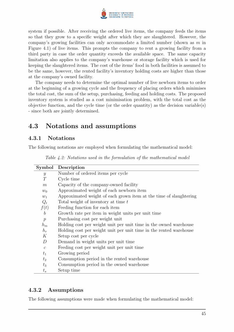
system if possible. After receiving the ordered live items, the company feeds the itemsso that they grow to a specific weight after which they are slaughtered. However, thecompany’s growing facilities can only accommodate a limited number (shown as m inFigure 4.1) of live items. This prompts the company to rent a growing facility from athird party in case the order quantity exceeds the available space. The same capacitylimitation also applies to the company’s warehouse or storage facility which is used forkeeping the slaughtered items. The cost of the items’ food in both facilities is assumed tobe the same, however, the rented facility’s inventory holding costs are higher than thoseat the company’s owned facility.

The company needs to determine the optimal number of live newborn items to orderat the beginning of a growing cycle and the frequency of placing orders which minimisesthe total cost, the sum of the setup, purchasing, feeding and holding costs. The proposedinventory system is studied as a cost minimisation problem, with the total cost as theobjective function, and the cycle time (or the order quantity) as the decision variable(s)- since both are jointly determined.


4.3.1 Notations

The following notations are employed when formulating the mathematical model:


Symbol Descriptiony Number of ordered items per cycleT Cycle timem Capacity of the company-owned facilityw0 Approximated weight of each newborn itemw1 Approximated weight of each grown item at the time of slaughteringQt Total weight of inventory at time tf(t) Feeding function for each itemb Growth rate per item in weight units per unit timep Purchasing cost per weight unithm Holding cost per weight unit per unit time in the owned warehousehr Holding cost per weight unit per unit time in the rented warehouseK Setup cost per cycleD Demand in weight units per unit timec Feeding cost per weight unit per unit timet1 Growing periodt2 Consumption period in the rented warehouset3 Consumption period in the owned warehousets Setup time

4.3.2 Assumptions

The following assumptions were made when formulating the mathematical model:

45



• A cost is incurred for feeding and growing the items.

• The cost of feeding the items is proportional to the weight gained by the items.


• Items arrive at both facilities at the same time.

• The company-owned growing facility and warehouse have limited capacities of munits.

• The rented growing facility and warehouse have unlimited capacity.

• The holding cost in the rented facility are higher than those in the owned warehouse.

• Items in the company owned warehouse are only sold after those in the rentedwarehouse are sold out.


4.4 Model formulation


Figure 4.1 depicts the proposed inventory system. At the beginning of a growing cycle,a company purchases y newborn items, each weighing w0, which are capable of growing.However, the company’s growing and storing facilities only have the capacity to growand store m items. The company makes use of rented facilities to grow and store theexcess (y−m) items. This means that at the beginning of a growing cycle, the companyowned growing facility receives m newborn items and at this point the total weight of theinventory is mw0. Likewise the total weight of the inventory in the rented facility at thispoint is (y−m)w0. The total weight of the inventory in both facilities at this point, Q0, isthe sum of the total weight of the inventory in both facilities (i.e. Q0 = yw0). The itemsare then fed and they grow for the period t1. The weight of each fully grown item w1 is afunction of time. The amount of food consumed by the items during the growth periodis modelled by the function f(t). At the end of the growth period, each item would havegrown to a target weight of w1. At this point, the total weight of the inventory in bothfacilities is Q1 = yw1. At the end of the growing period, the items are slaughtered. Thetotal weight of the inventory at the time of slaughter (or end of the growing period) inthe owned and the rented facilities are mw1 and (y −m)w1 respectively.

As a result of higher holding costs in the rented warehouse, inventory kept in thatparticular warehouse is cleared prior to consuming inventory in the company-owned ware-house. The consumption period in the rented warehouse, t2, is determined from the an-nual demand, D, and the weight of the inventory in the rented warehouse, (y−m)w1, as

t2 =(y −m)w1

D. (4.1)

46

Likewise, the weight of the inventory in the company-owned warehouse, mw1, and the de-mand rate, D, are utilized in determining an expression for the length of the consumptionperiod in the owned warehouse, t3, as

t3 =mw1

D. (4.2)

The cycle length, T , is the sum of the consumption periods in both facilities. It is givenby

T =yw1

D. (4.3)

An expression for the order quantity, y, is determined from Equation (4.3) as

y =DT

w1

. (4.4)

The objective of the proposed inventory model is to determine the optimal orderquantity which minimizes total cost (TC), which is the sum of the purchasing (PC),setup (SC), feeding (FC) and holding (HC) costs. The total cost per cycle is thus

TC = PC + SC + FC +HC. (4.5)

4.4.1.1 Purchasing cost per cycle

At beginning of each cycle, the company purchases y newborn items at a cost of p perweight unit. At the time of receiving the order, each item weighs w0 . The purchasingcost per cycle is determined as

PC = pyw0. (4.6)

4.4.1.2 Setup cost per cycle

A cost of K is incurred for setting up the growing/feeding facilities at the beginning ofeach cycle. Hence,

SC = K. (4.7)

4.4.1.3 Holding cost per cycle

The holding cost per cycle is determined from Figure 4.1 by multiplying the holding costper unit weight per unit time in the respective warehouses, hr and hm, by the relevantarea under the consumption period in the graph. The holding costs in the rented andcompany-owned warehouses are given, respectively, by

HCr = hr

[(y −m)2w2

1

2D

](4.8)

HCm = hm

[m(y −m)w2

1

D+m2w2

1

2D

]. (4.9)

The total holding cost per cycle is the sum of the holding costs in the rented and ownedwarehouses. It is given by

HC = hr

[(y −m)2w2

1

2D

]+ hm

[m(y −m)w2

1

D+m2w2

1

2D

]. (4.10)

47

4.4.1.4 Food procurement cost per cycle

Since the items in both company-owned and rented facilities have similar growth rates,it is assumed that they are fed the same type of food which is procured from the samesupplier. Hence, the cost of items’ food, c, is the same regardless of the facility. Thecost of the items food (c), the general feeding function f(t), the duration of the feedingperiod (which equals the growing period, i.e. t1) and the quantity of items in the rentedfacilities, (y −m), are used to determine the feeding cost in the rented facility as

FCr = c(y −m)

∫ t1

0

f(t) dt. (4.11)

Considering the amount of items grown and fed in the company-owned facility, m, thefeeding cost in the owned facility is determined as

FCm = cm

∫ t1

0

f(t) dt. (4.12)

The summation of Equations (4.11) and (4.12) yields an expression for the feeding costper cycle in both facilities as

FC = cy

∫ t1

0

f(t) dt. (4.13)

4.4.1.5 Total cost function

Equations (4.6), (4.7), (4.10) and (4.13) are substituted into Equation (4.5) to yield anexpression for the total cost as

TC = pyw0 +K+hr

[(y −m)2w2

1

2D

]+hm

[m(y −m)w2

1

D+m2w2

1

2D

]+cy

∫ t1

0

f(t) dt. (4.14)

The total cost per unit time, TCU , is computed using Equations (4.14) and (4.3) as

TCU =TC

T=pw0D

w1

+KD

yw1

+ hr

[(y −m)2w1

2y

]+ hm

[m(y −m)w1

y+m2w1

2y

]

+cD

w1

∫ t1

0

f(t) dt. (4.15)

Equation (4.15) is a general expression for the total cost per unit time which can be usedfor different types of growing items. It has two general functions, namely, the feeding(f(t)) and the growth (f(w1|w0)) functions. Because these functions are different fordifferent growing items, it is very difficult to solve the model for a general case whichworks for all growing items. Getting around this problem involves setting up a specificmodel which makes use of specific growth and feeding functions. In the available literatureon EOQ models for growing items, there are two approaches to solving the model for aspecific case. Rezaei (2014) and Zhang et al. (2016) used growth and feeding functionsfor broiler chickens, which were first developed by Richards (1959) and Goliomytis etal. (2003) respectively. These functions were complex and consequently both thosemodels were solved through numerical techniques, with Rezaei (2014) resorting to a

48

heuristic which applies the Newton-Raphson method. Nobil et al. (2018) assumed alinear growth rate for the items, which meant that the feeding function (which is assumedto be dependent on the weight gained by the items) could easily be determined from theinventory behaviour graph (in a manner similar to determining the holding cost). Themodel presented by Nobil et al. (2018) was solved using a relatively simpler heuristicas compared to the heuristic employed in the works by Rezaei (2014) and Zhang et al.(2016). Because of the reduced computational complexity in the model by Nobil et al.(2018), their assumption of a linear growth rate for the items is adapted to set up thespecific mathematical model.

4.4.2 Specific mathematical model: Case of a linear growthfunction

Suppose that the growth function of each item, w1, is modelled by a linear function. Thismeans that each item grows at a constant rate of b weight units per unit time. Notingthat the initial weight of the newborn items at the time of order receipt is w0 and theperiod of growth is t1, an expression for each item’s growth function can be formulatedas

w1 = w0 + bt1. (4.16)

When considering all the ordered items, Equation (4.16) becomes

yw1 = yw0 + ybt1, (4.17)

from which Figure 4.2, depicting the behaviour of the inventory system over time, isconstructed. An expression for the duration of the growth period is determined fromEquation (4.16) as

t1 =w1 − w0

b. (4.18)

Figure 4.2: Inventory system behaviour for growing items with two growing and storagefacilities and a linear growth function

4.4.2.1 Food procurement cost per cycle

The cost of procuring food in the rented facility is determined from Figure 4.2 throughmultiplying the cost of food per weight unit per unit time, c, with the duration of the

49

feeding (i.e. growing) period, t1, and the difference in weight of the inventory at thebeginning (yw0) and at the end (yw1) of the growing period.

FCr = c

[t1[(y −m)w1 − (y −m)w0

]2

](4.19)

By substituting Equation (4.18), Equation (4.19) becomes

FCr = c

[(w1 − w0)

[(y −m)w1 − (y −m)w0

]2b

]. (4.20)

Likewise, the food procurement cost in the owned facility is

FCm = c

[t1(mw1 −mw0)

2

]= c

[(w1 − w0)(mw1 −mw0)

2b

]. (4.21)

The cost of feeding the items in both facilities per cycle is determined by adding Equations(4.20) and (4.21). Hence,

FC = c

[y(w1 − w0)

2

2b

]. (4.22)

4.4.2.2 Total cost function

The other cost components (i.e. the purchasing, setup and holding costs) are not affectedby the assumption of a linear growth function and thus they remain the same as thosein Equations (4.6), (4.7) and (4.10). These three cost components along with the newfood procurement cost, given in Equation (4.22), are summed to give an expression forthe total cost per cycle as

TC = pyw0 +K + hr

[(y −m)2w2

1

2D

]+ hm

[m(y −m)w2

1

D+m2w2

1

2D

]

+ c

[y(w1 − w0)

2

2b

]. (4.23)

For computational convenience, Equation (4.4) is substituted into Equation (4.23) andthe result is

TC =pDTw0

w1

+K + hr

(DT 2

2

)+(hm − hr

)(2DTmw1 −m2w21

2D

)

+cDT

(w1 − w0

)22bw1

. (4.24)

The total cost per unit time (TCU) is computed, by dividing by Equation (4.24) thecycle time, as

TCU =TC

T=pDw0

w1

+K

T+ hr

(DT

2

)+(hm − hr

)(mw1 −

m2w21

2DT

)

+cD(w1 − w0

)22bw1

. (4.25)

50

4.4.2.3 Model constraint

The proposed inventory system is controlled by the following constraint which ensuresthat the slaughtered items are ready for consumption on time:

Constraint: In order to ensure that the slaughtered items are ready for sale on time(i.e. at the beginning of the consumption period T ), the setup time and the length of thegrowth period should be less than or equal to the consumption period. A restriction onthe consumption period, T , is formulated as

t1 + ts ≤ T. (4.26)

Through the substitution of the expression for t1 from Equation (4.18), Equation (4.26)becomes

T ≥{w1 − w0

b+ ts = Tmin

}. (4.27)

4.4.2.4 Mathematical formulation of the EOQ model for growing items withtwo growing and storage facilities

The mathematical formulation for the the proposed inventory system is formulated byusing the objective function in Equation (4.25) and the constraint in Equation (4.27) as

Min

{TCU =

pDw0

w1

+K

T+ hr

(DT

2

)+(hm − hr

)(mw1 −

m2w21

2DT

)

+cD(w1 − w0

)22bw1

}(4.28)

s.t. T ≥ Tmin

T ≥ 0.

4.4.3 Solution


The value of the cycle time, T , which minimises total costs per unit time, TCU , isdetermined as

∂TCU

∂T= −K

T 2+hrD

2+(hm − hr

)(m2w21

DT 2

)

= 0→ T =

√2KD +m2w2

1

(hr − hm

)hrD2

.

(4.29)

The order quantity which minimises the total costs per unit time, computed by substi-tuting T from Equation (4.29) into Equation (4.4), is given by

y =

√2KD +m2w2

1

(hr − hm

)hrw2

1

. (4.30)

51

4.4.3.2 Proof of convexity of the objective function

So as to show that the objective function, given in Equation (4.25), has a unique solution,the grad of that function is calculated in order to identify the optimum point and theHessian matrix of the function is shown to be positive. The location of the optimumpoint from the grad is shown by

∂TCU

∂T= −K

T 2+hrD

2+(hm − hr

)(m2w21

DT 2

). (4.31)

The Hessian matrix of the objective function, given by ∂2TCU∂T 2

∂2TCU∂T∂y

∂2TCU∂T∂y

∂2TCU∂y2

, (4.32)

is shown, in Equation (4.33), to be positive semi definite.KT 3 +

(hr − hm

)(m2w21

DT 3

)KT 3 +

(hr − hm

)(m2w21

DT 3

)

KT 3 +

(hr − hm

)(m2w21

DT 3

)0

(4.33)


[T y

]

KT 3 +

(hr − hm

)(m2w21

DT 3

)KT 3 +

(hr − hm

)(m2w21

DT 3

)

KT 3 +

(hr − hm

)(m2w21

DT 3

)0

[Ty

]

=K

T+ 2

[Ky

T 2+

(hr − hm

)ym2w1

2

DT 2

]≥ 0 (4.34)

The quadratic form of the objective function is shown to be positive in Equation (4.34)which indicates that the objective function is convex.


The following optimization algorithm is proposed for determining a solution to the pro-posed inventory system:


Step 2 Check the problem’s feasibility. The problem is feasible provided thatTmin ≥ 0. If it is feasible proceed to Step 3, otherwise proceed to Step 6.

Step 3 Compute T using Equation (4.29).

52

Step 4 T ∗ = T provided that T ≥ Tmin, otherwise T ∗ = Tmin.

Step 5 Compute y∗ and TCU∗ using Equations (4.30) and (4.25) respectivelyconsidering the value of T ∗.

Step 6 End.



The proposed inventory system is analysed through a numerical example utilising thefollowing parameters, mostly adapted from a study by Nobil et al. (2018):

Demand rate, D =1 000 000 g/year

Setup cost, K =1 000 ZAR/cycle

Holding cost in the owned warehouse, hm =0.04 ZAR/g/year

Holding cost in the rented warehouse, hr =0.06 ZAR/g/year

Capacity of the company-owned facility, m =100



Growth rate, b =15 330 g/chick/year


Purchase cost, p =0.025 ZAR/g


Solution procedure application: The proposed solution procedure is illustrated byapplying it to the numerical example. The procedure is outlined as follows:


Tmin =1267− 53

15330+ 0.01 = 0.0891

Step 2 The problem is feasible since Tmin ≥ 0, proceed to Step 3.

Step 3 Compute T using Equation (4.29).

T =

√2× 1000× 1000000 +

(1002 × 10000002

)(0.06− 0.04

)(0.06× 10000002)

= 0.1967

Step 4 Since T ≥ Tmin, T ∗ = T = 0.1967

53

Step 5 Compute y∗ and TCU∗.

y∗ =

√2× 1000× 1000000 +

(1002 × 10000002

)(0.06− 0.04

)(0.06× 12672)

= 155.2354

TCU∗ =0.025× 1000000× 53

1267+

1000

13347.91+ 0.06

(1000000× 13347.91

2

)+(0.04− 0.06

)(100× 1267− 1002 × 12672

2× 1000000× 13347.91

)

+0.08× 1000000

(1267− 53

)22× 15330× 1267

= 13347.91

Step 6 End.


Variable Units Quantityt1 year 0.0792t2 year 0.0700t3 year 0.1267T ∗ year 0.1967y∗ items 156

TCU∗ R/year 13 347.91

Based on the results of the numerical example, some of which are summarised inTable 4.3, the company should place an order for 156 day-old chicks at the beginning ofeach cycle. Since the owned facility can only grow and store 100 items, 56 items will begrown, slaughtered and stored at a rented facility. The items should be grown for 0.0792years (29 days). All the slaughtered items in the rented warehouse will be consumed after0.0700 years (26 days) and those in the owned warehouse will be sold out after 0.1267years (46 days). Orders should be replenished every 0.1967 years (72 days). Followingthis optimal inventory policy, the company will incur total costs of 13 347.91 ZAR peryear.

54

Figure 4.3: Graph of total cost per unit time, cycle time and order quantity

The changes to the objective function as a result of changes in the decision variablesare illustrated in Figure 4.3, which also shows that the objective function is convex. Thetotal cost per unit time decreases with the cycle time until it reaches minimum at theoptimal cycle time and order quantity (i.e. the EOQ).

4.5.2 The effect of limited growing and storage capacity of theowned facility

Figure 4.4: The effect of limited growing and storage capacity on the lot size

The effect of the limited capacity of the company-owned facility on the order quantityis investigated by comparing the EOQ under the assumption that there is no capacity limiton the company-owned growing and storage facilities with the EOQ from the proposedinventory system. In order to determine the base EOQ for growing items (i.e. the EOQunder the assumption that there is no capacity limit on the company owned growing and

55

storage facilities), m is set to zero and hr is set to hm. The capacity of the company-owned facility is increased gradually and the EOQ is determined at various capacities.The EOQ’s at various capacities are compared to the base EOQ for growing items bydetermining the number of number of items that need to be grown and stored at the rentedfacility. As the capacity of the owned facility increases, the number of items grown andstored in the rented facility increases until the capacity of the owned facility equals thebase EOQ for growing items (shown by the negative amount of items after the 176 itemsmark in Figure 4.4). After this point, the owned facility has excess growth and storagespace which is not utilized. While the company does not need to rent additional capacity,it has unused capacity in its owned facility which also has a negative cost implication.


Sensitivity analyses are performed on the major input parameters in order to investigatetheir impacts on the decision variables and to provide managerial insights for improvinginventory management.

Table 4.4: Changes to y∗ and TCU∗ due to changes in c

% change in EOQ TCUfeeding cost items % change ZAR/year % change

-50 156 0 11 826 -11.4-37.5 156 0 12 213 -8.5-25 156 0 12 587 -5.7

-12.5 156 0 12 974 -2.80 156 0 13 348 0

12.5 156 0 13 722 2.825 156 0 14 109 5.7

37.5 156 0 14 496 8.650 156 0 14 870 11.4

Table 4.4 shows the results of the sensitivity analysis of the EOQ and the total coststo the feeding cost. With regards to the order quantity, increasing the feeding cost doesnot change the EOQ at all. From a cost perspective, increasing the feeding cost has anegative effect on inventory management because it leads to increased total costs. Thereverse is also true and this presents inventory managers with an opportunity to reducetotal costs without the need to hold additional stock. By reducing feeding costs, eitherthrough better procurement practices or reducing the items’ rations, managers can savesignificant amounts of money without increasing the risk of stock-outs.

56

Table 4.5: Changes to y∗ and TCU∗ due to changes in K

% change in EOQ TCUsetup cost items % change ZAR/year % change

-50 118 -24.6 10 451 -21.7-37.5 128 -17.7 11 252 -15.7-25 138 -11.4 12 000 -10.1

-12.5 147 -5.5 12 694 -4.90 156 0 13 348 0

12.5 164 5.2 13 962 4.625 172 10.2 14 563 9.1

37.5 179 15 15 123 13.350 187 19.6 15 657 17.3

The setup cost has significant impacts on both the EOQ and the total inventory costs,as shown in Table 4.5. Decreasing the setup cost decreases the total costs. Managersshould pay close attention to the setup cost because trying to reduce this cost by orderingless frequently leads to an increase in the order size. Larger order sizes mean higherholding costs and the need to store more items in the rented facility which further escalatesthe costs.

Table 4.6: Changes to y∗ and TCU∗ due to changes in hm

% change in EOQ TCUowned facility items % change ZAR/year % changeholding cost

-50 166 6.7 11 599 -13.1-37.5 164 5.1 12 040 -9.8-25 161 3.4 12 480 -6.5

-12.5 159 1.7 12 291 -3.20 156 0 13 348 0

12.5 153 -1.7 13 775 3.225 151 -3.4 14 216 6.5

37.5 148 -5.1 14 656 9.850 146 -6.7 15 097 13.1

Table 4.6 shows that as the holding cost in the owned facility increases, the EOQdecreases and the total total costs increase. The increase in total costs is due to the factthat holding costs are one of the main components of the total cost function. In order toreduce costs, management should reduce the holding costs in their facility.

57

Table 4.7: Changes to y∗ and TCU∗ due to changes in hr

% change in EOQ TCUrented facility items % change ZAR/year % changeholding cost

-50 196 25.9 12 774 -4.3-37.5 181 16.2 12 974 -2.8-25 171 9.3 13 121 -1.7

-12.5 162 4.1 13 241 -0.80 156 0 13 348 0

12.5 151 -3.3 13 428 0.625 147 -6 13 508 1.2

37.5 143 -8.3 13 575 1.750 140 -10.3 13 628 2.1

Table 4.7 shows that as the rented facility holding cost increases the total costs increaseslightly. The increases in the total costs are not as dramatic as those caused by similarpercentage increases in the owned facility holding cost despite the fact that the rentedfacility charges more than the owned facility. This is because the amount of items keptin the rented warehouse is small and those items sell out within a short space of time. Ifthe items kept in the rented facility increases, the increase in the total costs will be muchgreater. In order to reduce total costs, management should keep as little inventory aspossible in the rented facility. While better results can be achieved by not keeping anyinventory in the rented warehouse, exceptional circumstances might necessitate rentingspace and in such instances, small amounts of amounts should be kept in the rented spaceand it is very important for management to start clear this stock ahead of the stock intheir own facility.

Table 4.8: Changes to y∗ and TCU∗ due to changes in m

% change in EOQ TCUcapacity of items % change ZAR/year % change

owned facility

-50 148 -5.3 13 989 4.8-37.5 149 -4.3 13 788 3.3-25 151 -3.1 13 615 2

-12.5 154 -1.6 13 468 0.90 156 0 13 348 0

12.5 159 1.8 13 241 -0.825 162 3.8 13 161 -1.4

37.5 165 6 13 108 -1.850 169 8.3 13 054 -2.2

From Table 4.8, it is evident that an increase in the capacity of the owned facilityresults in an increase in the EOQ and a decrease in the total costs. Managers shouldinvest in expanding their own facilities’ capacities because of the potential costs savings.While increasing capacity requires significant amounts of capital investment initially, the

58

benefits in the long term are that the company will not incur high holding costs chargedby third parties. The downside to increasing capacity is that if market conditions changenegatively and the company’s demand reduces significantly, the company will have ampleunutilised capacity. However, if market conditions change for the better the company willbe better positioned since they would have invested in extra capacity.

Table 4.9: Changes to y∗ and TCU∗ due to changes in w1

% change in EOQ TCUslaughter weight items % change ZAR/year % change

-50 295 89.3 13 388 0.3-37.5 239 53.1 13 188 -1.2-25 202 29.2 13 148 -1.5

-12.5 175 12.4 13 215 -10 156 0 13 348 0

12.5 141 -9.5 13 548 1.525 130 -16.9 13 775 3.2

37.5 120 -22.9 14 055 5.350 113 -27.8 14 362 7.6

Table 4.9 shows that as the slaughter weight increases, the EOQ decreases significantlyand the total cost increases. The EOQ decreases because the company slaughters theitems at larger weights and thus fewer items are required to meet annual demand. Whileit might be tempting to meet demand with slightly fewer items, this comes at a costbecause total costs increase with the slaughter weight. The increase in total costs is mostprobably due to the fact that if items are slaughtered at larger weights, they have togrown for a longer period of time or fed significantly more. In order to keep costs down,managers should opt to slaughter the items at smaller weights because they can reducetheir costs slightly.

4.6 Conclusion

This chapter incorporates the concepts of the basic two-warehouse inventory model andthe EOQ model for growing items to create a new EOQ model for growing items with twogrowing and storage facilities. The proposed EOQ model is studied through a mathemat-ical model which has cycle time (and order quantity, since they are jointly determined)as the decision variable(s) and the total costs as the objective function. The biggestcontribution to the literature on inventory modelling for growing items is the inclusion ofa limited capacity for the growing and storage facility. The capacity of the owned facilityhas a significant effect on the EOQ and the total inventory costs because of the differencein the holding costs charged by both facilities. As the capacity increases, the total costsdecrease and the EOQ increases, but increasing capacity is capital intensive and posesfinancial risks if market conditions change for the worst. On the other hand, if marketconditions change for the best and the company has invested in additional capacity, itwill be better positioned to deal with increased customer demand without the need tooutsource additional growing and storage capacities.

The proposed EOQ model only considered item growth and two growing and storage

59

facilities. It can be extended by considering multiple growing and storage facilities.This model can also be extended by assuming that the growth rates of the items inthe owned and rented facilities are different. Furthermore, popular extensions to thebasic EOQ model, such as shortages, deterioration, quantity discounts and permissibledelay in payments, can be incorporated to the model.

60

Chapter 5

Economic order quantity model forgrowing items with incrementalquantity discounts‡

5.1 Introduction

While the basic Economic Order Quantity (EOQ) model, developed by Harris (1913),has found some practical applications, it makes a number of assumptions which do notreflect most real life inventory systems. In order to model more realistic systems, variousresearchers have formulated new EOQ models by amending the model assumptions insome ways. In an attempt to create a new variation of the EOQ model, this chapterproposes an inventory system where the ordered items, purchased from a supplier whooffers incremental quantity discounts, are capable of growing during the course of theinventory replenishment cycle.

Rezaei (2014) was the first researcher to incorporate item growth into inventory theoryby developing an EOQ model for growing items. Rezaei (2014)’s proposed inventorysystem had two distinct periods, namely, growing and consumption. During the growingperiod, the ordered live items are fed and raised until they reach an acceptable weightfor sale. The items are then slaughtered, and put on sale during the consumption period.The increase in weight experienced by growing items during the growth period is whatdifferentiates them from conventional items, whose weight does not change if they arenot consumed or more items are added to the system (i.e. growth in this context isquantified only through a weight increase). Zhang et al. (2016) developed a carbon-constrained version of the EOQ model for growing items. Building on Rezaei (2014)’swork, Nobil et al. (2018) studied an inventory system for growing items where shortagesare allowed and fully backordered.

EOQ models with quantity discounts were first proposed by Hadley and Whitin(1963). Quantity discounts are usually offered by suppliers as a means of encourag-ing buyers to purchase larger volumes. In inventory theory, suppliers usually offer oneof two types of quantity discounts. These are all-units quantity discounts, which resultin reduced purchasing cost for the entire order if larger volumes are ordered; and in-cremental quantity discounts where the reduced purchasing cost only applies to items

‡A modified version of this chapter has been submitted to Journal of Industrial Engineering Inter-national for review.

61

bought above a certain quantity. Lal and Staelin (1984) studied an integrated vendor-buyer inventory where the vendor offers incremental quantity discounts to the buyer.Dada and Srikanth (1987) developed a lot sizing model with quantity discounts andprice-dependent holding cost. Abad (1988) presented an EOQ model with incrementalquantity discounts and a linear demand function. Federgruen and Lee (1990) developedthe Dynamic Economic Lot (DEL) version of the basic EOQ model with both all-unitsand incremental quantity discounts. Guder et al. (1994) studied a capacitated multi-iteminventory model with incremental quantity discounts. Tersine et al. (1995) developed aninventory model with incremental quantity discounts and freight discounts offered on thetransportation cost. Rubin and Benton (2003) presented a multi-item inventory modelwith incremental quantity discounts and space constraints. Mahmood and Kindi (2006)presented an inventory model for an item with shortages considering both all-units andincremental quantity discounts. Haksever and Moussourakis (2008) formulated a multi-item model with incremental quantity discounts and budget constraints. Mendoza andVentura (2008) incorporated transportation costs into the EOQ model under both all-units and incremental quantity discount structures. Bai (2011) formulated an inventorymodel considering quantity discounts and multiple suppliers. Lee (2013) studied an inte-grated supplier-vendor inventory system for supplier selection considering both all-unitsand incremental quantity discounts. Archetti et al. (2014) modelled an inventory systemwhere incremental and all-units discounts are offered simultaneously, the former being of-fered by a supplier for the ordered items while the latter are offered by the transportationcompany for transporting the items. Taleizadeh et al. (2015) formulated an EOQ modelwith incremental quantity discounts under the assumption that shortages are partiallybackordered. Bohner and Minner (2017) developed a supply chain model with supplierselection, multiple items and quantity discounts with an associated failure risk. Moham-madivojdan and Geunes (2018) studied the single -period inventory model with spaceconstraints under both all-units and incremental quantity discounts. Benton and Park(1996) and Pereira and Costa (2015) presented extensive literature reviews, covering re-search from the periods 1963 to 1994 and 1995 to 2013 respectively, for lot sizing modelsunder quantity discounts.


References

Characteristics of the inventory systemConventional Growing Incremental Carbon Shortage

items items quantity taxdiscounts

Harris (1913)Hadley and Whitin (1963)Rezaei (2014)Zhang et al. (2016)Nobil et al. (2018)This chapter

A review of literature on inventory management for growing items suggests incre-mental quantity discounts have not been incorporated into the EOQ model for growingitems. This chapter aims to address this gap in literature by developing an EOQ modelfor growing items with incremental quantity discounts. A comparison of the proposed

62

inventory system and related published works in literature is provided in Table 5.1, whichalso shows the contribution of this chapter to inventory management research for growingitems.


The proposed inventory system considers a situation where a company orders a certainnumber of items which are capable of growing during the course of the inventory planningcycle, for example livestock. The supplier of the newborn items offers the purchasingcompany incremental quantity discounts over fixed price breaks. Under the incrementalquantity discounts pricing structure, the discounted purchasing costs only apply to theincremental quantity. Figure 5.1 represents the typical behaviour of an inventory systemfor growing items. In order for growth to occur the company needs to feed the items.Every replenishment cycle can be divided into two periods, namely the growth and theconsumption periods. During the growth period (shown as period t in Figure 5.1), orderednewborn items are fed and raised until they grow to a certain target weight. Oncethe weight of items reach the target weight, the growth period ends and the items areslaughtered. During the consumption period (shown as period T in Figure 5.1), theslaughtered items are kept in stock and sold to market. The company incurs feeding costduring the growth period and it incurs holding costs for keeping the slaughtered items instock. The inventory level of one complete inventory cycle finishes up at time T and atthat point the items in the next inventory cycle would have completed their growth cycle(i.e. the items in the next cycle will have grown to the target weight and are ready forsale). The company wants to determine the optimal number of newborn items to orderat the beginning of the growth cycle in order to minimise total inventory costs (i.e. thesum of the purchasing, setup, feeding and holding costs).

Figure 5.1: Behaviour of an inventory system for growing items

The proposed inventory system is studied through a mathematical model, aimed atdetermining the optimal order quantity, frequency of order replenishments and slaughtertime, which minimise total inventory costs.

63


5.3.1 Notations

The following notations are employed when formulating the mathematical model:


Symbol DescriptionY Number of ordered newborn items per cyclew0 Approximated weight of each newborn itemw1 Approximated weight of each grown item at the time of slaughteringQt Total weight of inventory at time tf(t) Feeding function for each itemb Growth rate per item in weight units per unit timepj Purchasing cost per weight unit at the jth break pointm Number of break pointsyj Lower bound for the order quantity for price jh Holding cost per weight unit per unit timeK Setup cost per cycleD Demand in weight units per unit timec Feeding cost per weight unit per unit timet Growing periodT Cycle lengthts Setup time

5.3.2 Assumptions

The following assumptions were made when formulating the mathematical model:



• A cost is incurred for feeding and growing the items. This cost is proportional tothe weight gained by the items.


• The holding cost per weight unit per unit time is charged as a fixed percentage ofthe purchasing cost per weight unit.

• The supplier of the live newborn items offers incremental quantity discounts.


64

5.4 Model development


When a new growing cycle begins, a company purchases Y newborn items, each weighingw0, which are capable of growing during the replenishment cycle. The total weight ofthe inventory at this point, Q0, is determined by multiplying the weight of each of theitems by the number of items ordered (i.e. Q0 = Y w0). The company feeds the itemsand they grow to a target weight of w1. This marks the end of the growth period andat this point the items are slaughtered. The total weight of the inventory at the timeof slaughter is Q1 = Y w1. The behaviour of the inventory system over time is depictedin Figure 5.1. As a way of encouraging larger order sizes, the company’s supplier offersincremental quantity discounts. The discount cost structure is

pj =

p1 y1 = 0 ≤ Y < y2

p2 y2 ≤ Y < y3...

...

pm ym ≤ Y

.

Growth and consumption occur over the periods t and T respectively and hence thecompany incurs feeding and holding over those respective time periods. The demandrate, D, and the weight of the inventory level at the beginning of the consumption period,Q1 = Y w1, are utilised to determine the cycle time as

T =Y w1

D. (5.1)

Define y1 = 0, y2, ..., yj, yj+1, ..., ym as the order quantities at which the purchase costper weight unit changes. In such an instance, there are m price breaks. When a supplieroffers incremental quantity discounts, the purchasing cost per weight unit, pj, is the samefor all Y values in [yj, yj+1). The purchasing cost per weight unit decreases from oneprice break to the next (i.e. p1 > p2 > ... > pj > pj+1 > ... > pm).

5.4.1.1 Average purchasing cost per unit time

Let Y be in the jth price break (i.e. yj ≤ Y < yj+1). The purchasing cost per cycle forY items, each weighing w0, in this price break is given by

p(Y w0) = p1(y2 − y1)w0 + p2(y3 − y2)w0 + ...+ pj−1(yj − yj−1)w0 + pj(Y − yj)w0. (5.2)

Define Rj as the sum of the terms in Equation (5.2) which are independent of Y , andthus

Rj =

{p1(y2 − y1)w0 + p2(y3 − y2)w0 + ...+ pj−1(yj − yj−1)w0, j ≥ 2

0, j = 1. (5.3)

Equation (5.2) can be rewritten as

p(Y w0) = Rj + pjw0(Y − yj). (5.4)

65

The average unit purchasing cost per unit weight, p(Y w0)/Y w0, is equal to

p(Y w0)

Y w0

=Rj

Y w0

+ pj −pjyjY

. (5.5)

Multiplying Equation (5.5) by the demand in weight units per unit time, D, yields anexpression for the average unit purchasing cost per unit time (denoted by APCU), as

APCU = D

[Rj

Y w0

+ pj −pjyjY

]. (5.6)

5.4.1.2 Food procurement cost per unit time

The food procurement cost per cycle, FC, is determined from the feeding cost per weightunit per unit time, c, the number of items to be fed (i.e. the order quantity), Y , thefeeding duration, t, and the feeding function for each item, f(t), as

FC = cY

∫ t

0

f(t) dt. (5.7)

Dividing Equation (5.7) by the cycle time yields an expression for the feeding cost perunit time, FCU , given by

FCU =cD

w1

∫ t

0

f(t) dt. (5.8)

5.4.1.3 Setup cost per unit time

Every time the company places an order for live newborn items, it incurs a cost of K forsetting up the growth and feeding facilities. The setup cost per cycle is thus

SC = K. (5.9)

The setup cost per unit time, SCU , is determined by dividing the setup cost per cycleby the cycle time as

SCU =KD

Y w1

. (5.10)

5.4.1.4 Average holding cost per unit time

The holding cost per cycle, HC, is computed from Figure 5.1 using the area under theconsumption period (since the holding cost is incurred for the slaughtered inventory) andthus

HC = h

[Y 2w1

2

2D

]. (5.11)

The holding cost per unit time, HCU , is computed by dividing Equation (5.11) byEquation (5.1), hence

HCU = h

[Y w1

2

]. (5.12)

It is assumed that the holding cost per weight unit per unit time, h, is charged as a fixedpercentage of the purchasing cost per weight unit p. Defining i as the holding cost rateper unit time, it follows that the holding cost per weight unit per unit time is

h = ip. (5.13)

66

When considering the average unit purchasing cost per weight unit, p(Y w0)/Y w0, fromEquation (5.5), Equation (5.13) becomes

h = i

(Rj

Y w0

+ pj −pjyjY

). (5.14)

Substituting Equation (5.14) into Equation (5.12) yields an expression for the averageholding cost per unit time, AHCU , as

AHCU =i

2

[Rjw1

w0

+ pjw1

(Y − yj

)]. (5.15)

5.4.1.5 Average total cost per unit time

The average total cost per unit time, ATCU , is computed by summing Equations (5.6),(5.8), (5.10) and (5.15) and therefore

ATCU = D

[Rj

Y w0

+pj−pjyjY

]+cD

w1

∫ t1

0

f(t) dt+KD

Y w1

+i

2

[Rjw1

w0

+pjw1

(Y −yj

)]. (5.16)

Through rearranging the terms, Equation (5.16) becomes

ATCU = pjD +

(Rj

w0

− pjyj +K

w1

)D

Y+ipjY w1

2+i(Rjw1

w0− pjyjw1

)2

+cD

w1

∫ t

0

f(t) dt. (5.17)

Equation (5.17) is a general function for the average total cost per unit time which can beapplied to different growing items. As a result, it has two general expressions which arefunctions of time. These are the feeding function, f(t), and the growth function, f(w1|w0).In order to solve the model in a relatively easy manner, it is necessary to consider specificitems (i.e. with specific growth and feeding functions). Rezaei (2014), who presented thefirst EOQ model for growing items, used growth function for broiler chickens, developedby Richards (1959), and feeding function for broiler chickens, developed by Goliomytiset al. (2003). Consequently, Rezaei (2014)’s model had the slaughter time, in addition tothe cycle time and order quantity, as another decision variable. For that reason, Rezaei(2014) used a relatively complex heuristic to solve the model. Nobil et al. (2018) developedand solved an EOQ model for growing items with shortages in using a relatively simplerheuristic by assuming that the growth function of the items is linear. By assuming a lineargrowth function, the feeding cost in Nobil et al. (2018)’s model could be determined in thesame way as the holding cost is determined. Due to Nobil et al. (2018)’s model requiringless computations to solve because of the assumption of a linear growth function, thatassumption is adapted when formulating the specific mathematical model for the proposedinventory system.

5.4.2 Specific mathematical model: Case of a linear growthfunction

Suppose that the growth function of each item, w1, is linear. This implies that eachitem’s weight increases at a constant rate of b weight units per unit time. An expression

67

for the growth function of each item can be formulated considering the fact that growthoccurs for the duration t and keeping in mind that each item weighs w0 at the beginningof the cycle. This means that the slaughter weight of the items is a linear function withgradient b and y-intercept w0, as shown in Figure 5.2 which shows the behaviour of theinventory system over time, and hence

w1 = w0 + bt. (5.18)

If Y items are ordered, the growth function for all the ordered items is

Y w1 = Y w0 + Y bt. (5.19)

The duration of the growth period, t, is computed from Equation (5.18) as

t =w1 − w0

b. (5.20)

Figure 5.2: Inventory system behaviour for growing items under the assumption of lineargrowth function

5.4.2.1 Feeding cost per unit time

The feeding cost per cycle is computed using Figure 5.2 as the product of the feedingcost per weight unit per unit time (c) and the area under the growth period. Hence

FC = c

[t(Y w1 − Y w0

)2

]. (5.21)

Substituting Equation (5.20) into Equation (5.21) results in

FC = c

[Y(w1 − w0

)22b

]. (5.22)

The feeding cost per unit time (FCU), computed by dividing Equation (5.21) by thecycle time, is

FCU =cD(w1 − w0

)22bw1

. (5.23)

68

5.4.2.2 Average total cost per unit time

The average purchasing, setup and holding costs per unit time are not affected by theassumption of a linear growth function and thus they remain the same as those given inEquations (5.6), (5.10) and (5.15). The average total cost is thus

ATCU = pjD +

(Rj

w0

− pjyj +K

w1

)D

Y+ipjY w1

2+i(Rjw1

w0− pjyjw1

)2

+cD(w1 − w0

)22bw1

. (5.24)

5.4.2.3 Model constraints

Two constraints ensure the feasibility of the proposed inventory system. The first con-straint ensures that the items are ready for consumption at the required time. The secondconstraint ensures the feasibility of the optimal order quantity, meaning that the optimalquantity Yj is acceptable for each price break region and must fall between the the pricebreaks yj and yj+1.

Constraint 1: In order to ensure that the slaughtered items are ready for sale duringthe consumption period, the setup time and the duration of the growth period should beat least equal to the consumption period. This results in a constraint (on the durationof the consumption period) being formulated as

t+ ts ≤ T. (5.25)

Through substituting t from Equation (5.20), Equation (5.25) becomes

T ≥{w1 − w0

b+ ts = Tmin

}. (5.26)

Constraint 2: In order to ensure that the order quantity determined falls within therange of the given price break, a constraint on the order quantity is formulated as

yj ≤ Y < yj+1. (5.27)

5.4.2.4 Mathematical formulation of the EOQ model for growing items withincremental quantity discounts

The objective function, given in Equation (5.24), and the constraints are utilised toformulate a mathematical model for the proposed inventory system. Hence,

Min

{ATCU = pjD +

(Rj

w0

− pjyj +K

w1

)D

Y+ipjY w1

2+i(Rjw1

w0− pjyjw1

)2

+cD(w1 − w0

)22bw1

}(5.28)

s.t. yj ≤ Y < yj+1

T ≥ Tmin

T ≥ 0.

69

5.4.3 Solution


The optimal solution to the proposed inventory system is determined by setting theobjective function to zero resulting in

∂ATCU

∂Y= −

(Rj

w0

− pjyj +K

w1

)D

Y 2+ipjw1

2

= 0→ Y =

√2(Rjw1

w0− pjyjw1 +K

)D

ipjw12

.

(5.29)

The optimal cycle time is computed by substituting Equation (5.29) into Equation (5.1)and the result is

T =

√2(Rjw1

w0− pjyjw1 +K

)D

ipjD2. (5.30)

5.4.3.2 Proof of convexity of the objective function

In order to show that the objective function, given in Equation (5.24), has a uniquesolution, the grad of that function is calculated so as to identify the optimum point andthe Hessian matrix of the function is shown to be positive. The location of the optimumpoint from the grad is shown by:

∂ATCU

∂Y= −

(Rj

w0

− pjyj +K

w1

)D

Y 2+ipjw1

2(5.31)

The Hessian matrix of the objective function, given by ∂2ATCU∂Y 2

∂2ATCU∂Y ∂T

∂2ATCU∂Y ∂T

∂2ATCU∂T 2

, (5.32)

is shown, in Equation (5.33), to be positive semi-definite.(

Rj

w0− pjyj + K

w1

)DY 3

(Rj

w0− pjyj + K

w1

)DY 3

(Rj

w0− pjyj + K

w1

)DY 3 0

(5.33)


[Y T

](

Rj

w0− pjyj + K

w1

)DY 3

(Rj

w0− pjyj + K

w1

)DY 3

(Rj

w0− pjyj + K

w1

)DY 3 0

[YT

]

=2D

Y

(Rj

w0

− pjyj +K

w1

)+DT 2

Y 3

(Rj

w0

− pjyj +K

w1

)≥ 0. (5.34)

From Equation (5.34), the quadratic form of the objective function is shown to be positivewhich implies that the objective function is convex.

70


The solution to the EOQ model for growing items with incremental quantity discountsis determined using the following optimisation algorithm:

Step 1 Compute Y for each j using Equation (5.29). Denote this as Yj.

Step 2 Check each Yj’s feasibility. They are feasible if yj ≤ Y < yj+1. InfeasibleYj’s are disregarded and only the feasible ones proceed to Step 3.

Step 3 For each feasible Y , compute the corresponding T using Equation (5.30).

Step 4 Check the feasibility of each computed Yj with regards to the cycle time.Each Yj is feasible if T ≥ Tmin. Infeasible Yj’s are disregarded and only the feasibleones proceed to Step 5.

Step 5 Compute ATCU using Equation (5.24) for all the feasible Yj’s. The Yjvalue which results in the lowest ATCU is the EOQ.

Step 6 End.



The proposed inventory system is applied to a numerical example which considers acompany which purchases day-old chicks, feeds/grows them until they reach a targetedweight and then puts them on sale after screening for quality. The following parameters,mostly adapted from a study by Nobil et al. (2018), are utilised to analyse the proposedinventory system:

Demand rate, D =250 000 g/year

Setup cost, K =400 ZAR/cycle

Holding cost rate, i =0.4




Growth rate, b =15 330 g/chick/year (42 g/chick/day)


The purchasing cost structure is given in Table 5.3.

71

Table 5.3: Purchase cost structure under incremental quantity discounts

Quantity Price per weightpurchased unit (ZAR/g)

0-100 0.025101-200 0.023201-300 0.021301+ 0.019

Solution procedure application: The proposed solution algorithm is illustrated byapplying it to the numerical example. The procedure is outlined as follows:

Step 1 Compute Y for each j using Equation (5.29).

R1 = 0

R2 = 0.025(101− 0) = 133.8

R3 = 133.8 + 0.023(201− 101) = 255.7

R4 = 255.7 + 0.021(301− 201) = 367.0

Y1 =

√2(0×1267

53− 0.025× 0× 1267 + 400

)250000

0.4× 0.025× 12672 = 111.6

Y2 =

√2(133.8×1267

53− 0.023× 101× 1267 + 400

)250000

0.4× 0.023× 12672 = 149.0

Y3 =

√2(255.7×1267

53− 0.021× 201× 1267 + 400

)250000

0.4× 0.021× 12672 = 207.9

Y4 =

√2(367.0×1267

53− 0.019× 301× 1267 + 400

)250000

0.4× 0.019× 12672 = 281.1

Step 2 Check each Yj’s feasibility. They are feasible if yj ≤ Y < yj+1. InfeasibleYj’s are disregarded and only the feasible ones proceed to Step 3.

0 ≤ Y1 = 111.6 6< 101

101 ≤ Y2 = 149.0 < 201

201 ≤ Y3 = 207.9 < 301

301 6≤ Y4 = 281.1

Thus Y2 and Y3 are feasible.

Step 3 For each feasible Y , compute the corresponding T using Equation (5.30).

T2 =

√2(133.8×1267

53− 0.023× 101× 1267 + 400

)250000

0.4× 0.023× 2500002 = 0.7552

T3 =

√2(255.7×1267

53− 0.021× 201× 1267 + 400

)250000

0.4× 0.021× 2500002 = 1.0535

72

Step 4 Check the feasibility of each computed Yj with regards to the cycle time.Each Yj is feasible if T ≥ Tmin. Infeasible Yj’s are disregarded and only the feasibleones proceed to Step 5.

Tmin =1267− 53

15330+ 0.01 = 0.0891

Thus Y2 and Y3 are feasible since T2 ≥ Tmin and T3 ≥ Tmin.

Step 5 Compute ATCU using Equation (5.24) for all the feasible Yj’s. The Yjvalue which results in the lowest ATCU is the EOQ.

ATCU2 = 0.023× 250000 +

(133.8

53− 0.023× 101 +

400

1267

)250000

149.0

+0.4× 0.023× 149.0× 1267

2+

0.4(133.8×1267

53− 0.023× 101× 1267

)2

+0.08× 250000

(1267− 53

)22× 15330× 1267

= 8297.01

ATCU3 = 0.021× 250000 +

(255.7

53− 0.021× 201 +

400

1267

)250000

207.9

+0.4× 0.021× 207.9× 1267

2+

0.4(255.7×1267

53− 0.021× 101× 1267

)2

+0.08× 250000

(1267− 53

)22× 15330× 1267

= 8374.11

Y ∗ = Y2 since ATCU2 < ATCU3.

Step 6 End.


Variable Units Quantityt year 0.0792T ∗ year 0.7552Y ∗ items 149

ATCU∗ R/year 8 297.01

Based on the results of the numerical example, some of which are summarised in Table5.4, the company should place an order for 149 day-old chicks at the beginning of eachcycle. This order quantity lies in the 101-200 price-break and therefore the company willpay 0.023 ZAR per gram. Based on the targeted slaughter weight, the items should begrown for 0.0792 years (29 days). Orders should be replenished every 0.7552 years (275days). Following this optimal inventory policy, the company will incur an average totalcost of 8 297.01 ZAR per year.

Figure 5.3 shows the response of the the average total cost function to different orderquantities. The are four curves corresponding to the four price breaks. Each curve isvalid for a given order quantity interval. The valid interval for each curve is representedby a solid line.

73

Figure 5.3: Average total cost under incremental quantity discounts


Sensitivity analyses are performed on the major input parameters in order to investigatetheir impacts on the decision variables and to provide managerial insights for improvinginventory management.

Table 5.5: Changes to Y ∗ and ATCU∗ due to changes in K

% change in EOQ ATCUsetup cost items % change ZAR/year % change

-50 124 -16.8 8 008 -3.5-37.5 130 -12.8 8 086 -2.5-25 137 -8.1 8 159 -1.7

-12.5 143 -4.0 8 229 -0.80 149 0 8 297 0

12.5 154 3.4 8 362 0.825 159 6.7 8 425 1.5

37.5 165 10.7 8 485 2.350 170 14.1 8 544 3.0

Increasing the setup cost increases both the EOQ and the average total costs, asshown in Table 5.5. Nonetheless, changes to the setup cost did not shift the EOQ intoa different price break. Managers can offset the increase in the average total cost bypurchasing larger quantities (i.e. placing orders less frequently). However, this should bedone in moderation because if too much stock is ordered the holding cost will increaseand this will lead to an increase in total costs.

74

Table 5.6: Changes to Y ∗ and ATCU∗ due to changes in i

% change in EOQ ATCUholding cost items % change ZAR/year % change

rate

-50 397 166.4 7 576 -8.7-37.5 262 75.8 7 853 -5.3-25 240 61.1 8 039 -3.1

-12.5 159 6.7 8 178 -1.40 149 0 8 297 0

12.5 140 -6.0 8 409 1.325 133 -10.7 8 515 2.6

37.5 127 -14.8 8 616 3.850 121 -18.8 8 713 5.0

Increasing the holding cost rate increases the average total cost and reduces the EOQ,as shown in Table 5.6. The effect of decreasing the holding cost rate on the EOQ issubstantial because the EOQ shifts into different price breaks. As a result of the shiftin price breaks, the average cost reduces because of the lower purchasing cost per unitweight in the new price break. This shift into a lower price breaks offsets the increasedholding costs (due to the increase in the EOQ as a result of ordering larger quantities).

Table 5.7: Changes to Y ∗ and ATCU∗ due to changes in c

% change in EOQ ATCUfeeding cost items % change ZAR/year % change

-50 149 0 7 918 -4.6-37.5 149 0 8 012 -3.4-25 149 0 8 107 -2.3

-12.5 149 0 8 202 -1.10 149 0 8 297 0

12.5 149 0 8 392 1.125 149 0 8 487 2.3

37.5 149 0 8 582 3.450 149 0 8 676 4.6

Table 5.7 shows that the average total costs increase with increasing feeding costswhereas the EOQ is not affected by changes in the feeding cost. The feeding is essentiallythe cost of procuring feedstock for the items, and it is very difficult for managers to reducethis cost since it is set by the feedstock suppliers. Nonetheless, managers can reduce thiscost through procuring larger volumes (of the items’ feedstock) which normally havediscounted pricing.

75

Table 5.8: Changes to Y ∗ and ATCU∗ due to changes in w1

% change in EOQ ATCUslaughter weight items % change ZAR/year % change

-50 436 192.6 7 353 -11.4-37.5 377 153.0 7 660 -7.7-25 253 69.8 7 940 -4.3

-12.5 166 11.4 8 145 -1.80 149 0 8 297 0

12.5 135 -9.4 8 448 1.825 124 -16.8 8 599 3.6

37.5 81 -45.6 8 733 5.250 74 -50.3 8 836 6.5

Table 5.8 shows that increasing the slaughter weight decreases the EOQ and increasesthe average total cost. The EOQ decreases because the company slaughters the itemsat larger weights and therefore fewer items are required to meet annual demand. Theaverage total costs increase because if the company slaughters the items at larger weights,the items are allowed to grow for longer periods of time and this means that the morefeedstock is required not only because the items’ growth period is longer but also becauseas the items get larger they feeding requirements increase as well. In order to keep costsdown, managers should opt to slaughter the items at slightly smaller weights because theycan reduce their costs slightly, however this might not always be possible when takinginto account customer preferences.

Table 5.9: Changes to Y ∗ and ATCU∗ due to changes in yj

% change in EOQ ATCUlower bound for order items % change ZAR/year % change

quantity for price j

-50 133 -10.7 8 093 -2.5-37.5 137 -8.1 8 146 -1.8-25 141 -5.4 8 197 -1.2

-12.5 145 -2.7 8 248 -0.60 149 0 8 297 0

12.5 152 2.0 8 345 0.625 156 4.7 8 393 1.2

37.5 159 6.7 8 439 1.750 162 8.7 8 485 2.3

Increasing the lower bound for the order quantity in each price break increases both theEOQ and the average total costs, as shown in Table 5.9. The changes to the average costsare minimal most likely because the EOQ remains in the same price break. Managersdon’t have much control over the discount quantity structure as it is determined bythe supplier, but if it happens that the suppliers reduce the lower bounds on the orderquantities in each price break it is beneficial for managers to order less items.

76

Table 5.10: Changes to Y ∗ and ATCU∗ due to changes in pj

% change in EOQ ATCUpurchasing cost items % change ZAR/year % change

at jth price break

-50 240 61.1 4 742 -42.8-37.5 174 16.8 5 653 -31.9-25 163 9.4 6 539 -21.2

-12.5 155 4.0 7 420 -10.60 149 0 8 297 0

12.5 143 -4.0 9 172 10.525 139 -6.7 10 045 21.1

37.5 136 -8.7 10 916 31.650 91 -38.9 11 866 43.0

Table 5.10 shows that increasing the purchasing cost decreases the EOQ and increasesthe average total costs. In fact the EOQ shifts into different price breaks and consequentlythe effect on the average cost is significant as well. By reducing purchasing costs, man-agers can save significantly on their average total costs by ordering larger quantities.While this will result in an increase in the holding cost, the savings which result fromlower purchasing cost more outweigh the impact of the increased holding cost.

5.6 Conclusion

The major contribution made by this chapter to the literature on inventory modelling forgrowing items is the incorporation of incremental quantity discounts. This addition to lit-erature is important because suppliers often offer discounts for purchasing larger volumesof stock. The cost structure , in terms of both the purchasing cost in each price breakand the lower bounds for the order quantities in each price break, was shown to have asignificant impact on the order quantity and the average total cost of managing inventory.This indicates that incremental quantity discounts have considerable impact on inventorymanagement and this presents operations managers with opportunities to reduce coststhrough better procurement practices. However, certain factors need to be consideredwhen purchasing larger volumes, namely the available storage space, deterioration andthe available procurement budget.

The proposed inventory system did not take into account issues like deterioration,growing and storage facility capacity and budget constraints. These factors are impor-tant when purchasing larger quantities because in certain instances, management mightbe forced to lease extra capacity if they purchased more items than can be grown andstored in their owned facilities. This will certainly increase costs and negate the benefitof purchasing larger quantities. The model presented in this chapter can be extended toinclude capacity limits, budget limits, among other popular EOQ extensions. Deteriora-tion becomes increasingly important if larger quantities are purchased, extensions whichaccount for deterioration during the consumption period are another possible area forfuture research as they represent more realistic inventory systems.

77

Chapter 6

Conclusion

6.1 Summary of findings

The aim of this dissertation was to develop three lot sizing models for growing inven-tory items. The models were developed by extending the basic EOQ model for growingitems along three dimensions, namely quality, limited capacity and incremental quantitydiscounts.

The first model proposed an inventory system in which newborn items are orderedand fed/grown until they reach a specific weight. At this point, the items are slaughteredand kept in stock. Before the slaughtered items are sold, they are subjected to a screeningprocess which separates good quality items from poor quality items. Both item qualitiesare sold, but the poor quality items are sold at a much lower price. The inventory systemwas formulated mathematically to determine the optimal order quantity, slaughter weightand cycle time. The presence of poor quality items means that more items need to beordered in order to meet a specific demand for good quality items. This effect worsens asthe fraction of imperfect quality items increases. This finding should motivate productionand operations managers to pay attention to quality checks and ensure that the percentageof imperfect quality items is kept as low as possible.

The second model considered an inventory situation whereby a company orders new-born items and rears them until they are of acceptable weight for slaughter. However,the company-owned growth and storage facilities have limited capacities. In the eventthat the order quantity exceeds the capacity, the company rents secondary growing andstorage facilities. It is assumed that the holding costs in the rented storage facility arehigher than those in the company-owned facility. For this reason, stock kept in therented warehouse is consumed first. The capacity constraints on the growing and storagefacilities increased total costs mainly because of the higher holding costs in the rentedfacility. As the capacity increases, the total costs decrease, but increasing capacity iscapital intensive and poses financial risks if market conditions change for the worst.

The last model proposed an inventory system in which a company orders newbornitems and rears them until they reach a specific target weight, after which they areslaughtered. The supplier of the live newborn grants the company incremental quantitydiscounts. The cost structure, in terms of both the purchasing cost in each price breakand the lower bounds for the order quantities in each price break, was shown to have asignificant impact on the order quantity and the average total cost of managing inventory.This indicates that incremental quantity discounts have considerable impact on inventorymanagement and this presents operations managers with opportunities to reduce costs

78

through better procurement practices.

6.2 Possible practical applications of findings

Practical applications of the classic EOQ model are limited because of the assumptionsmade in the model which do not reflect most realistic inventory systems. For this reason,the model has been extended numerous times in order to model more realistic inventorysystems, as was the case in this study.

The models presented in this study can be applied to a variety of growing inventorysystems. While the focus of the examples was on livestock production, with some minormodifications, the models can be applied to crop production as well. Examples of mod-ifications which can be done to the models so that they are suited to crop productioninclude consideration of harvest periods, irrigation costs and weather conditions.

Possible beneficiaries of the results from this study are inventory managers in enter-prises involved in livestock and crop production. These enterprises face a variety issues,including, but not limited to, quality, limited storage capacity and quantity discounts.The three models presented in this study deal with those issues and as a result theycan assist those responsible for managing inventory and making purchasing decisions inlivestock- and crop-producing enterprises.

6.3 Contributions

The contributions made by this study to the literature on inventory theory is mainly thedevelopment of economic order quantity models for growing items under the following setof conditions:

• A certain fraction of the items fails a quality screening check and is classified asbeing of poor quality.

• Two growing and storage facilities are required because the growth facility for rais-ing the live items and the storage facility for stocking the slaughtered inventoryhave limited capacities.

• The supplier of the newborn items offers incremental quantity discounts.

6.4 Possible areas for future research

In addition to extending the imperfect quality model to account for popular extensionssuch as shortages, permissible delay in payment, among others, the model can be extendedby relaxing the assumption that the screening process is 100% effective at separating goodand poor quality items, this along with the inclusion of learning effects in the screeningprocess are other possible areas for further development.

The model with two growing and storage facilities can be extended to include multiplefacilities. The assumption that the rented facility has abundant capacity is not realistic.Furthermore, the model can be extended to include other popular EOQ extensions suchas shortages, imperfect quality and trade credit financing, to name a few.

The incremental quantity discount model did not take into account issues like deteri-oration, growing and storage facility capacity and budget constraints. These factors are

79

important when purchasing larger quantities because in certain instances, managementmight be forced to lease extra capacity if they purchased more items than can be grownand stored in their owned facilities. Therefore, the model presented in this chapter can beextended to include capacity limits, budget limits, among other popular EOQ extensions.Deterioration becomes increasingly important if larger quantities are purchased becauseif larger volumes are purchased the cycle time increases as well meaning that the itemsspend longer periods in stock. Extensions which account for deterioration during theconsumption period are another possible area for future research as they represent morerealistic inventory systems.

All three models presented in this dissertation made the assumption that the demandrate is deterministic. This assumption can be relaxed to account for stochastic demandand the resulting models will more closely represent real life inventory systems.

80

References

Abad, P. (1988). Joint price and lot size determination when supplier offers incrementalquantity discounts. Journal of the Operational Research Society , 39 , 603–607.

Andriolo, A., Battini, D., Grubbstrom, R., Persona, A., & Sgarbossa, F. (2014). Acentury of evolution from harris’ basic lot size model: Survey and research agenda.International Journal of Production Economics , 155 , 16–38.

Archetti, C., Bertazzi, L., & Speranza, M. (2014). Polynomial cases of the economic orderlot sizing problem with cost discounts. European Journal of Operational Research,237 , 519–527.

Bai, J., Q.G.and Xu. (2011). Optimal solutions for the economic lot-sizing problem withmultiple suppliers and cost structures. Journal of Applied Mathematical Computing ,37 , 331–345.

Benton, W., & Park, S. (1996). A classification of literature on determining the lot sizeunder quantity discounts. European Journal of Operational Research, 92 , 219–238.

Bertrand, J., & Fransoo, J. (2002). Operations management research methodologiesusing quantitative modeling. International Journal of Operations & ProductionManagement , 22 , 241–264.

Bhunia, A., & Maiti, M. (1998). A two-warehouse inventory model for deteriorating itemswith a linear trend in demand and shortages. Journal of the Operational ResearchSociety , 49 , 287–292.

Bhunia, A., Shaikh, A., & Sahoo, L. (2018). A two-warehouse inventory model for a dete-riorating item under permissible delay in payment via particle swarm optimization.International Journal of Logistics Systems and Management , 24 , 1–25.

Bohner, C., & Minner, S. (2017). Supplier selection under failure risk, quantity andbusiness volume discounts. Computers & Industrial Engineering , 104 , 145–155.

Burke, G., Carrillo, J., & Vakharia, A. (2006). Heuristics for sourcing from multiplesuppliers with alternative quantity discounts. European Journal of OperationalResearch, 186 , 317–329.

BusinessTech. (2018). A shocking number of south africans can’t afford even a basicfood basket right now. https://businesstech.co.za/news/finance/266027/

a-shocking-number-of-south-africans-cant-afford-even-a-basic-food

-basket-right-now/. (date accessed: 2018-08-22)Buzacott, J. (1975). Economic order quantities with inflation. Operational Research

Quarterly , 26 , 553–558.Cardenas-Barron, L. (2000). Observation on: Economic production quantity model

for items with imperfect quality” [int. j. production economics 64 (2000) 59-64].International Journal of Production Economics , 67 , 1201.

Chan, W., Ibrahim, R., & Lochert, P. (2003). A new epq model integrating lower pricing,rework and reject situations. Production Planning & Control , 14 , 588–595.

Chang, H. (2004). An application of fuzzy sets to the eoq model with imperfect quality

81

https://businesstech.co.za/news/finance/266027/a-shocking-number-of-south-africans-cant-afford-even-a-basic-food-basket-right-now/



items. Computers & Operations Research, 31 , 2079–2092.Chang, H., & Ho, C. (2010). Exact closed form solutions for optimal inventory model

for items with imperfect quality and shortage backordering. Omega, 38 , 233–237.Chen, L., & Kang, F. (2010). Coordination between vendor and buyer considering

trade credits and items of imperfect quality. International Journal of ProductionEconomics , 123 , 52–61.

Chung, K., Her, C., & Lin, S. (2009). A two-warehouse inventory model with imperfectquality production process. Computers & Industrial Engineering , 56 , 193–197.

Chung, K., & Huang, T. (2007). The optimal retailer’s ordering policies for deterioratingitems with limited storage capacity under trade credits financing. InternationalJournal of Production Economics , 106 , 127–145.

Dada, M., & Srikanth, K. (1987). Pricing policies for quantity discounts. ManagementScience, 33 , 1247–1252.

Dani, S. (2015). Food supply chain management: From farm to fork (1st ed.). KoganPage.

De, M., Das, B., & Maiti, M. (2018). Green logistics under imperfect production sys-tem: A rough age based multi-objective genetic algorithm approach. Computer &Industrial Engineering , 119 , 100–113.

Federgruen, A., & Lee, C. (1990). The dynamic lot size with quantity discount. NavalResearch Logistics , 37 , 707–713.

Ghare, P., & Schrader, G. (1963). A model for exponentially decaying inventory system.International Journal of Production Research, 21 , 449–460.

Ghiami, Y., Williams, T., & Wu, Y. (2013). A two echelon inventory model for adeteriorating item with stock-depedent demand, partial backlogging and capacityconstraints. European Journal of Operational Research, 231 , 587-597.

Goliomytis, M., Panopoulou, E., & Rogdakis, E. (2003). Growth curves for body weightand major component parts, feed consumption and mortality of male broiler chick-ens. Poultry Science, 82 , 1061–1068.

Goswami, A., & Chaudhuri, K. (1992). An economic order quantity model for itemswith two levels of storge for a linear trend in demand. Journal of the OperationalResearch Society , 43 , 157–167.

Goyal, S. (1985). Economic order quantity under conditions of permissible delay inpayments. Journal of the Operational Research Society , 36 , 35–38.

Goyal, S., & Cardenas-Barron, L. (2002). Note on: Economic production quantity modelfor items with imperfect quality- a practical approach. International Journal ofProduction Economics , 77 , 85–87.

Guder, F., Zydiak, J., & Chaudhry, S. (1994). Capacitated multiple item ordering withincremental quantity discounts. Journal of the Operational Research Society , 45 ,1197–1205.

Gurnani, C. (1983). Economic analysis of inventory systems. International Journal ofProduction Research, 21 , 261–277.

Hadley, G., & Whitin, T. (1963). Analysis of inventory systems. Prentice-Hall.Haksever, C., & Moussourakis, J. (2008). Joint price and lot size determination when

supplier offers incremental quantity discounts. European Journal of OperationalResearch, 184 , 930–945.

Hariga, M. (1998). Single period inventory models with two levels of storage. ProductionPlanning & Control , 9 , 553-560.

Harris, F. (1913). How many parts to make at once. Factory, The Magazine of Manage-

82

ment , 10 , 135–136.Hartley, R. (1976). Operations research- a managerial emphasis. Good Year Publishing

Company.Hsu, J., & Hsu, L. (2013). An eoq model with impact quality items, inspection er-

rors, shortage backordering and sales returns. International Journal of ProductionEconomics , 143 , 162–170.

Hu, J., Guo, C., Xu, R., & Ji, Y. (2010). Fuzzy economic order quantity model withimperfect quality and service level. In Chinese control and decision conference (pp.4042–4047).

Hua, G., Cheng, T., & Wang, S. (2011). Managing carbon footprints in inventorymanagement. International Journal of Production Economics , 132 , 178–185.

Huang, C. (2002). An integrated vendor-buyer cooperative inventory model for itemswith imperfect quality. Production Planning & Control , 13 , 355–361.

Jaber, M. (2006). Handbook of industrial & systems engineering (1st ed.). CRC Press.Jaber, M., Goyal, S., & Imran, M. (2008). Economic production quantity model for

items with imperfect quality subject to learning effects. International Journal ofProduction Economics , 115 , 143–150.

Jacobs, F., & Chase, R. (2018). Operations and supply chain management (15th ed.).McGraw-Hill.

Jaggi, C., Cardenas-Barron, L., Tiwari, S., & Shaffi, A. (2017). Two-warehouse inven-tory model for deteriorating items with imperfect quality under the conditions ofpermissible delay in payments. Scientia Iranica E , 24 , 390-412.

Jaggi, C., & Verma, P. (2008). Joint optimization of price and order quantity withshortages for a two-warehouse system. Top, 16 , 195–213.

Kar, S., Bhunia, A., & Maiti, M. (2000). Deterministic inventory model with two levels ofstorage, a linear trend in demand and a fixed time horizon. Computers & OperationsResearch, 28 , 1315–1331.

Khan, M., Jaber, M., & Bonney, M. (2011). An economic order quantity (eoq) for itemswith imperfect quality and inspection errors. International Journal of ProductionEconomics , 133 , 113–118.

Khan, M., Jaber, M., & Wahab, M. (2010). Economic order quantity model for items withimperfect quality with learning in inspection. International Journal of ProductionEconomics , 124 , 87–96.

Khan, M., Jaber, M., Zanoni, S., & Zavanella, L. (2016). Vendor-managed-inventorywith consignment stock agreement for a supply chain with defective items. AppliedMathematical Modelling , 40 , 7102–7114.

Lal, R., & Staelin, R. (1984). An approach for developing an optimal discount pricingpolicy. Management Science, 30 , 1524–1529.

Lee, A., Kang, H., & Hong, W. (2013). An integrated model for lot sizing with supplierselection and quantity discounts. Applied Mathematical Modelling , 37 , 4733–4746.

Lee, C. (2006). Two-warehouse inventory model with deterioration under fifo dispatchingpolicy. European Journal of Operational Research, 174 , 861–873.

Lee, C., & Hsu, S. (2009). A two-warehouse production model for deteriorating inventoryitems with time-dependent demands. European Journal of Operational Research,194 , 700–710.

Lee, C., & Ma, C. (2000). Optimal inventory policy for deteriorating items with twowarehouse and time dependent demand. Production Planning & Control , 11 , 689–696.

83

Lee, W., & Kim, D. (1993). Optimal and heuristic decision strategies for integratedproduction and marketing planning. Decision Sciences , 24 , 1203–1214.

Liao, J., Huang, K., & Chung, K. (2012). Lot-sizing decisions for deteriorating items withtwo warehouses under an order-size-dependent trade credit. International Journalof Production Economics , 137 , 102–115.

Lin, T. (2010). An economic order quantity with imperfect quality and quantity discounts.Applied Mathematical Modelling , 34 , 3158–3165.

Lin, T., & Srivastava, H. (2015). A two-warehouse inventory model with quantity dis-counts and maintenance action under imperfect quality production process. AppliedMathematics & Information Sciences , 9 , 2493-2505.

Lioa, J., & Huang, K. (2010). Deterministic inventory model for deteriorating items withtrade credit financing and capacity constraints. Computers & Industrial Engineer-ing , 59 , 611-618.

Maddah, B., & Jaber, M. (2008). Economic order quantity for items with imperfectquality: Revisited. International Journal of Production Economics , 112 , 808–815.

Maddah, B., Moussawi, L., & Jaber, M. (2010). Lot sizing with a markov production pro-cess and imperfect items scrapped. International Journal of Production Economics ,124 , 340–347.

Maddah, B., Salameh, M., & Moussawi-Haidar, L. (2010). Order overlapping: A practicalapproach for preventing shortages. Computers & Industrial Engineering , 58 , 691–695.

Mahapatra, N., Bhunia, A., & Maiti, M. (2005). A multiobjective model of warehouse-retailers’ problem via genetic algorithm. Journal of Applied Mathematics and Com-puting , 19 , 397–414.

Mahmood, B., & Kindi, A. (2006). Optimal ordering policies in response to a discountoffer. International Journal of Production Economics , 100 , 195–211.

Maiti, A., Bhunia, A., & Maiti, M. (2006). Application of real-coded genetic algo-rithm (rcga) for mixed integer non-linear programming in two-storage multi-iteminventory model with discount policy. Applied Mathematics and Computation, 183 ,903–915.

Mendoza, J., & Ventura, A. (2008). Incorporating quantity discounts to the eoq modelwith transportation costs. International Journal of Production Economics , 113 ,754–765.

Mentzer, J., Myers, M., & Stank, T. (2007). Handbook of global supply chain management(1st ed.). Sage.

Mohammadivojdan, R., & Geunes, J. (2018). The newsvendor problem with capacitatedsuppliers and quantity discounts. European Journal of Operational Research, 271 ,109–119.

Muckstadt, J., & Sapra, A. (2010). Principles of inventory management: When you aredown to four, order more (1st ed.). Springer.

Nobil, A., Sedigh, A., & Cardenas-Barron, L. (2018). A generalized economic orderquantity inventory model with shortage: Case study of a poultry farmer. https://

doi.org/10.1007/s13369-018-3322-z.Ouyang, L., Ho, C., Su, C., & Yang, C. (2015). An integrated inventory model with

capacity constraint and order-size dependent trade credit. Computers & IndustrialEngineering , 84 , 133–143.

Pakkala, T., & Achary, K. (1991). A two-warehouse probabilistic order-level inventorymodel for deteriorating items. Journal of the Operational Research Society , 42 ,

84

https://doi.org/10.1007/s13369-018-3322-z

https://doi.org/10.1007/s13369-018-3322-z

1117–1122.Palanivel, M., Priyan, S., & Mala, P. (2018). Two-warehouse system for non-

instantaneous deteriorating products with promotional effort over a finite time hori-zon. Journal of Industrial Engineering International , 14 , 603–612.

Palanivel, M., & Uthayakumar, R. (2016). Two-warehouse inventory model for non-instantaneous deteriorating items with partial backlogging and inflation over a finitetime horizon. Opsearch, 53 , 278–302.

Panda, D., Rong, M., & Maiti, M. (2014). Fuzzy mixture two warehouse inventorymodel involving fuzzy random variable lead time and fuzzy total demand. CentralEuropean Journal of Operations Research, 22 , 187-209.

Pereira, V., & Costa, H. (2015). A literature review on lot size with quantity discounts:1995-2013. Journal of Modelling in Management , 10 , 341–359.

Ray, J., Goswami, A., & Chaudhuri, K. (1998). On an inventory model with two levelsof storage and stock dependent demand rate. International Journal of SystemsScience, 29 , 249–254.

Rezaei, J. (2014). Economic order quantity for growing items. International Journal ofProduction Economics , 155 , 109–113.

Rezaei, J., & Salimi, N. (2012). Economic order quantity and purchasing price for itemswith imperfect quality when inspection shifts from buyer to supplier. InternationalJournal of Production Economics , 137 , 11–18.

Richards, F. (1959). A flexible growth function for empirical use. Journal of ExperimentalBotany , 10 , 290–301.

Rong, M., Mahapatra, N., & Maiti, M. (2008). A two warehouse inventory model fora deteriorating item with partial/fully backlogged shortage and fuzzy lead time.European Journal of Operational Research, 189 , 59–75.

Rubin, P., & Benton, W. (2003). A generalized framework for quantity discount pricingschedules. Decision Sciences , 34 , 173–188.

Sadjadi, S., Yazdian, S., & Shahanagi, K. (2012). Optimal pricing, lot sizing and mar-keting planning in a capacitated and imperfect production system. Computers &Industrial Engineering , 62 , 349–358.

Salameh, M., & Jaber, M. (2000). Economic production quantity model for items withimperfect quality. International Journal of Production Economics , 64 , 59–64.

Sarma, K. (1987). A deterministic order level inventory model for deteriorating itemswith two storage facilities. European Journal of Operational Research, 29 , 70–73.

Sett, B., Sarkar, B., & Goswami, A. (2012). A two-warehouse inventory model withincreasing demand and time varying deterioration. Scientia Iranica E , 19 , 1969–1977.

Simchi-Levi, R., Kaminsky, P., & Simchi-Levi, E. (2008). Desining and managing thesupply chain: Concepts, strategies and case studies (3rd ed.). McGraw Hill.

Stevenson, W. (2018). Operations management (13th ed.). McGraw-Hill.Taft, E. (1918). The most economic production lot. Iron Age, 101 , 1410–1412.Taleizadeh, A., Stojkovska, I., & Pentico, D. (2015). An economic order quantity model

with partial backordering and incremental discount. Computer & Industrial Engi-neering , 82 , 21–32.

Tamjidzad, S., & Mirohammadi, S. (2015). Optimal (r,q) policy in a stochastic inventorysystem with limited resource under incremental quantity discount. Computers &Industrial Engineering , 103 , 59–69.

Tersine, R., Barman, S., & Toelle, R. (1995). Composite lot sizing with quantity and

85

freight discounts. Computers & Industrial Engineering , 28 , 107–122.Tiwari, S., Daryanto, Y., & Wee, H. (2018). Sustainable inventory management with

deteriorating and imperfect quality items considering carbon emission. Journal ofCleaner Production, 192 , 281–292.

Tiwari, S., Jaggi, C., Bhunia, A., Shaikh, A., & Goh, M. (2017). Two-warehouse inventorymodel for non-instantaneous deteriorating items with stock-dependent demand andinflation using particle swarm optimization. Annals of Operations Research, 254 ,401–423.

Vahdani, B., Veysmoradi, D., Noori, F., & Mansour, F. (2018). Two-stage multi-objectivelocation-routing-inventory model for humanitarian logistics network under uncer-tainty. International Journal of Disaster Risk Reduction, 27 , 290–306.

Wagner, H., & Whitin, T. (1958). Dynamic version of the economic lot size model.Management Science, 5 , 89–96.

Wahab, M., Mamun, S., & Ongkunaruk, P. (2011). Eoq models for a coordinated supplychain considering imperfect items and environmental impact. International Journalof Production Economics , 134 , 151–158.

Wee, H., Yu, J., & M.C., C. (2007). Optimal inventory models for items with imperfectquality and shortage backordering. Omega, 35 , 7–11.

Wilson, R. (1934). A scientific routine for stock control. Harvard Business Review , 13 ,116–128.

Yadav, D., Singh, S., & Kumari, R. (2012). Effect of demand boosting policy on opti-mal inventory policy for imperfect lot size with backorder in a fuzzy environment.Control and Cybernetics , 41 , 191–212.

Yang, H. (2004). Two-warehouse inventory model for deteriorating items with shortagesunder inflation. European Journal of Operational Research, 157 , 344–356.

Yang, H., & Chang, C. (2013). A two-warehouse partial backlogging inventory modelfor deteriorating items with permissible delay in payment under inflation. AppliedMathematical Modelling , 37 , 2717–2726.

Yassine, A., Maddah, B., & Salameh, M. (2012). Disaggregation and consolidation ofimperfect quality shipments in an extended epq model. International Journal ofProduction Economics , 135 , 345–352.

Yu, J., Wee, H., & Chen, J. (2005). Optimal ordering policy for a deteriorating itemwith imperfect quality and partial backordering. Journal of the Chinese Instituteof Industrial Engineers , 22 , 509–520.

Zhang, Y., Li, L., Tian, X., & Feng, C. (2016). Inventory management research forgrowing items with carbon-constrained. In Chinese control conference (pp. 9588–9593).

Zhou, Y. (2003). A multi-warehouse inventory model for items with time-varying demandand shortages. Computers & Operations Research, 30 , 2115–2134.

Zhou, Y., & Yang, S. (2005). A two-warehouse inventory model for items with stock-level-dependent demand rate. International Journal of Production Economics , 95 ,215–228.

86

Selected deterministic models for lot sizing of growing items ...

Documents

Transcript of Selected deterministic models for lot sizing of growing items ...