https://lib.uliege.be https://matheo.uliege.be

Segment routing applications: Traffic matrix reconstruction and what-if visualization

Auteur : Ferir, Charles

Promoteur(s) : Leduc, Guy; 12796

Faculté : Faculté des Sciences appliquées

Diplôme : Master : ingénieur civil en informatique, à finalité spécialisée en "computer systems security"

Année académique : 2020-2021

URI/URL : http://hdl.handle.net/2268.2/11455

Avertissement à l'attention des usagers :

Tous les documents placés en accès ouvert sur le site le site MatheO sont protégés par le droit d'auteur. Conformément

aux principes énoncés par la "Budapest Open Access Initiative"(BOAI, 2002), l'utilisateur du site peut lire, télécharger,

copier, transmettre, imprimer, chercher ou faire un lien vers le texte intégral de ces documents, les disséquer pour les

indexer, s'en servir de données pour un logiciel, ou s'en servir à toute autre fin légale (ou prévue par la réglementation

relative au droit d'auteur). Toute utilisation du document à des fins commerciales est strictement interdite.

Par ailleurs, l'utilisateur s'engage à respecter les droits moraux de l'auteur, principalement le droit à l'intégrité de l'oeuvre

et le droit de paternité et ce dans toute utilisation que l'utilisateur entreprend. Ainsi, à titre d'exemple, lorsqu'il reproduira

un document par extrait ou dans son intégralité, l'utilisateur citera de manière complète les sources telles que

mentionnées ci-dessus. Toute utilisation non explicitement autorisée ci-avant (telle que par exemple, la modification du

document ou son résumé) nécessite l'autorisation préalable et expresse des auteurs ou de leurs ayants droit.

University of Liege Faculty of Applied Sciences

Academic year 2020-2021

Segment routing applications:

Traffic matrix reconstruction and

what-if visualization

Master thesis presented in partial fulfillment of the requirements for the

degree of Master of Science in Computer Science and Engineering

Charles Ferir

Academic supervisor: Prof. G. Leduc

Industrial supervisor: Dr. F. Clad

Jury members: Prof. L. Mathy & Prof. B. Donnet

Abstract

As segment routing starts being used in more and more operator networks, new applications of

this technology are being studied. These new applications further legitimise the use of segment

routing while bringing new powerful tools to operators. This study describes one of these new

application: the traffic matrix reconstruction.

This report presents a methodology to recover the traffic matrix of a network using segment

routing metrics. We prove that the traffic matrix can be inferred with great precision by re-

trieving traffic counts on segments. This recovery process is shown to scale much better than

previous direct measurement techniques based on Netflow and IP aggregation. As the matrix

is recovered using direct traffic measures, it is deterministic. It doesn’t rely on any heuristic or

important demand assumptions. This makes it more general than previous statistical methods.

It allows for a far greater adaptability on any network.

To demonstrate the accuracy of the traffic matrix recovery, a test topology has been set up.

This topology uses state of the art router images, more precisely Cisco-XRv images. With these

we were able to show that the recovery process is as accurate as other state of the art techniques.

The robustness of the algorithm is also proven by testing multiple topological arrangements and

demand scenarios.

Having access to the traffic matrix is, in itself, useful for network planners. However, the

study does not stop there. We also provide a what-if visualization tool to operators. This tool

has the form of a web interface and allows operators to leverage the traffic matrix. With it, they

can design scenarios such as link or node failures, or traffic surges towards a particular prefix,

and directly see the impact on their network. To compute the impact of a what-if scenario, we

propose an algorithm to compute the utilisation of each link in the network based on its traffic

matrix and topology. This tools aims at giving a deep insight on a network, going as far as

providing its remaining lifetime or its worst possible link failures.

1

Acknowledgements

First of all, I would like to express my gratitude towards Guy Leduc, my thesis supervisor, for

his availability and great advises throughout the year. He always had great insights on the

project and allowed to steer it in the best possible direction. More generally, he transmitted to

me the passion for computer networking and I am really grateful for it.

I would also link to thank everyone at Cisco that guided me during this year. Especially,

Francois Clad that also showed great availability. He defined the main objectives for this project

and followed it with a lot of care. He also provided needed technical support and theoretical

explanations. I also would like to mention Ahmed Abdelsalam that helped me set up the virtual

network used for testing.

Finally, I wish to express many thanks to my friends and family that provided moral and

emotional support during this thesis. Most notably, I would like to mention Simon, Guillaume,

Maxime, Pol, Florent, Thomas and of course Sophie.

2

Contents

1 Introduction 6

2 Context 8

2.1 Segment routing . . . . . . . . . . . . . . . . . . . . . . . . . . . . . . . . . . . . 8

2.2 Jalapeno . . . . . . . . . . . . . . . . . . . . . . . . . . . . . . . . . . . . . . . . . 10

3 Traffic Matrix reconstitution 12

3.1 Traffic Matrix basics . . . . . . . . . . . . . . . . . . . . . . . . . . . . . . . . . . 12

3.1.1 Definition . . . . . . . . . . . . . . . . . . . . . . . . . . . . . . . . . . . . 12

3.1.2 Applications . . . . . . . . . . . . . . . . . . . . . . . . . . . . . . . . . . 13

3.1.3 Direct measurement . . . . . . . . . . . . . . . . . . . . . . . . . . . . . . 13

3.1.4 Estimation techniques . . . . . . . . . . . . . . . . . . . . . . . . . . . . . 14

3.1.5 Implication of SR . . . . . . . . . . . . . . . . . . . . . . . . . . . . . . . . 15

3.2 SR Method Implementation . . . . . . . . . . . . . . . . . . . . . . . . . . . . . . 18

3.2.1 Forwarding traffic matrix recovery . . . . . . . . . . . . . . . . . . . . . . 19

3.2.2 Traffic matrix computation . . . . . . . . . . . . . . . . . . . . . . . . . . 21

3.2.3 Complexity . . . . . . . . . . . . . . . . . . . . . . . . . . . . . . . . . . . 22

3.2.4 Removing assumptions . . . . . . . . . . . . . . . . . . . . . . . . . . . . . 23

3.3 SR Method Evaluation . . . . . . . . . . . . . . . . . . . . . . . . . . . . . . . . . 24

3.3.1 Virtual topology . . . . . . . . . . . . . . . . . . . . . . . . . . . . . . . . 24

3.3.2 Topological data collection . . . . . . . . . . . . . . . . . . . . . . . . . . 25

3.3.3 Topology data structure . . . . . . . . . . . . . . . . . . . . . . . . . . . . 26

3.3.4 Traffic data collection . . . . . . . . . . . . . . . . . . . . . . . . . . . . . 29

3.3.5 Evaluation . . . . . . . . . . . . . . . . . . . . . . . . . . . . . . . . . . . 30

4 What-if scenarios 34

4.1 Link utilisation . . . . . . . . . . . . . . . . . . . . . . . . . . . . . . . . . . . . . 34

4.1.1 Computing the link utilisation . . . . . . . . . . . . . . . . . . . . . . . . 35

4.1.2 Routing algorithm implementation . . . . . . . . . . . . . . . . . . . . . . 36

4.1.3 Complexity . . . . . . . . . . . . . . . . . . . . . . . . . . . . . . . . . . . 36

4.1.4 Displaying the link utilisation . . . . . . . . . . . . . . . . . . . . . . . . . 39

4.2 Link failures . . . . . . . . . . . . . . . . . . . . . . . . . . . . . . . . . . . . . . . 43

4.2.1 Integration in what-if simulator . . . . . . . . . . . . . . . . . . . . . . . . 44

4.2.2 Example on a simple topology . . . . . . . . . . . . . . . . . . . . . . . . 44

4.2.3 Example on a complex topology . . . . . . . . . . . . . . . . . . . . . . . 46

4.2.4 Worst link failures . . . . . . . . . . . . . . . . . . . . . . . . . . . . . . . 49

4.3 Traffic surges . . . . . . . . . . . . . . . . . . . . . . . . . . . . . . . . . . . . . . 50

4.3.1 Base traffic matrix . . . . . . . . . . . . . . . . . . . . . . . . . . . . . . . 50

3

4.3.2 Modifying the traffic matrix . . . . . . . . . . . . . . . . . . . . . . . . . . 50

4.4 Changing the routing protocol . . . . . . . . . . . . . . . . . . . . . . . . . . . . 52

5 Conclusion 55

4

List of Abbreviations

• MPLS : Multiprotocol Label Switching

• BGP : Border Gateway Protocol

• ISP : Internet Service Provider

• ECMP : Equal-cost multi-path

• RSVP : Resource Reservation Protocol

• SR : Segment Routing

• SRv6 : Segment Routing over IPv6 dataplane

• BMP : BGP Monitoring Protocol

• IGP : Interior Gateway Protocol

• ISIS : Intermediate System to Intermediate System

• OSPF : Open Shortest Path First

• RIP : Routing Information Protocol

• SDN : Software-defined Networking

• SNMP : Simple Network Management Protocol

• FTM : Forwarding Traffic Matrix

• VPN : Virtual Private Network

5

Chapter 1

Introduction

Segment routing is a thriving new technology that greatly facilitates traffic engineering. It has

been created to tackle the inability of standard IP forwarding to be adapted for resource reser-

vation, Fortz [15]. Besides it offers a much more scalable way of creating tunnels compared to

MPLS, Awduche [6]. Instead of defining a tunnel end to end, segment routing allows to define

a set of passage points through which the traffic should flow, Filsfils [14]. Those passage points

are called segments and can be routers or links. The set of passage point is the segment list

and each packet gets tagged with a list. Between two segments, packets are routed based on

an IGP protocol, allowing to leverage ECMP, another big advantage over MPLS, Iselt [19]. A

more precise description of the segment routing protocol can be found at 2.1.

While this technology is impressive in itself, many applications can be derived from it. Traffic

matrix resolution is one of these applications. This problem is well know in computer networking

and SR shines a new light on it. Indeed, computing the traffic matrix by using direct measure-

ments of IP traffic was considered to be too computationally intensive on routers, Tootoonchian

[29]. Besides it generated an enormous amount of control traffic. The solution was to aggregate

traffic count per link rendering the problem unconstrained. Applying heuristics allowed to re-

covered the matrix but at the cost of many demand assumptions. SR brings a nice in between

solution. It allows to aggregate traffic based on destination segment. From these type of traffic

statistics, it is actually possible to retrieve a deterministic traffic matrix.

Chapter 3 is dedicated to this traffic matrix recovery process. Starting with a reminder of

the problematic and its context, it then goes right in the implementation. The complexity of the

recovery algorithm is then discussed. Afterwards, the algorithm is evaluated using a specially

designed virtual network. This network allows an in depth testing of our solution. Multiple

topologies are studied as well as many different traffic matrices. Interfacing between this virtual

topology and our algorithm is Jalapeno. Jalapeno is a brand new Cisco SDN that hasn’t been

released yet. It allows to collect statistics from the topology and exposes them in databases.

Those information range from link state to complex interface counters. This collection process

is also discussed in this thesis, as well as the necessary router configurations needed for our tool

to able to retrieve the matrix.

The interface counters are part of state of the art routers such as the Cisco-XRv, Filsfils

[11]. This router can not only count traffic on a specific interface, but also on specific labels.

This is used in this study as with SR over MPLS, segment are identified with particular MPLS

labels, Filsfils [12]. It really is these new capabilities of the Cisco-XRv and the creation of the

6

Jalapeno SDN that renders this new traffic recovery method possible.

The traffic matrix is a great tool for network planner. It allows them to know exactly from

where the traffic enters their network and where it exits. Having that information, the operator

can make educated guesses on how it should plan the future of its network. What we propose is

a tool that allows to fully exploit the recovered traffic. This tool allows an operator to visualize

its topology and traffic matrix and to modify them.

These modification are what-if scenarios that the operator can subject its network to. Chap-

ter 4 describes this tool. It starts by showcasing how the link utilisation of a network can be

computed from its traffic matrix and topology. The link utilisation allows to check the impact of

a specific demand on a topology. For example, if many links are near congestion it means that

the topology will not be able to carry much more demand. The link utilisation can be computed

from any traffic matrix and topology and is displayed back to the user. The tool provides an

interactive UI for the operator to create scenarios. Allowing him to create any combination of

link failures or traffic surges. Advanced statistics are also proposed such an estimation of the

network remaining lifetime. Finally, the possibility to derive SR policies from information given

by what-if scenarios is discussed.

7

Chapter 2

Context

2.1 Segment routing

Segment routing is a new technology that tackles scalability issues of the IP network for cloud-

base applications. SR allows nodes to steer packets based on a set of instructions (segments). It

allows for great scalability as it removes the need for per-flow entries in forwarding tables. This

chapter will shortly describe the inner working of SR.

The actual implementation can be done in two ways: using the MPLS data plane or using

IPv6, Filsfils [13]. Only SR over MPLS will be considered as it is what will be used later in the

study. Besides, the root principle is same with SR over MPLS and SRv6, so there is no real loss

of generality by only considering one.

SR uses segments to define the path that traffic should take throughout the network. In the

case of SR over MPLS those segments are special MPLS labels. They are called node-SID if

they identify a router, prefix-SID for one or a group of router and adjacency-SID for a link. A

SR route can then be, for example, a list a node-SID, representing the set of routers that should

be contained in the path of the traffic.

These segment are shared throughout the network via the SR control plane. This control

plane uses existing IGP protocols. More precisely, OSPF and ISIS have been adapted to be able

share node/prefix/adjacency-SID, Previdi [25]. This allows each router to get forwarding rules

for every router or link identifier. Those forwarding rule will be based on IGP metrics, Akiya [3].

Let’s take a concrete example of how a packet with a segment list is forwarded (Figure 2.1).

In this example, yellow and green packets have the same destination but will take different paths

based on their label stack. The green packet (resp. yellow packet) has a top label 100101 (resp.

100102) that correspond to the Prefix-SID of R01 (resp. R02). The top label is popped by R00

and forwarded to the corresponding router. Then since both packet have the label 100103 they

will be both forwarded to the egress router R03.

While this may seem similar to a MPLS tunnel, it is actually very different. Indeed, one

should remember that there is no Label Distribution Protocol (LDP) running, Andersson [5].

Label are shared using IGP protocols, this means that a router doesn’t have to be directly con-

nected to a router to know were to forward a packet tagged with that router node-SID.

8

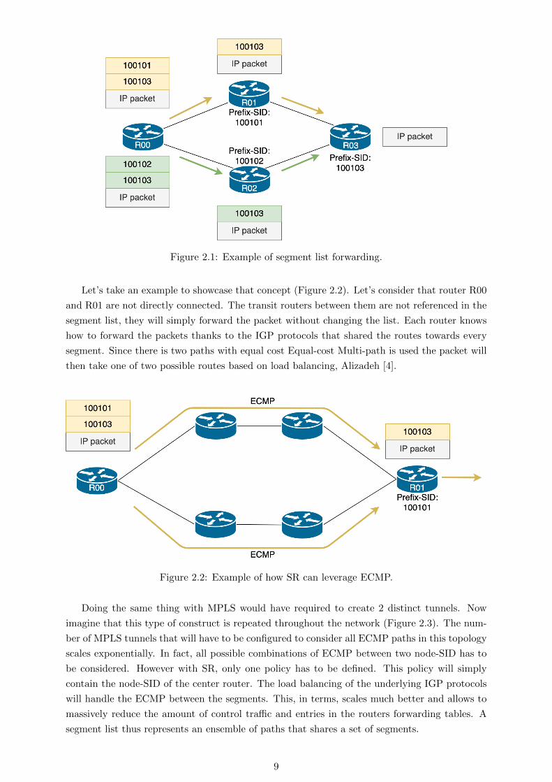
Figure 2.1: Example of segment list forwarding.

Let’s take an example to showcase that concept (Figure 2.2). Let’s consider that router R00

and R01 are not directly connected. The transit routers between them are not referenced in the

segment list, they will simply forward the packet without changing the list. Each router knows

how to forward the packets thanks to the IGP protocols that shared the routes towards every

segment. Since there is two paths with equal cost Equal-cost Multi-path is used the packet will

then take one of two possible routes based on load balancing, Alizadeh [4].

Figure 2.2: Example of how SR can leverage ECMP.

Doing the same thing with MPLS would have required to create 2 distinct tunnels. Now

imagine that this type of construct is repeated throughout the network (Figure 2.3). The num-

ber of MPLS tunnels that will have to be configured to consider all ECMP paths in this topology

scales exponentially. In fact, all possible combinations of ECMP between two node-SID has to

be considered. However with SR, only one policy has to be defined. This policy will simply

contain the node-SID of the center router. The load balancing of the underlying IGP protocols

will handle the ECMP between the segments. This, in terms, scales much better and allows to

massively reduce the amount of control traffic and entries in the routers forwarding tables. A

segment list thus represents an ensemble of paths that shares a set of segments.

9

Figure 2.3: Example of a topology with many ECMP.

The application of such technology are various to cite the most notable:

• Traffic engineering using SR tunnels. SR policies can be implemented in the network.

Those policies define paths that can be allocated to different types of traffic, Davoli [9].

• Creating back up paths. Since a policy is actually an ensemble of paths a SR route is more

robust than a standard MPLS tunnel in case of failure. Besides, SR policies can be defined

as alternate policies that should be used when the main SR route is down, Schuller [26].

• Access to traffic statistics on SR routes. Traffic on different SR routes can easily be

monitored as there is often a reasonable number of policies in a network. This can allow

to make some assumption on the demand in the network. This property will be used in

this study to recover the traffic matrix of a network running a SR protocol.

2.2 Jalapeno

Jalapeno is a cloud-native SDN infrastructure platform, Syed [31]. It is the application that

made this entire study possible. It is an open source program that is being developed by a

group of Cisco engineers. The main reason why Jalapeno was chosen is because it is generalized.

It collects a lot of information about the network, including SR related statistics and configura-

tions. It can, for example, retrieve the prefix-SID of all routers in the network.

The overall architecture can be found at Figure 2.4. Jalapeno is placed on top of a network

and collects streams of data form it. Those streams are BMP feeds and Telemetry feeds. BMP

conveys information about the topology while Telemetry relays traffic statistics, Scudder [27].

All those streams are processed using the Apache Kafka framework. Kafka is a log aggregator

that works especially well with operational metrics, Kreps [21]. It can be used, for example, to

get an up to date view of the network topology. It retrieves the link status from each router and

is able to infer the topology. It also can reconstitute sessions that exists between routers such

as BGP or IGP neighbors.

Then all this topology and performance data, exposed by Kafka, is parsed by base data

processors. Those processors are the ”Topology” and the ”Telegraf” pods. They are in charge

of respectively populating an Arango and an Influx database.

The Arango database contains many information about the topology. Those information

range from link state to complex VPN tunneling structures. This study will focus on informa-

tion regarding segment routing. In fact, the DB gives access to all routers prefix-SID and all

10

Figure 2.4: Jalapeno architecture, Syed [31].

links adjacency-SID. This will prove very useful for the traffic matrix resolution using SR.

The Influx database is a Time-Series DB containing traffic statistics. It is in this DB that

traffic counters value can be found. Since the DB is time oriented, the evolution of counters can

be observed over time. All counters mentioned in section 3.3.4 can be accessed via this DB.

Jalapeno also provides Grafana for data visualization. Grafana can be configure to display

graphs of the real time traffic. This is an powerful debugging tool as it allows to directly observe

what is collected by Jalapeno. It also allows to see if all routers are correctly transmitting at all

time.

An API is also being developed by the Jalapeno team. When finished, it will allow to re-

trieve information from the databases without having to know their internal structures. This

additional abstraction is always interesting, as if the DB changes, the tool that we are developing

won’t break. When this API is available, it should be integrated in our tool.

Note that this chapter is far from a full description of the Jalapeno tool. Indeed it provides

much more functionalities. For example, it is possible to request the shortest path between two

routers with node constraints. Furthermore, it is possible to implement new SR policies from

the SDN. However, since most of those advanced functionalities are not used in this study, they

won’t be described here.

11

Chapter 3

Traffic Matrix reconstitution

3.1 Traffic Matrix basics

3.1.1 Definition

The traffic matrix is a representation of how much traffic enters a network, where it enters, and

where it exits. It is usually represented as a matrix where each line is an entry point in the

studied network and each column an exit point. Each flow can then be characterized by its

index in the traffic matrix and its throughput.

A generic traffic matrix (Table 3.1) would be a two-dimensional matrix with its ij-th element

denoting the throughput, ti,j , sourcing from node i, ni, and exiting at node j, nj .

n0 n1 ... nj ... nN

n0 t0,0 t0,1 t0,j t0,N

n1 t1,0 t1,1 t1,j t1,N

...

ni ti,0 ti,1 ti,j ti,N

...

nN tN,0 tN,1 tN,j tN,N

Table 3.1: Generic traffic matrix with N nodes.

Nodes usually are routers in the network but can also be a subnetwork containing multiple

routers. The traffic matrix can be computed at different scales:

• At the scale of a small ISP network, nodes can be edge routers. In that case, entries

represent the demand of small group of client.

• When computing the traffic matrix at the scale of the internet. Core routers located in the

same city are agglomerated in point of presence (PoP). Then the PoP-to-PoP matrix can

then be studied to see the demand for each city. This implies that entries in this matrix

are an agglomeration of many flows.

There is an obvious trade-off between the readability of the traffic matrix and the granularity

of the nodes. Having smaller nodes allows to differentiate more flows but it also increases the

size of matrix.

12

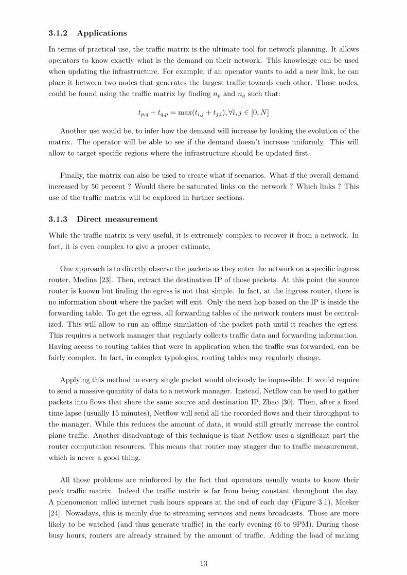
3.1.2 Applications

In terms of practical use, the traffic matrix is the ultimate tool for network planning. It allows

operators to know exactly what is the demand on their network. This knowledge can be used

when updating the infrastructure. For example, if an operator wants to add a new link, he can

place it between two nodes that generates the largest traffic towards each other. Those nodes,

could be found using the traffic matrix by finding np and nq such that:

tp,q + tq,p = max(ti,j + tj,i),∀i, j ∈ [0, N ]

Another use would be, to infer how the demand will increase by looking the evolution of the

matrix. The operator will be able to see if the demand doesn’t increase uniformly. This will

allow to target specific regions where the infrastructure should be updated first.

Finally, the matrix can also be used to create what-if scenarios. What-if the overall demand

increased by 50 percent ? Would there be saturated links on the network ? Which links ? This

use of the traffic matrix will be explored in further sections.

3.1.3 Direct measurement

While the traffic matrix is very useful, it is extremely complex to recover it from a network. In

fact, it is even complex to give a proper estimate.

One approach is to directly observe the packets as they enter the network on a specific ingress

router, Medina [23]. Then, extract the destination IP of those packets. At this point the source

router is known but finding the egress is not that simple. In fact, at the ingress router, there is

no information about where the packet will exit. Only the next hop based on the IP is inside the

forwarding table. To get the egress, all forwarding tables of the network routers must be central-

ized. This will allow to run an offline simulation of the packet path until it reaches the egress.

This requires a network manager that regularly collects traffic data and forwarding information.

Having access to routing tables that were in application when the traffic was forwarded, can be

fairly complex. In fact, in complex typologies, routing tables may regularly change.

Applying this method to every single packet would obviously be impossible. It would require

to send a massive quantity of data to a network manager. Instead, Netflow can be used to gather

packets into flows that share the same source and destination IP, Zhao [30]. Then, after a fixed

time lapse (usually 15 minutes), Netflow will send all the recorded flows and their throughput to

the manager. While this reduces the amount of data, it would still greatly increase the control

plane traffic. Another disadvantage of this technique is that Netflow uses a significant part the

router computation resources. This means that router may stagger due to traffic measurement,

which is never a good thing.

All those problems are reinforced by the fact that operators usually wants to know their

peak traffic matrix. Indeed the traffic matrix is far from being constant throughout the day.

A phenomenon called internet rush hours appears at the end of each day (Figure 3.1), Meeker

[24]. Nowadays, this is mainly due to streaming services and news broadcasts. Those are more

likely to be watched (and thus generate traffic) in the early evening (6 to 9PM). During those

busy hours, routers are already strained by the amount of traffic. Adding the load of making

13

measurements may cause traffic to be dropped.

In conclusion, direct measurement methods are extremely complicated to apply to real net-

works. They may be used as a one off-tool to get the traffic matrix at a precise point in time.

However, using them on a daily basis adds too much load on the network.

Figure 3.1: Internet rush hours in Europe and the US, Gunnar [17]

3.1.4 Estimation techniques

To circumvent the problems of direct measurement, the solution would be to infer the traffic

matrix using metrics that are already available on network manager. In fact, SNMP (Simple

Network Management Protocol), a widely use protocol, collects all sorts of measurement, Hare

[18]. One of which is the bytes and packets count on each router interfaces. From those counters,

the amount of traffic on each link can be determined. The problem is now to get the source

and destination of each flow only knowing the traffic counts on links. This problem is very well

known as it was first studied on the road and telephony networks, Sinclair [28].

Unfortunately, there is no easy solution to this problem. In fact, in most topologies, the

number of node pair is far greater than the number of links. Meaning that if the number of link

in a topology is L and the number of nodes is N , then usually:

L� N2 (3.1)

This simply states that topologies are often far from being full mesh. As a consequence,

the matrix estimation problem is under-constrained. Since the matrix is N × N , there is N2

variables but only L link measures (i.e. constrains). In order to make the problem well-posed, as-

sumptions need to be made. Those assumptions is what defines the different estimation methods.

One of the first estimation methods that were used in telephony are gravity models, Jung

[20]. It estimates the traffic from node np towards node nq as

t∗p,q = Ctin(p)tout(q) (3.2)

where tin(p) and tout(q) are respectively: the traffic entering the network at node np and the

14

the traffic exiting the network at node nq. C is a normalization constant:

C =1∑N

i=0 tout(i)(3.3)

The main assumption of this method can be derived from the equation. It simply states that

tp,q is proportional to the fraction of traffic that exits at node nq. It means that each end host

has its demand uniformly served from all the sources. This would be true for topology with few

large traffic sources and many smaller destinations. This is a pretty big assumption that can

break for a large number of topologies. Note that this approach only requires counters on edge

interfaces.

Many other methods and heuristics exits to approximate the matrix. Statistical approach

such as the Kruithof’s Projection Method that tackles the problem using information theory,

Krupp [22]. Bayesian methods also exists, they make the assumption that the probably of each

demands follows a normal distribution, Gunnar [17]. While all those methods are very effec-

tive for some known topologies, they are always as good as the assumptions they are build on.

Ideally, operators should not have to care about which hypotheses apply or not to their network.

In order to get deterministic results, the definition of traffic matrix can be modified. Instead

of having the actual source to destination traffic in the matrix, the worst-case bounds on demands

can be computed. Indeed, it is possible to compute the smallest and largest possible value

for each ti,j without assumptions. However those methods can be computationally expensive.

Besides they often lead to trivial results such as:

ti,j ∈ [0,max(tl)], l ∈ [0, L] (3.4)

were tl is the traffic on link l.

3.1.5 Implication of SR

The two previous sections made clear that the traffic matrix recovery problem is very complex.

However, there seems to be two main approaches:

• Retrieve a lot of information on the flows and the topology. No assumption needed on the

demand, at the cost of higher router computation loads and a large quantity of control

traffic.

• Use the existing traffic information collected by SNMP. No additional load or control

traffic, at the cost of making many assumptions about the demand in the network.

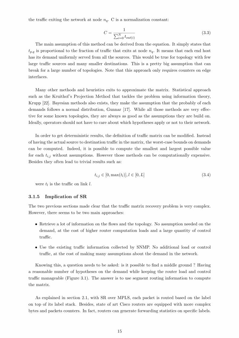
Knowing this, a question needs to be asked: is it possible to find a middle ground ? Having

a reasonable number of hypotheses on the demand while keeping the router load and control

traffic manageable (Figure 3.1). The answer is to use segment routing information to compute

the matrix.

As explained in section 2.1, with SR over MPLS, each packet is routed based on the label

on top of its label stack. Besides, state of art Cisco routers are equipped with more complex

bytes and packets counters. In fact, routers can generate forwarding statistics on specific labels.

15

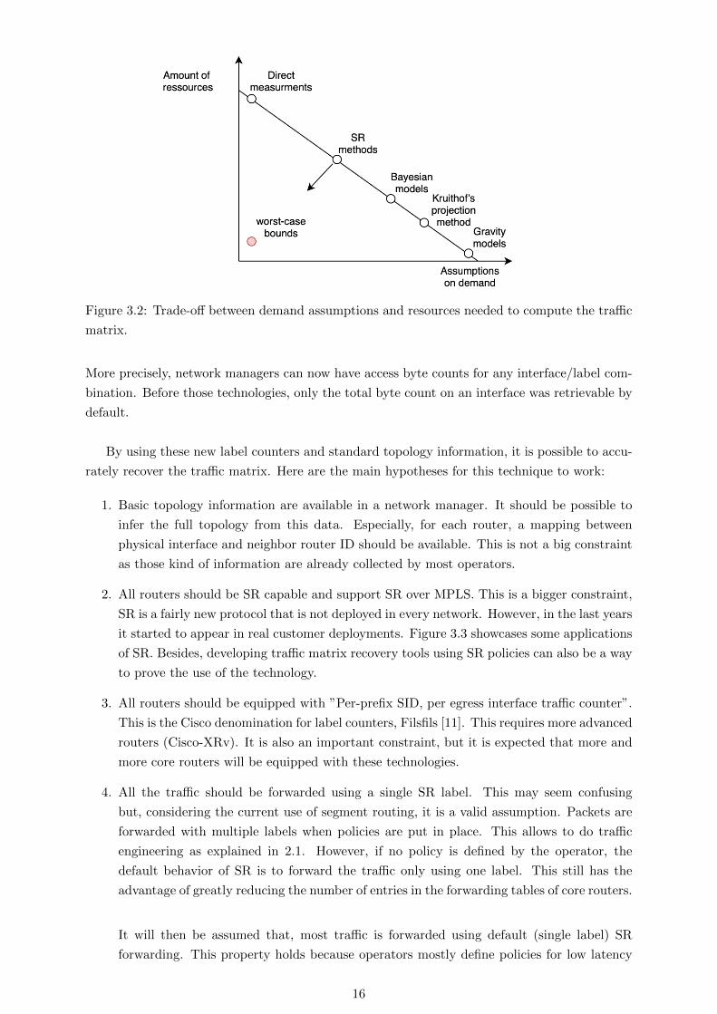
Figure 3.2: Trade-off between demand assumptions and resources needed to compute the traffic

matrix.

More precisely, network managers can now have access byte counts for any interface/label com-

bination. Before those technologies, only the total byte count on an interface was retrievable by

default.

By using these new label counters and standard topology information, it is possible to accu-

rately recover the traffic matrix. Here are the main hypotheses for this technique to work:

1. Basic topology information are available in a network manager. It should be possible to

infer the full topology from this data. Especially, for each router, a mapping between

physical interface and neighbor router ID should be available. This is not a big constraint

as those kind of information are already collected by most operators.

2. All routers should be SR capable and support SR over MPLS. This is a bigger constraint,

SR is a fairly new protocol that is not deployed in every network. However, in the last years

it started to appear in real customer deployments. Figure 3.3 showcases some applications

of SR. Besides, developing traffic matrix recovery tools using SR policies can also be a way

to prove the use of the technology.

3. All routers should be equipped with ”Per-prefix SID, per egress interface traffic counter”.

This is the Cisco denomination for label counters, Filsfils [11]. This requires more advanced

routers (Cisco-XRv). It is also an important constraint, but it is expected that more and

more core routers will be equipped with these technologies.

4. All the traffic should be forwarded using a single SR label. This may seem confusing

but, considering the current use of segment routing, it is a valid assumption. Packets are

forwarded with multiple labels when policies are put in place. This allows to do traffic

engineering as explained in 2.1. However, if no policy is defined by the operator, the

default behavior of SR is to forward the traffic only using one label. This still has the

advantage of greatly reducing the number of entries in the forwarding tables of core routers.

It will then be assumed that, most traffic is forwarded using default (single label) SR

forwarding. This property holds because operators mostly define policies for low latency

16

traffic (e.g. voice over IP). Indeed, those types of traffic require special routes in order to

face as less as congestion as possible. They also represent a very small proportion of the

overall traffic. For example, a WhatsApp call has a throughput of around 40 Kbps while

a HD Netflix stream is 5 Mbps (100 times greater), Davidson [8]. This is why neglecting

the traffic forwarded with SR policies doesn’t increase the error significantly.

Figure 3.3: Segment routing use cases

This technique seems to share some characteristics with the direct measurement method.

Indeed, similarly to Netflow, the interface counters agglomerate flows based on packet header

fields. However, compared to Netflow, the traffic is agglomerated based on labels which are

already an agglomeration of multiple IP flows. This means that, compared to Netflow, the

amount of data sent to the the manager is much smaller. Besides, since the traffic counters are

directly implemented in the OS of the router it is much more efficient. By consequence, the

added computational load is negligible compared to running Netflow.

Another advantage of this technique, is that the manager doesn’t have to collect the routers

forwarding tables. Since the SR labels represent the egress router there is no need to simulate

the packet route.

17

As for the assumptions, hypotheses 1 to 3 are entirely technical issues. This means that,

hopefully, as the router infrastructures gets upgraded they will become lesser constraints. Be-

sides, even hypotheses 4 could be solved by technological improvement. In fact, at first it seems

like an assumption on the traffic, but it could relaxed if traffic counters are improved. This will

be tackled in section 4.4.

As many constraints will be relaxed in the future, this new traffic matrix recovery methods

may become as good as worst-case bounds (Figure 3.2). However, SR methods will give the

exact ti,j not an interval.

3.2 SR Method Implementation

We will now propose a method to compute the traffic matrix based on SR counters. All four

previous assumptions will be considered valid. The presented method uses prefix-SID, but a

similar algorithm could be used with adjacency-SID (see 3.2.4).

The basic idea is to recover a router to prefix-SID traffic matrix. As explained in 2.1, Prefix-

SID are special labels that identify either a node (Node-SID) or a group of node (Anycast-SID)

in the topology. For the sake of this demonstration, let’s suppose that each prefix-SID corre-

sponds to a single router. Note that the algorithm is still valid for Anycast-SID (see 3.2.4). Each

router has a prefix-SID that is shared throughout the topology via ISIS. Then they will create

forwarding rules to reach each prefix-SID.

Our demonstration starts when this process has converged. This means that each router

knows about all prefix-SIDs and has deterministic rules for forwarding traffic toward those

prefix-SIDs. At first, we will suppose that those forward rules stay stable during the recovery

process.

In order to better understand the algorithm that will be presented in the next sections, we

will use a toy topology. This topology is chosen to be trivial for the sake of example. We have

chosen a four router diamond topology (Figure 3.4).

Figure 3.4: Toy topology.

All links have the same IGP cost and capacity. Each router has a prefix-SID and two

18

neighbors:

• R00 : 100100, [R01, R02]

• R01 : 100101, [R00, R03]

• R02 : 100102, [R00, R03]

• R03 : 100103, [R01, R02]

Router R00 will be generating 50 kbps of traffic towards each router of the topology (except

itself). Which gives us the traffic matrix at Table 3.2. The goal of our demonstration is to show

how this matrix can be recovered from SR traffic statistics.

100100 100101 100102 100103

R00 0 50 kbps 50 kbps 50 kbps

R01 0 0 0 0

R02 0 0 0 0

R03 0 0 0 0

Table 3.2: Target traffic matrix (router to prefix-SID)

3.2.1 Forwarding traffic matrix recovery

The first step of our design, is to recover the forwarding traffic matrix (FTM). The concept of

FTM is specially defined for this study. Each router has it’s own FTM, representing the traffic

that it forwards to its neighbor. More precisely, it is the byte count for each label forwarded to

each neighbor.

Algorithm 1 Forwarding traffic matrix recovery

function Get FTMs(topology, time interval)

FTMs← {}for all router in topology do

for all interface in router do

for all prefix-SID in topology do

neighbor ← Get neighbor(router, interface)

t1 ←Read counter(interface, prefix-SID, Now( ) - time interval)

t2 ←Read counter(interface, prefix-SID, Now( ))

FTMs[router][neighbor][prefix-SID]← (t2 - t1)/time interval

return FTMs

function Read counter(interface, prefix-SID, time)

return !byte count exiting interface with prefix-SID

function Get neighbor(router, interface)

return !neighbor router connected to interface

Algorithm 1 describes the process of recovering the FTM of each router. Note that the

function Get FTMs takes the topology as argument. This is in accord with Assumption 1 that

19

states that the network manager should have access to basic topology information.

Let’s describe precisely what is this ”topology information”. First, the manager should have

an identifier for each router (usually the loopback IP address). Besides, all router interfaces and

their corresponding neighbor should be available (function Get neighbor represent this map-

ping). Finally, all Prefix-SID should be known.

The function Read counter allows to get how much bytes exited an interface with a specific

label. It can be seen as a way to access the ”Per-prefix SID, per egress interface traffic counter”

inside the routers. It returns a raw byte count. This count is the number of bytes transmitted

from the router initialisation up until the requested time. In order to get the average through-

put, we take this raw byte count at two different time steps. Then, we subtract the less recent

from the most recent and divide by the time span between the two. The resultant throughput

is the average demand over the time interval.

Choosing the right time interval is crucial. It entirely depends on the type of traffic matrix

that should be recovered. In most cases, operators are interested in the rush hours matrix (see

3.1). This means that the time interval should be set to around 2 hours. However, it’s possible

to compute the throughput for much longer period. There no real upper limit on the interval,

the operator simply has to make sure that all routers were active at the time of the measure.

Note that here we compute the FTMs at the current time but its possible to get older FTMs.

Applying Algorithm 1 to our toy example (3.4), gets us the following FTMs (Tables 3.3, 3.4,

3.5, 3.6):

100100 100101 100102 100103

R01 0 50 kbps 0 25 kbps

R02 0 0 50 kbps 25 kbps

Table 3.3: Forwarding traffic matrix of R00

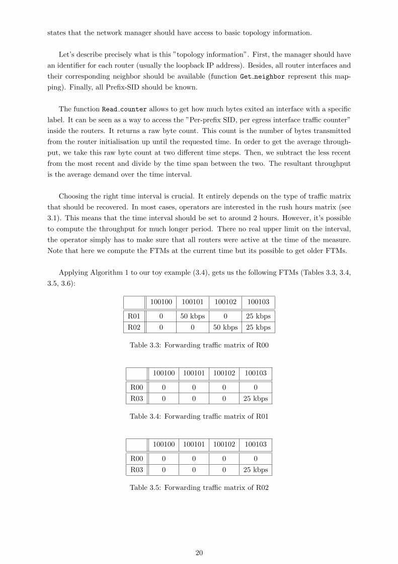
100100 100101 100102 100103

R00 0 0 0 0

R03 0 0 0 25 kbps

Table 3.4: Forwarding traffic matrix of R01

100100 100101 100102 100103

R00 0 0 0 0

R03 0 0 0 25 kbps

Table 3.5: Forwarding traffic matrix of R02

20

100100 100101 100102 100103

R01 0 0 0 0

R02 0 0 0 0

Table 3.6: Forwarding traffic matrix of R03

Table 3.3 is R00 FTM, it can be seen that R00 transmits 50 kbps with each prefix-SID. It

was to be expected as it tries to reach R01, R02 and R03. Since it is directly connected to R01

and R02, the traffic corresponding to their label (1001001 and 100102) is sent directly to them.

This is a straight implementation of the shortest path policy. To reach R03, R01 uses Equal-cost

Multi-path (ECMP) and splits the traffic in half. Half the traffic follows the path R01-R03 and

the other half follows R02-R03. ECMP can be applied because both paths have the same length

and IGP cost.

Table 3.4 and 3.5 shows that R01 and R02 forward the traffic they received from R00 to

R03. 3.6 is empty, as it neither generates nor forwards any traffic. Note that the traffic that

exits the network doesn’t appear in the FTM of the egress router. This is due to the fact that,

the traffic is accounted for only at the egress interface. When the traffic exits the last router its

no longer encapsulated in an SR header. In fact, the traffic has reached the end of the tunnel,

so the router removes the SR encapsulation. This prevents the counters from taking this exiting

traffic into account.

3.2.2 Traffic matrix computation

Now that the FTMs are recovered the rest of the process is straight forward. Algorithm 2

showcases the full process of recovering the traffic matrix:

• The FTMs are recovered for the chosen time interval.

• The traffic matrix is created. Its size is N ×N , where N is the number of routers in the

topology. It’s then filled with zeros.

• For each router, the traffic of each label is agglomerated. This means that we get the

overall traffic that each router sends towards every label.

• The transit traffic is then removed for each router. The transit traffic, for a router, is the

traffic that didn’t enter the network via one of its interfaces. It originated from an other

router and has been sent to the router by one of its neighbor. To retrieve the amount

of transit traffic for a router, one can go to its neighbor FTMs and get how much traffic

is sent to the router. By removing all the traffic sent by neighbors, the only remaining

demand is what enters the network at the router. This operation has to be done for each

label. The result is the traffic that enters at the router and towards which label. Doing

this for each router, computes the traffic matrix.

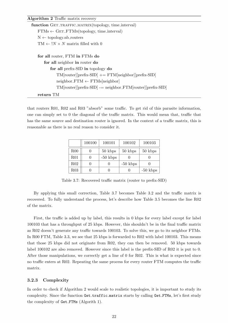
Applying this algorithm to our toy example (see 3.4) results in Table 3.7. This not the exact

traffic matrix presented as the objective (see 3.2). In fact, some negative throughput values

appear. While this may seem weird it is actually fairly logical. It is a consequence of the routers

not counting the exiting traffic (since it’s no longer SR traffic). It simply represents the fact

21

Algorithm 2 Traffic matrix recovery

function Get traffic matrix(topology, time interval)

FTMs← Get FTMs(topology, time interval)

N ← topology.nb routers

TM ← !N ×N matrix filled with 0

for all router, FTM in FTMs do

for all neighbor in router do

for all prefix-SID in topology do

TM[router][prefix-SID] += FTM[neighbor][prefix-SID]

neighbor FTM ← FTMs[neighbor]

TM[router][prefix-SID] -= neighbor FTM[router][prefix-SID]

return TM

that routers R01, R02 and R03 ”absorb” some traffic. To get rid of this parasite information,

one can simply set to 0 the diagonal of the traffic matrix. This would mean that, traffic that

has the same source and destination router is ignored. In the context of a traffic matrix, this is

reasonable as there is no real reason to consider it.

100100 100101 100102 100103

R00 0 50 kbps 50 kbps 50 kbps

R01 0 -50 kbps 0 0

R02 0 0 -50 kbps 0

R03 0 0 0 -50 kbps

Table 3.7: Recovered traffic matrix (router to prefix-SID)

By applying this small correction, Table 3.7 becomes Table 3.2 and the traffic matrix is

recovered. To fully understand the process, let’s describe how Table 3.5 becomes the line R02

of the matrix.

First, the traffic is added up by label, this results in 0 kbps for every label except for label

100103 that has a throughput of 25 kbps. However, this shouldn’t be in the final traffic matrix

as R02 doesn’t generate any traffic towards 100103. To solve this, we go to its neighbor FTMs.

In R00 FTM, Table 3.3, we see that 25 kbps is forwarded to R02 with label 100103. This means

that those 25 kbps did not originate from R02, they can then be removed. 50 kbps towards

label 100102 are also removed. However since this label is the prefix-SID of R02 it is put to 0.

After those manipulations, we correctly get a line of 0 for R02. This is what is expected since

no traffic enters at R02. Repeating the same process for every router FTM computes the traffic

matrix.

3.2.3 Complexity

In order to check if Algorithm 2 would scale to realistic topologies, it is important to study its

complexity. Since the function Get traffic matrix starts by calling Get FTMs, let’s first study

the complexity of Get FTMs (Algorith 1).

22

Get FTMs contains three nested loops, the first two are design to go through all the interfaces

of the topology. This amounts to 2L interfaces (L is the total number of links), considering that

each link is connected to 2 interfaces. The last loop goes through all prefix-SID in the topology

which is equal to the number of nodes N . This means that the complexity is:

O(2LN) = O(LN) (3.5)

The worst case complexity is reached when the topology is full mesh (i.e. L = N2). Leading

to a complexity of:

O(N3) (3.6)

However, this is not realistic as most of the studied topology are far from being full mesh.

Usually we have L << N2, taking this into account we can assumed that L = O(N). Under the

assumption of the ”usual topology”, the complexity is brought down to:

O(N2) (3.7)

Get traffic matrix has the exact same three loops. This means that its complexity is also

O(N2), bringing the overall complexity to O(2N2) = O(N2) in the average case.

As a consequence, this method doesn’t scale that well with respect to the number of nodes.

However, all of this computation can be done offline. Besides, this computation should be done

at most once a day. There is no real use case were the matrix has to be computed on the fly in

a short period.

3.2.4 Removing assumptions

All small assumptions that have been made at the start of this chapter can actually be removed.

Note that here we do not mention the four main assumptions done in section 3.1.5, but the

small assumptions made in section 3.2. Indeed they were simply put in place so not to confuse

the reader with additional complexity. Let’s go through those assumptions and see why the

proposed algorithm is not dependent on them:

1. Using Prefix-SID aver Adjacency-SID. While the algorithm is easier to understand when

destinations are routers (i.e. Prefix-SID) its still valid when they are links (i.e. Adjacency-

SID). Routers that are equipped with Prefix-SID traffic counters can also count traffic

with specific Adjacency-SIDs. The method stays exactly the same except that the result

is a router to Adjacency-SID traffic matrix. The meaning of an ”exit link” is that it is the

last link on which the traffic was SR encapsulated.

2. Using Node-SID over Anycast-SID. This is also an artificial constraint. It is never needed

in the algorithm to map a Prefix-SID to a single router. Once again, the only consequence

of having a label that identifies multiple routers, is the modification of traffic matrix

meaning. The result, in that case, is a router to routers traffic matrix. This matrix would

be less precise in term of egress node. It simply specifies a group node as egress, meaning

that the traffic may have exited by any node in that group.

23

3.3 SR Method Evaluation

In this chapter, the process of recovering the traffic matrix from SR metrics will be evaluated.

More precisely, we will compute Algorithm 2 on multiple topologies with different demands.

Then the accuracy of the recovered traffic matrix will be studied.

3.3.1 Virtual topology

In order to evaluate Algorithm 2, we need a topology. The idea is to create a virtual topology

using router images. From there, we can simulate some demand and try to compute the traffic

matrix from SR traffic statistics. A collector is also needed to retrieve those traffic statistics and

store them in a database. Another collector is required to collect topology information.

The first important choice is the router image. In fact, the simulated router should satisfy

Assumption 2 and 3. This means that they should be able to forward SR encapsulated packets

and record statistics based on egress interface and prefix-SID. This already rules out many

standard routers as those features are fairly advanced. The main candidates are in the Cisco-

XRv line of routers. They are advanced Cisco routers and offer many features that will be

essential for our application. Here are some configurations of the Cisco-XRv routers that are

useful:

• BGP Monitoring Protocol (BMP)

• Telemetry

• ISIS

• Segment routing over ISIS

However, since those routers have more features, they also require a lot resources to run.

Since we’re working in a virtual environment, this means that the computer that hosts the

topology must be fairly powerful. Here are the minimum requirements to host one Cisco-XRv

router images:

• 4 vCPUs

• 24GB memory

• 50GB disk

Obviously, this is an important constraint. In fact, simulating large typologies would require

a massive architecture. We had to make a compromise between the complexity of the test topol-

ogy and the amount of needed resources. The best trade-off seemed to be a topology of four

routers. The minimum requirements become 16 vCPUs, 96GB memory and 200GB disk. While

this is still a lot, a supercomputer disposing of such specifications is fairly common. Besides,

with four routers, it is possible to simulate multiple topologies. It is also possible to simulate

transit traffic. This is interesting as removing transit traffic is a big part of the algorithm and

it should be tested.

The next step was to choose the architecture. Our first choice was to use the Uliege super

calculator. In some clusters of the calculator (e.g. Hercules), it was possible to reserve such

24

resources (they provided large memory block, up to 100GB). However, it was proven to be ex-

tremely complex to run a virtual machine on multiple cores. In fact, due to the vast disparity

between the available CPUs, simulating the router images on top of them is close to impossible.

Besides, installing the necessary tools to run the VMs in the first place is not that trivial. In

fact, the calculator architecture is fairly outdated and many software such as QEMU were not

available.

The second choice was to use a cloud provider. This would allow to reserve a fixed amount

of resources and use them on demand. After a quick price comparison, gcloud was chosen. A set

of 16 vCPUs was selected, all with virtualization enabled. This also allowed to get full control

over the environment compared to the Uliege super calculator. All the necessary software could

then be installed on the machine. Finally, the topology of four routers was tested, without any

traffic the CPUs utilisation was around 60%. This seemed like a good benchmark, that’s why

we decided to go on with this solution for the evaluation.

Note that one of the reason gcloud was chosen is for there ”pay for what you use” philosophy.

Indeed, Google only charges us when the topology was active. This allowed to make many small

tests throughout a long period, without wasting money.

Once all routers were up and running, some basic configurations were done on the routers.

We created a full mesh of links. In order to build different typologies, we will simply shutdown

some interfaces. All the interfaces were given an IP address and brought up. Each router was

given an ID in the form of a loopback address. ISIS was configure to serve as an IGP and

thus is in charge of sharing IP routes throughout the topology. Figure 3.5 shows the topology

after those basics configurations. Note that the address directly under the router name, is the

loopback address.

3.3.2 Topological data collection

Now that the virtual topology is in place, the next step is to collect information about the

topology. Indeed, the traffic matrix recovery algorithm takes as argument a topology variable

that contains link and router information.

Collecting this data is a three steps process. First, the data is generated by the routers.

Then, it is sent out to a collector that stores it in a database. Finally, our application interfaces

with this database to get the necessary information to compute the traffic matrix. Let’s now

describe how those three steps are carried out.

One way for the router to monitor and collect topology information, is to use BGP monitor-

ing protocol (BMP). For BMP to work a BGP session must be established between all routers.

This allows to routers to exchange BMP messages that are special BGP packets.

BMP is based on a server-client model. In the case of our small topology 3.6, router R03 will

be the BMP server. R03 is charged with recovering the information of the three BMP clients:

R00, R01 and R02. From those information it can create a statistics report. The report is then

transmitted to a network collector. It contains many information such as:

• The loopback, prefix-SID and interfaces of each router.

25

Figure 3.5: Simulated four router topology (full mesh).

• The status, connected link, IP and name of each interface.

• The IGP cost, capacity, connected routers and Adjacency-SID of each link.

From this report one can easily infer the full topology.

All those information should be regularly refreshed to handle topological changes. The re-

fresh delay that we have chosen is 30 seconds. This keeps the throughput overhead of this control

traffic fairly low, while making sure that the recovered topology is up to date.

The collector receives this report, interprets it and stores it in a database. The collector

that we use is Jalapeno. As explained in section 2.2, Jalapeno is a tool developed by Cisco that

allows to collect BMP update messages. Then, Jalapeno selects the latest update and exposes

all those information in an Arango database. Here are the tables in which we are interested:

• LSLink: contains descriptions for each link.

• LSNode: contains descriptions for each node.

• LSv4 Topology: contains SR information such as the router Prefix-SIDs.

By making requests to those tables we are able to determine the full topology.

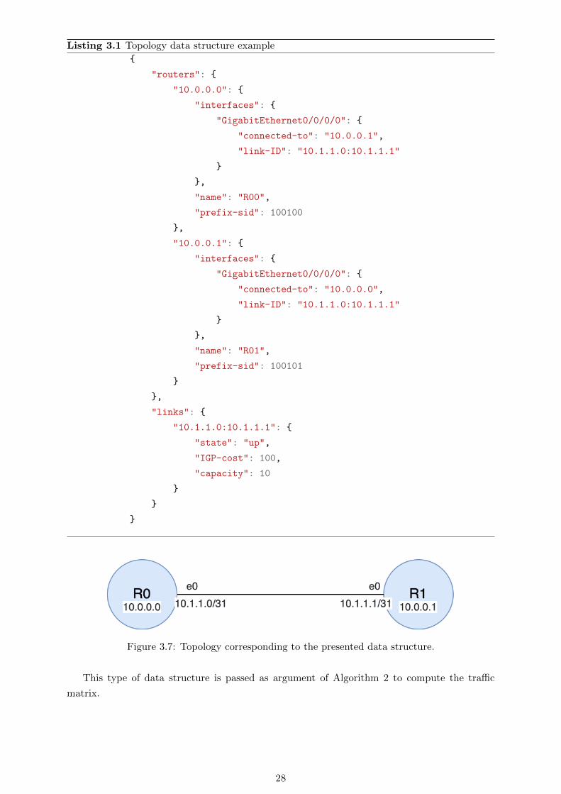
3.3.3 Topology data structure

Having access to all the needed topology information, we decided to create a data structure that

can be easily parsed.

26

Figure 3.6: BMP server/clients in the simulated topology.

Each router is stored with its prefix-SID, loopback address and a list of its interfaces. Each

interface structure contains the loopback of the neighbor connected to that interface and an

unique identifier. This ID is a concatenation of the IP addresses of both end interfaces of the

link.

Each link is stored with its ID, state (up or down), IGP cost and capacity.

Here is an example of a topology data structure (3.1), with its corresponding topology (Figure

3.7):

27

Listing 3.1 Topology data structure example

{

"routers": {

"10.0.0.0": {

"interfaces": {

"GigabitEthernet0/0/0/0": {

"connected-to": "10.0.0.1",

"link-ID": "10.1.1.0:10.1.1.1"

}

},

"name": "R00",

"prefix-sid": 100100

},

"10.0.0.1": {

"interfaces": {

"GigabitEthernet0/0/0/0": {

"connected-to": "10.0.0.0",

"link-ID": "10.1.1.0:10.1.1.1"

}

},

"name": "R01",

"prefix-sid": 100101

}

},

"links": {

"10.1.1.0:10.1.1.1": {

"state": "up",

"IGP-cost": 100,

"capacity": 10

}

}

}

Figure 3.7: Topology corresponding to the presented data structure.

This type of data structure is passed as argument of Algorithm 2 to compute the traffic

matrix.

28

3.3.4 Traffic data collection

In order to read the value of the traffic counters, we designed a three step process. This process

is very similar to what was done for the topology recovery. First, the routers produce traffic

statistics (in the form of byte and packet counts). Second, they stream those statistics to a

collector. Third, the collector exposes the statistics in database that can be accessed by our

application.

For the routers to collect traffic statistics, two sensors need to be configured. An interface

sensor to count the overall number of byte entering and exiting each interfaces. A ”mpls-

forwarding” sensor that allows to agglomerate based on MPLS label. Since Prefix-SIDs are

MPLS labels with specific values, this sensor can agglomerate traffic based on Prefix-SID. The

sample frequency of the counters is configured at 30 sec. Once again, this is a trade-off between

the amount of control traffic an the the fact that our traffic statistics should be up to date.

Each router sends directly its traffic telemetry to the collector. In this case, there is no

need for a router to centralize the information. In fact, each routers record independently the

throughput at each interface. Figure 3.8 shows that R01 sends its statistics directly to the col-

lector. R03 simply forwards them without any modification.

Figure 3.8: Traffic telemetry in the simulated topology.

Once again the collector is Jalapeno. It is charged with storing the traffic counts in an Influx

database. Influx is a particular database that stores entries based on time stamps. This means

that we have access, not only to the current value of the counters, but also to the full evolution

of the counters since the router first initialisation. It is especially useful as in Algorithm 1 we

want to read previous values of the counter to establish the throughput.

The main difference with the Arango database is that Arango only provides the newest

29

topological information. Inside the influx DB two tables are of interest:

• ”Cisco-IOS-XR-fib-common-oper:mpls-forwarding/nodes/node/label-fib/forwarding-details/forwarding-

detail” : for the counters on Prefix-SIDs.

• ”Cisco-IOS-XR-pfi-im-cmd-oper:interfaces/interface-xr/interface” : for the general inter-

face counters.

All the necessary tools are now in place on the simulated topology. The next step will be to

test our algorithm against multiple demand scenarios.

3.3.5 Evaluation

Now that the topology and traffic statistics can be recovered from the virtual topology, the

traffic matrix recovery process can be tested. The testing is fairly straight forward. First, simu-

late traffic in the network. Then, run Algorithm 2 and compare the result to what was simulated.

To simulate traffic, we created hosts connected to each router in the simulated topology

(Figure 3.5). Then we simulated traffic using Scapy. Scapy is a packet manipulation tool that

allows to create custom packets, Biondi [7]. It was used over a more classic iperf. The reason

for this is that, iperf was not able to simulate a small enough throughput. In fact, since we

are working with lab images for the router, they can’t forward more than 0.08 Mbps of through-

put. Scapy allowed us to simulate much lower demand, while iperf could not go under 0.1 Mbps.

Let’s first try to compute the control traffic matrix. In fact, without even simulating any traf-

fic, there already exists some throughput for control traffic (ISIS, BGP) and for topology/traffic

statistics (BMP, Telemetry). Running the traffic matrix recovery algorithm on the simulated

topology (full mesh), without simulating any traffic gives the following traffic matrix (Table 3.8):

100100 100101 100102 100103

R00 0 0.02 kbps 0.02 kbps 0.02 kbps

R01 0.04 kbps 0 0.02 kbps 0.02 kbps

R02 0 0 0 0.02 kbps

R03 1.85 kbps 0.65 kbps 0.02 kbps 0

Table 3.8: Control traffic matrix.

After observing the label counters in the network, this control traffic matrix seems fairly

accurate. The overall traffic is not very high but, for precision sake, we will take it into account.

Note that the fact R03 sends out a bit more traffic is probably due to the fact that it is the

BMP server and thus has to send some control traffic.

Now that we have a base matrix, let’s call it Tcontrol, we can simulate some actual traffic. A

standard traffic matrix is usually complete, meaning that all nodes send towards every destina-

tion. This is especially true if routers are in the backbone. A complete traffic matrix is also the

most general scenario. Let’s consider the following complete traffic matrix Tcomplete (Table 3.9):

30

100100 100101 100102 100103

R00 0 tsim tsim tsim

R01 tsim 0 tsim tsim

R02 tsim tsim 0 tsim

R03 tsim tsim tsim 0

Table 3.9: Simulated traffic matrix.

In order to test different level of demand lets consider:

tsim ∈ [0, 50 kbps] (3.8)

And so, we will compare the recovered traffic matrix (Trecov) with Tcontrol + Tcomplete for

different values of tsim.

Another variable that we wanted to test is the topology. In fact, since the algorithm is

very dependent on the topology we also wanted to test it with different network arrangements.

Unfortunately, there is a limited set of topology since we only have four routers. Here is the set

of topology on which we tested the traffic matrix recovery:

• A full mesh topology: Figure 3.9.

• An inline topology: Figure 3.10.

• A diamond topology: Figure 3.4.

• A star topology: Figure 3.11.

• A Y topology: Figure 3.12.

Figure 3.9: Test topology full mesh.

Here is the full testing methodology. First, choose a tsim in the interval. Then, simulate

the traffic in the one of the topologies. Get the mean value of the demand in Trecov let’s call it

trecov. Repeat for all the proposed topologies. Take the mean and variance of trecov over all the

31

Figure 3.10: Test topology ”inline”.

Figure 3.11: Test topology ”star”.

Figure 3.12: Test topology ”Y”.

32

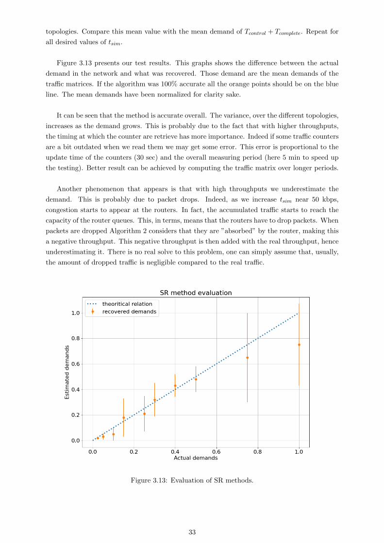
topologies. Compare this mean value with the mean demand of Tcontrol + Tcomplete. Repeat for

all desired values of tsim.

Figure 3.13 presents our test results. This graphs shows the difference between the actual

demand in the network and what was recovered. Those demand are the mean demands of the

traffic matrices. If the algorithm was 100% accurate all the orange points should be on the blue

line. The mean demands have been normalized for clarity sake.

It can be seen that the method is accurate overall. The variance, over the different topologies,

increases as the demand grows. This is probably due to the fact that with higher throughputs,

the timing at which the counter are retrieve has more importance. Indeed if some traffic counters

are a bit outdated when we read them we may get some error. This error is proportional to the

update time of the counters (30 sec) and the overall measuring period (here 5 min to speed up

the testing). Better result can be achieved by computing the traffic matrix over longer periods.

Another phenomenon that appears is that with high throughputs we underestimate the

demand. This is probably due to packet drops. Indeed, as we increase tsim near 50 kbps,

congestion starts to appear at the routers. In fact, the accumulated traffic starts to reach the

capacity of the router queues. This, in terms, means that the routers have to drop packets. When

packets are dropped Algorithm 2 considers that they are ”absorbed” by the router, making this

a negative throughput. This negative throughput is then added with the real throughput, hence

underestimating it. There is no real solve to this problem, one can simply assume that, usually,

the amount of dropped traffic is negligible compared to the real traffic.

Figure 3.13: Evaluation of SR methods.

33

Chapter 4

What-if scenarios

The second part of this study focuses on creating what-if scenarios based on a network topology

and traffic matrix. A what-if scenario is an alteration of the topology and/or traffic matrix. For

example, what-if scenarios on a network could be:

• A link failure.

• A router failure.

• Multiple link failure. This could append if links are part of the same SRLG (Shared Risk

Link Groups), Ahuja [2].

In terms of traffic matrix possible what-if scenarios could be:

• Traffic surge towards a destination. This is a very common scenario especially for web

servers.

• Traffic surge from a source.

• Traffic surge from a specific source/destination pair.

• Overall traffic increase.

The tool that we have created allows an user to create a what-if scenario and see the im-

pact of this scenario on his network. This impact can be derived from the link utilisation. For

example, in the case of a link failure, the traffic will be rerouted and it may create congestion

on certain links. Congestion can then lead to traffic drop which is critical for a network operator.

Analysing the impact such scenarios could be extremely useful for network planners. In fact,

it may allow them to identify critical links or nodes in their topology. This would help operators

to locate were redundancy should be added. It may also allow to locate were the topology should

be upgraded first. The ultimate goal would be to give an accurate estimation of the time left

before the network becomes saturated.

4.1 Link utilisation

The first step before any kind of interpretation of a what-if scenario is to be able to compute

the link utilisation. To compute the load on each link in a network three elements are neces-

sary. First, the topology should be known. Second, access to the traffic matrix representing

34

the demand in the network. Third, a routing algorithm to simulate how this demand will be

forwarded throughout the network.

4.1.1 Computing the link utilisation

Algorithm 3 shows how the link utilisation can be computed from those three arguments. The

Compute link util function takes a description of the network topology as argument. This

description has the same form as for the traffic matrix (see 3.5). It basically links all routers

with their neighbors (standard graph description). It also takes a traffic matrix as argument.

The traffic matrix computed with SR methods (see 3) can be used. However, any other traffic

matrix can be used as long as it corresponds to the topology. For example, one could use a

PoP-to-PoP traffic matrix in this algorithm, as long a the topology describes how those PoPs

are interconnected.

Algorithm 3 Link utilisation

function Compute link util(topology, TM)

links ← topology.links

for all link in links do

link.util ← 0

for all source in topology do

paths ← Routing algo(topology, source)

for all destination in topology do

for all path in paths[destination] do

for all link ID in path do

traffic ← TM[source][destination] × path.traffic portion

links[link ID].util ← links[link ID].util + traffic

for all link in links do

link.util ← (link.util / link.capacity)×100

return links

For the sake of the example, let’s consider that we pass in, a router to prefix-SID matrix,

where each prefix-SID uniquely identifies a router (Node-SID). First, the utilisation of all link

is set to zero. Then, the function goes through all routers and uses a routing algorithm to

compute the paths towards all destinations. This routing algorithm will be abstracted for now,

an implementation will be discussed later (see 4.1.2). Then, for all possible destinations, the

paths are extracted. Note that there can be multiple paths for a single destination as Equal-cost

Multi-path (ECMP) is considered active. While this is not always true, when using segment

routing ECMP should always be enabled.

The next step is fairly straight forward. Go through all link in each path and, and add traffic

to the link based on the demand fount in the traffic matrix. The entry in the traffic matrix corre-

sponds to the source and destination of the current path. This simply corresponds to redeploying

35

the traffic matrix demand in the topology. It can be seen as the exact opposite of the traffic ma-

trix recovery problem. In this case, instead of going from link traffic measurements towards the

traffic matrix, the process starts with the matrix and tries to deduce the throughput on each link.

Note that the traffic added is multiplied by a traffic portion variable. This is because ECMP

can split the demand based on the number of available paths towards a destination. This means

that each path only has portion of the traffic left. This traffic division is computed by the

routing algorithm.

Finally, the raw utilisation is divided by the link capacity. This gives as a final result the

percentage of utilisation for each link.

4.1.2 Routing algorithm implementation

There exists many routing algorithm with many different implementations. However, they of-

ten share the same overall principle: trying to find the shortest path between a source and a

destination. The notion shortest path can also have multiple definitions. In this case we will

interpret it as the path that has the minimum IGP weight. The IGP weight of a path is the

sum of the IGP weights of each link.

The Interior gateway protocol (IGP) weight was chosen because most routing algorithm

based their routing decisions on those metrics. This is true for ISIS, OSPF and RIP. Obviously

BGP has a much more complex decision process, recreating such an algorithm is outside the

scope of this study. Besides segment routing is built on top of ISIS.

Algorithm 4 shows an implementation of a generic Interior Gateway Protocol, based on the

Dijkstra’s algorithm.

In Fact, a priority queue Dijksrta’s algorithm can easily be discerned from Algorithm 4.

The priority queue maintains the paths sorted, such that the path with the minimum IGP cost

is always extracted first. The last router of the path is recovered. Each of its neighbors are

considered, if they can be reached at a lesser cost from the router. If that’s the case the neighbor

is added to the queue and the list of reached routers. Once the queue is empty, the function

goes through all paths and assign them their traffic portion. In this implementation, the traffic

fraction is inversely proportional to the amount of paths with the same IGP cost that go to the

same destination.

4.1.3 Complexity

While Algorithm 3 may seem straight forward, its complexity is non trivial. Starting with the

routing algorithm (Algorithm 4), it has a complexity of a priority queue Dijkstra:

O (L + N log(N)) (4.1)

Where L is the number of links and N the number of nodes. Note that, this not entirely

correct as Algorithm 4 is not an exact Dijkstra. In fact, it considers ECMP so its possible to

36

Algorithm 4 Routing algorithm (Dijkstra)

function Routing algo(topology, source)

Q ← !priority queue

Q.push([source, !empty path])

discovered routers ← {}discovered routers[source] ← [!empty path]

while Q not empty do

router, path ← Q.extract min cost()

for all neighbor, link in router do

cost ← path.cost + link.cost

if neighbor not in discovered routers

or cost ≤ discovered routers[neighbor].first path.cost then

Q.push([neighbor, path + neighbor])

discovered routers[neighbor].add path(path + neighbor)

for all destination, paths in discovered routers do

for all path in paths do

path.traffic portion = 1 / paths.length()

return discovered routers

find multiple paths towards a destination. Let’s first consider only one path per destination,

ECMP will be discussed later.

Algorithm 4 is computed for every possible sources (i.e. every node). Which leads to a

complexity of

O (N(L + N log(N))) (4.2)

Algorithm 3 checks all possible destinations. Then, it goes through all paths for a specific

destination. Here we only consider one path per destination so the overall complexity is not

affected. The next nested loop goes through all links in the selected path. The worst case for

this path length is N . This cannot be true for every paths but let’s consider it to have an upper

bound. This gives a complexity of:

O(N(L + N log(N) + N2)

)(4.3)

Finally, the last loop goes through all links adding L to the complexity:

O(N(L + N log(N) + N2) + L

)(4.4)

To further the search for an upper bound, we can consider that L = O(N2) (full mesh

topology):

O(N(N log(N) + 2N2) + N2

)= O(N3) (4.5)

O(N3) is thus the worst case complexity without ECMP. However this is fairly unrealistic

due to the assumption done at equation 4.3. In fact, in average, the path length is far from being

37

O(N). It is usually much closer of being O(log(N)). In the case of a tree this fairly obvious, for

a graph it is also true in the average case. Note that the base of this log is the average number

of connections of a node inside the graph. Rewriting equation, for the average case, 4.3 we get:

O (N(L + 2N log(N))) (4.6)

Another assumption that can be made is that the topology is far from being full mesh. In

fact, the number of links is usually much closer to the number of node (L = O(N)). Bringing

the complexity down to:

O (N(L + 2N log(N)) + L) = O (N(N + 2N log(N)) + N)

= O(N2 log(N))(4.7)

O(N2 log(N)) is thus the average complexity of the link utilisation algorithm.

Taking into account ECMP, the number of paths per destination can no longer be consid-

ered equal to one. This means that the complexity of the Dijkstra’s algorithm (equation 4.1) is

multiplied by the average number of equivalent paths per destination. To give an upper bound

to this average number of paths, lets consider the maximum number of path between two nodes

in a fully connected topology.

Considering that N > 2, the number of paths with k vertices is:

(N − 2)!

(N − k − 2)!for 0 ≤ k ≤ N − 2 (4.8)

This is because you can choose k other nodes out of the remaining N − 2 in (N−2)!(N−2−k)!k! ways

(e.q. CN−2k ), and then you can put those k nodes in any order in the path.

The total number of path can be obtained by summing this over all k to get all possible

paths:N−2∑k=0

(N − 2)!

(N − k − 2)!= (N − 2)!

N−2∑j=0

1

j!(4.9)

This can be overestimated using∑∞

j=01j! = e, the maximum number of paths between two

nodes is thus:

O((N − 2)!e) = O((N − 2)!) (4.10)

This would obviously greatly increase the overall complexity of the link utilisation algorithm.

For real topologies, the number of equivalent paths between a source and a destination is far

from this upper bound. It’s often considered as being O(1). However, this complexity can still

be used to compute an upper bound for the complete link utilisation algorithm with ECMP:

O(N3(N − 2)!) (4.11)

While this may seem like this algorithm would be useless at scale, consider that the com-

plexity for most typologies will be much closer to O(N2log(N)) (equation 4.7).

38

4.1.4 Displaying the link utilisation

Simply displaying the link utilisation values is not sufficient to get a sense of how the traffic

is distributed throughout the network. In order to fully capture the usefulness of the design

algorithm, it was decided to create a graphical interface.

This interface displays the topology, traffic matrix and the subsequent link utilisation. The

GUI was done as a web application using Flask, Grinberg [16]. Working in a web environment

allowed us to easily convey the link utilisation. We used colors ranging from green to red based

on the utilisation percentage. The thresholds for the colors can be configured but here are the

defaults:

• Green: link utilisation < 70%

• Orange: 70% ≤ link utilisation < 90%

• Red: link utilisation ≥ 90%

The default thresholds have been chosen based on traffic engineering decision process. In-

deed, if a link starts to get congested, some traffic engineering policies start dropping low priority

packets, Adams [1]. This means that some demands may not be satisfied. This is problematic

for a network operator. Links that starts to see congestion are marked orange or red, hence

alerting the operator that they may start dropping packets.

Note that the link utilisation algorithm doesn’t rule out a link utilisation even if it is over

100%. Indeed it is entirely possible that after a link failure, for example, the traffic is rerouted

such some links receive more traffic than their capacity.

Figure 4.1 showcases the complete web interface for link utilisation. It’s structured as such:

• At the top, the adjacency matrix. It is simply a matrix that displays which router is

connected to which. It shows the ID, capacity and utilisation of each link in the topology.

It follows the previously presented color code based on link utilisation. This matrix is

always symmetric since links are bidirectional. The lower half of the matrix is grayed

out as it does not bring any additional information. Note that besides the utilisation

percentage, the raw throughput of each link is also available on the left. Finally, the

status of each link is displayed.

• In the middle, the traffic matrix. This has been extensively discussed in chapter 3. This is

a straight up router to router traffic matrix. For this display to work with Prefix-SID as

destination, the prefix-SID should be Node-SID so that they can be mapped to a unique

router. This display also adds a cell per source and destination. These cells respectively

agglomerate the traffic sent out by each source and received y each destination.

• At the bottom, a graph of the topology. This graph is dynamic and can be rearranged by

the user. It uses a physic simulation where the nodes are linked together with springs. A

repulsion force is added between the nodes so that are well distributed across the display.

The user can interact with this simulation by dragging nodes around. Using this feature

an user can go from Figure 4.2 to Figure 4.3.

39

Figure 4.1: View of the complete web interface.

40

The user can also click on each node to reveal its loopback address and prefix-SID. Clicking

on a node will also fade-out all routers and links not connected to the selected node. This

allows to focus on a specific part of the topology. Figure 4.4 and Figure 4.5 show that

mechanism.

Finally, the color of each link represent its utilisation. This allows to see were congestion

is happening in the network. Having the full view of the topology, an operator can trace

back congestions to their sources. Simply from this display, operators can already deduce

many information.

Figure 4.2: View of a seven router topology in the GUI.

41

Figure 4.3: View of a seven router topology in the GUI (nested arrangement).

Figure 4.4: View of a seven router topology in the GUI (R03 selected).

42

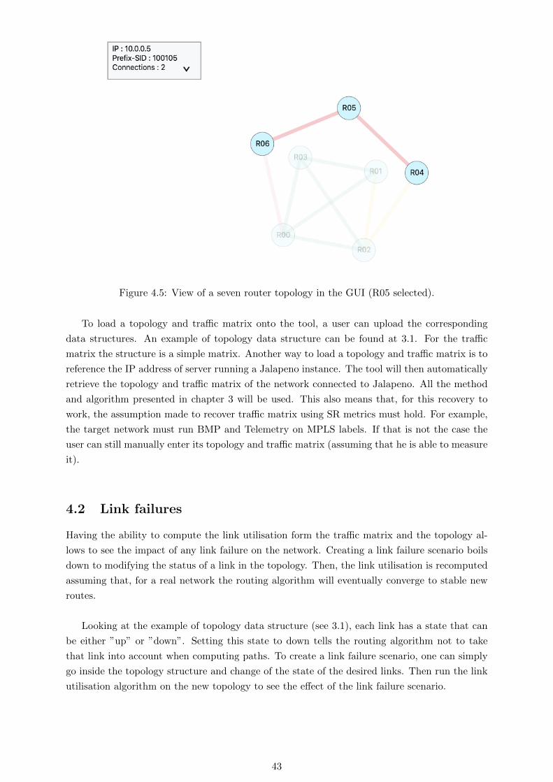
Figure 4.5: View of a seven router topology in the GUI (R05 selected).

To load a topology and traffic matrix onto the tool, a user can upload the corresponding

data structures. An example of topology data structure can be found at 3.1. For the traffic

matrix the structure is a simple matrix. Another way to load a topology and traffic matrix is to

reference the IP address of server running a Jalapeno instance. The tool will then automatically

retrieve the topology and traffic matrix of the network connected to Jalapeno. All the method

and algorithm presented in chapter 3 will be used. This also means that, for this recovery to

work, the assumption made to recover traffic matrix using SR metrics must hold. For example,

the target network must run BMP and Telemetry on MPLS labels. If that is not the case the

user can still manually enter its topology and traffic matrix (assuming that he is able to measure

it).

4.2 Link failures

Having the ability to compute the link utilisation form the traffic matrix and the topology al-

lows to see the impact of any link failure on the network. Creating a link failure scenario boils

down to modifying the status of a link in the topology. Then, the link utilisation is recomputed

assuming that, for a real network the routing algorithm will eventually converge to stable new

routes.

Looking at the example of topology data structure (see 3.1), each link has a state that can

be either ”up” or ”down”. Setting this state to down tells the routing algorithm not to take

that link into account when computing paths. To create a link failure scenario, one can simply

go inside the topology structure and change of the state of the desired links. Then run the link

utilisation algorithm on the new topology to see the effect of the link failure scenario.

43

4.2.1 Integration in what-if simulator

The ability to create any link failures is integrated in the GUI. Inside the adjacency matrix,

the user can put any link down. Then the tool will recompute the link utilisation on the fly

and change the UI accordingly. Any link that was downed can also be brought back up at any

time. Multiple links can be downed allowing to create complex scenarios such as router failure

or SRLG failure.

4.2.2 Example on a simple topology

Let’s take a concrete example with a simplified topology to showcase the tool. A four routers

diamond topology is considered (Figure 4.6), similarly to what was done for the traffic matrix

recovery. Traffic is generate from R00 towards R01, R02 and R03 as shown in traffic matrix

(Figure 4.10). The demand as been chosen so not to create congestion initially.

Figure 4.8 shows the result of the link utilisation algorithm on this toy topology. As expected

traffic towards R01 and R02 are directly forwarded. Their 0.02 Mbps of demand can only be

seen on the link from R00 to R01 and link from R01 to R02. However, the traffic going to R03

finds two paths with the same IGP cost. In fact, all links in this toy topology have the same

IGP cost. This demand is split in half and the 0.01 Mbps are distributed on each link of both

paths. This correspond to what can be observed in the adjacency matrix.

Figure 4.6: Toy topology.

Figure 4.7: Traffic matrix of the toy topology.

44

Figure 4.8: Adjacency matrix of toy topology before link failure.

Now let’s kill a link a topology. The link between R00 and R01 is brought down. The

application directly recomputes the link utilisation based on the new topology. The adjacency

matrix at Figure 4.8 is the result of this computation.

Since the link between R00 and R01 is down, its utilisation becomes 0%. The three other

link have to bear additional load as the traffic is no longer split in two paths. Link R00 to R02

now is charged with the full throughput (0.06 Mbps). Its color changes to orange, reflecting that

packet may start to get dropped if the traffic increases.

Figure 4.9: Adjacency matrix of toy topology after link failure between R00 and R01.

The topology display is also dynamically updated to reflect the changes in the link status

and utilisation. Figure 4.10 shows the topology after the failure. The R00 to R01 link is greyed

out to reflect the fact that it is down. The colors of the links have correctly been updated based

on their load.

45

Figure 4.10: Toy topology after link failure between R00 and R01.

4.2.3 Example on a complex topology

In order to further the testing of the link utilisation and failure algorithm, a more complex

example will be considered. In this scenario, four routers are full mesh and three other routers

are connected in line. Figure 4.11 shows this more complex topology.

Figure 4.11: Complex topology.

The idea behind this topology is to create some sort of data center serving an array of clients.

Routers R00 to R03 are supposed to be close together and connected to servers that streams

content. Routers R04 to R06 are closer to the edge of the internet serving content to clients.

Traffic matrix at Figure 4.12, represents this asymmetric demand. In fact, it can be observed

that R01 generates a large amount of traffic towards R05, while the traffic from R05 to R01 is

negligible. This is an usual scenario for a client/server application.

46

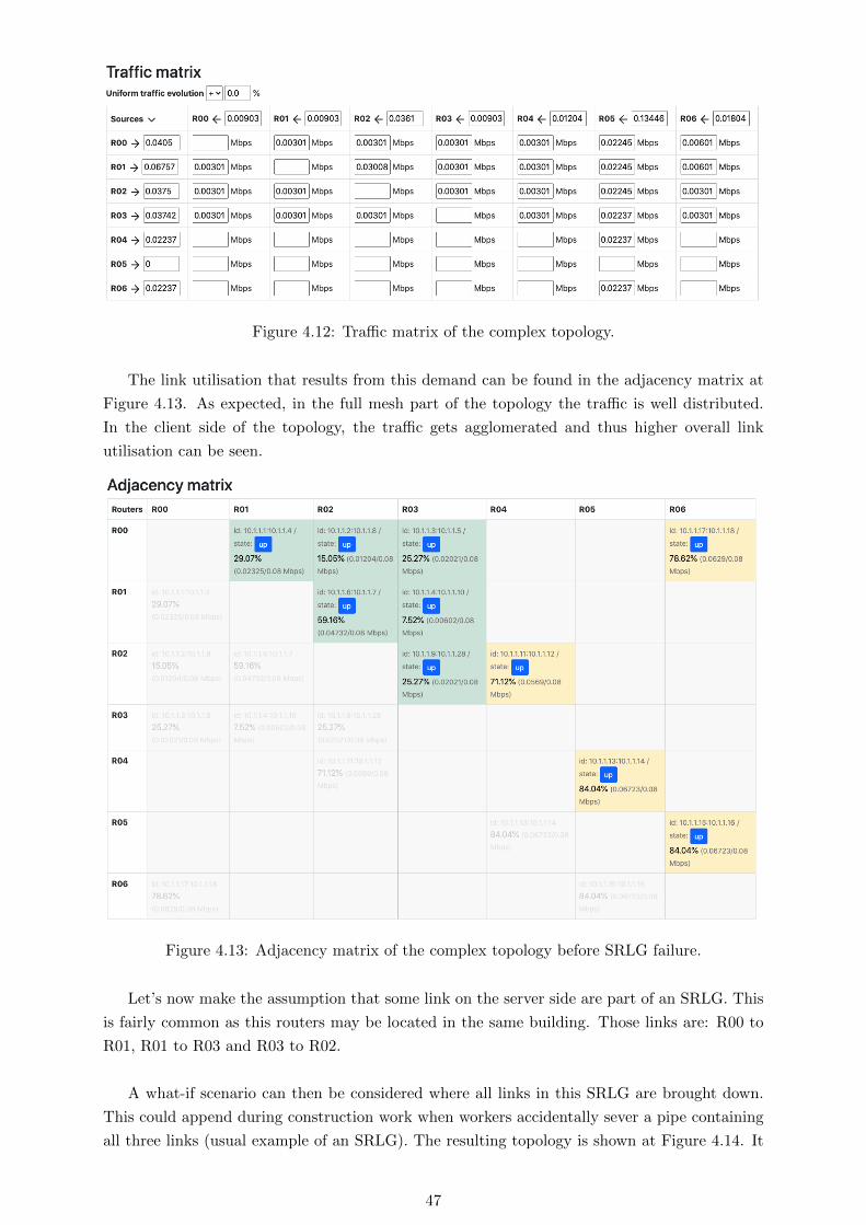
Figure 4.12: Traffic matrix of the complex topology.

The link utilisation that results from this demand can be found in the adjacency matrix at

Figure 4.13. As expected, in the full mesh part of the topology the traffic is well distributed.

In the client side of the topology, the traffic gets agglomerated and thus higher overall link

utilisation can be seen.

Figure 4.13: Adjacency matrix of the complex topology before SRLG failure.

Let’s now make the assumption that some link on the server side are part of an SRLG. This

is fairly common as this routers may be located in the same building. Those links are: R00 to

R01, R01 to R03 and R03 to R02.

A what-if scenario can then be considered where all links in this SRLG are brought down.

This could append during construction work when workers accidentally sever a pipe containing

all three links (usual example of an SRLG). The resulting topology is shown at Figure 4.14. It

47

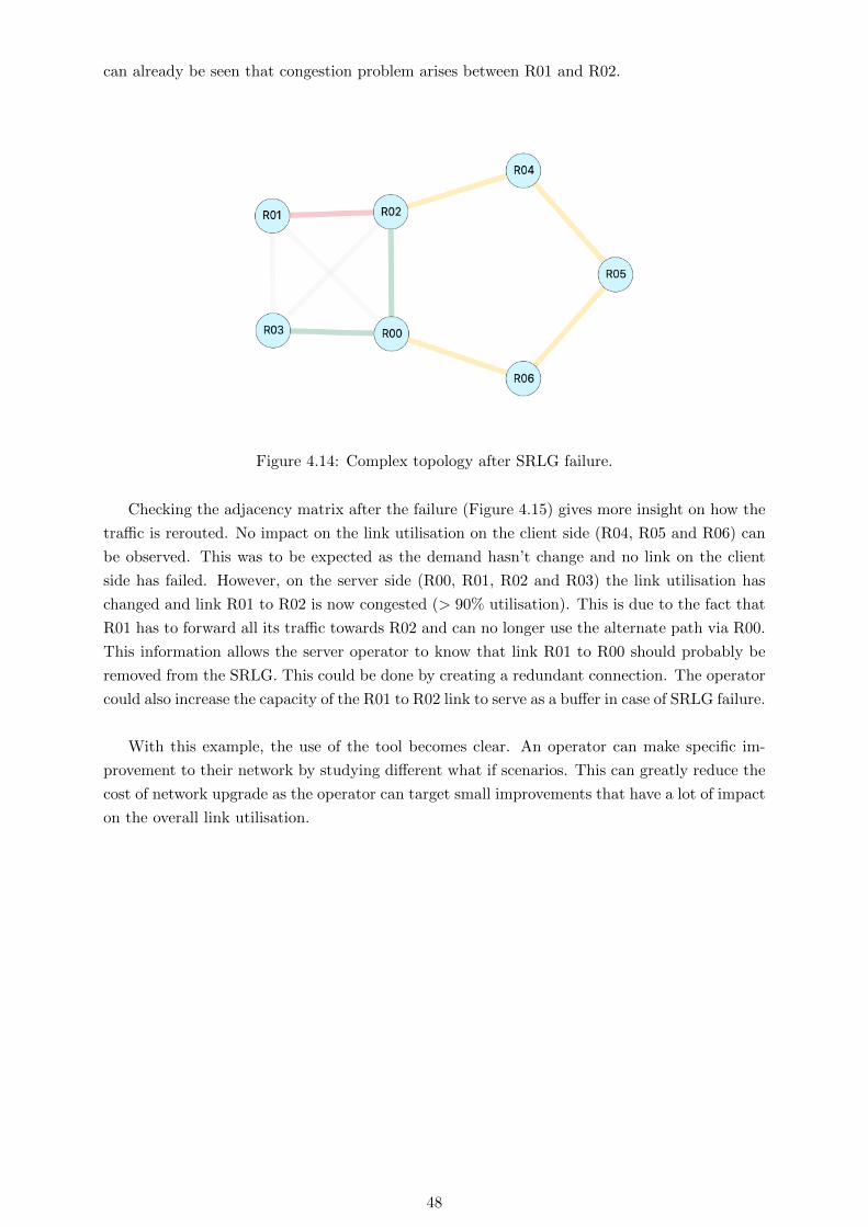
can already be seen that congestion problem arises between R01 and R02.

Figure 4.14: Complex topology after SRLG failure.

Checking the adjacency matrix after the failure (Figure 4.15) gives more insight on how the

traffic is rerouted. No impact on the link utilisation on the client side (R04, R05 and R06) can

be observed. This was to be expected as the demand hasn’t change and no link on the client

side has failed. However, on the server side (R00, R01, R02 and R03) the link utilisation has

changed and link R01 to R02 is now congested (> 90% utilisation). This is due to the fact that

R01 has to forward all its traffic towards R02 and can no longer use the alternate path via R00.

This information allows the server operator to know that link R01 to R00 should probably be

removed from the SRLG. This could be done by creating a redundant connection. The operator

could also increase the capacity of the R01 to R02 link to serve as a buffer in case of SRLG failure.

With this example, the use of the tool becomes clear. An operator can make specific im-

provement to their network by studying different what if scenarios. This can greatly reduce the

cost of network upgrade as the operator can target small improvements that have a lot of impact

on the overall link utilisation.

48

Figure 4.15: Adjacency matrix of the complex topology after SRLG failure.

4.2.4 Worst link failures

In addition to allowing the user to down any combination of links, the tool also computes in

advance the worst link failures. The tool quantifies the impact of a link failure based on the

number of overloaded link that results from this failure.

By default, a link is considered to be overloaded when its utilisation goes over 90%. However

this can be modified to fit any overload criterion. In the UI the list of the 5 worst link failures is

displayed (once again 5 is the default but can be modified) along with how much link overload

they would cause. Figures 4.16 shows worst link failures part of the UI:

Figure 4.16: Example of worst link failure UI.

In order to compute the worst link failures, all single link failure must be considered. Then

the link utilisation is computed in each scenario. Finally, all those scenarios are sorted based on

49

the number of overloaded link. Note this is also dynamically recomputed for each new topology.

This means that an operator can test which are the two worst link failures. To do that he

simply checks the worst link failure, simulates it by putting this link down and then check again

the worst link failures. This can be done any number of time to get insight on what are the

catastrophic scenarios that could append.

4.3 Traffic surges

After studying the impact of topological changes on link utilisation, the next logical step is to

check the influence of the traffic matrix. In fact, the demand, and thus the traffic matrix, changes

over times. Those changes can be seen at different scales. Throughout the year, the average

demand increases at close to a fix rate. Throughout the day, the demand changes abruptly with

internet rush hours (see 3.1). That is why allowing an operator to modify its traffic matrix and

see the impact on link loads is very important. Let’s see how an operator can design what-if

scenarios based on a custom traffic matrix, using our tool.

4.3.1 Base traffic matrix

Before designing any scenario the operator will be interested in recovering its current traffic

matrix. The process of retrieve such matrix was extensively discussed in chapter 3. The operator

can get its matrix simply by typing the IP address of a server running Jalapeno. This assumes

that a Jalapeno instance collects traffic and topology information from the operator network.

The tool will automatically run the recovery algorithm (see 2) and update the interface with

the operator topology and traffic matrix.

4.3.2 Modifying the traffic matrix

Once the operator has retrieved its traffic matrix, he can start creating what-if scenarios by

modifying it. Figure 4.17 show an example of the available UI once the matrix is recovered.

Figure 4.17: Example of a base traffic matrix.

All the individual entries of the matrix can be changed. Every time a cell is modified the

link utilisation algorithm runs and the load on each link gets updated in real time. This allows

the user to simulate an increase in traffic between a specific source and destination. This can

be useful for small topologies where the operator has a lot of information about how each flow

50

evolves over time.

However, for larger topologies, operators don’t usually have such a granular information

about the traffic. What is more realistic is that he knows how the demand may increase towards

a destination. He may also know how the traffic coming out of a specific source increases. That

is why our tool also allows to modify the values of the agglomerated throughput per source and

destination. Those are the sums of each line and column of the matrix.

For example, let’s say the operator knows that a new server will be added doubling the

throughput coming out of R01. To simulate this, he can simply double the R01 cell in the source

column. A new traffic matrix will be recomputed along with the new link loads. Interpolating

the new traffic matrix is not that trivial, there is actually two ways of doing it:

• With a multiplicative factor (Figure 4.18). For this interpolation, the tool computes by

how much percent the source (resp. destination) traffic was increased and increases by the

same percentage each cell in the line (resp. column). In this example the traffic sourcing

from R01 is increased by 100% so all cells in the line are doubled. The tool can also

compute traffic decrease. Note that this also affects the destination traffic towards R02

and R03.

• With an additive factor (Figure 4.19). In this case, the tool retrieves by how much the

source (resp. destination) traffic was increase. Takes this raw throughput difference and

divides it in the number of cells in the line (resp. column). Then this portion of the

difference is added to each cell in the line (resp. column).

Figure 4.18: Traffic matrix interpolation with multiplicative factor.

Figure 4.19: Traffic matrix interpolation with additive factor.

51

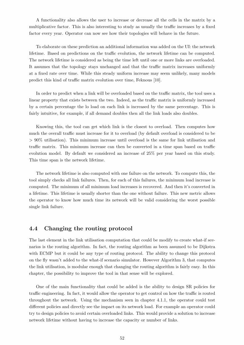
A functionality also allows the user to increase or decrease all the cells in the matrix by a

multiplicative factor. This is also interesting to study as usually the traffic increases by a fixed

factor every year. Operator can now see how their topologies will behave in the future.

To elaborate on these prediction an additional information was added on the UI: the network

lifetime. Based on predictions on the traffic evolution, the network lifetime can be computed.

The network lifetime is considered as being the time left until one or more links are overloaded.

It assumes that the topology stays unchanged and that the traffic matrix increases uniformly

at a fixed rate over time. While this steady uniform increase may seem unlikely, many models

predict this kind of traffic matrix evolution over time, Feknous [10].

In order to predict when a link will be overloaded based on the traffic matrix, the tool uses a

linear property that exists between the two. Indeed, as the traffic matrix is uniformly increased

by a certain percentage the lo load on each link is increased by the same percentage. This is

fairly intuitive, for example, if all demand doubles then all the link loads also doubles.

Knowing this, the tool can get which link is the closest to overload. Then computes how

much the overall traffic must increase for it to overload (by default overload is considered to be

> 90% utilisation). This minimum increase until overload is the same for link utilisation and

traffic matrix. This minimum increase can then be converted in a time span based on traffic

evolution model. By default we considered an increase of 25% per year based on this study.

This time span is the network lifetime.

The network lifetime is also computed with one failure on the network. To compute this, the

tool simply checks all link failures. Then, for each of this failures, the minimum load increase is

computed. The minimum of all minimum load increases is recovered. And then it’s converted in

a lifetime. This lifetime is usually shorter than the one without failure. This new metric allows

the operator to know how much time its network will be valid considering the worst possible

single link failure.

4.4 Changing the routing protocol

The last element in the link utilisation computation that could be modify to create what-if sce-

narios is the routing algorithm. In fact, the routing algorithm as been assumed to be Dijkstra

with ECMP but it could be any type of routing protocol. The ability to change this protocol

on the fly wasn’t added to the what-if scenario simulator. However Algorithm 3, that computes

the link utilisation, is modular enough that changing the routing algorithm is fairly easy. In this

chapter, the possibility to improve the tool in that sense will be explored.

One of the main functionality that could be added is the ability to design SR policies for

traffic engineering. In fact, it would allow the operator to get control on how the traffic is routed

throughout the network. Using the mechanism seen in chapter 4.1.1, the operator could test

different policies and directly see the impact on its network load. For example an operator could

try to design policies to avoid certain overloaded links. This would provide a solution to increase

network lifetime without having to increase the capacity or number of links.

52

Assuming that the ability to add SR policies is in the simulator, a methodology to implement

optimal SR policies will now be described. Figure 4.20 showcases this methodology.

1. The traffic and topological data is collected from the topology by the tool. The topology

and traffic matrix is then displayed to the operator, if SR policies are already in place they

should also be retrieved, and taken into account in the traffic matrix computation.

Note that this not the case in the current tool, as we made the assumption that most traffic

was not forwarded with SR policies. Removing this assumption requires technological im-

provements. In fact, for now, Cisco-XRv routers can’t agglomerate traffic based on a label

stack, only on a single label. Having most traffic forwarded with a label stack would es-

sentially break the traffic matrix recovery algorithm (2). However, if Cisco routers develop

the ability to agglomerate traffic based on label stack, the algorithm could be adapted. In

fact, to compute the matrix only the exiting prefix-SID is interesting. This means that the

overall label stack could be ignored and only the label on the bottom of the stack should

be considered. Thus, the ability to recover the traffic matrix with policy boils down to the

router ability to agglomerate traffic on label stack. Let’s now assume that this technology

is available and see what could be done with it.

2. Once all network information are recovered, the operator can try to design new SR policies.

The goal of those new policies will probably be to extend as much as possible the network

lifetime.

3. In a addition to the network lifetime, the tool offers many other statistics. Including the

utilisation of each link and the worst link failures. The operator will want to study those

factor. If he is not satisfied, he can go back to step two and twitch its policies until he is

content with the tool predictions. This process may also be automated. Indeed an algo-

rithm could be designed to optimize predicted values based on different policies. However,

those type of algorithms are beyond the scope of this study.

4. Finally, once the optimal policy has been determined, the operator can implement them

in his network. Afterwards, if the operator is not satisfied with the result or if its demand

changes, he can go back to step one. Indeed, this is be an iterative process. The operator

can get his topology back, make modifications to the policies check their impact and

redeploy. Hopefully, this will allow him to converge to a stable and efficient set of policies.

53

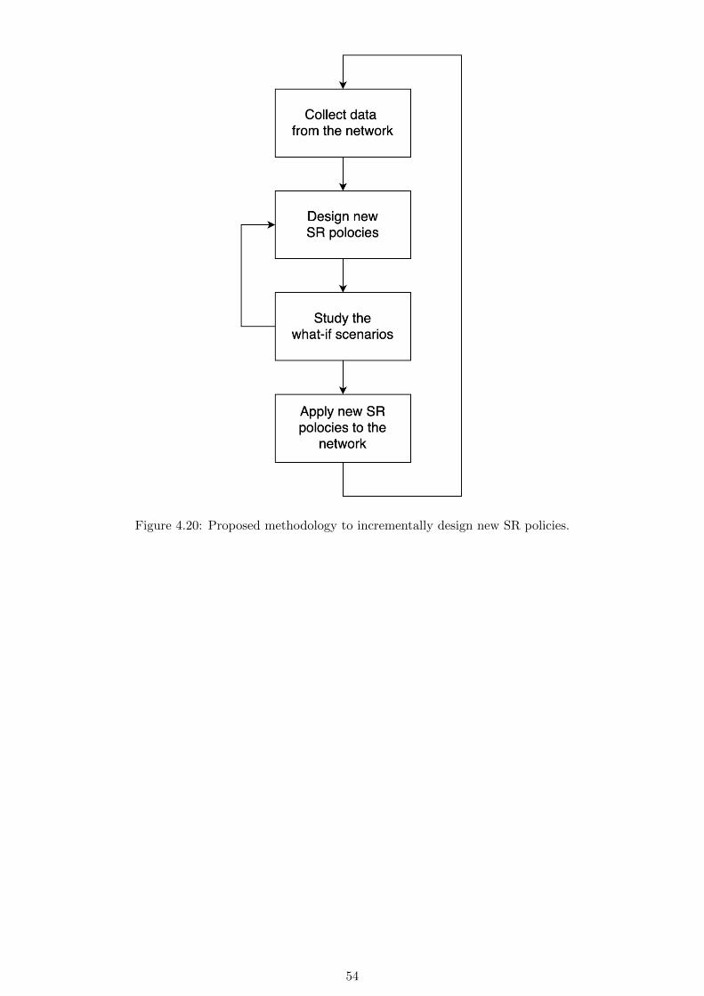
Figure 4.20: Proposed methodology to incrementally design new SR policies.

54

Chapter 5

Conclusion

To conclude this thesis let’s take a step back and try to consider what was achieved as a whole.

Indeed as there are two parts to the study, it will be interesting to break down the entirety

of our design. To do that, the initial high level requirements for the application will be listed.

Then, we will link back our implementation to those requirements to close the study. Here is

the original high level design of the application:

1. Extract a snapshot of the running network (leveraging the open-source Jalapeno collection

infrastructure)

2. Compute an estimation of the demand matrix of this network based on the topology and

traffic counters.

3. Display the network topology with a visual indication of each link utilization (e.g., color).

4. Allow the user to define a what-if scenario (e.g., link or node failure, or traffic surge towards

a particular prefix).

5. Compute an estimation of the link utilisations in the specified what-if scenario.

6. Update the network topology display considering the estimated link utilisations.

Step 1 has been achieved by deploying a virtual topology and a Jalapeno instance. With

this virtual environment, the Arango and Influx databases can be accessed at any time. The

limitation that we faced is that, due to funding limitation, we could only simulate 4 routers.

However, this small network still allowed to test many different traffic matrices and topology

configurations.

Step 2 was done with the design of the traffic matrix recovery algorithm (2). The traffic

counters and topological data were recovered from Jalapeno an then passed as arguments of

the algorithm. This estimation process was then thoroughly tested making sure that recovered

demand was accurate.

Step 3 is what inspired the GUI that displays the topology and traffic matrix. In order to

display the utilisation, Algorithm 3 was designed. It uses a priority queue Dijkstra in order

to simulate IGP routes. This allows to redistribute the demand on the network links. The

utilisation is then displayed as a color based on how close each link is from being congested.

55

The three final steps (4, 5 and 6) are also covered by the GUI. In fact, the GUI allows to test

any topology or demand scenario. It recomputes in real time the link utilisation and display it

back to the user.

At last, the application that we have developed can be seen as network planning tool. It will

hopefully help operators to better understand the demand on their network. Allowing them to

plan network improvement in advance and in an educated way. It may also have an impact on

the cost of infrastructure updates, as the tool targets problematic zones of the topology.

56

Bibliography

[1] Richelle Adams. “Active queue management: A survey”. In: IEEE communications surveys

& tutorials 15.3 (2012), pp. 1425–1476.

[2] Satyajeet S Ahuja, Srinivasan Ramasubramanian, and Marwan Krunz. “SRLG failure

localization in optical networks”. In: IEEE/ACM Transactions on Networking 19.4 (2011),

pp. 989–999.

[3] N Akiya, S Kini, and M Chen. “Label switched path (LSP) ping/traceroute for segment

routing (SR) IGP-prefix and IGP-adjacency segment identifiers (SIDs) with MPLS data

planes”. In: (2017).

[4] Mohammad Alizadeh et al. “CONGA: Distributed congestion-aware load balancing for

datacenters”. In: Proceedings of the 2014 ACM conference on SIGCOMM. 2014, pp. 503–

514.

[5] L Andersson et al. Rfc3036: Ldp specification. 2001.

[6] DGTLVSD Awduche et al. RSVP-TE: extensions to RSVP for LSP tunnels. 2001.

[7] Philippe Biondi. “Scapy documentation (!)” In: vol 469 (2010), pp. 155–203.

[8] Jonathan Davidson et al. Voice over IP fundamentals. Cisco press, 2000.

[9] Luca Davoli et al. “Traffic engineering with segment routing: SDN-based architectural

design and open source implementation”. In: 2015 Fourth European Workshop on Software

Defined Networks. IEEE. 2015, pp. 111–112.

[10] Moufida Feknous et al. “Internet traffic analysis: A case study from two major European

operators”. In: 2014 IEEE Symposium on Computers and Communications (ISCC). IEEE.

2014, pp. 1–7.

[11] Clarence Filsfils et al. Segment Routing Traffic Accounting Counters. Internet-Draft draft-

filsfils-spring-sr-traffic-counters-01. Work in Progress. Internet Engineering Task Force,

Apr. 2021. 13 pp. url: https://datatracker.ietf.org/doc/html/draft-filsfils-

spring-sr-traffic-counters-01.

[12] Clarence Filsfils et al. “Segment Routing with MPLS data plane”. In: draft-ietf-spring-

segment-routing-mpls-05 (2014).

[13] Clarence Filsfils et al. “SRv6 network programming”. In: Internet-Draft (2017).

[14] Clarence Filsfils et al. “The segment routing architecture”. In: 2015 IEEE Global Com-

munications Conference (GLOBECOM). IEEE. 2015, pp. 1–6.

[15] Bernard Fortz, Jennifer Rexford, and Mikkel Thorup. “Traffic engineering with traditional

IP routing protocols”. In: IEEE communications Magazine 40.10 (2002), pp. 118–124.

[16] Miguel Grinberg. Flask web development: developing web applications with python. ” O’Reilly

Media, Inc.”, 2018.

57

[17] Anders Gunnar, Mikael Johansson, and Thomas Telkamp. “Traffic matrix estimation on a

large IP backbone: a comparison on real data”. In: Proceedings of the 4th ACM SIGCOMM

conference on Internet measurement. 2004, pp. 149–160.

[18] Chris Hare. Simple Network Management Protocol (SNMP). 2011.

[19] Andreas Iselt et al. “Resilient routing using MPLS and ECMP”. In: 2004 Workshop on

High Performance Switching and Routing, 2004. HPSR. IEEE. 2004, pp. 345–349.

[20] Woo-Sung Jung, Fengzhong Wang, and H Eugene Stanley. “Gravity model in the Korean

highway”. In: EPL (Europhysics Letters) 81.4 (2008), p. 48005.

[21] Jay Kreps, Neha Narkhede, Jun Rao, et al. “Kafka: A distributed messaging system for

log processing”. In: Proceedings of the NetDB. Vol. 11. 2011, pp. 1–7.

[22] RS Krupp. “Properties of Kruithof’s projection method”. In: Bell System Technical Jour-

nal 58.2 (1979), pp. 517–538.

[23] Alberto Medina et al. “Traffic matrix estimation: Existing techniques and new directions”.

In: ACM SIGCOMM Computer Communication Review 32.4 (2002), pp. 161–174.

[24] Mary Meeker and Liang Wu. “Internet trends”. In: Proc D11 Conference. Rancho Palos

Verdes. Citeseer. 2013.

[25] Stefano Previdi et al. “IS-IS extensions for segment routing”. In: draft-ietf-isis-segment-

routing-extensions-06 (2015), pp. 1–39.

[26] Timmy Schuller et al. “Failure Resiliency With Only a Few Tunnels-Enabling Segment

Routing for Traffic Engineering”. In: IEEE/ACM Transactions on Networking (2020).

[27] John Scudder, Rex Fernando, and Stephen Stuart. “BGP Monitoring Protocol (BMP)”.

In: Internet Engineering Task Force (2016), pp. 1–27.

[28] MC Sinclair. “Improved model for European international telephony traffic”. In: Electron-

ics letters 30.18 (1994), pp. 1468–1470.

[29] Amin Tootoonchian, Monia Ghobadi, and Yashar Ganjali. “OpenTM: traffic matrix esti-

mator for OpenFlow networks”. In: International Conference on Passive and Active Net-

work Measurement. Springer. 2010, pp. 201–210.

[30] Qi Zhao et al. “Robust traffic matrix estimation with imperfect information: Making use

of multiple data sources”. In: Proceedings of the joint international conference on Mea-

surement and modeling of computer systems. 2006, pp. 133–144.

[31] Syed Zia. Jalapeno. https://github.com/cisco-ie/jalapeno. 2017.

58