Section 1.0: Introduction to Making Hard Decisions

Chapter 1 Making Hard Decisions—Multi-Criteria Decision Making (MCDM)

Lead Authors: Thomas Edwards and Kenneth Chelst

Section 1.0: Introduction to Making Hard Decisions We all face decisions in our jobs, in our communities, and in our personal lives. For example,

x Where should a new airport, manufacturing plant, power plant, or health care clinic be located?

x Which college should I attend, or which job should I accept? x Which car, house, computer, stereo, or health insurance plan should I buy? x Which supplier or building contractor should I hire?

Decisions such as these involve comparing alternatives that have strengths or weaknesses with regard to multiple objectives of interest to the decision. For example, your criteria in buying health insurance might be to minimize cost and maximize protection. Sometimes these multiple criteria get in each other’s way. Multi-criteria decision making (MCDM) is used when one needs to make a hard decision with many criteria. In this chapter, you will see one form of multi-criteria decision making. The method introduced in this chapter is a structured methodology designed to handle the tradeoffs among multiple criteria.

A Little History One of the first applications of this method of MCDM involved the study of possible locations for a new airport in Mexico City in the early 1970s. The criteria considered included cost, capacity, access time to the airport, safety, social disruption, and noise pollution.

The problems in this chapter use the steps of multi-criteria decision making to make hard decisions. MCDM is a systematic approach to quantify an individual’s preferences. Measures of interest are rescaled to numerical values on a 0–1 scale, with 0 representing the worst value of the measure and 1 representing the best. This allows the direct comparison of many diverse measures. In other words, with the right tool, it really is possible to compare apples to oranges! The result of this process is an evaluation of the alternatives in a rank order that reflects the decision makers’ preferences. For example, individuals, college sports teams, Master’s degree programs, or even hospitals can be ranked in terms of their performance on many diverse measures. Another example is the Bowl Championship Series (BCS) in college football that attempts to identify the two best college football teams in the United States to play in a national championship bowl game. This process has reduced, but not eliminated, the annual end-of-year arguments as to which college should be crowned national champion.



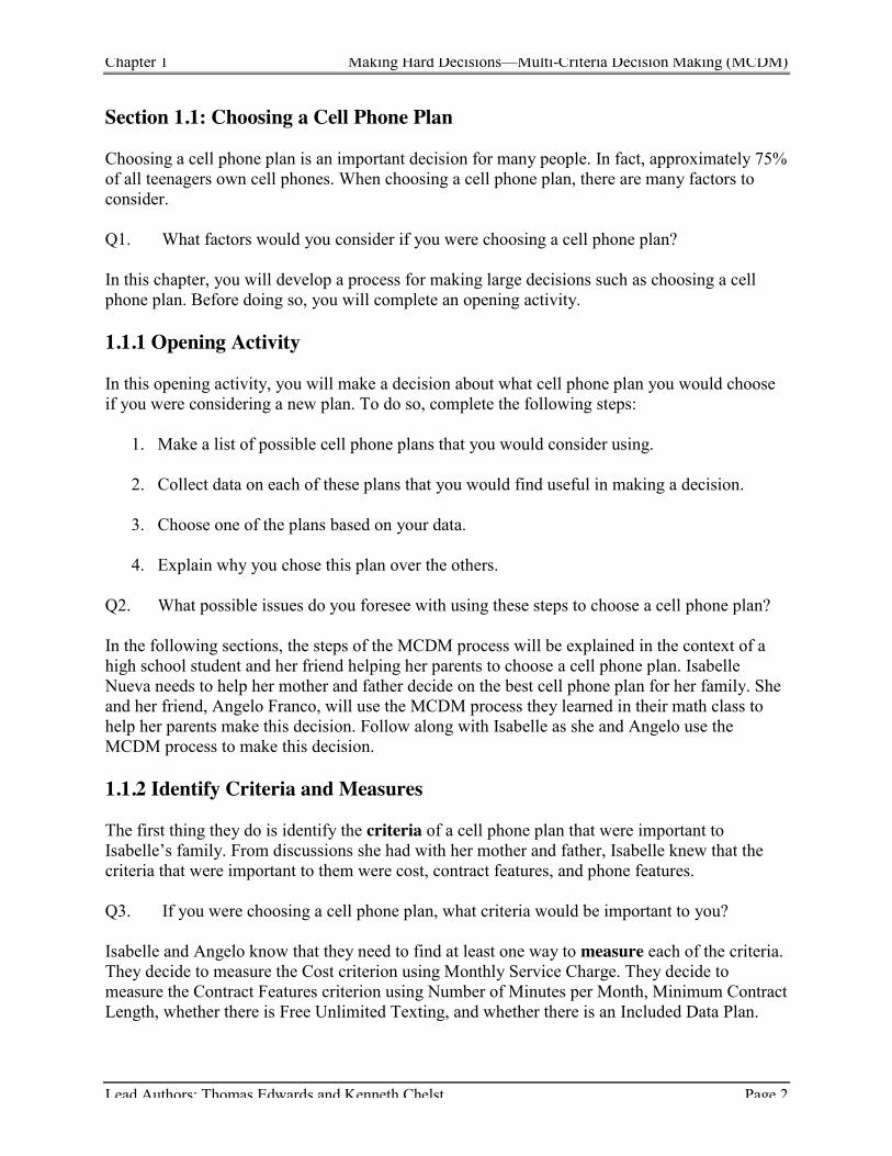
Section 1.1: Choosing a Cell Phone Plan Choosing a cell phone plan is an important decision for many people. In fact, approximately 75% of all teenagers own cell phones. When choosing a cell phone plan, there are many factors to consider. Q1. What factors would you consider if you were choosing a cell phone plan? In this chapter, you will develop a process for making large decisions such as choosing a cell phone plan. Before doing so, you will complete an opening activity. 1.1.1 Opening Activity In this opening activity, you will make a decision about what cell phone plan you would choose if you were considering a new plan. To do so, complete the following steps:

1. Make a list of possible cell phone plans that you would consider using.

2. Collect data on each of these plans that you would find useful in making a decision.

3. Choose one of the plans based on your data.

4. Explain why you chose this plan over the others. Q2. What possible issues do you foresee with using these steps to choose a cell phone plan? In the following sections, the steps of the MCDM process will be explained in the context of a high school student and her friend helping her parents to choose a cell phone plan. Isabelle Nueva needs to help her mother and father decide on the best cell phone plan for her family. She and her friend, Angelo Franco, will use the MCDM process they learned in their math class to help her parents make this decision. Follow along with Isabelle as she and Angelo use the MCDM process to make this decision. 1.1.2 Identify Criteria and Measures The first thing they do is identify the criteria of a cell phone plan that were important to Isabelle’s family. From discussions she had with her mother and father, Isabelle knew that the criteria that were important to them were cost, contract features, and phone features. Q3. If you were choosing a cell phone plan, what criteria would be important to you? Isabelle and Angelo know that they need to find at least one way to measure each of the criteria. They decide to measure the Cost criterion using Monthly Service Charge. They decide to measure the Contract Features criterion using Number of Minutes per Month, Minimum Contract Length, whether there is Free Unlimited Texting, and whether there is an Included Data Plan.



They measure the Phone Features using Quality of Service. Each criterion and its measures are provided in Table 1.1.1.

Criteria Measures Cost Monthly Service Charge

Contract Features

Number of Minutes per Month Minimum Contract Length Free Unlimited Texting Included Data Plan

Phone Features Quality of Service Table 1.1.1: Criteria and measures for choosing a cell phone plan

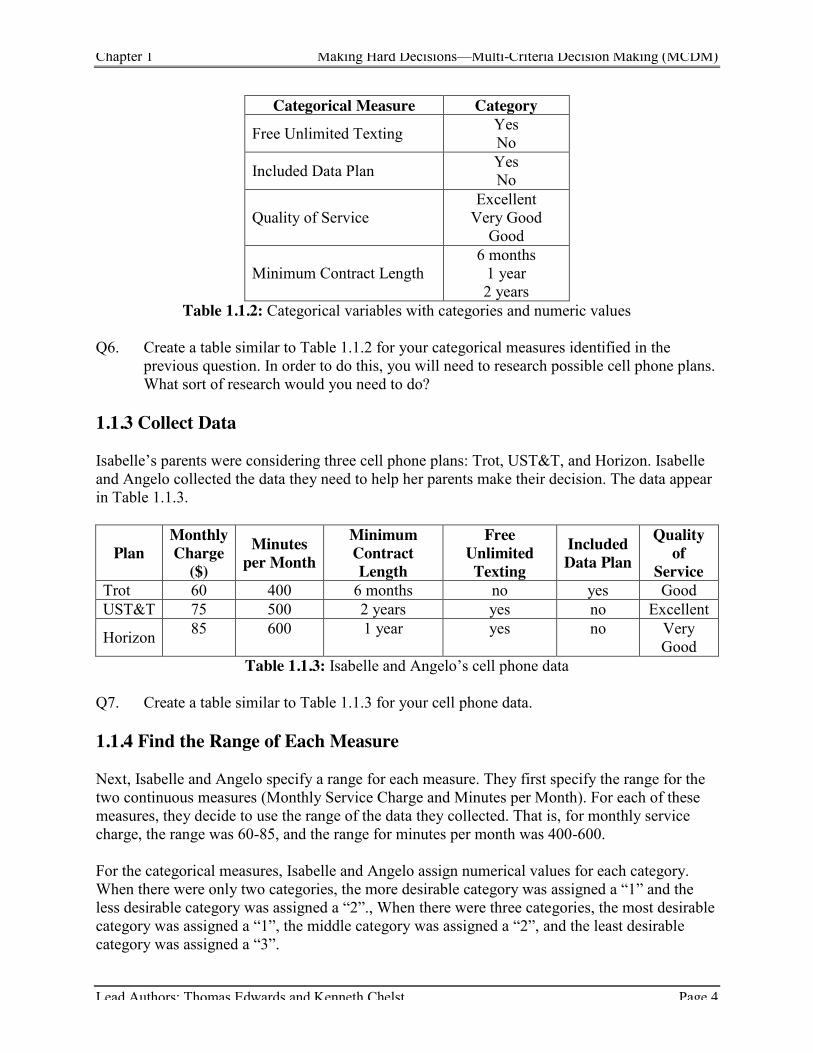
Q4. How would you measure each of your criteria? The value of two of the measures—the Monthly Service Charge and the Number of Minutes per Month—could be any numerical amount within a reasonable range. These are examples of continuous measures. That is, these measures can take on any numerical value within a range. Isabelle and Angelo decide that the data they collected for the other three measures can be grouped into a finite number of categories. For example, Free Unlimited Texting has only two categories: “yes” and “no.” Similarly, Included Data Plan has two categories: “yes” and “no.” Thus, these two measures are examples of categorical measures. Q5. Of the measures you listed in Q4, which are continuous and which are categorical? The next categorical measure Isabelle and Angelo consider is Quality of Service. For this measure, they decide to use ratings from a consumer magazine. The magazine considered dropped or disconnected calls, static and interference, and voice distortion to rate the quality of service. Isabelle and Angelo decide to only consider plans the magazine rated “Good”, “Very Good”, or “Excellent”. Therefore, this measure has three categories. The last categorical measure is Minimum Contract Length—the shortest time a customer must remain with a particular plan to avoid paying a fee to cancel the service. Isabelle’s parents were concerned about being locked into a plan for a long period of time. The plans under consideration have three different minimum contract lengths (6 months, 1 year, and 2 years). Thus, the Minimum Contract Length measure has three categories. The categorical measures and their possible values are provided in Table 1.1.2.



Categorical Measure Category

Free Unlimited Texting Yes No

Included Data Plan Yes No

Quality of Service Excellent

Very Good Good

Minimum Contract Length 6 months

1 year 2 years

Table 1.1.2: Categorical variables with categories and numeric values Q6. Create a table similar to Table 1.1.2 for your categorical measures identified in the

previous question. In order to do this, you will need to research possible cell phone plans. What sort of research would you need to do?

1.1.3 Collect Data Isabelle’s parents were considering three cell phone plans: Trot, UST&T, and Horizon. Isabelle and Angelo collected the data they need to help her parents make their decision. The data appear in Table 1.1.3.

Plan Monthly Charge

($) Minutes

per Month Minimum Contract Length

Free Unlimited Texting

Included Data Plan

Quality of

Service Trot 60 400 6 months no yes Good UST&T 75 500 2 years yes no Excellent

Horizon 85 600 1 year yes no Very Good

Table 1.1.3: Isabelle and Angelo’s cell phone data Q7. Create a table similar to Table 1.1.3 for your cell phone data. 1.1.4 Find the Range of Each Measure Next, Isabelle and Angelo specify a range for each measure. They first specify the range for the two continuous measures (Monthly Service Charge and Minutes per Month). For each of these measures, they decide to use the range of the data they collected. That is, for monthly service charge, the range was 60-85, and the range for minutes per month was 400-600. For the categorical measures, Isabelle and Angelo assign numerical values for each category. When there were only two categories, the more desirable category was assigned a “1” and the less desirable category was assigned a “2”., When there were three categories, the most desirable category was assigned a “1”, the middle category was assigned a “2”, and the least desirable category was assigned a “3”.



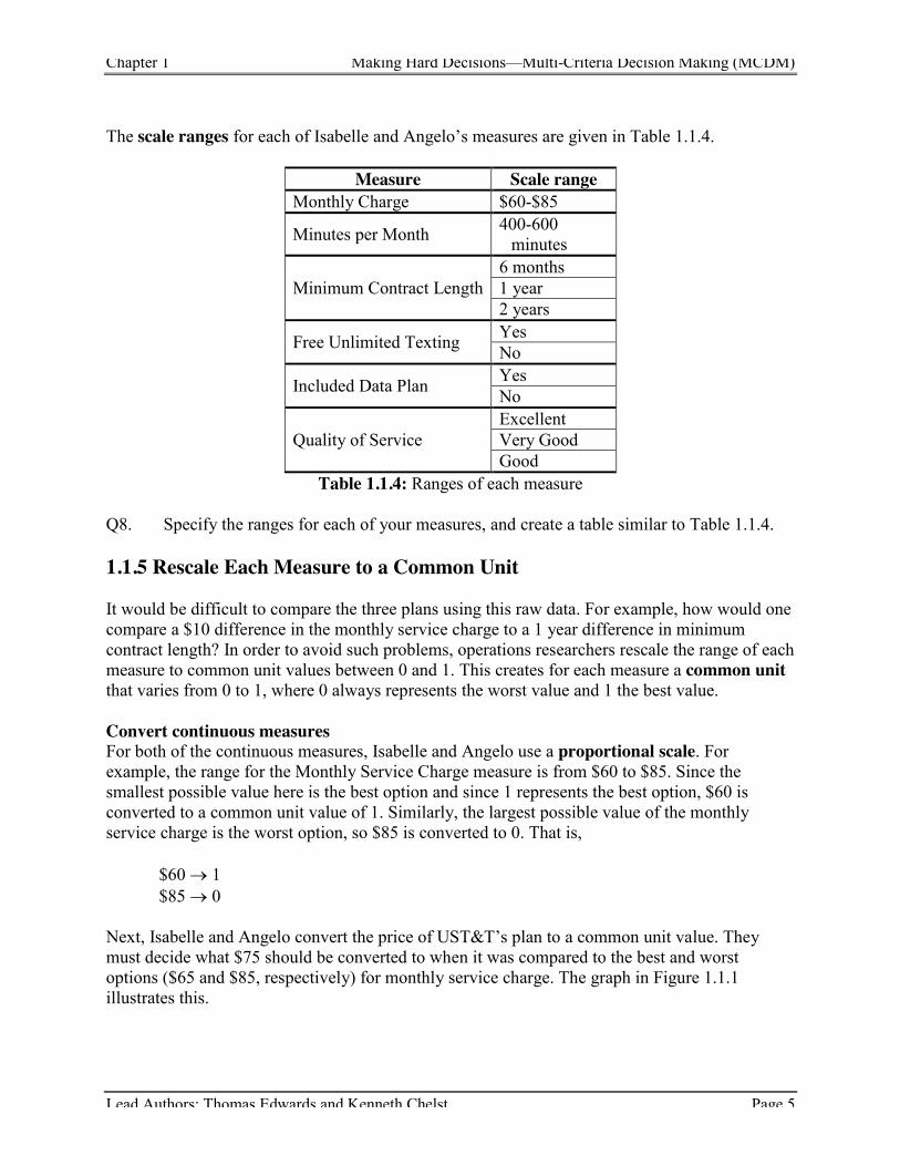
The scale ranges for each of Isabelle and Angelo’s measures are given in Table 1.1.4.

Measure Scale range Monthly Charge $60-$85

Minutes per Month 400-600 minutes

Minimum Contract Length 6 months 1 year 2 years

Free Unlimited Texting Yes No

Included Data Plan Yes No

Quality of Service Excellent Very Good Good

Table 1.1.4: Ranges of each measure

Q8. Specify the ranges for each of your measures, and create a table similar to Table 1.1.4. 1.1.5 Rescale Each Measure to a Common Unit It would be difficult to compare the three plans using this raw data. For example, how would one compare a $10 difference in the monthly service charge to a 1 year difference in minimum contract length? In order to avoid such problems, operations researchers rescale the range of each measure to common unit values between 0 and 1. This creates for each measure a common unit that varies from 0 to 1, where 0 always represents the worst value and 1 the best value. Convert continuous measures For both of the continuous measures, Isabelle and Angelo use a proportional scale. For example, the range for the Monthly Service Charge measure is from $60 to $85. Since the smallest possible value here is the best option and since 1 represents the best option, $60 is converted to a common unit value of 1. Similarly, the largest possible value of the monthly service charge is the worst option, so $85 is converted to 0. That is,

$60 o 1 $85 o 0

Next, Isabelle and Angelo convert the price of UST&T’s plan to a common unit value. They must decide what $75 should be converted to when it was compared to the best and worst options ($65 and $85, respectively) for monthly service charge. The graph in Figure 1.1.1 illustrates this.



1

$85

0

$60 $75

x

whole part

$85 $60 $75

1 0 x

Figure 1.1.1: Determining the common unit values for the monthly service charge measure

Q9. Is $75 closer to the best or the worst option? Q10. How far is $75 from the best option? How far from the worst? Q11. Using your responses to the previous questions, what do you think $75 should be

converted to? Isabelle and Angelo solve a proportion to arrive at the common unit value for the Monthly Service Charge of $75. To find the common unit value for $75 using proportions, Isabelle and Angelo write two equivalent fractions in the form part

whole . Figure 1.1.2 illustrates this.

Figure 1.1.2: Determining the proportion to find the common unit values In the first fraction, the “part” refers to the distance between $85 and $75, and the “whole” refers to the distance between $85 and $60. In the second fraction, the “part” refers to the distance between 0 and x, and the “whole” refers to the distance between 0 and 1. As can be seen in Figure 1.1.2, these two fractions are equivalent. Isabelle and Angelo solve for the unknown in the equivalent fractions, using absolute value to find the distance between two values.

75 85 060 85 1 0

1025 1

0.4

x

x

x

� �

� �

Therefore, $75 is converted to 0.4. Notice, each time these equivalent fractions are developed, the fraction on the right will always be:



01 0 1x x

x�

�

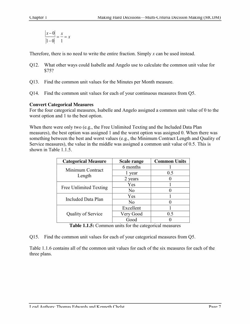
Therefore, there is no need to write the entire fraction. Simply x can be used instead. Q12. What other ways could Isabelle and Angelo use to calculate the common unit value for

$75? Q13. Find the common unit values for the Minutes per Month measure. Q14. Find the common unit values for each of your continuous measures from Q5. Convert Categorical Measures For the four categorical measures, Isabelle and Angelo assigned a common unit value of 0 to the worst option and 1 to the best option. When there were only two (e.g., the Free Unlimited Texting and the Included Data Plan measures), the best option was assigned 1 and the worst option was assigned 0. When there was something between the best and worst values (e.g., the Minimum Contract Length and Quality of Service measures), the value in the middle was assigned a common unit value of 0.5. This is shown in Table 1.1.5.

Categorical Measure Scale range Common Units

Minimum Contract Length

6 months 1 1 year 0.5 2 years 0

Free Unlimited Texting Yes 1 No 0

Included Data Plan Yes 1 No 0

Quality of Service Excellent 1

Very Good 0.5 Good 0

Table 1.1.5: Common units for the categorical measures Q15. Find the common unit values for each of your categorical measures from Q5. Table 1.1.6 contains all of the common unit values for each of the six measures for each of the three plans.



Plan Monthly Charge

($) Minutes

per Month Minimum Contract Length


Included Data Plan

Quality of Service

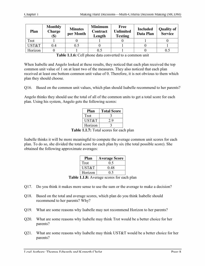
Trot 1 0 1 0 1 0 UST&T 0.4 0.5 0 1 0 1 Horizon 0 1 0.5 1 0 0.5

Table 1.1.6: Cell phone data converted to a common unit When Isabelle and Angelo looked at these results, they noticed that each plan received the top common unit value of 1 on at least two of the measures. They also noticed that each plan received at least one bottom common unit value of 0. Therefore, it is not obvious to them which plan they should choose. Q16. Based on the common unit values, which plan should Isabelle recommend to her parents? Angelo thinks they should use the total of all of the common units to get a total score for each plan. Using his system, Angelo gets the following scores:

Plan Total Score Trot 3 UST&T 2.9 Horizon 3

Table 1.1.7: Total scores for each plan Isabelle thinks it will be more meaningful to compute the average common unit scores for each plan. To do so, she divided the total score for each plan by six (the total possible score). She obtained the following approximate averages:

Plan Average Score Trot 0.5 UST&T 0.48 Horizon 0.5

Table 1.1.8: Average scores for each plan Q17. Do you think it makes more sense to use the sum or the average to make a decision? Q18. Based on the total and average scores, which plan do you think Isabelle should

recommend to her parents? Why? Q19. What are some reasons why Isabelle may not recommend Horizon to her parents? Q20. What are some reasons why Isabelle may think Trot would be a better choice for her

parents? Q21. What are some reasons why Isabelle may think UST&T would be a better choice for her

parents?



Q22. Calculate the total scores and the average scores for each of your cell phone plans. a. Based on these values, which plan would you choose? b. What are some reasons why these plans may not be the best choice for you? c. Was this plan what you expected to choose based on the opening activity? Why or

why not? Whether they use the sum or the average, Isabelle and Angelo realize that each plan has something in its favor. They wonder how to reach a decision. Then Isabelle remembers that her parents were really worried about the monthly service charge, and not as worried about the length of the contract. They decide that they need a system that does not treat all of the measures equally, as the sum and average do. They need a system that weights each measure according to how important it is to Isabelle’s parents. 1.1.6 Conduct an Interview to Calculate Weights In order to learn how important each measure is to her parents, Isabelle and Angelo decide to interview them. They want to learn which measure Isabelle’s parents believe is most important to have the most preferred value rather than the least preferred value. To find out, they ask Isabelle’s parents to rank the six measure ranges in their order of importance. They decided that the difference between the highest and lowest monthly payments was most important to them. Therefore they assigned “monthly charge” a rank of 1. Because they were concerned about the possibility of running up huge bills for texting, they made free texting their second most important measure. Table 1.1.9 shows their rank-ordering of the measures. For example, monthly service charge is the most important measure to Isabelle’s parents and minimum contract length is the least important. This table also includes the least preferred value and the most preferred value for each of the measures.

Measure Monthl

y Charge

($)

Minutes per

Month

Minimum

Contract Length


Included Data Plan

Quality of

Service

Least Preferred Value 85 400 2 years No No Good

Most Preferred Value 60 600 6 months Yes Yes Excellent

Rank 1 4 6 2 5 3 Table 1.1.9: Rank-order of the measures according to Isabelle’s parents

Q23. Rank-order each of your measures. Next, Isabelle and Angelo assign weights to each measure that capture more than the order of importance. They need a sense of how much more important one measure is than another. For example, if one measure is twice as important as another, then the assigned weights should reflect the strength of that difference.



Isabelle and Angelo ask Mr. and Mrs. Nueva to assign 100 points to the measure they ranked number 1—the measure they consider most important. Then, they ask them to assign a number of points less than 100 to the second-ranked measure, free unlimited texting. In doing so, they ask Isabelle’s parents to pick a number that reflects how important it is compared to the number one ranked measure. Mr. and Mrs. Nueva choose to assign 90 points to free unlimited texting, because they know Isabelle likes to text a lot. The interview continues until points have been assigned to each of the six measures. Table 1.1.10 shows the points that Mr. and Mrs. Nueva assigned to each measure.

Measure Monthly Charge

($)

Minutes per

Month



Included Data Plan

Quality of Service

Least Preferred Value 85 400 2 years No No Good

Most Preferred Value 60 600 6 months Yes Yes Excellent

Rank 1 4 6 2 5 3 Points 100 75 50 90 60 80

Table 1.1.10: Points assigned to each of the measures Q24. Assign points to each of your measures, and create a table similar to Table 1.1.10. Now, Isabelle and Angelo total all of the assigned points and obtain 455. Then, they divide the point assignment for each measure by that total. This number is the weight of that measure. For example, monthly charge was assigned 100 points. Thus, the weight of this measure is:

1000.22

455

Table 1.1.11 shows the calculated weight for each of the other measures.

Measure Monthly Charge

($)

Minutes per

Month



Included Data Plan

Quality of

Service Total

Rank 1 4 6 2 5 3 -- Points 100 75 50 90 60 80 455 Weight 100

455 0.22 0.16 0.11 0.20 0.13 0.18 1.00 Table 1.1.11: A weight is calculated for each measure

Q25. What is the largest weight? Which is the smallest? Q26. What is the ratio of the largest weight to the smallest weight? Q27. What should this ratio mean in the context of the decision?



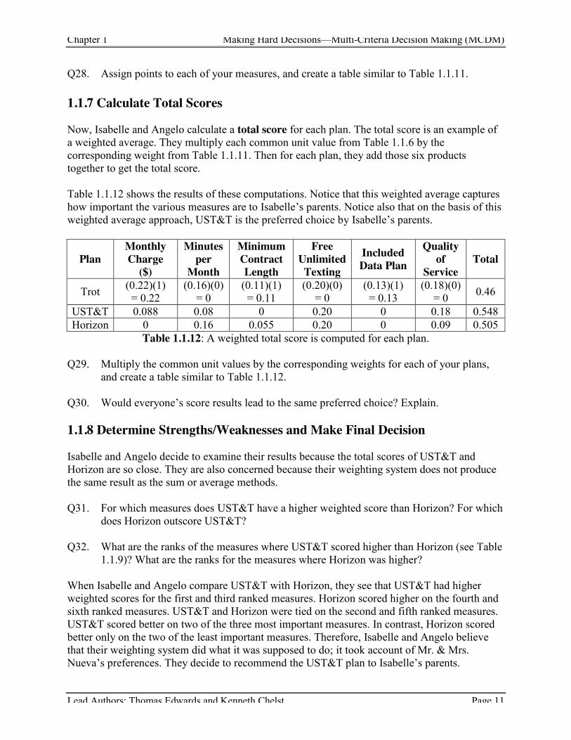
Q28. Assign points to each of your measures, and create a table similar to Table 1.1.11. 1.1.7 Calculate Total Scores Now, Isabelle and Angelo calculate a total score for each plan. The total score is an example of a weighted average. They multiply each common unit value from Table 1.1.6 by the corresponding weight from Table 1.1.11. Then for each plan, they add those six products together to get the total score. Table 1.1.12 shows the results of these computations. Notice that this weighted average captures how important the various measures are to Isabelle’s parents. Notice also that on the basis of this weighted average approach, UST&T is the preferred choice by Isabelle’s parents.

Plan Monthly Charge

($)

Minutes per

Month



Included Data Plan

Quality of

Service Total

Trot (0.22)(1) = 0.22

(0.16)(0) = 0

(0.11)(1) = 0.11

(0.20)(0) = 0

(0.13)(1) = 0.13

(0.18)(0) = 0 0.46

UST&T 0.088 0.08 0 0.20 0 0.18 0.548 Horizon 0 0.16 0.055 0.20 0 0.09 0.505

Table 1.1.12: A weighted total score is computed for each plan. Q29. Multiply the common unit values by the corresponding weights for each of your plans,

and create a table similar to Table 1.1.12. Q30. Would everyone’s score results lead to the same preferred choice? Explain. 1.1.8 Determine Strengths/Weaknesses and Make Final Decision Isabelle and Angelo decide to examine their results because the total scores of UST&T and Horizon are so close. They are also concerned because their weighting system does not produce the same result as the sum or average methods. Q31. For which measures does UST&T have a higher weighted score than Horizon? For which

does Horizon outscore UST&T? Q32. What are the ranks of the measures where UST&T scored higher than Horizon (see Table

1.1.9)? What are the ranks for the measures where Horizon was higher? When Isabelle and Angelo compare UST&T with Horizon, they see that UST&T had higher weighted scores for the first and third ranked measures. Horizon scored higher on the fourth and sixth ranked measures. UST&T and Horizon were tied on the second and fifth ranked measures. UST&T scored better on two of the three most important measures. In contrast, Horizon scored better only on the two of the least important measures. Therefore, Isabelle and Angelo believe that their weighting system did what it was supposed to do; it took account of Mr. & Mrs. Nueva’s preferences. They decide to recommend the UST&T plan to Isabelle’s parents.



1.1.9 Summary In this problem, Isabelle and Angelo needed to choose a cell phone plan for Isabelle’s parents. They completed the following steps:

1. Identify Criteria and Measures 2. Collect Data 3. Find the Range of Each Measure 4. Rescale Each Measure to a Common Unit

After completing these steps, Isabelle and Angelo found the total score and the average score for each cell phone plan. However, they found that these values took all measures into consideration equally. This was not a reasonable way to make a decision. They needed a way to weigh some measures more than others, because Isabelle’s parents were more concerned about the cost of the plan than anything else. In order to take account of Mr. and Mrs. Nueva’s preferences regarding a cell phone plan, Isabelle and Angelo completed three additional steps:

5. Conduct an Interview to Calculate Weights 6. Calculate a Total Score for Each Alternative 7. Interpret Results.

This seven-step process will be applied in the next two sections and in the homework to make slightly more complicated decisions. This process is also a life-skill, because you may find it useful to help you make some important decisions in your future.



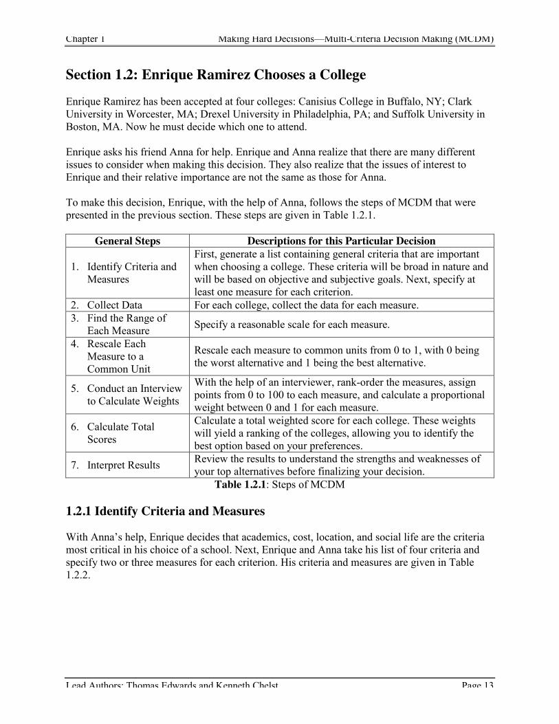
Section 1.2: Enrique Ramirez Chooses a College Enrique Ramirez has been accepted at four colleges: Canisius College in Buffalo, NY; Clark University in Worcester, MA; Drexel University in Philadelphia, PA; and Suffolk University in Boston, MA. Now he must decide which one to attend. Enrique asks his friend Anna for help. Enrique and Anna realize that there are many different issues to consider when making this decision. They also realize that the issues of interest to Enrique and their relative importance are not the same as those for Anna. To make this decision, Enrique, with the help of Anna, follows the steps of MCDM that were presented in the previous section. These steps are given in Table 1.2.1.

General Steps Descriptions for this Particular Decision

1. Identify Criteria and Measures

First, generate a list containing general criteria that are important when choosing a college. These criteria will be broad in nature and will be based on objective and subjective goals. Next, specify at least one measure for each criterion.

2. Collect Data For each college, collect the data for each measure. 3. Find the Range of

Each Measure Specify a reasonable scale for each measure.

4. Rescale Each Measure to a Common Unit

Rescale each measure to common units from 0 to 1, with 0 being the worst alternative and 1 being the best alternative.

5. Conduct an Interview to Calculate Weights

With the help of an interviewer, rank-order the measures, assign points from 0 to 100 to each measure, and calculate a proportional weight between 0 and 1 for each measure.

6. Calculate Total Scores

Calculate a total weighted score for each college. These weights will yield a ranking of the colleges, allowing you to identify the best option based on your preferences.

7. Interpret Results Review the results to understand the strengths and weaknesses of your top alternatives before finalizing your decision.

Table 1.2.1: Steps of MCDM 1.2.1 Identify Criteria and Measures With Anna’s help, Enrique decides that academics, cost, location, and social life are the criteria most critical in his choice of a school. Next, Enrique and Anna take his list of four criteria and specify two or three measures for each criterion. His criteria and measures are given in Table 1.2.2.



Criteria Measures

Academics Average SAT Score (based on last year’s freshman class) U.S. News & World Report Ranking

Cost Room & Board (annual) Tuition (annual)

Location Average Daily High Temperature Nearness to Home

Social Life Athletics Reputation Size

Table 1.2.2: Enrique’s criteria and measures 1.2.2 Collect Data For each measure, Enrique and Anna collect data, which is listed in Table 1.2.3. Some of the measures are naturally categorical. For example, U.S. News & World Report ranks schools into four categories:

1. Nationally ranked 2. Regionally ranked 3. Regionally tier 3 4. Regionally tier 4

Enrique and Anna divide Athletics into three categories:

1. Division 1 2. Division 2 3. Division 3

Similarly, they divide Reputation into three categories:

1. Seriously academic 2. Balanced academics and social life 3. Party school

The data for the remaining measures are numerical values. Enrique and Anna are able to find the average values for SAT score and daily high temperature and the exact values for room and board cost, tuition cost, nearness to home, and size.



Measure Canisius Clark Drexel Suffolk Average SAT Score 1590 1750 1700 1480 U.S. News & World Report Ranking

22nd (regional)

91st (national)

109th (national)

Tier 3 (regional)

Room & Board $10,150 $8,850 $12,135 $11,960 Tuition $28,157 $33,900 $30,470 $25,850 Average Daily High Temperature 56° 56° 64° 59°

Nearness to Home 297 mi 157 mi 81 mi 191 mi Athletics Division 1 Division 3 Division 1 Division 3

Reputation Balanced Seriously academic

Seriously academic Balanced

Size 3,300 students

2,175 students

12,348 students

4,985 students

Table 1.2.3: Raw data for Enrique’s four schools 1.2.3 Find the Range of Each Measure Next, Enrique and Anna choose an appropriate scale for each of the nine measures. Some of the measures are continuous (e.g., SAT score), while others are categorical (e.g., athletics). For the Nearness to Home measure, Enrique believes that exact mileage is not important, but rather broad ranges of mileage better represent his concerns. Therefore, Enrique and Anna convert this measure from continuous to categorical. Q1. Looking at Table 1.2.4, what other measure was converted from continuous to

categorical? Enrique and Anna also realize that the range of each scale is important. For example, the theoretical range of the average combined SAT score is 600–2400, but in actuality, the range of the average combined SAT score at the colleges Enrique is considering is 1480–1750, which is a much narrower range. Enrique and Anna decide that it is much more realistic to use a range that is close to the actual range. Q2. In the previous section, the ranges for the continuous measures were simply the ranges of

the data collected. In this section, the ranges are expanded slightly. For example, instead of the SAT range staying as 1480-1750, Enrique and Anna choose the range 1400-1800. Why might one prefer to use the ranges of the data collected? Why might one prefer to round the ranges?

Q3. Looking at Table 1.2.4, for what other measures do Enrique and Anna create realistic

ranges? Do you agree with their ranges? Why or why not? The type and scale range of each measure are given in Table 1.2.4.



Measure Type Scale range Average SAT Score Continuous 1400–1800

U.S. News & World Report Ranking Categorical

Nationally Ranked Regionally Ranked Regionally Tier 3 Regionally Tier 4

Room & Board Continuous $8,000–$14,000 Tuition Continuous $25,000–$35,000 Average Daily High Temperature Continuous 50˚–70˚F

Nearness to Home Categorical Within 1 hr. Drive (50-100 mi) Within 4 hr. Drive (101–200 mi) Within a Day’s Drive (201–300 mi)

Athletics Categorical Division 1 Division 2 Division 3

Reputation Categorical Seriously Academic Balanced Academics and Social Life Party School

Size Categorical

Under 3,000 students 3,001–6,000 students 6,001–12,000 students Over 12,000 students

Table 1.2.4: Types and ranges of measures Before continuing, Enrique and Anna convert the values of the categorical measures into the numerical values based on the ranges of each measure. The converted data for the categorical measures are given in Table 1.2.5.

Measure Canisius Clark Drexel Suffolk Average SAT Score 1590 1750 1700 1480 U.S. News & World Report Ranking 2 1 1 3 Room & Board $10,150 $8,850 $12,135 $11,960 Tuition $28,157 $33,900 $30,470 $25,850 Average Daily High Temperature 56˚ 56˚ 64˚ 59˚ Nearness to Home 3 2 1 2 Athletics 1 3 1 3 Reputation 2 1 1 2 Size 2 1 4 2

Table 1.2.5: Converted categorical data for Enrique’s four schools 1.2.4 Rescale Each Measure to a Common Unit Once Enrique and Anna choose appropriate scales for each of the measures, Anna reminds Enrique that if they compared the data in its current form, it would be like comparing apples to



1

1400

0

1800 1590

x

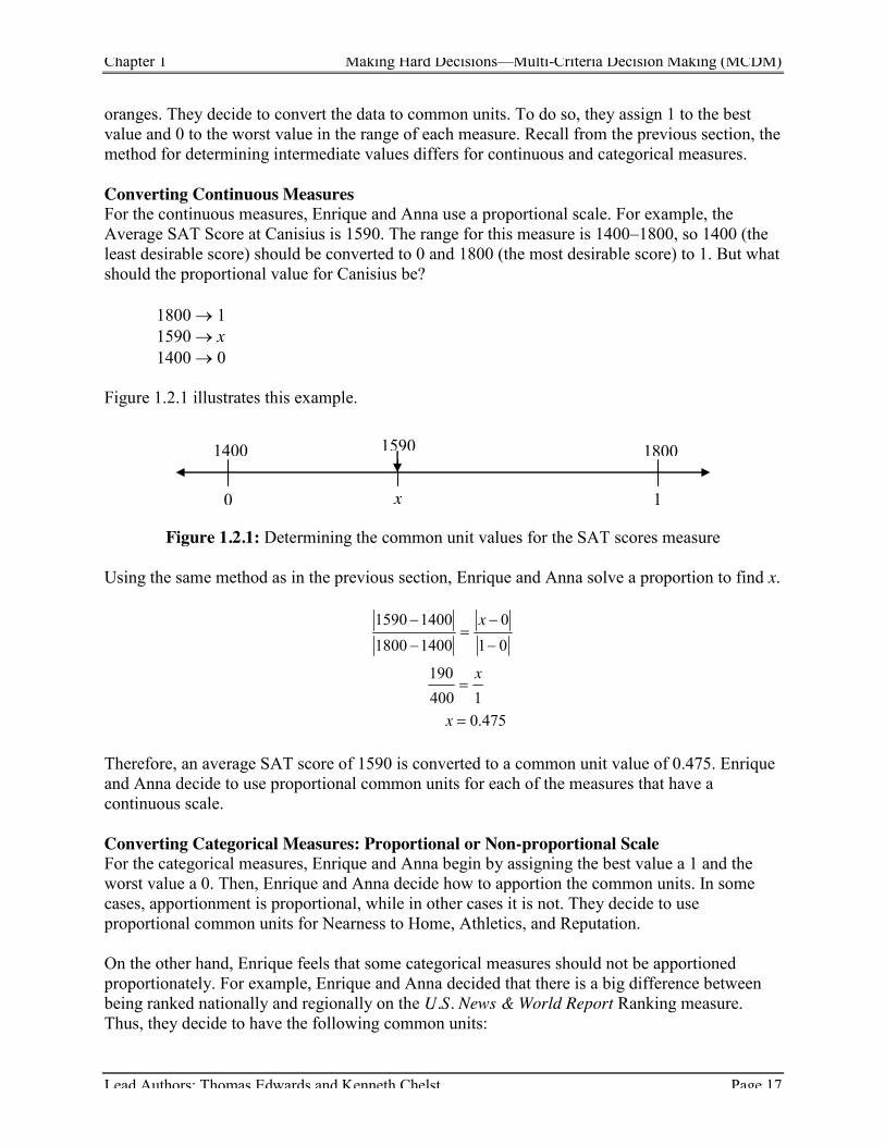
oranges. They decide to convert the data to common units. To do so, they assign 1 to the best value and 0 to the worst value in the range of each measure. Recall from the previous section, the method for determining intermediate values differs for continuous and categorical measures. Converting Continuous Measures For the continuous measures, Enrique and Anna use a proportional scale. For example, the Average SAT Score at Canisius is 1590. The range for this measure is 1400–1800, so 1400 (the least desirable score) should be converted to 0 and 1800 (the most desirable score) to 1. But what should the proportional value for Canisius be?

1800 o 1 1590 o x 1400 o 0

Figure 1.2.1 illustrates this example.

Figure 1.2.1: Determining the common unit values for the SAT scores measure

Using the same method as in the previous section, Enrique and Anna solve a proportion to find x.

1590 1400 01800 1400 1 0

190400 1

0.475

x

x

x

� �

� �

Therefore, an average SAT score of 1590 is converted to a common unit value of 0.475. Enrique and Anna decide to use proportional common units for each of the measures that have a continuous scale. Converting Categorical Measures: Proportional or Non-proportional Scale For the categorical measures, Enrique and Anna begin by assigning the best value a 1 and the worst value a 0. Then, Enrique and Anna decide how to apportion the common units. In some cases, apportionment is proportional, while in other cases it is not. They decide to use proportional common units for Nearness to Home, Athletics, and Reputation. On the other hand, Enrique feels that some categorical measures should not be apportioned proportionately. For example, Enrique and Anna decided that there is a big difference between being ranked nationally and regionally on the U.S. News & World Report Ranking measure. Thus, they decide to have the following common units:



Nationally Ranked o 1 Regionally Ranked o 0.5 Tier 3 o 0.25 Tier 4 o 0

Enrique prefers a smaller school. Therefore, he assigns the following common units:

Under 3,000 students o 1 3,000-6,000 students o 0.75 6,001-12,000 students o 0.25 Over 12,000 students o 0

Table 1.2.6 contains the results of Enrique and Anna’s rescaling of each measure to common units.

Measure Canisius Clark Drexel Suffolk Average SAT Score 0.475 0.875 0.750 0.200 U.S. News & World Report Ranking 0.50 1 1 0.25

Room & Board 0.642 0.858 0.311 0.340 Tuition 0.684 0.110 0.453 0.915 Average Daily High Temperature 0.30 0.30 0.70 0.45

Nearness to Home 1 0.5 0 0.5 Athletics 1 0 1 0 Reputation 1 0.5 0.5 1 Size 0.75 1 0 0.75

Table 1.2.6: Each measure rescaled to common units Q4. From Table 1.2.3, Clark University has the highest average combined SAT score and the

highest tuition. Why does it make sense in Table 1.2.6 that Clark has the highest common unit value on one of those measures, but the lowest common unit value on the other?

Q5. Looking at the Nearness to Home measure in Table 1.2.6, what was the most desirable

distance to Enrique? What was least desirable? Q6. Looking at the Athletics measure in Table 1.2.6, what was the most desirable division to

Enrique? What was least desirable? Q7. Looking at the Reputation measure in Table 1.2.6, what was the most desirable reputation

to Enrique? What was least desirable? To review, there are essentially three steps to rescale data to common units.

Step 1: Assign 1 to the best value in the range. Assign 0 to the worst value in the range.



Step 2: For continuous data, assign intermediate scores proportionally: score least preferred score

Scaled Scoremost preferred score least preferred score

�

�

Step 3: For categorical data, assign intermediate scores proportionally or based on your

own opinions and values. 1.2.5 Conduct an Interview to Calculate Weights Next, Enrique and Anna assign weights to each of the measures to reflect the relative importance Enrique attaches to each of them. They decide Anna will interview Enrique. She makes observations to ensure that Enrique understands the measures he chose and the effects of the weights he assigns to each of them. As a reference tool during the interview, they create Table 1.2.7.

Anna: We have some measures and their ranges for making a decision about your college preference. Focus first on the column of least preferred values. Which one of the measures would you most want to increase from the least preferred value to its most preferred value? For example, is it more important to you to move the SAT score from 1400 to 1800 or to reduce tuition from $35,000 to $25,000?

Enrique: Lower the tuition!

Anna: Are you sure that lowering the tuition to $25,000 is the most important

improvement in the whole list?

Enrique: Yes, so I think we should rank tuition number one.

Anna: Enrique, what would be the next most important measure to move from least preferred to most preferred?

Enrique: U.S. News & World Report ranking is important, so let’s rank that second, and

SAT score third. They continue like this until each measure has been ranked, as shown in Table 1.2.7.



Criterion Measure Least preferred

Most preferred

Rank order

Points (0–100)

Weight (Points/Sum)

Academics

Average SAT Score 1400 1800 3

U.S. News & World Report Ranking

Tier 4 Nat’l. Rank 2

Cost Room & Board $14,000 $8,000 4 Tuition $35,000 $25,000 1

Location

Average Daily High Temperature

50° F 70° F 9

Nearness to Home

Within 1 hr.

Within 1 day 6

Social life

Athletics Div. 3 Div. 1 8 Reputation Party Balanced 7

Size Over 12,000

Under 3,000 5

Sum: Table 1.2.7: Ranking and weighting the measures

The next task is to subjectively assign points from 0 to 100 for each measure based on the rank order. The points assigned reflected the relative importance Enrique places on each measure. They continue the interview to assign these points. During this interview process, Anna encourages Enrique to think about the relative importance of moving between the best and worst values of the two measures being considered. This is seen in the next part of the interview.

Anna: Let’s start by assigning 100 points to the tuition range, which you’ve ranked first. Now, you’ve ranked U. S. News & World Report rating second. How important is this rating, from worst to best, compared to reducing the cost of tuition from $35,000 to $25,000? If it’s close, you should use a number close to 100.

Enrique: I think it’s about 90% as important, so let’s use 90 points for that one, and

SAT scores are almost as important, so we’ll use 85 points for that range. Table 1.2.8 contains the rest of the points Enrique assigns to each of his measures.




Most preferred

Rank order

Points (0–100)

Weight (Points/Sum)

Academics

Average SAT Score 1400 1800 3 85


Tier 4 Nat’l. Rank 2 90

Cost Room & Board $14,000 $8,000 4 80 Tuition $35,000 $25,000 1 100

Location


50° F 70° F 9 20

Nearness to Home

Within 1 hr.

Within 1 day 6 60

Social life Athletics Div. 3 Div. 1 8 30 Reputation Party Balanced 7 50 Size > 12,000 < 3,000 5 70

Sum: 585 Table 1.2.8: Enrique’s rank and point assignment

The interview continues:

Anna: Enrique, what did you get for the total number of points for all your measures? Once you have the point total, you’ll need to divide the points for each measure by this total to get the weight.

Enrique: I got 585 total points. Now I can calculate the weights.

The weights Enrique calculates appear in Table 1.2.9. These were calculated by dividing the points for a particular measure by the total points. For example, Average SAT Score has a point value of 85. So, the weight for this measure is:

850.145

585 .




Most preferred

Rank order

Points (0–100)

Weight (Points/Sum)

Academics

Average SAT Score 1400 1800 3 85 0.145


Tier 4 Nat’l. Rank 2 90 0.154

Cost Room & Board $14,000 $8,000 4 80 0.137 Tuition $35,000 $25,000 1 100 0.171

Location


50° F 70° F 9 20 0.034

Nearness to Home

Within 1 hr.

Within 1 day 6 60 0.103

Social life

Athletics Div. 3 Div. 1 8 30 0.051 Reputation Party Balanced 7 50 0.085 Size > 12,000 < 3,000 5 70 0.120

Sum: 585 1.000 Table 1.2.9: Enrique’s assignment of weights to each measure

Next, Anna wants to ensure that Enrique has assigned an appropriate weight to each criterion. The interview continues.

Anna: Enrique, what is the total weight for each criterion?

Enrique: I get a total of 0.299 for academics, 0.308 for cost, 0.137 for location, and 0.256 for social life.

Anna: Which criterion has the greatest weight assigned to it?

Enrique: It looks like cost, with 0.308.

Anna: Are there criteria with similar weights?

Enrique: It looks like academics and cost are almost the same.

Anna: Are these the criteria you feel are the most important criteria for choosing a

college, and do you think they’re about the same in importance?

Enrique: I didn’t realize I placed so much importance on academics.

Anna: What did you expect to happen?

Enrique: I thought social life would be at the top of the list!



Anna: Well, you gave athletics only 30 points, reputation 50 points, and size 70 points. Do you want to change anything?

Enrique: No, I really think academics and cost are most important.

1.2.6 Calculate Total Scores Finally, Enrique and Anna calculate a total score for each school. They use the data from Table 1.2.6, where common units were computed, and the weights calculated in the last column of Table 1.2.9 to calculate a score for each school on each measure. In Table 1.2.10 below, Enrique has calculated the product of the weight, W, and the corresponding common unit, CU:

Score = W · CU For example, the common unit score for the average SAT score at Canisius College is 0.475, and the weight Enrique has assigned to average SAT score is 0.145. Multiplying these two numbers yields 0.069. This value appears opposite SAT score and below Canisius in Table 1.2.10. It is 10% of the total score for Canisius. The rest of the values in Table 1.2.10 are computed in the same way. Then, totaling the scores for each measure for each college yields the total scores that appear in the last row in Table 1.2.10, Now Enrique can see which of his college choices best suits his preferences.



Measure Weight Canisius Clark Drexel Suffolk

Average SAT Score 0.145 0.145 ∙ 0.475 = 0.069 0.127 0.109 0.029

U.S. News & World Report Ranking 0.154 0.077 0.154 0.154 0.038

Room & Board 0.137 0.088 0.117 0.043 0.046 Tuition 0.171 0.117 0.019 0.077 0.156 Average Daily High Temperature 0.034 0.010 0.010 0.024 0.015

Nearness to Home 0.103 0.103 0.051 0 0.051

Athletics 0.051 0.051 0 0.051 0 Reputation 0.085 0.085 0.043 0.043 0.085 Size 0.120 0.090 0.120 0 0.090

Total Score: 1.000 0.690 0.641 0.501 0.512 Table 1.2.10: Calculating the measure score and total scores of Enrique’s schools

1.2.7 Interpreting the Results Enrique reviews these results carefully. He notices that Drexel and Suffolk have scored much lower than his top-ranked choice, so he excludes them from further study. However, he decides to take a closer look at the relative strengths and weaknesses of Canisius, ranked first, and Clark, ranked second. There is only a 0.049 difference between the two, and he is not sure that it is enough evidence to make this critical life decision. Q8. What are some reasons why Enrique may not choose Canisius, even though it was ranked

first? Q9. On many of the measures, Clark received better scores than Canisius. Why did Canisius

end up having the higher total score? Q10. Suppose Enrique was offered a scholarship at Clark for $5,000. How do you think this

would affect Enrique’s decision?



Section 1.3: Judy Purchases a Used Car Judy is trying to decide which used car to purchase from among four possibilities: a 2006 Honda Civic Hybrid, a 2006 Toyota Prius, and a 2007 Nissan Versa that she has found at dealerships, as well as a 2005 Ford Focus that Judy’s uncle Roger is trying to sell by himself. Judy asks her friend Dave to help her structure her thoughts in a consistent manner and to use the steps in the process of multi-criteria decision making (see Section 1.2 for a list of the steps). With Dave’s help, Judy decides that the criteria most important for her choice of a used car are minimizing total cost and maximizing condition, accessories, and aesthetics. They identify two measures for each criterion, as shown in Table 1.3.1.

Table 1.3.1: Judy’s list of criteria and measures Judy and Dave collect data on each of the cars being considered. Their data appear in Table 1.3.2.

Car Purchase Price

Miles per

Gallon Odometer Reading

Body Condition

Air Conditioner and Heater

Sound System Color Body

Design

Honda Civic Hybrid

$15,000 43 85,000 Good Both Work Radio

and CD Players

Red Sedan

Toyota Prius $15,500 46 80,000 Good Both Work

Radio and CD Players

Silver Sedan

Ford Focus $7,700 25 95,000 Good Both Work

Radio, CD, and

MP3 Players

Blue Wagon

Nissan Versa $11,000 33 65,000 Excellent Both Work

Radio and CD Players

White Hatch-back

Table 1.3.2: Judy’s data on four used cars

Criterion Measures

Total cost Purchase price Miles per gallon, based on the EPA rating when new

Condition Odometer reading Body condition

Accessories Functional air conditioner and heater Sound system

Aesthetics Color Body design



After collecting data and determining the scale range for each measure, Judy and Dave create Table 1.3.3. At this point, for each of the categorical measures, she assigned an integer value. For example, the five possible colors were given values from 1 for blue, the least preferred to 5 for the most preferred color. She created four categories for the sound system and numbered them from 1 to 4.

Measure Scale range Type Purchase Price $6,000–$16,000 Continuous Miles per Gallon 20–50 mpg Continuous Odometer Reading 50,000–100,000 miles Continuous

Body Condition 1 Fair

Categorical 2 Good 3 Excellent

Functional Air Conditioner and Heater 1 Neither works

Categorical 2 Only one works 3 Both work

Sound System

1 None

Categorical 2 Radio only 3 Radio and CD player 4 Radio, CD, and MP3

Color

1 Blue

Categorical 2 Red 3 Silver 4 White 5 Black

Body Design 1 Wagon

Categorical 2 Hatchback 3 Sedan

Table 1.3.3: The type and range for each of Judy’s measures Next, Judy and Dave convert the data for each car into the numerical values given in Table 1.3.4.

Measure Honda Civic Hybrid

Toyota Prius

Ford Focus

Nissan Versa

Purchase Price $15,000 $15,500 $7,700 $11,000 Miles per Gallon 43 46 25 33 Odometer Reading 85,000 80,000 95,000 65,000 Body Condition 2 2 2 3 Functional Air Conditioner and

Heater 3 3 3 3

Sound System 3 3 4 3 Color 2 3 1 4 Body Design 3 3 1 2

Table 1.3.4: Converted categorical data for Judy’s four cars



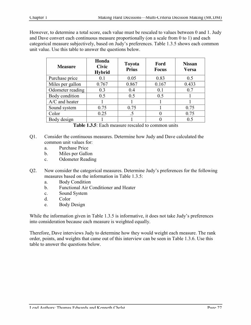
However, to determine a total score, each value must be rescaled to values between 0 and 1. Judy and Dave convert each continuous measure proportionally (on a scale from 0 to 1) and each categorical measure subjectively, based on Judy’s preferences. Table 1.3.5 shows each common unit value. Use this table to answer the questions below.

Measure Honda Civic

Hybrid Toyota Prius

Ford Focus

Nissan Versa

Purchase price 0.1 0.05 0.83 0.5 Miles per gallon 0.767 0.867 0.167 0.433 Odometer reading 0.3 0.4 0.1 0.7 Body condition 0.5 0.5 0.5 1 A/C and heater 1 1 1 1 Sound system 0.75 0.75 1 0.75 Color 0.25 .5 0 0.75 Body design 1 1 0 0.5

Table 1.3.5: Each measure rescaled to common units Q1. Consider the continuous measures. Determine how Judy and Dave calculated the

common unit values for: a. Purchase Price b. Miles per Gallon c. Odometer Reading

Q2. Now consider the categorical measures. Determine Judy’s preferences for the following

measures based on the information in Table 1.3.5: a. Body Condition b. Functional Air Conditioner and Heater c. Sound System d. Color e. Body Design

While the information given in Table 1.3.5 is informative, it does not take Judy’s preferences into consideration because each measure is weighted equally. Therefore, Dave interviews Judy to determine how they would weight each measure. The rank order, points, and weights that came out of this interview can be seen in Table 1.3.6. Use this table to answer the questions below.



Criteria Measure Least preferred

Most preferred

Rank order

Points (0–100)

Weight (Points/Sum)

Total cost

Purchase Price $16,000 $6,000 1 100 0.2 Miles per Gallon 20 mpg 50 mpg 2 95 0.19

Condition

Odometer Reading 100,000 mi 50,000 mi 5 60 0.12

Body Condition 1 (fair) 3 (excellent) 3 75 0.15

Accessories

Functional Air Conditioner and Heater

1 (neither works)

3 (both work) 7 35 0.07

Sound System 1 (none) 4 (radio, CD, MP3) 6 50 0.1

Aesthetics Color 1 (blue) 5 (black) 8 10 0.02 Body Design 1 (wagon) 3 (sedan) 3 75 0.15

Sum = 500 1 Table 1.3.6: Judy’s rank ordering, point assignment, and weight calculation for her measures

Q3. Which measure is most important to Judy? How do you know? Q4. Which measure is least important to Judy? How do you know? Q5. Which two measures have equal importance to Judy? How do you know? Q6. How would you describe Judy’s feelings towards Purchase Price versus her feelings

towards Miles per Gallon? Q7. How would you describe Judy’s feelings towards Miles per Gallon versus her feelings

towards Body Condition? Q8. How were the weights calculated? Q9. What criterion is most important to Judy? How do you know? Finally, Judy and Dave calculate the total scores for each car, as shown in Tables 1.3.7 and 1.3.8. Use these tables to answer the questions below.



Measure Weight Honda Civic

Hybrid Toyota Prius

Ford Focus

Nissan Versa

Purchase price 0.2 0.1 0.05 0.83 0.5 Miles per gallon 0.19 0.767 0.867 0.167 0.433 Odometer reading 0.12 0.3 0.4 0.1 0.7 Body condition 0.15 0.5 0.5 0.5 1 A/C and heater 0.07 1 1 1 1 Sound system 0.1 0.75 0.75 1 0.75 Color 0.02 0.25 .5 0 0.75 Body design 0.15 1 1 0 0.5

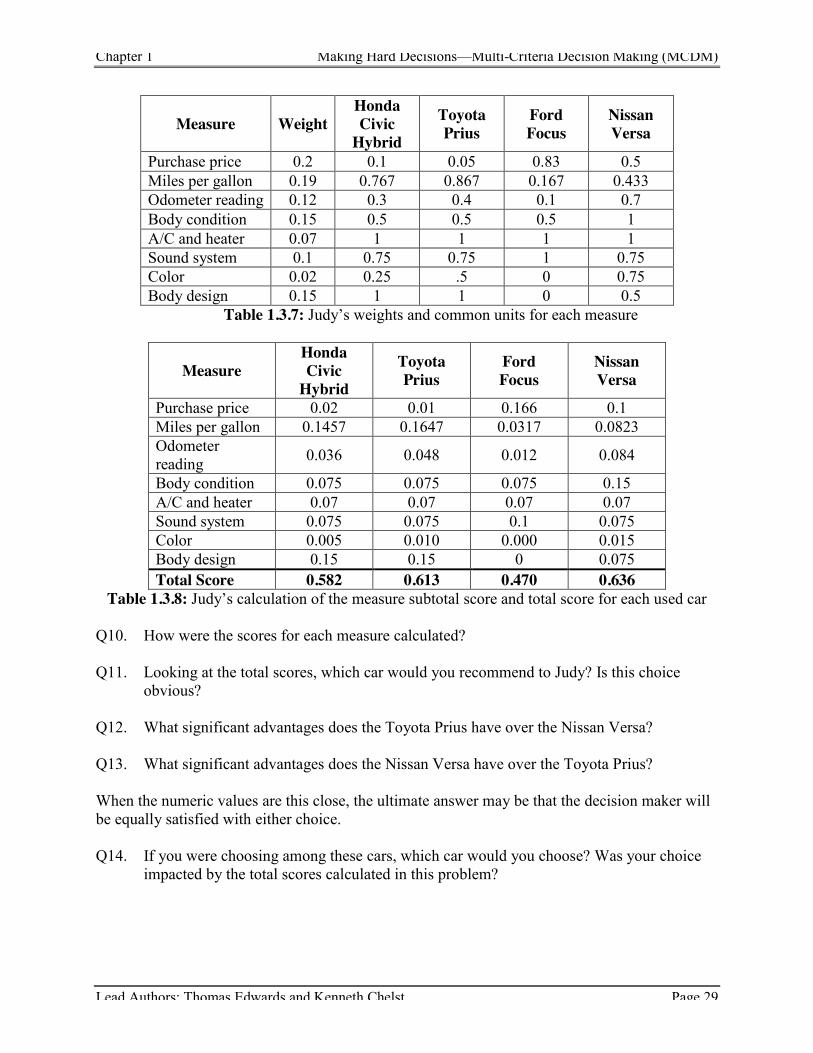
Table 1.3.7: Judy’s weights and common units for each measure

Measure Honda Civic

Hybrid Toyota Prius

Ford Focus

Nissan Versa

Purchase price 0.02 0.01 0.166 0.1 Miles per gallon 0.1457 0.1647 0.0317 0.0823 Odometer reading 0.036 0.048 0.012 0.084

Body condition 0.075 0.075 0.075 0.15 A/C and heater 0.07 0.07 0.07 0.07 Sound system 0.075 0.075 0.1 0.075 Color 0.005 0.010 0.000 0.015 Body design 0.15 0.15 0 0.075 Total Score 0.582 0.613 0.470 0.636

Table 1.3.8: Judy’s calculation of the measure subtotal score and total score for each used car Q10. How were the scores for each measure calculated? Q11. Looking at the total scores, which car would you recommend to Judy? Is this choice

obvious? Q12. What significant advantages does the Toyota Prius have over the Nissan Versa?

Q13. What significant advantages does the Nissan Versa have over the Toyota Prius? When the numeric values are this close, the ultimate answer may be that the decision maker will be equally satisfied with either choice. Q14. If you were choosing among these cars, which car would you choose? Was your choice

impacted by the total scores calculated in this problem?



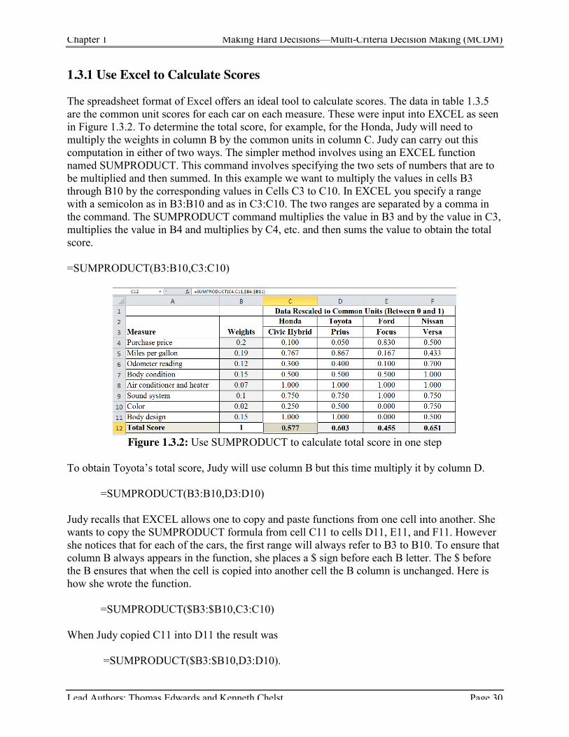
1.3.1 Use Excel to Calculate Scores The spreadsheet format of Excel offers an ideal tool to calculate scores. The data in table 1.3.5 are the common unit scores for each car on each measure. These were input into EXCEL as seen in Figure 1.3.2. To determine the total score, for example, for the Honda, Judy will need to multiply the weights in column B by the common units in column C. Judy can carry out this computation in either of two ways. The simpler method involves using an EXCEL function named SUMPRODUCT. This command involves specifying the two sets of numbers that are to be multiplied and then summed. In this example we want to multiply the values in cells B3 through B10 by the corresponding values in Cells C3 to C10. In EXCEL you specify a range with a semicolon as in B3:B10 and as in C3:C10. The two ranges are separated by a comma in the command. The SUMPRODUCT command multiplies the value in B3 and by the value in C3, multiplies the value in B4 and multiplies by C4, etc. and then sums the value to obtain the total score. =SUMPRODUCT(B3:B10,C3:C10)

Figure 1.3.2: Use SUMPRODUCT to calculate total score in one step

To obtain Toyota’s total score, Judy will use column B but this time multiply it by column D.

=SUMPRODUCT(B3:B10,D3:D10) Judy recalls that EXCEL allows one to copy and paste functions from one cell into another. She wants to copy the SUMPRODUCT formula from cell C11 to cells D11, E11, and F11. However she notices that for each of the cars, the first range will always refer to B3 to B10. To ensure that column B always appears in the function, she places a $ sign before each B letter. The $ before the B ensures that when the cell is copied into another cell the B column is unchanged. Here is how she wrote the function.

=SUMPRODUCT($B3:$B10,C3:C10) When Judy copied C11 into D11 the result was

=SUMPRODUCT($B3:$B10,D3:D10).



She repeated this for cells E11 and F11. Multi-step Method with more Details The above method determines the total score but does not show the individual measure components of each total score. Thus, Judy is unable to tell how much the purchase price contributes to the total score of each car. She decided to use EXCEL’s capabilities to replicate Table 1.3.8 which has the detailed information. (See also Table 1.1.12 and Table 1.2.10.) She set up a new area in the spreadsheet in rows 16 through 26 to calculate the individual subtotals. This is displayed in Figure 1.3.4. To obtain the value in cell C18, she multiplied C3 by $B3. She again placed a $ symbol before the B because she was going to use the copy and paste function to complete the table.

Figure 1.3.3: Calculate subtotals: multiply weight by common unit and sum the subtotals

Judy then copied cell C18 into cells C19 through C25. Judy then used the SUM function to calculate the total score. In cell C26 she wrote

=SUM(C18:C25) She then copied the entire column of values C18 through C26 to columns D, E, and F. She now can see the impact of the subtotals on each car’s total score. She noticed that the purchase price contributes only 0.02 to Honda’s total score of 0.582. In contrast, the purchase price contributes 0.10 to Nissan’s total score of 0.636.

Section 1.0: Introduction to Making Hard Decisions

Documents

Transcript of Section 1.0: Introduction to Making Hard Decisions