arX

iv:c

ond-

mat

/050

8094

v1 [

cond

-mat

.sof

t] 3

Aug

200

5

Secondary Structures in Long Compact Polymers

Richard Oberdorf1, Allison Ferguson1, Jesper L. Jacobsen2,3, and Jane Kondev1

1Department of Physics, Brandeis University, Waltham, MA 02454, USA2LPTMS, Universite Paris-Sud, Batiment 100, 91405 Orsay, France and

3Service de Physique Theorique, CEA Saclay, 91191 Gif-sur-Yvette, France

(Dated: February 2, 2008)

Compact polymers are self-avoiding random walks which visit every site on a lattice. This polymermodel is used widely for studying statistical problems inspired by protein folding. One difficultywith using compact polymers to perform numerical calculations is generating a sufficiently largenumber of randomly sampled configurations. We present a Monte-Carlo algorithm which uniformlysamples compact polymer configurations in an efficient manner allowing investigations of chainsmuch longer than previously studied. Chain configurations generated by the algorithm are usedto compute statistics of secondary structures in compact polymers. We determine the fraction ofmonomers participating in secondary structures, and show that it is self averaging in the long chainlimit and strictly less than one. Comparison with results for lattice models of open polymer chainsshows that compact chains are significantly more likely to form secondary structure.

I. INTRODUCTION

Proteins are long, flexible chains of amino acids which can assume, in the presence of a denaturant, an astronomicallylarge number of open conformations. Twenty different types of amino acids are found in naturally occurring proteins,and their sequence along the chain defines the primary structure of the protein. The native, folded state of theprotein contains secondary structures such as α-helices and β-sheets which are in turn arranged to form the largertertiary structures. Under proper solvent conditions most proteins will fold into a unique native conformation whichis determined by its sequence. One of the goals of protein folding research is to determine exactly how the foldedstate results from the specific sequence of amino acids in the primary structure.

A number of theories exist to describe the forces that are responsible for protein folding [1]. Since there are manyfewer compact polymer conformations than non-compact ones, entropic forces resist the tight packing of globularproteins. Tight packing is primarily the result of hydrophobic interactions between the amino acid monomers andthe solvent molecules around them. Compared to the local forces between neighboring monomers along the chain,the hydrophobic interactions were historically seen as nonlocal forces contributing to the collapse process, but notresponsible for determining the specific form of the native structure [2].

This view has been challenged by ideas from polymer physics [3, 4]. In particular, polymers with hydrophobicmonomers when placed in a polar solvent like water will collapse to a configuration where the hydrophobic residuesare protected from the solvent in the core of the collapsed structure. Similarly, protein folding can be viewed aspolymer collapse driven by hydrophobicity. The question then arises, how much of the observed secondary structureis a result of this non-specific collapse process?

To examine the role of hydrophobic interactions in folding, coarse-grained models of proteins have been developed,which reduce the 20 possible amino acid monomers to two types: hydrophobic (H) and polar (P). Further simplificationis affected by using random walks on two or three dimensional lattices to represent chain conformations. Verticesof the lattice visited by the walk are identified with monomers, which in the HP model are of the H or P variety.Furthermore, in order to capture the compact nature of the folded protein state, Hamiltonian walks are often usedfor chain conformations. The Hamiltonian walk (or “compact polymer”) is a self-avoiding walk on a lattice that visitsall the lattice sites. The compact polymer model was first used by Flory [5] in studies of polymer melting, and waslater introduced by Dill [3] in the context of protein folding. The HP model provides a simple model within which avariety of questions regarding the relation of the space of sequences (ordered lists of H and P monomers) to the spaceof protein conformations (Hamiltonian walks) can be addressed; for a recent example see Ref. [6].

One of the first questions to be examined within the compact polymer model was to what extent is the observedsecondary structure of globular proteins (i.e., the appearance of well ordered helices and sheets) simply the resultof the compact nature of their native states. Complete enumerations of compact polymers with lengths up to 36monomers found a large average fraction of monomers participating in secondary structure [7]. This added weightto the argument that the observed secondary structure in proteins is simply a result of hydrophobic collapse to thecompact state. This simple view was later challenged by off-lattice simulations, which showed that specific localinteractions among monomers are necessary in order to produce protein-like helices and sheets [8].

Here we reexamine the question of secondary structure in compact polymers on the square lattice using Monte-Carlosampling of the configuration space. We compute the probability of a monomer participating in secondary structurein the limit of very long chains. We show that this probability is strictly less than one, and that it depends on the

2

precise definition of secondary structure in the lattice model. We also show that, in the long-chain limit, compactpolymers are much more likely to exhibit secondary structure motifs than their non-compact counterparts, such asideal chains, described by random walks, or polymers in a good solvent, modelled by self-avoiding random walks. TheMonte-Carlo technique described below can be easily extended to three-dimensional lattices and other models (suchas the HP model) that make use of Hamiltonian walks. In a forthcoming paper we further demonstrate its utility inthe context of the Flory model of polymer melting [9].

Hamiltonian walks on different lattices are also interesting statistical mechanics models in their own right, as theirscaling properties give rise to new universality classes of polymers. An unusual property of these walks is thatdifferent lattices do not necessarily lead to the same universality class. This lattice dependence is linked to geometricfrustration that results from the constraint that Hamilton walks must visit all the sites of the lattice. In addition,compact polymers can be obtained as the zero-fugacity limit of fully packed loop models (the exact form of whichdepends on the lattice) allowing for the exact calculation of critical exponents [10].

Numerical investigations of compact polymers are typically hampered by the need to generate a sufficient numberof statistically independent compact configurations for the construction of a suitable ensemble. It is not hard tosee that attempting to generate compact structures by constructing self-avoiding random walks on a lattice wouldindeed be a problematic endeavor; current state-of-the-art algorithms are essentially “smarter” chain growth strategieswhere the next step in the random walk is taken based on not only the self-avoidance constraint but on a samplingprobability which improves as the program proceeds [11]. Enumerations of all possible states have been performed forboth regular self-avoiding random walks [12] and for compact polymers [13], but this has only been possible for smalllattices (N < 36). Therefore, an algorithm which can rapidly generate compact configurations on significantly largerlattices, without the complication of constructing advanced sampling probabilities would be an extremely useful tool.

In Ref. [14] a method for generating compact polymers based on the transfer matrix method was introduced. Onelimitation of the method is that the transfer matrices become prohibitively large as the number of sites in the directionperpendicular to the transfer direction increases above 10. A very efficient Monte-Carlo method based on a graphtheoretical approach was introduced in [15] and improved on in [16] by reducing the sampling bias.

One of the purposes of this paper is to describe a Monte-Carlo method for efficiently generating compact polymerconfigurations on the square lattice for chain lengths up to N = 2500. The Monte-Carlo algorithm outlined belowmakes use of the “back bite” move, which was first introduced by Mansfield in studies of polymer melts [17]. Weperform a number of measurements to assess the validity and practicality of the algorithm for generating compactpolymer configurations. Probably the most important and certainly the most elusive property is that of ergodicity,which would guarantee that the algorithm can sample all compact polymer configurations. While we have beenunsuccessful in constructing a proof of ergodicity, we find excellent numerical evidence for it based on a number ofdifferent tests. In particular, we check that the measured probability that the polymer endpoints are adjacent on thelattice is in agreement with exact enumeration results for polymer chain lengths up to N = 196. Furthermore, wedemonstrate that the Monte-Carlo process satisfies detailed balance, which guarantees, at least in the theoretical limitof infinitely long runs, that the sampling is unbiased. We check this in practice with a quantitative test of samplingbias for N = 36 (ie. for compact polymers on a 6 × 6 square lattice).

For the Monte-Carlo process to be useful it should also sample the space of compact polymer configurationsefficiently. To quantify this property of the algorithm, we measure the processing time required to generate a fixednumber of compact polymer conformations, and find it to be linear in chain length N . Since the sampling is of theMonte-Carlo variety a certain number of Monte-Carlo steps need to be performed before the initial and the finalstructure can be deemed statistically independent. We find that this correlation time, measured in Monte-Carlo stepsper monomer, grows with chain length as Nz with z ≈ 0.16.

We put the Monte-Carlo algorithm to good use by tackling the question of the statistics of secondary structurein compact polymer chains. While the previous study by Chan and Dill [7] found a large fraction of monomersparticipating in secondary-structure motifs, the polymer physics question of what happens to this quantity in thelong-chain limit, remained unanswered. Based on exact enumerations for chain lengths up to N = 36 the hypothesisthat was put forward was that in the long chain limit almost all the monomers will participate in secondary structure.Our computations on the other hand, show that the probability of a monomer participating in secondary structuretends to a fixed number strictly less than one. Furthermore the actual number depends on the precise definitions usedfor secondary structure motifs. Still, from gathered statistics on the appearance of helix-like motifs in simple randomwalks and self-avoiding walks, we conclude that the propensity for secondary structures in compact polymers is muchgreater than in their non-compact counterparts, even in the long chain limit. This provides further support for theidea that the global constraint of compactness, imposed on globular proteins by hydrophobicity, favors formation ofsecondary structure.

The paper is organized as follows. In section II we describe our Monte-Carlo process for sampling compact polymers,which is based on Mansfield’s backbite move [17]. The correctness and usefulness of the Monte-Carlo algorithm forsampling compact polymer configurations, is evaluated in section II A. Finally, in section III we give details of our

3

FIG. 1: Compact polymer configuration on a 6×6 lattice. This “plough” configuration is used as the initial state for theMonte-Carlo process.

FIG. 2: Illustration of the “backbite” move used to generate a new Hamiltonian walk from an ini-tial one. Starting from a valid walk a), one additional step is made starting at either of the twoends of the walk, b). Next we delete a step, shown in c), to produce a new valid walk, d).

computations of secondary structure statistics for compact polymers with lengths ranging from N = 36 to N = 2500.The main conclusion of this section is that the fraction of monomers participating in secondary structures is Gaussiandistributed with a variance that vanishes in the long-chain limit. Its mean is strictly less than one but still more thantwice as large as the values measured for non-compact lattice models of polymers.

II. MONTE-CARLO SAMPLING OF COMPACT POLYMERS

The Monte Carlo process starts with an initial Hamiltonian walk on the lattice. We use a square lattice with side√N , N being the polymer length. The initial walk is the “plough” shown in Fig. 1. Starting from this initial compact

polymer configuration, new configurations are generated by repeatedly applying the backbite move [17]. Namely,given a Hamiltonian walk (Fig. 2a), a link is added between one of the walk’s free ends and one of the lattice sitesadjacent, but not connected, to that end. This adjacent site is chosen at random with each possible site having anequal probability of being chosen (Fig. 2b). After the new link has been added we no longer have a valid Hamiltonianwalk, since three links are now incident to the chosen site. To correct this we remove one of the three links, which isuniquely characterized by being part of a cycle (closed path) and not being the link just added (Fig. 2c). After oneiteration of this process one of the ends of the walk has moved two lattice spacings, and a new Hamiltonian walk hasbeen constructed (Fig. 2d).

By repeatedly executing the backbite move it seems that all possible Hamiltonian walks are generated. To examine

4

FIG. 3: Enumeration of all possible Hamiltonian walks on a 3 × 3 square lattice.

this statement more closely, we first consider compact polymers on a 3× 3 lattice. Fig. 3 shows an enumeration of allpossible compact polymer configurations on this lattice. The corresponding walks may be divided into three classeswhere all the walks in a given class (Plough, Spiral or Locomotive—denoted P, S and L in the figure) are relatedby reflection (denoted R in the figure) and/or rotation. (Note that P-class walks are invariant under rotation by 180degrees, and that there are half as many P-class walks as S or L-class walks.) Fig. 4 shows the transition graph thatconnects compact polymer configurations on a 3 × 3 lattice that are related by a single backbite move. We see thatall the 20 possible walks can be reached from any initial walk. Furthermore, it is important to notice that the S-classwalks have four moves leading in and out of them, while the L and P-class walks only have two moves leading in andout of them. This happens as a result of the locations of a walk’s end points. Namely, on a square lattice an end pointon a corner can only be linked to one adjacent site by the backbite move, end points on the edges can be linked totwo sites, while end points in the interior of the lattice can be linked to three sites. Because there are twice as manymoves leading to S-class walks as there are for P-class or L-class, the S-class walks are twice as likely to be generatedif backbite moves are repeatedly performed (this subtlety is absent if periodic boundary conditions are employed).

In order to compensate for this source of bias in sampling of compact polymers, an adjustment to the originalprocess is made: for structures which have fewer paths available to access them, we introduce the option of leavingthe current walk unchanged in the next Monte-Carlo step. The probability of making a transformation from thecurrent walk is calculated by counting how many links l can be drawn from the end points of the current walk anddividing that number by the maximum number (lmax) of links that could be drawn for any walk on the lattice. Forexample, consider a P-class walk on a 3 × 3 lattice. There are two possible links that could be drawn from the endpoints of this walk, but there is a maximum of 4 links that could be drawn (which happens in the case of S-classwalks). Thus the probability of making a backbite move is l

lmax

= 24 = 0.5.

With this adjustment of the original Monte Carlo process, all walks accessible from the initial walk will occurwith equal probability, upon repeating the algorithm a sufficiently large number of times. Technically speaking, theamended algorithm satisfies detailed balance. In general, the criterion for detailed balance reads pαP (α → α′) =pα′P (α′ → α), where pα is the probability of the system being in the state α, and P (α → α′) is the transitionprobability of going from the state α to another state α′. In thermal equilibrium one must have pα = Z−1 exp(−βEα),where β is the inverse temperature, Eα is the energy of the state α, and Z =

∑α exp(−βEα) is the partition function.

In the problem at hand we have assigned the same energy (say, Eα = 0) to all states, whence the criterion for detailedbalance reads simply P (α → α′) = P (α′ → α).

Now suppose that the state α can make transitions to lα other states. (In the above example, lα = 2 for the P-classwalks and lα = 4 for the S-class walks.) Then we can choose P (α → α′) equal to π(α → α′) ≡ min(1/lα, 1/lα′)for α 6= α′. Define γ(α) =

∑′

α′ π(α → α′), where the sum is over the lα states α′ which can be reached by asingle move from the state α. In order to make sure that probabilities sum up to 1, we must introduce the probabilityP (α → α) = 1−γ(α) for doing nothing. Better yet, we can eliminate the possibility of doing nothing by renormalizingthe Monte-Carlo time. Namely, let the transition out of the state α correspond to a Monte-Carlo time 1/γ(α) andpick the transition probabilities as P (α → α′) = π(α → α′)/γ(α). Then the transition rates (i.e., the transitionprobability per unit time) satisfies detailed balance as it should. This renormalized dynamics is clearly optimal in

5

FIG. 4: Transition graph for compact polymers on the 3 × 3 square lattice generated by the backbite move.

the sense that now the probability of leaving the state unchanged is zero, P (α → α) = 0. In practice, the optimalchoice only presents an advantage if the numbers lα are easy to evaluate (which is the case here) and if their valuesvary considerably with α (which is not the case here). Accordingly, we have used only the simpler l/lmax prescriptiondescribed in the preceding paragraph.

Even though we have satisfied detailed balance, a walk generated by the Monte Carlo process does not immediatelystart occurring with a probability that is independent of the initial walk. For large N in particular, a walk generatedby the process will show a great deal of structural similarity to the walk that it was created from because only twolinks of the walk get changed in each iteration of the process. To work around this problem a large number of walksmust be generated to yield the final ensemble. Below we address this important practical issue in great detail.

A. Properties of the Monte Carlo process

In evaluating the suitability of the Monte-Carlo algorithm for statistical studies of compact polymers the followingissues must be addressed: 1. Does the process generate all possible Hamiltonian walks on a given lattice? 2. Is thesampling as described in the previous section truly unbiased? 3. How rapidly do descendant structures lose memoryof the initial structure? 4. How does the processing time to generate a fixed number of walks scale with the number oflattice sites? The first two questions relate to issues of ergodicity and detailed balance which both need to be satisfiedso that structures are sampled correctly. The last two questions pertain to the efficacy with which the algorithmcan generate uncorrelated structures that can be used in computations of ensemble averages. Below we give detailedanswers to these questions.

We have been unable to provide a general proof of ergodicity, i.e., that the Monte-Carlo process can generate allpossible Hamiltonian walks on square lattices of arbitrary size. However, we have observed that the process successfullygenerates all of the possible walks on square lattices of size 3× 3, 4× 4, 5 × 5, and 6 × 6. It should be noted that for5× 5 and 6× 6 lattices, all possible “combinations” of end point locations are possible, while on smaller lattices onlywalks with corner-corner, core-corner, and corner-edge combinations are allowed. Whether endpoints are on edges,corners, or in the bulk of the lattice is important because it determines how many links might be drawn from anendpoint which in turn determines the probability of making a Monte-Carlo step away from the current structure.Both 5 × 5 and a 6 × 6 lattices have lmax = 6, which is the largest possible lmax on the square lattice. In this sense,

6

0 20 40 60 80Number of Appearances

0

0.2

0.4

0.6

0.8

1

Pro

bab

ilit

y

Binomial Distribution6 x 6 sample

FIG. 5: Comparison of sampling statistics of compact polymers on the 6 × 6 lattice produced by theMonte Carlo process with the binomial distribution, which is to be expected for an unbiased sampling.

we consider these two lattices representative of larger lattices.It should also be noted that the algorithm is likely to exhibit parity effects. This is linked to the fact that a square

lattice can be divided into two sublattices (even and odd). Namely, on a lattice of N sites, the two end points mustnecessarily reside on opposite (resp. equal) sublattices if N is even (resp. odd). To see this, note that when movingalong the walk from one end point to the other, the site parity must change exactly N − 1 times. In particular, onlywhen N is even can the two end points be adjacent on the lattice. It is therefore reassuring to have tested ergodicityfor both 5 × 5 and 6 × 6 lattices.

To test whether or not the process generates unbiased samples, K = 107 compact polymer conformations weregenerated on a 6 × 6 lattice. All different conformations were identified and the number of occurrences of eachidentified conformation was counted. The number of conformations on a 6× 6 lattice is known by exact enumerationto be M = 229 348 [18], and our algorithm indeed generates all of these. Using a method similar to the one used inRef. [16] we construct the histogram of the frequency with which each one of the M possible conformations occurs.This histogram is then compared to the relevant binomial distribution. Namely, if each conformation occurs withequal probability p = 1

Nthen the probability of a given conformation occurring k times in K trials is P (k) =

K!k!(K−k)!p

k(1 − p)K−k. In Fig. 5 we compare P (k) to the distribution constructed from the actual 6 × 6 sample. A

close correspondence between the predicted distribution and the distribution constructed from the Monte-Carlo datais evident from the figure, indicating no detectable sampling bias in this case.

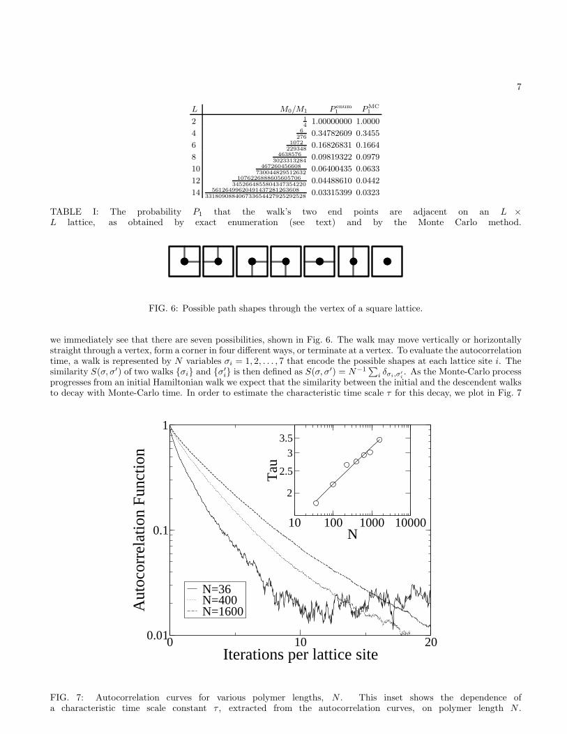
Further evidence that the sampling is unbiased is provided by computing the probability P1 that the end pointsof the generated walks are separated by one lattice spacing. Note that when this is the case, the walk could beturned into a closed walk, or Hamiltonian circuit, by adding a link that joins the two end points. Conversely, a closedwalk on an N -site lattice can be turned into N distinct open walks by removing any one of its N links. ThereforeP1 = NM0/M1, where M0 (resp. M1) is the number of closed (resp. open) walks that one can draw on the lattice.Using this formula, we can compare P1 as obtained by the Monte Carlo method, to P1 from exact enumeration data.The exact enumerations are done using a transfer-matrix method for lattice sizes up to 14 × 14 [18]. The resultsdisplayed in Table I show that the two determinations of P1 are in excellent agreement.

To quantify the rate at which descendant structures become decorrelated from an initial structure we must firstdevise a method for computing the similarity of two structures. The method used here is to compare, vertex byvertex, the different ways in which the walk can pass through a vertex. Looking at the examples of walks in Fig. 3

7

L M0/M1 P enum1 PMC

1

2 1

41.00000000 1.0000

4 6

2760.34782609 0.3455

6 1072

2293480.16826831 0.1664

8 4638576

30233132840.09819322 0.0979

10 467260456608

7300448295126320.06400435 0.0633

12 1076226888605605706

34526648558043473542200.04488610 0.0442

14 56126499620491437281263608

3318090884067336544279252925280.03315399 0.0323

TABLE I: The probability P1 that the walk’s two end points are adjacent on an L ×L lattice, as obtained by exact enumeration (see text) and by the Monte Carlo method.

FIG. 6: Possible path shapes through the vertex of a square lattice.

we immediately see that there are seven possibilities, shown in Fig. 6. The walk may move vertically or horizontallystraight through a vertex, form a corner in four different ways, or terminate at a vertex. To evaluate the autocorrelationtime, a walk is represented by N variables σi = 1, 2, . . . , 7 that encode the possible shapes at each lattice site i. Thesimilarity S(σ, σ′) of two walks {σi} and {σ′

i} is then defined as S(σ, σ′) = N−1∑

i δσi,σ′

i. As the Monte-Carlo process

progresses from an initial Hamiltonian walk we expect that the similarity between the initial and the descendent walksto decay with Monte-Carlo time. In order to estimate the characteristic time scale τ for this decay, we plot in Fig. 7

0 10 20Iterations per lattice site

0.01

0.1

1

Aut

ocor

rela

tion

Func

tion

N=36N=400N=1600

10 100 1000 10000N

2

3

2.5

3.5

Tau

FIG. 7: Autocorrelation curves for various polymer lengths, N . This inset shows the dependence ofa characteristic time scale constant τ , extracted from the autocorrelation curves, on polymer length N .

8

0 10000 20000 30000 40000

Chain length

0

50000

1e+05

1.5e+05

2e+05

Pro

cess

ing

tim

e(m

s)

Collected DataL inear Fit

FIG. 8: Effect of varying the compact polymer length on processing time re-quired to generate 106 consecutive structures by the Monte-Carlo process. Computa-tions were performed on a 500 Mhz Pentium III computer with 512 megabytes of RAM.

the autocorrelation function

A(t) =〈S(σ(0), σ(t))〉 − 〈S〉min

1 − 〈S〉min

(1)

where the average is taken over many runs and 〈S〉min is the smallest average similarity computed for the durationof the Monte-Carlo process, for a given N . The walk σ(t) is one obtained after t Monte-Carlo steps per lattice siteapplied to the initial walk σ(0).

The curves in Fig. 7 have an initial, exponentially decaying regime. In this regime we fit them to the functionA exp(−t/τ) to obtain as estimate for the autocorrelation time τ . The inset of Fig. 7 shows the dependence of τ onpolymer length N , plotted on a log-log plot. Fitting now the polymer length dependence using τ = BNz, we get theestimate z = 0.16 ± 0.03 for the dynamical exponent. The fact that the dynamical exponent is small tells us thatincreasing the polymer length in the simulation will not lead to a large increase in computational cost.

There are two ways in which polymer length plays a role in the performance of the algorithm described above.First, measurements show that the processor time needed to generate a fixed number of walks scales linearly withtheir length (see Fig. 8). However, this particular result only considers the time to generate a fixed number ofconsecutive structures in the Monte-Carlo process, which, as we have seen, are not statistically independent. Theactual processing time to generate an ensemble of properly sampled structures would increase the reported times bya factor equal to the number of iterations needed to achieve statistical independence of samples. This factor roughlyequals the autocorrelation time τ , which depends on N through the exponent z determined above.

III. SECONDARY STRUCTURES IN COMPACT POLYMERS

The presence of secondary structure-like motifs in compact polymers on the square lattice has been extensivelystudied for chain lengths up to N = 36 [7]. It was shown in Ref. [7] that it is very unlikely to find a compactchain with less than 50% of its residues participating in secondary structures and that the fraction of residues insecondary structures increases as the chain length increases. Based on studies of chains up to N = 36 it appeared thatthe fraction of participating residues would asymptotically approach 100% as N increased. Using the Monte-Carloapproach described above we have extended these calculations to N = 2500 and find that the fraction of residuesparticipating in secondary structures, in the long-chain limit, tends to a number strictly less than one. We also show

9

FIG. 9: Contact map for a Hamiltonian walk on a 4 × 4 square lattice. A filled circle in position (i, j) in-dicates that residues i and j are in “contact”; they are adjacent on the lattice but are not nearest neighborsalong the chain. Secondary structure motifs defined in Fig. 10 appear as distinct patterns in the contact map.

n+5

n+2 n+1

n

Helix

m

m+1 n

n+1

Anti-P arallel S heet

m+1

m

n+1

n

n+5

n+4

n

n+1

TurnP arallel S heet

1 n+5

n+2 n+1

n

Helix

m

m+1

n

n+1

Anti-P arallel S heet

m+1

m

n+1

n

n+5

n+4

n

n+1

TurnP arallel S heet

2

m+2

n+2

m+2 n+2

n+5

n+2 n+1

n

Helix

m

m+1

n

n+1

Anti-P arallel S heet

m+1

m

n+1

n

n+7

n+6

n

n+1

Turn

P arallel S heet

3

m+2

n+2

m+2 n+2

n+5 n+2

FIG. 10: Three definitions used to identify secondary structures in compact polymers. Theshaded vertices (monomers) are counted as participating in the particular secondary structure mo-tif. Definition 1 is the most liberal while 3 is the most conservative. Definitions 1 and 2are identical to those used in Ref. [7]. The rationale for definition 3 is described in the text.

that this number is definition dependent but is still substantially greater for compact polymers than for non-compactchains.

A. Identification of secondary structures

There is more than one way to identify secondary structures in lattice models of proteins. Following Ref. [7] wemake use of contact maps which provide a convenient and general way of representing secondary structure motifs. Acontact map is a matrix of ones and zeroes, where the ones represent those pairs of residues which are adjacent onthe lattice, but not connected along the chain. In this representation secondary structures are identified by searchingfor patterns in the contact map which represent helices, sheets, and turns; an example is shown in Fig. 9.

In order to test the generality of our findings, data was collected using three different sets of definitions for secondarystructure which are illustrated in Fig. 10. Since there is no unique definition of secondary structure for lattice modelsof proteins, these models can at best provide qualitative answers to questions relating to real proteins, like the role

10

Definition f∞ a x

1 0.9719 4.2511 1.1451

2 0.6972 11.7942 1.4303

3 0.6108 8.8789 1.3461

TABLE II: The parameters obtained from fitting the average fraction of residues participating in sec-ondary structures f for different chain lengths N , to the functional form f = f∞ − a/Nx.

of hydrophobic collapse in secondary structure formation. In other words, any conclusions derived from the latticemodel which might hope to apply to real proteins should certainly not depend on the particular definition employed.

The first definition summarized in Fig. 10 is the least restrictive one. Because sheets only require two pairs ofadjacent residues, this definition allows for pairs of residues to participate in both helices and sheets. Unfortunately,this property does not have any counterpart in real proteins. For this reason, and following Ref. [7], we also implementa second definition for both parallel and anti-parallel sheets which requires them to have three pairs of adjacentmonomers instead of just two. This makes it more difficult for a residue to be part of both a sheet and a helix. Thethird definition that we use, also shown in Fig. 10, is even more strict than the second definition: a turn now requiresthree pairs of residues to be in contact. This ensures that a turn can only be identified if it is part of a sheet, whichwas not necessarily the case in the second definition.

B. Statistics of secondary structures

To gather the statistics on secondary structure motifs, 50 000 statistically independent Hamiltonian walks on thesquare lattice were generated for chain lengths ranging between N = 36 and N = 2500. For each walk, the residuesparticipating in secondary structure were identified and counted using each of the three sets of definitions. Todetermine the fraction of residues participating in secondary structure for a given walk, the count is then dividedby N , the total number of residues. The histogram of the fraction of sites participating in secondary structure issubsequently constructed for each chain length.

Plots of the histograms of the participation fraction are shown in Fig. 11 for definitions 1 and 2. Both the meanand the variance of the participation fraction clearly depends on the definition employed. As the polymer lengthN increases the distributions appear to approach a Gaussian shape for all definitions, and they are more and moresharply peaked around the mean.

From the measured participation fractions we compute their mean and variance. The dependence of the mean onthe polymer length is shown in Fig. 12. As polymer length increases the average fraction of residues participatingin secondary structure approaches a fixed number f∞, which clearly depends on the definition used. Although thedefinition affects the specific value of f∞, each curve has roughly the same shape which is well fit by the functionf = f∞ − a/Nx. In all cases the numerical value of f∞, the participation fraction in the long chain limit, is less than1 (see Table II).

The variance of the fraction of residues participating in secondary structure is shown in Fig. 13. It clearly decreaseswith N in a power-law fashion. A linear fit on the log-log plot reveals that the variance scales as 1/N , regardless ofthe definition of secondary structure employed. This result indicates that for compact polymers on the square latticethe fraction of residues participating in secondary structure has a well defined long chain limit given by f∞.

In order to quantify how closely the histograms in Fig. 11 approach a Gaussian distribution, the percent of residuesparticipating in secondary structure is plotted against a normally distributed random variable. These plots appear asinsets in Fig. 11, and a straight line indicates a Gaussian distribution. Note that deviations from a straight line appearin the tails of the distributions. We attribute this primarily to the influence of the initial “plough” configuration onthe sampled walks. This we verified by comparing histograms for the participation fraction constructed from threedifferent ensembles of compact polymers which differed by the number of Monte-Carlo steps taken before samplingis initiated. As the initial wait time for the sampling to commence is increased we find that the deviations from theGaussian distribution decrease. In fact, in order to lose memory of the initial plough state, we found the wait timeto be of the order of 10τ , where τ is the measured correlation time.

In order to understand the degree to which global compactness, as opposed to local connectivity, of the chains isresponsible for the formation of helices we investigated the set of all 2 × 3 motifs that can be observed in a compactpolymer configuration. Namely, on a 2 × 3 section of square lattice there are 7 possible bonds that can be drawn,which means there are 27 different 2 × 3 motifs. Of course, not all of these are compatible with a compact polymerconfiguration. For example, motifs with all bonds present or no bonds present could not be part of a valid Hamiltonianwalk. In fact we found 67 allowed motifs, of which only two are helices. Therefore, the naive assumption that each of

11

the allowed motifs appears with an equal probability would lead to the expectation of only 3% of residues participatingin helix motifs. By comparison, simulations of long chains place the expected value near 28%.

To further assess the importance of being compact for the emergence of secondary structures, we generated ensemblesof random walks and self-avoiding random walks and compared their helix-content to that of Hamiltonian walks.Random walks were generated simply from a series of random steps on the square lattice. Self-avoiding walks weresampled using a Monte-Carlo process based on the pivot algorithm [19]. The results of these computations are shownin Fig. 14.

As might be expected, based on the results stated above, the measured helix content is self averaging (its distributionbecomes narrower with increasing N), for all three polymer models. This is explicitly seen in the insets in Fig. 14where we plot the variance of the fractional helix content distribution. We find that there is a clear difference in theaverage helical content of random walks and self-avoiding walks compared to Hamiltonian walks. The three differentpolymer models have 8%, 11%, and 28% helical content, respectively, in the long chain limit.

IV. CONCLUSION

In this paper we describe and test a Monte-Carlo algorithm for sampling compact polymers on the square lattice.The algorithm is based on the “backbite” move introduced by Mansfield [17] for the purpose of simulating a many-chain polymer melt. We demonstrate that the algorithm satisfies detailed balance which ensures that all the accessiblestates are sampled with the correct weight. While we have been unable to prove the ergodicity of the algorithm forlarge lattice sizes a number of numerical tests seem to indicate its validity. Furthermore, we measure the efficacy ofthe algorithm and find that the computational effort (measured in Monte-Carlo steps per site) grows slightly fasterthan linear with the polymer length. In practice, using a pentium-based workstation, it takes roughly an hour tosample 10000 statistically independent compact polymer configurations for a chain 2500 monomers in length.

We employ this algorithm in studies of secondary structure of compact polymers on the square lattice, in the longchain limit. Our results complement the results found previously for short chains by Chan and Dill [7]. Namely,we show that the fraction of residues participating in secondary structure has a well defined long-chain limit thatis strictly less than one. Looking at helix content alone, we find that helices are twice as likely to appear in longcompact chains then in random walks or self-avoiding walks. In the context of real proteins this result suggests thathydrophobic collapse to a compact native state might in large part be responsible for the observed preponderance ofsecondary structures.

The Monte-Carlo algorithm described here for two-dimensional compact polymers can be easily extended to threedimensions, and various kinds of interactions between the monomers can be introduced. This will amount to assigningdifferent energies to different compact chains for which a Metropolis-type algorithm with the backbite move can beemployed. How well the algorithm performs in these situations remains to be seen.

[1] K. A. Dill, S. Bromberg, K. Yue, K. M. Fiebig, D. P. Yee, P. D. Thomas, and H. S. Chan, Protein Science 4, 561 (1995).[2] C. B. Anfinsen and H. A. Scheraga, Advances in Protein Chemistry 29, 205 (1975).[3] K. A. Dill, Protein Science 8, 1166 (1999).[4] D. P. Yee, H. S. Chan, T. F. Havel, and K. A. Dill, Journal of Molecular Biology 241, 557 (1994).[5] P. J. Flory, Proceedings of the Royal Society of London Series A - Mathematical and Physical Sciences 234, 60 (1956).[6] H. Li, R. Helling, C. Tang, and N. Wingreen, Science 273, 666 (1996).[7] H. S. Chan and K. A. Dill, Macromolecules 22, 4559 (1989).[8] N. Socci, W. S. Bialek, and J. N. Onuchic, Physical Review E 49, 3440 (1994).[9] R. Oberdorf, J. L. Jacobsen, and J. Kondev (in preparation).

[10] J. L. Jacobsen and J. Kondev, Nuclear Physics B 532, 635 (1998).[11] J. Zhang, R. Chen, C. Tang, and J. Liang, Journal of Chemical Physics 118, 6102 (2003).[12] J. Liang, J. Zhang, and R. Chen, Journal of Chemical Physics 117, 3511 (2002).[13] C. J. Camacho and D. Thirumalai, Physical Review Letters 71, 2505 (1993).[14] A. Kloczkowski, R. L. Jernigan, J. Chem. Phys. 109, 5134 (1998).[15] R. Ramakrishnan, J. F. Pekny, J. M. Caruthers, J. Chem. Phys. 103, 7592 (1995).[16] R. Lua, A. L. Borovinskiy, and A. Y. Grosberg, Polymer 45, 717 (2004).[17] M. L. Mansfield, Journal of Chemical Physics 77, 1554 (1982).[18] J. L. Jacobsen, unpublished (2004).[19] R. J. Gaylord and P. R. Wellin, Computer Simulations With Mathematica: Explorations in Complex Physical and Biological

Systems (Springer-Verlag Telos, 1995).

12

0.5 0.6 0.7 0.8 0.9 1

Fraction of Secondary Structure0

0.05

0.1

0.15

0.2

Prob

abili

ty

-4 -2 0 2 4NDRV

0.5

0.6

0.7

0.8

0.9

1

FSS

CorrelationFit

(a) Definition 1, N=36

0.86 0.88 0.9 0.92 0.94 0.96 0.98 1

Fraction of Secondary Structure0

0.02

0.04

0.06

0.08

Prob

abili

ty

-4 -2 0 2 4NDRV

0.860.880.9

0.920.940.960.98

1

FSS

FitCorrelation

(b) Definition 1, N=400

0.94 0.95 0.96 0.97 0.98 0.99 1

Fraction of Secondary Structure0

0.005

0.01

0.015

0.02

0.025

0.03

Prob

abili

ty

-4 -2 0 2 4NDRV

0.94

0.95

0.96

0.97

0.98

0.99

1

FSS

CorrelationFit

(c) Definition 1, N=2500

0 0.2 0.4 0.6 0.8 1

Fraction of Secondary Structure0

0.02

0.04

0.06

0.08

Prob

abili

ty

-4 -2 0 2 4NDRV

0

0.2

0.4

0.6

0.8

1

FSS

CorrelationFit

(d) Definition 2, N=36

0.4 0.5 0.6 0.7 0.8 0.9

Fraction of Secondary Structure0

0.005

0.01

0.015

0.02

0.025

0.03

Prob

abili

ty

-4 -2 0 2 4NDRV

0.4

0.5

0.6

0.7

0.8

0.9

FSS

CorrelationFit

(e) Definition 2, N=400

0.6 0.7 0.8 0.9 1

Fraction of Secondary Structure0

0.002

0.004

0.006

0.008

Prob

abili

ty

-4 -2 0 2 4NDRV

0.6

0.7

0.8

0.9

1

FSS

CorrelationFit

(f) Definition 2, N=2500

FIG. 11: Probability distribution for the fraction of residues participating in secondary structure for varying polymer

13

0 1000 2000 3000Chain Length

0.50

0.60

0.70

0.80

0.90

1.00A

vera

ge P

artic

ipat

ion

Fra

ctio

n FitDefinition 1Definition 2Definition 3

FIG. 12: Average fraction of residues participating in secondary structure as a function ofchain length N . The full lines represent a three-parameter fit to the function f∞ − a/Nx.

1e+01 1e+02 1e+03 1e+04Chain Length

1e-05

1e-04

1e-03

1e-02

1e-01

Part

icip

atio

n Fr

actio

n V

aria

nce

Definition 1Definition 2Definition 3

FIG. 13: Variance of the participation fraction as a function of chain length for all three definitions of secondary struc-ture.

14

a)

0 2500 5000Chain Length

0.2

0.3

0.4

0.5

Ave

rage

Hel

ix C

onte

nt

100 1000 10000Chain Length

0.0001

0.001

0.01

0.1V

aria

nce

of H

elix

Con

tent

b)

0 2500 5000 7500 10000Chain Length

0

0.05

0.1

0.15

0.2

0.25

Ave

rage

Hel

ix C

onte

nt

100 1000 10000Chain Length

1e-05

0.0001

0.001

0.01

Var

ianc

e of

Hel

ix C

onte

nt

c)

0 500 1000 1500 2000Chain Length

0

0.05

0.1

0.15

0.2

0.25

Ave

rage

Hel

ix C

onte

nt

100 1000Chain Length

0.0001

0.001

0.01

Var

ianc

e of

Hel

ix C

onte

nt

FIG. 14: Average fraction of residues participating in helices for a) Hamiltonian walks, b) random walks and c)self-avoiding random walks. The insets show the variance of the helix content as a function of the chain length.