SECOND LIGHT-SCATTERING AND KERR-EFFECT VIRIAL COEFFICIENTS OF MOLECULES WITH LINEAR AND LOWER SYMMETRY

by

VINCENT WILLIAM COULING

M Sc (Natal)

A thesis submitted in partial fulfilment

of the requirements for the degree of

Doctor of Philosophy

in the Department of Physics

University of Natal

PI ETERMARI T2BURG

JANUARY 1995

Acknowledgements

I wish to express my sincerest gratitude to all those people who

assisted and encouraged me throughout this work. In particular:

my supervisor, Prof. C. Graham, 'for his guidance during the past two

years. The personal kindness he has shown me is greatly appreciated;

Mr. A. Hill and ~. J. Wilsenach of the Physics Department Workshop, and

Mr. G. Dewar of the Electronics Workshop, for the skilful manner in

which they assisted with the experimental aspects of this project;

Mr. K. Penzhorn of the Physics Department technical staff for his

tireless assistance in getting the Fortran programs used in this work

to run on the Physics Department's new IBM RISC/SOOO workstation;

the Foundat ion for Research Development for a Doctoral Bursary, and

Prof. R. E. Raab for generous financial assistance; and finally

my mother, Carol, for her unconditional support and encouragement.

Declaration

This thesis is the result of my own original work, unless specifically

indicated to the contrary in the text.

Abstract

Theoretical descriptions of the effects of molecular pair interactions

on the bulk optical properties of gases often lead to prohibitively

large volumes of algebraic manipulation, even for molecules of high

symmetry. For this reason, manual derivations of these molecular tensor

theories have generally been subject to sweeping approximations, with

only the simplest of the large series of molecular-interaction terms

being treated. Under such circumstances it is impossible to know whether

any discrepancies between experiment and theory should be attributed to

deficiencies in the theoretical model, to uncertainties in the molecular

parameters used in the calculations, or to perhaps substantial

contributions arising from the neglected higher-order interaction terms.

The advent of powerful new symbolic manipulation packages for personal

computers means that complete molecular tensor theories of the effects

of pair interactions on the various molecular-optic phenomena can now be

undertaken. By systematically evaluating successively higher-order terms

in the molecular interactions, convergence of the series of contributing

terms can now be definitively established. The particular effects

considered in this thesis are depolarized Rayleigh light scattering and

electro-optic birefringence, and the order of investigation is as

follows:

The molecular theory of the second light-scattering virial coefficient

B describing the effects of interacting pairs of molecules on the p depolarization ratio p of Rayleigh-scattered light is reviewed, and our

extended theory, yielding tensor expressions for contributions to B p

applicable to axially-symmetric molecules, is presented. These

expressions include dipole-dipole interactions up to the fifth power in

the molecular polarizability 0:, as well as additional contributions

arising from field gradient effects and induced quadrupole moments in

the molecular interactions. At these levels of approximation it is shown

that convergence of the expressions is assured. The expressions for B p

have been evaluated numerically by computer for ten gases: carbon

dioxide (CO ), nitrogen (N), ethane (CH CH) ethene (CH CH) carbonyl 2 2 33' 22'

sulphide (OCS), carbon monoxide - (CO), fluoromethane (CH F), 3

trifluoromethane (CHF3

) and hydrogen chloride (Hel). The results enabled

judicious selection of those molecules for which experimental

investigation would be most fruitful. A light scattering apparatus was

developed, and measurements of Bp for the five linear molecules CO2 , N2 ,

CH CH CH CI and CO were undertaken at room temperature with incident 3 3' 3

light of A = 514.5 nm. These are presented together with tabulations of

earlier measurements, and are compared with the calculated values. For

CO, Nand CH CI the calculated val ues agree wi th our measured val ues 2 2 3

to within 10%; while for CO and CH3

CH3

, theory and experiment agree to

within 20%.

It is then shown how application of the above molecular tensor theory

for axially-symmetric molecules to molecules of lower symmetry leads to

calculated values of B which are grossly discrepant with measured p

values. Subsequently, a complete molecular tensor theory of B for p non-l inear molecules is presented, and the result ing expressions are

evaluated numerically for ethene (CH CH ), sulphur dioxide (SO) and 2 2 2

dimethyl ether ((CH ) 0). This theory is more complete in the sense that 3 2

it can be used for molecules of higher symmetry, and checks confirm that

it yields the same values for the B of linear molecules as the simpler p

theory to within seven significant figures.

Our experimental investigations of linear and quasi-linear molecules

were extended to include ethene and sulphur dioxide. The apparatus used

in the investigations of the pressure-dependence of the depolarization

rat io p is discussed. Substantial improvements to the apparatus since

the measurements on I inear molecules now allow for experiments on

corrosive gases and vapours at elevated temperatures. Measured values of

B for ethene and sulphur dioxide are presented and critically compared p

with the calculated values. It is shown that acceptable agreement

between measured and calculated B values of about 10% to 20% is only p

achieved after a molecule's symmetry has .been fully taken into

considerat ion.

The levels of success achieved for 8 of linear and non-linear molecules p

prompted application of the new techniques to a different second virial

coefficient, namely that of the Kerr effect. A full review of all

theoretical and experimental work undertaken on the second Kerr-effect

virial coefficient 8 is given. A theory of 8 for molecules with IC IC non-linear symmetry is then presented. Again, the theory is general, and includes molecules of higher symmetry as a special case. Calculated

values for the polar axially-symmetric molecules fluoromethane (CH F) 3

and trifluoromethane (CHF) revealed good agreement with experiment, 3

al though the large uncertaint ies of ±50% in the measured data do not

provide a stringent assessment of the success of the theory. Values of

8 calculated for the non-l inear polar molecules sulphur dioxide and ~

dimethyl ether are generally within the uncertainty limits of the rather

precise experimental values quoted in the literature. 8 values for ~

non-polar molecules are often two orders of magnitude smaller than those

for polar species, making precise experimental measurements difficult to

undertake . Calculations for the linear molecules carbon dioxide,

nitrogen and ethane, and for ~he non-linear molecule ethene are

presented, and comparisons made with available experimental data.

Contents

Page

CHAPTER 1 A REVIEW

1.1 INTRODUCTION 1

1.2 A GENERAL EXPRESSION FOR SECOND VIRIAL COEFFICIENTS 3

1.3 LIGHT-SCATTERING PHENOMENA 5

1.3.1 Historical background 5

1.3.2 Interacting spherical molecules 7

1.3.3 Interacting linear and quasi-linear molecules 9

1.4 CALCULATIONS OF SECOND LIGHT-SCATTERING VIRIAL

COEFFICIENTS OF LINEAR AND QUASI-LINEAR MOLECULES 11

1.4.1 Expressions for molecules with threefold or

higher rotation axes 11

1.4.2 Classical expressions for the intermolecular

potential U (r) 28 12

1.4.3 Evaluation of B by numerical integration 31 p

1.4.4 Holecular properties used in the calculations 32

1.4.5 Results and discussion 34

1.5 COMPARISON OF MEASURED AND CALCULATED SECOND LIGHT­

SCATTERING VIRIAL COEFFICIENTS OF LINEAR AND QUASI-

LINEAR MOLECULES 37

1.6 THE AIM OF THIS WORK 40

1.7 REFERENCES 41

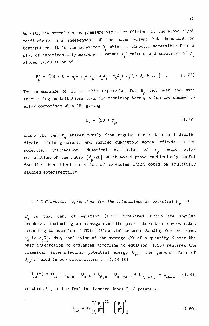
CHAPTER 2 CALCULATION OF THE SECOND LIGHT-SCATTERING

VIRIAL COEFFICIENTS OF NON-LINEAR MOLECULES

2.1 A· GENERAL THEORY OF LIGHT SCATTERING 45

2.1.1 Non-interacting molecules 48

2.1.2 Interacting non-linear molecules 51

2.2 DESCRIBING THE RELATIVE CONFIGURATION OF TWO NON-

LINEAR MOLECULES 60

2.3 EXPRESSIONS FOR CONTRIBUTIONS TO B FROM NON-LINEAR p

MOLECULES 61

2.4 EVALUATION OF B BY NUMERICAL INTEGRATION 73 p 2.4.1 Classical expressions for the intermolecular

potential energy U (r) 73 12

2.4.2 The integration procedure 80

2.5 CALCULATIONS OF B FOR ETHENE 81 p

2.5.1 Molecular properties of ethene 81

2.5.2 Results of calculations for ethene 86

2.6 CALCULATIONS OF B FOR SULPHUR DIOXIDE 88 p

2.6.1 Molecular properties of sulphur dioxide 88

2.6.2 Results of calculations for sulphur dioxide 92

2. 7 CALCULATIONS OF B FOR DIMETHYL ETHER 94 p

2.7.1 Molecular properties of dimethyl ether 94

2.7.2 Results of calculations for dimethyl ether 97

2.8 REFERENCES 99

CHAPTER 3 EXPERIMENTAL MEASUREMENTS OF SECOND LIGlIT­

SCATTERING VIRIAL COEFFICIENTS OF NON-LINEAR

MOLECULES

3. 1 THE LIGHT-SCATTERING APPARATUS

3.1.1 The optical bench

3.1.2 The laser

3.1.3 The scattering cell

3.1 . 4 The gas line

3.1.5 The analyzer

3 . 1. 6 The photomultiplier

3.1 . 7 The neutral density filter

3.1 . 8 The data acquisition system

3.2 EXPERIMENTAL MEASUREMENTS AND RESULTS

3.2.1 Results for ethene

3.2.2 Results for sulphur dioxide

3. 3 REFERENCES

CHAPTER 4 CALCULATION OF THE SECOND KERR-EFFECT VIRIAL

COEFFICIENTS OF MOLECULES WITH LINEAR AND

LOVER SYMMETRY

103

105

106

109

115

117

119

122

124

126

128

131

4. 1 INTRODUCTION 137

4.2 A GENERAL THEORY OF ELECTRO-OPTICAL BIREFRINGENCE

IN DENSE FLUIDS 138

4.2.1 Non-interacting molecules 139

4.2.2 Interacting spherical molecules 143

4.2 . 3 Interacting linear molecules 146

4.2.4 Interacting non-linear molecules 148

4.3 CALCULATIONS OF B FOR FLUOROMETHANE 165 " 4.3.1 Molecular properties of fluoromethane 165

4.3.2 Results of calculations for fluoromethane 166

4.4 CALCULATIONS OF B FOR TRIFLUOROMETHANE 168 " 4.4.1 Molecular properties of trifluoromethane 168

4.4.2 Results of calculations for trifluoromethane 169

4.5 CALCULATIONS OF B FOR SULPHUR DIOXIDE 170 " 4.5.1 Molecular properties of sulphur dioxide 170

4.5.2 Results of calculations for sulphur dioxide 173

4.6 CALCULATIONS OF B FOR DIMETHYL ETHER 176 " 4.6.1 Molecular properties of dimethyl ether 176

4.6.2 Results of calculations for dimethyl ether 178

4.7 CALCULATIONS OF B FOR THE LINEAR NON-POLAR MOLECULES " NITROGEN, CARBON DIOXIDE AND ETHANE 180

4.7.1 Molecular properties of nitrogen, carbon

dioxide and ethane

4.7.2 Results of calculations for nitrogen, carbon

dioxide and ethane

4.8 CALCULATIONS OF B FOR ETHENE " 4.8.1 Molecular properties of ethene

4.8.2 Results of calculations for ethene

4.9 REFERENCES

APPENDIX 1

Al.l ELECTRIC MULTIPOLE MOMENTS

APPENDIX 2

A2.1 AN EXAMPLE OF A FORTRAN PROGRAM TO CALCULATE

CONTRIBUTIONS TO B P

A2. 2 AN EXAMPLE OF A FORTRAN PROGRAM TO CALCULATE

CONTRIBUTIONS TO B "

180

180

184

184

187

190

193

195

205

1

CHAPTER 1

A REVIEW

1.1 Introduction

One of the primary tasks of the molecular physicist is the elucidation

of the electromagnetic properties of individual molecules. This is often

achieved by experimental investigation of the interaction of light with

macro?copic samples of matter, coupled with theories which relate the

macroscopic observables of such experiments to the molecular property

tensors of the molecules in the specimen. A typical example of this

technique is the measurement of the depolarization ratio p of light o

scattered by linear and quasi-linear molecules at low gas pressures,

which by suitable theoretical interpretation has long provided a means

for the accurate determination of the magnitude of the difference in

principal molecular polarizabilities, I all - aoll [1,2]. Often implicit in

such theories is the assumption that each molecule in the gas sample can

be treated as an independent system. This approximation is only

appl icable to a perfect gas, the typical gas sample in the laboratory

having bulk properties which differ from the ideal due to the presence

of molecular interactions.

Theoretical studies of the effects of these molecular interactions on

the optical properties of gases have, up until now, been limited to the

very restricted classes of spherical, quasi-spherical, linear and

quasi-linear molecules. The reasons for this are twofold. Firstly, there

is the almost prohibitively large volume of algebraic manipulation which

is required for the derivation of complete molecular tensor theories

describing the contributions even of pair interactions to the various

molecular-opt ic phenomena such as electric birefringence, molar

refraction and depolarized light-scattering. Secondly, the dipole­

induced-dipole (DID) model of Silberstein [3], where the dipoles induced

in molecules by an incident 1 ight wave g (t) interact with one another o

leading to DID coupling, appears to break down in calculations of the

various second virial coefficients of large quasi-spherical molecules

2

(see, for example, [4] and [5]). This may have led to a degree of

scepticism in the appl ication of DID theory to molecules of lower

symmetry.

It has recent ly been shown how the problem of . lengthy and tedious

hand-worked tensor manipulat ion can be managed by invoking t he use of

the powerful algebraic manipulation packages now available for personal

computers. In undertaking a molecular tensor theory of the second light­

scattering virial coefficient B for linear and quasi-linear molecules, p

Graham [6] made use of the Derive algebraic package. Later, Couling and

Graham [7] used the more powerful Macsyma symbolic manipulation package,

which unlike Derive has built-in tensor manipulation facilities, to

extend the series of tensor expressions contributing to B to include p field-gradient effects and induced quadrupole moments in the molecular

interactions. This allowed a definitive assessment of where the series

of interact ion terms had converged to a meaningful numerical value

for B . P

Once such theories for the second virial coefficients have been

developed for axially-symmetric molecules, there is a strong temptation

to approximate non-linear molecules to be of axial symmetry, and hence

calculate their virial coefficients. This thesis serves to show that

such approximations are grossly unsatisfactory. It will be shown, · for

example, that if the ethene molecule, which belongs to the D symmetry 2h

point group, is approximated to be of axial symmetry, the calculated B p

value differs from the experimental value by 40%. A similar discrepancy

has already been observed for sulphur dioxide, which is of C symmetry: 2v

when measured values of the second Kerr-effect virial coefficient, B, JC

for sulphur dioxide [8] were compared with values calculated using a

recent statistical-mechanical theory of B for axially-symmetric polar JC

molecules [9], the predicted values were generally found to be more than

twice as large as the experimental ones.

In this work we illustrate how the Macsyma package, which we ran on a

486 DX-2 66 MHz PC with 32 Mb of RAM, can be used to facil i tate the

development of complete molecular

light-scattering and Kerr-effect virial

tensor theories

coefficients for

of second

non-linear

molecules. It will become apparent that only when full account of a

non-linear molecule's symmetry is taken into consideration do we find

acceptable agreement between measured and calculated second virial

3 ,

coefficients.

Treatment of the various other second virial coefficients is not

considered here, although the same general methods are appl icable to

them, opening up new experimental possibilities in many molecular-optic

phenomena.

1.2 A general expression for second virial coefficients

In 1956, Buckingham and Pople demonstrated how the effects of molecular

interactions can be systematically accounted for by means of a

virial-type expansion [10). If Q represents a suitably chosen measurable

molecular-opt ic property, then its observed value can be expanded in

inverse powers of the molar volume Y . m

B C o 0

Q = Ao + V + + ... m y2

(1. 1)

m

where the virial coefficients A, B, Co' ... , are functions of Q 0

temperature alone. As expected, the ideal gas value for an assembly of

non-interacting molecules is recovered in the limit of infinite dilution

(y ~ (0), when Q becomes A. The higher-order virial coefficients B , m 0 Q

C, ... represent the deviations due to pair, triplet, ... interactions Q .

respectively.

If we consider one mole of non-interacting gas molecules, the

macroscopic property Q is simply the sum of N mean contributions q of A

the individual molecules. We have

Q = A = N q Q A (1. 2)

At higher densities, however, the contribution of molecule 1 to Q is not

always q since there are times when molecule 1 must be treated as half

of an interacting pair. If molecule 1 has a neighbouring molecule 2, the

relative configuration of which is given by the collective symbol T,

then the contri but ion of molecule 1 to Q at that instant is given by 1 tI12(T), where ql/ T ) is the corresponding contribution of the pair. If

we neglect triplet and higher-order interactions we obtain

4

(1. 3)

where P(T)dT is the probability of molecule 1 having a neighbour in the

range (T, T + dT). peT) is related to the intermolecular potential

energy U (T) by 12

N peT) = Q~ eXP(-U

12(T)/kT) (1. 4)

m

where Q = v:1 JdT is the integral over the orientational co-ordinates of

the neighbouring molecule. Now we have from equation (1.1)

B = Urn (1. 5) Q v ~ (XI

m

which coupled with equations (1.2), (1.3) and (1.4) yields a general

expression for B : Q

(1. 6)

This basic formula can then be applied to the various molecular-opt ic

properties Q.

The main thrust of this thesis is the extension of our previous

theoretical [6,7] and experimental [11 ] work on the second

light-scattering virial coefficient B for axially-symmetric molecules p into the regime of non-linear molecules. Hence, we proceed by reviewing

all previous work on B for molecules with spherical and linear p

symmetry. Our theoretical work on the second Kerr-effect virial

coefficient B for non-linear molecules grew out of the apparent success I

of the dipole-induced-dipole model in describing B for molecules of low p

symmetry (as will be seen in Chapters 2 and 3), and so is presented as a

separate, self-contained piece of work in Chapter 4.

5

1.3 Light-scattering phenomena

1.3.1 Historical background

Historically, the study of light scattering began in 1869 when Tyndall

conducted a series of experiments on aerosols [12]. A strong beam of

white light was passed through a colloidal suspension of particles, and

when viewed at right angles to the incident beam the scattered light was

seen to be blue in colour and linearly polarized. This provided some

justification for the already suggested idea that the blue colour of

skylight and its observed polarization was due to the scattering of

sunlight by small particles suspended in the atmosphere. Nevertheless,

the mechanisms involved in the scattering process remained unexplained,

with Tyndall saying (see Kerker [13]) "The blue colour of the sky, and

the polarization of skylight ... constitute, in the opinion of our most

eminent authorities, the two great standing enigmas of meteorology."

This enigma was resolved in 1871 by the third Baron Rayleigh, J. W.

Strutt, who in his theoretical discussion of the light-scattering

phenomenon [14] treated the incident light as vibrations in the ether

which, when encountering the suspended particles, set up forced

vibrations in them. These particles then in turn acted as secondary

sources of vibrations in all directions, hence scattering the incident

light. Rayleigh went on to show that the intensity of the light

scattered by a particle, assumed to be an isotropic sphere of diameter

much smaller than the wavelength A of the incident light vibration, was 4 proportional to 1/A, and that the component scattered at right angles

was completely linearly polarized perpendicular to the scattering plane.

This explained why blue light, which has a shorter wavelength than red

light, is more strongly scattered than red, leading to the blue colour

of the sky and of Tyndall's aerosols.

Lord Rayleigh refined his theory in 1899 by suggesting, as originally

postulated by Maxwell, that the blue skylight was not due to scattering

of sunlight by parti'cles suspended in the air, but rather due to

scattering by the individual air molecules themselves [15]. It was only

some seventeen years later, in 1916, that this theoretical prediction

was experimentally confirmed, with Cabannes [16] passing an incident

beam of white light through a pure, dust-free gas sample and observing

6

the 90° scattered light to be blue in colour and linearly polarized, but

much weaker in intensity than the light scattered by the relatively

larger particles in Tyndall's colloidal suspensions.

Imperfections in Lord Rayleigh's theory became apparent when his son R.

J. Strut t, the fourth Baron Rayleigh, conducted his own experiments

[17]. He found that the light scattered at right angles to the incident

beam was in fact not completely linearly polarized, and that the exact

extent to which depolarization occurred was a characteristic constant of

a particular gas. R. J. Strutt then extended his father's theory, which

assumed isotropic spherical scattering centres , by relating the

depolarization ratio to departures from spherical symmetry of the

optical properties of the gas molecules [18].

The following decade saw a prolific number of measurements being made on

a variety of gases and vapours, despite the almost insurmountable

experimental difficulties encountered. During this activity, the Raman

effect was discovered, in which the scattered light has well defined

frequency shifts . Most of the subsequent work was diverted into this new

field, and the conventional Rayleigh scattering was only seriously

revisited in 1961 when J. Powers [19] published new values for the

depolarization ratio of several gases . Powers, like the earlier workers

in this field, used a white light source; but rather than using the less

than adequate visual or photographic detection techniques of the earlier

workers, he employed a photomult iplier as the detector of scattered

light . His results indicated that the depolarization ratios measured in

the 1920-30 era were too high often by as much as 10%. The advent of the

laser had a revolutionizing impact on work in . this field, its highly

intense and parallel beam of monochromatic light first being exploited

by Bridge and Buckingham [20] and then by various other workers

[2,21-25] who made detailed and accurate measurements of the

depolarization ratios of many gases and vapours. Their values were even

lower than those of Powers, further confirming the inadequacy of the

experimental techniques used by workers in the 1920-30 era.

7

1.3.2 Interacting spherical molecules

Although isolated spherical molecules cannot depolarize the light which

they scatter, in gases of spherical molecules at elevated pressures a

small depolarization ratio is observed. This has been attributed to the

modification of the effective molecular polarizability a of a molecule

as a result of the molecular interactions which occur during collisions

or close encounters between neighbouring molecules, and has been the

subject of intensive theoretical and experimental investigation

[4,26,27 ].

This pressure-dependent depolarization ratio is best interpreted by

means of the virial expansion [28]

(1. 7)

where the second light-scattering virial coefficient B describes the p

contribution to p arising from interactions between pairs of molecules,

and where C describes contributions due to triplet interactions, etc. p Y is the molar volume of the gas. Using dipole-induced-dipole theory

m

[26], B can be written p

B = p

4nN 6a

s2 IOO

__ A _ R-4 exp (-U (R)/kT) dR , (4ncJ2 0 pq

(1. 8)

where N is Avogadro's number, A

a is the molecular polarizabil i ty, and U (R)

pq is the intermolecular potential energy between interacting

molecules p and q which are separated by a distance R. Retaining only

the leading term in equation (1.7), the depolarization ratio can now be

written

p = y- 1 x m

4nNA 6as

2 Ioo

R-4

exp (-U (R)/kT) dR . (4ncJ2 0 pq

(1. 9)

In early calculations, this integral

functions of Buckingham and Pople [28]: was evaluated using the H

k

( 1. 10)

8

where tfJ(R) is the Lennard-Jones 6: 12 potential [29]. Values of H (y) ~ k

have been tabulated [28] for k ranging from 6 to 17 in integral steps.

Watson and Rowell's calculated values of B [4] obtained from equation p (1. 8) are presented in table 1. 1, together with their experimentally

measured values of B. Subsequent workers have further confirmed the p

Bexpt/Btheory ratios given in table 1.1 for both argon [33,34,36] and p p

methane [33,35,36]. An important feature of these results is the

apparent breakdown of the DID theory of molecular interactions for the

larger spherical and quasi-spherical molecules. Note, for example, the

stark disagreement between the theoretically predicted and

experimentally measured depolarization ratios of sulphur hexafluoride

and neopentane as listed in table 1. 1. Watson and Rowell argued that

this discrepancy between theory and experiment for the large molecules

provides evidence of the inadequacy of the point-dipole approximation

used in the DID theory, but this has not been establ ished and the

problem remains unresolved.

Table 1.1. Theoretical and experimental second light-scattering virial coefficients B for several isotropic gases at T = 298 K, as reported by

p Watson and Rowell [4] and Thibeau and Oksengorn [30].

a

b

Molecule Theoretical Experimental [4 ]

argon 1. 313a <2

1. 206 b

krypton 2.72a 2.3 ± 0.3

2.205 b

methane 2.41 a 2.9 ± 0.4

2.39 b

sulphur 2.43a 6.1 ± 0.2

hexafluoride 1.93b

neopentane 4.7 b 32 ± 4

Using Lennard-Jones constants reported in

Using Lennard-Jones constants reported In

Experimental [30]

0.88 ± 0.04

1. 80 ± 0.06

[ 31]

[32]

Bexpt[4]

p Btheory

p

0.85

1. 04

1. 20

1. 21

2.51

3.16

6.8

9

1.3.3 Interacting linear and quasi-linear molecules

Non-interacting anisotropic molecules (i.e. molecules which have a

departure from spherical symmetry of their optical properties)

inherently produce a scattered depolarized intensity which has been

found to be proportional to the square of the polarizability anisotropy

(to be defined in due course). At elevated pressures, molecular

interactions modify this inherent depolarization ratio p of anisotropic o

molecules. The density dependence of the depolarizat ion rat io p is

described by means of the virial expansion

(1.11)

where the second light-scattering virial coefficient B describes the p

deviations from p due to pair interactions, C the deviations from p o p 0

due to triplet interactions, etc. The first detailed theories of

pressure-dependent light scattering by anisotropic molecules [37,38]

showed that the leading interaction term in equation (1.11), that in B , P

has the general form

B = (p - ~ p2) (2B + 1 ) p 0 3 0 P

(1. 12)

where B is the normal pressure virial coefficient, and where 1 arises p

from angular correlation [37] and collision-induced polarizability

anisotropy [38]. Dayan, Dunmur and Manterfield [39] have emphasized that

the presence of B in equation (1.12) may lead to a serious degradation

of the precision of ~ values deduced from experimental observations of p

Bp' especially when accurate values of B are not available. These

problems are further compounded by the fact that developing a complete

molecular tensor theory of B for anisotropic p molecules involves

extremely lengthy and tedious tensor manipulation coupled with very

time-consuming numerical integration of the resulting averaging

integrals even when using fast computers. A combination of these

difficulties, coupled with the lack of success in explanations of the

light-scat tering virial coefficients of spherical molecules, probably

accounts for the dearth of experimental and theoretical work that has

been undertaken in this field .

10

By 1980, Dayan, Dunmur and Manterfield [39] had measured Bp for carbon

dioxide, carbonyl sulphide and nitrogen; while Berrue, Chave, Dumon and

Thibeau [40] had measured B for nitrogen and ethane. By 1992, B had p p

not been measured for any other non-spherical gases, whi Ie the only

linear molecule to have been investigated theoretically [41,42] was

nitrogen. This gas probably received theoretical treatment because of

its particularly small B value at around room temperature, with a very

favourable ~ value of nearly five times as large. The expressions for p

the ~ p

contribution to B for nitrogen presented by Berrue, Chave, Dumon p

and Thibeau [41,42] included angular correlation and collision-induced

polarizability, but neglected the polarizability anisotropy in the

successive dipole-induced-dipole interactions which occur during

collisions. Their result for nitrogen agreed remarkably well with

experiment, although they argued that this may have been fortuitous in

view of the cancellation of large terms of opposite sign.

It is quite likely that expressions with the above approximations would

prove inadequate in describing the ~ p contribution to B for linear

p molecules in general. Fortunately, the advent of powerful computer

algebraic manipulation packages such as Derive and Macsyma, coupled with

high speed Fortran compilers, has made possible the development of a

complete molecular tensor theory of B. Graham [6] has presented a p

comprehensive set of calculations of B for molecules with threefold or p

higher rotation axes performed using the Derive algebraic manipulation

package coupled with the fast Salford FTN77/386 Fortran compiler.

However, due to the limitation of computer memory when using the Derive

package on an 80386 personal computer, the calculations were limited to

scattered intensities proportional to 4 IX at most. A new

personal-computer version of the symbolic manipulation package Macsyma,

which provides access to much larger amounts of computer memory, and

also to powerful tensor manipulation facilities not available on the

Derive package, was acquired by our research group in 1992. Couling and

Graham [7] subsequently used the Macsyma package to extend the series of

tensor expressions contributing to B to include dipole-dipole scattered p

intensi ties of the fifth power in the molecular polarizabi I i ty IX, as

well as a range of additional terms arising from field-gradient effects

and induced quadrupole moments in the molecular interactions . This

allowed a definitive assessment of where the series of interaction terms

had converged to a meaningful numerical value for B . The higher-order p

terms were found in some instances to make significant contributions to

11

B as shall be seen in due course, and these calculations served to p'

establish orders of precision to which one has to work to ensure

convergence.

1.4 Calculations of second light-scattering virial coefficients of

linear and quasi-linear molecules

1.4.1 Expressions for molecules with threefold or higher rotation axes

Buckingham and Stephen [38] have derived an expression for the

depolarization ratio p of Rayleigh-scattered light which includes the

effects of interacting pairs of molecules, obtaining

p = ( 1. 13)

N( (1) (1» N( (1) (2) ) 1( 1( + 1( 1( cos X

xx xx xx xx 12

Here, 1(p) is the differential polarizability of molecule p in space­(xo"

fixed axes (x,y,z) located in the gas sample, and the angular brackets

indicate an average over pair encounters. The probability that molecule

1 has a neighbour in dT at T has been related to the intermolecular

potential energy U (T) by Buckingham and Pople [4], yielding the 12

expression already quoted in equation (1.4).

We follow Buckingham [43] in writing the dipole moment ~ and quadrupole (X moment a~ induced in a non-magnetic molecule by an electrostatic field

E(X and its gradient E~ as

E ~ A E ~(X = (X~ ~ + 3 ~r ~r + ... , ( 1. 14)

and

( 1. 15)

Using the above two equations, which allow inclusion of dipole-dipole

terms as well as the leading terms arising from field gradient effects

and induced quadrupole moments in the molecular interactions, the

12

differential polarizability may be written [6,7]

1 (P)T(P)c(q) T(P) (p) + - a a

3 a$ ~ra ra£~ £~~ ~U

1 A(P)T(P) (q) + - a 3 a$r ~ra aU

1 A(P)T(P) (q)T (p) + - a a 3 a~r ~ra a£ £~ ~

+ .... (1. 16)

Here, the superscripts p and q indicate molecule p and q respectively,

whlle [43]

and

= _1_ 'iJ 'iJ R-1

41(£ a ~ o

1 ( 2) -5 41(£ 3RaR~ - R a a$ R (1. 17)

o

T(l) = __ 1_ 'iJ 'iJ 'iJ R- 1

a$r 41(£ a ~ r

are the second

field E( 1) and a

o

( 1. 18)

and third rank T-tensors used to express the electric

the electric field gradient E(l) at the origin of a$

molecule 1 arising from the point dipole and quadrupole moments of

molecule 2, which is at a position R from the centre of molecule 1, in a

the form

E( 1) = T~~) Il~ 2) - !. T~~) a~2) + . . . a ""fJ'" 3 ""fJr,..r

( 1. 19)

and

(1 . 20 )

13

We have from [43] that

(1.21)

where n is the order of the I-tensor. It follows from equation (1.21)

that the superscript may be omitted for I-tensors of second rank while

it has to be retained for I-tensors of third rank.

Use of equation (1 . 16) in (1.13) yields

where

a 5

p = a +a +a +a +aA +aA +aC + .. .

2 3 4 5 21 31 31

b + b 2 3

( (ll (ll) «1) (2»

a=ex ex +ex ex • 2 zx zx zx zx

( (OI ( 2) (2» « 0I ( 2) (ll) ex ex ex +ex ex ex • z~ ~r rx zx z~ ~r rx zx

(1. 22)

(1. 23)

(1. 24)

(1. 25)

(ex(l)T ex(2)T ex(l)T ex(2)ex(2»

zo or r~ ~v v~ ~c Cx zx •

(1. 26)

14

(1. 27)

(1. 28)

Yex(llT

(llC

(2) T(llex

(llex(2»

3\ zo oP1' P1'f34> f34>c Cx zx '

(1. 29)

= ex ex + ex ex COS b <

(1) (1» < (ll (2) X) 2 xx xx xx xx 12'

(1. 30)

(1. 31)

15

To proceed , the explicit forms of Taf3 , Taf3r , aaf3' · Aaf3r , and Caf3ro are

required. The molecular property tensors a f3' A f3 ' and C f3 s simplify a a r a ru considerably for molecules of high symmetry, with far fewer tensor

components being required to describe the molecular properties of, say,

a linear molecule than a molecule of lower symmetry.

The ensuing analysis is restricted to linear and quasi-linear molecules,

. and if the rotation axis of such a molecule co-incides with the 3-axis

of a molecule-fixed system 0 , 2,3)

a 11

= a = a 22 .l

and a 33

then a IJ

is diagonal with

The t erm (IV (1 ) ,) 1 ») l' n t . (1 23) f t f . d d ...... equa Ion . re ers 0 space- lxe axes, an

zx zx

may be referred to molecule-fixed axes by the normal tensor-projection

procedure to yield

(

(1) (1») a a = zx zx (

(1) (1») ( z z x x) a a aaaa 1 J kl 1 k J 1

(1. 32)

a where a is the direction cosine between the a space-fixed and i

1

molecule-fixed axes, and where the average is over all isotropic

orientations of molecule 1 in the space-fixed axes. Use of the standard

isotropic average [44]

leads to the familiar expression

(a(1)a(1l) = _1_ C )2

all - a.l . zx zx 1 5

Similar arguments, together with the result [44,1]

(xxxx) aaaa = 1 J k 1

1

1 5 (0 0 + 0 0 + 0 0 )

1 J kl 1 k J 1 11 Jk '

allows (a:~)a:~») in equation (1.30) to be simplified to

( (1) (1)) 2 4 a a = a + xx xx 45

where

(1. 33)

(1. 34)

0 . 35)

(1. 36)

(1) d (2) Now, in their own molecular axes, a

lJ an a l , J'

remaining averages in equations (1.23) to (1.26),

16

( 1. 37)

are diagonal, and the

and (1 . 30) and (1 . 31),

must be expressed in terms of these diagonal elements and a set of

interaction parameters . Equations (1.27) to (1.29) with their added

complications of third and fourth rank tensors, shall be dealt with in

due course. Meanwhile, the more manageable averages shall be considered.

Figure 1. 1 shows pictorially how the relative configuration "t of two

axially-symmetric molecules may be specified by the four parameters 81

,

8 , ~ and R [43]. Here, R is the distance between the centres; 8 and 8 2 1 2

are the angles between the line of centres and the dipole axes of

molecules 1 and 2; and ~ is the angle between the planes formed by the

molecular axes and the line of centres. The unit vectors ~(1) and l2) along the dipole axes, and ~ along ~, will be required later.

Now, the molecular property tensors of a molecule are generally

specified relat i ve to a co-ordinate system of mutually perpendicular

axes that is fixed in the molecule such that one of the axes co-inc ides

with a symmetry axis of the molecule. This is seen in figure 1.1 where

the co-ordinate systems of molecules 1 and 2 are 0(1,2,3) (referred to

by tensor indices i, J, k, .. . ) and 0'(1'2'3') (referred to by tensor

indices i', j', k', . . . ) with axes 3 and 3' chosen as the symmetry-axes

for molecules 1 and 2 respectively. The space-fixed system O(x, y, z)

(referred to by tensor indices a, ~, r, .. . ) has its origin at molecule

1, which does not shift with the changing orientation of either

molecule.

Initially, all tensors are referred to (1,2,3), including a(2) which is 1 J

in general not diagonal in (1,2,3). A projection from (1,2,3) into

(1' ,2' ,3'), where a~~~, is diagonal, will be carried out later. The

reason for initially referring all tensors to (1,2,3) lies in the fact

that for a given relative configuration of the pair of molecules, the

tensor product in (1 , 2,3) is fixed. If the pair of molecules is then

allowed to rotate isotropically as a rigid whole in (x,y,z), then the

projection into (x,y,z) of this pair property (referred to (1,2,3)) can

be averaged over all orientations. Averaging over the interaction

parameters may subsequently be carried out. Simplification during the

17

above procedure is facilitated by the following well-established

relationships , which allow the expressions to be cast in terms of the

four interaction parameters:

(1. 38)

t(1)t(2) = t(2) = cosS = -cosS cosS + sinS sinS cost/> , 1 1 3 12 1 2 1 2

(1. 39)

l1) 1\ = 1\ = cosS (1 . 40 ) 1 1 3 1

(1. 41)

Buckingham [43] has also shown that for axially-symmetric molecules, the

molecular property tensors themselves may be expressed in terms of t(2). 1

For example

a (2 ) = a 0 + rail - a ) l2) l2) . Ij .1 Ij \: .1 1 j

(1. 42)

Use of the anisotropy K. in the molecular polarizabi 1 i ty tensor a0:f3'

defined by

K. = (1. 43)

together with equation (1.37) allows equation (1 . 42) to be recast as

(1. 44)

Benoit and Stockmayer [37] were the first to establish the now familiar

results

/ (1) (2» 1 ( )2 < 2 ) \azx azx = 30 Lan - a.l 3cos S12- 1 , (1. 45)

which is a contribution known as the angular correlation term; and

< (1) (2) ) 1 2

a a cos X = xx xx 12 1 5 3 (1. 46)

where B is the second pressure virial coefficient.

18

The new higher-order terms are evaluated using a procedure which will be

ill ustrated by considering a specific example, i. e. the term

la(1)a(ll T a(2)T a(ll T a(2», which is the first term in a given by '\ zx zc5 c5)')'fl flv v{3 (3e ex 5

equation (1 . 26) . The first step is to project the term from space-fixed

axes (x,y,z) into the molecule-fixed axes (1,2,3) of molecule 1:

= a aa a aa aa a a:a a aa aaa aa

< (1) z x (1) z 15 T 15)' (2»), fl T aflaV (1) v f3T f3 e (2) e x) i J i J k 1 k 1 mn m n p q p q r s r stu t u v w v w 9 h 9 h

< (1) (1) T ( 2 ) T ( 1 ) T ( 2 » ( z z x x) = a a a a a aaaa . i J k m m n nr r s s v v w w h i k J h (1.47)

If the interaction configuration is fixed, then the term

la(1)a(1)T a(2)T a(1)T a(2» is a constant; and if the rigid pair of '\ i J km mn nr rs sv vw wh

molecules is allowed to rotate isotropically, then equation (1.33) may

be invoked to yield the average projection

= 1 (4a ( 1 ) a ( 1 ) T a ( 2) T a ( 1 ) T a ( 2 ) _ a ( 1 ) a ( 1 ) T a ( 2 ) T a ( 1 ) T a ( 2 ) 3 0 kh km mn nr rs sv vw wh i i km mn nr rs sv vw wk

(1) (1)T (2)T (1)T (2» -a a a a a

hk km mn nr rs sv vw wh

(1. 48)

in which the angular brackets now indicate an average over the pair

interaction co-ordinates R, 91

, 92

, and rp according to the general

relationship

(X) = J X peT) dT T

(1. 49)

where P( T) is the probabi 11 ty that molecule 1 has a neighbour in

19

dT at T. This probability has been related to the intermolecular

Potential energy U (T) in equation (1.4), which when substituted into 12

(1. 49) yields

<X) = N 00 1l

A J J 2V m R=O 8 =0

1

J21l 2

X exp (-U IkT) R dR sin8 sin8 d8 d8 d4>. 12 1 2 1 2

4>=0 (1. 50)

(1) (2) d T substituted When the appropriate values for a1J

, a1J

, an IJ are

into (1. 48) there resul ts a lengthy expression containing redundapt (2) (2)

interact ion parameters t , t , A, and A. Averaging according to 1 2 1 2

equation (1.50) can only be performed after these redundant interaction

parameters have been el iminated from the right hand side of equation

(1.48), and this is achieved by making use of equations (1.38) to

(1.44). When performed manually, this manipulation is extremely tedious

and time-consuming: one of the reasons why higher-order terms were

neglected from earlier calculations of B for linear molecules. Graham p

[6] ini t ially carried out all of the work up to a manually, and then 4

verified the results with the assistance of Derive, which is a computer

algebraic manipulation package from Soft Warehouse Inc. However, the

derivation of the a expression in equation (1.25) was found to be only 4

just within the 640 kb computer memory limitations of the Derive package

even when evaluating each of the terms in a individually. Subsequently, 4

Couling and Graham [7] evaluated the a term, as well as the a A , 521

a A, and a C terms which required tensor manipulation techniques not 3 1 3 1

available in the Derive package, using the algebraic manipulation

package Macsyma. A new version of Macsyma, compatible with the 80386

series of personal computers, was obtained, providing access to much

greater amounts of computer memory as well as to powerful tensor

manipulation facilities. Adequate speed and capacity were only obtained

after installation of 8 Mb of memory, the standard 4 Mb being totally

inadequate.

Eliminat ion of <2), l~2), A1

, and A2 from the expanded expr~ssions may

be achieved on computer by the piecemeal substitution of powers and

multiples of the parameters

(1. 51)

e = (D1(2»)2 + [D

2(2»)2 __ ( 2 {, (, 1 - cos 8

12) , (1.52)

20

and

f = l21;\ + l21;\ = - cose - cose COSe 1 1 2 2 2 1 12

(1. 53)

into the expanded forms, until they contain d, e, and f only, and no

terms in the redundant parameters. This elimination procedure is by no

means automatic, wi th considerable human intervent ion being required.

Such intervention carries with it the possibility of errors, but the

back-substitution of the explicit forms of d, e, and f (in terms of e(21 1

and ;\ ) into the simplified expressions followed by comparison with the 1

original expanded expression provides a quick and absolute means of

guaranteeing the correctness of the simplified expressions. This is

followed by final substitution according to the second parts of

equations (1.51) to (1.53), and compression of terms of similar order

into a single term. It was found that

( r 1

a3= 4::

0 a? (R- 3 (-27K(K - 1) (2K + 3)cos2e1

a= 4

- 324K2

(K + l)cose cose cose + 27K(K -1)(2K-l)cos2e 12 2 1 2

- 108K2

(K + 1)cos2e 12+ 36K(K - 1))) , (1. 54)

( 41(£ )-2 o 4 < -6 ( 2 2 4 30 ex R 324K (K - 2K + 1 )cos e 1

+ 1944K3

(K - l)cose cose cos3e + ((5103K4cos 2e 12 2 1 12

+ (405K3

(K - 1)cos2e - 27K(8K3

- 24K2+ 21K 5))cos2e 12 2

+ 567K4cos

4e - 27K2(9K2- 10K - 14)cos2e

12 12

( 43 2 + 18 2K - 9K + 11K - 6K + 2))) , (1. 55)

b= 3

a= 5

21

(4::,r'a 3 (R-3 (-36K(K _ 1)(2K + 7)C0529,

_ 108K2 (2K + 7)cosS cosS COSS1- 36K2(2K +7)cos

2S 2 12 12

(1. 56)

4 5 + 1458K (K - 1)cosS cosS COS S 2 12 1

+ 9K2(27K2(9KCOS2S + 2K - 2)cos2S - 9K(7K2

+ 25K - 23)cos2S 2 12 2

3 2 4 3 2 2 - 23K + 75K - 81K + 29)cos S + 27K cose cosS (54K COS S 1 2 12 12

2 2 344 - (54K(2K + 5)cos S + 52K - 23k - 11»cos S + 3K(81K COS S 2 1 12

2 2 432 2 + 81K (K - 7K + 6)cos S - 3K(K - 228K + 225K - 55)cos S 2 2

5 4 3 2 ) + 8(-2K + 7K - 13K + 14K - 7K + 1) (1. 57)

The presence of the third and fourth rank tensors A , T and C iJk iJk' iJkl

in the terms (1.27) to (1.29) necessitated the use of the tensor

manipulation facilities of Macsyma. Buckingham [43] has shown that for

axially-symmetric molecules, the molecular property tensors A and iJk

C may be expressed in terms of the t(2) as follows: i Jkl i

A (2) = ~ A (2) t(2) (3t(2) t(2) - 0 ) i Jk 2 II i J k i J

+ A (2) (t(2) 0 + t(2) 0 _ 2l 2 ) t(2) l2») .1 J ik k i J i J k '

(1. 58)

C(2) IJkl

1 = 1 0

1 +

2 8

rC + 8C1313

+ 8C ) [!. (0 0 + 0 0 ) - !. 0 0 ] L 3333 1111 2 1 k J 1 1 1 J k 3 1 J k 1

(5C 3333

+ 4C 1313

BC ) [(3e ( 2) e ( 2) - 0 ) 0 1111 1 k lk Jl

+ (3e(2) e(2) - 0 )0 + (3e(2) e(2) - 0 )0 1 1 11 lk 1 k lk 11

+ (3e(2) e(2) - 0 )13 - ~(3e(2) e(2) - 13 )13 J 1 Jl lk 3 1 J IJ kl

- ~(3e(2) e(2) - 13 )13 ] 3 k 1 kl IJ

. + 1 (2C _ 4C + C ) [35 e< 2) e ( 2) e ( 2) e ( 2) 3 5 3333 1313 1111 1 J k 1

22

+ e(2)e(2)13 + e(2)e(2)13 ) + 13 13 + 13 13 + 13 13 ] (1. 59) J 1 lk k 1 1 J 1 J kl 1 k J 1 11 J k

These tensors, with their superscript (2) , refer to molecule 2 as seen

the molecule-fixed axes of molecule 1. Now, (1) e(2) from since e and are

unit vectors along the dipole axes of molecules 1 and 2 respectively, in (1) (1) (1)

the axes ( 1,2,3) the vector t must have components t = t = 0 ~ 1 2

(1) (1) and t = 1. Hence, to obtain an expression for A from (1. 58), (2) 3 (1) (2) (2) (2) IJk e must be replaced by t = 13 ; while t t t must be replaced 1 1 13 1 J k

by t(l)t(1)t(1) = 13 13 13 etc. Similarly, to obtain an expression for 1 J k 13 P k3

C(l) from (1.59), t(2 •• • l2) must be replaced by 13 ••• 13 etc. IJkl 1 J 13 13

Finally the tensor expressions for each term in a2A

1, a A, and a C are

3 1 3 1

1 · itl d i t f (1) (2) T T(l) A(l) A(2) ex.p IC y expresse n erms 0 (XIJ' (XIJ' , , , IJ IJk IJk IJk'

C( 1) and C(2). after which Macsyma is used to eliminate redundant IJkl' IJkl'

interaction parameters and to compress the results as before, yielding

the final expressions

aA= 2 1

a A = 3 1

23

2 2 2 2 + cose ((-540K(K + l)cose + 540K )cos e + 216K cos e

1 12 2 12

2 + 108K cose + 216K)cose 12 2

2 3 1 + 540KCOS e (KCOSe - K - l)cose + 180K(K - l)cos e 1 12 2 1

+ All [-135K(K - 1)cos3e + cose (405K(K +l)cose cos2e

2 1 12 2

222 + (162K(K + l)cos e - 162K cose + 81K - 81K)cose 12 12 2

+ 810K2cos2e cose cose + 270K(K - 1)COS3 e11)) ,

1 12 2 (1. 60)

+ 810K(K - l)cose cose cos4e + (27K(45Kcos 2e + 11K 2 12 1 2

. 2 2 2 3 - 11)cos e - 45K(K + 8)cos e - 182K + 364K - 182)cos e

12 2 1

2 4 223 2 + 3(54K cos e + 27K (llcos e - 2)cos e - K(189Kcos e 12 2 12 2

(continued ... )

2 S + 6K(10K - 1)cos9 cos9 + 135(K - 2K + 1)cos 9

2 2 12

2 S + A [-9K(135(K - 2K + 1)cos 9

II 1

4 2 + 810K(K - 1)cos9 cos9 COS 9 + (21K(45KCOS 9

2 12 1 2

2 2 - 2 + 11K(K - 1))cos 9 + 45K(5K - 2)cos 9 - 2(85K - 146K

12 2

32322 + 61))cos 9 + 3cos9 (291K cos 9 + 81K (5cos 9

1 2 12 2

2 3 2 2 - 81K cos 9 + 3(99K(K - 1)cos - (21K - 49K 12

24

(1.61)

( )-2

41(£ < o 3 -8 2 6 A C = 10 ex R (6C K[150(K - 2K + 1)cos 9 3 1 l: 3333 1

( 2242 + 12K K - 1)cos 9 - 35(K - 2K + 1))cos 9 + 30Kcos9 (36KCOS 9

12 1 12 12

(continued • •• )

25

18K2cos2a )cosa - 10(K2- 2K + 1)cos4a + 3«33K

2+ 16K + 8)cos

2a

12 1 2 12

2 2 27K2 COs 49 _ 3(7K2- 1)cos29 - (4K2

+ 4K + 1)] + 2K + l)cos 92 + 12 12

26 5 _ 24C K[75(K - 2K + l)cos 9 + 450K(K - 1)cos9 cos9 cos a

1313 1 12 2 1

+ 5(15K(9KCOS2912

- (K + 2))COS292

+ 2(18K(K - 1)COS29

12- 11(K

2 - 2K

+ 1)))cos4a + 30KCOSa (18Kcos 2a + 11 - 17K)cosa Cos3a + 3(25(3K

2

1 12 12 2 1

4222224 + 2K + l)cos a - 15(9K (cos a + 2K + l)cos a + 36K COS 9 - K(55K

2 12 2 12

(1.62)

Upon gathering the results in equations (1.34), (1.36), (1.45), (1.46),

(1.54) to (1.57), and (1.60) to (1.62), equation (1.22) for p takes the

form

P =

1 +-

3 0 ( )

-2 4 4nc 0 a a' +

4

1

3 0

3

9 0 ( )

-1 2 4nc 0 a a A'

2 1

26

(1. 63)

in which a' represents that part of a in equation (1. 54) which is 3 3

contained within the angular brackets, with similar definitions for a', 4

a' a A' a A' and a C' which occur in equations (1.55), (1.57), 5' 2 l' 3 l' 3 1

(1.60), 0.61), and 0.62) respectively.

Equation (1 . 63) must now be cast in the virial form of equation (1.11).

We require the following expression for P for linear molecules, which o

was first derived by Bridge and Buckingham [21]:

where

3(lla)2

- a .J.

(1. 64)

(1. 65)

This allows equation (1.63) to be written in the form

Po [1 + ~ (3COS29 - 1) +

3 4 P = 1

( r1 a 1 ( r2 a - 4nc -- a' + - 4nc -- a' 2 12 2 o (lla)23 2 o (lla)24

1 5 2

( r3 a 1 ( r1 a + - 4nc -- a' + - 4nc -- a A' 2 o (lla)25 2 o (lla) 2 2 1

3 3

+ o[ ~~J] / {1 1 ( r2 a 3

( r2 a + - 4nc -- a A' + - 4nc -- a C' 2 0 (lla)2 3 1 2 o (lla)2 3 1

+ ~ P [~( 3cos 2 9 - 1) +

3 3

2B o( ~~]]} , - (4nc ) -1_a_ b' + - + 3 0 2 12 8 o (lla)23 Vm

0.66 )

27

which reduces to

p = p + P (1 - ~ p ) [2B + ~ \3COS2e - 1) + _cx_ {1 + ~2}(41[C r 1a' o 0 3 0 Vm 2 12 18,,2 5 0 3

+ ~ {1 4 2}( r2 a' + £ {1 + 4 2}C r 3

18,,2 + ~ 4rrc

o 4 18,,2 ~ 4rrc o a~

+ _1 {1 + 4 2}C r 1 + _cx_ {1 + ~2 }C4rrc J-2 a A' -K 4rrc a A' 18,,2 5 021 18,,2 3 1

+ ~ {1 4 2}C r 2 a C' cx C r 1 b' + o[~~J] . (1. 67) + ~ 4rrc

o - - 41[c

6,,2 3 1 30 0 3

It follows that

(1. 68) where

G = ~ (3cos2e - 1) V 2 12 m • (1. 69)

cx {1 4 2}C r 1 a = + -K 4rrc V a' 3 18,,2 5 0 m 3

(1. 70)

2 { cx 1 4 2}C r 2 a = + -K 4rrc V a' 4 18,,2 5 0 m 4

(1.71)

= L {1 4 2}C )-3 a + -K 4rrc V a' . 5 18,,2 5 0 m 5 (1. 72)

as4 1 {1 4 2}C )-1 = + -K 4rrc V a A' 2 1 18,,2 5 0 m 2 1 (1. 73)

as4 cx {1 4 2}C r 2 = + -K 41[C V a A' 3 1 18,,2 5 0 m 3 1

(1. 74)

a~ = ~ {1 + 4 2}C )-2 -K 4rrc V a C' 3 1 6,,2 5 0 m 3 1 (1. 75)

and

& cx C4rrc r 1v b' =

30 3 o m 3 (1. 76)

28

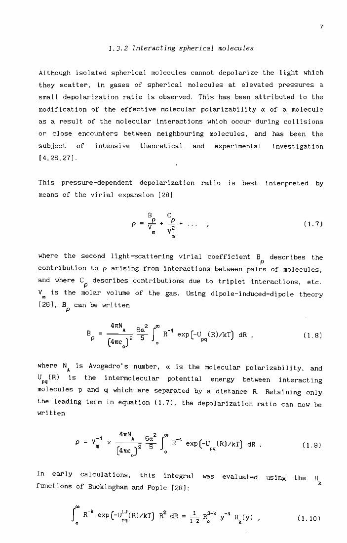
As with the normal second pressure virial coefficient 8, the above eight

coefficients are independent of the molar volume but dependent on

temperature. It is the parameter 8 which is directly accessible from a P

plot of experimentally measured P versus v:1 values, and knowledge of Po

allows calculation of

8' = (28 + G + a+ a+ a + aA+ aA+ a ~ + & + ... ) (1. 77) p 3 4 5 2 1 3 1 3 1 3

The appearance of 28 in this expression for 8' can mask the more p

interesting contributions from the. remaining terms, which are summed to

allow comparison with 28, giving

8' = (28 + 1 ) p p

(1. 78)

where the sum 1 arises purely from angular correlation and dipole­p

dipole, field gradient, and induced quadrupole moment effects in the

molecular interaction. Numerical evaluation of 1 would allow p

calculation of the ratio (1 128) which would prove part icularly useful p

for the theoretical selection of molecules which could be fruitfully

studied experimentally.

1.4.2 Classical expressions for the intermolecular potential U (L) 12

a; is that part of equation (1.54) contained within the angular

brackets, indicating an average over the pair interaction co-ordinates

according to equation (1.50); with a similar understanding for the terms

a' to a C'. Now, evaluation of the average (X) of a quantity X over the 4 3 1

pair interaction co-ordinates according to equation (1.50) requires the

classical intermolecular potential energy U . The general form of 12

U (L) used in our calculations is [1,45,46] 12

in which U is the familiar Lennard-Jones 6: 12 potential LJ

(1. 80)

U U and f..L,f..L f..L,S

quadrupo 1 e and

Us,s are the electrostatic dipole-dipole,

quadrupole-quadrupole interaction energies

29

dipole­

of the

permanent moments of the two molecules; while U and U are S,lnd f..L f..L,lnd f..L

dipole-induced-dipole and quadrupole-induced-dipole interaction

energies. The anisotropy of repulsive forces is represented by U h s ape

For interact ing linear molecules in the co-ordinate system shown in

figure 1. 1

(1.81)

Uf..L,S = 4!Co{~ f..LSR-4[cOSS1(3cos2S2- 1) + COSS2 (3cos2S1- 1)

+ 2sinS sinS cosS cos~ + 2sinS cosS sinS cos~]} , 1 2 2 1 1 2 (1. 82)

+ 2sin S sin S cos ~ + 16sinS cosS sinS cosS cos~ , 2 2 2 )} 1 2 1 1 2 2

(1. 83)

U = f..L,lnd f..L (1. 84)

and

U = S,lnd f..L

(1. 85)

Here, Uf..L,lnd f..L has been written so that its unweighted orientational

average is zero and the orientational-independent part is assumed to be

incorporated in the R-6

term of U [28]. In the two induction terms, LJ

the mean static polarizability a is used to describe the quasi-static s

interaction.

The shape potential is [28]

(1. 86)

where D is a dimensionless parameter called the shape factor, and which

Figure 1.2 (a). Colliding spheres.

3 ~~~ ....................... ..

Figure 1.2 (b). Colliding plates where 61 and 62 are 0 or It.

Figure 1.2 (c). Colliding plates where 61 and 62 are ± (It 12).

3 3

••••• , ................. ......... ........ .. ................... .. ........ t •••••••••••••••••••• • ••• •••••••••••••••• .. • .. •••• .. • • • ........... .

Figure 1.2 (d) . Colliding infinitely thin rods where a, and 62 are ± (It 12).

30

-12 lies in the range -0.25 to +0 . 50 to ensure that the R term is always

repulsi ve at short range. D is zero for spherical molecules, posi ti ve

for rod-like molecules (i . e. molecules which are elongated in the

direction of the axis of the dipole moment [47], such as fluoromethane),

and negative for plate-like molecules (i.e. molecules which are

fore-shortened along the axis of the dipole moment [47], such as

trifl uoromethane). This can be seen more clearly by the following

analysis.

For colliding spheres of diameter R , as depicted in figure 1. 2 (a), the o

Lennard-Jones potential is zero at an approach distance R = R ; while o

for approach distances R < R, the potential is positive and repulsive . o

In the case of colliding plate-like molecules in the configuration

depicted in figure 1. 2 (b), where e and e are 0 or 1£, the approach 1 2

distance can be less than R before the onset of contact forces. The o

-12 repulsive R term of U must be reduced, and we require a negative LJ

and hence a negative shape factor D. The very closest possible U shape

approach of two infinitely thin planes in the configuration of figure

1.2 (b) is for R = 0: there is no repulsive or contact potent ial, and D = _1 Of course, for plate-like molecules of finite thickness, D will

4

not reach this extreme value . When the colliding molecules approach as 1£ in figure 1.2 (c), where e and e are ±-, a negative D yields a

122

positive U shape

which enhances the repulsive potential, so that contact

forces first occur for R > R o

A simi lar analysis can be appl ied to

rod-like molecules, where the closest possible approach of two

infini tely thin rods in the configuration of figure 1. 2 (d), where e 1

1 1£ and e are ±-, occurs for R = O. For this extreme case, D

2 2 = +- and anv 2' or

finite thickness in the molecules will reduce this number .

The energy expressions in equations (1 . 80) to (1.86) are directly

appl icable to pair interactions of linear dipolar molecules, but are

easily adjusted to accommodate for interactions between non-polar linear

molecules or between spherical molecules simply by setting the relevant

multipole moments to zero . Earlier workers [45-48] have considered CH F 3 '

CHF3 , CH3Cl, and CH3

CH3

to be linear molecules with their dipoles lyin~

along their threefold rotation axes; and the calculations of B

undertaken in [6,7] were based upon this treatment . P

1.4.3 Evaluation of B by numerical integration p

31

The calculation of second virial coefficients of various molecular

properties such as the second refractivity virial coefficient BR

[49,28,46,50] and the second Kerr virial coefficient B( [80,52] requires

integration of the relevant functions over the molecular interaction

co-ordinates T . Early calculations were performed using the H( functions

tabulated by Buckingham and Pople [28]; and subsequently, the advent of

the computer either simplified, or in some cases made possible, the

theoretical evaluation of virial coefficients . Initially the numerical

integrations were computed using Simpson's rule for integration,

primarily because of the ease with which this method is programmed into

the computer [53] . Weller [53] undertook an extensive comparison of this

integration method with that of Gaussian quadrature, showing that for a

given precision only half the number of intervals per integration

variable are required for the Gaussian method. This was found to yield a

saving in computer time by a factor of at least sixteen for the

integration of interaction effects for linear molecules over the four

co-ordinates 9 , 9 , R,and ~. Consequently, all the calculations of B 1 2 P

in [6,7] (requiring the calculation of the averages (X) in equations

( 1. 69) to (1. 76) by numerical integrat ion of the appropriate form of

equation (1.50» were performed using Gaussian quadrature . A very useful

feature of the Hacsyma symbolic manipulation package is its ability to

translate the final expressions for a' to a C' directly into Fortran 3 3 1

code, thus preventing the introduction of errors into the integration

arguments.

In the integration procedure, the ranges of 9 , 9, and ~ were divided 1 2

into sixteen intervals while R was given a range of 0 . 1 to 3.0 nm

di vided into sixty four intervals. Since ~ always enters through the

cosine function, the ~ integral from 0 to 2n was replaced by twice the

integral from 0 to n to further reduce the time taken for computer

calculation. The Fortran programs were run in double precision on an AST

25 MHz 80386 personal computer (with an Intel 80387 maths coprocessor)

using the fast University of Salford FTN77/386 compiler. Typical running

times of the programs ranged from 4 minutes to 15 minutes, depending on

the complexity of the integrat ion argument. Doubling the number of

intervals for 91

, 92

, and ~ to 32 led to numerical results which, on

Table 1.2. Wavelength-independent molecular parameters used in the calculations .

104 °« 103

°11 104 0S R c/k s 0

Molecule Cm - K D C2 m2 J-t Cm2 nm

1. 936 [60) 0 -4.72 [69) 0.368 [54) 91. 50 [54) • N 0.112 [ (76) ) 2

3 . 245 [51) 0 -15 . 0 [70) 0 . 400 [74) [74) • CO 190 . 0 0 . 250 [ (59,76) ] 2

4.940 [61) 0 -3 . 34 [71) 0.4418 [54) 230 [54] • CH CH 0 . 200 [ (59) ] 3 3

[62] 0 6 . 60 [58) 0.4232 [63] [54] • CH CH 4.69 205 0.240 [ (76,77) ] 2 2

OCS 6.353 [63) 2 . 365 [66] -2.635 [72) 0.413 [54) 335 [54] 0.200 t

CO 2.17 [54) 0.3740 [67] -8.58 [69] 0.3765 • • • 92 0.050 [ (59, 77) ]

• • • CH F 3.305 [48) 6.170 [45] 7.70 [45) 0.377 200 0.256 [ (59) ] 3

• • • CHF 3.970 [48) 5.50 [ 45] 15.0 [45) 0.440 178.5 -0.050 [(59») 3

[64) 6.32 [64] 4.00 [73) 0.395 [60] [64] • CH CI 5 . 25 350 0.210 [ (59) ] 3

HCI 2 . 867 [65) 3.646 [68] 12.4 [68) 0.3641 [75) 191. 4 [75] 0.010 t

• Obtained by fitting to the pressure virial coefficients quoted in the references denoted [( »).

t Assigned on the basis of shape .

32

comparison with those obtained when using 16 intervals, were found to

agree to at least seven significant figures. Hence, the division into 16

intervals was retained for all calculations in order to save on computer

time . A useful double check on the calculations was the evaluation of,

for example, the integral of each of the six components of a4

in

equation (1. 25); the sum of these component parts then being compared

wi th the integral of the compact form of a in equat ion (1.55). 4

Repeating this procedure for as' etc., the . values obtained from the two

methods were always found to agree at least to within the sixth

significant figure for all the gases investigated.

1.4.4 Holecular properties used in the calculations

The data used in the calculations of B are summarized in table 1. 2, P

table 1. 3, and table 1. 4. Table 1. 2 lists the wavelength-independent

molecular parameters, while table 1.3 gives values of p, a , and K at o v

632.8 nm, 514 . 5 nm, and 488.0 nm respectively, with table 1.4 giving the

only available A-tensor and C-tensor components for the molecules

studied in [6,7], many of which are estimated trial values. Wherever

possible, published experimental values were used.

Few, if any, definitive values of the shape factor D are available in

the literature, and those listed here were obtained by fitting

calculated values of the second pressure vi rial coefficient B(T) to

reported experimental values over a wide range of temperatures. B(T) was

calculated according to the well-known expression for axially-symmetric molecules [54-56]

BCT) = N~ Ie) R=O

21f [ I 1-exp(-u IkTJ]R2dR sine sine de de d</>.

</>=0 12 1 2 1 2

0.87)

The values thus obtained for D were all physically reasonable in terms

of the criteria stated in section 1.4.2.

It should be noted that calculations of the terms arising from field­

gradient effects and induced quadrupole moments in the molecular

~ble 1.3. Values .of Po' «v and K at 632.8 nm, 514.5 nm and 488.0 nm used in the calculati.ons. Unless .otherwise stated, all data

re drawn fr.om B.ogaard, Buckingham, Pierens and White [2].

olecule

N 2

CO 2

:H CH 3 3

:H CH 2 2

ocs

CO

CH F 3

CHF 3

CH CI 3

HCI

•

lOOp at A/nm o

632.8 514.5

1.042 1. 059 [11]

4.049 4.085

0.166 0.188

1.207 1.247

3.88 3.95

0.480 0.519

0.094

0.0504 0.07

0.755 0.779

0.079 [211

488.0

1. 05 [39]

4.12

0.190

1.266

4.00

0.521

0.07

0.787

104.0« /C2 m2 J- t at A/nm

v

632.8 514.5

1. 961 [46, 1. 979 78]

2.907 [46, · 2.957 78]

5.01

4.70

5.79

2.200

2.916 [46, 78]

3.097 [46, 78]

5.04

2.893 [46, 78]

5.06

4.76

5.85

2.223

3.139

5.10

Effective IKI treating CH CH as a quasi-linear m.olecule. 2 2

K at A/nm

488.0 632.8 514.5 488.0

1.984 0 . 1327 0.1338 [11] 0.1332 [39]

2 . 965 0.2671 0.2683 0.2696

5.07 0.0526 0.0560 0.0563

4.78 • 0.1428 • 0.1454 • O. 1466

5.86 0.261 0.264 0.2654

2.231 0.0897 0.0933 0.0935

0.0396

3. 145 -0.029 -0.034 -0.034

5.12 0.133 0.115 0.115

0.0365

33

interactions are severely hampered by a dearth of numerical values for

the A- and C-tensor components. It is, of course, highly desirable to

know the relative magnitudes of these terms to gain insight into how

significant their contributions to B are. Fortunately, the molecule HCl p

has an almost comprehensive range of calculated and observed molecular

parameters at the wavelength 632.8 nm. Even so, values for the C-tensor

for HCl were not available, and so these were estimated by scaling the

values quoted by Rivail and Cartier [57] for HF in proportion to the

relative values of the a- and A-tensor components for HCl and HF at

A = 632.8 nm. The scaled C-tensor components for HCl were in turn scaled

in proportion to the a-tensor to obtain estimated trial values for the

molecules CHF and CH F at A = 632.8 nm. A-tensor components at this 3 3

wavelength are available for CH3F and CO, but not for CHF3.

Table 1.4. Estimated A-tensor and C-tensor components at A = 632.8 nm. (Unless otherwise indicated, all data are drawn from Burns, Graham and Weller [46].)

HCl CO CHF(al * CH F 3 3

1050AII/C2m3J-1 1. 16 -0.981 [58] 1. 72 [58]

1050A IC 2m3J-l 0.133 -1. 181 [58] .1.

2.77 [58]

106OC IC2m4J-l

1111 0.8144t

1. 10 0.90 0.85

106Oc IC2m4J-l

1313 0.658St

0.75 0.75 0.67

106Oc 3333

IC2 m4J-t 1. 0504 t 0.90 1. 10 1. 06

Estimated values by scaling of values quoted for HF by Rivail and ·Cartier [57].

(a), (b), and * are trial values of the relevant C-tensor components estimated by scaling the corresponding components of HCI in proportion to the polarizability tensors a [46].

Published experimental pressure virial coefficients for HCl and OCS were

not found in the literature, and so the fitting procedure to find D was

not possible. A D value of 0.20 was assigned to OCS, while a value of

0.01 was assigned to HCl; these values being considered physically

Table 1.5. Summary of calculations for T = 298.2 K and A = 632.8 nm, with relative magnitudes of the dipole contribution to 8 .

P

a s

Molecule

N 2

CO 2

CH CH 3 3

• CH CH 2 2

OCS

CH Cl 3

10BG

3 -1 m mole

0.250

4.151

4.786

4.709

8.785

24.647

10B& 3

3 -1 m mole

0 . 174

1.500

0 . 846

2.298

8.797

3.271

B 10 a

3

3 -1 m mole

-4.701

-11. 800

-133.352

-54.161

-73.259

-121. 445

10Ba4

3 -1 m mole

27.571

19.010

768.633

110.455

88.947

421. 765

B 10 as

3 -1 m mole

0.733

0.138

41. 454

3.970

0.614

25.671

lOB 9" •• p

3 -1 m mole

24.027

12.999

682.367

62.562

33.884

353.909

lOB

8

3 -1 m mole

-4.6

-122

-185

-136

-304 tt

-406

• This calculation is for positive K (A negative K is not physically reasonable [6]) .

•• 9" includes the a contribution. p 5

t 8 (a ) includes the a contribution. p 5 5

* 8 (a ) does not include the a term. p 4 5

tt Calculated.

10B8t (a ) p s

3 -1 m mole

0.152

-8.848

0.517

-2.487

-21. 123

-3.424

lOB8*(a )

P 4 3 -1 m mole

0.145

-8.854

0.449

-2.534

-21. 125

-3.616

dipole-

8 (a ) p s

8((ll p 4

1. 05

1. 00

1. 15

0.98

1. 00

0.95

34

reasonable bearing in mind the constraints on D for rod-like molecules

discussed in section 1.4.2. The B(T) values required in the evaluati~n

of B for HCl and for OCS were calculated according to equation (1.87). p

For all the other molecules studied, experimental values of B(T) were

used in the evaluation of B , as given in equation (1.68). p

1.4.5 Results and discussion

The results of the calculations for T = 298.2 K are presented as

follows:

(i) Table 1.5 contains a summary of the calculations at

A = 632.8 nm for those molecules which have no available A- and

C-tensor components. A comparison is made of B containing terms 4 p

up to a in the scattered intensity (i.e. the series of terms in

the scattered intensity is truncated after the a term) with B 4 P

containing terms up to S a (1. e. now including the a s

contributions). It is apparent that the a term does make a s significant contribution of between -5% and 15% to B ; however, it

p can be seen that the series is now rapidly converging so that the

a and higher-order terms in the dipole-dipole interaction should 6

contribute negligibly to B . p

(ii) Table 1.6 contains a summary of the calculations at A = 632.8 nm

for those molecules which have known A-tensor . and/or C-tensor

components. It is evident that while the a contribution is s

significant (from about 5% to 10%), the field gradient and induced

quadrupole terms for HCl and CO are much smaller and hence

negligible. For CH F, 3

the a A term makes quite a significant 2 1

contribution to B of -9%, p

negligible contributions.

whilst the a A and a t;' terms make 3 1 3 1

(iii) Table 1.7 and table 1.8 contain a summary of the calculations at

A = 514.5 nm and A = 488.0 nm respectively; once again a

comparison being made of B correct to a with B correct to p 4 P as'

Unfortunately, at both wavelengths there are no available A- and

C-tensor components for any of the gases investigated here.

Table 1.6. Relative magnitudes of the various contributions to 8p for T = 298.2 K and A = 632.8 nm where A- and C-tensors are available.

Term

G

& 3

a 3

a t

a 5

a s4 2 1

a s4 3 1

a ~ 3 1

28

8' P

8 P

106

HCI

numerical value

3 -1 m mole

4.707

-0.221

60.023

973.693

63.926

-8.410

-0.661

1.157

-254.2

840.7

0.663

% of 8

P

0.56

-0.03

7.14

115.81

7.60

-1.00

-0.08

0.14

-30.23

106

co

numer i cal OJ f value ,. 0

3 -1 8 m mole p

0.474 0.87

0.014 0.03

-0.767 -1. 41

69.156 127.45

2.438 4.49

-0.444 -0.82

-0.009 -0.02

-16.6 -30.57

593.4

0 . 557

CHF(a) 3

106 numer i cal OJ f

va I ue '0 0 3 -1 8

m mole p

5.410 0.83

0.196 0.03

-95.601 -14.72

1046.500 161. 15

47.004 7.24

0.126 0.02

-354 -54.51

649.4

0.327

106

CHF(b) 3

numerical value

3 -1 m mole

5.410

0.196

-95.601

1046.500

47.004

0.025

-354

593.4

0.557

% of 8

P

0.83

0.03

-14.72

161. 12

7.24

0.00 4

-54.51

106

CH F 3

numerical value

3 -1 m mole

19.302

0.344

-97.054

1083.593

66.920

-58.704

-3.296

0.305

-418

649.4

0.327

% of 8

P

2.93

0.05

-14.76

164.83

10.18

-8.93

-0.49

-0.05

-53.85

Table 1.7. Summary of calculations for T = 298.2 K and A = 514.5 nm. showing relative magnitudes of contribution to B .

the a dipole-dipole s

Molecule

N 2

CO 2

CH CH 3 3

• CH CH 2 2

OCS

co

CHF 3

CH Cl 3

•

P

106

G

3 -1 m mole

0.250

4. 151

4.786

4.709

8.785

0.474

5.410

24.647

106 & 106a 3 3 ----

3 -1 3 -1 m mole m mole

0.177 -4.646

1. 533 -11. 321

0.910 -126.652

2.371 -53.164

8.996 -69.673

0.015 -0.745

0.233 -82.595

3.371 -119.902

106

a4

3 -1 m mole

27.276

18.485

690.688

107.860

84.739

65.064

781. 840

413.607

6 10 as

3 -1 m mole

0.738

0.140

37.206

3.918

0.540

2.301

35.943

25.431

106 9" •• p

3 -1 m mole

23.795

12.988

606.938

65.694

33.387

67.109

740.831

347.154

106 B

3 -1 m mole

-4.6

-122

-185

-136

-304 tt

-8.3

-177

-406

This calculation is for positive K (A negative K is not physically reasonable [6]) .

•• !I' includes the a contribution. p 5

t B (a ) includes the a contribution. p 5 5

* B (a ) does not include the a term. p 4 5 tt

Calculated.

!I' P

2B

-2.59

-0.05

-1.64

-0.24

-0.05

-4.04

-2.09

-0.43

106Bt(a ) p s

3 -1 m mole

0.152

-8.923

0.444

-2.530

-21. 501

0.260

0.271

-3.584

106 B*(a ) P 4

3 -1 m mole

0.145

-8.928

0.375

-2.578

-21. 522

0.248

0.245

-3.780

B (a ) p 5

R----ra1 p 4

1. 05

1.00

1. 18

0.98

1. 00

1. 05

1.11

0.95

W In

Table 1.8. Summary of calculations for T = 298.2 K and A = 488.0 nm, showing relative magnitudes of the a dipole-dipole contribution to B . 5

Molecule

N 2

CO 2

CH CH 3 3

• CH CH 2 2

OCS

co

CHF 3

CH Cl 3

P

106

G

3 -1 m mole

0.250

4. 151

4.786

4.709

8.785

0.474

5.410

24.647

lOB&, 3

3 -1 m mole

0.176

1.545

0.917

2.401

9.062

0.015

0 . 233

3.384

6 10 a

3

3 -1 m mole

-4.742

-11. 973

- 126.584

-53.934

-73.461

-0.752

-82.830

-121. 646

10Ba4

3 - 1 m mole

28.032

19.527

687.837

108.994

89. 146

65.721

785.558

421. 268

10Ba5

3 - 1 m mole

0.752

0.142

36.987

3.875

0.512

2.315

36.149

5 .731

lOB 9" •• p

3 -1 m mole

24.468

13.392

603.942

66.044

34.045

67.773

744.520

353.384

106 B

3 -1 m mole

-4.6

-122

-185

-136

-304 tt

-8.3

-177

-406

• This calculation is for positive K (A negative K is not physically reasonable [6]) .

•• 9" includes the a contribution. p 5

t B (a ) includes the a contribution. p 5 5

* B (a ) does not include the a term. p 4 5

tt Calculated.

9" P

2B

-2.66

-0.05

-1.63

-0.24

-0.06

-4.08

-2.10

-0.44

106

Bt

(a ) p 5

3 - 1 m mole

0.158

-8.979

0.443

-2.563

-21. 734

0.265

0.273

-3.571

106 B*(a ) P 4

3 - 1 m mole

0.150

-8.985

0.373

-2.612

-21. 753

0.253

0 . 248

-3.772

B (a ) p 5

B((l) p 4

1. 05

1. 00

1. 19

0.98

1. 00

1. 05

1. 10

0.95

36

In deciding on whether a term's percentage contribution to Bp was

significant or not, considerat ion was made of the fact that typical

uncertainties in careful experimental observations of Bp lie between 1%

and 10%. Dymond and Smith [59] in their compilation of pressure virial

coefficients classify the values as Class I if the precision is better

than 2%, Class II if it lies between 2% and 10%, and Class III if worse

than 10%. Class I or at least Class I I data are avai lable for most

gases. Therefore, in theoretical investigations of the scattering

contribution!f to B through equation (1.68) it is not realistic to p p

attach significanqe to contributions less than 1%. On the other hand,

contributions of the order of 10% are significant, and the work carried

out in [7] serves to establish that the dipole-dipole terms up to the

fifth order in the scattered intensities DlJst be retained, while the

a sA term also needs attention. Disagreements between experiment and 2 1

theory are unl ikely to be due to convergence problems beyond these

limits; and would then most probably be due to uncertainties in

molecular data, the intermolecular potential expression, or other

deficiencies in the model. It is worth noting that the numerical

integration procedures used in [6,7] have a precision of much better

than 1%, and are not a factor in comparisons between experiment and

theory.

Now, in selecting gases which could be profitably investigated

experimentally, it is useful to combine equations (1 . 68) and (1.78);

yielding

(1. 88)

As has already been mentioned, the appearance of 2B in the expressions

for Bp can mask the more interesting !fp contributions; the ratio (!fp

I2B)

thus providing a means of selecting those gases where the!f terms p

contribute more substantially to Bp' Table 1.7 and table 1.8 contain the

ratio (!fpI2B) for several gases at A = 514.5 nm and A = 488.0 nm

respectively, the ratio being most favourable for HCI, CO, N, CH F, 2 3

CHF , 3

and CH CH . 3 3

unfavourable.

For CO 2

and OCS, the ratio is particularly

Table 1. 9 Suppliers and mi nimum stated purity of the gases used.

Stated minimum

Gas Supplier Grade purity %

N Fedgas High purity 99.98 2

CO Matheson Coleman instrument 99.99 2

CH Cl Matheson Standard 99.5 3

CH CH Matheson C.P. 99 . 0 3 3

CO Matheson C.P. 99.5

1. 14

1.12

1.10

0- 1.08 ~

8 1.06 - 'Q

1.04

1.02

1.00 0 500 1000 1500 2000 2500

Figure 1.3 . Experimental depolar i zation ratio as a function of gas density

for N . 2

37

Measurements of the second light-scattering virial coefficient Bp for

five different gases were undertaken by Couling and Graham [11], and the

results are now presented and compared with the above calculated values.

Where possible, comparisons are also made with experimental values in

the literature.

1.5 Comparison of measured and calculated second light-scattering

virial coefficients of linear and quasi-linear molecules

The light-scattering apparatus used in the measurements reported in [11]

is described in detail in Chapter 3. Depolarization ratios p were

measured at A = 514.5 nm over a range of gas densities for N2

, CO2

,

CH CH, CH Cl and CO at room temperature; and a value of B for each gas 3 3 3 P -1

was obtained as the slope of the 1 inear region of a p versus V plot. m

The molar volumes V were determined using the appropriate second and m

third pressure virial coefficients deduced from tabulations by Dymond

and Smith [59].

The resul ts for N, CO, CH CH, CH Cl and CO are plot ted in figures 2 2 3 3 3

1.3 to 1.7, each of which shows the depolarization as a function of

inverse molar volume. Gas purities are specified in table 1. 9, while

deduced values of Po are summarized in table 1.10 together with values

measured by other workers. Deduced values of B and!f, together with p p

any comparable 1 iterature values, are summarized in table 1. 11; which

also includes a comparison with calculated theoretical values.

For the five gases investigated experimentally in [111, the observed B p

values are between 3% and 18% lower than the corresponding calculated

val ues. As expected, the experimental !f for CO, which accounts for p 2

only 5% of the observed second light-scattering virial coefficient, is

considerably in error, and is not a fair test of the theory. Also shown

in table 1.11 are calculated values of B at the conditions of reported p

literature experimental values of other workers. The molecular data used

in the calculat ions are as reported in tables 1.2 to 1.4. There is a

large scatter of between 3% and 22% in the levels of agreement, but here

the sources of error are unknown.

4.2

3.9 CO

2

3.6

3.3

Q. 3.0

~

8 2.7 -2.4

2.1

1.8

1.5 0 400 800 1200 1600 2000 2400 2800 3200

V~l/mole m-3

Figure 1. 4 . Experimental depolari zation ratio as a function of gas density

for CO . 2

0-

X

8 -

0.80 .......... -------------------,

0.78

0.76

0.74

0.72 +0---40r-----.80---12'O--1'60r----2'OO--24-iO

Figure 1. 5 . Experimental depolarization ratio as a function of gas density

for CH Cl . 3

0.20 -------------------,

0.19

Q.

~ 8 0.18 -0.17

0.16 -l-0-~--2-00r-----400.-----600-r------1800

V;"l/mole m-3

38

Figure 1.S. Experimental depolarization ratio as a function of gas density

for CH CH . 3 3

0.60 ......------------------, co

0.58

Q. 0.56 ~

8 - 0.54

0.52

0.50 +0---4OQT"---S--rOO--1-2..-00--1--r600---2000-r----2-l4OQ

Figure 1.7. Experimental depolarization ratio as a function of gas density for CO.

Table 1.10. A collective summary 01 measured depolarization ratios p at a wavelength 01 o

514.5 nm lor the live gases investigated [11].

100 x P 0

Molecule Couling and Graham Bogaard et al . Baas et al. Alms et al.

[11 ] [2] [25] [23]

N 1. 0587 ± 0.0019 1.01 ± 0.03 1.06 ± 0.02 2

CO 4 . 072 ± 0.011 4.085 ± 0.02 4.0 ± 0.1 4.15 ± 0.05 2

CH CI 0.802 ± 0 . 004 0.779 ± 0.008 0 . 75 ± 0.02 0.78 ± 0.01 3

CH CH 0.1669 ± 0.006 0 . 188 ± 0.004 0.168 ± 0.006 3 3

CO 0.5251 ± 0.0014 0.519 ± 0.007 0.49 ± 0.02

Table 1.11 . Summary of our measured B values for linear and quasi-linear molecules [11] , together with all literature p

values. Comparison is made with values calculated at the experimental temperatures and wavelengths . ~ values deduced p from our measured B values are also compared with calculated ~ values.

p p

Molecule

N 2

CO 2

CH CI 3

CH CH 3 3

CO

CH CH t 2 2

OCS t

Reference

[39]

[41]

[11 ]

[39]

[ 11]

[ 11]

[ 11]

[ 11]

[40]

[39]

Alnm

488.0

514 . 5

514 . 5

488.0

514 . 5

514 . 5

514.5

514.5

514 . 5

488.0

TIK

290

310

295.5

300

298.2

299 . 6

295.9

298 . 2

328

291

10BB(ex p t) p

3 -1 m mole

0.14

0.16

0 . 138 ± 0 : 014

-10

- 8.29 ± 0.16

-3.30 ± 0.26

0 . 315 ± 0 . 018

0.213 ± 0.016

-1.78

-21

10BB(theor y ) p

3 -1 m mole

0.115

0 . 199

0.142

-9

-8 . 89

-3 . 68

0.381

0.259

-1 . 94

-21. 7

B(expt) p

B(theor y ) p

1. 22

0 . 80

0.97

1.11

0.93

0.90

0 . 83

0.82

0.92

0.97

t measurements of these gases were not undertaken in [11] because of unfavourable ~/2B ratios.

10B~( expt) p

3 - 1 m mole

23 . 4

28 . 7

386

565

57.4

~(expt)

p ~(theory)

p

0.98

2.21

1. 14

0.93

0 . 87

Lv \0

40

1.6 The aim of this work

Studies undertaken by several workers on the various virial

coefficients, such as the second refract i vi ty virial coefficient BR

[46,79], the second dielectric virial coefficient [48,51], and the

second Kerr-effect virial coefficient [80,52,9], have revealed good

agreement between theory and experiment for some spherical and linear

molecules, and very poor agreement for others.

The inclusion of the second light-scattering virial coefficient in the

range of studied second virial coefficients makes possible a critical

overview of the full range of coefficients. Certainly, for the five

linear and quasi-linear gases investigated in [6,7,11]' the agreement

between experiment and theory for B is much better than might have been p

expected, especially in view of the apparent breakdown in the long-range

dipole-induced-dipole theory in calculations of B p for the larger

quasi-spherical molecules [4]. It is this success that has prompted us

to extend the theory of second virial coefficients to describe the

effects which interactions between pairs of non-linear molecules have on

molecular-optic phenomena.

This thesis is concerned in part with extending the molecular tensor

theory of the second light-scattering virial coefficient B into the p

regime of molecules with non-l inear symmetry. Chapter 2 contains this

new theory, together with the results of calculations for ethene,

sulphur dioxide and dimethyl ether. In Chapter 3, the development of the

light-scattering apparatus is discussed. The apparatus has been

substantially improved since the paper by Couling and Graham [11] ' to

allow for experiments at elevated temperatures. This feature allows

pressure-dependence measurements of vapours with low saturat ion vapour

pressures to be undertaken. The experimental resul ts for ethene and

sulphur dioxide are presented, together with a comprehensive comparison

with the values predicted theoretically. The levels of success achieved

prompted application of the new techniques to a different second vi rial

coefficient, namely that of the Kerr effect.

41

In Chapter 4, all theoretical and experimental work undertaken on the

second Kerr-effect virial coefficient BJC to date is reviewed. A theory

of B for molecules with non-linear symmetry is then developed. Values JC

of B for several linear and non-l inear molecules are calculated and JC

compared with measured data in the literature.

1.7 References

[1] Andrews, A. L., and Buckingham, A. D. , . 1960, Ho1ec. Phys., 3, 183.

[2] Bogaard, M. P. , Buckingham, A. D., Pierens, R. K., and White,

A. H., 1978, J. chem. Soc. Faraday Trans. I, 74, 3008 .

[3] Silberstein, L., 1917, Phil. Hag., 33, 92, 521.

[4] Watson, R. C., and Rowell, R. L., 1974, J. chem. Phys., 52, 132.

[5] Dunmur, D. A., Hunt, D. C., and Jessup, N. E., 1979, Ho1ec. Phys.,

37, 713.

[6] Graham, C., 1992, Ho1ec. Phys., 77, 291.

[7] Couling, V. W., and Graham, C., 1993, Ho1ec. Phys., 79, 859.

[8] Gentle, I . R., Laver, D. R., and Ritchie, G. L. D., 1990, J. phys.

Chem. , 94, 3434.

[9] Buckingham, A. D., Gal was , P. A., and Liu Fan-Chen, 1983, J. Ho1.

Struct., 100, 3.

[10] Buckingham, A. D., and Pople, J. A., 1956, Disc. Faraday Soc., 22,

17.

[ 111 Couling,

[ 12] Tyndall,

[13] Kerker,

[14] Strutt,

[15] Strutt,

397.

V. W., and Graham, C., 1994, Ho1ec. Phys., 82, 235.

J . , 1869, Phil. Hag., 37, 384.

M., 1969, The Scattering of Light (New York: Academic).

J. W., (Third Baron Rayleigh), 1871, Phil. Hag., 44, 28.

J. W., (Third Baron Rayleigh), 1899, Scientific Papers IV,

[16] Cabannes, J., 1915, Comptes Rendus, 160, 62.

[17]

[18]

[19]

[20]

Strutt,

A, 94,

Strutt,

A, 97,

Powers,

Bridge,

2733.

R. J., (Fourth Baron Rayleigh), 1918, Proc. Roy. Soc : Lond.

453.

R. J., (Fourth Baron Rayleigh), 1920, Proc. Roy. Soc. Lond.

435.

J., 1961, J. chem. Phys., 35, 376.

N. J., and Buckingham, A. D., 1964, J. chem. Phys., 40,

42

[21] Bridge, N. J., and Buckingham, A. D., 1966, Proc. Roy. Soc. Lond.

A, 295. 334.

[22] Rowell, R. L., Aval, G. M., and Barrett, J. J., 1971, J. chem.

Phys., 54. 1960.

[23] Alms, G. R., Burnham, A. K., and Flygare, W. H., 1975, J. chem.

Phys., 63. 3321.

[24] Burnham, A. K., Buxton, L. W., and Flygare, W. H. , 1977, J. chem.

Phys., 67. 4990 .

[25] Baas, F., and Van Den Hout, K. D., 1979, Physica A, 95. 597.

[26] McTague, J. P., and Birnbaum, ~., 1968, Phys. Rev. Lett., 21. 661.

[27] Gelbart, W. M., 1974, Adv. chem. Phys., 26. 1.

[28] Buckingham, A. D., and Pople, J. A., 1955, Trans. Faraday Soc., 51.

1173.

[29] Lennard-Jones, J. E., 1924, Proc. Roy. Soc. Lond. A, 106. 441 .

[30] Thibeau, M., and Oksengorn, B., 1972, J. Phys. (Paris), 33, Cl-247.

[31] Hirschfelder, J. 0., Curtiss, C. F., and Bird, R. B., 1954,

Molecular Theory of Gases and Liquids (Chichester: Wiley).

[32] Tee, L. S., Gotoh, S., and Stewart, W., 1966, Ind. Eng. Chem.

Fundam., 5, 356.

[33] Lallemand, P., 1971, J. Phys. Paris, 32. 119.

[34] McTague, J. P., Elleson, W. D., and Hall, L. H., 1972, J. Phys.

Paris, 33. Cl-241.

[35] Barocchi, F., and McTague, J. P., 1975, Phys. Lett. A, 53. 488.

[36] Berrue, J., Chave, A., Dumon, B., and Thibeau, M., 1979, Opt.

Comm., 31. 317.

[37] Benoit, H., and Stockmayer, W. H., 1956, J. Phys. Radium, 17, 21.

[38] Buckingham, A. D., and Stephen, M. J., 1957, TranS. Faraday Soc.,

53, 884.

[39] Dayan, E., Dunmur, D. A., and Manterfield, M. R., 1980, J. chem.

Soc. Faraday Trans. II, 76, 309.

[40] Berrue, J., Chave, A, Dumon, B., and Thibeau, M., 1977, Rev. Phys.

appl., 12, 1743.

[41] Berrue, J., Chave, A, Dumon, B., and Thibeau, M., 1978, J. Phys.,

39, 815.

[42] Berrue, J. ,

Phys. , 59,

[43] Buckingham,

[44] Buckingham,

68. 905.

Chave, A, Dumon, B., and Thibeau, M., 1981, Can. J .

1510.

A. D., 1967, Adv. chem. Phys., 12. 107.

A. D., and Pople, J. A., 1955, Proc. Phys. Soc. A,

43

[45] Copeland, T. G., and Cole, R. H., 1976, J. chem. Phys., 64, 1741.

[46] Burns, R. C., Graham, C. , and Weller, A. R. M., 1986, Molec.

Phys. , 59, 41.

[47] Brookmeyer, B. , 1973 , M. Sc . Thesis, Brown University.

[48] Sutter, H. , and Cole, R. H. , 1970, J . chem. Phys. , 52, 132.

[49] Graham, C. , 1971, Ph. D. Thesis, University of Cambridge.

[50] Kielich, S. , 1962, Acta Phys. Polon., 22, 477.

[51] Bose, T. K. , and Cole, R. H., 1970, J. chem. Phys., 52, 140.

[52] Dunmur, D. A., and Jessup, N. E., 1979, Molec. Phys., 37, 697.

[53] Weller, A. R. M., 1985, M. Sc. Thesis, University of Natal.

[54] Hirschfelder, J. 0 . , Curtiss , C. F., and Bird, R. B., 1954,

Molecular Theory of Gases and Liquids (Chichester: Wiley).

[55] Maitland, G. C., Rigby, M., Smith, E. B., and Wakeham, W. A.,

1981, Intermolecular Forces, their Origin and Determination

(Oxford : Clarendon).

[56] Dymond, J. H. , and Smith, E. B., 1964, Trans. Faraday Soc., 60,

1378.

[57] Rivail, J. L., and Cartier, A. , 1978, Molec. Phys., 36, 1085.

[58] Amos, R. D., 1982, Chem. Phys. Lett . , 85, 123 .

[59] Dymond, J . H. , and Smith, E. B., 1980, The Virial Coefficients of

Gases (Oxford: Clarendon).

[60] Orcutt, R. H., and Cole, R. H., 1967, J. chem. Phys., 46, 697 .

[61] Battaglia, M. R., 1978, Non-linear Behaviour of Molecules, Atoms

and Ions in Electric, Magnetic or Electromagnetic Fields

(Amsterdam: Elsevier).

[62] Amos, R. D., 1979, Chem. Phys. Lett., 66, 471.

[63] Maryott, A. A., and Buckley, F., 1953, US National Bureau of

Standards Circular No. 537; see also WEAST, J., 1989, Handbook of

Chemistry and Physics , 70th Edn (CRC Press).

[64] Sutter, H., 1969, Ph. D. Thesis, Brown University.

[65] Williams, J . H., and Amos, R. D., 1980, Chem. Phys. Lett., 70,

162.

[66] Stogryn, D. E. ,and Stogryn, A. P. , 1966, Molec. Phys., 11, 371.

[67] Buckingham, A. D. , 1970, Physical Chemistry: An Advanced Treat ise, edited by W. Jost, H. Eyring, and D. Henderson

(London: Academic).

[68] De Leeuw, F . , and Dynamus , A., 1973, J. Molec. Spectrosc., 48,

427.

44

[69] Graham, C., Pierrus, J . , and Raab, R. E., 1989, Holec. Phys., 67,

939.

[70] Battaglia, M. R., Buckingham, A. D., Neumark, D., Pierens, R. K.,

and Williams, J. H., 1981, Holec. Phys., 43, 1015.

[71] Buckingham, A. D., Graham, C., and Williams, J. H., 1983, Holec.

Phys., 49, 703.

[72] Amos, R. D., and Battaglia, M. R., 1978, Holec. Phys., 36, 1517 .

[73] Nanderhart, D. , and Flygare, W. H., 1969, Holec. Phys., 18, 77.

[74] Mason, E. A., and Spurling, T. H. , The Virial Equation of State

(Oxford: Pergamon).

[75] Caldo, J. C. ,G. et al., 1978, J. chem. Soc. Faraday Trans. I, 74,

893.

[76] Butcher, E. G., and Dadson, R. S., 1964, Proc. Roy. Soc. Lond. A,

277, 448.

[77] Michels, A., Lupton, J. M., Wassenaar, T. and de Graaf, W., 1952,

Physica, 's Grav., 18, 121.

[78] Burns, R. C., 1978, Ph. D. Thesis, University of Natal.

[79] Buckingham, A. D., and Graham, C., 1974, Proc. R. Soc. Lond. A,

336, 275.

[80] Buckingham, A. D. ,1955, Proc. Phys. S.oc. A, 68, 910.

CHAPTER 2

CALCULATION OF THE SECOND LIGHT -SCATTERING VIRIAL COEFFICIENTS OF NON-LINEAR MOLECULES

2.1 A general theory of light scattering

45

The scattering of light by a single molecule can be considered to arise

when the incident light wave induces osci llating mul tipole moments in

the molecule, which then give rise to retarded scalar and vector

potentials and therefore to electric and magnetic fields at all points.

Landau and Lifshitz [1] and Buckingham and Raab [2] have related these

fields to the electric and magnetic multipole moments of the system. At

a point a distance R from an origin 0 fixed within the molecule's system

of oscillating charges, where R is very much larger than both the

dimensions of the system of charges and the wavelength of the radiated

light, the scattered electric field E(s) can be considered to be a plane a

wave, and is then given by [2]

(2. 1)

Here, n is a unit vector in the direction in which the wave is a

scattered, while ~ is the a-component of the electric dipole moment of a the system of charges, with each dot above it represent ing a partial

derivative with respect to time taken at the retarded time t' = t - Ric.

9~ is the traceless electric quadrupole moment, and rna is the magnetic

dipole moment. These multipole moments are defined in Appendix 1. A

cautionary comment which must be mentioned here is that several workers

[3] have demonstrated the existence of electrodynamic situations where

it is necessary to retain the primitive multipole moments (also defined

in Appendix 1). However, this work is carried out with the use of the

incident light wave

I\J\; y

x

macroscopic gas sample

, .. ;., .. ~';'> .. ,: ... :jconta;n;ng

N gas molecules

t: .. : .. ~':. : '.': ',.:\ z l . .. . . . ] \ • •••• i .. . : \ .- . .... ./

-'. .. . .' .: ......... . ....... ~ ... ~ ... .... ~ ... . ! ... ! ... .

Figure 2.1. The space-fixed system of axes used to describe the scattering of light by a macroscopic gas sample containing N molecules.

46

traditional traceless quadrupole moment, and future work wi 11 need to

consider this subtlety.

Now consider the arrangement in figure 2.1 where the origin of a space­

fixed system of axes O(x,y,z) is placed within a macroscopic gas sample,

the specimen containing a large number N of ident ical gas molecules.

Consider that this system under the influence of a uniform, parallel

beam of incident light which is linearly polarized in the vertical xz

plane and travelling in the z direction. The wavelength of the incident

light is assumed to be very large relative to the dimensions of the gas

molecules, and its frequency is supposed to be well below that of any

electronic absorption transition. The Rayleigh-scattered light is

observed at a point on the y-axis, with the depolarization ratio being

given by

I z

P = r x

(2.2)

where I z

and I are the scattered light intensities with the electric x

vector parallel to the z and x axes respectively.

Since p in equation (2.2) requires scattered intensities with the

electric vector parallel to the z and x axes, and since for light

travelling along the y axis the unit vector n has components a:

n = n = 0 and n = 1, the expression for the scattered electric field x z y

in equation (2.1) summed for the contributions from each molecule

in the system of N molecules simplifies to

N 1 1 ~"(p)(t')

41[£ 2 L.. Ila: o Rc p=l

(2.3)

where ;;~p) is the dipole I t th ~~ acce era ion of the p molecule, and where the

electric dipole radiation alone has been considered. The electric

quadrupole and magnetic dipole contributions are much smaller and are

neglected.

=

47

with

= + (2.4)

Even when using intense laser beams, the term non-linear in the field in

equation (2 . 4) can safely be neglected; and bearing in mind that

E = E{ 0) e -1W{t-R/c)

a. a.

so that

it follows from equations (2.3) and (2.4) for a monochromatic incident

light beam of wavelength A that

1 [~llJ 2 41l£ 1\

o

8 (p)

N Il 1 E ~E{P) R p=l 8E{ p) 0

o (2.5)

(p) th Here, Eo implies the value of the E-field at the p molecule. It is

useful to write

= ( p) 1l

0(,(1'

where 1l~:) is called the differential polarizability.

(2.6)

In general, the intensity I of a light wave with electric field vector E is given by

I = _1_ E.E* 21l c - -

o (2 . 7)

where the asterisk denotes the complex conjugate. Equation (2.2) then yields

48

I \Ez<) ~i1 ; n(p)n(q)exp iX ) q=l zx zx pq z (2,"8) p = = = I (Ex<) (31 ~ n(p)n(q)exp x ix ) q=l xx xx pq

where Xpq is the phase difference in the light scattered by molecules p

and q as seen at the observation point, and where the angular brackets

indicate an average over all configurations of the specimen , This

equation, first obtained by Buckingham and Stephen [4], has been used as

a basis for the discussion of the effects of pair interactions on the

depolarization ratio p for l inear 'and quasi-linear molecules by Graham

[5] and Couling and Graham [6],

2.1.1 Non-interacting molecules

For a dilute gas where molecular interactions are negligible, the

oscillating dipole moment /J(p) of molecule p arises solely due to the a

polarizing action of the applied field g, there being no neighbouring o

molecules q which are close enough for their moments to set up

significant fields and field gradients at molecule p. The differential

polarizabi I i ty naf3 then becomes simply the molecular polarizabU i ty

tensor aaf3' Furthermore, there is no average phase relationship between

the fields from anyone pair of molecules, self-correlations alone

contributing to the summation. The summations in equation (2 . 8) are thus

replaced by N times the contribution of a representative molecule 1,

yielding

p = (2 . 9)

where" the angular brackets now indicate an average over all unbiased

orientations of a molecule. The molecular tensors in (2.9) are referred

to the space-fixed axes (x, y, z) and must be projected into molecule­

fixed axes (1,2,3) . The normal tensor-projection procedure yields

a a = a a aaaa < (1) (1» (1) (1)( Z Z x x) zx zx 1 J k 11k J 1

(2,10)

49

where aex. is the direction cosine between the ex. space-fixed and i 1

molecule-fixed axes, and where the average is over all isotropic

orientations of molecule 1 in the space-fixed axes. For molecules with

C and D symmetry the polarizabil ity tensor ex. , when expressed in 2v 2h 1J

molecule-fixed axes with the 3-axis as the principal axis, is diagonal

and has three independent components:

n' 0

a~ ]. (1)

ex. = ex. 1 J 22

0 33

(2.11)

The mean polarizability ex. is then

ex.=~ex. =~(ex. +ex. +ex.) 311 311 2233'

(2. 12)

while the anisotropy in the polarizabil ity tensor is often defined in

the current literature (e.g. [7,8]) as

flex. = - (ex. - ex. ) 2 + (ex. - ex. ) 2 + (ex. _ ) 1 { 2}1/2 R 11 22 22 33 33 ex. 11 (2. 13)

Use of the standard isotropic average [9]

(zzxx) a a a a = 1 k J 1

1

3 0

in equation (2.10) leads to

< (1) (1»

ex. ex. = zx zx

(40 0 - 0 0 - 0 0 ) 1 k J 1 1 J kl 11 kJ

Simi larly the

result [9,10]

term 1ex.(1)ex.(1») in equation \' xx xx (2.9) ,

(xxxx) aaaa = 1 k J 1

yields

1

1 5 (0 0 + 0 0 + 0 0 ) 1 J kl 1k J 1 11 kJ '

(2.14)

(2.15)

together with the

(2.16)

Hence, equation (2.9) may now be expressed in the form

_1_ (Aa) 2 1 5

2 4 a +

4 5

50

(2.17)

(2.18 )

The anisotropy in the molecular polarizability tensor aa~ was originally

defined as the dimensionless quantity K [11]:

(3a a - a a ) 2 iJ ij 11 Jj

K = --~~~----~-2a a

11 J J

(2. 19)

where Aa is the alternative definition of the polarizability anisotropy

given in equation (2.13). It is a simple matter to show from equation 2 (2.18) that Po and K are related by the expression

(2.20)

This equation, first derived by Bridge and Buckingham [11], allows

the use of measured values of Po to obtain values for K.

For non-interacting spheres, the anisotropy K in equation (2.19) is

zero, and it follows from equation (2.20) that p = O. This confirms the o

well-known result that scattering from non-interacting spheres produces

no depolarization. Scattering from interacting spherical, quasi­

spherical, linear and quasi-linear molecules has been reviewed in the

previous chapter.

51

2.1.2 Interacting non-linear molecules

The depolarization ratio Po of the light scattered by a dilute gas

sample of non-interacting anisotropic molecules is modified if the gas

pressure is elevated to such an extent that molecular interactions

occur. This density dependence of p is described by means of the virial

expansion [4]

B C P = Po + vP + P + ...

m V2

m

(2.21)

in which the leading term is the second light-scattering virial

coefficient

interactions.

B , P

which describes deviations from due to pair

A complete molecular tensor theory of B for interacting non-l inear P

molecules is now presented. In a gas, these molecules are moving

randomly relative to one another, and so the scattered light waves

emit ted by each of these molecules arrive at the distant observat ion

point with different and randomly fluctuating phases. This allows the

summation in equation (2.8) to be considerably simplified. Apart from

self-correlation, there is significant correlation of phase only when

pairs of molecules are in the process of a close encounter. Since the

interaction mechanism for all terms (with one exception) is significant

only at short ranges of about 0.5 nm to 2 nm which are a small fraction

of typical wavelengths of around 500 nm, the phase differences X 12

between beams from interacting molecules p and q is effectively zero.

The exception is the term (1l(1)1l(2)COS X ), as established by BenoH and xx xx 12

Stockmayer [12]. This means that there is no need for the general

retention of X , exp (1x ) being set to unity in all but the pq pq

abovementioned term. Thus, allowing only for self-correlation and

pairwise contributions to the coherent fields, the summations in

equation (2.8) are replaced by N times the contribution of a

representative molecule 1, averaged over all pair encounters, giving

p = (2.22)

N( (ll (1) N( (1) (2) ) 1l 1l + 1l 1l cos X

xx xx xx xx 12

52

where the angular brackets now indicate an average over pair encounters.

Here, the probabil i ty that molecule 1 has a neighbour in d't' at 't' is

related to the intermolecular potential energy U ('t') by [9] 12

N P('t') = o.~ exp(-U

12('t')/kT) (2.23)

m

where 0. = v:1J d't' is the integral over the orientational co-ordinates

of the neighbouring molecule 2.

To obtain expressions for the differential polarizabilities in equation

(2.22), as defined in (2.6), the treatment of Graham [13] is followed.

The dipole moment IlIX and quadrupole moment 9 cx.(3 induced in a molecule

by an electric field E~ and an electric field gradient E~r are

(Buckingham [14])

/I = IX E + ~ A E + r-IX cx.(3 ~ 3 cx.(3r ~r • •• , (2 . 24)

and

(2.25)

The T-tensors [14] are now introduced to simplify the discussion. If E(l) (1)

IX and Ecx.(3 are the electric field and electric field gradient at the

origin of molecule 1 arising from the point dipole and quadrupole

moments of molecule 2, which is at a position R from the centre of IX

molecule 1, then

and

where

and

= _1_ IJ IJ R- 1

47(£ IX ~ o

+ ... , (2.26)

(2.27)

(2.28)

T( 1) = ex.(3r

1 -1 - fJ fJ fJ R 41tC ex. (3 r

o

are the second and third rank I~tensors respectively. Here,

53

(2.29)

(2.30)

where n is the order of the I-tensor. It follows from equation (2.30)

that the superscript may be omitted for I-tensors of second rank while

it has to be retained for I-tensors of third rank.

Graham [13] argued that the total oscillating dipole moment of molecule (1)

1, #lex. ' arises in part from the direct polarizing action of the

incident light wave field g, and in part from the fields and field o

gradients at molecule 1 due to the oscillating moments of a neighbouring

molecule 2, equation (2.24) becoming

(2.31)

Here, g f3 and g f3 are the field and field gradient of the incident o 0 r

light wave experienced by molecule 1, while ~~ 1) and ~~~) are the

addi t ional field and field gradient arising at molecule 1 due to the

oscillating multipole moments of the neighbouring molecule 2.

The molecular polarizability tensor of molecule 1, ex.~;/, in equation

(2.31) is assumed independent of the field and field gradient at it . If,

however, molecule 2 has permanent multipole moments which set up an

intense electric field F(l) and electric field gradient F(1) at molecule r ro

1, then non-linear terms should be included and equation (2 . 31) must be

modified to become

(2 . 32)

54

The field gradient of the applied light wave g (3 may be neglected since o r

molecular dimensions are usually very small compared with the wavelength

of the incident light wave. Furthermore, the non-linear effects

resulting from the intermolecular fields of permanent multipole moments

will be neglected. This should be borne in mind if numerical values of

B for strongly polar molecules calculated using this approximation are p

found to disagree with experimentally measured B values. In such p

instances, the calculations might have to be re-worked with inclusion of

the hyperpolarizability effects. It is possible, however, to proceed on

the precedent of the - refractivity virial coefficient BR of axially­

symmetric molecules for which Burns, Graham and Weller [15] showed that

hyperpolarizability effects were negligible. Equation (2.32) is now

written as

(1)(g) = o:.(t) [g + ~(1)] + ~ A(1) ~(1) •

~ 0 ~ 0(3 (3 3 ~r ~ (2.33)

If the oscillating octopoles and higher-order multipoles on molecule 2 (1)

are neglected, the field ~ (3 at molecule 1 due to the osci 11 ati ng

dipole and quadrupole moments on molecule 2 will, from equation (2.26),

have the form

(2.34)

It must be emphasized that ~~2) itself is the oscillating dipole induced

on molecule 2 by the fields and field gradients arising at 2 due not

only to the direct influence of g, but also to the oscillating dipole o

and quadrupole moments of molecule 1. The oscillating quadrupole induced

1 1 2 9 (2) . "1 1 U' . ( ) on mo ecu e , ro' arIses SImI ar y. sIng equatIons 2.24 and (2.25)

to provide expressions for ~~2) and 9~~), and substituting these

expressions into (2.34), yields

(2.35)

(2) (2) The terms ~ 0 and ~ Of: refer to the field and field gradient at

molecule 2 arising from the oscillating dipole and quadrupole moments of

molecule 1, and have the form given by equations (2.26) and (2.27)

respectively. Equation (2.35) becomes

f (ll and e(1) Substi tution of the expressions or f.Lcx. cx.J3

(2 . 24) and (2.25) respectively yields

+ e(l) :J(l)}] e4>lIA lIA

+ :J(l») + .!..A(ll:J(ll] 11 3 4>lIA lIA

_ .!..r(l)A(2)g _ .!..r(l)A(2)[r(2){cx.(1)(g 3 ~ra era oe 3 ~ra era e4> 4>11 ~ 011

_ .!..r(2){A(1) (g + :J(l») + e(l) :J(l)}] 3 e4>l1 A4>lI~ oA A 4>lIAT AT

55

(2 . 36)

gi ven in equations

(2.37)

(ll (1) (2) (2) Successive substitutions of:J~ and :J~r' and of:J~ and :J~r' leads

to a lengthy series of terms. It is difficult to know a priori after how

many terms the series is to be truncated since little is known about the

rate of convergence of the contributing terms. For some insight into the

problem, we turn to our work on B for linear and quasi-linear molecules p

[5,6], where B was calculated to successively higher orders until the p

higher order terms were seen to make a negligible contribution. Hence, (ll

under the guidance of [5,6], the series for:J~ is truncated at a

point which will lead to scattered intensities in cx.s , as well as all

scattered intensities in cx.2A, cx.3A and cx.3e. Equation (2.37) then yields

56

+ . .. . (2.38)

To understand the physical meaning of the terms in (2.38), consider as 1 (1)(2) (2)(1) . tdas

an example the term - 3 T~roCroc~Tc~nanA gOA which can be Interpre e

follows: the incident light wave field gOA induces on molecule 1 an

oscillating dipole moment a~~)goA' which in turn gives rise to an

oscillating field gradient at molecule 2 through the third rank T-tensor

T(2). This field gradient results in an oscillating quadrupole on c~n (2)

molecule 2 as described by Croc~' this quadrupole moment now making an

additional oscillating field contribution at molecule 1.

The field gradient ~~~) at molecule 1 in equation (2.33), due to induced

oscillating multipole moments on molecule 2, is in turn given by

equation (2.27):

(2.39)

Here, oscillating quadrupoles and multipoles of higher order have been

neglected, and substitution of yields only two terms whose

contributions to B were found to be significant enough for retention: p

(2.40)

It is worth sounding a cautionary note that the above field gradients

between interacting molecules at short r~ge are not to be confused with

the field gradients of the light-wave fields which are negligible over

the small dimensions of the molecules .

SUbstitution of equations (2.38) and (2.40) into (2.33) yields a final

expression for the oscillating dipole induced on molecule 1 by the light

wave field g in the presence of molecule 2. To obtain the differential o .

polarizability n as defined in (2.6), the dummy indices of the terms a(1'

in (2.33) have to be rewritten to allow for differentiation with respect

to g . For example, the term - ~ T(1)C(2) T(2)a(1)g in (2 36) must be 0(1' 3 (3ro roc~ c~n nA OA .

57

_ ~ T(1)C(2) T(2)a(1)g . Expression (2.33) now appears as rewri t ten as 3 /3ro roc ¢ c¢lI 110' 00'

(1)(6» (1) (1)T (2)6> (1)T (2)T (1)6> /I c> =a g +a a c> +a a a c> ""'a 0 aO' 00' a/3 /3r rO' 00' af3 /3r ro oc cO' 00'

1 A(1)T(1) (2)T (1)6> + - a a c> + 3 af3r /3ro oc c¢ </XT 00'

(2.41)

Wh th t · a i f d thi . f (1) th en e opera Ion ~ s per orme on s expressIon or f..La' e 00'

resulting expression for the differential polarizability is

+ ... , (2.42)

where the superscripts p and q indicate molecule p and q respectively.

Use of equation (2.42) in (2.22) yields

p =

where

a +a +a +a +aA +aA +aC + .. . 2 3 4 5 21 31 31

b + b 2 3

(2.43)

(2.44)

58

a Ta a +a a a , ( (1) (2) (2» «llT (2) (1»

z~ ~~ ~x zx z~ ~~ ~x zx (2.45)

(2.46)

+ (a(l)r a(2)r a(ll r a(2)a(1l) + (a(llr a(2)r a(l)r a(2)a(2» , z~ ~~ ~~. ~v v~ ~C Cx zx z~ ~~ ~~ ~v v~ ~C Cx zx

(2.47)

•

(2.48)

59

(2.49)

Ya(1)r(ll c(2) r(lla

(l)a(2» ,

3\ zc3 c3Pl Pl(3t/> (3t/>£ £x zx

(2.50)

b ( (ll (ll) (ll (2) X) = a a + a a cos , 2 xx xx xx xx 12

(2.51)

(2.52)

There are no literature values of the A- and C-tensor components for

non-linear molecules, and we therefore cannot calculate the

contributions arising from the a A, a A or a C terms. Once again, we 21 31 31

turn to our work on linear and quasi-linear molecules [5,6] for some

insight into the problem. The a C term is known to contribute less than 3 1

1% to B for all linear molecules studied thus far [6], and its omission P

here does not arouse concern. However, the a A term, which exists only 2 1

for polar molecules (the A-tensor vanishes for non-polar species), can

make significant contributions to B of as much as 9% [6]. The P

higher-order a A term contributes less than 1% to B for the 1 inear 3 1 P

molecules investigated in [6] . The problem remains unresolved until ab

initio calculated estimates of the A-tensor components of non-linear

polar molecules are forthcoming .

z

3'

\ ...... \ \ 2' \ .............. ~

. ~ ............... / ........ ' ................ .

l' 3

1~... . :/ .......................

~--------.. y ..•......•.. , .... , ........ "

2 x Figure 2.2. The molecule-fixed axes (1,2,3) and (1 ',2',31 of interacting molecules

1 and 2 respectively. The space-fixed axes are (x,y,z).

60

2.2 Describing the relative configuration of two non-linear molecules

To exploit the symmetry of a molecule, its physical property tensors

must be referred to a system of molecule-fixed axes. However, the

experimental measurement of the depolarization ratio p is performed in

the space-fixed system of axes which is orientated with respect to the

direct ion of propagat ion of the incident I ight beam. As a molecule in

the gas sample tumbles in space, its set of molecule-fixed axes is

continually changing with respect to the space-fixed axes. The average

projection of the molecule's tensor properties in the space-fixed axes

is obtained by (i) referring the molecular property tensors to

molecule-fixed axes, (ii) projecting these tensors into the space-fixed

axes, and (iii) averaging the projection over the orientational motion

of the molecule.

Let (x, y, z) be the space-fixed system of axes (referred to by tensor

indices a,{3,r, ... ), and let (1,2,3) (referred to by i,j,k ... ) and

(1' ,2' ,3') (referred to by i' ,j' ,k' ... ) be the axes fixed in molecules

1 and 2 respectively as shown in figure 2.2. Seven parameters are used

to describe the relative configuration of the two molecules, and these

are as follows:

(i) The displacement of the two molecular centres is described by the

parameter R, which is initially fixed along the z-axis.

(ii) The relative orientation of the molecule-fixed axes of molecule 1

and the space-fixed system of axes is described by the nine direction

cosines a7. However, it must be recognized that the complete

specificat ion of an arbitrary rotat ion of a system of cartesian axes

about its origin requires only three parameters. We shall describe such

a rotat ion by the three Euler angles a, f3 and r. To rotate (1,2,3) 1 1 1

into (x,y,z), three successive rotations are required [16,17]:

(a) rotation about the 3-axis through an angle a1

(0 ~ al~ 2n), (b) rotation about the new 2'-axis through an angle f3

1 (0 ~ f31~ n),

(c) rotation about the new 3"-axis (co-inciding with the z-axis)

through an angle r 1 (0 ~ r 1 ~ 2n).

The nine direction cosines aa can now in turn be expressed as functions 1

of the three Euler angles a , f3 and r . We have [16 17] 1 1 1 '

61

[ C05, sinr ~] [CO:~1 0 -51 off ,] [ C05a I sina

~l -51~': 1 1

a 1 a = cosr o -Slna cosa 1 1 1 1

0 1 sin{31 0 cos{3 0 0 1

cosa cos{3 cosr -sina sinr 1 1 1 1 1 sina cos{3 cosr +cosa sinr 1 1 1 1 1

-sin{3 cosr 1 1

= -cosa cos{3 sinr -sina cosr -sina cos{3 sinr +cosa cosr sin{3 sinr 111 11 111 11 11

cosa sin{3 1 1

sina sin{3 1 1

cos{3 1

(2.53)

(iii) Similarly, the relative orientation of the molecule-fixed axes of

molecule 2 and the space-fixed system of axes is described by the nine

direction cosines aa" which are in turn expressed as functions of the 1 a

three Euler angles a, {3 and r . The components of a , are as for equa-. 2 2 2 1

tion (2.53), except that the rotation angles now have the subscript 2:

a a , =

1

cosa cos{3 cosr -sina sinr sina cos{3 cosr +cosa sinr -sin{3 cosr 222 22 222 22 22

-cosa cos{3 sinr -sina cosr -sina cos{3 sinr +cosa cosr sin{3 sinr 222 22 222 22 22

cosa sin{3 2 2

sina sin{3 2 · 2

cos{3 2

(2.54)

Expressing the T-tensors in space-fixed axes (x,y,z) is a simple matter

since R is initially fixed along the z-axis. This is illustrated with

the second-rank T-tensor given in equation (2.28), which becomes

-1 -3

[

-1

Ta.f3 = (41lcJ R ~

o -1

o ~] (2 . 55)

Extension to higher-order T-tensors is obvious.

2.3 Expressions £or contributions to B £rom non-linear molecules p

The averages in equations (2.44) to (2.47), (2.51) and (2.52) must now be expressed in terms of the elements of the diagonal tensors a( 1) and

(2 ) a

1 ' j' • (1) (2) 1j

as given In (2.11) (a = a, ,), and the seven interaction 1 j 1 j

parameters R, al

, {3l' r, a, {3 and r. Initially, all tensors must be 122 2

62

referred to (1,2,3): thi s ensures that for a gi ven re 1 at i ve

configuration of the two molecules the tensor product in (1,2,3) is

fixed. If the pair of molecules is then allowed to rotate isotropically

as a rigid whole in (x,y,z), then the projection into (x,y,z) of this

pair property (referred to ( 1, 2,3) ) can be averaged over all

orientations : Averaging over the interaction parameters may subsequently

be carried out, the average (X) of the pair property X over the

interact ion co-ordinates following from the probabil i ty in equat ion

(2.23):

(X) = -16-:-~-V- J:=o m

n

J f3 =0 1

2 x R sin(3 sin(3 dR da df3 dr da df3 dr . (2.56)

1 2 1 1 1 222

The term (a( 1) a(2» from equation (2.44) is now referred to molecule­zx zx

fixed axes:

(

(1) (2» a a =

zx zx ( (1) (2» ( z z x x) a a aaaa lJ kl 1 k J 1

1 (3 (1) (2) 9 2) - a a-a 3 0 lJ lJ '

(2.57)

where ,)2) l'S th 1 i b'lit t .... lJ e po ar za 1 y ensor of molecule 2 expressed in the 1 1 (2) mo ecu e-fixed axes of molecule 1. To express a

1'J' in (1,2,3), we must

first rotate (1' ,2' ,3') into (x,y,z) (bearing in mind that for the time

being, R is fixed along the z-axis), and then rotate the resulting a~~)

from (x,y,z) into (1,2,3). We have

. (2) aa(3

a f3 (2) a a a l' J' l'J'

a where a

1, is given in equation (2.54). Then,

1 J a f3 (2) = a af3a ,a ,a , , a 1 J 1 J

(2.58)

(2.59)

h 1 b' were aa may e vIewed as the transpose of equation (2.53), but this is

taken care of by the summation over indices.

63

The tensor facilities of Macsyma were used to evaluate the term in

angular brackets in equation (2.57), yielding

(3 (ll (2) 0: 0: -

1 j 1 j 90:2) = (0: 0: [2A (A B B + A B B ) + 2A (A B B + A B B )

11 22 1 7 2 8 4 2 5 2 8 1 7 5 1 4

+ 0: 0: [2A (A B B + A B B ) + 2A (A B B + A B B ) + A2B2 + A2B2 11 33 1 7 3 9 4 3 6 3 9 1 7 6 1 4 1 3 3 1

+ A2B2 + A2B2 + A2B2 + A2B2 + 2A A B B + 2A A B B ] + 0: 0: [2A 4 6 6 4 7 9 9 7 4 7 6 9 6 9 4 7 22 33 2

x (A B B + A B B ) + 2A (A B B + A B B ) + A2B2 + A2B2 + A2B2 839 536 3 928 625 2 3 3 2 5 6

+ A2B2 + A2B2 + A2B2 + 2A A B B + 2A A B B ] + 0:2 [2A (A B B 6 5 8 9 9 8 5 969 695 8 11 1 7 1 7

+ A B B ) + 2A A B B + A2B2 + A2B2 + A2B2] + 0:2

[2A (A B B 414 474 7 1 1 4 4 7 7 22 2 8 2 8

+ A B B ) + 2A A B B + A2B2 + A2B2 + A2B2] + 0:2

[2A (A B B 525 5 8 5 8 2 2 5 5 8 8 33 3 9 3 9

+ A B B ) + 2A A B B + A2B2 + A2B2 + A2B2) - 90:2) . (2.60) 636 6 9 6 9 3 3 6 6 9 9

Here, A . . . A are the components of equation (2.53) while B B 1 9 1 9

are the components of (2.54) :

A = coso: cos~ cosr -sino: sinr 1 1 1 1 1 1

(2.61) B = coso: cos~ cosr -sino: sinr

1 22222

A = sino: cos~ cosr +coso: sinr 2 1 1 1 1 1 (2.62)

B = sino: cos~ cosr +coso: sinr 2 22222

A = -si~ cosr 3 1 1 (2.63)

B = -si~ cosr 3 2 2

A = -coso: cos~ 5 i nr -5 i no: cosr 4 1 1 1 1 1

(2 . 64) B = -coso: cos~ sinr -sino: cosr

4 22222

A = -sino: cos~ sinr +coso: cosr 5 1 1 1 1 1

B = -sino: cos~ sinr +coso: cosr 5 22222 (2 . 65)

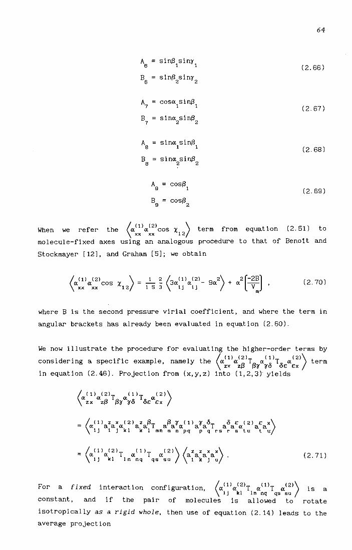
64

A = siIlj8 sin1' 6 1 1 (2.66)

B = sin/3 sin1' 6 2 2

A = cosO'. sin/3 7 1 1 (2.67)

B = sinO'. siIlj8 7 2 2

A = sinO'. siIlj8 8 1 1 (2.68)

B = sinO'. siIlj8 8 2 2

A = cos(3 9 1 (2.69)

B = cos(3 9 2

When we refer the a a cos X term from equation 2.51 to < (1) (2» ( ) xx xx 12

molecule-fixed axes using an analogous procedure to that of Benoit and

Stockmayer [12], and Graham [5]; we obtain

< (1) (2) ) 1 2 \3 (1) (2) 9 2) 2 [-2B) a a cos X = - - a a - a + a --xx xx 12 1 5 3 1 J 1 J V '

m

(2.70)

where B is the second pressure virial coefficient, and where the term in

angular brackets has already been evaluated in equation (2.60).

We now illustrate the procedure for evaluating the higher-order terms by

considering a specific example, namely the (a(1)a(2)T 0'.( 1)T 0'.(2» term zx z(3 (31' 1'0 oe ex

in equation (2.46). Projection from (x,y,z) into (1,2,3)· yields

= a aaa aa aaa aa aaa aa < (1) Z x (2) Z (3T (3 l' (1) l' 0T 0 e (2) e x) 1 J 1 J k 1 k 1 mn m n pq p q r s r stu t u

= a a a a aaaa. ( (1) ( 2 ) T ( 1) T ( 2») ( z z x x) 1J kl In nq qs su 1 k j u

For a fixed

constant, and

interaction

if the

configuration, /a(1)a(2)T a(l)T 0'.(2» '\ 1J kl In nq qs su

pair of molecules is allowed to

(2.71)

is a

rotate

isotropically as a rigid whole, then use of equation (2.14) leads to the

average projection

65

(2.72)

in which the angular brackets now indicate an average over the pair

interaction co-ordinates according to equation (2.56) . We introduce the

following notation to simplify the symbolic form of the expressions:

(1) 1 J a is as in equation (2.11). T =aaf3TNa , where TNa is given in

1 J 1 J a "'+' "'+'

(2.55), and where a 1 is the transpose of (2.53), yielding a

where

Finally,

[~11 T

~131 12 T ( r 1

-3

T = 41(£ R 1 J 0 12 22 23

T T T 13 23 33

T = 2A2 - A2 A2 11 7 4 1

T = 2A2 - A2 _ A2 22 8 5 2

T = 2A2 - A2 A2 33 9 6 3

T = 2A A - A A AA 12 7 8 4 5 1 2

T = 2A A - A A AA 13 7 9 4 6 1 3

T = 2A A A A AA 23 8 9 5 6 2 3

(2) 1 J a f3 (2) a1 J = a af3a , a , a , " a 1 J 1 J

yielding

(2) a

lJ = [~11 12

Z 13

Z 12

Z 22

Z 23

~131 23

Z 33

(2.73)

(2 . 74)

(2.75)

where

2 = 11

2 = 22

2 = 33

2 12

2 13

2 23

[a, [A2B2 + A2B2 + A2B2 + 2A A B B + 2B (A A B + A A B ) J + a [A2B2 + A'B' + A2B2 + 2A A B B + 2B (A A B + A A B ) J] 1 1 1 4 4 7 7 1 4 1 4 7 4 7 4 1 7 1 22 1 2 4 5 7 8 1 4 2 5 8 4 7 5 1 7 2

+ a (A2B2 + A2B2 + A2B2 + 2A A B B + 2B (A A B + A A B )] 33 1 3 4 6 7 9 1 4 3 6 9 4 7 6 1 7 3

[a [A2B2 + A2B2 + A2B2 + 2A A B B + 2B (A A B + A A B ) J + a [A2B2 + A2B2 + A2B2 + 2A A B B + 2B (A A B + A A B ) J] 11 2 1 5 4 8 7 2 5 1 4 7 5 8 4 2 8 1 22 2 2 5 5 8 8 2 5 2 5 8 5 8 5 2 8 2

+ a (A2B2 + A2B2 + A2B2 + 2A A B B + 2B (A A B + A A B )] 33 2 3 5 6 8 9 2 5 3 6 9 5 8 6 2 8 3

[a [A2B2 + A2B2 + A2B2 + 2A A B B + 2B (A A B + A A B ) J + a [A'B2

+ A2B2 + A2B2 + 2A A B B + 2B (A A B + A A B ) J] 11 3 1 6 4 9 7 3 6 1 4 7 6 9 4 3 9 1 22 3 2 6 5 9 8 3 6 2 5 8 6 9 5 3 9 2

+ a (A 2B2 + A 2B2 + A 2B2 + 2A A B B + 2B (A A B + A A B )) 33 3 3 6 6 9 9 3 6 3 6 9 6 9 6 3 9 3

a (A A B2 + A A B2 + A A B2 + B B (A A + A A) + 11 1 2 1 4 5 4 7 8 7 1 4 1 5 2 4

+BB (AA+AA) +B [B (AA+AA) +B (AA+ 2 5 1 5 2 4 8 5 4 8 5 7 218

+ B [B (A A + A A ) + B (A A + A A)]) 9 6 4 8 5 7 318 2 7

a (A A B2 + A A B2 + A A B2 + B B (A A + A A) + 11 1 3 1 4 6 4 7 9 7 1 4 1 6 3 4

+BB (AA+AA) +B [B (AA+AA) +B (AA+ 2 5 1 6 3 4 8 5 4 9 6 7 219

+ B [B (A A + A A ) + B (A A + A A)]) 9 649 6 7 319 3 7

a (A A B2 + A A B2 + A A B2 + B B (A A + A A) + 11 231 564 897 1426 35

+BB (AA+AA) +B [B (AA+AA) +B (AA+ 2 5 2 6 3 5 8 5 5 9 6 8 229

B [B (A A + A A ) + B (A A + A A)]) + 744857 11827

A A)]) + a [A A B2 + A A B2 + A A B2 2 7 33 1 2 3 4 5 6 7 8 9

B [B (A A + A A ) + B (A A + A A)]) + 744967 11937

A A)]) + a (A A B2 + A A B2 + A A B2 3 7 33 1 3 3 4 6 6 7 9 9

B [B (A A + A A ) + B (A A + A A)]) + 745968 12938

A A)]] + a (A A B2 + A A B2 + A A B2 3 8 33 2 3 3 5 6 6 8 9 9

a (A A B2 + A A B2 + A A B2 22 1 2 2 4 5 5 7 8 8

+BB (AA+AA) 3 6 1 5 2 4

a (A A B2 + A A B2 + A A B2 22 1 3 2 4 6 5 7 9 8

+BB (AA+AA) 3 6 1 6 3 4

a (A A B2 + A A B2 + A A B2 22 2 3 2 5 6 5 8 9 8

+BB (AA+AA) 3 6 2 6 3 5

9 6 5 9 6 8 329 3 8 + B [B (A A + A A ) + B (A A + A A)])

(2.76)

0\ 0\

67

Once the Macsyma tensor manipulation facilities are invoked to evaluate

the expressions for averages such as in equation (2.72), we obtain for

the key parameters in equation (2.43):

(47[£ r 1

( { ( b = 0 R - 3 Sa a (Z T + Z T + Z T ) + a (Z T + Z T 3 15 11 11 11 " 12 12 13 13 22 12 12 22 22

+ Z T ) + a (Z T + Z T + Z T )] + 4 (a2 (Z T + Z T

23 23 33 13 13 23 23 33 33 11 11 11 12 12

+ Z T ) + a2

(Z T + Z T + 2 T ) + a2

(2 T + Z T 13 13 22 12 12 22 22 23 23 33 13 13 23 23

(2.77)

(47[£ J -1 -3{ a3 = (R -4a (a (2 T + Z T + Z T ) + a (2 T + Z T

30 11 11 11 12 12 13 13 22 12 12 22 22

+ 2 T ) + a (2 T + 2 T + 2 T )] + 3 (a2 (Z T + Z T

23 23 33 13 13 23 23 33 33 11 11 11 12 12

+ Z T ) + a2

(Z T + Z T + Z T ) + a2 (Z T + Z T

13 13 22 12 12 22 22 23 23 33 13 13 23 23

+ 2 3}33)] + all [Tll (2211+ 22

12+ 22 ) + T (2 Z + Z Z + Z Z ) 13 12 11 12 12 22 13 23

+ T (z Z + Z Z + Z Z )] + IX (T (Z Z + Z Z + Z Z ) 13 11 13 12 23 13 33 22 12 11 12 12 22 13 23

+ T (22 + 22 + 22 ) + T (2 2 + 2 2 + )] [ 22 12 22 23 23 12 13 22 23 2 23Z33 + a

33 T

13

X (22+22+2Z)+T (2Z+2Z+ZZ) (2 11 13 12 23 13 33 23 12 13 22 23 23 33 + T33 Z13

(2.78)

(41tc ) -2 .

o < -6{ [2 2 [ ) ] 2 2 a = R 3a a 2 T + 2T 2 2 T + T 2 2 + 2 2 + T 2 2 + 2 2 + 2 2 + 22 2 T + 2 T 4 30 1122 13 23 23 12 13 22 13( 12 33 13 23) 12( 12 . 13 13 22 11 13 12 13 11 12 22

+ 2T [22 2 T + T (22 2 + 2 2 ) + 222 T ] + 22 T2 + 22 12 23 13 12 12 22 11 12 12 11 23 13

+ T2 (22 + 22 2 + 222 + 22 ) + 2T T (2 2 + 22 2 )) + 12 22 11 22 12 11 11 12 12 22 11 12

2T [T (2 2 + 2 2 + 2 2 ) + 2 2 T ] + 22 T2 13 12 22 23 11 23 12 13 12 23 11 12 11

3a a (22 T2 + 2T [2 2 T + T (22 2 + 2 2 ) 11 33 13 33 33 12 13 23 13 13 33 11 13

+ 22 2 T + 222 T ] + T2 (22 + 22 2 + 222 + 22 ) + 22 T2 + 13 23 12 13 11 13 33 11 33 13 11 12 23 2T2 [T (2 2 + 2 2 + 2 2 ) + T (2 2 + 2 2 )

23 13 12 33 13 23 11 12 12~ 12 23 13 22

+ 22 2 T ] + 22 T2 + 22 2 T T + 22 T2 + 2T [T (2 2 + 12 13 11 23 12 13 23 11 12 13 11 13 12 23 33

2 2 + 2 2 + T 2 2 + 22 2 + 3a a 2 T ) ( )]) ( 2 2

11 23 12 13 11 13 33 11 13 22 33 23 33

+ 2T [T (22 2 + 2 2 ) + 222 T + 2 2 T + 22 2 T ] + T2 (22 + 22 2 + 222 + 22 ) + 22 T2 + 2T [T (2 2 33 23 23 33 22 23 23 22 12 23 13 13 23 12 23 33 22 33 23 22 23 22 23 22 23 33

+ 22 2 ) + T (2 2 + 2 2 + 2 2 ) + T (2 2 + 2 2 + 2 2 )] + 22 T2 + 22 T2 + 2T (22 2 T + 2 2 T ) 22 23 13 12 33 13 23 12 22 12 13 33 12 23 13 22 12 13 13 12 22 12 23 13 13 23 12

+ T T (2 2 + 2 2 )) + 3a2

(T2 (22 + 2 2 + 22 + 322

) + 2T [T (2 2 + 2 2 + 2 2 + 32 2 ) + T (2 2 12 13 11 23 12 13 11 13 33 11 33 23 13 13 12~ 23 33 22 23 11 23 12 13 11 13 33

+ 2 2 + 42 2 )] + T2 (22 + 22 + 2 2 + 322

) + 2T T (2 2 + Z 2 + 42 2 ) + T2 (22 + 22 + 422 )) + 3a2 [T2 (22

12 23 11 13 12 23 22 11 22 12 11 12 13 23 12 22 11 12 11 13 12 11 22 23 33

+ 2 2 + 32 + 2 + 2T T 2 2 + 42 2 + 2 2 + T 2 2 + 32 2 + 2 2 + 2 2 + T 2 + 42 + 2 2 2 [ . )] 2 (2 2 2 ) 22 33 23 13) 23 22( 23 33 22 23 12 13) 12( 13 33 12 23 13 22 11 13 22 23 22 12

+ 2T T (2 2 + 42 2 + 2 2 ) + T2 (2 2 + 22 + 322 + 22 )) + 3a2

(T2 (422 + 22 + 22 ) + 2T [T (42 2 + 2 2 12 22 13 23 12 22 11 12 12 11 22 13 13 11 33 33 33 23 13 33 23 23 33 22 23

+ 2 2 ) + T (42 2 + 2 2 + 2 2 )] + T2 (2 2 + 322 + 22 + 22 ) + 2T T (2 2 + 32 2 + 2 2 + 2 2 )

12 13 13 13 33 12 23 11 13 23 22 33 23 22 12 13 23~ 12 33 13 23 12 22 11 12

+ T2 (2 2 + 322

+ 22 + 22 ))}) 13 11 33 13 12 11 (2.79)

0\ 00

69

Even with our compact notation, the a term is extremely large, and so 5

we introduce a new tensor to further compress the final expression:

E = o:(1)T 0:(2) where 1 J 1 J Jk kl '

with

E = 11

E = 12

E = 13

E = 21

E = 22

E = 23

E = 31

E = 32

E = 33

Then,

E = [~11 1 J 21

E 31

E 12

E 22

E 32

E 1 13

~23 '

33

0: (2 T + 2 T + 2 T ) 11 11 11 12 12 13 13

0: (2 T + 2 T + 11 12 11 22 12

2 T ) 23 13

0: (2 T + . 2 T + 2 T ) 11 13 11 23 12 33 13

0: (2 T + 2 T + 22 11 12 12 22

2 T ) 13 23

0: (2 T + 2 T + 22 12 12 22 22

2 T ) 23 23

0: (2 T + 2 T + 2 T ) 22 13 12 23 22 33 23

0: (2 T + 33 11 13

2T+2T) 12 23 13 33

0: (2 T + 2 T + 2 T ) 33 12 13 22 23 23 33

0: (2 T + 2 T + 2 T ) 33 13 13 23 23 33 33

(2.80)

(2.81)

(4nc )-3 a = R 9a T (E E + E E + 2E ) + T E 2E + E + E E + E E + E E T + T E (2E + E ) + E E o < -s{ [2 (

5 30 33 33 1 3 3 1 23 3 2 3 3 23 ( 33 ( 32 23 ) 22 32 1 2 3 1 ) 2 3 32 22 1 3 33 3 1 1 3 2 1 32

+ E E + T (E E + E E ) + E E T . + 9a E E T + T (E E + E E + 2E E + E E + T (E E + 2E + E E ) ) (

2

11 31 12 13 32 23 31 13 31 11 22 23 32 33 23 23 33 22 32 22 23 13 21 22 23 32 22 12 21

+ T (E E + E E ) + T (E E + E (2E + E ) + 9E E ) + E E T ) + 9a (E E T + T (E E + E E ) + E E T 13 21 32 12 23 12 23 31 22 21 12 11 21 12 21 11 11 13 31 33 23 12 31 13 21 12 21 22

+ T (E E + E E + E E + 2E E ) + T (E E + E E + E E + 2E E ) + T (E E + E E + 2E2 ») + 3T (2 (2E2

13 13 33 11 31 12 23 11 13 12 13 32 12 22 11 21 11 12 11 13 31 12 21 11 33 33 33

+ E E + E E ) + 2 (E ( 2E + E ) + E E + E E ) + E E 2 + 2 (E ( 2E + E ) + E E + E E ) + 2 ( E E 23 32 13 31 23 33 32 23 22 32 12 31 23 32 22 13 33 31 13 21 32 11 31 12 13 32

+ E E ) + E E 2 ) + 3T [2 (E (E + 2E ) + E E + E E ) + 2 (E2 + 2E E + E2 + 2E E + E E + E2 + E2 + E E )

23 31 13 31 11 23 33 33 32 23 22 23 13 21 23 33 22 33 32 23 32 13 31 23 22 12 21

+ 2 ( E E + 2E E + E E + E E ) + 2 (E ( E + E ) + E E + E E + E E + E E + E E ) + 2 (E E + E ( E 22 32 33 22 32 12 31 22 23 13 33 21 12 31 32 23 31 13 23 21 22 11 21 12 31 33 32 21

+ E ) + E (E + E ) + E E + E E ) + 2 (E E + E E ») + 3T (E E 2 + 2 (E E + E E + 2E E + E E ) + 2 12 31 22 11 21 23 13 22 11 12 31 13 21 22 23 32 33 23 23 33 22 32 22 23 13 21 22

2 ) (( x (E E + 2E + E E ) + 2 (E E + E E ) + 2 E E + E 2E + E ) + E E + E E 2 + 3T Z E (E + 2E ) 23 32 22 12 21 13 21 32 12 23 12( 23 31 22( 21 12 11 2J 12 21 11 13 33 33 31 13

) ( 2

+ E E + E E + 2 E (E + E ) + E (E + E ) + E E + E E + E E + 2 (E E + E E ) + 2 (E + 2E E 12 23 11 13 23 33 21 12 32 31 13 13 23 12 22 11 12) 22 21 32 12 23 13 33 11 33

+ E E + E2 + 2E E + E E + E2 + E2 ) + 2 (E E + E (E + E ) + E (E + E ) + E E + E E ) + 2 (E E + E E 23 32 31 13 31 12 21 13 11 12 32 33 32 22 11 31 21 12 11 23 12 13 11 31 33 21 32

+ 2E E + E E ) ) + 3T [2 ( E E + E E ) + 2 (E E + E E + E E + E ( E + E ) + E E + E E ) + 2 (E E 11 31 11 13 12 33 13 32 23 31 23 13 33 12 32 22 31 23 21 12 13 22 11 13 22 13 32

2 + E ( E + 2E ) + E E ) + 2 (E E + E E + E E + E ( E + E ) + E E + E E ) + 2 ( E E + E E + E + 2E E

22 21 12 11 12 13 23 33 11 32 21 31 23 22 11 13 21 12 13 12 23 32 13 31 22 11 22

+ E2 + 2E E + E2 + E2 ) + 2 (E E + E E + 2E E + E E ») + 3T (E E 2 + 2 (E E + E E ) + E E 2 + 2 (E E 21 12 21 12 11 11 23 31 21 22 11 21 11 12 11 13 31 33 23 12 31 13 21 12 21 22 13 13 33

+ E E + E E + 2E E ) + 2 (E E + E E + E E + 2E E ) + 2 (E E + E E + 2E») 12a(T (E2

+ E E + E E ) 11 31 12 23 11 13 12 13 32 12 22 11 21 11 12 11 13 31 12 21 11 33 33 23 32 13 31

+ T (E (E + E ) + E E + E E + E E + E E ) + T (E E + E2 + E E ) + T (E (E + E ) + E E + E E + E E 23 33 32 23 22 32 12 31 22 23 13 21 22 23 32 22 12 21 13 33 31 13 21 32 11 31 12 23

+ E E ) + T (E E + E E · + E (E + E ) + E E + E E ) + T (E E + E E + E2 ») - (E + E + E ) (3a (E T 11 13 12 13 32 23 31 22 21 12 11 21 11 12 11 13 31 12 21 11 11 22 33 33 33 33

+ E T + E T ) + 3a (E T + E T + E T ) + 3a (E T + E T + E T ) + T (E 2 + E 2 + E 2 ) + T (E 2 32 23 31 13 22 23 23 22 22 21 12 11 13 13 12 12 11 11 33 33 33 32 23 31 13 23 23 33

+ Z (E + E ) + E 2 + E 2 + E Z ) + T (E 2 + E 2 + E 2 ) + T (E Z + E 2 + 23 33 22 32 22 21 13 31 12 22 23 23 22 22 21 12 13 13 33 12 23

+ T (E 2 + E 2 + E 2 + 2 (E + E ) + E 2 ) + T (E 2 + E 2 + E 2 »)}) 12 13 23 12 22 23 13 12 22 11 21 11 11 13 13 12 12 11 11

2 (E + E ) + E 2 + E 2 ) 13 33 11 32 12 31 11

-..J o (2 . 82)

71

Upon gathering the results in equations (2.15), (2.17), (2.57), (2.60),

(2.70), (2 . 77), (2.78), (2 . 79) and (2.82) , equation (2 . 43) for p takes

the form

p = (_1_ (fl«) 2 + _1_ g' + 1 (41[£) -1 a' + _1_ (41[£ ) -2 a' 15 30 30 0 330 0 4

+ 310(41tE:J-3 a~ + .. . ]/(<<2 + /5 (fl«)2 + 1\ i g' + «2 [-e:J

+ 1 \ (41[£ J -1 b;] (2.83)

Here, g' (

(1) (2) 2) is the expression for 3« « - 9« gi ven in equat ion 1 J 1 J

(2.60), while b' represents that part of b in equation (2.77) contained 3 3

within the angular brackets, with similar definitions for a', a' and a' 345

with reference to equations (2 . 78), (2.79) and (2 . 82) respectively.

Equation (2.83) must now be cast into the virial form of equation

(2 . 21). We have from equation (2.18)

fl« having been defined in equation (2.13). Equation (2 . 83) can now be

written as

Po [I + 1 g' +

(41[£ J- 1

a' + (41[£ J-2

a' + P = 2(fl«)2 2(fl«)2 3 2(fl«)2 4

2B O[::]]/{I + i PO[2(~)2 3 (41[£ J- 1

+ - + g' + V 2(fl«)2 m

which reduces to

where

+ a 4

+ a 5

+ & 3

(41[£ J-3

a' 2(fl«)2 5

+ e~]) b' 3

(2.84)

+ ... ) (2 . 85)

72

g = 1 --- V g' 2 (t.o::) 2 m

(2.86)

a = {1 + _2 }(41lE: )-lV a' 3 2 (t.0::)2 480::2

0 m 3

(2.87)

(2.88)

a = {1 + _2 }(41U: )-3V a' 5 2 (t.0::)2 480::2

0 m 5

(2 . 89)

(41[£ r 1

& = _ 0 V b' 3 150::2 m 3

(2.90)

It follows that

B = P (1 - ~ P ) (2B + g + a + a + a + &3 + ... ) . po 30 345

(2.91)

As with the normal second pressure virial coefficient B, the

coefficients in equations (2 . 86) to (2.90) are independent of the molar

volume but dependent on temperature . It is the parameter B which is P -1

directly accessible from a plot of experimentally measured p versus V m

values, and if coupled with a measured value of p , one can extract from o

equation (2.91) a value for

(2.92)

It is the sum of terms arising purely from angular correlation and

collision-induced polarizability anisotropy, namely

!f = p g+a +a +a +& + 3 4 5 3

. . . , (2 . 93)

. (" .

which is of interest; and to extract a precise value of this sum from

the val ue for B' requires an (!f 12B) rat io of the order of uni ty or p p

greater .

2.4 Evaluation of B by numerical integration p

73

Evaluation of the average (X) of a quantity X over the pair interaction

co-ordinates according to equation (2.56) requires the classical

intermolecular potential V12

("r>. General tensor expressions for V1/'r> have been derived by Buckingham [14], who then evaluated them for the

special case of a pair of interacting linear molecules in the

configuration of figure 1.1 (opposite page 16), obtaining the

expressions listed in equations (1.80) to (1.86). We must now evaluate

Buckingham's general expressions for V (-r) in the case of a pair of 12

interacting non-linear molecules in the configuration described in

section 2.2.

2.4.1 Classical expressions for the intermolecular

potential energy V (or) . 12

Buckingham [14] has shown that for intermolecular separations R which

are large relative to molecular dimensions, the pair interaction energy

V (T) may be considered to consist of three components: 12

(i) The electrostatic energy, V , which arises from the elec

interactions of the zero-field electric moments (charge, dipole,

quadrupole, etc.) of the two molecules,

(11) The induction energy, V , which arises from the distortion of Ind

the electronic structure of a molecule due to the permanent

electric moments on the neighbouring molecule, and

(1·i1) The London dispersion energy, V , dlsp

which arises from

interactions of the electric moments due to fluctuations in the

charge distributions of the two molecules.

These interaction energies are the result of long-range forces which are

well understood [9,14,18,19], and which are evaluated on the assumption

that the overlap of the molecular wave functions is small. Now, at small

ranges of interact ion where the electron clouds of the molecules do

overlap significantly, the ab initio quantum-mechanical calculations

74

[20] which would be required to take into account the intetmediate-range

exchange forces are prohibit i vely complicated (especially for many­

electron atoms); and so it has been customary [21-23] to assume that the

interact ion energy components (i) , (i i) and (i i i) above are appl icable

also to short-range interactions provided that an additional term,

U ,is added to account for the repulsive short-range overlap

interactions. It is now possible to write

U (or) = U + U + U + U 12 elec Ind dlsp overlap

(2 . 94)

In most of the work previously undertaken on the properties of gases

[21-26] , the central-field Lennard-Jones 6: 12 potential U [27] has LJ

been used to represent (u + U ): dlsp overlap

Here,

while

andR o

U LJ = 4<[[ :f- [:oJl

the term [:0)" describes the attractive part of

[ R ] 12 .

RO

describes the short-range repulsive part.

are the well-known Lennard-Jones parameters.

(2 . 95)

the potent ial,

The symbols (:

Since U is spherically symmetric, Buckingham and Pople [21] proposed LJ

the addi t ion of a further term to U to account for the angular overlap

dependence of short-range overlap repulsive forces for non-spherical

molecules . For axially-symmetric molecules,

given by they found U to be

shape

(2.96)

where D is a dimensionless parameter called the shape factor, and which

lies in the range -0.25 to +0.50 to ensure that the shape potential is

always repulsive . D is zero for spherical molecules, positive for

rod-like molecules (i.e. molecules which are elongated in the direction

of the axis of the dipole moment [24], such as CH F), and negative for 3

plate-like molecules (i.e . molecules which are fore-shortened along the

axis of the dipole moment [24], such as CHF ) . 3

y

x •

r eJ H, I ;H r··· ~/~Te~t~3 . ./ ..

,. 0.309 nm

2 The ethene molecule. Molecular

geometry is taken from {B,31].

case (1): (x, and (X2 can be any angle (i.e. from 0 to 2n)

13, and 132 can be 0 or n

Y, and Y2

can be any angle (i.e. from 0 to 2n)

t 1

~ ~ ........ . c:::)

lO ,( 1······· .. · ........ 3 S .............. . ····)<--0

" 2. . 0.249 nm

The sulphur dioxide molecule. Molecular geometry

is taken from {53].

11 I

case (ii): (x, and (X2 can be any angle v v 13, and 132 can be 1: 1f. I 2 case (iii): (x, and (X2 can be any angle

Y, and Y2

can be 0 or 1f. 13, and 132 can be I. 1f.12

Y, and Y2

can be I. 1f./2

Figure 2 .3. The three extreme intermolecular approaches for two colliding ethene molecules. lOr sulphur dioxide, replace

the ethene molecules with the sulphur dioxide equivalent shown above.

..... z

75

We have used equation (2.96) as a basis for constructing a new shape

potent ial which describes the orientat ion effects arising from

short-range overlap repulsive forces for non-linear molecules. Since our

invest igations deal with molecules belonging to the D2h and C2V point

groups, we only consider molecules with these specific symmetries .

Ethene (of D2h symmetry) and sulphur dioxide (of C2V symmetry) are

chosen as representative molecules, and we orientate the molecule-fixed

axes (1,2,3) such that the 1-3 and molecular planes co-incide, with 3

along the principal molecular axis. The thr.ee extreme intermolecular

approaches for both species are depicted in figure 2.3. The shape

Potential is seen to be independent of ex and ex, and the simplest . 1 2

force-field which will reproduce the orientation effects of the shape of

these molecules is

U.h ... = 4£[ :or2{Dl[3COs2~1+ 3COS2~2- 2] + D 3sin ~ cos r [22

2 1 1

2 2 + 3sin ~ cos r -

2 2 (2.97)

where D and D are dimensionless parameters called the shape factors. 1 2

For axially symmetric molecules, we set D = 0 and recover Buckingham's 2

shape potential. To understand the physical meaning of equation (2.97),

imagine two planar ethene molecules approaching as in case (i i 1) of

figure 2.3. The approach distance R can be less than R before the onset o

of contact forces, and so in this orientation the repulsive part of the

Lennard-Jones potential is

(Dl+ D2

) is required. The

reduced: a negative U and positive shape

closest possible approach of two ideal

(infinitely thin) planes before contact is R = O. For this orientation

there is no repulsive potential, and [ RoJ 12

4£ If" from U LJ

must be

completely offset by U . Thus, (Dl+ D2

) =~. Of course ethene has a s~~ 2'

finite thickness with n-orbitals above and below the 1-3 plane; and it

is reasonable to expect (D + D) < ~ for this molecule. A similar 122

analysis, based on simple molecular geometry, can be undertaken for

sulphur dioxide.

U ) in overlap

Having found the two components U and U of the LJ shape

equation (2.94), it is now necessary

sum (U + disp

find the to

components of the sum (u + U ) . elec ind

As in previous studies of this

76

kind [23,28-30], U is taken to include potential energies arising elec

from the interactions of permanent dipole and quadrupole moments, while

U comprises energies due to permanent dipole and quadrupole moments Ind

on the one molecule interact ing with the induced dipole moment of the

second molecule.

components

The sum (U + U ) is found to then have the five elec Ind

U +U =U +U +U +U +U elec Ind J.L,J.L J.L,a a , a J.L,lnd J.L a,lnd J.L

(2.98)

where, U ,UII,a and Ua,a are the electrostatic dipole-dipole, dipole-. J.L,J.L r-

quadrupole and quadrupole-quadrupole interaction energies of the

permanent moments of the two molecules, while U and U are a,lnd J.L J.L,lnd J.L

the dipole-induced-dipole and quadrupole-induced-dipole interaction

energfes.

We have from Buckingham [14] that the e lectrostat ic contri but ion to

U (T) of two interacting molecules is 12

(2.99)

+ .. . .

For interacting non-linear polar molecules in the co-ordinate system

shown in figure 2.2, we have

(2.100)

where for molecules of C2v

symmetry with the 3-axis as the principal

molecular axis, the dipole moment has only one independent component [14]

(2 . 101)

Hence,

(2.102)

77

Similarly. for C and D symmetry. the traceless quadrupole moment 2v 2h

has two independent components [14]

o a

2 (2.103)

o

and we obtain for polar molecules

u = (4nc )-1{/l R- 4 [a (A (_B2 + B2 - B2 + B2 + 2B2 - 2B2) + 2B (A A /l.a 0 3 1 9 1 3 4 S 1 9 3 1 1

- A A ) + 2B (A A - A A ) - 2B (A B + A B ) + B (A2 - A2 + A2 3 9 S 4 1 S 9 131 S 4 9 1 3 4

- A2 - 2A2 + 2A2 + 2A B + 2A B )] + a (A (_B2 + B2 - B2 + B2 6 1 933 S S 292 3 5 6

+ 2B2 - 2B2) + 2B (A A - A A ) + 2B (A A - A A ) - 2B (A B 8 9 328 3 9 S 5 8 S 9 832

+ A B ) + B (A2 - A2 + A2 - A2 - 2A2 + 2A2 + 2A B + 2AsBs)]]} · 6 5 9 2 356 8 9 3 3

(2.104)

For both polar and non-polar molecules

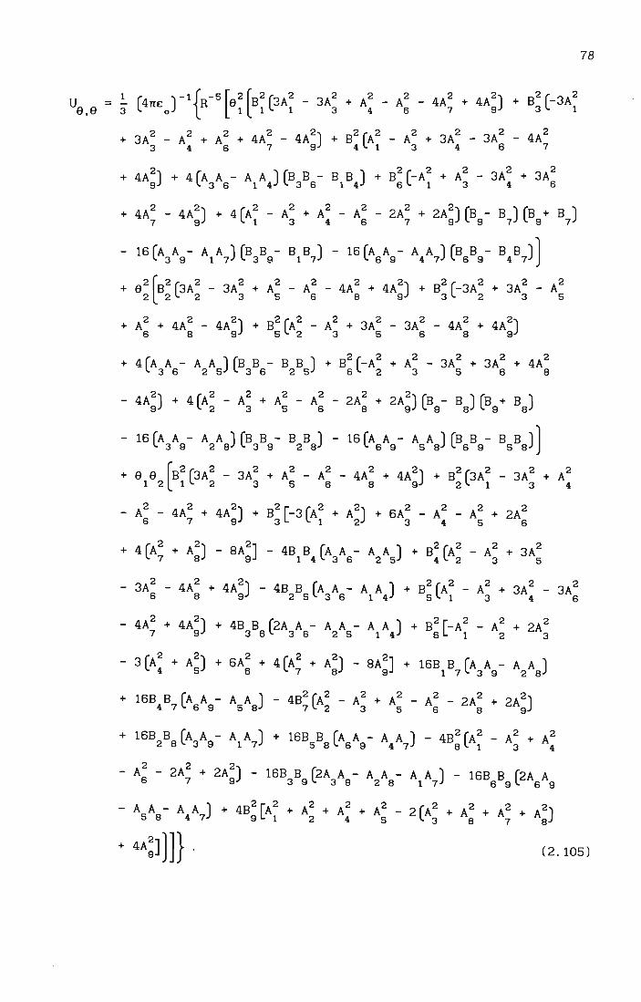
= ~ ( )-1{ -5[ 2 [B2(3A2 _ 3A2 + A2 _ A2 _ 4A2 + 4A2) + B2 (-3A2 U8 8 3 47[£0 R 81 1 1 3 4 6 7 9 3 1

•

+ 4A2) + 4(A A - A A ) (B B - B B ) + B2(_A2 + A2 - 3A2 + 3A2

9 3 6 1 4 3 6 1 4 613 4 6

+ 4A 2 - 4A 2) + 4 (A 2 - A 2 + A 2 - A 2 - 2A 2

+ 2A 2) (B - B ) (B + B ) 7 9 1 346 7 9 9 7 9 7

- 16 (A A - A A ) (B B - B B ) - 16 (A A - A A ) (B B - B B ) J 3 9 1 7 3 9 1 7 6 9 4 7 6 9 4 7

+ 4(A A - A A ) (B B - B B ) + B2(_A2 + A2 - 3A2 + 3A2

+ 4A2 3 6 2 5 3 6 2 5 623 5 6 8

- 4A:) + 4 (A~ - A~ + A: - A: - 2A: + 2A:) (Bg - B8) (Bg + B8)

- 16 (A3A9 - A2A8) (B3B9 - B2B8) - 16 (A6A9 - A5A8) (B6B9 - B5B8) J

+ 8 8 (B2 (3A 2 - 3A 2 + A 2 - A 2 - 4A 2

+ 4A 2) + B2 (3A 2 _ 3A 2 + A 2 121 2 356 8 9 2 1 3 4

+ 4(A2 + A2) - 8A2] - 4B B (A A - A A ) + B2(A2 _ A2 + 3A2 7 8 9 1 4 3 6 2 5 423 5

- 3A2 - 4A2 + 4A2) - 4B B (A A - A A ) + B2(A2 - A2 + 3A2 - 3A2 6 8 9 2 5 3 6 1 4 513 4 6

- 4A72 + 4A2g) + 4B B (2A A - A A - A A ) + B2[_A2 - A2 + 2A2 3 6 3 6 2 5 1 4 612 3

- 3 (A 24 + A 25) + 6A62 + 4 (A 2 + A 2) - 8A 2] + 16B B (A A - A A )

7 8 9 1 7 3 9 2 8

+ 16B B (A A - A A ) - 4B2(A2 - A2 + A2 - A2 - 2A2 + 2A2g) 4 7 6 9 5 8 7 2 3 5 6 8

+ 16B B (A A - A A ) + 16B B (A A - A A ) - 4B2 (A 2 _ A 2 + A 2 2 8 3 9 1 7 5 8 6 9 4 7 8 1 3 4

2 2 2) - A - 2A + 2A - 16B B (2A A - A A - A A ) - 16B B (2A A 679393928176969

78

(2.105)

79

Buckingham [14] also gives the contribution to U12

(-[") arising from the

induction energy:

where a is the mean static dipole polarizability. This leads to s

for polar molecules, and

(2.106)

(2.107)

+ 2A 2 (-A 2 + A 2 - A 2) + A 4 + 4A

2 (A

2 + A 2) + 4A

4 - SA A (A A s 1 3 4 S 7 3 S 779 1 3

+ A A ) + 4A2(A2 + A2 - 2A2) + 4A4] + a2[A4 -

4 S 914 7 922

+ 2A2(A2 _ A2) + A4 + 2A2(-A2 + A2 _ A2) + A4 523 5 S 2 3 5 S

+ 4A 4 - SA A (A A + A A ) + itA 2

(A 2

+ A 2

88923 5 S 925 - 2A:) + 4A:]

_ A2) + A2 (A2 351

_ A2 + A2) + 4A A (A A + A A ) + 2A2(_A2 + A2 - A2 + A2 5 S 7 8 1 2 4 5 8 1 3 4 S

+ 2A 2) - 4A [A (A A + A A ) + A (A A + AsAs)] + 2A 2

(A 2

79713 4 S 823 9 1

+ A~ + A: + A~ - 2A~ - 2A:) + 4A:)]} (2. lOS)

for both polar and non-polar molecules . Here, as in the paper by

Buckingham and Pople [21], U has been written so that its j..L, ind j..L

unweighted orientational average is zero: the orientation-independent

part is assumed to be incorporated in the R-6 term of U .

LJ

Finally, U (~) in equation (2.94) is written 12

80

with the explicit expressions of these components being given in

equations (2.95), (2.97), (2.102), (2 . 104), (2.105), (2.107) and

(2.108). These energy expressions are directly applicable to pair

interactions of non-linear dipolar molecules, but are easily adjusted to

accommodate for interactions between non-polar non-linear molecules,

polar or non-polar axially-symmetric molecules, or even spherical

molecules simply by setting the relevant multipole moments to zero.

The expressions for contributions to B given in equations (2.86) to p

(2.90) apply directly to non-linear molecules, and can be averaged over

pair interaction co-ordinates according to equation (2.56), using the

interaction energy expressions for non-linear molecules derived above.

Now, these expressions for contributions to B , in conjunction with the p

U (~), must fully describe linear molecules as a special case. Hence, 12

an acid test of these expressions was performed by using in the

calculations the molecular properties of the linear molecules studied in

[6,7]. The values thus obtained exactly matched those calculated using

the expressions for B and U (~) derived specifically for p 12

axially-symmetric molecules [6,7], which is most reassuring.

2.4.2 The integration procedure

The averages (X) in equations (2.86) to (2.90) were calculated by

numerical integration of the appropriate form of equation (2.56) using

Gaussian quadrature. A very useful feature of the Macsyma package is its

ability to translate the final expressions directly into Fortran code,

effectively eliminating the introduction of errors into the lengthy

integration arguments. The ranges of ex ex {3 {3 'Y and l' 2' l' 2' °1 "12 were

divided into sixteen intervals each, while R was given a range of 0.1 to

3.0 nm divided into sixty four intervals. The possibil ity of closer

approaches being allowed for by our shape potential was investigated by

gi ving R a range of 0.01 to 3.0 nm, again divided into sixty four

intervals. The calculated averages were found to remain constant to

81

at least seven significant figures, and the range t imi ts of 0.1 to

3.0 nm were justifiably retained.

The Fortran programs, examples of which are given in Appendix 2, were

run in double precision on a 486 DX-2 66 MHz PC with 32 Mb of RAM using

the fast University of Salford FTN77/486 compiler. A significant

departure from the Fortran programs used in previous work on linear

molecules [6,7], examples of which are given in [50], was the use of

large arrays to store the numerical values of the intermolecular

potential expressions for all required angular configurations. This

effectively bypasses repeated calculation of these values within the

Gaussian quadrature routine, yielding a speed enhancement of a

staggering 50 times; but has the disadvantage of requiring large amounts

of expensive memory for storing a few million double-precision numbers.

When the generation of these arrays exhausted the 32 Mb of RAM, use was

made of the facility to page data to hard disk, which effectively

provided a further 200 Mb of memory. Running times of these programs

were typically of the order of eight hours each, which is to be

contrasted with around fifteen minutes for the equivalent programs for

axially-symmetric molecules [6,7]. The arrival of the Physics

Department's new IBM RISC system/6000 workstat ion in October 1994 was

greeted with bated breath: the 60 MHz RISC processor yielded dedicated

run-times a factor of 3.3 times faster than the DX-2 machine.

2.5 Calculations of B for ethene p

2.5.1 Molecular properties of ethene

The molecular data required in the calculations of B for ethene are now p

presented. The molecule is taken to lie in the 1-3 plane with the C=C

bond on the 3-axis, the origin of the molecule-fixed axes incident with

the midpoint of the bond. For a molecule of D2h symmetry, the traceless

electric quadrupole moment tensor will have two independent components,

while the polarizability tensor has three independent components [14].

The electric quadrupole moment of ethene has been the subject of

extensive experimental and theoretical investigation. Unfortunately, the

82

experimental investigations are usually limited to partial

determinations of the quadrupole moment , or combine various experimental

data in order to determine estimates of the two independent components

of the quadrupole moment tensor 9iJ

. There are, however, the accurate

theoretical estimates of Spackman [7] at the MP2 (second-order Meller­

Plesset perturbation theory) level, and of Maroulis [31] at the MP4

level, which are in excellent agreement with each other. Table 2.1

summarizes the measured and calculated data.

Table 2.1. Selected experimental and theoretical values of the quadrupole moment tensor components of ethene.

104°9 104 °9 104 °9 Method 11 22 33

Cm2 Cm2 Cm2

Measurements of COllision-inducyd 6.73 -13 . 33 6.60 absorptiyn ~CIA spectra 32

Measurements[of CIA spectra 33] 5.16 -10.41 5.52

Ma?netizabilit y 4.67 -12 . 02 7.31 an sotropy

measurements [34]

Keasurements of induced birefrin?ence +

4.35 -10.99 6.68 second d electric virial coefficients + refractive index [35]

MP2 theory [ 7] 5. 43 -11. 03 5.60

KP4 theory [ 311 5.370 ± 0. 22 -10.92 ± 0.45 5.549 ± 0. 22

We have used Maroulis' theoretical values in our calculations, noting

their good agreement with the estimates of Dagg et ai. [33] obtained

from collision-induced absorption spectra measurements in ethene rare­

gas mixtures.

Whereas the two principal components of the opt ical frequency

polarizability tensor of a linear molecule can be deduced from

experimental values of Po and (Xv [11,36]; in the case of a non-linear

molecule, which we see from equation (2 . 12) has three principal

polarizabi 11 ty tensor components, an add it lonal physical relat ionship

between the components is required if the three components are to be

Table 2.2. The components of the optical-frequency polarizability tensor of ethene at a wavelength of 514.5 nm obtained from independently measured sets of values for p , a and R

o v 20

lO4 Oa 104o

(Aav ) 1040

a lOOp v

R 11

0 C2 m2J- 1 C2 m2 J- 1 20 C2 m2J- 1

1040

a 1040

a 22 33 -

C2 m2 J- 1 C2 m2 J- 1

1.241 5 ± 0.005 (36) 4.16 (36) 2.011 0.22 ± 0.03 (37) 4.34 3.82 6.11 1 6 2

1.250 ± 0.002 [Thl, 4 . 1811 (38) 2 . 091 0.21 ± 0.01 (39) 4.35 work 3

3.85 6 . 15 7 1

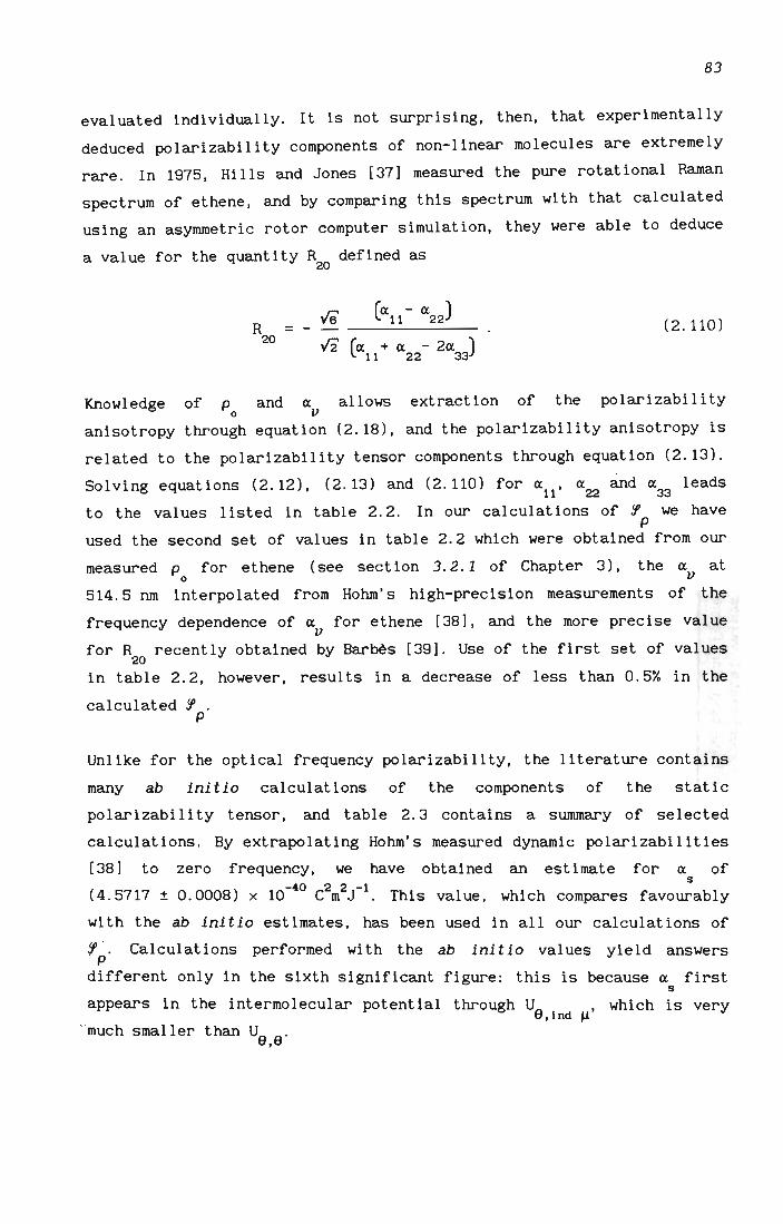
83

evaluated individually. It is not surprising, then, that experimentally

deduced polarizability components of non-linear molecules are extremely

rare. In 1975, Hills and Jones [37] measured the pure rotational Raman

spectrum of ethene, and by comparing this spectrum with that calculated

using an asymmetric rotor computer simulation, they were able to deduce

a value for the quantity R defined as 20

R = 20

16 (all - ( 22 )

12 (a + a - 2a ) L 11 22 33

(2.110)

Knowledge of Po and av

allows extraction of the polarizability

anisotropy through equation (2.18), and the polarizability anisotropy is

related to the polarizability tensor components through equation (2.13).

Solving equations (2.12), (2.13) and (2.110) for a , a and a leads 11 22 33

to the values listed in table 2.2. In our calculations of !I we have p

used the second set of values in table 2.2 which were obtained from our

measured Po for ethene (see section 3.2.1 of Chapter 3), the a at v

514.5 nm interpolated from Hohm's high-precision measurements of the

frequency dependence of a for ethene [38], and the more precise value v

for R recently obtained by Barbes [39]. Use of the first set of values 20

in table 2.2, however, results in a decrease of less than 0.5% in the

calculated !I . p

Unlike for the optical frequency polarizability, the literature contains

many ab ini t io calculat ions of the components of the stat ic

polarizability tensor, and table 2.3 contains a summary of selected

calculations. By extrapolating Hohm's measured dynamic polarizabilities

[38] to zero frequency, we have obtained an estimate for a of (

-40 2 2 -1 s 4.5717 ± 0.0008) x 10 C m J . This value, which compares favourably

with the ab initio estimates, has been used in all our calculations of

!I p' Calculations performed with the ab initio values yield answers

different only in the sixth significant figure: this is because a first s

appears in the intermolecular potential through U , which is very 9,lnd Il

--much smaller than U 9,9

Table 2.4. A comparison of the most precise experimental values for the second pressure virial coefficient of ethene, together with our calculated values (see text for force-constants and shape factors).

T/K 106 S(T)/m3 mol- 1

Douslin and McElroy and Leve 1 t Sengers Waxman and Achtermann et ai. Calculated in Harrison [42] Fang [44] and Hastings [45] Davis [46] [47] this work

238.15 -220.9 -225.35

243. 15 -212.0 -211. 6 -215 . 24

248. 15 -203.5 -205.87

253. 15 -195.5 -194.7 -197 . 15

258. 15 -188.1 -189.01

263.15 -180.9 -180.6 -181. 39

268. 15 -174.1 - 174.24

273.15 -167.6 -167.5 -167.7 -167.52

278. 15 -161. 6 -161. 18

283. 15 -155.7 -155.5 -155.8 -155. 18

288.15 -150.3 -150.3 -149.51

293. 15 -144.9 -144.6 -145.3 -144.13

298.15 -139.8 -139.8 -140.2 -139.02

303.15 -135.0 -134.7 -134.16

323.15 -117.7 -117.9 -117.6 -118.0 -116.85

348.15 -99.7 -99.6 -100.0 -99.04

373.15 -84.8 -84.6 -85.1 -84.39

398.15 -72.3 -72.1 -72.11

423. 15 -61.6 -61.3 -61. 67

448. 15 -52.4 -52.2 -52.67

84

Table 2 . 3 . Selected values of ab initio calculated static polarizability tensor components of ethene .

1040a 10

40a 1040a 10

40a

11 22 33 s Authors

C2m2J- 1 C2m2J- 1 C2m2J- 1 C2m2J- 1

Amos and 3.99 3 . 66 6.00 4.55 Wi 11 iams [ 401

Spackman [ 71 4.092 3 . 534 5 . 594 4 . 407

Maroulis [ 81 4.157 ± 0 . 020 3.695 ± 0.028 5 . 645 ± 0 . 012 4.500 ± 0.020

Sekino and 4.146 3 . 667 5.582 4.465 Bartlett [ 411

Finally, we present our values for the shape factors 01

and O2

, These

were determined by fitting values of the second pressure vi rial

coefficient B(T) calculated according to the equation

N 00 f21l B(T) = ~f

321l R=O a =0 1

x R2Si~ si~ dR da d~ dr da d~ dr 1 2 1 1 1 222 (2.111)

to the experimental values listed in table 2 . 4 over the temperature

range 238.15 K to 448.15 K. Force constants required for the

Lennard-Jones 6:12 potential are given in the appendices of the classic

text of Hirschfelder et ai . [48] . For ethene, the parameters obtained

from viscosity data are £/k = 205 K and R = 0 . 4232 nm. The more recent o

parameters of Oas Gupta et ai. obtained from a combination of viscosity

data and second pressure virial coefficients are £/k = 193.5 K and

R = 0.4236 nm [49]. We optimized the force constants for best agreement o

between the calculated and experimental B(T) values over the full

experimental temperature range, obtaining £/k = 190.0 K and R = 0 . 4232 nm. We note that these val ues compare very favourably wi th o

those of Oas Gupta et al .

In our choice of molecular shape we treat ethene as a planar molecule,

the dimensions of which are taken from simple molecular geometry . This

means that the approach distance R in case (iii) of figure 2.3 can be

85

less than R before the onset of contact forces, while the opposite is o

true for cases 0) and (ii) . D and D must both be positive, and must 1 2

satisfy the requirement that (Dl+ D2) !>~. As an initial approximation,

we choose that D should equal D (i. e. a square plane), and adjust 1 2

their numerical value until the calculated and experimental B(T) values

agree to within 1% over the full experimental temperature range . This

yields rough estimates of Dl and D2

. The ratio of the true Dl and D2

values for ethene is obtained from the molecular dimensions (see figure

2 . 3) by taking the ratio of approaches for cases Oi) and (i) when

contact forces first occur . We have

-2D + 4D 1 2

4D - 2D 0.249

~

0.309 ' 1 2

which gives

D 1 _ o - 1. 074 . 2

Using the rough D = D values obtained from the square plane treatment, 1 2

in conjunction with the known ratio of D and D, it is possible to home 1 2

in on the optimum values for the shape factors by adjusting them until

agreement between calculated and experimental B(T) values is reached.

This procedure was repeated for various values of the force-constants

elk and R until they, too, are optimized. After setting R to 0.4232 nm o 0

and elk to 190.0 K, and optimizing the shape factors CDl = 0.22965 and

D2 = 0.21383), the calculated and experimental curves were found to lie

within 1 . 0% of each other over almost the entire temperature range (see

table 2.4). This excellent agreement between theory and experiment fixed

our choice of force-constants and shape parameters. When the value for

elk was adjusted a few per cent above or below 190 K, with D and D 1 2

being re-optimized, the calculated curve was found to tilt with respect

to the experimental curve, matching it only for the specific

elk = 190 K. Hence, matching calculated second pressure virial

coefficients to experimental data remains an excellent route to the

optimization of the Lennard-Jones force constants and shape parameters

even in the case of non-linear molecules with low symmetry.

86

2.5.2 Results of calculations for ethene

We note that calculat ions of B for ethene when treated as an axially p

symmetric molecule have already been performed [5 , B]. Here, attempts to

optimize R and elk such that the calculated B(T) values would closely o

fit the experimental values I isted in table 2 . 4 were never entirely

successful . Choosing the shape factor D such that agreement between

theory and experiment at around 298 K was within 1% saw typical

disagreements at the two extremes of the temperature range of as much as

7%. This in itself indicates just how unsat isfactory it is to assume

axial symmetry for . the ethene molecule. With R = 0.4232 nm, elk = 205 K o

and D = 0.240; the calculated ~ at 298.2 K and a wavelength of 514.5 nm -6 3 -1 P

is 66 . 04 x 10 m mol [50]. Allowing for the non-linear shape of -6 3 -1 ethene changes this value to 94.36 x 10 m mol (as shown below), the

latter value being in much closer agreement with experiment (see

Chapter 3).

Table 2 . 5 summarizes our calculations allowing for the non-linearity of

ethene. The relative magnitudes of the various contributions to Bare p

calculated at T = 294 . 92 K, which is the mean temperature of our

experimental determination of B for ethene as presented in Chapter 3. p

Table 2.B presents the temperature dependence of the calculated ~ and p

B values for ethene . The very small temperature dependence in ~ would P . P

be obscured in the experimental uncertainty of measured values over this

temperature range.

We note that , as was found for most axially-symmetric molecules [5,61.

the as term makes a significant contribution to ~ . It is obvious, p

however, that the series of terms is now rapidly converging so that, as

was argued earlier [B], the a and higher-order terms in the 6

dipole-dipole interaction should contribute negligibly. In section 3.2.1

of Chapter 3 we report our measurement of the second light-scattering

virial coefficient B for ethene , and make a detai led comparison with p the value calculated here .

Table 2.5. The relative magnitudes of the various contributions to B of ethene calculated at 294.92 K and A = 514.5 nm. The Lennard­

p Jones force-constants R = 0.4232 nm and elk = 190.0 K, and the

o

shape factors D = 0.22965 and D = 0.21383, have been used. B is 1 2 P

obtained from equation (2.91) using p = 0.01250. The full symmetry o

of the ethene molecule had been allowed for.

6 Contribution Contr i but ing

10 x Value % 3 -1 to B

Term m mol P

g 23.42 -12.21

& 2.94 -1.53 3

a -68.11 35.52 3

a 128.97 -67.26 4

a 7.14 -3.72 5

~ 94.36 -49.21 P

2B -286. 12 149.21

B' -191. 76 x 10-6 3 -1 = m mol p

B = -2.357 x 10-6 m3 mol- 1

p

Table 2.6. Temperature dependence of the calculated ~ and B values ethene at A = 514.5 nm.

p p

T 106~ 6 10 B [42) ~ 106B K p p P

87

of

3 -1 m mol 3 -1 m mol 2B 3 -1 m mol

238. 15 103.22 -220.9 -0.23 -4.162

273. 15 96.80 -167.6 -0.29 -2.930

294.92 94.36 -143. 1 -0.33 -2.357

328.00 91. 87 -113.9 -0.40 -1. 671

373. 15 89.78 -84.8 -0.53 -0.981

448. 15 87.97 -52.4 -0.84 -0 . 207

88

There are no other non-linear non-polar molecules for which the

necessary molecular data required in a calculation of !I p have .been

measured or calculated. However, there are two polar molecules belonging

to the C point group for which such data are available, namely sulphur 2v

dioxide and dimethyl ether . We now focus our attention on these

molecules.

2.6 Calculations of B for sulphur dioxide p

2.6.1 Molecular properties of sulphur dioxide

The sulphur dioxide molecule is taken to lie in the 1-3 plane of the

molecule-fixed axes (1,2,3), with 3 along the prinCipal molecular axis.

The origin of the axes is at the centre of mass of the molecule. For a

molecule of C symmetry, the electric dipole moment tensor will have 2v

one component, while the traceless electric quadrupole moment tensor

wi 11 have two independent components, and the polarizabi 1 i ty tensor

three independent components [14].

The equilibrium dipole moment of sulphur dioxide has been precisely

determined by molecular beam electric resonance spectroscopy [51], and

this value, which is compared with theoretical estimates in table 2.7,

has been used in our calculations.

Table 2.7. Selected experimental and theoretical values of the dipole moment of sulphur dioxide.

Method

Value selected by the U.S. National Bureau of Standards [52]

Molecular beam electric resonance spectroscopy [51]

Ab initio SCF calculations [53]

Ab initio SCF calculations [54] t

Ab initio CPF(ED) calculations [54] t

Cm

-5.44

-5.4262 ± 0.0010

-6.6783

-6.553

-5.347

t The authors argue that the CPF(ED) values are the most accurate and reliable. Agreement between these values and experimental ones for the various molecular properties is, in general, good.

89

As for ethene, the electric quadrupole moment of sulphur dioxide has

been the subject of extensive experimental and theoretical

investigation. Table 2.8 summarizes the measured and calculated data. It

is important to note that since only the leading moment of charge in the

multipole expansion is origin independent [59], the quadrupole moment of

a polar molecule depends on the origin to which it is referred.

Buckingham and Longuet-Higgins [60] have investigated this matter in

some depth, and we must specify that for the magnetizability anisotropy

measurements and ab initio calculations in table 2.8, the origin is at

the centre of mass of the molecule. We have used the values of

Ellenbroek and Dymanus [57] obtained from magnetizability anisotropy

measurements, this being the most accurate set of experimental values,

and agreeing very well with the ab initio CPF(ED) calculations of

Bacskay et al. [54].

Table 2.9. The components of the optical-frequency polarizability tensor of sulphur dioxide.

Method

Experimental derivation from:

R = 0.212 ± 0.035 [61] } 20

a = 4.389 [36]

pv = 0.0185 ± 0.0001 [36] o

Experimental derivation from: R = 0.212 ± 0.035 [61] } 20

a = 4.389 [36] v [thl P = 0.0188 ± 0.0001 workj

o

Experimental derivation from: The Cotton-Mouton effect [62]}

a = 4.326 [36] IJ

R = 0.212 ± 0.035 [61] 20

Experimental derivation The Kerr effect [63]

a = 4.326 [36] IJ

from :

p = 0.0179 ± 0 . 0001 [36] o

} Ab initio calculation from } CPF(ED) theory [54]

;\/nm

514.5

514.5

632.8

632.8

514.5

632.8

40 10 all

C2 m2 J- 1

5 . 92 ± 0.01

5 . 928 ± 0.01

6.03 ± 0.29

5.80 ± 0.06

5.789

5.713

40 10 a

22

C2 m2 J- 1

3.35 ± 0.04

3.336 ± 0.04

3.16 ± 0.19

3.30 ± 0.04

3.281

3.237

40 10 a

33

C2 m2J-l

3.91 ± 0.05

3 . 902 ± 0.05

3.79 ± 0 . 12

3.88 ± 0.06

3.779

3.758

90

Table 2.8. Selected experimental and theoretical values of the d 1 t t r components of sulphur dioxide. The origin is qua rupo e momen enso

at the centre of mass of the molecule .

Method

Kagnetlzablilty anIsotropy measurements [55]

Kagnetlzablilty anIsotropy measurements [56]

Kagnetlzablilty anlsotrOQY measure­ments 571. (Thls molecu ar beam spectrometer had 50 tlmes better res­olutlon tha~ thQse]) used ln [551 & L56

SCF theory [58]

SCF theory [53]

SCF theory [54]

CPF(ED) theory [54]

-17.7±1.3

-22.0 ± 25.4

-16.4 ± 0.3

-22.9

-19.64 ± 0.18

-19.563

-16.386

13.3 ± 2.0 4.3 ± 1.0

-7 . 7 ± 25.4 29.7 ± 27.7

12.9 ± 0.2 3.5 ± 0 . 1

17.2 5.7

15.17 ± 0 . 40 4.48 ± 0.22

15. 158 4 . 405

13.036 3.350

The optical-frequency polarizability tensor components of sulphur

dioxide are particularly well-defined, having been measured by three

independent experimental techniques [61-63], and having been calculated

by CPF(ED) theory [54] . Table 2.9 contains a summary of these data. The

values given by Murphy [61] have been deduced using the method of Hills

and Jones [37] as described in section 2.5.1 . By measuring the pure

rotational Raman spectrum of sulphur dioxide at 514 . 5 nm, and modelling

the behaviour using an asymmetric rotor computer program, Murphy

obtained the value of R as defined in equation (2.110). Combining this 20

with the values of p and a at 514 . 5 nm reported for sulphur dioxide in o v

[36] allowed equations (2.12), (2.13) and (2.110) to be solved

simul taneously for a ,a and a . Of course, this yields two sets of 11 22 33

polarizabilities, and in order to choose between them Murphy argued that

the anisotropy ra -a) l: 33 V should be negative since the observed Kerr

constant of sulphur dioxide is negative [64,65]. This is confirmed by

CPF(ED) theory [54], so that no ambiguity in the choice remains . In our

calculations, we have made use of the values obtained from Murphy's R , 20

the a quoted in [36], and our p . This sees a negligible increase in ~ v 0 P

of less than 0.5% compared with results based on the p of Bogaard et o

91

al. [36]. The two other experimental determinations of the dynamic

polarizabil ity tensor components yield values at 632.8 nm. In [62],

measurements of the temperature dependence of the Cotton-Mouton effect

of sulphur dioxide were combined with known values of the

magnetizabilities, the mean dynamic polarizability a v and Murphy ' s R

20; and in [63], measurements of

at 632.8 nm [36],

the temperature

dependence of the electro-optical Kerr effect were combined with a and v Po [36] to yield very precise polarizabil i ty components. Not ice the

favourable agreement between the experimentally deduced components and

those calculated using CPF(ED) theory [54] .

Bacskay et al. have also performed ab initio CPF(ED) calculations of the

static polarizability of sulphur dioxide, obtaining a mean static

polarizabil i ty a of 3.974 x 10-40 C2m2 J-1 [54]. Extrapolat ion of the s

measured dynamic polarizabilities given in reference [36] to zero

frequency yields an estimate for a of s

(4.2072 ± 0.0013) x 10-40

C2m2J-1, and this value, which agrees well with CPF(ED) theory, has been

used in all our calculations for this molecule.

Once again,

values of

the shape · factors D 1

and D were determined by fitting 2

the second pressure virial coefficient B(T) calculated

according to equation (2.111) to experimental values. The B(T) values

obtained by Kang et al. [66] are the most precise in the literature

[43], and span the largest temperature range (from 283.15 K to

473.15 K) . The Lennard-Jones -force-constants given by Hirschfelder et

al. [48], which were derived from viscosity data, are elk = 252 K and

R = 0.4290 nm. Optimizing these values for best agreement between o

calculated and experimental B(T) values over the full experimental

temperature range yielded elk = 220.0 K and R = 0.3850 nm. As in the o

case of ethene, we initially set D = D, adjusting their numerical 2 1

value for optimal agreement between the experimental and calculated B(T)

values. Then, using simple molecular geometry (see figure 2.3) and the

rat io of approaches for cases (i i) and (i) when contact forces first

occur, we obtain

-2D + 4D 1 2

-4-=-=D=-----2'"""D- ~ 1 2

and hence

0.378 0.244

Table 2.10. A comparison of the most precise experimental values for the second pressure vi rial coefficient of sulphur dioxide. together with our calculated values (see text for force-constants and shape factors).

•

T/K

Kang et al. [66]

283.15 -500.0 ± 20

293.15 -452.0 ± 18

303.15 -404.0 ± 16

313. 15 -367.5 ± 15

323. 15 -332.8 ± 13

348 . 15 -279.0 ± 11

373. 15 -232.5 ± 9

398 . 15 -201. 0 ± 8

423. 15 -171. 1 ± 7

448. 15 -144. 1 ± 7

473. 15 -125 . 8 ± 7

Cooper and Maass [67]

• -482 • -434 • -394 • -360

-332

1Q6S (T)/m3 mol- 1

Cawood and Riedel h69] Followin~ valyes Patterson [68] given by aibuz 70]

-501

-433

-411. 2 -395

-360

-350.5

Calculated in this work

-501.32

-450.88

-408.17

-371.62

-340.04

-277.38

-231. 04

-195 . 53

-167.55

-144.98

-126.43

These values were interpolated from a least squares polynomial fit to the authors' measured values.

D 1 D - 0 . 866 . 2

92

Using this ratio in conjunction with the approximate D = D, the best 1 2

values for D and D were then obtained by performing trial and error 1 2

optimization as previously described. This yielded R = 0 . 3850 nm, o

elk = 220 . 0 K, D = 0 . 0873 and D = 0.1008. A comparison of the 1 2

experimental and calculated B(T) values is given in table 2.10. Although

the calculated values always fall well within the uncertainty limits of

the experimental values of Kang et al. [66], there are spurious

discrepancies of up to nearly 3% at some of the temperatures, almost

certainly due to imprecision in the measured values. Contrast this with

ethene, where the second pressure virial coefficient has been determined

to an extraordinari ly high precision by several different workers in

recent years [43-47]. The reason for this lies in economics : the growth

of the petrochemical industry has seen worldwide product ion of ethene

rise to megatons per year , and since large volume-flows of the gas have

to be measured precisely, there is a demand for accurate knowledge of

the compression factor . Whereas ethene's PVT properties have enjoyed

experimental investigation on an almost annual basis, the PVT properties

of sulphur dioxide were last measured by Kang et al. [66] in 1961. We

know that extraction of ~ from a measured value of B requires accurate p p

knowledge of the B(T) value at the temperature of the experimental

determination, especially for a small (~/2B) ratio. Measurement of B(T) . P

for sulphur dioxide ought to be revisited, especially in view of the

relatively simple and yet extremely precise new method of measuring B(T)

developed by Koschine and Lehmann [71 ].

2.6.2 Results of calculations for sulphur dioxide

Table 2.11 gives the relative magnitudes of the various contributions to

Bp calculated at the wavelength and mean temperature of our experimental

determination of Bp (see Chapter 3), namely i\ = 514 . 5 nm and

T = 338 . 35 K. Again we stress that contributions arising from the a A 2 1

term in equation (2.48) have been found to make, at least in the regime

of linear polar molecules, a sometimes significant contribution to ~ of p

as much as -9% [6], although contributions to some molecules were as

93

small as -0.8% . We currently have no way of estimating the A-tensor

components of sul phur dioxide, although calculated estimates are

probably within the reach of the later versions of the CADPAC (Cambridge

Analytic Derivatives Package) program of R. D. Amos and J. E. Rice, and

this avenue should certainly be explored further . In Chapter 3 we report

our measurement of B for sulphur dioxide, and make a comparison with P

the value calculated here at A = 514 . 5 nm.

Table 2.11 . The relative magnitudes of the various contributions to B of sulphur dioxide calculated at 338.35 K and A = 514.5 nm . The

P Lennard-Jones force-constants R = 0.3850 nm and elk = 220.0 K, and

o

the shape factors D = 0 . 0873 and D = 0.1008, have been used. B is 1 2 P

obtained from equation (2 . 91) using Po = 0 . 01879 .

Contributing Term

g

& 3

a 3

a 4

a 5

!f p

2B

6 10 x Value % 3 -1 m mol

-16 . 89

-3.35

53 . 31

194. 12

22 . 20

249.39

-594.82

B' = -345 . 43 X 10-6 m3 mol- 1 p

B = -6.328 x 10- 6 m3 mol- 1

p

Contribution to B p

4.89

0. 97

-15 . 43

-56.20

-6.43

-72 . 20

172 . 20

Table 2.12 lists the temperature dependence of the calculated!f and B p P

values . The rather significant temperature dependence of!f for this

molecule is surprising in as much as every other molecule i~vestigated thus far has been found to have a relatively tiny dependence on

temperature . This may be an artefact of the omission of a large and

negative a2 \ term which would diminish with increasing temperature,

94

perhaps stabilizing the calculated ~ (T). Once again, without estimates p

of A-tensor components, we can do no more than speculate . It would be

unrealistic to turn to experiment for an answer, since the large

uncertainty of about 4% in the B(T) values of Kang et al. [66] coupled

with the low (~ 12B) of around -0.4 means that ~ values extracted from p p

a series of B (T) measurements would have such large uncertainties as to p

obscure any temperature dependence. In any case, at T = 303 . 15 K the

saturation vapour pressure of sulphur dioxide is only 462 kPa [66], so

that the pressure range is insufficient to yield a precise experimental

value for B . p

Table 2 . 12. Temperature dependence of the calculated ~ and sulphur dioxide at A = 514.5 nm.

p

T K

303.15

338 . 35

473. 15

106~ 6 10 B [66] ~ P P

3 -1 m mol 3 -1 m mol 2B

322 . 99 -404.0 -0 . 40

249.39 -297 . 4 -0 . 42

146.27 -125.8 -0.58

2.7 Calculations of B for dimethyl ether p

2.7.1 Holecular properties of dimethyl ether

B values of p

106B P

3 -1 m mol

-8.885

-6.328

-1. 930

Dimethyl ether also belongs to the C point group, and the molecule is 2v

taken to lie in the 1-3 plane of the molecule-fixed axes with 3 along

the principal molecular axis.

The equilibrium dipole moment of dimethyl ether has been determined from

the Stark effect by

~ = -(4 . 37 ± 0.03) x 10-30 Cm. 3

Blukis et al. [72] , who found

95

The electric quadrupole moment tensor components have been obtained by

Benson and Flygare [73] from magnetizability anisotropy measurements.

These values, which have been used in our calculations, are compared

with ab initio calculated estimates at the MP2 level of theory in table

2 . 13. Once again, it is cautioned that the quadrupole moments of polar

molecules are origin dependent, and the origin is placed at the centre

of mass of the molecule .

Table 2.13. The experimental and theoretical values of the quadrupole moment tensor components of dimethyl ether . The origin is at the centre of mass of the molecule.

Method

Kagnetizability anIsotropy measurements [73]

KP2 theory [74]

11.0 ± 2.0

11 . 59

-4.3 ± 2.0 -6 . 7 ± 1.7

-2.56 -9.04

The optical-frequency polarizability tensor components of dimethyl ether

have not been measured at ~ = 514.5 nm. However, ab initio values at the

MP2 level of theory have been calculated for a range of common laser

wavelengths [75], including ~ = 514 . 5 nm. We note the excellent

agreement (within 3%) between the calculated [74,75] and measured

[74,76] polarizabil ity components at ~ = 632.8 nm; and so we use the

calculated values at ~ = 514 . 5 nm with confidence. These values are

listed in table 2 . 14.

Table 2.14 . The components of the optical-frequency polarizability tensor of dimethyl ether at ~ = 514 . 5 nm, as obtained from ab initio calculations [75] .

1040 ex 1040ex 1040

ex 11 22 33

C2m2J- 1 C2m2J- 1 C2m2J- 1

6.72 5 . 51 5.32

9.6

Spackman and co-workers have also performed ab ini tio MP2 calculat ions

of the static polarizability of dimethyl ether, obtaining a mean stat~c

polarizability ex of 5.420 x 10-40 C2m2J-1

[75]. Extrapolation of the s

measured dynamic polarizabilities for this molecule [36] to zero

of (5.726 ± 0.011) X 10-40 C2m2J-1 . frequency yields an est imate for ex s

This value, which is in good agreement with the theory, has been used in

all our calculations for dimethyl ether.

The shape factors D and D were once again determined by fitting values 1 2

of the second pressure virial coefficient B(T) calculated according to

equation (2.111) to the available experimental data. The only reliable

set of experimental measurements of B(T) for dimethyl ether are those of

Haworth and Sutton [77], which were taken at 298.2 K, 313.2 K and

328 . 2 K, and which have a quoted precision of less than 3% . Using the

molecular geometry of dimethyl ether given by Coonan et al. [74], we

obtain from the ratio of approaches for cases (ii) and (i) in figure 2.3

when contact forces first occur

and hence

-2D + 4D 1 2

4D - 2D 0 . 22 :::: 0.16

1 2

D1 _ o - 0.90 .

2

As before, approximate values of D and D are obtained by setting 1 2

D1 = D2 , and optimizing their numerical value for best agreement between

the calculated and measured BCT) values . Then, the ratio of D and D is 1 2

invoked, and the process repeated . There are no Lennard-Jones force-

constants for dimethyl ether in the literature, and so the values for

ethanol [48], namely R = 0 . 4455 nm and c/k = 391 K, were used as a o

first approximation. Optimization of the force-constants and shape

factors yielded

D2 = 0.2137. Values

R = 0 . 440 o

nm, c/k = 320.0 K, D1 = O. 1923 and of B(T) calculated using these parameters are

compared with the experimental data in table 2 . 15.

97

Table 2.15. A comparison of the most precise experimental values for the second pressure virial coefficient of dimethyl ether, together with our calculated values (see text for force-constants and shape factors).

TIK 106B(T)/m3mol -1

Haworth and Sutton [77] Calculated in this work

298 . 2 -456 ± 10 -455.7

313 . 2 -405 ± 10 -406.4

328.2 -368 ± 10 -366. 1

2.7.2 Results of calculations for dimethyl ether

Table 2.16 gives the relative magnitudes of the various contributions to

B calculated at the particular temperature of 328.2 K and wavelength of p 514.5 nm. Currently, there are no available values for the A-tensor

components of dimethyl ether, and so the extent to which the a A term

contributes to ~ p

2 1

cannot be estimated. Table 2.17 lists the temperature

dependence of the calculated ~ and B values. Dimethyl ether has a p p

relatively high calculated (~/2B) ratio of -2.7, and so is an ideal p

candidate for experimental investigation. We are still awaiting the

delivery of a cylinder of dimethyl ether, and so measurements are not

rePorted in this work.

Table 2.16 . The relative magnitudes of the various contributions 8 of dimethyl ether calculated at 328 . 2 K and A = 514 . 5 nm .

p Lennard-Jones force-constants R = 0 . 3850 nm and elk = 220 . 0 K,

o

the shape factors D = 0 . 0873 and D = 0 . 1008, have been used. 8 1 2 P

obtained from equation (2 . 91) using p = 0.00371 [36] . o

Contri buting Term

g

& 3

a 3

a 4

a 5

!f P

28

106 x Value 3 -1

m mol

19.78

-2.50

201. 32

1495.76

228.31

1942.67

-736.0

% Contribution to 8

P

1. 64

-0.21

16.68

123.95

18.92

160.99

-60.99

8" = 1206.7 X 10- 6 m3 mol- 1

P

8 = 4 . 455 x 10- 6 m3 mol- 1

P

to The

and

is

98

Table 2.17. Temperature dependence of the calculated !f and 8 values of dimethyl ether at A = 514.5 nm. P P

T 106

!f 6 10 8 [771 !f 106 8

K P P P 3 -1 3 -1 28 3 -1 m mol m mol m mol

298.2 2545. 10 -456 -2.79 6.029

313 . 2 2197.73 -405 -2.71 5. 123

328 . 2 1942 . 67 -368 -2.64 4.455

Unfortunately, there are no other non-linear molecules for which we have

all the necessary molecular data to

Molecules which could be profitably

perform calculations

investigated include

of !f. P

hydrogen

sulphide, dichloromethane and difluoromethane; but, to the best of our

knowledge , their quadrupole moments have not yet been determined.

99

2.8 References

[1] Landau, L. D., and Lifshitz, E. M., 1962, The Classical Theory of

Fi elds (Oxford: Pergamon).

[2] Buckingham, A. D. , and Raab, R. E., 1975 , Proc. Roy. Soc. Lond.

A, 345, 365.

[3] Raab, R. E., 1975, Molec. Phys . , 29, 1323; Logan, D. E., 1982,

Molec. Phys., 46, 271 ; Imrie, D. A. , and Raab, R. E., 1991, Molec.

Phys., 74, 833; Graham, E. B., Pierrus, J . , and Raab, R. E., 1992,

J. Phys . B: At. Mol. Opt. Phys., 25, 4673 .

[4] Buckingham, A. D. , and Stephen, M. J . , 1957 , Trans. Faraday Soc.,

53, 854.

[5] Graham, C. , 1992, Molec. Phys. , 77, 291.

[6] Couling, V. W., and Graham, C. , 1993, Molec. Phys . , 79, 859.

[7] Spackman, M. A., 1989, J. phys. Chem., 93, 7594.

[8] Maroulis, G, 1992, J. chem. Phys., 97, 4188.

[9] Buckingham, A. D., and Pople, J. A. , 1955, Proc. Phys. Soc. A,

68, 905.

[10] Andrews, A. L. , and Buckingham, A. D., 1960, Molec. Phys . , 3, 183 .

[11] Bridge, N. J . , and Buckingham, A. D., 1966, Proc. Roy. Soc. Lond.

A, 295, 334.

[12] Benoit, H. , and Stockmayer, W. H. , 1956, J. Phys. Radium, 17, 21.

[13] Graham, C., 1971, Ph. D. Thesis, University of Cambridge .

[14] Buckingham, A. D., 1967, Adv. chem. Phys., 12, 107 .

[15] Burns, R. C., Graham, C., and Weller, A. R. M., 1986, Molec .

Phys., 59, 41.

[16] Margenau, H. , and Murphy, G. M., 1956, The Mathematics of Physics

and Chemistry (New York: Van Nostrand).

[17] Varshalovich, D. A., Moskalev, A. N., and Kharsonskii, V. K. , 1988,

Quantum Theory of Angular Momentum (Teaneck: World Scientific).

[18] Buckingham, A. D., and Utting, B. D., 1970, Annu. Rev. Phys.

Chem., 21, 287.

[19] Maitland, G. C., Rigby, M., Smith, E. B., and Wakeham, W. A. , 1981,

Intermolecular Forces, their Origin and Determination (Oxford:

Clarendon) .

[20] Buckingham, A. D., and Watts, R. S. , 1973, Molec. Phys . , 26, 7.

[21] Buckingham, A. D. , and Pople, J. A., 1955, Trans. Faraday Soc. ,

51, 1029, 1173.

100

[22] Buckingham, A. D., 1956, Trans. Faraday Soc., 52, 747 .

[23] Copeland, T. G., and Cole, R. H., 1976, J. chem. Phys., 64, 1741.

[24] Sutter, H., and Cole, R. H. , 1970, J. chem. Phys., 52, 132.

[25] Brookmeyer, B., 1973, M. Sc. Thesis, Brown University.

[26] Buckingham, A. D. , and Graham, C. , 1974 , Proc . Roy. Soc. Lond. A,

336, 275.

[27] Lennard-Jones , J . E. , 1924, Proc. Roy. Soc. Lond. A, 106, 441 .

[28] Bose, T. K., and Cole, R. H. , 1970, J. chem. Phys., 52, 140.

[29] Burns, R. C. , 1978, Ph. D. Thesis, University of Natal.

[30] Weller, A. R. M. , 1985, M. Sc . Thesis, University of Natal.

[31] Maroul is, G. , 1993, J. Phys. B: At. 1101. Opt. Phys. , 26, 775 .

[32] Gray, C. G. , Gubbins, K. E. , Dagg. 1. R. , and Read, L. A. A. ,

Chem. Phys. Lett., 73, 278 .

1980,

[33] Dagg, I . R., Read, L. A. A., and Smith, W. , 1982, Can. J. Phys.,

60, 1431.

[34] Kukolich, s. G., Aldrich, P. D. , Read, W. G., and Campbell, E. J . ,

1983, J. chem. Phys., 79, 1105.

[35] Bose, T. K., Boudjarane, K., Huot, J . , and St Arnaud, J. M., 1988,

J. chem. Phys., 89, 7435.

[36] Bogaard, M. P., Buckingham, A. D., Pierens, R. K. , and White,

A. H., 1978, J. chem. Soc. Faraday Trans. I, 74, 3008.

[37] Hills, G. W., and Jones, W. J., 1975, J. chem. Soc . Faraday Trans.

II, 71, 812.

[38] Hohm, U. , 1993, 1101ec. Phys., 78, 929.

[39] Barbes, H. , 1987, J. Raman Spectrosc., 18, 507.

[40] Amos, R. D., and Williams, J . H., 1979, Chem. Phys. Lett . , 66, 471.

[41] Sekino, H., and Bartlett, R. J., 1993, J. chem. Phys., 98, 3022.

[42] Douslin, D. R., and Harr i son, R. H. , 1976,J. chem. Thermodyn., 8,

301.

[43] Dymond, J. H., and Smith, E. B. , 1980, The Viria1 Coefficients of

Pure Gases and l1ixtures (Oxford: Clarendon).

[44] McElroy, P. J., and Fang, J., 1993, J. Chem. Eng. Data, 38, 410.

[45] Levelt Sengers, J. M. H., and Hastings, J. R. , 1982, Proceedings of

the 8th Symposium on Thermophysica1 Properties, 1, 66 .

[46] Waxman, M. , and Davis, H. A., 1979, Equations of State in

Engineering and Research, Advances in Chemistry Series (American

Chemical Society: New York), 182, 285 .

[47] Achtermann, H. J., Bose, T. K. , and Magnus, G. , 1990 , Int. J.

Thermophys . , 11, 133.

101

[48] Hirschfelder, J. 0., Curtiss, C. F., and Bird, R. B., 1954,

Molecular Theory of Gases and Liquids (Chichester: Wiley).

[49] Das Gupta, A., Singh, Y., and Singh, S., 1973, J. chem. Phys., 59,

1999.

[50] Couling, V. W. , 1993, M. Sc . Thesis, University of Natal .

[51] Patel, D., Margolese, D., and Dyke, T. R., 1979, J. chem. Phys.,

70, 2740.

[52] Nelson, R. D., Lide, D. R., and Maryott, A. A., 1967, U.S . National

Bureau of Standards Standard Reference Data Series No. 10.

[53] Maroulis, G., 1992, J. Phys. B; At. Mol. Opt. Phys., 25, L77.

[54] Bacskay, G. B., Rendell, A. P. L., and Hush, N. S., 1988, J. chem.

Phys., 89, 5721.

[55] Pochan, J. M., Stone, R. G., and Flygare, W. H., 1969, J. chem.

Phys., 51, 4278.

[56] Bhattacharyya, P. K., and Dailey, B. P., 1969, J. chem. Phys., 51,

3051.

[57] Ellenbroek, A. W. , and Dymanus, A., 1976, Chem. Phys. Lett., 42,

303.

[58] Rothenberg, S., and Schaefer III, H. F., 1970, J. chem. Phys., 53,

3014.

[59] Buckingham, A. D., 1959, Q. Rev. Chem. Soc. Lond., 13, 183.

[60] Buckingham, A. D., and Longuet-Higgins, H. C., 1968, Molec. Phys.,

14, 63.

[61 ] Murphy, W. F. , 1981, J. Raman Spectrosc., 5, 339.

[62] Lukins, P. B. , and Ritchie, G. L. D., 1985, J. phys. Chem., 89,

3409.

[63] Gentle, I. R., Laver, D, R. , and Ritchie, G. L. D., 1990, J. phys.

Chem., 94, 3434.

[64] Szivessy, G., 1924, Z. Phys., 26, 323.

[65] Le Fevre, R. J. W., and Ritchie, G. L. D., 1965, J. chem. Soc.,

3520.

[66] Kang, T. L., Hirth, L. J., Kobe, K. A., and McKetta, J. J., 1961,

J. chem. Engng. Data, 6, 220.

[67] Cooper, D. Le B., and Maass, o. , 1931, Can. J. Res. , 4, 495. [68] Cawood, W. , and Patterson, H. S. , 1933, J. chem. Soc. , 619. [69] Riedel, L., 1939, Z. ges. Kal teind., 46, 22. [70] Baibuz, V. F. , 1958, Zh. fiz. Khim. , 32, 2644.

[71] Koschine, A, and Lehmann, J. K., 1992, Meas. Sci. Technol., 3, 411.

CHAPTER 3

EXPERIMENTAL MEASUREMENTS OF SECOND COEFFICIENTS OF NON-LINEAR

LIGHT -SCATTERING MOLECULES

3.1 The light-scattering apparatus

103

VIRIAL

Experimental determination of the second light-scattering virial

coefficient B of a gas requires an apparatus which can measure the p

depolarization ratio p of the light scattered at right angles to the

direct ion of propagat ion of an incident beam in the gas sample for a

wide range of pressures. The initial development of the light-scattering

apparatus used in this work was carried out in the period 1991-1992, and

was based upon a critical choice of optical components such as the light

source and the type of detection system, bearing in mind the

difficulties encountered by other workers in this field. In particular,

the design of the scattering cell was crucial to the success of the

experiment because an extremely low level of stray light within the cell

is essential if the very small horizontally polarized component of the

° 90 scattered light is to be accurately measured. This apparatus was

limited to measurements at room temperature, and was substantially

modified in the period 1993-1994 to allow vapour samples which have low

saturation vapour pressures at room temperature to be heated to an upper

limit of 100 °C. The substantial increase in saturation vapour pressure

at these elevated temperatures enabled a pressure-dependence study of

sulphur dioxide to be performed. To place the overall design of our

apparat us in its proper context, it is best to briefly review the

historical evolution of light-scattering experiments.

As has already been mentioned in section 1.3, the scattering of light by

gases was first experimentally observed by Cabannes in 1915 [1], hence

bringing to fruition the predictions made by Lord Rayleigh in his

theoretical discussion of the phenomenon in 1899 [2]. Before the advent

scattering cell

polarizer light tran sducer

~~

1 I L.. _a_rg_o_n_-'_·o_n_'a_s_e_r __ ...... I __ LSJ -- t:=::::: ~=~ ----

... ................... :

C660 1------\

~ computer i ..................... .. ,

C604-A

amplifier/ discriminator

LSJ I

=

I 0-

"----

Tr-

DVM

analyzer

neutral density filter

j.--- photomultiplie r tube

I-- PMT housing

dc power supply

dc power

Figure 3. 1. The optical system used for the measurement of the depolarization ratio of light scattered by gas samples.

104

of the laser, several other workers besides Cabannes made attempts to

measure p , and they were all confronted by the formidable experimental o

difficulties of measuring an extremely low level of scattered light

using photographic emulsion or visual detection techniques . Errors were

compounded by the convergence of the incident light beams being used in

the experiments, these being derived from the sun or from arc lamps and

being converged by lenses to intensify the beams as much as possible;

and it is not surprising that the results of the various workers were in

poor agreement and appear to be unreliable up to about ±10%.

Accurate measurements of p became possible in part by the use of photo-o

multipliers as scattered light detectors, but in the main due to the use

of lasers as light sources. Their intense and highly parallel beams of

monochromatic light are ideal for work in this field . The first workers

in this field to exploit the laser were Bridge and Buckingham in 1964

[3], and they placed their scattering cell containing the gas sample

inside the resonant cavity of the laser to obtain a very high incident

beam intensity of around 100 mW. Measurement of the 900 scattered

intensities polarized parallel and perpendicular to the electric vector

of the incident beam are necessary for the evaluation of p; and these

components were selected using a Glan-Thompson analyzer, and measured

using a red-sensitive photomultiplier. In 1978 Bogaard, Buckingham,

Pierens and White [4] reported p values for 39 gases at three different o

wavelengths. A 50 mW helium-neon laser was used for A = 632.8 nm, while

an argon-ion laser was used for A = 514. 5 nm and A = 488.0 nm. The

optical system was similar to that of Bridge and Buckingham's described

above, but the gas sample cell was placed outside the laser cavity to

enable easier alignment. The apparatus of other workers in this field is

very similar in design, and so will not be discussed here. Instead, a

detailed account of the apparatus used in this work is presented.

The optical system used for our experiment is shown schematically in the

adjacent figure 3 . 1. The output beam of the argon-ion laser is nominally

polarized vertical to the optical bench and pure polarized light is

obtained by using a polarizing prism. The polarized beam then passes

through the scattering cell and strikes a light transducer which allows

the stability of the incident beam's intensity to be continuously

105

moni tored. The 90° scattered beam passes through an analyzing prism,

which allows selection of its vertically and horizontally polarized

components. The neutral density filter is used to attenuate the more

intense vertically polarized component, hence overcoming problems due to

the slight non-linearity of the photomult iplier' s response at higher

count rates. The output signal from the photomultiplier is amplified and

fed into an electronic photon counting system housed in an IBM

compatible personal computer. Supporting software allows the computer to

count discrete photons reaching the photomultiplier's photocathode , and

by measuring the respective count rates of the horizontally and

vertically polarized components of the

depolarization ratio p is easily calculated)

3.1.1 The optical bench

scattered beam, the

The various optical components have to be aligned as precisely as

possible to reduce the presence of geometrical errors in the measurement

of p. Bridge [5] has shown that the error in p will be negligible (i.e.

less than 11500) provided that the vertical of the main optical rail

supporting the polarizer and scattering cell, and that of the 90°

optical rail supporting the analyzer and photomultiplier, co-incide to

within 1° . This necessitated a very stable, vibration free optical bench

to support the optical rails, which themselves had to be easily

adjustable for obtaining the vertical position.

Use was made of a very heavy L-shaped steel C-bar 2.3 m long, 25 cm wide

and 9 cm high; with the small 'L-piece' side arm being 0.5 m long . This

opt ical bench had three adjustable feet wi th ant i -vi brat ion pads to

allow it to rest upon a granite slab (supported by brick pillars). Each

of the two steel optical rails was mounted on the optical bench by

resting upon the tips of three bolts screwed into the bench, hence

providing a tripod support . Screwing the bolts allowed adjustment of the

vertical position of the rail. The 90° optical rail was positioned on

the side arm of the bench, with the main optical rail being positioned

on the 2.3 m length of the bench. The rails were set to be exactly

106

perpendicular to each other with a T-square; a precision engineering

spiri t level then being used to ensure that the rails were exactly

level. Finally , a plumb-bob was used to verify that the two rails were

vertical. The extent to which the vertical posit ions of the two rails

co-incided was accurately determined by aligning the transmission axis

of a polarizing prism such that it was truly vertical on one rail (using

the method described in section 3 . 1.2), and then placing it on the other

rail and re-aligning it to be vertical . The difference between the two

vertical positions was found to be 45' of arc, which satisfies the

requirement that they should co-incide to within 1° to keep geometrical

errors negligible.

3.1.2 The laser

The argon-ion (Ar+) laser is preferable to the helium-neon (He-Ne) laser

as a source of incident radiation for light-scattering experiments for

three reasons . Firstly, the output power of the green line of the Ar+

laser is often more than ten times as great as that of the He-Ne red

line. Secondly, the intensity of Rayleigh-scattered light is inversely

proportional to the fourth power of the wavelength of the incident beam,

and green light has a shorter wavelength than red light. Finally, most

photomult ipl iers operate more efficient ly in the blue-green spectral

range than in the red .

The Spectra Physics model 165 Ar + laser was used in this work, its

adjustable prism allowing a selection of anyone of eight different

wavelengths ranging from 514.5 nm in the green part of the visible

spectrum to 451.9 nm in the violet . A useful feature of the laser is the

abil tty to vary the plasma current and hence the output power of the

beam: when measuring pressure dependent effects, high density gas

samples are used, and these have high intens i ty scattered beams which

can push the response of the photomultiplier into non-linear regions . In

these instances, the abil tty to reduce the intensity of the incident

beam from the half a watt or so required for scattering samples at

around atmospheric pressure to a few milliwatts proves invaluable .

107

The 514.5 nm line, which has a maximum output power of about 0.8 W, was

used throughout this work . At this wavelength the laser beam has a

diameter of 1.5 mm at its l/e2 points, and a beam divergence of 0.5

milliradians. Bridge and Buckingham [6] have quantified the geometrical

error that arises in measurements of p due to the incident beam being

not exactly parallel. For a slightly divergent linearly polarized

incident beam, the observed p deviates from the true p by an amount

P = p' + ~ B2 observed true 4

(3. 1 )

where B is the maximum angle of divergence of the beam in radians.

Hence, for the Ar+ laser beam used in these experiments, the beam

divergence of 0.5 milliradians leads to a ~ B2 of the order of 10-7

, 4

which is a completely negligible error for a p value of down to about

10-4 • The p values for the anisotropic molecules investigated in this

study are of the order 10-2, and hence remain unaffected by this

geometrical error.

The laser was mounted on the optical bench by resting its four

adjustable feet in holders welded onto the bench, which enabled minor

adjustments of the beam's height and direction to be made with ease .. The

beam was carefully aligned to be exactly parallel to the main opt ical

rail, this being verified by mounting a metal disc with a small hole on

one end of the optical rail such that the beam passed exactly through

the hole, and then reposit ioning it on the other end of the rail a

distance of 1.0 m away to see if this condition was still satisfied.

The laser beam is almost completely linearly polarized in a plane

approximately vertical to the optical bench. The incident beam passing

through the gas sample needs to be a pure linearly polarized beam, the

electric field vector of which is oscillating in an accurately defined

vert ical plane. This is achieved by interposing a polarizing prism

between the laser and the scattering cell, with its transmission axis

set exactly parallel to the vertical of the optical rail. Use was made

of an air-spaced Glan-Thompson prism, suitable for use in the high-power

incident beam, which was mounted in a divided circle such that its end

108

faces were perpendicular to the axis of rotation . The divided circle's

vernier scale allowed the transmission axis of the prism to be set with

a resolution of 2' of arc, and in order to set this axis exactly

vertical to the optical rail, use was made of a second reference

polarizing prism in a similar mount. Both prisms were positioned on the

main opt ical rai I, the laser beam passing centrally through each of

them. The transmission axis of the polarizing prism was set

approximately vertical by adjusting it for extinction of the incident

beam and then rotating it through 90°. The reference prism was then

rotated until the transmitted reference beam was completely

extinguished, the setting on the divided circle a being noted. After 1

reversing the reference prism by rotating it through 180° about a

vertical axis, it was again adjusted for extinction at a setting a. The . 2

settings a and a will not be the same until the transmission axis of 1 2

the polarizing prism is exactly vertical, this condition being achieved

by rotating the polarizing prism through an angle 1~(a2- al

) I and

repeating

reference

the entire

prism, the

procedure until

beam transmitted

a = a . 1 2

by the

After removing the

polarizer was then

completely linearly polarized in a plane vertical to the optical bench

to within 2' of arc.

The laser output beam was found to fluctuate in intensity from time to

time, and this necessitated continuous monitoring of the intensity with

adjustment of the plasma current to keep it at a fixed value. After

passing through the scattering cell, the incident beam fell on the

photodiode of a Photamp model A-1805 light transducer, the output

voltage of which was monitored using a digital multimeter. The moment a

drift in the voltage was observed, the plasma current was adjusted to

maintain a constant beam intensity. Typically, the output could be kept

constant to one part in a thousand throughout anyone experimental

determination of p.

scattered light exit window

incident beam exit window

~ incident light beam ~ enters ttie cell

r--Di:=.=O L:

entrance window

light stop

bronze Rayleigh horn

Figure 3.2 Cross-sectional view of the scattering cell.

109

3.1.3 The scattering cell

The essential features of the scattering cell are that it must contain

the gas samples introduced into it in a pure and dust-free state , it

must withstand a gas pressure of at least 4 MPa if the density

dependence of p for a gas is to be a large enough effect so as not to be

obscured by the experimental uncertainty in the p measurements, and it

must be designed in such a manner as to keep the stray background light

to a bare minimum. In addition, since non-linear polar molecules are

generally vapours at room temperature, with typical saturation vapour

pressures of only a few hundred kPa, provision has to be made for

elevating the cell's temperature.

The cell was constructed out of stainless steel, which is inert to the

two gases investigated in this work, hence eliminating the possibility

of chemical react ion and subsequent contaminat ion of the scattering

medium. As can be seen from figure 3.2, the interior of the scattering

cell is essentially a pair of crossed cyl indrical tubes; the incident

laser beam travell ing along the axis of what wi 11 be called the main

tube, and the 90° scattered light travelling along the axis of what will

be called the perpendicular tube. The perpendicular tube was of 3.0 cm

diameter, and was bored out of a solid rectangular block of stainless

steel 4.9 cm by 4.9 cm by 12.4 cm, with circular end flanges 6.4 cm in

diameter to allow the attachment of the exit window and the light trap.

The tube was threaded throughout to allow precise positioning of light

stops . The main tube, 2 . 0 cm in diameter and also threaded throughout,

was bored out of two separate but identical cylinders of stainless steel

3. 4 cm in diameter; one for the entrance of the incident beam into the

cell and the other for its exit. Each cylinder had a circular flange of

6 . 4 cm diameter at one end to enable the attachment of a window, while

the other end was threaded to allow screw-in attachment to the cell body

wall, teflon a-rings providing leak-t i ght seals .

To ensure a dark background to the field of view of the scattered light

detector, a Rayleigh horn [7] was positioned on the far end of the

perpendicular tube as seen by the detector. In earlier work on

axially-symmetric molecules [8] we cast a bronze horn, since stainless

110

steel has a much higher melting point and as a result is considerably

more problematic for the foundryman to cast . Since bronze was inert to

most of the gases studied in [8], th i s presented no serious

complications. Similarly, the bronze horn sufficed for our current study

of ethene . However, after attempting measurements of hot sulphur

dioxide, the horn's highly pol ished interior surface was attacked and

severely tarnished, result ing in a significant loss of performance in

its ability to reflect stray light out of the detector's field of view.

Attempts to flash-coat the interior of the bronze horn with both gold

and hastelloy-C proved unsuccessful : the sulphur dioxide vapours

penetrated the thin metallic films and attacked the bronze underneath,

leaving the upper layer of inert metal in a crinkled mess . The Metals

Reference Book [9] provides a thorough tabulation of the corrosion

resistance of metals to chemical attack, and aluminium of at least 99 . 0%

purity is quoted as being completely resistant to attack from sulphur

dioxide. In fact, even moist sulphur dioxide, which forms highly

corrosive sulphurous acid , is unable to tarnish aluminium of this

purity. Aluminium has the additional advantage in that it can be

polished to yield a highly reflective surface, which is an essential

requirement of a Rayleigh horn. · The Huletts Aluminium Company kindly

donated us 10 kg of the purest aluminium pellets which they manufacture,

the aluminium content exceeding 99 . 7%, · and attempts were made to cast a

new horn out of this metal . The casting of pure aluminium is

troublesome, since shrinkage which occurs on cooling results in

porosity. Indeed, when the first casting was pressure tested using water

and a hydraul ic pump it fai led at 2 MPa, and a cross-sect ional cut

through the region of failure revealed a substantially porous interior .

A second horn was cast using a much larger gate feeding off a big

reservoir of molten aluminium, and a great deal of the hot metal in the

reservoir was sucked away to replenish the casting as it shrunk on

cool ing. This horn was successfully pressure tested to 6 MPa, and was

polished into an efficient light trap which is inert to sulphur dioxide

as well as a host of other gases and vapours which might be investigated

i n the future . The horn was bolted to the cell with eight Allen screws,

a teflon a-ring providing a leak-tight seal.

111

The measurement of the depolarization of light scattered at right angles

out of an incident beam of pure linearly polarized light by gas

molecules obviously requires that the entrance window and 90° exit

window of the cell do not introduce significant spurious depolarization

of the incident and scattered beams. Windows of Pockels glass were

chosen because of their inherent low strain, and their low stress

coefficient which is essential for high pressure work where shear

stresses can be induced in the windows resulting in additional strains

to those already present as a result of the clamping of the windows to

the cell. The windows, which were 5.2 mm thick and 25.0 mm in diameter,

were sandwiched between teflon discs with holes of 5.0 mm diameter to

allow the unhindered passage of light, these in turn being sandwiched

between two stainless steel discs with recessed holes. The discs were

bolted together with eight Allen screws which had to be tightened

systematically to ensure that the windows were exactly perpendicular to

the incident light beams. Care was taken not to overtighten the screws,

since this could result in unwanted strains in the windows. These steel

discs were then fastened onto the cell flanges with Allen screws and

using teflon O-rings for leak-tight seals, hence providing entrance and

exi t windows for the incident beam and an exit window for the 90°

scattered beam.

Once again, hot sulphur dioxide vapour exhibited destructive behaviour,

this time in its interaction with the windows . Wherever it came into

contact with the Pockels glass, it left behind opaque white stains which

penetrated beneath the surface, affecting both the transmission and the

state of polarization of incident light. These stains could not be

removed with organic sol vents, and the windows were salvaged by a

technician from the CSIR Optics Division who polished the deposits off.

We investigated possibilities to overcome this problem, and decided to

coat the windows with a protective film of quartz. We consulted the CSIR

Optics Division, and established that they have thin-film coating

facilities. They informed us that the ideal technique is to heat the

Pockels glass to a high temperature so that adhesion of the coating can

be guaranteed. However, since this could affect the low stress

coefficient of the glass, which is achieved by cooling gradually over a

112

period of many months, we opted for the process to be carried out at

room temperature . The windows were subsequently coated with a 0.5 /lm

layer of quartz, and the film appeared to adhere very well despite

having been deposited at room temperature. We were concerned that the

quartz might have been deposited in crystalline form, hence having the

potential to affect the state of polarization of a transmitted beam.

However, upon invest igation, the protect i ve layer was found not to

induce a discernible spurious depolarization of polarized light. The

windows were now quite inert to hot sulphur dioxide vapour, and

measurements were recommenced.

The teflon a-rings used to seal the flanges of the cell were found to

slowly absorb moisture from the atmosphere, this eventually leading to

corruption of the seals. Tightening of the Allen screws would often be

sufficient to re-seal these weak points, but from time to time the

teflon would become completely degraded, new washers having to be made

and fitted. The procedure for determining the precise location of a leak

was greatly simplified with the use of an Edwards Spectron model 300E

leak detection system. Whenever the presence of a new leak became

apparent; either as a result of a steady drop in gas pressure (as

measured by the pressure transducer attached to the cell) if the gas was

compressed above atmospheric pressure , or a steady increase in pressure

once the cell had been evacuated by a vacuum pump; the cell was filled

to a pressure of 4 MPa with an 80 : 20 helium-oxygen mixture, the leak

detector's sniffer probe then being used to detect where hel i um was

emanating from the cell. This detection system proved to be highly

efficient, the most minute leaks being readily located within minutes .

The cell was held in an aluminium cradle which could be firmly secured

to the optical rail, and which allowed fine adjustments to the height of

the ce 11 as we 11 as to the tilt of both the main and 90° tubes to be

made with ease, hence ensuring that they could be aligned to co-incide

exactly with the incident and 90° scattered light beams respectively.

This need for manoeuverability of the cell necessitated a link between

the cell and the gas system that was both flexible and capable of

withstanding a pressure of at least 6 MPa. The flexible stainless steel

cable used in the hydraulic systems of aircraft satisfied both of these

113

requirements, and was used to good effect. After complete assembly of

the cell, it was pressure tested by filling it with water, attaching ' a

suitable liquid pressure gauge, and elevating its pressure with a

hydraul ic pump. No leaks appeared for a pressure of up to 6 MPa,

allowing a safe maximum working pressure of 5 MPa which is in any case

the upper limit of the pressure transducer's measuring range.

When working with sulphur dioxide vapour, attempts to raise the

temperature of the cell by winding heating tape around the exterior

proved unsat isfactory, the temperature varying by as much as 20°C at

different points on the cell when aiming for a mean temperature of

100°C. Uniform heating was achieved by encasing the body of the cell in

a perspex bath filled with dimethicone oil. A Hewlett-Packard 3421A Data

Acquisition/Control Unit was used to control a commercial 350 W

immersion heater operating off mains: a simple BASIC program was written

to instruct the 3421A unit to monitor the mean temperature of the oil as

measured by two calibrated thermocouples, turning the heater on and off

via a relay switch so as to maintain the desired temperature to within

±0 . 2 DC. A mechanical stirrer with variable speed control ensured rapid

distri but ion of heated oil wi thin the bath. The maximum temperature

obtainable was l i mited to 100°C, this being the upper limit of the WIKA

pressure transducer . The interior temperature of the cell was moni t.ored

using a calibrated thermocouple positioned within the cell, and as close

to the scattering volume as possible . The interior temperature was

extremely stable (to within 0 . 1 DC) and hence well defined .

With each new gas, the cell was completely dismantled and cleaned of all

grease, dust and other contaminants using petroleum ether. The aluminium

horn was pol ished with Brasso to give a highly reflect i ve interior

surface, and the teflon washers were cleaned in ethanol and thoroughly

dried. The coated Pockels windows were cleaned of dust using only

freshly distilled ethanol and lens tissue .

As has already been alluded to, an extremely low level of stray light is

essential if the very small horizontally polarized component of the

scattered light is to be accurately measured . This condition was

achieved by using a series of light stops 2 mm and 3 mm in diameter , and

114

positioning them at various locations along the axis of the main tube by

screwing them along its thread. After passing the incident beam along

° the main axis of the cell, the light emanating from the 90 window was

observed with the naked eye until the background radiation was seen to

be at a bare minimum. It was found that if the incident beam so much as

grazed a light stop, this acted as a powerful source of stray light. The

optimum arrangement was found to be when a 3 mm stop was right against

both the entrance and exit windows of the main tube, with a 2 mm stop

very close to the entrance window. Stops were also placed in the 90°

tube of the cell, not only to reduce the level of stray light, but also

to limit the detector's field of view. This is necessary because the

measurement of p for light scattered in exactly the 90° direction is not

possible in practice, both the detector and the scattering volume being

of finite size. Bridge and Buckingham [6] have investigated the effect

of the divergence of the scattered light, showing that if the maximum

divergence accepted by the detector is an angle C, in radians, then

p = p (1 + ~ C2) + _1_ c4 + ... .

observed true 4 2 4 (3.2)

Thi s error is

term gives an

0.04% assuming

very small: even if C is as large as 6°, the ~ C2p 4 true

error of only 0.25% whi Ie _1_ C4 produces an error of 2 4

~ ° p is of the order 10 . Three stops were used in the 90

tube, a 3 mm one being positioned very close to the centre of the cell

whi Ie a 2 mm one was placed half way between the centre and the exit

window of the tube, another 2 mm one being placed right against the exit

window. The narrow cone of scattered light reaching the detector had a

divergence of less than 3°, hence rendering the geometrical error in p

completely negligible.

It was found that even a slight misalignment in the cell resulted in

measured val ues of p which were sometimes as much as double the true

value! Hence, the cell was painstakingly aligned, the photomultiplier

and photon counting system (described in sections 3.1.6 and 3.1.8

respectively) being used in preference to visual methods to obtain the

minimum background count rate when the incident beam was passed through

the evacuated cell. It came as no surprise that when this requirement

had been rigorously sat isfied, the incident beam's reflect ion off the

sintered steel filter

m illi pore filter

pressure transducer

scattering cell

Figure 3 . 3 A schematic representat i on of the gas line .

to the vacuum pump

115

entrance window was found to travel directly back into the output

aperture of the laser.

3.1.4 The gas line

The gas line, shown in the adjacent figure 3.3, was designed to allow

dust-free gas samples to be introduced into the scattering cell. Being

constructed from standard Hoke high-pressure stainless steel tubing and

val ves , the system was capable of withstanding pressures in excess of

15 MPa.

The requirement that the gas sample be completely free of dust and other

large particles arises because the 1 ight scattered from a single dust

particle passing through the incident beam is far more intense than the

light scattered by the gas sample itself , the light detector then

producing a large and strongly fluctuating signal. A dust-free sample

resul ts in a steady signal being produced, hence providing a means of

determining when this condition has been compl etely satisfied.

It was found that passing gas samples through a 2 ~m sintered stainless

steel fi Iter before introducing them into the cell was inadequate. A

steady detector signal was achieved only after placing a Hi 11 ipore

cellulose membrane with an average pore size of O. 2 ~ in series with

the steel filter. Sulphur dioxide was found to dissolve the cellulose,

and so the more resil ient Durapore polyvinyl idene fluoride membranes

were obtained, and used to good effect. A useful visual means of

ensuring that the gas sample was dust-free was to increase the output

power of the incident beam to its full 0.8 W and to then observe the 90°

scat tered beam with a travell ing microscope, any dust part icles being

readily detected as bright specks of light drifting about randomly.

The cell itself was dedusted by flushing it with a constant stream of

dry air which had been sucked through a O. 2 ~m membrane fi 1 ter by the

rotary oil pump. After a few minutes of flushing, no dust particles

could be detected with the microscope; the flushing being continued for

116

about an hour for good measure. The cell was then evacuated by closing

the Hoke Micromi te fine-metred valve whi Ie leaving the vacuum pump

running. The entire gas line was then tested for leaks with the Edwards

leak detection system, both when under vacuum and when filled with the

helium-oxygen mixture to a pressure of about 4 MPa.

Gas samples were introduced by connecting the required gas cylinder to

the inlet, opening all valves, and evacuating the entire line with the

vacuum pump. After isolating the pump by closing valve C, a little of

the gas was introduced into the system by closing the fine-metred valve

A, opening the gas cylinder and then slowly opening A. This gas was then

evacuated by opening valve C, the process being repeated once more to

remove any remaining traces of air or gases from previous samples.

Finally, the gas sample was admitted to the required pressure as

measured by the Wika model 4501 pressure transducer connected directly

to the scattering cell. This transducer had been calibrated against a

CSIR calibrated Budenburg Master Test Gauge, ensuring a pressure reading

correct to within 1% for pressures of the order 100 kPa, and correct to

within 0.1% for pressures in excess of 1 MPa, with a maximum measurable

pressure range of 0 kPa to 5 . 2 MPa.

Sulphur dioxide, which is a vapour at room temperature, was init ially

transferred into a 300 ml stainless steel cylinder which was connected

in between the Durapore filter and valve B. An additional valve D was

fitted between the filter and the cylinder. The procedure used to fill

the cylinder with sulphur dioxide was as follows. All valves were

opened, the entire gas line being evacuated. Valves A and B were then

closed, after which the commercial gas cyl inder was opened and the

fine-metred valve A adjusted to allow a gentle flow-rate. The steel

cyl inder was placed in an empty dewar which was slowly fi lled with

1 iquid nitrogen, hence freezing de-dusted vapour into the cyl inder.

After closing valves A and D, the dewar was removed, the cylinder and

the tubing linking it to the scattering cell being wrapped in heating

tape connected to a 48 V isolat ing transformer. The transformer was

relay controlled by the same 3421A Control Unit used to maintain the

temperature of the silicone oil bath, the temperature being measured by

a thermocouple attached to the cylinder. Heated vapour was then admitted

117

to the cell by opening valve B as required.

Once samples had been introduced into the cell, it was isolated from the

rest of the system by closing valve B, and was allowed to equilibrate

before measurements · of p were commenced. The flexible stainless steel

hose connecting the gas line to the cell, and the rubber hose connecting

tap C to the vacuum pump, ensured manoeuverabil ity of the cell for

accurate alignment purposes . Ethene, which is a highly flammable gas,

could not be exhausted to the atmosphere after measurements had been

taken, since our extractor fan is not spark proof. After consultation

with the Chemistry Department's safety officer, it was decided that the

spent gas should be burnt off in a controlled environment. Hence, the

ethene was exhausted from the cell via valve C into a lecture bottle,

being frozen out using liquid nitrogen. The bottle was then transferred

to a fume hood where the nozzle was directed above a Bunsen burner

flame. The bottle was allowed to warm up very gradually as the emerging

gas burnt off. Sulphur dioxide was also exhausted into a frozen

cylinder, was transferred to the fume hood and bubbled through a strong

sodium hydroxide solution. In the light-scattering laboratory itself, we

employed a gas alarm which could detect concentrat ions of ethene as

small as 50 ppm, although no gas leaks occurred during our experiments.

3.1.5 The analyzer

Bearing in mind that the depolarization ratio p of the 90° scattered

light is the ratio of the scattered intensities polarized parallel and

perpendicular to the direction of the electric vector of the incident

light beam respectively, the precise selection of these two components

is seen to be crucial for the accurate measurement of p , which is

commonly of the order 10-2

. A high quality prism polarizer is essential;

and in this work, use was made of a Melles-Griot Glan-Thompson prism of

square cross section and of dimensions 11 mm by 11 mm by 31 mm. The

transmission axis was parallel to the end faces of the prism, which was

bought already embedded in acyl indrical metal mount, the axis of

rotation of which was perpendicular to the end faces of the prism. This

Figure 3.4 (a) Shift in the field of view caused by tilting the analyzer prism.

Figure 3 . 4 (b) Distance-dependent shift in the field of view due to non­parallel prism end faces.

118

cylinder enabled the prism to be mounted in a divided circle, with the

transmission axis perpendicular to the axis of rotation. The vernier

scale permitted angular settings with a precision of 2' of arc.

The field of view of the scattered light detector should remain constant

as the analyzer is rotated. Bridge [5] has shown that the shift in the

field of view because of tilt in the prism, as shown in the adjacent

figure 3 . 4 Cal , is

d ~ I iCn-l) n

(3.3)

where n is the extraordinary refractive index of calcite, I is the

length of the prism, and i is the angle of incidence of the laser beam

at the prism surface. Since there was no visually discernible wobble in

the Melles-Griot prism as the divided circle was rotated, it was assumed

that i < 1°. Hence, putting i = 1° with n = 1.488 (for A = 514.5 nm) and

I = 31 mm, a d of 0.18 mm is obtained, which is negligible.

Of course, the transmitted beam with shift d is only parallel to the

incident beam if the two end faces are exactly parallel to each other.

In order to investigate this, the prism was mounted in a precision

lathe, the axis of rotation of the cylindrical mount then co-inciding

precisely with that of the lathe . A linearly polarized laser beam was

passed through the prism, and was found to be deflected in opposite

directions for the transmission axis being set parallel to the incident

beam's plane of polarization, and then being rotated through 180° . The

prism was removed from the lathe, the beam then fall ing exactly in

between the two deflected points . A net deflection of 4 mm over a

distance of 1. 5 m from the prism was observed, the deflection as the

beam left the prism being too small to be measured. The divergence of

the transmit ted beam away from the direction of the incident beam as

found here indicates that the prism faces are in fact not parallel, as

depicted in the exaggerated figure 3.4 (b). Fortunately, a divergence of

2 mm over 1. 5 m means a negligible divergence of only 0.1 mm over a

distance of about 10 cm, which is the distance of the detector from the

analyzer.

119

The orientat ion of the transmission axis of the prism was determined

using a second prism as described in 3.1.2 , with a helium-neon laser

beam arranged to travel exact ly parallel to the 90° optical rai I and

directly into the centre of the scattered light exit window. The laser

was linearly polarized approximately vertically to the 90° optical rail .

Once the transmission axis was exactly vert ical , the angle was noted

from the divided circle's scale to the nearest 2' of arc, the other

vert ical posit ion being 180° larger; and the two horizontal positions

being 90° greater and 90° smaller than this vert ical position. A good

check to verify the alignment of the apparatus is that the intensity of

the scattered light reaching the detector should be a minimum when the

transmission axis of the analyzer is exactly horizontal.

Finally, the analyzer prism was linked to the 90° exit window

of the scattering cell via a light-tight tube to prevent stray light

from interfering with the scattered light signal . This tube was

water-cooled during high-temperature work to prevent the analyzer from

being heated up.

3.1.6 The photomultiplier

The intensity of the 90° scattered light is very small, and in

particular that of the horizontal component which for a typical p of the

order 10-2

is a hundred times smaller than the vertical component . The

need for an extremely sensitive light detector can readily be

appreciated.

A photomult iplier tube provides the necessary detection capabil it ies,

and can in fact be used to count individual photons if the incident

intensi ty is not too high. When I ight reaches the photomul t ipl ier' s

photocathode, electrons are emitted as a result of the photoelectric

effect. Electrostatic acceleration and focusing of these photoelectrons

onto a dynode results in the emission of a number of secondary

electrons, which in turn are accelerated and focused onto yet another in

120

a chain of dynodes. Finally, the electrons emitted from the last dynode

are collected at the anode . If the ratio of this signal output current

to the photoelectric signal current from the photocathode - this ratio

. h' h (. above about 106), the being called the gain · - 1S very 19 1. e.

ampl ified signal from a single photoelectron can be detected as a

discrete pulse of current: hence the photomultiplier's ability to count

discrete photons.

The advantage of photon counting over analogue measurement of the anode

current lies in the ability of the counting technique to distinguish

between true photon events and the spurious pulses originating from the

spontaneous release of electrons from the dynodes. Electrons released

spontaneously result in current pulses of different amplitudes to those

arising from photon events, and these pulses can be discriminated

against and disregarded by an electronic circuit in the photon counting

technique, but not in the analogue measurements where all charge

contri but ions to the anode are integrated regardless of their origin.

Hence, photon counting leads to much greater accuracy and a far better

signal-to-noise ratio than the analogue method. Furthermore, the photon

counting output is of a digital nature, facilitating direct interfacing

to a computer for automatic collection and analysis of data.

An EHI 9128B photomultiplier, recently developed explicitly for photon

counting, was used throughout this work. It has a diameter of 29 mm, and

has eleven I inearly focused dynodes. These dynodes replace the older

venetian blind systems, resulting in a higher gain, excellent

single-electron response and good pulse height resolution, all of which

are essential to the photon counting technique. The photocathode is

sensitive to light in the blue-green region of the spectrum, which is

an obvious requirement when working wi th an Ar + laser. The tube was

placed in an EHI model QL30/RFI light-tight housing which also provided

screening from stray electric and magnetic fields.

The photomultiplier housing was firmly mounted onto the 90° optical rail

such that the incoming cone of 90° scattered light travelled

perpendicular to the window of the photomultiplier tube, and fell

symmetrically about its centre. The 9128B tube's window is plano-

121

concave, photons falling near the edges of the window being focused onto

the photocathode as readily as those falling near the centre. A

consequence of this is that the detector, positioned some 35 cm from the

centre of the scattering cell, and with a window diameter of 29 mm, has

a maximum angle of acceptance of 4.5°. This should not lead to

significant geometrical errors as seen by equation 3.2; nevertheless,

I ight stops reduced the angle of divergence of the cone of scattered

I ight reaching the detector to less than 3°. This ensured that the

background to the field of view was restricted to the Rayleigh horn,

helping to keep the level of stray light to a minimum. The

photomultiplier housing was connected to the analyzing prism by a light­

tight tube with a slot allowing the insertion of a neutral density

filter between the photomultiplier and the prism.

The optimum operating voltage of the photomultiplier tube which is used

in conjunction with a pulse amplifier, pulse height discriminator and

pulse counter has to be carefully ascertained. The 9128B photomultiplier

used in this work was powered by a stabilized Fluke model 415B high

voltage power supply, and the anode output pulses were fed into a Thorn

EMI model C604-A amp I ifier/discriminator using a 10 cm length of 50 n BNC screened cable to minimize pulse distortion and spurious pick-up

from stray fields. For each input pulse with ampl i tude wi thin the

acceptable limits, the amplifier/discriminator produces a single output

pulse of well defined width and amplitude which is then fed into the

photon counter. Following the output of a pulse, the output of further

pulses from the C604-A is disabled for a well defined dead time, hence

necessitating statistical correction of the count rates. A useful

feature of the computer program which controls the C660 photon counting

board used in this work (see section 3.1.8) is the inclusion of a

subroutine to calculate the statistical corrections for dead-time

automatically.

To determine the optimum voltage, a scattering medium of approximately

100 kPa of CO2

was introduced into the cell. The Ar+ laser was tuned to

deliver an incident beam of A = 514.5 nm, the incident intensity being

kept constant throughout the measurements. The vertical component of the

90° scattered light I was se ected by the analyzer, providing the

Figure 3.5. A plot to find the optimum operating voltage of PMT 91288

1£+06 IE~------------------------------------------------------------------------~~~~~~~-------' ................................................................... 7 .. ·· ............... . 1£+05 -I:-

1£+04 +

~ 1£+03 -I:­....... ~ l! § <31£+02 -I:-

1£+01 -I:-

1£+00 +

1£-01

900

........ .......... A . I A' s~na

£.,

/,A· ....

jf ~ dark count

! ........ ... ... ......... ..... .. ~ :.. .. ............. ~ .. ............. .. ................... . : .. .. ........ +, . .. , .... .... .. .

i .......... .... .. ..... .. ... ...... ... ... ...... . ....•. % ...... .... ................... / .. ....• : ....... . ....... ~.: ............ . .~., .•....

~....... ....•... signal/dark count ~ .

£ / .. ' ... [fI .....

:/:!A ....

./ .. ~ .... ri

•.... .............. I I

1000

I T

1100

I

1200

I

1300

I T

1400

I T

1500 -Photomultiplier tube voltage / V

I ~ I

1600 1700 1800 1900

122

photomultiplier with a light source of constant intensity. Care had to

be taken when selecting the intensity of the input beam such that the

count rate of the photomultiplier did not exceed about 106 I pu ses per

second, since the count rate can then become non-linear with respect to

the input light signal due to "pulse pile-up" arising from the dead time

of the electronic circuitry. The number of pulses arising per second

from the C604-A output were counted for a series of tube operating

voltages ranging from -900 V to -1800 V in steps of 20 V. The resulting

curve is shown in figure 3.5 (labelled "signal"), and has a well-defined

plateau. The dark count, obtained when the photomultiplier is in

complete darkness and arising mainly from thermionic emission of

electrons from the photocathode and dynodes, was then measured over the

same voltage range, the resulting curve also being shown in figure 3.5

(labelled "dark count"). The curve showing the ratio of the signal count

rate to the dark count rate is given in figure 3.5 (labelled

"signal/dark") . The optimum operating voltage maximizes this signal/dark

ratio while minimizing the dark count rate. This is because the dark

count rate limits the lower level of light detection, with a high dark

count rate obscuring a relatively tiny signal. The operating voltage

should preferably also lie on the plateau region of the signal curve so

that the count rate is independent of small fluctuations in the applied

voltage or photomultiplier gain. Since the company-recommended operating

voltage of -1270 V for the 9128B tube used here was found to satisfy the

above considerations, this voltage was used throughout our experiments.

3.1.7 The neutral density filter

The 9128B photomultiplier's response was found to be slightly non-linear

for count rates above about 100 kHz. Since the dark count rate of the

photomultipl ier when operated at -1270 V is about 200 Hz, it becomes

necessary to adjust the incident laser beam intensity so that the small

horizontal component of the scattered light has a count rate at least

twenty times as large so as not to be degraded by the dark count

'noise'. Now, typical values of p are of the order 10-2 , so that the

vertical component of the scattered light would thus have a typical

123

count rate of about 400 kHz which is well into the non-l inear region.

The solution to this problem is to attenuate the vert ically polarized

scattered light signal by a precisely known factor of about ten. This

was achieved by placing a high quality neutral density filter behind the

analyzer so as not to introduce spurious depolarization into the

scattered light signal. It was slotted into a light-tight holder in

order to prevent light from the room reaching the photomultiplier . The

attenuation factor of the filter was measured using two different

methods:

Firstly the method described by Bridge [5] was used, a scattered light

signal of constant intensity being measured by the photomultiplier

itself . The analyzer was set to transmit the vertically polarized

component of the light scat tered out of a medi urn of 150 kPa carbon

monoxide. The incident beam intensity was chosen such that a photon

count rate of approximately 25 kHz was obtained, which is well before

non-linearity in the photomultiplier response occurs . One hundred count

rates were obtained of the signal without the filter in place, followed

by a hundred with the fi 1 ter inserted in between the analyzer and

detector, the mean count rates and standard deviations being calculated

in each case. This was repeated with the cell evacuated, the means of

these background readings being subtracted out so that the fi Iter's

attenuation factor was calculated only for light scattered from the gas

sample itself. A filter attenuation factor of 10.1 ± 0.2 was obtained.

In the second method, a laser beam was diverged and allowed to fallon

the photodiode of the Photamp model A-1a05 light transducer, the output

being measured using a digital voltmeter. The suppl iers of the light

transducer specified excellent linearity over a wide range of light

intensities, even with the relative gain of the transducer being changed

from 1x to lOx , 100x , or even 1000x . This was verified by measuring the

intensity of a laser beam transmitted by crossed polarizers, a plot of 2

cos (crossed angle) versus measured intensity being linear to within

0.2% over a relative intensity range of 100. The neutral density filter

was then inserted into the diverged laser beam such that its faces were

perpendicular to the direction of propagation of the beam, the

attenuated signal being measured. The Photamp output voltages were

124

extremely stable, allowing precise measurements to be taken. The filter

was removed and re-inserted several times for several different laser

beam intensities, and the mean filter attenuation factor was calculated

to be 10.27 ± 0.05, which lies within the uncertainty of the factor

obtained above using Bridge's method. The uncertainty here is much

smaller, providing a more reliable value for the attenuation factor, and

this value has been used throughout the measurements of p undertaken in

this work.

3.1.8 The data acquisition system

The Thorn EMI mode I C660 counter/t imer board was installed in an IBM

compatible personal computer by insertion into one of the computer's

8 bit expansion slots. This effectively converted the computer into a

low cost but high performance pulse counting instrument for recording

the output from the 9128B photomultiplier when operating in the photon

counting mode. The enormous advantage of this photon-counting system

over the conventional counters is that computer programs can be used to

greatly simplify the collection, storage, and analysis of data.

Some specifications of the C660 counter/timer are summarized below.

The board has a 20 MHz 32 bit counter for ECL pulses, and is connected

to the C604-A module via a 9-way 'D' plug allowing current to be

transferred from the computer to power the amplifier/discriminator while

enabling the pulses emanating from the C604-A to be transferred to the

board for counting. A wide range of counting periods can be selected,

from a very fast 52 ~s to 20 s; and the counting period is accurate to

within ±1 ~s. The C660 board is controlled entirely by a set of computer

programs written in Microsoft QuickBasic suppl ied by Thorn EMI. These

programs are menu-driven, readily allowing selection of a range of

features. For example, measured count rates can be collectively viewed

on the computer screen, and can be printed out or stored in a data file

which can later be accessed by other computer programs wri t ten for

specific requirements. For example, the computer program "depoI2. bas",

written in BASIC as part of this project, accesses data files of

125

measured count rates for the 900 scattered light, and directly

calculates the depolarization ratio p and its statistical uncertainty.

Other features are the inclusion of a subroutine to statistically

correct measured count rates for the dead-time in the photon-counting

system's electronic circuitry, and the easy selection of the length of

time desired for each period of counting (in the allowable range of

52 IlS to 20 s), the counts accumulated during each period then being

averaged to allow the number of counts per second to be displayed.

For the measurements taken in this work, use was made of the faci I i ty

allowing the counter to cycle through a set of counts several times . A

considerable reduction in the effects of noise can be achieved by

accumulating large numbers of counts and taking an average. The count

period was set to 1 second, and sets of 20 counts were measured and

stored as elements in an array. Each count in every additional set was

added to its corresponding array element, and this was continued until

the desired number of cycles had been completed. A total of 10 cycles,

for example, would require that each of the 20 elements in the final set

of accumulated counts be divided by 10 to yield a set of 20 count rates

representing the intensity of the observed light signal. These 20 values

could then be averaged to yield a mean value X, and a measure of the

uncertainty is the standard deviation s given by x

s = x

N - 1

(3 . 4)

where N is the total number of values (N = 20 here), with x being the 1 th i value.

The count rates were stored in data files which were later accessed and

analyzed using the BASIC program written specifically to calculate the

depolarization ratio p and its estimated uncertainty.

126

3.2 Experimental measurements and results

The density dependence of the depolarization ratio p of a gas has been

described by means of the virial expansion in section 2 . 1.2 where, from

equation (2.21) ,

B C p = Po + yP + -E.. + ...

m y2 (3 . 5)

m

in which p is the extrapolated depolarization ratio at zero density. o

Here, the second light-scattering virial coefficient B describes p

contri butions to p from the molecular interact ions between pairs of

molecules, with the third virial coefficient C describing contributions p

to p from triplet interactions etc . If B is to be obtained from a plot p of experimentally observed values of p taken over a range of gas

densities, care has to be taken that the gas is not compressed to such

an extent that triplet or higher order interactions become significant . -1 A plot of p versus Y will be linear for intermediate pressures where m

pair interactions predominate, deviations from 1 ineari ty occurring at

higher pressures where the higher order interact ions begin to make

relatively large contributions. The B value of a gas at a given p

temperature can thus be obtained as the slope of the linear region of a -1

P versus Y plot for the gas, the intercept yielding a value for p . m 0

Since Graham [10] has emphasized the Significant temperature dependence

of B , it becomes obvious why such care has to be taken in the p measurement and control of temperature during the determinations of p.

The experimental procedure undertaken in this work for the determination

of p at a gi ven pressure and temperature requi red the measurement of

four distinct quantities, namely, (i) the intensity I of the 900

v

scattered light reaching the photomultiplier when the incident light

beam was passed through the cell and the scattering medium contained

therein, the transmission axis of the analyzer being set vertical (i.e.

parallel to the electric vector of the incident beam) ; (ii) the

scat tered light intensity Ih with the analyzer rotated through 900 to

set its transmission axis horizontal; Ci i i) the background intensity

127

I (b) after the cell had been evacuated and the analyzer transmission v

axis had again been set vertical; and finally (iv) the background

intensity I (b) with the transmission axis set horizontal. h

Of course, I was measured after attenuation of the full intensity by a v

neutral density filter to avoid errors due to non-linearity in the

photomultiplier's response at higher intensities, and the observed

reading then multiplied by the filter's attenuation factor to yield the

true I . v

The depolarization ratio p was then given by

I - I (b) h h

p = I I (b) (3.6) v v

A BASIC program was used to calculate p and its standard deviation from

data files containing the count rates of the various Iv' Ih

, Iv(b), and

I (b) signals as measured by the C660 counter/timer for a particular h

gas sample.

Another important consideration in taking measurements of p was the

stabilization of both the laser output intensi ty and the

photomultiplier's dark count rate. The laser generally stabilized after

one hour's operation, while the photomultiplier dark count generally

st.abil ized fifteen to twenty minutes after applying the high voltage,

provided it had been stored in its light-tight housing since it was last

used. If the photocathode was exposed to light, and in part icular to

fluorescent light, when the tube was not in use then an extremely high

dark count was observed after initial application of the high voltage,

and stability was realized only after about an hour of operation.

For the molecules investigated here, p is sufficiently large to mask o

the contribution to the polarized light arising from vibrational Raman

scattering, and no isolating filter was necessary.

128

3.2.1 Results for ethene

As seen in table 2.6, the theory indicates a ratio magnitude (Yp/2B) for

ethene of about 0.33 at room temperature, which is not very favourable .

However, the second pressure virial coefficient B(T) of this molecule is

precisely known, table 2.4 containing a comparison of selected

experimental values which are seen to be in agreement at least to within

0.5% over the temperature range 238.15 K to 448.15 K. Because of this,

the value of Y extracted from a measured B using the relationship p p

(3.7)

is not rendered overly imprecise despite the dominant presence of 2B.

Our measurement of the pressure dependence of the depolarization ratio p

of ethene was carried out at room temperature with no direct temperature

control on the cell. It took a month to gather a complete set of

measurements, and bearing in mind the significant temperature dependence

of B , the work was performed in a laboratory with no windows to ensure p

a well insulated environment . Variations in the ambient temperature were

less than 2 °c over the entire month, the mean being (294.9 ± 1.8) K.

c. P. grade ethene of 99 . 5% purity, supplied by Air Products, was

admitted to the scattering cell without further purification, being

passed through a 0.2 ~m Millipore membrane to remove dust. p was

measured over the pressure range 100 kPa to 3200 kPa in steps of about

100 kPa. The molar volume V for each gas pressure P and temperature T m

was determined first by finding Videal = RT/P as an initial m

approximation, and then by substituting this value into the vi rial

equation of state

The 'corrected ' value

substituting it for V m

all other variables

(3.8)

for V m thus obtained was further refined by

in the right hand side of equation (3.8) keeping

the same, and the procedure reiterated until

Q.

S -

Figure 3.6. Experimental depolarization ratio as a function of gas density for

ethene

1.3 Ir----------------------------------------------------------------------------,

1.2

1.1

1.0

0.9

0.8 ~--~--~--~--_+--~--~----~--~--~--4_--~--~--~--_+--~--~~--~~

o 200 400 600 800 1000 1200 1400 1600 1800 -1 ·3

\fulmol m

129

consecutive values differed by an amount less than one part in a

million . The second and third pressure virial coefficients B(T) and C(T)

in equation (3.7) were estimated by fitting fifth-order polynomials to

the B(T) and C(T) values of Douslin and Harrison [11 . 12] in the

temperature range 283 . 15 K to 303.15 K and interpolating to the

experimental temperatures. The results follow:

Table 3.1. Measurement of the pressure-dependence of the depolarization ratio p of ethene at A = 514.5 nm

reading

1

2

3

4

5

6

7

8

9

10

11

12

13

14

15

16

17

18

19

20

21

22

23

24

P/kPa

113

202

301

399

504

202

301

403

503

603

703

798

901

1000

1101

1200

1306

1406

1502

1598

1700

1801

1905

1999

22.0

20 . 5

20.5

19.8

20.0

22.7

23 . 0

22.4

22 . 6

22.9

23.0

21. 3

21. 5

21. 7

21. 0

21. 3

21. 5

22.4

22.0

22.1

22.3

22 . 5

22 . 7

22.0

46 . 4

83 . 7

125.5

167.9

213 . 3

83.1

124.4

168 . 0

210.8

254 . 0

297.9

342 . 5

389.0

434.3

482.9

529.3

579 . 9

626 . 2

674 . 9

722.8

774 . 1

825 . 6

879.4

933 . 0

100 x (p ± s ) x

1. 244 ± 0.016

1. 229 ± 0.013

1. 226 ± 0.013

1. 203 ± 0.014

1. 198 ± 0.014

1. 239 ± 0.013

1. 202 ± 0.016

1. 225 ± 0.014

1. 187 ± 0.012

1.174 ± 0 . 015

1. 191 ± 0 . 016

1. 163 ± 0.012

1. 155 ± 0.014

1. 137 ± 0.012

1. 148 ± 0 . 014

1. 137 ± 0.016

1. 117 ± 0 . 013

1. 105 ± 0 . 014

1. 097 ± 0 . 014

1. 077 ± O. 017

1. 068 ± 0.018

1. 060 ± 0.020

1. 042 ± 0.016

1. 029 ± 0.012

(continued .. . )

Table 3.2. Our measured B value for ethene, together with that of Berrue et al. Comparison is made with the p

theoretical values calculated in Chapter 2. Also, ~ values deduced from the measured B values are compared p p

with the calculated ~ values. p

Reference T/K 100 x P 0

this work 294 . 92 1. 250 ± 0.002

[13] 328.0 1. 357 ± 0.012

106

Bexp 106Beale P P

3 -1 m mol

3 -1 m mol

-2.384 ± 0.027 -2 . 357

-1. 78 ± 0.07 - 1. 671

Bexp 106~exp 106~eale ~exp

...1!. p p -----.£ Beale 3 -1 3 -1 ~eale

m mol m mol p p

1.011 92.2 ± 4 . 8 94 . 36 0 . 977

1.065 85.0 ± 8 . 0(a) 91.87 0 . 925

(a)Deduced from the B of Berrue et al. using our value for p . Their value for p is some 8.6% higher than p 0 0

ours, and yields an ~ of 98.3 x 10-6 m3 mol - 1 which is 7% higher than the theoretical value. The experimental p

uncertainty in their ~ value is from a least squares analysis of the data, and is almost certainly a p

conservative estimate.

130

Table 3.1. (Continued)

T/oC -1/ -3 100 x (p ± sJ reading P/kPa V mol m m

25 2203 21. 2 1050 1.007 ± 0 . 012

26 2201 21. 4 1048 1.009 ± 0 . 013

27 2304 21. 7 1105 0 . 986 .± 0 . 013

28 2403 22.0 1160 0.982 ± 0.013

29 2500 22.0 1217 0.967 ± 0.012

30 2605 21. 3 1286 0.954 ± 0.010

31 2702 21. 5 1344 0.940 ± 0 . 011

32 2798 21. 7 1403 0 . 920 ± 0 . 010

33 2902 21. 5 1472 0.918 ± 0.011

34 3002 21. 7 1536 0.900 ± 0 . 011

35 3100 22.0 1599 0.877 ± 0.010

36 3199 22.0 1667 0.871 ± 0 . 008

A plot of p versus V-1 is given in figure 3 . 6. From equation (3 . 5) it

m

can be seen that B is obtained as the slope of the linear region of the p

plot, while the intercept yields a value for p. There is no apparent ° deviation from linearity in the plot, indicating that pair interactions

are predominant over this range of densities. The statistical analysis

of the data was performed using the Statgraphics package written by the

Statistical Graphics Corporation. This package calculated the slope and

intercept 'of the graph, and their estimated uncertainties, using a least

squares analysis of the data. Deduced values of p and B are summarized ° p

in table 3.2, which also includes a comparison with the calculated

theoretical value for B obtained in Chapter 2 . Substitution of the p p °

and B values into equation (3.7), p together wi th a second pressure

virial coefficient at 294.92 K of (-143.1 ± -6 3 -1 1. 0) x 10 m mol , yields

the !I value given in table 3.2. This value is also compared with the p one calculated in Chapter 2 . Note how our value for 100 x P of

1. 250 ± 0.002 agrees very favourably with

measured at A = 514 . 5 nm by Bogaard et al. [4] .

that of ° 1. 247 ± 0.005 5

Figure 3.7. Experimental depolarization ratio as a function of gas density for

ethene using the data of Berrue et al. [13]

1.4 ,--------------------------------------------------------------------------------------,

1.3

1.2

1. 1 Q.

g -1.0

0 .9

0 .8

0.7 ~,~--~~--~~--~----_4----~----~~----~----~----~----~----~----~----~--~

o 500 tOoo 1500 2000 2500 3000 3500 V~ '/mol m ·3

131

In 1977, Berrue et al. [13] made measurements of light-scattering

density effects of ethene at 328 K, presenting their data in the form of

a small graph of depolarization ratio versus pressure. The wavelength of

the incident light was not stated, but was probably 514 . 5 nm as used in

subsequent work on other gases [14]. For comparison with our B value p

calculated for ethene when treated as a quasi-linear molecule [10,15] ,

the slope of this graph was estimated and multiplied by RT . This

neglects the non-ideal behaviour of the gas as expressed by equat ion

(3 . 8) , and we have now improved our estimate of this B value. The graph p

was enlarged to allow extraction of the depolarization ratios and

pressures of the -seven points lying on the I inear region up to about

60 bar pressure, and the molar volumes were calculated from equation -1 (3.8) . Figure 3.7 contains a plot of the p versus V values, and the m

deduced values of p , B and ~ are summarized alongside ours in table o p p

3 . 2 . It must be emphasized that this est i mation of B is extremely p

crude, and is included merely for completeness.

When ethene is approximated to have axial symmetry, it has a calculated

~ value of 66.04 x 10-6 m3mol-1 at 298 K and a wavelength of 514.5 nm p [16], which is some 40% lower than the experimentally deduced value of

(92 . 2 ± 4 . 8) x 10-6

m3mol-

1. Indeed, we are poised to draw a striking

conclusion: it is only after full account is taken of the molecule ' s low

symmetry, both in the optical properties and the physical molecular

shape, that we find acceptable agreement between the theoretical and

measured values of ~ . p

3.2.2 Results for sulphur dioxide

The relatively impreCise measured B(T) values of sulphur dioxide as

presented in table 2.10, coupled with the low (~/2B) ratio magnitude of o p

~ 0.4 at temperatures around 100 C, are a cause for concern. In the

case of ethene , the ~p value extracted from equation (3.7) had a rather

high precision of 5% despite the low (~p/2B) ratio magnitude of 0 . 33,

the redeeming factor being the accurately known B(T) value . It is

inevitable that the overriding presence of an imprecise B(T) in equation

132

(3.7) for sulphur dioxide will degrade the extracted 1p value no matter

how precise the measured B for this molecule. However, should more p

accurate determinations of B(T) be forthcoming in the future, the Bp

measured here can lead immediately to a more precise value for 1 . p

Commercial grade sulphur dioxide of 99.9% purity was suppl ied by the

AECI in a 112 kg industrial cylinder, and samples were initially passed

through a 0.2 ~m Durapore polyvinylidene fluoride membrane before being

frozen into a 300 ml stainless steel cylinder immersed in liquid

nitrogen. The saturation vapour pressure at room temperature is of the

order of 350 kPa, which is totally unsatisfactory for pressure­

dependence studies of p. Hence, The cylinder temperature was elevated to

about 70°C using heat ing tape, raising the saturation vapour pressure

to around 1.5 MPa. The scattering cell's oil bath was heated to give the

cell an internal equilibrium vapour temperature of (65.2 ± 0.1) °c as

measured by the calibrated thermocouple situated within the cell as

close as possible to the scattering volume. The saturation vapour

pressure at 65.2 °c is 1.298 MPa [17], allowing measurements of p to be

taken from 100 kPa to 1000 kPa, higher pressures probably coming too

close to the point of liquefaction where triplet and higher-order

interact ions come into play. Higher temperatures were avoided in the

fear that the Pockels windows might be weakened and shatter at the

elevated pressures used. The highly corrosive nature of suplhur dioxide,

and possible damage to expensive equipment, was always uppermost in our

minds.

The molar volume V for each vapour pressure P m at T = 65.2 °c could not

be determined by solving equation (3.8) because no C(T) values have been measured for sulphur dioxide. Instead, we made use of the compressibility factors Z measured by Kang et al. [ 17] for the isotherms 10°C, 20 °c, 30°C, 40 °c, 50°C , 75 °c, 100 °c and 125°C,

interpolating the data to obtain Z for the isotherm 65.2 °c as presented

in table 3.3. A polynomial was fitted to this isotherm, and was

interpolated to find Z for each experimental pressure P, which through

Z = PVm/RT yielded the molar volumes. The measured data for the pressure

dependence of p is presented in table 3.4, where readings are presented

in the order in which they were taken.

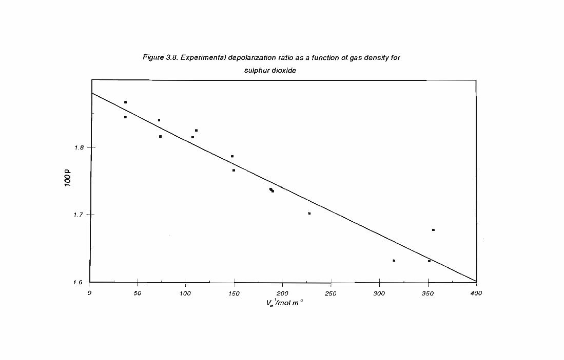
Q.

g -.-

1.8

1. 7

Figure 3.8. Experimental depolarization ratio as a function of gas density for

sulphur dioxide

1-~~~~-+ __ ~~~ __ ~~ __ ~~~ __ ~~~~~~ 1.6 ,

o 400 50 300 350 100 150 200

Vm·imol m·3

250

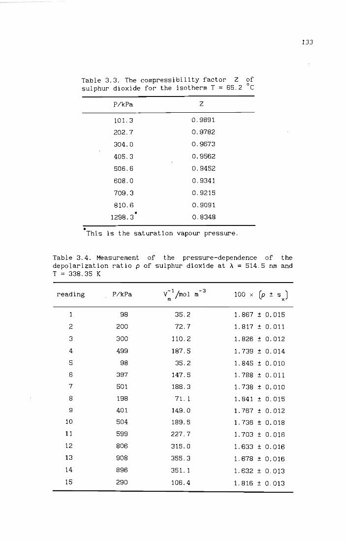
Table 3.3. The compressibility factor Z of sulphur dioxide for the isotherm T = 65 . 2 °c

P/kPa 2

101. 3 0.9891

202 . 7 0.9782

304.0 0 . 9673

405.3 0.9562

506.6 0 . 9452

608.0 0 . 9341

709.3 0.9215

810 . 6 0.9091 • 1298.3 0.8348

• This is the saturation vapour pressure .

Table 3.4. Measurement of the pressure-dependence of the depolarization ratio p of sulphur dioxide at A = 514.5 nm and T = 338.35 K

reading

1

2

3

4

5

6

7

8

9

10

11

12

13

14

15

P/kPa

98

200

300

499

98

397

501

198

401

504

599

806

908

896

290

35.2

72.7

110.2

187.5

35.2

147.5

188.3

71. 1

149 . 0

189 . 5

227.7

315.0

355.3

351 . 1

106 . 4

100 x (p ± sJ 1. 867 ± 0.015

1.817 ± 0.011

1. 826 ± 0.012

1. 739 ± 0.014

1. 845 ± 0.010

1. 788 ± O. 011

1. 738 ± 0.010

1.841 ± 0.015

1. 767 ± 0.012

1. 736 ± 0.018

1. 703 ± 0.016

1. 633 ± 0 . 016

1.678 ± 0.016

1. 632 ± 0 . 013

1. 816 ± 0.013

133

Table 3.5. Our measured B value for sulphur dioxide, together with the deduced ~ value. Comparison is p p

made with the theoretical values calculated in Chapter 2.

106

Bexp 106Beale B

exp 106~exp 106~eale ~exp

T/K 100 x P P P P P P P 0 3 -1 3 -1 Beale 3 -1 3 -1 ~eale m mol m mol m mol m mol

p p

338.35 1. 880 ± 0.009 -6.96 ± 0.49 -6.328 1.100 215 ± 53 249 . 39 0.862 7

134

A plot of p versus V-1 is given in figure 3 . 8. There is no discernible m

deviation from linearity, indicating a predominance of pair interactions

over this range of densities. Deduced values of p, Band Y together o p p

wi th their estimated uncertainties are presented in table 3.5, which

also contains the theoretical B p

and Y values calculated in Chapter 2. p

Notice how well our 100 x p o

of 1.88 ± 0.01 agrees with that of

1.85 ± 0.01 measured at A = 514 . 5 nm by Bogaard et ai . [ 4]. As was

anticipated, the experimentally deduced Y has quite a large uncertainty p

of some 25% . What is encouraging , though, is how the calculated Y lies p

comfortably within the uncertainty limits of the measured value. We have

discussed at length in Chapter 2 how

significant negative contribution to Y , P

polar molecules; and it is worth noting

the a A term can 2 1

and hence B, in the p

that if this term is

make a

case of

in fact

significant for sulphur dioxide, its effect will be to bring the

calculated Y closer to the measured value. This matter can only be p

resolved when estimates of A- tensor components become available .

For comparative purposes, we have calculated Y for sulphur dioxide p

after approximating its molecular shape and optical properties to be of

axial symmetry. The Lennard-Jones force-constants obtained for this

molecule in section 2.6.1 , namely R = 0.3850 nm and elk = 220 . 0 K, were o

used in equation (1.87) to calculate the second pressure virial

coefficient B(T). Choosing the shape factor D such that agreement

between the calculated B(T) and the experimental data [17] was to within

5% over the temperature range 283.15 to 473.15 K yielded D = 0.472 . This

shape factor is not physically reasonable, be i ng very close to the limit 1

of +- for infinitely thin rod-like linear molecules, as discussed in 2

section 1.4. 2. The molecular properties of sulphur dioxide required in

calculations of Y have been given is section 2 . 6.1, and it is obvious p that the quadrupole moment and polarizabi I i ty tensor of this molecule

cannot reasonably be approximated to

molecules with axial symmetry have 9 11

have 9 = -16 . 4 x 10-40 Cm2

11 we

Furthermore, I inear molecules have 0: 11

0: = 5.93 X 10-40 C2m2J-1 and 11

axial symmetry. For example,

= 922

, while for sulphur dioxide

and 9 = +12.9 x 10-40 Cm2.

22

= 0:22

, whi Ie sulphur dioxide has

0: = 3 . 34 X 10-40 C2m2J-1 22 at

A = 514.5 nm: a substantial difference of 78% . Using the dipole moment -30

113 = -5 . 4262 x 10 Cm, the mean static polarizability tensor

135

a = 4.2072 x 10-40 C2m2J-1, the dynamic polarizability components at s

A = 514.5 nm for an 'axially-symmetric' sulphur dioxide molecule of

10-40 C2m2J-1 and a = 5. 176 X 10-40 C2m2J-1, a" = 2.816 x 1 -40 2

approximate quadrupole moment a = a = 3.5 x 10 Cm, 33

and the

we obtain a

calculated sulphur dioxide at T = 338.35 K of

!f = P

!f = P

This value is 3.91 times larger than the -6 3 -1 249.39 x 10 m mol obtained after considering the full symmetry

of the molecule. When the two values are compared with the experimental -6 3 -1 estimate of!f = (215 ± 53) x 10 m mol , there can be no doubt as to

p the gross inadequacy of approximating non-linear molecules to be of

axial symmetry in the theory of B . It is desirable to establish whether p the second virial coefficients of the various other molecular-optic

phenomena will confirm this finding, and we turn to the Kerr effect for

guidance .

Calculations of the second Kerr-effect virial coefficients B of sulphur IC

dioxide performed by Gentle et al. [18], using the statistical-

mechanical theory of BIC presented by Buckingham et al. [19] for axially­

symmetric molecules, yielded results which were more than double the

experimental values. In the following chapter , we present a theory of B It:

for non-linear molecules, and apply it to various molecules, including

sulphur dioxide, with pleasing success .

3.3 References

[1] Cabannes, J, 1915, Comptes Rendus, 160. 62 .

[2] Strutt, J. W., (Third Baron Rayleigh), 1899, Scientific Papers IV,

397 .

[3]

[4]

[5 ]

[6]

Bridge,

2733.

Bogaard,

A. H. ,

Bridge,

Bridge,

N. J . , and Buckingham, A. D., 1964, J. chem. Phys. , 40.

M. P. , Buckingham, A. D., Pierens, R. K., and White,

1978, J. chem. Soc. Faraday Trans. I, 74. 3008.

N. J . , 1966, M. Sc . TheSis, University of Oxford.

N. J., and Buckingham, A. D. , 1966, Proc. Roy. Soc . Land.

A, 295. 334 .

136

[7] Strutt, R. J., (Fourth Baron Rayleigh), 1920, Proc. Roy. Soc. Land.

A, 97, 435 .

[8] Couling, V. W., and Graham, C., 1994, Malec. Phys., 82, 235.

[9] Smithells, C. J. , 1967, Metals Reference Book (London:

But terworths) .

[10] Graham, C., 1992, Malec. Phys., 77, 29l.

[11] Douslin, D. R., and Harrison, R. H., 1976, J. chem. Thermodyn., 8,

30l.

[12] Dymond, J. H., and Smith, E. B., 1980, The Virial Coefficients of

Pure Gases and Mixtures (Oxford: Clarendon).

[13] Berrue, J., Chave, A., Duman, B., and Thibeau, M., 1977, Rev. Phys.

Appl. , 12, 1743.

[14] Berrue, J. , Chave, A. , Duman, B. , and Thibeau, M. , 1981, Can. J.

Phys. , 59, 1510.

[15] Caul ing, V. W. , and Graham, C. , 1993, Molec. Phys. , 79, 859.

[ 16] Caul ing, V. W. , 1993, M. Sc. Thesis, University of Natal.

[17] Kang, T. L., Hirth, L. J. , Kobe, K. A. , and McKet ta, J. J. , 1961,

J. chem. Engng. Data, 6, 220.

[18] Gentle, I. R., Laver, D. R., and Ritchie, G. L. D., 1990, J. phys.

Chem., 94, 3434.

[19] Buckingham, A. D., Gal was , P. A., and Liu Fan-Chen, 1983, J. Mol.

Struct., 100, 3.

CALCULATION OF COEFFICIENTS

AND

CHAPTER 4

THE SECOND KERR-EFFECT VIRIAL OF MOLECULES WITH LINEAR

LOWER SYMMETRY

4.1 Introduction

137

The second light-scat tering virial coefficient B has now been the p

subject of comprehensive experimental and theoretical investigation for

molecular symmetries ranging from spherical to non-linear. It has been

established that the dipole-induced-dipole (DID) model of Silberstein

[1] reliably accounts for the contribution made by interacting pairs of

molecules to the depolarization ratio p of Rayleigh-scattered light for

the full range of molecular symmetries, although reasons for the

discrepancies between experiment and theory for the larger

quasi-spherical molecules [2] still need to be sought and explained. A

significant aspect of the theoretical investigation has been the

realization that attempts to treat non-linear molecules by approximating

them to be of axial symmetry lead to grossly inaccurate calculated

estimates of B . Certainly, such approximations are tempting; especially p

in view of the arduous task of developing a complete molecular tensor

theory of B even for molecules with linear symmetry. However, it has p

been successfully demonstrated how, after invoking the aid of the

powerful algebraic manipulation packages now available for personal

computers, the development of a complete molecular tensor theory of B p

for non-linear molecules is feasible. This theory has yielded calculated

estimates of B for ethene (Of 0 symmetry) and sulphur dioxide (Of C P 2h 2v

symmetry) which are in good accord with our measured values.

Approximating ethene to be of axial symmetry sees the calculated !f p

value significantly underestimating experiment by 40%, while a similar

approximation for sulphur dioxide yields a calculated!f which is four p

times larger than the measured value. It has been concluded that after

taking full account of the symmetry of a particular molecule, both in

its molecular property tensors and physical shape, the DID model

x

parallel plate electrodes

~ ! • z

y

Figure 4.1 . The Kerr cell, with space-fixed axes (x,y,z) where z is in the direction of propagation of the light beam,

x is in the direction of the applied electric field, and y is perpendicular to the field.

138

accurately describes the effects of pair interactions on p.

It is now desirable to turn to other molecular-opt ic phenomena for a

general confirmation of this conclusion. Of particular interest will be

the development of DID theories describing the effects of pair

interactions on these phenomena, followed by calculations where the same

Lennard-Jones force constants and shape factors obtained in work on B(T)

and B are utilized. Will good agreement between experiment and theory p

be maintained? Since substantial experimental invest igation into the

pressure-dependence of the Kerr effect has been carried out by various

independent research groups for molecules with spherical [3-5], linear

[6-10] and non-linear [11-131 symmetry; it seems natural to turn our

attention to this particular effect in seeking an answer to our

question.

4.2 A general theory of electro-optical birefringence in dense fluids

Kerr, in 1815, was the first to observe that an isotropic medium placed

in a strong uniform electric field generally becomes birefringent [14].

The scope of our investigation will be limited to fluids, where the

application of a static field leads to anisotropy in the molecular

distribution either as a result of intrinsic anisotropy in the

individual molecules, or because anisotropy is induced in the molecules

by the applied field itself.

Consider the arrangement in figure 4.1 where the space-fixed system of

axes O(x,y,z) is fixed in the Kerr cell such that z is in the direction

of propagation of the light beam, x is in the direction of the applied

electric field, and y is perpendicular to the field. When the cell is

filled with a fluid and a uniform electric field is applied (by means of

a pair of parallel-plate electrodes), a light beam propagating in the

z-direction and vibrating in the xz plane will experience a refractive

index n, which differs from the refract i ve index n experienced by a x y

beam propagating in the z-direction and vibrating in the yz plane. The

task in developing a theory of the Kerr effect lies in relating the

macroscopic observable (n - n) to the molecular property tensors of x y

the individual molecules in the fluid, and this has been achieved for

gases at low pressures by Buckingham and Pople [15].

139

4.2.1 Non-interacting molecules

For a dilute gas where molecular interactions are negligible in number, (p)

the osci 11 ati ng dipole moment /l of molecule p arises solely due to 1

the polarizing action of the oscillating electric field g associated o

with the light wave, there being no neighbouring molecules q which are

close enough for their oscillating moments to set up significant fields

and field gradients at molecule p. However, it is important to realize

that the optical-frequency polarizability tensor ex of molecule p may 1 J

be modified by the presence of the strong applied static electric field

E , to a new effective polarizability tensor n , written 1 1 J

n IJ

B/l 1 = ag-- = oj

+ .. . , (4.1)

where all tensors refer to the molecule-fixed axes 0(1,2,3) of molecule

p. Here, the polarizability tensor ex , and the first and second IJ

hyperpolarizability tensors 131Jk

and rlJkl respectively, are dependent

on the optical frequency of the incident light wave. Any orientational

bias arising from intrinsic molecular anisotropy wi 11 be accounted for

later on when we average over the biased orientat ional mot ion of the

molecule .

To compare the refract! ve indices parallel and perpendicular to the

applied static electric field E, we require the direction cosines aX 1 1

between the x space-fixed and i molecule-fixed axes, and aY between the 1

the y space-fixed and i molecule-fixed axes. Then, if the molecule is

held in a fixed configuration~, the difference between the differential

polarizabilities for this specific orientation is

(4 . 2)

Since the molecule is in fact tumbling in space, this quantity has to be

averaged over all configurations in the presence of the biasing

influence E1

• Assuming the period of oscillation of the light waves to

be much smaller than the time of rotation of the molecule, and assuming

that the rotational energy levels are suffiCiently close for the

orientation to be effectively continuous, it i s possible to average over

configurations with a Boltzmann-type weighting factor. We write

1l = Jll(~,E) exp(-U(~,E)/kT)dL

Jexp(-U(~,E)/kT)dL

140

(4 . 3)

where U(~,E) is the energy of the molecule in a particular configuration

~ while in the presence of the applied field E . In molecule-fixed axes, 1

this energy is given by

U{~, E) = dOl /l(OlE - ~ E E - ~b E E E -1 1 2 1 j 1 j 6 1 jk 1 j k

.. . , (4 . 4)

where dOl is the energy of the molecule in the absence of the appl ied

field, /l(Ol is the permanent dipole 1

moment of the molecule, a is the 1 j

static polarizabi 1 i ty, b1jk

is the static first-order hyper-

polarlzability, etc. The difference

now be written as

between the refractive indices may

n - n = x y

21lN It.

----1l (4 . 5)

We can write out the full expression for ll(~,E) in equation (4.2) by

writing Eax for E and by making use of equation (4.1): 1 1

(4.6)

We already know how to average over unbiased rotational motion (see the

isotropic averages in Chapter 2), and so the procedure adopted is to

convert the biased average in equation (4 . 3) into isotropic averages by

Taylor expanding n in powers of E while bearing in mind that it depends

on E both through ll(~,E) and through the energy U(~,E). It is fair to

assume that the series converges rapidly since the distortion and

orientational effects of E on gas molecules is extremely small. We have 1

1l = A + B E + C E2 + .. . (4.7)

where

A = (ii:)E=O ' (4.8)

141

B = [~~] • E=O

(4.9)

and

c = ~[a2rrJ . 2 aE2

E=O

(4 . 10)

We will denote an isotropic average of a quantity X(~.E) with E = 0 as

<X>. that is

JX(~.O) exp(-U(OJkT)dT

<X> = J (0) exp (-U ,lkT) dT (4.11)

Explicit expressions for the various coefficients A. B. C .. . are then

obtained by putting E = 0 after differentiating equation (4.3). We have

[ali] laTC) -1( a~ B = aE E=O = \BE - (kT) TCaE/· (4 . 12)

The quantities in angular brackets are easily obtained from equations

(4.4) and (4.6). which yield

and

(0) x -1-1 a

1 1 (4.13)

(4 . 14)

It is clear that both terms in equation (4 . 12) average to zero over all

directions of a;. and so the leading non-vanishing term in the expansion

f - . . E2 o TC IS In :

The second derivatives of equations (4.4) and (4.6) are

and

x x = -a a a 1 j 1 j

142

(4. 16)

(4.17)

Considering each term in equation (4 . 15), and making use of the standard

results for isotropic averages in equations (2 . 14) and (2.16) of Chapter

2 , we obtain:

(4. 18)

(4.19)

1 < (aU)2) 1 (0) (0)( x x x x y y x x) -- 1[- = 0: Il Il aaaa -aaaa 2k2T2 aE 2k2T2 1 j k 1 1 j k 1 1 j k 1

= 3 (0: (0) (0) _ 0: r (0») 2) 2 2 1 Jill IlJ LIl ,

15k T (4.20)

where 0: and a are the traces of 0: and a respectively. Hence, 1 J 1 J

equation (4.7) becomes

- {2 2 (0) 1 1[ = 30 1'l1JJ + 15kT,911JIlJ + 15kT(0:1Ja l J - 30:a)

+ 3 [0: (0) (0) _ C (0»)2)} 2 2 2 III IlJ 0: Il E

15k T (4 . 21)

143

Using the definition of the molecular Kerr constant Km proposed by

Otterbein [16] which, in the limit of low densities, reduces to

K = ti..m m v

m

we obtain

2rrN K

A = m 405 (4rre J

This equation,

{

2 (n - n )v } x y m

27 (4rre JE2

E~ =

2rrN A

27 (4rre ) o

[::~] , E=O

(kT)-l [4/3 ~(O) + 3 (a a - 3aa)] ll J J lJlJ {2711JJ +

+ _3_[« (0) (0) _ «( (0»)2]} 2 2 lJ~l ~J ~

k T

first derived by Buckingham and Pople [15],

(4.22)

(4.23)

is a

generalization of the well-known Langevin-Born equation to include the

effects of high field strengths on the polarizability.

For a gas of non-interacting spherical molecules, equation -(4 . 23)

reduces to

K = m

4rrN A

---- '1 81 (4rreJ

(4 . 24)

1 where '1 = - '1 measurement of the Kerr constant at low pressures can 5 1 J 1 J

directly yield a value for the hyperpolarizability constant '1 of the

gas . This value, although peculiar to the frequency of the light beam

used in the measurement of the refractive index, is unlikely to be

substantially different from the static value provided the optical

frequency is well below the electronic absorption band of the gas

molecules.

4 . 2.2 Interacting spherical molecules

The above Langevin-Born and Buckingham-Pople theory of electro-optical

birefringence pertains specifically to assemblies of non-interact ing

molecules . However, since the difference between refractive indices

144

parallel and perpendicular to the applied field is often very small at

low gas pressures (especially for typical field strengths readily

obtainable in the laboratory), experiments often have to be carried out

on compressed gases. In such cases the molecular Kerr constant K m

differs from that obtained in the I imit of infinite dilution. This

density-dependence of K is conveniently described by means of the m

virial expansion [17]

B C IC Ie

+ + ... , V

V2

m m

where the coefficients A, B, C, .. . , are the first, second, third, Ie K K

.. . , Kerr-effect virial coefficients. AK' equal to

V ~ 00 m

is given by equation (4.24) of section 4.2.1. BK

, which describes

deviations from A due to pair interactions, is K

B = Urn. K

V ~ 00

(K - A)V . m K m

(4.26)

m

In 1968, Buckingham and Dunmur [3] measured the pressure-dependence of

the Kerr effect for the atomic species argon, krypton and xenon, and for

the quasi-spherical molecule sulphur hexafluoride. The relationship

between the induced birefringence and gas density was observed to be

non-linear, indicating a significant presence of pair interactions.

Invoking dipole-induced-dipole theory, B was written [3] K

32 2N2 2 2

B = K

1l a a 00

A J R-4

exp(-U (R)/kT) dR 45 (41l£ J 3 kT 0 12

(4.27)

where N is Avogadro's number, A

polarizabilities respectively, a and a ar e the dynamic and static

and U (R) is the intermolecular 12

potential between interacting molecules 1 and 2 which are separated by a

distance R. It is worth noting that for atoms and spherical molecules,

the second Kerr-effect and light-scattering virial coefficients are closely related [18]:

27c kT B = __ 0_

p B K

145

(4.28)

Buckingham and Pople [19] have provided a means of evaluating the

integral in equation (4 . 27) :

() R-k exp(-~2(R)/kT) R2 dR = 1\ R~-k y-4 Hk(y) o

(4.29)

where If (R) is the Lennard-Jones 6: 12 potential [20] . Values of Hk(y) 12

have been tabulated for k ranging from 6 to 17 in integral steps [19].

Table 4.1 presents the ratio of all measured values of B for atoms and K

spherical molecules with the values calcul ated according to equation

(4.27). Also included are the ratio of measured second light-scattering

virial coefficients B with the values calculated according to equations p

(4.27) and (4.28). The ratio BexP/Bcalc displays the same trend observed K K exp calc

earlier by Watson and Rowell [2] for the ratio B IB , namely that p p the ratio is less than one for the rare gases , and increases more and

more above unity as the molecular size increases . This appears to

confirm the assertion made by Watson and Rowell [2] that the point­

dipole approximation of the DID model for molecular interactions is

inadequate for the larger quasi-spherical molecules . And yet, the DID

theory of B for the linear molecules nitrogen, ethane, methyl chloride p

and carbon monoxide [24,25], and for the non-linear molecules ethene and

sulphur dioxide (Chapter 2), is in good agreement with experiment (see

[26-28] and Chapter 3). Discrepancies between experiment and theory for

the large quasi-spherical molecules remain unresolved, and the problem

warrants further attention.

146

Table 4.1. Comparison of measured and calculated second K~rr-effect and light-scattering virial coefficients for atoms and spherIcal molecules as reported by Dunmur et al . [5] .

Bexp

Bexp

Atom/ Ie -p--molecule Beale Beale

Ie p

argon 0.73 ± 0 . 11 [3] 0 . 62 ± 0 . 96 [ 21]

0.65 ± 0.11 [5] 0.81 ± 0.12 [22]

0.67 ± 0 . 03 [ 4]

krypton 0 . 62 ± 0.54 [3 ] 0.85 ± 0.11 [2]

0 . 63 ± 0.09 [5]

xenon 0 . 46 ± 0 . 16 [3]

0.67 ± 0.12 [5]

methane 0 . 92 ± 0.09 [4] 0.75 ± 0.03 [4 ]

1. 40 ± 0 . 2 [5] 0 . 86 [23]

1. 20 ± 0.17 [2]

1. 03 ± 0 . 15 [22]

sulphur 1. 77 ± 0 . 24 [3] 2 . 51 ± 0.08 [2 ] hexafluoride

2.5 ± 0.4 [5]

tetrafluoromethane 1. 10 ± 0 . 1 [5]

neopentane 3. 9 ± 0. 3 [5] 6.8 ± 0.9 [2]

4 . 2 . 3 Interacting linear molecules

The second Kerr-effect virial coefficient B has been deduced from Ie

pressure-dependence measurements of electric field induced birefringenc~

for the linear molecules fluoromethane [6], tr i fluoromethane [6], carbon

dioxide [7,10], nitrogen [7] , ethane [7] and cyclopropane [7]; and for

the non-linear molecules ethene [7], difluoromethane [6], dimethyl ether

[11], hydrogen sulphide [12] and sulphur dioxide [13]. B has also been iii:

measured for cyclohexane and the n-alkanes from propane through to

decane [9] . Some important features of these measurements are now

147

discussed.

B JC

values for polar molecules are generally a hundred times larger than

those for non-polar species. Val ues of B deduced from Kerr-effect JC

measurements on polar gases often have poor precisions of around ±50%,

with additional systemat ic errors arising from uncertaint ies in the

pressure virial coefficients B(T) and eCT) used to obtain the molar

volumes V of gas samples. In the case of non-polar gases, the m

experimental difficulties are further compounded by the much smaller

densi ty-dependence of the molar Kerr constant K. This is evidenced by m

the almost random fluctuation in the B values measured over a range of JC temperature for both nitrogen [7] and carbon dioxide [7,10] .

In 1955, Buckingham [17] developed a statistical-mechanical theory of BJC

for axially-symmetric molecules. Buckingham and Orr [6] extended this

theory in 1969, including additional effects of polarizability and

angle-dependent repulsive forces. They proceeded to calculate B for the JC

fluoromethanes, and although approximate agreement with their

experimental values [6] for fluoromethane was obtained, the calculated

values for trifluoromethane were found to be much too small. This

disagreement was attributed to effects of short-range interactions on.

the polarizability and potential energy, and it was argued that

measurements of B for polar gases would probably not yield useful JC

information about the nature of intermolecular forces.

It was only much later, in 1983, that Buckingham et ai. [29] published a

paper in which the order-of-magnitude discrepancy between experiment and

theory for the fluoromethanes was resolved. The earlier theory of the

Kerr effect [17] was extended to include collision-induced

polarizability, which was found to be the dominant contributor to B . JC

Use was made of a simple Stockmayer-type potential [30], in which the

dipole-dipole interaction is added to a 6: 12 Lennard-Jones potential;

but the U contribution to the intermolecular potential. which has shape

been used before [19] to account for the angular dependence of

short-range overlap repulsive forces for non-spherical molecules. was

not included. Although no attempt was made to optimize the Lennard-Jones

force constants R and elk. the new theory of B was found to provide o JC

what was said to be a reasonable fi t to the observed values for the

fluoromethanes [6] over a range of temperature. However, as will be

shown later. this must be viewed in relation to a large uncertainty of

148

about 50% in the observed values .

It is noteworthy that although B has been measured for several K

non-polar molecules of linear symmetry, no calculated values of this

quantity have appeared in the literature .

Recently, Gentle et al. [13] undertook measurements of the Kerr effect

of sulphur dioxide over the temperature range 298.7 to 490.3 K, deducing

rather precise B values over this temperature span. In view of the K

relative success of Buckingham, Galwas and Fan-Chen's extended theory of

B for axially-symmetric molecules K

[29] when applied to the

fluoromethanes, Gentle et al. thought it profitable to attempt an

application of the theory to sulphur dioxide after approximating the

molecule to be quasi-linear . The Lennard-Jones force constants R and o

elk were opt imized, and when used in a simple Stockmayer potential to

compute the second pressure virial coefficient BCT) of this gas, the

calculated values were found to agree with experiment [31,32] to within

±6% over the full range of temperature . However, the calculated B K

val ues were generally more than double the experimental val ues, the

model proving unsatisfactory. Perhaps this is not surprising, since for

an axially symmetric molecule with the 3-axis as the principal axis, the

polarizabi I i ty components perpendicular to the 3-axis, IX and IX , are 11 22

equal; whi Ie for sulphur dioxide we have IX 11

= 5.80 x 10-40 C2m2J-l and

IX = 3.30 x 10-40 C2m2J-l at A = 632.8 nm 22

[ 13] : a substantial

difference of 76%. To definitively assess the extent to which the

assumption of axial symmetry is responsible for the discrepancy between

theory and experiment for sulphur dioxide, it is essential to develop a

complete molecular tensor theory of B for molecules with non-l inear K

symmetry. This theory is now presented, followed by application to both

polar and non-polar molecules with linear and lower symmetry.

4 . 2.4 Interacting non-linear molecules

Recall that in the I imit of infinite dil ut ion, the refract i ve index

difference (n - n) of a gas in a strong stat ic electric field E x y x

n - n = x y

2nN A

(4ne ) V o m

n

is

C4.30)

149

where n is the average over all configurat ions (j of the quant i ty

n (aXaX - aYaY) of a representative isolated molecule in the presence Ij 1 j 1 j

of the biasing influence E. The biased average n was converted into x

isotropic averages by Taylor expanding in powers of E. the leading

contribution

being expressed in terms of isotropic averages in equation (4 . 15).

For higher gas densities . we follow the philosophy established by

Buckingham and Pople [33]. and argue

representative molecule 1 to (n - n ) x Y

that the contribution of 2nN

a

A is now not always ---- n.

(4n£ JVm

there being times when molecule 1 must be treated as half of an

interacting pair. If molecule 1 has a neighbouring molecule 2. the

relative configuration of which is given by the collective symbol 't' .

then the contribution of molecule 1 to

given by ~ 2nNA n(12)('t'.E)}. Here.

(n - n) at that instant is x Y

1(4n£ )v o m

(12)( E) (12) ( x x Y Y) n 't' =n aa -aa • Ij 1 j 1 j

(4.31)

where n(2

) is the differential polarizability of the interacting pair. Ij

and an expl icit expression for this quantity will be derived in due

course.

If the pair of molecules are held in a fixed relative configuration 't'

and are allowed to rotate as a rigid whole in the presence of the

biasing influence E1

• the resulting biased orientational average

.... (12) ( ..... E) •• ~ can then be converted into isotropic averages by Taylor

expanding in powers of E. Analogous to the case of an isolated molecule.

the leading term is

(4 . 32)

E=Q

150

where

(4.33)

Here, U<12) (T, E) is the potential energy of the interacting pair of

molecules in the presence of E. 1

If the quantities within angular

brackets are all initially referred to the molecule-fixed axes (1,2,3)

of molecule 1, ' then for a given relative interaction configuration T,

the tensor product in (1,2,3) is fixed. When the pair rotates as a rigid

whole . in space-fixed axes (x,y,z), the average projection of pair

properties (referred to (1,2,3)) is averaged into (x,y,z) over all

orientat ions . Averaging over the pair int eract ion parameters T can

subsequently be performed.

Recall from equation (4.22) that the definition of the molecular Kerr

constant proposed by Otterbein [16], in the limit of low densities, is

[::;] . E=O

We are now in a position to extrapolate this expression to higher

densities, obtaining

J 21(N

+ A

27 (41(£ ) o

- [::;] } P( T)dT E=O E=O

(4.34)

where P(T)dT is the probability of molecule 1 having a neighbour in the

range (T, T + dT) . Buckingham and Pople [33] have related this

probability to the intermolecular potential U (T): 12

N peT) = Q~ eXP(-U

12(T)/kT)

m

Comparing equation (4.34) to equation (4.25) , we obtain for B Ie

(4.35)

B = K

E=O

[::;LJ exp(-U,2 (Y)/kT)

151

(4 . 36)

which for two non-l inear molecules with interact ion co-ordinates as

described in section 2.2 of Chapter 2 becomes

N2 00

B. = 216n2~4ne.) JR=o

- [a2

rr] } exp(-U (T)/kT) aE2 12

E=O E=O

x R2si~ si~ dR d~ d~ dr d~ d~ dr . 12 111222 (4.37)

[a

2rr] has already been evaluated in section 4.1.1, yielding aE2

E=O

[a2rr] {4 4 _0 (0) + _2_(~ a - 3~) aE2 = 30 r11JJ + I5kT""11J J.L J 15kT\: 1J 1J

E=O

6 [ (0) (0) ( (0»)2]} + ~ J.L J.L - ~LJ.L , 15k2T2 1J 1 J

(4 . 38)

. 1[a2n(12)(T,E) and we must now turn our attentlon to evaluating - ------~~-

2 aE2 E=O

As for a dilute gas, the refractive index of a dense gas is determined

by the total oscillating dipole moment induced in a molecule. The

difference now is that the dipole moment of a representative molecule 1

is induced not only by the oscillating electric field 5 associated

with the light wave, but also in part by the field ~(1~1 arising at 1

molecule 1 due to the oscillating moments of a neighbouring molecule 2.

If we neglect the small quadrupole and field gradient effects, we have

(1)(5) = [~(1l + ~(1)E +!. (1) E E + ... J[5 + ~(llJ J.L 1 0 1J 1jk k 2r 1jkl k 1 oj J

(4.39)

152

where E is the strong applied static field. J

Invoking the T-tensors (see equations (2 . 28) to (2.30)), we see that

?J{ 1) has the form J

?J{ 1) = J

T(1) (2)

Jk Ilk (4.40)

It must be emphasized that 1l~2) itself is the oscillating dipole induced

in molecule 2 by the field arising at 2 due not only to the direct

influence of g, but also to the oscillating dipole moment of o

molecule 1:

Ilk(2) (go) = (0:{2) + t3(2)E + ~r(2) E E + ... ] (g + ?J(1

2)] ,

kl kIm m 2 klmn m n 01

where ?J(2) has the form given by equation (4.40): 1

(2) T(2) 1I{ 1) ?J = r-

1 1m m

(4.41)

(4.42)

Substitution of equations (4.41) and (4.42) into equation (4.40), • (1) (2)

followed by successive subst 1 tutions of?J and?J, leads to a I I

lengthy series of terms contributing to the net field ?J(1) in equation J

(4.40); and substitution of this series into equation (4.39) yields a

final expression for the total oscillating dipole induced on molecule 1

by the light wave field in the presence of molecule 2:

153

(1) ((5 ) ~1 L 0

(l)T (2)/? +0:. 0:. C>

1j jk kw ow

+ ~(l)T r(2) E E (5 + ~(l)T r(2) E E T 0:.(1)(5 21J Jkkwmnmnow 21J Jkklmnmnlppw ow

+ ~(l)T 0:.(2)T r(l) E E (5 2 1 j J k k 11m mwnp n pow

+ ~(llT r(2) E E T o:.(llT 0:.(2)(5 + .... 2 1J Jk klmn m n Ip pq qr rw ow

(4.43)

When the operation :(5 is performed on this expression for ~~1l we ow

find the resulting expression for the differential polarizability of a

molecule p in the presence of both the applied static field E and a 1

neighbouring molecule q in a specific relative configuration L is

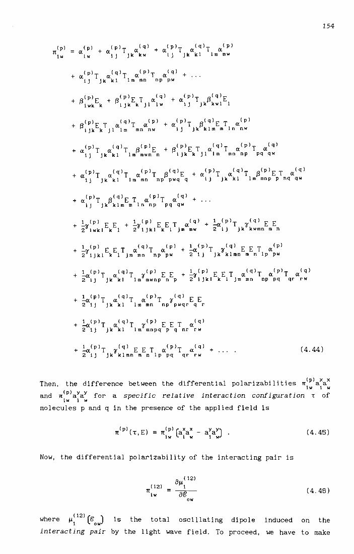
(P)T (q)T (P)T (q) +a a a a 1J Jk kl 1m mn np pw

+ .. .

+ .,.

+ ~ (p) E E 1 (p) E E T a(q) + ~(P)T r lq ) E E 2 r 1 w k 1 k 1 + 2r 1 j k 1 k 1 j m m w 2 1 j j k k w mn m n

+ ~ Ip) E E T alq)T alP) + ~lp)T r lq ) E E T alp) 2r ljkl k 1 jm mn np pw 2 lj Jk klmn m n Ip pw

+ ~(P)T alq)T rIp) E E 2 1j Jk kl 1m mwnp n p

+ ~IP)T alq)T rep) E E T a(q) 2 lj jk kl 1m mnpq p q nr rw

+ ~IP)T r lq ) E E T aIP)T a lq ) + .... 2 lJ jk klmn m n Ip pq qr rw

154

(4.44)

Then, the difference between the differential polarizabilities rrlp)axax 1w 1 w

and rrlp)aYaY for a specific relative interaction configuration L of lw 1 w

molecules p and q in the presence of the applied field is

Now, the differential polarizability of the interacting pair is

(12) 1(

lw = 8 (12)

III 88 ow

(4 . 45)

(4.46)

where III 12) (£5) is the total induced ""1 ow oscillating dipole on the

interacting pair by the light wave field. To proceed, we have to make

155

the assumption that the two interact i ng molecules each retain their

separate identities. Certainly , in the long-range limit this assumption

is perfectly valid. It is at very short range, when the charge

distributions of the interacting molecules begin to overlap, that

difficulties arise . The molecules can no longer be unambiguously

defined, and for a definitive description of this arrangement, one has

no alternative other than resorting to ab initio quantum-mechanical

calculations. These are notoriously difficul t, and have to be repeated

for each system under consideration. Instead (and in keeping with the

philosophy of this thesis) we follow the lead of past workers i n the

field [29,34-36] by treating the interacting molecules as if they retain

their separate identities even in the overlap region.

With this assumption, equation (4 . 46) become~

(12) 1l

lw ow ow

(4.47)

Th d · f (12) x x en, the 1 ference between the differential polarizabilities 1l a a (12) y y lw 1 w

and 1l a a of an interacting pair in a specific relative interaction lw 1 w

configuration ~ in the presence of the applied field may be written

= (1)( E) (2)( E) 1l ~, + 1l ~,

where 1l(p) is given by equation (4.44). lw

(4.48)

We follow Buckingham et al. [29] by writing the potential energy of the

interacting pair in the presence of the static field E as

where E has been written as EaX,

1 1

moment of the pair in the presence

1

and where 1l<t2) is the total 1

of E . As before, we write 1

(4.49)

dipole

(4.50)

156

where ~(p) is the total dipole moment of molecule p in the presence of 1

E and molecule 2. We have 1

(p) = (p) + a (p) (E + F(P») ~1 ~01 1j j j

(4.51)

where ~(p) is the permanent dipole moment of molecule p, and F(P) is the 01 j

static field arising at molecule p due to the permanent and induced

multipole moments of the neighbouring molecule q. Considering only the

total dipole moment of molecule q, we can write

Of course,

where, in turn,

= T ',,(q)

jk"'k

= (q) + a (q) (E + F(q») ~01 1j j j

(4.52)

(4.53)

(4.54)

Successive substitutions of F(P) and F(q) into equation (4.50) yield the J J

series of terms contributing to the total static dipole moment on

molecule p:

+ a(P)T a(q)T a(P)T a(q)E ( 2) 1j + . . . + 0 E +

jk kl 1m mn np pv v (4.55)

Hence, equation (4.49) becomes

(4 . 56)

where

(P)T a(q)T a(P)T (q) )E x + a /J. + . .. a1 1J Jk k1 1m mn nv ov

- ~(a(p) + a(P)T a(q) + a(P)T a(q)T alp) 2 1v 1J Jk kv 1J Jk k1 1m mv

(p) (q) (P)T (q) ) 2 x x +a Ta Ta a + ... Eaa 1J Jk k1 1m mn np pv 1 v

1[821(12) (T,E) We are now in a position to evaluate the term - -----------

2 8E2

157

(4.57)

in the

E=O expression for B given by equation (4.37). Recall from equation (4.33)

Ie

that

E=O

(4.58)

These isotropic averages are now systematically evaluated.

Invoking equation (4.48), (

82 (12» the average ~ 1( may be written as

2 8E2 _1 (821(1» + _1 (8

21(2», and since molecules 1 and 2 are ident ical,

2 8E2 2 8E2 the

isotropic averages of their polarizabilities must be the same. Hence,

(4.59)

Using similar arguments, together with equation (4.56), we have

( (12) (12» {(1) (1)

_(kT)-l 81( 8U = -2(kT)-1 (2~ ~) 8E 8E 8E 8E + (

81( 1) 8U( 2»} 2 8E 8E '

(4.60)

(4.61)

158

and

(4.62)

Collecting these expressions, we obtain

< an( 1) aut 2»}

2 aE aE

(4.63)

(p) (p) Substituting in the explicit expressions for n C1:, E) and U Ct", E)

(given in equations (4.45) and (4.57) respectively) with E = 0, as well

as their first and second derivatives with respect to the applied field

to !.[a2n(12) (T,E)

2 aE2 where appropriate, we obtain the contributions

E=O and hence, through equation (4.37), to B. We have

Ie

where

0: +0: +0: +0: + 234 5

+ r 0: + r 0: + 1 1 1 2

+ ~20:1 + ~20:2 + ~20:3 + ...

+ ~1(31 + ~1(310:1 + ... ,

N = (kT)-l{ (ll (2)} < x x x x y y x x) .... 2 0: a aaaa -aaaa , ab pq a b p q a b p q

(4.64)

(4.65)

159

a = kT a a a + a a a ( )-1{ (ll (llT (2) (1) (2)T (1)

3 ad pq qr rs ad pq qr rs

(llT (2) (ll (llT (2) (2)} +a a a +a a a

ab be cd ps ab be cd ps

(

XX x x Y Y x x) X a a a a - a a a a ,

a d p sad p s (4.66)

(llT (2) (llT (2) (1)T (2) (2)T (1) +a a a a +a a a a

ab be ef pq qr ru ab be ef pq qr ru

(llT (2)T (ll (ll (1)T (2)T (1) (2)} +a a a a +a a a a ab be cd de ef pu ab be cd de ef pu

(4.67)

+ a( llT a(2)T (ll a( llT (2) a a

ab be cd de eh pq qr rw

+ a( llT a(2)T ( 1 ) a(2)T (1) a a

ab be cd de eh pq qr rw

(XX x x Y Y x x) X a a a a - a a a a , a h p wah p w (4.68)

={,)l)T (2) (l)T (2)}(XXXX YYXX) o a +a r aaaa -aaaa

abed be ef ab be efed a fed a fed ' (4 . 69)

160

-2{ (1) (2) (2) 2 (1) (1) (2)} = (kT) aab ~01 ~op + aab ~01 ~op

(XX x x y y x X)

X aaaa -aaaa • ab1p ab1p

(4.70)

2 (1) (1) (2)T (1) 2 (1) (2) (1)T (2)

+a ~ a ~ +a ~ a ~ ad 01 pq qr or ado 1 p q q r 0 r

(OT (2) (1) (0 (1)T (2) (2) (2) +a a ~ ~ +a a ~ ~

a b be cd 0 1 0 P a b bee d 0 1 0 P

(4.71)

+ a ( 1 ) a ( 1 ) T ~ ( 2 ) a ( 2 ) T ~ ( 1) + 2a ( 1 ) T a ( 2 ) ~ ( 1 ) a ( 1 ) T ~ ( 2 ) af 1j jk ok pq qr or ab be ef 01 pq qr or

+ 2a ( 1 ) T a ( 2 ) ~ ( 2 ) a ( 2 ) T ~ ( 1) + 2a ( 1 ) T a ( 2) ~ ( 1 ) a ( 2 ) T ~ ( 1 ) ab be ef 01 pq qr or ab be ef 01 pq qr or

+ 2') 1) T ( 2 ) (2 ) (1) T (2) 2 (1) (1) (1) T ( 2 ) T ( 1) .... a ~ a ~ +a ~ a a ~

ab be ef 01 pq qr or af 01 pq qr rs st ot

2 (1) (2) (2)T (1)T (2) 2 (1) (1) (2)T (1)T (2)

+a ~ a a ~ +a ~ a a ~ af 01 pq qr rs st ot af 01 pq qr rs st ot

2 (1) (2) (1)T (2)T (1) (1)T (2)T (1) (1) (1)

+a ~ a a ~ +a · a a ~ ~ af 01 pq qr rs st ot ab be cd de ef 01 op

(1)T (2)T (1) (2) (2) 2 (1)T (2)T (1) (1) (2)} +a a a ~ ~ + a a a ~ ~

ab be cd de ef 01 op ab be cd de ef 01 op

( XX x x y y x x) X a a a a - a a a a •

a d 1 pad 1 p (4 . 72)

2(kT) -1{(3(l) (2)} ( x x x x y y x x) = ~ aaaa -aaaa . ab1 op a b 1 P a b 1 P

(4.73)

The isotropic averages in equations (4.65) to (4.73) are carried out

using the standard results in equations (2.14) and (2.16) of Chapter 2.

We illustrate the procedure by considering the term for a in equation 2

161

(4.65) :

( )-1{ (ll (2)} (x x x x - aYaYaXax) a = kT a a a a a a 2 ab pq a b p q a b p q

(kT)-1{a(lla(2)} 1 (-20 ° + 30 ° + 30 ° ) = ab pq 3 0 ab pq ap bq aq bp

6 {( 1) (2) = -- a a -30kT ap ap

3aa} . (4.74)

Here, a(l) is the dynamic polarizability tensor of molecule 1 expressed ap

in the molecule-fixed axes of molecule 1, (1,2,3), while a is the mean

dynamic polarizabi I i ty. Similarly, a (2) is the static polarizabil ity ap

tensor of molecule 2 expressed in (1,2 , 3), while a is the mean static

polarizabi I i ty.

It is useful to check that the above terms reduce to expressions

previously derived for linear molecules when the molecular tensors are (1)

reduced to their simplified forms. For such molecules, a is diagonal (2) (IJ) (2) (2)

with all = a 22 = aJ. and a 33 = an; while a.\.~ = aJ.0 IJ + all - aJ. tl tJ

t(2) being a unit vector along the dipole axis of molecule 2 . a [37] ,

d th t f N(1) and a(1) t· I U· th t an a are e races 0 ~ respec lve y. sIng ese ensors IJ Ij

in equation (4 . 74) yields

(4.75)

where e is the angle between the symmetry axes of molecules 1 and 2. 12 This is exactly the polarizability contribution to B originally derived

Ie .

by Buckingham [17] . Similarly, the permanent dipole contribution to 8 Ie

in Buckingham's original theory [17] is exactly reproduced by the term

~2al in equation (4 . 70) when applied to axially-symmetric polar

molecules. The higher-order terms of Buckingham et al. [29] , which

describe the collision-induced polarizability contributions to B , are K

approximate, the polarizability tensors having been rewritten as

isotropic polarizabilities; and so a direct comparison with our

higher-order terms is not possible .

(1) The exact forms of a and a for molecules with D and C symmetries

ap 2h 2v

have already been quoted in Chapter 2, but are repeated here for

convenience:

162

n' 0

«~1 ' (ll (2) = (4.76) (l = (ll'j'

(l 1 j 22

0 33

and

(l=~(l =~(l +(l +(l) 3 II 3 11 22 33

(4.77)

The form of the static polarizabil ity tensor is exactly analogous to

equation (4.76),

(1) a

1 j

o a

22 o

while the mean static polarizability i s

a~] , 33

a=~a =~(a +a +a). 3 II 3 11 22 33

(4 . 78)

(4.79)

a(2) in equation (4.74) is the static polarizability tensor of molecule ap

2 when expressed in the molecule-fixed axes of molecule 1, and our

procedure for expressing a(~), in (1,2,3) is identical to that given in 1 j

equations (2.58) and (2.59), yielding

(2) a

ap = [~11 12

W 13

W 12

W 22

W 23

W13

] W . 23

W 33

(4.80)

Here, the coefficients W , W , . .. , Ware exactly analogous to the 11 12 33

coefficients for (l2) given in equation (2.76), the dynamic 1 j

Z 1 j

components (l ,(l and (l being replaced by the static components 11 22 33

a22

and a33

respectively.

We are now poised to obtain an explicit expression for (l in equation 2

(4.74), and although the summation over indices is trivial for this

example, Macsyma's tensor manipulation facilities are indispensable for

the higher-order terms:

(4 . 81)

163

Substitution of this term into equation (4.37) followed by numerical

integration over the pair interaction co-ordinates R, ai' ~1' '1 1 ' a2 , ~2

and '12

'

coefficient B .

yields the a contribution to the second Kerr-effect virial 2

K

The procedure for eval uat ing the higher-order terms is much the same,

and is illustrated by considering a specific example, namely the

(kT)-I{a(1)a(1)T a(2)} (axaxaxax - aYaYaXax) term in equation (4.66). ad pq qr rs a d p sad p s

For a fixed interact ion configuration, a a T a is a constant, { (1) (1) (2)}

. ad pq qr rs

and if the pair of molecules is allowed to rotate isotropically as a

rigid whole, then use of equations (2.14) and (2.16) leads to the

average projection

=-- a a a -axa a 1 {(1) (1)T (2) (1)T (2)} 5kT ad dq qr ra pq qr rp

The form of the dynamic and stat ic polarizabi 11 ty tensors

known, and the form of the second-rankT-tensor is

T 12

T 22

T23

~131 23

T 33

(4.82)

is already

(4.83)

where Til' T12

, ... , T33 have already been expressed in terms of

direction cosines in equation (2.74). The tensor manipulation facilities

of Macsyma can now be invoked to evaluate an expression for equat ion

(4.82) which, when averaged over pair interaction co-ordinates by

equation (4.37), yields the term's contribution to B. Repeating the K

process for the other three terms in equation (4.66) yields the net a

contribution to B . 3

K

The final Macsyma-generated expressions for the a, a, ... , terms in 3 4

equation (4.64) will not be quoted, since even after compression they

are often immense, and too unwieldy to reproduce. It is felt that our

comprehensive outline of the procedure used to obtain the final

expressions, coupled with the ubiquitous availability of symbolic

164

manipulation packages such as Macsyma, would allow interested readers to

reproduce the expressions if required. Attempts by future workers to

manually produce faithful Fortran-code translat ions of these immense

expressions from the text would almost certainly fail; and this is a

further reason for interested readers to re-work the expressions in

Macsyma, which has the ability to translate them directly into Fortran

code without the introduction of errors.

The evaluation of B by integrating (i.e. averaging) terms over the pair K

interaction co-ordinates according to equation (4.37) requires the

classical intermolecular potential u (-'f), 12

which has already been

extended to molecules with non-linear symmetry in section 2.4.1 of

Chapter 2 (see equation (2.109». The integrals were calculated, as for

B , by numerical integration using Gaussian quadrature. The ranges of p

<X (3 "'1' <x, (3 and '¥ were again divided into sixteen intervals l' l' a 2 2 2

each, while R was given the range of 0.1 to 3.0 nm divided into sixty

four intervals. Examples of the Fortran programs, which were run in

double precision, are given in Appendix 2.

We proceed by applying our theory of B to polar molecules, since K

their molar Kerr constants K generally have a much greater pressure m

dependence than those of non-polar molecules, and so are more amenable

to precise experimental determination. In the first instance, we

calculate BK for the quasi-linear fluoromethanes, comparing our

values to both experimental data and the calculations of Buckingham et

ai. [29]. Two molecules with C symmetry, namely sulphur dioxide and 2v

dimethyl ether, are then investigated. Finally, we turn our attention to

non-polar molecules, and in particular the axially-symmetric species of

nitrogen, carbon dioxide and ethane, and the non-linear candidate

ethene.

4.3 Calculations of B for fluoromethane ~

4.3.1 Molecular properties of fluoromethane

165

Optimized values for the Lennard-Jones force constants Ro and £/k, and

the shape parameter D, of fluoromethane (obtained by fitting the second

pressure virial coefficient B(T) calculated according to equation (1.87)

to experimental data over a range of temperature [31]) have been

presented in table 1. 2. For convenience, we list the values again,

together with the dipole and quadrupole moment tensor components and

mean static polarizability required in the expressions for U12

(r):

Table 4.1 . A summary of the Lennard-Jones force constants, shape parameter, and wavelength-independent molecular properties required in the intermolecular potential U (r) of fluoromethane .

12

R = 0.380 nm D = D = 0 . 2540 0 1

elk = 190 . 0 K D = 0.0000 2

#J.3 = 6.170 x 10- 30 Cm [38]

a = 11 -3.85 x 10- 40 Cm2

a 22 = -3 . 85 x 10- 40 Cm2 [38]

a = 33 7.70 x 10- 40 Cm2

a = 3 . 305 x 10- 40 C2m2J- 1 [39]

Buckingham et al. [6] have measured B (T) for the fluoromethanes at ~

A = 632.8 nm, and the dynamic polarizabil i ty tensor components all = a33

and a = a = a required for our calculations are obtained from .J. 11 22

measured values of the mean polarizability a [35,36] and the

polarizability anisotropy ~a [40] at this wavelength, as listed in table

4.2. The mean static polarizability a [39] is combined with the static

anisotropy ~a (obtained by ab initio calculation at the MP2 level of

theory [41,42]) to obtain the components a" =a33

and a =a =a 1 11 22'

also listed in table 4 . 2 . We note that in 1981 , Miller et al. [43] refer

to experimental measurements of ~a undertaken by Bogaard et al. [44] at

i\ = 632.8 nm where the vibrational Raman contributions to the

depolarization ratio p are excluded, leading to much smaller

166

anisotropies !::.a for the fluoromethanes. We have not considered these

values in our calculations, the ab initio values [41,42] tending to

support the earlier measurements of !::.a [40] . However, this uncertainty

in the preferred !::.a should be borne in mind, since it does lead to

ambigui ty in the calculated BK values for the fluoromethanes. Further

experimental measurements of !::.a for these gases seem to be warranted.

Table 4 . 2. The components of the optical-frequency and static polariza­bility tensors a and a of fluoromethane .

1 j 1 j

40 10

40a

A/nm 1040

a 1040

!::.a 10 all .1.

C2m2J-l C2m2J-l C2m2J-l C2m2J-l

632.8 2.916 [35,36] 0.345 [40] 3.141 2 . 800

A -7 (Xl 3 . 305 [39] 0.29 [41,42] 3 . 498 3.208

There are no available values for the components of the dynamic hyper-

polarizabil i ty tensor (3 , and so the Il (3 term's contri but ion to B 1 jk 11K

cannot be calculated. This contribution is, however, found to be

negligible for sulphur dioxide (see section 4.5), and since the property

(3 = 3

1 0 (4.84)

for sulphur dioxide has the value (3 = -(0 . 05 ± 0 . 15) x 10-50 C3m3J-2

[13], which is comparable in magnitude to that of (3 = -(0 . 19 ± 0 . 15)

X 10-50 C3m3J-2 [6] f fl th or uorome ane , we proceed by omitting the

hyperpolarizability contribution with with some reassurance .

4 . 3 . 2 Results of calculations for fluoromethane

Table 4.3 gives the relative magnitudes of the various contributions to

BK calculated at the particular temperature T = 250.8 K. Here, the

dominant contribution to B is seen to arise from the Il a term. This K 2 2

predominance of a collision-induced contribution to B for polar K

molecules is in keeping with the findings of Buckingham et al. [29].

Despi te the Il a term's 2 2 dominant contribution to B of 105 . 61%,

K we

15

14

13

12

111 .. I .. ..

• 10 t j ~ 9 'l' ~ 8 .,.E ~7 fl 6 Q -

.. ... .. .. ... ..

Figure 4.2. Temperature dependence of the calculated and measured second

Kerr-effect virial coefficients of f/uoromethane.

.. .. .. ..

KEY:

Squares represent the measured values of Buckingham and Orr [6J

Diamonds represent the measured values of Schaeffer et al. [8J

The solid line is our calculated curve

The broken line is the calculated curve of Buckingham et al. [29J

167

cannot definitively claim convergence of the series of terms in ~a, the

~a term contributing as much as 31.44%. Although derivation of the 2 3

~ a term is not beyond our reach, especially in view of the substantial 2 4

capabil i ties of the Macsyma algebraic manipulation package, it would

nevertheless be an enormous undertaking requiring a few months of human

input . Time constraints have prevented derivation of the ~2a4 term for

the purposes of this thesis, but it is possible to argue from past

experience that it is usually one or two interaction terms that make the

dominant contribution to the second virial coefficients of the various

molecular-opt ic phenomena [24,25,2.9,34-361, with higher order contri­

but ions dropping off rapidly as the series of terms converges . It seems

reasonable to expect the ~ a contribution to be a few percent at most . 2 4

Table 4.3 . The relative magnitudes of the various contributions to B for fluoromethane calculated at T = 250.8 K.

I

30 % Contribution Contributing 10 x Value C2m8J-2mol-2 to B Term I

~2al -2 . 905 -38.41

~2a2 7 . 992 105.67

~2a3 2 . 378 31 . 44

a 2 0.002 0.03

a -0.009 -0 . 12 3

a 4

0 . 098 1. 30

a 0 . 007 0.09 5

The temperature dependence of our calculated B values are compared I

graphically with the experimental data [6,8] as well as the calculated

values of Buckingham et ai. [29], in figure 4.2. The experimental values

of Buckingham and Orr [6] have quite a high i mprecision of ±50%, while

those of Schaeffer et ai . [8] are much more precise, perhaps providing a

better standard against which to judge the theory. Our calculated values

agree with the values of Schaeffer et ai. to within 25%.

4.4 Calculations of B for trifluoromethane Ie

4.4.1 Molecular properties of trifluoromethane

168

Table 4.4 contains the optimized Lennard-Jones force constants, shape

factor and wavelength-independent molecular properties required for the

calculat ions of B . Ie

Table 4.4. A summary of the Lennard-Jones force constants, shape parameter , and wavelength-independent molecular properties required in the intermolecular potential U (T) of trifluoromethane.

12

R = 0.440 run 0 = 0 = -0.050 0 1

£/k = 178 . 5 K 0 = 0 . 0000 2

/l3 = 5.50 x 10- 30 Cm [38]

a = -7 . 5 x 10- 40 Cm2

11

a = -7.5 x 10- 40 Cm2 [38] 22

a = 15.0 x 10- 40 Cm2 33

a = 3.970 x 10- 40 C2m2J- 1 [39]

The dynamic and static polarizability tensor components at A = 632 . 8 run

are listed in table 4 . 5. The static 6« was obtained by extrapolating the

measured dynamic values [40] to zero frequency . Once again, we have not

considered the revised values of 6« reported in [43,44], noting that

subsequent measurements of the depolarization ratio p by Monan et al. o

[45], in which the vibrational Raman contribution was also explicitly

excluded, reconfirmed the earlier measurements of Bogaard et al. [40].

169

Table 4.5. The components of the optical-frequency and static polariza­bility tensors ~ and a of trifluoromethane.

1 J 1 J

40 1040~ 1040~ 1040t.~ 10 ~II .1 A/nm

C2m2J- 1 C2m2 J- 1 C2 m2J- 1 C2 m2 J- 1

632 . 8 3.097 [35,36] -0 . 27 [40] 2 . 917 3.187

A ~ (Xl 3 . 970 [39] -0 . 19 t 3.843 4.033

t obtained by extrapolating measured dynamic polarizability anisotropies

[40] to zero frequency .

Once again, there are no available values for the components of the

dynamic hyperpolarizability ' tensor l3iJk

,

be considered.

and so the j.l 13 term cannot 1 1

4.4.2 Results of calculations for trifluoromethane

Table 4.6 summarizes the relative magnitudes of the various

contributions to B as calculated at T = 245.5 K. Once again, the ~

dominant contribution to B arises from the j.l ~ term, with the j.l2~3 ~ 2 2

term making a not insignificant contribution of 23.16%.

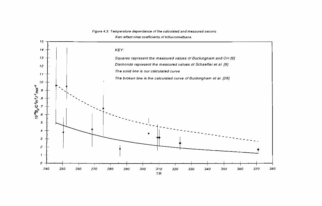
15

14

13

12

11

10

· i ~ 9 ')I

~ 8 <liE

3c 7

f 6 Q --

.. .. .. 1' ............

Figure 4.3. Temperature dependence of the calculated and measured second

Kerr-effect virial coefficients of trifluoromethane.

KEY:

Squares represent the measured values of Buckingham and Orr [6J

Diamonds represent the measured values of Schaeffer et al. [8J

The solid line is our calculated curve

The broken line is the calculated curve of Buckingham et al. [29J

Table 4.6. The relative magnitudes of the various contributions to B

t for trifluoromethane calculated at T = 245.5 K.

1030 x Value % Contribution Contributing

C2m8J-2mol-2 to B Term K

J..L2

<X1

0.202 4 . 05

J..L2

<X2

3 . 561 71.39

J..L 2 <X3 1.155 23.16

<X 0.000 0.00 2 2 4

<X 3

-0.006 -0. 12

<X 0.072 1. 44 4

<X 0.004 0.08 5

170

Figure 4.3 contains a comparison of the temperature-dependence of our

calculated B values with both the experimental data [6,8] and the Ie

calculated values of Buckingham et al. [29]. Again, the experimental

values of Buckingham and Orr have a rather substantial imprecision of

±50%. The more precise values of Schaeffer et al. [8] lie within 30% of

our calculated curve. We now turn our attention to non-linear polar

molecules.

4.5 Calculations of B for sulphur dioxide Ie

4.5.1 Molecular properties of sulphur dioxide

Sulphur dioxide is a non-linear molecule belonging to the C symmetry 2v

point group. Optimized values for the Lennard-Jones force constants and

shape factors of sulphur diOXide, obtained by fitting the second

pressure virial coefficients calculated according to equation (2.111) to

the experimental data over a range of temperature, have been presented

in section 2.6 of Chapter 2. These values, together with the dipole and

quadrupole moment tensor components and mean static polarizability

required in the expressions for U (,:), are presented in table 4.7 12

171

below.

Table 4.7. A summary of the Lennard-Jones force constants, shape parameters, and wavelength-independent molecular properties required in the intermolecular potential U (~) of sulphur dioxide.

12

R = 0.3850 nm o

elk = 220.0 K

113 =

e 11

e 22

e 33

a =

t Obtained by extrapolating

zero frequency

-5.4262 x 10- 30

= -16.4 x 10- 40

= 12.9 x 10- 40

= 3.5 x 10- 40

em

em2

em2

em2

D = 0.0873 1

D = O. 1008 2

[46]

[47]

4.2072 x 10- 40 e 2 m2J- 1 t

measured dynamic polarizabilities [40) to

All measured and .calculated values for the dynamic polarizability tensor

components of sulphur dioxide at A = 514.5 nm and A = 632.8 nm have

already been summarized in table 2.9. Gentle et ai. [13] deduced values

for B (T) from Kerr-effect experiments at A = 632.8 ·nm, and so our K

calculations for B (T) were performed using the most precise values at IC

this wavelength as listed in table 4.8.

Table 4.8. The components of the optical-frequency polarizability tensor of sulphr dioxide deduced from Kerr-effect measurements at A = 632.8 nm by Gentle et ai. [13].

5.80 ± 0.06 3.30 ± 0.04 3.88 ± 0.06

Since there are no experimental estimates of the individual static

polarizability tensor components, we use ab initio calculated values as

Table 4.9. The wavelength dependence of p , a and Aa for sulphur dioxide, together with o

values extrapolated to infinite wavelength. All data is taken from reference [40].

1040

a 100 x p 10

4o(Aa)

A/nm C2 m2 J-t 0

C2 m2 J-t

488.0 4.411 1. 86 ± 0.01 2.359

514.5 4.389 1.85 ± 0.01 2.341

632.8 4.326 1.79 ± 0.01 2.269

A ~ 00 4.207 ± 0.001 2.136 ± 0.010

172

a basis. These values can be refined by comparing their trace with the

mean static polarizability extrapolated from reported optical-frequency

values [40], and scaling accordingly. For this purpose, we list in table

4.9 the wavelength dependences of Po and a together with their

corresponding 6a values deduced via equation (2.18); and include values

extrapolated to zero frequency. Table 4.10 contains the ab initio

principal static polarizabilities calculated using CPF(ED) theory [48],

together with the scaled values. The 'quality' of the scaled values can

be cross-checked by comparing the scaled 6a with the value in table 4.9

extrapolated from experimental data: the values agree to wi thin 4.5%,

allowing confident use of the scaled all'

calculat ions of B .

a and a values in our 22 33

K

Table 4.10. Ab initio calculated static polarizability tensor components of sulphur dioxide together with the mean polarizability a and anisotropy 6a. Included are the values scaled according to the extrapolated a given in table 4.9 .

Polarizabi I i ty property

1040 x CPF(ED) Calculations[481

C2 m2J- 1

1040 x Scaled values

C2m2J- 1

a 5.347 5.661 11

a 22

3.027 3.205

a 3 . 548 33

3.756

a 3 . 974 4 . 207

6a 2.108 2.232

Sulphur dioxide is a polar molecule, with contribut ions to B arising K

from the Il and (3 tensors through equat i ons (4.70) to (4.73). 1/ is 1 IJk ""1

quoted in table 4 . 7, whi Ie table 4.11 contains a summary of the ab

initio SCF calculations of the three i ndependent components of the

static first-order hyperpolarizability tensor b IJk

as performed by

Maroulis [49]. Our means for verifying that the difference between the

optical-frequency components and those in the static limit is

sufficiently small is as follows:

The property

3 (3 =

1 0

173

(4 . 85)

for sulphur dioxide has been deduced by Gentle et al. [13] from their

Kerr-effect measurements at A = 632.8 nm to have the value

(3 = -(0 . 05 ± 0.15) x 10-50 C3m3J-2, while the static analogue obtained

from Maroulis' calculated b Ijk

components , namely b = 0 . 024 x 10-50

C3m3J-2 [49], is well within the experimental uncertainty limits. Hence ,

Maroulis' values should yield at worst an order of magnitude estimate of

the Il (3 contribution to B . 1 1 ){

Table 4.11. Ab initio SCF calculations of the static first-order hyperpolarizability tensor components of sulphur dioxide [49].

b = 7.05 x 10- 52 C3m3J-2 113

b = 2 . 05 x 10- 52 C3 m3J-2 223

b = 8.50 x 10- 52 C3m3J-2 333

Maroulis has also calculated values for the static second-order

hyperpolarizability tensor glJkl [49], but since the first-order

hyperpolarizability will make a much more significant contribution to

B , the r« term is not considered here . ){ 1 1

4.5.2 Results of calculations for sulphur dioxide

Table 4.12 gives the relative magnitudes of the various contributions to

B calculated at the particular temperature 298.7 K. Here, as for the ){

quasi-linear fluoromethanes, the dominant contributor to B is the Il« ){ 2 2

term. Again, however, it is not possible to definitively claim

convergence of the series of terms in Il« since the Il« term contributes 2 3

as much as 37.33% to B. Not ice how the Il (3 term makes a complete ly ){ 1 1

negligible contribution to B of 0.33%, hence lending justification to ){

our omission of the r« term. 1 1

14

12

'l' 10

~ 'l' ""')

co 8 .,.E ~ ~rt 6 0 -

4

2

j

Figure 4.4. Temperature dependence of the calculated and measured second

Kerr-effect virial coefficients of sulphur dioxide as listed in table 4. 13.

T

KEY:

Squares represent the measured values of Gentle et al. {13]

The' solid line is our calculated curve

I j

o ~1~--~--~--~--~--~--~--~--+---~--+---~--4---~--~--~--~--~---+--~---+--~ 290 310 330 350 370 390

TIK 410 430 450 470 490

Table 4.12. The relative magnitudes of the various contributions to B for sulphur dioxide calculated at T = 298 . 7 K.

~

30 % Contribution 10 x Value

Contributing C2m8J-2mol-2 to B

Term ~

1l2<Xl 1. 542 12.11

1l2<X2 5.730 45.02

1l2<X3 4. 752 37 . 33

<X -0 . 063 -0.49 2

<X 3

0 . 166 1. 30

<X 0 . 503 3.95 4

<X 0 . 057 0.45 5

III 13 1 0.042 0.33

Table 4 . 13 presents the temperature dependence of the calculated B

174

K values, and includes a comparison with the rather precise experimental

values recently measured by Gentle et al. [13]. A graphical comparison

of the calculated and measured data is given in figure 4.4 .

175

Table 4.13. Temperature dependence of the calculated B values of IC

sulphur dioxide , together with the measured values at A = 632.8 nm [13].

1030Bexp 1030Beale Bexp

T K K K

K C2m8J-2mol-2 C2m8J-2mol-2 Beale IC

298.7 13.8 ± 0 . 8 12 . 73 1.084

307 . 3 11. 4 ± 0.5 11 . 08 1. 029

315.4 10.1 ± 0 . 5 9.86 1. 024

330.7 7.5 ± 0.4 8 . 02 0 . 935

348 . 8 6.5 ± 0 . 6 6.42 1. 012

370.9 6.5 ± 0 . 5 5.03 1. 292

381.2 4 . 2 ± 0.9 4.52 0.929

395.7 7.6 ± 1.5 3.93 1. 934

423 . 7 4.7 ± 1.1 3. 07 1.531

457.0 2 . 1 ± 1.3 2.36 0 . 890

471. 5 3 . 4 ± 1.8 2. 13 1. 596

490.3 1.5 ± 0.6 1. 87 0.802

It is immediately apparent that the theory and experiment are in

excellent agreement . But could thi s level of agreement have been

obtained by approximating the molecular property tensors and physical

shape of the sulphur dioxide molecule to be of axial symmetry? Gentle et

al. [13] attempted such an analysis using the statistical-mechanical

theory of BIC for axially-symmetric molecules developed by Buckingham et

al. [29], and generally found the calculated B values to be more than IC twice as large as the experimental values . This finding substantiates

our earlier claim (see Chapter 2) that the effects which interacting

non-linear molecules have on molecular-optic phenomena can only be

calculated after full consideration of molecular symmetry.

4.6 Calculations of B for dimethyl ether JC

4.6.1 Holecular properties of dimethyl ether

176

Like sulphur dioxide, dimethyl ether belongs to the C point group. 2v

Table 4.14 lists the optimized values for the Lennard-Jones force

constants and shape factors of dimethyl ether obtained in section 2.7 of

Chapter 2, together with the dipole and quadrupole moment tensor

components and mean static polarizabi 1 ity required in the expressions

for U (-r). 12

Table 4. 14. A summary of the Lennard-Jones force constants, shape parameters, and wavelength-independent molecular properties required in the intermolecular potential U (T) of dimethyl ether.

12

t

R = 0.390 nm o

elk = 370.0 K

9

9

9

~3 = -4.37 x 10- 30 Cm [50]

= 11. 0 x 11

10-40 Cm2

= 22 -4.3 X 10- 40

Cm2

= 33

-6.7 X 10- 40 Cm2

D = O. 1923 1

D = 0.2137 2

[51]

Obtained by extrapolating measured dynamic polarizabilltles [40] to zero frequency

Since values of B (T) for dimethyl ether have been deduced from Kerr-JC

effect measurements at A = 632.8 nm [11], the dynamic polarizabi li ty

tensor components at this wavelength are required for our calculations.

Table 4. 15 lists the relevant data, the more precise set of measured

values obtained by Bogaard et al. [11] being used in our work .

Table 4. 15. The components tensor of dimethyl ether at h

of the optical-frequency = 632 . 8 nm.

Method 104 °0:

11

Experimental derivation from 6.69 ± 0 . 17 5.46 ± 0.14 the Kerr effect [ 11]

Experimental derivation from

6 . 60 ± 0.22 5.64 ± 0.60 the Cotton-Mouton effect [52]

Ab initio calculation from MP2 theory 6.68 4.47 (scaled) [52]

177

polarizability

5.28 ± 0.13

5.19 ± 0.40

5.28

Once again, scaled ab initio values of the static polarizability tensor

components are used in our calculations. Tabl e 4.16 lists the MP2 values

obtained by Spackman et al. [53], together with the values scaled

according to the mean static polarizability extrapolated from the

measured dynamic polarizabilities [40]. The scaled da of 1. 299 x 10-40

C2m

2J-

1 agrees with the value of (1.242 ± 0.005) x 10-40 C2m2J-1

extrapolated from experimental data [40] to within 4 . 6%.

Table 4.16. Ab initio calculated static polarizability tensor components of dimethyl ether together with the mean polarizability a and anisotropy da. Included are the values scaled according to the extrapolated a given in table 4.14.

1040 x MP2 Calculated 1 [53] 1040 x Scaled values Polarizability va ue

property C2m2J- 1 C2m2J- 1

a 6.232 6.584 11

a 4.917 5.195 22

a 5.110 5.399 33

a 5.420 5.726

da 1.230 1.299

178

There are no experimental or calculated estimates of the components of

the first-order hyperpolarizability tensor ~ for dimethyl ether, and lJk

we ignore this contribution to B bearing in mind that it was found to . K

be completely negligible in the case of sulphur dioxide.

4.6.2 Results of calculations for dimethyl ether

Table 4.17 summarizes the relative magnitudes of the various

contributions to B at T = 259.0 K. As was found for sulphur dioxide , K

the dominant contributors to B are the interaction-induced terms in ~a. I

Here, unl ike in the fluoromethanes and sulphur dioxide , the term ~2a3

contributes a higher percentage (44 . 73%) to B than the lower-order term I

~ a, and it is more difficult to be assured of convergence of this 2 2

series of terms. The ~ a term of this molecule definitely warrants 2 4

investigation in the near future .

Table 4.17 . The relative magnitudes of the various contributions to B for dimethyl ether calculated at T = 259.0 K.

I

30

Contributing 10 x Value % Contribution C2m8J-2mol-2 to B Term I

~2al 5.587 22 . 87

~2a2 4 . 302 17.61

~2a3 10.925 44 . 73

a 0.056 0.23 2

a 0. 482 1. 97 3

a 2.677 10.96 4

a 0 . 397 1. 63 5

40

35

30

'l'

~25 'l' .., ... e

<II 20

~~ ~ 15

10

5

Figure 4.5. Temperature dependence of the calculated and measured second

Kerr-effect virial coefficients of dimethyl ether listed in table 4 .18 .

KEY:

Squares represent the measured values of Bogaard et al. [11]

The solid line is our calculated curve

T

o ~'~--~--+---~--~--~---+--~--~----~--+---~--~--~--~--~~--~--~--~--~---1 250 260 270 280 290 300

TIK 310 320 330 340 350

179

Table 4.18 presents the temperature dependence of the calculated BIe

values , and includes a comparison with the experimental values of

Bogaard et ai. [11] . The experimental uncertainties in BIe were quoted to

be in the range ±10% to ±20%. A graphical comparison of the calculated

and measured data is given in figure 4.5.

Table 4 . 18 . Temperature dependence of the calculated B values of Ie

dimethyl ether, together with the measured values at A = 632.8 nm [11] .

1030Bexp 1030Bcalc Bexp

T Ie II: Ie K C2m8J-2mol-2 C2m8J-2mol-2 B

calc Ie

259.0 34 . 2 ± 6 . 8 24 . 4 1. 40

269 . 0 18.8 ± 3 . 8 19.8 0.95

278.4 16. 1 ± 3 . 2 16 . 4 0 . 98

288.2 13 . 1 ± 2 . 6 13.7 0 . 96

302.4 11. 1 ± 2.2 11. 0 1. 01

318.9 10 . 2 ± 2.0 8 . 9 1. 15

333 . 8 5.8 ± 1.2 7 . 2 0 . 81

By following the lead of Buckingham et ai . [29] and including the

collision-induced polarizability contribution into our theory of B for Ie

non-linear polar molecules, we have obtained good fits to the observed

values for the quasi-linear fluoromethanes as well as for the

low-symmetry sulphur dioxide and dimethyl ether molecules. Measurements

of B for hydrogen sulphide [12] and difluoromethane [6] , both of which Ie are of C symmetry, have been undertaken; but since the quadrupole 2v

moments of these molecules have not yet been measured, calculations of

B cannot be performed. II:

The very small pressure dependence of the molar Kerr constant K for m

non-polar gases, with resultant high uncertainties in deduced B values, Ie

has already been discussed . Nevertheless, we think it profitable to

obtain calculated values of B for those gases in which the II:

Table 4.19. Wavelength-independent molecular parameters used in calculations of B for linear non-polar molecules. K

t

* •

Molecule

N 2

CO 2

CH CH 3 3

1040

at

C2m2J-t

1. 936 [54)

t 2.885 [55)

t 4 . 870 [56)

104011a* 40

1040

a 10 an J.

C2m2J-t C2m2J-t C2m2J-t

0.734*(57) 2.425 1.691

2.252*(57) 4.387 2.134

0 . 638*(58) 5 . 295 4.657

104°0 R c/k • 33 0

D

Cm2 nm -y-

-4.72 [59) 0.368 (62) 91. 50 (62) 0.112

-15.0 [60] 0.400 (63) 190 . 0 (63) 0.250

-3.34 [6t) 0.4418 [62) 230 [62] 0.200

Obtained by extrapolating recent high-precision measurements of dynamic polarizabilities [55,56] to zero frequency.

Obtained by extarpolatlng the measured dynamic l1a values In references [57) and [58) to zero frequency .

Obtained by fitting to the pressure vlrlal coefficients quoted In [3t).

180

pressure-dependence of the Kerr effect has been measured, since this

will help to establ ish whether any correlation between theory and

experiment can be obtained. The linear molecules nitrogen, carbon

dioxide and ethane, and the non-linear molecule ethene, will be

investigated.

4.7 Calculations of B for the linear non-polar molecules IC

nitrogen, carbon dioxide and ethane

4.7.1 Molecular properties of nitrogen, carbon dioxide

and ethane

Wavelength-independent parameters required in the calculations of B for IC

the I inear non-polar molecules nitrogen, carbon dioxide and ethane are

listed in table 4.19 . The static anisotropies ~a are the values obtained

by extrapolating measured optical-frequency anisotropies ~a to zero

frequency. Table 4 . 20 contains the principal polarizability components

of the three molecules at the wavelength 632.8 nm. The leading

hyperpolarizability tensor for non-polar molecules is the second-order

~iJkl' and values for the individual components are generally not

available . Contributions arising from this tensor are, however, expected

to be negligibly small.

4.7 . 2 Results of calculations for nitrogen, carbon dioxide

and ethane

Table 4.21 summarizes the relative magnitudes of the contributions to B . IC

for nitrogen, carbon dioxide and ethane; each at a particular

temperature chosen from the respective experimental measurements

reported in [7]. For all three molecules, the a term is the dominant 4

contributor at over 100%, while the as term generally contributes

of the order of 5% to BIC

• Higher-order collision-induced polarizability

contributions are expected to be negligibly small, the series having

converged rapidly.

Table 4.20. The components of the optical-frequency polarizability tensors of nitrogen, carbon dioxide and ethane at a wavelength of 632 . 8 nm, as obtained from measured values for p and a.

Molecule

N 2

CO 2

CH CH 3 3

lOOp 0

1.042 ± 0.006 [40]

4.05 ± 0.02 [40]

0.149 ± 0.006 [58]

1040

a

C2 m2 J-t

1.961 [40]

2.9314 [55]

4.9680 [56]

o

40 10

40a

1040

Aa 10 all .l

C2 m2 J-t C2 m2 J-t C2 m2 J-t

0.183 2.498 1.115

2.349 4.491 2 . 149

0.143 5.464 4.120

Table 4.21. Relative magnitudes of the various contributions to 8 at A = 632 . 8 nm for the non-polar axially-symmetric molecules nitrogen, carbon dioxide and ethane. ~

Term

ex. 2

ex. 3

ex. 4

ex. 5

nitrogen (T = 248 K)

32 10 x Value X Contribution C2m8J-2mol-2 to 8

~

0.009 1. 03

-0 . 149 -17.01

0.984 112.33

0 . 032 3 . 65

8 = 0.876 x 1032 C2m8J-2mol-2 ~

carbon dioxide (T = 252 K)

32 10 x Value C2m8J-2mol-2

1.531

-3 . 353

5 . 124

0 . 174

% Contribution to 8

~

44 . 04

-96.46

147.41

5.01

8 = 3 . 476 X 1032 C2m8J-2mol-2 ~

ethane (T = 255 K)

32 10 x Value C2m8J-2mol-2

0.143

-4.079

23.049

1 . 380

% Contribution to 8

~

0 . 70

- 19 . 90

112.47

6.73

8 = 20.493 X 1032 C2m8J-2mol-2 K

..... Cb .....

182

The temperature dependence of the calculated B values for ni trogen, K

carbon dioxide and ethane are presented in tables 4.22 to 4.24

respect i vely, each table including a comparison with the available

experimental values . Notice how the experimental values of B for K

nitrogen and carbon dioxide are particularly poorly defined. This is not

at all surprising in view of the extremely small calculated values,

which indicate that measurement of the tiny pressure-dependence of the

.molar Kerr constant

experimental challenge .

K for these two gases is a considerable m

Ethane has B values which are an order of I

magnitude larger than the corresponding calculated data for nitrogen and

carbon dioxide, and it is not surprising that the measured values are

more clearly defined . Here, agreement with the calculated values is to

within 15% .

Table 4.22. Temperature dependence of the calculated B K values of nitrogen, together with the measured values

at A = 632.8 nm [1].

T 1032Bexp 1032Bcalc

I I K C2m8J-2mol-2 C2m8J-2mol-2

248 -0.08 ± 0.28 0.815

260 0.01 ± 0.39 0.834

211 -0.21 ± 0.33 0 . 182

286 -0.23 ± 0.45 0.151

299 -0 . 30 ± 0.59 0 . 125

315 0.04 ± 0 . 30 0.689

334 -0 . 41 ± 0.18 0 . 650

183

Table 4.23. Temperature dependence of the calculated B values of carbon dioxide, together with the measured

K

values at A = 632 . 8 nm [7,10].

T 1032Bexp 1032Bcalc

K K

K C2m8J-2mol-2 C2m8J-2mol-2

252 23 ± 19 [7] ~ 3 . 47

259 5 ± 27 3 . 29

267 -6 ± 11 3 . 11

279 -1 ± 13 2 . 86

287 -3 ± 9 2.71

301 -3 ± 7 2.48

302 0 ± 10 2 . 47

318 -11 ± 8 2.25

337 -9 ± 9 2 . 06

299.2 6 ± 1 [10]~ 2.51

314.9 0 ± 1 2 . 29

330.9 4 ± 2 2 . 11

348.8 2 ± 1 1. 96

370.9 -6 ± 2 1. 82

394.5 2 ± 2 1. 71

422.8 -3 ± 2 1. 60

455 . 8 -3 ± 4 1. 47

489.5 -5 ± 3 1. 27

184

Table 4.24 . Temperature dependence of the calculated B values of ethane, together with the measured values at

Ie

A = 632 . 8 nm [7].

1032Bexp 1032Bcalc T Ie Ie

K C2m8J-2mol-2 2 8 -2 -2 C m J mol

255 18.2 ± 3.7 20.49

259 17.7 ± 3.6 20 . 04

269 16.7 ± 3.3 19.00

278 18.0 ± 3.6 18.15

278 15 . 7 ± 3.1 18.15

287 16.8 ± 3. 3 17.37

299 17.7 ± 3.6 16.43

304 14 . 9 ± 3. 0 16.07

309 14 . 2 ± 2.9 15 . 73

318 15.0 ± 3.0 15. 15

We now turn our attention to the only non-polar non-linear molecule for

which B data has been measured, namely ethene. Ie

4.8 Calculations of B for ethene Ie

4 . 8 . 1 Molecular properties of ethene

Optimized values for the Lennard-Jones force constants R and elk, and o

shape parameters 0 and 0, of ethene (obtained by fi t t ing the second 1 2

pressure virial coefficient calculated according to equation (2.111) to

experimental data over a range of temperature) have been presented in

section 2.5 of Chapter 2 . For .convenience, we list the values again,

together with the quadrupole moment tensor components and mean stat ic

polarizability required in the expressions for U (T): 12

Table 4.26. The components of the optical-frequency polarizability tensor of ethene at a wavelength of 632.8 nm obtained from the measured values for p • a and R

o 20

1040

a 104o

(Aa) 1040

a 1040

a 1040

a lOOp R

tt 22 33

0 C2 m2J-t C2 m2J-t 20 C2 m2 J-t C2 m2 J-t C2 m2 J-t

1.201 ± 0 . 002 [40) 4 . 1124 [S6) 2.021 0.21 ± 0.03 (65) 4.30 3.80 6 . 02 5 5 4 9

Table 4.21. The wavelength dependence of p • a and Aa; together with values extrapolated to infinite wavelength. 0

1040a [56]

100 x p [40 104o (Aa) i\/run C2 m2 J-t 0

C2 m2 J-t

632.8 4.1124 ± 0.0005 1. 201 ± 0.002 2.0215

514 . 5 4 . 1811 ± 0.0005 1. 241 ± 0.005 2 . 0882

488 . 0 4.1918 ± 0.0005 1. 266 ± 0.005 2.1081

i\ ~ 00 4.5111 ± 0 . 0008 1 . 893 ± 0 . 0024

185

Table 4.25 . A summary of the Lennard-Jones parameters, and wavelength-independent molecular the intermolecular potential U (.) of ethene .

force constants, shape properties required in

t

12

R = 0.4232 nm o

elk = 190.0 K

9 = 5 . 370 X 10- 40 Cm2

11

D = 0 . 22965 1

D = 0 . 21383 2

9 = -10.92 X 10- 40 Cm2 [64] 22

9 = 5. 549 x 10- 40 Cm2

33

Obtained by extrapolating measured dynamic polarizabilities [56] to

zero frequency

Whereas our measurement of B for ethene was performed using an incident p

light beam with A = 514.5 nm, the measurements of B (T) undertaken by Ie

Buckingham et ai. [1] were performed at A = 632.8 nm . The dynamic

polarizability tensor components must be evaluated at the new

wavelength, and table 4.26 contains the values of p, a and R which o 20

allow equations (2.12), (2.13) and (2.110) to be solved simultaneously,

hence yielding all' a and a at 632 . 8 nm. 22 33

There are no experimental est imates of the individual stat ic

polarizability tensor components, and so the ab initio calculated values

of Spackman [41] at the MP2 level of theory are used as a basis. As

before, these values are refined by scaling according to the mean static

polarizability extrapolated from measured dynamic values [56]. Listed in

table 4.27 are the wavelength dependences of p , a and 6a, together with o

the values extrapolated to zero frequency . Table 4.28 quotes Spackman's

calculated a iJ

components, mean static polarizabil i ty a and

polarizability anisotropy 6a; together with the scaled values. The usual

cross-check is performed, the scaled 6a and the one extrapolated from

the experimental data in table 4. 27 agreeing to within 1.1%. The scaled

a a and a values can be used with reasonable confidence in our 11' 22 33

calculat ions of B . Ie

186

Table 4.28. Ab initio calculated static polarizability tensor components of ethene together with the mean polarizability a and anisotropy 6a. Also included are the values scaled according to the extrapolated a given in table 4.27.

Polarizability 1040

property

a 11

a 22

a 33

a

6a

x MP2 Calculated values

C2 m2 J- 1

4.092

3.534

5.594

4.407

1.845

[ 411 1040 x Scaled values

C2 m2 J- 1

4 . 245

3.666

5.803

4 . 571

1. 914

Both the dipole moment ~ and the first-order hyperpolarizability tensor 1

(3 vanish for molecules with D symmetry, and the only remaining IJk 2h

terms are those in the second-order hyperpolarizability tensor r . Ab IJkl

initio SCF calculations of the six independent components of the static

hyperpolarizability tensor g of ethene have been undertaken by IJkl

Maroulis [66], and these values, which are summarized in table 4 . 29,

are unlikely to differ substantially from the corresponding optical­

frequency ones. This assumption has been confirmed by Maroulis [66] who

compared the experimental value for the property

r = 1

1 0 (4.86)

of ethene; which has been deduced by Ward and Elliott [67] from

measurements of dc electric-field induced optical second harmonic gene­

ration (SHG) at A = 694 nm, yielding r = (0.563 ± 0.013) x 10-60

C4 m4 J-3., ith hi 1 f ( ) -60 4 4 -3 w s va ue 0 g = 0.421 ± 0.015 x 10 C m J obtained

from the components in table 4.29. Since the two values are consistent ,

it can concluded that the use of these components allows at least order

of magnitude estimates of the r a term's contribution to B to be made. 1 1 IC

187

Table 4.29. The SCF ab initio calculated estimates of the static hyperpolarizability tensor components of ethene [66]

gllll = (0 . 2429 ± 0.0049) x 10- 60 C4 m4J-3

g2222 = (0.6367 ± 0.0263) x 10- 60 C4m4J-3

g3333 = (0.1445 ± 0.0054) x 10- 60 C4m4J-3

gl122 = (0.1407 ± 0.0063) x 10- 60 C4 m4J-3

gl133 = (0.1185 ± 0.0039) x 10- 60 C4m4J-3

g2233 = (0.1706 ± 0.0083) x 10- 60 C4 m4J-3

4.8.2 Results of calculations for ethene

Table 4.30 gives the relative magnitudes of the various contributions to

B calculated at T = 333 K. Notice how the ex term is the dominant ~ 4

contributor to B, while the ex term makes a substantially smaller, yet ~ 5

still significant, contribution of 7.45%. The series is now rapidly

converging so that the ex 6

and higher-order terms in the

collision-induced polarizability should contribute negligibly to B. As ~

would be expected, the leading hyperpolarizabil i ty term r ex makes a 1 1

completely negligible contribution to B (0 . 04%). ~

Table 4.30. The relative magnitudes of the various contributions to B for ethene calculated at T = 333 K.

K

32 % Contribution 10 x Value Contributing

C2m8J-2mol-2 to B Term K

a 2.268 18.00 2

a -7 . 127 -56 . 58 3

a 16.513 131.09 4

a 0.938 7.45 s

rla

l 0.005 0.04

188

Table 4.31 presents the temperature dependence of the calculated B K

values, and includes a comparison with the experimentally measured

values of Buckingham et ai. [7]. We note that the quoted uncertainties

in the measured values were obtained from a least squares analysis of

the experimental data [7], and hence do not take into consideration any

systemat ic errors arising from uncertainties in the pressure virial

coefficients used to obtain the molar volume V. There are substantial m

discrepancies between the experiment and theory, generally of about 20%

to 50%; and the reasons for this are speculative. Certainly, the B K

values are very small, and hence difficult to meausure accurately. An

independent set of measurements of B for ethene seems desirable, since K

this will allow a definitive assessment of whether or not the DID model

is fai ling.

189

Table 4.31. Temperature dependence of the calculated B values of ~

ethene , together with the measured values at A = 632 . 8 nm [7].

1032Bexp 1032Bcalc Bexp

T Ie Ie Ie

K C2mBJ-2mol-2 C2mBJ-2mol-2 Bcalc Ie

262 34 ± 7 17 . 06 2 . 034

268 26 ± 6 16 . 54 1. 572

273 23 ± 5 16.13 1. 426

280 18 ± 3 15 . 60 1. 154

286 22 ± 5 15.18 1.449

294 24 ± 5 14 . 66 1. 637

298 18 ± 3 14.42 1. 248

302 18 ± 3 14.19 1.269

313 16 ± 3 13 . 59 1.177

314 18 ± 3 13.53 1.330

333 17 ± 3 12.60 1.350

334 17 ± 3 12.54 1. 356

PS. While this thesis was being printed, we received our copy of the

October edition of the Journal Molecular Physics. Therein is a paper by

Tammer and HUttner [68] describing their investigation into the Kerr

effect of gaseous ethene. First and second Kerr-effect virial

coefficients are given over the temperature range 202.4 to 363.7 K. The

A are generally 15% lower ~

the B are within 7% to 45% Ie

the theories of Buckingham

than those of Buckingham et ai. [7], while

of [7]. The authors have calculated Busing Ie

and Dunmur [17,3], and obtain values which

are 15% lower than ours quoted in table 4.31.

190

4.9 References

[1] Silberstein, L., 1917, Phil. Mag., 33, 92, 521 .

[2] Watson, R. C. and Rowell, R. L., 1974, J. chem. Phys., 52, 132.

[3] Buckingham, A. D. , and Dunmur, D. A., 1968, Trans . Faraday Soc.,

64, 1776.

[4] Thibeau, M., Tabisz, G. C. , Oksengorn, B., and Vodar, B. , 1970,

J. quant. Spectrosc. rad . Transfer, 10, 839 .

[5] Dunmur, D. A., Hunt, D. C. , and Jessup, N. E. , 1979, Molec. Phys.,

37, 713 .

[6] Buckingham, A. D., and Orr, B. J., 1969, Trans. Faraday Soc., 65,

673.

[7] Buckingham, A. D. , Bogaard, M. P., Dunmur, D. A., Hobbs, C. P. , and

Orr, B. J . , 1970, Trans. Faraday Soc., 66, 1548.

[8] Schaeffer, D. W., Sears, R. E. J., and Waugh, J. S. , 1970, J. chem.

Phys., 53, 1970 .

[9] Buckingham, A. D., and Sutter, H. , 1976, J. chem. Phys . , 64, 364.

[10] Gentle, I. R., Laver, D. R., and Ritchie, G. L. D. , 1989, J. phys .

Chem., 93, 3035.

[11] Bogaard, M. P., Buckingham, A. D., and Ritchie, G. L. D., 1981,

J. chem. Soc. Faraday Trans. II, 77, 1547.

[12] Bogaard, M. P., Buckingham, A. D., and Ritchie , G. L. D., 1982,

Chem. Phys. Lett., 90, 183.

[13] Gentle, I . R., Laver, D. R., and Ritchie, G. L. D., 1990, J. phys.

Chem., 94, 3434.

[14] Kerr, J., 1875, Phil . Hag., 50, 337, 446.

[15] Buckingham, A. D., and Pople, J . A., 1955 , Proc. Phys . Soc. A, 68,

905 .

[16] Otterbein, G., 1934, Phys. Z., 35, 249.

[17] Buckingham, A. D., 1955, Proc. Phys. Soc. A, 68, 910.

[18] Gray, C. G., and Ralph, H. I., 1970, Phys. Lett . A, 33, 165.

[19] Buckingham, A. D., and Pople, J. A. , 1955, Trans . Faraday Soc., 51,

1173 .

[20] Lennard-Jones, J. E., 1924, Proc. Roy. Soc. Lond. A, 106, 441 .

[21] McTague, J . P., Ellenson, W. D., and Hall, L. H., 1972, J. Phys.

Paris, 33, Cl-241 .

[22] Lallemand, P., 1971, J. Phys. Paris, 32, 119.

[23] Barocchi, F., and McTague, J. P., 1975, Phys. Lett. A, 53, 488.

[24] Graham, C., 1992, Molec. Phys., 77, 291 .

[25] Couling, V. W., and Graham, C. , 1993, Molec . Phys., 79, 859.

191

[26] Burrue, J., Chave, A., Dumon, B., and Thibeau, M., 1977, Rev. Phys.

appl., 12, 1743.

[27] Dayan., E., Dunmur, D. A., and Manterfield, M. R., 1980, J. chem.

Soc. Faraday Trans. II, 76, 309.

[28] Couling, V. W., and Graham, C., 1994, Molec. Phys., 82, 235 .

[29] Buckingham, A. D., Gal was , P. A., and Liu Fan-Chen, 1983, J. Mol.

Struct., 100, 3.

[30] Stockmayer, W. H., 1941, J. chem. Phys., 9, 398.

[31] Dymond, J. H., and Smith, E. B., 1980, The Virial Coefficients of

Pure Gases and Mixtures (Oxford: Clarendon).

[32] Kang, T. L., Hirth, L. J., Kobe, K. A., and McKetta, J. J., 1961,

J. chem. Engng. Data, 6, 220.

[33] Buckingham, A. D., and Pople, J. A., 1956, Far. Soc. Disc., 22, 17.

[34] Graham, C., 1971, Ph. D. Thesis, University of Cambridge.

[35] Burns, R. C., 1978, Ph. D. Thesis, University of Natal.

[36] Burns, R. C., Graham, C., and Weller, A. R. M., 1986, Molec. Phys.,

59, 41.

[37] Buckingham, A. D., 1967, Adv. chem. Phys., 12, 107.

[38] Copeland, T. G., and Cole, R. H., 1976, J. chem. Phys., 64, 1741.

[39] Sutter, H., and Cole, R. H., 1970, J. chem. Phys., 52, 132.

[40] Bogaard, M. P., Buckingham, A. D., Pierens, R. K., and White,

A. H., 1978, J. chem. Soc. Faraday Trans. I, 78, 3008.

[41] Spackman, M. A., 1989, J. phys. Chem., 93, 7594.

[42] Dougherty, J., and Spackman, M. A., 1994, Molec. Phys., 82, 193.

[43] Miller, C. K., Orr, B. J., and Ward, J. F., 1981, J. chem. Phys.,

74, 4858.

[44] Bogaard, M. P., Orr, B. J., Murphy, W. F., Srinivasan, K., and

Buckingham, A. D., (to be published).

[45] Honan, M., Bribes, J-L, and Gaufres, R. , 1982, J. Raman Spectrosc.,

12, 190.

[46] Patel, D., Margo lese , D., and Dyke, T. R., 1979, J. chem. Phys.,

70, 2740.

[47] Ellenbroek, A. W., and Dymanus, A., 1976, Chem. Phys. Lett., 42,

303.

[48] Bacskay, G. B., Rendell, A. P. L., and Hush, N. S., 1988, J. chem.

Phys., 89, 5721 .

[49] Maroulis, G., 1992, Chem. Phys. Lett., 189, 112.

[50] Blukis, U., Kasai, P. H., and Myers, R. J., 1963, J. chem. Phys.,

38, 2753.

[51] Benson, R. C., and Flygare, W. H., 1970, J. chem. Phys., 52, 5291.

192

[52] Coonan, M. H. , Craven, I . E., Hesling, M. R., Ritchie, G. L. D.,

and Spackman, M. A., 1992, J. phys . Chem., 96, 7301.

[53] Spackman, M. A., and Ritchie, G. L. D., Private Communication.

[54] Orcutt, R. H. , and Cole, R. H. , 1967, J. chem. Phys. , 46, 697 .

[55] Hohm, u. , 1994, Chem. Phys. , 179, 533.

[56] Hohm, U. , 1993, l101ec. Phys. , 78, 929.

[57] Alms, G. R. , Burnham, A. K. , and Flygare, W. H. , 1975, J. chem.

Phys., 63, 3321.

[58] Baas, F., and van den Hout, K. D., 1979, Physica A, 95, 597.

[59] Graham, C., Pierrus, J. and Raab, R. E., 1989, l101ec. Phys., 67,

939.

[60] Battaglia, M. R. , Buckingham, A. D., Neumark, D. , Pierens, R. K.,

and Williams, J. H., 1981, l101ec. Phys., 43, 1015.

[61] Buckingham, A. D., Graham, C., and Williams, J. H., 1983, l101ec.

Phys., 49, 703.

[62] Hirschfelder, J. 0., Curtiss, C. F., and Bird, R. B., 1954,

1101ecu1ar Theory of Gases and Liquids (Chichester: Wiley) .

[63] Mason, E. A., and Spurling, T. H., 1969, The Viria1 Equation of

State (Oxford: Pergamon) .

[64] Maroulis, G., 1993, J. Phys. B: At. 1101. Opt. Phys., 2, 775.

[65] Barbes, H., 1987, J. Raman Spectrosc., 18, 507.

[66] Maroulis, G., 1992, J. chem. Phys., 97, 4188.

[67] Ward, J. F., and Elliott, D. S., 1978, J. chem. Phys., 69, 5438 .

[68] rammer, R., and HUttner, W., 1994, 1101ec. Phys., 83, 579 .

193

APPENDIX 1

A1.1 Electric multipole moments

A static distribution of electric charges q at positions r relative to 1 -1

an arbi trari ly chosen origin 0, positioned wi thin the arrangement of

charges, gives rise to an electric potential ~ at all points in space.

For any given point P, with a vecto: displacement ~ from 0 with R » r1

,

the electric potential is given by the multipole expansion (Buckingham

[ 11 )

1 (A1. 1)

Here, Greek subscripts denote Cartesian tensor components x, y, or z;

with a repeated subscript implying summation over these components. The

second-rank tensor o~ is the Kronecker delta.

The summations in equation (Al.l) are the electric multipole moments of

the charge distribution:

is the electric monopole, or the total charge of the distribution;

is the electric dipole moment; and

e =t"'qr r ex{3 L.. 1 lex 1{3

1

is the primitive electric quadrupole moment, etc .

(A1. 2)

(A1.3)

(A1. 4)

Different definit ions have been adopted for electric mult ipole moments

of higher order than the dipole. For instance, an alternative form of

the electric quadrupole moment is the traceless moment

194

aNa = ~ L q (3r r a - r20Na) . "'+' 2 1 10: 1,.... 1 ""f"

1

(Al. 5)

This form of the quadrupole moment is often used by molecular physicists

because it vanishes for a spherically-symmetric electric charge

distribution, and so is intuitively appealing. Raab [2] has, however,

caut ioned against the indiscriminate use of the traceless mul t ipole

moments, pointing out the existence of electrodynamic situations · where

it is necessary to retain the primitive definitions of multipole

moments.

References

[1] Buckingham, A. D., 1959, J. Q. Chem. Rev. Soc., 13, 183.

[2] Raab, R. E., 1975, Molee. Phys., 29, 1323.

C

APPENDIX 2

A2.1 An example of a Fortran program to calculate contributions to B p

C 14 AUGUST 1994 C PROGRAM TO CALCULATE TERM A3 FOR S02 USING GAUSSIAN INTEGRATION WITH

195

C 64 INTERVALS FOR THE RANGE, AND 16 INTERVALS FOR ALL ANGULAR VARIABLES C (I.E. ALPHA 1 , BETA1, GAMMA 1 , ALPHA2, BETA2 AND GAMMA2). C DOUBLE PRECISION IS USED THROUGHOUT. C

C ----------------------C SYSTEM INITIALIZATION: C ----------------------

IMPLICIT DOUBLE PRECISION (A-H,O-Z) COMMON COEF1,DCTC DIMENSION COEF2(64,2),COEF1(16,2),SEP(64),AL1(16),BE1(16),GA1(16)

+ ,AL2(16),BE2(16),GA2(16),DCTC(9,16,16, 16),FI(16, 16, 16,16, 16),D1(6 + 4),E1(16,16, 16, 16, 16),F1(16,16,16,16,16),SE3(64),SE4(64),SE5(64), + SE6(64),SE8(64),SE12(64),G1(16,16,16),DDP(16, 16,16,16, 16),DQP(16, + 16,16,16, 16),DIDP(16,16,16, 16,16)

INTEGER X1,X2,X3,X4,X5,X6,X7 CHARACTER·30 FDATE@

C MOLECULAR DATA FOR S02:

C

SSl=O.O SS2=0.0 SS3=0.0 SS4=0.0 SS5=0.0 SS6=0.0 SS7=0.0 DIP=-5.42620 ALSTAT=3.9740 A11=5.941 A22=3.328 A33=3.898 Q1=-16.38 Q2=12.90 AMIN1=0. 1 AMAX1=3.0 ALPHA=(A11+A22+A33)/3 DELTA2=(A11··2+A22··2+A33··2-Al1·A22-A11·A33-A22·A33)

C READ THE GAUSSIAN COEFFICIENTS FROM THE DATAFILE GAUSS64.DAT: C

OPEN(UNIT=10,FILE='GAUSS64.DAT' ) DO 10 ICTR1=l,64

DO 20 ICTR2=1,2 READ(10, 1010,END=11)COEF2(~CTR1,ICTR2)

1010 FORMAT(F18.15)

20 CONTINUE 10 CONTINUE 11 CLOSE(UNIT=10)

C C CALCULATE THE INTEGRATION POINTS FOR THE RANGE: C

SEP1=(AMAXI-AMIN1)/2 SEP2=(AMAX1+AMIN1)/2 DO 30 INDX=1,64

SEP(INDX)=SEP1*COEF2(INDX,1)+SEP2 30 CONTINUE

C C READ THE GAUSSIAN COEFFICIENTS FROM THE DATAFILE GAUSS16.DAT: C

OPEN(UNIT=11,FILE='GAUSS16.DAT' ) DO 100 ICTR1=1,16

6000 110 100 12

C

DO 110 ICTR2=l, 2 READ(11,6000,END=12)COEF1(ICTR1,ICTR2)

FORMAT (F18. 15) CONTINUE

CONTINUE CLOSE ( UNIT=ll)

C CALCULATE THE INTEGRATION POINTS FOR ALPHA1: C

AMIN=O.O AMAX=2.*3.14159265358919323846

ALll=(AMAX-AMIN)/2. AL12=(AMAX+AMIN)/2. DO 120 INDX=1,16

AL1(INDX)=ALll*COEF1(INDX,1)+AL12 120 CONTI NUE

C C CALCULATE THE INTEGRATION POINTS FOR BETA1: C

AMIN=O.O AMAX=3.14159265358919323846

BEll=(AMAX-AMIN) 12. BE12=(AMAX+AMIN) 12. DO 121 INDX=l, 16

BE1(INDX)=BE11*COEF1(INDX,1)+BE12 121 CONTINUE

C C CALCULATE THE INTEGRATION POINTS FOR GAMMA1: C

AMIN=O.O AMAX=2.*3.14159265358919323846

GAll=(AMAX-AMIN)/2. GA12=(AMAX+AMIN)/2. DO 122 INDX=1,16

GA1(INDX)=GA11*COEF1(INDX,1)+GA12 122 CONTINUE

196

C C CALCULATE THE INTEGRATION POINTS FOR ALPHA2: C

AMIN=O.O AMAX=2.*3 . 14159265358979323846

AL21=(AMAX-AMIN)/2. AL22=(AMAX+AMIN) 12. DO 123 INDX=1,16

AL2(INDX)=AL21*COEF1(INDX,1)+AL22 123 CONTINUE

C C CALCULATE THE INTEGRATION POINTS FOR BETA2: C

AMIN=O.O AMAX=3. 14159265358979323846

BE21=(AMAX-AMIN)/2. BE22=(AMAX:AMIN) 12. DO 124 INDX=1,16

BE2(INDX)=BE21*COEF1(INDX,1)+BE22 124 CONTINUE

C C CALCULATE THE INTEGRATION POINTS FOR GAMMA2: C

AMIN=O.O AMAX=2.*3.14159265358979323846

GA21=(AMAX-AMIN) 12. GA22=(AMAX+AMIN)/2 . DO 125 INDX=1,16

GA2(INDX)=GA21*COEF1(INDX,1)+GA22 125 CONTI NUE

C -------------C MAIN PROGRAM: C -------------

C

OPEN(UNIT=4, FILE=' LPT1' ) CALL BEEP@

C I NPUf MOLECULAR PARAMETERS FROM THE KEYBOARD: C

c WRITE(6, 470) c470 FORMAT(1X, 'INPUf THE TEMPERATURE (IN KELVIN)') c READ(5,471)TEMP c471 FORMAT(F10.5)

c

TEMP=348 . 15 TEMPK=TEMP*1.380622E-23

c WRITE(6,472) c472 FORMAT(1X, 'INPUf R(O) (IN nm)') c READ(5,473)R c473 FORMAT(F10 . 5)

r=0.3800

197

c WRITE(6,474) c474 FORMAT(lX, 'INPUT ElK (IN K)') c READ(5,475)PARAM2 c475 FORMAT(FIO.5)

param2=217.0 c WRITE(6, 476) c476 FORMAT(lX, 'INPUT SHAPEl ') c READ(5,477)SHAPEl c477 FORMAT(FIO.5)

shapel=O.0280 c WRITE(6,478) c478 FORMAT(lX, 'INPUT SHAPE2 ')

.c READ(5,479)SHAPE2 c479 FORMAT(FIO.5)

shape2=O.0560 . CALL SECONDS_SINCE_1980@(START)

· C C CALCULATION OF THE LENNARD-JONES 6:12 POTENTIAL & STORAGE OF THE C VALUES IN AN ARRAY: C

DO 61 Xl=1,64

Dl(Xl)=4.*PARAM2*1.380622E-23*«RlSEP(Xl))**12-(RlSEP(Xl))**6) SE12(Xl)=SEP(Xl)**12 SE5(Xl)=SEP(Xl)**5 SE8(Xl)=SEP(Xl)**8 SE3(Xl)=SEP(Xl)**3 SE4(Xl)=SEP(Xl)**4 SE6(Xl)=SEP(Xl)**6

61 CONTINUE

C C THE DIRECTION COSINE TENSOR COMPONENTS ARE STORED IN AN ARRAY: C

C

DO 66 X4=1,16 DO 77 X3=1,16

DO 88 X2=1,16

C DIRECTION COSINE TENSOR COMPONENTS: C

198

Al=COS(AL1(X2))*COS(BE1(X3))*COS(GA1(X4))-1.*SIN(AL1(X2))*SIN(GAl + (X4))

A2=SIN(AL1(X2))*COS(BE1(X3))*COS(GA1(X4))+COS(AL1(X2))*SIN(GA1(X4 + ))

A3=-1.*SIN(BE1(X3))*COS(GA1(X4)) A4=-1.*COS(AL1(X2))*COS(BE1(X3))*SIN(GA1(X4))-1.*SIN(AL1(X2))*COS

+ (GA1(X4)) A5=-1.*SIN(AL1(X2))*COS(BE1(X3))*SIN(GA1(X4))+COS(AL1(X2))*COS(GA

+ 1(X4)) A6=SIN(BE1(X3))*SIN(GA1(X4)) A7=COS(AL1(X2))*SIN(BE1(X3)) A8=SIN(AL1(X2))*SIN(BE1(X3)) A9=COS(BE1(X3))

DCTC(1,X2,X3,X4)=Al DCTC(2,X2,X3,X4)=A2 DCTC(3,X2,X3,X4)=A3 DCTC(4,X2,X3,X4)=A4 DCTC(5,X2,X3,X4)=A5 DCTC(6,X2,X3,X4)=A6 DCTC(7,X2,X3,X4)=A7 DCTC(8,X2,X3,X4)=A8 DCTC(9,X2,X3,X4)=A9

88 CONTINUE 77 CONTINUE 66 CONTINUE

C C THE MULTIPOLE INTERACTION ENERGIES ARE CALCULATED AND STORED C IN ARRAYS: C

DO 939 X7=1,16 WRITE(6,1000)X7

1000 FORMAT (lX, 'INDEX (IN RANGE 1 TO 16) IS CURRENTLY' ,12 ) DO 40 X6=1,16

C WRITE(6,1111)X6 Cllll FORMAT (lX, 'sub-index (in range 1 to 16) is currently' ,12 )

DO 50 X5=1,16

C C MOLECULE 2'S DIRECTION COSINE TENSOR COMPONENTS: C

C

81=DCTC(1,X5,X6,X7) 82=DCTC(2,X5,X6,X7) 83=DCTC(3,X5,X6,X7) 84=DCTC(4,X5,X6,X7) 85=DCTC(5,X5,X6,X7) 86=DCTC(6,X5,X6,X7) 87=DCTC(7,XS.X6,X7) 88=DCTC(8,X5,X6.X7) 89=DCTC(9,X5,X6,X7)

DO 60 X4=1,16 DO 70 X3=1, 16 DO 80 X2=1,16

C MOLECULE l'S DIRECTION COSINE TENSOR COMPONENTS: C

Al=DCTC(1,X2,X3,X4) A2=DCTC(2,X2,X3,X4) A3=DCTC(3,X2,X3,X4) A4=DCTC(4,X2,X3,X4) A5=DCTC(5,X2,X3,X4) A6=DCTC(6,X2,X3,X4) A7=DCTC(7,X2,X3,X4) A8=DCTC(8,X2,X3,X4)

199

200

A9=DCTce9,X2,X3,X4)

C C CALCULATION OF THE DIPOLE-DIPOLE POTENTIAL: C

DDPeX2,X3,X4,XS,XS)=8.987S8E-24*DIP**2*e-2*A9*B9+AS*BS+A3*B3)

C C CALCULATION OF THE DIPOLE-QUADRUPOLE POTENTIAL: C

C

DQPCX2,X3,X4,XS,XS)=8.987S8E-2S*DIP*CQ2*C-2*A9*B9**2+C2*AS*BS+2*A + 3*B3+2*A9**2-2*A8**2-AS**2+AS**2-A3**2+A2**2)*B9+2*A9*B8**2+C-2*A + S*BS-2*A3*B2) *B8+A9*BS**2+ C2*AS*A8-2*AS*A9) *BS-A9*BS** 2+A9*B3**2+ + C2*A2*A8-2*A3*A9)*B3-A9*B2**2)+Q1*C-2*A9*B9**2+C2*AS*BS+2*A3*B3+2 + *A9**2-2*A7**2-AS**2+A4**2-A3**2+A1**2)*B9+2*A9*B7**2+C-2*AS*B4-2 + *A3*B1)*B7+A9*BS**2+C2*A4*A7-2*AS*A9)*BS-A9*B4**2+A9*B3**2+C2*A1* + A7-2*A3*A9)*B3-A9*B1**2»

C CALCULATION OF THE DIPOLE-INDUCED DIPOLE POTENTIAL: C

C

DIDPCX2,X3,X4,XS,XS)=-O.SO*ALSTAT*8.077SSE-27*DIP**2*C3*B9**2 + +3*A9**2-2)

C CALCULATION OF THE QUADRUPOLE-QUADRUPOLE POTENTIAL: C

C

quad1=-lS.*CaS*a9-aS*a8)*CbS*b9-bS*b8)-lS.*Ca3*a9-a2*a8)*Cb3*b9-b + 2*b8)+4.*C2.*a9**2-2.*a8**2-aS**2+aS**2-a3**2+a2**2)*eb9-b8)*Cb9+ + b8)+C-4.*a9**2+4.*a8**2+3.*aS**2-3.*aS**2+a3**2-a2**2)*CbS**2-bS* + *2)+4.*Ca3*aS-a2*aS)*Cb3*b6-b2*bS)+e-4.*a9**2+4.*a8**2+aS**2-aS** + 2+3.*a3**2-3.*a2**2)*Cb3**2-b2**2)

quad2=-lS. * CaS*a9-a4*a7) * CbS*b9-b4*b7)-lS. *Ca3*a9-a1*a 7)*Cb3*b9-b + 1*b7)+4.*(2.*a9**2-2.*a7**2-aS**2+a4**2-a3**2+a1**2)*(b9-b7)*eb9+ + b7)+(-4.*a9**2+4.*a7**2+3.*aS**2-3.*a4**2+a3**2-a1**2)*CbS**2-b4* + *2)+4.*(a3*aS-a1*a4)*(b3*bS-b1*b4)+(-4.*a9**2+4.*a7**2+as**2-a4** + 2+3.*a3**2-3.*a1**2)*(b3**2-b1**2)

quad3=4.*(4.*A9**2-2.*(A8**2+A7**2+AS**2+A3**2)+AS**2+A4**2+A2**2 + +A1**2)*B9**2-1S.*(2.*AS*A9-AS*A8-A4*A7)*B6*B9-1S*C2.*A3*A9-A2*A8 + -A1*A7)*B3*B9-4. *(2. *A9**2-2.*A7**2-AS**2+A4**2-A3**2+A 1**2)*B8** + 2+1S.*CAS*A9-A4*A7)*BS*B8+1S.*CA3*A9-A1*A7)*B2*B8-4.*(2.*A9**2-2. + *A8**2-AS**2+AS**2-A3**2+A2**2)*B7**2+1S.*(AS*A9-AS*A8)*B4*B7+1S. + *(A3*A9-A2*A8)*B1*B7+(-8.*A9**2+4.*(A8**2+A7**2)+S.*AS**2-3.*CA5* + *2+A4**2)+2*A3**2-A2**2-A1**2)*BS**2+4.*C2.*A3*AS-A2*A5-A1*A4)*B3 + *BS+C4.*A9**2-4.*A7**2-3.*AS**2+3.*A4**2-A3**2+A1**2)*BS**2-4.*(A + 3*AS-A1*A4)*B2*BS+(4.*A9**2-4.*A8**2-3.*AS**2+3.*AS**2-A3**2+A2** + 2)*~4**2-4.*CA3*AS-A2*AS)*B1*B4+C-8.*A9**2+4.*CA8**2+A7**2)+2.*AS + **2-AS**2-A4**2+S.*A3**2-3.*CA2**2+A1**2»*B3**2+C4.*A9**2-4.*A7* + *2-AS**2+A4**2-3.*A3**2+3.*A1**2)*B2**2+(4.*A9**2-4.*A8**2-AS**2+ + AS**2-3.*A3**2+3.*A2**2)*B1**2

E1CX2,X3,X4,XS,XS)=8.987S8E-2S*C1./3. )*CQ2**2*QUAD1+Q1**2*QUAD + 2+Q1*Q2*QUAD3)

C CALCULATION OF THE QUADRUPOLE-INDUCED DIPOLE POTENTIAL: C

C

201

QID1=Q2**2*C4.*A9**4+C-S.*AS**2+4 . *A5**2+4.*A2**2)*A9**2+C-S.*A5* + AS-S . *A2*A3)*AS*A9+4 . *AS**4+C4 . *AS**2+4 . *A3**2)*AS**2+AS**4+C-2.* + A5**2+2 . *A3**2-2 . *A2**2)*AS**2+AS**4+(2.*A2**2-2 . *A3**2)*A5**2+A3 + **4-2.*A2**2*A3**2+A2**4)+Q1**2*C4.*A9**4+C-S.*A7**2+4.*A4**2+4.* + A1**2)*A9**2+C-S.*A4*AS-S.*A1*A3)*A7*A9+4.*A7**4+C4.*AS**2+4.*A3* + *2)*A7**2+AS**4+C-2 . *A4**2+2.*A3**2-2.*A1**2)*AS**2+A4**4+C2.*A1* + *2-2.*A3**2)*A4**2+A3**4-2 . *A1**2*A3**2+A1**4)+Q1*Q2*(S.*A9**4+(­+ S. *AS**2-S.*A7**2+4.*A5**2+4 . *A4**2+4.*A2**2+4.*A1**2)*A9**2+«-S + .*A5*AS-S . *A2*A3)*AS+(-S.*A4*AS-S.*A1*A3)*A7)*A9+(S.*A7**2+4 . *AS* + *2-4.*A4**2+4.*A3**2-4.*A1**2)*AS**2+CS . *A4*A5+S.*A1*A2)*A7*AS+(4 + . *AS**2-4.*A5**2+4.*A3**2-4.*A2**2)*A7**2+2.*AS**4+(-2. *A5**2-2. * + A4**2+4.*A3**2-2.*A2**2-2.*A1**2)*AS**2+(2 . *A4**2-2.*A3**2+2.*A1* + *2)*A5**2+(2.*A2**2-2'.*A3**2)*A4**2+2.*A3**4+(-2 . *A2**2-2 . *A1**2) + *A3**2+2.*A1**2*A2**2)

QID2=Q2**2*(4.*B9**4+(-S.*BS**2+4.*B5**2+4.*B2**2)*B9**2+(-S . *B5* + BS-S.*B2*B3)*BS*B9+4 . *BS**4+(4.*BS**2+4.*B3**2)*BS**2+BS**4+(-2.* + B5**2+2.*B3**2-2.*B2**2)*BS**2+B5**4+(2.*B2**2-2 . *B3**2)*B5**2+B3 + **4-2.*B2**2*B3**2+B2**4)+Q1**2*(4.*B9**4+C-S.*B7**2+4.*B4**2+4.* + B1**2)*B9**2+(-S.*B4*BS-S.*B1*B3)*B7*B9+4.*B7**4+(4.*BS**2+4 . *B3* + *2)*B7**2+BS**4+(-2.*B4**2+2.*B3**2-2.*B1**2)*BS**2+B4**4+(2.*B1* + *2-2. *B3**2)*B4**2+B3**4-2 . *B1**2*B3**2+B1**4)+Q1*Q2*( S. *B9**4+(­+ S.*BS**2-S.*B7**2+4 . *B5**2+4.*B4**2+4.*B2**2+4 . *B1**2)*B9**2+«-S + . *B5*BS-S.*B2*B3)*BS+(-S . *B4*BS-S.*B1*B3)*B7)*B9+(S.*B7**2+4.*BS* + *2-4. *B4**2+4.*B3**2-4.*B1**2)*BS**2+CS. *B4*B5+S. *B1*B 2)*B7*BS+(4 + . *BS**2-4.*B5**2+4.*B3**2-4.*B2**2)*B7**2+2.*BS**4+(-2.*B5**2-2.* + B4**2+4 . *B3**2-2.*B2**2-2.*B1**2)*BS**2+(2.*B4**2-2 . *B3**2+2 . *B1* + *2)*B5**2+C2.*B2**2-2.*B3**2)*B4**2+2.*B3**4+C-2.*B2**2-2.*B1**2) + *B3**2+2.*B1**2*B2**2)

F1CX2,X3,X4,X5 , XS)=-O . 5*S.077S5E-29*ALSTAT*CQID1+QID2)

C CALCULATION OF THE INTEGRATION ARGUMENT: C

T11=2.*A7**2-A4**2-A1**2 T22=2.*AS**2-A5**2-A2**2 T33=2.*A9**2-AS**2-A3**2 T12=2 . *A7*AS-A4*A5-A1*A2 T13=2.*A7*A9-A4*AS-A1*A3 T23=2.*AS*A9-AS*AS-A2*A3

211 = A33* CA7**2*B9**2+C2*A4*A7*BS+2*A1*A7*B3) *B9+A4**2*BS** 2+2*A + 1*A4*B3*B6+A1**2*B3**2)+A22*(A7**2*BS**2+C2*A4*A7*B5+2*A1*A7*B2 + ) *BS+A4**2*B5**2+2*A1*A4*B2*B5+A1**2*B2**2)+A11*(A7**2*B7**2+(2 + *A4*A7*B4+2*A1*A7*B1)*B7+A4**2*B4**2+2*A1*A4*B1*B4+A1**2*B1**2)

222 = A33*CAS**2*B9**2+C2*A5*AS*BS+2*A2*AS*B3)*B9+A5**2*BS**2+2*A + 2*A5*B3*BS+A2**2*B3**2)+A22*CAS**2*BS**2+(2*A5*AS*B5+2*A2*AS*B2 + )*BS+A5**2*BS**2+2*A2*A5*B2*B5+A2**2*B2**2)+A11*CAS**2*B7**2+C2 + *A5*AS*B4+2*A2*AS*B1)*B7+A5**2*B4**2+2*A2*AS*B1*B4+A2**2*B1**2)

233 = A33*(A9**2*B9**2+C2*AS*A9*BS+2*A3*A9*B3)*B9+AS**2*BS**2+2*A + 3*AS*B3*BS+A3**2*B3**2)+A22*CA9**2*BS**2+C2*AS*A9*B5+2*A3*A9*B2 + )*BS+AS**2*BS**2+2*A3*AS*B2*B5+A3**2*B2**2)+A11*(A9**2*B7**2+(2 + *AS*A9*B4+2*A3*A9*B1)*B7+AS**2*B4**2+2*A3*AS*B1*B4+A3**2*B1**2)

212 = A33*CA7*AS*B9**2+CCA4*AS+A5*A7)*BS+CA1*AS+A2*A7)*B3)*B9+A4*

C

202

+ AS*BS**2+(A1*AS+A2*A4) *B3*BS+A1*A2*B3**2)+A22* (A7*AS*BS** 2+«A4 + *AS+AS*A7)*BS+(A1*AS+A2*A7)*B2)*BS+A4*AS*BS**2+(A1*AS+A2*A4)*B2 + *BS+A1*A2*B2**2)+A11*(A7*AS*B7**2+«A4*AS+AS*A7)*B4+(A1*AS+A2*A + 7)*B1)*B7+A4*AS*B4**2+(A1*AS+A2*A4)*B1*B4+A1*A2*B1**2)

Z13 = A33*(A7*A9*B9**2+«A4*A9+AS*A7)*BS+(A1*A9+A3*A7)*B3)*B9+A4* + AS*BS**2+(A1*AS+A3*A4) *B3*BS+A1*A3*B3**2)+A22* (A7*A9*BS **2+«A4 + *A9+AS*A7)*BS+(A1*A9+A3*A7)*B2)*BS+A4*AS*BS**2+(A1*AS+A3*A4)*B2 + *BS+A1*A3*B2**2)+A11*(A7*A9*B7**2+«A4*A9+AS*A7)*B4+(A1*A9+A3*A + 7)*B1)*B7+A4*AS*B4**2+(A1*AS+A3*A4)*B1*B4+A1*A3*B1**2)

Z23 = A33*(AS*A9*B9**2+«AS*A9+AS*AS)*BS+(A2*A9+A3*AS)*B3)*B9+AS* + AS*BS**2+ (A2*AS+A3*AS) *B3*BS+A2*A3*B3**2) +A22* (AS*A9*BS** 2+«AS + *A9+AS*AS)*BS+(A2*A9+A3*AS) *B2) * BS+AS*AS*BS**2+(A2*AS+A3 *AS)*B2 + *BS+A2*A3*B2**2)+A11*(AS*A9*B7**2+«AS*A9+AS*AS)*B4+(A2*A9+A3*A + S)*B1)*B7+AS*AS*B4**2+(A2*AS+A3*AS)*B1*B4+A2*A3*B1**2)

TERM4=-4.*ALPHA*(A33*(Z33*T33+Z23*T23+Z13*T13)+A22*(Z23*T23+Z22*T2 + 2+Z12*T12)+A11*(Z13*T13+Z12*T12+Z11*T11»+3.*(A33**2*(Z33*T33+Z23 + *T23+Z13*T13)+A22**2*(Z23*T23+Z22*T22+Z12*T12)+A11**2*(Z13*T13+Z1 + 2*T12+Z11*T11»+A33*«Z33**2+Z23**2+Z13**2)*T33+(Z23*Z33+Z22*Z23+ + Z12*Z13)*T23+(Z13*Z33+Z12*Z23+Z11*Z13)*T13)+A22*«Z23*Z33+Z22*Z23 + +Z12*Z13)*T23+(Z23**2+Z22**2+Z12**2)*T22+(Z13*Z23+Z12*Z22+Z11*Z12 + )*T12)+A11*«Z13*Z33+Z12*Z23+Z11*Z13)*T13+(Z13*Z23+Z12*Z22+Z11*Zl + 2)*T12+(Z13**2+Z12**2+Z11**2)*T11)

FI(X2,X3,X4,XS,XS)=(1/(lS.*3.141S92SS3SS979323S4S**3»*(51 + N(BE1(X3»*SIN(BE2(XS»)*TERM4

C CALCULATION OF THE SHAPE POTENTIAL: C

G1(X3,X4,XS)=4.*PARAM2*1.3S0S22E-23*R**12*(SHAPE1*(3.*COS(BE1(X3) + )**2+3.*COS(BE2(XS»**2-2. )+SHAPE2*(3.*COS(GA1(X4»**2*SIN(BE1(X3 + »**2+3 . *COS(GA2(X7»**2*SIN(BE2(XS»**2-2.»

SO CONTINUE 70 CONTINUE 60 CONTINUE 50 CONTINUE 40 CONTINUE

C C THE INTEGRAL IS CALCULATED: C

SSS=O.OO DO 940 XS=l, lS

C WRITE(S,1911)XS C1911 FORMAT (lX, 'sub-index (in range 1 to lS) is currently' ,12 )

SSS=O.OO DO 9S0 XS=l,lS

554=0.00 DO 960 X4=1,16

553=0.00 DO 970 X3=1, 16 552=0.00

DO 980 X2=l,16 SSl=O.OO DO 990 X1=l,64

C C SUMMATION OF THE ENERGY TERMS WITH SUBSEQUENT DIVISION BY (-kT) : C

203

G3=-1.*(D1(X1)+E1(X2,X3,X4,X5,X6)/SE5(X1)+F1(X2,X3,X4,X5, X6) ISE8 ( + X1)+G1(X3,X4,X6)/SE12(X1)+DDP(X2,X3,X4,X5,X6)/SE3(X1)+DIDP(X2,X3, + X4,X5,X6)/SE6(X1)+DQP(X2,X3,X4,X5,X6)/SE4(X1»/TEMPK

IF(G3.LT.-85) GO TO 5000 G4=2.71828**G3 GO TO 5010

5000 G4=0 5010 SSl=SSl+(FI(X2,X3,X4,X5,X6)/SEP(X1»*G4*COEF2(X1,2) 990 CONTINUE

C C

SS2=SS2+SS1*COEF1(X2,2)

980 CONTINUE SS3=SS3+SS2*COEF1(X3,2)

C C 970 CONTINUE

C C

SS4=SS4+SS3*COEF1(X4,2)

960 CONTINUE

C C

SS5=SS5+SS4*COEF1(X5,2)

950 CONTINUE

C C

SSS=SSS+SS5*COEF1(X6,2)

940 CONTINUE

C C

SS7=SS7+SSS*COEF1(X7,2)

939 CONTINUE

C

ANS=SS7*SEP1*AL11*BE11*GA11*AL21*BE21*GA21*1. E-9*6. 022169* 8.9875 + 8*30. *(1./(2 . *DELTA2) +2. 1(45. *alpha**2»

CALL BEEP@

C THE INTEGRAL IS PRINTED TOGETHER WITH MOLECULAR DATA USED C

WRITE(4,2266) 2266 FORMAT(lX, 'THE A3 TERM CONTRIBUTION TO B(Rho) FOR S02 : ')

WRITE(4,2267) 2267 FORMAT(lX,' ')

CALL SECONDS_SINCE_1980@(FINISH) WRITE(4,2250) (FINISH-START)

2250 FORMAT(lX, 'CPU time used = ' ,F12.3) WRITE(4,2260)FDATE@()

2260 FORMAT(lX,'Program run on ',A30) WRITE(4,2269)

2269 FORMAT(lX,' ' ) WRITE(4,l140)ANS

1140 FORMAT(lX, 'THE INTEGRAL IS ' ,E15 . 7) WRITE(4,2150)

2150 FORMAT(lX, 'INPUT DATA:') WRITE(4 , 2155)TEMP

2155 FORMAT(lX, 'TEMPERATURE: ' , F10 . 5) WRITE(4,9259)DIP

9259 FORMAT(lX, 'DIPOLE MOMENT: ' , F10 . 5) WRITE(4,9260)ALPHA

9260 FORMAT(lX, 'MEAN DYNAMIC ALPHA: ' ,F10.5) WRITE(4,9261)A11

9261 FORMAT(lX, 'DYNAMIC ALPHA11: ' , F10.5) WRITE(4,9262)A22

9262 FORMAT(lX, 'DYNAMIC ALPHA22: ' , F10 . 5) WRITE(4,9263)A33

9263 FORMAT(lX, 'DYNAMIC ALPHA33: ',F10 . 5) WRITE(4,9265)DELTA2

9265 FORMAT(lX,' (DELTA DYNAMIC ALPHA) **2: , ,F10.5) WRITE(4,9264)ALSTAT

9264 FORMAT(lX,'MEAN STATIC ALPHA: ',F10.5) WRITE(4,2190)Q1

2190 FORMAT(lX, 'THETA11: ',F10.5) WRITE(4,2241)Q2

2241 FORMAT(lX, 'THETA22 : ',F10.5) WRITE(4,2210)R

2210 FORMAT(lX, 'R(O): ',F6.5) WRITE(4,2220)SHAPE1

2220 FORMAT(lX,'SHAPE FACTOR 1: ',F10.5) WRITE(4,2221)SHAPE2

2221 FORMAT(lX,'SHAPE FACTOR 2: ',F10.5) WRITE(4,2230)PARAM2

2230 FORMAT(lX,'E/K: ',F9 . 5) WRITE(4,2235)AMIN1,AMAX1

204

2235 FORMAT(lX, 'MIN AND MAX POINTS OF RANGE (64 INTERVALS) : ' ,2(F10.5 , 3 + X))

WRITE(4,2240) 2240 FORMAT(lX, 'END B(Rho)')

WRITE(4,2261) 2261 FORMAT(lX,' ' )

WRITE(4,2262) 2262 FORMAT(lX,' ')

WRITE(4,2263) 2263 FORMAT(lX,' ')

WRITE(4,2264) 2264 FORMAT(lX,' ')

WRITE(4,2265) 2265 FORMAT(lX,' ')

END

A2.2 An example of a Fortran program to calculate contributions to BK

PROGRAM KS02D2A3 C C 29 JULY 1994. C PROGRAM TO CALCULATE THE D2A3 TERM'S CONTRIBUTION TO B(Kerr) FOR S02 C USING GAUSSIAN INTEGRATION WITH 64 INTERVALS FOR THE RANGE , AND C 16 INTERVALS FOR ALL ANGULAR VARIABLES C (I. E. ALPHA 1, BET A 1, GAMMA 1, ALPHA2 , BET A2 AND GAMMA2). C DOUBLE PRECISION IS USED THROUGHOUT. C

C ----------------------C SYSTEM INITIALIZATION: C ----------------------

IMPLICIT DOUBLE PRECISION (A-H,O-Z) COMMON COEF1,DCTC

205

DIMENSION COEF2(64,2),COEF1(16,2),SEP(64),AL1(16),BE1(16),GA1(16) + ,AL2(16),BE2(16),GA2(16),DCTC(9,16,16, 16),FI(16, 16, 16, 16,16),Dl(6 + 4),El(16,16,16,16,16),Fl(16,16 , 16,16,16),SE3(64),SE4(64),SE5(64), + SE6(64),SE8(64),SE12(64),Gl(16,16,16),DDP(16,16,16,16, 16),DQP(16, + 16,16,16, 16),DIDP(16,16,16,16,16)

INTEGER Xl,X2,X3,X4,X5,X6,X7 CHARACTER·30 FDATE@

C MOLECULAR DATA FOR S02 (632 . 8 NM) :

C

SSl=O.OOOOOO SS2=0.000000 SS3=0 . 000000 SS4=0 . 000000 SS5=0.000000 SS6=0.000000 SS7=0.000000 DIP=-5 . 426200 All=5 . 80 A22=3.30 A33=3 . 88 ALDYN=(All+A22+A33)/3 Vll=5 . 347 V22=3.027 V33=3.548 ALSTAT=(Vll+V22+V33)/3 Ql=-16.38000 Q2=12 . 900000 AMIN1=0 . 1000 AMAX1=3.0000

C READ THE GAUSSIAN COEFFICIENTS FROM THE DATAFILE GAUSS64.DAT : C

OPEN(UNIT=10,FILE='GAUSS64 . DAT' ) DO 10 ICTR1=1,64

DO 20 ICTR2=1,2 READ(10,1010,END=11)COEF2(ICTR1,ICTR2)

1010 FORMAT(F18 . 15) 20 CONTINUE 10 CONTINUE 11 CLOSE(UNIT=10)

C C CALCULATE THE INTEGRATION POINTS FOR THE RANGE : C

SEP1=(AMAXI-AMIN1)/2 SEP2=(AMAX1+AMIN1)/2 DO 30 INDX=1 , 64

SEP(INDX)=SEP1*COEF2(INDX,1)+SEP2 30 CONTINUE

C C READ THE GAUSSIAN COEFFICIENTS FROM THE DATAFILE GAUSS16.DAT : C

OPEN(UNIT=11,FILE='GAUSS16 . DAT' ) DO 100 ICTR1=1,16

6000 110 100 12

C

DO 110 ICTR2=1,2 READ(11,6000,END=12)COEF1(ICTR1 , ICTR2) FORMAT(F18 . 15)

CONTINUE CONTINUE CLOSE ( UNIT=l1)

C CALCULATE THE INTEGRATION POINTS FOR ALPHA1: C

AMIN=O.O AMAX=2.*3.14159265358979323846

ALll=(AMAX-AMIN)/2. AL12=(AMAX+AMIN)/2. DO 120 INDX=1,16

ALl(INDX)=ALll*COEF1(INDX,1)+AL12 120 CONTI NUE

C C CALCULATE THE INTEGRATION POINTS FOR BETA1: C

AMIN=O.O AMAX=3. 14159265358979323846

BEll=(AMAX-AMIN)/2 . BE12=(AMAX+AMIN)/2 . DO 121 INDX=1,16

BE1(INDX)=BEll*COEF1(INDX,1)+BE12 121 CONTINUE

C C CALCULATE THE INTEGRATION POINTS FOR GAMMA1: C

AMIN=O.O AMAX=2.*3.14159265358979323846

GAll=(AMAX-AMIN)/2 . GA12=(AMAX+AMIN)/2 . DO 122 INDX=1 , 16

GA1(INDX)=GAll*COEF1(INDX,1)+GA12

206

122 CONTI NUE

C C CALCULATE THE INTEGRATION POINTS FOR ALPHA2 : C

AMIN=O.O AMAX=2.*3.14159265358979323846

AL21=(AMAX-AMIN)/2. AL22=(AMAX+AMIN)/2. DO 123 INDX=1,16

AL2(INDX)=AL21*COEF1(INDX, 1)+AL22 123 CONTI NUE

C C CALCULATE THE INTEGRATION POINTS FOR BETA2: C

AMIN=O . O AMAX=3. 14159265358979323846

BE21=(AMAX-AMIN)/2. BE22= (AMAX+AMIN) 12 . DO 124 INDX=1,16

BE2(INDX)=BE21*COEF1(INDX, 1)+BE22 124 CONTINUE

C C CALCULATE THE INTEGRATION POINTS FOR GAMMA2: . C

AMIN=O.O AMAX=2.*3.14159265358979323846

GA21= (AMAX-AMIN) 12 . GA22= ( AMAX + AMI N) 12 . DO 125 INDX=1,16

GA2(INDX)=GA21*COEF1(INDX,1)+GA22 125 CONTINUE

C -------------C MAIN PROGRAM: C -------------

C

OPEN(UNIT=4, FILE=' LPT1' ) CALL BEEP@

C INPUT MOLECULAR PARAMETERS FROM THE KEYBOARD: C

C WRITE(6,470) C470 FORMAT(1X, 'INPUT THE TEMPERATURE (IN KELVIN)') C READ(5,471)TEMP C471 FORMAT(F10.5)

TEMP=457.0 TEMPK=TEMP*1.380622E-23

C WRITE(6,472) C472 FORMAT(1X, 'INPUT R(O) (IN nm) ' ) C READ(5,473)R C473 FORMAT(F10 . 5)

207

C C474 C C47S

C C476 C C477

C . C478

C C479

C

R=O.3800 WRITE(6,474) FORMAT(1X, 'ElK (IN K)') READ(S,47S)PARAM2 FORMAT (FlO. S)

P ARAM2=221. 0 WRITE(6,476) FORMAT(1X, 'SHAPE1 ') READ(S, 477)SHAPE1 FORMAT (FlO . S)

SHAPE1=O . OOOO WRITE(6,478) FORMAT(1X, 'SHAPE2 ' ) READ(S, 479)SHAPE2 FORMAT (FlO. S)

SHAPE2=O.OOOO CALL SECONDS_SINCE_1980@(START)

208

C CALCULATION OF THE LENNARD-JONES 6:12 POTENTIAL & STORAGE OF THE C VALUES IN AN ARRAY: C

DO 61 X1=1,64

D1(X1)=4.*PARAM2*1.380622E-23*«RlSEP(X1))**12-(RlSEP(X1))**6) SE3(X1)=SEP(X1)**3 SE4(X1)=SEP(X1)**4 SES(X1)=SEP(X1)**S SE6(X1)=SEP(X1)**6 SE8(X1)=SEP(X1)**8 SE12(X1)=SEP(X1)**12

61 CONTINUE

C C THE DIRECTION COSINE TENSOR COMPONENTS ARE STORED IN AN ARRAY: C

C

00 66 X4=1,16 DO 77 X3=1,16

DO 88 X2=1,16

C DIRECTION COSINE TENSOR COMPONENTS: C

A1=COS(AL1(X2))*COS(BE1(X3))*COS(GA1(X4))-1.*SIN(AL1(X2))*SIN(GA1 + (X4))

A2=SIN(AL1(X2))*COS(BE1(X3))*COS(GA1(X4))+COS(AL1(X2))*SIN(GA1(X4 + ))

A3=-1.*SIN(BE1(X3))*COS(GA1(X4)) A4=-1.*COS(AL1(X2))*COS(BE1(X3))*SIN(GA1(X4))-1 . *SIN(AL1(X2))*COS

+ (GA1(X4)) AS=-1 . *SIN(AL1(X2))*COS(BE1(X3))*SIN(GA1(X4))+COS(AL1(X2))*COS(GA

+ 1(X4)) A6=SIN(BE1(X3))*SIN(GA1(X4)) A7=COS(AL1(X2))*SIN(BE1(X3)) A8=SIN(AL1(X2))*SIN(BE1(X3))

A9=COS(BE1(X3»

DCTC(1,X2,X3,X4)=A1 DCTC(2,X2,X3,X4)=A2 DCTC(3,X2,X3,X4)=A3 DCTC(4,X2 ,-X3,X4)=A4 DCTC(5,X2 , X3,X4)=A5 DCTC(6,X2,X3,X4)=A6 DCTC(7,X2,X3,X4)=A7 DCTC(S,X2,X3,X4)=AS DCTC(9,X2,X3,X4)=A9

BB CONTINUE 77 CONTINUE 66 CONTINUE

C C THE MULTIPOLE INTERACTION ENERGIES ARE CALCULATED AND STORED C IN ARRAYS: C

DO 939 X7=1, 16 WRITE(6,1000)X7

1000 FORMAT (lX, 'INDEX (IN RANGE 1 TO 16) IS CURRENTLY' ,12 ) DO 40 X6=1, 16

WRITE ( 6, 1111) X6 1111 FORMAT (lX, 'sub-index (in range 1 to 16) is currently' ,12 )

DO 50 X5=1,16

C C MOLECULE 2'S DIRECTION COSINE TENSOR COMPONENTS: C

C

B1=DCTC(1,X5,X6,X7) B2=DCTC(2,X5,X6,X7) B3=DCTC(3,X5,X6,X7) B4=DCTC(4,X5,X6,X7) B5=DCTC(5,X5,X6,X7) B6=DCTC(6,X5,X6,X7) B7=DCTC(7,X5,X6,X7) BB=DCTC(B,X5,X6,X7) B9=DCTC(9,X5,X6,X7)

DO 60 X4=1,16 DO 70 X3=1,16

DO BO X2=1,16

C MOLECULE l'S DIRECTION COSINE TENSOR COMPONENTS: C

A1=DCTC(1,X2,X3,X4) A2=DCTC(2,X2,X3,X4) A3=DCTC(3,X2,X3,X4) A4=DCTC(4,X2,X3,X4) A5=DCTC(5,X2,X3,X4) A6=DCTC(6,X2,X3,X4) A7=DCTC(7,X2,X3,X4)

209

C

AS=DCTC(S,X2,X3,X4) A9=DCTC(9,X2,X3,X4)

210

C CALCULATION OF THE DIPOLE-DIPOLE POTENTIAL: C

DDP(X2,X3,X4,X5,XS)=S.9S75SE-24*DIP**2*(-2*A9*B9+AS*BS+A3*B3)

C C CALCULATION OF THE DIPOLE-QUADRUPOLE POTENTIAL: C

C

DQP(X2,X3,X4,X5,XS)=S.9S75SE-25*DIP*(Q2*(-2*A9*B9**2+(2*AS*BS+2*A + 3*B3+2*A9**2-2*AS**2-AS**2+A5**2-A3**2+A2**2)*B9+2*A9*BS**2+(-2*A + S*B5-2*A3*B2) *BS+A9*BS**2+(2*A5*AS-2*AS*A9) *BS-A9*B5** 2+A9*B3**2+ + (2*A2*AS-2*A3*A9)*B3-A9*B2**2)+Ql*(-2*A9*B9**2+(2*AS*BS+2*A3*B3+2 + *A9**2-2*A7**2-AS**2+A4**2-A3**2+Al**2)*B9+2*A9*B7**2+(-2*AS*B4-2 + *A3*Bl)*B7+A9*B6**2+(2*A4*A7-2*AS*A9)*BS-A9*B4**2+A9*B3**2+(2*Al* + A7-2*A3*A9)*B3-A9*Bl**2»

C CALCULATION OF THE DIPOLE-INDUCED DIPOLE POTENTIAL: C

C

DIDP(X2,X3,X4,X5,XS)=-O.50*ALSTAT*S.077S5E-27*DIP**2*C3*B9**2 + +3*A9**2-2)

C CALCULATION OF THE QUADRUPOLE-QUADRUPOLE POTENTIAL: C

C

QUAD1=-lS. *(AS*A9-A5*AS)*(BS*B9-B5*BS)-lS. * (A3*A9-A2*AS )*(B3*B9-B + 2*BS)+4.*(2.*A9**2-2.*AS**2-AS**2+A5**2-A3**2+A2**2)*(B9-BS)*(B9+ + BS)+(-4.*A9**2+4.*AS**2+3.*AS**2-3.*A5**2+A3**2-A2**2)*(BS**2-B5* + *2)+4.*(A3*AS-A2*A5)*(B3*BS-B2*B5)+(-4.*A9**2+4.*AS**2+AS**2-A5** + 2+3. *A3**2-3. *A2**2)*(B3**2-B2*.2)

QUAD2=-1S.*(AS*A9-A4*A7)*(BS*B9-B4*B7)-lS.*(A3*A9-A1*A7)*(B3*B9-B + 1*B7)+4. *(2. *A9**2-2. *A7**2-AS**2+A4**2-A3**2+Al**2) * ( B9-B7)*(B9+ + B7)+(-4.*A9**2+4.*A7**2+3.*AS**2-3.*A4**2+A3**2-A1**2)* (BS**2-B4* + *2)+4.*(A3*AS-A1*A4)*(B3*B6-B1*B4)+(-4.*A9**2+4.*A7**2+AS**2-A4** + 2+3. *A3**2-3. *A1**2)*(B3**2-B1**2)

QUAD3=4. *(4. *A9**2-2.*(AS**2+A7**2+AS**2+A3**2)+A5**2+A 4**2+A2**2 + +A1**2)*B9**2-1S.*C2.*AS*A9-A5*AS-A4*A7)*BS*B9-1S*C2.*A3*A9-A2*AS + -A1*A7)*B3*B9-4.*(2.*A9**2-2.*A7**2-AS**2+A4**2-A3**2+A1**2)*BS** + 2+1S.*(AS*A9-A4*A7)*B5*BS+1S.*(A3*A9-A1*A7)*B2*BS-4.*(2.*A9**2-2. + *AS**2-AS**2+A5**2-A3**2+A2**2)*B7**2+1S.*(AS*A9-A5*AS)*B4*B7+1S. + *(A3*A9-A2*AS)*Bl*B7+(-S.*A9**2+4.*(AS**2+A7**2)+S.*AS**2-3.*(A5* + *2+A4**2)+2*A3**2-A2**2-A1**2)*BS**2+4.*C2.*A3*AS-A2*A5-A1*A4)*B3 + *BS+C4.*A9**2-4.*A7**2-3.*AS**2+3.*A4**2-A3**2+A1**2)*B5**2-4.*CA + 3*AS-A1*A4)*B2*B5+(4.*A9**2-4.*AS**2-3.*AS**2+3.*A5**2-A3**2+A2** + 2)*B4**2-4.*(A3*AS-A2*A5)*B1*B4+(-S.*A9**2+4.*(AS**2+A7**2)+2.*AS + **2-A5**2-A4**2+S.*A3**2-3.*(A2**2+A1**2»*B3**2+(4.*A9**2-4.*A7* + *2-AS**2+A4**2-3.*A3**2+3.*A1**2)*B2**2+C4.*A9**2-4.*AS**2-AS**2+ + A5**2-3.*A3**2+3.*A2**2)*B1**2

E1(X2,X3,X4,X5,XS)=S.9S75SE-2S*(1./3. )*(Q2**2*QUAD1+Q1**2*QUAD + 2+Q1*Q2*QUAD3)

C CALCULATION OF THE QUADRUPOLE-INDUCED DIPOLE POTENTIAL:

C

C

211

QID1=Q2**2*(4 . *A9**4+(-S . *AS**2+4 . *AS**2+4.*A2**2)*A9**2+(-S.*AS* + AS-S.*A2*A3)*AS*A9+4 . *AS**4+(4 . *AS**2+4.*A3**2)*AS**2+AS**4+(-2.* + AS**2+2.*A3**2-2.*A2**2)*AS**2+AS**4+(2 . *A2**2-2.*A3**2)*AS**2+A3 + **4-2.*A2**2*A3**2+A2**4)+Q1**2*(4.*A9**4+(-S.*A7**2+4.*A4**2+4.* + A1**2)*A9**2+(-S.*A4*AS-S . *A1*A3)*A7*A9+4.*A7**4+(4 . *AS**2+4.*A3* + *2)*A7**2+AS**4+(-2.*A4**2+2 . *A3**2-2 . *A1**2)*AS**2+A4**4+(2.*A1* + *2-2 . *A3**2)*A4**2+A3**4-2. *A1**2*A3**2+A1**4)+Q1*Q2*( S. *A9**4+(­+ S.*AS**2-S.*A1**2+4.*AS**2+4.*A4**2+4 . *A2**2+4.*A1**2)*A9**2+((-S + .*AS*AS-S.*A2*A3)*AS+(-S . *A4*AS-S.*A1*A3)*A7)*A9+(S.*A7**2+4 . *AS* + *2-4.*A4**2+4.*A3**2-4 . *A1**2)*AS**2+(S.*A4*AS+S.*A1*A2)*A7*AS+(4 + . *AS**2-4.*AS**2+4.*A3**2-4.*A2**2)*A1**2+2 . *AS**4+(-2.*AS**2-2 . * + A4**2+4.*A3**2-2.*A2**2-2 . *A1**2)*AS**2+(2.*A4**2-2.*A3**2+2.*A1* + *2)*AS**2+(2.*A2**2-2.*A3**2)*A4**2+2 . *A3**4+(-2 . *A2**2-2.*A1**2) + *A3**2+2 . *A1**2*A2**2)

QID2=Q2**2*(4.*B9**4+(-S . *BS**2+4.*BS**2+4.*B2**2)*B9**2+(-S . *BS* + BS-S.*B2*B3)*BS*B9+4.*BS**4+(4.*BS**2+4.*B3**2)*BS**2+BS**4+(-2.* + BS**2+2.*B3**2-2.*B2**2)*BS**2+BS**4+(2 . *B2**2-2.*B3**2)*BS**2+B3 + **4-2.*B2**2*B3**2+B2**4)+Q1**2*(4.*B9**4+(-S.*B7**2+4.*B4**2+4.* + B1**2)*B9**2+(-S.*B4*BS-S.*B1*B3)*B7*B9+4.*B7**4+(4.*BS**2+4.*B3* + *2)*B1**2+BS**4+(-2 . *B4**2+2.*B3**2-2 . *B1**2)*86**2+B4**4+(2.*B1* + *2-2.*B3**2)*B4**2+B3**4-2. *B1**2*B3**2+B1**4)+Q1*Q2*(S.*B9**4+(­+ S. *BS**2-S . *B1**2+4.*BS**2+4 . *B4**2+4.*B2**2+4.*B1**2)*B9**2+((-S + .*BS*BS-S . *B2*B3)*BS+(-S.*B4*86-S.*B1*B3)*B7)*B9+(S.*B1**2+4.*BS* + *2-4.*B4**2+4.*B3**2-4.*B1**2)*BS**2+(S.*B4*BS+S.*B1*B2)*B1*BS+(4 + . *BS**2-4.*BS**2+4.*B3**2-4.*B2**2)*B7**2+2 . *BS**4+(-2. *BS**2-2. * + B4**2+4.*B3**2-2.*B2**2-2.*B1**2)*BS**2+(2 . *B4**2-2.*B3**2+2.*B1* + *2)*BS**2+(2.*B2**2-2.*B3**2)*B4**2+2. *B3**4+(-2.*B2**2-2 . *B1**2) + *B3**2+2.*B1**2*B2**2)

F1(X2,X3,X4,XS,XS)=- O.S*S.077SSE-29*ALSTAT*(QID1+QID2)

C CALCULATION OF THE INTEGRATION ARGUMENT: C

T11=2.*A7**2-A4**2-A1**2 T22=2.*AS**2-AS**2-A2**2 T33=2 . *A9**2-AS**2-A3**2 T12=2 . *A7*AS-A4*AS-A1*A2 T13=2.*A1*A9-A4*AS-A1*A3 T23=2.*AS*A9-AS*AS-A2*A3

211 = A33*(A1**2*B9**2+(2*A4*A1*BS+2*A1*A7*B3)*B9+A4**2*BS**2+2*A + 1*A4*B3*B6+A1**2*B3**2)+A22*(A1**2*BS**2+(2*A4*A1*BS+2*A1*A7*B2 + )*BS+A4**2*BS**2+2*A1*A4*B2*BS+A1**2*B2**2)+A11*(A1**2*B1**2+(2 + *A4*A7*B4+2*A1*A7*B1)*B7+A4**2*B4**2+2*A1*A4*B1*B4+A1**2*B1**2)

222 = A33*(AS**2*B9**2+(2*AS*AS*BS+2*A2*AS*B3)*B9+AS**2*BS**2+2*A + 2*AS*B3*BS+A2**2*B3**2)+A22*(AS**2*BS**2+(2*AS*AS*BS+2*A2*AS*B2 + )*BS+AS**2*BS**2+2*A2*AS*B2*BS+A2**2*B2**2)+A11*(AS**2*B1**2+(2 + *AS*AS*B4+2*A2*AS*B1)*B7+AS**2*B4**2+2*A2*AS*B1*B4+A2**2*B1**2)

233 = A33*(A9**2*B9**2+(2*AS*A9*BS+2*A3*A9*B3)*B9+AS**2*BS**2+2*A + 3*AS*B3*BS+A3**2*B3**2)+A22*(A9**2*BS**2+(2*AS*A9*BS+2*A3*A9*B2 + ) *BS+AS**2*BS**2+2*A3*AS*B2*BS+A3**2*B2**2)+A11*(A9**2*B7**2+(2 + *AS*A9*B4+2*A3*A9*B1)*B7+AS**2*B4**2+2*A3*AS*B1*B4+A3**2*B1**2)

212

212 = A33.(A7.AS.B9··2+((A4·AS+AS·A7)·BS+(A1·AS+A2·A7)·B3)·B9+A4· + AS.BS •• 2+(A1.AS+A2.A4).B3.B6+A1.A2.B3 •• 2)+A22·(A7·AS·BS··2+((A4 + .AS+AS.A7).8S+(A1.AS+A2.A7).82).8S+A4.AS.8S··2+(A1·AS+A2·A4)·82 + .BS+A1.A2.B2 •• 2)+A11.(A7.AS.87·.2+((A4·AS+AS·A7)·84+(Al·AS+A2·A + 7)·81)·87+A4·AS·84··2+(A1·AS+A2·A4)·81·B4+A1*A2·81**2)

213 = A33*(A7·A9·89**2+((A4·A9+AS*A7)·8S+(A1·A9+A3·A7)*83)*89+A4* + AS.8S**2+(A1*AS+A3*A4)*83*8S+A1*A3*83**2)+A22*(A7*A9·8S*·2+((A4 + *A9+AS.A7).8S+(A1.A9+A3·A7)*82)*8S+A4*AS·BS··2+(A1·AS+A3*A4)*B2 + *8S+A1*A3·82··2)+A11·(A7·A9·87*·2+( (A4·A9+AS·A7)*84+(A1*A9+A3*A + 7)*B1)·B7+A4·AS·B4**2+(A1*AS+A3·A4)*81*B4+A1*A3*B1··2)

223 = A33·(AS·A9·89·*2+((AS·A9+AS·AS)·BS+(A2·A9+A3·AS)*83)*B9+AS· + AS·BS**2+(A2*AS+A3*AS) *B3*8S+A2*A3*B3*·2)+A22* (AS*A9*BS* ·2+((AS + *A9+AS*AS).BS+(A2*A9+A3*AS)*B2)*8S+AS·AS*BS**2+(A2·AS+A3·AS)*82 + .BS+A2·A3*82··2)+A11·(AS*A9*87**2+((AS*A9+AS·AS)*84+(A2*A9+A3*A + S)*81)*87+AS·AS·84··2+(A2*AS+A3*AS) · 81*84+A2·A3·B1**2)

W11 = V33·(A7*·2*89**2+(2·A4·A7*B6+2·A1·A7·B3)·B9+A4**2·8S··2+2·A + 1·A4·83·B6+A1··2·83*·2)+V22·(A7··2*B8··2+(2*A4·A7*8S+2·A1·A7·B2 + ) *BS+A4··2·BS··2+2·A1*A4·82·BS+A1*·2·B2··2)+V11*(A7··2·B7··2+(2 + *A4·A7·84+2·A1*A7·81)*87+A4*·2*84**2+2·A1*A4*81·84+A1··2·81**2)

W22 = V33·(AS··2·B9··2+(2·AS·AS·B6+2·A2·AS*B3)·B9+AS*·2·BS*·2+2·A + 2*AS·B3·B6+A2··2·83··2)+V22·(AS··2·B8··2+(2·AS·AS·BS+2·A2·AS·82 + )·8S+AS··2·8S·*2+2·A2·AS*82*8S+A2**2·82··2)+V11·(AS*·2·87·*2+(2 + ·AS·AS·B4+2·A2*AS*B1)·B7+AS·*2·B4*·2+2·A2·AS·B1*B4+A2··2·B1*·2)

W33 = V33·(A9*·2·89·*2+(2*AS·A9·BS+2*A3·A9·83)*89+AS··2·8S··2+2·A + 3·AS·B3·B6+A3*·2*B3··2) +V22· (A9··2·B8··2+ (2·AS·A9·8S+2·A 3·A9·B2 + )·BS+AS··2·8S··2+2·A3·AS·82·BS+A3··2·82··2)+V11·(A9··2·87··2+(2 + ·AS·A9·84+2·A3·A9·81)·87+AS··2·84··2+2·A3·AS·81·84+A3··2·81··2)

W12 = V33·(A7·AS·89··2+((A4·AS+AS·A7)·B6+(A1·AS+A2·A7)·B3)·89+A4· + AS·B6··2+(A1·AS+A2·A4)·83·B6+A1·A2·B3··2)+V22·(A7·AS·8S··2+((A4 + ·AS+AS·A7)·BS+ (A1·AS+A2·A7)·B2)·8S+A4·AS·BS··2+ (A1·AS+A2 ·A4)·B2 + ·8S+A1·A2·82··2)+V11·(A7·AS·87··2+((A4·AS+AS·A7)·B4+(A1·AS+A2·A + 7)·81)·B7+A4·AS·84··2+(A1·AS+A2·A4)·81·84+A1·A2·81··2)

W13 = V33·(A7·A9·B9··2+((A4·A9+AS·A7)·B6+(A1·A9+A3·A7)·83)·89+A4. + AS·B6··2+(A1·AS+A3·A4)·83·B6+A1·A3·83··2)+V22·(A7·A9·8S··2+((A4 + ·A9+AS·A7)·8S+(A1·A9+A3·A7)·82)·B8+A4·AS·8S··2+(A1·AS+A3.A4).82 + ·BS+A1·A3·82··2)+V11·(A7·A9·87··2+((A4·A9+AS·A7)·84+(A1.A9+A3.A + 7)·B1)·87+A4·AS·84··2+(A1·AS+A3·A4)·81·84+A1·A3·81··2)

W23 = V33·(AS·A9·B9··2+((AS·A9+AS·AS)·B6+(A2·A9+A3·AS)·83)·89+AS. + AS·8S··2+(A2·AS+A3·AS)·B3·B6+A2·A3·83··2)+V22·(AS·A9·BS··2+((AS + ·A9+AS·AS)·BS+(A2·A9+A3·AS)·82)·B8+AS·AS·8S··2+(A2·AS+A3·AS).82 + ·8S+A2·A3·82··2)+V11·(AS·A9·87··2+((AS·A9+AS·AS)·84+(A2·A9+A3.A + S)·81)·B7+AS·AS·84*·2+(A2·AS+A3·AS)·81·84+A2·A3·81··2)

01=A7·B9+A4·BS+A1·83 02=AS·89+AS·B6+A2·83 03=A9·89+AS·BS+A3·83

C(cS93) FORTRAN(S·D42S); TERM1=-S·Dlp··2·

+ (((ALDYN-A33)·03··2·T33··2+((2·ALDYN-2·A33)·02·03·T23+(2· 1 ALDYN-2·A33)·Ol·03·T13)·T33+(ALDYN-A33)·02 •• 2.T23 •• 2+(2.ALDYN-2

213

2 *A33)*01*02*T13*T23+(ALDYN-A33)*01**2*T13**2)*V33**2+((ALDYN-A2 3 2)*03**2*T23**2+«2*ALDYN-2*A22)*02*03*T22+(2*ALDYN-2*A22)*01*0 4 3*T12) *T23+(ALDYN-A22) *02**2*T22**2+ (2*ALDYN-2*A22) *01*02*T 12*T 5 22+(ALDYN-A22)*01**2*T12**2)*V22**2+«ALDYN-A11)*03**2*T13**2+( 6 · (2*ALDYN-2*A11)*02*03*T12+(2*ALDYN-2*A11)*01*03*T11)*T13+(ALDYN 7 -All)*02**2*T12**2+(2*ALDYN-2*A11)*01*02*T11*T12+(ALDYN-A11)*01 8 **2*T11**2)*V11**2)

C(c594) FORTRAN(2*D454); TERM2=2*

+(3*DIP**2*(A33*«03*T33**2+(02*T23+01*T13)*T33)*V33*Z33+(03*T23*T 1 33+02*T23**2+01*T13*T23)*V33*Z23+(03*T13*T33+02*T13*T23+01*T13* 2 *2)*V33*Z13)+A22*«03*T23**2+(02*T22+01*T12)*T23)*V22*Z33+(03*T 3 22*T23+02*T22**2+01*T12*T22) *V22*Z23+ (03*T12*T23+02*T1 2*T22+01* 4 T12**2)*V22*Z13)+A11*«03*J13**2+(02*T12+01*T11)*T13)*V11*Z33+( 5 03*T12*T13+02*T12**2+01*T11*T12)*V11*Z23+(03*T11*T13+02*T11*T12 6 +01*T11**2)*V11*Z13))-2*DIP**2*(03*T33+02*T23+01*T13)*V33*(A33*( 7 T33*Z33+T23*Z23+T13*Z13)+A22*(T23*Z23+T22*Z22+T12*Z12)+A11*(T13 8 *Z13+T12*Z12+T11*Z11))+3*A33*DIP**2*«03*T33**2+(02*T23+01*T13)* 9 T33)*V33*Z33+«03*T23*T33+02*T23**2+01*T13*T23)*V33+(03*T23+02*

T22+01*T12)*T33*V22)*Z23+(03*T23**2+(02*T22+01*T12)*T23)*V22*Z2 2+«03*T13*T33+02*T13*T23+01*T13**2)*V33+(03*T13+02*T12+01*T11)

< *T33*V11)*Z13+«03*T13*T23+02*T13*T22+01*T12*T13)*V22+(03*T13+0 = 2*T12+01*T11)*T23*V11)*Z12+(03*T13**2+(02*T12+01*T11)*T13)*V11* > Zll))

C(c595) FORTRAN(6*D469); TERM3=-6*

+ (ALDYN-A33)*DIP**2*V33*(T33**2*W33+2*T23*T33*W23+T23**2*W22+2*T1 1 3*T33*W13+2*T13*T23*W12+T13**2*W11)

C(c596) FORTRAN(2*D477); TERM4=-2*

+DIP**2*(A33**2*(-2*T33**2*Z33-4*T23*T33*Z23-2*T23**2*Z22-4*T13*T 1 33*Z13-4*T13*T23*Z12-2*T13**2*Zll)+A22**2*(T23**2*Z33+2*T22*T23 2 *Z23+T22**2*Z22+2*T12*T23*Z13+2*T12*T22*Z12+T12**2*Zll)+A11**2* 3 (T13**2*Z33+2*T12*T13*Z23+T12**2*Z22+2*T11*T13*Z13+2*T11*T12*Z1 4 2+T11**2*Zll))

C(c597) FORTRAN(6*D485);

TERM5=-6* +DIP**2*«ALDYN-A33)*T33**2*W33**2+«2*ALDYN-2*A33)*T23*T33*W23+( 1 2*ALDYN-2*A33)*T13*T33*W13)*W33+«ALDYN-A22)*T33**2+(ALDYN-A33) 2 *T23**2)*W23**2+«2*ALDYN-2*A22)*T23*T33*W22+(2*ALDYN-2*A33)*T1 3 3*T23*W13+(2*ALDYN-2*A22)*T13*T33*W12)*W23+(ALDYN-A22)*T23**2*W 4 22**2+(2*ALDYN-2*A22)*T13*T23*W12*W22+«ALDYN-A11)*T33**2+(ALDY 5 N-A33)*T13**2)*W13**2+«2*ALDYN-2*A11)*T23*T33*W12+(2*ALDYN-2*A 6 11)*T13*T33*W11)*W13+«ALDYN-A11)*T23**2+(ALDYN-A22)*T13**2)*W1 7 2**2+(2*ALDYN-2*A11)*T13*T23*W11*W12+(ALDYN-A11)*T13**2*W11**2)

C(c598) FORTRAN(2*D504); TERM6A=-2*

+(3*DIP**2*CA33*CC03*T33**2*W33+03*T23*T33*W23+03*T13*T33*W13)*Z33 1 +(C02*T33**2+03*T23*T33)*W33+C02*T23*T33+03*T23**2)*W23+(02*T13 2 *T33+03*T13*T23)*W13)*Z23+C02*T23*T33*W33+02*T23**2*W23+02*T13* 3 . T23*W13)*Z22+«01*T33**2+03*T13*T33)*W33+(01*T23*T33+03*T13*T23 4 )*W23+(Ol*T13*T33+03*T13**2)*W13)*Z13+«Ol*T23+02*T13)*T33*W33+ 5 (Ol*T23**2+02*T13*T23)*W23+(01*T13*T23+02*T13**2)*W13)*Z12+(01* 6 T13*T33*W33+01*T13*T23*W23+01*T13**2*W13)*Zll)+A22*«03*T23*T33

214

7 *W23+03*T23**2*W22+03*T13*T23*W12)*Z33+«02*T23+03*T22)*T33*W23 8 +(02*T23**2+03*T22*T23)*W22+(02*T13*T23+03*T13*T22)*W12)*Z23+(0 9 2*T22*T33*W23+02*T22*T23*W22+02*T13*T22*W12)*Z22+«01*T23+03*T1

2)*T33*W23+(01*T23**2+03*T12*T23)*W22+(01*T13*T23+03*T12*T13)*W 12)*Z13+«01*T22+02*T12)*T33*W23+(01*T22+02*T12)*T23*W22+(01*T1

< 3*T22+02*T12*T13)*W12)*Z12+(01*T12*T33*W23+01*T12*T23*W22+01*T1 = 2*T13*W12)*Z11)+A11*«03*T13*T33*W13+03*T13*T23*W12+03*T13**2*W > 11)*Z33+«02*T13+03*T12)*T33*W13+(02*T13+03*T12)*T23*W12+(02*T1 ? 3**2+03*T12*T13)*W11)*Z23+(02*T12*T33*W13+02*T12*T23*W12+02*T12 @ *T13*W11)*Z22+«01*T13+03*T11)*T33*W13+(01*T13+03*T11)*T23*W12+ 1 (01*T13**2+03*T11*T13)*W11)*Z13+«01*T12+02*T11)*T33*W13+(01*T1 2 2+02*T11)*T23*W12+(01*T12+02*T11)*T13*W11)*Z12+(01*T11*T33*W13+ 3 01*T11*T23*W12+01*T11*T13*W11)*Z11»)

TERMSB=-2*(3*DIP**2*(A33*«03*T33**2*W 4 33+03*T23*T33*W23+03*T13*T33*W13) *Z33+ (03*T23*T33*W33+ (03*T33** 5 2+03*T23**2)*W23+03*T23*T33*W22+03*T13*T23*W13+03*T13*T33*W12)* S Z23+(03*T23*T33*W23+03*T23**2*W22+03*T13*T23*W12)*Z22+(03*T13*T 7 33*W33+03*T13*T23*W23+(03*T33**2+03*T13**2)*W13+03*T23*T33*W12+ 8 03*T13*T33*W11)*Z13+(03*T13*T33*W23+03*T13*T23*W22+03*T23*T33*W 9 13+(03*T23**2+03*T13**2)*W12+03*T13*T23*W11)*Z12+(03*T13*T33*W1

3+03*T13*T23*W12+03*T13**2*W11)*Z11)+A22*«02*T23*T33*W33+02*T2 3**2*W23+02*T13*T23*W13)*Z33+(02*T22*T33*W33+(02*T23*T33+02*T22

< *T23)*W23+02*T23**2*W22+02*T13*T22*W13+02*T13*T23*W12)* Z23+(02* = T22*T33*W23+02*T22*T23*W22+02*T13*T22*W12)*Z22+(02*T12*T33*W33+ > 02*T12*T23*W23+(02*T23*T33+02*T12*T13)*W13+02*T23**2*W12+02*T13 ? *T23*W11)*Z13+(02*T12*T33*W23+02*T12*T23*W22+02*T22*T33*W13+(02 @ *T22*T23+02*T12*T13)*W12+02*T13*T22*W11)*Z12+(02*T12*T33*W13+02 1 *T12*T23*W12+02*T12*T13*W11)*Z11)+A11*«01*T13*T33*W33+01*T13*T 2 23*W23+01*T13**2*W13)*Z33+(01*T12*T33*W33+(01*T13*T33+01*T12*T2 3 3)*W23+01*T13*T23*W22+01*T12*T13*W13+01*T13**2*W12)*Z23+(01*T12 4 *T33*W23+01*T12*T23*W22+01*T12*T13*W12)*Z22+(01*T11*T33*W33+01* 5 T11*T23*W23+(01*T13*T33+01*T11*TI3)*W13+01*T13*T23*W12+01*T13** S 2*WI1)*Z13+(01*TI1*T33*W23+01*T11*T23*W22+01*T12*T33*W13+(01*T1 7 2*T23+01*T11*T13)*W12+01*T12*T13*W11)*Z12+(01*T11*T33*W13+01*T1 8 1*T23*W12+01*T11*T13*W11)*Z11»)

TERMSC=-2*(-2*DIP**2*(03*T33*W33+(02*T33+03* 9 T23)*W23+02*T23*W22+(01*T33+03*T13)*W13+(01*T23+02*T13)* W12+01*

T13*WI1)*(A33*(T33*Z33+T23*Z23+T13*ZI3)+A22*(T23*Z23+T22*Z22+T1 2*Z12)+A11*(T13*Z13+T12*ZI2+T11*Z11»)

TERM6=TERMSA+TERMSB+TERMSC

C(c599) FORTRAN(S*D519); TERM7A=-S*DIP**2*

+««ALDYN-A33)*03**2*T33**2+«ALDYN-A33)*02*03*T23+(ALDYN 1 2 3 4 5 S 7 8 9

< = > ?

-A33)*01*03*TI3)*T33)*V33+«ALDYN-A33)*03**2*T23**2+«ALDYN-A33 )*02*03*T22+(ALDYN-A33)*01*03*T12)*T23)*V22+«ALDYN-A33)*03**2* T13**2+«ALDYN-A33)*02*03*T12+(ALDYN-A33)*01*03*T11)*T13)*V11)* W33+«(ALDYN-A22)*02*03*T33**2+«(ALDYN-A33)*03**2+(ALDYN-A22)* 02**2)*T23+(ALDYN-A22)*01*02*TI3)*T33+(ALDYN-A33)*02*03*T23**2+ (ALDYN-A33)*01*03*T13*T23)*V33+«ALDYN-A22)*02*03*T23**2+(«ALD YN-A33)*03**2+(ALDYN-A22)*02**2)*T22+(ALDYN-A22)*01*02*T12)*T23 +(ALDYN-A33)*02*03*T22**2+(ALDYN-A33)*01*03*T12*T22)*V22+((ALDY N-A22)*02*03*T13**2+«(ALDYN-A33)*03**2+(ALDYN-A22)*02**2)*T12+ (ALDYN-A22)*01*02*T11)*TI3+(ALDYN-A33)*02*03*T12**2+(ALDYN-A33) *01*03*T11*TI2)*V11)*W23+«(ALDYN-A22)*02*03*T23*T33+(ALDYN-A22 )*02**2*T23**2+(ALDYN-A22)*01*02*T13*T23)*V33+«ALDYN-A22)*02*0 3*T22*T23+(ALDYN-A22)*02**2*T22**2+(ALDYN-A22)*01*02*T12*T22)*V 22+«ALDYN-A22)*02*03*T12*TI3+(ALDYN-A22)*02**2*T12**2+(ALDYN-A 22)*01*02*T11*T12)*V11)*W22+«(ALDYN-A11)*01*03*T33**2+((ALDYN-

215

@ A11).01.02.T23+((ALDYN-A33).03 •• 2+(ALDYN-A11)·01··2)·T13)·T33+( 1 ALDYN-A33).02.03·T13·T23+(ALDYN-A33)·01·03·T13··2)·V33+((ALDYN-2 A11).01.03.T23··2+((ALDYN-A11)·01·02·T22+((ALDYN-A33)·03··2+(AL 3 DYN-A11).01··2)·T12)·T23+(ALDYN-A33)·02·03·T12·T22+(ALDYN-A33)· 4 01.03.T12··2)·V22+((ALDYN-A11)·01·03·T13··2+((ALDYN-A11)·01·02· 5 T12+((ALDYN-A33)·03··2+(ALDYN-A11)·01··2)·T11)·T13+(ALDYN-A33)· 6 02·03·T11·T12+(ALDYN-A33)·01·03·T11··2)·V11)·W13)

TERM7B=-6·Dlp··2·(((((ALDYN-A11) 7 .01.03·T23+(ALDYN-A22)·02·03·T13)·T33+(ALDYN-A11)·01·02·T23··2+ 8 ((ALDYN-A22)·02··2+(ALDYN-A11)·01··2)·T13·T23+(ALDYN-A22)·01·02 9 .T13 •• 2)·V33+(((ALDYN-A11)·01·03·T22+(ALDYN-A22)·02·03·T12)·T23

+(ALDYN-A11).01.02.T22 •• 2+((ALDYN-A22)·02··2+(ALDYN-A11)·01·*2) .T12.T22+(ALDYN-A22).01.02.T12 •• 2)·V22+(((ALDYN-A11)*01·03·T12+

< (ALDYN-A22).02.03.T11).T13+(ALDYN-A11).01.02·T12··2+((ALDYN-A22 = ).02 •• 2+(ALDYN-A11).01.*2).T11.T12+(ALDYN-A22)*01·02*T11··2)·V1 > 1).W12+(('(ALDYN-A11)*01.03.T13.T33+(ALDYN-A11)·01·02·T13·T23+(A ? LDYN-A11).01 •• 2.T13 •• 2).V33+((ALDYN-A11)·01·03·T12·T23+(ALDYN-A @ 11).01.02.T12.T22+(ALDYN-A11).01**2·T12··2)·V22+((ALDYN-A11)·01 1 ·03·T11.T13+(ALDYN-A11)·01·02·T11*T12+(ALDYN-A11)*01**2·T11·*2) 2 ·V11)·W11)

TERM7=TERM7A+TERM7B

C(c600) FORTRAN(2·D530); TERM8=-2·

+Dlp •• 2.(A11.(A33·(-6.01·03·T13·T33·233+(-6·01·03·T12·T33-6·01·03 1 *T13·T23)·223-6·01·03·T12·T23·222+(-6·01·03·T11·T33-6·01·03*T13 2 ··2)·213+(-6·01·03·T11·T23-6·01·03·T12·T13)·212-6*01·03*T11·T13 3 ·211)+A22·(-6·01·02·T13·T23·233+(-6·01·02·T12·T23-6·01·02·T13·T 4 22)·223-6·01·02·T12·T22·222+(-6·01·02·T11·T23-6·01·02·T12·T13)· 5 213+(-6·01*02·T11·T22-6·01·02·T12··2)·212-6·01·02·T11*T12·211» 6 +A33··2·((-2·03··2+02··2+01··2)·T33··2·233+(-4·03··2+2·02··2+2· 7 01··2)·T23·T33·223+(-2·03··2+02··2+01··2)·T23··2·222+(-4·03··2+ 8 2·02··2+2·01··2)·T13·T33·213+(-4·03··2+2·02··2+2·01*·2)*T13*T23 9 ·212+(-2·03··2+02··2+01··2)·T13··2·211)+A22·A33*(-6·02·03·T23·T

33*233+(-6*02*03·T22·T33-6*02*03*T23*·2)*223-6*02*03*T22*T23*22 2+(-6*02*03·T12·T33-6·02·03*T13·T23)·213+(-6*02·03*T12·T23-6·02

< ·03·T13·T22)·212-6·02·03·T12·T13·211)+A22*·2·((03··2-2·02**2+01 = ··2)·T23··2*233+(2·03··2-4·02··2+2·01··2)·T22·T23·223+(03··2-2· > 02··2+01··2)·T22··2·222+(2·03··2-4·02··2+2·01··2)·T12·T23·213+( ? 2·03··2-4·02··2+2·01··2)·T12·T22·212+(03··2-2·02··2+01··2)·T12· @ ·2·211)+A11**2*((03**2+02**2-2*01**2)·T13*·2*233+(2*03**2+2*02* 1 ·2-4·01··2)·T12·T13·223+(03*·2+02**2-2*01**2)*T12·*2*222+(2·03* 2 ·2+2·02··2-4*01**2)*T11·T13·213+(2·03**2+2*02**2-4*01··2)*T11*T 3 12·212+(03··2+02*·2-2*01*·2)·T11··2·211»

C(c601) FORTRAN(12*D538); TERM9=-12·

+Dlp··2*(((ALDYN-A33)·03·T33*·2+((ALDYN-A33)·02·T23+(ALDYN-A33)* 1 01·T13)*T33)·V33·W33+(((ALDYN-A33)*03·T23·T33+(ALDYN-A33)*02*T2 2 3**2+(ALDYN-A33)*01·T13*T23)·V33+((ALDYN-A22)·03·T23+(ALDYN-A22 3 )*02·T22+(ALDYN-A22)·01·T12)·T33·V22)·W23+((ALDYN-A22)·03·T23 •• 4 2+((ALDYN-A22)*02·T22+(ALDYN-A22)·01·T12)·T23)*V22·W22+(((ALDYN 5 -A33)·03·T13·T33+(ALDYN-A33)·02·T13·T23+(ALDYN-A33).01·T13 •• 2). 6 V33+((ALDYN-A11)·03·T13+(ALDYN-A11)·02·T12+(ALDYN-A11)·01.T11). 7 T33·V11)·W13+(((ALDYN-A22)*03*T13·T23+(ALDYN-A22)·02·T13·T22+(A 8 LDYN-A22)·01·T12·T13)·V22+((ALDYN-A11)*03·T13+(ALDYN-A11).02.T1 9 2+(ALDYN-A11)·01·T11)·T23·V11)·W12+((ALDYN-A11j·03·T13··2+((ALD

YN-A11)·02·T12+(ALDYN-A11)·01·T11)·T13)·V11·W11)

216

C(c602) FORTRAN(12*D545); TERMIO=-12*

+(ALDYN-A33)*DIP**2*«(03*T33**2+(02*T23+01*T13)*T33)*V33+(03*T2 1 3**2+(02*T22+01*T12)*T23)*V22+(03*T13**2+(02*T12+01*Tl1)*T13)*V 2 11)*W33+«03*T23*T33+02*T23**2+01*T13*T23)*V33+(03*T22*T23+02*T 3 22**2+01*T12*T22)*V22+(03*T12*T13+02*T12**2+01*Tll*T12)*V11)*W2 4 3+«03*T13*T33+02*T13*T23+01*T13**2)*V33+(03*T12*T23+02*T12*T22 5 +01*T12**2)*V22+(03*T11*T13+02*T11*T12+01*Tll**2)*V11)*W13)

C(c603) FORTRAN(12*D552); TERM11=-12*

+DIP**2*«(ALDYN-A33)*03*T33**2*V33+(ALDYN-A22)*02*T23*T33*V22+( 1 ALDYN-A11)*01*T13*T33*V11)*W33+«2*ALDYN-2*A33)*03*T23*T33*V33+ 2 «ALDYN-A22)*02*T22*T33+(ALDYN-A22)*02*T23**2)*V22+«ALDYN-A11) 3 *01*T12*T33+(ALDYN-A11)*01*T13*T23)*V11)*W23+«ALDYN-A33)*03*T2 4 3**2*V33+(ALDYN-A22)*02*T22*T23*V22+(ALDYN-A11)*01*T12*T23*V11) 5 *W22+«2*ALDYN-2*A33)*03*T13*T33*V33+«ALDYN-A22)*02*T12*T33+(A 6 LDYN-A22)*02*T13*T23)*V22+«ALDYN-All)*01*T11*T33+(ALDYN-A11)*0 7 1*T13**2)*V11)*W13+«2*ALDYN-2*A33)*03*T13*T23*V33+«ALDYN-A22) 8 *02*T12*T23+(ALDYN-A22)*02*T13*T22)*V22+«ALDYN-A11)*01*T11*T23 9 +(ALDYN-A11)*01*T12*T13)*V11)*W12+«ALDYN-A33)*03*T13**2*V33+(A

LDYN-A22)*02*T12*T13*V22+(ALDYN-A11)*01*T11*T13*V11)*W11)

C(c605) FORTRAN(2*D569); TERM12=2*

+(3*DIP**2*(A33*«T33**2*W33+T23*T33*W23+T13*T33*W13)*Z33+(T23*T33 1 *W33+T23**2*W23+T13*T23*W13)*Z23+(T13*T33*W33+T13*T23*W23+T13** 2 2*W13)*Z13)+A22*«T23*T33*W23+T23**2*W22+T13*T23*W12)*Z33+(T22* 3 T33*W23+T22*T23*W22+T13*T22*W12) *Z23+ (T12*T33*W23+T12*T2 3*W22+T 4 12*T13*W12)*Z13)+A11*«T13*T33*W13+T13*T23*W12+T13**2*W11)*Z33+ 5 (T12*T33*W13+T.12*T23*W12+T12*T13*W11)*Z23+(T11*T33*W13+T11*T23* 6 W12+T11*T13*W11)*Z13»-2*DIP**2*(T33*W33+T23*W23+T13*W13)*(A33*( 7 T33*Z33+T23*Z23+T13*Z13)+A22*(T23*Z23+T22*Z22+T12*Z12)+A11*(T13 8 *Z13+T12*Z12+T11*Z11»+3*A33*DIP**2*«T33**2*W33+T23*T33*W23+T13 9 *T33*W13) *Z33+(T23*T33*W33+ (T33**2+T23·*2) *W23+T23*T33* W22+T13*

T23*W13+T13*T33*W12)*Z23+(T23*T33*W23+T23**2*W22+T13*T23*W12)*Z 22+ (T13*T33*W33+T13*T23*W23+(T33**2+T13**2) *W13+T23*T33* W12+T13

< *T33*W11)*Z13+(T13*T33*W23+T13*T23*W22+T23*T33*W13+(T23**2+T13* = *2)*W12+T13*T23*W11)*Z12+(T13*T33*W13+T13*T23*W12+T13**2*W11)*Z > 11»

C(c606) FORTRAN(2*D582); TERM13A=2*

+(3*DIP**2*(A33*«03**2*T33**2+(02*03*T23+01*03*T13)*T33)*V33*Z33+ 1 2 3 4 5 6 7 8 9

< = > ?

«03**2*T23*T33+02*03*T23**2+01*03*T13*T23)*V33+(03**2*T23+02*0 3*T22+01*03*T12)*T33*V22)*Z23+(03**2*T23**2+(02*03*T22+01*03*T1 2)*T23)*V22*Z22+«03**2*T13*T33+02*03*T13*T23+01*03*T13**2)*V33 +(03**2*T13+02*03*T12+01*03*T11)*T33*V11)*Z13+«03**2*T13*T23+0 2*03*T13*T22+01*03*T12*T13)*V22+(03**2*T13+02*03*T12+01*03*T11) *T23*V11)*Z12+(03**2*T13**2+(02*03*T12+01*03*T11)*T13)*V11*Z11) +A22*«02*03*T23*T33+02**2*T23**2+01*02*T13*T23)*V33*Z33+«02*0 3*T22*T33+02**2*T22*T23+01*02*T13*T22) *V33+ (02*03*T23* *2+(02**2 *T22+01*02*T12)*T23)*V22)*Z23+(02*03*T22*T23+02**2*T22**2+01*02 *T12*T22)*V22*Z22+«02*03*T12*T33+02**2*T12*T23+01*02*T12*T13)* V33+(02*03*T13+02**2*T12+01*02*T11)*T23*V11)*Z13+«02*03*T12*T2 3+02**2*T12*T22+01*02*T12**2)*V22+(02*03*T13+02**2*T12+01*02*T1 1)*T22*Vl1)*Z12+(02*03*T12*T13+02**2*T12**2+01*02*T11*T12)*V11* Zll)+A11*«01*03*T13*T33+01*02*T13*T23+01**2*T13**2)*V33*Z33+« 01*03*T12*T33+01*02*T12*T23+01**2*T12*T13)*V33+(01*03*T13*T23+0

217

@ 1*02*T13*T22+0l**2*T12*T13)*V22)*Z23+(01*03*T12*T23+0l*02*T12*T 1 22+0l**2*T12**2)*V22*Z22+«01*03*Tll*T33+0l*02*Tll*T23+01**2*Tl 2 1*T13)*V33+(01*03*T13**2+(01*02*T12+0l**2*Tll)*T13)*Vl1)*Z13+« 3 01*03*Tll*T23+0l*02*Tll*T22+0l**2*Tll*T12)*V22+(01*03*T12*T13+0 4 1*02*T12**2+0l*·2·Tll*T12)*Vll)*Z12+(01·03*Tll·T13+0l·02*Tll·Tl 5 2+0l·*2*Tll*·2)*Vll*Zll)))

TERM13B=2*(3*DIP**2*(A33*«03*·2·T33*·2+(02*03*T2 6 3+0l*03*T13)*T33)·V33*Z33+(02*03*T33**2+«03**2+02·*2)*T23+0l*0 7 2·T13)*T33+02*03*T23**2+0l·03*T13·T23)·V33*Z23+(02·03·T23*T33+0 8 2**2*T23**2+0l*02·T13*T23)·V33·Z22+(01*03*T33··2+(01*02*T23+(03 9 **2+0l·*2)*T13)*T33+02*03*T13*T23+0l·03*T13··2)·V33*Zl3+«01·03

*T23+02*03*T13)*T33+0l*02*T23·*2+(02**2+0l**2)*T13*T23+01*02*Tl 3**2)*V33*Z12+(01*03*T13*T33+0l*02*T13*T23+0l**2*T13**2)*V33*Zl

< 1)+A22*«03**2*T23**2+(02*03*T22+0l*03*T12)*T23)*V22*Z33+(02*03 = ·T23**2+«03**2+02**2)*T22+0l*02*T12)*T23+02*03*T22**2+01*03*Tl > 2*T22) *V22*Z23+ (02*03*T22*T23+02**2*T22**2+0l*02*T12*T 22)*V22*Z ? 22+(01*03*T23**2+(01*02*T22+(03**2+0l**2)*T12)*T23+02*03*T12*T2 @ 2+0l*03*T12**2)*V22*Z13+«01*03*T22+02*03*T12)*T23+0l*02*T22**2 1 +(02**2+0l**2)*T12*T22+0l*02*T12**2)*V22*Z12+(01*03*Tl2*T23+0l* 2 02*T12*T22+0l**2*T12**2)*V22*Zll)+All*«03**2*T13**2+(02*03*T12 3 +01*03*Tll)*T13)*Vll*Z33+(02*03*T13**2+«03**2+02**2)*T12+0l*02 4 *Tll)*T13+02*03*T12**2+0l*03*Tll*T12)*Vll*Z23+(02*03*Tl2*T13+02 5 **2*T12**2+0l*02*Tll*T12)*Vll*Z22+(01·03*T13**2+(01*02*T12+(03* 6 *2+0l**2)*Tll)*T13+02*03*Tll*T12+0l*03*Tll**2)*Vll*Z13+«01*03* 7 T12+02*03*Tll)*T13+0l*02*T12**2+(02**2+0l**2)*Tll*T12+01*02*Tll 8 **2)*Vll*Z12+(01*03*Tll*T13+0l*02*Tll*T12+0l**2*Tll**2)*Vll*Zll 9 ))-2*DIP**2*«03**2*T33+02*03*T23+0l*03*T13)*V33+(02*03*T23+02**

2*T22+0l*02*T12)*V22+(01*03*T13+0l*02*T12+0l**2*Tll)·V11)*(A33* (T33*Z33+T23*Z23+T13*Z13)+A22*(T23*Z23+T22*Z22+T12*Z12)+All*(Tl

< 3*Z13+T12*Z12+Tll*Zll)))

TERM13=TERM13A+TERM13B C(c607) FORTRAN(4*D590)j

C

TERM14=-4* +DIP**2*(A33**2*(-2*03*T33**2*Z33-4*03*T23*T33*Z23-2*03*T23**2*Z2 1 2-4*03*T13*T33*Z13-4*03*T13*T23*Z12-2*03*T13**2*Zll)+A22*A33*(-2 3*02*T23*T33*Z33+ (-3*02*T22*T33-3*02·T23**2) *Z23-3*02*T2 2*T23*Z 3 22+(-3*02*T12*T33-3*02*T13*T23)*Z13+(-3*02*T12*T23-3*02*T13*T22 4 )*Z12-3*02*T12*T13*Zll)+All*A33*(-3*01*T13*T33*Z33+(-3*01*T12*T 5 33-3*01*T13*T23)*Z23-3*01*T12*T23*Z22+(-3*01*Tll*T33-3*01*T13** 6 2)*Z13+(-3*01*Tll*T23-3*01*T12*T13)*Z12-3*01*Tll*T13*Z11)+A22** 7 2* (03*T23**2*Z33+2*03*T22*T23*Z23+03*T22**2*Z22+2*03*T12*T23*Z1 8 3+2*03*T12*T22*Z12+03*T12**2*Zll)+A11**2*(03*T13**2*Z33+2*03*T1 9 2*T13*Z23+03*T12**2*Z22+2*03*Tll*T13*Z13+2*03*Tll*T12*Zl2+03*Tl

1**2*Zll))

TERM=TERM1+TERM2+TERM3+TERM4+TERM5+TERM6+TERM7+TERM8+TERM9+TERM10 + +TERM11+TERM12+TERM13+TERM14

FI(X2,X3,X4,X5,X6)=(1/(6480.·3. 14159265358979323846**2))*(SI + N(BE1(X3))*SIN(BE2(X6)))*TERM

C CALCULATION OF THE SHAPE POTENTIAL: C

C Gl(X3,X4,X6)=4.*PARAM2*1.380622E-23*R*.12*(SHAPEl C + *(3. *COS(BE1(X3))**2+3. *COS(BE2(X6))**2-2. ))

218

G1CX3,X4,X6)=4.*PARAM2*1 . 3S0622E-23*R**12*CSHAPE1*C3.*COSCBE1CX3) + )**2+3.*COSCBE2CX6))**2-2 . )+SHAPE2*C3 . *COSCGA1CX4))**2*SINCBE1C~3

. + ))**2+3 . *COSCGA2CX7))**2*SINCBE2CX6))**2-2.))

SO CONTINUE 70 CONTINUE 60 CONTINUE 50 CONTINUE 40 CONTINUE

C C THE INTEGRAL IS CALCULATED: C

556=0.00 DO 940 X6=1, 16

WRITE(6,1911)X6 1911 FORMAT (lX, 'sub-index (in range 1 to 16) is currently' ,12 )

555=0 . 00 DO 950 X5=1,16

554=0.00 DO 960 X4=1,16

553=0.00 DO 970 X3=1, 16

552=0.00 DO 9S0 X2=1, 16

551=0 . 00 DO 990 Xl=1,64

C C SUMMATION OF THE ENERGY TERMS WITH SUBSEQUENT DIVISION BY (-kT): C

G3=-1.*(Dl(Xl)+El(X2,X3,X4,X5,X6)/SE5(Xl)+Fl(X2,X3,X4,X5,X6)/SE8( + Xl)+Gl(X3,X4,X6)/SE12(Xl)+DDP(X2,X3,X4,X5,X6)/SE3(Xl)+DIDP(X2,X3, + X4,X5,X6)/SE6(Xl)+DQP(X2,X3,X4,X5,X6)/SE4(Xl))/TEMPK

IF(G3.LT.-S5) GO TO 5000 G4=2 . 7182S"G3 GO TO 5010

5000 G4=O 5010 SSl=SSl+(FI(X2,X3,X4,X5,X6)/(SEP(Xl)**4))*G4*COEF2(Xl,2) 990 CONTINUE

C C

SS2=SS2+SS1*COEF1(X2,2)

980 CONTINUE

C C

SS3=SS3+SS2*COEF1(X3,2)

970 CONTINUE

C C

SS4=SS4+SS3*COEF1(X4,2)

960 CONTINUE SS5=SS5+SS4*COEF1(X5,2)

C C 950 CONTINUE

C C

SS6=SS6+SS5·COEF1(X6,2)

940 CONTINUE

C C

SS7=SS7+SS6·COEF1(X7,2)

939 CONTINUE

C

ANS=SS7·SEP1·AL11·BE11·GA11·AL21·BE21·GA21·1. E-34·6. 02216 9··2· + 8.9875··3/(TEMP·1.380622)··2

CALL BEEP@

C THE INTEGRAL IS PRINTED TOGETHER WITH MOLECULAR DATA USED C

WRITE ( 4, 2266 ) 2266 FORMAT(lX, 'THE D2A3 TERM CONTRIBUTION TO B(Kerr) FOR S02')

WRITE(4,2268) 2268 FORMAT(lX, 'AT THE WAVELENGTH 632.8 nm')

WRITE(4,2267) 2267 FORMAT(lX,' ')

CALL SECONDS_SINCE_1980@(FINISH) WRITE(4,2250) (FINISH-START)

2250 FORMAT(lX, 'CPU time used = ',F12.3) WRITE(4,2260)FDATE@()

2260 FORMAT(lX, 'Program run on ' ,A30) WRITE(4,2269)

2269 FORMAT(lX,' ') WRITE(4,1140)ANS

1140 FORMAT(lX,'THE INTEGRAL IS' ,E15.7) WRITE(4,2150)

2150 FORMAT(lX,'INPUT DATA: ') WRITE(4,2155)TEMP

2155 FORMAT(lX,'TEMPERATURE: ' ,F10.5) WRITE(4,2156)DIP

2156 FORMAT(lX, 'DIPOLE MOMENT: ',F10.5) WRITE(4,2911)ALDYN

2911 FORMAT(lX,'MEAN DYNAMIC ALPHA: ',F10.5) WRITE(4,2912)A11

2912 FORMAT(lX,'DYNAMIC ALPHA11: ',F10.5) WRITE(4,2913)A22

2913 FORMAT(lX,'DYNAMIC ALPHA22: ',F10.5) WRITE(4,2914)A33

2914 FORMAT(lX, 'DYNAMIC ALPHA33: ',F10.5) WRITE(4,2160)ALSTAT

2160 FORMAT(lX, 'MEAN STATIC ALPHA: ',F10.5) WRITE(4,2161)V11

2161 FORMAT(lX,'STATIC ALPHA11: ',F10.5) WRITE(4,2162)V22

2162 FORMAT(lX, 'STATIC ALPHA22: ',F10.5) WRITE(4,2163)V33

2163 FORMAT(lX, 'STATIC ALPHA33: ',F10.5) WRITE(4,2190)Q1

2190 FORMAT(lX, 'THETAll: ',FlO.5)

219

WRITE(4,2241)Q2 2241 FORMAT(1X, 'THETA22: ',F10.5)

WRITE(4,2210)R 2210 FORMAT(lX, 'R(O): ',F6.5)

WRITE(4,2220)SHAPE1 2220 FORMAT(1X, 'SHAPE FACTOR 1: ', FIO.5)

WRITE(4,2221)SHAPE2 2221 FORMAT(1X, 'SHAPE FACTOR 2: ', F10 . 5)

WRITE(4,2230)PARAM2 2230 FORMAT(1X, 'ElK: ' ,F9 . 5)

WRITE(4,2235)AMIN1 , AMAXl 2235 FORMAT(1X, 'MIN AND MAX POINTS OF RANGE: ' ,2(F10 . 5,3X»

WRITE ( 4,2240) 2240 FORMAT(1X, 'END Bk')

WRITE(4,2261) 2261 FORMAT(1X,' ')

WRITE ( 4,226'2) 2262 FORMAT(1X,' ')

WRITE ( 4, 2263 ) 2263 FORMAT(1X,' ' )

WRITE(4,2264) 2264 FORMAT(lX,' ')

WRITE(4,2265) 2265 FORMAT(1X,' ')

END

220