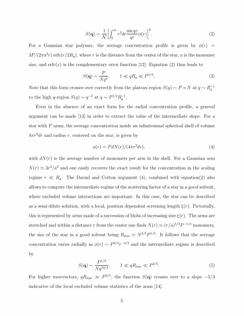
arX

iv:c

ond-

mat

/020

9354

v1 [

cond

-mat

.sof

t] 1

6 Se

p 20

02

Scattering from supramacromolecular structures

Carlos I. Mendoza and Carlos M. Marques

L.D.F.C.- UMR 7506, 3 rue de l’Universite, 67084 Strasbourg Cedex, France

(February 1, 2008)

Abstract

We study theoretically the scattering imprint of a number of branched supra-

macromolecular architectures, namely, polydisperse stars and dendrimeric,

hyperbranched structures. We show that polydispersity and nature of branch-

ing highly influence the intermediate wavevector region of the scattering struc-

ture factor, thus providing insight into the morphology of different aggregates

formed in polymer solutions.

Typeset using REVTEX

1

I. Introduction:

Scattering by light, x-rays or neutron radiation provides a fundamental tool to inves-

tigate the shapes and statistical nature of large molecules in solution [1]. For objects of

fixed shape, like spherical, ellipsoidal or cylindrical colloids, the scattering functions are

known and can easily be compared to experimental data, thus allowing for a determination

of shapes and relevant dimensions of the objects in a given experimental sample. For ob-

jects of a relatively simple geometry, but with a fluctuating nature, like polymer chains or

semi-flexible rods the scattering spectra contains not only information about the average

shape of the mass distribution but carries also a signature of the conformational disorder

determined by the nature of the thermodynamic fluctuations. For flexible polymers, for

instance, one can determine from the scattering data whether monomer-monomer excluded

volume interactions are relevant or not in a particular, given solvent.

Association of fixed-shape objects, like the aggregation of spherical colloids that lead

to fractal D.L.A.(diffusion-limited aggregation) structures [2], brings also some degree of

disorder into the spatial distribution of the scattering elements. Although the object as

a whole does not fluctuate in time, the spatial distribution of the scattering elements is

statistically fixed by the aggregation process itself. D.L.A. and other related processes have

been shown to lead to self-similar aggregates [3], where the frozen position correlations g(r)

between different elements at a distance r are described by a power law g(r) ∼ r−m. It

is well known that the scattering data from these objects also carries the signature of the

exponent m, thus providing some insight on the type of the aggregation process ruling the

solution behavior.

When the aggregation process involves fluctuating objects, the scattering function car-

ries information both on the connectivity between different scattering elements and on the

statistics of the fluctuations. In this paper we discuss the interplay between these two fac-

tors by studying a number of branched polymer structures. Branched polymers are arguably

the larger class of systems of connected fluctuating elements, systems that also include ag-

2

gregates of soft gel beads, emulsion droplets and others. In many polymer or polymer-like

structures, control of the branching chemistry allows for a careful choice of the connectivity,

like in dendrimers [4,5] or in star-branched polymers [6,7], and to some extent in dendrimeric

(also called hyperbranched) polymers [8–10]. Geometries with higher degree of disorder are

obtained by spontaneous aggregation in solutions of polymers carrying sticking groups, and

by random branching during polymerization growth. This leads to a great diversity in the

connections and to a polydispersity in sizes of the constitutive elements. In order to clarify

the role of each of these factors in shaping the scattering functions, we explore a number of

structures obtained by variations of star-like polymers: stars with polydisperse arms, and

dendrimeric polymers with different degrees of polydispersity.

The paper is organized as follows. In section II we recall some basic general features of

the scattering amplitude for well known, fixed-shape and fluctuating objects. Section III

discusses the scattering function of gaussian branched and hyperbranched structures, and

also discusses qualitatively the effects of excluded volume. Finally, in the conclusions we

discuss the different scattering signatures according to branching structure and statistical

nature of the fluctuations.

II. Scattering from simple polymer architectures.

The structure factor of an aggregate is given by

S(q) =1

N⟨ N

∑

n,m=1

exp {iq · ( Rn − Rm)}⟩

, (1)

where N is the number of scattering units in the aggregate (monomers), Ri is the position

of the i-th scattering unit, the ensemble average is denoted by 〈...〉, and q is the momentum

transfer given by q = qs − qi. Here qi and qs are the wave vectors of the incident and

scattered fields. For elastic scattering |qs| = |qi| = 2π/λ, where λ is the wavelength of

the incident wave. Hence, q ≡ |q| = (4π/λ) sin θ/2, with θ the scattering angle.

An illustration of the form of the scattering amplitude for two objects of well defined

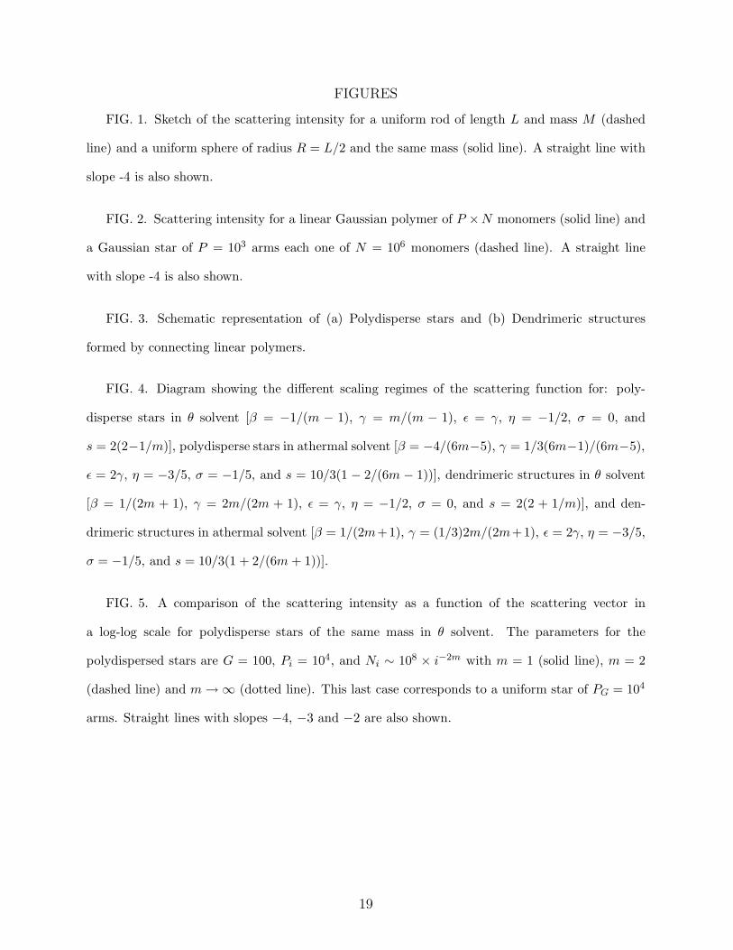
shapes is shown in Fig.1. In this figure, the spherically averaged scattering function of an

infinitely thin uniform rod of length L is compared to that of an uniform sphere of radius

3

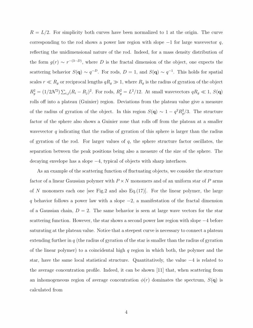
R = L/2. For simplicity both curves have been normalized to 1 at the origin. The curve

corresponding to the rod shows a power law region with slope −1 for large wavevector q,

reflecting the unidimensional nature of the rod. Indeed, for a mass density distribution of

the form g(r) ∼ r−(3−D), where D is the fractal dimension of the object, one expects the

scattering behavior S(q) ∼ q−D. For rods, D = 1, and S(q) ∼ q−1. This holds for spatial

scales r ≪ Rg or reciprocal lengths qRg ≫ 1, where Rg is the radius of gyration of the object

R2g = (1/2N 2)

∑

i,j(Ri − Rj)2. For rods, R2

g = L2/12. At small wavevectors qRg ≪ 1, S(q)

rolls off into a plateau (Guinier) region. Deviations from the plateau value give a measure

of the radius of gyration of the object. In this region S(q) ∼ 1 − q2R2g/3. The structure

factor of the sphere also shows a Guinier zone that rolls off from the plateau at a smaller

wavevector q indicating that the radius of gyration of this sphere is larger than the radius

of gyration of the rod. For larger values of q, the sphere structure factor oscillates, the

separation between the peak positions being also a measure of the size of the sphere. The

decaying envelope has a slope −4, typical of objects with sharp interfaces.

As an example of the scattering function of fluctuating objects, we consider the structure

factor of a linear Gaussian polymer with P ×N monomers and of an uniform star of P arms

of N monomers each one [see Fig.2 and also Eq.(17)]. For the linear polymer, the large

q behavior follows a power law with a slope −2, a manifestation of the fractal dimension

of a Gaussian chain, D = 2. The same behavior is seen at large wave vectors for the star

scattering function. However, the star shows a second power law region with slope −4 before

saturating at the plateau value. Notice that a steepest curve is necessary to connect a plateau

extending further in q (the radius of gyration of the star is smaller than the radius of gyration

of the linear polymer) to a coincidental high q region in which both, the polymer and the

star, have the same local statistical structure. Quantitatively, the value −4 is related to

the average concentration profile. Indeed, it can be shown [11] that, when scattering from

an inhomogeneous region of average concentration φ(r) dominates the spectrum, S(q) is

calculated from

4

S(q) ∼ 1

N[∫ ∞

0r2dr

sin qr

qrφ(r)

]2

. (2)

For a Gaussian star polymer, the average concentration profile is given by φ(r) =

3P/(2πa2r) erfc(r/2Rg), where r is the distance from the center of the star, a is the monomer

size, and erfc(x) is the complementary error function [12]. Equation (2) thus leads to

S(q) ∼ P

Nq4, 1 ≪ qRg ≪ P 1/2, (3)

Note that this form crosses over correctly from the plateau region S(q) ∼ P ×N at q ∼ R−1g

to the high q-region S(q) ∼ q−2 at q ∼ P 1/2R−1g .

Even in the absence of an exact form for the radial concentration profile, a general

argument can be made [13] in order to extract the value of the intermediate slope. For a

star with P arms, the average concentration inside an infinitesimal spherical shell of volume

4πr2dr and radius r, centered on the star, is given by

φ(r) = PdN(r)/(4πr2dr), (4)

with dN(r) is the average number of monomers per arm in the shell. For a Gaussian arm

N(r) ≃ 3r2/a2 and one easily recovers the exact result for the concentration in the scaling

regime r ≪ Rg. The Daoud and Cotton argument (4), combined with equation(2) also

allows to compute the intermediate regime of the scattering factor of a star in a good solvent,

where excluded volume interactions are important. In this case, the star can be described

as a semi-dilute solution, with a local, position dependent screening length ξ(r). Pictorially,

this is represented by arms made of a succession of blobs of increasing size ξ(r). The arms are

stretched and within a distance r from the center one finds N(r) ≃ (r/a)5/3P−1/3 monomers,

the size of the star in a good solvent being Rstar ≃ N3/5P 1/5. It follows that the average

concentration varies radially as φ(r) ∼ P 2/3r−4/3 and the intermediate regime is described

by

S(q) ∼ P 1/3

Nq10/3, 1 ≪ qRstar ≪ P 2/5. (5)

For higher wavevectors, qRstar ≫ P 2/5, the function S(q) crosses over to a slope −5/3

indicative of the local excluded volume statistics of the arms [14].

5

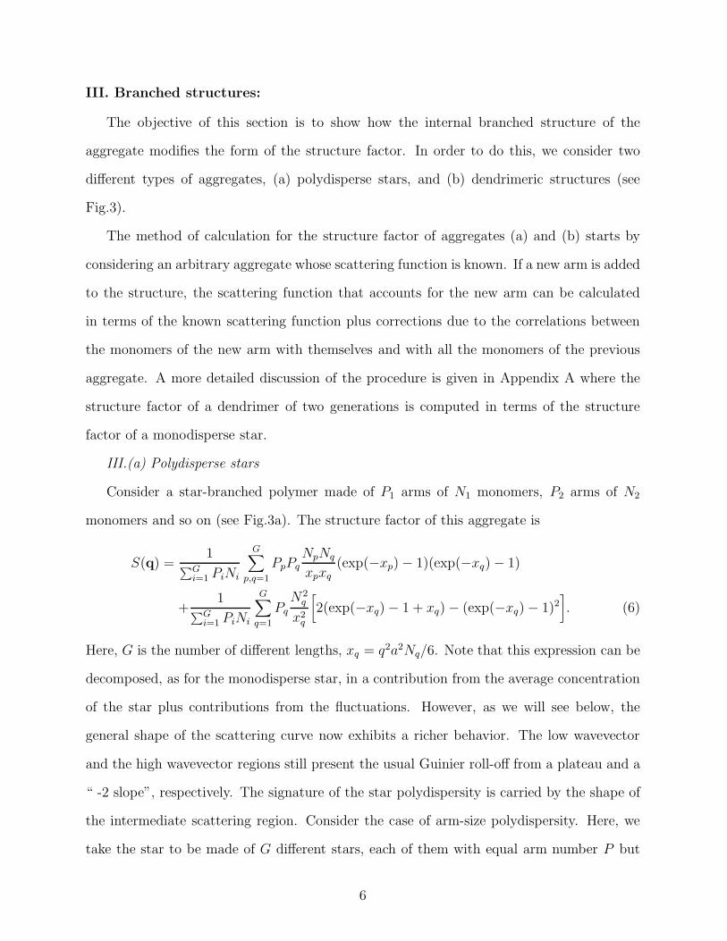
III. Branched structures:

The objective of this section is to show how the internal branched structure of the

aggregate modifies the form of the structure factor. In order to do this, we consider two

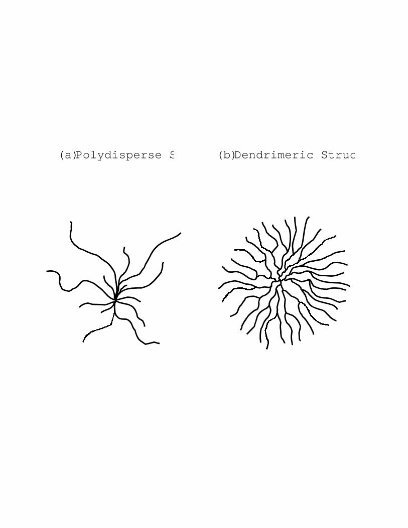
different types of aggregates, (a) polydisperse stars, and (b) dendrimeric structures (see

Fig.3).

The method of calculation for the structure factor of aggregates (a) and (b) starts by

considering an arbitrary aggregate whose scattering function is known. If a new arm is added

to the structure, the scattering function that accounts for the new arm can be calculated

in terms of the known scattering function plus corrections due to the correlations between

the monomers of the new arm with themselves and with all the monomers of the previous

aggregate. A more detailed discussion of the procedure is given in Appendix A where the

structure factor of a dendrimer of two generations is computed in terms of the structure

factor of a monodisperse star.

III.(a) Polydisperse stars

Consider a star-branched polymer made of P1 arms of N1 monomers, P2 arms of N2

monomers and so on (see Fig.3a). The structure factor of this aggregate is

S(q) =1

∑Gi=1 PiNi

G∑

p,q=1

PpPqNpNq

xpxq(exp(−xp) − 1)(exp(−xq) − 1)

+1

∑Gi=1 PiNi

G∑

q=1

Pq

N2q

x2q

[

2(exp(−xq) − 1 + xq) − (exp(−xq) − 1)2]

. (6)

Here, G is the number of different lengths, xq = q2a2Nq/6. Note that this expression can be

decomposed, as for the monodisperse star, in a contribution from the average concentration

of the star plus contributions from the fluctuations. However, as we will see below, the

general shape of the scattering curve now exhibits a richer behavior. The low wavevector

and the high wavevector regions still present the usual Guinier roll-off from a plateau and a

“ -2 slope”, respectively. The signature of the star polydispersity is carried by the shape of

the intermediate scattering region. Consider the case of arm-size polydispersity. Here, we

take the star to be made of G different stars, each of them with equal arm number P but

6

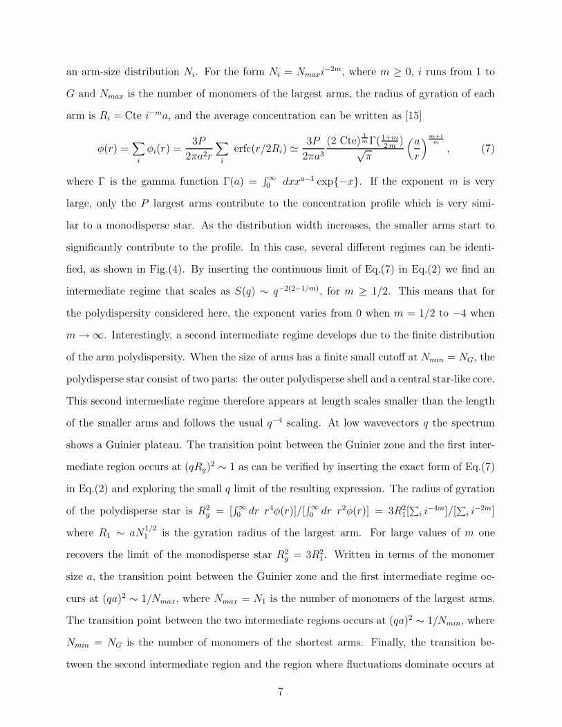
an arm-size distribution Ni. For the form Ni = Nmaxi−2m, where m ≥ 0, i runs from 1 to

G and Nmax is the number of monomers of the largest arms, the radius of gyration of each

arm is Ri = Cte i−ma, and the average concentration can be written as [15]

φ(r) =∑

i

φi(r) =3P

2πa2r

∑

i

erfc(r/2Ri) ≃3P

2πa3

(2 Cte)1m Γ(1+m

2 m)√

π

(

a

r

)m+1

m

, (7)

where Γ is the gamma function Γ(a) =∫ ∞

0 dxxa−1 exp{−x}. If the exponent m is very

large, only the P largest arms contribute to the concentration profile which is very simi-

lar to a monodisperse star. As the distribution width increases, the smaller arms start to

significantly contribute to the profile. In this case, several different regimes can be identi-

fied, as shown in Fig.(4). By inserting the continuous limit of Eq.(7) in Eq.(2) we find an

intermediate regime that scales as S(q) ∼ q−2(2−1/m), for m ≥ 1/2. This means that for

the polydispersity considered here, the exponent varies from 0 when m = 1/2 to −4 when

m → ∞. Interestingly, a second intermediate regime develops due to the finite distribution

of the arm polydispersity. When the size of arms has a finite small cutoff at Nmin = NG, the

polydisperse star consist of two parts: the outer polydisperse shell and a central star-like core.

This second intermediate regime therefore appears at length scales smaller than the length

of the smaller arms and follows the usual q−4 scaling. At low wavevectors q the spectrum

shows a Guinier plateau. The transition point between the Guinier zone and the first inter-

mediate region occurs at (qRg)2 ∼ 1 as can be verified by inserting the exact form of Eq.(7)

in Eq.(2) and exploring the small q limit of the resulting expression. The radius of gyration

of the polydisperse star is R2g = [

∫ ∞

0 dr r4φ(r)]/[∫ ∞

0 dr r2φ(r)] = 3R21[

∑

i i−4m]/[

∑

i i−2m]

where R1 ∼ aN1/21 is the gyration radius of the largest arm. For large values of m one

recovers the limit of the monodisperse star R2g = 3R2

1. Written in terms of the monomer

size a, the transition point between the Guinier zone and the first intermediate regime oc-

curs at (qa)2 ∼ 1/Nmax, where Nmax = N1 is the number of monomers of the largest arms.

The transition point between the two intermediate regions occurs at (qa)2 ∼ 1/Nmin, where

Nmin = NG is the number of monomers of the shortest arms. Finally, the transition be-

tween the second intermediate region and the region where fluctuations dominate occurs at

7

(qa)2 ∼ P/Nmax(Nmax/Nmin)1/m. One can see that the region where fluctuations dominates

appears only if Nmax > P m/(m−1)N−1/(m−1)min . If the exponent m is larger than one and the

number of monomers Nmax is very large, Nmax ≫ NminP m/(m−1), the region with slope q−4

disappears and one crosses over directly to the region dominated by fluctuations with slope

q−2. The transition point then occurs at (qa)2 ∼ P m/(m−1)/Nmax (see Fig.4). For values of m

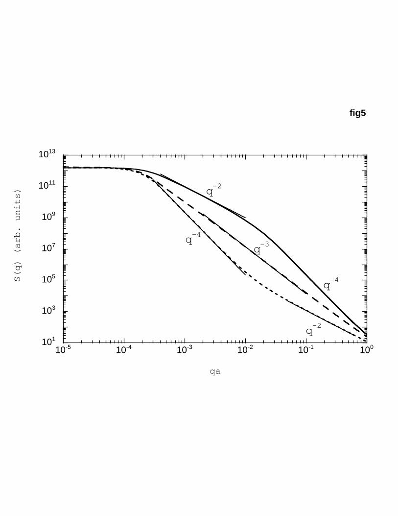
between 1 and 1/2, the scattering function always crosses from the regime S(q) ∼ q−2(2−1/m)

to a regime S(q) ∼ q−4 independently of the number of monomers Nmax. Examples of some

of these cases are presented in Fig. 5 (see note [15]). In the limit m = 1/2 the scattering

function does not exhibit a developed scaling but rolls over gently from the Guinier plateau

to the large wavevector limit of slope −2.

For a polydisperse star in a good solvent a Daoud-Cotton argument can also be applied

to determine the scattering regimes. Let p(r) be the number of arms at distance r from the

center. Then, the local correlation length is set by ξ(r) = rp(r)−1/2 and the concentration

is φ(r) = p(r)2/3r−4/3. In the infinitesimal shell of volume dV = 4πr2dr, there are then

dn = p(r)−1/3r2/3dr monomers in one arm. By knowing the polydispersity of the chains

p(n) one can compute the function p(r) and extract the concentration. If we choose, as

for the precedent Gaussian example, Ni = Nmaxi−2m, and a constant arm number of each

length, Pi = P , we get in the continuous limit p(n) = P (n/Nmax)−1/2m, leading to p(r) ∼

r−5/(6m−1). Correspondingly, the concentration scales as φ(r) ∼ r−α with the exponent

α = 23(2 + 5

6m−1) and the scattering from that intermediate region scales as S(q) ∼ q−s,

with exponent s = 103(1 − 2

6m−1). In the limit where m is very large one recovers the usual

intermediate slope s = 10/3. As m decreases we reduce the intermediate slope, as for the

Gaussian case. The transition point between the Guinier zone and this region occurs at

(qa)5/3 ∼ 1/(NmaxP1/3). As in the Gaussian case, we find a second intermediate region that

scales as S(q) ∼ q−10/3. The transition point between the two intermediate regions occurs at

(qa)5/3 ∼ 1/(NminP1/3). Finally, the transition between the second intermediate region and

the fluctuating regime occurs at (qa)5/3 ∼ P 1/3/Nmax(Nmax/Nmin)4/(6m−1). These results are

8

shown in Fig.4. One can see that the region where fluctuations dominates appears only if

Nmax > P 1/3(6m−1)/(6m−5)N−4/(6m−5)min . If the exponent m ≥ 5/6 and the number of monomers

Nmax is very large, Nmax ≫ NminP 2/3(6m−1)/(6m−5), the region with slope q−10/3 disappears

and one crosses over directly to the region dominated by fluctuations with slope q−5/3. The

transition point then occurs at (qa)5/3 ∼ P (2m+1)/(6m−5)/Nmax. Again, by choosing the value

of m between ∞ and 5/6, it is possible to obtain scattering functions with intermediate slopes

ranging from the monodisperse star value of −10/3 to −5/3 slope. For values of m between

5/6 and 1/2, the scattering function always crosses from the regime S(q) ∼ q−10/3(1−2/(6m−1))

to a regime S(q) ∼ q−10/3 independently of the number of monomers Nmax.

III.(b)Dendrimeric Structures

These structures are formed by starting from a uniform star of P1 = P arms of N1

monomers each one, and branching each arm twice so that in the second generation there

are P2 = 2P1 arms of length N2. We then branch each of the newest arms twice so that

in the third generation there are P3 = 2P2 = 22P1 arms of length N3. We repeat this

process up to any desired number of generations (see Fig.3b). This means that the number

of arms in each generation is Pi = 2i−1P . As in the case of the polydisperse stars, for a large

number of arms and generations, asymptotic shapes can be reached for particular types of

polydispersity distributions. Let us consider the case of a dendrimer of G generations with

arm-size polydispersity of the form Ni = 22m(i−1)Nmin, where Ni =∑i

j=1 Nj is the sum of

monomers per arm from generation 1 up to generation i. By choosing m ≥ 1/2, we assure

that the first generation always has the smallest number of monomers per arm. By using

arguments similar to the ones for the polydisperse star, we find for the Gaussian dendrimer,

an average concentration φ(r) ∼ r−(1−1/m), that gives rise to an intermediate scaling regime

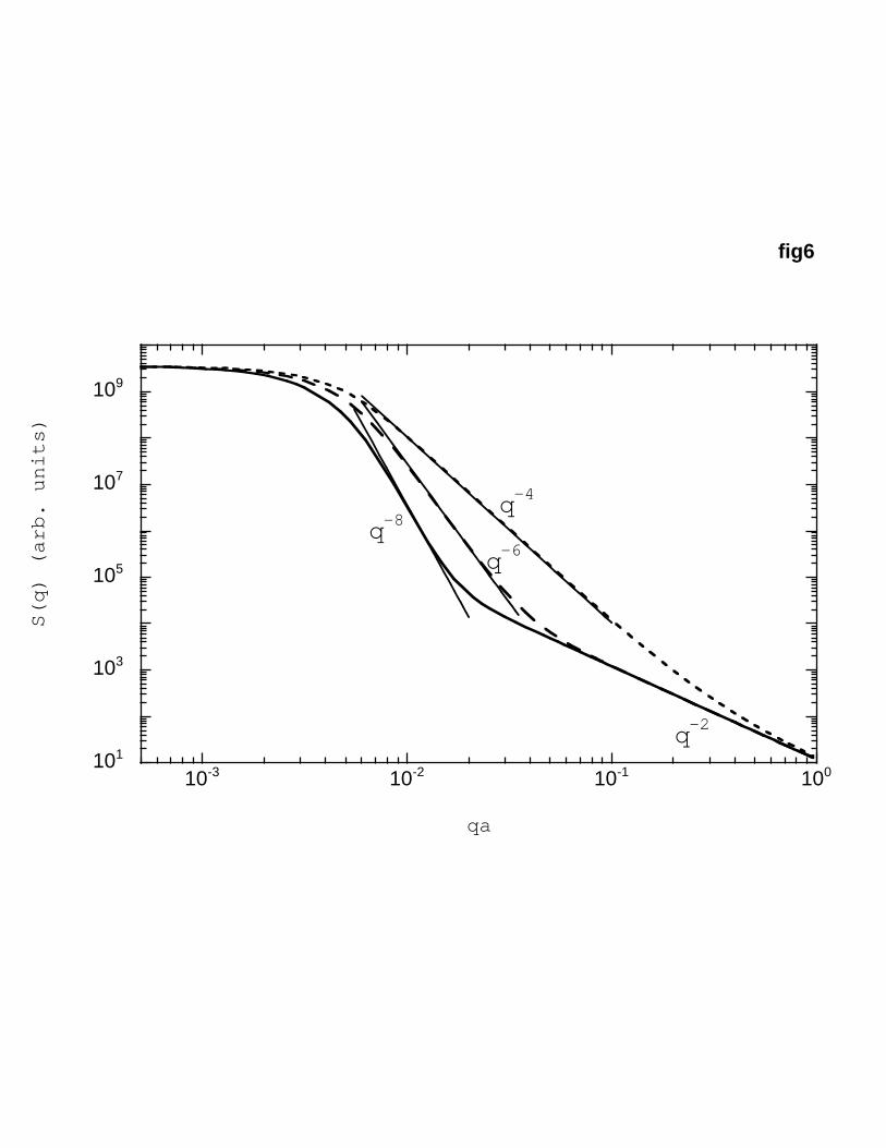
S(q) ∼ q−2(2+1/m) [16]. Again, if m is very large, only the last generation contributes to

the scattering, which is similar to the monodisperse star with PG arms. As m decreases,

the first generations start to contribute significantly, modifying the slope of the scattering

curves that reaches the steepest value of −8 when m = 1/2. The transition point between

the Guinier zone and this region occurs at (qa)2 ∼ 1/Nmax, where Nmax = NG. Also, there is

9

a second intermediate region which scales as S(q) ∼ q−4. The transition point between these

two intermediate regions occurs at (qa)2 ∼ 1/Nmin, where Nmin = N1 (see Fig.4). Finally,

the transition between the second intermediate region and the fluctuating regime occurs at

(qa)2 ∼ P/Nmax(Nmax/Nmin)−1/2m. The region where fluctuations dominates appears only

if Nmax > P 2m/(2m+1)N 1/(2m+1)min . The regime with S(q) ∼ q−4 disappears when Nmax ∼

NminP2m/(2m+1). In this case the transition point between the region with S(q) ∼ q−2(2+1/m)

and the fluctuating regime occurs at (qa)2 ∼ P m/(m+1)/Nmax(Nmax/Nmin)1/2(m+1). Note

that for large Nmax and by tuning m between ∞ and 1/2, it is possible to obtain scattering

functions with intermediate slopes ranging from the monodisperse star value of −4 to −8

slope. In Fig.6 we show examples of some of these cases.

Applying a Daoud-Cotton argument to the case of dendrimers in good solvent we de-

termine the corresponding scaling regimes. In this case, p(r) ∼ r5/(6m+1). Correspondingly,

the concentration scales as φ(r) ∼ r−α, with α = 23(2 − 5

6m+1) and the scattering from

that intermediate region scales as S(q) ∼ q−s, with s = 103(1 + 2

6m+1). In the limit where

m is very large one recovers the usual intermediate slope s = 10/3. As m decreases we

reduce the intermediate slope, as for the Gaussian case. The transition point between the

Guinier zone and this region occurs at (qa)5/3 ∼ 1/(P 1/3Nmax)(Nmax/Nmin)−1/6m. As in

the Gaussian case, we find another intermediate region that scales as S(q) ∼ q−10/3. The

transition point between the two intermediate regions occurs at (qa)5/3 ∼ 1/(P 1/3Nmin).

Finally, the transition between the second intermediate region and the fluctuating regime

occurs at (qa)5/3 ∼ P 1/3/Nmax(Nmax/Nmin)−1/2m. These results are shown in Fig.4. The

region where fluctuations dominates appears only if Nmax > N 1/(2m+1)min P 2m/(3(2m+1)). If Nmax

is very large, Nmax ≫ NminP4m/(3(2m+1)), the region with slope q−10/3 disappears and one

crosses over directly to the region dominated by fluctuations with slope q−5/3. The transition

point then occurs at (qa)5/3 ∼ P (2m−1)/(6m+5)/Nmax(Nmax/Nmin)(2m−1)/(2m(6m+5)) . Again, by

choosing the value of m between ∞ and 1/2, it is possible to obtain scattering functions

with intermediate slopes ranging from the monodisperse star value of −10/3 to −5 slope.

The results for the scaling regimes and the transitions between these regimes for both,

10

polydisperse stars and hyperbranched structures are summarized in Appendix B.

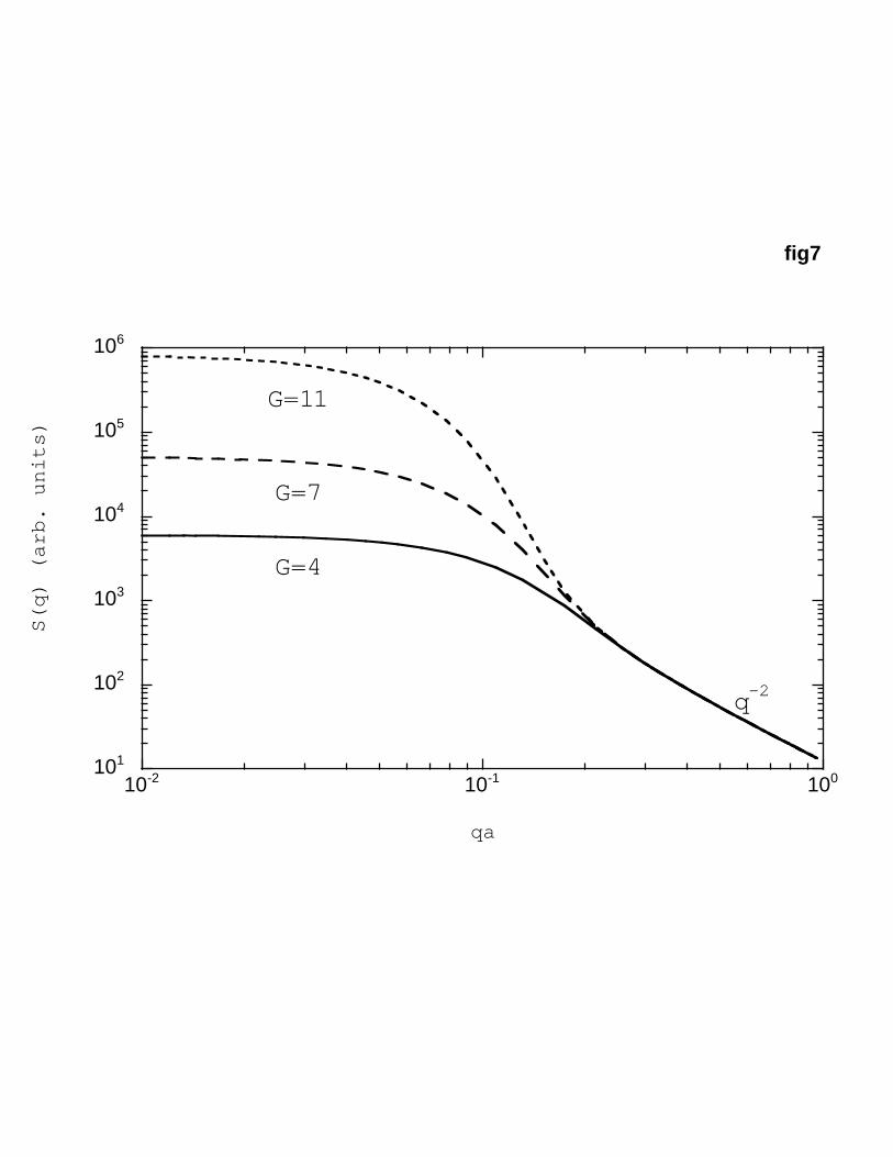
In Fig.7 we plot the structure factor for Gaussian dendrimers with arms of equal size for

all the generations. In this case a non-scaling regime is present between the Guinier zone

and the high q region. This region shows a hump that reflects the fact that as we increase the

number of generations, the outer core of the aggregate becomes very dense thus dominating

the structure of the spectrum which resembles the one for a spherical shell. We see in Fig.7

that the size of the hump increases as we increase the number of generations in qualitative

agreement with the experimental results of Ref. [17]. Note that while growth of dendrimers to

a high number of generations is usually hindered by steric reasons, a polydisperse dendrimer

can grow indefinitely if the polydispersity is correctly tuned.

From the scattering curves of branched structures in which there is a q region where

fluctuations dominate, we note that there is always an intermediate q region with a steeper

slope than the corresponding one for a linear polymer. This can be understood by using a

simple graphical argument. Consider a linear Gaussian polymer of mass N . Its structure

factor consist of a power law region with slope −2 and a Guinier zone for low wave vector q.

Now, let us consider any branched Gaussian polymer. Its structure factor coincides, in slope

and absolute value, with the one for the linear Gaussian polymer at short wave lengths.

This reflects the fact that the internal structure of the polymer is the same in both cases.

If the branched polymer has the same mass than the linear one, both spectra must coincide

in the plateau Guinier zone. However, since the radius of gyration of any branched polymer

is always smaller than the corresponding one for the linear polymer, the Guinier zone must

extend to a larger wave vector value, as shown for example in Fig.2. Therefore, the only

possible way of crossing from one region to the other is by an intermediate region with

an average slope larger than the slope at short-wave lengths. This argument is also valid

in good solvent conditions where the Gaussian model is not valid and monomer-monomer

interactions play an important role.

IV. Conclusions:

11

In this paper we have shown how different branched polymers give rise to different struc-

ture factors. This information can be used to probe the morphology of supramacromolecular

aggregates. We have shown how the slope in the intermediate q region can be tailored ac-

cording to the polydispersity in the length of the constitutive linear chains of the branched

aggregates. In particular, for polydisperse stars we found scaling regimes with slopes ranging

from −2 to −4 in θ solvent conditions and between −5/3 and −10/3 for athermal solvent.

In the case of dendrimeric structures, scaling regimes ranging from −4 to −8 in θ solvent

and between −10/3 and −5 for athermal conditions, although richer behavior was obtained

for specific choices of the polydispersity parameters. We have shown using simple arguments

that whenever there is a region where fluctuations dominate the scattering response, then

the structure factor of branched structures always present an intermediate q regime with at

least a small region where the slope in a log-log plot is larger than the corresponding slope

of the linear polymer. This means that these aggregates are not strictly self-similar over the

entire range of length scales a < l < Rg. Results presented in this paper can be qualitatively

used as a guiding tool for exploring the branching morphology of aggregates according to the

type of regimes presented in the scattering intensity curves. They also provide qualitative

information from the analysis of the values of the slopes of the intermediate q regimes.

Appendix A: Method of Calculation

In this appendix we outline the procedure to obtain the structure factor for the branched

structures described in this paper by considering a specific example. Suppose a branched

polymer that grows following a given rule like the one shown in Fig. 3b. In this figure, we

show a polymer that grows from a star of P1 arms each one made of N1 monomers. Each

arm is then branched in two other arms made of N2 monomers. Then, each arm of the

newest generation is branched again in two arms and so on. The structure factor of the

structure made of G generations is related to the structure factor of the structure made of

G − 1 generations by the equation

SG(q) =

∑G−1i=1 PiNi

∑Gi=1 PiNi

SG−1(q) + Scorr(q), (8)

12

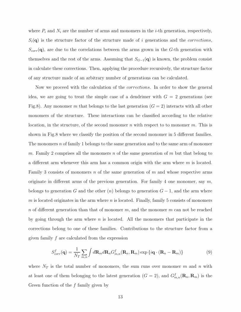
where Pi and Ni are the number of arms and monomers in the i-th generation, respectively,

Si(q) is the structure factor of the structure made of i generations and the corrections,

Scorr(q), are due to the correlations between the arms grown in the G-th generation with

themselves and the rest of the arms. Assuming that SG−1(q) is known, the problem consist

in calculate these corrections. Then, applying the procedure recursively, the structure factor

of any structure made of an arbitrary number of generations can be calculated.

Now we proceed with the calculation of the corrections. In order to show the general

idea, we are going to treat the simple case of a dendrimer with G = 2 generations (see

Fig.8). Any monomer m that belongs to the last generation (G = 2) interacts with all other

monomers of the structure. These interactions can be classified according to the relative

location, in the structure, of the second monomer n with respect to to monomer m. This is

shown in Fig.8 where we classify the position of the second monomer in 5 different families.

The monomers n of family 1 belongs to the same generation and to the same arm of monomer

m. Family 2 comprises all the monomers n of the same generation of m but that belong to

a different arm whenever this arm has a common origin with the arm where m is located.

Family 3 consists of monomers n of the same generation of m and whose respective arms

originate in different arms of the previous generation. For family 4 one monomer, say m,

belongs to generation G and the other (n) belongs to generation G − 1, and the arm where

m is located originates in the arm where n is located. Finally, family 5 consists of monomers

n of different generation than that of monomer m, and the monomer m can not be reached

by going through the arm where n is located. All the monomers that participate in the

corrections belong to one of these families. Contributions to the structure factor from a

given family f are calculated from the expression

Sfcorr(q) =

1

NT

∑

m,n

∫

dRmdRnGfm,n(Rn,Rm) exp {iq · (Rn − Rm)} (9)

where NT is the total number of monomers, the sum runs over monomer m and n with

at least one of them belonging to the latest generation (G = 2), and Gfm,n(Rn,Rm) is the

Green function of the f family given by

13

G1m,n(Rn,Rm) = G(Rn,Rm; m − n), (10)

G2m,n(Rn,Rm) = G(Rn,Rm; m + n), (11)

G3m,n(Rn,Rm) = G(Rn,Rm; m + n + 2N1), (12)

G4m,n(Rn,Rm) = G(Rn,Rm; m − n + N1), (13)

G5m,n(Rn,Rm) = G(Rn,Rm; m + n + N1), (14)

where

G(Rn,Rm; α) =(

3

2πa2|α|

)(3/2)

exp{

−3(Rm −Rn)2

2a2|α|

}

. (15)

Substituting these expressions in Eq.(9) and taking the continuos limit by transforming

the sums into integrals we find the structure factor for the dendrimer of two generations

S2(q) =N1

N1 + 2N2S1(q)

+2N2

N1 + 2N2

[

N2

x22

(exp {−x2} − 1)2 +2N2

x22

(exp {−x2} − 1 + x2)]

+2N2

N1 + 2N2

[

2N2

x22

(P0 − 1) exp {−2x1}(exp {−x2} − 1)2]

+2N2

N1 + 2N2

2N2

x22

[

1 + (P0 − 1) exp {−x1}]

(exp {−x1} − 1)(exp {−x2} − 1), (16)

where

S1(q) =(P1 − 1)N1

x21

(exp {−x1} − 1)2 +2N1

x21

(exp {−x1} − 1 + x1), (17)

is the structure factor of a star of P1 arms and N1 monomers [18]. This expression contains

two terms. The first term of the right-hand side expresses cross-correlations between the

different arms of the star. The second term refers to the normal Debye function for a linear

polymer of N1 monomers, as found by taking the appropriate limit P1 = 1. Note that the

general procedure explained above can be easily generalized to calculate the structure factors

of general branched structures like the ones studied in this paper.

14

Appendix B: Summary for the scaling regimes

In this appendix we summarize the results for the scaling regimes of the branched and

hyperbranched structures studied in this work and write them using a simpler notation. (a),

(b), (c), and (d) show the results for Gaussian polydisperse stars, SAW polydisperse stars,

Gaussian dendrimers and SAW dendrimers, respectively.

First intermediate regime S(q) ∼ q−s:

(a) s = 4(1 − 12m

)

(b) s = 103(1 − 2

6m−1)

(c) s = 4(1 + 12m

)

(d) s = 103(1 + 2

6m+1)

Transition points between the Guinier and the first intermediate regime:

(a) (qRg)2 ∼ 1

(b) (qRg)5/3 ∼ 1

(c) (qRg)2 ∼ 1

(d) (qRg)5/3 ∼ 1

Transition points between the first and second intermediate regimes:

(a) (qRg)2 ∼ Nmax/Nmin

(b) (qRg)5/3 ∼ Nmax/Nmin

(c) (qRg)2 ∼ Nmax/Nmin

(d) (qRg)5/3 ∼ NmaxP

1/3G /NminP

1/3

Transition points between the second intermediate regime and the region where fluctu-

ations dominate:

(a) (qRg)2 ∼ P (Nmax/Nmin)1/m

(b) (qRg)5/3 ∼ P 2/3(Nmax/Nmin)

46m−1

(c) (qRg)2 ∼ PG(Nmax/Nmin)−1/m

(d) (qRg)5/3 ∼ P

2/3G (NmaxP

1/3G /NminP

1/3)−4

(6m+1)

Transition points between the first intermediate regime and the region where fluctuations

15

dominate:

(a) (qRg)2 ∼ P m/(m−1)

(b) (qRg)5/3 ∼ P (2/3)(6m−1)/(6m−5)

(c) (qRg)2 ∼ P

m/(m+1)G

(d) (qRg)5/3 ∼ P

(2/3)(6m+1)/(6m+5)G

16

REFERENCES

[1] See for example, M.R. Gittings, Luca Cipelletti, V. Trappe, D.A. Weitz, M. In, and C.

Marques, J. Phys. Chem. B 104, 4381 (2000).

[2] T.A. Witten, and L.M. Sander, Phys. Rev. Lett. 47, 1400 (1981).

[3] However see, C. Oh, and C.M. Sorensen, Phys. Rev. E 57, 784 (1998).

[4] P.G. de Gennes, and H. Hervet, J. Phys. Lett. 44, L351 (1983).

[5] M. Murat, and G.S. Grest, Macromolecules 29, 1278 (1996).

[6] E. Mendes, P. Lutz, J. Bastide, and F. Bou, Macromolecules 28, 174 (1995).

[7] H.A. Al-Muallem, and D.M. Knauss, J. Polym. Sci. Part A Polym. Chem. 39, 3547

(2001).

[8] D.M. Knauss, H.A. Al-Muallem, T. Huang, and D.T. Wu, Macromolecules 33, 3557

(2000); D.M. Knauss, and H.A. Al-Muallem, J. Polym. Sci. Part A Polym. Chem. 38,

4289 (2000); H.A. Al-Muallem, and D.M. Knauss, J. Polym. Sci. Part A Polym. Chem.

39, 152 (2001).

[9] A. Sunder, J. Heinemann, and H. Frey, Chem. Eur. J 6, 2499 (2000).

[10] Z. Muchtar, M. Schappacher, and A. Deffieux, Macromolecules 34, 7595 (2001).

[11] C.M. Marques, D. Izzo, T. Charitat, and E. Mendes, Eur. Phys. J. B 3, 353 (1998).

[12] M. Abramowitz, and I.A. Stegun, Handbook of Mathematical Functions (Dover Publi-

cations Inc., New York, 1972), p 297.

[13] M. Daoud, and J.P. Cotton, J. Phys. France 43, 531 (1982).

[14] Asymptotically, for very high arm number, the high q-regime of slope −5/3 does not

cross over directly into the intermediate regime of slope −10/3 at qRstar = P 2/5. In fact,

the semidilute character of the corona shows up as a plateau for wavevectors smaller

17

than the reciprocal of an average blob size ξ ∼ RstarP−1/2. The scattering intensity

should then be a constant in the range P 9/20 ≪ qRstar ≪ P 1/2. However, the ratio of

the upper to the lower boundaries is only of the order of P 1/20, and therefore invisible

under normal conditions.

[15] We study the limit of high number of arms and large number of arm-sizes for which

asymptotic shapes are well developed.

[16] Strictly speaking, Eq.(2) only leads to a scaling form if the integral there converges. This

can be achieved by using a soft cutoff as for instance φ(r) = exp(−r/rmax)/rµ. In this

case S(q) ∼ q2(µ−3)(qrmax)2(2−µ)(1+(qrmax)

2)µ−2Γ2(2−µ) sin2((2−µ) arctan(qrmax)) for

µ < 3. If rmax ≫ 1 then S(q) ∼ q2(µ−3).

[17] T.J. Prosa, B.J. Bauer, and E.J. Amis, Macromolecules 34, 4897 (2001).

[18] J.S. Higgins and H.C. Benoıt, Polymers and neutron scattering, (Oxford University

Press, Oxford, 1996).

18

FIGURES

FIG. 1. Sketch of the scattering intensity for a uniform rod of length L and mass M (dashed

line) and a uniform sphere of radius R = L/2 and the same mass (solid line). A straight line with

slope -4 is also shown.

FIG. 2. Scattering intensity for a linear Gaussian polymer of P ×N monomers (solid line) and

a Gaussian star of P = 103 arms each one of N = 106 monomers (dashed line). A straight line

with slope -4 is also shown.

FIG. 3. Schematic representation of (a) Polydisperse stars and (b) Dendrimeric structures

formed by connecting linear polymers.

FIG. 4. Diagram showing the different scaling regimes of the scattering function for: poly-

disperse stars in θ solvent [β = −1/(m − 1), γ = m/(m − 1), ǫ = γ, η = −1/2, σ = 0, and

s = 2(2−1/m)], polydisperse stars in athermal solvent [β = −4/(6m−5), γ = 1/3(6m−1)/(6m−5),

ǫ = 2γ, η = −3/5, σ = −1/5, and s = 10/3(1 − 2/(6m − 1))], dendrimeric structures in θ solvent

[β = 1/(2m + 1), γ = 2m/(2m + 1), ǫ = γ, η = −1/2, σ = 0, and s = 2(2 + 1/m)], and den-

drimeric structures in athermal solvent [β = 1/(2m+1), γ = (1/3)2m/(2m+1), ǫ = 2γ, η = −3/5,

σ = −1/5, and s = 10/3(1 + 2/(6m + 1))].

FIG. 5. A comparison of the scattering intensity as a function of the scattering vector in

a log-log scale for polydisperse stars of the same mass in θ solvent. The parameters for the

polydispersed stars are G = 100, Pi = 104, and Ni ∼ 108 × i−2m with m = 1 (solid line), m = 2

(dashed line) and m → ∞ (dotted line). This last case corresponds to a uniform star of PG = 104

arms. Straight lines with slopes −4, −3 and −2 are also shown.

19

FIG. 6. A comparison of the scattering intensity as a function of the scattering vector in a

log-log scale for dendrimers with the same mass. The parameters used were G = 10, P = 20, and

Ni ∼ 103 × i−2m with m = 1/2 (solid line), m = 1 (dashed line) and m → ∞ (dotted line). This

last case corresponds to a uniform star of PG = 20 × 29 arms. Straight lines with slopes −8, −6

and −4 are also shown.

FIG. 7. A comparison of the scattering intensity as a function of the scattering vector in a

log-log scale for a dendrimeric structure of different number of generations, G. The parameters for

the dendrimer are Ni = 100, P = 20.

FIG. 8. Representation of a dendrimer with P = 4 arms, and G = 2 generations. The solid cir-

cle represents the location of monomer m and the open circles represent the locations of monomers

n representatives of the different families.

20

10 -6

10 -5

10 -4

10 -3

10 -2

10 -1

10 0

1 10 100

fig1

S(q)/M

qL

q-4

q-1

10 1

10 3

10 5

10 7

10 9

10 -5 10 -4 10 -3 10 -2 10 -1 10 0

fig2

S(q) (arb. units)

qa

q-4

q-2

(a) Polydisperse S (b) Dendrimeric Struc

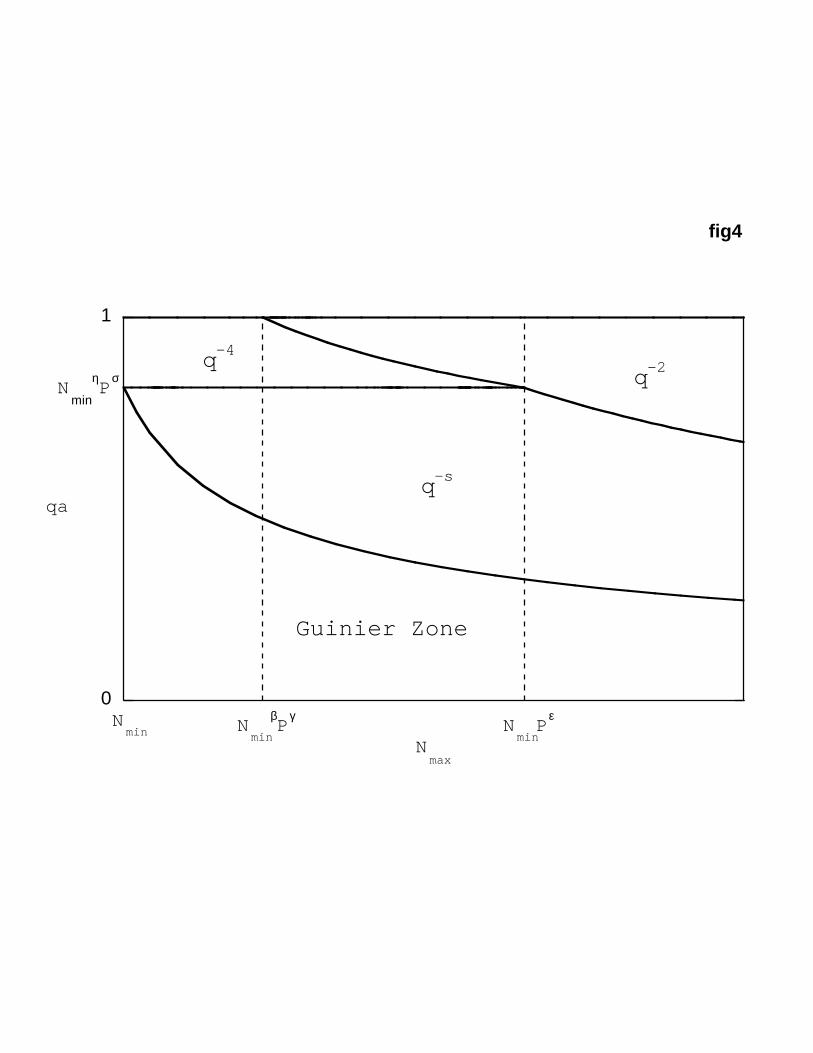
fig4

0

1

qa

Nmax

q-4

q-s

Guinier Zone

Nmin

η P

σ q-2

Nmin

β P

γ NminP

ε Nmin

10 1

10 3

10 5

10 7

10 9

10 11

10 13

10 -5 10 -4 10 -3 10 -2 10 -1 10 0

fig5

S(q) (arb. units)

qa

q-3

q-2

q-2

q-4

q-4

10 1

10 3

10 5

10 7

10 9

10 -3 10 -2 10 -1 10 0

fig6

S(q) (arb. units)

qa

q-8

q-2

q-4

q-6

10 1

10 2

10 3

10 4

10 5

10 6

10 -2 10 -1 10 0

fig7

S(q) (arb. units)

qa

q-2

G=4

G=7

G=11

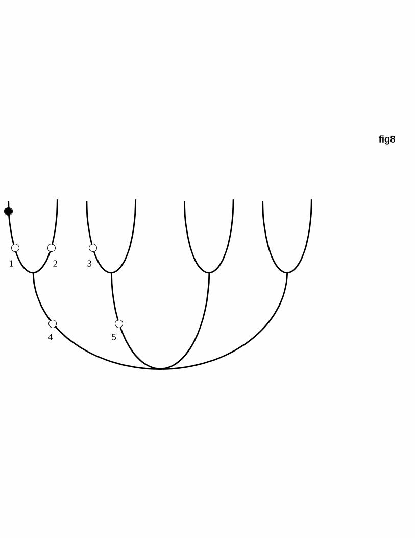
fig8

1 2 3

4 5