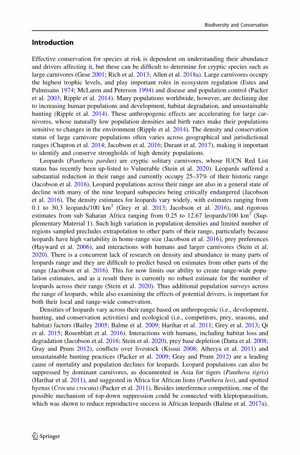
ORIGINAL PAPER

Counting cats for conservation: seasonal estimates of leoparddensity and drivers of distribution in the Serengeti

Maximilian L. Allen1 • Shaodong Wang2 • Lucas O. Olson3 • Qing Li2 •

Miha Krofel4

Received: 6 October 2019 / Revised: 24 May 2020 / Accepted: 14 August 2020� Springer Nature B.V. 2020

AbstractLarge carnivore conservation is important for ecosystem integrity and understanding drivers

of their abundance is essential to guide conservation efforts. Leopard (Panthera pardus)populations are in a general state of decline, although local studies demonstrated large

variation in their population trends and density estimates vary widely across their range. We

used spatially-explicit capture-recapture models for unmarked populations with camera trap

data from a citizen science project to estimate previously-unknown leopard population

densities in Serengeti National Park, Tanzania, and determine potential biological drivers of

their abundance and distribution. We estimated leopard densities, at 5.41 (95% CrI =

2.23–9.26) and 5.72 (95% CrI = 2.44–9.55) individuals/100 km2, in the dry and wet season,

respectively, which confirmed Serengeti National Park as one of the strongholds of this

species in Africa. In contrast to abundance estimates, we found that drivers of leopard

abundance and distribution varied among the dry and wet seasons, and were primarily

affected by interactions with other larger carnivores and cover. The underlying driver of

leopard distribution may be the dynamic prey availability which shifts between seasons,

leading to an avoidance of dominant carnivores when prey availability is low in the dry season

but an association with dominant carnivores when prey availability is high in the wet season.

As efforts to conserve large carnivore populations increase worldwide, our results highlight

the benefits of using data from citizen science projects, including large camera-trapping

surveys, to estimate local carnivore abundances. Using a Bayesian framework allows of

estimation of population density, but it is also important to understand the factors that dictate

their distribution across the year to inform conservation efforts.

Keywords Competition � Leopard � Panthera pardus � Population density � Predator–prey

dynamics � Seasonal variation � Spatially explicit capture recapture

Communicated by Karen E. Hodges.

Electronic supplementary material The online version of this article (https://doi.org/10.1007/s10531-020-02039-w) contains supplementary material, which is available to authorized users.

& Maximilian L. Allenmaxallen@illinois.edu

Extended author information available on the last page of the article

123

Biodiversity and Conservationhttps://doi.org/10.1007/s10531-020-02039-w(0123456789().,-volV)(0123456789().,-volV)

Introduction

Effective conservation for species at risk is dependent on understanding their abundance

and drivers affecting it, but these can be difficult to determine for cryptic species such as

large carnivores (Gese 2001; Rich et al. 2013; Allen et al. 2018a). Large carnivores occupy

the highest trophic levels, and play important roles in ecosystem regulation (Estes and

Palmisano 1974; McLaren and Peterson 1994) and disease and population control (Packer

et al. 2003; Ripple et al. 2014). Many populations worldwide, however, are declining due

to increasing human populations and development, habitat degradation, and unsustainable

hunting (Ripple et al. 2014). These anthropogenic effects are accelerating for large car-

nivores, whose naturally low population densities and birth rates make their populations

sensitive to changes in the environment (Ripple et al. 2014). The density and conservation

status of large carnivore populations often varies across geographical and jurisdictional

ranges (Chapron et al. 2014; Jacobson et al. 2016; Durant et al. 2017), making it important

to identify and conserve strongholds of high density populations.

Leopards (Panthera pardus) are cryptic solitary carnivores, whose IUCN Red List

status has recently been up-listed to Vulnerable (Stein et al. 2020). Leopards suffered a

substantial reduction in their range and currently occupy 25–37% of their historic range

(Jacobson et al. 2016). Leopard populations across their range are also in a general state of

decline with many of the nine leopard subspecies being critically endangered (Jacobson

et al. 2016). The density estimates for leopards vary widely, with estimates ranging from

0.1 to 30.3 leopards/100 km2 (Grey et al. 2013; Jacobson et al. 2016), and rigorous

estimates from sub Saharan Africa ranging from 0.25 to 12.67 leopards/100 km2 (Sup-

plementary Material 1). Such high variation in population densities and limited number of

regions sampled precludes extrapolation to other parts of their range, particularly because

leopards have high variability in home-range size (Jacobson et al. 2016), prey preferences

(Hayward et al. 2006), and interactions with humans and larger carnivores (Stein et al.

2020). There is a concurrent lack of research on density and abundance in many parts of

leopards range and they are difficult to predict based on estimates from other parts of the

range (Jacobson et al. 2016). This for now limits our ability to create range-wide popu-

lation estimates, and as a result there is currently no robust estimate for the number of

leopards across their range (Stein et al. 2020). Thus additional population surveys across

the range of leopards, while also examining the effects of potential drivers, is important for

both their local and range-wide conservation.

Densities of leopards vary across their range based on anthropogenic (i.e., development,

hunting, and conservation activities) and ecological (i.e., competitors, prey, seasons, and

habitat) factors (Bailey 2005; Balme et al. 2009; Harihar et al. 2011; Grey et al. 2013; Qi

et al. 2015; Rosenblatt et al. 2016). Interactions with humans, including habitat loss and

degradation (Jacobson et al. 2016; Stein et al. 2020), prey base depletion (Datta et al. 2008;

Gray and Prum 2012), conflicts over livestock (Kissui 2008; Athreya et al. 2011) and

unsustainable hunting practices (Packer et al. 2009; Gray and Prum 2012) are a leading

cause of mortality and population declines for leopards. Leopard populations can also be

suppressed by dominant carnivores, as documented in Asia for tigers (Panthera tigris)(Harihar et al. 2011), and suggested in Africa for African lions (Panthera leo), and spotted

hyenas (Crocuta crocuta) (Packer et al. 2011). Besides interference competition, one of the

possible mechanism of top-down suppression could be connected with kleptoparasitism,

which was shown to reduce reproductive success in African leopards (Balme et al. 2017a).

123

Biodiversity and Conservation

However, recent research gives equivocal results on the importance of top-down effects

and avoidance of dominant carnivores on leopard densities and activity (Steinmetz et al.

2013; Vanak et al. 2013; du Preez et al. 2015; Balme et al. 2017b). This suggests regional

differences in the factors driving leopard abundance and further studies are therefore

needed also to better understand the importance of interspecific interactions for leopards

across their range.

Serengeti National Park (hereafter Serengeti) is the site of many long-term ecology

studies (Mduma et al. 1999; Sinclair et al. 2007) and is a conservation stronghold for many

species, but is not immune from the impacts of human encroachment and environmental

change (Veldhuis et al. 2019). The leopard population in the Serengeti is anecdotally

thought to be robust (Kruuk and Turner 1967; Schaller 1976), but abundance estimates for

the leopard population are very rough (e.g., 800–1000) and lacking explanation of methods

(e.g., Borner et al. 1987). With a full suite of carnivores and a large diversity of prey, the

Serengeti is an ideal area to understand leopard population densities in a large natural

system and how interspecific interactions, seasons, and habitat may shape leopard densi-

ties. Such knowledge can then be used as a reference to guide conservation efforts aimed to

restore carnivore guilds in previously degraded ecosystems (Hayward et al. 2007a;

Dalerum et al. 2008).

Although rarely used, the application of modern analytical tools in combination with

data generated through citizen-science projects has the potential to improve our under-

standing of carnivore populations and the factors that affect densities across their range.

Our objectives were to estimate leopard population densities in the Serengeti, and deter-

mine potential biological drivers of their abundance and distribution. Leopard densities in

the Serengeti are unknown, and we used camera trap data from the largest citizen-science

project to date (Swanson et al. 2015) to obtain our estimates. We first used spatially-

explicit capture-recapture (SECR) models for unmarked populations to estimate a leopard

population from the Serengeti in 2012 during both the wet and dry season. In this way we

established the baseline information on leopard abundance, to which future surveys could

be compared in order to understand population trends and detect potential conservation

problems. We then tested 18 zero-inflated Poisson (ZIP) models in an a-priori modeling

framework using Akaike Information Criterion (AIC) to compare models based on 10

variables (Table 1) to determine the impact of habitat, dominant carnivores and prey

availability on leopard abundance documented during camera trapping in each season.

Materials and methods

Study area

The National Park in the Serengeti, established in 1951, is a vast area covering 14,750 km2

in northwestern Tanzania. The Serengeti is characterized by a mix of open and dense

woodlands in the north and treeless grass plains in the south, interspersed with rivers

(Norton-Griffiths et al. 1975; Grant et al. 2005). Grasslands vary in height, depending on

species, soil type, and rainfall (Norton-Griffiths et al. 1975). Rocky outcrops or ‘kopjes’

support trees and bushes and are found throughout the Serengeti, often providing the only

cover on the plains (Durant 1998). Mean annual rainfall ranges from 350 mm in the

southeast to 1200 mm in the northwest, and is concentrated in the wet season (November–

May) with very little rain in the dry season (June–October) (Norton-Griffiths et al. 1975;

Durant 1998). Ungulates perform long-distance seasonal migrations in the Serengeti

123

Biodiversity and Conservation

leading to strong seasonal patterns in their density and distribution (Sinclair and Arcese

1995; Mduma et al. 1999).

Data collection and preparation

We used data collected by the Snapshot Serengeti Project (Swanson et al. 2015). The

project systematically deployed camera traps in a randomly distributed grid using 5 km2

intervals, with camera traps placed in strategic locations within 250 m of the center of each

grid to maximize wildlife detections. We used data collected during the dry season (June–

October; n = 115 functioning camera traps) and wet season (November–May; n = 118

functioning camera traps) in 2012. The date, time, and camera trap site were recorded for

each photograph, and the project used community scientists (historically called ‘‘citizen

scientists’’) to determine the species in the photographs (Kosmala et al. 2016).

To reduce false replicates, we considered photos of the same species at the same camera

trap to be the same event if they occurred within 30 min of a previous photo (Rich et al.

2017; Allen et al. 2019). For each event we used the largest number of animals present in

the 30 min time period as the number of individuals for that time period. We then cal-

culated the relative abundance (events per 100 trap nights) as:

events=trap nightsð Þ � 100

for each dominant competitor (African lions and spotted hyenas) and potential preferred

Table 1 Individual variables considered in a-priori models of leopard abundance in Serengeti NationalPark, Tanzania

Name Abbreviation Description Hypothesized effect

Bushbuckabundance

BSBK The relative abundance of bushbucksat the camera site

Positive (Hayward et al. 2006)

Cover COVR The percent of tree and shrub coveravailable within 1 km2

Positive (Ray-Brambach et al.2018; Balme et al. 2019)

Trap nights DAYS The number of trap nights Positive

Dikdikabundance

DKDK The relative abundance of dikdiks atthe camera site

Positive (Hayward et al. 2006)

Spotted hyenaabundance

HYAB The relative abundance of spottedhyenas at the camera site

Negative (Vanak et al. 2013, duPerez et al. 2015)

Impalaabundance

IMPL The relative abundance of impalas atthe camera site

Positive (Hayward et al. 2006)

Lion abundance LNAB The relative abundance of Africanlions at the camera site

Negative (Vanak et al. 2013, duPerez et al. 2015)

Distance to river RIVR Distance to the nearest river Positive (Mkonyi et al. 2018;Strampelli et al. 2018)

Shade SHAD The amount of shade available Positive (Bailey 2005)

Thomson’sgazelleabundance

THGZ The relative abundance ofThomson’s gazelles at the camerasite

Positive (Hayward et al. 2006)

Included in the table is the variable name abbreviation, description, and hypothesized effect; listed alpha-betically by abbreviation

123

Biodiversity and Conservation

prey (bushbucks, Tragelaphus sylvaticus; dik-diks, Madoqua sp.; impalas, Aepycerosmelampus; and Thomson’s Gazelles, Eudorcas thomsonii).

We determined habitat variables (Table 1) for each camera trap. Shade was estimated on

an ordinal scale at each camera trap. We calculated other habitat variables using layers in

Arc GIS (Environmental Systems Research Institute, Redlands, CA). For percent of forest

cover, we created a 1 km2 buffer around the camera trap and determined the percent of

forest cover within the buffer using land cover information (available from https://

geoportal.rcmrd.org/layers/servir%3Atanzania_sentinel2_lulc2016). For rivers we calcu-

lated the Euclidian planar distance from the camera trap to the nearest river. River features

were available from a hydrology layer produced from LANDSAT TM images (available

from https://www.fao.org/geonetwork/srv/en/main.home).

Statistical analyses

We used unmarked SECR analyses based on (Chandler and Royle 2013; Royle et al. 2013).

SECR methods are generally non-invasive, using information from camera trapping and

genetic sampling to unstructured methods or other data (Royle et al. 2013; Broekhuis and

Gopalaswamy 2016). SECR methods allow estimation of heterogeneously distributed

populations by creating site-specific density estimates (Chandler and Royle 2013). A base

assumption of marked SECR analyses is that all marked individuals are identified correctly

at every incident, while partially marked SECR analyses assume that all marked indi-

viduals are identified correctly, and only unmarked individuals remain unknown. Indi-

vidual leopards are identifiable based on their unique spot patterns (Gray and Prum 2012;

Grey et al. 2013), but for all individuals to be identified it is necessary to have two camera

traps placed parallel in order to record both sides of the individual’s body (Rovero and

Zimmermann 2016). This was not possible in our study, but other studies have used data

from the side of the body captured more often (Strampelli et al. 2020). While this approach

works to determine an estimate, it also removes over half of the data (one side of the body

and blurry or otherwise unidentifiable photographs) and in doing so likely leads to higher

rates of error estimation than using all of the data collected in a Bayesian framework

(Chandler and Royle 2013; Royle et al. 2013).

In our model we assumed that each individual (i) had an activity center (si) that was

distributed within the study area (i.e. our state space, S). To define S, we used a portion of

our study area representing a square grid (13 camera traps 9 13 camera traps), and used a

buffer equaling two scale parameters (r; see below) around the outermost coordinates of

our camera traps (e.g., Royle et al. 2013) for an S (including our buffer area) of 2420 km2.

We used three monitoring periods of 15 days each in both seasons, using the 15th day and

the 7 days on either side of it for January, February, March, and July, August, September,

respectively. We used the 15-day monitoring periods instead of daily periods because

leopards are spatially dispersed and relatively infrequently caught on camera traps, and

detection rates close to zero can lead to estimation errors in SECR models (Rich et al.

2014). We also limited the data to a period of 3 months to meet the assumption of

population closure. We documented the number of detections for leopards for each camera

trap location during each trapping period. In our model we assumed that the number of

detections of a given leopard (i) at a given camera trap (j) during a given encounter

occasion (k), yijk, was a Poisson random variable with mean encounter rate kij. We then

calculated the mean encounter rate for individuals as a function of the distance (dij) from

the given trap (xj) to the individual’s activity center (si), using a half-normal encounter rate

123

Biodiversity and Conservation

model. The half-normal encounter rate model was based on the detection rate (W) and

encounter rate for a hypothetical camera trap (k0), and r which we assumed was constant

across all encounter occasions. In general, the whole model is

Yjk ¼X

i

yijk �Poisson Kj

� �

Kj ¼X

i

kij

kij ¼ k0 exp �xj � si

�� ��2

2r2

( )zij

zij � bernoulli wð Þ

where zij is the indicator of detection, zij ¼ 1 if individual i is able to be detected by camera

trap j; otherwise zij ¼ 0.

We did not have data from our study area for our prior model parameters (W, k0, r) so

we performed literature searches for studies from similar nearby systems to estimate the

parameters, and used the same parameters for each season. For W we used estimates from

(O’Brien and Kinnaird 2011); daily W of 0.0595), (Swanepoel et al. 2015); six daily Wvalues ranging from 0.003 to 0.039), and (Chapman and Balme 2010); W across 4 days of

0.112). We translated this to a detection rate for our 15-day monitoring period using 1 –

(1-W)15, to arrive at a mean of 0.322 and a range of 0.044–0.602, which we used to create

the beta distribution of our prior distribution. We based k0 on our detection rates and

number of detections, to create a gamma distribution for our prior distribution. The half-

normal detection function we assumed in our model implies a bivariate normal model of

space use, which allowed us to translate r into a 95% home-range radius, r, using the

formula

r ¼ r�ffiffiffiffiffiffiffiffiffi5:99

p

(Royle et al. 2013). To estimate home range sizes we used the two closest studies to our

study area (Hamilton 1981; Mizutani and Jewell 1988), and used the values from all adult

leopard home ranges to calculate a mean and 95% CI (mean = 27.07, 95%

CI 20.52–33.63). To ensure inclusion of the home range centers from all possible sampled

leopards, we used the value for the radius from the home range at the upper limit of our

calculated 95% CI multiplied by 1.5 to account for home range centers not being uniformly

distributed in a home range as our upper limit, and converted to a normal distribution for

our prior distribution.

We estimated the population density of leopards using data augmentation in a Bayesian

framework and used Markov chain Monte Carlo (MCMC) method to sample from the

posterior distributions using their full conditional distributions. We implemented MCMC

code (Supplementary Material 2) in the program R version 3.5.1 (R Core Team 2018),

adapted from the code developed by (Royle et al. 2013). In our MCMC model we used

three chains, with 100,000 total iterations and 20,000 iterations in each chain used as burn-

in. We considered models to have converged if trace plots exhibited adequate mixing and if

123

Biodiversity and Conservation

point estimates of the Gelman–Rubin statistic were\ 1.01 (Gelman and Rubin 1992). We

then used our density results to model the site level population density across the study area

by plotting the activity centers (si) of each individual (i) across the state space (S) for each

of the model iterations, and then scaling these numbers to derive a mean of the density for

each camera trap. We report the estimates, naıve SE, and 95% CrI for each variable in each

season.

To determine the drivers of the spatial distribution and abundance of leopards we tested

ZIP models using the pscl package (Zeileis et al. 2008). We used ZIP models because the

histogram of our leopard detection data revealed more zeros than expected in a Poisson

distribution, and ZIP models effectively account for detection rates using the presence of

non-informative, structured zeros in a binomial model followed by a Poisson model with

non-informative zeros accounted for (Zeileis et al. 2008). We used the same months as in

Table 2 A-priori candidate models for leopard abundance in Serengeti National Park, Tanzania

Variables Reason

COVR Leopards will select for forested habitat with cover

RIVR Leopards will use areas based on availability of water

SHAD Leopards will use areas based on availability of shade

COVR ? RIVR Leopards will use areas based on availability of cover near water

SHAD ? RIVR Leopards will seek out cool areas near water for thermoregulation

COVR*SHAD Leopards will select for forested habitat with shade forthermoregulation and camouflage

COVR*SHAD*RIVR Leopards will select for forested habitat with cover and shade nearwater

LION The larger sympatric African lion will exclude the smaller andsubordinate leopard

HYNA The larger sympatric spotted hyena will exclude the smaller andsubordinate leopard

LION*HYNA Larger social carnivores will exclude the smaller and solitaryleopard

COVR*LION*HYNA Leopards will select for areas with forest and shrub cover to mitigatethe negative effects of larger pack carnivores

THGZ Leopards will seek out areas where their preferred prey, Thomson’sgazelle, are most abundant

THGZ ? IMPL Leopards will seek out areas where their top two preferred prey,Thomson’s gazelle and impala, are most abundant

THGZ ? IMPL ? BSBK ? DKDK Leopards will seek out areas where their four common prey are mostabundant

COVR ? RIVR ? THGZ ? IMPL Leopards will seek out areas with cover near water and highavailability of their preferred prey for hunting

COVR*SHAD ? THGZ ? IMPL Leopards will seek out areas with cover and shade for camouflagewith a high availability of their preferred prey for hunting

Null Selection of areas used by leopards is independent of variables weconsidered

Global The selection of areas used by leopards is complex and can only beexplained by a combination of all of the variables

Included in the table are the combination(s) of variables and reasoning for each model

123

Biodiversity and Conservation

our population estimate for our ZIP models, but used the data from the entire month and

accounted for variation in the number of trap nights among cameras. For each season we

considered trap nights as the predictor of non-informative zeros in the binomial process,

and tested along with the variables for each of 18 a-priori models in the Poisson process

(Table 2). We compared the models in an AIC framework using AIC weight (w) after

removing models that did not converge from our comparisons, and considered any model

with\ 0.90 cumulative w to be a top model (Burnham and Anderson 2003).

Results

Population density

In the dry season, our posterior mean estimate of the leopard density in the study area was

5.41 (± 0.004 SE, 95% CrI = 2.23–9.26) individuals/100 km2. Leopards were heteroge-

neously distributed during the dry season with the posterior mean number of leopards/km2

per camera trap being 0.276 (range = 0.201–0.934; Fig. 1a). We found that r was not

updated by the model with a posterior mean of 1.22 km (± 0.0004 SE, 95% CrI =

0.80–1.65), similar to the prior mean and distribution. In contrast, both k0 and W were

updated by the model. The mean k0 was 0.069 (± 0.0001 SE, 95% CrI = 0.018–0.194),

lower than the prior mean and distribution. The mean W was 0.37 (± 0.0003 SE, 95%

CrI = 0.15–0.63), slightly higher than the prior mean and distribution. The mixing of the

model was even (Fig. 2) and the Gelman–Rubin convergence statistic was\ 1.01 for each

parameter.

In the wet season, our posterior mean estimate of the leopard density in the study area

was 5.71 (± 0.004 SE, 95% CrI = 2.44–9.55) individuals/100 km2. Leopards were

heterogeneously distributed during the wet season with the posterior mean number of

leopards/km2 per camera trap being 0.298 (range = 0.186–1.036; Fig. 1b). We found that

r was updated by the model with a posterior mean of r was 1.34 km (± 0.0004 SE, 95%

CrI = 0.95–1.75), slightly larger than the prior mean and distribution. We found that k0

was updated by the model, with a posterior mean of 0.078 (± 0.0001 SE, 95% CrI =

0.025–0.197); lower than the prior mean and distribution. We found that W was also

updated by the model with a posterior mean of 0.39 (± 0.0003 SE, 95% CrI = 0.17–0.65),

slightly higher than the prior mean and distribution. The mixing of the model was even

(Fig. 3) and the Gelman–Rubin convergence statistic was\ 1.01 for each parameter.

Drivers of density

During the dry season, the global model was our highest ranking model (w = 0.70), 15

times higher than the next closest model (Table 3, Supplementary Information 3). In this

model, BSBK had significant positive effect (ß = 0.92 ± 0.28, p = 0.011); and DKDK had

a significant negative effect (ß = - 0.82 ± 0.36, p = 0.02) on leopard density. SHAD had

a marginally significant positive effect (ß = 0.51 ± 0.28, p = 0.07), while LION had a

marginally significant negative effect (ß = - 0.17 ± 0.11, p = 0.12).

In the wet season our top models were COVR*LION*HYNA (w = 0.37) and

LION*HYNA (w = 0.36; Table 3, Supplementary Information 3). In the first model, the

effects of each variable were positive (COVR ß = 2.95 ± 1.88, p = 0.11; LION

ß = 1.28 ± 0.44, p = 0.004; HYNA ß = 0.80 ± 0.30, p = 0.008), all of the single inter-

actions were negative (ßCOVR:LION = - 2.07 ± 0.97, p = 0.03; ßCOVR:HYNA = -

123

Biodiversity and Conservation

123

Biodiversity and Conservation

0.82 ± 0.39, p = 0.04; ßLION:HYNA = - 0.19 ± 0.12, p = 0.12), and the COVR:LION:-

HYNA interaction was positive but not statistically significant (ß = 0.23 ± 0.28,

p = 0.42). In the second best model, the effects of each variable were positive (LION

ß = 0.33 ± 0.09, p = 0.0002; HYNA ß = 0.20 ± 0.06, p = 0.002), but the LION:HYNA

interaction was negative (ß = - 0.04 ± 0.01, p = 0.005).

Discussion

We determined the seasonal population density of leopards in the Serengeti and examined

the ecological factors that may be affecting site-level abundance. Densities showed min-

imal variation among seasons, with 5.41 individuals/100 km2 in the dry season and 5.72

individuals/100 km2 in the wet season, but the drivers of abundance changed among

seasons. These densities are slightly higher than many other areas (Fig. 4), as would be

expected in a large protected area. But importantly, the seasonal variation in drivers

indicates that leopard density is affected by ecological factors including dominant

b Fig. 1 Leopard density estimates during the dry (a) and wet (b) seasons within our camera grid in Serengeti

National Park, Tanzania

Fig. 2 Trace plots (left) and posterior density plots (right) of the posterior estimates for each modelparameter, including r, k0, W and total abundance (N), of leopards during the dry season in SerengetiNational Park, Tanzania

123

Biodiversity and Conservation

Fig. 3 Trace plots (left) and posterior density plots (right) of the posterior estimates for each modelparameter, including r, k0, W and total abundance (N), of leopards during the wet season in SerengetiNational Park, Tanzania

Table 3 Model selection results of top a-priori models ranked by their AIC weight (w) for drivers of leoparddensity in the dry season and wet season in Serengeti National Park, Tanzania

Rank Poisson variables AIC DAIC wAIC Cumulative wAIC

Dry season

1 Global 119.26 0.00 0.64 0.64

2 RIVR 124.70 5.43 0.05 0.75

3 SHAD 124.90 5.64 0.04 0.79

4 LION 125.32 6.05 0.03 0.82

5 SHAD ? RIVR 125.65 6.38 0.03 0.85

6 HYNA 125.79 6.53 0.03 0.88

Wet season

1 COVR*LION*HYNA 107.91 0.00 0.37 0.37

2 LION*HYNA 107.99 0.09 0.36 0.73

123

Biodiversity and Conservation

carnivores and access to water and other resources. Density estimates for leopards vary

widely across their range (Grey et al. 2013; Jacobson et al. 2016), making local studies of

density and their drivers important for understanding the species’ conservation status. The

relatively high leopard densities in the Serengeti suggest that leopards are a successful

species in natural conditions when not faced with human-related mortality (e.g., Balme

et al. 2019), even if faced with high densities of dominant carnivores. The Serengeti is a

conservation stronghold for many species, and our study confirms anecdotal reports that it

is a stronghold for leopards as well (Kruuk and Turner 1967; Schaller 1976). Considering

the substantial range-wide contractions for leopards (Jacobson et al. 2016), the Serengeti

leopard population may be particularly important for their future conservation.

When compared to other leopard studies from sub Saharan Africa, the densities from the

Serengeti are fairly robust (Fig. 4), but we must consider how methodology and size of

study areas affect estimates. Smaller study areas (i.e.,\ 1000 km2) have been shown to

have higher densities in Africa (e.g., 10.2 leopards/100 km2; (Grey et al. 2013), but these

small areas can be biased towards prime habitat, exclude surrounding areas with no

leopards present or be inflated due to artificial factors, such as fences, habitat modifica-

tions, artificially increased ungulate density or extermination of larger competitors (Power

2002; Hayward et al. 2007b; Mysterud 2010). Non-spatial population density models have

also been found to overestimate leopard density compared to spatial population models

(Devens et al. 2018), indicating our density estimates may be even larger relative to some

other areas. However, leopards vary at least 300-fold in their densities across their range

and it is important to understand leopard density across different landscapes for their

effective conservation (Jacobson et al. 2016). Much of the variation is based on habitat

productivity and prey populations (Jacobson et al. 2016), but the size of study areas should

also be considered when comparing density estimates.

The prior mean and distribution that should be considered most strongly in future

studies is the k0, which may vary among study areas or based on habitat, season, or other

variables. The posterior means and distributions for k0 was lower than the prior means and

distributions in both seasons, likely due to the cryptic nature of leopards and the difficulty

of documenting them. These could possibly be limited because the camera traps were not

set specifically for leopards, but instead were placed to document all wildlife species in the

Fig. 4 A comparison of leopard densities from rigorous peer-reviewed studies from sub Saharan Africa. Thedensities of studies are shown in ascending order in gray, and our density estimates from the wet and dryseason in the Serengeti are shown in black

123

Biodiversity and Conservation

Serengeti which notably enhances the data gained for a similar amount of effort (Rich et al.

2019). However, there are often sex-biased patterns in detection of leopards and other large

felids with the greater mobility of males and avoidance of trails by females leading to

male-biased detection (Gray and Prum 2012; Allen et al. 2016; Harmsen et al. 2017; Ray-

Brambach et al. 2018). This is likely to affect detection in any SECR or camera trap study,

and may lead to underestimates in k0 and abundance. In contrast, the posterior means and

distributions of W were slightly higher than the prior means and distributions in both

seasons, with the wet season being slightly higher than the dry season. This contrasts with

previous studies that found W was higher in the dry season (Mkonyi et al. 2018). The

posterior means and distributions of r were updated from the prior means and distributions

to be slightly higher in the wet season, but were still relatively small. This is because the

prior r we used was specific to the Serengeti, where the home ranges of leopards are

among the smallest documented (leopard home ranges vary from 8 to over 2000 km2;

(Marker and Dickman 2005). Our small r may be specific to the study area and larger

values should be expected in other areas with larger home ranges, and study area specific

prior values should always be considered in SECR models.

We used a SECR model for an unmarked population (Chandler and Royle 2013; Royle

et al. 2013), which tend to have larger variation than partially marked SECR or marked

SECR analyses (Chandler and Royle 2013; Royle et al. 2013), but are more accurate than

many estimates made using frequentist frameworks (e.g., Strampelli et al. 2020). The low

sample sizes and detection rates for large carnivores tend to lead to larger variation and

confidence intervals in estimates of their density (Gray and Prum 2012), and our study was

no exception. However, our posterior abundance estimates appear robust (Figs. 2 and 3)

and provide the first rigorous, peer-reviewed population density estimates for leopards in

the Serengeti. Our low k0 rates indicate the difficulty and infrequency of capturing leopards

on camera, which is one of the limitations of studying many large carnivores. Estimates

provided in this study highlight the benefit of analyses using a Bayesian framework and

data collected with citizen-science projects for understanding populations, but a worth-

while follow up study would be a comparison of all population methods using the same

dataset.

The distribution of animals often matches their resources, but also reflects a tradeoff of

risk vs. reward. Leopards had different relationships with the abundance of dominant

carnivores during the dry and wet seasons, which may indicate changes in risk for leopards

in the different seasons or be an indication of prey abundance. During the dry season, our

top model indicated leopard density was negatively affected by the abundance of lions, but

during the wet season both of our top models indicated a positive effect of lion and hyena

abundance on leopard density. Other studies have found unexpected positive relationships

among carnivores (Rich et al. 2017; Allen et al. 2018b; Davis et al. 2018; Lamichhane

et al. 2019), and specifically leopards exhibiting no avoidance of lions (Vanak et al. 2013;

Balme et al. 2017b, 2019; Strampelli et al. 2018). However, the underlying driver of

leopard distribution may be the dynamic prey availability which shifts on the landscape

between seasons. When prey availability is low, as in the dry season, it appears that

leopards avoid areas with more lions, an effect which has been found among other sub-

ordinate carnivores on the Serengeti (Swanson et al. 2014, 2016). During the wet season

when prey is abundant, there is less competition for prey and thus leopard abundance is

positively associated with lions which may be a proxy for prey availability in this system

(Steinmetz et al. 2013; Strampelli et al. 2018), as positive associations among competing

carnivores can also be result of their shared habitat affinities (Davis et al. 2018). We did not

test for the causation of the effects of dominant carnivores, but (Balme et al. 2019) found

123

Biodiversity and Conservation

that leopard detections correlated with areas with high hyena detections was actually

caused by hyenas seeking out and following leopards in order to kleptoparasitize their

killed prey. Lions and hyenas kleptoparasitize leopards, which can have negative effects on

leopard reproductive success (Balme et al. 2017a) and cause leopards in areas with higher

abundance of dominant carnivores to feed on smaller prey (Hayward et al. 2006) and cache

more of their prey in trees to avoid loss of food (Stein et al. 2015; Balme et al. 2017a).

Our study demonstrates the benefits of large, generalized camera-trapping surveys to

provide abundance estimates for a variety of species. Projects involving citizen scientists

can be used to provide density estimates for elusive carnivores from areas lacking species-

focused studies. Equally important, such databases can provide important information on

drivers of local abundances. In our case, our seasonal analyses of the distribution of

leopards revealed season-specific relationships among large predators and various habitat

characteristics. The conservation efforts for one species can negatively affect others

(Krofel and Jerina 2016), and the Serengeti is known for robust populations of many large

carnivores. Our study shows that the Serengeti is also a stronghold for leopard conser-

vation, but that leopards are also affected by dominant carnivores. In areas where it is

important to conserve or restore entire guild of large carnivores, a key step may be

ensuring that there is a sufficiently large prey base throughout the year and we suggest that

Serengeti could serve as a reference for such efforts.

Acknowledgements We thank the Snapshot Serengeti team (www.snapshotserengeti.org) for generouslyproviding the data for this study, and Ali Swanson specifically for comments on earlier drafts that greatlyimproved the manuscript. We thank the Illinois Natural History Survey, University of Illinois and SlovenianResearch Agency (Grant P4-0059) for funding.

References

Allen ML, Wittmer HU, Setiawan E et al (2016) Scent marking in Sunda clouded leopards (Neofelis diardi):novel observations close a key gap in understanding felid communication behaviours. Sci Rep 6:35433.https://doi.org/10.1038/srep35433

Allen ML, Norton AS, Stauffer G et al (2018a) A Bayesian state-space model using age- at-harvest data forestimating the population of black bears (Ursus americanus) in Wisconsin. Sci Rep 8:12440. https://doi.org/10.1038/s41598-018-30988-4

Allen ML, Peterson B, Krofel M (2018b) No respect for apex carnivores: distribution and activity patterns ofhoney badgers in the Serengeti. Mamm Biol 89:90–94. https://doi.org/10.1002/acp

Allen ML, Harris RE, Olson LO et al (2019) Resource limitations and competitive interactions affectcarnivore community composition at different ecological scales in a temperate island system. Mam-malia. https://doi.org/10.1515/mammalia-2017-0162

Athreya V, Odden M, Linnell JDC, Karanth KU (2011) Translocation as a tool for mitigating conflict withleopards in human-dominated landscapes of India. Conserv Biol 25:133–141. https://doi.org/10.1111/j.1523-1739.2010.01599.x

Bailey TN (2005) The African leopard: ecology and behavior of a solitary felid, 2nd edn. Blackburn Press,Caldwell, NJ

Balme GA, Slotow R, Hunter LTB (2009) Impact of conservation interventions on the dynamics andpersistence of a persecuted leopard (Panthera pardus) population. Biol Conserv 142:2681–2690.https://doi.org/10.1016/j.biocon.2009.06.020

Balme GA, Miller JRB, Pitman RT, Hunter LTB (2017a) Caching reduces kleptoparasitism in a solitary,large felid. J Anim Ecol 86:634–644. https://doi.org/10.1111/1365-2656.12654

Balme GA, Pitman RT, Robinson HS et al (2017b) Leopard distribution and abundance is unaffected byinterference competition with lions. Behav Ecol 28:1348–1358. https://doi.org/10.1093/beheco/arx098

Balme G, Rogan M, Thomas L et al (2019) Big cats at large: density, structure, and spatio-temporal patternsof a leopard population free of anthropogenic mortality. Popul Ecol 2019:1–12. https://doi.org/10.1002/1438-390X.1023

123

Biodiversity and Conservation

Borner M, FitzGibbon CD, Mo B et al (1987) The decline of the Serengeti Thomson’s gazelle population.Oecologia 73:32–40. https://doi.org/10.1007/BF00376974

Broekhuis FC, Gopalaswamy AM (2016) Counting cats: spatially explicit population estimates of cheetah(Acinonyx jubatus) using unstructured sampling data. PLoS ONE 11:e0153875. https://doi.org/10.5061/dryad.fc324

Burnham KP, Anderson DR (2003) Model selection and multimodel inference: a practical information-theoretic approach. Springer Science & Business Media, New York

Chandler RB, Royle JA (2013) Spatially explicit models for inference about density in unmarked or partiallymarked populations. Ann Appl Stat 7:936–954. https://doi.org/10.1214/12-AOAS610

Chapman S, Balme G (2010) An estimate of leopard population density in a private reserve in KwaZulu-Natal, South Africa, using camera-traps and capture-recapture models. S Afr J Wildl Res 40:114–120.https://doi.org/10.3957/056.040.0202

Chapron G, Kaczensky P, Linnell JDC et al (2014) Recovery of large carnivores in Europe’s modernhuman-dominated landscapes. Science 346:1517–1519. https://doi.org/10.1126/science.1257553

Dalerum F, Somers MJ, Kunkel KE, Cameron EZ (2008) The potential for large carnivores to act asbiodiversity surrogates in southern Africa. Biodivers Conserv 17:2939–2949. https://doi.org/10.1007/s10531-008-9406-4

Datta A, Anand MO, Naniwadekar R (2008) Empty forests: large carnivore and prey abundance in Nam-dapha National Park, north-east India. Biol Conserv 141:1429–1435. https://doi.org/10.1016/j.biocon.2008.02.022

Davis CL, Rich LN, Farris ZJ et al (2018) Ecological correlates of the spatial co-occurrence of sympatricmammalian carnivores worldwide. Ecol Lett 21:1401–1412. https://doi.org/10.1111/ele.13124

Devens C, Tshabalala T, McManus J, Smuts B (2018) Counting the spots: the use of a spatially explicitcapture–recapture technique and GPS data to estimate leopard (Panthera pardus) density in the Easternand Western Cape, South Africa. Afr J Ecol 56:850–859. https://doi.org/10.1111/aje.12512

du Preez B, Hart T, Loveridge AJ, Macdonald DW (2015) Impact of risk on animal behaviour and habitattransition probabilities. Anim Behav 100:22–37. https://doi.org/10.1016/J.ANBEHAV.2014.10.025

Durant SM (1998) Competition refuges and coexistence: an example from Serengeti carnivores. J AnimEcol 67:370–386

Durant SM, Mitchell N, Groom R et al (2017) The global decline of cheetah Acinonyx jubatus and what itmeans for conservation. Proc Natl Acad Sci USA 114:528–533. https://doi.org/10.1073/pnas.1611122114

Estes JA, Palmisano JF (1974) Sea otters: their role in structuring nearshore communities. Science185:1058–1060. https://doi.org/10.1126/science.185.4156.1058

Gelman A, Rubin DB (1992) Inference from iterative simulation using multiple sequences. Stat Sci7:457–472. https://doi.org/10.2307/2246093

Gese EM (2001) Monitoring of terrestrial carnivore populations. In: Gittleman JL, Funk SM, MacdonaldDW, Wayne RK (eds) Carnivore conservation. Cambridge University Press, New York, pp 372–396

Grant J, Hopcraft C, Sinclair ARE, Packer C (2005) Planning for success: Serengeti lions seek preyaccessibility rather than abundance. J Anim Ecol 74:559–566. https://doi.org/10.1111/j.1365-2656.2005.00955.x

Gray TNE, Prum S (2012) Leopard density in post-conflict landscape, Cambodia: evidence from spatiallyexplicit capture-recapture. J Wildl Manag 76:163–169. https://doi.org/10.1002/jwmg.230

Grey JNC, Kent VT, Hill RA (2013) Evidence of a high density population of harvested leopards in amontane environment. PLoS ONE 8:1–11. https://doi.org/10.1371/journal.pone.0082832

Hamilton PH (1981) The leopard Panthera pardus and the cheetah Acinonyx jubatus in Kenya: Ecology,Status, Conservation, Management. Report for The U.S. Fish and Wildlife Service, The AfricanWildlife Leadership Foundation, and The Government of Kenya

Harihar A, Pandav B, Goyal SP (2011) Responses of leopard Panthera pardus to the recovery of a tigerPanthera tigris population. J Appl Ecol 48:806–814. https://doi.org/10.1111/j.1365-2664.2011.01981.x

Harmsen BJ, Foster RJ, Silver SC et al (2017) Long term monitoring of jaguars in the Cockscomb BasinWildlife Sanctuary, Belize; Implications for camera trap studies of carnivores. PLoS ONE12:e0179505

Hayward MW, Henschel P, O’Brien J et al (2006) Prey preferences of the leopard (Panthera pardus). J Zool270:298–313. https://doi.org/10.1111/j.1469-7998.2006.00139.x

Hayward MW, Kerley GIH, Adendorff J et al (2007a) The reintroduction of large carnivores to the EasternCape, South Africa: an assessment. Oryx 41:205–214. https://doi.org/10.1017/S0030605307001767

Hayward MW, O’Brien J, Kerley GIH (2007b) Carrying capacity of large African predators: predictions andtests. Biol Conserv 139:219–229. https://doi.org/10.1016/J.BIOCON.2007.06.018

123

Biodiversity and Conservation

Jacobson AP, Gerngross P, Lemeris JR Jr et al (2016) Leopard (Panthera pardus) status, distribution, andthe research efforts across its range. PeerJ 4:e1974. https://doi.org/10.7717/peerj.1974

Kissui BM (2008) Livestock predation by lions, leopards, spotted hyenas, and their vulnerability to retal-iatory killing in the Maasai steppe, Tanzania. Anim Conserv 11:422–432. https://doi.org/10.1111/j.1469-1795.2008.00199.x

Kosmala M, Wiggins A, Swanson A, Simmons B (2016) Assessing data quality in citizen science. FrontEcol Environ 14:551–560. https://doi.org/10.1002/fee.1436

Krofel M, Jerina K (2016) Mind the cat: conservation management of a protected dominant scavengerindirectly affects an endangered apex predator. Biol Conserv 197:40–46. https://doi.org/10.1016/j.biocon.2016.02.019

Kruuk H, Turner M (1967) Comparative notes on predation by lion, leopard, cheetah and wild dog in theSerengeti area, east Africa. Mammalia 31:1–23

Lamichhane BR, Leirs H, Persoon GA et al (2019) Factors associated with co-occurrence of large carnivoresin a human-dominated landscape. Biodivers Conserv 28:1473–1491. https://doi.org/10.1007/s10531-019-01737-4

Marker LL, Dickman AJ (2005) Factors affecting leopard (Panthera pardus) spatial ecology, with particularreference to Namibian farmlands. S Afr J Wildl Res 35:105–115

McLaren BE, Peterson RO (1994) Wolves, moose, and tree rings on Isle Royale. Science 266:1555–1558.https://doi.org/10.1126/science.266.5190.1555

Mduma SAR, Sinclair ARE, Hilborn R (1999) Food regulates the Serengeti wildebeest: a 40-year record.J Anim Ecol 68:1101–1122. https://doi.org/10.1046/j.1365-2656.1999.00352.x

Mizutani F, Jewell PA (1988) Home-range and movements of leopards (Panthera pardus) on a livestockranch in Kenya. J Zool 244:269–286

Mkonyi FJ, Estes AB, Lichtenfeld LL, Durant SM (2018) Large carnivore distribution in relationship toenvironmental and anthropogenic factors in a multiple-use landscape of Northern Tanzania. Afr J Ecol56:972–983. https://doi.org/10.1111/aje.12528

Mysterud A (2010) Still walking on the wild side? Management actions as steps towards ‘semi-domesti-cation’ of hunted ungulates. J Appl Ecol 47:920–925. https://doi.org/10.1111/j.1365-2664.2010.01836.x

Norton-Griffiths M, Herlocker D, Pennycuick L (1975) The patterns of rainfall in the Serengeti Ecosystem,Tanzania. Afr J Ecol 13:347–374. https://doi.org/10.1111/j.1365-2028.1975.tb00144.x

O’Brien TG, Kinnaird MF (2011) Density estimation of sympatric carnivores using spatially explicit cap-ture—recapture methods and standard trapping grid. Ecol Appl 21:2908–2916. https://doi.org/10.1890/10-2284.1

Packer C, Holt RD, Hudson PJ et al (2003) Keeping the herds healthy and alert: implications of predatorcontrol for infectious disease. Ecol Lett 6:797–802. https://doi.org/10.1046/j.1461-0248.2003.00500.x

Packer C, Kosmala M, Cooley HS et al (2009) Sport hunting, predator control and conservation of largecarnivores. PLoS ONE 4:e5941. https://doi.org/10.1371/journal.pone.0005941

Packer C, Brink H, Kissui BM et al (2011) Effects of trophy hunting on lion and leopard populations inTanzania. Conserv Biol 25:142–153. https://doi.org/10.1111/j.1523-1739.2010.01576.x

Power RJ (2002) Prey selection of lions Panthera leo in a small, enclosed reserve. Koedoe 45:67–75. https://doi.org/10.4102/koedoe.v45i2.32

Qi J, Shi Q, Wang G et al (2015) Spatial distribution drivers of Amur leopard density in northeast China.Biol Conserv 191:258–265. https://doi.org/10.1016/j.biocon.2015.06.034

R Core Team (2018) R: the R project for statistical computing. https://www.r-project.org/. Accessed 28 Mar2018

Ray-Brambach RR, Stommel C, Rodder D (2018) Home ranges, activity patterns and habitat preferences ofleopards in Luambe National Park and adjacent Game Management Area in the Luangwa Valley,Zambia. Mamm Biol 92:102–110. https://doi.org/10.1016/j.mambio.2017.11.002

Rich LN, Russell RE, Glenn EM et al (2013) Estimating occupancy and predicting numbers of gray wolfpacks in Montana using hunter surveys. J Wildl Manag 77:1280–1289. https://doi.org/10.1002/jwmg.562

Rich LN, Kelly MJ, Sollmann R et al (2014) Comparing capture-recapture, mark-resight, and spatial mark-resight models for estimating puma densities via camera traps. J Mammal 95:382–391. https://doi.org/10.1644/13-MAMM-A-126

Rich LN, Miller DAW, Robinson HS et al (2017) Carnivore distributions in Botswana are shaped byresource availability and intraguild species. J Zool 303:90–98. https://doi.org/10.1111/jzo.12470

Rich LN, Miller DAW, Munoz DJ et al (2019) Sampling design and analytical advances allow for simul-

123

Biodiversity and Conservation

taneous density estimation of seven sympatric carnivore species from camera trap data. Biol Conserv233:12–20. https://doi.org/10.1016/j.biocon.2019.02.018

Ripple WJ, Estes JA, Beschta RL et al (2014) Status and ecological effects of the world’s largest carnivores.Science. https://doi.org/10.1126/science.1241484

Rosenblatt E, Creel S, Becker MS et al (2016) Effects of a protection gradient on carnivore density andsurvival: an example with leopards in the Luangwa valley, Zambia. Ecol Evol 6:3772–3785. https://doi.org/10.1002/ece3.2155

Rovero F, Zimmermann F (2016) Camera trapping for wildlife research, 1st edn. Pelagic Publishing, ExeterRoyle JA, Chandler RB, Sollmann R, Gardner B (2013) Spatial capture-recapture. Academic Press,

CambridgeSchaller GB (1976) The Serengeti lion: a study of predator-prey relations. University of Chicago Press,

ChicagoSinclair ARE, Arcese P (1995) Serengeti II: dynamics, management, and conservation of an ecosystem.

University of Chicago Press, ChicagoSinclair ARE, Mduma SAR, Hopcraft JGC et al (2007) Long-term ecosystem dynamics in the Serengeti:

lessons for conservation. Conserv Biol 21:580–590. https://doi.org/10.1111/j.1523-1739.2007.00699.xStein AB, Bourquin SL, McNutt JW (2015) Avoiding intraguild competition: leopard feeding ecology and

prey caching in northern Botswana. Afr J Wildl Res 45:247–257. https://doi.org/10.3957/056.045.0247Stein AB, Athreya V, Gerngross P, et al (2020) Panthera pardus, Leopard. The IUCN red list of threatened

species e.T15954A163991139Steinmetz R, Seuaturien N, Chutipong W (2013) Tigers, leopards, and dholes in a half-empty forest:

assessing species interactions in a guild of threatened carnivores. Biol Conserv 163:68–78. https://doi.org/10.1016/j.biocon.2012.12.016

Strampelli P, Andresen L, Everatt KT et al (2018) Habitat use responses of the African leopard in a human-disturbed region of rural Mozambique. Mamm Biol 89:14–20. https://doi.org/10.1016/j.mambio.2017.12.003

Strampelli P, Andresen L, Everatt KT et al (2020) Leopard Panthera pardus density in southern Mozam-bique: evidence from spatially explicit capture–recapture in Xonghile Game Reserve. Oryx54:405–411. https://doi.org/10.1017/S0030605318000121

Swanepoel LH, Somers MJ, Dalerum F (2015) Density of leopards Panthera pardus on protected and non-protected land in the Waterberg Biosphere, South Africa. Wildl Biol 21:263–268. https://doi.org/10.2981/wlb.00108

Swanson A, Caro T, Davies-Mostert H et al (2014) Cheetahs and wild dogs show contrasting patterns ofsuppression by lions. J Anim Ecol 83:1418–1427. https://doi.org/10.1111/1365-2656.12231

Swanson A, Kosmala M, Lintott C et al (2015) Snapshot Serengeti, high-frequency annotated camera trapimages of 40 mammalian species in an African savanna. Sci Data 2:150026. https://doi.org/10.1038/sdata.2015.26

Swanson A, Arnold T, Kosmala M et al (2016) In the absence of a ‘‘landscape of fear’’: how lions, hyenas,and cheetahs coexist. Ecol Evol 6:8534–8545. https://doi.org/10.1002/ece3.2569

Vanak AT, Fortin D, Thaker M et al (2013) Moving to stay in place: behavioral mechanisms for coexistenceof African large. Ecology 94:2619–2631

Veldhuis MP, Ritchie ME, Ogutu JO et al (2019) Cross-boundary human impacts compromise the Serengeti-Mara ecosystem. Science (New York, NY) 363:1424–1428. https://doi.org/10.1126/science.aav0564

Zeileis A, Kleiber C, Jackman S (2008) Regression models for count data in R. J Stat Softw 27:1–25. https://doi.org/10.18637/jss.v027.i08

Publisher’s Note Springer Nature remains neutral with regard to jurisdictional claims in published maps andinstitutional affiliations.

Affiliations

Maximilian L. Allen1 • Shaodong Wang2 • Lucas O. Olson3 • Qing Li2 •

Miha Krofel4

1 Illinois Natural History Survey, University of Illinois, 1816 S. Oak Street, Champaign, IL 61820,USA

123

Biodiversity and Conservation

2 Department of Industrial & Manufacturing Systems Engineering, Iowa State University, 3004Black Engineering Building, 2529 Union Drive, Ames, IA 50011, USA

3 University of Wisconsin, 1630 Linden Drive, Madison, WI 53706, USA

4 Department of Forestry, Biotechnical Faculty, University of Ljubljana, Vecna pot 83,1000 Ljubljana, Slovenia

123

Biodiversity and Conservation