Journal of Hydrology 377 (2009) 59–70

Contents lists available at ScienceDirect

Journal of Hydrology

journal homepage: www.elsevier .com/ locate / jhydrol

Seasonal and interannual relations between precipitation, surface soil moistureand vegetation dynamics in the North American monsoon region

Luis A. Méndez-Barroso a, Enrique R. Vivoni a,b,d,*, Christopher J. Watts b, Julio C. Rodríguez c

a Department of Earth and Environmental Science, New Mexico Institute of Mining and Technology, Socorro, NM 87801, United Statesb Departamento de Física, Universidad de Sonora, Hermosillo, Sonora, México 83100, Mexicoc Departamento de Agricultura y Ganadería, Universidad de Sonora, Hermosillo, Sonora, México 83100, Mexicod School of Earth and Space Exploration and School of Sustainable Engineering and the Built Environment, Arizona State University, Tempe, AZ 85287, United States

a r t i c l e i n f o

Article history:Received 1 May 2009Received in revised form 28 June 2009Accepted 2 August 2009

This manuscript was handled byK. Georgakakos, Editor-in-Chief, with theassistance of Phillip Arkin, Associate Editor

Keywords:North American monsoonSemiarid ecosystemsEcohydrologyRemote sensingSpatiotemporal variabilityWatershed

0022-1694/$ - see front matter � 2009 Elsevier B.V. Adoi:10.1016/j.jhydrol.2009.08.009

* Corresponding author. Address: School of Earth anState University, Bateman Physical Sciences Center FStates. Tel.: +1 480 965 5228; fax: +1 480 965 8102.

E-mail address: vivoni@asu.edu (E.R. Vivoni).

s u m m a r y

The North American monsoon (NAM) region in northwestern Mexico is characterized by seasonal precip-itation during the summer that leads to a major shift in ecosystem processes. Seasonal greening in thesemiarid region is important due to its impact on land surface conditions and its potential feedback toatmospheric and hydrologic processes. In this study, we analyzed vegetation dynamics using remotely-sensed Enhanced Vegetation Index (EVI) images over the period 2004–2006 for the Río San Miguel andRío Sonora basins, which contain a regional network of precipitation and soil moisture observations.Results indicate that changes in vegetation greenness are dramatic for all ecosystems and are directlyrelated to differences in hydrologic conditions. Vegetation responses depend strongly on the plant com-munities, with the highest greening occurring in mid-elevation Sinaloan thornscrub, which also exhibitedthe largest greenness–precipitation ratio (GPR), a measure of the plant capacity to convert precipitationinto biomass. Analyses of the spatial and temporal persistence of EVI fields are used to distinguish thespatial organization of the vegetation response during the NAM. Correlation of vegetation greennessand accumulated monthly precipitation increased with the number of preceding months, while the cor-relation between greenness and surface soil moisture was equal to that of precipitation for the currentmonth and lower than precipitation for longer lagged periods. Comparisons across ecosystems indicatethat different plant water use strategies exist in response to hydrologic variations and are strongly con-trolled by elevation along semiarid mountain fronts.

� 2009 Elsevier B.V. All rights reserved.

Introduction

The ecohydrology of northwestern Mexico is marked by ecosys-tem responses to precipitation during the North American mon-soon (NAM), which accounts for �60–75% of the annual rainfallin the region (Douglas et al., 1993). Plant responses during theNAM include the production of biomass required for photosynthe-sis, flowering and seed dispersal (e.g., Reynolds et al., 2004; Weisset al., 2004; Caso et al., 2007). The vegetation transition from leaf-off to leaf-on conditions occurs relatively rapidly and is closely tiedto the NAM onset time and its interannual variability. While thishas been recognized previously (e.g., Brown, 1994; Salinas-Zavalaet al., 2002), the direct linkage between hydrologic conditionsand ecosystem responses has not been quantified, primarily due

ll rights reserved.

d Space Exploration, Arizona-Wing, Room 650-A, United

to a lack of regional observations. Fortunately, the scarcity of fielddata has been recently addressed through the North AmericanMonsoon Experiment and the Soil Moisture Experiment in 2004(SMEX04-NAME) (Higgins and Gochis, 2007; Bindlish et al.,2008). As a result, an opportunity exists to relate hydrologic obser-vations to vegetation estimates derived from remote sensing prod-ucts (e.g., Vivoni et al., 2008a).

Satellite remote sensing has become an important tool for veg-etation monitoring (e.g., Xinmei et al., 1993; Guillevic et al., 2002;Bounoua et al., 2000; Wang et al., 2006). For example, the Normal-ized Difference Vegetation Index (NDVI) has been used widely toestimate changes in plant greenness (Sellers, 1985; Tucker et al.,1985; Goward, 1989; Zhang et al., 2003). NDVI is based on thereflection properties of green vegetation and is determined bythe ratio of the amount of absorption by chlorophyll in the redwavelength (600–700 nm) to the reflectance of the near infrared(720–1300 nm) radiation. To improve upon NDVI, the EnhancedVegetation Index (EVI) was developed for high biomass areas byde-coupling the canopy from the background signal and reducing

60 L.A. Méndez-Barroso et al. / Journal of Hydrology 377 (2009) 59–70

atmospheric effects. The canopy background correction is particu-larly relevant for monitoring areas consisting of open canopiessuch as desert shrublands, grasslands and savannas (Huete et al.,1997).

One of the most reliable sources of remotely-sensed vegetationdata is the MODIS (Moderate Resolution Imaging Spectroradiome-ter) sensor (Huete et al., 1997, 2002). MODIS products can indicatespatial and temporal variations in: (1) the onset of photosynthesis,(2) the peak photosynthetic activity, and (3) the senescence, mor-tality or removal of vegetation (e.g., Reed et al., 1994; Zhang et al.,2003). In prior studies, remote sensing of vegetation has yieldedmetrics useful for monitoring ecosystem changes (e.g., Lloyd,1990; Reed et al., 1994; Zhang et al., 2003). An important contribu-tion has been the time integrated NDVI (iNDVI), which is related tothe net primary productivity (NPP) in an ecosystem (Reed et al.,1994). iNDVI measures the magnitude of greenness integrated overtime and reflects the capacity of an ecosystem to support photo-synthesis and biomass production. As a result, the relation be-tween rainfall and iNDVI has been used as an indicator ofecosystem productivity. An analogous metric that integrates EVIin time (iEVI) can take advantage of the improved vegetation mon-itoring in semiarid regions achieved through this vegetation index.

In this study, we use MODIS-derived EVI fields to examine semi-arid ecosystems in northwestern Mexico, which respond vigor-ously to summer rainfall during the NAM. EVI is preferred overthe more traditional NDVI, as used in Salinas-Zavala et al. (2002),since most ecosystems have high background signals. Understand-ing vegetation dynamics and its relation to hydrologic conditionsduring the NAM is important as this period coincides with the ma-jor growing season (e.g., Watts et al., 2007; Vivoni et al., 2007,2008b). We base our investigation on previous studies that haveshown strong relations between precipitation and vegetation inother arid and semiarid areas (Prasad et al., 2005; Li et al., 2004;Wang et al., 2003; Chamaille-Jammes et al., 2006). Prior studiesindicate that maximum photosynthetic activity is linked with pre-cipitation in the current and preceding months. Although vegeta-tion growth is correlated to rainfall, the soil water balance alsoplays a key intermediary role between seasonal storms and plantwater uptake (Breshears and Barnes, 1999; Loik et al., 2004). As aresult, quantifying the correlation between soil moisture and veg-etation dynamics is also important. For water-limited ecosystems,the greenness–precipitation ratio (GPR), defined as the net primaryproductivity per unit rainfall, has been also used to quantify pro-ductivity (e.g., Davenport and Nicholson, 1993; Prasad et al.,2005). Quantifying the GPR in the NAM region would indicatethe strength of the linkage between hydrologic conditions andthe vegetation greening.

Methods

Study region and ecosystem distributions

The study region encompasses the Río San Miguel and Río So-nora basins in northwestern Mexico in Sonora (Fig. 1). The totalarea for both watersheds is �15,842 km2. The analysis extends be-yond the basin boundaries to cover an area of 53,269 km2 includ-ing portions of the Río Yaqui and San Pedro River basins. Thestudy region is characterized by complex terrain with north–southtrending mountain ranges. The two major ephemeral flow riversare Río San Miguel and Río Sonora, which run from north to south.Basin areas were delineated from a 29-m digital elevation model(DEM) using two stream gauging sites as outlet points (Fig. 1).For the Río San Miguel, the outlet is a gauging site managed bythe Comisión Nacional del Agua (CNA) known as El Cajón(110.73�W; 29.47�N), while the Río Sonora was delineated with re-

spect to the El Oregano CNA gauge (110.70�W; 29.22�N). Elevationabove sea level in the region fluctuates between 130 and 3000 m.Mean annual precipitation in the region varies approximately from300 to 500 mm and is controlled by latitudinal position and eleva-tion (Chen et al., 2002; Gochis et al., 2007). A wide variety of eco-systems are found in the study region due to the strong variationsin elevation and climate over short distances (e.g., Brown, 1994;Salinas-Zavala et al., 2002; Coblentz and Riitters, 2004). Ecosys-tems are arranged along elevation gradients in the following fash-ion (from low to high elevation): Sonoran desert scrub, Sinaloanthornscrub, Sonoran riparian deciduous woodland, Sonoran savan-na grassland, Madrean evergreen woodland and Madrean montaneconifer forest (Brown, 1994). The reader is referred to Méndez-Barroso (2009) for specific details on the ecosystem characteristics.

Field and remote sensing datasets

We selected a three-year period (2004–2006, with portions of2007) to capture vegetation dynamics during monsoons exhibitingdifferent rainfall amounts. Ground-based precipitation and soilmoisture observations were obtained from a network of 15 sitesinstalled during 2004 (Vivoni et al., 2007). Fig. 1 presents the loca-tions of the stations, with five sites in the Río Sonora and 10 sites inthe Río San Miguel. Table 1 presents the station locations, ecosys-tem classifications and elevations. Precipitation data (mm/h) wereacquired with a 6-inch tipping bucket rain gauge (Texas Electron-ics, T525I), while volumetric soil moisture (% in hourly intervals)was obtained at a 5-cm depth with a 50-MHz soil dielectric sensor(Stevens Water Monitoring, Hydra Probe). The Hydra Probe deter-mines soil moisture by making high frequency measurements ofthe complex dielectric constant. We used a factory calibration forsandy soils to transform the dielectric measurement to volumetricsoil moisture (Seyfried and Murdock, 2004). Missing data existsduring the study period due to equipment malfunction or site inac-cessibility (see Méndez-Barroso (2009) for details). Hourly precip-itation and soil moisture data were accumulated or averaged overthe 16-day intervals to match the MODIS compositing period.

In this study, we utilize surface soil moisture measurements at5 cm as representative of hydrologic conditions at each site. Thisdepth was selected based on the instrument network design andits use for validating remote sensing data (Vivoni et al., 2007,2008a). We found that surface moisture was well correlated withdeeper soil moisture values (10 and 15 cm) at station 147 usingdata from 2004 to 2006 (r2 = 0.68 and r2 = 0.71, respectively). Thiscorrelation was found to be strongest for concurrent periods at thedaily time scale (not shown). The use of surface soil moisture to in-fer conditions in the entire profile is particularly relevant duringdry periods because the variability in the soil moisture profile in-creases with wetter conditions (Martinez et al., 2008; Famigliettiet al., 1998; Mohanty et al., 2000; De Lannoy et al., 2006). These re-sults are in agreement with Martinez et al. (2008), Mahmood andHubbard (2007) and Calvet et al. (1998), who found that surfacesoil moisture is well correlated with root zone soil moisture(0–30 cm). For the shallow rooted plants in regional ecosystems,the surface moisture plays an important role in plant water uptakeand evapotranspiration (e.g., Casper et al., 2003; Seyfried andWilcox, 2006; Vivoni et al., 2008b). Nevertheless, the regionalecosystems are expected to have deeper roots, possibly up to1.5 m, that also control plant water uptake, though 50% of the rootsare expected in the top 30 cm (Schenk and Jackson, 2002).

MODIS EVI data were acquired from the EOS Data Gateway. Six-teen day composites of the 250-m EVI products from MODIS–Terrawere obtained from January 2004 to June 2007 for a total of 83images. MODIS–Terra overpasses the region around 11:00 AM localtime (18:00 UTC). Each of the MODIS images was clipped, mergedand reprojected using the HDF–EOS to GIS Format Conversion Tool

Fig. 1. (a) Regional map showing the location of the Río San Miguel (3798 km2) and Río Sonora (11,684 km2) basins in Sonora, Mexico. (b) Location of the regional stationswith precipitation and soil moisture observations.

L.A. Méndez-Barroso et al. / Journal of Hydrology 377 (2009) 59–70 61

(HEG tools version 2.8). This tool allows reprojection from the na-tive MODIS Integerized Sinusoidal (ISIN) grid to the UniversalTransverse Mercator (UTM) Zone 12 N projection used in our anal-ysis. To minimize the effect of human-impacted regions, we cre-ated a mask excluding zones with minimal EVI changes overtime (e.g., mines, urban areas and water bodies), thus focusingour analysis to areas of natural vegetation.

Metrics of the spatial and temporal vegetation dynamics

Remotely-sensed EVI data were characterized through: (1) tem-poral variations at each station; (2) derivation of vegetation met-rics; (3) analysis of time stability of the spatiotemporal fields;and (4) identification of elevation controls on vegetation statistics.Temporal variations at specific sites were obtained by determining

the mean and standard deviation of EVI for each MODIS imagefrom the 3 � 3 pixels around a site. The arithmetic mean providesthe averaged conditions at a site and accounts for uncertainties inthe georeferencing of the station and the MODIS image. The stan-dard deviation captures the spatial variability around an instru-ment site.

Temporal variations of EVI were used to estimate a set of vege-tation metrics using the methods of Lloyd (1990) and Reed et al.(1994). With the original EVI time series, we generated two differ-ent moving averages: (1) a backward moving average (BMA) ap-plied in reverse order and (2) a forward moving average (FMA).The moving averages were subsequently lagged by three time peri-ods, each 16 days in length, to detect the crossing properties of theoriginal EVI time series (e.g., timing of vegetation greening andsenescence). We tested the sensitivity of the method to different

Table 1Regional hydrometeorological station locations, altitudes and ecosystem classifications. The coordinate system for the locations is UTM 12 N, datum WGS84.

Station ID Ecosystem Easting (m) Northing (m) Altitude (m)

130 Sinaloan thornscrub 531,465 3,323,298 720131 Sinaloan thornscrub 532,166 3,317,608 719132 Sinaloan thornscrub 546,347 3,314,298 900133 Sinaloan thornscrub 539,130 3,305,014 638134 Madrean evergreen woodland 551,857 3,343,293 1180135 Sonoran riparian deciduous woodland 546,349 3,346,966 1040136 Sonoran desert scrub 532,579 3,353,405 1079137 Sonoran savanna grassland 571,287 3,312,065 660138 Sonoran savanna grassland 570,690 3,324,453 726139 Sonoran savanna grassland 568,744 3,336,421 760140 Sonoran savanna grassland 571,478 3,352,076 1013143 Sonoran riparian deciduous woodland 542,590 3,356,533 960144 Sonoran desert scrub 530,134 3,341,169 800146 Madrean evergreen woodland 551,091 3,315,638 1385147 Sinaloan thornscrub 544,811 3,290,182 620

62 L.A. Méndez-Barroso et al. / Journal of Hydrology 377 (2009) 59–70

lag lengths to best match the annual EVI cycle in the region (notshown).

Based on the above, we found the beginning of the vegetationgreening as the crossing between the original EVI time series andthe FMA. Similarly, the end of the greening season was found asthe crossing between the EVI series and the BMA. Fig. 2a is an exam-ple of the original EVI data and their moving averages. Once thestart and end of the greening are found, several vegetation metricscan be estimated (Reed et al., 1994): (1) Duration of Greenness(days), defined as the period between the onset and end of the

Fig. 2. Determination of vegetation metrics. (a) Identification of the beginning andend of the vegetation greening using EVI series and the backward (BMA) andforward (FMA) moving averages for station 130 (Sinaloan thornscrub). (b) Exampleof the vegetation metrics (iEVI, DEVI, Rate of Greenup, Rate of Senescence andDuration of Greenness) for station 130 during the 2004 season.

greenness; (2) Growing season integrated EVI (iEVI, dimensionless),measured as the area under the EVI series; (3) Seasonal range of EVI(DEVI, dimensionless) determined from the maximum (EVImax) andminimum (EVImin) EVI values; and the (4) Days to EVImax. Fig. 2bpresents an example of the determination of the vegetation metricsfor a Sinaloan thornscrub site during the 2004 growing season.

To analyze the temporal and spatial variability of EVI, we usedthe concepts of the spatial and temporal persistence (e.g., Vachaudet al., 1985; Jacobs et al., 2004; Vivoni et al., 2008a). We quantifiedthe spatial and temporal root mean square error (RMSE) of themean relative difference (d) for each EVI pixel during the study per-iod. The main difference between the spatial and temporal RMSE dis the mean used to compute the relative difference. For the spatialRMSE ds, we used the spatial mean of each image and calculatedthe difference between every pixel and the spatial mean. Con-versely, for the temporal RMSE dt, we used the temporal meanfor each pixel over all images and then calculated the differencebetween each pixel and its temporal mean.

To compute the spatial RMSE ds, we first calculated the spatialmean of EVI in the region for each MODIS composite as:

EVIsp;t ¼1n

Xn

s¼1

EVIs;t ; ð1Þ

where EVIsp;t is the spatial mean EVI for each date (t) over all pixels(s) and n is the total number of pixels (i.e., 992,450 pixels,863 � 1150). Using this method, we obtained 83 spatially-averagedEVI values. Conversely, the temporal mean of EVI in each pixel is:

EVItm;s ¼1Nt

XNt

t¼1

EVIs;t ð2Þ

where EVItm;s is the temporal mean EVI and Nt is the total number ofprocessed MODIS images (83 in total). In (1) and (2), EVIs,t is the EVIvalue for pixel (s) at time (t). The mean relative difference capturesthe difference between a pixel and the mean (spatial or temporal)for all EVI images. The mean relative difference d is computed as:

d ¼ 1Nt

XNt

t¼1

EVIs;t � EVI�

EVI�; ð3Þ

where EVI� is the spatial or temporal mean EVI, calculated by (1) or(2), respectively. The variance of the relative difference r(d)2 is:

rðdÞ2 ¼ 1Nt � 1

XNt

t¼1

EVIs;t � EVI�

EVI�� d

!2

ð4Þ

Finally, the root mean square error of the mean relative differ-ence (RMSE d) is a single metric which captures both the biasand the spread around the bias (Jacobs et al., 2004), computed as:

L.A. Méndez-Barroso et al. / Journal of Hydrology 377 (2009) 59–70 63

RMSE d ¼ d2 þ rðdÞ2� �1=2

ð5Þ

Low RMSE ds sites are stable pixels that closely track the spa-tially-averaged conditions in the region over time. This metriccan identify ecosystems that capture the temporal EVI dynamicsfor an entire region. We would expect ecosystems that dominatethe regional greening would exhibit low RMSE ds. On the otherhand, low RMSE dt indicates pixels with values close to the tempo-ral mean at the site and indicates ecosystems that have more lim-ited seasonal changes. We expect that ecosystems with lowerseasonality would exhibit low RMSE dt.

We also established a topographic transect in the Río San Mig-uel to assess the variability of EVI and its statistical properties withelevation (Fig. 1). The transect is �23 km in length, samples eleva-tions from 600 to 1600 m, and traverses different ecosystems.

Relationships between vegetation index (EVI), precipitation and soilmoisture

Several approaches were pursued to explore relations betweenEVI, precipitation and soil moisture. A linear regression betweenvegetation greening and precipitation was carried out using iEVIand accumulated seasonal rainfall. Due to sampling gaps, this anal-ysis was focused on the 2005 monsoon. For this season, we alsocomputed the greenness–precipitation ratio (GPR) to assess theefficiency of converting incoming rainfall into biomass. This ratiowas computed as the iEVI divided by seasonal rainfall (mm) andmultiplied by 100, to produce values close to unity. In addition,we calculated correlation coefficients between EVI and accumu-lated rainfall and time-averaged soil moisture using differentmonthly lags for 2005.

Results and discussion

Spatial and temporal vegetation dynamics in regional ecosystems

Fig. 3 presents spatial maps of the seasonal change in EVI (DE-

VI = (EVImax � EVImin)/EVImin, expressed as a percentage) for thethree monsoons. Clearly, there are variations in the DEVI pattern re-

Fig. 3. Comparison of seasonal EVI change (%). The percentage of EVI change is calculatedthe total summer rainfall (July–September) averaged over all stations.

lated to ecosystem distributions, terrain characteristics and rainfallamounts. The distribution and range of DEVI vary for each year, fol-lowing the total rainfall averaged over all stations (Rs) from July toSeptember. In 2004 (Rs ¼ 251 mm), the largest amount of vegeta-tion greening occurred in the southeastern part of the domain.The area between stations 146 and 147 in the Río San Miguel alsoexhibited high greening, in agreement with the elevated soil mois-ture observed by Vivoni et al. (2008a). In contrast, 2005 was thedriest year in the study (Rs ¼ 222 mm) and experienced the small-est DEVI, ranging from 50% to 150%. Note, however, that isolatedpatches had high degrees of greening, suggesting localized stormsduring this monsoon. Conversely, the year 2006 had the largestchange in EVI due to the elevated precipitation (Rs ¼ 350 mm)and the preceding dry winter. Note that DEVI is also more uniform,indicating that the ecosystem responses were vigorous and spa-tially extensive. Interestingly, smaller changes in seasonal EVI areobserved in riparian areas (Sonoran riparian deciduous woodland)and high mountains (Madrean montane conifer forests) as theseremain green throughout the year. Overall, the spatial EVI fieldsclearly show that the seasonal and interannual changes in vegeta-tion are linked to rainfall, ecosystem pattern and topography.

Fig. 4 presents the temporal variations of EVI, precipitation andsoil moisture from January 2004 to June 2007 (16-day intervals) at:(a) station 146 (Madrean evergreen woodland), (b) station 132(Sinaloan thornscrub), (c) station 139 (Sonoran savanna grassland),and (d) station 144 (Sonora desert scrub). Temporal variations inEVI are dramatic in each ecosystem and related to the hydrologicconditions at each site. The Madrean evergreen woodland(Fig. 4a) exhibited the highest precipitation in the region, with anexceptional rainfall in 2006 (>300 mm in July). In response, soilmoisture was elevated in 2006, reaching >20% in the surface soillayer. This plant-available water led to a vigorous summer green-ing reflected in a peak EVI of 0.55. In contrast, Sinaloan thornscrub(Fig. 4b) showed less rainfall than higher sites, but more consistentgreening across the summers, suggesting this ecosystem is fairlyresilient to hydrologic changes. Sonoran savanna grasslands(Fig. 4c) have a more muted response (smaller EVI range, withthe exception of year 2005) as compared to the other ecosystems.Nevertheless, the EVI exhibits high temporal variations in responseto wet and dry periods, including a spring peak in 2005 after a wet

using the lowest and highest EVI for a particular summer season (2004–2006). Rs is

Fig. 4. Temporal variation of EVI among different regional ecosystems: (a) Madrean evergreen woodland (station 146), (b) Sinaloan thornscrub (station 132), (c) Sonoransavanna grassland (station 139), and (d) Sonoran desert scrub (station 144). EVI symbols correspond to the average value calculated in the 3 � 3 pixel region around eachstation for each composite. The vertical bars depict the ±1 standard deviation of the 3 � 3 pixel region. Precipitation (mm) is accumulated during 16-day intervals (gray bars),while the surface soil moisture (%) is averaged during the 16-day periods (open circles).

64 L.A. Méndez-Barroso et al. / Journal of Hydrology 377 (2009) 59–70

winter. Finally, the Sonoran desert scrub (Fig. 4d) also experiencessummer greening, with small interannual variations. Interestingly,summer 2005 had more favorable hydrologic conditions than 2006at this station and thus the highest peak EVI in the three-yearrecord.

Quantifying ecosystem dynamics through vegetation metrics

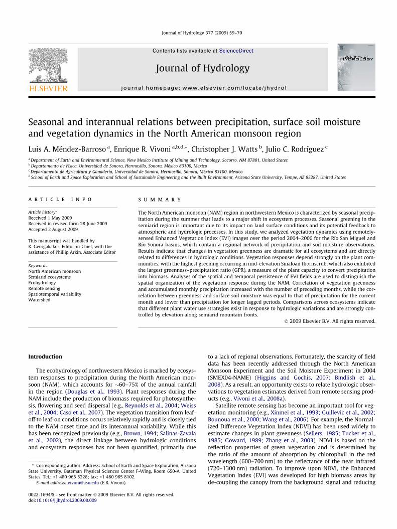
Vegetation metrics can quantify ecosystem responses to precip-itation and surface soil moisture during the NAM. Table 2 presentsthe phenological metrics obtained for each station from 2004 to2006. Overall, the vegetation metrics, in particular the iEVI andDEVI, confirm that 2006 had the most dramatic greening in mostof the stations. In contrast, some stations during 2004 had lowDuration of Greenness and Days to EVImax as well as the smallestiEVI and DEVI. However, other stations showed lower vegetationmetrics in 2005. This indicates that regional rainfall was not homo-geneous and some stations receive more rainfall than others in dif-ferent years.

The metrics also reveal differences and similarities in vegeta-tion productivity among the stations. Stations with common plantcommunities share similar response to summer rainfall. For exam-ple, lower productivity stations are all in Sonoran savanna grass-lands (stations 137, 138 and 139) with low iEVI, DEVI andDuration of Greenness. Similarities are also observed in vegetationmetrics for the Sonoran riparian deciduous woodland sites (sta-tions 135 and 143). For the wet 2006 summer, however, precipita-tion amount and soil water availability lead to certain degrees ofhomogenization in the vegetation response across all ecosystems.For instance, Madrean evergreen woodlands (station 146) andSinaloan thornscrub (station 132) share similar responses in

2006 (iEVI = 4.79 and 4.65 for 2006), despite having different plantcommunities. Differences in vegetation metrics among stations arestronger during drier monsoons. It is interesting to note that theMadrean evergreen woodland and Sinaloan thornscrub appear tohave different strategies to cope with interannual hydrologicchanges. Evergreen woodlands vary their maximum greening(EVImax) in response to increased rainfall amounts, while decidu-ous trees and shrubs vary the growing season productivity (iEVI).These two plant greenup strategies may explain how these ecosys-tems exist at different elevations in the region.

To explore this further, Table 3 presents temporal coefficients ofvariation (CVs) for each vegetation metric computed for the aver-age conditions in each ecosystem across all years. As a result, theCV primarily captures the interannual variations in vegetationmetrics in a particular ecosystem. Ecosystems with high CVs implylarge interannual changes. Sonoran savanna grassland have higherCVs for iEVI, DEVI, indicating strong variations between years.Small CV in iEVI and high CV in DEVI are observed in the Sonorandesert scrub, suggesting this ecosystem varies primarily in the EVIrange from year-to-year. Finally, the vegetation metric with thehighest interannual variation is Days to EVImax, indicating thatthe rate of ecosystem greening is highly influenced by rainfallamounts during the monsoon onset.

Spatial and temporal stability analyses of vegetation dynamics

The ecosystem response to precipitation and soil moisture con-ditions can be discerned through spatial and temporal persistenceof the EVI fields. Regions with low spatial RMSE ds (Fig. 5a, red col-ors) correspond to zones that closely track the spatially-averagedconditions. These areas coincide well with the location of Sinaloan

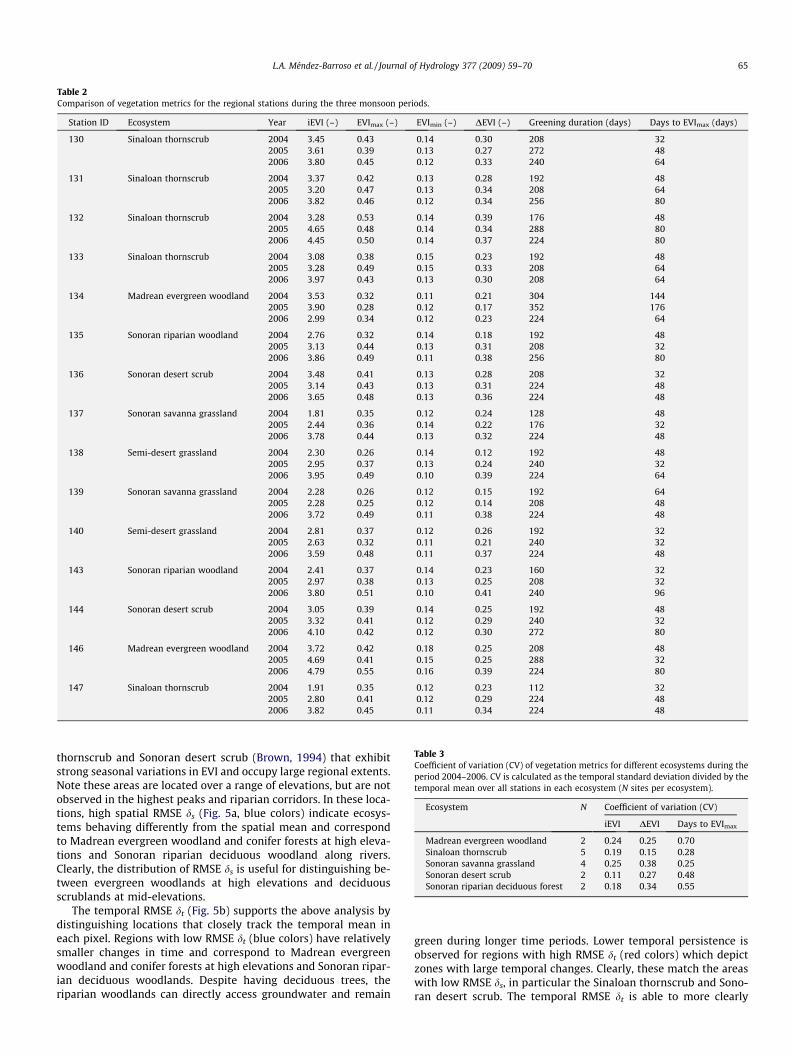
Table 2Comparison of vegetation metrics for the regional stations during the three monsoon periods.

Station ID Ecosystem Year iEVI (–) EVImax (–) EVImin (–) DEVI (–) Greening duration (days) Days to EVImax (days)

130 Sinaloan thornscrub 2004 3.45 0.43 0.14 0.30 208 322005 3.61 0.39 0.13 0.27 272 482006 3.80 0.45 0.12 0.33 240 64

131 Sinaloan thornscrub 2004 3.37 0.42 0.13 0.28 192 482005 3.20 0.47 0.13 0.34 208 642006 3.82 0.46 0.12 0.34 256 80

132 Sinaloan thornscrub 2004 3.28 0.53 0.14 0.39 176 482005 4.65 0.48 0.14 0.34 288 802006 4.45 0.50 0.14 0.37 224 80

133 Sinaloan thornscrub 2004 3.08 0.38 0.15 0.23 192 482005 3.28 0.49 0.15 0.33 208 642006 3.97 0.43 0.13 0.30 208 64

134 Madrean evergreen woodland 2004 3.53 0.32 0.11 0.21 304 1442005 3.90 0.28 0.12 0.17 352 1762006 2.99 0.34 0.12 0.23 224 64

135 Sonoran riparian woodland 2004 2.76 0.32 0.14 0.18 192 482005 3.13 0.44 0.13 0.31 208 322006 3.86 0.49 0.11 0.38 256 80

136 Sonoran desert scrub 2004 3.48 0.41 0.13 0.28 208 322005 3.14 0.43 0.13 0.31 224 482006 3.65 0.48 0.13 0.36 224 48

137 Sonoran savanna grassland 2004 1.81 0.35 0.12 0.24 128 482005 2.44 0.36 0.14 0.22 176 322006 3.78 0.44 0.13 0.32 224 48

138 Semi-desert grassland 2004 2.30 0.26 0.14 0.12 192 482005 2.95 0.37 0.13 0.24 240 322006 3.95 0.49 0.10 0.39 224 64

139 Sonoran savanna grassland 2004 2.28 0.26 0.12 0.15 192 642005 2.28 0.25 0.12 0.14 208 482006 3.72 0.49 0.11 0.38 224 48

140 Semi-desert grassland 2004 2.81 0.37 0.12 0.26 192 322005 2.63 0.32 0.11 0.21 240 322006 3.59 0.48 0.11 0.37 224 48

143 Sonoran riparian woodland 2004 2.41 0.37 0.14 0.23 160 322005 2.97 0.38 0.13 0.25 208 322006 3.80 0.51 0.10 0.41 240 96

144 Sonoran desert scrub 2004 3.05 0.39 0.14 0.25 192 482005 3.32 0.41 0.12 0.29 240 322006 4.10 0.42 0.12 0.30 272 80

146 Madrean evergreen woodland 2004 3.72 0.42 0.18 0.25 208 482005 4.69 0.41 0.15 0.25 288 322006 4.79 0.55 0.16 0.39 224 80

147 Sinaloan thornscrub 2004 1.91 0.35 0.12 0.23 112 322005 2.80 0.41 0.12 0.29 224 482006 3.82 0.45 0.11 0.34 224 48

Table 3Coefficient of variation (CV) of vegetation metrics for different ecosystems during theperiod 2004–2006. CV is calculated as the temporal standard deviation divided by thetemporal mean over all stations in each ecosystem (N sites per ecosystem).

Ecosystem N Coefficient of variation (CV)

iEVI DEVI Days to EVImax

Madrean evergreen woodland 2 0.24 0.25 0.70Sinaloan thornscrub 5 0.19 0.15 0.28Sonoran savanna grassland 4 0.25 0.38 0.25Sonoran desert scrub 2 0.11 0.27 0.48Sonoran riparian deciduous forest 2 0.18 0.34 0.55

L.A. Méndez-Barroso et al. / Journal of Hydrology 377 (2009) 59–70 65

thornscrub and Sonoran desert scrub (Brown, 1994) that exhibitstrong seasonal variations in EVI and occupy large regional extents.Note these areas are located over a range of elevations, but are notobserved in the highest peaks and riparian corridors. In these loca-tions, high spatial RMSE ds (Fig. 5a, blue colors) indicate ecosys-tems behaving differently from the spatial mean and correspondto Madrean evergreen woodland and conifer forests at high eleva-tions and Sonoran riparian deciduous woodland along rivers.Clearly, the distribution of RMSE ds is useful for distinguishing be-tween evergreen woodlands at high elevations and deciduousscrublands at mid-elevations.

The temporal RMSE dt (Fig. 5b) supports the above analysis bydistinguishing locations that closely track the temporal mean ineach pixel. Regions with low RMSE dt (blue colors) have relativelysmaller changes in time and correspond to Madrean evergreenwoodland and conifer forests at high elevations and Sonoran ripar-ian deciduous woodlands. Despite having deciduous trees, theriparian woodlands can directly access groundwater and remain

green during longer time periods. Lower temporal persistence isobserved for regions with high RMSE dt (red colors) which depictzones with large temporal changes. Clearly, these match the areaswith low RMSE ds, in particular the Sinaloan thornscrub and Sono-ran desert scrub. The temporal RMSE dt is able to more clearly

Fig. 5. Temporal and spatial RMSE of the mean relative difference (d) in the Río San Miguel and Río Sonora basins.

Fig. 6. (a) Relation between elevation and temporal mean (closed circles) andtemporal standard deviation of EVI (±1 std as vertical bars). (b) Relation betweenelevation and the spatial and temporal RMSE d.

Precipitation (mm)260 280 300 320 340 360 380 400

iEVI

2.5

3.0

3.5

4.0

4.5

5.0

r2 = 0.7628iEVI = 0.015Rs - 1.449

Fig. 7. Relation between iEVI and seasonal precipitation accumulation for themonsoon season in 2005.

66 L.A. Méndez-Barroso et al. / Journal of Hydrology 377 (2009) 59–70

separate these two ecosystems, with Sinaloan thornscrub furthersouth in the domain and replaced by Sonoran desert scrub at sim-ilar altitudes in the north. In conjunction, the spatial and temporalpersistence maps reveal ecosystem patterns that are not observedthrough simpler metrics such as seasonal EVI changes (Fig. 3). Fur-ther, this analysis extends applications of RMSE d beyond soilmoisture studies (e.g., Jacobs et al., 2004; Vivoni et al., 2008a).

To explore elevation controls, Fig. 6 presents the variation ofEVI, RMSE ds and RMSE dt for a topographic transect in Río San Mig-uel (see A–A0 in Fig. 1). The transect was selected to capture a rangeof elevations (550–1900 m) and span several ecosystems. The tem-poral mean EVI (symbols) increases with elevation, while the tem-poral standard deviation (vertical bars depict ±1 std) typicallydecreases with altitude These variations indicate that the mid-ele-vation Sinaloan thornscrub and Sonoran desert scrub are charac-terized by lower time-averaged greenness, which is more

Fig. 8. Distribution of greenness–precipitation ratio (GPR in mm�1* 100) at the regional stations (note that the region of interest is indicated in the inset by the square

polygon). For reference, the spatial distribution of ecosystems as mapped by INEGI (Instituto Nacional de Estadística, Geografía e Informática) is shown.

L.A. Méndez-Barroso et al. / Journal of Hydrology 377 (2009) 59–70 67

variable in time, as compared to the high elevation Madrean ever-green woodland. The mid-elevation ecosystems exhibit low spatialRMSE ds and high temporal RMSE dt, which indicate areas closelytracking the mean conditions in the region. These elevations corre-spond to Sinaloan thornscrub and Sonoran desert scrub which arehighly responsive to NAM precipitation and occupy large regionalextents. At high elevations, the Madrean evergreen woodland hasa larger spatial RMSE ds and a smaller temporal RMSE dt. This sug-gests that the evergreen species have time-stable conditions thatdo not track the spatially-averaged response. A range of elevations(�600–900 m) simultaneously have small spatial and temporalRMSE d. We interpret this as an elevation band of significant mon-soonal response that dominates the regional greening, as sug-

gested by Vivoni et al. (2007). Clearly, spatial and temporalpersistence reveal variations in vegetation dynamics along topo-graphic transects and can aid in the interpretation of vegetation–elevation relations in semiarid mountain fronts.

Relations between vegetation and hydrologic indices

To explore the relation between vegetation dynamics andhydrologic conditions, we compared iEVI, the greenness–precipita-tion ratio (GPR = (iEVI/Rs) � 100) and the total precipitation (Rs) ateach station for the 2005 monsoon. This particular summer was se-lected due to its limited amounts of missing data, resulting in thedecrease of the number of analyzed stations from 15 to 10. Fig. 7

68 L.A. Méndez-Barroso et al. / Journal of Hydrology 377 (2009) 59–70

presents the linear relation between iEVI and precipitation (Rs).Clearly, as rainfall amounts increase across the regional stations,ecosystem productivity during the summer monsoon increases.While ecophysiological differences are present in the regional eco-systems, seasonal rainfall is a good predictor of biomass produc-tion (iEVI). Results are consistent with other studies, wherehigher vegetation productivity was observed with increasing rain-fall (e.g., Li et al., 2004; Prasad et al., 2005). Further testing of theproposed relation during other summers and for a larger numberof stations may provide an indication of its robustness.

The GPR for summer 2005 is presented in Fig. 8 as a map over-laid on the regional ecosystems. As shown in Table 4, the range inGPR among the stations is from 0.92 (station 144, Sonoran desertscrub) to 1.22 (station 132, Sinaloan thornscrub). The spatial vari-ability in GPR indicates that ecosystems in the southern region ofthe Río San Miguel more efficiently use precipitation for biomassproduction. Interestingly, each of these ecosystems correspondsto the Sinaloan thornscrub (stations 130, 131, 132, 133, 147), sug-gesting that this plant community is well-tuned to utilizing sum-mer rainfall to produce vegetation greening. The response in theSinaloan thornscrub is consistent with seasonal changes in EVIfor 2005 (Fig. 3b) and a high temporal RMSE dt (Fig. 5b). Other re-gional ecosystems, such as Sonoran savanna grassland (stations137, 138, 139) and Sonoran riparian deciduous woodland (stations135, 143), show smaller GPR, suggesting lower rainfall use effi-ciency in grasslands and riparian trees. Lower GPR in riparian sites,despite access to groundwater, is likely due to human impacts in

Fig. 9. Linear correlation coefficients (CCs) between monthly EVI and accumulatedprecipitation and averaged soil moisture over a range of different monthly lags,arranged from current (lag 0) toward longer prior periods (lag 0 + 1 + 2). CCs areshown as averages (symbols) and standard deviations (±1 std as vertical bars) overall stations in 2005.

Table 4Comparison of iEVI, precipitation (mm) and greenness–precipitation ratio (GPR inmm�1

* 100) for the available regional stations during 2005. Greenness–precipitationratio is computed as a function of the iEVI divided by seasonal rainfall (mm) andmultiplied by 100.

Station ID iEVI (–) Precipitation (mm) GPR (mm�1) * 100

130 3.61 330.80 1.09131 3.20 287.50 1.11132 4.65 381.00 1.22133 3.28 327.60 1.00135 3.13 308.10 1.02136 3.14 329.90 0.95143 2.97 290.00 1.02144 3.32 360.00 0.92146 4.69 389.00 1.21147 2.80 279.00 1.00

the areas leading to decreased groundwater levels and to land cov-er changes associated with agriculture.

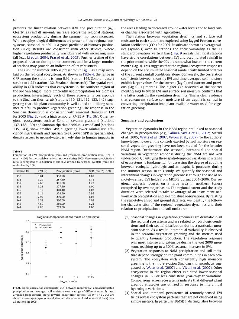
The relation between vegetation dynamics and surface soilmoisture in each station are explored using lagged Pearson corre-lation coefficients (CCs) for 2005. Results are shown as average val-ues (symbols) over all stations and their variability as the ±1standard deviation (vertical bars). Fig. 9 reveals that most stationshave strong correlations between EVI and accumulated rainfall inthe prior months, while the CCs are somewhat lower in the currentmonth (lag 0). This suggests that the regional ecosystem responsesdepend on the accumulated seasonal rainfall, with limited controlsof the current rainfall conditions alone. Conversely, the correlationcoefficients between monthly EVI and time-averaged soil moistureexhibit larger values for the current (lag 0) and current and previ-ous (lag 0 + 1) months. The higher CCs observed at the shortermonthly lags between EVI and surface soil moisture confirms thatthe latter controls the vegetation dynamics. This is clear evidencethat concurrent surface soil moisture (5-cm depth) is central inconverting precipitation into plant-available water used for vege-tation greening.

Summary and conclusions

Vegetation dynamics in the NAM region are linked to seasonalchanges in precipitation (e.g., Salinas-Zavala et al., 2002; Matsuiet al., 2005; Watts et al., 2007; Vivoni et al., 2007). To the authors’knowledge, however, the controls exerted by soil moisture on sea-sonal vegetation greening have not been studied for the broaderNAM region. Furthermore, the seasonal, interannual and spatialvariations in vegetation response during the NAM are not wellunderstood. Quantifying these spatiotemporal variations in a rangeof ecosystems is fundamental for assessing the degree of couplingbetween ecologic, hydrologic and atmospheric processes duringthe summer season. In this study, we quantify the seasonal andinterannual changes in vegetation greenness through the use of re-motely-sensed EVI fields from MODIS during 2004–2006. Our re-gional analysis focuses on a large area in northern Sonoracomprised by two major basins. The regional extent and the studyduration were selected to take advantage of an instrument net-work with precipitation and soil moisture observations. By relatingthe remotely-sensed and ground data sets, we identify the follow-ing characteristics of the regional vegetation dynamics and theirrelation to precipitation and soil moisture:

(1) Seasonal changes in vegetation greenness are dramatic in allthe regional ecosystems and are related to hydrologic condi-tions and their spatial distribution during a particular mon-soon season. As a result, interannual variability is observedin the seasonal vegetation greening and the metrics usedto quantify biomass production. The vegetation responsewas most intense and extensive during the wet 2006 mon-soon, reaching up to a 300% seasonal increase in EVI.

(2) Vegetation responses to NAM precipitation and soil mois-ture depend strongly on the plant communities in each eco-system. The ecosystem with consistently high monsoongreening is the mid-elevation Sinaloan thornscrub, as sug-gested by Watts et al. (2007) and Vivoni et al. (2007). Otherecosystems in the region either exhibited lower seasonalchanges in EVI or less consistent year-to-year variations.Comparisons across ecosystems indicate that different plantgreenup strategies are utilized in response to interannualhydrologic variations.

(3) Spatial and temporal persistence of remotely-sensed EVIfields reveal ecosystem patterns that are not observed usingsimple metrics. In particular, RMSE ds distinguishes between

L.A. Méndez-Barroso et al. / Journal of Hydrology 377 (2009) 59–70 69

evergreen woodlands at high elevations and deciduousscrublands at mid-elevations, while the temporal RMSE dt

can more clearly separate different ecosystems at similarelevations. Analysis along a topographic transects indicatethat elevation controls vegetation dynamics and serves toorganize ecosystems into elevation bands, with high mon-soonal response at mid-elevations.

(4) Accumulated seasonal precipitation is a strong indicator ofgreenness intensity across the regional ecosystems, withSinaloan thornscrub exhibiting the highest greenness–pre-cipitation ratio (GPR). During the study period, differencesbetween ecosystem responses were minimized during thewet 2006 monsoon and maximized during drier monsoons,in contrast to the common rainfall use efficiency found byHuxman et al. (2004) during drought. Additional studiesare required to quantify greenness–precipitation ratio inwet and dry periods in the region.

(5) Lagged correlation analysis indicates a strong degree of cou-pling between vegetation greening and hydrologic condi-tions at each regional station. Concurrent correlations formonthly EVI with surface soil moisture and precipitationare comparable, while lagged correlations are more signifi-cant for the accumulated precipitation. This suggests thatsoil moisture plays an important and immediate role in veg-etation response inside the NAM region.

The observational analysis and interpretations conducted hereshow the importance of combining satellite remote sensing andground networks for monitoring ecosystem dynamics and theirlink to precipitation and surface soil moisture conditions. Clearly,the study duration is a limitation in our interannual analysis, pri-marily due to the recent establishment of the regional network.Nevertheless, significant interannual variability in vegetationdynamics were observed in the three monsoon seasons, includingone of the driest (2005) and wettest (2006) seasons in the period1985–2006 (e.g., Dominguez et al., 2008). Additional analysis isdesirable either by extending the work as new datasets becomeavailable or by performing retrospective analysis with satellitedata (though ground data would be limited) over the current ba-sins or the broader NAM region. In particular, expanding this anal-ysis to include relations with root zone soil moisture observations(top 1-m, where available) would be desirable. Another focusshould be on identifying the long-term interannual vegetation var-iability and its relation to precipitation, which itself exhibitsyear-to-year changes due to several factors, including sea surfacetemperature (Castro et al., 2007) and continental snow and soilmoisture anomalies (Gutzler, 2000; Zhu et al., 2007). If the link be-tween interannual precipitation variations and vegetation responsecan be identified, enhanced predictability of the land surfaceresponse to the North American monsoon would be possible.

Acknowledgements

We acknowledge funding from the National Science FoundationIRES program (Grant OISE 0809946), the NOAA Climate ProgramOffice (Grant CPPA GC07-019), the US Fulbright Program to E.R.Vand the Consejo Nacional de Ciencias y Tecnología (CONACYT) fel-lowship to the first author. We also thank two reviewers whosesuggestions helped to improve earlier versions of the manuscript.

References

Bindlish, R., Jackson, T.J., Gasiewski, A.J., Stankov, B., Cosh, M.H., Mladenova, I.,Vivoni, E.R., Lakshmi, V., Watts, C.J., Keefer, T., 2008. Aircraft-based soil moistureretrievals in mixed vegetation and topographic conditions. Remote Sensing ofEnvironment 112 (2), 375–390.

Bounoua, L., Collatz, C.J., Los, S.O., Sellers, P.J., Dazlich, D.A., Tucker, C.J., Randall, D.A.,2000. Sensitivity of climate to NDVI changes. Journal of Climate 13, 2277–2292.

Breshears, D.D., Barnes, F.J., 1999. Interrelationships between plant functional typesand soil moisture heterogeneity for semiarid landscapes within the grassland/forest continuum: a unified conceptual model. Landscape Ecology 14 (5), 465–478.

Brown, E.D., 1994. Biotic Communities: Southwestern United States andNorthwestern Mexico. University of Utah Press. 342 pp.

Calvet, C., Noilhan, J., Bessemoulin, P., 1998. Retrieving the root-zone soil moisturefrom surface soil moisture or temperature estimates: a feasibility study basedon field measurements. Journal of Applied Meteorology 37, 371–386.

Caso, M., Gonzalez-Abraham, C., Ezcurra, E., 2007. Divergent ecological effects ofoceanographic anomalies on terrestrial ecosystems of the Mexican Pacific coast.Proceedings of the National Academy of Sciences 104 (25), 10530–10535.

Casper, B.B., Schenk, H.J., Jackson, R.B., 2003. Defining plant’s belowground zone ofinfluence. Ecology 84, 2313–2321.

Castro, C.L., Pielke, R.A., Adegoke, J.O., Schubert, S.D., Pegion, P.J., 2007. Investigationof the summer climate of the contiguous United States and Mexico using theregional atmospheric modeling system (RAMS). Part II: model climatevariability. Journal of Climate 20 (15), 3866–3887.

Chamaille-Jammes, S., Fritz, H., Murindagomo, F., 2006. Spatial patterns of theNDVI–rainfall relationship at the seasonal and inter-annual time scales in anAfrican savanna. International Journal of Remote Sensing 27 (23), 5185–5200.

Chen, M., Xie, P., Janowiak, J.E., Arkin, P.A., 2002. Global land precipitation: a 50-yrmonthly analysis based on gauge observations. Journal of Hydrometeorology 3,249–266.

Coblentz, D.D., Riitters, K.H., 2004. Topographic controls on the regional-scalebiodiversity of the south-western USA. Journal of Biogeography 31 (7), 1125–1138.

Davenport, M.L., Nicholson, S.E., 1993. On the relationship between rainfall and theNormalized Difference Vegetation Index for diverse vegetation types in EastAfrica. International Journal of Remote Sensing 14 (12), 2369–2389.

De Lannoy, J.M., Verhoest, N.C., Houser, P.R., Gish, T.J., Van Meirvenne, M., 2006.Spatial and temporal characteristics of soil moisture in an intensivelymonitored agricultural field (OPE3). Journal of Hydrology 331 (3–4), 719–730.

Dominguez, F., Kumar, P., Vivoni, E.R., 2008. Precipitation recycling variability andecoclimatological stability – a study using NARR data. Part II: North AmericanMonsoon Region. Journal of Climate 21, 5187–5203.

Douglas, M.W., Maddox, R.A., Howard, K., Reyes, S., 1993. The Mexican monsoon.Journal of Climate 6 (8), 1665–1677.

Famiglietti, J.S., Rudnicki, W., Rodell, M., 1998. Variability in surface moisturecontent along a hillslope transect: Rattlesnake Hill, Texas. Journal of Hydrology210 (1–4), 259–281.

Gochis, D.J., Watts, C.J., Garatuza-Payan, J., Rodríguez, J.C., 2007. Spatial andtemporal patterns of precipitation intensity as observed by the NAME EventRain gauge Network from 2002 to 2004. Journal of Climate 20 (9), 1734–1750.

Goward, N.S., 1989. Satellite bioclimatology. Journal of Climate 2 (7), 710–720.Guillevic, P., Koster, R.D., Suarez, M.J., Bounoua, L., Collatz, G.J., Los, S.O., Mahanama,

S.P.P., 2002. Influence of the interannual variability of vegetation on the surfaceenergy balance: a global sensitivity study. Journal of Hydrometeorology 3 (6),617–629.

Gutzler, D.S., 2000. Covariability of spring snowpack and summer rainfall across thesouthwest United States. Journal of Climate 13 (22), 4018–4027.

Higgins, R.W., Gochis, D.J., 2007. Synthesis of results from the North AmericanMonsoon Experiment (NAME) process study. Journal of Climate 20 (9), 1601–1607.

Huete, A.R., Liu, H.Q., Batchily, K., vanLeeuwen, W., 1997. A comparison ofvegetation indices global set of TM images for EOS–MODIS. Remote Sensingof Environment 59 (3), 440–451.

Huete, A.R., Didan, K., Miura, T., Rodriguez, E.P., Gao, X., Ferreira, L.G., 2002.Overview of the radiometric and biophysical performance of the MODISvegetation indices. Remote Sensing of Environment 83 (1–2), 195–213.

Huxman, T.E., Smith, M.D., Fay, P.A., Knapp, A.K., Shaw, M.R., Loik, M.E., Smith, S.D.,Tissue, D.T., Zak, J.C., Weltzin, J.F., Pockman, W.T., Sala, O.E., Haddad, B.M., Harte,J., Koch, G.W., Schwinning, S., Small, E.E., Williams, D.G., 2004. Convergenceacross biomes to a common rain-use efficiency. Nature 429, 651–654.

Jacobs, M.J., Mohanty, P.B., Hsu, C.E., Miller, D., 2004. SMEX02: field scale variability,time stability and similarity of soil moisture. Remote Sensing of Environment92 (4), 436–446.

Li, D., Lewis, J., Rowland, J., Tappan, G., Tieszen, L.L., 2004. Evaluation of landperformance in Senegal using multi-temporal NDVI and rainfall series. Journalof Arid Environments 59 (3), 463–480.

Lloyd, D., 1990. A phenological classification of terrestrial vegetation cover usingshortwave vegetation index imagery. International Journal of Remote Sensing11, 2269–2279.

Loik, M.E., Breshears, D.D., Lauenroth, W.K., Belnap, J., 2004. A multi-scaleperspective of water pulses in dryland ecosystems: climatology andecohydrology of the western USA. Oecologia 141 (2), 269–281.

Mahmood, R., Hubbard, K.G., 2007. Relationship between soil moisture of nearsurface and multiple depths of the root zone under heterogeneous land usesand varying hydroclimatic conditions. Hydrological Processes 21 (25), 3449–3462.

Martinez, C., Hancock, G.R., Kalma, J.D., Wells, T., 2008. Spatio-temporal distributionof near-surface and root zone soil moisture at the catchment scale. HydrologicalProcesses 22 (14), 2699–2714.

70 L.A. Méndez-Barroso et al. / Journal of Hydrology 377 (2009) 59–70

Méndez-Barroso, L.A., 2009. Changes in Hydrological Conditions and Surface Fluxesdue to Seasonal Vegetation Greening in North American Monsoon Region. M.S.Thesis. New Mexico Institute of Mining and Technology, Socorro, NM, 158 pp.

Mohanty, B.P., Skaggs, T.H., Famiglietti, J.S., 2000. Analysis and mapping of field-scale soil moisture variability using high-resolution, ground-based data duringthe Southern Great Plains 1997 (SGP1997) hydrology experiment. WaterResources Research 36 (4), 1023–1031.

Prasad, V.K., Anuradha, E., Badarinath, K.V.S., 2005. Climatic controls ofvegetation vigor in four contrasting forest types of India. Evaluation fromnational oceanic and atmospheric administration’s advanced very highresolution radiometer datasets (1990–2000). International Journal ofBiometeorology 50 (1), 6–16.

Reed, B.C., Brown, J.F., VanderZee, D., Loveland, T.R., Merchant, J.W., Ohlen, D.O.,1994. Measuring phenological variability from satellite imagery. Journal ofVegetation Science 5 (5), 703–714.

Reynolds, J.F., Kemp, P.R., Ogle, K., Fernadez, R.J., 2004. Modifying the ‘pulse-reserve’paradigm for deserts of North America: precipitation pulses, soil water, andplant responses. Oecologia 141 (2), 194–210.

Salinas-Zavala, C.A., Douglas, A.V., Diaz, H.F., 2002. Interannual variability of NDVIin northwest Mexico: associated climatic mechanisms and ecologicalimplications. Remote Sensing of Environment 82 (2–3), 417–430.

Schenk, H.J., Jackson, R.B., 2002. The global biogeography of roots. EcologicalMonographs 72 (3), 311–328.

Sellers, P.J., 1985. Canopy reflectance, photosynthesis and transpiration.International Journal of Remote Sensing 6, 1335–1372.

Seyfried, M.S., Murdock, M., 2004. Measurement of soil water content with a50 MHz soil dielectric sensor. Soil Science Society of America Journal 68 (2),394–403.

Seyfried, M.S., Wilcox, B., 2006. Soil water storage and rooting depth: keyfactors controlling recharge on rangelands. Hydrological Processes 20,3261–3275.

Tucker, C.J., Townsend, J.R.G., Goff, T.E., 1985. African land cover classification usingsatellite data. Science 227, 369–375.

Vachaud, G., Passerat De Silans, A., Balanis, P., Vauclin, M., 1985. Temporal stabilityof spatially measured soil water probability density function. Journal of the SoilSociety of America 49, 822–828.

Vivoni, E.R., Gutiérrez-Jurado, H.A., Aragón, C.A., Méndez-Barroso, L.A., Rinehart, A.J.,Wyckoff, R.L., Rodríguez, J.C., Watts, C.J., Bolten, J.D., Lakshmi, V., Jackson, T.J.,2007. Variation of hydrometeorological conditions along a topographic transectin northwestern Mexico during the North American monsoon. Journal ofClimate 20 (9), 1792–1809.

Vivoni, E.R., Gebremichael, M., Watts, J.C., Bindlish, R., Jackson, T.J., 2008a.Comparison of ground-based and remotely-sensed surface soil moistureestimates over complex terrain during SMEX04. Remote Sensing ofEnvironment 112 (2), 314–325.

Vivoni, E.R., Moreno, H.A., Mascaro, G., Rodriguez, J.C., Watts, C.J., Garatuza-Payan, J.,Scott, R.L., 2008b. Observed relation between evapotranspiration and soilmoisture in the North American Monsoon region. Geophysical Research Letters35, L22403. doi:10.1029/2008GL036001.

Wang, J., Rich, P.M., Price, K.P., 2003. Temporal responses of NDVI to precipitationand temperature in the central Great Plains, USA. International Journal ofRemote Sensing 24 (11), 2345–2364.

Wang, W., Anderson, T.B., Phillips, N., Kaufman, K.R., Potter, C., Myneni, B.R., 2006.Feedbacks of vegetation on summertime climate variability over the NorthAmerican Grasslands. Part I: statistical analysis. Earth Interactions 10 (17), 1–27.

Watts, C.J., Scott, R.L., Garatuza-Payan, J., Rodriguez, J.C., Prueger, J.H., Kustas, W.P.,Douglas, M., 2007. Changes in vegetation condition and surface fluxes duringNAME 2004. Journal of Climate 20 (9), 1810–1820.

Weiss, J.L., Gutzler, D.S., Coonrod, J.E.A., Dahm, C.N., 2004. Seasonal and inter-annualrelations between vegetation and climate in central New Mexico, USA. Journalof Arid Environments 57 (4), 507–534.

Xinmei, H., Lyons, T.J., Smith, R.C.G., Hacker, J.M., Schwerdtfeger, P., 1993.Estimation of surface energy balance from radiance surface temperature andNOAA–AVHRR sensor reflectances over agricultural and native vegetation.Journal of Applied Meteorology 32 (8), 1441–1449.

Zhang, X., Friedl, M.A., Schaaf, C.B., Strahler, A.H., Hodges, J.C.F., Gao, F., Reed, B.C.,Huete, A., 2003. Monitoring vegetation phenology using MODIS. RemoteSensing of Environment 84 (3), 471–475.

Zhu, C.M., Cavazos, T., Lettenmaier, D.P., 2007. Role of antecedent land surfaceconditions in warm season precipitation over northwestern Mexico. Journal ofClimate 20 (9), 1774–1791.