Experimental limit on the decay W+/--->pi+/-gamma at the cern proton-antiproton collider
Upload
khangminh22Category
view
0download
0
Search for double beta decay of 82Sewith the NEMO-3 detector anddevelopment of apparatus for
low-level radon measurements for theSuperNEMO experiment
James MottUniversity College London
Submitted to University College London in fulfilmentof the requirements for the award of the
degree of Doctor of Philosophy
September 25th, 2013
1

Declaration
I, James Mott, confirm that the work presented in this thesis is my own.Where information has been derived from other sources, I confirm thatthis has been indicated in the thesis.
James Mott
2
Abstract
The 2νββ half-life of 82Se has been measured as T 2ν1/2 = (9.93±
0.14(stat)± 0.72(syst))×1019 yr using a 932 g sample measured fora total of 5.25 years in the NEMO-3 detector. The correspondingnuclear matrix element is found to be |M2ν | = 0.0484± 0.0018. Inaddition, a search for 0νββ in the same isotope has been conductedand no evidence for a signal has been observed. The resulting half-life limit of T 0ν
1/2 > 2.18× 10²³ yr (90% CL) for the neutrino massmechanism corresponds to an effective Majorana neutrino mass of〈mββ〉 < 1.0−2.8 eV (90% CL). Furthermore, constraints on leptonnumber violating parameters for other 0νββ mechanisms, such asright-handed current and Majoron emission modes, have been set.
SuperNEMO is the successor to NEMO-3 and will be one of thenext generation of 0νββ experiments. It aims to measure 82Se withan half-life sensitivity of 1026 yr corresponding to 〈mββ〉 < 50 −100 meV. Radon can be one of the most problematic backgroundsto any 0νββ search due to the high Qββ value of its daughterisotope, 214Bi. In order to achieve the target sensitivity, the radonconcentration inside the tracking volume of SuperNEMO must beless than 150 µBq/m3. This low level of radon is not measurablewith standard radon detectors, so a “radon concentration line” hasbeen designed and developed. This apparatus has a sensitivityto radon concentration in the SuperNEMO tracker at the levelof 40 µBq/m3, and has performed the first measurements of theradon level inside a sub-section of SuperNEMO, which is underconstruction. It has also been used to measure the radon contentof nitrogen and helium gas cylinders, which are found to be in theranges 70− 120 µBq/m3 and 370− 960 µBq/m3, respectively.
3
Acknowledgements
First and foremost, I would like to express my extreme gratitude to my supervisor,Ruben Saakyan, without whose guidance this thesis would not have been possible.As annoying as it may be, always knowing the answer to any question I might pose,no matter how obscure, is certainly a very useful trait to have as a supervisor.
In addition, my thanks go to Stefano Torre, David Waters and Adam Davison formany constructive conversations on analysis techniques and software issues - I amsure I would have spent a lot more time groping in the dark without this guidinginfluence. In the same vein, collaborative work with fellow NEMO-3 students atother institutions, in particular Sophie Blondel and Summer Blot, was also pivotalin producing a coherent analysis.
Away from a computer screen and back in the real world, I am indebted to DerekAttree and Brian Anderson for their technical expertise and for their patience asI attempted to develop basic engineering skills. Without them, none of the real‘screw-driver’ physics in this thesis would have been remotely functional. I am alsotruly appreciative of the camaraderie shared with my fellow lab rats, Cristóvão Vilelaand Xin Ran Liu.
Away from phyics, the love and support from my family has been a comfortingpresence, not just for this PhD but throughout my life. For this, I feely greatlyblessed. Finally, special thanks go to Clara for her unflinching support throughoutthis whole process and for ensuring that my funding lasted as long as necessary withsuch rigorous budgeting.
4
Contents
List of Figures 11
List of Tables 16
1. Introduction 181.1. NEMO-3 . . . . . . . . . . . . . . . . . . . . . . . . . . . . . . . . . . 191.2. SuperNEMO . . . . . . . . . . . . . . . . . . . . . . . . . . . . . . . . 211.3. Author’s Contributions . . . . . . . . . . . . . . . . . . . . . . . . . . 22
1.3.1. NEMO-3 Contributions . . . . . . . . . . . . . . . . . . . . . . 221.3.2. SuperNEMO Contributions . . . . . . . . . . . . . . . . . . . 23
2. Neutrino Phenomenology 252.1. Standard Model Neutrinos . . . . . . . . . . . . . . . . . . . . . . . . 25
2.1.1. Discovery of the Neutrino . . . . . . . . . . . . . . . . . . . . 252.1.2. Neutrino Interactions . . . . . . . . . . . . . . . . . . . . . . . 252.1.3. Neutrino Flavours . . . . . . . . . . . . . . . . . . . . . . . . . 27
2.2. Neutrino Mixing and Oscillations . . . . . . . . . . . . . . . . . . . . 282.2.1. Oscillation Phenomenology . . . . . . . . . . . . . . . . . . . . 292.2.2. Oscillations in Matter . . . . . . . . . . . . . . . . . . . . . . 302.2.3. Measurement of Oscillation Parameters . . . . . . . . . . . . . 31
2.3. Neutrino Mass . . . . . . . . . . . . . . . . . . . . . . . . . . . . . . . 322.3.1. Dirac Mass . . . . . . . . . . . . . . . . . . . . . . . . . . . . 322.3.2. Majorana Mass . . . . . . . . . . . . . . . . . . . . . . . . . . 332.3.3. See-saw Mechanism . . . . . . . . . . . . . . . . . . . . . . . . 34
2.4. Experimental Constraints on Neutrino Mass . . . . . . . . . . . . . . 362.4.1. Tritium Decay . . . . . . . . . . . . . . . . . . . . . . . . . . . 362.4.2. Cosmology . . . . . . . . . . . . . . . . . . . . . . . . . . . . . 372.4.3. Neutrinoless double beta decay (0νββ) . . . . . . . . . . . . . 38
5
Contents 6
2.4.4. Oscillations . . . . . . . . . . . . . . . . . . . . . . . . . . . . 392.5. Outstanding questions . . . . . . . . . . . . . . . . . . . . . . . . . . 39
2.5.1. Number of neutrinos . . . . . . . . . . . . . . . . . . . . . . . 392.5.2. Absolute Mass and Mass Hierarchy . . . . . . . . . . . . . . . 402.5.3. CP Violation . . . . . . . . . . . . . . . . . . . . . . . . . . . 412.5.4. Nature of the neutrino . . . . . . . . . . . . . . . . . . . . . . 42
3. Double Beta Decay 433.1. Beta Decay . . . . . . . . . . . . . . . . . . . . . . . . . . . . . . . . 43
3.1.1. Allowed and Forbidden Decays . . . . . . . . . . . . . . . . . 443.2. Two Neutrino Double Beta Decay . . . . . . . . . . . . . . . . . . . . 453.3. Neutrinoless Double Beta Decay . . . . . . . . . . . . . . . . . . . . . 46
3.3.1. Neutrino Mass Mechanism . . . . . . . . . . . . . . . . . . . . 483.3.2. Right-handed Current . . . . . . . . . . . . . . . . . . . . . . 493.3.3. Majoron Emission . . . . . . . . . . . . . . . . . . . . . . . . . 51
3.4. Nuclear Matrix Elements . . . . . . . . . . . . . . . . . . . . . . . . . 543.4.1. Interacting Shell Model . . . . . . . . . . . . . . . . . . . . . . 553.4.2. Quasiparticle Random Phase Approximation . . . . . . . . . . 563.4.3. Interacting Boson Model . . . . . . . . . . . . . . . . . . . . . 563.4.4. Projected Hartree-Fock-Bogoluibov Method . . . . . . . . . . 563.4.5. Energy Density Functional Method . . . . . . . . . . . . . . . 573.4.6. Comparison of different NME calculations . . . . . . . . . . . 57
4. Double Beta Decay Experiments 594.1. Detector Design Considerations . . . . . . . . . . . . . . . . . . . . . 59
4.1.1. Maximising Signal . . . . . . . . . . . . . . . . . . . . . . . . 604.1.2. Minimising Background . . . . . . . . . . . . . . . . . . . . . 62
4.2. Detector Technologies . . . . . . . . . . . . . . . . . . . . . . . . . . . 634.2.1. Semiconductor Experiments . . . . . . . . . . . . . . . . . . . 634.2.2. Scintillation Experiments . . . . . . . . . . . . . . . . . . . . . 674.2.3. Bolometer Experiments . . . . . . . . . . . . . . . . . . . . . . 704.2.4. Time Projection Chamber Experiments . . . . . . . . . . . . . 714.2.5. Tracker-Calorimeter Experiments . . . . . . . . . . . . . . . . 73
4.3. Double Beta Decay Measurements . . . . . . . . . . . . . . . . . . . . 744.3.1. 2νββ Measurements . . . . . . . . . . . . . . . . . . . . . . . 744.3.2. 0νββ Limits . . . . . . . . . . . . . . . . . . . . . . . . . . . . 74

Contents 7
4.3.3. Future Measurement Prospects . . . . . . . . . . . . . . . . . 77
I. ββ-decay of 82Se with NEMO-3 79
5. NEMO-3 Detector 805.1. Source Foils . . . . . . . . . . . . . . . . . . . . . . . . . . . . . . . . 81
5.1.1. 82Se Source Foils . . . . . . . . . . . . . . . . . . . . . . . . . 835.2. Tracker . . . . . . . . . . . . . . . . . . . . . . . . . . . . . . . . . . . 865.3. Calorimeter . . . . . . . . . . . . . . . . . . . . . . . . . . . . . . . . 885.4. Electronics, DAQ and Trigger . . . . . . . . . . . . . . . . . . . . . . 89
5.4.1. Calorimeter Electronics . . . . . . . . . . . . . . . . . . . . . . 905.4.2. Tracker Electronics . . . . . . . . . . . . . . . . . . . . . . . . 905.4.3. Trigger System . . . . . . . . . . . . . . . . . . . . . . . . . . 91
5.5. Energy and Time Calibration . . . . . . . . . . . . . . . . . . . . . . 925.5.1. Radioactive Sources . . . . . . . . . . . . . . . . . . . . . . . . 925.5.2. Laser Survey . . . . . . . . . . . . . . . . . . . . . . . . . . . 93
5.6. Magnetic Coil and Passive Shielding . . . . . . . . . . . . . . . . . . 945.6.1. Magnetic Coil . . . . . . . . . . . . . . . . . . . . . . . . . . . 945.6.2. Mount Fréjus . . . . . . . . . . . . . . . . . . . . . . . . . . . 945.6.3. Iron Shield . . . . . . . . . . . . . . . . . . . . . . . . . . . . . 955.6.4. Neutron Shielding . . . . . . . . . . . . . . . . . . . . . . . . . 95
5.7. Anti-radon facility . . . . . . . . . . . . . . . . . . . . . . . . . . . . 95
6. General Analysis Techniques 976.1. Monte Carlo Simulation . . . . . . . . . . . . . . . . . . . . . . . . . 976.2. Reconstruction of Events . . . . . . . . . . . . . . . . . . . . . . . . . 986.3. Particle Identification . . . . . . . . . . . . . . . . . . . . . . . . . . . 98
6.3.1. Electron Identification . . . . . . . . . . . . . . . . . . . . . . 986.3.2. Gamma Identification . . . . . . . . . . . . . . . . . . . . . . 1006.3.3. Alpha Identification . . . . . . . . . . . . . . . . . . . . . . . . 101
6.4. Time of Flight Information . . . . . . . . . . . . . . . . . . . . . . . . 1026.4.1. Internal Probability . . . . . . . . . . . . . . . . . . . . . . . . 1036.4.2. External Probability . . . . . . . . . . . . . . . . . . . . . . . 105
6.5. Analysis Data Set . . . . . . . . . . . . . . . . . . . . . . . . . . . . . 106
Contents 8
6.6. Statistical Analysis . . . . . . . . . . . . . . . . . . . . . . . . . . . . 1076.6.1. Fitting MC Distributions to Data . . . . . . . . . . . . . . . . 1076.6.2. Extracting Limits on Signal Strength . . . . . . . . . . . . . . 109
6.7. Half-life Calculation . . . . . . . . . . . . . . . . . . . . . . . . . . . . 111
7. Estimation of Backgrounds for the 82Se Source Foils 1127.1. Sources of NEMO-3 Background . . . . . . . . . . . . . . . . . . . . . 1137.2. NEMO-3 Background Classification . . . . . . . . . . . . . . . . . . . 117
7.2.1. Internal Backgrounds . . . . . . . . . . . . . . . . . . . . . . . 1177.2.2. External Backgrounds . . . . . . . . . . . . . . . . . . . . . . 1197.2.3. Radon Backgrounds . . . . . . . . . . . . . . . . . . . . . . . 122
7.3. Channels for Background Measurements . . . . . . . . . . . . . . . . 1247.3.1. General Quality Criteria . . . . . . . . . . . . . . . . . . . . . 1257.3.2. Hot Spot Search . . . . . . . . . . . . . . . . . . . . . . . . . 1257.3.3. 1e1α Channel . . . . . . . . . . . . . . . . . . . . . . . . . . . 1287.3.4. 1e2γ Channel . . . . . . . . . . . . . . . . . . . . . . . . . . . 1297.3.5. 1e1γ Channel . . . . . . . . . . . . . . . . . . . . . . . . . . . 1307.3.6. 1e Channel . . . . . . . . . . . . . . . . . . . . . . . . . . . . 131
7.4. Results of Background Measurements . . . . . . . . . . . . . . . . . . 1327.4.1. Fitting Procedure . . . . . . . . . . . . . . . . . . . . . . . . . 1327.4.2. Activity Estimations . . . . . . . . . . . . . . . . . . . . . . . 1357.4.3. Control Distributions . . . . . . . . . . . . . . . . . . . . . . . 144
8. Double Beta Decay Results for 82Se 1488.1. Optimisation of 2νββ Cuts . . . . . . . . . . . . . . . . . . . . . . . . 149
8.1.1. Starting Point for Optimisation . . . . . . . . . . . . . . . . . 1498.1.2. Optimisation Procedure . . . . . . . . . . . . . . . . . . . . . 1528.1.3. Optimisation Results . . . . . . . . . . . . . . . . . . . . . . . 154
8.2. 2νββ Results . . . . . . . . . . . . . . . . . . . . . . . . . . . . . . . 1598.2.1. Re-measurement of Background Activities . . . . . . . . . . . 1598.2.2. 2νββ Distributions . . . . . . . . . . . . . . . . . . . . . . . . 1638.2.3. 2νββ systematics . . . . . . . . . . . . . . . . . . . . . . . . . 1678.2.4. 2νββ Half-life Measurement . . . . . . . . . . . . . . . . . . . 170
8.3. Optimisation of 0νββ Cuts . . . . . . . . . . . . . . . . . . . . . . . . 1718.4. 0νββ Results . . . . . . . . . . . . . . . . . . . . . . . . . . . . . . . 176
8.4.1. Mass Mechanism . . . . . . . . . . . . . . . . . . . . . . . . . 176
Contents 9
8.4.2. Right-handed Current . . . . . . . . . . . . . . . . . . . . . . 1788.4.3. Majoron Emission . . . . . . . . . . . . . . . . . . . . . . . . . 181
II. Radon Research and Development for SuperNEMO 184
9. The SuperNEMO Experiment 1859.1. SuperNEMO Baseline Design . . . . . . . . . . . . . . . . . . . . . . 1859.2. Research and Development . . . . . . . . . . . . . . . . . . . . . . . . 1879.3. Timescale and Sensitivity . . . . . . . . . . . . . . . . . . . . . . . . 189
10.Radon and SuperNEMO 19210.1. Properties of Radon . . . . . . . . . . . . . . . . . . . . . . . . . . . . 19210.2. Radon as a SuperNEMO Background . . . . . . . . . . . . . . . . . . 19410.3. Radon Suppression with Gas Flow . . . . . . . . . . . . . . . . . . . . 19410.4. 222Rn Decay Chain to 214Po . . . . . . . . . . . . . . . . . . . . . . . 197
10.4.1. 222Rn Activity . . . . . . . . . . . . . . . . . . . . . . . . . . . 19910.4.2. 218Po Activity . . . . . . . . . . . . . . . . . . . . . . . . . . . 20010.4.3. 214Pb Activity . . . . . . . . . . . . . . . . . . . . . . . . . . . 20010.4.4. 214Bi Activity . . . . . . . . . . . . . . . . . . . . . . . . . . . 20210.4.5. 214Po Activity . . . . . . . . . . . . . . . . . . . . . . . . . . . 20210.4.6. Decay chain activities . . . . . . . . . . . . . . . . . . . . . . . 203
11.Electrostatic Detector and Radon Concentration Line 20411.1. Electrostatic Detector . . . . . . . . . . . . . . . . . . . . . . . . . . 205
11.1.1. Detector Signal . . . . . . . . . . . . . . . . . . . . . . . . . . 20711.1.2. Detector Efficiency Calibration . . . . . . . . . . . . . . . . . 21111.1.3. Detector Background Measurement . . . . . . . . . . . . . . . 214
11.2. Radon Concentration Line (RnCL) . . . . . . . . . . . . . . . . . . . 21511.2.1. Design and Construction . . . . . . . . . . . . . . . . . . . . . 21611.2.2. Trapping Efficiency . . . . . . . . . . . . . . . . . . . . . . . . 21811.2.3. Trap Background . . . . . . . . . . . . . . . . . . . . . . . . . 223
12.Radon Concentration Line Sensitivity Estimates 22512.1. Minimum Detectable Activity . . . . . . . . . . . . . . . . . . . . . . 225
12.1.1. Normal Approximation . . . . . . . . . . . . . . . . . . . . . . 22712.2. Electrostatic Detector Sensitivity . . . . . . . . . . . . . . . . . . . . 228
Contents 10
12.3. Uniform Gas Measurement . . . . . . . . . . . . . . . . . . . . . . . . 23112.4. C-Section Measurement . . . . . . . . . . . . . . . . . . . . . . . . . 232
13.Low-level Radon Measurements 23613.1. Gas System . . . . . . . . . . . . . . . . . . . . . . . . . . . . . . . . 23613.2. Gas Cylinders . . . . . . . . . . . . . . . . . . . . . . . . . . . . . . . 238
13.2.1. Modelling Cylinder Activity . . . . . . . . . . . . . . . . . . . 23813.2.2. Measuring Full Cylinders . . . . . . . . . . . . . . . . . . . . . 24013.2.3. Measuring Used Cylinders . . . . . . . . . . . . . . . . . . . . 242
13.3. C-section . . . . . . . . . . . . . . . . . . . . . . . . . . . . . . . . . . 24413.3.1. Measurement Starting Point . . . . . . . . . . . . . . . . . . . 24413.3.2. Extracting C-section Activity . . . . . . . . . . . . . . . . . . 24613.3.3. Anti-Radon Tent . . . . . . . . . . . . . . . . . . . . . . . . . 24713.3.4. C-section Results . . . . . . . . . . . . . . . . . . . . . . . . . 247
14.Conclusion 251
Bibliography 255
List of Figures
2.1. Charged current and neutral current neutrino interactions . . . . . . 26
2.2. Combined LEP cross-section measurements for e+e− → hadronsaround the Z0 resonance . . . . . . . . . . . . . . . . . . . . . . . . . 28
2.3. Feynman diagrams for Dirac and Majorana propagators . . . . . . . . 34
2.4. Sample spectrum for tritium decay . . . . . . . . . . . . . . . . . . . 37
2.5. Normal and inverted mass hierarchies of absolute neutrino masses . . 41
3.1. Predictions of the SEMF for an even value of A . . . . . . . . . . . . 45
3.2. Feynman diagram for 2νββ . . . . . . . . . . . . . . . . . . . . . . . 46
3.3. Majorana propagator resulting from any 0νββ process . . . . . . . . 47
3.4. Feynman diagram from 0νββ for the neutrino mass mechanism . . . . 48
3.5. Allowed regions of 〈mββ〉 as a function of the lightest neutrino mass . 49
3.6. Distribution of the sum of electron energies for 2νββ and 0νββ . . . 50
3.7. Feynman diagram from 0νββ using a right handed weak current . . . 50
3.8. Angular and energy distributions for the mass mechanism and right-handed current decay modes . . . . . . . . . . . . . . . . . . . . . . . 52
3.9. Energy spectra for 2νββ, 0νββ and four Majoron modes . . . . . . . 54
3.10. 0νββ NME for the neutrino mass mechanism, calculated with fivedifferent approaches . . . . . . . . . . . . . . . . . . . . . . . . . . . . 58
4.1. Energy spectrum from the Heidelberg-Moscow experiment . . . . . . 65
4.2. The energy spectrum from GERDA-I with pulse-shape discriminationapplied . . . . . . . . . . . . . . . . . . . . . . . . . . . . . . . . . . . 66
4.3. Energy spectrum showing the first results from KamLAND-Zen . . . 69
4.4. Energy spectrum for single site events in EXO-200 . . . . . . . . . . . 72
11
LIST OF FIGURES 12
4.5. Comparison of limits on T 0ν1/2 from GERDA-I and EXO-200 and
KamLAND-Zen, compared with the KK signal claim . . . . . . . . . 76
5.1. Cut-away view of NEMO-3 . . . . . . . . . . . . . . . . . . . . . . . . 81
5.2. Section across the diameter of NEMO-3 . . . . . . . . . . . . . . . . . 82
5.3. Distribution of source isotopes in NEMO-3 . . . . . . . . . . . . . . . 83
5.4. Location of selenium source in NEMO-3 . . . . . . . . . . . . . . . . 84
5.5. Plan view of one sector of NEMO-3 . . . . . . . . . . . . . . . . . . . 87
5.6. Schematic of a NEMO-3 calorimeter module . . . . . . . . . . . . . . 88
6.1. An event from NEMO-3 data with two candidate electrons . . . . . . 99
6.2. Examples of calorimeter hits forming gamma clusters . . . . . . . . . 100
6.3. Candidate BiPo event from NEMO-3 data . . . . . . . . . . . . . . . 101
6.4. External background candidate events . . . . . . . . . . . . . . . . . 103
6.5. Internal probability distributions for the 2νββ and 1e1γ channels . . 105
6.6. External probability distribution for the 1e1γ channel . . . . . . . . . 106
6.7. Example distributions of the NLLR test statistic . . . . . . . . . . . . 110
7.1. 238U decay chain . . . . . . . . . . . . . . . . . . . . . . . . . . . . . 114
7.2. 232Th decay chain . . . . . . . . . . . . . . . . . . . . . . . . . . . . . 115
7.3. Decay scheme for the β-decay of 214Bi . . . . . . . . . . . . . . . . . . 116
7.4. Decay scheme for the β-decay of 208Tl . . . . . . . . . . . . . . . . . . 116
7.5. Feynman diagrams for internal backgrounds to the 2νββ channel . . . 118
7.6. Feynman diagrams for external backgrounds to the 2νββ channel . . 120
7.7. Radon level measured inside NEMO-3 . . . . . . . . . . . . . . . . . 123
7.8. BiPo event originating away from the source foil . . . . . . . . . . . . 123
7.9. Vertex position of electron tracks in the hot spot search . . . . . . . . 127
7.10. Electron energy vs. the sum of the two gamma energies for 214Bi and208Tl MC samples . . . . . . . . . . . . . . . . . . . . . . . . . . . . . 130
7.11. Alpha track length distributions . . . . . . . . . . . . . . . . . . . . . 133

LIST OF FIGURES 13
7.12. Alpha length distributions from the fit results . . . . . . . . . . . . . 136
7.13. Electron energy distributions from the 1e2γ channel . . . . . . . . . . 137
7.14. Electron energy distributions from the 1e1γ channel . . . . . . . . . . 139
7.15. Electron energy distributions from the 1e channel . . . . . . . . . . . 140
7.16. Distributions of variables from 1e1α channel . . . . . . . . . . . . . . 145
7.17. Distributions of variables from 1e1γ channel . . . . . . . . . . . . . . 146
8.1. Distribution of the electron energy sum for 2e events . . . . . . . . . 151
8.2. Optimisation of binary cuts for 2νββ channel . . . . . . . . . . . . . 154
8.3. Optimisation of energy and track length cuts for 2νββ channel . . . . 156
8.4. Optimisation of tracker layer, vertex separation and probability cutsfor 2νββ channel . . . . . . . . . . . . . . . . . . . . . . . . . . . . . 157
8.5. Efficiency for 2νββ as a function of vertex position . . . . . . . . . . 159
8.6. Distribution of electron energy sum in the 2νββ channel . . . . . . . 164
8.7. Correlation matrix for the parameters of the signal and background fit164
8.8. Distributions of single electron energies in the 2νββ channel . . . . . 165
8.9. Cosine of the angle between the two electron tracks in the 2νββ channel165
8.10. Distributions of vertex position in the 2νββ channel . . . . . . . . . . 166
8.11. Distribution of electron energy from special runs using well-calibrated207Bi sources . . . . . . . . . . . . . . . . . . . . . . . . . . . . . . . . 168
8.12. Distributions of energy asymmetry and maximum electron energy forthe three main 0νββ decay modes and largest backgrounds . . . . . . 174
8.13. Optimisation of cuts for the mass mechanism decay mode . . . . . . . 175
8.14. Optimisation of energy asymmetry cut for the right-handed currentdecay mode . . . . . . . . . . . . . . . . . . . . . . . . . . . . . . . . 176
8.15. Distribution of electron energy sum in the 0νββ mass mechanismchannel . . . . . . . . . . . . . . . . . . . . . . . . . . . . . . . . . . 177
8.16. Distribution of electron energy sum in the 0νββ right-handed current 180
9.1. Exploded view of a SuperNEMO module . . . . . . . . . . . . . . . . 186

LIST OF FIGURES 14
9.2. Schematic of the radon diffusion test bench . . . . . . . . . . . . . . . 189
9.3. Photos of SuperNEMO construction . . . . . . . . . . . . . . . . . . . 190
9.4. Projected sensitivity of SuperNEMO as a function of exposure . . . . 191
10.1. SuperNEMO sensitivity for different radon activities inside the tracker 195
10.2. Flow suppression factor for radon activity in the tracker . . . . . . . . 197
10.3. Activities of different isotopes in the 222Rn decay chain . . . . . . . . 203
11.1. Electrostatic detector used for all radon measurements in this work . 206
11.2. Schematic diagram of the electrostatic detector . . . . . . . . . . . . 206
11.3. Response of the DAQ system for different input frequencies . . . . . . 208
11.4. Examples of the four types of event identified by the filtering stage ofthe event analysis . . . . . . . . . . . . . . . . . . . . . . . . . . . . . 209
11.5. Example of a signal event with the fitting function superimposed . . . 211
11.6. Energy spectrum from a calibration run . . . . . . . . . . . . . . . . 212
11.7. 214Po and 218Po event rates for a spike-type calibration run . . . . . . 213
11.8. 214Po and 218Po event rates for a flow-through calibration run . . . . 214
11.9. Energy spectrum from a background measurement . . . . . . . . . . . 215
11.10. 214Po and 210Po event rates for a typical background measurement run 216
11.11. Schematic diagram of the design of the RnCL . . . . . . . . . . . . . 217
11.12. Photograph of the RnCL . . . . . . . . . . . . . . . . . . . . . . . . . 218
11.13. Typical 214Po and 218Po rates measured in the detector during atrapping and transfer efficiency measurement . . . . . . . . . . . . . . 219
11.14. 214Po activity in the detector during a flow-through trapping efficiencymeasurement . . . . . . . . . . . . . . . . . . . . . . . . . . . . . . . 222
11.15. Radon activity in the carbon trap during a flow-through calibrationrun and the trapping and transfer efficiency as a function of flow time 223
11.16. Measurement of the intrinsic background of the carbon trap . . . . . 224
12.1. Probability distributions for signal and signal-and-background hy-potheses . . . . . . . . . . . . . . . . . . . . . . . . . . . . . . . . . . 227
LIST OF FIGURES 15
12.2. Number of signal and background events expected in the electrostaticdetector . . . . . . . . . . . . . . . . . . . . . . . . . . . . . . . . . . 230
12.3. MDA for the electrostatic detector as a function of the measurementtime . . . . . . . . . . . . . . . . . . . . . . . . . . . . . . . . . . . . 230
12.4. MDA for a uniform supply of nitrgoen as a function of volume . . . . 233
12.5. MDA for different quantities of uniform gas supplied to the RnCL . . 233
12.6. Sensitivty of the RnCL for a C-section measurement . . . . . . . . . . 235
13.1. Measurements of the radon emanation from the SuperNEMO gas system238
13.2. Specific activity at the output of four cylinders as a function of thevolume remaining . . . . . . . . . . . . . . . . . . . . . . . . . . . . . 240
13.3. Measurements of radon emanation from the MSSL gas supply lineand a nitrogen cylinder . . . . . . . . . . . . . . . . . . . . . . . . . . 242
13.4. Activity inside the C-section whilst flushing prior to a radon measurement245
13.5. Photograph of the anti-radon tent covering the C-section . . . . . . . 247
13.6. Measurements of radon level and humidity inside the anti-radon tent 248
List of Tables
1.1. Results from a 0νββ search in 82Se . . . . . . . . . . . . . . . . . . . 20
2.1. Best current estimates for neutrino mixing parameters . . . . . . . . 32
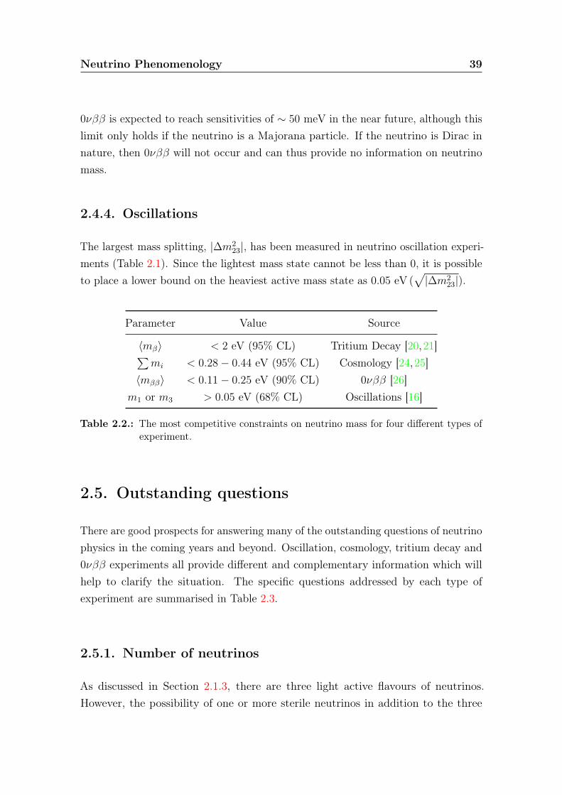
2.2. Constraints on neutrino mass from different types of experiment . . . 39
2.3. Unknown neutrino properties that can be observed using differentexperimental techniques . . . . . . . . . . . . . . . . . . . . . . . . . 40
3.1. Ten different Majoron models and their main properties . . . . . . . . 54
4.1. Details of isotopes commonly used in 0νββ experiments . . . . . . . . 61
4.2. Measurements of the 2νββ half-life for nine isotopes where a directobservation has been made . . . . . . . . . . . . . . . . . . . . . . . . 75
4.3. Half-life limits for different 0νββ isotopes . . . . . . . . . . . . . . . . 75
4.4. Summary of future 0νββ experiments . . . . . . . . . . . . . . . . . . 77
5.1. Summary of selenium source foils . . . . . . . . . . . . . . . . . . . . 84
5.2. HPGe measurements of selenium foil strips . . . . . . . . . . . . . . . 85
6.1. NEMO-3 data set . . . . . . . . . . . . . . . . . . . . . . . . . . . . . 107
7.1. Details of the external background model . . . . . . . . . . . . . . . . 121
7.2. Details of areas excluded as hot spots . . . . . . . . . . . . . . . . . . 128
7.3. Division of histograms used in the binned log-likelihood fit . . . . . . 134
7.4. Internal background activities from the fit . . . . . . . . . . . . . . . 141
7.5. Internal background activites compared with HPGe results . . . . . . 142
7.6. Fit results for external backgrounds . . . . . . . . . . . . . . . . . . . 142
16
LIST OF TABLES 17
7.7. Fit results for radon activities . . . . . . . . . . . . . . . . . . . . . . 143
8.1. Estimated number of internal, external and radon background eventspassing the 2νββ selection criteria . . . . . . . . . . . . . . . . . . . . 158
8.2. Background activities after fitting with 2νββ signal . . . . . . . . . . 161
8.3. Expected numbers of internal background events in the 2νββ channel 162
8.4. Expected numbers of external background events in the 2νββ channel 162
8.5. Expected numbers of radon background events in the 2νββ channel . 163
8.6. Comparison of analyses performed using phase 1, phase 2 and bothphase 1 and phase 2 data . . . . . . . . . . . . . . . . . . . . . . . . . 167
8.7. Summary of systematic errors contributing to the 2νββ half-life mea-surement . . . . . . . . . . . . . . . . . . . . . . . . . . . . . . . . . . 170
8.8. Predicted numbers of background events between 2.6−3.2 MeV, usingthe 2νββ selection criteria . . . . . . . . . . . . . . . . . . . . . . . . 172
8.9. Results of a 0νββ search for the mass mechanism decay mode . . . . 178
8.10. Effective Majorana neutrino mass calculated using the half-life limitset in this work . . . . . . . . . . . . . . . . . . . . . . . . . . . . . . 179
8.11. Results of a 0νββ search for the two right-handed current decay modes180
8.12. Half-life limits for Majoron emission decay modes . . . . . . . . . . . 182
8.13. Majoron-neutrino coupling limits extracted from experimental results 182
9.1. Summary of experimental achievements of NEMO-3 and target levelsfor SuperNEMO . . . . . . . . . . . . . . . . . . . . . . . . . . . . . . 189
10.1. Details of isotopes in the radon decay chain . . . . . . . . . . . . . . 198
11.1. Typical results of calibration of the electrostatic detector for spikeand flow-through calibration modes . . . . . . . . . . . . . . . . . . . 214
11.2. Trapping and transfer efficiency measurement results . . . . . . . . . 221
13.1. Measurements of gas cylinders of helium and nitrogen . . . . . . . . . 244
13.2. Measurements of radon activity inside the first C-section . . . . . . . 249
Chapter 1.
Introduction
Over many years, the Standard Model (SM) of particle physics has been tested withever-greater precision. Up to now, it has proved incredibly successful and has beenverified to a truly remarkable level of accuracy. However, in recent years, therehas been a discovery in the neutrino sector that goes beyond the SM. Successiveexperiments have now confirmed the phenomenon of neutrino oscillations, whereneutrinos change from one flavour to another. This flavour mixing and its associatednon-zero mass cannot be unambiguously included in the SM, such that, uniquelyamongst the known fundamental particles, neutrinos have measurable propertiesthat are not accurately described by the SM.
Furthermore, it is not straight-forward to supplement the SM to agree with theseobservations of neutrino mixing and neutrino mass. Difficulties arise since theneutral nature of the neutrino allows the possibility of it being either a Dirac orMajorana fermion. Dirac neutrinos would have a distinct antineutrino partner,whereas Majorana neutrinos would be their own antiparticles. This ambiguity meansthat, given the current state of knowledge, it is not possible to unequivocally confirmor refute either possibility.
Neutrinoless double beta decay (0νββ) is a hypothesised, but as yet unobserved,nuclear process where two electrons are emitted from the same nucleus withoutaccompanying neutrinos. The observation of 0νββ would confirm that the neutrino isa Majorana particle and the decay rate would allow (model-dependent) extraction ofthe absolute mass scale of the neutrino and may give insight into the mass hierarchy.
18
Introduction 19
As well as 0νββ, there is an allowed SM process of two neutrino double beta decay(2νββ) and, despite its rare nature, this process has been directly observed in nineisotopes. It is important to measure the 2νββ process precisely as this may beused to improve nuclear models which are used to extract information about 0νββ.In addition, due to its similar event topology, 2νββ represents one of the majorbackgrounds to the 0νββ process.
The search for 0νββ is a highly active research area with many different experiments,using various technologies, studying the full range of viable 0νββ isotopes. The mostimportant of these experiments are described in detail in Chapter 4. At present,there is a transition from a series of successful older experiments to a new generationof larger-scale detectors which hope to probe 0νββ further.
In the recent past, the strongest limits on 0νββ have come from semiconductorexperiments using 76Ge, such as Heidelberg-Moscow (H-M) and IGEX, with limitsof 〈mββ〉 < 0.25 − 0.50 eV. In addition, there has been a controversial claim fordiscovery of 0νββ from a subset of the H-M collaboration.
In the last year, three of the new generation of experiments have produced resultswhich supercede those of H-M and IGEX. No evidence for 0νββ has yet been foundand the results strongly disfavour the previous discovery claim. These experimentsall use different technologies: GERDA uses 76Ge as a semiconductor in the samefashion as Heidelberg-Moscow; KamLAND-Zen uses 136Xe-loaded liquid scintillatorand EXO-200 uses 136Xe in a scintillating time projection chamber. Many moreexperiments with similar expected sensitivities to these experiments, down to 〈mββ〉 <0.05− 0.10 eV, are either in advanced R&D stages or under construction.
The SuperNEMO experiment, which evolved from the NEMO-3 experiment, is onesuch experiment. Both SuperNEMO and NEMO-3 use a detector type known astracker-calorimeter, and they perfectly encapsulate the transition between differentgenerations of experiment.
1.1. NEMO-3
The NEMO-3 detector operated from 2003 to 2011 in the Laboratoire Souterrainde Modane (LSM), where it searched for 0νββ in seven different candidate isotopes
Introduction 20
(100Mo, 82Se, 150Nd, 116Cd, 130Te, 48Ca and 96Zr) with a total source mass of 10 kg.This source mass was contained in thin foils that were surrounded by a gas trackerand a calorimeter made from plastic scintillator. This configuration allowed fordetailed event topology reconstruction. NEMO-3 has observed 2νββ in all sevenisotopes, producing the most accurate 2νββ measurements for each isotope. Thelarger masses of 100Mo (6.9 kg) and 82Se (0.9 kg) mean that these isotopes can alsoprovide results for 0νββ decay that are competitive with the current generation ofexperiments.
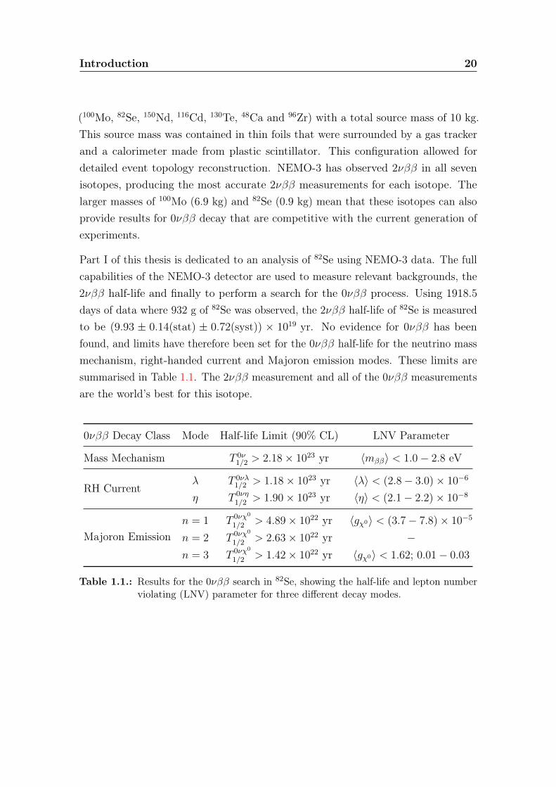
Part I of this thesis is dedicated to an analysis of 82Se using NEMO-3 data. The fullcapabilities of the NEMO-3 detector are used to measure relevant backgrounds, the2νββ half-life and finally to perform a search for the 0νββ process. Using 1918.5days of data where 932 g of 82Se was observed, the 2νββ half-life of 82Se is measuredto be (9.93 ± 0.14(stat) ± 0.72(syst)) × 1019 yr. No evidence for 0νββ has beenfound, and limits have therefore been set for the 0νββ half-life for the neutrino massmechanism, right-handed current and Majoron emission modes. These limits aresummarised in Table 1.1. The 2νββ measurement and all of the 0νββ measurementsare the world’s best for this isotope.
0νββ Decay Class Mode Half-life Limit (90% CL) LNV Parameter
Mass Mechanism T 0ν1/2 > 2.18× 10²³ yr 〈mββ〉 < 1.0− 2.8 eV
RH Currentλ T 0νλ
1/2 > 1.18× 10²³ yr 〈λ〉 < (2.8− 3.0)× 10−6
η T 0νη1/2 > 1.90× 10²³ yr 〈η〉 < (2.1− 2.2)× 10−8
Majoron Emissionn = 1 T 0νχ0
1/2 > 4.89× 10²² yr 〈gχ0〉 < (3.7− 7.8)× 10−5
n = 2 T 0νχ0
1/2 > 2.63× 10²² yr −n = 3 T 0νχ0
1/2 > 1.42× 10²² yr 〈gχ0〉 < 1.62; 0.01− 0.03
Table 1.1.: Results for the 0νββ search in 82Se, showing the half-life and lepton numberviolating (LNV) parameter for three different decay modes.

Introduction 21
1.2. SuperNEMO
SuperNEMO is a next-generation 0νββ experiment that will build on the successof the NEMO-3 experiment, using the same tracker-calorimeter design and housing100 kg of 82Se. It is anticipated that a half-life sensitivity of 1026 years will be reached,corresponding to an effective Majorana neutrino mass of 〈mββ〉 < 50− 100 meV.
Radon is a radioactive gas that is part of naturally occurring radioactive decay chains.If radon is present inside SuperNEMO, it can be a significant background to thesearch for 0νββ. The most stable isotope of radon (222Rn; t1/2 = 3.82 days), can enterthe detector either through diffusion, contamination during detector construction oremanation from the detector materials themselves. Once inside the detector, thisradon can move freely and deposit its progenies on the 82Se foils. One of theseprogenies is 214Bi which undergoes β-decay with a high Qβ value. This decay canmimic the rare 0νββ signal.
In order to achieve the target sensitivity for SuperNEMO, the radon level insidethe detector must be less than 150 µBq/m3. This is significantly lower than the5 mBq/m3 level that was achieved in the NEMO-3 detector. As a result, significantR&D effort has gone into reducing the level of radon inside the detector and measuringradon down to this low-level.
Part II of this thesis will discuss the R&D work that has been undertaken to measureradon levels at the sub mBq/m3 level. State-of-the-art electrostatic detectors areonly able to measure down to ∼ 1− 2 mBq/m3, so a “Radon Concentration Line”(RnCL) has been developed that can first concentrate any radon present beforemaking a measurement. The RnCL has a sensitivity of 40 µBq/m3 for a uniformsupply of gas and can measure the level inside a quarter-section of the SuperNEMOtracker down to a similar level. It has been used to measure gas bottles, gas supplylines and to make the first radon measurements of a SuperNEMO sub-module duringthe construction phase.
Introduction 22
1.3. Author’s Contributions
1.3.1. NEMO-3 Contributions
• Analysis of double beta decay in 82Se:
– Background measurements of the 82Se foils
– Optimisation of analysis cuts
– Measurement of the 2νββ half-life
– Search for 0νββ processes
• Development of core tools for a new analysis framework, so the user can:
– Record exposure, including dead time corrections
– Extract detector efficiencies correctly
– Search for events with alpha candidates
– Weight events for radon progenies based on previous radon measurements
– Fit activities of isotopes in many different channels
– Process multiple analysis jobs simultaneously on computing clusters
• Validation and verification of this new analysis framework:
– Reconstruction of raw data and MC samples for calibration runs
– Analysis of 207Bi calibration runs to cross-check 2e & 1e1γ channels
– Analysis of 232U calibration runs to validate 1e2γ channel
– Verification of implementation of data-quality cuts at reconstruction level
– Comparison with another NEMO-3 software framework to ensure identicalresults
• Selection of runs to be included in a standardised run list
• Tuning of MC for gamma interactions to better replicate the energy and timingresponse of the NEMO-3 calorimeter
Introduction 23
• Running of NEMO-3 data acquisition shifts
• Partial dis-assembly of NEMO-3 and recovery of electronics for use in commis-sioning of SuperNEMO
1.3.2. SuperNEMO Contributions
• Commissioning of an electrostatic radon detector:
– Assembly of a data acquisition system to record signals
– Application of styrene butadiene rubber (SBR) to stop diffusion throughseals
– Measurement of detector efficiency and background
• R&D for the RnCL:
– Design, construction and further development of the system
– Measurement of trapping and transfer efficiency
– Measurement of radon emanation from cold trap
– Calculation of the sensitivity of the RnCL to different experimental scenarios
• Radon measurements:
– Quarter-section of the SuperNEMO tracker
– He and N2 gas bottles and gas delivery lines
– SuperNEMO gas mixing and delivery system
– Clean room where SuperNEMO is being built
– Modelling of radon levels in connected volumes and extraction of separateemanation results
• Diffusion Studies:
– Calculations of expected levels of radon diffusion into the SuperNEMOtracker

Introduction 24
– Calculations of the radon emanation expected from different materials
– Participation in a cross-calibration of many institutions using radon ema-nation from glass beads
• Design and construction of a separate electrostatic radon detector
• Presentation of the collaboration’s work at Neutrino2012 & LRT2013
Chapter 2.
Neutrino Phenomenology
2.1. Standard Model Neutrinos
2.1.1. Discovery of the Neutrino
As early as 1914, it had been observed that the electron emitted in beta decay has acontinuous energy spectrum, however it was not until 1930 that Pauli hypothesisedan additional particle as a “desperate remedy” to conserve energy, momentum andspin [1]. This particle was initially termed a neutron, but was re-named as a neutrinoby Fermi in 1933 in order to distinguish it from Chadwick’s recently discoveredneutron [2]. Over the next few years, Bethe and Peierls elaborated on Pauli’s theoryand showed that this new particle must interact very weakly. It is this property thatallowed the neutrino to remain elusive for a further quarter-century, until the adventof the atomic age when neutrinos were produced at high enough intensity to bedetected. In 1956, at the Savannah River nuclear reactor, Reines and Cowan observedinverse beta decay, giving a unique signature of an anti-neutrino interaction [3].
2.1.2. Neutrino Interactions
Experimental observations have guided the addition of neutrinos to the SM. However,these experiments never directly observe neutrinos, instead studying the products ofneutrino interactions. As such, it is worthwhile briefly noting how neutrinos interact.In the SM, neutrinos can only interact via the weak force, which can be broken down
25
Neutrino Phenomenology 26
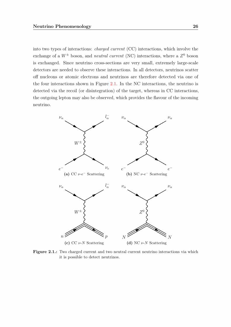
into two types of interactions: charged current (CC) interactions, which involve theexchange of a W± boson, and neutral current (NC) interactions, where a Z0 bosonis exchanged. Since neutrino cross-sections are very small, extremely large-scaledetectors are needed to observe these interactions. In all detectors, neutrinos scatteroff nucleons or atomic electrons and neutrinos are therefore detected via one ofthe four interactions shown in Figure 2.1. In the NC interactions, the neutrino isdetected via the recoil (or disintegration) of the target, whereas in CC interactions,the outgoing lepton may also be observed, which provides the flavour of the incomingneutrino.
�W±
e−
να
νe
l−α
(a) CC ν-e− Scattering
�Z0
e−
να
e−
να
(b) NC ν-e− Scattering
�W±
n
να
p
l−α
(c) CC ν-N Scattering
�Z0
N
να
N
να
(d) NC ν-N Scattering
Figure 2.1.: Two charged current and two neutral current neutrino interactions via whichit is possible to detect neutrinos.
Neutrino Phenomenology 27
2.1.3. Neutrino Flavours
In 1962, a group of researchers at Brookhaven National Laboratory undertook thefirst experiment with an accelerator as a source of neutrinos. They observed a clearsignature of a CC interaction with an outgoing muon, confirming that there were atleast two different flavours of neutrino (νe and νµ) [4]. A third generation of leptonswas found with the discovery of the tau particle in 1975 [5], but it would be 25 moreyears before direct evidence for the tau neutrino, ντ , was attained by the DONUTexperiment in 2000 [6].
It is no coincidence that accelerator experiments were required to discover νµ andντ . Indeed, a simple kinematic calculation shows that if the CC process shown inFigure 2.1c is to proceed, νµ and ντ must have energy greater than 110 MeV and3.5 GeV respectively. Solar neutrinos have typical energies of ∼ 1 MeV, and so onlyνe from the sun can interact via a CC interaction. Atmospheric neutrinos havesimilar energies to accelerator neutrinos at ∼ 1 GeV, but have greatly reduced flux,such that accelerator neutrinos were a clear front-runner for the discovery. The NCinteractions (Figures 2.1b and 2.1d) are elastic and therefore have no fundamentalkinematic constraints.
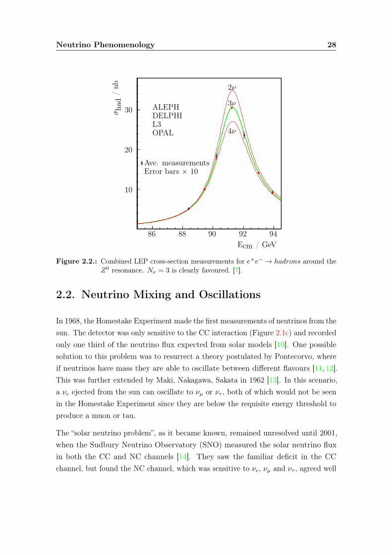
Up to the present, three generations of neutrino have been directly observed (νe, νµand ντ ) which produce the three generations of charged leptons in CC interactions.There is strong evidence that there are only three active light neutrino generations,which comes from the four experiments that studied e+e− collisions at the LEPcollider [7]. By measuring the width of the Z0 resonance, as shown in Figure 2.2,the combined result from the four experiments measured the number of light activeneutrinos, Nν = 2.9840± 0.0082.
It should be noted that the Z0 width provides a measure of the number of Z0 → νανα
decays. This means that it is not sensitive to neutrinos with a mass greater thanZ0/2 (45.6 GeV) nor neutrinos that do not couple to the Z0, which are commonlytermed sterile neutrinos. This may be pertinent since sterile neutrinos have beenoffered as a possible explanation for recent unexpected experimental results [8, 9].
Neutrino Phenomenology 28
Ecm / GeV
σha
d/nb
3ν
2ν
4ν
Ave. measurementsError bars × 10
ALEPHDELPHIL3OPAL
88 90 92 9486
10
20
30
Figure 2.2.: Combined LEP cross-section measurements for e+e− → hadrons around theZ0 resonance. Nν = 3 is clearly favoured. [7].
2.2. Neutrino Mixing and Oscillations
In 1968, the Homestake Experiment made the first measurements of neutrinos from thesun. The detector was only sensitive to the CC interaction (Figure 2.1c) and recordedonly one third of the neutrino flux expected from solar models [10]. One possiblesolution to this problem was to resurrect a theory postulated by Pontecorvo, whereif neutrinos have mass they are able to oscillate between different flavours [11,12].This was further extended by Maki, Nakagawa, Sakata in 1962 [13]. In this scenario,a νe ejected from the sun can oscillate to νµ or ντ , both of which would not be seenin the Homestake Experiment since they are below the requisite energy threshold toproduce a muon or tau.
The “solar neutrino problem”, as it became known, remained unresolved until 2001,when the Sudbury Neutrino Observatory (SNO) measured the solar neutrino fluxin both the CC and NC channels [14]. They saw the familiar deficit in the CCchannel, but found the NC channel, which was sensitive to νe, νµ and ντ , agreed well
Neutrino Phenomenology 29
with predictions from solar models. This was certainly compelling evidence for theoscillation hypothesis.
2.2.1. Oscillation Phenomenology
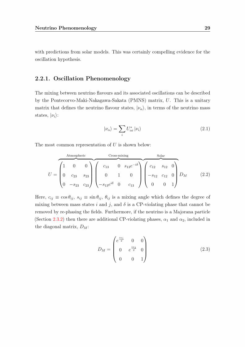
The mixing between neutrino flavours and its associated oscillations can be describedby the Pontecorvo-Maki-Nakagawa-Sakata (PMNS) matrix, U . This is a unitarymatrix that defines the neutrino flavour states, |να〉, in terms of the neutrino massstates, |νi〉:
|να〉 =∑i
U∗αi |νi〉 (2.1)
The most common representation of U is shown below:
U =
Atmospheric︷ ︸︸ ︷1 0 0
0 c23 s23
0 −s23 c23
Cross-mixing︷ ︸︸ ︷
c13 0 s13e−iδ
0 1 0
−s13eiδ 0 c13
Solar︷ ︸︸ ︷
c12 s12 0
−s12 c12 0
0 0 1
DM (2.2)
Here, cij ≡ cos θij, sij ≡ sin θij, θij is a mixing angle which defines the degree ofmixing between mass states i and j, and δ is a CP-violating phase that cannot beremoved by re-phasing the fields. Furthermore, if the neutrino is a Majorana particle(Section 2.3.2) then there are additional CP-violating phases, α1 and α2, included inthe diagonal matrix, DM :
DM =
eiα12 0 0
0 eiα22 0
0 0 1
(2.3)

Neutrino Phenomenology 30
It can be shown that, in vacuum, a neutrino of flavour α has probability to turn toflavour β given by [15]:
P (να → νβ) =
∣∣∣∣∣∑i
U∗αie−im2
iL2EUβi
∣∣∣∣∣2
= δαβ − 4∑i>j
<(U∗αiUβiU
∗αjUβj
)sin2
(∆m2
ij
L
4E
)+ 2
∑i>j
=(U∗αiUβiU
∗αjUβj
)sin2
(∆m2
ij
L
2E
)(2.4)
where L is the distance travelled, E is the energy of the neutrino and m2ij is the mass
splitting between the states i and j:
∆m2ij ≡ m2
i −m2j (2.5)
From Equation (2.4), it is clear that if a neutrino is produced in a weak interactionas a particular flavour with a given energy, it will mix between the different flavoursas it travels. This mixing is governed by the parameters in the PMNS matrix andmass splittings.
2.2.2. Oscillations in Matter
If instead of propagating through vacuum, a neutrino propagates through matter withsignificant density, then coherent forward scattering from particles within the matterbecomes important. The oscillatory behaviour of the neutrino will change, since thereare now interactions that differ between the different flavour states. For example, aνe may interact with ambient electrons via both NC and CC interactions, exchangingeither a W± or Z0, whereas a νµ or µτ will interact via the NC interaction alone.This change in behaviour in matter is known as the Mikheyev-Smirnov-Wolfenstein(MSW) effect.
The MSW effect is particularly important when considering the passage of solarneutrinos from the centre of the sun to the earth. These neutrinos are created aselectron neutrinos close to the centre of the sun where the electron energy density islarge, such that matter effects dominate over vacuum oscillation. In this scenario,

Neutrino Phenomenology 31
the electron neutrinos are approximately in the heavier of the two possible masseigenstates, when taking into account a modified potential for the MSW interactions.
As the neutrinos move radially outwards from the sun, the electron density decreasesslowly enough that the neutrinos propagate adiabatically. They thus remain inmass eigenstates of the modified vacuum potential as it slowly changes. When theneutrinos reach the edge of the sun and the electron density has become negligible,they are in a mass eigenstate of the vacuum potential, ν2. Being an eigenstate of thevacuum Hamiltonian, this state will propagate all the way to earth without mixingand arrive in the same ν2 state, which can be used to provide information on thesign of m2
21.
2.2.3. Measurement of Oscillation Parameters
The early indication of neutrino oscillations from SNO has been corroborated inrecent years by evidence from a series of dedicated neutrino oscillation experiments.There are two main types of experiment that contribute to these measurements:reactor and accelerator experiments.
Reactor experiments are usually detectors placed near one or more nuclear reactorswhich measure the flux of neutrinos as a function of energy and distance fromthe reactor core. Accelerator experiments typically involve a neutrino beam thatis measured in a near detector and then propagated over a long baseline to a fardetector. This allows the tuning of E and L to maximise the measurement sensitivity.
Neutrino oscillation experiments have enjoyed considerable success in measuringmost of the mixing parameters which are summarised in Table 2.1. Despite thissuccess, there are notable gaps in the current state of knowledge, including the signof ∆m2
32 and any information on the CP-violating parameters, δ, α1 and α2.
Irrespective of these unknowns, it is now beyond doubt that neutrino oscillationoccurs and as a result of this mixing, it is known that neutrinos must have finitemasses.

Neutrino Phenomenology 32
Parameter Value
sin2 2θ12 0.857+0.023−0.025
sin2 2θ23 > 0.95
sin2 2θ13 0.095± 0.010
∆m221 7.50+0.19
−0.20 × 10⁻⁵ eV2
|∆m232| 2.32+0.12
−0.08 × 10⁻³ eV2
Table 2.1.: Best current estimates for neutrino mixing parameters from a global fit [16]
2.3. Neutrino Mass
There is now clear evidence that neutrinos have mass and as a result, many theoristshave studied how to add this neutrino mass into the SM. Two methods arise naturally,where two distinct mass terms are added to the SM Lagrangian. These correspond todifferent types of neutrino - one is a Dirac particle, similar to the other SM fermions,and the other is a Majorana particle which is its own antiparticle. A combination ofthe two mass terms is theoretically preferable, as it may explain why the masses ofthe observed neutrinos are many orders of magnitude smaller than the other knownfermions. This so-called see-saw mechanism (Section 2.3.3), also predicts high massneutrinos which may play an important role in explaining the matter-antimatterasymmetry in the universe.
Throughout this section, for ease of understanding and simplicity of notation, onlyone flavour of neutrino will be considered. However, all results still hold for anarbitrary number of neutrinos. Sections 2.3.1–2.3.3 have been written with referenceto [15,17].
2.3.1. Dirac Mass
The SM, which omits neutrino masses, contains only chirally left-handed (LH)neutrinos, νL, which participate in the weak interaction, and no right-handed (RH)neutrinos, νR. Perhaps the most obvious method to add mass terms to the SMis to do so in the same way as for the charged leptons and quarks, which is doneby coupling of LH and RH fields with the Higgs field. This type of mass term iscalled a Dirac mass term. To implement a Dirac mass term therefore requires the
Neutrino Phenomenology 33
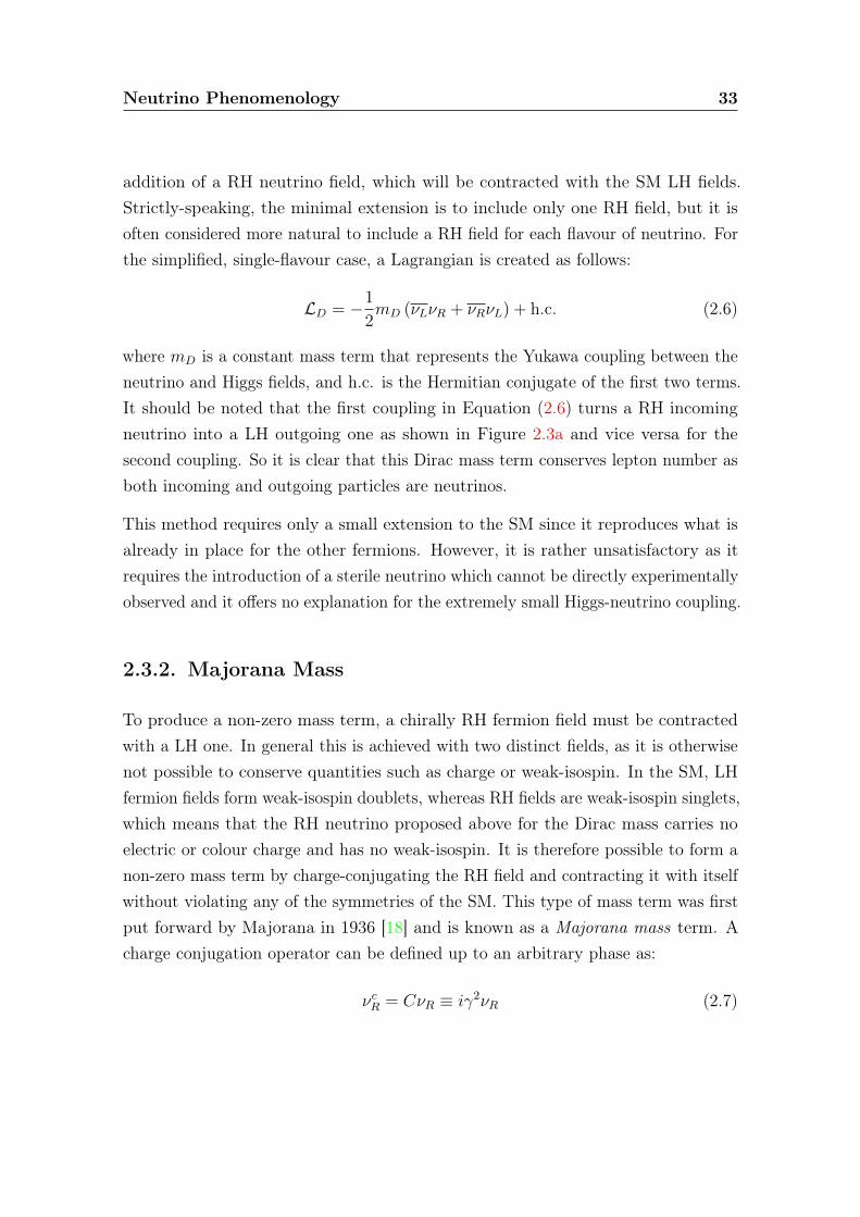
addition of a RH neutrino field, which will be contracted with the SM LH fields.Strictly-speaking, the minimal extension is to include only one RH field, but it isoften considered more natural to include a RH field for each flavour of neutrino. Forthe simplified, single-flavour case, a Lagrangian is created as follows:
LD = −1
2mD (νLνR + νRνL) + h.c. (2.6)
where mD is a constant mass term that represents the Yukawa coupling between theneutrino and Higgs fields, and h.c. is the Hermitian conjugate of the first two terms.It should be noted that the first coupling in Equation (2.6) turns a RH incomingneutrino into a LH outgoing one as shown in Figure 2.3a and vice versa for thesecond coupling. So it is clear that this Dirac mass term conserves lepton number asboth incoming and outgoing particles are neutrinos.
This method requires only a small extension to the SM since it reproduces what isalready in place for the other fermions. However, it is rather unsatisfactory as itrequires the introduction of a sterile neutrino which cannot be directly experimentallyobserved and it offers no explanation for the extremely small Higgs-neutrino coupling.
2.3.2. Majorana Mass
To produce a non-zero mass term, a chirally RH fermion field must be contractedwith a LH one. In general this is achieved with two distinct fields, as it is otherwisenot possible to conserve quantities such as charge or weak-isospin. In the SM, LHfermion fields form weak-isospin doublets, whereas RH fields are weak-isospin singlets,which means that the RH neutrino proposed above for the Dirac mass carries noelectric or colour charge and has no weak-isospin. It is therefore possible to form anon-zero mass term by charge-conjugating the RH field and contracting it with itselfwithout violating any of the symmetries of the SM. This type of mass term was firstput forward by Majorana in 1936 [18] and is known as a Majorana mass term. Acharge conjugation operator can be defined up to an arbitrary phase as:
νcR = CνR ≡ iγ2νR (2.7)

Neutrino Phenomenology 34
It is immediately clear that this will produce a field with LH chirality since γ2
anti-commutes with γ5 in the projection operator, PL,R = (1∓ γ5) /2, such that:
νcR ≡ iγ21
2
(1 + γ5
)ν =
1
2
(1− γ5
)iγ2ν = PLν
c (2.8)
The Majorana mass term to be included in the SM Lagrangian is therefore of theform:
LM = −1
2mRνcRνR + h.c. (2.9)
where mR is a constant mass term. Equation (2.9) destroys an incoming neutrinoand creates an outgoing anti-neutrino as shown in Figure 2.3b, so this mass termdoes not conserve lepton number and Majorana particles are their own anti-particles.
�
νR νLmD
(a) Dirac Mass: mDνLνR
�
ν νmR
(b) Majorana Mass: mRνcRνR
Figure 2.3.: Feynman diagrams showing the propagators for the Dirac and Majoranaterms in Equations (2.6) and (2.9).
It is possible to level a similar criticism at the Majorana mass, regarding the additionof a sterile RH neutrino, as was raised with the Dirac mass, and this criticism wouldbe justified. However, the great strength of the Majorana mass is that it offers apossible explanation of the disparity between neutrino masses and the masses of thecharged leptons.
2.3.3. See-saw Mechanism
The see-saw mechanism is a class of model that predicts small masses for the knownlight neutrinos. The type 1 see-saw mechanism brings together the Dirac and
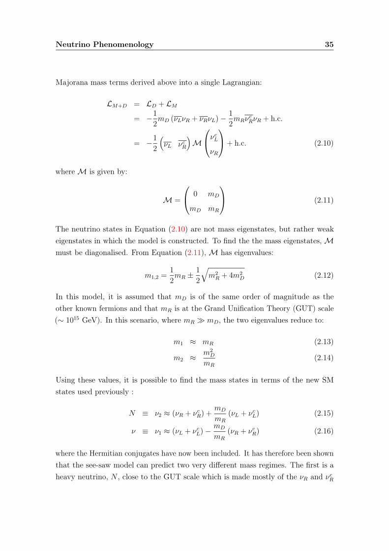
Neutrino Phenomenology 35
Majorana mass terms derived above into a single Lagrangian:
LM+D = LD + LM
= −1
2mD (νLνR + νRνL)− 1
2mRνcRνR + h.c.
= −1
2
(νL νcR
)M
νcLνR
+ h.c. (2.10)
whereM is given by:
M =
0 mD
mD mR
(2.11)
The neutrino states in Equation (2.10) are not mass eigenstates, but rather weakeigenstates in which the model is constructed. To find the the mass eigenstates,Mmust be diagonalised. From Equation (2.11),M has eigenvalues:
m1,2 =1
2mR ±
1
2
√m2R + 4m2
D (2.12)
In this model, it is assumed that mD is of the same order of magnitude as theother known fermions and that mR is at the Grand Unification Theory (GUT) scale(∼ 1015 GeV). In this scenario, where mR � mD, the two eigenvalues reduce to:
m1 ≈ mR (2.13)
m2 ≈m2D
mR
(2.14)
Using these values, it is possible to find the mass states in terms of the new SMstates used previously :
N ≡ ν2 ≈ (νR + νcR) +mD
mR
(νL + νcL) (2.15)
ν ≡ ν1 ≈ (νL + νcL)− mD
mR
(νR + νcR) (2.16)
where the Hermitian conjugates have now been included. It has therefore been shownthat the see-saw model can predict two very different mass regimes. The first is aheavy neutrino, N , close to the GUT scale which is made mostly of the νR and νcR
Neutrino Phenomenology 36
fields. This neutrino forces the other state, ν, which is almost entirely composed ofthe νL and νcL fields, to be very light as is observed in nature. The existence of a RHneutrino at the GUT scale is not only favourable for this reason, but may explaineven more fundamental questions about the matter-antimatter asymmetry in theuniverse and why we exist at all (Section 2.5.3).
2.4. Experimental Constraints on Neutrino Mass
Experimental information on neutrino mass comes from four main sources. Tritiumdecay, 0νββ and cosmological models measure different combinations of masses andPMNS parameters, and all provide upper bounds on neutrino masses. This is incontrast to information from oscillation experiments which puts a lower bound onthe heaviest mass state. A summary of the best results from each type of experimentis presented in Table 2.2.
2.4.1. Tritium Decay
Tritium (3H) is an isotope of hydrogen that undergoes beta decay:
3H→ 3He + e− + νe (2.17)
where the energy of the electron obeys a beta decay spectrum. If the neutrino ismassless, then the endpoint of the decay spectrum, Qβ, will be equal to the differencebetween the 3H and 3He+ e− rest masses. However, in reality, Qβ will be reduced bythe neutrino mass, which will cause the energy spectrum of the electron to deviatefrom the massless case as shown in Figure 2.4.
Theoretically, there are at least three separate Qβ values – one for each neutrino massstate. However, in reality, the energy resolution of any feasible experiment is notable to discern these different decays. Therefore an average deviation is measured,from which it is possible to infer the average of the neutrino mass states weighted by
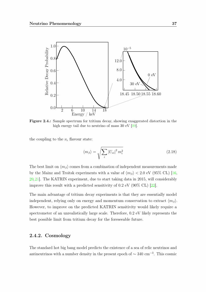
Neutrino Phenomenology 37
0.0
0.2
0.4
0.6
0.8
1.0
2 6 10 14 18Energy / keV
4.0
8.0
12.0
10−5
18.45 18.50 18.55 18.60
0 eV
30 eV
RelativeDecay
Proba
bility
Figure 2.4.: Sample spectrum for tritium decay, showing exaggerated distortion in thehigh energy tail due to neutrino of mass 30 eV [19].
the coupling to the νe flavour state:
〈mβ〉 =
√∑i
|Uei|2m2i (2.18)
The best limit on 〈mβ〉 comes from a combination of independent measurements madeby the Mainz and Troitsk experiments with a value of 〈mβ〉 < 2.0 eV (95% CL) [16,20,21]. The KATRIN experiment, due to start taking data in 2015, will considerablyimprove this result with a predicted sensitivity of 0.2 eV (90% CL) [22].
The main advantage of tritium decay experiments is that they are essentially modelindependent, relying only on energy and momentum conservation to extract 〈mβ〉.However, to improve on the predicted KATRIN sensitivity would likely require aspectrometer of an unrealistically large scale. Therefore, 0.2 eV likely represents thebest possible limit from tritium decay for the foreseeable future.
2.4.2. Cosmology
The standard hot big bang model predicts the existence of a sea of relic neutrinos andantineutrinos with a number density in the present epoch of ∼ 340 cm−3. This cosmic
Neutrino Phenomenology 38
neutrino background (CNB) has not yet been directly observed, but its existence iswell-established as a result of the accurate predictions of the primordial abundanceof light elements alongside other cosmological observables [23].
Neutrinos play an important role in the evolution of the universe and by studyingparticular observables it is possible to glean information on the sum of neutrinomasses,
∑mi. To extract the strongest limits, many different observables are often
combined. This means that the large amount of available data can be used, whichaffords very strong limits, but comes with the cost that these limits can be verymodel-dependent.
The most important probes for neutrino mass in cosmology are anisotropies in thecosmic microwave background (CMB) and large scale structure formation. TheCMB is only sensitive to neutrino mass via secondary effects, but nonetheless,using the WMAP7 data alone, it is possible to extract an impressive limit of∑mi < 1.3 eV (95% CL) [24]. This result can be improved significantly, and
in a relatively robust manner, by including independent measurements of baryonacoustic oscillations and a direct determination of the Hubble constant, giving∑mi < 0.44 eV (95% CL) [24].
Finally, it is possible to introduce information from galaxy power spectra, which canproduce the most stringent limit of
∑mi < 0.28 eV (95% CL) [25]. However, this
result should be interpreted with care, since there are known difficulties in relatinggalaxy power spectra to the total matter power spectrum from which the limit isextracted [23].
2.4.3. Neutrinoless double beta decay (0νββ)
0νββ (discussed in Chapter 3), if mediated by light neutrino exchange (Section 3.3.1),is sensitive to the effective Majorana neutrino mass, 〈mββ〉:
〈mββ〉 =
∣∣∣∣∣∑i
U2eimi
∣∣∣∣∣ (2.19)
The strongest limit currently comes from a combination of the Kamland-Zen and EXOexperiments in 136Xe, with a value of 〈mββ〉 < 0.11− 0.25 eV (90% CL) where therange is a result of the chosen nuclear matrix element calculations (Section 3.4) [26].
Neutrino Phenomenology 39
0νββ is expected to reach sensitivities of ∼ 50 meV in the near future, although thislimit only holds if the neutrino is a Majorana particle. If the neutrino is Dirac innature, then 0νββ will not occur and can thus provide no information on neutrinomass.
2.4.4. Oscillations
The largest mass splitting, |∆m223|, has been measured in neutrino oscillation experi-
ments (Table 2.1). Since the lightest mass state cannot be less than 0, it is possibleto place a lower bound on the heaviest active mass state as 0.05 eV (
√|∆m2
23|).
Parameter Value Source
〈mβ〉 < 2 eV (95% CL) Tritium Decay [20,21]∑mi < 0.28− 0.44 eV (95% CL) Cosmology [24,25]
〈mββ〉 < 0.11− 0.25 eV (90% CL) 0νββ [26]m1 or m3 > 0.05 eV (68% CL) Oscillations [16]
Table 2.2.: The most competitive constraints on neutrino mass for four different types ofexperiment.
2.5. Outstanding questions
There are good prospects for answering many of the outstanding questions of neutrinophysics in the coming years and beyond. Oscillation, cosmology, tritium decay and0νββ experiments all provide different and complementary information which willhelp to clarify the situation. The specific questions addressed by each type ofexperiment are summarised in Table 2.3.
2.5.1. Number of neutrinos
As discussed in Section 2.1.3, there are three light active flavours of neutrinos.However, the possibility of one or more sterile neutrinos in addition to the three
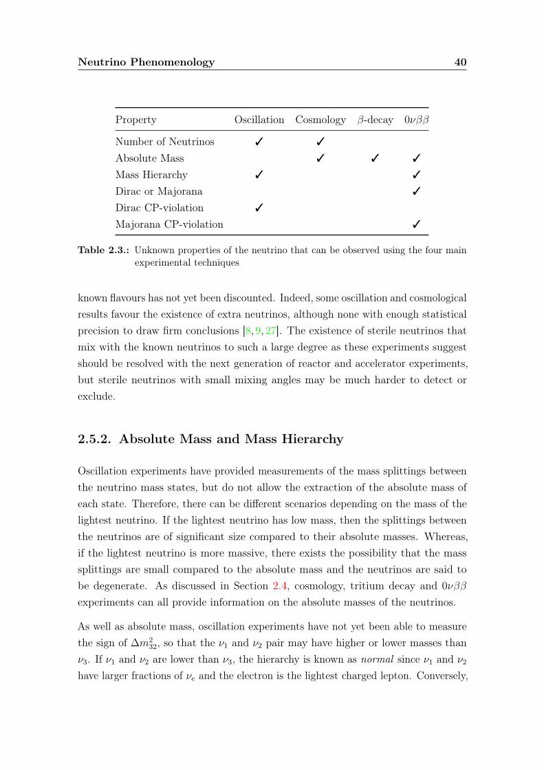
Neutrino Phenomenology 40
Property Oscillation Cosmology β-decay 0νββ
Number of Neutrinos 3 3
Absolute Mass 3 3 3
Mass Hierarchy 3 3
Dirac or Majorana 3
Dirac CP-violation 3
Majorana CP-violation 3
Table 2.3.: Unknown properties of the neutrino that can be observed using the four mainexperimental techniques
known flavours has not yet been discounted. Indeed, some oscillation and cosmologicalresults favour the existence of extra neutrinos, although none with enough statisticalprecision to draw firm conclusions [8, 9, 27]. The existence of sterile neutrinos thatmix with the known neutrinos to such a large degree as these experiments suggestshould be resolved with the next generation of reactor and accelerator experiments,but sterile neutrinos with small mixing angles may be much harder to detect orexclude.
2.5.2. Absolute Mass and Mass Hierarchy
Oscillation experiments have provided measurements of the mass splittings betweenthe neutrino mass states, but do not allow the extraction of the absolute mass ofeach state. Therefore, there can be different scenarios depending on the mass of thelightest neutrino. If the lightest neutrino has low mass, then the splittings betweenthe neutrinos are of significant size compared to their absolute masses. Whereas,if the lightest neutrino is more massive, there exists the possibility that the masssplittings are small compared to the absolute mass and the neutrinos are said tobe degenerate. As discussed in Section 2.4, cosmology, tritium decay and 0νββexperiments can all provide information on the absolute masses of the neutrinos.
As well as absolute mass, oscillation experiments have not yet been able to measurethe sign of ∆m2
32, so that the ν1 and ν2 pair may have higher or lower masses thanν3. If ν1 and ν2 are lower than ν3, the hierarchy is known as normal since ν1 and ν2have larger fractions of νe and the electron is the lightest charged lepton. Conversely,
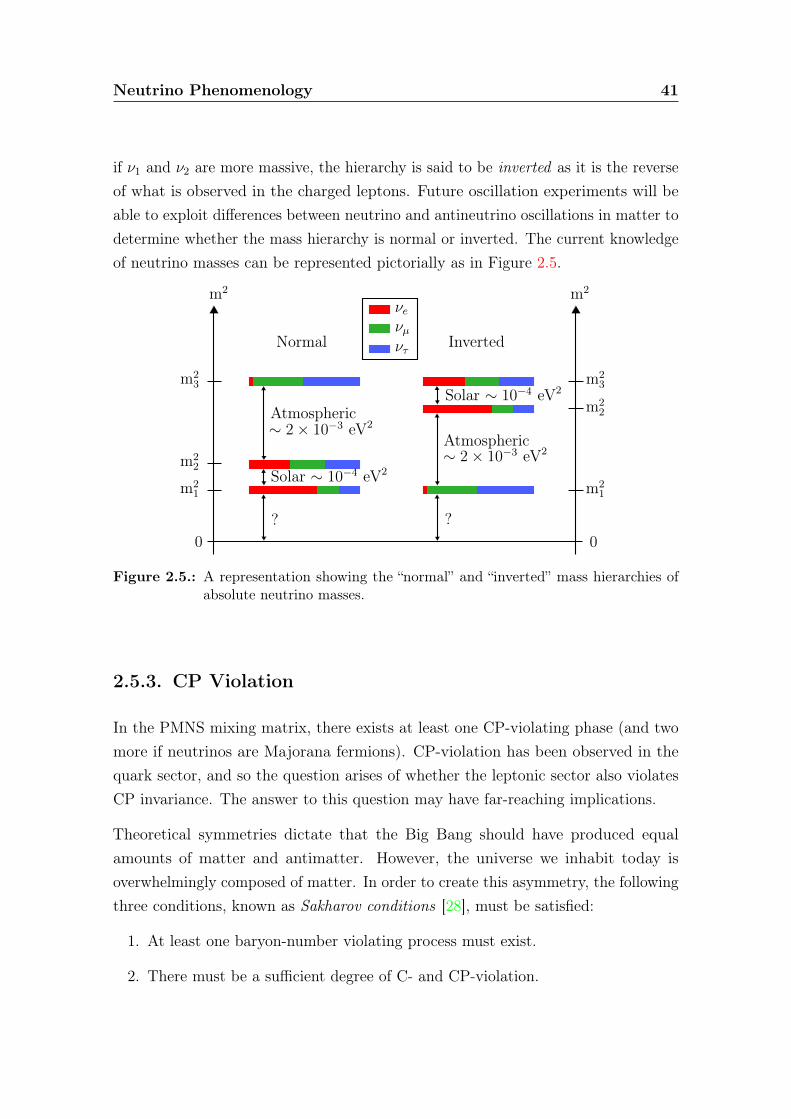
Neutrino Phenomenology 41
if ν1 and ν2 are more massive, the hierarchy is said to be inverted as it is the reverseof what is observed in the charged leptons. Future oscillation experiments will beable to exploit differences between neutrino and antineutrino oscillations in matter todetermine whether the mass hierarchy is normal or inverted. The current knowledgeof neutrino masses can be represented pictorially as in Figure 2.5.
Atmospheric
Normal Inverted
Solar ∼ 10−4 eV2
Atmospheric
? ?
m2m2
m23
m22
m21
0
m23
m22
m21
0
∼ 2× 10⁻³ eV2
∼ 2× 10⁻³ eV2
νeνµντ
Solar ∼ 10−4 eV2
Figure 2.5.: A representation showing the “normal” and “inverted” mass hierarchies ofabsolute neutrino masses.
2.5.3. CP Violation
In the PMNS mixing matrix, there exists at least one CP-violating phase (and twomore if neutrinos are Majorana fermions). CP-violation has been observed in thequark sector, and so the question arises of whether the leptonic sector also violatesCP invariance. The answer to this question may have far-reaching implications.
Theoretical symmetries dictate that the Big Bang should have produced equalamounts of matter and antimatter. However, the universe we inhabit today isoverwhelmingly composed of matter. In order to create this asymmetry, the followingthree conditions, known as Sakharov conditions [28], must be satisfied:
1. At least one baryon-number violating process must exist.
2. There must be a sufficient degree of C- and CP-violation.
Neutrino Phenomenology 42
3. Interactions outside of thermal equilibrium must occur.
The known CP-violation in the quark sector alone is not large enough to satisfythe second condition, so there is an intriguing possibility that CP-violation in theleptonic sector could be responsible. If CP-violation is observed in the known lightneutrinos, it adds credibility to the “leptogenesis” argument where CP-violating heavyright-handed neutrinos transmit a matter-antimatter asymmetry to the baryons andas such are the progenitors of the universe as we know it.
The Dirac CP-violating phase, δ, may soon be accessible to current or near-futureaccelerator experiments or to precision measurements of atmospheric neutrinos [29].A measurement of 0νββ will be required to determine the Majorana CP-violatingphase, although this must also be coupled with another independent measurementfrom either oscillation or collider experiments as well as independent knowledge ofthe absolute mass scale to fully disentangle α1 and α2.
2.5.4. Nature of the neutrino
The preceding questions are very important, but perhaps the most fundamentalquestion to be answered concerns the very nature of the neutrino itself - is it a Diracor Majorana particle? Currently, the only feasible proposal to answer this questionis through 0νββ, which is discussed in detail in the next chapter.
Chapter 3.
Double Beta Decay
3.1. Beta Decay
Beta decay (β decay) is a type of radiocative decay that transmutes a nucleus tothat of a different element. It is mediated by the weak force, and always results inthe emission of a neutrino or antineutrino. The process can occur in three separateforms where the emission is either accompanied by an electron (β− decay), a positron(β+ decay) or, in the case of electron capture (EC), no other emissions.
In β− decay, a neutron converts to a proton and an electron and antineutrino areemitted:
n→ p+ e− + νe (3.1)
Whilst in β+ decay, a proton converts to a neutron and a positron and neutrino areejected:
p→ n+ e+ + νe (3.2)
Finally, EC occurs when an atomic electron exchanges a W boson with a quarkinside the nucleus. It converts to a neutrino and a proton in the nucleus changes toa neutron.
p+ e− → n+ νe (3.3)
43
Double Beta Decay 44
EC occurs in all isotopes where β+ decay is energetically allowed. In some nuclei,where β+ decay is not energetically possible, it can be the sole decay mode. Thecaptured electron is usually in a low-lying orbital (most often in the K-Shell), whichleaves a hole that the remaining orbital electrons can cascade into. EC is thereforeusually accompanied by numereous low energy X-rays and/or Auger electrons.
3.1.1. Allowed and Forbidden Decays
All three β decay processes involve the emission of particles and loss of energy, so βdecay can only occur if
M(A,Zi) > M(A,Zf ) (3.4)
where M(A,Z) is the mass of the nucleus with A nucleons and Z protons, and thesubscripts i and f denote the initial and final nuclear states.
The semi-empirical mass formula (SEMF) can be used to approximate the mass ofan atomic nucleus for a given (A,Z) pairing [30] and can therefore be used to predictwhether transititions between nuclear states are allowed or forbidden. The SEMFgives the mass of a nucleus, m, as:
m = Zmp + (A− Z)mn − aVA+ asA2/3 + ac
Z2
A1/3+ aA
(A− 2Z)2
A+ δ (A,Z)
(3.5)
where
δ (A,Z) =
apA1/2 Z,N even (A even)
0 A odd−apA1/2 Z,N odd (A even)
(3.6)
The first two terms in this equation give an approximation of the mass of the nucleusby calculating the masses of individual nucleons. The remaining terms then providecorrections to this approximation in the form of a volume term, a surface term, aCoulomb term, an asymmetry term and a pairing term. For fixed A, parabolic curvesare generated as a function of Z, which dictate which β decays are energetically
Double Beta Decay 45
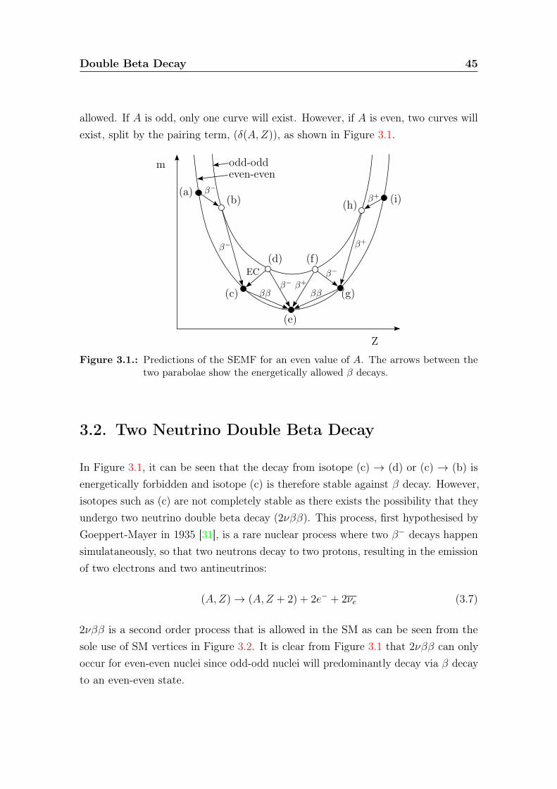
allowed. If A is odd, only one curve will exist. However, if A is even, two curves willexist, split by the pairing term, (δ(A,Z)), as shown in Figure 3.1.
m
Z
(a)(b)
(c)
(d)
(e)
(f)
(g)
(h) (i)
odd-oddeven-even
β−
β−
β− β+
β−
β+
β+
EC
ββ ββ
Figure 3.1.: Predictions of the SEMF for an even value of A. The arrows between thetwo parabolae show the energetically allowed β decays.
3.2. Two Neutrino Double Beta Decay
In Figure 3.1, it can be seen that the decay from isotope (c) → (d) or (c) → (b) isenergetically forbidden and isotope (c) is therefore stable against β decay. However,isotopes such as (c) are not completely stable as there exists the possibility that theyundergo two neutrino double beta decay (2νββ). This process, first hypothesised byGoeppert-Mayer in 1935 [31], is a rare nuclear process where two β− decays happensimulataneously, so that two neutrons decay to two protons, resulting in the emissionof two electrons and two antineutrinos:
(A,Z)→ (A,Z + 2) + 2e− + 2νe (3.7)
2νββ is a second order process that is allowed in the SM as can be seen from thesole use of SM vertices in Figure 3.2. It is clear from Figure 3.1 that 2νββ can onlyoccur for even-even nuclei since odd-odd nuclei will predominantly decay via β decayto an even-even state.
Double Beta Decay 46
�W−
W−
n
n
p
e−
νe
νe
e−
p
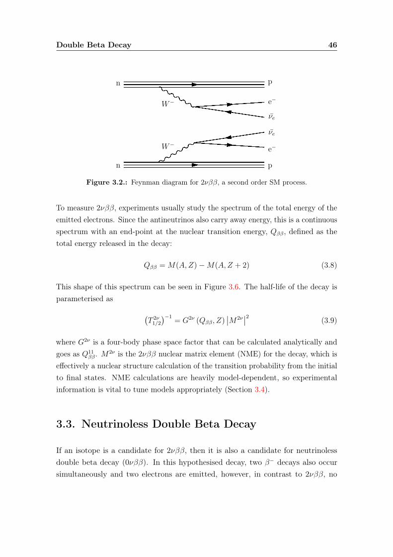
Figure 3.2.: Feynman diagram for 2νββ, a second order SM process.
To measure 2νββ, experiments usually study the spectrum of the total energy of theemitted electrons. Since the antineutrinos also carry away energy, this is a continuousspectrum with an end-point at the nuclear transition energy, Qββ, defined as thetotal energy released in the decay:
Qββ = M(A,Z)−M(A,Z + 2) (3.8)
This shape of this spectrum can be seen in Figure 3.6. The half-life of the decay isparameterised as
(T 2ν1/2
)−1= G2ν (Qββ, Z)
∣∣M2ν∣∣2 (3.9)
where G2ν is a four-body phase space factor that can be calculated analytically andgoes as Q11
ββ. M2ν is the 2νββ nuclear matrix element (NME) for the decay, which iseffectively a nuclear structure calculation of the transition probability from the initialto final states. NME calculations are heavily model-dependent, so experimentalinformation is vital to tune models appropriately (Section 3.4).
3.3. Neutrinoless Double Beta Decay
If an isotope is a candidate for 2νββ, then it is also a candidate for neutrinolessdouble beta decay (0νββ). In this hypothesised decay, two β− decays also occursimultaneously and two electrons are emitted, however, in contrast to 2νββ, no
Double Beta Decay 47
antineutrinos are emitted:
(A,Z)→ (A,Z + 2) + 2e− (3.10)
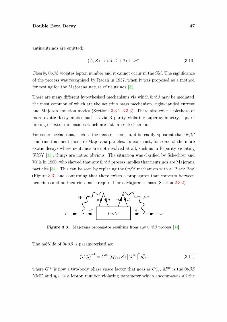
Clearly, 0νββ violates lepton number and it cannot occur in the SM. The significanceof the process was recognised by Racah in 1937, when it was proposed as a methodfor testing for the Majorana nature of neutrinos [32].
There are many different hypothesised mechanisms via which 0νββ may be mediated,the most common of which are the neutrino mass mechanism, right-handed currentand Majoron emission modes (Sections 3.3.1–3.3.3). There also exist a plethora ofmore exotic decay modes such as via R-parity violating super-symmetry, squarkmixing or extra dimensions which are not presented herein.
For some mechanisms, such as the mass mechanism, it is readily apparent that 0νββconfirms that neutrinos are Majorana paricles. In constrast, for some of the moreexotic decays where neutrinos are not involved at all, such as in R-parity violatingSUSY [33], things are not so obvious. The situation was clarified by Schechter andValle in 1980, who showed that any 0νββ process implies that neutrinos are Majoranaparticles [34]. This can be seen by replacing the 0νββ mechanism with a “Black Box”(Figure 3.3) and confirming that there exists a propagator that converts betweenneutrinos and antineutrinos as is required for a Majorana mass (Section 2.3.2).
0νββ
W± W±
e− e−
ddu u
ν ν
Figure 3.3.: Majorana propagator resulting from any 0νββ process [34].
The half-life of 0νββ is parameterised as:
(T 0ν1/2
)−1= G0ν (Qββ, Z)
∣∣M0ν∣∣2 η2LV (3.11)
where G0ν is now a two-body phase space factor that goes as Q5ββ, M0ν is the 0νββ
NME and ηLV is a lepton number violating parameter which encompasses all the

Double Beta Decay 48
physics behind the decay mechanism. Thus, ηLV takes on different forms dependingon the mechanism via which 0νββ is mediated.
3.3.1. Neutrino Mass Mechanism
The neutrino mass mechanism, also called the light neutrino exchange mechanism, isthe most commonly postulated 0νββ decay mode, since it involves the least deviationfrom the SM. In this mechanism, a scenario using only SM vertices is constructedwhere a RH (helicity) Majorana neutrino (simlar to a Dirac antineutrino) is emittedfrom one W boson and absorbed by another as a LH Majorana neutrino (Figure 3.4).
�WL
WL
νL
νR
n
n
p
e−
e−
p
Figure 3.4.: Feynman diagram from 0νββ for the neutrino mass mechanism. The decayis facilited by the exhange of a Majorana neutrino.
In this mechanism, ηLV is given by the effective Majorana neutrino mass, 〈mββ〉:(T 0ν1/2
)−1= G0ν (Qββ, Z)
∣∣M0ν∣∣2 〈mββ〉2 (3.12)
The form of 〈mββ〉 can be explained intuitively. Since the RH helicity neutrino hasmass, it must have a LH component proportional to mi, and each vertex picks up afactor Uei:
〈mββ〉 =
∣∣∣∣∣∑i
U2eimi
∣∣∣∣∣=
∣∣∣ cos2 θ13(m1 cos2 θ12 +m2e
iα1 sin2 θ12)
+m3ei(α2−2δ) sin2 θ13
∣∣∣(3.13)
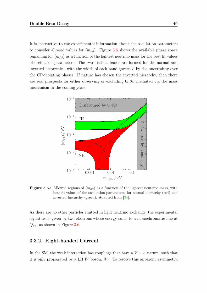
Double Beta Decay 49
It is instructive to use experimental information about the oscillation parametersto consider allowed values for 〈mββ〉. Figure 3.5 shows the available phase spaceremaining for 〈mββ〉 as a function of the lightest neutrino mass for the best fit valuesof oscillation parameters. The two distinct bands are formed for the normal andinverted hierarchies, with the width of each band governed by the uncertainty overthe CP-violating phases. If nature has chosen the inverted hierarchy, then thereare real prospects for either observing or excluding 0νββ mediated via the massmechanism in the coming years.
10−4
10−3
10−2
10−1
10−0
〈mββ〉/
eV
mlight / eV
NH
IH
0.001 0.01 0.1
Disfavoured by 0νββ
Disfavoured
bycosm
ology
Figure 3.5.: Allowed regions of 〈mββ〉 as a function of the lightest neutrino mass, withbest fit values of the oscillation parameters, for normal hierarchy (red) andinverted hierarchy (green). Adapted from [35].
As there are no other particles emitted in light neutrino exchange, the experimentalsignature is given by two electrons whose energy sums to a monochromatic line atQββ, as shown in Figure 3.6.
3.3.2. Right-handed Current
In the SM, the weak interaction has couplings that have a V − A nature, such thatit is only propagated by a LH W boson, WL. To resolve this apparent asymmetry,
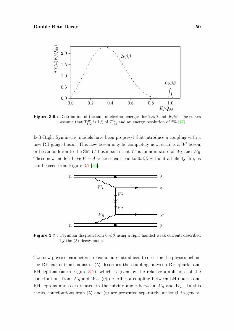
Double Beta Decay 50
dN/d
(E/Q
ββ)
2.0
1.5
1.0
0.5
0.00.0 0.2 0.4 0.6 0.8 1.0
2νββ
0νββ
E/Qββ
Figure 3.6.: Distribution of the sum of electron energies for 2νββ and 0νββ. The curvesassume that T 2ν
1/2 is 1% of T 0ν1/2 and an energy resolution of 2% [17].
Left-Right Symmetric models have been proposed that introduce a coupling with anew RH gauge boson. This new boson may be completely new, such as a W ′ boson,or be an addition to the SM W boson such that W is an admixture of WL and WR.These new models have V + A vertices can lead to 0νββ without a helicity flip, ascan be seen from Figure 3.7 [36].
�WR
WL
νR
νR
n
n
p
e−
e−
p
Figure 3.7.: Feynman diagram from 0νββ using a right handed weak current, describedby the 〈λ〉 decay mode.
Two new physics parameters are commonly introduced to describe the physics behindthe RH current mechanism. 〈λ〉 describes the coupling between RH quarks andRH leptons (as in Figure 3.7), which is given by the relative amplitudes of thecontributions from WR and WL. 〈η〉 describes a coupling between LH quarks andRH leptons and so is related to the mixing angle between WR and WL. In thisthesis, contributions from 〈λ〉 and 〈η〉 are presented separately, although in general
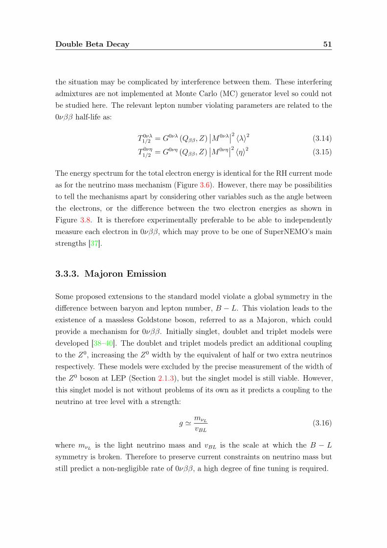
Double Beta Decay 51
the situation may be complicated by interference between them. These interferingadmixtures are not implemented at Monte Carlo (MC) generator level so could notbe studied here. The relevant lepton number violating parameters are related to the0νββ half-life as:
T 0νλ1/2 = G0νλ (Qββ, Z)
∣∣M0νλ∣∣2 〈λ〉2 (3.14)
T 0νη1/2 = G0νη (Qββ, Z)
∣∣M0νη∣∣2 〈η〉2 (3.15)
The energy spectrum for the total electron energy is identical for the RH current modeas for the neutrino mass mechanism (Figure 3.6). However, there may be possibilitiesto tell the mechanisms apart by considering other variables such as the angle betweenthe electrons, or the difference between the two electron energies as shown inFigure 3.8. It is therefore experimentally preferable to be able to independentlymeasure each electron in 0νββ, which may prove to be one of SuperNEMO’s mainstrengths [37].
3.3.3. Majoron Emission
Some proposed extensions to the standard model violate a global symmetry in thedifference between baryon and lepton number, B − L. This violation leads to theexistence of a massless Goldstone boson, referred to as a Majoron, which couldprovide a mechanism for 0νββ. Initially singlet, doublet and triplet models weredeveloped [38–40]. The doublet and triplet models predict an additional couplingto the Z0, increasing the Z0 width by the equivalent of half or two extra neutrinosrespectively. These models were excluded by the precise measurement of the width ofthe Z0 boson at LEP (Section 2.1.3), but the singlet model is still viable. However,this singlet model is not without problems of its own as it predicts a coupling to theneutrino at tree level with a strength:
g ' mνL
vBL(3.16)
where mνL is the light neutrino mass and vBL is the scale at which the B − L
symmetry is broken. Therefore to preserve current constraints on neutrino mass butstill predict a non-negligible rate of 0νββ, a high degree of fine tuning is required.
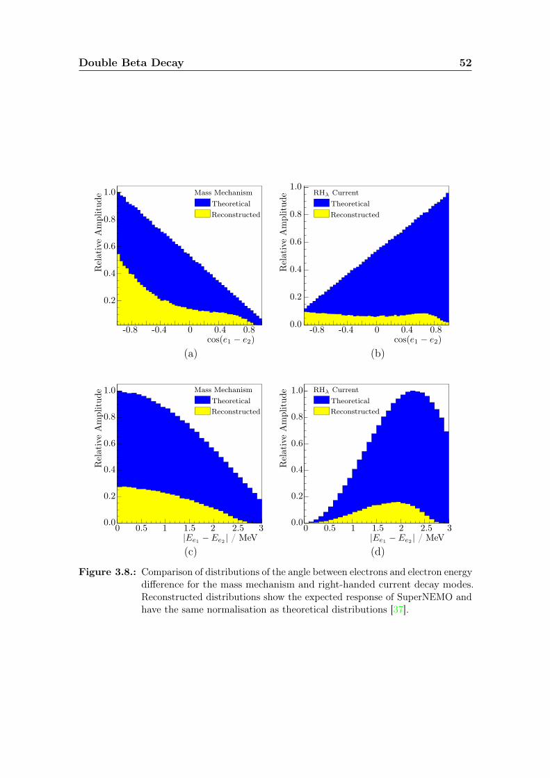
Double Beta Decay 52
cos(e1 − e2)(a)
cos(e1 − e2)(b)
|Ee1 − Ee2 | / MeV(c)
|Ee1 − Ee2 | / MeV(d)
Mass MechanismTheoreticalReconstructed
RHλ CurrentTheoreticalReconstructed
Mass MechanismTheoreticalReconstructed
RHλ CurrentTheoreticalReconstructed
Rel
ativ
eA
mpl
itud
e
Rel
ativ
eA
mpl
itud
e
Rel
ativ
eA
mpl
itud
e
Rel
ativ
eA
mpl
itud
e
0.2
0.4
0.6
0.8
1.0
0.2
0.4
0.6
0.8
1.0
0.0
0.2
0.4
0.6
0.8
1.0
0.0
0.2
0.4
0.6
0.8
1.0
0.0-0.8 -0.4 0 0.4 0.8 -0.8 -0.4 0 0.4 0.8
0 0.5 1 1.5 2 2.5 30 0.5 1 1.5 2 2.5 3
Figure 3.8.: Comparison of distributions of the angle between electrons and electron energydifference for the mass mechanism and right-handed current decay modes.Reconstructed distributions show the expected response of SuperNEMO andhave the same normalisation as theoretical distributions [37].

Double Beta Decay 53
To avoid such unnatural fine tuning, a range of new models have been developed,including decay modes where the Majoron can have lepton charge and need not bea Goldstone boson [41]. Furthermore, some of these new modes also predict theemission of two Majorons so that models now exist where 0νββ can proceed viaeither of the two processes:
(A,Z) → (A,Z + 2) + 2e− + χ0 (3.17)
(A,Z) → (A,Z + 2) + 2e− + 2χ0 (3.18)
The half-life of the process takes a similar form to previous decay modes, with anadditional coupling factor for modes with more than one Majoron:(
T 0νχ0
1/2
)−1= G0νχ0
(Qββ, Z)∣∣∣M0νχ0
∣∣∣2 〈gχ0〉2 for 0νββχ0 (3.19)(T 0νχ0
1/2
)−1= G0νχ0
(Qββ, Z)∣∣∣M0νχ0
∣∣∣2 〈gχ0〉4 for 0νββχ0χ0 (3.20)
where as before G0νχ0 is a phase space factor, M0νχ0 is a NME and 〈gχ0〉 defines thecoupling between the Majoron and the neutrino. As with the other 0νββ modes,the experimental signature for Majoron emission is identified by measuring thedistribution of total electron energy. However, unlike the mass mechanism and RHcurrent decay modes, there are now extra particles emitted in the decay, so that theenergy spectrum is no longer a monochromatic line, but a continuous spectrum. Theshape of the spectrum may be different for different Majoron models, and this isgoverned by a spectral index, n, which describes the dependence of the phase spacefactor on the energy of the Majoron(s):
G0νχ0 ∝ (Qββ − (Ee1 + Ee2))n (3.21)
where Ee is the energy of an emitted electron. For the models presented herein,allowed values for n are 1, 2, 3 and 7, and these give four distinct energy spectra asshown in Figure 3.9.
The ten different Majoron models that are most commonly discussed are presentedin Table 3.1. These are grouped into lepton number violating (I) and lepton numberconserving (II) modes and are presented along with their most important properties.The names of the models follow the conventions dictated in [41].

Double Beta Decay 54
Ee1 + Ee2 / MeV
Arbitrary
units n = 1
n = 2
n = 3
n = 7
0νββχ0χ0 2νββ0νββχ0χ0
0νββχ0 0νββ0νββχ0
0νββχ0
0.0
0.2
0.4
0.6
0.8
1.0
1.2
1.4
1.6
1.8
2.0
0 500 1000 1500 2000 2500 3000 3500
Figure 3.9.: Energy spectra for 2νββ and 0νββ, along with four different Majoron decaymodes with spectral indices 1, 2, 3 and 7 [42].
Model Decay Mode Goldstone L n Matrix Element
IB 0νββχ0 7 0 1 MF −MGT
IC 0νββχ0 3 0 1 MF −MGT
ID 0νββχ0χ0 7 0 3 MFω2 −MGTω2
IE 0νββχ0χ0 3 0 3 MFω2 −MGTω2
IIB 0νββχ0 7 -2 1 MF −MGT
IIC 0νββχ0 3 -2 3 MCR
IID 0νββχ0χ0 7 -1 3 MFω2 −MGTω2
IIE 0νββχ0χ0 3 -1 7 MFω2 −MGTω2
IIF 0νββχ0 Gauge boson -2 3 MCR
Bulk 0νββχ0 Bulk field 0 2 −
Table 3.1.: Ten different Majoron models and their main properties [43]. The modelnames follow [41], with IIF from [44] and the Bulk model from [45].
3.4. Nuclear Matrix Elements
Experiments searching for 0νββ produce a limit on the half-life of the decay, T 0ν1/2.
To convert this to the physics parameter of interest (usually 〈mββ〉), the appropriate
Double Beta Decay 55
nuclear matrix element (NME) must be used (Equation (3.11)). Therefore theaccuracy with which NMEs can be calculated directly impacts the interpretation ofany experimental result. NME calculations must be performed using the tools ofnuclear structure theory and since there is no other observable that can be directlylinked to the magnitude of M0ν , the results are necessarily model-dependent. Thesitutation is further complicated as the ground state and many different excited statesof open-shell nuclei with complicated nuclear structures must be considered [46].
To date, five different techniques have been applied to the problem and in each ofthese frameworks, two different stages are followed. Firstly, a many-body Hamiltonianis created which describes the interactions between nucleons and encompasses knownnuclear physics and the physics mechanism behind 0νββ. Then, a mean field isintroduced which supplies information about the nuclear structure and residualinteractions. The complexity of the calculations mean that some approximationand/or truncation is always needed, and it is in these simplifying assumptions thatthe different techniques vary.
In this section, the five calculational techniques are briefly discussed and a comparisonof the results from each technique is presented to give an overview of the remaininglevel of uncertainty (Section 3.4.6).
3.4.1. Interacting Shell Model
The interacting shell model (ISM) considers only a limited number of nuclear orbitalsclose to the Fermi level, but all possible correlations for these orbitals are included.This full treatment of the correlations tends to reduce the values of the NMEs,however the ISM may overestimate this effect due to the limited number of orbitsin the valence space which causes a similar reduction. Despite being technicallychallenging, the ISM has been used to perform calculations for several nuclei. Theresults do not vary significantly between them (with the exception of doubly-magic48Ca). It is known that the ISM does not treat deformed nuclei, such as 150Nd,correctly, and it is commonly accepted that the ISM produces more reliable resultsfor smaller nuclei such as 48Ca, 76Ge and 82Se.
Double Beta Decay 56
3.4.2. Quasiparticle Random Phase Approximation
The quasiparticle random phase approximation (QRPA) takes a constrasting approachto the ISM. In this method, the number of different nuclear orbitals is greatlyincreased, but the complexity of the interactions between nucleons must be reducedaccordingly. To calculate the NMEs, the initial and final nuclear states are connectedvia many virtual intermediate collective states. Recently, it has been shown thatthe uncertainties associated with QRPA calculations can be significantly reducedif the gpp parameter, which parameterises proton-proton interactions, is tuned toreproduce 2νββ data. The QRPA is, to some degree, complementary to the ISM,and produces more reliable results for larger nuclei.
3.4.3. Interacting Boson Model
In the interacting boson model (IBM), the low-lying nuclear states are modelledas bosons. These bosons are restricted to angular momentum states of L = 0 (sboson) or L = 2 (d boson). Therefore only 0+ and 2+ neutron pairs can turn intotwo protons in 0νββ. The IBM is similar in form to the ISM and therefore has thesame advantages, but suffers from similar short-comings.
3.4.4. Projected Hartree-Fock-Bogoluibov Method
In the projected Hartree-Fock-Bogoluibov (PHFB) method, nuclear wave functionswith good particle number and angular momentum are constructed by projectionon the HFB wavefunctions. The nuclear Hamiltonian is simplified to include onlyquadrupole interactions and only neutron pairs with even momentum and positiveparity (0+, 2+, 4+ etc.) can participate in 0νββ, although non-0+ pairs are heavilysuppressed compared to other calculations. The PHFB uses fewer model dependentparameters to calculate NMEs, although may suffer from a certain degree of over-simplification.
Double Beta Decay 57
3.4.5. Energy Density Functional Method
The energy density functional (EDF) method is considered to be an improvementwith respect to the PHFB. The inter-nucleon interaction is modified to reproducethe Gogny interaction and the single particle basis is enlarged.
3.4.6. Comparison of different NME calculations
As described above, each method of NME calculations makes differing assumptionsin order to simplify the calculation. To understand the effect of each of theseassumptions and the associated systematic error with the resulting NMEs, it ishelpful to compare the NME results for each method.
In the conversion from an experimental half-life to 〈mββ〉 (Equation (3.12)), thephase space factor, G0ν , enters into the calculation alongside the NME. This factorexhibits a proportionality given by
G0ν ∼ g4AR2A
(3.22)
where gA is the ratio of the vector and axial-vector couplings and RA is the atomicradius, commonly parameterised as r0A1/3 [47]. Unfortunately, mostly for historicalreasons, different NME calculations are performed with different values of gA and r0 sothat the phase space factors, and therefore NME results, are not directly comparable.Common values for gA are either 1.0 or 1.25 and for r0 either 1.1 or 1.2 fm.
Therefore for a meaningful comparison, the NME results should be adjusted to usethe same values of gA and r0. Results for 11 isotopes of experimental interest, withappropriate adjustments made, are shown graphically in Figure 3.10.
In general, there is disagreement across the range of methods for any given isotope upto a factor 2-3. For reasons discussed above (Section 3.4.1), the ISM produces resultsthat are at the lower end of this range, but there does not seem to be a particularmethod producing high NMEs. It can also be seen that the ISM predicts similarvalues across all the different nuclei since only the outermost shells are considered.
For some isotopes, notably 130Te and 128Te, there is good agreement across allcalculations (except for the ISM as previously explained). Additionally, the QRPA(T)
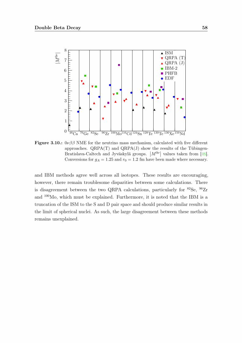
Double Beta Decay 58
48Ca 76Ge 82Se 96Zr 100Mo116Cd 124Sn 128Te 130Te 136Xe 150Nd
|M0ν|
0
1
2
3
4
5
6
7
8 ISMQRPA (T)QRPA (J)IBM-2PHFBEDF
Figure 3.10.: 0νββ NME for the neutrino mass mechanism, calculated with five differentapproaches. QRPA(T) and QRPA(J) show the results of the Tübingen-Bratislava-Caltech and Jyväskylä groups.
∣∣M0ν∣∣ values taken from [46].
Conversions for gA = 1.25 and r0 = 1.2 fm have been made where necessary.
and IBM methods agree well across all isotopes. These results are encouraging,however, there remain troublesome disparities between some calculations. Thereis disagreement between the two QRPA calculations, particularly for 82Se, 96Zrand 100Mo, which must be explained. Furthermore, it is noted that the IBM is atruncation of the ISM to the S and D pair space and should produce similar results inthe limit of spherical nuclei. As such, the large disagreement between these methodsremains unexplained.
Chapter 4.
Double Beta Decay Experiments
4.1. Detector Design Considerations
Double beta decay experiments search for a small signal from 0νββ on top ofbackgrounds from natural radioactivity and 2νββ. It is possible to approximatelyparametrise the expected half-life sensitivity of any given experiment using thefollowing expression [17]:
T 0ν1/2 >
4.16× 1026 yrnσ
(εaMt
Z
)√1
NB
(4.1)
where
• T 0ν1/2 is the half-life sensitivity to 0νββ in years
• nσ is the number of standard deviations for a given confidence level (90% CLcorresponds to nσ = 1.64)
• ε is the event detection and identification efficiency
• a is the isotopic abundance of the 0νββ source isotope in the source mass
• Z is the molecular weight of the source isotope
• Mt is the total exposure of the experiment in kg yr
• NB is the number of expected background events for the exposure
59
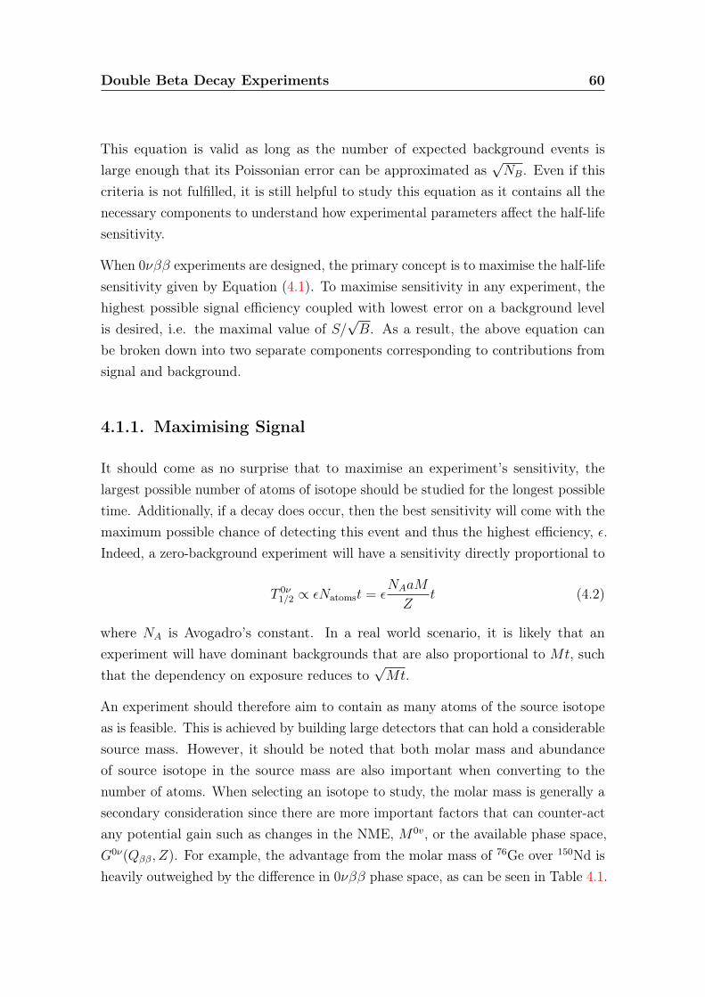
Double Beta Decay Experiments 60
This equation is valid as long as the number of expected background events islarge enough that its Poissonian error can be approximated as
√NB. Even if this
criteria is not fulfilled, it is still helpful to study this equation as it contains all thenecessary components to understand how experimental parameters affect the half-lifesensitivity.
When 0νββ experiments are designed, the primary concept is to maximise the half-lifesensitivity given by Equation (4.1). To maximise sensitivity in any experiment, thehighest possible signal efficiency coupled with lowest error on a background levelis desired, i.e. the maximal value of S/
√B. As a result, the above equation can
be broken down into two separate components corresponding to contributions fromsignal and background.
4.1.1. Maximising Signal
It should come as no surprise that to maximise an experiment’s sensitivity, thelargest possible number of atoms of isotope should be studied for the longest possibletime. Additionally, if a decay does occur, then the best sensitivity will come with themaximum possible chance of detecting this event and thus the highest efficiency, ε.Indeed, a zero-background experiment will have a sensitivity directly proportional to
T 0ν1/2 ∝ εNatomst = ε
NAaM
Zt (4.2)
where NA is Avogadro’s constant. In a real world scenario, it is likely that anexperiment will have dominant backgrounds that are also proportional to Mt, suchthat the dependency on exposure reduces to
√Mt.
An experiment should therefore aim to contain as many atoms of the source isotopeas is feasible. This is achieved by building large detectors that can hold a considerablesource mass. However, it should be noted that both molar mass and abundanceof source isotope in the source mass are also important when converting to thenumber of atoms. When selecting an isotope to study, the molar mass is generally asecondary consideration since there are more important factors that can counter-actany potential gain such as changes in the NME, M0v, or the available phase space,G0ν(Qββ, Z). For example, the advantage from the molar mass of 76Ge over 150Nd isheavily outweighed by the difference in 0νββ phase space, as can be seen in Table 4.1.
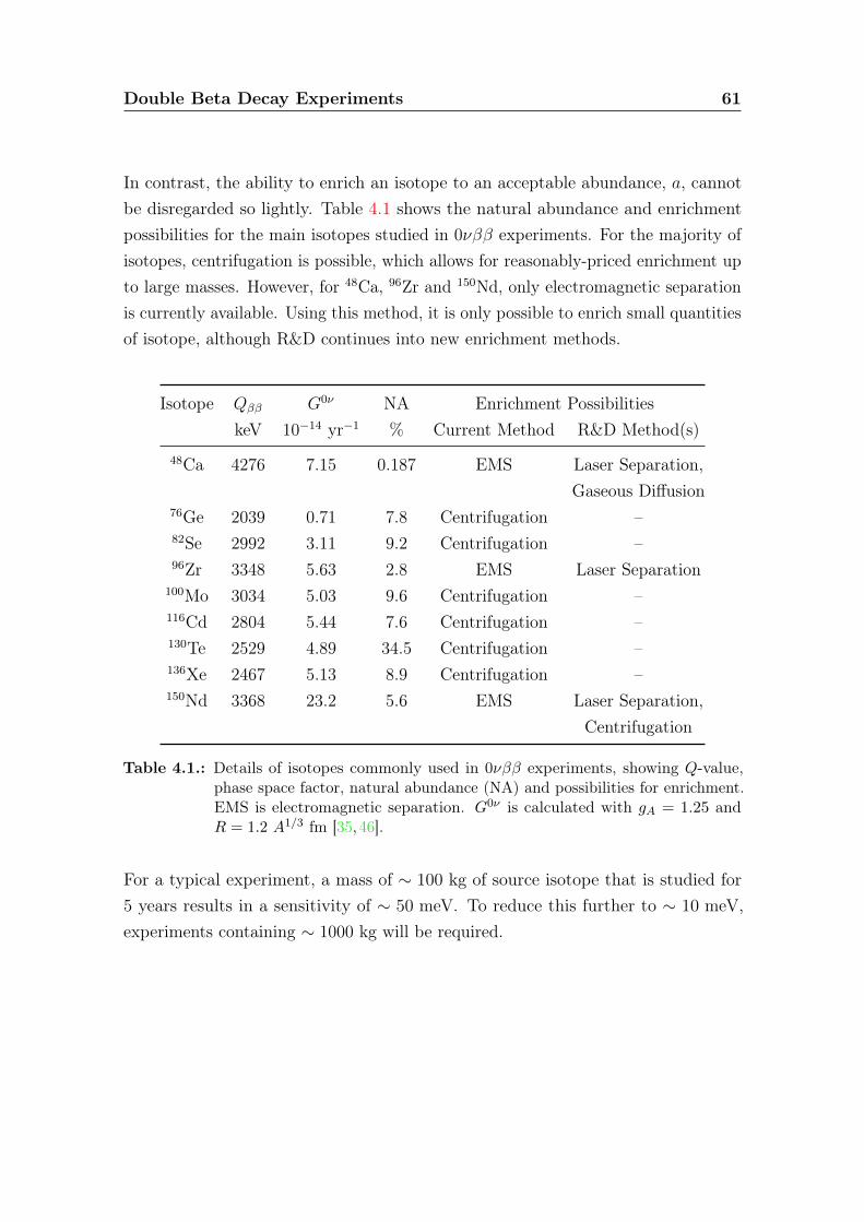
Double Beta Decay Experiments 61
In contrast, the ability to enrich an isotope to an acceptable abundance, a, cannotbe disregarded so lightly. Table 4.1 shows the natural abundance and enrichmentpossibilities for the main isotopes studied in 0νββ experiments. For the majority ofisotopes, centrifugation is possible, which allows for reasonably-priced enrichment upto large masses. However, for 48Ca, 96Zr and 150Nd, only electromagnetic separationis currently available. Using this method, it is only possible to enrich small quantitiesof isotope, although R&D continues into new enrichment methods.
Isotope Qββ G0ν NA Enrichment PossibilitieskeV 10−14 yr−1 % Current Method R&D Method(s)
48Ca 4276 7.15 0.187 EMS Laser Separation,Gaseous Diffusion
76Ge 2039 0.71 7.8 Centrifugation –82Se 2992 3.11 9.2 Centrifugation –96Zr 3348 5.63 2.8 EMS Laser Separation
100Mo 3034 5.03 9.6 Centrifugation –116Cd 2804 5.44 7.6 Centrifugation –130Te 2529 4.89 34.5 Centrifugation –136Xe 2467 5.13 8.9 Centrifugation –150Nd 3368 23.2 5.6 EMS Laser Separation,
Centrifugation
Table 4.1.: Details of isotopes commonly used in 0νββ experiments, showing Q-value,phase space factor, natural abundance (NA) and possibilities for enrichment.EMS is electromagnetic separation. G0ν is calculated with gA = 1.25 andR = 1.2 A1/3 fm [35,46].
For a typical experiment, a mass of ∼ 100 kg of source isotope that is studied for5 years results in a sensitivity of ∼ 50 meV. To reduce this further to ∼ 10 meV,experiments containing ∼ 1000 kg will be required.
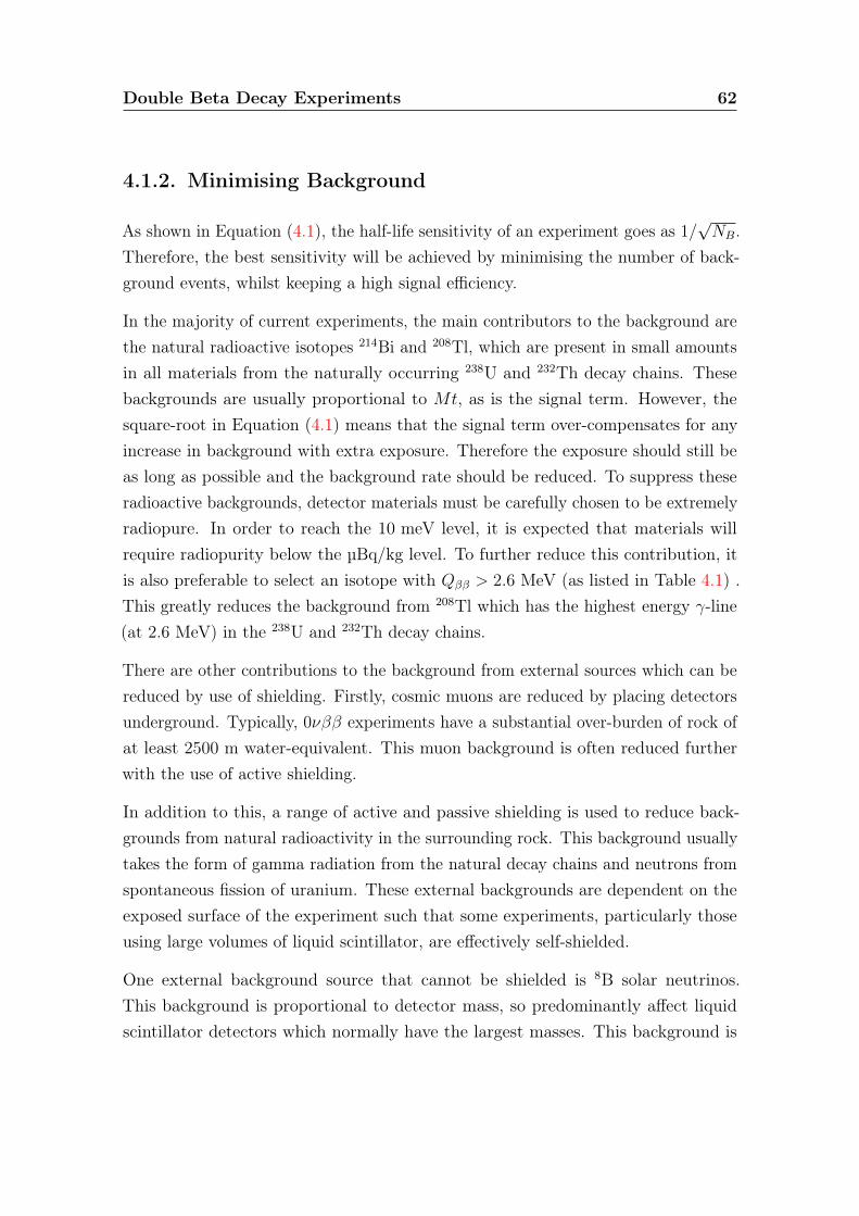
Double Beta Decay Experiments 62
4.1.2. Minimising Background
As shown in Equation (4.1), the half-life sensitivity of an experiment goes as 1/√NB.
Therefore, the best sensitivity will be achieved by minimising the number of back-ground events, whilst keeping a high signal efficiency.
In the majority of current experiments, the main contributors to the background arethe natural radioactive isotopes 214Bi and 208Tl, which are present in small amountsin all materials from the naturally occurring 238U and 232Th decay chains. Thesebackgrounds are usually proportional to Mt, as is the signal term. However, thesquare-root in Equation (4.1) means that the signal term over-compensates for anyincrease in background with extra exposure. Therefore the exposure should still beas long as possible and the background rate should be reduced. To suppress theseradioactive backgrounds, detector materials must be carefully chosen to be extremelyradiopure. In order to reach the 10 meV level, it is expected that materials willrequire radiopurity below the µBq/kg level. To further reduce this contribution, itis also preferable to select an isotope with Qββ > 2.6 MeV (as listed in Table 4.1) .This greatly reduces the background from 208Tl which has the highest energy γ-line(at 2.6 MeV) in the 238U and 232Th decay chains.
There are other contributions to the background from external sources which can bereduced by use of shielding. Firstly, cosmic muons are reduced by placing detectorsunderground. Typically, 0νββ experiments have a substantial over-burden of rock ofat least 2500 m water-equivalent. This muon background is often reduced furtherwith the use of active shielding.
In addition to this, a range of active and passive shielding is used to reduce back-grounds from natural radioactivity in the surrounding rock. This background usuallytakes the form of gamma radiation from the natural decay chains and neutrons fromspontaneous fission of uranium. These external backgrounds are dependent on theexposed surface of the experiment such that some experiments, particularly thoseusing large volumes of liquid scintillator, are effectively self-shielded.
One external background source that cannot be shielded is 8B solar neutrinos.This background is proportional to detector mass, so predominantly affect liquidscintillator detectors which normally have the largest masses. This background is
Double Beta Decay Experiments 63
not currently at a sensitivity-limiting level, but may become a significant problemfor future experiments.
One of the most effective methods to reduce contributions to the background is thedevelopment of analysis techniques that distinguish between backgrounds and signal.These are applied in a number of different ways, ranging from full event reconstructionto simple algorithms to differentiate between electron and alpha particles.
As well as reducing backgrounds, it is important to design an experiment with goodenergy resolution so that the signal window can also be reduced. Since the signal ismono-energetic, the window can in principle be very narrow, but in practice is limitedby the energy resolution of the detector. Since many of the background contributionsare approximately constant in energy over a narrow range, a reduction in the signalwindow results in significant reduction of total background. Furthermore, it should benoted that even if contributions from natural radioactivity and external backgroundscan be reduced to negligible levels, there is an irreducible background from the tailof the 2νββ process which is only suppressed by improving energy resolution.
4.2. Detector Technologies
In general, signal or background contributions can be improved at the cost of reducingthe other. For example, it is very difficult to build a tonne-scale detector whilstkeeping very low backgrounds from natural radioactive contaminants. As a result ofthis trade-off, there are many different plausible experimental designs and numerousdetector technologies, each of which has advantages and disadvantages. In thissection, the five main technologies will be briefly described along with notableexperiments and their main results. A comparative overview of 2νββ and 0νββresults is presented in Section 4.3.
4.2.1. Semiconductor Experiments
Semiconductor experiments use a 0νββ candidate that can be used as a semiconductor,such as 76Ge, and place it between two electrodes to form a diode. Nuclear decays (orincident radiation) create electron-hole pairs in the material. Some of the electrons
Double Beta Decay Experiments 64
are transferred from the valence band to the conduction band and are migrated tothe electrodes with an applied potential where they are measured.
Germanium can be readily enriched to produce large crystals which have a depletionlayer of a few centimetres, allowing total absorption of gamma rays up to ∼ 5 MeV.Germanium detectors of this size must necessarily be pure and are often referredto as high-purity germanium (HPGe) detectors. HPGe detectors must be operatedat cryogenic temperatures to reduce electronic noise, but in this configuration theycan achieve truly excellent energy resolution of ∼ 0.3% (FWHM). For many years,HPGe detectors provided the strongest limits on 〈mββ〉 with the results from theHeidelberg-Moscow (H-M) and IGEX experiments.
• Heidelberg-Moscow (H-M) ran from 1990 to 2003, with five HPGe detectorsenriched to 86% in 76Ge. For a total exposure of 35.5 kg yr, a limit of T 0ν
1/2 >
1.9× 1025 yr was obtained [48], corresponding to 〈mββ〉 < 250− 500 meV.
In this result and those following, a range of values for 〈mββ〉 is given. This rangereflects the variation in 〈mββ〉 as a result of uncertainties in NME calculations.
In 2001, a subset of the H-M collaboration claimed a discovery of a 0νββsignal using the data from the spectrum shown in Figure 4.1 [49]. For anexposure of 71.7 kg yr, a half-life of T 0ν
1/2 = 1.19+2.99−0.50(3σ)× 1025 yr was claimed,
corresponding to 〈mββ〉 = 100−900 meV. This so called Klapdor-Kleingrothaus(KK) claim has proved controversial due to the presence of an unidentified peakat 2030 keV, the wrong ratio of amplitudes of the nearby 214Bi peaks, spuriouspeak identification and claims that the background and systematic uncertaintyof the experiment are underestimated [50].
Three experiments that have recently started collecting data are becomingsensitive to 〈mββ〉 at the level of the KK claim and the initial results stronglydisfavour the claim (Section 4.3).
• IGEX was a similar experiment to H-M, with six HPGe detectors enriched to86% in 76Ge containing 2.0 kg of source isotope. 8.9 kg yr of data produced a half-life limit of T 0ν
1/2 > 1.57× 1025 yr [51], corresponding to 〈mββ〉 < 280− 550 meV.
A new generation of HPGe experiments, namely GERDA and MAJORANA, arenow building on the successes of the H-M and IGEX experiments:
Double Beta Decay Experiments 65
2000 2010 2020 2030 2040 2050 20600
5
10
15
20
25
Energy / keV
Cou
nts/keV
214Bi214Bi
Unidentified
Claimed 0νββSignal
Figure 4.1.: Energy spectrum from the H-M experiment, from which a controversial claimof discovery of 0νββ has been made. Alongside the claimed 0νββ peak at2309 keV, an unidentified peak at 2030 keV and four 214Bi peaks can beseen [49].

Double Beta Decay Experiments 66
• GERDA consists of a series of HPGe detectors immersed in a 64 m3 cryostatfilled with liquid argon (LAr). This LAr acts both as a coolant and as shieldingfrom external backgrounds. This passive shielding is supplemented by 3 mof water shielding instrumented with PMTs to detect Cherenkov light fromcosmic muons. The experiment is divided into two phases named GERDA-Iand GERDA-II.
GERDA-I used eight reprocessed HPGe detectors from H-M and IGEX, totalling17.7 kg, along with 3.6 kg of new Broad Energy Ge (BEGe) detectors. Data-taking ran from Nov 2011 - May 2013, and no 0νββ signal has been observed(Figure 4.2). Despite the shorter running time, a much lower background meansthat a stronger limit can be set than that of H-M or IGEX. The resultinghalf-life of T 0ν
1/2 > 2.1× 1025 yr corresponds to 〈mββ〉 < 240− 480 meV [52].
Energy / keV
1900 1950 2000 2050 2100 2150 2200
Cou
nts/2keV
0
2
4
6
8
214B
i220
4ke
V
1930
keV
2190
keV
2039
keV
Qββ
Background Interpolation
2025 2030 2035 2040 2045 2050 2055 2060
Cou
nts/keV
0
1
2
3 0νββ KK Claim0νββ GERDA 90% CL
Figure 4.2.: The energy spectrum from GERDA-I with pulse-shape discrimination applied.The top panel shows the region used for background interpolation and thebottom shows the region around Qββ. The 0νββ signals for the 90% CLfrom GERDA-I and the KK claim are also shown [52]
The next phase of the experiment, GERDA-II, involves the addition of a further20 kg of enriched Germanium with an increase in sensitivity to reach the50− 100 meV level [53].
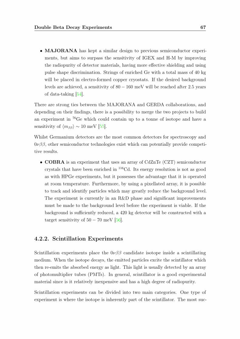
Double Beta Decay Experiments 67
• MAJORANA has kept a similar design to previous semiconductor experi-ments, but aims to surpass the sensitivity of IGEX and H-M by improvingthe radiopurity of detector materials, having more effective shielding and usingpulse shape discrimination. Strings of enriched Ge with a total mass of 40 kgwill be placed in electro-formed copper cryostats. If the desired backgroundlevels are achieved, a sensitivity of 80− 160 meV will be reached after 2.5 yearsof data-taking [54].
There are strong ties between the MAJORANA and GERDA collaborations, anddepending on their findings, there is a possibility to merge the two projects to buildan experiment in 76Ge which could contain up to a tonne of isotope and have asensitivity of 〈mββ〉 ∼ 10 meV [55].
Whilst Germanium detectors are the most common detectors for spectroscopy and0νββ, other semiconductor technologies exist which can potentially provide competi-tive results.
• COBRA is an experiment that uses an array of CdZnTe (CZT) semiconductorcrystals that have been enriched in 116Cd. Its energy resolution is not as goodas with HPGe experiments, but it possesses the advantage that it is operatedat room temperature. Furthermore, by using a pixellated array, it is possibleto track and identify particles which may greatly reduce the background level.The experiment is currently in an R&D phase and significant improvementsmust be made to the background level before the experiment is viable. If thebackground is sufficiently reduced, a 420 kg detector will be constructed with atarget sensitivity of 50− 70 meV [56].
4.2.2. Scintillation Experiments
Scintillation experiments place the 0νββ candidate isotope inside a scintillatingmedium. When the isotope decays, the emitted particles excite the scintillator whichthen re-emits the absorbed energy as light. This light is usually detected by an arrayof photomultiplier tubes (PMTs). In general, scintillator is a good experimentalmaterial since is it relatively inexpensive and has a high degree of radiopurity.
Scintillation experiments can be divided into two main categories. One type ofexperiment is where the isotope is inherently part of the scintillator. The most suc-
Double Beta Decay Experiments 68
cessful experiments of this type, for example ELEGANT VI, have crystal scintillatorscontaining 48Ca.
• ELEGANT VI studied 23 CaF2(Eu) crystal scintillators with a total massof 6.6 kg and 7.6 g of 48Ca. These crystals were completely surrounded by anactive veto to reduce background. A total exposure of 0.015 kg yr produced ahalf-life limit of T 0ν
1/2 > 5.8× 10²² yr or 〈mββ〉 < 3.5− 22 eV [57].
• CANDLES III evolved from ELEGANT VI. 305 CaF2 crystals are used thathave a total mass of 305 kg and 300 g of 48Ca. These crystals are surroundedby liquid scintillator which acts as active shielding and removes the need fordoping of the crystals. The experiment is currently taking data and a sensitivityto 〈mββ〉 of 0.5 eV is expected. If improvements in enrichment technologyare realised, then the scale of the experiment will be increased by an order ofmagnitude to contain ∼ 3 kg of 48Ca and achieve a sensitivity of 50 meV [58].
An alternative technology is to use a large volume of liquid scintillator, into whicha 0νββ isotope is dissolved. Experiments of this type commonly suffer from poorenergy resolution. However, this is compensated by the ability to study relativelylarge masses of isotopes such as 136Xe, 130Te or 150Nd without difficulty. Often, thelarge volume of scintillator comes with the added bonus that it provides a highlevel of self-shielding. The KamLAND-Zen experiment is studying liquid scintillatorloaded with 136Xe, whilst the SNO+ experiment has chosen 130Te.
• KamLAND-Zen is an experiment that utilises the KamLAND detector, whichwas originally built to study neutrino oscillations. In KamLAND-Zen, 13 tonnesof xenon-loaded liquid scintillator is suspended in a nylon balloon at the centreof the KamLAND detector. This balloon is surrounded by 1000 tonnes of liquidscintillator which strongly suppresses backgrounds. The scintillation light isdetected by 2000 PMTs and the whole assembly is surrounded by a 3200 tonnewater-Cherenkov detector to veto cosmic-ray muons. The experiment contains300 kg of 136Xe and has achieved an exposure of 89.5 kg yr. From the resultingspectrum (Figure 4.3), it can be seen that there is a considerable backgroundlevel in the region of Qββ (2.46 MeV). This background is thought to becaused by 110mAg either as a result of cosmogenic activation or the Fukushimanuclear disaster. Despite this unexpected background, KamLAND-Zen stillprovides the strongest single constraint on 〈mββ〉, by measuring a half-life
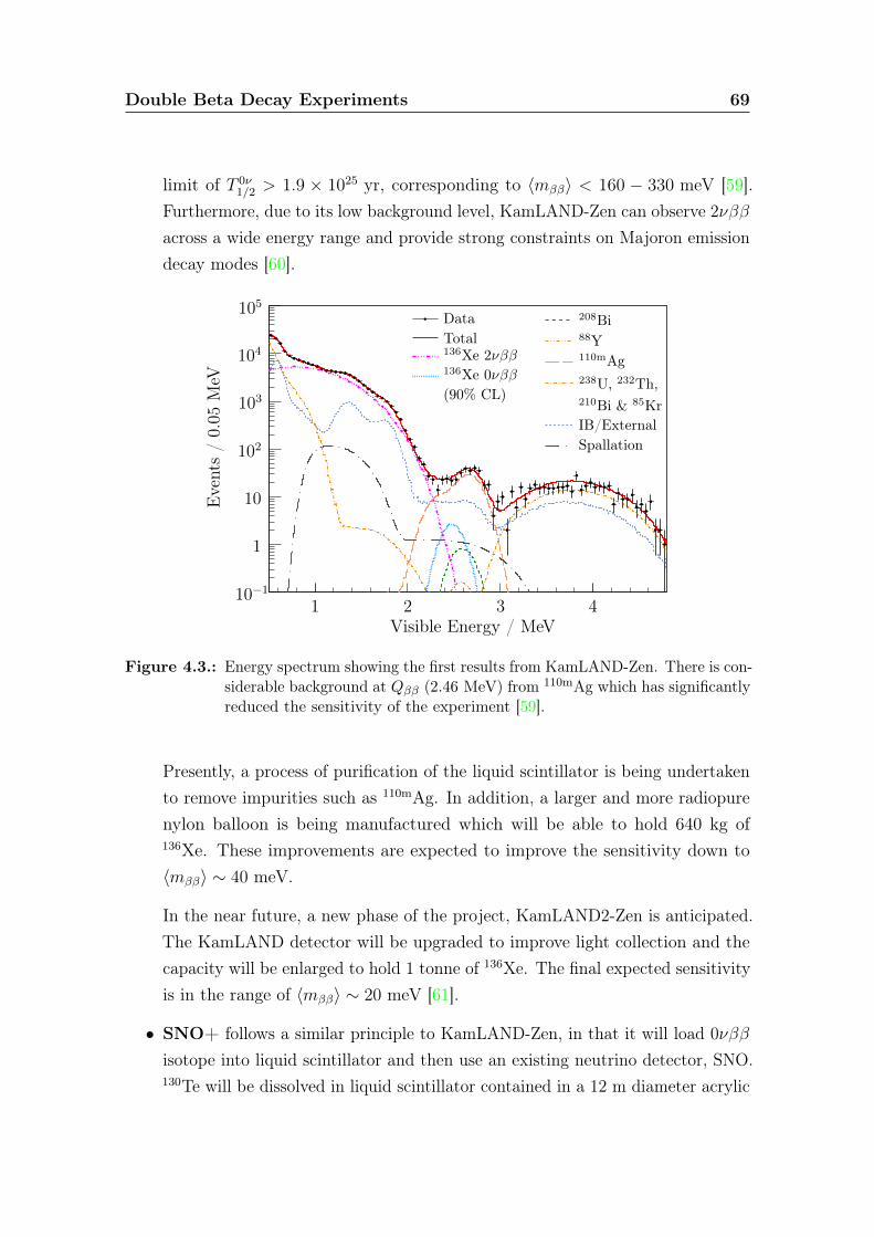
Double Beta Decay Experiments 69
limit of T 0ν1/2 > 1.9 × 1025 yr, corresponding to 〈mββ〉 < 160 − 330 meV [59].
Furthermore, due to its low background level, KamLAND-Zen can observe 2νββacross a wide energy range and provide strong constraints on Majoron emissiondecay modes [60].
Visible Energy / MeV
Events/0.05
MeV
10−1
1
10
102
103
104
105208Bi88Y110mAg
Spallation
DataTotal136Xe 2νββ136Xe 0νββ(90% CL)
238U, 232Th,210Bi & 85KrIB/External
1 2 3 4
Figure 4.3.: Energy spectrum showing the first results from KamLAND-Zen. There is con-siderable background at Qββ (2.46 MeV) from 110mAg which has significantlyreduced the sensitivity of the experiment [59].
Presently, a process of purification of the liquid scintillator is being undertakento remove impurities such as 110mAg. In addition, a larger and more radiopurenylon balloon is being manufactured which will be able to hold 640 kg of136Xe. These improvements are expected to improve the sensitivity down to〈mββ〉 ∼ 40 meV.
In the near future, a new phase of the project, KamLAND2-Zen is anticipated.The KamLAND detector will be upgraded to improve light collection and thecapacity will be enlarged to hold 1 tonne of 136Xe. The final expected sensitivityis in the range of 〈mββ〉 ∼ 20 meV [61].
• SNO+ follows a similar principle to KamLAND-Zen, in that it will load 0νββisotope into liquid scintillator and then use an existing neutrino detector, SNO.130Te will be dissolved in liquid scintillator contained in a 12 m diameter acrylic
Double Beta Decay Experiments 70
sphere. This acrylic sphere is shielded by a water bath and instrumented with9500 PMTs. In an initial phase, tellurium will be loaded at 0.3%, giving 800 kgof 130Te and a sensitivity of 〈mββ〉 < 50 − 100 meV. A second phase is thenplanned, with 3% loading and 8000 kg of 130Te. This will allow SNO+ to reachthe level of 〈mββ〉 < 20− 40 meV [62].
4.2.3. Bolometer Experiments
Bolometer experiments measure small increases in temperature caused by the absorp-tion of energy from radioactive decays. The increase in temperature of a materialis inferred by changes in its electrical properties. At low temperatures, the heatcapacity of material at temperature T is proportional to T 3. Therefore to measurea large temperature increase and improve the resolution of the bolometer, thesedetectors are typically operated at temperatures of 10 mK and below.
As a rule, bolometer experiments have good energy resolution. However, if onlybolometry is used, as in the CUORICINO and CUORE experiments, particle identi-fication is challenging. This can pose problems in reducing the background to therequired levels.
• CUORICINO was a tower array of 62 TeO2 crystals that operated between2003 and 2008. The array was placed inside a dilution refrigerator to maintaincryogenic temperatures and surrounded by passive shielding. In total, 507 gof 130Te was contained within the crystals and a total exposure of 19.75 kg yrwas studied. A half-life limit of T 0ν
1/2 > 2.8× 1024 yr was set, such that 〈mββ〉 <300− 700 meV [63].
• CUORE will build on the technology of CUORICINO, increasing the numberof TeO2 crystals to 988 and the mass of 130Te to 204 kg. A prototype detector,CUORE-0, containing 52 crystals and 10.7 kg of 130Te is currently taking data.This is re-using the cryostat from CUORICINO and consequently has a higherbackground than that anticipated for CUORE. The expected sensitivities forCUORE-0 and CUORE are T 0ν
1/2 > 8× 1024 yr (〈mββ〉 < 180− 420 meV) andT 0ν1/2 > 2.1× 1026 yr (〈mββ〉 < 35− 82 meV) respectively [64].
In order to reduce the background level of bolometric experiments, it may bepreferential to use a bolometric crystal that also acts as a scintillator. In this
Double Beta Decay Experiments 71
scenario, a small fraction of the energy deposited in the crystal is released as lightwhich can be used to significantly reduce backgrounds from surface contamination.
• LUCIFER will use crystals of either ZnSe, CdWO4 or ZnMoO4 as scintillatingbolometric crystals. The most sensitive proposed configuration is to use ZnSecrystals in an array of tens of bolometers contained within the same cryostatin a similar fashion to CUORE. In addition, an extra bolometer will act as alight detector for the scintillation light. The crystals will contain ∼ 18 kg of82Se and have a sensitivity of 〈mββ〉 ∼ 60 meV [65].
4.2.4. Time Projection Chamber Experiments
Time projection chamber (TPC) experiments are able to track the path of an electronas it passes through a detector. This allows an experiment to search for two electronsfrom a common vertex, which greatly reduces background contributions. In a TPC,electrons ionise the detector medium and an electric field is applied to drift theionisation electrons to a collection device. The level of ionisation is proportional tothe energy deposited by an electron, so that the electron energy is also measured.As a result, the density of the detector medium is usually selected such that 0νββevents would be entirely contained.
Whilst it is possible to perform a 0νββ search using TPC technology alone, currentlythe most successful TPC experiments use a detector medium that is also a scintillator.These experiments therefore have a restricted choice of isotopes that may be used.The most promising scintillating-TPC experiments are EXO and NEXT which bothsearch for 0νββ in 136Xe, utilising the scintillating properties of xenon.
• EXO-200 is a cylindrical homogeneous TPC that is filled with liquid xenonenriched to 80% in 136Xe and observing a total mass of 80 kg. The TPC issymmetric about a cathode grid at its centre and at each end there are planesof wires and an array of avalanche photodiodes. The wires apply an electricfield and read out ionisation signals and the photodiodes detect scintillationlight. EXO-200 began taking data in 2011 and its initial results show that thetarget experimental parameters have been reached. No signal has been observedin an exposure of 32.5 kg yr (Figure 4.4), and a limit of T 0ν
1/2 > 1.6× 1025 yr,corresponding to 〈mββ〉 < 170− 360 meV, has been set [66].
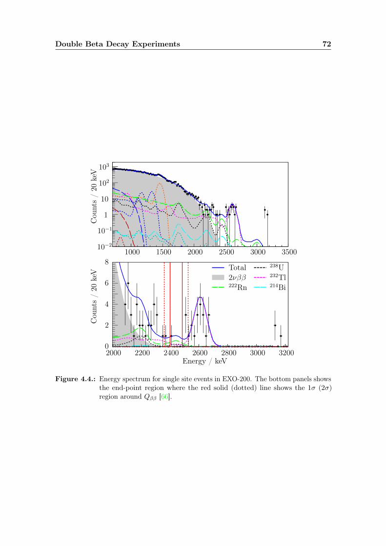
Double Beta Decay Experiments 72
Cou
nts/20
keV
10−2
10−1
1
10
102
103
Energy / keV
Cou
nts/20
keV Total
2νββ222Rn
238U232Tl214Bi
1000 1500 2000 2500 3000 35008
6
4
2
02000 2200 2400 2600 2800 3000 3200
Figure 4.4.: Energy spectrum for single site events in EXO-200. The bottom panels showsthe end-point region where the red solid (dotted) line shows the 1σ (2σ)region around Qββ [66].
Double Beta Decay Experiments 73
EXO-200 will continue running and aims to achieve a final sensitivity of T 0ν1/2 >
6.4× 1025 yr (〈mββ〉 < 85− 180 meV), before being superseded by EXO [67].The EXO experiment will attempt to scale similar technology to EXO-200 up tothe tonne scale. In addition, a novel technique to tag the barium ions which aredaughters of 136Xe decay may significantly reduce the background level. Thetarget sensitivity for EXO is T 0ν
1/2 > 2× 1027 yr or 〈mββ〉 < 15− 32 meV [67].
• NEXT-100 follows similar ideas to EXO, using both scintillation and ionisationsignals. However, it differs in the use of gaseous xenon at high pressure ratherthan liquid xenon. At one end of the TPC, an array of PMTs measuresthe energy resolution and at the other end the ionisation signal is convertedinto electroluminescent signals and read by silicon photomultipliers. Thisconfiguration allows energy resolution better than 1% whilst maintaining theability to reconstruct electron tracks which greatly reduces background. TheNEXT-100 detector is currently under construction and will contain 100 kgof gaseous xenon enriched to 91% in 136Xe. After five years of running ithas an anticipated sensitivity of T 0ν
1/2 > 9× 1025 yr corresponding to 〈mββ〉 <70− 150 meV [68].
One of the main strengths of the NEXT-100 concept is that it is readily scalable.If the experiment is successful, there is the possibility to enlarge it to contain atonne of material and achieve sensitivities of 〈mββ〉 < 15− 32 meV.
4.2.5. Tracker-Calorimeter Experiments
Tracker-calorimeter experiments combine tracking technology with an energy mea-surement by a separate calorimeter. Since the energy measurement is performedseparately, the constraint of TPCs that require a high density tracking scintillator isremoved and low density gases can be used. This minimises scattering of the emittedelectrons which allows full reconstruction of the decay products and therefore greatlyincreases background rejection power. Tracker-calorimeter experiments thereforehave amongst the lowest background rates of all 0νββ experiments across the entireenergy spectrum, which makes them excellent detectors for both 2νββ and 0νββmeasurements. The separation between source and detector also means that any0νββ isotope can be studied. The most notable tracker-calorimeter experiments arethe NEMO-3 and SuperNEMO experiments.
Double Beta Decay Experiments 74
• NEMO-3 operated from 2003 to 2011 and performed a 0νββ search in sevendifferent 0νββ isotopes. The isotopes were housed in thin foils which weresurrounded by a gas tracker containing a mix of helium, argon, alcohol andwater. This was enclosed by a calorimeter made from plastic scintillator.NEMO-3 contained 6.9 kg of 100Mo, which provides its strongest 0νββ limit of〈mββ〉 < 0.3− 0.8 eV for an exposure of 34.5 kg yr [69]. NEMO-3 is discussedat greater length in Chapter 5.
• SuperNEMO will build upon the successful NEMO-3 design, making im-provements in radiopurity, calorimeter design and detection efficiency. 20identical modules are envisaged that will contain up to 100 kg of 82Se. Thetarget sensitivity for SuperNEMO is T 0ν
1/2 > 1.0 × 1026 yr corresponding to〈mββ〉 < 50− 100 meV [70]. More information on SuperNEMO can be found inChapter 9.
4.3. Double Beta Decay Measurements
4.3.1. 2νββ Measurements
Direct measurements of the 2νββ process have been made for nine isotopes. Themost accurate values to date are presented in Table 4.2. 2νββ measurements aredominated by the NEMO-3 experiment, which has made the best measurement forseven of these nine isotopes. As described above, NEMO-3 has major advantages formeasuring 2νββ since it has a very low background across the whole energy spectrumand can study any isotope. The remaining two isotopes of 76Ge and 136Xe have beenrecently remeasured by GERDA-I and EXO-200 respectively.
4.3.2. 0νββ Limits
In contrast to 2νββ, a universally accepted observation of 0νββ has never been made.The most stringent present limits from individual experiments are listed in Table 4.3.The strongest bounds come from the measurements of 136Xe by KamLAND-Zen andEXO-200 with the limits from 76Ge experiments approaching the same level.
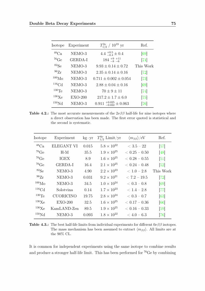
Double Beta Decay Experiments 75
Isotope Experiment T 2ν1/2 / 1019 yr Ref.
48Ca NEMO-3 4.4 +0.5−0.4 ± 0.4 [69]
76Ge GERDA-I 184 +9−8
+11−6 [71]
82Se NEMO-3 9.93± 0.14± 0.72 This Work96Zr NEMO-3 2.35± 0.14± 0.16 [72]
100Mo NEMO-3 0.711± 0.002± 0.054 [73]116Cd NEMO-3 2.88± 0.04± 0.16 [69]130Te NEMO-3 70± 9± 11 [74]136Xe EXO-200 217.2± 1.7± 6.0 [75]150Nd NEMO-3 0.911 +0.025
−0.022 ± 0.063 [76]
Table 4.2.: The most accurate measurements of the 2νββ half-life for nine isotopes wherea direct observation has been made. The first error quoted is statistical andthe second is systematic.
Isotope Experiment kg · yr T 0ν1/2 Limit/yr 〈mββ〉/eV Ref.
48Ca ELEGANT VI 0.015 5.8× 10²² < 3.5 – 22 [57]76Ge H-M 35.5 1.9× 1025 < 0.25 – 0.50 [48]76Ge IGEX 8.9 1.6× 1025 < 0.28 – 0.55 [51]76Ge GERDA-I 16.4 2.1× 1025 < 0.24 – 0.48 [52]82Se NEMO-3 4.90 2.2× 10²³ < 1.0 – 2.8 This Work96Zr NEMO-3 0.031 9.2× 10²¹ < 7.2 – 19.5 [72]
100Mo NEMO-3 34.5 1.0× 1024 < 0.3 – 0.8 [69]116Cd Solotvina 0.14 1.7× 10²³ < 1.4 – 2.8 [77]130Te CUORICINO 19.75 2.8× 1024 < 0.3 – 0.7 [63]136Xe EXO-200 32.5 1.6× 1025 < 0.17 – 0.36 [66]136Xe KamLAND-Zen 89.5 1.9× 1025 < 0.16 – 0.33 [59]150Nd NEMO-3 0.093 1.8× 10²² < 4.0 – 6.3 [76]
Table 4.3.: The best half-life limits from individual experiments for different 0νββ isotopes.The mass mechanism has been assumed to extract 〈mββ〉. All limits are atthe 90% CL.
It is common for independent experiments using the same isotope to combine resultsand produce a stronger half-life limit. This has been performed for 76Ge by combining
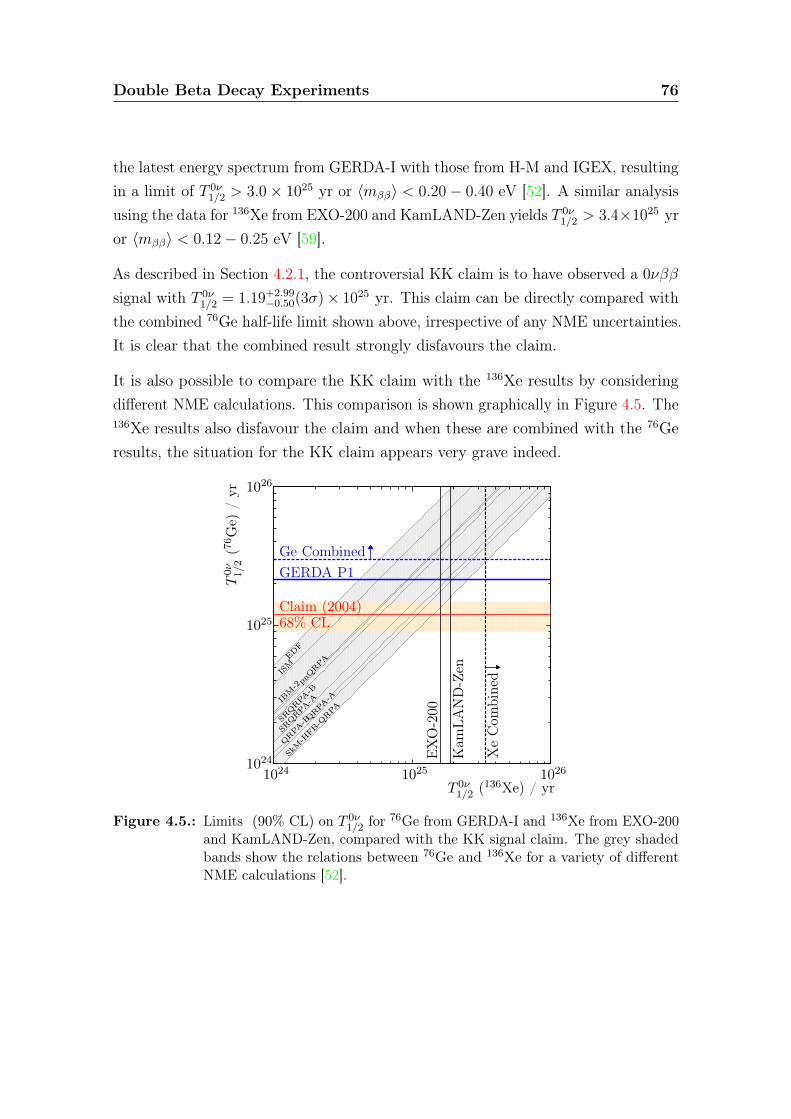
Double Beta Decay Experiments 76
the latest energy spectrum from GERDA-I with those from H-M and IGEX, resultingin a limit of T 0ν
1/2 > 3.0× 1025 yr or 〈mββ〉 < 0.20− 0.40 eV [52]. A similar analysisusing the data for 136Xe from EXO-200 and KamLAND-Zen yields T 0ν
1/2 > 3.4×1025 yror 〈mββ〉 < 0.12− 0.25 eV [59].
As described in Section 4.2.1, the controversial KK claim is to have observed a 0νββsignal with T 0ν
1/2 = 1.19+2.99−0.50(3σ)× 1025 yr. This claim can be directly compared with
the combined 76Ge half-life limit shown above, irrespective of any NME uncertainties.It is clear that the combined result strongly disfavours the claim.
It is also possible to compare the KK claim with the 136Xe results by consideringdifferent NME calculations. This comparison is shown graphically in Figure 4.5. The136Xe results also disfavour the claim and when these are combined with the 76Geresults, the situation for the KK claim appears very grave indeed.
T 0ν1/2 (136Xe) / yr
1024
1025
1026
1024 1025 1026
XeCom
bined
Kam
LAND-Zen
EXO-200
Ge CombinedGERDA P1
Claim (2004)68% CL
T0ν
1/2(7
6Ge)
/yr
EDF
IBM-2
ISM
pnQRPA
SRQRPA
-B
SRQRPA
-A
QRPA
-BQRPA
-A
SkM-H
FB-Q
RPA
Figure 4.5.: Limits (90% CL) on T 0ν1/2 for 76Ge from GERDA-I and 136Xe from EXO-200
and KamLAND-Zen, compared with the KK signal claim. The grey shadedbands show the relations between 76Ge and 136Xe for a variety of differentNME calculations [52].
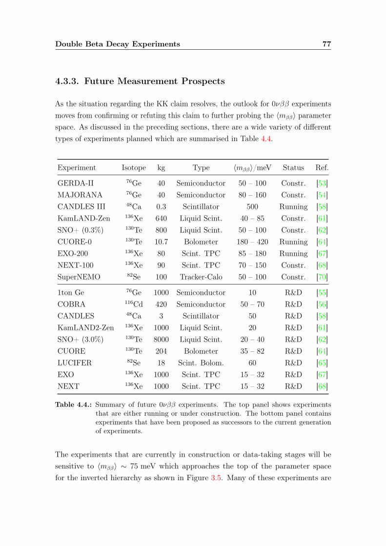
Double Beta Decay Experiments 77
4.3.3. Future Measurement Prospects
As the situation regarding the KK claim resolves, the outlook for 0νββ experimentsmoves from confirming or refuting this claim to further probing the 〈mββ〉 parameterspace. As discussed in the preceding sections, there are a wide variety of differenttypes of experiments planned which are summarised in Table 4.4.
Experiment Isotope kg Type 〈mββ〉/meV Status Ref.
GERDA-II 76Ge 40 Semiconductor 50 – 100 Constr. [53]MAJORANA 76Ge 40 Semiconductor 80 – 160 Constr. [54]CANDLES III 48Ca 0.3 Scintillator 500 Running [58]KamLAND-Zen 136Xe 640 Liquid Scint. 40 – 85 Constr. [61]SNO+ (0.3%) 130Te 800 Liquid Scint. 50 – 100 Constr. [62]CUORE-0 130Te 10.7 Bolometer 180 – 420 Running [64]EXO-200 136Xe 80 Scint. TPC 85 – 180 Running [67]NEXT-100 136Xe 90 Scint. TPC 70 – 150 Constr. [68]SuperNEMO 82Se 100 Tracker-Calo 50 – 100 Constr. [70]
1ton Ge 76Ge 1000 Semiconductor 10 R&D [55]COBRA 116Cd 420 Semiconductor 50 – 70 R&D [56]CANDLES 48Ca 3 Scintillator 50 R&D [58]KamLAND2-Zen 136Xe 1000 Liquid Scint. 20 R&D [61]SNO+ (3.0%) 130Te 8000 Liquid Scint. 20 – 40 R&D [62]CUORE 130Te 204 Bolometer 35 – 82 R&D [64]LUCIFER 82Se 18 Scint. Bolom. 60 R&D [65]EXO 136Xe 1000 Scint. TPC 15 – 32 R&D [67]NEXT 136Xe 1000 Scint. TPC 15 – 32 R&D [68]
Table 4.4.: Summary of future 0νββ experiments. The top panel shows experimentsthat are either running or under construction. The bottom panel containsexperiments that have been proposed as successors to the current generationof experiments.
The experiments that are currently in construction or data-taking stages will besensitive to 〈mββ〉 ∼ 75 meV which approaches the top of the parameter spacefor the inverted hierarchy as shown in Figure 3.5. Many of these experiments are
Double Beta Decay Experiments 78
planning to scale to larger masses, where there are possibilities to reach the bottomof the inverted hierarchy parameter space at 〈mββ〉 ∼ 10 meV. Therefore, if there isconclusive evidence from oscillation experiments that nature has chosen the invertedhierarchy, this generation of experiments will either discover or exclude the 0νββprocess.
Part I.
ββ-decay of 82Se with NEMO-3
79

Chapter 5.
NEMO-3 Detector
NEMO-3 was a double beta decay experiment that searched for 0νββ in sevendifferent isotopes. The experiment ran from February 2003 to January 2011, andin this time measured 2νββ in all seven isotopes. The strongest limit produced for0νββ comes from 100Mo, with a measurement of T 0ν
1/2 > 1.0× 1024 yr correspondingto 〈mββ〉 < 0.3− 0.8 eV [69].
The detector, shown in Figure 5.1, was cylindrical in design with a diameter of 5 mand a height of 3 m. It was composed of 20 identical segments, referred to as sectors,surrounding a hollow central column as depicted schematically in Figure 5.2. At thecentre of each sector were thin vertical strips of either 0νββ isotope or copper, thelatter of which were used for background measurements. These source foils, describedin Section 5.1, contained a total mass of 10 kg.
The principle behind the experiment was the direct detection of two electrons fromthe source material. In order to facilitate this, the foils were surrounded by a gastracker consisting of 6180 drift cells operating in Geiger mode (Section 5.2) ontowhich a magnetic field of 2.5 mT was applied (Section 5.6.1). The tracking volumewas enclosed by the calorimeter walls which were composed of 1940 individualoptical modules made of plastic scintillator blocks coupled to low-radioactivity PMTs(Section 5.3). The whole detector was then surrounded by passive shielding fromiron, paraffin, borated water and wood.
The experiment was based in the Laboratoire Souterrain de Modane (LSM) on theFrench-Italian border. This underground laboratory is adjacent to a road tunnel
80
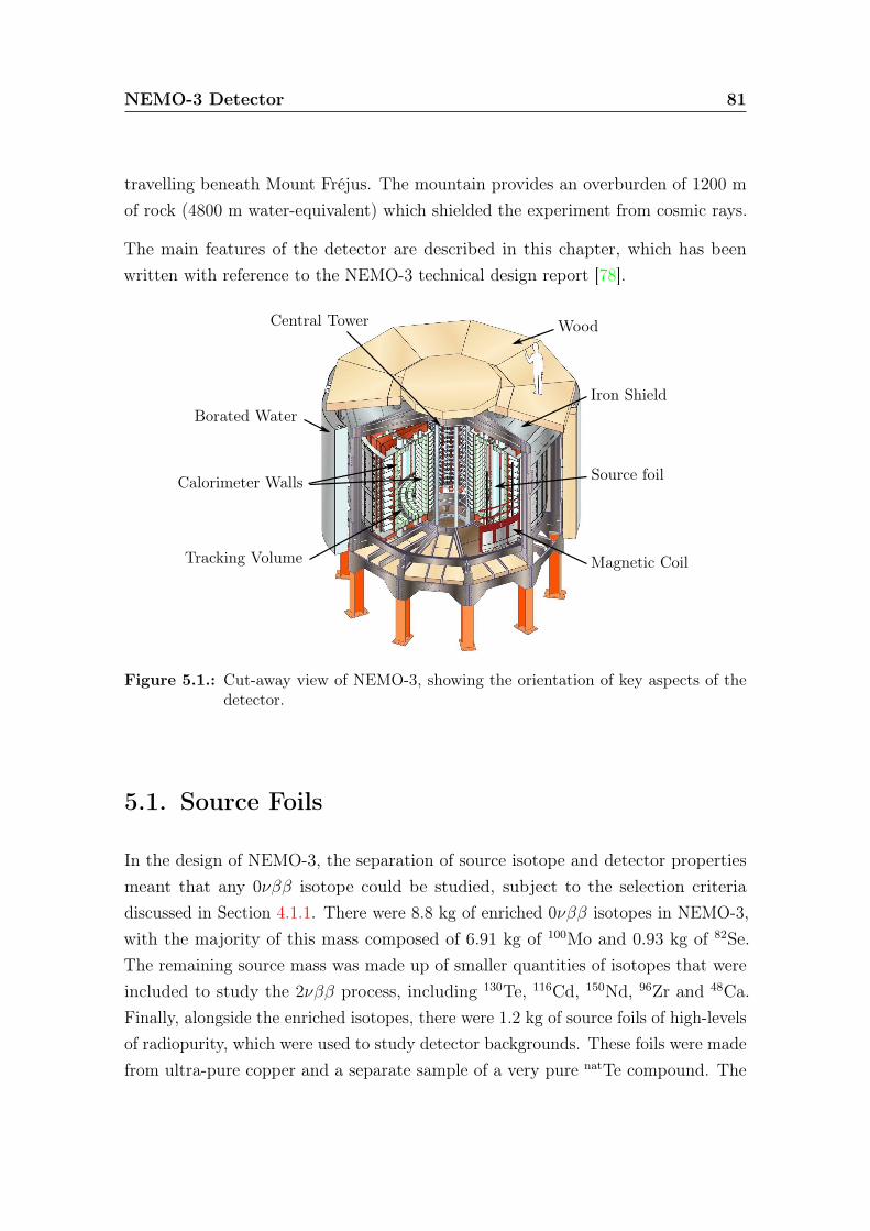
NEMO-3 Detector 81
travelling beneath Mount Fréjus. The mountain provides an overburden of 1200 mof rock (4800 m water-equivalent) which shielded the experiment from cosmic rays.
The main features of the detector are described in this chapter, which has beenwritten with reference to the NEMO-3 technical design report [78].
Borated WaterIron Shield
WoodCentral Tower
Source foilCalorimeter Walls
Magnetic CoilTracking Volume
Figure 5.1.: Cut-away view of NEMO-3, showing the orientation of key aspects of thedetector.
5.1. Source Foils
In the design of NEMO-3, the separation of source isotope and detector propertiesmeant that any 0νββ isotope could be studied, subject to the selection criteriadiscussed in Section 4.1.1. There were 8.8 kg of enriched 0νββ isotopes in NEMO-3,with the majority of this mass composed of 6.91 kg of 100Mo and 0.93 kg of 82Se.The remaining source mass was made up of smaller quantities of isotopes that wereincluded to study the 2νββ process, including 130Te, 116Cd, 150Nd, 96Zr and 48Ca.Finally, alongside the enriched isotopes, there were 1.2 kg of source foils of high-levelsof radiopurity, which were used to study detector backgrounds. These foils were madefrom ultra-pure copper and a separate sample of a very pure natTe compound. The
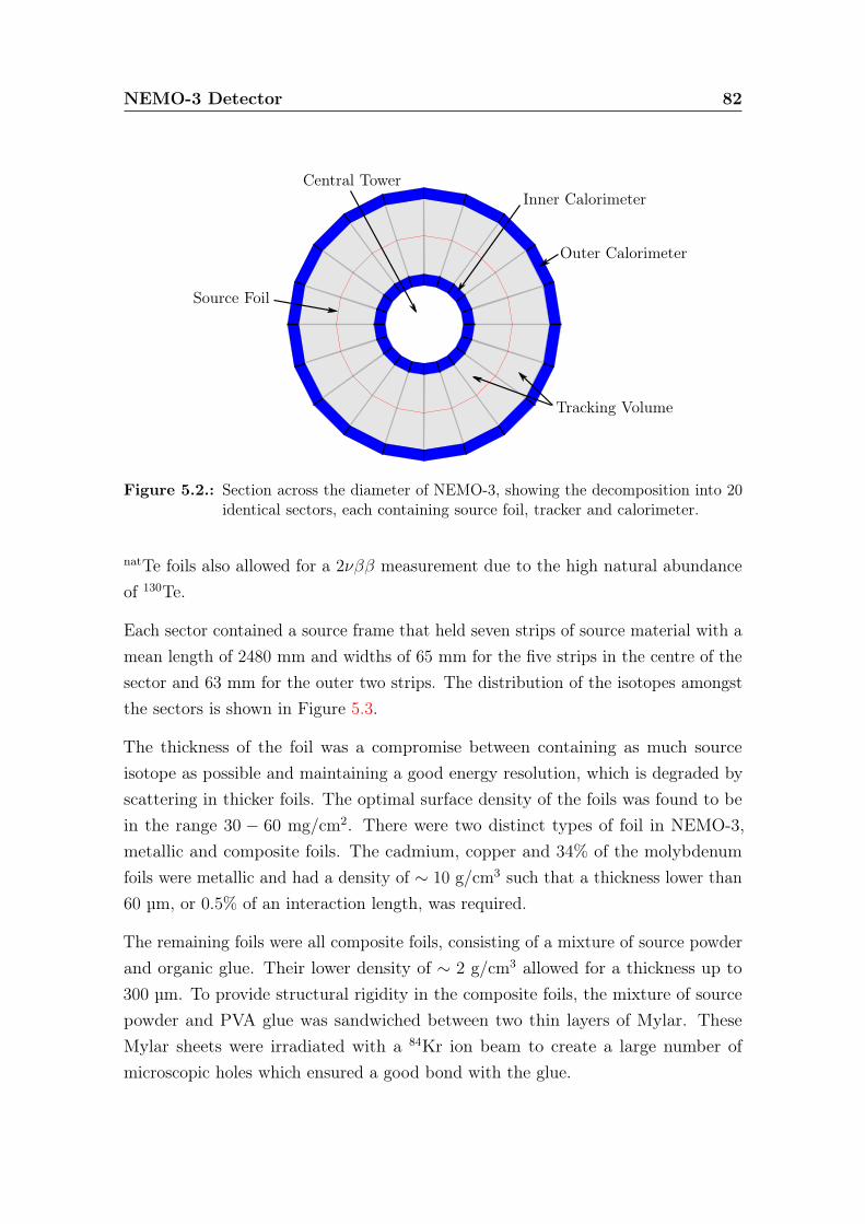
NEMO-3 Detector 82
Central TowerInner Calorimeter
Outer Calorimeter
Source Foil
Tracking Volume
Figure 5.2.: Section across the diameter of NEMO-3, showing the decomposition into 20identical sectors, each containing source foil, tracker and calorimeter.
natTe foils also allowed for a 2νββ measurement due to the high natural abundanceof 130Te.
Each sector contained a source frame that held seven strips of source material with amean length of 2480 mm and widths of 65 mm for the five strips in the centre of thesector and 63 mm for the outer two strips. The distribution of the isotopes amongstthe sectors is shown in Figure 5.3.
The thickness of the foil was a compromise between containing as much sourceisotope as possible and maintaining a good energy resolution, which is degraded byscattering in thicker foils. The optimal surface density of the foils was found to bein the range 30 − 60 mg/cm2. There were two distinct types of foil in NEMO-3,metallic and composite foils. The cadmium, copper and 34% of the molybdenumfoils were metallic and had a density of ∼ 10 g/cm3 such that a thickness lower than60 µm, or 0.5% of an interaction length, was required.
The remaining foils were all composite foils, consisting of a mixture of source powderand organic glue. Their lower density of ∼ 2 g/cm3 allowed for a thickness up to300 µm. To provide structural rigidity in the composite foils, the mixture of sourcepowder and PVA glue was sandwiched between two thin layers of Mylar. TheseMylar sheets were irradiated with a 84Kr ion beam to create a large number ofmicroscopic holes which ensured a good bond with the glue.
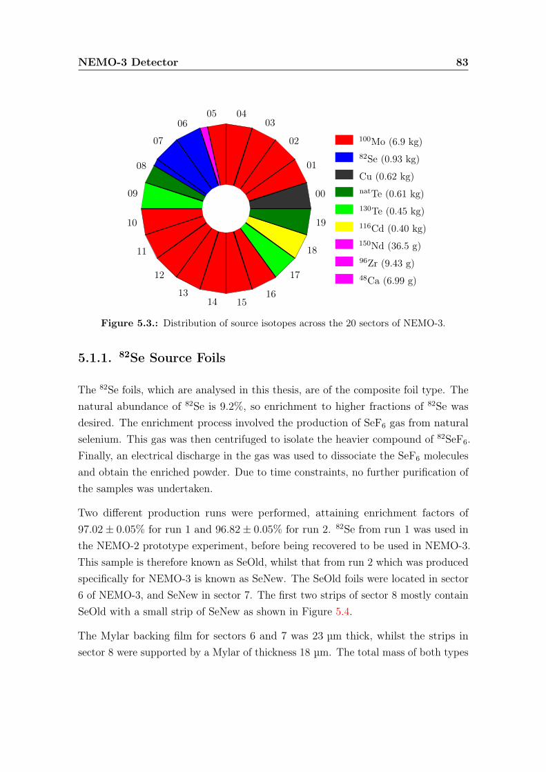
NEMO-3 Detector 83
100Mo (6.9 kg)82Se (0.93 kg)
Cu (0.62 kg)
116Cd (0.40 kg)
130Te (0.45 kg)
natTe (0.61 kg)
150Nd (36.5 g)96Zr (9.43 g)48Ca (6.99 g)
00
01
02
030405
06
07
08
09
10
11
12
1314 15
16
17
18
19
Figure 5.3.: Distribution of source isotopes across the 20 sectors of NEMO-3.
5.1.1. 82Se Source Foils
The 82Se foils, which are analysed in this thesis, are of the composite foil type. Thenatural abundance of 82Se is 9.2%, so enrichment to higher fractions of 82Se wasdesired. The enrichment process involved the production of SeF6 gas from naturalselenium. This gas was then centrifuged to isolate the heavier compound of 82SeF6.Finally, an electrical discharge in the gas was used to dissociate the SeF6 moleculesand obtain the enriched powder. Due to time constraints, no further purification ofthe samples was undertaken.
Two different production runs were performed, attaining enrichment factors of97.02± 0.05% for run 1 and 96.82± 0.05% for run 2. 82Se from run 1 was used inthe NEMO-2 prototype experiment, before being recovered to be used in NEMO-3.This sample is therefore known as SeOld, whilst that from run 2 which was producedspecifically for NEMO-3 is known as SeNew. The SeOld foils were located in sector6 of NEMO-3, and SeNew in sector 7. The first two strips of sector 8 mostly containSeOld with a small strip of SeNew as shown in Figure 5.4.
The Mylar backing film for sectors 6 and 7 was 23 µm thick, whilst the strips insector 8 were supported by a Mylar of thickness 18 µm. The total mass of both types
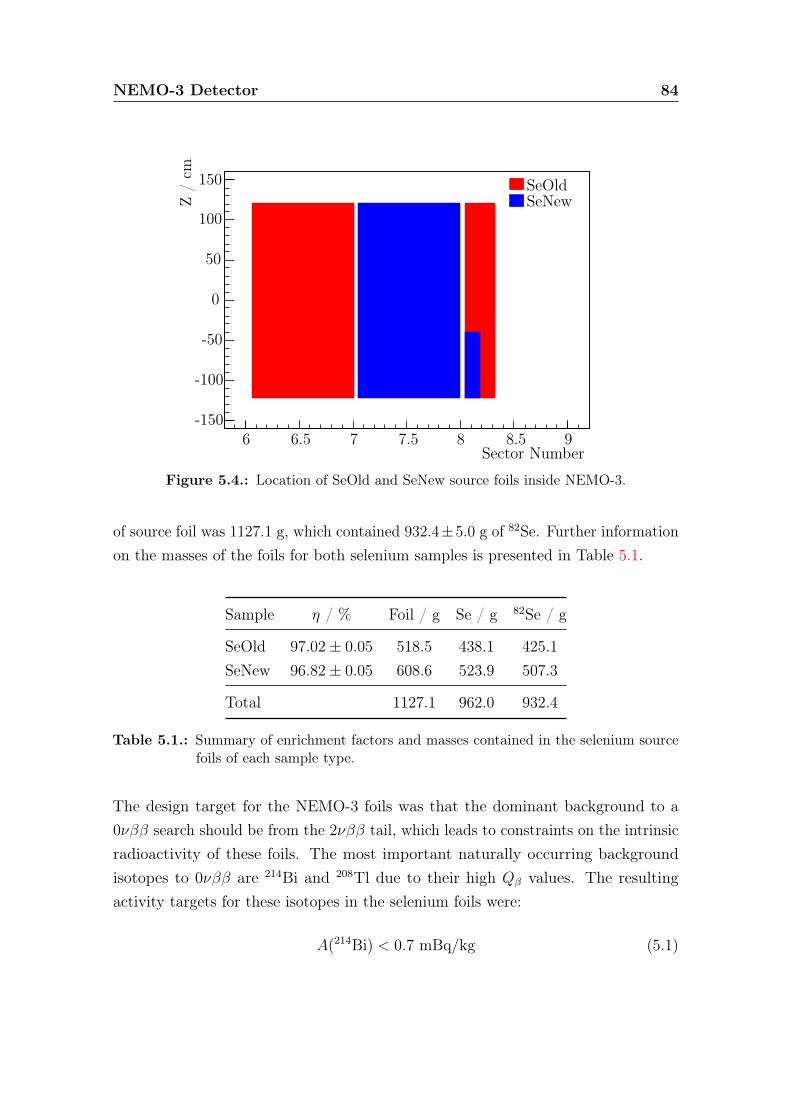
NEMO-3 Detector 84
Sector Number6 6.5 7 7.5 8 8.5 9
Z/cm
-150
-100
-50
0
50
100
150 SeOldSeNew
Figure 5.4.: Location of SeOld and SeNew source foils inside NEMO-3.
of source foil was 1127.1 g, which contained 932.4±5.0 g of 82Se. Further informationon the masses of the foils for both selenium samples is presented in Table 5.1.
Sample η / % Foil / g Se / g 82Se / g
SeOld 97.02± 0.05 518.5 438.1 425.1SeNew 96.82± 0.05 608.6 523.9 507.3
Total 1127.1 962.0 932.4
Table 5.1.: Summary of enrichment factors and masses contained in the selenium sourcefoils of each sample type.
The design target for the NEMO-3 foils was that the dominant background to a0νββ search should be from the 2νββ tail, which leads to constraints on the intrinsicradioactivity of these foils. The most important naturally occurring backgroundisotopes to 0νββ are 214Bi and 208Tl due to their high Qβ values. The resultingactivity targets for these isotopes in the selenium foils were:
A(214Bi) < 0.7 mBq/kg (5.1)
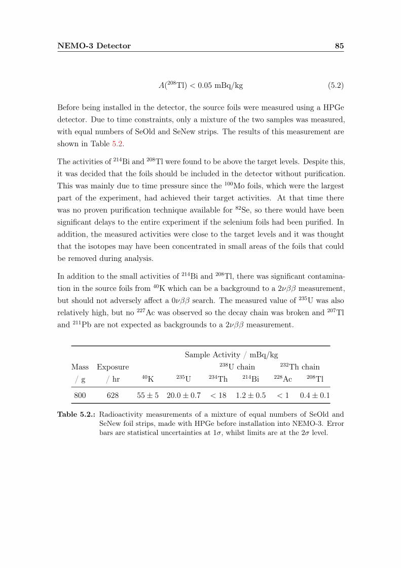
NEMO-3 Detector 85
A(208Tl) < 0.05 mBq/kg (5.2)
Before being installed in the detector, the source foils were measured using a HPGedetector. Due to time constraints, only a mixture of the two samples was measured,with equal numbers of SeOld and SeNew strips. The results of this measurement areshown in Table 5.2.
The activities of 214Bi and 208Tl were found to be above the target levels. Despite this,it was decided that the foils should be included in the detector without purification.This was mainly due to time pressure since the 100Mo foils, which were the largestpart of the experiment, had achieved their target activities. At that time therewas no proven purification technique available for 82Se, so there would have beensignificant delays to the entire experiment if the selenium foils had been purified. Inaddition, the measured activities were close to the target levels and it was thoughtthat the isotopes may have been concentrated in small areas of the foils that couldbe removed during analysis.
In addition to the small activities of 214Bi and 208Tl, there was significant contamina-tion in the source foils from 40K which can be a background to a 2νββ measurement,but should not adversely affect a 0νββ search. The measured value of 235U was alsorelatively high, but no 227Ac was observed so the decay chain was broken and 207Tland 211Pb are not expected as backgrounds to a 2νββ measurement.
Sample Activity / mBq/kgMass Exposure 238U chain 232Th chain/ g / hr 40K 235U 234Th 214Bi 228Ac 208Tl
800 628 55± 5 20.0± 0.7 < 18 1.2± 0.5 < 1 0.4± 0.1
Table 5.2.: Radioactivity measurements of a mixture of equal numbers of SeOld andSeNew foil strips, made with HPGe before installation into NEMO-3. Errorbars are statistical uncertainties at 1σ, whilst limits are at the 2σ level.

NEMO-3 Detector 86
5.2. Tracker
The NEMO-3 tracker provided three-dimensional tracking of charged particles andwas integral to the ability of the detector to fully reconstruct events. It consistedof 6180 vertical drift cells operating in Geiger mode. Each cell had an octagonalcross-section, with a central anode surrounded by eight cathode wires, as shownin the enlarged section of Figure 5.5. An elementary cell is 3 cm in diameter and2.7 m long, with all wires made of stainless steel with a diameter of 50 µm. A coppercathode ring was positioned at either end of the cell to collect signals from plasmapropagation. An extra ground wire was added between adjacent layers of the trackerto reduce electrostatic cross-talk. Cathode wires are shared between adjacent cells,which minimises the amount of material inside the tracking chamber. This hasadvantages from a radiopurity perspective and also reduces the amount of scatteringinside the tracker.
The cells are divided into nine different layers which are configured in a group offour layers closest to the source foils, then two layers in the middle of the trackingvolume and finally three layers closest to the calorimeter wall as shown in Figure 5.5.This 4-2-3 layout gave better the tracking resolution at the foil and scintillator walls,whilst allowing for calorimeter blocks in the spaces between the tracking layers.These extra calorimeter blocks significantly increased the coverage of the detector.
The drift cells were operated in a gas mixture consisting of 95% helium, 4% ethanoland 1% argon held at 10 mbar above atmospheric pressure. Helium was used as thebasis of the tracking gas, since its low atomic number, Z, minimises multiple scatteringof electrons. As a result, a typical electron only lost ∼ 30 keV when traversing thetracker. The ethanol was included in the mix to quench the photoionisation processby absorbing UV photons. This improved the performance of the detector by reducingthe re-firing effect of one cell to another. The final component of the gas mixturewas argon, which has a lower ionisation potential than helium and thus made theplasma propagation more stable. Additionally, in the final years of the detector, asmall quantity of water vapour was introduced with the aim of rejuvenating some ofthe ageing cells.
As implied above, the tracker functioned via the principle of ionisation. As a chargedparticle passed through the gas mixture, an ionisation of ∼ 6 electrons/cm was
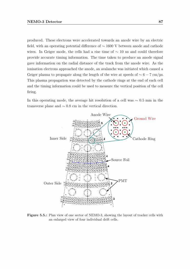
NEMO-3 Detector 87
produced. These electrons were accelerated towards an anode wire by an electricfield, with an operating potential difference of ∼ 1600 V between anode and cathodewires. In Geiger mode, the cells had a rise time of ∼ 10 ns and could thereforeprovide accurate timing information. The time taken to produce an anode signalgave information on the radial distance of the track from the anode wire. As theionisation electrons approached the anode, an avalanche was initiated which caused aGeiger plasma to propagate along the length of the wire at speeds of ∼ 6− 7 cm/µs.This plasma propagation was detected by the cathode rings at the end of each celland the timing information could be used to measure the vertical position of the cellfiring.
In this operating mode, the average hit resolution of a cell was ∼ 0.5 mm in thetransverse plane and ∼ 0.8 cm in the vertical direction.
Inner Side
Outer Side
Source Foil
Cathode Ring
Anode WireGround Wire
PMT
Figure 5.5.: Plan view of one sector of NEMO-3, showing the layout of tracker cells withan enlarged view of four individual drift cells.
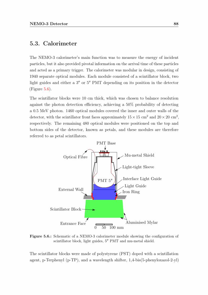
NEMO-3 Detector 88
5.3. Calorimeter
The NEMO-3 calorimeter’s main function was to measure the energy of incidentparticles, but it also provided pivotal information on the arrival time of these particlesand acted as a primary trigger. The calorimeter was modular in design, consisting of1940 separate optical modules. Each module consisted of a scintillator block, twolight guides and either a 3′′ or 5′′ PMT depending on its position in the detector(Figure 5.6).
The scintillator blocks were 10 cm thick, which was chosen to balance resolutionagainst the photon detection efficiency, achieving a 50% probability of detectinga 0.5 MeV photon. 1460 optical modules covered the inner and outer walls of thedetector, with the scintillator front faces approximately 15× 15 cm2 and 20× 20 cm2,respectively. The remaining 480 optical modules were positioned on the top andbottom sides of the detector, known as petals, and these modules are thereforereferred to as petal scintillators.
Scintillator Block
Entrance Face Aluminised Mylar
Light GuideExternal Wall
PMT 5"
Optical Fibre
PMT Base
Mu-metal Shield
Light-tight Sleeve
Interface Light Guide
Iron Ring
0 50 100 mm
Figure 5.6.: Schematic of a NEMO-3 calorimeter module showing the configuration ofscintillator block, light guides, 5′′ PMT and mu-metal shield.
The scintillator blocks were made of polystyrene (PST) doped with a scintillationagent, p-Terphenyl (p-TP), and a wavelength shifter, 1,4-bis(5-phenyloxazol-2-yl)
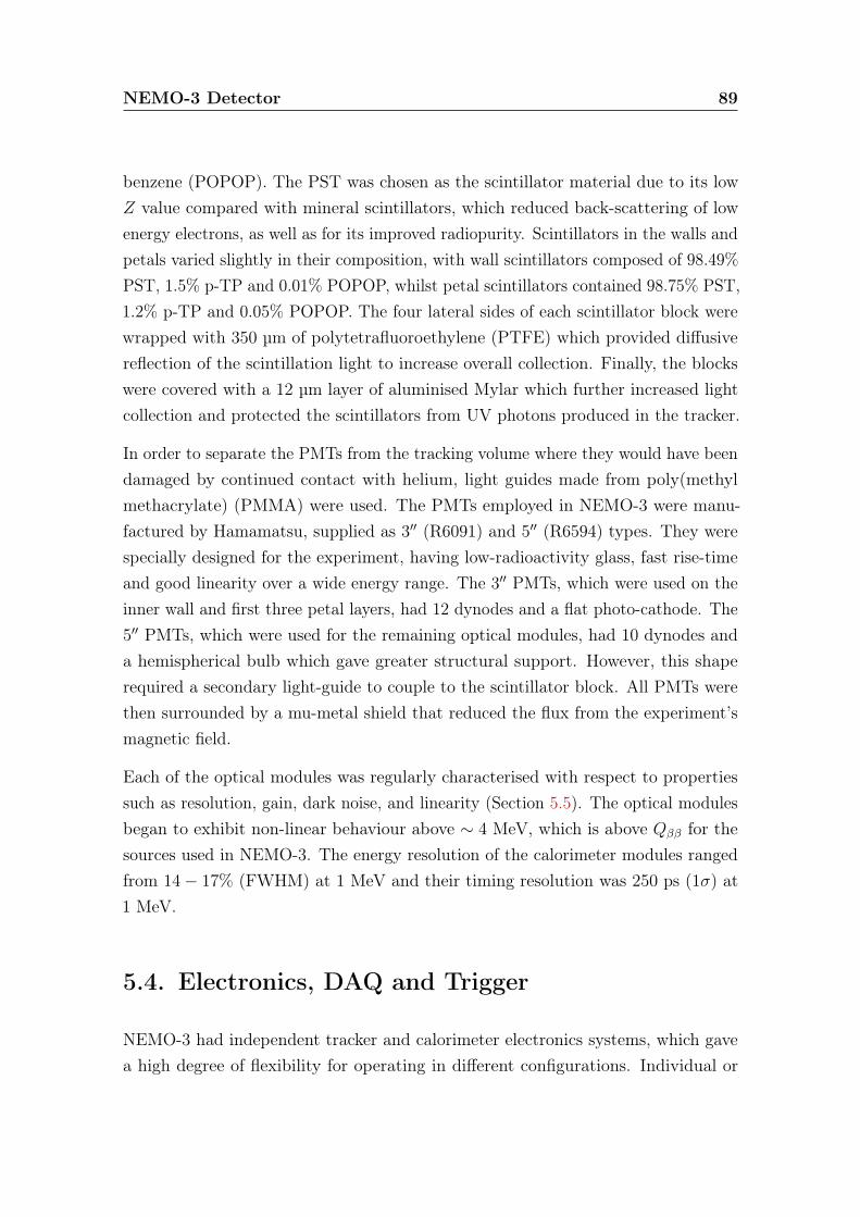
NEMO-3 Detector 89
benzene (POPOP). The PST was chosen as the scintillator material due to its lowZ value compared with mineral scintillators, which reduced back-scattering of lowenergy electrons, as well as for its improved radiopurity. Scintillators in the walls andpetals varied slightly in their composition, with wall scintillators composed of 98.49%PST, 1.5% p-TP and 0.01% POPOP, whilst petal scintillators contained 98.75% PST,1.2% p-TP and 0.05% POPOP. The four lateral sides of each scintillator block werewrapped with 350 µm of polytetrafluoroethylene (PTFE) which provided diffusivereflection of the scintillation light to increase overall collection. Finally, the blockswere covered with a 12 µm layer of aluminised Mylar which further increased lightcollection and protected the scintillators from UV photons produced in the tracker.
In order to separate the PMTs from the tracking volume where they would have beendamaged by continued contact with helium, light guides made from poly(methylmethacrylate) (PMMA) were used. The PMTs employed in NEMO-3 were manu-factured by Hamamatsu, supplied as 3′′ (R6091) and 5′′ (R6594) types. They werespecially designed for the experiment, having low-radioactivity glass, fast rise-timeand good linearity over a wide energy range. The 3′′ PMTs, which were used on theinner wall and first three petal layers, had 12 dynodes and a flat photo-cathode. The5′′ PMTs, which were used for the remaining optical modules, had 10 dynodes anda hemispherical bulb which gave greater structural support. However, this shaperequired a secondary light-guide to couple to the scintillator block. All PMTs werethen surrounded by a mu-metal shield that reduced the flux from the experiment’smagnetic field.
Each of the optical modules was regularly characterised with respect to propertiessuch as resolution, gain, dark noise, and linearity (Section 5.5). The optical modulesbegan to exhibit non-linear behaviour above ∼ 4 MeV, which is above Qββ for thesources used in NEMO-3. The energy resolution of the calorimeter modules rangedfrom 14− 17% (FWHM) at 1 MeV and their timing resolution was 250 ps (1σ) at1 MeV.
5.4. Electronics, DAQ and Trigger
NEMO-3 had independent tracker and calorimeter electronics systems, which gavea high degree of flexibility for operating in different configurations. Individual or
NEMO-3 Detector 90
interdependent triggering and data readout systems were possible, which allowedfor special triggering for calibration runs and specific studies of different elements ofdetector performance.
5.4.1. Calorimeter Electronics
The high voltage (HV) required to operate the 1940 PMTs of the calorimeter, typically1800 V and 1350 V for 3′′ and 5′′ PMTs respectively, was supplied by three CAENpower supplies each of which was capable of supplying 240 HV channels. These720 HV channels were transferred to the detector via 180 distribution boards (nineper sector). Each board had four HV inputs which were split into 12 outputs, suchthat each HV channel was shared by three PMTs. The outputs from the shared HVchannel were then fine-tuned by selecting fixed resistors to act as a potential divider.The resistor values where chosen based on data from a 207Bi source.
NEMO-3 had 97 optical modules per sector which were divided by the source foilinto 46 modules on the inner side and 51 modules on the outer side. Each of these40 half-sectors had a mother board supporting a daughter board for each PMTchannel, which performed signal processing. Each daughter board had a low andhigh threshold leading edge discriminator. When the low threshold was exceeded,corresponding to 7 mV or 23 keV, a TDC (time-to-digital-converter) counter wasstarted and a charge integration window of 80 ns was opened. If the high thresholdof 48 mV or 150 keV was breached, the daughter board passed a signal to the motherboard which, in turn, passed the number of fired PMTs to the trigger system.
If the desired multiplicity of PMT signals was reached, which for normal dataacquisition was only one PMT, the integrated charge was digitised in preparationfor storage of the data. The analog-to-digital conversions were performed with two12-bit ADCs, allowing an energy resolution of 0.36 pC/channel (∼ 3 keV/channelup to ∼ 12 MeV) and a timing resolution of 53 ps/channel.
5.4.2. Tracker Electronics
Two CAEN power supplies, each with 16 HV channels, were used to supply HV to theanode wires of the NEMO-3 tracker, usually at the level of 1620−1650 V. There were
NEMO-3 Detector 91
18 concentric layers of cells that made up the tracker and due to electrostatic effects,each layer required a slightly different voltage to those adjacent. For this reason, theinner-most nine layers were each supplied with a HV channel, and the outer-mostnine each with two. Every sector was supplied with eight distribution boards whichwere used for fine control of the HV and contained a total of 15 daughter boardseach with eight channels. These 15 daughter boards were assigned equally to anode,upper cathode and lower cathode signals.
In addition to the HV supply boards, eight data acquisition boards were providedper sector which contained 20 application specific integrated circuits (ASICs). TheseASICs were programmed to first amplify and then discriminate signals above thresholdbefore performing timing measurements for the anode and top and bottom cathoderings.
In a typical 2νββ event, a trigger from the calorimeter started the anode wire TDCcounter. A signal from the anode wire stopped this timing measurement, allowing aradial measurement of the ionisation point. The anode signal also started the TDCcounters for the top and bottom cathode rings, so that when a signal arrived at theserings, a measurement of the plasma propagation time was made. This measurementallowed the extraction of the vertical position of the ionisation point.
An important addition to the tracker was the ability to wait up to 710 µs after aninitial trigger to search for delayed firings of the tracker cells. As previously discussed,214Bi from 222Rn can be a problematic background to a 0νββ search. However, theimmediate daughter isotope of 214Bi, 214Po, decays via α-decay with a half-life of164.3 µs. This α particle may create a short, straight track in the tracker after theprompt electron track, leaving a distinct signature for these so-called BiPo events.Therefore, these delayed hits are very important in measuring the level of 214Bi insideNEMO-3 and in vetoing such BiPo events. This technique is discussed in greaterdetail in Section 6.3.3.
5.4.3. Trigger System
The NEMO-3 trigger system has three separate levels known as T1, T2 and T3.
The first level trigger, T1, is based on information from the calorimeter. Specifically,it requires that a given number of PMTs have registered an energy above 150 keV.
NEMO-3 Detector 92
For the normal acquisition mode, only one PMT is required, but for some calibrationruns a higher number of PMTs may be required. For example, during 60Co sourceruns, two PMTs above 150 keV are required (Section 5.5.1).
The second level trigger, T2, is applied based on information supplied by the tracker.To pass this trigger, there must be a hit in at least three out of the nine layers onone side of the foil, in the same or adjacent sectors. Further, at least two of thesehits must be in the same group of layers in the 4− 2− 3 configuration (i.e. layers 0 -3, 4 - 5 or 6 - 8).
The third level trigger, T3, is only used during calibration runs. It combinesinformation from T2 with information from the calorimeter to select events that arelikely to have originated from radioactive sources placed in specific detector locations.
The trigger rate during normal data acquisition was 7.4±0.1 Hz before the installationof the anti-radon facility (Section 5.7), reducing to 5.7± 0.1 Hz afterwards. This rateis dominated by events from radon and external radioactivity and has an associateddetector dead time of ∼ 1% of total running time. During calibration runs, wherethere are radioactive sources in the detector, the trigger rate increased to ∼ 250 Hzwith a dead time of ∼ 5%.
5.5. Energy and Time Calibration
In order to calibrate NEMO-3 with respect to absolute energy and time measurements,a procedure of dedicated calibration runs with radioactive sources was developed(Section 5.5.1). These calibration runs required ∼ 24 hrs of data-taking and so onlytook place every ∼ 40 days. To monitor the stability of the detector in betweenthese runs, twice daily laser surveys were undertaken as described in Section 5.5.2.
5.5.1. Radioactive Sources
Every sector of NEMO-3 was equipped with a copper calibration tube, located at thesame radius as the source foils, such that it ran vertically along the edge of a sourcestrip. Each flattened tube had three pairs of kapton windows of thickness 25 µm andsurface area ∼ 500 mm2, which faced towards the inner and outer calorimeter walls.
NEMO-3 Detector 93
The size of the windows and their vertical positions (z = 0,±90 cm) were chosento maximise the illumination uniformity of the scintillator blocks when using threeradioactive sources. Sources were introduced into the detector via a long delrin rodwhich could simultaneously contain three sources.
Absolute energy calibrations of the PMTs were carried out every ∼ 40 days using 207Bisources, which provided 482 keV and 976 keV conversion electrons with branchingratios of 1.5% and 7.0%, respectively. In addition, a calibration run at the beginningof NEMO-3 was performed using a 90Sr source, whereby the end-point of the β-decay spectrum of its daughter, 90Y, provided a higher energy calibration point at2.28 MeV.
Whilst every energy calibration provided important information on the stability ofthe detector, it was also possible to study the linearity of the NEMO-3 detectorover its entire lifetime by using all 207Bi calibrations from seven years of data-taking.This allowed the observation of the very rare 1682 keV conversion electron, with abranching ratio of 0.02%, and confirmed the energy linearity of the detector up to1.7 MeV.
Furthermore, by combining multiple 207Bi runs, it was also possible to correlate theimpact point of 1 MeV electrons on the scintillator block with the energy responseof the optical module. This effect was first observed with an electron spectrometerduring assembly of the optical modules and may be as large as 10% for the 5′′ PMTs.However, using these calibration measurements, it is possible to apply corrections tothe energy response based on the impact point with the scintillator, which has beenshown to improve detector response.
For timing calibration of the calorimeter, 60Co sources were used. This isotopeemits two coincident γ-rays with energies of 1173 keV and 1332 keV. The differencebetween arrival times at each of the 1940 channels can be used to calculate andcalibrate the relative time shifts between each channel. Since tracking is not requiredfor this calibration, relatively intense sources could be used.
5.5.2. Laser Survey
To provide a more frequent measure of the stability of the calorimeter, a twice-dailylaser survey was undertaken. A N2 laser with wavelength 337± 15 nm was passed

NEMO-3 Detector 94
through a series of attenuators and optical filters to allow control of its output.This light was then passed to a small sphere of scintillator wrapped in Teflon andaluminium to mimic an electron signal. This replica signal was transmitted viaoptical fibres to six reference PMTs fitted with 207Bi sources and also to the PMTsof the calorimeter.
By interpolating from the results of two absolute energy comparisons and comparingwith the output of the reference PMTs, it was possible to predict the expectedresponse of the PMT to the incident laser survey. PMTs that were found to exhibitunexpected or unstable behaviour are excluded from analysis for the whole surveyperiod. It has been found that there is no instability for 82% of the optical moduleexposure, with a further 7% showing only one deviation within a given period, whichmay be attributed to laser system instability.
5.6. Magnetic Coil and Passive Shielding
5.6.1. Magnetic Coil
To aid in particle identification inside the tracker, a solenoid coil was placed aroundthe detector producing a magnetic field of 2.5 mT parallel to the drift cells. Thecoil has a diameter of 5.3 m, a height of 2.7 m and a mass of 5 tonnes. The fieldwas generated by passing ∼ 30A of current through the coil and allows chargeidentification using the curvature of tracks. It was a very effective tool, allowingrejection of 95% of e+e− pairs at 1 MeV.
5.6.2. Mount Fréjus
As previously described, NEMO-3 was located in the LSM which has an overburdenof 1200 m of rock or 4800 m water-equivalent, which greatly reduces the cosmicmuon flux. Measurements inside the LSM have shown the cosmic muon flux to be5 × 10−5 m−2s−1 which is a reduction by a factor of one million from that at sealevel.
NEMO-3 Detector 95
5.6.3. Iron Shield
177 tonnes of iron, selected for its radiopurity, was used to provide 20 cm of shieldingcovering the whole detector. Its primary function was to suppress the γ-ray fluxcaused by radioactive decays in the surrounding rock and neutron capture. As asecondary advantage, it also acted as a flux return for the magnetic coil.
5.6.4. Neutron Shielding
Spontaneous fission of naturally-occurring uranium and thorium in the rock sur-rounding the experiment produced both fast and thermal neutrons, which could becaptured by the detector materials, causing the emission of high energy photons. Inorder to reduce this background, a dedicated shield was constructed that suppressedthe neutron flux inside the detector.
This shield was composed of three parts and placed outside the iron shield. The firstwas 20 cm of paraffin positioned below the central tower (not shown in Figure 5.1).Secondly, 35 cm of borated water was placed in tanks attached to the cylindricalexterior of the detector. Finally, 28 cm of wood was used between the borated watertanks and above and below the detector end caps.
Incident fast neutrons were moderated to lower energies by the paraffin, wood orwater and then captured on boron or in the iron shield. Any photons emitted in theneutron capture reaction were shielded from the detector by the iron shield.
5.7. Anti-radon facility
After one year of data-taking, it was discovered that the radon level inside NEMO-3was considerably higher than that expected from contamination of input gases oremanation from detector components. It was postulated that radon could be diffusinginto the detector from the surrounding air. In order to suppress this process, apolyethylene tent was installed around NEMO-3 with the intention of filling thiswith radon-free air.
NEMO-3 Detector 96
To create air with a low-level of radon, a radon trapping facility was installed atthe LSM. This facility cools compressed air from the laboratory to −50◦C where itis passed through two adsorption columns. Each of these columns has an internaldiameter of 0.6 m and a height of 3 m and contains 500 kg of activated charcoal cooledto the same temperature. This vast amount of cooled charcoal has an enormoussurface area and any radon passing through is adsorbed. Once trapped, this radondecays inside the columns before it has time to pass through. The anti-radon facilitytakes air from the LSM at a rate of 150 m3/hr and an activity of 15 Bq/m3 andproduces an output with an activity of 18 mBq/m3, achieving a reduction of threeorders of magnitude.
After installation of the anti-radon facility, the level of radon inside NEMO-3 decreasedfrom 37.7±0.1 mBq/m3 to 6.46±0.05 mBq/m3 [79]. This reduction factor was muchlower than that from the anti-radon facility, which has not been fully explained. Thetwo strongest hypotheses are that there is a higher radon level inside the anti-radontent than at the facility output so the tent reduction factor is not as large as 1000,or a significant level of radon maybe be emanating from detector components.
There were clearly different detector conditions before and after the installation ofthe anti-radon facility in which there were different background levels. Accordingly,NEMO-3 data are split into two phases separated by the installation of the anti-radonfacility. Phase 1 incorporates data from the beginning of the experiment in February2003 to September 2004. Phase 2 encompasses data from October 2004 to January2011.

Chapter 6.
General Analysis Techniques
The general principle behind a NEMO-3 analysis is the comparison of experimentaldata with those generated using a Monte Carlo simulation of physics processes andthe detector response (Sections 6.1 and 6.2). The NEMO-3 detector provides alarge amount of information for each individual event and this is fully utilised in theanalysis process. The detector’s ability to identify particle types and supply timinginformation are used to create a consistent background model (Sections 6.3 and 6.4).Once a background model has been built, a measurement of the 2νββ process and asearch for the 0νββ process is undertaken (Section 6.6).
6.1. Monte Carlo Simulation
Monte Carlo simulation (MC) for NEMO-3 is performed using the DECAY0 eventgenerator [80], which is capable of generating the initial particles in radioactivedecays with the correct kinematics, timing and branching ratios. It provides all thenecessary information on 2νββ and many 0νββ decay modes and is also used for allbackground isotopes.
Events generated with DECAY0 are propagated through a full detector descriptionby GEANT-3.21 [81]. This simulates the interactions of the particles as they movethrough the detector according to their full and differential cross-sections. Eventsemerge from the simulation program in exactly the same format as raw data to allowfor the same reconstruction process.
97
General Analysis Techniques 98
6.2. Reconstruction of Events
The reconstruction process takes raw output from the detector or MC and convertsit into a useful form for a physics analysis. As a simple example, ADC and TDCcontent from a particular optical module is cross-referenced against information fromcalibration runs (Section 5.5) and accurate energy and timing information is created.
In general, the treatment of data and MC at reconstruction level is as similar aspossible. To ensure that the simulation describes the data, an attempt to replicatereal running conditions in the MC is performed. This encompasses such effects asthe removal of hits generated for tracker cells that are not working, or the smearingof the energy response of individual optical modules based on calibration data.
In order to ensure that the conditions accurately reflect the state of the detector,MC events are distributed evenly across the entire detector lifetime, before applyingappropriate running conditions.
6.3. Particle Identification
One of the main strengths of tracker-calorimeter detectors, such as NEMO-3, is theirability to distinguish between different types of particle. By using a combinationof tracking and calorimetry, electrons, positrons, photons and alpha particles areidentifiable in NEMO-3 data.
6.3.1. Electron Identification
Electrons and positrons are identified by tracks that can be extrapolated to an energydeposit in the calorimeter. An example of an event where two electrons have beenidentified in NEMO-3 data is shown in Figure 6.1. Electrons and positrons should befully contained in a single scintillator block, so only calorimeter blocks that have nosurrounding calorimeter hits are used to identify electrons. To distinguish betweenelectrons and positrons, the curvature of the track as a result of the magnetic fieldcan be used.
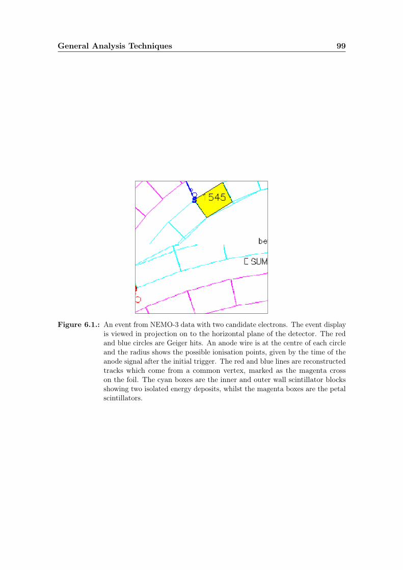
General Analysis Techniques 99
Figure 6.1.: An event from NEMO-3 data with two candidate electrons. The event displayis viewed in projection on to the horizontal plane of the detector. The redand blue circles are Geiger hits. An anode wire is at the centre of each circleand the radius shows the possible ionisation points, given by the time of theanode signal after the initial trigger. The red and blue lines are reconstructedtracks which come from a common vertex, marked as the magenta crosson the foil. The cyan boxes are the inner and outer wall scintillator blocksshowing two isolated energy deposits, whilst the magenta boxes are the petalscintillators.
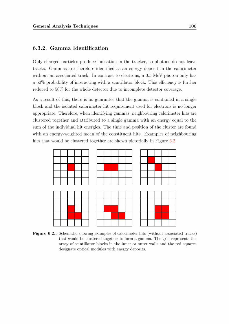
General Analysis Techniques 100
6.3.2. Gamma Identification
Only charged particles produce ionisation in the tracker, so photons do not leavetracks. Gammas are therefore identified as an energy deposit in the calorimeterwithout an associated track. In contrast to electrons, a 0.5 MeV photon only hasa 60% probability of interacting with a scintillator block. This efficiency is furtherreduced to 50% for the whole detector due to incomplete detector coverage.
As a result of this, there is no guarantee that the gamma is contained in a singleblock and the isolated calorimeter hit requirement used for electrons is no longerappropriate. Therefore, when identifying gammas, neighbouring calorimeter hits areclustered together and attributed to a single gamma with an energy equal to thesum of the individual hit energies. The time and position of the cluster are foundwith an energy-weighted mean of the constituent hits. Examples of neighbouringhits that would be clustered together are shown pictorially in Figure 6.2.
Figure 6.2.: Schematic showing examples of calorimeter hits (without associated tracks)that would be clustered together to form a gamma. The grid represents thearray of scintillator blocks in the inner or outer walls and the red squaresdesignate optical modules with energy deposits.

General Analysis Techniques 101
6.3.3. Alpha Identification
Alpha particles are charged and therefore trigger hits in the tracker. However, dueto their increased mass in comparison to electrons, they interact more strongly inthe tracking gas. For alpha particles from radioactive decays, the maximum distancetravelled is ∼ 35 cm, so they do not reach the calorimeter. Furthermore, the increasedalpha mass means that there is very little deflection of the particle’s trajectory by themagnetic field. Alpha particles can therefore be identified by short straight tracks.
For a double-beta decay analysis with NEMO-3, alpha particles from the vicinity ofthe foils do not, themselves, contribute to the background. However, they can bea useful tool for rejecting background events or measuring the background level inthe detector. 214Bi is a progeny of 222Rn that can deposited on the source foils or ontracker cells close to the foil. 214Bi decays to 214Po via β-decay with a Qβ value of3.27 MeV, which can be a problematic background for a 0νββ search. To identifyevents from 214Bi, it is possible to use the short half-life of 214Po, which decays viaα-decay with T1/2 = 164.3 µs. NEMO-3 is therefore able to identify this type ofbismuth-polonium (BiPo) event by searching for a prompt electron track followed bya delayed alpha track originating from the same location. An example of such anevent from NEMO-3 data is shown in Figure 6.3.
Figure 6.3.: Candidate BiPo event from NEMO-3 data. The red track is from a promptelectron, whilst the black squares are delayed Geiger hits that form a muchshorter alpha track.
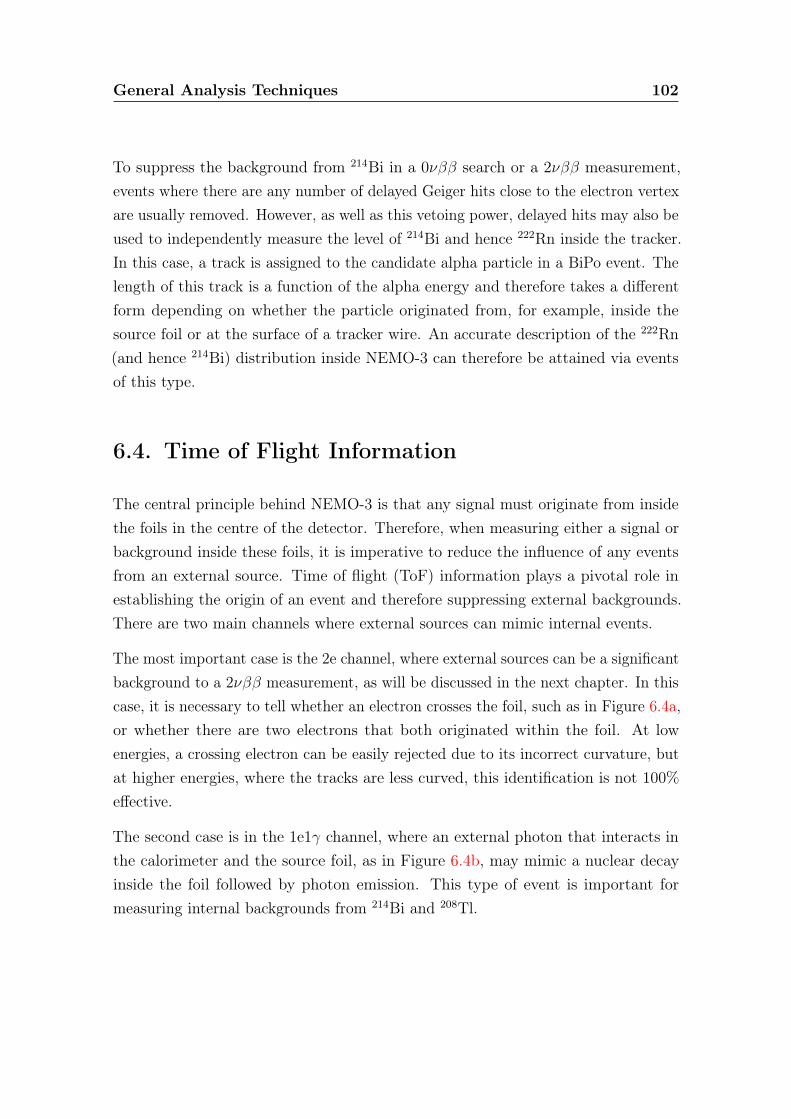
General Analysis Techniques 102
To suppress the background from 214Bi in a 0νββ search or a 2νββ measurement,events where there are any number of delayed Geiger hits close to the electron vertexare usually removed. However, as well as this vetoing power, delayed hits may also beused to independently measure the level of 214Bi and hence 222Rn inside the tracker.In this case, a track is assigned to the candidate alpha particle in a BiPo event. Thelength of this track is a function of the alpha energy and therefore takes a differentform depending on whether the particle originated from, for example, inside thesource foil or at the surface of a tracker wire. An accurate description of the 222Rn(and hence 214Bi) distribution inside NEMO-3 can therefore be attained via eventsof this type.
6.4. Time of Flight Information
The central principle behind NEMO-3 is that any signal must originate from insidethe foils in the centre of the detector. Therefore, when measuring either a signal orbackground inside these foils, it is imperative to reduce the influence of any eventsfrom an external source. Time of flight (ToF) information plays a pivotal role inestablishing the origin of an event and therefore suppressing external backgrounds.There are two main channels where external sources can mimic internal events.
The most important case is the 2e channel, where external sources can be a significantbackground to a 2νββ measurement, as will be discussed in the next chapter. In thiscase, it is necessary to tell whether an electron crosses the foil, such as in Figure 6.4a,or whether there are two electrons that both originated within the foil. At lowenergies, a crossing electron can be easily rejected due to its incorrect curvature, butat higher energies, where the tracks are less curved, this identification is not 100%effective.
The second case is in the 1e1γ channel, where an external photon that interacts inthe calorimeter and the source foil, as in Figure 6.4b, may mimic a nuclear decayinside the foil followed by photon emission. This type of event is important formeasuring internal backgrounds from 214Bi and 208Tl.
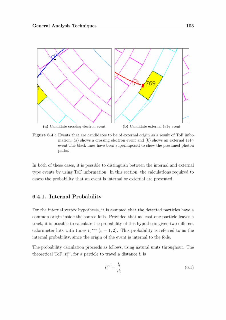
General Analysis Techniques 103
(a) Candidate crossing electron event (b) Candidate external 1e1γ event
Figure 6.4.: Events that are candidates to be of external origin as a result of ToF infor-mation. (a) shows a crossing electron event and (b) shows an external 1e1γevent.The black lines have been superimposed to show the presumed photonpaths.
In both of these cases, it is possible to distinguish between the internal and externaltype events by using ToF information. In this section, the calculations required toassess the probability that an event is internal or external are presented.
6.4.1. Internal Probability
For the internal vertex hypothesis, it is assumed that the detected particles have acommon origin inside the source foils. Provided that at least one particle leaves atrack, it is possible to calculate the probability of this hypothesis given two differentcalorimeter hits with times tmeas
i (i = 1, 2). This probability is referred to as theinternal probability, since the origin of the event is internal to the foils.
The probability calculation proceeds as follows, using natural units throughout. Thetheoretical ToF, ttofi , for a particle to travel a distance li is
ttofi =liβi
(6.1)
General Analysis Techniques 104
where li is either the track length of an electron or the straight-line distance betweenthe hypothesised vertex and the scintillator for a photon. For photons, βi = 1, andfor electrons, βi is given by
βi =
√Ei (Ei + 2me)
Ei +me
(6.2)
where Ei is the calibrated energy recorded in the calorimeter and me is the electronrest mass. Assuming that the particles have an internal origin, the time of emissionof each particle, tinti , can be written
tinti = tmeasi − ttofi = tmeas
i − liβi
(6.3)
The timing distributions are approximately Gaussian and so a χ2 test may be usedwith an appropriate χ2 variable
χ2int =
((tmeas1 − l1
β1
)−(tmeas2 − l2
β2
))2σ2tint1
+ σ2tint2
(6.4)
σ2tinti
is the variance of the emission timing measurement, tinti , which is dominated bycontributions from uncertainties on the measurement time, σtmeas
i, the particle speed
σβi and the distance travelled σli :
σ2tinti
=
(∂tint
∂tmeasi
)2
σ2tmeasi
+
(∂tint
∂βi
)2
σ2βi
+
(∂tint
∂li
)2
σ2li
(6.5)
For electrons, the uncertainty on the path length can be neglected since theirinteraction point in the scintillator is well known from a combination of trackinginformation and their shallow interaction depth. Therefore to a good approximation,the variance of the measurement for electrons may be written
σ2tinti' σ2
tmeasi
+
(ttofi m
2e
Ei (Ei +me) (Ei + 2me)
)2
σ2Ei
(6.6)
In the case of photons, the uncertainty on particle speed is negligible, but there aresignificant unknown quantities relating to the uncertainty on the path length. This isdue to a combination of no tracking information, so it is unknown where the photonintersected the face of the block, and the possibility of an interaction at any depth

General Analysis Techniques 105
in the block. As a result, the variance for photons takes the form
σ2tinti' σ2
tmeasi
+ σ2li
(6.7)
To convert the χ2int value into a probability, it should be noted that there is one
degree of freedom, so that the probability is defined as
P(χ2int
)= 1− 1√
2π
∫ χ2int
0
x−12 e−
x2 dx (6.8)
The internal probabilities for the 2e channel (Section 8.2) and the 1e1γ channel(Section 7.3.5), constructed using this formulation are shown in Figure 6.5. Goodagreement is seen between experimental data and simulation.
(a) 2e Channel (b) 1e1γ Channel (SeOld)
Figure 6.5.: Internal probability distributions for the (a) 2νββ channel and (b) 1e1γchannel for the SeOld sample. Both distributions have been calculated usingthe above method. For more information on these channels, please refer toSections 8.2 and 7.3.5.
6.4.2. External Probability
The external vertex hypothesis is that the two hits have a common origin that isexternal to the source foils. In this scenario, it is assumed that an incident photoninteracts in the first PMT and causes either a crossing electron or an external 1e1γevent.
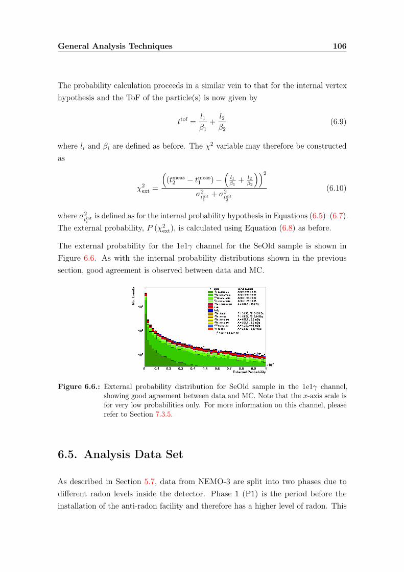
General Analysis Techniques 106
The probability calculation proceeds in a similar vein to that for the internal vertexhypothesis and the ToF of the particle(s) is now given by
ttof =l1β1
+l2β2
(6.9)
where li and βi are defined as before. The χ2 variable may therefore be constructedas
χ2ext =
((tmeas
2 − tmeas1 )−
(l1β1
+ l2β2
))2σ2tint1
+ σ2tint2
(6.10)
where σ2tinti
is defined as for the internal probability hypothesis in Equations (6.5)–(6.7).The external probability, P (χ2
ext), is calculated using Equation (6.8) as before.
The external probability for the 1e1γ channel for the SeOld sample is shown inFigure 6.6. As with the internal probability distributions shown in the previoussection, good agreement is observed between data and MC.
Figure 6.6.: External probability distribution for SeOld sample in the 1e1γ channel,showing good agreement between data and MC. Note that the x-axis scale isfor very low probabilities only. For more information on this channel, pleaserefer to Section 7.3.5.
6.5. Analysis Data Set
As described in Section 5.7, data from NEMO-3 are split into two phases due todifferent radon levels inside the detector. Phase 1 (P1) is the period before theinstallation of the anti-radon facility and therefore has a higher level of radon. This
General Analysis Techniques 107
phase encompasses February 2003 - September 2004 (runs 1869 - 3395). Phase 2(P2) covers the remainder of the experiment which has a lower radon level over theperiod October 2004 - January 2011 (runs 3396 - 9186).
The relevant exposures for P1 and P2 are presented in Table 6.1. This thesis analysesdata from the standard analysis runs of the entire NEMO-3 data set, which, excludingdetector dead time, gives a total time of 5.25 yr and an exposure to 82Se of 4.90 kg yr.
Phase Run Time / d Dead Time / d Exposure / d
P1 391.9 5.3 386.6P2 1548.3 16.3 1531.9
P1+P2 1940.2 21.6 1918.5
Table 6.1.: Exposure of NEMO-3 using the standard analysis run set broken down intophase 1 and phase 2.
6.6. Statistical Analysis
All statistical analysis presented in this thesis is performed with C++ in the ROOTdata analysis framework. Backgrounds, and signal where appropriate, are measuredusing a binned log-likelihood fit (Section 6.6.1). Where no statistically significantsignal is observed, a limit on the signal strength is set using a negative log-likelihoodratio technique (Section 6.6.2).
6.6.1. Fitting MC Distributions to Data
In order to estimate the activities of different isotopes, a binned log-likelihood fitis used. This takes into account the shapes of different background and signaldistributions to produce estimates of the most likely activity values. To form thelikelihood function, it is assumed that the MC reliably produces the expected numbersof events in each bin of a number of histograms. Then, the number of expectedevents in the ith bin of the nth histogram is given by the addition of the signal events,si,n, and the sum of the j background contributions,
∑j bi,n,j. Poisson statistics
General Analysis Techniques 108
apply to the number of observed events such that the probability, pi,n, of observingdi,n events in data is
pi,n =e−(si,n+
∑j bi,n,j)
(si,n +
∑j bi,n,j
)di,ndi,n!
(6.11)
The likelihood, L, is defined as the product of all the binned probabilities
L =∏i,n
e−(si,n+∑j bi,n,j)
(si,n +
∑j bi,n,j
)di,ndi,n!
(6.12)
It gives a measure of the overall likelihood of the particular set of data given theexpectation from the MC and therefore the maximal value of L gives the bestestimates for s and bj. The maximum of L is unaffected by a monotonic functionsuch as a logarithm, so that the maximum of L will correspond to the maximum ofln (L):
ln (L) =∑i,n
(−
(si,n +
∑j
bi,n,j
)+ di,n ln
(si,n +
∑j
bi,n,j
)− ln (di,n!)
)(6.13)
The parameters s and bj are proportional to the activities of these samples so thatit is possible to numerically maximise Equation (6.13) by varying the activities ofdifferent samples. The errors on the activities are found by noting that L follows aχ2 distribution such that a 1σ error reduces ln (L) by 1
2.
It is also possible to include additional information into the binned log-likelihoodfit, for example by adding a Gaussian constraint. This is typically used wherethere is very little distinguishing information in the data about the activity of aparticular background as it is almost identical to another sample. In this scenario, ameasurement from another source may be included in the log-likelihood fit.
For example, if an activity of A = A0 ± σA0 has been measured elsewhere, then aterm constraining MC activity, AMC , such as the following may be included in ln (L):
ln (L)→ ln (L)− ln(√
2πσA0
)− 1
2
(AMC − A0
σA0
)2
(6.14)
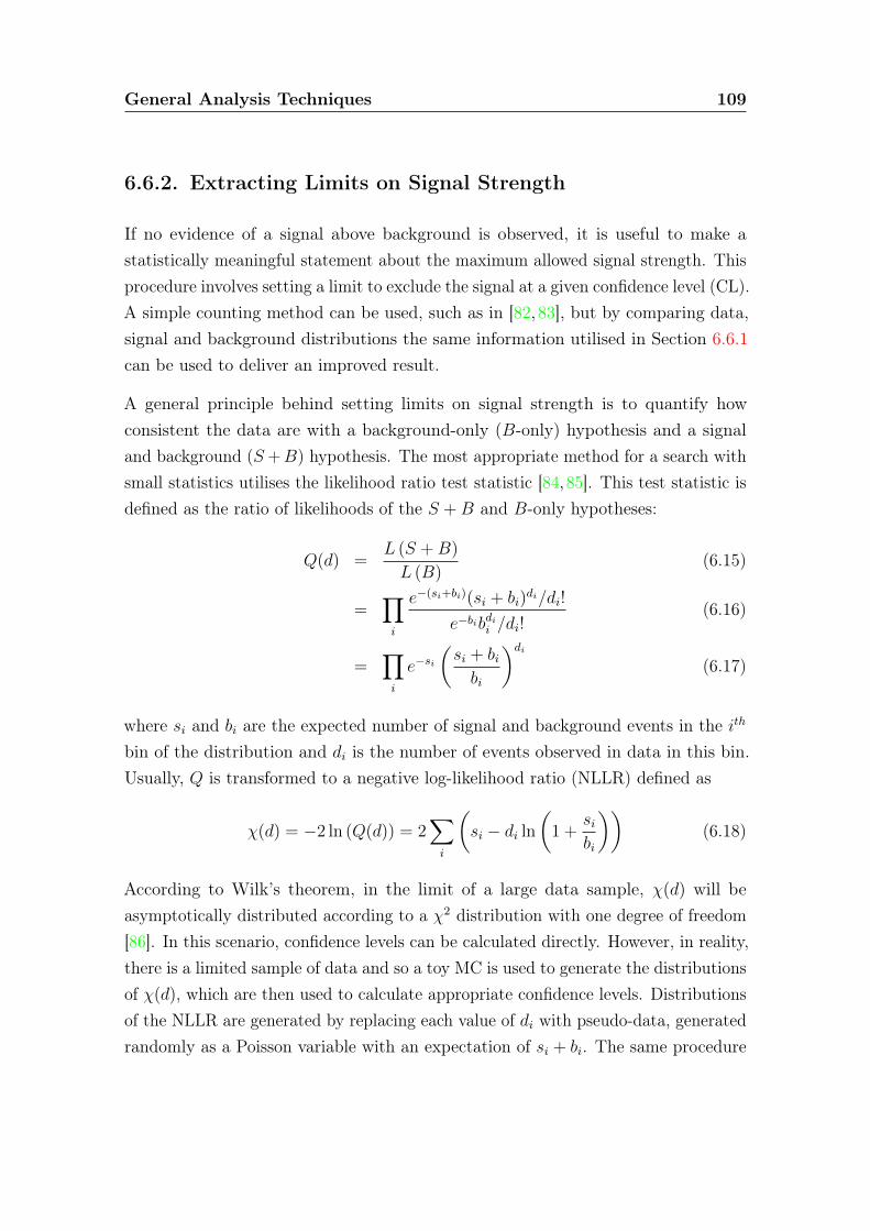
General Analysis Techniques 109
6.6.2. Extracting Limits on Signal Strength
If no evidence of a signal above background is observed, it is useful to make astatistically meaningful statement about the maximum allowed signal strength. Thisprocedure involves setting a limit to exclude the signal at a given confidence level (CL).A simple counting method can be used, such as in [82,83], but by comparing data,signal and background distributions the same information utilised in Section 6.6.1can be used to deliver an improved result.
A general principle behind setting limits on signal strength is to quantify howconsistent the data are with a background-only (B-only) hypothesis and a signaland background (S +B) hypothesis. The most appropriate method for a search withsmall statistics utilises the likelihood ratio test statistic [84, 85]. This test statistic isdefined as the ratio of likelihoods of the S +B and B-only hypotheses:
Q(d) =L (S +B)
L (B)(6.15)
=∏i
e−(si+bi)(si + bi)di/di!
e−bibdii /di!(6.16)
=∏i
e−si(si + bibi
)di(6.17)
where si and bi are the expected number of signal and background events in the ith
bin of the distribution and di is the number of events observed in data in this bin.Usually, Q is transformed to a negative log-likelihood ratio (NLLR) defined as
χ(d) = −2 ln (Q(d)) = 2∑i
(si − di ln
(1 +
sibi
))(6.18)
According to Wilk’s theorem, in the limit of a large data sample, χ(d) will beasymptotically distributed according to a χ2 distribution with one degree of freedom[86]. In this scenario, confidence levels can be calculated directly. However, in reality,there is a limited sample of data and so a toy MC is used to generate the distributionsof χ(d), which are then used to calculate appropriate confidence levels. Distributionsof the NLLR are generated by replacing each value of di with pseudo-data, generatedrandomly as a Poisson variable with an expectation of si + bi. The same procedure

General Analysis Techniques 110
is followed for the B-only hypothesis to create distributions such as those shown inFigure 6.7.
Figure 6.7.: Example distributions of the NLLR test statistic generated for the S + Bhypothesis (red) and B-only hypothesis (blue). Image sourced from [87].
From these distributions, it becomes clear that a confidence level can be constructedfor outcomes where a result is less like the S +B hypothesis than the observed valueof χ(d). This confidence level is given by
CLS+B = PS+B(χ > χ(d)) =
∫ ∞χ(d)
∂PS+B∂χ
dχ (6.19)
with a similar confidence level for the B-only hypothesis
CLB = PB(χ > χ(d)) =
∫ ∞χ(d)
∂PB∂χ
dχ (6.20)
Finally, the confidence level for the signal is related to the S + B and B-onlyhypotheses by
CLS =CLS+BCLB
(6.21)
To find the appropriate limit, the signal strength is increased until 1− CLS ≥ 0.9 sothat the 90% CL is reached.
General Analysis Techniques 111
6.7. Half-life Calculation
If a signal is observed, then it is customary to report the resulting signal strength asa half-life of the source isotope. The appropriate calculation is detailed here.
As with all radioactive isotopes, those in NEMO-3 decay exponentially such that
N(t) = N(0)e−λt (6.22)
where N(t) is the number of atoms of the isotope remaining after time t, and λ is thedecay constant for the isotope that is related to its lifetime, τ , and half-life, T1/2 as
λ =1
τ=
ln (2)
T1/2(6.23)
Since the half-lives involved in NEMO-3 are very large (O(1020 yr)) compared withthe lifetime of the experiment, a Taylor expansion can be made in λt and to a verygood approximation
e−λt ' (1− λt) (6.24)
The number of decays that occur over t is given by N(0)−N(t), so that if these aredetected with efficiency ε, the number of observed events is given by
Nobs = εN(0)(1− e−λt
)' εN(0)λt = εN(0)
ln (2)
T1/2t (6.25)
The number of atoms at the start of the experiment, N(0), can be written as
N(0) =NAm
A(6.26)
where NA is Avogadro’s constant, m is the mass of the source isotope and A is itsatomic mass. Therefore Equation (6.25) can be re-arranged to find an expression forthe half-life:
T1/2 =ε
Nobs
NAm
Aln (2)t (6.27)
Chapter 7.
Estimation of Backgrounds for the82Se Source Foils
Double beta decay signals in NEMO-3 are characterised by the observation of twoelectrons originating from the same location inside a source foil. Therefore, anyother process that can mimic this signal is a background for the experiment. To bea background to a 0νββ search, electrons must also have energies that sum to a highQββ. In contrast, the 2νββ process is observed across the entire energy spectrumand so all two electron-like backgrounds contribute.
The sensitivity of NEMO-3 is directly related to the background level (as discussedin Section 4.1), and so it is vitally important to be able to accurately measure thisbackground level and to develop techniques that can remove background events.
This chapter is devoted to the determination of background levels for NEMO-3. Itwill discuss the main sources of background (Section 7.1), categorising them intothree types based - internal backgrounds, which are caused by contamination ofthe source foils, external backgrounds that originate outside the source foils andradon-induced backgrounds (Section 7.2). Next, the selection channels that are usedto measure the background levels are outlined (Section 7.3) before finally presentingthe results of these measurements (Section 7.4).
112
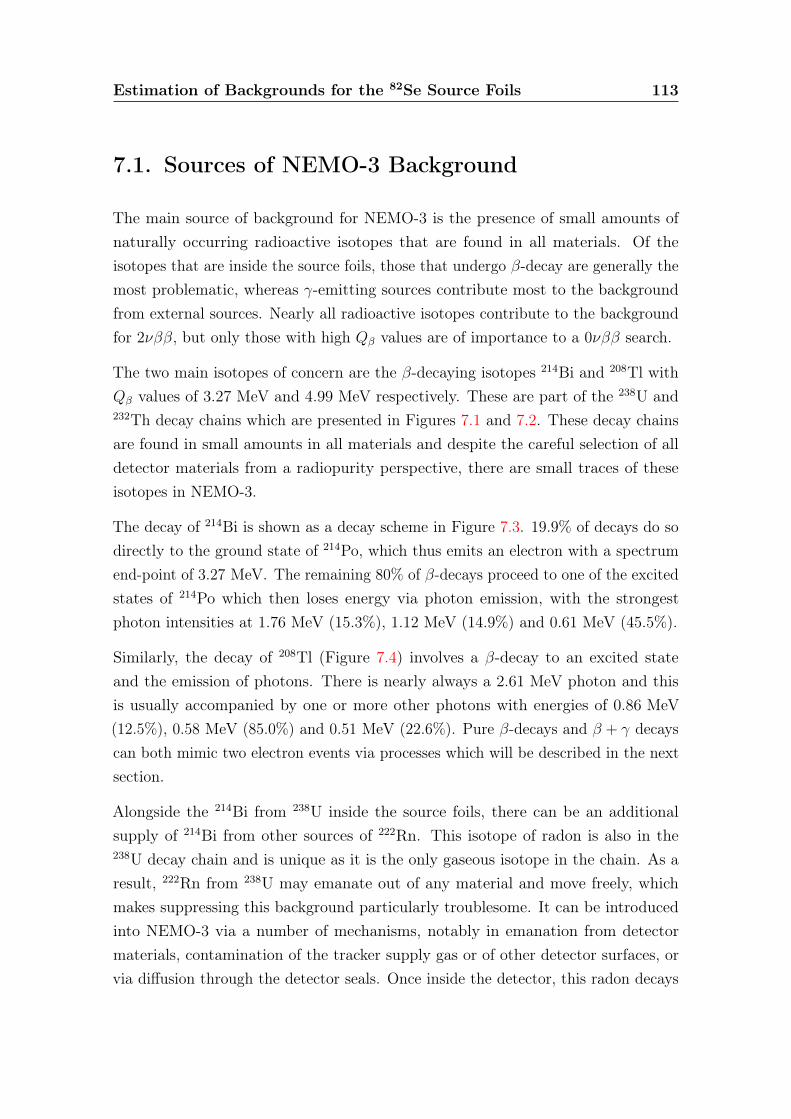
Estimation of Backgrounds for the 82Se Source Foils 113
7.1. Sources of NEMO-3 Background
The main source of background for NEMO-3 is the presence of small amounts ofnaturally occurring radioactive isotopes that are found in all materials. Of theisotopes that are inside the source foils, those that undergo β-decay are generally themost problematic, whereas γ-emitting sources contribute most to the backgroundfrom external sources. Nearly all radioactive isotopes contribute to the backgroundfor 2νββ, but only those with high Qβ values are of importance to a 0νββ search.
The two main isotopes of concern are the β-decaying isotopes 214Bi and 208Tl withQβ values of 3.27 MeV and 4.99 MeV respectively. These are part of the 238U and232Th decay chains which are presented in Figures 7.1 and 7.2. These decay chainsare found in small amounts in all materials and despite the careful selection of alldetector materials from a radiopurity perspective, there are small traces of theseisotopes in NEMO-3.
The decay of 214Bi is shown as a decay scheme in Figure 7.3. 19.9% of decays do sodirectly to the ground state of 214Po, which thus emits an electron with a spectrumend-point of 3.27 MeV. The remaining 80% of β-decays proceed to one of the excitedstates of 214Po which then loses energy via photon emission, with the strongestphoton intensities at 1.76 MeV (15.3%), 1.12 MeV (14.9%) and 0.61 MeV (45.5%).
Similarly, the decay of 208Tl (Figure 7.4) involves a β-decay to an excited stateand the emission of photons. There is nearly always a 2.61 MeV photon and thisis usually accompanied by one or more other photons with energies of 0.86 MeV(12.5%), 0.58 MeV (85.0%) and 0.51 MeV (22.6%). Pure β-decays and β + γ decayscan both mimic two electron events via processes which will be described in the nextsection.
Alongside the 214Bi from 238U inside the source foils, there can be an additionalsupply of 214Bi from other sources of 222Rn. This isotope of radon is also in the238U decay chain and is unique as it is the only gaseous isotope in the chain. As aresult, 222Rn from 238U may emanate out of any material and move freely, whichmakes suppressing this background particularly troublesome. It can be introducedinto NEMO-3 via a number of mechanisms, notably in emanation from detectormaterials, contamination of the tracker supply gas or of other detector surfaces, orvia diffusion through the detector seals. Once inside the detector, this radon decays

Estimation of Backgrounds for the 82Se Source Foils 114
234U238U4.4 Gy 250 ky
234Th24.1 d
234mPa1.17 m
230Th75 ky
226Ra1600 y
222Rn3.82 d
218Po3.1 m
214Pb26.8 m
214Bi19.9 m
214Po164.3 µs
210Tl1.3 m
210Pb22.3 y
210Bi5.0 d
210Po138.4 d
206PbStable
206Tl4.2 m
0.02
1%
10−
4%
α decay
β decay
Figure 7.1.: 238U decay chain, sometimes referred to as the radium series. α decays areshown as downwards arrows and β decays go upwards and to the right so thathorizontal lines all show the same element. Where an isotope can decay inmore than one mode, the branching fractions are marked on the α transition.
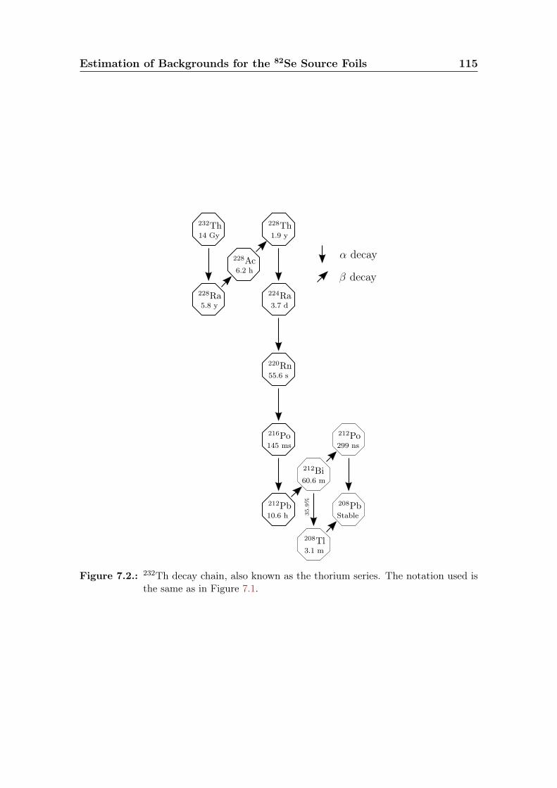
Estimation of Backgrounds for the 82Se Source Foils 115
α decay
β decay
232Th14 Gy
228Th1.9 y
228Ac6.2 h
228Ra5.8 y
224Ra3.7 d
220Rn55.6 s
216Po145 ms
212Pb10.6 h
212Bi60.6 m
212Po299 ns
208PbStable
208Tl3.1 m
35.9
%
Figure 7.2.: 232Th decay chain, also known as the thorium series. The notation used isthe same as in Figure 7.1.
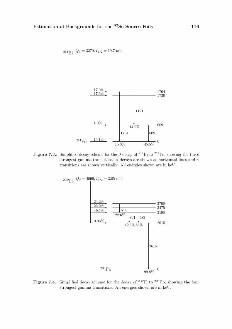
Estimation of Backgrounds for the 82Se Source Foils 116
609
17301764
609
1121
17.6%
1.0%
17.0%
Qβ = 3270, T1/2 = 19.7 min214Bi
214Po
14.9%
45.5%019.1%
15.3%
1764
Figure 7.3.: Simplified decay scheme for the β-decay of 214Bi to 214Po, showing the threestrongest gamma transitions. β-decays are shown as horizontal lines and γtransitions are shown vertically. All energies shown are in keV.
2615
319834753708
2615
511
583861
49.1%
0.03%
22.2%24.2%
Qβ = 4999, T1/2 = 3.05 min208Tl
208Pb
22.6%
12.5% 85%
99.8%0
Figure 7.4.: Simplified decay scheme for the decay of 208Tl to 208Pb, showing the fourstrongest gamma transitions. All energies shown are in keV.
Estimation of Backgrounds for the 82Se Source Foils 117
and in general, does so to predominantly positive ions. These charged progenies thendrift towards the source foils or tracker wires where they settle, leaving deposits of214Bi near to the source material.
The 232Th chain also contains a gaseous isotope of radon, 220Rn, also known as thoron,which can decay to 208Tl. However, this isotope does not cause such a problem forNEMO-3 since its very short half-life of 55.6 s means that very little thoron canemanate from detector materials before decaying. The resulting low level of 208Tl onthe surface of the tracking wires is measured separately using NEMO-3 data.
Finally, when considering a 0νββ process as the signal, the high energy tail of the2νββ process can become a background rather than a signal. This can be particularlyproblematic for most decay mechanisms as it has an almost identical experimentalsignature to 0νββ. The only practical way to suppress this background is withimproved energy resolution. For isotopes such as 100Mo, which have comparativelyshort 2νββ half-lives, this can produce a significant background but it is not expectedto significantly affect the sensitivity of a 0νββ search in 82Se with NEMO-3.
7.2. NEMO-3 Background Classification
7.2.1. Internal Backgrounds
Internal backgrounds are those which originate inside the source foils themselvesand are dominated by the radioactive contaminants. The most harmful isotopesare those which undergo β-decay since they can mimic two electron events via theprocesses of β-decay with Møller scattering, β decay followed by internal conversionor β-decay to an excited state with Compton scattering of the de-excitation photon(Figure 7.5).
HPGe measurements of the selenium foils were made prior to their inclusion inthe detector (Section 5.1.1), so that activity measurements made by NEMO-3 canbe directly compared with these results. From these HPGe measurements andby considering commonly-found naturally occurring isotopes, the list of expectedcontaminants is comprised of 214Bi, 214Pb, 208Tl, 212Bi, 228Ac, 234mPa and 40K. Allthese isotopes are from the 238U and 232Th chains with the exception of 40K.
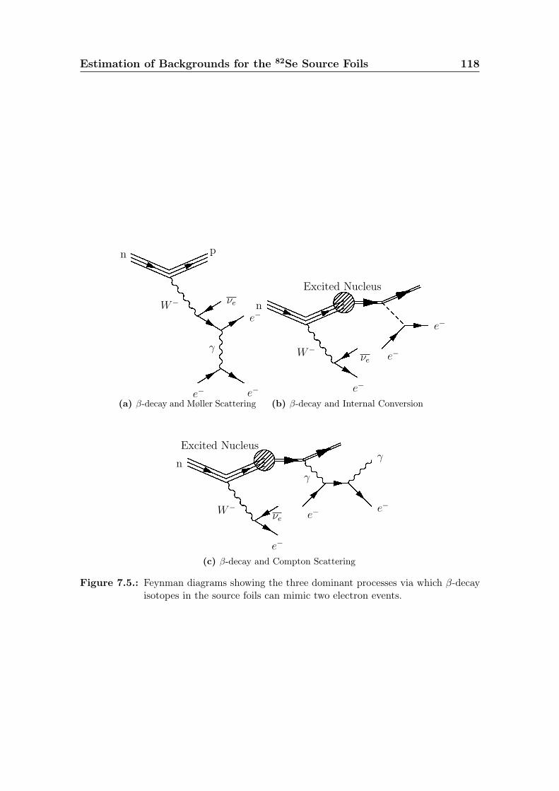
Estimation of Backgrounds for the 82Se Source Foils 118
�W−
γ
n p
νe
e−
e− e−
(a) β-decay and Møller Scattering
�W−
n
νe
e−
Excited Nucleus
e−
e−
(b) β-decay and Internal Conversion
�W−
γn
νe
e−
Excited Nucleus
e−e−
γ
(c) β-decay and Compton Scattering
Figure 7.5.: Feynman diagrams showing the three dominant processes via which β-decayisotopes in the source foils can mimic two electron events.
Estimation of Backgrounds for the 82Se Source Foils 119
Within these chains, certain isotopes have short half-lives and must therefore be inequilibrium with each other. For example, the activities of 214Bi and 214Pb must beequal and 212Bi, 228Ac and 208Tl must also be in equilibrium, taking into account thebranching fraction of 36% between 212Bi and 208Tl. However, due to long intermediatehalf-lives, equilibrium is not guaranteed between 234mPa and 214Bi.
The HPGe measurement also produced a non-zero result for contamination by 235U,however, there was no evidence of 227Ac so the equilibrium must be broken and no207Tl or 211Pb is expected to contribute.
In this work, the internal backgrounds in the selenium foils of NEMO-3 are measuredand verified by comparison with the results of the HPGe measurement.
7.2.2. External Backgrounds
External backgrounds are classed as those that originate anywhere in the detectorother than the source foils and that are not radon-induced. In order to mimictwo electron events, external backgrounds usually involve a photon that interactswith the source foil as shown in Figure 7.6. In the case of pair production, theoutgoing positron must also be misidentified as an electron, which is unlikely giventhe magnetic field. Electrons that do not interact in the foil, but cross the detectoras discussed in Section 6.4, can also be mistaken for two electron events. However,these crossing electrons are heavily suppressed by removing events based on theirtiming information.
Sources of external background are predominantly due to radioactive decay withinthe rock surrounding the laboratory, neutron capture and decay within the detectorcomponents themselves. The main types of event are external 1e1γ and crossingelectron events as were shown in Figure 6.4. Analysis of these channels has allowedfor the construction of an external background model that is capable of describingthe γ flux incident on the detector.
External Background Model
The external background model is an effective model that is used to quantify thecontribution of external background events to two electron measurements and is
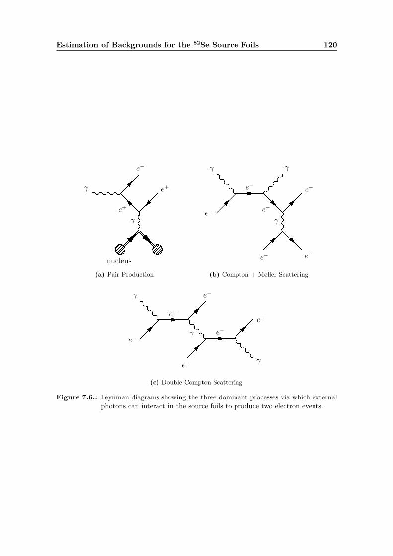
Estimation of Backgrounds for the 82Se Source Foils 120
�e+
γ
γ e+
e−
nucleus
(a) Pair Production
�e−
e−
γe−
γ
e−
e−
γ
e−
(b) Compton + Møller Scattering
�e−
γ e−
e−
γ
γ
e−
e−
e−
(c) Double Compton Scattering
Figure 7.6.: Feynman diagrams showing the three dominant processes via which externalphotons can interact in the source foils to produce two electron events.
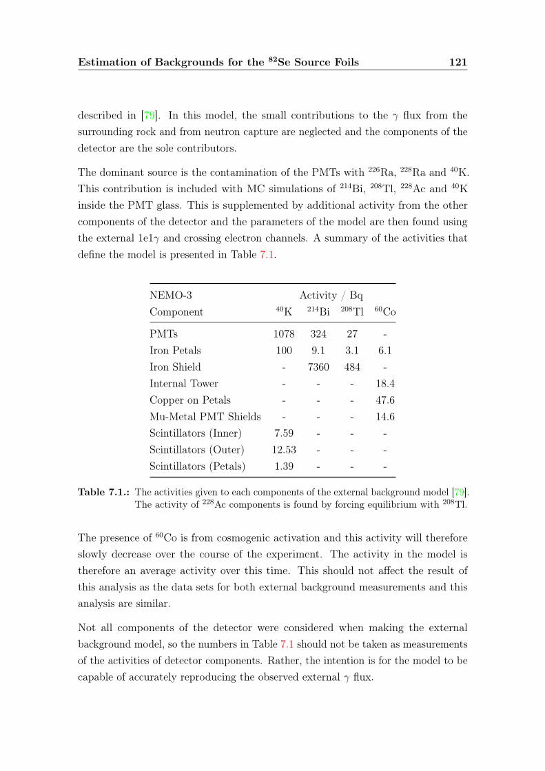
Estimation of Backgrounds for the 82Se Source Foils 121
described in [79]. In this model, the small contributions to the γ flux from thesurrounding rock and from neutron capture are neglected and the components of thedetector are the sole contributors.
The dominant source is the contamination of the PMTs with 226Ra, 228Ra and 40K.This contribution is included with MC simulations of 214Bi, 208Tl, 228Ac and 40Kinside the PMT glass. This is supplemented by additional activity from the othercomponents of the detector and the parameters of the model are then found usingthe external 1e1γ and crossing electron channels. A summary of the activities thatdefine the model is presented in Table 7.1.
NEMO-3 Activity / BqComponent 40K 214Bi 208Tl 60Co
PMTs 1078 324 27 -Iron Petals 100 9.1 3.1 6.1Iron Shield - 7360 484 -Internal Tower - - - 18.4Copper on Petals - - - 47.6Mu-Metal PMT Shields - - - 14.6Scintillators (Inner) 7.59 - - -Scintillators (Outer) 12.53 - - -Scintillators (Petals) 1.39 - - -
Table 7.1.: The activities given to each components of the external background model [79].The activity of 228Ac components is found by forcing equilibrium with 208Tl.
The presence of 60Co is from cosmogenic activation and this activity will thereforeslowly decrease over the course of the experiment. The activity in the model istherefore an average activity over this time. This should not affect the result ofthis analysis as the data sets for both external background measurements and thisanalysis are similar.
Not all components of the detector were considered when making the externalbackground model, so the numbers in Table 7.1 should not be taken as measurementsof the activities of detector components. Rather, the intention is for the model to becapable of accurately reproducing the observed external γ flux.
Estimation of Backgrounds for the 82Se Source Foils 122
The external model is used as a basis for the external backgrounds in this analysisand was constructed using measurements from all sectors. However, it is expectedthat small variations in the γ flux may be observed from sector-to-sector. As thisanalysis will only use sectors containing 82Se, small variations in the activities of themodel are expected in the final measurements.
7.2.3. Radon Backgrounds
The final background classification is radon-induced backgrounds. Although theorigin of these backgrounds is external, they are given a separate classification asradon progenies can be deposited on the source foil surfaces, effectively becominginternal backgrounds, and as they should vary significantly between phases 1 and 2.
The radon level inside the detector can be measured with a fine granularity in timeby studying BiPo type events as described in Section 6.3.3. The resulting radonactivity over time is displayed in Figure 7.7, where a clear reduction can be seenbetween phases 1 and 2.
In addition to measuring the total activity of radon in the detector, it is possible touse BiPo events to measure the distribution of its progenies. In addition to BiPoevents that originate from the source foils (Figure 6.3), it is also possible to locateBiPo events that start at tracking wires some distance away from the foil with eventssuch as that shown in Figure 7.8. Using events of this type, an extensive radon modelhas been developed which distributes 214Bi on the surface of the tracker wires, sourcefoils and scintillators, denoted SWire, SFoil and SScin respectively. In addition, theSWire contribution is mapped by sector and tracker layer.
In the work described in this thesis, the SFoil contribution has been re-measuredalong with the contribution from the first layer of tracker wires in each sector. Forthe remaining wire activities, an overall normalisation is used, with relative activitiestaken from the previously measured radon map.
In addition to the 214Bi and 214Pb components that are measured with BiPo events,there are three further members of the set of radon backgrounds. The first is aproduct of thoron decay, 208Tl, deposited on the surface of the wires, which wasmeasured using 1e2γ and 1e3γ channels where the electron track starts away from
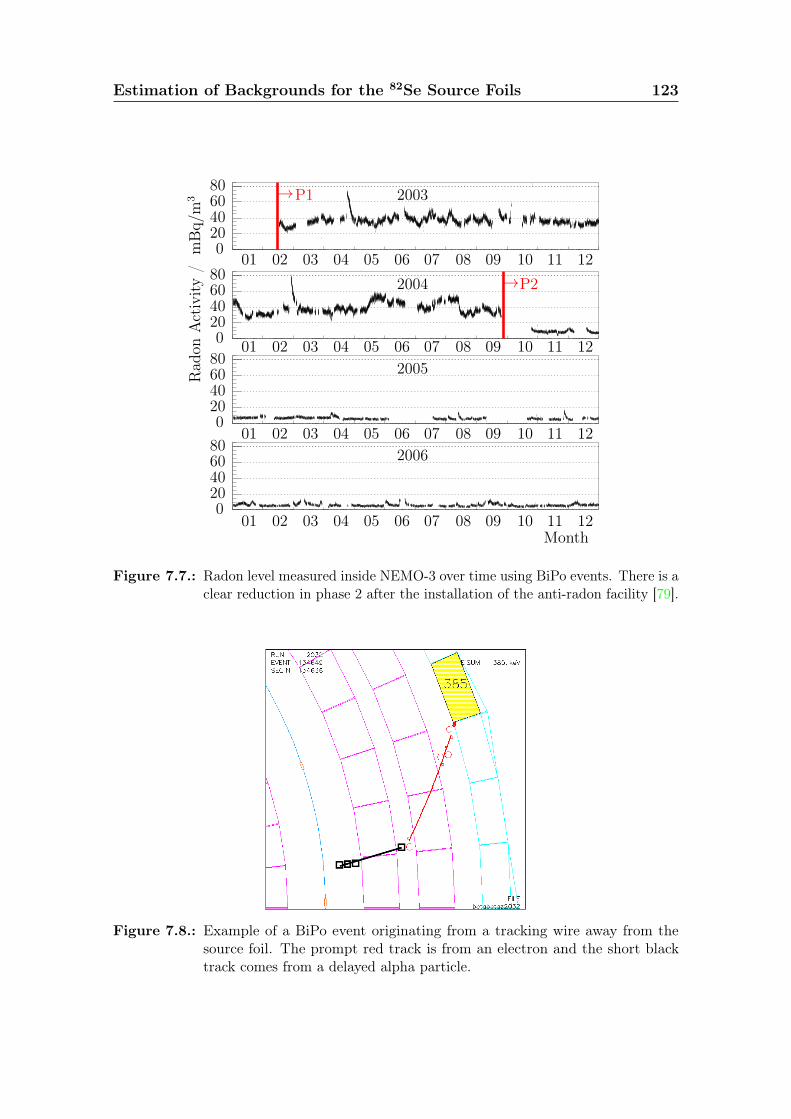
Estimation of Backgrounds for the 82Se Source Foils 123
→P1Rad
onActivity
/mBq/
m3
→P2
Month
2006
2005
2004
2003
01 02 03 04 05 06 07 08 09 10 11 12
01 02 03 04 05 06 07 08 09 10 11 12
01 02 03 04 05 06 07 08 09 10 11 12
01 02 03 04 05 06 07 08 09 10 11 12
020406080020406080020406080
020406080
Figure 7.7.: Radon level measured inside NEMO-3 over time using BiPo events. There is aclear reduction in phase 2 after the installation of the anti-radon facility [79].
Figure 7.8.: Example of a BiPo event originating from a tracking wire away from thesource foil. The prompt red track is from an electron and the short blacktrack comes from a delayed alpha particle.
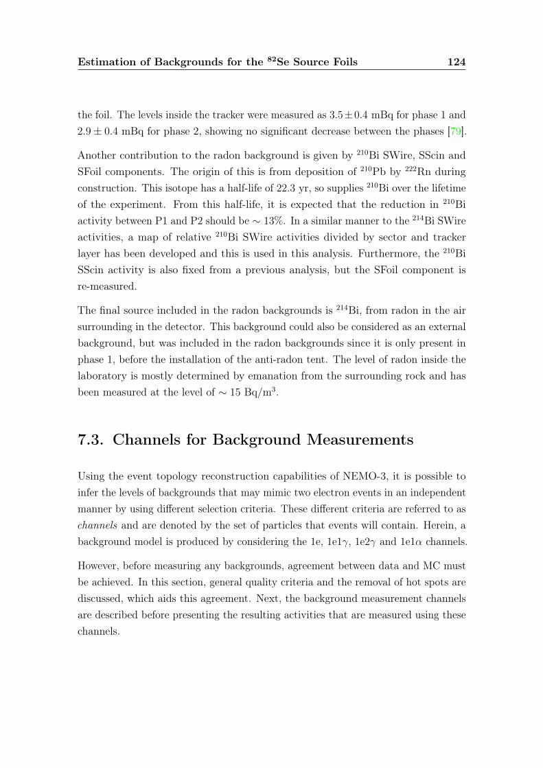
Estimation of Backgrounds for the 82Se Source Foils 124
the foil. The levels inside the tracker were measured as 3.5±0.4 mBq for phase 1 and2.9± 0.4 mBq for phase 2, showing no significant decrease between the phases [79].
Another contribution to the radon background is given by 210Bi SWire, SScin andSFoil components. The origin of this is from deposition of 210Pb by 222Rn duringconstruction. This isotope has a half-life of 22.3 yr, so supplies 210Bi over the lifetimeof the experiment. From this half-life, it is expected that the reduction in 210Biactivity between P1 and P2 should be ∼ 13%. In a similar manner to the 214Bi SWireactivities, a map of relative 210Bi SWire activities divided by sector and trackerlayer has been developed and this is used in this analysis. Furthermore, the 210BiSScin activity is also fixed from a previous analysis, but the SFoil component isre-measured.
The final source included in the radon backgrounds is 214Bi, from radon in the airsurrounding in the detector. This background could also be considered as an externalbackground, but was included in the radon backgrounds since it is only present inphase 1, before the installation of the anti-radon tent. The level of radon inside thelaboratory is mostly determined by emanation from the surrounding rock and hasbeen measured at the level of ∼ 15 Bq/m3.
7.3. Channels for Background Measurements
Using the event topology reconstruction capabilities of NEMO-3, it is possible toinfer the levels of backgrounds that may mimic two electron events in an independentmanner by using different selection criteria. These different criteria are referred to aschannels and are denoted by the set of particles that events will contain. Herein, abackground model is produced by considering the 1e, 1e1γ, 1e2γ and 1e1α channels.
However, before measuring any backgrounds, agreement between data and MC mustbe achieved. In this section, general quality criteria and the removal of hot spots arediscussed, which aids this agreement. Next, the background measurement channelsare described before presenting the resulting activities that are measured using thesechannels.
Estimation of Backgrounds for the 82Se Source Foils 125
7.3.1. General Quality Criteria
For any selection of NEMO-3 data, a number of quality cuts are applied that aim toremove events that involve unstable detector components. This means that eventsare removed from the data set if any of the following criteria are met:
• A non-calibrated PMT (in energy or time) is fired.
• An optical module with a known problem, such as a low counting rate ornon-linearity, is present. These modules are identified during calibration runswith radioactive sources.
• There is a hit in an unstable optical module, as identified by the laser survey.
• The only calorimeter hit that passes other selection criteria has an out-of-timePMT hit, which means it is likely to be the result of noise from the PMT.
In addition, a misconfiguration of the latest reconstruction of data and MC acciden-tally removed electrons that were hitting the petal scintillators. As a result, theseevents are not present in this analysis.
7.3.2. Hot Spot Search
In simulation, signal and internal background events are distributed uniformly acrossthe source foils. However, in reality, contaminants may be concentrated togetherin clusters to form so-called hot spots. The reasons for searching for and removingthese hot spots are twofold: firstly, removing them will reduce the background levelinside the detector with a minimal effect on signal efficiency; secondly, the detectoracceptance varies as a function of the position of the event, so that in order to getgood agreement between data and MC efficiencies, the distribution of backgroundevents should be as similar as possible in data and MC.
In order to search for these hot spots, the vertex distribution of single electron eventsin real data is used. An event is accepted if the following criteria are met:
• There was only one track in the event, which has negative curvature andintersects the source foil in a region given by 5.9− 8.5 in sector number and±120 cm in z.
Estimation of Backgrounds for the 82Se Source Foils 126
• This track is associated to an isolated calorimeter hit, which was not in thepetals and deposited an energy > 400 keV.
• The track has a length of 50 cm, and Geiger hits in one of the two layers closestto the foil and one of the two layers before the scintillator. This improves trackreconstruction efficiency and intersection resolution.
• There are no prompt unassociated hits within 15 cm of the electron intersectionin the xy-plane. This aids in track reconstruction efficiency and suppressesbackgrounds caused by emission from wires on the opposite side of the foil fromthe track.
After applying the hot spot search criteria, the intersection of the electron track withthe foil, known as its vertex, can be plotted to search for areas with a non-uniformdistribution of events. This can be seen in Figure 7.9a, where there are clear areas ofhigher activity. The strongest sources are based in the source foils of sector 5 on theleft side of the plot, which have a relatively high level of internal contamination.
In addition, the windows of the calibration tubes (Section 5.5.1) can be seen atthe start of sectors 6, 7 and 8. The calibration tubes are nominally located in theregion from S.00− S.07, where S is the sector, but it can be seen that the trackingvertex resolution misreconstructs some events into the source foil regions. Therefore,to remove events from the calibration tubes, exclusion zones are defined based ondata from the hot spot search channel. These zones are elliptical to account for thedifferent tracking resolutions in the transverse and vertical directions.
After removal of the calibration tubes, six hot spots are identified in the selenium foils.Two are in sector 6 and four are in sector 7, all of which are detailed in Table 7.2.
The location of the electron vertices after removing all calibration tube windows andhot spots and selecting events from the selenium foils are shown in Figure 7.9b. It isclear that there is extra contamination of the SeNew strip in sector 8, which willlater be attributed to extra 210Bi SFoil contamination. With the exception of thisstrip, the distribution of events is relatively uniform in each selenium sample, with aslightly higher level of contamination in SeNew than SeOld.
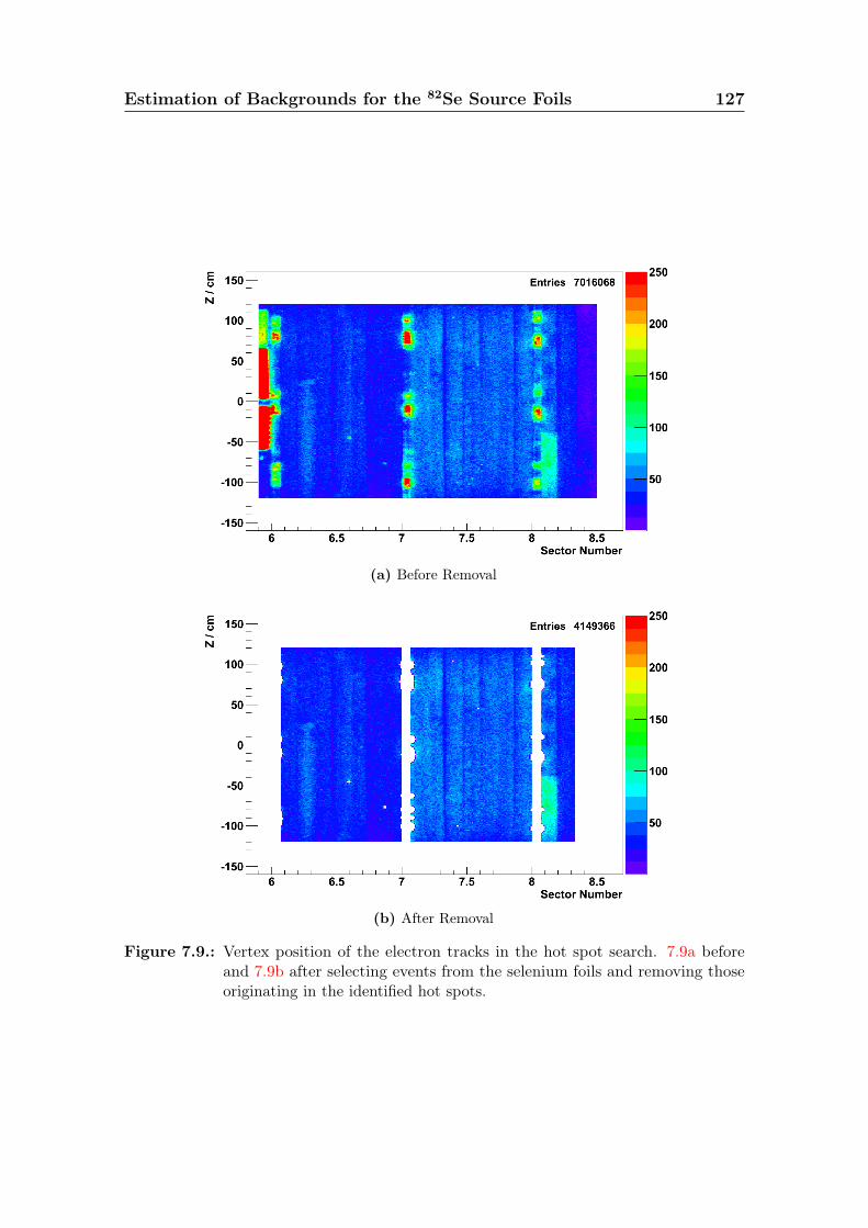
Estimation of Backgrounds for the 82Se Source Foils 127
(a) Before Removal
(b) After Removal
Figure 7.9.: Vertex position of the electron tracks in the hot spot search. 7.9a beforeand 7.9b after selecting events from the selenium foils and removing thoseoriginating in the identified hot spots.
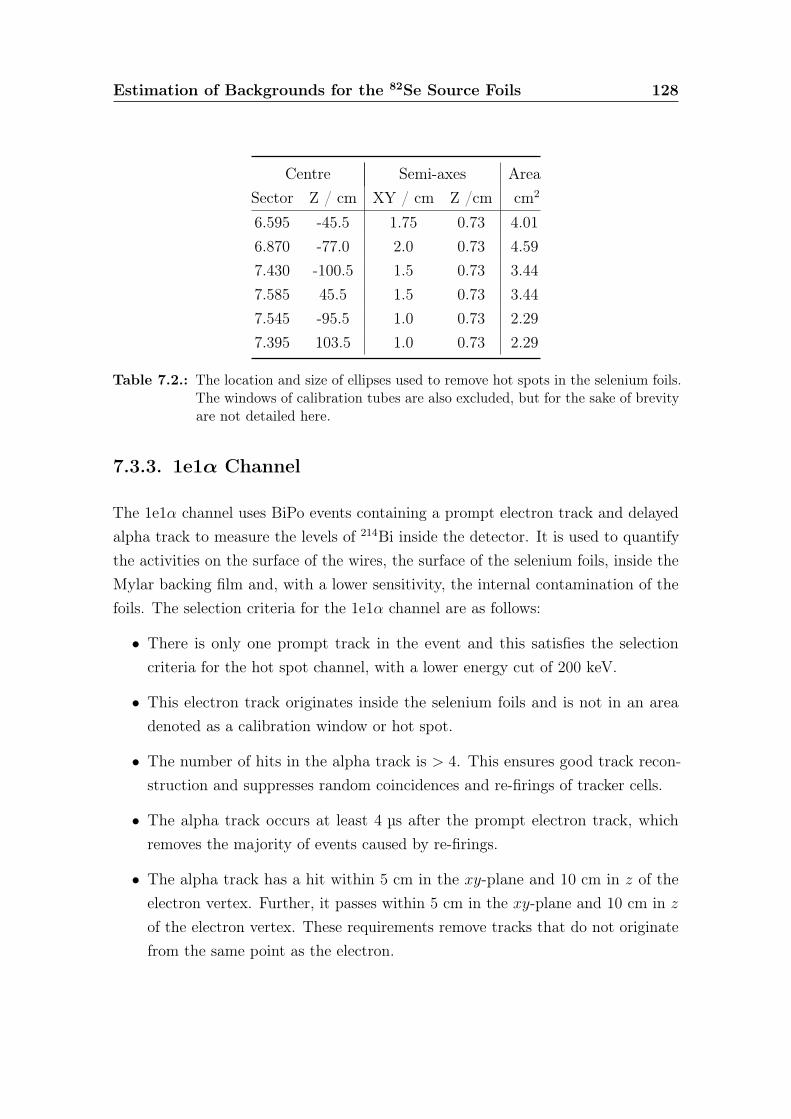
Estimation of Backgrounds for the 82Se Source Foils 128
Centre Semi-axes AreaSector Z / cm XY / cm Z /cm cm2
6.595 -45.5 1.75 0.73 4.016.870 -77.0 2.0 0.73 4.597.430 -100.5 1.5 0.73 3.447.585 45.5 1.5 0.73 3.447.545 -95.5 1.0 0.73 2.297.395 103.5 1.0 0.73 2.29
Table 7.2.: The location and size of ellipses used to remove hot spots in the selenium foils.The windows of calibration tubes are also excluded, but for the sake of brevityare not detailed here.
7.3.3. 1e1α Channel
The 1e1α channel uses BiPo events containing a prompt electron track and delayedalpha track to measure the levels of 214Bi inside the detector. It is used to quantifythe activities on the surface of the wires, the surface of the selenium foils, inside theMylar backing film and, with a lower sensitivity, the internal contamination of thefoils. The selection criteria for the 1e1α channel are as follows:
• There is only one prompt track in the event and this satisfies the selectioncriteria for the hot spot channel, with a lower energy cut of 200 keV.
• This electron track originates inside the selenium foils and is not in an areadenoted as a calibration window or hot spot.
• The number of hits in the alpha track is > 4. This ensures good track recon-struction and suppresses random coincidences and re-firings of tracker cells.
• The alpha track occurs at least 4 µs after the prompt electron track, whichremoves the majority of events caused by re-firings.
• The alpha track has a hit within 5 cm in the xy-plane and 10 cm in z of theelectron vertex. Further, it passes within 5 cm in the xy-plane and 10 cm in zof the electron vertex. These requirements remove tracks that do not originatefrom the same point as the electron.
Estimation of Backgrounds for the 82Se Source Foils 129
Since no other isotope in NEMO-3 has a delayed alpha on the same timescale as214Bi, the 1e1α channel is a clean channel to measure this signal, with only a smallfraction of contamination caused by re-firing of nearby tracker cells after the prompttrack. This fraction, and that of random coincidences, can be assessed by studyingthe timing distribution of the delayed alpha tracks. The efficiencies for selectionof 214Bi with this channel are 0.49% and 0.41% for the SeOld and SeNew samplesrespectively, where the majority of the events are lost when requiring delayed hits inthe designated time window.
Independent cross-checks between 1e1α and 1e1γ channels have shown agreementbetween measurements of 214Bi to within 10%, providing an assessment of thesystematic uncertainty of these measurements.
7.3.4. 1e2γ Channel
The 1e2γ channel exploits the decay scheme of 208Tl (Figure 7.4) to obtain a highpurity sample of 208Tl events. In this channel, an electron is accompanied by twogamma candidates, one of which is required to be of high energy. This high energyrequirement removes most other isotopes from this channel, with only a smallcontamination from 214Bi, which has very little effect due to strong constraints fromthe 1e1α channel. The selection criteria for the 1e2γ channel are as follows:
• There is one electron candidate which passes the same selection criteria as the1e1α electron.
• There are two gamma candidates with energy deposits greater than 200 keV,one of which must be above 1700 keV to remove events from 214Bi whilst keepingthose from 208Tl.
• In addition, there may be no other gamma candidates with energies above150 keV. This requirement selects events with two high energy gammas withoutbeing affected by the small amounts of noise from the PMTs.
• The internal probability of each gamma and electron pair is > 4% and theexternal probability is < 1%. These values are the “usual” NEMO-3 values,which will be considered for re-optimisation for the two electron channels(Section 8.1).
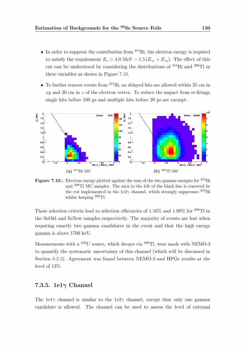
Estimation of Backgrounds for the 82Se Source Foils 130
• In order to suppress the contribution from 214Bi, the electron energy is requiredto satisfy the requirement Ee > 4.0 MeV− 1.5 (Eγ1 + Eγ2). The effect of thiscut can be understood by considering the distributions of 214Bi and 208Tl inthese variables as shown in Figure 7.10.
• To further remove events from 214Bi, no delayed hits are allowed within 25 cm inxy and 30 cm in z of the electron vertex. To reduce the impact from re-firings,single hits before 100 µs and multiple hits before 20 µs are exempt.
(a) 214Bi MC (b) 208Tl MC
Figure 7.10.: Electron energy plotted against the sum of the two gamma energies for 214Biand 208Tl MC samples. The area to the left of the black line is removed bythe cut implemented in the 1e2γ channel, which strongly suppresses 214Biwhilst keeping 208Tl.
These selection criteria lead to selection efficencies of 1.16% and 1.09% for 208Tl inthe SeOld and SeNew samples respectively. The majority of events are lost whenrequiring exactly two gamma candidates in the event and that the high energygamma is above 1700 keV.
Measurements with a 232U source, which decays via 208Tl, were made with NEMO-3to quantify the systematic uncertainty of this channel (which will be discussed inSection 8.2.3). Agreement was found between NEMO-3 and HPGe results at thelevel of 13%.
7.3.5. 1e1γ Channel
The 1e1γ channel is similar to the 1e2γ channel, except that only one gammacandidate is allowed. The channel can be used to assess the level of external
Estimation of Backgrounds for the 82Se Source Foils 131
backgrounds and the 214Bi in the air of LSM in phase 1. In addition, there arecontributions from the isotopes of the 1e1α and 1e2γ channel with smaller additionsfrom internal contamination of 234mPa and 40K. The selection criteria are as detailedbelow:
• There is one electron candidate in the event as described in the 1e1α and 1e2γevents, although this electron must have an energy > 400 keV to reduce copiouslow energy backgrounds.
• There is one gamma candidate with energy > 200 keV, internal probability> 4% and external probability < 1%.
• The total energy of all other gamma candidates is < 150 keV, which allows forlow energy decays and small amounts of noise, but ensures that only one highenergy gamma is detected.
• The same delayed hit criteria as in the 1e2γ channel are required to reduce theimpact of events from 214Bi.
Unlike the 1e1α and 1e2γ channels, it is not possible to perform stand-alone mea-surements in the 1e1γ channel, due to cross contamination with the 1e channel. Thismeans that results from the 1e1γ channel must be extracted simultaneously with the1e channel.
7.3.6. 1e Channel
The 1e channel is the simplest channel available and is very sensitive to β-decayisotopes. This means that it is used to measure all the remaining backgrounds towhich the other channels are not sensitive, which are predominantly 210Bi, 234mPaand 40K. The large number of data events in this channel, means that it is possibleto disentangle the different background contributions by fitting them to the shape ofthe energy spectrum, when accompanied by information from the other backgroundchannels. The selection criteria for the 1e channel are understandably similar tothose for the 1e1γ channel:
• There is one electron candidate in the event as set out in the 1e1γ channel.
Estimation of Backgrounds for the 82Se Source Foils 132
• There may be any number of gamma candidates in the event, as long as theirtotal energy is < 150 keV.
• The same delayed hit criteria as in the 1e1γ and 1e2γ channels are applied.
7.4. Results of Background Measurements
In order to extract the activities, the four channels described above (1e, 1e1γ, 1e2γand 1e1α) are simultaneously fitted with a number of parameters that describe theactivities of each MC sample. The data used was described in Section 6.5, totallinga dead-time corrected exposure of 1918.5 days. In this section, the procedure usedfor fitting is described (Section 7.4.1), followed by the presentation of the resultsof this process (Section 7.4.2). Finally, distributions that were not used to fit thebackground activities are shown as a cross-check of the validity of the backgroundmodel (Section 7.4.3).
7.4.1. Fitting Procedure
The fitting procedure used to extract the different isotope activities is based on abinned log-likelihood fit as described in Section 6.6.1. All four channels are used tosimultaneously extract the most likely activity parameters.
In the 1e, 1e1γ and 1e2γ channels, the electron energy distribution is used, sincethere are different isotopes present and each has a different spectral shape. However,in the 1e1α channel, only 214Bi is present and so another variable is required toextract the relevant information. In this case, the length of the alpha track is used,which is suitable as it is a strong function of the energy of the alpha when releasedinto the tracking gas. It is therefore sensitive to whether the particle originated, say,at the surface of the foil or inside the Mylar film.
In order to separate out the available information in each channel, different histogramsare constructed with the aim of minimising the number of fit parameters to whicheach is sensitive. In particular, the 1e1α channel is separated out into 24 histogramsof alpha track length, with different combinations of event geometry for each sectorand each phase. The geometrical divisions relate to the sides of the detector of the

Estimation of Backgrounds for the 82Se Source Foils 133
alpha and electron tracks, giving four separate combinations as shown in Figure 7.11.
(a) Inner side, α & e− same side (b) Inner side, α & e− opposite side
(c) Outer side, α & e− same side (d) Outer side, α & e− opposite side
Figure 7.11.: Distributions of the alpha track length in the 1e1α channel, which are thoseused in the fit. The distributions for sector 6 are shown with differentcombinations of alpha and electron side.
Where electron energy histograms are used (1e, 1e1γ and 1e2γ), the histograms aredivided into different samples for SeOld and SeNew. In addition, for the 1e and 1e1γchannels, the SeNew sample is further subdivided into histograms for sector 7 andsector 8 to account for the higher activity observed in sector 8 during the hot spotsearch (Figure 7.9). Finally, these histograms are split between the two phases togive a total of 38 histograms for the binned log-likelihood fit as shown in Table 7.3.
These 38 histograms are fitted with 28 parameters that describe the background ac-tivities for the detector and are divided across the different background classificationsas follows:
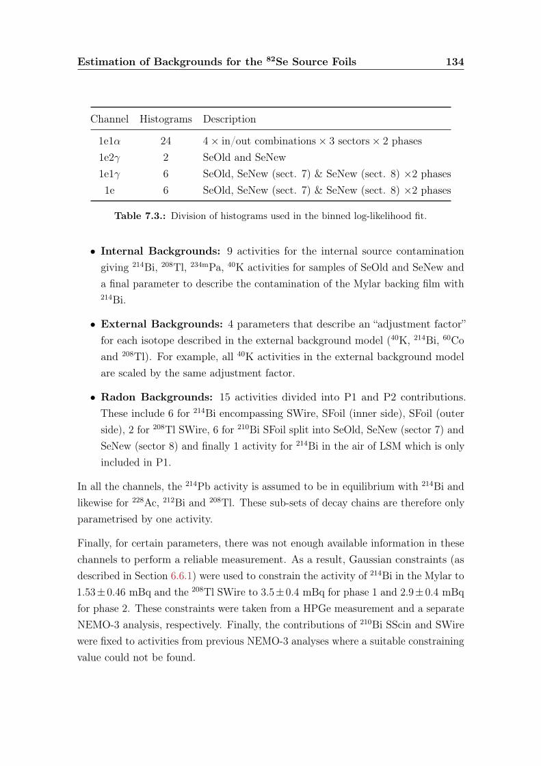
Estimation of Backgrounds for the 82Se Source Foils 134
Channel Histograms Description
1e1α 24 4× in/out combinations× 3 sectors× 2 phases1e2γ 2 SeOld and SeNew1e1γ 6 SeOld, SeNew (sect. 7) & SeNew (sect. 8) ×2 phases1e 6 SeOld, SeNew (sect. 7) & SeNew (sect. 8) ×2 phases
Table 7.3.: Division of histograms used in the binned log-likelihood fit.
• Internal Backgrounds: 9 activities for the internal source contaminationgiving 214Bi, 208Tl, 234mPa, 40K activities for samples of SeOld and SeNew anda final parameter to describe the contamination of the Mylar backing film with214Bi.
• External Backgrounds: 4 parameters that describe an “adjustment factor”for each isotope described in the external background model (40K, 214Bi, 60Coand 208Tl). For example, all 40K activities in the external background modelare scaled by the same adjustment factor.
• Radon Backgrounds: 15 activities divided into P1 and P2 contributions.These include 6 for 214Bi encompassing SWire, SFoil (inner side), SFoil (outerside), 2 for 208Tl SWire, 6 for 210Bi SFoil split into SeOld, SeNew (sector 7) andSeNew (sector 8) and finally 1 activity for 214Bi in the air of LSM which is onlyincluded in P1.
In all the channels, the 214Pb activity is assumed to be in equilibrium with 214Bi andlikewise for 228Ac, 212Bi and 208Tl. These sub-sets of decay chains are therefore onlyparametrised by one activity.
Finally, for certain parameters, there was not enough available information in thesechannels to perform a reliable measurement. As a result, Gaussian constraints (asdescribed in Section 6.6.1) were used to constrain the activity of 214Bi in the Mylar to1.53±0.46 mBq and the 208Tl SWire to 3.5±0.4 mBq for phase 1 and 2.9±0.4 mBqfor phase 2. These constraints were taken from a HPGe measurement and a separateNEMO-3 analysis, respectively. Finally, the contributions of 210Bi SScin and SWirewere fixed to activities from previous NEMO-3 analyses where a suitable constrainingvalue could not be found.
Estimation of Backgrounds for the 82Se Source Foils 135
7.4.2. Activity Estimations
The fitting procedure utilised to obtain the results is described in this section. First,the histograms that have been used to perform the fit are presented, showing goodagreement between data and simulation. Then the best estimates for backgroundactivities are summarised and compared with other results where appropriate.
1e1α Channel Distributions
The alpha length distributions from the 1e1α channel, using the resulting 214Biactivities, can be seen in Figure 7.12. The internal contribution (in red) has theshortest track lengths as these alpha particles must traverse the most material beforeentering the tracking gas. The mylar contribution (in yellow) has intermediatelengths between the internal and SFoil and SWire contributions (in blue and greenrespectively). The SWire sample has the longest tracks, out to 40 cm, since thesealphas may originate from tracker cells away from the foil. Since the track length iscalculated from the foil intersection, this artificially elongates the length. The peaksin the distribution are caused by the geometry of the tracker with the second peakat ∼ 33 cm a result of the next layers of tracker cells.
The difference between phases 1 and 2 is immediately clear, with a significantlyhigher proportion of SWire and SFoil events during phase 1. In phase 2 there is alarger contribution from the internal and Mylar components which have commonactivities across both phases. There is also higher activity on the outer side of thefoils than on the inner side, which is expected given the large volume on this side ofthe detector.
In general, there is fair agreement between data and simulation. There is moreMC than data in the peak at 30 cm and the data appears systematically higherin the region of 20 − 30 cm. This is likely to be as a result of poor replication ofthe composition of the tracking gas in the simulation as the length of the alphatrack is sensitive to small changes in its alcohol content. This results in a transferralof activities from the SWire to SFoil samples which does not significantly affectthe 2νββ or 0νββ channels, since these two samples have similar efficiencies whenselecting 2e events.
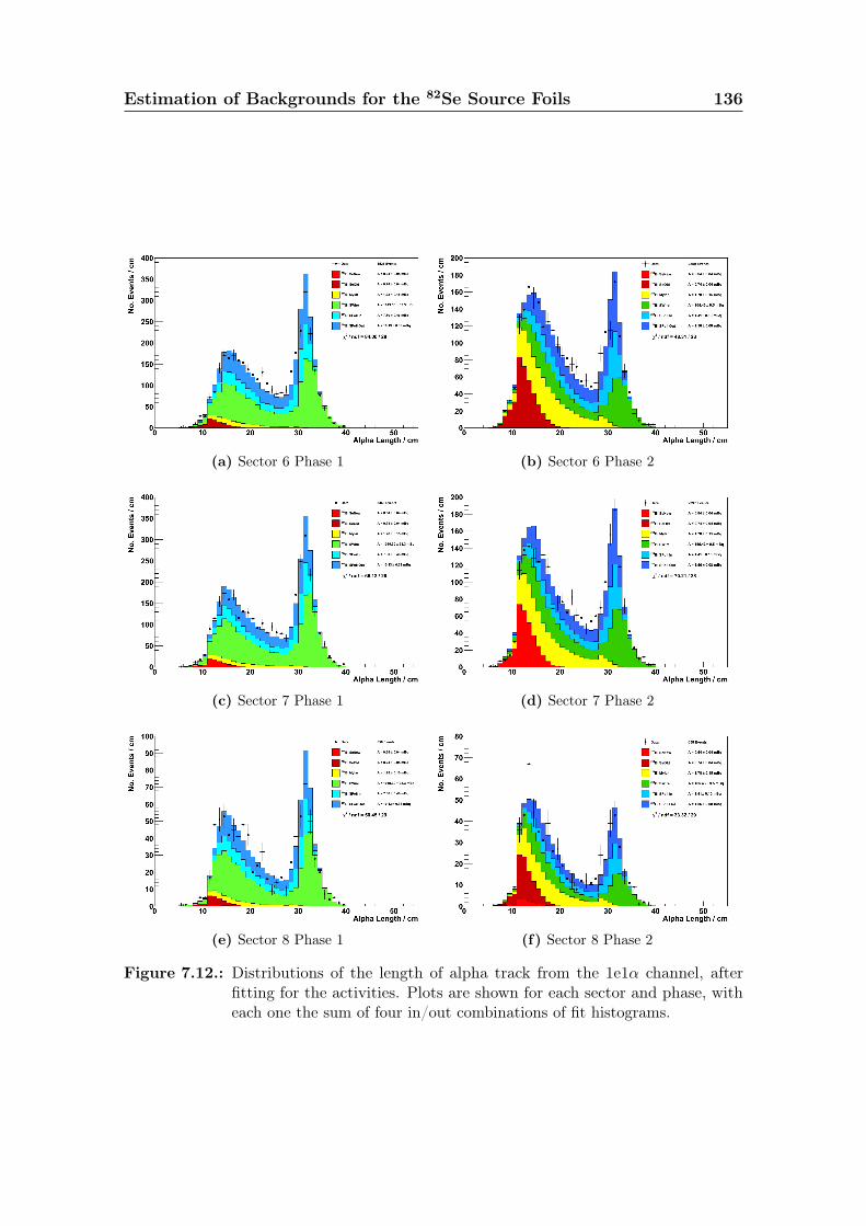
Estimation of Backgrounds for the 82Se Source Foils 136
(a) Sector 6 Phase 1 (b) Sector 6 Phase 2
(c) Sector 7 Phase 1 (d) Sector 7 Phase 2
(e) Sector 8 Phase 1 (f) Sector 8 Phase 2
Figure 7.12.: Distributions of the length of alpha track from the 1e1α channel, afterfitting for the activities. Plots are shown for each sector and phase, witheach one the sum of four in/out combinations of fit histograms.
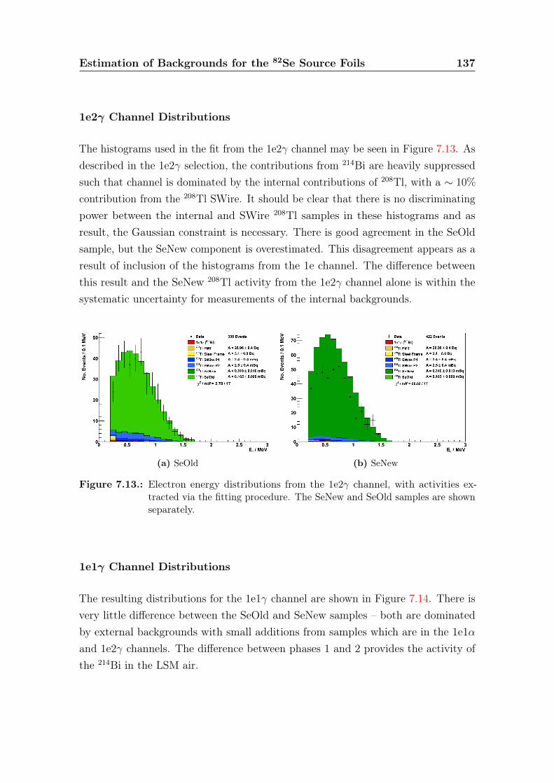
Estimation of Backgrounds for the 82Se Source Foils 137
1e2γ Channel Distributions
The histograms used in the fit from the 1e2γ channel may be seen in Figure 7.13. Asdescribed in the 1e2γ selection, the contributions from 214Bi are heavily suppressedsuch that channel is dominated by the internal contributions of 208Tl, with a ∼ 10%
contribution from the 208Tl SWire. It should be clear that there is no discriminatingpower between the internal and SWire 208Tl samples in these histograms and asresult, the Gaussian constraint is necessary. There is good agreement in the SeOldsample, but the SeNew component is overestimated. This disagreement appears as aresult of inclusion of the histograms from the 1e channel. The difference betweenthis result and the SeNew 208Tl activity from the 1e2γ channel alone is within thesystematic uncertainty for measurements of the internal backgrounds.
(a) SeOld (b) SeNew
Figure 7.13.: Electron energy distributions from the 1e2γ channel, with activities ex-tracted via the fitting procedure. The SeNew and SeOld samples are shownseparately.
1e1γ Channel Distributions
The resulting distributions for the 1e1γ channel are shown in Figure 7.14. There isvery little difference between the SeOld and SeNew samples – both are dominatedby external backgrounds with small additions from samples which are in the 1e1αand 1e2γ channels. The difference between phases 1 and 2 provides the activity ofthe 214Bi in the LSM air.
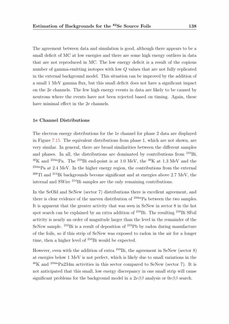
Estimation of Backgrounds for the 82Se Source Foils 138
The agreement between data and simulation is good, although there appears to be asmall deficit of MC at low energies and there are some high energy outliers in datathat are not reproduced in MC. The low energy deficit is a result of the copiousnumber of gamma-emitting isotopes with low Q values that are not fully replicatedin the external background model. This situation can be improved by the addition ofa small 1 MeV gamma flux, but this small deficit does not have a significant impacton the 2e channels. The few high energy events in data are likely to be caused byneutrons where the events have not been rejected based on timing. Again, thesehave minimal effect in the 2e channels.
1e Channel Distributions
The electron energy distributions for the 1e channel for phase 2 data are displayedin Figure 7.15. The equivalent distributions from phase 1, which are not shown, arevery similar. In general, there are broad similarities between the different samplesand phases. In all, the distributions are dominated by contributions from 210Bi,40K and 234mPa. The 210Bi end-point is at 1.0 MeV, the 40K at 1.3 MeV and the234mPa at 2.4 MeV. In the higher energy region, the contributions from the external208Tl and 214Bi backgrounds become significant and at energies above 2.7 MeV, theinternal and SWire 214Bi samples are the only remaining contributions.
In the SeOld and SeNew (sector 7) distributions there is excellent agreement, andthere is clear evidence of the uneven distribution of 234mPa between the two samples.It is apparent that the greater activity that was seen in SeNew in sector 8 in the hotspot search can be explained by an extra addition of 210Bi. The resulting 210Bi SFoilactivity is nearly an order of magnitude larger than the level in the remainder of theSeNew sample. 210Bi is a result of deposition of 210Pb by radon during manufactureof the foils, so if this strip of SeNew was exposed to radon in the air for a longertime, then a higher level of 210Bi would be expected.
However, even with the addition of extra 210Bi, the agreement in SeNew (sector 8)at energies below 1 MeV is not perfect, which is likely due to small variations in the40K and 234mPa234m activities in this sector compared to SeNew (sector 7). It isnot anticipated that this small, low energy discrepancy in one small strip will causesignificant problems for the background model in a 2νββ analysis or 0νββ search.

Estimation of Backgrounds for the 82Se Source Foils 139
(a) SeOld Phase 1 (b) SeNew Phase 1
(c) SeOld Phase 2 (d) SeNew Phase 2
(e) SeOld Phase 2 (log scale) (f) SeNew Phase 2 (log scale)
Figure 7.14.: Electron energy distributions for the 1e1γ channel for the SeOld and SeNewsample. The phase 1 and phase 2 histograms are displayed, with the phase2 plots also shown on a logarithmic scale.
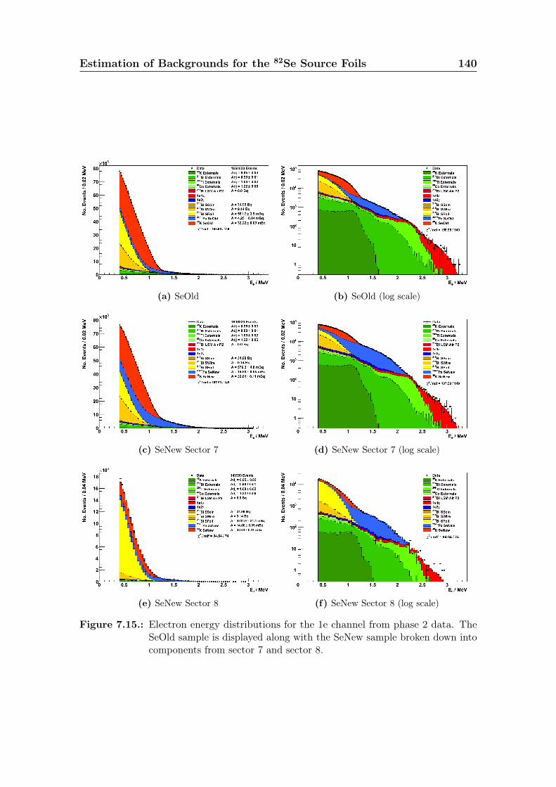
Estimation of Backgrounds for the 82Se Source Foils 140
(a) SeOld (b) SeOld (log scale)
(c) SeNew Sector 7 (d) SeNew Sector 7 (log scale)
(e) SeNew Sector 8 (f) SeNew Sector 8 (log scale)
Figure 7.15.: Electron energy distributions for the 1e channel from phase 2 data. TheSeOld sample is displayed along with the SeNew sample broken down intocomponents from sector 7 and sector 8.
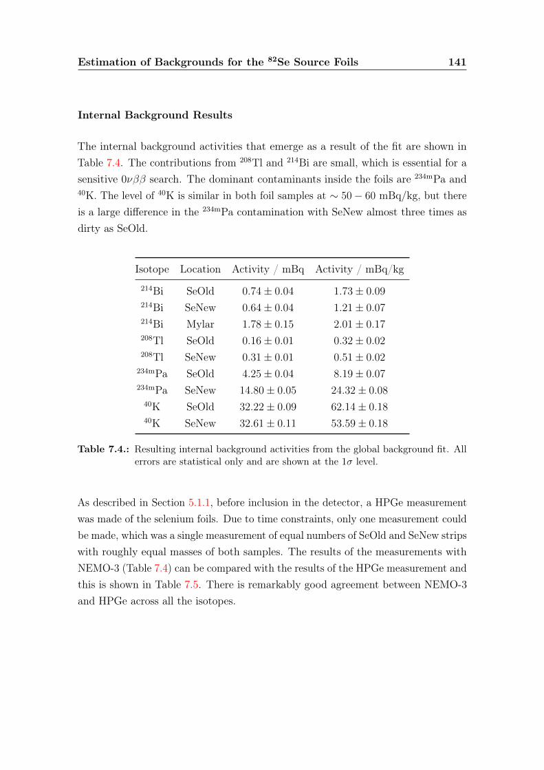
Estimation of Backgrounds for the 82Se Source Foils 141
Internal Background Results
The internal background activities that emerge as a result of the fit are shown inTable 7.4. The contributions from 208Tl and 214Bi are small, which is essential for asensitive 0νββ search. The dominant contaminants inside the foils are 234mPa and40K. The level of 40K is similar in both foil samples at ∼ 50− 60 mBq/kg, but thereis a large difference in the 234mPa contamination with SeNew almost three times asdirty as SeOld.
Isotope Location Activity / mBq Activity / mBq/kg
214Bi SeOld 0.74± 0.04 1.73± 0.09214Bi SeNew 0.64± 0.04 1.21± 0.07214Bi Mylar 1.78± 0.15 2.01± 0.17208Tl SeOld 0.16± 0.01 0.32± 0.02208Tl SeNew 0.31± 0.01 0.51± 0.02
234mPa SeOld 4.25± 0.04 8.19± 0.07234mPa SeNew 14.80± 0.05 24.32± 0.0840K SeOld 32.22± 0.09 62.14± 0.1840K SeNew 32.61± 0.11 53.59± 0.18
Table 7.4.: Resulting internal background activities from the global background fit. Allerrors are statistical only and are shown at the 1σ level.
As described in Section 5.1.1, before inclusion in the detector, a HPGe measurementwas made of the selenium foils. Due to time constraints, only one measurement couldbe made, which was a single measurement of equal numbers of SeOld and SeNew stripswith roughly equal masses of both samples. The results of the measurements withNEMO-3 (Table 7.4) can be compared with the results of the HPGe measurement andthis is shown in Table 7.5. There is remarkably good agreement between NEMO-3and HPGe across all the isotopes.
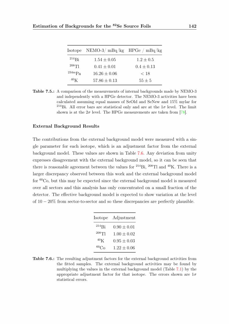
Estimation of Backgrounds for the 82Se Source Foils 142
Isotope NEMO-3/ mBq/kg HPGe / mBq/kg
214Bi 1.54± 0.05 1.2± 0.5208Tl 0.41± 0.01 0.4± 0.13
234mPa 16.26± 0.06 < 1840K 57.86± 0.13 55± 5
Table 7.5.: A comparison of the measurements of internal backgrounds made by NEMO-3and independently with a HPGe detector. The NEMO-3 activities have beencalculated assuming equal masses of SeOld and SeNew and 15% mylar for214Bi. All error bars are statistical only and are at the 1σ level. The limitshown is at the 2σ level. The HPGe measurements are taken from [78].
External Background Results
The contributions from the external background model were measured with a sin-gle parameter for each isotope, which is an adjustment factor from the externalbackground model. These values are shown in Table 7.6. Any deviation from unityexpresses disagreement with the external background model, so it can be seen thatthere is reasonable agreement between the values for 214Bi, 208Tl and 40K. There is alarger discrepancy observed between this work and the external background modelfor 60Co, but this may be expected since the external background model is measuredover all sectors and this analysis has only concentrated on a small fraction of thedetector. The effective background model is expected to show variation at the levelof 10− 20% from sector-to-sector and so these discrepancies are perfectly plausible.
Isotope Adjustment
214Bi 0.90± 0.01208Tl 1.00± 0.0240K 0.95± 0.0360Co 1.22± 0.06
Table 7.6.: The resulting adjustment factors for the external background activities fromthe fitted samples. The external background activities may be found bymultiplying the values in the external background model (Table 7.1) by theappropriate adjustment factor for that isotope. The errors shown are 1σstatistical errors.
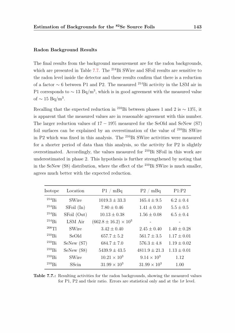
Estimation of Backgrounds for the 82Se Source Foils 143
Radon Background Results
The final results from the background measurement are for the radon backgrounds,which are presented in Table 7.7. The 214Bi SWire and SFoil results are sensitive tothe radon level inside the detector and these results confirm that there is a reductionof a factor ∼ 6 between P1 and P2. The measured 214Bi activity in the LSM air inP1 corresponds to ∼ 13 Bq/m3, which is in good agreement with the measured valueof ∼ 15 Bq/m3.
Recalling that the expected reduction in 210Bi between phases 1 and 2 is ∼ 13%, itis apparent that the measured values are in reasonable agreement with this number.The larger reduction values of 17 − 19% measured for the SeOld and SeNew (S7)foil surfaces can be explained by an overestimation of the value of 210Bi SWirein P2 which was fixed in this analysis. The 210Bi SWire activities were measuredfor a shorter period of data than this analysis, so the activity for P2 is slightlyoverestimated. Accordingly, the values measured for 210Bi SFoil in this work areunderestimated in phase 2. This hypothesis is further strengthened by noting thatin the SeNew (S8) distribution, where the effect of the 210Bi SWire is much smaller,agrees much better with the expected reduction.
Isotope Location P1 / mBq P2 / mBq P1:P2
214Bi SWire 1019.3± 33.3 165.4± 9.5 6.2± 0.4214Bi SFoil (In) 7.80± 0.46 1.41± 0.10 5.5± 0.5214Bi SFoil (Out) 10.13± 0.38 1.56± 0.08 6.5± 0.4214Bi LSM Air (662.8± 16.2)× 103 - -208Tl SWire 3.42± 0.40 2.45± 0.40 1.40± 0.28210Bi SeOld 657.7± 5.2 561.7± 3.5 1.17± 0.01210Bi SeNew (S7) 684.7± 7.0 576.3± 4.8 1.19± 0.02210Bi SeNew (S8) 5439.9± 43.5 4811.9± 21.3 1.13± 0.01210Bi SWire 10.21× 10³ 9.14× 10³ 1.12210Bi SScin 31.99× 10³ 31.99× 10³ 1.00
Table 7.7.: Resulting activities for the radon backgrounds, showing the measured valuesfor P1, P2 and their ratio. Errors are statistical only and at the 1σ level.
Estimation of Backgrounds for the 82Se Source Foils 144
7.4.3. Control Distributions
As a further check of the validity of the background model, it useful to study controldistributions which have not been used in the fitting procedure. These can highlightinconsistencies in the background model or degeneracies in the electron energydistributions where the wrong combination has been found.
Regular calibrations are made with electron sources inside NEMO-3 and as a result,the response of the detector to electrons is well-understood. However, alpha calibra-tion sources are necessarily open and were therefore never used. As a result, it isparticularly important to study well calibrated distributions for the 1e1α channel,rather than relying solely on the length of the alpha track. Some of these otherdistributions for the 1e1α channel can be seen in Figure 7.16.
In order to confirm the 1e1α channel is indeed studying BiPo type events, it ispossible to use the time of the delayed alpha track to measure the 214Po half-life.This distribution is shown in Figure 7.16b. In addition to true BiPo events, there isalso a small contamination from re-firing of tracker cells at early times. Once this hasbeen taken into account, a half-life of 162.1± 4.0 µs is measured, in good agreementwith the expected value of 164.3 µs. The remaining distributions of electron andgamma energies confirm that there is good agreement between data and MC andthe overall normalisation of 214Bi is correct. Finally, the distribution of events acrossdifferent runs also shows that both phase 1 and phase 2 data are well reproduced.
Another set of control plots can be observed from the 1e1γ channel, shown inFigure 7.17. In these plots, the cosine of the angle between the electron and gammais shown, along with the energy of the gamma.
The cosine of the angle between the electrons shows reasonable agreement, althoughthere may be a small deficit of back-to-back particles and those at acute angles.However, the Bremsstrahlung electrons produced by 40K, 234mPa and 210Bi at verynarrow angles appears to be replicated accurately in simulation. The energy of thegamma appears well reproduced over the whole energy range in both the SeOld andSeNew samples, although there may be a hint of the same overestimation of 208Tl inthe SeNew sample as seen in the 1e2γ channel.
In general, there is good agreement between the NEMO-3 measurements and all otheravailable information, so it is reasonable to have a high degree of confidence in this
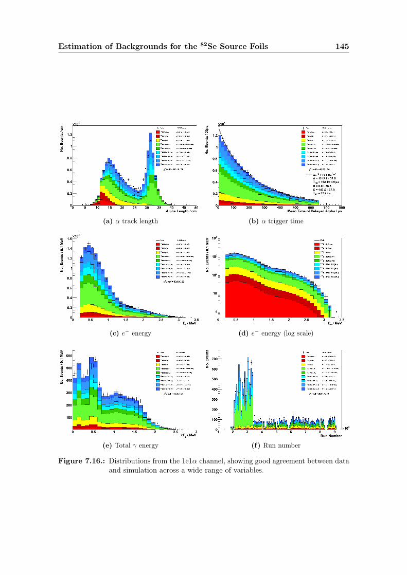
Estimation of Backgrounds for the 82Se Source Foils 145
(a) α track length (b) α trigger time
(c) e− energy (d) e− energy (log scale)
(e) Total γ energy (f) Run number
Figure 7.16.: Distributions from the 1e1α channel, showing good agreement between dataand simulation across a wide range of variables.

Estimation of Backgrounds for the 82Se Source Foils 146
(a) e− − γ cosine SeOld (b) e− − γ cosine SeNew
(c) γ Energy SeOld (d) γ Energy SeNew
Figure 7.17.: Distributions from the 1e1γ channel. The cosine of the angle between theγ and e− emissions and the energy of the γ are displayed.

Estimation of Backgrounds for the 82Se Source Foils 147
background description. Further, as will be shown in Section 8.2.3, the systematicuncertainties associated with these background measurements have a small effect onany 2νββ measurement compared to other systematic uncertainties. The backgroundlevels detailed here are ultimately re-measured along with any observed signal, butthis model is used to optimise the appropriate cuts for a 2νββ measurement, whichwill be described in the next chapter.
Chapter 8.
Double Beta Decay Results for 82Se
The main aims of the NEMO-3 analysis described in this thesis are the measurementof the 2νββ half-life of 82Se and a search for 0νββ with the same isotope. Theextraction of these results is the focus of this chapter. The double beta decayanalyses follow the procedure outlined in Chapter 6, where simulated 2νββ, 0νββand background events are propagated through a description of the NEMO-3 detectorand then compared with experimental data.
The measurement of the 2νββ half-life is performed first, as it is required for the0νββ search. In order to achieve the best measurement of 2νββ, the backgroundmodel that was defined in the previous chapter is used to optimise a set of selectioncriteria to create a 2νββ channel (Section 8.1). This optimised channel is then usedto produce a measurement of the 2νββ half-life (Section 8.2).
Having measured the 2νββ process, it is possible to perform a similar optimisationto ensure the best sensitivity for the various different 0νββ mechanisms (Section 8.3).Finally, the results of measurements with these 0νββ channels are outlined (Sec-tion 8.4).
148
Double Beta Decay Results for 82Se 149
8.1. Optimisation of 2νββ Cuts
8.1.1. Starting Point for Optimisation
In order to make a measurement of the 2νββ half-life with NEMO-3, a new channelis introduced alongside the four background channels described in Section 7.3. This2νββ channel should aim to allow the best possible measurement of the 2νββ half-life,which here is taken to mean the measurement with the lowest possible statisticaland systematic errors. In this section, the optimisation of the channel is detailed.
It is important not to introduce any bias by using experimental data to perform theoptimisation and so MC simulations will be used for the process. However, beforemoving to the sole use of MC, a suitable starting point must be found where dataand MC are in good agreement. The key principle behind this starting point is tofind a very loose set of analysis cuts, which leave plenty of room for optimisation,whilst ensuring that un-simulated detector behaviour or backgrounds do not affectthe result.
The optimisation is performed on MC distributed over the same set of runs as thebackground measurements, which gives an exposure of 1918.5 days (Section 6.5).The sum of the electron energy will be used to extract the 2νββ half-life, so it isimperative that there is good agreement between data and MC in this distribution.To assess the level of agreement, the background model described in the previouschapter is used, along with a signal with half-life of 1020 yr which is similar to thepreviously measured phase 1 value of (9.6± 0.3(stat)± 1.0(syst))× 1019 yr [73].
To find the starting point for the optimisation, the minimal set of cuts that form atwo electron channel is applied, as set out below:
• There are two tracks in the event, both of which intersect the foil and areassociated with isolated (and different) calorimeter hits.
• These calorimeter hits pass the quality criteria set out in Section 7.3.1.
• The vertex of the event, defined as the midpoint of the two track intersections,must be within the selenium foils, ±120 cm in z and not in a hot spot.
Double Beta Decay Results for 82Se 150
• There is a maximum of one prompt, unassociated Geiger hit within 15 cmof the vertex in the xy-plane, which acts as a safe-guard against poor trackreconstruction.
• If the tracks are on the same side of the foil, no prompt, unassociated Geigerhits are allowed within 15 cm of the vertex in the xy-plane and there are amaximum of two anywhere in the detector.
• If the tracks are on the same side of the foil, at least one of the track hits is inthe first tracker layer.
After the application of these cuts, the distribution of total electron energy appears asin Figures 8.1a and 8.1b, where it can be seen that although the overall normalisationis impressively similar, there are significant disagreements at low and high energies.To improve this agreement, a further set of very loose cuts is applied according tothe following selection criteria:
• The two electrons have an internal probability > 0.0001% and an externalprobability < 10%. These values remove a large proportion of backgroundevents from external sources.
• The energy of each electron is > 400 keV. This value is chosen as this was theminimum energy of electrons when building the background model.
• The distance between the two electron intersections is < 30 cm in the xy-planeand < 50 cm in z.
• There are enough Geiger cathode signals to locate the vertex in z.
• The total γ energy in the event is < 250 keV.
The total electron energy distribution, after applying these extra cuts, can be seenin Figures 8.1c and 8.1d. There is clearly much better agreement between data andsimulation and the optimisation can proceed from this point using only simulateddata.
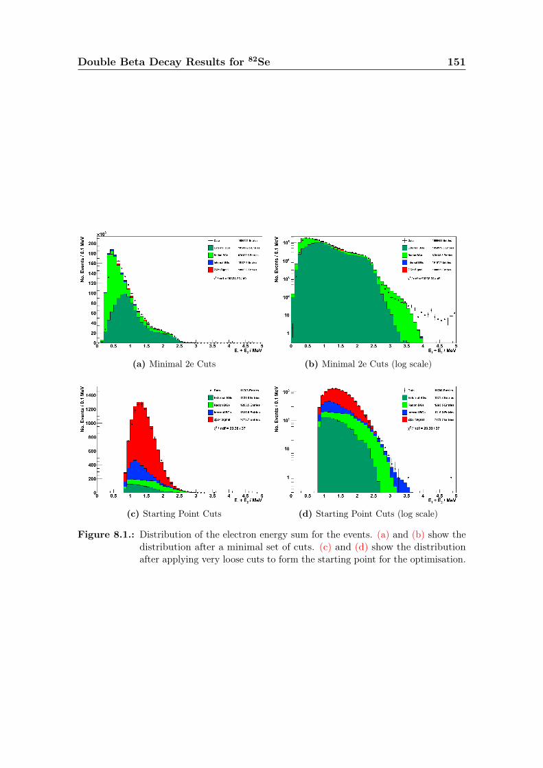
Double Beta Decay Results for 82Se 151
(a) Minimal 2e Cuts (b) Minimal 2e Cuts (log scale)
(c) Starting Point Cuts (d) Starting Point Cuts (log scale)
Figure 8.1.: Distribution of the electron energy sum for the events. (a) and (b) show thedistribution after a minimal set of cuts. (c) and (d) show the distributionafter applying very loose cuts to form the starting point for the optimisation.

Double Beta Decay Results for 82Se 152
8.1.2. Optimisation Procedure
In this optimisation procedure, two different types of cuts are considered. The firsttype are “binary” cuts, which are those cuts that may either be on or off and mayor may not improve the 2νββ result. The second type are “optimisable” cuts whichcan take a range of values and which may improve the 2νββ result if an appropriatevalue is chosen.
Five different cuts of the binary type were considered for optimisation:
• Phase 1: There is a higher level of background in phase 1, with roughlyequal numbers of radon events in phases 1 and 2, despite having only 20% ofthe exposure. Therefore, it may be beneficial to remove this period from theanalysis.
• Run status: There is a sub-set of data runs in the NEMO-3 standard analysisdata set where the detector is performing at its very best. An improved resultmay be achieved by using only these runs, obtaining higher quality data with areduction of exposure of ∼ 10%.
• Negative tracks: Requiring negative tracks suppresses backgrounds frompositrons and crossing electrons, but it also removes true signal events due toidentification inefficiencies.
• SeNew (sector 8): The strip of SeNew in sector 8 has a much higher levelof 210Bi and a comparatively small amount of 82Se. The measurement may bemore accurate without this strip.
• Delayed alphas: Requiring no delayed alpha candidate near to the vertexremoves 214Bi events, which should remove background without affecting signal.The proximity to the vertex is defined as in Section 7.3.4.
At the same time as optimising these binary cuts, the following continuous variableswere considered for an optimisable cut:
• Electron energy: As detailed above, the minimum requirement for agreementbetween data and MC is that electrons must have an energy deposit > 400 keV.There may be further improvement by putting further requirements on any of
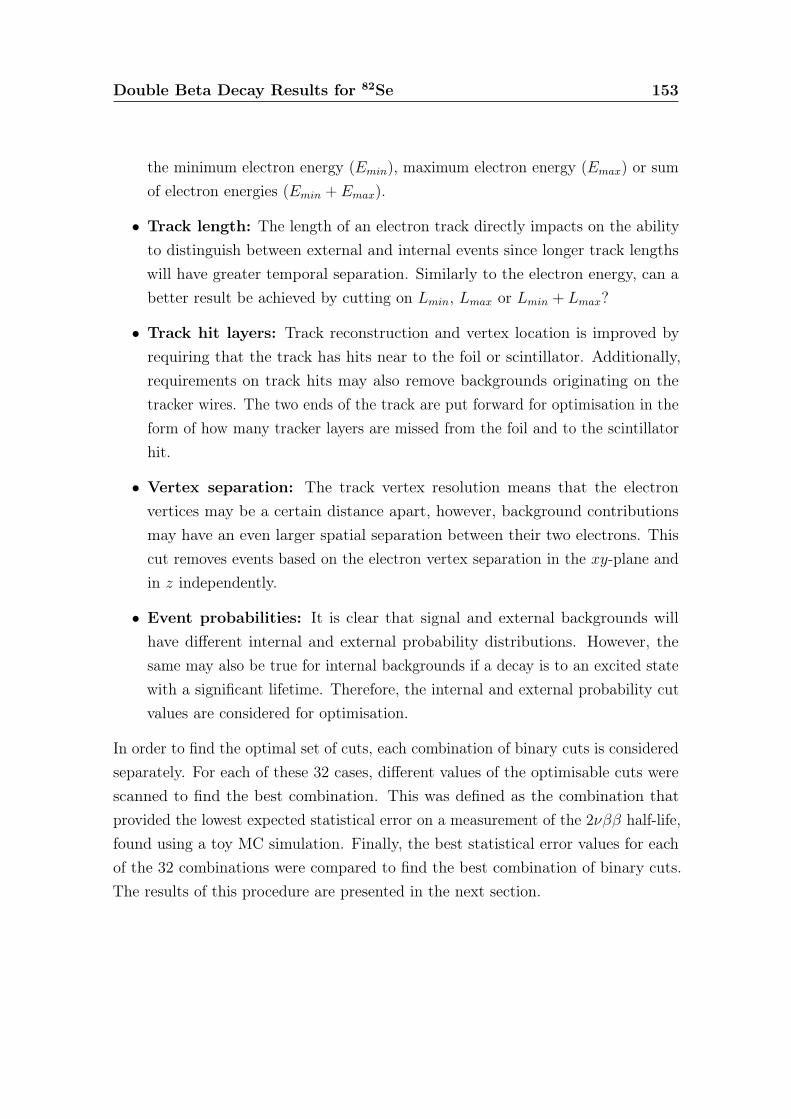
Double Beta Decay Results for 82Se 153
the minimum electron energy (Emin), maximum electron energy (Emax) or sumof electron energies (Emin + Emax).
• Track length: The length of an electron track directly impacts on the abilityto distinguish between external and internal events since longer track lengthswill have greater temporal separation. Similarly to the electron energy, can abetter result be achieved by cutting on Lmin, Lmax or Lmin + Lmax?
• Track hit layers: Track reconstruction and vertex location is improved byrequiring that the track has hits near to the foil or scintillator. Additionally,requirements on track hits may also remove backgrounds originating on thetracker wires. The two ends of the track are put forward for optimisation in theform of how many tracker layers are missed from the foil and to the scintillatorhit.
• Vertex separation: The track vertex resolution means that the electronvertices may be a certain distance apart, however, background contributionsmay have an even larger spatial separation between their two electrons. Thiscut removes events based on the electron vertex separation in the xy-plane andin z independently.
• Event probabilities: It is clear that signal and external backgrounds willhave different internal and external probability distributions. However, thesame may also be true for internal backgrounds if a decay is to an excited statewith a significant lifetime. Therefore, the internal and external probability cutvalues are considered for optimisation.
In order to find the optimal set of cuts, each combination of binary cuts is consideredseparately. For each of these 32 cases, different values of the optimisable cuts werescanned to find the best combination. This was defined as the combination thatprovided the lowest expected statistical error on a measurement of the 2νββ half-life,found using a toy MC simulation. Finally, the best statistical error values for eachof the 32 combinations were compared to find the best combination of binary cuts.The results of this procedure are presented in the next section.
Double Beta Decay Results for 82Se 154
Figure 8.2.: The lowest statistical error, achieved by varying the optimisable cuts, foreach combination of binary cuts.
8.1.3. Optimisation Results
The best statistical error value found for each combination of binary cuts is showngraphically in Figure 8.2. In this plot, the upper pane shows the expected error forthe set of cuts given in the bottom pane. At a glance, it can be seen that there is ageneral trend of improved performance for the application of fewer cuts, with thebest combination using only the alpha-proximity cut. The effects of the binary cutsare of increasing importance moving down those listed in the plot, with the strongesteffect from the phase 1 cut and weakest from the alpha proximity cut.
Once the best collection of binary cuts has been found, it is possible to set the valuesused by the optimisable cuts. When choosing these values, it should be noted thatas well as minimising statistical error, the level of systematic uncertainty must alsobe reduced. Therefore as a general principle, when there is little improvement instatistical accuracy, conservative cut values are chosen.
The results of scanning over the optimisable cut parameters, using the best combina-tion of binary cuts (no α candidates only), are presented in Figures 8.3 and 8.4. Inthe plots shown, when scanning across one parameter, all others are fixed to theirchosen values indicated by the red lines on each plot.
Double Beta Decay Results for 82Se 155
The results of moving the electron energy cut values are shown Figures 8.3a–8.3c.From these plots, there is no advantage in increasing any of the cut values fromtheir minimum values. Indeed, for the minimum electron energy in particular, theresponse is a strong function of energy and there may be considerable improvementby lowering this value. However, this would require re-building the background modelwith a lower cut threshold which may prove challenging.
The track length parameters (Figures 8.3d–8.3f) are chosen to have the longestpossible tracks without losing accuracy in the measurement. This increases theseparation between the time of calorimeter hits and mitigates systematic uncertaintyassociated with this timing. The values chosen are Lmin > 20 cm, Lmax > 50 cmand Lmin + Lmax > 80 cm.
The parameters controlling the cuts based on the tracker layers that have been hitare shown in Figures 8.4a and 8.4b. There is no significant advantage from increasingthe threshold to allow more than one missed layer and this could amplify the effectof noisy tracker cells in experimental data. As such, the first tracker hit is requiredto be in one of the first two layers, and the last tracker hit must be in one of the lasttwo layers.
Similar reasoning is employed when considering the choice of the vertex separationcut values (Figures 8.4c and 8.4d). There is minimal improvement for a large vertexseparation which would increase the possibilities of spurious tracks from noisy trackercells, so conservative cut values of ∆XY < 2 cm and ∆Z < 4 cm are chosen.
The final optimisation parameters relate to the internal and external probabilities(Section 6.4) and are shown in Figures 8.4e and 8.4f. The internal probability variablehas a stronger influence than the external probability value with the result improvingdown to very low probabilities. The “usual” NEMO-3 cut values are 4% and 1% forinternal and external probability respectively. There is no variation in the accuracyof the measurement with external probability, so this value is kept at 1%. However,this analysis suggests that a slightly improved result can be achieved by lowering theminimum internal probability from 4%. It should be noted that the “usual” NEMO-3values refer to 0νββ events so it is may be expected that a lower requirement isset for 2νββ. A minimum internal probability value of 1% is chosen to improvethe result whilst minimising any effects from systematic uncertainty associated withtiming of calorimeter hits.
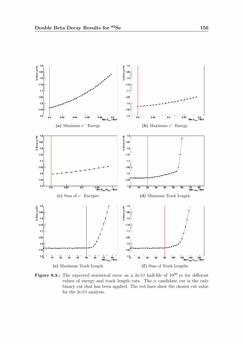
Double Beta Decay Results for 82Se 156
(a) Minimum e− Energy (b) Maximum e− Energy
(c) Sum of e− Energies (d) Minimum Track Length
(e) Maximum Track Length (f) Sum of Track Lengths
Figure 8.3.: The expected statistical error on a 2νββ half-life of 1020 yr for differentvalues of energy and track length cuts. The α candidate cut is the onlybinary cut that has been applied. The red lines show the chosen cut valuefor the 2νββ analysis.

Double Beta Decay Results for 82Se 157
(a) Lowest Tracker Layer (b) Missed Layers to Calorimeter
(c) Vertex Separation - xy (d) Vertex Separation - z
(e) Minimum Internal Probability (f) Maximum External Probability
Figure 8.4.: The expected statistical error on a 2νββ half-life of 1020 yr for different valuesof tracker layer, vertex separation and probability cuts. The α candidate cutis the only binary cut that has been applied. The red lines show the chosencut value for the 2νββ analysis.
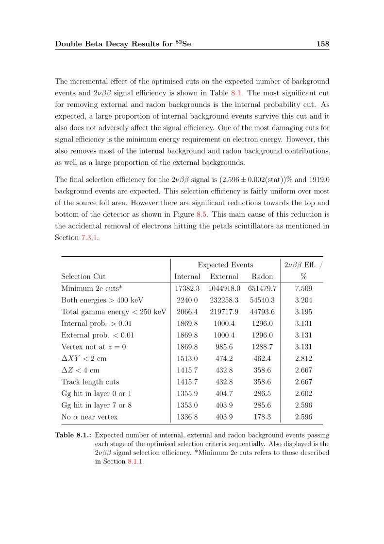
Double Beta Decay Results for 82Se 158
The incremental effect of the optimised cuts on the expected number of backgroundevents and 2νββ signal efficiency is shown in Table 8.1. The most significant cutfor removing external and radon backgrounds is the internal probability cut. Asexpected, a large proportion of internal background events survive this cut and italso does not adversely affect the signal efficiency. One of the most damaging cuts forsignal efficiency is the minimum energy requirement on electron energy. However, thisalso removes most of the internal background and radon background contributions,as well as a large proportion of the external backgrounds.
The final selection efficiency for the 2νββ signal is (2.596± 0.002(stat))% and 1919.0
background events are expected. This selection efficiency is fairly uniform over mostof the source foil area. However there are significant reductions towards the top andbottom of the detector as shown in Figure 8.5. This main cause of this reduction isthe accidental removal of electrons hitting the petals scintillators as mentioned inSection 7.3.1.
Expected Events 2νββ Eff. /Selection Cut Internal External Radon %Minimum 2e cuts* 17382.3 1044918.0 651479.7 7.509Both energies > 400 keV 2240.0 232258.3 54540.3 3.204Total gamma energy < 250 keV 2066.4 219717.9 44793.6 3.195Internal prob. > 0.01 1869.8 1000.4 1296.0 3.131External prob. < 0.01 1869.8 1000.4 1296.0 3.131Vertex not at z = 0 1869.8 985.6 1288.7 3.131∆XY < 2 cm 1513.0 474.2 462.4 2.812∆Z < 4 cm 1415.7 432.8 358.6 2.667Track length cuts 1415.7 432.8 358.6 2.667Gg hit in layer 0 or 1 1355.9 404.7 286.5 2.602Gg hit in layer 7 or 8 1353.0 403.9 285.6 2.596No α near vertex 1336.8 403.9 178.3 2.596
Table 8.1.: Expected number of internal, external and radon background events passingeach stage of the optimised selection criteria sequentially. Also displayed is the2νββ signal selection efficiency. *Minimum 2e cuts refers to those describedin Section 8.1.1.
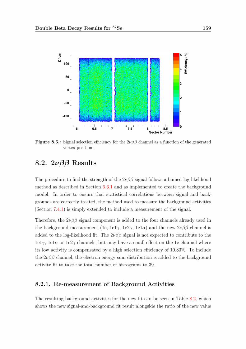
Double Beta Decay Results for 82Se 159
Figure 8.5.: Signal selection efficiency for the 2νββ channel as a function of the generatedvertex position.
8.2. 2νββ Results
The procedure to find the strength of the 2νββ signal follows a binned log-likelihoodmethod as described in Section 6.6.1 and as implemented to create the backgroundmodel. In order to ensure that statistical correlations between signal and back-grounds are correctly treated, the method used to measure the background activities(Section 7.4.1) is simply extended to include a measurement of the signal.
Therefore, the 2νββ signal component is added to the four channels already used inthe background measurement (1e, 1e1γ, 1e2γ, 1e1α) and the new 2νββ channel isadded to the log-likelihood fit. The 2νββ signal is not expected to contribute to the1e1γ, 1e1α or 1e2γ channels, but may have a small effect on the 1e channel whereits low activity is compensated by a high selection efficiency of 10.83%. To includethe 2νββ channel, the electron energy sum distribution is added to the backgroundactivity fit to take the total number of histograms to 39.
8.2.1. Re-measurement of Background Activities
The resulting background activities for the new fit can be seen in Table 8.2, whichshows the new signal-and-background fit result alongside the ratio of the new value
Double Beta Decay Results for 82Se 160
to that attained with the background-only fit. There is no significant change to anyof the background activities, with the exception of the internal 234mPa contributionswhich have been slightly reduced. This is to be expected as the 2νββ signal has amore similar spectral shape to this isotope than any other. Further confirmation of2νββ as the cause of this reduction comes by noting that the absolute reduction inactivities of the 234mPa in SeOld and SeNew is similar.
In the 2νββ channel, a total of 8426 data events were selected from the 1918.5 daysof data. The measurement predicts a total of 1890.1 background events, with 1309.5
from internal backgrounds, 402.9 from external backgrounds and 177.7 from radonbackgrounds.
The sub-division of the internal background events can be seen in Table 8.3, where itcan be seen that by far the largest proportion comes from contamination by 234mPa,which accounts for nearly half of the total expected background. The only otherlarge contributor is 214Bi which will become important for the 0νββ search. Betweenthe two samples, there are more than twice as many expected background eventsfrom SeNew as SeOld and this is mainly due to its much higher level of 234mPa.
The breakdown of the external backgrounds is equally asymmetric as can be seenfrom Table 8.4. In this case, the majority of events come from sources of 208Tl and214Bi. As discussed in Section 7.2.2, the origin of these backgrounds is from photonspenetrating the detector and the strong gamma transitions of 208Tl and 214Bi arethe cause of these dominating external backgrounds.
In the events from radon backgrounds (Table 8.5), again 214Bi is dominant. Themajority of these events come from the surface of the tracker wires with smallercontributions from the surface of the foil and from the air of the LSM. There aremore than twice as many expected events in phase 1 compared to phase 2, but theoverall contribution of the radon events is still sufficiently small that it is beneficialto include this period in the analysis.
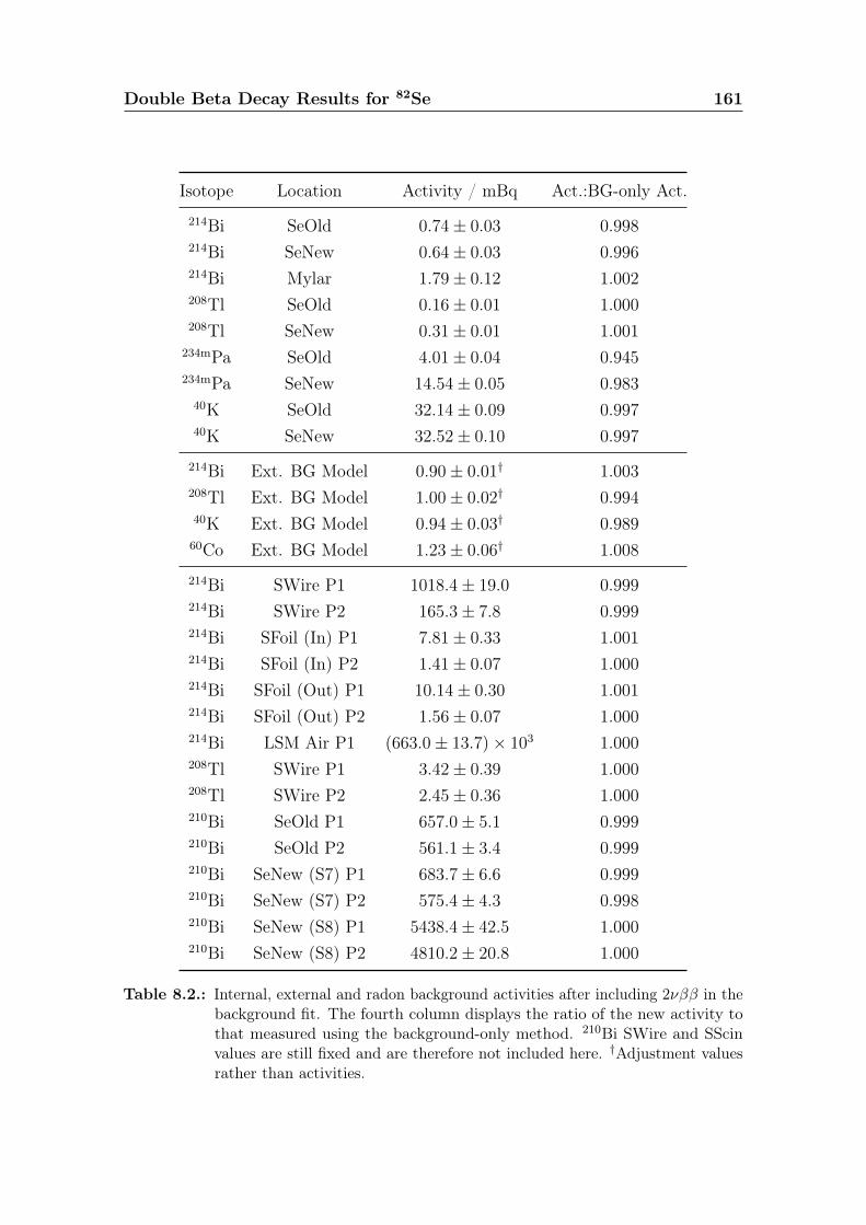
Double Beta Decay Results for 82Se 161
Isotope Location Activity / mBq Act.:BG-only Act.
214Bi SeOld 0.74± 0.03 0.998214Bi SeNew 0.64± 0.03 0.996214Bi Mylar 1.79± 0.12 1.002208Tl SeOld 0.16± 0.01 1.000208Tl SeNew 0.31± 0.01 1.001
234mPa SeOld 4.01± 0.04 0.945234mPa SeNew 14.54± 0.05 0.98340K SeOld 32.14± 0.09 0.99740K SeNew 32.52± 0.10 0.997
214Bi Ext. BG Model 0.90± 0.01† 1.003208Tl Ext. BG Model 1.00± 0.02† 0.99440K Ext. BG Model 0.94± 0.03† 0.98960Co Ext. BG Model 1.23± 0.06† 1.008
214Bi SWire P1 1018.4± 19.0 0.999214Bi SWire P2 165.3± 7.8 0.999214Bi SFoil (In) P1 7.81± 0.33 1.001214Bi SFoil (In) P2 1.41± 0.07 1.000214Bi SFoil (Out) P1 10.14± 0.30 1.001214Bi SFoil (Out) P2 1.56± 0.07 1.000214Bi LSM Air P1 (663.0± 13.7)× 103 1.000208Tl SWire P1 3.42± 0.39 1.000208Tl SWire P2 2.45± 0.36 1.000210Bi SeOld P1 657.0± 5.1 0.999210Bi SeOld P2 561.1± 3.4 0.999210Bi SeNew (S7) P1 683.7± 6.6 0.999210Bi SeNew (S7) P2 575.4± 4.3 0.998210Bi SeNew (S8) P1 5438.4± 42.5 1.000210Bi SeNew (S8) P2 4810.2± 20.8 1.000
Table 8.2.: Internal, external and radon background activities after including 2νββ in thebackground fit. The fourth column displays the ratio of the new activity tothat measured using the background-only method. 210Bi SWire and SScinvalues are still fixed and are therefore not included here. †Adjustment valuesrather than activities.

Double Beta Decay Results for 82Se 162
Expected EventsIsotope SeOld SeNew Mylar Total214Bi 91.3± 3.9 72.3± 3.6 15.4± 1.1 179.0208Tl 13.1± 0.7 21.7± 0.7 - 34.8212Bi 7.5± 0.4 13.0± 0.4 - 20.5228Ac 20.1± 1.1 33.2± 1.1 - 53.3234mPa 219.5± 2.1 727.0± 2.3 - 946.540K 45.0± 0.1 30.5± 0.1 - 75.5
Total 396.5 897.7 15.4 1309.5
Table 8.3.: Expected numbers of events in the 2νββ channel from the internal backgrounds,divided by isotope and broken down into SeOld and SeNew samples. 214Pbhas no expected events and is therefore not included.
Isotope Expected Events214Bi 144.6± 2.2208Tl 229.3± 3.3228Ac 3.7± 0.140K 16.4± 0.660Co 8.9± 0.4
Total 402.9
Table 8.4.: Predicted background events for the external backgrounds in the 2νββ channel,by isotope. 214Bi and 208Tl are located in the PMT glass, steel frame and ironshielding. 40K is in the PMT glass, steel frame and scintillator blocks. 60Co isin the steel frame, mu-metal shielding, copper on petals and internal tower.
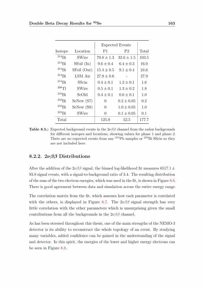
Double Beta Decay Results for 82Se 163
Expected EventsIsotope Location P1 P2 Total214Bi SWire 70.8± 1.3 32.6± 1.5 103.5214Bi SFoil (In) 9.6± 0.4 6.4± 0.3 16.0214Bi SFoil (Out) 15.4± 0.5 9.1± 0.4 24.6214Bi LSM Air 27.9± 0.6 - 27.9214Bi SScin 0.4± 0.1 1.2± 0.1 1.6208Tl SWire 0.5± 0.1 1.3± 0.2 1.8210Bi SeOld 0.4± 0.1 0.6± 0.1 1.0210Bi SeNew (S7) 0 0.2± 0.05 0.2210Bi SeNew (S8) 0 1.0± 0.05 1.0210Bi SWire 0 0.1± 0.05 0.1
Total 125.0 52.5 177.7
Table 8.5.: Expected background events in the 2νββ channel from the radon backgroundsfor different isotopes and locations, showing values for phase 1 and phase 2.There are no expected events from any 214Pb samples or 210Bi SScin so theyare not included here.
8.2.2. 2νββ Distributions
After the addition of the 2νββ signal, the binned log-likelihood fit measures 6517.1±93.8 signal events, with a signal-to-background ratio of 3.4. The resulting distributionof the sum of the two electron energies, which was used in the fit, is shown in Figure 8.6.There is good agreement between data and simulation across the entire energy range.
The correlation matrix from the fit, which assesses how each parameter is correlatedwith the others, is displayed in Figure 8.7. The 2νββ signal strength has verylittle correlation with the other parameters which is unsurprising given the smallcontributions from all the backgrounds in the 2νββ channel.
As has been stressed throughout this thesis, one of the main strengths of the NEMO-3detector is its ability to reconstruct the whole topology of an event. By studyingmany variables, added confidence can be gained in the understanding of the signaland detector. In this spirit, the energies of the lower and higher energy electrons canbe seen in Figure 8.8.
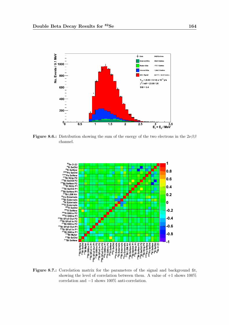
Double Beta Decay Results for 82Se 164
Figure 8.6.: Distribution showing the sum of the energy of the two electrons in the 2νββchannel.
Figure 8.7.: Correlation matrix for the parameters of the signal and background fit,showing the level of correlation between them. A value of +1 shows 100%correlation and −1 shows 100% anti-correlation.
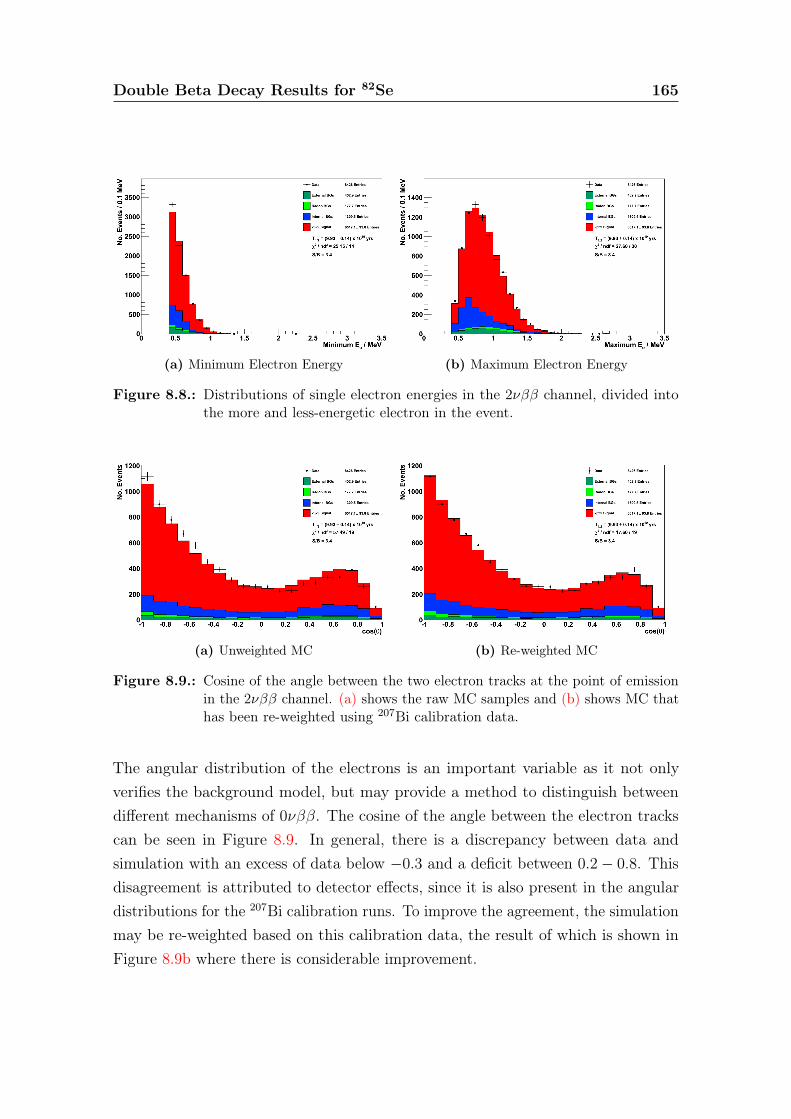
Double Beta Decay Results for 82Se 165
(a) Minimum Electron Energy (b) Maximum Electron Energy
Figure 8.8.: Distributions of single electron energies in the 2νββ channel, divided intothe more and less-energetic electron in the event.
(a) Unweighted MC (b) Re-weighted MC
Figure 8.9.: Cosine of the angle between the two electron tracks at the point of emissionin the 2νββ channel. (a) shows the raw MC samples and (b) shows MC thathas been re-weighted using 207Bi calibration data.
The angular distribution of the electrons is an important variable as it not onlyverifies the background model, but may provide a method to distinguish betweendifferent mechanisms of 0νββ. The cosine of the angle between the electron trackscan be seen in Figure 8.9. In general, there is a discrepancy between data andsimulation with an excess of data below −0.3 and a deficit between 0.2− 0.8. Thisdisagreement is attributed to detector effects, since it is also present in the angulardistributions for the 207Bi calibration runs. To improve the agreement, the simulationmay be re-weighted based on this calibration data, the result of which is shown inFigure 8.9b where there is considerable improvement.
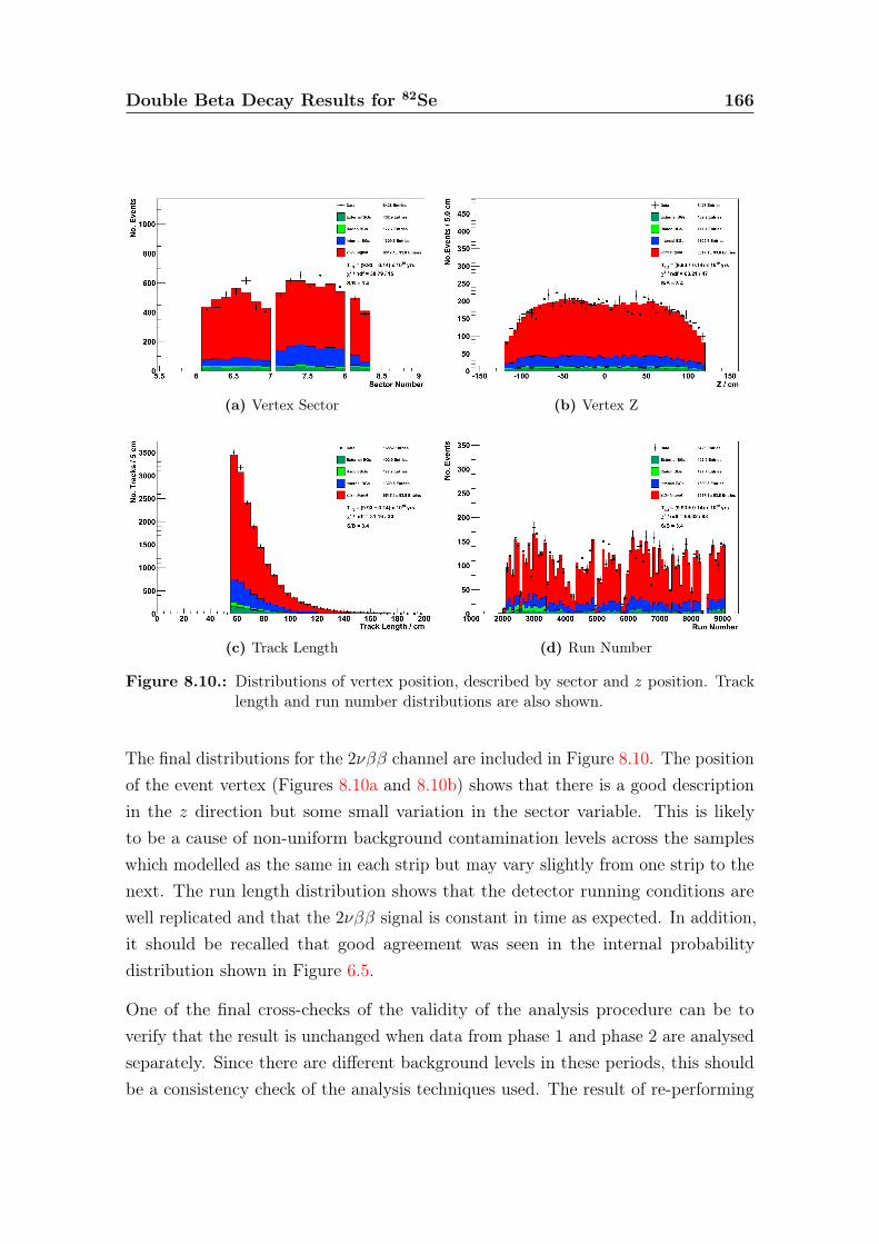
Double Beta Decay Results for 82Se 166
(a) Vertex Sector (b) Vertex Z
(c) Track Length (d) Run Number
Figure 8.10.: Distributions of vertex position, described by sector and z position. Tracklength and run number distributions are also shown.
The final distributions for the 2νββ channel are included in Figure 8.10. The positionof the event vertex (Figures 8.10a and 8.10b) shows that there is a good descriptionin the z direction but some small variation in the sector variable. This is likelyto be a cause of non-uniform background contamination levels across the sampleswhich modelled as the same in each strip but may vary slightly from one strip to thenext. The run length distribution shows that the detector running conditions arewell replicated and that the 2νββ signal is constant in time as expected. In addition,it should be recalled that good agreement was seen in the internal probabilitydistribution shown in Figure 6.5.
One of the final cross-checks of the validity of the analysis procedure can be toverify that the result is unchanged when data from phase 1 and phase 2 are analysedseparately. Since there are different background levels in these periods, this shouldbe a consistency check of the analysis techniques used. The result of re-performing
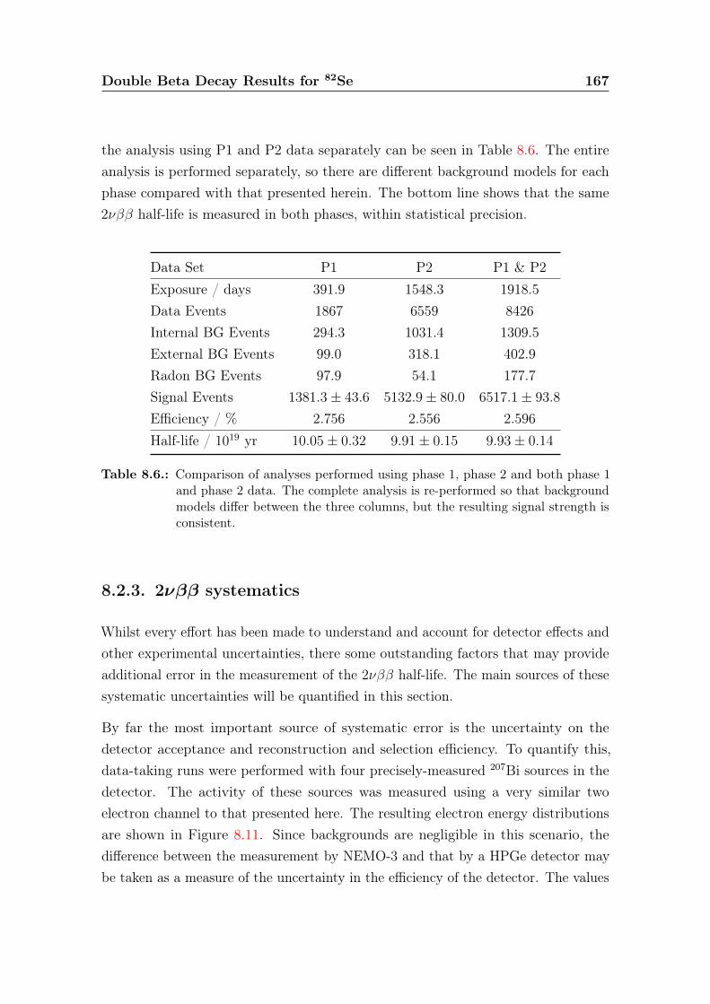
Double Beta Decay Results for 82Se 167
the analysis using P1 and P2 data separately can be seen in Table 8.6. The entireanalysis is performed separately, so there are different background models for eachphase compared with that presented herein. The bottom line shows that the same2νββ half-life is measured in both phases, within statistical precision.
Data Set P1 P2 P1 & P2Exposure / days 391.9 1548.3 1918.5Data Events 1867 6559 8426Internal BG Events 294.3 1031.4 1309.5External BG Events 99.0 318.1 402.9Radon BG Events 97.9 54.1 177.7Signal Events 1381.3± 43.6 5132.9± 80.0 6517.1± 93.8
Efficiency / % 2.756 2.556 2.596Half-life / 1019 yr 10.05± 0.32 9.91± 0.15 9.93± 0.14
Table 8.6.: Comparison of analyses performed using phase 1, phase 2 and both phase 1and phase 2 data. The complete analysis is re-performed so that backgroundmodels differ between the three columns, but the resulting signal strength isconsistent.
8.2.3. 2νββ systematics
Whilst every effort has been made to understand and account for detector effects andother experimental uncertainties, there some outstanding factors that may provideadditional error in the measurement of the 2νββ half-life. The main sources of thesesystematic uncertainties will be quantified in this section.
By far the most important source of systematic error is the uncertainty on thedetector acceptance and reconstruction and selection efficiency. To quantify this,data-taking runs were performed with four precisely-measured 207Bi sources in thedetector. The activity of these sources was measured using a very similar twoelectron channel to that presented here. The resulting electron energy distributionsare shown in Figure 8.11. Since backgrounds are negligible in this scenario, thedifference between the measurement by NEMO-3 and that by a HPGe detector maybe taken as a measure of the uncertainty in the efficiency of the detector. The values
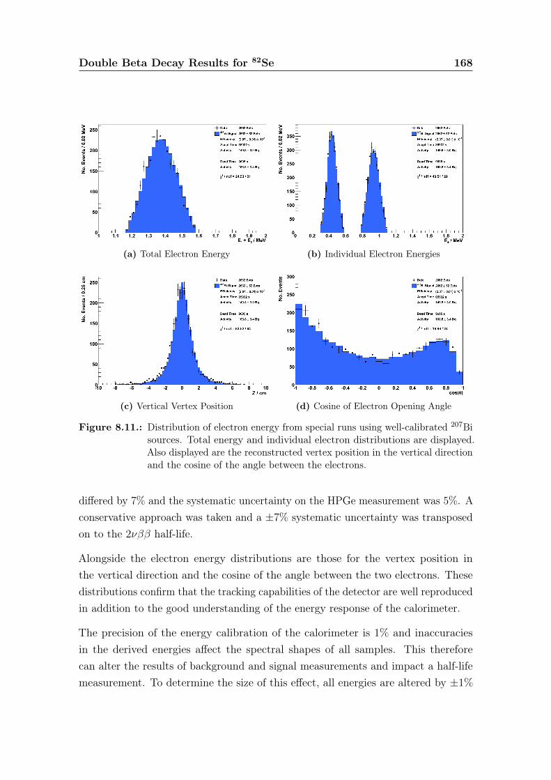
Double Beta Decay Results for 82Se 168
(a) Total Electron Energy (b) Individual Electron Energies
(c) Vertical Vertex Position (d) Cosine of Electron Opening Angle
Figure 8.11.: Distribution of electron energy from special runs using well-calibrated 207Bisources. Total energy and individual electron distributions are displayed.Also displayed are the reconstructed vertex position in the vertical directionand the cosine of the angle between the electrons.
differed by 7% and the systematic uncertainty on the HPGe measurement was 5%. Aconservative approach was taken and a ±7% systematic uncertainty was transposedon to the 2νββ half-life.
Alongside the electron energy distributions are those for the vertex position inthe vertical direction and the cosine of the angle between the two electrons. Thesedistributions confirm that the tracking capabilities of the detector are well reproducedin addition to the good understanding of the energy response of the calorimeter.
The precision of the energy calibration of the calorimeter is 1% and inaccuraciesin the derived energies affect the spectral shapes of all samples. This thereforecan alter the results of background and signal measurements and impact a half-lifemeasurement. To determine the size of this effect, all energies are altered by ±1%
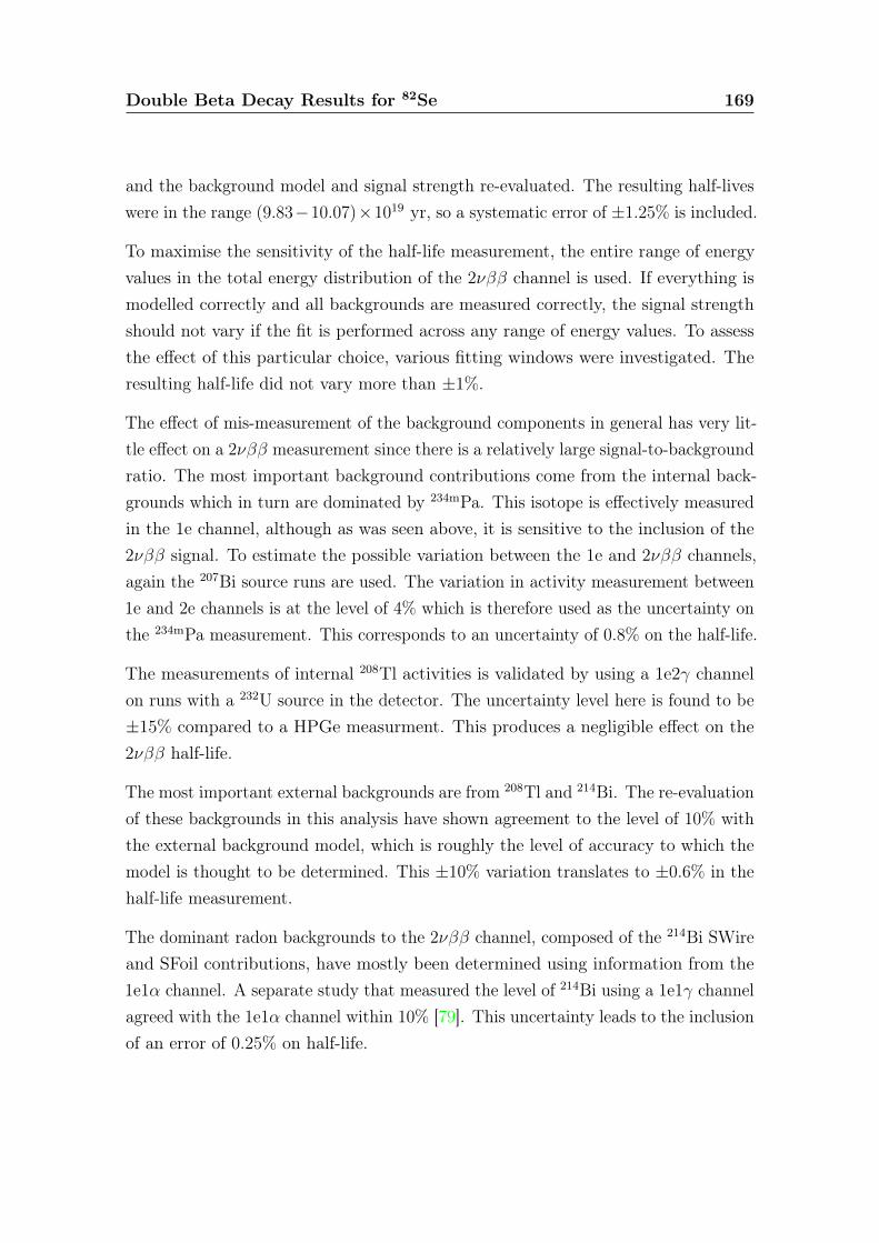
Double Beta Decay Results for 82Se 169
and the background model and signal strength re-evaluated. The resulting half-liveswere in the range (9.83−10.07)×1019 yr, so a systematic error of ±1.25% is included.
To maximise the sensitivity of the half-life measurement, the entire range of energyvalues in the total energy distribution of the 2νββ channel is used. If everything ismodelled correctly and all backgrounds are measured correctly, the signal strengthshould not vary if the fit is performed across any range of energy values. To assessthe effect of this particular choice, various fitting windows were investigated. Theresulting half-life did not vary more than ±1%.
The effect of mis-measurement of the background components in general has very lit-tle effect on a 2νββ measurement since there is a relatively large signal-to-backgroundratio. The most important background contributions come from the internal back-grounds which in turn are dominated by 234mPa. This isotope is effectively measuredin the 1e channel, although as was seen above, it is sensitive to the inclusion of the2νββ signal. To estimate the possible variation between the 1e and 2νββ channels,again the 207Bi source runs are used. The variation in activity measurement between1e and 2e channels is at the level of 4% which is therefore used as the uncertainty onthe 234mPa measurement. This corresponds to an uncertainty of 0.8% on the half-life.
The measurements of internal 208Tl activities is validated by using a 1e2γ channelon runs with a 232U source in the detector. The uncertainty level here is found to be±15% compared to a HPGe measurment. This produces a negligible effect on the2νββ half-life.
The most important external backgrounds are from 208Tl and 214Bi. The re-evaluationof these backgrounds in this analysis have shown agreement to the level of 10% withthe external background model, which is roughly the level of accuracy to which themodel is thought to be determined. This ±10% variation translates to ±0.6% in thehalf-life measurement.
The dominant radon backgrounds to the 2νββ channel, composed of the 214Bi SWireand SFoil contributions, have mostly been determined using information from the1e1α channel. A separate study that measured the level of 214Bi using a 1e1γ channelagreed with the 1e1α channel within 10% [79]. This uncertainty leads to the inclusionof an error of 0.25% on half-life.
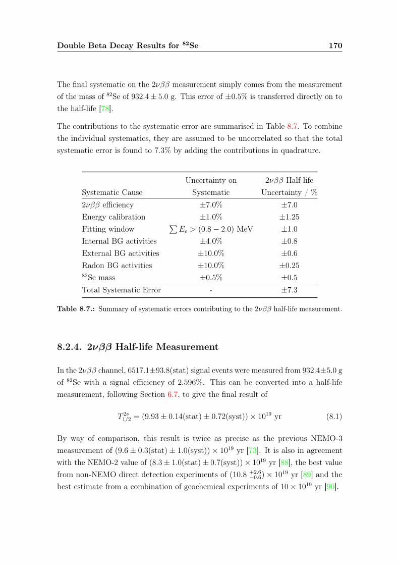
Double Beta Decay Results for 82Se 170
The final systematic on the 2νββ measurement simply comes from the measurementof the mass of 82Se of 932.4± 5.0 g. This error of ±0.5% is transferred directly on tothe half-life [78].
The contributions to the systematic error are summarised in Table 8.7. To combinethe individual systematics, they are assumed to be uncorrelated so that the totalsystematic error is found to 7.3% by adding the contributions in quadrature.
Uncertainty on 2νββ Half-lifeSystematic Cause Systematic Uncertainty / %2νββ efficiency ±7.0% ±7.0
Energy calibration ±1.0% ±1.25
Fitting window∑Ee > (0.8− 2.0) MeV ±1.0
Internal BG activities ±4.0% ±0.8
External BG activities ±10.0% ±0.6
Radon BG activities ±10.0% ±0.2582Se mass ±0.5% ±0.5
Total Systematic Error - ±7.3
Table 8.7.: Summary of systematic errors contributing to the 2νββ half-life measurement.
8.2.4. 2νββ Half-life Measurement
In the 2νββ channel, 6517.1±93.8(stat) signal events were measured from 932.4±5.0 gof 82Se with a signal efficiency of 2.596%. This can be converted into a half-lifemeasurement, following Section 6.7, to give the final result of
T 2ν1/2 = (9.93± 0.14(stat)± 0.72(syst))× 1019 yr (8.1)
By way of comparison, this result is twice as precise as the previous NEMO-3measurement of (9.6± 0.3(stat)± 1.0(syst))× 1019 yr [73]. It is also in agreementwith the NEMO-2 value of (8.3± 1.0(stat)± 0.7(syst))× 1019 yr [88], the best valuefrom non-NEMO direct detection experiments of (10.8 +2.6
−0.6)× 1019 yr [89] and thebest estimate from a combination of geochemical experiments of 10× 1019 yr [90].
Double Beta Decay Results for 82Se 171
The 2νββ matrix element, M2ν , which is of importance when tuning NME modelsfor 0νββ, can be deduced from this measurement using Equation (3.9), which isre-iterated below.
(T 2ν1/2
)−1= G2ν (Qββ, Z)
∣∣M2ν∣∣2
where G2ν (2995.5 keV, 82) = 4.3 × 10⁻¹⁸ yr−1 is the analytically calculated phasespace factor, evaluated for gA = 1.254 [91]. The resulting matrix element is thenextracted as
∣∣M2ν∣∣ = 0.0484± 0.0018 (8.2)
where the quoted error includes both statistical and systematic errors. This value canbe compared with a value calculated in the shell model, 0.084 [92], and a value foundusing the QRPA technique, 0.046 [93]. Care should be taken when interpreting thelatter result as there is considerable tuning of the QRPA model based on experimentaldata, so the comparison becomes rather circular. However, this does highlight thatthis more precise value of M2ν may be used to tune NME calculations for M0ν in82Se.
8.3. Optimisation of 0νββ Cuts
Now that all backgrounds and the 2νββ half-life have been measured, it is possibleto conduct a search for 0νββ. In order to maximise the sensitivity, an optimisationprogramme is undertaken similar to that for the 2νββ channel.
The starting point for the optimisation is the 2νββ channel and additional analysiscuts are investigated to see whether improvements in the 0νββ sensitivity can bemade. Each 0νββ decay mode is treated separately with an individual optimisation.
Before selecting the cuts that may be suitable for optimisation, it is instructive toconsider the different backgrounds that are expected for a 0νββ search. The mostcommon decay modes of the mass mechanism (Section 3.3.1), right-handed current(Section 3.3.2) and Majoron with n = 1 (Section 3.3.3) all have an experimentalsignature at energies around Qββ. The main backgrounds in the region 2.6−3.2 MeVare shown in Table 8.8.
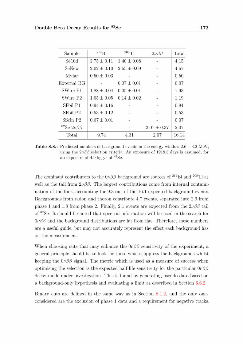
Double Beta Decay Results for 82Se 172
Sample 214Bi 208Tl 2νββ TotalSeOld 2.75± 0.11 1.40± 0.08 - 4.15SeNew 2.02± 0.10 2.65± 0.09 - 4.67Mylar 0.50± 0.03 - - 0.50
External BG - 0.07± 0.01 - 0.07SWire P1 1.88± 0.04 0.05± 0.01 - 1.93SWire P2 1.05± 0.05 0.14± 0.02 - 1.19SFoil P1 0.94± 0.16 - - 0.94SFoil P2 0.53± 0.12 - - 0.53SScin P2 0.07± 0.01 - - 0.0782Se 2νββ - - 2.07± 0.37 2.07
Total 9.74 4.31 2.07 16.14
Table 8.8.: Predicted numbers of background events in the energy window 2.6− 3.2 MeV,using the 2νββ selection criteria. An exposure of 1918.5 days is assumed, foran exposure of 4.9 kg yr of 82Se.
The dominant contributors to the 0νββ background are sources of 214Bi and 208Tl aswell as the tail from 2νββ. The largest contributions come from internal contami-nation of the foils, accounting for 9.3 out of the 16.1 expected background events.Backgrounds from radon and thoron contribute 4.7 events, separated into 2.9 fromphase 1 and 1.8 from phase 2. Finally, 2.1 events are expected from the 2νββ tailof 82Se. It should be noted that spectral information will be used in the search for0νββ and the background distributions are far from flat. Therefore, these numbersare a useful guide, but may not accurately represent the effect each background hason the measurement.
When choosing cuts that may enhance the 0νββ sensitivity of the experiment, ageneral principle should be to look for those which suppress the backgrounds whilstkeeping the 0νββ signal. The metric which is used as a measure of success whenoptimising the selection is the expected half-life sensitivity for the particular 0νββdecay mode under investigation. This is found by generating pseudo-data based ona background-only hypothesis and evaluating a limit as described in Section 6.6.2.
Binary cuts are defined in the same way as in Section 8.1.2, and the only onesconsidered are the exclusion of phase 1 data and a requirement for negative tracks.
Double Beta Decay Results for 82Se 173
As was the case with the 2νββ channel, it transpires that neither of these cuts isbeneficial and so are not applied.
Similar parameters are considered for the optimisable cuts as were with the 2νββchannel. One idea is to exploit the differences in spectral shapes of the backgroundsand signals by cutting on electron energies individually and the sum of both energies.Additionally, the internal probability is re-evaluated as at the high energies concernedtiming of electrons is more accurate and external backgrounds are less significant.
The third category of optimisable cut aims to exploit the different division of totalenergy between the two electrons for different samples. The parameter that isconsidered for optimisation is a measure of the asymmetry between the electronenergies defined as:
A =Emax − Emin
Emax + Emin(8.3)
By looking at the distribution of this variable, shown in Figure 8.12a, it is clear thatthere may be significant gains made in the right-handed current mode using thisparameter, but other decay modes are not expected to benefit greatly.
The final optimisable cut is intended to suppress the background from 208Tl bytargeting electrons caused by the 2.6 MeV nuclear transition (Figure 7.4). Eventsresulting from this 208Tl transition have conversion electrons that deposit energy at∼ 2.4 MeV as shown in Figure 8.12b. This proposed cut is implemented by excludingevents in the region given by nσ around 2.42 MeV, where the nσ is the number ofenergy resolutions found from calibration data.
The results of scanning over the optimisable parameters using the mass mechanismdecay mode are shown in Figure 8.13. Figures 8.13a–8.13c make it immediately clearthat there is no advantage gained by removing events based on their constituentenergies.
The sensitivity for different internal probability cuts are relatively flat across theentire range shown (Figure 8.13d), which is a result of the small contribution fromthe external backgrounds. The advantage that was present for a 1% cut in the 2νββchannel is no longer present, and so a cut is implemented at the more conservativevalue of 4%. This is the extremity of the the flat region before the sensitivity begins
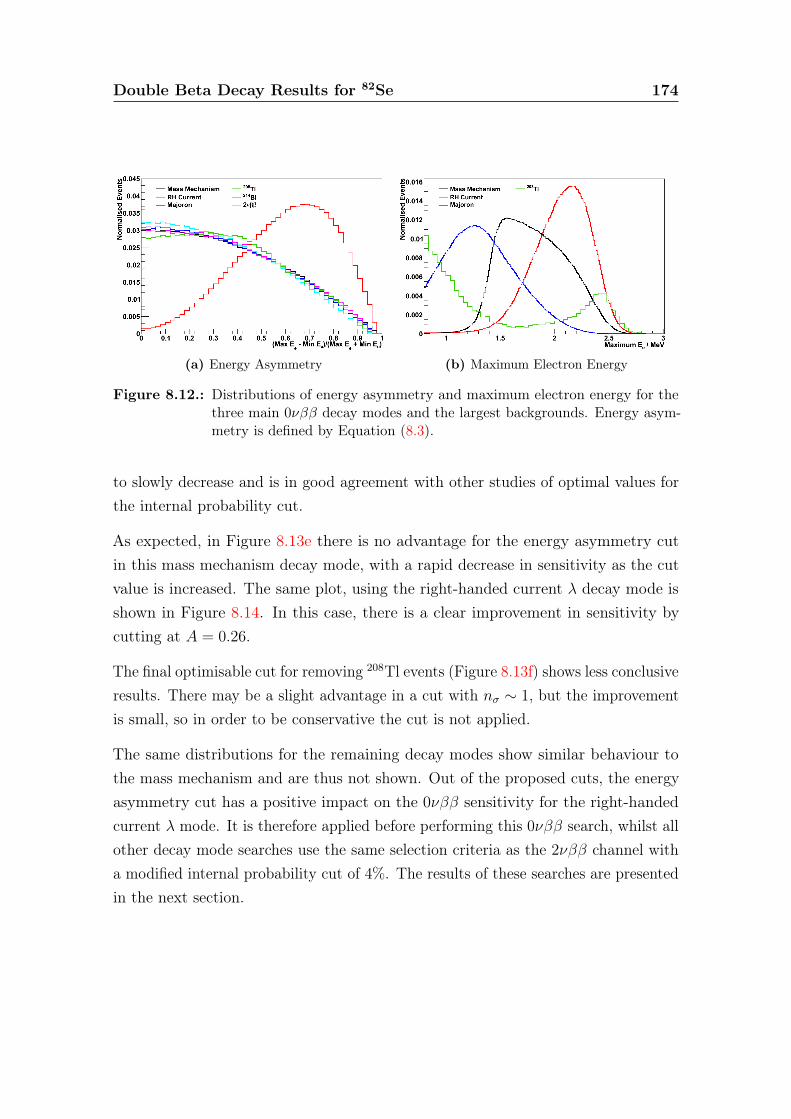
Double Beta Decay Results for 82Se 174
(a) Energy Asymmetry (b) Maximum Electron Energy
Figure 8.12.: Distributions of energy asymmetry and maximum electron energy for thethree main 0νββ decay modes and the largest backgrounds. Energy asym-metry is defined by Equation (8.3).
to slowly decrease and is in good agreement with other studies of optimal values forthe internal probability cut.
As expected, in Figure 8.13e there is no advantage for the energy asymmetry cutin this mass mechanism decay mode, with a rapid decrease in sensitivity as the cutvalue is increased. The same plot, using the right-handed current λ decay mode isshown in Figure 8.14. In this case, there is a clear improvement in sensitivity bycutting at A = 0.26.
The final optimisable cut for removing 208Tl events (Figure 8.13f) shows less conclusiveresults. There may be a slight advantage in a cut with nσ ∼ 1, but the improvementis small, so in order to be conservative the cut is not applied.
The same distributions for the remaining decay modes show similar behaviour tothe mass mechanism and are thus not shown. Out of the proposed cuts, the energyasymmetry cut has a positive impact on the 0νββ sensitivity for the right-handedcurrent λ mode. It is therefore applied before performing this 0νββ search, whilst allother decay mode searches use the same selection criteria as the 2νββ channel witha modified internal probability cut of 4%. The results of these searches are presentedin the next section.

Double Beta Decay Results for 82Se 175
(a) Minimum e− Energy (b) Maximum e− Energy
(c) Sum of e− Energies (d) Internal Probability
(e) Energy Asymmetry (f) 208Tl Cut nσ
Figure 8.13.: Expected half-life sensitivity for the mass mechanism 0νββ mode as afunction of different optimisable cut parameters.
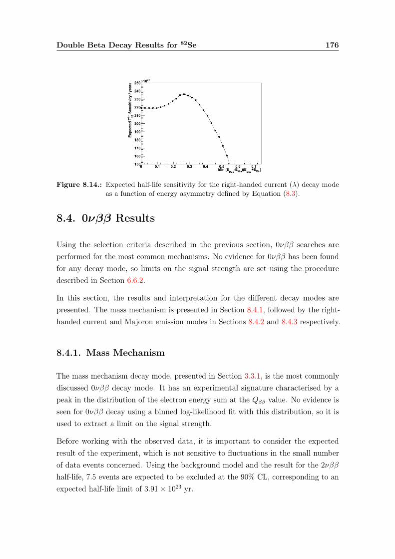
Double Beta Decay Results for 82Se 176
Figure 8.14.: Expected half-life sensitivity for the right-handed current (λ) decay modeas a function of energy asymmetry defined by Equation (8.3).
8.4. 0νββ Results
Using the selection criteria described in the previous section, 0νββ searches areperformed for the most common mechanisms. No evidence for 0νββ has been foundfor any decay mode, so limits on the signal strength are set using the proceduredescribed in Section 6.6.2.
In this section, the results and interpretation for the different decay modes arepresented. The mass mechanism is presented in Section 8.4.1, followed by the right-handed current and Majoron emission modes in Sections 8.4.2 and 8.4.3 respectively.
8.4.1. Mass Mechanism
The mass mechanism decay mode, presented in Section 3.3.1, is the most commonlydiscussed 0νββ decay mode. It has an experimental signature characterised by apeak in the distribution of the electron energy sum at the Qββ value. No evidence isseen for 0νββ decay using a binned log-likelihood fit with this distribution, so it isused to extract a limit on the signal strength.
Before working with the observed data, it is important to consider the expectedresult of the experiment, which is not sensitive to fluctuations in the small numberof data events concerned. Using the background model and the result for the 2νββhalf-life, 7.5 events are expected to be excluded at the 90% CL, corresponding to anexpected half-life limit of 3.91× 10²³ yr.
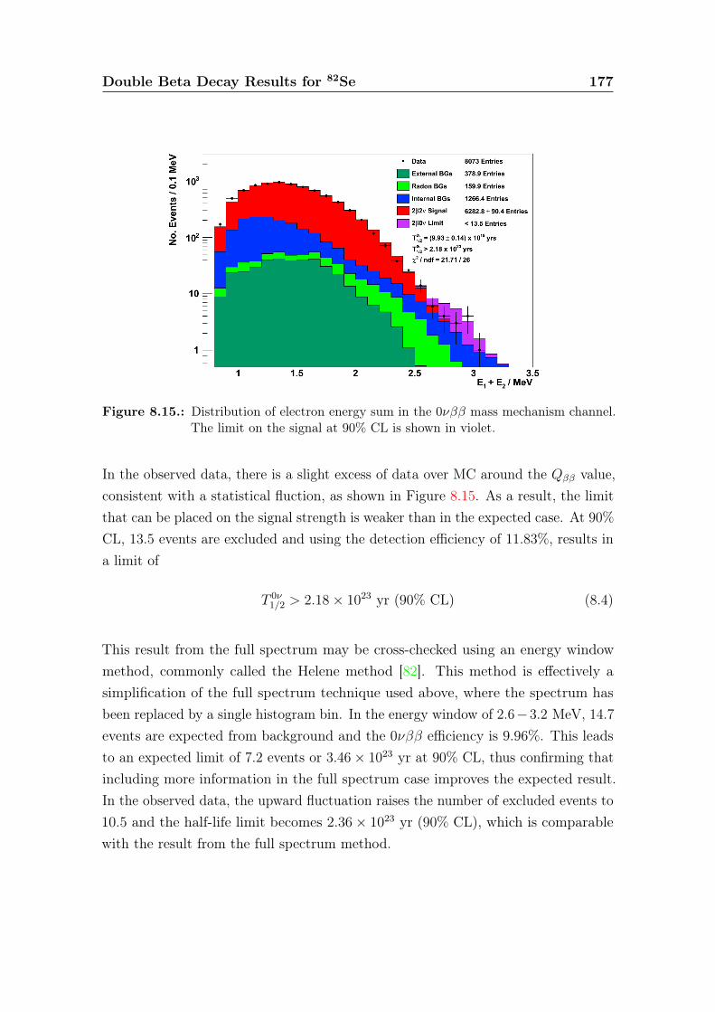
Double Beta Decay Results for 82Se 177
Figure 8.15.: Distribution of electron energy sum in the 0νββ mass mechanism channel.The limit on the signal at 90% CL is shown in violet.
In the observed data, there is a slight excess of data over MC around the Qββ value,consistent with a statistical fluction, as shown in Figure 8.15. As a result, the limitthat can be placed on the signal strength is weaker than in the expected case. At 90%CL, 13.5 events are excluded and using the detection efficiency of 11.83%, results ina limit of
T 0ν1/2 > 2.18× 10²³ yr (90% CL) (8.4)
This result from the full spectrum may be cross-checked using an energy windowmethod, commonly called the Helene method [82]. This method is effectively asimplification of the full spectrum technique used above, where the spectrum hasbeen replaced by a single histogram bin. In the energy window of 2.6−3.2 MeV, 14.7
events are expected from background and the 0νββ efficiency is 9.96%. This leadsto an expected limit of 7.2 events or 3.46× 10²³ yr at 90% CL, thus confirming thatincluding more information in the full spectrum case improves the expected result.In the observed data, the upward fluctuation raises the number of excluded events to10.5 and the half-life limit becomes 2.36× 10²³ yr (90% CL), which is comparablewith the result from the full spectrum method.
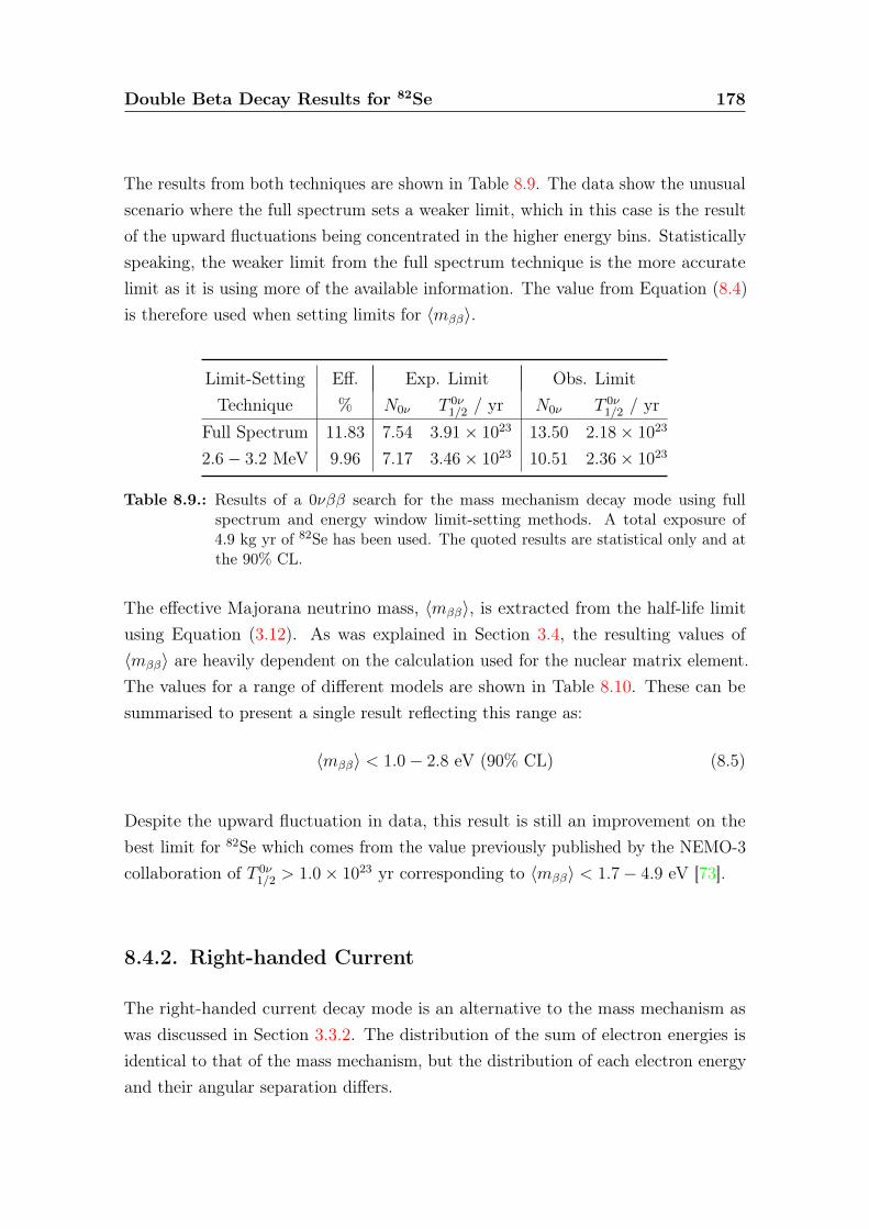
Double Beta Decay Results for 82Se 178
The results from both techniques are shown in Table 8.9. The data show the unusualscenario where the full spectrum sets a weaker limit, which in this case is the resultof the upward fluctuations being concentrated in the higher energy bins. Statisticallyspeaking, the weaker limit from the full spectrum technique is the more accuratelimit as it is using more of the available information. The value from Equation (8.4)is therefore used when setting limits for 〈mββ〉.
Limit-Setting Eff. Exp. Limit Obs. LimitTechnique % N0ν T 0ν
1/2 / yr N0ν T 0ν1/2 / yr
Full Spectrum 11.83 7.54 3.91× 10²³ 13.50 2.18× 10²³
2.6− 3.2 MeV 9.96 7.17 3.46× 10²³ 10.51 2.36× 10²³
Table 8.9.: Results of a 0νββ search for the mass mechanism decay mode using fullspectrum and energy window limit-setting methods. A total exposure of4.9 kg yr of 82Se has been used. The quoted results are statistical only and atthe 90% CL.
The effective Majorana neutrino mass, 〈mββ〉, is extracted from the half-life limitusing Equation (3.12). As was explained in Section 3.4, the resulting values of〈mββ〉 are heavily dependent on the calculation used for the nuclear matrix element.The values for a range of different models are shown in Table 8.10. These can besummarised to present a single result reflecting this range as:
〈mββ〉 < 1.0− 2.8 eV (90% CL) (8.5)
Despite the upward fluctuation in data, this result is still an improvement on thebest limit for 82Se which comes from the value previously published by the NEMO-3collaboration of T 0ν
1/2 > 1.0× 10²³ yr corresponding to 〈mββ〉 < 1.7− 4.9 eV [73].
8.4.2. Right-handed Current
The right-handed current decay mode is an alternative to the mass mechanism aswas discussed in Section 3.3.2. The distribution of the sum of electron energies isidentical to that of the mass mechanism, but the distribution of each electron energyand their angular separation differs.
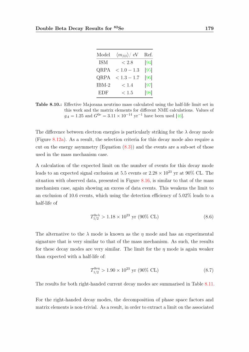
Double Beta Decay Results for 82Se 179
Model 〈mββ〉/ eV Ref.ISM < 2.8 [94]
QRPA < 1.0− 1.3 [95]QRPA < 1.3− 1.7 [96]IBM-2 < 1.4 [97]EDF < 1.5 [98]
Table 8.10.: Effective Majorana neutrino mass calculated using the half-life limit set inthis work and the matrix elements for different NME calculations. Values ofgA = 1.25 and G0ν = 3.11× 10⁻¹⁴ yr−1 have been used [46].
The difference between electron energies is particularly striking for the λ decay mode(Figure 8.12a). As a result, the selection criteria for this decay mode also require acut on the energy asymmetry (Equation (8.3)) and the events are a sub-set of thoseused in the mass mechanism case.
A calculation of the expected limit on the number of events for this decay modeleads to an expected signal exclusion at 5.5 events or 2.28× 10²³ yr at 90% CL. Thesituation with observed data, presented in Figure 8.16, is similar to that of the massmechanism case, again showing an excess of data events. This weakens the limit toan exclusion of 10.6 events, which using the detection efficiency of 5.02% leads to ahalf-life of
T 0νλ1/2 > 1.18× 10²³ yr (90% CL) (8.6)
The alternative to the λ mode is known as the η mode and has an experimentalsignature that is very similar to that of the mass mechanism. As such, the resultsfor these decay modes are very similar. The limit for the η mode is again weakerthan expected with a half-life of:
T 0νη1/2 > 1.90× 10²³ yr (90% CL) (8.7)
The results for both right-handed current decay modes are summarised in Table 8.11.
For the right-handed decay modes, the decomposition of phase space factors andmatrix elements is non-trivial. As a result, in order to extract a limit on the associated
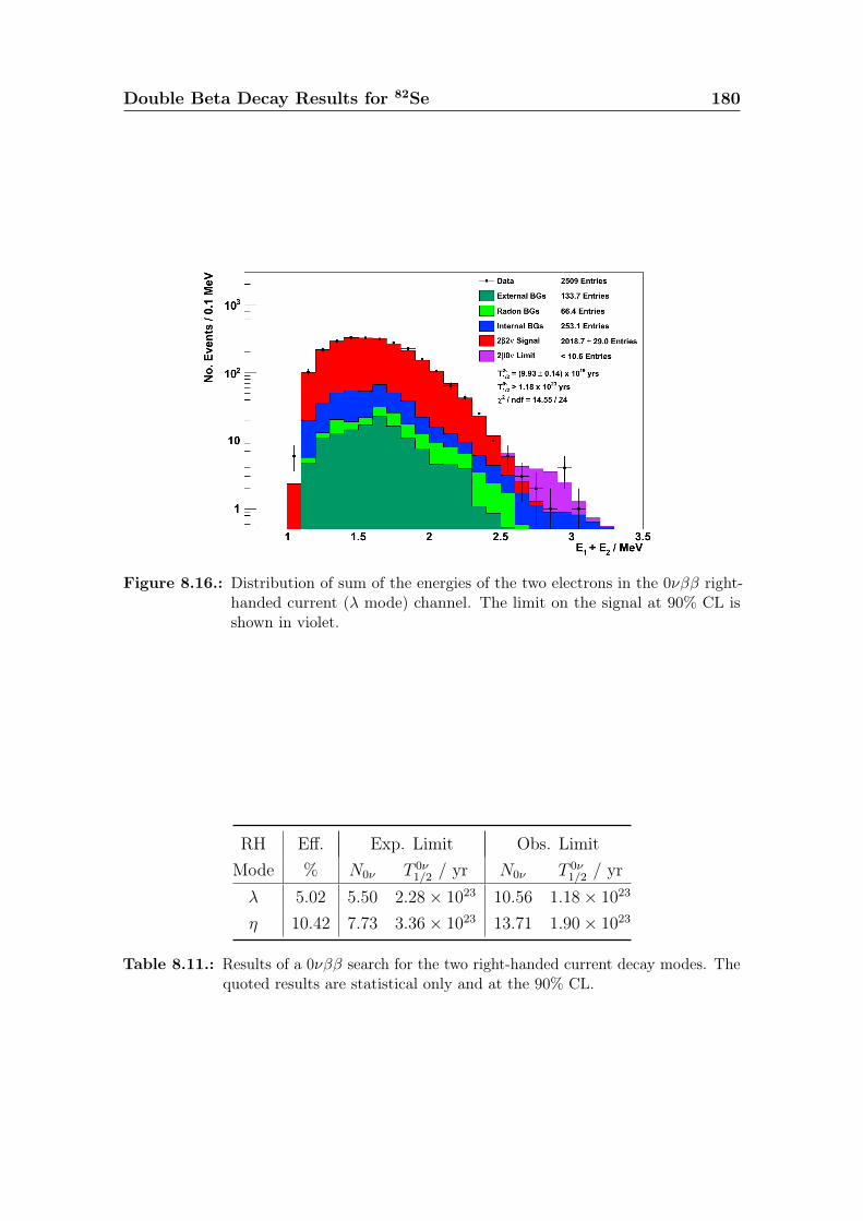
Double Beta Decay Results for 82Se 180
Figure 8.16.: Distribution of sum of the energies of the two electrons in the 0νββ right-handed current (λ mode) channel. The limit on the signal at 90% CL isshown in violet.
RH Eff. Exp. Limit Obs. LimitMode % N0ν T 0ν
1/2 / yr N0ν T 0ν1/2 / yr
λ 5.02 5.50 2.28× 10²³ 10.56 1.18× 10²³
η 10.42 7.73 3.36× 10²³ 13.71 1.90× 10²³
Table 8.11.: Results of a 0νββ search for the two right-handed current decay modes. Thequoted results are statistical only and at the 90% CL.
Double Beta Decay Results for 82Se 181
lepton number violating parameters, C factors are defined such that
(T 0ν1/2
)−1= Cη2LV (8.8)
C0λλ describes the coupling for the λ decay mode and has been calculated in the range
(0.90− 1.05)× 10−12 yr−1 [99]. This leads to a limit on the coupling parameter, 〈λ〉,as
〈λ〉 < (2.8− 3.0)× 10−6 (8.9)
This limit is the best in 82Se and only a factor 2− 3 weaker than the best resultsfrom the Heidelberg-Moscow experiment of 〈λ〉 < 1.1× 10⁻⁶ [100] and the NEMO-3100Mo result of 〈λ〉 < 1.4× 10⁻⁶.
The equivalent C factor for the η decay mode, C0ηη is calculated to be (1.08− 1.21)×
10−8 yr−1 [99], leading to a limit of
〈η〉 < (2.1− 2.2)× 10−8 (8.10)
Whilst this limit is the strongest found in 82Se, it is not particularly competitivewith Heidelberg-Moscow, which produced a value of 〈η〉 < 0.64× 10⁻⁸ [100].
8.4.3. Majoron Emission
The Majoron emission mode, which was described in Section 3.3.3, is consideredmore exotic than the mass mechanism or right-handed current modes. The modediffers significantly from the previous mechanisms as hypothetical Majorons are alsoemitted with the electrons. This means that the sum of the two electrons is no longera single peak at the Qββ value, but rather a continuous spectrum.
The shape of the spectrum is described by the spectral index of the model, denotedn. As n increases, the peak of the spectrum shifts to lower energies, so that then = 7 distribution is much more similar to that of 2νββ than the n = 1 case asillustrated in Figure 3.9. There is no evidence for the n = 1, 2, 3 modes and limitsfor these signal strengths are presented in Table 8.12. However, there is not enough
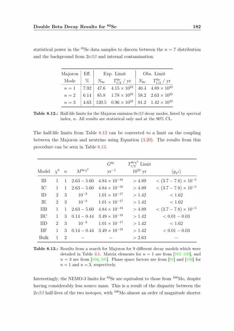
Double Beta Decay Results for 82Se 182
statistical power in the 82Se data samples to discern between the n = 7 distributionand the background from 2νββ and internal contamination.
Majoron Eff. Exp. Limit Obs. LimitMode % N0ν T 0ν
1/2 / yr N0ν T 0ν1/2 / yr
n = 1 7.92 47.6 4.15× 10²² 40.4 4.89× 10²²
n = 2 6.14 85.8 1.78× 10²² 58.2 2.63× 10²²
n = 3 4.63 120.5 0.96× 10²² 81.2 1.42× 10²²
Table 8.12.: Half-life limits for the Majoron emission 0νββ decay modes, listed by spectralindex, n. All results are statistical only and at the 90% CL.
The half-life limits from Table 8.12 can be converted to a limit on the couplingbetween the Majoron and neutrino using Equation (3.20). The results from thisprocedure can be seen in Table 8.13.
G0ν T 0νχ0
1/2 LimitModel χ0 n M0νχ0 yr−1 1022 yr 〈gχ0〉
IB 1 1 2.63− 5.60 4.84× 10⁻¹⁶ > 4.89 < (3.7− 7.8)× 10−5
IC 1 1 2.63− 5.60 4.84× 10⁻¹⁶ > 4.89 < (3.7− 7.8)× 10−5
ID 2 3 10−3 1.01× 10⁻¹⁷ > 1.42 < 1.62
IE 2 3 10−3 1.01× 10⁻¹⁷ > 1.42 < 1.62
IIB 1 1 2.63− 5.60 4.84× 10⁻¹⁶ > 4.89 < (3.7− 7.8)× 10−5
IIC 1 3 0.14− 0.44 3.49× 10⁻¹⁸ > 1.42 < 0.01− 0.03
IID 2 3 10−3 1.01× 10⁻¹⁷ > 1.42 < 1.62
IIF 1 3 0.14− 0.44 3.49× 10⁻¹⁸ > 1.42 < 0.01− 0.03
Bulk 1 2 − − > 2.63 −
Table 8.13.: Results from a search for Majoron for 9 different decay models which weredetailed in Table 3.1. Matrix elements for n = 1 are from [101–103], andn = 3 are from [104, 105]. Phase space factors are from [91] and [106] forn = 1 and n = 3, respectively.
Interestingly, the NEMO-3 limits for 82Se are equivalent to those from 100Mo, despitehaving considerably less source mass. This is a result of the disparity between the2νββ half-lives of the two isotopes, with 100Mo almost an order of magnitude shorter.

Double Beta Decay Results for 82Se 183
These results are the strongest limits using 82Se, however they have been supersededby recent results from KamLAND-Zen with an improvement of a factor ∼ 3 [60].
Part II.
Radon Research and Developmentfor SuperNEMO
184
Chapter 9.
The SuperNEMO Experiment
The SuperNEMO experiment is a next-generation double beta decay experiment thatbuilds on the successes of NEMO-3, using the same tracker-calorimeter technology. Itsaims are to search for 0νββ of 82Se with a half-life sensitivity of 1026 yr, correspondingto an effective neutrino mass of 50− 100 meV.
The baseline design of SuperNEMO consists of 20 identical modules, each housing5− 7 kg of source isotope. The general layout of each module is similar to NEMO-3,with thin source foils surrounded by a gas tracker which in turn is enclosed by acalorimeter. These modules are discussed in greater detail in Section 9.1.
SuperNEMO is not simply a scaled-up version of NEMO-3. A considerable amountof research and development (R&D) has been undertaken to improve many aspectsof the design. This R&D programme concentrated on the key areas of source foilproduction, tracker development, calorimeter development and ensuring that ultra-low levels of background are achieved. The successes of each area of research will bebriefly outlined in Section 9.2.
The remainder of this chapter (Section 9.3) is dedicated to the expected timescaleand sensitivity of the experiment.
9.1. SuperNEMO Baseline Design
In its baseline design, the SuperNEMO experiment will contain 100 kg of 82Se,although 150Nd and 48Ca may also be considered if improved enrichment possibilities
185
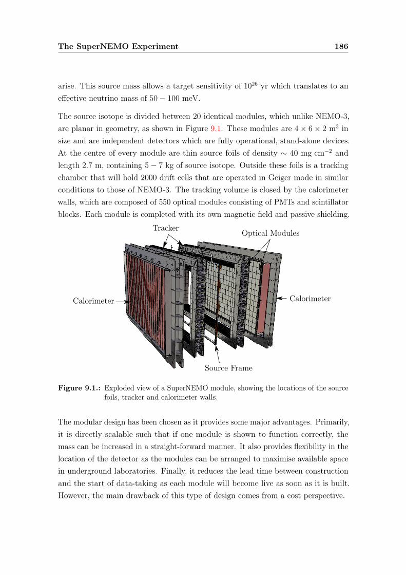
The SuperNEMO Experiment 186
arise. This source mass allows a target sensitivity of 1026 yr which translates to aneffective neutrino mass of 50− 100 meV.
The source isotope is divided between 20 identical modules, which unlike NEMO-3,are planar in geometry, as shown in Figure 9.1. These modules are 4× 6× 2 m3 insize and are independent detectors which are fully operational, stand-alone devices.At the centre of every module are thin source foils of density ∼ 40 mg cm−2 andlength 2.7 m, containing 5− 7 kg of source isotope. Outside these foils is a trackingchamber that will hold 2000 drift cells that are operated in Geiger mode in similarconditions to those of NEMO-3. The tracking volume is closed by the calorimeterwalls, which are composed of 550 optical modules consisting of PMTs and scintillatorblocks. Each module is completed with its own magnetic field and passive shielding.
Tracker
Calorimeter
Optical Modules
Source Frame
Calorimeter
Figure 9.1.: Exploded view of a SuperNEMO module, showing the locations of the sourcefoils, tracker and calorimeter walls.
The modular design has been chosen as it provides some major advantages. Primarily,it is directly scalable such that if one module is shown to function correctly, themass can be increased in a straight-forward manner. It also provides flexibility in thelocation of the detector as the modules can be arranged to maximise available spacein underground laboratories. Finally, it reduces the lead time between constructionand the start of data-taking as each module will become live as soon as it is built.However, the main drawback of this type of design comes from a cost perspective.
The SuperNEMO Experiment 187
9.2. Research and Development
By using design concepts similar to those of NEMO-3, the valuable experience ofrunning this detector may be exploited for SuperNEMO. The areas where improve-ments could be made on the NEMO-3 design were the focus of an extensive andvaried programme of R&D, outlined in this section.
As was seen in the measurement of 0νββ with NEMO-3 in the previous chapter,backgrounds inside the source foils can severely hamper the physics reach of anexperiment such as SuperNEMO. There has therefore been concerted effort intoreducing the contamination of the source material using chemical and distillationpurification techniques. Furthermore, a new large-scale detector has been developedwhich is capable of measuring very low levels of 214Bi and 208Tl contamination insidethe foils using BiPo type events [107]. This detector will ensure that the requiredlevel of radiopurity of the foils has been reached before they are installed into themodules of the detector.
Due to the larger height of the SuperNEMO modules compared to NEMO-3, thetracker cells must be 10% longer in the new design. This prompted a re-evaluationof all properties of the drift cells and an optimisation of the cell dimensions lookingat properties such as plasma propagation, efficiency and ageing. Prototypes werebuilt, including a large tank that could house 90 cells which showed that resolutionsof 0.7 mm in the transverse plane and 1.3 cm in the longitudinal direction could beachieved.
An additional step forward in tracker production has been the design and constructionof a wiring robot, which has automated the manufacturing process. This greatlyreduces the risk of contamination of the 260,000 wires required for the 20 modules.This contamination can prove problematic for the radiopurity of the detector and forachieving good plasma propagation along the drift cells.
As was seen in Section 4.1, the sensitivity of a 0νββ experiment is heavily dependenton its energy resolution. Therefore, a key target for SuperNEMO is to improve thisresolution by a factor of ∼ 2. One improvement has been replacing the polystyrenescintillator used in NEMO-3 with poly-vinyl toluene (PVT), but the biggest effecthas been as a result of removing the need for a light guide. This was achieved by
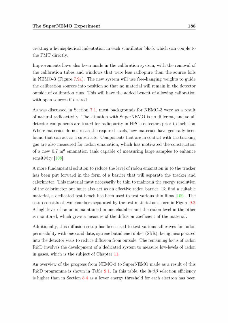
The SuperNEMO Experiment 188
creating a hemispherical indentation in each scintillator block which can couple tothe PMT directly.
Improvements have also been made in the calibration system, with the removal ofthe calibration tubes and windows that were less radiopure than the source foilsin NEMO-3 (Figure 7.9a). The new system will use free-hanging weights to guidethe calibration sources into position so that no material will remain in the detectoroutside of calibration runs. This will have the added benefit of allowing calibrationwith open sources if desired.
As was discussed in Section 7.1, most backgrounds for NEMO-3 were as a resultof natural radioactivity. The situation with SuperNEMO is no different, and so alldetector components are tested for radiopurity in HPGe detectors prior to inclusion.Where materials do not reach the required levels, new materials have generally beenfound that can act as a substitute. Components that are in contact with the trackinggas are also measured for radon emanation, which has motivated the constructionof a new 0.7 m3 emanation tank capable of measuring large samples to enhancesensitivity [108].
A more fundamental solution to reduce the level of radon emanation in to the trackerhas been put forward in the form of a barrier that will separate the tracker andcalorimeter. This material must necessarily be thin to maintain the energy resolutionof the calorimeter but must also act as an effective radon barrier. To find a suitablematerial, a dedicated test-bench has been used to test various thin films [109]. Thesetup consists of two chambers separated by the test material as shown in Figure 9.2.A high level of radon is maintained in one chamber and the radon level in the otheris monitored, which gives a measure of the diffusion coefficient of the material.
Additionally, this diffusion setup has been used to test various adhesives for radonpermeability with one candidate, sytrene butadiene rubber (SBR), being incorporatedinto the detector seals to reduce diffusion from outside. The remaining focus of radonR&D involves the development of a dedicated system to measure low-levels of radonin gases, which is the subject of Chapter 11.
An overview of the progress from NEMO-3 to SuperNEMO made as a result of thisR&D programme is shown in Table 9.1. In this table, the 0νββ selection efficiencyis higher than in Section 8.4 as a lower energy threshold for each electron has been
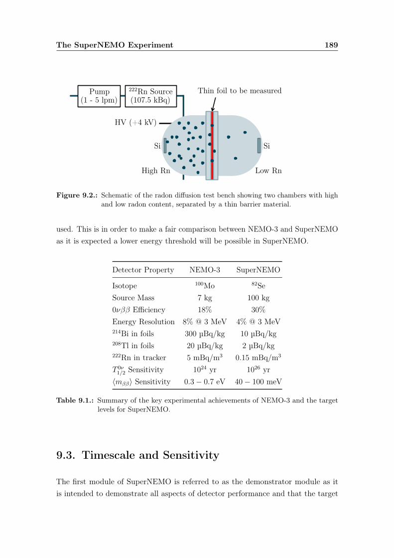
The SuperNEMO Experiment 189
HV (+4 kV)
SiSi
High Rn
Thin foil to be measured
Low Rn
Pump(1 - 5 lpm)
222Rn Source(107.5 kBq)
Figure 9.2.: Schematic of the radon diffusion test bench showing two chambers with highand low radon content, separated by a thin barrier material.
used. This is in order to make a fair comparison between NEMO-3 and SuperNEMOas it is expected a lower energy threshold will be possible in SuperNEMO.
Detector Property NEMO-3 SuperNEMO
Isotope 100Mo 82SeSource Mass 7 kg 100 kg0νββ Efficiency 18% 30%
Energy Resolution 8% @ 3 MeV 4% @ 3 MeV214Bi in foils 300 µBq/kg 10 µBq/kg208Tl in foils 20 µBq/kg 2 µBq/kg222Rn in tracker 5 mBq/m3 0.15 mBq/m3
T 0ν1/2 Sensitivity 1024 yr 1026 yr〈mββ〉 Sensitivity 0.3− 0.7 eV 40− 100 meV
Table 9.1.: Summary of the key experimental achievements of NEMO-3 and the targetlevels for SuperNEMO.
9.3. Timescale and Sensitivity
The first module of SuperNEMO is referred to as the demonstrator module as itis intended to demonstrate all aspects of detector performance and that the target
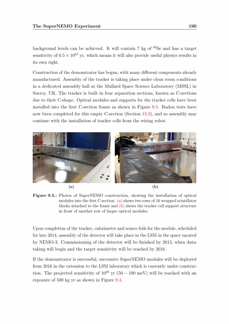
The SuperNEMO Experiment 190
background levels can be achieved. It will contain 7 kg of 82Se and has a targetsensitivity of 6.5× 1024 yr, which means it will also provide useful physics results inits own right.
Construction of the demonstrator has begun, with many different components alreadymanufactured. Assembly of the tracker is taking place under clean room conditionsin a dedicated assembly hall at the Mullard Space Science Laboratory (MSSL) inSurrey, UK. The tracker is built in four separation sections, known as C-sectionsdue to their C-shape. Optical modules and supports for the tracker cells have beeninstalled into the first C-section frame as shown in Figure 9.3. Radon tests havenow been completed for this empty C-section (Section 13.3), and so assembly maycontinue with the installation of tracker cells from the wiring robot.
(a) (b)
Figure 9.3.: Photos of SuperNEMO construction, showing the installation of opticalmodules into the first C-section. (a) shows two rows of 16 wrapped scintillatorblocks attached to the frame and (b) shows the tracker cell support structurein front of another row of larger optical modules.
Upon completion of the tracker, calorimeter and source foils for the module, scheduledfor late 2014, assembly of the detector will take place in the LSM in the space vacatedby NEMO-3. Commissioning of the detector will be finished by 2015, when data-taking will begin and the target sensitivity will be reached by 2016.
If the demonstrator is successful, successive SuperNEMO modules will be deployedfrom 2016 in the extension to the LSM laboratory which is currently under construc-tion. The projected sensitivity of 1026 yr (50− 100 meV) will be reached with anexposure of 500 kg yr as shown in Figure 9.4.
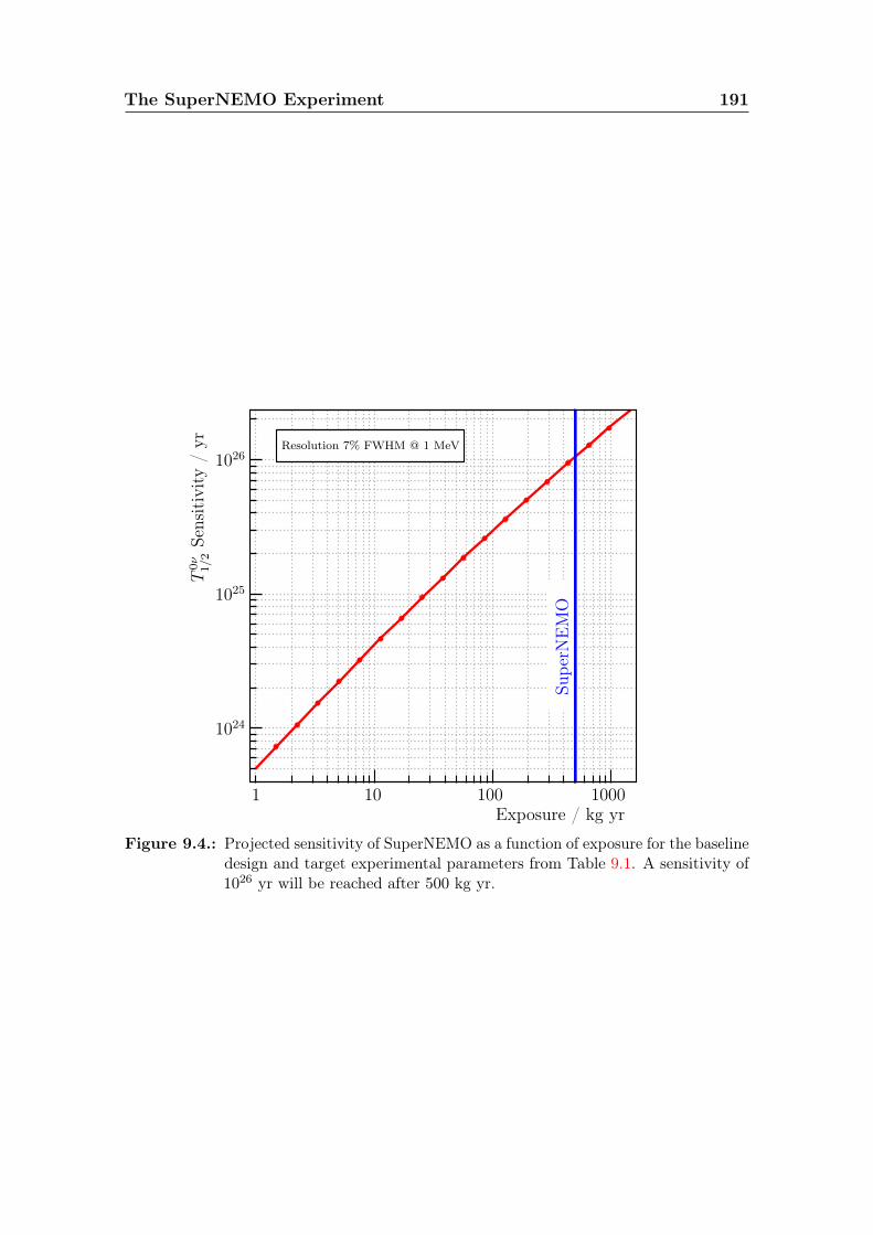
The SuperNEMO Experiment 191
Supe
rNEMO
Resolution 7% FWHM @ 1 MeV
Exposure / kg yr1 10 100 1000
1024
1025
1026
T0ν
1/2Sensitivity
/yr
Figure 9.4.: Projected sensitivity of SuperNEMO as a function of exposure for the baselinedesign and target experimental parameters from Table 9.1. A sensitivity of1026 yr will be reached after 500 kg yr.
Chapter 10.
Radon and SuperNEMO
10.1. Properties of Radon
Radon is a chemical element with atomic number 86. It is found as monatomic gaswith the unusual property that it is the only gas that has solely radioactive isotopes.
In 1900, Friedrich Ernst Dorn reported experiments that showed emanation of aradioactive gas from radium compounds [110]. This is commonly attributed as thediscovery of radon, although there are claims that the discovery should be attributedto Ernest Rutherford for his discovery of similar emanation from thorium oxidein 1899 [111]. These gases were simply named radium emanation and thoriumemanation, as little else about their properties was known.
The situation improved between 1904 and 1910, when William Ramsay studied theproperties of these gases at University College London. From similarities betweentheir spectra and those of argon, krypton and xenon and their low level of chemicalinteraction, Ramsay correctly postulated that the emanations may be a new elementin the group of noble gases [112]. Furthermore, he successfully isolated radonand determined that it was the densest known gas at that time. After a series ofsuggestions, finally, in 1920, the new names of radon and thoron were accepted forthe emanated gases.
All isotopes of radon are radioactive, and only four are found in nature. Radon(222Rn) comes from the 238U decay chain (Figure 7.1), which also causes a very smallamount of the 218Rn isotope. In addition, the 232Th decay series (Figure 7.2) provides
192

Radon and SuperNEMO 193
thoron (220Rn) and the 228Ac series supplies actinon (219Rn). 222Rn is the most stableof all radon isotopes with a half-life of 3.8235 days. As far as 0νββ experiments areconcerned, the only radon isotopes of interest are radon and thoron due to theirprogenies of 214Bi and 208Tl (Section 7.1).
Under standard temperature and pressure (STP) conditions, radon is a colourlessand odourless gas. Its melting and boiling points are comparatively high for a noblegas, at −71 ◦C and −61.7 ◦C, respectively. With a density of 9.7 kg/m3, it is thedensest of the noble gases, and one of the most dense of all known gases. Althoughit is colourless at STP, radon emits a brilliant radioluminescence when cooled belowits freezing point and a hazy glow upon condensation.
As a noble gas, radon is inert to most chemical reactions due to its full outer valenceshell. This means that it cannot easily be filtered via chemical means and removalmust be achieved using physical methods. It is only slightly soluble in water, but isconsiderably easier to dissolve in organic liquids, such as liquid scintillator. A furtherresult of this chemical inactivity is that radon often exhibits a long diffusion lengthin solids which makes forming large scale seals difficult.
Typical radon activities from natural sources are 30− 50 Bq/m3 indoors, however,these values can vary significantly. For example, clean rooms, usually with highrates of ventilation and lack of exposed brickwork, normally have levels < 5 Bq/m3.Atmospheric radon activities are nominally ∼ 10 Bq/m3, but may be as low as0.1 Bq/m3 above oceans or in Antarctica. Underground laboratories, where lowbackground experiments reside, display a similar level of variation dependent on thecontent of the surrounding rock. Salt mines are amongst the lowest at ∼ 2 Bq/m3,rising up to uranium mines which unsurprisingly have very high levels of up to10 kBq/m3.
There is a high degree of general interest in measurement of radon activities as itis hazardous to health in high quantities. Indeed, it is responsible for the majorityof public exposure to ionising radiation and is the second greatest cause of lungcancer, after smoking [113]. Activity levels that are considered dangerous to healthfor long term exposure vary, but are normally above 200 − 400 Bq/m3. As aresult, there are a wide range of commercial devices available for measuring radonactivity in the 0.5 Bq/m3 − 1 MBq/m3 range. However, the activity requirements
Radon and SuperNEMO 194
for low background experiments are far below these sensitivities and so custom-madedetectors are normally required.
10.2. Radon as a SuperNEMO Background
As was the case with NEMO-3, radon can present a significant source of backgroundto SuperNEMO. The mechanism is identical with radon inside the tracker depositing214Bi on the source foils or tracker wires. The sources of radon background can comefrom emanation, contamination or diffusion, all of which have been addressed in theSuperNEMO R&D programme to improve on the performance of NEMO-3.
In order to quantify an acceptable level of radon contamination of the tracker,simulations were undertaken for varying radon activities. The resulting sensitivitycurves are shown in Figure 10.1. In this study, the contributions of radon from thetracker and from internal 214Bi contamination were treated separately, so that thesensitivity of 1026 yr that is achieved for 280 µBq/m3 is only possible with no 214Biinside the foils. Therefore, when setting a target level for radon activity inside thetracker, the activity of 214Bi is divided between internal contamination and radon inthe tracking chamber, leading to a requirement that the tracker activity must be< 150 µBq/m3.
10.3. Radon Suppression with Gas Flow
In addition to the raft of improvements for the radon level from the R&D programme,an additional defence against radon in SuperNEMO is gained by the flow of gasthrough the modules. Provided that the supply gas has a lower level of radoncontamination than that in the tracking chamber, the replacement of the dirtier gasproduces a suppression of the radon level in the tracker.
As one might expect, the suppression that can be achieved is a function of theactivity of the supply gas and the flow rate. The latter is limited by the tracker,which has decreased performance if gas volumes are exchanged too quickly. Thisnominal flow rate is ∼ 0.5 m3/hr into the tracking volume of 15.2 m3, but flow ratesup to 1.0 m3/hr are expected to be possible.
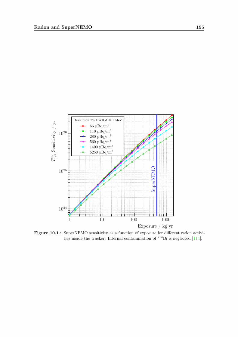
Radon and SuperNEMO 195
Exposure / kg yr1 10 100 1000
1024
1025
1026
T0ν
1/2Sensitivity
/yr
Resolution 7% FWHM @ 1 MeV
Supe
rNEMO
55 µBq/m3
110 µBq/m3
280 µBq/m3
560 µBq/m3
1400 µBq/m3
5250 µBq/m3
Figure 10.1.: SuperNEMO sensitivity as a function of exposure for different radon activi-ties inside the tracker. Internal contamination of 214Bi is neglected [114].
Radon and SuperNEMO 196
Naively, it might be assumed that gas can be supplied to the tracker at an arbitrarilylow radon concentration. However, a gas-mixing system must be used to create theappropriate tracking mixture that, despite being carefully designed, will emanatea small activity of radon. Therefore, whilst clean gas can be supplied to the gassystem via a series of radon traps, the output to the detector will be contaminated.
In order to calculate a flow suppression factor, a model is created where radon activityemanates uniformly within the gas system and is passed into the tracker as a result.The number of radon atoms inside the gas system, NG, is given by the relationshipbetween emanation from the gas system, atoms decaying within the gas system andthose that are extracted by the gas flow:
dNG
dt= AG − λNG −
fNG
VG(10.1)
Here, AG is the intrinsic 222Rn activity of the gas system, λ is the radon decayconstant, f is the gas flow rate and VG is the total volume of the gas system. Ingeneral running conditions, the gas system will be in equilibrium, so that NG is givenby
NG =AG
λ+ fVG
=AGVGλVG + f
≈ AGVGf
(10.2)
where the final approximation is very good since it is expected that λVG ∼ O(10−3)
m3/hr and f ∼ O(1) m3/hr.
A similar equation gives the number of radon atoms inside the tracker, NT , with anextra term for the radon supplied by the gas system:
dNT
dt= AT +
fNG
VG− fNT
VT− λNT = AT + AG − λ′TNT (10.3)
where VT is the volume of the tracker and the calculated form of NG (Equation (10.2))has been used to illustrate that any emanation from the gas system has the sameeffect as if it were in the tracker itself. Further, the effect of the flow is shown tobe equivalent to increasing the natural 222Rn decay constant to become an effectivedecay constant λ′T :
λ′T = λ+f
VT(10.4)

Radon and SuperNEMO 197
Under static conditions, with no gas flow in the tracker, the number of radon atomsis simply given by N0
T = AT/λ. Therefore a flow suppression factor, FS, can be foundby considering Equation (10.3) in the case of equilibrium:
FS =NT
N0T
=AT + AG
λ′T
λ
AT=
1 + AG/AT1 + f/VTλ
(10.5)
This relationship is shown graphically in Figure 10.2 for three different values of AG.For the anticipated gas flow rate of 0.5 m3/hr (8.3 lpm) there is a reduction in radonactivity by a factor of ∼ 5.
Gas flow / lpm0 2 4 6 8 10 12 14
0 T /
NT
N
0
0.2
0.4
0.6
0.8
1
1.2
3 = 15.2 mTV
= 0.0 % T / AGA
= 7.5 % T / AGA
= 15.0 % T / AGA
Figure 10.2.: Flow suppression factor for radon activity in the tracker. The three differentcurves are for three different activities of the gas system at 0%, 7.5% and15% of the tracker activity.
10.4. 222Rn Decay Chain to 214Po
Up to now, only radon itself has been considered. However, electrostatic detectorswhich are commonly used to detect radon (Section 11.1) measure the levels of radonprogenies 214Po and 218Po. It is therefore important to understand how the activityof these isotopes is related to that of their parent isotope 222Rn. The details of thedecay of each isotope are summarised in Table 10.1. The relationships between theactivities in this decay chain are derived in this section.
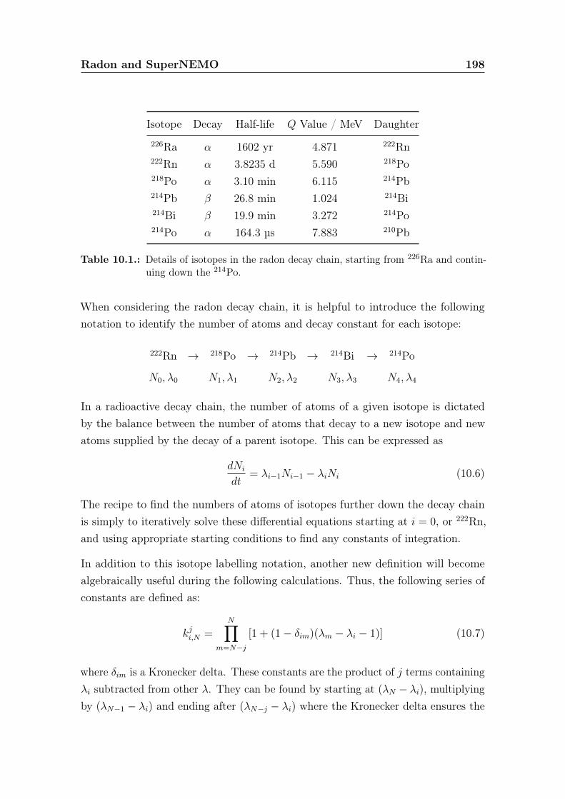
Radon and SuperNEMO 198
Isotope Decay Half-life Q Value / MeV Daughter
226Ra α 1602 yr 4.871 222Rn222Rn α 3.8235 d 5.590 218Po218Po α 3.10 min 6.115 214Pb214Pb β 26.8 min 1.024 214Bi214Bi β 19.9 min 3.272 214Po214Po α 164.3 µs 7.883 210Pb
Table 10.1.: Details of isotopes in the radon decay chain, starting from 226Ra and contin-uing down the 214Po.
When considering the radon decay chain, it is helpful to introduce the followingnotation to identify the number of atoms and decay constant for each isotope:
222Rn → 218Po → 214Pb → 214Bi → 214Po
N0, λ0 N1, λ1 N2, λ2 N3, λ3 N4, λ4
In a radioactive decay chain, the number of atoms of a given isotope is dictatedby the balance between the number of atoms that decay to a new isotope and newatoms supplied by the decay of a parent isotope. This can be expressed as
dNi
dt= λi−1Ni−1 − λiNi (10.6)
The recipe to find the numbers of atoms of isotopes further down the decay chainis simply to iteratively solve these differential equations starting at i = 0, or 222Rn,and using appropriate starting conditions to find any constants of integration.
In addition to this isotope labelling notation, another new definition will becomealgebraically useful during the following calculations. Thus, the following series ofconstants are defined as:
kji,N =N∏
m=N−j
[1 + (1− δim)(λm − λi − 1)] (10.7)
where δim is a Kronecker delta. These constants are the product of j terms containingλi subtracted from other λ. They can be found by starting at (λN − λi), multiplyingby (λN−1 − λi) and ending after (λN−j − λi) where the Kronecker delta ensures the
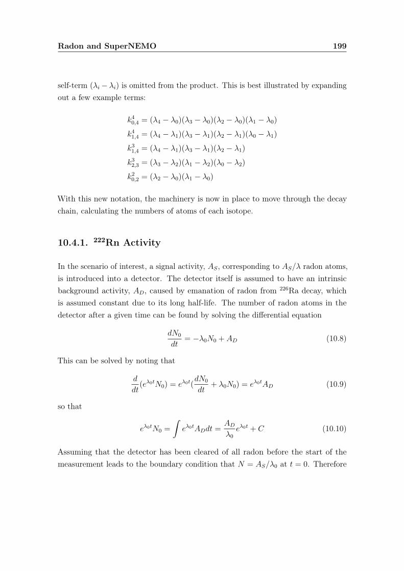
Radon and SuperNEMO 199
self-term (λi− λi) is omitted from the product. This is best illustrated by expandingout a few example terms:
k40,4 = (λ4 − λ0)(λ3 − λ0)(λ2 − λ0)(λ1 − λ0)
k41,4 = (λ4 − λ1)(λ3 − λ1)(λ2 − λ1)(λ0 − λ1)
k31,4 = (λ4 − λ1)(λ3 − λ1)(λ2 − λ1)
k32,3 = (λ3 − λ2)(λ1 − λ2)(λ0 − λ2)
k20,2 = (λ2 − λ0)(λ1 − λ0)
With this new notation, the machinery is now in place to move through the decaychain, calculating the numbers of atoms of each isotope.
10.4.1. 222Rn Activity
In the scenario of interest, a signal activity, AS, corresponding to AS/λ radon atoms,is introduced into a detector. The detector itself is assumed to have an intrinsicbackground activity, AD, caused by emanation of radon from 226Ra decay, whichis assumed constant due to its long half-life. The number of radon atoms in thedetector after a given time can be found by solving the differential equation
dN0
dt= −λ0N0 + AD (10.8)
This can be solved by noting that
d
dt(eλ0tN0) = eλ0t(
dN0
dt+ λ0N0) = eλ0tAD (10.9)
so that
eλ0tN0 =
∫eλ0tADdt =
ADλ0eλ0t + C (10.10)
Assuming that the detector has been cleared of all radon before the start of themeasurement leads to the boundary condition that N = AS/λ0 at t = 0. Therefore

Radon and SuperNEMO 200
C = AS/λ0 − AD/λ0 and
N0 =ADλ0
(1− e−λ0t) +ASλ0e−λ0t (10.11)
which can be seen as the characteristic sum of the increasing background term andthe exponentially decaying signal term.
10.4.2. 218Po Activity
For 218Po the equation to be solved is
dN1
dt= λ0N0 − λ1N1 (10.12)
which following the same process as for equation (Equation (10.9)) yields
eλ1tN1 =
∫eλ1tλ0N0dt =
∫ADe
λ1t + (AS − AD)e(λ1−λ0)tdt
=ADeλ1t
λ1+ (AS − AD)
e(λ1−λ0)t
λ1 − λ0+ C (10.13)
where C is again a constant of integration. Applying the same boundary conditionthat N1 = 0 at t = 0, the form of N1 is
N1 =ADλ1
(1− e−λ1t) + (AS − AD)
(e−λ0t
λ1 − λ0+
e−λ1t
λ0 − λ1
)(10.14)
which using the kji,N notation can be written
N1 =ADλ1
(1− e−λ1t) + (AS − AD)
(e−λ0t
k10,1+e−λ1t
k11,1
)(10.15)
10.4.3. 214Pb Activity
Continuing down the decay chain to 214Pb, the differential equation to be solved is
dN2
dt+ λ2N2 = λ1N1 (10.16)
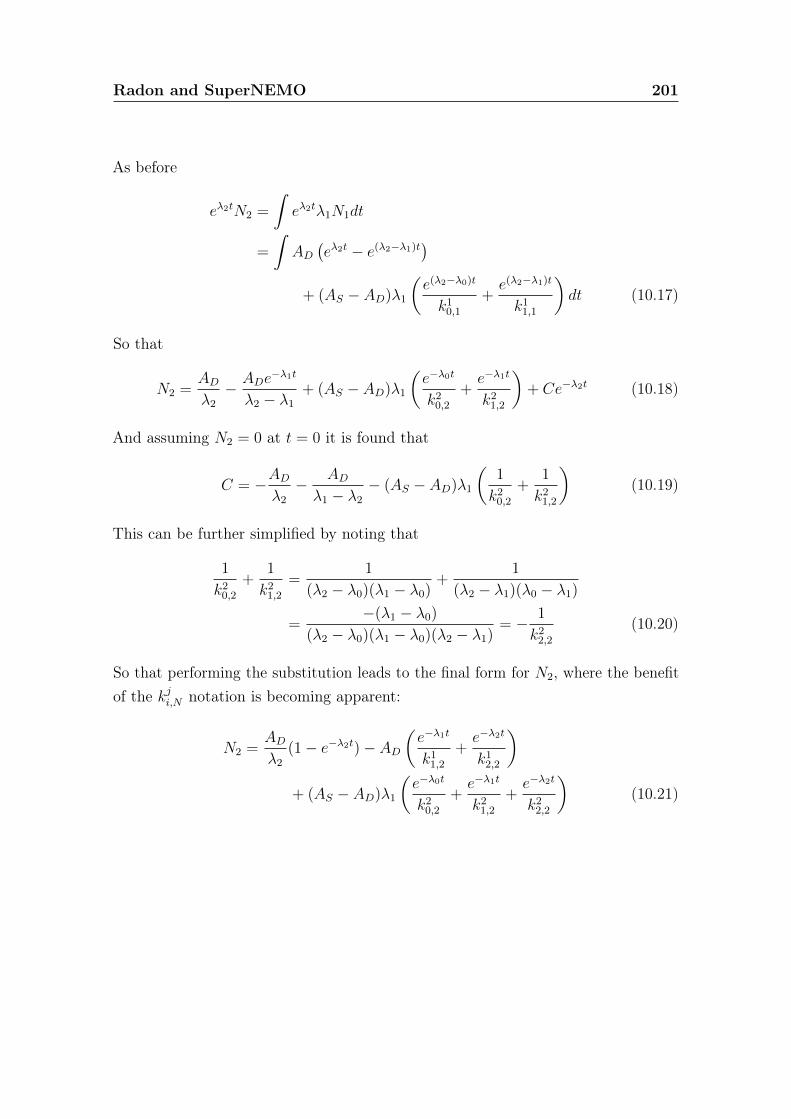
Radon and SuperNEMO 201
As before
eλ2tN2 =
∫eλ2tλ1N1dt
=
∫AD(eλ2t − e(λ2−λ1)t
)+ (AS − AD)λ1
(e(λ2−λ0)t
k10,1+e(λ2−λ1)t
k11,1
)dt (10.17)
So that
N2 =ADλ2− ADe
−λ1t
λ2 − λ1+ (AS − AD)λ1
(e−λ0t
k20,2+e−λ1t
k21,2
)+ Ce−λ2t (10.18)
And assuming N2 = 0 at t = 0 it is found that
C = −ADλ2− ADλ1 − λ2
− (AS − AD)λ1
(1
k20,2+
1
k21,2
)(10.19)
This can be further simplified by noting that
1
k20,2+
1
k21,2=
1
(λ2 − λ0)(λ1 − λ0)+
1
(λ2 − λ1)(λ0 − λ1)
=−(λ1 − λ0)
(λ2 − λ0)(λ1 − λ0)(λ2 − λ1)= − 1
k22,2(10.20)
So that performing the substitution leads to the final form for N2, where the benefitof the kji,N notation is becoming apparent:
N2 =ADλ2
(1− e−λ2t)− AD(e−λ1t
k11,2+e−λ2t
k12,2
)+ (AS − AD)λ1
(e−λ0t
k20,2+e−λ1t
k21,2+e−λ2t
k22,2
)(10.21)
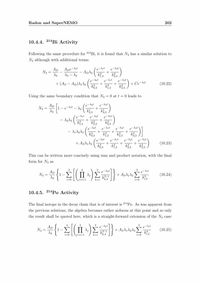
Radon and SuperNEMO 202
10.4.4. 214Bi Activity
Following the same procedure for 214Bi, it is found that N3 has a similar solution toN2 although with additional terms:
N3 =ADλ3− ADe
−λ2t
λ3 − λ2− ADλ2
(e−λ1t
k21,3+e−λ2t
k22,3
)+ (AS − AD)λ1λ2
(e−λ0t
k30,3+e−λ1t
k31,3+e−λ2t
k32,3
)+ Ce−λ3t (10.22)
Using the same boundary condition that N3 = 0 at t = 0 leads to
N3 =ADλ3
[1− e−λ3t − λ3
(e−λ2t
k12,3+e−λ3t
k13,3
)− λ2λ3
(e−λ1t
k21,3+e−λ2t
k22,3+e−λ3t
k23,3
)− λ1λ2λ3
(e−λ0t
k30,3+e−λ1t
k31,3+e−λ2t
k32,3+e−λ3t
k33,3
)]+ ASλ1λ2
(e−λ0t
k30,3+e−λ1t
k31,3+e−λ2t
k32,3+e−λ3t
k33,3
)(10.23)
This can be written more concisely using sum and product notation, with the finalform for N3 as
N3 =ADλ3
{1−
3∑i=0
[(3∏
j=i+1
λj
)3∑k=i
e−λkt
k3−ik,3
]}+ ASλ1λ2
3∑i=0
e−λit
k3i,3(10.24)
10.4.5. 214Po Activity
The final isotope in the decay chain that is of interest is 214Po. As was apparent fromthe previous solutions, the algebra becomes rather arduous at this point and so onlythe result shall be quoted here, which is a straight-forward extension of the N3 case:
N4 =ADλ4
{1−
4∑i=0
[(4∏
j=i+1
λj
)4∑k=i
e−λkt
k4−ik,4
]}+ ASλ1λ2λ3
4∑i=0
e−λit
k4i,4(10.25)

Radon and SuperNEMO 203
10.4.6. Decay chain activities
Now that the expected numbers of atoms of each isotope in this decay chain have beencalculated, the resulting activities inside the detector can be plotted to more readilyunderstand the properties of the decay chain. This plot is shown in Figure 10.3. Itshould be noted that the 218Po reaches equilibrium with the 222Rn rather quicklywhilst the decay chain delays the 214Po for some time so it is only in equilibriumafter 4.5 hrs.
Time / days0 0.05 0.1 0.15 0.2 0.25 0.3 0.35 0.4 0.45 0.5
Iso
top
e A
ctiv
ity
/ mB
q
0
0.2
0.4
0.6
0.8
1
Rn222
Po218
Pb214
Bi214
Po214
= 1.0 mBq SA
= 0.1 mBq DA
Figure 10.3.: Activities of different isotopes in the 222Rn decay chain with respect totime after introduction of 1 mBq of 222Rn into a detector with 0.1 mBqbackground.
Chapter 11.
Electrostatic Detector and RadonConcentration Line
The SuperNEMO requirement of radon activity inside the tracker at a level less than150 µBq/m3 poses significant technical challenges in the design and construction ofthe detector. Furthermore, the level is so low that even confirming that the targethas been reached is not straight-forward. A considerable amount of effort has goneinto the design and construction of a system capable of measuring below this level ofradon in gases, which is the subject of this chapter.
As mentioned in the previous chapter, commercial radon detectors are available withsensitivities down to ∼ 0.5 Bq/m3, which is some four orders of magnitude awayfrom the sensitivity required for a reliable measurement of the radon activity in thetracker. Therefore, a custom-made electrostatic detector, developed for use in manylow background experiments is used in this work. The commissioning of this radondetector is discussed in Section 11.1.
Even this state-of-the-art detector is only capable of measuring down to the level of∼ 1− 2 mBq/m3, as will be shown in Section 12.2. Therefore, in order to reach thetarget sensitivity, a “radon concentration line” (RnCL) has been developed, whichuses a cooled carbon trap to store radon from gases that are passed through it.This concentrated sample of radon is then passed to the electrostatic detector to bemeasured. The design and operation of the RnCL will be outlined in the second halfof this chapter (Section 11.2).
204
Electrostatic Detector and Radon Concentration Line 205
The combination of RnCL and electrostatic detector easily reaches the desiredsensitivity for the SuperNEMO tracker and is amongst the world’s most sensitivepieces of apparatus for measuring low levels of radon in gases as will be shown inChapter 12.
11.1. Electrostatic Detector
Electrostatic detectors operate by using an electric field to move the progenies ofradon decay to a region of the detector where their subsequent decay is measured.The technique exploits a particular property of alpha decay that the daughter atomis likely to be be found as a charged atom or part of a charged compound. Thecharge can either be negative or positive and in some cases progenies become multiplypositively charged. The fraction of positive ions and compounds from radon decay inair was measured to be 88% as long ago as 1913 [115], in surprisingly good agreementwith more modern measurements of 87.3± 1.6% [116].
The electrostatic detector used in this work was developed to measure low-levels ofradon for the ELEGANT V and Super-Kamiokande experiments [117,118], and isshown in Figure 11.1.
The detector is relatively simple, consisting of an electro-polished stainless steelchamber with a volume of 70 litres, which has a silicon PIN diode placed at one end,as shown schematically in Figure 11.2. The associated electronics are separated fromthe measurement chamber by a sheet of perspex with a feedthrough for the PINdiode. There is an inlet and outlet for gas flow and all valves are either metallic orhave been coated in styrene butadiene rubber (SBR) to reduce diffusion. An electricfield is generated inside the chamber by applying a negative high voltage (typically−1500 V) onto the PIN diode.
In standard operation, a measurement sample is introduced into the detector, whereany radon subsequently decays to predominantly positive ions. These ions arecollected onto the PIN diode as a result of the applied electric field. Once on thediode, their decays are detected, particularly the alpha decays of 218Po and 214Po,and are identified by the amount of energy deposited.

Electrostatic Detector and Radon Concentration Line 206
(a) Normal operation (b) With lid removed
Figure 11.1.: Electrostatic detector used for all radon measurements in this work. (a)shows the detector in normal operation, and (b) shows the lid removedwhere the feedthrough for the PIN diode can be seen.
In Out
-HV
Stainless Vessel
Si PIN Diode
Electronics
Figure 11.2.: Schematic diagram of the electrostatic detector shown in Figure 11.1.

Electrostatic Detector and Radon Concentration Line 207
214Po is most commonly used as a measure of the radon level, as it generally has ahigher detection efficiency. Naively one might expect that the efficiencies for 214Poand 218Po should be identical, but in reality the collection efficiency for 218Po is not100%. The intermediate isotopes of 214Pb and 214Bi may also be collected onto thePIN diode so that the level of 214Po is higher than that of 218Po. In addition, theseisotopes, and 214Po itself, are not as susceptible to neutralisation as 218Po such thatthe collection efficiency for 214Po is more stable in the presence of trace amounts ofimpurities.
11.1.1. Detector Signal
The detector has a self-contained set of electronics, which filters the HV supply,supplies a bias voltage and provides the required voltage rails for the multi-stageamplification of the signal. These electronics are housed within the lid of the detectorwhich minimises the distance of signal cable before pre-amplification and providesshielding from external noise.
The detector signal is passed to a NEMbox DAQ system (Wiener NEMbox SU706),which is a programmable FPGA intended to perform the functions of a NIM crate ina small, stand-alone, bench-top unit. The NEMbox is used to trigger and digitise thepulse for storage along with preventing re-triggering from after pulses. The full pulsesare stored for offline analysis which causes a dead time of ∼ 17 ms whilst the signalsare written to disk. This dead time was quantified by supplying signals of knownfrequency and measuring the response of the system as shown in Figure 11.3. It hasa negligible effect in normal data-taking modes, but must be taken into account insome calibration runs where there is a high activity in the detector.
The analysis of signal events from the detector proceeds in two stages. The firststage is a preliminary filter and the second stage involves the extraction of relevantparameters with a fitting function.
Event Filtering
The filtering stage of the analysis is present to reduce the possibility of mis-identification of an event and to deal with cases that may be pathological for
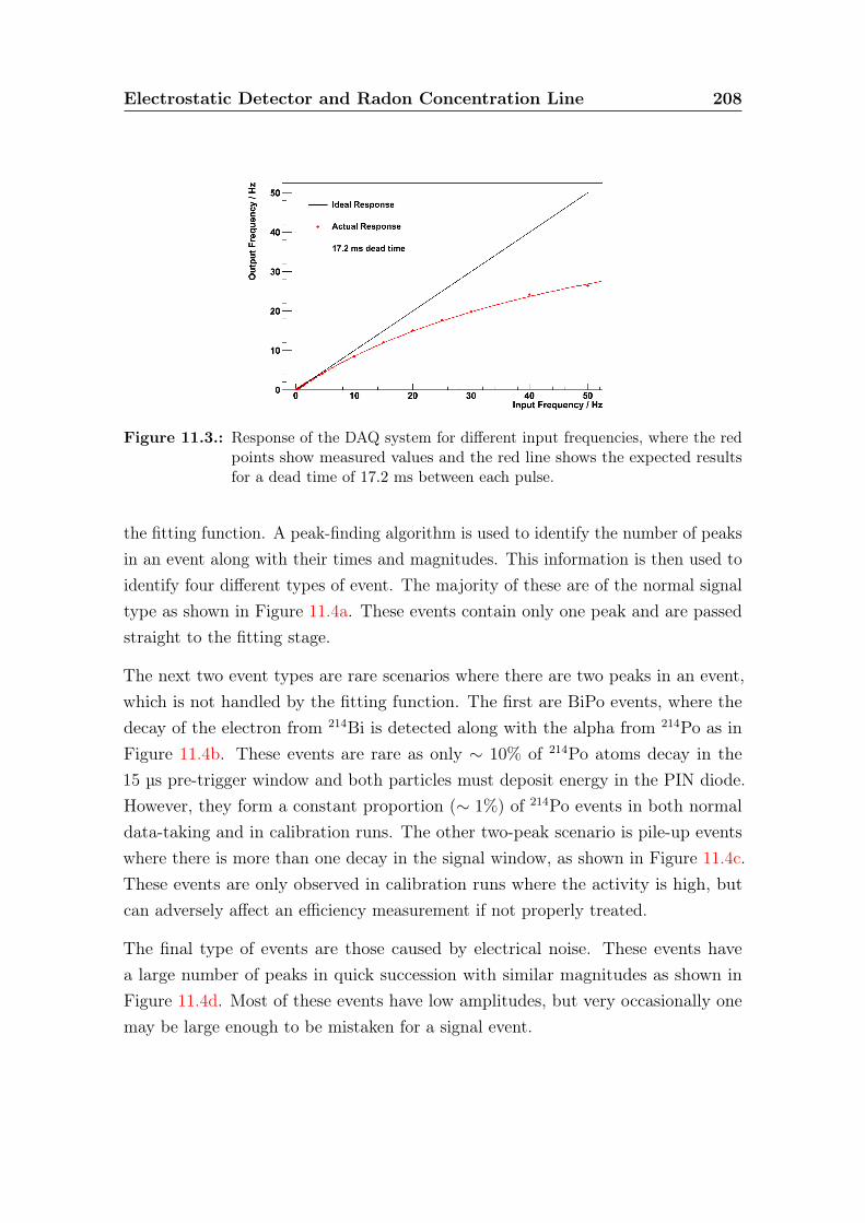
Electrostatic Detector and Radon Concentration Line 208
Figure 11.3.: Response of the DAQ system for different input frequencies, where the redpoints show measured values and the red line shows the expected resultsfor a dead time of 17.2 ms between each pulse.
the fitting function. A peak-finding algorithm is used to identify the number of peaksin an event along with their times and magnitudes. This information is then used toidentify four different types of event. The majority of these are of the normal signaltype as shown in Figure 11.4a. These events contain only one peak and are passedstraight to the fitting stage.
The next two event types are rare scenarios where there are two peaks in an event,which is not handled by the fitting function. The first are BiPo events, where thedecay of the electron from 214Bi is detected along with the alpha from 214Po as inFigure 11.4b. These events are rare as only ∼ 10% of 214Po atoms decay in the15 µs pre-trigger window and both particles must deposit energy in the PIN diode.However, they form a constant proportion (∼ 1%) of 214Po events in both normaldata-taking and in calibration runs. The other two-peak scenario is pile-up eventswhere there is more than one decay in the signal window, as shown in Figure 11.4c.These events are only observed in calibration runs where the activity is high, butcan adversely affect an efficiency measurement if not properly treated.
The final type of events are those caused by electrical noise. These events havea large number of peaks in quick succession with similar magnitudes as shown inFigure 11.4d. Most of these events have low amplitudes, but very occasionally onemay be large enough to be mistaken for a signal event.

Electrostatic Detector and Radon Concentration Line 209
(a) Normal Signal (b) BiPo Signal
(c) Pile-up Event (d) Noise Event
Figure 11.4.: Examples of the four types of event identified by the filtering stage of theevent analysis, described in the text.
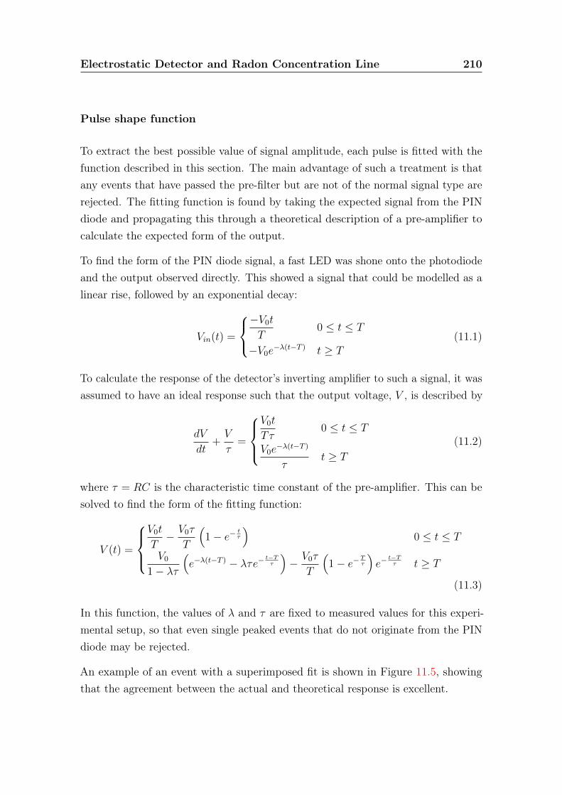
Electrostatic Detector and Radon Concentration Line 210
Pulse shape function
To extract the best possible value of signal amplitude, each pulse is fitted with thefunction described in this section. The main advantage of such a treatment is thatany events that have passed the pre-filter but are not of the normal signal type arerejected. The fitting function is found by taking the expected signal from the PINdiode and propagating this through a theoretical description of a pre-amplifier tocalculate the expected form of the output.
To find the form of the PIN diode signal, a fast LED was shone onto the photodiodeand the output observed directly. This showed a signal that could be modelled as alinear rise, followed by an exponential decay:
Vin(t) =
−V0tT
0 ≤ t ≤ T
−V0e−λ(t−T ) t ≥ T(11.1)
To calculate the response of the detector’s inverting amplifier to such a signal, it wasassumed to have an ideal response such that the output voltage, V , is described by
dV
dt+V
τ=
V0t
T τ0 ≤ t ≤ T
V0e−λ(t−T )
τt ≥ T
(11.2)
where τ = RC is the characteristic time constant of the pre-amplifier. This can besolved to find the form of the fitting function:
V (t) =
V0t
T− V0τ
T
(1− e−
tτ
)0 ≤ t ≤ T
V01− λτ
(e−λ(t−T ) − λτe−
t−Tτ
)− V0τ
T
(1− e−
Tτ
)e−
t−Tτ t ≥ T
(11.3)
In this function, the values of λ and τ are fixed to measured values for this experi-mental setup, so that even single peaked events that do not originate from the PINdiode may be rejected.
An example of an event with a superimposed fit is shown in Figure 11.5, showingthat the agreement between the actual and theoretical response is excellent.

Electrostatic Detector and Radon Concentration Line 211
Figure 11.5.: Example of a signal event (black) with the fitting function (Equation (11.3))superimposed (red).
11.1.2. Detector Efficiency Calibration
In order to investigate the response of the detector to a known activity of radon,a calibrated source was procured. This source is a 1.32 kBq “flow-through” 226Rasource (Pylon Electronics, RN-1025), the design of which allows the flow of gasthrough the source material. This ensures that all the emanated radon is exhaustedand provides considerable flexibility in the possible measurements that can be made.
Radon progenies are identified by the energy they deposit in the PIN diode, which isproportional to the amplitude of the signal. Three isotopes of polonium, all of whichdecay via alpha decay, are clearly visible in an energy spectrum after introducingradon from the source into the detector as displayed in Figure 11.6. The 214Popeak, which is used to measure the radon level is the highest energy peak (7.9 MeV).The 218Po peak (6.1 MeV) has a slightly lower height as its collection efficiency islower for reasons discussed above. Finally, a much smaller peak from 210Po is visible(5.4 MeV), the height of which is unrelated to the current level of radon in thedetector as it is caused by residual activity from previous calibration runs. Theresolution of the detector is excellent with clear separation between the peaks. Evenso, there is overlap between the tail of the 218Po peak and the 210Po which is furtherreason to base radon measurements on the 214Po activity.
In order to calibrate the efficiency of the detector, two different methods are used.The first is a “spike” method, where a known amount of radon is introduced into the
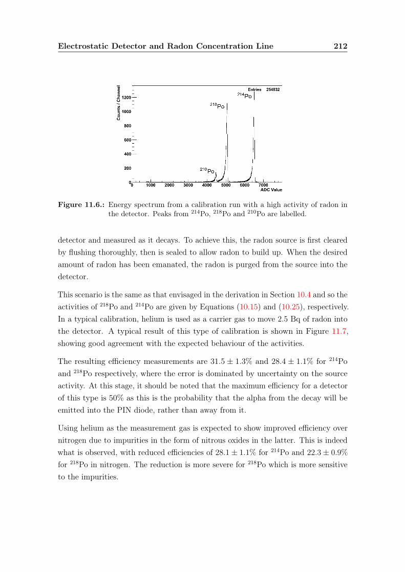
Electrostatic Detector and Radon Concentration Line 212
Figure 11.6.: Energy spectrum from a calibration run with a high activity of radon inthe detector. Peaks from 214Po, 218Po and 210Po are labelled.
detector and measured as it decays. To achieve this, the radon source is first clearedby flushing thoroughly, then is sealed to allow radon to build up. When the desiredamount of radon has been emanated, the radon is purged from the source into thedetector.
This scenario is the same as that envisaged in the derivation in Section 10.4 and so theactivities of 218Po and 214Po are given by Equations (10.15) and (10.25), respectively.In a typical calibration, helium is used as a carrier gas to move 2.5 Bq of radon intothe detector. A typical result of this type of calibration is shown in Figure 11.7,showing good agreement with the expected behaviour of the activities.
The resulting efficiency measurements are 31.5 ± 1.3% and 28.4 ± 1.1% for 214Poand 218Po respectively, where the error is dominated by uncertainty on the sourceactivity. At this stage, it should be noted that the maximum efficiency for a detectorof this type is 50% as this is the probability that the alpha from the decay will beemitted into the PIN diode, rather than away from it.
Using helium as the measurement gas is expected to show improved efficiency overnitrogen due to impurities in the form of nitrous oxides in the latter. This is indeedwhat is observed, with reduced efficiencies of 28.1± 1.1% for 214Po and 22.3± 0.9%
for 218Po in nitrogen. The reduction is more severe for 218Po which is more sensitiveto the impurities.
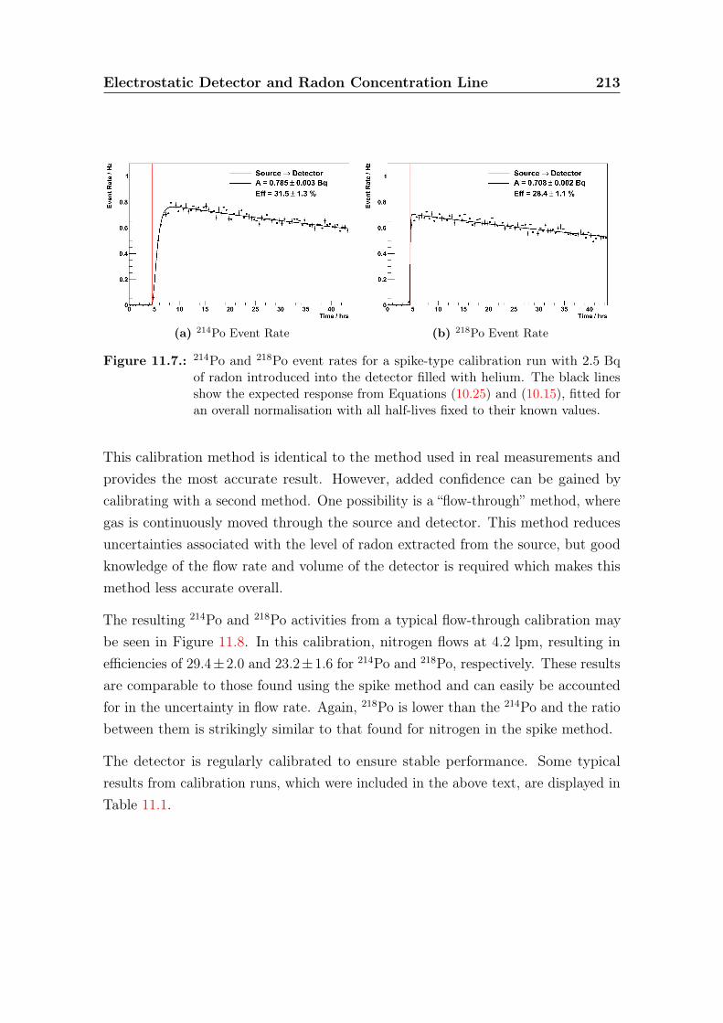
Electrostatic Detector and Radon Concentration Line 213
(a) 214Po Event Rate (b) 218Po Event Rate
Figure 11.7.: 214Po and 218Po event rates for a spike-type calibration run with 2.5 Bqof radon introduced into the detector filled with helium. The black linesshow the expected response from Equations (10.25) and (10.15), fitted foran overall normalisation with all half-lives fixed to their known values.
This calibration method is identical to the method used in real measurements andprovides the most accurate result. However, added confidence can be gained bycalibrating with a second method. One possibility is a “flow-through” method, wheregas is continuously moved through the source and detector. This method reducesuncertainties associated with the level of radon extracted from the source, but goodknowledge of the flow rate and volume of the detector is required which makes thismethod less accurate overall.
The resulting 214Po and 218Po activities from a typical flow-through calibration maybe seen in Figure 11.8. In this calibration, nitrogen flows at 4.2 lpm, resulting inefficiencies of 29.4±2.0 and 23.2±1.6 for 214Po and 218Po, respectively. These resultsare comparable to those found using the spike method and can easily be accountedfor in the uncertainty in flow rate. Again, 218Po is lower than the 214Po and the ratiobetween them is strikingly similar to that found for nitrogen in the spike method.
The detector is regularly calibrated to ensure stable performance. Some typicalresults from calibration runs, which were included in the above text, are displayed inTable 11.1.

Electrostatic Detector and Radon Concentration Line 214
(a) 214Po Event Rate (b) 218Po Event Rate
Figure 11.8.: 214Po and 218Po event rates for a flow-through calibration run with a flowrate of 4.2 lpm of nitrogen. The black lines show the expected response froma similar calculation to that shown in Section 10.4, fitted for an effectiveradon half-life and overall normalisation.
Calibration Measurement Efficiency / %Mode Gas 214Po 218PoSpike He 31.5± 1.3 28.4± 1.1
Spike N2 28.1± 1.1 22.3± 0.9
Flow-through N2 29.3± 2.0 23.2± 1.6
Table 11.1.: Typical results of calibration of the electrostatic detector for spike andflow-through calibration modes in helium and nitrogen.
11.1.3. Detector Background Measurement
As shown above, the electrostatic detector has an efficiency of over 30%. However,a sensitive detector must also have a low background counting rate, which is thesubject of this section.
In general, before performing every measurement, the background level of the detectoris measured to ensure that the best estimate of the activity of introduced radon ismade. Additionally, on occasion there have been some extended runs which weresolely dedicated to a background measurement of the detector. In order to performthese measurements, the detector is sealed for 20− 25 days whilst the radon activityinside is measured. The energy spectrum from this type of run is different to that ofa calibration run as can be seen in Figure 11.9.
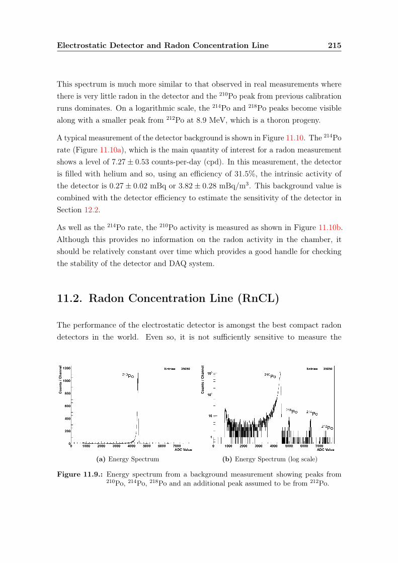
Electrostatic Detector and Radon Concentration Line 215
This spectrum is much more similar to that observed in real measurements wherethere is very little radon in the detector and the 210Po peak from previous calibrationruns dominates. On a logarithmic scale, the 214Po and 218Po peaks become visiblealong with a smaller peak from 212Po at 8.9 MeV, which is a thoron progeny.
A typical measurement of the detector background is shown in Figure 11.10. The 214Porate (Figure 11.10a), which is the main quantity of interest for a radon measurementshows a level of 7.27± 0.53 counts-per-day (cpd). In this measurement, the detectoris filled with helium and so, using an efficiency of 31.5%, the intrinsic activity ofthe detector is 0.27± 0.02 mBq or 3.82± 0.28 mBq/m3. This background value iscombined with the detector efficiency to estimate the sensitivity of the detector inSection 12.2.
As well as the 214Po rate, the 210Po activity is measured as shown in Figure 11.10b.Although this provides no information on the radon activity in the chamber, itshould be relatively constant over time which provides a good handle for checkingthe stability of the detector and DAQ system.
11.2. Radon Concentration Line (RnCL)
The performance of the electrostatic detector is amongst the best compact radondetectors in the world. Even so, it is not sufficiently sensitive to measure the
(a) Energy Spectrum (b) Energy Spectrum (log scale)
Figure 11.9.: Energy spectrum from a background measurement showing peaks from210Po, 214Po, 218Po and an additional peak assumed to be from 212Po.
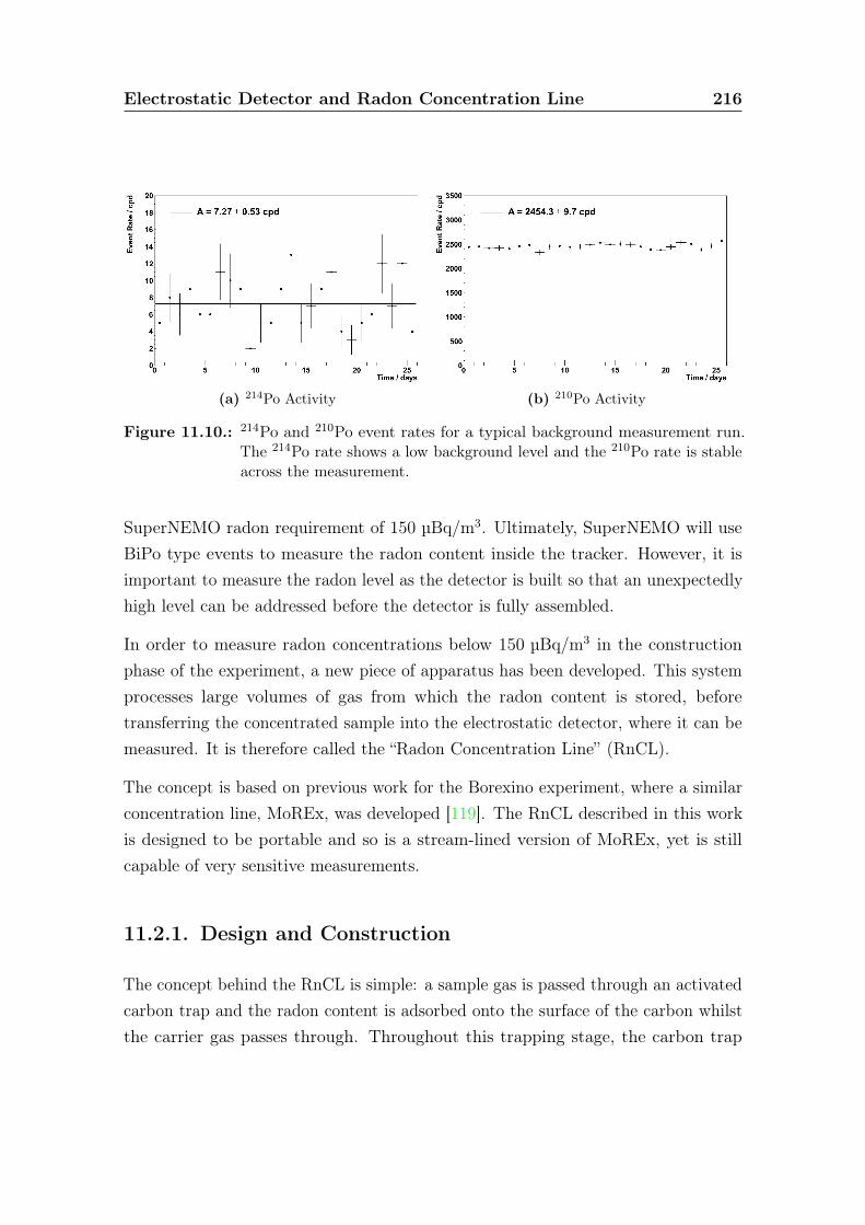
Electrostatic Detector and Radon Concentration Line 216
(a) 214Po Activity (b) 210Po Activity
Figure 11.10.: 214Po and 210Po event rates for a typical background measurement run.The 214Po rate shows a low background level and the 210Po rate is stableacross the measurement.
SuperNEMO radon requirement of 150 µBq/m3. Ultimately, SuperNEMO will useBiPo type events to measure the radon content inside the tracker. However, it isimportant to measure the radon level as the detector is built so that an unexpectedlyhigh level can be addressed before the detector is fully assembled.
In order to measure radon concentrations below 150 µBq/m3 in the constructionphase of the experiment, a new piece of apparatus has been developed. This systemprocesses large volumes of gas from which the radon content is stored, beforetransferring the concentrated sample into the electrostatic detector, where it can bemeasured. It is therefore called the “Radon Concentration Line” (RnCL).
The concept is based on previous work for the Borexino experiment, where a similarconcentration line, MoREx, was developed [119]. The RnCL described in this workis designed to be portable and so is a stream-lined version of MoREx, yet is stillcapable of very sensitive measurements.
11.2.1. Design and Construction
The concept behind the RnCL is simple: a sample gas is passed through an activatedcarbon trap and the radon content is adsorbed onto the surface of the carbon whilstthe carrier gas passes through. Throughout this trapping stage, the carbon trap

Electrostatic Detector and Radon Concentration Line 217
is cooled to improve its adsorption power. After collection is complete, the trap isheated to release the radon, which is then passed into the electrostatic detector.
In order to facilitate a high degree of flexibility in operation of the RnCL, the designshown in Figure 11.11 was chosen. In this schematic, the gas enters from the left-handside and moves to the right. All gas is passed though a 3 nm particle filter beforemeeting a series of valves to allow the opportunity to choose a path through thesystem. During a measurement, the typical path is through the carbon trap and oneof the flow meters, by-passing the detector and out to exhaust through the buffervolume.
This buffer volume is an addition to the core design, which is coupled with a diaphragmpump to allow a lower pressure on the RnCL output. This means that samples atatmospheric pressure can also be collected, which is important for the C-sectionmeasurement described in Section 13.3, as this cannot mechanically accommodate alarge over-pressure.
To ExhaustTo Vacuum Pump
ParticleFilter
He/N2
Flowmeter 1
Flowmeter 2CarbonTrap To Exhaust
Detector
BufferVolume
DiaphragmPump
Figure 11.11.: Schematic diagram of the design of the RnCL.
The main challenge in the design and construction of the RnCL is maintaining therequired degree of radiopurity. To this end, only essential components are placed inthe critical region upstream of the carbon trap. All pipework is made from stainlesssteel and all valves are fully metallic, which reduces radon emanation. The onlynon-metal component before the carbon trap is the particle filter, which is madefrom a PTFE membrane (Pall Emflon series) in a stainless steel housing.
The carbon trap itself is made entirely from stainless steel with the smallest possibleamount of welding. This welding was undertaken with zirconiated, rather than
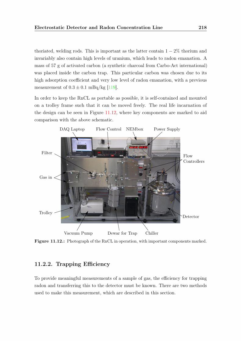
Electrostatic Detector and Radon Concentration Line 218
thoriated, welding rods. This is important as the latter contain 1− 2% thorium andinvariably also contain high levels of uranium, which leads to radon emanation. Amass of 57 g of activated carbon (a synthetic charcoal from Carbo-Act international)was placed inside the carbon trap. This particular carbon was chosen due to itshigh adsorption coefficient and very low level of radon emanation, with a previousmeasurement of 0.3± 0.1 mBq/kg [119].
In order to keep the RnCL as portable as possible, it is self-contained and mountedon a trolley frame such that it can be moved freely. The real life incarnation ofthe design can be seen in Figure 11.12, where key components are marked to aidcomparison with the above schematic.
Trolley
Gas in
Filter
Vacuum Pump Dewar for Trap Chiller
Detector
Power SupplyNEMboxFlow ControlDAQ Laptop
FlowControllers
Figure 11.12.: Photograph of the RnCL in operation, with important components marked.
11.2.2. Trapping Efficiency
To provide meaningful measurements of a sample of gas, the efficiency for trappingradon and transferring this to the detector must be known. There are two methodsused to make this measurement, which are described in this section.
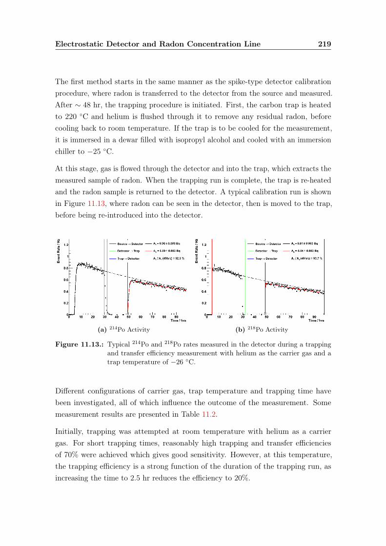
Electrostatic Detector and Radon Concentration Line 219
The first method starts in the same manner as the spike-type detector calibrationprocedure, where radon is transferred to the detector from the source and measured.After ∼ 48 hr, the trapping procedure is initiated. First, the carbon trap is heatedto 220 ◦C and helium is flushed through it to remove any residual radon, beforecooling back to room temperature. If the trap is to be cooled for the measurement,it is immersed in a dewar filled with isopropyl alcohol and cooled with an immersionchiller to −25 ◦C.
At this stage, gas is flowed through the detector and into the trap, which extracts themeasured sample of radon. When the trapping run is complete, the trap is re-heatedand the radon sample is returned to the detector. A typical calibration run is shownin Figure 11.13, where radon can be seen in the detector, then is moved to the trap,before being re-introduced into the detector.
(a) 214Po Activity (b) 218Po Activity
Figure 11.13.: Typical 214Po and 218Po rates measured in the detector during a trappingand transfer efficiency measurement with helium as the carrier gas and atrap temperature of −26 ◦C.
Different configurations of carrier gas, trap temperature and trapping time havebeen investigated, all of which influence the outcome of the measurement. Somemeasurement results are presented in Table 11.2.
Initially, trapping was attempted at room temperature with helium as a carriergas. For short trapping times, reasonably high trapping and transfer efficienciesof 70% were achieved which gives good sensitivity. However, at this temperature,the trapping efficiency is a strong function of the duration of the trapping run, asincreasing the time to 2.5 hr reduces the efficiency to 20%.
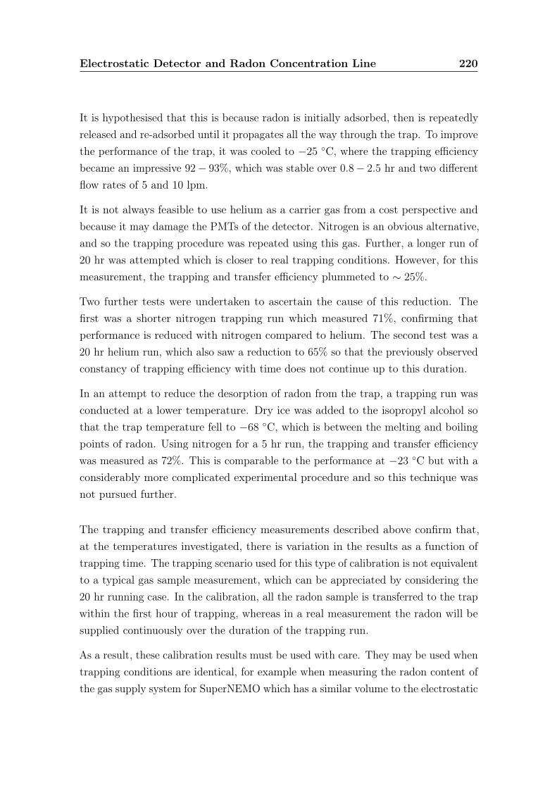
Electrostatic Detector and Radon Concentration Line 220
It is hypothesised that this is because radon is initially adsorbed, then is repeatedlyreleased and re-adsorbed until it propagates all the way through the trap. To improvethe performance of the trap, it was cooled to −25 ◦C, where the trapping efficiencybecame an impressive 92− 93%, which was stable over 0.8− 2.5 hr and two differentflow rates of 5 and 10 lpm.
It is not always feasible to use helium as a carrier gas from a cost perspective andbecause it may damage the PMTs of the detector. Nitrogen is an obvious alternative,and so the trapping procedure was repeated using this gas. Further, a longer run of20 hr was attempted which is closer to real trapping conditions. However, for thismeasurement, the trapping and transfer efficiency plummeted to ∼ 25%.
Two further tests were undertaken to ascertain the cause of this reduction. Thefirst was a shorter nitrogen trapping run which measured 71%, confirming thatperformance is reduced with nitrogen compared to helium. The second test was a20 hr helium run, which also saw a reduction to 65% so that the previously observedconstancy of trapping efficiency with time does not continue up to this duration.
In an attempt to reduce the desorption of radon from the trap, a trapping run wasconducted at a lower temperature. Dry ice was added to the isopropyl alcohol sothat the trap temperature fell to −68 ◦C, which is between the melting and boilingpoints of radon. Using nitrogen for a 5 hr run, the trapping and transfer efficiencywas measured as 72%. This is comparable to the performance at −23 ◦C but with aconsiderably more complicated experimental procedure and so this technique wasnot pursued further.
The trapping and transfer efficiency measurements described above confirm that,at the temperatures investigated, there is variation in the results as a function oftrapping time. The trapping scenario used for this type of calibration is not equivalentto a typical gas sample measurement, which can be appreciated by considering the20 hr running case. In the calibration, all the radon sample is transferred to the trapwithin the first hour of trapping, whereas in a real measurement the radon will besupplied continuously over the duration of the trapping run.
As a result, these calibration results must be used with care. They may be used whentrapping conditions are identical, for example when measuring the radon content ofthe gas supply system for SuperNEMO which has a similar volume to the electrostatic
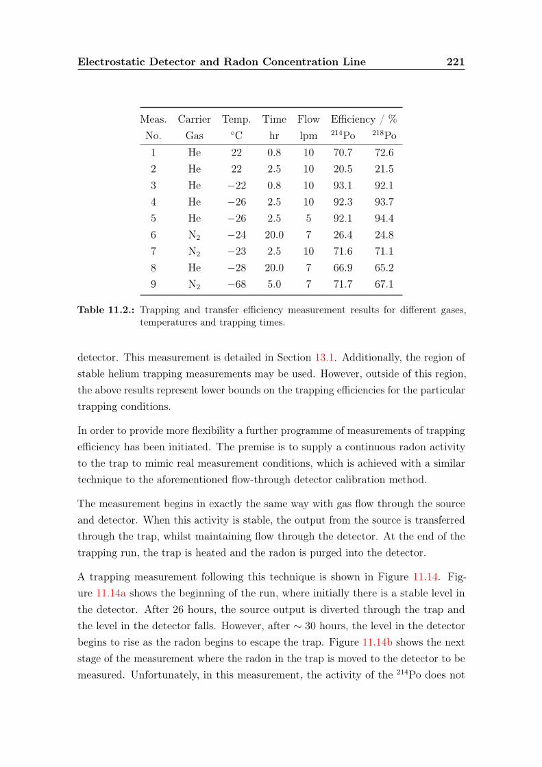
Electrostatic Detector and Radon Concentration Line 221
Meas. Carrier Temp. Time Flow Efficiency / %No. Gas ◦C hr lpm 214Po 218Po1 He 22 0.8 10 70.7 72.62 He 22 2.5 10 20.5 21.53 He −22 0.8 10 93.1 92.14 He −26 2.5 10 92.3 93.75 He −26 2.5 5 92.1 94.46 N2 −24 20.0 7 26.4 24.87 N2 −23 2.5 10 71.6 71.18 He −28 20.0 7 66.9 65.29 N2 −68 5.0 7 71.7 67.1
Table 11.2.: Trapping and transfer efficiency measurement results for different gases,temperatures and trapping times.
detector. This measurement is detailed in Section 13.1. Additionally, the region ofstable helium trapping measurements may be used. However, outside of this region,the above results represent lower bounds on the trapping efficiencies for the particulartrapping conditions.
In order to provide more flexibility a further programme of measurements of trappingefficiency has been initiated. The premise is to supply a continuous radon activityto the trap to mimic real measurement conditions, which is achieved with a similartechnique to the aforementioned flow-through detector calibration method.
The measurement begins in exactly the same way with gas flow through the sourceand detector. When this activity is stable, the output from the source is transferredthrough the trap, whilst maintaining flow through the detector. At the end of thetrapping run, the trap is heated and the radon is purged into the detector.
A trapping measurement following this technique is shown in Figure 11.14. Fig-ure 11.14a shows the beginning of the run, where initially there is a stable level inthe detector. After 26 hours, the source output is diverted through the trap andthe level in the detector falls. However, after ∼ 30 hours, the level in the detectorbegins to rise as the radon begins to escape the trap. Figure 11.14b shows the nextstage of the measurement where the radon in the trap is moved to the detector to bemeasured. Unfortunately, in this measurement, the activity of the 214Po does not
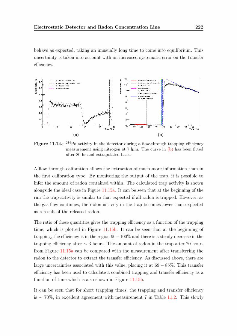
Electrostatic Detector and Radon Concentration Line 222
behave as expected, taking an unusually long time to come into equilibrium. Thisuncertainty is taken into account with an increased systematic error on the transferefficiency.
(a) (b)
Figure 11.14.: 214Po activity in the detector during a flow-through trapping efficiencymeasurement using nitrogen at 7 lpm. The curve in (b) has been fittedafter 80 hr and extrapolated back.
A flow-through calibration allows the extraction of much more information than inthe first calibration type. By monitoring the output of the trap, it is possible toinfer the amount of radon contained within. The calculated trap activity is shownalongside the ideal case in Figure 11.15a. It can be seen that at the beginning of therun the trap activity is similar to that expected if all radon is trapped. However, asthe gas flow continues, the radon activity in the trap becomes lower than expectedas a result of the released radon.
The ratio of these quantities gives the trapping efficiency as a function of the trappingtime, which is plotted in Figure 11.15b. It can be seen that at the beginning oftrapping, the efficiency is in the region 90−100% and there is a steady decrease in thetrapping efficiency after ∼ 3 hours. The amount of radon in the trap after 20 hoursfrom Figure 11.15a can be compared with the measurement after transferring theradon to the detector to extract the transfer efficiency. As discussed above, there arelarge uncertainties associated with this value, placing it at 69− 85%. This transferefficiency has been used to calculate a combined trapping and transfer efficiency as afunction of time which is also shown in Figure 11.15b.
It can be seen that for short trapping times, the trapping and transfer efficiencyis ∼ 70%, in excellent agreement with measurement 7 in Table 11.2. This slowly
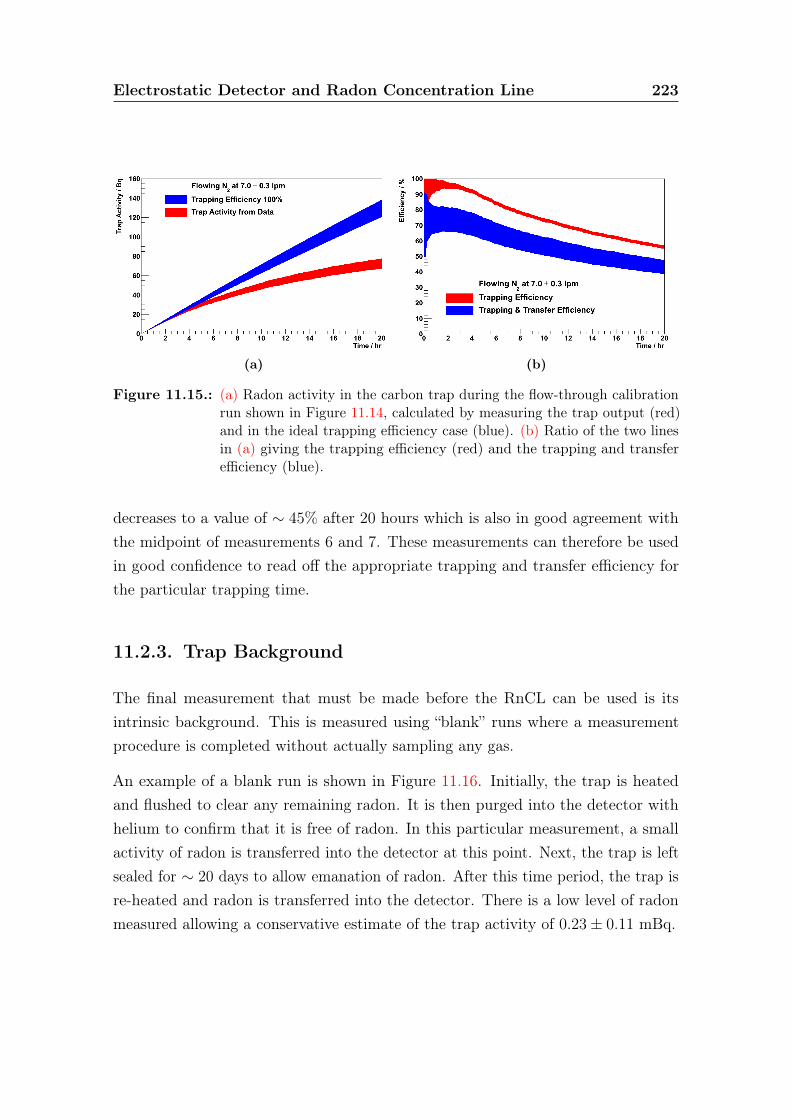
Electrostatic Detector and Radon Concentration Line 223
(a) (b)
Figure 11.15.: (a) Radon activity in the carbon trap during the flow-through calibrationrun shown in Figure 11.14, calculated by measuring the trap output (red)and in the ideal trapping efficiency case (blue). (b) Ratio of the two linesin (a) giving the trapping efficiency (red) and the trapping and transferefficiency (blue).
decreases to a value of ∼ 45% after 20 hours which is also in good agreement withthe midpoint of measurements 6 and 7. These measurements can therefore be usedin good confidence to read off the appropriate trapping and transfer efficiency forthe particular trapping time.
11.2.3. Trap Background
The final measurement that must be made before the RnCL can be used is itsintrinsic background. This is measured using “blank” runs where a measurementprocedure is completed without actually sampling any gas.
An example of a blank run is shown in Figure 11.16. Initially, the trap is heatedand flushed to clear any remaining radon. It is then purged into the detector withhelium to confirm that it is free of radon. In this particular measurement, a smallactivity of radon is transferred into the detector at this point. Next, the trap is leftsealed for ∼ 20 days to allow emanation of radon. After this time period, the trap isre-heated and radon is transferred into the detector. There is a low level of radonmeasured allowing a conservative estimate of the trap activity of 0.23± 0.11 mBq.
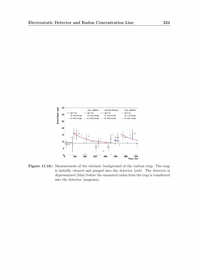
Electrostatic Detector and Radon Concentration Line 224
Figure 11.16.: Measurement of the intrinsic background of the carbon trap. The trapis initially cleared and purged into the detector (red). The detector isdepressurised (blue) before the emanated radon from the trap is transferredinto the detector (magenta).
Chapter 12.
Radon Concentration LineSensitivity Estimates
The main aim of the research and development described in part II of this thesisis to measure radon at the low levels required for SuperNEMO. This chapter willassess whether the combination of radon concentration line (RnCL) and electrostaticdetector, described in Chapter 11, have sufficient sensitivity to make a measurementat the level of ∼ 150 µBq/m3.
In the first section, a definition of the minimum detectable activity is introduced(Section 12.1). This will be used to quantify the sensitivity of the system in threedifferent cases. Firstly, the detector-only sensitivity will be addressed (Section 12.2),which is shown to be insufficient for the required SuperNEMO radon level. Ahypothetical measurement with the RnCL is then studied to find the sensitivityof the system to a supply of gas of uniform activity (Section 12.3). Finally, arealistic scenario for the measurement of a C-section is put forward to confirm thata measurement at the target level is indeed achievable (Section 12.4).
12.1. Minimum Detectable Activity
In order to quantify the sensitivity of the apparatus that has been developed, astringent definition must first be found for the sensitivity of a measurement. In thiswork, the definition of Minimum Detectable Activity (MDA) given in ‘RadiationDetection and Measurement’ by G. F. Knoll is used [120].
225

Radon Concentration Line Sensitivity Estimates 226
This definition is based on a binary decision of whether the output of the detector isrepresentative of background only or indicates the presence of a signal along withthe background. The concept is that prior to any measurement, the probability of afalse positive is identified, where signal is indicated when there is only backgroundpresent, as is the probability of a false negative, where a signal that is present ismisidentified as background only.
To decide whether there is a signal, a critical number of counts, nc, is predefined andif more counts than this number are observed, it is concluded that there is a signalpresent. Firstly, nc must be found for a well-known expected number of backgroundevents, B, and measurement confidence level, CL, such that the probability of a falsepositive is less than 1 − CL. If B is Poisson-distributed then to satisfy the abovecriterion, nc must be increased until the following inequality is satisfied:
PB(n ≥ nc) =∞∑
n=nc
Pois(n;B) = 1−nc−1∑n=0
e−BBn
n!≤ 1− CL (12.1)
Once nc has been set high enough to reduce the false positive probability to 1− CL,the probability for false negatives can be used to calculate the minimum expectednumber of signal events, S, that satisfies the MDA requirement. S is thereforeincreased until the following is true:
PS+B(n < nc) =nc−1∑n=0
Pois(n;S +B) =nc−1∑n=0
e−(S+B) (S +B)n
n!≤ 1− CL (12.2)
These results are most readily understood graphically as shown in Figure 12.1.The black curve represents the Poisson distributed background expectation, fromwhich nc has been set so that the black shaded area corresponds to 1− CL as perEquation (12.1). The red line is the distribution for the minimum signal on the samebackground, where S has been set such that the red shaded area also corresponds to1− CL as in Equation (12.2).
Once the minimum signal has been found, it can be converted into an activity. Thisminimum activity is what is referred to as the MDA.
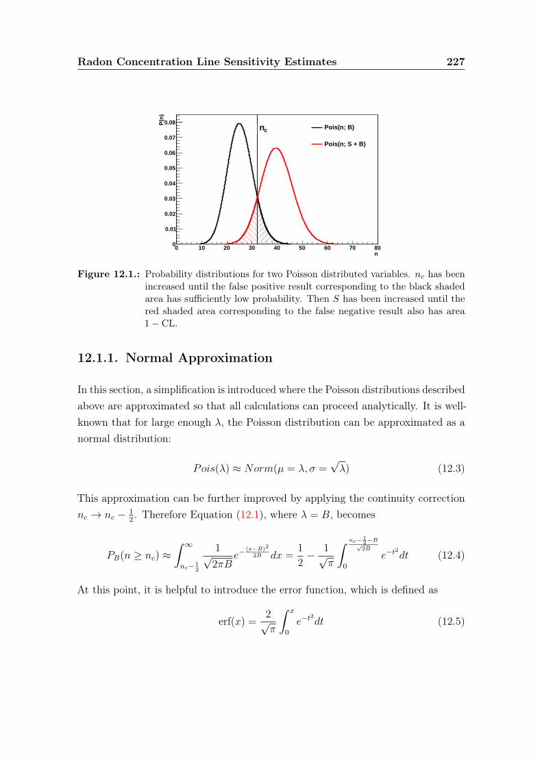
Radon Concentration Line Sensitivity Estimates 227
n0 10 20 30 40 50 60 70 80
P(n
)
0
0.01
0.02
0.03
0.04
0.05
0.06
0.07
0.08cn Pois(n; B)
Pois(n; S + B)
Figure 12.1.: Probability distributions for two Poisson distributed variables. nc has beenincreased until the false positive result corresponding to the black shadedarea has sufficiently low probability. Then S has been increased until thered shaded area corresponding to the false negative result also has area1− CL.
12.1.1. Normal Approximation
In this section, a simplification is introduced where the Poisson distributions describedabove are approximated so that all calculations can proceed analytically. It is well-known that for large enough λ, the Poisson distribution can be approximated as anormal distribution:
Pois(λ) ≈ Norm(µ = λ, σ =√λ) (12.3)
This approximation can be further improved by applying the continuity correctionnc → nc − 1
2. Therefore Equation (12.1), where λ = B, becomes
PB(n ≥ nc) ≈∫ ∞nc− 1
2
1√2πB
e−(x−B)2
2B dx =1
2− 1√
π
∫ nc− 12−B√2B
0
e−t2
dt (12.4)
At this point, it is helpful to introduce the error function, which is defined as
erf(x) =2√π
∫ x
0
e−t2
dt (12.5)
Radon Concentration Line Sensitivity Estimates 228
Using this definition and Equations (12.1) and (12.4) it can be seen that
PB(n ≥ nc) ≈1
2
(1− erf
(nc − 1
2−B
√2B
))≤ 1− CL (12.6)
The equivalent procedure can be applied to Equation (12.2) to give
P (n < nc) ≈1
2
(1 + erf
(nc − 1
2− (S +B)√
2(S +B)
))≤ 1− CL (12.7)
The MDA definition provides the smallest possible value of S for a given B, so ncis not of direct interest and can be eliminated. Equations (12.6) and (12.7) can becombined to find
S −√
2BE ≥√
2(S +B)E (12.8)
where E is a positive number defined as:
E = erf−1(2CL− 1) (12.9)
Therefore, discounting the unphysical S ≤ 0 solution, it is found that
S ≥ 2E(E +√
2B) (12.10)
The minimum value of S is when the inequality is equal, so under this approximationthe MDA can be calculated from the minimum number of signal events that aredetectable, S0, which is given by
S0 = 2E(E +√
2B) (12.11)
12.2. Electrostatic Detector Sensitivity
The simplest case to be considered is the detector-only sensitivity. The samemeasurement is imagined as in Section 10.4, where a signal activity, AS, is introducedinto a detector with intrinsic background activity, AD, which detects 214Po decays.
Radon Concentration Line Sensitivity Estimates 229
In this case, to find the number of signal events, S, expected to have been detectedafter a given time, T , in a detector with detection efficiency, εD, the detectorbackground is set to zero in Equation (10.25) and it is found that
S = εD
∫ T
0
λ4N4dt = εD
∫ T
0
(ASλ1λ2λ3λ4
4∑i=0
e−λit
k4i,4
)dt
= εDASλ1λ2λ3λ4
4∑i=0
(1− e−λiT )
λik4i,4(12.12)
Similarly, to find the number of expected background events, AS is set to zero whichgives
B = εD
∫ T
0
AD
{1−
4∑i=0
[(4∏
j=i+1
λj
)4∑k=i
e−λkt
k4−ik,4
]}dt
= εDADT − εDAD4∑i=0
[(4∏
j=i+1
λj
)4∑k=i
(1− e−λkT )
λkk4−ik,4
](12.13)
These quantities are shown in Figure 12.2 alongside the equivalent values for 222Rn.It can be seen that there is very little difference between the 214Po and 222Rn casesat any time during the measurement, and using only 222Rn gives a very similarsensitivity.
To calculate the MDA, Equation (12.13) is used to find B, which is then combinedwith Equation (12.11) to extract the minimum number of signal events, S0, for agiven confidence level. Finally, Equation (12.12) is used to convert S0 into the MDA,which is shown as a function of the measurement time in Figure 12.3.
As might be expected, at short measurement times there is very little sensitivitysince there has been no time for any radon to decay. However, as time increasesthe MDA falls rapidly before reaching a shallow minimum at ∼3 days. After this itbegins to increase again as the increasing number of background counts begins totake effect. As expected, there is very little difference between 214Po and 222Rn, withthe two methods converging after a measurement time of ∼1 day.
From Figure 12.3, the minimum detectable activity for the electrostatic detectoralone is 0.12 mBq or 1.7 mBq/m3, which is an order of magnitude larger than thetarget value of 150 µBq/m3.

Radon Concentration Line Sensitivity Estimates 230
Time / days0 0.5 1 1.5 2 2.5 3 3.5 4
Nu
mb
er o
f S
ign
al E
ven
ts
0
1
2
3
4
5
6
7
8
9
10
Rn222
Po214
= 0.12 mBq SA
= 0.00 mBq DA
= 31.5 % ∈
(a) Signal Events, S
Time / days0 0.5 1 1.5 2 2.5 3 3.5 4
Nu
mb
er o
f B
ackg
rou
nd
Eve
nts
0
1
2
3
4
5
6
7
8
9
10
Rn222
Po214
= 0.00 mBq SA
= 0.27 mBq DA
= 31.5 % ∈
(b) Background Events, B
Figure 12.2.: (a) Expected number of signal events, S, for events from both 222Rn and214Po decays with AD = 0.27 mBq and AS = 0.12 mBq. (b) Expectednumber of background events, B, for the same activities.
Measurement Time / days0 1 2 3 4 5 6 7 8 9 10
Min
imu
m D
etec
tab
le A
ctiv
ity
/ mB
q
0
0.05
0.1
0.15
0.2
0.25
0.3
Rn222
Po214
CL = 90 % = 0.27 mBqDA = 31.5 %D∈
Figure 12.3.: MDA for the electrostatic detector as a function of the measurement time,showing the 222Rn and 214Po results.
Radon Concentration Line Sensitivity Estimates 231
12.3. Uniform Gas Measurement
As the required sensitivity is not achieved with the detector alone, the RnCL must beused. The simplest case involving the RnCL is where a gas is supplied with constantactivity. This scenario is studied in this section.
If a gas with activity per unit volume, aG, is supplied to the RnCL at a flow rate, f ,the number of radon atoms in the carbon trap, NC , is described by
dNC
dt= AC − λNC +
εTfaGλ
(12.14)
where AC is the intrinsic activity of the carbon trap and εT is the trapping efficiency.If the conservative assumption is made that none of the intrinsic activity from thecarbon trap is exhausted during the trapping run, then the above equation has asolution given by
NC (Tf ) =
(ACλ
+εT (Tf ) faG
λ2
)(1− e−λTf
)(12.15)
where Tf is the time that gas has been flowing. In this section, this is limited to20 hr as this is the range over which the trapping efficiency has been measured. Ifafter a trapping run of length, Tf , the radon is transferred to the detector, then thenumber of radon atoms is the same as was found before:
ND =ADλ
(1− e−λt
)+ εtrNC (Tf ) e
−λt (12.16)
where εtr is the transfer efficiency. To calculate the minimum detectable activity,the number of signal and background events must be calculated. As was seen above,there is little difference between using 222Rn and 214Po, so the simpler 222Rn case isshown here. If the detector is left to measure for a time, Tm, the number of expectedsignal events is
S = εtrNSC (Tf ) εD
(1− e−λTm
)(12.17)
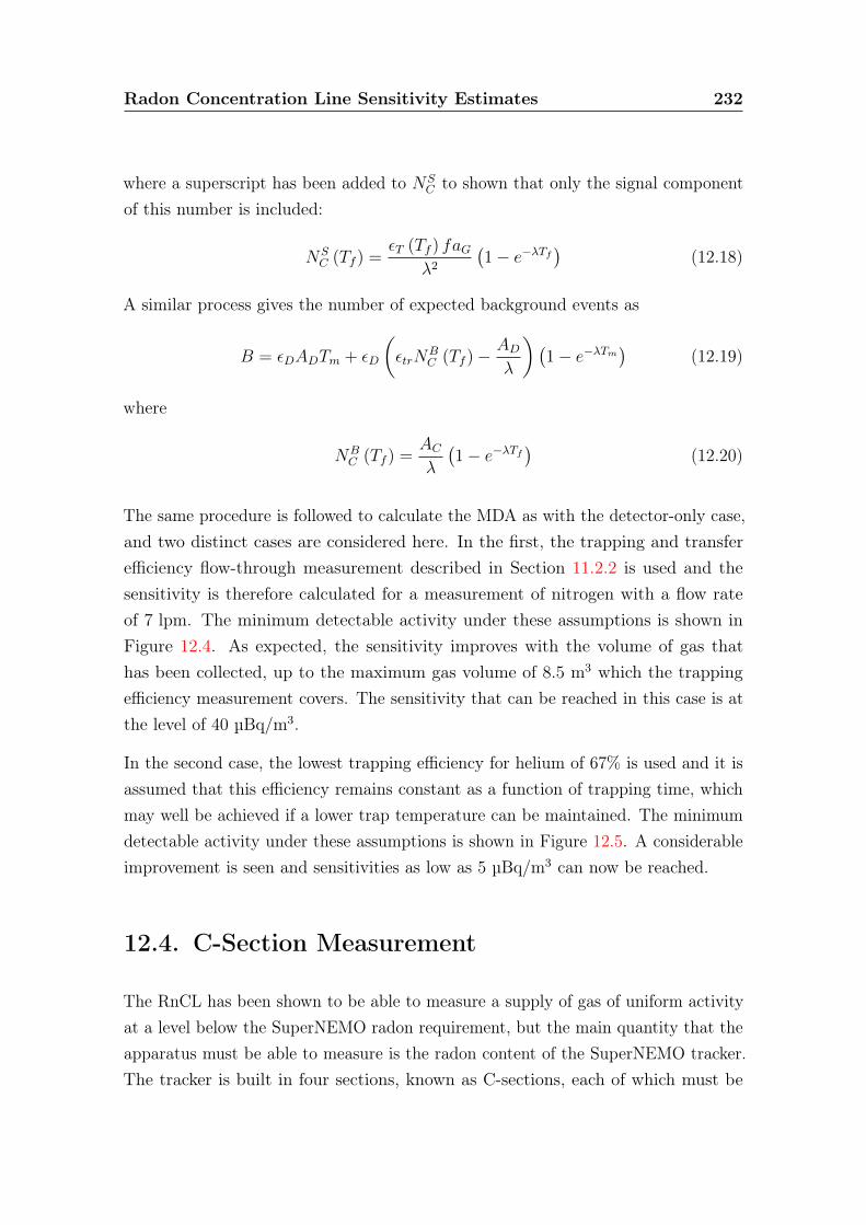
Radon Concentration Line Sensitivity Estimates 232
where a superscript has been added to NSC to shown that only the signal component
of this number is included:
NSC (Tf ) =
εT (Tf ) faGλ2
(1− e−λTf
)(12.18)
A similar process gives the number of expected background events as
B = εDADTm + εD
(εtrN
BC (Tf )−
ADλ
)(1− e−λTm
)(12.19)
where
NBC (Tf ) =
ACλ
(1− e−λTf
)(12.20)
The same procedure is followed to calculate the MDA as with the detector-only case,and two distinct cases are considered here. In the first, the trapping and transferefficiency flow-through measurement described in Section 11.2.2 is used and thesensitivity is therefore calculated for a measurement of nitrogen with a flow rateof 7 lpm. The minimum detectable activity under these assumptions is shown inFigure 12.4. As expected, the sensitivity improves with the volume of gas thathas been collected, up to the maximum gas volume of 8.5 m3 which the trappingefficiency measurement covers. The sensitivity that can be reached in this case is atthe level of 40 µBq/m3.
In the second case, the lowest trapping efficiency for helium of 67% is used and it isassumed that this efficiency remains constant as a function of trapping time, whichmay well be achieved if a lower trap temperature can be maintained. The minimumdetectable activity under these assumptions is shown in Figure 12.5. A considerableimprovement is seen and sensitivities as low as 5 µBq/m3 can now be reached.
12.4. C-Section Measurement
The RnCL has been shown to be able to measure a supply of gas of uniform activityat a level below the SuperNEMO radon requirement, but the main quantity that theapparatus must be able to measure is the radon content of the SuperNEMO tracker.The tracker is built in four sections, known as C-sections, each of which must be
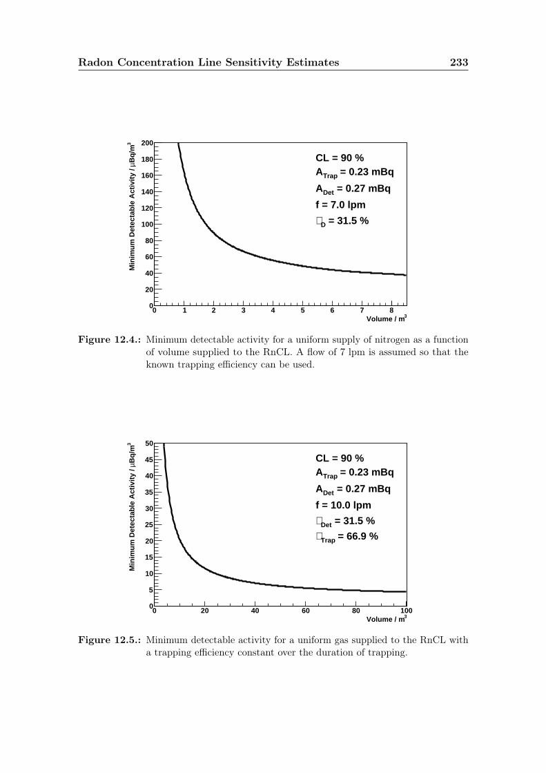
Radon Concentration Line Sensitivity Estimates 233
3Volume / m0 1 2 3 4 5 6 7 8
3B
q/m
µM
inim
um
Det
ecta
ble
Act
ivit
y /
0
20
40
60
80
100
120
140
160
180
200
CL = 90 % = 0.23 mBqTrapA
= 0.27 mBqDetA
f = 7.0 lpm
= 31.5 %D∈
Figure 12.4.: Minimum detectable activity for a uniform supply of nitrogen as a functionof volume supplied to the RnCL. A flow of 7 lpm is assumed so that theknown trapping efficiency can be used.
3Volume / m0 20 40 60 80 100
3B
q/m
µM
inim
um
Det
ecta
ble
Act
ivit
y /
0
5
10
15
20
25
30
35
40
45
50
CL = 90 % = 0.23 mBqTrapA
= 0.27 mBqDetA
f = 10.0 lpm
= 31.5 %Det∈ = 66.9 %Trap∈
Figure 12.5.: Minimum detectable activity for a uniform gas supplied to the RnCL witha trapping efficiency constant over the duration of trapping.
Radon Concentration Line Sensitivity Estimates 234
measured prior to assembly. Therefore, the radon activity inside a C-section is thekey measurement.
In an ideal scenario, the C-section would be left sealed for an extended period priorto the measurement to build up radon. However, in reality, a C-section is not a sealedunit and has small leaks. This means that it must be kept at a slight overpressure toprevent environmental radon from entering. Therefore, the number of radon atomsinside a C-section, NT is given by
dNT
dt= AT − λNT −
finNT
VT+finaGλ
(12.21)
where fin is the flow rate of gas which is supplied to sustain an overpressure,VT = 3.8 m3 is the volume of one C-section and aG is the activity of the supply gasper unit volume. Before starting a measurement, it is imagined that the C-sectionwill be left to come into equilibrium such that it has an activity per unit volume of
aT =λNT
VT=AT + finaG/λ
VT + fin/λ(12.22)
Once the C-section is in equilibrium, a trapping run can take place where the gasfrom the tracker is passed through the RnCL. The number of atoms in the trap,NC , takes the same form as Equation (12.15), replacing aG → aT and distinguishingthe flow through the trap as fRnCL. The form of S and B are identical to Equa-tions (12.17) and (12.19), where in this measurement, the signal relates to the activityof the C-section, AT , so that
NSC (Tf ) =
εT (Tf ) fRnCLλ2
ATVT + fin/λ
(1− e−λTf
)(12.23)
and the activity from the supply gas now becomes part of the background contribution:
NBC (Tf ) =
ACλ
(1− e−λTf
)+εT (Tf ) fRnCL
λ2finaG
λVT + fin
(1− e−λTf
)(12.24)
The calculated minimum detectable activity for such a C-section measurement isshown in Figure 12.6 as a function of the activity of the supply gas. In this plot,nitrogen has again been assumed as the carrier gas and a flow suppression factor has

Radon Concentration Line Sensitivity Estimates 235
been applied (Section 10.3). The target level is achievable, provided that the activityof the supply gas does not exceed 1.5 mBq/m3.
3Supply Gas Activity / mBq/m0 0.2 0.4 0.6 0.8 1 1.2 1.4 1.6 1.8 2
3B
q/m
µM
inim
um
Det
ecta
ble
Act
ivit
y /
0
20
40
60
80
100
120
140
160
180
200
CL = 90 % = 0.23 mBqCA = 0.27 mBqDA
3 = 3.8 mTV = 16.6 lpminf
= 7.0 lpmRnCLf = 31.5 %Det∈ = 20.0 hr fT∆
Figure 12.6.: Sensitivty of the RnCL for a C-section measurement as a function of theinput gas activity. The sensitivity is presented as in Equation (12.22) withthe reduction in activity from flow suppression already applied.
The sensitivity of this measurement may be improved further by a number of differentmeasures. One of the most significant is a reduction of the input flow rate, whichrequires that the leak rate from the C-section is reduced. Other improvements mayarise from changing to a new carrier gas with improved trapping efficiency, or byincreasing the trapping time.
Having shown that the RnCL is capable of providing useful measurements of theradon activity inside a C-section, there is clearly good justification for performinga measurement such as that described here. This is the culmination of the nextchapter, described in Section 13.3.
Chapter 13.
Low-level Radon Measurements
A substantial amount of work has gone into the development and commissioning ofboth the electrostatic detector and radon concentration line (RnCL), as describedin Chapter 11. The new apparatus has been put to good use, making a series ofmeasurements of low-level radon activities from large gas volumes, which are thesubject of this chapter.
There have been three different types of measurements that will be presented herein.The first is of the intrinsic radon activity of the gas system, which has been developedto prepare the tracking gas mixture for SuperNEMO (Section 13.1). Next, the radonactivity from off-the-shelf gas cylinders is considered, with measurements of bothhelium and nitrogen presented in Section 13.2. Finally, a measurement of the radoncontent of the first tracker C-section for the SuperNEMO demonstrator is introducedin Section 13.3.
13.1. Gas System
The tracking gas for SuperNEMO will be a mixture of helium, argon and ethanolin the same proportions as used for NEMO-3 (Section 5.2). In order to obtainthe appropriate proportions, a dedicated gas supply system has been developed forthe experiment. This design was based on the system used for NEMO-3, with thereplacement of all components with more radiopure alternatives, with the exceptionof the large bubbler. This bubbler is a stainless steel cylinder with a length of 2 mand a diameter of 0.2 m. In operation, it is filled with alcohol and gas is passed
236

Low-level Radon Measurements 237
through at high pressure to add approximately the right proportion of alcohol to thegas mixture.
As was shown in Section 10.3, due the small volume of the gas system comparedto the required flow rates and radon half-life, there is no difference between radonemanating in the gas system and that emanating from the tracker. Furthermore, acarbon trap of the type used in the RnCL cannot be used to filter the output fromthe gas system since it will also remove the ethanol. As a result there are strictrequirements on the radon emanation from the gas system with a target of 0.2 mBq,corresponding to 10% of the total radon budget.
The first measurement of the emanation from the gas system was undertaken withthe RnCL in the early stages of its commissioning. The volume of the gas system isdominated by the large bubbler from NEMO-3, which is of comparable size to theelectrostatic detector. As a result, the spike-type trapping efficiency calibrations canbe reliably used if the same flow rate, trap temperature and timing conditions arereplicated.
In this measurement, the gas system was thoroughly flushed with helium and thenleft for 4.1 days for radon to emanate. After this time, helium was flushed throughthe gas system and into the RnCL at 10 lpm. The trap was kept at room temperaturefor this run, which lasted 50 minutes, so that the measured trapping efficiency of70.7% (Table 11.2) could be used.
After transferring the radon to the detector, 18.9 ± 4.0 cpd of 214Po was seen, asshown in Figure 13.1a. The expected contribution from the intrinsic trap activity was0.2 cpd, so that the activity from the gas system in the detector was 0.69±0.15 mBq.When the trapping efficiency and radon build-up time are taken into account, thegas system activity is found to be 1.9± 0.4 mBq.
This value is an order of magnitude higher than the target level, so it was importantto isolate the main cause of the emanation. The prime suspect was the large bubblerfrom NEMO-3 as not only is this the largest component from the gas system, it is alsothe only one not specifically designed for a low-level of radon emanation. As such, ithas a glass window, welded seams and viton seals all of which may contribute to anelevated radon level. To reduce this contribution, the glass window was replaced withstainless steel and the viton seals were covered in SBR to reduce radon diffusion.
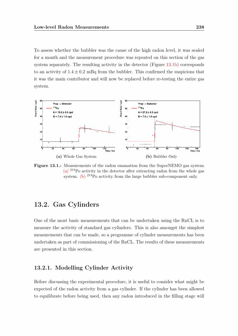
Low-level Radon Measurements 238
To assess whether the bubbler was the cause of the high radon level, it was sealedfor a month and the measurement procedure was repeated on this section of the gassystem separately. The resulting activity in the detector (Figure 13.1b) correspondsto an activity of 1.4± 0.2 mBq from the bubbler. This confirmed the suspicions thatit was the main contributor and will now be replaced before re-testing the entire gassystem.
(a) Whole Gas System (b) Bubbler Only
Figure 13.1.: Measurements of the radon emanation from the SuperNEMO gas system.(a) 214Po activity in the detector after extracting radon from the whole gassystem. (b) 214Po activity from the large bubbler sub-component only.
13.2. Gas Cylinders
One of the most basic measurements that can be undertaken using the RnCL is tomeasure the activity of standard gas cylinders. This is also amongst the simplestmeasurements that can be made, so a programme of cylinder measurements has beenundertaken as part of commissioning of the RnCL. The results of these measurementsare presented in this section.
13.2.1. Modelling Cylinder Activity
Before discussing the experimental procedure, it is useful to consider what might beexpected of the radon activity from a gas cylinder. If the cylinder has been allowedto equilibrate before being used, then any radon introduced in the filling stage will
Low-level Radon Measurements 239
have decayed and the activity contained is purely from emanation from the cylinderitself.
The quantity of interest is usually the specific radon activity, that is, the radonactivity per unit volume. As the bottle is emptied, radon is removed from the cylinderand replaced by newly emanated radon. However, the volume of gas contained withinthe cylinder will decrease and so the specific activity will increase. This can be seenby considering the differential equation that describes the number of radon atomsremaining in the gas cylinder:
dNG
dt= AG − λNG −
fNG
(VG − ft)(13.1)
where VG is the total volume of gas (at STP) contained in the cylinder at the startof the measurement. It is clear that the radon in the bottle reduces more quickly astime increases, so the specific activity of its output must be higher. This equationcan be solved using an integrating factor, to find
eλtNG
VG − ft=
∫eλtAGVG − ft
dt = −AGλf
∫eλt
λt− λVGf
dt = −AGfeλVGf
∫ex
xdx (13.2)
This final integral has no analytic solution, but can be shown to be equal to theexponential integral defined as
Ei(x) =
∫ x
−∞
et
tdt (13.3)
Assuming that the cylinder was in equilibrium at the start of the measurement, theconstant of integration can be found, leading to the final form for NG:
NG =AGλVG
(VG − ft) e−λt +AGf
(VG − ft) eλVGf−λt[Ei(−λVG
f
)− Ei
(λt− λVG
f
)](13.4)
The instantaneous specific activity at the output of the cylinder, aG, is simply givenby the specific activity in the bottle at that time:
aG =λNG
VG − ft=AGVG
e−λt +λAGf
eλVGf−λt[Ei(−λVG
f
)− Ei
(λt− λVG
f
)](13.5)

Low-level Radon Measurements 240
This is plotted as a function of the volume remaining in the cylinder in Figure 13.2.As expected, the radon activity increases as the bottles are emptied, with a moresevere effect for lower flow rates. This is simply because the faster flow rates emptythe bottles before a significant amount of radon has had time to emanate.
3Volume Remaining / m5 10 15 20 25 30 35 40
3B
q/m
µ O
utp
ut
Act
ivit
y /
0
500
1000
1500
2000
2500
3000
1 Gas Bottle = 5.00 mBq
Num Bottles = 43Starting Vol. = 40.0 m
f = 1.0 lpm
f = 5.0 lpm
f = 10.0 lpm
f = 20.0 lpm
Figure 13.2.: Specific activity at the output of four cylinders as a function of the volumeremaining, predicted by the model shown here. The cylinders are assumedto have a combined activity of 20 mBq and a starting volume of 40 m3.
To simplify the measurements conducted, all bottles are drained at flow rates between10− 20 lpm and never completely emptied such that, to a good approximation, theiroutput activity is uniform over time.
13.2.2. Measuring Full Cylinders
In order to disentangle the low levels of activity in the output from gas cylinders fromthe background emanation from the gas supply line, the latter must be separatelymeasured. The cylinder measurements shown here were undertaken at MSSL, wherethe gas supply line consists of 30 m of stainless steel pipe, which is expected tocontribute very little radon, along with two regulators and a coloured plastic filter ofunknown provenance. The latter is considered particularly likely to be a source ofradon emanation.
A measurement was performed where the line was sealed for ∼ 20 hours to allowradon to emanate, before flushing through the trap with 50 l of helium. The trap washeated and the radon purged into the detector with a further 25 l of helium. This

Low-level Radon Measurements 241
75 l produces a negligible contribution to the measurement as will be seen when thespecific activity results are presented later. The resulting activity of 25.1±3.3 cpd inthe detector, corresponding to 0.92± 0.12 mBq, is shown in Figure 13.3a. Followingthe derivation in Section 12.3, the activity of radon in the detector immediately aftertransfer from the trap is given by
AD = εtrAC(1− e−λTC
)+ εtr
(εT (Tf )AG +
εT (Tf ) faGλ
)(1− e−λTf
)e−λTtrans
(13.6)
where the relevant timings for this measurement are as follows
• TC : time between clearing the trap and detector transfer (1449 min).
• Tf : time that the line is in contact with the trap (1163 min).
• Ttrans: time between stopping collection and detector transfer (63 min).
In addition to neglecting the activity from the small volume of helium used, thisvolume also places the trapping and transfer efficiency firmly in the stable regionfor helium, with a value of 92%, such that the activity of the line is extracted as7.4± 1.0 mBq.
Once the contribution of the line has been measured, it is possible to begin mea-surements of the gas from cylinders. The experimental procedure is simple – afterclearing the trap, it is cooled and a sample of gas is collected for ∼ 20 hours. Atthis point, the trap is heated and the radon transferred to the detector. A typicalmeasurement of a nitrogen cylinder is shown in Figure 13.3b.
In order to extract the activity of the gas, Equation (13.6) is again applied. Inthe case shown here, 4.53 ± 0.25 mBq has been measured with TC = 1462 min,TF = 1070 min and Ttrans = 128 min. Using the trapping and transfer efficienciesfrom the flow-through calibration, the specific radon activity of the gas is extractedas 957± 132 µBq/m3, such that mean intrinsic activity of each bottle is 9.6 mBq.
A similar measurement of helium cylinders produced a result of 69− 118 µBq/m3,where the range is due to uncertainties in the trapping efficiency and the boundingcases of 66% and 92% have been used. These cylinders were the same as those usedin the line activity measurement, justifiying the declaration that their contributionof ∼ 5− 10 µBq could be neglected. The discrepancy between helium and nitrogen
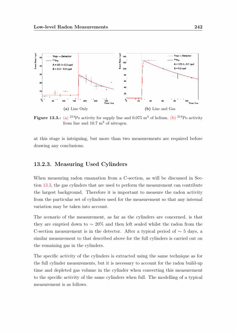
Low-level Radon Measurements 242
(a) Line Only (b) Line and Gas
Figure 13.3.: (a) 214Po activity for supply line and 0.075 m3 of helium. (b) 214Po activityfrom line and 10.7 m3 of nitrogen.
at this stage is intriguing, but more than two measurements are required beforedrawing any conclusions.
13.2.3. Measuring Used Cylinders
When measuring radon emanation from a C-section, as will be discussed in Sec-tion 13.3, the gas cylinders that are used to perform the measurement can contributethe largest background. Therefore it is important to measure the radon activityfrom the particular set of cylinders used for the measurement so that any internalvariation may be taken into account.
The scenario of the measurement, as far as the cylinders are concerned, is thatthey are emptied down to ∼ 20% and then left sealed whilst the radon from theC-section measurement is in the detector. After a typical period of ∼ 5 days, asimilar measurement to that described above for the full cylinders is carried out onthe remaining gas in the cylinders.
The specific activity of the cylinders is extracted using the same technique as forthe full cylinder measurements, but it is necessary to account for the radon build-uptime and depleted gas volume in the cylinder when converting this measurementto the specific activity of the same cylinders when full. The modelling of a typicalmeasurement is as follows.
Low-level Radon Measurements 243
At the start of use, the cylinders are assumed to be in equilibrium with total intrinsicactivity, AB. The flow rate is sufficiently fast that the specific activity from thecylinders is approximately constant and the activity in the cylinders at the end ofthis period is simply given by the the proportion of gas remaining.
A(T1) =V (T1)
V (0)AB (13.7)
After the cylinders are re-sealed, the radon level increases back towards equilibrium,so that when the next measurement starts at time, T2, the radon activity in thebottles is given by
A(T2) =
((1− e−λ(T2−T1)) +
V (T1)
V (0)e−λ(T2−T1)
)AB (13.8)
As an example of this type of measurement, consider a C-section measurementwhere the volume in the cylinders is reduced from 38.5 m3 to 11.5 m3. The activityremaining in the bottles at the end of this flushing is therefore 29.9% of AB. Thesecylinders were then left for 100 hours, rising to an activity of 67.0% of AB, beforebeing measured themselves. The measurement of 1.83±0.22 mBq/m3 from a startingvolume of 11.5 m3 can then be propagated to find the specific activity at the start ofthe C-section flushing:
aG =ABV (0)
=(1.83± 0.22) mBq/m3 × V (T1)
V (0)× (67.0± 0.6)%= 815± 105 µBq/m3 (13.9)
A number of measurements of gas cylinders are shown in Table 13.1. It is immediatelyclear that the measured nitrogen cylinders have considerably higher radon activitythan those of helium. The reason for this difference remains unclear, as the cylindersupplier maintains that there is no material difference between them, althoughof course the cylinders may be manufactured from different batches of steel withdifferent levels of radon contamination.
Even amongst the nitrogen cylinders, there is considerable variation in the bottleactivities. This means it is imperative that each combination of bottles is measuredafter a C-section measurement so that this background can be accurately subtracted.
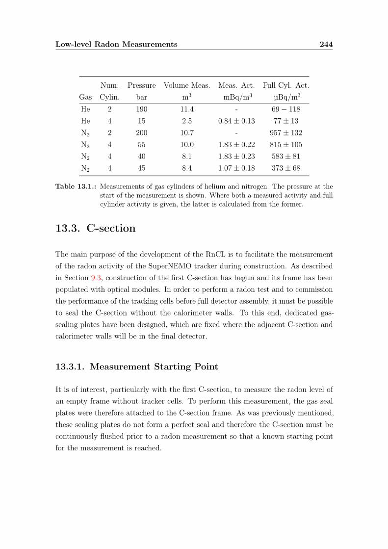
Low-level Radon Measurements 244
Num. Pressure Volume Meas. Meas. Act. Full Cyl. Act.Gas Cylin. bar m3 mBq/m3 µBq/m3
He 2 190 11.4 - 69− 118
He 4 15 2.5 0.84± 0.13 77± 13
N2 2 200 10.7 - 957± 132
N2 4 55 10.0 1.83± 0.22 815± 105
N2 4 40 8.1 1.83± 0.23 583± 81
N2 4 45 8.4 1.07± 0.18 373± 68
Table 13.1.: Measurements of gas cylinders of helium and nitrogen. The pressure at thestart of the measurement is shown. Where both a measured activity and fullcylinder activity is given, the latter is calculated from the former.
13.3. C-section
The main purpose of the development of the RnCL is to facilitate the measurementof the radon activity of the SuperNEMO tracker during construction. As describedin Section 9.3, construction of the first C-section has begun and its frame has beenpopulated with optical modules. In order to perform a radon test and to commissionthe performance of the tracking cells before full detector assembly, it must be possibleto seal the C-section without the calorimeter walls. To this end, dedicated gas-sealing plates have been designed, which are fixed where the adjacent C-section andcalorimeter walls will be in the final detector.
13.3.1. Measurement Starting Point
It is of interest, particularly with the first C-section, to measure the radon level ofan empty frame without tracker cells. To perform this measurement, the gas sealplates were therefore attached to the C-section frame. As was previously mentioned,these sealing plates do not form a perfect seal and therefore the C-section must becontinuously flushed prior to a radon measurement so that a known starting pointfor the measurement is reached.
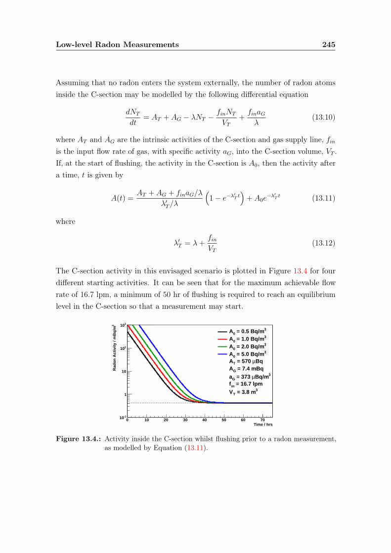
Low-level Radon Measurements 245
Assuming that no radon enters the system externally, the number of radon atomsinside the C-section may be modelled by the following differential equation
dNT
dt= AT + AG − λNT −
finNT
VT+finaGλ
(13.10)
where AT and AG are the intrinsic activities of the C-section and gas supply line, finis the input flow rate of gas, with specific activity aG, into the C-section volume, VT .If, at the start of flushing, the activity in the C-section is A0, then the activity aftera time, t is given by
A(t) =AT + AG + finaG/λ
λ′T/λ
(1− e−λ′T t
)+ A0e
−λ′T t (13.11)
where
λ′T = λ+finVT
(13.12)
The C-section activity in this envisaged scenario is plotted in Figure 13.4 for fourdifferent starting activities. It can be seen that for the maximum achievable flowrate of 16.7 lpm, a minimum of 50 hr of flushing is required to reach an equilibriumlevel in the C-section so that a measurement may start.
Time / hrs0 10 20 30 40 50 60 70
3R
ado
n A
ctiv
ity
/ mB
q/m
-110
1
10
210
310
3 = 0.5 Bq/m0A 3 = 1.0 Bq/m0A 3 = 2.0 Bq/m0A 3 = 5.0 Bq/m0A
Bq µ = 570 TA = 7.4 mBq GA
3Bq/mµ = 373 Ga = 16.7 lpm inf
3 = 3.8 mTV
Figure 13.4.: Activity inside the C-section whilst flushing prior to a radon measurement,as modelled by Equation (13.11).
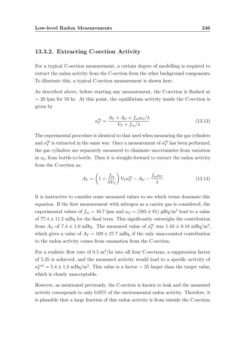
Low-level Radon Measurements 246
13.3.2. Extracting C-section Activity
For a typical C-section measurement, a certain degree of modelling is required toextract the radon activity from the C-section from the other background components.To illustrate this, a typical C-section measurement is shown here.
As described above, before starting any measurement, the C-section is flushed at∼ 20 lpm for 50 hr. At this point, the equilibrium activity inside the C-section isgiven by
aeqT =AT + AG + finaG/λ
VT + fin/λ(13.13)
The experimental procedure is identical to that used when measuring the gas cylindersand aeqT is extracted in the same way. Once a measurement of aeqT has been performed,the gas cylinders are separately measured to eliminate uncertainties from variationin aG from bottle-to-bottle. Then it is straight-forward to extract the radon activityfrom the C-section as:
AT =
(1 +
finλVT
)VTa
eqT − AG −
finaGλ
(13.14)
It is instructive to consider some measured values to see which terms dominate thisequation. If the first measurement with nitrogen as a carrier gas is considered, theexperimental values of fin = 16.7 lpm and aG = (583± 81) µBq/m3 lead to a valueof 77.4± 11.2 mBq for the final term. This significantly outweighs the contributionfrom AG of 7.4 ± 1.0 mBq. The measured value of aeqT was 1.43 ± 0.18 mBq/m3,which gives a value of AT = 109± 27.7 mBq, if the only unaccounted contributionto the radon activity comes from emanation from the C-section.
For a realistic flow rate of 0.5 m3/hr into all four C-sections, a suppression factorof 5.35 is achieved, and the measured activity would lead to a specific activity ofarealT = 5.4± 1.2 mBq/m3. This value is a factor ∼ 35 larger than the target value,which is clearly unacceptable.
However, as mentioned previously, the C-section is known to leak and the measuredactivity corresponds to only 0.05% of the environmental radon activity. Therefore, itis plausible that a large fraction of this radon activity is from outside the C-section.
Low-level Radon Measurements 247
13.3.3. Anti-Radon Tent
In order to disentangle the possible origins of the observed high level of radon, ananti-radon tent was built around the C-section. This tent was constructed from adouble layer of polythene which was heat-sealed to form an airtight cover as shownin Figure 13.5. The tent was flushed with nitrogen at 3.5 m3/hr, and maintained aclear overpressure as can be seen from the bulging in the photograph.
Figure 13.5.: Photograph of the anti-radon tent covering the C-section.
In order to assess the efficacy of the tent, a commercial radon detector (DurridgeRAD7) was used to measure the radon level inside. The ambient level in the roomwas measured to be 2 − 3 mBq/m3 over an extended period. The tent provideda significant reduction as can be seen from Figure 13.6a. The measured level iscompatible with the intrinsic background of the RAD7, such that a limit on theactivity of aout < 0.15 Bq/m3 (90% CL) may be set, confirming a reduction of afactor > 15. In addition, a measurement of the humidity inside the tent also shows apromising reduction as can be seen in Figure 13.6b.
13.3.4. C-section Results
Four measurements of the radon activity inside the first C-section have been made asdetailed in Table 13.2. Three have been made with high environmental radon levels,giving results of tracker activities of ∼ 100 mBq corresponding to ∼ 5 mBq/m3
inside SuperNEMO for nominal tracker flow conditions.
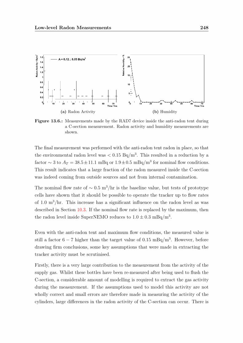
Low-level Radon Measurements 248
(a) Radon Activity (b) Humidity
Figure 13.6.: Measurements made by the RAD7 device inside the anti-radon tent duringa C-section measurement. Radon activity and humidity measurements areshown.
The final measurement was performed with the anti-radon tent radon in place, so thatthe environmental radon level was < 0.15 Bq/m3. This resulted in a reduction by afactor ∼ 3 to AT = 38.5±11.1 mBq or 1.9±0.5 mBq/m3 for nominal flow conditions.This result indicates that a large fraction of the radon measured inside the C-sectionwas indeed coming from outside sources and not from internal contamination.
The nominal flow rate of ∼ 0.5 m3/hr is the baseline value, but tests of prototypecells have shown that it should be possible to operate the tracker up to flow ratesof 1.0 m3/hr. This increase has a significant influence on the radon level as wasdescribed in Section 10.3. If the nominal flow rate is replaced by the maximum, thenthe radon level inside SuperNEMO reduces to 1.0± 0.3 mBq/m3.
Even with the anti-radon tent and maximum flow conditions, the measured value isstill a factor 6− 7 higher than the target value of 0.15 mBq/m3. However, beforedrawing firm conclusions, some key assumptions that were made in extracting thetracker activity must be scrutinised.
Firstly, there is a very large contribution to the measurement from the activity of thesupply gas. Whilst these bottles have been re-measured after being used to flush theC-section, a considerable amount of modelling is required to extract the gas activityduring the measurement. If the assumptions used to model this activity are notwholly correct and small errors are therefore made in measuring the activity of thecylinders, large differences in the radon activity of the C-section can occur. There is
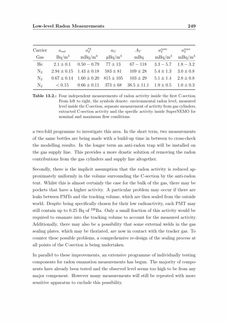
Low-level Radon Measurements 249
Carrier aout aeqT aG AT anomT amaxT
Gas Bq/m3 mBq/m3 µBq/m3 mBq mBq/m3 mBq/m3
He 2.1± 0.1 0.50− 0.79 77± 13 67− 118 3.3− 5.7 1.8− 3.2
N2 2.94± 0.15 1.43± 0.18 583± 81 109± 28 5.4± 1.3 3.0± 0.8
N2 0.67± 0.14 1.60± 0.20 815± 105 103± 29 5.1± 1.4 2.8± 0.8
N2 < 0.15 0.66± 0.11 373± 68 38.5± 11.1 1.9± 0.5 1.0± 0.3
Table 13.2.: Four independent measurements of radon activity inside the first C-section.From left to right, the symbols denote: environmental radon level, measuredlevel inside the C-section, separate measurement of activity from gas cylinders,extracted C-section activity and the specific activity inside SuperNEMO fornominal and maximum flow conditions.
a two-fold programme to investigate this area. In the short term, two measurementsof the same bottles are being made with a build-up time in between to cross-checkthe modelling results. In the longer term an anti-radon trap will be installed onthe gas supply line. This provides a more drastic solution of removing the radoncontributions from the gas cylinders and supply line altogether.
Secondly, there is the implicit assumption that the radon activity is reduced ap-proximately uniformly in the volume surrounding the C-section by the anti-radontent. Whilst this is almost certainly the case for the bulk of the gas, there may bepockets that have a higher activity. A particular problem may occur if there areleaks between PMTs and the tracking volume, which are then sealed from the outsideworld. Despite being specifically chosen for their low radioactivity, each PMT maystill contain up to 0.25 Bq of 226Ra. Only a small fraction of this activity would berequired to emanate into the tracking volume to account for the measured activity.Additionally, there may also be a possibility that some external welds in the gassealing plates, which may be thoriated, are now in contact with the tracker gas. Tocounter these possible problems, a comprehensive re-design of the sealing process atall points of the C-section is being undertaken.
In parallel to these improvements, an extensive programme of individually testingcomponents for radon emanation measurements has begun. The majority of compo-nents have already been tested and the observed level seems too high to be from anymajor component. However many measurements will still be repeated with moresensitive apparatus to exclude this possibility.

Low-level Radon Measurements 250
The detection of a radon level above what is acceptable for the final detector withina matter of months of beginning construction highlights the importance of the RnCL.The early warning from the apparatus, which was specifically designed for thispurpose, will be crucial in re-visiting the prototype SuperNEMO design to ensurethat the SuperNEMO demonstrator achieves its target background levels.
Chapter 14.
Conclusion
Neutrinoless double beta decay (0νββ) is a hypothesised, but as yet unobserved,process whereby a nucleus decays emitting two electrons without any accompanyingneutrinos. It violates lepton number conservation and is forbidden in the standardmodel. If it were to be observed, it would imply that the neutrino is a Majoranaparticle and the associated decay rate would allow (model-dependent) extractionof the absolute mass scale of the neutrino. Its observation would therefore havefar-reaching implications for the fields of particle physics, cosmology and astrophysics.
The most common mechanism for 0νββ is the neutrino mass mechanism, where thedecay is mediated by a helicity flip of the exchanged neutrino. In addition, there aremechanisms mediated by a right-handed current or by the emission of a hypotheticalparticle known as a Majoron.
In addition to 0νββ, there is the process of two neutrino double beta decay (2νββ).This decay is allowed in the Standard Model, although it is doubly weak and thereforeheavily suppressed. Despite its rare nature, it has been directly observed in nineisotopes. It is important to measure the 2νββ process precisely as it may be usedto tune nuclear models which are required to obtain useful information from 0νββ.Furthermore, 2νββ is often one of the major backgrounds to a 0νββ search and soits rate must be precisely known.
The NEMO-3 detector, which operated between 2003− 2011 in the Souterrain deModane (LSM), searched for 0νββ in seven different candidate isotopes with atotal source mass of 10 kg. The experiment has also produced the most accuratemeasurements of the 2νββ half-life for each isotope that it contains. A detailed
251
Conclusion 252
description of the main components of the detector is included in this thesis, with aparticular focus on its ability to completely reconstruct the topology of an event.
The second largest mass of source isotope in the detector was 932g of 82Se. Thedouble beta decay analysis of this isotope forms a major part of this thesis. Theonly backgrounds to a 0νββ search with NEMO-3 come from those that can mimicevents containing two electrons. A large analysis effort has gone into using the fullcapabilities of NEMO-3 to identify and measure all sources of background, the resultsof which are presented. There is good agreement between the measurements withNEMO-3 and independent measurements using HPGe.
After optimising a set of selection criteria, a 2νββ signal is clearly identified in 1918.5days of data, with a signal-to-background ratio of 3.4. The resulting half-life is
T 2ν1/2 = (9.93± 0.14(stat)± 0.72(syst))× 1019 yr
The nuclear matrix element for 82Se may then be extracted as
∣∣M2ν∣∣ = 0.0484± 0.0018
After measuring the 2νββ half-life, a 0νββ search is conducted in optimised channelsfor the mass mechanism, right-handed current and Majoron emission decay modes.No evidence for 0νββ is found for any modes, so limits on the signal strength foreach decay mode are set. For the mass mechanism, the half-life limit is the world’sstrongest limit using 82Se, with a value of
T 0ν1/2 > 2.18× 10²³ yr (90% CL)
corresponding to an effective Majorana neutrino mass of
〈mββ〉 < 1.0− 2.8 eV (90% CL)
The asymmetry between the two electron energies was exploited in the right-handedcurrent λ mode, to produce a half-life limit of
T 0νλ1/2 > 1.18× 10²³ yr (90% CL)
Conclusion 253
with a corresponding lepton number violating parameter
〈λ〉 < (2.8− 3.0)× 10−6 (90% CL)
This limit is the best in 82Se and only a factor 2−3 weaker than the best results fromthe Heidelberg-Moscow experiment of 〈λ〉 < 1.1× 10⁻⁶ [100] and the NEMO-3 100Moresult of 〈λ〉 < 1.4× 10⁻⁶. The final 0νββ mode considered is the Majoron emissiondecay mode, where half-life limits were set for three different spectral indices as:
n = 1 T 0νχ0
1/2 > 4.89× 10²² yr (90% CL)
n = 2 T 0νχ0
1/2 > 2.63× 10²² yr (90% CL)
n = 3 T 0νχ0
1/2 > 1.42× 10²² yr (90% CL)
The corresponding limits on neutrino-Majoron coupling are the strongest producedby NEMO-3, despite having less source mass than 100Mo. This is a result of thedisparity between the 2νββ half-lives of the two isotopes, with 100Mo almost an orderof magnitude shorter. These results are the strongest limits using 82Se, however theyhave been superseded by recent results from KamLAND-Zen with an improvementof a factor ∼ 3 [60].
SuperNEMO is a next-generation 0νββ experiment that will build on the successof the NEMO-3 experiment, using the same tracker-calorimeter technology. In itsbaseline design it will house 100 kg of 82Se and achieve a half-life sensitivity of 1026 yror an effective Majorana neutrino mass of 〈mββ〉 < 50 − 100 meV. In this thesis,the SuperNEMO detector design is introduced, with particular emphasis on theimprovements that have been made to the NEMO-3 design.
Radon is a radioactive gas that is found in all materials as it is part of naturallyoccurring radioactive decay chains. It can enter the detector either through diffusion,contamination during detector construction or emanation from the detector materialsthemselves. Once inside, it can cause a significant background via its progeny 214Bi.In order to reach its target sensitivity, the radon level inside SuperNEMO mustbe less than 150 µBq/m3, which is significantly lower than the 5 mBq/m3 level ofNEMO-3. As a result, significant R&D effort has gone into reducing the level ofradon inside the detector and measuring these low-levels of radon.
Conclusion 254
The latter part of this radon R&D is the focus of Part II of this thesis, where thedevelopment of a radon concentration line (RnCL) is described. The premise behindthe operation of this apparatus is to adsorb radon in a cooled carbon trap so that itcan be concentrated from large volumes and transferred to a smaller volume whereit may be measured. The RnCL has been constructed and commissioned, with ameasured sensitivity of 40 µBq/m3 for a uniform supply of nitrogen and sensitivitiesdown to 5 µBq/m3 in helium if current measurements are extrapolated.
The first measurements using the RnCL have shown that typical activities for standardgas cylinders when full are 70− 120 µBq/m3 for helium and 370− 960 µBq/m3 fornitrogen with considerable variation in the latter measurements. This confirms thata cleaner gas supply is required for both SuperNEMO and future measurementsusing the RnCL, prompting the design of a radon removal trap, which is currentlybeing constructed.
The main purpose of the development of the RnCL is to measure the four sub-modules of the SuperNEMO tracker, known as C-sections, as they are built. The firstC-section is currently under construction and the RnCL has been used to measure itsradon content. Initial measurements put the level at ∼ 3 mBq/m3 in SuperNEMO formaximum flow suppression. An anti-radon tent has subsequently been constructedaround the C-section and the level has reduced down to 1.0±0.3 mBq/m3, confirmingthat a large proportion of the measured radon was coming from external sources.
The radon activity measured inside the first C-section is currently a factor ∼ 6− 7
above the target level. However, there are considerable systematic effects that mustbe addressed and the origin of the measured radon must be understood before anyconclusions may be drawn. A programme of further work which will address theseissues is outlined with the presentation of the measurements.
The RnCL has clearly served its main purpose to identify problematic levels of radoninside SuperNEMO at the earliest possible stages of construction, so that any sourcesof radon can be addressed to ensure that SuperNEMO reaches its target backgroundlevels.
Bibliography
[1] W. Pauli, Dear radioactive ladies and gentlemen, Phys.Today 31N9 (1978) 27.
[2] E. Fermi, An attempt of a theory of beta radiation., Z.Phys. 88 (1934)161–177.
[3] C. Cowan, F. Reines, F. Harrison, H. Kruse, and A. McGuire, Detection of thefree neutrino: A Confirmation, Science 124 (1956) 103–104.
[4] G. Danby, J. Gaillard, K. A. Goulianos, L. Lederman, N. B. Mistry, et al.,Observation of High-Energy Neutrino Reactions and the Existence of TwoKinds of Neutrinos , Phys.Rev.Lett. 9 (1962) 36–44.
[5] M. L. Perl, G. Abrams, A. Boyarski, M. Breidenbach, D. Briggs, et al.,Evidence for Anomalous Lepton Production in e+e− Annihilation,Phys.Rev.Lett. 35 (1975) 1489–1492.
[6] DONUT Collaboration, K. Kodama et al., Observation of tau neutrinointeractions , Phys.Lett. B504 (2001) 218–224, arXiv:hep-ex/0012035[hep-ex].
[7] ALEPH Collaboration, DELPHI Collaboration, L3 Collaboration, OPALCollaboration, SLD Collaboration, LEP Electroweak Working Group, SLDElectroweak Group, SLD Heavy Flavour Group, S. Schael et al., Precisionelectroweak measurements on the Z resonance, Phys.Rept. 427 (2006)257–454, arXiv:hep-ex/0509008 [hep-ex].
[8] MiniBooNE Collaboration, A. Aguilar-Arevalo et al., Event Excess in theMiniBooNE Search for νµ → νe Oscillations , Phys.Rev.Lett. 105 (2010)181801, arXiv:1007.1150 [hep-ex].
[9] G. Mention, M. Fechner, T. Lasserre, T. Mueller, D. Lhuillier, et al., The
255
BIBLIOGRAPHY 256
Reactor Antineutrino Anomaly , Phys.Rev. D83 (2011) 073006,arXiv:1101.2755 [hep-ex].
[10] J. Davis, Raymond, D. S. Harmer, and K. C. Hoffman, Search for neutrinosfrom the sun, Phys.Rev.Lett. 20 (1968) 1205–1209.
[11] B. Pontecorvo, Mesonium and anti-mesonium, Sov.Phys.JETP 6 (1957) 429.
[12] B. Pontecorvo, Inverse beta processes and nonconservation of lepton charge,Sov.Phys.JETP 7 (1958) 172–173.
[13] Z. Maki, M. Nakagawa, and S. Sakata, Remarks on the unified model ofelementary particles , Prog.Theor.Phys. 28 (1962) 870–880.
[14] SNO Collaboration, Q. Ahmad et al., Direct evidence for neutrino flavortransformation from neutral current interactions in the Sudbury NeutrinoObservatory , Phys.Rev.Lett. 89 (2002) 011301, arXiv:nucl-ex/0204008[nucl-ex].
[15] B. Kayser, Neutrino physics , eConf C040802 (2004) L004,arXiv:hep-ph/0506165 [hep-ph].
[16] Particle Data Group, J. Beringer et al., Review of Particle Physics (RPP),Phys.Rev. D86 (2012) 010001.
[17] F. T. Avignone, S. R. Elliott, and J. Engel, Double Beta Decay, MajoranaNeutrinos, and Neutrino Mass , Rev.Mod.Phys. 80 (2008) 481–516,arXiv:0708.1033 [nucl-ex].
[18] E. Majorana, Theory of the Symmetry of Electrons and Positrons , Nuovo Cim.14 (1937) 171–184.
[19] T. Bowles and R. Robertson, Tritium beta decay and the search for neutrinomass , Los Alamos Sci. 25 (1997) 86–91.
[20] Troitsk Collaboration, V. Aseev et al., An upper limit on electron antineutrinomass from Troitsk experiment , Phys.Rev. D84 (2011) 112003,arXiv:1108.5034 [hep-ex].
[21] C. Kraus, B. Bornschein, L. Bornschein, J. Bonn, B. Flatt, et al., Final resultsfrom phase II of the Mainz neutrino mass search in tritium beta decay ,
BIBLIOGRAPHY 257
Eur.Phys.J. C40 (2005) 447–468, arXiv:hep-ex/0412056 [hep-ex].
[22] G. Drexlin, V. Hannen, S. Mertens, and C. Weinheimer, Current directneutrino mass experiments , Adv.High Energy Phys. 2013 (2013) 293986,arXiv:1307.0101 [physics.ins-det].
[23] J. Lesgourgues and S. Pastor, Neutrino mass from Cosmology , Adv.HighEnergy Phys. 2012 (2012) 608515, arXiv:1212.6154 [hep-ph].
[24] WMAP Collaboration, G. Hinshaw et al., Nine-Year Wilkinson MicrowaveAnisotropy Probe (WMAP) Observations: Cosmological Parameter Results ,arXiv:1212.5226 [astro-ph.CO].
[25] S. A. Thomas, F. B. Abdalla, and O. Lahav, Upper Bound of 0.28 eV on theNeutrino Masses from the Largest Photometric Redshift Survey ,Phys.Rev.Lett. 105 (2010) 031301, arXiv:0911.5291 [astro-ph.CO].
[26] P. Bhupal Dev, S. Goswami, M. Mitra, and W. Rodejohann, ConstrainingNeutrino Mass from Neutrinoless Double Beta Decay , arXiv:1305.0056[hep-ph].
[27] M. Archidiacono, N. Fornengo, C. Giunti, S. Hannestad, and A. Melchiorri,Sterile Neutrinos: Cosmology vs Short-BaseLine Experiments ,arXiv:1302.6720 [astro-ph.CO].
[28] A. Sakharov, Violation of CP Invariance, c Asymmetry, and BaryonAsymmetry of the Universe, Pisma Zh.Eksp.Teor.Fiz. 5 (1967) 32–35.
[29] T. Ohlsson, H. Zhang, and S. Zhou, Probing the leptonic Dirac CP-violatingphase in neutrino oscillation experiments , Phys.Rev. D87 (2013) 053006,arXiv:1301.4333 [hep-ph].
[30] C. Weizsacker, Zur Theorie der Kernmassen, Z.Phys. 96 (1935) 431–458.
[31] M. Goeppert-Mayer, Double beta-disintegration, Phys.Rev. 48 (1935) 512–516.
[32] G. Racah, On the symmetry of particle and antiparticle, Nuovo Cim. 14(1937) 322–328.
[33] M. Hirsch, H. Klapdor-Kleingrothaus, and S. Kovalenko, Supersymmetry andneutrinoless double beta decay , Osaka 1995, Weak and electromagnetic
BIBLIOGRAPHY 258
interactions in nuclei, 1995.
[34] J. Schechter and J. Valle, Neutrino Masses in SU(2) × U(1) Theories ,Phys.Rev. D22 (1980) 2227.
[35] W. Rodejohann, Neutrinoless double beta decay and neutrino physics , J.Phys.G39 (2012) 124008, arXiv:1206.2560 [hep-ph].
[36] M. Doi, T. Kotani, H. Nishiura, and E. Takasugi, DOUBLE BETA DECAY ,Prog.Theor.Phys. 69 (1983) 602.
[37] SuperNEMO Collaboration, R. Arnold et al., Probing New Physics Models ofNeutrinoless Double Beta Decay with SuperNEMO , Eur.Phys.J. C70 (2010)927–943, arXiv:1005.1241 [hep-ex].
[38] Y. Chikashige, R. N. Mohapatra, and R. Peccei, Spontaneously Broken LeptonNumber and Cosmological Constraints on the Neutrino Mass Spectrum,Phys.Rev.Lett. 45 (1980) 1926.
[39] C. Aulakh and R. N. Mohapatra, Neutrino as the Supersymmetric Partner ofthe Majoron, Phys.Lett. B119 (1982) 136.
[40] G. Gelmini and M. Roncadelli, Left-Handed Neutrino Mass Scale andSpontaneously Broken Lepton Number , Phys.Lett. B99 (1981) 411.
[41] P. Bamert, C. Burgess, and R. Mohapatra, Multi-Majoron modes forneutrinoless double beta decay , Nucl.Phys. B449 (1995) 25–48,arXiv:hep-ph/9412365 [hep-ph].
[42] N. Fatemi-Ghomi, Measurement of the double beta decay half-life of 150Nd andsearch for neutrinoless decay modes with NEMO-3 detector , arXiv:0905.0822[hep-ex].
[43] NEMO-3 Collaboration, R. Arnold et al., Limits on different Majoron decaymodes of 100Mo and 82Se for neutrinoless double beta decays in the NEMO-3experiment , Nucl.Phys. A765 (2006) 483–494, arXiv:hep-ex/0601021[hep-ex].
[44] C. D. Carone, Double beta decay with vector majorons , Phys.Lett. B308(1993) 85–88, arXiv:hep-ph/9302290 [hep-ph].
BIBLIOGRAPHY 259
[45] R. Mohapatra, A. Perez-Lorenzana, and C. de S Pires, Neutrino mass, bulkMajoron and neutrinoless double beta decay , Phys.Lett. B491 (2000) 143–147,arXiv:hep-ph/0008158 [hep-ph].
[46] J. Vergados, H. Ejiri, and F. Simkovic, Theory of Neutrinoless Double BetaDecay , Rept.Prog.Phys. 75 (2012) 106301, arXiv:1205.0649 [hep-ph].
[47] A. Smolnikov and P. Grabmayr, Conversion of experimental half-life toeffective electron neutrino mass in 0νββ decay , Phys.Rev. C81 (2010) 028502.
[48] H. Klapdor-Kleingrothaus, A. Dietz, L. Baudis, G. Heusser, I. Krivosheina, etal., Latest results from the Heidelberg-Moscow double beta decay experiment ,Eur.Phys.J. A12 (2001) 147–154, arXiv:hep-ph/0103062 [hep-ph].
[49] H. Klapdor-Kleingrothaus, I. Krivosheina, A. Dietz, and O. Chkvorets, Searchfor neutrinoless double beta decay with enriched 76Ge in Gran Sasso1990-2003 , Phys.Lett. B586 (2004) 198–212, arXiv:hep-ph/0404088[hep-ph].
[50] C. Aalseth, I. Avignone, F.T., A. Barabash, F. Boehm, R. Brodzinski, et al.,Comment on ‘Evidence for neutrinoless double beta decay’ , Mod.Phys.Lett.A17 (2002) 1475–1478, arXiv:hep-ex/0202018 [hep-ex].
[51] C. Aalseth, F. Avignone, R. Brodzinski, W. Hensley, H. Miley, et al., Recentresults of the IGEX 76Ge double-beta decay experiment , Phys.Atom.Nucl. 63(2000) 1225–1228.
[52] GERDA Collaboration, M. Agostini et al., Results on neutrinoless double betadecay of 76Ge from GERDA Phase I , arXiv:1307.4720 [nucl-ex].
[53] GERDA Collaboration, K. Knöpfle, GERDA - Status and Perspectives ,Nucl.Phys.Proc.Suppl. 237-238 (2013) 31–33.
[54] Majorana Collaboration, N. Abgrall et al., The Majorana DemonstratorNeutrinoless Double-Beta Decay Experiment , arXiv:1308.1633[physics.ins-det].
[55] GERDA Collaboration, M. Barnabe Heider, Semiconductor-based experimentsfor neutrinoless double beta decay search, Nucl.Phys.Proc.Suppl. 229-232(2012) 141–145.
BIBLIOGRAPHY 260
[56] J. R. Wilson, Double beta decay measurement with COBRA,Nucl.Phys.Proc.Suppl. 221 (2011) 313–316.
[57] S. Umehara, T. Kishimoto, I. Ogawa, R. Hazama, H. Miyawaki, et al.,Neutrino-less double-beta decay of 48Ca studied by CaF2(Eu) scintillators ,Phys.Rev. C78 (2008) 058501, arXiv:0810.4746 [nucl-ex].
[58] S. Umehara, T. Kishimoto, M. Nomachi, S. Yoshida, K. Matsuoka, et al.,Search for neutrino-less double beta decay with CANDLES , AIP Conf.Proc.1441 (2012) 448–450.
[59] KamLAND-Zen Collaboration, A. Gando et al., Limit on 0νββ Decay of136Xe from the First Phase of KamLAND-Zen and Comparison with thePositive Claim in 76Ge, Phys.Rev.Lett. 110 (2013) no. 6, 062502,arXiv:1211.3863 [hep-ex].
[60] KamLAND-Zen Collaboration, A. Gando et al., Limits on Majoron-emittingdouble-beta decays of 136Xe in the KamLAND-Zen experiment , Phys.Rev. C86(2012) 021601, arXiv:1205.6372 [hep-ex].
[61] KamLand-Zen Collaboration, J. Shirai, KamLAND-Zen: Status and Future,Nucl.Phys.Proc.Suppl. 237-238 (2013) 28–30.
[62] J. R. Wilson, Non-accelerator Neutrino Physics , IoP HEPP & APP GroupMeeting, 2013.
[63] E. Andreotti, C. Arnaboldi, F. Avignone, M. Balata, I. Bandac, et al., 130TeNeutrinoless Double-Beta Decay with CUORICINO , Astropart.Phys. 34(2011) 822–831, arXiv:1012.3266 [nucl-ex].
[64] CUORE, L. Pattavina, Status of the CUORE experiment , J.Phys.Conf.Ser.447 (2013) 012066.
[65] LUCIFER Collaboration, L. Pattavina, LUCIFER: Neutrinoless double betadecay search with scintillating bolometers , J.Phys.Conf.Ser. 335 (2011) 012047.
[66] EXO Collaboration, M. Auger et al., Search for Neutrinoless Double-BetaDecay in 136Xe with EXO-200 , Phys.Rev.Lett. 109 (2012) 032505,arXiv:1205.5608 [hep-ex].
[67] D. J. Auty, EXO-200 Experiment , Implications of Neutrino Flavor
BIBLIOGRAPHY 261
Oscillations, 2011.
[68] NEXT Collaboration, J. J. Gómez-Cadenas, Present status and futureperspectives of the NEXT experiment , arXiv:1307.3914[physics.ins-det].
[69] NEMO-3 Collaboration, L. Simard, The NEMO-3 results after completion ofdata taking , J.Phys.Conf.Ser. 375 (2012) 042011.
[70] R. Saakyan, Tracking-based Experiments in Double Beta Decay ,Nucl.Phys.Proc.Suppl. 229-232 (2012) 135–140.
[71] GERDA Collaboration, M. Agostini et al., Measurement of the half-life of thetwo-neutrino double beta decay of 76Ge with the Gerda experiment , J.Phys.G40 (2013) 035110, arXiv:1212.3210 [nucl-ex].
[72] NEMO-3 Collaboration, J. Argyriades et al., Measurement of the two neutrinodouble beta decay half-life of 96Zr with the NEMO-3 detector , Nucl.Phys.A847 (2010) 168–179, arXiv:0906.2694 [nucl-ex].
[73] NEMO-3 Collaboration, R. Arnold et al., First results of the search ofneutrinoless double beta decay with the NEMO-3 detector , Phys.Rev.Lett. 95(2005) 182302, arXiv:hep-ex/0507083 [hep-ex].
[74] NEMO-3 Collaboration, R. Arnold et al., Measurement of the Double BetaDecay Half-life of 130Te with the NEMO-3 Detector , Phys.Rev.Lett. 107(2011) 062504, arXiv:1104.3716 [nucl-ex].
[75] EXO-200 Collaboration, J. Albert et al., An improved measurement of the2νββ half-life of 136Xe with EXO-200 , arXiv:1306.6106 [nucl-ex].
[76] NEMO-3 Collaboration, J. Argyriades et al., Measurement of the Double BetaDecay Half-life of 150Nd and Search for Neutrinoless Decay Modes with theNEMO-3 Detector , Phys.Rev. C80 (2009) 032501, arXiv:0810.0248[hep-ex].
[77] F. A. Danevich, A. S. Georgadze, V. V. Kobychev, B. N. Kropivyansky, A. S.Nikolaiko, et al., Search for double beta decay of cadmium and tungstenisotopes: Final results of the solotvina experiment , Phys.Rev. C68 (2003)035501.
BIBLIOGRAPHY 262
[78] R. Arnold, C. Augier, A. Bakalyarov, J. Baker, A. Barabash, et al., Technicaldesign and performance of the NEMO-3 detector , Nucl.Instrum.Meth. A536(2005) 79–122, arXiv:physics/0402115 [physics].
[79] NEMO-3 Collaboration, J. Argyriades et al., Measurement of the backgroundin the NEMO-3 double beta decay experiment , Nucl.Instrum.Meth. A606(2009) 449–465, arXiv:0903.2277 [nucl-ex].
[80] O. Ponkratenko, V. Tretyak, and Y. Zdesenko, The Event generator DECAY4for simulation of double beta processes and decay of radioactive nuclei ,Phys.Atom.Nucl. 63 (2000) 1282–1287, arXiv:nucl-ex/0104018 [nucl-ex].
[81] R. Brun, F. Bruyant, M. Maire, A. McPherson, and P. Zanarini, GEANT3 ,CERN-DD-EE-84-1 (1987) .
[82] O. Helene, Upper Limit of Peak Area, Nucl.Instrum.Meth. 212 (1983) 319.
[83] G. J. Feldman and R. D. Cousins, A Unified approach to the classicalstatistical analysis of small signals , Phys.Rev. D57 (1998) 3873–3889,arXiv:physics/9711021 [physics.data-an].
[84] A. L. Read, Presentation of search results: The CL(s) technique, J.Phys. G28(2002) 2693–2704.
[85] T. Junk, Confidence level computation for combining searches with smallstatistics , Nucl.Instrum.Meth. A434 (1999) 435–443, arXiv:hep-ex/9902006[hep-ex].
[86] S. Wilks, The Large-Sample Distribution of the Likelihood Ratio for TestingComposite Hypotheses , Annals Math.Statist. 9 (1938) no. 1, 60–62.
[87] M. Kauer, Search for the double beta decay of 96Zr with NEMO-3 andcalorimeter development for the SuperNEMO experiment. PhD thesis,University College London, 2010.
[88] NEMO-2 Collaboration, R. Arnold et al., Double beta decay of 82Se,Nucl.Phys. A636 (1998) 209–223.
[89] S. Elliott, A. Hahn, M. Moe, M. Nelson, and M. Vient, Double beta decay of82Se, Phys.Rev. C46 (1992) 1535–1537.

BIBLIOGRAPHY 263
[90] O. Manuel, Geochemical Measurements of Double beta Decay , J.Phys. G17(1991) S221.
[91] J. Suhonen and O. Civitarese, Weak-interaction and nuclear-structure aspectsof nuclear double beta decay , Phys.Rept. 300 (1998) 123–214.
[92] E. Caurier, F. Nowacki, A. Poves, and J. Retamosa, Shell Model Studies of theDouble Beta Decays of 76Ge, 82Se and 136Xe, Phys.Rev.Lett. 77 (1996)1954–1957.
[93] A. Staudt, K. Muto, and H. Klapdor-Kleingrothaus, Calculation of 2νββ and0νββ decay rates , Europhys.Lett. 13 (1990) 31–36.
[94] J. Menendez, A. Poves, E. Caurier, and F. Nowacki, Disassembling theNuclear Matrix Elements of the Neutrinoless beta beta Decay , Nucl.Phys.A818 (2009) 139–151, arXiv:0801.3760 [nucl-th].
[95] F. Simkovic, V. Rodin, A. Faessler, and P. Vogel, 0νββ and 2νββ nuclearmatrix elements, QRPA, and isospin symmetry restoration, Phys.Rev. C87(2013) 045501, arXiv:1302.1509 [nucl-th].
[96] M. Kortelainen and J. Suhonen, Improved short-range correlations and 0νββnuclear matrix elements of 76Ge and 82Se, Phys.Rev. C75 (2007) 051303,arXiv:0705.0469 [nucl-th].
[97] F. Iachello, J. Barea, and J. Kotila, A compilation of 0νββ nuclear matrixelements in the interacting boson model , Nucl.Phys.Proc.Suppl. 237-238(2013) 21–23.
[98] T. R. Rodriguez and G. Martinez-Pinedo, Energy density functional study ofnuclear matrix elements for 0νββ decay , Phys.Rev.Lett. 105 (2010) 252503,arXiv:1008.5260 [nucl-th].
[99] M. Aunola and J. Suhonen, Mean field effects on neutrinoless double betadecay , Nucl.Phys. A643 (1998) 207–221.
[100] M. Gunther, J. Hellmig, G. Heusser, M. Hirsch, H. Klapdor-Kleingrothaus, etal., Heidelberg - Moscow beta-beta experiment with 76Ge: Full setup with fivedetectors , Phys.Rev. D55 (1997) 54–67.
[101] F. Simkovic, G. Pantis, J. Vergados, and A. Faessler, Additional nucleon
BIBLIOGRAPHY 264
current contributions to neutrinoless double beta decay , Phys.Rev. C60 (1999)055502, arXiv:hep-ph/9905509 [hep-ph].
[102] S. Stoica and H. Klapdor-Kleingrothaus, Critical view on double-beta decaymatrix elements within quasi random phase approximation-based methods ,Nucl.Phys. A694 (2001) 269–294.
[103] O. Civitarese and J. Suhonen, Light neutrino masses and hierarchies and theobservability of neutrinoless double beta decay , Nucl.Phys. A729 (2003)867–883, arXiv:nucl-th/0208005 [nucl-th].
[104] C. Barbero, J. M. Cline, F. Krmpotic, and D. Tadic, Exact evaluation of thenuclear form-factor for new kinds of majoron emission in neutrinoless doublebeta decay , Phys.Lett. B392 (1997) 419–425, arXiv:hep-ph/9609421[hep-ph].
[105] Heidelberg - Moscow-Collaboration, J. Bockholt et al., Bounds on newMajoron models from the Heidelberg - Moscow experiment , Phys.Rev. D54(1996) 3641–3644, arXiv:nucl-ex/9511001 [nucl-ex].
[106] M. Hirsch, H. Klapdor-Kleingrothaus, S. Kovalenko, and H. Pas, On theobservability of majoron emitting double beta decays , Phys.Lett. B372 (1996)8–14, arXiv:hep-ph/9511227 [hep-ph].
[107] SuperNEMO Collaboration, H. Gómez, BiPo: A dedicated radiopurity detectorfor the SuperNEMO experiment , AIP Conference Proceedings 1549 (2013)no. 1, 94–97.
[108] SuperNEMO Collaboration, B. Soulé, Radon emanation chamber: Highsensitivity measurements for the SuperNEMO experiment , AIP ConferenceProceedings 1549 (2013) no. 1, 98–101.
[109] SuperNEMO Collaboration, F. Mamedov, I. Štekl, K. Smolek, and P. Čermák,High sensitivity detectors for measurement of diffusion, emanation and lowactivity of radon, AIP Conference Proceedings 1549 (2013) no. 1, 120–123.
[110] J. R. Partington, Discovery of Radon, Nature 179 (1957) 912.
[111] J. L. Marshall and V. R. Marshall, Ernest Rutherford, the "True Discoverer"of Radon, Bull.Hist.Chem. 28 (2003) 76.
BIBLIOGRAPHY 265
[112] W. Ramsay and J. N. Collie, The Spectrum of the Radium Emanation,Proc.Roy.Soc.Lond. 73 (1904) 470–476.
[113] National Academy of Sciences, Health Effects of Exposure to Radon: BEIR VI,Committee on Health Risks of Exposure to Radon (BEIR VI),ISBN-0-309-056454-4 (1999) .
[114] V. Vasiliev, Radon in SuperNEMO , Internal Note DocDB:297 (2008) .
[115] E. Wellisch, The distribution of the active deposit of radium in an electricfield , Philosophical Magazine Series 6 26 (1913) no. 154, 623–635.
[116] P. Pagelkopf and J. Porstendörfer, Neutralisation rate and the fraction of thepositive 218Po-clusters in air , Atmospheric Environment 37 (2003) no. 8, 1057– 1064.
[117] E. Choi, M. Komori, K. Takahisa, N. Kudomi, K. Kume, K. Hayashi,S. Yoshida, H. Ohsumi, H. Ejiri, T. Kishimoto, K. Matsuoka, and S. Tasaka,Highly sensitive radon monitor and radon emanation rates for detectorcomponents , Nucl.Instrum.Meth. A459 (2001) 177–181.
[118] C. Mitsuda, T. Kajita, K. Miyano, S. Moriyama, M. Nakahata, et al.,Development of super-high sensitivity radon detector for theSuper-Kamiokande detector , Nucl.Instrum.Meth. A497 (2003) 414–428.
[119] G. Heusser, W. Rau, B. Freudiger, M. Laubenstein, M. Balata, and T. Kirsten,222Rn detection at the µBq/m3 range in nitrogen gas and a new Rnpurification technique for liquid nitrogen, Applied Radiation and Isotopes 52(2000) no. 3, 691 – 695.
[120] G. Knoll, Radiation Detection and Measurement , ISBN-9780470131480 (2000).
Copyright © 2022 FDOKUMEN