School Foodservice Costs: Location Matters - USDA ERS
52
United States Department of Agriculture Economic Research Service Economic Research Report Number 117 May 2011 Michael Ollinger Katherine Ralston Joanne Guthrie School Foodservice Costs Location Matters
-
Upload
khangminh22 -
Category
Documents
-
view
2 -
download
0
Transcript of School Foodservice Costs: Location Matters - USDA ERS

United StatesDepartment ofAgriculture
EconomicResearchService
EconomicResearchReportNumber 117
May 2011
Michael OllingerKatherine RalstonJoanne Guthrie
School Foodservice Costs Location Matters

The U.S. Department of Agriculture (USDA) prohibits discrimination in all its programs and activities on the basis of race, color, national origin, age, disability, and, where applicable, sex, marital status, familial status, parental status, religion, sexual orientation, genetic information, political beliefs, reprisal, or because all or a part of an individual's income is derived from any public assistance program. (Not all prohibited bases apply to all programs.) Persons with disabilities who require alternative means for communication of program information (Braille, large print, audiotape, etc.) should contact USDA's TARGET Center at (202) 720-2600 (voice and TDD).
To file a complaint of discrimination write to USDA, Director, Office of Civil Rights, 1400 Independence Avenue, S.W., Washington, D.C. 20250-9410 or call (800) 795-3272 (voice) or (202) 720-6382 (TDD). USDA is an equal opportunity provider and employer.
ww
ww
w.wwer
sr .usda.govoo
Visit Our Website To Learn More!
See ERS research on food assistance and nutrition programs at:
www.ers.usda.gov/briefing/FoodNutritionAssistance
Recommended citation format for this publication:
Ollinger, Michael, Katherine Ralston, and Joanne Guthrie. School Foodservice Costs: Location Matters, ERR-117, U.S. Dept. of Agriculture, Econ. Res. Serv. May 2011.
Photo credits: Girl with lunch tray, Comstock. All others, USDA

i School Foodservice Costs: Location Matters / ERR-117
Economic Research Service / USDA
United States Department of Agriculture
www.ers.usda.gov
A Report from the Economic Research Service
Economic Research ReportNumber 117
May 2011
School Foodservice Costs Location Matters
Abstract
Over 42 million meals—31.2 million lunches and 11 million breakfasts—were served on a typical school day in fiscal year 2009 to children through USDA’s National School Lunch and School Breakfast Programs. School food authorities (SFAs) operate local school feeding programs and deliver the meals to the schools. SFAs must serve appealing, healthful meals while covering food, labor, and other operating costs, a chal-lenge that may be more difficult for some SFAs than for others due to differences in costs per meal across locations. Analysis of data on school costs per meal from a large, nation-ally representative sample reveals that geographic variation is important. In the 2002-03 school year, SFAs in the Southwestern United States had, on average, consistently lower foodservice costs per meal than did SFAs in other regions. Urban locations had lower costs per meal than did their rural and suburban counterparts. Wage and benefit rates, food expenditures per meal, and SFA characteristics such as the mix of breakfasts and lunches served each contributed to the differences in foodservice costs per meal across locations. The importance of these factors varied by location.
Keywords: National School Lunch Program, School Breakfast Program, school meals, school foodservice costs per meal.
Michael Ollinger, [email protected] Katherine Ralston, [email protected] Joanne Guthrie, [email protected]

ii School Foodservice Costs: Location Matters / ERR-117
Economic Research Service / USDA
Acknowledgments
The authors thank Jay Variyam, Elise Golan, Mark Prell, David Smallwood, Fred Kuchler, Laurian Unevehr, and two anonymous reviewers for their comments on earlier drafts of this report. We also thank Linda Hatcher for editing and Sue DeGeorge for design and layout.

iii School Foodservice Costs: Location Matters / ERR-117
Economic Research Service / USDA
Contents
Summary . . . . . . . . . . . . . . . . . . . . . . . . . . . . . . . . . . . . . . . . . . . . . . . . . . . iv
Introduction: Two Issues for School Meal Costs . . . . . . . . . . . . . . . . . . . . . 1
Previous Research Provides Limited Information on the Effects of Location . . . . . . . . . . . . . . . . . . . . . . . . . . . . . . . . . . . . . . . 6
Using a Statistical Model To Measure and Explain Geographic Cost Variation . . . . . . . . . . . . . . . . . . . . . . . . . . . . . . . . . . . . . . . . . . . . . . . . . . . . 9
Developing the Cost Function Model . . . . . . . . . . . . . . . . . . . . . . . . . . . . 9
Isolating Geographic Cost Variation Due to Input Prices and Characteristics . . . . . . . . . . . . . . . . . . . . . . . . . . . . . . . . . . . . . . . . . . . . 13
Relative Contribution of Cost-Influencing Factors. . . . . . . . . . . . . . . . . 19
Conclusions . . . . . . . . . . . . . . . . . . . . . . . . . . . . . . . . . . . . . . . . . . . . . . . . . 20
References . . . . . . . . . . . . . . . . . . . . . . . . . . . . . . . . . . . . . . . . . . . . . . . . . . 22
Appendix A: The Model and Model Diagnostics . . . . . . . . . . . . . . . . . . . . 24
Econometric Model. . . . . . . . . . . . . . . . . . . . . . . . . . . . . . . . . . . . . . . . . 24
Model Details . . . . . . . . . . . . . . . . . . . . . . . . . . . . . . . . . . . . . . . . . . . . . 25
Input Price Measures. . . . . . . . . . . . . . . . . . . . . . . . . . . . . . . . . . . . . . . . 28
Characteristics of School Food Authorities . . . . . . . . . . . . . . . . . . . . . . 28
Estimation . . . . . . . . . . . . . . . . . . . . . . . . . . . . . . . . . . . . . . . . . . . . . . . . 31
Survey Weights . . . . . . . . . . . . . . . . . . . . . . . . . . . . . . . . . . . . . . . . . . . . 32
Tests for Model Selection . . . . . . . . . . . . . . . . . . . . . . . . . . . . . . . . . . . . 32
Model Diagnostics and Discussion of Model Estimates. . . . . . . . . . . . . 34
Elasticities . . . . . . . . . . . . . . . . . . . . . . . . . . . . . . . . . . . . . . . . . . . . . . . . 38
Appendix B: School Breakfast. . . . . . . . . . . . . . . . . . . . . . . . . . . . . . . . . . . 42
Examination of Costs by Region . . . . . . . . . . . . . . . . . . . . . . . . . . . . . . 42
Breakfast Costs and Why They May Be the Same as Lunch Costs . . . . 43

iv School Foodservice Costs: Location Matters / ERR-117
Economic Research Service / USDA
Summary
The National School Lunch Program and School Breakfast Program reim-burse school food authorities (SFAs) for providing school meals that meet USDA nutritional standards. Reimbursement rates depend on whether the meal is lunch or breakfast and whether the student is certified to receive the meal for free or at reduced or full price. Reimbursement rates are the same for all SFAs, except those in Alaska or Hawaii and for schools in which a certain percentage of children receive free or reduced-price lunches even though cost-of-living indexes for all 50 States show considerable variation in food and labor costs. No previous research has rigorously examined whether school foodservice costs vary geographically, or identified the factors that help explain those differences.
What Are the Major Findings?
In this study, we measured geographic variation in school foodservice costs, after accounting for nongeographic factors, to better clarify economic and operational factors that help explain why per meal costs vary by school loca-tion. We examined the impact of (1) location; (2) total USDA reimbursable breakfasts and lunches served; (3) measures of input prices for labor, food, and supplies; and (4) several SFA characteristics affecting total school food-service cost: the mix of breakfasts and lunches served, a measure of meal value that was based on prices charged to students paying the full price for lunch, a la carte revenue per meal, and other aspects of foodservice operation.
•After accounting for nongeographic characteristics of SFAs, we found that average foodservice costs per reimbursable meal (including all break-fasts and lunches) in 21 locations (rural, urban, and suburban areas across 7 U.S. regions) range from 21 percent below the national average for the rural Southwest to 19 percent above in the suburban Midwest. The Southwest and Southeast regions had average costs per meal below the national average, and urban locations had lower average costs per meal than their rural and suburban counterparts.
•The main drivers of differences in foodservice cost varied by location. Wage and benefit rates were the largest contributors in five locations. SFA characteristics—particularly the total number of reimbursable meals served, this study’s measure of meal value, and the presence of a la carte foods—were the most important factors behind cost differences in five locations. In the remaining 11 locations, per meal cost variation was largely due to differences in total food expenditure per meal, which include differences in food item prices and food items served.
•Per meal costs dropped when the number of meals served rose and when the SFA served more lower-value meals. Per meal costs rose when the SFA served more higher-value meals and had more than 10 cents per meal in a la carte food sales.
This study examines the extent to which location influences school foodser-vice costs per meal. It does not examine the effects of cost variation on finan-cial solvency of an SFA or the adequacy of USDA meal reimbursements. Higher per meal costs do not necessarily indicate that an SFA is operating at

v School Foodservice Costs: Location Matters / ERR-117
Economic Research Service / USDA
a loss because higher cost SFAs may also have higher revenues. Due to data limitations, we can determine neither the extent to which higher per meal costs are associated with higher revenues per meal nor whether higher cost SFAs are more likely to serve meals that meet USDA nutrition standards.
How Was the Study Conducted?
Previous cost estimates for school meals used accounting methods to esti-mate the cost per meal to SFAs of providing USDA-reimbursable lunches and breakfasts, but lacked the necessary sample size to obtain regional averages. We, however, used data from 1,432 SFAs participating in the 2004 School Food Authority Characteristics survey, a nationally representa-tive survey that was stratified to allow estimates by region and urbanicity. The survey was administered by USDA’s Food and Nutrition Service and collected data for the 2002-03 school year. To measure the effects of loca-tion on total school foodservice costs, we employed a flexible econometric approach and controlled for total reimbursable meals served (including breakfasts and lunches), measures for input prices, and SFA characteristics.
Due to limitations of our data set, our measure of the input price for food was constructed as total food expenditure per reimbursable meal. This measure reflects both differences in prices paid by SFAs for individual food items and in food items served, making the separation of these two influences on per meal costs difficult. We developed a measure of meal “value” to adjust for differences in food items served; this measure may also reflect differences in food item prices to some extent. For the labor cost measure, we used local salaries and wages reported in the survey to estimate the cost to each SFA of a standardized set of foodservice personnel.


1 School Foodservice Costs: Location Matters / ERR-117
Economic Research Service / USDA
Introduction: Two Issues for School Meal Costs
On a typical school day in fiscal year (FY) 2009, 31.2 million lunches and 11 million breakfasts were served to children in schools participating in the U.S. Department of Agriculture’s (USDA) National School Lunch Program (NSLP) and School Breakfast Program (SBP) (Oliveira, 2010). USDA reim-bursements for these meals in 2009 added up to expenditures of $10 billion for NSLP and $2.6 billion for SBP (Oliveira, 2010). Under these programs, participating school food authorities1 (SFAs), which are the administering units for the operation of local school feeding programs, are expected to meet nutrition guidelines for the meals they serve. They are reimbursed for part or all of the meal costs by the Food and Nutrition Service (FNS), the agency that administers USDA’s food assistance programs at the Federal level.
Reimbursement rates depend on whether the meal is a lunch or a breakfast and whether the student is certified to receive the meal for free or at reduced or full price. Due to the large volume of meals involved, differences of even a few cents in meal costs incurred by SFAs, meal prices paid by students to SFAs, or meal reimbursements paid to SFAs by USDA can significantly affect the budgets for schools, households, and USDA. The reimbursement rates are the same for all SFAs except for adjustments for SFAs in Alaska or Hawaii and for individual schools in areas where most children receiving school meals live in low-income households. No other adjustments are made even though it has been argued that costs vary geographically.
To understand school meal operations and reimbursement policies, one needs to distinguish between two issues associated with school meal costs:
•Issue 1: How large are differences in foodservice costs per meal across locations after accounting for nongeographic factors?
•Issue 2: What factors help explain which locations have higher per meal costs and which have lower per meal costs?
Previous research has not rigorously examined the geographic variations in foodservice costs per reimbursable meal or the economic and operational factors that can help explain the differences. This report provides information and analysis on both issues.
Differences between reimbursement rates and per meal costs can create not only budgetary issues but also nutrition issues and issues of access to and participation in school meals by their target population. USDA reimburses school food authorities for meals at rates that vary based on student economic need (see box, “USDA School Meal Reimbursements,” for a more detailed explanation of USDA reimbursement rates). SFAs that participate in the USDA school meals programs are required to operate on a nonprofit basis, but even covering their costs to avoid a loss may be a challenge for some SFAs. Such SFAs may attempt to obtain more revenue from sources other than USDA reimbursements. Sources include subsidies from the State or the school district, revenues from students who pay full price, and revenues from meals and snacks sold by SFAs but not subsidized by USDA, which
1An SFA is the management unit that provides the meal to the local school. In terms of geographic size or student population, an SFA often has the same boundaries as a school district but can be smaller than the district or made up of more than one district.

2 School Foodservice Costs: Location Matters / ERR-117
Economic Research Service / USDA
USDA School Meal ReimbursementsThe table shows reimbursement rates for the 2005-06 school year for which meal cost data were collected for a Food and Nutrition Service study (the following section highlights selected results from the study). USDA reim-burses school food authorities (SFAs) for meals served as part of the National School Lunch Program (NSLP) and the School Breakfast Program (SBP) at levels that are set nationally but differ depending on a student’s household income. Students may be certified to receive the meals for free if household income is below 130 percent of the poverty level, or at a reduced price of no more than 40 cents for lunch and 30 cents for breakfast for households with income between 130 and 185 percent of poverty. For example, a student in a family of four with a household annual income below $28,665, which is 130 percent of $22,050 (the 2010 poverty level for a family of four), could be eligible to receive free meals.
Free and reduced-price meals are reimbursed at higher rates than those of higher income students who pay a “full” price (or “paid”) established by the SFA. In addition, schools receive an extra 2 cents per lunch if at least 60 percent of lunches served in the second preceding school year were reimbursed at the free or reduced-price rates. In the SBP, the bar is set lower and additional reimbursement is higher: schools are designated as “severe need” and receive an additional 24 cents for free and reduced-price breakfasts if 40 percent of lunches served in the second preceding school year were free or reduced price. Each year, reimbursement rates are updated based on the national average Consumer Price Index for all Urban Consumers for Food Away From Home.
USDA cash reimbursement rates to school food authorities, 2005-06 school year1,2
School classification
Program and benefitsLess than 60 percent of lunches are free or reduced price
60 percent or more of lunches are free or reduced price
---------------Dollars per meal per student---------------
National School Lunch Program:
Paid 0.22 0.24
Reduced price 1.92 1.94
Free 2.32 2.34
Nonsevere need(up to 40 percent of students receive
free or reduced-price lunches)
Severe need(more than 40 percent of students receive
free or reduced-price lunches)
---------------Dollars per meal per student---------------
School Breakfast Program:
Paid 0.23 0.23
Reduced price 0.97 1.21
Free 1.27 1.51
1Reimbursement rates for the 2010-11 school year and earlier are available at http://www.fns.usda.gov/cnd/Governance/notices/naps/NAPs.htm2In addition to cash reimbursements, school food authorities (SFAs) receive USDA foods that can be used to aug-ment purchased foods. Some USDA foods are “entitlement” foods that are assured to SFAs by law, whereas some USDA foods are “bonus” foods that depend on availability from surplus stocks. The per meal value of entitlement foods was 17.5 cents in the 2005-06 school year (more recently, in the 2010-11 school year, the figure is 20.25 cents). In 2005-06, USDA cash reimbursements and support with USDA foods made up, on average, 51 percent of SFA revenues (Bartlett et al., 2008).
Source: Food and Nutrition Service, USDA, http://www.fns.usda.gov/cnd/Governance/notices/naps/NAPs02-03.pdf

3 School Foodservice Costs: Location Matters / ERR-117
Economic Research Service / USDA
are often called “competitive” or “a la carte” foods. Cash-strapped SFAs have an incentive to control costs by reducing the offerings of reimbursable meals, perhaps by eliminating (or not adding) a school breakfast service or by reducing the quality of meals.
We know from previous findings, which are reviewed in detail in the following section, that costs per meal vary across SFAs. However, analysis of the factors that can help account for cost differences has been limited. Some information does suggest that differences in food and labor costs asso-ciated with location are a source of cost variation.
Cost-of-living indexes are directly related to food and labor costs, and indexes for all 50 States show considerable variation (Missouri Economic and Research Information Center, 2009).2 For example, the cost of living in Alabama (ranked ninth lowest) was 0.91 in 2008, meaning that the cost of living there is 91 percent of the national average, or 9 percent less than the national average. The cost of living in New Hampshire (ranked ninth highest) was 1.19, or 19 percent above the national average. The cost of living in Hawaii, the most expensive State, is nearly twice as high as the cost of living in the least expensive State, Tennessee (1.63 versus 0.88). These cost-of-living data and anecdotal comments from school foodservice profes-sionals suggest that their foodservice operation costs may vary, leading to the hypothesis that SFA location affects costs per meal.
Understanding the sources of cost variation across location can provide useful insights for program and policy officials. In addition to food, labor, and supply cost differences, SFA characteristics may also influence costs per meal. For example, both operational decisions, such as the use of foodser-vice management companies, and SFA size, with its associated economies of scale, could influence per meal costs. Knowing the numbers of SFAs that use foodservice management companies or the different mixes of larger and smaller SFAs in different parts of the country could help explain per meal cost differences across locations.
This study provides new information and analysis that examines the extent to which location and other factors influence school foodservice costs. We used data from 1,432 SFAs participating in the School Food Authority Characteristics Survey (see box, “Study Data,” for a more detailed descrip-tion of the survey). We addressed the first issue—how large are location-based differences in school meal costs?—by comparing foodservice costs per meal across locations after adjusting for characteristics. Location is defined as one of 21 combinations of 7 FNS regions and 3 levels of urban-icity. FNS organizes States into seven geographic regions for administrative purposes (fig. 1). Urbanicity is defined as whether the SFA is located in an urban, rural, or suburban area. Per meal cost is defined as total foodservice costs divided by total USDA reimbursable breakfasts and lunches. Using these definitions of output makes accommodating SFAs with different levels of breakfast service— including no breakfast service—possible, which is critical because although lunch service is ubiquitous, breakfast service varies widely. Therefore, results of this study are not directly comparable with results of other studies discussing lunch and breakfast costs separately.
2The Bureau of Economic Analysis provides several types of price indexes for different periods for the country as a whole, but it does not provide similar indexes by which to compare cost of living across regions of the country.

4 School Foodservice Costs: Location Matters / ERR-117
Economic Research Service / USDA
We used a single output translog cost function to address both issues. The model combines USDA reimbursable breakfasts and lunches into one output and controls for differences in the proportion of meals that are breakfasts. Previous research shows that the cost of serving breakfast drops as the number of breakfasts served rises (Sackin, 2008; Hilleren, 2007). To account for differences in the types of food served in different SFAs and other char-acteristics, the model also includes a measure of meal value that is based on the quality/appeal of meals and the resultant prices charged to students paying the full price.
Due to limitations in our data set, the study’s measure of the input price for food is defined as total food expenditure per meal. This measure reflects both differences in prices paid by SFAs for individual food items and in food items served, making these two influences on costs difficult to separate. The meal value variable adjusts for differences in food items served, but this measure too reflects differences in food item prices to some extent. The measure of labor costs uses local salaries and wages to estimate the cost to each SFA of a standardized set of foodservice personnel.
Results of this statistical model were used to examine the separate contri-butions of input price measures (wage and benefit rates, food expenditures per meal, and supply costs per meal) and SFA characteristics to geographic differences in per meal costs.
Study DataWe used data from 1,432 SFAs participating in the School Food Authority Characteristics Survey. The sample was administered by Mathematica Policy Research, Inc. (MPR), in spring 2004 to collect data for the 2002-03 school year (Mathematica Policy Research, Inc., 2004) to support the School Lunch and Breakfast Cost Study II (SLBCS-II). Two strengths of the sample are that it is nationally representative and it was stratified by Food and Nutrition Service region. The stratification at the regional level is advantageous for developing cost estimates at the subnational level. The survey data were collected with three instruments: a one-page fax-back form, a brief telephone interview, and a four-page self-administered survey on costs and revenues and related char-acteristics. The fax-back form requested general SFA characteristics, such as student enrollment; the telephone survey obtained information on the use of foodservice management companies and other nonnumeric information; the self-administered cost and revenue file contains detailed information on 1,665 SFAs and contains detailed information on food, labor, and material costs. MPR also constructed a link file containing information on school district enrollment and demographic and wealth characteristics that was drawn from the National Center for Education Statistics Common Core of Data CCD (National Center for Education Statistics, 2004) and from U.S. Census Bureau data.

5 School Foodservice Costs: Location Matters / ERR-117
Economic Research Service / USDA
NM
TX
OK AR
LASWROMS AL GA
TN
KYNC
SC
FL
SERO
MT
WY
UTCO
KS MO
IANE
ND
SD
MPRO
MN
WI
IL IN
MI
OH
MWRO
NY
MEVT
NH
RIMA
CT
NERO
AZ
NV
OR
WA
ID
HI
AK
CA
American Samoa
CNMI
WRO
Guam
PR
VAWV
PA
MDDE
NJ
DC
VI
MARO
Figure 1U.S. regions established by the Food and Nutrition Service
Source: Food and Nutrition Service, USDA.
MARO = Mid-Atlantic Regional OfficeMPRO = Mountain Plains Regional OfficeMWRO = Midwest Regional OfficeNERO = Northeast Regional Office
SERO = Southeast Regional OfficeSWRO = Southwest Regional OfficeWRO = Western Regional Office
Key:

6 School Foodservice Costs: Location Matters / ERR-117
Economic Research Service / USDA
Previous Research Provides Limited Information on the Effects of Location
FNS has supported several nationally representative school lunch and breakfast cost studies to determine national reimbursement rates for school meals. The most recent of these, the School Lunch and Breakfast Cost Study (SLBCS-II), was completed by Abt Associates for the 2005-06 school year (Bartlett et al., 2008). Previous studies sponsored by FNS include the Child Nutrition Programs Operations Study (St. Pierre et al., 1991, 1992), collected in 1987-88 and 1988-89, and the first School Lunch and Breakfast Cost Study (SLBCS-I), collected during the 1992-93 school year (Glantz et al., 1994).
SLBCS-II used direct accounting methods and actual meal production records to estimate the reported cost and the full cost of producing a lunch or a breakfast. To understand the findings of both the SLBCS-II and this study, one must distinguish between “reported” costs, “unreported” costs, and “full” costs, which are the sum of reported and unreported costs. “Reported costs” include only costs that are charged to SFA budgets. From the SFA’s perspec-tive, reported costs are the costs that the SFA is expected to cover in running the NSLP and SBP. Examples of reported costs are the costs of labor, food, and supplies. Food and labor costs account, on average, for about 90 percent of reported costs, with each accounting for approximately half of the total (Bartlett et al., 2008). Nonfood supplies and miscellaneous other costs make up the remaining reported expenses. Unreported costs, in contrast, are paid by the school district but not charged to the SFA. SFAs, for example, use facilities that require capital expenditures, yet these costs are not charged to the SFA.
SLBCS-II provides information on variation across SFAs in both reported costs and full costs for reimbursable lunches and breakfasts. Because our findings are based on data for SFA reported costs, our summary of the SLBCS-II results mainly focus on reported costs rather than on full costs.3 For the remainder of this report, “cost” refers to “reported cost” unless other-wise noted, and “lunch” and “breakfast” are understood to be complete meals that meet the USDA standard for reimbursement. SLBCS-II estimated the average cost per meal for a “typical” SFA to be $2.36 for a lunch and $1.92 for a breakfast.4
Figure 2 illustrates differences in SFA costs per lunch, as reported in SLBCS-II. For example, about a quarter (26.8 percent) of SFAs had costs per lunch in the range of $2.20-$2.40—the range with the largest percentage of SFAs and the range that includes the $2.36 average for a typical SFA. At the extremes of the distribution, 2.9 percent of SFAs had costs per lunch below $1.40 and more than 1 in 10 (12.7 percent) had per meal costs of $3.00 or more. These findings from SLBCS-II are useful in providing estimates of the number of SFAs for which estimated per meal costs exceed USDA subsidies—about a fifth of SFAs for lunches and half for breakfasts, given reimbursement amounts in the study year (see box, “USDA School Meal Reimbursements"). Although these findings indicate that cost per meal varies across SFAs, they do not themselves identify the roles of location and other factors in influencing these costs.
3For the sake of completeness, note that SLBCS-II estimated the average full cost for a “typical” SFA to be $2.91 for lunch and $2.50 for breakfast.
4These averages are based on an SFA-level analysis that weights the sample in order to count each SFA equally na-tionwide, regardless of size. From this perspective, estimated costs represent the average cost for a “typical” SFA (Bartlett et al., 2008, p. i). An alterna-tive approach develops cost estimates for an average reimbursable meal, recognizing that larger SFAs produce relatively more meals. For the purposes of this study, with its focus on school meal costs at the SFA level but across locations, the SFA-level analysis pro-vides the most appropriate perspective.

7 School Foodservice Costs: Location Matters / ERR-117
Economic Research Service / USDA
Despite interest in the topic, none of the studies reviewed here were designed to produce estimates of cost differences by region or urbanicity. Responding to public interest in the issue, a 1993 analysis by the U.S. General Accounting (now Government Accountability) Office used data from the Child Nutrition Programs Operations Study, collected in 1987-88 and 1988-89, to estimate average costs for each FNS region separately. However, no conclusive findings could be obtained because the samples from some regions were small, resulting in imprecise estimates with large standard errors around estimated costs (U.S. General Accounting Office, 1993).
Bartlett et al. (2008) provided some additional analysis on the effects of loca-tion on costs. The purpose of their analysis was to examine how close an econometric method could come to calculating a nationwide average school meal cost, as estimated by the accounting method used in SLBCS-II. Using data from the School Food Authority Characteristics Survey, they conducted an econometric analysis in which region and urbanicity were treated as control variables. They found cost per meal to be negatively associated with urban location. They did not find cost per meal to vary by region.
Bartlett et al. (2008) invoked two assumptions in their analysis that are subject to scrutiny. First, they assumed that nonreimbursable costs (i.e., the cost of a la carte foods that do not meet the FNS nutrient or serving-size stan-dards of “reimbursable” meals) are independent of reimbursable costs (those subsidized by USDA). This assumption allowed them to deduct estimated nonreimbursable costs from total costs to obtain reimbursable costs. Yet, it is unlikely that the two types of costs are independent because SFAs produce reimbursable and non-reimbursable meals with the same people, under the same conditions, and with ingredient sharing. Second, Bartlett et al. assumed
Figure 2Distribution of school food authorities (SFAs) by reported production cost per lunch, 2005-06 school year1
Percent of SFA’s
1In the School Lunch and Breakfast Cost Study-II, reported costs were costs paid by the SFA, while unreported costs were covered by the school district and not charged to the SFA.Source: School Lunch and Breakfast Cost Study-II: Final Report (Bartlett et al., 2008).
$0 -<$1.40
$1.40 -<$1.60
$1.60 -<$1.80
$1.80 -<$2.00
$2.00 -<$2.20
$2.20 -<$2.40
$2.40 -<$2.60
$2.60 -<$2.80
$2.80 -<$3.00
$3.00 -or more
0
5
10
15
20
25
30
1.0
12.7
5.7
2.9 2.3
5.6
17.8
13.7
Cost per lunch
26.8
11.8
8 School Foodservice Costs: Location Matters / ERR-117
Economic Research Service / USDA
that breakfasts are a fixed fraction of the cost of a lunch across all SFAs. However, smaller studies (Hilleren, 2007; Sackin, 2008) indicate that cost per breakfast can vary depending on participation rates and style of service (in-classroom versus cafeteria, etc.).
Bartlett’s assumptions may not fully account for SFA differences because not all SFAs serve a la carte foods or breakfasts or serve them in the same quantities. These assumptions could obscure differences associated with local input price differences.

9 School Foodservice Costs: Location Matters / ERR-117
Economic Research Service / USDA
Using a Statistical Model To Measure and Explain Geographic Cost Variation
Cost-of-living indexes indicate substantial variation across the United States and suggest differences in labor and food costs for different locations. Foodservice costs may reflect these differences in the cost of living, but they also differ due to other factors. Those other factors include economies of scale based on the total number of meals served, the mix of student age groups who receive the meals, the mix of breakfasts and lunches served, types of food items served, or amounts and types of a la carte foods served, in addition to other management decisions.
This section explains the econometric model we used to examine the effects of location after controlling for the many factors that can influence school meal costs. We then used these estimates and the underlying data to conduct simulations that identify which factors are the most important drivers of cost differences across locations.
Developing the Cost Function Model
To measure the geographic variation in foodservice costs per meal after controlling for nongeographic factors, we used a multivariate translog cost function to examine the impact of the following variables on an SFA’s total school foodservice costs: (1) “output” as measured by total USDA-reimbursable breakfasts and lunches served, (2) measures of input prices for labor, food, and supplies, and (3) several SFA characteristics. Translog cost functions have been used in a variety of empirical studies and can include one, two, or more measures of output as independent variables. As discussed previously, we used a single output cost function in which breakfasts and lunches were treated as one output, “meals.” This approach closely follows that used by many transportation economists (Allen and Liu, 1995; Baltagi et al., 1995; Caves et al., 1985) and MacDonald et al. (1999) and Ollinger et al. (2000), who examined meatpacking and poultry plants. In each of these studies, some firms produced many products and others only one. To deal with this discrepancy, the researchers treated all products as one common output and then accounted for product-specific differences with other vari-ables. In this study, we apply this approach, for the first time, to the school meals setting. The single output specified here, the number of SFA “meals,” is the sum of the number of reimbursable breakfasts and lunches. The share of meals that are made up of breakfasts is accounted for in the model.5 This approach allows the model to accommodate both SFAs that serve breakfast and those that do not and relaxes the assumption that the cost of producing breakfast is a fixed fraction of the cost of producing lunch.
Due to limitations in the data set, the measure of the input price for food is constructed as total food expenditure per meal. This measure reflects both differences across SFAs in prices paid for individual food items and in food items served, making it difficult to separate these two influences on costs.
To adjust for differences in food items served, we included a measure of meal “value” that captures the monetary value placed on the meal by the
5We created three groups of breakfast service and account for them in our empirical model: no breakfasts, more than zero but less than one out of three meals is a breakfast, and more than one out of three meals are a breakfast. These groupings were selected based on model fit and are consistent with studies by Hilleren (2007) and Sackin (2008) in that they demonstrate that breakfast costs are high when few are served. We provide a detailed analysis of the contribution of breakfast volume to total cost per meal in appendix B.

10 School Foodservice Costs: Location Matters / ERR-117
Economic Research Service / USDA
students and their parents. The measure of meal value is based on the quality/appeal of meals and the resultant prices charged to students paying the full price, which is a price that the SFA establishes. Here, the concept of “high-value” does not necessarily mean that the food is “healthier.”6 Instead, “high-value” refers to meals that are more expensive to students and for which their parents are willing to pay a higher full price. For example, a high-value meal may include brand-name pizza, fresh salad, and tropical fruits rather than pizza made in the school or a central kitchen, canned peas, and canned peaches. The two meals have similar nutrient profiles but the high-value meal may be more appealing to both the student and/or the parents.
The underlying motivation for this approach was that SFAs that provide rela-tively more appealing foods can charge more to households paying the full out-of-pocket meal price than can SFAs that serve less appealing foods. We used a pair of variables to capture this “meal value” effect. The “high meal value” variable reflects the probability that an SFA is charging full price in the highest 10 percent of the distribution of SFA full prices (of those SFAs in the sample). The “low meal value” variable reflects the probability that an SFA is charging full price in the lowest 10 percent of the distribution of SFA full prices.7 Although this measure was developed to measure the effects of differences in food items on meal costs (which are then reflected in the SFA’s full price), to some extent, this measure can reflect differences in food item prices as well.
SFA characteristics, particularly those related to breakfast servings, are important to note. About 10 percent of all SFAs do not serve any breakfasts (table 1). Breakfast accounts for fewer than one in three meals for most (75 percent) SFAs. This result is important because Hilleren (2007) and Sackin (2008) found that costs per breakfast can be higher when few breakfasts are served. That is, previous research has found that there are economics of scale for serving breakfast. Initial analysis of this study’s sample of SFAs found similar results.
Capital costs associated with producing school meals can include costs of building, equipment, and vehicles. Capital costs may be charged to the SFA only partially, if at all. Of the 1,655 SFAs in the original sample data set, nearly half (790) reported no capital costs at all, 1,285 identified no vehicle capital costs, and 1,607 had no building costs. In the final sample, about a third of the SFAs did not report any capital costs and the average capital cost for all SFAs was about 1.9 percent of total costs. These data suggest that many SFAs view themselves—or are viewed by the school district in which they operate—as providers of meal services in which schools districts furnish most capital investment and they incur none.
Another set of variables captured whether or not:
1. The SFA had a la carte sales per meal in excess of 10 cents.
2. The SFA reported any capital costs.
3. Less than 30 percent of all students enrolled in the SFA attended high school.
6Wagner et al. (2007) examined the relationship between school foodser-vice cost and compliance with USDA regulations, as a measure of nutritional quality.
7Because the SFA’s foodservice costs can affect the SFA’s full price, we used a predicted probability that the SFA falls in the highest or lowest 10 percent of prices charged.

11 School Foodservice Costs: Location Matters / ERR-117
Economic Research Service / USDA
4. More than 70 percent of students attended high school.
5. The SFA offered health benefits to foodservice workers.
6. The SFA used a foodservice management company for labor, purchasing food or supplies, or both.
7. The SFA used the universal free lunch option.
Table 1 provides descriptive statistics of the variables used in the model. Appendix table 1 provides detailed definitions of price measures, meals, and characteristics. Appendix A provides a more detailed discussion of our choice in methodology, model, variable definitions, and model selection.
In the year covered by the SFA Characteristics Survey, the average annual food service cost per meal across SFAs nationally was $2.70 (table 2). The average hourly wage (including fringe benefits) amounted to $11.72 across SFAs. Food expenditure per meal averaged $1.21. Other per meal costs, which averaged 25 cents per meal, include such costs as nonfood supplies and other miscellaneous items. The number of meals served varied widely, ranging from 2,700 meals per year to more than 143.6 million meals per year. The average annual number of meals served per SFA was about 500,000. Almost half (48 percent) of all SFAs were located in suburban areas, and about a fifth (19 percent) of all SFAs were in the Midwest.
After extensive testing, we selected a model that best fit the data. Each of the location and characteristics variables were subjected to a goodness-of-fit test (the Gallant-Jorgenson test), which showed that all of the variables signifi-cantly affected costs. Appendix A provides a detailed discussion of these statistical tests.8 Appendix A also provides the parameter estimates for the entire model, a detailed interpretation of the model results, estimated elas-ticities, and detailed discussions of how we controlled for meal-value. The model had good overall fit with an R2 value of 0.9817.
The Gallant-Jorgenson test indicates that all variables included in the model significantly affect costs, but it does not indicate how much costs vary across locations. To examine cost differences, we needed to simulate foodservice costs under scenarios that varied one factor at a time. The next section uses such simulations to isolate geographic cost variation due to each input price and the characteristics.
8We also tested numerous other variables, including central kitchens and meal planning methods, but these variables failed the Gallant-Jorgenson test for contribution to model fit. As suggested by an anonymous reviewer, we also examined the impact of State subsidies. The effects of these subsidies are statistically significant but insig-nificant in monetary terms. Because including the subsidies did not alter our substantive findings, we did not change our model.

12 School Foodservice Costs: Location Matters / ERR-117
Economic Research Service / USDA
Table 1
Model variables and descriptive statistics, school year 2002-03
Model variables National average across SFAs
Cost per meal and input price measures: Dollars
Cost per meal (total annual foodservice cost divided by total reimbursable lunches and breakfasts served),
2.70
Labor (average wage plus fringe benefits per hour per cafeteria worker) 11.72
Food (expenditures per reimbursable meal) 1.21
Other (expenditures per reimbursable meal) 0.25
Geography: Percent of all SFAs
Urbanicity—
Urban 13
Suburban 48
Rural 39
Food and Nutrition Service region—
Mid-Atlantic 12
Midwest 19
Mountain Plains 14
Northeast 11
Southeast 16
Southwest 14
Western 14
SFA characteristics: Number
Meals served per year, national average across SFAs 500,000
Percent
SFA served no breakfasts 10
Between 0 and 33 percent of meals served are breakfasts 75
More than 33 percent of meals are breakfasts 15
Revenue from sales of a la carte items exceeds 10 cents per meal 64
Low meal value 9.4
High meal value 10.6
Reported capital costs 68
Less than 30 percent of SFA students attend high school 54
More than 70 percent of SFA students attend high school 2
SFA provides foodservice workers with health insurance 93
Foodservice management company provides some inputs 16
More than 80 percent of schools are designated as universal free lunch 6
Source: School Food Authority Characteristics Survey, Mathematica Policy Research, Inc. (2004), and analysis by the Economic Research Service, USDA.

13 School Foodservice Costs: Location Matters / ERR-117
Economic Research Service / USDA
Isolating Geographic Cost Variation Due to Input Prices and Characteristics
The concern over geographic differences in foodservice costs focuses on differences in the cost of food and labor inputs, but other SFA characteris-tics also contribute to cost differences. We used simulations to isolate these effects and to measure the extent to which our measures of input prices and other SFA characteristics included in our model explain higher and lower costs across locations. To construct the estimates, we used the econometric model and characteristics of each location to compute “simulated per meal costs.” This estimated per meal cost includes the effects of only factors in the model. The set of simulated per meal costs then becomes the baseline against which other simulations are compared. For each simulation, we varied one factor at a time to examine the effect of that factor on estimated per meal costs (see box, “Simulating Contributions to Differences in Per Meal Costs”).
The simulated per meal costs for each location are reported in table 2. The per meal costs in 13 of the 21 locations in table 2 are within 5 percent of the unadjusted average per meal cost, and only 4 locations had per meal costs that differed by more than 10 percent from the unadjusted average.
Figure 3 illustrates how simulated per meal costs of rural, suburban, and urban areas of the seven FNS regions differ from the simulated national per meal cost. The Southeast, Southwest, and urban locations have per meal costs below the national average, and the Mid-Atlantic, Midwest, Northeast, and Western suburban locations have higher per meal costs (fig. 3). The differ-ence in average per meal costs in these locations, compared with the national average, is due to the combined influence of differences in food, labor, supply prices, and characteristics included in the model across locations. These results suggest that average per meal cost differences across locations still exist even after controlling for SFA characteristics. For each location, the question then becomes which particular factors drive cost variation.
Table 2
Simulated per meal costs by urbanicity and Food and Nutrition Service (FNS) region, school year 2002-03
FNS region
Urbanicity Mid-Atlantic MidwestMountain
Plains Northeast Southeast Southwest Western
------------------------------------------------------Dollars per meal--------------------------------------------
Rural 2.49 2.49 2.29 2.65 2.31 2.15 2.72
Suburban 3.16 3.05 2.47 2.84 2.55 2.48 2.78
Urban 2.30 2.10 2.09 2.02 2.38 1.94 2.17
Average1 2.93 2.74 2.34 2.70 2.40 2.22 2.641Weighted by the share of school food authorities (SFA) from each region. Assumptions: Total foodservice cost per meal is simulated by using the estimated cost equation together with mean location-specific values for wages and benefit rates, food expenditures per meal, supply expenditures per meal, SFA size (annual reimbursable breakfasts and lunches served), and other characteristics included in the model.
Source: School Food Authority Characteristics Survey, Mathematica Policy Research, Inc. (2004), and analysis by the Economic Research Service, USDA.

14 School Foodservice Costs: Location Matters / ERR-117
Economic Research Service / USDA
Simulating Contributions to Differences in Per Meal CostsWe conducted 4 separate simulations of average per meal costs for each of the 21 locations. First, we substituted the location’s average values for input prices and characteristics into the econometric model and came up with an estimated cost per meal per location (see table 2). Then, we substituted one national average input price (there are three input prices) or national average characteristics into the model and estimated cost per meal again for each of the three input prices or national average characteristics. This gives us four estimated costs per meal with each one based on all but one of the location’s average values and one national average value. We then subtract these four estimated costs per meal containing one national average value from the estimated per meal cost based only on the location’s input prices and characteristics. The results show the contribution of each component to differences in per meal costs across locations. The table below summarizes the design of the four simulations.
A = Simulated per meal costs using location-specific averages for our measures of input prices and SFA characteristics.
B = Simulated per meal costs using national averages for our measures of input prices and SFA characteristics.
C = Simulated per meal costs using location-specific averages for our measures of input prices and the national average for SFA characteristics.
D = Simulated per meal costs using the national average for food expenditure per meal and location-specific averages for SFA characteristics, wage and benefit rates, and supply expenditures per meal.
E = Simulated per meal costs using the national average for wage and benefit rates and location-specific averages for SFA characteristics, food expenditures per meal, and supply expenditures per meal.
F = Simulated per meal costs using the national average for supply expenditures per meal and location-specific averages for SFA characteristics, food expenditures per meal, and wage and benefit rates.
Five measures of contributions to per meal costs follow from the five simulations:
A – B: Total cost difference due to all factors included in the cost function model (fig. 3 and table 4).
A - C: Cost differences due to location-specific differences in SFA characteristics (fig. 6 and table 4).
A – D: Cost differences due to location-specific food expenditure per meal (fig. 4 and table 4).
A – E: Cost differences due to location-specific wage and benefit rates (fig. 5 and table 4).
A – F: Cost differences due to location-specific supply expenditures per meal (table 4).
Cost simulation specifications
Components of per meal cost differences
SimulationFood expenditures
per mealWage and benefit
rates Supply expenditures
per mealSchool food authority (SFA) characteristics
A Location Location Location Location
B National National National National
C Location Location Location National
D National Location Location Location
E Location National Location Location
F Location Location National Location

15 School Foodservice Costs: Location Matters / ERR-117
Economic Research Service / USDA
The second stage of the simulation was based on answering a series of “what if” questions. For example, to isolate the role of, say, wage rates on (simulated) per meal costs, one would ask the counterfactual question “What would per meal cost be if all SFAs had the same wage rate?” Simulated figures for each location are developed by replacing the wage rate for each location with a single national wage rate and then re-simulating per meal cost. The difference between the two simulations—one setting the wage rate at the location-specific level and the other using a single wage rate—measures the contribution of differences in wage rates to differences in per meal cost. This methodology is used to derive the four separate contributions to cost differences: food expenditures per meal, labor prices (wage rates and fringe benefits on an hourly basis), supply expenditures per meal, and SFA characteristics (see box, “Simulating Contributions to Differences in Per Meal Costs”). The results are shown in figs. 4-6 and table 3.
When we considered the contribution of per meal food expenditures to differences in per meal costs for each location,9 we found that differences across SFAs in food expenditures may reflect different input prices for the same products or differences in food items served that are not captured by the study’s measure of meal value (fig. 4). Differences due to per meal food expenditures vary from about 38 cents below the national average for Southwestern urban SFAs to about 35 cents above the national average for Mid-Atlantic suburban SFAs (fig. 4). In addition, meal costs in suburban areas differ by about 50 cents between high-cost Mid-Atlantic SFAs and rela-tively low-cost Southeast SFAs. Finally, per meal food expenditures in rural and urban locations are relatively low.
Differences due to wage and benefit rates are shown in figure 5. In the case of labor, our data set contained detailed data on wage and benefit rates for different job categories in each SFA. Therefore, differences due to wages and benefits reflect only differences in input prices for labor and not differences in a mix of staffing across SFAs (see appendix A for details on wage and
9 Due to data limitations, the study’s measure of food input price is the proxy total food expenditures per meal. See the section on “Developing the Model” and appendix A for details.
Mid-Atlantic Mountain Plains Northeast Southeast Southwest WestMidwest
Figure 3Simulated differences in per meal costs from the national average by location, school year 2002-03
Dollars per meal
Source: School Food Authority Characteristics Survey, Mathematica Policy Research, Inc. (2004), and analysis by the Economic Research Service, USDA. See box, “Simulating Contributions to Differences in Per Meal Costs,” for an explanation of simulations.
Rural Suburban Urban
0.80
-0.80
0.60
-0.60
0.40
-0.40
0.20
-0.20
0

16 School Foodservice Costs: Location Matters / ERR-117
Economic Research Service / USDA
benefit rates in our model). Mid-Atlantic, Midwestern, and Western urban and suburban locations have relatively high labor costs. Meal costs attribut-able to wage and benefit rates differ by about 50 cents between high-cost Western suburban SFAs and low-cost Southwestern rural SFAs.
In addition to food expenditures and labor, SFA characteristics contribute substantially to cost variation (fig. 6). For example, in the Northeast, per meal costs differ very sharply between suburban/rural SFAs, with SFA character-
0.40
-0.40
0.30
-0.30
0.20
-0.20
0.10
-0.10
0
Mid-Atlantic Mountain Plains Northeast Southeast Southwest WestMidwest
Figure 4Contribution of per meal food expenditures to differences between locations’ simulated per meal costs and the national average, school year 2002-031
Dollars per meal
1Due to data limitations, food expenditures per meal are used as a proxy for food input prices. This measure reflects both differences in food prices and food items served in a location.Source: School Food Authority Characteristics Survey, Mathematica Policy Research, Inc. (2004), and analysis by the Economic Research Service, USDA. See box, “Simulating Contributions to Differences in Per Meal Costs,” for an explanation of simulations.
Rural Suburban Urban
-0.40
0.30
-0.30
0.20
-0.20
0.10
-0.10
0
Mid-Atlantic Mountain Plains Northeast Southeast Southwest WestMidwest
Figure 5Contribution of wage rates and fringe benefits to differences between locations’ simulated per meal costs and the national average, school year 2002-03Dollars per meal
Source: Source: School Food Authority Characteristics Survey, Mathematica Policy Research, Inc. (2004), and analysis by the Economic Research Service, USDA.
Rural Suburban Urban

17 School Foodservice Costs: Location Matters / ERR-117
Economic Research Service / USDA
istics adding about 40 cents per meal to the national average cost per meal, and urban SFAs, with SFA characteristics subtracting about 20 cents from the national average cost per meal.
Four major SFA characteristics drive these cost differences within the Northeast across urban, suburban and rural areas: SFA size, as measured by the number of meals served; breakfast volume; meal value; and sales of a la carte foods. Northeastern urban SFAs are, on average, seven times larger than the national average, whereas Northeastern rural and suburban SFAs are one-tenth and one-fifth the size of the national average. The sizes of the SFAs are associated with economies of scale. Thus, costs per meal are lower in the far larger SFAs and higher in the smaller SFAs.10 In the urban Northeast, 20 percent of SFAs serve more than 33 percent of their meals as breakfasts. In contrast, about 10 percent of Northeastern rural SFAs serve more than 33 percent of their meals as breakfasts and no Northeastern suburban SFAs serve more than 33 percent of its meals as breakfast.
The other two main drivers of cost differences are meal values, as reflected in prices paid by full-price students, and a la carte revenues. Northeastern urban SFAs tend to serve lower value meals, while Northeastern suburban SFAs tend to have higher value meals. Northeastern rural SFAs serve meals with a meal value at about the average across SFAs. Estimates based on our model suggest that high-value meals were 23-27 cents more costly to produce than low-value meals. In addition, about 85 percent of Northeastern rural and suburban SFAs have a la carte sales that are more than 10 cents per meal, whereas 65 percent of Northeastern urban SFAs have a la carte sales that are more than 10 cents per meal.11
In the other locations as well, much of the cost difference due to SFA char-acteristics can be attributed to these four major drivers. Southwestern urban SFAs, for example, serve about half as many meals as Northeastern urban
10See appendix A for a discussion of the econometric model and its estimates for economies of scale and other cost-influencing factors highlighted in this section.
11The costs of a la carte foods are included in our measure of per meal costs.
0.30
0.40
0.50
-0.30
0.20
-0.20
0.10
-0.10
0
Mid-Atlantic Mountain Plains Northeast Southeast Southwest WestMidwest
Figure 6Contribution of school food authority characteristics to differences between locations’ simulated per meal costs and the national average, school year 2002-03Dollars per meal
Source: Source: School Food Authority Characteristics Survey, Mathematica Policy Research, Inc. (2004), and analysis by the Economic Research Service, USDA.
Rural Suburban Urban
18 School Foodservice Costs: Location Matters / ERR-117
Economic Research Service / USDA
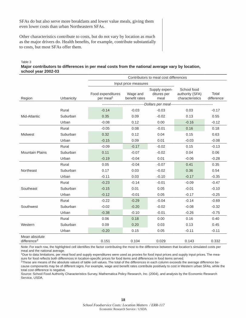
SFAs do but also serve more breakfasts and lower value meals, giving them even lower costs than urban Northeastern SFAs.
Other characteristics contribute to costs, but do not vary by location as much as the major drivers do. Health benefits, for example, contribute substantially to costs, but most SFAs offer them.
Table 3
Major contributors to differences in per meal costs from the national average vary by location, school year 2002-03
Contributors to meal cost differences
Region Urbanicity
Input price measures
School food authority (SFA) characteristics
Totaldifference
Food expenditures per meal1
Wage and benefit rates
Supply expen-ditures per
meal
-----------------------------------Dollars per meal-----------------------------------
Mid-Atlantic
Rural -0.14 -0.03 -0.03 0.03 -0.17
Suburban 0.35 0.09 -0.02 0.13 0.55
Urban -0.08 0.12 0.00 -0.16 -0.12
Midwest
Rural -0.05 0.08 -0.01 0.16 0.18
Suburban 0.32 0.12 0.04 0.15 0.63
Urban -0.15 0.09 0.01 -0.03 -0.08
Mountain Plains
Rural -0.09 -0.17 -0.02 0.15 -0.13
Suburban 0.11 -0.07 -0.02 0.04 0.06
Urban -0.19 -0.04 0.01 -0.06 -0.28
Northeast
Rural 0.05 -0.04 -0.07 0.41 0.35
Suburban 0.17 0.03 -0.02 0.36 0.54
Urban -0.11 0.03 -0.10 -0.17 -0.35
Southeast
Rural -0.23 -0.14 -0.01 -0.09 -0.47
Suburban -0.15 0.01 0.05 -0.01 -0.10
Urban -0.12 -0.01 0.05 -0.17 -0.25
Southwest
Rural -0.22 -0.29 -0.04 -0.14 -0.69
Suburban -0.02 -0.20 -0.02 -0.08 -0.32
Urban -0.38 -0.10 -0.01 -0.26 -0.75
Western
Rural 0.06 0.18 0.00 0.16 0.40
Suburban 0.09 0.20 0.03 0.13 0.45
Urban -0.20 0.15 0.05 -0.11 -0.11
Mean absolute difference2 0.151 0.104 0.029 0.143 0.332
Note: For each row, the highlighted cell identifies the factor contributing the most to the difference between that location’s simulated costs per meal and the national average.1Due to data limitations, per meal food and supply expenditures were used as proxies for food input prices and supply input prices. The mea-sure for food reflects both differences in location-specific prices for food items and differences in food items served. 2These are means of the absolute values of table cell values. The total of the differences in each column exceeds the average difference be-cause components may be of different signs. For example, wage and benefit rates contribute positively to cost in Western urban SFAs, while the total cost difference is negative.Source: School Food Authority Characteristics Survey, Mathematica Policy Research, Inc. (2004), and analysis by the Economic Research Service, USDA.

19 School Foodservice Costs: Location Matters / ERR-117
Economic Research Service / USDA
Relative Contribution of Cost-Influencing Factors
In table 3, we examine the relative contribution of each factor to cost varia-tion in each of the 21 locations. We also examine the overall contribution of the location-specific differences in food expenditures per meal, wage and hourly benefits, and supplies relative to the impact of SFA characteristics on costs.
Table 3 allows us to distinguish between location-specific food, labor, and supply costs from nongeographic characteristics. After accounting for nongeographic characteristics of SFAs, average foodservice costs per reim-bursable meal (including all breakfasts and lunches) in 21 locations (rural, urban, and suburban areas in each of 7 U.S. regions) range from 21 percent below the national average for the rural Southwest to 19 percent above in the suburban Midwest. The Southwest and Southeast regions had average costs per meal below the national average, and urban locations had lower average costs per meal than their rural and suburban counterparts.
Any one location can differ from others in terms of which factor(s) make its per meal costs different from the national average. For example, one location may have relatively high wage costs that result in a relatively high per meal costs, while another may have especially small SFAs or some other SFA characteristic driving its costs. For each row in table 3, the highlighted cells identify the factor that contributes the most to the difference between that location’s simulated per meal costs and the national average per meal cost. In 11 of the 21 locations, food expenditures per meal are the largest drivers of differences in simulated per meal costs. Wage and benefit rates are the largest contributors in five other locations. SFA characteristics, particularly total number of meals served, the study’s measure of meal value, and the presence of a la carte foods, were the most important drivers in five locations. Supply costs per meal contribute minimally to cost differences.
Table 3 can also be used to derive a measure of the overall impact of differ-ences in location-specific food expenditures per meal, wage and hourly bene-fits, and supplies relative to the impact of SFA characteristics. The bottom row of the table reports the mean absolute difference for each input price and the characteristics. The mean absolute difference is defined as the average (or mean) of the absolute values of the table cells. For food, the mean abso-lute difference is plus or minus 15 cents, indicating that, on average across the Nation, differences in food expenditures per meal contribute about this much to the location’s difference from the national average per meal cost. The other mean absolute differences are 10 cents for labor (wage and benefit rates), 3 cents for supplies, and 14 cents for SFA characteristics. The sum of differences associated with our measures of input prices is plus or minus 28 cents, twice the difference associated with SFA characteristics.
Note that, although due to data limitations, we may not have been able to control for all factors, particularly those related to meal values and break-fasts, the results do indicate that, even after controlling for SFA characteris-tics, location-related input prices have a significant effect.
20 School Foodservice Costs: Location Matters / ERR-117
Economic Research Service / USDA
Conclusions
SFAs that participate in USDA’s National School Lunch and School Breakfast Programs are required to be nonprofit but are generally expected by local school districts to cover their variable costs. Some SFAs may have difficulty reaching this goal because of differences in local prices for food, labor, and supplies or because of their own operational characteristics. Budgetary issues can become issues of student participation in school meals depending on how SFAs adjust to close gaps between costs and revenues and the mix of low-cost healthy foods available to the SFA.
The purposes of this study were (1) to measure how large the differences are in school meal costs across locations, regions, and levels of urbanicity, after accounting for SFA characteristics other than prices, and (2) to measure the contributions of factors that help explain which locations have higher costs and which have lower costs.
In answer to the first issue, we found that average adjusted per meal food-service costs (including all breakfasts and lunches) in SFAs grouped into 21 locations (rural, urban, and suburban areas in each of 7 U.S. regions) differed by as much as 20 percent above or below the national average. The Southeast and Southwest regions had consistently lower adjusted per meal costs on average, and urban locations had lower adjusted per meal costs on average than their rural and suburban counterparts.
We used an econometric model to account for SFA characteristics and esti-mate how much of the cost variation across locations is due to differences in our measures of input prices versus SFA characteristics. Although the SFA Characteristics Survey offered a large national sample stratified by region and urbanicity, data limitations posed challenges. In particular, labor wage and benefits rates were available, but food prices were not, forcing us to use food expenditures per meal as a proxy.
The study results show that the main drivers of cost differences varied by location. Labor costs were the largest contributors in five locations. SFA characteristics (particularly the total number of meals served), the study’s measure of meal value, and the presence of a la carte foods were the most important drivers in five locations. In the remaining 11 locations, the largest contributor to cost variation was differences in total food expenditures per meal, which include differences in food item prices and food items served. Overall, location-associated differences in labor costs and per meal food and supply expenditures outweighed cost differences associated with SFA characteristics.
The survey-based estimates of per meal costs and the simulations do not directly assess the adequacy of a reimbursement rate for NSLP lunches or SBP breakfasts, the issue addressed by the SLBCS-II study. Because we combine lunches and breakfasts to generate an overall per meal cost estimate, results are not directly comparable to those of the SLBCS-II. Neither do the findings answer the question of whether the USDA reimbursement is suffi-cient to produce a nutritious meal because the data used in the study did not include information on which SFAs produced meals that met USDA nutrition standards. The findings do not imply that higher cost SFAs are operating at

21 School Foodservice Costs: Location Matters / ERR-117
Economic Research Service / USDA
a loss. Higher cost SFAs may also be obtaining higher revenues from such sources as higher meal prices charged to students paying full price for meals, increased sales of a la carte foods, or State or local subsidies to the SFA. More research that includes data on revenues as well as costs is necessary to answer the question of whether SFAs in some locations of the country are more likely to operate at a loss.
Although the findings do not answer all of the complex questions about reim-bursement rates, nutrition, and the likelihood of SFAs operating at a loss, the findings do provide information on the two issues the study was designed to address—the sizes of differences of per meal cost across SFAs and the factors that help explain those differences. Complementing this analysis with more data and research on school revenues and meal quality would further enhance understanding of school food finances and their implications for meeting Federal child nutrition policy objectives.
22 School Foodservice Costs: Location Matters / ERR-117
Economic Research Service / USDA
References
Allen, W. Bruce, and Dong Liu, “Service Quality and Motor Carrier Costs: An Empirical Analysis,” The Review of Economics and Statistics 77(3): 499-510, August 1995.
Antle, John M. “No Such Thing as a Free Safe Lunch: the Cost of Food Safety Regulation in the Meat Industry,” American Journal of Agricultural Economics 82(2):310-22. May 2000.
Baltagi, Badi H., James M. Griffin, and Daniel P. Rich. “Airline Deregulation: The Cost Pieces of the Puzzle,” International Economic Review 36(1):245-60, February 1995.
Bartlett, Susan, Frederic Glantz, and Christopher Logan. School Lunch and Breakfast Cost Study-II: Final Report, Special Nutrition Programs Report No. CN-08-MCII, U.S. Department of Agriculture, Food and Nutrition Service, Office of Research, Nutrition and Analysis, Project Officer: Patricia McKinney and John R. Endahl, April 2008.
Baumol, William J., John C. Panzar, and Robert D. Willig. Contestable Markets and the Theory of Industry Structure, New York: Harcourt Brace Jovanovich, June 1982.
Berndt, Ernst R. The Practice of Econometrics: Classic and Contemporary, New York: Addison Wesley Publishing, 1991.
Blackorby, C., and R.R. Russell. “The Morishima Elasticity of Substitution: Symmetry, Consistency, Separability, and its Relationship to the Hicks and Allen Elasticities,” Review of Economic Studies 48(1):147-58, January 1981.
Blackorby, C., and R.R. Russell. “Will the Real Elasticity of Substitution Please Stand Up? A Comparison of the Allen/Uzawa and Morishima Elasticities,” American Economic Review 49(4):882-88, September 1989.
Caves, Douglas W., Laurits R. Christensen, Michael W. Tretheway, and Robert J. Windle. “Network Effects and the Measurement of Returns to Scale and Density for U.S. Railroads,” Andrew F. Daugherty, ed., Analytical Studies in Transport Economics, Cambridge, UK: Cambridge University Press, 1985.
Gallant, A. Ronald, and Dale W. Jorgenson. “Statistical Inference for a System of Simultaneous, Non-Linear, Implicit Equations in the Context of Instrumental Variable Estimation,” Journal of Econometrics 11(2-3):275-302, October-December 1979.
Glantz, Frederic B., Christopher Logan, Hope M. Weiner, Michael Battaglia, Ellen Gorowitz. School Lunch and Breakfast Cost Study, U.S. Department of Agriculture, Food and Nutrition Service, Office of Analysis and Evaluation, Project Officer: John R. Endahl, October 1994.

23 School Foodservice Costs: Location Matters / ERR-117
Economic Research Service / USDA
Hilleren, Heather. School Breakfast Program Cost/Benefit Analysis: Achieving a profitable SBP, University of Wisconsin Extension Family Living Program, Madison, WI, 2007.
Mathematica Policy Research, Inc. School Food Authority Characteristics Survey of 2002-03, 2004
MacDonald, James M., Michael Ollinger, Kenneth Nelson, and Charles Handy. Consolidation in U.S. Meatpacking, Agricultural Economics Report No. 785, U.S. Department of Agriculture, Economic Research Service, March 1999.
Missouri Economic and Research Information Center, Missouri Department of Economic Development. Cost of Living Indices, 2009.
National Center for Education Statistics, U.S. Department of Education. The Common Core of Data, http://nces.ed.gov/ccd/, 2004.
Oliveira, V. The Food Assistance Landscape, FY 2009 Annual Report, Economic Information Bulletin No. 6-7, U.S. Department of Agriculture, Economic Research Service, March 2010.
Ollinger, Michael, James MacDonald, and Milton Madison. Structural Change in U.S. Chicken and Turkey Slaughter, Agricultural Economic Report No. 787, U.S. Department of Agriculture, Economic Research Service, November 2000.
Ponza, Michael. NSLP/SBP Access, Participation, Eligibility, and Certifi-cation Study—Erroneous Payments in the NSLP and SBP, Volume I: Study Findings, Special Nutrition Programs Report No. CN-07-APEC, U.S. Department of Agriculture, Food and Nutrition Service, Office of Research, Nutrition and Analysis, Project Officer: John R. Endahl, November 2007.
Sackin, Barry. “Analysis of a Proposed Breakfast Mandate for California,” submitted to the California School Nutrition Association, 2008.
St. Pierre, Robert, Mary Kay Fox, Michael Puma, Frederic Glantz, and Marc Moss. Child Nutrition Program Operations Study: First Year Report, U.S. Department of Agriculture, Food and Nutrition Service, Office of Analysis and Evaluation, Project Officer: John R. Endahl, August 1991.
St. Pierre, Robert, Mary Kay Fox, Michael Puma, Frederic Glantz, and Marc Moss. Child Nutrition Program Operations Study: Second Year Report, U.S. Department of Agriculture, Food and Nutrition Service, Office of Analysis and Evaluation, Project Officer: John R. Endahl, June 1992.
U.S. General Accounting Office. Food Assistance: Information on Meal Costs in the National School Lunch Program, GAO/RCED-94-32BR, December 1993.
Wagner, Barbara, Benjamin Senauer, and C. Ford Runge. “An Empirical Analysis of and Policy Recommendations to Improve the Nutritional Quality of School Meals,” Review of Agricultural Economics 29(4):672-88, December 2007.

24 School Foodservice Costs: Location Matters / ERR-117
Economic Research Service / USDA
Appendix A: The Model and Model Diagnostics
Econometric Model
Partial and total cost function analyses have been used to examine costs. Partial cost analyses are models like Bartlett, Glanz, and Logan (2008) in which costs are regressed on a group of variables thought to affect costs. The model may or may not be grounded in theory. Three types of commonly used total cost functions are the Cobb-Douglas, Constant Elasticity of Substitution (CES), and translog cost functions.
Only the translog cost function allows for more than two inputs, places no a priori restrictions on substitution elasticities—i.e., the ratio at which inputs, such as capital and labor, substitute for each other—and is consistent with constraints typically assumed by economists (Berndt, 1991). In addition, this second-order Taylor expansion in log form is very general and permits a variety of possible production relationships, including returns to scale, optimal input shares that vary with the level of output and characteristics, and nonconstant elasticities of input demand.12 Different specifications allow for alternative ways in which characteristics can be combined to examine their impact on costs, which is important because it allows us to accommodate the diverse production practices followed by SFAs across the United States.
The translog cost function can be adapted for either single or multiple prod-ucts. A single product cost function assumes that one product may or may not have slight variations. Product variations are accounted for by model characteristics. In the context of this study, breakfasts and lunches could be described as generic meals with different characteristics. A multiple-product (or multiproduct) cost function (Baumol, Panzar, and Willig, 1982) allows for two or more distinct products.
The school meal program includes three types of meals: breakfasts, lunches, and after-school snacks. SFAs may offer only one meal (e.g., lunches), all three meals, or any combination of two meals. School lunches are by far the most popular meal in terms of meals served, but breakfasts must be accounted for because a substantial number of them are served. After-school snacks are a much less popular item and are generally very low cost. These were dropped after they were shown to be insignificant to model fit.
We use a single-product cost function for several reasons. First, this analysis requires a model that is applicable both to SFAs serving only lunch as well as those serving multiple meal types. Further, multiproduct cost functions are most applicable for distinct products, so determining whether lunches and breakfasts are types of one product (meals) or two very distinct meals is important. SLBCS-II results suggest that meal preparation costs differ greatly, but these cost differences melt away when breakfast participation rates are low, which is important because most SFAs in our sample serve mostly lunches (Hilleren, 2007; Sackin, 2008).
12 The use of production func-tions in economic analyses date to the 1920s when economists used them to estimate labor productiv-ity. Since then, there have been a number of refinements, including the introduction of the dual of the production function called the cost function. These cost functions have evolved as a way to explain average labor productivity, quantify relationships among inputs and outputs in agriculture, estimate substitution elasticities among inputs, and estimate economies of scale. The translog cost function was seen as an advancement of production theory from estimation of labor productivity from produc-tion functions to estimation of cost functions with no prior restrictions on substitution elasticities.

25 School Foodservice Costs: Location Matters / ERR-117
Economic Research Service / USDA
Lunch and breakfast costs can also vary widely. Cost differences between lunches and breakfasts at SFAs may be smaller if they serve high-cost break-fasts and low-cost lunches. Intuitively, this makes sense. A breakfast can be a sandwich, potatoes, orange juice and milk, while a lunch could be a hamburger, French fries, a vegetable, and milk. These differences suggest a continuum of costs in which breakfast and lunch costs may be interchange-able. We confirmed this hypothesis with regression analyses that showed no difference in costs between breakfasts and lunches unless breakfasts comprised more than one-third of all meals.
The single product translog cost function with product characteristics describing variations of one single product has been used by economists under different conditions. Output was defined as ton-miles for hauling freight in trucking (Allen and Liu, 1995) and railroads (Caves, Christensen, Tretheway, and Windle, 1985), passenger-miles in airlines (Baltagi, Griffin, and Rich, 1995), and pounds of meat in meat and poultry (MacDonald et al., 1999; Ollinger, MacDonald, and Madison, 2000). Output characteristics were used to distinguish variations in the common output (e.g. processed pork rather than raw pork in hog slaughter or size of shipments, types of routes, locations served, etc., in transportation industries).
Model Details
The econometric model (equation A.1) is quite long but actually quite simple:
•ln is the natural log operator
•Ci is the cost of school meals in SFAi
•Pi represents prices for labor (PLAB), food (PFOOD), and nonfood supplies (PSUPPLY)
•MEALS refers to the total of USDA-reimbursable breakfasts and lunches
•CURBANICITY represents the type of metropolitan statistical area of the SFA—CSUBURB and CRURAL
•CREGION represents the Food Nutrition Service region of the SFA—CATLANTIC , CMIDWEST, CMOUNTAIN, CNORTHEAST, CSOUTHEAST, CSOUTHWEST, and CWEST.
The other C variables are additional dummy variables reflecting SFA charac-teristics as defined in appendix table 1 and then discussed further.

26 School Foodservice Costs: Location Matters / ERR-117
Economic Research Service / USDA
2
1( .1) ln ln ln ln ln2
1 ln ) ln *ln *ln2
*ln *ln
i
I i i i
I
i j miji i j
Mi i URBANICITY ij URBANICITY jMM i i i j
MA URBANICITY i REGION ij REGION ji i i j
MR RE
A C = + + P * P MEALSPi0 ii
( MEALS MEALS P C C P
C MEALS C C P
C
β β γα
γ σ
σ π π
π
γ
+
∑+ + + + +
+ + +
∑ ∑∑
∑ ∑ ∑
∑ ∑ ∑ ∑
*ln *
*ln *ln *
*ln *ln
i j i
i i i
i
GION ARi URBANICITY REGION B BFASTj ii i
Bij BFAST i BMi BFAST ij BFASTi URBANICITY L lacartei ij i j
lacarte i lacarte cap cap capP capil Mli i
MEALS C C C
w C P C MEALS C C C
C P C MEALS C C
π ψ
ω ω ϕ
δ δ
Σ Σ
Σ Σ
ϕ ϕΣ Σ
+ + +
∑ ∑+ + + +
+ + +
∑ ∑
∑
_ _
_ _
_
*ln
*ln *ln
*ln *
* *ln
*ln
i i
i
i
capM cap HSi HIGH SCHOOL HSij HIGH SCHOOL ji i j
HSMi HIGH SCHOOL HSiK HIGH SCHOOLi capi i
HSiS HIGH SCHOOLi SERVICE H HEALTH Hi HEALTH ii i
HM HEALTH
P
C MEALS C C P
C MEALS C C
C C C C P
C ME
δ ψ ψ
ψ ψ
ψ ψ ψ
ψ
Σ∑ ∑+ + +
∑ ∑+ + +
∑ ∑+ + +
*
*ln *ln
*ln *ln
ln *ln ln *ln
i
i i
i i iI i
HRi HEALTH REGION S SERVICEi
Si Service i SM Servicei
F FREE F FREE i FM FREEi
i Value ij Value j MV Value ii i j i
ALS C C C
C P C MEALS
C C P C MEALS
C w C P C MEALS
π υ
υ υ
ψ ψ ψ
ω ω ε
Σ
+ + +
+ +
∑+ + +
+ + +
∑
∑ ∑ ∑ ∑

27 School Foodservice Costs: Location Matters / ERR-117
Economic Research Service / USDA
Appendix table 1
Definitions of cost function variables
Variable Definition
Cost Total wage and fringe benefit, food, including donated food, and supply costs
PLAB _ _ _ _LAB average SFA wage average SFA benefitsP = +
where22 3 4
_ * tan _ * _ *sup _29 29 29
Mean wage assis t wage cook wage ervisor wage= + +
( _ _ )_ _ *[ ]
( _ _ _ )SFA fringe benefits
Mean benefits Mean wageSFA wages SFA fringe benefits
=+
PFOOD __FOOD
FOOD COSTNUMBER REIMBURSABLE MEALSP =
−
where FOOD-COST = purchased food plus donated commodities used + State and processor charges related to donated commodities + foodservice management fees. Note that food costs include expendi-tures needed to prepare a la carte and snack foods in addition to expenditures for reimbursable school meals.
PSUPPLY _ __ _SUPPLY
NON FOOD COSTNUMBER REIMBURABLE MEALSP =
NON_FOOD_COST = supplies and expendable equipment + utilities + other contracted or purchased services + other direct costs + indirect costs charged to SFA account.
MEALS Number of reimbursable breakfasts and lunches served by the SFA
Location Includes region and urbanicity variables
CSUBURB One if Common Core data indicate that SFA is a suburban area. Zero otherwise.
CRUR One if Common Core data indicate that SFA is a rural area. Zero otherwise.
CATLANTIC One if SFA located in FNS “Mid-Atlantic” region and zero otherwise.
CMIDWEST One if SFA located in FNS “Midwest” region and zero otherwise.
CMOUNT One if SFA located in FNS “Mountain” region and zero otherwise.
CNORTHEAST One if SFA located in FNS “Northeast” region and zero otherwise.
CSOUTHWEST One if SFA located in FNS “Southwest” region and zero otherwise.
CWEST One if SFA located in FNS “Western” region and zero otherwise.
SFA characteristics
CBFAST0 One if SFA served no breakfasts and zero otherwise.
CBFAST33 One if breakfasts as share of all meals is greater than 33 percent and zero otherwise. Meals served equals number of breakfasts plus lunches.
CVALUE_LO Probability that meal value fell in the 10 percentile or lower of the value distribution.
CVALUE_HI Probability that meal value fell in the 90 percentile or higher of the value distribution.
CLACARTE One if revenues from a la carte food exceeds $0.10 per meal, zero otherwise. A la carte foods come from survey question asking for food sales, such as a la carte foods.
CCAP One if SFA had capital costs and zero otherwise.
CHIGH_SCHOOL_LO One if the number of high school students enrolled in NSLP program as a share of all students (elemen-tary, middle and high school) enrolled in the NSLP program is less than 30 percent. It is zero otherwise.
CHIGH_SCHOOL_HI One if the number of high school students as a share of all students is more than 70 percent. It is zero otherwise.
CHEALTH One if SFA provides workers with health insurance and zero otherwise.
CFOOD_SERVICE One if service management company provides some or all (1) workers, (2) food or supplies purchasing, or (3) food or supplies purchasing and labor. Zero otherwise.
CFREE One if more than 80 percent of schools in the SFA are designated as free lunch for all schools and zero otherwise.

28 School Foodservice Costs: Location Matters / ERR-117
Economic Research Service / USDA
Input Price Measures
Input prices include labor, food, and supplies—PLAB , PFOOD , and PSUPPLY. The price of labor is the average wage per hour plus average employee bene-fits per hour. Average wage equals the weighted average wage of a typical kitchen staff that includes 22 assistants, 3 cooks, and 4 supervisors for a total of 29 workers and average employee benefits are average wages times fringe benefits as a share of total labor costs, where total labor costs are the sum of wage and benefit costs.
The wages of kitchen assistants (assistant_wage), cooks (cook_wage), and supervisors (supervisor_wage) come from the survey and are specific to each SFA. The mix of assistants, cooks, and supervisors are averages across SFAs. Fringe benefit (cost_fringe_benefits) and wage (cost_wages) costs come from the survey and are specific for each SFA.
Ideally, the cost function would be estimated using actual food prices similar to those we have for labor, but we lack these data. Hence, prices of food and supplies are defined as total expenditures in those categories divided by the total number of USDA breakfasts and lunches. Note that expenditures for food and supplies are influenced by SFA choices and thus our price measures for these inputs are endogenous. Further, a la carte foods contribute to food and supply expenditures but are not counted in reimbursable meals. We control for these issues by including indicators of meal value and a la carte sales volume described below.
Characteristics of School Food Authorities
Breakfasts: All SFAs offer the USDA reimbursable-type school lunch (that is, one that meets FNS nutrient and serving size standards), and many also provide other offerings. About 90 percent of all SFAs in our sample serve breakfasts as part of the School Breakfast Program, but they account for only a small share of all meals. Preliminary tests suggested that there is no differ-ence in costs between lunches and breakfasts when relatively few breakfasts are served (see discussion in appendix B). This suggested that one important characteristic is whether SFAs serve no, few, or many breakfasts.
We examined several variables that could describe different characteristics of breakfasts. We settled on two dummy variables: CBFAST0 and CBFAST33—no breakfasts and more than one out of three meals served is a breakfast. About 75 percent of all SFAs report that they serve some breakfasts but that break-fasts account for less than one out of three meals; about 10 percent of the total number of SFAs offer no breakfasts at all (see table 1). Producing just a few breakfasts is costly per unit because there are setup, preparation, and cleanup costs regardless of the number of breakfasts served. Hilleren (2007) and Sackin (2008) confirm that breakfast costs are high when few are served. We provide a detailed analysis of the contribution of breakfast volume to total cost per meal in appendix B.
A la Carte Foods: A la carte foods are particularly vexing because they can be a substantial cost to SFAs, yet the SFA Characteristics Survey did not indicate the number of students purchasing them. The only available data

29 School Foodservice Costs: Location Matters / ERR-117
Economic Research Service / USDA
indicating their importance to the SFA are revenue data. This is probably because those foods are sold in more flexible quantities than USDA meals, acting as snacks, as whole meals, or as additional side items to a USDA meal. In general, they appear to be snacks or side items. More than a third of all SFAs report less than 10 cents per meal in a la carte revenue, and more than half of SFAs obtain less than 20 cents per meal.13 A variable repre-senting after-school snacks was also tested but was dropped because it was not significant.
Meal Value: SFAs may incur higher costs by serving higher priced, more popular foods, such as fresh vegetables, while others may serve lower priced foods, such as canned vegetables. We need to account for these higher costs driven by the use of high-value inputs because assuming that all SFAs use the same type of inputs would bias the results. Despite its importance, only one previous study has examined the effect of quality on foodservice costs. That study focused on compliance with USDA regulations as a measure of nutritional quality (Wagner et al., 2007).
Previous economic analyses of other industries provide a strategy for accounting for value (quality). Economists, such as Antle (2000), interpret prices as measures of quality. Making this assumption about the link between prices and quality and using a consumption model of the demand for food, we regress meal prices on income, wealth, and variables representing types of inputs and school meal and SFA characteristics.
Two measures of meal value were estimated: the probabilities of an SFA falling in the 90-99th percentile of food prices (high value) and the prob-ability of an SFA falling in the 0-10th percentile of food prices. Estimation proceeded in the following way. First, we ranked the average price paid for a full-priced meal by each SFA from highest to lowest price. Then, we recog-nized that truly high-value meals exist at the 90th percentile or higher of all average prices paid for a school lunch and truly lower value meals occupy the 10th percentile or lower of all average prices of school lunches. Next, for the higher value group, we set a dependent variable equal to one if it fell in the 90-99th percentile and zero otherwise, and, for the lower value group, we set the dependent variable equal to one if it fell in the 10th percentile or lower and zero otherwise. After that, we defined the variables shown in appendix table 2 as independent variables and, using a probit regression, estimated the probabilities of an SFA serving high-value or low-value meals—i.e., falling in the 10th or lower percentile or falling in the 90th or higher percentile. We label the predicted probabilities of a meal price in the 10th or lower or 90th or higher percentile as CVALUE_LO and CVALUE_HI in appendix table 2.
Capital Costs: Most SFAs did not report any capital costs and, of those that did, most indicated those costs were quite small. The school districts of these SFAs likely covered most or all capital costs—i.e., the school district provides a place to eat and the necessary facilities, and the SFA staffs those facilities. However, since some SFAs report some capital costs and they are a real cost of providing a meal, we include a dummy variable (CCAP) to account for differences in accounting for capital costs.14
13The cutoff values for breakfasts and a la carte revenues were chosen by trial and error. That is, these cut-off values gave the best model fit.
14No SFAs accounted for cafeteria space and other major capital costs that would be considered a capital cost by restaurants.
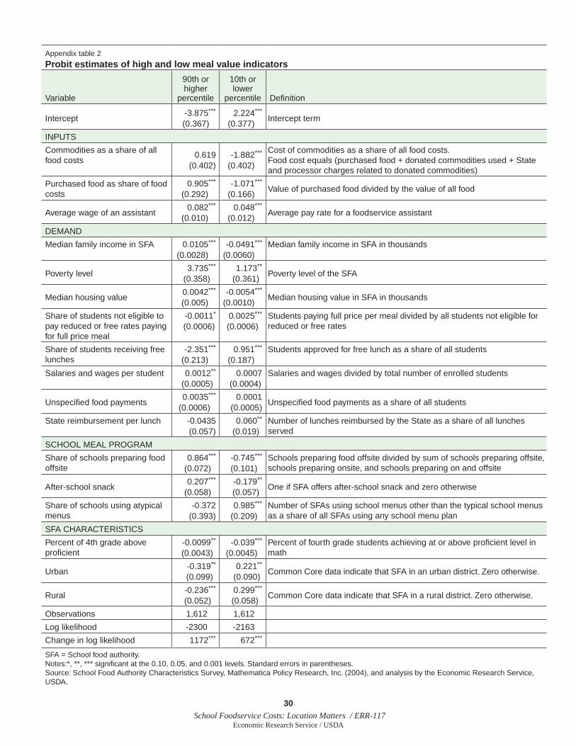
30 School Foodservice Costs: Location Matters / ERR-117
Economic Research Service / USDA
Appendix table 2
Probit estimates of high and low meal value indicators
Variable
90th or higher
percentile
10th or lower
percentile Definition
Intercept-3.875***
(0.367)2.224***
(0.377)Intercept term
INPUTS
Commodities as a share of all food costs
0.619(0.402)
-1.882***
(0.402)
Cost of commodities as a share of all food costs. Food cost equals (purchased food + donated commodities used + State and processor charges related to donated commodities)
Purchased food as share of food costs
0.905***
(0.292)-1.071***
(0.166)Value of purchased food divided by the value of all food
Average wage of an assistant0.082***
(0.010)0.048***
(0.012)Average pay rate for a foodservice assistant
DEMAND
Median family income in SFA 0.0105***
(0.0028)-0.0491***
(0.0060)Median family income in SFA in thousands
Poverty level3.735***
(0.358)1.173**
(0.361)Poverty level of the SFA
Median housing value0.0042***
(0.005)-0.0054***
(0.0010)Median housing value in SFA in thousands
Share of students not eligible to pay reduced or free rates paying for full price meal
-0.0011*
(0.0006)0.0025***
(0.0006)Students paying full price per meal divided by all students not eligible for reduced or free rates
Share of students receiving free lunches
-2.351***
(0.213)0.951***
(0.187)Students approved for free lunch as a share of all students
Salaries and wages per student 0.0012**
(0.0005)0.0007
(0.0004)Salaries and wages divided by total number of enrolled students
Unspecified food payments0.0035***
(0.0006)0.0001
(0.0005)Unspecified food payments as a share of all students
State reimbursement per lunch -0.0435(0.057)
0.060**
(0.019)Number of lunches reimbursed by the State as a share of all lunches served
SCHOOL MEAL PROGRAM
Share of schools preparing food offsite
0.864***
(0.072)-0.745***
(0.101)Schools preparing food offsite divided by sum of schools preparing offsite, schools preparing onsite, and schools preparing on and offsite
After-school snack0.207***
(0.058)-0.179**
(0.057)One if SFA offers after-school snack and zero otherwise
Share of schools using atypical menus
-0.372(0.393)
0.985***
(0.209)Number of SFAs using school menus other than the typical school menus as a share of all SFAs using any school menu plan
SFA CHARACTERISTICS
Percent of 4th grade above proficient
-0.0099**
(0.0043)-0.039***
(0.0045)Percent of fourth grade students achieving at or above proficient level in math
Urban-0.319**
(0.099)0.221**
(0.090)Common Core data indicate that SFA in an urban district. Zero otherwise.
Rural-0.236***
(0.052)0.299***
(0.058)Common Core data indicate that SFA in a rural district. Zero otherwise.
Observations 1,612 1,612
Log likelihood -2300 -2163
Change in log likelihood 1172*** 672***
SFA = School food authority.Notes:*, **, *** significant at the 0.10, 0.05, and 0.001 levels. Standard errors in parentheses.Source: School Food Authority Characteristics Survey, Mathematica Policy Research, Inc. (2004), and analysis by the Economic Research Service, USDA.

31 School Foodservice Costs: Location Matters / ERR-117
Economic Research Service / USDA
Share of High School Students: High school food service offers larger portion sizes and often offers more variety. Thus, SFAs with either a large or small share of students attending high schools should have different costs and must be accounted for in the model.
Health Insurance: Labor costs can vary substantially with employee bene-fits. Health insurance is a particularly high labor cost that may attract higher quality workers and can substitute for higher wages.
Foodservice Management Company: Perhaps to reduce labor costs, some SFAs opt to have meals supplied by a private foodservice management company. This shifts costs from labor to another account—food—meaning that the labor share of costs should drop and the food share of costs should rise. Table 2 indicates that about 6 percent of all SFAs contract out work to foodservice management companies.
Universal Free Meals: Another potentially cost-reducing mechanism for schools that serve mainly free and reduced-price meals is offering free meals for all students under “universal free meal” provisions of the NSLP (Ralston et al., 2008). From a cost and revenue perspective, this option reduces the administrative costs of encouraging families to apply for free meals and collecting money from paying students at a relatively small loss in revenue because most students in these schools would have received free meals anyway. Table 2 shows that use of these provisions is modest.
Estimation
The cost function can be estimated directly, but parameter estimates are often inefficient because of multicollinearity among explanatory variables. Gains in efficiency can be realized by estimating the input demand equations (cost-share equations) jointly with the cost function. The equations are obtained from the derivatives of the total cost function with respect to each price.
_
.2 ln lni i
i i i i
i i i
i iMiij j ij URBANICITY ij REGIONi
i j i j i j
Bi BFAST L LACARTE cap CAPi HSi HIGH SCHOOL i Hi HEALTHi ii
Si SERVICE Fi FREE Vi VALUE
lnC P X A ) = = + P + M + C CClnP
w C C C C Ci
C C w C i
β β γ σ π
κ δ ψ ψ
υ ψ
Σ+
∂+
∂
∑+ + + +
∑+ ++ +
∑ ∑ ∑ ∑ ∑
∑
The shortrun cost function (equation A.1) is estimated jointly in a multi-variate regression system with three input demand equations. To account for likely cross-equation correlation in the error terms, we used a nonlinear itera-tive, seemingly unrelated regression procedure. Since the input shares add to one, we dropped the demand for supplies equation to avoid a singular covari-ance matrix.
All variables are normalized (i.e., divided by their mean values before esti-mation); thus, the first-order terms (the bs) can be interpreted as the esti-mated cost-share of input i at mean values. The other coefficients capture

32 School Foodservice Costs: Location Matters / ERR-117
Economic Research Service / USDA
changes in the estimated input shares with changes in other prices, number of meals served, and other model components.
Symmetry and homogeneity of degree one are imposed on the cost function in order to gain improvements in efficiency and reduce the number of parameters estimated (Berndt, 1991). Symmetry means that the coefficients on all interac-tion terms with identical components are equal (that is, the coefficients bij=bji = γiM, dcap,i = di,cap, wi,j = wj,i , ψHS,i = ψi,HS , ψH,i = ψi,H, υS,i = υS,i, ψF,i = ψMC,F , σU,i = σi,U, and πi,j = πj,i ). The omitted variables are not reported because they are implied.
Homogeneity of degree one means that if all inputs are doubled, then output (meals served) also doubles. Systems that are homogeneous of degree one have the following properties: ∑bi =1, ∑bi,j =0, ∑ γMi =0, ∑ dcap,i =0, ∑ wi,j =0, ∑ ψHS,i = 0, ψH,i =0, ∑υS,i =0, ∑ ψF,i =0, ∑ σU,i =0, ∑ πi,j =0. Since some parameters equal combinations of other variables, some parameters could be dropped. In this analysis, we dropped the price of supplies and all of its interaction terms.
Survey Weights
In a memo dated August 6, 2004, Hall and Zheng (Mathematica Policy Research, Inc.) assert that survey data used in the analysis should reflect the population of local public SFAs in the 50 States and the District of Columbia. Survey data used in the analysis were a representative sample, but it is still necessary to use weights to account for differences in the probability of selection associated with sample design, nonresponse, and ineligibility. These weights were provided by Mathematica Policy Research, Inc.
Tests for Model Selection
Gallant-Jorgenson (G-J) likelihood ratio tests are commonly used to assess model fit in cost function analyses—i.e., whether a selected variable or group of variables affect production costs (Gallant and Jorgenson, 1979). A likeli-hood ratio test is preferable to single-variable statistical significance because translog cost functions have many interaction terms for each explanatory variable, making any single variable a poor measure of variable importance. Hypotheses are tested by comparing a reference model containing a vari-able of interest to a model in which that variable is excluded (the restricted model). If the difference in the G-J statistic exceeds a critical value, then the hypothesis that the test variable does not affect costs is rejected.
Appendix table 3 contains the model numbers and descriptions of the models to be examined, the G-J statistic, number of parameters estimated, models tested (test versus reference models), number of restrictions (the number of variables left out of the test model), the critical chi-square value (significance at the 0.01 level), and the model chi-square statistic (the difference between the G-J statistics of the two models).15
We proceed with the test as follows. For each test, we compare the fit of the restricted model (all models in which at least one variable is left out of the reference model) to that of the reference model. The reference model is the full model. If the difference in the G-J—a chi-square statistic—exceeds the
15The difference in the values of the objective function equals N*S(a, v)R - N*S(a1, v1)u, where S(a, v)R is the minimum value of the objective function of the restricted model, S(a1, v1)u is the minimum value of the objective function of the unrestricted, reference model, and N is the number of observations. The value of the objective function is printed as output from the nonlinear estimation of the seemingly unrelated regression model in the SAS statistical package.

33 School Foodservice Costs: Location Matters / ERR-117
Economic Research Service / USDA
critical value, then the restricted model is rejected in favor of the reference model.
Model I is a very basic, 10-parameter model that accounts for input prices and meals produced. Model II (the reference model) is the final model containing 118 parameters representing input prices, meals, metropolitan area, regional variables, breakfasts, a la carte revenues, capital costs, share of high school students, health care for workers, the use of foodservice compa-nies, free meals for all students, and meal values. The third last column shows that there are 108 restrictions and the second last column shows that the critical chi-square statistic is 145. The critical chi-square is the minimum value needed to conclude that the model is significantly different from the reference model. The last column indicates that the model chi-square easily surpasses the critical chi-square, meaning that the variables are significant to model fit.
Appendix table 3Model selection tests for school meal cost functions
Test statistics1
Model DescriptionG-J
statisticParametersestimated Test Restrictions
Critical chi-squareat 0.01 level
Model chi-square
I Translog input prices and output 4025 10 - - - -
II Full, reference model2 3442 118 II vs I 108 145 583***
IIIRemoves areas (rural and suburban) from II
3486 94 III vs II 24 45 44**
IV Removes region from II 3534 76 IV vs II 42 71 92***
V Removes breakfasts from II 3520 102 V vs II 16 34 78***
VIRemoves a la carte rev-enues from II
3516 114 VI vs II 4 15 74***
VIIRemoves capital costs from reference model
3464 112 VII vs II 6 18 22***
VIIIRemoves shares of high school students from II
3496 106 VIII vs. II 10 25 28***
IXRemoves health care for workers from II
3475 108 IX vs II 10 25 33***
XRemoves foodservice com-panies from II
3483 112 X vs II 6 18 40***
XI Removes free meals, all students from II
3455 114 XI vs II 4 15 13*
XIIRemoves high, low value meals from II
3470 104 XII vs II 14 31 28*
XIIIa Adds enhanced menus to II 3448 122 XIII vs II 4 15 -6
XIIIb Imposes homotheticity on II 3504 114 XIII vs II 4 15 -62
*** , **,* significant at the 0.01, 0.02, and 0.05 levels of confidence.1Chi-square statistics are the difference in G-J statistics between the test and reference models. Restrictions are the differences in the num-ber of parameters estimated between the two models.2The full model includes variables for our input price measures, output, and meal value and dummy variables for determining if the SFA had capital expenditures, if schools served no breakfasts or if schools that served breakfasts accounted for 33 percent or more of all meals, if ratios of high school students as shares of all students exceeded two different limits, if a la carte revenues exceeded a critical amount, if the SFA offered free meals to all students, if health care was provided to workers, if the SFA uses a foodservice companies, and for types of metropolitan areas and regions.

34 School Foodservice Costs: Location Matters / ERR-117
Economic Research Service / USDA
In subsequent tests, one optional characteristic (any variable except for prices and meals) is removed and that restricted model is compared against the reference model. For example, we removed the two variables representing breakfasts from the reference model and determined model fit by subtracting the G-J statistic of the reference model from this model. Since the model chi-square surpasses the critical chi-square statistic, breakfasts do significantly affect meal costs. All of the remaining tests proceeded in the same fashion, and all of these tests, except for the universal free meals, demonstrated that the restricted variables should be included in the model. We kept the variable for universal free meals in the model because it still contributed to explaining model fit.
In the second last test (second last row of the table), a variable representing enhanced menus was added to the model. Although nutrition standards and meal reimbursements are consistent across schools, USDA offers SFAs the flexibility to use either a food-based or a nutrient-based meal planning approach in creating meals that meet these nutrition standards. This flex-ibility allows SFAs to choose a meal planning option that best suits their needs.
As shown, it was not significant and even detracts from the model, so we dropped it. Other variables tested at earlier stages of modeling included whether the SFA participated in the school snack program and whether the SFA used a central cooking facility, but they proved to be not significant and were dropped.
In the last test (last row of the table), we tested for homotheticity. This test evaluates whether labor, food, and supply prices vary with the number of meals served by eliminating the interaction terms between factor prices and output volume (forcing factor shares to be invariant with respect to output). The test indicates that these input prices vary with the number of meals served. Thus, we reject Model XIIIb in favor of Model II.
Model Diagnostics and Discussion of Model Estimates
Appendix table 4 contains the estimated coefficients from equation A.1. The 23 terms after the intercept are all of the first-order coefficients. Next, there are six quadratic terms and then all of the interaction terms. All of the input price and meal variables are interacted with all other variables. There are also a few other interaction terms: the breakfast variables with the meal value variable, breakfasts with urbanicity variables, the high school dummy vari-ables with dummy variables for capital and foodservice companies, and each regional variable with dummy variables for health care, suburban SFAs, and rural SFAs.
The model R2 was typical for cost functions—about 0.9829. The first-order coefficients of input prices can be interpreted as cost shares at sample means and should always be positive to meet regularity conditions. All three coef-ficients are positive, satisfying this condition. A negative value for one of the input share coefficients would imply that an input has a negative price (someone would have to pay the user to use the input). A large number of estimated negative values could imply a poorly estimated regression. There were few violations. Only 3.0 percent of all observations for supplies were

35 School Foodservice Costs: Location Matters / ERR-117
Economic Research Service / USDA
Appendix table 4
Translog cost function estimates for school meals, school year 2002-03, continued
Variable Coefficient t-statistic Variable Coefficient t-statistic
Intercept -0.008 -0.09 PSUPPLY*MEALS 0.001 0.89
PLAB 0.327*** 19.39 PSUPPLY*CSUBURB 0.005 0.74
PFOOD 0.608*** 36.34 PSUPPLY*CRUR 0.004 0.54
PSUPPLY 0.065*** 5.39 PSUPPLY*CATLANTIC -0.013* -1.67
MEALS 0.966*** 38.18 PSUPPLY*CMIDWEST -0.026*** -3.40
PSUPPLY*CMOUNT -0.022** -3.01
CSUBURB 0.027 0.43 PSUPPLY*CNORTHEAST -0.037*** -4.61
CRUR 0.079 1.25 PSUPPLY*CSOUTHWEST -0.026*** -3.70
CATLANTIC -0.189* -1.78 PSUPPLY*CWEST -0.007 -0.86
CMIDWEST -0.236** -2.55 PSUPPLY *CBFAST33 -0.002 -0.50
CMOUNT -0.193** -1.98 PSUPPLY*CBFAST0 -0.003 -0.56
CNORTHEAST -0.178* -1.81 PSUPPLY* CLACARTE 0.017*** 4.79
CSOUTHWEST -0.105 -1.02 PSUPPLY*CCAP -0.001 -0.31
CWEST -0.311*** -2.91 PSUPPLY*CHIGH_SCHOOL_LO
-0.006* -1.75
CBFAST33 -0.049 -1.35 PSUPPLY *CHIGH_SCHOOL_HI
0.030*** 3.26
CBFAST0 0.091 1.12 PSUPPLY *CHEALTH 0.016*** 3.08
CLACARTE 0.075*** 4.53 PSUPPLY*CSERVICE 0.012*** 2.70
CCAP 0.033* 1.66 PSUPPLY*CFREE 0.016*** 2.63
CHIGH_SCHOOL_LO 0.007 0.32 PSUPPLY* CVALUE_LO -0.002** -2.51
CHIGH_SCHOOL_HI 0.248** 2.41 PSUPPLY* CVALUE_HI 0.005*** 3.09
CHEALTH 0.049 0.76 MEALS *CSUBURB -0.004 -0.34
CSERVICE -0.068*** -2.86 MEALS *CRURAL -0.020 -1.42
CFREE -0.011 -0.39 MEALS *CATLANTIC 0.012 0.68
CVALUE_LO -0.022*** -4.23 MEALS *CMIDWEST 0.016 0.92
CVALUE_HI -0.008 -0.74 MEALS *CMOUNT -0.003 -0.14
PLAB * PLAB 0.148*** 20.10 MEALS *CNORTHEAST -0.017 -0.88
P FOOD * PFOOD 0.162*** 32.31 MEALS *CSOUTHWEST 0.014 0.86
PSUPPLY*PSUPPLY 0.064 - MEALS *CWEST -0.009 -0.50
MEALS*MEALS 0.007* 1.60 MEALS*CBFAST33 -0.017** -2.05
CVALUE_LO *CVALUE_LO -0.0003** -2.59 MEALS*CBFAST0 -0.025** -2.03
CVALUE_HI *CVALUE_HI -0.002 -1.41 MEALS * CLACARTE -0.007 -1.02
PLAB * PFOOD -0.123*** -20.47 MEALS *CCAP -0.008 -1.22
PLAB * PSUPPLY -0.025*** -5.17 MEALS*CHIGH_SCHOOL_LO
0.011* 1.68
PLAB * MEALS -0.011*** -4.98 MEALS*CHIGH_SCHOOL_HI
0.047* 1.66
PLAB * CSUBURB 0.048*** 5.23 MEALS *CHEALTH 0.017* 1.60
PLAB * CRUR 0.063*** 6.69 MEALS *CSERVICE -0.009 -1.06
PLAB *CATLANTIC 0.013 1.16 MEALS*CFREE -0.015 -1.46
PLAB *CMIDWEST -0.007 -0.67 MEALS * CVALUE_LO -0.002 -1.18
continued

36 School Foodservice Costs: Location Matters / ERR-117
Economic Research Service / USDA
Appendix table 4
Translog cost function estimates for school meals, school year 2002-03, continued
Variable Coefficient t-statistic Variable Coefficient t-statistic
PLAB *CMOUNT 0.005 0.53 MEALS * CVALUE_HI -0.001 -0.39
PLAB *CNORTHEAST 0.009 0.82 CSUBURB*CATLANTIC 0.067 0.89
PLAB *CSOUTHWEST 0.029*** 2.94 CSUBURB *CMIDWEST 0.098 1.32
PLAB *CWEST -0.002* -0.14 CSUBURB *CMOUNT 0.007 0.08
PLAB *CBFAST33 -0.024*** -3.90 CSUBURB*CNORTHEAST -0.038 -0.48
PLAB * CBFAST0 -0.007 -0.96 CSUBURB*CSOUTHWEST 0.034 0.46
PLAB * CLACARTE 0.020*** 4.06 CSUBURB*CWEST 0.018 0.25
PLAB *CCAP 0.0003 0.64 CSUBURB*CBFAST33 -0.0001 -0.00
PLAB *CHIGH_SCHOOL_LO 0.002 0.50 CSUBURB*CBFAST0 -0.224*** -2.88
PLAB *CHIGH_SCHOOL_HI -0.014 -1.05 CRURAL*CATLANTIC 0.039 0.50
PLAB *CHEALTH 0.042*** 5.64 CRURAL *CMIDWEST 0.002 0.03
PLAB *CFOOD_SERVICE -0.076*** -11.96 CRURAL *CMOUNT -0.037 -0.44
PLAB * CFREE -0.004 -0.39 CRURAL*CNORTHEAST -0.100 -1.18
PLAB * CVALUE_LO -0.0025*** -2.64 CRURAL*CSOUTHWEST -0.002 -0.02
PLAB * CVALUE_HI -0.006** -2.31 CRURAL*CWEST -0.038 -0.51
PFOOD * PSUPPLY -0.039*** -8.74 CRURAL *CBFAST33 -0.039 -1.06
PFOOD * MEALS 0.010*** 4.39 CRURAL*CBFAST0 -0.209*** -2.68
PFOOD*CSUBURB -0.053** -5.75 CHEALTH *CATLANTIC 0.114 1.41
PFOOD *CRUR -0.067*** -7.05 CHEALTH *CMIDWEST 0.051 0.76
PFOOD *CATLANTIC 0.0002 0.02 CHEALTH *CMOUNT 0.095* 1.60
PFOOD *CMIDWEST 0.034*** 3.12 CHEALTH *CNORTHEAST 0.076 1.01
PFOOD *CMOUNT 0.016 1.55 CHEALTH *CSOUTHWEST 0.134* 1.61
PFOOD *CNORTHEAST 0.028** 2.49 CHEALTH *CWEST 0.177** 1.99
PFOOD*CSOUTHWEST -0.003 -0.034 CBFAST33* CVALUE_LO 0.004 0.63
PFOOD *CWEST 0.009 0.76 CBFAST33* CVALUE_HI 0.011 1.26
PFOOD*CBFAST33 0.026*** 4.29 CBFAST0* CVALUE_LO -0.009*** -2.31
PFOOD*CBFAST0 0.009 1.36 CBFAST0* CVALUE_HI -0.016 -1.39
PFOOD * CLACARTE -0.037*** -7.48 CCAP*CHIGH_SCHOOL_LO -0.006 -0.40
PFOOD *CCAP -0.002 -0.42 CCAP*CHIGH_SCHOOL_HI -0.111* -1.87
PFOOD *CHIGH_SCHOOL_LO 0.003 0.73 CHIGH_SCHOOL_LO*CFOOD_SERVICE
-0.007 -0.35
PFOOD*CHIGH_SCHOOL_HI -0.016 -1.23 CHIGH_SCHOOL_HI*CFOOD_SERVICE
-0.102** -1.91
PFOOD*CHEALTH -0.058*** -7.91
PFOOD*CFOOD_SERVICE 0.064*** 10.11
PFOOD* CFREE -0.013 -1.45
PFOOD* CVALUE_LO 0.004*** 4.45
PFOOD * CVALUE_HI 0.0003 0.12
Notes: *,**, *** significant at the 0.10, 0.05 and 0.001 levels. All variables are standardized at their means, so first-order coefficients can be interpreted as elasticities at the sample means. Dummy variable capture shifts in costs. There were 1,432 observations taken from the 2002-03 SFA Characteristics Survey on the costs of producing school meals at the school food authority level. The model R2 was 0.9817.
Source: School Food Authority Characteristics Survey, Mathematica Policy Research, Inc. (2004), and analysis by the Economic Research Service, USDA.

37 School Foodservice Costs: Location Matters / ERR-117
Economic Research Service / USDA
negative and no observations for food or labor were negative.
Parameter values for the first-order input price terms provide estimates of the share of costs devoted to labor (PLAB), food (PFOOD), and supplies (PSUPPLY). Food inputs account for about 61 percent of meal costs, while labor and supplies comprise about 33 and 6 percent of costs. These cost shares apply only to the reference category, which is Southeastern SFAs in an urban setting that claim no capital costs, do not provide health care to foodservice staff or free meals to all students, serve breakfasts that account for between 0 and 33 percent of total meals served, serve an average number of elementary and high school students, prepare average-value meals that generate less than 10 cents per meal in revenue from a la carte sales, and do not contract with foodservice companies.
The interaction terms show how cost shares vary from the reference SFA value. For example, the coefficients on the interactions of the urbanicity variables (CSUBURB and CRURAL) with labor and food input prices (PLAB and PFOOD) show how labor and food cost shares change from urban to suburban and rural settings.
There is a sizable change if the Southeastern SFA was a suburban SFA rather than an urban one. In this case, the suburban dummy variable would equal one. For a suburban, Southeastern SFA, the labor share would rise to about 37 percent, since the value of the interaction of the suburban dummy variable with the price of labor (PLAB *CSUBURB) is added to the coefficient on the price of labor (PLAB) to determine the labor share. The food share (PFOOD + PFOOD*CSUBURB) would drop to about 55 percent.
There is also a substantial difference for an urban, southeastern SFA that offered health care. In that case, the labor share rises from 33 to about 37 percent (PLAB + PLAB*CHEALTH) and the food share drops to about 55 percent (PFOOD + PFOOD*CHEALTH). Finally, if the southeastern SFA offered health care and was located in a suburban area, then the labor share would rise to about 41 percent (PLAB + PLAB *CSUBURB+ PLAB*CHEALTH) and the food share would drop to about 50 percent (PFOOD + PFOOD*CSUBURB+ PFOOD*CHEALTH).
The coefficients shown in appendix table 4 indicate sizable drops (more than 1 percent) in the labor share from the reference case for SFAs that serve no breakfasts, serve meals to a high proportion of high school students, or SFAs that use a foodservice company. In a similar way, there would be a substan-tial increase in the labor share (and usually a decrease in the food share) for SFAs that are smaller than average, generate more than 10 cents per meal from a la carte items, offer health care to their workers, are either suburban or rural, and are located in either the Mid-Atlantic or Southwestern regions.
The a la carte and labor share findings are of particular interest. SFAs that have a la carte services devote 2 percent more of each dollar spent for labor and spend about 3.7 percent less for food. This means that non-a la carte foods—i.e., NSLP meals—provide more food per dollar spent than a la carte foods.

38 School Foodservice Costs: Location Matters / ERR-117
Economic Research Service / USDA
Elasticities
The Allen cross price elasticity indicates the degree of substitutability among inputs—i.e., how a change in the use of one input affects usage of a different input. The Morishima cross-price elasticity indicates how a change in the price of one input affects use of another input. Positive values for either of the cross elasticities indicate substitutability between inputs, and negative values indicate that the inputs are complements.
The own- and cross-price elasticities of input demand and the Allen elastici-ties of input substitution indicate the degree of responsiveness to changes in input prices. The own-price input demand elasticity shows how a given change in prices for food or other input affects demand for that input. A cross-price elasticity shows how a change in the price of food or another input affects demand for a different input. A positive sign means that the two inputs are complements, and a negative sign indicates that they are substi-tutes. Equations A.3 and A.4 define mathematically own- and cross-price elasticities.
The input demand own- and cross-price elasticities for any inputs i and j are equal to:
2( ).3 jj j j
jjj
A S SS
ϕε
+ −=
and
( ).4 jk j k
jkj
A S SS
ϕε
+=
The Allen elasticity of input substitution indicates the degree to which a given percentage change in input k—labor—can substitute for a percentage change in input j—food. A higher positive number indicates greater substitut-ability. The Allen partial cross elasticity of input substitution can be written as
( )
.5 jk j kjk j
i
A S S SSϕ
ε+
=
where the S represents input shares of jth or kth input and comes from the first-order price coefficients; φjk is the coefficient on the kth input price for the jth input and is also the coefficient on the interaction term between the jth and kth input prices in equation A.1; φjj is the coefficient on the jth input price in the demand equation for that input and is also the coefficient on the squared input in equation A.1.16
Appendix table 5 contains the own-price and the Allen and Morishima cross elasticities for the major inputs of labor, food, and supplies. Model coeffi-cients and the equations shown in the appendix are used to estimate the elas-ticities. Own-price elasticities for labor imply that a 10-percent increase
16We use fitted input shares with rep-resentative data to estimate equations A.5-A.7 because predicted input shares may vary with output, input prices, and/or plant characteristics. Reported elasticities should also use representa-tive values.

39 School Foodservice Costs: Location Matters / ERR-117
Economic Research Service / USDA
in the price of labor leads to a 2.2-percent decline in demand for that input. The change is much stronger for food—about a 4.7-percent decrease in food with a 10-percent increase in the price. The own-price elasticity for supplies is highly inelastic—i.e., there is very little change in input usage with a change in prices. The positive sign is the opposite from what would be expected, but it is of such low magnitude that it really is reflecting a lack of responsiveness and not a shift in usage as prices change.
The Allen cross elasticity implies that a 10-percent increase in labor usage results in a 3.81-percent decrease in food inputs. For example, SFAs may begin making pizza from scratch, which would raise labor requirements, but would also reduce food costs since prepared pizzas cost more than the cost of the ingredients. The negative sign on labor and supplies indicates that a rise in the use of labor inputs results in an increase in the use of supplies.
Blackorby and Russell (1981, 1989) argue that Morishima elasticities have a bias toward showing inputs as substitutes and that Allen elasticities are biased toward showing inputs as complements. Not surprisingly, appendix table 5 shows that Morishima elasticities are higher than Allen elasticities for comparable cells.
The elasticity of total costs with respect to output (meals) provides a natural measure of scale economies by showing how costs change as SFA size changes. A number less than one means that the percentage rise in costs is less than the percentage rise in meals, or it becomes less costly to prepare the next meal. For example, a value of 0.90 indicates that costs increase by 0.9 percent for every 1-percent increase in the number of meals produced (average costs fall as the number of meals rise). Because the variables are all divided by their sample means before estimation, the first-order term, φγM, can be interpreted as estimated scale economies for SFAs at the sample mean
Appendix table 5
Input demand estimates and elasticities
Input price variables
Item PLAB PFOOD PSUPPLY
Estimated input shares 0.327 0.608 0.065
εii (own input price) -0.220 -0.468 0.050
Aij (Allen cross elasticities)
PLAB - 0.381 -0.177
PFOOD - - 0.025
PSUPPLY - - -
Mij (Morishima cross elasticities)
PLAB - 0.452 0.208
PFOOD 0.593 - 0.470
PSUPPLY -0.108 -0.035 -
= ?
Source: School Food Authority Characteristics Survey, Mathematica Policy Research, Inc. (2004), and analysis by the Economic Research Service, USDA.

40 School Foodservice Costs: Location Matters / ERR-117
Economic Research Service / USDA
size. The cost elasticity equation is defined as the derivative of the cost func-tion with respect to output:
, _
.6 ln lnln I I i
i
I i
iCM Mi MU URBANICITY MR REGIONM MMii
Cap McBMi BFAST LM LACARTE HSM HIGH SCHOOL
i i
HM HEALTH SM SERVICE FM FREE MV VALUEi
lnC A ) = = + M + C CPM i
C C + C
C C C + C
γ γ γ σ πε
ω κ ψδ
ψ υ ψ ω
∂∑ ∑+ +
∂
∑ ∑+ + +
+ + +
∑
∑
where values of the cost elasticity, εCM, that are less than 1 imply scale econ-omies and values above 1 imply scale diseconomies.
Equation A.6 allows the estimated cost elasticity to vary with output, prices, capital costs, urbanicity, region, breakfasts served, a la carte foods, share of high school students, health benefits, foodservice management companies, share of schools with free meals for all students, and meal value. The param-eters, γMM and γMi and the other coefficients show the dimensions along which scale economies vary.
Values of the cost elasticity that are less than 1 indicate economies of scale. For example, a value of 0.90 indicates that costs increase by 0.9 percent for every 1-percent increase in output (in turn, average costs fall as output increases). Values in excess of 1 show diseconomies of scale.
Appendix table 6 shows how cost elasticities and costs change at SFA sizes equal to one-fourth, one-half, one, and two times the regional mean size. Overall, the table shows that the cost elasticity is less than one when evalu-ated at sample mean prices and that costs drop as SFA size increases. Large SFAs produce meals that are anywhere from 10 to 27 cents less costly than small SFAs. The average cost difference across the 7 regions due to an eight-fold increase in size is 19 cents per meal.
The eightfold difference in size and the associated meal costs illustrated in appendix table 6 actually understate the economies of scale that exist between urban SFAs, which are the largest SFAs, and rural SFAs, which are the smallest. Northeastern urban SFAs are about 7 times the mean size SFA, whereas Northeastern rural SFAs are 0.09 times the mean size SFA or, on average, about 80 times smaller than an average-sized Northeastern urban SFA. Overall, urban SFAs are about 3.7 times the sample mean size SFA, and rural SFAs are about 0.21 times the sample mean size SFA.
The derivative of the second-order output term in the cost elasticity equa-tion indicates the change in per meal cost as the number of meals served increases. A negative sign indicates that the cost of preparing and serving the next meal is less than the cost of the previous meal; a positive sign means the opposite. Since the coefficient on the second-order output term is positive (appendix table 4), the cost of preparing the next meal is more than the cost of preparing the previous one. However, since the cost elasticity is less than one for all the regions, the cost of preparing the next meal is still below the average.17
17Typically, cost functions are U-shaped—the cost of producing the first unit is very high and the costs of later units are lower. At some point, it be-comes more costly to produce the next unit. The cost of production at this point is actually below the average cost of production since average costs include the first, very high-cost, items. Thus, costs can be increasing in the presence of economies of scale.

41 School Foodservice Costs: Location Matters / ERR-117
Economic Research Service / USDA
Appendix table 6
Simulated per meal costs by region and school food authority (SFA) size
RegionOne-fourth mean sizea
One-half mean size Mean size
Twice mean size
Regional size rel-ative to sample
mean sizes
Regional cost elasticity at sample mean output/prices
----------------------------Dollars----------------------------
Mid-Atlantic $2.97 $2.90 $2.85 $2.81 0.856 0.978
Midwest $2.69 $2.63 $2.58 $2.54 0.489 0.982
Mountain Plains $2.27 $2.19 $2.12 $2.06 0.439 0.963
Northeast $2.61 $2.51 $2.42 $2.34 1.100 0.949
Southeast $2.52 $2.44 $2.38 $2.32 1.500 0.966
Southwest $2.25 $2.21 $2.17 $2.15 0.816 0.980
Western $2.72 $2.63 $2.56 $2.49 1.325 0.957
--------------------------Number--------------------------
Meals served 413,250 826,000 1,653,000 3,306,000 NA NA
----------------------Cost elasticity----------------------
Reference cost elasticity 0.956 0.961 0.966 0.971 NA NA
NA = Not applicable.
Note: Assumptions used in simulations: All input price measures and SFA characteristics are set at regional averages, except size, which is set at one-fourth, one-half, one, and two times sample average.
Source: School Food Authority Characteristics Survey, Mathematica Policy Research, Inc. (2004), and analysis by the Economic Research Service, USDA.

42 School Foodservice Costs: Location Matters / ERR-117
Economic Research Service / USDA
Appendix B: School Breakfasts
Rigorous cost accounting methods used to estimate school breakfast and lunch meal preparation costs in SLBCS-II indicated that it cost much less to prepare a breakfast than a lunch. However, costs rise when few breakfasts are served (Sackin, 2008; Helleren, 2007). Results from our cost analyses indicate breakfasts are less costly than lunches only if more than one of every three meals served by the SFA are breakfasts. If fewer breakfasts are served, then breakfast costs are the same as lunch costs. Below, we examine whether breakfasts, even at low volumes, are the same cost as lunches by examining regional regressions and testing for differences in costs due to share of meals comprised of breakfasts. Then, we consider why costs might be the same.
Examination of Costs by Region
In this analysis, we investigate whether the conclusions reached about break-fasts from the larger model hold up in more simplified analyses that focus directly on the impact of breakfasts on costs. To do this, we stripped the cost function (equation A.1.1) of all explanatory variables except for the expres-sions for input prices, number of meals, and dummy variables for 33-percent SFAs and lunch-only SFAs and their interactions with input prices and number of meals served (equation B.1):
2
1( .1) ln ln ln ln2
ln ln ) ln *ln
*ln *ln
i jiji i j
Mi im MM i
B Bij BFAST iiBFAST BM BFASTj
B C = + + P * PPi0 ii
MEALS ( MEALS MEALS P
C w C P C MEALSi ii ii ii
β βα
γ γ
ψ ω ε
γ
Σ
∑+ + +
∑ ∑∑+ + + +
∑ ∑∑
where the variables are defined as above.
We ran 21 regressions in total (3 urbanicities and 7 regions) and examined signs on the lunch-only and 33-percent breakfast dummy variables (the refer-ence category is 0-33 percent breakfasts). If breakfasts are less costly than lunches to produce, the dummy variable for lunch-only SFAs should be posi-tive and the dummy variable for the 33-percent SFAs should be negative. Since each region/urbanicity regression has two comparisons (signs on the lunch-only and 33-percent parameters) of dummy variables, 42 comparisons are possible. Of the comparisons, 14 have outcomes that differ from expec-tations, 15 have outcomes consistent with expectations, and the remaining either could not be estimated or were biased.
An even simpler model that excludes the interactions of prices with the breakfast dummy variables and meals with the breakfast dummy variables was also tested. Results indicated that that 18 of 42 comparisons differed from their expected outcomes. These results indicate that breakfasts cost as much or more to produce as lunches in about one-half the cases in which there was a direct comparison between the two meals. Since costs are indis-tinguishable, it is valid to treat breakfasts and lunches as similar meals.

43 School Foodservice Costs: Location Matters / ERR-117
Economic Research Service / USDA
Breakfast Costs and Why They May Be the Same as Lunch Costs
Appendix table 7 provides a comparison of costs by the number of breakfasts served, as a percentage of total meals. The three panels compare estimated meal costs for urban, rural, and suburban SFAs serving different numbers of breakfasts. Each panel compares estimated costs for SFAs in which break-fasts account for 33 percent or more of all meals, lunch-only SFAs, and SFAs in which 0-33 percent of all meals served are breakfasts (0-33 percent SFAs).
One might expect SFAs that serve more breakfasts would have lower costs since SLBCS-II indicated that breakfasts have lower costs of production than lunches. This lower cost relationship is true for urban 33-percent SFAs, which have much lower costs than either the urban lunch-only or urban 0-33 percent SFAs. The cost difference ranges from 34 cents for Western SFAs to 54 cents for Southeastern SFAs, and the cost difference between 33-percent SFAs and 0-33 percent SFAs ranges from 17 cents for Midwestern SFAs to 26 cents for Southeastern SFAs.
The cost-breakfast relationship breaks down for suburban and rural SFAs. Lunch-only SFAs have lower costs than both 33-percent and 0-33 percent SFAs in suburban SFAs across all regions. The breakdown of the cost- breakfast relationship is not as strong for rural SFAs as it is for suburban SFAs, but it still exists. The 33-percent SFAs have the lowest costs in all regions, but the difference between them and lunch-only SFAs varies from only 2 cents for Western SFAs to 13 cents for Southeastern SFAs. Lunch-only SFAs have lower estimated costs than 0-33 percent SFAs for every region except the Mid-Atlantic.
An examination of the cost function results suggests that high setup costs and weak economies of scale may explain the results. Consider setup costs. Coefficients are lower for urban 33-percent SFAs (CBFAST33) and lunch-only suburban and rural SFAs (interactions of CBFAST0 with CSUBURB and CRURAL). Second, 0-33 percent SFAs have weaker economies of scale than lunch-only and 33-percent SFAs (coefficients on MEALS*CBFAST0 and MEALS*CBFAST33 are both negative in appendix table 4).
Results also show that 0-33 percent SFAs have a high labor share of costs, perhaps due to meal participation imbalances. The coefficients on the labor cost shares (PLABOR and its interactions) show that 33-percent SFAs have labor cost shares that are about 2.5 percent lower than either the 0-33 percent share or lunch-only SFAs.18
Meal participation imbalances mean that all facilities and resources may not be used, raising average costs. Under unbalanced conditions, managers may have to schedule excess labor to serve lower volume meals (typically breakfasts) in order to have sufficient workers to serve higher volume meals (typically lunches). Alternatively, a school may have to purchase additional equipment to accommodate a different meal.
Results for breakfasts are consistent with research showing that per meal costs can be high when the number of breakfasts served is small. In an
18Coefficients on PLab*CBFAST33 and PLab*CBFAST0 indicate changes in labor share for high-breakfast-share and lunch-only SFAs.

44 School Foodservice Costs: Location Matters / ERR-117
Economic Research Service / USDA
analysis for the California State Nutrition Association, Sackin (2008) showed that schools need to serve at least 91 breakfasts to cover the cost of hiring the minimum 2 extra hours of labor required to prepare and serve the meal. In smaller schools, this may be a problem. A University of Wisconsin study (Helleren, 2007) asserts that participation rates must be high enough to over-come setup, service, and equipment costs.
Appendix table 7
Cost comparison by the share of meals that are breakfasts: Simulations using location-specific means for input price measures and school food authority (SFA) characteristics
Urbanicity of SFAs and share of meals that are breakfasts
Mid-Atlantic Midwest
MountainPlains Northeast Southeast Southwest Western
-----------------------------------------------Dollars/meal-----------------------------------------------
Urban SFAs:
No breakfasts served 2.58 2.29 2.39 2.24 2.71 2.28 2.35
Breakfasts less than 33 percent of meals
2.36 2.11 2.13 2.07 2.43 2.05 2.20
Breakfasts more than 33 percent of meals
2.14 1.94 1.95 1.86 2.17 1.83 2.01
Suburban SFAs:
No breakfasts served 2.99 2.91 2.31 2.67 2.31 2.31 2.57
Breakfasts less than 33 percent of meals
3.24 3.10 2.49 2.83 2.58 2.52 2.82
Breakfasts more than 33 percent of meals
3.05 3.00 2.35 2.75 2.34 2.35 2.66
Rural SFAs:
No breakfasts served 2.41 2.42 2.26 2.60 2.28 2.15 2.61
Breakfasts less than 33 percent of meals
2.41 2.52 2.32 2.67 2.41 2.23 2.77
Breakfasts more than 33 percent of meals
2.31 2.36 2.15 2.50 2.15 2.04 2.59
Source: School Food Authority Characteristics Survey, Mathematica Policy Research, Inc. (2004), and analysis by the Economic Research Service, USDA.