PNNL-22816

Prepared for the U.S. Department of Energy under Contract DE-AC05-76RL01830

Scaling Theory for Pulsed Jet Mixed Vessels, Sparging, and Cyclic Feed Transport Systems for Slurries WL Kuhn DR Rector SD Rassat CW Enderlin MJ Minette JA Bamberger GB Josephson BE Wells EJ Berglin September 2013

PNNL-22816

Scaling Theory for Pulsed Jet Mixed Vessels, Sparging, and Cyclic Feed Transport Systems for Slurries WL Kuhn DR Rector SD Rassat CW Enderlin MJ Minette JA Bamberger GB Josephson BE Wells EJ Berglin September 2013 Prepared for the U.S. Department of Energy under Contract DE-AC05-76RL01830 Pacific Northwest National Laboratory Richland, Washington 99352

iii

Preface

This document is a previously unpublished work based on a draft report prepared by Pacific Northwest National Laboratory (PNNL) for the Hanford Waste Treatment and Immobilization Plant (WTP) in 2012. Work on the report stopped when WTP’s approach to testing changed. PNNL is issuing a modified version of the document a year later to preserve and disseminate the valuable technical work that was completed.

In 2012, testing at less than full scale was the planned approach to resolve technical uncertainties associated with pulse-jet mixers (PJMs) and to address associated nuclear safety issues identified by the Defense Nuclear Facilities Safety Board.1 This activity, known as the Large Scale Integrated Testing (LSIT) Program, also supported design verification of the plant alongside computational fluid dynamic modeling. Tests were to be conducted using test vessels of 4-, 8-, and 14-ft diameter and the results extrapolated, or “scaled”, to the full size of the actual plant vessels, which are up to 47 ft in diameter. PNNL was tasked under this program with developing a scaling basis report that, in conjunction with a separate report prepared by WTP and consultant MixTech,2 was meant to:

• Define the basis for less-than-full-scale testing, including vessel configurations, operating parameters, and simulant parameters

• Address the basis for scaling both vessel physical performance and simulant physical performance

• Address physical scale laws observed in test results and scale laws used to establish operating conditions for testing.3

Draft versions of the report were prepared and were submitted to and reviewed by WTP and by others. In late 2012, however, the U.S. Department of Energy (DOE) changed the approach to resolving technical issues on pulse-jet mixing to one based on full-scale testing of the actual vessels.4 Since scaling was no longer needed, the scaling basis report was shelved.

Nevertheless, the report is a significant technical effort that aggregated and applied PNNL expertise on the physics of mixing of Newtonian and non-Newtonian slurries by pulsed, turbulent jets. Rather than lose the value of the technical information created specifically to support the LSIT Program, and in accordance with DOE’s direction to ensure dissemination of the results of scientific and technological endeavors within its programs,5 PNNL is issuing this version of the scaling basis report. This report goes beyond the fully reviewed second revision of the draft and incorporates additional scaling content that appeared in earlier drafts but was deemed unnecessary for the initial Newtonian vessel testing phase of

1 Defense Nuclear Facilities Safety Board Recommendation 2010-2, Pulse Jet Mixing at the Waste Treatment and Immobilization Plant, December 17, 2010. 2 Dickey DS, PJ Keuhlen, JW Olson, RB Daniel, and RL Hansen. Technical Scaling Selection Basis, 24590-WTP-RPT-PET-12-001, Rev. A – Draft, June 2012. 3 Energy Secretary S. Chu to Defense Nuclear Facilities Safety Board Chairman P. Winokur, Re: Department of Energy’s (DOE) Recommendation 2010-2 Implementation Plan (IP), Pulse Jet Mixing (PJM) at the Waste Treatment and Immobilization Plant (WTP), November 8, 2012. 4 S. Chu to Washington State Governor C. Gregoire, Re: Review of the Waste Treatment and Immobilization Plant (WTP) project technical issues and Hanford tank waste treatment strategies, January 14, 2013. 5 DOE Order 241.1B, “Scientific and Technical Information Management,” December 13, 2010.

iv

the program. However, no attempt has been made to update any information specific to the design of the plant, its operating conditions, performance requirements, or plans for completion; hence, any such information in this report should be considered to be potentially out of date.

The report includes sections describing the scaling of phenomena that are specific to the mixing requirements in WTP, i.e., clearing of solids from the vessel bottom to release trapped gas in settled layers, accumulation of solids between transferred batches, transfer of solids out of the vessel without line plugging, liquid blending, and collection of samples. (Note that the report does not address these last two topics for non-Newtonian fluids because they were added to the scope of report after the behavior of non-Newtonian flows was removed from its scope for the initial report.) Since some of the vessels are sparged, which provides additional mixing energy, the scaling of sparging operations is also described. There are also several appendices, most of which are “working papers” that provide a more detailed basis for the scaling approaches in the body of the report.

The interested reader will also benefit from a large number of other reports on the subject of scaled testing and scaling as it relates to WTP that were produced over more than two decades of PNNL support to the Hanford Site. The reports in the bibliography below include experimental, analytical, and computational efforts to understand and predict mixing and transfer of Hanford tank waste slurries. These reports are available from the “SciTech Connect” server at DOE’s Office of Scientific and Technical Information (http://www.osti.gov/scitech). Reports with document numbers of the form WTP-RPT-XXX are also available at PNNL’s web site for reports published under the Waste Treatment Plant Support Project (www.pnl.gov/rpp-wtp). A report compiling the abstracts from those reports published from 1999-2010 is also available (Beeman 2010).

Loni Peurrung

Director, National Laboratory Technical Authority Team WTP FSVT Program

Pacific Northwest National Laboratory

A Bibliography of Waste Mixing and Transfer Studies at PNNL

PNNL began supporting the Hanford Site and other DOE sites in the 1990s through development of integrated programs coupling analysis, scaling, experiment, and computational modeling. Areas of investigation included mobilizing and mixing of salt cake and sludges in waste tanks using rotary jet pumps, evaluating jet forces on in-tank components, and slurry transport. In the 2000s, activities expanded to include studies of pulsating jets being designed for the Waste Ttreatment Plant to mix Newtonian and Non-Newtonian waste slurries. Other investigations have included pipeline transfer, simulant development, and development of instrumentation to detect solids settling during transfer. Reports developed during these studies are described below.

In the 1990s, PNNL’s first scaling studies supported understanding slurry mixing and uniformity related to tank 241-AZ-101 rotary jet mixer pump operation. Scaled experiments to determine concentration uniformity of a single-centered dual-opposed rotating mixer pump were conducted at

v

1/12-scale (Bamberger et al. 1990b, 1993, 2007; Bamberger and Liljegren 1994). Mixing experiments at 1/12th scale were also conducted to support evaluation of hydrogen mitigation for tank 241-SY-101 (Fort et al. 1993; Liljegren 1993).

Complementary mobilization experiments were conducted by Powell et al. (1995a, b, 1997) and Shekarriz et al. (1997) evaluated scaling correlations for mobilization. Enderlin et al. (2003a) conducted tests and made recommendations for advance design mixer pump operation. More recently, Fort et al. (2007) documented waste feed delivery mixing and sampling issues; Wells et al. (2009) assessed jet erosion for K-basin sludge; and Wells et al. (2013) provided preliminary scaling estimates for select small-scale mixing demonstration tests. Additional scaled mixer pump operational studies evaluated the jet forces impacting in-tank hardware (Bamberger et al. 1990a; Bamberger 1992).

Later experimental focus expanded to support understanding of pulse-jet mixer technology that is being implemented at WTP. Initial tests focused on evaluating single pulse jet mixer performance (Enderlin et al. 2003b) and conducting PJM experiments to gather data to support computational fluid dynamics modeling of these processes (Bontha et al. 2003a, b; Johnson et al. 2003).

The next studies focused on understanding scaling of pulse jet mixing of non-Newtonian slurries by investigating cavern formation (Bamberger et al. 2005; Meyer et al. 2005; Meyer and Etchells 2007). Additional scaled studies of non-Newtonian PJM designs were conducted to evaluate ultrafiltration process feed and high-level waste lag storage vessels (Amidan et al. 2004; Bates et al. 2004; Bontha et al. 2005; Johnson et al. 2005). Russell et al. (2005) and Stewart et al. (2007) investigated gas retention and release in hybrid pulsed jet mixed tanks. Poloski et al. (2005) investigated using air sparging for mixing of non-Newtonian slurries.

More recently, experiments at three scales were conducted to evaluate pulse jet mixing of Newtonian slurries (Meyer et al. 2009, 2010, 2012).

To support these tests, waste has been evaluated (Poloski et al. 2006; Wells et al. 2011a, b; Meacham et al. 2012) and simulants for non-Newtonian wastes developed (Golcar et al. 2000). Gauglitz et al. (2009, 2010) investigated the role of cohesive particles on mixing and mobilization.

Slurry transport via pipeline investigations began in the 1990s (Bamberger and Liljegren 1990). Deposition velocity studies were conducted (Poloski et al. 2009a, b; Yokuda 2009) and a slurry retrieval, pipeline transport and plugging, and mixing workshop was conducted (Smith et al. 2009).

Additional scaled testing utilizing chemical simulants was completed at the WTP Pretreatment Engineering Platform (Billing et al. 2009; Kuhn et al. 2008; Kurath et al. 2009).

Integrated Reference List

Amidan BG, GF Piepel, DS Kim, and JD Vienna. 2004. Statistical Assessment of Bias and Random Uncertainties in WTP HLW CRV Mixing and Sampling. PNWD-3441; WTP-RPT-126, Rev. 0, Battelle–Pacific Northwest Division, Richland, Washington.

Bamberger JA. 1992. Test Plan Characterization of Jet Forces Upon Waste Tank Components. PNL-7820, Pacific Northwest Laboratory, Richland, Washington.

vi

Bamberger JA and LM Liljegren. 1990. Strategy Plan A Methodology to Define the Flow Rate and Pressure Requirements for Transfer of Double-Shell Tank Waste Slurries. PNL-7664, Pacific Northwest Laboratory, Richland, Washington.

Bamberger J and LM Liljegren. 1994. Test Plan for 1/12-Scale Scoping Studies for the Double-Shell Tank Uniformity Task. PNL-8900, Pacific Northwest Laboratory, Richland, Washington.

Bamberger JA, JM Bates, and ED Waters. 1990a. Final Report Experimental Characterization of Jet Static Forces Impacting Waste Tank Components. PNL-7394, Pacific Northwest Laboratory, Richland, Washington.

Bamberger JA, LM Liljegren, and PS Lowery. 1990b. Strategy Plan A Methodology to Predict the Uniformity of Double-Shell Tank Waste Slurries Based on Mixing Pump Operation. PNL-7665, Pacific Northwest Laboratory, Richland, Washington.

Bamberger JA, LL Eyler, and RE Dodge. 1993. Mathematical Modeling of Submerged Liquid Jet for Agitation of Radioactive Slurries in One-Million Gallon Underground Storage Tanks at Hanford. PNL-8295, Pacific Northwest Laboratory, Richland, Washington.

Bamberger JA, PA Meyer, JR Bontha, CW Enderlin, DA Wilson, AP Poloski, JA Fort, ST Yokuda, HD Smith, F Nigl, M Friedrich, DE Kurath, GL Smith, JM Bates, and MA Gerber. 2005. Technical Basis for Testing Scaled Pulse Jet Mixing Systems for Non-Newtonian Slurries. PNWD-3551; WTP-RPT-113, Rev. 0, Battelle–Pacific Northwest Division, Richland, Washington.

Bamberger JA, LM Liljegren, CW Enderlin, PA Meyer, MS Greenwood, PA Titzler, and G Terrones. 2007. Final Report One-Twelfth-Scale Mixing Experiments to Characterize Double-Shell Tank Slurry Uniformity. PNNL-16859, Pacific Northwest National Laboratory, Richland, Washington.

Bates JM, JW Brothers, JM Alzheimer, DE Wallace, and PA Meyer. 2004. Test Results for Pulse Jet Mixers in Prototypic Ultrafiltration Feed Process and High-Level Waste Lag Storage Vessels. PNWD-3496; WTP-RPT-110, Rev. 0, Battelle–Pacific Northwest Division, Richland, Washington.

Beeman GH. 2010. Waste Treatment Plant Support Program: Summaries of Reports Produced During Fiscal Years 1999-2010. PNNL-19648, Pacific Northwest National Laboratory, Richland, Washington.

Billing JM, RC Daniel, DE Kurath, and RA Peterson. 2009. Bench-Scale Filtration Testing in Support of the Pretreatment Engineering Platform (PEP). PNNL-18673; WTP-RPT-203, Rev. 0, Pacific Northwest National Laboratory, Richland, Washington.

Bontha JR, DS Trent, MD Johnson, TE Michener, and JM Bates. 2003a. Development and Assessment of the TEMPEST CFD Model of the Pulsed Jet Mixing Systems. PNWD-3261; WTP-RPT-061, Rev. 0, Battelle–Pacific Northwest Division, Richland, Washington.

Bontha JR, JM Bates, CW Enderlin, and MG Dodson. 2003b. Large Tank Experimental Data for Validation of the FLUENT CFD Model of Pulsed Jet Mixers. PNWD-3033; WTP-RPT-081, Rev. 0, Battelle–Pacific Northwest Division, Richland, Washington.

vii

Bontha JR, CW Stewart, DE Kurath, PA Meyer, ST Arm, CE Guzman-Leong, MS Fountain, M Friedrich, SA Hartley, LK Jagoda, CD Johnson, KS Koschik, DL Lessor, F Nigl, RL Russell, GL Smith, W Yantasee, and ST Yokuda. 2005. Technical Basis for Predicting Mixing and Flammable Gas Behavior in the Ultrafiltration Feed Process and High-Level Waste Lag Storage Vessels with Non-Newtonian Slurries. PNWD-3676; WTP-RPT-132, Rev. 0, Battelle–Pacific Northwest Division, Richland, Washington.

Enderlin CW, G Terrones, CJ Bates, BK Hatchell, and B Adkins. 2003a. Recommendations for Advanced Design Mixer Pump Operation in Savannah River Site Tank 18F. PNNL-14443, Pacific Northwest National Laboratory, Richland, Washington.

Enderlin CW, MG Dodson, F Nigl, J Bontha, and JM Bates. 2003b. Results of Small-Scale Particle Cloud Tests and Non-Newtonian Fluid Cavern Tests. PNWD-3360; WTP-RPT-078, Battelle–Pacific Northwest Division, Richland, Washington.

Fort, JA, JA Bamberger, JM Bates, CW Enderlin, and MR Elmore. 1993. 1/12-Scale Physical Modeling Experiments in Support of 241-SY-101 Hydrogen Mitigation. PNL-8476, Pacific Northwest Laboratory, Richland, Washington.

Fort JA, JA Bamberger, PA Meyer, and CW Stewart. 2007. Initial Investigation of Waste Feed Delivery Tank Mixing and Sampling Issues. PNNL-17043, Pacific Northwest National Laboratory, Richland, Washington.

Gauglitz PA, BE Wells, JA Fort, and PA Meyer. 2009. An Approach to Understanding Cohesive Slurry Settling, Mobilization, and Hydrogen Gas Retention in Pulsed Jet Mixed Vessels. PNNL-17707, Pacific Northwest National Laboratory, Richland, Washington.

Gauglitz PA, BE Wells, JA Bamberger, JA Fort, J Chun, and JWJ Jenks. 2010. The Role of Cohesive Particle Interactions on Solids Uniformity and Mobilization During Jet Mixing: Testing Recommendations. PNNL-19245, Pacific Northwest National Laboratory, Richland, Washington.

Golcar GR, KP Brooks, JB Darab, JM Davis, and LK Jagoda. 2000. Development of Inactive High Level Waste Envelope D Simulants for Scaled Crossflow Filtration Testing. PNWD-3042; BNFL-RPT-033, Rev. 0, Battelle–Pacific Northwest Division, Richland, Washington.

Johnson MD, JR Bontha, and JM Bates. 2003. Demonstration of Ability to Mix in a Small-Scale Pulsed-Jet Mixer Test Facility. PNWD-3273; WTP-RPT-077, Battelle–Pacific Northwest Division, Richland, Washington.

Johnson MD, MA Gerber, JR Bontha, AP Poloski, RT Hallen, SK Sundaram, and DE Wallace, 2005. Hybrid Mixing System Test Results for Prototype Ultrafiltration Feed Process and High-Level Waste Lag Storage Vessels. PNWD-3586; WTP-RPT-128, Rev. 0, Battelle–Pacific Northwest Division, Richland, Washington.

Kuhn WL, ST Arm, JL Huckaby, DE Kurath, and SD Rassat. 2008. Technical Basis of Scaling Relationships for the Pretreatment Engineering Platform. PNNL-16948; WTP-RPT-160, Rev. 0, Pacific Northwest National Laboratory, Richland, Washington.

viii

Kurath DE, BD Hanson, MJ Minette, DL Baldwin, BM Rapko, LA Mahoney, PP Schonewill, RC Daniel, PW Eslinger, JL Huckaby, JM Billing, PS Sundar, GJ Josephson, JJ Toth, ST Yokuda, EBK Baer, SM Barnes, EC Golovich, SD Rassat, CF Brown, JGH Geeting, GJ Sevigny, AJ Casella, JR Bontha, RL Aaberg, PM Aker, CE Guzman-Leong, ML Kimura, SK Sundaram, RP Pires, BE Wells, and OP Bredt. 2009. Pretreatment Engineering Platform Phase 1 Final Test Report. PNNL-18894; WTP-RPT-197, Rev. 0, Pacific Northwest National Laboratory, Richland, Washington.

Liljegren LM. 1993. Similarity Analysis Applied to the Design of Scaled Tests of Hydraulic Mitigation Methods for Tank 241-SY-101. PNL-8518, Pacific Northwest Laboratory, Richland, Washington.

Meacham JE, SJ Harrington, JS Rodriguez, VC Nguyen, JG Reynolds, BE Wells, GF Piepel, SK Cooley, CW Enderlin, DR Rector, J Chun, A Heredia-Langner, and RF Gimpel. 2012. One System Evaluation of Waste Transferred to the Waste Treatment Plant. RPP-RPT-51652, Washington River Protection Solutions LLC, Richland, Washington.

Meyer PA and AW Etchells. 2007. “Mixing with Intermittent Jets with Application in Handling Radioactive Waste Sludges.” Chemical Engineering Research & Design 85(A5):691-696.

Meyer PA, DE Kurath, and CW Stewart. 2005. Overview of the Non-Newtonian Pulse Jet Mixer Test Program. PNWD-3677; WTP-RPT-127, Rev. 0, Battelle–Pacific Northwest Division, Richland, Washington.

Meyer PA, JA Bamberger, CW Enderlin, JA Fort, BE Wells, SK Sundaram, PA Scott, MJ Minette, GL Smith, CA Burns, MS Greenwood, GP Morgan, EBK Baer, SF Snyder, M White, GF Piepel, BG Amidan, and A Heredia-Langner. 2009. Pulse Jet Mixing Tests With Noncohesive Solids. PNNL-18098; WTP-RPT-182, Rev. 0, Pacific Northwest National Laboratory, Richland, Washington.

Meyer PA, EBK Baer, JA Bamberger, JA Fort, and MJ Minette. 2010. Assessment of Differences in Phase 1 and Phase 2 Test Observations for Waste Treatment Plant Pulse Jet Mixer Tests with Non-Cohesive Solids. PNNL-19085, Rev. 0; WTP-RPT-208, Rev. 0, Pacific Northwest National Laboratory, Richland, Washington.

Meyer PA, JA Bamberger, CW Enderlin, JA Fort, BE Wells, SK Sundaram, PA Scott, MJ Minette, GL Smith, CA Burns, MS Greenwood, GP Morgan, EBK Baer, SF Snyder, M White, GF Piepel, BG Amidan, and A Heredia-Langner. 2012. Pulse Jet Mixing Tests With Noncohesive Solids. PNNL-18098, Rev. 1; WTP-RPT-182, Rev. 1, Pacific Northwest National Laboratory, Richland, Washington.

Poloski AP, ST Arm, JA Bamberger, B Barnett, R Brown, BJ Cook, CW Enderlin, MS Fountain, M Friedrich, BG Fritz, RP Mueller, F Nigl, Y Onishi, LA Schienbein, LA Snow, S Tzemos, M White, and JA Vucelick. 2005. Technical Basis for Scaling of Air Sparging Systems for Mixing in Non-Newtonian Slurries. PNWD-3541; WTP-RPT-129, Rev. 0, Battelle–Pacific Northwest Division, Richland, Washington.

ix

Poloski AP, ST Arm, OP Bredt, TB Calloway, Y Onishi, RA Peterson, GL Smith, and HD Smith. 2006. Final Report: Technical Basis for HLW Vitrification Stream Physical and Rheological Property Bounding Conditions. PNWD-3675; WTP-RPT-112, Rev. 0, Battelle–Pacific Northwest Division, Richland, Washington.

Poloski AP, HE Adkins, J Abrefah, J Chun, AM Casella, F Nigl, MJ Minette, RE Hohimer, ST Yokuda, JM Tingey, and JJ Toth. 2009a. Deposition Velocities of Newtonian and Non-Newtonian Slurries in Pipelines. PNNL-17639; WTP-RPT-175, Rev. 0, Pacific Northwest National Laboratory, Richland, Washington.

Poloski AP, HE Adkins, ML Bonebrake, J Chun, AM Casella, KM Denslow, MD Johnson, ML Luna, PJ MacFarlan, JM Tingey, and JJ Toth. 2009b. Deposition Velocities of Non-Newtonian Slurries in Pipelines: Complex Simulant Testing. PNNL-18316; WTP-RPT-189, Rev. 0, Pacific Northwest National Laboratory, Richland, Washington.

Powell MR, GR Golcar, CR Hymas, and RL McKay. 1995a. Fiscal Year 1993 1/25th Scale Sludge Mobilization Testing. PNL-10464, Pacific Northwest Laboratory, Richland, Washington.

Powell MR, CM Gates, CR Hymas, MA Sprecher, and NJ Morter. 1995b. Fiscal Year 1994 1/25th Scale Sludge Mobilization Testing. PNL-10582, Pacific Northwest Laboratory, Richland, Washington.

Powell MR, Y Onishi, and R Shekkariz. 1997. Research on Jet Mixing of Settled Sludges in Nuclear Waste Tanks at Hanford and Other DOE Sites: A Historical Perspective. PNNL-11686, Pacific Northwest National Laboratory, Richland, Washington.

Russell RL, SD Rassat, ST Arm, MS Fountain, BK Hatchell, CW Stewart, CD Johnson, PA Meyer, and CE Guzman-Leong. 2005. Final Report: Gas Retention and Release in Hybrid Pulse Jet Mixed Tanks Containing Non-Newtonian Waste Simulants. PNWD-3552; WTP-RPT-114, Rev. 1, Battelle–Pacific Northwest Division, Richland, Washington.

Shekarriz A, KJ Hammad, and MR Powell. 1997. Evaluation of Scaling Correlations for Mobilization of Double-Shell Tank Waste. PNNL-11737, Pacific Northwest National Laboratory, Richland, Washington.

Smith GL, AP Poloski, MW Rinker, RL Demmer, BE Lewis, and SL Marra. 2009. Slurry Retrieval, Pipeline Transport & Plugging and Mixing Workshop. PNNL-18751, Vol. 3, Pacific Northwest National Laboratory, Richland, Washington.

Stewart CW, CE Guzman-Leong, ST Arm, MG Butcher, EC Golovich, LK Jagoda, WR Park, RW Slaugh, Y Su, C Wend, LA Mahoney, JM Alzheimer, JA Bailey, SK Cooley, DE Hurley, CD Johnson, LD Reid, HD Smith, BE Wells, and ST Yokuda. 2007. Results of Large-Scale Testing on Effects of Anti-Foam Agent on Gas Retention and Release. PNNL-17170; WTP-RPT-156, Rev. 0, Pacific Northwest National Laboratory, Richland, Washington.

Wells BE, CW Enderlin, PA Gauglitz, and RA Peterson. 2009. Assessment of Jet Erosion for Potential Post-Retrieval K-Basin Settled Sludge. PNNL-18831, Pacific Northwest National Laboratory, Richland, Washington.

x

Wells BE, PA Gauglitz, and DR Rector. 2011a. Comparison of Waste Feed Delivery Small Scale Mixing Demonstration Simulant to Hanford Waste. PNNL-20637, Rev. 1, Pacific Northwest National Laboratory, Richland, Washington.

Wells BE, DE Kurath, LA Mahoney, Y Onishi, JL Huckaby, SK Cooley, CA Burns, EC Buck, JM Tingey, RC Daniel, and KK Anderson. 2011b. Hanford Waste Physical and Rheological Properties: Data and Gaps. PNNL-20646, Pacific Northwest National Laboratory, Richland, Washington.

Wells, BE, JA Fort, PA Gauglitz, DR Rector, and PP Schonewill. 2013. Preliminary Scaling Estimate for Select Small Scale Mixing Demonstration Tests. PNNL-22737, Pacific Northwest National Laboratory, Richland, Washington.

Yokuda ST, AP Poloski, HE Adkins, AM Casella, RE Hohimer, NK Karri, M Luna, MJ Minette, and JM Tingey. 2009. A Qualitative Investigation of Deposition Velocities of a Non-Newtonian Slurry in Complex Pipeline Geometries. PNNL-17973; WTP-RPT-178, Rev. 0, Pacific Northwest National Laboratory, Richland, Washington.

xi

Executive Summary

This document establishes technical bases for evaluating the mixing performance of Waste Treatment Plant (WTP) pretreatment process tanks based on data from less-than-full-scale testing, relative to specified mixing requirements. The technical bases include the fluid mechanics affecting mixing for specified vessel configurations, operating parameters, and simulant properties. They address scaling vessel physical performance, simulant physical performance, and “scaling down” the operating conditions at full scale to define test conditions at reduced scale and “scaling up” the test results at reduced scale to predict the performance at full scale. Essentially, this document addresses the following questions:

• Why and how can the mixing behaviors in a smaller vessel represent those in a larger vessel?

• What information is needed to address the first question?

• How should the information be used to predict mixing performance in WTP?

The design of Large Scale Integrated Testing (LSIT) is being addressed in other, complementary documents.

“Mixing performance” has been defined by WTP in terms of specific mixing requirements that are the focus of this document. The technical bases for scaling include the effects of vessel configurations, operating parameters, simulant properties, and fluid mechanics affecting both vessel physical performance and simulant physical performance. The technical bases address “scaling down” the operating conditions from WTP to LSIT to define test conditions at reduced scale and “scaling up” the LSIT data to predict WTP performance.

This document is organized into an introduction, discussions of technical issues and resources and the Pacific Northwest National Laboratory team’s approach and recommendations, followed by seven topical chapters specific to mixing requirements, culminating in conclusions pertaining to individual mixing requirements defined by WTP. There are five appendices intended both to provide additional technical detail for the topical chapters and to form standalone “white papers” constituting repositories of background, technical development, and analysis of LSIT data as experiments proceed. Occasionally, these white papers can be rejoined and this document updated accordingly as the overall understanding of WTP needs and requirements and understanding of scaling issues are improved based on LSIT data.

This document fulfills part of the U.S. Department of Energy’s Implementation Plan (Chu 2011) that responded to Recommendation 2010-2 of the Defense Nuclear Facilities Safety Board. It meets, in conjunction with other documents listed below, a deliverable in the Implementation Plan Commitment 5.1.3.13 for a Large Scale Integrated Testing “technical scaling basis” for:

“… defining the basis for less-than-full-scale testing, including vessel configurations, operating parameters, and simulant parameters. The basis for scaling both vessel physical performance and simulant physical performance will be addressed. The scaling basis should address physical scale laws observed in test results” (i.e., scaling up) “and scale laws used to establish operating conditions for testing” (i.e., scaling down).

xii

Commitment 5.1.3.13 is addressed by this report in combination with the complementary reports described below.

• The technical bases for vessel sizing and array choices are provided in R Hanson and J Meehan, April 2012, Vessel Configuration for Large Scale Integrated Testing, 24590-WTP-RPT-ENG-12-017, Rev. 0, Bechtel National, Inc., Richland, Washington. On June 12, 2012, WTP directed Pacific Northwest National Laboratory (PNNL) to “… make Newtonian and non-Newtonian Scaling Documents segregated parts,”1 which resulted in this document being focused only on the scaling of tests of vessels designed to process suspended, nominally Newtonian2 slurries.

• Recommendations on simulant parameters are built upon those recommended by DC Koopman, CJ Martino, and MR Poirier, April 2012, Properties Important to Mixing for WTP Large Scale Integrated Testing, SRNL-STI-2012-00062, Rev. 0, Savannah River National Laboratory, Aiken, South Carolina. The document establishes the key physical and chemical properties of Hanford waste simulants important to testing large scale pulse jet mixer (PJM) systems. The authors found that the most important properties for testing with Newtonian slurries are the Archimedes number distribution and the particle concentration.

• Additional details on vessel configuration and testing conditions are covered in DS Dickey, RB Daniel, PJ Keuhlen, RL Hanson, and JW Olson, 2012, Technical Scaling Selection Basis, 24590-WTP-RPT-PET-12-001, current revision, Bechtel National, Inc., Richland, Washington.

• WTP defines the performance of the WTP process vessels in terms of nine mixing requirements, described in Section 1.5 of this report. These requirements determined the technical scope of this document, which is limited to addressing these requirements as specified by WTP. For each requirement, performance metrics are defined that can be measured quantitatively in LSIT tests and that enable quantifying the performance and uncertainty in the performance predicted for the full-scale process. Summarized by category, the requirements and metrics are:

– Mix to Release Gas. PJM velocity at which all settled solids are suspended at some point in the PJM cycle

– Blend Liquids. Time to attain a specified uniformity in the vessel of the concentration of a soluble tracer species

– Sampling. Difference or ratio of the concentration of species of interest in the transfer line compared to the volume-averaged value in the vessel

– Limit Solids Accumulation. Accumulation relative to all of the mass of solid species of interest during “pump-down” tests

– Prevent Plugging. Pressure drop versus flow rate in the transfer line from the vessel for inlet concentrations determined from integrated tests of mixing in vessels.

The requirements are documented in J Mauss and I Papp, 2010, Determination of Mixing Requirements for Pulse-Jet Mixed Vessels in the Waste Treatment Plant, 24590-WTP-ES-ENG-09-001, Rev. 2, Bechtel National, Inc., Richland, Washington. While the ultrafiltration

1 E-mail from Haukur Hazen to Michael Minette, June 12, 2012, “MOA WA39 Support Work Prioritization of Newtonian deliverables over Non-Newtonian deliverables,” Bechtel National, Inc., Richland, Washington. 2 Newtonian slurries can develop a yield stress at sufficiently large solids concentrations.

xiii

process PJM system UFP-VSL-00002A/B (UFP-02) is designed to mix both Newtonian and non-Newtonian wastes, it is not included in this document because it will be tested at full scale.

Principles of similitude and dimensional analysis are reviewed in the context of specific physical phenomena expected to control the performance of the WTP relative to the mixing requirements and a general scaling approach is identified and recommended. The elements of the “technical scaling basis” commitment are addressed in this report as follows:

• Vessel configurations. General test requirements are recommended based principally on geometric similitude that enables scaling between WTP and LSIT. Key geometric ratios include 1) the ratio to the vessel diameter of the PJM nozzle diameter, the nozzle offset from the vessel floor, the transfer line suction nozzle offset from the floor, and initial liquid height; 2) the number and arrangement of PJMs; 3) the initial ratio of solids volume to liquid volume; and 4) the fraction of slurry volume replaced when refilling a vessel. These parameters can and should be matched between LSIT and WTP for LSIT results to best represent WTP performance.

• Operating parameters. General test requirements are recommended based principally on kinematic similitude that enables scaling between LSIT and WTP. Key kinematic ratios include 1) the ratio of the product of cycle time and PJM velocity to vessel diameter; 2) the ratio of PJM drive time to cycle time; and 3) the ratio of the transfer line volumetric flow rate to the product of PJM velocity and square of the vessel diameter. Some of these parameters can and should be matched between LSIT and WTP for LSIT to best represent WTP; others should be varied to best understand the physical phenomena involved to enable correcting for the effect of not being able to “scale” all aspects of LSIT tests to represent WTP conditions.

• Simulant parameters. General test requirements are recommended based principally on kinematic and dynamic similitude that enable scaling between LSIT and WTP. Key ratios include 1) the ratio of settling velocity of solids to PJM velocity; 2) the Froude number; and 3) the Reynolds number based on the critical stress to erode settled solids by flow along the vessel floor. These parameters depend on 1) the particle size density distribution of solids in the waste compared to the distribution in the simulated waste and 2) the work required to erode particles from a bed of settled particles.

Considering the mixing requirements, past work, and scaling approaches described below, an approach is recommended and essential test controls and measurements are defined for scaling the test results to predict WTP performance. The recommendations are intended to support a complementary document entitled Technical Scaling Selection Basis (Dickey et al. 2012), in which individual tests are identified and associated specific scaling strategies for the tests are selected. With this intent, we recommend the scaling strategy summarized below.

• For all tests

– Key geometric ratios can and should be matched to those for the corresponding vessel in WTP (see Table 2.1).

– A simulant should be chosen for an LSIT test campaign based on recommendations in Properties Important to Mixing for WTP Large Scale Integrated Testing (Koopman et al. 2012) and on additional issues described in this document (see Section 2.2.1.5).

– The PJM velocity should equal or exceed the bottom clearing velocity for the scale of the test and for geometric and waste parameters (see Section 3.4.2).

xiv

– When the PJM velocity in an LSIT test is adjusted, the kinematic ratios in the LSIT vessel should be adjusted to remain matched to the ratios in the corresponding WTP vessel (see Section 3.4.2).

– The volumetric flow rate into the transfer line should be scaled with vessel size as discussed in this document; the line should be sized so that the resulting velocity precludes settling of solids in the line (see Section 3.4.2).

• The following procedure is recommended for determining the bottom clearing velocity (see Chapter 4)

– Measure the fraction of the vessel bottom covered by solids versus time during PJM pulses for a given PJM velocity and values of other parameters.

– Determine the minimum PJM velocity to clear solids during a PJM pulse by varying the velocity and simultaneously adjusting kinematic ratios that depend on velocity so the ratios remain matched to corresponding WTP values.

– Repeat this measurement for several (i.e., unscaled) values of the settling velocity to determine the sensitivity of bottom clearing to the ratio of settling velocity to PJM velocity. This requires use of special-purpose simulants designed to provide several settling velocities at the same solids density so the Froude number is not varied simultaneously.

– Repeat this measurement for several (i.e., unscaled) values of the solids density to determine the sensitivity of bottom clearing to Froude number. This requires use of special-purpose simulants designed to provide several solids densities at the same settling velocity so the ratio of settling velocity to PJM velocity is not varied simultaneously.

– Repeat this measurement for several (i.e., unscaled) values of the transfer line volumetric flow rate to determine the sensitivity of bottom clearing to the ratio of the transfer line volumetric flow rate to the PJM volumetric flow rate. This effect may be small, and the priority of these tests is commensurately low.

• The following is recommended to support predicting performance metrics for mixing requirements for Prevent Plugging, Sampling, and Limit Solids Accumulation (see Sections 6.5 and 10.5, and Chapter 5)

– Measure the concentration of solid species in the transfer line near its inlet as a function of time over individual PJM cycles and over an entire pump-down sequence.

– Measure1 the vertical solids concentration profile frequently during each PJM cycle at several radii. Such measurements made during M3 tests have been very useful in understanding the physical phenomena affecting bottom clearing and vertical mixing of solids in M3 experiments.

– Determine bounding conditions within which plugging in the transfer line does not occur.

– Conduct tests at full scale or in the largest available piping system available.

1 The tractability of this measurement was demonstrated during M3 tests for monodisperse solids (Meyer et al. 2009, 2012). For complex simulated waste, the measurement might be limited to the total solids volume fraction, or simply an integrated response of the instrument to the distribution of solids in the slurry. Deconvoluting the measurement to infer the composition would be ideal, but may not be possible, and should not be necessary to test physical models.

xv

– Conduct tests at the peak concentration over a PJM cycle (found from separate integrated scaled tests) of solids entering the transfer line.

– Measure pressure drop, net positive suction head, and plugging due to solids deposition, as described in Section 6.3.

• The following is recommended to support predicting performance metrics for mixing requirements for blending liquids (see Section 9.3)

– The first priority for complying with performance metrics for blending is to determine the likelihood of compliance when bottom clearing is attained. This can be done by measuring the concentration of soluble tracer species in the transfer line near its inlet, from which the blend time can be estimated (see Section 9.3). If suitable blend times are found with a comfortable margin when bottom clearing is attained, additional testing devoted to evaluating blend times will not be necessary.

– If, and as necessary, measure the concentration of soluble tracer species in the vessel at several locations, and use the information to infer “blend times” for conditions representing a specific WTP vessel.

In support of many of the above tests, we recommend defining and conducting supplemental tests to determine the effect of parameters in key dimensionless groups that cannot be matched to WTP values to attain similitude with respect to specific phenomena. These include:

• Using simple, specialized simulants with particle sizes and densities changed from the LSIT simulant to explore the effect of solids density (through the Froude number) separate from settling velocity or, by changing the particle sizes, or settling velocity (through the ratio of settling velocity to PJM velocity) separate from solids density.

• Conducting separate settling experiments using the LSIT simulant to validate or improve available settling rate correlations.

The above recommendations apply to tanks intended for processing both Newtonian and non-Newtonian fluids. However, for the reasons described below, the technical bases are weaker for scaling for tests with non-Newtonian fluids.

• Non-Newtonian fluids are more complex, including at least one additional key parameter—yield stress—that must be considered in establishing conditions representative of the WTP.

• The rheological behavior in non-Newtonian fluids depends on the flow that it affects, resulting in variation over time and position during a single PJM cycle. The relative importance to the combined PJM mixing cycle of the different phenomena is described in Sections 2.1.1.1 through 2.1.1.9.

In particular,

• The differences between Newtonian and non-Newtonian behavior can be simultaneously conservative and anti-conservative relative to WTP performance because including a yield stress simultaneously suppresses both mixing and the settling that needs to be overcome by mixing.

Many variations of the above test strategy are possible, depending on programmatic objectives and constraints (see Section 3.3). The concept of “scaling” is widely used in engineering testing, but can be

xvi

understood in different ways. To clarify, we define three canonical approaches to scaling, consider each in the context of “scaling down” and “scaling up,” and consider for each the uncertainty of predicting performance from scaled tests (see Section 3.2 and Appendix A, Section A.7). The three canonical approaches are:

1. Pure similitude. This approach involves establishing complete geometric, kinematic, and dynamic similitude so the performance of the scaled system is the same as that at full scale at the same dimensionless locations and times. Thus, scale-down is entirely by similitude, and scale-up is simply the performance of the actual system directly represented by the observed performance of the scaled system. Uncertainty in predicting the performance metric is primarily the uncertainty in the extent to which similitude is established. A classic (albeit simple) example is testing a scaled-model airplane in a wind tunnel. Also, where partial similitude can be established and where the remaining departure from similitude is known to be conservative (i.e., resulting in performance at reduced scale inferior to the actual system), scale-up is achieved by bounding the performance rather than representing it directly.

2. Pure physics. This approach involves establishing physical models that describe, in terms of first principles, the important phenomena of the PJM mixing cycle. Existing knowledge about the important physical phenomena is used to deduce geometric and kinematic ratios to be matched to scale-down from the actual system. The value of the performance metric is predicted from correlations based on first principles and fit to test data obtained specifically to build and test the correlation, which then is the basis for scaling up to the actual system. The uncertainty in predicting the performance metric is principally a combination of the uncertainty in the fit of the physically based functional form to the data and propagation of uncertainty in the coefficients fit to the model. A pertinent example is turbulence modeling, which is based on first principles but must address great complexity and diversity in practical flow situations.

3. Pure statistics. This approach involves executing a statistically designed test matrix over the ranges of interest of all parameters significantly affecting one or more performance metrics such that regression of the composite set of data provides an approximate but simple and general model of the performance metric. Existing knowledge about the physical phenomena need only suffice to identify pertinent parameters and their ranges of interest to scale down from the actual system. The value of the performance metric is predicted from multi-linear regression of log-log data, which is then used to scale up the data by evaluating the regression for the values of the parameters in the actual system. Uncertainty in predicting the performance metric is principally a combination of the uncertainty in the fitted multi-linear coefficients and the uncertainty that the regression is valid beyond the largest length scale of the tests analyzed. A pertinent example is the regression of M3 data on bottom clearing velocity and cloud height. For more details, see Appendix F of Meyer et al. (2012).

In the context of these canonical approaches, the scaling strategy recommended above is a combination of mainly similitude (especially geometric similitude, and also a bounding approach for plugging) and physics in that data would be used mainly to develop and fit component physical models to be combined to predict the performance metrics.

xvii

The advantages and disadvantages of each of the “pure” scaling approaches dictate that none be used exclusively or avoided entirely. We identify tradeoffs among the “pure” approaches that are useful for choosing a scaling strategy that uses elements of each approach (see Section 3.3 and Table 3.1). Some of the important tradeoffs are identified below:

• Resource tradeoffs. For performance metrics where understanding the “physics” is a particular challenge, emphasizing “similitude” over “statistics” results in efficient tests that represent a single vessel, but that must be repeated for each vessel. Similarly, emphasizing “statistics” over “similitude” results in more extensive tests that cover generic ranges of parameters, but are applicable to many vessels and waste types.

• Management tradeoffs. For performance metrics where establishing “similitude” is a particular challenge, emphasizing “physics” over “statistics” results in a flexible test plan intended to efficiently “follow” the development of physical understanding for which predicting cost and schedule is difficult. Similarly, emphasizing “statistics” over “physics” results in a static test plan for which predicting the schedule and resources for success is simple but that requires committing to a statistically designed test matrix extensive enough to explore the pertinent range of all parameters.

• Knowledge tradeoffs. For performance metrics where supporting the “statistical” approach is too extensive, emphasizing “similitude” over “physics” requires sufficient initial knowledge to scale down WTP parameters to design LSIT tests, but where scale up is greatly facilitated in that the performance observed in LSIT closely represents the corresponding performance in WTP. Similarly, emphasizing “physics” over “similitude” requires less initial knowledge to scale-down, but requires more testing to build the knowledge of “physics” required to scale-up the observed performance to predict WTP performance.

Making a choice among the three approaches—similitude, statistics, or physics—depends both on constraints and opportunities involving departures from similitude imposed by specific vessel or waste attributes and tradeoffs among programmatic goals. These tradeoffs can include:

• Qualifying a vessel design for a specified design basis waste as opposed to qualifying a waste feed for a specified set of vessel designs

• Estimating uncertainty in predictions from LSIT to WTP by “extrapolating data” rather than by “interpolating knowledge” (see Appendix A, Section A.7.3, for an explanation)

• Predicting WTP performance using a simple, easily understood scaling approach that provides less certainty rather than using a complex, difficult-to-understand approach that provides greater certainty.

The recommended scaling strategy described above is biased toward qualifying vessels, interpolating knowledge, and emphasizing complex, difficult-to-understand models as necessary to minimize uncertainty. Alternatives to consider are described below.

• Emphasize qualifying a waste feed once the vessel designs are fixed.

• Evaluate bounding, rather than predicting, the performance relative to the Limit Solids Accumulation requirement.

• Compare the cost of fewer, more extensive and more versatile test matrices to the combined cost of many smaller test matrices focused on one or few tanks. Also, compare the uncertainty of predicting performance in a specific vessel from few data specific to the vessel to the uncertainty of predicting

xviii

performance from many data not specific to the vessel. This alternative applies when performance is predicted either by physical models or by regression analysis.

A greater emphasis on “statistics” and regression analysis of a large data set probably would be easier to understand than building physical models, which are computational tools. However, emphasizing statistics from the beginning would require a challenging commitment to a large, statistically designed test matrix. Where the “pure statistics” approach might seem attractive, a more suitable adaptation would be to supplement efforts to develop physically based models in which the physical phenomena, or more probably the interactions among phenomena, are too complex to correlate except by regression over a statistically designed test matrix of moderate extent.

Based on all parts of this document, conclusions and recommendations are listed in the Chapter 11, Conclusions. These conclusions and recommendations are abridged and summarized here for convenience. See the technical chapters for nomenclature and details; the sections are identified in parentheses.

1. Bottom clearing is both a technical strategy for meeting the mix to release gas requirement and a minimum condition to be met before evaluating other mixing criteria (Section 3.4.2)

2. We assume that simulants will not be scaled with the size of LSIT vessels (Appendix A, Section A.4)

3. Maintaining kinematic similitude categorically does not refer to the ratio of settling velocity to PJM velocity in that the former is constant over scale (same simulant) while the latter varies (e.g., to exceed the bottom clearing velocity) (Section 3.4.2)

4. The bottom clearing velocity should be determined by maintaining geometric and kinematic similitude while measuring the fraction of solids cleared versus PJM velocity (Section 3.4.2)

5. The concentration of solids entering the transfer line should be measured with the inlet volumetric flow rate (Q) scaled differently in different experiments: as Q~UD2, and as Q~usD

2 (Section 5.6), where D is the tank diameter, U is the PJM velocity, and uS is the settling velocity.

6. Plugging tests should be done in a separate, large flow loop where the inlet concentration is controlled to match that found from bottom clearing tests in LSIT equipment (Section 6.5)

7. Blending requirements should be evaluated in terms of measurements of the concentration difference in the vessel of a tracer species while maintaining geometric and kinematic similitude to the extent possible (Section 9.3).

This entire document addresses specifically the mixing requirements established by WTP. Table S.1 summarizes the mixing requirements, performance metrics, and the recommended approach to scale-down from WTP to LSIT for test planning and to scale up to predict WTP performance.

xix

Table S.1. Summary of Recommended Technical Approaches

Mixing Requirement

Technical Strategy

Technical Scaling Basis

Key Controls

Key Measurements

Use of Measurements

Mix to Release Gas Chapter 4

The requirement is only to ensure solids are disturbed sufficiently to release gas. However, given an opaque slurry, this will be difficult to establish unless one observes from below that the entire tank floor has been swept clear of solids by fluid motion by the end of the PJM pulse. Thus, bottom clearing is assumed as the strategy to ensure the requirement is met.

Conservation of momentum and self-similarity in wall jets are the basis for describing stresses acting on particles to mobilize them. Some theory is available about the relationship between the wall jet velocity and the stress acting on particles. Empirical extensions to the theory are needed to estimate the stress occurring under jet collisions. Empirical relations are needed for the erosion rate of settled solids.

Match: φS, (s-1), dJ/D, HT/D, H/D, UtC/D, DC, Q/UD2 Characterize: Particle size and density distribution Vary as a test parameter: U

Fraction of bottom cleared vs. time. Thickness of settled layer at start of PJM pulse. Supplemental tests of erosion rate of settled simulant for simple wall jets.

Fraction cleared is the fundamental measurement of the technical strategy. The thickness of the layer is expected to determine the time needed in jet collision regions to clear solids, which ultimately determines the bottom clearing velocity. Validate or develop a relationship for rate of clearing for known attributes of jet collisions.

xx

Table S.1. (contd)

Mixing Requirement

Technical Strategy

Technical Scaling Basis

Key Controls

Key Measurements

Use of Measurements

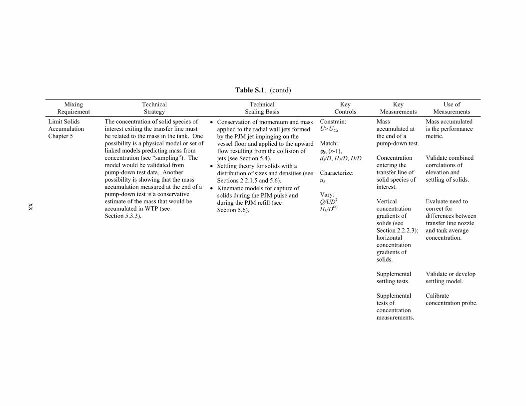
Limit Solids Accumulation Chapter 5

The concentration of solid species of interest exiting the transfer line must be related to the mass in the tank. One possibility is a physical model or set of linked models predicting mass from concentration (see “sampling”). The model would be validated from pump-down test data. Another possibility is showing that the mass accumulation measured at the end of a pump-down test is a conservative estimate of the mass that would be accumulated in WTP (see Section 5.3.3).

• Conservation of momentum and mass applied to the radial wall jets formed by the PJM jet impinging on the vessel floor and applied to the upward flow resulting from the collision of jets (see Section 5.4).

• Settling theory for solids with a distribution of sizes and densities (see Sections 2.2.1.5 and 5.6).

• Kinematic models for capture of solids during the PJM pulse and during the PJM refill (see Section 5.6).

Constrain: U>UCS Match: φS, (s-1), dJ/D, HT/D, H/D Characterize: uS Vary: Q/UD2 HL/D(a)

Mass accumulated at the end of a pump-down test. Concentration entering the transfer line of solid species of interest. Vertical concentration gradients of solids (see Section 2.2.2.3); horizontal concentration gradients of solids. Supplemental settling tests. Supplemental tests of concentration measurements.

Mass accumulated is the performance metric. Validate combined correlations of elevation and settling of solids. Evaluate need to correct for differences between transfer line nozzle and tank average concentration. Validate or develop settling model. Calibrate concentration probe.

xxi

Table S.1. (contd)

Mixing Requirement

Technical Strategy

Technical Scaling Basis

Key Controls

Key Measurements

Use of Measurements

Prevent Plugging Section 6.1

The governing factors identified for assessing the Prevent Plugging requirement are: • Line pressure drop, NPSHA at

pump, and solids deposition or accumulation in transfer line.

• Pump performance.

A conservative approach using reduced-scale testing is proposed for assessing plugging in the WTP transfer line as a result of the cyclical flow. The approach evaluates separately solids deposition and system pressure drop and requires the use of segregated portions of the test simulant based on the results obtained from the limit solids accumulation test and adoption of a no solids deposition requirement within the transfer line.

To assess the Prevent Plugging requirement, test data from the LSIT reduced-scale tests performed to address the Limit Solids Accumulation requirement can be used as the basis for the transfer line inlet feed (solids PSDD and concentration).

Pressure drop, solids deposition in transfer line (see also limit solids accumulation, which supports this testing). Concentration of solids in transfer line; solids makeup.

Compare results to industrial models for deposition in pipes, pump performance. Infer bounds on WTP performance from LSIT performance.

Blend Liquids Section 9.1

Blending can be characterized by adding a miscible liquid for which the concentration is conveniently measured at several locations in the vessel. The differences in concentration vs. time can be compared directly to the mixing requirement to determine the time at which a vessel is blended.

Turbulent mixing is described by mature theories, such as the “Corrsin time” related to the power dissipation rate. These can be formulated in terms of a dimensionless blend time.

Constrain: U>UCS Match: φS, (s-1), dJ/D, HT/D, H/D, UtC/D, DC, Q/UD2 Characterize: PSDD Vary as a test parameter: U

Dimensionless blend time

Blend time is the performance metric.

xxii

Table S.1. (contd)

Mixing Requirement

Technical Strategy

Technical Scaling Basis

Key Controls

Key Measurements

Use of Measurements

Sampling Chapter 10

The essential functional requirement for sampling is that “the PJM mixing system must mix the slurry to ensure a representative sample can be obtained.”(b) One strategy would be to ensure that the tank is homogeneously mixed, but the mixing is cyclic and the settling times of some particles can be short relative to the cycle time due to practical limitations on the mixing power available in WTP tanks. Homogeneous mixing probably is unattainable. Therefore, the technical strategy assumed here is relating the concentration in the transfer line, from which samples will be taken, to the mass of solid species of interest in the tank.

Settled solids are elevated depending on collisions of PJM jets on the tank floor and resulting negatively buoyant upward flow. The fraction of solids settling depends on the elevation of the solids, settling velocity, and any dispersion remaining from the PJM pulse. The conservation of momentum and self-similarity in free jets determine dimensionless groups as a basis for correlating these phenomena. The correlations can be combined to estimate the vertical concentration profile in a tank and relate the concentration at the inlet to the transfer line to the total mass in the tank. Then the sample “is representative” after correcting for the concentration profile.

Constrain: U>UCS Match: φS, (s-1), dJ/D, HT/D, H/D Characterize: uS Vary: Q/UD2 HL/D(a)

Concentration entering the transfer line of solid species of interest. Vertical concentration gradients of solids (see Section 2.2.2.3). Horizontal concentration gradients of solids. Supplemental settling tests. Supplemental tests of concentration measurements.

Part of the fundamental definition of “representative” sample. Validate combined correlations of elevation and settling of solids. Evaluate need to correct for differences between transfer line nozzle and tank average concentration. Validate or develop settling model. Calibrate concentration probes.

(a) HL is height of the liquid in the tank. (b) Mauss J and I Papp. 2010. Determination of Mixing Requirements for Pulse-Jet-Mixed Vessels in the Waste Treatment Plant. 24590-WTP-RPT-ES-ENG-09-001,

Rev. 2, Table 2, p. 22, Bechtel National, Inc., Richland, Washington.

xxiii

Acknowledgements

PNNL would like to recognize the following individuals for their expert contributions to this document. Special acknowledgment is noted for Professor Sanjoy Banerjee of City College of New York and Professor Emeritus Graham Wallis of Dartmouth College who provided extensive analysis and insight regarding physical modeling and mixing.

Dr. David S. Dickey of MixTech, Inc., Dr. Art Etchells of DuPont, and Dr. Si Lee from Savannah River National Laboratory are recognized for their review of the approach and document.

PNNL would also like to thank the Expert Review Team for their review, comments, and valuable insights. This team consists of Dr. Loni Peurrung, Chair; Dr. Richard Calabrese, Dr. Richard Grenville, Erich Hansen, and Dr. Ramesh Hemrajani.

The authors would also like to recognize the following PNNL staff for their outstanding support in providing calculational support, computational confirmations, technical reviews and editorial support:

Ellen Baer Mona Champion Scott Cooley Cary Counts James Fort Elizabeth Golovich Kirsten Meier Kathy Neiderhiser Dave Payson Richard Pires Mark Stewart S Thomas Yokuda

xxv

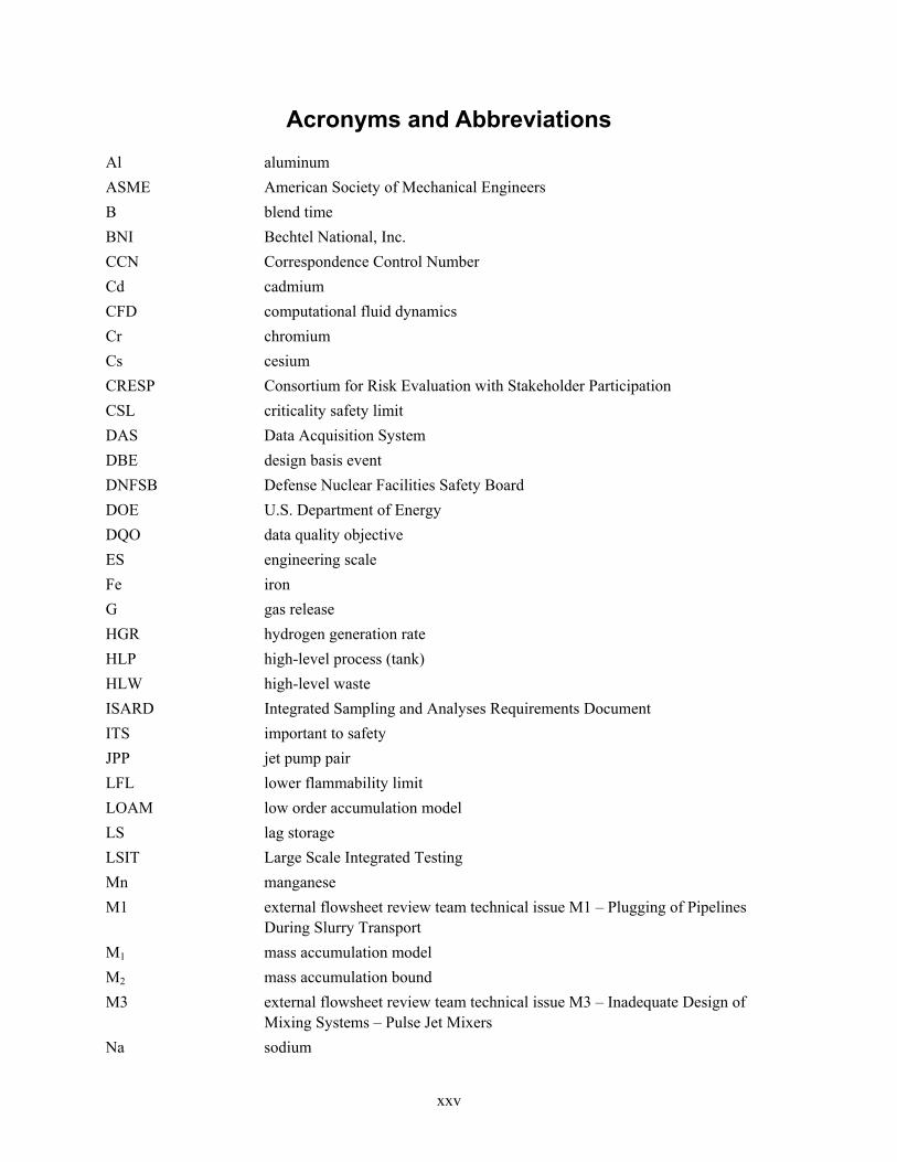
Acronyms and Abbreviations

Al aluminum

ASME American Society of Mechanical Engineers

B blend time

BNI Bechtel National, Inc.

CCN Correspondence Control Number

Cd cadmium

CFD computational fluid dynamics

Cr chromium

Cs cesium

CRESP Consortium for Risk Evaluation with Stakeholder Participation

CSL criticality safety limit

DAS Data Acquisition System

DBE design basis event

DNFSB Defense Nuclear Facilities Safety Board

DOE U.S. Department of Energy

DQO data quality objective

ES engineering scale

Fe iron

G gas release

HGR hydrogen generation rate

HLP high-level process (tank)

HLW high-level waste

ISARD Integrated Sampling and Analyses Requirements Document

ITS important to safety

JPP jet pump pair

LFL lower flammability limit

LOAM low order accumulation model

LS lag storage

LSIT Large Scale Integrated Testing

Mn manganese

M1 external flowsheet review team technical issue M1 – Plugging of Pipelines During Slurry Transport

M1 mass accumulation model

M2 mass accumulation bound

M3 external flowsheet review team technical issue M3 – Inadequate Design of Mixing Systems – Pulse Jet Mixers

Na sodium

xxvi

NaOH sodium hydroxide

Ni nickel

NPH natural phenomena hazard

NPSH net positive suction head

NPSHA net positive suction head available

NPSHR net positive suction head required

P plugging

PDSA Preliminary Documented Safety Analysis

PEP Pretreatment Engineering Platform

PETD Process Engineering & Technology Department

PJM pulse jet mixer

PNNL Pacific Northwest National Laboratory

PSD particle size distribution

PSDD particle size and density distribution

P/V power-per-unit volume

Pu plutonium

QA Quality Assurance

R&D research and development

RFD reverse flow diverter

RLD radioactive liquid-waste disposal (tank)

rms root mean square

ROB region of bubbles

S sampling

Sr strontium

ss steady state

SS-PJM small-scale pulse jet mixer

TBD to be determined

TLFL time to lower flammability limit

TSG technical steering group

U uranium

UDS undissolved solids

UFP ultrafiltration process (tank)

ULD Unit Liter Dose

vol% volume percent

wt% weight percent

WTP Hanford Waste Treatment and Immobilization Plant

WTPSP Waste Treatment Plant Support Project

ZOI zone of influence

xxvii

Symbols

A area; cross-sectional area of vessel influenced by sparge gas

Ai surface area of the interface

Anoz cross-sectional area of each orifice

Ap area of particle

Ar particle Archimedes number

AROB area of region of bubbles

AZOI area of zone of influence

a1, a2 exponents

b0 characteristic length of fountain jet source such as a radius for a circular jet or width for a plane jet; characteristic fountain thickness

C model coefficient

CD drag coefficient

CD(Rep) correlation of drag coefficient in terms of particle Reynolds number

CE erosion coefficient

CK correction for contraction of jet as it exited nozzle

CRES adjustable coefficient that is a property of the sediment type

Cμ, C1, C2 model coefficients

CI constant from inertial approach to calculate applied stress

CII constant from shear stress approach to calculate applied stress

D diameter of tank or vessel

d jet diameter, nozzle diameter

DC duty cycle = tD/tC

De effective hydrodynamic dispersion coefficient

dJ jet diameter

Dnoz diameter of each orifice

Dnoz,ES diameter of each orifice in the engineering-scale vessel

Dnoz,WTP diameter of each orifice in the WTP vessel

dS particle diameter or size, solids diameter

DT diameter of transfer line

DWTP diameter of WTP vessel

d50 diameter above which 50% of particles by weight lie

%d average absolute value for % deviation

E erodibility coefficient

F fraction of particles with sizes greater than some specified value

f friction factor for pipe flow; function

Fr Froude number: ratio of inertial to gravitational stresses

xxviii

Frp particle Froude number

FrT tube or pipe Froude number

F(δ, s) cumulative probability that particles will have attributes less than specified values

f(φS) function correcting for hindered settling FU fissile uranium FU/U fissile uranium to total uranium ratio

g gravitational acceleration, function

g′ reduced gravity

H PJM nozzle offset from vessel floor; distance of the source jet to the wall; depth of sparger nozzle below surface

HCAV correlation for cavern height

hS height of solids

Hsl slurry fill level

HT height of transfer line inlet above tank bottom measured directly below inlet

HWTP height of transfer line inlet above tank bottom measured directly below inlet in WTP vessel

I0 zeroth moment of the vertical distribution of solids loading which is the total volume of solids per horizontal area

I1 first moment of the vertical distribution of solids loading

K kinematic momentum flow at the jet nozzle

k kinetic energy

k dimensionless kinetic energy

Kc kinematic momentum flow at the limit of bottom clearing

kτ constant

K0 kinematic momentum flow rate at the jet nozzle

k0 initial condition of kinetic energy; ratio of distance from nozzle to nozzle diameter

0k initial condition of dimensionless kinetic energy

L characteristic length scale

lK Kolmogorov length scale

Kl dimensionless Kolmogorov length scale

mi mass of species i in the tank

mliquid mass of liquid

msolids mass of solids

N number of particles with sizes and densities less than a specified value, number of particle groups

n scaling exponent; number of independent variables, constituents

xxix

NJ number of PJMs or operating jets

nnoz number of nozzles

nnoz,ES number of nozzles in the engineering-scale vessel

nnoz,WTP number of nozzles in the WTP vessel

N0 total number of particles of all sizes and densities per volume of slurry

P piezometric pressure (pressure relative to hydrostatic pressure); total length of linear fountain segments located halfway between adjacent pulse tubes

P dimensionless pressure

P’ fluctuating turbulent component of pressure

Pa ambient pressure

PbV bubble power

Pstd total standard reference condition for atmospheric pressure, 1.0 atm

Q volumetric flow rate in the transfer line, total volumetric flow rate of sparge gas through the area

qa volume flux per unit length

Qstd total standard air flow rate

Qstd,ES total standard air flow rate in the engineering-scale vessel

Qstd,WTP total standard air flow rate in the WTP vessel

QT volumetric flow rate through suction line inlet, transfer line

qz fountain volume flux

zQΔ average sparge air volumetric flow rate integrated over sparged depth

Q0 total actual flow rate of purge gas at nozzle depth; time-averaged rate of addition of volume-averaged over pump-out cycles

Q0,ES total actual flow rate of purge gas at nozzle depth in the engineering-scale vessel

Q0, WTP total actual flow rate of purge gas at nozzle depth in the WTP vessel

r radius from the impingement of a radial wall jet; radial distance from jet centerline, clearing radius

r position vector

Re Reynolds number: ratio of inertial to viscous forces

Rec critical stress Reynolds number

Rep particle Reynolds number

Re0 yield Reynolds number

rmax maximum radius (halfway between adjacent jet centerlines)

S geometric scale factor, ratio of full scale to test length scale

s density ratio, ratio of particle density to liquid density, ρs/ρl; ratio of particle density to fluid density ρs/ρF

s particle volume weighted density ratio

SE rate of sediment surface erosion

xxx

T, t time

t dimensionless time

tC cycle time

Ct dimensionless cycle time

tD drive time

tdispersion duration of hydrodynamic dispersion

tK Kolmogorov time scale

Kt dimensionless Kolmogorov time scale

tmix Corrsin mixing time

mixt dimensionless Corrsin mixing time

tRES time for residual clearing

tS settling time

tsp characteristic sparger time

Tstd standard reference condition for temperature, 25°C

t0 characteristic decay time

t1 time constant that scales as length squared

t2 time constant that scales linearly with length scale

t12 time constant for events 1 and 2

U characteristic velocity, PJM velocity, maximum local velocity

u jet velocity

u velocity vector

u dimensionless velocity vector

u volume-averaged settling velocity

u′ turbulent component of velocity

u0 unhindered settling velocity 0u particle volume average unhindered settling velocity

Ucd critical pipe velocity for solids deposition

Ucd-WTP critical deposition velocity for WTP obtained from model

UCS critical suspension velocity

UD-WTP specified WTP design velocity for the transfer line of the vessel being evaluated

uerosion erosion velocity of a settled layer, the rate of decrease of the thickness of the layer

UF characteristic fountain jet velocity; velocity of carrier fluid

Uh hindered settling velocity for solids

uJ nozzle velocity

Um mean jet velocity; volumetric average velocity within the pipe, the volumetric average slurry velocity

xxxi

unoz effective average nozzle velocity

unoz,ES effective average nozzle velocity in the engineering-scale vessel

unoz,WTP effective average nozzle velocity in the WTP vessel

UPA peak average velocity

Ur relative or slip velocity between the fluid and solids

Ur0 dimensionless single-particle slip velocity

US steady jet velocity; velocity of solid particles

uS settling velocity 0Su settling velocity of the solid particle relative to the surrounding fluid for the

limiting case of vanishing solids concentration in the fluid

UT terminal (unhindered) settling velocity

U(t) charted instantaneous velocity *zU sparge gas superficial velocity at elevation z

uZOI erosion velocity, rate of change if clearing radius with respect to time

( , )u z t settling velocity of the distribution of particles at some elevation and time,

expressed as the ratio of volume weighted flux to the total particle volume fraction

u(δ,s) hindered settling velocity of a given particle size and density ratio

u0(δ,s) unhindered settling velocity of a given particle size and density ratio *

zUΔ integrated average superficial velocity

uτ velocity at infinite deformation rate

U0 nozzle velocity

U* velocity used for applying to models to assess WTP conditions, it is the greater of Ucd-WTP or UD-WTP; sparge gas superficial velocity

u* a material property of the settled waste in the form of a velocity

u∞ steady-state velocity far from the object

V volume of liquid in the tank, volume of slurry

Vp volume of the particle

VS volume of solids

Vsl volume of slurry

V0 volume of slurry with solids mass concentration 0iρ

V pump-out flow rate

SV volume weighted volume flux

X setpoint used by DAS, a threshold velocity for distinguishing assumed zero flow from pulse flow

XΔP dimensionless solids contribution to pressure drop resulting from solids flow

xxxii

XΔP0 dimensionless solids contribution to pressure drop for solids concentration <0.25

x(δ,s) volume fraction of solid volume of a given particle size and density ratio

xh hindered settling factor

xi fraction of total particle volume due to the specified particle

za top elevation of the slurry region

zm maximum penetration height

zS height of uniform distribution, vertical extent of solids distribution

z0 height of hypothetical uniform vertical profile of solids

z1 characteristic vertical length scale

z relative interface elevation

0z relative interface elevation at time t=0.

xxxiii

Greek Symbols α scale factor

αij empirical powers; scale factor of performance metric i

β set of geometric ratios describing the shape of the boundary γ magnitude of rate of deformation tensor; coefficient of spreading of radial wall

jet; coefficient of spreading of a radial wall jet

γNewtonian shear rate for a Newtonian fluid

δ thickness of an impinging radial wall jet; sediment thickness; specified particle size

Δmi mass of species i transferred out of the tank accumulateimΔ mass accumulation during the cycle

ΔP pressure drop

ΔPF pressure drop of the fluid component, the continuous phase

ΔPm pressure drop of the total slurry

ΔPS pressure drop of the solid constituents, the individual particles

Δρ density difference

δmin smallest particle with settling velocity of concern

δS thickness of waste to be eroded

ε dissipation rate per mass (proportional to power per volume)

ε dimensionless dissipation rate

ε0 initial condition of dissipation rate

0ε initial condition of dimensionless dissipation rate

η micro-length scale or Kolmogorov micro-scale of turbulence; consistency

θ dimensionless dissipation rate

θc ratio of characteristic settling distance to characteristic length scale

θS dimensionless group related to particle suspension that affects ability to clear solids from bottom of the vessel

μ fluid dynamic viscosity; consistency index of Bingham plastic

μF fluid viscosity

μm slurry viscosity (viscosity of total mixture)

μ0 effective Newtonian viscosity at infinite deformation rate ν kinematic viscosity

νt turbulent kinematic viscosity

ν0 kinematic viscosity at infinite deformation rate

ρ slurry density

ρF fluid density

xxxiv

nozzleiρ density of fluid entering suction nozzle Piρ concentration at the inlet to the transfer line

0iρ solids mass concentration entering the tank

iρ average concentration in the tank

ρl liquid density

ρmix slurry mixture density

ρs solids density

σ model coefficient; fraction of the velocity in the jet at its front edge; material property (work/area) similar to surface tension acting over the area of the particle

σε, σΚ model coefficients

τ stress (or magnitude of stress tensor), force per area applied to particles

τc critical stress for eroding a settled solids layer; critical wall shear stress

cτ dimensionless critical stress for eroding a settled solids layer

τn applied normal stress

τw wall shear stress

τ0 yield stress of a Bingham fluid

φ solids volume fraction – quantitative response of a measurement probe to the

solids volume fraction

φb solids volume fraction at bottom

φE solids volume fraction in the entraining fluid

φi volume fractions of solid “i”; peak individual constituent concentration

φimax maximum concentration of species “i”

φS volume fraction of solids in the fluid volume; total solids volume fraction in slurry (VS/V); peak bulk solids concentration

φSmax peak solids concentration corresponding to peak bulk density

φS0 characteristic volume fraction; nominal solids volume fraction of the total waste slurry

φS(z) vertical distribution of solids volume fraction

φ0 solids volume fraction in settled layer or in vortices after entraining solids from tank floor

χ differential probability distribution

χ(δ,s,z,t) differential probability distribution, a function of particle size, density ratio, elevation and time

χi coefficients for Equations (6.3) and (6.4)

∇ gradient

∇ dimensionless gradient

xxxv

Contents

Preface .................................................................................................................................................. iii Executive Summary .............................................................................................................................. xi Acknowledgements ............................................................................................................................... xxiii Acronyms and Abbreviations ............................................................................................................... xxv Symbols ................................................................................................................................................ xxvii Greek Symbols ...................................................................................................................................... xxxiii 1.0 Introduction ................................................................................................................................. 1.1

1.1 Organization and Use of This Document ....................................................................... 1.1 1.2 Purpose and Scope ......................................................................................................... 1.2 1.3 Acknowledgements ........................................................................................................ 1.3 1.4 Background .................................................................................................................... 1.4 1.5 Vessel and Testing Mixing Requirements ..................................................................... 1.5 1.6 “Three Dimensions” of LSIT ......................................................................................... 1.7

2.0 Technical Challenges and Resources .......................................................................................... 2.1 2.1 Technical Challenges ..................................................................................................... 2.1

2.1.1 Physical Complexity of the PJM Mixing Cycle ............................................ 2.1 2.1.1.1 Initial Layer of Solids .......................................................................... 2.2 2.1.1.2 Radial Wall Jets ................................................................................... 2.2 2.1.1.3 Collision of Radial Wall Jets ............................................................... 2.3 2.1.1.4 Turbulent Entrainment of Solids .......................................................... 2.4 2.1.1.5 Upward Flow from Collisions .............................................................. 2.5 2.1.1.6 Limit to Upward Suspension of Solids ................................................ 2.5 2.1.1.7 Density-Driven Oscillations ................................................................. 2.5 2.1.1.8 Settling ................................................................................................. 2.6 2.1.1.9 Capture into the Suction Nozzle .......................................................... 2.6 2.1.1.10 Combined Cycle ................................................................................... 2.7

2.1.2 Effect of Yield Stress on Shear Rate .............................................................. 2.8 2.1.3 Extrapolation over Length Scale .................................................................... 2.10 2.1.4 Uncertainty .................................................................................................... 2.11

2.2 Resources ....................................................................................................................... 2.13 2.2.1 Fundamentals ................................................................................................. 2.13

2.2.1.1 Dimensionless Conservation of Mass and of Momentum in a Liquid ................................................................................................... 2.13

2.2.1.2 Similitude and Dimensional Analysis .................................................. 2.15 2.2.1.3 Submerged Jets .................................................................................... 2.17 2.2.1.4 Turbulence ........................................................................................... 2.18 2.2.1.5 Sedimentation ...................................................................................... 2.22

xxxvi

2.2.2 Physical Models ............................................................................................. 2.24 2.2.2.1 Erosion ................................................................................................. 2.24 2.2.2.2 Clearing Velocity ................................................................................. 2.26 2.2.2.3 Integral Height of Vertical Concentration Profiles .............................. 2.29 2.2.2.4 Upward Flow ....................................................................................... 2.30

2.2.3 M3 Data ......................................................................................................... 2.31 2.2.3.1 Bottom Clearing Velocity .................................................................... 2.31 2.2.3.2 Observations of Concentration Profiles and “Cloud Height” .............. 2.33

2.2.4 Considering the Effect of Yield Stress on Bottom Clearing .......................... 2.36 3.0 Technical Approach .................................................................................................................... 3.1

3.1 Scaling Process .............................................................................................................. 3.1 3.1.1 Scaling Down ................................................................................................. 3.1 3.1.2 Scaling Up ..................................................................................................... 3.2 3.1.3 Scaling Down Sparging in Tanks Designed for Non-Newtonian Fluids ....... 3.2

3.2 Scaling Approaches ........................................................................................................ 3.3 3.2.1 Pure Similitude .............................................................................................. 3.3 3.2.2 Pure Statistics ................................................................................................. 3.3 3.2.3 Pure Physics ................................................................................................... 3.4

3.3 Programmatic Tradeoffs and Optimization of Certainty ................................................ 3.4 3.4 Implementation of Scaling Approaches ......................................................................... 3.7

3.4.1 Scaling Approaches for Specific Mixing Requirements ................................ 3.7 3.4.2 Recommendations About LSIT Testing to Facilitate Scaling Up to

WTP Performance .......................................................................................... 3.11 3.4.3 Recommended Measurements ....................................................................... 3.13

4.0 Gas Retention .............................................................................................................................. 4.1 4.1 Gas Release Requirements ............................................................................................. 4.1

4.1.1 Gas Release – Normal Operations ................................................................. 4.2 4.1.2 Gas Release – Design Basis Event ................................................................ 4.3

4.2 Bottom Motion Scaling .................................................................................................. 4.5 4.2.1 Clearing Velocity Analysis ............................................................................ 4.6

4.2.1.1 Radial Clearing Region ........................................................................ 4.7 4.2.1.2 Residual Clearing Region .................................................................... 4.7

4.2.2 Transient Clearing Analysis ........................................................................... 4.10 4.2.2.1 Transient Clearing Analysis – Radial Clearing .................................... 4.10 4.2.2.2 Transient Clearing Analysis – Residual Bottom Motion ..................... 4.11

4.2.3 Non-Newtonian Fluid in a Newtonian Vessel ............................................... 4.11 4.2.4 Non-Newtonian Fluid in a Non-Newtonian Vessel ....................................... 4.12

4.3 Concepts for Testing ...................................................................................................... 4.13 4.4 Conclusions .................................................................................................................... 4.15

xxxvii

5.0 Technical Basis for Scaling Performance Metrics for the Limit Solids Accumulation Requirement ................................................................................................................................ 5.1 5.1 Introduction .................................................................................................................... 5.1 5.2 Requisite Measurements, Data Interpretation, and Evaluation Against Mixing

Requirements ................................................................................................................. 5.1 5.3 Overall Mass Balance Model ......................................................................................... 5.3

5.3.1 Available Information .................................................................................... 5.4 5.3.2 Analysis ......................................................................................................... 5.5 5.3.3 Potential for a Bounding Test ........................................................................ 5.7 5.3.4 Additional Considerations for Tanks Processing Non-Newtonian Fluids ..... 5.7

5.4 Suspension of Solids from Collision of Radial Jets ....................................................... 5.8 5.4.1 Available Information .................................................................................... 5.8 5.4.2 Physically Based Model ................................................................................. 5.8 5.4.3 Application to M3 Experimental Data ........................................................... 5.9

5.5 Application to LSIT ....................................................................................................... 5.11 5.5.1 Scaling Parameters Inferred from a Physical Model ..................................... 5.11 5.5.2 Data Reduction .............................................................................................. 5.12 5.5.3 Predicting Concentration versus Depth Using a Settling Model ................... 5.12

5.6 Capture of Settled and Settling Solids by the Suction Nozzle ....................................... 5.13 5.7 Concepts for Testing ...................................................................................................... 5.15

6.0 Transfer and Pump Out ............................................................................................................... 6.1 6.1 Transfer and Pump-Out Requirements Relative to PJM Mixing Requirements ............ 6.2 6.2 WTP Operations and Transfer Line Plugging Mechanisms Associated with the

Prevent Plugging Requirement ...................................................................................... 6.3 6.3 Approach for Assessing Pipe Plugging in WTP Vessel Transfer Lines ........................ 6.9

6.3.1 Obtaining Non-Steady-State Conditions from LSIT ..................................... 6.12 6.3.2 Obtaining Bounding Steady-State Conditions from LSIT Results ................ 6.14 6.3.3 Benchmarking of Predictive Models ............................................................. 6.16 6.3.4 Assessing WTP Performance ......................................................................... 6.17

6.4 Evaluation of Individual Failure Mechanisms ............................................................... 6.18 6.4.1 Evaluation of Plugging Due to Solids Deposition ......................................... 6.18 6.4.2 Evaluation of System Pressure Drop ............................................................. 6.21

6.4.2.1 Methodology for Determination of Pressure Drop for Multi-Constituent Slurry ................................................................................ 6.22

6.4.3 Evaluation of NPSH....................................................................................... 6.26 6.4.4 Assessment of Pump Performance................................................................. 6.27

6.5 Summary and Recommendations ................................................................................... 6.27

xxxviii

7.0 Air Spargers ................................................................................................................................ 7.1 7.1 Steam Ring and Purge Air System Design in the WTP UFP-01 Vessel ........................ 7.1 7.2 Scaling Down Steam Ring Purge Air Flow Rates for LSIT........................................... 7.3

7.2.1 General Considerations and Approach .......................................................... 7.3 7.2.2 Recommendations for Steam Ring Purge Air Flow Rates in LSIT ............... 7.5

7.2.2.1 Assumptions for LSIT ES Vessel Steam Ring Scaling and Test Conditions ............................................................................................ 7.5

7.2.2.2 Specific Recommendations for Steam Ring Air Flow Rates in Bottom Motion Studies: Matching U* at Nozzle Depth ...................... 7.6

7.2.2.3 Specific Recommendations for Steam Ring Air Flow Rates in Blending Studies: Matching Bubble Power-Per-Unit Volume ........... 7.7

7.3 LSIT ES UFP-01 Vessel Steam Ring Design ................................................................ 7.8 8.0 Observing Critical Suspension Velocity, UCS, and Bottom Motion ............................................ 8.1

8.1 Protocols for Observing UCS .......................................................................................... 8.1 8.2 Definition of Bottom Motion ......................................................................................... 8.4

9.0 Blending/Neutralization .............................................................................................................. 9.1 9.1 Blending Requirements .................................................................................................. 9.1 9.2 Approach for Newtonian Vessels ................................................................................... 9.2 9.3 Concepts for Testing ...................................................................................................... 9.6 9.4 Air Sparger and Steam Ring Purge Air Scaling for Blending ........................................ 9.7

9.4.1 Background – Previous Experimental Studies of Air Spargers ..................... 9.7 9.4.2 Calculated Circulation Times and Sparge Air Flow Rate Scaling ................. 9.9 9.4.3 Summary and Recommendations for Steam Ring Purge Air Operations

in UFP-01 Blending Studies .......................................................................... 9.11 10.0 Sampling ..................................................................................................................................... 10.1

10.1 Sampling Requirements Related to Mixing ................................................................... 10.1 10.2 Presentation of Sampling Problem ................................................................................. 10.4

10.2.1 Measuring Separable Plutonium .................................................................... 10.7 10.2.2 Assumptions Applied to Evaluation of Sampling .......................................... 10.10

10.3 Potential Approaches for Predicting Contents of Vessels from Line Samples .............. 10.11 10.3.1 WTP Slurry Solids Constituents and Potential Methods of Predicting

Concentration ................................................................................................. 10.12 10.3.2 Generalities Applicable to All Predictive Methods ....................................... 10.13 10.3.3 Dynamic Sampling ........................................................................................ 10.14 10.3.4 Bounding Sampling ....................................................................................... 10.15 10.3.5 Physical Modeling Based on Sample Characterization ................................. 10.16

10.4 Application of Approach to Assess Mixing Requirements ............................................ 10.17 10.4.1 Quiescent Settling .......................................................................................... 10.20 10.4.2 Pulsed Settling ............................................................................................... 10.21 10.4.3 Evaluate Transfer Line Sampling for LSIT ................................................... 10.21

xxxix

10.4.4 Integrated Sampling Methodology ................................................................ 10.23 10.4.5 Test Setup Needs ........................................................................................... 10.24 10.4.6 Simulant Needs .............................................................................................. 10.25

10.5 Conclusions, Recommendations, and Issues .................................................................. 10.25 11.0 Conclusions ................................................................................................................................. 11.1

11.1 Metrics ........................................................................................................................... 11.1 11.1.1 Mix to Release Gas ........................................................................................ 11.1 11.1.2 Blend Liquids ................................................................................................. 11.1 11.1.3 Limit Solids Accumulation ............................................................................ 11.1 11.1.4 Sampling ........................................................................................................ 11.2 11.1.5 Prevent Plugging ............................................................................................ 11.2

11.2 Scale-Down .................................................................................................................... 11.2 11.2.1 Mix to Release Gas ........................................................................................ 11.3 11.2.2 Blend Liquids ................................................................................................. 11.3 11.2.3 Limit Solids Accumulation ............................................................................ 11.3 11.2.4 Sampling ........................................................................................................ 11.4 11.2.5 Prevent Plugging ............................................................................................ 11.4

11.3 Testing ............................................................................................................................ 11.4 11.3.1 Mix to Release Gas ........................................................................................ 11.5 11.3.2 Blend Liquids ................................................................................................. 11.5 11.3.3 Limit Solids Accumulation ............................................................................ 11.5 11.3.4 Sampling ........................................................................................................ 11.5 11.3.5 Prevent Plugging ............................................................................................ 11.5

11.4 Measurements ................................................................................................................ 11.5 11.4.1 Mix to Release Gas ........................................................................................ 11.6 11.4.2 Blend Liquids ................................................................................................. 11.6 11.4.3 Limit Solids Accumulation ............................................................................ 11.6 11.4.4 Sampling ........................................................................................................ 11.6 11.4.5 Prevent Plugging ............................................................................................ 11.6

11.5 Analysis .......................................................................................................................... 11.6 11.5.1 Mix to Release Gas ........................................................................................ 11.6 11.5.2 Blend Liquids ................................................................................................. 11.7 11.5.3 Limit Solids Accumulation ............................................................................ 11.7 11.5.4 Sampling ........................................................................................................ 11.7 11.5.5 Prevent Plugging ............................................................................................ 11.7

11.6 Scale-Up ......................................................................................................................... 11.7 11.6.1 Mix to Release Gas ........................................................................................ 11.7 11.6.2 Blend Liquids ................................................................................................. 11.7 11.6.3 Limit Solids Accumulation ............................................................................ 11.7

xl

11.6.4 Sampling ........................................................................................................ 11.8 11.6.5 Prevent Plugging ............................................................................................ 11.8

11.7 Scaling of Sparger Operations ....................................................................................... 11.8 11.8 Summary of Technical Strategies .................................................................................. 11.9

12.0 References ................................................................................................................................... 12.1 Appendix A – Selected Technical Background .................................................................................... A.1 Appendix B – Working Paper for the Technical Basis for Scaling of Bottom Motion ........................ B.1 Appendix C – Working Paper for the Technical Basis for Scaling Transfer and Pump Out ................ C.1 Appendix D – Working Paper for Sparger Operations ......................................................................... D.1 Appendix E – Working Paper for the Technical Basis to Assess the Prevent Plugging

Requirement Associated with Pump Out....................................................................... E.1

xli

Figures

1.1 Depiction of Implementation of LSIT in the Three Dimensions of Problems, Approaches, and Process ............................................................................................................ 1.8

2.1 Single PJM Mixing Cycle .......................................................................................................... 2.2 2.2 Depiction of a Generic Power-Law Correlation Where a Single Performance Metric is

Correlated Against the Ratio of the Test Length Scale to Full Scale ......................................... 2.12 2.3 Plot of Drag Force versus Product of Size of Sphere and Velocity of Fluid .............................. 2.12

2.4 Comparison of Measured and Fitted Values of K at the Limit of the Bottom Clearing from M3 Experiments Where the Settling Distance Did Not Exceed the Cloud Height ............ 2.33

2.5 Solids Volume Fraction versus Time During a PJM Cycle at Various Depths for Test 70E_6s1d2Vc_2 .................................................................................................................. 2.35

2.6 Solids Volume Fraction versus Time During a PJM Cycle at Various Depths for Test 34S_4s1d2Yd_1 .................................................................................................................. 2.36

2.7 Plot of g(θ) as a Function of θ .................................................................................................... 2.38 3.1 Scaling Approach Space ............................................................................................................. 3.5 3.2 Tradeoffs Among Scaling Approaches ....................................................................................... 3.5 3.3 Relative Emphasis of Scaling Approach for Mixing Requirements ........................................... 3.10 4.1 Residual Sediment Regions During the Second Phase of Transient Clearing ............................ 4.6 5.1 Density Variation in Transfer Line During Single PJM Pulse ................................................... 5.5 5.2 Density Variation in Transfer Line Over Multiple PJM Cycles ................................................. 5.5 5.3 Reduction of M3 Data on Cloud Height, Based on a Momentum Balance Described in

Appendix C, Section C.4.1 ......................................................................................................... 5.10 5.4 Illustrative Shapes of Volumes in Which Particles are Captured by a Suction Nozzle .............. 5.14 6.1 Schematic Depicting WTP Vessel Mixing and Transfer Line Inlet Flow .................................. 6.4 6.2 Instantaneous Slurry Density in Transfer Line versus Time During LOAM Test 1 Pump

Out .............................................................................................................................................. 6.7 6.3 Schematic Depicting Particle Segregation That Can Occur Because of Variation in

Particle Concentration at the Transfer Line Inlet ....................................................................... 6.8 6.4 High-Level Steps Applied to Each Plugging Mechanism Being Assessed for the

Prevent Plugging Requirement ................................................................................................... 6.10 6.5 Logic Diagram for Steady-State Testing to Benchmark Models ................................................ 6.11 6.6 Flowchart of Integrated Tasks Used to Assess the Prevent Plugging Requirement ................... 6.12 8.1 Illustration of Nozzle Velocity as a Function of Time for Several Discharge Cycles ................ 8.3 9.1 Illustration of Flow Patterns and Boundaries for a Single Air Sparge Tube .............................. 9.9 10.1 Transfer Line Specific Gravity versus Time for a Reduced-Scale Test First-Quarter-

Batch Pump Out ......................................................................................................................... 10.7 10.2 Technical Strategy ...................................................................................................................... 10.19 10.3 Application of Approach ............................................................................................................ 10.19 10.4 Quiescent Settling ....................................................................................................................... 10.20 10.5 Pulsed Settling ............................................................................................................................ 10.22

xlii

10.6 Evaluating Transfer Line Sampling for LSIT ............................................................................. 10.23 10.7 Assessment of Integrated Sampling Methodology ..................................................................... 10.24

Tables

S.1 Summary of Recommended Technical Approach ......................................................................... xxiii

2.1 Scaling Parameters Deduced in Section 2.2 ............................................................................... 2.14 2.2 Scale Factors Predicted for Parameters Affecting the Bottom Clearing Velocity,

Assuming No Variation in the Critical Erosion Stress ............................................................... 2.29 2.3 Correlation Coefficients Among the Independent Variables ...................................................... 2.32 2.4 Values of Model Coefficients Fitted to “M3” Bottom Clearing Velocity Data ......................... 2.32 3.1 Problems with “Pure” Approaches to Scaling Performance Metrics ......................................... 3.4 3.2 Technical Approaches for Scaling by Mixing Requirement ...................................................... 3.9 3.3 Testing Measurements ................................................................................................................ 3.14 4.1 Velocity Scaling Exponents for UCS ........................................................................................... 4.9 4.2 Summary of Simulant Property Ranges Recommended for LSIT ............................................. 4.14 5.1 Technical Bases for Scaling for the Limit Solids Accumulation Requirement .......................... 5.2 6.1 Target Vessel Pump Design Limits for Newtonian Scaled Testing ........................................... 6.3 6.2 Coefficient and Exponent Values for Oroskar and Turian and Turian et al. Models

Predicting Critical Velocity for Solids Deposition Presented in Equations (6.3) and (6.4) ....... 6.20 8.1 Pattern of Cleared Region Viewed from Beneath the Tank ....................................................... 8.2 8.2 Particle Motion Descriptors for Visual Observations ................................................................. 8.3 9.1 Requirements 3/4 Blending/Neutralization Liquids Requirements ............................................ 9.1 9.2 Experimental and Calculated Circulation Times and Velocities for a Single Air Sparger ......... 9.8 10.1 Samples from Target Vessels—HLP-22, UFP-01, UFP-02, and RLD-08 ................................. 10.3 11.1 Summary of Technical Strategies for Complying with the Mix to Release Gas, Prevent

Plugging, Limit Solids Accumulation, Blend Liquids, and Sampling Mixing Requirements .............................................................................................................................. 11.10

1.1

1.0 Introduction

1.1 Organization and Use of This Document

This document is organized into three sets of related chapters. Chapters 1, 2, and 3 present the introduction, technical challenges and resources, and technical approach, respectively, for large scale integrated testing of pulse jet mixing systems. Technical issues related to specific requirements are presented in Chapters 4 through 10, and our conclusions are presented in Chapter 11. In addition, there are five technical appendices (Appendices A through E) that provide background, technical development and analysis of Large Scale Integrated Test (LSIT) data as experimentation proceeds.

The document is focused on scaling the performance measured in the LSIT to full-scale performance in the Hanford Waste Treatment and Immobilization Plant (WTP) relative specifically to mixing requirements defined by WTP for vessels employing pulse jet mixers (PJM), which are presented in Section 1.5. Existing knowledge pertinent to scaling PJM mixing phenomena is discussed in Chapter 2, including descriptions of technical challenges such as the complexity of the PJM mixing cycle, extrapolating over length scale, and estimating the uncertainty in predicting the performance of the complex mixing process. Chapter 2 also discusses technical concepts and resources, such as similitude and dimensional analysis, the nature of submerged jets, and observations from and analysis of pertinent results from past “M3” tests (see Section 2.2.3). Three “canonical” approaches to scaling data from reduced to full scale are discussed in Chapter 3 in the context of the commitment to provide a “technical basis for scaling” and of considering issues with extrapolating data over length scale and the uncertainty in the extrapolated performance. Chapter 3 culminates with recommendations about parameters defining LSIT tests, addressing in tests the specific mixing requirements and measurements required to enable extrapolation from LSIT to WTP.

The scaling recommendations (Section 3.4) in this document are intended to address the technical basis for scaling in terms of information needs and use of data, while technical decisions about the extent and organization of LSIT tests supporting actual tests plans will be provided in a complementary document that is described below. The recommendations made in this document are intended to provide technical guidance and rationale, while also maintaining flexibility for more detailed decisions about testing described in the complementary document.

Chapters 4 through 10 provide background and analyses that lead to recommendations about test parameters, controls, measurements, and scaling up from LSIT to WTP. The five technical appendices (Appendices A through E) are intended both to provide additional detail that supports the technical chapters and to ultimately form standalone “white papers” that are repositories of background, technical development, and analysis of LSIT data as experimentation proceeds. (Hence, there is some intentional redundancy between the appendices and the technical chapters.) Occasionally, these “white papers” can be rejoined and this document updated accordingly as the overall understanding of WTP needs and requirements and technical understanding of scaling issues improves based on LSIT data.

1.2

1.2 Purpose and Scope

Hanford’s WTP project will predict the mixing performance of full-scale vessels based on tests to be conducted in reduced-scale vessels, using equipment and facilities denoted as the LSIT. The purpose of this document is to provide a technical basis for “scaling” the LSIT results to predict performance in the WTP.

Essentially, this document addresses the following three questions:

1. Why and how can the mixing behaviors in a smaller vessel represent those in a larger vessel?

2. What information is required to answer the first question?

3. How should the information be used to predict mixing performance in WTP?

The design of LSIT tests is being addressed in other, complementary documents.

This document fulfills part of the U.S. Department of Energy’s (DOE’s) Implementation Plan (Chu 2011) responding to Recommendation 2010-2 of the Defense Nuclear Facilities Safety Board (DNFSB). The Implementation Plan specifies a set of documents that provide the technical basis for LSIT. Those documents focus on the following subject areas:

• Test objectives

• Construction specifications

• Test specifications

• Simulant basis documents

• Vessel configurations for testing.

As part of the set specified by the Implementation Plan, this document was developed 1) to define the basis for less-than-full-scale testing, including vessel configurations, operating parameters, and simulant parameters, and 2) to address the basis for scaling the various parameters (e.g., PJMs and vessel geometry, PJM discharge velocity, PJM nozzle diameter, pump suction line diameter, etc.) for the tests conducted in the program. The document addresses Commitment 5.1.3.13 in the Implementation Plan to provide an LSIT “technical scaling basis” for:

“… defining the basis for less-than-full-scale testing, including vessel configurations, operating parameters, and simulant parameters. The basis for scaling both vessel physical performance and simulant physical performance will be addressed. The scaling basis should address physical scale laws observed in test results” (i.e., scaling up) “and scale laws used to establish operating conditions for testing” (i.e., scaling down).

Complementary reports addressing Commitment 5.1.3.13 include the following.

• WTP is providing as a complement to this document a document focused on selecting scaling strategies and supporting development of test plans for specific vessels: DS Dickey, RB Daniel, PJ Keuhlen, RL Hanson, and JW Olson, 2012, Technical Scaling Selection Basis, 24590-WTP-RPT-PET-12-001, current revision, Bechtel National, Inc., Richland, Washington (Dickey et al. 2012).

1.3

• The technical basis for vessel sizing and array choices are provided in R Hanson and J Meehan, April 2012, Vessel Configuration for Large Scale Integrated Testing, 24590-WTP-RPT-ENG-12-017, Rev. 0, Bechtel National, Inc., Richland, Washington (Hanson and Meehan 2012). On June 12, 2012, WTP directed Pacific Northwest National Laboratory (PNNL) to “… make Newtonian and non-Newtonian Scaling Documents segregated parts,”1 which focused this document on only the scaling of tests of vessels designed to process suspended, nominally Newtonian2 slurries.

• Recommendations on simulant parameters are based on those recommended by DC Koopman, CJ Martino, and MR Poirier, April 2012, Properties Important to Mixing for WTP Large Scale Integrated Testing, SRNL-STI-2012-00062, Rev. 0, Savannah River National Laboratory, Aiken, South Carolina (Koopman et al. 2012). Their document establishes the key physical and chemical properties of Hanford waste simulants important to testing large scale PJM systems. The authors found that the most important properties for testing with Newtonian slurries are the Archimedes number distribution and particle concentration.

• Performance of WTP process vessels is defined in terms of nine mixing requirements, which are described in Section 1.5 of this report. These requirements determined the technical scope of this document, which is limited to addressing these requirements as specified by WTP. For each requirement, performance metrics are defined that can be measured quantitatively in LSIT tests and enable quantifying the performance and uncertainty in the performance predicted for full-scale operations. The requirements are documented by J Mauss and I Papp, 2010, Determination of Mixing Requirements for Pulse-Jet Mixed Vessels in the Waste Treatment Plant, 24590-WTP-ES-ENG-09-001, Rev. 2, Bechtel National, Inc., Richland, Washington (Mauss and Papp 2010). While the ultrafiltration process (UFP) PJM system UFP-VSL-00002A/B (hereafter referred to as UFP-02) is designed to mix both Newtonian and non-Newtonian wastes, it is not included in this document because it will be tested at full scale.

During the development of this document, Bechtel National, Inc. (BNI) requested that it include a discussion of alternative scaling approaches to provide some flexibility in decisions based on specific process and equipment issues outside the scope of this document. Accordingly, this document identifies alternative scaling approaches and discusses them in terms of advantages and disadvantages. A combination of these approaches is then recommended for consideration by BNI and may be included in a complementary Technical Scaling Selection Basis document (Dickey et al. 2012).

1.3 Acknowledgements

This work was led by PNNL with expert contributions and reviews provided by Professor Sanjoy Banerjee of City College of New York, Professor Emeritus Graham Wallis of Dartmouth College, Dr. David S. Dickey of MixTech Inc., Dr. Art Etchells of DuPont, and Dr. Si Lee of Savannah River National Laboratory. PNNL would also like to thank the Expert Review Team for their review, comments, and valuable insights. This team consists of Dr. Loni Peurrung, Chair; Dr. Richard Calabrese, Dr. Richard Grenville, Erich Hansen, and Dr. Ramesh Hemrajani. In the development of this scaling

1 E-mail from Haukur Hazen to Michael Minette, June 12, 2012, “MOA WA39 Support Work Prioritization of No Newtonian Deliverables Over Non-Newtonian Deliverables,” Bechtel National, Inc., Richland, Washington. 2 Newtonian slurries can develop a yield stress at sufficiently large solids concentrations.

1.4

document, PNNL engaged the team of national experts identified above. In addition, PNNL experts who worked on the project included Dr. William Kuhn (also a professor at Washington State University), Dr. David Rector, Dr. James Fort, Beric Wells, Dr. Scot Rassat, Carl Enderlin, Dr. Judith Bamberger, Gary Josephson, Eric Berglin, and Michael Minette.

1.4 Background

WTP is being designed and built to pretreat and vitrify a large portion of the waste stored in Hanford’s 177 underground waste storage tanks. Several process vessels will hold the waste at various processing stages. These vessels have the mixing1 system requirements needed to maintain conditions in which hydrogen gas accumulation remains below acceptable limits and mixing within the vessels is sufficient to ensure that pump transfer and normal operations occur reliably (Mauss and Papp 2010).

Some of the WTP process streams are slurries of solid particles suspended in Newtonian fluids that may behave as non-Newtonian slurries. The effects of large particles and rapidly settling slurries may affect mixing and the ability of the slurry to maintain particles in suspension.

WTP uses PJM technology for slurry mixing applications requiring solids suspension, solids mixing, fluid blending, and release of hydrogen gas. Compressed air is used as the motive force for jet pump pairs (JPPs) that drive PJMs. The suction phase draws process liquid into the PJM from the vessel. The drive phase pressurizes the PJMs via a JPP. This pressurization discharges the PJM liquid contents at high velocity into the vessel, causing mixing. The drive phase is followed by a vent phase that allows depressurization of the PJM by venting through the JPP into the pulse jet vent system. These three phases (i.e., suction, drive, and vent) make up the mixing cycle (see Section 2.1.1 for details).

DOE’s Office of River Protection has directed WTP to plan large scale integrated testing of selected WTP pulse jet mixed vessels. This testing will reduce risks associated with engineering, procurement, and construction of these vessel systems, and is considered to be necessary to complete system designs (CCN 229346, Morris 2010). In the course of test planning, WTP Engineering conducted a workshop to identify test objectives (CCN 225791, Papp 2011). Eight general objectives were identified in that workshop. These objectives have been incorporated in draft responses to DNFSB Recommendation 2010-2 (Chu 2011) and the latest drafts of the Integrated Pulse Jet Mixed Vessel Design and Control Strategy (24590-WTP-RPT-ENG-10-001, Rev. 1, Campbell 2011) and Test Objectives for Large Scale Testing (LST) for Increment I (24590-WTP-RTD-RT-10-0002, Rev. 1, Papp 2010c).

1 Mixing refers to mobilization and subsequent suspension of undissolved solids within a vessel. Mixing can have varying results: 1) a fully mixed vessel in which the solids concentration is uniform throughout the vessel, 2) a partially mixed vessel in which a solids concentration gradient exists with the concentration higher at the bottom of the vessel, or 3) a poorly mixed vessel in which solids are disturbed but remain on or near the bottom of the vessel.

1.5

Two of the eight LSIT objectives, 1) Performance and Scaled Testing and 2) Transfer and Pump-Out Testing, were adopted to reduce uncertainty in PJM mixing performance and transfer systems. Specifically, testing is to be conducted to determine the ability of the WTP mixing system to:

• Mobilize solids on the vessel bottom during normal operation

• Prevent batch-to-batch accumulation of solids (particularly fissile materials)

• Establish conditions for operating the PJM mixing system that are required after a design basis event (DBE)

• Establish process limits of the PJM mixing and transfer systems.

The general approach is to 1) select mixing systems that have the least operating margin to focus resources on the greatest need, 2) conduct mixing performance tests of those systems in three successively larger geometrically scaled test vessels to enable determining the effect of length-scale on performance, and 3) extrapolate observed performance to full-scale systems (see Hanson and Meehan 2012 for details).

The three test vessel sizes are to be 43 in., 8 ft, and 14 ft in diameter. The vessels that are 43 in. and 8 ft in diameter are existing vessels that are fabricated of clear acrylic to allow visual observation of mixing phenomena. The 14-ft-diameter vessel will be procured to support this and other large scale test needs, and will, at a minimum, allow visual observation of key regions of the vessel bottom to assess mixing performance.

Depending on process requirements, the PJMs can be operated in a continuous pulsing mode (e.g., all PJMs on during normal operation) or they can be turned off for a time and restarted in the pulsing mode (e.g., for some post-DBE scenarios, vessels that use the 50:50 PJM operation approach will only have half their PJMs operational for any drive pulse). In vessels that contain particulates, solids will settle to the bottom between mixing periods. When the PJMs restart, the settled solids must be resuspended.

1.5 Vessel and Testing Mixing Requirements

Vessel functions and mixing criteria/requirements were developed based on the functional requirements of the vessels listed in the Contract, System Descriptions, the Operations Requirements Document, and other technical baseline documents, and are documented in 24590-WTP-ES-ENG-09-001 (Mauss and Papp 2010). Mixing of the vessels was divided into four main operational functions (i.e., transfer, blend, sample, and store), and the design for mixing related to those functions was categorized into 10 requirements. The requirements are used to break down the mixing needs into more specific categories. These requirements, which are described below, are used to further define the mixing needs for the vessels.

Transfer

• Requirement 1 – Cool for Transfer (Process-related requirement)

Temperature control to support vessel cooling – For vessels that have a cooling or heating function, mixing is required to facilitate heat transfer. Specific temperature requirements are defined to quantify the degree to which temperature control should be maintained throughout the vessel. The WTP project will address Requirement 1 by engineering analysis so it is not discussed in this document.

1.6

• Requirement 2 – Prevent Plugging (Process-related requirement)

Characterizing solids concentration related to prevention of pump suction and line plugging - Requirements for avoiding solids concentrations near the suction intake of pumping devices (i.e., centrifugal pumps, reverse flow diverters [RFDs], and ejectors) are identified. These limits are related to the design viscosity and density limitations of each of the pumping devices, both to facilitate flow of solids to the intake and proper operation of the pumping device to maintain fluid transfer rates and avoid settling of solids in pipelines.

When solids in slurries settle, the solids concentration increases near the bottom of the vessel, thus increasing effective viscosity and density of the slurry. This requirement articulates that the PJM mixing system shall be capable of mixing the slurry sufficiently to prevent the effective viscosity and density of the slurry from exceeding design limits in the vicinity of the pump suction.

Blend

• Requirement 3 – Blend Liquids (Process-related requirement)

This requirement is provided to quantify acceptable deviations for the control of key process parameters and/or chemical constituents in the liquid phase of each vessel to support chemical reactions such as leaching.

• Requirement 4 – Neutralization (Process-related requirement)

The pH of the vessel contents is neutralized to minimize formation of precipitates, for process and corrosion, etc. The requirements related to this are, in some cases, included with blend liquids or sampling for process control.

Sample

• Requirement 5 – Criticality (Safety-related requirement)

This quantitative requirement is identified to define the type of sample to be taken and the required confidence level of the sample.

• Requirement 6 – Hydrogen Generation Rate (HGR) Estimation (Safety-related requirement)

This requirement is identified to indicate where confirmatory sampling of received waste is required.

• Requirement 7 – Process Control (Process-related requirement)

This quantitative requirement is identified to indicate control of key process parameters and/or constituents that are used to control each process or unit operation (e.g., pH, solids, radionuclides).

Store

• Requirement 8 – Mix to Release Gas (Safety-related requirement)

This requirement defines the degree of mixing (degree of solids mobilization) required to release flammable gas that is retained in settled solids layers or non-Newtonian fluid.

• Requirement 9 – De-minimis Solids (Safety-related requirement)

Requirement 10, Limit Solids Accumulation, has replaced this requirement.

1.7

• Requirement 10 – Limit Solids Accumulation (Safety-related requirement)

This requirement is applied to ensure that the mixing system is capable of preventing accumulation of solids from batch to batch.

WTP conducted engineering assessments for all 38 vessels that use PJM mixing to determine that the vessels met each requirement. A key tool used in the WTP assessments was the application of the Low Order Accumulation Model (LOAM) that was based on work by Poreh et al. (1967) and benchmarked to engineering-scale (ES) tests conducted on simulated waste in a 43-in. diameter vessel. Several review bodies including DNFSB and Consortium for Risk Evaluation with Stakeholder Participation (CRESP) challenged that the technical basis of LOAM was inadequate to extrapolate over such a range. Following is a summary of findings from the CRESP review (Kosson et al. 2010).

“There are several important PJM vessel design uncertainties and definitions of operating requirements that remain to be resolved, including revision of the criticality controls, validation of scale-up relationships for PJM zone of influence, integrated validation of vessel performance, recovery from a DBE, and viable sampling strategies, that result in PJM vessel performance and programmatic risks. The greatest risk is that the actual zone of influence (ZOI) during WTP operations is smaller than predicted by the current design basis and therefore solids accumulation may require more frequent cleanout than predicted. Experimental programs that validate scaling relationships for the ZOI and the integrated vessel performance at full scale or near full-scale systems are needed.”

To address the concerns about the technical basis for scaling PJM performance, the WTP Technology Steering Group (TSG) recommended that, “… large scale testing be conducted prior to commissioning to increase the confidence in the projected full-scale vessel mixing performance and operations” (CCN 220454, Edwards et al. 2010). DOE included the LSIT program in its Implementation Plan for DNFSB Recommendation 2010-2 (Chu 2011).

1.6 “Three Dimensions” of LSIT

In this document, we develop scaling strategies to predict WTP performance by scaling LSIT test results. We envision “three dimensions” in which the challenges involved can be considered. These three dimensions are described below:

1. The Problem Set – The nine mixing requirements introduced above can be placed into the following four categories: 1) blending, 2) sampling, 3) accumulation, and 4) plugging.

2. The Scaling Approaches - In Chapter 3, we distinguish three “canonical” approaches to extrapolating performance measured at reduced scale in LSIT to full scale. The approaches are 1) pure similitude, 2) pure statistics, and 3) pure physics. For each approach, there are different knowledge needs for each step of the scaling process (see “The Scaling Process” below).

3. The Scaling Process – Once a solution method is selected for each problem, there are three process steps: 1) scale down (essentially, design scaled tests), 2) test and interpret data, and 3) scale up (predict performance at full scale).

Thus, we can envision implementation of the LSIT in terms of these three dimensions. Figure 1.1 graphically depicts this implementation.

1.8

Similitude

Statistics

Physics

Scale Down

Test

Scale Up

Problems

Process

ActionMatrix

Decision Matrix

Figure 1.1. Depiction of Implementation of LSIT in the Three Dimensions of Problems, Approaches, and Process

When considered in this fashion, the “dimensions” are edges of the cube. Conceptual representations

of the faces are described below.

• The “Approaches-Process” face of the cube is a “Knowledge Matrix.” For any particular problem, each approach can be considered in terms of each step of the solution process, which is essentially a consideration of the knowledge required at each step of the process for each approach (see Appendix A for details). The purpose of this document in meeting the “technical basis for scaling” commitment in the Implementation Plan is essentially within the “Approaches-Process” face of the cube, which is the domain of questions such as “Why and how can the mixing behaviors in a smaller vessel represent those in a larger vessel, what information is required to do this, and how should it be used to predict mixing performance in WTP?”

• The “Problems-Process” face of the cube is an “Action Matrix.” The relationships between the problem set and solution process choices are the basis for defining specific tests. WTP requested that the recommendations from this document be sufficiently flexible that the WTP could adapt them based on detailed information beyond the scope of and not considered within this document. Subsequently, WTP decided to provide a complementary “action” document (Dickey et al. 2012) on the “technical scaling selection basis.” Therefore, the “Action Matrix” face of this cube is essentially the domain of the complementary “implementation document” that addresses questions such as, based on which tanks will specific tests be designed, how many tests are needed to acquire the knowledge determined by the scaling approach, and many other practical questions related to defining technical resources to implement LSIT.

• The “Problems-Approaches” face of the cube is a “Decision Matrix” in that alternative choices of scaling approaches (see Chapter 3 for a discussion of the need to combine all three choices, but with

1.9

many possible “mixtures” of the three “pure” approaches to be decided) need to be considered for each problem and a particular approach decided. Once these decisions are made, one knows how existing knowledge is to be used to design tests and what new knowledge is required from them to predict WTP performance. Then, the process of scaling down, testing and interpreting data, and scaling up can be completed. The “Decision Matrix” is the domain of WTP and will be supported by this document and the complementary “action” document (Dickey et al. 2012).

2.1

2.0 Technical Challenges and Resources

In this chapter, we describe major technical challenges to scaling the performance of PJM systems and, based on the technical challenges, describe technical resources upon which a technical basis for scaling PJM performance should be built. Parameters are identified that determine the degree of similitude between LSIT and WTP and parameters that likely will be included in models or correlations of mixing performance. A list of these parameters is included in Section 2.2. Based on these parameters, recommendations are made in Chapter 3 about test strategies and test measurements to address the mixing requirements considered in this document. See Section 3.4.2 for recommended test strategies.

2.1 Technical Challenges

Four important technical challenges to scaling LSIT performance data to full scale are the physical complexity of the PJM mixing cycle, the possibility of non-Newtonian behavior of slurries being mixed, the concept of extrapolating data over length scale, and contributions to the uncertainty in predictions of performance at full scale. These challenges are discussed in the following four sections. In particular, the physical phenomena described in Section 2.1.1 serve to focus us in Section 2.2 on technical resources that help us quantify, correlate, or model mixing performance. Issues with extrapolation and uncertainty considered in Sections 2.1.3 and 2.1.4 serve to focus us in Chapter 3 (Section 3.2) and Appendix A (Section A.7) on essential reasons for discriminating among three “canonical” scaling approaches in terms of extrapolation and uncertainty in “scaled” predictions of performance in WTP.

2.1.1 Physical Complexity of the PJM Mixing Cycle

The PJM mixing cycle and its departure from common mixers, mixing correlations, and mixing phenomena need to be considered in establishing a technical basis for scaling down from or up to full WTP scale. This section gives an overview of the phenomena and their interdependencies.

A PJM system differs fundamentally from many industrial mixers. PJMs alternate between mixing success and failure during every pulse cycle. Between pulses, some of the solids settle from the slurry, which nominally is a failure in mixing, but during the pulses (if operated to attain bottom clearing conditions), all of the solids are resuspended and made available for processing or transfer through the suction nozzle. Overall, mixing is successful if the solids are processed and removed as needed when averaged over repeated PJM cycles.

The mixing cycle, without depicting suction into the transfer line, is shown in Figure 2.1 for a single PJM. For clarity in depicting the sequence, the content of the tank is depicted as though it is divided into clear liquid, slurry, settled solids, and heavily laden solids. The distribution of solids in the liquid is, of course, actually more complicated.

The phenomena or features of the PJM mixing cycle are described in the following sections.

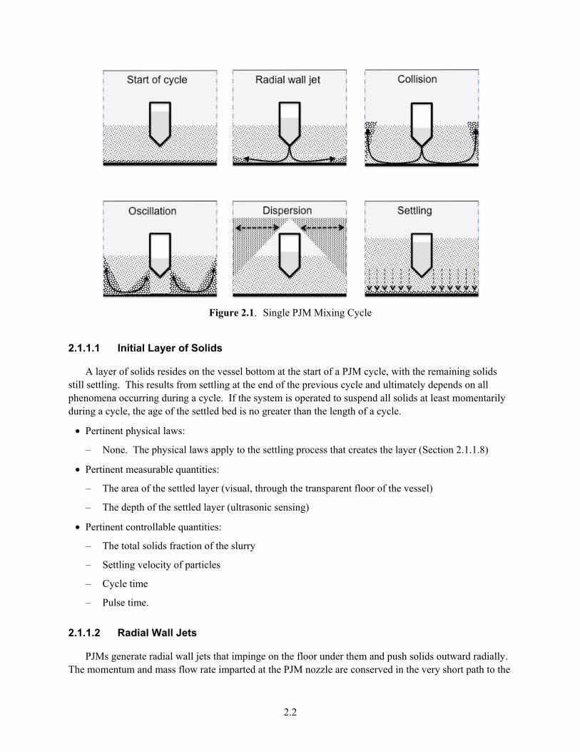
2.2

Figure 2.1. Single PJM Mixing Cycle

2.1.1.1 Initial Layer of Solids

A layer of solids resides on the vessel bottom at the start of a PJM cycle, with the remaining solids still settling. This results from settling at the end of the previous cycle and ultimately depends on all phenomena occurring during a cycle. If the system is operated to suspend all solids at least momentarily during a cycle, the age of the settled bed is no greater than the length of a cycle.

• Pertinent physical laws:

– None. The physical laws apply to the settling process that creates the layer (Section 2.1.1.8)

• Pertinent measurable quantities:

– The area of the settled layer (visual, through the transparent floor of the vessel)

– The depth of the settled layer (ultrasonic sensing)

• Pertinent controllable quantities:

– The total solids fraction of the slurry

– Settling velocity of particles

– Cycle time

– Pulse time.

2.1.1.2 Radial Wall Jets

PJMs generate radial wall jets that impinge on the floor under them and push solids outward radially. The momentum and mass flow rate imparted at the PJM nozzle are conserved in the very short path to the

2.3

tank floor, where the jet impinges and spreads to flow radially. After a short radial distance, the flow becomes a self-similar radial wall jet, which already is turbulent because of impingement on the floor (Rajaratnam 1976, pp. 226-245). The momentum decreases slightly because of the shear stress acting on the floor, which slightly alters the velocity as was demonstrated by Poreh et al. (1967).

The mass attributed to the jet grows because of entrainment of the fluid adjacent to it. Turbulence dislodges and entrains the settled layer on the tank floor into the leading vortex torus of the wall jet as the jet penetrates radially outward. The rate of removal depends on processes whereby the turbulent wall jet erodes particles from the settled bed. It appears from preliminary attempts that this can be correlated in terms of the wall shear stress imposed by the jet. The actual mechanism is not necessarily based on stress, but if not, it is likely that any pertinent aspect of the turbulence at the jet boundary can be correlated with the attending shear stress. The mass entrainment rate, which is increasing at nearly constant momentum results in the velocity decreasing radially, which determines the conditions at the collision of radial wall jets on the tank floor. The pertinent measurable quantity includes the area of the bed (as visually observed through the transparent floor of the vessel). Supplemental tests could include operation of single PJMs impinging on a bed of known design with measurements of bed depth and coverage, wall stress, and possibly velocity. Models of radial wall jets exist in the literature and can be adapted to the specific geometry and conditions under a PJM.

• Pertinent physical laws:

– Conservation of momentum; self-similar velocity profiles. There is considerable literature (see Rajaratnam 1976 for especially pertinent references) on immersed, impinging radial wall jets based on these physical laws

– Constitutive relation for rate of erosion of particles from a settled bed

• Pertinent measurable quantities:

– Radius of cleared area versus time (visually observed through the transparent floor of the vessel)

• Pertinent controllable quantities:

– Depth of the settled layer (through the total solids fraction)

– Jet velocity

– Pulse time.

2.1.1.3 Collision of Radial Wall Jets

Radial wall jets collide with each other or a tank wall, resulting in relatively stagnant regions where solids tend to accumulate. Nominally, these regions exist at lines or points of geometric symmetry defined by the location of the PJM nozzles, but actually occur at different locations determined by inequalities and fluctuations in the actual contributing radial wall jets. Consequently, actual stagnation at such locations is unlikely. Instead, one can expect turbulence, albeit likely reduced compared to that in a jet not impeded by any collision, resulting in a slower scouring of solids. Pertinent measurable quantities include the area of the bed. Supplemental tests could include testing an array of three PJMs generating wall jets impinging on a bed of known design, converging on a collision point, with measurements of the rate of clearing under the PJMs and at the collision points and of solids concentration versus elevation and time. Colliding wall jets have been studied and discussed in the literature, as have “fountains” of upward

2.4

dense jets into less dense surrounding jets, but a comprehensive model of the collision of solids-laden radial wall jets likely is not available in the literature. We believe that simple models should be proposed based on the principles of conservation of mass and momentum, drawing upon available information from the literature on component phenomena. See Sections 5.4.2 and Appendix C, Section C.4.1.

• Pertinent physical laws:

– Conservation of momentum (fluid)—determines the penetration of the solids-laden jet upward at locations of collisions

– Conservation of momentum (particles)—settling

• Pertinent measureable quantities:

– The area of the settled layer versus time (visually observed through the transparent floor of the vessel)

• Pertinent controllable quantities:

– Jet velocity

– Total solids fraction

– Cycle time

– Pulse time.

2.1.1.4 Turbulent Entrainment of Solids

Turbulence at collision points scours solids and entrains them into the upward convergence of the collided flows. The velocity is much less than at the point of impingement; therefore, the scouring rate is much less, as is suggested by observations of solids lingering at collision boundaries after a decisive removal of solids over the area within them. Pertinent measurable quantities include the concentration of solids versus time and elevation at the nominal locations of collisions of jets. Supplemental tests are the same as described above in Section 2.1.1.3, Collision of Radial Wall Jets.

No applicable literature models have been identified. The simplest possible empirical models should be attempted to complete a calculation of the last phase of clearing solids from the tank floor.

• Pertinent physical laws:

– Conservation of momentum (and turbulence modeling concepts based on it)

• Pertinent measurable quantities:

– Fraction of area of solids removed from tank floor

• Pertinent controllable quantities:

– Jet velocity

– Pulse time

– Total solids loading.

2.5

2.1.1.5 Upward Flow from Collisions

Mass and momentum are conserved as the collided wall jets are turned upward. The solids-laden upward flow decelerates because of the greater density than the surrounding fluid and gravitational acceleration. Momentum decreases in accordance with the law of conservation of momentum, where the excess weight of entrained solids applies a decelerating force. Pertinent measurable quantities and supplemental tests are the same as described in Section 2.1.1.3, Collision of Radial Wall Jets, and Section 2.1.1.4, Turbulent Entrainment of Solids. As noted in Section 2.1.1.3, we have not identified comprehensive applicable models in the literature. We believe the conservation of momentum and similarity principals can be applied to propose plausible functional forms for correlating data on the upward flow of entrained solids (see Sections 5.4.2 and Appendix C, Section C.4.1).

• Pertinent physical laws:

– Conservation of momentum; concept of self-similar flow combined with dimensional analysis

• Pertinent measurable quantities:

– Vertical distribution of solids concentration versus time

• Pertinent controllable quantities:

– Same as described in Section 2.1.1.4, Turbulent Entrainment of Solids.

2.1.1.6 Limit to Upward Suspension of Solids

If the flow continues long enough, it reaches a maximum attainable height determined by its density and the momentum of colliding jets that generate it, after which the flow must become horizontal (and then downward), resulting in horizontal dispersion. Pertinent measurable quantities include the concentration of solids versus time and elevation at the nominal locations of collisions of jets. Supplemental tests could include generating upward, solids-laden jets and measuring the elevation attained and horizontal dispersion versus time. Models could be attempted as described in Section 2.1.1.5, Upward Flow from Collisions.

• Pertinent physical laws:

– Same as described in Section 2.1.1.5, Upward Flow from Collisions

• Pertinent measurable quantities:

– Same as described in Section 2.1.1.5, Upward Flow from Collisions

• Pertinent controllable quantities:

– Same as described in Section 2.1.1.5, Upward Flow from Collisions.

2.1.1.7 Density-Driven Oscillations

If the flow does not continue long enough to reach the maximum attainable height, a solids-laden vertical column or sheet exists at the end of the pulse, which then falls because of its density difference, thereby creating a converging wall jet on the tank floor that similarly generates an upward flow at the point of convergence, which then falls under its own weight after reaching its maximum elevation, and so on. Thus, oscillatory vertical flow ensues after the PJM pulse ends because of equilibration of columns of

2.6

dense fluid with the surrounding less dense fluid. Entrainment into the oscillating columns and sheets disperses the solids laterally. Pertinent measurable quantities are as for Section 2.1.1.6, Limit to Upward Suspension of Solids. Modeling could be attempted as for Section 2.1.1.6, Limit to Upward Suspension of Solids.

• Pertinent physical laws:

– Same as described in Section 2.1.1.6, Limit to Upward Suspension of Solids

• Pertinent measurable quantities

– Same as described in Section 2.1.1.6, Limit to Upward Suspension of Solids

• Pertinent controllable quantities:

– Same as described in Section 2.1.1.6, Limit to Upward Suspension of Solids.

2.1.1.8 Settling

Particles settle according to their size, density, and shape, and as hindered by the concentration of other particles. Particles with settling velocities that are less than their elevation at the end of a pulse divided by the remaining time in the cycle will not reach the floor, and will be dispersed by the turbulence of the next PJM pulse. Particles with faster-settling velocities will reach the floor and contribute to the settled layer existing at the start of the next cycle. Supplemental tests could include settling tests for particles of known distributions of terminal velocities.

• Pertinent physical laws:

– Conservation of momentum adapted to the case of particle motion

• Pertinent measurable quantities:

– Vertical distribution of solids concentration versus time

– Depth of settled layer at start of pulse

– Transient concentration in the transfer line (during pump down)

• Pertinent controllable quantities:

– Same as described in Section 2.1.1.3, Collision of Radial Wall Jets.

2.1.1.9 Capture into the Suction Nozzle

When slurry is transferred from a tank, it enters the suction nozzle of the transfer line. Transfer occurs over a large number of PJM cycles. The total mass of solids species entering the suction nozzle over the transfer period compared to the total mass of corresponding species charged to the tank after a transfer period (i.e., a mass balance) determines the accumulation in the tank, if any, of solids species over time. The composition of the slurry at the suction nozzle inlet versus time determines the mass of various solids species removed over the course of the PJM cycles within the transfer period.

We propose that behavior in the transfer line and pump be tested independently of other LSIT tests. To decouple this problem from other aspects of LSIT, we need to determine the composition versus time at the suction nozzle inlet from “scaled” LSIT data. This topic is discussed in Chapters 5 and 6.

2.7

We assume that each PJM cycle will resuspend all or nearly all solids that settle during a cycle, and that, when the suction nozzle is located near the center of the tank, the horizontal distribution of solids as settling occurs will be sufficiently uniform so a separate model of the horizontal distribution will not be required.

The composition at the inlet is predicted from a transient model of particle settling and a model of the capture of specific species of settling solids as they approach the tank floor in the vicinity of the suction nozzle. For particles with vertical settling paths passing near the suction nozzle inlet, the velocity into the nozzle will be great enough to capture essentially any particle. Further from the nozzle, the velocity is essentially that of a point sink with a flow rate equal to that of the nozzle. The path of a particle will depend on the distribution over space of this velocity compared to the settling velocity of the particle.

Kinematic models can be devised to estimate the fraction of all particles settling at a given velocity that are captured by the suction nozzle instead of settling on the floor of the tank. Key parameters will be the settling velocities, volumetric flow rate into the nozzle, and distance from nozzle to floor.

• Pertinent physical laws:

– Conservation of momentum (as settling velocity); conservation of mass

• Pertinent measurable quantities:

– Vertical distribution of solids concentration versus time

– Transient concentration in the transfer line

• Pertinent controllable quantities:

– Suction volumetric flow rate

– Location of suction nozzle.

2.1.1.10 Combined Cycle

Dickey in Smith et al. (2009) describes a hierarchy of accomplishment for a mixing system designed to disperse solids in a liquid, progressing from bottom motion of unsuspended particles to suspending all particles off the bottom to suspending all particles nearly uniformly through the liquid. A continuously operating mixing system establishes a steady-state particle distribution that falls somewhere within this range of accomplishment.

PJM mixing is sequential and transient: during a cycle, the solids experience all three of the degrees of mixing listed in the hierarchy described above. First, solids are moved on the bottom, and then suspended near the bottom by turbulence in the radial wall jet. These steps constitute clearing solids from the bottom. Suspended particles are entrained into the upward motion from collided jets and dispersed to form a vertical concentration profile with some degree of homogeneity depending on the force of the PJM pulse. This determines the inlet conditions at the suction nozzle of the transfer line. The vertical distribution becomes non-uniform as settling occurs in the liquid and, hence, is simply redistributed to a more uniform concentration profile during each pulse. The remaining particles settle by the end of each pulse cycle. The thickness of the settled layer is the initial condition for the next pulse. Thus, all of the phenomena ultimately are coupled, thus complicating the dependence on length scale, and the PJM mixing system progresses through all three of the conditions described above during every pulse

2.8

cycle. It is apparent that the performance likely does not vary with length scale in any simple manner; that is, it seems unlikely that a single scale factor could be defined to describe the effect of length scale on PJM mixing.

2.1.2 Effect of Yield Stress on Shear Rate

Solids may concentrate sufficiently in some tanks so that the slurry exhibits a yield stress, thus acting like a “Bingham fluid.” A yield stress decreases the fluid motion resulting from applied stresses, but not necessarily significantly, as discussed in this section. We find that, if the power dissipation in an element of a Bingham fluid is great enough, the fluid behaves as though it were a Newtonian fluid. Then, as the power dissipation throughout a vessel increases, the fraction of the volume in the vessel in which non-Newtonian attributes will be important decreases.

When the slurry in a tank behaves as a Bingham fluid, a yield stress exists that tends to dampen fluid motion. Essentially, the yield stress reduces the shear rate in the slurry for a given stress applied to the fluid. In terms of mixing, less mixing occurs for a given applied inertial or shear force. However, the effect is not necessarily significant. For sufficient shear rates, the fluid will behave as a Newtonian fluid with a viscosity equal to the viscosity limit at high-shear rate for the Bingham fluid. This condition can be expressed in terms of the local dissipation rate (i.e., the local power-per-volume dissipated). The dissipation rate per volume is the scalar product of the rate of deformation tensor with magnitude1 γ and the stress tensor with magnitude τ. From the definition of the relationship between these two tensors for a Bingham fluid,

ρε = μ0γ2 + τ 0γ (2.1)

where ρ = the slurry density ε = the dissipation rate per mass (proportional to power per volume) μ0 = the effective Newtonian viscosity at infinite deformation rate τ0 = the yield stress of a Bingham fluid.

Solving the quadratic expression and rearranging gives

γ =uτ

2

2ν0

1+ 4ν0εuτ

4 − 1

(2.2)

1 The magnitude is the square root of half the sum of the diagonal elements of the second-rank tensor. Thus, we

define the scalar γ 2 ≡ 12γ :γ . The rate of deformation tensor is the symmetric sum of the velocity gradient tensors,

i.e., γ ≡ ∇u + ∇ut where the double under-bar signifies the tensors are second-rank, “t” signifies the transpose, and

u is the velocity vector. The stress tensor τ is a function of γ. Consequently, both tensors are symmetric. The

stress-strain relationship for a Bingham fluid is τ = − μ0 + τ 012 γ :γ( )γ where the “:” signifies the scalar (“inner”)

product. The relation is valid for 12τ :τ ≤ τ 0

2 . For lesser stresses, the strain is zero. The dissipation rate is found

from ρε = −τ : ∇u .

2.9

where ν0 is μ0/ρ, the kinematic viscosity at infinite deformation rate, and uτ is defined as

uτ ≡ τ 0 ρ

(2.3)

For a Newtonian fluid with specified dissipation rate ε, the corresponding shear rate, γNewtonian, is

γ Newtonian = ε ν0 (2.4)

Comparing, the actual shear rate compared to the equivalent for a Newtonian fluid is

γγ Newtonian

=ν0

εuτ

2

2ν0

1+ 4ν0εuτ

4−1

= g θ( )

(2.5)

where

g θ( )=1+ 4θ − 1

4θ

(2.6)

and θ is the dimensionless dissipation rate

θ =

ν0εuτ

4

(2.7)

The function g(θ) is essentially unity for θ >>1 and essentially θ ½ for θ <<1. Thus, for sufficiently large dissipation rate per mass, the deformation rate is that of a Newtonian fluid with the same dissipation rate. Therefore, to mix a Bingham fluid as intensely as if the fluid were Newtonian with a viscosity equal to the consistency index, the dissipation rate (proportional to power per volume) should be large enough that θ >>1. Put differently, for sufficiently large dissipation rates, the Bingham fluid acts similar to a Newtonian fluid. Hence, the dimensionless argument of the function “g” describes the “Newtonian nature” of the fluid in the system, and hence provides a means for matching the Newtonian nature (i.e., the power-per-volume).

The existence of a yield stress must be included in any dimensional analysis (such as evaluating self-similarity of jet flows) or of conditions for similitude (i.e., matching the Bingham number).

The existence of a yield stress can affect the nature of the phenomena of the PJM cycle described in Section 2.1.1. In general, the effect of a yield stress depends on the dissipation rate in the fluid, and may not be important if a sufficient dissipation rate can be imposed. Some potential effects include the following:

• The fluid between particles in the settled bed can exhibit a yield stress, making the settled solids “cohesive.” This both complicates defining scaled properties of the bed and impedes erosion of the bed by a radial wall jet or by the turbulence at the locations of collisions of jets.

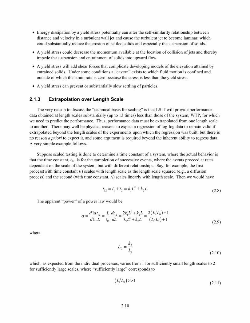
2.10

• Energy dissipation by a yield stress potentially can alter the self-similarity relationship between distance and velocity in a turbulent wall jet and cause the turbulent jet to become laminar, which could substantially reduce the erosion of settled solids and especially the suspension of solids.

• A yield stress could decrease the momentum available at the location of collision of jets and thereby impede the suspension and entrainment of solids into upward flow.

• A yield stress will add shear forces that complicate developing models of the elevation attained by entrained solids. Under some conditions a “cavern” exists to which fluid motion is confined and outside of which the strain rate is zero because the stress is less than the yield stress.

• A yield stress can prevent or substantially slow settling of particles.

2.1.3 Extrapolation over Length Scale

The very reason to discuss the “technical basis for scaling” is that LSIT will provide performance data obtained at length scales substantially (up to 13 times) less than those of the system, WTP, for which we need to predict the performance. Thus, performance data must be extrapolated from one length scale to another. There may well be physical reasons to expect a regression of log-log data to remain valid if extrapolated beyond the length scales of the experiments upon which the regression was built, but there is no reason a priori to expect it, and some argument is required beyond the inherent ability to regress data. A very simple example follows.

Suppose scaled testing is done to determine a time constant of a system, where the actual behavior is that the time constant, t12, is for the completion of successive events, where the events proceed at rates dependent on the scale of the system, but with different relationships. Say, for example, the first process(with time constant t1) scales with length scale as the length scale squared (e.g., a diffusion process) and the second (with time constant, t2) scales linearly with length scale. Then we would have

t12 = t1 + t2 = k1L2 + k2L (2.8)

The apparent “power” of a power law would be

( )( )

2012 12 1 2

212 1 2 0

2 1ln 2

ln 1

L Ld t dt k L k LL

d L t dL k L k L L Lα

++= = = =+ +

(2.9)

where

L0 = k2

k1 (2.10)

which, as expected from the individual processes, varies from 1 for sufficiently small length scales to 2 for sufficiently large scales, where “sufficiently large” corresponds to

( )0 1L L >> (2.11)

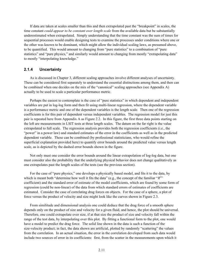
2.11

If data are taken at scales smaller than this and then extrapolated past the “breakpoint” in scales, the time constant could appear to be constant over length scale from the available data but be substantially underestimated when extrapolated. Simply understanding that the time constant was the sum of times for sequential processes would enable designing tests to examine the processes under conditions where one or the other was known to be dominant, which might allow the individual scaling laws, as presumed above, to be quantified. This would amount to changing from “pure statistics” to a combination of “pure statistics” and “pure physics,” and similarly would amount to changing from mostly “extrapolating data” to mostly “interpolating knowledge.”

2.1.4 Uncertainty

As is discussed in Chapter 3, different scaling approaches involve different analyses of uncertainty. These can be considered first separately to understand the essential distinctions among them, and then can be combined when one decides on the mix of the “canonical” scaling approaches (see Appendix A) actually to be used to scale a particular performance metric.

Perhaps the easiest to contemplate is the case of “pure statistics” in which dependent and independent variables are put in log-log form and then fit using multi-linear regression, where the dependent variable is a performance metric and one of the dependent variables is the length scale. Then one of the regression coefficients is for this pair of dependent versus independent variables. The regression model for just this pair is repeated here from Appendix A as Figure 2.2. In this figure, the first three data points starting on the left are measurements in LSIT tests at three length scales. The datum on the far right is the value extrapolated to full scale. The regression analysis provides both the regression coefficients (i.e., the “power” in a power law) and standard estimates of the error in the coefficients as well as in the predicted dependent variable. These can be combined (by professional statisticians, who would refine the superficial explanation provided here) to quantify error bounds around the predicted value versus length scale, as is depicted by the dashed error bounds shown in the figure.

Not only must one consider the error bounds around the linear extrapolation of log-log data, but one must consider also the probability that the underlying physical behavior does not change qualitatively as one extrapolates past the length scales of the tests (see the previous section).

For the case of “pure physics,” one develops a physically based model, and fits it to the data, by which is meant both “determine how well it fits the data” (e.g., the concept of the familiar “R2” coefficient) and the standard error of estimate of the model coefficients, which are found by some form of regression (could be non-linear) of the data from which standard errors of estimates of coefficients are estimated. Consider the case of correlating drag forces on objects. For the case of a sphere, a plot of force versus the product of velocity and size might look like the curves shown in Figure 2.3.

From similitude and dimensional analysis one could deduce that the drag force of a smooth sphere depends only on the product of size and velocity for a given fluid, and hence, the plot should be universal. Therefore, one could extrapolate over size, if at that size the product of size and velocity fall within the range of the test data, by interpolating over this plot. By fitting a functional form to the plot, one would have a model to predict the drag force. The solid line shown in the data is such a function of the size-velocity product; in fact, the data shown are artificial, plotted by randomly “scattering” the values from the correlation. In an actual situation, the error in the correlation developed from such data would include two sources of error in its coefficients: first, from the scatter in the measurements upon which it

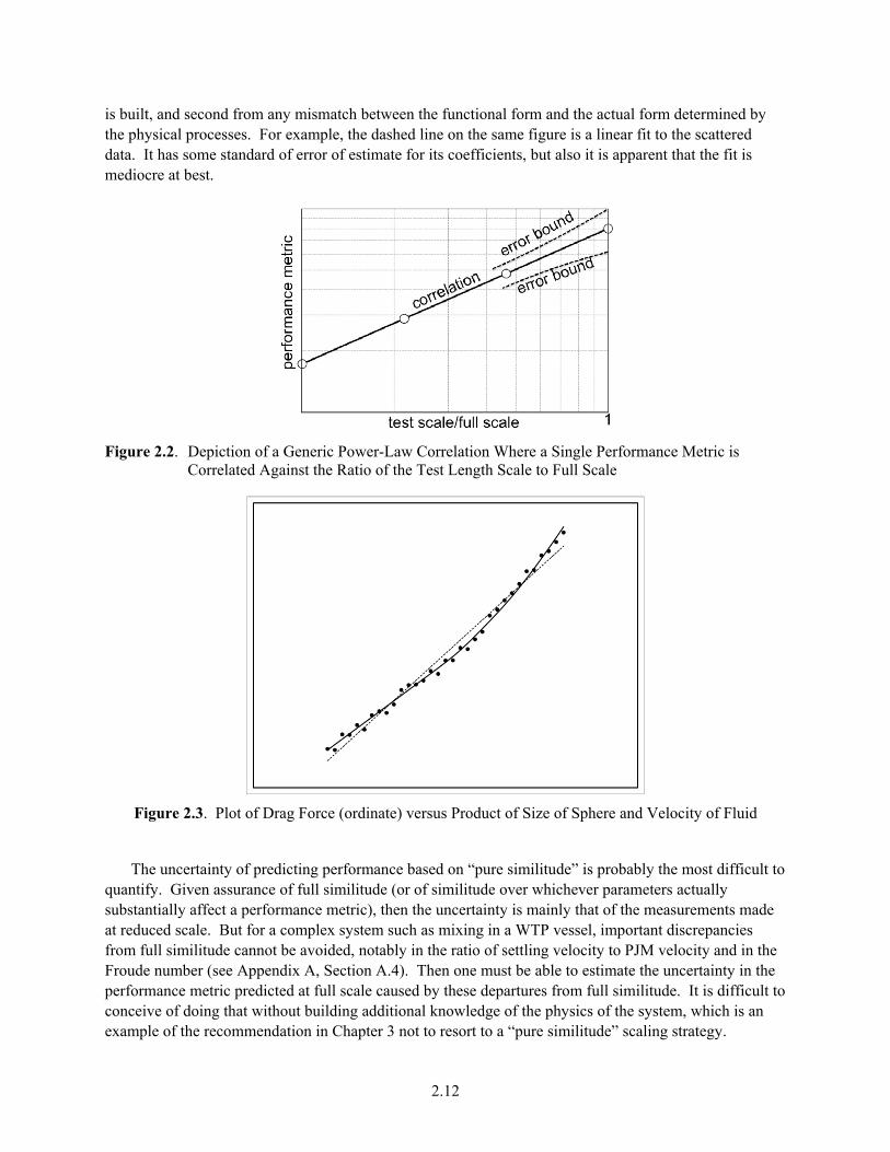
2.12

is built, and second from any mismatch between the functional form and the actual form determined by the physical processes. For example, the dashed line on the same figure is a linear fit to the scattered data. It has some standard of error of estimate for its coefficients, but also it is apparent that the fit is mediocre at best.

Figure 2.2. Depiction of a Generic Power-Law Correlation Where a Single Performance Metric is Correlated Against the Ratio of the Test Length Scale to Full Scale

Figure 2.3. Plot of Drag Force (ordinate) versus Product of Size of Sphere and Velocity of Fluid

The uncertainty of predicting performance based on “pure similitude” is probably the most difficult to

quantify. Given assurance of full similitude (or of similitude over whichever parameters actually substantially affect a performance metric), then the uncertainty is mainly that of the measurements made at reduced scale. But for a complex system such as mixing in a WTP vessel, important discrepancies from full similitude cannot be avoided, notably in the ratio of settling velocity to PJM velocity and in the Froude number (see Appendix A, Section A.4). Then one must be able to estimate the uncertainty in the performance metric predicted at full scale caused by these departures from full similitude. It is difficult to conceive of doing that without building additional knowledge of the physics of the system, which is an example of the recommendation in Chapter 3 not to resort to a “pure similitude” scaling strategy.

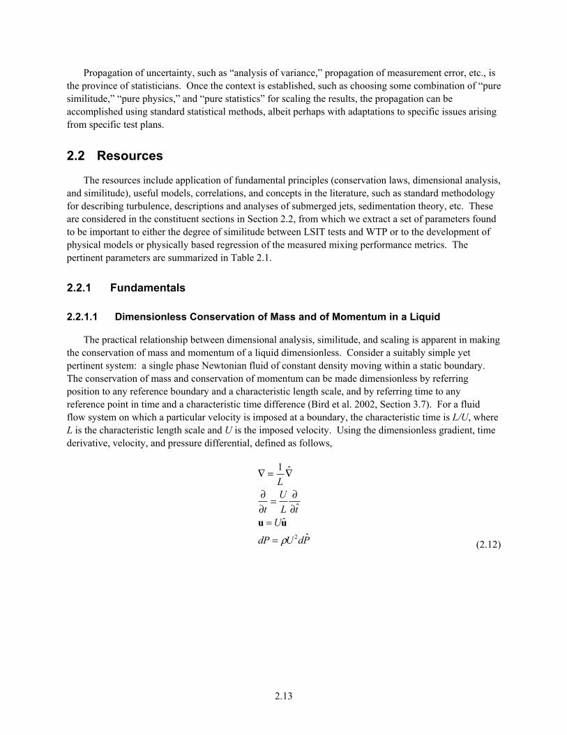
2.13

Propagation of uncertainty, such as “analysis of variance,” propagation of measurement error, etc., is the province of statisticians. Once the context is established, such as choosing some combination of “pure similitude,” “pure physics,” and “pure statistics” for scaling the results, the propagation can be accomplished using standard statistical methods, albeit perhaps with adaptations to specific issues arising from specific test plans.

2.2 Resources

The resources include application of fundamental principles (conservation laws, dimensional analysis, and similitude), useful models, correlations, and concepts in the literature, such as standard methodology for describing turbulence, descriptions and analyses of submerged jets, sedimentation theory, etc. These are considered in the constituent sections in Section 2.2, from which we extract a set of parameters found to be important to either the degree of similitude between LSIT tests and WTP or to the development of physical models or physically based regression of the measured mixing performance metrics. The pertinent parameters are summarized in Table 2.1.

2.2.1 Fundamentals

2.2.1.1 Dimensionless Conservation of Mass and of Momentum in a Liquid

The practical relationship between dimensional analysis, similitude, and scaling is apparent in making the conservation of mass and momentum of a liquid dimensionless. Consider a suitably simple yet pertinent system: a single phase Newtonian fluid of constant density moving within a static boundary. The conservation of mass and conservation of momentum can be made dimensionless by referring position to any reference boundary and a characteristic length scale, and by referring time to any reference point in time and a characteristic time difference (Bird et al. 2002, Section 3.7). For a fluid flow system on which a particular velocity is imposed at a boundary, the characteristic time is L/U, where L is the characteristic length scale and U is the imposed velocity. Using the dimensionless gradient, time derivative, velocity, and pressure differential, defined as follows,

∇ =1

L∇

∂∂t

=U

L

∂∂t

u = Uu

dP = ρU 2dP (2.12)

2.14

Table 2.1. Scaling Parameters Deduced in Section 2.2

Parameter Expression or Symbol Significance

Tank diameter D Length characterizing size of the system

PJM velocity U Velocity for dynamic and kinematic scaling

Dimensionless cycle time UtC /D The principal measure of kinematic similitude; pertinent to the importance of many phenomena

Ratio of nozzle diameter/tank diameter

dJ/D Affects development of radial wall jet from impingement of PJM jet

Number of PJMs NJ Affects development of radial wall jet from impingement of PJM jet

Ratio of PJM nozzle offset/tank diameter

H/D Affects development of radial wall jet from impingement of PJM jet

Solids volume fraction φS Ratio of total volume of solids to total volume of slurry in a tank

Nozzle Reynolds number K0 ν Affects shear stress imposed on radial wall jet on the tank floor

Characteristic dissipation rate U3/D Ubiquitously affects the magnitude of all turbulent forces, length scales, and time scales

Characteristic dispersion constant

UL Affects the relative importance of dispersion to coherent motion of solids

Ratio of characteristic(a) settling velocity to PJM velocity

uS/U Affects the fraction of solids that settle during PJM refill; affects the fraction of solids that are captured by the inlet to the transfer line

Froude Number (Fr) U2/(s-1)gD Affects the height to which upward flows from PJM pulses can penetrate into and mix with unmixed slurry above

Reynolds number based on erosion critical stress (Rec)

ρu2/τc Affects ability to clear solids from bottom of vessel

θS (see Section 2.2.2.1)

( )0

S S S

* D

u t

u t

φφ

Affects ability to clear solids from bottom of vessel

(a) There will be a very large range of settling velocities among the solid particles; the volume-weighted average over an appropriate subset of the particles can be defined for the purpose of quantifying the ratio of “settling velocity” to PJM velocity. See Appendix A, Section A.5.

where P is the piezometric pressure (i.e., the pressure relative to the hydrostatic pressure). The conservation of mass becomes

uˆ •∇ (2.13)

and the conservation of momentum becomes

ˆ 1ˆ ˆ ˆ ˆ ˆˆ ˆ ˆˆ

Pt Re

∂ + ∇ = ∇ ∇ − ∇∂

u u u u (2.14)

2.15

where Re is the Reynolds number, UL/ν, where using the piezometric pressure eliminates the gravitational term; ν is the kinematic viscosity. This approach is admissible if the pressure does not appear in the boundary conditions. In principle, these two equations can be solved given boundary and initial conditions to give the dimensionless velocity and pressure in terms of dimensionless (or “scaled”) position and time

( )

( ) 2

Utˆ,t;L,U , U , , ,Re

L L

UtˆP ,t;L,U , U P , , ,ReL L

ν β

ν ρ β

=

=

ru r u

rr (2.15)

where r is a position vector, and β represents a set of geometric ratios describing the shape of the boundary. This is a specific example of the principles of dimensional analysis discussed in Appendix A, Section A.1, and illustrates the concept of the behavior in one system representing another when the behaviors are “scaled” in terms of position and time.

This illustrates three important conditions for establishing full similitude:

1. The shapes of flow boundaries must match between systems being compared (i.e., geometric similitude).

2. Dimensionless dependent variables are addressed as functions of dimensionless position and time.

3. The effects of shapes, operational parameters, and material properties are described by dimensionless parameters, which must match between systems being compared.

This also illustrates the concept of “similitude that matters” in that, for sufficiently large values of the Reynolds number, the effect of the Reynolds number diminishes, when the behavior is described in dimensionless form, as is apparent from its appearance as its reciprocal in terms that add to the term not involving the Reynolds number. Thus, we can anticipate that the Reynolds number does not matter for sufficiently large values as is reiterated below.

2.2.1.2 Similitude and Dimensional Analysis

Similitude or similarity is central to the concept of a technical basis for scaling even though the complexity of the PJM mixing cycle precludes establishing complete similitude between LSIT tests and WTP process tanks.

In the context of fluid flow, “similar,” as in geometry, means “with the same shape.” There are three categories of similarity:

1. Geometric similarity, denoting the same shape of the boundary—whether simple or complex—around the flowing system. For PJM tanks, geometric similarity implies all corresponding dimensions are in the same ratio between the reduced-scale and full-scale tank. In particular, all PJM and transfer line dimensions (e.g., the ratio of diameters of PJM nozzle and transfer line nozzle, offsets of PJM nozzle and transfer line suction nozzle from the tank floor, and the height of the fluid) are in the same ratio between full and reduced scale as the tank diameters. Ideally, the ratio of particle sizes to tank diameter would also be the same in each system but as discussed below, this is impractical.

2.16

2. Kinematic similarity, denoting the same shape of flow streamlines at similar elapsed times. Elapsed times are similar if their ratio to the characteristic flow time is the same between the systems. The characteristic flow time is the characteristic length, which conveniently is the tank diameter, because by the principle of geometric similitude, all other lengths will be in proportion divided by the characteristic velocity, which conveniently is the PJM nozzle velocity (specifically, some unambiguous definition of this, such as peak velocity or velocity averaged over the drive time). Where more than one velocity is imposed on the system, such as imposing the velocity (or equivalently, given geometric similitude, volumetric flow rate) into the transfer line, then the ratio of these velocities must match. Further, one must match between systems the ratios of multiple elapsed times imposed as part of controlling the process.

3. Dynamic similarity, denoting the same ratio of characteristic forces affecting the flow. Dynamic similitude is required to attain kinematic similitude. The characteristic forces (or equivalently stresses, pressures, or momentum fluxes important to PJM mixing) include

– Inertial force (or stress or pressure): ρu2

– Viscous force (or stress): µ(u/L)

– Gravitational stress: ΔρgL

where ρ is fluid density, Δρ is the difference between the density of two phases, μ is dynamic viscosity, u is a characteristic velocity, and L is a characteristic length

– Critical stress to erode a settled layer: τc.

These characteristic forces can be combined to form dimensionless ratios of forces, as follows.

• The Reynolds number is the ratio of inertial to viscous forces, which affects in particular the characteristics of turbulence: Re = ρUL/µ.

• The Froude number is the ratio of inertial-to-gravitational forces, which affects in particular the motion of one phase (e.g., solid particles) relative to another, or the motion of liquid with density differences caused by differences in concentration of solids: Fr = ρu2/ΔρgL.

• The Reynolds number based on critical stress to erode a settled layer: Rec = ρu2/τc.

In addition, different length scales may apply, which can be specified based on geometric similitude. If (as in fact is not practical) the ratio of particle size dS to tank diameter D were matched between

systems, then the particle Reynolds number, 0S Su dρ μ , would be matched, where 0

Su is the resulting

settling velocity of the solid particle relative to the surrounding fluid, for the limiting case of vanishing solids concentration in the fluid. Specifically, the drag coefficient of a settling particle depends on the particle Reynolds number, Rep, and a balance between gravitational forces and the drag force results in the relationship (see Appendix C, Section C.4.2.2)

( )23

2 p D pAr Re C Re= (2.16)

where 3 2= Δ SAr gdρ ρν is the Archimedes number, ν is the kinematic viscosity of the fluid, and CD(Rep)

is a correlation of the drag coefficient in terms of particle Reynolds number.

2.17

The expression can be inverted (Camenen 2007) to give approximately

( )2

0 15 10 3 15S pS S

v vu Re Ar /

d d= + −

(2.17)

The Archimedes number can be formed from other dimensionless groups involving size ratios and material property ratios

33 2

2S Sgd d Re

Arv L Fr

ρρ

Δ = = (2.18)

2.2.1.3 Submerged Jets

In Appendix A, we apply dimensional analysis to the similitude of submerged jets. This provides several useful relationships. The thickness of an impinging radial wall jet is

( )0, Jf r H k d H

r δδ =

(2.19)

where δ = thickness of impinging jet r = radius from the impingement H = distance from the source jet to the wall k0 = ratio of distance from nozzle to nozzle diameter dJ = nozzle diameter.

Similarly, we find for the velocity, U,

( )0

0

,U J

Urf r H k d H

K=

(2.20)

where K0 is the kinematic momentum flow rate at the jet nozzle (see Appendix A, Section A.3). The wall shear stress, τw, is expected to take the form

( )2

00

0

,

b

wJ

Kra f r H k d H

K τ ττρ ν

−

= (2.21)

Finally, 0K is proportional to dJU, where dJ is the diameter of the source jet. The jet radius at the

collision with other jets is found by assuming that each PJM “sweeps” an equal fraction of the area of the vessel floor; therefore, we evaluate r to be proportional to the tank diameter, D, divided by the square root of the number of PJMs, NJ.

Thus, considering all of the above, the key scaling parameters describing the variation of flow attributes in the radial wall jets on the tank floor are as shown in Table 2.1.

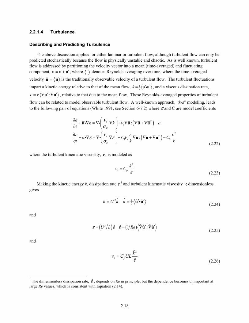
2.18

2.2.1.4 Turbulence

Describing and Predicting Turbulence

The above discussion applies for either laminar or turbulent flow, although turbulent flow can only be predicted stochastically because the flow is physically unstable and chaotic. As is well known, turbulent flow is addressed by partitioning the velocity vector into a mean (time-averaged) and fluctuating component, u = u + ′u , where denotes Reynolds averaging over time, where the time-averaged

velocity u = u is the traditionally observable velocity of a turbulent flow. The turbulent fluctuations

impart a kinetic energy relative to that of the mean flow, 12k ′ ′= u u , and a viscous dissipation rate,

:ε ν ′ ′= ∇ ∇u u , relative to that due to the mean flow. These Reynolds-averaged properties of turbulent

flow can be related to model observable turbulent flow. A well-known approach, “k-ε” modeling, leads to the following pair of equations (White 1991, see Section 6-7.2) where σ and C are model coefficients

( )

( )2

1 2

:

:

Ttt

K

Ttt

kk k

t

C Ct k kε

ν ν εσ

νε ε εε ε νσ

∂ + ∇ = ∇ ∇ + ∇ ∇ + ∇ − ∂ ∂ + ∇ = ∇ ∇ + ∇ ∇ + ∇ − ∂

u u u u

u u u u

(2.22)

where the turbulent kinematic viscosity, νt, is modeled as

2

t

kCμν

ε=

(2.23)

Making the kinetic energy k, dissipation rate ε,1 and turbulent kinematic viscosity νt dimensionless gives

2 1

2ˆ ˆ ˆ ˆk U k k ′ ′= = u u

(2.24)

and

( ) ( )3 ˆ ˆˆ ˆ ˆ ˆ1 :U L Reε ε ε ′ ′= = ∇ ∇u u

(2.25)

and

2ˆ

ˆt

kC ULμν

ε=

(2.26)

1 The dimensionless dissipation rate, ε , depends on Re in principle, but the dependence becomes unimportant at large Re values, which is consistent with Equation (2.14).

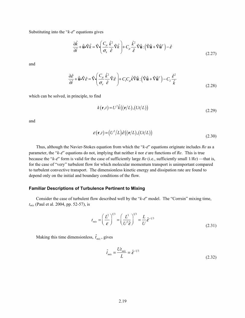
2.19

Substituting into the “k-ε” equations gives

( )

2 2ˆ ˆ ˆˆ ˆˆ ˆ ˆ ˆ ˆ ˆˆ ˆ ˆ ˆ ˆ:

ˆ ˆ ˆT

k

Ck k kk k C

tμ

μ εσ ε ε ∂ + ∇ = ∇ ∇ + ∇ ∇ + ∇ − ∂

u u u u (2.27)

and

( )

2 2

1 2

ˆˆ ˆˆˆ ˆ ˆ ˆ ˆ ˆˆ ˆ ˆ ˆˆ ˆ :ˆˆ ˆ

TC kC C k C

t k

μμ

ε

ε εε εσ ε ∂ + ∇ = ∇ ∇ + ∇ ∇ + ∇ − ∂

u u u u (2.28)

which can be solved, in principle, to find

( ) ( ) ( )( )2 ˆ, ,k t U k L Ut L=r r

(2.29)

and

( ) ( ) ( ) ( )( )3 ˆ, ,t U L L Ut Lε ε=r r

(2.30)

Thus, although the Navier-Stokes equation from which the “k-ε” equations originate includes Re as a parameter, the “k-ε” equations do not, implying that neither k nor ε are functions of Re. This is true because the “k-ε” form is valid for the case of sufficiently large Re (i.e., sufficiently small 1/Re) —that is, for the case of “very” turbulent flow for which molecular momentum transport is unimportant compared to turbulent convective transport. The dimensionless kinetic energy and dissipation rate are found to depend only on the initial and boundary conditions of the flow.

Familiar Descriptions of Turbulence Pertinent to Mixing

Consider the case of turbulent flow described well by the “k-ε” model. The “Corrsin” mixing time, tmix (Paul et al. 2004, pp. 52-57), is

tmix =

L2

ε

1 3

=L3

U 3ε

1 3

=L

Uε −1 3

(2.31)

Making this time dimensionless, mixt , gives

tmix =

Utmix

L= ε −1 3

(2.32)

2.20

Similarly, the Kolmogorov time scale, tK, is

tK =

νε

1 2

=νL

U 3ε

1 2

(2.33)

Making this dimensionless gives

1 2 1 2KK

Utˆ ˆt ReL

ε− −= = (2.34)

The Kolmogorov length scale is

1 4 1 43 3

3 ˆK

Ll

U

ν νε ε

= = (2.35)

Making this dimensionless gives

3 4 1 4ˆ ˆK

K

ll Re

Lε− −= =

(2.36)

The Reynolds average of the fluctuating turbulent component of the pressure, P’, is

(2.37)

Compare this to, say, a critical stress, τc, for suspending solids. In dimensionless form, we have

′P 2

τ c

≈ρk

ρU 2τ c

=k

τ c (2.38)

where τ c = τ c ρU 2 is the critical stress made dimensionless as was the pressure.

We expect the effective hydrodynamic dispersion coefficient, De, to be proportional to the turbulent kinematic diffusivity; for example, as e tD Cν= . Then,

De = Cν t = CCμ

k 2

ε= CCμUL

k 2

ε (2.39)

2.21

Finally, consider the case of decay of homogeneous turbulence as predicted by “k-ε” theory (White 1991; see Section 6-7.2.2). The model equations reduce to

∂k

∂t= −ε

∂ε∂t

= −C2

ε 2

k (2.40)

with initial conditions

k t = 0( )= k0

ε t = 0( )= ε0 (2.41)

Solving gives

k =k0

1+ t t0( )( )1

C2 −1

ε =ε0

1+ t t0( )( )C2

C2 −1

(2.42)

where the characteristic decay time, t0, is

t0 ≡k0

C2 −1( )ε0 (2.43)

Also, we would have

De = Cν t = CCμk 2

ε= CCμ

k02

ε0

1+ t t0( )( )C2 −2

C2−1 = UL( )CCμk0

2

ε0

1+ C2 −1( ) ε0

k0

t

C2 −2

C2 −1

(2.44)

where k0 and ε0 are the dimensionless initial values of k and ε. To this level of approximation, the

duration of the hydrodynamic dispersion, tdispersion, would be approximately t0, so that

tdispersion ~ t0 = L

U

k0

C2 −1( )ε0 (2.45)

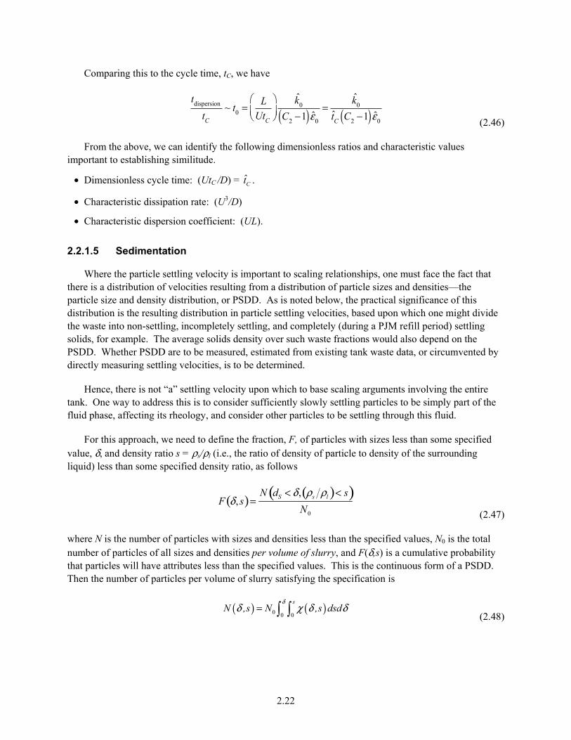
2.22

Comparing this to the cycle time, tC, we have

tdispersion

tC

~ t0 = L

UtC

k0

C2 −1( )ε0

=k0

tC C2 −1( )ε0 (2.46)

From the above, we can identify the following dimensionless ratios and characteristic values important to establishing similitude.

• Dimensionless cycle time: (UtC /D) = Ct .

• Characteristic dissipation rate: (U3/D)

• Characteristic dispersion coefficient: (UL).

2.2.1.5 Sedimentation

Where the particle settling velocity is important to scaling relationships, one must face the fact that there is a distribution of velocities resulting from a distribution of particle sizes and densities—the particle size and density distribution, or PSDD. As is noted below, the practical significance of this distribution is the resulting distribution in particle settling velocities, based upon which one might divide the waste into non-settling, incompletely settling, and completely (during a PJM refill period) settling solids, for example. The average solids density over such waste fractions would also depend on the PSDD. Whether PSDD are to be measured, estimated from existing tank waste data, or circumvented by directly measuring settling velocities, is to be determined.

Hence, there is not “a” settling velocity upon which to base scaling arguments involving the entire tank. One way to address this is to consider sufficiently slowly settling particles to be simply part of the fluid phase, affecting its rheology, and consider other particles to be settling through this fluid.

For this approach, we need to define the fraction, F, of particles with sizes less than some specified value, δ, and density ratio s = ρs/ρl (i.e., the ratio of density of particle to density of the surrounding liquid) less than some specified density ratio, as follows

F δ , s( )=

N dS < δ , ρs ρl( )< s( )N0 (2.47)

where N is the number of particles with sizes and densities less than the specified values, N0 is the total number of particles of all sizes and densities per volume of slurry, and F(δ,s) is a cumulative probability that particles will have attributes less than the specified values. This is the continuous form of a PSDD. Then the number of particles per volume of slurry satisfying the specification is

( ) ( )0 0 0

sN ,s N ,s dsd

δδ χ δ δ= (2.48)

2.23

where χ is the differential probability distribution

( )

2

,F

ss

χ δδ

∂=∂ ∂ (2.49)

The volume fraction of the solid volume, x(δ,s), of a given particle size and density ratio is

( ) ( )( )

3

3

0 0

,,

,

sx s

s dsd

δ χ δδ

δ χ δ δ∞ ∞= (2.50)

The particle volume weighted density ratio, s , is

s = x δ , s( )s ds

0

s

dδ0

δ

(2.51)

The particle volume average unhindered settling velocity, 0u , of the distribution of particles is

u 0 = u0 δ , s( )x δ , s( )ds

0

∞

dδ0

∞

(2.52)

Also, the hindered settling velocity, ( ),u sδ , is related to the unhindered settling velocity, ( )0 ,u sδ ,

by

u δ , s( )= u0 δ , s( ) f φS( ) (2.53)

where f(φS) is the correction for hindered settling, assumed here to be a function of only the total solids loading (see Appendix C, Section C.4.2.9 for a discussion of alternatives; the simple form of Richardson and Zaki (1954) may suffice and was used by Meyer et al. (2009) to estimate the effect of hindered settling).

Finally, as settling occurs, local PSDD changes over elevation and time because of differences in settling rates over the particles. Hence, the differential PSDD is a function of elevation and time as well

as of size and density ratio, ( ), , ,s z tχ δ , and is denoted

χ δ , s, z,t( )=

∂2F δ , s, z,t( )∂s∂δ

z,t (2.54)

The settling velocity of the distribution of particles at some elevation and time, ( )u z,t ,which can be

expressed as the volume weighted volume flux divided by the total particle volume fraction, is

u z,t( )=

dVS

dt( )Aφ

S

= u0 δ ,s( ) f φS( )x δ ,s, z,t( )ds

0

∞

dδ0

∞

(2.55)

2.24

Similarly, the slurry density is found from

( ) ( )( )11 1liquid solids l S l S

l S

m m V V ss

V V

ρ φ ρ φρ ρ φ

+ − += = = + −

(2.56)

where mliquid is the mass of liquid, msolids is the mass of solids, and V is the slurry volume.

The volume-averaged settling velocity, u , can be further refined to consider only particles that settle appreciably during a PJM cycle (see Appendix A, Section A.5).

2.2.2 Physical Models

2.2.2.1 Erosion

The erosion velocity of a settled layer of waste, defined as the rate of decrease of the thickness of the layer, is taken to be zero if the forces applied to waste particle on the surface of the layer are not greater than some critical force expressed in terms of a critical stress apparent at the surface. A simple representative functional form1 is

uerosion =

u*

τ c

τ − τ c( ) (2.57)

where uerosion = the erosion velocity u* = a material property of the settled waste in the form of a velocity τ = the force per area applied to the particles τc = the critical stress.

Critical stress (as any stress) can be interpreted as work per volume, which in this case is work required to remove a volume of particles from the layer. Following are two simple examples of a critical stress.

Gravitational work is required to lift a particle its own diameter to disentangle it from other particles. Then the work is the product of the mass of the particle compared to the mass of the fluid it displaces, the acceleration of gravity, and the displacement, which is taken to be its diameter. The volume moved per particle is the volume of the particle, VP. The work per volume then is ΔρVpgdS /Vp or τc = ΔρgdS, where Δρ is the density difference between the particle and the surrounding fluid, Vp is the volume of the particle, and dS is its diameter.

If particles are bound by cohesive forces, a simple model is that the work per particle is a material property σ (work/area), akin to surface tension, acting over the area of the particle. Then the work per volume is σAp/Vp, where Ap is the area of the particle. Taking the particle to be spherical (corrections for the actual shape would be empirically subsumed into σ), then τc = σAp/Vp = 6σ/dS.

1 See Chapter 4 and Appendix B for detailed discussions about development and application of this form.

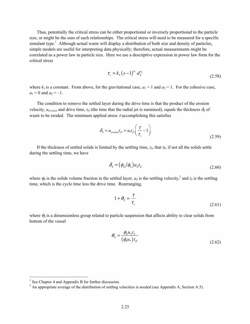
2.25

Thus, potentially the critical stress can be either proportional or inversely proportional to the particle size, or might be the sum of such relationships. The critical stress will need to be measured for a specific simulant type.1 Although actual waste will display a distribution of both size and density of particles, simple models are useful for interpreting data physically; therefore, actual measurements might be correlated as a power law in particle size. Here we use a descriptive expression in power law form for the critical stress

( ) 1 21

a ac Sk s dττ = −

(2.58)

where kτ is a constant. From above, for the gravitational case, a1 = 1 and a2 = 1. For the cohesive case, a1 = 0 and a2 = –1.

The condition to remove the settled layer during the drive time is that the product of the erosion velocity, uerosion and drive time, tD (the time that the radial jet is sustained), equals the thickness δS of waste to be eroded. The minimum applied stress τ accomplishing this satisfies

δS = uerosiontD = u*tD

ττ c

−1

(2.59)

If the thickness of settled solids is limited by the settling time, tS, that is, if not all the solids settle during the settling time, we have

δS = φS φ0( )uStS (2.60)

where φ0 is the solids volume fraction in the settled layer, uS is the settling velocity,2 and tS is the settling time, which is the cycle time less the drive time. Rearranging,

1+ θS =

ττ c (2.61)

where θS is a dimensionless group related to particle suspension that affects ability to clear solids from bottom of the vessel

( )0 *

S S SS

D

u t

u t

φθφ

= (2.62)

1 See Chapter 4 and Appendix B for further discussion. 2 An appropriate average of the distribution of settling velocities is needed (see Appendix A, Section A.5).

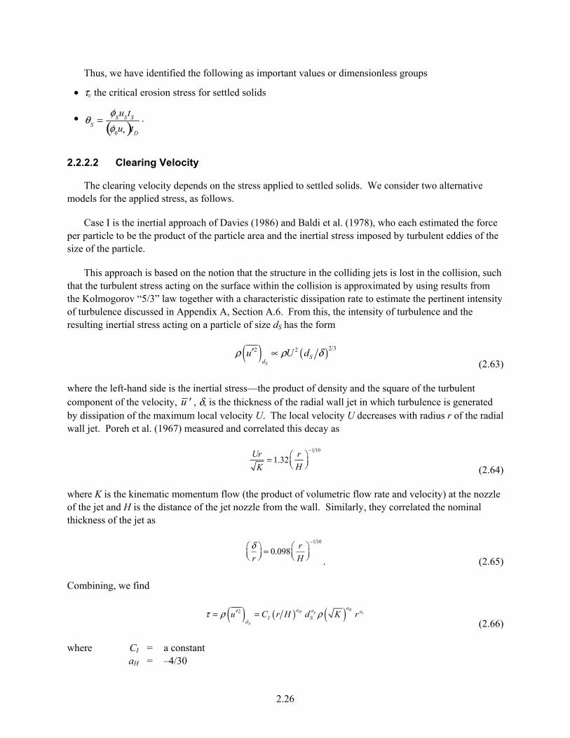
2.26

Thus, we have identified the following as important values or dimensionless groups

• τc the critical erosion stress for settled solids

•

θS

=φ

Su

St

S

φ0u

*( )tD

.

2.2.2.2 Clearing Velocity

The clearing velocity depends on the stress applied to settled solids. We consider two alternative models for the applied stress, as follows.

Case I is the inertial approach of Davies (1986) and Baldi et al. (1978), who each estimated the force per particle to be the product of the particle area and the inertial stress imposed by turbulent eddies of the size of the particle.

This approach is based on the notion that the structure in the colliding jets is lost in the collision, such that the turbulent stress acting on the surface within the collision is approximated by using results from the Kolmogorov “5/3” law together with a characteristic dissipation rate to estimate the pertinent intensity of turbulence discussed in Appendix A, Section A.6. From this, the intensity of turbulence and the resulting inertial stress acting on a particle of size dS has the form

( ) ( )2 32 2

S

Sd

u U dρ ρ δ′ ∝ (2.63)

where the left-hand side is the inertial stress—the product of density and the square of the turbulent component of the velocity, u ' , δ, is the thickness of the radial wall jet in which turbulence is generated by dissipation of the maximum local velocity U. The local velocity U decreases with radius r of the radial wall jet. Poreh et al. (1967) measured and correlated this decay as

Ur

K= 1.32

r

H

−1 10

(2.64)

where K is the kinematic momentum flow (the product of volumetric flow rate and velocity) at the nozzle of the jet and H is the distance of the jet nozzle from the wall. Similarly, they correlated the nominal thickness of the jet as

δr

= 0.098r

H

−1 10

. (2.65)

Combining, we find

( ) ( ) ( )2 K

H p r

S

aa a aI S

du C r H d K rτ ρ ρ′= =

(2.66)

where CI = a constant aH = –4/30

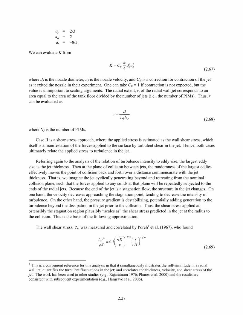
2.27

ap = 2/3 aK = 2 ar = –8/3.

We can evaluate K from

K = CK

π4

dJ2uJ

2

(2.67)

where dJ is the nozzle diameter, uJ is the nozzle velocity, and CK is a correction for contraction of the jet as it exited the nozzle in their experiment. One can take CK = 1 if contraction is not expected, but the value is unimportant to scaling arguments. The radial extent, r, of the radial wall jet corresponds to an area equal to the area of the tank floor divided by the number of jets (i.e., the number of PJMs). Thus, r can be evaluated as

r =

D

2 NJ (2.68)

where NJ is the number of PJMs.

Case II is a shear stress approach, where the applied stress is estimated as the wall shear stress, which itself is a manifestation of the forces applied to the surface by turbulent shear in the jet. Hence, both cases ultimately relate the applied stress to turbulence in the jet.

Referring again to the analysis of the relation of turbulence intensity to eddy size, the largest eddy size is the jet thickness. Then at the plane of collision between jets, the randomness of the largest eddies effectively moves the point of collision back and forth over a distance commensurate with the jet thickness. That is, we imagine the jet cyclically penetrating beyond and retreating from the nominal collision plane, such that the forces applied to any solids at that plane will be repeatedly subjected to the ends of the radial jets. Because the end of the jet is a stagnation flow, the structure in the jet changes. On one hand, the velocity decreases approaching the stagnation point, tending to decrease the intensity of turbulence. On the other hand, the pressure gradient is destabilizing, potentially adding generation to the turbulence beyond the dissipation in the jet prior to the collision. Thus, the shear stress applied at ostensibly the stagnation region plausibly “scales as” the shear stress predicted in the jet at the radius to the collision. This is the basis of the following approximation.

The wall shear stress, τw, was measured and correlated by Poreh1 et al. (1967), who found

τwr2

ρK= 0.3

K

ν

− 3 10r

H

− 3 10

(2.69)

1 This is a convenient reference for this analysis in that it simultaneously illustrates the self-similitude in a radial wall jet; quantifies the turbulent fluctuations in the jet; and correlates the thickness, velocity, and shear stress of the jet. The work has been used in other studies (e.g., Rajaratnum 1976; Phares et al. 2000) and the results are consistent with subsequent experimentation (e.g., Hargrave et al. 2006).

2.28

Substituting as above, we have

τ = τ w = CII ρν −aH

r

H

aH

K( )aK

rar

(2.70)

where CII = a constant aK = +17/10 aH = –3/10 ar = –2.

Thus, we can represent either Case I or Case II in terms of a function

( ) ( ) KH p r

aa a aSC r / H d K rτ =

(2.71)

From Section 2.2.2.1, we have

1 S

c

τθτ

+ = (2.72)

where

τ c = kτ s −1( )a1 ds

a2

(2.73)

and

θS =φSuStS

φ0u*( )tD (2.74)

Combining,

( )( ) ( ) ( )constant 1 1H Sp rc c cc c

c S sK r H d r sθθ= + − (2.75)

where Kc = the kinematic momentum flow at the limit of bottom clearing cθ = 1/aK cH = –aH/aK cp = –(ap – a2)/aK cr = –ar/aK cS = a1/aK.

The values of a1 and a2 depend on how and if one models the critical erosion stress. At this point, we choose not to attempt this, even for the M3 data (Meyer et al. 2009). We do not know the cohesive properties, if any, and using the “gravitational” model for critical erosion stress has a good physical interpretation for a particle on the verge of settling but not for a particle already in a settled bed and on the verge of separating. Therefore, we set a1 and a2 to zero in order to focus on the fluid side of the

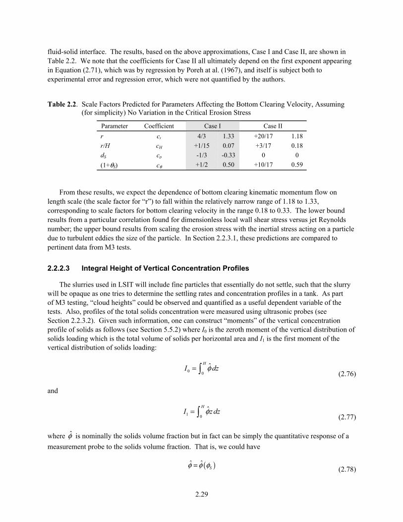
2.29

fluid-solid interface. The results, based on the above approximations, Case I and Case II, are shown in Table 2.2. We note that the coefficients for Case II all ultimately depend on the first exponent appearing in Equation (2.71), which was by regression by Poreh at al. (1967), and itself is subject both to experimental error and regression error, which were not quantified by the authors.

Table 2.2. Scale Factors Predicted for Parameters Affecting the Bottom Clearing Velocity, Assuming (for simplicity) No Variation in the Critical Erosion Stress

Parameter Coefficient Case I Case II

r cr 4/3 1.33 +20/17 1.18

r/H cH +1/15 0.07 +3/17 0.18

dS cp -1/3 -0.33 0 0

(1+θS) cθ +1/2 0.50 +10/17 0.59

From these results, we expect the dependence of bottom clearing kinematic momentum flow on length scale (the scale factor for “r”) to fall within the relatively narrow range of 1.18 to 1.33, corresponding to scale factors for bottom clearing velocity in the range 0.18 to 0.33. The lower bound results from a particular correlation found for dimensionless local wall shear stress versus jet Reynolds number; the upper bound results from scaling the erosion stress with the inertial stress acting on a particle due to turbulent eddies the size of the particle. In Section 2.2.3.1, these predictions are compared to pertinent data from M3 tests.

2.2.2.3 Integral Height of Vertical Concentration Profiles

The slurries used in LSIT will include fine particles that essentially do not settle, such that the slurry will be opaque as one tries to determine the settling rates and concentration profiles in a tank. As part of M3 testing, “cloud heights” could be observed and quantified as a useful dependent variable of the tests. Also, profiles of the total solids concentration were measured using ultrasonic probes (see Section 2.2.3.2). Given such information, one can construct “moments” of the vertical concentration profile of solids as follows (see Section 5.5.2) where I0 is the zeroth moment of the vertical distribution of solids loading which is the total volume of solids per horizontal area and I1 is the first moment of the vertical distribution of solids loading:

I0 = φ dz

0

H

(2.76)

and

I1 = φz dz

0

H

(2.77)

where φ is nominally the solids volume fraction but in fact can be simply the quantitative response of a

measurement probe to the solids volume fraction. That is, we could have

( )ˆ ˆ= Sφ φ φ (2.78)

2.30

and still be able to define the moment integrals I0 and I1. Then, we can define a characteristic vertical length scale, z1, for the solids concentration profile, from

11

0

2Iz

I=

(2.79)

which is defined so that if the profile of φ is “square”, then z1 is the height of the profile. Note that this

ratio of moment integrals is insensitive to the magnitude of the concentrations, but it is sensitive to the characteristic height of the profiles. One can define higher moment integrals and combine them to indicate, for example, a characteristic scale of “length squared” from which to infer information about the shape as well as the height of the profile. Increasingly precise data are required to obtain higher moments precise enough to be useful. Evaluating and interpreting second moments probably is worth pursuing.

The value of z1 is not very sensitive to the relationship between the actual concentration and the probe response. The more linear the relationship, the better, and a monotonic relationship is essential, but a quasi-linear monotonic relationship should suffice. It should not be necessary to infer the actual concentration of either combined or individual solids species (although anything that can be done to indicate concentration as a function of particle size would be very useful). We anticipate that the height of solids can be determined sufficiently from the moment integrals, and by combining height of solids with other information, such as concentrations in the transfer line and mass in the tank heel after pump down, models of suspension and settling can be validated sufficiently to estimate “sampling” and “accumulation” performance metrics and the uncertainty. Whether the estimated uncertainty is acceptable remains to be determined.

2.2.2.4 Upward Flow

Models of the upward flow resulting from the collision of radial wall jets on the floor of WTP vessels are proposed in Appendix C and summarized in Chapter 5. These are speculative and incomplete, but also illustrative and perhaps encouraging. Much needs to be done to develop models sufficient to support predicting performance metrics related to sampling and mass accumulation. The analyses do serve to identify the following as dimensionless groups important to developing needed models (not including those already introduced elsewhere).

• Ratio of settling velocity1 to PJM velocity (uS /U).

• Froude number (U2/(s – 1)gD)

• Solids volume fraction ϕS.

1 As noted in Section 2.2.1.5 and in Appendix A, “settling velocity” for a complex simulant will at best be some weighted average of the settling velocity of its constituents, and will depend on the total solids loading (see Appendix C). Further, the pertinent settling velocity might be a weighted average of some portion of the simulant, such as for particles that settle faster or slower than some limit.

2.31

2.2.3 M3 Data

Extensive testing of simplified PJM mixing systems using monodisperse glass beads as solids in the slurry were conducted as part of M3 testing (Meyer et al. 2009, 2012). Results from these tests provide a large set of data particularly pertinent to LSIT scaling issues. The experiments were conducted to determine the bottom clearing velocity and the “cloud height,” which is the maximum elevation of solids as they were suspended during each PJM pulse. Because the simulated wastes used in these tests were glass beads in water, the solids elevation could be estimated visually.

The bottom clearing velocity reported for the M3 work provides an obvious opportunity to compare pertinent data to models built upon the technical resources described above. Similarly, the cloud height measured during M3 testing is the available data closest in physical interpretation to the vertical distribution of the solids concentration referred to above.

The following sections compare these data with physical models or a physical modeling approach, both to illustrate physical modeling in a pertinent context, and to test modeling concepts to the extent they have been developed in this document.

2.2.3.1 Bottom Clearing Velocity

Refer to Sections 2.2.2.1 and 2.2.2.2 for background leading up to this section. The product u*φ0 appearing there is treated here as just u* because only the product appears and neither term is known separately and neither can be estimated except as the product.

Based on the functional form developed in Section 2.2.2.2, bottom clearing velocity measurements reported (Meyer et al. 2012) for the M3 experiments are fit here using the form

( ) ( ) ( )constant 1H pr

c cccc S SK r r / H d θθ= +

(2.80)

where Kc is the kinematic momentum flow (at the limit of bottom clearing), proportional to the square of the product of the nozzle velocity (at the limit of bottom clearing) and the nozzle diameter, r is the radius of colliding jets, dS is the diameter of settled solids, and θS, a dimensionless group related to particle suspension that affects ability to clear solids from bottom of vessel ,is defined and explained in Sections 2.2.2.1 and 2.2.2.2. θS includes the product of the solids volume fraction, settling velocity, and drive time.

The data were selected from 172 scaled experiments conducted in 14-in.-, 34-in.-, and 70-in.-diameter tanks. Recall that the above analysis is based on the assumption that the thickness of settled solids does not scale with the length scale because the thickness is not limited by the settling time. Therefore, the set of experiments analyzed was limited to 126 cases where the product of the settling velocity and settling time was less than the reported cloud height. The correlation coefficient matrix for the logarithms of the independent variables is shown in Table 2.3. The correlation between dS and θS probably is due in part to each being related to uS.

M3 UCS data expressed as square root of Kc were fit using Equation (2.80). The results are shown in Table 2.4.

2.32

Table 2.3. Correlation Coefficients Among the Independent Variables

r r/H 1+θS r/H +20% 1+θS -4% +2% dS +12% +4% +45%

Table 2.4. Values of Model Coefficients Fitted to “M3” Bottom Clearing Velocity Data

Coeff Fitted

Predicted (see Section 2.2.2.2)

Case I Case II

R2 95%

cr +1.22 ± 2% +1.33 +1.18

cH +0.11 ± 69% +0.07 +0.18

cp -0.14 ± 32% -0.33 0

cθ +0.25 ± 6% +0.50 +0.59

Because the value of u* is not known, the values of θS are not known from the data. Therefore, a value of u* must be assumed. The assumed value is not important for sufficiently small values, for which θS >> 1 and the value of u* no longer matters to the exponent for (1+θS). Therefore, a value of u* was assumed for which θS >> 1 for the experiments included in the data set.

The resulting fit of the data is shown as the following Figure 2.4. The fitted value of the square root of Kc for each experiment is plotted as the abscissa; the corresponding measured value is plotted as the ordinate. The line “1:1” would be a perfect fit. The data are distinguished by tank diameter as indicated in the legend.

Several observations can be made. First, this is an example of developing a physical model and fitting it to the data to estimate its coefficients, and thus, in terms of alternative scaling approaches, is a combination of “pure physics” and “pure statistics:” the functional form is found from “physics,” and the coefficients and their estimated uncertainty are found from “statistics” (regression). The results are extrapolated to a different length scale by evaluating the length scale (“r” in this expression) for WTP.

Second, the exponents for the length scale and for the particle size are within the bounds of the two predictions of the approximations described above. The exponent for (1+θS) is substantially smaller than predicted. This might result if θS >> 1 were not true; however, the fitted exponent on (1+θS) was very close to the exponents found by fitting separately each of the parameters that form θS, suggesting that actually θS >> 1.

Third, the fit (R2 = 95%) is remarkable considering only the length scale (r) and three parameters--one geometric (r/H), one material property (dS), and one mixture of kinematic parameters and material properties (1+θS)—were included in the fit, and dS has little effect. This increases our confidence in the physical model itself, which increases our confidence that the uncertainty estimated by propagating uncertainty in the coefficients through the functional form of the model is a valid estimate of the uncertainty of the predicted bottom clearing velocity.

2.33

Figure 2.4. Comparison of Measured (ordinate) and Fitted (abscissa) Values of K at the Limit of the Bottom Clearing from M3 Experiments Where the Settling Distance Did Not Exceed the Cloud Height. Symbols correspond to different tank sizes as indicated in the legend.

This analysis is encouraging, suggesting that developing a physical model for a crucial mixing

attribute—bottom clearing velocity—is not only feasible but likely, in which case it is likely one could “interpolate knowledge” (see Appendix A, Section A.7.3) rather than “extrapolate data” from LSIT scale to WTP scale.

2.2.3.2 Observations of Concentration Profiles and “Cloud Height”

During 2007 and 2008, simulated PJM mixing systems were tested by PNNL to support closing issue M3, Inadequate Design of Mixing Systems, raised by an External Flowsheet Review Team assembled by Bechtel National, Inc. The results are documented in WTP-RPT-182, Pulse Jet Mixing Tests with Noncohesive Solids (Meyer et al. 2009, 2012). The tests are particularly instructive in that the particulates were glass beads of nominally one size and the tanks included transparent bottoms and sides that allowed the motion of solids in the tank to be observed during each PJM cycle. In addition, the concentration of solids measured using ultrasonic probes at various locations and various times within PJM cycles, provided information on the spatial and temporal distribution of solids during each cycle.1 Further, video recordings made through the tank walls for several tests were available to help develop

1 Obtaining measures of the actual vertical distribution of solids (or some reasonable measure thereof for this comment) will be important to, if not fundamentally enabling of, developing and explaining the physical concepts. These measurements made during M3 testing are recommended for use in LSIT to better understand the physics. If the measurements cannot be adapted for complex simulants, relying on only concentration measurements from the transfer line and starting and stopping masses for an experiment would have to be the “backup plan.”

2.34

intuitions about the behavior of solids. From such information, we developed the following intuitions, limited to slurries of one settling velocity, about the fluid dynamics during a PJM cycle.

• The concentration profiles, consistent with observations through the tank wall of the slurry, displayed a distinct height above which the concentration was much smaller than in the region below, such that a “cloud height” was both visible and measurable. This seems reasonable for solids with one settling velocity, which are found to settle such that clear fluid appears above a clear interface with the settling slurry.

• The top of the “cloud” is seen in videos to fluctuate with apparent surface waves. This is reasonable considering the distinct cloud height, constituting a sharp density difference across the interface, enabling surface waves. The upward momentum from colliding jets is horizontally inhomogeneous due to the origin in a discrete set of PJMs. This generates effectively surface waves in the upper boundary of the solids distribution, which are seen to have both radial and circumferential spatial modes. That these waves are not actually turbulence is apparent in the remarkably reproducible effects the waves had on the concentrations sampled near the cloud height. Given the steepness of the concentration profiles, the concentration measured at a fixed elevation as the liquid rises and falls with the period of the surface waves will show cycling variations corresponding to the wave motion. This is notably apparent in Figure 2.5, adopted from Figure C.66A in Meyer et al. (2009), which shows the concentration of 70-μm-diameter glass beads in a 70-in.-diameter tank, averaged over several PJM cycles, at the center of the tank at six elevations relative to the tank diameter, as a function of time relative the PJM cycle time. This tank modeled the eight-tube array (8TA) pulse tube configuration with a nozzle diameter equivalent to a 6-in.-diameter full-scale nozzle.

Figure 2.6 depicts a similar situation for a test in the 34-in.-diameter tank, adapted from Figure C.28A in Meyer et al. (2009). This test modeled the HLP-VSL-00022 (hereafter referred to as HLP-22) configuration of four inner and eight outer pulse tubes with a nozzle diameter equivalent to 4-in.-diameter full-scale nozzle.

In the figures, note:

• the coherence—systematic cyclic variation with time—when averaged over five cycles

• the constant period of the cyclic variations

• that the period is much less than the PJM cycle

• the decrease of the variation with increasing depth below the cloud height.

Other notable features in Figure 2.5 (70-in.-diameter tank) include

• The effect of the PJM pulse is rapid at the lower elevations (panels 1 through 4), although with slightly increasing delay. This appears to be the solids entrained from the tank floor reaching the elevation of the measurement.

• At elevation H/D=0.6 (panel 5), the fluid is elevated by displacement from the pulse before the entrained solids actually arrive, resulting in the greater concentration change. This is followed by cyclic changes in measured concentration as the fluid moves moderately at appreciable depth beneath the waves at the interface.

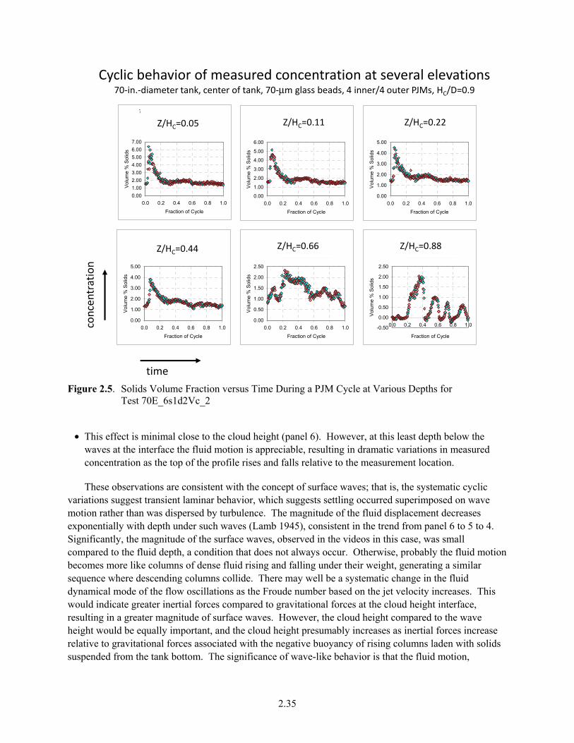
2.35

70E_6s1d2Vc_2 H 0.05D R 0R 70_07_18_2008_14_02 (5)

0.00

1.00

2.00

3.00

4.00

5.00

6.00

7.00

0.0 0.2 0.4 0.6 0.8 1.0

Fraction of Cycle

Vol

ume

% S

olid

sAverage Volume%

70E_6s1d2Vc_2 H 0.1D R 0R 70_07_18_2008_13_56 (5)

0.00

1.00

2.00

3.00

4.00

5.00

6.00

0.0 0.2 0.4 0.6 0.8 1.0

Fraction of Cycle

Vol

ume

% S

olid

s

Average Volume%

70E_6s1d2Vc_2 H 0.2D R 0R 70_07_18_2008_13_50 (5)

0.00

1.00

2.00

3.00

4.00

5.00

0.0 0.2 0.4 0.6 0.8 1.0

Fraction of Cycle

Vol

ume

% S

olid

s

Average Volume%

70E_6s1d2Vc_2 H 0.4D R 0R 70_07_18_2008_13_43 (5)

0.00

1.00

2.00

3.00

4.00

5.00

0.0 0.2 0.4 0.6 0.8 1.0

Fraction of Cycle

Vol

ume

% S

olid

s

Average Volume%

70E_6s1d2Vc_2 H 0.6D R 0R 70_07_18_2008_13_37 (5)

0.00

0.50

1.00

1.50

2.00

2.50

0.0 0.2 0.4 0.6 0.8 1.0

Fraction of Cycle

Vol

ume

% S

olid

sAverage Volume%

70E_6s1d2Vc_2 H 0.8D R 0R 70_07_18_2008_13_31 (5)

-0.50

0.00

0.50

1.00

1.50

2.00

2.50

0.0 0.2 0.4 0.6 0.8 1.0

Fraction of Cycle

Vol

ume

% S

olid

s

Average Volume%

Cyclic behavior of measured concentration at several elevations70-in.-diameter tank, center of tank, 70-μm glass beads, 4 inner/4 outer PJMs, HC/D=0.9

Z/HC=0.05

Z/HC=0.66 Z/HC=0.88

Z/HC=0.11 Z/HC=0.22

Z/HC=0.44

time

conc

entr

atio

n

Figure 2.5. Solids Volume Fraction versus Time During a PJM Cycle at Various Depths for Test 70E_6s1d2Vc_2

• This effect is minimal close to the cloud height (panel 6). However, at this least depth below the

waves at the interface the fluid motion is appreciable, resulting in dramatic variations in measured concentration as the top of the profile rises and falls relative to the measurement location.

These observations are consistent with the concept of surface waves; that is, the systematic cyclic variations suggest transient laminar behavior, which suggests settling occurred superimposed on wave motion rather than was dispersed by turbulence. The magnitude of the fluid displacement decreases exponentially with depth under such waves (Lamb 1945), consistent in the trend from panel 6 to 5 to 4. Significantly, the magnitude of the surface waves, observed in the videos in this case, was small compared to the fluid depth, a condition that does not always occur. Otherwise, probably the fluid motion becomes more like columns of dense fluid rising and falling under their weight, generating a similar sequence where descending columns collide. There may well be a systematic change in the fluid dynamical mode of the flow oscillations as the Froude number based on the jet velocity increases. This would indicate greater inertial forces compared to gravitational forces at the cloud height interface, resulting in a greater magnitude of surface waves. However, the cloud height compared to the wave height would be equally important, and the cloud height presumably increases as inertial forces increase relative to gravitational forces associated with the negative buoyancy of rising columns laden with solids suspended from the tank bottom. The significance of wave-like behavior is that the fluid motion,

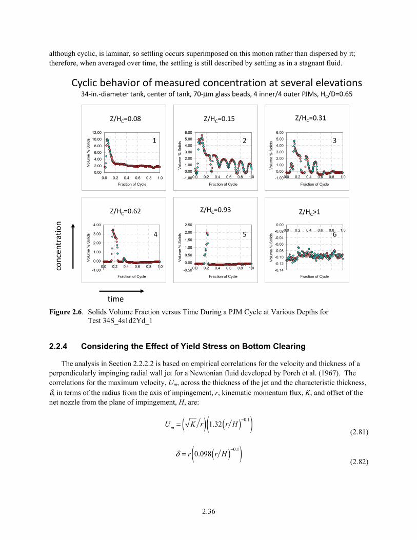
2.36

although cyclic, is laminar, so settling occurs superimposed on this motion rather than dispersed by it; therefore, when averaged over time, the settling is still described by settling as in a stagnant fluid.

34E_4s1d2Yd_1 H 0.2D R 0R 34_03_09_2008_17_17 (5)

-1.00

0.00

1.00

2.00

3.00

4.00

5.00

6.00

0.0 0.2 0.4 0.6 0.8 1.0

Fraction of CycleV

olum

e %

So

lids

Average Volume%

34E_4s1d2Yd_1 H 0.3D R 0R 34_03_09_2008_17_13 (5)

-1.00

0.00

1.00

2.00

3.00

4.00

5.00

6.00

0.0 0.2 0.4 0.6 0.8 1.0

Fraction of Cycle

Vol

ume

% S

olid

s

Average Volume%

34E_4s1d2Yd_1 H 0.4D R 0R 34_03_09_2008_17_09 (5)

-1.00

0.00

1.00

2.00

3.00

4.00

0.0 0.2 0.4 0.6 0.8 1.0

Fraction of Cycle

Vol

ume

% S

olid

s

Average Volume%

34E_4s1d2Yd_1 H 0.5D R 0R 34_03_09_2008_17_04 (5)

-0.50

0.00

0.50

1.00

1.50

2.00

2.50

0.0 0.2 0.4 0.6 0.8 1.0

Fraction of Cycle

Vol

ume

% S

olid

s

Average Volume%

34E_4s1d2Yd_1 H 0.6D R 0R 34_03_09_2008_17_00 (5)

-0.14

-0.12

-0.10

-0.08

-0.06

-0.04

-0.02

0.00

0.0 0.2 0.4 0.6 0.8 1.0

Fraction of Cycle

Vol

ume

% S

olid

s

Average Volume%

34E_4s1d2Yd_1 H 0.1D R 0R 34_03_09_2008_17_21 (5)

0.00

2.00

4.00

6.00

8.00

10.00

12.00

0.0 0.2 0.4 0.6 0.8 1.0

Fraction of Cycle

Vol

ume

% S

olid

s

Average Volume%Z/HC=0.31

Z/HC=0.62 Z/HC=0.93 Z/HC>1

Z/HC=0.08 Z/HC=0.15 Z/HC=0.31

Z/HC>1

Cyclic behavior of measured concentration at several elevations34-in.-diameter tank, center of tank, 70-μm glass beads, 4 inner/4 outer PJMs, HC/D=0.65

1 2 3

4 5 6

time

conc

entr

atio

n

Figure 2.6. Solids Volume Fraction versus Time During a PJM Cycle at Various Depths for Test 34S_4s1d2Yd_1

2.2.4 Considering the Effect of Yield Stress on Bottom Clearing

The analysis in Section 2.2.2.2 is based on empirical correlations for the velocity and thickness of a perpendicularly impinging radial wall jet for a Newtonian fluid developed by Poreh et al. (1967). The correlations for the maximum velocity, Um, across the thickness of the jet and the characteristic thickness, δ, in terms of the radius from the axis of impingement, r, kinematic momentum flux, K, and offset of the net nozzle from the plane of impingement, H, are:

Um = K r( ) 1.32 r H( )−0.1( )

(2.81)

δ = r 0.098 r H( )−0.1( )

(2.82)

2.37

White (1991)1 points out that the Kogolmorov length for eddies in a boundary layer—which a plane

jet resembles mathematically—is roughly ν 3δ U 3( )1 4, whereas in terms of dissipation rate per mass, ε, it

is ν 3 ε( )1 4(Tennekes and Lumley 19922). Thus, as follows also from dimensional analysis,

ε ~ U 3 δ( )

(2.83)

A wall jet is partly a plane jet and partly a plane boundary layer, so we adopt this approximation for the dissipation rate to describe dissipation in the wall jet. Combining, the dissipation rate per mass in the wall jet is approximately

ε ~

Um3

δ= K 3 2 r4( ) 1.32( )3

0.098( ) r H( )−0.2

(2.84)

From Section 2.1.2, we have,

θ = νε uτ

4( ) = ν τ y ρ( )2

K 3 2 r4( ) 1.32( )30.098( ) r H( )−0.2

(2.85)

where shear rate in the jet compared to that if the fluid were Newtonian (with the same viscosity as the

limiting viscosity of a yield stress fluid) is found from

γγ Newtonian

= g θ( ) = 1+ 4θ4θ (2.86)

This function is shown in Figure 2.7; the ordinate is g(θ) and the abscissa is θ.

Clearly, the transition from non-Newtonian to Newtonian shear rates for a given shear stress is centered on θ = 1. Some representative values are g(0.1) = 0.29, g(1) = 0.62, and g(10) = 0.85.

Consider a PJM system resembling that in a WTP tank, where

uJ ~ 12 m/s (jet velocity) ρ ~ 103 kg/m3 ν ~ 10-6 m2/s H ~ 0.1 m (off set of nozzle from floor) dJ ~ 0.1 m (jet nozzle diameter).

1 See beginning of Chapter 6. 2 See Section 3.2.

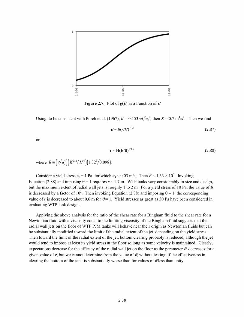
2.38

Figure 2.7. Plot of g(θ) as a Function of θ

Using, to be consistent with Poreh et al. (1967), K = 0.153πdJ

2uJ2, then K ~ 0.7 m4/s2. Then we find

θ ~ B(r/H)-4.2 (2.87)

or

r ~ H(B/θ)1/4.2 (2.88)

where B ≡ ν uτ4( ) K 3 2 H 4( ) 1.323 0.098( ) .

Consider a yield stress τy = 1 Pa, for which uτ ~ 0.03 m/s. Then B ~ 1.33 × 105. Invoking Equation (2.88) and imposing θ = 1 requires r ~ 1.7 m. WTP tanks vary considerably in size and design, but the maximum extent of radial wall jets is roughly 1 to 2 m. For a yield stress of 10 Pa, the value of B is decreased by a factor of 102. Then invoking Equation (2.88) and imposing θ = 1, the corresponding value of r is decreased to about 0.6 m for θ = 1. Yield stresses as great as 30 Pa have been considered in evaluating WTP tank designs.

Applying the above analysis for the ratio of the shear rate for a Bingham fluid to the shear rate for a Newtonian fluid with a viscosity equal to the limiting viscosity of the Bingham fluid suggests that the radial wall jets on the floor of WTP PJM tanks will behave near their origin as Newtonian fluids but can be substantially modified toward the limit of the radial extent of the jet, depending on the yield stress. Then toward the limit of the radial extent of the jet, bottom clearing probably is reduced, although the jet would tend to impose at least its yield stress at the floor so long as some velocity is maintained. Clearly, expectations decrease for the efficacy of the radial wall jet on the floor as the parameter θ decreases for a given value of r, but we cannot determine from the value of θ, without testing, if the effectiveness in clearing the bottom of the tank is substantially worse than for values of θ less than unity.

3.1

3.0 Technical Approach

In this chapter, the technical approach is developed by

• Providing a context of “scaling down” and “scaling up” for the commitment on “technical basis for scaling” in the Implementation Plan (Chu 2011)

• Distinguishing three complementary approaches to “scaling”

• Considering the advantages and disadvantages of the three approaches

• Recommending a combined approach for planning LSIT tests, in support of a WTP complementary implementation document (Dickey et al. 2012)

• Putting strategies for addressing the mixing requirements into the context of the scaling approach

• Summarizing recommended measurements and their use.

3.1 Scaling Process

At the highest level, scaling divides into two challenges: 1) “scaling down” and 2) “scaling up.” Scaling down involves deriving the conditions for a test at reduced scale so it either represents behavior at full scale or can be related to behavior at full scale. Scaling up involves providing a credible means for predicting the performance of the full-scale system from the measured performance in the reduced-scale system, taking into account the scaled-down basis for the design and operation of the reduced-scale system.

Both scaling down and scaling up are necessary and interdependent; the credibility of scaling up depends on the merit of scaling down, and the strategy for scaling down must meet the needs of scaling up. Technical bases are needed both for scaling down and scaling up. The technical bases are, if not the same, at least related, because they are interdependent. However, given the technical bases, the technical approaches for scaling down and up can be different.

3.1.1 Scaling Down

Commitment 5.1.3.13 of the Implementation Plan (Chu 2011) specifies “Defining the basis for … vessel configurations, operating parameters, and simulant parameters” and addressing “… scale laws used to establish operating conditions for testing.” That is, the technical basis for scaling should describe the basis for designing tests at reduced scale so the results can be used to predict behavior at full scale, where the design includes the following:

• Vessel configurations. Choices about the dimensions, shapes, positions, and number of features in an LSIT tank compared to a WTP tank

• Operating parameters. Choices about the velocities, flow rates, times, and mass ratios in an LSIT tank compared to a WTP tank

• Simulant parameters. Choices about simulant parameters that affect mixing, which include the settling velocity, density, and cohesive properties of the simulated waste.

3.2

The technical basis for these are described below for three canonical scaling approaches as a basis for developing a practical scaling approach that combines all three approaches.

3.1.2 Scaling Up

Commitment 5.1.3.13 of the Implementation Plan specifies addressing “… physical scale laws observed in test results.” That is, the technical basis for scaling should describe the basis for inferring the performance at full scale from specific, reduced-scale LSIT tests in terms of “physical scale laws.” For these to be considered “physical” and “laws” and to address “scale,” they should:

• Pertain to quantifiable mixing requirement metrics

• Have a functional relationship between the metrics and length scale tied to physical laws known to control the mixing phenomena pertinent to the performance metric

• Be describable in terms of a scale factor ( )ln lnf Dα = ∂ ∂ for f(D), where f is the functional

relationship between a performance metric and the tank diameter, D

• Display a very weak dependence of the scale factor on size or it will not constitute a “physical law”

• Be understood in terms of the physics of the processes that determine the value of the performance metric, learned or confirmed from testing in order to claim to have defined “physical scale laws observed in testing.”

The practicality of attaining these attributes affects how and why one might combine distinct scaling approaches into a combined approach to minimize the uncertainty of predictions of performance at full scale. This is discussed further in Appendix A, Section A.4.

3.1.3 Scaling Down Sparging in Tanks Designed for Non-Newtonian Fluids

For the case of tanks designed to mix non-Newtonian liquids, air spargers are included to agitate, especially the upper portions of the slurry in a tank. The behavior of all of the slurry in the tank will be affected to some degree by agitation by the spargers, because as the agitation increases, the non-Newtonian fluid behaves increasingly like a Newtonian fluid. Thus, to ensure that defensible conclusions are drawn from tests addressing the above three mixing requirements, the extent to which the non-Newtonian fluid acts similarly to a Newtonian fluid should be the same in LSIT as in WTP. This report describes, as one alternative, scaling down sparger operations so that the power-per-volume from sparging a non-Newtonian fluid matches that expected in the WTP. As is discussed in Section 2.1.2, this may determine the similarity to Newtonian behavior. See Chapter 7 and Appendix D for technical issues, recommendations, and details about scaling down sparger design and operations from WTP.

The dampening of shear by a yield stress will result in regions of unsheared slurry at the top of a tank. To keep all of the slurry sheared, spargers are included in tanks to overcome a yield stress. To create the same degree of Newtonian-like behavior, the number of spargers and airflow rates must be selected to provide sparging in LSIT tanks scaled from proposed sparging operations in corresponding WTP tanks. Alternative bases for scaling are discussed in Chapter 7 and Appendix D. The purpose is not to provide scaled tests of sparger performance, or in terms of scaling, the purpose is not to “scale up” sparger performance. The purpose is to create a shear environment in a Bingham fluid representative of a WTP

3.3

tank so that other aspects of the mixing cycle behave as in a WTP tank, or in terms of scaling, spargers in LSIT must be “scaled down” from the WTP design as part of the technical basis for “scaling up” the performance with respect to other requirements.

3.2 Scaling Approaches

The term “scaling” seems familiar; yet, it often is used imprecisely, with different meanings inadvertently attached to the term by different engineers while discussing the same technical issue. In Appendix A, Section A.7, three canonical approaches, 1) pure similitude, 2) pure statistics, and 3) pure physics, are identified for the purpose of clarifying fundamentally different component scaling. These approaches can and should be combined to create a practical scaling strategy. For each approach, we describe its use in scaling down and scaling up and issues of uncertainty in predicting full-scale performance. The three approaches are summarized below.

3.2.1 Pure Similitude

“Pure similitude” is a technical approach for scaling described in detail in Appendix A, Section A.7.1, as follows.

• It entails establishing complete geometric, kinematic, and dynamic similitude such that the performance of the scaled system is the same as that at full scale at the same dimensionless locations and times.

• Scaling down is entirely by similitude.

• Scaling up is simply that the observed performance of the scaled system directly represents that of the actual system.

• The uncertainty in predicting the performance metric is primarily the uncertainty in the extent to which similitude is established.

• A classic (albeit simple) example is testing a scaled-model airplane in a wind tunnel. Also, where partial similitude can be established and where the remaining departure from similitude is known to be conservative (i.e., resulting in performance at reduced scale inferior to the actual system), scale up is achieved by bounding the performance rather than representing it directly.

3.2.2 Pure Statistics

“Pure statistics” is a technical approach for scaling described in detail in Appendix A, Section A.7.2, as follows.

• It entails executing a statistically designed test matrix over the ranges of interest of all parameters that significantly affect one or more performance metrics so regression of the composite set of data provides an approximate but simple and general model of the performance metric.

• It is sufficient that existing knowledge about the physical phenomena need only identify pertinent parameters and their ranges of interest to scale down from the actual system.

• The performance metric is predicted from multi-linear regression of log-log data, which is then used to scale up the data by evaluating the regression for the values of the parameters in the actual system.

3.4

• The uncertainty in predicting the performance metric is principally a combination of the uncertainty in the fitted multi-linear coefficients and the uncertainty that the regression is valid beyond the largest length scale of the tests analyzed.

• A pertinent example is the regression of M3 data on bottom clearing velocity and cloud height.

3.2.3 Pure Physics

“Pure physics” is a technical approach for scaling described in detail in Appendix A, Section A.7.3, as follows.

• It entails establishing physical models describing, in terms of first principles, the important phenomena of the PJM mixing cycle.

• Existing knowledge about the important physical phenomena is used to deduce geometric and kinematic ratios to be matched to scale down from the actual system.

• The performance metric is predicted from correlations based on first principles and fit to test data obtained specifically to build and test the correlation, which is then the basis to scale up to the actual system.

• The uncertainty in predicting the performance metric is principally a combination of the uncertainty in the fit of the physically based functional form to the data and propagation of uncertainty in the coefficients fit to the model.

• A pertinent example is turbulence modeling, which, although based on first principles, must address great complexity and diversity in practical flow situations.

3.3 Programmatic Tradeoffs and Optimization of Certainty

Considering the disadvantages of each of the canonical scaling approaches leads to a combined scaling strategy that avoids any of the “pure” approaches, and likewise, considering the advantages of each approach leads to a combined approach that retains some of the attributes of each of the canonical approaches. The issues are described in Table 3.1.

Table 3.1. Problems with “Pure” Approaches to Scaling Performance Metrics

Problems with Including the Approach Exclusively Problems with Excluding the Approach Entirely

Pure Similitude

Intractable Constraints. Requires matching between length scales all pertinent geometric, kinematic, and dynamic ratios simultaneously, which is impossible for a PJM mixed vessel.

Limited Representation. Test results do not correspond to any specific vessel configuration, operating strategy, or waste properties.

Pure Statistics

Intractable Resources. Requires testing over the entire range of interest of each parameter known to affect a performance metric specified by a statistical test plan established and committed to prior to testing.

Much Initial Knowledge Required. Not enough is known initially about PJM mixing phenomena and their interactions to design experiments with no statistical exploration of the effects of parameters.

Pure Physics

Intractable Complexity. Requires building a predictive mechanistic understanding of all pertinent phenomena and their interactions, including turbulent or chaotic flow.

Limited Knowledge Acquired. Test plans focus on describing PJM mixing over a wide range of conditions, with little flexibility to explore hypotheses about physical explanations.

3.5

This can be expressed graphically by imagining a “composition space” with pure components of “similitude,” “statistics,” and “physics” and where any location in the composition triangle represents various “fractions” of the three components. The result is depicted in Figures 3.1 and 3.2, which summarizes Table 3.1 graphically, showing a practical “space” (center hexagon) where one can optimize a scaling strategy, surrounded by “space” (shaded region inside the perimeter) that can be excluded because of the difficulties summarized in the table.

puresimilitude

purephysical

purestatistical

mixedapproachto scaling

optimize the approach for:knowledgeresourcescontrol

intractableconstraints

provides limitedrepresentation of WTP

Figure 3.1. Scaling Approach Space

qualifytank

qualifywaste

MANAGEMENT

puresimilitude

purestatistical

purephysical

Figure 3.2. Tradeoffs Among Scaling Approaches

3.6

The advantages and disadvantages of each “pure” scaling approach dictate that none be used exclusively or avoided entirely. We identify tradeoffs among the “pure” approaches useful for choosing a scaling strategy utilizing elements of each approach.

If one minimizes resorting to physical modeling, then some choice that is a tradeoff in resources between “similitude” and “statistics” is required:

1. Many tests with each focusing on a particular tank-waste combination for which conditions of similitude are described but that need to be replicated for many tanks

2. Few tests with large test matrices, each covering a range for many parameters simultaneously but that apply to many tanks.

If one minimizes resorting to maximum similitude, then some choice between “statistics” and “physics” is required that is a tradeoff in management between:

1. Large, static test plans that explore a range over each of many parameters to build a regression model, which requires much time and funding, but which provides much data for which resources can be estimated before committing to it

2. Smaller, adaptive tests that explore the behavior of individual phenomena involving a focused set of parameters, which potentially require less time and funding and provide much knowledge, but for which the time and funding are difficult to predict in advance.

If one minimizes the need for large, statistically designed test matrices, a choice between “similitude” and “physics” is required that is a tradeoff in knowledge between:

1. Application of initial knowledge to define and establish conditions of similitude, scale down, and, to the extent similitude can be established, scale up simply by observing the performance at reduced scale, but where it may be difficult to establish sufficient similitude to obtain a favorable uncertainty in the prediction.

2. Apply initial knowledge to plan tests to fill gaps in knowledge about the “physics” that control the performance to enable building technically credible models, but where the complexity of the phenomena and especially of their interactions make the success of physical modeling ultimately uncertain.

Further, the choice of emphasis among “similitude,” “statistics,” and “physics” depends both on constraints and opportunities involving departures from similitude imposed by specific vessel or waste attributes, and tradeoffs among programmatic goals. These tradeoffs can include:

• Qualifying a vessel design for a specified design-basis waste as opposed to qualifying a waste feed for a specified set of vessel designs

• Estimating uncertainty in predictions from LSIT to WTP by “extrapolating data” as opposed to by “interpolating knowledge” (see Appendix A, Section A.7.3, for an explanation)

• Predicting WTP performance using a simple, easily understood scaling approach that involves less certainty as opposed to using a complex, difficult to understand approach with greater certainty.

These tradeoffs are reiterated graphically in Figure 3.2 by overlaying the practical region in the “scaling approach space.”

3.7

The “default scaling strategy” recommended above is slanted toward qualifying vessels, “interpolating knowledge,” and emphasizing complex, difficult to understand models as necessary to minimize uncertainty. Alternatives to consider include the following:

• An increased emphasis on qualifying a waste feed once the vessel designs are fixed.

• The possibility should be evaluated of bounding, rather than predicting, the performance relative to Limit Solids Accumulation requirements.

• The cost of fewer, more extensive, and more versatile test matrices should be compared to the combined cost of many smaller test matrices focused on one or few tanks, and the uncertainty of predicting performance in a specific vessel from few data specific to the vessel should be compared to the uncertainty of predicting performance from many data not specific to the vessel. This applies whether the performance is predicted by developing physical models or by regression.

At the highest level, the goal of “credibility” in the eyes of diverse audiences probably involves some tradeoff between technical credibility and simplicity of approach. A greater emphasis on “statistics” and regression of a large set of data probably would be easier to understand, but would require a difficult commitment at the beginning to a large, statistically designed test matrix. A more likely adaptation of the “pure statistics” approach is to supplement efforts to develop physically based models where the physical phenomena, or more probably the interactions among the phenomena, are too complex to correlate except by regression over a statistically designed test matrix of moderate extent.

3.4 Implementation of Scaling Approaches

In this section, we combine the definition of WTP performance in terms of mixing requirements provided in Chapter 1, the characterization of physical phenomena by which the vessels are mixed and the identification of test parameters that affect the phenomena provided in Chapter 2, and the scaling approaches described in Sections 3.2 and 3.3 to develop an implementation of the scaling approaches for LSIT.

3.4.1 Scaling Approaches for Specific Mixing Requirements

The mixing requirements identified by WTP are discussed generally in Section 1.5, and technical issues and strategies for addressing them are discussed at length in the technical chapters. From these, technical strategies for addressing the mixing requirements can be summarized as follows:

• Requirement 2 (Prevent Plugging) – Chapter 6. Determine the concentration of solids entering the transfer line during a PJM cycle from tests in LSIT vessels where the flow rate is scaled relative to the PJM velocity to create a representative inlet concentration. This needs to be done for two cases: Q ~ UD2 and Q ~ uSD

2, where Q is the volumetric flow rate in the transfer line, U is the PJM velocity, us is the settling velocity, and D is the tank diameter (see Section 5.6). Measure the flow rate and pressure drop in a separate flow evaluation loop at the largest scale possible if not at full scale. Evaluate steady-state conditions at the inlet to the transfer line, based on results from tests in scaled vessels. Confirm acceptably constant flow rate and pressure drop considering deposition of solids, pump net positive suction head (NPSH), and line pressure drop, using conservative evaluations so that the observed performance bounds the performance in the WTP (see Sections 6.3 and 6.4).

3.8

• Requirements 3 (Blend Liquids) and 4 (Neutralization) – Chapter 9. Measure the blend time in the transfer line by measuring the approach to steady-state concentration of a soluble tracer while scaling the flow rate as Q ~ UD2 (see Sections 9.3 and 5.6).

• Requirements 5 (Criticality), 6 (Hydrogen Generation Rate), and 7 (Process Control) – Chapter 10. Measure the density of the slurry continuously versus time at the inlet to the transfer line, sample the composition of the slurry by sampling at frequent time intervals or at certain times aligned with the PJM cycle, measure the mass of the solids in the LSIT vessel, and measure solids concentration versus time and vertical position in scaled LSIT vessels. Infer from the vertical profiles the characteristic elevation of solids by PJM mixing. Combine the results and a settling model to relate the concentration in the transfer line to the mass in the vessel and provide this model to predict the mass of solids species in a WTP tank with an uncertainty determined for the model (see Section 10.5).

• Requirement 8 (Mix to Release Gas) – Chapter 4. Measure the fraction of the bottom cleared versus velocity while maintaining kinematic similitude as the velocity changes. Establish the minimum velocity to clear the bottom by the end of each PJM pulse. Establish the drive time required to clear the bottom. Apply models of impinging jets supplemented by power-law correlations as necessary to develop a predictive model specific to WTP tank designs (see Section 4.2). For a low yield stress fluid in a Newtonian tank after a DBE establish the minimum velocity required to mobilize the tank.

• Requirement 10 (Limit Solids Accumulation) – Chapter 5. Measure the mass of solids remaining in a scaled vessel at the end of a pump-down sequence over multiple PJM cycles. Scale the flow rate in the transfer line as Q ~ UD2 both to create a conservative concentration exiting the tank and to match the ratio of PJM cycles per pump-down sequence to that of the WTP. Provide either a composite model (similar to that required for the sampling requirements) based on the entire PJM cycle to relate the exiting concentration to the mass in the vessel, or demonstrate that conservative conditions exist during a pump-down sequence for a scaled tank such that the fraction of solids remaining after a pump-down sequence is a conservative representation of the performance in the WTP (see Chapter 5).

In Table 3.2, the performance metric, approaches for scaling down test conditions and scaling up performance predictions, and the nature of testing to implement these strategies are shown by category of mixing requirement.

From Table 3.2, we see that the relative emphasis on “similitude,” “statistics,” and “physics” is different for the strategies to address the mixing requirements. They can be indicated approximately on the “scaling approach space” diagram, which is shown as Figure 3.3.

The rationale for the diagram is described, considering the relative attributes of the phenomena pertaining to the mixing requirements.

Blend time (B) is expected to depend on simple physical phenomena with less importance of interactions among phenomena, resulting in a higher probability that it can be correlated using a power law form.

3.9

Table 3.2. Technical Approaches for Scaling by Mixing Requirement

Category Requirement Metric(s) Scale Down Test Scale Up P

lugg

ing

2: P

reve

nt P

lugg

ing

• Stability of flow

• ΔP vs. flow • Solids

deposition

• Scale transfer line flow to find peak concentration in line

• Create bounding conditions in separate flow evaluation loop

• Measure concentration of solids in transfer line over a PJM cycle

• Measure flow rate and ΔP in separate flow evaluation loop with inlet concentration based on scaled vessel tests

• Results from separate flow evaluation loop bound the tendency for solids deposition in WTP transfer line

• Benchmark existing models to predict bounding WTP conditions for no plugging

• Benchmark models for ΔP and solids deposition using WTP simulant

Ble

ndin

g

3: B

lend

Liq

uids

4:

Neu

tral

izat

ion Blend time • Operate at or above

bottom clearing velocity

• Match all geometric and kinematic ratios possible

• Measure concentration difference of soluble tracer in vessel vs. time

Predict blend time from empirical correlation vs. vessel size

Sam

plin

g

5: C

riti

cali

ty

6: H

ydro

gen

Gen

erat

ion

rate

7:

Pro

cess

Con

trol

Error in estimating tank mass from slurry composition determined at inlet to transfer line

• Operate at or above bottom clearing velocity

• Match all geometric and kinematic ratios possible

• Scale flow rate for either peak or inter-peak concentrations at inlet

• Supplemental simulants will be needed for some experiments to provide a series of settling rates

• Measure solids species concentrations at transfer line inlet

• Measure mass of solids species in scaled vessel

• Measure concentration profiles of solids vs. time, position in scaled vessel

Demonstration can predict average concentration in scaled vessel from concentration determined at inlet to the transfer line

Gas

Rel

ease

8: M

ix to

R

elea

se G

as Fraction of

bottom cleared • Match all geometric

and kinematic ratios possible while varying velocity

• Measure fraction of bottom cleared vs. time and velocity

• Measure thickness of settled solids near jet collisions

Develop physically based model with power law as needed

Mas

s A

ccum

ulat

ion

10:

Lim

it S

olid

s A

ccum

ulat

ion Mass of solids

remaining after pump down

Either as “Sampling” or operate pump down at one set of conditions providing maximum similitude with WTP

• Run pump-down test over multiple PJM cycles

• As for “Sampling”

Demonstrate that difference between exit concentration and average concentration in tank can be predicted or bounded Observe mass accumulation and use as bound for WTP

3.10

puresimilitude

purephysical

purestatistical

SBM1

M2

G

P

Figure 3.3. Relative Emphasis of Scaling Approach for Mixing Requirements (P = plugging, B = blending, S = sampling, G = gas release, M1 = mass accumulation model, M2 = mass accumulation bound)

Plugging (P) will be tested in a separate flow evaluation loop intended to confirm existing models and

associated material properties. A separate loop is proposed to enable testing at a scale larger than the 4-ft-, 8-ft-, and 14-ft-diameter scales of integrated LSIT testing because of the impracticality of scaling the transfer line in integrated LSIT tests for phenomena in the vessel important to the concentration entering the transfer line simultaneous with scaling the transfer line for phenomena important to solids deposition and pressure drop (see Chapter 6). Consequently, we expect prevent plugging—in terms of solids deposition and pressure drop—to be evaluated using a combination of a scaled flow evaluation loop and calibrated existing models—that is, a combination of the “pure similitude” and “pure physical” approaches.

Gas release (G) (i.e., bottom clearing per se) would be modeled, in part, based on existing models of impinging turbulent jets and turbulence affecting particles. Applying such models to M3 bottom clearing data has been encouraging.

Mass accumulation can be approached either by 1) building several interacting models (M1), which is a difficult but perhaps inescapable challenge, or 2) establishing that the mass accumulation in an LSIT pump-down test with conservative settling velocities and transfer line flow rates (relative to the size and velocity of the scaled test) is a conservative measure of performance (M2).

For the sampling requirement (S), the emphasis should be on physical modeling or complemented by data regression to evaluate model coefficients. Given initial uncertainty about the ability to develop models, this can be supplemented as necessary by general regression of data where the model cannot be found. However, by either approach, one must relate the concentration in the transfer line to the contents of the tank, given that the PJMs are not capable of homogenizing the solids distribution in a tank. Even if complicated in absolute terms, the simplest credible approach starts with estimating the vertical profile of solids at the end of the drive cycle and then modeling as simply as possible settling that ensues during the

3.11

refill part of the cycle in order to estimate the vertical profile at the end of a cycle. This must be combined with an estimate of the “pulse” in concentration caused by the scouring of solids by the leading edge of the PJM flow along the vessel floor. This is also complicated, but some of the analysis in Appendix C suggests a starting path. See Chapter 10 for a logic for developing models systematically, as needed.

3.4.2 Recommendations About LSIT Testing to Facilitate Scaling Up to WTP Performance

Considering the mixing requirements (Chapter 1), past work and physical fundamentals (Chapter 2), and the scaling approaches described above, an approach is recommended, and essential test controls and measurements are defined, for scaling the test results to predict WTP performance. The recommendations are intended to support a complementary implementation document (Dickey et al. 2012) in which individual tests are identified and associated specific scaling strategies for the tests are selected. Accordingly, in this document we recommend a default scaling strategy, which is summarized as follows.

• Generally, for tests for any performance metric:

– Match the key geometric ratios to those for the corresponding tank in WTP. Based on the fundamental behavior of impinging jets, these should include the ratio to vessel size of PJM nozzle diameter; offset of the PJM nozzle and the suction nozzle from the vessel floor; and the number and arrangement of PJMs. Based on settling phenomena and overall mass balances, these should include the ratio of the initial and final slurry volumes compared to the nominal vessel volume.

– Control the PJM velocity to equal or exceed the bottom clearing velocity for the scale of the test and for geometric and waste parameters.

– As the PJM velocity in an LSIT test is adjusted for any reason, adjust the kinematic ratios in the LSIT tank to remain matched to the ratios in the corresponding WTP tank. Based on a review of the phenomena affecting the PJM mixing cycle, these should include the dimensionless cycle time (UtC/D) and duty cycle. The ratio of settling velocity to PJM velocity is important but cannot be matched across scales without matching the simulant properties between LSIT and WTP.

• To determine the bottom clearing velocity:

– Measure the fraction of the tank bottom covered by solids versus time during PJM pulses for a given PJM velocity and values of other parameters. Determine the minimum PJM velocity to clear solids during a PJM pulse by varying it and, using that information, adjust dependent kinematic ratios so they remain matched to corresponding WTP values.

– Assuming that the properties of the main complex simulant are not scaled with length scale over LSIT tests, the ratio of settling velocity to PJM velocity cannot be matched to the value for the WTP. Conduct supplemental tests with specialized, simplified simulants with the same particle density but with particle sizes to more nearly match the ratio of settling velocity to bottom clearing velocity to the value in WTP. Combine the test results to estimate the effect on the bottom clearing velocity of a mismatch in the ratio of settling velocity to PJM velocity.

3.12

– Assuming that the properties of the main complex simulant are not scaled with length scale over LSIT tests, the ratio of critical stress to erode a settled bed to inertial forces from the PJM jet (i.e., the Reynolds number based on the critical stress) will vary substantially across tests at different scales, and will not match the value for WTP. Conduct supplemental tests with specialized, simplified simulants with the same settling velocity but with a critical stress designed to match the critical stress Reynolds number, Rec to its value in WTP. Combine the test results to estimate the effect on the bottom clearing velocity of a mismatch in the value of Rec.

– Conduct supplemental tests to measure the critical stress for erosion of settled solids.

– Conduct supplemental tests to measure the settling velocity of different size fractions for the simulated waste to validate or improve a settling model.

• To support predicting performance metrics for mixing requirements for sampling, no plugging, and no mass accumulation:

– Measure the concentration of liquid species and of solid species in the transfer line near its inlet as a function of time over individual PJM cycles and over an entire pump-down sequence.

– Repeat this measurement for different values of the transfer line volumetric flow rate to accommodate scaling of different phenomena, such as during a PJM pulse and during PJM refill.

– Measure1 the vertical solids concentration profile frequently during each PJM cycle at several radii. Initial focus will be the period of PJM refill.

– Reduce the concentration profile data to the form of integral moments of the (nominal) concentration measurement. As is explained in Section 2.2.2.3, the length scale and potentially more than one length scale of the vertical distribution of solids can be defined from integrals over elevation of measurements that are sensitive to the solid concentration, whether or not the concentration of a specific species or the sum of species can be inferred directly from the measurement.

– Supplemental simulants will be needed for some experiments to test the effect of the ratio of settling velocity to PJM velocity, which cannot be either independently varied or scaled to WTP except by altering the simulant to provide a series of settling rates. This would not amount to scaling the particles to tank size as the objective, but would require exploring a substantial range of settling velocities.

• To support predicting performance metrics for mixing requirements for blending:

– The first priority for complying with performance metrics for blending is to determine the likelihood of compliance when bottom clearing is attained. This can be done by measuring the concentration of soluble tracer species in the transfer line near its inlet, from which the blend time can be estimated (see Section 9.3). If suitable blend times are found with a comfortable margin when bottom clearing is attained, additional testing devoted to evaluating blend times will not be necessary.

1 The tractability of this measurement was demonstrated during M3 tests for monodisperse solids. For complex simulated waste, the measurement might be limited to the total solids volume fraction, or simply an integrated response of the instrument to the distribution of solids in the slurry. Deconvoluting the measurement to infer the composition would be ideal but may not be possible, and should not be necessary to test physical models.

3.13

– If, and as needed, measure the concentration of soluble tracer species in the vessel at several locations from which “blend times” can be inferred for conditions representing a specific WTP vessel.

• To determine bounding conditions within which plugging in the transfer line does not occur:

– Conduct tests in scaled vessels to determine the worst-case concentration at the transfer line inlet to evaluate in bounding, steady-state tests in a separate flow evaluation loop.

– Evaluate whether the combination of a scaled transfer line inlet and unscaled particle sizes do not change the fraction of solids captured across scales.

– Benchmark existing models to enable scaling up bounding conditions for no solids deposition in WTP transfer line.

– For bounding concentration conditions obtained from the steps described above, measure pressure drop, NPSH, and velocity for solids deposition due to solids deposition in a separate flow evaluation loop at the largest scale available, and ideally at full scale (see Sections 6.4.1 and 6.4.2).

3.4.3 Recommended Measurements

Table 3.3 describes the associated test measurements required to implement the alternative scaling approaches for each mixing requirement. The recommendations are based in part on measurements successfully made during M3 testing, which provided considerable insight into PJM mixing phenomena as is discussed in Section 2.2.3.

3.14

Table 3.3. Testing Measurements

Requirement Measurements Purpose

Prevent Plugging (see Chapter 6) • Pressure drop, static head at pump inlet

• Solids deposition in flow evaluation loop (see also limit solids accumulation, which supports this testing)

• Slurry density continuously vs. time

• Slurry composition from samples.

• Deposition is a performance metric for this requirement

• Pressure drop affects pump performance and plugging; used to determine NPSH at pump inlet

• Sample concentrations are used to define bounding conditions; defines sampling needs and requirements.

Blend Liquids, Neutralization (see Chapter 9)

• Transient concentration of a miscible tracer at several locations in the vessel.

• Blend time is a metric for these requirements, which can be inferred from the history of homogeneity of concentration of a tracer in the vessel.

Sampling – Hydrogen Generation Rate, Process Control (see Chapter 10)

• Samples from transfer line to determine the concentration of hydrogen generating species and species monitored for process control

• Include measurements for limit solids accumulation.

• Ability to relate the sampled concentration to the mass in the tank is the performance metric for these requirements, which is determined by comparing these measured quantities.

Sampling – Criticality (see Chapter 10)

• Samples from transfer line to determine the concentration of specific solid species

• Ultrasonic measurements in the slurry to determine characteristic elevations of solids concentrations as a function of elevation and time.

• Ability to relate the sampled concentration to the mass in the tank is the performance metric for this requirement, which is determined by comparing these measured quantities

• Ability to predict solids loading vs. time at transfer line inlet.

Mix to Release Gas (see Chapter 4) • Tank floor area covered by solids at the end of a PJM pulse

• Depth of solids on tank floor at start of a PJM pulse.

• Technical strategy for demonstrating bottom motion is to demonstrate solids are cleared from the tank floor.

Limit Solids Accumulation (see Chapter 5)

• Include measurements for “sampling – criticality,” which support this testing

• Include measurements for “mix to release gas,” which support this testing.

• Ability to relate the exit concentration to the mass in the tank enables determining the overall mass balance, which is the performance metric for this requirement.

4.1

4.0 Gas Retention (Bottom Motion)

High-energy radiation (gamma, beta, or alpha) decomposes water and forms hydrogen gas, which can form unsafe conditions in the headspaces of vessels unless the gas is purged. If slurry solids settle in a tank, the hydrogen gas accumulates between the solid particles held by interstitial forces. If the solids are disturbed, the gas can release and suddenly create potentially explosive conditions in the vessel. Safety requires that any accumulated hydrogen gas be released before unsafe conditions can be created in the vessel. The gas release requirement defines the degree of mixing (degree of solids mobilization) required to release flammable gas that is retained in settled solids layers or non-Newtonian fluid. This section reviews the gas release requirements and evaluates the metrics for evaluating the requirement and the technical basis for scaling the jet velocity, pulse times, and other factors for conducting testing at less than full scale. In some conditions, such as full bottom motion as measured by bottom clearing of the residual zone, empirical testing needs are identified.

This section is supplemented by Appendix B, Working Paper for the Technical Basis for Scaling of Bottom Motion.

4.1 Gas Release Requirements

The gas release requirement covers both normal operations and gas release from DBEs. The WTP vessel mixing requirements for Requirement 8 for gas release during normal operations are specified in 24590-WTP-ES-ENG-09-001, Appendix A (Mauss and Papp 2010). The requirements for the vessels being tested are as follows: “Agitate fluid to release gas to prevent hydrogen concentration in the headspace from exceeding 25% of lower flammability limit (LFL) during normal operations and 100% of LFL during and following accident conditions” (Mauss and Papp 2010).

Vessels are considered to meet the gas release requirement when the mixing is sufficient that all the particles on the bottom of the tank are lifted from the bottom at some point in the PJM cycle, a condition termed “bottom clearing.” The technical basis for using bottom clearing during steady-state operations to establish gas release in Newtonian1,2 vessels was provided by Gauglitz et al. (2009). The following is from Gauglitz et al. (2009):

The mechanism of how gas bubbles will be released by waste mobilization depends on whether the bubbles are retained by capillary forces or by the waste strength. For bubbles retained by capillary forces, which is the expected retention mechanism for larger non-cohesive particles, it is expected that simply mobilizing3 the settled particles will be

1 Should Newtonian vessels’ wastes develop a yield stress greater than 3 Pa in the slurry above the bottom zone of the vessel (where bottom shearing is created during bottom clearing), shearing of the upper zones in the vessel will also need to be established. The shearing in the upper zones of the vessel will need to be adequate to release the bubbles from the yield stress conditions of the slurry. 2 In non-Newtonian vessel designs, several sources of shearing energy are used to release the hydrogen gases including PJMs at the vessel bottom and the spargers at multiple locations within the vessel. The Newtonian-designed vessels rely on the PJMs to provide the shear forces for the entire vessel (with the exception of UFP-01, which also provides some shear energy from purge air flowing to the steam ring; see Chapter 7). 3 Shearing.

4.2

sufficient to initiate bubble release. Specifically, once a bed of settled non-cohesive particles is mobilized, individual particles can easily move away from their neighboring particles. When this happens, the pore throats that were retaining the bubbles by capillary forces can become much larger, and any retained bubbles can be readily released. The release of gas bubbles from non-cohesive beds of particles via fluidization or mobilization is not a common research topic, but the work of Ohshima et al. (1976) is one specific example explicitly showing that the holdup of trapped (stagnant) gas bubbles approaches zero as the minimum fluidization velocity is reached [text bolded for emphasis]. In the review article by Cheremisinoff and Gupta (1983), this behavior reported by Ohshima et al. (1976) is noted and accepted.

Note: The terms “bottom clearing” and “bottom motion” sometimes are used interchangeably (Campbell et al. 2010b, p. A-32), but for clarity the terms are distinguished separately as follows.

• Bottom clearing is the mixing condition for which all particles in an area of interest are suspended off-bottom for some period of the drive cycle.

• Bottom motion is the mixing condition for which all particles in an area of interest are in motion for at least some part of the drive cycle.

The observation instructions for bottom clearing and for the critical suspension velocity, UCS, are provided in detail in Chapter 8.

4.1.1 Gas Release – Normal Operations

During normal conditions PJMs are operating and the vessel purge gas system is operating. The purge system is sized with sufficient flow rate to assure that the hydrogen concentration will be maintained below 0.5 percent (Campbell et al. 2010b, p. A-33). The LFL for hydrogen gas is 4 percent (Hinckley 2010), and 25 percent of this LFL is 1 percent, so under normal conditions, the requirement is met when mixing is sufficient to mobilize all of the waste in the vessel (Campbell et al. 2010b, p. A-32).

An accident scenario could occur if part of the tank is not mixed. Hydrogen gas could accumulate in the unmixed volume until the buoyancy of the accumulated hydrogen caused a rapid release of the accumulated hydrogen and the 25 percent of LFL concentration would be exceeded in the headspace.

The WTP vessel requirements for Requirement 8 for gas release during normal operations are specified in 24590-WTP-ES-ENG-09-001 (Mauss and Papp 2010). The requirements for the HLP-22 and UFP-VSL-00001 (hereafter referred to as UFP-01) vessels being tested are as follows: Requirement 8 for normal operations states, “Agitate fluid to release gas to prevent hydrogen concentration in the headspace from exceeding 25% of LFL during normal operations and 100% of LFL during and following accident conditions.”

The requirement for tank RLD-VSL-00008 (hereafter referred to as RLD-08) is different because the hydrogen gas generation rate is expected to be too low to generate a hazardous condition during accident conditions. Requirement 8 for normal operations states, “PJM’s are present in vessel for process functions, but do not have a safety function related to hydrogen release. Per 24590-WTP-M4C-V11T-00011, “Revised Calculation of Hydrogen Generation Rates and Time to LFL for WTP,” (Eager 2010) if there is a loss of purge for RLD-08, the time to LFL is determined to be

4.3

1,020 hr @ 140°F.” The Preliminary Documented Safety Analysis (PDSA) for high-level waste (HLW) (24590-WTP-PSAR-ESH-01-002-04, Section 3.4.1.7, Kulp 2011) states, “Except for vessels with SL-1 events to the public, for vessels with time to LFL (TLFL) for hydrogen greater than 1000 hr, normal operating systems will provide adequate protection and no additional important to safety (ITS) protective features are required.”

During testing, the gas release requirement for Newtonian vessels will be established by determining bottom motion as measured by bottom clearing.

The technical basis for using bottom motion to establish gas release in Newtonian vessels was provided by Gauglitz et al. (2009), and is the same as for bottom clearing shown in Section 4.1.

The testing of gas release in the upper portion of non-Newtonian vessels had been conducted in prior testing.

The testing of the bottom portion of the non-Newtonian vessel will be established by determining bottom motion as measured by bottom clearing.

4.1.2 Gas Release – Design Basis Event

In a DBE, it is assumed that mixing stops, solids settle to the bottom, and hydrogen accumulates in the settled solids until the solids are mobilized and the gas is released. After a DBE, a higher concentration of hydrogen is allowed in the vessel headspace, up to the LFL (4 vol%). Safety systems are designed to provide some amount of air for PJM mixing of those vessels where hydrogen generation rates are sufficient that the safe condition would be exceeded if the tank remained unmixed for greater than 1000 hr.1

The air for the mixing system is limited. The safety air system is designed to provide 1 hr of mixing every 24 hr to designated vessels. 24590-WTP-ES-ENG-09-001 (Mauss and Papp 2010, pp. A-8, A-9) states for HLP-22:

During accident conditions, the criteria is to mobilize solids to release gas within 1 hr (per ABAR 05-0084 COA #28). Percent of solids to be mobilized within a 24 hr period is 85%.

A further complication is that settled solids develop cohesive strength over time. It takes more mixing energy to overcome the cohesive strength and mobilize the settled solids as time passes and the solids pack.

An average upper bound settled layer shear strength of up to 200 Pa can be expected within 24 hr based on information presented in Table 2.1 of PNNL-17707 (Gauglitz et al. 2009), “An Approach to Understanding Cohesive Slurry Settling, Mobilization, and Hydrogen Gas Retention in Pulsed Jet Mixed Vessels.”

1 The PDSA for HLW (Kulp 2011, 24590-WTP-PSAR-ESH-01-002-04, Section 3.4.1.7) states, “…for vessels with time to LFL (TLFL) for hydrogen greater than 1000 hr, normal operating systems will provide adequate protection and no additional ITS protective features are required.”

4.4

Gas release Requirement 8 for a DBE applies to HLP-22 and UFP-01 of the tanks under consideration in the scale testing. Requirement 8 for a DBE does not apply to RLD-08 because the time to LFL has been determined to be 1020 hr. Therefore, ITS mixing systems will not be installed in RLD-08.

The WTP vessel requirements for Requirement 8 for gas release during a DBE are specified in 24590-WTP-ES-ENG-09-001, Appendix A (Mauss and Papp 2010). The requirements for the vessels being tested are as follows:

• HLP-22’s Requirement 8 for DBE operations states:

Agitate fluid to release gas to prevent hydrogen concentration in the headspace from exceeding … 100% of LFL during and following accident conditions. During accident conditions, the criteria is to mobilize solids to release gas within 1 hr (per ABAR 05-0084 COA #28). Percent of solids to be mobilized within a 24-hr period is 85% (Note: The criteria to mobilize less than 100 percent of the solids applies to post accident conditions only.) based on Table 2.1 estimates in 24590-WTP-RPT-PET-10-007, “M3 Gas Release in Newtonian Pulse Jet Mixer (PJM) Mixed Vessels.” An average upper bound settled layer shear strength of up to 200 Pa can be expected within 24 hr based on information presented in Table 2.1 of PNNL-17707, “An Approach to Understanding Cohesive Slurry Settling, Mobilization, and Hydrogen Gas Retention in Pulse Jet Mixed Vessels.” Higher yield strengths have been measured at solids concentrations much greater than WTP waste feeds and/or waste materials that are not representative of those planned for transfer to WTP. Note: This requirement will be met by application of ITS mixing (assumed to be implemented as mitigation feature for hydrogen release) within the required timeframe.

It further notes that, “HLP-22 may be susceptible to a steam bump. The steam bump is bounded by the hydrogen release requirement (Kulp 2011; 24590-WTP-PSAR-ESH-01-002-02).”

• For tanks HLP-VSL-00027A (hereafter referred to as HLP-27), HLP-27B, UFP-02A and UFP-02B, the requirement is the same. Requirement 8 for DBE operations states:

Agitate fluid to release gas to prevent hydrogen concentration in the headspace from exceeding … 100% of LFL during and following accident conditions. Per 24590-WTP-PSAR-ESH-01-002-02, Hydrogen concentrations in the vessel headspace must be maintained … less than 4% by volume, LFL, under accident conditions leading to a loss of normal or offsite power including natural phenomena hazard (NPH) events. Note: This requirement will be met by application of mixing (implemented as mitigation feature for hydrogen release) within the required timeframe.

It further notes that these tanks, “may be susceptible to a steam bump. The steam bump is bounded by the hydrogen release requirement (Kulp 2011; 24590-WTP-PSAR-ESH-01-002-02).”

• UFP-01’s Requirement 8 for DBE operations states:

Agitate fluid to release gas to prevent hydrogen concentration in the headspace from exceeding … 100% of LFL during and following accident conditions. Per 24590-WTP-PSAR-ESH-01-002-02, Hydrogen concentrations in the vessel headspace must be maintained … less than 4% by volume, LFL, under accident conditions leading to a loss

4.5

of normal or offsite power including natural phenomena hazard (NPH) events. Note: This requirement will be met by application of mixing (implemented as mitigation feature for hydrogen release) within the required timeframe.

• RLD-08’s Requirement 8 for DBE operations states:

PJMs are present in vessel for process functions, but do not have a safety function related to hydrogen release. Per 24590-WTP-M4C-V11T-00011, “Revised Calculation of Hydrogen Generation Rates and Time to LFL for WTP” (Eager 2010), if there is a loss of purge in for RLD-08, the time to LFL is determined to be 1,020 hr @ 140°F (Table 8-2). The PDSA for HLW (24590-WTP-PSAR-ESH-01-002-04, Section 3.4.1.7) (Kulp 2011) states that “Except for vessels with SL-1 events to the public, for vessels with time to LFL (TLFL) for hydrogen greater than 1000 hr, normal operating systems will provide adequate protection and no additional ITS protective features are required.

Note that RLD-08 is representing other distributed arrays for scaling.

Without additional vessel instrumentation, the fraction of solids to be mobilized cannot be directly observed during testing. For HLP-22, the proposed measurement metric is to mobilize or clear 85 percent of the vessel bottom area during the DBE test.

During design basis event testing, the gas release requirements for Newtonian vessel HLP-22 will be based on 85% of the bottom area being cleared.

The technical basis for using bottom clearing to establish gas release in vessels was provided by Gauglitz et al. (2009), and was described previously in Section 4.1.

4.2 Bottom Motion Scaling

The metric chosen to demonstrate bottom motion of sediment is bottom clearing; that is, movement of all solids at least momentarily from the tank bottom. This is similar to but different than the critical suspension velocity requirement, UCS, defined as the velocity at which the solids are completely suspended off the vessel bottom at the end of the jet pulse, that was used in Phase 1 (Meyer et al. 2009) and Phase 2 (Edmonson and Thomson 2010) of the M3 tests.

The transient bottom clearing behavior during the jet pulse occurs in two sequential phases. At the beginning of the first phase, designated as radial clearing, the impinging jet clears a circular region in the sediment bed immediately below the pulse tube, and the radius of the cleared region begins to expand as a function of time and velocity. The rate of expansion slows as the edge of the cleared region moves away from the jet centerline. The radial clearing phase ends as the edge of the radial cleared regions approach the interaction zone between adjacent jets. The radial jet behavior begins to change as the radius approaches the halfway point between two adjacent pulse jet centerlines. The radial velocity slows and up-wash fountain flows and circumferential flows begin to form.

The second transient phase is the clearing of residual sediment regions that remain after the jet radial regions begin to intersect. Examples of these residual regions are shown in Figure 4.1. One type of residual region occurs at the intersection of multiple jets, such as the center region in Figure 4.1. Another

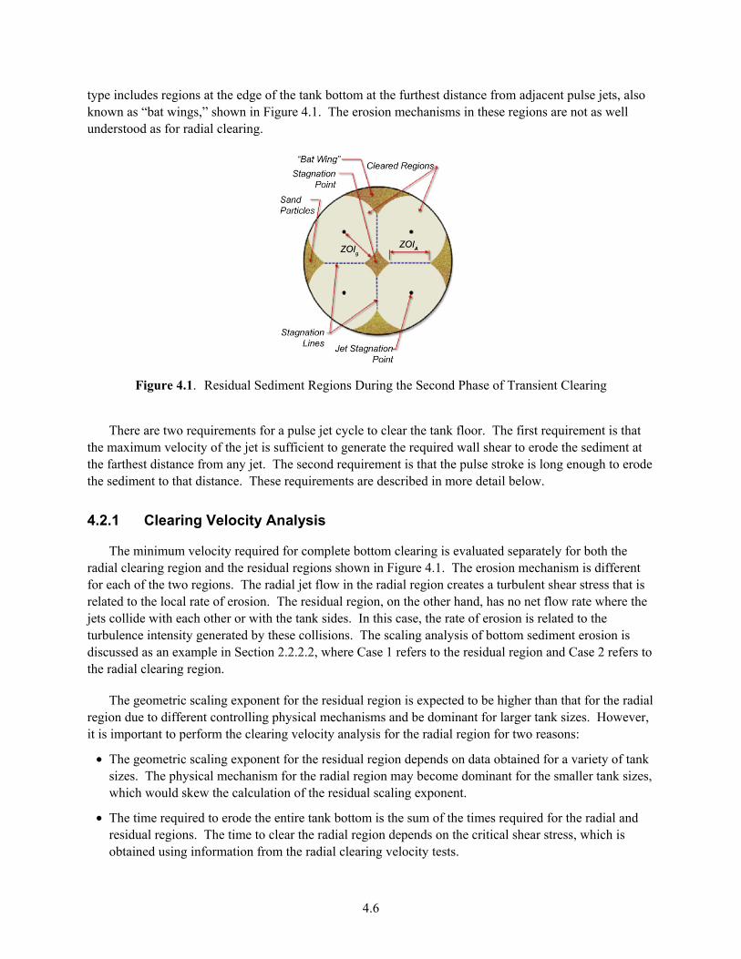
4.6

type includes regions at the edge of the tank bottom at the furthest distance from adjacent pulse jets, also known as “bat wings,” shown in Figure 4.1. The erosion mechanisms in these regions are not as well understood as for radial clearing.

Figure 4.1. Residual Sediment Regions During the Second Phase of Transient Clearing

There are two requirements for a pulse jet cycle to clear the tank floor. The first requirement is that

the maximum velocity of the jet is sufficient to generate the required wall shear to erode the sediment at the farthest distance from any jet. The second requirement is that the pulse stroke is long enough to erode the sediment to that distance. These requirements are described in more detail below.

4.2.1 Clearing Velocity Analysis

The minimum velocity required for complete bottom clearing is evaluated separately for both the radial clearing region and the residual regions shown in Figure 4.1. The erosion mechanism is different for each of the two regions. The radial jet flow in the radial region creates a turbulent shear stress that is related to the local rate of erosion. The residual region, on the other hand, has no net flow rate where the jets collide with each other or with the tank sides. In this case, the rate of erosion is related to the turbulence intensity generated by these collisions. The scaling analysis of bottom sediment erosion is discussed as an example in Section 2.2.2.2, where Case 1 refers to the residual region and Case 2 refers to the radial clearing region.

The geometric scaling exponent for the residual region is expected to be higher than that for the radial region due to different controlling physical mechanisms and be dominant for larger tank sizes. However, it is important to perform the clearing velocity analysis for the radial region for two reasons:

• The geometric scaling exponent for the residual region depends on data obtained for a variety of tank sizes. The physical mechanism for the radial region may become dominant for the smaller tank sizes, which would skew the calculation of the residual scaling exponent.

• The time required to erode the entire tank bottom is the sum of the times required for the radial and residual regions. The time to clear the radial region depends on the critical shear stress, which is obtained using information from the radial clearing velocity tests.

4.7

4.2.1.1 Radial Clearing Region

The minimum required velocity for the radial clearing region is based on the correlation from Poreh et al. (1967) for wall shear, τw, for a submerged radial wall jet as a function of r, the radial distance from the jet centerline

0 3 2 32

0 3

. .

wH K r.

K H

τρ ν

− − = (4.1)

where 2 204

K U dπ= = the kinematic momentum flow from the jet nozzle

U0 = the nozzle velocity d = the nozzle diameter ρ = density ν = kinematic viscosity H = the nozzle offset from the vessel floor.

If geometric similarity is enforced, the length ratios H/D and r/H are the same in both scales, as are the physical properties ρ and τw. The scale-up relationship (Dickey 2010) for the minimum velocity for the radial clearing region becomes (see Appendix B)

0.3 0.1761.7 = =

Full Full

Full Scale ScaleScale Scale

D Du u u

D D (4.2)

This exponent is expected to be less than that for the residual clearing region.

4.2.1.2 Residual Clearing Region

The clearing mechanisms for the residual sediment regions are not as clearly understood as for the radial clearing region. Complexities related to the interactions of the slurries from opposing jets, the curved floor geometries, the impact of thicker than thin film solids concentrations and the buildup of solids on the leading edge of the cleared material wave have not been combined to evaluate the scaling of the bottom motion phenomenon (as measured by bottom clearing).1 Therefore, the scaling exponent must be empirically determined based on experimental data. The scaling behavior is assumed to have the same form as for the radial clearing

n

FullFull Scale

Scale

Du u

D

=

(4.3)

1 The scaling of the UCS solids suspension phenomenon with these conditions was evaluated in reports by Meyer et al. (2009, 2010).

4.8

The geometric scaling exponent for the residual region may be estimated based on the assumption that the production of turbulent energy at large scales equals energy dissipation at small scales (power-per-unit mass). From turbulence theory, we know that the energy dissipation rate, ε, is of the order

ε ~

u3

D (4.4)

where u is the macroscopic characteristic velocity, in this case, the jet velocity and D is the macroscopic characteristic length, in this case, the tank diameter. On average, ɛ is just the power per mass of fluid supplied by the jets during the discharge cycle. The turbulent energy in the residual region is assumed to be proportional to the average turbulent energy of the vessel created by the jets. This approach is also discussed in Appendix A, Section A.6 and in Section 2.2.2.2.

The micro-length scale or Kolmogorov micro-scale of turbulence, η, is given by

η = ν 3

ε

1

4

(4.5)

where v is the kinematic viscosity. The small-scale turbulence structure remains similar for all vessel sizes and is homogeneous and isotropic. It depends only on the amount of power and not on how the power was delivered. If it is assumed that particle erosion is performed by the smallest eddies, then the vessels with equivalent power-per-unit volume, ɛ, have similar clearing behavior. This is true if the particle size is not much larger than the micro-scale and is of size, where particle motion is most heavily influenced by inertial sub-range eddies, then the smaller eddies will most heavily influence particle motion and suspension. This assumption is made by Baldi et al. (1978) in their analysis. The geometric scaling exponent is then

uFull = uScale

DFull

DScale

1

3

(4.6)

This approach to scaling has been applied to industrial mixing applications, including impellor mixing (Grenville et al. 2010), but not for pulse jet mixing. However, others, such as Ayranci et al. (2012), argue that macroscopic flow patterns influenced by the tank geometry also affects solids suspension. Therefore, we must rely on data to establish the geometric scaling exponent.

A series of WTP-scaled tank tests with an array of PJMs (also known as the first phase of the M3 project) were performed in FY 2007 and FY 2008 by staff at PNNL (Meyer et al. 2009). The tests were conducted at three scales with non-cohesive solids (14.4-in.-, 34-in.-, and 70-in.-diameter vessels). Performance of the pulse jet mixing systems was evaluated during this testing based on two performance requirements: 1) all solids have been suspended and 2) the suspended solids concentration is below 20 wt% at the pump inlet.

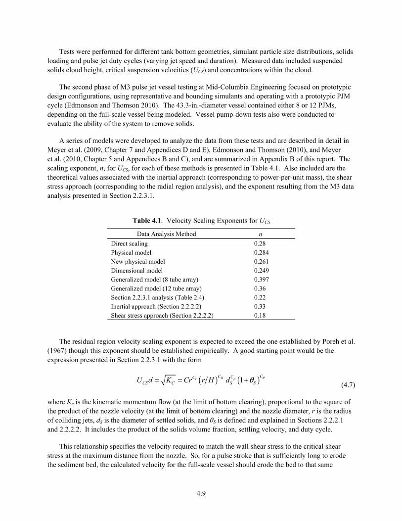
4.9

Tests were performed for different tank bottom geometries, simulant particle size distributions, solids loading and pulse jet duty cycles (varying jet speed and duration). Measured data included suspended solids cloud height, critical suspension velocities (UCS) and concentrations within the cloud.

The second phase of M3 pulse jet vessel testing at Mid-Columbia Engineering focused on prototypic design configurations, using representative and bounding simulants and operating with a prototypic PJM cycle (Edmonson and Thomson 2010). The 43.3-in.-diameter vessel contained either 8 or 12 PJMs, depending on the full-scale vessel being modeled. Vessel pump-down tests also were conducted to evaluate the ability of the system to remove solids.

A series of models were developed to analyze the data from these tests and are described in detail in Meyer et al. (2009, Chapter 7 and Appendices D and E), Edmonson and Thomson (2010), and Meyer et al. (2010, Chapter 5 and Appendices B and C), and are summarized in Appendix B of this report. The scaling exponent, n, for UCS, for each of these methods is presented in Table 4.1. Also included are the theoretical values associated with the inertial approach (corresponding to power-per-unit mass), the shear stress approach (corresponding to the radial region analysis), and the exponent resulting from the M3 data analysis presented in Section 2.2.3.1.

Table 4.1. Velocity Scaling Exponents for UCS

Data Analysis Method n

Direct scaling 0.28 Physical model 0.284 New physical model 0.261 Dimensional model 0.249 Generalized model (8 tube array) 0.397 Generalized model (12 tube array) 0.36 Section 2.2.3.1 analysis (Table 2.4) 0.22 Inertial approach (Section 2.2.2.2) 0.33 Shear stress approach (Section 2.2.2.2) 0.18

The residual region velocity scaling exponent is expected to exceed the one established by Poreh et al. (1967) though this exponent should be established empirically. A good starting point would be the expression presented in Section 2.2.3.1 with the form

( ) ( )1H pr

CC CCCS C S SU d K Cr r H d θθ= = +

(4.7)

where Kc is the kinematic momentum flow (at the limit of bottom clearing), proportional to the square of the product of the nozzle velocity (at the limit of bottom clearing) and the nozzle diameter, r is the radius of colliding jets, dS is the diameter of settled solids, and θS is defined and explained in Sections 2.2.2.1 and 2.2.2.2. It includes the product of the solids volume fraction, settling velocity, and duty cycle.

This relationship specifies the velocity required to match the wall shear stress to the critical shear stress at the maximum distance from the nozzle. So, for a pulse stroke that is sufficiently long to erode the sediment bed, the calculated velocity for the full-scale vessel should erode the bed to that same

4.10

maximum relative distance. However, the expression does not provide information on the time it will take to erode the sediment bed to that distance. Therefore, we need a separate requirement that addresses the rate of sediment bed erosion.

4.2.2 Transient Clearing Analysis

Video recordings of transient bottom clearing during the jet pulse indicate that the clearing process occurs in two sequential phases. The first phase is radial clearing beginning at the jet centerline and expanding as a function of time until the radial jet begins to interact with the jets from other pulse tubes. The second phase is the clearing of residual sediment in the vicinity of these jet interaction zones. The total clearing time for a single pulse is the sum of the times for these two phases. Each phase is described in more detail below.

4.2.2.1 Transient Clearing Analysis – Radial Clearing

The ZOI achieved during the drive phase of a pulse cycle is a function of both velocity and time. The standard expression used in the field of hydrology to describe the rate of sediment surface erosion (Partheniades 1965 via Simon et al. 2002) per unit surface area, SE, is

SE = E τ w −τ c( )n

where τw ≥ τc (4.8)

SE = 0 where τw < τc

where n is assumed to be equal to one.

The critical wall shear stress, τc, is defined as the minimum shear above which surface erosion of particular sediment occurs. The difference between the fluid stress and the critical stress also is known as the excess shear stress. The erodibility coefficient, E, is a rate constant that is a property of the sediment composition. This expression has been used in previous analysis of Hanford tank waste (Powell et al. 1997).

Imagine sediment with a thickness, δ, eroding on the vessel floor. Assume that the total bed erosion at any given time is proportional to the excess shear stress at the leading edge of the sediment. The erosion is expected to be concentrated near the leading edge, because as the jet fluid picks up zero velocity sediment particles, the velocity profile changes and the wall shear stress decreases. The added suspension concentration also reduces the rate of erosion downstream from the edge. A second assumption is that the shape of the sediment edge vertical profile does not significantly change with radius. Therefore, the total volume of sediment eroded from the top of the sediment layer is proportional to the product of the height of the sediment and the change in radius.

An erosion velocity, uZOI, defined as the rate of change of clearing radius with respect to time, is given by the expression

( ) ( ) ( )E

ZOI c

Cdru r r r

dtτ τ

δ= = −

(4.9)

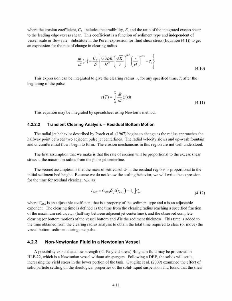
4.11

where the erosion coefficient, CE, includes the erodibility, E, and the ratio of the integrated excess shear to the leading edge excess shear. This coefficient is a function of sediment type and independent of vessel scale or flow rate. Substitute in the Poreh expression for fluid shear stress (Equation (4.1)) to get an expression for the rate of change in clearing radius

( )0 3 2 3

2

0 3. .

Ec

Cdr . K K rr

dt H H

ρ τδ ν

− − = − (4.10)

This expression can be integrated to give the clearing radius, r, for any specified time, T, after the beginning of the pulse

r(T) = dr

dt(r)

0

T

dt (4.11)

This equation may be integrated by spreadsheet using Newton’s method.

4.2.2.2 Transient Clearing Analysis – Residual Bottom Motion

The radial jet behavior described by Poreh et al. (1967) begins to change as the radius approaches the halfway point between two adjacent pulse jet centerlines. The radial velocity slows and up-wash fountain and circumferential flows begin to form. The erosion mechanisms in this region are not well understood.

The first assumption that we make is that the rate of erosion will be proportional to the excess shear stress at the maximum radius from the pulse jet centerline.

The second assumption is that the mass of settled solids in the residual regions is proportional to the initial sediment bed height. Because we do not know the scaling behavior, we will write the expression for the time for residual clearing, tRES, as

tRES = CRESδ τ rmax( )− τ c[ ]rmax

n

(4.12)

where CRES is an adjustable coefficient that is a property of the sediment type and n is an adjustable exponent. The clearing time is defined as the time from the clearing radius reaching a specified fraction of the maximum radius, rmax (halfway between adjacent jet centerlines), and the observed complete clearing (or bottom motion) of the vessel bottom and δ is the sediment thickness. This time is added to the time obtained from the clearing radius analysis to obtain the total time required to clear (or move) the vessel bottom sediment during one pulse.

4.2.3 Non-Newtonian Fluid in a Newtonian Vessel

A possibility exists that a low strength (<1 Pa yield stress) Bingham fluid may be processed in HLP-22, which is a Newtonian vessel without air spargers. Following a DBE, the solids will settle, increasing the yield stress in the lower portion of the tank. Gauglitz et al. (2009) examined the effect of solid particle settling on the rheological properties of the solid-liquid suspension and found that the shear

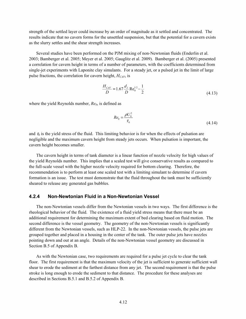
4.12

strength of the settled layer could increase by an order of magnitude as it settled and concentrated. The results indicate that no cavern forms for the unsettled suspension, but that the potential for a cavern exists as the slurry settles and the shear strength increases.

Several studies have been performed on the PJM mixing of non-Newtonian fluids (Enderlin et al. 2003; Bamberger et al. 2005; Meyer et al. 2005; Gauglitz et al. 2009). Bamberger et al. (2005) presented a correlation for cavern height in terms of a number of parameters, with the coefficients determined from single-jet experiments with Laponite clay simulants. For a steady jet, or a pulsed jet in the limit of large pulse fractions, the correlation for cavern height, HCAV, is

1/20

11.67 Re

2CAV JH d

D D= −

(4.13)

where the yield Reynolds number, Re0, is defined as

20

00

URe

ρτ

= (4.14)

and τ0 is the yield stress of the fluid. This limiting behavior is for when the effects of pulsation are negligible and the maximum cavern height from steady jets occurs. When pulsation is important, the cavern height becomes smaller.

The cavern height in terms of tank diameter is a linear function of nozzle velocity for high values of the yield Reynolds number. This implies that a scaled test will give conservative results as compared to the full-scale vessel with the higher nozzle velocity required for bottom clearing. Therefore, the recommendation is to perform at least one scaled test with a limiting simulant to determine if cavern formation is an issue. The test must demonstrate that the fluid throughout the tank must be sufficiently sheared to release any generated gas bubbles.

4.2.4 Non-Newtonian Fluid in a Non-Newtonian Vessel

The non-Newtonian vessels differ from the Newtonian vessels in two ways. The first difference is the rheological behavior of the fluid. The existence of a fluid yield stress means that there must be an additional requirement for determining the maximum extent of bed clearing based on fluid motion. The second difference is the vessel geometry. The geometry of the non-Newtonian vessels is significantly different from the Newtonian vessels, such as HLP-22. In the non-Newtonian vessels, the pulse jets are grouped together and placed in a housing in the center of the tank. The outer pulse jets have nozzles pointing down and out at an angle. Details of the non-Newtonian vessel geometry are discussed in Section B.5 of Appendix B.

As with the Newtonian case, two requirements are required for a pulse jet cycle to clear the tank floor. The first requirement is that the maximum velocity of the jet is sufficient to generate sufficient wall shear to erode the sediment at the farthest distance from any jet. The second requirement is that the pulse stroke is long enough to erode the sediment to that distance. The procedure for these analyses are described in Sections B.5.1 and B.5.2 of Appendix B.

4.13

4.3 Concepts for Testing

The range of physical properties for the simulants to be used in the LSIT mixing tests are specified in the simulant properties document (Koopman et al. 2012) and are based on measured properties of Hanford waste as summarized by Wells et al. (2011). The recommendations made in the simulant basis report include:

• Particle size and density distribution. The design basis testing should test particles with a size range of 0.2 to 700 µm. The distribution should include particles similar to non-co-precipitated plutonium particles found in certain Hanford wastes.

• Liquid density and viscosity. The LSIT should test liquids with a density of 1.0 to 1.46 g/mL. The LSIT should test liquids with viscosity of 1 to 15 cP for Newtonian vessels and 1 to 30 cP for Newtonian fluids in non-Newtonian vessels.

• Archimedes number. The range of Archimedes numbers for the LSIT design basis testing should be 1 × 10-7 to 6.7 × 103.

• Non-Newtonian suspensions. The basis of design WTP non-Newtonian vessels is 6 to 30 Pa yield stress and 1 to 30 cP consistency. The limits of performance testing need to evaluate lower values of yield stress (between 6 Pa and 1 Pa) and higher values of yield stress and consistency (greater than 30 Pa and 30 cP). For the Newtonian vessels, limits of performance testing need to evaluate a yield stress of at least 1 Pa.1

• Settled beds. The design basis shear strength is up to 200 Pa. During the limits of performance testing, the shear strength should be increased from 200 Pa to at least 1500 Pa to determine the maximum shear strength slurry for which the PJMs can remobilize solids.

• Solids concentration. For Newtonian simulants, the undissolved solids (UDS) concentration will range from nearly 0 to 10 wt%. Tests should be performed over this range of UDS concentrations, including but not limited to either extreme because either may be the more challenging. For non-Newtonian simulants, the maximum concentration of UDS will be that needed to achieve a yield stress of 30 Pa, a consistency of 30 cP, and shear strength of 200 Pa. Testing of off normal plant operating conditions should consider testing to much higher shear strengths to determine the ability of the design to recover from an off normal event.

The simulant property ranges recommended for LSIT in Koopman et al. (2012) are summarized in Table 4.2.

The test vessel and PJM configurations will be varied to represent scaled versions of the HLP-22, HLP-27, UFP-02, and RLD-08. The geometric parameters such as tank diameter, PJM nozzle diameter, PJM offset, etc., will be scaled according to geometric similitude.

1 Note if the 1-Pa bulk slurry is in a vessel that is less than homogenously mixed, the impact of the solids gradient in the lower portion of the tank and the potential for higher relative yield stresses must also be evaluated.

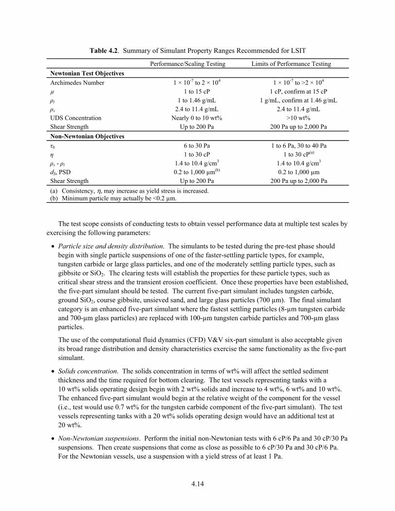
4.14

Table 4.2. Summary of Simulant Property Ranges Recommended for LSIT

Performance/Scaling Testing Limits of Performance Testing

Newtonian Test Objectives Archimedes Number 1 × 10-7 to 2 × 104 1 × 10-7 to >2 × 104 µ 1 to 15 cP 1 cP, confirm at 15 cP ρl 1 to 1.46 g/mL 1 g/mL, confirm at 1.46 g/mL ρs 2.4 to 11.4 g/mL 2.4 to 11.4 g/mL UDS Concentration Nearly 0 to 10 wt% >10 wt% Shear Strength Up to 200 Pa 200 Pa up to 2,000 Pa

Non-Newtonian Objectives τ0 6 to 30 Pa 1 to 6 Pa, 30 to 40 Pa η 1 to 30 cP 1 to 30 cP(a) ρs - ρl 1.4 to 10.4 g/cm3 1.4 to 10.4 g/cm3 dS, PSD 0.2 to 1,000 µm(b) 0.2 to 1,000 µm Shear Strength Up to 200 Pa 200 Pa up to 2,000 Pa

(a) Consistency, η, may increase as yield stress is increased. (b) Minimum particle may actually be <0.2 µm.

The test scope consists of conducting tests to obtain vessel performance data at multiple test scales by exercising the following parameters:

• Particle size and density distribution. The simulants to be tested during the pre-test phase should begin with single particle suspensions of one of the faster-settling particle types, for example, tungsten carbide or large glass particles, and one of the moderately settling particle types, such as gibbsite or SiO2. The clearing tests will establish the properties for these particle types, such as critical shear stress and the transient erosion coefficient. Once these properties have been established, the five-part simulant should be tested. The current five-part simulant includes tungsten carbide, ground SiO2, course gibbsite, unsieved sand, and large glass particles (700 µm). The final simulant category is an enhanced five-part simulant where the fastest settling particles (8-µm tungsten carbide and 700-µm glass particles) are replaced with 100-µm tungsten carbide particles and 700-µm glass particles.

The use of the computational fluid dynamics (CFD) V&V six-part simulant is also acceptable given its broad range distribution and density characteristics exercise the same functionality as the five-part simulant.

• Solids concentration. The solids concentration in terms of wt% will affect the settled sediment thickness and the time required for bottom clearing. The test vessels representing tanks with a 10 wt% solids operating design begin with 2 wt% solids and increase to 4 wt%, 6 wt% and 10 wt%. The enhanced five-part simulant would begin at the relative weight of the component for the vessel (i.e., test would use 0.7 wt% for the tungsten carbide component of the five-part simulant). The test vessels representing tanks with a 20 wt% solids operating design would have an additional test at 20 wt%.

• Non-Newtonian suspensions. Perform the initial non-Newtonian tests with 6 cP/6 Pa and 30 cP/30 Pa suspensions. Then create suspensions that come as close as possible to 6 cP/30 Pa and 30 cP/6 Pa. For the Newtonian vessels, use a suspension with a yield stress of at least 1 Pa.

4.15

The procedure described below will apply to each separate test condition (simulant, solids loading, vessel configuration):

• Clean and prepare the test vessel with the PJM array appropriate for the WTP vessel being simulated. Add simulant solids and liquid to achieve the minimum solids concentration to be tested.

• The pulse jet duty cycle (ratio of PJM pulse time to cycle time) should be the same at all scales and the cycle time should be proportional to the tank diameter and inversely proportional to the PJM velocity.

• Perform a series of pulse jet duty cycles for a specified maximum PJM nozzle velocity beginning at 1 m/s and increasing to 11 m/s in 1 m/s increments. At each velocity step, record the effective clearing radius for each nozzle. Continue until total bottom clearing has been achieved.

• Return to the last velocity where total bottom clearing had not occurred. Run the PJM duty cycles until a repeatable cycle occurs. Then increase the specified PJM nozzle velocity in increments of 0.1 m/s until bottom clearing has been achieved.

A possibility exists that a low strength (<1 Pa yield stress) Bingham fluid may be processed in HLP-22, which is a Newtonian vessel without air spargers (discussed in Section 4.2.3). The procedure for this test is:

• Clean and prepare the test vessel with the PJM array appropriate for the WTP vessel being simulated. Add simulant solids and liquid to achieve the minimum solids concentration and appropriate fluid rheology to be tested.

• Position flow measurement devices within the vessel to monitor the formation and growth of the cavern region during the pulse cycle. The test must demonstrate that the fluid throughout the tank must be sufficiently sheared to release any generated gas bubbles.

• Perform a series of pulse jet duty cycles for a specified maximum PJM nozzle velocity beginning at 1 m/s and increasing to 11 m/s in 1 m/s increments. At each velocity step, record the flowing cavern size and shape based on flow measurements. Continue until the entire vessel has been mobilized.

• Return to the last velocity where total mobilization had not occurred. Run the PJM duty cycles until a repeatable cycle occurs. Then increase the specified PJM nozzle velocity in increments of 0.1 m/s until mobilization has been achieved.

4.4 Conclusions

The metric chosen to demonstrate bottom motion of sediment is bottom clearing; that is, the movement of all solids at least momentarily from the tank bottom (defined in Chapter 8). This is similar to the critical suspension velocity requirement, UCS, defined as the velocity at which the solids are completely suspended off the vessel bottom at the end of the jet pulse, that was used in Phase 1 (Meyer et al. 2009) and Phase 2 (Edmonson and Thomson 2010) of the M3 tests. The transient bottom clearing behavior during the jet pulse occurs in two sequential phases: 1) a radial clearing phase and 2) a subsequent residual sediment region clearing phase.

4.16

There are two requirements for a pulse jet cycle to clear the tank floor. The first requirement is that the maximum velocity of the jet is sufficient to generate the required wall shear to erode the sediment at the farthest distance from any jet. The second requirement is that the pulse stroke is long enough to erode the sediment to that distance.

The scale-up exponent for velocity with respect to geometry for the radial clearing region is approximately 0.18 based on the Poreh et al. (1967) model and experimental verification (Dickey 2010). The scaling exponent for the residual sediment bed region must be empirically determined. Analysis of UCS data taken from M3 vessel experiments result in velocity scaling exponents ranging from 0.25 to 0.40. The residual region velocity scaling exponent is expected to exceed the one established by Poreh et al. (1967) though this exponent should be established empirically.

The total time to clear is the sum of the radial clearing time and the residual clearing time. An expression for the radial clearing time was obtained by combining the Poreh model with an erosion rate equation based on the excess wall shear. The residual clearing time also is expressed in terms of excess wall shear. The critical shear stress and erosion coefficients are determined based on data from visual observation.

A possibility exists that a low strength (<1 Pa yield stress) Bingham fluid may be processed in HLP-22, which is a Newtonian vessel without air spargers. Following a DBE, the solids will settle, increasing the yield stress in the lower portion of the tank. We recommend that at least one scaled test be performed with a limiting simulant to determine if cavern formation is an issue. The test must demonstrate that the fluid throughout the tank must be sufficiently sheared to release any generated gas bubbles.

We recommend using empirical methods at three different scales to scale bottom motion as measured by bottom clearing. The impact of clearing time will be determined by testing.

5.1

5.0 Technical Basis for Scaling Performance Metrics for the Limit Solids Accumulation Requirement

5.1 Introduction

The WTP vessel requirements for Requirement 10 for Limit Solids Accumulation are specified as follows in 24590-WTP-ES-ENG-09-001 (Mauss and Papp 2010).

“The PJM vessels systems shall be designed, considering the mixing and transfer systems, such that solids will not accumulate from batch to batch and limit the bulk density and solids weight percent to less than or equal to the limits established for the Unit Liter Dose (ULD) calculation.”

The requirement is further elaborated as follows:

“Specifically, this mixing function demonstrates that the beginning weight % solids of a batch equals or exceeds the solids present when the batch has been transferred. This requirement applies over the range of particles/solids and demonstrates that they do not accumulate from batch to batch.”

In its simplest application, this testing is to show that no solids accumulate from batch to batch over the entire size and density range of the process stream entering the vessel. Referencing the ULD ties the ultimate requirement directly to the primary safety driver, which is preventing a criticality. Tying the requirement to the ULD also gives the requirement a bit of flexibility to handle extreme conditions. For example, testing (and modeling) may find that the extremes of the statistical distributions may not show zero accumulation. Referencing the ULD provides a fallback to meet the requirement if one can statistically show that the amount of accumulation will never reach the ULD.

The Limit Solids Accumulation requirement applies to all of the vessels. The differences between the vessels are primarily due to different PJM operating conditions and slurry characteristics. Determining the appropriate simulants for LSIT-scaled testing is part of another effort, simulant development.

The potential accumulation of mass in a PJM mixed tank depends upon all of the important phenomena constituting the PJM cycle. Different technical bases apply to scaling down or scaling up each phenomenon, as is discussed in Appendix C, and are summarized in Table 5.1.

5.2 Requisite Measurements, Data Interpretation, and Evaluation Against Mixing Requirements

All of the scaling approaches described in Section 3.2 require the following:

• Reduced-scale tanks as geometrically similar to the WTP tank as possible

• Control over key experimental parameters such as viscosity, initial liquid level, PJM (nominal) velocity, “duty cycle,” PJM pulse volume fraction, and initial total solids volume fraction

5.2

• Measurements of 1) concentrations and volumes entering and exiting a tank to determine the accumulation of solids and 2) concentration of individual solids species and volumetric flow rate in the transfer line over PJM cycles as a function of time within the cycles.

Table 5.1. Technical Bases for Scaling for the Limit Solids Accumulation Requirement

Phenomenon Technical Basis for Scaling Down Technical Basis for Scaling Up

Entrain solids into radial wall jets on tank floor

• Literature describing the behavior of radial wall jets

• Assumption of operating to clear the bottom during each PJM pulse

Applies to capturing solids into the suction nozzle at point of collision of wall jets: operation at bottom clearing conditions

Capture solids into suction nozzle at point of collision of radial wall jets

• Literature describing the behavior of radial wall jets

• Assumption of operating to clear the bottom during each PJM pulse

A successful correlation of concentration peaks with experimental parameters, or successful comparison of concentration peaks predicted by physically based model as a function of experimental parameters to measurements in transfer line, will serve as the technical basis

Suspend solids by upward flow from collision of jets

• Assumption of operating to clear solids from the tank bottom during each PJM pulse

• Conservation of mass and momentum applied to jet collision

Applies to capturing solids into the suction nozzle: successful comparison of vertical concentration profiles measured in LSIT to correlation with length scale and experimental parameters will serve as the technical basis

Solids settle between PJM pulses

• Literature on the theory of settling solids

• Unimportance of dispersion during settling inferred from M3 concentration profiles

Applicable to capturing solids into the suction nozzle: successful comparison of vertical concentration profiles measured in LSIT to correlation with length scale and experimental parameters will serve as the technical basis

Capture solids into suction nozzle as they settle between PJM pulses

• Kinematic similitude of the velocity field around the suction nozzle

Same as scale down, plus either a successful correlation of results with experimental parameters or successful comparison of concentration measured in transfer line with prediction from integrated model will serve as the technical basis

In addition, the scaling approaches described in Sections 3.2.2 and 3.2.3 require the following experiments and data from LSIT:

• Measurements of 1) solids volume fraction versus elevation and time at selected radii in the tank and 2) thickness of settled solids at several locations, as function of time. These measurements can be made using acoustic (ultrasonic) methods (see footnote in Section 3.4.2).

• Operation at conditions at which solids are cleared from the tank bottom at some point in each PJM cycle (other conditions could also be investigated as needed).

5.3

Concentration profiles obtained in the form of these measurements can be reduced to the following three principal values, as is described in Section 5.5.2, Data Reduction, and in Appendix C:

1. The total volume of solids per horizontal area of slurry, for validating the settling model.

2. The solids volume fraction at the bottom of the profile, for validating the settling model and supporting calculating the concentration and mass flows of species captured by the suction nozzle.

3. The vertical length scale of the profile, for validating settling calculations and supporting a correlation for suspension of solids.

The ultimate use of the data is to validate the overall mass balance model, which is used to predict accumulation of mass in the WTP and thereby evaluate compliance with the Limit Solids Accumulation requirement.

It may be possible to develop a more sophisticated sensing system—possibly the “M3” device plus more signal analysis or a more sophisticated sensor or sensor system—that would allow inferring more than the local density, such as something about the size distribution. However, whatever model or correlation of the solids distribution that needs to be tested, it is likely a prediction of the solids distribution would provide the expected response of the instrument such that the model can be tested against the available measurement even if the solids distribution itself is not measured. Clearly this would be less desirable than directly measuring the solids distribution, which would provide a powerful test of any conceptual model of the mixing behavior, but it seems far less likely. In a sense, resorting to predicting the sensor response instead of measuring the solids distribution and comparing the measured information to model predictions to validate would be a “backup” approach using more direct measurements.

5.3 Overall Mass Balance Model

If at the end of each pump-out cycle, the tank is refilled with slurry with solids mass concentration ρi0

and then the evolution of the concentration of particulates in a tank during pump out is described by a simple differential equation (see Appendix C, Section C.4.2):

V

dρi

dt= −Q ρi

P − ρi( )+ Q0ρi0

(5.1)

where V is the decreasing slurry volume, Q is the volumetric flow rate being pumped out, the concentration difference P

i iρ ρ− (concentration at the inlet to the transfer line less the average

concentration in the tank) varies with iρ as determined by the settling model described in Appendix C,

Section C.4.2, and the last term is the average rate at which the mass of species “i” is added during

refills of the tank. The term ρi0 is the mass concentration in the slurry added at the end of a pump-down

cycle, and the Q0 is the time-averaged inlet flow rate, evaluated so that Q0ρi0 is the mass of species “i”

added at the end of every pump-down cycle. LSIT test results over repeated PJM cycles are used to confirm or, if necessary, revise the settling model, which then is used to predict the mass versus time of the various particulate species in WTP, which quantifies “accumulation” in the WTP. That is, we implement the settling model repeatedly to solve the mass balance over the pump-out cycles to

5.4

predict the mass of species “i” in the tank over time to address the no solids accumulation mixing requirement (see Appendix C, Section C.4.2.8 for details).

As the fill/pump-out sequence proceeds, settling calculations predict both ρ iP

and ρ i as the slurry

volume decreases, and hence provides ρiP

as a function of iρ . Combining with the mass balance above

and solving the mass balance gives ρ iP

as a function of slurry volume and other parameters, including the

concentration in the slurry fill. Then, the mass of species “i”, Δmi, transferred out of the tank is found from

Δmi = ρi

P V ;ρi0( )dV

V1

V2 (5.2)

This calculation is repeated for each fill/pump-out cycle. For each cycle, the mass of species “i”

added is V1 −V2( )ρi0. Thus, the mass accumulation during the cycle, accumulate

imΔ , is

( ) ( )2

1

accumulate 0 01 2 ;

V Pi i i iV

m V V V dVρ ρ ρΔ = − + (5.3)

From Equation (5.1), the accumulation over time is found implicitly from

dρi

Q0 Q( )ρi0 − ρi

P − ρi( )ρi0

ρi t( ) =

Qt

V (5.4)

Implementing this requires quantifying the effects of the coupled phenomena, which is discussed

above and in detail in Appendix C, to predict ρiP V ;ρi

0( ).

5.3.1 Available Information

The nature of the mass balance over multiple PJM cycles during pump down was illustrated during LOAM tests involving multiple PJMs and a polydisperse simulated waste. Figure 5.11 shows the variation of density over a single PJM cycle, and Figure 5.21 shows the variation over many PJM cycles as the tank is pumped down.

1 C Chapman, e-mail to JA Bamberger, April 24, 2012, RE: “Density vs time for Loam tests used as examples in Sect 6, 10, and App-E, stating: [the file] density of slurry during pump outs was a collection of pump out density profiles extracted from a range of engineering reports for LOAM test 1, 2, 5, and 6 and from INFO testing.” The author was Chris Chapman and this assembly was made in January 2012.

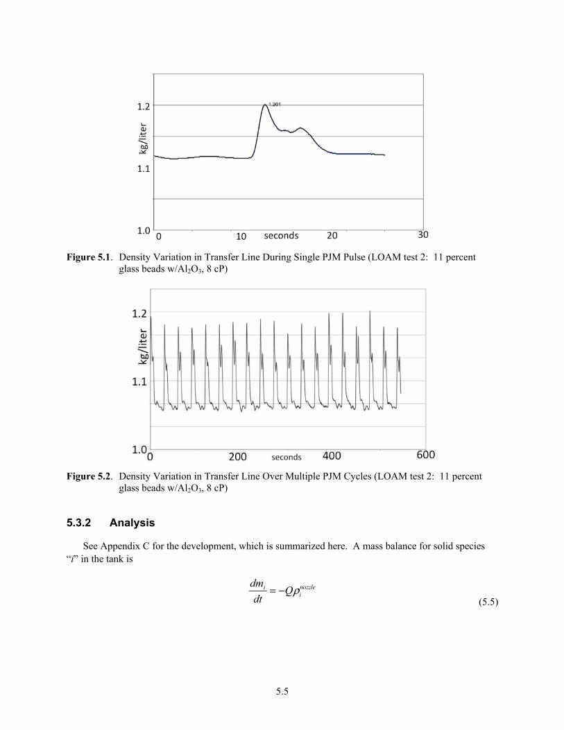
5.5

Figure 5.1. Density Variation in Transfer Line During Single PJM Pulse (LOAM test 2: 11 percent glass beads w/Al2O3, 8 cP)

Figure 5.2. Density Variation in Transfer Line Over Multiple PJM Cycles (LOAM test 2: 11 percent glass beads w/Al2O3, 8 cP)

5.3.2 Analysis

See Appendix C for the development, which is summarized here. A mass balance for solid species “i” in the tank is

dmi

dt= −Qρi

nozzle

(5.5)

5.6

where mi of solid species “i” is the mass in the tank, Q is the volumetric flow rate out of the tank, and the

density, nozzleiρ , is that for fluid entering the suction nozzle. The mass in the tank is related to the average

density in the tank by

dmi

dt=

d

dtVρi( )= −Qρi + V

dρi

dt (5.6)

where V is the volume of liquid in the tank. The volume decreases with time as

V = V0 − Qt (5.7)

where V0 is the volume of slurry with solids mass concentration 0iρ . Combining,

V0 − Qt

Q

dρi

dt= − ρi

nozzle − ρi( ) (5.8)

Rearranging and integrating,

dρi

ρinozzle − ρi

start

end

= ln 1−Qtend

V0

(5.9)

From this, we obtain the average concentration in the tank over time, which combined with the volume over time gives us the mass of “i” over time, which is the metric for the no accumulation of solids requirement.

The significance of this expression is that the mass balance depends on the difference between the average density and the density at the nozzle. In a PJM-mixed tank, this difference results from several causes:

• Large (relative to most of the tank) transients in the density at the nozzle because of the motion of solids at the bottom of the tank caused by PJM pulses.

• Vertical gradients in solids concentration caused by repeated suspension and settling during each PJM cycle.

• Where the suction nozzle is substantially off-center, circumferential variations in solids concentrations may be important, where the density at the suction nozzle might be substantially less than the average density in the tank.

To determine mass accumulation through observation, we need to create representative conditions in a pump-down test and conduct the test over a representative fraction of the volume removed. This must be done for permutations of mixing conditions as needed depending on how the metric is to be correlated to scale up to evaluate full-scale tanks. If one pursues a “representation” approach to scaling (see Section 3.2), the strategy is to define one representative condition, scale down to LSIT conditions, demonstrate (or not) limit solids accumulation in LSIT, and scale up to WTP on the basis the test results are representative, then a single pump-down test might suffice. If one pursues a “correlation” approach to

5.7

scaling, the strategy is to demonstrate limit solids accumulation over a range of conditions or to determine the boundary of limit solids accumulation in terms of waste properties or operating parameters, a series of tests over permutations in the test parameters is needed. If one pursues specifically a physically based correlation approach (see Section 3.2.3), the strategy is to validate a mass-balance model, a series of tests would need to be defined based on the intended model. A mass-balance model probably would be an integration of sub-models, including some correlations, such as power laws.

To determine performance using a mass-balance model predicting the performance at any scale, we need to relate the density at the nozzle to the average density in the tank. There are two parts to the calculation: 1) the difference between the tank average density and the peak density (see Figure 5.1) during a PJM pulse, and 2) the difference between the tank average density and the density of solids captured into the suction nozzle as they settle.

5.3.3 Potential for a Bounding Test

The velocity used in reduced-scale tests is less than at full scale, so the ratio of settling velocity to PJM velocity is greater than for reduced scale assuming that the simulant is not scaled with length scale. The Froude number scales as U2/L. We expect the bottom clearing velocity to scale in the range L3/17 to L1/3 (see Section 2.2.3.1). Then if we control the velocity over scale to be, for example, in proportion to the bottom clearing velocity, the Froude number will scale as L2/3 or less; that is, it is less at reduced scale. We expect the decreasing Froude number to decrease the suspension of settled solids and for increasing ratio of settling velocity to PJM velocity to decrease it. Thus, the two most important departures from similitude relative to suspension of settled solids tend to be conservative in the sense solids should be suspended less effectively in reduced-scale tests. This suggests that the fraction of solids captured by the suction nozzle per PJM pulse might be less, especially considering the need to move solids horizontally to reach the suction nozzle. On this basis, it might be possible to defend that pump-down tests at reduced scale provide a conservative estimate of the fraction of solids accumulated.

5.3.4 Additional Considerations for Tanks Processing Non-Newtonian Fluids

Tanks designed to process non-Newtonian fluids have the PJMs clustered in the center and enclosed above so solids can only ascend or settle in an annulus between the cluster and the tank wall. The annulus and the outer part of the tank floor will be agitated by spargers (see Chapter 7) to keep the non-Newtonian fluid sheared, which we presume enables some fraction of the particles to settle. In this case, the suction nozzle will be tested at locations toward the tank wall, where solids can settle from above after being suspended and dispersed by PJM mixing. Then a mass balance model over repeated PJM cycles during a pump-out cycle needs to consider circumferential dispersion by PJM mixing of suspended solids, which will be the means by which most settling solids in the tank find their way to the suction nozzle. This concept is still being developed, but would involve the same differential mass balance, plus the simplest possible model of circumferential dispersion, which might be approached technically using scaling based on principles of turbulence. Of course, the settling model potentially is quite different in a Bingham fluid, depending on the effect of sparger shearing on the particle environment.

5.8

In general, either scaling down test conditions or scaling up test results for tests done using Bingham fluids will be more complicated and less certain than for Newtonian fluids for the following reasons:

• There is less experience industrially and fewer studies published to guide the effort.

• Although the Bingham fluid model is adopted as the design basis, rheograms of actual waste and of simulated waste can exhibit more complicated phenomena such as a shear strength and pseudo-plastic behavior at low shear rates, which might confound interpretation of test data.

• Any physically based model would be significantly more complicated and involve more adjustable parameters for a non-Newtonian fluid compared to a Newtonian fluid.

5.4 Suspension of Solids from Collision of Radial Jets

In Appendix C, Section C.4.1, we present an example of developing a physically based correlation describing the suspension of solids caused by the collision of radial jets on the tank floor resulting in upward, jet-like flow. The conceptual model is described below. It is an example of basing a correlation on a physical concept.

5.4.1 Available Information

Experiments done during the M3 project, in which the “cloud height” was measured for over a thousand sets of parameters, provides the best known information pertinent to suspension of solids by colliding jets on the tank floor. This data set is used below.

5.4.2 Physically Based Model

Here we present an example of developing a physically based correlation for the elevation attained by solids entrained from the tank floor because of upward flow from colliding jets on the floor of the tank. The conceptual model is as follows.

• The rate of loss of linear momentum of the ascending vortices is known from the conservation of momentum and the density of the ascending vortices relative to the surrounding fluid. The elevation at which the linear momentum expires is the jet height. We assume that the remaining angular momentum has provided sufficient axial dispersion to cause the concentration within the vortices to be roughly uniform and the vertical concentration profile to be uniform at the end of the jet pulse. This is a gross approximation enabling initial efforts to develop models. Horizontal homogeneity will depend strongly on the dispersion of solids by residual angular momentum after the maximum elevation is attained compared to the rate of settling during such dispersion.

• The volume of the vortices grows as the difference between the volumetric flow rate in the jet behind the vortices and the flow rate that would occur if the jet were moving at the speed the vortices advance. (This is similar to the analysis of the volume of the vortices for the radial wall jet.) From the volume and angular momentum of the vortices at the end of the jet pulse, we can estimate the associated kinetic energy from the angular velocity.

• The forces acting on the vortices result from resistance from the fluid they are penetrating and negative buoyancy.

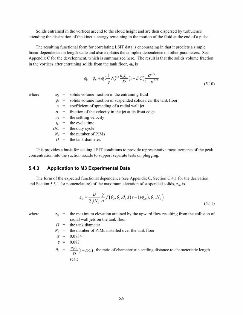
5.9

Solids entrained in the vortices ascend to the cloud height and are then dispersed by turbulence attending the dissipation of the kinetic energy remaining in the motion of the fluid at the end of a pulse.

The resulting functional form for correlating LSIT data is encouraging in that it predicts a simple linear dependence on length scale and also explains the complex dependence on other parameters. See Appendix C for the development, which is summarized here. The result is that the solids volume fraction in the vortices after entraining solids from the tank floor, φ0, is

( )

3 23 2

0 1 3 2

13 1

1

// S C

E J /

u tN DC

D

σφ φ φγ σ

= + −− (5.10)

where φE = solids volume fraction in the entraining fluid φ1 = solids volume fraction of suspended solids near the tank floor γ = coefficient of spreading of a radial wall jet σ = fraction of the velocity in the jet at its front edge uS = the settling velocity tC = the cycle time DC = the duty cycle NJ = the number of PJMs D = the tank diameter.

This provides a basis for scaling LSIT conditions to provide representative measurements of the peak concentration into the suction nozzle to support separate tests on plugging.

5.4.3 Application to M3 Experimental Data

The form of the expected functional dependence (see Appendix C, Section C.4.1 for the derivation and Section 5.5.1 for nomenclature) of the maximum elevation of suspended solids, zm, is

( )( )( )0, , , 1 , ,

2m d u g S c J

J

Dz f s N

N

γ θ θ θ φ θα

= − (5.11)

where zm = the maximum elevation attained by the upward flow resulting from the collision of radial wall jets on the tank floor

D = the tank diameter NJ = the number of PJMs installed over the tank floor α = 0.0734 γ = 0.087

θc = ( )1S Cu tDC

D− , the ratio of characteristic settling distance to characteristic length

scale

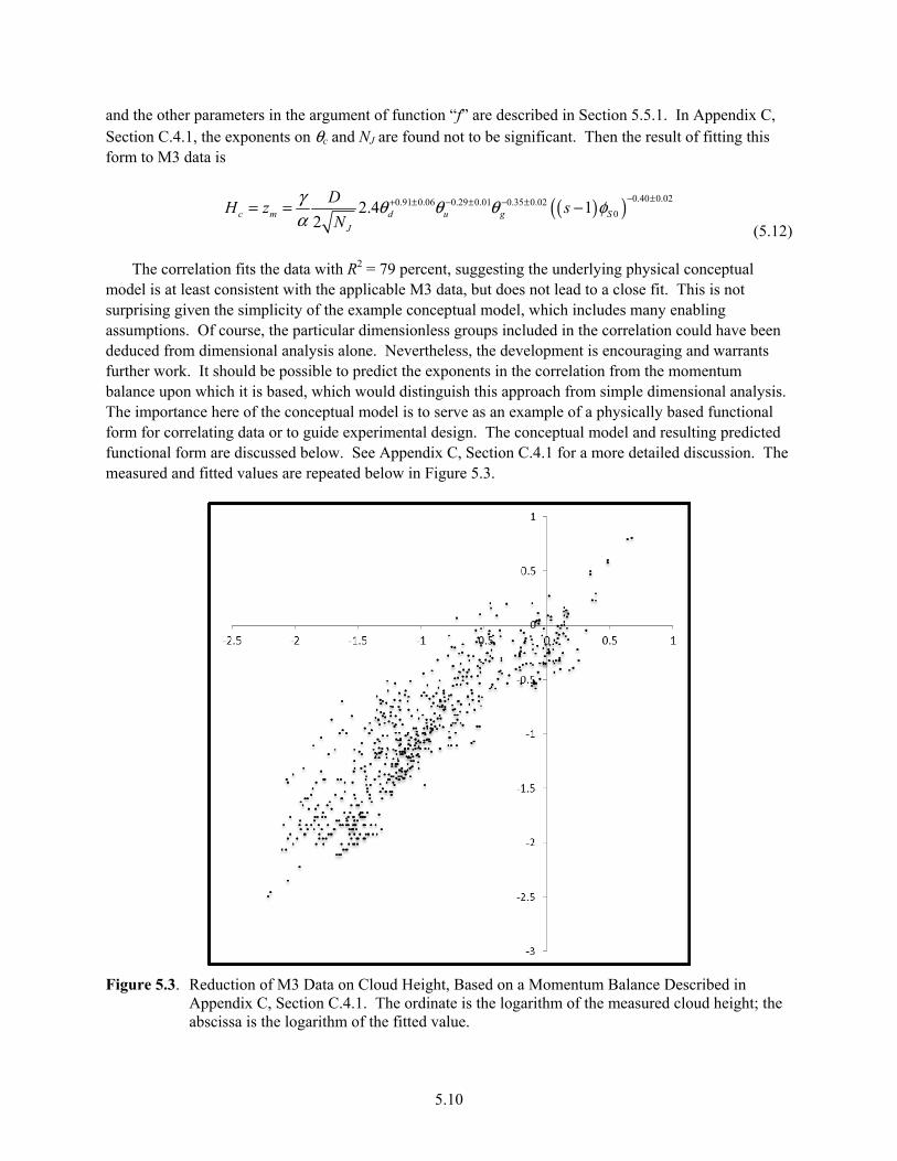
5.10

and the other parameters in the argument of function “f” are described in Section 5.5.1. In Appendix C, Section C.4.1, the exponents on θc and NJ are found not to be significant. Then the result of fitting this form to M3 data is

( )( ) 0.40 0.020.91 0.06 0.29 0.01 0.35 0.02

02.4 12

c m d u g S

J

DH z s

N

γ θ θ θ φα

− ±+ ± − ± − ±= = − (5.12)

The correlation fits the data with R2 = 79 percent, suggesting the underlying physical conceptual model is at least consistent with the applicable M3 data, but does not lead to a close fit. This is not surprising given the simplicity of the example conceptual model, which includes many enabling assumptions. Of course, the particular dimensionless groups included in the correlation could have been deduced from dimensional analysis alone. Nevertheless, the development is encouraging and warrants further work. It should be possible to predict the exponents in the correlation from the momentum balance upon which it is based, which would distinguish this approach from simple dimensional analysis. The importance here of the conceptual model is to serve as an example of a physically based functional form for correlating data or to guide experimental design. The conceptual model and resulting predicted functional form are discussed below. See Appendix C, Section C.4.1 for a more detailed discussion. The measured and fitted values are repeated below in Figure 5.3.

Figure 5.3. Reduction of M3 Data on Cloud Height, Based on a Momentum Balance Described in Appendix C, Section C.4.1. The ordinate is the logarithm of the measured cloud height; the abscissa is the logarithm of the fitted value.

5.11

5.5 Application to LSIT

5.5.1 Scaling Parameters Inferred from a Physical Model

The correlation described above results from a physical model from which several parameters are derived from a momentum balance over the radial jets on the tank floor and the upward flow that results from their collision. These are

θg = gD

u02

(5.13)

where g is the acceleration of gravity, D is the tank diameter, and u0 is the nominal velocity of the PJM jets

Jd

d

Dθ =

(5.14)

where dJ is the nozzle diameter of a PJM

Su

u

uθ =

(5.15)

where uS is the settling velocity (nominal value for a monodisperse distribution of solids, such as in M3 tests, and a volume-weighted average [see Section 2.2.1.5] for complex PSDDs), and the term

( ) 01 Ss φ−

(5.16)

where s is the ratio of solids to liquid density and φs0 is the nominal solids volume fraction of the total waste slurry.

Some of the parameters are easily matched between LSIT and WTP. The product sφ0 can be matched by simulating actual waste. The parameter θd is matched through geometric similitude. However, some of the parameters lead to conflicting requirements. For example, if, as expected for practical reasons, the simulated waste used in LSIT is not scaled with the size of the system, then the settling velocity (or its average value) will be the same at different scales, including full scale. Then, for example, matching parameter θu between LSIT and WTP requires matching the jet velocity, while matching θg requires different jet velocities at different scales. Hence, even without attempting to attain full similitude, conflicting requirements arise and must be resolved based on considering the phenomena of greatest interest. Matching θu is important to the fraction of solids that settle during a cycle, while θg is particularly important to the elevation attained when resuspending the solids after they settle.

For LSIT, using simulated waste including particles over a wide range of settling velocities, the slowest settling particles likely will distribute essentially over the height of the liquid, obscuring the distribution of faster-settling particles. The concept of cloud height needs to be changed to a characteristic height of the concentration profile, which might not display a distinct boundary beneath the

5.12

physical boundary of the slurry. Measurements of the vertical concentration profiles are crucial to understanding the mass balance in a tank, as well as quantifying the conditions affecting the suspension of solids and their capture by the transfer line suction nozzle.

5.5.2 Data Reduction

Given measurements of the vertical profile of the solids volume fraction, the apparent cloud height can be constructed unambiguously from the data using first and higher moments of the distribution. These are defined in terms of the following integrals:

I0 = φS z( )dz0

HI1 = φS z( )zdz

0

H (5.17)

Note that I0 is the total volume of solids per horizontal area. Then, if the vertical distribution of the solids volume fraction, φS(z), was uniform at fraction φS0 to height hS, we would have

I0 = hSφS 0

I1 = 12 hS

2φS 0 (5.18)

Then if we define

zS = 2 I1 I0( ) (5.19)

then zS is the height of the uniform distribution. If the distribution is not uniform, zS still quantifies its vertical extent. For example, if the actual distribution were linear from φb at the bottom and zero at elevation z0, we would calculate from the data

zS = 23 z0 (5.20)

The concentration at the bottom of the profile can be found from the data by regressing some suitable function (probably linear, possibly log linear) form through the data, extrapolating to z = 0. Thus, we have three characteristics of the vertical distribution that can be unambiguously calculated from measured data and compared to the results of a settling calculation: the volume of solids, the characteristic height of the profile, and the concentration at the bottom of the profile.

5.5.3 Predicting Concentration versus Depth Using a Settling Model

In Appendix C, Section C.4.2, we describe a mass balance on settling solids to be solved to predict the vertical profile of solids versus time. The model requires as input the concentration profile estimated at the end of the PJM pulse (e.g., one alternative is to assume a uniform initial profile), the Archimedes numbers of the various particle types (available from the PSDD and properties of the fluid), a hindered settling correlation based on the available literature, and a correlation for a cloud height (see Appendix C, Section C.4.1, Suspension of Solids by Collision of Radial Wall Jets) and, if necessary, a hydrodynamic dispersion coefficient correlated from LSIT data. Measured concentration profiles can be reduced to

5.13

three physical parameters: 1) total volume of solids suspended, 2) characteristic height of the concentration profile, and 3) concentration at the bottom of the profile, and compared to values computed from the results of a settling calculation. Differences then are used to correlate the minimum possible number of adjustable parameters, such as a parameter in a hindered settling correlation or a dispersion coefficient.

Implementation includes solving a first-order partial differential equation numerically. However, this is not difficult, and can be implemented using spreadsheets if desired. Although the model itself is complicated, it is essentially a textbook model, neither ambiguous nor speculative; the input parameters are few and are available, and it provides exactly the information needed to implement a mass balance over the PJM cycle required to implement a mass balance over a pump-out cycle.

Regardless of the means employed to solve the settling mass balance, the purpose and the result is to find, from the initial profile, the volume fraction profile for species “i” during the course of settling, where the resulting profile can be applied, if necessary, as part of correlating the cloud height for the next pulse. This is required to determine the mass flow rate of the various species into the transfer line, which in turn is required to support evaluation against mixing requirements.

5.6 Capture of Settled and Settling Solids by the Suction Nozzle

The analysis in this section is an initial analysis. It can and needs to be refined further to add the effect of the flow into PJMs during refill, and the effect of the flow close to the nozzle, which is upward rather than a point sink. The former can be addressed in the same fashion as the analysis shown below; the latter can be addressed by adding a point dipole flow potential at the point sink, with magnitude causing the velocity on the upward side of the point sink to be zero. What follows illustrates the nature of the technical issues and can be thought of as a “first installment” on whatever additional calculations ultimately are found to be necessary to properly scale the phenomena. The most important features are developed, however.

The capture of settling particles by the flow field into the suction nozzle can be evaluated in terms of a “capture volume” calculated from the suction flow rate, particle settling velocity, and distance of the suction nozzle above the tank floor. Thus, a capture zone is calculated for each settling velocity, and thus is calculated for each size fraction of a species of given density. For a flow limited to only that imposed by the suction on an otherwise quiescent fluid, and for distances from the nozzle not small compared to the nozzle diameter, the velocity distribution can be estimated from a simple point sink matched by a mirror-image point sink on “the other side” of the tank floor. Then the capture zone is found from a straightforward evaluation of kinematics, following the path of the summed settling and suction flow field velocities. Example capture volumes are illustrated in Figure 5.4.

Mass enters the suction nozzle in two steps. First, a PJM pulse pushes settled solids outward as the radial wall jet that forms on the tank floor spreads radially. Either the suction nozzle falls in the path of one such radial wall jet on the tank floor, or it sits above a zone of collision of jets. This determines the peak concentration of solids that must be accommodated by the transfer line and pump without plugging. Thus, this concentration peak as a function of time is determined from LSIT tests and is provided to full-scale line plugging test activities as a condition to be imposed in those tests. The result, described in

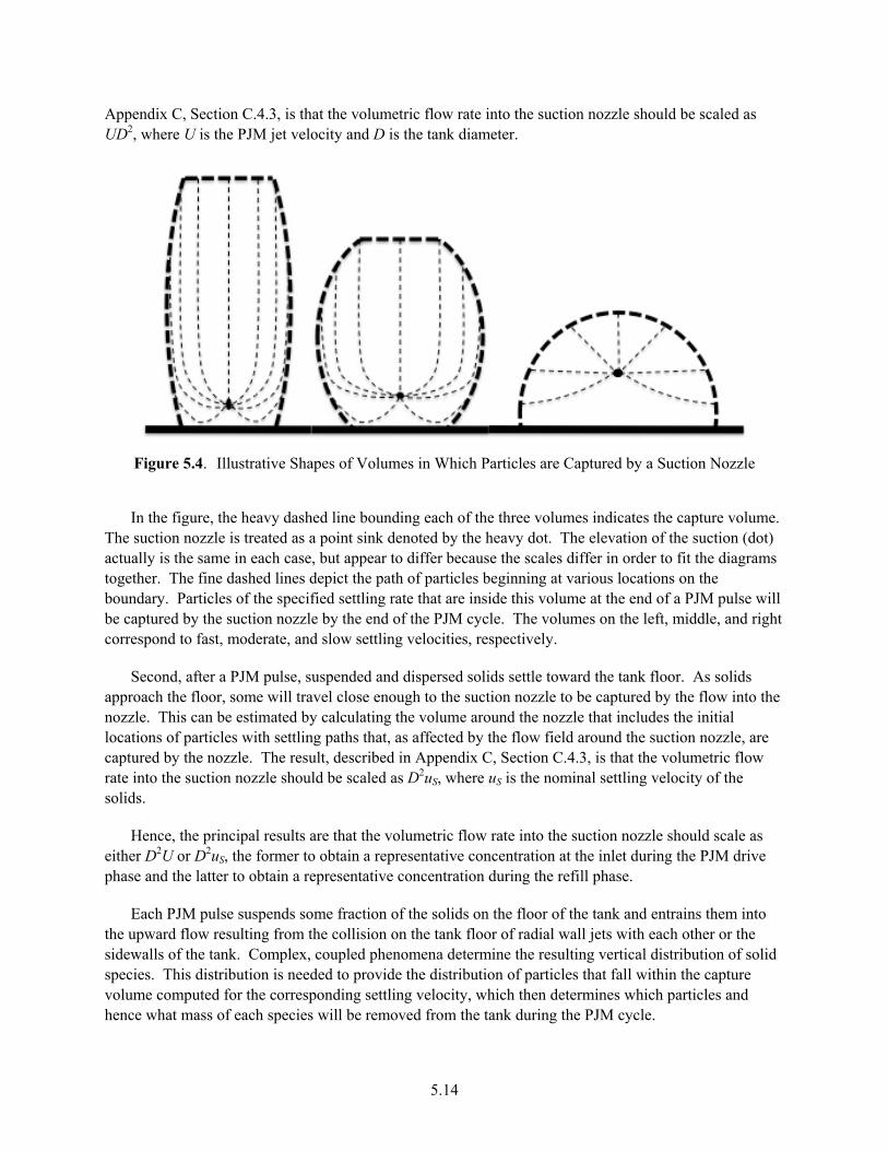
5.14

Appendix C, Section C.4.3, is that the volumetric flow rate into the suction nozzle should be scaled as UD2, where U is the PJM jet velocity and D is the tank diameter.

Figure 5.4. Illustrative Shapes of Volumes in Which Particles are Captured by a Suction Nozzle

In the figure, the heavy dashed line bounding each of the three volumes indicates the capture volume.

The suction nozzle is treated as a point sink denoted by the heavy dot. The elevation of the suction (dot) actually is the same in each case, but appear to differ because the scales differ in order to fit the diagrams together. The fine dashed lines depict the path of particles beginning at various locations on the boundary. Particles of the specified settling rate that are inside this volume at the end of a PJM pulse will be captured by the suction nozzle by the end of the PJM cycle. The volumes on the left, middle, and right correspond to fast, moderate, and slow settling velocities, respectively.

Second, after a PJM pulse, suspended and dispersed solids settle toward the tank floor. As solids approach the floor, some will travel close enough to the suction nozzle to be captured by the flow into the nozzle. This can be estimated by calculating the volume around the nozzle that includes the initial locations of particles with settling paths that, as affected by the flow field around the suction nozzle, are captured by the nozzle. The result, described in Appendix C, Section C.4.3, is that the volumetric flow rate into the suction nozzle should be scaled as D2uS, where uS is the nominal settling velocity of the solids.

Hence, the principal results are that the volumetric flow rate into the suction nozzle should scale as either D2U or D2uS, the former to obtain a representative concentration at the inlet during the PJM drive phase and the latter to obtain a representative concentration during the refill phase.

Each PJM pulse suspends some fraction of the solids on the floor of the tank and entrains them into the upward flow resulting from the collision on the tank floor of radial wall jets with each other or the sidewalls of the tank. Complex, coupled phenomena determine the resulting vertical distribution of solid species. This distribution is needed to provide the distribution of particles that fall within the capture volume computed for the corresponding settling velocity, which then determines which particles and hence what mass of each species will be removed from the tank during the PJM cycle.

5.15

5.7 Concepts for Testing

Consideration of the phenomena covered in this chapter suggests the following test strategy:

• Conduct pump-down tests in LSIT vessels

• Establish geometric similitude for the PJM nozzle diameter, nozzle stand-off distance, PJM array configuration, and transfer line nozzle stand-off distance

• Match the solids loading to WTP

• Maintain kinematic similitude of cycle time and duty cycle

• Maintain kinematic similitude of the volumetric flow rate in two ways in two separate tests (see Section 5.6):

– Match the ratio Q/UD2

– Match the ratio Q/uSD2

• Maintain the PJM velocity at or above the bottom clearing velocity

• Use the LSIT simulant as recommended by Koopman et al. (2012)

• Conduct supplemental tests of settling of the LSIT simulant to test settling models

• Conduct supplemental tests using special simulants that provide a range of settling velocities at the same solids density and a range of solids densities at the same settling velocity

• Measure the following:

– Concentration of solids species in the transfer line by sampling at practical intervals

– Density of the slurry in the transfer line continuously using a Coriolis meter

– Vertical distribution of total solids in the vessel during pump-down tests using acoustic probes as was done during M3 testing.

6.1

6.0 Transfer and Pump Out

The Prevent Plugging requirement developed for the mixing requirements (Mixing Requirement 2) is closely coupled with the M1 - Plugging in Process Piping scope (Poloski et al. 2009a, 2009b). The design of the WTP vessel transfer lines has been completed with limited information regarding the actual tank wastes that will be processed. In addition, the condition (concentration and particle size and density distribution [PSDD]) of the feed stream entrained from the vessel bottom into the transfer line was unknown. Therefore, bounding conditions were prescribed by WTP to guide the design process. It is unclear whether increased understanding of the wastes will identify limits or changes in the requirements that are beyond those evaluated by the past M1 effort using the then WTP prescribed bounding conditions.

Solids in slurries will naturally settle (driven by gravitational forces) because of density differences between solid particles and the surrounding liquid unless rheological properties are sufficient to overcome the effects of gravity. The settling rate is dependent on the viscous forces between the surface of the particle and the liquid. In balance between gravitational and viscous forces, larger denser particles tend to settle faster. When slurry is pumped into a vessel and if mixing is insufficient, the largest/most dense particles may preferentially settle, creating a region of elevated solids concentration near the bottom of the vessel. If the solids concentration in the flow stream entrained by the transfer line is too high, the effective viscosity or density of the slurry may exceed pump design limits. These conditions could result in the line plugging or cavitation of the pumps because of the excessive pressure drop.

Therefore, the transfer line operating conditions, and thus the assessment of the Prevent Plugging requirement, is dependent on PJM mixing operations relative to solids suspension and transport to the transfer line inlet. The development of an approach to predict the properties of the suction line feed stream in WTP based on the design of reduced-scale tests of the PJM mixer operations is presented in Chapter 5 and is also presented in greater detail in Appendix C.

A scaling approach and corresponding test requirements for assessing the Prevent Plugging requirement are evaluated in this section. The requirements address line plugging mechanisms other than direct plugging by high-density slurry that enters the transfer line resulting in the net positive suction head available (NPSHA) at the pump inlet being below that required for pump operation. Transition to lower relative flow velocities such that the critical pipe velocity for solids deposition, Ucd, is not maintained and segregation of heavy solids during the transport are considered. The Prevent Plugging requirement includes:

• Viscosity and density limits for entrained slurry to prevent the pipeline pressure drop from exceeding pump capacity

• Viscosity and density limits for entrained slurry to prevent the NPSHA from falling below the net positive suction head required (NPSHR) for pump operations

• Flow rate (transfer line velocity) requirements to maintain solids in suspension to avoid line plugging resulting from solids deposition within the transfer line.

It should be noted that the solids concentration and PSDD impact the density, viscosity, and flow rate requirements. Changes in the solids makeup beyond the makeup considered for the design window could lead to conditions in which the slurry viscosity, density, and velocity are within the design limits but

6.2

unacceptable pump performance or line plugging still can occur. Consider the limit as particle size increases. A few, very large particles can result in a slurry density and viscosity that are within the design limits but the particles are too large to be transported by the line velocity. The same example applies if high-density solids are considered. Plugging is often a transient phenomenon. Therefore, even if the solids concentration is low, plugging can occur if the solids cannot be transported through the entire system. Slurry viscosity and bulk density do not necessarily form a complete set of design parameters for avoiding plugging.

This chapter and Appendix E consider the impact the PJM mixing operations have on the pump-out operations, the appropriateness of the requirements prescribed to address the Prevent Plugging requirement, and the methods and metrics that can be used for assessing the Prevent Plugging requirement (i.e., Mixing Requirement 2). The discussion is directed at developing a defensible technical basis that allows assessment of the Prevent Plugging requirement at less than full-scale conditions for the line plugging mechanisms. WTP neither accepted nor rejected consideration of additional plugging mechanisms as part of WTP vessel PJM mixing requirements.

Section 6.1 presents the WTP requirements associated with the Prevent Plugging requirement and Section 6.2 introduces additional issues to be considered in the assessment of transfer line plugging as a result of PJM mixer operations. An approach for assessing the Prevent Plugging requirement is presented in Section 6.3. Evaluation of specific failure modes are presented in Section 6.4, and a summary is provided in Section 6.5.

6.1 Transfer and Pump-Out Requirements Relative to PJM Mixing Requirements

WTP vessel requirements for Mixing Requirement 2, Prevent Plugging, are specified in 24590-WTP-ES-ENG-09-001 (Rev. 2), “The PJM mixing system and pump suction shall be capable of maintaining the fluid properties to meet the pump suction requirements” (Mauss and Papp 2010). The requirement is fulfilled by demonstrating mixing (through either testing or validated modeling) that is sufficient to prevent exceeding the WTP pump design limits for viscosity and density. The four target vessels of concern and associated design limits from WTP vessel requirements 24590-WTP-ES-ENG-09-001 are presented in Table 6.1. The target vessels are those specified by WTP as the focus of the LSIT effort.

The limits for the four target vessels are based on WTP design calculations that assure there is sufficient NPSHA at the pump suction to prevent cavitation. If there is not sufficient NPSHA, the pump will cavitate and the line may “plug.” The onset of cavitation also will result in increased pump wear. The design limit for HLP-22 is from a suction line pressure drop calculated assuming a Newtonian fluid with a viscosity of 50 cP, a density of 1.7 g/cm3, and a flow of 145 gpm (Campbell et al. 2010b).

If a design limiting non-Newtonian slurry (Bingham plastic, 30 Pa shear strength 30 cP consistency [Bamberger et al. 2005]) were used in testing, any stratification within the tank will result in the system failing this requirement because of the increase in slurry consistency with increasing concentration. For other fluid rheology, a degree of settling could occur without exceeding the design limits.

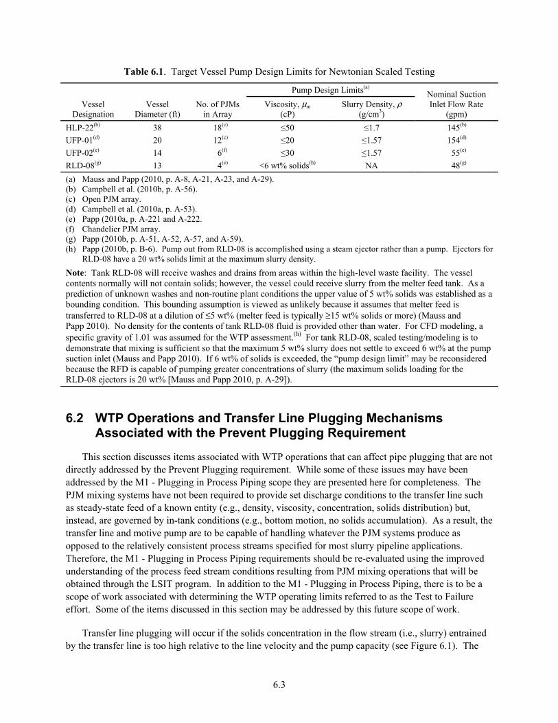
6.3

Table 6.1. Target Vessel Pump Design Limits for Newtonian Scaled Testing

Vessel Designation

Vessel Diameter (ft)

No. of PJMs in Array

Pump Design Limits(a) Nominal Suction Inlet Flow Rate

(gpm) Viscosity, μm

(cP) Slurry Density, ρ

(g/cm3)

HLP-22(b) 38 18(c) ≤50 ≤1.7 145(b)

UFP-01(d) 20 12(c) ≤20 ≤1.57 154(d)

UFP-02(e) 14 6(f) ≤30 ≤1.57 55(e)

RLD-08(g) 13 4(c) <6 wt% solids(h) NA 48(g)

(a) Mauss and Papp (2010, p. A-8, A-21, A-23, and A-29). (b) Campbell et al. (2010b, p. A-56). (c) Open PJM array. (d) Campbell et al. (2010a, p. A-53). (e) Papp (2010a, p. A-221 and A-222. (f) Chandelier PJM array. (g) Papp (2010b, p. A-51, A-52, A-57, and A-59). (h) Papp (2010b, p. B-6). Pump out from RLD-08 is accomplished using a steam ejector rather than a pump. Ejectors for

RLD-08 have a 20 wt% solids limit at the maximum slurry density.

Note: Tank RLD-08 will receive washes and drains from areas within the high-level waste facility. The vessel contents normally will not contain solids; however, the vessel could receive slurry from the melter feed tank. As a prediction of unknown washes and non-routine plant conditions the upper value of 5 wt% solids was established as a bounding condition. This bounding assumption is viewed as unlikely because it assumes that melter feed is transferred to RLD-08 at a dilution of ≤5 wt% (melter feed is typically ≥15 wt% solids or more) (Mauss and Papp 2010). No density for the contents of tank RLD-08 fluid is provided other than water. For CFD modeling, a specific gravity of 1.01 was assumed for the WTP assessment.(h) For tank RLD-08, scaled testing/modeling is to demonstrate that mixing is sufficient so that the maximum 5 wt% slurry does not settle to exceed 6 wt% at the pump suction inlet (Mauss and Papp 2010). If 6 wt% of solids is exceeded, the “pump design limit” may be reconsidered because the RFD is capable of pumping greater concentrations of slurry (the maximum solids loading for the RLD-08 ejectors is 20 wt% [Mauss and Papp 2010, p. A-29]).

6.2 WTP Operations and Transfer Line Plugging Mechanisms Associated with the Prevent Plugging Requirement

This section discusses items associated with WTP operations that can affect pipe plugging that are not directly addressed by the Prevent Plugging requirement. While some of these issues may have been addressed by the M1 - Plugging in Process Piping scope they are presented here for completeness. The PJM mixing systems have not been required to provide set discharge conditions to the transfer line such as steady-state feed of a known entity (e.g., density, viscosity, concentration, solids distribution) but, instead, are governed by in-tank conditions (e.g., bottom motion, no solids accumulation). As a result, the transfer line and motive pump are to be capable of handling whatever the PJM systems produce as opposed to the relatively consistent process streams specified for most slurry pipeline applications. Therefore, the M1 - Plugging in Process Piping requirements should be re-evaluated using the improved understanding of the process feed stream conditions resulting from PJM mixing operations that will be obtained through the LSIT program. In addition to the M1 - Plugging in Process Piping, there is to be a scope of work associated with determining the WTP operating limits referred to as the Test to Failure effort. Some of the items discussed in this section may be addressed by this future scope of work.

Transfer line plugging will occur if the solids concentration in the flow stream (i.e., slurry) entrained by the transfer line is too high relative to the line velocity and the pump capacity (see Figure 6.1). The

6.4

transfer line conditions may result in the Prevent Plugging requirement not being achieved because of one or more of the following plugging mechanisms (failure modes):

• Line plugging from solids deposition (critical pipe velocity for solids deposition, Ucd, not maintained). This can be the result of an excessive total solids concentration or the increase in concentration of a challenging constituent (e.g., heavier and/or larger particles).

• Excessive pressure drop exceeding pump capability to deliver required flow rate. Increases in concentration can result in an increase in the effective viscosity or density of the mixture resulting in a shift in the system pressure curve that exceeds the pump capability or reduces the flow rate below that for complete solids suspension.

• Insufficient NPSHA at pump inlet resulting in reduced pump performance (e.g., flow rate, delivered head) and potentially excessive pump wear because of cavitation.

TransferLine

Pump

Rec

ircul

atio

n

PJM

s (m

ultip

le)

Spa

rger

s(m

ultip

le)

TransferLine

Pump

Rec

ircul

atio

n

PJM

s (m

ultip

le)

Spa

rger

s(m

ultip

le)

Figure 6.1. Schematic Depicting WTP Vessel Mixing and Transfer Line Inlet Flow. The figure on the left depicts suspension following the completion of PJM discharge and the figure on the right represents the accumulation of solids due to settling of larger/heavier particles during the refill phase of the PJM operating cycle, which yields an increase in the concentration entering the transfer line. Non-homogeneous mixing may cause the largest/most dense particles to accumulate at high concentrations near the vessel bottom, which may be suspended and resettle with each PJM cycle.

The WTP operating conditions associated with the Prevent Plugging requirement start with mixing

Hanford tank waste in the large WTP cylindrical vessels with concave bottoms (see Figure 6.1). Mixing is done primarily by an array of PJMs that, in unison, periodically inject a downward jet of slurry fluid from each PJM nozzle located near the bottom of the tank. The multiple jet action from the PJM array is intended to mobilize any and all settled slurry particles on the vessel floor, clear the vessel floor (see Chapter 5 and Appendix C, Working Paper for the Technical Basis for Scaling Transfer and Pump Out), and mix these slurry particles into the vessel bulk slurry waste. When mixing components are operating, the concentration of individual components suspended within the tank may be constantly changing (transient conditions). Heavy/large settling particles at the bottom of the tank will achieve varying levels of gradient height within the vessel (e.g., clouds), with the maximum height achieved likely near the end or immediately following the PJM firing/discharge pulse.

6.5

After the PJMs have fired, vessel mixing action is reduced significantly and heavy particles begin settling back towards the vessel bottom. The amount of solids that settle prior to the next firing of the PJMs depends on the concentration and settling velocity of the solids as well as the vessel fluid level. Depending on slurry rheology (i.e., Newtonian or non-Newtonian), various settling phenomena can be expected including “hindered settling” when the slurry has higher concentrations and/or large particles. During this period of reduced mixing action, some lesser mixing/settling actions may occur including:

• PJM recharge that sucks vessel slurry back into the PJM nozzle

• Operation of multiple spargers that bubble air into the lower half of the vessel to promote overall mixing activity to the top of the slurry

• Retrieval (entrainment) of slurry from the vessel bottom through the transfer line and, when configured to recirculate, the subsequent discharge of slurry back into the vessel.

Depending on slurry rheology and mixing component configuration, the mixing action from the PJMs may not mix the top portion of the vessel slurry, and consequently, heavy/large particles from the bottom may only achieve a limited height within the vessel slurry.

The transfer line, for moving slurry out of a WTP vessel or for recirculation of the vessel contents, horizontally penetrates the vessel wall and contains an inclined section that extends the inlet to a location near the vessel bottom. The inlet of the transfer line is relatively small compared to the overall vessel cross-sectional area, so it has a limited zone of influence from which to draw particles into the transfer line when the transfer pump is running. When PJMs discharge, it is expected that the resulting radial jets scouring the tank bottom will produce a wave of concentrated solids that are transported along the tank bottom. The wave of solids can have a high solids loading similar to that of a fluidized bed that when pushed towards the transfer line inlet effectively floods or overloads (referred to as “swamping”) the inlet resulting in an overwhelming slug of solids being entrained. This wave of high solids concentration can result in the following:

• Line plugging because the transfer velocity within the pipe is too low, resulting in high rate of solids deposition.

• An increase in the pipeline pressure drop, resulting in a reduction of the NPSHA at the pump inlet.

• Burying the inlet of the suction line, resulting in a stoppage of flow to the pump. This is a higher probability if the inlet of the suction line is positioned in a stagnation zone between the PJMs that corresponds to one of the last locations where solids are cleared from the tank bottom by the radial jets of the PJM mixers.

During the PJM refill phase, solids will settle to the vessel bottom with the larger/heavier (i.e., more dense) particles settling at a faster rate than smaller/lighter (i.e., less dense) material. Because the transfer line inlet is located off the bottom of the vessel, the faster-settling, larger/heavier particles have a limited time to be entrained into the transfer line inlet during the PJM refill phase and may only be entrained by being swept into the inlet during the PJM discharge phase, or in the “worst case” do not obtain the height or radial location of the transfer line zone of suction influence.

The slurry level in the vessel also will affect the mixing dynamics and concentration of suspended solids. As the transfer line pump is activated to transport the slurry out of the vessel through the transfer line, the slurry level in the vessel will be lowered assuming no additional waste is being added. As the

6.6

vessel slurry level decreases, the PJM action will continue to mix the slurry until the vessel level is low enough that the PJMs can no longer function. The transfer line can never remove all the liquid (i.e., slurry) from the vessel as the onset of vortexing created at the inlet will entrain air into the transfer line and pump.

The periodic operation of the PJMs and the wide size distribution of the WTP process stream will result in the particles not being uniformly mixed and a concentration gradient existing within the tank. It is expected that, because the transfer line is located close to the vessel bottom, a concentration of large/heavy particles greater than the bulk average within the vessel will initially be removed, and the concentration of these particles within the tank and entering the transfer line will decrease with time as the liquid level in the vessel is reduced. In addition, the cyclical nature of the inlet conditions, the PSDD and concentration can vary with time as can the static head and the flow field in the region of the suction line, can lead to a non-uniform stream relative to pipe length (i.e., time variation in measurement at fixed location) as observed during previous reduced-scale PJM mixing and pump-out tests.

Figures 6.21 is an example of the variation in slurry density (i.e., concentration) measured in the transfer tests during a LOAM test 1 pump out. The scaling applied to the reduced-scale transfer line size and flow rate is unknown. The LOAM tests were conducted by Energy Solutions for BNI to obtain data for the confirmation of the LOAM model. Figure 6.2 presents the data for the initial pump out from a full tank to a tank that is three-quarters full. Refer to Appendix E for plots of subsequent pump outs.

From Figure 6.2, the data trend indicates both the average concentration and variation in concentration continually decreases with time (i.e., tank level) as a greater fraction of the larger/heavier particles, which are concentrated in the lower region of the vessel, were retrieved during the initial pump out. While the results of LOAM test 1 are not expected to readily scale to the WTP, it does provide an example of the periodic conditions in a transfer line that can exist as the result of PJM operations. The effects of the variations in solids loading conditions at the suction line inlet and thus in the transfer line include:

• Greater solids concentration than the average bulk value for the vessel potentially results in the WTP design limits for the transfer line viscosity and density being exceeded.

• Greater solids concentration increases Ucd required to prevent deposition of solids, thus potentially resulting in solids settling.

• Predicting the slurry density and rheology becomes difficult. The same slurry density and viscosity can be obtained from a variety of constituent combinations obtained from a given mixture. This becomes a factor in using published correlations for predicting Ucd or system pressure drop. The bulk of these correlations were developed using slurries with monodisperse solids or a single solids density. The application of these correlations to polydisperse mixtures requires the determination of bulk material properties (e.g., particle size, density) to represent the mixture, and these properties are not always the same from one application to another for the same mixture.

1 C Chapman, e-mail to JA Bamberger, April 24, 2012, RE: “Density vs time for Loam tests used as examples in Sect 6, 10, and App-E, stating: [the file] density of slurry during pump outs was a collection of pump out density profiles extracted from a range of engineering reports for LOAM test 1, 2, 5, and 6 and from INFO testing.” The author was Chris Chapman and this assembly was made in January 2012.

6.7

Figure 6.2. Instantaneous Slurry Density in Transfer Line versus Time During LOAM Test 1 Pump Out. Pump out is from a full level to a three-quarter-full level. Data obtained by Energy Solutions for BNI.1

In addition, the frequency of PJM operations relative to the transport time through the transfer line

piping means that the occurrences will be independent of each other (distinguishable) and observable far downstream of the inlet. As slugs of higher concentration slurry are periodically entrained into the pipe, the solids can become segregated because of the differences in relative velocities among the constituents. This segregation of solids can result in changes to the localized rheological conditions and, thus, deposition of larger, heavier solids that would have remained suspended in a steady-state flow of the original entrained mixture. Figure 6.3 is a schematic depicting this phenomenon resulting from particle segregation.

Additional aspects of system operations that can impact pipe plugging include:

• Pipeline flushing after each transfer − Because of the relatively short duration of the WTP batch transfers from the mixing vessels (i.e., on the order of 3 to 6 hr), it is possible for solids holdup to occur that does not result in pipeline plugging during the course of a single transfer. However, if line flushing operations do not clear all solids from the line, then solids holdup can lead to plugging over the course of multiple transfers. Flushing operations (e.g., frequency, velocity, duration/volume) need to be assessed for the transfer line operating conditions predicted by the LSIT test program.

• Idle pipeline during mixing operations − If the pipeline remains idle during mixing operations, there is the potential for solids and/or air/gas accumulation within the inlet of the suction line. Gas can

1 C Chapman, e-mail to JA Bamberger, April 24, 2012, RE: “Density vs time for Loam tests used as examples in Sect 6, 10, and App-E, stating: [the file] density of slurry during pump outs was a collection of pump out density profiles extracted from a range of engineering reports for LOAM test 1, 2, 5, and 6 and from INFO testing.” The author was Chris Chapman and this assembly was made in January 2012.

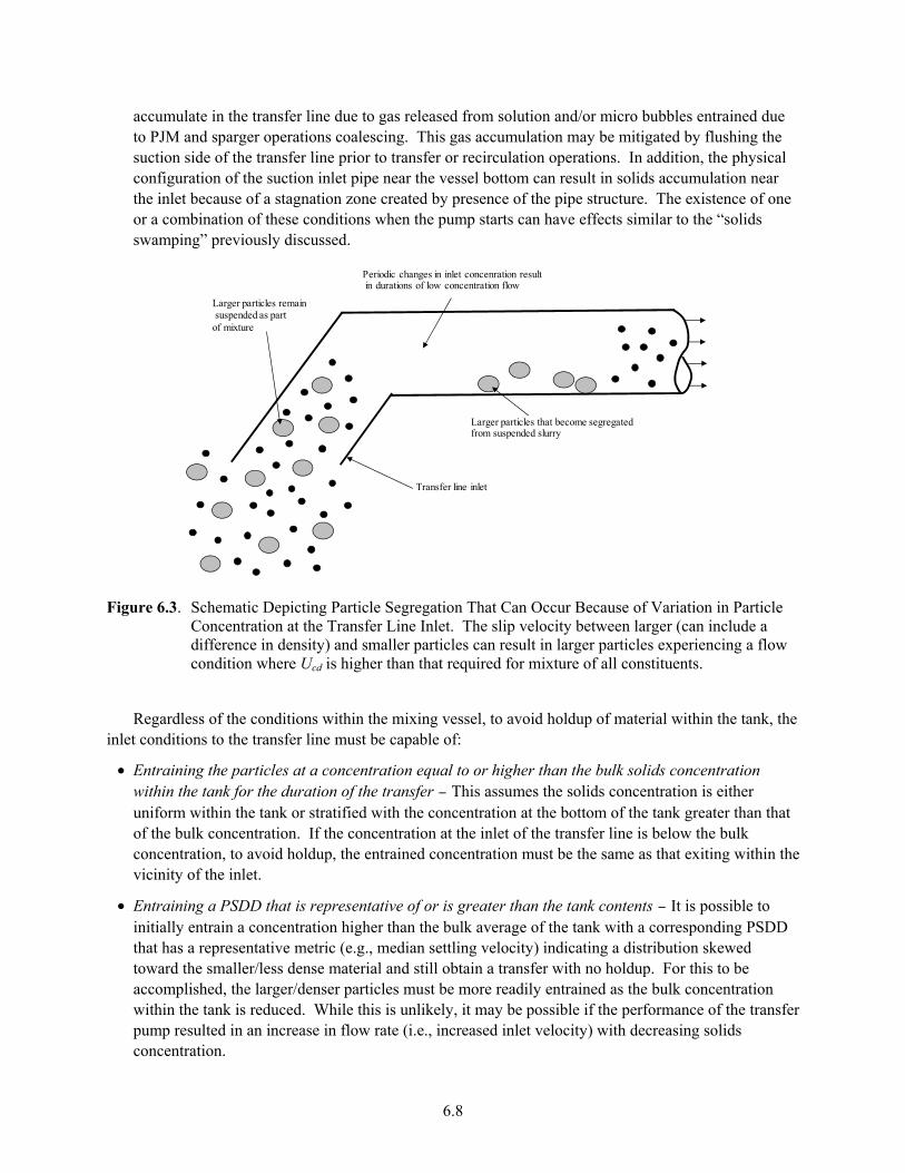
6.8

accumulate in the transfer line due to gas released from solution and/or micro bubbles entrained due to PJM and sparger operations coalescing. This gas accumulation may be mitigated by flushing the suction side of the transfer line prior to transfer or recirculation operations. In addition, the physical configuration of the suction inlet pipe near the vessel bottom can result in solids accumulation near the inlet because of a stagnation zone created by presence of the pipe structure. The existence of one or a combination of these conditions when the pump starts can have effects similar to the “solids swamping” previously discussed.

Larger particles that become segregatedfrom suspended slurry

Periodic changes in inlet concenration resultin durations of low concentration flow

Transfer line inlet

Larger particles remainsuspended as part

of mixture

Figure 6.3. Schematic Depicting Particle Segregation That Can Occur Because of Variation in Particle Concentration at the Transfer Line Inlet. The slip velocity between larger (can include a difference in density) and smaller particles can result in larger particles experiencing a flow condition where Ucd is higher than that required for mixture of all constituents.

Regardless of the conditions within the mixing vessel, to avoid holdup of material within the tank, the

inlet conditions to the transfer line must be capable of:

• Entraining the particles at a concentration equal to or higher than the bulk solids concentration within the tank for the duration of the transfer − This assumes the solids concentration is either uniform within the tank or stratified with the concentration at the bottom of the tank greater than that of the bulk concentration. If the concentration at the inlet of the transfer line is below the bulk concentration, to avoid holdup, the entrained concentration must be the same as that exiting within the vicinity of the inlet.

• Entraining a PSDD that is representative of or is greater than the tank contents − It is possible to initially entrain a concentration higher than the bulk average of the tank with a corresponding PSDD that has a representative metric (e.g., median settling velocity) indicating a distribution skewed toward the smaller/less dense material and still obtain a transfer with no holdup. For this to be accomplished, the larger/denser particles must be more readily entrained as the bulk concentration within the tank is reduced. While this is unlikely, it may be possible if the performance of the transfer pump resulted in an increase in flow rate (i.e., increased inlet velocity) with decreasing solids concentration.

6.9

6.3 Approach for Assessing Pipe Plugging in WTP Vessel Transfer Lines

This section provides an approach for using reduced-scale testing and associated industrial correlations to assess the WTP for the plugging mechanisms summarized in Section 6.2. Appendix E provides discussions associated with:

• The assumptions applied for generating this approach to assess the Prevent Plugging requirement

• Relevant parameters and slurry pipeline flow conditions

• Summary of general pipeline design objectives and guidelines for comparison to the WTP circumstances.

The key mechanism to avoid plugging in the transfer line is to avoid solids settling (i.e., solids deposition) that can restrict the flow, resulting in an increased head loss and a reduced NPSHA at the pump inlet. The operating cycle for the PJMs results in an intermittent mixing action of slurry in the vessel causing the concentration at the transfer line inlet to vary with PJM operations. The approach presented simplifies transfer line operations by using “worst-case,” bounding slurry properties/conditions that can then be applied at steady-state conditions. This strategy can be compared to assessing a vehicle’s fuel consumption rate (slurry flow) running at full throttle (steady state) up an incline with a head wind (bounding conditions). Industrial models or correlations are chosen and representative slurry properties are defined based on matching test data, within acceptable error bands, obtained at various scales and operating conditions. These models then are used to “predict” full-scale WTP operations. Because this is a conservative approach, failure cannot be confirmed, only success can. If successful operations are not confirmed then the approach will require either:

• A reduction in the conservatism applied to establish the bounding, steady-state conditions, or

• A change in WTP design and/or operating conditions that coincide with bounding conditions for which successful operations can be confirmed by this approach.

Refer to Chapter 3 and Appendix A for a summary of the different scaling approaches and Appendix A, Section A.7.1.1 where bounding conditions are discussed as a form of similitude. With a bounding approach, the actual range of WTP operating conditions is not being evaluated. Instead the approach defines bounding conditions or an operating envelope to be assessed. While specific WTP operating conditions are not predicted, acceptable performance at the bounding conditions indicates that satisfactory performance will be achieved within the operating envelope.

The strategy for assessing the Prevent Plugging requirement against bounding conditions uses a stepped approach integrated with the LSIT reduced-scale testing. This section presents the strategy in increasing detail to help the reader understand the overall concept and then outlines the separate phases of the approach to assess the individual failure modes listed in Appendix E, Section E.2.1.

The approach is designed to take advantage of industrial correlations developed and verified by test data and industrial applications and to allow testing to commence using a design simulant consisting of multiple constituents as opposed to requiring development work utilizing a less complex simulant. A high-level approach for applying the bounding condition scaling to each plugging mechanism is represented in Figure 6.4.

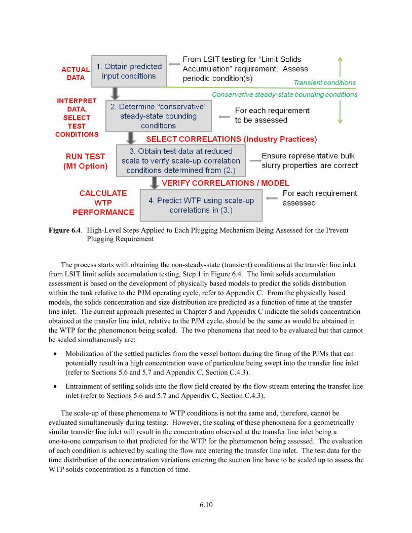
6.10

Figure 6.4. High-Level Steps Applied to Each Plugging Mechanism Being Assessed for the Prevent Plugging Requirement

The process starts with obtaining the non-steady-state (transient) conditions at the transfer line inlet

from LSIT limit solids accumulation testing, Step 1 in Figure 6.4. The limit solids accumulation assessment is based on the development of physically based models to predict the solids distribution within the tank relative to the PJM operating cycle, refer to Appendix C. From the physically based models, the solids concentration and size distribution are predicted as a function of time at the transfer line inlet. The current approach presented in Chapter 5 and Appendix C indicate the solids concentration obtained at the transfer line inlet, relative to the PJM cycle, should be the same as would be obtained in the WTP for the phenomenon being scaled. The two phenomena that need to be evaluated but that cannot be scaled simultaneously are:

• Mobilization of the settled particles from the vessel bottom during the firing of the PJMs that can potentially result in a high concentration wave of particulate being swept into the transfer line inlet (refer to Sections 5.6 and 5.7 and Appendix C, Section C.4.3).

• Entrainment of settling solids into the flow field created by the flow stream entering the transfer line inlet (refer to Sections 5.6 and 5.7 and Appendix C, Section C.4.3).

The scale-up of these phenomena to WTP conditions is not the same and, therefore, cannot be evaluated simultaneously during testing. However, the scaling of these phenomena for a geometrically similar transfer line inlet will result in the concentration observed at the transfer line inlet being a one-to-one comparison to that predicted for the WTP for the phenomenon being assessed. The evaluation of each condition is achieved by scaling the flow rate entering the transfer line inlet. The test data for the time distribution of the concentration variations entering the suction line have to be scaled up to assess the WTP solids concentration as a function of time.

6.11

Therefore, the test data will result in two predictions for the inlet conditions of the WTP transfer line being made for each condition evaluated in the reduced-scale LSIT setup. The approach is required to determine the phenomena resulting in the most challenging conditions for transport. The reduced-scale testing for accumulation may provide a clear indication of which phenomena results in the most challenging feed stream conditions allowing only one phenomenon to be focused on for subsequent tests.

From the limit solids accumulation tests, data is obtained from the transfer line for periodic vessel conditions in which the transfer line is operated in recirculation mode (i.e., no pump out). The data and samples are evaluated to establish steady-state conditions that bound the periodic observed conditions (Step 2 of Figure 6.4). These bounding steady-state conditions then are used for testing to benchmark models for predicting the phenomenon of interest (Step 3 of Figure 6.4). The benchmarked model then is used to predict WTP performance for the applicable bounding steady-state condition. Acceptable WTP performance under the bounding, steady-state conditions is assurance that the plant will demonstrate acceptable performance for the non-steady-state conditions being assessed.

Figure 6.5 depicts at a high level, the decision logic applied to the approach. The bulk of Figure 6.5 logic occurs within Step 3 of Figure 6.4. The logic of Figure 6.5 is intended to be self-explanatory and will not be detailed within the text. However, it is emphasized that the application of the models/ correlations and the conducting of the reduced-scale, state-steady tests are independent of one another. Not displayed in the figure is the material characterization effort that accompanies the test effort. The application of the models can consist of parallel efforts to determine which model provides the best comparison.

Figure 6.5. Logic Diagram for Steady-State Testing to Benchmark Models

6.12

The integrated approach for using all of the presented plugging mechanisms to assess the Prevent Plugging mixing requirement is described by the flowchart displayed in Figure 6.6. The items presented in Figure 6.6 will be elaborated in Sections 6.3.1 through 6.3.4. These sections attempt to follow the flow of Figures 6.4 and 6.6 and the reader is encouraged to refer to these figures to relate the process being described to the overall approach for assessing the Prevent Plugging requirement. Appendix E, Section E.7 provides a number of items to be considered, such as the test setup and simulants, for the application of the approach presented in this section.

Figure 6.6. Flowchart of Integrated Tasks Used to Assess the Prevent Plugging Requirement. U* denotes velocity used for applying to models to assess WTP conditions. U* is the greater of Ucd-WTP, critical depostion velocity for WTP obtained from model, or UD-WTP, the specified WTP design velocity for the transfer line of the vessel being evaluated.

6.3.1 Obtaining Non-Steady-State Conditions from LSIT

This section describes the activities associated with the reduced-scale LSIT, which are depicted in Step 1 of Figure 6.4 and in the dashed (i.e., green) box at the top of Figure 6.6. The reduced-scale LSIT to assess the Limit Solids Accumulation mixing requirement will require the test vessel solids be mobilized and a periodic condition be reached. This also will be required for the assessment of the mixing requirements related to sampling (Mixing Requirements 5, 6, and 7). Once a periodic condition

6.13

has been reached, the transfer line should be operated in the recirculation mode with negligible change in tank contents. With respect to the Prevent Plugging requirement, the LSIT effort needs to obtain the following:

• Determine the time of peak slurry concentration entering the transfer line relative to the PJM operating cycle. Tests need to be conducted for transfer line flow rates scaled relative to both solids mobilization and quiescent settling.

• At the transfer line inlet obtain for multiple test scales:

– Mass flow rate and bulk density as a function of time. The bulk-density measurements provide a check against sample characterization measurements with respect to total mass. The inline measurements also allow fluctuations in density to be used to assess the degree of conservatism resulting from applying worst-case conditions to evaluate the pressure drop for steady-state process feed conditions.

– Peak solids concentration (ϕSmax) corresponding to the peak bulk density.

– Total solids concentration (ϕS) and maximum concentration of individual solids species (ϕimax) that correspond to the peak density for various fill/pump-out levels.

– Static pressure at transfer line inlet as a function of time (minimum pressure within cycle is the most important) and tank level (fill/pump-out levels).

• Obtain transfer line pressure drop (ΔP/L) over horizontal section of transfer line for slurry flows that exhibit cyclic solids concentrations because of intermittent PJM operations, and compare test results to the calculated pressure drop for the same section of transfer line (ΔP/L) assuming “steady-state” conditions and the WTP design limits for slurry density (ρ) and slurry viscosity (μm) (specific to each target vessel, refer to Table 6.1). While the inlet configuration and flow rate need to be scaled for the limit solids accumulation tests, the downstream configuration need not be prototypic in configuration. The transfer line needs to be sized to assure no solids deposition and turbulent flow conditions. It is recommended that the transfer line length contain a horizontal length, L, over which the pressure drop is measured, that satisfies the conditions of the following relationship:

2 2

48 ≤ ≤ T CT D

T T

Q tQ tL

D Dπ π (6.1)

where QT is the volume flow rate through the transfer line having an inside diameter of DT, tC is the total PJM cycle time, and tD is the duration of the PJM discharge. This will ensure that the entire volume of slurry retrieved during the discharge of the PJM can exist within the transfer line and that only the entrained slurry associated with one PJM discharge can exist within the transfer line at a given time. This will allow the measurement of reasonable pressure drops for comparison to calculated values for the design limits. The horizontal length can contain non-prototypic bends to accommodate space issues. While this pressure drop is not intended to be representative of WTP pressure drops, it does provide for a meaningful comparison to the WTP prescribed design limits. This comparison provides initial feedback as to whether the WTP design limits are conservative for the anticipated WTP operations to be encountered as a result of the PJM mixing operations.

• Obtain samples of the entrained process stream. Sampling should be performed to correspond to any observed peak in the entrained solids concentration. Based on previous LOAM and M3 test results,

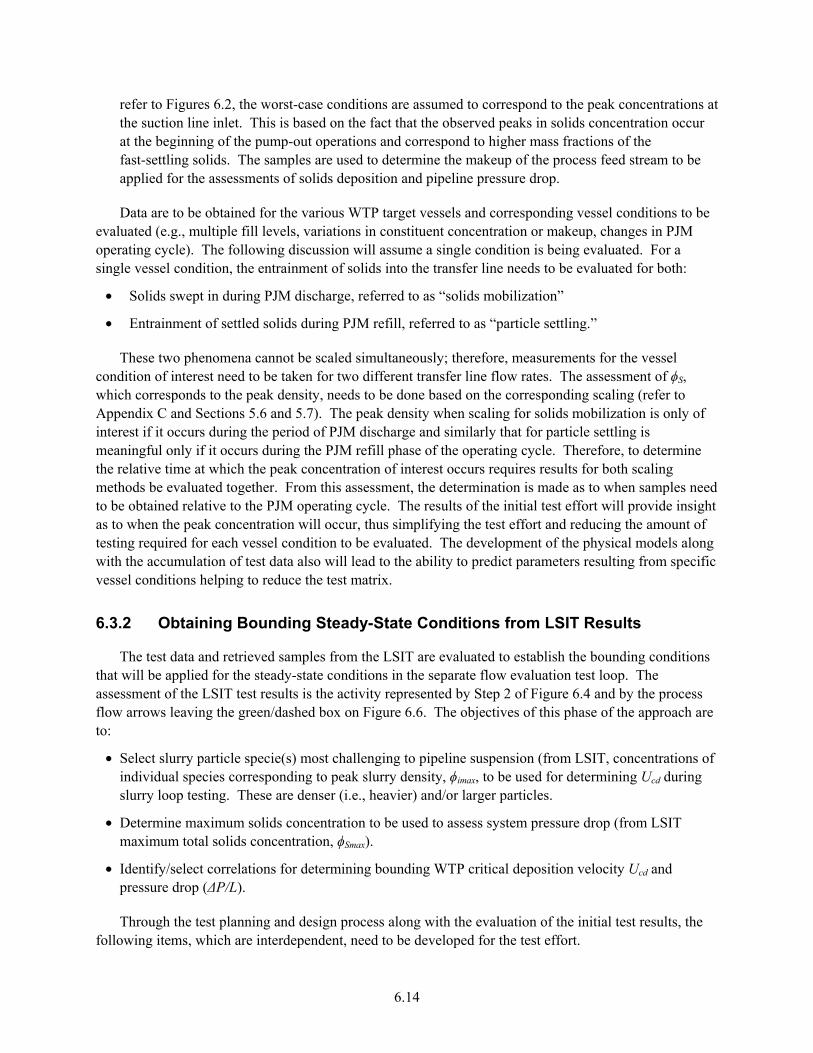
6.14

refer to Figures 6.2, the worst-case conditions are assumed to correspond to the peak concentrations at the suction line inlet. This is based on the fact that the observed peaks in solids concentration occur at the beginning of the pump-out operations and correspond to higher mass fractions of the fast-settling solids. The samples are used to determine the makeup of the process feed stream to be applied for the assessments of solids deposition and pipeline pressure drop.

Data are to be obtained for the various WTP target vessels and corresponding vessel conditions to be evaluated (e.g., multiple fill levels, variations in constituent concentration or makeup, changes in PJM operating cycle). The following discussion will assume a single condition is being evaluated. For a single vessel condition, the entrainment of solids into the transfer line needs to be evaluated for both:

• Solids swept in during PJM discharge, referred to as “solids mobilization”

• Entrainment of settled solids during PJM refill, referred to as “particle settling.”

These two phenomena cannot be scaled simultaneously; therefore, measurements for the vessel condition of interest need to be taken for two different transfer line flow rates. The assessment of ϕS, which corresponds to the peak density, needs to be done based on the corresponding scaling (refer to Appendix C and Sections 5.6 and 5.7). The peak density when scaling for solids mobilization is only of interest if it occurs during the period of PJM discharge and similarly that for particle settling is meaningful only if it occurs during the PJM refill phase of the operating cycle. Therefore, to determine the relative time at which the peak concentration of interest occurs requires results for both scaling methods be evaluated together. From this assessment, the determination is made as to when samples need to be obtained relative to the PJM operating cycle. The results of the initial test effort will provide insight as to when the peak concentration will occur, thus simplifying the test effort and reducing the amount of testing required for each vessel condition to be evaluated. The development of the physical models along with the accumulation of test data also will lead to the ability to predict parameters resulting from specific vessel conditions helping to reduce the test matrix.

6.3.2 Obtaining Bounding Steady-State Conditions from LSIT Results

The test data and retrieved samples from the LSIT are evaluated to establish the bounding conditions that will be applied for the steady-state conditions in the separate flow evaluation test loop. The assessment of the LSIT test results is the activity represented by Step 2 of Figure 6.4 and by the process flow arrows leaving the green/dashed box on Figure 6.6. The objectives of this phase of the approach are to:

• Select slurry particle specie(s) most challenging to pipeline suspension (from LSIT, concentrations of individual species corresponding to peak slurry density, ϕimax, to be used for determining Ucd during slurry loop testing. These are denser (i.e., heavier) and/or larger particles.

• Determine maximum solids concentration to be used to assess system pressure drop (from LSIT maximum total solids concentration, ϕSmax).

• Identify/select correlations for determining bounding WTP critical deposition velocity Ucd and pressure drop (ΔP/L).

Through the test planning and design process along with the evaluation of the initial test results, the following items, which are interdependent, need to be developed for the test effort.

6.15

• The sampling requirements, techniques, and methodology, which may be scale dependent – To accommodate sampling needs, the transfer line velocity (e.g., the line diameter) may need to be adjusted. There is a specific time duration for the transfer line flow associated with an acquired sample. As the system scale is reduced, the absolute time associated with a concentration spike will be reduced. Therefore, at reduced scale, samples may begin to represent time-averaged properties as opposed to instantaneous results. If sample sizes and times are reduced significantly in an attempt to better resolve a transient in solids loading, the result may be an increase in sample variability and uncertainty in the measured properties.

• The measurement requirement, which will be simulant dependent – The operation of the LSIT with the transfer loop in recirculation mode will allow for repeat measurements and samples to be obtained. The number and frequency of measurements and samples will depend on:

– The concentration profile that needs to be resolved

– The definition of bounding conditions. That is, how straightforward is it to define conservative conditions from the observed transients, and how conservative should the testing be to establish the needed margin of safety and performance?

– How complex is the simulant and the associated characterization of the samples?

• Determination of bounding conditions, which will depend on the nature of the concentration variations observed and the phenomenon being assessed – For a step function change in the concentration that exists for a sufficient duration of the pulse cycle (e.g., 20 to 50 percent), the selection of the sustained peak concentration would represent a fairly conservative, but reasonable, bounding condition to impose for steady-state testing with respect to pressure drop. The transfer line would be exposed to these conditions such that the majority of the line may experience these conditions simultaneously. For a short-lived transient with a relatively large increase in concentration, applying the peak value in concentration of the corresponding challenging particles may be needed to provide a bounding condition for assessing solids deposition. However, applying this same peak concentration for evaluating pressure drop may lead to needlessly designing/ specifying a system capable of transferring an order of magnitude greater amount of material than is necessary. Applying a multiple to the timed-averaged concentration may provide sufficient conservatism while still yielding a feasible design point. The final determination of the approach used to define the bounding conditions will require an understanding of the concentration variations to be assessed. The main two phenomenon for which bounding conditions need to be assigned are:

– Assessment of the critical velocity for solids deposition Ucd (refer to Section 6.4.1)

– Assessment of the system pressure drop (refer to Section 6.4.2).

It is currently anticipated via the development of the physical models and associated scaling recommendations that the solids concentration relative to the PJM cycle obtained during the LSIT effort will have a one-to-one relationship with WTP performance. Therefore, similar results are expected at each scale tested. As data is accumulated, the scalability and predictability of the transfer line inlet conditions is to be assessed. This assessment may result in a variation in the physical models and associated scaling recommendation.

6.16

6.3.3 Benchmarking of Predictive Models

This section defines the performance testing required to benchmark the correlations identified during the previous phase of work (Appendix E, Section E.5.2), and the associated material properties to be applied to the correlation. The activities defined in this section are represented as Step 3 on Figure 6.4 and by the box labeled Flow Evaluation Loop Testing in Figure 6.6 and utilize the logic presented in Figure 6.5. Based on the bounding conditions prescribed for each phenomenon to be evaluated, models and correlations for predicting WTP performance are selected for benchmarking via testing in a flow evaluation loop. Recommended models are presented in Section 6.4 and Appendix E, Section E.6. The established models used by industry for predicting Ucd and slurry pressure drop have been developed for narrower particle size and density distributions than anticipated in the complex WTP process stream. These models use limited material property parameters to represent the flow stream. Therefore, the selection of representative properties can be critical for successful application of the models. The test effort is intended to benchmark both the models and the material properties selected to represent the process stream.

All performance tests are done at steady-state conditions selected as “worst-case” bounding conditions based on results of reduced-scale LSIT tests or associated sample analyses. The performance tests are conducted in a flow evaluation loop. Testing is focused on two phenomena:

1. Critical velocity for solids deposition (Ucd) – Slurry solid particles with greater settling velocity require greater transfer velocity. WTP simulant segregated with maximum settling velocity particles, φimax, will yield a conservative Ucd for WTP. The flow rate in the flow loop will be varied until the velocity at which solid deposition, Ucd, occurs is identified. Refer to Section 6.4.1 and Appendix E, Section E.6.1.

2. Pressure drop in pipe per length (ΔP/L) – The maximum total solids concentration, φSmax, obtained from LSIT limit solids accumulation test is the basis for determining the bounding solids loading used for testing. A steady-state flow with φS yields a greater pressure drop than the same volumetric flow rate for which the slurry concentration periodically varies between 0 and φS. The pressure drop as a function of flow rate will be measured for conditions exceeding the corresponding deposition velocity (i.e., useful data will not be obtained for conditions of settling solids within the transfer line) and/or WTP design velocity. Refer to Section 6.4.2 and Appendix E, Section E.6.2.

Because the selection of representative material properties for the models needs to be verified, the simulant makeup for the “baseline” bounding conditions needs to be adjusted and corresponding test results obtained. This is especially needed for the assessment of Ucd as the selected bounding condition should yield a unique value for Ucd compared with the prediction for the pressure drop, which can be compared over a range of flow rates. Performing tests with variations in the simulant makeup from the baseline also will support:

• Evaluating the uncertainty in the model predictions

• Evaluating potential WTP design margins

• Evaluating sensitivity of WTP performance to changes in design/operating conditions.

6.17

6.3.4 Assessing WTP Performance

The tasks in this section are to be conducted both in concert with and following the collection of the test data. A portion of this effort is represented by the logic in Figure 6.5 and the bulk of the effort is depicted in Figure 6.6 by the box titled WTP Full-Scale Calculations.

While the data from the test loop can be collected independently of the evaluation of predictive models, performing the tasks in concert will allow:

• Adjustment of the test matrix as needed to add tests for obtaining desired resolution or eliminating tests that do not help in developing the comparison

• Determination of additional simulant characterization requirements that may be required of the bulk simulant or from samples drawn from the test loop

• Changes in measurement resolution, location, frequency, etc., to be made.

An iterative process is used to determine and verify the representative material properties for the models that yield predictions comparable to the steady-state test results. Once the models are verified, they are used to predict performance at WTP full-scale configuration and conditions.

If WTP performance prediction is within the WTP design, no further testing is required. If WTP performance prediction is outside of WTP design, client resolution may be required to resolve design shortfalls or retest/recalculate using less conservative assumptions.

The logic associated with the assessment of the various plugging mechanisms for WTP (refer to Figures 6.5 and 6.6) is:

• The pressure drop can only be assessed for conditions having no solids deposition. The evaluation of the pressure drop has to be done at a velocity equal to or greater than Ucd. Therefore, the pressure drop for WTP needs to be predicted at the larger velocity between Ucd and the WTP minimum design velocity.

• A system curve for pressure drop is calculated using the benchmarked correlation, test data, and the WTP system configuration. The recommended model presented in Section 6.4.2 allows a system curve to be developed for the WTP systems being assessed. Pressure drop data for unique components should be evaluated to determine loss coefficients for the components. The loss coefficients resulting from slurry flow may vary from those published for liquid only conditions. The development of the system curve provides both the pressure drop in the suction leg of the transfer line and the head requirements for the transfer pump.

• To determine NPSHA, static pressure measurements at the transfer line inlet obtained from the reduced-scale LSIT tests are scaled up to WTP conditions. The static pressure at the transfer line inlet is added to the pressure drop for the WTP transfer line upstream of the pump and the result compared to the NPSHR for the WTP pump.

The assessment of WTP transfer line performance will yield a minimum velocity (i.e., volumetric flow rate), required head (i.e., pump discharge pressure), and an NPSHA. An assessment of the selected transfer pump needs to be performed for a full-scale pump to ensure that the pump can operate under the defined conditions for pumping the required slurry. This can be accomplished using data from the vendor

6.18

or from industry applications. However, the assessment should not be made based on pump performance with only water or a representative liquid. A confirmatory test using the slurry simulant with the prescribed back pressure applied is recommended for verifying and evaluating pump performance prior to final selection.

6.4 Evaluation of Individual Failure Mechanisms

The evaluation of the separate failure modes are presented in the following sections:

• Section 6.4.1 – Solids deposition within the transfer line

• Section 6.4.2 – Pressure drop through transfer line that exceeds system limits

• Section 6.4.3 – Insufficient NPSHA at the transfer pump inlet.

Recommended models for assessing the failure modes are presented in Sections 6.4.1 and 6.4.2, however, the approach presented in Section 6.3 is still applicable using other models. Evaluation of the pump performance is discussed in Section 6.4.4 and Appendix E, Section E.6.4. Appendix E, Section E.6.5 presents an approach to be used if full-scale conditions are employed for the assessment.

6.4.1 Evaluation of Plugging Due to Solids Deposition

This section presents a conservative approach using reduced-scale testing to assess plugging in the WTP transfer line due to solids deposition. The approach takes into consideration the cyclical flow conditions existing at the suction line inlet. Refer to Appendix E, Section E.6.1 for an expanded discussion. The approach is outlined below, follows the same progression as presented in Figures 6.4 through 6.6, and requires the following:

• Use of a segregated portion of the test simulant denser and/or larger solid constituents. The determination of the constituents to use will depend upon the results of the LSIT for limit solids accumulation. It is also recommended that the LSIT test simulant be designed to provide solids ranges with corresponding densities so size separation can be used to characterize the constituent concentration of test samples.

• Adoption of a no solids deposition requirement within the transfer line − Solids deposition is assumed to be the metric that will be used for assessing the potential for pipeline plugging. This requirement is often applied within industry but can be considered conservative for WTP pump-out operations because of the batch process nature of pump outs, which are of relatively short duration (i.e., on the order of 2- to 6-hr transfers based on vessel active volumes [refer to references in Table 6.1 for each vessel], flow rates provided in Table 6.1, and assuming four pump outs of similar volume to empty a vessel), and are followed immediately by flush operations.

The approach consists of:

• Using the peak solids concentration condition obtained from reduced-scale, limit solids accumulation LSIT testing (refer to Section 6.3.1 and Appendix E, Sections E.5.1 and E.5.2), the solids loading for the larger and heavier particles (i.e., fast-settling solids) are determined from the condition of the peak concentration.

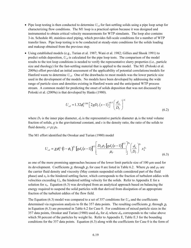
6.19

• Pipe loop testing is then conducted to determine Ucd for fast-settling solids using a pipe loop setup for characterizing flow conditions. The M1 loop is a practical option because it was designed and instrumented to obtain critical velocity measurements for WTP simulants. The loop also contains 3-in. Schedule 40, stainless-steel piping, which provides full-scale conditions for a number of WTP transfer lines. Pipe loop testing is to be conducted at steady-state conditions for the solids loading and makeup obtained from the previous step.

• Using established models (e.g., Turian et al. 1987; Wani et al. 1982; Gillies and Shook 1991) to predict solids deposition, Ucd is calculated for the pipe loop tests. The comparison of the model results to the test loop conditions is needed to verify the representative slurry properties (i.e., particle size and rheology) for the fast-settling material that is applied to the model. The M1 (Poloski et al. 2009a) effort provided an initial assessment of the applicability of potential correlations/models for Hanford waste to determine Ucd. One of the drawbacks to most models was the lower particle size used in the development of the models. No models have been developed by addressing the wide range of particle sizes and densities existing in Hanford waste and the anticipated WTP process stream. A common model for predicting the onset of solids deposition that was not discussed by Poloski et al. (2009a) is that developed by Hanks (1980).

( )

1.60.50.1861.32 2 1 S

cd S TT

dU gD s

Dφ

= −

(6.2)

where DT is the inner pipe diameter, dS is the representative particle diameter φS is the total volume fraction of solids, g is the gravitational constant, and s is the density ratio, the ratio of the solids to fluid density, s=ρs/ρF.

The M1 effort identified the Oroskar and Turian (1980) model

Ucd = χ1φSχ2 1− φS( )χ3

gdS s −1( )[ ]0.5 DT ρF gdS s −1( )[ ]0.5

μF

χ4

dS

DT

χ5

xhχ6

(6.3)

as one of the more promising approaches because of the lower limit particle size of 100 µm used for its development. Coefficients χ1 through χ5 for case 0 are listed in Table 6.2. Where ρF and µF are the carrier fluid density and viscosity (May contain suspended solids considered part of the fluid phase) and xh is the hindered settling factor, which corresponds to the fraction of turbulent eddies with velocities exceeding Uh, the hindered settling velocity for the solids. Refer to Appendix E for a solution for xh. Equation (6.3) was developed from an analytical approach based on balancing the energy required to suspend the solid particles with that derived from dissipation of an appropriate fraction of the turbulent eddies of the flow field.

The Equation (6.3) model was compared to a set of 357 conditions for Ucd and the coefficients determined via regression analysis to fit the 357 data points. The resulting coefficients χ1 through χ6 in Equation (6.3) are presented in Table 6.2 for Case 0. For conditions of mixed particle sizes in the 357 data points, Oroskar and Turian (1980) used d50 for dS where d50 corresponds to the value above which 50 percent of the particles by weight lie. Refer to Appendix E, Table E.3 for the bounding conditions for the 357 data points. Equation (6.3) along with the coefficients for Case 0 is the form of

6.20

the model used for the M1 effort and in the WTP design guide, Minimum Flow Velocity for Slurry Lines (Hall 2010). However, a particle size of 100 μm is still significantly larger than a majority of the solids existing within the Hanford waste inventory, and the model was developed using data for fairly narrow particle size distributions. Follow-on comparisons have been made to PSDDs significantly different and narrower than those measured for the Hanford waste. The Oroskar and Turian model does not take into account the effects of the range/width of the particle size distribution.

Turian et al. (1987) used a collection of 864 data points for critical velocity to evaluate a number of previously developed models including that developed by Oroskar and Turian (1980), Equation (6.3) (note: the evaluation did not consider Equation (6.2) (Hanks 1980)). From the evaluation, it was determined that the analytical development of Oroskar and Turian (1980) provided a better match than the other models evaluated. Turian et al. (1987) provided a revised model and determined the coefficients by fitting the 864 critical velocity data points using multilinear regression, in which the linearized log form of the Equation (6.4) is fitted.

Ucd = χ1φSχ2 1− φS( )χ3

2gDT s −1( )[ ]0.5 DT ρF gDT s −1( )[ ]0.5

μF

χ4

dS

DT

χ5

(6.4)

Table 6.2 provides the values for χ1 through χ5 for five different variations of Equation (6.4), refer to

cases 1 through 5. The table also contains the average of the absolute values of the deviations, d % ,

and the associated root mean square deviation, rms, obtained for the five variations of the model when compared to the experimental data (Turian et al. 1987). Refer to Appendix E for the

calculations of d % and rms.

For conditions of mixed particle sizes in the 864 data points, Turian et al. (1987) used d50 for dS. Refer to Appendix E, Table E.3 for bounding conditions for the 864 data points. Based on the data presented in Table 6.2, all five variations of the equation appear equally effective for predicting Ucd.

• The representative slurry properties for the fast-settling solids then are applied to the model for WTP conditions to obtain Ucd at full scale. Because of the uncertainty associated with the application of the

models (refer to %d in Table 6.2), a design factor should be applied in determining the final full-scale

design velocity relative to deposition. This is in addition to any requirements for design margin.

Table 6.2. Coefficient and Exponent Values for Oroskar and Turian and Turian et al. Models Predicting Critical Velocity for Solids Deposition (Ucd) Presented in Equations (6.3) and (6.4)

Case No. χ1 χ2 χ3 χ4 χ5 χ6

d % (Average of absolute

values for % deviation) rms 0(a) 1.85 0.1536 0.3564 0.09 -0.378 0.3 N/A N/A 1 1.7951 0.1087 0.2501 0.00179 0.06623 n/a 20.53 0.3416 2 1.8471 0.1126 0.03421 -0.03093 0 n/a 21.54 0.3447 3 1.8176 0.1086 0.2525 0 0.06486 n/a 20.57 0.3412 4 1.3213 0.1182 0.3293 0 0 n/a 21.04 0.3552 5 1.1228 0.07367 0 0 0 n/a 21.35 0.3559

(a) The value of the coefficients used for model comparison for the M1 effort and in WTP design guide (Hall 2010).

6.21

As previously mentioned, the flow condition and the slurry rheology both impact slurry transport. Even if matching experimental results are obtained for a model/model prediction at scaled conditions, the flow conditions at which the model is applied need to be the same at both scaled and WTP conditions. The Oroskar and Turian and Turian et al. models were developed for fully turbulent Newtonian flow. For non-Newtonian conditions, the practice is to apply an apparent viscosity, but depending on flow conditions, this can be troublesome when applying the model over multiple scales. Poloski et al. (2009a) presents the impact of yield stress via a stability map for flow conditions. Poloski’s approach for non-Newtonian fluids is to evaluate the predicted flow conditions against a critical deposition boundary, transitional deposition boundary, and laminar deposition boundary.

6.4.2 Evaluation of System Pressure Drop

This section is associated with assessing the system pressure drop to ensure it does not exceed system limits. An expansion of this approach is presented in Appendix E, Section E.6.2. The evaluation of the system pressure drop allows:

• Evaluation or specification of the NPSHR for the WTP pump if final pump selection has not been completed

• Evaluation or specification of the WTP pump discharge requirements.

The approach requires the use of a pipe loop separate from the reduced-scale PJM mixing vessel in which a steady-state process feed can be applied over a range of flow rates. The pipe loop (i.e., flow evaluation loop) is to be configured to allow the slurry and flow conditions to be well characterized via instrumentation and sampling. The test loop can be of reduced scale and does not have to be consistently scaled for all WTP systems being evaluated. For example, the previously used M1 test loop has 3-in.-diameter, Schedule 40, stainless-steel piping, which is full scale for a number of WTP transfer lines. It is recommended the test loop allow for pressure drop measurements over both horizontal and vertical pipe runs.

The test loop separate from the LSIT PJM mixing vessel setup is used to obtain steady-state, pressure drop measurements for conservative conditions that can be used to verify an applicable correlation for pressure drop. The correlation is then used to determine bounding pressure drops for the WTP system. The process stream conditions to be used for evaluating the pressure drop in the separate test loop are obtained from the results of the LSIT for Limit Solids Accumulation requirement (refer to Sections 6.3.1 and 6.3.2).

The application of steady-state conditions to the process stream peak concentration, while not conservative for assessing solids deposition, does provide a conservative approach for the pressure drop as long as equal volume-averaged line velocities are maintained between the LSIT transfer line inlet and the flow evaluation loop. To obtain conservative predictions for the pressure drop within the WTP resulting from PJM mixer operations, the following summarized approach is provided:

• Obtain the retrieval line solids concentration and size distributions from LSIT reduced-scale test data for both scaling phenomena discussed in Section 6.3 and presented in Chapter 5.

• Independently evaluate the LSIT results for both scaling phenomena to obtain the most conservative condition. The conservative condition is assumed to exist at the condition of peak concentration.

6.22

However, the peak concentration for each phenomenon must occur during the phase of PJM operation being scaled (refer to Sections 6.3 and 6.3.1). From the LSIT results, bounding steady-state conditions are prescribed for the pressure drop measurement tests conducted in the flow evaluation loop.

• Perform pressure drop measurement tests in a pipe loop for steady-state conditions of the slurry mixture identified in the preceding step (could use M1 test loop or LSIT transfer line if fully instrumented for this task).

• Select an established correlation to calculate the slurry pressure drop per unit length of pipe (e.g., Crowe 2006; Churchill 1977; Darby 2000, 2001; Govier and Aziz 1987; Saleh 2002; Molerus 1993; Wasp et al. 1977; Turian and Yuan 1977). The correlation selected must be applicable to similar conditions for solids content, flow regime, solids suspension, and rheology. While the integral equations for the analysis of the pressure drop for two-phase flow are of the same form as for single-phase flow, their solution is more formidable because of:

– The additional parameters required to describe a condition of two-phase flow

– The interaction between the phases that must be taken into account

– The non-steady dynamic interactions that can occur, such as particle settling, suspension, segregation, and mixing.

The complexities of two-phase flow require that empirical models based on experimental data be employed. Efforts to develop models/correlations that can predict pipeline pressure drops for slurries have progressed using slurries comprised of more uniform constituents than mixtures anticipated for processing at WTP. While variations in particle size and densities have been applied in the development and evaluation of pressure drop correlations, no slurries (mixtures) with variations as broad as those anticipated for WTP have been encountered in the literature. A method for determining the pressure drop for multi-constituent slurries of various rheology is presented in Section 6.4.2.1 and Appendix E, Section E.6.2.1.

• Using the pressure drop model, calculate the pressure drop per unit length for the test loop conditions. The comparison of model predictions to the test loop results is needed to establish proper determination of the representative material properties to apply to the model. The development and evaluation of such models has been done for slurries having much narrower PSDDs than those anticipated for the WTP process streams.

• The benchmarked pressure drop correlation with the representative slurry properties is then applied to WTP conditions and configuration to calculate the pressure drop within the WTP transfer line. The velocity applied to WTP needs to be sufficient to assure full solids suspension, refer to Section 6.4.1.

6.4.2.1 Methodology for Determination of Pressure Drop for Multi-Constituent Slurry

This section provides a methodology, developed by Molerus (1993) and Darby (2000), and presented by Saleh (2002) and Darby (2001) for predicting the pressure drop for multi-constituent slurry flowing under steady-state conditions. Applications to Newtonian, Bingham plastic, and power-law modeled fluids are presented in Appendix E, Section E.6.2.1. While the process vessels may be designated Newtonian, the increased solids concentration and variation in constituent makeup can result in the transfer line slurry exhibiting non-Newtonian behavior.

6.23

Frictional pressure drop within a pipe can be considered to be composed of both a pure fluid component and a solids component such that:

ΔPm = ΔPF + ΔPS (6.5)

where ΔPm, ΔPF, and ΔPS represent the pressure drops for the total slurry (i.e., mixture of solids and liquid), the fluid component (i.e., the continuous phase), and the solids constituents (i.e., individual particles), respectively. ΔPF is obtained for the fluid (fluid may include non-settling solids that are considered part of the continuous phase) but applying the average slurry velocity, Um. ΔPS is obtained using the Molerus diagram for suspension transport. The Molerus diagram (Saleh 2002), refer to Appendix E, Figure E.9, was obtained from over 1000 data points, the conditions of which Saleh (2002) describes as:

• Pipe diameters of 25 mm to 315 mm

• Particle diameters of 12 µm to 5.2 mm

• Solid specific gravities of 1.27 to 5.25

• Carrier fluids of both gas and liquid

• Fully suspended slurry flow for both homogenous/symmetrical and heterogeneous/asymmetrical suspensions.

The relative dimensionless groups associated with the suspension transport are:

• The dimensionless single-particle slip velocity

0

rr

m

UU

U=

(6.6)

where Ur = the relative or “slip” velocity between the fluid and solids (Ur = UF – US) UF = the velocity of the carrier fluid US = the velocity of the solid particles Um = the volumetric average velocity within the pipe (the volumetric average slurry

velocity).

• The particle Froude number, Frp, as obtained from Molerus (1993)

22

( 1)m

pS

UFr

s d g=

− (6.7)

where s = the density ratio; ratio of particle density to fluid density (ρs/ρF) Frp = particle Froude number dS = the particle diameter g = gravitational constant.

6.24

• The tube or pipe Froude number as obtained from Molerus (1993)

22

( 1)T

TT

UFr

s D g=

− (6.8)

where FrT is the tube or pipe Froude number, UT is the unhindered terminal settling velocity, and DT is the tube or pipe diameter.

• The diameter ratio

dS

DT (6.9)

The defined Froude numbers are somewhat arbitrary and Molerus (1993) provides no explanation for their origin. Molerus (1993) correlated the data in the form

( )0.5 20

0.5,r

p T

Uf Fr s Fr

s=

(6.10)

With respect to the defined fluid, if some of the solids are uniformly suspended to create a homogenous continuous phase (i.e., carrier fluid), this fraction of solids can be assumed to contribute to the fluid pressure drop and contribute to the fluid material properties. If the carrier fluid or concentration of uniformly suspended solids result in non-Newtonian behavior, the process is more complex but still applicable. The application of the process to both Bingham plastic and power-law modeled fluids is presented in Appendix E, Section E.6.2.1.

Molerus (1993) developed a relation for the dimensionless pressure drop, XΔP, resulting from the

solids flow. His development is based on the rate of energy dissipation in the flow because of the solids and the rate of energy to the particles resulting from the relative velocity between the solids and the fluid. The resulting relation is:

XΔP ≡

ΔPS

φSρF (s −1)gL

UT

Um

2

(6.11)

where φS is the total volume fraction of solids, and L is the relative pipe length such that the pressure drop per unit length of pipe (ΔPS/L) is calculated.

The value of XΔP depends on the value of φS.

6.25

For 0 < φS < 0.25:

2

20

001

1

r

m rP P

rr

m

UU U

X XUU

U

Δ Δ

= = =

− − (6.12)

For φS > 0.25:

XΔP = XΔP 0 + 0.1FrT

2 φS − 0.25( ) (6.13)

Darby (2000) and Saleh (2002) both present a method for determining XΔP, which is presented in

Appendix E, Section E.6.2.1. The method involves the following five steps.

1. Determine UT for the correct flow condition

2. Determine Ur0 by obtaining Ur0

s0.5 from the Molerus diagram for suspension transport (refer to

Appendix E, Figure E.9) for solid suspension using the values calculated for Frps0.5 and FrT2.

3. Calculate XΔP0

4. If necessary (φS > 0.25) calculate XΔP from Equation (6.13)

5. ΔPS

L is then calculated using Equation (6.11).

After obtaining ΔPS

L, the pressure drop ΔPF

Lcan be calculated from the Fanning equation

22 F mF

T

f UP

L D

ρΔ = (6.14)

where f, the friction factor for pipe flow, can be defined in terms of the shear stress at the pipe wall, τw, such that

2

2= w

F m

fU

τρ (6.15)

The pressure drop resulting from solids for specific particle size ranges (bins) or species of solids can be considered individually such that n constituents of volume concentration φSi having dSi and ρsi would result in

ΔPm = ΔPF + ΔPSi

i=1

n

(6.16)

6.26

Again, a portion of the non-settling, uniformly suspended solid constituents may be considered part of the fluid, and these materials would not be considered as part of the n solid constituents. For multiple solid materials and/or solid sizes, the five steps listed above are repeated for each of the n solid constituents/size ranges to obtain

ΔPSi

Li=1

n

(6.17)

The particle terminal velocity, UT, and the friction factor, f, are dependent on the fluid rheology. Non-Newtonian behavior for the fluid changes the process by which these parameters are calculated. The following sections in Appendix E will provide the method for obtaining UT and f for Newtonian (Appendix E, Sections E.6.2.1.1.1 and E.6.2.1.2.1), Bingham plastic (Appendix E, Sections E.6.2.1.1.2 and E.6.2.1.2.2), and power-law (Appendix E, Sections E.6.2.1.1.3 and E.6.2.1.2.3) modeled fluids, respectively. The outline provided in Appendix E is intended to steer the reader to the rheology of interest, thus avoiding the other sections.

6.4.3 Evaluation of NPSH

The modeling presented in Chapter 5 and Appendix C determines the distribution of particles within the reduced-scale test tank to provide a means for predicting the WTP hydrostatic head at the pump inlet based on the distribution of particles within the reduced-scale test tank. From an experimental approach, the static pressure measured at the suction inlet, can be scaled up to WTP conditions that are predicted based on the approach presented in Chapter 5 and Appendix C. This is because the static head of interest is dependent only on the fraction of particles that are suspended above the suction line inlet and not on the distribution of the solids. To assess the system for plugging, the minimum pressure should be used because pump performance can be degraded with a reduction in NPSHA. A decrease in vessel fluid level will contribute to a lowering of the NPSHA at the pump inlet. However, based on the LOAM test results (refer to Appendix E, Section E.2.1), the solids concentration is expected to decrease with vessel level. A reduction in solids concentration will contribute to increasing the NPSHA at the pump inlet due to the reduced pressure drop in the upstream transfer line.

The pressure at the WTP pump inlet then is predicted by solving the energy equation for flow from the liquid surface of the PJM mixing vessel to the pump inlet (i.e., pipeline calculation). The pressure drop associated with the flow through the WTP suction line is obtained from the approach presented in Section 6.4.2.

The predicted WTP pressure is then compared to the specified NPSHR for the pump. It should be noted that the NPSHR for pumps handling slurries is on the order of 1.5 to 2 times greater than that for water. This factor is driven higher by the presence of gas in the flow with factors on the order of 2 to 3 times that of the NPSHR for water reported by Poloski et al. (2009b). Many solids have an affinity for gas bubbles; therefore, slurries can readily become gas laden. In addition, there are many opportunities for particulates to come into contact with entrained gases during operation of the PJM and the sparger. This point is mentioned because many slurry pump vendors use only water to characterize their systems. Assessment of the Prevent Plugging requirement relative to the NPSHA relies on having a realistic value for NPSHR for comparison.

6.27

6.4.4 Assessment of Pump Performance

To complete the assessment of the Prevent Plugging requirement, the pump performance under prototypic operating conditions must be assessed. If pipe plugging (i.e., with no solids deposition being the evaluated metric) is avoided and the NPSHA meets the pump performance requirements, plugging will still be experienced if the motive pump is incapable of producing the required slurry flow rate at the required system head (i.e., needed pump discharge pressure). Prototypic conditions include operations at:

• The design flow rate or, if greater, the flow rate required to avoid solids deposition.

• The solids loading determined from the limit solids accumulation tests (refer to Chapter 5 and Appendix C). Testing would be done with a steady-state solids concentration.

• The calculated system back pressure, which is based on the prediction of WTP pressure drop obtained using steady-state solids loading determined from the LSIT for limit solids accumulation.

There is no way to assess the full-scale pump performance at a reduced scale. Either prior performance data must be obtained or a pumpability test is required. Sources of past performance data are vendor testing with an acceptable simulant or operational data from a representative industrial application. The uniqueness of the anticipated WTP process feed stream creates a challenge for identifying applicable past performance data.

6.5 Summary and Recommendations

An approach for using reduced-scale testing has been presented to assess Mixing Requirement No. 2, Prevent Plugging. The recommended approach provides a complete assessment of the Prevent Plugging requirement using a complex simulant. Industry applied correlations developed from experimental data and reduced-scale testing are used to assess the Prevent Plugging mixing requirement relative to the performance of the WTP vessel transfer lines and motive pumps. The test strategy is designed to identify potential problems associated with slurry transport in the WTP transfer line based on bounding (conservative) conditions and is not intended to characterize the slurry transport over the full range of WTP transfer line conditions. Because of the conservative/bounding approach used, this test strategy only confirms success and not failure. If testing is found to be too conservative, then full-scale testing of the transfer line will likely be needed.

The approach is based on assessing the periodic conditions at the transfer line inlet resulting from PJM operations during reduced-scale LSIT activities. Critical factors associated with the recommended approach include:

• Determining the feed stream conditions from LSIT testing

• Developing the representative steady-state bounding conditions

• Selecting representative material properties for application of the predictive models.

6.28

LSIT performance testing to assess the Limit Solids Accumulation mixing requirement will be conducted at multiple geometric scales. From these tests, transient conditions at the transfer line inlet will be used to define bounding steady-state conditions for separately assessing:

• Solids deposition/holdup within the transfer line

• System pressure drop through the transfer line

• NPSHA at the transfer pump inlet.

Additional reduced-scale tests conducted in a separate pipe test loop then are performed at steady-state conditions, which are determined from the LSIT performance tests for the Limit Solids Accumulation requirement. The pipe loop tests are carried out to benchmark correlations and the associated representative material properties applied to the correlations. Based on existing loops, testing at full-scale pipe diameter and flow rates may be achievable.

The correlations and associated test results are used to predict WTP performance for the bounding steady-state operating conditions. Predictions of performance will include uncertainty in model predictions based on past applications/approaches and the benchmark testing of the correlations for application to WTP.

However, no viable recommendation is considered to exist for assessing the pump performance with less than a prototypic pump.

The inlet conditions for the suction line are not known or specified; therefore, reduced-scale testing will be performed to provide solids loading conditions for the assessment. The reduced-scale testing for no solids accumulation will provide a one-to-one comparison of the inlet solids loading for full-scale WTP conditions. Time scaling will be required to obtain the solids loading as function of time for WTP. The conditions for peak solids loading will be used as the basis for performing the prevent plugging assessment.

The approaches provided for assessing system pressure drop and solids deposition are conservative. The conservative method for determining the system pressure drop is used to assess the NPSHR and the pump discharge requirements. The effects of changing liquid level on the solids loading will be assessed via the no solids accumulation tests, while the effect on the NPSHA will be determined from pressure drop calculations.

The assessment is based on incorporating the requirement of no solids deposition within the transfer line. This condition is recommended for the application of the models presented and because the existence of settled solids greatly increases the potential for plugging. The potential for plugging is proportional to the mass of material within the transfer line.

The approaches presented for evaluating system pressure drop and critical pipe velocity for solids deposition, Ucd, require validation of selected models/correlations via testing in a test loop configured for flow characterization. The existing M1 test loop is recommended to meet these needs because it was designed for this purpose and to accommodate WTP simulants.

It is recommended the M1 - Plugging in Process Piping requirements be re-evaluated for the solids loading obtained from the limit solids accumulation tests. This will assure closure/integration of the mixing and process piping requirements.

7.1

7.0 Air Spargers

Dedicated air spargers are deployed in a number of the vessels in the WTP Pretreatment Facility that process non-Newtonian waste slurries (e.g., HLP-27 and UFP-02) to supplement PJMs, thereby creating “hybrid” mixing systems. Process air also is used to purge the two-segment steam rings in WTP Newtonian slurry process vessels, UFP-01, and UFP-02. A primary purpose of this purge air is to clear from and prevent backflow of waste slurry into the multiple orifices of the steam rings and the associated headers when steam is not flowing.1 While additional slurry mixing resulting from the use of purge air is a secondary benefit in the WTP vessels, it is an important, and perhaps the most important, consideration for scaling steam ring systems in the LSIT vessels.

In the LSIT program, there will be no direct, independent measures of steam ring and purge air performance as a function of vessel scale (i.e., the steam ring system will be used in conjunction with PJMs, and steam ring heating will not be evaluated). The intent of scaling steam ring purge air operations for these tests is to help establish representative environmental conditions in the vessel for other elements of the program to be evaluated—bottom motion and clearing resulting from PJM operations and WTP blending (and sampling) requirements for PJM mixed vessels (as discussed further in Chapter 9). The recommendations for steam ring air sparge flow rates differ for tests evaluating these two classes of requirements, as described below.

This chapter specifically addresses scale-down of the steam ring purge air systems and operations in engineering-scale (ES) versions of UFP-01 to be used in LSIT. The steam ring purge air scaling approach summarized in this document is derived significantly from a related study completed in support of WTP Pretreatment Engineering Platform testing recommendations in UFP-01 and UFP-02 (Appendix B of Kuhn et al. 2008, which also addresses scaling of dedicated air spargers in UFP-02). Additionally, scale-down of dedicated air spargers in non-Newtonian process vessels HLP-27 and UFP-02 is discussed in some detail in Appendix D of this report, with particular emphasis on scaling operations for three proposed LSIT vessel sizes with diameters of 43-in., 8-ft, and 14-ft diameter.

Specific air sparger and steam ring purge air examples in this report use the best available vessel and system design information at the time of the analyses and may not be current. The scaling approach is generalized and can be applied to other designs.

7.1 Steam Ring and Purge Air System Design in the WTP UFP-01 Vessel

An optimal LSIT vessel steam ring purge air system design will address backflow prevention and provide comparable mixing effects. Scale-down requires knowledge of the full-scale WTP UFP-01 steam ring system including information on the location of the steam ring in the vessel, how purge air

1 For example, the purpose is described in the Background section of Calculation No. 24590-PTF-M6C-UFP-00023, Rev. A, Bechtel National, Inc., Richland, Washington. The Calculation also provides information on steam ring and purge air system design.

7.2

(and steam) are distributed in the vessel, and the flow rate and velocity of air into the slurry. Applicable WTP UFP-01 steam ring design features include:

• Steam Ring Type and Location

– The steam ring in each vessel is split in two, with each segment covering about half the vessel circumference. The two steam ring segments are connected to separate air/steam supply header tubes in the vessel.

– The centerline of the 4-in. Schedule 80 steam ring tube is 112-in. radius (224-in. diameter),1 placing it ~8 in. from the wall of the 240-in. (20-ft) inside diameter vessel.

– The bottom of the steam ring in WTP UFP-01 is 36 in. above the bottom vessel head tangent line,1 where the 2:1 semi-elliptical bottom head intersects the cylindrical portion of the vessel. The bottom of the steam ring is 96 in. (8 ft) above the bottom center of the tank.2

• Number, Size , and Distribution of Steam Ring Holes

– There are 70 holes per steam ring segment (~180° half-ring) or 140 orifices total in each WTP UFP-01 vessel. These holes are distributed (for the most part) uniformly along the steam ring and alternate between facing vertically down and 30° toward the vessel interior.3 Each hole serves as a steam/air orifice or nozzle.

– The design steam ring orifice diameter, applicable to plant startup, is 1/8 in., with an estimated end of life diameter of 3/16 in.4 (The increase is due to erosion.)

• Purge Air Flow Rate and Velocity

– For an alternate 160-hole steam ring design, an air flow rate of 73 scfm per segment or ~146 scfm total in each WTP UFP-01 vessel was calculated (where standard conditions are defined as 60°F [520 R] and 1 atm pressure).5 (Converted to standard state reference conditions used in this report [25°C and 1 atm pressure], the design flow rate is 151 scfm.6)

– The corresponding velocity through each of the 160 1/8-in.-diameter holes was calculated as 96.3 ft/s. This equates to a total actual flow rate of 78.8 acfm through the holes. The reduced actual flow rate at steam ring nozzle depth is consistent with a minimum slurry (and air) temperature of 77°F (25°C) in WTP UFP-01 and a bounding maximum static head of

1 See the drawing attached to WTP Supplier Document No. 24590-QL-POD-MVA0-00001-02-00005, Rev. H, Bechtel National, Inc., Richland, Washington. 2 96 in. = 36 in. (tangent line to bottom of steam ring) + 120 in./2 (the inside height of a 2:1 semi-elliptical head in a 10-ft radius vessel). 3 See the drawing attached to WTP Supplier Document No. 24590-QL-POD-MVA0-00001-02-00005, Rev. H, Bechtel National, Inc., Richland, Washington. 4 See Calculation No. 24590-PTF-M6C-UFP-00023, Rev. A, Bechtel National, Inc., Richland, Washington. 5 Flow rates are shown in Table 1 (Section 7.1) and standard conditions are defined in Section 5.1.1 of Calculation No. 24590-PTF-M6C-UFP-00023, Rev. A, Bechtel National, Inc., Richland, Washington. 6 520R (60°F) = 288.9K and 25°C = 298.15K; 150.7 scfm (at 1 atm, 25°C) = 298. 15K/288.9K•2•73 scfm (at 1 atm, 60°F).

7.3

~1 atmosphere (headspace) plus the load of maximum, 1.5 specific gravity slurry filled to the vessel overflow level (i.e., maximum slurry depth, 29.17 ft1).2

– Assuming that the bounding case nozzle velocity of 96.3 ft/s is maintained in the final 140-hole steam ring design, the total standard and actual purge air flow rates are reduced by a factor of 0.875 (= 140/160) to 128 scfm (at 1 atm, 60°F; or 132 scfm at 1 atm, 25°C) and 69 acfm, respectively.

A number of these WTP UFP-01 steam ring and purge air system design basis parameters are considered further in the discussion of scale-down approaches below.

7.2 Scaling Down Steam Ring Purge Air Flow Rates for LSIT

There is significant overlap in the scale-down approach for air flow rates to dedicated air spargers (e.g., see discussions in Appendix D) and steam ring purge air. The primary mixing work of the air sources results from the net vertical rise of gas bubbles (e.g., delivered air + water vapor) through relatively dense slurry and the resulting localized entrainment and bulk motion of slurry fluid. The air-induced “mixing effectiveness” is a product of the “intensity of mixing,” which is a direct function of the supplied air flow rate, and the distribution of this “mixing energy” across the slurry contained in the vessel.

Considering the LSIT program objectives, scaling down purge air flow rates to provide comparable mixing in the LSIT UFP-01 vessels is the first priority. Steam ring operational parameters, including air flow rates, are addressed in this section. Backflow prevention is clearly a lesser factor in the more readily accessible LSIT system processing non-radioactive simulant slurries than it is in the WTP vessels. However, the latter situation is discussed further in Section 7.3 in conjunction with steam ring design for the LSIT vessels.

7.2.1 General Considerations and Approach

The recommendations for steam ring purge air flow rates differ for tests investigating bottom motion and blending requirements, as described in the following section. However, the air flow rate scale-down approaches for overall vessel mixing and bottom region effects overlap significantly.

In Appendix B of Kuhn et al. (2008) and Appendix D of this report, the mixing intensity resulting from operation of dedicated air spargers and steam ring purge air in WTP slurry processing vessels is

1 29.17 ft = 5 ft from tank bottom center to the lower vessel tangent line + 24.17 ft from the lower vessel tangent line to the bottom of the overflow nozzle. This corresponds to a dimensionless design basis fill level of 1.46 Hsl/D, where Hsl is the depth of slurry measured from the bottom center of the tank to the slurry-headspace interface, and D is the vessel diameter. 2 Velocity and static head are shown in Table 1 (Section 7.1) and calculation Inputs and Assumptions are given in Sections 2 and 6, respectively, of Calculation No. 24590-PTF-M6C-UFP-00023, Rev. A, Bechtel National, Inc., Richland, Washington. In the Calculation, the headspace pressure in the WTP vessels is assumed to be the average Hanford atmospheric pressure, 14.35 psia, and the total static pressure at nozzle depth is 28.117 psia.

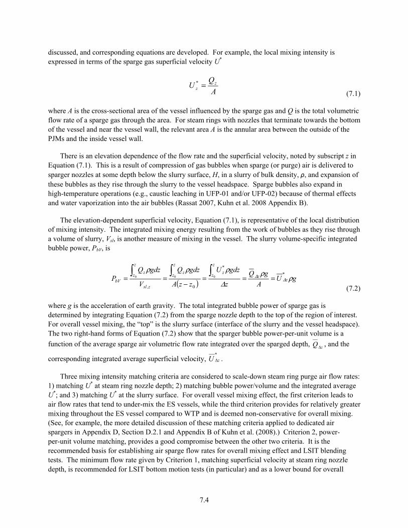
7.4

discussed, and corresponding equations are developed. For example, the local mixing intensity is expressed in terms of the sparge gas superficial velocity U*

A

QU z

z =*

(7.1)

where A is the cross-sectional area of the vessel influenced by the sparge gas and Q is the total volumetric flow rate of a sparge gas through the area. For steam rings with nozzles that terminate towards the bottom of the vessel and near the vessel wall, the relevant area A is the annular area between the outside of the PJMs and the inside vessel wall.

There is an elevation dependence of the flow rate and the superficial velocity, noted by subscript z in Equation (7.1). This is a result of compression of gas bubbles when sparge (or purge) air is delivered to sparger nozzles at some depth below the slurry surface, H, in a slurry of bulk density, ρ, and expansion of these bubbles as they rise through the slurry to the vessel headspace. Sparge bubbles also expand in high-temperature operations (e.g., caustic leaching in UFP-01 and/or UFP-02) because of thermal effects and water vaporization into the air bubbles (Rassat 2007, Kuhn et al. 2008 Appendix B).

The elevation-dependent superficial velocity, Equation (7.1), is representative of the local distribution of mixing intensity. The integrated mixing energy resulting from the work of bubbles as they rise through a volume of slurry, Vsl, is another measure of mixing in the vessel. The slurry volume-specific integrated bubble power, PbV, is

( ) gU

A

gQ

z

gdzU

zzA

gdzQ

V

gdzQP

*z

z

z

z

*z

z

zz

z,sl

z

zz

bV ρρΔ

ρρρΔ

Δ ===−

==

000

0 (7.2)

where g is the acceleration of earth gravity. The total integrated bubble power of sparge gas is determined by integrating Equation (7.2) from the sparge nozzle depth to the top of the region of interest. For overall vessel mixing, the “top” is the slurry surface (interface of the slurry and the vessel headspace). The two right-hand forms of Equation (7.2) show that the sparger bubble power-per-unit volume is a

function of the average sparge air volumetric flow rate integrated over the sparged depth, zQΔ , and the

corresponding integrated average superficial velocity, *

zU Δ .

Three mixing intensity matching criteria are considered to scale-down steam ring purge air flow rates: 1) matching U* at steam ring nozzle depth; 2) matching bubble power/volume and the integrated average U*; and 3) matching U* at the slurry surface. For overall vessel mixing effect, the first criterion leads to air flow rates that tend to under-mix the ES vessels, while the third criterion provides for relatively greater mixing throughout the ES vessel compared to WTP and is deemed non-conservative for overall mixing. (See, for example, the more detailed discussion of these matching criteria applied to dedicated air spargers in Appendix D, Section D.2.1 and Appendix B of Kuhn et al. (2008).) Criterion 2, power-per-unit volume matching, provides a good compromise between the other two criteria. It is the recommended basis for establishing air sparge flow rates for overall mixing effect and LSIT blending tests. The minimum flow rate given by Criterion 1, matching superficial velocity at steam ring nozzle depth, is recommended for LSIT bottom motion tests (in particular) and as a lower bound for overall

7.5

mixing tests. The air flow rates for all three mixing intensity bases scale roughly as 1/S2, where S is the linear geometric scale factor (i.e., S = length in WTP/length in ES = LWTP/LES).

7.2.2 Recommendations for Steam Ring Purge Air Flow Rates in LSIT

Steam ring sparge nozzles located a minimum of 36 in. above the bottom head in the WTP UFP-01 vessels are expected to have little direct impact on scouring or disturbing settled solids layers, even though the calculated design basis nozzle velocities are high (Section 7.1). However, to be conservative, steam ring air sparger operating conditions for bottom motion studies in LSIT vessels should be selected so that the local mixing effect and nozzle velocities in the bottom region of the vessel are not greater than in the WTP vessels. For blending studies, the goal should be to provide comparable purge air-induced overall vessel mixing, from the steam ring nozzles located toward the bottom of the vessel to the slurry surface. These specific steam ring purge air flow rate recommendations are discussed below, following a summary of scaling assumptions.

7.2.2.1 Assumptions for LSIT ES Vessel Steam Ring Scaling and Test Conditions

Below, equations are provided to calculate the steam ring purge air flow rates for a range of operating conditions (e.g., varying slurry fill level and density) in the WTP and LSIT (ES) vessels, subject to the following simplifying assumptions:

• Vessels, components (e.g., PJM bodies), and steam ring locations (e.g., steam/air nozzle elevations) are geometrically scaled.

• Steam ring purge air mixing affects (primarily) the vessel cross-sectional area between the outside of the PJM bodies and the inside vessel wall. Because the vessel diameter, D, scales with the geometric scale factor S (=DWTP/DES) and other vessel components (are assumed to) scale geometrically, the sparge area affected scales as S2 (= AWTP/AES).

• The dimensionless slurry fill level, Hsl/D, is constant with vessel scale. Because the vessel diameter scales as S, the slurry fill height (or depth) measured from the tank bottom at center, Hsl, also scales as S (= Hsl,WTP/Hsl,ES).

The previous three bullets imply that the volume of slurry affected by steam ring purge air, V, nominally the volume in cross-section A from nozzle depth to the slurry surface (H), scales as S3 (= VWTP/VES = AWTPHWTP/AESHES).

• The bulk density of slurry, ρ, is the same in the WTP and the LSIT ES vessels.

• The total standard air flow rate, Qstd, to the WTP UFP-01 steam rings is constant, independent of slurry fill level and density (i.e., 132 scfm at 1 atm and 25°C, as summarized in Section 7.1).

7.6

• The standard state reference conditions used to define Qstd are a gas temperature of Tstd = 25°C and ambient, atmospheric pressure Pstd = Pa = 1.0 atm. The vapor headspace above the slurry of the WTP and LSIT vessels is also assumed to be at these standard conditions.1

• Changes in sparge gas volume due to water vapor enhancement and thermal contraction or expansion are neglected (i.e., the water vapor pressure is assumed to be negligible and isothermal operation near ambient temperature is assumed).

• The previous bullet is consistent with the assumption that steam ring heating will not be used or tested in the LSIT program.

Subject to these assumptions, the steam ring purge air flow rates for bottom motion and blending studies in the ES UFP-01 vessels are calculated as follows.

7.2.2.2 Specific Recommendations for Steam Ring Air Flow Rates in Bottom Motion Studies: Matching U* at Nozzle Depth

Approaches for determining steam ring purge air and dedicated air sparger flow rates to provide a representative environment for bottom motion testing resulting from PJM operations can be grouped in two categories: 1) those seeking to provide a comparable local mixing intensity, or magnitude of bubble shearing effect, in the bottom region of the vessel; and 2) those attempting to shear the same fractional volume of the bottom contents through sparger bubble motion, irrespective of the intensity (e.g., bubble power). Both approaches are discussed in Appendix D for the dedicated air spargers that are located ~6 in. from the bottom head in WTP non-Newtonian slurry process vessels: approach 1) is recommended to determine nominal (higher) flow rates, and approach 2) is recommended to establish the lower-bound flow rates for bottom motion studies in vessels having dedicated air spargers. However, the steam ring sparge nozzles are >36 in. from the bottom head in WTP UFP-01 (and WTP UFP-02), and it is more unlikely that bottom motion of solids will result from air flow through the steam rings, even at the higher nominal flow rate conditions.

Therefore, the following steam ring purge air flow rates are recommended for bottom motion tests in LSIT ES UFP-01 vessels:

• At the low end, to help assess whether there is any benefit (e.g., PJM performance enhancement) or degradation due to steam ring purge air operations, the purge air is turned off. (Note that this could result in backflow into the steam ring system and changes in the slurry level in the vessel.)

• Primary Recommendation – At the upper end, nominal steam ring purge air flow rates are based on matching the WTP vessel sparge gas superficial velocity at the steam ring sparger nozzle depth (i.e., matching U* at z = zsr; see below).

1 The WTP vessel (and black cell) temperature is likely to be higher, and the pressure will typically be sub-ambient for ventilation purposes. Also note that in the WTP steam ring air flow rate design basis calculations, a headspace pressure in the WTP vessels equal to the average Hanford atmospheric pressure, 14.35 psia, was assumed (Calculation No. 24590-PTF-M6C-UFP-00023, Rev. A, Bechtel National, Inc., Richland, Washington). Higher temperatures and lower headspace pressure (e.g., <1.0 atm) result in increased actual volumetric air flow rates to the nozzles.

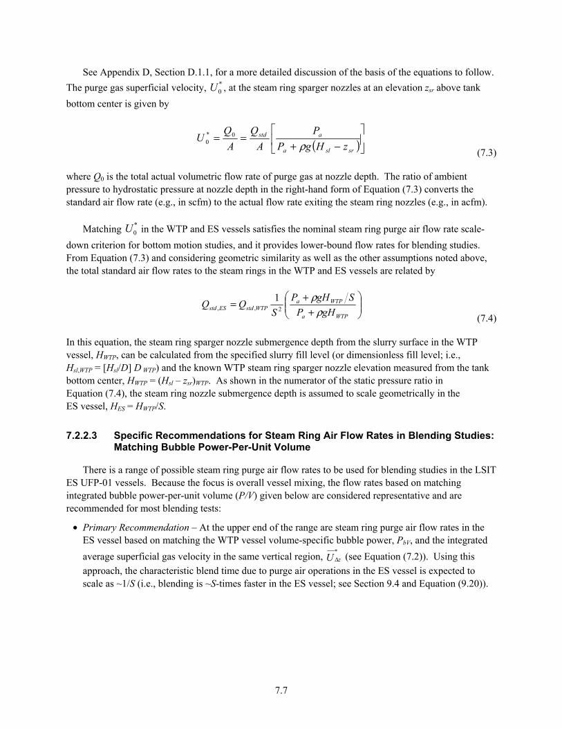
7.7

See Appendix D, Section D.1.1, for a more detailed discussion of the basis of the equations to follow.

The purge gas superficial velocity, *0U , at the steam ring sparger nozzles at an elevation zsr above tank

bottom center is given by

( )

−+

==srsla

astd

zHgP

P

A

Q

A

QU

ρ0*

0

(7.3)

where Q0 is the total actual volumetric flow rate of purge gas at nozzle depth. The ratio of ambient pressure to hydrostatic pressure at nozzle depth in the right-hand form of Equation (7.3) converts the standard air flow rate (e.g., in scfm) to the actual flow rate exiting the steam ring nozzles (e.g., in acfm).

Matching *0U in the WTP and ES vessels satisfies the nominal steam ring purge air flow rate scale-

down criterion for bottom motion studies, and it provides lower-bound flow rates for blending studies. From Equation (7.3) and considering geometric similarity as well as the other assumptions noted above, the total standard air flow rates to the steam rings in the WTP and ES vessels are related by

+

+=

WTPa

WTPaWTPstdESstd gHP

SgHP

SQQ

ρρ

2,,

1

(7.4)

In this equation, the steam ring sparger nozzle submergence depth from the slurry surface in the WTP vessel, HWTP, can be calculated from the specified slurry fill level (or dimensionless fill level; i.e., Hsl,WTP = [Hsl/D] D WTP) and the known WTP steam ring sparger nozzle elevation measured from the tank bottom center, HWTP = (Hsl – zsr)WTP. As shown in the numerator of the static pressure ratio in Equation (7.4), the steam ring nozzle submergence depth is assumed to scale geometrically in the ES vessel, HES = HWTP/S.

7.2.2.3 Specific Recommendations for Steam Ring Air Flow Rates in Blending Studies: Matching Bubble Power-Per-Unit Volume

There is a range of possible steam ring purge air flow rates to be used for blending studies in the LSIT ES UFP-01 vessels. Because the focus is overall vessel mixing, the flow rates based on matching integrated bubble power-per-unit volume (P/V) given below are considered representative and are recommended for most blending tests:

• Primary Recommendation – At the upper end of the range are steam ring purge air flow rates in the ES vessel based on matching the WTP vessel volume-specific bubble power, PbV, and the integrated

average superficial gas velocity in the same vertical region, *

zU Δ (see Equation (7.2)). Using this

approach, the characteristic blend time due to purge air operations in the ES vessel is expected to scale as ~1/S (i.e., blending is ~S-times faster in the ES vessel; see Section 9.4 and Equation (9.20)).

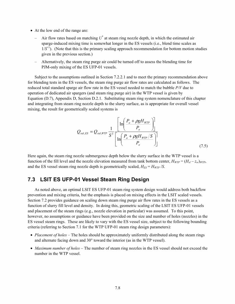
7.8

• At the low end of the range are:

– Air flow rates based on matching U* at steam ring nozzle depth, in which the estimated air sparge-induced mixing time is somewhat longer in the ES vessels (i.e., blend time scales as 1/S<1). (Note that this is the primary scaling approach recommendation for bottom motion studies given in the previous section.)

– Alternatively, the steam ring purge air could be turned off to assess the blending time for PJM-only mixing of the ES UFP-01 vessels.

Subject to the assumptions outlined in Section 7.2.2.1 and to meet the primary recommendation above for blending tests in the ES vessels, the steam ring purge air flow rates are calculated as follows. The reduced total standard sparge air flow rate in the ES vessel needed to match the bubble P/V due to operation of dedicated air spargers (and steam ring purge air) in the WTP vessel is given by Equation (D.7), Appendix D, Section D.2.1. Substituting steam ring system nomenclature of this chapter and integrating from steam ring nozzle depth to the slurry surface, as is appropriate for overall vessel mixing, the result for geometrically scaled systems is

+

+

=

a

WTPa

a

WTPa

WTPstdESstd

P

SgHP

P

gHP

SQQ

ρ

ρ

ln

ln1

3,,

(7.5)

Here again, the steam ring nozzle submergence depth below the slurry surface in the WTP vessel is a function of the fill level and the nozzle elevation measured from tank bottom center, HWTP = (Hsl – zsr)WTP, and the ES vessel steam ring nozzle depth is geometrically scaled, HES = HWTP /S.

7.3 LSIT ES UFP-01 Vessel Steam Ring Design

As noted above, an optimal LSIT ES UFP-01 steam ring system design would address both backflow prevention and mixing criteria, but the emphasis is placed on mixing effects in the LSIT scaled vessels. Section 7.2 provides guidance on scaling down steam ring purge air flow rates in the ES vessels as a function of slurry fill level and density. In doing this, geometric scaling of the LSIT ES UFP-01 vessels and placement of the steam rings (e.g., nozzle elevation in particular) was assumed. To this point, however, no assumptions or guidance have been provided on the size and number of holes (nozzles) in the ES vessel steam rings. These are likely to vary with the ES vessel size, subject to the following bounding criteria (referring to Section 7.1 for the WTP UFP-01 steam ring design parameters):

• Placement of holes – The holes should be approximately uniformly distributed along the steam rings and alternate facing down and 30° toward the interior (as in the WTP vessel).

• Maximum number of holes – The number of steam ring nozzles in the ES vessel should not exceed the number in the WTP vessel.

7.9

• Minimum number of holes – In keeping with a recommendation for an ES UFP-02 vessel that the number of dedicated air spargers having nozzles located near the bottom of the vessel be an integer multiple of the number of outer PJMs to maintain symmetry (Appendix B of Kuhn et al. 2008), the minimum number of steam ring nozzles in the ES UFP-01 vessel is 16 (=8•2). There are eight PJMs in WTP UFP-01 (two groups of four interspersed PJMs),1 and both types of steam ring nozzles (downward and 30° interior facing) are assumed to be included per PJM.

• Maximum size of holes – The maximum diameter of nozzles in the ES UFP-01 steam rings is the design, plant-startup diameter of nozzles in the WTP vessel steam rings.

• Minimum size of holes – The minimum nozzle size may be a practical limitation based on plugging considerations (e.g., greater than the maximum expected slurry particle size) and/or machining capability.

• Maximum nozzle velocity – The maximum average design steam ring nozzle velocity in the ES vessel should not exceed the design basis average nozzle velocity in the WTP vessel.

• Minimum nozzle velocity – The minimum average design steam ring nozzle velocity in the ES vessel should be scaled down from the design basis average nozzle velocity in the WTP vessel based on the relative static pressure at nozzle submergence depth (as discussed near the end of this section).

It is recommended that all these criteria be met in design of the ES vessel steam rings.

Preventing backflow of slurry into the orifices of the steam ring using purge air is a function of the air velocity through the holes (i.e., nozzles). Assuming the steam rings are placed horizontally in the slurry at a fixed elevation within the WTP and ES UFP-01 vessels and the hydrostatic pressure is equal at each of the nnoz (nearly) symmetrically distributed and uniformly sized circular orifices,2 the effective average nozzle velocity unoz is given by

4200

noznoznoznoznoz Dn

Q

An

Qu

π==

(7.6)

In this equation, Q0 is (as defined above) the total actual flow rate of air delivered to the submerged steam ring and flowing through all nozzles, and Anoz is the cross-section of each orifice, which is also represented in terms of its diameter Dnoz.

Equations (7.4) and (7.5) in Section 7.2, for example, show that the standard steam ring purge air flow rate in ES vessels is a function of slurry fill level and density. For the purpose of designing the ES vessel steam ring nozzles (number and size), the following WTP vessel design basis parameters from

1 See, for example, UFP-VSL-00001B Drawing No. 24590-PTF-MV-UFP-00002, Rev. 2, Bechtel National, Inc., Richland, Washington. 2 WTP UFP-01 steam ring design information is provided in Section 7.1. It is assumed here that the elevations of the steam ring nozzles that alternate between facing vertically down and 30° toward the vessel interior are effectively the same (i.e., to a very close approximation, both are given by the elevation of the downward facing nozzles).

7.10

Section 7.1 should be applied in calculations where practical, or otherwise be used for guidance: 1.46 Hsl/D slurry fill level; 1.5 specific gravity slurry (ρ = 1500 kg/m3), Qstd,WTP = 132 scfm; 140 steam ring holes (maximum); 1/8-in.-diameter steam ring nozzles (maximum); and ~96 ft/s (maximum) steam ring nozzle velocity.1

For example, using these slurry fill level and density and air flow rate parameters in Equation (7.4) gives the standard air flow rate in an ES vessel that is needed to match the superficial gas velocity at steam ring nozzle depth in the WTP and ES vessels (e.g., Qstd,ES = 15.0 scfm in an 8-ft-diameter vessel, in which S = DWTP/DES = 20-ft/8-ft = 2.5)2. In turn, the actual flow rate at nozzle depth in the ES vessel (e.g., 10.9 acfm at 25°C3) is determined from the following form of Equation (7.3)

( )

+

=

−+

=gHP

PQ

zHgP

PQQ

a

astd

srsla

astd ρρ0

(7.7)

Rearranging Equation (7.7) in terms of Qstd and substituting for Qstd,WTP and Qstd,ES in Equation (7.4) gives

2,0,0

1

SQQ WTPES =

(7.8)

Equation (7.8) simply confirms that the actual air flow rate at nozzle depth in the ES vessel scales exactly as 1/S2 when matching superficial velocity at nozzle depth in geometrically scaled vessels (i.e., the vessel cross-section also scales as 1/S2).

The actual ES vessel air flow rate determined in this manner should be used in conjunction with Equation (7.6) to determine the relationship between the number and size of steam ring orifices and the average nozzle velocity under bounding conditions (i.e., maximum slurry fill level and density). Further, to obtain the WTP equivalent nozzle velocity in the ES UFP-01 vessels (i.e., unoz,WTP = unoz,ES = constant),

1 For the 1.0 atm (14.696 psia) headspace pressure assumed here, the calculated nozzle velocity in the WTP UFP-01 vessel is reduced from the design value of 96.3 ft/s to 95.1 ft/s. This is due to an increase in the static pressure from the design basis value of 28.117 psia at 14.35 psia headspace pressure (Calculation No. 24590-PTF-M6C-UFP-00023, Rev. A, Bechtel National, Inc., Richland, Washington) to 28.463 psia at 1.0 atm headspace pressure (= 28.117 psia + [14.696 psia – 14.35 psia]). Both the air volumetric flow rate at nozzle depth and the nozzle velocity scale inversely with the static pressure for a given standard air feed rate (e.g., 95.1 ft/s = 96.3 ft/s [28.117/28.463]). This is seen, for example, in Equations (7.3) and (7.7), where Pa = Pstd = 1.0 atm in the numerator of the pressure ratio of both equations and the denominator is the static pressure at nozzle depth, which varies with headspace pressure (e.g., Pa < 1.0 atm in the denominator for the original WTP design basis calculations). 2 Subject to the assumptions in Section 7.2.2.1 and using WTP design basis parameters from Section 7.1 in Equation (7.4), Qstd,ES = 15.0 scfm = 132.5 scfm/(2.5)2•[1.01325•105 Pa + (1500 kg/m3)(9.807m/s2)(6.45 m)/2.5]/ [1.01325•105 Pa + (1500 kg/m3)(9.807m/s2)(6.45 m)], where the slurry depth to the steam ring nozzles in WTP is HWTP = Hsl – zsr = 29.17 ft – 8 ft = 21.17 ft = 6.45 m and S = 2.5 in an 8-ft-diameter ES UFP-01 vessel. 3 Using Equation (7.7), Q0,ES = 10.9 scfm = 15.0 scfm•1.01325•105 Pa /[1.01325•105 Pa + (1500 kg/m3)(9.807m/s2)(6.45 m)/2.5], where the slurry depth to the steam ring nozzles in WTP is HWTP = Hsl - zsr = 29.17 ft – 8 ft = 21.17 ft = 6.45 m, HES = HWTP/S, and S = 2.5 in an 8-ft-diameter ES UFP-01 vessel.

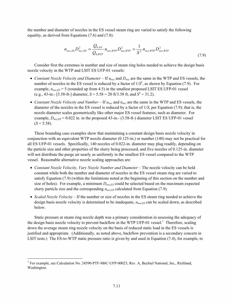
7.11

the number and diameter of nozzles in the ES vessel steam ring are varied to satisfy the following equality, as derived from Equations (7.6) and (7.8):

2,,2

2,,

,0

,02,,

1WTPnozWTPnozWTPnozWTPnoz

WTP

ESESnozESnoz Dn

SDn

Q

QDn ==

(7.9)

Consider first the extremes in number and size of steam ring holes needed to achieve the design basis nozzle velocity in the WTP and LSIT ES UFP-01 vessels:

• Constant Nozzle Velocity and Diameter – If unoz and Dnoz are the same in the WTP and ES vessels, the number of nozzles in the ES vessel is reduced by a factor of 1/S2, as shown by Equation (7.9). For example, nnoz,ES = 5 (rounded up from 4.5) in the smallest proposed LSIT ES UFP-01 vessel (e.g., 43-in.- [3.58-ft-] diameter, S = 5.58 = 20 ft/3.58 ft, and S2 = 31.2).

• Constant Nozzle Velocity and Number – If unoz and nnoz are the same in the WTP and ES vessels, the diameter of the nozzles in the ES vessel is reduced by a factor of 1/S, per Equation (7.9); that is, the nozzle diameter scales geometrically like other major ES vessel features, such as diameter. For example, Dnoz,ES = 0.022 in. in the proposed 43-in.- (3.58-ft-) diameter LSIT ES UFP-01 vessel (S = 5.58).

These bounding case examples show that maintaining a constant design basis nozzle velocity in conjunction with an equivalent WTP nozzle diameter (0.125-in.) or number (140) may not be practical for all ES UFP-01 vessels. Specifically, 140 nozzles of 0.022-in. diameter may plug readily, depending on the particle size and other properties of the slurry being processed, and five nozzles of 0.125-in. diameter will not distribute the purge air nearly as uniformly in the smallest ES vessel compared to the WTP vessel. Reasonable alternative nozzle scaling approaches are:

• Constant Nozzle Velocity, Vary Nozzle Number and Diameter – The nozzle velocity can be held constant while both the number and diameter of nozzles in the ES vessel steam ring are varied to satisfy Equation (7.9) (within the limitations noted at the beginning of this section on the number and size of holes). For example, a minimum Dnoz,ES could be selected based on the maximum expected slurry particle size and the corresponding nnoz,ES calculated from Equation (7.9).

• Scaled Nozzle Velocity – If the number or size of nozzles in the ES steam ring needed to achieve the design basis nozzle velocity is determined to be inadequate, unoz,ES can be scaled down, as described below.

Static pressure at steam ring nozzle depth was a primary consideration in assessing the adequacy of the design basis nozzle velocity to prevent backflow in the WTP UFP-01 vessel.1 Therefore, scaling down the average steam ring nozzle velocity on the basis of reduced static load in the ES vessels is justified and appropriate. (Additionally, as noted above, backflow prevention is a secondary concern in LSIT tests.) The ES-to-WTP static pressure ratio is given by and used in Equation (7.4), for example, to

1 For example, see Calculation No. 24590-PTF-M6C-UFP-00023, Rev. A, Bechtel National, Inc., Richland, Washington.

7.12

relate actual flow rates at nozzle depth in the WTP and ES vessels. Assuming that the average nozzle velocity is scaled down linearly with this pressure ratio gives

WTPnoz

WTPa

WTPaESnoz u

gHP

SgHPu ,,

+

+=

ρρ

(7.10)

Note that while the static pressure ratio is a function of S, the functionality is not linear due to the additive ambient (headspace) pressure contribution to the total static pressure at depth in the slurry. In conjunction with the reduced unoz,ES value from Equation (7.10) and Q0,ES determined from Equation (7.8)1 for the WTP design basis conditions, the number and diameter of steam ring nozzles in the ES vessel are determined to satisfy Equation (7.6).

It should be re-emphasized that the LSIT ES vessel purge air flow rates computed in this section in pursuit of defining the number and size of steam ring nozzles are based on limiting WTP design basis parameters. The standard (and actual) purge air flow rate to the steam rings in LSIT ES vessels will vary with slurry fill level and density, which will typically be less than the design basis values in normal operations. The LSIT ES test air flow rates should be determined following the recommendations of Section 7.2.2.

1 Or, as described above, using the combination of Equations (7.4) and (7.7) instead of Equation (7.8).

8.1

8.0 Observing Critical Suspension Velocity, UCS, and Bottom Motion

This chapter addresses the protocols to be used to observe the critical suspension velocity, UCS, and bottom motion as measured by bottom clearing. This chapter is included to assure consistent understanding of these critical metrics across the test platforms, testing teams, and contractors.

8.1 Protocols for Observing UCS

These protocols for observing UCS were extracted from Meyer et al. (2009) and were used to determine the flow conditions during the M3 Phase 1 tests described in that report. All observations were recorded when the measured flow and the particle motion in the tank appeared to have reached steady state and when no observable change in solids behavior (e.g., transient behavior in cloud height) was detected over the observation period.

The pattern of cleared region observed from beneath the tank at the end of the pulse was described using the three-character nomenclature (two letters followed by a numeral) shown in Table 8.1. Testing started by operating the PJMs at a fixed velocity until the test tank stabilized at which point the observer evaluated and documented the pattern of clearing using Table 8.1 as a guide. The velocity was then increased until BP6 or UCS conditions were observed. When condition BP6 (the UCS velocity) was achieved, the observer documented the UCS velocity. The settled solids may or may not have been moving.

Steady state for pulsed flow, cyclic steady state (a true periodic condition), was considered to exist when, for a period of five pulses, the charted instantaneous velocity, U(t), yielded a visually observed peak average velocity, UPA, which appeared to remain constant to within ±5 percent (see Figure 8.1). UPA was obtained by visually monitoring a data acquisition system (DAS) velocity chart screen that was configured to display the range of target UPA to ±5 percent.

Steady state for steady flow conditions was said to exist when the steady jet velocity, US, was constant to within ±5 percent over 2 minutes. US was a running time average of the instantaneous velocity, U(t), taken over a time interval sufficient to smooth out noise in the velocity signal. US was calculated by the DAS.

The time required to reach steady state may depend on settling velocity of the simulant and concentration. Thus, observers needed to be cognizant of slow transients occurring in the mobilization of the solids.

The method used to monitor solids suspension was visual observation at the end of the pulse. Optional use of an ultrasonic Doppler velocimeter to supplement the observation is acceptable. Particle motion is either observed visually through a transparent tank bottom or through an observation window in the center of the bottom of the tank. Table 8.2 lists a scale of observations relative to the condition of visually determined UCS. The critical outcome of these tests is to determine UCS, which is the velocity at which the transition to/from the state of complete solids suspension occurred for incremental increases/decreases in nozzle discharge velocity. After the initial Phase 1 tests, the center of the tank was selected as a readily scalable location to monitor the solids mobilization and likely would be the last

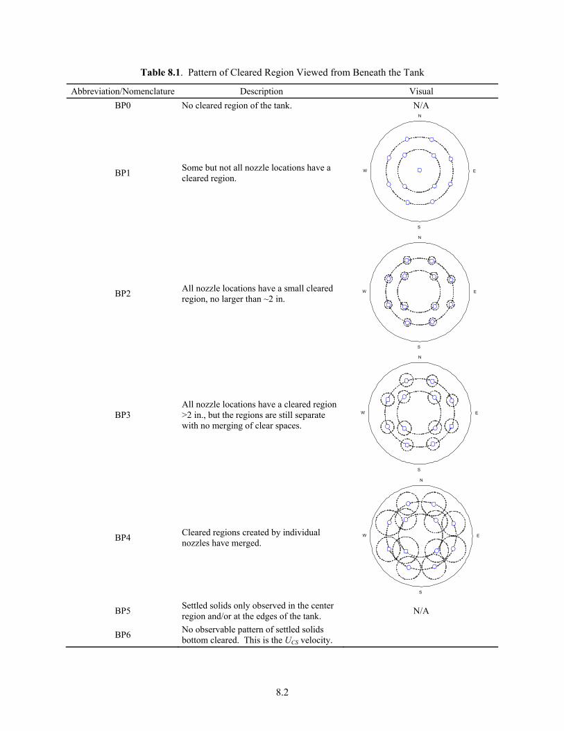
8.2

Table 8.1. Pattern of Cleared Region Viewed from Beneath the Tank

Abbreviation/Nomenclature Description Visual

BP0 No cleared region of the tank. N/A

BP1 Some but not all nozzle locations have a cleared region.

N

E

S

W

BP2 All nozzle locations have a small cleared region, no larger than ~2 in.

N

E

S

W

BP3 All nozzle locations have a cleared region >2 in., but the regions are still separate with no merging of clear spaces.

N

E

S

W

BP4 Cleared regions created by individual nozzles have merged.

N

E

S

W

BP5 Settled solids only observed in the center region and/or at the edges of the tank.

N/A

BP6 No observable pattern of settled solids bottom cleared. This is the UCS velocity.

8.3

-2.0

0.0

2.0

4.0

6.0

8.0

10.0

12.0

14.0

10 15 20 25 30 35 40

Elasped Time (s)

Noz

zle

Vel

ocity

(m

/s)

X

UPA

UPA ±5%

tC

tD

Figure 8.1. Illustration of Nozzle Velocity as a Function of Time for Several Discharge Cycles. X, the set point used by the DAS, is a threshold velocity for distinguishing assumed zero flow from the pulse flow. A pulse or discharge is the portion of the cycle for which the velocity (calculated from the mass flow rate signal) is greater than X. tD is the discharge or pulse time. For this example, assume target UPA =12.1 m/s over the observation period.

Table 8.2. Particle Motion Descriptors for Visual Observations

Number Meaning Description

1 Below critical suspension velocity <UCS Solids may be moving or partly suspended; regions of settled particles are apparent (settled particles may be moving).

2 Critical suspension, UCS at tank center Initial state of complete solids suspension (all moving from the bottom) occurs with the last solids clearing at the center of the tank. This behavior may not be observed for all combinations of simulants and geometries/tube arrays.

3 Overall critical suspension(a) Initial state of complete solids suspension (all moving from the bottom) occurs over the entire tank. For pulsing jets, this is defined as all particles moving at the end of a pulse. For steady jets, any settling particles appear to lift off the bottom within 2 s of touching down. By definition, this behavior exists only at a single velocity for a given set of operating, geometry, and physical conditions (not at multiple velocities for the same test conditions).

4 Beyond critical suspension velocity >UCS Discharge velocity is greater than UCS. For pulsing jets, particles are fully suspended before the end of the pulse.

(a) In the large scale systems used for the M3 tests, overall UCS (condition 3) was not visually observable due to the steel heads (viewing ports only allow observation of the particulate at the bottom center).

8.4

location from which solids were mobilized.1 Therefore, visual UCS observations distinguished between conditions for which the final solids mobilization occurred at the tank center instead of conditions for which the final solids mobilization occurred at some other location in the tank. For the M3 test program, the desire was to identify/determine metrics that could be used to evaluate trends over geometric scales. Without identifying the best metrics before testing, a decision was made to monitor both the occurrence of a condition at a specific location and a defined condition regardless of location.

For the WTP test distributed-array vessel configurations tested during M3 Phase 1 (e.g., HLP-22 and RLD-08), the center of the vessel was usually the last location from which the solids became mobilized. However, for other configurations evaluated to investigate the effects of pulse tube location, such as a four-tube configuration that consisted of only the inner ring of HLP-22 pulse tubes, the center region was not the last to mobilize. To accommodate the potential of having to monitor UCS other than at tank center, observation conditions 2 and 3 were defined as shown in Table 8.2.

Condition 2 was noted by the test observers for a discharge velocity if the UCS condition at the tank center was satisfied but solids elsewhere on the tank bottom were not fully suspended at the end of a pulse. This condition was never observed for the WTP configurations tested. This condition also could not be monitored in the 70-in.-diameter vessel because of the limited viewing port on the tank bottom. Therefore, testing in the 70-in.-diameter system was performed only for those configurations and conditions that yielded the location of final solids mobilization at the tank center. These conditions were later tested in the 15-in.-diameter system to confirm that final solids mobilization occurred at the tank center. It was assumed, based on these results that final mobilization occurred at the tank center for the conditions tested in the 70-in. vessel.

8.2 Definition of Bottom Motion

Bottom motion and bottom clearing are WTP-developed metrics used during M3 Phase 2 testing. In Plan for M3 Test Platform Testing (24590-PTF-PL-PET-10-0001, Rev. 0, Barnes 2010), the definition of bottom clearing is given as

Bottom clearing: The mixing condition for which all particles in an area of interest are suspended off-bottom for some period of the PJM cycle.

This definition was specifically developed to replace previous requirements for bottom movement and off-bottom suspension. It is used as a mixing test success requirement where it is stated that, “The PJM mixing system must demonstrate that the entire vessel bottom can be cleared at all vessel operating levels for the normal PJM firing mode(s). This can be done by firing all PJMs and clearing the complete bottom at one time or by sequential firing of the PJMs to clear portions of the bottom, resulting in the total bottom area having been cleared once all PJMs have been fired in one sequential cycle. The normal PJM firing mode will be established as a baseline operating condition of the PJM mixed vessel.”

1 For the Newtonian tank arrays, early testing needs to confirm that the center of the vessel head is the last location from which solids were mobilized.

8.5

The following guidelines are provided for the purpose of clarifying the definition of bottom clearing from the reference in the test vessel.

1. The “area of interest” is an arbitrarily small region that can be observed by a single viewer, even when the objective is to demonstrate complete bottom clearing. The focus of the observer should be on any areas that may remain covered by a bed of moving or stationary particles for the entire PJM campaign. If at any time during the PJM campaign, the given area appears to have off-bottom suspended particles, then bottom clearing can be declared for that area.

2. Complete bottom clearing is NOT achieved if there are any patches of stationary settled solids that are not mobilized by the PJMs.

3. Bottom clearing is only credited to the PJM jet (i.e., the sliding of settled solids patches down the steep sections of the bottom by gravity after the PJM drive phase has ended is not evidence that those portions of the bottom have been cleared).

4. Bottom clearing does NOT require off-bottom suspension1 of all particles simultaneously or even that all particles in the tank be suspended during each PJM drive. Specifically, particles trapped in the eddies of colliding jets that move with the eddies are considered suspended, and the existence of such trapped particles does not preclude total bottom clearing. For simulants containing a significant number of sub-micron particles that make visual identification of bottom clearing difficult in areas, the apparent bulk motion of simulant in an area may be taken to be evidence of bottom clearing in that area.

5. Small regions of settled solids on the bottom that are intermittently cleared and not cleared during successive PJM campaigns do not preclude a declaration of complete bottom clearing. Any such settled solids must be cleared at least every third PJM pulse.

1 Bottom clearing is assumed to be tested for a full vessel. During the pump-out process, as the volume of slurry left in the vessel decreases, it is expected that PJM nozzle velocities will increase. The no solids accumulation tests will be needed to confirm that solids are adequately mobilized to be removed during the total pump-out process.

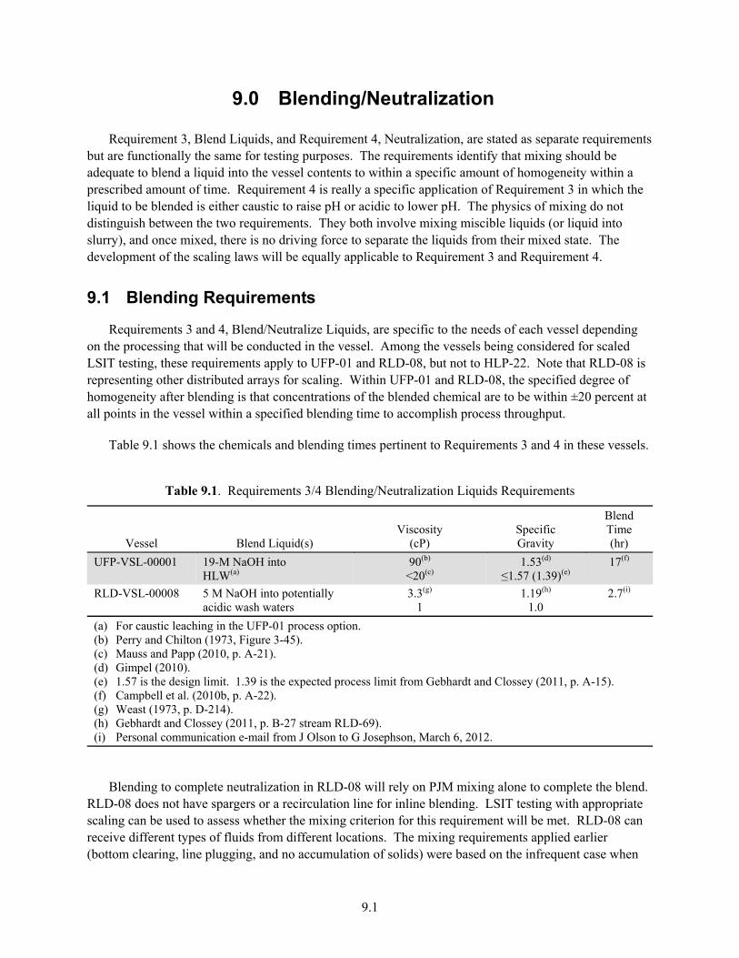
9.1

9.0 Blending/Neutralization

Requirement 3, Blend Liquids, and Requirement 4, Neutralization, are stated as separate requirements but are functionally the same for testing purposes. The requirements identify that mixing should be adequate to blend a liquid into the vessel contents to within a specific amount of homogeneity within a prescribed amount of time. Requirement 4 is really a specific application of Requirement 3 in which the liquid to be blended is either caustic to raise pH or acidic to lower pH. The physics of mixing do not distinguish between the two requirements. They both involve mixing miscible liquids (or liquid into slurry), and once mixed, there is no driving force to separate the liquids from their mixed state. The development of the scaling laws will be equally applicable to Requirement 3 and Requirement 4.

9.1 Blending Requirements

Requirements 3 and 4, Blend/Neutralize Liquids, are specific to the needs of each vessel depending on the processing that will be conducted in the vessel. Among the vessels being considered for scaled LSIT testing, these requirements apply to UFP-01 and RLD-08, but not to HLP-22. Note that RLD-08 is representing other distributed arrays for scaling. Within UFP-01 and RLD-08, the specified degree of homogeneity after blending is that concentrations of the blended chemical are to be within ±20 percent at all points in the vessel within a specified blending time to accomplish process throughput.

Table 9.1 shows the chemicals and blending times pertinent to Requirements 3 and 4 in these vessels.

Table 9.1. Requirements 3/4 Blending/Neutralization Liquids Requirements

Vessel Blend Liquid(s) Viscosity

(cP) Specific Gravity

Blend Time (hr)

UFP-VSL-00001 19-M NaOH into HLW(a)

90(b) <20(c)

1.53(d) ≤1.57 (1.39)(e)

17(f)

RLD-VSL-00008 5 M NaOH into potentially acidic wash waters

3.3(g) 1

1.19(h) 1.0

2.7(i)

(a) For caustic leaching in the UFP-01 process option. (b) Perry and Chilton (1973, Figure 3-45). (c) Mauss and Papp (2010, p. A-21). (d) Gimpel (2010). (e) 1.57 is the design limit. 1.39 is the expected process limit from Gebhardt and Clossey (2011, p. A-15). (f) Campbell et al. (2010b, p. A-22). (g) Weast (1973, p. D-214). (h) Gebhardt and Clossey (2011, p. B-27 stream RLD-69). (i) Personal communication e-mail from J Olson to G Josephson, March 6, 2012.

Blending to complete neutralization in RLD-08 will rely on PJM mixing alone to complete the blend. RLD-08 does not have spargers or a recirculation line for inline blending. LSIT testing with appropriate scaling can be used to assess whether the mixing criterion for this requirement will be met. RLD-08 can receive different types of fluids from different locations. The mixing requirements applied earlier (bottom clearing, line plugging, and no accumulation of solids) were based on the infrequent case when

9.2

solids from the HLW melter feed vessel were diverted to RLD-08. This was the “worst case” condition for these mixing requirements. The condition requiring blending in RLD-08 is to transfer contents back to the pretreatment area if the contents of the vessel are below the pH target. HLW melter feed is above pH 12 so this mixing requirement would not be applied if the vessel contains up to 6 wt% solids slurry as applied for the previous requirements. The contents of RLD-08 that might require neutralization would come from other vessels that are not expected to contain suspended solids. For the blending liquids requirement, the tank contents are most similar to water to which 5 M sodium hydroxide (NaOH) will be blended to reach a target pH ≥12.

LSIT testing can determine the proper scaling of blending times that would apply to using only in-tank mixing at full scale. If the determined blend times did not meet targets, LSIT testing could also incorporate inline blending, but the scaling approach described below and the mechanisms described could not be applied. It is expected that where inline mixing is applied, in-tank mixing would not be needed to meet blending requirements and a rigorous technical basis for scaling blend times would be moot.

9.2 Approach for Newtonian Vessels

The liquid to be blended in a Newtonian vessel may be introduced either in the transfer line or into the vessel through an elevated port. It is assumed for this analysis that the two fluids begin as separate layers with the liquid with density ρ1 introduced on top of solid-liquid slurry with a mixture density of ρmix at the beginning of the PJM transient. If the liquid has a lower density than the slurry, the layers remain stratified.

A series of miscible liquid mixing tests were performed in the small-scale pulsed jet mixer (SS PJM) facility, which consisted of a single pulse jet in a scaled mixing vessel (Johnson et al. 2003). The simulants used in the tests were a 50 wt% solution of sodium thiosulfate pentahydrate (specific gravity ~1.31) and water (specific gravity ~1.0). The time-to-mix results for different pulse jet operating cycles were expressed in terms of P/V or specific energy, which is the ratio of test power per volume to that expected in the full vessel. The theory behind this approach was that the kinetic energy introduced into the vessel through the velocity of the fluid through the pulse jet nozzles is converted into turbulent energy throughout the vessel that results in fluid mixing.

The mixing time for industrial jet mixed vessels is given by the following expression (Paul et al. 2004)1

0 0

22

mix

D d Dt ~ ~

U d U d (9.1)

where D is the vessel diameter, d is the nozzle diameter, and U0 is the nozzle velocity. The ratio inside the parentheses is constant for geometrically similar vessels. This expression has been used extensively in industry in a wide variety of applications.

1 “Handbook of Industrial Mixing,” Section 9-5.1, Equation (9-53) from Fossett and Prosser (1949).

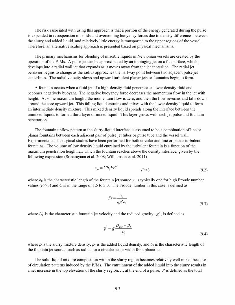
9.3

The risk associated with using this approach is that a portion of the energy generated during the pulse is expended in resuspension of solids and overcoming buoyancy forces due to density differences between the slurry and added liquid, and relatively little energy is transported to the upper regions of the vessel. Therefore, an alternative scaling approach is presented based on physical mechanisms.

The primary mechanisms for blending of miscible liquids in Newtonian vessels are created by the operation of the PJMs. A pulse jet can be approximated by an impinging jet on a flat surface, which develops into a radial wall jet that expands as it moves away from the jet centerline. The radial jet behavior begins to change as the radius approaches the halfway point between two adjacent pulse jet centerlines. The radial velocity slows and upward turbulent planar jets or fountains begin to form.

A fountain occurs when a fluid jet of a high-density fluid penetrates a lower density fluid and becomes negatively buoyant. The negative buoyancy force decreases the momentum flow in the jet with height. At some maximum height, the momentum flow is zero, and then the flow reverses and falls down around the core upward jet. This falling liquid entrains and mixes with the lower density liquid to form an intermediate density mixture. This mixed density liquid spreads along the interface between the unmixed liquids to form a third layer of mixed liquid. This layer grows with each jet pulse and fountain penetration.

The fountain upflow pattern at the slurry-liquid interface is assumed to be a combination of line or planar fountains between each adjacent pair of pulse jet tubes or pulse tube and the vessel wall. Experimental and analytical studies have been performed for both circular and line or planar turbulent fountains. The volume of low density liquid entrained by the turbulent fountain is a function of the maximum penetration height, zm, which the fountain reaches above the density interface, given by the following expression (Srinarayana et al. 2008; Williamson et al. 2011)

zm = Cb0Frn

Fr>3 (9.2)

where b0 is the characteristic length of the fountain jet source, n is typically one for high Froude number values (Fr>3) and C is in the range of 1.5 to 3.0. The Froude number in this case is defined as

Fr = UF

g 'b0 (9.3)

where UF is the characteristic fountain jet velocity and the reduced gravity, 'g , is defined as

' mix l

l

g gρ ρ

ρ−=

(9.4)

where ρ is the slurry mixture density, ρ1 is the added liquid density, and b0 is the characteristic length of the fountain jet source, such as radius for a circular jet or width for a planar jet.

The solid-liquid mixture composition within the slurry region becomes relatively well mixed because of circulation patterns induced by the PJMs. The entrainment of the added liquid into the slurry results in a net increase in the top elevation of the slurry region, za, at the end of a pulse. P is defined as the total

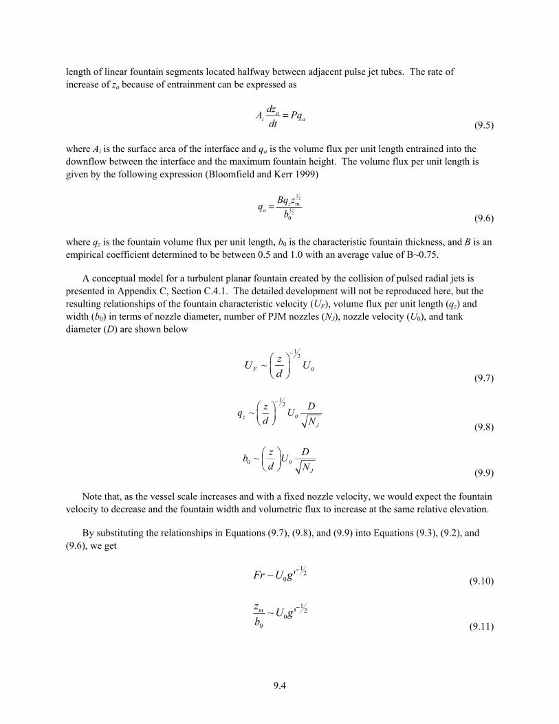
9.4

length of linear fountain segments located halfway between adjacent pulse jet tubes. The rate of increase of za because of entrainment can be expressed as

Ai

dza

dt= Pqa

(9.5)

where Ai is the surface area of the interface and qa is the volume flux per unit length entrained into the downflow between the interface and the maximum fountain height. The volume flux per unit length is given by the following expression (Bloomfield and Kerr 1999)

qa = Bqzzm

12

b0

12

(9.6)

where qz is the fountain volume flux per unit length, b0 is the characteristic fountain thickness, and B is an empirical coefficient determined to be between 0.5 and 1.0 with an average value of B~0.75.

A conceptual model for a turbulent planar fountain created by the collision of pulsed radial jets is

presented in Appendix C, Section C.4.1. The detailed development will not be reproduced here, but the resulting relationships of the fountain characteristic velocity (UF), volume flux per unit length (qz) and width (b0) in terms of nozzle diameter, number of PJM nozzles (NJ), nozzle velocity (U0), and tank diameter (D) are shown below

12

F 0

zU ~ U

d

− (9.7)

12

z 0

J

z Dq ~ U

d N

− (9.8)

0 0

J

z Db ~ U

d N

(9.9)

Note that, as the vessel scale increases and with a fixed nozzle velocity, we would expect the fountain velocity to decrease and the fountain width and volumetric flux to increase at the same relative elevation.

By substituting the relationships in Equations (9.7), (9.8), and (9.9) into Equations (9.3), (9.2), and (9.6), we get

Fr ~ U0g '

−12

(9.10)

zm

b0

~ U0g '−1

2

(9.11)

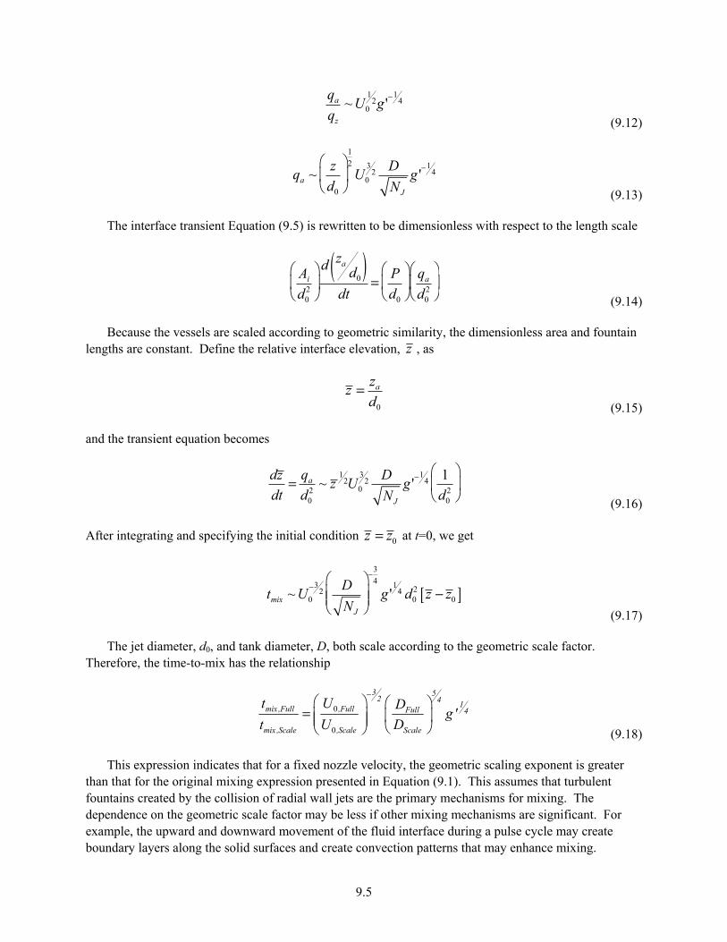
9.5

qa

qz

~ U0

12g '

−14

(9.12)

qa ~z

d0

1

2

U0

32 D

NJ

g '−1

4

(9.13)

The interface transient Equation (9.5) is rewritten to be dimensionless with respect to the length scale

Ai

d02

d zad0

( )dt

= P

d0

qa

d02

(9.14)

Because the vessels are scaled according to geometric similarity, the dimensionless area and fountain lengths are constant. Define the relative interface elevation, z , as

z = za

d0 (9.15)

and the transient equation becomes

dz

dt= qa

d02

~ z1

2U0

32 D

NJ

g '−1

4 1

d02

(9.16)

After integrating and specifying the initial condition z = z0 at t=0, we get

tmix ~ U0

−32 D

NJ

−3

4

g '1

4 d02 z − z0[ ]

(9.17)

The jet diameter, d0, and tank diameter, D, both scale according to the geometric scale factor. Therefore, the time-to-mix has the relationship

0

0

3 52 4

1mix ,Full ,Full Full 4

mix ,Scale ,Scale Scale

t U Dg'

t U D

−

= (9.18)

This expression indicates that for a fixed nozzle velocity, the geometric scaling exponent is greater than that for the original mixing expression presented in Equation (9.1). This assumes that turbulent fountains created by the collision of radial wall jets are the primary mechanisms for mixing. The dependence on the geometric scale factor may be less if other mixing mechanisms are significant. For example, the upward and downward movement of the fluid interface during a pulse cycle may create boundary layers along the solid surfaces and create convection patterns that may enhance mixing.

9.6

The primary difference between this mixing application and typical industrial mixing applications is the combination of turbulent fountains created by pulse jets and the existence of a slurry-liquid interface that tends to concentrate the mixing in a two-dimensional plane.

The recommendation for liquid blending in Newtonian vessels is to measure the time-to-mix relationship at different scales and nozzle velocities to determine the functional relationship in the form

( ) 1

40

n mmixt C S U g'=

(9.19)

using the exponents derived from Equation (9.1) as a starting point.

9.3 Concepts for Testing

The blending requirements are specific to each vessel being tested. Table 9.1 identifies the current requirements for vessel blending that were used as a basis for the test matrix.

Blending/neutralization tests will be performed for the physical properties listed for each of the mixing operations listed in Table 9.1. The use of a chemically based simulant (beyond the use of chemical indicators needed for testing) is not needed for this round of tests.

• Case 1 – 19M NaOH into HLW (UFP-01)

– 90 cP, 1.53 specific density, 17-hr blend time

– 20 cP at 30 Pa, 1.57 specific density, 7-hr blend time

• Case 2 – 5M NaOH into potentially acidic wash waters (RLD-08)

– 1 cP, 1.0 specific density, 2.7-hr blend time

– 3.3 cP, 1.19 specific density, 2.7-hr blend time.

The first priority for complying with performance metrics for blending is to determine the likelihood of compliance when bottom clearing is attained. This can be done by measuring the concentration of soluble tracer species at several locations in a vessel, from which the blend time can be estimated. If suitable blend times are found with a comfortable margin when bottom clearing is attained, additional testing devoted to evaluating blend times will not be necessary.

The procedure described below will apply to each separate test condition (simulant, solids loading, vessel configuration):

• Clean and prepare the test vessel with the PJM array appropriate for the WTP vessel being simulated. Add simulant solids and liquid to achieve the minimum solids concentration to represent the slurry mixture. Gently add the liquid to be mixed on top of the slurry, taking care not to disturb the interface and mix the two types of fluids.

• For non-Newtonian vessels, start air spargers and control volumetric air flow rate to specified conditions.

9.7

• Perform a series of pulse jet duty cycles for a specified maximum PJM nozzle velocity. Record concentration measurements from the different vessel locations as a function of time. Continue until concentrations of the blended chemical are within ±20 percent at all points in the vessel. Record the mixing time.

• Repeat the test for different pulse jet velocities, beginning at 6 m/s and increasing to 11 m/s in 1-m/s increments, and different air sparger flow rates.

9.4 Air Sparger and Steam Ring Purge Air Scaling for Blending

9.4.1 Background – Previous Experimental Studies of Air Spargers

Combined PJM-dedicated air sparger hybrid mixing systems for non-Newtonian slurries have been evaluated experimentally in previous WTP-sponsored studies. These studies included tests in the approximately quarter-scale UFP (ultrafiltration feed process) and HLW lag storage (LS) vessels (Johnson et al. 2005). While this earlier study used air spargers in some testing and demonstrated enhanced mixing performance compared to PJMs alone, PJM configurations and mixing performance were the primary focus, not sparger operations. Bontha et al. (2005) evaluated mixing and flammable gas release in an approximately half-scale LS vessel for a number of WTP plant operating scenarios including normal vessel operations, post-DBEs, and Near Term Accident Response, in which spargers alone (i.e., no PJMs) were operated (intermittently). Mixing time and effectiveness were assessed using dye and chemical tracers in a clay/water slurry simulant. In normal operations using both PJMs and spargers, blending times of ~5 to ~9 hr were reported, depending on whether tracer was added near the tank bottom or on the slurry surface, respectively. For the fraction of slurry mixed when only spargers were operated (e.g., ~63 vol% at a fill level of ~0.81 Hsl /D), the 95 percent mixing time ranged from 5 to 28 hr.

Bontha et al. (2005) noted that the sparging system used in the half-scale LS (e.g., HLP-27) tests was designed according to the scaling principles outlined in Poloski et al. (2005). The sparger system consisted of seven spargers distributed around the PJM cluster (eight PJMs total; seven around, one central). This is consistent with guidance that the number of deep annular spargers should minimally be a multiple of the number of outer PJMs and that the spargers should be located symmetrically about the PJMs (e.g., Appendix B of Kuhn et al. (2008); Appendix D of this report). According to Bontha et al. (2005), BNI provided air sparger flow rate guidance to attain the “… approximate equivalent of the (flow) rate at the surface of the slurry in the WTP LS vessel” (i.e., a superficial velocity matching criteria).

Air sparger scaling in a 1/4.5-scale UFP-02 vessel for Pretreatment Engineering Platform (PEP) testing was based on matching the WTP vessel bubble power-per-unit volume and the integrated average superficial gas velocity (Equation (7.2)) (Kuhn et al. 2008). The PEP tests evaluated pretreatment processes such as caustic leaching and did not specifically assess the impact of spargers on mixing performance.

Like the work of Bontha et al. (2005), the dedicated air sparger scaling approach described in Kuhn et al. (2008) was derived significantly from the sparger-only testing of Poloski et al. (2005). As noted in Appendix D, the sparger regions of bubbles (ROB) and ZOI diameter correlations (Equations (D.6a) and (D.6b)) developed by Poloski et al. (2005) are the basis of design for dedicated air spargers in the WTP

9.8

non-Newtonian process vessels. Rising bubbles in ROBs entrain slurry, resulting in a net upward movement of slurry, while ZOIs define regions for slurry to return to depth completing a recirculation pathway.

Poloski et al. (2005) also conducted sparger-only circulation time studies using dye and chemical (salt) tracers. For example, Table 9.2 summarizes their results for a single air sparger submerged 117 in. (2.97 m) in a clay/water simulant of bounding rheology (i.e., nominally 30 Pa yield stress and 30 cP consistency using the Bingham plastic model). The air flow rates used in the tests, 15 and 40 acfm at sparger nozzle depth, are comparable to the per sparge tube flow rates specified for the WTP HLP-27 and UFP-02 non-Newtonian process vessels, which range from 6 to 35 acfm (Claghorn and Waddell 2007; Appendix D of this report). Therefore, the tests were full scale in terms of flow rate and approximately half scale in terms of slurry depth, depending on actual slurry fill level in the WTP vessels.

Table 9.2. Experimental and Calculated Circulation Times and Velocities for a Single Air Sparger

Experimentally Measured/Estimated(a) Calculated(b)

Sparger Flow Rate(c) 15 acfm 40 acfm 15 acfm 40 acfm

Circulation Segment(d)

Circulation Time (Est. Velocity)

Circulation Time (Est. Velocity)

Minimum Average Minimum Average Average Average

ROB 2 s

(1.4 m/s) N/M

2 s (1.4 m/s)

N/M 2.7 min

(1.8 cm/s) 2.0 min

(2.5 cm/s)

ROB to ZOI 1 min

(2.2 cm/s) N/M

1 min (2.2 cm/s)

N/M -- --

ZOI 2 min

(1.3 cm/s) 3.5 min

(0.73 cm/s) 2 min

(1.3 cm/s) 7.5 min

(0.34 cm/s) 23.1 min(e) (0.21 cm/s)

16.9 min(e) (0.29 cm/s)

ZOI to ROB 9 min

(0.26 cm/s) 29.5 min

(0.08 cm/s) 5 min

(0.49 cm/s) 29.5 min

(0.08 cm/s) -- --

Total 12 min, 2 s (1.0 cm/s)

33 min (0.37 cm/s)

8 min, 2 s (1.6 cm/s)

37 min (0.36 cm/s)

25.8 min (0.38 cm/s)

18.9 min (0.52 cm/s)

(a) Experimental values are given in Tables 10.1 and 10.2 of Poloski et al. (2005) for a single sparge tube nozzle submerged 117 in. (2.97 m) in non-Newtonian clay/water slurry of ~1.2 specific gravity in a 152-in. (3.86-m) -diameter cone bottom tank.

(b) Upward ROB and downward ZOI velocities are the calculated superficial gas velocities, and the circulation times are the sparge tube depth divided by the velocities. The superficial velocities are calculated as the sparger flow rate at nozzle depth divided by the projected ROB and ZOI (minus ROB) areas, respectively. ROB and ZOI circle areas are computed from their diameters, as given by the correlations in Equations (D.6a) and (D.6b), Appendix D, respectively.

(c) Actual air flow rate at sparger nozzle depth. (d) The specific “Circulation Path Segment” headings in Poloski et al. (2005) are 1) ROB – “Sparge Tube

Nozzle to Surface;” 2) ROB to ZOI – “Surface to ZOI Boundary;” 3) ZOI – “ZOI Surface to ZOI midpoint;” and 4) ZOI to ROB – “ZOI midpoint to Sparge Tube Nozzle.”

(e) For calculation purposes, the ROB to ZOI, ZOI, and ZOI to ROB segments are lumped into a single ZOI segment.

N/M = Not measured.

The single-sparger circulation times and velocities shown in Table 9.2 were determined experimentally in the four regions depicted schematically in Figure 9.1: 1) upward in ROB, from the

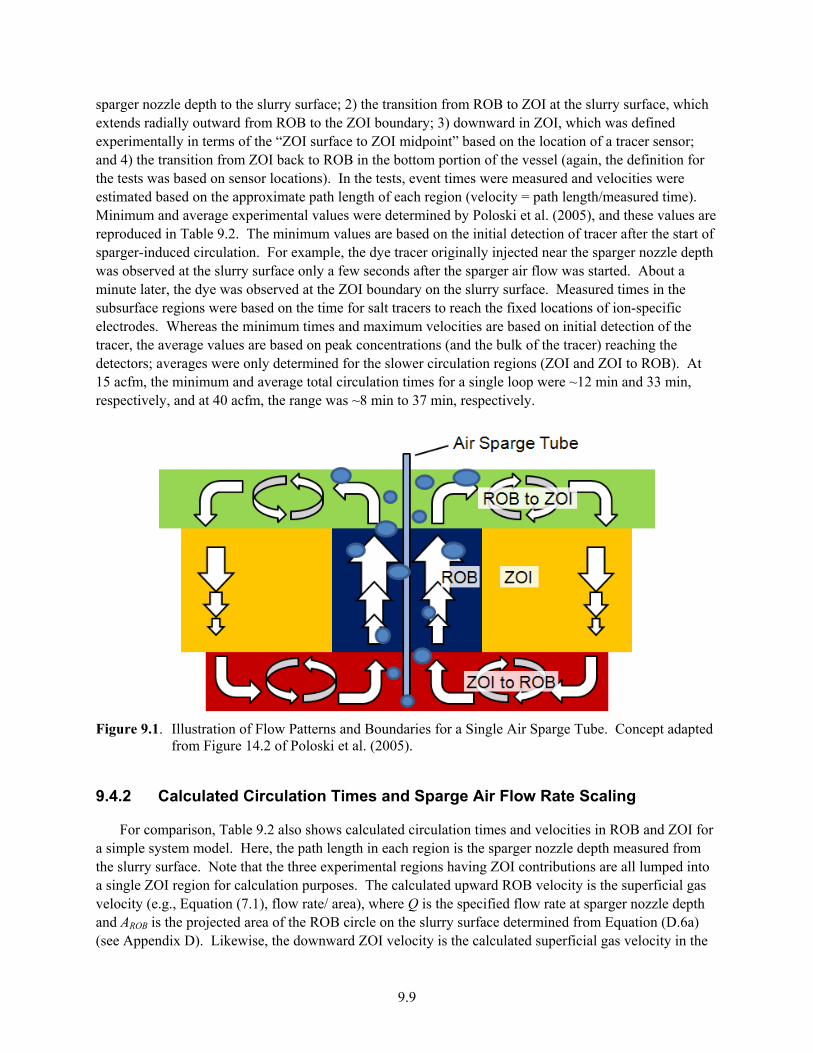
9.9

sparger nozzle depth to the slurry surface; 2) the transition from ROB to ZOI at the slurry surface, which extends radially outward from ROB to the ZOI boundary; 3) downward in ZOI, which was defined experimentally in terms of the “ZOI surface to ZOI midpoint” based on the location of a tracer sensor; and 4) the transition from ZOI back to ROB in the bottom portion of the vessel (again, the definition for the tests was based on sensor locations). In the tests, event times were measured and velocities were estimated based on the approximate path length of each region (velocity = path length/measured time). Minimum and average experimental values were determined by Poloski et al. (2005), and these values are reproduced in Table 9.2. The minimum values are based on the initial detection of tracer after the start of sparger-induced circulation. For example, the dye tracer originally injected near the sparger nozzle depth was observed at the slurry surface only a few seconds after the sparger air flow was started. About a minute later, the dye was observed at the ZOI boundary on the slurry surface. Measured times in the subsurface regions were based on the time for salt tracers to reach the fixed locations of ion-specific electrodes. Whereas the minimum times and maximum velocities are based on initial detection of the tracer, the average values are based on peak concentrations (and the bulk of the tracer) reaching the detectors; averages were only determined for the slower circulation regions (ZOI and ZOI to ROB). At 15 acfm, the minimum and average total circulation times for a single loop were ~12 min and 33 min, respectively, and at 40 acfm, the range was ~8 min to 37 min, respectively.

Figure 9.1. Illustration of Flow Patterns and Boundaries for a Single Air Sparge Tube. Concept adapted from Figure 14.2 of Poloski et al. (2005).

9.4.2 Calculated Circulation Times and Sparge Air Flow Rate Scaling

For comparison, Table 9.2 also shows calculated circulation times and velocities in ROB and ZOI for a simple system model. Here, the path length in each region is the sparger nozzle depth measured from the slurry surface. Note that the three experimental regions having ZOI contributions are all lumped into a single ZOI region for calculation purposes. The calculated upward ROB velocity is the superficial gas velocity (e.g., Equation (7.1), flow rate/ area), where Q is the specified flow rate at sparger nozzle depth and AROB is the projected area of the ROB circle on the slurry surface determined from Equation (D.6a) (see Appendix D). Likewise, the downward ZOI velocity is the calculated superficial gas velocity in the

9.10

projected ZOI area AZOI from Equation (D.6b) (see Appendix D) minus AROB (i.e., the ZOI area free of ROB). The calculated ROB velocities are a factor of 8.6 times higher than the ZOI velocities, which is consistent with the inverse ratio of the areas, (AZOI - AROB)/AROB.

The circulation time in each region is the calculated characteristic sparger time, tsp, which is defined as

*U

H

Q

AH

Q

Vtsp ===

(9.20)

The characteristic sparger time is a representative volume (V = area, A, times height or depth, H) divided by the volumetric flow rate, Q, or as shown in the right-hand form of Equation (9.20), and used here, it is the sparger nozzle depth H divided by the superficial gas velocity U*.

The calculated tsp values in Table 9.2 show that, like the experimental results, the time in ZOI is dominant and limiting. The total calculated circulation time, which is simply the sum of ROB time and ZOI time [= AZOI•H/Q = AROB •H/Q + (AZOI - AROB)•H /Q], is ~26 min at 15 acfm and ~19 min at 40 acfm. These results are in the middle of the experimental minimum and average values for the corresponding sparger flow rates. Therefore, characteristic mixing times derived from calculated superficial sparge gas velocities are representative. While slurry may not attain the same velocity as bubbles in the ROB, it is reasonable to assume that the upward slurry velocity, on average, is proportional to the superficial gas velocity in the region. In turn, for the mass balance, the upward flow of slurry in ROB must be balanced by a downward flow of slurry in ZOI (which is spread over a much larger area and volume).

The data and calculations shown in Table 9.2 are for a single sparge tube. In multiple-dedicated air sparger systems, such as the WTP HLP-27 and UFP-02 vessels, it is much more practical to use relevant vessel cross-sectional areas1 for superficial velocity calculations than to use ZOI areas, which depend on Q. The use of the vessel cross-section as the basis of U* calculations is further justified by considering the design basis of dedicated air spargers in the WTP vessels. Effectively, spargers were laid out and per sparge tube air flow rates were determined so projected ZOI circles cover the vessel cross-section.

Except for the circulation time calculation example given above, the correct absolute values of the superficial velocities are not significant when scaling dedicated air sparger or steam ring purge (sparge) air flow rates, provided the relevant area is scaled appropriately (e.g., geometric scaling of the vessel cross-section). For example, Section 7.2.2 shows that U* is not used explicitly to calculate scaled-down steam ring purge air flow rates. Also note that, while mixing is not the purpose of steam rings, the purge air flow to the multiple nozzles (holes) in the steam rings is obviously analogous in function to the distributed, dedicated air sparger system, and the possible blending effects of steam rings should be similarly considered in reduced-scale WTP vessel tests.

The liquid blending in WTP non-Newtonian process vessels and Newtonian process vessel UFP-01 involves the use of pulse jet mixers in addition to sparge air sources. The bottom region of the vessel

1 For example, the annular area between the outside of the PJMs and the inside vessel wall is used to calculate superficial velocities for deep annular spargers, and the remaining vessel cross-sectional area above the PJMs is used for shallow central sparger calculations. See Appendix D for more detail.

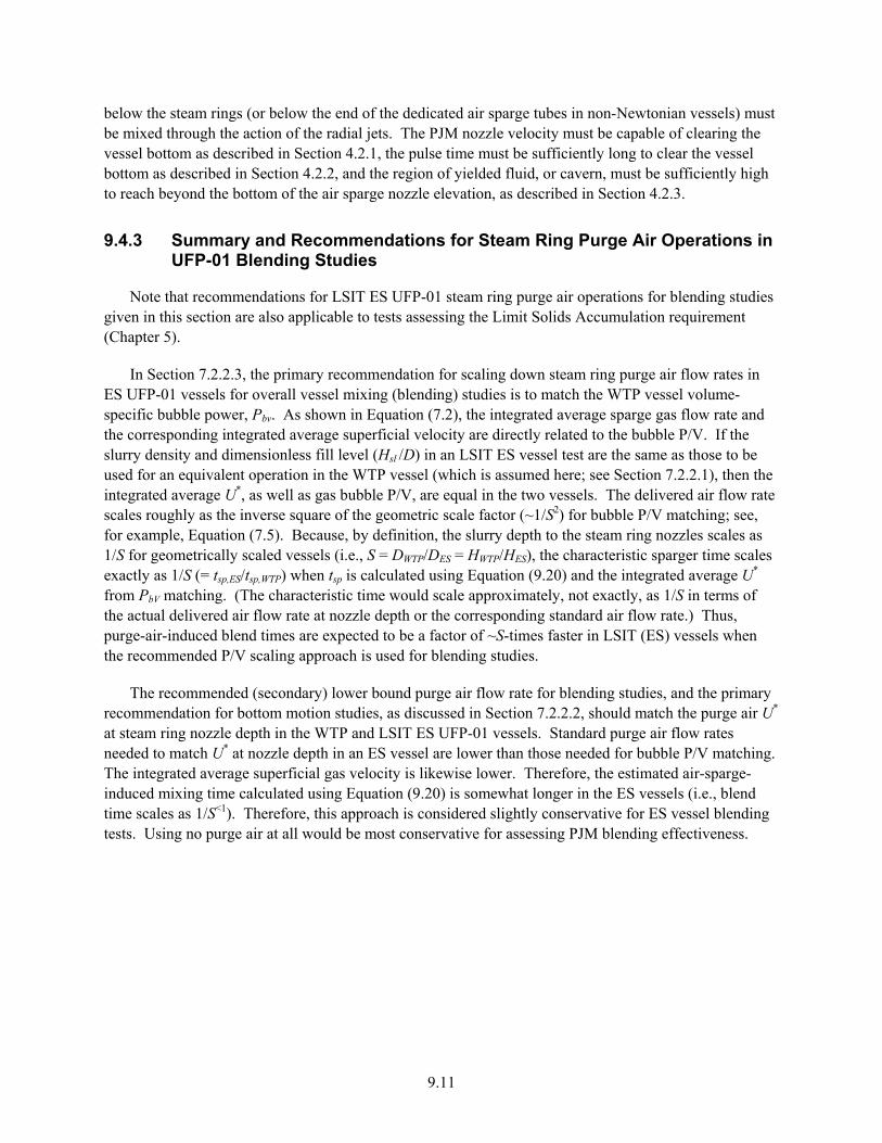
9.11

below the steam rings (or below the end of the dedicated air sparge tubes in non-Newtonian vessels) must be mixed through the action of the radial jets. The PJM nozzle velocity must be capable of clearing the vessel bottom as described in Section 4.2.1, the pulse time must be sufficiently long to clear the vessel bottom as described in Section 4.2.2, and the region of yielded fluid, or cavern, must be sufficiently high to reach beyond the bottom of the air sparge nozzle elevation, as described in Section 4.2.3.

9.4.3 Summary and Recommendations for Steam Ring Purge Air Operations in UFP-01 Blending Studies

Note that recommendations for LSIT ES UFP-01 steam ring purge air operations for blending studies given in this section are also applicable to tests assessing the Limit Solids Accumulation requirement (Chapter 5).

In Section 7.2.2.3, the primary recommendation for scaling down steam ring purge air flow rates in ES UFP-01 vessels for overall vessel mixing (blending) studies is to match the WTP vessel volume-specific bubble power, Pbv. As shown in Equation (7.2), the integrated average sparge gas flow rate and the corresponding integrated average superficial velocity are directly related to the bubble P/V. If the slurry density and dimensionless fill level (Hsl /D) in an LSIT ES vessel test are the same as those to be used for an equivalent operation in the WTP vessel (which is assumed here; see Section 7.2.2.1), then the integrated average U*, as well as gas bubble P/V, are equal in the two vessels. The delivered air flow rate scales roughly as the inverse square of the geometric scale factor (~1/S2) for bubble P/V matching; see, for example, Equation (7.5). Because, by definition, the slurry depth to the steam ring nozzles scales as 1/S for geometrically scaled vessels (i.e., S = DWTP/DES = HWTP/HES), the characteristic sparger time scales exactly as 1/S (= tsp,ES/tsp,WTP) when tsp is calculated using Equation (9.20) and the integrated average U* from PbV matching. (The characteristic time would scale approximately, not exactly, as 1/S in terms of the actual delivered air flow rate at nozzle depth or the corresponding standard air flow rate.) Thus, purge-air-induced blend times are expected to be a factor of ~S-times faster in LSIT (ES) vessels when the recommended P/V scaling approach is used for blending studies.

The recommended (secondary) lower bound purge air flow rate for blending studies, and the primary recommendation for bottom motion studies, as discussed in Section 7.2.2.2, should match the purge air U* at steam ring nozzle depth in the WTP and LSIT ES UFP-01 vessels. Standard purge air flow rates needed to match U* at nozzle depth in an ES vessel are lower than those needed for bubble P/V matching. The integrated average superficial gas velocity is likewise lower. Therefore, the estimated air-sparge-induced mixing time calculated using Equation (9.20) is somewhat longer in the ES vessels (i.e., blend time scales as 1/S<1). Therefore, this approach is considered slightly conservative for ES vessel blending tests. Using no purge air at all would be most conservative for assessing PJM blending effectiveness.

10.1

10.0 Sampling

This chapter focuses on the LSIT need to develop and verify WTP sampling methodology (as opposed to sampling operations/technique) for obtaining representative sample(s) of WTP waste feed slurries mixing in WTP target vessels. Target vessels are those selected by WTP to be the focus of the LSIT effort and are listed in Table 6.1. The WTP sample(s) will be analyzed to determine the inventory of various individual solid constituents within the target vessels and to ensure process control and related safety requirements are met prior to transferring the waste feed slurry out of the WTP vessels to downstream processes. The current WTP target vessel design has samples obtained in the vessel transfer line configured in a recirculation mode and continuously pumped during sampling. Sampling in the transfer line location for LSIT will focus on the following:

• Determining if the waste feed slurry can be adequately mixed in the vessel and pumped into the recirculation/transfer line so the bulk average waste feed slurry contents of the vessel in the vicinity of the transfer line inlet are “duplicated” at the sample location

• Demonstrating and verifying that the bulk average waste feed slurry contents of the vessel can be determined from samples drawn from the recirculation/transfer line.

The evaluation or qualification of the WTP prototypic sampler is not discussed in this chapter and is not part of the scaling effort being conducted in support of LSIT. Plans are for the WTP prototypic sampler and associated sampling techniques to be tested in the 14-ft-diameter vessel. Test requirements for prototypic sampler evaluation activities are beyond the scope of this document. Testing will focus on verification of sampler operations but test conditions will not be adjusted to accommodate any differences between scale of vessel and sampler. The WTP prototypic sampler may be used as a sampler to evaluate the mixing requirements; however, the development of final test requirements and test methodology for implementing the approach presented is beyond the scope of this work.

Throughout Chapter 10, references to associated work presented in earlier sections will be made instead of repeating the material. The current mixing requirements associated with sampling are presented in Section 10.1. A description of the problem and the assumptions made in addressing the problem is presented in Section 10.2. Potential approaches to achieve the sampling needs are discussed in Section 10.3. The application of an approach to assess the sampling requirements is presented in Section 10.4 and conclusions, recommendations, and issues are discussed in Section 10.5.

10.1 Sampling Requirements Related to Mixing

The sampling requirements related to mixing performance are obtained from Mixing Requirements 5, 6, and 7, elaborated in Determination of Mixing Requirements for Pulse-Jet-Mixed Vessels in the Waste Treatment Plant (24590-WTP-ES-ENG-09-001, Rev. 2) (Mauss and Papp 2010), and are summarized below:

• Requirement 5 – Criticality – (Safety-related requirement): Quantitative criteria are identified to define the type of sample to be taken and the required confidence level of the sample.

• Requirement 6 – Hydrogen Generation Rate (HGR) Estimation – (Safety-related requirement): Criteria are identified to indicate where confirmatory sampling of received waste is required.

10.2

• Requirement 7 – Process Control – (Process-related requirement): Quantitative criteria are identified to indicate control of key process parameters and/or constituents that are used to control each process or unit operation (e.g., pH, solids, radionuclides).

The functional requirements for all the mixing requirements are the same. As stated in the WTP functional mixing requirements, “… The PJM mixing system shall mix the slurry to ensure the process control requirements are met and a representative sample can be obtained…” (Mauss and Papp 2010, Table 2, p. 22).

The sampling strategy for WTP is still being developed. Integrated Sampling and Analysis Requirements Document (ISARD), 24590-WTP-PL-PR-04-0001, Rev. 2 was issued in 2008 and provides the basis for the majority of requirements presented in Table 10.1 (Dodd and Arakali 2008). The ISARD was prepared before the need for LSIT emerged. It is expected that issues and concerns that have driven the need for LSIT also will prompt additional controls on waste feed acceptability. In turn, additional sampling and analyses will be needed to implement new controls.

Samples taken from WTP vessels will be processed and analyzed by various methods to determine characteristics of the waste slurry related to various safety/process control requirements. Table 10.1 was generated by PNNL in an attempt to summarize the samples to be withdrawn from the four target vessels, methods for processing, components to be analyzed, results used for WTP operations, and the success criteria for satisfactory mixing/detection of the constituents of interest. The sample type numbers indicated in the first column have been assigned for the purpose of this discussion and have no relevance to WTP protocol.

PNNL has indicated by sample type 7 in column 1 of Table 10.1 some additional samples and analyses that may be necessary to implement WTP waste feed acceptance requirements. Because the mixing concerns, which are drivers for the LSIT focus on particle size and mixing of dense particles, especially separable fissile particles, it is anticipated that additional sampling and analyses will be needed to collect data on these characteristics of the WTP HLW feed. WTP has not established any specific sampling requirements or procedures to implement the “process control requirements.” They are included here because of the generalization of the previously stated functional mixing requirement (Mauss and Papp 2010). The same mixing issues causing concerns for processing could make fulfilling the requirement for “representative sample” most difficult for some samples. It is not the objective of LSIT testing to design an appropriate sampling system or modify the current design. LSIT testing will determine whether the degree of mixing in appropriately scaled tests will be adequate to fulfill the functional requirement for representative samples and provide some insight that may guide future sampling development or verification activities. There is additional effort required for specifying detailed mixing and associated sampling requirements.

Mixing Requirement 5, Criticality Sampling, only applies to HLP-22 among the target vessels. Samples for criticality testing are not taken from UFP-01 or RLD-08. The functional mixing requirement for Mixing Requirement 5 (and its sampling criterion) comes from the WTP mixing requirements “Table 2 – Functional Mixing Requirements,” which provides the previously stated high level requirement (Mauss and Papp 2010, Table 2, p. 22). This statement implies that HLP-22 is expected to be well mixed in regards to fissile material within the vessel and near the sample collection inlet (i.e., no settled solids). Should portions of the components of interest not be homogenously mixed when samples are collected, correlations/models for predicting the bulk concentrations of constituents in the vessel based on known materials collected from samples will need to be developed.

10.3

Table 10.1. Samples from Target Vessels—HLP-22, UFP-01, UFP-02, and RLD-08

Sample Type Vessel Sample(a) Processing Analyses(a) Data Use Mixing Success Requirements 1(a) HLP-22 PT 17 Sample is filtered into

liquid and solid fractions: Liquid Solids

Pu, U, Fe, Ni Pu, U, Fe, Ni Al Cr

CSL 8.2, 8.3, 8.4(b) CSL 8.1, 8.2(b) Caustic leach Oxidative leach

Liquid blended to ±10% homogeneity(c) Fe-rich solids representative to ±10% homogeneity(c) Al solids representative to ±15% homogeneity(b)

Cr solids representative to ±15% homogeneity(b)

2(a) HLP-22 PT 17a Sample homogenized Liquid/Solid Mixture

wt% UDS(d) Rheology(d) Particle size(d) pH(d)

HGR HGR, transfer control Waste acceptance Process control

Solids representative to ±10% homogeneity(c) wt% UDS vs. rheology, representative to ±10% homogeneity(c) Sample “representative” to contain large particles Liquid blended to ± 0.2 pH units(d)

3(a) HLP-22 PT 17b Sample is filtered to separate Liquid

90Sr, 137Cs Na, SO4

2-

HGR Process control Low-activity waste control

Liquid blended to ±10% homogeneity(c) Cs included due to requirement to calculate decay heat(d)

4 UFP-01 PT 5(e) Sample is filtered to separate Liquid

OH-

Process control

Liquid blended to ±10% homogeneity(c)

5 UFP-02 PT 4(e) Sample is filtered to separate Liquid

OH-

Process control

Liquid blended to ±10% homogeneity.(c) This vessel will be tested at full scale.

6(a) RLD-08 HLW 3 Sample homogenized Liquid/Solid Mixture

wt% UDS pH

Process control Process control

Solids representative to ±20% homogeneity(f) Liquid blended to ±0.25 pH units(f)

7(g) HLP-22 TBD TBD Separable Pu(h)

Criticality, <450 g separable Pu in the total vessel(i)

Pu particles collected in the sample are “representative” or “bounded”

(a) Samples and Analyses are identified in Dodd and Arakali (2008, Appendix B). (b) Mauss and Papp (2010, p. A-8). (c) Success criteria are determined by sample data quality objectives, which require ±10 percent accuracy unless otherwise established (Dodd and Arakali 2008, pp. B-22 and

B-23). (d) Dodd and Arakali (2008, p. B-24). (e) Identified as a “potential” sample (Dodd and Arakali 2008, p. 20). No details provided; details are authors’. (f) Dodd and Arakali (2008, p. B-68). (g) Sample NOT in ISARD. Potentially needed to implement waste feed acceptance criteria or safety requirements to be established by WTP. (h) PJM action can separate PuO2 particles. The requirement to analyze for separable Pu is not yet established. The method to analyze for separable Pu has not been

established. (i) Personal communication from D Loesy, WTP criticality safety, to GB Josephson, PNNL, February 16, 2012.

10.4

To keep HLP-22 below criticality limits, samples are to be taken from HLP-22 after the vessel has been filled. The vessel contents are to be completely mixed for a representative sample. This is a process hold point (i.e., waste cannot advance through the process until analytical data is available for process evaluation). A solids/liquids separation is made on two independent samples of the material and analyses of the two solids fractions are performed independently to verify the ratios of fissile components to neutron absorber components (e.g., Fe, Ni) are below bounding criticality safety limits (CSL). The criticality safety evaluation report is under revision and CSLs presented in this document are subject to change. Independent analyses also are conducted on the liquid fraction to verify that dissolved Pu and the fissile uranium to total uranium ratio (FU/U) ratio are below action limits. The analyses are used to determine that the vessel contents comply with four criticality safety limits (Mauss and Papp 2010, p. A-8):

• CSL 8.1 requires that the Pu/metal ratio in the solids fraction is <6.2 g Pu/kg of absorber metals (Fe, Mn, Ni, and Cd).

• CSL 8.2 requires that the fissile uranium to total uranium ratio in the liquid and solids fraction is <8.4 g/kg.

• CSL 8.3 requires that the total Pu concentration in the liquid fraction is <0.013 g/l.

• CSL 8.4 requires that the Pu/metal ratio is <6.2 g/kg in the liquid.

The required accuracy of the laboratory analyses is to be better than ±10 percent and the total statistical confidence that CSLs are being met is >95 percent (Dodd and Arakali 2008, pp. B-23, B-26).

10.2 Presentation of Sampling Problem

The task of LSIT, relative to the mixing requirements and sampling, is to assess how well the bulk concentrations in the PJM target mixing vessels can be quantified for the constituents identified in Table 10.1 based on samples drawn from the transfer line operating in recirculation mode (i.e., recirculation line and transfer line are the same conduit operating in different modes). The nomenclature conventions described above are used throughout Chapter 10:

• The transfer line may be referred to as the recirculation line, suction line, or at times the suction inlet; refer to Section 10.2.2 for assumptions related to this discussion. The transfer line and recirculation line are the same conduit considered for Mixing Requirement 2, Prevent Plugging, and are discussed in Chapter 6 and Appendix E. The same transfer line and associated transfer pump used to transfer material from the vessel during pump out (also referred to as pump down) operations will be used to recirculate slurry within each target vessel.

• Sample will refer to an LSIT sample drawn while the transfer line is operating in recirculation mode and will include all yet to be determined test sample locations within the recirculation loop. Samples drawn from other locations will be provided additional description (e.g., vessel sample, verification sample).

The development of an approach to predict the transfer line feed stream properties in WTP based on the design of reduced-scale tests of the PJM mixer operations is presented in Appendix C and summarized in Chapter 5.

10.5

The samples in Table 10.1 for which the analyses are conducted only on the liquid phase, sample types 3, 4, and 5, will meet the functional criterion for vessel sampling; that is, “… a representative sample can be obtained ...” if the vessel meets Mixing Requirements 3 and 4, Blend Liquids and Neutralization (Mauss and Papp 2010, p. 22). If the vessel is blended, the dissolved constituents within the liquid fraction of the samples withdrawn will be representative. Therefore, the remainder of the discussion will exclude sample types 3, 4, and 5, or the liquid phase of the other sample types.

Whether assessment of solids contained in the samples can meet the sample representativeness requirement will depend upon how homogeneous the solids pertinent to the analysis are mixed within the vessel and near the sample collection inlet. Solids that are low density and/or very fine are likely to be nearly homogeneous. The major challenge whether samples will be “representative” will come from solids that are not dispersed through the entire vessel and those that settle rapidly enough to segregate within the vessel. This potential issue is expected for the criticality sampling associated with sample types 1 and 7 listed in column 1 of Table 10.1.

To meet and assess Mixing Requirements 5, 6, and 7, the following will have to be developed:

• A methodology to predict the bulk concentration of the constituents in a PJM mixing vessel given a set of parameters determined from sample characterization and knowing the vessel operating parameters.

• The parameters determined from sample characterization that will allow the bulk concentration of vessel constituents to be predicted.

• A technical basis for scaling up the vessel conditions yielding a unique sample. This will be discussed further in Section 10.3, but in summary, an understanding must be developed that allows the vessel solids distribution to be predicted from a given sample and conversely allows the retrieved sample makeup to be predicted from a given vessel inventory, solids distribution, and prescribed set of operating conditions over the range of scales tested.

• A basis for the uncertainty associated with the predictive methodology. This uncertainty is separate from the uncertainties associated with each parameter determined from sample characterization and the uncertainty in sample makeup associated with sample retrieval. The combination of these uncertainties is required to meet the limits provided in Table 10.1. In addition, the assessment of the overall uncertainty will be impacted by the experimental uncertainty in the measurements taken to verify the vessel conditions. The nature of PJM operations means the measurements will be taken for periodic conditions. The verification/development of the approach through testing will be required to determine if time averaged or instantaneous results averaged over multiple cycles will be required.

For this discussion, the “perfect or ideal” sample representing the entrained slurry at the transfer line inlet is to be considered. If even a perfect or ideal sample is not sufficient to predict vessel contents, then there is no need to evaluate prototypic samplers and assess uncertainties resulting from sampler operations relative to predicting vessel contents. The assessment of the sampling relative to slurry mixing is to verify that task is possible; therefore, the related test program for development and verification should not be restricted to WTP sampling constraints relative to sample location, sample volume, etc. Again, it is emphasized that while LSIT may include the following, the scope of this document is not associated with:

• Assessing the effectiveness of the prototypic sampler to retrieve a sample representative of the slurry at the WTP-prescribed sampling location.

10.6

• Assessing any WTP sampling process or procedures as the test results associated with this task may impose additional requirements on the WTP sampling process.

• Assessing the physical location of the prototypic sampler within the recirculation/transfer line. The current scaling/modeling presented in this report has focused on scaling the feed stream entrained at the transfer line suction and assessing downstream effects based on the input conditions. Appendix E and Chapter 6 rely on bounding conditions for downstream assessments. The effect on slurry makeup resulting from transport within the pipeline will have to be assessed separately if the WTP sampler is far removed from the transfer line suction.

Conditions and issues that impact the development of a predictive scheme and the assessment of the sampling requirements include:

• LSIT pipeline samplers and vessel samplers may not readily scale to smaller physical scales. Issues associated with sampling over multiple geometric scales include:

– LSIT does not call for the scaling of simulant. Therefore, the particle sizes, densities, and corresponding dynamic response time of the particles will be held constant for all scales evaluated. This can impact particle segregation when drawing in a sample from a slipstream.

– The transfer line size will be scaled to provide the desired fluid conditions relative to the scaled flow rate. Refer to Appendix C, Section C.4.3.3 for the scaling of the transfer line inlet flow rate. Changes in line size can require changes in sampler size and corresponding retrieved volumes. Refer to Appendix E, Section E.3.2 for a description of flow conditions.

– For LSIT vessel samplers, it may be possible to use the same sampler at multiple scales; however, the relative volume of the sample retrieved will not scale. This issue is more significant if the samples are intended to assess concentration gradients. The impact of this is reduced with smaller sample volumes. However, uncertainties can be increased with a reduction in sample size especially when concentrations are low.

The sampling methods and protocols used over the multiple test scales may be partially scale dependent and require an assessment of uncertainty and representativeness for each scale for which they are applied.

• No current specifications are provided by the ISARD for the assessment of separable plutonium, sample type 7 in Table 10.1 (refer to Section 10.2.1).

• The concentration profile within the transfer line operating in recirculation mode as a function of time is anticipated to be cyclical and in phase with PJM operations (refer to Figure 10.1; Sections 6.2, 10.2.1; and Appendix E, Section E.2.1).

• Entrainment at the transfer line suction inlet may be dominated by two separate phenomena depending on the phase of the PJM cycle (refer to Appendix C, Section C.4.3.3 for comparison of scaling laws).

– The sweeping of particles into the transfer line suction inlet as the radial jet from the PJM mobilizes particles on the vessel floor (refer to Sections 5.5, 5.6; and Appendix C, Section C.4.1).

– Entrainment of settling solids under semi-quiescent conditions after flow from the PJMs has terminated (e.g., during PJM refill) (refer to Section 5.6; and Appendix C, Section C.4.1).

10.7

• For vessels with spargers, spargers may have an impact on the settling models and the scaling of sparger operations to assess particle dispersion and settling may be further complicated if they also impact the mobilization of solids from the vessel floor (refer to Chapter 7 and Appendix D). The various ways in which the multiple phenomena scale may impose too many restrictions on the spargers so that they can only be fully evaluated at full-scale conditions.

• Gas entrainment can impact the fluid rheology, fluid density, and effective particle density. Both sparger and PJM operations are susceptible to enhancing gas entrainment depending on the slurry mixture. Many particles have an affinity for gas bubbles to become affixed until the particle is subjected to a high enough shear field to release the gas. It is uncertain how any impact due to gas entrainment will scale until measurements are made. In addition, a consequence of the sampling process and sample handling is that the gas content can often be reduced or eliminated from the sample (e.g., higher free surface to slurry volume ratios) making measurements that compare with inline density and concentration difficult.

Figure 10.1. Transfer Line Specific Gravity versus Time for a Reduced-Scale Test First-Quarter-Batch Pump Out. Graph indicates effect of PJM cycling on slurry density in a retrieval line. Test conducted with 10 wt% solids in water and the transfer line was not scaled for WTP operations (Campbell et al. 2010b, p. A-21).

10.2.1 Measuring Separable Plutonium

The CSLs identified in the current mixing requirements address dissolved and “co-precipitated” Pu. Most of the Pu that enters the WTP is associated with the Fe-rich sludge that does not separate from the Pu in PJM-mixed vessels. This Pu is not the real basis of concern relative to criticality or a driver for LSIT. As long as the ratios of Pu to the absorbers with which it is associated are below limits, there is no criticality issue. The major safety concerns from potentially inadequate mixing arise from “separable” Pu particles (such as plutonium oxides and plutonium metal) that can 1) separate from their mitigating

10.8

neutron absorbers or poisons because of their high density and 2) potentially accumulate on the bottom of the vessel. In this case, absorbers are not in proximity, and the criticality limits for the vessel are much lower (e.g., 450 g Pu).1 Currently, there is no criticality limit for this type of “separable” Pu. In anticipation that such limits will also be part of the safety basis for WTP, this report considers that scaled testing will be conducted to provide important data for a future effort by others to prepare a sampling strategy and design that will meet requirements; refer to sample type 7 in Table 10.1.

The validity that a sample representative of vessel concentrations of dissolved Pu, co-precipitated Pu, and separable Pu can be obtained is at the root of the safety questions that drive the need for LSIT. The issue regarding PJM mixing within WTP is captured by Mixing Requirement 10, Limit Solids Accumulation. The major safety concern is that PJM mixing will not be adequate to sufficiently mix the heavy “separable” Pu and fissile U particles and that the particles will settle and accumulate on the bottom of the HLP vessel over multiple pump outs, and eventually lead to a criticality event. Previous reduced-scale testing with open PJM arrays (as opposed to chandelier configurations) showed that, by locating the transfer line suction inlet close to the bottom of the vessel, the fast-settling heavy particles were preferentially transferred from the tank as long as mixing is sufficient to lift the particles, at least momentarily, from the vessel bottom to the pump suction inlet (Campbell et al. 2010b, pp. A-46 through A-47). This same reduced-scale testing, which showed preferential retrieval of the heavy-heavy particles (simulated fissile particles), indicated that taking a random sample of the contents from the vessel transfer line will not likely be representative of the heavy, fast-settling fissile vessel contents. Requirement 10 may be fulfilled, but a representative sample, Requirement 5, may not be fulfilled without some dynamic sampling. Dynamic sampling (refer to Section 10.3.3) means that the sample will not be taken at random, but will be timed to vessel events (e.g., the PJM stroke).

In Recommendation 2010-2, the DNFSB also emphasized the sampling concern (Winokur 2010, p. 3).

The WTP safety strategy depends upon obtaining representative samples from the high-level waste feed tanks to support WTP’s waste feed certification requirements, and from WTP process vessels to ensure safety-related criteria are met. This capability has not been demonstrated in the Hanford Tank Farms or WTP process vessels. Obtaining samples that are sufficiently representative to support bounding estimates of the composition and properties of both the solid and liquid fractions of the high-level waste is required in order to demonstrate that the WTP can be operated safely (e.g., prevent inadvertent criticality and plugging of transfer lines).

Figure 10.1 presents an example from reduced-scale testing of how the concentration of fast-settling solids rapidly peaks and then decreases with each PJM stroke (Campbell et al. 2010b, p. A-21). The scaling applied to the transfer line and associated flow rate, relative to WTP operations, in the reduced-scale testing is not known. These results are similar to those presented in Figures 6.1 and E.2. The results presented in Figure 10.1 come from tests listed in the M3 Platform Test Summary for HLP-22-NQA-007 (CCN 218353, Chapman and Lehrman 2010), and consist of instantaneous (i.e., no time averaging) data captured by the DAS during testing. These results provide slurry density (i.e., specific gravity) as a function of time during a pump out and depict the impact that PJM cycling has on

1 Personal communication from D Loesy, WTP criticality safety, to GB Josephson, PNNL, February 16, 2012.

10.9

the transfer line inlet conditions. Only the results from the first quarter pump out (i.e., vessel liquid level reduced from full vessel to 75 percent of initial level) batch are shown because they contain the most-dense slurry. The test was conducted with 10 wt% solids in water at room temperature in a scaled vessel (referred to as Case 1 for the test program).

The peak in specific gravity is attributed to the faster-settling solids (i.e., higher density and/or larger diameter solids) that segregate near the bottom of the vessel and are mobilized and lifted above the transfer line suction inlet during each PJM discharge phase and then rapidly settle to the vessel bottom during the refill phase of the PJM drive cycle. Therefore, these particles are not entrained into the suction line during the entire duration between PJM pulses, resulting in a reduced slurry concentration.

Because these fast-settling particles are not suspended very high in the vessel, their relative concentration, when suspended, is higher at the suction inlet compared to other materials dispersed to greater elevations within the vessel. This condition results in the faster-settling solids preferentially being removed during the initial stages of pump out, thus reducing their concentration within the vessel. This effect is observed in Figure 10.1 by the progressive decrease in peak concentration obtained with each PJM pulse. The later stages of the pump out have lower concentrations of fast-settling solids than the initial stages so the concentration of fast-settling solids in the heel is expected to be less than the original bulk average concentration. When this behavior occurs for the fastest settling solids, the system should meet Mixing Requirement 10, Limit Solids Accumulation as long as Mixing Requirement 8, Mix to Release Gas (i.e., assessed by bottom clearing), has been satisfied and the particles are lifted above the transfer line suction inlet elevation for all operating conditions. In addition, the minimum specific gravity obtained with each PJM pulse also diminishes, which indicates that other materials contributing to the slurry density also are segregating in the vessel and are being preferentially removed. The minimum specific gravity is anticipated to approach a constant corresponding to that of the homogeneously mixed portion of the slurry.

The assumption made for the development of the predictive methodology is that sampling will be performed when the transfer line is operating in the recirculation mode. Therefore, a periodic condition for the concentration (i.e., bulk specific gravity) is anticipated during sampling operations instead of the decreasing trend observed in Figure 10.1. Testing will be required to assess the potential variability in the transfer line concentration from cycle to cycle.

NOTE: When considering the small volume fraction 450 g of Pu in a vessel with an assumed working volume of 152,000 gal ( i.e., consider HLP-22, which has an active volume of 160,000 gal), it is reasonable to question the probability of collecting a “representative” sample from pure statistical “rarity” in addition to the difficulties caused by mixing. If the probability of capturing the Pu particles becomes rare, the representativeness approaches “nugget” sampling. That is, the probability of getting a Pu particle itself is rare so the variance of any analyzed concentration is so large that one could not meet the 95 percent confidence limits that the Pu in the vessel was below criticality limits (i.e., 450 g). An initial statistical assessment was conducted assuming that 450 g of 10 µm separable Pu particles were homogeneously distributed in an assumed vessel with a working volume of 152,000 gal based on the approximate active volume of HLP-22, which is 160,000 gal (Campbell et al. 2010b, Table 16, p. A-54). The statistical assessment considered the probability of capturing particles in a 15 mL sample. The expected number of particles in the sample was estimated as a hyper-geometric random variable. In this

10.10

approach, a 15-mL sample would on average contain over 1965 Pu particles.1 With numbers this large, the sample variance approaches a continuous distribution function, and the sampling contribution to the overall analytical variance can be estimated like typical chemical analyses rather than “nugget” sampling. In addition, for similar conditions and assumptions, the Pu particle count would be 711 and 17,072 for sample volumes of 5 mL and 120 mL. A sample can be obtained by retrieving sub-samples at some frequency (e.g., WTP plans to collect 24 5-mL subsamples to create a final 120-mL sample for characterization2).

The particle size (i.e., 10 µm) was estimated as an average particle size for the Hanford waste based on a “bounding Pu particle” (Campbell et al. 2010b, p. A-46). The sampling statistics could change if larger particle sizes were used for testing.3 In addition, the statistical assessment assumes that all of the Pu particles are suspended for the time duration corresponding to the sampling duration. There will be some duration associated with drawing each sample from the pipeline. This duration corresponds to both some upstream length of pipe and some period of time over which slurry is entrained at the transfer line inlet. The number of Pu particles retrieved in a sample will be reduced if the Pu particles are not suspended for the full duration of entrainment corresponding to the duration of sampling.

10.2.2 Assumptions Applied to Evaluation of Sampling

For the evaluation of the sampling task, the following assumptions are made and need to be confirmed as part of any test effort conducted to develop the prediction of sample contents from transfer line samples. The following assumptions apply to the period of operation that samples would be drawn.

• Sampling is performed during a period of recirculation through the transfer line suction inlet using the transfer pump. The net contents of the mixing vessel will not change during the sampling period.

• The following parameters for the vessel will be known: minimum and maximum vessel fluid levels, the average PJM discharge velocity, and the PJM drive time.

• The PJM mixing system is capable of raising all constituents to an elevation above the suction line. This is required so that the particles of each constituent can be entrained by the suction line. This assumption is expected to be satisfied as long as Mixing Requirement 10, Limit Solids Accumulation, is satisfied. If all particles cannot be entrained by the suction inlet, accumulation will occur.

• All of the material on the bottom of the vessel has been suspended to some degree during the PJM cycle. This is a slight expansion on the requirement for bottom motion covered by Mixing Requirement 8, Mix to Release Gas, which is discussed in Chapter 4 and Appendix B. The bulk concentration of vessel constituents cannot be fully (i.e., accurately) predicted from the retrieved sample if the suspended concentration does not represent the entire inventory of vessel material and if the transfer line does not have the possibility of entraining all of the particles associated with each constituent. When considering just a single vessel batch, some form of prediction could be made if

1 Analysis performed by Dr. SK Cooley, PNNL, in CCP-WTPSP-1097. 2 WTP sampling plan communicated by R Hanson, BNI, at February 2012 Scaling Basis Document Workshop. 3 Preliminary information about Hanford waste history indicates that PuO2/Pu metal particles may range up to 100 µm with a specific gravity of 19 (Pu metal) (Meacham et al. 2012, pp. ii, 53). For particles this large, a 15-mL sample may contain less than two particles, and a 5-mL sample would contain less than one particle on average. Obtaining statistically representative samples may not be practicable.

10.11

this assumption does not hold, but it would create a bias uncertainty in the predictions. This would also create another phenomenon that has to be scaled up for predicting WTP performance. However, in such a case, Mixing Requirement 10, Limit Solids Accumulation, would not be satisfied unless pump out operation resulted in particles that were not suspended under full vessel conditions being suspended after vessel conditions change (e.g., change in fluid level and solids concentration). This is an example of where an examination of the interdependence of the mixing requirements may need some information in the existing requirements to be refined or expanded to assure testing and WTP predictions against the requirements lead to all requirements being simultaneously satisfied.

• The duration of the PJM pulse is sufficient to radially disperse all solids within the vessel such that the radial concentration gradient of each constituent approaches zero. This assumption must hold for two reasons:

– The transfer line inlet is a point location for the retrieval of solids and the mass flux across a horizontal plane of the vessel must be uniform for the entrained slurry to be representative of the vessel contents.

– The mobilization of the settled solids can create plumes of concentrated solids to be transported upward in the central or wall regions of the vessels. If the motive source of flow for these plumes is terminated prior to the radial dispersion of the plume, the density gradient between the plume and the surrounding fluid can create a rapid settling of the concentrated suspension that can greatly exceed that of the terminal settling velocity for a single particle.

• The transfer line inlet creates no preferential entrainment or segregation of the particles.

• Transfer line flow conditions do not result in solids deposition or significant holdup.

• Sampling operations used to assess Mixing Requirements 5, 6, and 7 during LSIT are not restricted to WTP specifications regarding sampler selection, operation, location, etc. LSIT sampling operations used to assess the mixing requirements can be designed to approach ideal sampling conditions (e.g., full port sampling of entire volume entrained during PJM cycle).

10.3 Potential Approaches for Predicting Contents of Vessels from Line Samples

This section discusses potential approaches to be used to predict the bulk concentration for constituents of interest from analysis of the retrieved sample. A final solution is not provided because a development effort is required to refine and verify potential approaches and models to be used in the development of a predictive methodology. Development of the requirements for sample analysis also is needed and cannot be completed until testing demonstrates the effectiveness of the process. The requirements may need to be refined for the method to achieve the total uncertainty limits specified in Table 10.1. Total uncertainty includes uncertainties associated with sample retrieval, sample analysis, operational variation, predictive method, and uncertainty associated with verification measurements. For this task, either all contributing uncertainties could be assessed in parallel with the LSIT, or estimates could be made for contributing factors and the uncertainty specifications provided in Table 10.1 could be

10.12

revised (i.e., reduced/tightened) to include only those factors associated with the LSIT scope. Potential methods for predicting vessel contents include:

• Dynamic or phased sampling – refer to Section 10.3.3

• Bounding sampling – refer to Section 10.3.4

• Physical modeling to obtain an implicit solution from sample contents – refer to Section 10.3.5.

10.3.1 WTP Slurry Solids Constituents and Potential Methods of Predicting Concentration

The discussions and models presented in Appendix C and summarized in Chapter 5 are the basis for the approach presented in Section 10.3. Previous work will be referenced by section but not repeated.

Mixing requirements for sampling presented in Section 10.1 are summarized in Table 10.1. The solids constituents and associated parameters of interest to be evaluated are listed below along with a brief summary of the potential methods that may be applicable to meeting the WTP needs.

• Co-precipitated Pu – The ratio of Pu to neutron absorbers and poisons to assess that they are below CSLs defined in Section 10.1. This requirement is concerned only with relative ratios of materials existing with individual particles; therefore, if the formation of the solids results in uniform ratios of elements regardless of particle size, the assessment only requires capture of some material, and no prediction of bulk concentration is required. Because the results are used to compare against limits, this would be considered a simple form of bounding sampling. However, if the ratios of elements within a particle are size dependent, then the following would be required:

– Size distribution of the co-precipitated Pu

– Prediction of bulk concentration within the vessel for each binned size range

– Assessment of material makeup by binned size ranges

– Total CSLs calculated from weighted averages of binned size ranges.

To achieve these requirements would require determining material concentration based on physical modeling of the solids transport within the vessel and into the transfer suction line inlet. To accomplish this:

– The retrieved sample is segregated by particle size

– The volume fraction of each size range is determined

– Elemental analysis is conducted on each size range of material

– The ratio of Pu to absorbers and poisons is determined for each size range of material.

A conservative approach could be applied and the “worst-case” condition obtained among the size ranges could be applied to the entire inventory.

• Separable Pu – The quantity within the vessel relative to a maximum CSL (not yet established). The need is to assure quantities are below an upper limit. Therefore, the first approach should be to assess via bounding sampling. If this approach results in too conservative a prediction, then concentrations would need to be determined from physical modeling. The approach for this constituent may still make use of bounding conditions to simplify the physical modeling applied.

10.13

• Al – bulk concentration within the vessel – It is anticipated that these particles will be small and of low enough density that they will be homogenously suspended within the vessel if the mixing requirements for blending are satisfied. Therefore, a bounding sampling approach that only confirms the material size has a negligible settling velocity relative to the PJM cycle time is anticipated.

• Cr – Same as for Al.

• UDS – bulk concentration within the vessel – It is assumed that, because this information is used for process control and the large size distribution anticipated in the waste, physical modeling will be required to satisfy this need.

10.3.2 Generalities Applicable to All Predictive Methods

A number of factors or items that apply to all predictive methods and should be considered in formulating an approach for method development and testing include:

• Developing a test approach that allows various methodologies or refinements to be evaluated simultaneously. The objective should be to develop the most robust, simplified predictive method that meets the WTP needs and requirements while reducing the number of iterative tests to be performed. The key is to assure the instrumentation, test procedures, and test sample characterization and analysis methods allow for more than one approach to be assessed from a single test. This will be discussed further in Section 10.3.3.

• The assessment of uncertainty should be included as part of test design and test execution rather than being a task to be performed after data gathering activities are complete. A statistical evaluation can be employed:

– Prior to testing, to identify what sources are likely to be the greatest contributors of variation and uncertainties. This information can be invaluable in identifying where resources are most beneficially applied for improving sensor accuracy, resolution of measurement location, frequency of data acquisition, and number of measurements.

– During the test program, using test data to evaluate both system variation and uncertainties, prioritize future test cases, assess the benefit of acquiring additional samples, and determine level of model refinement required to meet uncertainty specifications.

• Determination of carrier fluid rheology based on sample analysis. For model application, representative rheology will need to be determined and this may not come from a single assessment. Rheology characterization may be required for the entire slurry, the suspended slurry with fast-settling (criteria to be determined) solids removed, and the filtered liquid. Assessment of rheology should not be restricted to those methods anticipated to be employed by WTP because additional techniques may be required for model development. However, the final techniques employed to assess rheology for the predictive methodology (as with other parameters) need to be applicable to the WTP. In other words, multiple techniques can be used to develop models and predict scaling, however, the final methodology can only use parameters that can be assessed by the WTP. Rheology is singled out here for the following reasons:

– The measurements of rheological parameters from complete samples often are not representative of the process rheology. The complete samples are not expected to be representative of the vessel contents. That is the reason a predictive scheme is being recommended/employed to satisfy some sampling needs.

10.14

– The rheology of interest often is not obtained (e.g., need rheology of carrier fluid that includes homogenously mixed solids, not that for the whole slurry or filtered liquid) or at the conditions of interest (e.g., appropriate range of strain rates or for constant strain rate).

– Rheology for some instances can be better predicted from other measured parameters or measurements taken on a conditioned/processed sample. It is anticipated the vessel will contain concentration gradients and, therefore, viscosity gradients that may need to be predicted.

– There are times when process measurements can yield apparent viscosity measurements that are more applicable than those obtained from sampling (e.g., pressure drop in pipe, pressure change in PJM).

10.3.3 Dynamic Sampling

Dynamic or phased sampling is the term used to indicate sampling being performed at a prescribed point in time or process sequence that:

• Yields a sample representative of the material or specific properties of interest at a particular time (e.g., obtaining sample just prior to PJM firings to assess material with fastest settling particles removed) or

• Yields a sample with properties that can be correlated to a known condition. Results are most often correlated to a fit of previously collected data. This is synonymous with predictions of cloud height (stirring up settled and settling solids) measured at the end of the PJM drive cycle. However, this approach is often used for data collected in the prototypic system. An attempt to scale up (or scale down) such results is a separate issue. The application of dynamic sampling does not rely on a physical understanding of the process but rather relies on a demonstrated history of repeatability that can be correlated (e.g., the density or concentration of a sample taken 5 min after reaching temperature correlates with consistency that will exist at room temperature).

Application of this method to the PJM mixing vessels would present a challenge in determining when a sample could be drawn from the recirculation line that is representative or could be correlated to the bulk average concentrations of the constituents of interest. The effort is complicated by the fact that the application of these results would require scale-up to WTP. Currently, the authors are unaware of any data sets indicating that such a condition should be investigated further. In addition, the sampling is taking place in a pipeline that also requires scale-up of the pipeline transport from the vessel to the sampling location due to the cyclical nature of the concentration at the inlet.

While this method does not look promising, it is mentioned here for two reasons:

1. LSIT test data may yield results that warrant using dynamic settling (i.e., this method should not completely be ruled out until actual LSIT data have been evaluated, but at this time, we recommend not banking on such an approach unless extensive full-scale testing becomes an option).

2. A form of dynamic sampling is being recommended to aid potential physical modeling. Solids entrainment into the suction line inlet is anticipated to occur via the following mechanisms:

– Solids mobilized from the vessel bottom by the radial jets produced during the PJM discharge phase being swept into the suction line. Refer to Chapter 4, Section 5.5; Appendix C,

10.15

Sections C.3, C.4.1, C.4.3.2, and C.4.3.3 for discussions on scaling required for achieving representative concentration versus time at the inlet of the transfer line suction inlet.

– Entrainment during quiescent settling of solids. Refer to Section 5.6; Appendix C, Sections C.3, and C.4.1 for discussions and required scaling to achieve representative concentration versus time at the inlet of the transfer line suction inlet.

Two different scaling laws apply to solids entrainment for the different phenomena. To simplify the modeling and scaling of results, a recommendation is made to only perform sampling operations between PJM pulses (no discharge flow) when quiescent settling occurs. As stated earlier, the proposed WTP sampling protocol calls for obtaining 24 5-mL subsamples to generate a 120-mL sample. Sampling would start when the PJM discharge flow ceases, and depending on the sample rate, it would be possible to continue sampling throughout the refill phase of the PJM cycle. This will be discussed further in Sections 10.4.3 and 10.4.4.

10.3.4 Bounding Sampling

Bounding sampling simply refers to a sampling protocol and/or associated analysis that is focused on obtaining limiting or conservative predictions for the parameters of interest. For application to the WTP mixing requirements, it is anticipated that a limited amount of modeling would be applied to avoid having an approach that is too conservative.

A basic approach for applying bounding sampling to WTP would be to obtain a sample at the very end of the PJM pulse, when all constituents will have reached their maximum elevation of suspension and corresponding lowest localized concentrations. The concentration of the retrieved samples is then assumed to apply over the entire liquid volume in the vessel. For homogenously mixed constituents, the actual concentration is attained. For other materials, the greater the settling velocity or particle Archimedes number the greater the degree of conservatism.

Bounding sampling is considered a potential approach for satisfying the need to determine the bulk concentration for separable Pu. As previously discussed, the sample to be acquired would be obtained following the discharge of the PJMs. However, instead of applying the retrieved concentration to the entire liquid volume in the vessel, a conservative approach is used to estimate the peak elevation achieved by each constituent of interest (in this case separable Pu) in the vessel during mixing operations. The elevation predicted is used to calculate the volume occupied by the constituent and the concentration obtained from the retrieved sample is applied to the calculated volume to provide a bounding estimate for the total mass of a constituent existing within the vessel. The method used to determine the conservative volume would be based on the particle dispersion modeling presented in Appendix C. The conservatism applied would be determined through the course of the test effort with the conservatism intended to reduce both the modeling and sample analysis needs.

10.16

10.3.5 Physical Modeling Based on Sample Characterization

The physical modeling and scaling approach consists of applying models for each of the following mechanisms that have been identified to contribute to particle transport:

• Mobilization from the vessel bottom – Chapter 4 and Appendix C, Section C.4.1

• Dispersion – Appendix C, Section C.4.1

• Settling – Appendix C, Section C.4.2

• Entrainment into the suction inlet – Appendix C, Section C.4.3.

These physical models were developed to assess Mixing Requirements 10, Limit Solids Accumulation, and 8, Mix to Release Gas. However, for Mixing Requirement 10, time averaging of the results can be used to assess the metric of solids accumulation. For sampling, results are to be predicted as a function of time to achieve the task objectives.

PNNL recommends sampling operations be conducted only during the period between the PJM discharge pulses, which results in quiescent settling throughout the vessel at this time. This is done to simplify modeling and scale-up because the mechanisms for entrainment of solids scale differently.

The approach is described below:

• Allow the vessel to mix until a periodic condition is obtained in which all solids are being suspended above the vessel bottom.

• Initiate sampling immediately after discharge flow from the PJMs has ended.

– For bounding sampling, this is the point in time at which the sample is desired.

– Sampling to support the physical modeling effort can be taken using subsamples obtained during the period between PJM discharge pulses. The subsamples would be combined into a single sample for characterization.

• Conduct sample characterization to obtain the PSDD and other characterization information from the sample.

– Determine the portion of suspended solids to be considered part of the fluid and obtain rheology for “carrier fluid.”

• Input material properties and PJM operating conditions into solution scheme.

• Implicitly solve for the solids profiles within the vessel for each of the solid constituents. The objective is to determine the volume over which each constituent is distributed within the vessel. The solution will take into account the hindered settling and viscosity impact.

– From the prediction of settling velocity, some constituents may settle to the vessel bottom prior to the sampling process being completed. The fraction of the sample time (i.e., duration) the constituent was suspended needs to be predicted and applied to the model to account for a constituent not being present in the suspension such that it could be entrained.

• Calculate uncertainties in predicted bulk concentrations.

• Compare predictions to actual vessel measurements and determine if uncertainty criteria were met.

10.17

The objective of the effort is to develop as simple and robust a set of applicable models as possible. Therefore, the initial approach would be to use bulk material properties to represent the various constituents. Refinement to the model(s) can be made, as needed, to meet the uncertainty specifications. Modifying, adding, or deleting the mathematical descriptions used to represent the mechanisms occurring can be done to refine the model(s). The other possibility is to refine the representation of the constituents within the model. Instead of treating a constituent as a single material with a single diameter, the material may need to be treated as multiple constituents by applying size binning.

In Section 10.2, the concept of obtaining or predicting a unique sample for a given slurry and vessel operating condition was introduced. For the application of the models, a unique sample will not exist because of the use of bulk material properties. For example, multiple particle size distributions can exist that yield identical values for d50 and d90. The development of the predictive methodology will require an understanding be gained for:

• Determining how refined the representation of a constituent needs to be to obtain predictions of vessel contents within the specified uncertainty

• Determining the degree of characterization to be performed on a sample to address the previous item.

The approach for testing would be to assess the concentration profiles within the vessel just after and just before the PJM discharge phase. The objective would be to predict the following:

• The initial condition for settling occurs at the end of a PJM discharge. At this time, there should be no solids that are not suspended to some degree. The solids will have attained their lowest local concentration within the vessel.

• The solids concentration as a function of time at the transfer line inlet during the period between PJM pulses.

• The final conditions prior to the PJM discharge. This includes predicting the accumulation of solids that settle to the vessel bottom because of settling.

10.4 Application of Approach to Assess Mixing Requirements

The approach recommended for assessing sampling-related mixing requirements is to develop the physically based models listed in Section 10.3.5 and apply dynamic sampling relative to the PJM operating cycle. For sampling requirements related to separable Pu, a bounding sample approach should be investigated during LSIT.

The recommended approach is based on the following premises:

• If the concentration profile within a vessel can be predicted as a function of time during the refill phase of the PJM cycle given the tank level, PJM nozzle velocity as a function of time and tank contents, then concentration of solid constituents at the transfer line inlet can be predicted during the refill phase of the PJM cycle and thus the sample makeup (concentration of each constituent) can be predicted. The sample makeup is essentially the sum of the integrals of the concentration profiles, with respect to time, for each constituent.

10.18

• If a model to predict sample makeup can be developed from the known vessel concentration profile(s), then a model can be developed to predict the vessel concentration profile from a known sample.

• If the prediction of the concentration profile can be predicted at a reduced scale from a given transfer line sample then it can be predicted at larger scales provided the following:

– Bottom clearing is satisfied.

– The flow regimes experienced throughout the tank are consistent for both relative time and space.

The approach is also based on being able to account for a known quantity of material within a vessel by being able to:

• Predict the material distribution for each constituent throughout the tank when fully suspended (i.e., end of a PJM pulse).

• Predict the amount of material that settles to the tank bottom during a specified time (i.e., duration of the PJM refill cycle) and the new distribution of suspended solids.

• By accomplishing the previous two items, the solids concentration as a function of time at the transfer inlet will be attainable.

The prediction is to be made for periodic conditions in which the transfer line is operated in recirculation mode. Therefore, the mass of solids and the liquid volume remain constant within the combination of the PJMs and vessel. The transfer line sample that is acquired will be obtained from the combination of multiple subsamples taken over the course of the PJM refill phase. For this approach, it is recommended the sample be acquired such that it represents the inlet flow during the duration of the PJM refill phase, which is the time period from maximum suspension to the initiation of discharge flow from the PJMs. Figure 10.2. is a flow diagram for the technical strategy of the recommended approach.

The execution of the application in support of model development and verification is divided into four phases, which consist of:

1. Quiescent settling – Section 10.4.1

2. Pulsed settling – Section 10.4.2

3. Verification of transfer line and sample acquisition – Section 10.4.3

4. Assessment of Integrated Sampling System – Section 10.4.4.

Additional considerations for the test setup and simulant related to the application of the approach are presented in Sections 10.4.5 and 10.4.6, respectively. A flow diagram for the application of the approach is presented in Figure 10.3. A box for each of the activities presented in Sections 10.4.1 through 10.4.4 is included in the figure.

10.19

Figure 10.2. Technical Strategy

Figure 10.3. Application of Approach

10.20

10.4.1 Quiescent Settling

The quiescent settling portion of the effort evaluates settling models under ideal conditions. Associated testing can most likely be performed at bench scale. The results of the LSIT for limit solids accumulation that support the prevent plugging assessment (refer to Chapter 6) are used to define the slurry makeup that must be modeled. The slurry solid constituents of greatest interest are those necessary to validate tank contents are within criticality limits, determine hydrogen generation rate, and maintain process control. Quiescent settling tests are performed to:

• Refine settling models for quiescent conditions and multi-constituent mixtures (assumes first models are based on total solids loading)

• Provide a baseline for the settling models and data for comparison to settling occurring during PJM operations

• Evaluate the impact of concentration on the models

• Evaluate the impact of variations in multiple constituents (i.e., particle densities/sizes – assessed via Archimedes No., settling velocity, etc.)

• Validate representativeness of selected characteristic particle(s) (e.g., d50).

A flow diagram for developing and verifying the settling models for quiescent flow conditions is presented in Figure 10.4.

Figure 10.4. Quiescent Settling

10.21

10.4.2 Pulsed Settling

Pulsed settling is performed within the LSIT test fixture to evaluate and if needed refine the dispersion and settling models under the influence of the PJM refill flow. The pulsed settling tests are performed within the LSIT test vessels to:

• Evaluate/refine dispersion models for PJM discharge conditions meeting and exceeding bottom clearing. Objective is to predict solids distribution within vessel at end of PJM pulse. The condition of bottom clearing also needs to be determined for simplified simulant prior to performing settling and concentration profile tests.

• Compare quiescent condition settling model predictions against settling between PJM pulses. Determine to what degree periodic conditions exist within the vessel.

• Obtain concentration profiles of individual solid constituents within vessel between PJM pulses for simulant mixtures of varying degrees of complexity (relative to number of constituents and variations in settling velocities) at multiple scales. Critical time periods are just after and just prior to PJM discharge. Simulant variations include:

– Single constituent with fast-settling particles. Verify the prediction of concentration for a single constituent that will completely settle during the period between PJM discharges.

– One constituent with fast-settling particles and a second constituent with slower settling particles which do not mix homogeneously and will display stratification during the period between PJM discharges.

– Confirm hindered settling model for individual constituents based on total solids volume fraction made up of multiple constituents.

– Determine variability caused by holding total solids volume fraction constant but varying makeup of other constituents.

• Evaluate the impacts of non-Newtonian behavior (Note: Non-Newtonian behavior can occur in Newtonian designated tanks if the localized slurry concentration is high enough) on the settling models during PJM operations.

Figure 10.5 is a flow diagram for assessing the models under PJM operating conditions.

10.4.3 Evaluate Transfer Line Sampling for LSIT

Beyond developing the settling and dispersion models, the entrainment of the solids into the suction line needs to be assessed both from a predictive model standpoint and for the scaled test setups. The ideal condition is for the concentration in the region of the transfer line inlet to be exactly the same as that inside the transfer line. In addition, the representativeness of the samples obtained from the transfer line need to be assessed. The transfer line, transfer line inlet, and sampling system need to be evaluated to:

• Verify the scaled transfer line inlet and the associated pipeline (not necessarily to scale) result in conditions applicable for testing.

– Verify that the transfer line inlet geometry for each scale tested does not result in preferential entrainment (i.e., separation of solids).

10.22

Figure 10.5. Pulsed Settling

– The transfer line flow conditions (e.g., turbulent flow with heterogeneous suspension) are similar

to that predicted for WTP (i.e., full scale).

– Solids deposition does not occur within the test line.

– Significant solids holdup does not exist within the transfer line.

• Determine transfer line inlet conditions as function of time and the variability in the transfer line concentration from cycle to cycle.

– Verify that the sampling system and other measurements are capable of capturing the highest frequencies of interest relative to operations and associated system response.

• Validate sampling is representative of transfer line conditions.

• Evaluate variation and uncertainty in the sampling process. The sampling that is applied for LSIT may be scale dependent.

• Determine whether the suction line entrainment (each constituent as a function of time) can be predicted if the vessel concentration profile at start and end of pulse are known. If so, then sample makeup can be predicted.

A flow diagram for assessing the performance of the LSIT transfer line and associated sampling system is presented in Figure 10.6.

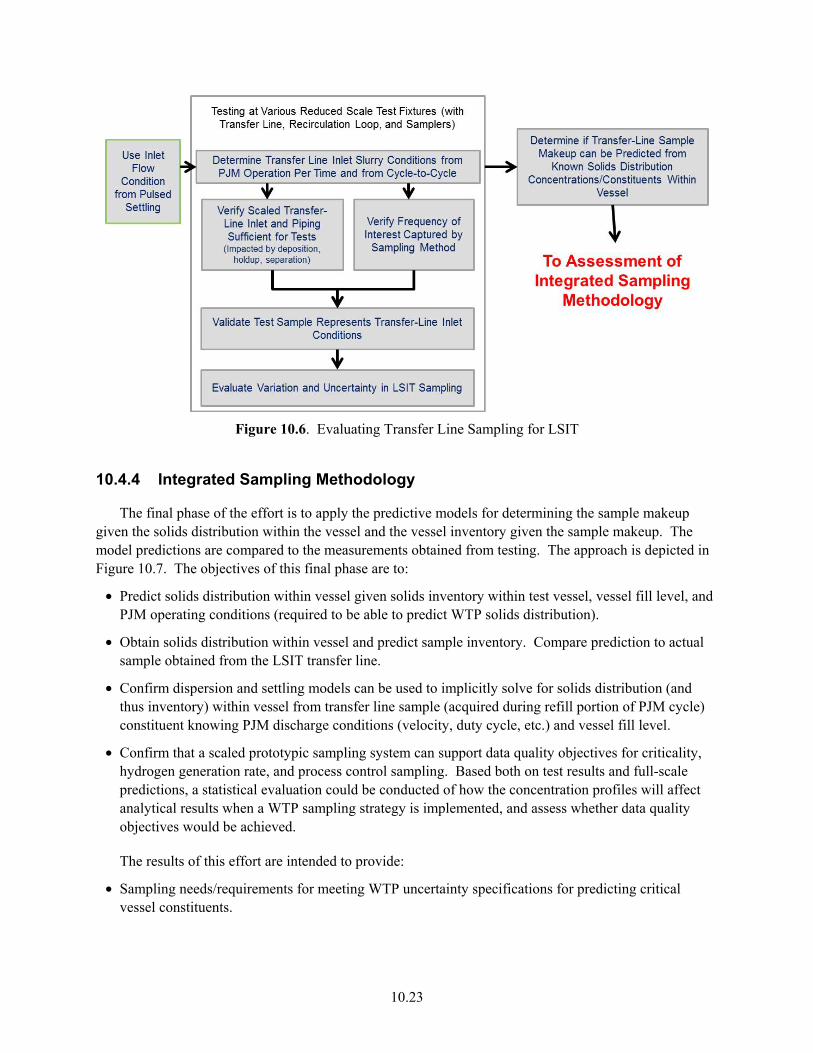
10.23

Figure 10.6. Evaluating Transfer Line Sampling for LSIT

10.4.4 Integrated Sampling Methodology

The final phase of the effort is to apply the predictive models for determining the sample makeup given the solids distribution within the vessel and the vessel inventory given the sample makeup. The model predictions are compared to the measurements obtained from testing. The approach is depicted in Figure 10.7. The objectives of this final phase are to:

• Predict solids distribution within vessel given solids inventory within test vessel, vessel fill level, and PJM operating conditions (required to be able to predict WTP solids distribution).

• Obtain solids distribution within vessel and predict sample inventory. Compare prediction to actual sample obtained from the LSIT transfer line.

• Confirm dispersion and settling models can be used to implicitly solve for solids distribution (and thus inventory) within vessel from transfer line sample (acquired during refill portion of PJM cycle) constituent knowing PJM discharge conditions (velocity, duty cycle, etc.) and vessel fill level.

• Confirm that a scaled prototypic sampling system can support data quality objectives for criticality, hydrogen generation rate, and process control sampling. Based both on test results and full-scale predictions, a statistical evaluation could be conducted of how the concentration profiles will affect analytical results when a WTP sampling strategy is implemented, and assess whether data quality objectives would be achieved.

The results of this effort are intended to provide:

• Sampling needs/requirements for meeting WTP uncertainty specifications for predicting critical vessel constituents.

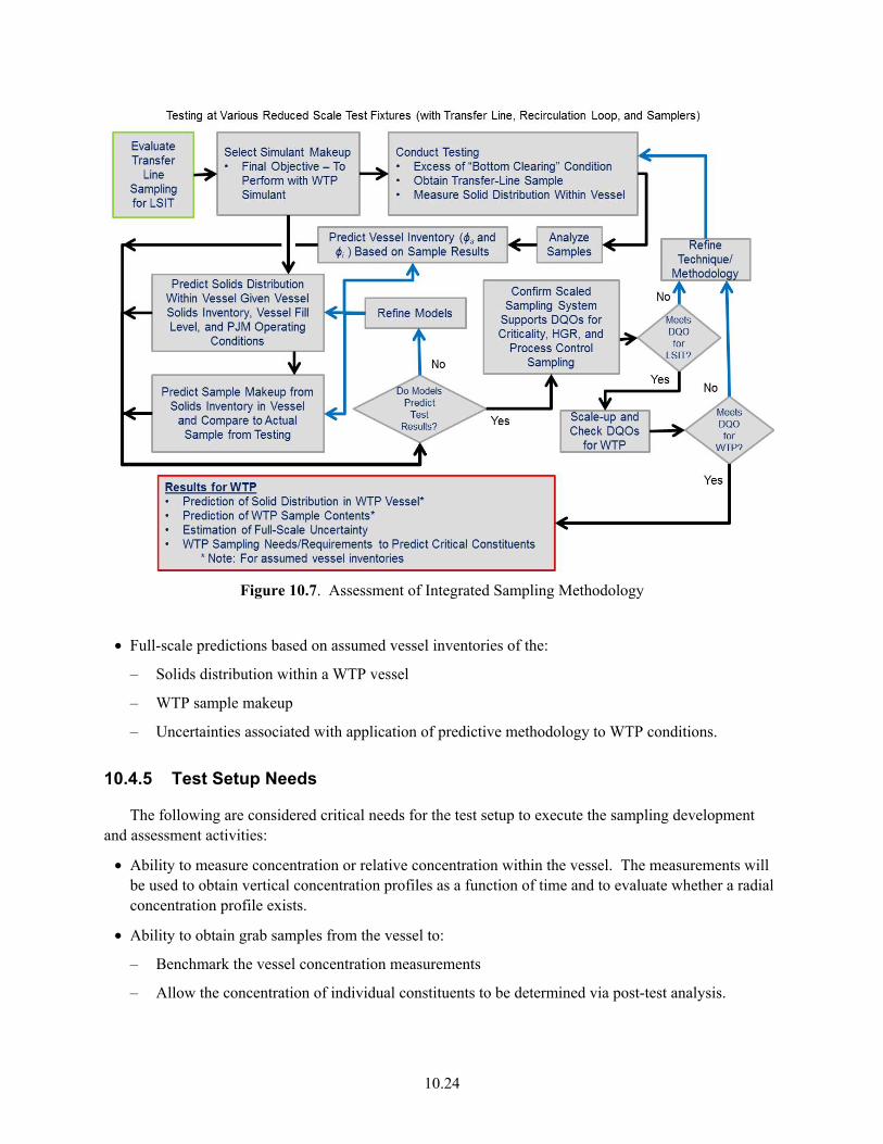
10.24

Figure 10.7. Assessment of Integrated Sampling Methodology

• Full-scale predictions based on assumed vessel inventories of the:

– Solids distribution within a WTP vessel

– WTP sample makeup

– Uncertainties associated with application of predictive methodology to WTP conditions.

10.4.5 Test Setup Needs

The following are considered critical needs for the test setup to execute the sampling development and assessment activities:

• Ability to measure concentration or relative concentration within the vessel. The measurements will be used to obtain vertical concentration profiles as a function of time and to evaluate whether a radial concentration profile exists.

• Ability to obtain grab samples from the vessel to:

– Benchmark the vessel concentration measurements

– Allow the concentration of individual constituents to be determined via post-test analysis.

10.25

• The same transfer line concentration measurements required for the LSIT effort supporting the prevent plugging assessment, refer to Section 6.3.1. The concentration measurements will also be used to assess variation in the concentration profile with distance down the transfer line. This assessment will be qualitative for each test setup. The assessment may be better served by obtaining transfer line samples from two different distances from the inlet locations to evaluate the impact on transfer line flow on the lateral solids distribution (i.e., concentration gradient as a function of distance) within the flow stream.

10.4.6 Simulant Needs

The bulk of this document has presented methods of scaling or conducting tests regardless of the simulants employed for testing. The assumption is that simulants will be developed to represent the WTP process stream for each vessel evaluated. However, because the development effort for sampling will need to generate a predictive scheme, simulant components will need to be selected that allow a buildup in complexity of the simulant makeup as development/testing progresses. It is assumed that constituents should be selected to represent:

• Base simulant constituents for representing co-precipitated Pu, Al, Cr, and separable Pu

– It is recommended the size distribution of the base constituents be relatively tight, preferably with minimal overlap

– Additional materials of the same constituents should be obtained that can be used as additives to increase the size distribution of each of the base constituents

• Number of additives to represent other UDS so that uncertainty in results can be assessed for variations in mixture of UDS.

For this portion of the test effort, the program should be prepared to work with simulant makeups that do not represent WTP process streams but instead allow model parameters to be exercised and sensitivity evaluations to be conducted.

10.5 Conclusions, Recommendations, and Issues

As stated in Section 10.1, the functional requirements for all the mixing requirements are the same. Based on the WTP functional mixing requirements, “… The PJM mixing system shall mix the slurry to ensure the process control requirements are met and a representative sample can be obtained...” (Mauss and Papp 2010, Table 2, p. 22). However, based on past test data, some vessels may never be mixed to a degree that will allow a representative sample of the vessel contents to be drawn. Therefore, an approach has been outlined to use the sample to predict the vessel contents.

For assessments based on the liquid fractions of the samples (e.g., dissolved solids), concentrations in the vessel can be determined if the mixing requirements for blending are achieved.

For the solids, if the constituent concentration at the bottom of vessel can be predicted as a function of time for the period between PJM discharges, vessel inventories should be predictable from sample concentrations. The approach would use physical models and would require an implicit solution of the

10.26

concentration profiles as a function of time between PJM pulses. The additional challenge is to obtain predictions within ±10 percent of the bulk concentration for each constituent of interest.

The models developed to assess Mixing Requirement 10, Limit Solids Accumulation, were formulated to predict solids transport throughout the vessel and into the transfer line. The models need to be formulated in a solution scheme and refined to determine the material characteristics best applied for predicting solids behavior. However, attaining this ability constitutes a significant development effort. No past work was identified that uses pipeline samples to predict vessel contents for a periodic flow condition consisting of numerous solid constituents that could have size and density ranges that vary by four and two orders of magnitude, respectively.

Consideration was given to developing a bounding sampling approach to assess the separable plutonium. With respect to dynamic sampling, a recommendation was made to consider conducting sampling operations in phase with time during PJM refill to simplify the modeling and scale-up tasks.

The scope of this document is not associated with LSIT sample validation testing to design the WTP sampling system and sampling strategy (i.e., timing of sampling). The contribution of the scaled testing will be to determine the concentration versus time profiles in the vessel at the location where the process stream is withdrawn (transfer line inlet) for simulants representing fissile and other vessel constituents of the waste feed slurry. The LSIT also will build a methodology to predict the concentrations of these materials at full-scale conditions based on testing at a smaller scale. The test setup, test approach, and sample analysis need be designed to allow more than one methodology or model refinement to be evaluated simultaneously.

Additional factors that can have a significant impact on approach include:

• Spargers – The operation of spargers will eliminate the period of quiescent settling corresponding to the PJM refill phase and will affect the local rheology. Operating spargers also impact scaling as the spargers need to be scaled for bottom motion, particle dispersion, and solids settling. These combined factors may result in the only solution being testing at full-scale conditions.

• Non-Newtonian behavior – The rheology can have a significant impact on the particle settling rate.

• Air/gas entrainment – The entrainment and holdup of gas can impact the settling rate.

11.1

11.0 Conclusions

This document addresses extrapolating the performance of PJM-mixed vessels from three reduced scales in LSIT to the performance of full-scale WTP vessels. This involves “scaling down” from WTP conditions to LSIT test conditions, testing in LSIT at reduced scale, and “scaling up” LSIT performance to predict WTP performance, as described in Section 3.1. There are multiple physical phenomena involved, and the mixing system is complex (Section 2.1); however, fundamental laws of fluid dynamics, pertinent studies published in the literature, and experience with small-scale PJM systems are available as resources from which to develop a technical basis for scaling PJM performance (Section 2.2). The mixing performance is defined in terms of mixing requirements defined by the WTP project (Section 1.5). Considering the multiple requirements and scaling approaches, decisions about implementing alternative test strategies need to be made and will be described in greater detail in a companion to this document (Section 1.6). Unambiguous, measureable performance metrics are defined for each requirement that can be “scaled up” using a combination of scaling approaches described in Section 3.2, as is summarized immediately below.

11.1 Metrics

We conclude that the performance of the WTP relative to specific mixing requirements must be evaluated in terms of unambiguous quantities that can be measured in LSIT and extrapolated to WTP. In the following subsections, we describe these metrics.

11.1.1 Mix to Release Gas

The requirement that gas not accumulate in solids is met when the settled solids are sufficiently disturbed during a PJM cycle so that gas bubbles are released. The fraction of solids disturbed is difficult to quantify. However, the solids obviously have been disturbed if they have been suspended for even a short duration; if they are cleared from the bottom, they have been at least briefly suspended, and the fraction of the bottom of an LSIT vessel cleared of solids can be viewed through a transparent vessel floor. Therefore, we conclude the metric for mixing to release gas from settled solids should be the fraction of solids cleared during a PJM pulse. Further, we conclude that all of the solids should be cleared during a PJM pulse; that is, the mixing requirement for gas release is met if the metric equals 100 percent.

11.1.2 Blend Liquids

The requirement for blending is that a liquid is blended into the vessel to within a specific amount of homogeneity within a prescribed amount of time. The homogeneity and time can be specific to a vessel. The metric is the time to blend for the specified homogeneity for a specified vessel.

11.1.3 Limit Solids Accumulation

The requirement is that solids not accumulate in vessels over multiple pump-down cycles. The performance metric is the mass of solids species of interest that accumulate during a pump-down test in LSIT.

11.2

11.1.4 Sampling

The functional requirements for all the sampling-related mixing requirements are the same. As stated in the WTP functional mixing requirements, “... the PJM mixing system shall mix the slurry to ensure the process control requirements are met and a representative sample can be obtained” (Mauss and Papp 2010, Table 2, p. 22). The sampling strategy for WTP still is being developed. The document Integrated Sampling and Analysis Requirements Document (ISARD), 24590-WTP-PL-PR-04-0001, Rev. 2, was issued in 2008 (Dodd and Arakali 2008), and provides the basis for the requirements considered in this report (see Table 10.1). The assumed process is for the samples to be drawn from the transfer line when the system is operating in recirculation mode. Therefore, no pump-out operations occur, and a periodic condition will exist within the vessel.

The performance of a sampling system is the degree to which the sample represents the vessel contents through some relationship validated by LSIT testing. Therefore, the performance metric is the ratio (or difference) of the mass of a species in the tank compared to the mass predicted from a sample taken from the composition measured at the inlet to the transfer line. The WTP project specified that this document consider only the representativeness of the concentration entering the transfer line and not the accuracy of the WTP sampling process in determining that concentration. The latter will be considered in other documents. Sampling methods specific to LSIT will be developed as necessary to obtain an accurate sample of the slurry entering the transfer line. The performance metric is based on this concentration.

11.1.5 Prevent Plugging

The requirement is that mixing is sufficient to prevent plugging from occurring in the transfer line. WTP has specified design limits for slurry viscosity and density in the transfer line that are intended to serve as bounding conditions to ensure that pump failure and pipe plugging do not occur. After considering the difficulties in scaling plugging, solids deposition and pressure drop were chosen as necessary metrics to assess the potential for line plugging in a flow evaluation loop representing the horizontal portion of the transfer line from WTP vessels. These metrics are measured in the flow evaluation loop when concentrations are imposed to represent those at the inlet to the WTP transfer line, which are determined from scaled tests and sampling of the concentration versus time at the inlet to the transfer line for integrated LSIT tests (see Section 11.3.5 and Section 6.3.1). In addition, the static head within the vessel at the transfer line elevation is measured. The pump performance at a delivered head as a function of flow rate for bounding slurry conditions is measured for a full-scale pump.

11.2 Scale-Down

Conditions in the WTP pertinent to mixing performance relative to each requirement must be represented by corresponding conditions in LSIT sufficient to be able to relate the performance of the two systems. This is “scaling down” from WTP to LSIT (see Section 3.1.1). We conclude that the following conditions should be imposed for LSIT tests for all mixing requirements.

• Geometric similitude should be maintained (see Section 2.2.1.2) between LSIT and WTP in the ratio of tank diameter (the length scale) to:

– PJM nozzle diameter

– Distance from the PJM nozzle to the vessel floor

11.3

– Distance from the transfer line inlet to the vessel floor

– Initial depth of slurry in the vessel

• The same solids volume fraction in LSIT as in WTP

• Kinematic similitude (see Section 2.2.1.2) should be maintained between LSIT and WTP by making the following parameters the same:

– Dimensionless cycle time, UtC/D, where U is the PJM velocity, tC is the cycle time, and D is the tank diameter

– The ratio of PJM drive time to total cycle time

– The ratio of volumetric flow rate into the transfer line to characteristic flow rate UD2

• Dynamic similitude should be maintained (see Section 2.2.1.2) between LSIT and WTP where practicable, including the average solids density (see Section 2.2.1.5).

At least two important aspects of dynamic similitude cannot or should not be matched as described below:

• The Froude number based on the PJM velocity can be matched, but it is more important first to ensure that the PJM velocity exceeds the bottom clearing velocity. The effect of velocities greater than this can be measured and analyzed in terms of the Froude number at the length scale of the experiment.

• The ratio of the PJM velocity to the settling velocity volume-averaged over the particle size density distribution of the LSIT simulant is important for solids species that settle appreciably but not so fast that they settle completely before the end of each PJM cycle.

Other conclusions about conditions for “scaling down” that are specific to individual mixing requirements are discussed in the following sections.

11.2.1 Mix to Release Gas

No additional requirements.

11.2.2 Blend Liquids

No additional requirements.

11.2.3 Limit Solids Accumulation

The concentration of solids species entering the transfer line varies sharply during each PJM pulse (see Sections 5.3.1 and 10.2). This results from two processes: 1) during a PJM pulse, the radial wall jet from the PJM sweeps solids from the vessel floor to the transfer line inlet, and 2) during PJM refill, solids settling from above are captured by the flow rate into the transfer line inlet. The flow rate into the transfer line must be scaled in two different ways to make the concentration of solids at the inlet to the LSIT transfer line represent those in the WTP for these two different processes (see Section 5.6).

11.4

11.2.4 Sampling

See conditions for Section 11.2.3 and Section 10.2 for a presentation of the sampling problem.

11.2.5 Prevent Plugging

For LSIT, see conditions for Section 11.2.3. See Sections 6.3.1 and 6.3.2 for an explanation of the strategy for separating tests in a flow evaluation loop from integrated tests in LSIT. For evaluations of solids deposition and pressure drop in a flow evaluation loop, see Sections 6.4.1 and 6.4.2.

11.3 Testing

Four categories of testing are required to implement the technical basis for scaling presented in this document:

1. Integrated tests (i.e., LSIT) of selected WTP vessels that include recirculation or pump down through a transfer line, used for all mixing requirements

2. A flow evaluation loop to test for solids deposition and pressure drop across the portion of the pipe loop simulating the transfer line, used only for the Prevent Plugging requirement

3. LSIT tests involving specialized simulants to explore the effects of settling velocity in a vessel or solids deposition in a transfer line and effects of macroscopic density variations (variations in Froude number)

4. Supplemental tests that can range from measuring the rheology and settling behavior of complex simulants to measuring the erosion resistance of beds of settled solids to testing specific PJM behavior in simplified systems.

Because the LSIT simulant will be complex, its solid particles will exhibit a wide range of settling velocities. Some particles will settle slowly enough that they can be considered to not settle and to be essentially part of the liquid in which other particles settle, thereby affecting the liquid density and rheology. Some particles will settle fast enough that all will settle during a PJM pulse at any scale for practical PJM refill times. Thus, there will be some remaining fraction of particles whose settling velocities determine the fraction of solids that settle and must be resuspended during each PJM cycle. A volume-averaged settling velocity can be defined for such solids as a basis for scaling analyses (Section 2.2.1.5 and Appendix A, Section A.5).

Integrated testing for all mixing requirements begins with establishing the minimum velocity for clearing solids from the vessel floor during each PJM drive period (Section 4.3), while maintaining kinematic similitude as described in Section 11.2. This should be established for a given vessel geometry, LSIT simulant, waste loading, and duty cycle. Because dynamic similitude—defined in terms of Froude number and ratio of average settling velocity to PJM velocity—cannot be matched to corresponding WTP values for all LSIT tests, the effect of departures of these values from those for similitude need to be evaluated in supplemental tests with specialized simulants. Tracers can be included during such tests to evaluate the blend time (see Chapter 9).

11.5

11.3.1 Mix to Release Gas

In addition to testing described in Section 11.3, supplemental tests are needed to determine the erosion resistance of settled solids beds by wall jets imposed on the vessel flow by PJMs (Section 4.2 and Appendix B).

11.3.2 Blend Liquids

We expect blending will be adequately addressed by including appropriate instrumentation in tests described above in Section 11.3.1, with additional recommendations described in detail in Section 9.3.

11.3.3 Limit Solids Accumulation

LSIT tests similar to those described in Section 11.3 must be continued while pumping down the vessel through the transfer line. This needs to be repeated to measure any accumulation of solids in the vessel over multiple pump-down cycles (see Section 5.2).

11.3.4 Sampling

LSIT tests similar to those described in Section 11.3 need to be repeated for two methods of scaling the volumetric flow rate in the transfer line as explained in Sections 5.6 and 5.7 for the purpose explained in Section 10.2.

11.3.5 Prevent Plugging

Tests described in Section 11.3.4 are required for the purpose explained in Section 6.0. In addition, testing in a flow evaluation loop is required for the purposes explained in Sections 6.3 and 6.4.

11.4 Measurements

For all tests, the initial conditions in the test vessel need to be measured, including slurry composition and volume. The operating conditions need to be measured for all tests, including the PJM drive and refill times, the PJM velocity, and the volumetric flow rate into the transfer line for both the recirculation mode of operation and pump-down tests.

For LSIT testing, measurements required to address specific mixing performance metrics and to evaluate models or enable regression analyses should be coordinated and integrated into LSIT. Some tests done to address one mixing requirement might also serve to address other requirements if the instrumentation included in the test provides data pertinent to multiple requirements. An obvious example is to add miscible tracers and instruments to monitor them to assess blending in tests done primarily to determine the bottom clearing velocity.

11.6

11.4.1 Mix to Release Gas

The principal measurement is the fraction of the vessel bottom cleared of settled solids at the end of the drive portion of a PJM cycle, augmented by the fraction cleared versus time during the drive portion and the thickness of the settled layer at the start of the drive portion.

11.4.2 Blend Liquids

The principal measurement is the concentration of a soluble tracer determined at several locations in the tank over many PJM cycles until the concentrations are nearly uniform. This is for the purpose of quantifying the blend time as defined for specific tanks.

11.4.3 Limit Solids Accumulation

The principal measurement is the mass of solids of interest at the start and end of a pump-down test (Sections 5.2 and 5.3). This measurement allows the development of models or correlations explaining and predicting the observed mass accumulation (Section 5.5). One must also continuously measure the density of the slurry entering the transfer line continuously with time, obtain samples of the slurry entering the transfer line at frequent sample times, and measure the vertical profiles of solids in the vessel as a function of time at several horizontal locations (e.g., using instrumentation employed successfully during M3 Phase 1 testing; see Sections 2.2.2.3 and 2.2.3.2).

11.4.4 Sampling

All of the measurements of Section 11.4.3 are required, but not during pump-down tests.

11.4.5 Prevent Plugging

All of the measurements of Section 11.4.3 are required. In addition, in a flow evaluation loop, solids deposition and the pressure drop in the transfer line portion of the pipe loop must be measured as described in Section 6.5.

11.5 Analysis

Although the same tests can provide data from simultaneous data acquisition from multiple sets of instrumentation, the data need to be analyzed specific to each of the different categories of mixing requirements.

11.5.1 Mix to Release Gas

Data need to be analyzed and compared to adaptation of existing models for the effect of wall jets on erosion of settled solids (see Section 4.2).

11.7

11.5.2 Blend Liquids

The basis for analyzing blending data is described in detail in Section 9.2.

11.5.3 Limit Solids Accumulation

The basis for analyzing data on mass accumulation is described in detail in Sections 5.3, 5.4, and 5.5. This should include a comparison of results from integrated tests using specialized simulants and from supplemental tests of specific phenomena, such as settling.

11.5.4 Sampling

A detailed strategy for analyzing data for the mixing requirements for sampling is presented in Section 10.3.

11.5.5 Prevent Plugging

A detailed strategy for analyzing data taken in a flow evaluation loop is presented in Section 6.3 (see especially Figures 6.4 and 6.5) and Section 6.4.

11.6 Scale-Up

Performance metrics measured in LSIT vessels must be related quantitatively to the performance of the corresponding full-scale WTP vessels. This is “scaling up” from LSIT to WTP (see Section 3.1.2). We conclude that scaling down, testing, and scaling up provide a technical basis specific to performance metrics for each category of mixing requirement, as is presented in the following sections.

11.6.1 Mix to Release Gas

The PJM velocity at which the performance metric, fraction of bottom cleared, attains its specified value, assumed here to be 100 percent, should be correlated or modeled based on data from the testing described in Section 11.3.1. We expect scale-up to be done using regression analysis to evaluate coefficients in models based on the theory presented and explained in Chapter 4.

11.6.2 Blend Liquids

The performance metric, the “blend time” described in Section 11.4.2, should be correlated or modeled based on data from the testing described in Section 11.3.2. We expect scaling up to be done by using regression analysis to evaluate coefficients in models based on the theory presented and explained in Chapter 9.

11.6.3 Limit Solids Accumulation

The performance metric, the accumulation of mass during multiple pump-down cycles described in Section 11.4.3, should be correlated or modeled based on data from the testing described previously in

11.8

Section 11.3.3. We expect scale-up to be done using regression analysis to evaluate coefficients in models based on the theory presented and explained in Chapter 5.

11.6.4 Sampling

See Section 10.3 for potential approaches for predicting vessel contents from samples taken from the transfer line based on testing done in a flow evaluation loop and from LSIT tests done to predict the concentrations entering the transfer line in WTP, as described in Section 11.3.4, which refers to the detailed discussion presented in Chapter 10.

11.6.5 Prevent Plugging

See Section 6.3 for a detailed approach to predicting pipe plugging in the transfer line from WTP vessels based on testing in a flow evaluation loop, and for a detailed approach to predicting the pressure drop in the transfer line from WTP vessels. The approach includes benchmarking existing models.

11.7 Scaling of Sparger Operations

Air spargers are deployed in a number of the vessels in the WTP Pretreatment Facility to supplement PJMs, thus creating “hybrid” mixing systems. The primary mixing work of air spargers results from the net vertical rise of sparge bubbles through relatively dense slurry and the resulting localized entrainment and bulk motion of slurry fluid. The sparger “mixing effectiveness” is a product of the “intensity of mixing” and the distribution of this “mixing energy” across the slurry contained in the vessel.

Process air is also used to purge the two-segment steam rings in a WTP Newtonian slurry process vessel (e.g., UFP-01). A primary purpose of this purge air is to clear and prevent backflow of waste slurry into the multiple orifices of the steam rings and the associated headers when steam is not flowing. While additional slurry mixing resulting from the use of purge air is a secondary benefit in the WTP vessels, it is an important, and perhaps the most important, consideration for scaling steam ring systems in the LSIT vessels.

To be conservative, steam ring air sparger operating conditions for bottom motion studies in LSIT vessels should be selected so that the local mixing effect and nozzle velocities in the bottom region of the vessel are not greater than in the WTP vessels. For blending studies, the goal should be to provide comparable purge air-induced overall vessel mixing, from the steam ring nozzles located toward the bottom of the vessel to the slurry surface.

Specific steam ring purge air flow rate recommendations and other important details are discussed in Chapter 7, Section 9.4, and Appendix D. Other than controlling and measuring the purge air flow rate, there are no additional measurements required to those noted in Section 11.4 for vessels employing sparge or purge air. Rather, the purpose of scaling down sparger operations is to create WTP-representative conditions in the LSIT vessels for other requirements (e.g., PJM bottom clearing [gas release] and blending) to be evaluated.

11.9

11.8 Summary of Technical Strategies

The technical strategies for complying with the mixing requirements are summarized in Table 11.1.

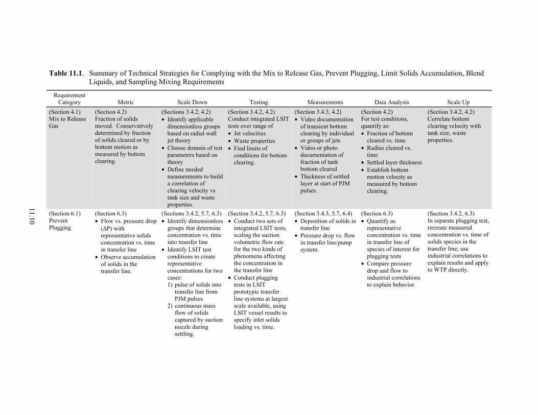
11.10

Table 11.1. Summary of Technical Strategies for Complying with the Mix to Release Gas, Prevent Plugging, Limit Solids Accumulation, Blend Liquids, and Sampling Mixing Requirements

Requirement Category Metric Scale Down Testing Measurements Data Analysis Scale Up

(Section 4.1) Mix to Release Gas

(Section 4.2) Fraction of solids moved. Conservatively determined by fraction of solids cleared or by bottom motion as measured by bottom clearing.

(Sections 3.4.2, 4.2) • Identify applicable

dimensionless groups based on radial wall jet theory

• Choose domain of test parameters based on theory

• Define needed measurements to build a correlation of clearing velocity vs. tank size and waste properties.

(Section 3.4.2, 4.2) Conduct integrated LSIT tests over range of • Jet velocities • Waste properties • Find limits of

conditions for bottom clearing.

(Section 3.4.3, 4.2) • Video documentation

of transient bottom clearing by individual or groups of jets

• Video or photo documentation of fraction of tank bottom cleared

• Thickness of settled layer at start of PJM pulses.

(Section 4.2) For test conditions, quantify as: • Fraction of bottom

cleared vs. time • Radius cleared vs.

time • Settled layer thickness • Establish bottom

motion velocity as measured by bottom clearing.

(Section 3.4.2, 4.2) Correlate bottom clearing velocity with tank size, waste properties.

(Section 6.1) Prevent Plugging

(Section 6.3) • Flow vs. pressure drop

(ΔP) with representative solids concentration vs. time in transfer line

• Observe accumulation of solids in the transfer line.

(Sections 3.4.2, 5.7, 6.3) • Identify dimensionless

groups that determine concentration vs. time into transfer line

• Identify LSIT test conditions to create representative concentrations for two cases: 1) pulse of solids into

transfer line from PJM pulses

2) continuous mass flow of solids captured by suction nozzle during settling.

(Section 3.4.2, 5.7, 6.3) • Conduct two sets of

integrated LSIT tests, scaling the suction volumetric flow rate for the two kinds of phenomena affecting the concentration in the transfer line

• Conduct plugging tests in LSIT prototypic transfer line systems at largest scale available, using LSIT vessel results to specify inlet solids loading vs. time.

(Section 3.4.3, 5.7, 6.4) • Deposition of solids in

transfer line • Pressure drop vs. flow

in transfer line/pump system.

(Section 6.3) • Quantify as

representative concentration vs. time in transfer line of species of interest for plugging tests

• Compare pressure drop and flow to industrial correlations to explain behavior.

(Section 3.4.2, 6.3) In separate plugging test, recreate measured concentration vs. time of solids species in the transfer line; use industrial correlations to explain results and apply to WTP directly.

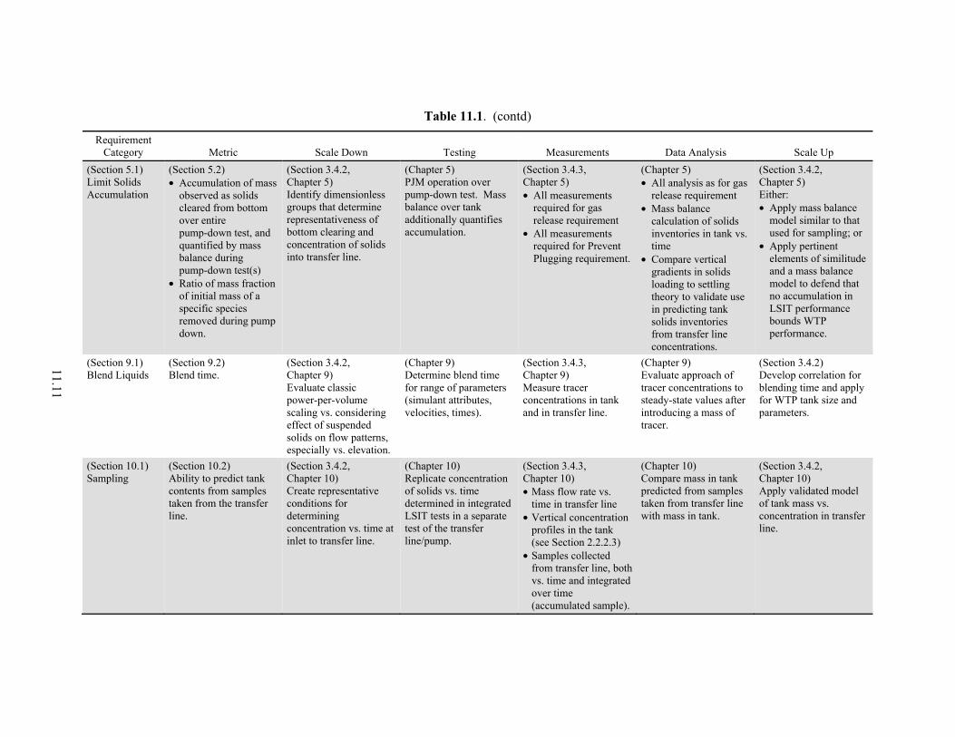
11.11

Table 11.1. (contd)

Requirement Category Metric Scale Down Testing Measurements Data Analysis Scale Up

(Section 5.1) Limit Solids Accumulation

(Section 5.2) • Accumulation of mass

observed as solids cleared from bottom over entire pump-down test, and quantified by mass balance during pump-down test(s)

• Ratio of mass fraction of initial mass of a specific species removed during pump down.

(Section 3.4.2, Chapter 5) Identify dimensionless groups that determine representativeness of bottom clearing and concentration of solids into transfer line.

(Chapter 5) PJM operation over pump-down test. Mass balance over tank additionally quantifies accumulation.

(Section 3.4.3, Chapter 5) • All measurements

required for gas release requirement

• All measurements required for Prevent Plugging requirement.

(Chapter 5) • All analysis as for gas

release requirement • Mass balance

calculation of solids inventories in tank vs. time

• Compare vertical gradients in solids loading to settling theory to validate use in predicting tank solids inventories from transfer line concentrations.

(Section 3.4.2, Chapter 5) Either: • Apply mass balance

model similar to that used for sampling; or

• Apply pertinent elements of similitude and a mass balance model to defend that no accumulation in LSIT performance bounds WTP performance.

(Section 9.1) Blend Liquids

(Section 9.2) Blend time.

(Section 3.4.2, Chapter 9) Evaluate classic power-per-volume scaling vs. considering effect of suspended solids on flow patterns, especially vs. elevation.

(Chapter 9) Determine blend time for range of parameters (simulant attributes, velocities, times).

(Section 3.4.3, Chapter 9) Measure tracer concentrations in tank and in transfer line.

(Chapter 9) Evaluate approach of tracer concentrations to steady-state values after introducing a mass of tracer.

(Section 3.4.2) Develop correlation for blending time and apply for WTP tank size and parameters.

(Section 10.1) Sampling

(Section 10.2) Ability to predict tank contents from samples taken from the transfer line.

(Section 3.4.2, Chapter 10) Create representative conditions for determining concentration vs. time at inlet to transfer line.

(Chapter 10) Replicate concentration of solids vs. time determined in integrated LSIT tests in a separate test of the transfer line/pump.

(Section 3.4.3, Chapter 10) • Mass flow rate vs.

time in transfer line • Vertical concentration

profiles in the tank (see Section 2.2.2.3)

• Samples collected from transfer line, both vs. time and integrated over time (accumulated sample).

(Chapter 10) Compare mass in tank predicted from samples taken from transfer line with mass in tank.

(Section 3.4.2, Chapter 10) Apply validated model of tank mass vs. concentration in transfer line.

12.1

12.0 References

Ayranci I, MB Machado, AM Madej, JJ Derksen, DS Nobes, and SM Kresta. 2012. “Effect of Geometry on the Mechanisms for Off-Bottom Solids Suspension in a Stirred Tank.” Chemical Engineering Science 79:163-176.

Baldi G, R Conti, and E Alaria. 1978. “Complete Suspension of Particles in Mechanically Agitated Vessels.” Chemical Engineering Science 33(1):21-25.

Bamberger JA, PA Meyer, JR Bontha, CW Enderlin, DA Wilson, AP Poloski, JA Fort, ST Yokuda, HD Smith, F Nigl, M Friedrich, DE Kurath, GL Smith, JM Bates, and MA Gerber. 2005. Technical Basis for Testing Scaled Pulse Jet Mixing Systems for Non-Newtonian Slurries. PNWD-3551; WTP-RPT-113, Rev. 0, Battelle–Pacific Northwest Division, Richland, Washington.

Bird RB, WE Stewart, and EN Lightfoot. 2002. Transport Phenomena, Second Edition. John Wiley & Sons, New York.

Bloomfield LJ and RC Kerr. 1999. “Turbulent Fountains in a Confined Stratified Environment.” Journal of Fluid Mechanics 389:27-54.

Bontha JR, CW Stewart, DE Kurath, PA Meyer, ST Arm, CE Guzman-Leong, MS Fountain, M Friedrich, SA Hartley, LK Jagoda, CD Johnson, KS Koschik, DL Lessor, F Nigl, RL Russell, GL Smith, W Yantasee, and ST Yokuda. 2005. Technical Basis for Predicting Mixing and Flammable Gas Behavior in the Ultrafiltration Feed Process and High-Level Waste Lag Storage Vessels with Non-Newtonian Slurries. PNWD-3676; WTP-RPT-132, Rev. 0, Battelle–Pacific Northwest Division, Richland, Washington.

Camenen B. 2007. “Simple and General Formula for the Settling Velocity of Particles.” Journal of Hydraulic Engineering – ASCE 133(2):229-233.

Cheremisinoff NP and R Gupta. 1983. Handbook of Fluids in Motion, pp. 544-558. Ann Arbor Science, Ann Arbor, Michigan.

Churchill SW. 1977. “Friction Factor Equation Spans all Fluid-Flow Regimes.” Chemical Engineering 84:91-92.

Crowe CT. 2006. MultiPhase Flow Handbook. CRC Press Taylor and Francis Group LLC, Boca Raton, Florida.

Darby R. 2001. Chemical Engineering Fluid Mechanics. Marcel Dekker, New York.

Darby R. 2000. “Pressure Drop for Non-Newtonian Slurries: A Wider Path.” Chemical Engineering 107(5):64-67.

Davies JJ. 1986. “Particle Suspension and Mass Transfer Roles in Agitated Vessels.” Chemical Engineering Progress 20:175-181.

12.2

Enderlin CW, MG Dodson, F Nigl, J Bontha, and JM Bates. 2003. Results of Small-Scale Particle Cloud Tests and Non-Newtonian Fluid Cavern Tests. PNWD-3360; WTP-RPT-078, Battelle–Pacific Northwest Division, Richland, Washington.

Fossett H and LE Prosser. 1949. “The Application of Free Jets to Mixing of Fluids in Bulk.” Proceedings of the Institution of Mechanical Engineers 160(1):224-232.

Gauglitz PA, BE Wells, JA Fort, and PA Meyer. 2009. An Approach to Understanding Cohesive Slurry Settling, Mobilization, and Hydrogen Gas Retention in Pulsed Jet Mixed Vessels. PNNL-17707, Pacific Northwest National Laboratory, Richland, Washington.

Gillies RG and CA Shook. 1991. “A Deposition Velocity Correlation for Water Slurries.” Canadian Journal of Chemical Engineering 69(5):1225-1228.

Govier GW and K Aziz. 1987. The Flow of Complex Mixtures in Pipe, pp. 160-161, 620-623. Robert Kreiger Publishing, Malabar, Florida.

Grenville RK, ATC Mak, and DAR Brown. 2010. “An Improved Correlation to Predict “Just Suspension” Speed for Solid-Liquid Mixing with Axial Flow Impellers in Stirred Tanks.” North American Mixing Forum, June 20-25, 2010, Victoria, Canada.

Hanks RW. 1980. “Slurry Pipeline Hydraulics: Principles, Problems and Solutions.” American Society of Mechanical Engineers (Paper), n 80 -Pet-45, 1980.

Hargrave GK, TC Williams, K Anandaraja, and NA Halliwell. 2006. “The 3D Velocity Field of an Impacting Turbulent Jet.” Journal of Physics: Conference Series 45:162-172.

Johnson MD, JR Bontha, and JM Bates. 2003. Demonstration of Ability to Mix in a Small-Scale Pulsed-Jet Mixer Test Facility. PNWD-3273; WTP-RPT-077, Battelle–Pacific Northwest Division, Richland, Washington.

Johnson MD, MA Gerber, JR Bontha, AP Poloski, RT Hallen, SK Sundaram, and DE Wallace. 2005. Hybrid Mixing System Test Results for Prototype Ultrafiltration Feed Process and High-Level Waste Lag Storage Vessels. PNWD-3586; WTP-RPT-128, Rev. 0, Battelle–Pacific Northwest Division, Richland, Washington.

Kosson DS, RV Calabrese, WC Gekler, RL Powell and SI Sandler. 2010. Letter to Shirley Olinger. July 1, 2010. Transmittal of CRESP Review Team Letter Report 7 – PJM Vessels, The Consortium for Risk Evaluation with Stakeholder Participation III.

Kuhn WL, ST Arm, JL Huckaby, DE Kurath, and SD Rassat. 2008. Technical Basis for Scaling Relationships for the Pretreatment Engineering Platform. PNNL-16948; WTP-RPT-160, Pacific Northwest National Laboratory, Richland, Washington.

Lamb H. 1945. Hydrodynamics. Reprint of original 1932 publication by Cambridge University Press, of the work first published in 1879, Dover Publications, New York. See article 229.

12.3

Meacham JE, SJ Harrington, JS Rodriguez, VC Nguyen, JG Reynolds, BE Wells, GF Piepel, SK Cooley, CW Enderlin, DR Rector, J Chun, A Heredia-Langner, and RF Gimpel. 2012. One System Evaluation of Waste Transferred to the Waste Treatment Plant. RPP-RPT-51652, Washington River Protection Solutions LLC, Richland, Washington.

Meyer PA, DE Kurath, and CW Stewart. 2005. Overview of the Non-Newtonian Pulse Jet Mixer Test Program. PNWD-3677; WTP-RPT-127, Rev. 0, Battelle–Pacific Northwest Division, Richland, Washington.

Meyer PA, JA Bamberger, CW Enderlin, JA Fort, BE Wells, SK Sundaram, PA Scott, MJ Minette, GL Smith, CA Burns, MS Greenwood, GP Morgan, EBK Baer, SF Snyder, M White, GF Piepel, BG Amidan, and A Heredia-Langner. 2009. Pulse Jet Mixing Tests With Noncohesive Solids. PNNL-18098; WTP-RPT-182, Rev. 0, Pacific Northwest National Laboratory, Richland, Washington.

Meyer PA, JA Bamberger, CW Enderlin, JA Fort, BE Wells, SK Sundaram, PA Scott, MJ Minette, GL Smith, CA Burns, MS Greenwood, GP Morgan, EBK Baer, SF Snyder, M White, GF Piepel, BG Amidan, and A Heredia-Langner. 2012. Pulse Jet Mixing Tests With Noncohesive Solids. PNNL-18098, Rev. 1; WTP-RPT-182, Rev. 1, Pacific Northwest National Laboratory, Richland, Washington.

Meyer PA, EBK Baer, JA Bamberger, JA Fort, and MJ Minette. 2010. Assessment of Differences in Phase 1 and Phase 2 Test Observations for Waste Treatment Plant Pulse Jet Mixer Tests with Non-Cohesive Solids. PNNL-19085, Rev. 0; WTP-RPT-208, Rev. 0, Pacific Northwest National Laboratory, Richland, Washington.

Molerus O. 1993. Principles of Flow in Disperse Systems. Chapman and Hall, London.

Ohshima S, T Takematsu, Y Kuriki, K Shimada, M Suzuki, and J Kato. 1976. “Liquid-Phase Mass Transfer Coefficient and Gas Holdup in a Packed-Bed Concurrent Up-Flow Column.” Journal of Chemical Engineering of Japan 9:29-34.

Oroskar AR and RM Turian. 1980. “The Critical Velocity in Pipelines Flow of Slurries.” AIChE Journal 26(4):550-558.

Partheniades E. 1965. “Erosion and Deposition of Cohesive Soils.” Journal of the Hydraulics Division, Proceedings of the American Society of Civil Engineers 91(1):105-139.

Paul EL, VA Atiemo-Obeng, and SM Kresta (eds.). 2004. Handbook of Industrial Mixing Science and Practice, pp. 52-57, 532-533. John Wiley & Sons, Inc., Hoboken, New Jersey.

Perry RH and CH Chilton (eds.). 1973. Chemical Engineers’ Handbook, Fifth Edition, Figure 3-45. McGraw-Hill, New York.

Phares DJ, GT Smedley, and RC Flagan. 2000. “The wall shear stress produced by the normal impingement of a jet on a flat surface.” Journal of Fluid Mechanics 418:351-375.

12.4

Poloski AP, HE Adkins, J Abrefah, J Chun, AM Casella, F Nigl, MJ Minette, RE Hohimer, ST Yokuda, JM Tingey, and JJ Toth. 2009a. Deposition Velocities of Newtonian and Non-Newtonian Slurries in Pipelines. PNNL-17639; WTP-RPT-175, Rev. 0, Pacific Northwest National Laboratory, Richland, Washington.

Poloski AP, HE Adkins, ML Bonebrake, J Chun, AM Casella, KM Denslow, MD Johnson, ML Luna, PJ MacFarlan, JM Tingey, and JJ Toth. 2009b. Deposition Velocities of Non-Newtonian Slurries in Pipelines: Complex Simulant Testing. PNNL-18316; WTP-RPT-189, Rev. 0, Pacific Northwest National Laboratory, Richland, Washington.

Poloski AP, ST Arm, JA Bamberger, B Barnett, R Brown, BJ Cook, CW Enderlin, MS Fountain, M Friedrich, BG Fritz, RP Mueller, F Nigl, Y Onishi, LA Schienbein, LA Snow, S Tzemos, M White, and JA Vucelick. 2005. Technical Basis for Scaling of Air Sparging Systems for Mixing in Non-Newtonian Slurries. PNWD-3541; WTP-RPT-129, Rev. 0, Battelle–Pacific Northwest Division, Richland, Washington.

Poreh M, YG Tsuei, and JE Cermak. 1967. “Investigation of a Turbulent Radial Wall Jet.” Journal of Applied Mechanics June 1967:457-463.

Powell MP, Y Onishi, and R Shekkariz. 1997. Research on Jet Mixing of Settled Sludges in Nuclear Waste Tanks at Hanford and Other DOE Sites: A Historical Perspective. PNNL-11686, Pacific Northwest National Laboratory, Richland, Washington.

Rajaratnam N. 1976. Turbulent Jets, pp. 226-245. Elsevier Scientific Publishing Company, New York.

Richardson JF and WN Zaki. 1954. “Sedimentation and fluidisation. Part 1.” Transactions of the Institute of Chemical Engineers 32:35-53.

Saleh JM. 2002. “Two-Phase Flow: Liquid-Solid and Gas-Solid Flow.” In Fluid Flow Handbook, McGraw-Hill, New York.

Simon A, RE Thomas, AJC Collison, W Dickerson, and CV Alonso. 2002. Erodibility of Cohesive Streambeds in the Yalobusha River System. Research Report No. 26, National Sedimentation Laboratory, Channel and Watershed Processes Research Unit, Oxford, Mississippi.

Smith GL, AP Poloski, MW Rinker, RL Demmer, BE Lewis, and SL Marra. 2009. Slurry Retrieval, Pipeline Transport & Plugging and Mixing Workshop. PNNL-18751, Vol. 3, Pacific Northwest National Laboratory, Richland, Washington.

Srinarayana N, GD McBain, SW Armfield, and WX Lin. 2008. “Height and Stability of Laminar Plane Fountains in a Homogeneous Fluid.” International Journal of Heat and Mass Transfer 51:4717-4727.

Tennekes H and JL Lumley. 1992. A First Course In Turbulence. The MIT Press, Cambridge, Massachusetts.

Turian RM and T-F Yuan. 1977. “Flow of Slurries in Pipelines.” AIChE Journal 23(3):232-243.

12.5

Turian RM, FL Hsu, and MTW Ma. 1987. “Estimation of the Critical Velocity in Pipeline Flow of Slurries.” Powder Technology 51:35-47.

Wani GA, MK Sarkar, and BP Mani. 1982. “Critical-Velocity in Multisized Particle Transportation through Horizontal Pipes.” Journal of Pipelines 2:57-62.

Wasp EL, JP Kenny, and RL Gandhi. 1977. Solids Liquid Flow-Slurry Pipeline Transportation, 1st ed., Trans-Tech Publications, Clausthal, Germany.

Weast RC (ed.). 1973. CRC Handbook of Chemistry and Physics, 53rd Edition, p. D-214. CRC Press, Inc., Boca Raton, Florida.

Wells BE, PA Gauglitz, and DR Rector. 2011. Comparison of Waste Feed Delivery Small Scale Mixing Demonstration Simulant to Hanford Waste. PNNL-20637, Rev. 1, Pacific Northwest National Laboratory, Richland, Washington.

White FM. 1991. Viscous Fluid Flow. McGraw-Hill, Boston, Massachusetts.

Williamson N, SW Armfield, and WX Lin. 2011. “Forced Turbulent Fountain Flow Behaviour.” Journal of Fluid Mechanics 671:535-558.

Winokur PS. 2010. Letter to S Chu on December 17, 2010, “RECOMMENDATION 2010-2 TO THE SECRETARY OF ENERGY Pulse Jet Mixing at the Waste Treatment and Immobilization Plant Pursuant to 42 U.S.C. § 2286(a)(5) Atomic Energy Act of 1954, As Amended,” Defense Nuclear Facilities Safety Board, Washington D.C.

References Not Publicly Available

Barnes S. 2010. Plan for M3 Test Platform Testing. 24590-PTF-PL-PET-10-0001, Rev. 0, Bechtel National, Inc., Richland, Washington.

Campbell T. 2011. Integrated Pulse Jet Mixed Vessel Design and Control Strategy. 24590-WTP-RPT-ENG-10-001, Rev. 1, Bechtel National, Inc. Richland, Washington.

Campbell T, M Parker, A Moon, and B Fant. 2010a. EFRT Issue M3 PJM Vessel Mixing Assessment, Volume 7–UFP-01. 24590-WTP-RPT-ENG-08-021-07, Rev. 1, Bechtel National, Inc., Richland, Washington.

Campbell T, M Parker, A Moon, B Fant, K Clossey, and J Cook. 2010b. EFRT Issue M3 PJM Vessel Mixing Assessment, Volume 8—HLP-22. 24590-WTP-RPT-ENG-08-021-08, Rev 1, Bechtel National, Inc., Richland, Washington.

Chapman C and S Lehrman. 2010. Memorandum to Distribution for Transmittal of “M3 Platform Test Summary for HLP-22-NQA-007.” CCN 218353, Bechtel National, Inc., Richland, Washington.

Chu S. 2011. Letter to PS Winokur. November 10, 2011. Transmittal of Department of Energy Plan to Address Waste Treatment and Immobilization Plant Vessel Mixing Issues Rev. 0 Implementation Plan for Defense Nuclear Safety Board Recommendation 2010-2, U.S. Department of Energy, Washington, D.C.

12.6

Claghorn R and P Waddell. 2007. System Description for Pulse Jet Mixers and Supplemental Mixing Subsystems. 24590-WTP-3YD-50-00003, Rev. B, Bechtel National, Inc., Richland, Washington.

Dickey DS. 2010. Scaling of PJM Vessels Containing Settling Solids in Newtonian Slurries. TR-099, MixTech, Inc., Dayton, Ohio.

Dickey DS, RB Daniel, PJ Keuhlen, RL Hanson, and JW Olson. 2012. Technical Scaling Selection Basis. 24590-WTP-RPT-PET-12-001, Rev. A – Draft, Bechtel National, Inc., Richland, Washington.

Dodd DA and A Arakali. 2008. Integrated Sampling and Analysis Requirements Document (ISARD). 24590-WTP-PL-PR-04-0001, Rev. 2, Bechtel National, Inc., Richland, Washington.

Eager K. 2010. Revised Calculation of Hydrogen Generation Rates and Time to Lower Flammability Limit for WTP. 24590-WTP-M4C-V11T-00011, Rev. C, Bechtel National, Inc., Richland, Washington.

Edmonson A and S Thomson. 2010. M3 Platform Test Data Study. 24590-WTP-ES-PET-09-001, Rev. 0, Bechtel National, Inc., Richland, Washington.

Edwards R, C Myler, G Ashley, L Holton, D Alexander, and G Brunson. 2010. Technology Steering Group-Issue Closure Record – Partial Closure EFRT Issue M3 (Closure Package Volume 8, HLP-VSL-00022), Inadequate Mixing System Design. CCN 220454, Bechtel National, Inc., Richland, Washington.

Gebhardt M and K Clossey. 2011. Process Inputs Basis of Design (PIBOD). 24590-WTP-DB-PET-09-001, Rev. 1, Bechtel National, Inc., Richland, Washington.

Gimpel R. 2010. Slurry Property Ranges in Non-Newtonian Pretreatment Vessels at WTP. 24590-WTP-RPT-PET-10-014, Rev. 2, Bechtel National, Inc., Richland, Washington.

Hall MN. 2010. Minimum Flow Velocity for Slurry Lines. WTP Project Doc. No. 24590-WTP-GPG-M-0058, Rev 0, Bechtel National, Inc., Richland, Washington.

Hanson R and J Meehan. 2012. Vessel Configuration for Large Scale Integrated Testing. 24590-WTP-RPT-ENG-12-017, Rev. 0, Bechtel National, Inc., Richland, Washington.

Hinckley J. 2010. Preliminary Documented Safety Analysis To Support Construction Authorization; PT Facility Specific Information. 24590-WTP-PSAR-ESH-01-002-02, Rev. 4, Bechtel National, Inc., Richland, Washington.

Koopman DC, CJ Martino, and MR Poirier. 2012. Properties Important to Mixing for WTP Large Scale Integrated Testing. SRNL-STI-2012-00062, Revision 0, Savannah River National Laboratory, Aiken, South Carolina.

Kulp M. 2011. Preliminary Documented Safety Analysis To Support Construction Authorization; HLW Facility Specific Information. 24590-WTP-PSAR-ESH-01-002-04, Rev. 4w, Bechtel National, Inc., Richland, Washington.

12.7

Mauss J and I Papp. 2010. Determination of Mixing Requirements for Pulse-Jet-Mixed Vessels in the Waste Treatment Plant. 24590-WTP-ES-ENG-09-001, Rev. 2, Bechtel National, Inc., Richland, Washington.

Minette M. 2011. Test Plan for PNNL Support of Large Scale Testing. TP-WTPSP-027, Rev. 0, WTP Support Program at Pacific Northwest National Laboratory, Richland, Washington.

Morris A. 2010. Letter to NF Grover. December 22, 2010. “Contract Modification No. M199, Change Order for Large Scale Testing.” CCN 229346, U.S. Department of Energy, Richland, Washington.

Papp I. 2010a. EFRT Issue M3 PJM Vessel Mixing Assessment, Volume 3-HLP-VSL-00027A/B, HLP-VSL-00028, UFP-VSL-00002A/B, pp. A-76, A-221. 24590-WTP-RPT-ENG-08-021-03, Rev. 1, Bechtel National, Inc., Richland, Washington.

Papp I. 2010b. EFRT Issue M3 PJM Vessel Mixing Assessment, Volume 4-HOP-VSL-00903/904, PWD-VSL-00015/16, TCP-VSL-00001, TLP-VSL-00009A/B, RLD-VSL-00008, p. A-59. 24590-WTP-RPT-ENG-08-021-04, Rev. 1, Bechtel National, Inc., Richland, Washington.

Papp IG. 2010c. Test Objectives for Large Scale Testing (LST) for Increment I. 24590-WTP-RTD-RT-10-0002, Rev. 1, Bechtel National, Inc., Richland, Washington.

Papp IG. 2011. Memorandum to GM Duncan. March 11, 2011. “LSIT Workshop – Stakeholder Disposition and LSIT Test Objectives.” CCN 225791, Bechtel National, Inc., Richland, Washington.

Rassat SD. 2007. A Scaling Approach for Full Scale Sparger Operations in the UFP2 Vessel. WTP-RPT-162, Rev. 0, Pacific Northwest National Laboratory, Richland, Washington.

Appendix A –

Selected Technical Background

A.iii

Acronyms and Abbreviations

HLP high-level process (tank)

LSIT Large Scale Integrated Testing

PJM pulse jet mixer

PSDD particle size and density distribution

RLD radioactive liquid-waste disposal (tank)

UFP ultrafiltration process (tank)

WTP Hanford Waste Treatment and Immobilization Plant

Symbols

A flow cross-sectional area

Ar Archimedes number for the solid particle; ratio of buoyant (gravitational) to viscous stresses

aτ constant

A0 flow cross-section at the start of the jet

C constant of integration

Ci an empirical constant

CD drag coefficient

D tank diameter

DC duty cycle

d nozzle diameter

dJ nozzle diameter

dS diameter of solid particle, particle size

E(κ) energy spectrum

F force acting to slow the jet

f , fw, fδ, fτ function

F(δ, s) cumulative probability that particles will have attributes less than the specified values

FD drag force

Fr Froude Number, ratio of inertial stress to gravitational stress acting on a fluid with inhomogeneous solids distribution

f(φS) correction for hindered settling

g acceleration of gravity

H jet offset above tank floor

HL height of liquid in tank

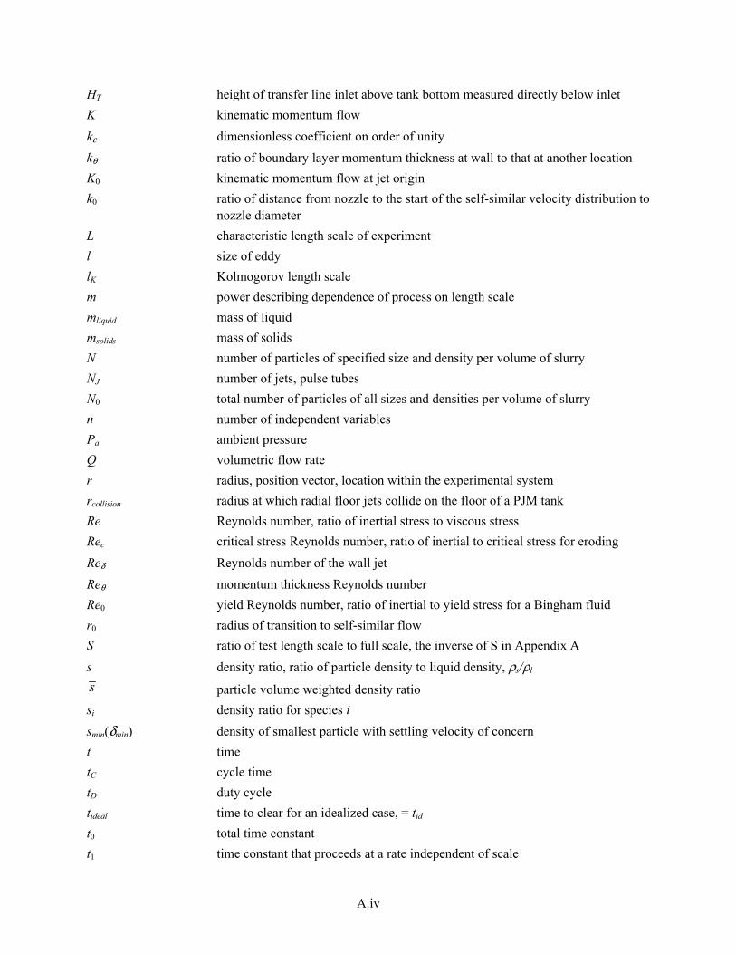
A.iv

HT height of transfer line inlet above tank bottom measured directly below inlet

K kinematic momentum flow

kε dimensionless coefficient on order of unity

kθ ratio of boundary layer momentum thickness at wall to that at another location

K0 kinematic momentum flow at jet origin

k0 ratio of distance from nozzle to the start of the self-similar velocity distribution to nozzle diameter

L characteristic length scale of experiment

l size of eddy

lK Kolmogorov length scale

m power describing dependence of process on length scale

mliquid mass of liquid

msolids mass of solids

N number of particles of specified size and density per volume of slurry

NJ number of jets, pulse tubes

N0 total number of particles of all sizes and densities per volume of slurry

n number of independent variables

Pa ambient pressure

Q volumetric flow rate

r radius, position vector, location within the experimental system

rcollision radius at which radial floor jets collide on the floor of a PJM tank

Re Reynolds number, ratio of inertial stress to viscous stress

Rec critical stress Reynolds number, ratio of inertial to critical stress for eroding

Reδ Reynolds number of the wall jet

Reθ momentum thickness Reynolds number

Re0 yield Reynolds number, ratio of inertial to yield stress for a Bingham fluid

r0 radius of transition to self-similar flow

S ratio of test length scale to full scale, the inverse of S in Appendix A

s density ratio, ratio of particle density to liquid density, ρs/ρl

s particle volume weighted density ratio

si density ratio for species i

smin(δmin) density of smallest particle with settling velocity of concern

t time

tC cycle time

tD duty cycle

tideal time to clear for an idealized case, = tid

t0 total time constant

t1 time constant that proceeds at a rate independent of scale

A.v

t2 time constant that proceeds at a rate that depends on scale

U velocity

u characteristic velocity of experiment

u fluctuating component of velocity

u average settling velocity

u0 particle unhindered settling velocity 0u particle volume average unhindered settling velocity

ui0

unhindered settling velocity for species “i”

UT unhindered particle terminal settling velocity 0Tiu unhindered settling velocity for species with density ratio si and velocity ui

0

( )z ,tu settling velocity of the distribution of particles at elevation, z, and time, t

u(δ,s) settling velocity of particles of size and density ratio

u∞ the steady-state fluid velocity

VS volume of solids, volume of particles

V volumetric flow rate of jet

SV rate of addition of the volume of particles

x(δ,s) volume fraction of solid volume

xi fraction of total particle volume due to specified particle

z distance along the jet

z0 distance along jet at which self-similarity begins

Greek Symbols

αij empirical powers

γ ratio of jet thickness to nozzle radius at origin, δ0/r0

Δm mass

Δρ density difference

δ thickness of jet, thickness of wall jet; specified value

δmin smallest particle with settling velocity of concern

δθ boundary layer momentum thickness at the wall

ε power dissipation per mass

θi a dimensionless form of a dependent performance metric

θϕ parameters

κ wave number

μ viscosity

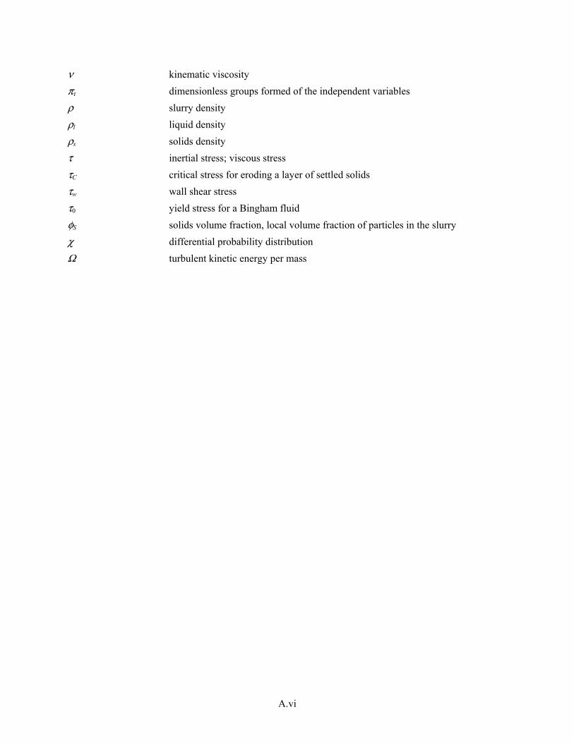
A.vi

ν kinematic viscosity

πι dimensionless groups formed of the independent variables

ρ slurry density

ρl liquid density

ρs solids density

τ inertial stress; viscous stress

τC critical stress for eroding a layer of settled solids

τw wall shear stress

τ0 yield stress for a Bingham fluid

φS solids volume fraction, local volume fraction of particles in the slurry

χ differential probability distribution

Ω turbulent kinetic energy per mass

A.vii

Contents

Acronyms and Abbreviations ............................................................................................................... A.iii Symbols ................................................................................................................................................ A.iii Greek Symbols ...................................................................................................................................... A.v A.1 Similitude .................................................................................................................................... A.1 A.2 Dimensional Analysis ................................................................................................................. A.3 A.3 Similitude and Dimensional Analysis for Submerged Jets ......................................................... A.5 A.4 Conditions for Full Similitude .................................................................................................... A.9 A.5 Scaling Basis for Particle Size Distributions ............................................................................... A.11 A.6 Turbulent Velocity at the Size of a Particle ................................................................................ A.16 A.7 Scaling Approaches ..................................................................................................................... A.18

A.7.1 Pure Similitude ............................................................................................................... A.19 A.7.1.1 Attributes of Pure Similitude ......................................................................... A.19 A.7.1.2 Use in Scaling Down ..................................................................................... A.20 A.7.1.3 Use in Scaling Up .......................................................................................... A.20 A.7.1.4 Addressing Uncertainty ................................................................................. A.20

A.7.2 Pure Statistics ................................................................................................................. A.20 A.7.2.1 Use in Scaling Down ..................................................................................... A.22 A.7.2.2 Use in Scaling Up .......................................................................................... A.23 A.7.2.3 Addressing Uncertainty ................................................................................. A.23

A.7.3 Pure Physics ................................................................................................................... A.23 A.7.3.1 Use in Scaling Down ..................................................................................... A.25 A.7.3.2 Use in Scaling Up .......................................................................................... A.25 A.7.3.3 Addressing Uncertainty ................................................................................. A.25

A.8 References ................................................................................................................................... A.26

Figure

A.1 Depiction of a Generic Power-Law Correlation Where a Single Performance Metric is Correlated Against the Ratio of the Test Length Scale to Full Scale ......................................... A.21

Tables

A.1 Dimensions of Variables and Parameters of Interest .................................................................. A.3 A.2 Example of Scaling Viscosities for the LSIT Test Vessels ........................................................ A.10

A.1

Appendix A

Selected Technical Background

A.1 Similitude

A simple example of identifying and enforcing similitude in an experiment is considered in this section. When a fluid of infinite extent flows around an object, it imposes a pressure distribution on the object that results in a net force tending to pull it in the direction of flow. This force is known as the drag force, FD. The distribution of the pressure around the object depends on the relative importance of the two types of stresses (force per area, like pressure, which is itself a stress) acting in the fluid: inertial and

viscous. The inertial stress has the form 2~ uτ ρ , where τ is the inertial stress, ρ is the density, and u is a

characteristic velocity (in this case, the steady-state fluid velocity far from the object). The viscous stress has the form τ ~ μ u L( ), where μ is the fluid viscosity and L is a characteristic length scale of the

experiment, meaning the length of the settling object, because the fluid is assumed to be infinite in extent. Finally, suppose that the liquid is initially stagnant, and at the start of the experiment its velocity begins to increase at a certain rate until it reaches a steady-state value.

To relate the results of this experiment to another object in another flow requires enforcing three types of similitude: 1) geometric, 2) kinematic, and 3) dynamic.

1. Geometric similitude denotes that the shape of all pertinent boundaries is the same in the systems to be compared. In this case, that means the objects must be of the same shape.

2. Kinematic similitude denotes that the ratio of times for similar events is the same in the systems compared. For a flowing system, this implies also that the streamlines are geometrically similar between systems when observed at the same dimensionless time. The simplest example in this case is that the time for a fluid element far from the object to pass the object is the same for the two systems, at the respective steady-state velocities. Therefore, the ratio of this time to the time for the velocity to reach (say) 90 percent of its steady-state value is the same between the systems.

3. Dynamic similitude denotes that the ratio of like forces or fluxes (a force can be treated as a momentum flux) be the same for the systems compared at geometrically similar locations and kinematically similar times. Unless a flowing system is controlled by one kind of force, dynamic similitude among competing forces is required to attain kinematic similitude, which includes geometrically similar streamlines. For example, in this case, the ratio of inertial to viscous forces (or momentum fluxes) would be the same at (say) a location directly upstream of the object that is separated from the object by the length of the object, and at a time from the start of the experiment that is equal to the time derived above from the velocity and size of the object.

To attain full similitude in this case, we need:

• The objects to be the same shape, but not the same size (e.g., defined as the cube root of the volume of the object).

• The measurement locations to be reported in terms of distance from some geometrically similar point, such as the center of volume of the object, divided by the size of the object.

A.2

• The measurement times reported in terms of the product of elapsed time and the steady-state velocity divided by some measure of the size of the object. The ratio of forces will be the same at geometrically similar locations and kinematically similar times if the ratio of characteristic values for the experiment of these forces is the same.

• The ratio of inertial to viscous force must be the same. The ratio is the Reynolds number:

( )( ) ( )2Re u u L uLρ μ ρ μ= =

(A.1)

Principles of similitude apply also to measurements that will be geometrically and kinematically similar between the systems if they are referred to characteristic values. In this case, the pressure distribution is referred to the difference in pressure far from the object, at the characteristic velocity, and at the stagnation point at the front of the object. More likely, one would measure the drag force, FD, directly, which would be referred to the product of this characteristic pressure difference and the characteristic area (square of the “size”) of the object. The result is a dimensionless drag force, termed the “drag coefficient.” The result of the experiment would be a determination of the drag coefficient, CD, in the form

( ) ( )( )2 21

2 ,= =D DC F u L f ut L Reρ (A.2)

where t is the time, which would apply to all objects of the same shape, immersed in an (essentially) infinite fluid, and where the rate of increase of the velocity (relative to the characteristic time, (L/u)) is the same.

This simple example reminds us that:

• There is one characteristic length, from which all other dimensions are specified by geometric similitude.

• There is one characteristic time, from which all other times are specified by kinematic similitude.

• Ratios of forces or fluxes, which form inherently dimensionless groups, are matched between systems.

• Measurements are referred to characteristic values built from the characteristic length and time scales and material properties.

Not all obvious experimental parameters affect similitude. In the above example, although gravity exists, it did not affect the conditions of similitude. The effect of gravity in this case is only through the hydrostatic pressure, which does not contribute to the drag force, and hence is not part of this analysis. Excluding this force was based on physical reasoning. In a system characterized by a single fluid phase of a uniform density, all pressures can be referred to the hydrostatic pressure with no effect on similitude. However, where the density is not uniform, or where solid phases of different density are embedded in the fluid, the continuity of stress across fluid-solid boundaries or across interfaces between different fluid densities causes inhomogeneous gravity forces that affect the fluid motion. To enforce dynamic similitude, we need to consider the characteristic gravitational stress, τ = ΔρgL , where Δρ is the density

difference and g is the acceleration of gravity. This invokes ratios such as the Froude number,

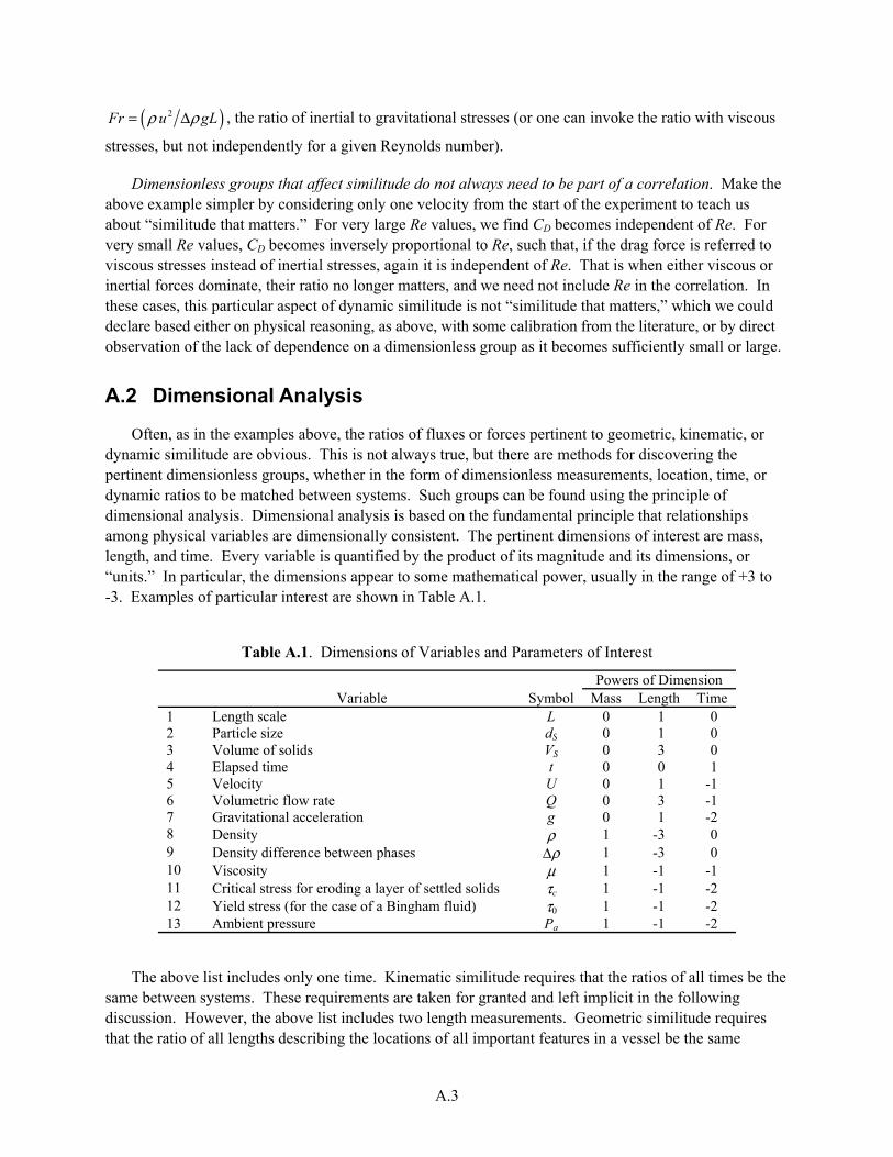
A.3

( )2Fr u gLρ ρ= Δ , the ratio of inertial to gravitational stresses (or one can invoke the ratio with viscous

stresses, but not independently for a given Reynolds number).

Dimensionless groups that affect similitude do not always need to be part of a correlation. Make the above example simpler by considering only one velocity from the start of the experiment to teach us about “similitude that matters.” For very large Re values, we find CD becomes independent of Re. For very small Re values, CD becomes inversely proportional to Re, such that, if the drag force is referred to viscous stresses instead of inertial stresses, again it is independent of Re. That is when either viscous or inertial forces dominate, their ratio no longer matters, and we need not include Re in the correlation. In these cases, this particular aspect of dynamic similitude is not “similitude that matters,” which we could declare based either on physical reasoning, as above, with some calibration from the literature, or by direct observation of the lack of dependence on a dimensionless group as it becomes sufficiently small or large.

A.2 Dimensional Analysis

Often, as in the examples above, the ratios of fluxes or forces pertinent to geometric, kinematic, or dynamic similitude are obvious. This is not always true, but there are methods for discovering the pertinent dimensionless groups, whether in the form of dimensionless measurements, location, time, or dynamic ratios to be matched between systems. Such groups can be found using the principle of dimensional analysis. Dimensional analysis is based on the fundamental principle that relationships among physical variables are dimensionally consistent. The pertinent dimensions of interest are mass, length, and time. Every variable is quantified by the product of its magnitude and its dimensions, or “units.” In particular, the dimensions appear to some mathematical power, usually in the range of +3 to -3. Examples of particular interest are shown in Table A.1.

Table A.1. Dimensions of Variables and Parameters of Interest

Variable Symbol

Powers of Dimension Mass Length Time

1 Length scale L 0 1 0 2 Particle size dS 0 1 0 3 Volume of solids VS 0 3 0 4 Elapsed time t 0 0 1 5 Velocity U 0 1 -1 6 Volumetric flow rate Q 0 3 -1 7 Gravitational acceleration g 0 1 -2 8 Density ρ 1 -3 0 9 Density difference between phases Δρ 1 -3 0 10 Viscosity μ 1 -1 -1 11 Critical stress for eroding a layer of settled solids τc 1 -1 -2 12 Yield stress (for the case of a Bingham fluid) τ0 1 -1 -2 13 Ambient pressure Pa 1 -1 -2

The above list includes only one time. Kinematic similitude requires that the ratios of all times be the same between systems. These requirements are taken for granted and left implicit in the following discussion. However, the above list includes two length measurements. Geometric similitude requires that the ratio of all lengths describing the locations of all important features in a vessel be the same

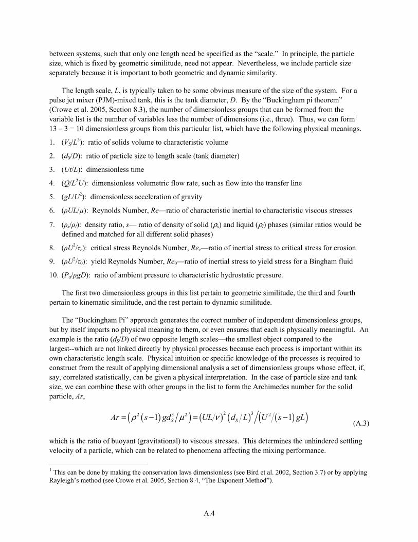
A.4

between systems, such that only one length need be specified as the “scale.” In principle, the particle size, which is fixed by geometric similitude, need not appear. Nevertheless, we include particle size separately because it is important to both geometric and dynamic similarity.

The length scale, L, is typically taken to be some obvious measure of the size of the system. For a pulse jet mixer (PJM)-mixed tank, this is the tank diameter, D. By the “Buckingham pi theorem” (Crowe et al. 2005, Section 8.3), the number of dimensionless groups that can be formed from the variable list is the number of variables less the number of dimensions (i.e., three). Thus, we can form1 13 – 3 = 10 dimensionless groups from this particular list, which have the following physical meanings.

1. (VS/L3): ratio of solids volume to characteristic volume

2. (dS/D): ratio of particle size to length scale (tank diameter)

3. (Ut/L): dimensionless time

4. (Q/L2U): dimensionless volumetric flow rate, such as flow into the transfer line

5. (gL/U2): dimensionless acceleration of gravity

6. (ρUL/µ): Reynolds Number, Re—ratio of characteristic inertial to characteristic viscous stresses

7. (ρs/ρl): density ratio, s— ratio of density of solid (ρs) and liquid (ρl) phases (similar ratios would be defined and matched for all different solid phases)

8. (ρU2/τc): critical stress Reynolds Number, Rec—ratio of inertial stress to critical stress for erosion

9. (ρU2/τ0): yield Reynolds Number, Re0—ratio of inertial stress to yield stress for a Bingham fluid

10. (Pa/ρgD): ratio of ambient pressure to characteristic hydrostatic pressure.

The first two dimensionless groups in this list pertain to geometric similitude, the third and fourth pertain to kinematic similitude, and the rest pertain to dynamic similitude.

The “Buckingham Pi” approach generates the correct number of independent dimensionless groups, but by itself imparts no physical meaning to them, or even ensures that each is physically meaningful. An example is the ratio (dS/D) of two opposite length scales—the smallest object compared to the largest--which are not linked directly by physical processes because each process is important within its own characteristic length scale. Physical intuition or specific knowledge of the processes is required to construct from the result of applying dimensional analysis a set of dimensionless groups whose effect, if, say, correlated statistically, can be given a physical interpretation. In the case of particle size and tank size, we can combine these with other groups in the list to form the Archimedes number for the solid particle, Ar,

( )( ) ( ) ( ) ( )( )2 32 3 2 21 1S SAr s gd UL d L U s gLρ μ ν= − = −

(A.3)

which is the ratio of buoyant (gravitational) to viscous stresses. This determines the unhindered settling velocity of a particle, which can be related to phenomena affecting the mixing performance.

1 This can be done by making the conservation laws dimensionless (see Bird et al. 2002, Section 3.7) or by applying Rayleigh’s method (see Crowe et al. 2005, Section 8.4, “The Exponent Method”).

A.5

Another example is the Froude number, Fr, which represents the ratio of inertial to gravitational forces acting on a fluid with inhomogeneous solids distribution:

( ) ( )( )( )2 21Fr U gL gL Uρ ρ ρ ρ= Δ = Δ

(A.4)

A.3 Similitude and Dimensional Analysis for Submerged Jets

A differential momentum balance for a submerged free (not substantially affected by surrounding shear stress) jet is

0

dFdK dz

dzρ= +

(A.5)

where K is the kinematic momentum flow, 20K A U= ; A0 is the flow cross-section at the start of the jet,

F is the force acting to slow the jet, and z is the distance along the jet. A free jet, or even a wall jet, experiences no or little stress acting to slow it, so that K is, or nearly is, constant along the jet. Its value at the origin of the jet is

2 2

0 4 JK d Uπ= (A.6)

where dJ is the nozzle diameter and U is the mass- or volume-average nozzle velocity (e.g., volumetric flow rate divided by the nozzle area). The flow cross-sectional area, A, at some distance z from the jet origin must depend on the jet momentum, density, nozzle diameter, and length along the jet. It does not depend on the viscosity because, as a free jet, it experiences negligible shear stress. Functionally, we must have

( ) ( )0 ; , ,JA z A f z d Kρ=

(A.7)

The argument of function f must be dimensionless. From dimensional analysis, the density cannot be part of the argument because it is the only parameter with mass in its units. Similarly, K cannot be part of the argument because it is the only parameter with time in its units. Then the only dimensionally consistent possibility is

( ) ( )0 JA z A f z d=

(A.8)

As the jet exits the nozzle, the velocity profile adjusts from a nearly square profile in the nozzle to its self-similar profile, established a few diameters from the nozzle. The self-similar velocity distribution begins once this transition is complete. Applying again rudimentary principles of similitude and dimensional analysis, this distance must be proportional to the nozzle diameter, and the ratio between them will be constant for a given nozzle shape. Denote this ratio as k0. Then self-similarity begins at

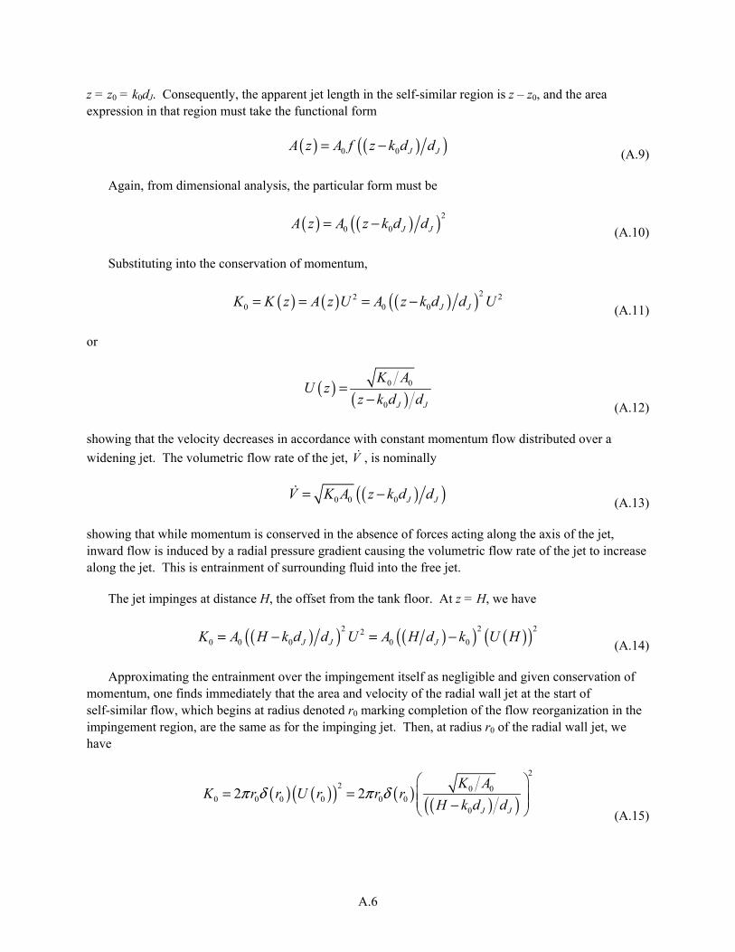
A.6

z = z0 = k0dJ. Consequently, the apparent jet length in the self-similar region is z – z0, and the area expression in that region must take the functional form

( ) ( )( )0 0 J JA z A f z k d d= −

(A.9)

Again, from dimensional analysis, the particular form must be

( ) ( )( )2

0 0 J JA z A z k d d= − (A.10)

Substituting into the conservation of momentum,

( ) ( ) ( )( )22 2

0 0 0 J JK K z A z U A z k d d U= = = − (A.11)

or

( ) ( )0 0

0 J J

K AU z

z k d d=

− (A.12)

showing that the velocity decreases in accordance with constant momentum flow distributed over a

widening jet. The volumetric flow rate of the jet, V , is nominally

( )( )0 0 0 J JV K A z k d d= −

(A.13)

showing that while momentum is conserved in the absence of forces acting along the axis of the jet, inward flow is induced by a radial pressure gradient causing the volumetric flow rate of the jet to increase along the jet. This is entrainment of surrounding fluid into the free jet.

The jet impinges at distance H, the offset from the tank floor. At z = H, we have

( )( ) ( )( ) ( )( )2 2 22

0 0 0 0 0J J JK A H k d d U A H d k U H= − = − (A.14)

Approximating the entrainment over the impingement itself as negligible and given conservation of momentum, one finds immediately that the area and velocity of the radial wall jet at the start of self-similar flow, which begins at radius denoted r0 marking completion of the flow reorganization in the impingement region, are the same as for the impinging jet. Then, at radius r0 of the radial wall jet, we have

( ) ( )( ) ( ) ( )( )

2

2 0 00 0 0 0 0 0

0

2 2J J

K AK r r U r r r

H k d dπ δ π δ

= = − (A.15)

A.7

where δ(r) is the thickness of the jet at radius r. The “thickness” can be defined as the distance from the wall at which the velocity falls to some specified fraction of the maximum velocity at the same radius. For example, Poreh et al. (1967) specify the thickness at which the velocity is half the maximum. Because, beyond radius r0, the radial wall jet is self-similar, then from dimensional analysis we must have

( ) ( )( ) ( )= 0 0 0r r r r f r rδ δ

(A.16)

where δ0 = δ(r0) and so f(1) = 1. Combining,

( )( )( )

( )( )( )( )

20 0 00 00 0

0 2 220 40 0

22= =

− −JJ J

r r rr rK KK

A dH d k H d kπ

π δπ δ

(A.17)

or

( )( )( )

( )0 00

0 088

J JJ J

H d k H d kr d d

r r γδ

− −= =

(A.18)

where

( )0 0/ rγ δ= (A.19)

Substituting,

( ) ( ) ( )0 0 0

8 8

1J J J

r rr H

r H d k d k d H

γ γ= =

− − (A.20)

Thus, we must have (if in terms of r/H)

( ) ( ) ( )0 0, J

rf r r f r H k d H

r

δγ γ= =

(A.21)

Because K is essentially constant, at other radii we have

( ) ( )( ) ( ) ( )( )2 2

0 0 0 02 2r r U r K K r r U rπ δ π δ= = = (A.22)

or

( ) ( )( ) ( ) ( )( )

0

0 0

U rU r

r r r rδ δ=

(A.23)

A.8

Combining all of the above, we can expect measurements of radial wall jet velocity distributions and related attributes such as thickness and wall shear stress to scale as

( )0

0

,U J

Urf r H k d H

K=

(A.24)

( )0, Jf r H k d H

r δδ =

(A.25)

Also, for a self-similar wall jet, from dimensional analysis the boundary layer momentum thickness δθ at the wall will be proportional to δ (i.e., δθ = kθδ), so the momentum thickness Reynolds number, Reθ, will have the form

( ) ( ) 0

0 0, ,J U J

KURe k f r H k d H f r H k d Hθ

θ θ δδ

ν ν= =

(A.26)

where ν is the kinematic viscosity.

The wall shear stress under the boundary layer, τw, will scale with Reθ ; a classic form is (White 1991, Section 6-8.1)

2

bw a ReU θτ

ρ−=

(A.27)

Combining, we obtain the form

( )2

00

0

,

b

wJ

Kra f r H k d H

K τ ττρ ν

−

= (A.28)

Thus, these functional forms follow from the conservation laws, dimensional analysis, and invoking self-similarity of submerged jets. They compare favorably to the work of Poreh et al. (1967), who correlated their measurements of submerged jets (a free air jet in air is “submerged”) in terms of r/H, as follows (see also Section 2.2.2.2).

0.1

0

1.32Ur r

HK

− =

(A.29)

0.1

0.098r

r H

δ − = (A.30)

A.9

0.3 0.320

0

0.3wKr r

K H

τρ ν

− − = (A.31)

That is, implicitly, Poreh et al. did not distinguish from their data any dependence on dJ /H when the data were analyzed in terms of K and r/H, and further did not find a strong dependence on r/H. There is, of course, a strong dependence on dJ through K0. This can rewritten as

( ) ( ) ( ) ( ) ( ) ( )1 0.1 1 0.1

0 1.32 4 1.17J JU r U r r d r H r d r Hπ − − − −= = (A.32)

which can be compared to the correlation of Rajaratnum (1976) (see Equation 11-26 therein) of the data of Poreh et al.:

( ) ( ) ( ) 1

0 1.03 JU r U r r d−=

(A.33)

They are nearly the same, except Rajaratnum argued against including H in the correlation, which is consistent with the very weak dependence of velocity on r/H proposed by Poreh et al.

The radius at which radial floor jets collide on the floor of a PJM tank, rcollision, scales as the square root of the area swept by the jet before colliding, which on average is the area of the tank floor divided by the number of jets, NJ. Thus, the radius scales as

2

collision

J

Dr

N≈

(A.34)

A.4 Conditions for Full Similitude

In Section 3.2, we distinguish several approaches to scaling, including “full similitude” (see Section 3.2.1 for details). Irrespective of the scaling approach used, it is important to identify the conditions for full similitude, even though it cannot be attained, because:

1. It is important to know how and how much conditions depart from full similitude when evaluating data or developing correlations that ostensibly depend at least in part on the extent to which test conditions represent those of the Hanford Waste Treatment and Immobilization Plant (WTP).

2. Representing the performance in Large Scale Integrated Testing (LSIT) as being a conservative representation of WTP invokes a subset of full similitude and cannot be defended without understanding how it departs from full similitude. This is an example of one.

3. Physically based models or correlations are developed from data obtained from experiments that must provide sufficient similitude that the results clearly pertain to the full-scale system. This requires understanding full similitude as the context.

4. Pertinent experimental parameters to include in any model or correlation are determined by considering the phenomena that determine the conditions for full similitude.

A.10

Above, we identified that geometric and time ratios need to be matched and left those constraints as implicit in the rest of the analysis, which applies here as well. The remaining dimensionless groups must all be matched to attain full similitude. The dimensionless solids volume is proportional to the solids volume fraction φS, which can be matched between groups. The dimensionless time, such as dimensionless cycle time, also can be matched, as can the density ratio, s. However, the dimensionless groups describing dynamic similitude cannot be matched simultaneously without “scaling” the properties of the simulated waste with system size, which is not practical.

From the definition of the Froude and Reynolds number, matching both simultaneously at constant density requires scaling both the velocity and viscosity with length scale, L. In particular, the viscosity would have to scale as L3/2. The consequence of this is illustrated for several vessels in the following table.

As is apparent from Table A.2, viscosities less than that of water, and in some cases much less than water, are required to maintain full similitude in the smaller LSIT tanks where the viscosity is water-like at full scale. If even scientifically feasible, this would require testing using expensive fluids likely presenting safety and disposal issues.

Table A.2. Example of Scaling Viscosities for the LSIT Test Vessels

Vessel Designation(a)

Diameter (ft)

Viscosity(b) at Full Scale (cP)

Viscosity (cP) Required at Reduced Scale to Match Re and Fr Simultaneously

43 in. 8 ft 14 ft

UFP-01(c) 20 1 0.076 0.25 0.59

RLD-08(d) 13 1 0.14 0.48 1.1

HLP-22(e) 38 1 0.029 0.097 0.22

(a) These vessels were designated by WTP for pilot-scale performance evaluation. (b) These are nominal minimum viscosities. Actual viscosities depend on the solids loading in a tank. (c) UFP-VSL-00001. (d) RLD-VSL-00008. (e) HLP-VSL-00022.

If waste properties are not scaled with system size, the fluid viscosity and density of fluid and of solids will be the same, and therefore one cannot simultaneously match the Reynolds and Froude numbers. Fortunately, probably the Reynolds number is not important to “scaling” the behavior during a PJM cycle, as is discussed in Section 2.2.1.1. The velocity can be adjusted to match the Froude number and then elapsed times can be adjusted to match corresponding dimensionless times between systems. However, the velocity in a test may be set by other considerations, such as clearing solids from the vessel floor during a PJM pulse. Then resulting departures of the Froude number from full similitude need to be considered when “scaling up” results, and especially when estimating the uncertainty in predicting the performance from scaled to actual system.

Perhaps the most important departure from similitude will be the ratio of settling velocity of solids to the characteristic velocity of the system, which ultimately affects the fraction of solids that settle and are resuspended during each PJM pulse. If the simulated waste properties are not scaled with system size, then the settling velocity is constant across length scales. As the system velocity is adjusted across length

A.11

scales to meet various constraints, the ratio of settling velocity to, for example, PJM velocity, will vary commensurately, presenting two problems: 1) the ratio of velocities is not matched between the scaled and actual system, and 2) the ratio varies from scale to scale over LSIT tests, adding an uncontrolled factor to consider when interpreting test results.

To scale the settling velocity properly ultimately requires scaling the particle sizes proportionate to the system size. Then for the smallest LSIT vessel to represent the largest WTP vessel (e.g., HLP-22), the solid particles would have to be about a tenth of the actual size. This would result in a significant fraction of very fine particles that likely would change the rheological properties of the slurry and the settled solids, perhaps resulting in a yield stress, which likely would create more problems than it solved.

Other important dimensionless groups include the Reynolds number based on critical erosion stress and yield stress in the case of a Bingham fluid. To maintain dynamic similitude, these would both have to be matched between LSIT and WTP.

As is developed in the Section A.5, for actual wastes with a particle size and density distribution (PSDD), there are two attributes representing the effect of the distribution on the fluid dynamics of the slurry in a PJM system: 1) the particle volume weighted density ratio, s , and 2) the particle volume weighted terminal velocity, UT/U. Thus, one would match s (in place of “s”) between systems at different scales, and match the ratio UT/U rather than the dimensionless particle size, where the terminal (unhindered) settling velocity, UT, is discussed below. In cases where the fluid dynamics of a particular species must be matched, then one must match the density ratio for species “i”, si, and the unhindered

settling velocity, 0iu , for species “i”, 0

Tiu .

A.5 Scaling Basis for Particle Size Distributions

There are three practical effects of particle settling in the PJM cycle: 1) deposition of solids on the tank floor; 2) capture of solids into the suction nozzle due to the radial velocity field around it; and 3) relating the concentration of solids sampled from some point in the tank to the total mass of solids species in the tank. The rate of the first is the volume-averaged volumetric flux of the local distribution of particles, and the second depends directly on this volumetric flux. This flux has units of velocity and can be taken to be “the” settling velocity despite there being a distribution of settling velocities at any given elevation and time in the tank. The third effect is a matter of understanding hindered settling for the particular waste attributes and understanding the settling environment, particularly any residual turbulence. See Appendix C for details.

Where the particle settling velocity is important to scaling relationships, one must face the fact that there is a distribution of velocities resulting from a distribution of particle sizes and densities. That is, there is not “a” settling velocity upon which to base scaling arguments involving the entire tank. One way to address this is to consider sufficiently slowly settling particles to be simply part of the fluid phase, affecting its rheology, and consider other particles to be settling through this fluid. For this we need to define the fraction, F(δ,s), of particles with sizes less than some specified value, δ, and density ratio s=ρs/ρl (ratio of density of particle to density of the surrounding liquid) less than some specified density ratio, as follows.

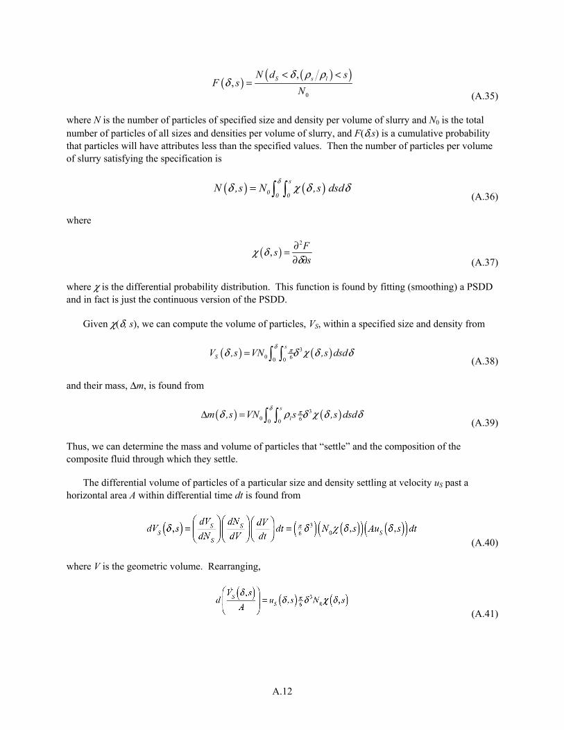
A.12

( ) ( )( )

0

,, S s lN d s

F sN

δ ρ ρδ

< <=

(A.35)

where N is the number of particles of specified size and density per volume of slurry and N0 is the total number of particles of all sizes and densities per volume of slurry, and F(δ,s) is a cumulative probability that particles will have attributes less than the specified values. Then the number of particles per volume of slurry satisfying the specification is

( ) ( )s

0 0 0N ,s N ,s dsd

δδ χ δ δ= (A.36)

where

( )

2

,F

ss

χ δδ

∂=∂ ∂ (A.37)

where χ is the differential probability distribution. This function is found by fitting (smoothing) a PSDD and in fact is just the continuous version of the PSDD.

Given χ(δ, s), we can compute the volume of particles, VS, within a specified size and density from

( ) ( )3

0 60 0

s

SV ,s VN ,s dsdδ πδ δ χ δ δ= (A.38)

and their mass, Δm, is found from

( ) ( )3

0 60 0

s

lm ,s VN s ,s dsdδ πδ ρ δ χ δ δΔ = (A.39)

Thus, we can determine the mass and volume of particles that “settle” and the composition of the composite fluid through which they settle.

The differential volume of particles of a particular size and density settling at velocity uS past a horizontal area A within differential time dt is found from

(A.40)

where V is the geometric volume. Rearranging,

(A.41)

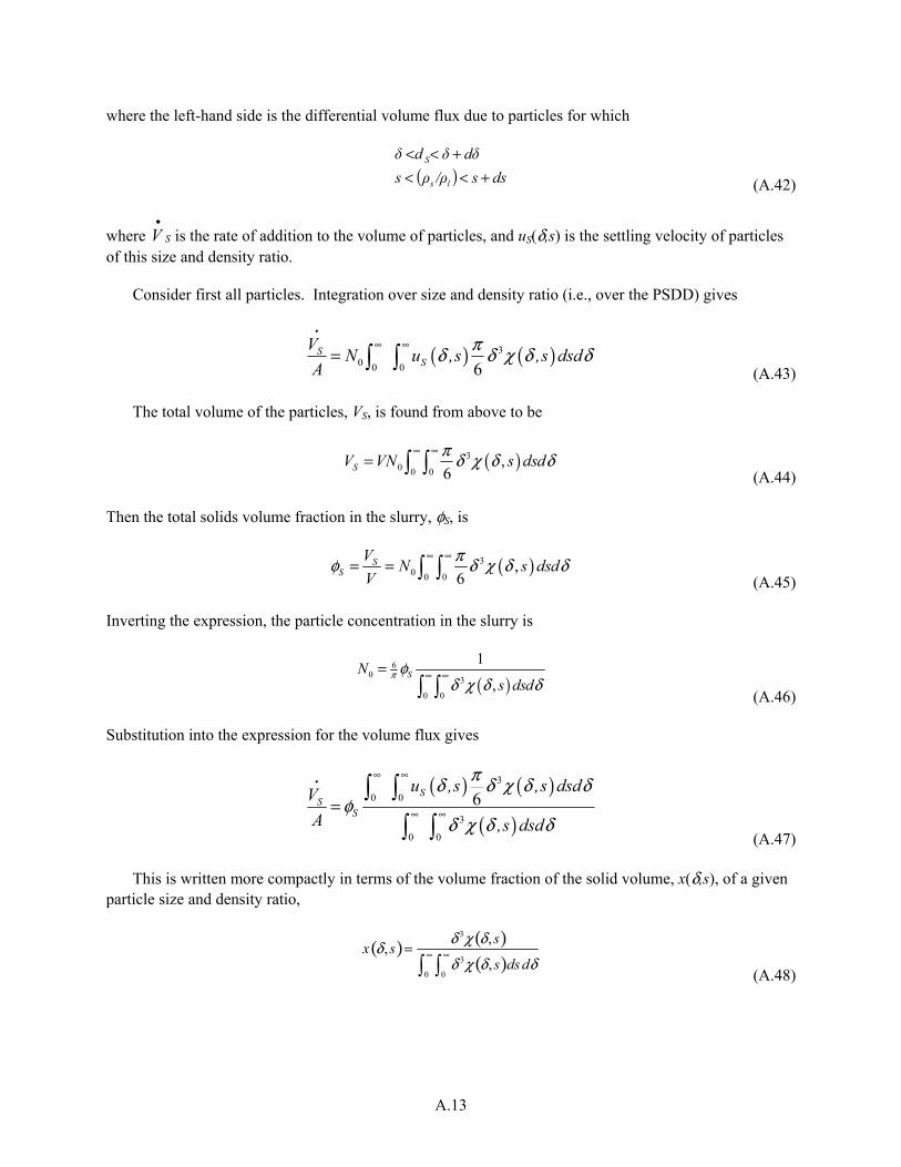
A.13

where the left-hand side is the differential volume flux due to particles for which

( ) dss/ρρs

dδδdδ

ls

S

+<<+<<

(A.42)

where SV•

is the rate of addition to the volume of particles, and uS(δ,s) is the settling velocity of particles of this size and density ratio.

Consider first all particles. Integration over size and density ratio (i.e., over the PSDD) gives

( ) ( )3

0 0 0 6S

S

VN u ,s ,s dsd

A

πδ δ χ δ δ∞ ∞

=

(A.43)

The total volume of the particles, VS, is found from above to be

( )3

0 0 0,

6SV VN s dsdπ δ χ δ δ

∞ ∞=

(A.44)

Then the total solids volume fraction in the slurry, φS, is

( )3

0 0 0,

6S

S

VN s dsd

V

πφ δ χ δ δ∞ ∞

= = (A.45)

Inverting the expression, the particle concentration in the slurry is

( )

60

3

0 0

1

,SN

s dsdπ φ

δ χ δ δ∞ ∞= (A.46)

Substitution into the expression for the volume flux gives

( ) ( )

( )

3

0 0

3

0 0

6SS

S

u ,s ,s dsdV

A ,s dsd

πδ δ χ δ δφ

δ χ δ δ

∞ ∞

∞ ∞=

(A.47)

This is written more compactly in terms of the volume fraction of the solid volume, x(δ,s), of a given particle size and density ratio,

x δ , s( )=δ 3χ δ , s( )δ 3χ δ , s( )ds

0

∞

dδ0

∞

(A.48)

A.14

Substituting,

( ) ( )

0 0, ,S

S

Vu s x s dsd

Aφ δ δ δ

∞ ∞=

(A.49)

Similarly, substituting into the expression for the mass of the particles gives

( ) ( )0 0

_s

S l S l

m ,sx ,s sdsd s

V

δδφ ρ δ δ φ ρ

Δ= =

(A.50)

where the particle volume weighted density ratio

( )

0 0,

ss x s sdsd

δδ δ= (A.51)

Defining, at some elevation and time, the particle unhindered settling velocity, u0, and its volume

average over the distribution of particles, u 0 , as the volume flux, then we have

( ) ( )0 0

0 0, ,u u s x s dsdδ δ δ

∞ ∞= (A.52)

Also, the hindered settling velocity is related to the unhindered settling velocity by

( ) ( ) ( )0

S Su ,s u ,s fδ δ φ= (A.53)

where f(φS) is the correction for hindered settling, assumed here to be a function of only the total solids loading.1 Finally, as settling occurs, the local PSDD changes over elevation and time due to differences in settling rates over the particles. Hence, the differential PSDD is a function of elevation and time as well as of size and density ratio, and is denoted

( )2

,

, ; ,z t

Fs z t

sχ δ

δ ∂= ∂ ∂ (A.54)

Combining, the settling velocity of the distribution of particles at some elevation and time, defined as the volume weighted volume flux divided by the total particle volume fraction, is

u z,t( ) =

VS

AφS

= u0 δ ,s( ) f φS( ) x δ ,s,z,t( )ds

0

∞

dδ0

∞

(A.55)

1 The function of Richardson and Zaki (1954) (see Equation C.176) can be taken as a default. See Appendix C, Section C.4.2.9 for a discussion of alternatives.

A.15

Define the volume weighted average unhindered settling velocity

u 0 z,t( )= u0 δ , s( )x δ , s, z, t( )ds

0

∞

dδ0

∞

(A.56)

Combining, the average settling velocity is

u z,t( ) =

VS

AφS

= u 0 z,t( ) f φS

z,t( )( ) (A.57)

This average settling velocity is denoted elsewhere in this report as “the” settling velocity, e.g., UT. Similarly, the slurry density is found from the mass of liquid, mliquid, and mass of solids, msolids,

( ) ( )( )11 1liquid solids l S l S

l S

m m V V ss

V V

ρ φ ρ φρ ρ φ

+ − += = = + −

(A.58)

For a discrete PSDD where particles are binned into N groups of specified size and density ratio, the volume weighted average unhindered settling velocity is

u 0 z,t( )= u0 δ , s( )x δ , s, z,t( )ds

0

∞

dδ0

∞

= xi z,t( )ui0

i

(A.59)

and the volume weighted particle density ratio is

( ) ( ) ( ) ==

∞ ∞

iii0 0

_

stz,xsdsdδtz,s,δ,xtz,s (A.60)

where xi is the fraction of the total particle volume due to the specified particle. These are the forms used in discussions elsewhere in this document about the settling attributes of simulated waste. Whether from a continuous or discrete PSDD, this average settling velocity is referred to as UT (terminal velocity) and the average density ratio is referred to as s elsewhere in this document and immediately below.

The above averaged properties can be defined alternatively for a subset of particles, namely, those settling faster than some essentially de minimis value, below which particles are considered a stable part of the fluid. In particular, we would have

( ) ( ) ( )

( )( )

min min min

0 0 0

slow

, , , , , ,i isi

u z t u s x s z t dsd x z t uδ δ

δ δ δ∞ ∞

≠

= = (A.61)

where δmin is the smallest particle with settling velocity of concern, and smin(δmin) is a potential similar limit on particle density, based on particle size, to ultimately constrain the settling velocity of particles included in these averages. Further, the unhindered settling velocity would be computed from the fluid viscosity considering the concentration of non-settling particles. The resulting average properties (settling velocity, particle density) would be used as the averages computed for all particles.

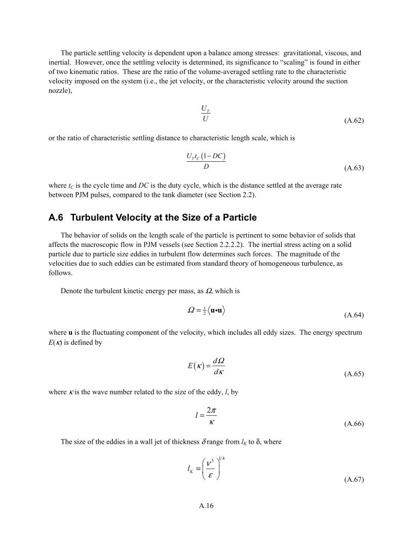
A.16

The particle settling velocity is dependent upon a balance among stresses: gravitational, viscous, and inertial. However, once the settling velocity is determined, its significance to “scaling” is found in either of two kinematic ratios. These are the ratio of the volume-averaged settling rate to the characteristic velocity imposed on the system (i.e., the jet velocity, or the characteristic velocity around the suction nozzle),

TU

U (A.62)

or the ratio of characteristic settling distance to characteristic length scale, which is

( )1T CU t DC

D

−

(A.63)

where tC is the cycle time and DC is the duty cycle, which is the distance settled at the average rate between PJM pulses, compared to the tank diameter (see Section 2.2).

A.6 Turbulent Velocity at the Size of a Particle

The behavior of solids on the length scale of the particle is pertinent to some behavior of solids that affects the macroscopic flow in PJM vessels (see Section 2.2.2.2). The inertial stress acting on a solid particle due to particle size eddies in turbulent flow determines such forces. The magnitude of the velocities due to such eddies can be estimated from standard theory of homogeneous turbulence, as follows.

Denote the turbulent kinetic energy per mass, as Ω, which is

12Ω = u u

(A.64)

where u is the fluctuating component of the velocity, which includes all eddy sizes. The energy spectrum E(κ) is defined by

( ) d

Ed

Ωκκ

= (A.65)

where κ is the wave number related to the size of the eddy, l, by

2l

πκ

= (A.66)

The size of the eddies in a wall jet of thickness δ range from lK to δ, where

1 43

Klνε

= (A.67)

A.17

is the Kolmogorov length scale and ε is the power dissipation per mass. In the inertial subrange, the energy spectrum has the form

( ) 2 3 5 3E Cκ ε κ −=

(A.68)

Integrating over wave numbers from the largest eddies to the Kolmogorov length scale overestimates the turbulent kinetic energy, but given that the jet thickness is well defined (even though it is not bounded physically) and given that most of the energy is in the smaller wave numbers, this suffices to describe how the energy scales with particle size. Equating this integral to the intensity of turbulence gives

( ) ( ) ( )( )( ) ( )( )

2 / 2 3 2 32 3 5 3 2 3 322 /

2 3 2 332

2 2

2 1

Kl

K

K

C d C l

C l

π

π δε κ κ ε π π δ

π εδ δ

− −−

−

Ω = = − −

= −

(A.69)

where C is a constant of integration.

The dissipation rate in the wall jet is (see White 1991, Section 6-1.1, inferred from Kolmogorov length scale in a turbulent boundary layer)

3Ukεε

δ=

(A.70)

where kε is a dimensionless coefficient on order of unity. Substituting into the expression for the Kolmogorov length scale gives

1 4 3 431 4 1 4 3 4

3Kl k k Rek U Uε ε δ

ε

ν δ ν δ δδ

− − − = = = (A.71)

Rearranging,

1 4 3 4Kl k Reε δδ− −=

(A.72)

For the case of large Reynolds number for the wall jet, Reδ, (i.e., 1Reδ >> ), the expression for Ω

becomes

( ) 2/332 2 /CΩ π εδ −= (A.73)

Substituting,

( ) ( ) 2 3 5 32

3 2E κ δ π Ωκ− −= (A.74)

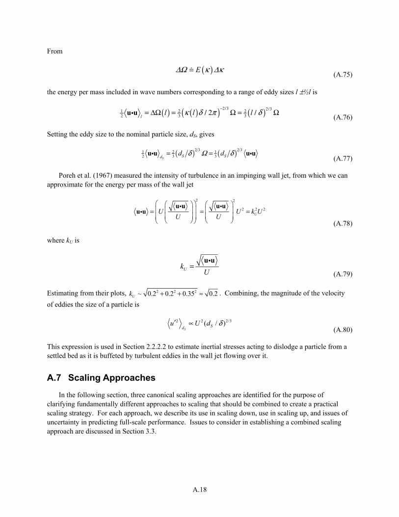
A.18

From

( )EΔΩ κ Δκ=

(A.75)

the energy per mass included in wave numbers corresponding to a range of eddy sizes l ±½l is

( ) ( )( ) ( )2 3 2 31 2 22 3 32

ll l lκ δ π δ−

= ΔΩ = Ω = Ω/ /u u / /

(A.76)

Setting the eddy size to the nominal particle size, dS, gives

( ) ( )2 3 2 31 2 1

2 3 3= =u u u u S

S Sdd dδ Ω δ

(A.77)

Poreh et al. (1967) measured the intensity of turbulence in an impinging wall jet, from which we can approximate for the energy per mass of the wall jet

2 2

2 2 2UU U k U

U U

= = =

u u u uu u

(A.78)

where kU is

Uk

U=

u u

(A.79)

Estimating from their plots, 2 2 2~ 0.2 0.2 0.35 0.2Uk + + ≈ . Combining, the magnitude of the velocity

of eddies the size of a particle is

2 2 2/3( / )

SSd

u U d δ′ ∝ (A.80)

This expression is used in Section 2.2.2.2 to estimate inertial stresses acting to dislodge a particle from a settled bed as it is buffeted by turbulent eddies in the wall jet flowing over it.

A.7 Scaling Approaches

In the following section, three canonical scaling approaches are identified for the purpose of clarifying fundamentally different approaches to scaling that should be combined to create a practical scaling strategy. For each approach, we describe its use in scaling down, use in scaling up, and issues of uncertainty in predicting full-scale performance. Issues to consider in establishing a combined scaling approach are discussed in Section 3.3.

A.19

A.7.1 Pure Similitude

A.7.1.1 Attributes of Pure Similitude

“Pure similitude” refers to meeting all of the requirements of geometric, kinematic, and dynamic similitude as identified in Section A.4. To reiterate, this would entail simultaneously matching between WTP and LSIT the following ratios.

• Geometric: d/D, H/D, NJ, HT/D, HL/D, φS

• Kinematic: UtC/D, tD/tC, Q/UD2, uS/U

• Dynamic: (s-1), Re, Fr, Rec.

where d is the nozzle diameter, H is the jet offset above tank floor, HL is the height of liquid in the tank, HT is the height of the transfer line, and tD is the drive time.

As is explained in Section A.4, it is impractical to match Re and Fr simultaneously, but we expect Re to be large enough in LSIT tests and in WTP tanks to be unimportant. Also, as is explained in Sections 5.6 and 5.7, there are different phenomena affected by the transfer/recirculation volumetric flow rate, Q. This requires matching a second relationship for Q—Q/uSD

2—which would require matching uS/U. As is explained in Section A.4, we assume it is impractical to scale the simulant with system size, and hence, we cannot match uS/U.

Where one can match all pertinent geometric, kinematic, and dynamic ratios, the observed behavior of the reduced-scale system will represent the behavior in the full-scale system at corresponding dimensionless locations and times. Then observing the scaled system would be virtually observing the full-scale system. A classic example is observing the forces and vibrations induced on a scale-model airplane while “flying” it in a wind tunnel, a case where all of the behavior, if converted to dimensionless form, depend only on Re, given sufficiently small Mach number (an example of simplifying the parameter set based on knowledge of when parameters do not affect similitude significantly). However, this is a much simpler system than a PJM mixer.

Notwithstanding difficulties in implementing full similitude as a scaling approach, it is always important to consider how a system departs from full similitude, and hence, it is always important to identify the conditions for full similitude even if they are unattainable. The closer one can attain full similitude, the more the reduced-scale system directly represents the full-scale system, and consequently, the less one needs to be able to predict performance simultaneously for ranges of parameters describing the vessel configuration, operating parameters, and simulant properties. Conversely, the need to develop descriptive or physically based models of a system is essentially the need to compensate for the inability to attain full similitude, and the aspects of the behavior of a system that most need to be understood physically tend to be those for which the lack of similitude is most important.

Where full similitude cannot be imposed, one might show that imposing partial similitude will result in behavior that bounds the behavior in the actual system. If so, such a scaled test would provide a “bounding” test in the sense that, if a mixing requirement is met for the test, it would be met for the full-scale system. Then the result is qualitative: one predicts that either the full-scale system meets the requirement or not. If this can be done, it has the advantage of requiring few data to show compliance with a specific requirement, and the knowledge about the phenomena required to support a qualitative

A.20

conclusion is less than to build a quantitative correlation; it may suffice to understand only how a phenomenon scales (trends up or down) with, say, velocity and size. However, there are several disadvantages. First, if the test does not show compliance, little else is learned. Second, even if the results are favorable, because the data are intentionally limited, they likely are insufficient to validate that the test is, in fact, conservative. That is, the margin of error of a favorable result is not determined from the test itself.

A.7.1.2 Use in Scaling Down

If “pure similitude” could be attained, its sole use would be to “scale down” from a description of a WTP tank, its operation, and its contents to define the geometrically, kinematically, and dynamically similar reduced-scale tank, operations, and contents for an LSIT test at reduced scale.

A.7.1.3 Use in Scaling Up

If “perfect similitude” could be attained, “scaling up” would consist of nothing more than describing observations of behavior in the LSIT tank of dimensionless-dependent variables, such as concentrations or masses relative to initial masses, in terms of dimensionless positions and times.

A.7.1.4 Addressing Uncertainty

The uncertainty in “scaling up” performance based on an assertion of “perfect similitude” will include

• The uncertainty in the assertion of full similitude, including knowing all the pertinent parameters from which the dimensionless groups are formed, and some quantitative sense of the sensitivity of observed performance to the departure of dimensionless groups from their ideal values (i.e., “how close to similitude are we?”)

• Uncertainty in measuring parameters determining closeness to full similitude

• Uncertainty in measuring performance metrics.

A.7.2 Pure Statistics

Where neither full similitude nor “conservative” conditions can be established, one alternative is to maintain partial similitude (i.e., geometric and kinematic similitude, see Chapter 3) while varying parameters such as velocities, times, and material properties such as total solids loading independently over a series of tests, such as was attempted for testing activity M3.1 The result is usually expressed graphically in the form shown in Figure A.1. Note that only a single value, such as some performance metric, can be plotted against scale, reminding us that the method does not apply to scaling sets of data or relationships.

1 M3 refers to a testing activity that included testing in “PJM-like” and in actual PJM mixing systems in which key system parameters were varied independently over limited domains. See Meyer et al. (2009, 2010, 2012).

A.21

Figure A.1. Depiction of a Generic Power-Law Correlation Where a Single Performance Metric is Correlated Against the Ratio of the Test Length Scale to Full Scale

Using this approach, if a single dependent variable—a performance metric—can be defined and

measured, one can impose a power-law relationship on the data of the form

θi = Ci π j

α ij

j≠ i

∏ (A.81)

or

lnθi = lnCi + α ij lnπ j

j≠i

(A.82)

where θi = a dimensionless form (see previous discussion of dimensional analysis in this appendix) of a dependent performance metric

Ci = an empirical constant πi = dimensionless groups formed of the independent variables αij = empirical powers.

The logarithmic form corresponds to a multi-linear fit to log-log data.

The dimensionless term πi can be arranged so only one, π1, includes the length scale. Then, “the” length scale factor for a given θi is αi1. However, there is no reason a priori to expect that the PJM phenomena in combination result in a performance metric inherently following the power-law form relative to length scale. Nevertheless, one can always extract from the data “the” scale factor for some particular combination of n independent variables by evaluating αi1, defined above.

If over multiple scales “the” scale factor is essentially constant, the result is compelling, seeming to vindicate the use of a power law. Yet, some theory about the apparent dependence on length scale still is desired before believing that the “law” applies for, say, other waste properties or other geometries. Thus, this method has the disadvantage of offering little confidence in its generality unless the data are indeed very linear in the log-log form, and even then confidence is diminished if no physical explanation for the “scale” is apparent. A very simple example follows.

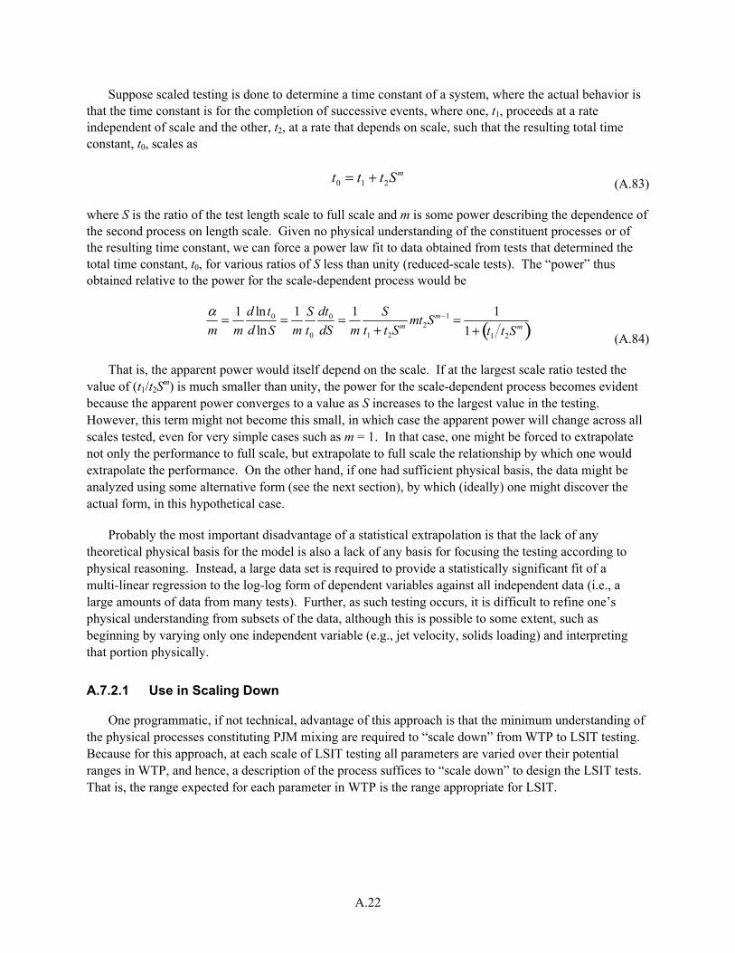
A.22

Suppose scaled testing is done to determine a time constant of a system, where the actual behavior is that the time constant is for the completion of successive events, where one, t1, proceeds at a rate independent of scale and the other, t2, at a rate that depends on scale, such that the resulting total time constant, t0, scales as

t0 = t1 + t2Sm

(A.83)

where S is the ratio of the test length scale to full scale and m is some power describing the dependence of the second process on length scale. Given no physical understanding of the constituent processes or of the resulting time constant, we can force a power law fit to data obtained from tests that determined the total time constant, t0, for various ratios of S less than unity (reduced-scale tests). The “power” thus obtained relative to the power for the scale-dependent process would be

αm

=1

m

d ln t0

d lnS=

1

m

S

t0

dt0

dS=

1

m

S

t1 + t2Sm

mt2Sm−1 =

1

1+ t1 t2Sm( ) (A.84)

That is, the apparent power would itself depend on the scale. If at the largest scale ratio tested the value of (t1/t2S

m) is much smaller than unity, the power for the scale-dependent process becomes evident because the apparent power converges to a value as S increases to the largest value in the testing. However, this term might not become this small, in which case the apparent power will change across all scales tested, even for very simple cases such as m = 1. In that case, one might be forced to extrapolate not only the performance to full scale, but extrapolate to full scale the relationship by which one would extrapolate the performance. On the other hand, if one had sufficient physical basis, the data might be analyzed using some alternative form (see the next section), by which (ideally) one might discover the actual form, in this hypothetical case.

Probably the most important disadvantage of a statistical extrapolation is that the lack of any theoretical physical basis for the model is also a lack of any basis for focusing the testing according to physical reasoning. Instead, a large data set is required to provide a statistically significant fit of a multi-linear regression to the log-log form of dependent variables against all independent data (i.e., a large amounts of data from many tests). Further, as such testing occurs, it is difficult to refine one’s physical understanding from subsets of the data, although this is possible to some extent, such as beginning by varying only one independent variable (e.g., jet velocity, solids loading) and interpreting that portion physically.

A.7.2.1 Use in Scaling Down

One programmatic, if not technical, advantage of this approach is that the minimum understanding of the physical processes constituting PJM mixing are required to “scale down” from WTP to LSIT testing. Because for this approach, at each scale of LSIT testing all parameters are varied over their potential ranges in WTP, and hence, a description of the process suffices to “scale down” to design the LSIT tests. That is, the range expected for each parameter in WTP is the range appropriate for LSIT.

A.23

A.7.2.2 Use in Scaling Up

The dependent variable of interest (i.e., a performance metric) is measured in a statistically determined test matrix across the multi-dimensional parameter “space,” including the length scale as one of the parameters. The data are put in log-log form and then fit using multi-linear regression. The regression coefficients are the “scale factors” for each of the parameters, which can and should be made dimensionally consistent. The performance metric is predicted in the WTP by entering into the regression equation the parameters for WTP, including the full-size length scale. Examples of dimensionally consistent, multi-linear regression of log-log data are found in Appendix F of Meyer et al. (2009).

A.7.2.3 Addressing Uncertainty

The uncertainty in “scaling up” performance based on an assertion of “perfect statistics” will include

• The uncertainty in the multi-linear regression coefficients, which will depend mainly on

– The extent to which the data actually conform to the power-law form

– Uncertainty in measurements of both dependent and independent test variables

• Uncertainty that the regression coefficient for the dependence of the performance metric on system size is not itself a function of system size.

On one hand, calculating the uncertainty of the predicted performance is simplest for this approach because multi-linear regression is well understood and standard statistical procedures and computational tools apply. On the other hand, prediction of performance at full scale is inherently an extrapolation of a model for which there is no evidence of its validity over the extrapolation other than a sense that if the relationship depicted in Figure A.1 seems linear over the range of interpolation, probably it is linear over the extrapolation.

A.7.3 Pure Physics

Another alternative is to use a combination of dimensional analysis, similitude, and models, developed from a combination of first principles and LSIT data, to predict the behavior in a full-scale system by correlating behavior in terms of dimensionless groups. The resulting correlations should be as theoretical as practicable but as empirical as necessary or prudent. They are developed in terms of dimensionless functional forms that often can be obtained from existing models of discrete phenomena, such as the radial wall jet formed on the floor of a WTP tank under a PJM, or from a dimensional analysis of phenomena taken in isolation, such as considering jets, upward flow, and settling in terms of separate models before attempting to integrate them.

This approach presents several challenges. It requires:

• An understanding of the physical phenomena and of the various flow domains and their interactions

• Viable concepts to fit or modeling them

• Data over the domain of the model sufficient to show qualitative agreement with the model and to enable estimates of model coefficients and their uncertainty.

A.24

Just as evaluating departures from similitude is important for any of the alternative technical approaches, so is establishing a physical basis for scaling down even if a physically based model is not selected for scaling up. Thus, there are reasons to understand the physics aside from advantages versus disadvantages of the approach. But, although challenging, this approach does provide a very important advantage. Waste properties and operating conditions in the WTP can be covered in LSIT tests so any correlation or model in terms of these parameters is an interpolation. But, by definition, predicting performance at scale larger than for LSIT tests is extrapolation with respect to length. Then the principal objective of this scaling approach is to “interpolate knowledge” rather than extrapolate results. “Interpolate knowledge” means developing a physical understanding of the behavior observed at each LSIT test scale and demonstrating that, while the behavior may differ even qualitatively over scale, the explanation does not, and moreover demonstrating that there is no reason to suspect it does not apply as well at full scale. Then predicting the performance is equally valid at any scale, and, in that sense, even at full scale one is “extrapolating knowledge.” Two simple illustrations follow.

Consider the trivial problem of predicting the time to fill a bucket with water. Suppose the actual system is a giant bucket and a tiny hose, taking weeks to fill the bucket. Scaled tests are used to predict the fill time. By testing many buckets and hoses, a promising power would appear, but there would be some uncertainty in extrapolating the results to much bigger buckets than those tested. If rather than rely on a power law fit to the data one understood the behavior was due to the conservation of mass and that would be true at any scale, the conservation of mass simply could be applied at full scale with no uncertainty other than in the physical measurements per se, which would be known and could be small. One would be “interpolating knowledge” to full scale.

A second example is predicting drag coefficients of submerged objects. If the actual system were a very large object, it would be difficult to test directly. If one recognized from first principles or from correlating data that the drag coefficient depended only on Reynolds number, one could test smaller objects at fast velocities and find the coefficient at the same Reynolds number as at full scale. Again, one would be “interpolating knowledge” to full scale.

Put more technically, the advantages include:

• The dependence on length scale can be based on first principles known a priori, such as conservation laws or self-similarity in submerged jets.

• The dependence on waste properties can be based on first principles, thus allowing the correlations to be improved later if data become available from tests using additional simulants.

• Very complex behavior due to interactions of many component phenomena can be simplified by taking on the phenomena individually by developing component sub-models.

• Sub-models, for which scaling relative to length, velocity, etc., can be straightforward, can be linked mathematically to create a combined model for a performance metric for which scaling relative to length, velocity, etc., would otherwise be complex and resist correlation using simple forms, such as a power law.

• Even if such sub-models must be developed empirically (e.g., in power-law form), they can be developed based on dimensionless forms of independent and dependent variables for which the dependence on length scale is determined by dimensional analysis.

• Sub-models often are available from or suggested by the existing literature.

A.25

• Potentially, modeling can describe conceptually the consequence of imposing incomplete similitude, and provide means for putting test results into perspective and thereby managing (limiting) extrapolation of the data. Probably the most important application would be to understand the consequences of not matching the ratio of settling velocity to jet velocity.

• In principle, sub-models can be developed and validated using both LSIT data obtained over a range of independent variables and separate auxiliary experiments.

A.7.3.1 Use in Scaling Down

Notwithstanding that a scaled test may be far from full similitude, the essential purpose of applying understanding of the physical phenomena to predict performance is to compensate for departures from similitude between the scaled and full-scale systems. This implies that some understanding of “physics” is required initially to decide how the scaled system departs from similitude, what phenomena need to be understood rather than taken to be representative of full scale due to similitude, and what parameters are important to the phenomena that need to be varied in LSIT experiments. If one can anticipate the form of models to be fit to the data, statisticians can use that information to design efficient test matrices resulting in minimum contribution by undesirable cross correlations to the uncertainty in the fitted model coefficients, which is part of optimizing the certainty of the predictive models built from sub-models.

A.7.3.2 Use in Scaling Up

Given the physical models developed from LSIT data, “scaling up” is similar to “perfect statistics” in that the parameters describing WTP, including the length scale, are entered into the models to predict the performance metric with some estimate of the uncertainty. One difference is that the models likely are not linear and are fit by nonlinear regression methods.

A.7.3.3 Addressing Uncertainty

The uncertainty in “scaling up” performance based on an assertion of “perfect physics” will include

• The uncertainty in the non-linear regression coefficients, which will depend mainly on

– The extent to which the data actually conform to the physically based functional form

– Uncertainty in measurements of both dependent and independent test variables

• Uncertainty that the non-linear regression coefficients for the dependence of the performance metric on system size is not itself a function of system size.

Calculating the uncertainty of the predicted performance is the most esoteric for this approach because the validity depends entirely on building a functional form from physical understanding. But, more importantly, prediction of performance at full scale can be “interpolation of knowledge,” providing maximum technical credibility if the sub-models fit well.

A.26

A.8 References

Bird RB, WE Stewart, and EN Lightfoot. 2002. Transport Phenomena, Second Edition. John Wiley & Sons, New York.

Crowe CT, DE Elger, and JA Roberson. 2005. Engineering Fluid Mechanics. John Wiley & Sons, New York.

Meyer PA, JA Bamberger, CW Enderlin, JA Fort, BE Wells, SK Sundaram, PA Scott, MJ Minette, GL Smith, CA Burns, MS Greenwood, GP Morgen, EBK Baer, SF Snyder, M White, GF Piepel, BG Amidan, A Heredia-Langner, SA Bailey, JC Bower, KM Denslow, DE Eakin, MR Elmore, PA Gauglitz, AD Guzman, BK Hatchell, DF Hopkins, DE Hurley, MD Johnson, LJ Kirihara, BD Lawler, JS Loveland, OD Mullen, MS Pekour, TJ Peters, PJ Robinson, MS Russcher, S Sande, C Santoso, SV Shoemaker, SM Silva, DE Smith, YF Su, JJ Toth, JD Wiberg, XY Yu, and N Zuljevic. 2009. Pulse Jet Mixing Tests With Noncohesive Solids. PNNL-18098; WTP-RPT-182, Rev. 0, Pacific Northwest National Laboratory, Richland, Washington.

Meyer PA, EBK Baer, JA Bamberger, JA Fort, and MJ Minette. 2010. Assessment of Differences in Phase 1 and Phase 2 Test Observations for Waste Treatment Plant Pulse Jet Mixer Tests with Non-Cohesive Solids. PNNL-19085, Rev. 0; WTP-RPT-208, Rev. 0, Pacific Northwest National Laboratory, Richland, Washington.

Meyer PA, JA Bamberger, CW Enderlin, JA Fort, BE Wells, SK Sundaram, PA Scott, MJ Minette, GL Smith, CA Burns, MS Greenwood, GP Morgen, EBK Baer, SF Snyder, M White, GF Piepel, BG Amidan, A Heredia-Langner, SA Bailey, JC Bower, KM Denslow, DE Eakin, MR Elmore, PA Gauglitz, AD Guzman, BK Hatchell, DF Hopkins, DE Hurley, MD Johnson, LJ Kirihara, BD Lawler, JS Loveland, OD Mullen, MS Pekour, TJ Peters, PJ Robinson, MS Russcher, S Sande, C Santoso, SV Shoemaker, SM Silva, DE Smith, YF Su, JJ Toth, JD Wiberg, XY Yu, and N Zuljevic. 2012. Pulse Jet Mixing Tests With Noncohesive Solids. PNNL-18098, Rev. 1; WTP-RPT-182, Rev. 1, Pacific Northwest National Laboratory, Richland, Washington.

Poreh M, YG Tsuei, and JE Cermak. 1967. “Investigation of a Turbulent Radial Wall Jet.” Journal of Applied Mechanics June 1967:457-463.

Rajaratnam N. 1976. Turbulent Jets, pp. 226-245. Elsevier Scientific Publishing Company, New York.

Richardson JF and WN Zaki. 1954. “Sedimentation and fluidisation. Part 1.” Transactions of the Institute of Chemical Engineers 32:35-53.

White FM. 1991. Viscous Fluid Flow. McGraw-Hill, Boston, Massachusetts.

Appendix B –

Working Paper for the Technical Basis for Scaling of Bottom Motion

B.iii

Acronyms and Abbreviations

DBE design basis event

DNS direct numerical simulation

ECR effective cleaning radius

FY fiscal year

HGR hydrogen generation rate

HLP high-level process (tank)

HLW high level waste

ITS important to safety

LFL lower flammability limit

LSIT Large Scale Integrated Testing

M3 external flowsheet review team technical issue M3 – Inadequate Design of Mixing Systems – Pulse Jet Mixers

NPH natural phenomena hazard

PDSA preliminary documented safety analysis

PJM pulse jet mixer

PNNL Pacific Northwest National Laboratory

RFD reverse flow diverter

RLD radioactive liquid-waste disposal (tank)

rms root mean square

TLFL time to lower flammability limit

UFP ultrafiltration process (tank)

WTP Hanford Waste Treatment and Immobilization Plant

ZOI zone of influence

Symbols

A sediment bed dependent adhesion coefficient

Ar Archimedes number

C sediment bed dependent cohesion coefficient, constant

CD drag coefficient

ˆDC effective drag coefficient

CE erosion coefficient

Cint constant of integration

CNon coefficient for non-Newtonian fluid

CRES adjustable coefficient that is a property of the sediment type

B.iv

C1 constant

d nozzle diameter of PJM

da equivalent particle size, based on arithmetic mean diameter of particles in the mixture bed

D vessel or tank diameter

DC duty cycle = tD/tC

dm mass-averaged mixture particle diameter

dS solids diameter, particle diameter

D* non-dimensional critical suspension

D* Ar1/3

d* non-dimensional particle diameter

E erodibility coefficient

F force

Ga Galileo number

g gravitational constant

H height PJM nozzle is offset from vessel floor

h half height of flow (to the velocity maximum in the flow)

K kinematic momentum flow from jet nozzle, von Karman constant; ratio of the maximum wall-normal velocity and the rms wall-normal velocity

K’ empirical function that depends on cohesive bed properties

K fitted constant

KC kinematic momentum flow at the limit of bottom clearing

L maximum spacing between jets

M multiplier

N Newtonian

NJ number of operating jets or pulse tubes

NN non-Newtonian

n adjustable exponent

Pc clay percentage of mixture

r radial distance from jet centerline

rc maximum radial distance of clearing; distance particle lift off will first occur

Re jet Reynolds number

Re0 jet nozzle Reynolds number; yield Reynolds number

Re* shear Reynolds number

Re*h flow shear Reynolds number

Re*p shear Reynolds number based on non-dimensional particle size

pRe effective particle Reynolds number

B.v

*pRe effective Reynolds number based on non-dimensional particle size

Re*δ Reynolds number based on wall shear velocity and half-velocity boundary layer

thickness

rmax maximum radius from pulse jet centerline

Rp modified particle Reynolds number

S geometric scale factor

s density ratio, ratio of particle density to liquid density = ρs/ρl

sa density ratio (ρa-ρl)/ρ based on the solids density for particle component a

SE rate of sediment surface erosion per unit surface area

T, t time

tavail maximum available time for pulse drive

tC cycle time

tD drive time

tideal time to clear out to the maximum radius for an idealized case

tRES time for residual clearing

u nozzle velocity

ue entraining velocity

uT particle fall velocity

ˆTU effective settling velocity

u* shear velocity, wall shear velocity *u effective wall shear velocity

uZOI erosion velocity

U velocity

UCS unconfined compressive strength

UCS* non-dimensional unconfined compressive strength

UCS critical suspension velocity

Um maximum jet velocity

UT unhindered terminal settling velocity

UTH hindered terminal settling velocity

U0 jet discharge velocity

Vcr critical velocity

VP volume of pulse per PJM

VPT volume of pulse tube

VREF reference volume based on volume of a right circular cylinder of diameter D where height equals diameter, VREF = πD3/4

w' fluctuating wall-normal velocity

w’rms root mean square of fluctuating wall-normal velocity

B.vi

z wall-normal distance

z+ non-dimensional distance from wall

Greek Symbols

α scale-up exponent

Γ0 term from O’Conner model δ half-velocity boundary layer thickness, sediment thickness, jet thickness at

collision, wall jet thickness

ε energy dissipation rate

εp particle volume fraction

η micro length scale, Kolmogorov microscale of turbulence

θ jet half-angle of expansion

θc Brownlie’s expression for Shield’s data

θcc Torf’s expression for Shield’s data that includes cohesion

θS variable which includes product of solids volume fraction, settling velocity, and drive time

μ viscosity

μ effective viscosity

ν kinematic viscosity

ν effective kinematic viscosity

ξ measure of maximum compared to average wall shear stress

ρ density

ρ effective mixture density

ρa solids density for particle component a

ρl liquid density

ρm mass-averaged mixture density

ρs solids density

τ effective shear

τc critical shear of sediment bed, critical wall shear stress, critical shear stress for erosion

τcc cohesive bed shear strength

τn applied normal stress from the fluid stream

τw wall shear, shear stress acting on the sediment surface layer

τy sludge yield stress, the shear stress that just entrains particles

τ0 carrier fluid yield stress

B.vii

τ* non-dimensional shear stress for erosion, Shields parameter

φJ jet density = NJd2/D2

φp pulse volume fraction = N VP/VREF

φS solids volume fraction, ratio of volume of solids (particulate) to reference volume = VS/VREF = VS/(πD3/4)

φS,max solids volume fraction corresponding to maximum packing

B.ix

Contents

Acronyms and Abbreviations ............................................................................................................... B.iii Symbols ................................................................................................................................................ B.iii Greek Symbols ...................................................................................................................................... B.vi B.1 Issue ............................................................................................................................................ B.1 B.2 Vessel and Testing Mixing Requirements .................................................................................. B.1

B.2.1 Gas Release – Normal Operation ................................................................................... B.3 B.2.2 Gas Release – Design Basis Event ................................................................................. B.3 B.2.3 Limit Solids Accumulation ............................................................................................ B.5

B.3 Background ................................................................................................................................. B.5 B.4 Approach for Newtonian Vessels ................................................................................................ B.7

B.4.1 Maximum Clearing Analysis ......................................................................................... B.7 B.4.1.1 Radial Clearing Region .................................................................................. B.8 B.4.1.2 Residual Clearing Region .............................................................................. B.9

B.4.2 Transient Clearing Analysis ........................................................................................... B.13 B.4.2.1 Transient Clearing Analysis – Radial Clearing ............................................. B.13 B.4.2.2 Transient Clearing Analysis – Residual Bottom Motion ............................... B.17

B.5 Approach for Non-Newtonian Vessels ....................................................................................... B.18 B.5.1 Maximum Clearing Analysis ......................................................................................... B.19 B.5.2 Transient Clearing Analysis ........................................................................................... B.20

B.6 LSIT Test Analysis ..................................................................................................................... B.21 B.6.1 Maximum Clearing Analysis ......................................................................................... B.21 B.6.2 Transient Clearing Analysis ........................................................................................... B.22

B.7 Uncertainty Quantification .......................................................................................................... B.23 B.8 Estimation of Critical Shear Stress for Sediment Beds ............................................................... B.23

B.8.1 Non-Cohesive Beds ........................................................................................................ B.24 B.8.1.1 More Recent Theories for Onset of Liftoff .................................................... B.26 B.8.1.2 A Modified Theory for Particle Entrainment Threshold ................................ B.30 B.8.1.3 Extension to Non-Dilute Suspensions ........................................................... B.31 B.8.1.4 Extension to the Colliding Jet Region ........................................................... B.32 B.8.1.5 The Onset of Particle Liftoff in Radial Wall Jets .......................................... B.34 B.8.1.6 The Onset of Particle Liftoff in Colliding Jets ............................................... B.35

B.8.2 Cohesive Beds ................................................................................................................ B.36 B.9 Analysis of Single Impinging Jet Results ................................................................................... B.37

B.9.1 Maximum Clearing Analysis ......................................................................................... B.38 B.9.2 Transient Clearing Analysis ........................................................................................... B.40

B.10 Effective Cleaning Radius Growth Rate Calculations and Comparison to Prototypic Scale ...... B.41 B.11 References ................................................................................................................................... B.59

B.x

Figures

B.1 Impinging Jet .............................................................................................................................. B.6 B.2 Residual Sediment Regions During the Second Phase of Transient Clearing ............................ B.8 B.3 Effect of Critical Shear Stress on Time to Clear ........................................................................ B.15 B.4 Log-Log Plot of Time to Clear ................................................................................................... B.17 B.5 Details of the Scaled PJM Test Platform PJMs for HLP-27A/B ................................................ B.18 B.6 Critical Stress for Erosion as a Function of Re........................................................................... B.25 B.7 Shields’ Correlation Compared to Nino et al.’s Data ................................................................. B.27 B.8 Bagnold’s Correlation Compared to Nino et al.’s Data .............................................................. B.28 B.9 van Rijn’s Correlation Compared to Nino et al.’s Data .............................................................. B.28 B.10 Lines are Equation (B.44) at Various Reynolds Numbers Compared to Nino et al.’s Data ....... B.29 B.11 ECR As a Function of Fluid Jet Nozzle Velocity, Complete Data Set ....................................... B.39 B.12 ECR As a Function of Fluid Jet Nozzle Velocity, Partial Bed Data Set .................................... B.40 B.13 ECR As a Function of Time for the N Fluid, N Interstitial Fluid Case ...................................... B.41 B.14 Test 4s1d2Yc_1 ECR As a Function of Time ............................................................................ B.48 B.15 Test 4s1d2Zc_1 ECR As a Function of Time ............................................................................. B.49 B.16 Test 4s1d2Rc_1 ECR As a Function of Time ............................................................................ B.50 B.17 Test 4s1d2Xc_1 ECR As a Function of Time ............................................................................ B.51 B.18 Test 4s1d2Zd_1 ECR As a Function of Time ............................................................................ B.52 B.19 Test 4s1d2Xd_1 ECR As a Function of Time ............................................................................ B.53 B.20 Test 4s1d1Zc_1 ECR As a Function of Time ............................................................................. B.54 B.21 Test 4s1d1Zd_1 ECR As a Function of Time ............................................................................ B.55 B.22 Test 4s2d2Zc_1 ECR As a Function of Time ............................................................................. B.56 B.23 Test 4s2d2Yc_1 ECR As a Function of Time ............................................................................ B.57 B.24 Effect of Altered Nozzle Velocity and Resultant Drive Time on ECR Difference to

Bottom Motion Condition in Prototype Vessel for sld2 Solid at 0.015 Solids Volume Fraction ....................................................................................................................................... B.58

B.25 Estimated Erosion Coefficient As a Function of Particulate Critical Stress for Erosion at Constant Duty Cycle and Solids Concentration ......................................................................... B.58

B.26 Estimated Erosion Coefficient As a Function of Solids Concentration at Constant Particulate Critical Stress for Erosion and Duty Cycle .............................................................. B.59

Table

B.1 Meyer et al. (2009) Test Parameters and Calculated Results........................................................ B.46

B.1

Appendix B

Working Paper for the Technical Basis for Scaling Bottom Motion

B.1 Issue

Scaled tests are planned for the Large Scale Integrated Testing (LSIT) to reduce engineering, procurement and construction risks associated with vessel mixing performance. A technical basis for scaling must be established to support test operating conditions when conducting tests at less than full scale. The topics covered in this report include settled solids resuspension and settled solids bottom motion.

A set of 10 functional mixing requirements was established for the pulse jet mixed vessels in the Hanford Waste Treatment and Immobilization Plant (WTP). The work presented in this report directly addresses Requirement 8, Mix to Release Gas. The scaling results will also support Requirement 10, Limit Solids Accumulation, and will indirectly impact the sampling requirements.

The test objectives are outlined in Section 3.3 of the Test Plan for Pulse Jet Mixer Performance and Scaling Tests in the 43-in. Acrylic Test Vessel.1

B.2 Vessel and Testing Mixing Requirements

Vessel functions and mixing criteria/requirements were developed based on the functional requirements of the vessels listed in the Contract, System Descriptions, Operations Requirements Document and other technical baseline documents and are described in 24590-WTP-ES-ENG-09-001 (Mauss and Papp 2010). Mixing of the vessels was divided into four main operational functions (transfer, blend, sample, and store) and requirements for mixing related to those functions were categorized into 10 requirements. The requirements are utilized to break down the mixing requirements into more specific categories. These requirements are used to further define the mixing requirements for the vessels and are to be considered as requirements.

Transfer

• Requirement 1 – Cool for Transfer (Process-related requirement)

Temperature control to support vessel cooling – For vessels that have a cooling or heating function, mixing is required to facilitate heat transfer. Specific temperature requirements are defined to quantify the degree to which temperature control should be maintained throughout the vessel.

1 Toth J. 2011. Test Plan for Pulse Jet Mixer Performance and Scaling Tests in the 43-in. Acrylic Test Vessel. TP-WTPSP-039 Draft, Pacific Northwest National Laboratory, Richland, Washington.

B.2

• Requirement 2 – Prevent Plugging (Process-related requirement)

Viscosity and density control related to prevention of pump suction and line plugging – Requirements for bounding solids concentrations near the suction intake of pumping devices (centrifugal pumps, reverse flow diverters [RFDs], and ejectors) are identified. These limits are related to the design viscosity and density limitations of each of the pumping devices both to facilitate flow of solids to the intake and proper operation of the pumping device to maintain fluid transfer rates and avoid solids settling in pipelines.

Blend

• Requirement 3 – Blend Liquids (Process-related requirement)

Requirements are provided to quantify acceptable deviations for the control of key process parameters and/or chemical constituents in the liquid phase of each vessel to support chemical reactions such as leaching.

• Requirement 4 – Neutralization (Process-related requirement)

Neutralizing vessel contents is performed to control pH of vessel contents to minimize formation of precipitates, process control, corrosion control, etc. In some cases this requirement is included with blend liquids or sampling for process control.

Sample

• Requirement 5 – Criticality (Safety-related requirement)

Quantitative requirements are identified to define the type of sample to be taken and the required confidence level of the sample.

• Requirement 6 – Hydrogen Generation Rate estimation (HGR) (Safety-related requirement)

Requirements are identified to indicate where confirmatory sampling of received waste is required.

• Requirement 7 – Process Control (Process-related requirement)

Quantitative requirements are identified to indicate control of key process parameters and/or constituents that are used to control each process or unit operation (e.g., pH, solids, radionuclides).

Store

• Requirement 8 – Mix to Release Gas (Safety-related requirement)

Defines the degree of mixing (degree of solids mobilization) required to release flammable gas that is retained in settled solids layers or non-Newtonian fluid.

• Requirement 9 – De-minimis Solids (Safety-related requirement)

This requirement has been replaced by Requirement 10, Limit Solids Accumulation.

• Requirement 10 – Limit Solids Accumulation (Safety-related requirement)

This requirement is applied to ensure that the mixing system is capable of preventing accumulation of solids from batch to batch.

B.3

The vessel requirements being evaluated in this report (Appendix B) are established in Requirement 8.

B.2.1 Gas Release – Normal Operation

The WTP vessel requirements for Requirement 8 for gas release during normal operations are specified in 24590-WTP-ES-ENG-09-001 (Mauss and Papp 2010). The requirements for the vessels being tested are as follows.

The requirements to meet Requirement 8 for normal operations in tanks HLP-VSL-00022 (hereafter referred to as HLP-22) and UFP-VSL-00001 (hereafter referred to as UFP-01) are the same, “Agitate fluid to release gas to prevent hydrogen concentration in the headspace from exceeding 25% of lower flammability limit (LFL) during normal operations and 100% of LFL during and following accident conditions.”

Tank RLD-VSL-00008’s (hereafter referred to as RLD-08) requirement is a bit different because the hydrogen gas generation rate is expected to be too low to generate a hazardous condition during accident conditions. The requirement for normal operations states, “PJM’s are present in vessel for process functions, but do not have a safety function related to hydrogen release. Per 24590-WTP-M4C-V11T-00011 (Eager 2010), “Revised Calculation of Hydrogen Generation Rates and Time to Lower Flammability Limit for WTP,” if there is a loss of purge in RLD-08, the time to LFL is determined to be 1,020 hr @ 140°F (Eager 2010, Table 8-2). The preliminary documented safety analysis (PDSA) for High Level Waste (24590-WTP-PSAR-ESH-01-002-04 [Kulp 2011], Section 3.4.1.7) states, “Except for vessels with SL-1 events to the public, for vessels with time to LFL (TLFL) for hydrogen greater than 1000 hr, normal operating systems will provide adequate protection and no additional important to safety (ITS) protective features are required.”

During testing, the gas release requirement for Newtonian vessels will be established by determining bottom motion as measured by bottom clearing.

B.2.2 Gas Release – Design Basis Event

The WTP vessel requirements for Requirement 8 for gas release during a design basis event (DBE) are specified in 24590-WTP-ES-ENG-09-001 (Mauss and Papp 2010). The requirements for the vessels being tested are as follows:

• HLP-22’s Requirement 8 for DBE operations states:

Agitate fluid to release gas to prevent hydrogen concentration in the headspace from exceeding … 100% of LFL during and following accident conditions. During accident conditions, the requirement is to mobilize solids to release gas within 1 hr (per ABAR 05-0084 COA #28). Percent of solids to be mobilized within a 24-hr period is 85% (see Note 4)1 based on Table 2.1 estimates in 24590-WTP-RPT-PET-10-007 (Meehan and Sherwood 2010), “M3 Gas Release in Newtonian Pulse Jet Mixer (PJM)

1 Note 4: The criterion to mobilize less than 100 percent of the solids applies to post-accident conditions only.

B.4

Mixed Vessels.” An average upper bound settled layer shear strength of up to 200 Pa can be expected within 24 hr based on information presented in Table 2.1 of An Approach to Understanding Cohesive Slurry Settling, Mobilization, and Hydrogen Gas Retention in Pulse Jet Mixed Vessels (PNNL-17707, Gauglitz et al. 2009) cited in Mauss and Papp (2010, p. A-8). Higher yield strengths have been measured at solids concentrations much greater than WTP waste feeds and/or waste materials that are not representative of those planned for transfer to WTP. Note: The requirements will be met by application of ITS mixing (assumed to be implemented as mitigation feature for hydrogen release) within the required timeframe. See also, Note 3.”1

• UFP-01’s Requirement 8 for DBE operations states:

Agitate fluid to release gas to prevent hydrogen concentration in the headspace from exceeding … 100% of LFL during and following accident conditions. Per 24590-WTP-PSAR-ESH-01-002-02 [Hinckley 2010], Hydrogen concentrations in the vessel headspace must be maintained … less than 4% by volume, LFL, under accident conditions leading to a loss of normal or offsite power including natural phenomena hazard (NPH) events. Note: This requirement will be met by application of mixing (implemented as mitigation feature for hydrogen release) within the required timeframe.

• RLD-08’s Requirement 8 for DBE operations states:

PJM’s are present in vessel for process functions, but do not have a safety function related to hydrogen release. Per 24590-WTP-M4C-V11T-00011 (Eager 2010), “Revised Calculation of Hydrogen Generation Rates and Time to Lower Flammability Limit for WTP,” if there is a loss of purge in for RLD-08, the time to LFL is determined to be 1,020 hr @ 140°F (Table 8-2). The PDSA for HLW (24590-WTP-PSAR-ESH-01-002-04 [Kulp 2011], Section 3.4.1.7) states, “Except for vessels with SL-1 events to the public, for vessels with time to LFL (TLFL) for hydrogen greater than 1000 hr, normal operating systems will provide adequate protection and no additional ITS protective features are required.

Without additional vessel instrumentation, the percent of solids to be mobilized cannot be directly observed during testing. For HLP-22, the proposed measurement metric is to mobilize or clear 85 percent of the vessel bottom during the DBE test.

During Design Basis Event testing, the gas release requirements for Newtonian vessel HLP-22 will be based on 85% of the bottom area being cleared. For HLP-VSL-00027 and UFP-VSL-00002, success will be established by obtaining full bottom motion as measured by bottom clearing.

1 Note 3: HLP-22 may be susceptible to a steam bump. The steam bump is bounded by the hydrogen release requirement (24590-WTP-PSAR-ESH-01-002-02, Hinckley 2010).

B.5

B.2.3 Limit Solids Accumulation

The WTP vessel requirements for Requirement 10, Limit Solids Accumulation, are specified in 24590-WTP-ES-ENG-09-001 (Mauss and Papp 2010). The requirements for the vessels being tested are as follows.

HLP-22’s Requirement 10 states, “Average slurry bulk density ≤1500 g/l and solids ≤10 wt% (based on the revised contract limit of 107 grams of unwashed solids/liter at 0.1 M Na to 144 grams/liter at 7 M Na), when applied over the entire vessel fluid volume.”

RLD-08’s Requirement 10 states, “Per 24590-WTP-PSAR-ESH-01-002-04, section 3.4.1.7.1, the concentration in vessel RLD-VSL-00008 will be controlled so that it contains less than 5 weight percent solids. Note: Fluid density and wt% solids are not addressed in the Unit Liter Dose calculation for this vessel, 24590-WTP-Z0C-W14T-00020 (Smith 2010).”

The Requirement 10 elements above focus on controlling the waste characteristics with the purpose of preventing the disproportionate accumulation of solids from batch to batch. The key solids of importance are the fissile particles (which are higher in density) that are associated with a nuclear criticality. The testing metric will focus on the limit solids accumulation from batch to batch requirement. A broad distribution simulant is necessary if differential solids recovery is to be observed.

The limit solids accumulation performance acceptance requirements are based on a Tungsten Carbide1 calculated mass comparison and a calculated Tungsten Carbide Weight Percent Comparison.

• Requirement 1 – The mass comparison of the starting Tungsten Carbide1 mass in the heel must be larger than the post-pump-out Tungsten Carbide calculated mass in the heel.

• Requirement 2 – It is also desired that the calculated weight percent comparison of the starting Tungsten Carbide4 in the heel be larger than the post-pump-out Tungsten Carbide weight percent in the heel.

B.3 Background

The pulse jet can be approximated by an impinging jet on a flat surface, which develops into a radial wall jet that expands as it moves away from the jet centerline (Figure B.1). One of the earliest theoretical treatments of this problem was done by Poreh et al. (1967), who developed a correlation for wall shear, τw, for a submerged radial wall jet as a function of r, the radial distance from the jet centerline. A review of early analytical and experimental research on radial wall jets is presented in Rajaratnam (1976).

Two different pulse jet vessel tests were performed by Pacific Northwest National Laboratory (PNNL) in 2003. The Large-Tank Test Stand was a 153-in.-diameter vessel containing four PJMs, each with 4-in.-diameter nozzles (Bontha et al. 2003). The tests were performed with water and 10 or 35 μm glass beads. The small-scale pulsed jet mixer was a 34-in.-diameter vessel with a single pulse jet and a 2-in.-diameter nozzle (Johnson et al. 2003). Tests were performed with liquid layers of a sodium thiosulfate pentahydrate solution and pure water to characterize liquid mixing.

1 Note a similar simulant component may be used instead of Tungsten Carbide.

B.6

0D

0U

H

r

Leading-Edge Ring Vortex

Nozzle

Radial Wall Jet

5.10

≈D

H

δθ mm U,δ

Δ

δΔθ

d

Hd Um

Figure B.1. Impinging Jet

A series of WTP scaled tank tests with an array of PJMs (also known as the first phase of the

M3 project) were performed in fiscal year (FY) 2007 and FY 2008 by staff at PNNL (Meyer et al. 2009, 2012). The tests were conducted with non-cohesive solids at three scales in 14.4-in.-, 34-in.-, and 70-in.-diameter vessels. The performance of the pulse jet mixing systems was evaluated based on two performance requirements: that all settled solids have been disturbed, and that the suspended solids concentration is below 20 wt% at the pump inlet. Tests were performed for different tank bottom geometries, simulant particle size distributions, and pulse jet duty cycles (varying jet speed and duration). Measured data included suspended solids cloud height concentration within the cloud and extent of bottom clearing.

The second phase of M3 pulse jet vessel testing conducted at Mid-Columbia Engineering focused on prototypic design configurations, using representative and bounding simulants and operating with a prototypic PJM cycle (Edmonson and Thomson 2010). The 43.3-in.-diameter vessel contained either 8 or 12 PJMs, depending on the full-scale vessel being modeled. Vessel pump-down tests were also conducted to evaluate the ability of the system to remove solids.

A series of flume tests were conducted at Washington State University to measure the zone of influence (ZOI) created by a two pulse jets in a bed of the geometrical likeness of HLP-22 (Thomson and Edmonson 2010). Tests were performed for different jet velocities and non-cohesive sediment bed thicknesses.

A series of analytical studies have been performed which support scaling of pulse jet bottom clearing data. Dickey (2010) developed a technical basis for scaling based on the theoretical treatment by Poreh mentioned earlier.

The primary mechanism for sediment bed erosion depends on the creation of turbulent microbursts in the fluid above the bed that penetrate the laminar sublayer and dislodge particles from the bed. Therefore,

B.7

the existence and rate of sediment bed erosion is a function of the turbulence intensity in the fluid jet above the bed. There are several approaches for scaling the bottom motion behavior:

• Perform an empirical fitting of the data based on dimensionless groups without the use of a physical model, in a manner similar to that used in the M3 project described above.

• Assume that the intensity of fluid turbulence is correlated to the turbulent wall shear stress, which can be modeled using analytical expressions such as Poreh et al. (1967).

• Correlations have been developed based on the assumption that particle suspension is due to turbulent eddies of a scale on the order of the particle size. Examples include Baldi et al. (1978) and Davies (1986).

The procedure presented here is based on the first two approaches, where the clearing of the radial region is described by the Poreh expression and the residual regions are characterized using an empirical fit of the data.

B.4 Approach for Newtonian Vessels

An individual pulse jet in a Newtonian vessel behaves in a manner similar to a circular jet impinging on a flat plate. The jet leaving the nozzle begins to develop into a free circular jet until it impinges on the floor and transforms into a radial wall jet as shown in Figure B.1. The nozzle has a jet discharge velocity of U0, a diameter d, and is offset from the bottom by height H. The radial jet grows as a function of distance from the jet centerline, r, by a constant angle, the jet half angle of expansion, θ. As the radial jet grows, the maximum velocity, Um, decreases, and the wall shear also decreases. Sediment bed erosion is a function of the wall shear generated by the radial jet. The effective cleaning radius (ECR) is defined as the radius from the jet centerline of the circular area of tank floor that has been cleared of solids.

Two requirements must be satisfied for a pulse jet cycle to clear the tank floor. The first requirement is that the maximum velocity of the jet is sufficient to generate the required wall shear to erode the sediment at the farthest distance from any jet. The second requirement is that the pulse stroke is long enough to erode the sediment to that distance. Each of these requirements is addressed below.

B.4.1 Maximum Clearing Analysis

The minimum velocity required for complete bottom clearing is evaluated separately for both the radial clearing region and the residual regions shown in Figure B.2. The erosion mechanism is different for each of the two regions. The radial jet flow in the radial region creates a turbulent shear stress that is related to the local rate of erosion. The residual region, on the other hand, has no net flow rate where the jets collide with each other or with the tank sides. In this case, the rate of erosion is related to the turbulence intensity generated by these collisions.

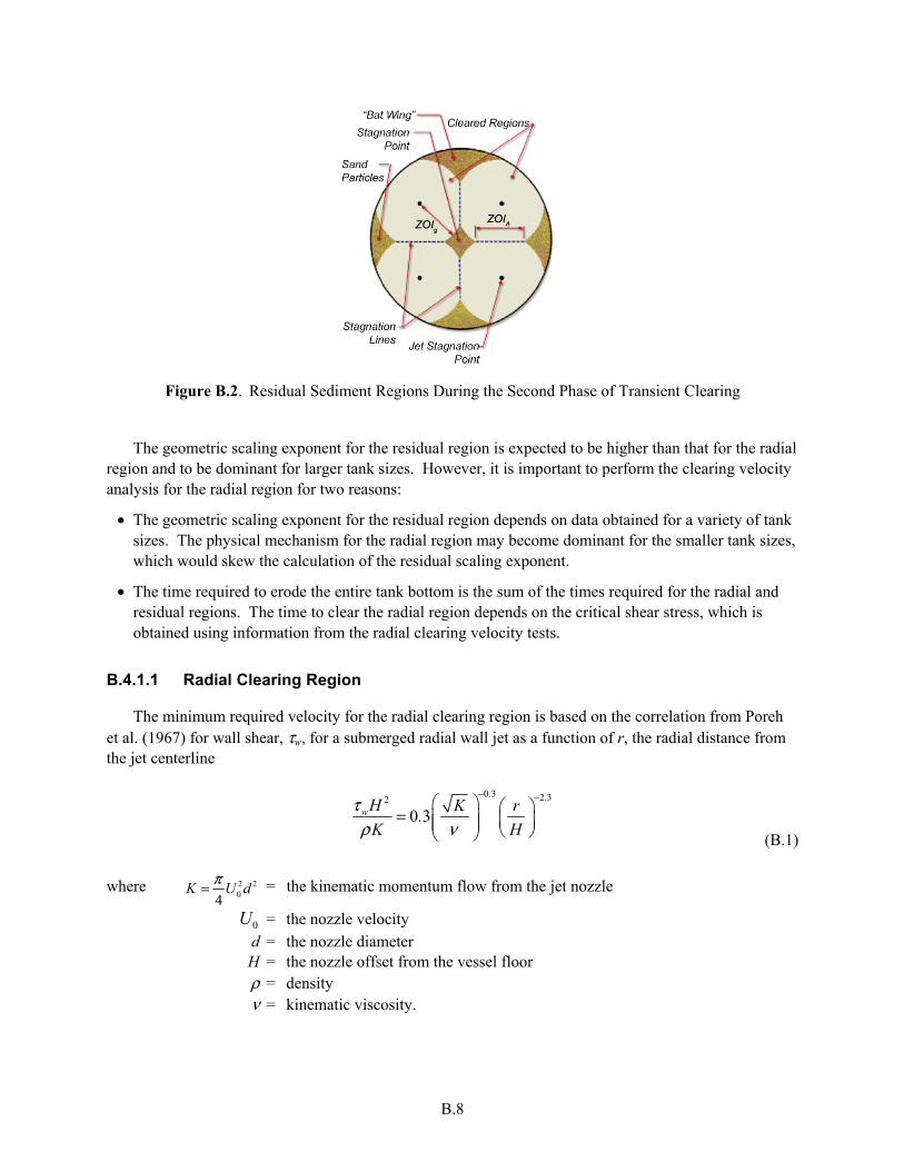
B.8

Figure B.2. Residual Sediment Regions During the Second Phase of Transient Clearing

The geometric scaling exponent for the residual region is expected to be higher than that for the radial

region and to be dominant for larger tank sizes. However, it is important to perform the clearing velocity analysis for the radial region for two reasons:

• The geometric scaling exponent for the residual region depends on data obtained for a variety of tank sizes. The physical mechanism for the radial region may become dominant for the smaller tank sizes, which would skew the calculation of the residual scaling exponent.

• The time required to erode the entire tank bottom is the sum of the times required for the radial and residual regions. The time to clear the radial region depends on the critical shear stress, which is obtained using information from the radial clearing velocity tests.

B.4.1.1 Radial Clearing Region

The minimum required velocity for the radial clearing region is based on the correlation from Poreh et al. (1967) for wall shear, τw, for a submerged radial wall jet as a function of r, the radial distance from the jet centerline

0 3 2 32

0 3

. .

wH K r.

K H

τρ ν

− − = (B.1)

where 2 204

K U dπ= = the kinematic momentum flow from the jet nozzle

U0 = the nozzle velocity

d = the nozzle diameter H = the nozzle offset from the vessel floor ρ = density ν = kinematic viscosity.

B.9

Note that we are assuming that this expression, which was developed for a flat surface, can also be applied to the curved bottom of a mixing vessel.

If the critical shear of the sediment bed is known, τc, we can calculate the corresponding maximum radial distance of clearing, rc,

12 30 3

2

0 3

..

cc

H Kr H

. K

τρ ν

− =

(B.2)

If the maximum clearing radius exceeds the maximum radial distance of sediment bed to the nearest pulse jet, then the sediment bed will be cleared, given enough time at that velocity.

If the critical shear is not known, a scaling relationship can still be developed to relate the clearing behavior of one scale vessel to another scale. When the definition for K is substituted in, the expression is rearranged to give the nozzle velocity, u, required to give a specified wall shear stress at a distance r from the nozzle centerline

0 3 2 311 7 1 7 1 71 1

1 7 1 70 244. .

. . .. .

w

H d ru .

d Hρ τ

ν− − =

(B.3)

If geometric similarity is enforced, the length ratios H/D and r/H are the same in both scales, as are the physical properties ρ and τw. The scale-up relationship (Dickey 2010) becomes

uFull = uScale

DFull

DScale

0.31.7

= uScale

DFull

DScale

0.176

(B.4)

This exponent is expected to be less than that for the residual clearing region.

An alternative expression for the radial clearing may be developed from the Poreh equation presented in Section B.7.1.5.

B.4.1.2 Residual Clearing Region

The clearing mechanisms for the residual sediment regions are not as clearly understood as for the radial clearing region. Therefore, the scaling exponent must be empirically determined based on experimental data. The scaling behavior is assumed to have the same form as for radial clearing

n

FullFull Scale

Scale

Du u

D

=

(B.5)

B.10

The geometric scaling exponent for the residual region may be estimated based on the assumption that the production of turbulent energy at large scales equals energy dissipation at small scales (power-per-unit mass). From turbulence theory, we know that the energy dissipation rate, ε, is of the order

ε ~

u3

D (B.6)

where u is the macroscopic characteristic velocity, in this case the jet velocity and D is the macroscopic characteristic length, in this case the tank diameter. On average, ɛ is just the power per mass of fluid supplied by the jets during the discharge cycle. The turbulent energy in the residual region is assumed to be proportional to the average turbulent energy of the vessel created by the jets.

The micro length scale or Kolmogorov microscale of turbulence, η, is given by

η = ν 3

ε

1

4

(B.7)

where v is the kinematic viscosity. The small scale turbulence structure remains similar for all vessel sizes and is homogeneous and isotropic. It depends only on the amount of power and not on how the power was delivered. If it is assumed that particle erosion is performed by the smallest eddies, then the vessels with equivalent power-per-unit volume, ɛ, have similar clearing behavior. This is true if the particle size, dS, is not much larger than the microscale and is of size D>>dS>>η, where particle motion is most heavily influenced by inertial subrange eddies, then the smaller eddies will most heavily influence particle motion and suspension. This assumption is made by Baldi et al. (1978) in their analysis. The geometric scaling exponent is then

uFull = uScale

DFull

DScale

1

3

(B.8)

This approach to scaling has been applied to industrial mixing applications, including impellor mixing (Grenville et al. 2010), but not for pulse jet mixing. However, others, such as Ayranci et al. (2012), argue that macroscopic flow patterns influenced by the tank geometry also affect solids suspension. Therefore, we must rely on data to establish the geometric scaling exponent.

The M3 Phase 1 tests are a relevant data set. Note that these tests only modeled the drive portion of the PJM pulse. Tests were performed for different tank bottom geometries, simulant particle size distributions, solids loading and pulse jet duty cycles (varying jet speed and duration). Measured data included suspended solids cloud height and extent of bottom clearing.

The M3 Phase 2 tests also provide a relevant data set. These tests used a prototypic PJM operating cycle. Vessel pump-down tests were also conducted to evaluate the ability of the system to remove solids.

B.11

A series of models were developed to analyze the data from these tests and are described in detail in Meyer et al. (2009, Chapter 7 and Appendices D-E), Edmonson and Thomson (2010), and Meyer et al. (2010, Chapter 5 and Appendices B-C). A brief description of each model and the scaling exponent are presented below.

The first modeling approach was the direct scale-up between cases with similar operating conditions at two different geometric scales. The critical suspension velocity, UCS, was determined for each case and scaling exponents were calculated for each simulant and duty cycle combination. The average scale-up exponent for UCS based on the data for 14 comparisons was n=0.28 ± 0.05.

The physical model considers the data from the perspective of the physical processes underlying the observed behavior. The process for developing the model is to identify the physical laws that govern the physical process, identify the important dimensionless groups and the relationships between groups and define physically reasonable functions that describe the relationships. The resulting expression for UCS is

UCS = 2.220UTH

D s −1( ) g

UTH2

0.284

φJ−0.487DC−0.284φS

0.284φp−0.198Ga−0.142

(B.9)

where 4 5

1 10 5

p .

S STH T T

S ,max

U U U.

φ φφ

= − = −

UCS = critical suspension velocity UTH = hindered terminal settling velocity UT = unhindered terminal settling velocity D = vessel diameter (m) s = ratio of particulate density to liquid density= ρs/ρl g = gravitational constant DC = PJM duty cycle, the ratio of drive time to total cycle time φJ = jet density =NJd

2/D2

NJ = number of operating jets φS = solids volume fraction φS,max = solids volume fraction corresponding to maximum packing φp = pulse jet volume fraction, the ratio of jet volume to vessel volume Ga = Galileo number

resulting in a scaling exponent of n=0.284.

After the physical model was presented in Meyer et al. (2009), several observations were made on potential improvements to the method. In response, a new physical model was developed with an enhanced method for benchmarking the model (Meyer et al. 2010). The UCS expression obtained from this analysis was

UCS = 2.302UTH

D*

Ga0.673

0.261

(B.10)

B.12

where 6

1 10 6

p

S STH T T

S ,max

U U U.

φ φφ

= − = −

and D* is the non-dimensional critical suspension

( )2 0 898 1 958

1 S*. .

TH p J

D s gD

DCU

φφ φ−

= (B.11)

resulting in a scaling exponent of n=0.261.

A multiple regression analysis was performed on the data to determine the dependence of both the UCS and cloud height as a function of a number of variables. This approach is also known as the dimensional model. The UCS expression obtained from this analysis was (Meyer et al. 2009)

ln 1.173 1.321ln( ) 0.471ln( 1) 0.222ln( ) 0.148ln( ) 0.247ln( )CS S TU D s U DCφ= − + + − + + −

−0.211ln φp( ) − 0.525ln NJ( ) −1.072 ln d( ) (B.12)

where UT = unhindered terminal settling velocity (m/s) NJ = number of active PJMs d = PJM nozzle diameter (m).

Varying the vessel diameter, D, and the nozzle diameter, d, while holding the rest of the variables constant, the scaling exponent for UCS from this expression becomes n=0.249.

The constant for the dimensional model makes use of dimensioned variables, implying that the constant must also have a dimensioned value. For this reason, a generalized model was developed which consists of dimensionless groups. The expression for UCS using this approach is (Meyer et al. 2009)

UCS = 0.273UT

D s −1( ) g

UT2

0.397d

D

−0.991

s −1( )0.086DC−0.205φS

0.243φp−0.221NJ

−0.511

(B.13)

resulting in a scaling exponent of n=0.397.

The values for the UCS scaling exponent for these methods range from 0.25 to 0.40. The residual region velocity scaling exponent is expected to exceed the one established by Poreh et al. (1967) though this exponent should be established empirically. A good starting point would be the expression presented in Section 2.2.3.1 with the form

( ) ( )1H pr

CC CCCS C S SU d K Cr r H d θθ= = +

(B.14)

where KC is the kinematic momentum flow (at the limit of bottom clearing), proportional to the square of the product of the nozzle velocity (at the limit of bottom clearing) and the nozzle diameter, r is the radius

B.13

of colliding jets, dS is the diameter of settled solids, and θS is defined in Section 2.2.2.1 and explained in Section 2.2.2.2. θS includes the product of the solids volume fraction, settling velocity, and drive time.

These scaling relationships specify the velocity required to match the wall shear stress at the maximum distance from the nozzle. So, for a pulse stroke that is sufficiently long to erode the sediment bed, the calculated velocity for the full-scale vessel should erode the bed to that same maximum relative distance. However, the expression does not provide information on the time it will take to erode the sediment bed to that distance. Therefore, we need a separate requirement that addresses the rate of sediment bed erosion.

B.4.2 Transient Clearing Analysis

Video recordings of transient bottom clearing during the jet pulse indicate that the clearing process occurs in two sequential phases. The first phase is radial clearing beginning at the jet centerline and expanding as a function of time until the radial jet begins to interact with the jets from other pulse tubes. The second phase is the clearing of residual sediment in the vicinity of these jet interaction zones. The total clearing time for a single pulse is the sum of the times for these two phases. Each phase is described in more detail below.

B.4.2.1 Transient Clearing Analysis – Radial Clearing

The ZOI achieved during the drive phase of a pulse cycle is a function of both velocity and time. The standard expression used in the field of hydrology to describe SE, the rate of sediment surface erosion (Partheniades 1965 via Simon et al. 2002) per unit surface area is

SE = E τ w −τ c( )n

where τw ≥ τ c (B.15)

SE = 0 where τw < τ c (B.16)

where n is assumed to be equal to one and E is the erodibility coefficient.

The critical wall shear stress, τc, is defined as the minimum shear above which surface erosion of particular sediment occurs. The difference between the fluid stress and the critical stress is also known as the excess shear stress. The erodibility coefficient, E, is a rate constant that is a property of the sediment composition. This expression has been used in previous analysis of Hanford tank waste (Powell et al. 1997).

Imagine an eroding sediment with a thickness, δ, on the vessel floor. Assume that the total bed erosion, which is determined by the radial integral over the sediment bed of the excess shear, is proportional to the excess shear stress at the leading edge of the sediment. The erosion is expected to be concentrated near the leading edge since as the jet fluid picks up zero velocity sediment particles, the velocity profile changes and the wall shear stress decreases. The added suspension concentration also reduces the rate of erosion downstream from the edge. A second assumption is that the shape of the

B.14

sediment edge vertical profile does not significantly change with radius. Therefore, the total volume of sediment eroded from the top of the sediment is proportional to the product of the height of the sediment and the change in radius.

An erosion velocity, uZOI, defined as the rate of change of clearing radius with respect to time, is given by the expression

( ) ( ) ( )E

ZOI c

Cdru r r r

dtτ τ

δ= = −

(B.17)

where the erosion coefficient, CE, includes the erodibility and the ratio of the integrated excess shear to the leading edge excess shear. This coefficient is a function of sediment type and independent of vessel scale or flow rate. Substitute in the Poreh expression for fluid shear stress (Equation (B.1)) to get an expression for the rate of change in clearing radius

( )0 3 2 3

2

0 3. .

Ec

Cdr . K K rr

dt H H

ρ τδ ν

− − = − (B.18)

This expression can be integrated to give the clearing radius for any specified time, T, after the beginning of the pulse

r(T) = dr

dt(r)

0

T

dt (B.19)

This equation may be integrated by spreadsheet using a Newton’s method.

Therefore, once we have determined the erosion coefficient (CE) and the critical shear stress (τc) for a sediment type, we can calculate the clearing radius evolution for any vessel size, flow rate and sediment thickness.

Sample results for time integration analysis are shown in Figure B.3 to illustrate the effect of critical shear stress on radial clearing time. The calculation was performed for the full-scale HLP-22 vessel with a nozzle velocity of 12 m/s. The erodibility coefficient was arbitrarily specified as 1.0. The starting point for the radial jet development was chosen to be three-halves the nozzle radius from the jet centerline. The results do not appear to be sensitive to the location of the starting point since the gradient is so steep at that point in the transient.

Calculations were performed for three different critical shear stresses. The lines show the clearing radius as a function of time. Note that the radius grows relatively quickly at the beginning of the transient and slows as the wall shear drops off with radial distance. The dashed purple line indicates the half-way position between a pulse jet in the inner circle and a neighboring pulse jet in the outer circle.

The radius versus time behavior during the initial portion of the transient, where the wall shear is significantly higher than the critical shear stress, is similar for all three cases. As the radius increases and the wall shear stress decreases, the effect of the critical shear stress becomes more important.

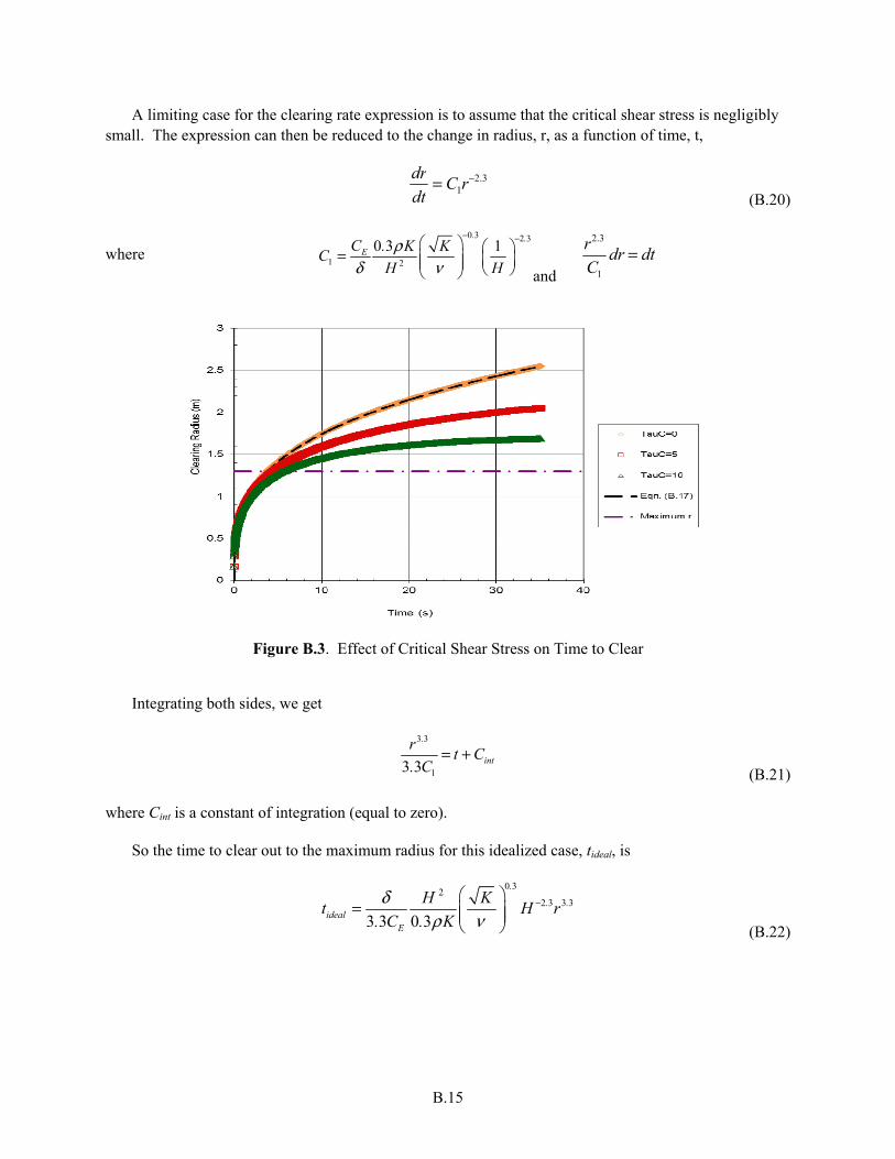
B.15

A limiting case for the clearing rate expression is to assume that the critical shear stress is negligibly small. The expression can then be reduced to the change in radius, r, as a function of time, t,

dr

dt= C1r

−2.3

(B.20)

where

0 3 2 3

1 2

0 3 1. .

EC . K KC

H H

ρδ ν

− − = and

r2.3

C1

dr = dt

Figure B.3. Effect of Critical Shear Stress on Time to Clear

Integrating both sides, we get

3 3

13 3

.

int

rt C

. C= +

(B.21)

where Cint is a constant of integration (equal to zero).

So the time to clear out to the maximum radius for this idealized case, tideal, is

0 32

2 3 3 3

3 3 0 3

.

. .ideal

E

H Kt H r

. C . K

δρ ν

− =

(B.22)

B.16

Or substituting for kinematic momentum flow K yields

0 850 3 1 7 1 7 3 3

00 30 99 4

.. . . .

ideal .E

t H U d r. C

δ πρν

−− − − =

(B.23)

The variables H, D, and r all scale linearly with vessel size, so the scaling relationship for time to clear in the idealized case, tid is

tid ,FULL

tid ,SCALE

= UFULL

USCALE

−1.7rFULL

rSCALE

1.3δFULL

δSCALE

(B.24)

The actual time to clear will exceed the idealized time by an amount determined by the relative magnitude of the critical shear stress. This effect can be expressed in terms of a time multiplier, M, that provides the effect of a critical shear stress

tFULL

tSCALE

= UFULL

USCALE

−1.7rFULL

rSCALE

1.3δFULL

δSCALE

MFULL

MSCALE

(B.25)

The time multiplier, M, is calculated using the time integration method described above and is a function of the erosion coefficient, critical shear stress, and nozzle velocity.

Assume that the velocity ratio is that obtained from the maximum clearing analysis (Section B.4.1). The ratio of pulse time to clear an equivalent radius would be

tid,FULL

tid,SCALE

= rFULL

rSCALE

0.176

−1.7

rFULL

rSCALE

1.3δFULL

δSCALE

= rFULL

rSCALE

δFULL

δSCALE

(B.26)

or proportional to the geometric scaling. However, the maximum available pulse time, tavail, is determined by both the tube volume, VPT, and nozzle velocity

tavail = VPT

U0π4 d 2

(B.27)

resulting in a ratio of the full and scaled pulse times that follows the relationship

tavail,FULL

tavail,SCALE

= rFULL

rSCALE

UFULL

USCALE

−1.0

(B.28)

which is less than geometric scaling. In addition, the sediment thickness is expected to be greater in the full-scale tank due to the greater settling during the longer refill portion of the pulse cycle. Therefore, the time to clear requirement appears to be more restrictive than the maximum velocity requirement.

B.17

The erosion coefficient, CE, can be estimated from clearing radius versus time scaled test data. Clearing radius versus time data that follows this relationship, when plotted on a log-log plot with ln(t) on the x-axis and ln(r) on the y-axis, results in a slope of the line of approximately 1/3.3 or 0.3 (see Figure B.4). At the beginning of the pulse cycle after the velocity has ramped up, the shear stress at the sediment bed edge should be substantially higher than the critical shear stress. Therefore, the log slope of the data should be close to the theoretical limit at the beginning of the pulse and decrease as the effect of the critical shear stress becomes more important towards the end of the stroke. The initial time used in the data analysis should not be the beginning of the acceleration phase of the stroke, but the beginning of the log-linear portion of the radius versus time plot.

Figure B.4. Log-Log Plot of Time to Clear

B.4.2.2 Transient Clearing Analysis – Residual Bottom Motion

The radial jet behavior described by Poreh et al. (1967) begins to change as the radius approaches the halfway point between two adjacent pulse jet centerlines. The radial velocity slows and up-wash fountain and circumferential flows begin to form. The erosion mechanisms in this region are not well understood.

The first assumption that we make is that the rate of erosion will be proportional to the excess shear stress at the maximum radius from the pulse jet centerline, rmax.

The second assumption is that the mass of settled solids in the residual regions is proportional to the initial sediment bed height. Since we do not know the scaling behavior, we will write the expression for the time for residual clearing, tRES, as

( ) n

RES RES max c maxt C r rδ τ τ = − (B.29)

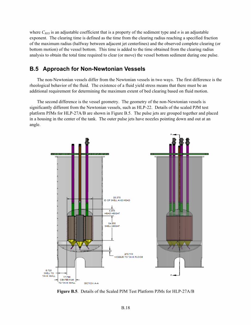
B.18

where CRES is an adjustable coefficient that is a property of the sediment type and n is an adjustable exponent. The clearing time is defined as the time from the clearing radius reaching a specified fraction of the maximum radius (halfway between adjacent jet centerlines) and the observed complete clearing (or bottom motion) of the vessel bottom. This time is added to the time obtained from the clearing radius analysis to obtain the total time required to clear (or move) the vessel bottom sediment during one pulse.

B.5 Approach for Non-Newtonian Vessels

The non-Newtonian vessels differ from the Newtonian vessels in two ways. The first difference is the rheological behavior of the fluid. The existence of a fluid yield stress means that there must be an additional requirement for determining the maximum extent of bed clearing based on fluid motion.

The second difference is the vessel geometry. The geometry of the non-Newtonian vessels is significantly different from the Newtonian vessels, such as HLP-22. Details of the scaled PJM test platform PJMs for HLP-27A/B are shown in Figure B.5. The pulse jets are grouped together and placed in a housing in the center of the tank. The outer pulse jets have nozzles pointing down and out at an angle.

Figure B.5. Details of the Scaled PJM Test Platform PJMs for HLP-27A/B

B.19

As with the Newtonian case, two requirements are required for a pulse jet cycle to clear the tank floor. The first requirement is that the maximum velocity of the jet is sufficient to generate sufficient wall shear to erode the sediment at the farthest distance from any jet. The second requirement is that the pulse stroke is long enough to erode the sediment to that distance. Evaluation of the requirements differs from the Newtonian case. These requirements are addressed below.

B.5.1 Maximum Clearing Analysis

Erosion of a sediment bed in a non-Newtonian fluid must satisfy two requirements:

• The radial jet must be sufficient to shear the non-Newtonian fluid out to the furthest distance of the sediment bed. This requirement is a function of the fluid properties, especially the Bingham yield stress.

• The radial jet must be sufficient to overcome the critical yield stress of the sediment bed, as described in Section B.4.1.1. This requirement is a function of the sediment bed properties.

The mobilization distance for non-Newtonian materials is defined as the fluidization radius, rf. The region of fluid with this radius occurs when the applied normal stress, τn, from a yielded non-Newtonian fluid acting on the face of a fluid parcel before yielding is equal to the yield stress, τ0, of that fluid. A model for this radius can be derived from the Poreh et al. (1967) relation for the mean jet velocity Um:

Umr

K=1.32

r

H

−0.1

(B.30)

where 2204dUK

π= = the kinematic momentum flux from the jet nozzle

U0 = the nozzle velocity d = the nozzle diameter H = the nozzle offset from the vessel floor.

In terms of d and U0, Equation (B.30) can be rewritten as

1110

0 4321

..

m d

r

d

H.UU

−

= π

(B.31)

The applied normal stress from the fluid stream, τn, is given by the stagnation pressure

( )

222022

02

4321

2

1

2

1..

mn d

r

d

H.UU

−

== πρρτ

(B.32)

B.20

Set the applied normal stress, τn, equal to the yield stress of the fluid, τ0, and rearrange to obtain an expression for the fluidization radius

( )

20

0

202

22

4321

2

1..

d

HU.

d

r

=

τρπ

(B.33)

( )

09104550

0

20

45502

4321

2

1...

d

HU.

d

r

=

τρπ

(B.34)

45500

0910

8410 ..

Red

H.

d

r

=

(B.35)

where Re0 ≡ ρU02 /τ 0 is the yield Reynolds number. If the expression τn=2τ0, which is based on the

mechanics of materials expression relating solid normal stress to shear stress, the expression for fluidization radius becomes

45500

0910

6140 ..

Red

H.

d

r

=

(B.36)

The physical mechanism described by Equation (B.35) is assumed to be correct and Equation (B.36) is presented as a lower limit.

B.5.2 Transient Clearing Analysis

The clearing transient occurs in two phases. During the initial stages of the pulse, the individual pulse jets will begin to clear the sediment in a radial direction, in a manner similar to the Newtonian vessel. The erodibility coefficient may be estimated during this radial part of the transient using the Poreh expression. However, the flow from the center tube and the interior side of the outer tubes cannot form upward fountains, so the flow will begin to be diverted outward past the outer tubes, skewing the radial distribution toward the perimeter of the vessel.

In the second phase, the net effect of the tube array will be to create one large radial jet along the bottom toward the outer diameter of the vessel. We assume that the sediment under the tube array will erode before the sediment beyond the tube array housing radius. This radial wall jet cannot be characterized using the Poreh expression, because of the assumption that the origin of the radial jet is near the impinging jet centerline. A separate expression must be developed to allow the jet origin to be at a specified radius.

Following the dimensional analysis described in Rajaratnam (1976), the expression for wall shear, τw, for this geometry would have the form

τw

ρlU02

= CR

r

r0

r − r0 + b0

b0

(B.37)

B.21

where U0 is the average velocity through a radial slot of height b0 located at a radial distance r0, equivalent to the outer radius of the pulse jet array shell. The total radial flow rate is equal to the sum of the flow rates of the individual pulse jets. The first term in the denominator on the right hand side describes the diffusion of momentum in the radial direction and the second term describes the diffusion of momentum in the axial direction beginning at a distance of r0–b0 from the origin.

The coefficient CR may possibly be a function of jet Reynolds number. If we assume similar Reynolds number behavior as Poreh, the expression becomes

+−

=

−

0

00

0

30

20

b

brr

r

r

CK

UNon

.

l

w

νρτ

(B.38)

where CNon is an adjustable parameter and the kinematic momentum flux is now defined as

K = U022πr0b0 (B.39)

As in the Newtonian vessel case, an erosion velocity, uZOI, defined as the rate of change of clearing radius with respect to time, is given by the expression

uZOI = dr

dtr( )= CE

δτ r( )− τ c[ ]

(B.40)

and substituting in the expression for wall shear gives

( )

−

+−

=

−

cNon

.

lE

b

brr

r

r

CKU

Cr

dt

dr τν

ρδ

0

00

0

30

20

(B.41)

which can be integrated using a Newton’s method.

B.6 LSIT Test Analysis

The analysis of data taken from the 43-in.-diameter scaled tank is described in Chapter 6 of the Test Plan for Pulse Jet Mixer Performance Tests in the 43-in. Acrylic Test Vessel (TP-WTPSP-039).1

B.6.1 Maximum Clearing Analysis

Section 6.1 of the 43-in.-diameter tank test plan describes a method for obtaining the velocity scale-up exponent from a series of ECR measurements at different nozzle velocities. A series of pulse jet

1 Toth J. 2011. Test Plan for Pulse Jet Mixer Performance and Scaling Tests in the 43-in. Acrylic Test Vessel. TP-WTPSP-039 Draft, Pacific Northwest National Laboratory, Richland, Washington.

B.22

cycles will be operated with a maximum velocity ranging from 1 m/s to 11 m/s in increments of 1 m/s. At the end of each pulse when the radius is no longer changing, the ECR will be recorded corresponding to the nozzle velocity. If bottom clearing has not been achieved by 11 m/s, the nozzle velocity is increased by increments of 0.1 m/s until clearing is achieved.

The first step in determining the velocity scaling is to determine the nozzle velocities for equivalent scaled radii for the 43-in.-, 8-ft-, and 14-ft-diameter tanks. The radii could be expressed in terms of the fraction of distance between pulse jet centerlines.

The velocity scale-up exponent, α, is determined using the expression (using the 43-in.- and 8-ft-diameter tanks as examples)

( )( )

96 43

96 43

ln /

ln

U U

Sα

−

= (B.42)

where S is the geometric scale factor based on the actual tank diameters

96 43 96 43/ 93.2 / 43.25 2.15S D D− = = = (B.43)

The same procedure is also used to determine the scaling for total bottom clearing.

This analysis can be used to verify whether the Poreh model can be used for pulse jet conditions, including nozzle offset, jet Reynolds numbers, etc. The scaling exponent calculated by Equation (B.42) should be approximately α=0.176 at each location if Poreh is applicable. If the scaling exponent is significantly different or varies as a function of radius, the wall shear as a function of distance from jet centerline may require a new model.

The ECR data collected using this procedure allows the determination of the critical shear stress, τc, for a specific sediment type. If the Poreh expression is determined to be representative, the critical shear stress may be calculated directly from Equation (B.1) and should be the same at each radial location.

The calculated value does not depend in any way on erosion models or correlations. With that said, there may be some benefit in calculating bounding values using the erosion models found in the literature as a check on the reasonableness of the value calculated from pulse jet data. A literature review of critical shear stress correlations for non-cohesive and cohesive beds is presented in Section B.8, in support of this option.

B.6.2 Transient Clearing Analysis

A second series of tests are recommended to characterize the time scaling behavior of the scaled pulse jet vessels. Each test consists of establishing a sediment bed of a specified thickness and then performing a jet pulse with a specified nozzle velocity. The clearing radius is recorded as a function of time through the use of video with a time stamp.

A least-squares fit of the data will be performed to determine the optimal value of the erosion coefficient, CE, using the critical shear stress that was obtained from the maximum clearing analysis.

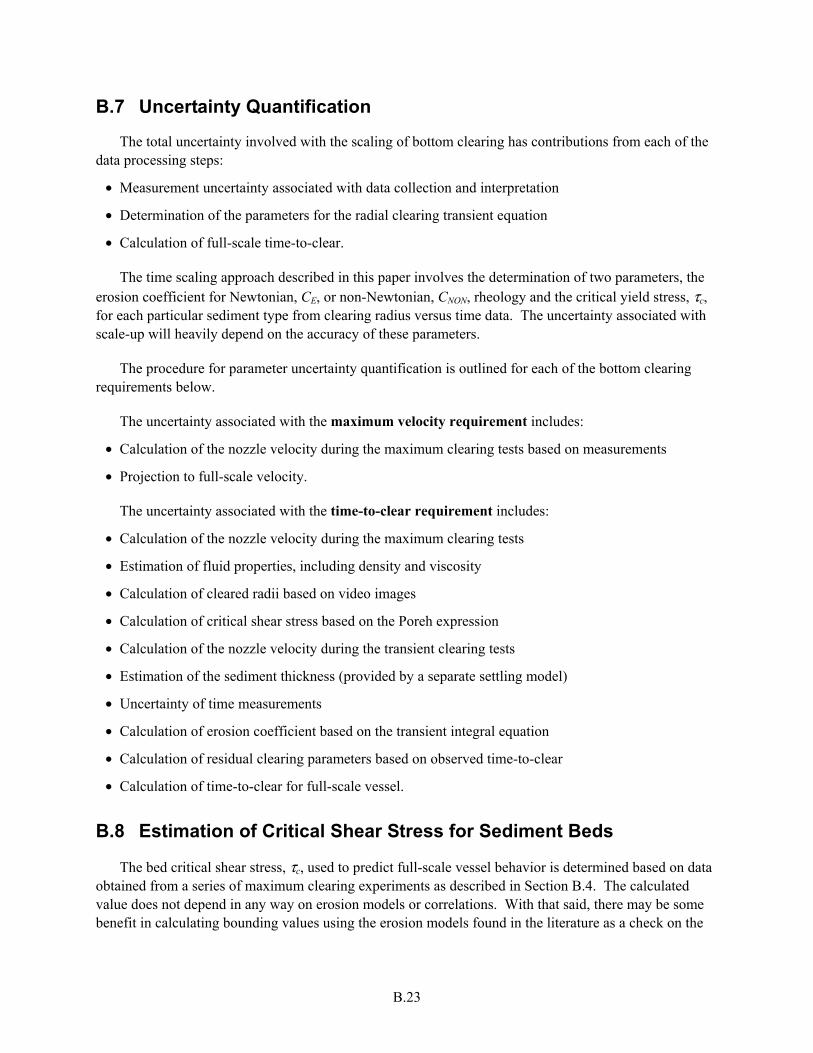
B.23

B.7 Uncertainty Quantification

The total uncertainty involved with the scaling of bottom clearing has contributions from each of the data processing steps:

• Measurement uncertainty associated with data collection and interpretation

• Determination of the parameters for the radial clearing transient equation

• Calculation of full-scale time-to-clear.

The time scaling approach described in this paper involves the determination of two parameters, the erosion coefficient for Newtonian, CE, or non-Newtonian, CNON, rheology and the critical yield stress, τc, for each particular sediment type from clearing radius versus time data. The uncertainty associated with scale-up will heavily depend on the accuracy of these parameters.

The procedure for parameter uncertainty quantification is outlined for each of the bottom clearing requirements below.

The uncertainty associated with the maximum velocity requirement includes:

• Calculation of the nozzle velocity during the maximum clearing tests based on measurements

• Projection to full-scale velocity.

The uncertainty associated with the time-to-clear requirement includes:

• Calculation of the nozzle velocity during the maximum clearing tests

• Estimation of fluid properties, including density and viscosity

• Calculation of cleared radii based on video images

• Calculation of critical shear stress based on the Poreh expression

• Calculation of the nozzle velocity during the transient clearing tests

• Estimation of the sediment thickness (provided by a separate settling model)

• Uncertainty of time measurements

• Calculation of erosion coefficient based on the transient integral equation

• Calculation of residual clearing parameters based on observed time-to-clear

• Calculation of time-to-clear for full-scale vessel.

B.8 Estimation of Critical Shear Stress for Sediment Beds

The bed critical shear stress, τc, used to predict full-scale vessel behavior is determined based on data obtained from a series of maximum clearing experiments as described in Section B.4. The calculated value does not depend in any way on erosion models or correlations. With that said, there may be some benefit in calculating bounding values using the erosion models found in the literature as a check on the

B.24

reasonableness of the value calculated from pulse jet data. A literature review of critical shear stress correlations for non-cohesive and cohesive beds is presented below in support of this option.

B.8.1 Non-Cohesive Beds

The critical shear stress for a particle bed is defined as the minimum shear exerted by the flowing fluid over the bed to overcome the gravity force holding the particle in place. The critical shear stress for a Newtonian particle suspension can be expressed as a relationship between the non-dimensional critical shear stress, also known as the Shields1 parameter (Shields 1936), τ* (also θc)

( )* c

cs l Sgd

ττ θρ ρ

= =−

(B.44)

where ρs is the solids density and ρl is the liquid density, and the shear Reynolds number, Re*p

cS*

l* Sp

du d

Re

τρ

ν ν= =

(B.45)

where u* is the shear velocity, τc is the critical shear stress, and dS is the particle diameter. The Shields parameter contains gravitational force information and the shear Reynolds number contains fluid drag information.

The Shields parameter is calculated from a series of non-cohesive erosion tests and plotted as a function of the shear Reynolds number, Re*, to give the Shields diagram as shown in Figure B.6. For non-cohesive solids, the Shields diagram uniquely determines the critical shear stress. Note that there is a range of erosion behavior below a shear Reynolds number of one.

A variety of analytical expressions have been developed to fit the Shields data. Brownlie (1981) proposed the expression

0.30.3 7.70.22 0.06 10 Ar

c Arθ−− −= + ⋅ (B.46)

where the Archimedes number, Ar, is defined as

( ) 3s l S

l

gdAr

ρ ρρν

−=

(B.47)

1 Based on work presented by Shields in 1936.

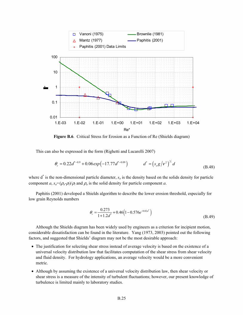
B.25

0.01

0.1

1

10

100

1.E-03 1.E-02 1.E-01 1.E+00 1.E+01 1.E+02 1.E+03 1.E+04

Re*

*

Vanoni (1975) Brownlie (1981)

Mantz (1977) Paphitis (2001)

Paphitis (2001) Data Limits

Figure B.6. Critical Stress for Erosion as a Function of Re (Shields diagram)

This can also be expressed in the form (Righetti and Lucarelli 2007)

( )0 9 0 090 22 0 06 17 77* . * .

c . d . exp . dθ − −= + −

( ) 132*

ad s g dν= (B.48)

where d* is the non-dimensional particle diameter, sa is the density based on the solids density for particle component a, sa=(ρa-ρl)/ρl and ρa is the solid density for particle component a.

Paphitis (2001) developed a Shields algorithm to describe the lower erosion threshold, especially for low grain Reynolds numbers

( )*0.02

*

0.2730.46 1 0.576

1 1.2d

c ed

θ −= + −+ (B.49)

Although the Shields diagram has been widely used by engineers as a criterion for incipient motion, considerable dissatisfaction can be found in the literature. Yang (1973, 2003) pointed out the following factors, and suggested that Shields’ diagram may not be the most desirable approach:

• The justification for selecting shear stress instead of average velocity is based on the existence of a universal velocity distribution law that facilitates computation of the shear stress from shear velocity and fluid density. For hydrology applications, an average velocity would be a more convenient metric.

• Although by assuming the existence of a universal velocity distribution law, then shear velocity or shear stress is a measure of the intensity of turbulent fluctuations; however, our present knowledge of turbulence is limited mainly to laboratory studies.

B.26

• Shields derived his criterion for incipient motion by using the concept of a laminar sublayer, according to which the sublayer should not have any effect on the velocity distribution when the shear velocity Reynolds number is greater than 70. However, the Shields diagram clearly indicates that this dimensionless critical shear stress still varies with shear velocity Reynolds number in this range.

• The parameters contain shear stress and shear velocities that are not independent, requiring an iterative procedure for determining the critical shear stress.

• Shields simplified the problem by neglecting the lift force and considered only the drag force. The lift force cannot be neglected, especially at high-shear velocity Reynolds numbers.

As an alternative, Yang (2003) proposed using a critical velocity, Vcr, as a criterion for incipient motion of particles where uT is the particle fall velocity. The expressions for the transition and turbulent regimes are

( )

2 50 66

0 06cr

*T S

V ..

u log u d .ν= +

−

1 2 70*

Su d.

ν< <

(B.50)

2 05cr

T

V.

u=

70

*Su d

ν≤

(B.51)

where u* is the wall shear velocity, u* = τ w ρ .

The advantage of these expressions is that they address the objections to the Shields criterion listed above. One major disadvantage is that the extensions to cohesive beds that are described in Section B.8.2 have been developed using the Shields parameter as the basis.

B.8.1.1 More Recent Theories for Onset of Liftoff1

Shields’ relationship is shown in Figure B.7 together with the recent data of Nino et al. (2003), which is seen to be substantially underpredicted (i.e., the τ* needed to entrain particles of diameter Re*p is substantially underpredicted).

Bagnold (1966) (as given in Nino et al. 2003) took a more mechanistic approach and attempted to

predict the onset of particle entrainment by finding the wall shear stress given by *wu τ ρ= where

1

*

T

u

U=

(B.52)

Here UT (ws in Figures B.8, B.9, and B.10) is the particle settling velocity.

1 Sections B.8.1.1 through B.8.1.6 were contributed by Professor Sanjoy Banerjee.

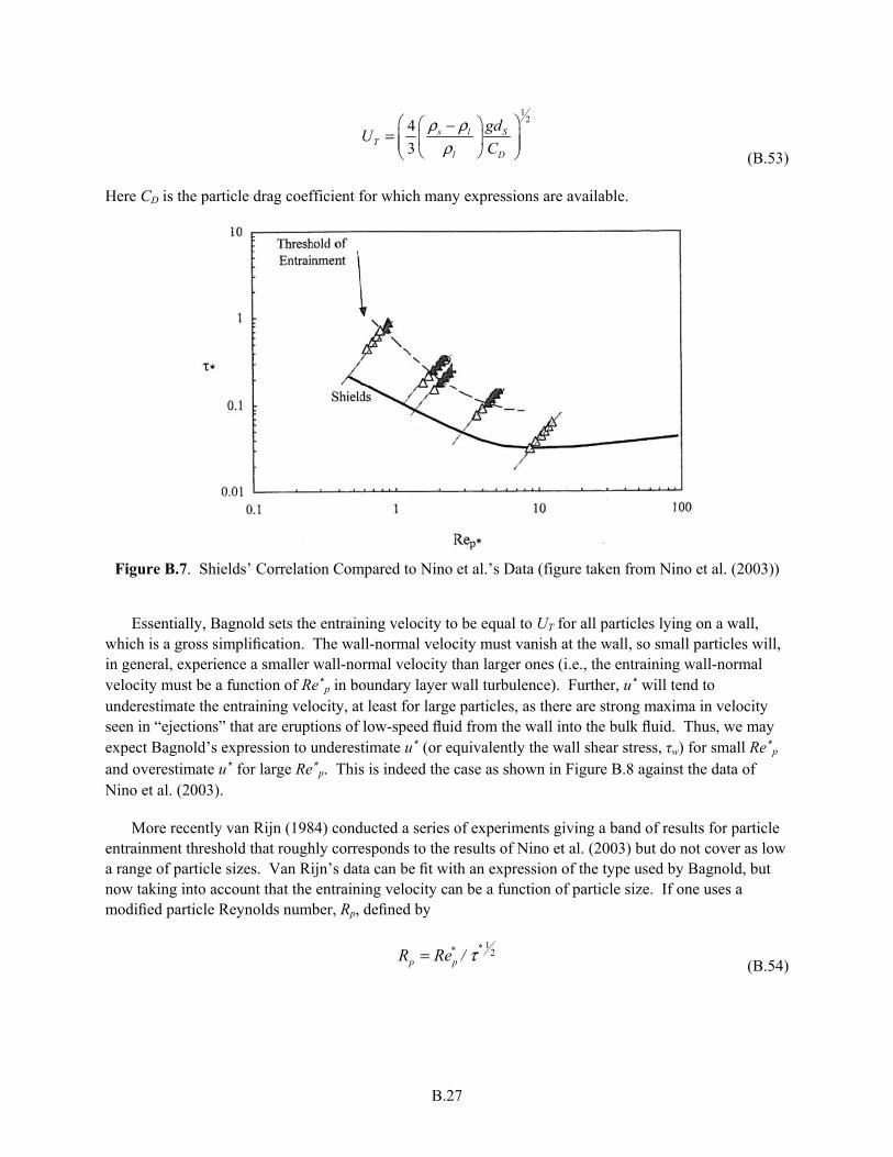
B.27

124

3

−= s l S

Tl D

gdU

C

ρ ρρ

(B.53)

Here CD is the particle drag coefficient for which many expressions are available.

Figure B.7. Shields’ Correlation Compared to Nino et al.’s Data (figure taken from Nino et al. (2003))

Essentially, Bagnold sets the entraining velocity to be equal to UT for all particles lying on a wall,

which is a gross simplification. The wall-normal velocity must vanish at the wall, so small particles will, in general, experience a smaller wall-normal velocity than larger ones (i.e., the entraining wall-normal velocity must be a function of Re*p in boundary layer wall turbulence). Further, u* will tend to underestimate the entraining velocity, at least for large particles, as there are strong maxima in velocity seen in “ejections” that are eruptions of low-speed fluid from the wall into the bulk fluid. Thus, we may expect Bagnold’s expression to underestimate u* (or equivalently the wall shear stress, τw) for small Re*p and overestimate u* for large Re*p. This is indeed the case as shown in Figure B.8 against the data of Nino et al. (2003).

More recently van Rijn (1984) conducted a series of experiments giving a band of results for particle entrainment threshold that roughly corresponds to the results of Nino et al. (2003) but do not cover as low a range of particle sizes. Van Rijn’s data can be fit with an expression of the type used by Bagnold, but now taking into account that the entraining velocity can be a function of particle size. If one uses a modified particle Reynolds number, Rp, defined by

12**

p pR Re / τ= (B.54)

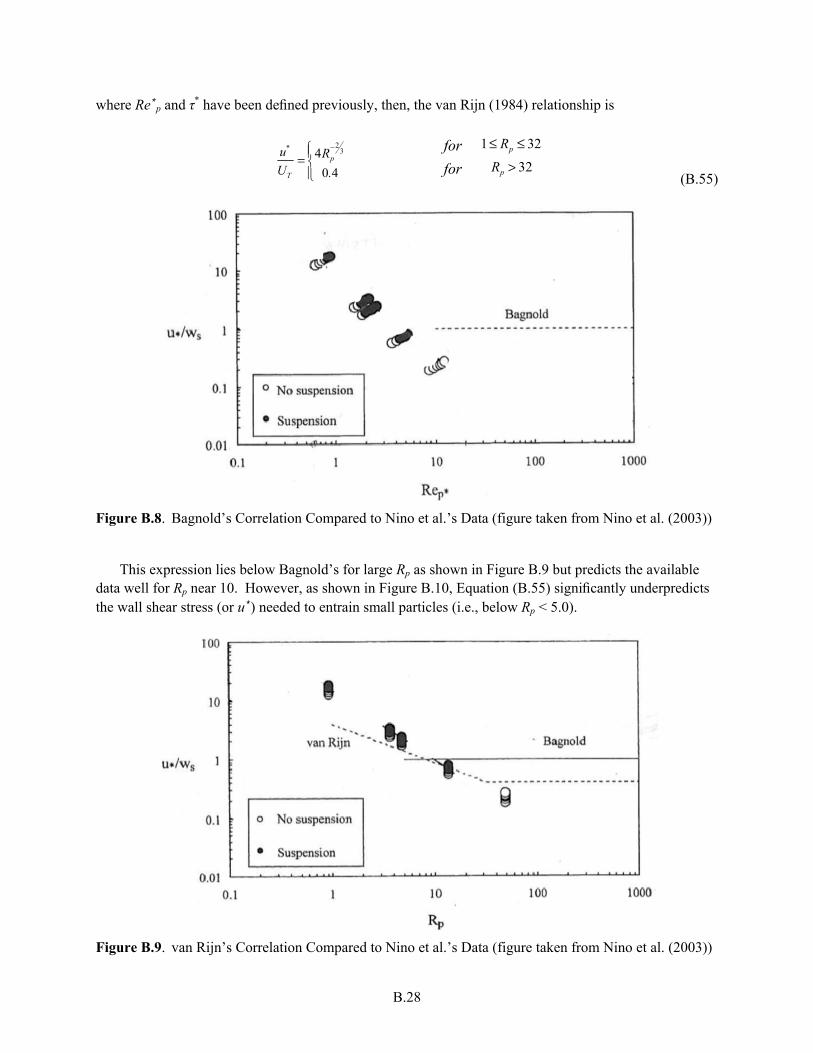
B.28

where Re*p and τ* have been defined previously, then, the van Rijn (1984) relationship is

234

0 4

*

p

T

u RU .

−=

for

for

1≤ Rp ≤ 32

Rp > 32 (B.55)

Figure B.8. Bagnold’s Correlation Compared to Nino et al.’s Data (figure taken from Nino et al. (2003))

This expression lies below Bagnold’s for large Rp as shown in Figure B.9 but predicts the available

data well for Rp near 10. However, as shown in Figure B.10, Equation (B.55) significantly underpredicts the wall shear stress (or u*) needed to entrain small particles (i.e., below Rp < 5.0).

Figure B.9. van Rijn’s Correlation Compared to Nino et al.’s Data (figure taken from Nino et al. (2003))

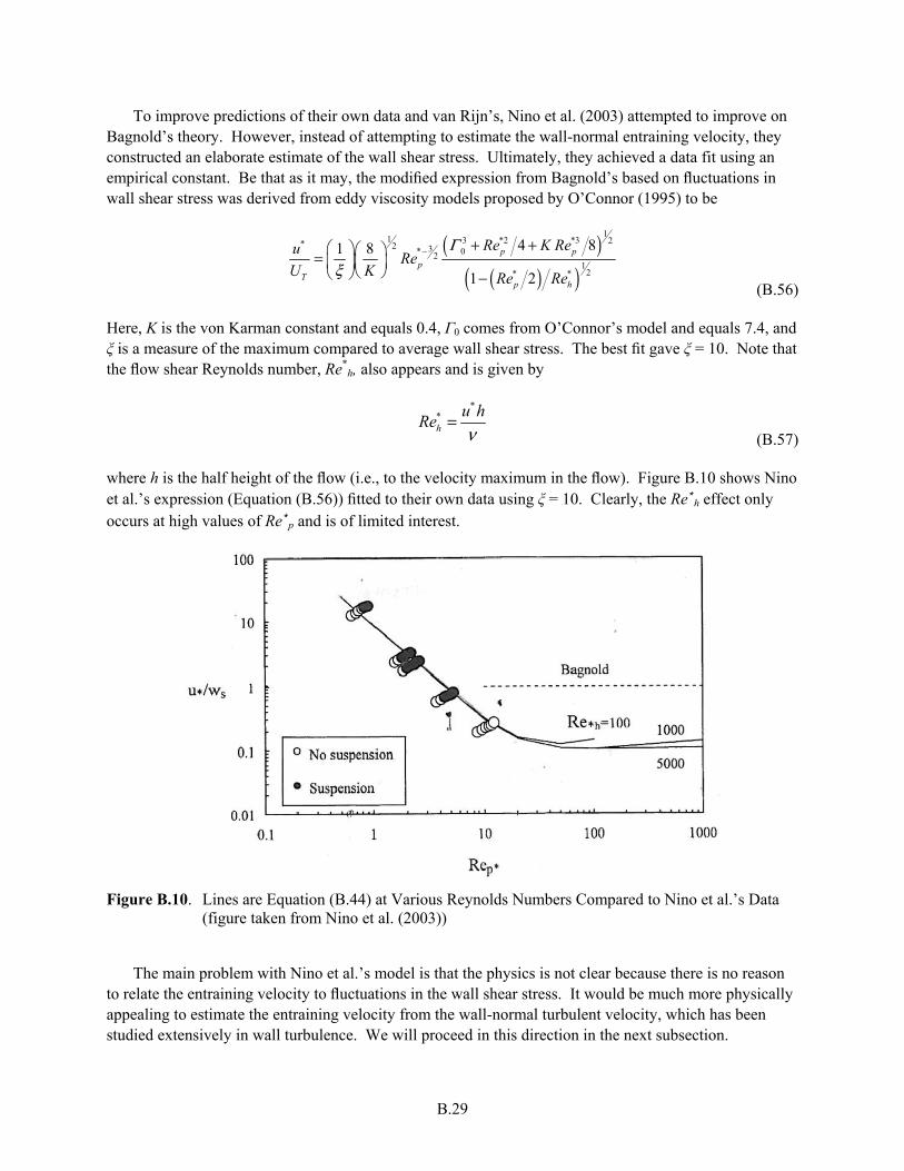
B.29

To improve predictions of their own data and van Rijn’s, Nino et al. (2003) attempted to improve on Bagnold’s theory. However, instead of attempting to estimate the wall-normal entraining velocity, they constructed an elaborate estimate of the wall shear stress. Ultimately, they achieved a data fit using an empirical constant. Be that as it may, the modified expression from Bagnold’s based on fluctuations in wall shear stress was derived from eddy viscosity models proposed by O’Connor (1995) to be

( )( )( )

11 3 2 3 2

2 3 021

2

4 81 8

1 2

* *** p p

p* *Tp h

Re K ReuRe

U K Re Re

Γξ

− + + = −

(B.56)

Here, K is the von Karman constant and equals 0.4, Γ0 comes from O’Connor’s model and equals 7.4, and ξ is a measure of the maximum compared to average wall shear stress. The best fit gave ξ = 10. Note that the flow shear Reynolds number, Re*

h, also appears and is given by

**h

u hRe

ν=

(B.57)

where h is the half height of the flow (i.e., to the velocity maximum in the flow). Figure B.10 shows Nino et al.’s expression (Equation (B.56)) fitted to their own data using ξ = 10. Clearly, the Re*h effect only occurs at high values of Re*p and is of limited interest.

Figure B.10. Lines are Equation (B.44) at Various Reynolds Numbers Compared to Nino et al.’s Data (figure taken from Nino et al. (2003))

The main problem with Nino et al.’s model is that the physics is not clear because there is no reason

to relate the entraining velocity to fluctuations in the wall shear stress. It would be much more physically appealing to estimate the entraining velocity from the wall-normal turbulent velocity, which has been studied extensively in wall turbulence. We will proceed in this direction in the next subsection.

B.30

B.8.1.2 A Modified Theory for Particle Entrainment Threshold

We will use as a starting point Bagnold’s theory, but instead of equating the entraining velocity, ue, with u*, we will estimate the maximum wall-normal velocity, i.e.,

1e

T

u

U=

(B.58)

where the velocity to just entrain particles of settling velocity UT is ue, and this is assumed to be the maximum in the fluctuating wall-normal velocity, w’, i.e.,

ue

u*= max w '

(B.59)

Note that ue and w’ will be a function of z+, the non-dimensional distance from the wall.

The variation of w’ as a function of z+ can be obtained from the direct numerical simulation (DNS) of Kim et al. (1987). From Figure 13 in their paper, a good fit to the root mean square (rms) value of the fluctuating velocity w’rms is given by

w 'rms

z+1.33≈ 0.015

(B.60)

where z+ = zu* /ν . This fit is good to 1 ≤ z+ ≤ 12. Note w’rms is non-dimensionalized with u*. To evaluate the onset of liftoff, the maximum wall-normal velocity must be estimated. Equation (B.60) estimates the rms wall-normal velocity from which the maximum may be obtained by referring to Figure 21 in the same paper, where z is the wall-normal distance. A reasonable estimate of the maximum velocity in the wall-normal velocity is found to be

max w ' ≅ 8w 'rms

for z+ ≤12 (B.61)

for the case of w’>0, which corresponds to the wall turbulent “ejections” associated with particle liftoff.

Noting that w’rms is non-dimensionalized with u*, so substituting in Equation (B.58) we have

( )( ) ( )( )1 33

1 33

18 33

8 0 015

*.

.T

u. z

U . z+ −

+= = (B.62)

If we consider z+ to be roughly equal to the non-dimensional particle size Re*p, then the onset of liftoff is given by

( )1 338 33*

* .p

T

u. Re

U−=

12*

pfor Re ≤ (B.63)

B.31

This result is in the spirit of Bagnold’s original proposal and should hold for Re*p < 12. As the result is based on DNS of wall turbulence, there are no assumptions other than the onset of particle entrainment occurs when the maximum wall-normal velocity fluctuation equals the particle settling velocity.

B.8.1.3 Extension to Non-Dilute Suspensions

No data are available for entrainment threshold conditions in suspensions where the particle concentration in the near-wall region is sufficiently high to affect settling velocity. In view of this, the following analysis is speculative and requires validation.

Suspensions with high concentrations of particles may affect entrainment conditions in at least two ways; first by affecting the settling velocity, UT, and second by affecting the turbulence phenomena near the wall. Rashidi et al. (1990) and Kaftori et al. (1995) have studied the particle effects on turbulence for dilute suspensions, but no data were taken in dense suspensions, so there is little data available to guide the following analysis, which is based on a set of assumptions.

The first assumption is that the wall shear stress in turbulence is only reduced in suspensions by a reduction in the effective Reynolds number of the flow. In turn, the effective Reynolds number of the flow is assumed to decrease because of an increase in the viscosity that can be estimated, it again is assumed, by the Einstein formula for effective viscosity, μ .

If εp is the particle volume fraction, then the Einstein formula for viscosity is

μ = μ 1+ 5εp 2( ) (B.64)

where μ is the viscosity.

The effective mixture density is

ρ = εpρs + 1−εp( ) ρ

(B.65)

This gives the effective kinematic viscosity, ν , as

( ) ( )ˆ /p p s p1 5 2 1ν μ ε ε ρ ε ρ = + + − (B.66)

The various non-dimensional groups should now be calculated using the effective viscosities and densities.

The second effect is on the settling velocity of the particles that are slowed because of hindering. The

primary effect is through the drag, which in turn depends on the effective drag coefficient, CD. Here, CD

is given by

( ) ( )2

32 65 1 7824

1 16

. .pD p p

p

ReC

Reε ε

− − = − + − (B.67)

B.32

and the effective particle Reynolds number

S Tp

ˆd URe

ν=

(note ν rather than ν ) (B.68)

where ^

TU is the effective settling velocity. This formula is from O’Rourke (1981) and goes to the correct

limits.

If we denote all “effective” quantities for nondilute suspensions by a “hat” (e.g., TU for the effective

settling velocity in a suspension), then assuming that all the formulas derived retain their form in the mixture, which forms the particle-bearing flow, we have the conditions for onset of liftoff as

( )1 338 33*

* .p

T

u ˆ. ReU

−= (B.69)

which is analogous with Equation (B.63) where u* = τ ρ is the effective wall shear velocity based on

the effective shear ^

τ , and TU is calculated using CD from Equation (B.67) and * *

p Sˆ ˆˆRe u d / ν= . Whether

a formula of this nature holds for suspensions remains to be determined by comparison with experimental results.

B.8.1.4 Extension to the Colliding Jet Region

The relationship for the onset of particle entrainment derived previously applies to boundary layers where the flow is attached to the wall and the near-wall flow is governed by “inner” variables (i.e., the wall shear stress and viscosity). When jets collide, however, the flow separates and the wall shear stress vanishes. The experiments of Gilbert (1989) and the DNS of Johansson and Andersson (2005) indicate that the correct length scale is now a measure of the thickness of the colliding wall jets. However, the best velocity scale to use is unclear, and Johansson and Andersson continue to use the wall shear stress (the friction velocity) as the velocity scale even in the separation bubble formed by the wall jets colliding. The friction velocity is taken to be that in the wall jets at the position of collision. Whether this has physical significance is also unclear, since the wall shear stress vanishes below the separation bubble.

Nonetheless, the DNS results presented by Johansson and Andersson indicate that the wall-normal velocity could be scaled in terms of this mixed approach (i.e., the entrainment velocity) normalized by the friction velocity at the position of jet collision is considered to be a function of wall-normal distance non-dimensionalized by the jet thickness at collision, δ. This gives

ue

u*= F z δ( )

(B.70)

where ue and z are dimensional entrainment velocity and wall-normal distance, respectively.

B.33

It is clear from Johansson and Andersson’s DNS that the wall-normal velocity in the center of the separation bubble is less than in the colliding jets, even though there is no stagnation point and the turbulent fluctuations are violent. The results presented for w’rms in Figure 9 (x=-0.0) of their paper are not sufficiently detailed to confidently derive a relationship between w’rms and z/δ, and the relationship between w’rms and max|w’| is also unclear. Nonetheless, it does appear that a relationship of the type

' *ˆn

e rms

zu Kw KK u

δ = = (B.71)

is reasonable. Here K is a constant that captures the ratio between the maximum wall-normal velocity and the rms wall-normal velocity. For the boundary layer case considered previously, this constant was

~8 but its value is not known for the case of colliding wall jets. The other constant, K , relates w’rms to (z/d)n. A reasonable fit to the DNS data of Johansson and Andersson gives

( )1*

nzT

uˆU KK δ

= (B.72)

where K ~2.0 and n~0.25.

If we continue to assume that 1e Tu U ~ for the onset of particle liftoff, as we did previously, then

after some algebra

( )1n n**

T p

ReuC

U Reδ

+

= (B.73)

where C = 1 KK( )

1n+1( ) , ( )* *Re uδ δ ν= , and the particle Reynolds number, ( )p T SRe U d ν= , is now

based on settling velocity. Again, K ~2.0 and n~0.25 but K is unknown.

Note that the scaling in this case is different from the boundary layer. After some manipulation, Equation (B.63) for the boundary layer can be expressed in somewhat similar form for comparison with Equation (B.73) and indicates (for the boundary layer case)

0 572 5*

.p

T

u. Re

U−=

(B.74)

Note that there is no dependence on Re*δ.

B.34

B.8.1.5 The Onset of Particle Liftoff in Radial Wall Jets

The velocity field in radial wall jets was investigated by Poreh et al. (1967). Further work was done by Kataoka et al. (1982) and Phares and Smedley (2000) among others and essentially confirmed Poreh’s results. Poreh et al. suggested that

( )

2 2 30 3

20

..w H r

C ReU d H

τρ

−− =

(B.75)

where C is a constant and Re is the jet Reynolds number.

However, on examination of Poreh et al.’s results, it is clear that they neglected data reported by Bradshaw and Love (1959) (see Figure 8 in Poreh et al.’s paper). In fact an alternate fit to the data is obtained for the jet nozzle Reynolds number, Re0 >105 by

τ w

ρU02

H

d

2

= 0.004r

H

−2.3

(B.76)

This suggests that there is no viscosity dependence in correlating τw (i.e., no dependence on Re). Whether there is a slight dependence at higher Re values (e.g., above 106) remains to be determined. In any case, it will be rather small, if any.

If we substitute from Equation (B.74) into Equation (B.76) to obtain the radius, rc, at which particle liftoff will first occur, the clearing radius is given by

( )20 57 2 2 3

20

2 50 004

. .p T. Re U H r

.U d H

− − = (B.77)

The error introduced by putting the power of (r/H) in Equation (B.77) to -2.0 rather than -2.3 is not large in the final expression, so based on this, if L/2 is the spacing of the jets

( ) 0 5700 025

2

.p

cT

. U d ReLr

U= ≅

(B.78)

The relationship Equation (B.78) indicates that for a given particle settling velocity, UT, and particle Reynolds number based on settling velocity, Rep, the clearing radius is proportional to (U0d), a measure of the jet momentum. Note that UT occurs in Re so that the clearing radius rc ∼ UT

-0.43 (i.e., decreases with increasing settling velocity). However, for a fixed settling velocity, the clearing radius increases with particle size (i.e., rc ∼ dS

0.57) because very small particles lie within the viscous sublayer and cannot as easily be entrained as larger particles of the same settling velocity.

B.35

Note that Equation (B.78) is very similar to the clearing radius equation proposed by Hamm et al. (1989) and the “Sellafield model” by McArthur and Tinsley (2005) which has the form

rc = C U0d( ) ρ2τ y (B.79)

where C is a constant and τy is the sludge yield stress. This expression is primarily for non-Newtonian fluids, but if we equate τy to the shear stress that just entrains particles in Equation (B.78) (phrased in our case through the shear velocity u* = 2.5Rep

-0.57UT), then the forms of the two equations are identical. McArthur points out that C may have a small Reynolds number, Re, dependence which is perhaps true for non-Newtonian systems. For Newtonian systems, the effect appears to be negligible based on analysis of Poreh et al.’s data.

Finally, two points regarding clearing radius relationship Equation (B.78) need to be mentioned. If

particle concentration is significant, then the effective settling velocity ^

TU given by Equation (B.68) using

CD from Equation (B.67) should be used to correct for particle concentration. Also, the particle Reynolds

number in Equation (B.78) should be pRe from Equation (B.68).

B.8.1.6 The Onset of Particle Liftoff in Colliding Jets

The wall-normal (vertical) velocity fluctuations in the “stagnation region” of colliding jets appear to be lower in magnitude than in the radial wall jets themselves at the line of collision, at least from the available DNS results. Therefore, even if the clearing radius rc > L/2, where L is the maximum spacing between jets or between jets and the vertical vessel wall, the particles in the collision “stagnation region” may not lift off. The scaling for liftoff in this region is different as discussed now.

The relationship required to find which conditions cause the onset of particle liftoff in the colliding jet region given particle characteristics (i.e., Rep and UT). We may use Equation (B.73) for the onset of particle liftoff but need to express Re*p in terms of Re0, the jet nozzle Reynolds number.

If Poreh et al.’s results are examined, we find

0 1. rδ ≅ (B.80)

(i.e., the wall jet thickness, δ, is about a tenth of the radius). Since τ = ρu*2 , we have using

Equation (B.76) with an (r/H) exponent of 2

ρu*2

ρU02

H

d

2

= 0.004H

10δ

2

(B.81)

giving

000 006 0 006

** u du

Re . . Reδδ

ν ν= = =

(B.82)

B.36

The conditions for liftoff can then be phrased in terms of the jet momentum and jet spacing as

( )10

0

nn

Tp

ReU d CU L

Re

+ =

(B.83)

where C is a constant and L is the spacing between jets. Here, n~0.25 as discussed earlier. It is clear that there is a Re0 dependence in the liftoff relationship that depends on particle settling velocity, particle Reynolds number based on settling velocity, the spacing between jets, L, and the jet parameters. However, while Equation (B.83) does show a dependence on fluid viscosity, it is less prominent than would appear at first sight. Actually the dependence on viscosity comes only through the drag coefficient for particle settling which affects UT through Equation (B.53). Simplifying Equation (B.83) gives

( )

1 11 1

0 1 /( 1)n n

T n nS

LU d C U

d+ +

+

=

(B.84)

However, Equation (B.84) does indicate that for fixed particle characteristics UT and dS, the jet spacing, L scales as

L ~ U0d( )1 n+1( )

(B.85)

where n has to be determined from experiments but should be n ~1.0. This equation indicates the scaling for particle liftoff in the collision region of the jets. In contrast, L scales as (U0d) for the radial jet.

B.8.2 Cohesive Beds

The cohesive beds in pulse jet applications typically consist of a mixture of large particles with small particles filling the interstitial spaces, resulting in a cohesive bed critical shear stress, τcc. Nearly all analyses of this problem express τcc in terms of the critical stress to mobilize non-cohesive “large” particles, τc, augmented to account for cohesion from much smaller interstitial particles. A literature search was performed by Peltier1 (2011) to identify correlations for cohesive bed critical shear stress. A summary of this literature search is provided below.

Torfs et al. (2001) extended the theory for mobilization of single-sized grain sand beds to mobilization of beds with multiple grain size mixtures. Their theory is based on the existence of a critical shear stress for erosion and develops a modified Shields parameter for mixtures that accommodates cohesion. The underlying model can be written (note: change of notation) as

03

6

cccc c c c

l a m l a m l a m

FK'

s gd s gd s gdπ

τ τθ θ θ θρ ρ ρ

= = + = + (B.86)

1 Personal communication from L. Joel Peltier, Bechtel National, Inc. to David R. Rector, PNNL, November 9, 2011.

B.37

where K’ is an empirical function that depends on cohesive bed properties, dm and ρm are the mass-averaged mixture particle diameter and density, respectively, and τ0 is the carrier fluid yield stress. Torfs et al. (2001) introduce multiple sub-models to parameterize the force, F, in terms of a fine sediment weight fraction. Experimental results are presented for kaolinite/sand and natural mud/sand mixtures and their study shows that the two systems behave the same. Peltier applied the Torfs model to WTP waste properties to obtain estimates of critical shear stress for different particle size distributions.

Righetti and Lucarelli (2007) present a particle moment balance which yields an expression for the critical stress required to mobilize large particles with cohesive/adhesive properties in the interstitial fluid written in terms of a cohesion/adhesion modification to the Shields relation. The modified Shields is written (note: change of notation) as

2

6 6

1cccc c

l a S l a S l a S

C A

s gd s gd s gdπ π

τθ θρ ρ ρ

= = + +

(B.87)

where A is the bed-dependent adhesion coefficient and C is the bed-dependent cohesion coefficient. The non-cohesive Shields parameter is calculated using the Brownlie expression (Equations (B.60) or (B.61)). Comparisons were made to data from Lick et al. (2004).

Kothyari and Jain (2008) collected experimental data for the critical shear stress, τcc, to mobilize cohesive clay/sand/gravel mixtures. Using dimensional analysis and experimental data, they developed a correlation relating the critical stress for mobilization of cohesive mixtures to the critical stress for non-cohesive beds from the Shields relations with an equivalent particle size, da, and bulk properties of the clay/sand mixture. Pc is the clay percentage of the mixture; sa is the density ratio (ρa-ρl)/ρl.

τ cc

τ c

= 0.94 1+ Pc( )32 e− 1

6 1+ 0.001UCS*( )9

20

UCS* = UCS

ρl sagda (B.88)

where UCS is the unconfined compressive strength of the cohesive mixture. They define da as the arithmetic mean diameter of the particles in the mixture bed.

The Kothyari and Jain (2008) model was applied to the WTP waste properties for a range of particle size distributions. Comparing the observed and computed critical shear stress ratios, the majority of data points were within the 20 percent error lines.

B.9 Analysis of Single Impinging Jet Results

A series of single impinging jet tube experiments were conducted at the Mid-Columbia Engineering facility from September 21, 2011 to October 31, 2011 to determine the clearing behavior of Newtonian and non-Newtonian fluid jets on cohesive and non-cohesive sediment beds. The test apparatus consisted of a glass rectangular tank with a vertical 0.5-in.-diameter tube set at 1.5 d (nozzle diameter) distance from the bottom of the tank. A video camera was positioned under the tank to record the evolution of the sediment bed as a function of time during the pulse. The test setup is described in more detail in Campbell et al. (2010).

B.38

The two simulants were designed to match the densities and viscosity/consistency of the Newtonian and non-Newtonian fluids. The Newtonian simulant was a glycerin/water mixture and the non-Newtonian simulant was a clay/water mixture, where the clay was composed of 80 percent kaolin and 20 percent bentonite. The non-cohesive bed consisted of 775-μm-diameter glass beads. The cohesive bed consisted of a mixture of glass beads and kaolin-bentonite slurry.

The sediment bed material was applied to the tank bottom to a specified thickness. The simulant was then slowly introduced, covering the sediment bed and filling the tank. The pump was started at a specified time and held at an average nozzle velocity of approximately 6 m/s. The growth of the cleared region of the sediment bed was recorded by the video camera and the jet was terminated when the cleared region stopped growing. The jet was then restarted at approximately 9-m/s and 12-m/s nozzle velocity and the growth of the cleared region was recorded until a steady state was reached. Other tests were performed where an undisturbed or “full” bed was cleared using the 9-m/s and 12-m/s nozzle velocities.

The video images were processed electronically to obtain an average cleared radius for specified times. The video was played until the first sign of motion beneath the nozzle was noted. The video records at a rate of 30 frames/second. From this “zero time,” the video was advanced a specific time and a still image was captured. These images were then brought into a graphics program where, using the rulers taped to the bottom of the vessel, the still image was scaled. Subsequently, the extent of the cleared area was traced electronically, and the area contained within the enclosed, traced geometry was determined electronically. With this total cleared area, an average cleared radius was calculated.

B.9.1 Maximum Clearing Analysis

The minimum required velocity for the radial clearing region is based on the correlation from Poreh et al. (1967) for wall shear, τw, for a submerged radial wall jet as a function of r, the radial distance from the jet centerline

0 3 2 32

0 3

. .

wH K r.

K H

τρ ν

− − = (B.89)

where 2 204

K U dπ= = the kinematic momentum flow from the jet nozzle

U0 = the nozzle velocity

d = the nozzle diameter H = the nozzle offset from the vessel floor.

If the critical shear of the sediment bed is known, τc, we can calculate the corresponding maximum radial distance of clearing, rc,

12 30 3

2

0 3

..

cc

H Kr H

. K

τρ ν

− =

(B.90)

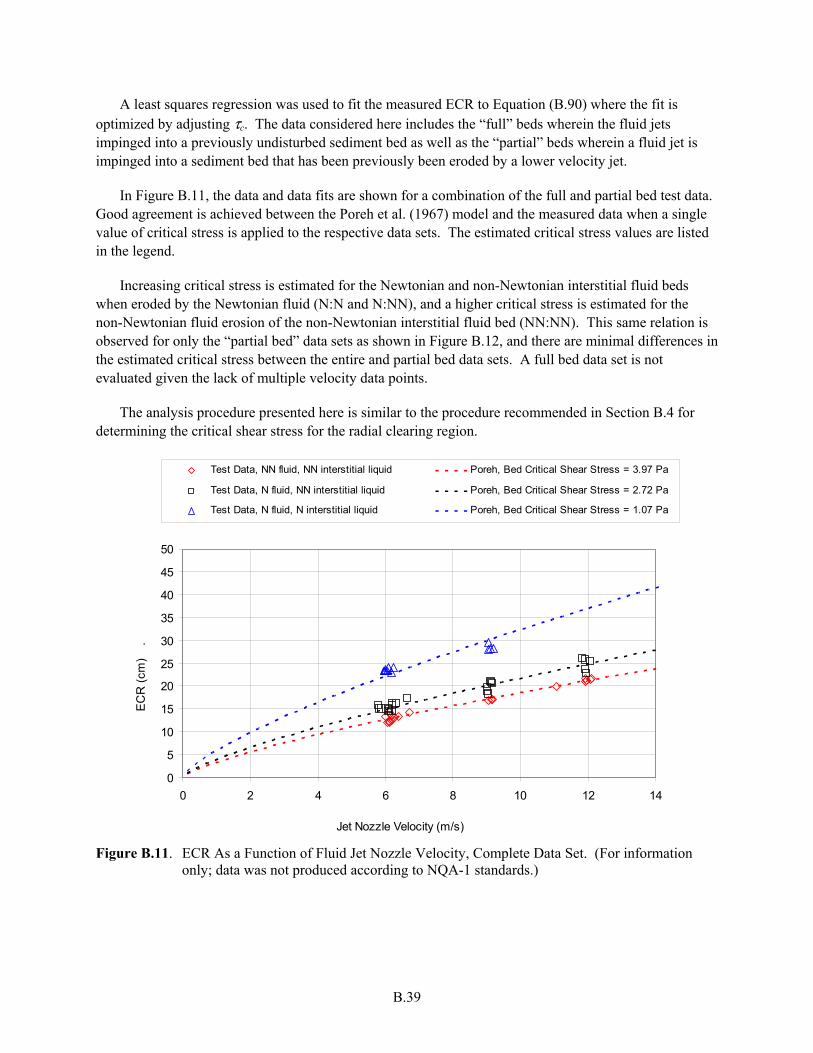
B.39

A least squares regression was used to fit the measured ECR to Equation (B.90) where the fit is optimized by adjusting τc. The data considered here includes the “full” beds wherein the fluid jets impinged into a previously undisturbed sediment bed as well as the “partial” beds wherein a fluid jet is impinged into a sediment bed that has been previously been eroded by a lower velocity jet.

In Figure B.11, the data and data fits are shown for a combination of the full and partial bed test data. Good agreement is achieved between the Poreh et al. (1967) model and the measured data when a single value of critical stress is applied to the respective data sets. The estimated critical stress values are listed in the legend.

Increasing critical stress is estimated for the Newtonian and non-Newtonian interstitial fluid beds when eroded by the Newtonian fluid (N:N and N:NN), and a higher critical stress is estimated for the non-Newtonian fluid erosion of the non-Newtonian interstitial fluid bed (NN:NN). This same relation is observed for only the “partial bed” data sets as shown in Figure B.12, and there are minimal differences in the estimated critical stress between the entire and partial bed data sets. A full bed data set is not evaluated given the lack of multiple velocity data points.

The analysis procedure presented here is similar to the procedure recommended in Section B.4 for determining the critical shear stress for the radial clearing region.

0

5

10

15

20

25

30

35

40

45

50

0 2 4 6 8 10 12 14

Jet Nozzle Velocity (m/s)

EC

R (

cm)

.

Test Data, NN fluid, NN interstitial liquid Poreh, Bed Critical Shear Stress = 3.97 Pa

Test Data, N fluid, NN interstitial liquid Poreh, Bed Critical Shear Stress = 2.72 Pa

Test Data, N fluid, N interstitial liquid Poreh, Bed Critical Shear Stress = 1.07 Pa

Figure B.11. ECR As a Function of Fluid Jet Nozzle Velocity, Complete Data Set. (For information only; data was not produced according to NQA-1 standards.)

B.40

0

5

10

15

20

25

30

35

40

45

0 2 4 6 8 10 12 14

Jet Nozzle Velocity (m/s)

EC

R (

cm)

.

Test Data, NN fluid, NN interstitial liquid Poreh, Bed Critical Shear Stress = 3.96 Pa

Test Data, N fluid, NN interstitial liquid Poreh, Bed Critical Shear Stress = 2.73 Pa

Test Data, N fluid, N interstitial liquid Poreh, Bed Critical Shear Stress = 1.18 Pa

Figure B.12. ECR As a Function of Fluid Jet Nozzle Velocity, Partial Bed Data Set. (For information only; data was not produced according to NQA-1 standards.)

B.9.2 Transient Clearing Analysis

The evolution of clearing radius as a function of time, T, may be calculated using the expression (Section B.4.2.1)

r(T ) = dr

dt0

T

r( ) dt (B.91)

where the rate of change in clearing radius is

( )0 3 2 3

2

0 3. .

Ec

Cdr . K K rr

dt H H

ρ τδ ν

− − = − (B.92)

which requires an erosion coefficient, CE, and a critical shear stress, τc.

A series of tests was performed where a full bed was cleared with a 12-m/s nozzle velocity. Tank bottom images were taken as a function of time and clearing radii were determined as a function of time from the beginning of the transient. The erosion coefficient, CE, and critical shear stress, τc, were adjusted to match the data.

B.41

Results are shown in Figure B.13 for the Newtonian fluid/Newtonian interstitial fluid bed (N:N) case using an erosion coefficient of 0.2 cm3-s/g and a critical shear stress of 0.8 Pa. As discussed in Section B.4.2.1, the erosion coefficient, CE, controls the rate of radial growth in the initial part of the transient and the critical shear stress, τc, determines the asymptotic limit at the end of the transient.

0

0.05

0.1

0.15

0.2

0.25

0.3

0.35

0.4

0.45

0.5

0 5 10 15 20 25

Cle

arin

g R

adiu

s (m

)

Time (s)

Measured Calculated

Figure B.13. ECR As a Function of Time for the N Fluid, N Interstitial Fluid Case. (For information only; data was not produced according to NQA-1 standards.)

B.10 Effective Cleaning Radius Growth Rate Calculations and Comparison to Prototypic Scale

The transient clearing expressions developed in Section B.4.2 are used to predict ECR results that are then compared with data taken from the 15-in.-, 34-in.-, and 70-in.-diameter tanks for the pulse tube tests of Meyer et al. (2009). For each test condition, there is relatively good agreement between the prediction and assumed experimental ECRs for each scale at the respective drive times with equivalent CE.

As previously described, the erosion rate of a sediment material described by previous investigators (e.g., Mehta 1991) can be written as the rate of change in the ECR with time via

dr

dt= CE

δτ w −τ c( )

(B.93)

where r = effective cleaning radius from jet nozzle (m) t = time (s) CE = erosion coefficient (m3 s/kg) δ = sediment depth (m) τw = shear stress acting on the sediment surface layer (Pa) τc = critical shear stress for erosion (Pa).

B.42

Prediction of the ECR at prototypic scale from geometrically scaled tests via Equation (B.93) is considered. Values for the erosion coefficient, CE, are considered from the critical suspension velocity (velocity for complete bottom motion, UCS) for erosion of different simulants in comparison with the jet drive time and jet center-line to vessel wall distance from concurrent tests from the 15-in.-, 34-in.-, and 70-in.-diameter tanks for the pulse tube tests of Meyer et al. (2009). For this analysis, the Poreh et al. (1967) expression for the shear stress acting on a sediment from an impinging radial jet is used for τw as

0 3 2 3

2

0 3. .

w

. K K r

H H

ρτν

− − = (B.94)

where ρ = density of jet fluid (kg/m3)

Κ = kinematic momentum flow from the jet nozzle (m4/s2), ( )2

04K U d

π= where U0

and are the jet nozzle velocity and diameter, respectively Η = nozzle stand-off distance for vessel bottom (m) ν = kinematic viscosity of jet fluid (m2/s).

For τc, the Shields diagram (e.g., Vanoni 1975; Julien 1998) provides a relationship for the critical shear stress for erosion for a given particle. For non-cohesive solids (i.e., particles with negligible surface attractive forces), the Shields diagram with the shear Reynolds number (Re*) greater than approximately 2 determines the critical shear stress. For fine cohesive solids, Re* < 2, the Shields diagram provides a qualitative trend of the critical shear stress, but does not provide specific critical shear stress values.

The relation of Paphitis (2001), presented in Beheshti and Ataie-Ashatiani (2008) as

( )0 020 273

0 046 1 0 5761 1 2

*. D*

*

.. . e

. Dτ −= + −

+ (B.95)

where D* = Ar1/3, where the Archimedes number Ar is given by

3

2

1sS

l

gd

Ar

ρρ

ν

−

= (B.96)

compares well with both the Re* > 2 relation from the Shields diagram and data of Mantz (1977) wherein the Shields diagram was extended below Re* ~ 2 for fine non-cohesive particles as shown in Wells et al. (2011). In Equation (B.96), ρs and ρl are the particle and liquid densities, respectively, dS is the particle diameter, and g is gravitational acceleration. The non-dimensional critical shear stress for erosion, τ* of Equation (B.95), is related to the dimensional critical stress via the Shields diagram as

( )c

*s l Sgd

ττρ ρ

=−

(B.97)

B.43

Caution must be taken in applying the critical stress for erosion results for a given particulate directly. Wells et al. (2009) noted that there does not appear to be tools for predicting sediment erosion without obtaining data for similar or related types of material. Clark and Wynn (2007) compared different methods of determining the critical shear stress for erosion. Jet erosion test results were compared to estimates from the Shields diagram and empirical relations based on parameters of percent clay, plasticity index, particle size, and percent silt-clay. The jet erosion test results were as much as four orders of magnitude greater than the Shields diagram and empirical methods indicating that models applied outside of the specific study area should be applied with caution.

The test conditions, simulant properties, and critical stresses for the considered tests of Meyer et al. (2009) are listed in Table B.1. Water was used as the test liquid. Also included are prototypic vessel HLP-22 conditions. The Test IDs indicate test conditions, as detailed in Table B.1, where all test conditions are equivalent except for geometric scale. Thus there are 10 test cases from Meyer et al. (2009) considered to estimate the erosion coefficient with three different solids. Five of the test cases have data at all three tank sizes, and there are five additional tests with only 15-in.- and 70-in.-diameter test data. The experimental ECR at the UCS condition, where all solids mobilized at the end of the drive time, is approximated as the distance from the jet nozzle centerline to the vessel wall.

The tests discussed in detail in Meyer et al. (2009) can be nominally described as conducted by ramping up the jet nozzle velocity in 0.2 m/s increments until the complete suspension or the bottom motion condition was reached.1 Thus, it can be assumed that at 0.2 m/s less than the UCS velocity reported in Table B.1, the ECR did not cover the extent of the tank bottom, or did not extend to the vessel wall. It follows that at UCS, the ECR did extend to the vessel wall. This assumption does not address whether the last solids to be mobilized were in fact at the tank wall, at what specific time that happened during the pulse, and does not account for jet interaction or wall effects. However, in the absence of actual ECR measurements, it is deemed to be a reasonable approximation for this exercise.

The assumed experimental ECR and drive time for test 4s1d2Yc_1 from Table B.1 are shown in Figure B.14 for each tank scale (asterix symbols). The horizontal bar data points are the radius at which τw and τc of Equation (B.92) are equivalent (computed via Equations (B.94) and (B.95), (B.96), and (B.97)) for each scale at which condition the jet velocity has decayed such that no further erosion will occur. The values are reported in Table B.1. The difference between the assumed experimental and τw = τc ECR increases from approximately 20 percent in the 15-in.-diameter vessel to 100 percent in the 70-in.-diameter vessel. These differences (i.e., apparent under-prediction by the assumed ECR) may indicate the influence of jet-to-jet or jet-to-vessel wall interactions.

The traces in Figure B.14 are the numerical integration results of Equation (B.93) with a time step of 0.01 s. The results are not significantly influenced by the choice of time step. It is reasonable to expect that the erosion coefficient, CE of Equation (B.93), is independent of scale and dependent on the simulant. Thus, for each test ID (again, all parameters are constant except geometric scale), the erosion coefficient is adjusted constant with scale via a least squares regression to minimize the error between the experimental data and the predicted ECR at the drive time. The calculated erosion coefficient is also provided in Table B.1, and it can be seen in Figure B.14 that there is relatively good agreement between

1 The bottom motion condition can be described as when all particles at the vessel bottom have been suspended off the bottom or are all moving relative to each other and the vessel.

B.44

the prediction and assumed experimental ECRs for each scale at the respective drive times with equivalent CE. All traces are extended to the prototypic drive time listed in Table B.1, but are not meaningful for the actual test conditions beyond the specified drive time.

It can be noted that the difference between the prediction and assumed experimental ECRs is different for the different test vessels. The 34-in.-diameter test vessel is unique from the other scales in that the bottom dish shape is a 0.59R spherical (S) as opposed to the elliptical (E) of the 15-in.- and 70-in.-diameter vessels and flanged and dished (F) of the 70-in.-diameter vessel.

As illustrated in Meyer et al. (2009), the nozzle impingement angles for the outer pulse tubes are substantially different for the spherical bottom 34-in.-diameter tank than the E and F tanks, approaching 50 percent further from perpendicular to vessel bottom (i.e., from an axial jet). Kale and Patwardhan (2005) performed jet mixing tests in which the effect of nozzle angle in a flat bottom tank was considered and found that the jet suspension capability was poor for inclined nozzles relative to axial jets. This result would suggest that the ECR in the spherical bottom tank should require an increased nozzle velocity for bottom motion. However, this is not indicated by the relation of the prediction and assumed experimental ECRs for the 34-in.-diameter vessel in Figure B.14. An alternative explanation is the effect of the “more abrupt” transition to vertical in the E and F bottom shaped tanks, which may suggest a higher velocity is required for the elliptical (E) and flanged and dished (F) tanks relative to the S tank to achieve bottom motion. Note that the spherical data was not used in the evaluation for direct scale-up of the velocity for complete suspension by Meyer et al. (2009).

Relatively similar results are shown for the remaining test IDs of Table B.1 in Figure B.15 through Figure B.23. For each test condition, there is relatively good agreement between the prediction and assumed experimental ECRs for each scale at the respective drive times with equivalent CE.

The black colored data points in Figure B.14 through Figure B.23 show the prototypic tank (HLP-22 for this analysis, see Table B.1) conditions, and the trace is the extrapolation to the prototype using the previously determined CE, all with the same simulant and solids concentration as the scaled tests. An under-prediction of the required ECR ranging from approximately 7 percent (from the 4s1d2Zc_1 test erosion coefficient) to 37 percent (from the 4s2d2Yc_1 test erosion coefficient) is shown for a nozzle velocity of 12 m/s. The percentage under-prediction is increased with increased solids loading.

A limit on the prototypic system is the volume of fluid that can be expelled from the pulse tubes during a single pulse. For a prototypic pulse volume fraction of 0.13, a working tank volume of nominally 141,000 gallons, and 18 PJMs, the under-prediction of the 4s1d2Xd_1 test (approximately 34 percent) can be reduced to a limited extent by increasing the nozzle velocity (which shortens the drive time) as shown in Figure B.24. Note that other system limits are not considered in this example.

As previously described, it is reasonable to expect that the erosion coefficient is dependent on the simulant. Comparison of the erosion coefficient, CE, to the critical stress for erosion, τC, for the three simulants over the five test IDs is made in Figure B.25 (data from Table B.1). In the limited data set, the physically plausible higher erosion coefficient for the lower critical stress particulate is shown. The effect of solids concentration is shown to be more significant than that of duty cycle.

The influence of the sediment depth, δ, in Equation (B.93) which is directly related to the solids concentration in the vessel on the estimated erosion coefficient is shown in Figure B.26. For the tests

B.45

with a duty cycle of approximately 0.33, the higher erosion coefficient is again shown for the lower critical stress particulate, and the erosion coefficient increases with increasing concentration for the respective tests. At the solids concentration, φS (phiS), of 0.005, the ~95 percent increase in the calculated critical stress results in a ~49 percent reduction in CE, while a 100 percent increase in the solids concentration (0.005 to 0.01) results in a ~58 percent increase in CE. Consideration of the critical stress for erosion of Hanford sediment in the tank farms or WTP may thus require analyses that include the effect of the sediment depth as well as its other physical and chemical properties.

Given that the test conditions evaluated are at the critical suspension or bottom motion condition, it is not meaningful to directly compare the effect of duty cycle on the estimated erosion coefficient. However, at the slightly reduced drive time of the lower duty cycle (0.18) tests, there is a similar effect of concentration on the estimated erosion coefficient (Figure B.26).

Alternatively, to adjust the PJM parameters of the prototypic system, as discussed relative to Figure B.24, the required adjustment of CE such that the prototypic assumed ECR and drive time are achieved via Equation (B.93) is evaluated for the 4s1d2Xd_1 test. This condition is met with CE = 1.36E-3 m3s/kg as opposed to 3.41E-4 m3s/kg estimated from the scaled tests (see Table B.1). This change is larger than the difference in CE estimated from the test data reported in Table B.1.

The calculated required change in CE for prototypic conditions is compared to literature results for the erosion coefficient, CE, of Chapter 4. Clark and Wynn (2007) provide relations for erodability coefficient, E, as a function of the critical stress for erosion. As shown in Wells et al. (2011), the calculated critical stress for erosion for Hanford waste particulate can vary by up to O(1000).1 The resultant variation in E from the models of Clark and Wynn (2007) is, at a maximum, 100 percent. Thus, it may be unlikely that under-prediction of the required prototypic performance is due to error in evaluation of CE from the scaled tests.

1 A given sediment is obviously comprised of a distribution of solid particulate and will have a characteristic critical stress for erosion. Consideration of the range of the critical stress for erosion of the individual particulate comprising a sediment is made for illustrative purpose only.

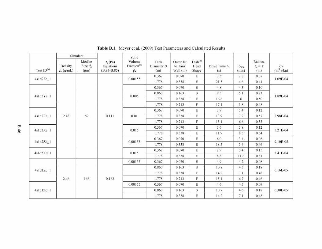
B.46

Table B.1. Meyer et al. (2009) Test Parameters and Calculated Results

Test ID(a)

Simulant

τc (Pa) Equations

(B.83-B.85)

Solid Volume

Fraction(b) φS

Tank Diameter D

(m)

Outer Jet to Tank

Wall (m)

Dish(c) Head Shape

Drive Time tD (s)

UCS (m/s)

Radius, τw = τc

(m) CE

(m3 s/kg) Density

ρs (g/mL)

Median Size dS (μm)

4s1d2Zc_1

2.48 69 0.111

0.00155 0.367 0.070 E 7.3 2.8 0.07

1.09E-04 1.778 0.338 E 21.3 4.6 0.41

4s1d2Yc_1 0.005

0.367 0.070 E 4.8 4.3 0.10

1.89E-04 0.860 0.163 S 9.5 5.1 0.23

1.778 0.338 E 16.6 6 0.50

1.778 0.213 F 17.1 5.8 0.48

4s1d2Rc_1 0.01

0.367 0.070 E 3.9 5.4 0.12

2.98E-04 1.778 0.338 E 13.9 7.2 0.57

1.778 0.213 F 15.1 6.6 0.53

4s1d2Xc_1 0.015 0.367 0.070 E 3.6 5.8 0.12

5.21E-04 1.778 0.338 E 11.9 8.5 0.64

4s1d2Zd_1 0.00155 0.367 0.070 E 6.0 3.4 0.08

9.10E-05 1.778 0.338 E 18.5 5.4 0.46

4s1d2Xd_1 0.015 0.367 0.070 E 2.9 7.4 0.15

3.41E-04 1.778 0.338 E 8.8 11.6 0.81

4s1d1Zc_1

2.46 166 0.162

0.00155 0.367 0.070 E 4.9 4.2 0.08

6.16E-05 0.860 0.163 S 10.8 4.5 0.18

1.778 0.338 E 14.2 7.1 0.48

1.778 0.213 F 15.1 6.7 0.46

4s1d1Zd_1

0.00155 0.367 0.070 E 4.6 4.5 0.09

6.30E-05 0.860 0.163 S 10.7 4.6 0.18

1.778 0.338 E 14.2 7.1 0.48

B.47

Table B.1. (contd)

Test ID(a)

Simulant

τc (Pa) Equations

(B.83-B.85)

Solid Volume

Fraction(b) φS

Tank Diameter D

(m)

Outer Jet to Tank

Wall (m)

Dish(c) Head Shape

Drive Time tD (s)

UCS (m/s)

Radius, τw = τc

(m) CE

(m3 s/kg) Density

ρs (g/mL)

Median Size dS (μm)

4s2d2Zc_1

4.18 76 0.216

0.00155 0.367 0.070 E 3.9 5.4 0.09

4.38E-05 0.860 0.163 S 8.8 5.6 0.19

1.778 0.338 E 12.0 8.4 0.48

4s2d2Yc_1

0.005 0.367 0.070 E 2.8 7.6 0.11

9.63E-05 0.860 0.163 S 5.7 8.6 0.26

1.778 0.338 E 8.2 12.5 0.64

1.778 0.213 F 9.5 10.6 0.57

Prototypic(d) Adjusted to match test conditions 11.582 1.219 F 34.85 12 Test Dependent

(a) Prototypic 4-in. nozzle, “s#” and “d#” designate simulant particulate density and size, “R,” “X,” “Y,” and “Z” designate solid volume fraction, “c” and “d” designate nominal duty cycles of 0.33 and 0.18, respectively (prototypic is 0.13), and “_1” indicates the nominal pulse volume fraction and jet number and configuration for the test.

(b) Solid volume fraction is the volume of undissolved solid per volume of tank related by π*D3/4 where D is the tank diameter. The sediment depth, δ, in Equation (B.81) is related to this volume by assuming a flat bottom tank of diameter, D, with a solid packing fraction by volume as listed in Meyer et al. (2009) for the respective simulant. As such, this value is approximate at best, but is consistent between tests and scales.

(c) E = Elliptical head shape; S = Spherical head shape; F = Flanged and dished head shape. (d) HLP-22, 4.25-in.-diameter nozzles.

B.48

0.001

0.01

0.1

1

10

0 5 10 15 20 25 30 35 40

Time (s)

EC

R (

m)

4s1d2Yc_1 Ce ~ 0.000188604456774995 (m4/N s)

15E vessel 34S vessel

70E vessel 70F vessel

15E UCS condition 34S UCS condition

70E UCS condition 70F UCS condition

HLP-22 4.25 in nozzle, 12 m/s, 18 PJM s, 2.45 wt% solids, phiS* = 0.005, s1d2 HLP-22 UCS condition

15E r(Tw=Tc) 34S r(Tw=Tc)

70E r(Tw=Tc) 70F r(Tw=Tc)

HLP-22 r(Tw=Tc)

Figure B.14. Test 4s1d2Yc_1 ECR As a Function of Time

B.49

0.001

0.01

0.1

1

10

0 5 10 15 20 25 30 35 40

Time (s)

EC

R (

m)

4s1d2Zc_1 Ce ~ 0.00010876114336994 (m4/N s)

15E vessel 70E vessel

15E UCS condition 70E UCS condition

HLP-22 4.25 in nozzle, 12 m/s, 18 PJM s, 0.78 wt% solids, phiS* = 0.0016, s1d2 HLP-22 UCS condition

15E r(Tw=Tc) 70E r(Tw=Tc)

HLP-22 r(Tw=Tc)

Figure B.15. Test 4s1d2Zc_1 ECR As a Function of Time

B.50

0.001

0.01

0.1

1

10

0 5 10 15 20 25 30 35 40

Time (s)

EC

R (

m)

4s1d2Rc_1 Ce ~ 0.000297841564344139 (m4/N s)

15E vessel 70E vessel

70F vessel 15E UCS condition

70E UCS condition 70F UCS condition

HLP-22 4.25 in nozzle, 12 m/s, 18 PJM s, 4.86 wt% so lids, phiS* = 0.01, s1d2 HLP-22 UCS condition

15E r(Tw=Tc) 70E r(Tw=Tc)

70F r(Tw=Tc) HLP-22 r(Tw=Tc)

Figure B.16. Test 4s1d2Rc_1 ECR As a Function of Time

B.51

0.001

0.01

0.1

1

10

0 5 10 15 20 25 30 35 40

Time (s)

EC

R (

m)

4s1d2Xc_1 Ce ~ 0.000521082132382053 (m4/N s)

15E vessel 70E vessel

15E UCS condition 70E UCS condition

HLP-22 4.25 in nozzle, 12 m/s, 18 PJM s, 7.19 wt% solids, phiS* = 0.015, s1d2 HLP-22 UCS condition

15E r(Tw=Tc) 70E r(Tw=Tc)

HLP-22 r(Tw=Tc)

Figure B.17. Test 4s1d2Xc_1 ECR As a Function of Time

B.52

0.001

0.01

0.1

1

10

0 5 10 15 20 25 30 35 40

Time (s)

EC

R (

m)

4s1d2Zd_1 Ce ~ 9.10482898987651E-05 (m4/N s)

15E vessel 70E vessel

15E UCS condition 70E UCS condition

HLP-22 4.25 in nozzle, 12 m/s, 18 PJM s, 0.78 wt% solids, phiS* = 0.0016, s1d2 HLP-22 UCS condition

15E r(Tw=Tc) 70E r(Tw=Tc)

HLP-22 r(Tw=Tc)

Figure B.18. Test 4s1d2Zd_1 ECR As a Function of Time

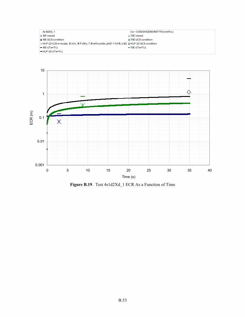
B.53

0.001

0.01

0.1

1

10

0 5 10 15 20 25 30 35 40

Time (s)

EC

R (

m)

4s1d2Xd_1 Ce ~ 0.000341320601597778 (m4/N s)

15E vessel 70E vessel

15E UCS condition 70E UCS condition

HLP-22 4.25 in nozzle, 12 m/s, 18 PJM s, 7.19 wt% solids, phiS* = 0.015, s1d2 HLP-22 UCS condition

15E r(Tw=Tc) 70E r(Tw=Tc)

HLP-22 r(Tw=Tc)

Figure B.19. Test 4s1d2Xd_1 ECR As a Function of Time

B.54

0.001

0.01

0.1

1

10

0 5 10 15 20 25 30 35 40

Time (s)

EC

R (

m)

4s1d1Zc_1 Ce ~ 0.000061566164256347 (m4/N s)

15E vessel 34S vessel

70E vessel 70F vessel

15E UCS condition 34S UCS condition

70E UCS condition 70F UCS condition

HLP-22 4.25 in nozzle, 12 m/s, 18 PJM s, 0.765 wt% solids, phiS* = 0.0016, s1d1 HLP-22 UCS condition

15E r(Tw=Tc) 34S r(Tw=Tc)

70E r(Tw=Tc) 70F r(Tw=Tc)

HLP-22 r(Tw=Tc)

Figure B.20. Test 4s1d1Zc_1 ECR As a Function of Time

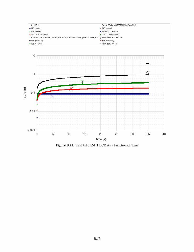
B.55

0.001

0.01

0.1

1

10

0 5 10 15 20 25 30 35 40

Time (s)

EC

R (

m)

4s1d1Zd_1 Ce ~ 6.30424980555758E-05 (m4/N s)

15E vessel 34S vessel

70E vessel 15E UCS condition

34S UCS condition 70E UCS condition

HLP-22 4.25 in nozzle, 12 m/s, 18 PJM s, 0.765 wt% solids, phiS* = 0.0016, s1d1 HLP-22 UCS condition

15E r(Tw=Tc) 34S r(Tw=Tc)

70E r(Tw=Tc) HLP-22 r(Tw=Tc)

Figure B.21. Test 4s1d1Zd_1 ECR As a Function of Time

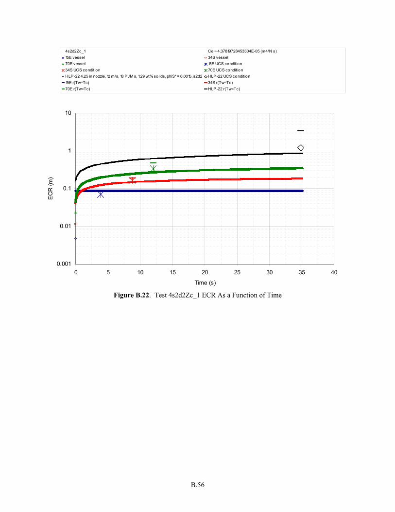
B.56

0.001

0.01

0.1

1

10

0 5 10 15 20 25 30 35 40

Time (s)

EC

R (

m)

4s2d2Zc_1 Ce ~ 4.37819728453304E-05 (m4/N s)

15E vessel 34S vessel

70E vessel 15E UCS condition

34S UCS condition 70E UCS condition

HLP-22 4.25 in nozzle, 12 m/s, 18 PJM s, 1.29 wt% solids, phiS* = 0.0015, s2d2 HLP-22 UCS condition

15E r(Tw=Tc) 34S r(Tw=Tc)

70E r(Tw=Tc) HLP-22 r(Tw=Tc)

Figure B.22. Test 4s2d2Zc_1 ECR As a Function of Time

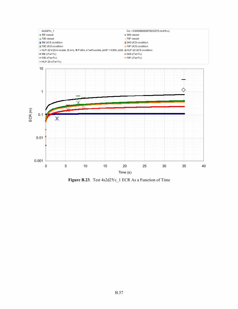
B.57

0.001

0.01

0.1

1

10

0 5 10 15 20 25 30 35 40

Time (s)

EC

R (

m)

4s2d2Yc_1 Ce ~ 0.000096292879233375 (m4/N s)

15E vessel 34S vessel

70E vessel 70F vessel

15E UCS condition 34S UCS condition

70E UCS condition 70F UCS condition

HLP-22 4.25 in nozzle, 12 m/s, 18 PJM s, 4.1 wt% solids, phiS* = 0.005, s2d2 HLP-22 UCS condition

15E r(Tw=Tc) 34S r(Tw=Tc)

70E r(Tw=Tc) 70F r(Tw=Tc)

HLP-22 r(Tw=Tc)

Figure B.23. Test 4s2d2Yc_1 ECR As a Function of Time

B.58

10

15

20

25

30

35

40

5 10 15 20 25 30 35

Nozzle Velocity (m/s)

% D

iffer

ence

of

Pre

dict

ed E

CR

at

End

of

Driv

e to

Bot

tom

Mot

ion

Rad

ius

.

0

15

30

45

60

Driv

e T

ime

(s)

.

% Difference to Radius Drive Time Prototypic Drive Time

Figure B.24. Effect of Altered Nozzle Velocity and Resultant Drive Time on ECR Difference to Bottom Motion Condition in Prototype Vessel for sld2 Solid (2.48 g/mL and 69 µm) at 0.015 Solids Volume Fraction

2.0E-05

4.0E-05

6.0E-05

8.0E-05

1.0E-04

1.2E-04

1.4E-04

1.6E-04

1.8E-04

2.0E-04

0.1 0.12 0.14 0.16 0.18 0.2 0.22

TauC (Pa)

CE

(m

3 s/

kg)

phiS* = 0.00155, DC = 0.33 phiS* = 0.005, DC = 0.33phiS* = 0.00155, DC = 0.18

Figure B.25. Estimated Erosion Coefficient As a Function of Particulate Critical Stress for Erosion at Constant Duty Cycle and Solids Concentration

B.59

2.0E-05

1.2E-04

2.2E-04

3.2E-04

4.2E-04

5.2E-04

6.2E-04

0 0.005 0.01 0.015 0.02

Solid Volume Fraction

CE

(m

3 s/

kg)

TauC = 0.111, DC = 0.33 TauC = 0.111, DC = 0.18 TauC = 0.216, DC = 0.33

Figure B.26. Estimated Erosion Coefficient As a Function of Solids Concentration at Constant Particulate Critical Stress for Erosion and Duty Cycle

B.11 References

Ayranci I, MB Machado, AM Madej, JJ Derksen, DS Nobes, and SM Kresta. 2012. “Effect of Geometry on the Mechanisms for Off-Bottom Solids Suspension in a Stirred Tank.” Chemical Engineering Science 79:163-176.

Bagnold R. 1966. An Approach to the Sediment Transport Problem from General Physics. Geological Survey Professional Paper 422-I, U.S. Geological Survey, Washington D.C.

Baldi G, R Conti, and E Alaria. 1978. “Complete suspension of particles in mechanically agitated vessels.” Chemical Engineering Science 33:21-25.

Beheshti AA and B Ataie-Ashatiani. 2008. “Analysis of Threshold and Incipient Conditions for Sediment Movement.” Coastal Engineering 55(5):423-430.

Bontha JR, JM Bates, CW Enderlin, and MG Dodson. 2003. Large Tank Experimental Data for Validation of the FLUENT CFD Model of Pulsed Jet Mixers. PNWD-3033; WTP-RPT-081, Rev. 0, Battelle–Pacific Northwest Division, Richland, Washington.

Bradshaw P and EM Love. 1961. The Normal Impingement of a Circular Air Jet on a Flat Surface. Great Britain Aeronautical Research Council, ARC R. & M. No 3205.

B.60

Brownlie WR. 1981. “Prediction of flow depth and sediment discharge in open channels.” Rep. KH-R-43A, California Institute of Technology, Pasadena.

Clark LA and TM Wynn. 2007. “Methods for Determining Streambank Critical Shear Stress and Soil Erodibility: Implications for Erosion Rate Predictions.” Transactions of the American Society of Agricultural Engineers 50(1):95-106.

Davies JT. 1986. “Particle suspension and mass transfer rates in agitated vessels.” Chemical Engineering and Processing: Process Installation 20(4)175-181.

Gauglitz PA, BE Wells, JA Fort, and PA Meyer. 2009. An Approach to Understanding Cohesive Slurry Settling, Mobilization, and Hydrogen Gas Retention in Pulsed Jet Mixed Vessels. PNNL-17707, Pacific Northwest National Laboratory, Richland, Washington.

Gilbert B. 1989. “Turbulence measurements in a flow generated by the collision of radially flowing wall jets.” Experiments in Fluids 7:103.

Grenville RK, ATC Mak, and DAR Brown. 2010. “An Improved Correlation to Predict “Just Suspension” Speed for Solid-Liquid Mixing with Axial Flow Impellers in Stirred Tanks.” North American Mixing Forum, June 20-25, 2010, Victoria, Canada.

Hamm BA, WL West, and GB Tatterson. 1989. “Sludge suspension in waste storage tanks.” AIChE Journal 35:1391-1394.

Johansson PS and HI Andersson. 2005. “Direct numerical simulation of two opposing wall jets.” Physics of Fluids 17:005109.

Johnson MD, JR Bontha, and JM Bates. 2003. Demonstration of Ability to Mix in a Small-Scale Pulsed-Jet Mixer Test Facility. PNWD-3273; WTP-RPT-077, Rev. 0, Battelle–Pacific Northwest Division, Richland, Washington.

Julien PY. 2010. Erosion and Sedimentation, 2nd Ed. pp. 147-149. Cambridge University Press, Cambridge, United Kingdom.

Kaftori D, G Hetsroni, and S Banerjee. 1995. “Particle behavior in the turbulent boundary layer. II. Velocity and distribution profiles.” Physics of Fluids 7:1107-1121.

Kale RN and AW Patwardhan. 2005. “Solid Suspension in Jet Mixers.” The Canadian Journal of Chemical Engineering 83(5):816-828.

Kataoka K, Y Kamiyama, S Hashimoto, and T Komai. 1982. “Mass transfer between a plane surface and an impinging turbulent jet: the influence of surface-pressure fluctuations.” Journal of Fluid Mechanics 119:91-105.

Kim J, P Moin, and R Moser. 1987. “Turbulence statistics in fully developed channel flow at low Reynolds number.” Journal of Fluid Mechanics 177:133-166.

Kothyari UC and RK Jain. 2008. “Influence of cohesion on the incipient motion condition of sediment mixtures.” Water Resources Research 44, W04410:1-15.

B.61

Lick W, L Jin, and J Gailani. 2004. “Initiation of movement of quartz particles.” Journal of Hydraulic Engineering 130(8):755-761.

Mantz PA. 1977. “Incipient Transport of Fine Grains and Flakes by Fluids – Extended Shields Diagram.” Journal of the Hydraulics Division, Proceedings of the American Society of Civil Engineers 103(6):601-615.

McArthur GAH, D Tinsley, and TP McKendrick. 2005. “Development of a Liquid Jet Sludge Resuspension Model (used on pulse jets or jet ballasts).” Paper presented at The AIChE 2005 Annual Meeting, November 3, 2001, Cincinnati, Ohio.

Mehta AJ. 1991. “Review Notes on Cohesive Sediment Erosion.” In Coastal Sediments, Proceedings of a Specialty Conference on Quantitative Approaches to Coastal Sediment Processes, Vol 1, pp. 40-43, NC Kraus, KJ Gingerich, and DI Kriebel (eds.), American Society of Civil Engineers.

Meyer PA, JA Bamberger, CW Enderlin, JA Fort, BE Wells, SK Sundaram, PA Scott, MJ Minette, GL Smith, CA Burns, MS Greenwood, GP Morgen, EBK Baer, SF Snyder, M White, GF Piepel, BG Amidan, and A Heredia-Langner. 2009. Pulse Jet Mixing Tests with Noncohesive Solids. PNNL-18098; WTP-RPT-182, Rev. 0, Pacific Northwest National Laboratory, Richland, Washington.

Meyer PA, JA Bamberger, CW Enderlin, JA Fort, BE Wells, SK Sundaram, PA Scott, MJ Minette, GL Smith, CA Burns, MS Greenwood, GP Morgen, EBK Baer, SF Snyder, M White, GF Piepel, BG Amidan, and A Heredia-Langner. 2012. Pulse Jet Mixing Tests with Noncohesive Solids. PNNL-18098, Rev. 1; WTP-RPT-182, Rev. 1, Pacific Northwest National Laboratory, Richland, Washington.

Meyer PA, EBK Baer, JA Bamberger, JA Fort, and MJ Minette. 2010. Assessment of Differences in Phase 1 and Phase 2 Test Observations for Waste Treatment Plant Pulse Jet Mixer Tests with Non-Cohesive Solids. PNNL-19085; WTP-RPT-208, Rev. 0, Pacific Northwest National Laboratory, Richland Washington.

Nino Y, F Lopez, and M Garcia. 2003. “Threshold for particle entrainment into suspension.” Sedimentology 50:247-263.

O’Connor DJ. 1995. “Inner region of smooth pipes and open channels.” Journal of Hydraulic Engineering 121:555-560.

O’Rourke PJ. 1981. Collective Drop Effects on Vaporizing Liquid Sprays. PhD Thesis, Princeton University, Princeton, New Jersey.

Paphitis D. 2001. “Sediment Movement Under Unidirectional Flows: An Assessment of Empirical Threshold Curves.” Coastal Engineering 43:227-245.

Partheniades E. 1965. “Erosion and deposition of cohesive soils.” Journal of the Hydraulics Division, Proceedings of the American Society of Civil Engineers 91(1):105-139.

Phares DJ, GT Smedley, and RC Flagan. 2000. “The wall shear stress produced by the normal impingement of a jet on a flat surface.” Journal of Fluid Mechanics 418:351-375.

B.62

Poreh M, YG Tsuei, and JE Cermak. 1967. “Investigation of a Turbulent Radial Wall Jet.” Journal of Applied Mechanics 34:457-463.

Powell MP, Y Onishi, and R Shekarriz. 1997. Research on Jet Mixing of Settled Sludges in Nuclear Waste Tanks at Hanford and Other DOE Sites: A Historical Perspective. PNNL-11686, Pacific Northwest National Laboratory, Richland, Washington.

Rajaratnam N. 1976. Turbulent Jets. Elsevier Scientific Publishing Company, New York, New York.

Rashidi M, G Hetsroni, and S Banerjee. 1990. “Particle-turbulence interaction in a boundary layer.” International Journal of Multiphase Flow 16:935-949.

Righetti M and C Lucarelli. 2007. “May the Shields theory be extended to cohesive and adhesive benthic sediments?” Journal of Geophysical Research 112, C05039:1-14.

Shields A. 1936. “Anwendung der Ahnlichkeits-Mechanik und der Turbulenz forschung auf die Geschiebebewegung.” Mitteilungen der Preussischen Versuchanstalt fur Wasserbau und Schiffbau 26.

Simon A, RE Thomas, AJC Collison, W Dickerson, and CV Alonso. 2002. Erodibility of Cohesive Streambeds in the Yalobusha River System. Research Report No. 26, National Sedimentation Laboratory, Channel and Watershed Processes Research Unit, Oxford, Mississippi.

Torfs H, J Jiang, and AJ Mehta. 2001. “Assessment of the erodibility of fine/coarse sediment mixtures.” Coastal and Estuarine Fine Sediment Processes, Elsevier Science B.V., WH McAnally and AJ Mehta (eds.), 3:109-123.

van Rijn RC. 1984. “Sediment transport, Part II: Suspended load transport.” Journal of Hydraulic Engineering 110:1613-1641.

Vanoni VA (ed.). 2006. Sedimentation Engineering, the ASCE Task Committee for the Preparation of the Manual on Sedimentation of the Sedimentation Committee of the Hydraulic Division. The American Society of Civil Engineers, New York.

Wells BE, PA Gauglitz, and DR Rector. 2011. Comparison of Waste Feed Delivery Small Scale Mixing Demonstration Simulant to Hanford Waste. PNNL-20637, Rev. 1, Pacific Northwest National Laboratory, Richland, Washington.

Wells BE, CW Enderlin, PA Gauglitz, and RA Peterson. 2009. Assessment of Jet Erosion for Potential Post-Retrieval K-Basin Settled Sludge. PNNL-18831, Pacific Northwest National Laboratory, Richland, Washington.

Yang CT. 1973. “Incipient motion and sediment transport.” Journal of the Hydraulics Division, ASCE, 99, HY10, Proceeding Paper 10067:1679-1704.

Yang CT. 2003. Sediment Transport: Theory and Practice. Krieger Publishing Company, Malabar, Florida.

B.63

References Not Publicly Available

Campbell T, M Parker, A Moon, B Fant, K Clossey, and J Cook. 2010. ERFT Issue M3 PJM Vessel Mixing Assessment, Volume 8 – HLP-22. 24590-WTP-RPT-ENG-08-021-08, Rev. 1, p. 6, Bechtel National, Inc., Richland, Washington.

Dickey DS. 2010. Scaling of PJM Vessels Containing Settling Solids in Newtonian Slurries. TR-099, MixTech, Inc., Dayton, Ohio.

Eager K. 2010. Revised Calculation of Hydrogen Generation Rates and Time to Lower Flammability Limit for WTP. 24590-WTP-M4C-V11T-00011, Rev. C, Bechtel National, Inc., Richland, Washington.

Edmonson A and S Thomson. 2010. M3 Platform Test Data Study. 24590-WTP-ES-PET-09-001, Rev. 0, Richland, Washington.

Hinckley J. 2011. Preliminary Documented Safety Analysis To Support Construction Authorization; PT Facility Specific Information. 24590-WTP-PSAR-ESH-01-002-02, Rev. 4w, Bechtel National, Inc., Richland, Washington.

Kulp M. 2011. Preliminary Documented Safety Analysis To Support Construction Authorization; HLW Facility Specific Information. 24590-WTP-PSAR-ESH-01-002-04, Rev. 4w, Bechtel National, Inc., Richland, Washington.

Mauss J and I Papp. 2010. Determination of Mixing Requirements for Pulse-Jet-Mixed Vessels in the Waste Treatment Plant. 24590-WTP-ES-ENG-09-001, Rev. 2, Bechtel National, Inc., Richland, Washington.

Meehan J and D Sherwood. 2010. “M3 Gas Release in Newtonian Pulse Jet Mixer (PJM) Mixed Vessels.” 24590-WTP-RPT-PET-10-007, Bechtel National, Inc., Richland, Washington.

Smith RI. 2010. Unit Dose Factors for Use in Updated MAR Accident Analyses. 24590-WTP-Z0C-W14T-00020, Rev. C, Bechtel National, Inc., Richland, Washington.

Thomson S and A Edmonson. 2010. WSU Radial Flume Test Data Study. 24590-WTP-ES-PET-10-001, Rev. 0, Richland, Washington.

Appendix C –

Working Paper for the Technical Basis for Scaling Transfer and Pump Out

C.iii

Acronyms and Abbreviations

HLP high-level process (tank)

LSIT Large Scale Integrated Testing

M3 external flowsheet review team technical issue M3 – Inadequate Design of Mixing Systems – Pulse Jet Mixers

MLB Masliyah-Lockett-Bassoon (equation)

PJM pulse jet mixer

PSDD particle size and density distribution

ULD Unit Liter Dose

WTP Hanford Waste Treatment and Immobilization Plant

Symbols

A apparent jet cross-section; tank floor area attributed to a single PJM

a exponents

ai coefficients

Ar particle Archimedes number

Az0 flow cross-section of the upward jet from the point of collision

A0 apparent jet cross-section at location 0, flow cross-section of the upward jet from the point of collision

a1 fitted value

b nominal width of an axisymmetric jet

C area factor

CA area correction coefficient

Caxisymmetric area factor for an axisymmetric jet

CD drag coefficient

Cf friction factor

Cradial area factor for a radial jet

C0 leading coefficient

D tank diameter

d nozzle diameter, jet diameter

DC duty cycle = tD/tC

De effective hydrodynamic dispersion coefficient

de characteristic linear dimension of the liquid space

dk particle diameter for particle type k

DS hydrodynamic dispersion

dS particle diameter, solids diameter

C.iv

F force

f function

fD drag coefficient for the particle

fp function of the particle Archimedes number

g acceleration of gravity

H liquid height in tank, momentum balance function

h distance of the source of the impinging jet to the wall, distance from suction nozzle to floor (point sink distance above the floor)

HC cloud height

hS hindered settling factor

hS height of solids

I0 zeroth moment of the vertical distribution of solids loading which is the total volume of solids per horizontal area

I1 first moment of the vertical distribution of solids loading

I1, I2, I3 integrals

Jnozzle momentum flow rate at nozzle

Jz0 momentum flow rate at z0

k particle type designator

ke dimensionless dispersion coefficient

M jet momentum

M0 jet momentum at location of self-similarity

m mass of solid cylinder

mi mass of species “i” in the tank

mS mass of settled solids that have been suspended by the jet after clearing the bottom, mass of solids in the vortices

mS,settled mass of solids entrained from tank floor

mS,sus mass of suspended solids per PJM

mS,tot total mass of solids in the tank

N number of parameters

ni mass flux of particle species “i”

NJ number of PJMs or operating jets

Q volumetric flow rate into nozzle of transfer line

q power

Q0 time-averaged rate of addition of volume averaged over pump-out cycles

Rep particle Reynolds number

Reδ Reynolds number of the radial wall jet

r radius

rA radius of solid cylinder of rotation

rJ radius at the front of the jet; radial jet effective clearing radius, jet radius

C.v

rT major radius of leading jet vortex

rV radius of solid cylinder inferred from volume, minor radius of the jet leading vortex

r0 jet radius at which self-similarity is established relative to geometric axis of symmetry

r+ radial distance to positive sink location

r- radial distance to negative sink location

s density ratio, ratio of particle density to liquid phase density, ρs/ρl

Skj sedimentation coefficients

t time

tC cycle time

tcapture time required to capture fluid at some radius from the nozzle

tD drive time

tJ time of advancement of the front of the jet

tV time that a vortex occupies a specific location

U jet velocity, characteristic velocity

u characteristic velocity of jet

uA tangential velocity of solid cylinder of rotation

UCS critical suspension velocity

ui settling velocity of species “i” 0iu settling velocity at infinite dilution

uJ rate of advancement of the front of the jet

up settling velocity of particle

ur radial velocity

ur,p velocity of particle in radial direction

uS settling velocity of particles relative to fluid, characteristic settling velocity, local velocity

uV velocity of vortex

uz motion (velocity) of the fluid phase in which the particles are embedded, axial velocity

uz,p velocity of particle in axial direction

uz0 jet velocity upward from point of collision

u0 velocity of the jet at the point of self-similarity 0u volume fraction weighted unhindered settling velocity

V volume of jet to its current extent, xJ; slurry volume in the tank

Vi volume fraction of particle species “i”

VS volume of total solids entering the nozzle during the pulse

Vs,k hindered settling velocity for a single particle, k

C.vi

VT,k terminal velocity for a single particle, k

VV volume of leading vortex of jet

Vvortex volume of the vortices

V0 initial volume of the vortices, apparent volume of the jet at r0

V volumetric flow rate of jet

rJV volumetric flow rate of jet at rJ

0V volumetric flow rate of jet at r0

0zV volumetric flow rate in one of colliding jets

w length of solid cylinder, distance to the sink

x location inside an axisymmetric jet

xi independent parameter

xJ extent of jet

x0 location at which jet self-similarity is established

y metric

z elevation; elevation of a pair of vortices

zJ maximum elevation before angular momentum dissipation at the leading vortices at the end of the jet

zP(t) elevation of transfer line

zp path of particle

zS height of solids distribution if distribution were uniform, measure of the vertical extent of the suspended solids

z0 elevation of zero solids; elevation of jet at the point of collision

Greek Symbols

α entrainment coefficient analogous to γ for a radial wall jet

αC celerity constant

β proportionality constant for jet width Γ angular momentum of a solid cylinder

γ coefficient of spreading of a radial wall jet, shear rate; ratio of jet thickness to nozzle radius at origin, δ0/r0

Δr radial component of distance to sink, w

Δz vertical component of distance to sink, w

δ thickness of the wall jet

δ0 thickness of wall jet at r0

ε dissipation per mass (proportional to power per volume); combined measurement error

C.vii

ζ distance along the jet relative to the apparent distance from the original of similitude to the actual origin at the collision on the tank floor, zJ/z0; dimensionless axial coordinate z/h

ζm dimensionless mixing height

ζ0 dimensionless elevation within which particle settling paths beginning at η0 will end at the suction nozzle instead of the tank floor

η dimensionless radial coordinate r/h

η0 dimensionless radius within which particle settling paths beginning at ζ0 will end at the suction nozzle instead of the tank floor

θ dimensionless dissipation rate

θc ratio of characteristic settling distance to characteristic length scale

μ∞ apparent viscosity at infinite shear rate

ρ slurry density

ρE density of the entraining fluid

iρ solids mass concentration entering the transfer line Piρ mass concentration of specie “i" entering the transfer line

0iρ solids mass concentration in slurry entering the tank at the end of the pump-out

cycle 'iρ density of the particle

ρi,nozzle mass of concentration “i” at the nozzle

ρl liquid density

ρs solids density

ρ suspension density defined by Equation (C.182)

iρ mass concentration of “i” averaged over the slurry in the tank

sρ average solids concentration in tank

σ fraction of the velocity in the jet at its front edge, ratio of velocity of the vortices to the velocity at the same location inside the jet behind the vortices

τ applied stress

τw shear stress acting on the wall of the jet

τ0 yield stress of a Bingham fluid

φ solids volume fraction

φb solids volume fraction at the bottom of tank

φE solids volume fraction in the entraining fluid

φi volume fraction of particle specie “i”

φnozzle solids volume fraction entering the suction nozzle

C.viii

Sφ local total solids volume fraction in the slurry, volume fraction of all solids

0Sφ characteristic volume fraction

φS0 nominal solids volume fraction in tank, corresponding to all of the solids suspended and distributed normally

φS(z) vertical distribution of solids volume fraction

Φ(w) potential field for point sink

φ0 solids volume fraction in the vortices after entraining solids from the tank floor

φ1 φ(ζ=1) solids volume fraction at the bottom of the concentration profile at z=0

χ concentration profile shape parameter; gradient of the logarithm of solids volume fraction

ψ dimensionless velocity ratio uz/uz0

C.ix

Contents

Acronyms and Abbreviations ............................................................................................................... C.iii Symbols ................................................................................................................................................ C.iii Greek Symbols ...................................................................................................................................... C.vi C.1 Technical Approach for Scaling the Limit Solids Accumulation Requirement .......................... C.1 C.2 Technical Basis for Addressing the Limit Solids Accumulation Requirement ........................... C.2

C.2.1 Scaling Approaches ........................................................................................................ C.2 C.2.2 Observations from M3 Phase 1 Testing ......................................................................... C.6 C.2.3 Conceptual Model of Phenomena Affecting a Mass Balance ........................................ C.9

C.2.3.1 Entrainment of Solids in Radial Wall Jets on Tank Floor ............................. C.9 C.2.3.2 Upward Suspension of Settled Solids ............................................................ C.10 C.2.3.3 Solids Settling ................................................................................................ C.11 C.2.3.4 Capture of Settling Solids by the Suction Nozzle .......................................... C.13

C.3 Mass Balance During Pump Out ................................................................................................. C.14 C.3.1 Components of Mass Balance Model ............................................................................ C.14 C.3.2 Overall Mass Balance Model ......................................................................................... C.16 C.3.3 Non-Newtonian Tanks ................................................................................................... C.18

C.3.3.1 General ........................................................................................................... C.18 C.3.3.2 Newtonian/Bingham Fluids: Equivalence Based on Power-per-Volume ..... C.18

C.4 Appendices to Appendix C ......................................................................................................... C.20 C.4.1 Suspension of Solids by Collision of Radial Wall Jets .................................................. C.20

C.4.1.1 Purpose .......................................................................................................... C.20 C.4.1.2 Pertinent Observations of M3 Phase 1 Tests ................................................. C.21 C.4.1.3 Axisymmetric Free Jet ................................................................................... C.21 C.4.1.4 Radial Wall Jet ............................................................................................... C.23 C.4.1.5 Entrainment into a Radial Wall Jet ................................................................ C.25 C.4.1.6 Volume Entrained into the Lead Vortex ........................................................ C.27 C.4.1.7 Ascending Vortices ........................................................................................ C.30 C.4.1.8 Suspended Solids ........................................................................................... C.31 C.4.1.9 Preliminary Comparison to Data ................................................................... C.40 C.4.1.10 Application to LSIT Data .............................................................................. C.43

C.4.2 Calculating Particle Settling ........................................................................................... C.43 C.4.2.1 Purpose .......................................................................................................... C.44 C.4.2.2 Settling of Individual Species ........................................................................ C.45 C.4.2.3 Differential Mass Balance ............................................................................. C.46 C.4.2.4 Behavior of Total Solids Volume Fraction .................................................... C.47 C.4.2.5 Expected Behavior of Concentration Profiles ................................................ C.48

C.x

C.4.2.6 Analysis and Use of Measured Concentration Profiles ................................. C.49 C.4.2.7 Reduction of Concentration Profiles to Time-Dependent Parameters ........... C.49 C.4.2.8 Application to Overall Mass Balance ............................................................ C.50 C.4.2.9 Hindered Settling ........................................................................................... C.51 C.4.2.10 Unstable Sedimentation ................................................................................. C.53

C.4.3 Scaling for Capture of Particles By the Suction Nozzle ................................................ C.54 C.4.3.1 Capture of Settling Particles .......................................................................... C.55 C.4.3.2 Capture of Swept Solids ................................................................................ C.57 C.4.3.3 Summary of Scaling Laws ............................................................................. C.60

C.5 References ................................................................................................................................... C.60

Figures

C.1 Solids Volume Fraction versus Time During a PJM Cycle at Various Depths for Test 70E_6s1d2Vc_2 .................................................................................................................. C.8

C.2 Solids Volume Fraction versus Time During a PJM Cycle at Various Depths for Test 34S_4s1d2Yd_1 .................................................................................................................. C.9

C.3 Illustrative Shapes of Volumes in Which Particles are Captured by a Suction Nozzle .............. C.14 C.4 Depiction of Penetration of Radial Wall Jet and Entrainment of Solids into the Leading

Vortex ......................................................................................................................................... C.26 C.5 Dimensions and Arrangement for Conceptual Model ................................................................ C.31 C.6 Reduction of Dimensionless M3 Data on Cloud Height for a Reduced Parameter Set,

Derived from a Momentum Balance as Described in the Text .................................................. C.41 C.7 Reduction of M3 Data on Cloud Height for a Reduced Parameter Set, Derived from a

Momentum Balance as Described in the Tex ............................................................................. C.42 C.8 Streamlines Ending in Point Flow Sinks Near Suction Nozzle Above the Tank Floor

and for a Mirror-Image Sink Below It ........................................................................................ C.55 C.9 Settling Path Lines Relative to Flow Streamlines Toward a Point Flow Sink Near

Suction Nozzle ............................................................................................................................ C.57

Table

C.1 Summary of Phenomena and Technical Basis for Scaling ......................................................... C.6

C.1

Appendix C

Working Paper for the Technical Basis for Scaling Transfer and Pump Out

In this appendix, we present an initial working paper addressing the mass balance for a tank from which slurry is pumped continuously while being mixed by pulse jet mixers (PJMs). This necessarily addresses most of the hydrodynamic phenomena occurring in the tank; these are listed and discussed in Section 2.2, to which the reader is referred as background for this appendix.

C.1 Technical Approach for Scaling the Limit Solids Accumulation Requirement

Three alternative approaches for scaling Large Scale Integrated Testing (LSIT) data to predict Hanford Waste Treatment and Immobilization Plant (WTP) performance are presented in Section 3.2, to which the reader is referred for details. Considering them in turn, we find:

• Pure Similitude – For reasons explained in Section A.7.1, it is not practical to establish “pure similitude” for a PJM mixing system. It is practical to establish “similitude that matters” relative to individual phenomena that contribute to the mass balance, but providing this simultaneously for all of the important phenomena constitutes essentially providing full similitude. Given this, it is still important to establish as much similitude as possible. This would include geometric similarity to the extent practical, use of a simulated waste that represents at least the actual waste if in fact it cannot be scaled down to the LSIT length scale (which is not expected), and kinematic similarity (notably, scaling time according to length scale and jet velocity).

It may be possible to define and conduct tests in which the performance relative to the requirement is known to be conservative relative to WTP – based on the analysis in Section C.4.2.8, a test will be conservative for a particular solid species if the ratio of its concentration in the transfer line relative to that averaged over the tank is assured to be less in the scaled test than in the WTP tank. Because multiple phenomena contribute to the mass balance that determines this ratio, it is difficult to define and difficult to defend that a single test specification assures it is “conservative.” However, this should be considered for the Limit Solids Accumulation requirement. Implementation would be operating LSIT over a pump down sequence and determining the accumulation of solids by mass balances based on sampling the inlet and outlet mass flows. If, by some statistical requirement, taking into account uncertainties in controlling experimental parameters and in measurements, no accumulation occurs, then the requirement is met, but still is subject to the most important uncertainty—conservatism of the test condition. Because “pure similitude” is not feasible, a physically based conceptual model is needed as a technical basis for determining the aspects of dynamic similitude (e.g., which dimensionless groups) that are most important to match, and which aspects, if not matched, have effects understood well enough to know whether departures from full similitude render the mixing performance better or worse than in the WTP.

C.2

• Pure Physics – Develop physically based correlations of performance metrics useful for extrapolating performance to the size of the WTP. Implementation would involve the following:

– Proposing functional forms (a power law is one such example) derived from a physical model to which experimental data is fitted, or more likely, propose functional forms for sub-models derived from physical models, each corresponding to key phenomena in the mixing cycle, that are integrated to form a correlation of the overall performance metric

– Maintaining geometric and kinematic similitude to the extent practical

– Designing test plans to vary experimental parameters based on their effect predicted by the physical model

– Correlating experimental results within the functional form of the physical model to predict the performance metric or, if the top-level correlation is an integration of sub-models, to predict an intermediate performance variable, such as the vertical extent of suspension of solids, with uncertainties in the model coefficients determined from the fit.

• Pure Statistics – Develop generic statistically developed power-law models of performance metrics by measuring performance of a wide, statistically chosen domain of experimental parameters – this is essentially the approach taken in interpreting data from M3 testing in terms of the metrics UCS (bottom clearing velocity) and HC (cloud height) (Meyer et al. 2009, 2012). These are important intermediary results, but do not by themselves address the Limit Solids Accumulation requirement. For the Limit Solids Accumulation requirement, the performance metric is essentially the mass balance itself: no continuing accumulation of solids over time. This can be measured during LSIT pump-down tests, providing a metric to correlate in the same fashion as UCS and HC. However, implementation involves repetition over sufficient permutations of test parameters to support a statistically valid power-law correlation over the parameters. Therefore, the necessary testing could be extensive. As for any scheme, a conceptual physical model is still important to a credible extrapolation over length scale. Therefore, some of the testing might still be devoted to testing some aspect of a physical model.

C.2 Technical Basis for Addressing the Limit Solids Accumulation Requirement

C.2.1 Scaling Approaches

The WTP vessel requirements for Requirement 10 for Limit Solids Accumulation are specified in 24590-WTP-ES-ENG-09-001. “The PJM vessels systems shall be designed, considering the mixing and transfer systems, such that solids will not accumulate from batch to batch and limit the bulk density and solids weight percent to less than or equal to the limits established for the Unit Liter Dose (ULD) calculation” (Mauss and Papp 2010). The requirement is further elaborated to state, “Specifically, this mixing function demonstrates that the beginning weight % solids of a batch equals or exceeds the solids present when the batch has been transferred. This requirement applies over the range of particles/solids and demonstrates that they do not accumulate from batch to batch” (Mauss and Papp 2010).

In its simplest application this testing is to show that no solids accumulate from batch to batch over the entire size and density range of the process stream entering the vessel. Referencing the ULD ties the

C.3

ultimate requirement directly to the primary safety driver, preventing a criticality. Tying the requirement to the ULD also gives the requirement a bit of flexibility to handle extreme conditions. For example, testing (and modeling) may find that the extremes of the statistical distributions may not show zero accumulation. Referencing the ULD provides a fall back to meet the requirement if one can statistically show that the amount of accumulation will not ever reach the ULD.

The Limit Solids Accumulation requirement applies to all of the vessels. The differences between the vessels are primarily due to different PJM operating conditions and slurry characteristics. Determining the appropriate simulants for LSIT-scaled testing is part of another effort, Slurry Development.

Applying this directly to the LSIT program, compliance can be determined by quantifying the accumulation of solids from batch to batch and finding no significant accumulation, if the conditions can credibly be shown to represent or bound the behavior at full scale in the WTP.

In principle, this requires establishing full similitude. Practical limitations on establishing full similitude between LSIT and WTP are discussed in Appendix A, Section A.4. Not all aspects of full similitude are necessarily important, depending on the phenomena controlling the performance. As is discussed in Section 2.1.1, the entire PJM mixing cycle and associated phenomena, because they are coupled by cause and effect over the course of a cycle, ultimately affect the concentration of solids species exiting the tank during pump down through the transfer line. This greatly complicates defending that aspects of full similitude not attained during scale-down from WTP to LSIT cause the system to be conservative, or at least not unconservative. However, this alternative needs to be considered.

Where conditions cannot be created to fully represent WTP or be shown to be conservative relative to some performance attribute of interest, the alternatives are to develop empirical correlations of the performance attribute quantified as, and reduced to, some metric, or to choose or develop and validate a model predicting the performance at full scale. To develop an empirical correlation for this requirement, we must be able to reduce the performance attribute to some metric to be correlated. If this is taken to be simply the mass accumulation, then this must be measured over the course of pump-down sequences over a series of tests in which pertinent experimental parameters are varied. Such correlations usually (e.g., as in past analysis of M3 data) take the following form. This form is a power-law form in which the metric y is correlated against N independent parameters xi, where the ai is coefficients to be fitted.

0

1

i

Nai

i

y a x=

= ∏ (C.1)

Of particular interest is the length scale, meaning some characteristic that defines the size of the system, such as tank diameter, D. Correlations of this type can be considered statistical interpolations, assuming the test parameters in LSIT can cover the expected range in WTP, except necessarily the correlation in length scale is an extrapolation. Separating this parameter, the correlation would be

10

2

i

Naai

i

y a D x=

= ∏ (C.2)

where then the fitted value of a1 is crucial to predicting the performance in the WTP. The less physical basis one has for accepting the fitted value of this coefficient, the less certain, and hence the less credible,

C.4

is an extrapolation over length scale. If the correlation is such that the predicted performance easily exceeds the requirement, this may not matter. The less margin this provides, the greater the certainty in a1 that is required, and then the greater the number of tests required to support the statistical analysis.

Applying this approach to meeting the Limit Solids Accumulation requirement requires multiple pump-down tests, each conducted for a different set of parameters, xi. As is discussed in Section A.7.2, without a specific physical basis to the functional form of a correlation, there is no guarantee that the metric will correlate well when forced into a power-law relationship, even for a very large number of tests. Certainly, there is no reason a priori to expect the coupled phenomena determining the cyclic redistribution of solids in a PJM-mixed tank to result in a simple power-law relationship between the mass, if any, accumulated over multiple pump-down cycles.

Complex systems sometimes appear to behave and correlate more simply than expected from their complexity, perhaps because of averaging of some kind over interdependent phenomena that “scale” differently when considered independently. Therefore, seeking a power-law correlation also should be considered as an alternative, but with the realization that the “power” may itself depend on length scale if it results from averaging over multiple phenomena that each scale differently with size.

Finally, one can conduct LSIT to validate a physically based model of the accumulation that occurs as a function of the independent parameters xi. The independent parameters can be varied over their corresponding range in WTP, such that a correlation in terms of them is an interpolation of test results. The exception is the length scale, which inherently must be extrapolated from LSIT to WTP. An extrapolation over the length scale is most credible if there is a physically based and understood technical basis. In the case of accumulation of mass, the technical basis must span the multiple phenomena that affect potential accumulation. Summarizing from Section 2.1.1, these include the following:

• Entrainment of settled solids by the radial wall jets formed on the tank floor by the PJM pulses. The technical basis for modeling or correlating this phenomenon is the literature on radial wall jets combined with direct application of the conservation of momentum and mass.

• Suspension of solids by the turbulence and upward flow from colliding jets on the tank floor. This is a complex phenomenon with little reason to expect a simple correlation. The vertical extent of suspension is related to the cloud height data obtained during M3 Phase 1 testing as reported in WTP-RPT-182 (Meyer et al. 2009). Based on a simple theory of solids entrained into the leading vortices of the colliding jets and ascending to a maximum height determined by their negative buoyancy due to the entrained solids (see Section C.4.1), we obtain a form where the cloud height, HC, correlates as

( )( )0.290.91 0.35

0.40

021

− −− ∝ −

SC S

J

uD d gDH s

D U UNφ

(C.3)

where D = the tank diameter NJ = the number of PJMs in the tank d = the PJM nozzle diameter uS = the settling velocity of the particles U = the jet velocity g = the acceleration of gravity

C.5

s = the density ratio, the ratio of particle density to liquid phase density, ρs/ρl φS0 = the nominal solids volume fraction in the tank.

The correlation is R2 = 79 percent. The fit suggests that the effects of variables other than length scale can be determined from LSIT in the form of an interpolating empirical correlation, while relying on a physical understanding as the basis for extrapolating over length to determine the vertical suspension of solids during a pulse. In this case, the role of the physically based model is conceptual, rather than computational. It determines which parameters are important to establishing aspects of similitude important for this mixing requirement. The parameters found in the conceptual model are essential to providing test conditions that represent WTP, in terms of this requirement.

• Vertical concentration gradients measured during M3 tests showed, especially at larger scales, that fluctuations over time were reproducible over multiple PJM cycles, illustrating (see Section C.2.2) that although there is motion between PJM pulses and the motion is complex, it is not turbulent. Visual observations of videos of the “cloud height” across the largest tanks reveal that the motion of the cloud height interface is as waves moving both radially and circumferentially. Consequently, we infer that settling occurs undisrupted by turbulent dispersion, and that, while the concentration profiles caused by settling do move vertically because of coherent motion of the fluid, relative to this motion the settling occurs as in a stagnant fluid. Therefore, the technical bases for addressing settling of solids between PJM pulses are fundamental “textbook” models and empirical correlations for hindered settling (see Chapter 5). Given the initial vertical distribution of solids, determined from a correlation as discussed above, a differential mass balance gives the change of the concentration profile with time. This determines the fraction and composition and thickness of the layer of settled solids that forms during each cycle. This, in turn, determines the concentration and composition of solids in the vortices of the radial jets on the floor, which determines the peak concentration entering the suction nozzle during a pulse and also the concentration of solids suspended by collision of jets on the floor.

• Given the concentration profiles and the thickness of the settled solids, and using models of the radial jets on the tank floor and of solids settling between PJM pulses, one can correlate or calculate the concentration and composition of solids captured by the suction nozzle of the transfer line. Further, the physically based models discussed above provide the basis for determining conditions in LSIT representative of those in WTP that affect the concentration versus time of solids entering the suction nozzle. This is important because, aside from validating models that predict the concentration, it can be measured under representative conditions and used to specify the corresponding conditions in the transfer line, which are used in separate testing for plugging of the line and transfer pump (see Chapter 6).

This alternative results in a model of the concentration and composition of solids in the transfer line compared to the mass of the species in the tank. The mass of the species in the tank at any time during the pump-down is calculated from a prediction of the time integral over a PJM cycle of the solid volume fraction entering the transfer line. This prediction will be a combination of models or correlations for the entrainment of solids into radial wall jets on the tank floor, suspension of solids by collisions of those jets, settling of solids between PJM pulses, and the local solids volume fraction near the suction nozzle both during and between PJM pulses. This combination of models and correlations can be validated from experiments repeated for a PJM cycle and then used to predict the mass of a species in the tank over the course of repeated pump-down cycles without the need to run a series of pump-down cycles at each permutation of a set of parameters to be varied to build the correlations.

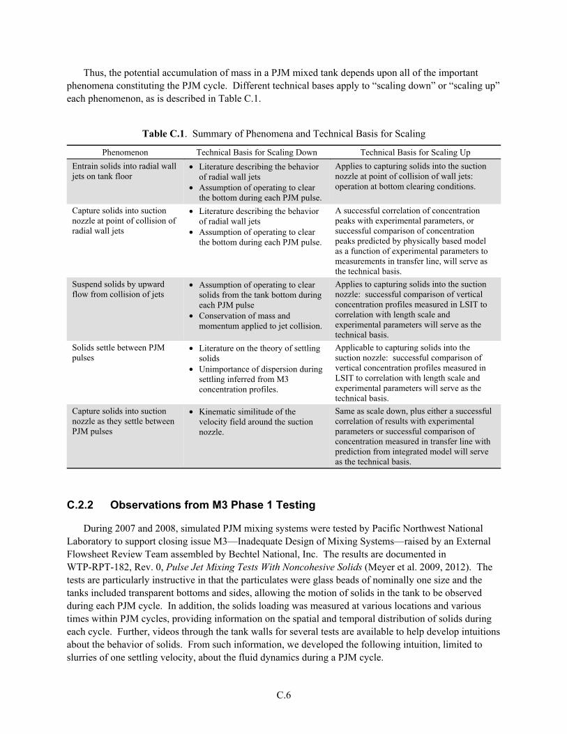
C.6

Thus, the potential accumulation of mass in a PJM mixed tank depends upon all of the important phenomena constituting the PJM cycle. Different technical bases apply to “scaling down” or “scaling up” each phenomenon, as is described in Table C.1.

Table C.1. Summary of Phenomena and Technical Basis for Scaling

Phenomenon Technical Basis for Scaling Down Technical Basis for Scaling Up

Entrain solids into radial wall jets on tank floor

• Literature describing the behavior of radial wall jets

• Assumption of operating to clear the bottom during each PJM pulse.

Applies to capturing solids into the suction nozzle at point of collision of wall jets: operation at bottom clearing conditions.

Capture solids into suction nozzle at point of collision of radial wall jets

• Literature describing the behavior of radial wall jets

• Assumption of operating to clear the bottom during each PJM pulse.

A successful correlation of concentration peaks with experimental parameters, or successful comparison of concentration peaks predicted by physically based model as a function of experimental parameters to measurements in transfer line, will serve as the technical basis.

Suspend solids by upward flow from collision of jets

• Assumption of operating to clear solids from the tank bottom during each PJM pulse

• Conservation of mass and momentum applied to jet collision.

Applies to capturing solids into the suction nozzle: successful comparison of vertical concentration profiles measured in LSIT to correlation with length scale and experimental parameters will serve as the technical basis.

Solids settle between PJM pulses

• Literature on the theory of settling solids

• Unimportance of dispersion during settling inferred from M3 concentration profiles.

Applicable to capturing solids into the suction nozzle: successful comparison of vertical concentration profiles measured in LSIT to correlation with length scale and experimental parameters will serve as the technical basis.

Capture solids into suction nozzle as they settle between PJM pulses

• Kinematic similitude of the velocity field around the suction nozzle.

Same as scale down, plus either a successful correlation of results with experimental parameters or successful comparison of concentration measured in transfer line with prediction from integrated model will serve as the technical basis.

C.2.2 Observations from M3 Phase 1 Testing

During 2007 and 2008, simulated PJM mixing systems were tested by Pacific Northwest National Laboratory to support closing issue M3—Inadequate Design of Mixing Systems—raised by an External Flowsheet Review Team assembled by Bechtel National, Inc. The results are documented in WTP-RPT-182, Rev. 0, Pulse Jet Mixing Tests With Noncohesive Solids (Meyer et al. 2009, 2012). The tests are particularly instructive in that the particulates were glass beads of nominally one size and the tanks included transparent bottoms and sides, allowing the motion of solids in the tank to be observed during each PJM cycle. In addition, the solids loading was measured at various locations and various times within PJM cycles, providing information on the spatial and temporal distribution of solids during each cycle. Further, videos through the tank walls for several tests are available to help develop intuitions about the behavior of solids. From such information, we developed the following intuition, limited to slurries of one settling velocity, about the fluid dynamics during a PJM cycle.

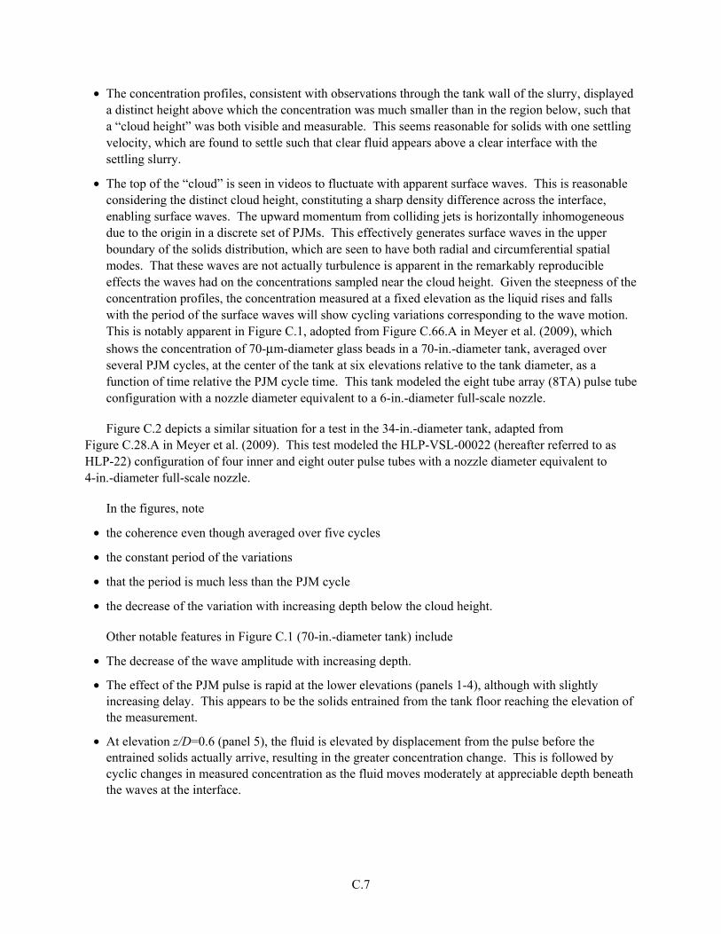
C.7

• The concentration profiles, consistent with observations through the tank wall of the slurry, displayed a distinct height above which the concentration was much smaller than in the region below, such that a “cloud height” was both visible and measurable. This seems reasonable for solids with one settling velocity, which are found to settle such that clear fluid appears above a clear interface with the settling slurry.

• The top of the “cloud” is seen in videos to fluctuate with apparent surface waves. This is reasonable considering the distinct cloud height, constituting a sharp density difference across the interface, enabling surface waves. The upward momentum from colliding jets is horizontally inhomogeneous due to the origin in a discrete set of PJMs. This effectively generates surface waves in the upper boundary of the solids distribution, which are seen to have both radial and circumferential spatial modes. That these waves are not actually turbulence is apparent in the remarkably reproducible effects the waves had on the concentrations sampled near the cloud height. Given the steepness of the concentration profiles, the concentration measured at a fixed elevation as the liquid rises and falls with the period of the surface waves will show cycling variations corresponding to the wave motion. This is notably apparent in Figure C.1, adopted from Figure C.66.A in Meyer et al. (2009), which shows the concentration of 70-μm-diameter glass beads in a 70-in.-diameter tank, averaged over several PJM cycles, at the center of the tank at six elevations relative to the tank diameter, as a function of time relative the PJM cycle time. This tank modeled the eight tube array (8TA) pulse tube configuration with a nozzle diameter equivalent to a 6-in.-diameter full-scale nozzle.

Figure C.2 depicts a similar situation for a test in the 34-in.-diameter tank, adapted from Figure C.28.A in Meyer et al. (2009). This test modeled the HLP-VSL-00022 (hereafter referred to as HLP-22) configuration of four inner and eight outer pulse tubes with a nozzle diameter equivalent to 4-in.-diameter full-scale nozzle.

In the figures, note

• the coherence even though averaged over five cycles

• the constant period of the variations

• that the period is much less than the PJM cycle

• the decrease of the variation with increasing depth below the cloud height.

Other notable features in Figure C.1 (70-in.-diameter tank) include

• The decrease of the wave amplitude with increasing depth.

• The effect of the PJM pulse is rapid at the lower elevations (panels 1-4), although with slightly increasing delay. This appears to be the solids entrained from the tank floor reaching the elevation of the measurement.

• At elevation z/D=0.6 (panel 5), the fluid is elevated by displacement from the pulse before the entrained solids actually arrive, resulting in the greater concentration change. This is followed by cyclic changes in measured concentration as the fluid moves moderately at appreciable depth beneath the waves at the interface.

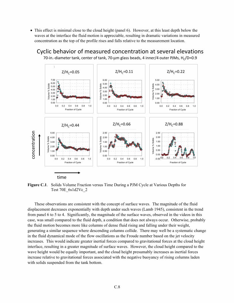
C.8

• This effect is minimal close to the cloud height (panel 6). However, at this least depth below the waves at the interface the fluid motion is appreciable, resulting in dramatic variations in measured concentration as the top of the profile rises and falls relative to the measurement location.

70E_6s1d2Vc_2 H 0.05D R 0R 70_07_18_2008_14_02 (5)

0.00

1.00

2.00

3.00

4.00

5.00

6.00

7.00

0.0 0.2 0.4 0.6 0.8 1.0

Fraction of Cycle

Vol

ume

% S

olid

s

Average Volume%

70E_6s1d2Vc_2 H 0.1D R 0R 70_07_18_2008_13_56 (5)

0.00

1.00

2.00

3.00

4.00

5.00

6.00

0.0 0.2 0.4 0.6 0.8 1.0

Fraction of Cycle

Vol

ume

% S

olid

s

Average Volume%

70E_6s1d2Vc_2 H 0.2D R 0R 70_07_18_2008_13_50 (5)

0.00

1.00

2.00

3.00

4.00

5.00

0.0 0.2 0.4 0.6 0.8 1.0

Fraction of Cycle

Vol

ume

% S

olid

s

Average Volume%

70E_6s1d2Vc_2 H 0.4D R 0R 70_07_18_2008_13_43 (5)

0.00

1.00

2.00

3.00

4.00

5.00

0.0 0.2 0.4 0.6 0.8 1.0

Fraction of Cycle

Vol

ume

% S

olid

s

Average Volume%

70E_6s1d2Vc_2 H 0.6D R 0R 70_07_18_2008_13_37 (5)

0.00

0.50

1.00

1.50

2.00

2.50

0.0 0.2 0.4 0.6 0.8 1.0

Fraction of Cycle

Vol

ume

% S

olid

s

Average Volume%

70E_6s1d2Vc_2 H 0.8D R 0R 70_07_18_2008_13_31 (5)

-0.50

0.00

0.50

1.00

1.50

2.00

2.50

0.0 0.2 0.4 0.6 0.8 1.0

Fraction of Cycle

Vol

ume

% S

olid

s

Average Volume%

Cyclic behavior of measured concentration at several elevations70-in.-diameter tank, center of tank, 70-μm glass beads, 4 inner/4 outer PJMs, HC/D=0.9

Z/HC=0.05

Z/HC=0.66 Z/HC=0.88

Z/HC=0.11 Z/HC=0.22

Z/HC=0.44

time

conc

entr

atio

n

Figure C.1. Solids Volume Fraction versus Time During a PJM Cycle at Various Depths for Test 70E_6s1d2Vc_2

These observations are consistent with the concept of surface waves. The magnitude of the fluid

displacement decreases exponentially with depth under such waves (Lamb 1945), consistent in the trend from panel 6 to 5 to 4. Significantly, the magnitude of the surface waves, observed in the videos in this case, was small compared to the fluid depth, a condition that does not always occur. Otherwise, probably the fluid motion becomes more like columns of dense fluid rising and falling under their weight, generating a similar sequence where descending columns collide. There may well be a systematic change in the fluid dynamical mode of the flow oscillations as the Froude number based on the jet velocity increases. This would indicate greater inertial forces compared to gravitational forces at the cloud height interface, resulting in a greater magnitude of surface waves. However, the cloud height compared to the wave height would be equally important, and the cloud height presumably increases as inertial forces increase relative to gravitational forces associated with the negative buoyancy of rising columns laden with solids suspended from the tank bottom.

C.9

34E_4s1d2Yd_1 H 0.2D R 0R 34_03_09_2008_17_17 (5)

-1.00

0.00

1.00

2.00

3.00

4.00

5.00

6.00

0.0 0.2 0.4 0.6 0.8 1.0

Fraction of Cycle

Vol

um

e %

Sol

ids

Average Volume%

34E_4s1d2Yd_1 H 0.3D R 0R 34_03_09_2008_17_13 (5)

-1.00

0.00

1.00

2.00

3.00

4.00

5.00

6.00

0.0 0.2 0.4 0.6 0.8 1.0

Fraction of Cycle

Vol

um

e %

Sol

ids

Average Volume%

34E_4s1d2Yd_1 H 0.4D R 0R 34_03_09_2008_17_09 (5)

-1.00

0.00

1.00

2.00

3.00

4.00

0.0 0.2 0.4 0.6 0.8 1.0

Fraction of Cycle

Vol

um

e %

Sol

ids

Average Volume%

34E_4s1d2Yd_1 H 0.5D R 0R 34_03_09_2008_17_04 (5)

-0.50

0.00

0.50

1.00

1.50

2.00

2.50

0.0 0.2 0.4 0.6 0.8 1.0

Fraction of Cycle

Vol

um

e %

Sol

ids

Average Volume%

34E_4s1d2Yd_1 H 0.6D R 0R 34_03_09_2008_17_00 (5)

-0.14

-0.12

-0.10

-0.08

-0.06

-0.04

-0.02

0.00

0.0 0.2 0.4 0.6 0.8 1.0

Fraction of Cycle

Vol

um

e %

Sol

ids

Average Volume%

34E_4s1d2Yd_1 H 0.1D R 0R 34_03_09_2008_17_21 (5)

0.00

2.00

4.00

6.00

8.00

10.00

12.00

0.0 0.2 0.4 0.6 0.8 1.0

Fraction of Cycle

Vol

ume

% S

olid

sAverage Volume%

Z/HC=0.31

Z/HC=0.62 Z/HC=0.93 Z/HC>1

Z/HC=0.08 Z/HC=0.15 Z/HC=0.31

Z/HC>1

Cyclic behavior of measured concentration at several elevations34-in.-diameter tank, center of tank, 70-μm glass beads, 4 inner/4 outer PJMs, HC/D=0.65

1 2 3

4 5 6

time

conc

entr

atio

n

Figure C.2. Solids Volume Fraction versus Time During a PJM Cycle at Various Depths for Test 34S_4s1d2Yd_1

C.2.3 Conceptual Model of Phenomena Affecting a Mass Balance

Here, we present an example of developing a physically based correlation for the elevation attained by solids entrained from the tank floor, due to upward flow from colliding jets on the floor of the tank. The model is based on the above observations about M3 data, and considering numerous “textbook” descriptions of jets and turbulence.

C.2.3.1 Entrainment of Solids in Radial Wall Jets on Tank Floor

The conceptual model is as follows:

Based on observations of certain behavior in videos of M3 tests described above, we adopt the following initial conceptual model for planning and analyzing LSIT data.

• Radial wall jets formed on the tank floor by PJM pulses expand while scouring settled solids until they collide with each other or a tank wall. The jet velocity is controlled to scour all of the settled solids by the end of the pulse jet duration.

C.10

• At the tank floor, solids are entrained into the leading vortex of the wall jet. The volume of the vortex increases due to the difference in the fluid velocity in the jet near the front of the jet and the lesser velocity of the front of the jet.

• Readily accessible information about the rate of growth and spreading of an axisymmetric jet can be transformed using a momentum balance to estimate the rate of advance of the jet front and the extent of entrainment into the jet behind it.

• The entrainment into the wall jet enables estimating both the volume and density of the leading vortex at the location of collision with adjacent vortices.

The result is that the solids volume fraction in the vortices after entraining solids from the tank floor, φ0, is

( )

3 23 2

0 1 3 2

13 1

1

// S C

E J /

u tN DC

D

σφ φ φγ σ

= + −− (C.4)

where φE = solids volume fraction in the entraining fluid φ1 = solids volume fraction of suspended solids near the tank floor γ = coefficient of spreading of a radial wall jet σ = fraction of the velocity in the jet at its front edge uS = the settling velocity tC = the cycle time DC = the duty cycle NJ = the number of PJMs D = the tank diameter.

See Section C.4.1.6 for the development. See Section C.4.1.8 for the evaluation of φE and φ1. This provides a basis for scaling LSIT conditions to provide representative measurements of the peak concentration into the suction nozzle to support separate tests on plugging (see Section 5.7).

C.2.3.2 Upward Suspension of Settled Solids

The conceptual model is as follows:

• The rate of loss of linear momentum of the ascending vortices is known from the conservation of momentum and the density of the ascending vortices relative to the surrounding fluid. The elevation at which the linear momentum expires is the jet height. We assume that the remaining angular momentum has provided sufficient axial dispersion to cause the concentration within the vortices to be roughly uniform and the vertical concentration profile to be uniform at the end of the jet pulse.

• The volume of the vortices grows as the difference between the volumetric flow rate in the jet behind the vortices and the flow rate that would occur if the jet were moving at the speed the vortices advance. (This is similar to the analysis elsewhere of the volume of the vortices for the radial wall jet.) From the volume and angular momentum of the vortices at the end of the jet pulse, we can estimate the associated kinetic energy from the angular velocity.

C.11

• The forces acting on the vortices result from resistance from the fluid they are penetrating and negative buoyancy.

Solids entrained in the vortices ascend to the cloud height and are then dispersed by turbulence attending the dissipation of the kinetic energy remaining in the motion of the fluid at the end of a pulse.

In Section C.4, a momentum balance for the upward mixing is constructed based on this conceptual model. The analysis serves as an example of the process of developing a physically based model or correlation. We have not attempted to complete the model in sufficient detail to predict a cloud height a priori. However, just as for experimental data, a power-law form can be obtained from a multi-linear fit of data or equations in log-log form using means described in Section C.4.1.9. The same power-law form applied to correlate M3 HC, “cloud height,” data results in the following set of “scaling” exponents on dimensionless groups obtained in deriving the momentum balance.

( )( )0.29 0.010.91 0.06 0.35 0.02

0.40 0.02

021S

C S

J

uD d gDH s

D U UNφ

− ++ − +− + ∝ − (C.5)

where D = the tank diameter NJ = the number of PJMs in the tank d = the PJM nozzle diameter uS = the settling velocity of the particles U = the characteristic velocity g = the acceleration of gravity s = the ratio of particle density to liquid phase density φS0 = the nominal solids volume fraction in the tank.

The results are physically reasonable and suggest the momentum balance concept should be pursued in combination with greater detail in the settling calculation to develop a physically based model or correlation for the concentration profile of individual settling species in LSIT tests, based on examining, correlating, and adapting to actual LSIT data.

C.2.3.3 Solids Settling

Cloud Height and Other Attributes of a Solids Concentration Profile

The concept of cloud height implies a discrete limit of coherent upward flows and specifically a discrete limit of the upward transport of settled solids entrained in the flows. A cloud height was obvious and measurable during M3 Phase 1 tests using particles of one size. We presume a distinct cloud height attends a distinct, severe gradient in density, which causes a commensurate distinct, severe gradient in the negative buoyancy of upward flows, resulting in a commensurate deceleration in the flow, which corresponds to a distinct end of the flows (reminiscent of the “anvil tops” of cumulus clouds formed where the upward flow reaches a distinct change in the temperature gradient). A distinct cloud height, as seen during M3 testing, corresponds to a sharp decrease in density with elevation. This impedes upward jets of denser fluid from penetrating to higher elevations, which serves to preserve the distinct cloud height.

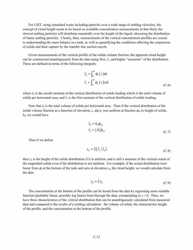
C.12

For LSIT, using simulated waste including particles over a wide range of settling velocities, the concept of cloud height needs to be based on available concentration measurements in that likely the slowest settling particles will distribute essentially over the height of the liquid, obscuring the distribution of faster-settling particles. Clearly, then, measurements of the vertical concentration profiles are crucial to understanding the mass balance in a tank, as well as quantifying the conditions affecting the suspension of solids and their capture by the transfer line suction nozzle.

Given measurements of the vertical profile of the solids volume fraction, the apparent cloud height can be constructed unambiguously from the data using first, I1, and higher “moments” of the distribution. These are defined in terms of the following integrals:

( )

( )0 0

1 0

H

S

H

S

I z dz

I z zdz

φ

φ

=

=

(C.6)

where I0 is the zeroth moment of the vertical distribution of solids loading which is the total volume of solids per horizontal area, and I1 is the first moment of the vertical distribution of solids loading.

Note that I0 is the total volume of solids per horizontal area. Then if the vertical distribution of the solids volume fraction as a function of elevation, z, φS(z), was uniform at fraction φS0 to height of solids, hS, we would have

0 0

211 02

S S

S S

I h

I h

φφ

=

= (C.7)

Then if we define

zS = 2 I1 I0( ) (C.8)

then zS is the height of the solids distribution if it is uniform, and is still a measure of the vertical extent of the suspended solids even if the distribution is not uniform. For example, if the actual distribution were linear from φb at the bottom of the tank and zero at elevation z0, the cloud height, we would calculate from the data

zS = 23 z0 (C.9)

The concentration at the bottom of the profile can be found from the data by regressing some suitable function (probably linear, possibly log linear) form through the data, extrapolating to z = 0. Thus, we have three characteristics of the vertical distribution that can be unambiguously calculated from measured data and compared to the results of a settling calculation: the volume of solids, the characteristic height of the profile, and the concentration at the bottom of the profile.

C.13

Predicting Concentration at Depth Using a Settling Model

In Section C.4.2, we describe a mass balance on settling solids to be solved to predict the vertical profile of solids versus time. The model requires as input the concentration profile estimated at the end of the PJM pulse (for example, one alternative is to assume a uniform initial profile), the Archimedes numbers of the various particle types (available from the particle size and density distribution [PSDD] and properties of the fluid), a hindered settling correction based on the available literature, and a correlation for a cloud height (see Section C.4.1, “Suspension of Solids by Collision of Radial Wall Jets”) and, if necessary, a hydrodynamic dispersion coefficient correlated from LSIT data. Measured concentration profiles can be reduced to three physically meaningful parameters—total volume of solids suspended, characteristic height of the concentration profile, and concentration at the bottom of the profile—and compared to values computed from the results of a settling calculation. Differences are then used to correlate the minimum possible number of adjustable parameters, such as a parameter in a hindered settling correction or a dispersion coefficient.

Implementation includes solving a first-order partial differential equation numerically. However, this is not difficult, and can be implemented using spreadsheets if desired. Although the model itself is complicated, it is essentially a textbook model, neither ambiguous nor speculative, the input parameters are few and available, and it provides exactly the information needed to implement a mass balance over the PJM cycle that is required to implement a mass balance over a pump-out cycle.

Whatever the means employed to solve the settling mass balance, the purpose of the calculation is to find, from the initial profile, the volume fraction profile for species “i” at the end of a pulse. This profile determines the density profile into which the next pulse must penetrate.

C.2.3.4 Capture of Settling Solids by the Suction Nozzle

The capture of settling particles by the flow field into the suction nozzle can be evaluated in terms of a “capture volume” calculated from the suction flow rate, particle settling velocity, and distance of the suction nozzle above the tank floor. Thus, a capture zone is calculated for each settling velocity, and thus is calculated for each size fraction of a species of given density. For a flow limited to only that imposed by the suction on an otherwise quiescent fluid, and for distances from the nozzle not small compared to the nozzle diameter, the velocity distribution can be estimated from a simple point sink matched by a mirror-image point sink on “the other side” of the tank floor. Then the capture zone is found from a straightforward evaluation of kinematics, following the path of the summed settling and suction flow field velocities. Example capture volumes are illustrated in the following Figure C.3.

In the figure, the heavy dashed line bounding each of the three volumes indicates the capture volume. The suction nozzle is treated as a point sink denoted by the heavy dot. The fine dashed lines depict the path of particles beginning at various locations on the boundary. Particles of the specified settling rate that are inside this volume at the end of a PJM pulse will be captured by the suction nozzle by the end of the PJM cycle. The volumes on the left, middle, and right correspond to fast, moderate, and slow settling velocities, respectively.

Mass enters the suction nozzle in two steps. First, a PJM pulse pushes settled solids outward as the radial wall jet that forms on the tank floor spreads radially. The suction nozzle will fall horizontally within the jet radius of at least one PJM. Thus, as the solids pushed by the radial jet pass under the

C.14

suction nozzle, the nozzle will capture a pulse of solids. This determines the peak concentration of solids that must be accommodated by the transfer line and pump without plugging. Thus, this concentration peak as a function of time is determined from LSIT tests and provided to full-scale line plugging test activities as a condition to be imposed in those tests.

Figure C.3. Illustrative Shapes of Volumes in Which Particles are Captured by a Suction Nozzle

Second, after a PJM pulse, suspended and dispersed solids settle toward the tank floor. As solids

approach the floor, some will travel close enough to the suction nozzle to be captured by the flow into the nozzle. This can be estimated by calculating the volume around the nozzle that includes the initial locations of particles whose settling paths, as affected by the flow field around the suction nozzle, are captured by the nozzle.

Each PJM pulse suspends some fraction of the solids on the floor of the tank and entrains them into the upward flow resulting from the collision on the tank floor of radial wall jets with each other or the side walls of the tank. Complex, coupled phenomena determine the resulting vertical distribution of solid species. This distribution is needed to provide the distribution of particles that fall within the capture volume computed for the corresponding settling velocity, which then determines which particles and hence what mass of each species will be removed from the tank during the PJM cycle.

C.3 Mass Balance During Pump Out

The Limit Solids Accumulation mixing requirement is addressed by predicting the accumulation (e.g., no accumulation) of solids in the WTP tank using a model validated from LSIT data.

C.3.1 Components of Mass Balance Model

This mass balance model consists of a hierarchy of sub-models, as follows. During PJM cycles, the following sub-models are used repeatedly.

C.15

• A correlation of the velocity required to at least momentarily clear solids from the tank bottom is used to specify the jet velocity. This might depend on the depth of settled solids at the time of the pulse. If so, the depth is determined from the settling calculation from the prior pulse.

• A correlation of the cloud height—specifically, a measure of the vertical extent of the solids concentration profile at the end of a PJM pulse. This correlation probably will depend on the depth of settled solids at the start of the pulse, which is determined from the settling calculation for the prior pulse.

• A model for the competition between dispersion and settling of solids as they are suspended into the cloud height, which provides the initial vertical profile for calculating settling between pulses.

• A model for settling of solids between pulses depends on the initial vertical profile and, possibly, on a coefficient quantifying hydrodynamic dispersion attending residual turbulence from the preceding pulse. The coefficient is correlated from fits of repeated settling measurements of concentration profiles.

• A calculation of the concentration and mass flows of solids species entering the transfer line, based on the local concentration of solids predicted from the settling model, and from a correlation of the fraction of solids captured from the leading edge of radial wall jets that move settled solids under the suction nozzle during each PJM pulse. This calculation supports the mass balance model over pump-out cycles, discussed below, and is used to specify the conditions at the inlet of the transfer line to be used in separate testing for plugging in the transfer line and pump.

The results of calculating the vertical solids concentration profile are used in several ways within the overall mass balance model:

1. The mass concentration predicted at the inlet to the transfer line suction nozzle is used to predict the concentrations and mass flow rates entering the transfer line, which

a. Provides the information needed to implement a mass balance over a pump-out cycle.

b. Provides the information needed to design and operate separate scaled tests of potential plugging in the transfer line and pump.

2. The mass concentration profile predicted at the end of settling provides the vertical density profile to be used as part of correlating the cloud height or similar attributes used as an initial condition for the next settling cycle.

3. The settling calculation predicts the thickness of settled solids at the start of the next PJM pulse, which is required to assure that bottom clearing (the proposed technical strategy for assuring bottom motion) occurs within the drive time of the PJM cycle.

Note that these sub-models involve few adjustable parameters except for the correlation of cloud height. We expect essentially all experimental parameters can be important to that correlation, which affects the settling, which affects the mass flows out of the tank, which determine compliance with the no accumulation of solids and no plugging requirements. The objective is to develop a correlation for which the empirical coefficients are found by interpolation (if not predicted a priori by the physical basis) over LSIT data while extrapolation of the correlation to larger length scales is done based on a physical model. The physical basis and implementation of the model needs to be validated at one scale, then validated again at a greater scale, and then again at the greatest scale available. Thus validated, the correlation is

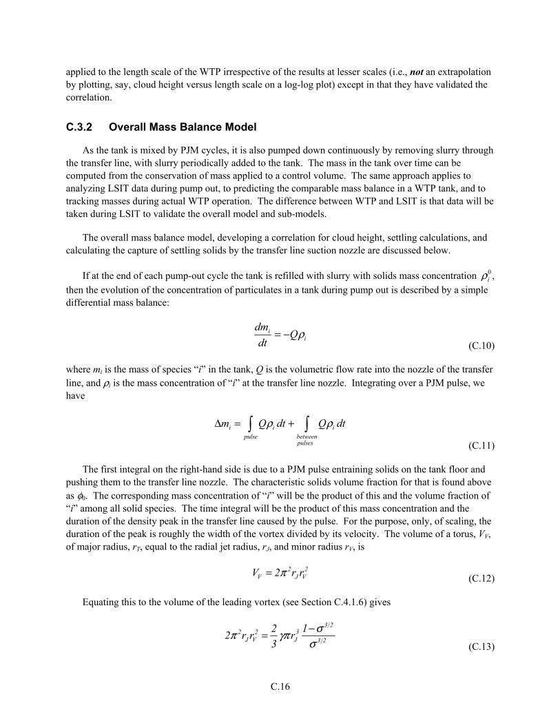
C.16

applied to the length scale of the WTP irrespective of the results at lesser scales (i.e., not an extrapolation by plotting, say, cloud height versus length scale on a log-log plot) except in that they have validated the correlation.

C.3.2 Overall Mass Balance Model

As the tank is mixed by PJM cycles, it is also pumped down continuously by removing slurry through the transfer line, with slurry periodically added to the tank. The mass in the tank over time can be computed from the conservation of mass applied to a control volume. The same approach applies to analyzing LSIT data during pump out, to predicting the comparable mass balance in a WTP tank, and to tracking masses during actual WTP operation. The difference between WTP and LSIT is that data will be taken during LSIT to validate the overall model and sub-models.

The overall mass balance model, developing a correlation for cloud height, settling calculations, and calculating the capture of settling solids by the transfer line suction nozzle are discussed below.

If at the end of each pump-out cycle the tank is refilled with slurry with solids mass concentration ρi0 ,

then the evolution of the concentration of particulates in a tank during pump out is described by a simple differential mass balance:

dmi

dt= −Qρi

(C.10)

where mi is the mass of species “i” in the tank, Q is the volumetric flow rate into the nozzle of the transfer line, and ρi is the mass concentration of “i” at the transfer line nozzle. Integrating over a PJM pulse, we have

Δmi = Qρi dtpulse + Qρi dt

betweenpulses

(C.11)

The first integral on the right-hand side is due to a PJM pulse entraining solids on the tank floor and pushing them to the transfer line nozzle. The characteristic solids volume fraction for that is found above as φ0. The corresponding mass concentration of “i” will be the product of this and the volume fraction of “i” among all solid species. The time integral will be the product of this mass concentration and the duration of the density peak in the transfer line caused by the pulse. For the purpose, only, of scaling, the duration of the peak is roughly the width of the vortex divided by its velocity. The volume of a torus, VV, of major radius, rT, equal to the radial jet radius, rJ, and minor radius rV, is

2 2

V J VV 2 r rπ= (C.12)

Equating this to the volume of the leading vortex (see Section C.4.1.6) gives

3 22 2 3

J V J 3 2

2 12 r r r

3

σπ γπσ−=

(C.13)

C.17

where σ is the ratio of the velocity of the vortices to the velocity at the same location inside the jet behind the vortices, and γ is the coefficient of spreading of a radial wall jet.

Therefore, the width of the vortex is

3 2

V j 3 2

4 12r r

3

γ σπ σ

−= (C.14)

The velocity of the vortex, uV, is

uv = σu rJ( )= σu0 r0 rJ( ) (C.15)

where u is the characteristic velocity of the jet and r0 is the jet radius at which self-similarity is established.

Then the duration of the density peak scales with time, t, as

23 2

2 3 2 3 23 2

7 2 7 20 0

422 4 43 8

3 3

JV J J

V J

J

D1r

r r N 1 D 1 Dt

ru Ur Ud N d UUr

γ σγγ σ γ σπ σ γ

π σ π σσ

−− − Δ = = = =

(C.16)

Then the volume of total solids, VS, entering the nozzle during the pulse scales as

( )

3 2 3 23 21

0 3 2 7 2

23 11

31S C

S E JJ

u t D QDV Q t N DC

D N d U

γφ σ γ σφ φγ πσ σ

− Δ Δ = + − −

/ //

/ /~ (C.17)

where φ0 is the solids volume fraction in the vortex (see Section C.4.1.6). Since rJ /u0 scales as D/U and velocity u0 occurs at the location of self-similarity, we expect

( )

3/2 3/23/21

3 3/2 7/2 2

23 11

1 3S S C

E JJ

V u t D QN DC

D D N d UD

γφ σ γ σφγ σ π σ

Δ − + − −

(C.18)

Thus, we obtain a simple scaling law, Q ~ UD2, all else being equal. It is apparent that other parameters are involved, but it may not be practicable to match all pertinent parameters, just as it is not practicable to attain full similitude, in which case the priority should be on following the simple scaling law to attain a representative concentration pulse due to clearing solids from the bottom.

The mass or volume of species “i” leaving the tank will be in proportion to its volume fraction among the solids species and the volume of all solids exiting the tank during a PJM pulse.

LSIT results over repeated PJM cycles are used to confirm or revise the conceptual model for suspending, settling, and capturing the solids, which then is used as noted here to predict the mass versus time of the various particulate species in WTP. This quantifies “accumulation” in the WTP. That is, we

C.18

would implement the settling model repeatedly to solve the mass balance over the pump-out cycles to predict the mass of species “i” in the tank over time to address the Limit Solids Accumulation mixing requirement.

C.3.3 Non-Newtonian Tanks

C.3.3.1 General

In principle, the same set of models applies to the overall mass balance for pump out, but not for the component sub-models and correlations listed in Section C.3.1. Recognizing the difficulties discussed below, this working paper is written initially with the expectation that the very technical approach to scaling LSIT data will require analysis of initial data to develop a strategy for scaling it to WTP tanks.

Tanks designed to process non-Newtonian fluids have the PJMs clustered in the center and enclosed above so solids can only ascend or settle in an annulus between the cluster and the tank wall. The annulus and the outer part of the tank floor will be agitated by spargers (see Chapter 7) to keep the non-Newtonian fluid sheared, which we presume enables some fraction of the particles to settle. In this case, the suction nozzle will be tested at locations toward the tank wall, where solids can settle from above after being suspended and dispersed by PJM mixing. Then a mass balance model over repeated PJM cycles during a pump-out cycle needs to consider circumferential dispersion by PJM mixing of suspended solids, which will be the means by which most settling solids in the tank find their way to the suction nozzle. This concept is still being developed, but would involve the same differential mass balance, plus the simplest possible model of circumferential dispersion, which might be approached technically using scaling based on principles of turbulence. Of course, the settling model potentially is quite different in a Bingham fluid, depending on the effect of sparger shearing on the particle environment.

In general, “scaling” tests done using Bingham fluids will be more complicated and less certain than for Newtonian fluids because

• There is less experience industrially and fewer studies published to guide the effort.

• Although the Bingham fluid model is adopted as the design basis, rheograms of actual waste and simulated waste can exhibit more complicated phenomena such as a shear strength and pseudo-plastic behavior at low shear rates, which might confound interpretation of test data.

• Any physically based model would be significantly more complicated, and involve more adjustable parameters, for a non-Newtonian fluid compared to a Newtonian fluid.

C.3.3.2 Newtonian/Bingham Fluids: Equivalence Based on Power-per-Volume

Bingham fluids exhibit a yield stress, τ0, such that the shear rate is zero until the applied stress exceeds the yield stress. Once the fluid shears, the shear rate is proportional to the difference between the applied stress and the yield stress. Thus, the behavior is similar to a Newtonian fluid if the applied stress, and hence the actual shear rate, is large enough. The conditions for which this applies are derived below. The result is that a Bingham fluid will exhibit the same shear rate for a given power dissipation rate as a

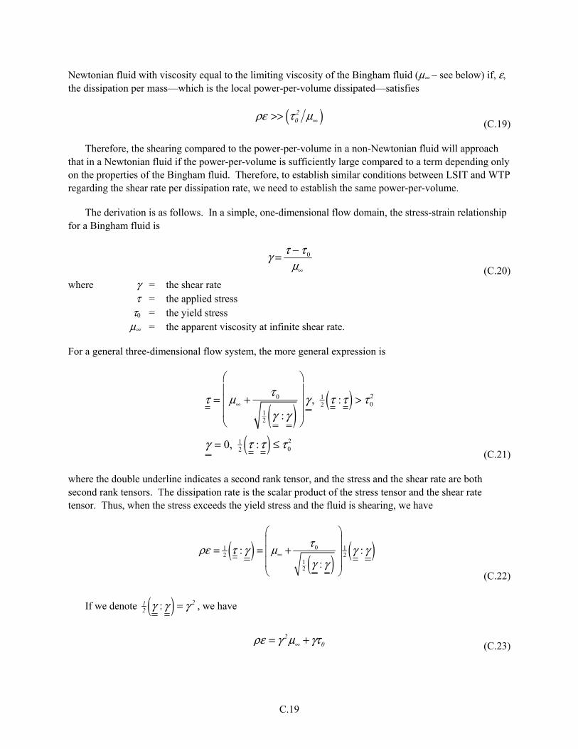
C.19

Newtonian fluid with viscosity equal to the limiting viscosity of the Bingham fluid (μ∞ – see below) if, ε, the dissipation per mass—which is the local power-per-volume dissipated—satisfies

( )∞>> 2

0ρε τ μ (C.19)

Therefore, the shearing compared to the power-per-volume in a non-Newtonian fluid will approach that in a Newtonian fluid if the power-per-volume is sufficiently large compared to a term depending only on the properties of the Bingham fluid. Therefore, to establish similar conditions between LSIT and WTP regarding the shear rate per dissipation rate, we need to establish the same power-per-volume.

The derivation is as follows. In a simple, one-dimensional flow domain, the stress-strain relationship for a Bingham fluid is

γ = τ − τ 0

μ∞ (C.20) where γ = the shear rate τ = the applied stress τ0 = the yield stress μ∞ = the apparent viscosity at infinite shear rate.

For a general three-dimensional flow system, the more general expression is

τ = μ∞ +τ 0

12 γ :γ( )

γ , 12 τ :τ( ) > τ 0

2

γ = 0, 12 τ :τ( ) ≤ τ 0

2

(C.21)

where the double underline indicates a second rank tensor, and the stress and the shear rate are both second rank tensors. The dissipation rate is the scalar product of the stress tensor and the shear rate tensor. Thus, when the stress exceeds the yield stress and the fluid is shearing, we have

( ) ( ) ( )01 12 2

12

: : :

∞

= = +

τρε τ γ μ γ γγ γ

(C.22)

If we denote ( ): 212 γ γ γ= , we have

∞= +20ρε γ μ γτ (C.23)

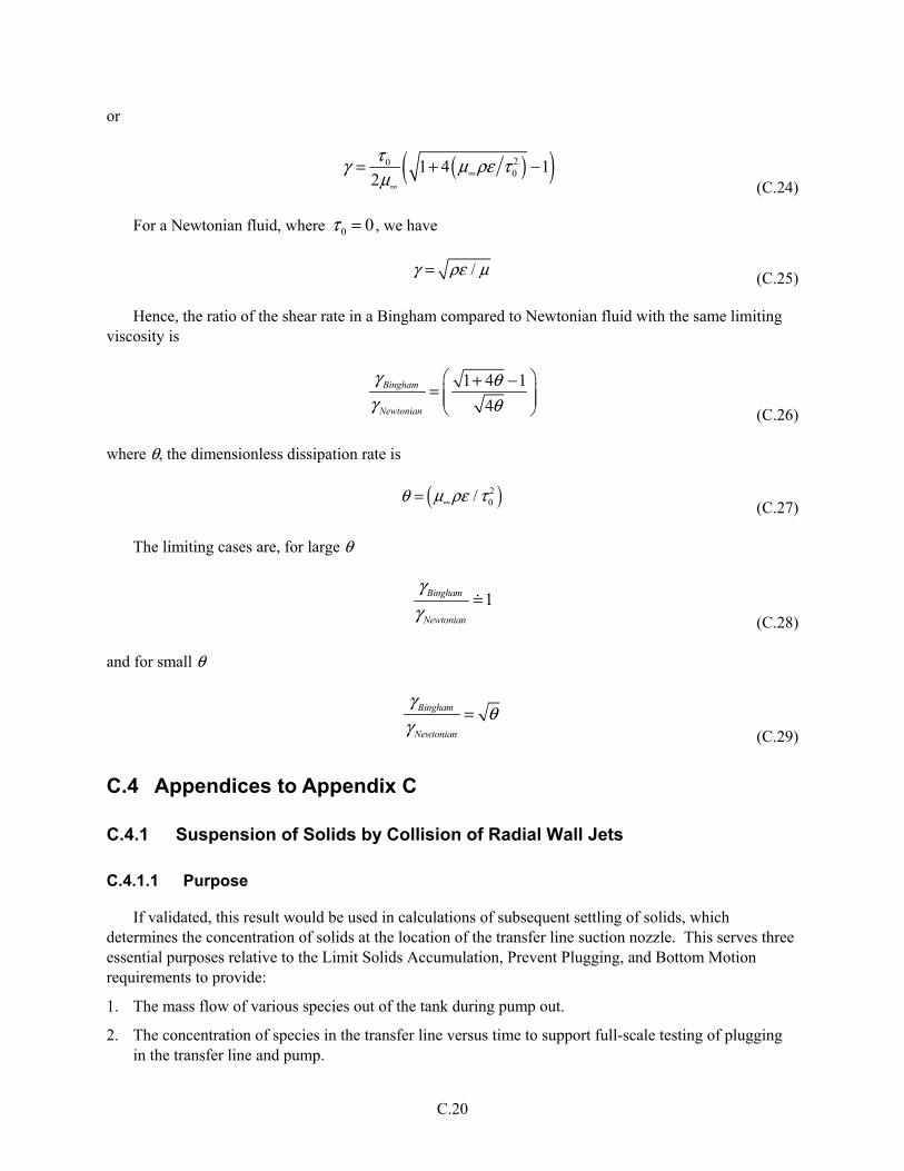
C.20

or

( )( )20

01 4 1 2 ∞

∞

= + −τγ μ ρε τμ (C.24)

For a Newtonian fluid, where τ 0 = 0, we have

/γ ρε μ= (C.25)

Hence, the ratio of the shear rate in a Bingham compared to Newtonian fluid with the same limiting viscosity is

1 4 1

4Bingham

Newtonian

γ θγ θ

+ −= (C.26)

where θ, the dimensionless dissipation rate is

( )2

0/θ μ ρε τ∞= (C.27)

The limiting cases are, for large θ

1Bingham

Newtonian

γγ

= (C.28)

and for small θ

Bingham

Newtonian

γθ

γ=

(C.29)

C.4 Appendices to Appendix C

C.4.1 Suspension of Solids by Collision of Radial Wall Jets

C.4.1.1 Purpose

If validated, this result would be used in calculations of subsequent settling of solids, which determines the concentration of solids at the location of the transfer line suction nozzle. This serves three essential purposes relative to the Limit Solids Accumulation, Prevent Plugging, and Bottom Motion requirements to provide:

1. The mass flow of various species out of the tank during pump out.

2. The concentration of species in the transfer line versus time to support full-scale testing of plugging in the transfer line and pump.

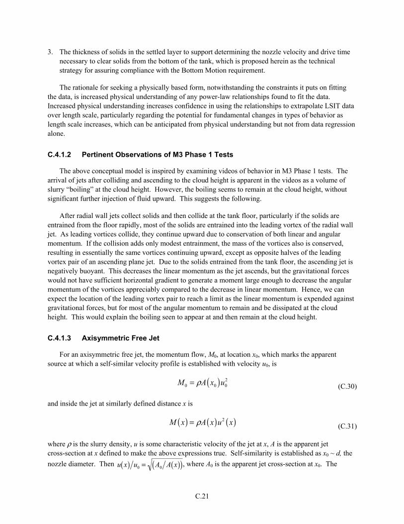
C.21

3. The thickness of solids in the settled layer to support determining the nozzle velocity and drive time necessary to clear solids from the bottom of the tank, which is proposed herein as the technical strategy for assuring compliance with the Bottom Motion requirement.

The rationale for seeking a physically based form, notwithstanding the constraints it puts on fitting the data, is increased physical understanding of any power-law relationships found to fit the data. Increased physical understanding increases confidence in using the relationships to extrapolate LSIT data over length scale, particularly regarding the potential for fundamental changes in types of behavior as length scale increases, which can be anticipated from physical understanding but not from data regression alone.

C.4.1.2 Pertinent Observations of M3 Phase 1 Tests

The above conceptual model is inspired by examining videos of behavior in M3 Phase 1 tests. The arrival of jets after colliding and ascending to the cloud height is apparent in the videos as a volume of slurry “boiling” at the cloud height. However, the boiling seems to remain at the cloud height, without significant further injection of fluid upward. This suggests the following.

After radial wall jets collect solids and then collide at the tank floor, particularly if the solids are entrained from the floor rapidly, most of the solids are entrained into the leading vortex of the radial wall jet. As leading vortices collide, they continue upward due to conservation of both linear and angular momentum. If the collision adds only modest entrainment, the mass of the vortices also is conserved, resulting in essentially the same vortices continuing upward, except as opposite halves of the leading vortex pair of an ascending plane jet. Due to the solids entrained from the tank floor, the ascending jet is negatively buoyant. This decreases the linear momentum as the jet ascends, but the gravitational forces would not have sufficient horizontal gradient to generate a moment large enough to decrease the angular momentum of the vortices appreciably compared to the decrease in linear momentum. Hence, we can expect the location of the leading vortex pair to reach a limit as the linear momentum is expended against gravitational forces, but for most of the angular momentum to remain and be dissipated at the cloud height. This would explain the boiling seen to appear at and then remain at the cloud height.

C.4.1.3 Axisymmetric Free Jet

For an axisymmetric free jet, the momentum flow, M0, at location x0, which marks the apparent source at which a self-similar velocity profile is established with velocity u0, is

M 0 = ρA x0( )u02

(C.30)

and inside the jet at similarly defined distance x is

M x( ) = ρA x( )u2 x( ) (C.31)

where ρ is the slurry density, u is some characteristic velocity of the jet at x, A is the apparent jet cross-section at x defined to make the above expressions true. Self-similarity is established as x0 ~ d, the

nozzle diameter. Then u x( ) u0 = A0 A x( )( ), where A0 is the apparent jet cross-section at x0. The

C.22

nominal width “b” of an axisymmetric jet increases in proportion to its length as b = βx , where β is a

proportionality constant for jet width, so that

( )( ) ( )22

0A x A x dβ= (C.32)

Therefore, inside the jet we have

u x( ) u0( ) = d βx( ) (C.33)

A transient jet penetrates the surrounding fluid at a rate characterized by Bajpai and Tirumkudulu (2008)

0

J

C

xd

d

u td

d

α

=

(C.34)

where αC is a “celerity constant,” i.e.,

0=J Cx u dtα (C.35)

where xJ is the extent of the jet.

Differentiating, the rate of penetration of the jet is

( ) ( ) ( )2

0 01 2 2J J C C Ju dx dt u d t u d xα α= = = (C.36)

where uJ is the rate of advancement of the front of the jet and t is the time.

The velocity inside the jet at its forward boundary is

( ) ( )( ) ( )( )0 0 0/ /J J Ju x u A A x u d xβ= =

(C.37)

Define the ratio

( )( ) ( )= = 2

J J Cu u x 2σ α β (C.38)

From Bajpai and Tirumkudulu (2008), the celerity parameter is ~2.47; from Rajaratnam (1976, Equation 2.87), 1/β~6.3. Then

σ ~ 2.47( )2

2 6.3( )( ) ~ 0.48 (C.39)

C.23

That is, the jet front proceeds at about half the velocity of the fluid “running into” the jet front from inside the jet. The result is that the fluid is diverted laterally, generating angular momentum and the attending leading vortex ring at the jet front.

The same ratio can be obtained from a momentum balance where the force, F, acting externally on the jet is taken as the stagnation pressure for the rate of advancement of the jet, uJ, acting on an effective frontal area that is some multiple “C” of the nominal flow cross-section evaluated at the location of the front of the jet. The momentum balance is

d

dtρu( )dV

V

= M0 − F = M0 − 12 ρuJ

2CA xJ( ) (C.40)

where V is the volume of the jet out to its current extent, xJ. Differentiating the integral and substituting for M0,

d

dtρu( )dV

V

= ρuJ dV dt( )x J= ρσu2 xJ( )A xJ( )

= M0 − F = ρA0u02 − 1

2 ρσ 2u2 xJ( )CA xJ( ) (C.41)

Rearranging,

σ + 1

2 σ 2C( ) u2 xJ( )A xJ( )A0u0

2=1

(C.42)

For this to be true, it must be true also at the start of the jet. Hence, we must have

C = 2 1−σ( ) σ 2( ) (C.43)

Using σ ≈ 0.48, we have C ≈ 4.5, implying that the area of the front of the jet “mushrooms” laterally as expected; the jet generates a lead vortex ring as it penetrates, with flow from within the jet colliding at the center of the ring with the fluid being penetrated. Thus, the jet front is a moving stagnation point slightly in front of the vortex ring, and the ring itself. The radius of the front is a factor 4.5 = 2.1 greater than the radius of the nominal flow cross-section. That is, the radius of the vortex ring is about twice the radius of the jet extrapolated to the location of the front.

C.4.1.4 Radial Wall Jet

From the geometry of a radial wall jet, the flow cross-section varies radially as

A r( ) A0( ) = rδ r0δ0( ) (C.44)

where r0 is the apparent location at which self-similarity is established relative to the geometric axis of symmetry and δ is the thickness of the wall jet (δ0 at r0). The existence of a wall shear stress in principle

C.24

invalidates arguments for similitude in the shape of the velocity profile in the jet. However, the effect actually is negligible and similitude can be invoked as for a free jet. This is justified as follows.

A differential momentum balance at some radius, r, into the jet is

−d 2πrδρu2( ) − 2πrτ wdr = 0

(C.45)

where τw is the shear stress acting on the wall of the jet. Rearranging,

d ln u2δ( ) d ln r( ) = − 1+ r δ( ) τ w ρu2( )( ) = − 1+ r δ( ) 1

2 C f( ) (C.46)

where Cf is the friction factor. For radial wall jets, r δ( ) ~ 0.087( )−1 =11.5 (Rajaratnam 1976,

Equation 11-30). The friction factor is (Poreh et al. 1967, Equation 29)

( ) ( ) 0 162 0 30 06

..w / u . Re r / hδτ ρ −−=

(C.47)

where h is the distance of the source of the impinging jet to the wall (Poreh et al. 1967), roughly r ~ h at the location of the greatest stress. For WTP, we expect u ~ 12 m/s, and putting nominally ρ ~ 1000 kg/m3 and μ ~ 1 cP = 10-3 kg/m/s, and taking δ = 0.087r ~ 0.087h and using h ~ 6 in. = 0.15 m, we find the

Reynolds number of the radial wall jet, 51 5 10Re ~ .δ × and hence, r δ( ) 12 C f ~ 10−2 . Therefore, we have

( )2ln1

ln

d u

d r

δ= −

(C.48)

or

d ln u d ln r( ) = − 1

2 1+ d lnδ d ln r( )( ) = − 12 1+ d ln 0.087r( ) d ln r( )( ) = −1

(C.49)

Hence,

0

0

ru

u r=

(C.50)

Similar to the analysis above for an axisymmetric jet, the momentum balance for a radial wall jet is

d

dtρu( )dV

V

= ρuJ dV dt( )x J= ρσu2 xJ( )A xJ( ) = M0 − F

= ρu02A0 − 1

2 ρσ 2u2 xJ( )CA xJ( ) (C.51)

C.25

Rearranging,

( ) ( ) ( )2

212 2

0 0

1J Ju x A xC

u Aσ σ+ =

(C.52)

For this to be true at the start of the jet, again assuming unit ratio of densities, we must have

σ + 12 Cσ 2 =1 (C.53)

which is the same as for an axisymmetric jet. While an axisymmetric jet expands in two dimensions in proportion to its length due to entrainment in two dimensions, a radial wall jet expands in one dimension due to entrainment (i.e., perpendicular to the wall of the jet) and in one dimension due to the expanding circumference of the front of the jet. Thus, the area factor due to the front of the jet being diverted laterally will be that of one of the dimensions for an axisymmetric jet. Thus, the area factor will be the square root of the area factor for an axisymmetric jet. Adopting Cradial = (Caxisymmetric)

1/2 for this reason, we have

( )1 2 1axisymmetricCσ = + −( ) ( )1 2 4.5 1axisymmetricC = + −( )4.5 0.61=

(C.54)

C.4.1.5 Entrainment into a Radial Wall Jet

Following is a working conceptual model of the effect of entrainment on the density of the upward flow resulting from colliding radial wall jets formed by impingement of the PJM jets on the tank floor.

The radial wall jet formed by impingement of the PJM jet on the tank floor expands with time (sequence a-b-c-d in Figure C.4) and suspends solids as it passes over the settled bed. At the penetration front of the jet, the internal volumetric flow is diverted by the resistance of the fluid being penetrated, forming a leading vortex in the form of a torus, shown in the figure in cross-section. By the time the jet has advanced to clear its share of the tank bottom (sequence “d” in the figure), the solids it has suspended are in the leading vortex.

Following Bajpai and Tirumkudulu (2008), we assume that the velocity profile in a transient jet, except close to the penetration front, is the same as for the steady jet that would result by sustaining the transient jet to reach steady-state at the distance of interest. Then the velocity inside the jet is

u r( ) = dr dt( ) = u0 r0 r( ) (C.55)

Therefore,

dr2 = 2r0u0dt (C.56)

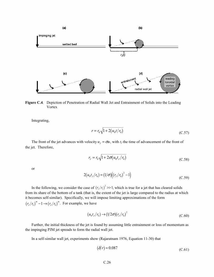
C.26

Figure C.4. Depiction of Penetration of Radial Wall Jet and Entrainment of Solids into the Leading Vortex

Integrating,

r = r0 1+ 2 u0t r0( ) (C.57)

The front of the jet advances with velocity uJ = σu , with tJ the time of advancement of the front of

the jet. Therefore,

rJ = r0 1+ 2σ u0tJ r0( ) (C.58)

or

2 u0tJ r0( ) = 1 σ( ) rJ r0( )2 −1( ) (C.59)

In the following, we consider the case of rJ r0( )2 >> 1, which is true for a jet that has cleared solids from its share of the bottom of a tank (that is, the extent of the jet is large compared to the radius at which it becomes self-similar). Specifically, we will impose limiting approximations of the form

rJ r0( )m −1→ rJ r0( )m . For example, we have

u0tJ r0( ) → 1 2σ( ) rJ r0( )2

(C.60)

Further, the initial thickness of the jet is found by assuming little entrainment or loss of momentum as the impinging PJM jet spreads to form the radial wall jet.

In a self-similar wall jet, experiments show (Rajaratnam 1976, Equation 11-30) that

δ r( ) = 0.087 (C.61)

C.27

Imposing this relation at the beginning of the self-similarity and naming the ratio, γ,

γ ≡ δ0 r0( ) = 0.087 (C.62)

On the other hand, equating the volumetric flow rate (implying no entrainment in the impingement) of the jet exiting the nozzle and the radial wall jet at r0—the radius at which self-similarity is established—and equating the momentum flow rate, we find u0 is equal to the PJM jet velocity (the velocity is the ratio of momentum flow to mass flow, the two quantities we are holding constant). Then equating the mass flows requires equating the flow areas,

2 21

0 0 04 2 2d r rπ π δ π γ= = (C.63)

or

0

8

dr

γ=

(C.64)

where d is the nozzle diameter.

Below, we find the ratio rJ r0( ) is important and results in simplifications if it is large compared to unity. If a tank has diameter D and contains NJ pulse jets, then rJ is the effective radius to be cleared by

each jet roughly 2J Jr D N≈ , and then ( ) ( ) ( )( ) ( )( )0 ~ 2 / 8 2 /J J Jr r D N d N D dγ γ= . For an array of

18 PJMs in HPL-22 (d = 4 in., D = 38 ft), this is ~11, which is great enough to vindicate the simplifications made below on this basis.

C.4.1.6 Volume Entrained into the Lead Vortex

Analysis of Solids Loading in Colliding Vortices

Submerged radial wall jets caused by impinging axisymmetric jets are discussed by Rajaratnam (1976, Chapter 11). The velocity in the jet decreases linearly with radius, relative to the apparent radial origin of similitude for the jet, while the jet thickness increases linearly to maintain (nearly) constant

momentum flow. Consequently, the volumetric flow rate of the jet, V

, increases linearly with radius (relative to the origin of similitude). That is,

0

0

dV rV V

dt r= =

(C.65)

where 0V

, the volumetric flow rate at r0, 0

0 r rV V

== is not a function of r.

C.28

From the discussion of conservation of momentum and mass during impingement, this becomes

21

0 04V d uπ= (C.66)

Combining,

( ) 21

040

/ = r

dV dt d ur

π (C.67)

We can relate the time and spatial derivatives using

00

rdV dr dV dV dVu u

dt dt dr dr r dr = = =

(C.68)

where u is the velocity in the jet, and in a radial wall jet (Rajaratnam 1976, Chapter 11)

u = u0(r0/r) (C.69)

Hence,

2

214

0

dV rd

dr rπ

=

(C.70)

Therefore, the volume in the growing jet, V(r), compared to its apparent volume, V0, at r0 is

( ) ( ) ( )( )

0

3210 0 012 = / = / 1

r

rV r V dV dr dr d r r rπ− −

(C.71)

The velocity of the growth of the jet is some fraction σ of the velocity in the jet at its front edge (Bajpai and Tirumkudulu 2008). The time, t, for the jet to grow to a specified radius is

t =dr

u=

r0

u0

r

r0

d

r

r0

1

r r0( )r0

r

=r0

2u0

r

r0

2

− 1

(C.72)

Thus, at the same time, the radii attained by radial velocities u and σu are related by

r0

ur r0( )2 −1( ) = r0

σurJ r0( )2 −1( )

(C.73)

C.29

For radii large compared to r0, which is typical of the radii cleared by a PJM, this is

r2 =

rJ2

σ (C.74)

where rJ is the radius to the front of a jet and r is the radius that would be attained at the same time if the front of the jet was not converted into a leading vortex by lateral diversion caused by the stagnation pressure at the front face of the jet. Then we have the following expression, which is the volume accumulated in the vortices.

( ) ( ) ( ) ( )

3 23 33 32 20 0 03 3 3 2

1J J J JV r V r r r r r r r

σγπ σ γπσ− − = − = (C.75)

The mass of solids in the vortices, mS, is the sum of the mass entrained into the jet from the surrounding fluid and the mass entrained from the tank floor, mS,settled, over the area covered by the jet to its radius of collision with an adjacent jet. Because the volume of the vortices, Vvortex, originated almost entirely from entrainment of surrounding fluid, we have approximately

,S s E vortex S settledm V mρ φ= + (C.76)

where φE is the solids volume fraction in the entraining fluid and the second term is the mass of solids entrained from the tank floor. Then the solids volume fraction in the vortices at the point of collision is

0 3 232

3 3 2

1S ,settled

E /

s J /

m

rφ φ

σρ γπσ

= +−

(C.77)

We can estimate the mass of the settled mass as the product of the solids density, settling area, solids volume fraction at the location of the tank floor (φ1, which is discussed further below), settling velocity, uS, and settling time. The settling time is the product of the cycle time tC and the complement of the duty cycle, 1-DC. This gives

( )2

1 1 4 1S ,settled s settled s S Cm V D u t DCπρ φ ρ φ= = − (C.78)

Also, the radius of the area cleared by the jet is the radius of the fraction of the tank area cleared by the jet, which gives

2

J

J

Dr

N=

(C.79)

C.30

where NJ is the number of jets. Combining,

( )

3 23 2

0 1 3 2

13 1

1

// S C

E J /

u tN DC

D

σφ φ φγ σ

= + −− (C.80)

The angular momentum, Γ, of a solid cylinder with tangential velocity uA, radius rA, and length w is

31

2 A Awr uΓ π ρ= (C.81)

while the mass, m, is

m = πrA2wρ (C.82)

Combining,

12 A Amr uΓ = (C.83)

Putting the radius equal to that inferred from the volume, rv, and the tangential velocity equal to the difference between the jet velocity and the vortex velocity, we have

( ) ( ) ( )1 1

0 02 21 1V V Jmr u mr r / r uΓ σ σ= − = − (C.84)

C.4.1.7 Ascending Vortices

Conceptual Model of Jet Collision

Figure C.5 depicts the geometric arrangement assumed for the collision and ascension of a pair of leading vortices of radial wall jets. In the figure, “A” is the impingement of the PJM jet on the tank floor, resulting in a radial wall jet with radial similitude established at radius r0. At the front of the jet is a leading vortex (“B”).

Vortices from adjacent jets collide to form a pair of vortices (“C”) that continue upward as the leading pair of vortices of a plane jet formed from the two colliding jets (“D”). The conceptual model is to treat the ascending vortices and the trailing turbulent plane jet as negatively buoyant objects with growing mass and changing density. The negative buoyancy decreases the upward momentum with time while having little effect on the angular momentum. Thus, the vortex pair arrives at some maximum elevation, zJ, before the angular momentum has dissipated, resulting in dispersion of solids at elevation after being entrained from the settled layer on the tank floor.

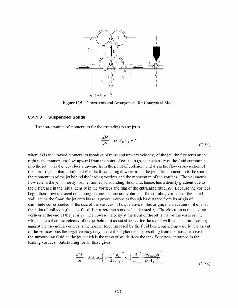
C.31

Figure C.5. Dimensions and Arrangement for Conceptual Model

C.4.1.8 Suspended Solids

The conservation of momentum for the ascending plane jet is

dM

dt= ρEuz0

2 Az0 − F (C.85)

where M is the upward momentum (product of mass and upward velocity) of the jet; the first term on the right is the momentum flow upward from the point of collision (ρE is the density of the fluid entraining into the jet, uz0 is the jet velocity upward from the point of collision, and Az0 is the flow cross-section of the upward jet at that point), and F is the force acting downward on the jet. The momentum is the sum of the momentum of the jet behind the leading vortices and the momentum of the vortices. The volumetric flow rate in the jet is mostly from entrained surrounding fluid, and, hence, has a density gradient due to the difference in the initial density in the vortices and that of the entraining fluid, ρE. Because the vortices begin their upward ascent containing the momentum and volume of the colliding vortices of the radial wall jets on the floor, the jet entrains as it grows upward as though its distance from its origin of similitude corresponded to the size of the vortices. Thus, relative to this origin, the elevation of the jet at the point of collision (the tank floor) is not zero but some value denoted z0. The elevation at the leading vortices at the end of the jet is zJ. The upward velocity at the front of the jet is that of the vortices, uv, which is less than the velocity of the jet behind it as noted above for the radial wall jet. The force acting against the ascending vortices is the normal force imposed by the fluid being pushed upward by the ascent of the vortices plus the negative buoyancy due to the higher density resulting from the mass, relative to the surrounding fluid, in the jet, which is the mass of solids from the tank floor now entrained in the leading vortices. Substituting for all these gives

2

,20 0 2

0 0 0 0

11

2S settledv

E z z Az z E z z

m gudM AA u C

dt u A A uρ

ρ

= − − (C.86)

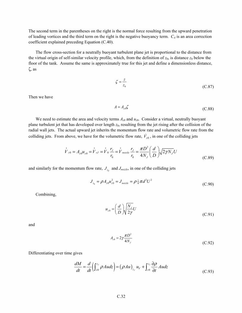
C.32

The second term in the parentheses on the right is the normal force resulting from the upward penetration of leading vortices and the third term on the right is the negative buoyancy term. CA is an area correction coefficient explained preceding Equation (C.40).

The flow cross-section for a neutrally buoyant turbulent plane jet is proportional to the distance from the virtual origin of self-similar velocity profile, which, from the definition of z0, is distance z0 below the floor of the tank. Assume the same is approximately true for this jet and define a dimensionless distance, ζ, as

0

z

zζ =

(C.87)

Then we have

A = Az0ζ (C.88)

We need to estimate the area and velocity terms Az0 and uz0. Consider a virtual, neutrally buoyant plane turbulent jet that has developed over length z0, resulting from the jet rising after the collision of the radial wall jets. The actual upward jet inherits the momentum flow rate and volumetric flow rate from the

colliding jets. From above, we have for the volumetric flow rate, 0zV , in one of the colliding jets

2

0 00 00 0

24

J Jz rJ nozzlez z J

J

r r D dV A u V V V N U

r r N D

π γ = = = = =

(C.89)

and similarly for the momentum flow rate, 0zJ and Jnozzle, in one of the colliding jets

0

2 2 210 0 4z z z nozzleJ A u J d Uρ ρ π= = =

(C.90)

Combining,

0 2

Jz

Ndu U

D γ = (C.91)

and

2

0 24z

J

DA

N

πγ= (C.92)

Differentiating over time gives

( ) ( )

0 0

J J

J

z z

Vzz z

dM dAudz Au u Audz

dt dt t

ρρ ρ ∂= = +∂

(C.93)

C.33

The variation in density in the jet is due to the variation in the solids volume fraction; thus

( )1

∂ ∂= −∂ ∂l st t

ρ φρ (C.94)

From Section C.4.2, we have

( )

( ) ( )

0

20 0

2

S e z

S zS e z e

lnu f D u

t z z

f uln lnu f D u u D

z z z z z

φ φφ φ

φφ φ φφ φ

∂ ∂ ∂ = + − ∂ ∂ ∂ ∂ ∂∂ ∂ ∂ = + − + + − ∂ ∂ ∂ ∂ ∂ (C.95)

where 0u is the weighted unhindered settling velocity volume fraction, De is an effective hydrodynamic dispersion coefficient and uz is the motion (velocity) of the fluid phase in which the particles are embedded. Also, we make the simplifying assumption that the settling velocity (which actually varies due to the effect of total solids volume fraction on hindered settling – see Section C.4.2) is a single, constant value, uS, implying the hindered settling is constant and therefore can be subsumed into uS for the purpose of this development. To simplify further, assume that, χ, the gradient of the logarithm of solids volume fraction, φ, is constant over elevation. That is,

∂lnφ∂ z z0( ) = χ

∂2 lnφ∂ z z0( )2 = 0

(C.96)

Substituting, we have

( )

2

0 0 0

1

/e z

S z

D uu u

t z z z z

φ φ χ χ χ ∂∂ = + − − ∂ ∂ (C.97)

Substituting,

( ) ( )( ) ( ) ( )

( ) ( )

20 2

0 01 10

0 01

1

21

J J

J

J

J

z z

z V z zzl J z V lz

S e z z

A uA u u d A u ddM

A u u sdt

u D / z A u d

ζ ζ

ζ

ζ φ φζ ζ φχ ζ ζζρ ζ ρ

χ χ φ ζ ζ

∂ − −

∂ = + −

+ +

(C.98)

where ζJ = zJ/z0. As the jet attains its maximum elevation, both uz and uV (the velocity of the leading vortices, which is the velocity of the front of the jet) vanish (there is no upward component of velocity). This is consistent with approximating the ratio of these velocities as a constant as for an axisymmetric or radial wall jet (see Sections C.4.1.3 and C.4.1.4). That is, we put

V zu uσ=

(C.99)

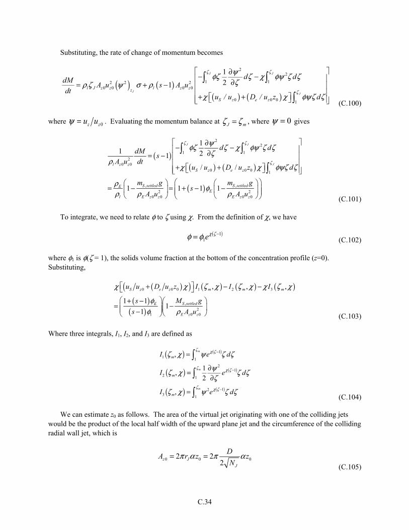
C.34

Substituting, the rate of change of momentum becomes

( ) ( )( ) ( )

22

1 12 2 20 0 0 0

0 0 0 1

1

21

J J

JJ

l J z z l z zz

S z e z

d ddMA u s A u

dtu / u D / u z d

ζ ζ

ζ

ψφζ ζ χ φψ ζ ζζρ ζ ψ σ ρ

χ χ φψζ ζ

∂− − ∂= + − + +

(C.100)

where ψ = uz uz0 . Evaluating the momentum balance at ζ J = ζ m , where ψ = 0 gives

( )( ) ( )

( )

22

1 1

20 0

0 0 0 1

, ,

2 20 0 0 0

11 21

/ /

1 1 1 1

J J

Jl z zS z e z

S settled S settledEE

l E z z E z z

d ddMs

A u dtu u D u z d

m g m gs

A u A u

ζ ζ

ζ

ψφζ ζ χ φψ ζ ζζ

ρχ χ φψζ ζ

ρ φρ ρ ρ

∂− − ∂= − + +

= − = + − −

(C.101)

To integrate, we need to relate φ to ζ using χ. From the definition of χ, we have

φ = φ1eχ ζ −1( )

(C.102)

where φ1 is φ(ζ = 1), the solids volume fraction at the bottom of the concentration profile (z=0). Substituting,

( )( ) ( ) ( ) ( )( )

( )

0 0 0 1 2 3

,

21 0 0

, , ,

1 11

1

S z e z m m m

S settledE

E z z

u u D u z I I I

M gs

s A u

χ χ ζ χ ζ χ χ ζ χ

φφ ρ

+ − − + −

= − − (C.103)

Where three integrals, I1, I2, and I3 are defined as

I1 ζm, χ( ) = ψ eχ ζ −1( )ζ dζ1

ζm

I2 ζm, χ( ) = 1

2

∂ψ 2

∂ζeχ ζ −1( )ζ dζ

1

ζm

I3 ζm, χ( ) = ψ 2eχ ζ −1( )ζ dζ1

ζm

(C.104)

We can estimate z0 as follows. The area of the virtual jet originating with one of the colliding jets would be the product of the local half width of the upward plane jet and the circumference of the colliding radial wall jet, which is

0 0 02 2

2z J

J

DA r z z

Nπ α π α= =

(C.105)

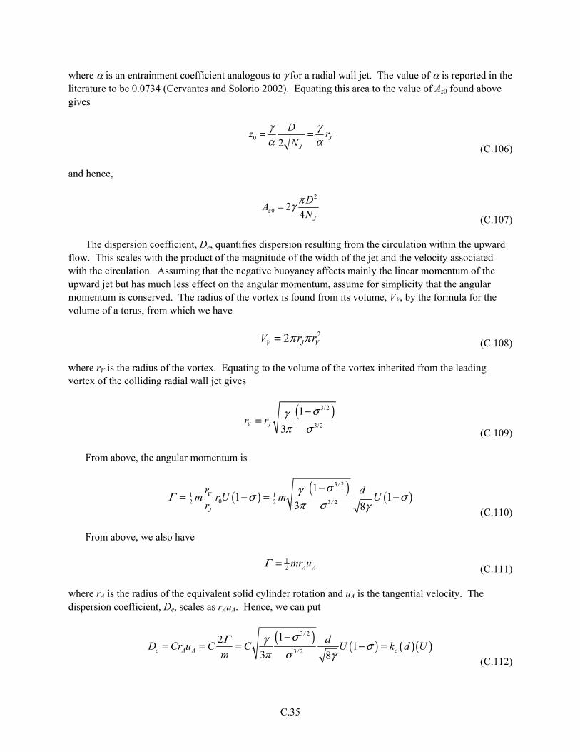
C.35

where α is an entrainment coefficient analogous to γ for a radial wall jet. The value of α is reported in the literature to be 0.0734 (Cervantes and Solorio 2002). Equating this area to the value of Az0 found above gives

0

2J

J

Dz r

N

γ γα α

= = (C.106)

and hence,

2

0 24z

J

DA

N

πγ= (C.107)

The dispersion coefficient, De, quantifies dispersion resulting from the circulation within the upward flow. This scales with the product of the magnitude of the width of the jet and the velocity associated with the circulation. Assuming that the negative buoyancy affects mainly the linear momentum of the upward jet but has much less effect on the angular momentum, assume for simplicity that the angular momentum is conserved. The radius of the vortex is found from its volume, VV, by the formula for the volume of a torus, from which we have

VV = 2πrJπrV2

(C.108)

where rV is the radius of the vortex. Equating to the volume of the vortex inherited from the leading vortex of the colliding radial wall jet gives

( )3/2

3/2

1

3V Jr rσγ

π σ−

= (C.109)

From above, the angular momentum is

( ) ( ) ( )

3 2

1 102 2 3 2

11 1

3 8

/

V/

J

r dm r U m U

r

σγΓ σ σπ σ γ

−= − = −

(C.110)

From above, we also have

12 A Amr uΓ = (C.111)

where rA is the radius of the equivalent solid cylinder rotation and uA is the tangential velocity. The dispersion coefficient, De, scales as rAuA. Hence, we can put

( ) ( ) ( )( )3 2

3 2

121

3 8

/

e A A e/

dD Cr u C C U k d U

m

σΓ γ σπ σ γ

−= = = − =

(C.112)

C.36

where ke is the dimensionless dispersion coefficient

ke = C

1− σ( )2

24π1− σ 3 2

σ 3 2 (C.113)

and C is a constant to be determined. Therefore, ke is to be determined, i.e., by fitting data. Substituting for Az0, z0, and De in the momentum balance gives

( ) ( ) ( )

( )( )

1 2 3

,2

21

2 8, , ,

1 11

14

Se m m m

J

S settledE

E

u Dk I I I

U d N

m gs

dsU

γχ α χ χ ζ χ ζ χ χ ζγ

φπφ ρ

+ − − + −

= − − (C.114)

The total mass of solids, mS,tot, in the tank associated with tank floor area A attributed to a single PJM is1

0 0

3 3

S ,tot s S l SJ J

D Dm s

4N 4N

π πρ φ ρ φ= = (C.115)

where φS0 is the nominal solids volume fraction corresponding to all of the solids suspended and distributed uniformly. The solids suspended at the start of a pulse are represented herein as though they were uniformly distributed with density ρE, signifying the density of the fluid that entrains into the plane jet. Given this approximation, the mass of suspended solids per PJM, mS,sus, is

3

, 4S sus l EJ

Dm s

N

πρ φ= (C.116)

Then the mass of settled solids, the difference between the total and suspended solids, can also be estimated as the product of the settling area, velocity, solids density, and time. The density of suspended solids at the location of the tank floor is

( ) ( ) ( )( ) ( )( )10 1 1 0 1 1l lz s z sρ ρ φ ρ φ= = + − = = + − (C.117)

1 The solids volume fraction is defined here to be consistent with the M3 project and report WTP-RPT-182 (Meyer

et al. 2009, 2012); that is, φS = VS

14 π D3

.

C.37

Then we have, per PJM,

3

, 14S settled c lJ

Dm s

N

π θ ρ φ= (C.118)

where θc is the ratio of characteristic settling distance to characteristic length scale

( )1S C

c

u tDC

Dθ = −

(C.119)

Combining,

0 1S E cs s sφ φ θ φ= + (C.120)

Also, at the end of a PJM pulse, when the upward flow from colliding jets has attained its maximum elevation, we have assumed all of the solids are suspended. Then the concentration gradient described by χ corresponds to the total solids in the tank attributed to a PJM. This is found by integrating the concentration gradient over the volume associated with the PJM. Then the suspended solid mass is

( )( )

0

3 2

0

13 310

1 11

4 4

1 1

4 4 2

m

mm

z

S tot l S S sus lzJ J

l lJ J J

D Dm s m s dz

N N

zD D es e d s

N D N N

χ ζζ χ ζ

π πρ φ ρ φ

π π γρ φ ζ ρ φα χ

−−

= = =

−= =

, ,

(C.121)

Therefore,

( )1 01

2

1m

JS

N

eχ ζ

αχφ φγ−

=− (C.122)

Substituting,

( )

3

, 01

2

4 1m

JS settled l c S

J

NDm s

N eχ ζ

απ χρ θ φγ−=

− (C.123)

Then also

( )

3 3

, 01

2

4 4 1m

JS settled l E l c S

J J

ND Dm s s

N N eχ ζ

απ π χρ φ ρ θ φγ−= =

− (C.124)

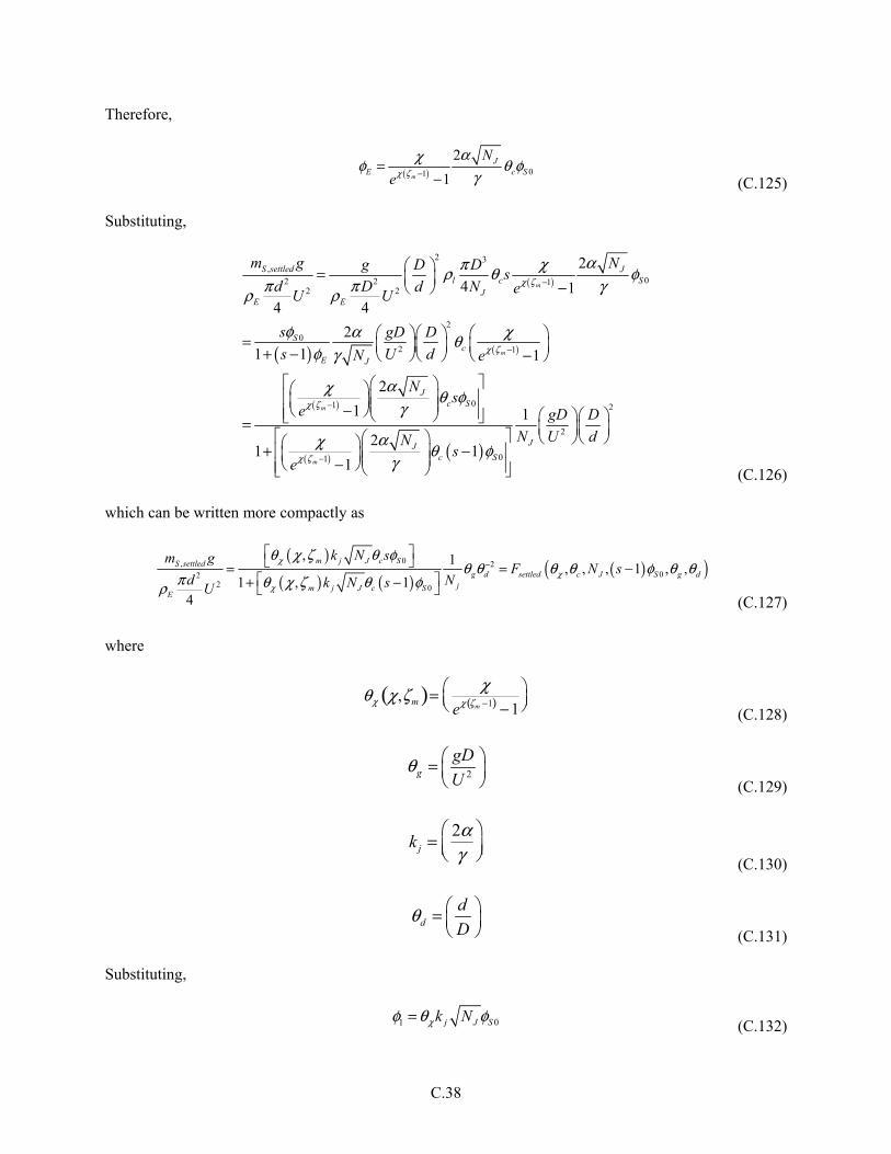
C.38

Therefore,

( ) 01

2

1m

JE c S

N

eχ ζ

αχφ θ φγ−

=− (C.125)

Substituting,

( )

( ) ( )

( )

( ) ( )

2 3,

02 2 12 2

2

02 1

01

01

2

4 14 4

2

1 1 1

2

1

21 1

1

m

m

m

m

S settled Jl c S

JE E

Sc

E J

Jc S

Jc S

m g Ng D Ds

d D d N eU U

s gD D

s U dN e

Ns

e

Ns

e

χ ζ

χ ζ

χ ζ

χ ζ

απ χρ θ φπ π γρ ρ

φ α χθφ γ

αχ θ φγ

αχ θ φγ

−

−

−

−

= −

= + − −

− = + − −

2

2

1

J

gD D

N U d

(C.126)

which can be written more compactly as

( )( ) ( )

( )( )0,02

2 0

, 1, , , 1 , ,

1 , 14

m j J c SS settledg d settled c J S g d

jm j J c SE

k N sm gF N s

d Nk N sU

χχ

χ

θ χ ζ θ φθ θ θ θ φ θ θ

π θ χ ζ θ φρ

−2 = = − + −

(C.127)

where

θχ χ,ζm( )= χ

eχ ζm −1( ) − 1

(C.128)

2g

gD

Uθ =

(C.129)

kj = 2α

γ

(C.130)

d

d

Dθ =

(C.131)

Substituting,

1 0j J Sk Nχφ θ φ= (C.132)

C.39

0E j J c Sk Nχφ θ θ φ= (C.133)

The momentum balance becomes

( )( ) ( ) ( ) ( )

( ) ( ) ( )( )

( )( )( )

10 1

02 3 0

0

, , , 1 , , , , 2 / ,

1 1, , 1 , , , 1 , , 0

1

u c J S g d m J u d j J e m

j J c Sm m settled c J S g d

j J S

H N s N k N k I

k N sI I F N s

k N s

χχ

χ

θ θ φ θ θ χ ζ χ γ θ θ χ χ ζ

θ θ φχ ζ χ χ ζ θ θ φ θ θ

θ φ

− − = + + − − − − − − = − (C.134)

where

Su

u

Uθ =

(C.135)

That is, we have the form

H xi , χ,ζm( )= 0 (C.136)

where the xi represent the various arguments of the momentum balance function H.

The arguments of H include a set of dimensionless groups that can be deduced from dimensional analysis alone. However, if the integrals I1, I2, and I3 can be calculated, which would require postulating functional forms for the velocity function ψ(ζ), then H can be evaluated for values of the dimensional groups and the concentration profile shape parameter χ and the dimensionless mixing height ζm. The differential of H can be written in logarithmic form as

, ,

ln ln 0ln ln

i m

m jjm jx

H HdH d d x

xχ χ ζ

ζζ

∂ ∂= + = ∂ ∂

(C.137)

Differentiating with respect to a particular dimensionless group xi gives

, , ,

ln ln0

ln ln ln lni m m

m J

jm i J ix

xH H

x x xχ χ χ ζ χ ζ

ζζ

∂ ∂∂ ∂+ = ∂ ∂ ∂ ∂

(C.138)

The last derivative is just the Kronecker delta function, which after summation gives

, ,

ln0

ln ln lni m

m

m i ix

H H

x xχ χ χ ζ

ζζ

∂∂ ∂+ = ∂ ∂ ∂ (C.139)

C.40

Therefore, we find

,

,

lnln

ln

ln

m

i

im

i

m x

Hx

x H

χ ζ

χ

χ

ζ

ζ

∂ ∂ ∂ = − ∂ ∂ ∂ (C.140)

Thus, noting again that some form of ψ(ζ) would have to be postulated to evaluate I1, I2, and I3, we could calculate the “scale factors” for the variation of the dimensionless mixing height with the dimensionless groups. The “cloud height” measured as part of M3 Phase 1 testing provides a useful set of data to which the above model, notwithstanding its many shortcomings at this point, could be applied to gain further insight. Given that the entire development of Section C.4 serves only as an example of “developing a physically based correlation,” we have not attempted this at this point. However, that data can be fit with a simple power-law form over the dimensionless groups to consider the reasonableness of the fitted exponents. That is, we can fit the form

( )( )0 0 01

2gd u c N

aaa a a am m d u c g S J

J

Dz z C s N

N

φγζ θ θ θ θ φα

= = − (C.141)

where, in principle, the leading coefficient C0 and all of the exponents “a” are functions of χ. Data exist for the M3 tests from which values of χ might be estimated, but at this point we have not attempted this.

An attempt to fit the physically based power-law form to the M3 data is described in the next section.

C.4.1.9 Preliminary Comparison to Data

The compilation of “cloud height” data of the M3 project reported in WTP-RPT-182 (Meyer et al. 2009) is analogous to the “maximum jet elevation” analyzed above. Hence, it is instructive to attempt a fit as developed above to this data. If we impose on the data the functional form given above, we find

( )( ) 0.43 0.021.00 0.09 0.22 0.03 0.38 0.02 0.09 0.02 0.31 0.15

01.8 1m d u g c S Js Nζ θ θ θ θ φ − ±+ ± − ± − ± − ± + ±= − (C.142)

for which R2 = 50 percent. The error terms are the standard errors of estimate of the exponents.

The exponent on ( )=d d Dθ is very close to unity, which suggests that z0 (notwithstanding the

conceptual model used herein) might be as well put in terms of d as D, but so far a physical basis for this has not been developed.

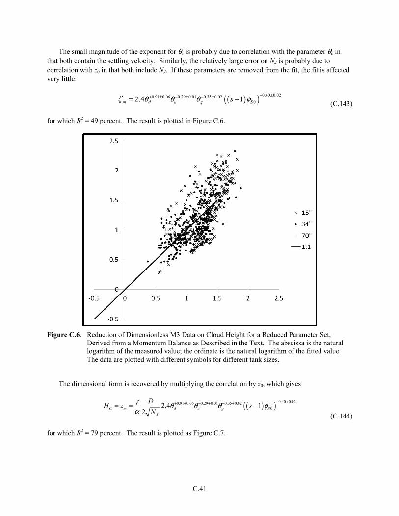
C.41

The small magnitude of the exponent for θc is probably due to correlation with the parameter θc in that both contain the settling velocity. Similarly, the relatively large error on NJ is probably due to correlation with z0 in that both include NJ. If these parameters are removed from the fit, the fit is affected very little:

( )( ) 0.40 0.020.91 0.06 0.29 0.01 0.35 0.0202.4 1m d u g Ssζ θ θ θ φ − ±+ ± − ± − ±= −

(C.143)

for which R2 = 49 percent. The result is plotted in Figure C.6.

Figure C.6. Reduction of Dimensionless M3 Data on Cloud Height for a Reduced Parameter Set, Derived from a Momentum Balance as Described in the Text. The abscissa is the natural logarithm of the measured value; the ordinate is the natural logarithm of the fitted value. The data are plotted with different symbols for different tank sizes.

The dimensional form is recovered by multiplying the correlation by z0, which gives

( )( ) 0.40 0.020.91 0.06 0.29 0.01 0.35 0.0202.4 1

2C m d u g S

J

DH z s

N

γ θ θ θ φα

− ++ + − + − += = − (C.144)

for which R2 = 79 percent. The result is plotted as Figure C.7.

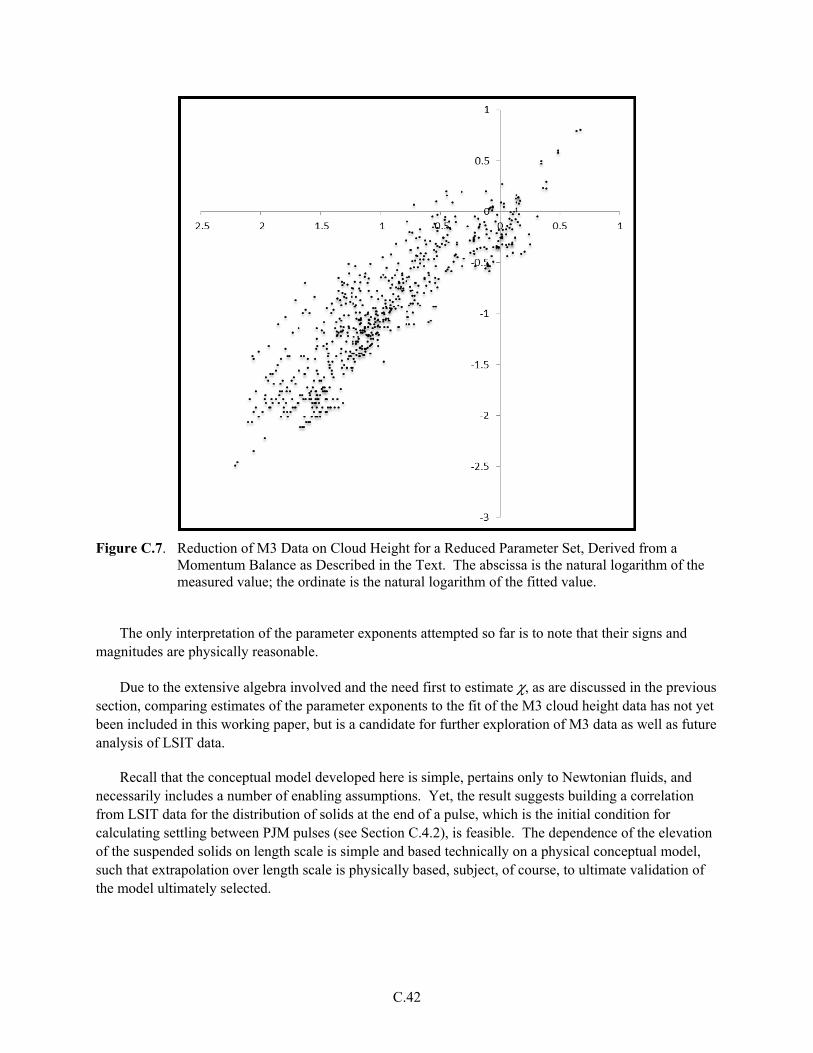
C.42

Figure C.7. Reduction of M3 Data on Cloud Height for a Reduced Parameter Set, Derived from a Momentum Balance as Described in the Text. The abscissa is the natural logarithm of the measured value; the ordinate is the natural logarithm of the fitted value.

The only interpretation of the parameter exponents attempted so far is to note that their signs and

magnitudes are physically reasonable.

Due to the extensive algebra involved and the need first to estimate χ, as are discussed in the previous section, comparing estimates of the parameter exponents to the fit of the M3 cloud height data has not yet been included in this working paper, but is a candidate for further exploration of M3 data as well as future analysis of LSIT data.

Recall that the conceptual model developed here is simple, pertains only to Newtonian fluids, and necessarily includes a number of enabling assumptions. Yet, the result suggests building a correlation from LSIT data for the distribution of solids at the end of a pulse, which is the initial condition for calculating settling between PJM pulses (see Section C.4.2), is feasible. The dependence of the elevation of the suspended solids on length scale is simple and based technically on a physical conceptual model, such that extrapolation over length scale is physically based, subject, of course, to ultimate validation of the model ultimately selected.

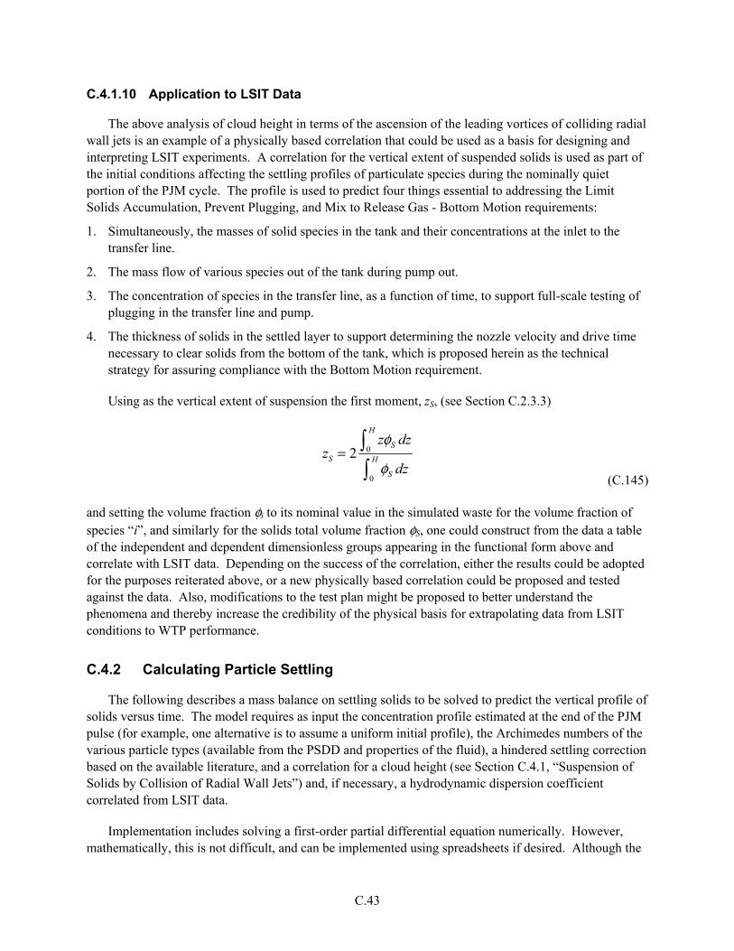
C.43

C.4.1.10 Application to LSIT Data

The above analysis of cloud height in terms of the ascension of the leading vortices of colliding radial wall jets is an example of a physically based correlation that could be used as a basis for designing and interpreting LSIT experiments. A correlation for the vertical extent of suspended solids is used as part of the initial conditions affecting the settling profiles of particulate species during the nominally quiet portion of the PJM cycle. The profile is used to predict four things essential to addressing the Limit Solids Accumulation, Prevent Plugging, and Mix to Release Gas - Bottom Motion requirements:

1. Simultaneously, the masses of solid species in the tank and their concentrations at the inlet to the transfer line.

2. The mass flow of various species out of the tank during pump out.

3. The concentration of species in the transfer line, as a function of time, to support full-scale testing of plugging in the transfer line and pump.

4. The thickness of solids in the settled layer to support determining the nozzle velocity and drive time necessary to clear solids from the bottom of the tank, which is proposed herein as the technical strategy for assuring compliance with the Bottom Motion requirement.

Using as the vertical extent of suspension the first moment, zS, (see Section C.2.3.3)

zS = 2zφS dz

0

H

φS dz

0

H

(C.145)

and setting the volume fraction φi to its nominal value in the simulated waste for the volume fraction of species “i”, and similarly for the solids total volume fraction φS, one could construct from the data a table of the independent and dependent dimensionless groups appearing in the functional form above and correlate with LSIT data. Depending on the success of the correlation, either the results could be adopted for the purposes reiterated above, or a new physically based correlation could be proposed and tested against the data. Also, modifications to the test plan might be proposed to better understand the phenomena and thereby increase the credibility of the physical basis for extrapolating data from LSIT conditions to WTP performance.

C.4.2 Calculating Particle Settling

The following describes a mass balance on settling solids to be solved to predict the vertical profile of solids versus time. The model requires as input the concentration profile estimated at the end of the PJM pulse (for example, one alternative is to assume a uniform initial profile), the Archimedes numbers of the various particle types (available from the PSDD and properties of the fluid), a hindered settling correction based on the available literature, and a correlation for a cloud height (see Section C.4.1, “Suspension of Solids by Collision of Radial Wall Jets”) and, if necessary, a hydrodynamic dispersion coefficient correlated from LSIT data.

Implementation includes solving a first-order partial differential equation numerically. However, mathematically, this is not difficult, and can be implemented using spreadsheets if desired. Although the

C.44

model itself is complicated, it is essentially a textbook model, neither ambiguous nor speculative, the input parameters are few and available, and it provides exactly the information needed to implement a mass balance over the PJM cycle required to implement a mass balance over a pump-out cycle.

C.4.2.1 Purpose

Whatever the means employed to solve the settling mass balance, the purpose and the result is to find, from the initial profile, the volume fraction profile for species “i” during the course of settling, where the resulting profile can be applied, if necessary, as part of correlating the cloud height from the next pulse. This is required to determine the mass flow rate of the various species into the transfer line, which in turn is required to support evaluation against mixing requirements.

1. Predicting the concentration at the inlet to the transfer line suction nozzle is required for full-scale testing for plugging in the transfer line and pump.

2. Predicting the mass flows at the inlet to the transfer line suction nozzle is required to support a mass balance over the tank for repeated pump-out cycles as PJM mixing continues.

3. The result of calculating the settling profiles, combined with calculating the capture of settling solids by the suction nozzle, is to predict the thickness of settled solids at the start of a PJM pulse and thence calculate the initial profile for settling after that pulse.

The results of calculating the vertical solids concentration profile are used in several ways within the overall mass balance model.

1. The mass concentration predicted at the inlet to the transfer line suction nozzle is used to predict the concentrations and mass flow rates entering the transfer line, which

a. Provides the information needed to implement a mass balance over a pump-out cycle.

b. Provides the information needed to design and operate separate scaled tests of potential plugging in the transfer line and pump.

2. The mass concentration profile predicted at the end of settling provides the vertical density profile to be used as part of correlating the cloud height or similar attributes used as an initial condition for the next settling cycle.

3. The settling calculation predicts the thickness of settled solids at the start of the next PJM pulse, which is required to assure that bottom clearing (the proposed technical strategy for assuring bottom motion) occurs within the drive time of the PJM cycle.

See Section C.4.2.8, “Application to Overall Mass Balances,” below.

C.45

C.4.2.2 Settling of Individual Species

Waste solids are characterized by discrete PSDD. A number of categories are defined, each for a particular mean size and density of the particles in the category. For a particle settling in a liquid at the limit of vanishing solids volume fraction, we find from a force balance1 that

( )23

2= p D pAr Re f Re (C.146)

where fD is the drag coefficient for the particle, and

( ) 3

2

−= s l S

l

gdAr

ρ ρρν (C.147)

Ar is the Archimedes number for the particle, and Rep is the particle Reynolds number,

p Sp

u dRe

ν=

(C.148)

where up is the settling velocity of the particle and dS is its diameter. Inverting, we have

( )p p

S

vu f Ar

d=

(C.149)

That is, we know the unhindered settling velocity of the solids from their PSDD, the liquid attributes, and a known function fp of the particle Archimedes number.

The actual settling velocity, ui, of species “i” is diminished by the effects of other particles. This is usually modeled as a correction of the form

ui = ui0 f φS,φi( ) (C.150)

where 0iu is the settling velocity at infinite dilution and Sφ and iφ are the volume fractions of all solids

and of solid “i”. The function has also been formulated as and is often used in the form of

ui = ui0 f φS( ) (C.151)

1 The buoyant force is ( )( )3 6 −S s ld gπ ρ ρ and the drag force is ( ) ( )2 24S T D pd U f Reπ ρ where fD is the drag coefficient

correlation and ( )p T SRe U d ν= . Putting ( )=T S pU d Reν and equating the two forces for a particle at its terminal

velocity gives ( )( ) ( ) ( ) ( )23 2 26 4− =S s l S S p D pd g d d Re C Reπ ρ ρ π ρ ν , where CD is the drag coefficient. Simplifying and

rearranging, we have ( )( ) ( ) ( )3 2 23 2− = =s l S p D pgd Ar Re f Reρ ρ ρ ν .

C.46

where the hindered correction is the same for all particles. See Section C.4.2.9, “Hindered Settling,” below, for further discussion about settling models.

C.4.2.3 Differential Mass Balance

Denoting the mass concentration of particles, i, as ρi and the mass flux of particles i (positive when up, due to definition of upward coordinate z) as ni, the one-dimensional differential mass balance is

∂ρi

∂t= −

∂ni

∂z (C.152)

where the mass flux is

ni = ρi uz − ui( ) (C.153)

where uz is the motion of the fluid phase in which the particles are embedded. The motion of the liquid after a PJM pulse appears from M3 data to be coherent due to wave-like phenomena associated with macroscopic density profiles. Hence, we assume that, after a PJM pulse ends, hydrodynamic dispersion is not important and that the effect of coherent motion averages over time so we can approximate

uz dtsettling

time

≈ 0

(C.154)

As noted above, the settling velocity, ui, can be written

ui = ui0 f φS( ) (C.155)

where we are assuming f is independent of i; this assumption would need to be vindicated from test data. The total solids volume fraction is

φS = φi

i

(C.156)

where the volume fraction of “i” is

φi =

ρi

′ρi (C.157)

and

′ρi =mparticle

Vparticle (C.158)

C.47

'iρ is the density of the particle. Substituting,

∂φi

∂t=

∂∂z

φiui0 f φS( )( )

(C.159)

This simple first-order, partial differential equation is easily made discrete (with respect to both location and particle attribute) and integrated over time to compute the change of the concentration profiles between PJM pulses as well as the volume of solids that settle between pulses where the total solids volume fraction is recomputed as the integration proceeds. This information is needed to address several aspects of the mixing requirements:

1. The thickness of solids that settle between PJM pulses determines the solids loading in the leading vortices of the radial wall jets on the tank floor that entrain and transport solids to or past the suction nozzle at the start of each pulse. This information is needed both for mass balances over the solids exiting through the transport line, and to specify concentration conditions to be recreated during separate plugging tests to make them representative of conditions in the WTP.

2. The thickness of settled solids affects the conditions required to clear solids from the tank bottom.

3. The thickness of settled solids affects the vertical extent of the concentration profile, which ultimately affects the thickness of settled solids—that is, it is both a cause and an effect of the combined PJM mixing cycle.

C.4.2.4 Behavior of Total Solids Volume Fraction

The behavior of the total solids loading is important because it is much easier to measure than for individual species and because hindered settling tends to correlate with the total loading. To obtain this, sum over “i” to get1

∂φS

∂t=

∂∂z

φSu0 f φS( )( )

(C.160)

where

u 0 = φi φS( )ui

0

i

(C.161)

is a weighted average of the settling velocities (see Section 2.2.1.5). Because the range over particle sizes and densities of unhindered particle velocities can be orders of magnitude, this average will tend to be weighted heavily toward the fast-settling particles.

1 If the fluid motion and hydrodynamic dispersion, DS, cannot be neglected, as during the PJM pulse, then the

corresponding result is ( )0 lnS SS S S zu f D u

t z z

φ φφ φ∂ ∂ ∂ = + − ∂ ∂ ∂ .

C.48

Expanding the mass balance gives

( ) ( ) ( )0

0 0 SS SS S S S

fuu f f u

t z z z

φφ φ φ φ φ φ∂∂ ∂ ∂= + +

∂ ∂ ∂ ∂ (C.162)

Dividing by φS and rearranging gives

( ) ( ) 0

0 lnln ln ln1

ln lnSS S

SS S

d f uu f

t z d

φφ φ φφ φ

∂ ∂ ∂= + + ∂ ∂ ∂ (C.163)

From differential calculus,

( ) ( )1 00 lnln ln ln

1ln ln

S

SS SS

z t S S

d fz uu f

t t z dφ

φφ φ φφ φ

− ∂ ∂∂ ∂ − = = + + ∂ ∂ ∂ ∂ (C.164)

Define

g φS( )= f φS( ) 1+

d ln f φS( )d lnφS

(C.165)

The rate of descent of the concentration (solids volume fraction) profile depends locally on the solids volume fraction. Define this local velocity as

S

S

zu

t φ

∂ = − ∂ (C.166)

Combining,

( ) ( )

00 ln

lnS S SS

uu u g fφ φ

φ ∂= + ∂ (C.167)

C.4.2.5 Expected Behavior of Concentration Profiles

The derivative on the right-hand side of the above expression is the ratio of the gradients of u 0 and φS. The gradients are not the same but are closely related. Hence, approximate this derivative as being a function of φS. Then uS depends only on φS. This means that the shape of the concentration profile determines how its shape changes with time.

The function f decreases with increasing φS. Therefore, in the absence of significant dispersion in regions of higher φS, the profile will drop more slowly, and in regions of lower φS, the profile will drop faster. Consequently, where the profile is vertical (no gradient), it will tend to stay vertical. Where the concentration increases with elevation, it will tend to flatten, becoming more vertical. Where the concentration decreases with elevation, the gradient will tend to become steeper. This expectation needs

C.49

to be checked systematically against M3 concentration profile data, in part to evaluate further if dispersion was not important, or in which cases it was least important, as well as to check the assumptions made above. If the analysis is qualitatively correct, one consequence of settling behavior would be to maintain the sharpness of an initially sharp “cloud-height-like” discontinuity in the concentration gradient.

C.4.2.6 Analysis and Use of Measured Concentration Profiles

From the above, predicted concentration profiles will depend on the initial profile (i.e., at the end of a PJM pulse), the unhindered settling velocities of the particles (available from the known particle attributes), a hindered settling correction, and, if necessary, a hydrodynamic dispersion term. The results of the settling calculation must be compared to LSIT data, which will need to include:

1. The solids volume fraction versus elevation and time during settling, but especially the vertical profile at the end of a PJM pulse and at the start of the next.

2. The concentration and mass flows of particulate species versus time in the transfer line, either during pump-out tests or as a sample at other times.

3. The thickness of settled solids versus time over an entire PJM cycle.

The settling calculation will provide both the concentration profile of total solids to compare with (1), and the concentration of the particulate species at the elevation of the suction nozzle, which, when combined with a calculation of the capture of particulates by the nozzle, provides the concentrations and mass flows in the transfer line, to compare with (2), and the volume of total solids volume settled versus time, to compare with (3).

As is developed below, of particular interest to the mass balance over a pump-out cycle is the difference between the concentration of particulate species averaged over the tank and the concentration at the level of the suction nozzle (notwithstanding the additional calculations needed to calculate the competition between suction and settling in capturing the various particle types). To this end, certain simple reductions of measured concentration profiles can be done and used to facilitate mass balance calculations as well as validate the settling calculations.

C.4.2.7 Reduction of Concentration Profiles to Time-Dependent Parameters

An important measurement to make during LSIT is the total solids volume fraction versus elevation and time in a tank, e.g., using acoustic probes already tested during M3 Phase 1 (Meyer et al. 2009, Appendix A). Then for each PJM cycle, or average of several cycles, we have data of the form

φS z, t( ) + ε, where ε is the combined measurement error. When plotted, the data will be scattered, as is

evident in the results of M3 Phase 1 testing. To answer questions such as “What is the total solids volume suspended?”, “What is the “cloud height”?”, or “What is the concentration near the nozzle”, it is useful to define an average concentration, apparent height, and apparent concentration at the bottom of the profile. These can be estimated from simple, unambiguous integrals and regressions of the concentration data. Define the integrals

I0 t( )= φS z,t( )dz

0

H

(C.168)

C.50

( ) ( )1 0

,H

SI t z t zdzφ= (C.169)

where I0 is the zeroth moment of the vertical distribution of solids loading which is the total volume of solids per horizontal area, I1 is the first moment of the vertical distribution of solids loading, H is the liquid height in the tank, and the extrapolation

( ) ( )0

0

lim ,→

=S Sz

t z tφ φ (C.170)

The last of these is done by fitting some suitable, simple function to the data by regression and evaluating at the limit.

C.4.2.8 Application to Overall Mass Balance

The mass balance over some species “i” during a PJM cycle is

dmi

dt= −Qρi zP( )

(C.171)

where mi is the mass of the species in the tank, Q is the volumetric flow rate into the transfer line, ρ iP is

the mass concentration of “i” entering the transfer line, and zP is the elevation of the transfer line. The

mass concentration ρ iP is sampled in the transfer line. The ability to meet criteria for sampling and for

limiting solids accumulation depends on relating mi to ρiP, which, unfortunately, is quite complicated.

The concentration ρiP is closely related to the concentration of “i” in the slurry at the elevation of the

suction nozzle.

Obtaining representative data on the difference between these through LSIT testing is discussed in Section 5.6 “Capture of Settled and Settling Solids by the Suction Nozzle.” The strategy is to describe the concentration profile in a tank as a function of time. This would enable relating the concentration at the nozzle to the average concentration in the slurry. If solids are cleared from the tank floor during each PJM cycle, as is proposed herein as a strategy for meeting the “mix to release gas” requirement, then the average concentration in the slurry, before solids settle after a pulse, is the mass of the species in the tank divided by the slurry volume. Then we can write the mass balance as

( ) ( )i i

i i i p

dm ddV Q V Q z

dt dt dt

ρρ ρ ρ= = − + = − (C.172)

where V is the slurry volume in the tank and iρ is the mass concentration of “i” averaged over the slurry

in the tank.

C.51

If the concentration data are reduced as suggested above, we have sρ the average solids concentration

in the tank

( ) ( )= =

H

s s 00

1 1z,t dz I t

H Hρ ρ

(C.173)

where H is the current height of the liquid; the calculation is based on mass concentration instead of volume fraction. Then we have

( )i

i i p

dQ V Q z

dt

ρρ ρ− + = − (C.174)

which is determined by extrapolating the logarithm of the measured profile to z = 0, as noted above. Thus, reducing the data as described above provides the variables in fact needed to evaluate the mass balance over a PJM cycle.

If at the end of each pump-out cycle, the tank is refilled with slurry at a volumetric flow rate averaged

over the pump-out cycles of Q0 with solids mass concentration ρi0 , then we can express the effective

mass added per PJM cycle in terms of a time-averaged rate to get

V

dρi

dt= −Q ρi

P − ρi( )+ Q0ρi0

(C.175)

where Q0 is the time-averaged rate of addition of volume. The difference ρiP − ρi varies with iρ as

determined by the settling model described above. Repeating this integration over successive fill-pump-down cycles determines the accumulation of solids in a tank, which is the metric for evaluating performance relative to the Limit Solids Accumulation requirement.

Thus, LSIT results over repeated PJM cycles are used to confirm—or, if necessary, revise—the settling model—which then is used to predict the mass versus time of the various particulate species in WTP, which quantifies accumulation in the WTP.

That is, we implement the settling model repeatedly to solve the mass balance over the pump-out cycles to predict the mass of species “i” in the tank over time to address the no solids accumulation mixing requirement.

C.4.2.9 Hindered Settling

The settling velocity decreases as the solids concentration increases, due to the hydrodynamic interaction of particle wakes on other particles. The simplest expression for the hindered settling velocity, Vs,k for a single particle type, k, was developed by Richardson and Zaki (1954)

( )= − n

s ,k T ,kV V 1 φ (C.176)

C.52

where φ is the solids volume fraction, n equals 4.65 for Stokes settling, and VT,k is the terminal velocity for a single particle, k. Other versions of this expression include a maximum solids volume fraction

= −

n

s ,k T ,kS ,max

V V 1φ

φ (C.177)

The N particle species are ordered in increasing terminal velocity with specie 1 being the slowest and specie N being the fastest. Assume that the highest cloud height is associated with the lowest terminal velocity, HC,1. Therefore, the region between HC,1 and HC,2 contains only particle specie 1 while the region between HC,N and the bottom of the tank contains all particle species. The thickness and composition of the sediment layer is determined by the polydisperse settling occurring in the bottom cloud height region during the pulse tube refill portion of the duty cycle.

Several models have been developed to predict the settling of polydisperse particle systems:

• The simplest model proposed by Richardson and Shabi (1960) is an extension of the single-particle hindered expression

( ), , 1

n

s k T kV V φ= − (C.178)

where ϕ is the total solids volume fraction.

• Batchelor (1982) proposed an empirical expression in the form

, ,

1

1=

= +

N

s k T k kj jj

V V S φ (C.179)

where the sedimentation coefficients, Skj, are functions of particle size and density ratios. This expression is limited to low solids concentrations.

• This approach was extended to higher concentrations by Davis and Gecol (1994) using the expression

( ) ( ), , 1 1kk

NS

s k T k kj kk jj k

V V S Sφ φ−

≠

= − + −

(C.180)

Both the Batchelor and Davis and Gecol expressions do not adequately account for differences in the return flow of fluid caused by the downward movement of different species.

• A more general extension of the Richardson-Zaki expression for polydisperse systems is the Masliyah-Lockett-Bassoon (MLB) equation (Lockett and Bassoon 1979; Masliyah 1979)

, , ,

1=

− −= − − −

Njs k

s k T k k MLB jjk l k l

V V hρ ρρ ρ φ

ρ ρ ρ ρ (C.181)

C.53

where ρ is the density of the suspension defined by Equation (C.182)

( )

=

= − +N

l i ii 1

1ρ φ ρ φ ρ (C.182)

and where hS is the hindered settling factor

( ) −= − n 2Sk ,MLBh 1 φ

(C.183)

A different hindered settling factor was proposed by Patwardhan and Tien (1985)

23

, 1 1

n

S ek PT

k

dh

d

−− = − +

( )11 3 1

N

i ii

e

dd

φφ

φ−== −

(C.184)

where de is the characteristic linear dimension of the liquid space and dk is the particle diameter for particle type, k.

The procedure for determining the hindered settling that occurs during a duty cycle is:

1. Determine the average solid volume fractions for each particle specie in the cloud height region nearest the bottom of the tank.

2. Calculate the rate of settling for each specie using one of the methods described above.

3. Determine if the settling time for the highest velocity particle type is less than that for the refill portion of the duty cycle. If it is, then calculate the amount of settling for each particle type for that period of time and then proceed to the next cloud height region, excluding the highest velocity particle type.

Repeat steps 1 through 3 until the refill time is completed.

C.4.2.10 Unstable Sedimentation

It has been observed during sedimentation tests of Hanford waste that the sedimentation rate under certain circumstances greatly exceeds the expected rate based on particle size and density information (Wells et al. 2011). The increase in sedimentation rate may be due to a variety of factors:

• The existence of particles that are sufficiently small (typically less than a μm) may result in colloidal particle aggregation to form clusters known as flocs or particle agglomerants. These flocs settle faster than individual particles and may sweep up particles or smaller flocs as they descend. The existence of colloidal aggregation depends on particle size, particle surface charge (which in turn depends on particle composition and solution pH) and the ionic strength of the solution.

• The existence of particles with large density differences may lead to an instability where the more dense and less dense particles segregate into vertical columns, which allows the more dense particles

C.54

to convect downward, displacing the lighter particles. Batchelor and Janse van Rensburg (1986) developed a stability criterion for a bidisperse particle system

2

1 1 2 2 1 21 2

1 2 2 1

4 0V V V Vφ φ φ φ

φ φ φ φ ∂ ∂ ∂ ∂− + < ∂ ∂ ∂ ∂ (C.185)

where Vi and φi are the settling velocity and volume fraction of particle specie i. This criterion was extended to the MLB and Patwardhan and Tien equations by Biesheuvel et al. (2001) and Burger et al. (2002).

C.4.3 Scaling for Capture of Particles By the Suction Nozzle

During PJM pulses, radial wall jets on the tank floor sweep solids to or past the suction nozzle, resulting in a pulse of solids concentration in the transfer line. Between PJM pulses, particles settle in quiescent fluid above the suction nozzle of the transfer line. In either case, the capture of solids results from the interaction of the flow field around the suction nozzle with the transport of solids near it.

The fluid streamlines near the suction nozzle can be approximated as flow into a point sink. The resulting streamlines would be spherically symmetric about an isolated point sink. However, the suction nozzle is close enough to the tank floor to substantially alter the flow field and similarly affect the ability of the nozzle to capture settling particles before they reach the tank floor. Therefore, to approximate the fraction of particles that are captured by the suction nozzle, the flow needs to be modeled so that the vertical component of the velocity is zero at the tank floor. This is accomplished by approximating the flow as being due to two flow sinks of equal strength, positioned equal distances above and below the tank floor. This results in a plane of symmetry at the location of the tank floor, such that the vertical component of the velocity is zero there, corresponding to the physical presence of the solid tank floor. The resulting streamlines, including those in the virtual mirror-image flow field below the tank floor are depicted in Figure C.8.

The point sink is distance “h” above the floor—the distance from the suction nozzle to the floor. The velocity field is found by superimposing the corresponding potential (pressure) field for the two sinks, and adding them. Then the velocity field is found from the gradient of this summed potential field. The potential fields for the point sinks, Φ(w), are (Batchelor 1967, Equation 2.5.2)

( )

2 24 4

Q Qw

w r zΦ

π π− −= − = −

Δ + Δ (C.186)

where Q is the volumetric flow rate into the suction nozzle (negative r-direction) and w is the distance to the sink and Δr and Δz are the radial and vertical components of that distance. Then for a sink “+” located a distance h above the tank floor and the matching virtual sink “–” located the same distance below the tank floor, the summed potential field is

( ) ( )( )

( )( )2 22 24 4

Q Qr,z

r z h r z hΦ

π π

− −= − −

+ − + − (C.187)

C.55

Figure C.8. Streamlines Ending in Point Flow Sinks Near Suction Nozzle Above the Tank Floor and for a Mirror-Image Sink Below It

The resulting fluid velocity components for radial, ur, and axial, uz, velocity are

ur = −Q

4πr

r+3

+r

r−3

uz = −Q

4πz − h

r+3

+z + h

r−3

(C.188)

where the spherically radial distances to the two sinks are

r+ = r2 + z − h( )2

r− = r2 + z + h( )2

(C.189)

C.4.3.1 Capture of Settling Particles

The velocity of a particle settling relative to this flow field in the radial direction, ur,p, and axial direction, uz,p, is

ur , p = ur

uz, p = uz − uS (C.190)

C.56

where uS is the settling velocity of the particle relative to the fluid. The path of the particle, zp(t), starting at some location r0, z0 is found from

( ) ( )0

0

0 , 0 0 3 30 0

0 3 3

3 3

4

4

4

t t rS

p z p z S rr

rS

r

uQ z h z h drz t z u dt z u u dt r

r r Q u

uz h z h drr

r r Q r r

r r

ππ

π+ −

+ −

+ −

− += + = + − = − + +

− += + + + +

(C.191)

or

( )0

0 3 3

3 3 3 3

4

1 11 1

rS

p r

uz h z h drz t r

rr rQ

r r r r

π

+ −

− + + −

− + = + + + + + +

(C.192)

Each of the location coordinates can be made dimensionless with respect to h by defining

η =r

h

ζ =z

h (C.193)

Substituting,

η+ =r+

h= η2 + ζ − 1( )2

η− =r−

h= η2 + ζ + 1( )2

(C.194)

and

ζ p t( )= η0 +ζ − 1

1+ η+3

η−3

+ζ + 1

η−3

η+3 + 1

+4πuSh

2

Q

1

1

η+3 + 1

η−3

dηηη0

η

(C.195)

Thus, the geometrically scaled location of the particle relative to the location of the suction nozzle depends on the dimensionless term uSh

2/Q. The dimensionless radius η0 within which particle settling paths beginning at dimensionless elevation ζ0 will end at the nozzle instead of the tank floor depends on this dimensionless parameter. Thus, matching uSh

2/Q between WTP and LSIT will result in the same fraction of settling solids being captured by the suction nozzle. Figure C.9 depicts the paths of settling

C.57

particles relative to the streamlines of the fluid in which they are embedded. For geometrically similar equipment, the shape of this figure depends only on the parameter uSh

2/Q.

Figure C.9. Settling Path Lines (solid) Relative to Flow Streamlines (dashed) Toward a Point Flow Sink Near Suction Nozzle

C.4.3.2 Capture of Swept Solids

A very different situation occurs during a PJM pulse. The PJM pulse impinges on the tank floor and spreads as a radial wall jet, pushing up a circumferential vortex in front of the jet into which the solids from the tank floor are suspended, assuming the radial jet scours the solids as fast as it reaches them. For “Newtonian” tanks, in which the suction nozzle is centered and surrounded by equidistant PJMs, these vortices arrive approximately simultaneously, briefly enveloping the suction nozzle with fluid of higher solids volume fraction than the surrounding fluid. The solids volume fraction, φ0, is estimated in Section C.4.1.6. The volume VV, radius rV, and velocity uV of the vortex are estimated in Section C.3.2. The time, tV, during which the vortex occupies a specific location is its width divided by its velocity:

tV ~

2rV

uV (C.196)

As the radial wall jets collide on the tank floor at the location of the suction nozzle, they are sucked into the transfer line at a volumetric flow rate Q. The volume captured by the nozzle during the time the vortex is near the nozzle is approximately QtV. The time required to capture fluid, tcapture, at some radius from the nozzle is roughly

tcapture =dt

drdr

r0

0

=dr

urr0

0

=4πh3

Q

dηηη+

3 + ηη−

3

0

η0

(C.197)

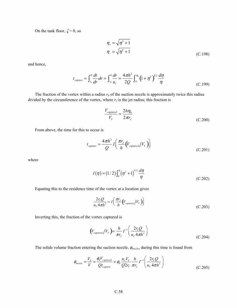
C.58

On the tank floor, ζ = 0, so

η+ = η2 + 1

η− = η2 + 1 (C.198)

and hence,

tcapture =

dt

drdr

r0

0

=dr

urr0

0

=4πh3

2Q1+ η2( )3 2 dη

η0

η0

(C.199)

The fraction of the vortex within a radius r0 of the suction nozzle is approximately twice this radius divided by the circumference of the vortex, where rJ is the jet radius; this fraction is

Vcaptured

VV

=2hη0

2πrJ (C.200)

From above, the time for this to occur is

tcapture =

4πh3

QI

πrJ

hVcaptured VV( )

(C.201)

where

( ) ( ) ( )3/22

01 / 2 1

dI

η ηη ηη

= + (C.202)

Equating this to the residence time of the vortex at a location gives

2rVQ

uV 4πh3= I

πrJ

hVcaptured VV( )

(C.203)

Inverting this, the fraction of the vortex captured is

Vcaptured VV( )=

h

πrJ

I −1 2rVQ

uV 4πh3

(C.204)

The solids volume fraction entering the suction nozzle, φnozzle, during this time is found from

0 10 3

2

2 4capturedS V V V

nozzlecapture V J V

VV u V r QhI

V Qt Q r r u h

φφ φ

π π−

= = = (C.205)

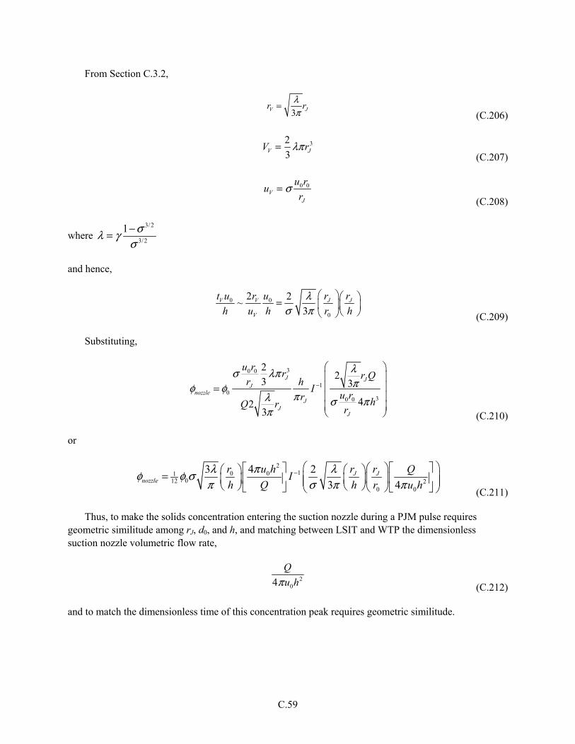
C.59

From Section C.3.2,

rV =

λ3π

rJ

(C.206)

VV =

2

3λπrJ

3

(C.207)

uV = σ u0r0

rJ (C.208)

where 3/2

3/2

1 σλ γσ−=

and hence,

0 0

0

2 2~

3V V J J

V

t u r u r r

h u h r h

λσ π

= (C.209)

Substituting,

30 0

10

30 0

22

3 3

423

J JJ

nozzleJ

JJ

u rr r Q

r hI

u rr hQ rr

λσ λππφ φ

πλ σ ππ

−

= (C.210)

or

210 01

012 20 0

43 2

3 4J J

nozzle

r u h r r QI

h Q h r u h

πλ λφ φ σπ σ π π

− = (C.211)

Thus, to make the solids concentration entering the suction nozzle during a PJM pulse requires geometric similitude among rJ, d0, and h, and matching between LSIT and WTP the dimensionless suction nozzle volumetric flow rate,

Q

4πu0h2

(C.212)

and to match the dimensionless time of this concentration peak requires geometric similitude.

C.60

C.4.3.3 Summary of Scaling Laws

To provide a representative concentration versus time in the transfer line out of an LSIT tank, the volumetric flow rate into the transfer line should be scaled as follows for the two cases:

Case 1—solids swept on tank floor by PJM pulse: Q ~ UD2 (C.213)

Case 2—solids settling between PJM pulses: Q ~ uSD2 (C.214)

For Case 2, some average of the settling velocities must be used, such as is discussed in Section 2.2.1.5 and Appendix A.5.

C.5 References

Bajpai S and MS Tirumkudulu. 2008. “An experimental study of impulsively started turbulent axisymmetric jets.” The European Physical Journal B 61:293-297.

Batchelor GK. 1967. An Introduction to Fluid Dynamics, Equation 2.5.2. Cambridge University Press, United Kingdom.

Batchelor GK. 1982. “Sedimentation in a dilute polydisperse system of interacting spheres. Part 1. General theory.” Journal of Fluid Mechanics 119:379-408.

Batchelor GK and RW Janse van Rensburg. 1986. “Structure Formation in Bidisperse Sedimentation.” Journal of Fluid Mechanics 166:379-407.

Biesheuvel PM, H Verweij, and V Breedveld. 2001. “Evaluation of Instability Criterion for Bidisperse Sedimentation.” AIChE Journal 47(1):45-52.

Burger R, KH Karlsen, EM Tory, and WL Wendland. 2002. “Model Equations and Instability Regions for the Sedimentation of Polydisperse Suspensions of Spheres.” Journal of Applied Mathematics and Mechanics (Zentralblatt für Angewandte Mathematik und Mechanik) 82(10):699-722.

Cervantes J and F Solorio. 2002. “Entropy generation in a plane turbulent oscillating jet.” International Journal of Heat and Mass Transfer 45:3125-3129.

Davis RH and H Gecol. 1994. “Hindered Settling Function with No Empirical Parameters for Polydisperse Suspensions.” AIChE Journal 40(3):570-575.

Lamb H. 1945. Hydrodynamics. Reprint of original 1932 publication by Cambridge University Press, of the work first published in 1879, Dover Publications, New York. See article 229.

Lockett MJ and KS Bassoon. 1979. “Sedimentation of Binary Particle Mixtures.” Powder Technology 24(1979):1-7.

Masliyah JH. 1979. “Hindered settling in a multi-species particle system.” Chemical Engineering Science 34: 1166-1168.

C.61

Meyer PA, JA Bamberger, CW Enderlin, JA Fort, BE Wells, SK Sundaram, PA Scott, MJ Minette, GL Smith, CA Burns, MS Greenwood, GP Morgen, EBK Baer, SF Snyder, M White, GF Piepel, BG Amidan, A Heredia-Langner, SA Bailey, JC Bower, KM Denslow, DE Eakin, MR Elmore, PA Gauglitz, AD Guzman, BK Hatchell, DF Hopkins, DE Hurley, MD Johnson, LJ Kirihara, BD Lawler, JS Loveland, OD Mullen, MS Pekour, TJ Peters, PJ Robinson, MS Russcher, S Sande, C Santoso, SV Shoemaker, SM Silva, DE Smith, YF Su, JJ Toth, JD Wiberg, XY Yu, and N Zuljevic. 2009. Pulse Jet Mixing Tests With Noncohesive Solids. PNNL-18098; WTP-RPT-182, Rev. 0, Pacific Northwest National Laboratory, Richland, Washington.

Meyer PA, JA Bamberger, CW Enderlin, JA Fort, BE Wells, SK Sundaram, PA Scott, MJ Minette, GL Smith, CA Burns, MS Greenwood, GP Morgen, EBK Baer, SF Snyder, M White, GF Piepel, BG Amidan, A Heredia-Langner, SA Bailey, JC Bower, KM Denslow, DE Eakin, MR Elmore, PA Gauglitz, AD Guzman, BK Hatchell, DF Hopkins, DE Hurley, MD Johnson, LJ Kirihara, BD Lawler, JS Loveland, OD Mullen, MS Pekour, TJ Peters, PJ Robinson, MS Russcher, S Sande, C Santoso, SV Shoemaker, SM Silva, DE Smith, YF Su, JJ Toth, JD Wiberg, XY Yu, and N Zuljevic. 2012. Pulse Jet Mixing Tests With Noncohesive Solids. PNNL-18098, Rev. 1; WTP-RPT-182, Rev. 1, Pacific Northwest National Laboratory, Richland, Washington.

Patwardhan VS and C Tien. 1985. “Sedimentation and Liquid Fluidization of Solid Particles of Different Sizes and Densities.” Chemical Engineering Science 40:1051-1060.

Poreh M, YG Tsuei, and JE Cermak. 1967. “Investigation of a Turbulent Radial Wall Jet.” Journal of Applied Mechanics June 1967:457-463.

Rajaratnam N. 1976. Turbulent Jets. Elsevier, Amsterdam.

Richardson JF and WN Zaki. 1954. “Sedimentation and fluidisation. Part 1.” Transactions of the Institute of Chemical Engineers 32:35-53.

Richardson JF and FA Shabi. 1960. “The Determination of Concentration Distribution in a Sedimenting Suspension Using Radio-active Solids.” Transactions of the Institute of Chemical Engineers 38:33-42.

Wells BE, DE Kurath, LA Mahoney, Y Onishi, JL Huckaby, SK Cooley, CA Burns, EC Buck, JM Tingey, RC Daniel, and KK Anderson. 2011. Hanford Waste Physical and Rheological Properties: Data and Gaps. PNNL-20646, Pacific Northwest National Laboratory, Richland, Washington.

References Not Publicly Available

Mauss J and I Papp. 2010. Determination of Mixing Requirements for Pulse-Jet-Mixed Vessels in the Waste Treatment Plant. 24590-WTP-ES-ENG-09-001, Rev. 2, Bechtel National, Inc., Richland, Washington.

Appendix D –

Working Paper for Sparger Operations

D.iii

Acronyms and Abbreviations

ES engineering scale (i.e., reduced scale compared to WTP)

HLP high-level process (tank)

LSIT Large Scale Integrated Test

PEP Pretreatment Engineering Platform

PJM pulse jet mixer

ROB region(s) of bubbles

UFP ultrafiltration process (tank)

WTP Hanford Waste Treatment and Immobilization Plant

ZOI zone(s) of influence

Symbols

A cross-sectional area of the vessel affected by a group of spargers

Abz elevation-dependent projected spherical bubble area

An PJM nozzle cross-sectional area

AROB area of region of bubbles

C scaled constant; dimensionless coefficient

D tank or vessel diameter

Dbz elevation-dependent bubble diameter

DC PJM duty cycle

DROB diameter of region of bubbles

DZOI diameter of zone of influence

fv,m bubble region volume fraction in the bottom of the vessel due to type m spargers

g acceleration of gravity

H overall depth or height (e.g., sparger nozzle to slurry surface)

Hsl depth or height of slurry from tank bottom center to the slurry surface

Hsl /D ratio of slurry fill-level (height) to vessel diameter

L length scale

m designation for a sparger type

n number of air spargers

NJ number of PJMs

P pressure; or power (in context)

Pa ambient or atmospheric pressure; vessel headspace pressure

Pb bubble power

PbV bubble power-per-unit volume of slurry

D.iv

PPJM power per PJM cycle

Pstd standard state pressure

Pz elevation-dependent absolute pressure in slurry

P0 pressure at sparger nozzle depth (zsp = 0)

Q volumetric flow rate (sparge gas)

QJ volumetric flow rate from a single PJM during the drive phase

Qn actual flow rate at nozzle depth per sparge tube

Qstd standard volumetric feed rate of sparge air (e.g., in scfm)

Qz elevation-dependent flow rate of sparge gas

zQΔ average sparge air volumetric flow rate integrated over sparger depth

S vessel geometric scale factor (WTP-vessel dimension: test-vessel dimension)

T absolute temperature

tC characteristic time; PJM cycle time

tsp characteristic sparger time

Tstd standard state temperature

U characteristic velocity

Un nozzle velocity

U* superficial gas velocity

U*std superficial gas velocity corresponding to the sparge air feed rate at standard

conditions

0*U superficial gas velocity at nozzle depth

*zUΔ integrated average superficial gas velocity

V volume

Vb,min minimum volume of slurry swept by rising bubbles from a sparger

Vbot slurry volume in the vessel bottom region

Vbz elevation-dependent bubble volume

Vb0 initial bubble volume

VROB volume of region of bubbles

Vsl slurry volume

z elevation; elevation with respect to tank bottom center

zsp elevation with respect to sparger nozzle depth

z0 initial lower value of elevation

D.v

Greek Symbols

Δz elevation change

ρ density; slurry density

φ diameter of sparger layout circle in WTP vessels

Subscripts

0 initial or reference state value

a ambient or atmospheric

b bubble

Bv bubble power-per-unit volume

ES engineering-scale vessel

H surface elevation

J PJM

m air sparger type

min minimum

n nozzle

ROB region of bubble

sl slurry, waste or simulant

sp sparger

std standard atmospheric conditions

WTP WTP vessel

z elevation-dependence

ZOI zone of influence

D.vii

Contents

Acronyms and Abbreviations ............................................................................................................... D.iii Symbols ................................................................................................................................................ D.iii Subscripts .............................................................................................................................................. D.v D.1 Air Sparger Design Criteria ........................................................................................................ D.2

D.1.1 Local and Integrated Mixing Intensity ........................................................................... D.3 D.1.2 Sparger Number, Layout, and Bottom Offset Considerations ....................................... D.5

D.1.2.1 Number and Layout of Spargers .................................................................... D.5 D.1.2.2 Sparger Nozzle Offset from Tank Bottom ..................................................... D.8

D.2 Air Sparger Flow Rates for Overall Vessel Mixing Effect ......................................................... D.9 D.2.1 Mixing Intensity and Bubble Power-Per-Unit Volume Matching ................................. D.9 D.2.2 Multi-Elevation Air Sparger Option .............................................................................. D.14 D.2.3 Alternative Sparger Flow Rate Scaling Approaches for Overall Vessel Mixing

Effect .............................................................................................................................. D.16 D.2.3.1 Scaling Characteristic Mixing Time .............................................................. D.16 D.2.3.2 Scaling to Match ZOI Coverage .................................................................... D.18

D.2.4 Summary and Recommendations – Sparger Flow Rates for Overall Vessel Mixing ............................................................................................................................ D.19

D.3 Air Sparger Flow Rates and Bottom Motion Phenomenon ......................................................... D.21 D.3.1 Power of Sparged Bubbles in the Vessel Bottom Region .............................................. D.22 D.3.2 Comparison of Air Sparger Bubble Power and PJM Power .......................................... D.26 D.3.3 Volume Fraction Swept by Sparged Bubbles ................................................................ D.27

D.3.3.1 Bubble Volume Fraction from the ROB Empirical Model ............................ D.27 D.3.3.2 Bubble Volume Fraction from Initial Bubble Volume Models ..................... D.29

D.3.4 Summary and Recommendations for Sparger Operations in Bottom Motion Studies ............................................................................................................................ D.32

D.4 References ................................................................................................................................... D.36

Figures

D.1 Process Flow Diagram for Scaling Sparger Operation and Layout in the PEP-Scale UFP-02 Vessel ............................................................................................................................ D.3

D.2 Illustration of Sparger Fluid Mechanics Concepts in Non-Newtonian Fluids for a Single Sparge Tube ................................................................................................................................ D.6

D.3 Section of the WTP HLP-27 Vessel Showing PJM and Air Sparge Tube Layouts: Twenty-eight Deep Annular Spargers in Three Circles and Eight Shallow, Central Spargers above the PJMs ............................................................................................................ D.7

D.viii

D.4 Section of the WTP UFP-02 Vessel Showing PJM and Air Sparge Tube Layouts: Ten Deep Annular Spargers in Two Circles and Six Shallow, Central Spargers above the PJMs ........................................................................................................................... D.7

D.5 Superficial Sparge Gas Velocity as a Function of the Fractional Elevation Above the Tank Bottom z/Hsl in the WTP and the 1/3.89 ES UFP-02 Vessels for the Three Sparger Types: Top – Shallow, Central; Middle – Deep, Annular Type 2; and Bottom - Deep, Annular Type 1 ........................................................................................................................... D.12

D.6 Superficial Sparge Gas Velocity as a Function of Total Deep Annular Sparge Air Flow Rate and the Fractional Elevation Above the Tank Bottom z/Hsl in the WTP and ES HLP-27 Vessels: Top, D = 14 ft; Middle, D = 8 ft; and Bottom, D = 43 in. ....................... D.13

D.7 Total Flow Rate to Deep Annular Spargers as a Function of Vessel Scale in HLP-27 and UFP-02 for Three Mixing Intensity Matching Criteria ........................................................ D.15

D.8 Total Standard Air Flow Rate to Deep Annular Spargers in the 1/6.94 ES HLP-27 Vessel as a Function of Slurry Density and Fill Level – Matching the Integrated Bubble Power-Per-Unit Volume and U* at Intermediate Depth of the WTP Vessel .................. D.16

D.9 Total Flow Rate to Deep Annular Spargers in Scaled HLP-27 Vessels for Two Characteristic Mixing Time Scaling Approaches and for ZOI Area Scaling with 7, 14 and 28 Spargers ................................................................................................................. D.18

D.10 Total Actual Sparge Air Flow Rate at Nozzle Depth in the Deep Annular Region of the 1/6.94 ES HLP-27 Vessel to Match the 2/3 ZOI Area Fraction of the WTP Vessel for Type 1, Type 2&3, and All Deep Spargers ................................................................................ D.19

D.11 Bottom Region of the WTP HLP-27 Vessel and the Three Deep Annular Sparger Types and Elevations ............................................................................................................................ D.22

D.12 Superficial Sparge Gas Velocity Profiles in the Vessel Bottom Region Affected by Type 2&3 and Type 1 Deep Annular Spargers for Three Mixing Intensity Matching Criteria in the WTP and 1/6.94 ES HLP-27 Vessels .................................................................. D.23

D.13 Combined Superficial Sparge Gas Velocity Profiles in Vessel Bottom Region Due to Type 2&3 and Type 1 Deep Annular Spargers for Three Mixing Intensity Matching Criteria in the WTP and 1/6.94 ES HLP-27 Vessels .................................................................. D.24

D.14 Superficial Sparge Gas Velocity Profiles in the Vessel Bottom Region Affected by Type 1 Deep Annular Spargers for Three Mixing Intensity Matching Criteria in the WTP and ES UFP-02 Vessels: Top, D = 43 in., S = 3.89; and Bottom, D = 8 ft, S = 1.75 ....................................................................................................................................... D.25

D.15 Total Actual Sparge Air Flow Rate at Nozzle Depth for Type 1 and Type 2&3 Deep Annular Spargers of the 1/6.94 Engineering-Scale HLP-27 Vessel to Reproduce Bottom Region Effects of the WTP Vessel Using Three Scaling Approaches .......................... D.33

D.16 Recommended Range of Total Air Flow Rates to All Deep Annular Spargers in Geometrically Scaled HLP-27 and UFP-02 Vessels for Bottom Motion Studies ...................... D.35

D.1

Appendix D

Working Paper for Sparger Operations

Multiple dedicated air sparge tubes are deployed in a number of the vessels in the Hanford Waste Treatment and Immobilization Plant (WTP) Pretreatment Facility that process non-Newtonian waste slurries (e.g., WTP HLP-VSL-00027A/B [hereafter referred to as HLP-27] and WTP UFP-VSL-00002A/B [hereafter referred to as UFP-02]). These spargers supplement pulse jet mixers (PJMs), thus creating “hybrid” mixing systems. Process air also is used to purge the two-segment steam rings in a WTP Newtonian slurry process vessel, WTP UFP-VSL-00001A/B (hereafter referred to as UFP-01), and UFP-02, which handles both Newtonian and non-Newtonian slurries. A primary purpose of this purge air is to clear and prevent backflow of waste slurry into the multiple orifices of the steam rings and the associated headers when steam is not flowing. Additional slurry mixing resulting from the use of purge air is a secondary benefit in the WTP vessels, and it is considered the more important factor for scaling down steam ring systems in engineering-scale (ES) vessels in which non-radioactive, simulated waste slurries are processed.

Dedicated air sparger scaling approaches that are discussed in some detail in this working paper (i.e., Appendix D), scale-down of steam ring systems, and operations for ES UFP-01 vessels to be used in the Large Scale Integrated Testing (LSIT) program are developed in Chapter 7 of this report. Steam ring purge air flow rate scale-down recommendations are provided there for tests designed to evaluate 1) bottom motion and clearing resulting from PJM operations and 2) WTP blending and sampling requirements for PJM mixed vessels. Blending and potential sparge air impacts on overall vessel mixing are discussed further in Chapter 9. The focus of the main report and of the current LSIT program is Newtonian process vessels. However, this appendix is written from the perspective of possible (and originally planned) ES versions of the non-Newtonian process vessels UFP-02 and HLP-27. Specific examples are given for scaling down dedicated air sparger operations in the proposed 43-in.-, 8-ft-, and 14-ft-diameter LSIT ES vessels.

Air sparger scaling for a proposed 43-in.-diameter (1/6.94-scale) version of HLP-27 also is described in a letter report (Rassat 2010), and dedicated air sparger scaling in UFP-02 and steam ring purge air scaling for UFP-01 and UFP-02 in the 1/4.5-scale vessels used in Pretreatment Engineering Platform (PEP) testing are discussed in Appendix B of report WTP-RPT-160, Rev. 0 (Kuhn et al. 2008). The air sparger and steam ring purge air system scaling approach described here is derived significantly from these earlier documents.

In the LSIT program, there will be no direct measures of sparger performance as a function of vessel scale. The intent of scaling sparger operations for these tests is to help establish the representative environmental conditions in the vessel for other elements of the program to be evaluated (e.g., bottom motion and clearing and blending resulting from PJM operations). The focus of the previous sparger scaling efforts was the overall vessel mixing effect, from sparger nozzles located near the bottom of the vessel to the slurry surface. Overall sparger mixing effects, significant to blending, are further addressed here for the three proposed LSIT vessel scales. In addition, because there is an expected interplay of

D.2

dedicated air sparger operations and bottom motion resulting from PJM operations, special consideration is given to specifying sparger operations for tests having the primary purpose of investigating the scaling of bottom motion.

Choosing “conservative” dedicated air sparger operating conditions for bottom motion studies is not straightforward, as there are a number of tradeoffs to consider. For example, while spargers located 6 in. above the bottom head in WTP vessels are expected to have little direct impact on scouring or disturbing settled solids layers (i.e., negligible air jet effect), continuous air flow to spargers will shear a significant fraction of the slurry in the bottom portion of the vessel and may facilitate the PJMs to be more effective at inducing bottom motion during the PJM drive phase and may lead to larger (taller) PJM caverns. On the other hand, the shearing action and recirculation resulting from spargers may result in enhanced settling of high-density solids that would otherwise be hindered from settling in an un-yielded, non-Newtonian slurry (e.g., in the PJM vent, refill, and rest phases). Therefore, turning spargers off may not be conservative in scaled testing. It may be necessary to test for bottom motion both with and without spargers operating to further our understanding of their impact.

This working paper addresses the scaling of sparger layout and operations and attempts to define representative, as well as bounding, sparger operating conditions for reduced-scale HLP-27 and UFP-02 systems. The scaling approach, design equations, and air sparger layout and operating conditions in the WTP vessels are first summarized in Section D.1. A number of examples to illustrate scaling options and the impact of vessel conditions (e.g., slurry density and fill level) on selected sparger operations (e.g., air flow rates) are provided in this document. Approaches for scaling of sparger operations for overall vessel mixing effect and blending are addressed in Section D.2; and approaches for scaling of sparger operations targeted for bottom motion PJM studies are covered in detail in Section D.3. Specific recommendations for air sparger use in blending and bottom motion studies are also summarized in Sections D.2.4 and D.3.4, respectively.

D.1 Air Sparger Design Criteria

The primary mixing work of dedicated air spargers and steam ring purge air spargers is the result of the net vertical rise of sparge bubbles through relatively dense slurry and the resulting localized entrainment and bulk motion of slurry. The sparger “mixing effectiveness” is a product of the “intensity of mixing” and the distribution of this “mixing energy” across the slurry contained in the vessel. The approach used to scale dedicated air sparger systems is described in this section. Expressions for sparge air mixing intensity and bubble power and the calculations guiding the distribution of spargers in a vessel are summarized.

Figure D.1 provides an overview of the approach that was used to recommend air sparger design and operating conditions for the 1/4.5-scale UFP-02 vessel used in the PEP, as described in Appendix B of Kuhn et al. (2008). For the most part, the overall approach is directly applicable to spargers in the ES UFP-02 and HLP-27 vessels for the LSIT program. However, special consideration is given in this document to impacts of sparger operations in the bottom region of the vessels.

D.3

No

WTP- & PEP-Scale UFP-2

Acceptable?

PEP-Scale ROB & ZOI

Yes

Mixing Power Scaling Approach?

e.g., constant superficial velocity at

specified elevation

WTP-ScaleDesign Basis

&Operating Conditions

Calculate Vertical Distribution of

“Mixing Intensity”

Fix SpargerParameters:

Depth of Nozzles, HTotal Flow Rate, Q

Distribute Spargers:Number, nVertical, H

Radial and Angular, ΦFlow Rate, Q(H,Φ)

No

WTP- & PEP-Scale UFP-2

Acceptable?Acceptable?

PEP-Scale ROB & ZOI

Yes

Mixing Power Scaling Approach?

Mixing Power Scaling Approach?

e.g., constant superficial velocity at

specified elevation

WTP-ScaleDesign Basis

&Operating Conditions

WTP-ScaleDesign Basis

&Operating Conditions

Calculate Vertical Distribution of

“Mixing Intensity”

Calculate Vertical Distribution of

“Mixing Intensity”

Fix SpargerParameters:

Depth of Nozzles, HTotal Flow Rate, Q

Fix SpargerParameters:

Depth of Nozzles, HTotal Flow Rate, Q

Distribute Spargers:Number, nVertical, H

Radial and Angular, ΦFlow Rate, Q(H,Φ)

Distribute Spargers:Number, nVertical, H

Radial and Angular, ΦFlow Rate, Q(H,Φ)

Figure D.1. Process Flow Diagram for Scaling Sparger Operation and Layout in the PEP-Scale UFP-02 Vessel (reproduced from Figure B.1 of Kuhn et al. 2008) (ROB is region of bubbles and ZOI is zone of influence)

D.1.1 Local and Integrated Mixing Intensity

In Appendix B of Kuhn et al. (2008), the mixing intensity resulting from operation of air spargers in WTP slurry processing vessels is discussed and corresponding equations are developed. For example, the local mixing intensity is expressed in terms of the sparge gas superficial velocity U*

A

QU z

z =*

(D.1)

where A is the cross-sectional area of the vessel influenced by the sparge gas and Q is the total volumetric flow rate of a sparge gas through the area. There is an elevation dependence of the flow rate and the superficial velocity, noted by subscript z in Equation (D.1). This is a result of compression of gas bubbles when sparge air is delivered to sparger nozzles at some depth, H, in a slurry of density, ρ, and expansion of these bubbles as they rise through the slurry to the vessel headspace. Sparge bubbles also expand in high-temperature operations (e.g., caustic leaching in UFP-02) because of thermal effects and water vaporization into the air bubbles.

The elevation-dependent superficial velocity, Equation (D.1), is representative of the local distribution of mixing intensity. The integrated mixing energy resulting from the work of bubbles as they rise through a volume of slurry, Vsl, is another measure of mixing in the vessel. For example, Equation (B.4) of Kuhn et al. (2008) gives the slurry volume-specific integrated bubble power, PbV, as

( ) z

gdzU

zzA

gdzQ

V

gdzQP

z

z z

z

z z

zsl

z

z z

bV Δ=

−==

000

*

0,

ρρρ

(D.2)

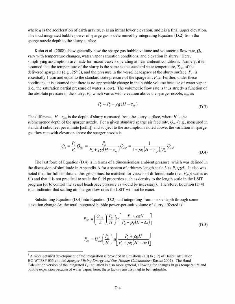
D.4

where g is the acceleration of earth gravity, z0 is an initial lower elevation, and z is a final upper elevation. The total integrated bubble power of sparge gas is determined by integrating Equation (D.2) from the sparge nozzle depth to the slurry surface.

Kuhn et al. (2008) show generally how the sparge gas bubble volume and volumetric flow rate, Qz, vary with temperature changes, water vapor saturation conditions, and elevation in slurry. Here, simplifying assumptions are made for mixed vessels operating at near ambient conditions. Namely, it is assumed that the temperature of the slurry is the same as the standard state temperature, Tstd, of the delivered sparge air (e.g., 25°C), and the pressure in the vessel headspace at the slurry surface, Pa, is essentially 1 atm and equal to the standard state pressure of the sparge air, Pstd. Further, under these conditions, it is assumed that there is no appreciable change in the bubble volume because of water vapor (i.e., the saturation partial pressure of water is low). The volumetric flow rate is thus strictly a function of the absolute pressure in the slurry, Pz, which varies with elevation above the sparger nozzle, zsp, as

)( spaz zHgPP −+= ρ

(D.3)

The difference, H – zsp, is the depth of slurry measured from the slurry surface, where H is the submergence depth of the sparger nozzle. For a given standard sparge air feed rate, Qstd (e.g., measured in standard cubic feet per minute [scfm]) and subject to the assumptions noted above, the variation in sparge gas flow rate with elevation above the sparger nozzle is

( ) ( ) std

aspstd

spa

astd

z

az Q

PzHgQ

zHgP

PQ

P

PQ

−+=

−+==

ρρ 1

1

(D.4)

The last form of Equation (D.4) is in terms of a dimensionless ambient pressure, which was defined in the discussion of similitude in Appendix A for a system of arbitrary length scale L as Pa /ρgL. It also was noted that, for full similitude, this group must be matched for vessels of different scale (i.e., Pa /ρ scales as L1) and that it is not practical to scale the fluid properties such as density to the length scale in the LSIT program (or to control the vessel headspace pressure as would be necessary). Therefore, Equation (D.4) is an indicator that scaling air sparger flow rates for LSIT will not be exact.

Substituting Equation (D.4) into Equation (D.2) and integrating from nozzle depth through some elevation change ∆z, the total integrated bubble power-per-unit volume of slurry affected is1

( )

Δ−+

+

=zHgP

gHP

H

P

A

QP

a

aastdbV ρ

ρln

(D.5)

( )

Δ−+

+

=

zHgP

gHP

H

PUP

a

aastdbV ρ

ρln*

1 A more detailed development of the integration is provided in Equations (10) to (12) of Hand Calculation HC-WTPSP-033 entitled Sparger Mixing Energy and Gas Holdup Calculations (Rassat 2007). The Hand Calculation version of the integrated PbV equation is also more general, allowing for changes in gas temperature and bubble expansion because of water vapor; here, these factors are assumed to be negligible.

D.5

The numerator of the pressure ratio is the absolute pressure at nozzle depth, and the denominator is the absolute pressure at the upper level of the region of interest. When considering overall vessel mixing effect, the upper level is the slurry surface (∆z = H) and the denominator reduces to Pa. For bottom motion studies, the upper level over which bubble power is integrated is only a fraction of the nozzle depth. In the first form of Equation (D.5), the slurry volume affected by spargers is written as AH. If the volume term is excluded from the expression, bubble power is calculated instead of the specific power-per-unit volume. (This is done, for example, to compare to PJM power.) Note in the second expression of Equation (D.5) that the group Qstd/A is replaced with U*

std, the superficial gas velocity corresponding to the sparge air feed rate at standard conditions. In this case, where the temperature and pressure of the vessel headspace are assumed to be equal to the standard state conditions (e.g., 25°C and 1 atm), and there is no bubble volume enhancement because of water vapor, U*

std is also the superficial velocity at the slurry surface (i.e., after bubbles rise from the nozzles to the surface).

D.1.2 Sparger Number, Layout, and Bottom Offset Considerations

D.1.2.1 Number and Layout of Spargers

The following briefly captures some of the more significant aspects of scaling the number and layout of spargers, which is discussed more broadly in Appendix B of Kuhn et al. (2008). Claghorn and Waddell (2007) specify the WTP-scale vessel “design basis” sparger operating conditions including air flow rates, number of spargers, and sparger locations (see Figures D.3 and D.4 below for a summary of values for WTP HLP-27 and WTP UFP-02, respectively). Calculated sparger regions of bubbles (ROB) and overlap of zones of influence (ZOI) were used as a basis to position spargers to provide adequate mixing in the WTP vessels. Rising bubbles in ROB entrain slurry resulting in a net upward movement of slurry, while ZOIs define regions for slurry to return to depth completing a recirculation pathway, as depicted in Figure D.2 (Poloski et al. 2005). In support of WTP vessel PJM-sparger hybrid mixing studies, Poloski et al. evaluated mixing resulting from air sparging in non-Newtonian simulants at ambient temperature and obtained expressions relating sparge gas flow rate and ROB and ZOI diameters, DROB and DZOI,

34.011QDROB = (D.6a)

and

34.034QDZOI = (D.6b)

where Q is the actual flow rate at the sparger nozzle in actual cubic feet per minute (acfm) and the diameters are in inches at the slurry surface. Note that DZOI is essentially three-times DROB. If spargers are distributed such that the nozzles are separated by 2/3 DZOI, then ZOI circles of neighboring spargers just meet adjacent ROB circles, as projected on the slurry surface. In this way, the upward flow of bubbles and slurry in ROBs interferes minimally with the downward recirculation in ZOIs, while providing maximum coverage over the slurry surface area.

D.6

Figure D.2. Illustration of Sparger Fluid Mechanics Concepts in Non-Newtonian Fluids for a Single

Sparge Tube (reproduced from Figure 3.1 of Poloski et al. (2005))

Figures D.3 and D.4 show layouts of spargers in the WTP HLP-27 and UFP-02 vessels, respectively.

The figures define sparger types,1 provide location information including the diameter of the circle on which the sparge tubes are placed, φ, and the elevation, z, of the sparge tube nozzles measured from tank bottom center, and give the total standard air flow rate to all sparge tubes of a given type.2 Claghorn and Waddell (2007) also show the projection and overlap of ZOI circles on the slurry surface for these layouts where DZOI was calculated from Equation (D.6b) for the design basis flow rate to each sparge tube (in acfm at the sparger nozzle depth). Because of their potential impact on bottom motion, deep annular spargers that run vertically between the outside of the PJM bodies and inside the vessel wall and end with nozzles located near the bottom head of the vessel (i.e., 10 deep spargers of two types in UFP-02 and 28 deep spargers of three types in HLP-27), are the primary focus of this analysis. There also are shallow central spargers with nozzles terminating above the tops of the PJMs (i.e., six in UFP-02 and eight in HLP-27) to provide mixing in the center of the vessel. The scaling approaches for both deep annular and shallow central spargers are similar.

1 Sparger type designations are based on the order of entry of sparger properties (number, location, flow rate, etc.) in Figure 6-13 (WTP-UFP-02) and Figure 6-19 (WTP-HLP-27) of Claghorn and Waddell (2007). 2 The per sparge tube flow rate is the total standard flow rate for a given sparger type divided by the number of spargers of that type.

D.7

Figure D.3. Section of the WTP HLP-27 Vessel Showing PJM (seven around one) and Air Sparge Tube Layouts: Twenty-eight Deep Annular Spargers in Three Circles and Eight Shallow, Central Spargers above the PJMs (adapted from Claghorn and Waddell (2007))

Figure D.4. Section of the WTP UFP-02 Vessel Showing PJM (five around one) and Air Sparge Tube Layouts: Ten Deep Annular Spargers in Two Circles and Six Shallow, Central Spargers above the PJMs (adapted from Claghorn and Waddell (2007))

The ROB and ZOI diameters calculated using Equations (D.6a) and (D.6b) were derived

experimentally for sparge air flow rates in the range of ~2 acfm to ~50 acfm per sparge tube using a rheologically bounding non-Newtonian clay waste simulant having a density of ~1.2 kg/L (Poloski et al. 2005). Figure 6.2 of Poloski et al. (2005) shows that the ROB and ZOI diameters are a weak function of

D.8

submergence depth for sparger nozzles submerged from 66 in. to 118 in. If anything, the ZOI data suggest a slight trend toward increasing DZOI with increasing submergence depth. Thus, for relatively deep spargers in a WTP vessel, the actual ZOI diameters might be larger than predicted by the correlation, and therefore, using the correlation as the design basis was considered somewhat conservative. On the other hand, the converse is also likely true—that is, the ROB and ZOI diameters may be somewhat smaller than predicted by Equations (D.6a) and (D.6b) for nozzle submergence depths less than those used to develop the correlations. Such may be the case for the ES vessels, especially the 43-in.-diameter test stand. However, there currently is insufficient information to suggest that anything other than Equations (D.6a) and (D.6b) should be used to estimate sparger influence areas at the slurry surface (e.g., the circular area of ROBs and ZOIs calculated from their diameters and multiplied by the number of spargers having similar characteristics).

Furthermore, as discussed in Appendix B of Kuhn et al. (2008), the number of spargers needed to produce ROB and ZOI coverage areas comparable to the WTP vessel (e.g., as a fraction of the cross-sectional area of the sparged region in the vessel) in small-scale vessels approaches one (or fractional values, which are meaningless) when the total air flow rate is selected to match bubble power-per-unit volume in the two scales. Kuhn et al. (2008) argued that sparger design and operation should address the following two requirements:

1. The number of deep annular spargers in the PEP UFP-02 vessels should be the minimum number that provides sufficient ROB and ZOI coverage.

2. The number of deep annular spargers should maintain symmetry with the outer circle of PJMs (e.g., five in UFP-02 vessels).

Therefore, five deep annular spargers were recommended in PEP UFP-02 even though <<5 would have been sufficient to provide the equivalent ROB and ZOI coverage. The apparent excess in ROB and ZOI coverage resulting from the use of “too many” spargers more than makes up for the possible overestimation of ROB and ZOI diameters determined from Equations (D.6a) and (D.6b) when scaling down.

Air sparger flow rate scaling approaches based on matching ROB and ZOI coverage (e.g., projected area fractions) are considered below. Namely, the sparger air flow rate in an ES vessel is adjusted such that the sparger ZOI coverage (as determined from Equation (D.6b) and the number of spargers) matches the WTP vessel. This approach is different from others described below in that the total sparge air flow rate is not chosen to provide equivalent mixing intensity (i.e., superficial velocity or power-per-unit volume). As will be shown in Section D.2, scaling the sparge rate to match the ZOI coverage in the two scale vessels leads to lower flow rates in the ES unit that may be overly conservative (i.e., under-mixed) for overall vessel mixing. However, the ROB (and ZOI) scaling approach provides a basis for the low flow rate bound for bottom motion studies (Section D.3).

D.1.2.2 Sparger Nozzle Offset from Tank Bottom

As for the sparger nozzle location with respect to the bottom surface of the vessel, it is assumed for calculational purposes that this value scales geometrically. The typical 6-in. vertical offset in the WTP vessels corresponds to ~0.9 in. (i.e., 6 in./6.94) in the 43-in.-diameter ES HLP-27 vessel. Results in Poloski et al. (2005) suggest that this is physically reasonable. Figure 14.1 of the Poloski et al.’s (2005) report shows the ZOI boundary below the sparger nozzle as a function of air flow rate, and it provides a

D.9

linear correlation for the same.1 As demonstrated in examples below, the recommended per sparge tube flow rate in the smallest LSIT HLP-27 and UFP-02 vessels (43-in. diameter) is on the order of 2 scfm (or less). The actual flow rate at nozzle depth in acfm is somewhat less, but for this exercise, it is assumed to be of the same order (e.g., 2 acfm). Using this flow rate in the correlation given in Poloski et al. (2005), the ZOI only extends ~1/3 of an inch below the nozzle. Therefore, setting the spargers in the ES vessels approximately 1 in. from the bottom head would not be expected to result in extensive local scouring of the surface by the sparge bubbles.

To first order, the total sparge air flow rate scales with the vessel cross-sectional area (∝ L2) to maintain constant sparge gas superficial velocity in the tanks, as shown below. Application of geometric scaling results in sparge tube cross-sectional areas that also vary as L2. Therefore, if the number of sparge tubes is held constant with vessel scale, the air velocity of sparge tube “jets” is constant also.

D.2 Air Sparger Flow Rates for Overall Vessel Mixing Effect

Three bases for scaling air sparger flow rates for overall vessel mixing effect and blending are considered in this section: 1) mixing intensity and bubble power-per-unit volume matching; 2) defining and scaling of sparger characteristic mixing time; and 3) scaling to match sparger zone of influence areas. The first of these is emphasized here as there is a strong computational basis for using it, and it is the approach generally accepted in the mixing community. This section also provides a number of examples for geometrically scaled HLP-27 (Rassat 2010)2 and UFP-02 vessels to demonstrate sparger scaling options and considerations.

D.2.1 Mixing Intensity and Bubble Power-Per-Unit Volume Matching

In an ES vessel that is intended to replicate mixing operations in a WTP vessel at some reduced geometric scale (by a factor 1/S), it is necessary to adjust the air sparger flow rates and possibly to modify the number and layout of the spargers. See Appendix B of Kuhn et al. (2008) for a general discussion of sparger scaling considerations and a specific case study (e.g., spargers for the PEP UFP-02 vessel). As noted in the earlier report, the sparger flow rate in the engineering-scaled vessel can be reduced to match the local mixing intensity at a comparable location in the WTP vessel (e.g., to attain the same superficial velocity at depth [or at the slurry surface]), or the flow rate of the ES vessel can be reduced to match the integrated power-per-unit volume in the two vessels. For a known standard flow rate in the WTP vessel, Qstd,WTP, the reduced flow rate in the ES vessel, Qstd,ES, to match U* at some elevation fraction of the sparger nozzle depth, zsp /H (e.g., 0 at nozzle depth or 1 at the slurry surface), is determined by

1 The ZOI boundary correlation in Figure 14.1 of Poloski et al. (2005) is y = -0.188x + 0.0459, where x is the actual per sparge tube flow rate at nozzle depth in acfm and y is the distance below the nozzle in inches of the ZOI. 2 In Letter WTP/RPP-MOA-PNNL-00508 (Rassat 2010), sparger scaling recommendations were provided for a proposed 43-in. version of HLP-27 that was not scaled geometrically throughout. For example, there were differences in the PJM shroud construction that did not allow geometric scaling of the annular area between the PJMs and the vessel wall.

D.10

straightforward application of Equations (D.1) and (D.4).1 The reduced flow rate in the ES vessel needed to match the integrated power-per-unit volume in the WTP vessel is determined from Equation (D.5):

( ) ( )

Δ−+

+

=

Δ−+

+

=

WTPa

WTPa

WTP

a

WTP

WTPstd

ESa

ESa

ES

a

ES

ESstdbV zHgP

gHP

H

P

A

Q

zHgP

gHP

H

P

A

QP

ρρ

ρρ

lnln ,,

or, after rearranging,

( )

( )

Δ−+

+

Δ−+

+

=

ESa

ESa

WTPa

WTPa

WTP

ES

WTP

ESWTPstdESstd

zHgP

gHP

zHgP

gHP

H

H

A

AQQ

ρρ

ρρ

ln

ln

,,

(D.7)

The (H - ∆z) terms are zero when integration is from sparger nozzle depth to the slurry surface (∆z = H). In a case where the sparger depth and the cross-sectional area affected scale geometrically, the area and height ratio terms of Equation (D.7) reduce to volumetric scaling, 1/S3.

When PbV is matched in nominally geometrically scaled vessels, the superficial velocity profiles

( *zU versus zsp/H or z/Hsl) intersect at some intermediate z/Hsl, where z = 0 at tank bottom and Hsl is the

overall height (or depth) of slurry measured from tank bottom center: the smaller vessel has higher U* values from the nozzle depth up to the point of intersection and lower U* values above it. This is due to the larger bubble expansion factor in the full-scale vessel because of the depth of slurry and the more extreme pressure changes. The intermediate elevation fraction where the U* curves cross can be determined once Qstd,ES is found from Equation (D.7). The two unknowns, U*(zsp/H) and zsp/H, can be calculated using Equations (D.1) and (D.4), as follows: 1) the superficial velocities at z/H in the two vessels are equated using Equation (D.1); 2) Qz in terms of Qstd, using Equation (D.4), is substituted on both sides of the equation; and 3) rearrange to solve for zsp/H, realizing that zsp,WTP/HWTP = zsp,ES/HES = zsp/H. The result is

WTPES

ESstd

WTPstd

ESstd

WTPstda

WTPESWTP

ES

ESstd

WTPstd

WTP

ES

ESstd

WTPstda

sp

gHgHU

U

U

UP

gHgHA

A

Q

Q

A

A

Q

QP

H

z

ρρρρ −

−

+=−

−

+=

*,

*,

*,

*,

,

,

,

, 1

1

1

1

(D.8)

Subsequently, the solved zsp/H value can be used to determine Qz using Equation (D.4) and then *zU using

Equation (D.1).

1 The calculation process is as follows for a selected slurry density and fill level (usually given as a height/diameter ratio) and a specified U* matching elevation fraction zsp/H: 1) determine the absolute z for each vessel by multiplying zsp/H and H; 2) determine Qz,WTP from Equation (D.4) using the known Qstd,WTP and other WTP vessel parameters; 3) use Qz,WTP and AWTP to determine U*, which is the same for both vessels, from Equation (D.1); 4) use U* and AES in Equation (D.1) to determine Qz,ES; and 5) use Qz,ES and other engineering-scale vessel parameters in Equation (D.4) to calculate Qstd,ES.

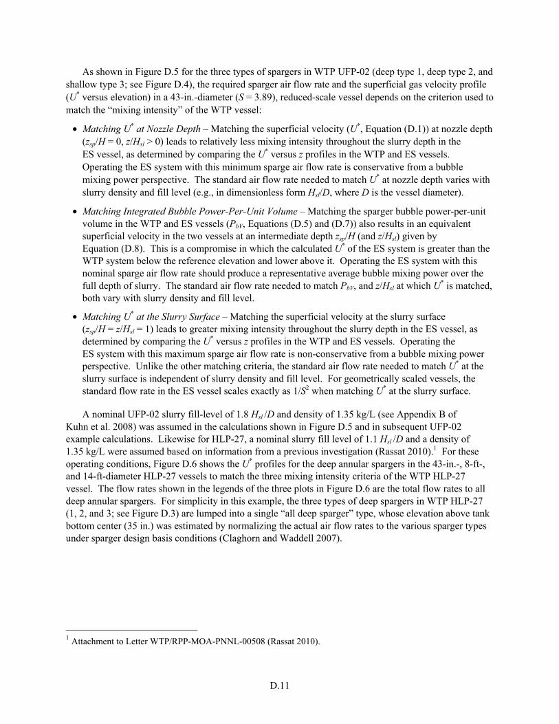
D.11

As shown in Figure D.5 for the three types of spargers in WTP UFP-02 (deep type 1, deep type 2, and shallow type 3; see Figure D.4), the required sparger air flow rate and the superficial gas velocity profile (U* versus elevation) in a 43-in.-diameter (S = 3.89), reduced-scale vessel depends on the criterion used to match the “mixing intensity” of the WTP vessel:

• Matching U* at Nozzle Depth – Matching the superficial velocity (U*, Equation (D.1)) at nozzle depth (zsp/H = 0, z/Hsl > 0) leads to relatively less mixing intensity throughout the slurry depth in the ES vessel, as determined by comparing the U* versus z profiles in the WTP and ES vessels. Operating the ES system with this minimum sparge air flow rate is conservative from a bubble mixing power perspective. The standard air flow rate needed to match U* at nozzle depth varies with slurry density and fill level (e.g., in dimensionless form Hsl/D, where D is the vessel diameter).

• Matching Integrated Bubble Power-Per-Unit Volume – Matching the sparger bubble power-per-unit volume in the WTP and ES vessels (PbV, Equations (D.5) and (D.7)) also results in an equivalent superficial velocity in the two vessels at an intermediate depth zsp/H (and z/Hsl) given by Equation (D.8). This is a compromise in which the calculated U* of the ES system is greater than the WTP system below the reference elevation and lower above it. Operating the ES system with this nominal sparge air flow rate should produce a representative average bubble mixing power over the full depth of slurry. The standard air flow rate needed to match PbV, and z/Hsl at which U* is matched, both vary with slurry density and fill level.

• Matching U* at the Slurry Surface – Matching the superficial velocity at the slurry surface (zsp/H = z/Hsl = 1) leads to greater mixing intensity throughout the slurry depth in the ES vessel, as determined by comparing the U* versus z profiles in the WTP and ES vessels. Operating the ES system with this maximum sparge air flow rate is non-conservative from a bubble mixing power perspective. Unlike the other matching criteria, the standard air flow rate needed to match U* at the slurry surface is independent of slurry density and fill level. For geometrically scaled vessels, the standard flow rate in the ES vessel scales exactly as 1/S2 when matching U* at the slurry surface.

A nominal UFP-02 slurry fill-level of 1.8 Hsl /D and density of 1.35 kg/L (see Appendix B of Kuhn et al. 2008) was assumed in the calculations shown in Figure D.5 and in subsequent UFP-02 example calculations. Likewise for HLP-27, a nominal slurry fill level of 1.1 Hsl /D and a density of 1.35 kg/L were assumed based on information from a previous investigation (Rassat 2010).1 For these operating conditions, Figure D.6 shows the U* profiles for the deep annular spargers in the 43-in.-, 8-ft-, and 14-ft-diameter HLP-27 vessels to match the three mixing intensity criteria of the WTP HLP-27 vessel. The flow rates shown in the legends of the three plots in Figure D.6 are the total flow rates to all deep annular spargers. For simplicity in this example, the three types of deep spargers in WTP HLP-27 (1, 2, and 3; see Figure D.3) are lumped into a single “all deep sparger” type, whose elevation above tank bottom center (35 in.) was estimated by normalizing the actual air flow rates to the various sparger types under sparger design basis conditions (Claghorn and Waddell 2007).

1 Attachment to Letter WTP/RPP-MOA-PNNL-00508 (Rassat 2010).

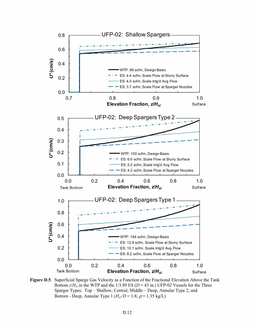
D.12

0.0

0.2

0.4

0.6

0.8

0.7 0.8 0.9 1.0

U*

(cm

/s)

Elevation Fraction, z/Hsl

UFP-02: Shallow Spargers

WTP: 66 scfm, Design Basis

ES: 4.4 scfm, Scale Flow at Slurry Surface

ES: 4.0 scfm, Scale Intg'd Avg Flow

ES: 3.7 scfm, Scale Flow at Sparger Nozzles

Surface

0.0

0.1

0.2

0.3

0.4

0.5

0.0 0.2 0.4 0.6 0.8 1.0

U*

(cm

/s)

Elevation Fraction, z/Hsl

UFP-02: Deep Spargers Type 2

WTP: 100 scfm, Design Basis

ES: 6.6 scfm, Scale Flow at Slurry Surface

ES: 5.2 scfm, Scale Intg'd Avg Flow

ES: 4.3 scfm, Scale Flow at Sparger Nozzles

Tank Bottom Surface

0.0

0.2

0.4

0.6

0.8

1.0

0.0 0.2 0.4 0.6 0.8 1.0

U*

(cm

/s)

Elevation Fraction, z/Hsl

UFP-02: Deep Spargers Type 1

WTP: 194 scfm, Design Basis

ES: 12.8 scfm, Scale Flow at Slurry Surface

ES: 10.1 scfm, Scale Intg'd Avg Flow

ES: 8.2 scfm, Scale Flow at Sparger Nozzles

Tank Bottom Surface

Figure D.5. Superficial Sparge Gas Velocity as a Function of the Fractional Elevation Above the Tank Bottom z/Hsl in the WTP and the 1/3.89 ES (D = 43 in.) UFP-02 Vessels for the Three Sparger Types: Top – Shallow, Central; Middle – Deep, Annular Type 2; and Bottom - Deep, Annular Type 1 (Hsl /D = 1.8; ρ = 1.35 kg/L)

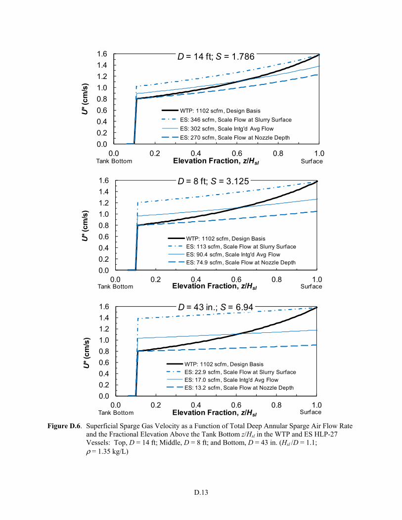
D.13

0.0

0.2

0.4

0.6

0.8

1.0

1.2

1.4

1.6

0.0 0.2 0.4 0.6 0.8 1.0

U*

(cm

/s)

Elevation Fraction, z/Hsl

D = 14 ft; S = 1.786

WTP: 1102 scfm, Design Basis

ES: 346 scfm, Scale Flow at Slurry Surface

ES: 302 scfm, Scale Intg'd Avg Flow

ES: 270 scfm, Scale Flow at Nozzle Depth

Tank Bottom Surface

0.0

0.2

0.4

0.6

0.8

1.0

1.2

1.4

1.6

0.0 0.2 0.4 0.6 0.8 1.0

U* (

cm

/s)

Elevation Fraction, z/Hsl

D = 8 ft; S = 3.125

WTP: 1102 scfm, Design Basis

ES: 113 scfm, Scale Flow at Slurry Surface

ES: 90.4 scfm, Scale Intg'd Avg Flow

ES: 74.9 scfm, Scale Flow at Nozzle Depth

Tank Bottom Surface

0.0

0.2

0.4

0.6

0.8

1.0

1.2

1.4

1.6

0.0 0.2 0.4 0.6 0.8 1.0

U*

(cm

/s)

Elevation Fraction, z/Hsl

D = 43 in.; S = 6.94

WTP: 1102 scfm, Design Basis

ES: 22.9 scfm, Scale Flow at Slurry SurfaceES: 17.0 scfm, Scale Intg'd Avg Flow

ES: 13.2 scfm, Scale Flow at Nozzle Depth

Tank Bottom Surface

Figure D.6. Superficial Sparge Gas Velocity as a Function of Total Deep Annular Sparge Air Flow Rate and the Fractional Elevation Above the Tank Bottom z/Hsl in the WTP and ES HLP-27 Vessels: Top, D = 14 ft; Middle, D = 8 ft; and Bottom, D = 43 in. (Hsl /D = 1.1; ρ = 1.35 kg/L)

D.14

The legends of each of the plots in Figures D.5 and D.6 show how sparger flow rate varies with the flow rate scaling criterion used: matching superficial velocity at nozzle depth, equivalent integrated bubble power-per-unit volume, and matching U* at the slurry surface. For nominal fill levels and slurry density in HLP-27 and UFP-02, Figure D.7 shows the variation in required total deep annular sparger air flow rate as a function of vessel scale factor, where S = 1 in the WTP vessel, and S is inversely proportional to vessel diameter. Like Figure D.6, the flow rate required varies with the flow rate scaling criterion used as well as the geometric scale factor, converging to the WTP design basis value as the value of S approaches one.

It is noted above that the required sparge air flow rate varies with slurry density and vessel fill level (or sparger nozzle depth) when flow rate scaling is based on matching superficial velocity at any elevation below the slurry surface and when matching power-per- unit volume. Figure D.8 shows the effect of fill level and density on the deep annular sparger air flow rates for the 1/6.94 ES (43-in.-diameter) HLP-27 vessel in the case in which integrated bubble power-per-unit volume is scaled to equal that in the WTP vessel.

D.2.2 Multi-Elevation Air Sparger Option

As shown in Figure D.6, the goodness of the fit of the WTP and ES vessel superficial velocity profiles (e.g., the integrated bubble power-per-unit volume matching case in the ES vessels) improves with increasing vessel size and decreasing S. The reason for this is the increasing hydrostatic pressure and increasing bubble expansion from nozzle depth to the slurry surface with greater slurry depth. An

alternative approach to improve matching the WTP *zU profile, especially in smaller-scale vessels, would

be to have sparge tubes/nozzles located at multiple elevations in the vessel. For example, deep annular sparge nozzles could be located at three elevations, zsp/H = 0, zsp /H = 1/3, and zsp /H = 2/3: the flow rate to the deepest set of nozzles (zsp /H = 0) would be set to match the superficial velocity at nozzle depth or to match the integrated average U* over the first third of the slurry (from the bottom up); additional sparge air would be added at zsp /H = 1/3 to better match the *

zU profile in the middle third; and likewise, more

sparge air would be added at zsp /H = 2/3 to better match the *zU profile in the upper third. It is not clear

that the improved reproduction of the velocity profile for overall vessel mixing alone warrants the added experimental complexity (e.g., in this case, three sets of sparge tubes and three sets of flow controllers). However, such an approach may be warranted for studies where bottom motion (see Section D.3) and overall mixing effects are considered together. Further note that in UFP-02, the steam ring purge air is effectively an annular sparge air source at a higher elevation than the dedicated air spargers (see Chapter 7 of this report and Appendix B of Kuhn et al. 2008). One could consider adjusting the air flow rates to the spargers and the steam ring in the ES vessels to optimize the match of the overall WTP superficial gas velocity profile in the annular region.

D.15

S = 6.94;D = 43 in.

S = 3.125;D = 8 ft

S = 1.79;D = 14 ft

10

100

1000

1 2 3 4 5 6 7 8

To

tal A

ir F

low

rate

(s

cfm

)

Geometric Scale Factor, S

HLP-27, All Deep Spargers

Match U* at Slurry Surface

Match Intg'd Avg U* & PbV

Match U* at Nozzle Depth

1/S2

Scaling of Qstd

Full Scale

S = 3.89;D = 43 in.

S = 1.75;D = 8 ft

10

100

1 2 3 4 5

To

tal A

ir F

low

rate

(s

cfm

)

Geometric Scale Factor, S

UFP-02, All Deep Spargers

Match U* at Slurry Surface

Match Intg'd Avg U* & PbV

Match U* at Nozzle Depth

Full Scale

1/S2

Scaling of Qstd

Figure D.7. Total Flow Rate to Deep Annular Spargers as a Function of Vessel Scale in HLP-27 (top) and UFP-02 (bottom) for Three Mixing Intensity Matching Criteria (Hsl /D = 1.1 in HLP-27 and 1.8 in UFP-02; ρ = 1.35 kg/L in both)

D.16

16

17

18

19

20

1.0 1.1 1.2 1.3 1.4 1.5

To

tal S

pa

rge

Air

Flo

w R

ate

(s

cfm

)

Slurry Density (kg/L)

HLP-27: Match Power/Volume, All Deep Spargers

0.75 H/D

0.9 H/D

1.0 H/D

1.1 H/D

1.25 H/D

Figure D.8. Total Standard Air Flow Rate to Deep Annular Spargers in the 1/6.94 ES (43-in.-diameter) HLP-27 Vessel as a Function of Slurry Density and Fill Level (H/D = Hsl /D) – Matching the Integrated Bubble Power-Per-Unit Volume and U* at Intermediate Depth of the WTP Vessel

D.2.3 Alternative Sparger Flow Rate Scaling Approaches for Overall Vessel

Mixing Effect

D.2.3.1 Scaling Characteristic Mixing Time

In Appendix A of this report, we note that, “Given full similitude, observations of behavior at reduced scale would represent those in the full-scale system at geometrically similar locations and kinematically similar times, meaning elapsed times relative to some characteristic time for the system. Because the mixing behavior of interest is driven by the fluid velocities imposed on the system, the characteristic time is the characteristic length of the system, L, divided by the characteristic velocity imposed, U (i.e., L/U).” While cyclic and transient PJM operations were the primary focus of this statement, a characteristic time for continuously operated air spargers also can be defined. A characteristic velocity for air spargers is the superficial gas velocity, and the characteristic length is the sparger nozzle depth, H (which scales with L). Therefore, a characteristic sparger time, tsp, may be defined in these terms

*U

H

Q

AH

Q

Vt sl

sp === (D.9)

The superficial velocity used to calculate tsp varies with the choice of mixing intensity matching criterion, as described in the previous section. For sparger bubble power-per-unit volume matching, the

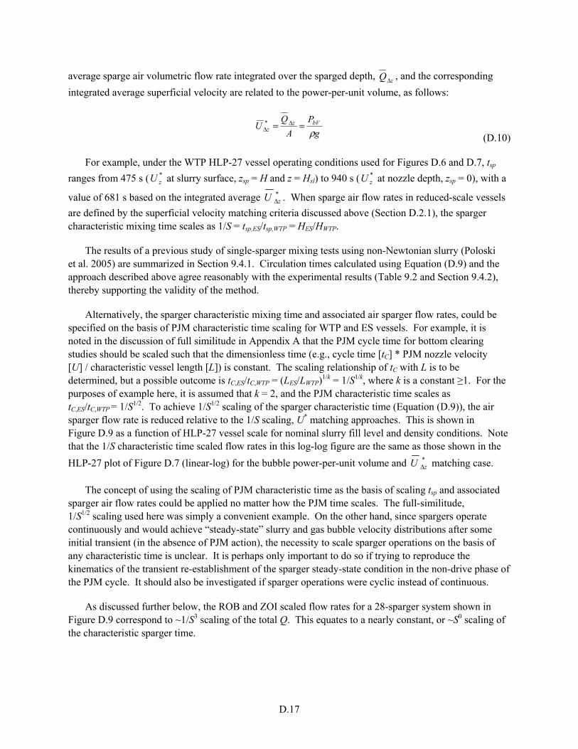
D.17

average sparge air volumetric flow rate integrated over the sparged depth, zQΔ , and the corresponding

integrated average superficial velocity are related to the power-per-unit volume, as follows:

g

P

A

QU bVz

z ρ== Δ

Δ*

(D.10)

For example, under the WTP HLP-27 vessel operating conditions used for Figures D.6 and D.7, tsp

ranges from 475 s ( *zU at slurry surface, zsp = H and z = Hsl) to 940 s ( *

zU at nozzle depth, zsp = 0), with a

value of 681 s based on the integrated average *zU Δ . When sparge air flow rates in reduced-scale vessels

are defined by the superficial velocity matching criteria discussed above (Section D.2.1), the sparger characteristic mixing time scales as 1/S = tsp,ES/tsp,WTP = HES/HWTP.

The results of a previous study of single-sparger mixing tests using non-Newtonian slurry (Poloski et al. 2005) are summarized in Section 9.4.1. Circulation times calculated using Equation (D.9) and the approach described above agree reasonably with the experimental results (Table 9.2 and Section 9.4.2), thereby supporting the validity of the method.

Alternatively, the sparger characteristic mixing time and associated air sparger flow rates, could be specified on the basis of PJM characteristic time scaling for WTP and ES vessels. For example, it is noted in the discussion of full similitude in Appendix A that the PJM cycle time for bottom clearing studies should be scaled such that the dimensionless time (e.g., cycle time [tC] * PJM nozzle velocity [U] / characteristic vessel length [L]) is constant. The scaling relationship of tC with L is to be determined, but a possible outcome is tC,ES/tC,WTP = (LES/LWTP)1/k = 1/S1/k, where k is a constant ≥1. For the purposes of example here, it is assumed that k = 2, and the PJM characteristic time scales as tC,ES/tC,WTP = 1/S1/2. To achieve 1/S1/2 scaling of the sparger characteristic time (Equation (D.9)), the air sparger flow rate is reduced relative to the 1/S scaling, U* matching approaches. This is shown in Figure D.9 as a function of HLP-27 vessel scale for nominal slurry fill level and density conditions. Note that the 1/S characteristic time scaled flow rates in this log-log figure are the same as those shown in the

HLP-27 plot of Figure D.7 (linear-log) for the bubble power-per-unit volume and *zU Δ matching case.

The concept of using the scaling of PJM characteristic time as the basis of scaling tsp and associated sparger air flow rates could be applied no matter how the PJM time scales. The full-similitude, 1/S1/2 scaling used here was simply a convenient example. On the other hand, since spargers operate continuously and would achieve “steady-state” slurry and gas bubble velocity distributions after some initial transient (in the absence of PJM action), the necessity to scale sparger operations on the basis of any characteristic time is unclear. It is perhaps only important to do so if trying to reproduce the kinematics of the transient re-establishment of the sparger steady-state condition in the non-drive phase of the PJM cycle. It should also be investigated if sparger operations were cyclic instead of continuous.

As discussed further below, the ROB and ZOI scaled flow rates for a 28-sparger system shown in Figure D.9 correspond to ~1/S3 scaling of the total Q. This equates to a nearly constant, or ~S0 scaling of the characteristic sparger time.

D.18

S = 6.94;D = 43 in.

S = 3.125;D = 8 ft

S = 1.786;D = 14 ft

1

10

100

1000

1 10

To

tal A

ir F

low

rate

(s

cfm

)

Geometric Scale Factor, S

HLP-27, All Deep Spargers

Time Scaling, 1/S, Intg'd Avg Q

Time Scaling, S^-0.5, Intg'd Avg Q

ROB & ZOI Scaling, n = 7

ROB & ZOI Scaling, n = 14

ROB & ZOI Scaling, n = 28

Full Scale

~1/S TimeScaling

~S0 TimeScaling

Figure D.9. Total Flow Rate to Deep Annular Spargers in Scaled HLP-27 Vessels for Two Characteristic Mixing Time Scaling Approaches (1/S1 and 1/S0.5, each based on integrated average flow rate) and for ZOI Area Scaling with 7, 14 and 28 Spargers (Hsl /D = 1.1; ρ = 1.35 kg/L)

D.2.3.2 Scaling to Match ZOI Coverage

The analysis above is predicated on matching the mixing intensity resulting from sparger operations in the ES and WTP vessels. This approach is consistent with previous air sparger scaling efforts (Kuhn et al. 2008). Another possible scaling approach would be to adjust the sparger air flow rate in the ES vessels such that the sparger ZOI coverage in terms of the total 2/3 ZOI area fraction matches the WTP vessel (e.g., 2/3 ZOI area/sparged area ~1.5 for deep annular spargers in WTP HLP-27 under sparger design basis conditions). Assuming a constant area fraction, one can calculate the 2/3 ZOI area per sparge tube for any number of spargers. From this area, the 2/3 ZOI diameter and DZOI are back-calculated, and the actual flow rate at nozzle depth per sparge tube, Qn, is determined by inverting Equation (D.6b). Ultimately, the total actual air flow rate at sparger nozzle depth is the product of Qn and the number, n, of air spargers. Figure D.10 shows the calculated total actual air flow rate needed to match the WTP 2/3 ZOI area fraction for the same nominal operating conditions used to generate Figure D.6. Results are shown for type 1, combined types 2 and 3, and all deep annular spargers. In the WTP vessel, there are 14 type 1, 7 type 2, and 7 type 3, for a total of 14 combined types 2 and 3 (see Figure D.3 and Section D.1.2 for additional discussion).

Figure D.10 indicates that the total sparge air flow rate to match the ZOI area fraction decreases with increasing number of spargers, and for all values of n, the flow rate is less than the 11.6 acfm total required for matching the superficial velocity at sparger nozzle depth in the 1/6.94 (43 in.-diameter) ES and WTP HLP-27 vessels. With seven spargers of each defined type in the ES vessel (14 total), the calculated total air flow rate to match the WTP 2/3 ZOI area fraction is 2.6 acfm, and with 14 spargers of each defined type (28 total) spargers, it is 1.9 acfm. If either of these reduced air flow rates were used in ES tests, the vessel would be very conservatively under mixed from a sparger mixing intensity perspective (e.g., U* and PbV). The calculated flow rates (in scfm) to match ZOI coverage with 7, 14, and

D.19

28 spargers in geometrically scaled HLP-27 vessels are shown in Figure D.9. Analogous examples are also presented in the bottom motion phenomenon section below, under the topic of matching slurry volume fractions sheared by the sparger ROB. Because ZOI and ROB diameters scale with the same exponent on flow rate (Q0.34, Equations (D.6a) and (D.6b)), ES sparger flow rates derived from either ZOI or ROB coverage areas are the same.

0

2

4

6

8

10

12

0 7 14

To

tal A

ir F

low

Ra

te (

acf

m)

Number of Spargers, Each Type

HLP-27, D = 43 in.; ZOI Area Basis

Match U* at Nozzle Depth, All Deep Spargers

Match WTP ZOI Area Fraction, All Deep Spargers

Match WTP ZOI Area Fraction, Type 1 Spargers

Match WTP ZOI Area Fraction, Type 2&3 Spargers

~1/S2

Scaling of Q

Figure D.10. Total Actual Sparge Air Flow Rate at Nozzle Depth in the Deep Annular Region of the 1/6.94 ES (43-in.-diameter) HLP-27 Vessel to Match the 2/3 ZOI Area Fraction of the WTP Vessel for Type 1, Type 2&3 (combined), and All Deep Spargers (Hsl /D = 1.1; ρ = 1.35 kg/L). Results are shown as a function of the number of spargers in the ES vessel and are compared to the flow rate needed to match the mixing intensity in the ES and WTP vessels (e.g., matching U* at nozzle depth).

D.2.4 Summary and Recommendations – Sparger Flow Rates for Overall Vessel

Mixing

In this section, three bases for scaling air sparger flow rates for overall vessel mixing effect (and blending) were outlined: 1) mixing intensity and bubble power-per-unit volume matching; 2) defining and scaling of sparger characteristic mixing time; and 3) scaling to match sparger ROB and ZOI area fractions. An example of the range of air sparger flow rates obtained for these scaling approaches is shown in Figure D.9 for deep annular spargers in HLP-27 as a function of vessel size.

The first of these bases, and specifically bubble power/volume matching, is the primary recommended approach to scaling sparge air flow rates for overall vessel mixing (blending). Because, by definition, the sparger depth scales as 1/S for geometrically-scaled vessels (i.e., S = DWTP/DES = HWTP/HES), the characteristic sparger time scales exactly as 1/S (= tsp,ES/tsp,WTP) when tsp is calculated using Equation (D.9) from the integrated average U* (Equation (D.10)) obtained from PbV matching (assuming that the slurry density and dimensionless fill-level, Hsl/D, are the same in WTP and ES vessels). Thus,

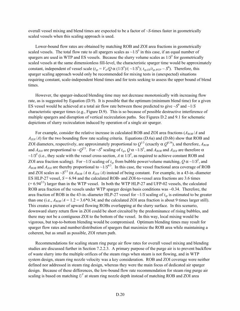
D.20

overall vessel mixing and blend times are expected to be a factor of ~S-times faster in geometrically scaled vessels when this scaling approach is used.

Lower-bound flow rates are obtained by matching ROB and ZOI area fractions in geometrically scaled vessels. The total flow rate to all spargers scales as ~1/S3 in this case, if an equal number of spargers are used in WTP and ES vessels. Because the slurry volume scales as 1/S3 for geometrically scaled vessels at the same dimensionless fill-level, the characteristic sparger time would be approximately constant, independent of vessel scale (tsp = Vsl/Q α (1/S3)/( ~1/S3); tsp,ES/tsp,WTP ~ S0). Therefore, this sparger scaling approach would only be recommended for mixing tests in (unexpected) situations requiring constant, scale-independent blend times and for tests seeking to assess the upper bound of blend times.

However, the sparger-induced blending time may not decrease monotonically with increasing flow rate, as is suggested by Equation (D.9). It is possible that the optimum (minimum blend time) for a given ES vessel would be achieved at a total air flow rate between those predicted to give ~S0 and ~1/S characteristic sparger times (e.g., Figure D.9). This is so because of possible destructive interference of multiple spargers and disruption of vertical recirculation paths. See Figures D.2 and 9.1 for schematic depictions of slurry recirculation induced by operation of a single air sparger.

For example, consider the relative increase in calculated ROB and ZOI area fractions (AROB /A and AZOI /A) for the two bounding flow rate scaling criteria. Equations (D.6a) and (D.6b) show that ROB and ZOI diameters, respectively, are approximately proportional to Q1/3 (exactly α Q0.34), and therefore, AROB and AZOI are proportional to ~Q2/3. For ~S0 scaling of tsp, Q α ~1/S3, and AROB and AZOI are therefore α ~1/S2 (i.e., they scale with the vessel cross-section, A α 1/S2, as required to achieve constant ROB and ZOI area fraction scaling). For ~1/S scaling of tsp from bubble power/volume matching, Q α ~1/S2, and AROB and AZOI are thereby proportional to ~1/S4/3. In this case, the vessel fractional area coverage of ROB and ZOI scales as ~S2/3 (α AROB /A α AZOI /A) instead of being constant. For example, in a 43-in.-diameter ES HLP-27 vessel, S = 6.94 and the calculated ROB- and ZOI-to-vessel area fractions are 3.6 times (= 6.942/3) larger than in the WTP vessel. In both the WTP HLP-27 and UFP-02 vessels, the calculated ROB area fraction of the vessels under WTP sparger design basis conditions was ~0.34. Therefore, the area fraction of ROB in the 43-in.-diameter HLP-27 vessel for ~1/S scaling of tsp is estimated to be greater than one (i.e., AROB /A = 1.2 = 3.6*0.34; and the calculated ZOI area fraction is about 9 times larger still). This creates a picture of upward flowing ROBs overlapping at the slurry surface. In this scenario, downward slurry return flow in ZOI could be short circuited by the predominance of rising bubbles, and there may not be a contiguous ZOI to the bottom of the vessel. In this way, local mixing would be vigorous, but top-to-bottom blending would be compromised. Optimum blending times may result for sparger flow rates and number/distribution of spargers that maximize the ROB area while maintaining a coherent, but as small as possible, ZOI return path.

Recommendations for scaling steam ring purge air flow rates for overall vessel mixing and blending studies are discussed further in Section 7.2.2.3. A primary purpose of the purge air is to prevent backflow of waste slurry into the multiple orifices of the steam rings when steam is not flowing, and in WTP system design, steam ring nozzle velocity was a key consideration. ROB and ZOI coverage were neither defined nor addressed in steam ring design, whereas they were the main focus of dedicated air sparger design. Because of these differences, the low-bound flow rate recommendation for steam ring purge air scaling is based on matching U* at steam ring nozzle depth instead of matching ROB and ZOI area

D.21

fractions. However, slurry mixing resulting from the use of steam ring purge air and dedicated air spargers is considered the more important factor for scaling-down flow rates in both air systems for overall vessel mixing/blending tests in ES vessels. Therefore, the primary (and upper-bound) air flow rate recommendation for steam rings and dedicated spargers is based on matching the WTP vessel

volume-specific bubble power, PbV, and the integrated average superficial gas velocity, *

zU Δ . To scale

standard air flow rates to meet this criterion in geometrically-scaled vessels, the simplified form of Equation (D.7) given in Equation (7.5), Section 7.2.2.3, is equally applicable to dedicated air spargers and steam ring purge air (subject to the simplifying assumptions of Section 7.2.2.1, which can be generalized to either air source).

D.3 Air Sparger Flow Rates and Bottom Motion Phenomenon

Approaches to determine air sparger flow rates to provide a representative environment for bottom motion testing resulting from PJM operations can be grouped in two categories: 1) those seeking to provide a comparable local mixing intensity, or magnitude of bubble shearing effect, in the bottom region of the vessel, and 2) those attempting to shear the same fractional volume of the bottom contents through sparger bubble motion, irrespective of the intensity (e.g., bubble power). These scaling approaches are summarized in this section.

A first challenge is to define the bottom region, and more specifically the “top of the bottom” region. The inner vessel head boundary is naturally the true bottom, and it is a focal point for bottom motion and clearing studies. The bottom heads of the WTP vessels are dished and slope downward toward the center of the tank. For example, as shown in Figure D.11 for WTP HLP-27, the nozzles of the deep annular spargers follow the contour of the vessel bottom with a constant offset, typically 6 in. In this way, more centrally located spargers have lower elevation, z, with respect to tank bottom center and are deeper relative to the slurry surface. For the case studies to follow, the types 2 and 3 HLP-27 spargers (z = 24 in. and 20 in., respectively) are lumped into a single type defined as the inner circle (z ~ 21 in.), and the type 1 spargers (z = 41 in.) define an outer circle. The annular area between the outside of the PJM cluster and inside the vessel wall is used to calculate superficial gas velocity for all deep annular sparger types. Air spargers have minimal influence in the center of the tank, under the PJMs; the central volume from the bottom head to the bottom plate of the PJM shroud (at an elevation defined by the intersection of PJM cones and cylindrical bodies) is mixed almost exclusively by the PJMs. Therefore, this is a rationale for defining the elevation of the bottom of the PJM shroud as the “top of the bottom” (~77 in. in WTP HLP-27, see Figure D.11, and ~47 in. in WTP UFP-02). Another possibility is to use the PJM cavern height, which may extend vertically upward into the annular area between the PJM bodies and the inner vessel wall. For practical purposes, given the variable nature of the PJM cavern size with operating conditions, the fixed reference bottom region definition is preferred.

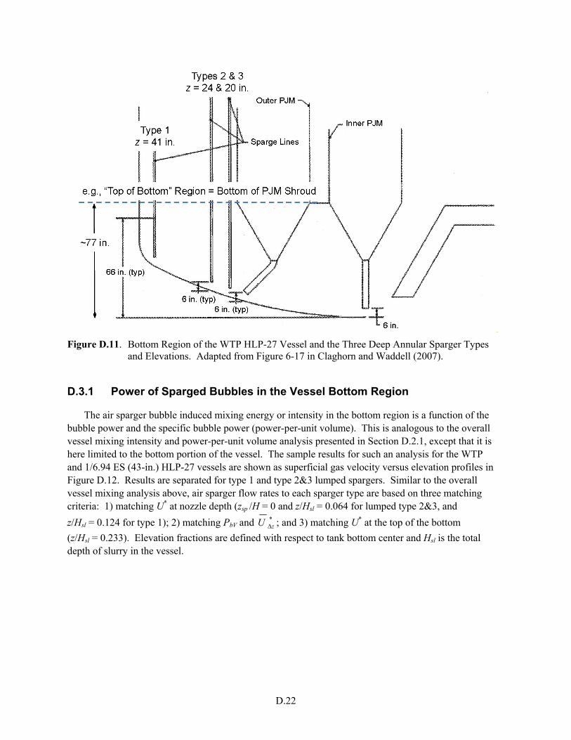
D.22

Figure D.11. Bottom Region of the WTP HLP-27 Vessel and the Three Deep Annular Sparger Types and Elevations. Adapted from Figure 6-17 in Claghorn and Waddell (2007).

D.3.1 Power of Sparged Bubbles in the Vessel Bottom Region

The air sparger bubble induced mixing energy or intensity in the bottom region is a function of the bubble power and the specific bubble power (power-per-unit volume). This is analogous to the overall vessel mixing intensity and power-per-unit volume analysis presented in Section D.2.1, except that it is here limited to the bottom portion of the vessel. The sample results for such an analysis for the WTP and 1/6.94 ES (43-in.) HLP-27 vessels are shown as superficial gas velocity versus elevation profiles in Figure D.12. Results are separated for type 1 and type 2&3 lumped spargers. Similar to the overall vessel mixing analysis above, air sparger flow rates to each sparger type are based on three matching criteria: 1) matching U* at nozzle depth (zsp /H = 0 and z/Hsl = 0.064 for lumped type 2&3, and

z/Hsl = 0.124 for type 1); 2) matching PbV and *zU Δ ; and 3) matching U* at the top of the bottom

(z/Hsl = 0.233). Elevation fractions are defined with respect to tank bottom center and Hsl is the total depth of slurry in the vessel.

D.23

Top of Bottom

Inner Circle Nozzles

0.20

0.22

0.24

0.26

0.28

0.00 0.05 0.10 0.15 0.20 0.25

Su

pe

rfic

ial G

as

Ve

loc

ity

(c

m/s

)

Elevation Fraction, z/Hsl

HLP-27: Deep Spargers Type 2&3 - Inner Circle

WTP: 341 scfm, Design Basis

ES: 4.3 scfm, Scale Flow at 'Top of Bottom'

ES: 4.2 scfm, Scale Power/Volume

ES: 4.0 scfm, Scale Flow at Nozzles

Tank Bottom

Top of Bottom

Outer Circle Nozzles

0.52

0.54

0.56

0.58

0.60

0.62

0.10 0.15 0.20 0.25

Su

pe

rfic

ial G

as

Ve

loc

ity

(c

m/s

)

Elevation Fraction, z/Hsl

HLP-27: Deep Spargers Type 1 - Outer Circle

WTP: 761 scfm, Design Basis

ES: 9.6 scfm, Scale Flow at 'Top of Bottom'

ES: 9.4 scfm, Scale Power/Volume

ES: 9.2 scfm, Scale Flow at Nozzles

Figure D.12. Superficial Sparge Gas Velocity Profiles in the Vessel Bottom Region Affected by Type 2&3 (top) and Type 1 (bottom) Deep Annular Spargers for Three Mixing Intensity Matching Criteria in the WTP and 1/6.94 ES (43-in. diameter) HLP-27 Vessels (Hsl /D = 1.1; ρ = 1.35 kg/L)

D.24

Figure D.13 combines the inner and outer deep annular sparger effects into a single plot. Here, a normalized superficial gas velocity is calculated from the total gas flow rate at elevation z/Hsl from all deep sparger types and the annular cross-section. Note that the total flow rate to all deep annular spargers to match U* at nozzle depth (i.e., 13.2 scfm) is the same as that shown in Figure D.6 for the same ES vessel (43 in.) when all deep annular spargers are lumped into a single type. However, the variation in flow rate for the three matching criteria is significantly less in the bottom region analysis (13.2 scfm to 13.9 scfm, ~5-percent variation) compared to the overall vessel analysis (13.2 scfm to 22.9 scfm, ~73-percent variation). From this analysis, one could argue that matching the sparge air superficial velocity at nozzle depth (or at any elevation in the bottom region) provides a representative amount of sparge gas for bottom motion tests. One might produce representative sparger mixing in the bottom and also throughout the vessel by supplying air to match U* at nozzle depth and by providing supplemental sparge air at higher elevations (e.g., above the bottom region, or above the PJM cavern, if conveniently defined). A multi-level sparge tube system was also suggested as an option in Section D.2.2.

Top of Bottom

Outer Circle Nozzles

Inner Circle Nozzles

0.2

0.3

0.4

0.5

0.6

0.7

0.8

0.9

0.00 0.05 0.10 0.15 0.20 0.25

Su

pe

rfic

ial G

as

Ve

loc

ity

(c

m/s

)

Elevation Fraction, z/Hsl

HLP-27: All Deep Spargers

WTP: 1102 scfm, Design Basis

ES: 13.9 scfm, Scale Flow at 'Top of Bottom'

ES: 13.6 scfm, Scale Power/Volume

ES: 13.2 scfm, Scale Flow at Nozzles

Tank Bottom

Figure D.13. Combined Superficial Sparge Gas Velocity Profiles in Vessel Bottom Region Due to Type 2&3 (inner circle) and Type 1 (outer circle) Deep Annular Spargers for Three Mixing Intensity Matching Criteria in the WTP and 1/6.94 ES (43-in.-diameter) HLP-27 Vessels (Hsl /D = 1.1; ρ = 1.35 kg/L)

Figure D.14 shows superficial gas velocity profiles for the deep type 1 annular spargers in the WTP

and 43-in.-diameter and 8-ft-diameter ES UFP-02 vessels. Again, results are presented for the three mixing intensity matching criteria. Like the overall vessel mixing U* profiles shown in Figure D.6 for HLP-27, the agreement of the ES and WTP vessel profiles improves as the ES vessel diameter increases (and S decreases). Further, there is less relative variability in the flow rates for the various matching criteria as the vessel size increases. For example, the difference in flow rates for matching U* at nozzle depth and bubble power/volume in the bottom region is 1.3 percent for the 43-in.-diameter UFP-02 vessel and 0.6 percent for D = 8 ft. Such small differences and the uncertainty in the definition of the vertical extent of the bottom region are justification for using U* matching at the nozzle depth as the basis for nominal sparge air flow rates for bottom motion studies.

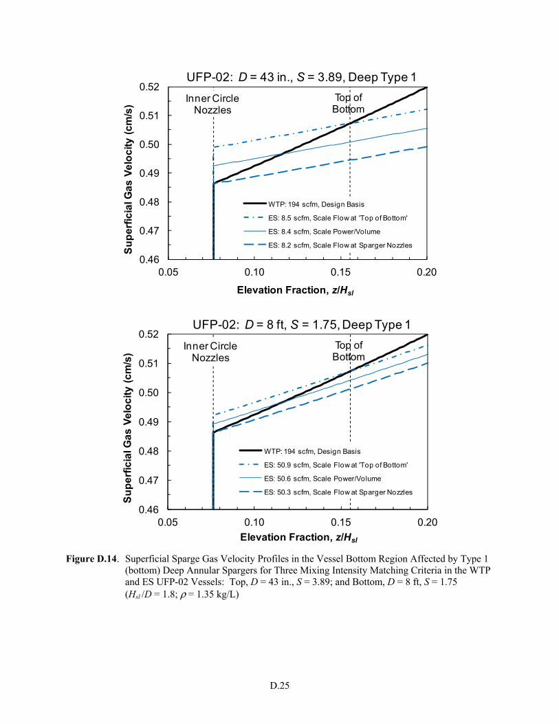
D.25

Top of Bottom

Inner Circle Nozzles

0.46

0.47

0.48

0.49

0.50

0.51

0.52

0.05 0.10 0.15 0.20

Su

pe

rfic

ial G

as

Ve

loc

ity

(c

m/s

)

Elevation Fraction, z/Hsl

UFP-02: D = 43 in., S = 3.89, Deep Type 1

WTP: 194 scfm, Design Basis

ES: 8.5 scfm, Scale Flow at 'Top of Bottom'

ES: 8.4 scfm, Scale Power/Volume

ES: 8.2 scfm, Scale Flow at Sparger Nozzles

Top of Bottom

Inner Circle Nozzles

0.46

0.47

0.48

0.49

0.50

0.51

0.52

0.05 0.10 0.15 0.20

Su

pe

rfic

ial G

as

Ve

loc

ity

(c

m/s

)

Elevation Fraction, z/Hsl

UFP-02: D = 8 ft, S = 1.75, Deep Type 1

WTP: 194 scfm, Design Basis

ES: 50.9 scfm, Scale Flow at 'Top of Bottom'

ES: 50.6 scfm, Scale Power/Volume

ES: 50.3 scfm, Scale Flow at Sparger Nozzles

Figure D.14. Superficial Sparge Gas Velocity Profiles in the Vessel Bottom Region Affected by Type 1 (bottom) Deep Annular Spargers for Three Mixing Intensity Matching Criteria in the WTP and ES UFP-02 Vessels: Top, D = 43 in., S = 3.89; and Bottom, D = 8 ft, S = 1.75 (Hsl /D = 1.8; ρ = 1.35 kg/L)

D.26

D.3.2 Comparison of Air Sparger Bubble Power and PJM Power

The relative magnitude of PJM and air sparger mixing effects is another consideration for assessing the importance of spargers to establishing a representative environment for bottom motion testing. One metric is the power dissipated per unit volume (specific power), which can be used to compare spargers and PJMs within a vessel and for vessels of different geometric scale. For comparing the sparger and PJM mixing “magnitude” in a given vessel, in which the normalizing volume (e.g., total slurry volume) is equal, the absolute power can be used instead of power/volume.

The power per PJM cycle dissipated in slurry for NJ PJMs operating at Un nozzle velocity is given by

2 31 1

2 2PJM n J J n n JP U Q N DC U A N DCρ ρ= = (D.11)

The volumetric flow rate during the drive phase, QJ, is written as the product of Un and the PJM nozzle cross-sectional area, An, in the right-hand form of the equation. Excluding the PJM duty cycle (DC = drive time/cycle time), Equation (D.11) would give the power during the drive phase of the cycle only. Including the DC multiplier, the PJM power is effectively normalized over the entire PJM cycle time. Therefore, it can be compared to the continuous air sparger power resulting from bubble expansion. Sparger bubble power-per-unit volume is shown in integral form in Equation (D.2), and the PbV solution for bubble expansion from sparger nozzle depth (a distance H below the surface, zsp = 0) to an elevation ∆z above the nozzles is given in Equation (D.5). Multiplying these equations by volume (or simply excluding the volume divisor from the development), gives the bubble power, Pb, continuously dissipated in slurry during bubble transit:

( )

Δ−+

+=

zHgP

gHPPQP

a

aastdb ρ

ρln

(D.12)

Equation (D.12) is applied separately to each sparger type, since H, ∆z, and Qstd vary by type.

Consider WTP HLP-27 as an example, assuming a slurry density of 1350 kg/m3, a fill level of 1.1 Hsl/D (27.5 ft = 8.38 m depth; ~360 m3 of slurry), and headspace pressure of 1 atm (101,325 Pa). The total standard air flow rate to all deep annular spargers types 1, 2, and 3 is 1102 scfm (0.520 m3/s). The calculated power of bubbles rising from these spargers in the bottom region of the vessel to an elevation of ~77-in. (1.96-m) above tank bottom center (see Figure D.11) is 3860 W, and for transit of these bubbles to the slurry surface, the total power dissipated is ~36,000 W. Therefore, less than 11 percent of the sparger power is dissipated in the defined bottom region. The PJM power computed from Equation (D.11) for eight PJMs in HLP-27 operating at 12 m/s through 4-in. nozzles (0.0081 m2 cross-sectional area), and a DC of 0.14 is 10,600 W. The total sparger power in the vessel, a consideration for tank blending, is more than three times the PJM power. However, in the bottom of the vessel, the sparger power is a fraction of the PJM power, ~36 percent in the example given. This is a significant fraction, and therefore, sparger influence in the bottom region should not be neglected. To achieve equivalent specific bubble power (power-per-unit volume) in the bottom of the WTP and ES HLP-27 vessels, one would scale the flow rates per the discussion above of Figures D.12, D.13, and D.14.

D.27

D.3.3 Volume Fraction Swept by Sparged Bubbles

As noted above, another metric to establish the proper environment for bottom motion testing is the volume fraction of the non-Newtonian slurry in the vessel bottom that is sheared by continuous operation of the spargers. For simplicity, this will be defined as a primary sheared volume that is directly in the path of rising bubbles and a secondary sheared volume that is the entrained fluid volume due to bubble motion. The latter is more difficult to quantify and is currently outside the scope of this analysis. We focus here on the primary or minimum volume sheared by spargers, which is defined as the volume in the vertical track of expanding bubbles from nozzle depth to the “top of the bottom” region.

Defining the bubble volume affected in absolute terms also is challenging. It requires an understanding of the initial bubble volume as it parts from the sparger nozzle, which is a strong function of flow rate as well as nozzle diameter and fluid properties, and a number of simplifying assumptions on the shape of bubbles (e.g., spherical instead of oblate spheroid or spherical caps) and non-physical limitations on bubble coalescence and break up in their rise through the bottom region. However, modeling how the primary bubble region volume fraction scales with vessel size is more straightforward. Two approaches are considered. The first approach uses the air sparger ROB empirical model, and in the second approach, literature models for initial bubble volume are coupled with bubble expansion as a function of elevation to compute affected volume.

D.3.3.1 Bubble Volume Fraction from the ROB Empirical Model

As a starting point, consider the established model for the sparger region of bubbles given by Equation (D.6a). It specifies the diameter of ROB measured at the slurry surface in terms of the sparge air volumetric flow rate at nozzle depth (i.e., Q at zsp/H = 0 in acfm, not scfm), and has an approximate functional form of DROB ∝ Q1/3. Assuming that the ROB has the same functional form in the bottom of the vessel, the projected area of the ROB, varies with Q to the two-thirds power, AROB ∝ Q2/3. When matching U* at nozzle depth, as discussed above, Q at zsp/H = 0 scales with the vessel area, 1/S2. Therefore, AROB is proportional to S-4/3. This is consistent with the scaling for the sparger number and layout in the PEP UFP-02 vessel (Kuhn et al. 2008), and it is the basis of reduced sparge air flow rates in ES vessels to match ZOI coverage area fraction (e.g., Figures D.9 and D.10). The volume of ROB in the bottom region is proportional to the elevation through which the bubbles rise, ∆z, which scales as 1/S. The volume of ROB is VROB = AROB • ∆z, and it scales as S-7/3. Because the slurry volume in the vessel bottom, Vbot, scales as S-3, the volume fraction of slurry sheared in the primary bubble track (=VROB/Vbot) of a single sparge tube is not equal in scaled vessels when the sparge gas superficial velocity at nozzle depth is matched.

Instead of imposing superficial velocity matching at sparger nozzle depth or power/volume matching in the bottom region to establish the air sparger flow rate, one can estimate the flow rate to achieve equal bottom region bubble volume fractions in vessels at two scales. As above, assume that the projected area of the ROB from a single sparge point varies approximately as AROB ∝ Q2/3 from Equation (D.6a),1 and the volume of the ROB is VROB = AROB • ∆z. The total volume of the bubble region resulting from operation of type m spargers (having a characteristic nozzle depth and flow rate per tube, Qm) is simply the number

1 Per Equation (D.6a), ROB area would scale as Q0.68 instead of the approximate integer form used here, Q2/3.

D.28

of the spargers, nm, multiplied by the volume of an individual ROB. The bubble region volume fraction in the bottom of the vessel because of type m spargers, fv,m, is then given by

2

3/2

2

3/2

,L

Qn

zL

zQn

V

Vnf mmmm

bot

ROBmmv ∝

ΔΔ

∝= (D.13)

where L is a geometrically scaled vessel length (LWTP/LES = S), and the bottom volume is proportional to L3 or L2∆z. Therefore, to achieve an equivalent bubble volume fraction in WTP and ES vessels, the number of spargers and the flow rate per sparge tube must satisfy the equality

( ) 2

3/2,,

2

3/2,,3/2

,,S

Qn

LL

QnQn WTPmWTPm

ESWTP

WTPmWTPmESmESm ==

(D.14)

or

3

,2/3

,,

2/3,

S

QnQn WTPmWTPm

ESmESm =

It is apparent in the second form of Equation (D.14) that the flow rate per tube (at nozzle depth) scales volumetrically for an identical number of spargers in the two vessels when matching the bubble volume fraction derived from the empirical ROB coverage expression (Equation (D.6a)). The air flow rate per tube varies by area when matching superficial velocity at nozzle depth (i.e., nm,ESQm,ES = nm,WTPQm,WTPS-2). Substituting this U* matching flow rate requirement into Equation (D.14) and rearranging gives the number of spargers needed in the ES vessel to simultaneously satisfy the bubble volume fraction and superficial velocity matching criteria,

2

,,−= Snn WTPmESm (D.15)

Substituting Equation (D.15) into Equation (D.14), one also notes that the flow rate per sparge tube is equal in the WTP and ES vessels (Qm,ES = Qm,WTP) in this case. However, the number of spargers given by Equation (D.15) is impractical, especially for small-scale vessels. For example, there are 14 type 1 deep annular spargers in WTP HLP-27; for 43-in.-, 8-ft-, and 14-ft-diameter scaled vessels (S = 6.94, 3.125, and 1.79, respectively), the calculated number of spargers are 0.3, 1.4, and 4.4, respectively. Of course, fractional spargers are meaningless, but even rounding up to whole numbers of spargers, the maximum number (4.4 rounded to 5) is still fewer than the number of outer PJMs in the vessel (7). Therefore, it would not be possible to distribute the deep annular spargers symmetrically with respect to the PJMs that the spargers supplement. In conclusion, simultaneously achieving comparable air sparger bubble power and sheared bubble volume fractions is not feasible.

Solving Equation (D.14) for the flow rate per sparger as a function of number of spargers in the ES vessel and multiplying by nm,ES gives the total flow rate (actual, at nozzle depth) to type m deep annular spargers needed to obtain a WTP-vessel equivalent VROB-based bubble volume fraction. The results of such calculations for the 43-in.-diameter ES HLP-27 vessel are nearly identical to the flow rates obtained from ZOI area matching criteria and shown in Figures D.9 and D.10. The reason for this is the ROB and ZOI diameters vary with Q0.34 per Equations (D.6a) and (D.6b), and the projected area of each

D.29

varies as Q0.68. The results of Figures D.9 and D.10 and solutions to Equation (D.14) would be exactly the same, except that the exponent on Q used in the ROB-based volume fraction was defined as 1/3 instead of 0.34 for expedience. For comparison, Figure D.10 also shows the total flow rate Q to match the superficial velocity at nozzle depth. When the numbers of spargers are equal in the ES and WTP vessels (e.g., 14 type 1 and 14 type 2&3 combined in HLP-27), the total supplied air to all deep spargers in the fv,m matching case is roughly a factor of S smaller than the U* matching case due to ~1/S3 versus ~1/S2 scaling of Q.

D.3.3.2 Bubble Volume Fraction from Initial Bubble Volume Models

In this section, literature models for initial bubble volume are coupled with bubble expansion as a function of elevation to estimate the volume fraction in the bottom of the vessel sheared in the path of rising bubbles. The development is somewhat analogous to that for the ROB-based volume fraction in the previous section. For the purposes of this analysis, the complex and incompletely understood subjects of initial bubble volume, bubble shape changes, and bubble coalescence and breakup during formation and transit are simplified greatly. First, it is assumed that the initial bubble volume, Vb0, for bubbles formed at submerged circular orifices (e.g., WTP sparge tube nozzles) is given by a function of the form

5/35/6

0−= gCQVb (D.16)

where Q is the volumetric flow rate at the injection point and C is a dimensionless coefficient. Summarizing the work of Davidson and Schüler (1960), Kumar and Kuloor (1970), and others, Badam et al. (2007) note that a number of simple, one-stage bubble formation models have initial volume correlations of the form shown in Equation (D.16), where C has a value between 0.976 and 1.378. Wraith (1971) presented a two-stage bubble formation and release model that also is given by this equation; the data for air injection into water through a single orifice (0.63 to 1.91 cm diameter) from ~0.3 L/s to ~12.5 L/s were well correlated with C = 1.090. Acharya et al. (1978) reported that bubble sizes in shear-thinning and viscoelastic non-Newtonian polymer solutions also were correlated by Equation (D.16) using C = 0.976 (per Kumar and Kuloor 1970) for injection rates greater than ~1 mL/s (measured up to ~60 mL/s). However, it should be noted that in all these studies gas was injected upwards through orifices into fluid reservoirs, whereas the sparge tube nozzles in the WTP vessels face downward. Further, orifices were smaller than the WTP sparge tube diameters (2 in. = 5 cm), and the WTP slurry rheological and other physical properties are significantly different.

Nonetheless, because the present goal is to understand how bubble volume scales with vessel size and sparger flow rate, not to determine bubble volumes absolutely, Equation (D.16) seems to be a reasonable basis, assuming that C is constant regardless of its value. Additional simplifying assumptions include: 1) bubbles are spherical from inception and throughout the rise; 2) there is no bubble coalescence or breakup throughout the vessel bottom region; 3) initial bubble size is independent of sparge tube nozzle diameter and nozzle velocity; 4) air bubbles are ideal and growth is governed by changes in absolute pressure with elevation (as is sparge gas volumetric flow rate, Equation (D.4)); and 5) bubble rise is perfectly vertical. Subject to these assumptions, the minimum volume of slurry in the bottom swept by

D.30

rising bubbles from a single sparger, Vb,min, is the projected area of the spherical bubble, Abz, integrated over the elevation z from sparger nozzle depth to the top of the bottom region.1

==z

bz

z

zbzb dzAdzAV

0min,

0 (D.17)

The bubble diameter, Dbz, and projected area are elevation dependent, as is the bubble volume, Vbz, from which they are calculated. In terms of the initial spherical bubble volume Vb0 at nozzle depth and pressure (zsp = 0, P0), the elevation-dependent bubble volume at reduced pressure Pz is

( ) 000

ba

ab

zbz V

zHgP

gHPV

P

PV

−++

==ρ

ρ

(D.18)

Here again, Pa is the ambient pressure at the upper slurry surface and H is the sparge tube nozzle depth (which varies by type, location, etc.). The projected spherical bubble area, diameter, and volume are related by, Abz = π(Dbz /2)2 = π1/3(3Vbz/4)2/3. Substituting for Abz in Equation (D.17) in terms of Vbz and Vb0 (Equations (D.18) and (D.16)) gives

( ) ( )

−+

+

= − z

aab dz

zHgPgHP

CgQV

0

3/23/2

3/23/15/25/4

min,

1

4

3

ρρπ

(D.19)

Note that this minimum volume of the bubble track through the bottom scales as Q4/5, whereas the affected slurry volume in terms of ROB scales approximately as Q2/3 (see above, e.g., Equation (D.13)). The further dependence of Vb,min on vessel scale is not particularly intuitive by inspection of Equation (D.19), because both H and z in the pressure terms are functions of S.

The complexity of Equation (D.19) arises because the bubble volume depends on absolute pressure, not just the hydrostatic pressure component, and gas volume is inversely proportional to pressure. Therefore, the volume varies non-linearly with elevation. This is noted, for example, in the curvature of the superficial velocity profiles over the whole sparge tube depth shown in Figure D.5. The non-linear effect is more pronounced near the slurry surface when the hydrostatic pressure becomes less significant. Near the bottom of the vessel, and over limited elevation changes, the volume is essentially linear with z, as shown in the bottom region superficial velocity profiles, Figures D.12 and D.14. Therefore, to a first approximation, it is reasonable to assume that bubble volume varies linearly from bottom to top of the vessel bottom region. An average bubble volume in the bottom region can be used to calculate the average bubble diameter and projected area, for the purpose of estimating the volume of slurry swept by rising bubbles instead of the “exact” solution given by Equation (D.19). The average bubble volume

1 For the purposes of example only, the initial bubble volumes and corresponding spherical diameters for the three WTP HLP-27 deep annular sparger types were calculated from Equation (D.16) using C = 1, an HLP-27 fill level of 1.1 Hsl/D, and slurry density of 1350 kg/m3. The initial bubble diameters were 5.5 in. (14 cm) for type 1 spargers, 3.1 in. (7.9 cm) for type 2 spargers, and 4.5 in. (11.5 cm) for type 3 spargers. At most, the bubbles expanded by 0.2 in. (<0.5 cm) in rising to the top of the bottom region using the calculation methods outlined here. For comparison, the ROB diameters calculated from Equation (D.6a) for the same vessel and sparger operating conditions were 34 in., 21 in., and 29 in. for type 1, 2, and 3 spargers, respectively. This supports the definition of the volume swept by bubbles derived from the initial bubble volume as a “minimum” value.

D.31

could be defined as the mean of Vb0 and Vbz evaluated at the top of the bottom region, or, to simplify further, it can be and is here defined as the bubble volume at mid-elevation, ∆z/2. Substituting ∆z/2 into Equation (D.18) and solving for the corresponding “average” projected bubble area gives

( )

3/20

3/2

3/12/, 24

3b

a

azb V

zHgP

gHPA

Δ−+

+

=

ρρπ

(D.20)

The approximate minimum volume of the bubble path using this mid-elevation average bubble volume approach is simply the projected area multiplied by the height of the bottom region affected, Vb,min,z/2 = Ab,z/2 * ∆z. Substituting Equation (D.20) and Equation (D.16) for Vb0 into this definition gives

( ) z

zHgP

gHPCgQV

a

azb Δ

Δ−+

+

= −

3/23/23/15/25/4

2/,, 24

3

ρρπmin

(D.21)

Comparing Equations (D.21) and (D.19), the flow rate dependence is identical, and the integral in Equation (D.19) is approximated as

( ) ( ) z

zHgPdz

zHgP a

z

a

Δ

Δ−+

≈

−+

3/2

0

3/2

2

11

ρρ (D.22)

Defining the bottom region of HLP-27 as shown in Figure D.11, the bracketed pressure ratio term in Equation (D.21) raised to the 2/3 power varies from <1.04 for S = 1 (WTP vessel) to <1.01 for S = 6.94 (43-in.-diameter ES vessel). Therefore, the dependence of the term on scale factor approaches S0 (=1), and the volume of the bubble path scales approximately as Q4/5∆z.

Analogous to the development of Equation (D.13), the total volume of the bubble region resulting from operation of type m spargers is simply the number of the spargers multiplied by the volume of an individual sparger bubble track, which is given precisely as Vb,min in Equation (D.19) or approximately as Vb,min,z/2 in Equation (D.21). The minimum bubble region volume fraction in the bottom of the vessel of volume Vbot due to type m spargers, fv,m,min, is thereby

bot

bm

bot

bmmv V

Vn

V

Vnf z/2min,min

min,,

,, ≈= (D.23)

Substituting the approximate bubble track volume from Equation (D.21) into Equation (D.23),

( ) 2

5/43/2

2

5/4,

,, 2 L

Qn

zHgP

gHP

zL

zQn

V

Vnf mm

a

amm

bot

bmmv ≈

−+

+Δ

Δ∝≈

ρρz/2min,

min (D.24)

Once again, the bottom volume of the vessel has been set proportional to L2∆z, where L is a geometrically scaled vessel length. The right-hand form of Equation (D.24) uses the near S0 dependence

D.32

of the pressure ratio term, as noted above. Using this simplest form to express the scaling of the minimum bubble volume fraction in WTP and ES vessels, the number of spargers and the flow rate per sparge tube must satisfy the equality

( ) 2

5/4,,

2

5/4,,5/4

,,S

Qn

LL

QnQn WTPmWTPm

ESWTP

WTPmWTPmESmESm ==

(D.25)

or

2/5

,4/5

,,

4/5,

S

QnQn WTPmWTPm

ESmESm =

The second form of Equation (D.25) shows that the flow rate per tube (at nozzle depth) scales as 1/S2.5 for an equal number of spargers in the two vessels when matching the minimum bubble volume fraction derived from expanding spherical bubbles from an initial volume given by Equation (D.16). The ES flow rates calculated from Equation (D.25), or more generally, by equating fv,m,min at two vessel scales using any of the forms shown in Equations (D.23) and (D.24), are between those obtained for U* matching at nozzle depth (1/S2 scaling of Q total) and fv,m matching based on ROB areas (1/S3 scaling of Q for an equal number of sparge tubes, Equation (D.14)). This is shown in Figure D.12 for the 1/6.94 ES HLP-27 vessel. Total air flow rates to all spargers of a given type are shown as a function of the number of spargers used in the ES vessel for type 1 and combined type 2&3 deep annular spargers. In the WTP vessel, there are 14 type 1 spargers and 14 combined type 2&3 spargers (i.e., 7 type 2 + 7 type 3). When the number of spargers are equal in the ES and WTP vessels, the total supplied air in the fv,m,min matching case is a factor of S1/2 smaller than the U* matching case because of ~1/S5/2 versus ~1/S2 scaling of Q, and as noted above, Q total is a factor of S smaller than the U* value for bubble volume fraction matching based on ROB coverage (fv,m). Note also that the sum of the U* matching flow rates for type 1 (8.1 acfm) and type 2&3 (3.5 acfm) spargers shown in Figure D.15 is the same as that shown for all deep sparger types (11.6 acfm) in Figure D.10.

D.3.4 Summary and Recommendations for Sparger Operations in Bottom Motion Studies

Our assessment of the relative sparger-to-PJM-mixing magnitude suggests that sparger effects could be moderately significant in bottom motion studies. However, because there is uncertainty in the importance of spargers, early tests to determine the impact of spargers on bottom motion are recommended for non-Newtonian vessel investigations. These screening tests could be run at extremes in sparge air flow rates: at the low end, spargers would turned off, and at the high end, for example, sparger flow rates would be set to match power-per-unit volume for overall vessel mixing (Sections D.2.1 and D.2.4). The latter is higher than would be recommended for “representative” bottom motion studies (Section D.3.1 and below). Another option that could be investigated for achieving representative conditions for both bottom motion and overall vessel mixing would be to deploy spargers at multiple elevations. For example, flow rates to the deep annular spargers would be set for bottom motion effect, and a second set of spargers would be located above the bottom region with air flow rates established to make the total bubble power-per-unit volume in the ES vessel equal to that in the WTP vessel (see Section D.2.2). The need for the added complexity of multi-elevation spargers might be clarified by the screening tests outlined above.

D.33

0

2

4

6

8

10

0 7 14

To

tal A

ir F

low

Ra

te (

ac

fm)

Number of Spargers

HLP-27, D= 43 in., Deep Type 1 Spargers

Match U* at Nozzle Depth

Match Initial Bubble Vol Fraction

Match ROB Bubble Vol Fraction

~1/S2 Scaling of Q

0

1

2

3

4

0 7 14

To

tal A

ir F

low

Ra

te (

ac

fm)

Number of Spargers

HLP-27, D= 43 in., Deep Type 2&3 Spargers

Match U* at Nozzle Depth

Match Initial Bubble Vol Fraction

Match ROB Bubble Vol Fraction

~1/S2 Scaling of Q

Figure D.15. Total Actual Sparge Air Flow Rate at Nozzle Depth for Type 1 (upper) and Type 2&3 (lower) Deep Annular Spargers of the 1/6.94 Engineering-Scale (43-in.-diameter) HLP-27 Vessel to Reproduce Bottom Region Effects of the WTP Vessel Using Three Scaling Approaches. Results are shown as a function of the number of spargers in the ES vessel.

For spatial (lateral) distribution of air spargers, it is recommended that the minimum number of

bottom air spargers be a multiple of the number of outer PJMs in the vessel to provide symmetry (i.e., five in UFP-02 and seven in HLP-27). In HLP-27, 14 spargers is the minimum number recommended to provide representative areal coverage of the type 1 outer and combined type 2&3 inner spargers. For bottom motion studies, it may be advisable to have the full complement of bottom spargers installed in the ES vessels (i.e., 10 in UFP-02 and 28 in HLP-27). For greatest benefit and flexibility, it

D.34

would be preferable to have these spargers in groups equal to the number of outer PJMs with each group controlled separately. This configuration would allow fewer spargers to be run if necessary or so desired while still maintaining symmetry. For example, the 14 type 1 spargers in HLP-27 could be controlled as two interspersed groups of 7 so that only 7 of 14 spargers could be run at a given time. (This could be accomplished with a single controller and a header/valve system to stop flow to half the spargers.)

One of the goals of the screening experiments noted above is to shed light on how critical air sparger flow rates are to establishing a representative environment for bottom motion testing. The preliminary tests would be run at flow rate extremes, whereas the bottom motion tests would be run at “nominal” flow rates. However, the various flow rate-scaling approaches described in this section suggest that there is a significant range of justifiable flow rates that would provide representative conditions. At the upper end of the nominal range are flow rates based on matching sparger mixing intensity in the bottom of the vessel. These include matching the WTP vessel gas superficial velocity at either nozzle depth or the top of the bottom region and matching the bubble power-per-unit volume in the bottom region. Matching U* at the top of the bottom region is dismissed because relatively greater bubble power is imparted in the ES vessels. Matching the specific bubble power requires a total air flow rate intermediate of the other two approaches and results in U* matching in the middle of the region. However, the difference in flow rates for matching U* at nozzle depth and power-per-unit volume in the bottom region is at most 4 percent in the 43-in.-diameter HLP-27 ES vessel, and the difference is less with increasing ES vessel size and lower in UFP-02 at all scales. For this reason and given the uncertainty in the definition of the vertical extent of the “bottom,” bottom-region air sparger flow rates based on matching U* at sparger nozzle depth are recommended for the nominal (and high end) operating conditions for most bottom motion studies. The flow rates based on U* and power-per-unit volume in ES vessels all scale approximately as 1/S2, and the total air flow rate to the spargers is independent of the number of spargers used (i.e., the flow rate per sparge tube is adjusted to achieve the target total Q).

Scaling approaches to maintain the volume fraction of the bottom region sheared by bubbles in vessels of different size results in reduced total air flow rates and flow rates per sparge tube that vary with the number of spargers used. If an equal number of spargers are used in the WTP and ES vessels, then the total flow rate to all bottom spargers scales as 1/S2.5 for bubble track volume fractions based on calculated initial bubble sizes and bubble expansion, and it scales as ~1/S3 if the volume fraction is based on the region of bubbles empirical expression (Equation (D.6a)). The ROB flow rate scaling approach also provides for equal sparger ZOI coverage in vessels of different size. However, the sparger ROB and ZOI correlations were developed from observations at the slurry surface; therefore, the dependence of the ROB size on flow rate does not necessarily translate to the bottom region of the vessel (the magnitude of ROB is certainly less there). On the other hand, while the initial bubble volume approach has a literature pedigree for the correlation used, the WTP and ES vessel operating conditions are relatively unique, and a number of simplifying assumptions were made to develop the bubble volume fraction scaling model. Given that both approaches have limitations, and in the interest of testing at extremes, the ROB based flow rates are the lowest nominal values recommended for bottom motion studies.

Figure D.16 summarizes the approximate range of total air sparger flow rates to all deep spargers1 recommended for bottom motion studies in the ES HLP-27 and UFP-02 vessels under nominal slurry fill level and density conditions. Results are shown as a function of vessel size from WTP full scale (S = 1) to vessels smaller than the smallest LSIT vessel diameter (43 in.; S = 6.94 in HLP-27 and S = 3.89 in 1 The per sparge tube flow rate is the total standard flow rate shown divided by the number of deep spargers used.

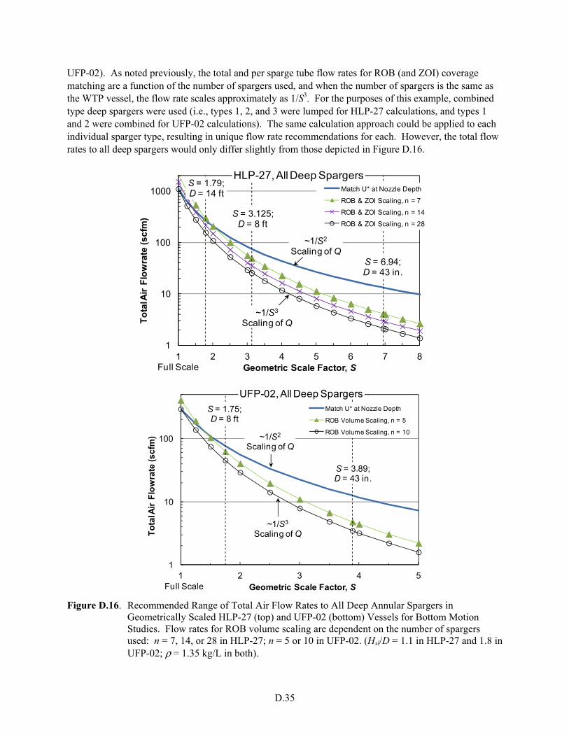
D.35

UFP-02). As noted previously, the total and per sparge tube flow rates for ROB (and ZOI) coverage matching are a function of the number of spargers used, and when the number of spargers is the same as the WTP vessel, the flow rate scales approximately as 1/S3. For the purposes of this example, combined type deep spargers were used (i.e., types 1, 2, and 3 were lumped for HLP-27 calculations, and types 1 and 2 were combined for UFP-02 calculations). The same calculation approach could be applied to each individual sparger type, resulting in unique flow rate recommendations for each. However, the total flow rates to all deep spargers would only differ slightly from those depicted in Figure D.16.

S = 6.94;D = 43 in.

S = 3.125;D = 8 ft

S = 1.79;D = 14 ft

1

10

100

1000

1 2 3 4 5 6 7 8

To

tal A

ir F

low

rate

(s

cfm

)

Geometric Scale Factor, S

HLP-27, All Deep SpargersMatch U* at Nozzle Depth

ROB & ZOI Scaling, n = 7

ROB & ZOI Scaling, n = 14

ROB & ZOI Scaling, n = 28

~1/S2

Scaling of Q

~1/S3

Scaling of Q

Full Scale

S = 3.89;D = 43 in.

S = 1.75;D = 8 ft

1

10

100

1 2 3 4 5

To

tal A

ir F

low

rate

(s

cfm

)

Geometric Scale Factor, S

UFP-02, All Deep SpargersMatch U* at Nozzle Depth

ROB Volume Scaling, n = 5

ROB Volume Scaling, n = 10

Full Scale

~1/S2

Scaling of Q

~1/S3

Scaling of Q

Figure D.16. Recommended Range of Total Air Flow Rates to All Deep Annular Spargers in Geometrically Scaled HLP-27 (top) and UFP-02 (bottom) Vessels for Bottom Motion Studies. Flow rates for ROB volume scaling are dependent on the number of spargers used: n = 7, 14, or 28 in HLP-27; n = 5 or 10 in UFP-02. (Hsl/D = 1.1 in HLP-27 and 1.8 in UFP-02; ρ = 1.35 kg/L in both).

D.36

Recommendations for scaling steam ring purge air flow rates for bottom motion studies are discussed further in Section 7.2.2.2. The steam rings are relatively high in the WTP UFP-01 and WTP UFP-02 vessels (e.g., a minimum of >3 ft from the bottom head and 8 ft from tank bottom center in WTP UFP-01) compared to dedicated air sparger nozzles located ~6 in. from the bottom head. Therefore, steam ring purge air is much less likely to directly shear slurry in the bottom region of the vessel. Because of these differences, the low-bound flow rate recommendation for steam ring purge air scaling is not based on matching the bubble volume fraction in the bottom region as it is for dedicated air spargers. Instead, having steam ring purge air turned off defines the minimum flow rate for bottom motion studies. Note that no air flow is equivalent to that recommended for dedicated air spargers in screening tests, but is less than the low-bound flow rate recommended for dedicated spargers to create representative test conditions. On the other hand, the primary recommendation for scaling nominal (and upper-bound) air flow rates for both steam rings and dedicated air spargers in bottom motion studies in ES vessels is to match the WTP

superficial gas velocity at nozzle depth ( *0U ). To scale standard air flow rates to meet this criterion in

geometrically scaled vessels, Equation (7.4), Section 7.2.2.2, is equally applicable to dedicated air spargers and steam ring purge air (subject to the simplifying assumptions of Section 7.2.2.1, which can be generalized to either air source).

D.4 References

Acharya A, RA Mashelkar, and JJ Ulbrecht. 1978. “Bubble Formation in Non-Newtonian Liquids.” Industrial & Engineering Chemistry Fundamentals 17(3):230-232.

Badam VK, V Buwa, and F Durst. 2007. “Experimental Investigations of Regimes of Bubble Formation on Submerged Orifices Under Constant Flow Condition.” The Canadian Journal of Chemical Engineering 85(3):257-267.

Davidson JF and BOG Schüler. 1960. “Bubble Formation at an Orifice in an Inviscid Liquid.” Transactions of the Institute of Chemical Engineers 38:335-342.

Kuhn WL, ST Arm, JL Huckaby, DE Kurath, and SD Rassat. 2008. Technical Basis for Scaling Relationships for the Pretreatment Engineering Platform. PNNL-16948; WTP-RPT-160, Rev. 0, Pacific Northwest National Laboratory, Richland, Washington.

Kumar R and NR Kuloor. 1970. “The Formation of Bubbles and Drops.” Advances in Chemical Engineering Vol. 8, TB Drew, GR Cokelet, JW Hoopes, Jr., and T Vermeulen (eds.), pp. 255-368. Academic Press, New York.

Poloski AP, ST Arm, JA Bamberger, B Barnett, R Brown, BJ Cook, CW Enderlin, MS Fountain, M Friedrich, BG Fritz, RP Mueller, F Nigl, Y Onishi, LA Schienbein, LA Snow, S Tzemos, M White, and JA Vucelick. 2005. Technical Basis for Scaling of Air Sparging Systems for Mixing in Non-Newtonian Slurries. PNWD-3541; WTP-RPT-129, Rev. 0, Battelle–Pacific Northwest Division, Richland, Washington.

Wraith AE. 1971. “Two Stage Bubble Growth at a Submerged Plate Orifice.” Chemical Engineering Science 26(10):1659-1671.

D.37

References Not Publicly Available

Claghorn R and P Waddell. 2007. System Description for Pulse Jet Mixers and Supplemental Mixing Subsystems. 24590-WTP-3YD-50-00003, Rev. B, Bechtel National, Inc., Richland, Washington.

Rassat SD. 2010. Guidance on the Scaling and Operation of Air Spargers for the Proposed Engineering-Scale HLP-27 Test Vessel. WTP/RPP-MOA-PNNL-00508, Pacific Northwest National Laboratory, Richland, Washington.

Appendix E –

Working Paper for the Technical Basis to Assess the Prevent Plugging Requirement Associated with Pump Out

E.iii

Acronyms and Abbreviations

BNI Bechtel National, Inc.

CFD computational fluid dynamics

HLP high-level process (tank)

LSIT Large Scale Integrated Testing

LOAM low order accumulation model

M1 expert flowsheet review team technical issue M1 – Plugging of Pipelines during Slurry Transport

M3 expert flowsheet review team technical issue M3 – Inadequate Design of Mixing Systems – Pulse Jet Mixers

NPSH net positive suction head

NPSHA net positive suction head available

NPSHR net positive suction head required

PJM pulse jet mixer

PSDD particle size and density distribution

RFD reverse flow diverter

RLD radioactive liquid-waste disposal (tank)

rms root mean square

ss steady state

UFP ultrafiltration process (tank)

WTP Hanford Waste Treatment and Immobilization Plant

Symbols

Ar particle Archimedes number: ratio of gravitational to drag force

Bi Bingham number

CD particle drag coefficient

DC duty cycle, tD/tC

dS diameter of solids particulate

DT diameter of tube, pipe, or transfer line

d50 representative diameter of solid particulate for a size distribution in which 50 percent of the particles by weight have a diameter greater than d50

d% percent deviation

%d average of the absolute values of the deviation

Frp particle Froude number

FrT tube or pipe Froude number

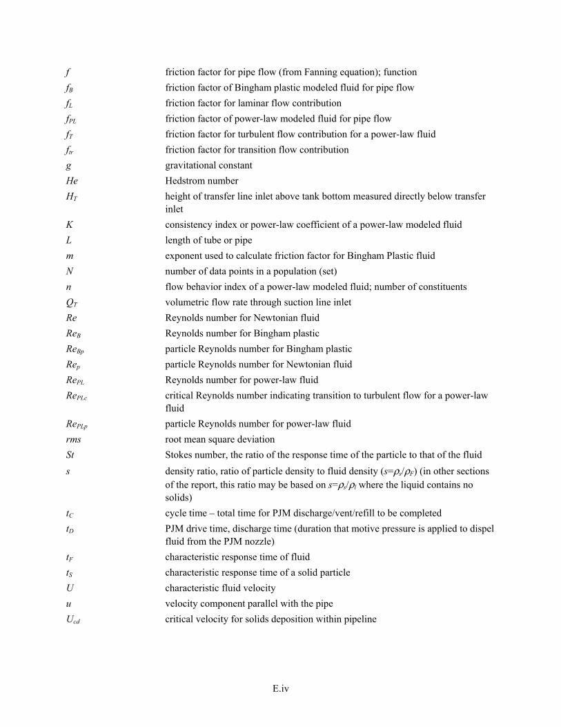
E.iv

f friction factor for pipe flow (from Fanning equation); function

fB friction factor of Bingham plastic modeled fluid for pipe flow

fL friction factor for laminar flow contribution

fPL friction factor of power-law modeled fluid for pipe flow

fT friction factor for turbulent flow contribution for a power-law fluid

ftr friction factor for transition flow contribution

g gravitational constant

He Hedstrom number

HT height of transfer line inlet above tank bottom measured directly below transfer inlet

K consistency index or power-law coefficient of a power-law modeled fluid

L length of tube or pipe

m exponent used to calculate friction factor for Bingham Plastic fluid

N number of data points in a population (set)

n flow behavior index of a power-law modeled fluid; number of constituents

QT volumetric flow rate through suction line inlet

Re Reynolds number for Newtonian fluid

ReB Reynolds number for Bingham plastic

ReBp particle Reynolds number for Bingham plastic

Rep particle Reynolds number for Newtonian fluid

RePL Reynolds number for power-law fluid

RePLc critical Reynolds number indicating transition to turbulent flow for a power-law fluid

RePLp particle Reynolds number for power-law fluid

rms root mean square deviation

St Stokes number, the ratio of the response time of the particle to that of the fluid

s density ratio, ratio of particle density to fluid density (s=ρs/ρF) (in other sections of the report, this ratio may be based on s=ρs/ρl where the liquid contains no solids)

tC cycle time – total time for PJM discharge/vent/refill to be completed

tD PJM drive time, discharge time (duration that motive pressure is applied to dispel fluid from the PJM nozzle)

tF characteristic response time of fluid

tS characteristic response time of a solid particle

U characteristic fluid velocity

u velocity component parallel with the pipe

Ucd critical velocity for solids deposition within pipeline

E.v

Ucd(calc) predictions of critical velocity for solids deposition within pipeline obtained with Equation (E.8) (Turian et al. 1987) for comparison to experimental data points Ucd(exp) identified in Turian et al. (1987)

Ucd(exp) critical velocity for solids deposition within pipeline obtained from data points identified in Turian et al. (1987)

Ucd-WTP critical depostion velocity for WTP obtained from model

UD-WTP the specified WTP design velocity for the transfer line of the vessel being evaluated

UF fluid velocity

Uh hindered settling velocity for the solids

Um volumetric average slurry/mixture velocity

Ur relative or “slip” velocity between the fluid and solids (Ur = UF – US)

Ur0 dimensionless single-particle slip velocity (Ur0 = Ur/U)

US solids or particle velocity

UT unhindered terminal settling velocity

U* velocity used for applying to models to assess WTP conditions

xh hindered settling factor which corresponds to the fractino of turbulent eddies withvelocities exceeding Uh

XΔP dimensionless solids contribution to the pressure drop resulting from solids flow

XΔP 0 dimensionless solids contribution pressure drop for solids concentration < 0.25

Y dimensionless parameter for the ratio of forces due to yield stress and gravity acting on a sphere in a visco-plastic fluid

y direction perpendicular to the pipe

ZB correction to Stokes Law for Bingham plastic

ZPL1 dimensionless power-law parameter

ZPL2 dimensionless power-law parameter

Greek Symbols

α coefficient used to calculate friction factor for power-law fluid

β coefficient used to calculate friction factor for Bingham plastic fluid

Δ difference between RePL and RePLc

ΔP pressure drop

ΔPF pressure drop for the fluid component

ΔPm pressure drop for the total slurry

ΔPS pressure drop for the solid constituents

ΔU velocity difference associated with δl (i.e., the shear layer)

δl characteristic size of the fluid structure

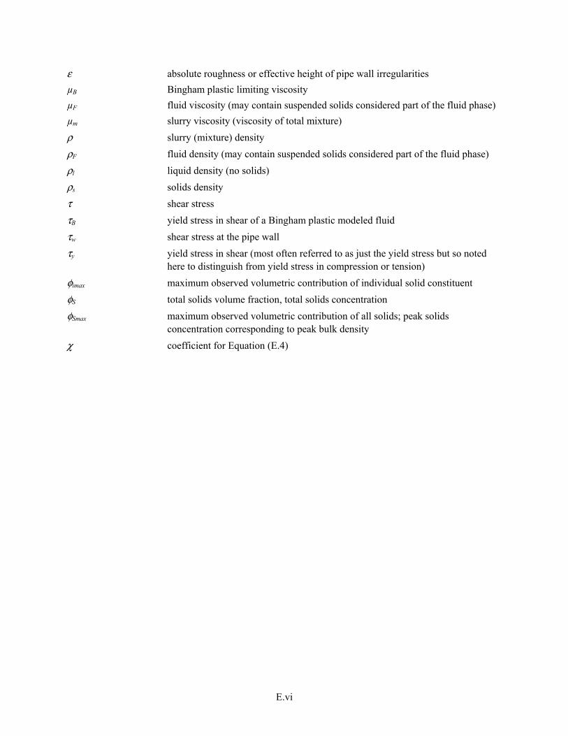
E.vi

ε absolute roughness or effective height of pipe wall irregularities

µB Bingham plastic limiting viscosity

µF fluid viscosity (may contain suspended solids considered part of the fluid phase)

µm slurry viscosity (viscosity of total mixture)

ρ slurry (mixture) density

ρF fluid density (may contain suspended solids considered part of the fluid phase)

ρl liquid density (no solids)

ρs solids density

τ shear stress

τB yield stress in shear of a Bingham plastic modeled fluid

τw shear stress at the pipe wall

τy yield stress in shear (most often referred to as just the yield stress but so noted here to distinguish from yield stress in compression or tension)

φimax maximum observed volumetric contribution of individual solid constituent

φS total solids volume fraction, total solids concentration

φSmax maximum observed volumetric contribution of all solids; peak solids concentration corresponding to peak bulk density

χ coefficient for Equation (E.4)

E.vii

Contents

Acronyms and Abbreviations ............................................................................................................... E.iii Symbols ................................................................................................................................................ E.iii Greek Symbols ...................................................................................................................................... E.v E.1 Introduction ................................................................................................................................. E.1 E.2 Transfer and Pump-Out Requirements Relative to PJM Mixing Requirements ......................... E.2

E.2.1 WTP Operations and Transfer Line Plugging Mechanisms Associated with Preventing Plugging ....................................................................................................... E.3

E.3 Assumptions and Phenomena Associated with Transfer and Pump Out .................................... E.10 E.3.1 Assumptions Applied to Assessment ............................................................................. E.11 E.3.2 Transfer Line Conditions and Relevant Parameters ....................................................... E.12 E.3.3 Summary of Pipeline Design Objectives and Guidelines .............................................. E.15

E.4 Transfer Line Scaling .................................................................................................................. E.16 E.5 Approach for Assessing Pipe Plugging in WTP Vessel Transfer Lines ..................................... E.17

E.5.1 Obtaining Non-Steady-State Conditions from Limit Solids Accumulation Tests ......... E.21 E.5.2 Obtaining Bounding Steady-State Conditions from LSIT Test Results ......................... E.22 E.5.3 Benchmarking of Predictive Models .............................................................................. E.24 E.5.4 Assessing WTP Performance ......................................................................................... E.25

E.6 Evaluation of Individual Failure Mechanisms ............................................................................ E.26 E.6.1 Evaluation of Plugging Due to Solids Deposition ......................................................... E.26 E.6.2 Evaluation of System Pressure Drop .............................................................................. E.30

E.6.2.1 Methodology for Determination of Pressure Drop for Multi-Constituent Slurry ............................................................................................................. E.32

E.6.3 Evaluation of Net Positive Suction Head ....................................................................... E.43 E.6.4 Pump Performance ......................................................................................................... E.44 E.6.5 Full-Scale Test Approach ............................................................................................... E.44

E.7 Considerations for Application of Approach .............................................................................. E.47 E.7.1 Test Setup Needs ............................................................................................................ E.47 E.7.2 Simulant Considerations ................................................................................................ E.48 E.7.3 Additional Considerations .............................................................................................. E.48

E.8 Summary and Recommendations ................................................................................................ E.49 E.9 References ................................................................................................................................... E.51

E.viii

Figures

E.1 Schematic Depicting WTP Vessel Mixing and Transfer Line Inlet Flow .................................. E.4 E.2 Instantaneous Slurry Density in Transfer Line versus Time During LOAM Test 1

Pump Out .................................................................................................................................... E.7 E.3 Instantaneous Slurry Density in Non-Scaled Transfer Line versus Time During LOAM

Test 1 Pump Out ......................................................................................................................... E.7 E.4 Instantaneous Slurry Density in Non-Scaled Transfer Line versus Time During LOAM

Test 1 Pump Out for a Single PJM Cycle ................................................................................... E.8 E.5 Schematic Depicting Particle Segregation That Can Occur Because of Variation in

Particle Concentration at the Inlet .............................................................................................. E.9 E.6 High-Level Steps Applied to Each Plugging Mechanism Being Assessed for the

Prevent Plugging Requirement ................................................................................................... E.18 E.7 Logic Diagram for Steady-State Testing to Benchmark Models ................................................ E.20 E.8 Flowchart of Integrated Tasks Used to Assess the Prevent Plugging Requirement ................... E.20

E.9 Molerus Diagram for Suspension Transport Correlating the Data for Ur0

s0.5 = fn Frps0.5,FrT2( ) ......... E.33

Tables

E.1 Newtonian Scaled Testing Target Vessel Pump Design Limits ................................................. E.3 E.2 Coefficient and Exponent Values for Oroskar and Turian (1980) and Turian et al. (1987)

Models Predicting Critical Velocity for Solids Deposition Presented in Equations (E.4) and (E.8) ..................................................................................................................................... E.29

E.3 Bounding Conditions of Data Sets Used to Determine Coefficients for Oroskar and Turian (1980) Turian et al. (1987) Models for Predicting Ucd .................................................... E.30

E.1

Appendix E

Working Paper for the Technical Basis to Assess the Prevent Plugging Requirement Associated with Pump Out

E.1 Introduction

The Prevent Plugging requirement developed for the mixing requirements (Mixing Requirement 2, Mauss and Papp 2010, p. 22) is closely coupled with the “M1 - Plugging in Process Piping” scope (Poloski et al. 2009a, 2009b). The design of the Hanford Waste Treatment and Immobilization Plant (WTP) vessel transfer lines has been completed with limited information of the actual tank wastes that will be processed. In addition, the condition (concentration and particle size and density distribution [PSDD]) of the feed stream entrained from the vessel bottom into the transfer line was unknown. Therefore, bounding conditions were prescribed by WTP to guide the design process. It is unclear whether increased understanding of the wastes will identify limits or changes in the requirements that are beyond those evaluated by the past M1 effort using the then WTP prescribed bounding conditions.

Solids in slurries will naturally settle (driven by gravitational forces) because of density differences between solid particles and the surrounding liquid unless rheological properties are sufficient to overcome the effects of gravity. The settling rate is dependent on the viscous forces between the surface of the particle and the liquid and any yield stress exhibited by the fluid or mixture. In balance between gravitational and viscous forces, larger denser particles tend to settle faster. When slurry is pumped into a vessel and if mixing is insufficient, the largest/most dense particles may preferentially settle, creating a region of elevated solids concentration near the bottom of the vessel. If the solids concentration in the flow stream entrained by the transfer line is too high, the effective viscosity or density of the slurry may exceed pump design limits. These conditions could result in the line plugging or cavitation of the pumps because of the excessive pressure drop.

Therefore, the transfer line operating conditions and, thus, the assessment of the Prevent Plugging requirement are dependent on the pulse jet mixer (PJM) mixing operations relative to solids suspension and transport to the inlet of the transfer line. The development of an approach to predict the suction line feed stream properties in WTP based on the design of reduced-scale tests of PJM operations is presented in Appendix C, “Working Paper for the Technical Basis for Scaling Transfer and Pump Out.”

A scaling approach and corresponding test requirements for assessing the Prevent Plugging requirement are evaluated in this working paper. The requirements address line-plugging mechanisms other than direct plugging by high-density slurry that enters the transfer line resulting in the net positive suction head available (NPSHA) at the pump inlet being below that required for pump operation. Transition to lower relative flow velocities such that the critical pipe velocity for solids deposition is not maintained and segregation of heavy solids during the transport are considered also. The Prevent Plugging requirement includes:

• Viscosity and density limits for entrained slurry to prevent the pipeline pressure drop from exceeding pump capacity.

E.2

• Viscosity and density limits for entrained slurry to prevent the NPSHA from falling below the net positive suction head required (NPSHR) for pump operations.

• Flow rate (transfer line velocity) requirements to maintain solids in suspension to avoid line plugging resulting from solids deposition within the transfer line.

It should be noted that the solids concentration and PSDD of the entrained slurry directly impact the density, viscosity, and flow rate requirements. Changes in the solids makeup beyond the makeup included in the design window could lead to conditions in which the slurry viscosity, density, and velocity are within the design limits but unacceptable pump performance or line plugging still can occur. Consider the limit as particle size increases. A few very large particles can result in a slurry density and viscosity that are within the design limits but the particles are too large to be transported by the line velocity. The same example applies if high-density solids are considered. Plugging is often a transient phenomenon. Therefore, even if the solids concentration is low, plugging can occur if the solids cannot be transported through the entire system. Slurry viscosity and bulk density do not necessarily form a complete set of design parameters for avoiding plugging.

This working paper considers the impact the PJM mixing operations have on pump-out operations, the appropriateness of the requirements prescribed to address the Prevent Plugging requirement, and the methods and metrics that can be used for assessing Requirement 2, Prevent Plugging. The discussion is directed at developing a defensible technical basis that allows assessment of the Prevent Plugging requirement at less than full-scale conditions for the line-plugging mechanisms. WTP has neither accepted nor rejected consideration of additional plugging mechanisms as part of WTP vessel PJM mixing requirements.

Section E.2 presents the WTP requirements associated with the Prevent Plugging requirement and introduces additional issues to be considered in the assessment of transfer line plugging as a result of PJM-mixer operations. The assumptions employed and the important parameters and issues to be considered in assessing pipeline transfer for potential plugging are presented in Section E.3. Scaling issues for slurry transfer lines are discussed in Section E.4, and an approach for assessing the Prevent Plugging requirement is presented in Section E.5. Evaluations of specific failure modes are presented in Section E.6. Section E.7 provides items to be considered for the application of the approach presented in Section E.5, and summary and recommendations are provided in Section E.8.

E.2 Transfer and Pump-Out Requirements Relative to PJM Mixing Requirements

WTP vessel requirements for Mixing Requirement 2, Prevent Plugging, are specified in 24590-WTP-ES-ENG-09-001 (Rev. 2), which states, “The PJM mixing system and pump suction shall be capable of maintaining the fluid properties to meet the pump suction requirements” (Mauss and Papp 2010, p. 22). Demonstrating mixing (through either testing or validated modeling), which is sufficient to prevent WTP pump design limits for viscosity and density from being exceeded, fulfills the requirement. The four target vessels of concern and corresponding WTP design limits from WTP vessel requirements in Mauss and Papp (2010) are listed in Table E.1. The target vessels are those specified by WTP as the focus of the Large Scale Integrated Testing (LSIT) effort.

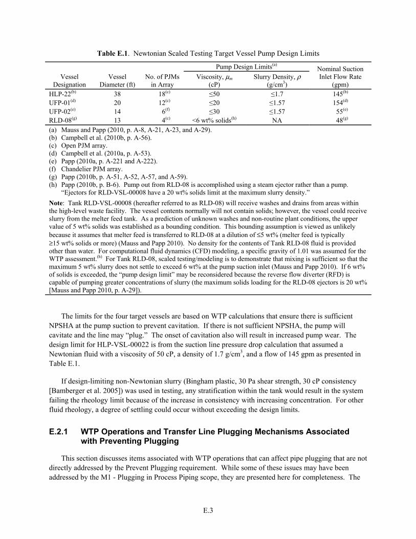
E.3

Table E.1. Newtonian Scaled Testing Target Vessel Pump Design Limits

Vessel Designation

Vessel Diameter (ft)

No. of PJMs in Array

Pump Design Limits(a) Nominal Suction Inlet Flow Rate

(gpm) Viscosity, μm

(cP) Slurry Density, ρ

(g/cm3)

HLP-22(b) 38 18(c) ≤50 ≤1.7 145(b) UFP-01(d) 20 12(c) ≤20 ≤1.57 154(d) UFP-02(e) 14 6(f) ≤30 ≤1.57 55(e)

RLD-08(g) 13 4(c) <6 wt% solids(h) NA 48(g) (a) Mauss and Papp (2010, p. A-8, A-21, A-23, and A-29). (b) Campbell et al. (2010b, p. A-56). (c) Open PJM array. (d) Campbell et al. (2010a, p. A-53). (e) Papp (2010a, p. A-221 and A-222). (f) Chandelier PJM array. (g) Papp (2010b, p. A-51, A-52, A-57, and A-59). (h) Papp (2010b, p. B-6). Pump out from RLD-08 is accomplished using a steam ejector rather than a pump.

“Ejectors for RLD-VSL-00008 have a 20 wt% solids limit at the maximum slurry density.”

Note: Tank RLD-VSL-00008 (hereafter referred to as RLD-08) will receive washes and drains from areas within the high-level waste facility. The vessel contents normally will not contain solids; however, the vessel could receive slurry from the melter feed tank. As a prediction of unknown washes and non-routine plant conditions, the upper value of 5 wt% solids was established as a bounding condition. This bounding assumption is viewed as unlikely because it assumes that melter feed is transferred to RLD-08 at a dilution of ≤5 wt% (melter feed is typically ≥15 wt% solids or more) (Mauss and Papp 2010). No density for the contents of Tank RLD-08 fluid is provided other than water. For computational fluid dynamics (CFD) modeling, a specific gravity of 1.01 was assumed for the WTP assessment.(h) For Tank RLD-08, scaled testing/modeling is to demonstrate that mixing is sufficient so that the maximum 5 wt% slurry does not settle to exceed 6 wt% at the pump suction inlet (Mauss and Papp 2010). If 6 wt% of solids is exceeded, the “pump design limit” may be reconsidered because the reverse flow diverter (RFD) is capable of pumping greater concentrations of slurry (the maximum solids loading for the RLD-08 ejectors is 20 wt% [Mauss and Papp 2010, p. A-29]).

The limits for the four target vessels are based on WTP calculations that ensure there is sufficient NPSHA at the pump suction to prevent cavitation. If there is not sufficient NPSHA, the pump will cavitate and the line may “plug.” The onset of cavitation also will result in increased pump wear. The design limit for HLP-VSL-00022 is from the suction line pressure drop calculation that assumed a Newtonian fluid with a viscosity of 50 cP, a density of 1.7 g/cm3, and a flow of 145 gpm as presented in Table E.1.

If design-limiting non-Newtonian slurry (Bingham plastic, 30 Pa shear strength, 30 cP consistency [Bamberger et al. 2005]) was used in testing, any stratification within the tank would result in the system failing the rheology limit because of the increase in consistency with increasing concentration. For other fluid rheology, a degree of settling could occur without exceeding the design limits.

E.2.1 WTP Operations and Transfer Line Plugging Mechanisms Associated with Preventing Plugging

This section discusses items associated with WTP operations that can affect pipe plugging that are not directly addressed by the Prevent Plugging requirement. While some of these issues may have been addressed by the M1 - Plugging in Process Piping scope, they are presented here for completeness. The

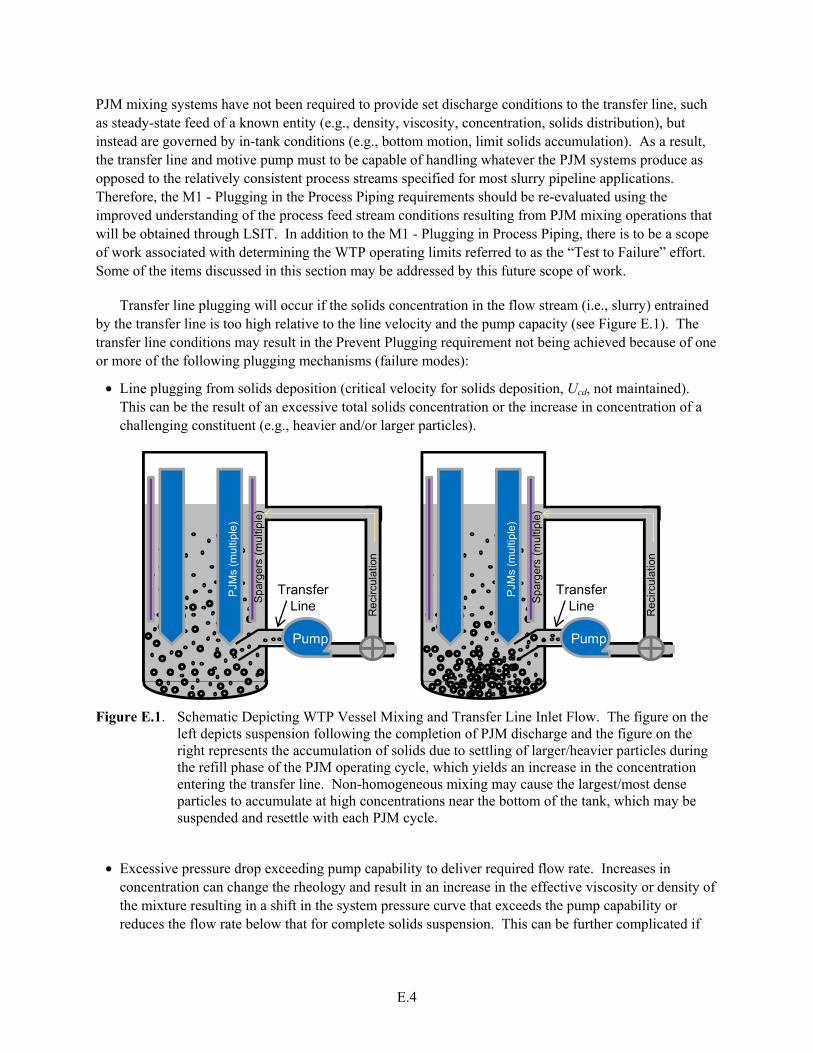
E.4

PJM mixing systems have not been required to provide set discharge conditions to the transfer line, such as steady-state feed of a known entity (e.g., density, viscosity, concentration, solids distribution), but instead are governed by in-tank conditions (e.g., bottom motion, limit solids accumulation). As a result, the transfer line and motive pump must to be capable of handling whatever the PJM systems produce as opposed to the relatively consistent process streams specified for most slurry pipeline applications. Therefore, the M1 - Plugging in the Process Piping requirements should be re-evaluated using the improved understanding of the process feed stream conditions resulting from PJM mixing operations that will be obtained through LSIT. In addition to the M1 - Plugging in Process Piping, there is to be a scope of work associated with determining the WTP operating limits referred to as the “Test to Failure” effort. Some of the items discussed in this section may be addressed by this future scope of work.

Transfer line plugging will occur if the solids concentration in the flow stream (i.e., slurry) entrained by the transfer line is too high relative to the line velocity and the pump capacity (see Figure E.1). The transfer line conditions may result in the Prevent Plugging requirement not being achieved because of one or more of the following plugging mechanisms (failure modes):

• Line plugging from solids deposition (critical velocity for solids deposition, Ucd, not maintained). This can be the result of an excessive total solids concentration or the increase in concentration of a challenging constituent (e.g., heavier and/or larger particles).

TransferLine

Pump

Rec

ircul

atio

n

PJM

s (m

ultip

le)

Spa

rger

s(m

ultip

le)

TransferLine

PumpR

ecirc

ulat

ion

PJM

s (m

ultip

le)

Spa

rger

s(m

ultip

le)

Figure E.1. Schematic Depicting WTP Vessel Mixing and Transfer Line Inlet Flow. The figure on the left depicts suspension following the completion of PJM discharge and the figure on the right represents the accumulation of solids due to settling of larger/heavier particles during the refill phase of the PJM operating cycle, which yields an increase in the concentration entering the transfer line. Non-homogeneous mixing may cause the largest/most dense particles to accumulate at high concentrations near the bottom of the tank, which may be suspended and resettle with each PJM cycle.

• Excessive pressure drop exceeding pump capability to deliver required flow rate. Increases in

concentration can change the rheology and result in an increase in the effective viscosity or density of the mixture resulting in a shift in the system pressure curve that exceeds the pump capability or reduces the flow rate below that for complete solids suspension. This can be further complicated if

E.5

the changes in rheology result in a shift in the suspension regime associated with a stability map (Poloski et al 2009b) for the transfer condtions.

• Insufficient NPSHA at pump inlet resulting in reduced pump performance (e.g., flow rate, delivered head) and potentially excessive pump wear because of cavitation.

The WTP operating conditions associated with preventing plugging start with mixing Hanford tank waste in the large WTP cylindrical vessels with concave bottoms (see Figure E.1). Mixing is done primarily by an array of PJMs that, in unison, periodically inject a downward jet of slurry fluid from each PJM nozzle located near the bottom of the tank. The multiple jet action from the PJM array is intended to mobilize any and all settled slurry particles on the vessel floor, clear the vessel floor (see Chapter 5 and Appendix C, “Working Paper for the Technical Basis for Scaling Transfer and Pump Out”), and mix these slurry particles into the vessel bulk slurry waste. When mixing components are operating, the concentration of individual components suspended within the tank may be constantly changing (transient conditions). Heavy/large settling particles at the bottom of the tank will achieve varying levels of gradient height within the vessel (e.g., clouds), with the maximum height achieved likely near the end of, or immediately after the PJM firing/discharge pulse.

After the PJMs have fired, vessel mixing action is reduced significantly and heavy particles begin settling back towards the vessel bottom. The amount of solids that settle prior to the next firing of the PJMs depends on the concentration and settling velocity of the solids as well as the vessel fluid level. Depending on slurry rheology (i.e., Newtonian, non- Newtonian, or a combination that is concentration dependent), various settling phenomena can be expected including “hindered settling” when the slurry has higher concentrations and/or large particles. During this period of reduced mixing action, some lesser mixing/settling actions may occur including:

• PJM recharge that draws slurry from the vessel back into the PJM nozzle

• Operation of multiple spargers that bubble air into the lower half of the vessel to promote overall mixing activity to the top of the slurry

• Retrieval (entrainment) of slurry from the vessel bottom through the transfer line and when configured to re-circulate, the subsequent discharge of slurry back into the vessel.

Depending on slurry rheology and mixing component configuration, the mixing action from the PJMs may not mix the top portion of the vessel slurry, and consequently, heavy/large particles from the bottom may only achieve a limited height within the vessel slurry.

The transfer line, for moving slurry out of the WTP vessel or for recirculation of the vessel contents, horizontally penetrates the vessel wall and contains an inclined section that extends the inlet to a location near the vessel bottom (Arulampalam 2011). The inlet of the transfer line is relatively small compared to the overall vessel cross-sectional area, so it has a limited zone of influence from which to draw particles into the transfer line when the transfer pump is running. When PJMs discharge, it is expected that the resulting radial jets scouring the tank bottom will produce a wave of concentrated solids that are transported along the tank bottom. The wave of solids can have an extremely high solids loading similar to that of a fluidized bed that when pushed towards the transfer line inlet effectively floods or overloads

E.6

(referred to as “swamping”) the inlet resulting in an overwhelming slug of solids being entrained. This wave of high solids concentration can result in the following:

• Line plugging because the transfer velocity within the pipe is too low, resulting in a high rate of solids deposition.

• An increase in the pipeline pressure drop, resulting in a reduction of the NPSHA at the pump inlet.

• Burying the inlet of the suction line, resulting in a stoppage of flow to the pump. This is a higher probability if the inlet of the suction line is positioned in a stagnation zone between the PJMs that corresponds to one of the last locations where solids are cleared from the tank bottom by the radial jets of the PJM mixers.

During the PJM refill phase, solids will settle to the vessel bottom with the larger/heavier (i.e., more dense) particles settling at a faster rate than smaller/lighter (i.e., less dense) material. Because the transfer line inlet is located off the bottom of the vessel, the faster-settling, larger/heavier particles have a limited time to be entrained into the transfer line inlet during the PJM refill phase and may only be entrained by being swept into the inlet during the PJM discharge phase, or in the “worst case” do not obtain the height or radial location of the transfer line zone of suction influence.

The slurry level in the vessel also will affect the mixing dynamics and concentration of suspended solids. As the transfer line pump is activated to transport the slurry out of the vessel through the transfer line, the slurry level in the vessel will be lowered assuming no additional waste is being added. As the vessel slurry level decreases, the PJM action will continue to mix the slurry until the vessel level is low enough that the PJMs can no longer function. The transfer line can never remove all the slurry from the vessel as onset of vortexing created at the inlet will entrain air into the transfer line and pump.

The periodic operation of the PJMs and the wide size distribution of the WTP process stream will result in the particles not being uniformly mixed and a concentration gradient existing within the tank. It is expected that, because the transfer line is located close to the vessel bottom, a concentration of large/heavy particles greater than the bulk average within the vessel will initially be removed, and the concentration of these particles within the tank and entering the transfer line will decrease with time as the liquid level in the vessel is reduced. In addition to the cyclical nature of the inlet conditions, the PSDD and concentration can vary with time as can the static head and the flow field in the region of the suction line, which can lead to a non-uniform stream relative to pipe length (i.e., time variation in measurements at fixed location) as observed during previous reduced-scale PJM mixing and pump-out tests.

Figures E.2 through E.4 are examples of the variation in slurry density (i.e., concentration) measured in the transfer tests during low order accumulation model (LOAM) test 1 pump outs. The scaling applied to the reduced-scale transfer line size and flow rate is unknown. The LOAM tests were conducted by Energy Solutions for Bechtel National, Inc. (BNI) to obtain data for the confirmation of the LOAM model. Figure E.2 presents the data for the initial pump out from a full tank to a tank that is three-quarters full. Figure E.3 presents similar data for the same test during the third pump out from a half-full tank to a one-quarter-full tank. A series of four pump outs were conducted to retrieve the tank contents.

E.7

Figure E.2. Instantaneous Slurry Density in Transfer Line versus Time During LOAM Test 1 Pump Out. Pump out is from a full level to a three-quarter-full level. Data obtained by Energy Solutions for BNI.1

Figure E.3. Instantaneous Slurry Density in Non-Scaled Transfer Line versus Time During LOAM Test 1 Pump Out. Pump out is from a half-full level to one-quarter-full level. Data obtained by Energy Solutions for BNI.1

1 C Chapman, e-mail to JA Bamberger, April 24, 2012, RE: “Density vs time for Loam tests used as examples in Sect 6, 10, and App-E, stating: [the file] density of slurry during pump outs was a collection of pump out density profiles extracted from a range of engineering reports for LOAM test 1, 2, 5, and 6 and from INFO testing.” The author was Chris Chapman and this assembly was made in January 2012.

E.8

Figure E.4. Instantaneous Slurry Density in Non-Scaled Transfer Line versus Time During LOAM Test 1 Pump Out for a Single PJM Cycle. Pump out is from a half-full level to a one-quarter-full level. Data obtained by Energy Solutions for BNI.1

From Figures E.2 and E.3, the data trend indicates both the average concentration and variation in

concentration continually decreases with time (i.e., tank level) as a greater fraction of the larger/heavier particles, which are concentrated in the lower region of the vessel, were retrieved during the initial pump out. Figure E.4 presents the same data shown in Figure E.3 but for the duration of a single PJM cycle. The variation in measured density was partially attributed to the performance of the centrifugal pump, which most likely experienced significant variations in flow rate with changes in the inlet concentration. While the results of LOAM test 1 are not expected to readily scale to the WTP, they do provide an example of the periodic conditions in a transfer line that can exist as the result of PJM operations. The effects of the variations in solids loading at the suction-line inlet and thus in the transfer line include:

• Greater solids concentration than the average bulk value for the vessel results potentially in the WTP design limits for the transfer line viscosity and density being exceeded.

• Greater solids concentrations increase the critical velocity required to prevent deposition of solids, thus potentially resulting in solids settling.

• Predicting the slurry density and rheology becomes difficult. The same slurry density and viscosity is obtainable from a variety of constituent combinations from a given mixture. This becomes a factor in using published correlations for predicting the critical velocity for solids deposition (Ucd) or system pressure drop. The bulk of these correlations were developed using slurries with monodisperse solids or a single solids density. The application of these correlations to polydisperse mixtures requires the

1 C Chapman, e-mail to JA Bamberger, April 24, 2012, RE: “Density vs time for Loam tests used as examples in Sect 6, 10, and App-E, stating: [the file] density of slurry during pump outs was a collection of pump out density profiles extracted from a range of engineering reports for LOAM test 1, 2, 5, and 6 and from INFO testing.” The author was Chris Chapman and this assembly was made in January 2012.

E.9

determination of bulk material properties (e.g., particle size, density) to represent the mixture, and these properties are not always the same from one application to another for the same mixture.

In addition, the frequency of PJM operations relative to the transport time through the transfer line piping means that the occurrences will be independent of each other (distinguishable) and observable far downstream of the inlet. As slugs of higher concentration slurry are periodically entrained into the pipe, the solids can become segregated because of the differences in relative velocities among the constituents. This segregation of solids can result in changes to the localized rheological conditions and, thus, deposition of larger, heavier solids that would have remained suspended in a steady-state flow of the original entrained mixture. Figure E.5 is a schematic depicting this phenomenon resulting from particle segregation.

• Pipeline flushing after each transfer − Because of the relatively short duration of WTP batch transfers from the mixing vessels (i.e., on the order of 3 to 6 hr), it is possible for solids holdup to occur that does not result in pipeline plugging during the course of a single transfer. However, if line flushing operations do not clear all solids from the line, solids holdup can lead to plugging over the course of multiple transfers. Flushing operations (e.g., frequency, velocity, duration, volume) need to be assessed for the transfer line operating conditions predicted by the LSIT test program.

Larger particles that become segregatedfrom suspended slurry

Periodic changes in inlet concenration resultin durations of low concentration flow

Transfer line inlet

Larger particles remainsuspended as part

of mixture

Figure E.5. Schematic Depicting Particle Segregation That Can Occur Because of Variation in Particle Concentration at the Inlet. The slip velocity between larger (can include difference in density) and smaller particles can result in larger particles experiencing flow condition where Ucd is higher than that required for mixture of all constituents.

• Idle pipeline during mixing operations − If the pipeline remains idle during mixing operations, there

is the potential for solids and/or air/gas accumulation within the inlet of the suction line. Gas can accumulate in the transfer line due to gas released from solution and/or micro bubbles entrained due to PJM and sparger operations coalescing. This gas accumulation may be mitigated by flushing the suction side of the transfer line prior to transfer or recirculation operations. In addition, the physical configuration of the suction inlet pipe near the tank bottom can result in solids accumulation near the

E.10

inlet because of a stagnation zone created by the pipe structure. The existence of one or a combination of these conditions when the pump starts can have effects similar to the “solids swamping” previously discussed.

• Non-Newtonian conditions within the mixing vessel that allow for solids suspension within the vessel can result in unacceptable flow conditions for the pipeline due to effects of shear thinning, flow regime changes, and increased pressure drop. When a non-Newtonian fluid/mixture is entrained from the vessel into the pipeline, a sudden change in the relative flow field is experienced by the fluid, which impacts the localized rheology of the mixture.

The effects can be assessed by evaluating a “stability map” (Poloski et al 2009b) for the slurry flow conditions. The stability map defines the conditional boundaries for solids suspension within a pipe through the various flow conditions (i.e., laminar, transitional, and turbulent flow) over the range of potential rheological properties (e.g., yield stress).

This mapping defines four major regimes that may exist within the pipe depending on the rheological properties and the slurry velocity defined as:

– Stable turbulent regime – turbulence is sufficient to generate drag forces that overcome the settling of the particles due to gravity. This regime includes the flow of fully turbulent Newtonian flows with no deposition.

– Unstable turbulent regime – turbulent flow but insufficient energy to maintain solids in suspension.

– Unstable laminar regime – turbulence is dissipated by the viscous damping. Any yield stress possessed by the fluid is insufficient to maintain the solids in suspension and deposition occurs.

– Stable laminar regime – the yield stress dominates the undisturbed (non-sheared) core region of the pipe flow, which flows as an annular plug with suspended solids. In addition, solids deposited at the pipe wall can be transported due to the wall shear stress acting on them. This flow condition can be impacted by regions where transitional flow conditions occur and shearing of the center core allows particles to settle, which are not re-suspended as the core region is re-established downstream.

E.3 Assumptions and Phenomena Associated with Transfer and Pump Out

The discussions in Sections E.2 through E.4 focus on application to WTP PJM mixing vessel operations. With respect to pump out, this section will discuss entrainment of solids in the pipeline and its transport through the pipeline and pump. Section E.3.1 provides the assumptions associated with the prevent plugging assessment. A description of transfer line flow conditions and relevant parameters are presented in Section E.3.2. A brief list of pipeline design objectives and guidelines are presented in Section E.3.3 as a comparison to the WTP circumstances.

E.11

E.3.1 Assumptions Applied to Assessment

The discussion presented in Appendix E is based on the following assumptions for the WTP operations and the LSIT effort:

• The transfer line inlet is in the vicinity of the vessel bottom (HT/DT ∼1) where DT is the inside diameter of the transfer line and HT is the height of the transfer line inlet above the tank bottom measured directly below the inlet.

• Transfers from the mixing vessel are performed as batch operations with the vessel level continually decreasing throughout the transfer.

• The slurry flow conditions during recirculation and transfer operations are either homogeneous or heterogeneous full suspension.

• PJM operations consist of simultaneous firing and discharge phases (durations).

• The solids to be entrained and transported are granular material having aspect ratios on the order of one to ten based on reported shape factors (Wells et al. 2011). The transport of fibrous material is not considered.

• Slurry mixtures to be pumped consist of multiple species with particle diameter variations of four orders of magnitude and one order of magnitude variation for specific gravity.

• Transfer line inlet solids concentration and PSDD are expected to be cyclical relative to the PJM operating cycle.

• Application of steady-state conditions to access pipeline pressure drop for cyclical concentrations is a conservative approach as long as the peak concentration is applied and the volume flow rate (i.e., velocity) is maintained.

• Assessment and sampling of the transfer line concentration is not restricted to WTP methods and can be scale specific.

• The entrained material has reached a stable chemical condition within the vessel prior to any transfer operations being performed. Phenomena such as solids precipitation or agglomeration are not considered. The physical nature of the slurry particulate entering the transfer line stays constant throughout the pipeline. The location of the in-line addition of caustic for UFP caustic leaching and neutralization of the non-Newtonian storage vessels is assumed close enough to the discharge of the recirculation line that it will not affect the slurry makeup within the pipeline.

• The vessel contents are sufficiently mobilized to allow for full entrainment at the pump inlet. Transfer line performance is only of interest for conditions of complete bottom motion.

• Monitoring transfer line inlet conditions during the limit solids accumulation testing will only be performed for conditions of full bottom motion/clearing. Transfer line performance for vessel conditions with less than full bottom motion is of no interest.

• The pump-inlet design and pump-system selection have the capacity to sufficiently entrain solids so that holdup of material within the vessel from insufficient entrainment of suspended solids is avoided.

E.12

• It is assumed that transfer pump operations are steady throughout each transfer and will be terminated if conditions occur that can result in air entrainment or absence of NPSHR for the pump system (i.e., pump operations will not be varied as the vessel level is lowered). No other operating conditions or scenarios are considered.

• Solids deposition is an assumed metric that will be used to assess the potential for pipeline plugging. The approach assumes that a “No Deposition” requirement within the transfer line will be adopted.

• The transfer line and pump are flushed after material transfers and remain idle between transfer operations.

• The suction line is back flushed from the pump inlet, but the pump and downstream piping are forward flushed.

• The requirement to prevent plugging potentially includes both Newtonian and non-Newtonian slurries. The designation of a mixing vessel as “Newtonian” (i.e., for processing Newtonian behaving slurries) does not preclude the process stream in the transfer line from exhibiting non-Newtonian behavior if the solids concentration within the line exceeds that within the vessel.

• It is unknown whether the transfer pump is a dynamic pump or a displacement pump.

• The transfer line for the reduced-scale test setup(s) can be operated in both recirculation and transfer modes. Operation in a recirculation mode will allow any periodic condition existing at the transfer line inlet to be monitored for an extended duration.

• Testing will be conducted to validate that operating the transfer line in recirculation mode has a negligible impact on the solids distribution within the vessel and, thus, on the solids concentration at the transfer line inlet.

To avoid holdup of material within the tank, the inlet conditions to the transfer line must be capable of:

• Entraining and transporting the particles at an average concentration equal to or greater than the bulk solids concentration within the vessel − This assumes the solids concentration is either uniform within the vessel or stratified, with the concentration at the bottom of the vessel greater than that of the vessel bulk concentration.

• Entraining a PSDD that is representative of or is greater than the vessel contents − It is possible to initially entrain a concentration higher than the bulk average of the vessel with a corresponding PSDD that has a representative metric (e.g., median settling velocity) indicating a distribution skewed toward the smaller/less dense material and still obtain a transfer with no holdup. For this to be accomplished, the larger/denser particles must be more readily entrained as the bulk concentration within the vessel is reduced. While this is unlikely, it may be possible if the performance of the transfer pump results in an increase in flow rate (i.e., increased inlet velocity) with decreasing solids concentration.

E.3.2 Transfer Line Conditions and Relevant Parameters

Besides the conditions of laminar, transitional, and turbulent flow, slurry transport can occur via a variety of mixture conditions that exist within the pipe. A high-level summary of these conditions for granular material in a horizontal pipeline is provided below (Govier and Aziz 1987).

E.13

• Homogenous suspension (also referred to as symmetric suspension) – All particles are fully suspended, and no stratification exists.

• Heterogeneous suspension (also referred to as asymmetric suspension) – All particles are fully suspended, but a vertical stratification of material exists. The variation may be in solids concentration, size distribution, solids density, or a combination of these parameters. For this condition to exist, the average slurry velocity, Um, must be equal to or greater than the critical velocity for solids deposition, Ucd (Um ≥ Ucd).

• Sliding particles – Larger, denser particles are deposited on the bottom of the pipe and transported by sliding or bouncing along the bottom of the pipe. The entire inventory of such particles is not necessarily deposited. The particles transported along the bottom of the pipe can be individually identified, and the particle-to-particle interactions on the bottom of the pipe are negligible. The onset of this condition exists below Ucd (Um < Ucd).

• Sliding bed or dune flow – A significant amount of particles accumulate at the bottom of the pipeline and travel by sliding along the bottom of the pipe. This transport may be either in the form of “dunes,” in which groups of particles appear to summersault or leapfrog along the bottom of the pipe, or as a continuous moving bed. In this flow condition, all particles still possess some downstream velocity.

• Settled bed – For this flow regime, stationary particles exist on the bottom of the pipe. This condition may be the result of 1) self correction, in which settling occurs until an increased pipe velocity is established that maintains a constant transport condition, or 2) continuous holdup of the larger/denser particles that will eventually lead to pipe plugging.

For solids transport, the previously mentioned conditions are often considered in terms of onset conditions or critical transport velocity. In other words, above a prescribed velocity, a defined condition exists (e.g., critical velocity for homogeneous flow, critical velocity for full suspension). It also is possible for a combination of conditions to exist. For example, in the case of a sliding bed, the flow above the sliding bed may be clear as all solids are transported within the sliding bed, a heterogeneous flow may exist above the bed, or the PSDD of the suspended bed may allow homogeneous flow to occur above the bed.

Parameters and conditions that influence slurry transport within the pipeline include:

• Physical properties of the solids

– Density (or densities) of the solids (relevance: density difference between solids and liquid)

– Particle size (i.e., material size distribution)

– Particle shape

• Loading (concentration) of the solids

• Fluid properties

– Liquid density (relevance: density difference between solids and liquid)

– Liquid rheology

– Mixture (slurry) rheology

E.14

• Pipe conditions

– Pipe diameter

– Pipe roughness (i.e., the inside surface condition)

– Pipe joinery

– Orientation of pipe (e.g., horizontal, angle of incline)

– Pipeline geometry/components (e.g., bends, contractions, expansions)

• Flow conditions

– Pipeline velocity/flow rate

– Flow regime – turbulent, transition, laminar

– Inlet conditions – solids concentration as a function of time, inlet pressure as a function of time, consistency of inlet flow field as a function of time (e.g., sweeping jet similar to waste tank mixer pump, periodic flow produced by PJMs)

– Motive pump characteristics – pulsating flow (e.g., peristaltic pump), pressure drop dependent flow rate (e.g., centrifugal pump).

Other factors that can influence the development of specific slurry flow conditions include:

• Pipe length – A required entrance length exists for flow stabilization, which is the pipe length required for full development of the flow conditions. For slurry flow, this involves both the fluid flow field and the slurry stratification. Depending on the slurry composition, this length can be sufficiently long for slow or gradual segregation of material. Some process lines have line lengths in which full stratification is not achieved.

• Upstream configuration – Changes in flow direction or line velocity can cause changes in material stratification as particles may have a significant time response to the change compared to that of the fluid. Each change in stratification (assuming fully developed conditions upstream of the component) has an associated pipe length required to re-achieve stabilized flow. This is often evaluated via the Stokes number (St), which is the ratio of the response time of the particle to that of the fluid (Crowe et al. 1985).

2

218

18

Δ= = =

Δ

s S

S s SF

lF F l

d

t d USt

tU

ρρμ

δ μ δ (E.1)

In this relationship, tS and tF are the characteristic response times for the solid particle and the fluid, respectively, U is the characteristic fluid velocity, δl is the characteristic size of the large scale fluid structure, and ΔU is the velocity difference associated with δl (i.e., the shear layer). The parameters dS and ρs are the diameter and density for the solid particulate, respectively, and µF is the fluid viscosity (may contain suspended solids considered part of the fluid phase). For a given flow condition, St varies with particle properties as ρs(dS)

2. For St <<1, the particle response time is much less than that of the fluid, and the particle can be assumed to follow the fluid. If St ∼1, the particle

E.15

can be centrifuged by the turbulent structure, and while not necessarily separating from the flow the distribution of particles can be impacted. For St >>1, the particles are incapable of responding to changes in the fluid-flow field and will continue with their original trajectory. The effects of pipe elbows/bends also need to be considered. The existence of an elbow or bend can cause stratification of the solids, which often is observed as deposition of material downstream of the elbow in flow visualization experiments. The re-suspension of the deposited material results in an associated pipe length for flow stabilization.

E.3.3 Summary of Pipeline Design Objectives and Guidelines

The major objectives of slurry pipeline design and operations usually are to:

• Transport material at conditions that will prevent the occurrence of plugging conditions. This is often accomplished by ensuring fully suspended flow throughout the transfer line.

• Transport material with no or minimal material holdup. Holdup is the condition where the mass exiting the pipeline, or section of pipeline, is less than the mass entering the pipeline.

• Attain transport with minimal component wear rates or with wear rates that are within design limits for component service requirements.

• Provide for variation of system operation to allow recovery from observed/detected off-normal events. This is often accomplished via dilution options within the system and additional pump capacity to temporarily increase line velocity or overcome increased system pressure drop.

• Require minimal degradation to the physical properties of the material, if necessary.

Basic guidelines often applied to slurry pipeline design for heterogeneous suspension flow conditions include:

• Maintaining suspension of the solids in the horizontal line will be more challenging than transport of solids up a vertical line of the same diameter. Guidelines associated with pipe velocities include:

– The minimum line velocity for vertical flow should be at least twice the vertical settling velocity of the fastest settling particles.

– The velocity in horizontal lines (in transfer lines where vertical pipe runs exist) must be greater than the minimum vertical line design velocity to avoid deposition and, depending on material properties and rheology, can be significantly higher.

• The preferred direction for flushing operations is from upstream to downstream within the pipeline. Back flushing pipes to source tanks can prohibit the transfer of the most challenging particles as they are returned to the source vessel.

• For conditions containing particles with a wide range of settling characteristics, recommended practices include ramping up the flow rate of the flushing fluid to preferentially resuspend particles or erode a sediment bed to reduce the risk of creating a plug condition.

The majority of slurry pipeline design activities focus on one of the following four problems:

• Determining the net driving force required to move a given slurry at a specified flow rate through a given pipeline. This approach is the most applicable to the WTP situation. First, the slurry flow

E.16

concentration that needs to be transported will be determined from LSIT, and then, Ucd will be determined for the specified pipe diameter yielding a prescribed flow rate (refer to Section E.5).

• Determining the flow rate for slurry transported through a given pipeline with a specified driving force.

• Determining the pipe diameter required to transport a given slurry at a specified flow rate with a given driving force. A solution does not always exist for this case as the increase in pipe diameter to reduce the driving force (i.e., reduce the line velocity) can result in velocities that are too low to maintain slurry transport.

• Determining the optimum (economically – material costs versus power costs) pipe size and pump power required to pump a given slurry at a specified flow rate. This is the problem most frequently encountered.

Assessment of the Prevent Plugging requirement for the WTP transfer line provides a less common design activity because the feed stream conditions are not readily defined. In this case, the design or assessment of the design is conducted against a bounding set of operating conditions. For multiphase systems, the development of bounding conditions can become complex, as bounding conditions for physical properties do not always result in bounding conditions for system operations. For example, the maximum Ucd does not necessarily correspond to the maximum solids loading. Therefore, determining the feed stream conditions or developing the bounding conditions can be as critical as the approach used to evaluate the system operation. This will be discussed further in Section E.4.

E.4 Transfer Line Scaling

For pipelines that transport uniform single constituent slurries in a steady-state homogenous suspension, the design process applied for single-phase flow often can be applied. Bulk properties are applied and the pressure drop calculated based on the concept of a friction factor (i.e., dimensionless ratio of the wall shear stress to the kinetic energy per unit volume of fluid) (refer to Section E.6.2.1, Equations (E.21) and (E.22)).

For more complex slurry materials, appropriate correlations applicable to steady-state conditions are selected as design aids. Reduced-scale testing is conducted to verify the application of the correlations over a range of operating conditions. Scaled testing also is used to evaluate the bulk mixture properties applied to the correlation. Testing can be done over a range of conditions to verify that reasonable methods have been employed for determining mixture properties such as rheology and representative particle size. The verified correlations and representative properties then are applied to the full-scale conditions and used for system design. The evaluation of non-steady-state conditions in the system tends to lead the development effort toward full-scale testing, especially for multi-constituent slurries or non-Newtonian carrier fluids.

Verification of slurry pump selection/design is almost always done at full-scale conditions as most pump operations/conditions do not lend themselves to scaling. Conditions contributing to this include:

• The cost of obtaining an ideal pump for specific scaled conditions is often cost prohibitive. Manufacturing of pumps is based on commercial needs, and particular designs are only manufactured in discrete sizes. Therefore, a scaled version would often require custom design and fabrication. In

E.17

addition, a pump can be designed to meet a range of operating conditions by adjusting its operating parameters, such as speed (frequency of operation) and stroke length. Therefore, geometric scaling alone will not be sufficient.

• It is difficult to match shear rate within a pump. For reduced pump size and equivalent internal velocities, the internal shear rate is increased, which raises the problem of scaling rheology for non-Newtonian materials for both pump performance and pipeline performance.

• NPSHA and NPSHR do not scale.

• Pump performance is dependent on slurry makeup, but pump performance at a given slurry condition does not necessarily scale. The first issue is to produce a prototypic slurry mixture at the scaled conditions. However, a scaled pump may not successfully operate at the same slurry conditions that a full-scale pump can (e.g., impact of reduced internal clearances).

• Variations exist in time scaling. Because of the periodic operating nature of the PJM system, the inlet conditions may be time dependent. Matching the time scale of the fluctuations in slurry makeup relative to the time-scale associated with pump operation at reduced scale can be difficult.

E.5 Approach for Assessing Pipe Plugging in WTP Vessel Transfer Lines

This section details an approach for using reduced-scale testing and associated industrial correlations to assess the WTP for the plugging mechanisms summarized in Section E.2.1. The key mechanism to avoid plugging in the transfer line is to avoid solids settling (i.e., solids deposition) that can restrict the flow, resulting in an increased head loss and a reduced NPSHA. The operating cycle for the PJMs results in an intermittent mixing action of slurry in the vessel causing the concentration at the transfer line inlet to vary with PJM operations. The approach simplifies transfer line operations by using “worst-case,” bounding slurry properties/conditions that can then be applied at steady-state conditions. This strategy can be compared to assessing a vehicle’s fuel consumption rate (slurry flow) running at full throttle (steady-state) up an incline with a head wind (bounding conditions). Industrial models or correlations are chosen and representative slurry properties are defined based on matching test data, within acceptable error bands, obtained at various scales and operating conditions. These models then are used to “predict” full-scale WTP operations. Because this is a conservative approach, failure cannot be confirmed, only success can. If successful operations are not confirmed then the approach would require either:

• A reduction in the conservatism applied to establish the bounding, steady-state conditions

• A change in WTP design and/or operating conditions that coincide with bounding conditions for which successful operations can be confirmed by this approach.

Refer to Chapter 3 and Appendix A for a summary of the different scaling approaches and Appendix A, Section A.7.1.1 where bounding conditions are discussed as a form of similitude. With a bounding approach, the actual range of WTP operating conditions is not being evaluated. Instead the approach defines bounding conditions or an operating envelope to be assessed. While specific WTP operating conditions are not predicted, acceptable performance at bounding conditions indicates that satisfactory performance will be achieved within the operating envelope.

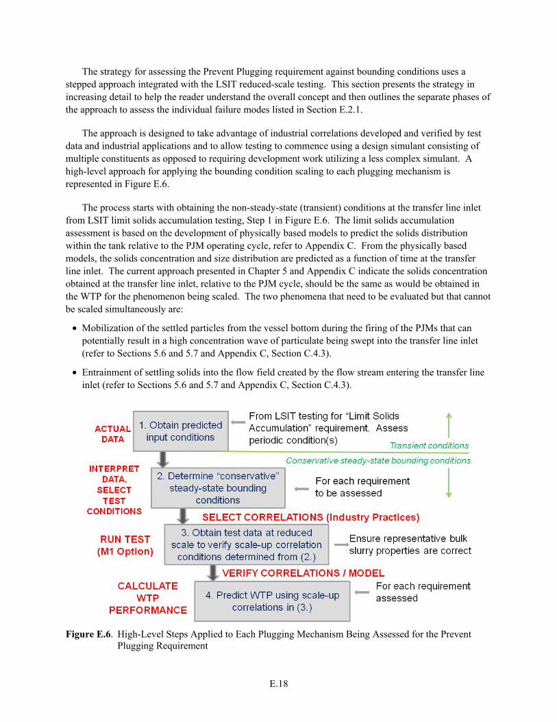
E.18

The strategy for assessing the Prevent Plugging requirement against bounding conditions uses a stepped approach integrated with the LSIT reduced-scale testing. This section presents the strategy in increasing detail to help the reader understand the overall concept and then outlines the separate phases of the approach to assess the individual failure modes listed in Section E.2.1.

The approach is designed to take advantage of industrial correlations developed and verified by test data and industrial applications and to allow testing to commence using a design simulant consisting of multiple constituents as opposed to requiring development work utilizing a less complex simulant. A high-level approach for applying the bounding condition scaling to each plugging mechanism is represented in Figure E.6.

The process starts with obtaining the non-steady-state (transient) conditions at the transfer line inlet from LSIT limit solids accumulation testing, Step 1 in Figure E.6. The limit solids accumulation assessment is based on the development of physically based models to predict the solids distribution within the tank relative to the PJM operating cycle, refer to Appendix C. From the physically based models, the solids concentration and size distribution are predicted as a function of time at the transfer line inlet. The current approach presented in Chapter 5 and Appendix C indicate the solids concentration obtained at the transfer line inlet, relative to the PJM cycle, should be the same as would be obtained in the WTP for the phenomenon being scaled. The two phenomena that need to be evaluated but that cannot be scaled simultaneously are:

• Mobilization of the settled particles from the vessel bottom during the firing of the PJMs that can potentially result in a high concentration wave of particulate being swept into the transfer line inlet (refer to Sections 5.6 and 5.7 and Appendix C, Section C.4.3).

• Entrainment of settling solids into the flow field created by the flow stream entering the transfer line inlet (refer to Sections 5.6 and 5.7 and Appendix C, Section C.4.3).

Figure E.6. High-Level Steps Applied to Each Plugging Mechanism Being Assessed for the Prevent Plugging Requirement

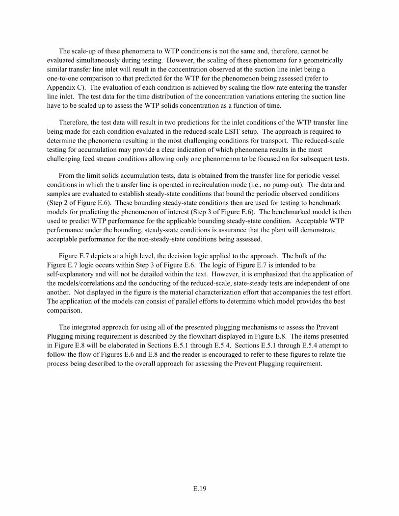
E.19

The scale-up of these phenomena to WTP conditions is not the same and, therefore, cannot be evaluated simultaneously during testing. However, the scaling of these phenomena for a geometrically similar transfer line inlet will result in the concentration observed at the suction line inlet being a one-to-one comparison to that predicted for the WTP for the phenomenon being assessed (refer to Appendix C). The evaluation of each condition is achieved by scaling the flow rate entering the transfer line inlet. The test data for the time distribution of the concentration variations entering the suction line have to be scaled up to assess the WTP solids concentration as a function of time.

Therefore, the test data will result in two predictions for the inlet conditions of the WTP transfer line being made for each condition evaluated in the reduced-scale LSIT setup. The approach is required to determine the phenomena resulting in the most challenging conditions for transport. The reduced-scale testing for accumulation may provide a clear indication of which phenomena results in the most challenging feed stream conditions allowing only one phenomenon to be focused on for subsequent tests.

From the limit solids accumulation tests, data is obtained from the transfer line for periodic vessel conditions in which the transfer line is operated in recirculation mode (i.e., no pump out). The data and samples are evaluated to establish steady-state conditions that bound the periodic observed conditions (Step 2 of Figure E.6). These bounding steady-state conditions then are used for testing to benchmark models for predicting the phenomenon of interest (Step 3 of Figure E.6). The benchmarked model is then used to predict WTP performance for the applicable bounding steady-state condition. Acceptable WTP performance under the bounding, steady-state conditions is assurance that the plant will demonstrate acceptable performance for the non-steady-state conditions being assessed.

Figure E.7 depicts at a high level, the decision logic applied to the approach. The bulk of the Figure E.7 logic occurs within Step 3 of Figure E.6. The logic of Figure E.7 is intended to be self-explanatory and will not be detailed within the text. However, it is emphasized that the application of the models/correlations and the conducting of the reduced-scale, state-steady tests are independent of one another. Not displayed in the figure is the material characterization effort that accompanies the test effort. The application of the models can consist of parallel efforts to determine which model provides the best comparison.

The integrated approach for using all of the presented plugging mechanisms to assess the Prevent Plugging mixing requirement is described by the flowchart displayed in Figure E.8. The items presented in Figure E.8 will be elaborated in Sections E.5.1 through E.5.4. Sections E.5.1 through E.5.4 attempt to follow the flow of Figures E.6 and E.8 and the reader is encouraged to refer to these figures to relate the process being described to the overall approach for assessing the Prevent Plugging requirement.

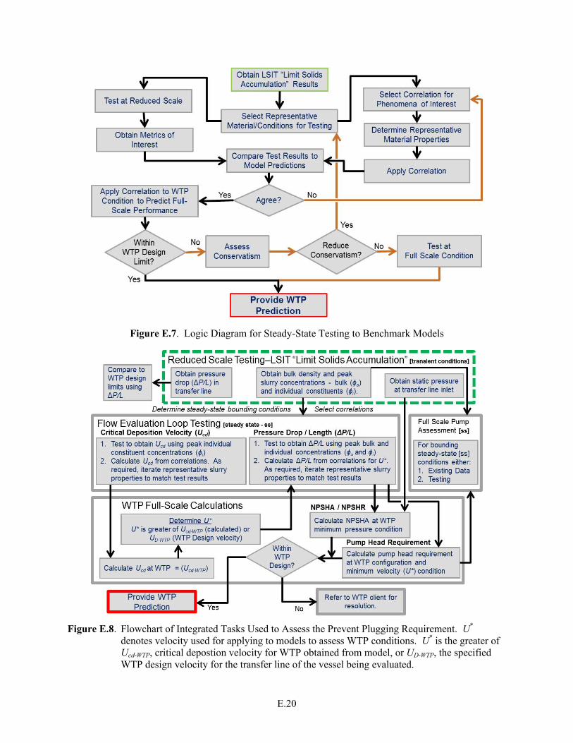
E.20

Figure E.7. Logic Diagram for Steady-State Testing to Benchmark Models

Figure E.8. Flowchart of Integrated Tasks Used to Assess the Prevent Plugging Requirement. U* denotes velocity used for applying to models to assess WTP conditions. U* is the greater of Ucd-WTP, critical depostion velocity for WTP obtained from model, or UD-WTP, the specified WTP design velocity for the transfer line of the vessel being evaluated.

E.21

E.5.1 Obtaining Non-Steady-State Conditions from Limit Solids Accumulation Tests

This section describes the activities associated with the reduced-scale LSIT, which are depicted in Step 1 of Figure E.6 and in the dashed (i.e., green) box at the top of Figure E.8. The reduced-scale LSIT to assess the Limit Solids Accumulation mixing requirement will require the test vessel solids be mobilized and a periodic condition be reached. This also will be required for the assessment of the mixing requirements related to sampling (Mixing Requirements 5, 6, and 7). Once a periodic condition has been reached, the transfer line should be operated in the recirculation mode with negligible change in tank contents. With respect to the Prevent Plugging requirement, the LSIT effort needs to obtain the following:

• Determine the time of peak slurry concentration entering the transfer line relative to the PJM operating cycle. Tests need to be conducted for transfer line flow rates scaled relative to both solids mobilization and quiescent settling.

• At the transfer line inlet obtain for multiple test scales:

– Mass flow rate and bulk density as a function of time. The bulk-density measurements provide a check against sample characterization measurements with respect to total mass. The inline measurements also allow fluctuations in density to be used to assess the degree of conservatism resulting from applying worst-case conditions to evaluate the pressure drop for steady-state process feed conditions.

– Peak solids concentration, ϕSmax, corresponding to the peak bulk density

– Total solids concentration, ϕS, and maximum concentration of individual solid species, ϕimax, that correspond to the peak density for various fill/pump-out levels.

– Static pressure at transfer line inlet as a function of time (minimum pressure within cycle is the most important) and tank level (fill/pump-out levels).

• Obtain transfer line pressure drop (ΔP/L) over horizontal section of LSIT transfer line for slurry flows that exhibit cyclic solids concentrations because of intermittent PJM operations, and compare test results to the calculated pressure drop for the same section of transfer line (ΔP/L) assuming steady-state conditions and the WTP design limits for slurry density, ρ, and slurry viscosity, μm, (specific to each target vessel, refer to Table E.1). While the inlet configuration and flow rate need to be scaled for the limit solids accumulation tests, the downstream configuration need not be prototypic in configuration. The transfer line needs to be sized to assure no solids deposition and turbulent flow conditions. It is recommended that the transfer line contain a horizontal length, L, over which the pressure drop is measured, that satisfies the conditions of the relationship

2 2

48 ≤ ≤ T CT D

T T

Q tQ tL

D Dπ π (E.2)

where QT is the volume flow rate through the transfer line, tC is the total PJM cycle time, and tD is the duration of the PJM discharge. This will ensure that the entire volume of slurry retrieved during the discharge of the PJM can exist within the transfer line and that only the entrained slurry associated with one PJM discharge can exist within the transfer line at a given time. This will allow the measurement of reasonable pressure drops for comparison to calculated values for the design limits.

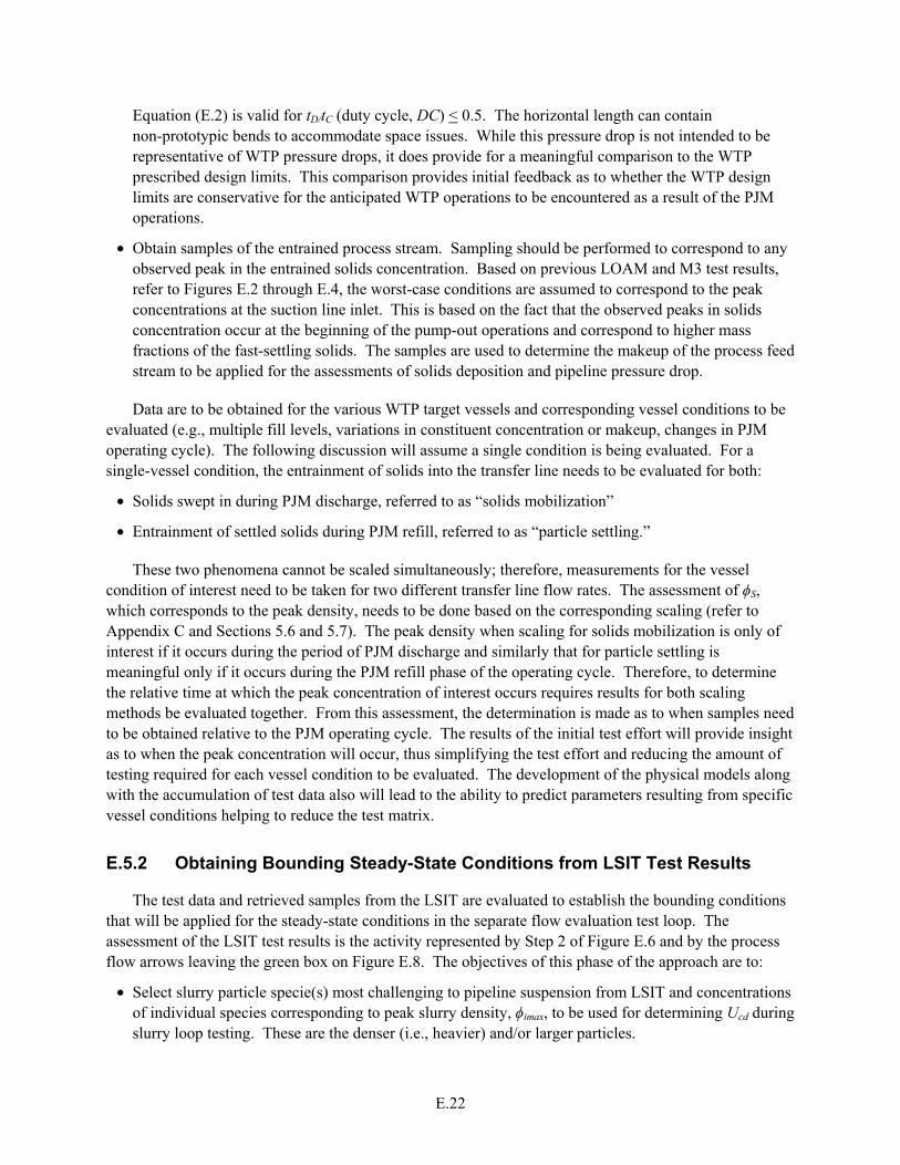
E.22

Equation (E.2) is valid for tD/tC (duty cycle, DC) < 0.5. The horizontal length can contain non-prototypic bends to accommodate space issues. While this pressure drop is not intended to be representative of WTP pressure drops, it does provide for a meaningful comparison to the WTP prescribed design limits. This comparison provides initial feedback as to whether the WTP design limits are conservative for the anticipated WTP operations to be encountered as a result of the PJM operations.

• Obtain samples of the entrained process stream. Sampling should be performed to correspond to any observed peak in the entrained solids concentration. Based on previous LOAM and M3 test results, refer to Figures E.2 through E.4, the worst-case conditions are assumed to correspond to the peak concentrations at the suction line inlet. This is based on the fact that the observed peaks in solids concentration occur at the beginning of the pump-out operations and correspond to higher mass fractions of the fast-settling solids. The samples are used to determine the makeup of the process feed stream to be applied for the assessments of solids deposition and pipeline pressure drop.

Data are to be obtained for the various WTP target vessels and corresponding vessel conditions to be evaluated (e.g., multiple fill levels, variations in constituent concentration or makeup, changes in PJM operating cycle). The following discussion will assume a single condition is being evaluated. For a single-vessel condition, the entrainment of solids into the transfer line needs to be evaluated for both:

• Solids swept in during PJM discharge, referred to as “solids mobilization”

• Entrainment of settled solids during PJM refill, referred to as “particle settling.”

These two phenomena cannot be scaled simultaneously; therefore, measurements for the vessel condition of interest need to be taken for two different transfer line flow rates. The assessment of ϕS, which corresponds to the peak density, needs to be done based on the corresponding scaling (refer to Appendix C and Sections 5.6 and 5.7). The peak density when scaling for solids mobilization is only of interest if it occurs during the period of PJM discharge and similarly that for particle settling is meaningful only if it occurs during the PJM refill phase of the operating cycle. Therefore, to determine the relative time at which the peak concentration of interest occurs requires results for both scaling methods be evaluated together. From this assessment, the determination is made as to when samples need to be obtained relative to the PJM operating cycle. The results of the initial test effort will provide insight as to when the peak concentration will occur, thus simplifying the test effort and reducing the amount of testing required for each vessel condition to be evaluated. The development of the physical models along with the accumulation of test data also will lead to the ability to predict parameters resulting from specific vessel conditions helping to reduce the test matrix.

E.5.2 Obtaining Bounding Steady-State Conditions from LSIT Test Results

The test data and retrieved samples from the LSIT are evaluated to establish the bounding conditions that will be applied for the steady-state conditions in the separate flow evaluation test loop. The assessment of the LSIT test results is the activity represented by Step 2 of Figure E.6 and by the process flow arrows leaving the green box on Figure E.8. The objectives of this phase of the approach are to:

• Select slurry particle specie(s) most challenging to pipeline suspension from LSIT and concentrations of individual species corresponding to peak slurry density, ϕimax, to be used for determining Ucd during slurry loop testing. These are the denser (i.e., heavier) and/or larger particles.

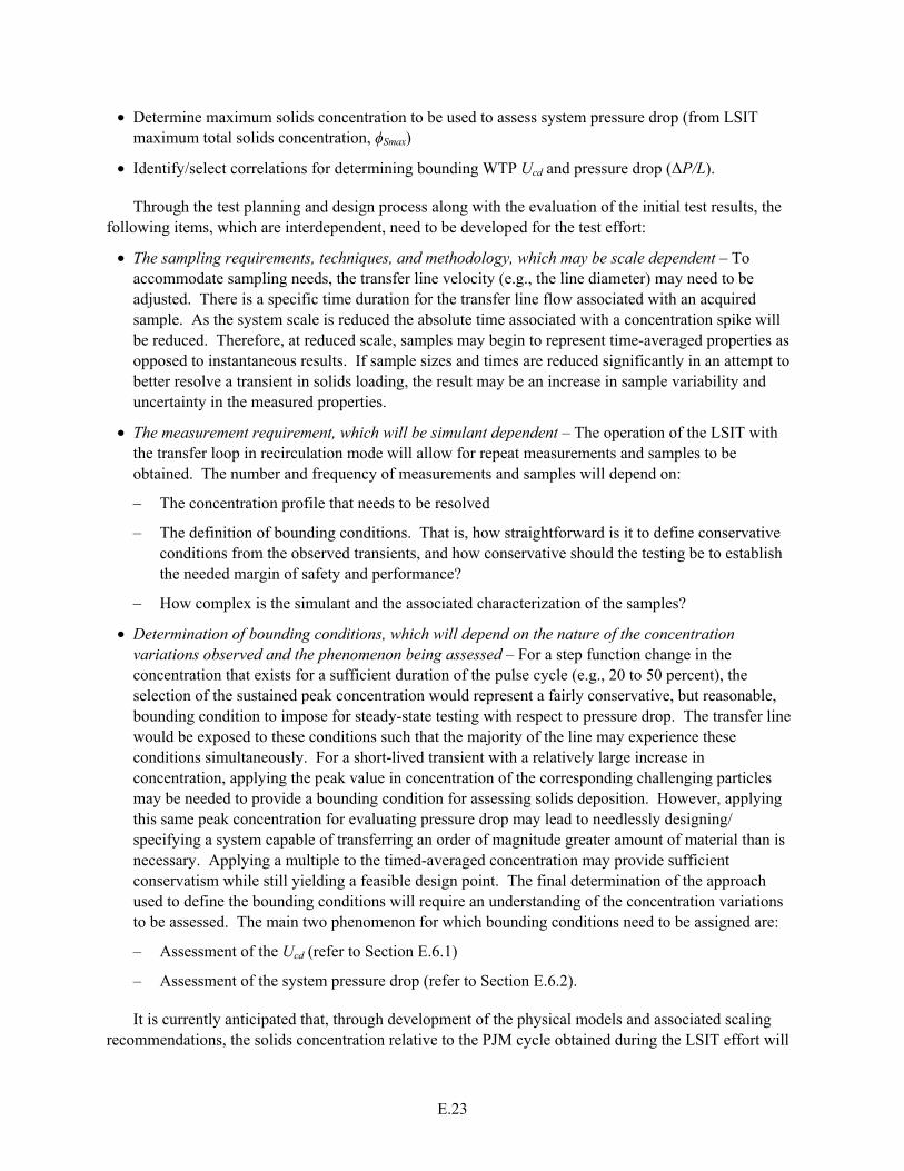
E.23

• Determine maximum solids concentration to be used to assess system pressure drop (from LSIT maximum total solids concentration, ϕSmax)

• Identify/select correlations for determining bounding WTP Ucd and pressure drop (ΔP/L).

Through the test planning and design process along with the evaluation of the initial test results, the following items, which are interdependent, need to be developed for the test effort:

• The sampling requirements, techniques, and methodology, which may be scale dependent – To accommodate sampling needs, the transfer line velocity (e.g., the line diameter) may need to be adjusted. There is a specific time duration for the transfer line flow associated with an acquired sample. As the system scale is reduced the absolute time associated with a concentration spike will be reduced. Therefore, at reduced scale, samples may begin to represent time-averaged properties as opposed to instantaneous results. If sample sizes and times are reduced significantly in an attempt to better resolve a transient in solids loading, the result may be an increase in sample variability and uncertainty in the measured properties.

• The measurement requirement, which will be simulant dependent – The operation of the LSIT with the transfer loop in recirculation mode will allow for repeat measurements and samples to be obtained. The number and frequency of measurements and samples will depend on:

– The concentration profile that needs to be resolved

– The definition of bounding conditions. That is, how straightforward is it to define conservative conditions from the observed transients, and how conservative should the testing be to establish the needed margin of safety and performance?

– How complex is the simulant and the associated characterization of the samples?

• Determination of bounding conditions, which will depend on the nature of the concentration variations observed and the phenomenon being assessed – For a step function change in the concentration that exists for a sufficient duration of the pulse cycle (e.g., 20 to 50 percent), the selection of the sustained peak concentration would represent a fairly conservative, but reasonable, bounding condition to impose for steady-state testing with respect to pressure drop. The transfer line would be exposed to these conditions such that the majority of the line may experience these conditions simultaneously. For a short-lived transient with a relatively large increase in concentration, applying the peak value in concentration of the corresponding challenging particles may be needed to provide a bounding condition for assessing solids deposition. However, applying this same peak concentration for evaluating pressure drop may lead to needlessly designing/ specifying a system capable of transferring an order of magnitude greater amount of material than is necessary. Applying a multiple to the timed-averaged concentration may provide sufficient conservatism while still yielding a feasible design point. The final determination of the approach used to define the bounding conditions will require an understanding of the concentration variations to be assessed. The main two phenomenon for which bounding conditions need to be assigned are:

– Assessment of the Ucd (refer to Section E.6.1)

– Assessment of the system pressure drop (refer to Section E.6.2).

It is currently anticipated that, through development of the physical models and associated scaling recommendations, the solids concentration relative to the PJM cycle obtained during the LSIT effort will

E.24

have a one-to-one relationship with WTP performance. Therefore, similar results are expected at each scale tested. As data is accumulated, the scalability and predictability of the transfer line inlet conditions is to be assessed. This assessment may result in a variation in the physical models and associated scaling recommendation.

E.5.3 Benchmarking of Predictive Models

This section defines the performance testing required to benchmark the correlations, identified during the previous phase of work (Section E.5.2), and the associated material properties to be applied to the correlation. The activities defined in this section are represented as Step 3 on Figure E.6 and by the box labeled Flow Evaluation Loop Testing in Figure E.8 and utilize the logic presented in Figure E.7. Based on the bounding conditions prescribed for each phenomenon to be evaluated, models and correlations for predicting WTP performance are selected for benchmarking via testing in a flow evaluation loop. Recommended models are presented in Section E.6. The established models used by industry for predicting Ucd and slurry pressure drop have been developed for narrower particle size and density distributions than anticipated in the complex WTP process stream. These models use limited material property parameters to represent the flow stream. Therefore, the selection of representative properties can be critical for successful application of the models. The test effort is intended to benchmark both the models and the material properties selected to represent the process stream.

All performance tests are done at steady-state conditions selected as “worst-case” bounding conditions based on results of reduced-scale LSIT tests or associated sample analysis. The performance tests are conducted in a flow evaluation loop. Testing is focused on two phenomena:

1. Critical velocity for solids deposition velocity, Ucd – Slurry solid particles with greater settling velocity require greater transfer velocity. WTP simulant segregated with maximum settling velocity particles, φimax, will yield a conservative Ucd for WTP. The flow rate in the flow loop will be varied until the velocity at which solid deposition, Ucd, occurs is identified (refer to Section E.6.1).

2. Pressure drop in pipe per length, ΔP/L – The maximum total solids concentration, φSmax, obtained from LSIT limit solids accumulation tests is the basis for determining the bounding solids loading used for testing. A steady-state flow with, φS, yields a greater pressure drop than the same volumetric flow rate for which the slurry concentration periodically varies between 0 and φS. The pressure drop as a function of flow rate will be measured for conditions exceeding the corresponding deposition velocity (i.e., useful data will not be obtained for conditions of settling solids within the transfer line) and/or WTP design velocity (refer to Section E.6.2).

Because the selection of representative material properties for the models needs to be verified, the simulant makeup for the “baseline” bounding conditions needs to be adjusted and corresponding test results obtained. This is especially needed for the assessment of Ucd as the selected bounding condition should yield a unique value for Ucd compared with the prediction for the pressure drop, which can be compared over a range of flow rates. Performing tests with variations in the simulant makeup from the baseline also will support:

• Evaluating the uncertainty in the model predictions

• Evaluating potential WTP design margins

• Evaluating the sensitivity of WTP performance to changes in design/operating conditions.

E.25

E.5.4 Assessing WTP Performance

The tasks in this section are to be done both in concert with and following the collection of the test data. A portion of this effort is represented by the logic in Figure E.7 and the bulk of the effort is depicted on Figure E.8 by the box titled WTP Full-Scale Calculations.

While the data from the test loop can be collected independently of the evaluation of predictive models, performing the tasks in concert will allow:

• Adjustment of the test matrix as needed to add tests for obtaining desired resolution or eliminating tests that do not help in developing the comparison

• Determination of additional simulant characterization requirements that may be required for the bulk simulant or from samples drawn from the test loop

• Changes in measurement resolution, location, frequency, etc., to be made.

An iterative process is used to determine and verify the representative material properties for the models that yield predictions comparable to the steady-state test results. Once the models are verified, they are used to predict performance at WTP full-scale configuration and conditions.

If WTP performance prediction is within the WTP design, no further testing is required. If WTP performance prediction is outside of WTP design, client resolution may be required to resolve design shortfalls or retest/recalculate using less conservative assumptions.

The logic associated with the assessment of the various plugging mechanisms for WTP (refer to Figures E.7 and E.8) is:

• The pressure drop can only be assessed for conditions having no solids deposition. The evaluation of the pressure drop has to be done at a velocity equal to or greater than Ucd. Therefore, the pressure drop for WTP needs to be predicted at the larger velocity between Ucd and the WTP minimum design velocity.

• A system curve for pressure drop is calculated using the benchmarked correlation, test data, and the WTP system configuration. The recommended model presented in Section E.6.2 allows a system curve to be developed for variations in solids makeup. Pressure drop data for unique components should be evaluated to determine loss coefficients for the components. The loss coefficients resulting from slurry flow may vary from those published for liquid only conditions. The development of the system curve provides both the pressure drop in the suction leg of the transfer line and the head requirements for the transfer pump.

• To determine NPSHA, static pressure measurements at the transfer line inlet obtained from the reduced-scale LSIT tests are scaled up to WTP conditions. The static pressure at the transfer line inlet is added to the pressure drop for the WTP transfer line upstream of the pump and the result compared to the NPSHR for the WTP pump.

The assessment of WTP transfer line performance will yield a minimum velocity (i.e., volumetric flow rate), required head (i.e., pump discharge pressure), and an NPSHA. An assessment of the selected transfer pump needs to be performed for a full-scale pump to ensure that the pump can operate under the defined conditions for pumping the required slurry. This can be accomplished using data from the vendor

E.26

or from industry applications. However, the assessment should not be made based on pump performance with only water or a representative liquid. A confirmatory test using the slurry simulant, with the prescribed back pressure applied, is recommended for verifying and evaluating pump performance prior to final selection.

E.6 Evaluation of Individual Failure Mechanisms

The evaluation of the separate failure modes are presented in the following sections:

• Section E.6.1 – Solids deposition within the transfer line

• Section E.6.2 – Pressure drop through transfer line that exceeds system limits

• Section E.6.3 – Insufficient NPSHA at the transfer pump inlet.

Sections E.6.1 and E.6.2 provide recommended models for assessing the failure modes. The approach presented in Section E.5 is still applicable using other models. Evaluation of the pump performance is presented in Section E.6.4 and an approach to be used if full-scale conditions are employed is discussed in Section E.6.5.

E.6.1 Evaluation of Plugging Due to Solids Deposition

A conservative approach using reduced-scale testing is proposed to assess plugging in the WTP transfer line as a result of the cyclical flow conditions existing at the transfer line inlet. The approach outlined below follows the same progression as presented in Figures E.6 through E.8, and requires the following:

• Use of a segregated portion of the test simulant containing denser and/or larger solid constituents − It is also recommended that the LSIT test simulant be designed to provide solids ranges with corresponding densities so size separation can be used to characterize the constituent concentration of test samples.

• Adoption of a no solids deposition requirement within the transfer line − Solids deposition is assumed to be the metric that will be used for assessing the potential for pipeline plugging. This requirement is often applied within industry but can be considered conservative for WTP pump-out operations because of the batch process nature of pump outs, which are of relatively short duration (i.e., approximately 2- to 6-hr transfers based on flow rates provided in Table E.1, the vessel volumes, and assuming four pump outs of similar volume to empty a vessel), and are followed immediately by flush operations.

The approach consists of:

• Using the peak solids concentration condition obtained from reduced- scale, limit solids accumulation LSIT testing (refer to Sections E.5.1 and E.5.2), the solids loading for the heaviest and largest particles (i.e., fast-settling solids) are determined from the condition of the peak concentration. The constituents of greatest interest for assessing solids deposition are those that appear only in significant amounts during the spikes in solids concentration. It is recommended that the constituents be ranked relative to their potential to settle within the transfer line. The impact on Ucd of adding or removing the next ranked constituent can then be assessed during pipe loop testing. Sensitivity studies will be

E.27

required to assess the uncertainty in solids loading for the constituents having the greatest potential for settling/deposition. The degree of sensitivity to be assessed will depend on the uncertainty obtained in the sampling and characterization process, which can be enhanced by using a simulant with unique correlations between particle size and material density.

• Pipe loop testing is then conducted to determine Ucd for fast-settling solids using a pipe loop setup for characterizing flow conditions. The M1 loop is a practical option because it was designed and instrumented to obtain critical velocity measurements for WTP simulants. The loop also contains 3-in. Schedule-40, stainless-steel pipe, which provides full-scale conditions for a number of WTP transfer lines. Pipe loop testing is to be conducted at steady-state conditions for the solids loading and makeup obtained from the previous step. Additional testing is to be done to assess the impact of concentration and constituents on Ucd, which contribute to the uncertainty associated with predicting WTP performance.

• Using established models (e.g., Turian et al. 1987; Wani et al. 1982; Gillies and Shook 1991) to predict solids deposition, Ucd is calculated for the pipe loop tests. The comparison of the model results to the test loop conditions is needed to verify the representative slurry properties (i.e., particle size and rheology) for the fast-settling material that are applied to the model. The M1 (Poloski et al. 2009a) effort provided an initial assessment of the applicability of potential correlations/models for Hanford waste to determine the critical velocity for deposition. One of the drawbacks to most models was the lower particle size used in the development of the models. No models identified have been developed by addressing the wide range of particle sizes and densities existing in Hanford waste and the anticipated WTP process stream. A common model for predicting the onset of solids deposition that was not discussed by Poloski et al. (2009a) is that developed by Hanks (1980).

Ucd =1.32φS

0.186 2gDT s −1( )[ ]0.5 dS

DT

1.6

(E.3)

where DT is the inner pipe diameter, dS is the representative particle diameter, φS is the total volume fraction of solids, g is the gravitational constant, and s is the density ratio, the ratio of the solids to fluid density, s =ρs/ρF.

The M1 effort identified the Oroskar and Turian (1980) model as one of the more promising approaches because of the lower limit particle size of 100 µm used for its development.

Ucd = χ1φSχ2 1− φS( )χ3

gdS s −1( )[ ]0.5 DT ρF gdS s −1( )[ ]0.5

μF

χ4

dS

DT

χ5

xhχ6

(E.4)

where ρF and µF are the carrier fluid density and viscosity (may contain suspended solids considered part of the fluid phase) and xh is the hindered settling factor, which corresponds to the fraction of turbulent eddies with velocities exceeding Uh, the hindered settling velocity for the solids, and χ1 through χ6 are fitted coefficients. Equation (E.4) was developed from an analytical approach based on balancing the energy required to suspend the solid particles with that derived from dissipation of

E.28

an appropriate fraction of the turbulent eddies of the flow field. The analysis defines ( ) 0 51

.

Sgd s − as

the characteristic velocity and the dimensionless form of the equation is

( )

( ) 0.5

0.5

1, ,

1

T F Scd SS

T FS

D gd sU df

Dgd s

ρφ

μ

− = − (E.5)

The Equation (E.4) model was compared to a data set of 357 conditions for Ucd and the coefficients determined via regression analysis to fit the 357 data points. The resulting coefficients χ1 through χ6 in Equation (E.4) are presented in Table E.2 for Case 0. For conditions of mixed particle sizes in the 357 data points, Oroskar and Turian (1980) used d50 for dS where d50 corresponds to the value above which 50 percent of the particles by weight lie. The bounding conditions for the 357 data points are presented in Table E.3. Equation (E.4) along with the coefficients for Case 0 is the form of the model used for the M1 effort and is in the WTP design guide, Minimum Flow Velocity for Slurry Lines (Hall 2010). Oroskar and Turian (1980) provides a solution for xh based on the distribution of eddy velocities being similar to the distribution of molecular velocities as derived in the kinetic theory of gases.

( ) ( )2 22 2exp 4 / exp 4 /hx

γ

γ γ π γ π ∂γπ π

∞ = − + −

(E.6)

where

cd

h

U

Uγ =

(E.7)

However, a particle size of 100 μm is still significantly larger than a majority of the solids existing within the Hanford waste inventory, and the model was developed using data for fairly narrow particle size distributions. Follow-on comparisons have been made to PSDDs significantly different and narrower than those measured for the Hanford waste. The Oroskar and Turian model does not take into account the effects of the range/width of the particle size distribution.

Turian et al. (1987) used a collection of 864 data points for critical velocity to evaluate a number of previously developed models including that developed by Oroskar and Turian (1980), Equation (E.4) (note: the evaluation did not consider Equation (E.3) (Hanks 1980)). From the evaluation it was determined the analytical development of Oroskar and Turian (1980) provided a better match than the other models evaluated. Turian et al. (1987) provided a revised model and determined the coefficients by fitting the 864 critical velocity data points using multilinear regression, in which the linearized log form of the Equation (E.8) is fitted.

Ucd = χ1φSχ2 1− φS( )χ3 2gDT s −1( )[ ]0.5 DT ρF gDT s −1( )[ ]0.5

μF

χ4

dS

DT

χ5

(E.8)

Table E.2 provides the values for χ1 through χ5 for five different variations of Equation (E.8) (refer to

cases 1 through 5). The table also contains the average of the absolute values of the deviations, d % (refer

to Equations (E.9) and (E.10)), and the associated root mean square deviation, rms (refer to

E.29

Equation (E.11)), obtained for the five variations of the model when compared to the experimental data (Turian et al. 1987). The percent deviation, d%, between the calculated value for the critical velocity, Ucd(calc), obtained from Equation (E.8) and the experimentally determined value, Ucd(exp), was obtained from

d% =Ucd (calc) −Ucd (exp)

Ucd (exp)

100

(E.9)

The d % and rms presented in Table E.2 are defined by Turian et al. (1987) as

d % =

d%i

Ni=1

N

(E.10)

rms =Ucd (calc ) −Ucd (exp)( )2

N

0.5

(E.11)

where N is the number of data points in the population. For conditions of mixed particle sizes in the 864 data points, Turian et al. (1987) used d50 for dS. The bounding conditions for the 864 data points are presented in Table E.3. Based on the data presented in Table E.2, all five variations of the equation appear equally effective for predicting Ucd.

• The representative slurry properties for the fast-settling solids then are applied to the model for WTP conditions to obtain Ucd at full scale. Because of the uncertainty associated with the application of the

models (refer to d % in Table E.2), a design factor should be applied in determining the final full-scale

design velocity relative to deposition. This is in addition to any requirements for design margin.

Table E.2. Coefficient and Exponent Values for Oroskar and Turian (1980) and Turian et al. (1987) Models Predicting Critical Velocity for Solids Deposition (Ucd) Presented in Equations (E.4) and (E.8)

Case No. χ1 χ2 χ3 χ4 χ5 χ6

d % (Average of absolute

values for % deviation) rms 0(a) 1.85 0.1536 0.3564 0.09 -0.378 0.3 N/A N/A 1 1.7951 0.1087 0.2501 0.00179 0.06623 n/a 20.53 0.3416 2 1.8471 0.1126 0.03421 -0.03093 0 n/a 21.54 0.3447 3 1.8176 0.1086 0.2525 0 0.06486 n/a 20.57 0.3412 4 1.3213 0.1182 0.3293 0 0 n/a 21.04 0.3552 5 1.1228 0.07367 0 0 0 n/a 21.35 0.3559

(a) The value of the coefficients used for model comparison for the M1 effort and in WTP design guide (Hall 2010).

E.30

Table E.3. Bounding Conditions of Data Sets Used to Determine Coefficients for Oroskar and Turian (1980) Turian et al. (1987) Models for Predicting Ucd

Parameter of Data Set

Bounding Conditions for Ucd Data Points Used by Oroskar and Turian (1980)

Bounding Conditions for Ucd Data Points Used by Turian et al. (1987)

N 357 864 ρs (kg/m3) 1300 to 5240 1150 to 7470 ρF (kg/m3) 900 to 1350 800 to 1300

µF (Pa s 10-3) 0.47 to 38 0.98 to 38.1 dS (µm) 100 to 2040 20 to 19000 DT (m) 0.019 to 0.26 0.019 to 0.31

φS 0.01 to 0.5 0.01 to 0.56

As mentioned previously, the flow condition and the slurry rheology both impact slurry transport. Even if matching experimental results are obtained for a correlation/model prediction at scaled conditions, the flow conditions at which the model is applied need to be the same at both scaled and WTP conditions. The Oroskar and Turian (1980) and Turian et al. (1987) models were developed for fully turbulent Newtonian flow. For non-Newtonian conditions the practice is to apply an apparent viscosity, but depending on flow conditions, this can be troublesome when applying the correlation over multiple scales. Poloski et al. (2009a) presents the impact of yield stress via a stability map for flow conditions. Poloski’s approach for non-Newtonian fluids is to evaluate the predicted flow conditions against a critical deposition boundary, transitional deposition boundary, and laminar deposition boundary.

Poloski et al. (2009a) used data from the M1 test loop run with Hanford simulants to expand on the model developed by Shook et al. (2002). Shook’s model does not provide predictions of Ucd for an Archimedes number less than 80. Expansion of the model for Archimedes numbers less than 80 was needed to fully assess the Hanford waste for effects of yield stress.

It should be noted that the Shook model and thus Poloski’s expansion have the advantage of not being dependent on solids concentration; however, this comes with a greater uncertainty for the prediction of deposition velocity over the range of comparable results. While the Oroskar and Turian correlation is expected, based on previous comparisons of the model to experimental data, to over predict Ucd, compared to that obtained via Shook’s and Poloski’s model(s), it is recommended that the check be made to ensure Ucd has not been predicted to exist within an unstable region due to non-Newtonian properties of the slurry. The prediction for flow condition also needs to be made for full-scale conditions to assure that the predicted flow condition holds over the range of scale-up. The greater of the two predictions for Ucd can then be used to calculate the minimum WTP steady-state pump flow rate to maintain the segregated solids in suspension. The greater of either the design velocity or the experimentally determined Ucd is to be applied for the assessment of the pressure drop in Section E.6.2.

E.6.2 Evaluation of System Pressure Drop

The evaluation of the system pressure drop allows:

• Evaluation or specification of the NPSHR for the WTP pump if final pump selection has not been completed

• Evaluation or specification of the WTP pump discharge requirements.

E.31

This section presents a method for assessing the system pressure drop using a reduced-scale pipe loop. The approach requires measuring the pressure drop in a test pipe loop separately from the reduced-scale PJM mixing vessel in which a steady-state process feed can be applied over a range of flow rates. The pipe loop is to be configured to allow the slurry and flow conditions to be well characterized via instrumentation and sampling. The test loop does not necessarily have to be scaled for all WTP systems being evaluated. For example, the previous M1 test loop has 3-in.-diameter, Schedule-40 piping, which is full scale for a number of transfer lines. It is recommended that the test loop allow for pressure drop measurements over both horizontal and vertical pipe runs.

The test loop separate from the LSIT PJM mixing vessel setup is used to obtain steady-state, pressure drop measurements for conservative conditions that can be used to verify an applicable correlation for pressure drop. The correlation is then used to determine bounding pressure drops for the WTP system.

The process stream conditions to be used for evaluating the pressure drop in the separate test loop are obtained from the results of the limit solids accumulation tests (refer to Sections E.5.1 and E.5.2). The recommended approach is to design multi-constituent simulants so that size segregation also results in segregation of constituents by density. This can be achieved by using unique particle size ranges for constituents of a given density. (Note: The same density can be used for different size ranges as long as the various particle size ranges are readily separated.)

The application of steady-state conditions to the process stream, while not conservative for assessing solids deposition, does provide a conservative approach for the pressure drop as long as the volume-averaged line velocity is maintained between the limit solids accumulation inlet velocity and the pressure drop test loop.

While the integral equations for the analysis of the pressure drop for two-phase flow are of the same form as for single-phase flow, their solution is much more formidable because of:

• The additional parameters required to describe a condition of two-phase flow

• The interaction between the phases that must be taken into account

• The non-steady dynamic interactions that can occur, such as particle settling, suspension, segregation, and mixing.

The complexities of two-phase flow require that empirical models based on experimental data be employed. Efforts to develop models/correlations that can predict pipeline pressure drops for slurries has progressed using slurries comprised of more uniform constituents than mixtures anticipated for processing at WTP. While variations in particle size and densities have been applied in the development and evaluation of pressure drop correlations, no slurries (mixtures) with variations as wide as those anticipated for WTP have been encountered in the literature. Applications of these models are often extrapolated to conditions other than the conditions used to develop the models, which can result in errors on the order of 25 to 30 percent compared to test or process data. These errors can be significantly reduced by:

• Selecting models developed to handle conditions similar to the application of interest. Effort should be made to verify that the conditions used for model development of the correlations are applicable to the process streams and flow conditions being evaluated.

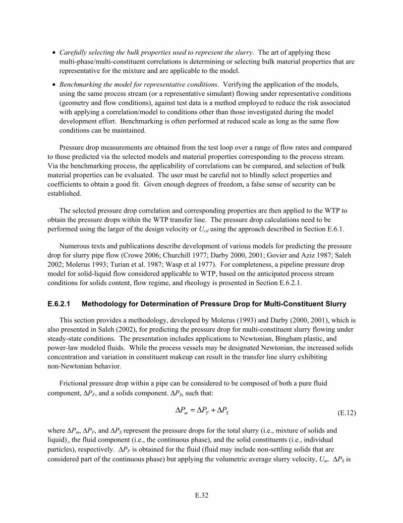
E.32

• Carefully selecting the bulk properties used to represent the slurry. The art of applying these multi-phase/multi-constituent correlations is determining or selecting bulk material properties that are representative for the mixture and are applicable to the model.

• Benchmarking the model for representative conditions. Verifying the application of the models, using the same process stream (or a representative simulant) flowing under representative conditions (geometry and flow conditions), against test data is a method employed to reduce the risk associated with applying a correlation/model to conditions other than those investigated during the model development effort. Benchmarking is often performed at reduced scale as long as the same flow conditions can be maintained.

Pressure drop measurements are obtained from the test loop over a range of flow rates and compared to those predicted via the selected models and material properties corresponding to the process stream. Via the benchmarking process, the applicability of correlations can be compared, and selection of bulk material properties can be evaluated. The user must be careful not to blindly select properties and coefficients to obtain a good fit. Given enough degrees of freedom, a false sense of security can be established.

The selected pressure drop correlation and corresponding properties are then applied to the WTP to obtain the pressure drops within the WTP transfer line. The pressure drop calculations need to be performed using the larger of the design velocity or Ucd using the approach described in Section E.6.1.

Numerous texts and publications describe development of various models for predicting the pressure drop for slurry pipe flow (Crowe 2006; Churchill 1977; Darby 2000, 2001; Govier and Aziz 1987; Saleh 2002; Molerus 1993; Turian et al. 1987; Wasp et al 1977). For completeness, a pipeline pressure drop model for solid-liquid flow considered applicable to WTP, based on the anticipated process stream conditions for solids content, flow regime, and rheology is presented in Section E.6.2.1.

E.6.2.1 Methodology for Determination of Pressure Drop for Multi-Constituent Slurry

This section provides a methodology, developed by Molerus (1993) and Darby (2000, 2001), which is also presented in Saleh (2002), for predicting the pressure drop for multi-constituent slurry flowing under steady-state conditions. The presentation includes applications to Newtonian, Bingham plastic, and power-law modeled fluids. While the process vessels may be designated Newtonian, the increased solids concentration and variation in constituent makeup can result in the transfer line slurry exhibiting non-Newtonian behavior.

Frictional pressure drop within a pipe can be considered to be composed of both a pure fluid component, ΔPF, and a solids component. ΔPS, such that:

ΔPm = ΔPF + ΔPS (E.12)

where ΔPm, ΔPF, and ΔPS represent the pressure drops for the total slurry (i.e., mixture of solids and liquid),, the fluid component (i.e., the continuous phase), and the solid constituents (i.e., individual particles), respectively. ΔPF is obtained for the fluid (fluid may include non-settling solids that are considered part of the continuous phase) but applying the volumetric average slurry velocity, Um. ΔPS is

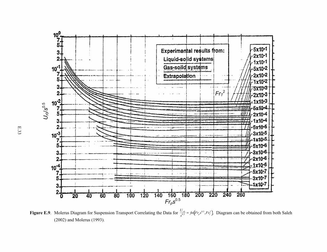
E.33

Figure E.9. Molerus Diagram for Suspension Transport Correlating the Data for Ur0

s0.5 = fn Frps0.5,FrT2( ). Diagram can be obtained from both Saleh

(2002) and Molerus (1993).

FrT2

Ur0

/s0.

5

Frps0.5

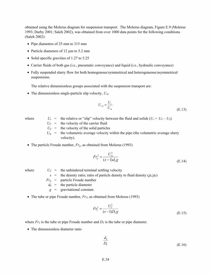
E.34

obtained using the Molerus diagram for suspension transport. The Molerus diagram, Figure E.9 (Molerus 1993; Darby 2001; Saleh 2002), was obtained from over 1000 data points for the following conditions (Saleh 2002):

• Pipe diameters of 25 mm to 315 mm

• Particle diameters of 12 µm to 5.2 mm

• Solid specific gravities of 1.27 to 5.25

• Carrier fluids of both gas (i.e., pneumatic conveyance) and liquid (i.e., hydraulic conveyance)

• Fully suspended slurry flow for both homogenous/symmetrical and heterogeneous/asymmetrical suspensions.

The relative dimensionless groups associated with the suspension transport are:

• The dimensionless single-particle slip velocity, Ur0

0

rr

m

UU

U=

(E.13)

where Ur = the relative or “slip” velocity between the fluid and solids (Ur = UF – US) UF = the velocity of the carrier fluid US = the velocity of the solid particles Um = the volumetric average velocity within the pipe (the volumetric average slurry

velocity).

• The particle Froude number, Frp, as obtained from Molerus (1993)

Frp

2 =Um

2

(s −1)dSg (E.14)

where UT = the unhindered terminal settling velocity s = the density ratio; ratio of particle density to fluid density (ρs/ρF) Frp = particle Froude number dS = the particle diameter g = gravitational constant.

• The tube or pipe Froude number, FrT, as obtained from Molerus (1993)

FrT

2 =UT

2

(s −1)DT g (E.15)

where FrT is the tube or pipe Froude number and DT is the tube or pipe diameter.

• The dimensionless diameter ratio

dS

DT (E.16)

E.35

The defined Froude numbers are somewhat arbitrary and Molerus (1993) provides no explanation for their origin. Molerus (1993) correlated the data in the functional form

( )0.5 20

0.5,r

p T

Uf Fr s Fr

s=

(E.17)

With respect to the defined fluid, if some of the solids are uniformly suspended to create a homogenous continuous phase (i.e., carrier fluid), this fraction of solids can be assumed to contribute to the fluid pressure drop and contribute to the fluid material properties. If the carrier or the uniformly suspended solids concentration leads to non-Newtonian behavior, the process is more complex but still is applicable. The application of the process to both Bingham plastic and power-law modeled fluids will be presented in the following sections.

Molerus (1993) developed a relation for the dimensionless solids contribution to the pressure drop, XΔP, resulting from the solids flow. His development is based on the rate of energy dissipation in the flow due to the solids and the rate of energy transferred to the particles resulting from the relative velocity between the solids and the fluid. The resulting relation as presented by Saleh (2002) is:

XΔP ≡

ΔPS

φSρF (s −1)gL

UT

Um

2

(E.18)

where φS is the total volume fraction of solids, and L is the relative pipe length such that the pressure drop per unit length of pipe (ΔPS/L) is calculated.

The value of XΔP depends on the value of φS.

For 0 < φS < 0.25:

2

20

001

1

r

m rP P

rr

m

UU U

X XUU

U

Δ Δ

= = =

− − (E.19)

For φS > 0.25:

XΔP = XΔP 0 + 0.1FrT2 φS − 0.25( ) (E.20)

Darby (2000) and Saleh (2002) both present methods for determining XΔP, which is presented in the following sections. The method involves the following five steps.

1. Determine UT for the correct flow condition

2. Determine Ur by obtaining 0.50rU s from the Molerus diagram for suspension transport (refer to

Figure E.9) for solids suspension using the values calculated for Frps0.5 and FrT2

3. Calculate XΔP0

E.36

4. If necessary (φS > 0.25) calculate XΔP from Equation (E.20)

5. ΔPS

L is then calculated using Equation (E.18)

After obtaining ΔPS

L, the pressure drop ΔPF

Lcan be calculated from the Fanning equation

22 F mF

T

f UP

L D

ρΔ = (E.21)

where f, the friction factor for pipe flow, can be defined in terms of the shear stress at the pipe wall, τw, such that

2

2= w

F m

fU

τρ (E.22)

and Um equals U, the fluid velocity for conditions where the carrier fluid is pure liquid.

The pressure drop resulting from solids for specific particle size ranges (bins) or species of solids can be considered individually such that n constituents of volume concentration φSi having dSi and ρsi would result in

ΔPm = ΔPF + ΔPSi

i=1

n

(E.23)

Again, a portion of the non-settling, uniformly suspended solids constituents may be considered part of the fluid, and these materials would not be considered as part of the n solids constituents. For multiple solid materials and/or solid sizes, the five steps listed above are repeated for each of the n solids constituents/size ranges to obtain

1

nSi

i

P

L=

Δ (E.24)

The particle terminal velocity, UT, and the friction factor, f, are dependent on the fluid rheology. Non-Newtonian behavior for the fluid changes the process by which these parameters are calculated. The following subsections will provide the method for obtaining these parameters for Newtonian (Sections E.6.2.1.1.1 and E.6.2.1.2.1), Bingham plastic (Sections E.6.2.1.1.2 and E.6.2.1.2.2), and power-law (Sections E.6.2.1.1.3 and E.6.2.1.2.3) modeled fluids. The outline is intended to allow the reader to focus on the rheology of interest and skip the other sections.

The determination of whether any solids constituents are to be included as part of the fluid is often based on the settling velocity, and there are a number of criteria that can be evaluated. Wasp (1977) proposes the following criterion for a Newtonian carrier fluid, ρF, as presented in Saleh (2002):

UT

Um

f

2

0.5

≤ 0.022

(E.25)

E.37

Chhabra and Richardson (1999) present a criterion for evaluating the settling of particles in a visco-plastic fluid. It is based on evaluating the forces acting on the particle by taking the ratio between the force due to the yield stress and that due to gravity. This ratio is represented by the dimensionless parameter Y where

Y =

τy

gdS ρS − ρ( ) (E.26)

where ρ is the mixture (slurry) density and τy is the yield stress in shear (most often referred to as just the yield stress but so noted here to distinguish from yield stress in compression or tension) for a visco-plastic fluid. τy = τB for a Bingham plastic modeled fluid.

Based on different approaches used to evaluate Y, values between 0.06 and 0.2 have been identified as the condition at which particle settling will occur in a quiescent visco-plastic fluid. Chhabra and Richardson (1999) suggest using the range of values for Y to establish the upper and lower bounds for the particles (i.e., size and density) that will settle. While this criterion has been applied to pipe flow for evaluating those particles that can be considered part of the homogeneous carrier fluid, the flow conditions must be considered in the assessment. For a fully turbulent flow, the effects of yield stress on particle deposition become negligible. For laminar and transition flows, particle settling can still occur because of the effective strain rate especially for shear thinning fluids (i.e., for both Bingham plastic and power-law [if the flow behavior index, n<1] fluids, settling can occur in laminar flow conditions, where shearing between the wall and uniform plug reduces the apparent viscosity). Therefore, the use of Equation (E.26) can over-predict the particle size range or the constituents that can be considered as part of the fluid phase (i.e., carrier fluid).

E.6.2.1.1 Determination of Settling Velocity, UT

Again, the following approaches for determining the particle settling velocity for all three rheologies presented in Sections E.6.2.1.1.1 through E.6.2.1.1.3 are those presented by Darby (2000) and Saleh (2002).

E.6.2.1.1.1 Newtonian Fluid – UT

For Newtonian flow, the particle Archimedes number, Ar, a non-dimensional relationship between gravitational and drag forces, is used to assess the condition of particle flow. The Archimedes number is calculated from

( )3 2

2

1S F

F

d g sAr

ρμ

−=

(E.27)

If 15Ar < , then from Stokes’ Law

( )2 1

18F S

TF

g d sU

ρμ

−=

(E.28)

E.38

If 15Ar > , then UT is obtained from the particle Reynolds number for a Newtonian fluid, Rep, which is determined from the Dallavalle equation (Darby 2000).

( )

20 50 514 42 1 827 3 798..S F T

pF

d URe . . Ar .

ρμ

= = + − (E.29)

Camenen (2007) provides a closed form for UT that covers the entire range of Archimedes number,

20.50.50.515 15

0.3F

TF S

ArU

d

μρ

= + − (E.30)

which yields similar results as both Equations (E.28) and (E.29).

E.6.2.1.1.2 Bingham Plastic – UT

As with the Newtonian material, the determination of UT will depend on the relative flow conditions where u is the velocity component parallel with the pipe and y is the direction perpendicular to the pipe wall. A material whose rheology is modeled as a Bingham plastic will have a limiting viscosity, µB, and Bingham plastic yield stress, τB, defined such that the shear stress ,τ

B B

u

yτ μ τ∂= +

∂ where 0

u

y

∂ =∂

for τ < τB (E.31)

To assess the flow for a Bingham plastic, the Bingham number, Bi, and Bingham plastic particle Reynolds number, ReBp, are defined by Darby (2000) as

B S

B T

dBi

U

τμ

= (E.32)

S TBp

B

d URe

ρμ

= (E.33)

Darby applies the slurry density, ρ, not the fluid density, ρF, used to define the Newtonian and power-law Reynolds numbers of Equations (E.29) and (E.40), respectively. Darby’s assumption is that if the slurry is “thick” enough to exhibit a yield stress, then it is most likely stable enough to be treated as a pseudo-homogeneous fluid; in other words, only those large particles which are heavy enough to overcome the yield stress will settle at an appreciable rate (Darby 2000) (refer to Equation (E.26)). However, consideration should be given to cases where the density ratio, s, is high and/or the particle concentration is low. In such instances, ρF should be substituted for ρ in Equations (E.33) and (E.36) as this is the localized density affecting the particle Reynolds number.

E.39

The drag coefficient, CD, for a particle is defined as

( )2

4 1

3S

DT

gd sC

U

−=

(E.34)

According to Chhabra and Richardson (1999), creeping flow exists for the condition

ReBp <100Bi0.4 (E.35)

For the condition of creeping flow, the coefficient of drag can be defined as

2424 B BD B

Bp S T

ZC Z

Re d U

μρ

= = (Darby 2000) (E.36)

where ZB is the correction to Stoke’s Law for Bingham plastic material.

ZB = 1 + 2.93Bi0.83 (E.37)

For larger Reynolds numbers beyond creeping flow, where ReBp <100Bi0.4, Darby (2000) provides the following relationship for CD

2

0.5

4.80.632D

Bp

B

CRe

Z

= + (E.38)

The equations, (E.36) and (E.38), are implicit in UT and are solved via iteration.

E.6.2.1.1.3 Power-Law Fluid – UT

As with Newtonian and Bingham plastic materials, the determination of UT will depend on the relative flow conditions for a power-law modeled fluid. A material whose rheology is modeled as a power-law fluid will be characterized by a flow behavior index, n (dimensionless), and consistency index (i.e., power-law coefficient), K (SI units Pa sn), such that

nu

Ky

τ ∂= ∂ (E.39)

To assess the flow in a power-law fluid, Equation (E.34) still holds as a definition for the coefficient of drag. To apply the same approach as presented in Section E.6.2.1.1.2, a particle Reynolds number for a power-law fluid, RePLp, needs to be defined. RePLp does not have the same physical meaning as the particle Reynolds number, Rep, for Newtonian fluid, or particle Reynolds number for Bingham plastic,

E.40

ReBp, but is defined to produce a comparable form to Equations (E.29) and (E.33) for defining flow regimes. Darby (2000) and Crowe (2006) define the particle Reynolds number for a power-law fluid, RePLp as

2n nS T F

PLp

d URe

K

ρ−

= (E.40)

The following approach was obtained from Darby (2000) with no caveats on the applicable range relative to the behavior index, n. Two dimensionless power-law parameters, ZPL1 and ZPL2, are defined to simplify the presentation of subsequent equations

ZPL1 =

1.88

n

8

+ 34

−0.125

(E.41)

and

ZPL2 =

1.33+ 0.37n

1+ 0.7n3.7 (E.42)

For a power-law fluid, creep flow is considered to exist for the condition

1PLpRe <

(E.43)

and

224 PLD

PLp

ZC

Re=

(E.44)

For the entire range of RePLp, Darby (2001) defines the coefficient of drag as

2

1 0.5

2

4.8D PL

PLp

PL

C ZRe

Z

= + (E.45)

This equation is implicit in UT and to simplify the iterative process, Equation (E.45) is rearranged to yield

2

2 0 51

4 8PLp PL .

D PL

.Re Z

C Z

= − (E.46)

E.41

E.6.2.1.2 Determination of Friction Factor, f, for Pipe Flow

Again, the following approaches for determining the friction factor for pipe flow for all three rheologies presented in Sections E.6.2.1.2.1 through E.6.2.1.2.3 are those presented by Darby (2000) and Saleh (2002).

E.6.2.1.2.1 Newtonian Fluid – f

For Newtonian fluids, the friction factor can be obtained using the Moody diagram (Crane 1986), which was based on the following equation developed by Karman and modified by Colebrook (Crowe 2006).

0 5 0 5

1 1 2554 0log

3 7T

. .

D ..

f . Re f

ε = − + (E.47)

where ε is the absolute roughness or effective height of pipe wall irregularities, and Re, the Reynolds number for a Newtonian fluid, is based on the pipe inner diameter. Churchill (1977) provided an equation explicit in f and applicable to both smooth and rough pipe surfaces in either laminar or turbulent flows.

( )1 1212

1.5

1 2

8f Z Z

Re

− = + + (E.48)

where

Z1 = 2.457ln 1

Z3

16

,

16

2

37530 =

ZRe ,

0 9

3

70 27

.

T

Z .Re D

ε = + (E.49)

E.6.2.1.2.2 Bingham Plastic – fB

Again, a Bingham plastic is modeled by defining a limiting viscosity, µB, and Bingham plastic yield stress, τB. To determine the friction factor, fB, in a Bingham plastic, the Bingham Reynolds number, ReB, and Hedstrom number, He, for pipe flow are defined as:

2T m

BB

D URe

ρμ

= (E.50)

2

2T B

B

DHe

ρτμ

= (E.51)

E.42

The friction factor for a Bingham plastic modeled fluid, fB, can be determined from a combination of the friction factors for laminar, fL, and turbulent flow, fT.

fB = fLm + fT

m( )1/ m

(E.52)

where m, the exponent to calculate friction factor for Bingham plastic fluid, is

400001 7

B

m .Re

= + (E.53)

For laminar flow, fL is obtained from

4

3 7

16 1 11

6 3

= + −

L

B B L B

He Hef

Re Re f Re (Crowe 2006) (E.54)

which is the Buckingham-Reiner equation (Darby 2001) implicit in fL that must be solved by iteration for known values of He and ReB. For turbulent flow, fT is represented by the empirical expression of Darby and Melson (1981) as modified by Darby et al. (1992) and presented in Darby (2001)

0 19310 .

T Bf Reβ −= (E.55)

The value of β is given by Darby (2001) as a function of He

( )51.47 1 0.146exp 0.29 10 Heβ − = − + − × (E.56)

Crowe (2006) provides an expression for β as a function of ReB

( )51.378 1 0.146exp 0.29 10− = − + − × BReβ

(E.57)

Equation (E.56) does not apply when He, defined by Equation (E.51) is less than 1000, but this is not a constraint for most slurries with a measureable yield stress (Crowe 2006).

E.6.2.1.2.3 Power Law – fPL

Again, a power-law fluid is modeled using a flow behavior index, n, and consistency, K (refer to Equation (E.39)). To determine the friction factor, fPL, for a power-law modeled fluid, a critical Reynolds number, RePLc, indicating transition to turbulent flow for a power-law fluid is defined as:

2100 875 1PLcRe ( n )= + − (Darby 2000) (E.58)

Darby (2001) and Crowe (2006) define a power-law Reynolds number for pipe flow, RePL, by Equation (E.59). However, RePL does not have the same physical meaning as Re for Newtonian or Bingham plastic materials, but is defined to produce a comparable form for Equation (E.63). For

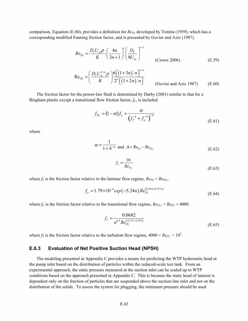
E.43

comparison, Equation (E.60), provides a definition for RePL developed by Tomita (1959), which has a corresponding modified Fanning friction factor, and is presented by Govier and Aziz (1987).

14

3 1 8

nn

T m TPL

m

D U DnRe

K n U

ρ−

= + (Crowe 2006) (E.59)

( )( )

12 6 1 3

Re2 1 2

nn

T mPL n

n nD U

K n n

ρ−

− + = + (Govier and Aziz 1987) (E.60)

The friction factor for the power-law fluid is determined by Darby (2001) similar to that for a Bingham plastic except a transitional flow friction factor, ftr, is included.

fPL = 1 − α( ) fL +α

fT−8 + f tr

−8( )1/ 8

(E.61)

where

α =

1

1+ 4−Δ and PL PLcRe ReΔ = − (E.62)

16L

PL

fRe

= (E.63)

where fL is the friction factor relative to the laminar flow regime, RePL < RePLc.

( ) ( )0.414 0.75741.79 10 5.24 +−= × − n

tr PLf exp n Re (E.64)

where ftr is the friction factor relative to the transitional flow regime, RePLc < RePL < 4000.

( )1 1.87 2.390.5

0.0682T n

PL

fn Re +=

(E.65)

where fT is the friction factor relative to the turbulent flow regime, 4000 < RePL < 105.

E.6.3 Evaluation of Net Positive Suction Head (NPSH)

The modeling presented in Appendix C provides a means for predicting the WTP hydrostatic head at the pump inlet based on the distribution of particles within the reduced-scale test tank. From an experimental approach, the static pressure measured at the suction inlet can be scaled up to WTP conditions based on the approach presented in Appendix C. This is because the static head of interest is dependent only on the fraction of particles that are suspended above the suction line inlet and not on the distribution of the solids. To assess the system for plugging, the minimum pressure should be used

E.44

because pump performance can be degraded with a reduction in NPSHA. A decrease in vessel fluid level will contribute to a lowering of the NPSHA at the pump inlet. However based on the LOAM test results, refer to Section E.2.1, the solids concentration is expected to decrease with vessel level. A reduction in solids concentration will contribute to increasing the NPSHA at the pump inlet due to the reduced pressure drop in the upstream transfer line.

The pressure at the WTP pump inlet then is predicted by solving the energy equation for flow from the liquid surface of the PJM mixing vessel to the pump inlet (i.e., pipeline calculation). The pressure drop associated with the flow through the WTP suction line is obtained from the approach presented in Section E.6.2.

The predicted WTP pressure is then compared to the specified NPSHR for the pump. It should be noted that the NPSHR for pumps handling slurries is on the order of 1.5 to 2 times greater than that for water. This factor is driven higher by the presence of gas in the flow with factors on the order of 2 to 3 times that of the NPSHR for water reported by Poloski et al. (2009b). Many solids have an affinity for gas bubbles; therefore, slurries can readily become gas laden. In addition, there are many opportunities for particulates to come into contact with entrained gases during operation of the PJM and the sparger. This point is mentioned because many slurry pump vendors use only water to characterize their systems. Assessment of the Prevent Plugging requirement relative to the NPSHA relies on having a realistic value for NPSHR for comparison.

E.6.4 Pump Performance

To complete the assessment of the Prevent Plugging requirement, the pump performance under prototypic operating conditions must be assessed. If pipe plugging (i.e., with no solids deposition being the evaluated metric) is avoided and the NPSHA meets the pump performance requirements, plugging will still be experienced if the motive pump is incapable of producing the required slurry flow rate at the required system head (i.e., needed pump discharge pressure). Prototypic conditions include operations at:

• The design flow rate or, if greater, the flow rate required to avoid solids deposition

• The solids loading determined from the limit solids accumulation tests (refer to Appendix C). Testing would be done with a steady-state solids concentration.

• The calculated system back pressure, which is based on the prediction of WTP pressure drop obtained using steady-state solids loading determined from the LSIT for limit solids accumulation.

There is no way to assess the full-scale pump performance at a reduced scale. Either prior performance data must be obtained or a “pumpability” test is required. Sources of past performance data are vendor testing with an acceptable simulant or operational data from a representative industrial application. The uniqueness of the anticipated WTP process feed stream creates a challenge for identifying applicable past performance data.

E.6.5 Full-Scale Test Approach

The following discussion addresses assessing the Prevent Plugging requirement based on full-scale testing. An approach for accomplishing the assessment using scaled testing, other than the demonstration of pumpability, has been presented in Sections E.5. However, this approach relies on conservatism being

E.45

applied to the assessment of system pressure drop (and thus NPSHA) and solids deposition. If the conservatism applied to the assessment results is too great, an over-prediction of transfer line flow rate may result such that:

• Verification of the Prevent Plugging requirement is brought into question

• Achieving acceptable operating conditions (based on the assessment) is cost prohibitive.

Under these circumstances, full-scale conditions may then need to be considered to complete the assessment.

The inlet conditions at the transfer line are expected to be periodic as a result of the PJM operations. Both the solids concentration and the flow field are expected to vary with the discharge cycle of the PJMs. The slurry within the WTP vessels also will contain a polydisperse PSDD. The most important factor to be evaluated is the variation in solids loading because of the potential for solids segregation discussed in Section E.2.1 and depicted in Figure E.4 that can result in solids deposition. The following approach assumes that the variation in the flow field at the inlet will not be evaluated at full scale. The results and observations observed for the limit solids accumulation test will be used to assess the potential of solids swamping to create plugging issues.

A prototypic inlet line size and configuration to the pump are recommended for use during full-scale testing. Results of the reduced-scale limit solids accumulation testing will provide the solids concentration as a function of time that will exist at the pipe inlet. Refer to Appendix C regarding scaled testing to obtain transfer line inlet conditions. The appropriate scale-up of time will need to be applied to the scaled test results to obtain a representative profile of solids concentration as a function of time. The simplest and recommended approach would assume a constant PSDD for the entrained material based on the worst-case conditions observed during the reduced-scale tests, and the concentration of the uniform mixture would be varied only as a function of time. The variation in solids concentration would be intended only to capture the significant difference between the peak and low concentrations, not to match the exact time history.

The objectives of the full-scale tests would be to:

• Assess pump performance for the range of operating conditions to be encountered. Does the pump deliver specified/required discharge head and flow rate without cavitation? An optional test for consideration is to provide a source of air in the slurry feed tank/feed system to assess the potential impact of air entrainment by the solids.

• Determine if the inlet line delivers the prescribed slurry PSDD to avoid holdup within the process vessel.

• Determine if holdup exists within the suction or discharge lines that does or could lead to plugging. Assess if solids deposition exists in pipe if condition of fully-suspended solids is accepted as a design requirement. The opportunity will exist for flushing operations to be evaluated during this assessment.

• Determine or verify the predicted pressure drop through the prototype discharge line to assure the correct discharge head is used to assess pump and system performance.

E.46

• Testing should include monitoring of the slurry density and sampling to assess particle size distribution in sections of the transfer line both upstream and downstream of the pump to evaluate for system holdup. Observation can also be made for solids deposition by monitoring pipe sections using visual monitoring (e.g., transport pipe section) or ultrasonic techniques. Of course, the slurry line contents need to be monitored to verify that the prescribed slurry makeup is being entrained and the inlet geometry is not resulting in solids segregation. Additional measurements for comparison against the pump NPSHR should include the line pressure at the pump inlet.

For evaluating the pump operation and assessing the inlet line for plugging, a single or series of pinch valves are recommended to simulate system head. For positive displacement pumps, full simulation of the discharge head is not required. The use of other types of valves can create solids holdup issues.

To assess pump plugging and the driving force needed for the downstream transfer line, a graduated approach can be taken. The ideal condition would be to have a prototypic line in which to perform testing; however, a successful assessment could be obtained without such a setup. Performance within the horizontal/inclined sections will be critical to avoid pipeline plugging (there are exceptions that are not considered applicable to WTP). The assessment will require a mock-up of the longest horizontal/ inclined run including all pipeline components. The mock-up also should include a vertical section and any additional critical components not contained within the longest prototypic horizontal/inclined run.

The strategy is to test for holdup within the prototypic line by monitoring upstream and downstream PSDDs. Pressure drop measurements over horizontal, inclined, and vertical sections as well as across individual components can be used to develop a system curve for the prototypic pipe run. Pinch valves can then be used to apply a prototypic discharge head for assessing the pump performance with the simulated inlet conditions. If no change in slurry makeup is observed over the critical prototypic pipe run and the pump can meet design specifications, then the test objectives will have been met.

However, if holdup is detected within the prototypic run, then either 1) more of the plant design needs to be incorporated into the test loop, or 2) testing should be performed with the current test loop to determine the line velocity (i.e., WTP flow rate) that eliminates the observed holdup, and based on the findings, new operating conditions for the plant should be prescribed.

Full-scale testing of pump performance does not require a full-scale upstream system (mixing vessel with PJMs), but it is recommended that a full-scale inlet system (e.g., transfer line inlet geometry) be used. The full-scale pump can be tested using a mechanically agitated tank and/or for a prescribed set of inlet conditions including time-dependent conditions. These can be accomplished using programmed feed/injection systems and programmed pressure variations. Consideration has been given to performing the full-scale pump assessment using PJM operations in the 14-ft-diameter tank to provide the inlet conditions. A final decision on the validity of this may not be possible until results for the limit solids accumulation tests are obtained. An initial concern arises from having the full-scale flow rate into the transfer line coupled with scaled PJM operations. The relatively higher inlet flow rate could result in

• An increase in the duration of any concentration spikes, thus a reduction of concentration gradients observed within the transfer line.

• Potential dilution of the faster-settling particles as the influence of the inlet flow will have a greater “sphere” of influence allowing the entrainment of less dilute fluid. The proximity of the suction line

E.47

to the tank floor means the boundary for the increased affected flow field volume cannot extend below the tank floor. Therefore, the expansion of the flow field influence will be biased upward.

• A reduction of the number of PJM cycles to be experienced during a pump out, thus reducing the impact of any detrimental effects resulting from cyclical conditions.

E.7 Considerations for Application of Approach

The following sections provide a list of items to be considered for applying the approach presented in Section E.5. The considerations are for the failure modes presented in Sections 6.1 through 6.3. No consideration has been made in this section for performing the alternative full-scale assessment discussed in Section 6.5. Section E.7.1 discusses functional needs for the test setup. Simulants are discussed in Section E.7.2 and additional considerations associated with non-Newtonian behavior and gas entrainment are addressed in Section E.7.3.

E.7.1 Test Setup Needs

The setup needs for the testing to assess the Prevent Plugging requirement are listed below:

• A scaled transfer line inlet for each LSIT setup. The remainder of the transfer line does not need to be scaled or prototypic.

• The transfer line downstream of the inlet needs to be sized to ensure that no solids deposition occurs in the pipe downstream of the inlet.

• A section of the transfer line for each LSIT setup should include a horizontal run (but not necessarily a straight section) from which a pressure drop can be measured during the limit solids accumulation testing.

• The transfer line is to be plumbed for the reduced-scale test setups so that it can be operated in both recirculation and transfer modes. Consideration should be made as to whether the return line for the recirculation flow is to be prototypic or split to allow the return stream to be uniformly distributed azimuthally around the tank. Validation test are recommended to assess the impact of the recirculation line on the vessel mixing.

• To allow the flow rate through the transfer line to be readily adjusted, it is recommended that a variable frequency drive be used with the transfer pump for each test setup.

• Coriolis or other mass-flow-rate and density meters in the transfer line should be located as close to the transfer line inlet as possible. Current plans for the LSIT have the transfer line running vertically from the test vessels to avoid breaching the sidewall of the acrylic tanks. This may result in a dampening of the concentration variations between the transfer line inlet and the location of measurements and sampling because of holdup effects in the vertical run.

• Transfer line sampling methods should be selected based on the individual physical scale of each test setup, and do not need to be identical for each scale or prototypic of the WTP. The sampling needs will be influenced by the assessment of the sampling requirements for Mixing Requirements 5, 6, and 7 (refer to Chapter 10).

E.48

• The inclusion of full-port/full-volume sampling techniques is recommended. If not used for acquiring all samples, these systems are useful for benchmarking other sampling techniques.

• A flow evaluation loop is required for benchmarking the correlations for deposition velocity and pressure drop. An example of such a loop is the pipe loop used to support the M1 – Plugging in Process Piping scope (Poloski et al. 2009a, 2009b), which is still intact. The flow evaluation loop needs to include features such as:

– Pipe sections for visual observation of slurry flow

– Instrumentation for detecting solids deposition

– Pressure drop measurement over various pipeline components including straight pipe sections of fully developed flow

– Mass and density flow meters for measuring slurry flow rate and assessing solids holdup

• Test facility for full-scale pump testing with prescribed simulant and back pressure.

E.7.2 Simulant Considerations

The test approach has been developed with the goal of being able to assess WTP performance for a complex multi-constituent simulant. While this objective has been met, the use of solid constituents with narrow size distributions is recommended for LSIT tests. The simulant also should consist of a unique density for each particle size. These recommendations will greatly simplify the characterization of samples, as size characterization also will yield a density distribution for the solids. These same simulants also should be used for the initial tests conducted in the flow evaluation loop. The size range of the constituents then can be broadened for additional testing in the flow evaluation loop to evaluate the impact of size distribution on the selection of representative material properties and model predictions.

The assessment of the sampling requirements presented in Chapter 10 yields similar recommendations for simulant selection. The full sampling assessment will require that the size distribution in the LSIT tests be broadened.

E.7.3 Additional Considerations

Additional complications associated with assessing the Prevent Plugging requirement are described below:

• Non-Newtonian materials. All slurries having significant solids loading exhibit some form of non-Newtonian behavior. The recommended correlations have been applied to conditions of non-Newtonian flow. Many of the models will not have been developed using non-Newtonian rheological parameters. Instead apparent viscosities will have to be determined and verified via testing. The impact of this approach on predictions may result from benchmarking the correlation using a significantly smaller pipe diameter than that applied for WTP predictions. In addition, similarity for non-Newtonian condtions is not readily maintained for changes in geometric scale. For example, consider the reduction in scale for shear-thinning materials. For cases where the velocity is held constant between scales, the velocity gradient or shear rate will be higher at the reduced scale resulting in a lower effective viscosity. Any impact associated with non-Newtonian behavior is reduced the closer the test loop and WTP transfer line are in size.

E.49

• Air entrainment. Sparger and PJM operations are conducive to entraining air into the process stream. The greatest issue can result from small micro-sized bubbles that attach to the solid particulate. These bubbles can have several impacts:

– They can change the effective density of particulate and the bulk slurry.

– They can changes the effective rheology.

– They are released from the particulate at reduced pressure (i.e., suction line, pump inlet).

– They can reduce the representativeness of samples because they are released from solids or gas released from retrieved samples occurs over time (i.e., sample characterization becomes time dependent).

The impact or occurrence of air entrainment is difficult to scale for many reasons, one of which is that it is difficult to directly quantify. The operation of the flow evaluation loop will not be subjected to the same potentials for entrainment. Often, characterization loops are operated at an elevated pressure to help keep the gas in solution, thus minimizing the occurrence of a gas phase.

E.8 Summary and Recommendations

An approach for using reduced-scale testing has been presented to assess Mixing Requirement 2, Prevent Plugging. The recommended approach provides a complete assessment of the Prevent Plugging requirement using a complex simulant. Industry applied correlations developed from experimental data and reduced-scale testing are used to assess the Prevent Plugging mixing requirement relative to the performance of the WTP vessel transfer lines and motive pumps. The test strategy is designed to identify potential problems associated with slurry transport in the WTP transfer line based on bounding (conservative) conditions and is not intended to characterize the slurry transport over the full range of WTP transfer line conditions. Because of the conservative/bounding approach used, this test strategy only confirms success and not failure. If testing is found to be too conservative, then full-scale testing of the transfer line will likely be needed.

The approach is based on assessing the periodic conditions at the transfer line inlet resulting from PJM operations during reduced-scale LSIT activities. Critical factors associated with the recommended approach include:

• Determining the feed stream conditions from LSIT testing

• Developing the representative steady-state bounding conditions

• Selecting representative material properties for application of the predictive models.

LSIT performance testing to assess the Limit Accumulation of Solids mixing requirement will be conducted at multiple geometric scales. From these tests, transient conditions at the transfer line inlet will be used to define bounding steady-state conditions for separately assessing:

• Solids deposition/holdup within the transfer line

• System pressure drop through the transfer line

• NPSHA at the transfer pump inlet.

E.50

Additional reduced-scale tests conducted in a separate pipe test loop then are performed at steady-state conditions, which are determined from the LSIT performance tests for limit accumulation of solids. The pipe loop tests are carried out to benchmark correlations and the associated representative material properties applied to the correlations. Based on existing loops, testing at full-scale pipe diameter and flow rates may be achievable.

The correlations and associated test results are used to predict WTP performance for the bounding steady-state operating conditions. Predictions of performance will include uncertainty in model predictions based on past applications/approaches and the benchmark testing of the correlations for application to WTP.

However, no viable recommendation is considered to exist for assessing the pump performance with less than a prototypic pump.

The inlet conditions for the transfer line are not known or specified; therefore, reduced-scale testing will be performed to provide solids loading conditions for the assessment. The reduced-scale testing for limit solids accumulation will provide a one-to-one comparison of the inlet solids loading for full-scale WTP conditions. Time scaling will be required to obtain the solids loading as function of time for WTP. The conditions for peak solids loading will be used as the basis for performing the prevent plugging assessment.

The approaches provided for assessing system pressure drop and solids deposition are conservative. The conservative method for determining the system pressure drop is used to assess the NPSHR and the pump discharge requirements. The effects of changing liquid level on the solids loading will be assessed via the limit solids accumulation tests while the effect on the NPSHA will be determined from pressure drop calculations.

The assessment is based on incorporating the requirement of no solids deposition within the transfer line. This condition is recommended for the application of the models presented and because the existence of settled solids greatly increases the potential for plugging. The potential for plugging is proportional to the mass of material within the transfer line.

The approaches presented for evaluating system pressure drop and critical deposition pipeline velocity, Ucd, require validation of selected models/correlations via testing in a test loop configured for flow characterization. The existing M1 test loop (Poloski et al. 2009a, 2009b) is recommended to meet these needs because it was designed for this purpose and to accommodate WTP simulants.

If full-scale testing of the pump is conducted, the following recommendations are provided:

• A prototypic inlet line size and configuration to the pump

• A constant particle size and density distribution, PSDD, for the entrained material based on the worst-case conditions observed during the reduced-scale tests, and the concentration of the uniform mixture be varied only as a function of time

• Variation in solids concentration made only to capture the significant difference between the peak and low concentrations of the inlet slurry.

E.51

It is recommended that the M1 - Plugging in Process Piping requirements be re-evaluated for the solids loading obtained from the limit solids accumulation tests. This will ensure closure/integration of the mixing and process piping requirements.

E.9 References

Bamberger JA, PA Meyer, JR Bontha, CW Enderlin, DA Wilson, AP Poloski, JA Fort, ST Yokuda, HD Smith, F Nigl, M Friedrich, DE Kurath, GL Smith, JM Bates, and MA Gerber. 2005. Technical Basis for Testing Scaled Pulse Jet Mixing Systems for Non-Newtonian Slurries. PNWD-3551; WTP-RPT-113, Rev. 0, Battelle–Pacific Northwest Division, Richland, Washington.

Camenen B. 2007. “Simple and General Formula for the Settling Velocity of Particles.” Journal of Hydraulic Engineering, ASCE 133(2):229-233.

Chhabra RP and JF Richardson. 1999. Non-Newtonian Flow in the Process Industries. Butterworth Heinemann, Woburn, Massachusetts.

Churchill SW. 1977. “Friction factor equation spans all fluid-flow regimes.” Chemical Engineering 84:91-92.

Crane Engineering Dept. 1988. “Flow of Fluids Through Valves, Fittings, and Pipe.” Technical Paper No. 410, Crane Co. New York, New York.

Crowe CT. 2006. MultiPhase Flow Handbook. CRC Press Taylor and Francis Group LLC., Boca Raton, Florida.

Crowe CT, RA Gore, and TR Trout. 1985. “Particle Dispersion by Coherent Structures in Free Shear Flows.” Particle Science and Technology 3:149.

Darby R. 2000. “Pressure Drop for Non-Newtonian Slurries: A Wider Path.” Chemical Engineering pp. 64-67.

Darby R. 2001. Chemical Engineering Fluid Mechanics. Marcel Dekker, New York.

Darby R and J Melson 1981. “How to Predict the Friction Factor for Flow of Bingham Plastics” Chemical Engineering, December 28:59-61.

Darby R, R Mun, and DV Boger. 1992. “Predict Friction Loss in Slurry Pipes.” Chemical Engineering September 1992.

Gillies RG and CA Shook. 1991. “A Deposition Velocity Correlation for Water Slurries.” Canadian Journal of Chemical Engineering 69(5):1225-1228.

Govier GW and K Aziz. 1987. The Flow of Complex Mixtures in Pipes. Robert E. Kreiger Publishing Co., Malabar, Florida.

Hanks RW. 1980. “Slurry Pipeline Hydraulics: Principles, Problems and Solutions.” American Society of Mechanical Engineers (Paper), n 80-Pet-45, 1980.

E.52

Molerus O. 1993. Principles of Flow in Disperse Systems. Chapman and Hall, London.

Oroskar AR and RM Turian. 1980. “The Critical Velocity in Pipeline Flow of Slurries.” AIChE Journal 26(4):550-558.

Poloski AP, HE Adkins, J Abrefah, J Chun, AM Casella, F Nigl, MJ Minette, RE Hohimer, ST Yokuda, JM Tingey, and JJ Toth. 2009a. Deposition Velocities of Newtonian and Non-Newtonian Slurries in Pipelines. PNNL-17639; WTP-RPT-175, Rev. 0, Pacific Northwest National Laboratory, Richland, Washington.

Poloski AP, HE Adkins, ML Bonebrake, J Chun, AM Casella, KM Denslow, MD Johnson, ML Luna, PJ MacFarlan, JM Tingey, and JJ Toth. 2009b. Deposition Velocities of Non-Newtonian Slurries in Pipelines: Complex Simulant Testing. PNNL-18316; WTP-RPT-189, Rev. 0, Pacific Northwest National Laboratory, Richland, Washington.

Saleh JM. 2002. “Two-Phase Flow: Liquid-Solid and Gas-Solid Flow.” Fluid Flow Handbook. McGraw-Hill, New York.

Shook CA, RG Gillies, and RS Sanders. 2002. Pipeline Hydrotransport with Applications in the Oil-Sand Industry. SRC Publication No. 11508-1E02, Saskatchewan Research Council, Saskatoon, Canada.

Tomita Y. 1959. “On the Fundamental Formula of Non-Newtonian Flow.” Bulletin of JSME 2:469-474.

Turian RM, FL Hsu, and MTW Ma. 1987. “Estimation of the Critical Velocity in Pipeline Flow of Slurries.” Powder Technology 51:35-47.

Wani GA, MK Sarkar, and BP Mani. 1982. “Critical Velocity in Multisize Particle Transportation through Horizontal Pipes.” Journal of Pipelines 2:57-62.

Wasp EL, JP Kenny, and RL Gandhi. 1977. Solid-Liquid Flow-Slurry Pipeline Transportation, 1st ed., Trans-Tech Publications, Clausthal, Germany.

Wells BE, Y Onishi, CA Burns, RC Daniel, DE Kurath, JL Huckaby, EC Buck, KK Anderson, LA Mahoney, SK Cooley, and JM Tingey. 2011. Hanford Waste Physical and Rheological Properties: Data and Gaps. PNNL-20646; EMSP-RPT-006, Rev. 0, Pacific Northwest National Laboratory, Richland, Washington.

References Not Publically Available

Arulampalam M. 2011. Mixing Assessment Equipment Changes Section and Detail Views. WTP drawing No. 24590-PTF-MV-HLP-00003003, Bechtel, River Protection Project, Waste Treatment Plant, Richland, Washington.

Campbell T, M Parker, A Moon, and B Fant. 2010a. EFRT Issue M3 PJM Vessel Mixing Assessment, Volume 7–UFP-01. 24590-WTP-RPT-ENG-08-021-07, Rev. 1, Bechtel National, Inc., Richland, Washington.

E.53

Campbell T, M Parker, A Moon, B Fant, K Clossey, and J Cook. 2010b. EFRT Issue M3 PJM Vessel Mixing Assessment, Volume 8—HLP-22. 24590-WTP-RPT-ENG-08-021-08, Rev. 1, Bechtel National, Inc., Richland, Washington.

Hall MN. 2010. Minimum Flow Velocity for Slurry Lines. WTP Project Doc. No. 24590-WTP-GPG-M-0058, Rev. 0, Bechtel National, Inc., Richland, Washington.

Mauss J and I Papp. 2010. Determination of Mixing Requirements for Pulse-Jet-Mixed Vessels in the Waste Treatment Plant. 24590-WTP-ES-ENG-09-001, Rev. 2, Appendix A, Bechtel National, Inc., Richland, Washington.

Papp I. 2010a. EFRT Issue M3 PJM Vessel Mixing Assessment, Volume 3-HLP-VSL-00027A/B, HLP-VSL-00028, UFP-VSL-00002A/B, pp. A-76, A-221. 24590-WTP-RPT-ENG-08-021-03, Rev. 1, Bechtel National, Inc., Richland, Washington.

Papp I. 2010b. EFRT Issue M3 PJM Vessel Mixing Assessment, Volume 4-HOP-VSL-00903/904, PWD-VSL-00015/16, TCP-VSL-00001, TLP-VSL-00009A/B, RLD-VSL-00008, p. A-59. 24590-WTP-RPT-ENG-08-021-04, Rev. 1, Bechtel National, Inc., Richland, Washington.

PNNL-22816

Distribution

No. of No. of Copies Copies

Distr.1

ONSITE* DOE Headquarters RV Rimando, Jr. EM-23 14 Pacific Northwest National Laboratory JA Bamberger K7-15 EJ Berglin K5-22 CW Enderlin K7-15 JA Fort K7-15

GB Josephson K9-69 WL Kuhn K7-15 MJ Minette K7-15 TE Michener K7-15 LM Peurrung K3-52 SD Rassat K6-28 DR Rector K7-15 BE Wells K7-15 Information Release K3-52 Project File (1) K3-52

*All distribution will be made electronically.