Scale-dependent controls on ecological functions in agroecosystems of Argentina

Chave & Levin 8/6/02
1
Scale and scaling in ecological and economic systems
Jérôme Chave1 and Simon Levin2
Department of Ecology and Evolutionary Biology,
Guyot Hall, Princeton University, Princeton NJ 08544-1003, USA.
Abstract We review various aspects of the notion of scale applied to natural systems, in particular complex adaptive systems. We argue that scaling issues are not only crucial from the standpoint of basic science, but also in many applied issues, and discuss tools for detecting and dealing with multiple scales. We also suggest that the techniques of statistical mechanics, which have been successful in describing many emergent patterns in physical systems, can also prove useful in the study of complex adaptive systems.
1. Introduction One of the fundamental truths in the study of natural systems is that there is no single correct scale on which to study dynamics. In ecological systems, processes (such as behaviors) at the level of whole organisms represent the collective dynamics of cells (such as neurons) and molecules operating on much faster time scales, largely shaped by evolutionary processes operating over much longer scales of space and time. Similarly, organizations and economies, societies and the Internet exhibit collective dynamics that emerge from the behaviors of individual agents, mediated through levels of interaction and aggregation. The distinctions among scales need not be sharp, as between individuals and their societies, but may represent a continuous gradation, as in atmospheric phenomena, across many orders of magnitude. It is thus of fundamental importance to recognize how our perceptual scales condition the way we describe systems, how patterns change across scales, and how phenomena at different scales influence one another (Levin 1992, 1993). These pervasive scientific verities become of applied importance when attention turns to the interactions among systems with different dominant scales of activity. The emergence of antibiotic resistance, for example, has become a problem of overwhelming concern because typical bacterial generation times are much shorter than those of humans; and what is perhaps more relevant, resistance has arisen faster than we have been able to produce genuinely novel antibiotics. Other disease-causing organisms, such as Plasmodium (the etiological agent of malaria), influenza and HIV have also presented challenges to the development of treatments because of similar mismatches in time scales.
1 [email protected]. Present address: Laboratoire d’Ecologie Terrestre, CNRS UMR 5552, 12 avenue du colonel Roche, BP 4072, F-31029 Toulouse cedex 4, France. 2 [email protected].
Chave & Levin 8/6/02
2
These examples make clear that, although we usually think of evolutionary change in biological systems as operating much more slowly than in socioeconomic ones, the interconnection between biological and socioeconomic systems brings these scales much more into concord. Human activities have sped the evolution of antibiotic resistance, of pesticide resistance in agricultural systems, and of heavy metal tolerance in plants. Harvesting practice, similarly, has influenced the life history dynamics of fish species, selecting for those that mature earlier, and at smaller sizes. Nor do we need to be reminded that human activities increasingly are leading to extinction of species and to changes in the composition of our atmosphere, again accelerating the scales of environmental change well beyond what we have seen in previous centuries of human existence. Disease management, global change and conservation of Earth's biodiversity are only some of the spectrum of environmental issues that exist at the interface between natural systems and sociopolitical ones. Models can play a fundamental role in informing decision-making, because they allow the integration of processes operating at diverse scales. However, the art of developing models to act across widely different scales of space, time or organizational complexity involves more than just the inclusion of every possible detail, at every possible scale. In the study of general circulation models, for example, building models with finer and finer spatial resolution not only is limited by computational complexity; it also introduces detail that can confound interpretation. The same applies to the analysis of any nonlinear system, in which the challenge in moving across scales is not to include as much detail as possible, but to find ways to suppress irrelevant detail and simplify system description (Ludwig and Walters 1985; Levin 1991; Levin and Pacala 1997). No sensible scientist would try to build a model of the behavior of an individual organism by accounting for the processes within every cell, tied together in a network of interaction of numbing complexity. Similarly, no sensible scientist should try to build models of ecological systems in which one reproduces the behaviors of every organism, or even every species. The goal rather should be to identify relevant detail, and to describe the dynamics of whole systems in terms of the statistical properties of the units that make them up. Methods of statistical mechanics permit extrapolation from the microscopic to the macroscopic in many physical systems. To describe how water boils or ice melts, or how fluid flows, we do not require detailed information on the atomic structure of the constitutive particles, or their positions and movements. From the rules governing the movement of individual particles, we can derive partial differential equations describing their collective behaviors. Indeed, such models may be mathematically complex, yielding instabilities, chaotic dynamics and nonlinear pattern formation. Nonetheless, they reliably capture the macroscopic behavior in terms of the microscopic displacement of the particles. In biological and socio-economic systems, deriving such macroscopic equations is also a worthwhile goal, although much more difficult to achieve, despite recent progress (Durlauf 1993; Flierl et al. 1999). First of all, unlike physical systems, the underlying processes are not well-described. Secondly, the range of actions of biological and economic agents, involving rational and not-so-rational decision-making in the face of complex environmental signals, adds a novel form of complexity, beyond the mathematical complexity of relatively simple physical systems. Thirdly, and most vexing, the elements that make up biological and socio-
Chave & Levin 8/6/02
3
economic systems cannot be well-represented as uniform ensembles of billiard balls. It is the heterogeneity of these systems, and the importance of the continual infusion of new types of unpredictable character, that sets these systems apart. These characteristics define complex adaptive systems (Levin 1999, 2000), in which pattern emerges from the interplay between processes that generate novelty and those that winnow that novelty, based on localized interactions among self-replicating entities of diverse characters. Economies, societies, ecosystems and the biosphere are prototypical complex adaptive systems. Issues of scaling are fundamentally involved in the analysis of complex adaptive systems, in which macroscopic behaviors of collectives emerge from microscopic interactions among individual agents. In this paper we will direct attention to such complex adaptive systems, across a range of applications. Individuals may interact locally by mechanisms of attraction and repulsion, by exchange of biomass, energy, chemical compounds, financial currencies or information; or by other forms of signaling. These processes engender phenomena at higher levels, such as aggregation into herds or cities, cooperation and warfare, the development of social norms and endogenous organization into societies and religions. By focusing attention on emergent phenomena, we seek to explicate the mechanisms underlying pattern. It might seem that theories developed for billiard balls might be completely inappropriate as points of departure for describing the collective dynamics of conscious and rational agents, such as humans. Nonetheless, the point is that many phenomena arise as statistical regularities, independent of the fine-scale detail. Collectives then achieve status as super-organisms, whose behaviors may not be conscious in the whole, but may be described as if they were. One often hears market experts, for example, report that "the market was nervous today," or similar expressions. Indeed, the notion that the market has real ceilings and floors is not only an anthropomorphism, but is self-fulfilling if the individual agents that comprise the market believe it. Financial crashes and recoveries, traffic jams, aggregation in animal societies, are typical of the dynamics found in complex adaptive systems. 2. Scaling laws in natural systems A convenient place to begin in the study of the effects of scale is to ask how one set of variables changes in relationship to changes in others. In the small, of course, that is the stuff of the differential calculus; but scaling laws seek to capture those relationships across a range, and in terms of compact analytical relationships. Brock (1999) defines a scaling law as a “common property of a set of plots of one quantity against another”. He furthermore reminds us that Gell-Mann (1994, p97) attributes the admission to Mandelbrot that “quite frankly … early in his career he was successful in part because he placed more emphasis on finding and describing the power laws than on trying to explain them”. In many applications, the search for scaling relationships has focused on length or time scales as the primary variables, and asked how other variables change in relation. Mandelbrot (1975) has illustrated the power of such analyses, demonstrating for example how the measurement of the perimeter of a land mass, or a snowflake, or a cloud may vary in relationship to the length of the measuring stick used. Following Mandelbrot (1975), we may ask what the length εL of

Chave & Levin 8/6/02
4
a coastline, when measured with a measuring stick of length ε, is. This length generally increases steadily as ε decreases, suggesting that εL only makes sense if one has specified the
scale first. The relation between εL and ε is of the form fdL −≈ εε as ε tends to zero, which
allows us to define the fractal dimension ( )( )ε
εε /1ln
lnlim
Ld
of →= of the set (Hastings and Sugihara
1993). It is possible, and indeed quite easy, to give rules for the construction of “self-similar” sets, for which the above scaling law fdL −≈ εε is in fact valid at all scales. An example is von Koch’s snowflake (figure 1, Mandelbrot 1975). The existence of such relationships implies that geometric concepts such as perimeter may not be absolutes, but make sense only relative to the length scale used, so that there are no natural scales that must be employed. Such scale-free phenomena are ubiquitous in Nature, and beg explanation. They are characteristic of critical phenomena in physical systems, but can also arise in other ways, as for example in the development of bronchial networks (Barabási et al. 1996, West et al. 1997). In ecological systems, such scaling relationships in regard to length (or area or volume) are among the most robust empirical generalizations found. Particularly influential have been allometric relationships, which govern the dependence of variables such as metabolic rate on body size; species-area curves, which relate the number of species found to the area of study; and self-thinning laws, which for example relate the total biomass of a forest to the mean size of the trees. The relationship between metabolic rate M and body mass B is a well-documented one, often fitted by a power-law function (Calder 1984, Peters 1983, see figure 2): baBM ≈ When plotted on log-log paper, M is a linear function of B, and the straight line has a slope b. The coefficient a varies across the life forms, and the exponent b between 2/3 and 3/4. The exponent 2/3 can be justified for endothermic animals by the equilibrium between the thermal energy produced, proportional to the metabolic rate M, and the energy that can be dissipated, proportional to the body area, which scales as length squared if shape is preserved. Since the body mass is proportional to length cubed for constant shape, one should expect 3/2aBM ≈ . On the other hand, arguments have been presented in favor of the 3/4 law for aquatic organisms (Niklas 1992), and more generally (West et al. 1997). We shall return to these arguments when we discuss scaling laws from an evolutionary perspective. Trees have been much studied in the context of allometric relationships. The relation between tree height and stem diameter, for example, is mechanically constrained. Indeed, a tree cannot only grow in height (primary growth), for the stem would be unable to prevent it from buckling. The maximal height H reached for a stem diameter D can be found by means of dimensional analysis. The torque exerted on the tree by wind, or some other destabilizing factor, is proportional to H3, while the elastic force is proportional to the cross-sectional area of the stem, D2. Equating these two forces yields 3/2aDH ≈ . In competitive environments, such as tropical rain forests, trees often attempt to maximize their height and their form factor is only limited by buckling (O’Brien et al. 1995). A similar allometric relationship has also been found for the largest trees in the US forests (McMahon 1975). Likewise, a relation between

Chave & Levin 8/6/02
5
tree mass and diameter of the form baDB ≈ has been suggested. While a simple dimensional analysis suggests that b should be 3, Enquist et al. (1998) have shown that the exponent 8/3 may be more appropriate. Indeed, empirical analysis using more than 300 tropical trees yields an even smaller value (b = 2.42, Chave et al., 2001). Species-area curves probably are the most famous empirical generalization in ecology. It has been long observed that the number of sampled species increased when the survey area was increased. In the beginning of the twentieth century, Arrhenius (1921) suggested that the allometric dependency of species number with area should follow a power law zcAS ≈ . Since then, an impressive body of studies has sought to test this relationship in a large variety of systems and have found values of z ranging between 0.1 and 0.4 (Connor and McCoy 1979, Rosenzweig 1995, figure 3). Such power-law relations clearly imply self-similarity, and provide attractive generalizations (see for example Harte et al. 1999). Yet, recent studies (Condit et al. 2000, Plotkin et al. 2000, May and Stumpf 2000, Crawley and Harral 2001) question the universality of these relations. In physics, scaling laws have similarly received much attention. Ohm’s law, which predicts a linear scaling of the electrical potential when the electrical intensity through a conductor is varied, has never been rigorously proved, but emerged as a robust experimental result during the nineteenth century. The critical behavior of physical systems near a transition point has also yielded important experimental results. The susceptibility, a measure of how sensitive the system is to small perturbations near the transition, scales with the distance to the transition. Examples of such systems are water near the boiling point, iron becoming spontaneously magnetized, or the transition to superconductivity. In economics, the use of scaling laws has also been highly informative, especially since the work of Zipf (1949). Zipf’s law states that city size decreases in inverse proportion to its rank (Makse et al. 1995). Other power laws have been applied to the distribution of the sizes of firms (Gibrat’s law, see Ijiri and Simon 1977, Amaral et al. 1997, Brock 1999), ofpersonal income (Pareto's law) and of stock market gyrations. Indeed, the scaling of market fluctuations with the size of the temporal window is the basis for options pricing. Pareto’s law (Pareto 1896, see Mandelbrot 1963) states that the density of individuals with incomes greater than u satisfies the form α−≈ cuuf )( , where α is a scaling exponent. MacAuley (1922) criticized Pareto’s generalizations on several grounds, pointing out that the exponent varies among countries, and disputed its validity for small incomes. Still, it remains a popular notion. 3. Detecting scales Finding the relevant scale of description is an important step in the theoretical analysis of a natural system. Usually, only a few scales are relevant, each corresponding with one process that drives the dynamics of the system. In many cases, the investigator must perform rather sophisticated analysis of data to detect the relevant scales in the system of study, and we give a few examples of these techniques. Detecting relevant scales is of crucial importance in areas such as econometrics. If one is able to find the regularities in financial data, an advantage will be gained in attempting to predict
Chave & Levin 8/6/02
6
the future evolution of the market. The science of financial markets has witnessed a very rapid development during the 1990s (for an introduction, see Mandelbrot 1997, Mills 1999; Bouchaud and Potters 2000). Financial markets are a good example of complex adaptive systems, and data are widely available. Figure 2 (top, left) displays Standard & Poor’s 500 financial index (daily data normalized by the annual average). We use these data to present some of the techniques used to detect relevant temporal scales. Clearly, this signal is not purely random, as one can see from the histogram (figure 2, bottom, right), which is skewed to the right. In order to detect temporal scales in this signal, one usually uses the correlation function:
2)()()()( tftftfC −+= ττ , where the brackets denote the time average. )(τC gives the probability that the signal is identical at two instants separated by a time lag τ. The function does not depend upon t if the studied time process is stationary. In figure 2 (bottom, left), we have plotted )(τC normalized by the variance of f, 2)(tf , so that 1)0( =C . Many processes have a “finite memory”; that is, the corresponding correlation function falls off exponentially as τ goes to infinity. For these types of processes, one defines the correlation time as
( )TC /exp)( ττ −≈ For the S&P500 data, we find T = 421 business days. Beyond this time, one can assume that the events are perfectly uncorrelated. For time lags much smaller than T, on the contrary, one can assume that there has been no loss of memory. For further discussion of scales in finance, the reader is referred to Mandelbrot (1997). Many time series show a certain level of periodicity. These may be caused by exogenous forces, such as climate fluctuations, or by biotic fluctuations, such as prey-predator cycles. An appealing idea is to decompose a signal into weighted sums of oscillating functions with different periods, for example sine or cosine functions. This procedure is the Fourier decomposition. A Fourier spectrum (figure 2, top, right) gives the relative magnitude of the different frequencies in a signal. There should be only one peak if the function is a sinusoidal. In our example, we see that the frequencies have the same magnitude from 0.1 to around 0.4 (in year units, 1 yr = 270 business days), and then fall off as a power law. This suggests a first temporal scale of around 100 business days. These techniques also apply for spatial patterns. Fourier transforms can be used for multidimensional data, or along a predefined direction. Spatial correlation functions are also easily defined. In fact many other techniques have been developed in the context of pattern recognition and image processing. One of the most interesting of these techniques is the wavelet transform. The wavelet transform compares with the Fourier transform in that the data (often multidimensional) are decomposed into a linear combination of simple orthonormal functions )(xiφ ; that is, functions such that ( )∫ −= jidxxx ji δφφ )()( , where ( ) 0=iδ if 0≠i
and ( ) 10 =δ . However, instead of using sine or cosine functions to form an orthonormal basis as in the Fourier transform, wavelet transforms use functions parameterized by a scale factor. In other words, while the Fourier spectrum informs one about the magnitude of a certain

Chave & Levin 8/6/02
7
frequency in the pattern, the wavelet spectrum informs about the magnitude of a certain scale in this pattern. Therefore, this is a very natural tool to detect spatial scales in an image. 4. The adaptive significance of scale We now turn our attention to the evolutionary consequences of scale in biological systems. Mechanical and thermal constraints for maintenance of life and for reproduction of biological organisms are at the core of the theory of natural selection. D’Arcy Thompson first brought forward the relation between design and mechanical constraints for organisms. The shape of a bone and the size of a tree are the result of evolutionary optimization within a game-theoretic framework. Observed allometric relationships therefore are the products of evolution as well, and expose implicit tradeoffs and constraints. Following this idea, authors such as Niklas (1992) and West et al. (1997) take an engineering approach to explaining observed allometric relationships, with remarkable success. They hypothesize appropriate constraints and optimization principles (in terms of efficiency), and from them derive observed relationships. For trees, one constraint is that the tree should be area-preserving; that is when it branches, the cross-sectional area before the branch equals the total cross-sectional area beyond the branch (Shinozaki’s pipe model, Shinozaki et al. 1964, Enquist et al. 1999). However, such a choice of constraints can be criticized (Horn 2000), and comparison with real data is often difficult (Schmidt-Nielsen 1984). In addition, as Jacob (1977) has pointed out, evolution does not optimize, but tinkers; furthermore, all evolution takes place within the context of other types, which argues for game-theoretic approaches. Despite these caveats, this theory has been astoundingly successful. Scale and the evolution of dispersal Environments vary and the degree of variation depends upon the temporal and spatial window of observation. A wise investor considers this in her strategies, and manages portfolios by widening the window of investments to spread risks. Evolution takes a similar path to reduce the risks that organisms face, for example by spreading risks through dormancy or dispersal. The reproduction of plant species is highly limited by the dispersal stage. Plant species exhibit a vast spectrum of dispersal strategies to address this problem. Some species invest in a few large seeds, dispersed nearby the parent plant, while some species produce a tremendous amount of seeds that can be dispersed far. In a tropical forest of French Guiana, the smallest seeds are less than a milligram (e.g. Cecropia spp., Cecropiaceae), while some are well over a kilogram (Couroupita guianensis, Lecythidaceae). The diversity of strategies is evidence of the fact that there is no single optimum strategy, but rather that adaptations occur within a game-theoretic framework. While most propagules are dispersed near the parent plant, a few centimeters for weeds to a few meters for trees, some are dispersed far away. Short-distance dispersal is mostly driven by gravity. In contrast, long distance dispersal is mostly mediated by animals (Fragoso 1997), wind (Nathan et al. 2000) or water (Whittaker et al. 1989). At the plant scale, the adaptation of the dispersal mode to environmental constraints is crucial for reproduction. At the stand scale,

Chave & Levin 8/6/02
8
dispersal patterns control the spatial distribution of species and their coexistence (Hubbell 1997, Pitman et al. 1999, Chave et al., in review). At the landscape scale, dispersal controls the dynamics of ecological succession after major disturbances. For example, after the last glacial stage (18,000 radiocarbon years before present), forest tree species migrated northwards in North America. The rate at which this process occurred has puzzled scientists for decades, because they assumed that the expansion of the range of a species should occur gradually, as a result of multiple short-distance dispersal events (Skellam 1951). The rapid spread, however, has its explanation in rare occurrences of long-distance dispersal events as evidenced by Clark and collaborators (1998). In fact, the importance of long distance dispersal had been perceived much earlier for the founding of new genetically isolated populations (Wright 1943), for the spread of epidemics (Mollison 1995), and for the dispersal of pest species (Andow et al 1990). At the regional and continental scales, seed dispersal is an important factor in determining plant species distributions. For example, many neotropical plant species are endemic to a sub-region. Gentry (1992) estimated that, in each of the 9 phytogeographic regions in Central and South America, plant endemism was greater than 50 % (except in the coastal zone of Colombia). This endemism cannot be explained only by the variety of environmental types, as evidenced by Prance in several speciose families such as Chrysobalanaceae (Prance 1973). In principle, mathematical models of long distance dispersal allow for dispersal events over any scale. However, the frequency of large-scale dispersal events is very low. If a seed is dispersed hundreds of kilometers away from any conspecific tree, and it does not die in the juvenile stage, this individual will be the founder of a new population, genetically isolated from the parent population, and therefore likely to initiate speciation (Brown and Lomolino 1998, Nathan 2001). Dispersal is a form of exploration conditioned by the scales of variation in a system. There is direct analogy here with the investment strategies or the degree of risk-taking in the management of organizations. Innovation is advantageous in a changing environment; how advantageous depends upon the scales of environmental variation. Scale and marine organisms Life in (moving) fluids presents fascinating challenges (Vogel 1994). Swimming organisms span a huge range of body sizes, from bacteria to whales. We shall focus on the evolutionary significance of this variation in the next section; but for the moment, we seek to understand what it means for the organism, to live in a moving environment. The dynamics of fluids are fully described by a well-known set of partial differential equations, the Navier-Stokes equations (Batchelor 1953). One can accurately predict the flux of water transported though a pipe when the water velocity V is known. Yet, as the velocity increases, the flow becomes turbulent. The reason for this transition is that two processes are operating at the same time. At small velocity, the momentum flux carries water in the pipe along linear streamlines (laminar flow). At high velocities, however, the laminar flow is destabilized by frictional forces. Dimensional analysis of the Navier-Stokes equations, which govern the
Chave & Levin 8/6/02
9
dynamics of the fluid, gives an insight to this problem. To illustrate this, consider the Navier-Stokes equation, in one dimension, in the absence of gravitational effect or pressure:
02
2
=∂∂−
∂∂+
∂∂
xV
xVV
tV ν
in which t is time and ν is the viscosity (coefficient of friction). This equation describes the rate of change of velocity, tV ∂∂ , as a function of the spatial profile of this velocity. The momentum flux is the term xVV ∂∂ , and has the dimensions of LV /2 , where L is the cross-section of the pipe. If x is measured in meters and V in meters per second, the frictional term is
22 xV ∂∂ν , which has the dimensions of 2/ LVν (ν has units square meters per second). The ratio of these two quantities is a basic scaling parameter, the Reynolds number
ννVL
LVLV == 2
2
//Re
Re has no dimension. A laminar flow is observed for Re < 2,000 in a typical water pipe, while turbulence is usually observed for Re > 40,000. The Navier-Stokes equations are simply balance equations. One can incorporate many other processes that drive the fluid dynamics, such as the change in pressure (this would be an additional term xP ∂∂ρ1 , where P is the pressure and ρ the density), or the gravity (–g, which is the acceleration constant). Therefore, the relative magnitude of the other processes at work can be summarized into other non-dimensional numbers, like the Reynolds number. The analysis of the Navier-Stokes equations in the turbulent regime poses a formidable mathematical challenge. An intriguing property of the turbulent regime is that eddies dissipate the energy over a broad spectrum of scales. This is often described in a temporal context, since air sensors are static. The energy-frequency spectrum )(ωE - that is, the energy dissipated for a given frequency ω, - is (Kolmogorov 1941, Batchelor 1953, Frisch 1995) 3/5)( −≈ ωωE This scaling relationship can be translated in a spatial context, since large eddies are those that are rare (low frequency ω) and that therefore dissipate the largest amount of energy )(ωE . The Kolmogorov – 5/3 scaling law has been observed in a large number of real fluids. The turbulent regime is chaotic: in a turbulent fluid, two configurations infinitesimally close initially diverge exponentially fast. Although the system is governed by deterministic (Navier-Stokes) equations, the rapid divergence of initially similar states occurs. To further illustrate the difficulty of analyzing the Navier-Stokes equations, let us mention that the existence or the non-existence of “blow-up” solutions in the three-dimensional problem (tornado-like solutions) is still not established, and recent work suggests that no such singular solution exists (Ya. Sinai, unpublished results). The study of turbulent fluids is of paramount importance for the current challenges of oceanic and atmospheric sciences. Indeed, these equations govern the dynamics of both environments and they constitute the core of most globally coupled models of ocean-atmosphere interaction (Stull 1988). Obviously, it makes a big difference whether the surrounding environment is turbulent or if it is not for a swimming organism. Since both velocity and size increase with body weight, minute organisms live in a laminar and indeed quite viscous liquid, while fish live in a turbulent fluid. Sub-millimetric animals displace themselves using flagella; they use the same
Chave & Levin 8/6/02
10
technique as snakes on the ground. This is not to say that these animal cannot move large distances; they can easily be carried by streams. In contrast, large fish have a highly optimized design. A most important optimization constraint, in this case, is the minimization of the energy needed to displace the fish’s body, a quantity called the drag. This is why fish have an aerodynamic shape, and well-designed body surfaces (Vogel 1994). Constraints are different for flying animals. Drag is not a crucial issue, because of the low density of air, but they must overcome gravity. Flying devices are wonderful instances of evolutionary design. The technical solutions are varied, from insects propelled by small wings, flapped at high frequency, to large birds, which take full advantage of wind upwelling streams. So far, we have considered the consequences of living in a moving fluid for a single organism; but at the level of a community of organisms, environmental constraints also have deep implications. For example, birds often assemble in geometric, vee-shaped groups, during their migration flight. This technique reflects community-level optimization: birds reduce their energy expense globally by this formation. This emergent pattern is therefore intimately related to the physical properties of the environment. Numerous examples reinforce this observation for other organisms, such as the clustered large-scale distribution of zooplankton in the ocean, likely due to a response to physical or chemical conditions (Levin et al. 1989), or the multi-scale distribution of tree species in tropical rainforests (Plotkin et al., in prep.). Importantly, the explanation for observed spatial distributions may differ across scales, say with exogenous forces dominating on broad scales, and endogenous forces on small scales. Spectral analysis shows a –5/3 scaling on broad scales, typical of turbulence, but much flatter distributions on finer scales (Levin et al. 1989). Spatial aggregation is a property of interest not only to ecologists, but to economists and other social scientists as well. Recently, Flierl et al. (1999) used numerical techniques coupled with methods of statistical mechanics (see section 5) to investigate the role of local interaction among organisms as an important cause of pattern formation in communities of marine organisms. We return to this in section 6. 5. Power laws in physical systems: how do they arise? A number of theories have attempted to provide a better understanding of the conspicuousness of power laws in Nature. Most of them, for example the idea of self-organized criticality, are closely related to the fundamental concept of critical transitions. Critical systems and renormalization When one heats water to the boiling point, or cools steel down to the Curie temperature, the system undergoes a dramatic transition, whence the term “critical”. The state of water changes from liquid to gas, whereas steel below its Curie temperature has a spontaneous magnetization (Stanley 1971, Yeomans 1992, Binney et al. 1992). In this case, the transition is from an ordered state (liquid, ferromagnet) to a disordered state (gas, paramagnet). In the words of Kauffman (1993), the transition point is a “sweet spot” between a too-ordered system and a too-disordered one. It has been observed experimentally that, in the vicinity of the transition, many physical quantities vary according to a power-law as the parameter varies (Stanley 1971,

Chave & Levin 8/6/02
11
Binney et al. 1992). A conceptual breakthrough in the study of these systems was the realization that although a vast number of such transitions are observed in Nature, they all fall into a few classes, referred to as universality classes. The simplest example of critical transition is encountered in porous media or fractured rocks (Broadbent and Hammersley 1957). The question is ‘What is the chance that water will percolate through the medium?’ Obviously, this question is related to the fraction of accessible pores in the medium. To model this system, it is helpful to think of a lattice with open and closed bonds. Let us consider a taxi driver in Manhattan, New York. He wants to drive from the upper side to the lower side, without respect for the one-way signs, and without knowing its direction beforehand. However, p−1 of the streets are jammed. Then, it can be shown that the taxi driver succeeds in his enterprise if only if 21≥p (Kesten 1980). This result actually holds only in the limit of an infinite system size. The probability of percolation, when p is just slightly larger than ½, behaves as ( )β21−p , where β=5/36, and a set of exponents characterizes this transition. At criticality, that is at 21=p , the set of occupied bonds is fractal, and the fractal dimension is 48/91=fd . A very useful approximate scheme makes full use of this scale invariance: It is the renormalization procedure. Since the system is scale-invariant, its properties at criticality should not be much changed when the scale unit is varied. Therefore, let us take a scale twice as large (Reynolds et al. 1977). In figure 5, we show how open and closed bonds can be redefined by using a larger unit of measurement. After the transform, blocks of 2x2 bonds are considered as a single bond, either open (if the underlying 2x2 network is open) or closed. Thus, knowing the fraction of open bonds 1p at scale 1=k , we find the fraction of open bonds 2p at scale 2=k . The relationship is in general valid from scale k to scale k+1, and it reads ( ) ( ) ( )322345
1 121815 kkkkkkkk pppppppp −+−+−+=+ The equation here deals explicitly with scale, for it relates the state of the system at scale k to its state at scale k+1. The key observation, made by Kadanoff (1966), is that the system at criticality should be scale invariant, so that the critical p should be a fixed point (i.e. a stable root) of the above equation. The only fixed point of this equation is at 21=p . This threshold usually depends on the choice of the renormalization scheme; the fact that p coincides with the exact threshold is fortuitous. One can also use this equation to estimate a wealth of critical exponents. Moreover, a fascinating correspondence between the percolation problem and a model of dynamic critical transition, the Ising model, has been found (Fortuin and Kastelyn 1972). The study of the static model of percolation therefore provides valuable information on the equilibrium state of a dynamical system. The techniques of the renormalization group were first developed as a technical tool in quantum field theory (Bogoliubov and Shirkov 1959), where most of the theory can be dealt with in an abstract space (Fourier space). In contrast, Kadanoff’s renormalization is referred to as “real-space” renormalization (Wilson and Kogut 1974). The notion of critical transitions is of great potential interest, both in ecology and in economics. In both disciplines, the spatial (or more abstract) organization of individual agents into interacting networks can determine the emergence of patterns (cities, aggregations of animals, human societies, trophic webs) and thereby influence fundamentally the flows (capital, information, energy, disease). Thus,
Chave & Levin 8/6/02
12
extensions of the Ising model, such as intyeracting particle systems, have become the objects of quantitative study in examining these problems (Durrett and Levin 1994). Self-organized criticality As just discussed, empirical studies have shown that when a parameter (temperature, occupation of the percolation lattice, reproduction rate) is tuned near the transition point, these systems become insensitive to the scale of study; that is they become scale-invariant. Bak, Tang, and Wiesenfeld (1988), have suggested that complex systems of interacting agents “evolve naturally towards a critical state, with no intrinsic time or length scale”. For example, a pile of sand constructed by slowly adding one grain of sand at a time, eventually reaches an angle for which the addition of one grain can cause an avalanche. They have sought to apply this idea to systems as diverse as earthquakes (Sornette and Sornette, 1989), the species extinctions observed in the fossil record (Bak and Sneppen 1993), and forest fires (Malamud et al. 1998). Kauffman (1993) has suggested that such concepts should also apply to economic and social systems. Ecosystems and societies, however, are not sandpiles; they are made up of heterogeneous assemblages of individual agents interconnected through irregular networks. Although valuable as a concept, self-organized criticality is too simplistic a notion for most natural systems (Levin 1999). Criticality in ecosystems The classical model of the dynamics of a single species is the Verhulst equation
2)()()()( tautmutbudt
tdu −−=
In this, individuals produce offspring at a rate b, and die at a rate m ( mb > ). The population reaches its carrying capacity ambu /)(* −= , after an initially exponential growth. Such a model also applies to the growth of the population of a city. The borderline region where the reproductive ratio mbR =0 is close to one is often observed in real communities. Exactly at
10 =R , the population undergoes a critical transition and exhibits non-trivial properties. For example, P(t), the population’s survival probability, decreases as ttP /1)( ≈ . In addition, for the model on a lattice with limited distance dispersal, 0R should be at least 10 >cR (Harris 1974), and it is observed numerically that δ−≈ ttP )( where δ=0.451 in two dimensions of space. Note that the non-spatial theory predicts δ=1. Also, starting from a small population cluster, the number of individuals grows over time as
θttN ≈)( , with θ=0.230. One may also wonder how an initially small population cluster spreads over time. The radius R(t) (averaged over surviving populations) also grows as a power law of the time zttR /1)( ≈ , with z=1.73 in two dimensions (z=2 in the non-spatial model). The three exponents δ, θ, and z are independent of each other, and are related to other exponents, such as the fractal dimension of the set of occupied sites, 2/θzd f = . A recent review of this theory is given in Hinrichsen (2000). Figure 1 shows the spatial patterns. Note that the simple on-lattice population model depicted above also undergoes a critical transition around

Chave & Levin 8/6/02
13
cRR 00 = , belonging to the so-called “directed percolation universality class”. This universality class is characterized by a set of scaling exponents, among which are δ, θ, and z. Indeed, virtually any quantities satisfy power laws near the critical point, and the behavior of many quantities in the vicinity of the critical point are given by functions of ( )cRR 00 − . These exponents take non-trivial values in low-dimensional system (dimension d=1 to d=4), and they are related by a relationship between exponents, referred to as the hyperscaling relation (Grassberger and de la Torre 1979)
δθ 2−=zd
When more than a single species is present in the community, interactions drive the important processes, and shape community-scale patterns. In a real community, competition interacts with dispersal and differential mortality patterns in a non-trivial way. To test for all possible combinations of processes, factorial experiments can in theory be set up, but these are difficult. Models provide an alternative insight into this problem. Early models of species coexistence were built upon Lotka-Volterra equations, which describe the competition for resources. One of the main conclusions of this approach is that two species feeding upon the same resource cannot coexist. A number of theories have been offered to explain this apparent problem. We have already seen that at the largest scale, dispersal and speciation play an important role, together with environmental variations (climate, rainfall, matrix type). At such large scales, interspecies competition is irrelevant. It becomes important, however, at smaller scales. A simple individual-based model such as the one discussed earlier can serve as a basis to address the issue of species richness and to provide theoretical predictions for the species-area curves. In the simplest model, it can be shown that the species with the largest reproductive ratio always drives all other species to extinction. However, if a tradeoff is incorporated, the species with largest reproductive ratio also is the poorest competitor. In this case, a non-trivial equilibrium is reached (Levins 1969, Buttel et al. in press, Chave et al. in review). Figure 6 shows the spatial arranegment of coexisting species at different instants of the simulation. A power-law species-area relationship is observed. We observe that this relationship does not come from the critical nature of the system. Other scaling laws for abundance distributions have also been derived (e.g. Kinzig et al. 1999). 6. Statistical mechanics and kinetic theory The utility of the concepts developed in the previous section make one may wonder whether these could apply to other systems, which lack such a well-defined mathematical representation. A crucial remark is that the large-scale patterns observed in complex adaptive systems such as markets, social interactions, and ecosystems are generally not the mere superposition of an assembly of organisms, but the result of interactions among these “agents.” This situation is reminiscent of what happens in a gas: each particle performs a complex displacement, changing its velocity and orientation during the interactions with other particles. However, the gas as a whole has well-understood properties, and these properties are not directly related to the history of each particle in the gas. For example, the temperature of a gas is a purely macroscopic concept, and it does not apply at the scale of a particle.

Chave & Levin 8/6/02
14
We here briefly sketch the method of statistical mechanics used to find the macroscopic kinetic equations of an assembly of interacting organisms, and we shall continue to refer to the example of gas particles. We assume that the particle is punctual, described by a position vector x and an instantaneous velocity vector v. The elementary displacement of the particle,
xδ , depends on the value of the velocity. In addition, an interaction of the particle with its environment is recorded by a displacement )','( vx δδ from the position ),( vx . The total microscopic equation therefore is:
e
e
vtavxtvx
δδδδδδ
+=+=
(1)
where a is the acceleration of the particle. If the particle is solitary, Newton’s equation maF = (force exerted upon the particle equals the particle’s mass times its acceleration) closes
the description of the system. The external displacements ),( ee vx δδ can be taken as random variables, and we are left with a set of two coupled stochastic differential equations, called Langevin equations. The vector ),( ee vx δδ contains the information of the action of other particles, while F describes other forcings (e.g. an electric force, if the particle is charged). The global description of a large assembly of such particles requires the definition of a configuration (or microstate). This is just the value of the vectors ),( ii vx , for all the particles in the system. If we have N particles, the system has 6N free variables, and a configuration is a point in a 6N-dimensional space called the phase space. The heart of the kinetic theory consists in writing down the balance equation for the number of particles contained in a small volume of this phase space (cf. Appendix). The resulting differential equation can then transformed into Boltzmann’s equation by neglecting collision terms ),( ee vx δδ in equations (1). In a more general setting, forms of the Fokker-Planck equation can be deduced directly when the particles are considered as random walkers, i.e. when 0=eVδ . A large assembly of – interacting or non-interacting – random walkers possesses important macroscopic properties. In the non-interacting case, the dynamic equation (equation 4, appendix) becomes:
∑ ∂∂∂=
∂∂
βααβ
βα,),(
21),( tXnD
XXttXn (5)
which simply is the diffusion equation. The matrix αβD is the covariance matrix βαδδ ee XX , also called the diffusion matrix (this reduces to the diffusion coefficient in one dimension of space). 7. Analysis of multiple-scale systems Interfacing ecological and socioeconomic systems presents fundamental challenges because the dominant scales on which these systems operate are so different. Indeed, the problems associated with multiple scale systems are not unique to the interface: Any ecological system (Levin 1992) or any socioeconomic system involves the interplay of processes operating on diverse scales of space, time and organization. Individuals are organized into families, families into populations, populations into species, species into communities, and communities into

Chave & Levin 8/6/02
15
global assemblages. Small-scale processes, operating typically over relatively fast time scales, become integrated into larger scale processes, operating over longer time scales. Events in ecological time are shaped by evolutionary processes, and in turn drive new episodes of evolution. These problems are not unique to these systems; scaling problems are among the most pervasive in the physical sciences as well. General circulation models, which are used to predict climate change and other phenomena, require translating small-scale processes into global patterns of circulation, and in turn using those models to predict changes at local scales. This leads to the need for multigrid methods, with varying degrees of resolution at different spatial (and temporal scales). Temporally, the problem of multiple scales also represents an active area of research. If the scales are sufficiently distinct, so that one may be regarded as slow enough that its variables are constant on the fast scale, numerous methods exist, such as singular perturbation theory, to deal with the systems. Guckenheimer (2000) identifies three complementary approaches to such problems: nonstandard analysis, "classical" asymptotic methods, and geometric singular perturbation theory. The development of numerical methods to explore such phenomena is an active area of research. When the scales in question are very different, substantial simplification is possible by treating the variables on the slow scale as constants for the purpose of the fast-time-scale dynamics, whose asymptotic behavior is then assumed to track the movement of the slow variables on the slow time scale. In enzyme kinetics, this "quasi-steady-state" assumption allows one to assume that enzyme-substrate complexes reach an "equilibrium" concentration, determined by the free concentrations of enzyme and substrate, thereby reducing the dimensionality of the system on the fast time scale. Formally, the mathematical justification for such assumptions are to be found in theorems like those of Tykhonov (1952), but intuitively the idea is clear: On the fast time scale, the slow variables are treated as constants, while on the slow time scale, the fast variables are assumed to be in equilibrium. Through such an assumption, for example, the classical Lotka-Volterra predation equations (with damping) collapse to a logistic equation for the predator if it is assumed that resource dynamics are much faster than predator dynamics. Formally, the methods of the last section should be replaced by singular perturbation methods, which account explicitly for the relative strength of time scales. Treatment of singular perturbation theory is beyond the scope of this paper, but the reader is referred to the excellent discussion in Lin and Segel (1974), in which the enzyme kinetic problem is treated explicitly. Multiple-scale methods have been very influential in economics as well, especially since the seminal paper of Simon and Ando (1961). Simon and Ando address the problem of aggregation into sectors, introducing formal notions of system decomposability. In particular, they focus on "nearly decomposable" systems. Based on the network of interactions among agents or firms, a system may be decomposed into clusters within which there is strong interaction, and among which interactions are weak. When this is done, one treats within-cluster dynamics as operating on fast time scales, which reach quasi-steady-states that then interact on the slower time scale. Fisher and Ando (1971) extend this work further, dealing with "completely decomposable" systems, whose internal dynamics may be treated as autonomous on the fast time scale.
Chave & Levin 8/6/02
16
Of course, there are problems with this approach, not the least of which is the validity of the assumption of separation of scales, and the notion that clusters reach steady-states on the fast time scale. When the asymptotic dynamics are more complicated, for example chaotic, these simple results do not apply (but see Earn et al, 2000). Second, the approach is essentially linear; more generally, the network of connections will not exhibit constant strengths, and methods are poor for dealing with systems of changing connectivities. Yet the problem of aggregation and dimensional reduction remains a central one, and a rich area of research (Ijiri 1971; Iwasa et al. 1987, 1989; Li and Rabitz 1991a,b). When scales are separable, as in the earlier examples, the analysis on the slower time scale still can introduce complexities. As the slow variables change, the fast equilibrium (if it exists) may change slowly for a while, but ultimately reach thresholds (bifurcation points) at which qualitative changes take place in the phase portrait. This may result in a discontinuous jump from one equilibrium point to another, a transition to periodic or chaotic behavior, or other transitions. Technically the subject of bifurcation theory, such phenomena also fueled interest thirty years ago in catastrophe theory (Thom 1983). Catastrophe theory attempts to catalogue the fundamental kinds of transitions that can take place. Because catastrophe theory usually did not deal with systems with known dynamics, but tried to intuit underlying dynamics from observed macroscopic behavior, its application generated considerable resistance, and is today much less in evidence outside pure mathematics (Arnol’d 1986). Bifurcation theory, however, which begins from the underlying dynamics and explores the consequences for macroscopic behavior, is a very powerful and popular tool. The simplest form of bifurcation in Thom's generic scheme is the cusp catastrophe, in which one equilibrium loses stability at a critical threshold in the slow variables, and the system jumps to a new equilibrium. Epidemic systems may fit this scheme neatly, as the level of susceptibility in the population reaches a threshold level at which outbreaks can be sustained. Ludwig et al (1978) exploited this structure in their consideration of the dynamics of the economically important pest, the spruce budworm. In their model, when the budworm is at low densities, forest quality improves on a slow time scale. When forest quality has reached a sufficiently high level, the budworm population outbreaks, leaping from its low endemic level to a new epidemic one. Now, with the budworm at epidemic levels, forest quality gradually declines until it reaches a point at which the budworm can no longer be sustained; the budworm then crashes back to endemic levels (Figure 7). This is an example of a relaxation oscillation. The threshold for explosion is not the same as the threshold for collapse; between the two, the system can exist in either of two quasi-steady-states, depending on history. Thus, it exhibits hysteresis. The cusp catastrophe has also enjoyed recent influence in the field of environmental economics, through attention to the dynamics of lake systems, especially shallow lakes, subject to eutrophication (e.g. Carpenter et al 1999; Arrow et al. 2000). In the shallow lake example, the level of phosphorus is a balance between processes that inject the element into the lake (loading), and those that clear it (purification). For intermediate levels of purification, as phosphorus loading is increased, the system may jump from a low (oligotrophic) phosphorus level to a high (eutrophic) one, which may be refractory to amelioration.
Chave & Levin 8/6/02
17
The luxury of easily separable scales does not apply to all systems; obviously, when we cannot so separate scales, the dynamics become even more complicated. For example, many systems have intrinsic periodic dynamics, with their own natural scale of fluctuation. When such systems, for example host-parasite systems, are forced say by annual periodicities, things are relatively simple if the scales are very different- one fluctuation will be superimposed on top of another. When the scales are not too different, however, the periodicities interfere with one another, and may give rise to chaos. Chaos, of course, can also arise in systems that are characterized by multiple endogenous periodicities, as when turbulence arises in fluid dynamics, or chaos in population dynamics (May 1974). So far in this section, most of the focus has been on time scales. The discussion of Simon and Ando's work, however, makes clear that temporal and organizational scales interact, as do spatial and temporal ones (figure 8). It is well beyond the scope of this paper to discuss the problem of pattern formation in spatial systems, and the interplay between space and time (but see Levin 1979, 1992). In general, however, pattern formation emerges from the interplay between processes that break symmetry, and those that stabilize non-uniform structures. Alan Turing, in a classic paper (Turing 1952) motivated by problems in developmental biology, showed how local interactions could give rise to global patterns, through the interplay of activation and inhibition. Turing hypothesized the existence of two chemicals, termed morphogens, one an activator and the other an inhibitor. In his scheme, both chemicals diffuse, but the inhibitor does so on a much broader scale. It is possible then to show that local (short-range) activation breaks symmetry, and long-range inhibition stabilizes it (Segel and Levin 1976, Levin and Segel 1985). Pattern arises, then, through the interplay between processes operating on very different scales. In general, the problem of pattern formation, and the interplay between activation and inhibition, is of deep importance for understanding the organization of societies and economies. 8. Synthesis: scale and complex adaptive systems The problem of scale is by no means a purely conceptual one. Careful analyses of the scaling properties of biological systems have had far-reaching consequences in the theory of evolution. Similar reflections have led to major achievements in physics, for example in the study of turbulence, and in unveiling the universal properties of systems near critical transitions. New techniques have emerged for detecting scales (wavelet transforms), and others have exploited the consequences of scale invariance (renormalization group methods). It is obviously easier to derive robust experimental results with small systems than with large ones. However, problems such as the stability of the climate of the Earth cannot be addressed at the regional scale, and even the current globally coupled ocean-atmosphere-biosphere models can only describe the climate of the Earth on a resolution of half a degree (~55 kms). They capture many of the large-scale feedbacks, such as the El Nino oscillation, otherwise inaccessible. However, the incorporation subgrid scale processes – what is going on inside the 0.5x0.5 degree cells – is of fundamental importance.

Chave & Levin 8/6/02
18
However we have here made a more ambitious proposal. We have suggested that scaling concepts offer an avenue to study heterogeneous assemblies for which the microscopic processes are not known, and probably not knowable (e.g. in the case of social systems), except in terms of their statistical properties. These systems are complex adaptive systems (Levin 2000), which must be studied across levels of organization too. Acknowledgements We are pleased to acknowledge the support of the Andrew W. Mellon Foundation and of the David and Lucile Packard Foundation (grant 99-8307), and the stimulus of the Santa Fe Institute, and of the Beijer Institute. References
Amaral, L., Buldyrev, S., Havlin, S., Leschhon, H., Maas, P., Stanley, H.E., and Stanley, M. 1997. Scaling behavior in economics. I. Empirical results for company growth. Journal de Physique, 7, 621-633.
Andow, D.A., Kareiva, P.M., Levin, S.A., and Okubo, A. 1990. Spread of invading organisms. Landscape Ecology 4, 177-188.
Arnol’d. V.I. 1986. Catastrophe Theory. Springer-Verlag, Berlin. 108 pp.
Arrhenius, O. 1921. Species and area. Journal of Ecology 9, 95-99.
Arrow, K., Daily, G., Dasgupta, P., Levin, S., Maler, K.-G., Maskin, E., Starrett, D, Sterner, T., and Toetenberg, T. 2000. Managing Ecosystem Resources . Environmental Science and Technology, 34, 1401-1406. Website http://dx.doi.org/10.1021/ES990672T
Bak, P. and Sneppen, K. 1993. Punctuated equilibrium and criticality in a simple model of evolution. Physical Review Letters 71, 4083-4086.
Bak, P., Tang, C., and Wiesenfeld, K. 1988. Self-organized criticality. Physical Review A, 38, 364-374.
Barabási, A.-L., Buldyrev, S.V., Stanley, H.E., and Suki, B. 1996. Avalanches in the lung: a statistical mechanical model. Physical Review Letters, 76, 2192-2195.
Batchelor, G. K. 1953. The Theory of Homogeneous Turbulence. Cambridge University Press.
Binney, J.J., Dowrick, N.J., Fisher, A.J., and Newman, M.E.J. 1992. The Theory of Critical Phenomena – An Introduction to the Renormalization Group. Oxford Science Publications, Clarendon Press, Oxford, 464 pp.
Bogoliubov, N.N. 1946. Studies in Statistical Mechanics. J. de Boer and G.E. Uhlenbeck eds. North-Holland Publishing Company, Amsterdam.
Bogoliubov, N. N., and Shirkov, D. V. 1959. Introduction to the Theory of Quantized Fields. Interscience Publishers, New York, 720 pp.
Bouchaud, J.-P., and Potters, M. 2000.Theory of Financial Risks, Cambridge University Press.
Chave & Levin 8/6/02
19
Broadbent, S.R., and Hammersley, J.M. 1957. Percolation processes. Proceedings of the Cambridge Philosophical Society, 53, 629-645.
Brock, 1999. Scaling in economics: a reader’s guide. Industrial and Corporate Change, 8, 409-446.
Brown, J.H., and Lomolino, M.V. 1998. Biogeography. Sinauer, Sunderland Mass.
Buttel, L., Durrett, R., and Levin S. In press. Theoretical Population Biology.
Calder III, W. A. 1984. Size, Function, and Life History. Harvard University Press, Cambridge Mass.
Carpenter, S.R., Ludwig, D., and Brock, W.A. 1999. Management of eutrophication for lakes subject to potentially irreversible change. Ecological Applications, 9, 751-771.
Chave, J., Riéra, B., Dubois, M. 2001. Evaluation of biomass in a neotropical forest of French Guiana: spatial and temporal variability. Journal of Tropical Ecology, 17, in press.
Chave, J., Muller-Landau, H., Levin, S. Comparing classical community models: theoretical consequences for patterns of diversity. American Naturalist, in review.
Clark, J.S., Fastie, C., Hurtt, G., Jackson, S.T., Johnson, C., King, G., and Lewis, M. 1998. Reid’s paradox of rapid plant migration. BioScience, 48, 13-24.
Clark, J.S., 1998. Why trees migrate so fast: confronting theory with dispersal biology and the paleorecord. American Naturalist, 152, 204-224.
Connor, E. F., and McCoy, E. D. 1979. The statistics and biology of the species-area relationship. American Naturalist 113, 791--833.
Crawley, M.J., and Harral, J.E. 2001. Scale dependence in plant biodiversity. Science, 291, 864-868.
Durlauf, S. 1993. Nonergodic economic growth. Review of Economic Studies, 60, 349-366.
Durrett, R. and Levin, S. 1994. Stochastic spatial models: a user’s guide to ecological applications. Philosophical Transactions of the Royal Society of London B, 343, 329-350.
Durrett, R. and Levin, S. A. 1996. Spatial models for species-area curves. Journal of Theoretical Biology 179 119-127.
Earn, D., Levin, S., Rohani, P. 2000. Coherence and conservation .Science 290, 1360-1363.
Enquist, B.J., Brown, J.H., West, G.H. 1998. Allometric scaling of plant energentics and population density. Nature, 395, 163-165.
Ferziger, J.H., and Kaper, H.G. 1972. Mathematical Theory of Transport Processes in Gas. North-Holland Publishing Company, Amsterdam, London, 579 pp.
Fisher, F. M. and Ando, A. 1971. Two theorems on "ceteris paribus" in the analysis of dynamic systems. In H. M.Blalock, Jr. (Ed.), Pp 190-199 in Causal models in the social sciences. Chicago: Aldine Publishing Co
Flierl, G., Grünbaum, D., Levin, S., and Olson, D. 1999. From individuals to aggregations: the interplay between behavior and physics. Journal of Theoretical Biology, 196, 397-454.
Chave & Levin 8/6/02
20
Fortuin, C.M., and Kastelyn, P.W. 1972. On the random cluster model, I. Introduction and relation to other models. Physica 57, 536-564.
Fragoso, J., 1997. Tapir-generated seed shadows: scale-dependent patchiness. Journal of Ecology, 85, 519-529.
Frisch, U. 1995. Turbulence: The Legacy of A.N. Kolmogorov. Cambridge University Press, Cambridge, 296 pp.
Gell-Mann, M. 1994. The Quark and the Jaguar. Freeman and Co, New York.
Gentry, A.H. 1992. Tropical forest diversity: distributional patterns and their conservational significance. Oikos, 63, 19-28.
Grassberger, P., and de la Torre, A. 1979. Reggeon field theory (Schlogl’s first model) on a lattice: Monte-Carlo calculations of critical behaviour. Annals of Physics, 122, 373.
Guckenheimer, J. 2000. Numerical computation of canards. Website http://www.cam.cornell.edu/guckenheimer/timescale.html.
Harris, T.E. 1974. Contact interactions on a lattice. Annals of Probability, 2, 969.
Harte, J., Kinzig, A., and Green, J. 1999. Self-similarity in the abundance of species. Science, 284, 334-336.
Hastings, H.M., and Sugihara, G. 1993. Fractals. A User’s Guide for the Natural Sciences. Oxford Science Publications, Oxford University Press, Oxford, 235 pp.
Haury, L.R., McGowan, J.A., and Wiebe, P.H. 1978. Patterns and processes in the time-space scales of plankton distributions. Pp. 277-327 in (J.H. Steele ed.) Spatial Pattern in Plankton Communities. Plenum, New York, USA.
Hinrichsen, H. 2000. Nonequilibrium critical phenomena and phase transitions into absorbing states. Advances of Physics, 49, 815. Available online at http://xxx.lanl.gov, (Los Alamos e-archive), section Condensed Matter, number cond-mat/0001070. 153 pp.
Hubbell, S.P. 1997. A unified theory of biogeography and relative species abundance and its application to tropical rain forests and coreal reefs. Coral Reefs, 16, S9-S21.
Horn, H.S. 2000. Twigs, trees, and the dynamics of carbon in the landscape. Pp. 199-220 in Scaling in Biology, J.H. Brown and G.B. West eds., Santa Fe Institute, Oxford University Press, 352 pp.
Ijiri, Y. 1971. Fundamental queries in aggregation theory. Journal of the American Statistical Association, 66, 766-782.
Ijiri, Y. and Simon, H. 1977. Skew distributions and the size of business firms. North Holland, Amsterdam.
Iwasa, Y., SA Levin, and V. Andreasen. 1987. Aggregation in model ecosystems. I. Perfect aggregation. Ecological Modelling 37, 287-302.
Iwasa, Y., SA Levin, and V. Andreasen. 1989. Aggregation in model ecosystems. II. Approximate aggregation. IMA Journal of Mathematics Applied in Medicine 6, 1-23
Jacob, F. 1977. Evolution and tinkering. Science, 196, 1161-1166.
Chave & Levin 8/6/02
21
Kadanoff , L. P. 1966. Scaling laws for Ising models near Tc. Physics, 2, 263.
Kauffman, S. 1993. The Origins of Order. Oxford University Press, Oxford.
Kesten, H. 1980. The critical probability for bond percolation on the square lattice equals ½. Communications in Mathematical Physics 74, 41-59.
Kinzig, A.P., Levin, S.A., Dushoff, J., and Pacala, S.W. 1999. Limiting similarity, species packing, and system stability for hierarchical competition-colonization models. American Naturalist, 153, 371-383.
Kolmogorov, A. N. 1941. The local structure of turbulence in incompressible viscous fluid for very large Reynolds number. Comptes Rendus Académie des Sciences URSS, 30, 301.
Levin, S.A. 1979. Non-uniform stable solutions to reaction-diffusion equations: applications to ecological pattern formation Pp. 210-222 in H. Haken, (Ed.) Pattern Formation by Dynamic Systems and Pattern Recognition Springer-Verlag, Berlin.
Levin, S.A., and Segel, L.A. 1985. Pattern generation in space and aspect. SIAM Review 27:45-67.
Levin, S.A.1991. The problem of relevant detail. Pp. 9-15 in (S. Busenberg and M. Martelli eds.). Differential Equations. Models in Biology, Ecology, and Epidemiology. Springer Verlag.
Levin, S.A. 1992. The problem of pattern and scale in ecology. Ecology, 73, 1943-1967.
Levin, S.A. 1993. Concept of scale at the local level. Pp 7-19 in Scaling Physiological Processes. Leaf to Globe, J.R. Ehlringer and C.B. Field, eds. Academic Press 388 pp.
Levin, S.A. 2000. Complex adaptive systems: exploring the known, the unknown and the unknowable. In (F. Browder) Mathematical Challenges of the XXIth Century. American Mathematical Society, Providence RI.
Levin, S.A., Morin, A., and Powell, T.H. 1989. Patterns and processes in the distribution and dynamics of Antartic krill. Pp. 281-299 in Scientific Committee for the Conservation of Antarctic Marine Living Resources – Selected Scientific Papers, Part 1, SC-CAMLR-SSp/5, Hobart, Tasmania, Australia.
Levin, S.A. and Pacala, S.W. 1997. Theories of simplification and scaling of spatially distributed processes. Pp. 271-296 in Spatial Ecology: The Role of Space in Population Dynamics and Interspecific Interactions, D. Tilman and P. Kareiva eds. Princeton University Press, Princeton NJ.
Levin, S.A. 1999. Fragile Dominion. Helix Books. Perseus Reading, Massachussets.
Levins, R. 1968. Evolution in Changing Environments. Princeton University Press, Princeton NJ.
Li, G. and Rabitz, H. 1991a. A General Lumping Analysis of a Reaction System Coupled with Diffusion, Chemical Engineering Science, 46, 2041.
Li, G. and Rabitz, H. 1991b. A General Analysis of Lumping. Pp. 49-62 in Chemical Kinetics, in Kinetic and Thermodynamic Lumping of Multicomponent Mixtures, G. Astarita and S.I. Sandler (eds.), Elsevier Science Publishers B.V., Amsterdam.

Chave & Levin 8/6/02
22
Lin, C.C., and Segel L.A. 1974. Mathematics Applied to Deterministic Problems in the Natural Sciences. Macmillan , New York
Ludwig, D., and Walters, C.J. 1985. Are age-structured models appropriate for catch-effort data? Canadian Journal of Fish Aquatic Science, 42, 1066-1072.
Ludwig, D., Jones, D.D., and Holling C.S. 1978. Qualitative analysis of insect outbreak systems: the spruce budworm and forest. Journal of Animal Ecology, 47, 315-332.
Mac Auley, F.R. 1922. Pareto’s laws and the general problem of mathematically describing the frequency of income. Income in the United States: Its Amount ands Distribution 1909-1919. New York. National Bureau of Economic Research.
Major, J. Endemism: a botanical perspective. Pp. 117-146 in Analytical Biogeography – An Integrated Approach to the Study of Animal and Plant Distributions, A.A. Myers and P.S. Giller eds. Chapman and Hall, London.
Makse, H.A., Havlin, S., Stanley, H.E. Modelling urban growth patterns. Nature, 377, 608-612.
Malamud, B.D., Morein, G., and Turcotte, D.L. 1998. Forest fires: an example of self-organized critical behavior. Science 281, 1840-1842.
Mandelbrot, B.B. 1963. New methods in statistical economics. Journal of Political Economy, 71, 421-440.
Mandelbrot, B.B. 1975. Les Objets Fractals. Forme, Hasard et Dimension. Nouvelle Bibliothèque Scientifique, Flammarion, Paris 190 pp.
Mandelbrot, B.B. 1997. Fractals and Scaling in Finance. Springer-Verlag.
May, R. M. 1974 Biological populations with non-overlapping generations: stable points, stable cycles, and chaos. Journal of Theoretical Biology 49, 511-524
May, R.M. and Stumpf, P.F. 2000. Species-area relationships for tropical forests. Science, 290, 2084-2086.
McMahon, T.A. 1975. The mechanical design of trees. Scientific American, 233, 93-102.
Mills, T.C. 1999. The Econometric Modelling of Financial Time Series. Cambridge University Press, 372 pp.
Mollison, D., and Levin, S.A. 1995. Spatial dynamics of parasitism. Pp. 384-398 in Ecology of Infectious Diseases in Natural Populations, B.T. Greenfell and A.P. Dobson. Cambridge University Press, Cambridge UK.
Nathan, R., Safriel, U.N., Noy-Meir, I., and Schiller, G. 2000. Spatiotemporal variation in seed dispersal and recruitment near and far from Pinus halepensis trees. Ecology, 81, 2156-2161.
Nathan, R. 2001. Dispersal biogeography. Pp 127-152 in Encyclopedia of Biodiversity, S. Levin ed., Academic Press.
Niklas, K. 1992. Plant Biomechanics: An Engineering Approach to Plant Form and Function. University of Chicago Press, Chicago and London, 607 pp.

Chave & Levin 8/6/02
23
O’Brien, S.T., Hubbell, S.P., Spiro, P., Condit, R., and Foster, R.B. 1995. Diameter, height, crown and age relationships in eight neotropical tree species. Ecology, 76, 1926-1939.
Okubo, A., and Levin, S.A. 1989. A theoretical framework for data analysis of wind dispersal of seeds and pollen. Ecology, 70, 329-338.
Pareto, V. 1896. Cours d’Economie Politique. Reprinted in Pareto. Oeuvres Complètes. Droz, Geneva, 1965.
Peters, R. H. 1983. The Ecological Implications of Body Size. Cambridge University Press, Cambridge, 324 pp.
Pitman N.C.A., Terborgh, J., Silman, M.R., and Nuñez, P.V. 1999. Tree species distribution in an upper Amazonian forest. Ecology 80, 2651-2661.
Plotkin J.B., Potts, M.D., Yu, D.W., Bunyavejchewin, S., Condit, R., Foster, R., Hubbell, S., LaFrankie, J., Manokaran, N., Hua Seng, L., Sukumar, R., Nowak, M.A., and Ashton, P.S. 2000. Predicting species diversity in tropical forests. Proceedings of the National Academy of Sciences USA, 97, 10850-10854.
Plotkin, J.B., Chave, J., and Ashton, P.S. Spatial patterns of woody plant species in Peninsular Malaysia: beyond spatial statistics. In preparation.
Prance, G.T. 1973. Phytogeographic support for the theory of Pleistocene forest refuges in the Amazon basin, based on evidence from distribution patterns in Caryocaraceae, Chrysobalanaceae, Dichapetalaceae and Lecythidaceae. Acta Amazônica, 3, 5-28.
Prance, G.T. 1978. Floristic inventory of the tropics: where do we stand? Annals of the Missouri Botanical Garden, 64, 659-684.
Prance, G.T. 1994. A comparison of the efficacy of higher taxa and species numbers in the assessment of biodiversity in the tropics. Philosophical Transactions of the Royal Society of London B, 345, 89-99.
Reynolds, P.J., Klein, W., and Stanley, H.E. 1977. A real-space renormalization group for site and bond percolation, Journal of Physics C, 10, L167.
Rodríguez-Iturbe, I., and Rinaldo, A. 1997. Fractal River Basins. Chance and Self-Organization. Cambridge University Press, Cambridge, 547 pp.
Schmidt-Nielsen, K. 1984. Scaling. Why is Animal Size so Important? Cambridge University Press, Cambridge, 241 pp.
Segel, L.A., and Levin, S.A. 1976. Applications of nonlinear stability theory to the study of the effects of diffusion on predator prey interactions. In Piccirelli, R.A (ed. ) Topics in Statistical Mechanics and Biophysics: A Memorial to Julius L. Jackson. AIP New York.
Shinozaki, K., Yoda, K., Hozumi, K., and Kira, T. 1964. A quantitative analysis of plant form – The pipe model theory I. Basic analyses. Japanese Journal of Ecology, 14, 97-105.
Skellam, J.G. 1951. Random dispersal in theoretical populations. Biometrika, 38, 196-218.
Simon, H. A., and Ando A. 1961. Aggregation of Variables in Dynamic Systems. Econometrica, 29, 111-138.

Chave & Levin 8/6/02
24
Sornette, A., and Sornette, D. 1989. Self-organized criticality and earthquakes. Europhysics Letters, 9, 197-202.
Stanley, H.E. 1971. Introduction to Phase Transitions and Critical Phenomena. Oxford Science Publications, Clarendon Press, Oxford.
Stull, R.B. 1988. An Introduction to Boundary Layer Meteorology. Atmospheric Sciences Library, Kluwer Academic Publishers, Dordrecht, Boston, London, 670 pp.
Thom R. 1983. Mathematical Models of Morphogenesis. Halsted Press, New York, 305 pp.
Turing, A. 1952. The chemical basis of morphogenesis. Philosophical Transactions of the Royal Society of London B, 237, 37-72.
Tykhonov, A.N. 1952. Systems of differential equations containing small parameters multiplying the derivatives. Mat
Vogel S. 1994. Life in Moving Fluids. Princeton University Press, Princeton, NJ 467 pp.
West, G. B., Brown, J. H., and Enquist, B. J. 1997. A general model for the origin of allometric scaling laws in biology. Science, 276, 122-126.
Whittaker, R.J., Bush, M.B., and Richards, K. 1989. Plant recolonization and vegetation succession on the Krakatau islands, Indonesia. Ecological Monographs, 59, 59-123.
Williams, C.B. 1964. Patterns in the Balance of Nature and Related Problems in Quantitative Ecology. Academic Press, New York.
Wilson, K. G. and Kogut J. 1974. The renormalization group and the ε-expansion. Physics Reports 12C, 75-200.
Yeomans, J.M. 1992. Statistical Mechanics of Phase Transitions. Oxford Science Publications, Clarendon Press, Oxford, 153 pp
Zipf, G.K. 1949. Human behavior and the principle of least effort. Addison Wesley.
Appendix Now, let us consider the macroscopic scale, which is experimentally accessible. Practically, one is interested in the density of particles in a domain of size dX around a location X, and within a range of velocity dV around V, dXdVVXn ),( . We use capital letters to avoid possible confusion between the microscopic variables ),( ii vx and the macroscopic ones ),( VX . The rate equation for ),( VXn is: ∫
Ω
=+ dXdVtVXnVXVXVXPttVXn ee ),,(),;,|','(),','( δδδ (2)
where ),;,|','( ee VXVXVXP δδ is the transition rate from the elementary volume around ),( VX in the phase space to the elementary volume around )','( VX . This equation describes
the dynamics of the density ),( VXn . At this point, we are dealing with a macroscopic equation: ),( VX is not the position of a particle, but that of a small volume of “fluid” made out of a large number of particles. Well-known methods exist to transform equation (3) into a
Chave & Levin 8/6/02
25
tractable dynamic equation. The simplest form is Boltzmann’s equation. Assuming that the collision term ),( ee vx δδ is negligible in equation (1), the microscopic description coincides with the macroscopic one, and we rewrite (1) as: ),,(),,( tVXntttAVtVXn =+++ δδδ where A is the acceleration (force per unit mass) of the element of system. This is equivalently rewritten ),|,(),;,|','( VXtAVtVXPVXVXVXP ee δδδδ ++= . Taking the limit 0→tδ yields the following differential equation
0),,(),,(),,( =∂
∂+∂
∂+∂
∂ ∑∑α α
αα α
α VtVXnA
XtVXnV
ttVXn (3)
where ,, 321 XXXX = . Now, if collisions are present, we can generalize equation (3) by:
collt
tVXnV
tVXnAX
tVXnVt
tVXn∂
∂=∂
∂+∂
∂+∂
∂ ∑∑ ),,(),,(),,(),,(α α
αα α
α
This is Boltzmann’s equation. Of course, the interesting part of this equation is the right-hand term, and one must deduce it from the microscopic laws (1) and from the conservation of momentum ( ctevmvm =+ 2211 ) and of kinetic energy ( ctevmvm =+ 2
222
11 ) during a collision. This can be carried out using macroscopic arguments, as in the Chapman-Enskog derivation (Chandrasekar 1943). A partial differential equation, the Fokker-Planck equation, can be used as an alternative kinetic equation in certain limiting cases:
),,(21),,(),,(
,tVXn
VVtVXnA
VV
XttVXn
Γ∂∂∂=
∂∂+
∂∂+
∂∂ ∑∑∑
βααβ
βααα
αα
α α
(4)
Equation (4) is valid in the absence of random hops ( 0=eXδ ). In this case, the matrix αβΓ is
the covariance matrix βαδδ ee VV . For a discussion of this approach for natural systems, see Flierl et al. (1999) and Levin (2001). The above procedure can also be directly derived from the microscopic theory by constructing the Liouville equation, a microscopic equivalent of equation (3), in which collisions are added. This procedure is due to Bogoliubov (1946), and often referred to as the BBGKY procedure (after its authors, Bogoliubov, Born, Green, Kirkwood, and Yvon; see Ferziger and Kaper 1972).

Chave & Levin 8/6/02
26
Figure Captions Figure 1: Two classic examples of fractals. Top: first three stages in the construction of von Koch’s snowflake fractal (from left to right). The total area increases as the procedure iterates. Assuming that the first-stage figure has an area A0, the second-stage triangle has an area
00010 3/49/33 AAAAA =+=+ . More generally the nth-stage figure has an area ( )( ) 0
1)9/4(15/31 An+−+ , which tends to 05/8 A as n goes to infinity. The perimeter, however, is unbounded, as its length is multiplied by 4/3 from one stage to the next. The fractal dimension of the von Koch fractal is ).3ln(/)4ln( Bottom: fractal structure of the coastline of Norway. Figure 2: Metabolic rate versus body mass for mammals and birds, logarithmic axes. Reproduced from Calder (1983) ASK FOR PERMISSION
Figure 3: Species area curve for vascular plant species, for 316 islands, regions, or continents (after Williams 1964, Major 1988, and Prance 1978, 1994). The rightmost point is a recent estimate of the number of vascular plants on Earth (320,000 species). Note that both axes are logarithmic. A best fit with a power-law function gives zcAS = , with 23.0=z . The apparent convexity of the dataset is probably due to the under-representation of the tropical biome. Figure 4: Detecting the scales in the Standard & Poor’s 500 financial daily index, from 1928 to 1997 (data from Mills 1999). Left, top panel: standardized normalized S&P500, xxx /)( − , where x is the daily index and x is the annual index (running average). Right, top panel: Fourier spectrum )(ωS of the time series. The spectrum decreases with frequency (i.e. large fluctuations are more rare) like a power law 93.0)( −≈ ωωS . Left, bottom panel: correlation function for the temporal signal. The correlation has a characteristic time of about a year. Right, bottom panel: histogram of the temporal signal. The data are obviously skewed towards the right, and non-normal. Figure 5: Description of the real-space renormalization procedure for the bond percolation problem used by Reynolds et al. (1977). Left: step 1 corresponds to a change in scale, from scale 2k to scale 2k+1. Step 2 corresponds to the renormalization procedure. During this procedure, an eight-bond cell is replaced by a two-bond cell. Right: examples of the renormalization of a few of the possible 8-bond cells. The renormalization rule is identical for the horizontal bond and for the vertical bond: if there exists an open path from the left to the right then the renormalized horizontal bond is open. Figure 6: Output of a spatially-explicit model of biodiversity: the tradeoff model. Each species possesses a different death rate and the same birth rate. Species with the smallest death rate are at an advantage over the other. However, these species are poorer competitors: when they compete for a site with a species with a larger death rate, they always loose. At early times (t=16 to t=64), there is little interspecific competition, and monospecific domains grow as in the supercritical contact process. However, at later times, competition becomes important, and

Chave & Levin 8/6/02
27
strategies with a large death rate, but with little habitat limitation, are increasingly often observed. Figure 7: Spruce budworm and cusp bifurcation. A: equilibria of the spruce budworm-forest interaction (circles). The central circle is unstable, while the two other equilibria are stable. R is the reproductive rate of the budworm. B: cusp bifurcation. Depending on the slope and on the position of the straight line in panel A, one or three equilibria can be found. The curve separating these two regimes is cusp-shaped. Adapted from Ludwig et al. (1978). Figure 8: Zooplankton biomass variability across scales (Stommel diagram). Processes are mostly observed along a straight line of increasing spatial and temporal scales. After Haury et al. (1978), reprinted in Levin (1992).

Chave & Levin 8/6/02
28
Figure 1

Chave & Levin 8/6/02
29
Figure 2

Chave & Levin 8/6/02
30
Figure 3
1
10
100
1000
10000
100000
1000000
1.E+00 1.E+02 1.E+04 1.E+06 1.E+08 1.E+10 1.E+12
Area (in square meters)
Num
ber o
f spe
cies

Chave & Levin 8/6/02
31
Figure 4
Time series Fourier transform
Correlation function Histogram
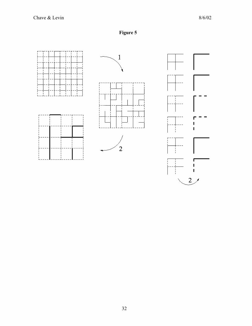
Chave & Levin 8/6/02
32
Figure 5

Chave & Levin 8/6/02
33
Figure 6

Chave & Levin 8/6/02
34
Figure 7
Q
3 roots
Budworm density
R
1 root
RA B

Chave & Levin 8/6/02
35
Figure 8
Copyright © 2022 FDOKUMEN