A primer on the study of transitory dynamics in ecological series using the scale-dependent...
20
Oecologia (2004) 138: 485–504 DOI 10.1007/s00442-003-1464-4 METHODS Miquel Àngel Rodríguez-Arias . Xavier Rodó A primer on the study of transitory dynamics in ecological series using the scale-dependent correlation analysis Received: 6 July 2003 / Accepted: 12 November 2003 / Published online: 31 January 2004 # Springer-Verlag 2004 Abstract Here we describe a practical, step-by-step primer to scale-dependent correlation (SDC) analysis. The analysis of transitory processes is an important but often neglected topic in ecological studies because only a few statistical techniques appear to detect temporary features accurately enough. We introduce here the SDC analysis, a statistical and graphical method to study transitory processes at any temporal or spatial scale. SDC analysis, thanks to the combination of conventional procedures and simple well-known statistical techniques, becomes an improved time-domain analogue of wavelet analysis. We use several simple synthetic series to describe the method, a more complex example, full of transitory features, to compare SDC and wavelet analysis, and finally we analyze some selected ecological series to illustrate the methodology. The SDC analysis of time series of copepod abundances in the North Sea indicates that ENSO primarily is the main climatic driver of short-term changes in population dynamics. SDC also uncovers some long- term, unexpected features in the population. Similarly, the SDC analysis of Nicholson’ s blowflies data locates where the proposed models fail and provides new insights about the mechanism that drives the apparent vanishing of the population cycle during the second half of the series. Keywords Ecological series . Transitory dynamics . Discontinuities . Ecological interactions . Environmental forcing The study of transitory dynamics in ecological series The analysis of temporal and spatial ecological series has typically focused on the detection and extraction of permanent signals (trends and stable oscillations) and on the explanation of the remaining residuals (Platt and Denman 1975; Chatfield 1989; Legendre and Fortin 1989). Trends, stable cycles, and structured residuals are the signature of permanent ecological processes such as those encountered in population dynamics, ecological interactions, or studies of environmental forcings (Butler 1953; Steele 1978; Broomhead and King 1986; Powell and Steele 1995). Transitory signals Sometimes important signatures laid by a process inter- acting with a variable of interest, hereafter referred to as signals, can be non-permanent because ecological pro- cesses do not remain constant and might be subject to changes. Figure 1 shows the natural series we will study. The three series display stable oscillations corresponding to the annual cycle in North Sea zooplankton (Fig. 1A, B) and to an internal population cycle in the blowflies experiment (Fig. 1C), but also they contain a large fluctuating behavior raising non-permanent features. Co- pepod populations show, apparently at random, periods of high and low summer abundance peaks (Fig. 1A, B). The annual cycle of total copepod abundance changed gradually after 1960 (Fig. 1A), while the abundance of Calanus decreased considerably during the period of study (Fig. 1B) and, after 1970, even failed sometimes to develop the annual cycle. Similarly, blowfly populations (Fig. 1C) display a clear cycle the first year, behave at random the next 10 months, and afterwards recover a periodic-like dynamics at the end of the experiment (Stokes et al. 1988). Signals manifest in ecological series only when the forcing process (the driver) exceeds the minimum intensity threshold that originates a response in the system. The M. À. Rodríguez-Arias . X. Rodó (*) Climate Research Laboratory, Parc Científic de Barcelona, Universitat de Barcelona c/Baldiri Reixach, 4-6 (Torre D), 08028 Barcelona, Catalonia, Spain e-mail: [email protected] M. À. Rodríguez-Arias Systems Ecology Group, Institutt for fiskeri-og marinbiologi, Universiteten i Bergen, Høyteknologisenteret, Thormøhlens Gate 55, P.O. Box 7800, 5020 Bergen, Norway
-
Upload
independent -
Category
Documents
-
view
1 -
download
0
Transcript of A primer on the study of transitory dynamics in ecological series using the scale-dependent...
Oecologia (2004) 138: 485–504DOI 10.1007/s00442-003-1464-4
METHODS
Miquel Àngel Rodríguez-Arias . Xavier Rodó
A primer on the study of transitory dynamics in ecological series
using the scale-dependent correlation analysis
Received: 6 July 2003 / Accepted: 12 November 2003 / Published online: 31 January 2004# Springer-Verlag 2004
Abstract Here we describe a practical, step-by-stepprimer to scale-dependent correlation (SDC) analysis.The analysis of transitory processes is an important butoften neglected topic in ecological studies because only afew statistical techniques appear to detect temporaryfeatures accurately enough. We introduce here the SDCanalysis, a statistical and graphical method to studytransitory processes at any temporal or spatial scale.SDC analysis, thanks to the combination of conventionalprocedures and simple well-known statistical techniques,becomes an improved time-domain analogue of waveletanalysis. We use several simple synthetic series to describethe method, a more complex example, full of transitoryfeatures, to compare SDC and wavelet analysis, and finallywe analyze some selected ecological series to illustrate themethodology. The SDC analysis of time series of copepodabundances in the North Sea indicates that ENSOprimarily is the main climatic driver of short-term changesin population dynamics. SDC also uncovers some long-term, unexpected features in the population. Similarly, theSDC analysis of Nicholson’s blowflies data locates wherethe proposed models fail and provides new insights aboutthe mechanism that drives the apparent vanishing of thepopulation cycle during the second half of the series.
Keywords Ecological series . Transitory dynamics .Discontinuities . Ecological interactions . Environmentalforcing
The study of transitory dynamics in ecological series
The analysis of temporal and spatial ecological series hastypically focused on the detection and extraction ofpermanent signals (trends and stable oscillations) and onthe explanation of the remaining residuals (Platt andDenman 1975; Chatfield 1989; Legendre and Fortin1989). Trends, stable cycles, and structured residuals arethe signature of permanent ecological processes such asthose encountered in population dynamics, ecologicalinteractions, or studies of environmental forcings (Butler1953; Steele 1978; Broomhead and King 1986; Powelland Steele 1995).
Transitory signals
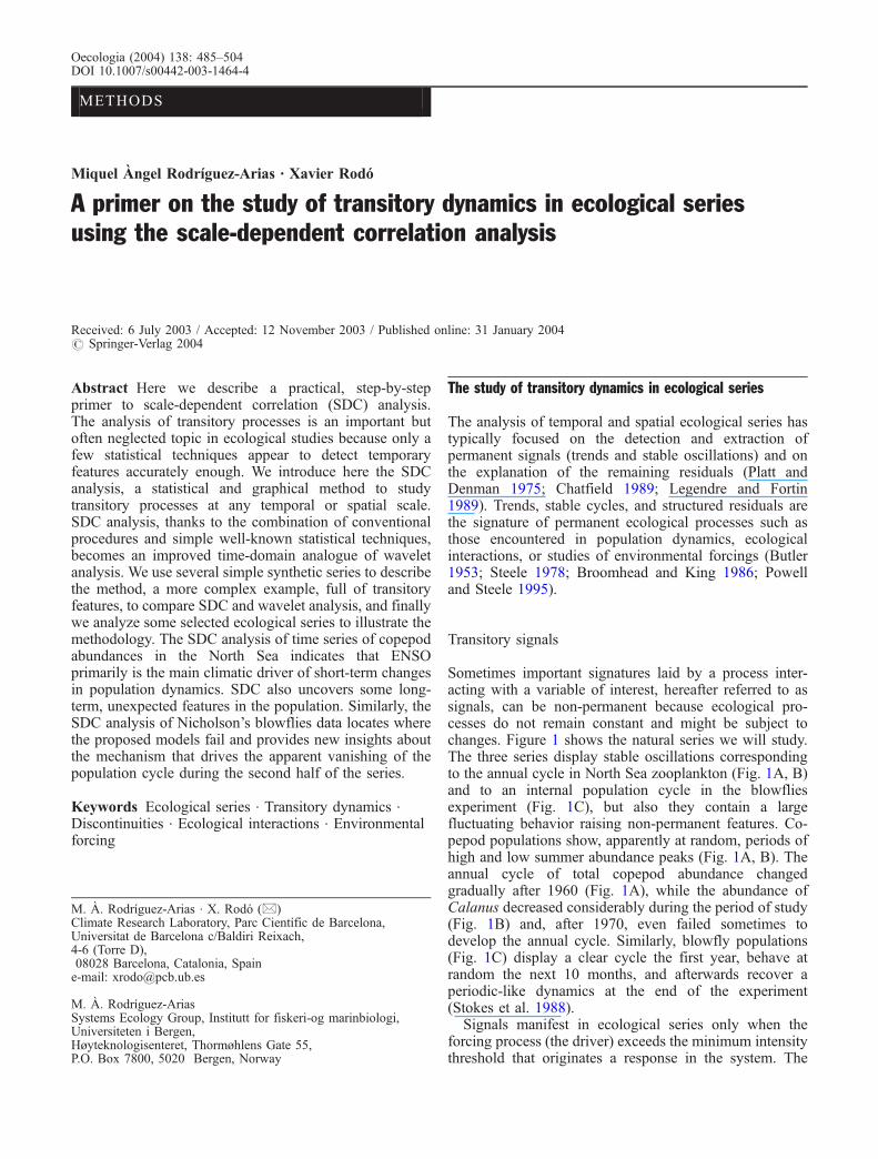
Sometimes important signatures laid by a process inter-acting with a variable of interest, hereafter referred to assignals, can be non-permanent because ecological pro-cesses do not remain constant and might be subject tochanges. Figure 1 shows the natural series we will study.The three series display stable oscillations correspondingto the annual cycle in North Sea zooplankton (Fig. 1A, B)and to an internal population cycle in the blowfliesexperiment (Fig. 1C), but also they contain a largefluctuating behavior raising non-permanent features. Co-pepod populations show, apparently at random, periods ofhigh and low summer abundance peaks (Fig. 1A, B). Theannual cycle of total copepod abundance changedgradually after 1960 (Fig. 1A), while the abundance ofCalanus decreased considerably during the period of study(Fig. 1B) and, after 1970, even failed sometimes todevelop the annual cycle. Similarly, blowfly populations(Fig. 1C) display a clear cycle the first year, behave atrandom the next 10 months, and afterwards recover aperiodic-like dynamics at the end of the experiment(Stokes et al. 1988).
Signals manifest in ecological series only when theforcing process (the driver) exceeds the minimum intensitythreshold that originates a response in the system. The
M. À. Rodríguez-Arias . X. Rodó (*)Climate Research Laboratory, Parc Científic de Barcelona,Universitat de Barcelona c/Baldiri Reixach,4-6 (Torre D),08028 Barcelona, Catalonia, Spaine-mail: [email protected]
M. À. Rodríguez-AriasSystems Ecology Group, Institutt for fiskeri-og marinbiologi,Universiteten i Bergen,Høyteknologisenteret, Thormøhlens Gate 55,P.O. Box 7800, 5020 Bergen, Norway
magnitude of the response is a balance between thevarying intensity and timing of the forcing and thefluctuating sensitivity of the system. Since in nature noneof these factors is independent and they do not remainconstant, environmental and biological forcing can bringabout temporary responses when the thresholds are notpermanently exceeded or when the forcing itself isdiscontinuous. The non-permanent components of climate,the episodic occurrence of other perturbations, and thediscreteness and variability of biological interactions havea large influence over ecosystem dynamics and areresponsible for unique temporary imprints in ecologicalseries (Margalef 1991; Nils et al. 1999). In populations,non-permanent fluctuations may arise as a consequence ofthe variability among individuals (May 1973; Stokes et al.1988; Kendall et al. 1999). Transients are other possiblesources of temporary processes. Modelers define transientsas the unstable dynamics following a perturbation andlasting until the recovery of the long-term behavior (Lawand Edley 1990; Chen and Cohen 2001). Transientbehavior has also been described in complex ecologicalmodels and in ecological studies (Hastings and Higgins1994; Neubert and Caswell 1997). Independently of theprocess underneath, we will use in this paper the terms“transitory” to describe signals that do not last for the fulllength of the series and “discontinuity” to indicate thelimits of these structures.
Scale of the driving processes
Every ecological process has a characteristic temporal andspatial scale (Butler 1953; Levin 1992; Martínez andLawton 1995). In ecological time series, the scale is thetime span between two outcomes of the dynamics such as
the generation-time in a population or the period in anenvironmental cycle (i.e., tidal, daily, lunar, annual, ordecadal). In space, the scale is the size of the structures(patch size, eddy size) usually referred to by a size range(micro-, meso-, or macroscale). Though most processeslay their signatures in time series at their own scale (e.g.,the annual cycle is an oscillation of period 12 in monthlyseries), large-scale patterns can emerge from small-scaleprocesses, and high-frequency features can be affected bylarge-scale dynamics (Levin 1992). Another importantfactor is the complex multi-scale dynamics of someenvironmental drivers. The El Niño-Southern Oscillation(ENSO) signature, for instance, combines a quasi-biennial(QB) pseudo-oscillation with a scale of around 30 monthsand a quasi-quadriennial (QQ) component with variableperiod ranging between 3 and 7 years (Torrence andCompo 1998).
Analysis of ecological series
Signal-detection techniques decompose the variance intooscillatory components (frequency domain) or withrespect to time lags and spatial distances (time domain).The first approach is the spectral analysis, while thesecond approach embraces the correlation methods (Plattand Denman 1975; Chatfield 1989). Most of thesetechniques were developed to study permanent signalsbut not to deal with transitory processes at different scales.Transitory signals cannot be detected using these methodsand remain embedded into the unexplained portion of thevariance. Ideally, the error term must include only noisyunstructured variance (purely random white noises andshort-term autoregressive red noises), but it should neverinclude structured components such as transitory signals.
Fig. 1A–C The ecological se-ries used in this study to illus-trate the SDC method. AMonthly series of total copepodsabundance in the North Sea(ICES areas IVa, IVb, and IVc)from 1950 to 1997. B Monthlyabundance of adult (stages Vand VI) Calanus finmarchicusand Calanus helgolandicus inthe same area and period.Abundance values correspond toindividuals per 10 m3 (Heath etal. 1999). C Nicholson’s blow-flies (Lucilla cuprina, Weid)time series. Nicholson recordedevery 2 days the number ofadult blowflies in a populationwith constant food supply dur-ing 2 years
486
Fortunately, the growing interest in temporary dynamicshas stimulated the development of new statistical methodsto cope with this sort of signals (Manuca and Savit 1996;Neubert and Caswell 1997).
Strong discontinuities in time series can be detectedwith simple techniques such as chronological clustering(Legendre et al. 1985) or SLOTSEE analysis (Green 1995)and with edge-detection algorithms (Fortin 1994) in spatialdata. The detection of weaker discontinuities requiresmore complex procedures such as change-point detectorsor recurrence plots (Casdagli 1997). All these methods,however, do not allow us to study the underlyingprocesses, they demand long data series and, in somecases, heavy statistical training. Scale-oriented studiesusually have been performed by partitioning the seriesbefore the analysis into their low- and high-frequencycomponents (Legendre and Legendre 1998). This ap-proach works nicely for permanent structures but not fortransitory signals. In this respect, floating windowscorrelation analysis (Childers et al. 1994) is one of thefew time-domain methods that can be used to studytemporary relationships. This method calculates the cor-relation between paired segments from both series. Theresulting line plot shows the temporal (or spatial) evolu-tion of the relationship at the selected fragment-size andallows us to detect discontinuities and some transitorysignals (Childers et al. 1994). Although the method couldbe easily improved to also consider shifted correlations, ana priori methodology to decide which fragment-sizes and
shifts should be used is still lacking. As a result, the userrequires dozens of plots to fully understand the dynamics.
In the frequency domain, wavelet analysis (WA) (Mallat1989; Daubechies 1993; Chiu et al. 1994; Lau and Weng1995; Torrence and Compo 1998) identifies discontinu-ities and transitory signals at several scales. The output ofWA is a time and frequency variance decompositionobtained by “filtering” the data with a small, moving,wave-like function (the wavelet base) with changingfrequency (Torrence and Compo 1998). Though a power-ful tool, WA cannot handle very short time series and stillneeds further developments in the bivariate case (see“Detection of transitory forcings”). WA also requires someexperience in signal-detection procedures. In ecologicalliterature, WA has been applied mainly to investigatevegetation (Bradshaw and Spies 1992; Dale and Mah1998; Harper and MacDonald 2001), landscape patterns(Saunders et al. 1998; Brosofske et al. 1999; Li andKafatos 2000), soil properties (Hu et al. 1998; Lark andWebster 2001), hydrology (Bradshaw and McIntosh 1994;Labat et al. 1999; Compagnucci et al. 2000), water quality(Dohan and Whitfield 1997; Whitfield and Dohan 1997),fish acoustics (Stepnowski and Morzynski 2000), propa-gation of epidemics (Grenfell et al. 2001), and phyto-plankton distributions (Machu et al. 1999).
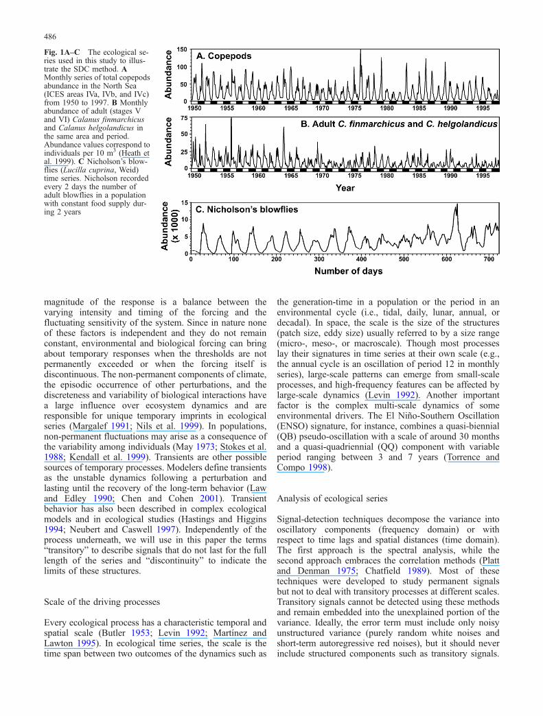
Fig. 2 Description of the iterative procedure used in SDC analysis(see main text for details). Prior to the analysis, the fragment size (s),the number of permutations (m), and the significance level (α) are
selected. In every iteration, the method extracts two segments oflength s, calculates their correlation, and, if it is significant, places acolored dot in the SDC plot at {i,j}
487
A new tool
SDC analysis is a new statistical tool in the time domainthat combines conventional techniques and some well-known statistical procedures to detect scale-dependenttransitory processes (Rodó 2001; Rodó et al. 2002; Rodóand Rodríguez-Arias, submitted for publication). SDC is arobust method, extremely tolerant to missing values, thatcan handle very short time series (Rodó and Rodríguez-Arias, submitted for publication). The method has beendeveloped to be a user-friendly time-domain analogue ofWA. The present paper is a tutorial on the use of SDCanalysis to detect transitory features in ecological series.The next section briefly describes the methodologyexplained in detail elsewhere (Rodó and Rodríguez-Arias, submitted for publication). The third section focuseson understanding SDC patterns—the most critical point ofthe analysis—while the fourth deals with plot interpreta-tion and compares results of SDC and WA. The fifth andsixth sections include the analysis of well-knownecological series. The seventh section discusses theadvantages and disadvantages of the method and high-lights some future developments. Finally, the last section isa summary that provides a practical guide to SDC analysis.
SDC analysis
SDC analysis calculates floating correlations between twodata series. Once a fragment-size (s) has been selected, themethod computes the correlation between all possiblepairs of segments and displays the significant values. Theresulting scatter plot can show all the features of the
system at the selected scale of observation. Afterperforming several SDC analyses at some other seg-ment-lengths, the user can describe all the scale-dependentinteractions between two series, including those that aretransitory.
Rationale of the method
The core of SDC analysis is an iterative procedure asfollows (Fig. 2). Given two series, Xi of length n1 and Yj oflength n2, select two segments of the same length (s),beginning in the ith element of Xi and in the jth of Yj (X[i+k] and Y[j+k], with k=0,1,...,s–1). Compute their corre-lation, ri,j=r(X[i+k],Y[j+k]) and use a randomization test todecide the significance (Legendre and Legendre 1998). Ifthe correlation is significant, place a dot in a plot, coloredaccording to the sign and value of ri,j, and with i on the x-axis and j on the y-axis. If the correlation is non-significant, omit the {i,j} dot in the plot. Repeat theprocess for every {i,j} (i=1,2,...,n1–s+1 and j=1,2,...,n2–s+1).
SDC analysis is essentially a bivariate method (two-waySDC, hereafter TW-SDC, with Yj≠Xi) that works also as aone-way procedure (one-way SDC, hereafter OW-SDC)when both series are the same (Yj=Xi). The main diagonalshows the correlation between paired segments (i=j),whereas the other points refer to the correlation betweenunpaired fragments: in the upper sector above thediagonal, the first series lags the second series (i>j),while in the lower sector, Xi leads Yj (i<j) (Fig. 2). Thevalue of the shift between fragments is the distance inpixels from any point to the main diagonal (be it
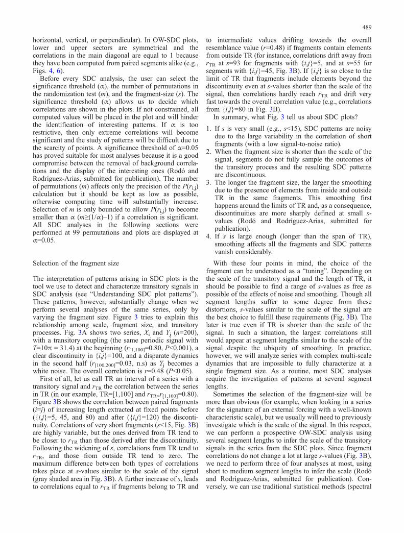
Fig. 3 A Two transitorycoupled series, Xi=sin(0.2i)+εand Yj=sin(0.2j)δ(j)+ (2/1+δ(j))ε, i,j=1,2,...,200, with δ(j)=1 if j<100 and δ(j)=0 otherwise[errors are random outcomesfrom a normal distribution, ε≡N(0,0.25)]. TR is the interval withthe transitory coupling. B Cor-relations between synchronicfragments (i=j) of increasinglength but constant origin ({i,j}=5, 45, 80, and 120, denoted byblack arrows in A). Gray arrowsshow places where correlationsof fragments extracted from TRbegin to decrease after reachingtheir maximum, while the grayshaded area indicates which s-values provide the best separa-tion between correlations offragments from inside and out-side TR
488
horizontal, vertical, or perpendicular). In OW-SDC plots,lower and upper sectors are symmetrical and thecorrelations in the main diagonal are equal to 1 becausethey have been computed from paired segments alike (e.g.,Figs. 4, 6).
Before every SDC analysis, the user can select thesignificance threshold (α), the number of permutations inthe randomization test (m), and the fragment-size (s). Thesignificance threshold (α) allows us to decide whichcorrelations are shown in the plots. If not constrained, allcomputed values will be placed in the plot and will hinderthe identification of interesting patterns. If α is toorestrictive, then only extreme correlations will becomesignificant and the study of patterns will be difficult due tothe scarcity of points. A significance threshold of α=0.05has proved suitable for most analyses because it is a goodcompromise between the removal of background correla-tions and the display of the interesting ones (Rodó andRodríguez-Arias, submitted for publication). The numberof permutations (m) affects only the precision of the P(ri,j)calculation but it should be kept as low as possible,otherwise computing time will substantially increase.Selection of m is only bounded to allow P(ri,j) to becomesmaller than α (m≥(1/α)–1) if a correlation is significant.All SDC analyses in the following sections wereperformed at 99 permutations and plots are displayed atα=0.05.
Selection of the fragment size
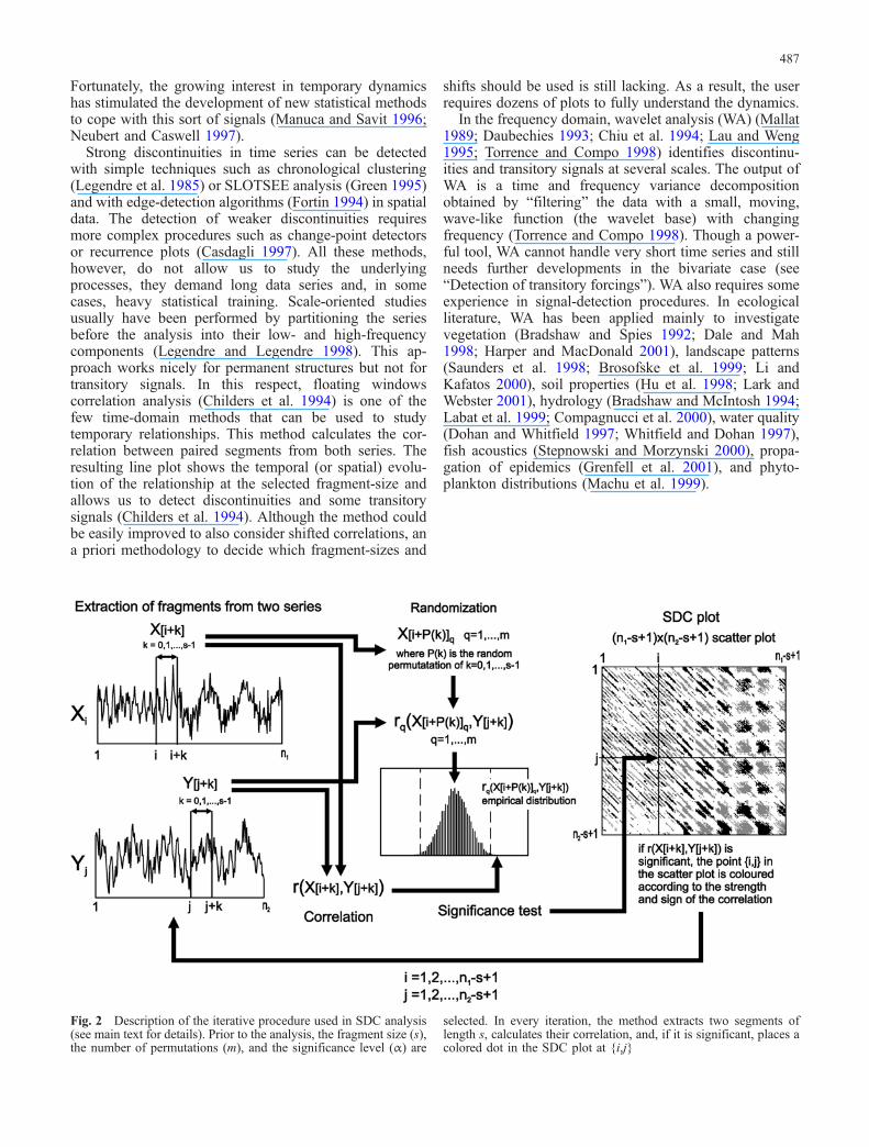
The interpretation of patterns arising in SDC plots is thetool we use to detect and characterize transitory signals inSDC analysis (see “Understanding SDC plot patterns”).These patterns, however, substantially change when weperform several analyses of the same series, only byvarying the fragment size. Figure 3 tries to explain thisrelationship among scale, fragment size, and transitoryprocesses. Fig. 3A shows two series, Xi and Yj (n=200),with a transitory coupling (the same periodic signal withT=10π = 31.4) at the beginning (r[1,100]=0.80, P<0.001), aclear discontinuity in {i,j}=100, and a disparate dynamicsin the second half (r[100,200]=0.03, n.s) as Yj becomes awhite noise. The overall correlation is r=0.48 (P<0.05).
First of all, let us call TR an interval of a series with atransitory signal and rTR the correlation between the seriesin TR (in our example, TR=[1,100] and rTR=r[1,100]=0.80).Figure 3B shows the correlation between paired fragments(i=j) of increasing length extracted at fixed points before({i,j}=5, 45, and 80) and after ({i,j}=120) the disconti-nuity. Correlations of very short fragments (s<15, Fig. 3B)are highly variable, but the ones derived from TR tend tobe closer to rTR than those derived after the discontinuity.Following the widening of s, correlations from TR tend torTR, and those from outside TR tend to zero. Themaximum difference between both types of correlationstakes place at s-values similar to the scale of the signal(gray shaded area in Fig. 3B). A further increase of s, leadsto correlations equal to rTR if fragments belong to TR and
to intermediate values drifting towards the overallresemblance value (r=0.48) if fragments contain elementsfrom outside TR (for instance, correlations drift away fromrTR at s=93 for fragments with {i,j}=5, and at s=55 forsegments with {i,j}=45, Fig. 3B). If {i,j} is so close to thelimit of TR that fragments include elements beyond thediscontinuity even at s-values shorter than the scale of thesignal, then correlations hardly reach rTR and drift veryfast towards the overall correlation value (e.g., correlationsfrom {i,j}=80 in Fig. 3B).
In summary, what Fig. 3 tell us about SDC plots?
1. If s is very small (e.g., s<15), SDC patterns are noisydue to the large variability in the correlation of shortfragments (with a low signal-to-noise ratio).
2. When the fragment size is shorter than the scale of thesignal, segments do not fully sample the outcomes ofthe transitory process and the resulting SDC patternsare discontinuous.
3. The longer the fragment size, the larger the smoothingdue to the presence of elements from inside and outsideTR in the same fragments. This smoothing firsthappens around the limits of TR and, as a consequence,discontinuities are more sharply defined at small s-values (Rodó and Rodríguez-Arias, submitted forpublication).
4. If s is large enough (longer than the span of TR),smoothing affects all the fragments and SDC patternsvanish considerably.
With these four points in mind, the choice of thefragment can be understood as a “tuning”. Depending onthe scale of the transitory signal and the length of TR, itshould be possible to find a range of s-values as free aspossible of the effects of noise and smoothing. Though allsegment lengths suffer to some degree from thesedistortions, s-values similar to the scale of the signal arethe best choice to fulfill these requirements (Fig. 3B). Thelater is true even if TR is shorter than the scale of thesignal. In such a situation, the largest correlations stillwould appear at segment lengths similar to the scale of thesignal despite the ubiquity of smoothing. In practice,however, we will analyze series with complex multi-scaledynamics that are impossible to fully characterize at asingle fragment size. As a routine, most SDC analysesrequire the investigation of patterns at several segmentlengths.
Sometimes the selection of the fragment-size will bemore than obvious (for example, when looking in a seriesfor the signature of an external forcing with a well-knowncharacteristic scale), but we usually will need to previouslyinvestigate which is the scale of the signal. In this respect,we can perform a prospective OW-SDC analysis usingseveral segment lengths to infer the scale of the transitorysignals in the series from the SDC plots. Since fragmentcorrelations do not change a lot at large s-values (Fig. 3B),we need to perform three of four analyses at most, usingshort to medium segment lengths to infer the scale (Rodóand Rodríguez-Arias, submitted for publication). Con-versely, we can use traditional statistical methods (spectral
489
analysis, autocorrelation, and cross-correlation functions)to detect the scale of strong transitory signals, or waveletanalysis if the signal is weaker. Once we have someestimates, we can carry out accurate SDC analysis atsegment lengths similar to the presumed scale. Eventually,we might perform additional analysis at small fragmentsizes to precisely define the exact position of thediscontinuities.
Understanding SDC plot patterns
A signal is a recurrent sequence of elements with arecognizable shape (the opposite is a noise or datasequence with unpredictable behavior). The scale is thelength of the sequence, while the recurrence is the spanbetween two outcomes. A pure permanent oscillation is,
for instance, a continuous wave with the same recurrenceand scale (period). At the other extreme, we have the odd-shaped signals with sporadic and unpredictable returns.SDC analysis is devoted to detecting such sporadicreturns. In every series, the particular evolution of theindividual outcomes of a transitory signal determines howfragment correlations merge to build up SDC patterns.
From transitory signals to SDC patterns
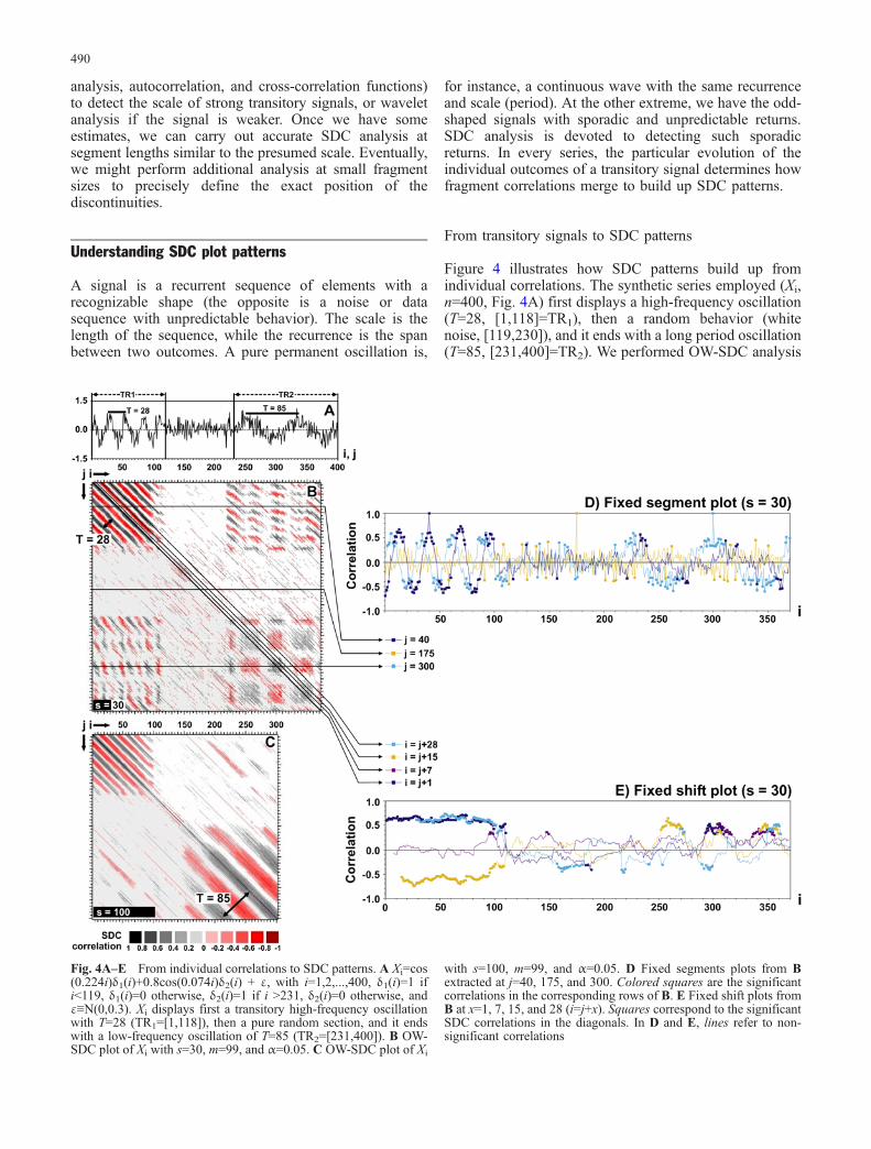
Figure 4 illustrates how SDC patterns build up fromindividual correlations. The synthetic series employed (Xi,n=400, Fig. 4A) first displays a high-frequency oscillation(T=28, [1,118]=TR1), then a random behavior (whitenoise, [119,230]), and it ends with a long period oscillation(T=85, [231,400]=TR2). We performed OW-SDC analysis
Fig. 4A–E From individual correlations to SDC patterns. A Xi=cos(0.224i)δ1(i)+0.8cos(0.074i)δ2(i) + ε, with i=1,2,...,400, δ1(i)=1 ifi<119, δ1(i)=0 otherwise, δ2(i)=1 if i >231, δ2(i)=0 otherwise, andε≡N(0,0.3). Xi displays first a transitory high-frequency oscillationwith T=28 (TR1=[1,118]), then a pure random section, and it endswith a low-frequency oscillation of T=85 (TR2=[231,400]). B OW-SDC plot of Xi with s=30, m=99, and α=0.05. C OW-SDC plot of Xi
with s=100, m=99, and α=0.05. D Fixed segments plots from Bextracted at j=40, 175, and 300. Colored squares are the significantcorrelations in the corresponding rows of B. E Fixed shift plots fromB at x=1, 7, 15, and 28 (i=j+x). Squares correspond to the significantSDC correlations in the diagonals. In D and E, lines refer to non-significant correlations
490
at s-values similar to the scale of the signals (s=30 ands=100, in Fig. 4B, C, respectively). Figure 4D, E derivefrom Fig. 4B. Figure 4D shows the floating correlationbetween three fixed fragments and all the others in theoriginal series (equivalent to extract rows of SDC plots),while Fig. 4E shows the correlation of fragments with aconstant shift in between (this being equivalent to extractdiagonals of SDC plots).
A fixed segment of 30 elements from TR1 (j=40) showsalternating correlation peaks and valleys 14 elements apartwith fragments from TR1, no correlation with segmentsfrom the random interval, and weak correlations 40elements apart with segments from TR2 (dark-blue plotin Fig. 4D). A segment sampled from the random sector(j=175), despite some spurious significant values, does notcorrelate with any other fragment except itself (orange plotin Fig. 4D). A segment from TR2 (j=300) showsalternating correlations 14 elements apart with fragmentsfrom TR1, no correlation with fragments from the randomsector, and alternating correlation peaks and valleys 40–45elements apart with segments from TR2 (light blue plot inFig. 4D).
In SDC plots, correlations of fragments extracted fromTR1 or from TR2 build up alternating bands of positiveand negative values parallel to the main diagonal with adistance between stripes of the same sign equal to theperiod of the oscillation (Fig. 4B–D). The bands arecontinuous when the fragment size is similar to or largerthan the scale of the signal (Fig. 4C and TR1 in Fig. 4B,E), but discontinuous when s is shorter than the scale (TR2
in Fig. 4B, E). In the first situation, all correlations offragments with the same shift in between have the samevalue (the lagged rTR of the signal in such a particularinterval) and raise a continuous band (Fig. 4E). In thesecond case, fragments are much shorter than a singleoutcome of the transitory signal and, as a consequence,those centered in the peaks and valleys of the signal cannotbe distinguished from a random sequence. These segmentsresult in non-significant correlations that prevent thecontinuity of the bands and raise a chess board-likepattern (TR2 in Fig. 4B).
Similarly, we can sometimes find significant correla-tions in short fragments extracted from intervals withdifferent transitory signals. The upper-right and lower-leftcorners of Fig. 4B (s=30) show the correlation of pairswith one fragment extracted from TR1 and the other fromTR2. Any segment extracted from TR1 contains a fullcycle of the high-frequency signal (T=28), while afragment from TR2 contains less than half a cycle of thelow-frequency signal (T=85). The fragment from TR2 canbe centered in the monotonic increase or decrease of theoscillation, as well as in a peak or a valley. If centered in amonotonic interval, the resulting correlation will be non-significant and close to zero, but if centered in a peak or avalley, a significant correlation can arise if the correspond-ing fragment from TR1 is also centered in a peak or valleyof the other signal. The result is the discontinuous verticaland horizontal bands exhibiting alternating positive andnegative correlations in the upper-right and lower-left
corners of Fig. 4B. Fortunately, when s is large enough,most fragments include full cycles and the presence ofsuch annoying significant correlations is prevented (as inthe upper-right and lower-left corner of Fig. 4C). Insummary, continuous striped patterns parallel to the maindiagonal reveal a signal in both series with a scale similarto the fragment size, while vertical and horizontal bands orchess board-like patterns require further analyses at largers-values (Rodó and Rodríguez-Arias, submitted forpublication). Obviously, SDC patterns of non-periodical,odd-shaped signals are more complex. In such a case,oblique bands will still develop but will be discontinuousand have irregular spacing. Additionally, if severaltransitory signals with different scales are present in thesame interval of the series, some horizontal and verticalbanding will be impossible to prevent at a few of theappropriate segment lengths for the analyses. Never-theless,when using the main basic rules listed above andremembering the relationship between scale and fragmentsize—developed in “Selection of the fragment size”—itshould be possible to effectively derive the meaning of anyparticular SDC pattern. A more exhaustive description ofSDC pattern interpretation is available in Rodó andRodriguez-Arias (submitted for publication).
Testing SDC patterns
The occurrence of significant spurious correlations whenperforming multiple tests is a well-known statisticalartifact (Legendre and Legendre 1998) that may alsoaffect SDC plots. For instance, the result of the analysis oftwo uncorrelated white noises (series of normallydistributed random data) has no recognizable patterns,but it contains some scattered significant correlations(Rodó and Rodríguez-Arias, submitted for publication). Inthis respect and despite the lack of independence amongadjacent correlations, we have developed an overallpattern significance test that allows us to reject SDCplots derived from completely unrelated series (Rodó2001). Other dynamics such as colored noises, determi-nistic chaos, and random walks also display significantcorrelations in SDC plots and have also been wellcharacterized (Rodó and Rodríguez-Arias, submitted forpublication). This time, however, significant correlationsare non-spurious and the development of a particular testfor them is therefore more difficult. Fortunately, all theseprocesses can be asserted thanks to the unique patternsthey raise in SDC plots (Rodó and Rodríguez-Arias,submitted for publication).
Facing complex transitory processes
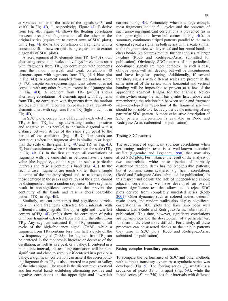
To compare the performance of SDC and other methodswith complex transitory dynamics, a synthetic series wasdeveloped (Fig. 5). The forcing series (Yj, n=750) is asequence of peaks 35 units apart (Fig. 5A), while theforced series (Xi, n= 750) has four intervals with different
491
transitory signals (Fig. 5B): TR1=[1,135] with a high-frequency oscillation (T=12); TR2=[136,377] with a low-frequency wave (T=90); TR3=[378,570] with both highand low periods (T=12 and T=90); and, after a shortrandom interval, TR4=[614,750] with an oscillation ofvariable period (T=9–16). The varying oscillation emu-lates pseudo-oscillatory natural dynamics (with a non-fixed characteristic period) like those that have alreadybeen described in climatic studies (Wang and Wang 1996;Rodó et al. 2002) and in population dynamics (Stokes etal. 1988). Yj drives Xi during three short intervals (Fig. 5):two synchronic forcings (shift = 0) in TR1 and TR3 andone lagged forcing (shift = +10) in TR2.
The univariate analysis of a complex series
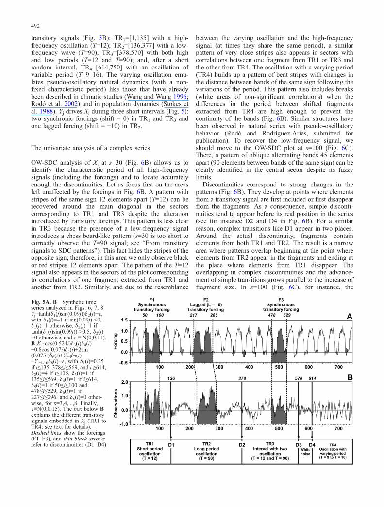
OW-SDC analysis of Xi at s=30 (Fig. 6B) allows us toidentify the characteristic period of all high-frequencysignals (including the forcings) and to locate accuratelyenough the discontinuities. Let us focus first on the areasleft unaffected by the forcings in Fig. 6B. A pattern withstripes of the same sign 12 elements apart (T=12) can berecovered around the main diagonal in the sectorscorresponding to TR1 and TR3 despite the alterationintroduced by transitory forcings. This pattern is less clearin TR3 because the presence of a low-frequency signalintroduces a chess board-like pattern (s=30 is too short tocorrectly observe the T=90 signal; see “From transitorysignals to SDC patterns”). This fact hides the stripes of theopposite sign; therefore, in this area we only observe blackor red stripes 12 elements apart. The pattern of the T=12signal also appears in the sectors of the plot correspondingto correlations of one fragment extracted from TR1 andanother from TR3. Similarly, and due to the resemblance
between the varying oscillation and the high-frequencysignal (at times they share the same period), a similarpattern of very close stripes also appears in sectors withcorrelations between one fragment from TR1 or TR3 andthe other from TR4. The oscillation with a varying period(TR4) builds up a pattern of bent stripes with changes inthe distance between bands of the same sign following thevariations of the period. This pattern also includes breaks(white areas of non-significant correlations) when thedifferences in the period between shifted fragmentsextracted from TR4 are high enough to prevent thecontinuity of the bands (Fig. 6B). Similar structures havebeen observed in natural series with pseudo-oscillatorybehavior (Rodó and Rodríguez-Arias, submitted forpublication). To recover the low-frequency signal, weshould move to the OW-SDC plot at s=100 (Fig. 6C).There, a pattern of oblique alternating bands 45 elementsapart (90 elements between bands of the same sign) can beclearly identified in the central sector despite its fuzzylimits.
Discontinuities correspond to strong changes in thepatterns (Fig. 6B). They develop at points where elementsfrom a transitory signal are first included or first disappearfrom the fragments. As a consequence, simple disconti-nuities tend to appear before its real position in the series(see for instance D2 and D4 in Fig. 6B). For a similarreason, complex transitions like D1 appear in two places.Around the actual discontinuity, fragments containelements from both TR1 and TR2. The result is a narrowarea where patterns overlap beginning at the point whereelements from TR2 appear in the fragments and ending atthe place where elements from TR1 disappear. Theoverlapping in complex discontinuities and the advance-ment of simple transitions grows parallel to the increase offragment size. In s=100 (Fig. 6C), for instance, the
Fig. 5A, B Synthetic timeseries analyzed in Figs. 6, 7, 8.Yj=tanh(δ1(j)sin(0.09j))δ2(j)+ε,with δ1(j)=–1 if sin(0.09j) <0,δ1(j)=1 otherwise, δ2(j)=1 iftanh(δ1(j)sin(0.09j)) >0.5, δ2(j)=0 otherwise, and ε ≡ N(0,0.11).B Xi=cos(0.524i)δ3(i)δ4(i)+0.8cos(0.07i)δ5(i)+2sin(0.075i)δ6(i)+Yj=iδ7(i)+Yj=i-10δ8(i)+ε, with δ1(i)=0.25if i≤135, 378≤i≤569, and i ≥614,δ2(i)=4 if i≤135, δ3(i)=1 if135≤i≤569, δ4(i)=1 if i≥614,δ5(i)=1 if 50≤i≤100 and478≤i≤529, δ6(i)=1 if227≤i≤296, and δx(i)=0 other-wise, for x=3,4,...,8. Finally,ε≡N(0,0.15). The box below Bexplains the different transitorysignals embedded in Xi (TR1 toTR4; see text for details).Dashed lines show the forcings(F1–F3), and thin black arrowsrefer to discontinuities (D1–D4)
492
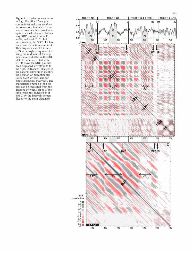
Fig. 6 A Xi (the same series asin Fig. 5B). Black lines (dis-continuities) and gray shadow-ing (transitory forcings) are ex-tended downwards to provide anoptimal visual reference. B One-way SDC plot of A at s=30,m=99, and α=0.05. To helpinterpretation, the SDC plot hasbeen centered with respect to A.This displacement of 15 units(s/2) to the right is equivalent tousing the midpoint of the seg-ments as coordinates in the SDCplot. C Same as B, but withs=100. Now the SDC plot hasbeen displaced s/2=50 units tothe right. In B and C, changes inthe patterns allow us to identifythe position of discontinuities(thick black arrows) and for-cings (horizontal intervals). Thecharacteristic period of the sig-nals can be measured from thedistance between stripes of thesame color (as indicated in Band C by the intervals perpen-dicular to the main diagonal)
493
position of discontinuities cannot be identified anymore.Using very short segment lengths, however, we canprevent most of these effects, but at the cost of losingclarity in the low-frequency signals (Fig. 6B).
In Figure 6B, every forcing disrupts the underlyingpatterns with an oblique banding around the main diagonalwith stripes of the same sign 35 units apart. In TR1, boththe forcing and its boundaries are clearly identifiable. InTR2, the low-frequency signal prevents a clear identifica-tion of the limits, but the period can still be recovered. InTR3, the complexity of the transitory signal prevents aclear identification of the forcing. Far from the maindiagonal, the interaction between forcings and transitorysignals changes with fragment size and depends on theirrespective periods. For instance, in Fig. 6B (s=30) forcingsmask the pattern arising from the high-frequency signalbut develop into spurious horizontal and vertical bands inthe areas where forcings meet the long period oscillation.In Fig. 6C (s=100), fragments are longer than the timespan of forcings and smoothing prevents their detection,but we can still notice some degree of pattern disruption.
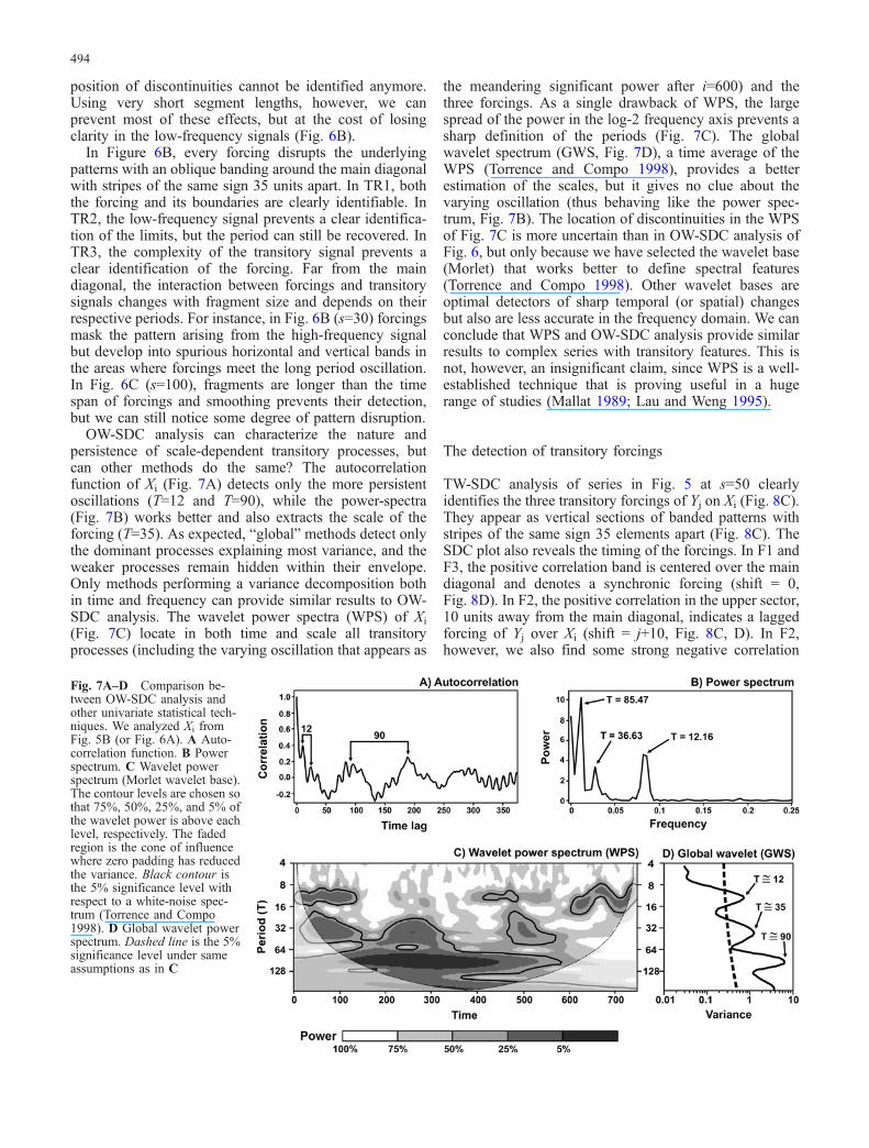
OW-SDC analysis can characterize the nature andpersistence of scale-dependent transitory processes, butcan other methods do the same? The autocorrelationfunction of Xi (Fig. 7A) detects only the more persistentoscillations (T=12 and T=90), while the power-spectra(Fig. 7B) works better and also extracts the scale of theforcing (T=35). As expected, “global” methods detect onlythe dominant processes explaining most variance, and theweaker processes remain hidden within their envelope.Only methods performing a variance decomposition bothin time and frequency can provide similar results to OW-SDC analysis. The wavelet power spectra (WPS) of Xi
(Fig. 7C) locate in both time and scale all transitoryprocesses (including the varying oscillation that appears as
the meandering significant power after i=600) and thethree forcings. As a single drawback of WPS, the largespread of the power in the log-2 frequency axis prevents asharp definition of the periods (Fig. 7C). The globalwavelet spectrum (GWS, Fig. 7D), a time average of theWPS (Torrence and Compo 1998), provides a betterestimation of the scales, but it gives no clue about thevarying oscillation (thus behaving like the power spec-trum, Fig. 7B). The location of discontinuities in the WPSof Fig. 7C is more uncertain than in OW-SDC analysis ofFig. 6, but only because we have selected the wavelet base(Morlet) that works better to define spectral features(Torrence and Compo 1998). Other wavelet bases areoptimal detectors of sharp temporal (or spatial) changesbut also are less accurate in the frequency domain. We canconclude that WPS and OW-SDC analysis provide similarresults to complex series with transitory features. This isnot, however, an insignificant claim, since WPS is a well-established technique that is proving useful in a hugerange of studies (Mallat 1989; Lau and Weng 1995).
The detection of transitory forcings
TW-SDC analysis of series in Fig. 5 at s=50 clearlyidentifies the three transitory forcings of Yj on Xi (Fig. 8C).They appear as vertical sections of banded patterns withstripes of the same sign 35 elements apart (Fig. 8C). TheSDC plot also reveals the timing of the forcings. In F1 andF3, the positive correlation band is centered over the maindiagonal and denotes a synchronic forcing (shift = 0,Fig. 8D). In F2, the positive correlation in the upper sector,10 units away from the main diagonal, indicates a laggedforcing of Yj over Xi (shift = j+10, Fig. 8C, D). In F2,however, we also find some strong negative correlation
Fig. 7A–D Comparison be-tween OW-SDC analysis andother univariate statistical tech-niques. We analyzed Xi fromFig. 5B (or Fig. 6A). A Auto-correlation function. B Powerspectrum. C Wavelet powerspectrum (Morlet wavelet base).The contour levels are chosen sothat 75%, 50%, 25%, and 5% ofthe wavelet power is above eachlevel, respectively. The fadedregion is the cone of influencewhere zero padding has reducedthe variance. Black contour isthe 5% significance level withrespect to a white-noise spec-trum (Torrence and Compo1998). D Global wavelet powerspectrum. Dashed line is the 5%significance level under sameassumptions as in C
494
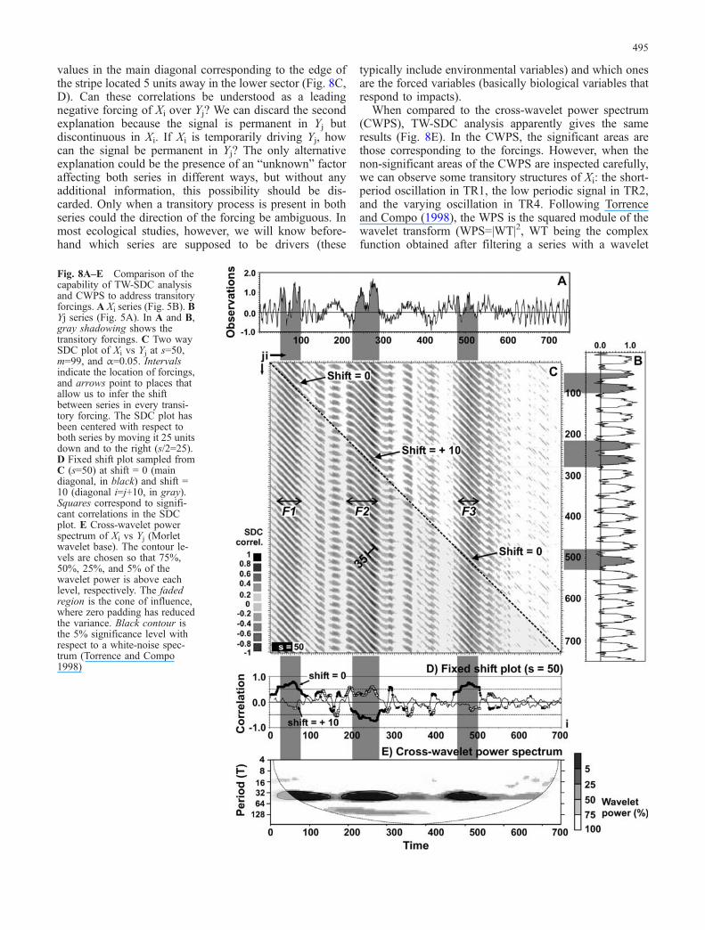
values in the main diagonal corresponding to the edge ofthe stripe located 5 units away in the lower sector (Fig. 8C,D). Can these correlations be understood as a leadingnegative forcing of Xi over Yj? We can discard the secondexplanation because the signal is permanent in Yj butdiscontinuous in Xi. If Xi is temporarily driving Yj, howcan the signal be permanent in Yj? The only alternativeexplanation could be the presence of an “unknown” factoraffecting both series in different ways, but without anyadditional information, this possibility should be dis-carded. Only when a transitory process is present in bothseries could the direction of the forcing be ambiguous. Inmost ecological studies, however, we will know before-hand which series are supposed to be drivers (these
typically include environmental variables) and which onesare the forced variables (basically biological variables thatrespond to impacts).
When compared to the cross-wavelet power spectrum(CWPS), TW-SDC analysis apparently gives the sameresults (Fig. 8E). In the CWPS, the significant areas arethose corresponding to the forcings. However, when thenon-significant areas of the CWPS are inspected carefully,we can observe some transitory structures of Xi: the short-period oscillation in TR1, the low periodic signal in TR2,and the varying oscillation in TR4. Following Torrenceand Compo (1998), the WPS is the squared module of thewavelet transform (WPS=|WT|2, WT being the complexfunction obtained after filtering a series with a wavelet
Fig. 8A–E Comparison of thecapability of TW-SDC analysisand CWPS to address transitoryforcings. A Xi series (Fig. 5B). BYj series (Fig. 5A). In A and B,gray shadowing shows thetransitory forcings. C Two waySDC plot of Xi vs Yj at s=50,m=99, and α=0.05. Intervalsindicate the location of forcings,and arrows point to places thatallow us to infer the shiftbetween series in every transi-tory forcing. The SDC plot hasbeen centered with respect toboth series by moving it 25 unitsdown and to the right (s/2=25).D Fixed shift plot sampled fromC (s=50) at shift = 0 (maindiagonal, in black) and shift =10 (diagonal i=j+10, in gray).Squares correspond to signifi-cant correlations in the SDCplot. E Cross-wavelet powerspectrum of Xi vs Yj (Morletwavelet base). The contour le-vels are chosen so that 75%,50%, 25%, and 5% of thewavelet power is above eachlevel, respectively. The fadedregion is the cone of influence,where zero padding has reducedthe variance. Black contour isthe 5% significance level withrespect to a white-noise spec-trum (Torrence and Compo1998)
495
base), the cross-wavelet spectrum (CWS) is the product ofthe WT of every series (CWS=WT1 WT2*, WT2* beingthe complex conjugate of WT2), and CWPS is the squaremodule of CWS (CWPS=|CWS|2). Developing algebrai-cally the last expression, CWPS=|WT1|
2 |WT2|2, and
therefore CWPS=WPS1 WPS2. This simply means that thecross-wavelet power spectrum is the product of theindivdual WPS. Now we can understand why the CWPSin Fig. 8E looks like an overlap of the WPS of Xi (Fig. 7C)and the WPS of Yj (not shown here, but it is just a time-continuous band of significant power at T=35). In ourexample, CWPS has provided nice results becauseforcings account for a lot of variance. In natural series,with a smaller signal-to-noise ratio, the approach of CWPScould often lead to misleading results. As an additionaldrawback, CWPS shows only the synchronic matching ofindividual WPS. If we want information about shiftedrelationships, we need to calculate the phase of the CWPSand then translate the results into time lags or leads(Torrence and Compo 1998) with less resolution than thatprovided by TW-SDC analysis.
In contrast to CPWS, TW-SDC analysis is a directmethod that exclusively extracts the common variance. InSDC analysis, the series mutually filter each other and theresult is a method capable of detecting a common signaleven when it is masked by other processes (Fig. 8C). Thislarge sensitivity, however, can also be dangerous. Signif-icant correlations can rise just because some shortsequences of the two series look alike (for example, inFig. 8C the narrow sectors with oblique banding outsidethe influence of forcings). Such spurious interactionsappear more easily when studying short-lasting, high-frequency signals and when working with small segmentlengths. The larger the scale, the span of transitory signal,or the fragment size, the more difficult it is to find bychance a spurious resemblance between sequences. Whenperforming SDC analysis, we should be strongly aware ofthis possibility and be suspicious of very short transitoryfeatures. But, if these structures persist at large s-values orwe have additional information supporting their existence,we should keep them for ulterior analysis.
Complex link between zooplankton abundance andclimate in the North Sea
North Atlantic zooplankton populations have been inten-sively studied in fisheries research. Calanus, the mostabundant genus of large zooplankton in the North Sea,represents the main resource for juvenile fish and regulatesfish recruitment (Fromentin and Planqué 1996). Thenatural variability of these populations can be studiedwith the long-term ecological series compiled by SAHFOS(Sir Alister Hardy Foundation for Ocean Science, Ply-mouth, UK) with the Continuous Plankton Recorder(CPR), a high-speed plankton sampler designed to betowed in the surface layer (0–20 m) from commerciallyoperated ships over long distances (Planqué and Fromen-tin 1996; Heath et al. 1999). In the North Sea, temporal
fluctuations of zooplankton abundance (Fig. 1A, B) havebeen related to changes in food availability, to competitionbetween zooplankton species, and to the extent of thespring invasion of species overwintering outside the basin(Ottersen et al. 2001). The amount of food available isrelated to the intensity of the spring phytoplankton bloomand, through an ecological cascade, eventually affects thecatches in the main fisheries (Stephen et al. 1998; Reid etal. 2001). The timing and intensity of the spring phyto-plankton bloom depends on the combined evolution at theend of winter of sea surface temperatures (SST), westerlywinds activity, and inflow of water into the North Sea(Planqué and Taylor 1998; Reid et al. 2001). On the otherhand, competition between the most abundant Calanusspecies (C. finmarchicus and C. helgolandicus) seems tobe related to SST, with high SSTs favoring C. helgolandi-cus, and low SSTs favoring C. finmarchicus (Planqué andFromentin 1996). C. finmarchicus and other speciesoverwinter in the deep Norwegian Sea (Stephen et al.1998). During winter, a volume of Norwegian Sea DeepWater (NSDW) overflows into the shallower Faeroe-Shetland Channel on the northwestern edge of the NorthSea. In spring, animals emerge from the overwinteringstage and migrate to surface waters, where the north-westerly winds drive them into the North Sea (Heath et al.1999).
Environmental drivers of North Sea zooplanktonpopulations
SST, wind stress, NSDW overflow, and surface waterinflow into the basin are thus important environmentaldrivers of zooplankton populations in the North Sea. Themost dramatic population changes recorded have beenrelated to such external drivers. For instance, the contin-uous decline of planktonic biomass observed since the1960s (Fig. 1A, B) seems to be a response to theintensification of the northerly winds (Stephen et al. 1998),while the strong regime shift of ecosystem dynamics in1987 has been explained by changes of surface and deepwater flows (Heath et al. 1999; Reid et al. 2001).Therefore, what drives these and several other changesin the North Atlantic environmental variables? Mostauthors say these drivers are the latitudinal shift of thenorthern edge of the Gulf Stream or the dynamics of theNorth Atlantic Oscillation (NAO, Stephen et al. 1998;Planqué and Taylor 1998). The latitude of the northernedge of the Gulf Stream in front of the American coast is avaluable climatic indicator of biological changes on theEuropean side (Taylor 1995). It accounts, for instance, forup to 45% of the variance in some North Sea zooplanktonpopulations (Planqué and Taylor 1998). The Gulf Streamshift seems to affect the onset of the spring stratification,but the underlying mechanism is still unclear. However,the possibility that it is atmospheric is high, due to therapid ecological response (less than 1 month) followingthis latitudinal displacement (Planqué and Taylor 1998).
496
Most studies have found a strong negative correlationbetween winter NAO index and the average annualabundance of C. finmarchicus in the Northeast Atlantic,while a positive relationship has been described betweenNAO and C. helgolandicus (Fromentin and Planqué 1996;Stephen at al. 1998; Planqué and Taylor 1998). The samestudies find strong relationships of NAO with mostenvironmental variables identified as population driversin the North Sea. Reid et al. (2001) ascribed the highestpositive value of NAO in the whole century to thealteration of water flows that supposedly led to the regimeshift of 1987. Planqué and Taylor (1998) explained thepopulation decrease of C. finmarchicus during the last fewdecades as a response to the positive NAO trend since the1960s. They postulated that a positive NAO leads toincreases of SST and winter westerly wind stress (WWS)in the North Sea. A larger SST favors competitively C.
helgolandicus with respect to C. finmarchicus, while alarger winter WWS increases the mixing. As a result thespring phytoplankton bloom is delayed and food avail-ability reduced. Additionally, in the Greenland Sea,positive NAO reduces the intensity of the convectivemixing processes that supply deep water to the NorwegianSea. As a result, the NSDW volume shrinks and theNSDW overflow to the Faeroe-Shetland Channel ispartially prevented. In such conditions, the spring invasionof C. finmarchicus and other species is severely reduced(Heath et al. 1999).
The role of NAO
NAO is considered the main climate driver in the NorthAtlantic (Ottersen et al. 2001). Most of the high
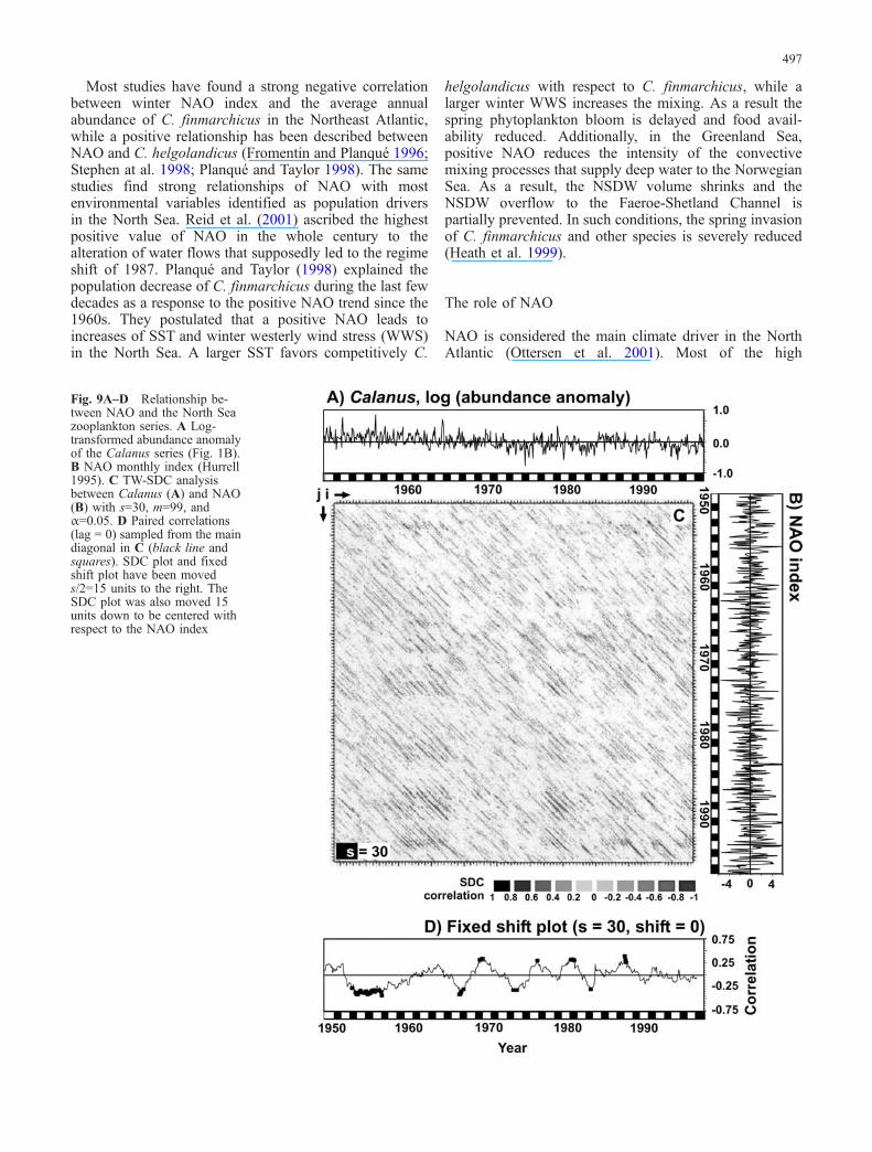
Fig. 9A–D Relationship be-tween NAO and the North Seazooplankton series. A Log-transformed abundance anomalyof the Calanus series (Fig. 1B).B NAO monthly index (Hurrell1995). C TW-SDC analysisbetween Calanus (A) and NAO(B) with s=30, m=99, andα=0.05. D Paired correlations(lag = 0) sampled from the maindiagonal in C (black line andsquares). SDC plot and fixedshift plot have been moveds/2=15 units to the right. TheSDC plot was also moved 15units down to be centered withrespect to the NAO index
497
correlations published between NAO and ecological datahave been found in annually averaged short-time seriesusually representing populations of large areas (Fromentinand Planqué 1996). Data averaging sometimes raisesmisleading interpretations as it can overestimate theautocorrelation of individual series or increase artificiallythe cross-correlation arising between two scarcely relateddatasets (Legendre and Legendre 1998). Interpretations ofthese associations should be restricted to processes thatcan be adequately covered by our sampling. In an annualtime series we can investigate, for instance, the effects oflong-term drivers but not those of short-term forcings ortemporary ecological interactions. If we postulate a linkbetween the NAO and a fast changing ecological process,we need data with higher resolution. Zooplanktonpopulations change approximately in a monthly timescale (Margalef 1991), and so do most environmentaldrivers (namely, SST, wind stress, etc.). A majority of thestrong correlations with the NAO have been published forannually averaged data but not for monthly time series,even when easily available. Fromentin and Planqué (1996)obtained correlations of –0.76 and 0.42 between the winterNAO index (average of NAO index during winter months)and the annually averaged log-abundance of, respectively,C. finmarchicus and C. helgolandicus, between 1962 and1992 in the eastern North Atlantic. In the North Sea andfor the same time period, we obtained significantcorrelations (P>0.05) of –0.35 between the winter NAOindex and the annually averaged log-abundance of totalcopepods and of –0.42 between the winter NAO index andthe accumulated abundances of C. finmarchicus and C.helgolandicus (log-transformed and annually averaged).Despite being calculated in amalgamated series from asmaller area, our results are similar to the published ones.However, when reanalyzed for monthly series (Fig. 1A,B), the resulting correlations were very low and non-significant (–0.11 for NAO vs total copepods, and –0.09for NAO vs Calanus). A simple change of time units hasreduced the correlation values by 3–5 times. The NAOindex is a time series that exhibits a low-frequencycomponent corresponding to positive and negative phasesthat allow us to separate between severe and mild winteryears (Ottersen et al. 2001). The NAO also displays ashort-term autoregressive behavior that makes it unpre-dictable on a monthly basis. Under such a perspective, ourresults (a strong correlation between NAO and copepodsin annual series and a lack of relationship in monthlyseries) could indicate a modulation of zooplanktonpopulations by average winter conditions but not a directenvironmental forcing driven by NAO.
From preceding sections, we already know that weakcross-correlation values do not invalidate the possibilitythat transitory relationships may exist. To check for suchtemporary interactions between NAO and copepods, wecomputed a TW-SDC analysis of the monthly NAO indexand the log-transformed Calanus series (the residuals afterremoving the annual cycle of the amalgamated abundanceof C. finmarchicus and C. helgolandicus). The resultingSDC plot lacks any identifiable pattern (Fig. 9C) and is
similar to the OW-SDC of the monthly NAO index (Rodóand Rodríguez-Arias, submitted for publication). In such aplot, the short-term autoregressive component of NAOconcentrates the most significant correlations around themain diagonal (with small shifts), but the long-termbehavior does not yield any identifiable pattern because itis non-structured and unpredictable. As a consequence, inany TW-SDC analysis between NAO and other series,significant correlations should be expected only aroundthe main diagonal and preferably at very short time shifts.In Fig. 9C, such correlations seem to be absent, thoughthis claim is difficult to support from the visual inspectionof the SDC plot alone. Figure 9D shows the paired SDCcorrelations (s=30) from the main diagonal (shift = 0) ofthe SDC plot in Fig. 9C. Few of these local synchroniccorrelations are significant and none of them reachesvalues above or below ±0.45. Significant values do nottend to cluster together except in the period 1954–1957(positive correlation), the only interval that can beconsidered a weak NAO transitory forcing on a monthlybasis (Fig. 9D). The same analysis between NAO and totalcopepods (analysis not shown) provides similar resultswith a single transitory coupling from 1971 to 1973.
The role of El Niño-Southern Oscillation
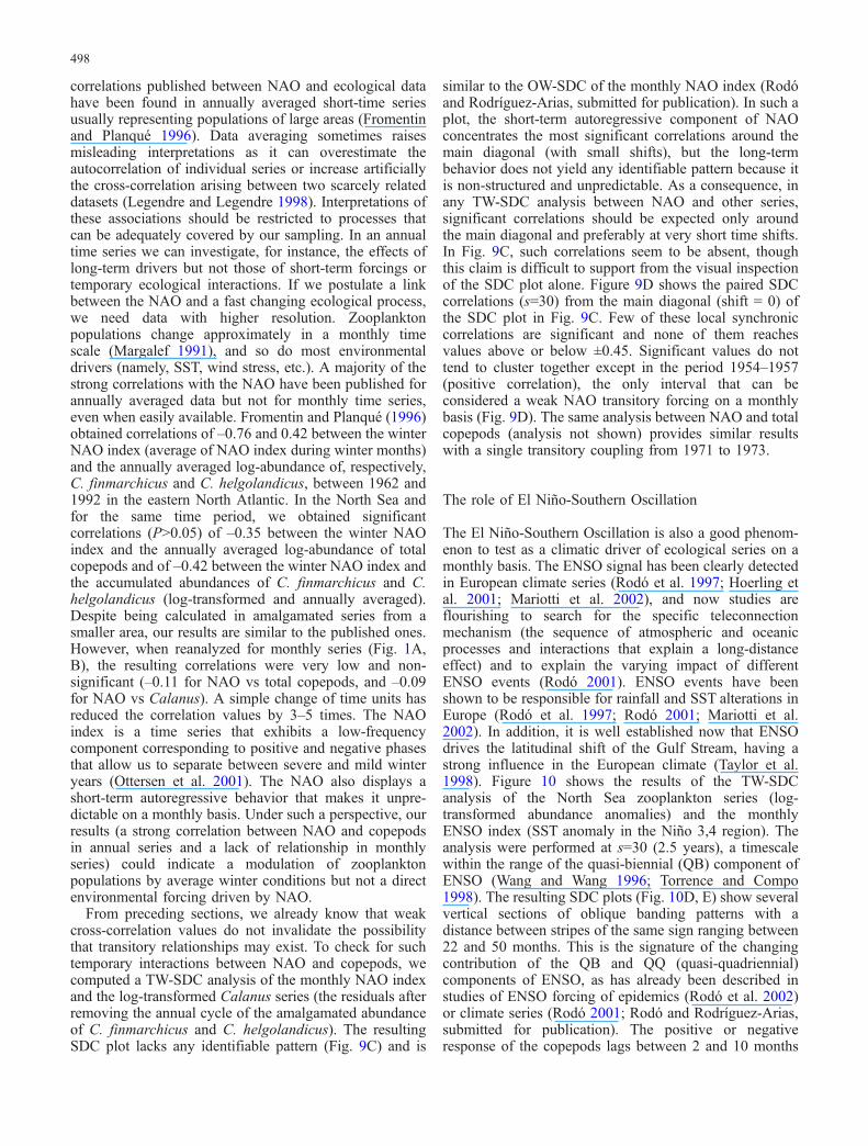
The El Niño-Southern Oscillation is also a good phenom-enon to test as a climatic driver of ecological series on amonthly basis. The ENSO signal has been clearly detectedin European climate series (Rodó et al. 1997; Hoerling etal. 2001; Mariotti et al. 2002), and now studies areflourishing to search for the specific teleconnectionmechanism (the sequence of atmospheric and oceanicprocesses and interactions that explain a long-distanceeffect) and to explain the varying impact of differentENSO events (Rodó 2001). ENSO events have beenshown to be responsible for rainfall and SST alterations inEurope (Rodó et al. 1997; Rodó 2001; Mariotti et al.2002). In addition, it is well established now that ENSOdrives the latitudinal shift of the Gulf Stream, having astrong influence in the European climate (Taylor et al.1998). Figure 10 shows the results of the TW-SDCanalysis of the North Sea zooplankton series (log-transformed abundance anomalies) and the monthlyENSO index (SST anomaly in the Niño 3,4 region). Theanalysis were performed at s=30 (2.5 years), a timescalewithin the range of the quasi-biennial (QB) component ofENSO (Wang and Wang 1996; Torrence and Compo1998). The resulting SDC plots (Fig. 10D, E) show severalvertical sections of oblique banding patterns with adistance between stripes of the same sign ranging between22 and 50 months. This is the signature of the changingcontribution of the QB and QQ (quasi-quadriennial)components of ENSO, as has already been described instudies of ENSO forcing of epidemics (Rodó et al. 2002)or climate series (Rodó 2001; Rodó and Rodríguez-Arias,submitted for publication). The positive or negativeresponse of the copepods lags between 2 and 10 months
498
after the forcing of ENSO, with maxima around 4 and8 months (Fig 10D, E). This delay between the forcing andthe response is the same that has been observed inEuropean climatic series affected by ENSO (Rodó et al.1997; Rodó 2001). Such similarity in the biological andenvironmental responses seems to point towards anindirect ENSO effect over copepods mediated by localenvironmental drivers, but the local mechanism respon-sible for the forcing remains to be investigated.
Figure 10F, G shows in detail the lagged SDCcorrelation between the zooplankton series and ENSO atthe lags with highest correlations in Fig. 10D, E (4 and8 months). Significant correlations are common, andsometimes individual values rise up to ±0.75 in accor-dance with, or shortly after, the strongest ENSO events.The intensity and extent of transitory correlations haveincreased since the 1970s, probably in response to theintensification of ENSO itself (Wang and Wang 1996;Torrence and Compo 1998). The dominant shift alsochanged, being shorter during the 1950s and 1960s (withlarger correlations at 4 months) than in the present (with
the highest correlations occurring 8 months after). Theresponse of total copepods and Calanus is similar for mostof the time, but after 1990 Calanus became less sensitiveto ENSO (Fig. 10E, G). This fact is probably in agreementwith the decrease of C. finmarchicus spring invasions inresponse to the reduced NSDWoverflow during the 1990s(Heath et al. 1999). A similar decrease in the Calanusresponse to ENSO forcing happened between 1954 and1960 (Fig. 10E, G).
The forcing is not only restricted to ENSO extremephases, a result in accordance with some recent observa-tions and model outputs that point towards a major role ofthe tropics in midlatitude climate (Rodó 2001; Hoerling etal. 2001). Similarly, we observe temporary phases ofpositive or negative correlation between ENSO and thecopepods, lasting 3–8 years (Fig. 10F, G). A hidden factoris probably modulating the ENSO response and control-ling the switch between positive and negative correlationphases. A seasonal control of the ENSO impact overrainfall has already been postulated in Europe (Mariotti etal 2002), and an interdecadal modulation of ENSO
Fig. 10A–G Relationship between ENSO and North Sea zoo-plankton. A Log-transformed abundance anomaly of the totalcopepod series (Fig. 1A). B Log-transformed abundance anomaly ofthe Calanus series (Fig. 1B). C Niño 3,4 SST anomaly. D TW-SDCanalysis between the total copepods (A) and ENSO (C) with s=30,m=99, and α=0.05. E TW-SDC analysis between Calanus (B) andENSO (C) with s=30, m=99, and α=0.05. F Lagged correlations for
4 (light blue line and squares) and 8 months (dark blue line andsquares), sampled from D. G Same as F but sampled from E. In C,F, and G, red bars refer to “El Niño” events, while the blue barsrefer to “La Niña” episodes. SDC plots (D and E) and fixed lag plots(F,G) have been moved s/2=15 units to the right to be centered withrespect to the zooplankton series. SDC plots were also displaced 15units down to be centered with respect to the ENSO series (C)
499
teleconnections by the North Pacific Oscillation (NPO)was also described for North America (Gershinov andBarnett 1998). The time scale of the persistence of thetemporary phases points towards a decadal to interdecadalmodulator of the ENSO forcing in the North Sea. SDCanalysis has revealed the complexity of the climaticcontrol of the zooplankton population dynamics in theNorth Sea. Therefore, it is feasible to state that NAO canbe discarded as an important forcing factor of short-termtemporal dynamics, while ENSO appears to be a commondriver at this time scale. The analysis thus raises severalother issues that still remain unanswered. As a result,further research is needed to understand the decadalmodulation of North Sea zooplankton dynamics.
SDC as a model diagnostic tool: Nicholson’s blowflies
The sensitivity of SDC in detecting temporary interactionscan be applied to isolate transitory departures fromexpected dynamics. Thanks to this feature, the TW-SDCanalysis becomes a valuable diagnostic tool for ecologicalmodeling. SDC can perform validations by confrontingmodel outputs with the original series. To provide apractical example, we examine here some populationmodels for the classical Nicholson’s blowfly (Australiansheep blowfly, Lucilla cuprina, Wied) time series(Nicholson 1957; Fig. 1C), one of the most intensivelystudied data in population dynamics (Gurney et al. 1980;Readshaw and Cuff 1980; Stokes et al. 1988; Kendall etal. 1999; Thomas and Wasserstein-Robbins 1999).
A variety models for the same population
Several authors have provided different explanations forboth the initial oscillations and the final loss of stability inthe blowflies series. For instance, Kendall et al. (1999)reviewed time-delay models for the oscillatory behavior.The cycles there observed can been reproduced by meansof models with density-dependent adult fertility (adultcompetition models, AC) or with density-dependent larvalgrowth (larval competition model, LC). Recent studies andnew experimental data seem to favor AC over LC models(Gurney et al. 1980; Readshaw and Cuff 1980; Kendall etal. 1999). To explain the loss of stability at the end of theexperiment, Nicholson (1957) postulated that naturalselection was acting during the experiment to change thedemographic characteristics of the population. Followinghis ideas, several authors provided some possible evolu-tionary mechanisms to account for this drift in theblowflies’ population dynamics (Stokes et al. 1988;Thomas and Wasserstein-Robbins 1999).
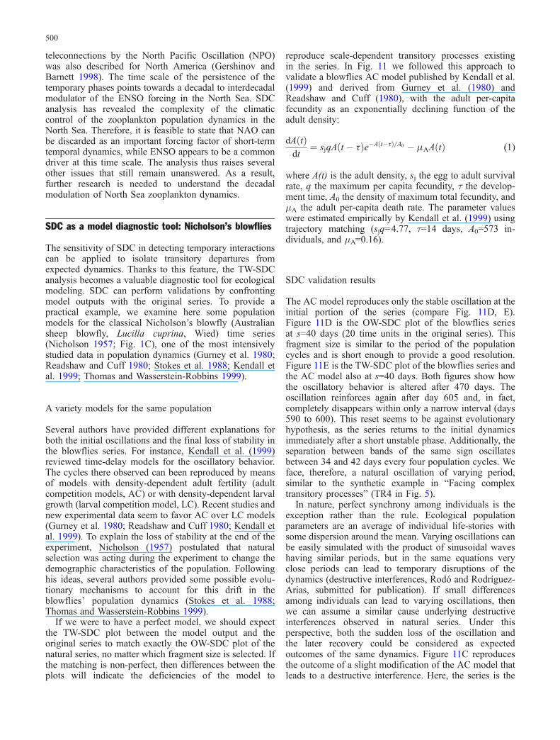
If we were to have a perfect model, we should expectthe TW-SDC plot between the model output and theoriginal series to match exactly the OW-SDC plot of thenatural series, no matter which fragment size is selected. Ifthe matching is non-perfect, then differences between theplots will indicate the deficiencies of the model to
reproduce scale-dependent transitory processes existingin the series. In Fig. 11 we followed this approach tovalidate a blowflies AC model published by Kendall et al.(1999) and derived from Gurney et al. (1980) andReadshaw and Cuff (1980), with the adult per-capitafecundity as an exponentially declining function of theadult density:
dA tð Þdt
¼ sjqA t � �ð Þe�A t��ð Þ=A0 � �AA tð Þ (1)
where A(t) is the adult density, sj the egg to adult survivalrate, q the maximum per capita fecundity, τ the develop-ment time, A0 the density of maximum total fecundity, andμA the adult per-capita death rate. The parameter valueswere estimated empirically by Kendall et al. (1999) usingtrajectory matching (sjq=4.77, τ=14 days, A0=573 in-dividuals, and μA=0.16).
SDC validation results
The AC model reproduces only the stable oscillation at theinitial portion of the series (compare Fig. 11D, E).Figure 11D is the OW-SDC plot of the blowflies seriesat s=40 days (20 time units in the original series). Thisfragment size is similar to the period of the populationcycles and is short enough to provide a good resolution.Figure 11E is the TW-SDC plot of the blowflies series andthe AC model also at s=40 days. Both figures show howthe oscillatory behavior is altered after 470 days. Theoscillation reinforces again after day 605 and, in fact,completely disappears within only a narrow interval (days590 to 600). This reset seems to be against evolutionaryhypothesis, as the series returns to the initial dynamicsimmediately after a short unstable phase. Additionally, theseparation between bands of the same sign oscillatesbetween 34 and 42 days every four population cycles. Weface, therefore, a natural oscillation of varying period,similar to the synthetic example in “Facing complextransitory processes” (TR4 in Fig. 5).
In nature, perfect synchrony among individuals is theexception rather than the rule. Ecological populationparameters are an average of individual life-stories withsome dispersion around the mean. Varying oscillations canbe easily simulated with the product of sinusoidal waveshaving similar periods, but in the same equations veryclose periods can lead to temporary disruptions of thedynamics (destructive interferences, Rodó and Rodríguez-Arias, submitted for publication). If small differencesamong individuals can lead to varying oscillations, thenwe can assume a similar cause underlying destructiveinterferences observed in natural series. Under thisperspective, both the sudden loss of the oscillation andthe later recovery could be considered as expectedoutcomes of the same dynamics. Figure 11C reproducesthe outcome of a slight modification of the AC model thatleads to a destructive interference. Here, the series is the
500
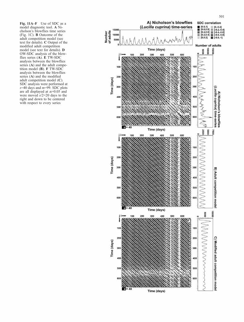
Fig. 11A–F Use of SDC as amodel diagnostic tool. A Ni-cholson’s blowflies time series(Fig. 1C). B Outcome of theadult competition model (seetext for details). C Output of themodified adult competitionmodel (see text for details). DOW-SDC analysis of the blow-flies series (A). E TW-SDCanalysis between the blowfliesseries (A) and the adult compe-tition model (B). F TW-SDCanalysis between the blowfliesseries (A) and the modifiedadult competition model (C).SDC analysis were performed ats=40 days and m=99. SDC plotsare all displayed at α=0.05 andwere moved s/2=20 days to theright and down to be centeredwith respect to every series
501
sum of individuals from two blowfly subpopulations thatfollow the AC model with a very small difference in thedevelopment time (τ) of their individuals. The new modelalso shows both the loss and the recovery of the dynamics,and the resulting TW-SDC plot (Fig. 11F) resembles morethe OW-SDC plot of Fig. 11D.
Discussion
Throughout this article, we have tried to demonstrate thattemporary dynamics are more common than expected inecological processes and that most transitory features mayremain masked and lead to misinterpretations when usingoverall signal-detection techniques. The uniqueness ofSDC analysis lies mainly in the graphical output, the SDCplot. Several authors before, suggested breaking the seriesinto fragments and calculating local correlations, but inthese methods only a small subset of all possible fragmentcorrelations was examined. SDC is now capable ofproviding simultaneously all the local information, as allpossible correlations of a given fragment size are shown ina single plot. SDC is also a flexible technique.Randomization testing was implemented to make SDCindependent of the resemblance measure. Users are thenfree to modify SDC by changing the present resemblancecoefficient—Pearson correlation—for any other similaritymeasure. In SDC analysis, neighboring individual correla-tions are not independent because they derive fromfragments sharing many elements in common, but theproportion of individual correlations becoming significantby chance alone is equivalent to the significance threshold,the same that occurs for independent correlations (Rodóand Rodríguez-Arias, submitted for publication). The mainproblem derived from the lack of independence ofindividual correlations is that they cannot be used forinference. Consequently, a group of significant correla-tions clustering together is a good indicator of a stronglocal relationship but cannot be used to estimate theamount of variance explained. As in any other correlationstudy, individual SDC values can become significant moreeasily if derived from autocorrelated series (Legendre andLegendre 1998). Autocorrelation, however, introduces akind of long-term resemblance that does not build upshort-term interactions, nor does it transform a purerandom pattern into a significant one. In most SDCanalyses, the effects of autocorrelation can be disdainedexcept in the analyses with very long fragments (Rodó andRodríguez-Arias, submitted for publication).
The robustness and tolerance of SDC in front of missingvalues are side consequences of the way the methodworks. Since it performs local calculations, the effect ofgaps is also local. The longer the gap and the fragmentsize, the larger the effect of missing points in SDC plots(still a local effect). If missing points are accuratelyinterpolated, SDC patterns can still be recovered with even25% of the missing values scattered on each series(Legendre and Legendre 1998). For this same reason, SDCis extremely robust and can be used to analyze very short
time series. This is particularly important because long andcontinuous ecological records are rare and difficult toobtain. However, this does not at all mean that SDC can beapplied to data series of any length, and restrictionsregarding the minimum sampling effort needed still apply.Data length should be enough as to provide a goodestimation of the underlying processes. In the context ofSDC, this means that series should at least contain oneoccurrence of an identifiable transitory process. Ob-viously, the longer the length of the series, the easier itwill be to find temporary features and discontinuities, butit is impossible to define a priori the minimum length ofthe series if we have no previous knowledge about theprocesses underneath. Like any other method, SDCanalysis works better if sampling is regular. When it isirregular (with changing temporal or spatial distancebetween successive samples), SDC analysis can still beused, but then the distortions introduced by the varyingdistance between elements should be taken into accountduring the investigation of the plots. Alternately, we caninterpolate to obtain an equally spaced series.
Pattern interpretation is the most critical point in theSDC method. At present, quantitative pattern testingallows us to discard, on the basis of overall plots, patternsderived from pure random processes (white noises), whilequalitative inspection allows us to refuse those arisingfrom other unpredictable dynamics such as red noises orrandom walks (Rodó and Rodríguez-Arias, submitted forpublication). One of the future improvements of the SDCmethodology should be the extension of quantitativepattern testing to include such processes that we nowdiscard only on the basis of visual inspection. The mainproblem of pattern interpretation from a practical point ofview is the masking of weak transitory features by strongpermanent processes. Although SDC would still some-times manage to reveal such faint signals, an unequivocalinterpretation is still difficult. If a series has strongpermanent processes such as an annual cycle, the bestoption will be to remove it and to perform again the SDCanalysis with the residuals.
Though direct inference cannot be obtained alone fromindividual SDC correlation values, the information derivedfrom SDC plots, in fact, consists of indirect inferences thatcan be used later for several purposes. SDC results canprovide new clues about mechanisms, interactions, and thestructure of systems that can be further tested. Theinformation derived from SDC plots also allows us toimprove the descriptive and predictive capabilities ofecological models. For example, the discovery of a linkbetween lagged transitory ENSO forcing and choleraoutbreaks in Bangladesh was used to build a nonlineartime-series model that provided remarkable two-step-ahead forecasts of the epidemics (Pascual et al. 2000).While a more quantitative version of the SDC methodremains under development, SDC analysis can still play animportant descriptive role in helping to uncover transitoryecological processes that remain hidden to other statisticaltechniques.
502
Summary
Temporary processes are common in ecological series andcannot be detected with most common hand statisticalmethods. Scale-dependent correlation (SDC) analysis is auseful tool to study scale-dependent transitory features inecological series. The method measures the degree ofsimilarity between all possible pairs of segments of aselected length extracted from two ecological data seriesand displays only the significant values. In the plot, we canlocate transitory processes and discriminate betweendifferent kinds of dynamics that result in different patterns.These patterns or structures may change when the seriesare analyzed at different segment lengths as a result of thescale dependence of the underlying processes. In OW-SDC plots, patterns arise from the constituent signals in asingle series, while in TW-SDC analysis, patterns build upfrom the local interactions between two series. TW-SDCanalysis is therefore very useful to relate forcing factorsand transitory ecological responses. SDC is also a user-friendly technique that is robust to missing values and thatcan be used with high accuracy to analyze very shortseries. The steps involved in a TW-SDC analysis are asfollows:
1. Check whether the series contain strong permanentsignals (the annual cycle, for instance). If so, removethem.
2. Find estimates of the characteristic scale of theprocesses by performing prospective OW-SDC analysisof the individual series or by applying other statisticalmethods or available additional information (forexample, knowledge of the scale of an environmentaldriver).
3. Perform TW-SDC analysis at s-values slightly largerthan the scale estimates. Set m=19 for previews andm=99 for definitive analysis. Check the overallsignificance of the plots with respect to white noiseexpectations, and discard those that are non-significant.
4. Inspect every significant SDC plot at α=0.05. Definethe periodicity of the transitory signals from thebanding of oblique patterns, and their persistencefrom the position of discontinuities.
5. If necessary, perform an additional SDC analysis with ashorter fragment size, to accurately define the likelyposition of discontinuities.
As an example, the SDC analysis of the North Seazooplankton series has revealed a complex dynamics withENSO as the main climatic driver of the short-termdynamics of copepods and has highlighted the need forfurther research in this area. The use of SDC to diagnose amodel of Nicholson’s blowflies shows clearly when themodel fails and provides new insights about the rulesgoverning the internal dynamics of the population.
Acknowledgements We thank S. Pueyo, J.J. Camarero, J. Piera, F.Bartomeus, and X. de Pedro at the Department of Ecology(Universitat de Barcelona, UB) for their fruitful discussions duringthe development of the SDC method. We gratefully acknowledge M.Pascual, R. Solow, E. Ranta, C. Osenberg, A. Steward-Oaten, andtwo anonymous reviewers for their useful comments on preliminaryversions of this manuscript. We also especially thank Parc Científicde Barcelona (UB), Servei Meteorològic de Catalunya, CIRIT(ACES98 29/7), Moelco (Research branch), and BATMARE (MarieCurie Training Site at the Institutt for fiskeri- og marinbiologi,Universiteten i Bergen, EVK3-CT-2000-57129) for support, fund-ing, and computing facilities. NAO and ENSO indices were kindlyprovided by the Climate Analysis Section, NCAR, Boulder, Colo.,USA (Hurrel 1995). Nicholson’s blowflies and North Sea zoo-plankton series can be found, respectively, at the URLs of theMonash University and the Sir Alister Hardy Foundation for OceanSciences (SAHFOS). Wavelet software (http://paos.colorado.edu/research/wavelets/) was provided by C. Torrence and G.P Compo.
References
Bradshaw GA, McIntosh BA (1994) Detecting climate-inducedpatterns using wavelet analysis. Environ Pollut 83:135–142
Bradshaw GA, Spies TA (1992) Characterizing canopy gap structurein forests using wavelet analysis. J Ecol 80:205–215
Broomhead DS, King GP (1986) Extracting qualitative dynamicsfrom experimental data. Physica D 20:217–236
Brosofske KD, Chen J, Crow TR, Saunders SC (1999) Vegetationresponses to landscape structure at multiple scales across anorthern Wisconsin, USA, pine barrens landscape. Plant Ecol143:203–218
Butler L (1953) The nature of cycles in populations of Canadianmammals. Can J Zool 31:242–262
Casdagli MC (1997) Recurrence plots revisited. Physica D 108:12–44
Chatfield C (1989) The analysis of time series: an introduction. 4thedn. Chapman and Hall, London
Chen X, Cohen JE (2001) Transient dynamics and food-webcomplexity in the Lotka-Volterra cascade model. Proc R SocLond B 268:869–877
Childers DL, Sklar FH, Hutchinson SE (1994) Statistical treatmentand comparative analysis of scale-dependent aquatic transectdata in estuarine landscapes. Landscape Ecol 9:127–141
Chiu CK, Montefusco L, Puccio L (eds) (1994) Wavelets: theory,algorithms and applications. Academic Press, San Diego
Compagnucci RH, Blanco SA, Figliola MA, Jacovkis PM (2000)Variability in subtropical Andean Argentinean Atuel river; awavelet approach. Environmetrics 11:251–269
Dale MRT, Mah M (1998) The use of wavelets for spatial patternanalysis in ecology. J Veg Sci 9:805–814
Daubechies I (ed) (1993) Different perspectives on wavelets.American Mathematical Society, Providence, Rhode Island
Dohan K, Whitfield PH (1997) Identification and characterization ofwater quality transients using wavelet analysis. I. Waveletanalysis methodology. In: Beck MB, Lessard P (eds) Water-matex-97, systems analysis and computing in water qualitymanagement: towards a new agenda. Elsevier, Amsterdam
Fortin MJ (1994) Edge detection algorithms for two-dimensionalecological data. Ecology 75:956–965
Fromentin JM, Planqué B (1996) Calanus and environment in theeastern North Atlantic. II. Influence of the North AtlanticOscillation on C. finmarchicus and C. helgolandicus. Mar EcolProg Ser 134:111–118
Gershinov A, Barnett TP (1998) Interdecadal modullation of ENSOteleconnections. Bull Am Meteorol Soc 79:2715–2726
Green DG (1995) Time and spatial analysis. In: Maddy D, Brew JS(eds) Statistical modeling of quaternary science data. Quater-nary Research Association, Cambridge
503
Grenfell BT, Bjørnstad ON, Kappey J (2001) Travelling waves andspatial hierarchies in measles epidemics. Nature 414:6865 716–723
Gurney WSC, Blythe SP, Nisbet RM (1980) Nicholson’s blowfliesrevisited. Nature 287:17–21
Harper KA, Macdonald SE (2001) Structure and composition ofriparian boreal forest: New methods for analyzing edgeinfluence. Ecology 82:649–659
Hastings A, Higgins K (1994) Persistence of transients in spatiallystructured ecological models. Science 263:1133–1136
Heath MR, Backhaus JO, Richardson K, Mckenzie E, Slagstad D,Beare D, Dunn J, Fraser JG, Gallego A, Hainbucher D, Hay S,Jónasdóttir S, Madden H, Mardaljevic J, Schacht A (1999)Climate fluctuations and the spring invasion of the North Seaby Calanus finmarchicus. Fish Oceanogr 8 [Suppl 1]:163–176
Hoerling MP, Kumar A, Xu T (2001) Robustness of the nonlinearclimate response to ENSO’s extreme phases. J Clim 14:1277–1293
Hu Z, Chen Y, Islam S (1998) Multiscaling properties of soilmoisture images and decomposition of large- and small-scalefeatures using wavelet transforms. Int J Remote Sens 19:2451–2467
Hurrell JW (1995) Decadal trends in the North Atlantic oscillation:regional temperatures and precipitation. Science 269:676–679
Kendall BE, Briggs CJ, Murdoch WW, Turchin P, Ellner SP,McCauley E, Nisbet RM, Wood SN (1999) Why dopopulations cycle? A synthesis of statistical and mechanisticmodelling approaches. Ecology 80:1789–1805
Labat D, Ababou R, Mangin A (1999) Wavelet analysis in karstichydrology. II: Rainfall-runoff cross-wavelet analysis. C R AcadSci II A 329:881–887
Lark RM, Webster R (2001) Changes in variance and correlation ofsoil properties with scale and location: analysis using anadapted maximal overlap discrete wavelet transform. Eur J SoilSci 52:547–562
Lau KM, Weng H (1995) Climate signal detection using wavelettransform: how to make a time series sing. Bull Am MeteorolSoc 76:2391–2402
Law R, Edley MT (1990) Transient dynamics of population withage- and size-dependent vital rates. Ecology 71:1863–1870
Legendre P, Fortin JH (1989) Spatial pattern and ecological analysis.Vegetatio 80:107–138
Legendre P, Legendre L (1998) Numerical ecology, 2nd Englishedn. Developments in ecological modeling, vol 20. Elsevier,Amsterdam
Legendre P, Dallot S, Legendre L (1985) Succession of specieswithin a community: chronological clustering, with applica-tions to marine and freshwater zooplankton. Am Nat 125:257–288
Levin SA (1992) The problem of pattern and scale in ecology.Ecology 73:1943–1967
Li Z, Kafatos M (2000) Interannual variability of vegetation in theUnited States and its relation to El Nino/Southern Oscillation.Remote Sens Environ 71:239–247
Machu E, Ferret G, Garcon V (1999) Phytoplankton pigmentdistribution from SeaWiFS data in the subtropical convergencezone south of Africa: a wavelet analysis. Geophys Res Lett26:1469–1472
Mallat SG (1989) A theory for multiresolution signal decomposi-tion: the wavelet representation. IEEE Trans Pattern Anal MachIntell 11:674–693
Manuca R, Savit R (1996) Stationarity and nonstationarity in timeseries analysis. Physica D 99:134–161
Margalef R (1991) Teoría de los sistemas ecológicos. PublicacionsUniversitat de Barcelona, Barcelona
Mariotti A, Zeng N, Lau KM (2002) Euro-Mediterranean rainfalland ENSO –a seasonally varying relationship. Geophys ResLett 29:10
Martínez ND, Lawton JH (1995) Scale and food-web structure-fromlocal to global. Oikos 73:148–154
May RM (1973) Stability and complexity in model ecosystems.Princeton University Press, New Jersey
Neubert MG, Caswell H (1997) Alternatives to resilience formeasuring the responses of ecological systems to perturbations.Ecology 78:653–665
Nicholson AJ (1957) The self-adjustment of populations to change.Cold Spring Harbor Symp Quant Biol 22:153–173
Nils S, Chan KS, Tong H, Boonstra R, Boutin S, Krebs CJ, Post E,O’Donoghue M, Yoccoz NG, Forchhammer MC, Hurrell JW(1999) Common dynamic structure of Canada lynx populationswithin three climatic regions. Science 285:1071–1073
Ottersen G, Planqué B, Belgrano A, Post E, Reid PC, Stenseth NC(2001) Ecological effects of the North Atlantic oscillation.Oecologia 128:1–14
Pascual M, Rodó X, Ellner S, Colwell R, Bouma M (2000) Choleradynamics and El Niño-southern oscillation. Science 289:1766–1769
Planqué B, Fromentin JM (1996) Calanus and environment in theeastern North Atlantic. I. Spatial and temporal patterns of C.finmarchicus and C. helgolandicus. Mar Ecol Prog Ser134:101–109
Planqué B, Taylor AH (1998) Long-term changes in zooplanktonand the climate of the North Atlantic. ICES J Mar Sci 55:644–654
Platt T, Denman KL (1975) Spectral analysis in ecology. Annu RevEcol Syst 6:189–210
Powell TM, Steele JH (eds) (1995) Ecological time series. Chapman& Hall, New York
Readshaw JL, Cuff WR (1980) A model of Nicholson’s blowflycycles and its relevance to predation theory. J Anim Ecol49:1005–1010
Reid PC, Borges MF, Svendsen E (2001) A regime shift in the NorthSea circa 1988 linked to changes in the North Sea horsemackerel fishery. Fish Res 50:163–171
Rodó X (2001) Reversal of three global atmospheric fields linkingchanges in SST anomalies in the Pacific, Atlantic and Indianoceans at tropical latitudes and midlatitudes. Clim Dyn 18:203–217
Rodó X, Baert E, Comín FA (1997) Variations in seasonal rainfall insouthern Europe during the present century: relationship withthe North Atlantic Oscillation and the El Nino-SouthernOscillation. Clim Dyn 13:275–284
Rodó X, Pascual M, Fuchs G, Faruque ASG (2002) ENSO andcholera: a non-stationary link related to climate change. ProcNatl Acad Sci USA 99:12901–12906
Saunders SC, Chen J, Crow TR, Brosofske KD (1998) Hierarchicalrelationships between landscape structure and temperature in amanaged forest landscape. Landscape Ecol 13:381–395
Steele JH (ed) (1978) Spatial pattern in plankton communities.Plenum, New York
Stephen JA, Jordan MB, Taylor AH, Proctor R (1998) The effects offluctuations in North Sea flows on zooplankton abundance. JPlankton Res 5:943–956
Stepnowski A, Moszynski M (2000) Inverse problem solutiontechniques as applied to indirect in situ estimation of fish targetstrength. J Acoust Soc Am 107:2554–2562
Stokes TK, Gurney WS, Nisbet RM, Blythe SP (1988) Parameterevolution in a laboratory insect population. Theor Popul Biol34:248–265
Taylor AH (1995) North-south shifts of the Gulf Stream and theirclimatic connection with the abundance of zooplankton in theUK and surrounding seas. ICES J Mar Sci 52:711–721
Taylor AH, Jordan MB, Stephens JA (1998) Gulf Stream shiftsfollowing ENSO events. Nature 393:638
Thomas DM, Wasserstein-Robbins F (1999) Analysis of a non-autonomous Nicholson Blowfly model. Physica A 273:198–211
Torrence C, Compo GP (1998) A practical guide to waveletanalysis. Bull Am Meteorol Soc 79:61–78
Wang B, Wang Y (1996) Temporal structure of the SouthernOscillation as revealed by waveform and wavelet analysis. JClim 9:1586–1598
Whitfield PH, Dohan K (1997) Identification and characterization ofwater quality transients using wavelet analysis. II. Applicationto electronic water quality data. In: Beck MB, Lessard P (eds)Watermatex-97, systems analysis and computing in waterquality management: towards a new agenda. Elsevier, Amster-dam
504