IOP PUBLISHING JOURNAL OF PHYSICS: CONDENSED MATTER

J. Phys.: Condens. Matter 20 (2008) 294203 (8pp) doi:10.1088/0953-8984/20/29/294203

A divide-and-conquer linear scalingthree-dimensional fragment method forlarge scale electronic structure calculationsZhengji Zhao1, Juan Meza and Lin-Wang Wang2

Computational Research Division, Lawrence Berkeley National Laboratory, Berkeley,CA 94720, USA

E-mail: lwwang@lbl.gov

Received 24 January 2008, in final form 13 February 2008Published 24 June 2008Online at stacks.iop.org/JPhysCM/20/294203

AbstractWe present a new linear scaling ab initio total energy electronic structure calculation methodbased on a divide-and-conquer strategy. This method is simple to implement, easy to parallelize,and produces accurate results when compared with direct ab initio methods. The new methodhas been tested on nanosystems with up to 15 000 atoms using up to 8000 processors.

(Some figures in this article are in colour only in the electronic version)

1. Introduction

In theoretical material science and nanoscience research, thereare many cases where thousands or tens of thousands of atomsneed to be simulated. It could be a molecular dynamicssimulation for water absorption on a metal oxide surface,or catalytic processes for nanostructure growth. It couldalso be charge density self-consistent calculations for a largenanocrystal with tens of thousands of atoms for determining itsinternal electric field and surface state coupling to the internalstates. For all of these calculations, ab initio density functionaltheory (DFT), especially with the use of the local densityapproximation (LDA), is the method of choice. However, dueto the O(N3) computational scaling [1] of the direct LDAmethod, it can only be applied to about one to two thousandatoms, even for the largest supercomputers available today [2].In addition, future increases in supercomputer power will bedue more to an ever larger number of processors and computingcores, instead of increasing CPU speeds. Unfortunately, theparallelization of direct DFT methods might have a limiton the order of 10 000 processors, due to a communicationbottleneck [2]. Thus, both the total computational cost andthe limits of parallelization call for a change in the direct LDAalgorithm to linear scaling O(N) methods [3] for large systemsimulations. Indeed, for systems with more than 500 atoms

1 Present address: National Energy Research Scientific Computing Center,Lawrence Berkeley National Laboratory, Berkeley, California, 94720, USA.2 Author to whom any correspondence should be addressed.

most of the O(N) methods already become faster than directLDA methods.

Currently, there are many O(N) methods, and many ofthem are discussed in this special journal issue. A commonO(N) algorithm is based on localized orbitals [4]. However,there are some technical difficulties in this approach. Onedifficulty is the possible existence of local minima in thetotal energy function introduced by the restriction of thewavefunctions on the local orbital manifold. Obviouslythese local minima could cause numerical convergenceproblems. Special methods and algorithms have been devisedto overcome these problems [5]. Another issue is that mostof the local orbital methods are naturally represented by alocalized basis set (either atomic basis set or real space grids).It is therefore not straightforward to use plane-wave basis setsto represent the localized orbitals [6]. Compared to real spacegrids [7], the plane-wave basis and its convergence propertieshave been more thoroughly studied, and it is more widelyused in material science simulations. On the computationalside, the overlap between neighboring local orbitals poses achallenge for code parallelization. A closely related methodto the localized orbital method is the truncated density matrixmethod [8]. The truncated density matrix method mighthave avoided the local minimum problem, but it is costly torepresent the matrix based on real space grids. As a result, itis mostly represented by atomic orbitals. Another approachis to first construct a localized basis set from a plane-waveor real space grid basis, then use this localized basis set to

0953-8984/08/294203+08$30.00 © 2008 IOP Publishing Ltd Printed in the UK1

J. Phys.: Condens. Matter 20 (2008) 294203 Z Zhao et al

represent the density matrix. In the energy minimization, onethen optimizes the density matrix coefficients and the localizedbasis set simultaneously. This approach is exemplified by theCONQUEST project [9].

Another approach for realizing O(N) scaling is a divide-and-conquer method. In a divide-and-conquer method, a largesystem is divided into small pieces (fragments), and eachfragment is calculated independently. The fragment resultsare placed together to give the total energy and the chargedensity of the whole system. The critical issue here is howto put the fragments together without introducing artificialboundary effects. One of the earliest methods in this approachwas introduced by Yang [10]. In Yang’s method, spatialpartition functions are applied to the charge densities of thefragments when generating the charge density of the wholesystem. Thus, only the central parts of the fragment chargedensities (and their corresponding kinetic energy density) areused. One technical problem is that the total energy cannotbe expressed in a variational formula. Furthermore, in orderto reach charge neutrality, a global Fermi energy has to beused for the occupation of the fragment wavefunctions, thusallowing charge transfer between fragments. In this regard, thefragments are treated almost like metallic pieces. Another issueis how to partition the kinetic energy where different ways ofpartitioning might lead to different results [11]. Nevertheless,this divide-and-conquer method has been used to calculatesystems with tens of thousands of atoms in molecular dynamicssimulations [11].

In this paper, we present a new O(N) method basedon the divide-and-conquer approach. We call it a linearscaling three-dimensional fragment (LS3DF) method. Thismethod has been reported briefly in a previous paper [12],but here more technical details will be provided. Comparedwith Yang’s method, we used a different scheme to patch thefragment charge densities. Instead of using spatial partitionfunctions, we use positive and negative fragments. Byjudiciously combining the positive and negative fragments,the artificial boundary effects will cancel out. Our methodhas the following features: (1) its accuracy increasesexponentially with the fragment size, and very accurateresults can be obtained with relatively small fragments;(2) its formalism and implementation are straightforward.It can be implemented easily using an existing ab initiocode; (3) since the fragment wavefunction calculations areindependent for different fragments, it can be parallelizedeasily; (4) it can be applied to ab initio methods otherthan DFT.

In this paper, we have only tested our method oncovalently bonded systems with a band gap. One feature inour current implementation of the method is that after someartificial surface passivation, each fragment is an insulatingsystem with a band gap. This can be easily done by usingpartial charge pseudo-hydrogen atoms for covalently bondedsystems (where a pseudo-hydrogen atom will be placed at thecenter of a cut-off bond). Although further tests are needed,we do expect the method will work for ionic systems withband gaps. Usually artificial atoms can be used to provide theelectrons to fill the ionic close shell orbitals and at the same

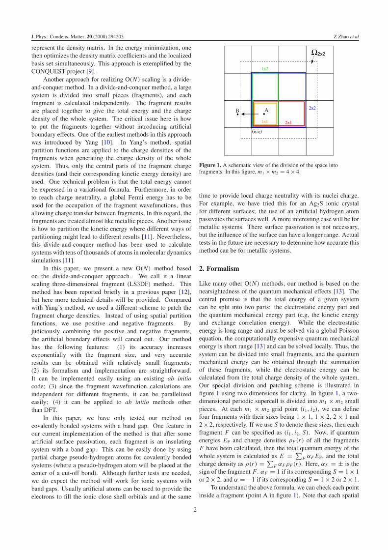
Figure 1. A schematic view of the division of the space intofragments. In this figure, m1 × m2 = 4 × 4.

time to provide local charge neutrality with its nuclei charge.For example, we have tried this for an Ag2S ionic crystalfor different surfaces; the use of an artificial hydrogen atompassivates the surfaces well. A more interesting case will be formetallic systems. There surface passivation is not necessary,but the influence of the surface can have a longer range. Actualtests in the future are necessary to determine how accurate thismethod can be for metallic systems.

2. Formalism

Like many other O(N) methods, our method is based on thenearsightedness of the quantum mechanical effects [13]. Thecentral premise is that the total energy of a given systemcan be split into two parts: the electrostatic energy part andthe quantum mechanical energy part (e.g, the kinetic energyand exchange correlation energy). While the electrostaticenergy is long range and must be solved via a global Poissonequation, the computationally expensive quantum mechanicalenergy is short range [13] and can be solved locally. Thus, thesystem can be divided into small fragments, and the quantummechanical energy can be obtained through the summationof these fragments, while the electrostatic energy can becalculated from the total charge density of the whole system.Our special division and patching scheme is illustrated infigure 1 using two dimensions for clarity. In figure 1, a two-dimensional periodic supercell is divided into m1 × m2 smallpieces. At each m1 × m2 grid point (i1, i2), we can definefour fragments with their sizes being 1 × 1, 1 × 2, 2 × 1 and2 × 2, respectively. If we use S to denote these sizes, then eachfragment F can be specified as (i1, i2, S). Now, if quantumenergies EF and charge densities ρF (r) of all the fragmentsF have been calculated, then the total quantum energy of thewhole system is calculated as E = ∑

F αF EF, and the totalcharge density as ρ(r) = ∑

F αFρF (r). Here, αF = ± is thesign of the fragment F . αF = 1 if its corresponding S = 1 × 1or 2 × 2, and α = −1 if its corresponding S = 1 × 2 or 2 × 1.

To understand the above formula, we can check each pointinside a fragment (point A in figure 1). Note that each spatial

2

J. Phys.: Condens. Matter 20 (2008) 294203 Z Zhao et al

point will be included in 32 fragments: four 2 × 2 fragments,two 2 × 1 fragment, two 1 × 2 fragments and one 1 × 1fragment. After the above ± cancellations, it will be coveredby only one fragment, which is what is needed to contributeto one copy of the whole system. We can now check for eachboundary point. A boundary can be defined with a direction,thus a boundary from A to B will be different from a boundaryfrom B to A. We have used an arrow in figure 1 to represent adirectional boundary (from A to B). A point on this directionalboundary is covered by six fragments (two 2 × 2, two 1 × 2,one 1 × 2 and one 1 × 1 fragments), with equal numbersof positive and negative signs. Since all these pieces havethe same (directional) boundary at this point, and given thenearsightedness, their charge density will be the same near thispoint. As a result, the boundary effects will cancel out. Thesame is true for the corner effect.

The above scheme can be extended to a three-dimensionalsystem in a straightforward way. Here, a periodic supercell isdivided into m1 ×m2 ×m3 fragments, and from each grid pointcorner (i1, i2, i3) there are eight fragments, with sizes S(αS)

equal to 1×1×1(−), 1×1×2(+), 1×2×1(+), 2×1×1(+),1 × 2 × 2(−), 2 × 1 × 2(−), 2 × 2 × 1(−), and 2 × 2 × 2(+).The same formula E = ∑

F αF EF and ρ(r) = ∑F αFρF (r)

can be used, where the fragment F = (i1, i2, i3, S), and thisformula has the same property of canceling out all the surface,edge and corner effects.

In the above scheme (figure 1), we have used the size oftwo grid points in the m1 × m2 × m3 grid for the 2 × 2 × 2fragment in each direction. Actually, it is possible to use asmaller size for the ‘2 × 2 × 2’ fragment. Then the smallerfragments can be defined as the overlapping areas of the‘2 × 2 × 2’ fragments originated from neighboring grid point(i1, i2, i3). Further tests are needed to find out whether this willsave computing time for the same accuracy of calculations.

To carry out our LS3DF scheme shown in figure 1, wefirst divide our three-dimensional supercell into an M =m1 × m2 × m3 grid. Atoms located inside a grid cube areassigned to the corresponding fragments. Thus, the divisionof the whole system into fragments is automatic. No priorknowledge about the physical system is necessary. As aresult, sometimes one fragment can consist of a few physicallyseparated clusters. But this will not affect the applicability andaccuracy of this method. One critical point is to passivatethe artificial surface created by this division, so that eachfragment is still an insulating system. For covalently bondedsystems, this can be done automatically by placing pseudo-hydrogen atoms with partial charges at the centers of thecut-off bonds [15]. This automatic procedure works wellfor all covalent bonding systems. A fragment is definedby the atoms (including the passivation atoms) plus a buffervacuum region as indicated in by the dashed lines in figure 1.The fragment spatial domains can be denoted as �F , whereF = (i1, i2, i3, S) is the fragment index. Each fragment canbe treated as an open system, or a periodic system with aperiodic cell �F . Due to the vacuum buffer region, thereis no difference whether we treat it as an open system or aperiodic system. In our method, we will treat it as a periodicsystem so that plane-wave basis can be used to describe the

fragment wavefunctions. The fragment wavefunction ψF,i (r)sare defined only within the fragment domain �F , and i is thewavefunction index.

Now we can write the total energy Etot of thesystem as a variational form in terms of the fragmentwavefunctions ψF,i (r):

Etot =∑

F

αF

∑

i

O(εF,i , EF)

∫

ψ∗F,i (r)[− 1

2∇2]ψF,i (r)d3r

+ Vion(r)ρtot(r)d3r + 1

2

∫ρtot(r)ρtot(r ′)

|r − r ′| d3rd3r ′

+∫

εxc(ρtot(r))ρtot(r)d3r +

∑

F

αF

∫

�VF(r)ρF (r)d3r

(1)

where the total charge density ρtot is calculated as

ρtot(r) =∑

F

αFρF (r), (2)

and the fragment charge density ρF (r) is calculated as

ρF (r) =∑

i

O(εF,i , EF)|ψF,i (r)|2 for r ∈ �F (3)

where O(εF,i , EF) is the Fermi–Dirac occupation functionbased on the overall Fermi energy EF and the fragmentwavefunction eigenenergy εF,i .

In equation (1), Vion(r) is the total ionic potential. Theterm �VF(r) is an additional surface passivation potentialthat is only nonzero near the boundary of the fragment.For different fragments sharing the same boundary B , their�VF(r) at that boundary B should be the same. Due to thefragment cancellations (the

∑F ′ αF ′ρF ′(r) for F ′ sharing the

same boundary B should be small), the net value of the lastterm in equation (1) should be small. The amplitude of thisterm can be used as a measure for the accuracy of this method.

The total energy Etot is a variational minimum (ormaximum, depending on the sign of αF ) with regard toψF,i (r),subject to the orthonormal constraints:

∫

�F

ψ∗F,i (r)ψF, j (r)d

3r = δi, j . (4)

As a result, we can derive the fragment Kohn–Shamequation from δEtot/δψ

∗F,i (r) = αF O(εF,i , EF)εF,iψF,i (r),

which gives us

[− 12∇2 + VF (r)]ψF,i(r) = εF,iψF,i (r), (5)

and

VF(r) = Vtot(r)+�VF (r) for r ∈ �F , (6)

where Vtot(r) is the usual LDA total potential calculatedfrom ρtot(r) by solving a global Poisson equation for thewhole system. The global charge density self-consistencycan be achieved iteratively using the usual potential mixingscheme [1] for Vtot(r). The overall computational flow isillustrated in figure 2 in comparison with the direct LDAmethod. We have used a plane-wave expansion for the

3

J. Phys.: Condens. Matter 20 (2008) 294203 Z Zhao et al

Figure 2. The computational flow charts for the direct LDA method and the LS3DF method. In the LS3DF method, the first box correspondsto equation (6) in the text, the second box corresponds to equation (5), and the third box corresponds to equations (2) and (3). Theself-consistent iteration potential mixing schemes in LDA and LS3DF are the same.

wavefunctions ψF,i (r) and norm conserving pseudopotentialsfor the Hamiltonian. Equation (5) (the second box in theLS3DF flow chart in figure 2) is solved using a conjugatedgradient method based on the plane-wave code, PEtot [16].After the charge self-consistency is reached, due to thevariational principle, atomic forces can be calculated usingthe Hellman–Feynman theory. Of practical importance isthe observation that the calculations of equation (5), thecomputationally most expensive step in figure 2, can be carriedout independently for each fragment, which makes the overallcomputation trivially parallelizable. In the above formalism,we have used a Fermi–Dirac occupation function O(εF,i , EF)

in the summation over fragment wavefunction index i . Thisis necessary if the overall system is metallic. However, ifthe system is an insulator, and with proper surface passivationeach fragment is also an insulator, then O(εF,i , EF) is a sharpstep function for index i , with NF (2NF being the number ofelectrons in a fragment) occupied states, and the rest of thestates unoccupied. In this case, O(εF,i , EF) does not dependsensitively on EF, and the summation over i with O(εF,i , EF)

can be replaced by a summation over i up to NF without theuse of O(εF,i , EF).

One technical issue in our method is how to calculatethe passivation potential �VF(r) (so the resulting fragmentsremain insulators). The pseudo-hydrogen atoms placed at thesurface of a fragment will make the fragment an insulator witha fragment potential VF (r) if the fragment is calculated self-consistently by itself. However, what we need in equation (6) isto change the total potential Vtot(r) into the fragment potentialVF(r) by adding a surface passivation potential �VF (r).Thus, �VF(r) is not just the hydrogen potential, it has to besomething more which can change the Vtot(r) in the bufferregion into a vacuum-like potential. To solve this problem,we have used the sum of atomic charge densities to construct a(non-self-consistent) ρF,atom(r), ρtot,atom(r). From these chargedensities and atomic pseudopotentials, we can calculate the

corresponding VF,atom(r) for the fragment LDA potential, andVtot,atom(r) for the total system LDA potential using the LDAformula. Based on this potential, we have calculated thesurface passivation potential as

�VF (r) = VF,atom(r)− Vtot,atom(r) for r ∈ �F . (7)

Furthermore, to assure that �VF(r) at a given boundary B isthe same for all the fragments sharing this common boundary,we have taken the average among all the fragments sharing thisboundary. A typical passivation potential �VF (r) is shown infigure 3. Also shown in figure 3 are the fragment potentialVF(r) and the global total potential Vtot(r) as in equation (6).Note that in an actual self-consistent calculation �VF (r) isfixed throughout the calculation, and the generation of�VF(r)does not take much time.

As discussed in the introduction, our approach is similarto Yang’s divide-and-conquer method in that they both dividethe system into small pieces in three dimensions. Our LS3DFmethod can also be compared to the fragment molecularorbital (FMO) method [14]. FMO is specifically designedfor biological systems where a long molecule chain is dividedinto many small segments (monomers). In the FMO method,all monomers and monomer–monomer pairs are calculatedto take into account the artificial effects caused by breakingthe covalent bonds between the neighboring monomers. Thebreaking of the chain molecule to monomers is basically anone-dimensional event. As a result, only monomer–monomerpairs need to be calculated. In contrast, in LS3DF we havethree-dimensional fragments with different sizes in a spatiallycompact form. If we identify our smallest 1 × 1 × 1 fragmentwith the monomers in FMO, then we have calculated up toeight monomer clusters (the 2 × 2 × 2 fragments). As a resultof the spatial division (instead of focusing on molecule chains),the LS3DF has a rigorous cancelation of the boundary effects.As we will show, the error in LS3DF drops rapidly as thefragment size increases.

4

J. Phys.: Condens. Matter 20 (2008) 294203 Z Zhao et al

Figure 3. The surface passivation potential �VF (r) (a); the whole system total potential Vtot(r) (showing only the portion for r ∈ �F ) (b);and the fragment potential VF (r) (c). Note that�VF (r)+ Vtot(r) = VF (r), and in the self-consistent iterations �VF (r) is fixed while Vtot(r)and VF (r) keep changing.

3. Numerical results

As a numerical test, we first show a comparison betweenthe LS3DF method and the direct LDA method. Weuse a Si235H104 quantum dot (QD) with surface hydrogenpassivation. Norm conserving pseudopotentials are used andthe plane-wave basis set cutoff is 35 Ryd. The size of the1 × 1 × 1 grid space is a, the lattice constant of the diamond

structure. Thus, the smallest fragment has eight Si atoms, anda 0.5 a buffer space on each side. The total energy differencebetween the LS3DF method and the direct LDA method is3 meV/atom. The average charge density difference is 0.2%,and the average atomic force difference is 5 × 10−5 au. Wealso tested Si slabs and rods, and CdSe quantum dots. Theerrors for these tests are similar to the above Si QD results.We also calculated the quantum dot polarization under an

5

J. Phys.: Condens. Matter 20 (2008) 294203 Z Zhao et al

Figure 4. The convergence of the dipole moment as a function ofself-consistent iteration steps for a CdSe quantum dot.

Table 1. The convergence of the LS3DF results in comparison withdirect LDA results for bulk Si calculations. The fragment sizes 0.5 a,1 a, 1.5 a correspond to 8, 64, 216 Si atoms in the 2 × 2 × 2fragments respectively. �E is the total energy error,�ρ is the totalcharge density error.

Fragment size 0.5 a 1 a 1.5 a

�E (meV/at) 30 2.9 4.0�ρ 1.1% 0.14% 0.08%∑

F αF

∫�VFρF dr (meV/at) 213 5.5 1.0

external electric field in a Si quantum dot using the above 1.0 afragment size. The LS3DF and direct LDA differences forthe response charge and total induced dipole moment are bothabout 2%.

We next test the effects of fragment size on the LS3DFerror. For this test, we have calculated the bulk Si with theLS3DF method. The bulk system is chosen so we can have theexact result for the direct LDA method. Our tests are shown intable 1. From table 1 we can see that the LS3DF errors droprapidly as the fragment size increases from 0.5 a to 1.5 a. Wenote that the total energy error does increase a bit in going from1.0 a to 1.5 a. This is due to the use of negative fragments.Because of this, although the LS3DF total energy is variationalwith regard to fragment wavefunctions ψF,i (r), it is not anupper limit of the converged total energy; it does not approachthe converged energy monotonically from above when the sizeof the fragment increases. This does pose a challenge for howto estimate the accuracy of the LS3DF calculations. A morerobust test is based on the charge density error, which dropsrapidly with the fragment size. In table 1, we have also shownthe last term in equation (1). As we discussed before, this termshould be canceled out from different fragments. This is indeedtrue. If all αF are all set to unity, then this term can be tens ofthousands of times larger.

Another direct way to test the accuracy of the LS3DFmethod is to compare the physical properties calculated by theLS3DF method and the direct LDA method. One very sensitiveproperty is the total dipole moment of a quantum dot. As weknow the total energy error depends on the second order ofthe wavefunction and charge density errors, while the dipole

Figure 5. Self-consistent convergence curves for LS3DF and directLDA methods.

moment error depends on the first order of the wavefunctionand charge density errors. We calculated the dipole momentsfor a small 178-atom wurtzite CdSe quantum dot. In the chargedensity self-consistent calculations, for both LS3DF and directLDA methods, we have solved the Poisson equation using anopen boundary condition, thus there is no neighboring dipole–dipole interaction due to the use of a periodic supercell. Usinga 1 × 1 × 1 fragment of 12 Cd + Se atoms, the LS3DF z-direction (c-axis) dipole moment was computed to be 3.52 au,while the LDA result was 3.49 au. The absolute difference(0.03 au) is much smaller than the error introduced by usingdifferent pseudopotentials. Figure 4 shows the convergence ofthe dipole moments through the self-consistent iterations. Thiscan be compared with the total energy convergence shown infigure 5.

As discussed in the introduction, one common problem forsome of the O(N) methods is the existence of local minimaand the resulting slow total energy convergence. Figure 5shows the convergence of the self-consistent iterations inLS3DF in comparison with the direct LDA result. As onecan see, the LS3DF method has a convergence rate similar tothe direct LDA method. Thus, the LS3DF method does nothave the convergence problem seen in other methods. Thisis understandable because we are using the same potentialmixing scheme as the direct LDA method (figure 2), and thewhole system charge to potential formula (Poisson equationand LDA exchange correlation formula) is the same for thesetwo methods, and the potential to charge response function isessentially the same as we have tested by applying an externalelectric field discussed before. Besides, since the calculation offragment wavefunction is independent for different fragments,the convergence of the Schrodinger’s equation (5) is fast usingthe traditional conjugate gradient method. In figure 6, weshow the computational cost as the flop counts of the LS3DFmethod and the direct LDA method. As we can see, these twomethods cross around 500 atoms when a 1 a fragment size isused. This crossover is similar to the crossover reported bymany other O(N) methods. In the flow chart of figure 2, theKohn–Sham equations for different fragments (equation (5))are solved independently. As a result, this step (the secondbox of the LS3DF flow chart in figure 2) can be parallelizedtrivially. The time spent on the global Poisson equation is lessthan 5% of the total computational time. As a result, we havebeen able to achieve an excellent linear scaling up to thousands

6

J. Phys.: Condens. Matter 20 (2008) 294203 Z Zhao et al

Figure 6. The computation flops needed for one step inself-consistent calculation. A typical 1 a fragment size for thesmallest fragment is used for the LS3DF calculations. The flopcounts are measured on an IBM-SP power3 machine using theprofiling tool IPM.

Figure 7. The speed-up of the LS3DF method versus the number ofprocessors. The speed-up is measured starting from 256 processors.The system calculated is a CdSe quantum dot with about 2000 atoms.The smallest fragment contains 12 Cd and Se atoms. 32 processorsare used to calculate each fragment. The computation is done on aCray XT4 computer.

of processors. In figure 7, we show the speed-up of the LS3DFmethod with the number of processors for a 2000 atom CdSequantum dot. The method scales well up to 6000 processors.In this test, 32 processors are used to calculate each fragment.We are working on other parts of the code (e.g. the first andthird boxes in the LS3DF flow chart of figure 2) and the fileI/O to further improve the performance of the code.

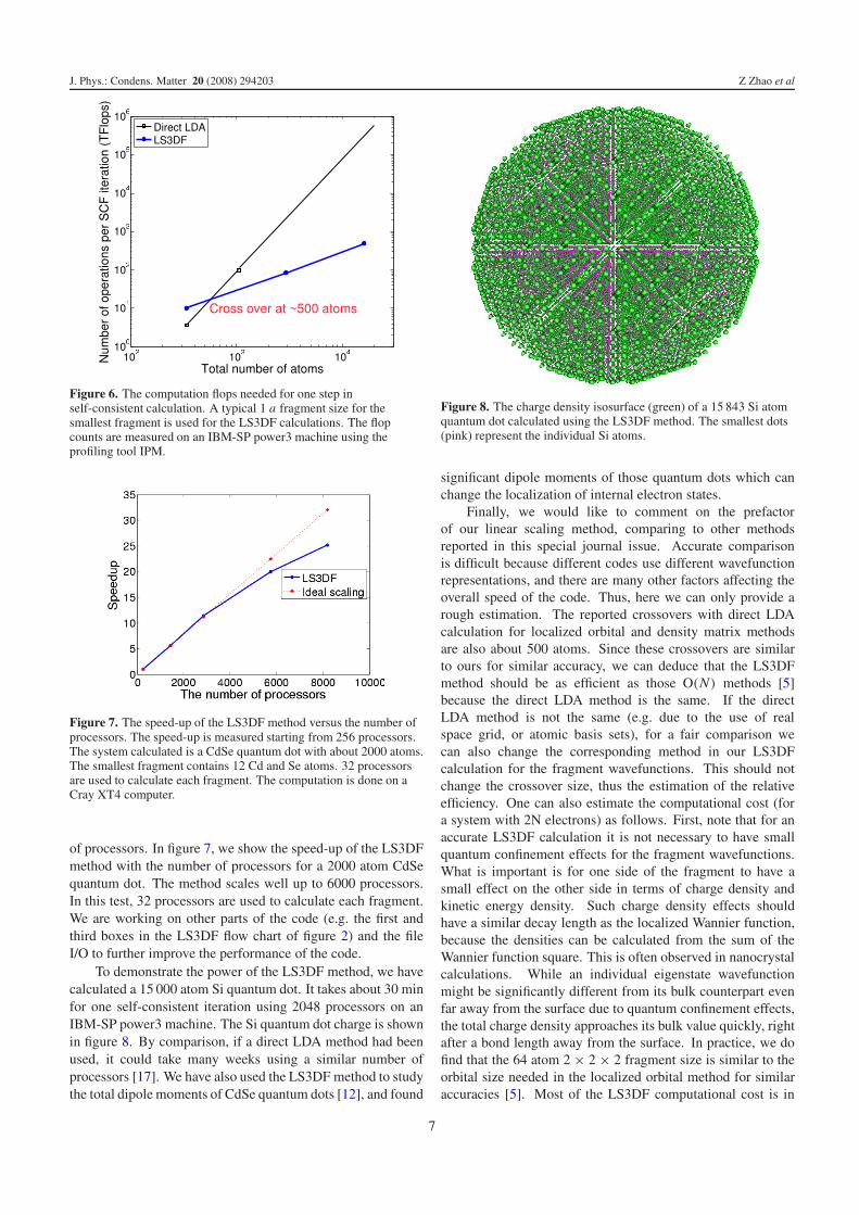
To demonstrate the power of the LS3DF method, we havecalculated a 15 000 atom Si quantum dot. It takes about 30 minfor one self-consistent iteration using 2048 processors on anIBM-SP power3 machine. The Si quantum dot charge is shownin figure 8. By comparison, if a direct LDA method had beenused, it could take many weeks using a similar number ofprocessors [17]. We have also used the LS3DF method to studythe total dipole moments of CdSe quantum dots [12], and found

Figure 8. The charge density isosurface (green) of a 15 843 Si atomquantum dot calculated using the LS3DF method. The smallest dots(pink) represent the individual Si atoms.

significant dipole moments of those quantum dots which canchange the localization of internal electron states.

Finally, we would like to comment on the prefactorof our linear scaling method, comparing to other methodsreported in this special journal issue. Accurate comparisonis difficult because different codes use different wavefunctionrepresentations, and there are many other factors affecting theoverall speed of the code. Thus, here we can only provide arough estimation. The reported crossovers with direct LDAcalculation for localized orbital and density matrix methodsare also about 500 atoms. Since these crossovers are similarto ours for similar accuracy, we can deduce that the LS3DFmethod should be as efficient as those O(N) methods [5]because the direct LDA method is the same. If the directLDA method is not the same (e.g. due to the use of realspace grid, or atomic basis sets), for a fair comparison wecan also change the corresponding method in our LS3DFcalculation for the fragment wavefunctions. This should notchange the crossover size, thus the estimation of the relativeefficiency. One can also estimate the computational cost (fora system with 2N electrons) as follows. First, note that for anaccurate LS3DF calculation it is not necessary to have smallquantum confinement effects for the fragment wavefunctions.What is important is for one side of the fragment to have asmall effect on the other side in terms of charge density andkinetic energy density. Such charge density effects shouldhave a similar decay length as the localized Wannier function,because the densities can be calculated from the sum of theWannier function square. This is often observed in nanocrystalcalculations. While an individual eigenstate wavefunctionmight be significantly different from its bulk counterpart evenfar away from the surface due to quantum confinement effects,the total charge density approaches its bulk value quickly, rightafter a bond length away from the surface. In practice, we dofind that the 64 atom 2 × 2 × 2 fragment size is similar to theorbital size needed in the localized orbital method for similaraccuracies [5]. Most of the LS3DF computational cost is in

7

J. Phys.: Condens. Matter 20 (2008) 294203 Z Zhao et al

the computation of the 2 × 2 × 2 fragments. There are M =m1 × m2 × m3 such fragments, each with 16N/M electrons.Thus, in total, there will be 8N fragment wavefunctions for thetotal calculation each in a domain of �2×2×2. In the localizedorbital method, the number of localized wavefunctions isabout N–2N depending on the implementation [5]. Thus,from this count, our method does have a larger numberof fragment wavefunctions than the localized orbitals. Butthis can be compensated by the fast iterative convergenceof the fragment wavefunctions (equation (5)) due to thewavefunction decoupling among the fragments. In a localizedorbital method, the change of the local orbital from one sitemight affect the local orbitals at far away sites due to theorthogonalization among the localized orbitals. This will slowdown its iterative convergency. Besides, in our wavefunctioncalculation for each fragment, the O(N3) step is not dominatingyet due to the relative small fragment sizes. Thus, this is acomputational sweet spot for the fragment calculations. Lastly,as discussed before, one can reduce the size of the ‘2 × 2 × 2’fragment (smaller than the 2 grid size of the m1 × m2 × m3

grid) to see whether it can speed up the calculation. Overall, itis not clear at this stage which O(N)method will be the fastest.It might very well be that the answer depends on the physicalproblem to be solved. A further study on this topic is needed,especially after all the methods become more mature.

4. Conclusion

We have presented a new divide-and-conquer linear scalingthree-dimensional fragment method for ab initio electronicstructure calculations. We have presented the technicaldetails for how the method is implemented, and described itsperformance. We demonstrated that this method can be usedto calculate the electronic structures of large nanosystems, andthat this method can be used to achieve excellent computationalefficiencies for massively parallel machines. In terms ofprogramming, the new method can be adapted from anexisting ab initio package relatively easily; it can also beused for other quantum mechanical methods, and not just thedensity functional theory. The results of this new method are

very accurate when compared with the direct LDA method.In addition, it has a variational formalism; therefore, thecalculation of atomic forces is straightforward using Hellman–Feynman theory.

Acknowledgments

This work was supported by the DMSE/BES/SC andMICS/ASCR/SC of the US Department of Energy undercontract No DE-AC02-05CH11231. It used the resources ofthe National Energy Research Scientific Computing Center(NERSC) and the National Center for Computational Sciences(NCCS).

References

[1] Payne M C, Teter M P, Allan D C, Arias T A andJoannopoulos J D 1992 Rev. Mod. Phys. 64 1045

[2] Gygi F, Yates R K, Lorenz J, Draeger E W, Franchetti F,Ueberhuber C W, de Supinski B R, Kral S, Gunnels J A andSexton J C 2005 Proc. 2005 ACM/IEEE Conf. onSupercomputing

[3] Goedecker G 1999 Rev. Mod. Phys. 71 1085[4] Galli G and Parrinello M 1992 Phys. Rev. Lett. 69 3547[5] Fattebert J-L and Gygi F 2006 Phys. Rev. B 73 115124[6] Skylaris C K, Mostofi A A, Haynes P D, Dieguez O and

Payne M C 2002 Phys. Rev. B 66 35119[7] Skylaris C K, Dieguez O, Haynes P D and Payne M C 2002

Phys. Rev. B 66 73103[8] Li X P, Nunes R W and Vanderbilt D 1993 Phys. Rev. B

47 10891[9] Bowler D R, Choudhury R, Gillan M J and Miyazaki T 2006

Phys. Status Solidi b 243 989[10] Yang W 1991 Phys. Rev. Lett. 66 1438[11] Shimojo F, Kalia R K, Nakano A and Vashishta P 2005

Comput. Phys. Commun. 167 151[12] Wang L W, Zhao Z and Meza J 2008 Phys. Rev. B at press[13] Kohn W 1996 Phys. Rev. Lett. 76 3168[14] Kitaura K, Ikeo E, Asada T, Nakano T and Uebayasi M 1999

Chem. Phys. Lett. 313 701[15] Li J and Wang L W 2005 Phys. Rev. B 72 125325[16] http://hpcrd.lbl.gov/linwang/PEtot/PEtot.html[17] Chelikowsky J 2005 APS Bull. 51 612

8