Satellite interferometric observations of displacements

associated with seasonal groundwater

in the Los Angeles basin

Karen M. Watson, Yehuda Bock, and David T. SandwellCecil H. and Ida M. Green Institute of Geophysics and Planetary Physics, Scripps Institution of Oceanography, La Jolla,California, USA

Received 13 February 2001; revised 23 October 2001; accepted 28 October 2001; published 19 April 2002.

[1] The Newport-Inglewood fault zone (NIFZ) displays interferometric synthetic aperture radar(SAR) phase features along most of its length having amplitudes of up to 60 mm. However,interpretation in terms of right-lateral, shallow slip along the fault fails to match the range ofgeologic estimates of slip. Recently, Bawden et al. [2001] proposed that these phase features, aswell as a broader deformation pattern in the Los Angeles basin, are due to vertical motion related toannual variations in the elevation of the water table. We confirm this hypothesis through theanalysis of a longer span of data consisting of 26 SAR images collected by the ERS-1 and ERS-2spacecraft between June 1992 and June 2000. Moreover, we use continuous GPS measurementsfrom 1995 to the present to establish the amplitude and phase of the vertical deformation. The LosAngeles basin becomes most inflated one quarter of the way through the year, which is consistentwith water table measurements as well as with the end of the rainy season when the aquifer shouldbe at a maximum. The spatial pattern of the amplitude of the annual signal derived from continuousGPS measurements is consistent with the shape of the interferometric fringes. GPS sites both nearthe NIFZ and in a 20 by 40 km zone within the basin also show significant N-S annual variationsthat may be related to the differential expansion across the fault. Since these horizontal signals havepeak-to-trough amplitudes of 6 mm, they mask the smaller tectonic signals and need to be takeninto account when interpreting GPS time series of site position. Moreover, since the groundwatersignal appears to have a long-term vertical trend which varies in sign depending on location, it willbe difficult to distinguish interseismic tectonic slip along the NIFZ and within the affected areas inthe basin. INDEX TERMS: 1206 Geodesy and Gravity: Crustal movements—interplate (8155);1294 Geodesy and Gravity: Instruments and techniques; 1829 Hydrology: Groundwater hydrology;1894 Hydrology: Instruments and techniques; KEYWORDS: Interferometric synthetic aperture radar(InSAR), Global Positioning System (GPS), groundwater seasonal deformation, subsidence, LosAngeles basin

1. Introduction

[2] The Los Angeles basin has become an area of intense focusof modern geodetic investigations since the MW 6.8 1994 North-ridge earthquake [Hudnut et al., 1996]. This destructive eventspurred a significant expansion of continuous GPS (CGPS) cover-age in southern California, unlike the 1992 MW 7.3 Landersearthquake that occurred in a lightly populated region and causedminor damage. The goal of regional coverage provided by thePermanent GPS Geodetic Array [Bock et al., 1997] was diverted infavor of densification in the basin in an effort referred to as theDense GPS Geodetic Array [Hensley, 2000]. Both arrays were latermerged into a single array called the Southern California IntegratedGPS Network (SCIGN; see http://www.scign.org), which nowconsists of more than 250 sites with a concentration of sitescentered in the basin, as well as a less dense but well-distributedregional component. In parallel, the technique of interferometricsynthetic aperture radar (InSAR), so successful in imaging theLanders earthquake [Massonnet et al., 1993], began to be appliedto studies in the basin. The Los Angeles basin turns out to be quiteamenable to InSAR investigations because its widespread urbansprawl results in minimal image decorrelation (although errors dueto topography and atmospheric propagation are still significant).

[3] Even moderate earthquakes in the Los Angeles metropolitanregion can cause significant damage, e.g., the 1971 San Fernandoearthquake (MW = 6.6), the 1987 Whittier Narrows earthquake(MW = 6.0), the 1991 Sierra Madre earthquake (MW = 5.6), and the1994 Northridge earthquake (MW = 6.8). Blind thrust faults in thisregion pose a significant earthquake hazard [e.g., Dolan et al.,1995; Shaw and Suppe, 1996] but are difficult to detect, whichmakes quantifying the hazard difficult. One of the goals of theSCIGN array is to identify active blind thrust faults and test modelsof compressional tectonics in the Los Angeles basin (see http://www.scign.org).[4] An important constraint in determining earthquake haz-

ards for Los Angeles is the geodetically determined rate ofcontraction across the region. The Los Angeles basin (nearly100 km wide and heavily populated) is contracting at a mini-mum rate of 4–7 mm/yr (over the last 2 m.y.) in a directionperpendicular to the San Andreas Fault, along a line from PalosVerdes to the fault [Davis et al., 1989]. The orientation of theserates is normal to the dominant structural grain as evidenced byfold axes and thrust fault trends.[5] The rate of contraction is significant in that this signal is

presumed to show the rate at which faults in the region are beingloaded toward eventual seismic rupture, as part of the earthquakecycle. Dolan et al. [1995] argue that the geodetic shortening rateof �8.5 mm/yr across the Los Angeles metropolitan region wouldsuggest that far too few moderate earthquakes have occurred in

JOURNAL OF GEOPHYSICAL RESEARCH, VOL. 107, NO. B4, 2074, 10.1029/2001JB000470, 2002

Copyright 2002 by the American Geophysical Union.0148-0227/02/2001JB000470$09.00

ETG 8 - 1

response to such strain accumulation, meaning that seismicenergy is possibly being stored for one or more larger earth-quakes (MW 7.2–7.6). An alternative explanation is that asignificant part of this apparent strain buildup is being relievedas aseismic deformation. In this case, hazard estimates shouldonly consider moderate earthquakes, such as have been experi-enced in the last 10 years, since most of the strain release wouldbe aseismic and not accumulating toward release in large events.Recent GPS results and geological models indicate that a con-jugate system of strike-slip faults with variable oblique compo-nents may accommodate as much as half of the observedshortening [Walls et al., 1998]. Consequently, surface and blindthrust faults may have lower slip rates and be less of a seismicrisk than some recent models imply. On the other hand, Argus etal. [1999] maintain that the north-south shortening is accommo-dated mainly by vertical crustal thickening and only minor east-west lengthening.[6] In order to measure how the total contraction rate is

accommodated within the basin it is necessary to achieve ageodetic measurement accuracy of a fraction of a millimeterper year. Combining CGPS and InSAR observations provideshigher accuracy and spatial resolution than either method alone[Bock and Williams, 1997]. In the course of this work we initiallynoticed that the Newport-Inglewood fault zone (NIFZ) displayedsignificant interferometric phase signatures along most of itslength [Watson et al., 1998]. This work was motivated by ourdesire to understand this feature and to determine whether or notit had tectonic significance. Our investigations have led to theconclusion that quantifying small crustal deformation by geodeticmeans is a more difficult task than originally imagined when thedecision to deploy a concentration of SCIGN stations in the basinwas made.

1.1. Tectonic History

[7] The NIFZ is a narrow band of deformation �2 km wideextending �70 km through the Los Angeles basin from BeverlyHills at the northwest limit to Newport Beach in the southeast[Yerkes et al., 1965; Hill, 1971; Freeman et al., 1992]. It consistsof a series of en echelon folds and faults. Ten short (<10 km)anticlinal folds, which trend generally westward and whichaccommodate a series of major oil fields, form a right-steppingen echelon series with longer (<20 km) dextral strike-slip faultswhich strike roughly northwest and are arranged in a left-steppingen echelon manner [Hill, 1971, 1974]. At depth, an unconformityin the region of the NIFZ (assumed to be a ‘‘master’’ dextralstrike-slip fault [Yerkes et al., 1965]) separates continental (Pen-insular Ranges) basement material in the southwest from oceanic(Catalina Schist) to the northeast [Hill, 1971; Yeats, 1973; Plattand Stuart, 1974; Yeats, 1974; Hauksson, 1987]. Wilcox et al.[1973] used plasticene to model the NIFZ using the theory ofwrench tectonics [Harding, 1973]. This wrenching modelexplained both the juxtaposition of the basement facies and theen echelon fold and fault arrangement. Hauksson [1987], how-ever, believed that the surface features were instead due to north-south basin compression.[8] Slip rates in the NIFZ have been estimated by various

authors and tabulated by Petersen and Wesnousky [1994]. Theycite a mean value of 0.6 mm/yr for the Holocene vertical slip rateand note that the dextral slip rate could be larger. Grant et al.[1997] estimate a minimum dextral slip of 0.35–0.55 mm/yr basedon cone penetrometer tests and a rate of 1.0–3.5 mm/yr based ongraben geometry. It should be noted that Walls et al. [1998] use arate of 0.5 mm/yr [after Grant et al., 1997] in their seismic riskassessment for the region. However, Dolan et al. [1995], whoestimate a recurrence interval of >16,690 years for a MW = 6.3earthquake in the northern portion of the NIFZ, use a slip rate of<0.1 mm/yr. Currently, over 10 million people live in Los Angeles(LA) and Orange Counties. Most of that area, according to Top-

pozada et al. [1989], would fall within the modified Mercalli(MM) VII isoseismal resulting from a postulated major (M = 7)earthquake on the NIFZ.[9] The rate of seismicity in the NIFZ is high compared to other

LA basin faults of Quaternary age with similar slip rates [Hauks-son, 1987]. The largest recorded earthquake to have occurred in theregion was the ML = 6.3 Long Beach earthquake of 10 March1933. The earthquake left 120 people dead and many morewounded. The MM intensities of VI to IX extended from LagunaBeach north to Santa Monica and east to Whittier [Toppozadaet al., 1989].[10] Hauksson [1987] relocated 64 earthquakes of ML � 2.5

from 1973 to 1985 and showed that there was less scattering ofseismicity about the fault than previously thought. The relocatedepicenters formed a roughly northwest striking trend from SantaMonica to Dominguez Hills and then along the Los Alamitos fault.Most seismicity occurred at a depth of �7–10 km, with a lack ofseismicity shallower than 5 km. Using the focal mechanismsdetermined for a subset of the data (39 events), he demonstrateda variation in the stress field from north to south in the NIFZ withreverse and strike-slip mechanisms in the north indicating com-pression and normal and strike-slip mechanisms in the southindicating tension. This trend conflicts in the north with the faultparameters tabulated by Barrows [1974]. Cross sections by Shawand Suppe [1996] show the NIFZ to be dipping to the northeast atangles of roughly 70� in the north (Cherry Hill fault region) toroughly 80� in the south (Seal Beach fault region), with normalslip.

1.2. Hydrologic Characteristics

[11] The NIFZ is known to separate the central and west coastgroundwater basins of Los Angeles [Nikkel et al., 1988]. Thestructure of the region is conducive to oil reservoir formation(compared to other basins, the Los Angeles basin is, globally, thelargest producer of hydrocarbons per unit area [Nilsen and Syl-vester, 1999]), and the NIFZ also creates a barrier which in somecases prevents seawater from polluting the groundwater reservoirson the northeastern side of the zone [Barrows, 1973; Testa et al.,1988]. It is considered, though, an incomplete barrier to water flowin the region [see Poland, 1959].[12] There are three main groundwater bodies in the region

of this study. They are semiperched water in strata of Hol-ocene age; freshwater in Holocene, Pleistocene, and Pliocenedeposits; and connate saline water underlying the freshwater[Piper et al., 1953; Poland et al., 1956]. The semiperchedwater is of varied chemistry and extends northeastward fromthe ocean via the gaps between the hills and mesas of theNIFZ. The connate saline water underlies the whole LongBeach–Santa Ana area and is separated from the freshwaterbody by an abrupt, largely impermeable transition. The fresh-water body itself occurs in a very large volume of strata; itoccurs in lower Holocene through upper Pliocene deposits[Piper et al., 1953; Poland et al., 1956].

1.3. Surface Deformation Across the NIFZ

[13] Results obtained byWatson et al. [1998] showed an InSARphase feature in the region of the NIFZ. Since the NIFZ is an activefault zone (albeit with a low rate of deformation), our initial studycentered around a tectonic source for the phase feature. Modelingshowed, however, at least an order of magnitude discrepancybetween the required (modeled) slip rates and those found in theliterature. Bawden et al. [2000, 2001] postulated a nontectonicsource: aquifer pumping and recharge in a seasonal cycle. Theyshowed up to 110 mm of vertical movement and up to 15 mm ofhorizontal movement in InSAR and GPS observations, respec-tively, over the period between 1997 and 1999 in the Santa Anabasin, with focused deformation along the NIFZ. This study seeks

ETG 8 - 2 WATSON ET AL.: INSAR AND GPS OBSERVATIONS OF LOS ANGELES BASIN

to refine the interferometric results of Watson et al. [1998],correlating them with CGPS observations of SCIGN stations overthe period 1993–1999, longer than that of Bawden et al. [2001].

2. Satellite Interferometry

2.1. InSAR and GPS

[14] CGPS and InSAR are highly complementary measure-ment techniques [Bock and Williams, 1997]. CGPS offers three-dimensional vector measurements at widely spaced points withvery high temporal resolution [Bock et al., 2000]. Ionosphericrefraction effects on GPS signal propagation are minimized byobservations at two radio frequencies, and tropospheric refrac-tion effects can be well determined through a combination ofmodeling and estimation. The much greater spatial resolution ofinterferometric synthetic aperture radar (InSAR) (�100 m) isoffset by its poor temporal sampling (>35 days), single lookdirection, greater susceptibility to tropospheric and ionosphericdelays [Massonnet et al., 1993; Zebker et al., 1994; Massonnetand Feigl, 1998; Rosen et al., 2000], and lower accuracy.Inherent errors (contributions to the phase) in the InSAR resultsare introduced by the atmosphere, the satellite orbits, and thetopography. Methods such as stacking and using phase gradientsenable minimization of these errors [see, e.g., Sandwell andPrice, 1998]. Integrated satellite interferometry uses CGPSobservations as a way to externally calibrate these InSAR errors[Williams et al., 1998]. This current work follows that of Watsonet al. [1998] and investigates InSAR phase signals occurring inthe Los Angeles basin region using both geodetic tools alongwith supplemental data and analyses.

2.2. Interferometry

[15] The region of the NIFZ and the phase feature is includedin ERS-1/2 frame 2925 track 170, which covers an area of about100 km � 100 km extending from Santa Catalina Island in thesouthwest to Pomona in the northeast. Up to December 2000,there are 65 orbits available for this region, beginning in June1992. These orbits include both the nominal ERS-1 and ERS-2phases (with a repeat interval of 35 days per satellite) and thetandem phase (with repeat intervals of 1 day and 34 days forERS-1 to ERS-2 and ERS-2 to ERS-1, respectively). SeeFigure 1 for a plot of the perpendicular baselines for all 65orbits, referenced to E1-23705.[16] The data used in this study were pairs of ERS-1 and/or

ERS-2 synthetic aperture radar (SAR) C band (5 GHz) scenes.These raw data were processed using software developed atStanford University and the Jet Propulsion Laboratory and sincemodified at the Scripps Institution of Oceanography (see Priceand Sandwell [1998], Sandwell and Price [1998], and Baeret al. [1999] for other examples of InSAR studies using this

particular software for processing). The resultant signal consistsof a map of complex values representing, among other things,the range to the ground and the scattering properties of thatground. Since the satellites do not exactly repeat their orbit andhence viewing geometry each pass, each successive image willsample a slightly different region of the Earth’s surface. Inorder to compare the same region for a deformation analysis theimages must be matched by aligning them all to one referenceimage. We used the precise orbits generated at Delft Institutefor Earth-Oriented Space Research (DEOS [see Scharroo andVisser, 1998]) along with an algorithm that compares theamplitudes of the pixels in the two images in order todetermine shift and stretch parameters to be applied to therepeat images.[17] Once the reference and repeat images were aligned, we

took the complex value of each pixel in the reference imageCref and multiplied it by the complex conjugate of thecorresponding pixel value in the repeat image Crep to createan interferogram:

Rþ iI ¼ CrefC�repe

�if ð1Þ

Rþ iI ¼ ArefArepei fref�frepð Þ; ð2Þ

where R is the real part of the interferogram, I is the imaginary part,andAref andArep are theamplitudesof the referenceand repeat images,respectively. Using the method of Sandwell and Price [1998], westacked the x and y phase gradients for 18 scenes (nine pairs) fromframe 2925 track 170 using the precise DEOS orbits to derive theperpendicular baseline component B? for each pixel, where

B? ¼ B cos q0 � að Þ ð3Þ

and B is the baseline or difference between the reference and repeatimages which varies along the scene, q0 is the look angle, anda is thebaseline orientation angle (q0 and a both vary along and across thescene). The pairs used for topographic recovery (indicated by dashedlines in Figure 1) had short time spans of 1–35 days and B? rangingfrom 68 to 377 m (Table 1). These pairs were iteratively used toimprove on U.S. Geological Survey (USGS) 1:250,000 digitalelevation model (DEM) data for the region (using the method ofSandwell and Sichoix [2000]).[18] The need for accurate topography is integral to InSAR.

More accurate topography allows the use of interferometric pairswith longer baselines, which would otherwise be too decorrelatedor corrupted by topographic phase to decipher. Further, the use ofmore interferograms, with varied baselines, leads to a moreaccurate representation of the topography, which can then be usedin other ways.

Table 1. Image Pairs Used for Topographic Stackinga

Orbits Dates Time Span,days

B?��

��, m

Master Slave

E1-23705b E2-04032 22 Jan. 1996 23 Jan. 1996 1 159E2-05535 E1-25208 11 May 1996 10 May 1996 1 164E2-03531 E1-23204 23 Dec. 1995 22 Dec. 1995 1 265E2-02529 E1-22202 14 Oct. 1995 13 Oct. 1995 1 377E1-11838 E1-11337 20 Oct. 1993 15 Sept. 1993 35 68E2-11547 E2-11046 5 July 1997 31 May 1997 35 86E2-23571 E2-24072 23 Oct. 1999 27 Nov. 1999 35 165E2-14553 E2-14052 25 Jan. 1998 27 Dec. 1997 35 174E2-13050 E2-13551 18 Oct. 1997 22 Nov. 1997 35 251

aAll images are ERS-1/2 frame 2925, track 170. SAR pairs are identified by orbit number and satellite (ERS-1 (E1) or ERS-2(E2)). B?

��

�� is the absolute value of the mean B? over the image.

bThe master orbit.

WATSON ET AL.: INSAR AND GPS OBSERVATIONS OF LOS ANGELES BASIN ETG 8 - 3

[19] In order to study deformation we differenced the SAR/DEM-derived topographic phase from nine interferometric pairsranging in time span from 560 to 2052 days and in B? from 2to 114 m (Table 2). These nine interferograms should, in theory,be free from the effects of topography. Further, the atmosphericeffect in the topographic phase should have been averagedamong the nine topographic pairs and therefore minimized(but the deformation phases, having been created from onlyone pair, will still contain the full atmospheric effect). Note that

there are many more examples that can be derived, probablymore than 30, considering the high number of orbits availablefor the region.

2.3. Results

[20] The InSAR results are shown in Figures 2 and 3. Note thatthe coverage of Figures 2 and 3 is only �70 km by �70 km (abouthalf of the area of a regular ERS-1/2 SAR image) for clarity, sincemuch of the rest is decorrelated or out of the focus of this

Table 2. Image Pairs Used for Deformationa

Orbits Dates Time Span,days

B?��

��, m

Master Slave

E1-23705 E2-12048 26 Jan. 1996 9 Aug. 1997 560 114E2-22068 E2-11547 10 July 1999 5 July 1997 735 10E2-07539 E2-19563 28 Sept. 1996 16 Jan. 1999 839 16E1-23705 E2-17559 26 Jan. 1996 29 Aug. 1998 945 67E1-11337 E1-25208 15 Sept. 1993 10 May 1996 968 2E1-11838 E2-18060 20 Oct. 1993 3 Oct. 1998 1808 2E2-14052 E1-07830 27 Dec. 1997 13 Jan. 1993 1808 6E1-23204 E2-21567 22 Dec. 1995 5 June 1999 1260 16E2-14553 E1-04824 31 Jan. 1998 17 June 1992 2052 9

aAll images are ERS-1/2 frame 2925, track 170. SAR pairs are identified by orbit number and satellite (ERS-1 (E1) or ERS-2(E2)). B?

��

�� is the absolute value of the mean B? over the image.

Figure 1. Perpendicular baselines for ERS-1 orbit E1-23705, frame 2925, track 170. Pairs used for stackedtopographic phase are connected by dashed lines, and those used for deformation phases are connected by solid lines.

ETG 8 - 4 WATSON ET AL.: INSAR AND GPS OBSERVATIONS OF LOS ANGELES BASIN

discussion. We see a large phase feature coincident with the NIFZin over half of the interferograms (E1-23705_E2-17559, E2-14553_E1-04824, E2-07539_E2-19563, E1-23705_E2-12048,E1-23204_E2-21567, and E1-11838_E2-18060). The featureappears to be well defined in the region of the Long Beach toNewport Beach segment of the NIFZ and shows a strikingcorrelation along its SE boundary with the trace of the NIFZ.

Overall, the wrapped phase appears as an elliptical-shaped signal,with an amplitude of up to two fringes of phase (56 mm ofdeformation in the line-of-sight direction of the radar, whichcorrelates to 61 mm of vertical deformation (uplift/subsidencedepending on the epoch)). Comparing the interferograms and timeperiods for E2-14052_E1-07830 (19971227_19930113 = 1808days) that does not show the feature and E2-14553_E1-04824

Figure 2. Excerpt of interferogram for ERS-1/2 frame 2925, track 170, orbit pair E1-23705_E2-17559. Also plottedare the coastline (black), SCIGN stations (red), 50-m topographic contours (green), and the NIFZ (yellow). See colorversion of this figure at back of this issue.

WATSON ET AL.: INSAR AND GPS OBSERVATIONS OF LOS ANGELES BASIN ETG 8 - 5

(19980131_19920617 = 2052 days, overlapping the prior epoch)that does, we come to the conclusion that the feature must begenerated in the extra 244 days, indicating a possible transientdeformation source.[21] On closer inspection of the InSAR images and GPS time

series (below), we find an annual cycle to the vertical deformationhaving a peak one quarter of the way through the year and a troughthree quarters of the way through the year. Interferograms withspring to fall time spans show the largest signal, while timeintervals of exactly 1 year have small signals. The only exceptionto this observation is E1-11838_E2-18060 (1808 days = 4.95years), which shows over one fringe of phase (Figure 3g). Sincethe fringes occur in areas where the topography is flat, a topo-graphic error cannot be responsible. Indeed, since the flat areas are

basins, it may imply a hydrological cause, as proposed by Bawdenet al. [2001].

3. Discussion

3.1. Hydrology and GPS

[22] To further evaluate the annual signal, we analyzed mete-orological data using the total monthly surface precipitation(TPCP) data obtained online from the National Virtual DataSystem (http://www.nvds.noaa.gov). Plots showing the precipita-tion per month were prepared. The data show a consistent yearlypeak in the January–February region. During the period coveredby the InSAR analysis (17 June 1992 to 5 June 1999), there werethree consistent maxima occurring both in the regions southwest of

Figure 3. Excerpts of remaining interferograms: (a) E1-23705_E2-12048, (b) E2-07539_E2-19563, (c) E2-14553_E1-04824, (d) E1-23204_E2-21567, (e) E2-22068_E2-11547, (f ) E1-11337_E1-25208, (g) E1-11838_E2-18060, and (h) E2-14052_E1-07830. Also plotted are the coastline (black) and the NIFZ (white).

ETG 8 - 6 WATSON ET AL.: INSAR AND GPS OBSERVATIONS OF LOS ANGELES BASIN

and northeast of the NIFZ. These maxima occurred in January1993, January 1995, and February 1998.[23] We also analyzed groundwater data using water surface

elevation (WSE) data obtained from three sources: both offline(courtesy of G. Gilbreath, personal communication, 2000) andonline from the California Department of Water Resources (http://well.water.ca.gov), and offline from the Los Angeles CountyDepartment of Public Works (courtesy of M. Utley, personalcommunication, 2000). Comparisons of groundwater levels foreach of the InSAR epochs were created on a 20-day basis for themaster and slave passes. (Data for 10 days before each pass and 10days after each pass were averaged.) The differences were thencontoured and compared to the interferograms. These contour plotsof differential groundwater showed no similarity to the respectiveinterferograms. However, when groundwater surface elevation(WSE) time series were plotted with GPS up component andprecipitation TPCP time series (Figure 4), a clear correlation couldbe seen. It appears that in general, a maximum WSE and up sinecurve amplitude occurs following a maximum precipitation rate.The offset in the precipitation and the seeming response of theWSE and GPS is about one quarter of a year (p/2 = 3 months),which is what would be expected if they are indeed responding to amaximum water flux in the region due to the precipitation. Sincethe interferometric phase and GPS signals occur in the same regionNE of the NIFZ and do not cross the NIFZ, it implies that the NIFZdoes indeed form a watertight barrier in the region. The Talbertwater-bearing zone, which underlies the region and should facil-itate water flow, seems ineffective.

[24] We further investigated the effect on both the verticaland horizontal GPS data. As shown in Figures 5 and 6, thereis a strong annual sinusoidal signal in the GPS up componentvalues for sites close to, and on the NE side of, the NIFZ.This signal is also apparent in the north components (Figures 7and 8a) but at smaller amplitudes. No such signal is readilyapparent in the east component (Figure 8b). Note that there arealso linear trends in the up time series, which are indicative ofvertical deformation, but there is no consistent direction, up ordown.[25] We modeled the time series trends using the method of

least squares to estimate the amplitude (A) and phase (f) of asinusoidal curve fit to the up (U ) time series:

U ¼ A sin 2p t þ fð Þ½ � þ mt þ c ð4Þ

U ¼ a sin 2ptð Þ þ b cos 2ptð Þ þ mt þ c; ð5Þ

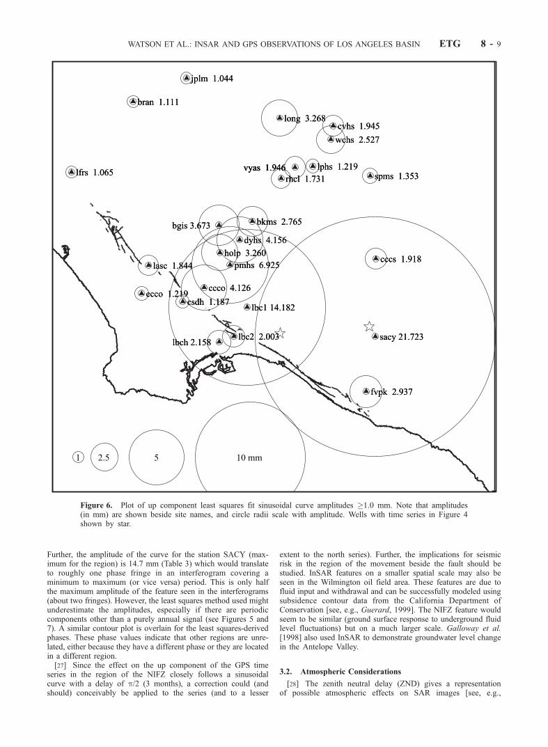
where t is the time (years), m is the gradient of the linear slope, andc is a constant. The estimated amplitudes and phases, like theTPCP and WSE comparisons, were then contoured.[26] The amplitudes of least squares-derived sine curve fits to

the up components for sites in the region with time series longerthan 1.5 years (except SACY, which is just over 1 year long) areshown as a contour map in Figure 9. The spatial character of thecontours shows a remarkable consistency with the major InSARfeature on the NW side of the NIFZ (compare to Figures 2 and 3).

Figure 4. Plot of GPS Up component (in mm) for SCIGN site HOLP (pluses) with least squares fit sinusoidal curvefor HOLP overlain (shaded curve). Plot of total monthly precipitation (TPCP) (in mm) for six meteorological stationsin the region, bottom curves. Plot of groundwater surface elevation (WSE) (in m) for two stations (locations shown bystar in Figures 6 and 7), top curves. Dashed vertical lines are drawn at i.25 years.

WATSON ET AL.: INSAR AND GPS OBSERVATIONS OF LOS ANGELES BASIN ETG 8 - 7

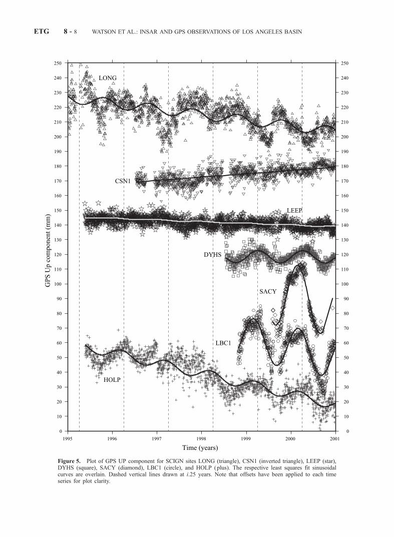
Figure 5. Plot of GPS UP component for SCIGN sites LONG (triangle), CSN1 (inverted triangle), LEEP (star),DYHS (square), SACY (diamond), LBC1 (circle), and HOLP (plus). The respective least squares fit sinusoidalcurves are overlain. Dashed vertical lines drawn at i.25 years. Note that offsets have been applied to each timeseries for plot clarity.

ETG 8 - 8 WATSON ET AL.: INSAR AND GPS OBSERVATIONS OF LOS ANGELES BASIN

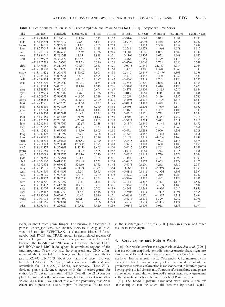
Further, the amplitude of the curve for the station SACY (max-imum for the region) is 14.7 mm (Table 3) which would translateto roughly one phase fringe in an interferogram covering aminimum to maximum (or vice versa) period. This is only halfthe maximum amplitude of the feature seen in the interferograms(about two fringes). However, the least squares method used mightunderestimate the amplitudes, especially if there are periodiccomponents other than a purely annual signal (see Figures 5 and7). A similar contour plot is overlain for the least squares-derivedphases. These phase values indicate that other regions are unre-lated, either because they have a different phase or they are locatedin a different region.[27] Since the effect on the up component of the GPS time

series in the region of the NIFZ closely follows a sinusoidalcurve with a delay of p/2 (3 months), a correction could (andshould) conceivably be applied to the series (and to a lesser

extent to the north series). Further, the implications for seismicrisk in the region of the movement beside the fault should bestudied. InSAR features on a smaller spatial scale may also beseen in the Wilmington oil field area. These features are due tofluid input and withdrawal and can be successfully modeled usingsubsidence contour data from the California Department ofConservation [see, e.g., Guerard, 1999]. The NIFZ feature wouldseem to be similar (ground surface response to underground fluidlevel fluctuations) but on a much larger scale. Galloway et al.[1998] also used InSAR to demonstrate groundwater level changein the Antelope Valley.

3.2. Atmospheric Considerations

[28] The zenith neutral delay (ZND) gives a representationof possible atmospheric effects on SAR images [see, e.g.,

Figure 6. Plot of up component least squares fit sinusoidal curve amplitudes �1.0 mm. Note that amplitudes(in mm) are shown beside site names, and circle radii scale with amplitude. Wells with time series in Figure 4shown by star.

WATSON ET AL.: INSAR AND GPS OBSERVATIONS OF LOS ANGELES BASIN ETG 8 - 9

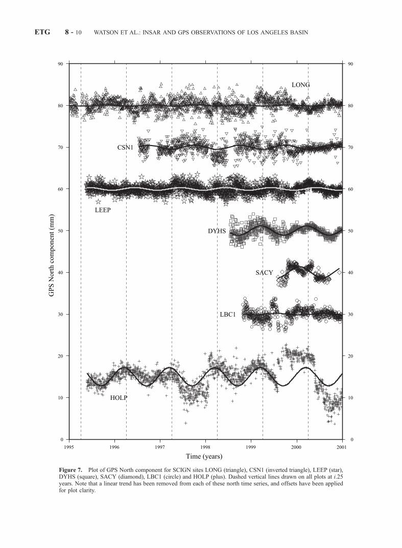
Figure 7. Plot of GPS North component for SCIGN sites LONG (triangle), CSN1 (inverted triangle), LEEP (star),DYHS (square), SACY (diamond), LBC1 (circle) and HOLP (plus). Dashed vertical lines drawn on all plots at i.25years. Note that a linear trend has been removed from each of these north time series, and offsets have been appliedfor plot clarity.

ETG 8 - 10 WATSON ET AL.: INSAR AND GPS OBSERVATIONS OF LOS ANGELES BASIN

cccs 1.731dyhs 1.116

fvpk 5.447

lbc2 1.569

lphs 1.228

pmhs 2.257

sacy 1.343

holp 2.184 cccs 1.731dyhs 1.116

fvpk 5.447

lbc2 1.569

lphs 1.228

pmhs 2.257

sacy 1.343

holp 2.184

a

1 2.5 5

bkms 1.119

ccco 3.519

lbc2 1.107

lphs 1.039vyas 1.004

bkms 1.119

ccco 3.519

lbc2 1.107

lphs 1.039vyas 1.004

b

1 2.5 5

Figure 8. (a) Plot of north component least squares fit sinusoidal curve amplitudes �1.0 mm. Note that amplitudes(in mm) are shown beside site names and circle radii scale with amplitude. Wells with time series in Figure 4 areshown by star. (b) Plot of east component least squares fit sinusoidal curve amplitudes �1.0 mm. Circle radii scalewith amplitude. Wells with time series in Figure 4 are shown by star.

WATSON ET AL.: INSAR AND GPS OBSERVATIONS OF LOS ANGELES BASIN ETG 8 - 11

Williams et al., 1998]. Hence ZND data derived from GPSsolutions were investigated. An average of the hourly data forthe two GPS epochs occurring about the SAR satellite flyovertime was determined for those SAR passes which had corre-sponding GPS data. The data from the master SAR pass wassubtracted from the data of the slave SAR pass, and acomparison map of differenced ZND was plotted. The mapwas then compared to the relevant interferogram. We also

looked for any large differences between the ZND values forsites on different sides of the NIFZ. Unfortunately, there werelittle or no ZND results available for the region for the earliestepochs (pre-1994).[29] The maximum ZND difference across the NIFZ was

�42 mm between sites PVEP and TRAK for the orbit pairE1-23705_E2-12048 (6 December 1996 to 9 August 1997). Thismaps into �85 mm of two-way delay in the line of sight of the

Figure 9. Contour plot of up component least squares fit sinusoidal curve amplitudes (yellow solid lines) in mmand phase (green dashed lines) in years for the SCIGN sites labeled. See color version of this figure at back of thisissue.

ETG 8 - 12 WATSON ET AL.: INSAR AND GPS OBSERVATIONS OF LOS ANGELES BASIN

radar, or about three phase fringes. The maximum difference inpair E1-23705_E2-17559 (26 January 1996 to 29 August 1998)was �15 mm for PVEP/TRAK, or about one fringe. Unfortu-nately, both PVEP and TRAK appear in decorrelated regions ofthe interferograms, so no direct comparison could be madebetween the InSAR and ZND results. However, stations USC1and HOLP (and LBCH) do appear in correlated regions of theinterferograms. These two sites have approximate ZND differ-ences of about one half of a fringe and less than one sixth forpair E1-23705_E2-17559, about one tenth and more than onehalf for E2-07539_E2-19563, and about one sixth and oneseventieth for E1-23705_E2-12048, respectively. These ZND-derived phase differences agree with the interferograms forstation USC1 but not for station HOLP. Overall, the ZND contourplots did not match the interferograms, but the data set was rathersparse. As a result, we cannot rule out the possibility that ZNDeffects are responsible, at least in part, for the phase features seen

in the interferograms. Watson [2001] discusses these and otherresults in more depth.

4. Conclusions and Future Work

[30] Our results confirm the hypothesis of Bawden et al. [2001]that the 60-mm amplitude periodic interferometric phase signaturealong the NIFZ and in a zone of about 20 km by 40 km to thenortheast has an annual cycle. Continuous GPS measurementsclearly display the annual cycle, while the spatial extent of thegroundwater surface deformation is most apparent in interferogramshaving spring to fall time spans. Contours of the amplitude and phaseof the annual signal derived from GPS are in remarkable agreementwith the vertical motions derived from InSAR in this zone.[31] The broad signature associated with such a shallow

source implies that the water table achieves hydrostatic equili-

Table 3. Least Squares Fit Sinusoidal Curve Amplitude and Phase Values for GPS Up Component Time Series

Site Latitude Longitude Elevation, m A, mm sA, mm f, years sf, years m, mm/yr sm, mm/yr Length, years

azu1 �117.896484 34.126018 144.76 0.235 0.152 �0.3108 0.3097 0.945 0.091 4.481bgis �118.159694 33.967117 2.83 3.673 0.239 0.0918 0.0095 1.546 0.328 1.762bkms �118.094695 33.962257 11.00 2.765 0.253 �0.1518 0.0153 5.568 0.254 2.436bran �118.277047 34.184893 246.24 1.111 0.188 0.2241 0.0276 �1.966 0.078 6.112ccco �118.211195 33.876258 �16.93 4.126 0.245 0.0001 0.0086 1.083 0.307 1.942cccs �117.864940 33.862741 31.83 1.918 0.351 �0.1309 0.0307 9.622 0.468 1.942chil �118.025997 34.333422 1567.51 0.405 0.287 0.4463 0.1153 4.179 0.113 6.359cit1 �118.127283 34.136708 215.33 0.316 0.130 �0.4504 0.0660 0.765 0.056 6.348cjms �117.479381 34.313798 933.36 0.933 0.821 �0.0915 0.1340 21.183 0.984 2.044clar �117.708807 34.109927 373.63 0.831 0.160 0.1426 0.0301 1.370 0.068 5.737cmp9 �118.411422 34.353179 1138.02 3.001 0.830 0.3440 0.0449 �15.476 0.368 5.559crfp �117.099680 34.039051 688.81 1.975 0.186 �0.3213 0.0147 0.400 0.069 6.584csdh �118.256714 33.861476 �9.17 1.187 0.192 �0.4560 0.0245 3.703 0.180 2.507csn1 �118.523809 34.253549 261.43 0.084 0.204 0.2343 0.1301 2.626 0.111 4.489cvhs �117.901714 34.082010 119.10 1.945 0.206 �0.3407 0.0159 1.440 0.198 2.471dshs �118.348539 34.023930 �2.11 0.694 0.169 0.4374 0.0403 �2.353 0.259 1.644dyhs �118.125979 33.937987 1.47 4.156 0.215 �0.0139 0.0080 �0.061 0.204 2.496ecco �118.329023 33.886751 �19.35 1.219 0.175 0.2059 0.0240 0.110 0.257 1.745ewpp �117.525582 34.104197 330.48 2.479 0.235 �0.4505 0.0139 �1.599 0.314 1.827fvpk �117.935711 33.662325 �11.53 2.937 0.195 �0.0411 0.0117 1.428 0.218 2.285holp �118.168168 33.924538 �6.69 3.260 0.432 0.0493 0.0202 �7.019 0.184 5.652jplm �118.173224 34.204819 423.98 1.044 0.349 0.3166 0.0536 4.467 0.109 8.541lasc �118.306502 33.927941 24.69 1.844 0.179 �0.4240 0.0121 0.723 0.170 2.244lbc1 �118.137180 33.832068 �21.94 14.182 0.785 0.0808 0.0072 �6.651 0.757 2.219lbc2 �118.173239 33.791608 �28.47 2.003 0.295 �0.3221 0.0224 6.442 0.311 2.219lbch �118.203340 33.787769 �27.57 2.158 0.458 �0.1374 0.0340 �6.348 0.188 6.452leep �118.321752 34.134600 485.05 0.333 0.113 0.2611 0.0552 �1.135 0.049 5.660lfrs �118.412822 34.095069 146.90 1.065 0.212 �0.4924 0.0288 2.900 0.291 1.729long �118.003407 34.111899 74.27 3.268 0.328 0.4428 0.0157 �3.812 0.133 6.156lphs �117.956717 34.026768 68.51 1.219 0.188 0.3021 0.0225 �0.226 0.162 2.436math �117.436813 33.856685 396.88 2.700 0.437 �0.3618 0.0256 4.902 0.143 7.679msob �117.210123 34.230844 1733.15 4.795 0.349 �0.3717 0.0108 3.650 0.409 2.167oat2 �118.601377 34.329891 1112.59 1.695 0.403 �0.4937 0.0373 6.808 0.167 5.940pmhs �118.153683 33.902633 �11.13 6.925 0.287 0.0477 0.0063 0.244 0.275 2.436ppbf �117.182086 33.835725 428.10 2.230 0.258 �0.4622 0.0142 1.729 0.279 2.044pvrs �118.320585 33.773861 59.83 0.724 0.211 0.3147 0.0511 2.151 0.292 1.937rhcl �118.026167 34.019050 176.88 1.731 0.208 �0.4917 0.0175 1.669 0.274 1.827rths �117.353332 34.089149 328.69 1.782 0.344 �0.4078 0.0291 4.262 0.337 2.767sacy �117.895575 33.743244 �11.24 21.723 1.364 0.0962 0.0138 �5.959 4.769 1.351scms �117.634560 33.444139 23.26 3.955 0.408 �0.4181 0.0142 �5.934 0.399 2.337snhs �117.928625 33.927336 66.43 0.289 0.208 �0.4960 0.1024 3.210 0.288 1.742spms �117.848772 33.992653 207.04 1.353 0.191 �0.3269 0.0210 2.492 0.184 2.340torp �118.330601 33.797797 �5.21 0.675 0.198 0.3051 0.0517 0.715 0.175 2.852trak �117.803432 33.617934 115.55 0.401 0.301 �0.3647 0.1159 �4.139 0.108 6.606uclp �118.441907 34.069120 111.55 0.701 0.116 0.4664 0.0266 �0.919 0.049 5.855usc1 �118.285112 34.023950 21.93 1.918 0.218 �0.2506 0.0179 �3.032 0.091 5.855vyas �117.992048 34.030915 56.46 1.946 0.221 �0.4899 0.0171 �1.817 0.211 2.436wchs �117.911108 34.061897 100.11 2.527 0.235 �0.4216 0.0130 1.329 0.282 1.970whc1 �118.031166 33.979884 94.28 0.556 0.293 0.4818 0.0839 �5.075 0.124 5.775wlsn �118.055910 34.226120 1705.25 3.420 0.233 �0.0143 0.0106 0.922 0.153 5.677

WATSON ET AL.: INSAR AND GPS OBSERVATIONS OF LOS ANGELES BASIN ETG 8 - 13

brium on timescales much shorter than 1 year. This signal is ofhydrologic importance and could be used to assess groundwaterrecharge and usage. The sharp interferometric phase gradientacross the NIFZ is consistent, therefore, with a model where thefault acts as a barrier to groundwater. Annual variation ingroundwater on the northeast side of the NIFZ causes volu-metric expansion of the sediments that appear to induce bothvertical and horizontal differential motions across the fault.Oddly, the horizontal motions are not just confined to theNIFZ but correlate to areas where annual vertical motions aregreatest.[32] The presence of large annual signals of hydrologic origin

in the southeastern part of the Los Angeles basin will need to betaken into account when interpreting the geodetic data fortectonic motion. For GPS, amplitudes of annual vertical dis-placements are significant for at least 11 SCIGN sites and rangefrom 3 to 22 mm in the affected zone with an uncertainty ofonly a fraction of a millimeter, as well as for other sitesdistributed over a larger part of the basin in the range of 1–3mm (Figure 6). Furthermore, amplitudes of annual horizontalmotions are �1–2 mm, primarily in the north direction awayfrom the NIFZ (Figure 8a) but only in the affected zone. This isconsiderable, however, since the entire horizontal signal (i.e., thecontraction rate) in the Los Angeles basin is only �7–8 mm/yr,and we are seeking to detect horizontal displacement rates withsubmillimeter precision. Most disturbingly, some GPS siteswithin this zone show a long-term vertical trend (both up anddown) that may be related to secular trends in groundwaterlevels and may mask interseismic tectonic signals such as wouldbe related to vertical crustal thickening hypothesized by Arguset al. [1999].[33] To address these issues, it is clear that we will need to take

better advantage of the strengths of both GPS and InSAR. Forexample, the dense GPS coverage in the basin can be use tocalibrate the InSAR measurements for tropospheric, ionospheric,and orbital errors, but this approach has not yet been fullyexploited. We need to analyze more interferometric images tofurther improve our determination of the topography, to reducetropospheric effects, and to better identify zones with significantnontectonic signatures. The continuous GPS time series are stillshort at most sites, and the SCIGN network is only now reachingits full complement in the basin. Finally, we need to make morecomparisons with hydrologic data.

[34] Acknowledgments. This work benefited from discussions withDuncan Agnew, Gerald Bawden, Wayne Thatcher, Peng Fang, andMatthijs van Domselaar. Synthetic aperture radar data were provided bythe European Space Agency through their North American distributors,SpotImage and Eurimage. We acknowledge the Southern CaliforniaIntegrated GPS Network and its sponsors, the W. M. Keck Foundation,NASA, NSF, USGS, and SCEC, for providing data used in this study. Wethank our colleagues at the Scripps Orbit and Permanent Array Center(SOPAC) for access to the CGPS position time series. This work wassupported by the National Science Foundation and NASA (EAR9619201).SAR data were purchased by NASA and NSF (EAR9619201) and werelater contributed to the WInSAR consortium. This research was alsosupported by the Southern California Earthquake Center. SCEC is fundedby NSF Cooperative Agreement EAR-8920136 and USGS CooperativeAgreements 14-08-0001-A0899 and 1434-HQ-97AG01718. SCEC con-tribution 623.

ReferencesArgus, D. F., M. B. Heflin, A. Donnellan, F. H. Webb, D. Dong, K. J. Hurst,D. C. Jefferson, G. A. Lyzenga, M. M. Watkins, and J. F. Zumberge,Shortening and thickening of metropolitan Los Angeles measured andinferred by using geodesy, Geology, 27, 703–706, 1999.

Baer, G., D. Sandwell, S. Williams, Y. Bock, and G. Shamir, Coseismicdeformation associated with the November 1995, MW = 7.1 Nuweibaearthquake, Gulf of Elat (Aqaba), detected by synthetic aperture radarinterferometry, J. Geophys. Res., 104, 25,221–25,232, 1999.

Barrows, A. G., Earthquakes along the Newport-Inglewood structural zone,Calif. Geol., 26, 60–68, 1973.

Barrows, A. G., A review of the geology and earthquake history of theNewport-Inglewood structural zone, southern California, Spec. Rep. 114,115 pp., Calif. Div. of Mines and Geol., Sacramento, 1974.

Bawden, G. W., W. Thatcher, R. S. Stein, C. Wicks, K. Hudnut, andG. Peltzer, Ground water pumping masks tectonic deformation nearLos Angeles, California, Eos Trans. AGU, 81(48), Fall Meet. Suppl.,Abstract H21G-05, 2000.

Bawden, G. W., W. Thatcher, R. S. Stein, C. Wicks, K. Hudnut, andG. Peltzer, Tectonic contraction across Los Angeles after removal ofgroundwater pumping effects, Nature, 412, 812–815, 2001.

Bock, Y., and S. Williams, Integrated satellite interferometry in southernCalifornia, Eos Trans. AGU, 78, 293, 299–300, 1997.

Bock, Y., et al., Southern California permanent GPS geodetic array: Con-tinuous measurements of regional crustal deformation between the 1992Landers and 1994 Northridge earthquakes, J. Geophys. Res., 102,18,013–18,033, 1997.

Bock, Y., R. M. Nikolaidis, P. J. de Jonge, and M. Bevis, Instantaneousgeodetic positioning at medium distances with the Global PositioningSystem, J. Geophys. Res., 105, 28,223–28,253, 2000.

Davis, T. L., J. Namson, and R. F. Yerkes, A cross section of the Los Angelesarea: Seismically active fold and thrust belt, the 1987 Whittier Narrowsearthquake, and earthquake hazard, J. Geophys. Res., 94, 9644–9664,1989.

Dolan, J. F., K. Sieh, T. K. Rockwell, R. S. Yeats, J. Shaw, J. Suppe, G. J.Huftile, and E. M. Gath, Prospects for larger or more frequent earthquakesin the Los Angeles metropolitan region, Science, 267, 199–205, 1995.

Freeman, S. T., E. G. Heath, P. D. Guptill, and J. T. Waggoner, Seismichazard assessment, Newport-Inglewood fault zone, in Engineering Geol-ogy Practice in Southern California, edited by B. W. Pipkin and R. J.Proctor, Spec. Publ. 4, pp. 211–231, Assoc. of Eng. Geol., South. Calif.Sect., Belmont, Calif., 1992.

Galloway, D. L., K. W. Hudnut, S. E. Ingebritsen, S. P. Phillips, G. Peltzer,F. Rogez, and P. A. Rosen, Detection of aquifer system compaction andland subsidence using interferometric synthetic aperture radar, AntelopeValley, Mojave Desert, California, Water Resour. Res., 34, 2573–2585,1998.

Grant, L. B., J. T. Waggoner, T. K. Rockwell, and C. von Stein, Paleoseis-micity of the North Branch of the Newport-Inglewood fault zone inHuntington Beach, California, from cone penetrometer test data, Bull.Seismol. Soc. Am., 87, 277–293, 1997.

Guerard, W. F., 1998 annual report of the State Oil and Gas Supervisor,Rep. PR 06, 269 pp., Calif. Dep. of Conserv., Div. of Oil, Gas, andGeotherm. Resour., Sacramento, 1999.

Harding, T. P., Newport-Inglewood trend, California—An example ofwrenching style of deformation, Am. Assoc. Pet. Geol. Bull., 57, 97–116, 1973.

Hauksson, E., Seismotectonics of the Newport-Inglewood fault zone in theLos Angeles basin, southern California, Bull. Seismol. Soc. Am., 77,539–561, 1987.

Hensley, E., A SCIGN before its Time, A history of the southern Californiaintegrated GPS network, South. Calif. Earthquake Cent. Q. Newsl., 5, 4–11, 25–31, 2000.

Hill, M. H., Newport-Inglewood zone and Mesozoic subduction, California,Geol. Soc. Am. Bull., 82, 2957–2962, 1971.

Hill, M. H., The Newport-Inglewood zone of dDeformation, in Guidebookto Selected Features of Palos Verdes Peninsula and Long Beach, Cali-fornia, edited by M. S. Woyski, pp. 32–35, South Coast Geol. Surv.,Irvine, Calif., 1974.

Hudnut, K. W., et al., Coseismic displacements of the 1994 Northridge,California, earthquake, Bull. Seismol. Soc. Am., 86, 19–36, 1996.

Massonnet, D., and K. Feigl, Radar interferometry and its application tochanges in the Earth’s surface, Rev. Geophys., 36, 441–500, 1998.

Massonnet, D., M. Rossi, C. Carmona, F. Adragna, G. Peltzer, K.Feigl, and T. Rabaute, The displacement field of the Landers earth-quake mapped by radar interferometry, Nature, 364, 138–142,1993.

Nikkel, M., T. Mueller, K. Thompson, and P. Rechard, Assessment of theadequacy of the ground-water monitoring system for artificial recharge ofaquifers in the Los Angeles area, California, report, pp. 45–69, Assoc. ofGround Water Sci. and Eng., Westerville, Ohio, 1988.

Nilsen, T. H., and A. G. Sylvester, Strike-slip basins, part 2, Leading Edge,18, 1258–1267, 1999.

Petersen, M. D., and S. G. Wesnousky, Fault slip rates and earthquakehistories for active faults in southern California, Bull. Seismol. Soc.Am., 84, 1608–1649, 1994.

Piper, A. M., et al., Native and contaminated ground waters in the LongBeach–Santa Ana area, California, U.S. Geol. Surv. Water Supply Pap.,1136, 320 pp., 1953.

ETG 8 - 14 WATSON ET AL.: INSAR AND GPS OBSERVATIONS OF LOS ANGELES BASIN

Platt, J. P., and C. J. Stuart, Newport-Inglewood fault zone, Los Angelesbasin, California: Discussion, AAPG Bull., 58, 877–883, 1974.

Poland, J. F., Hydrology of the Long Beach–Santa Ana area, California,U.S. Geol. Surv. Water Supply Pap., 1471, 257 pp., 1959.

Poland, J. F., et al., Ground-water geology of the coastal zone Long Beach–Santa Ana area, California, U.S. Geol. Surv. Water Supply Pap., 1109,162 pp., 1956.

Price, E. J., and D. T. Sandwell, Small-scale deformation associated withthe 1992 Landers, California, earthquake mapped by synthetic apertureradar interferometry phase gradients, J. Geophys. Res., 103, 27,001–27,016, 1998.

Rosen, P. A., S. Hensley, I. R. Joughin, F. K. Li, S. N. Madsen, E. Rodri-guez, and R. M. Goldstein, Synthetic aperture radar interferometry, Proc.IEEE, 88, 333–382, 2000.

Sandwell, D. T., and E. J. Price, Phase gradient approach to stacking inter-ferograms, J. Geophys. Res., 103, 30,183–30,204, 1998.

Sandwell, D. T., and L. Sichoix, Topographic phase recovery from stackedERS interferometry and a low-resolution digital elevation model, J. Geo-phys. Res., 105, 28,211–28,222, 2000.

Scharroo, R., and P. N. A. M. Visser, Precise orbit determination andgravity field improvement for the ERS satellites, J. Geophys. Res., 103,8113–8127, 1998.

Shaw, J. H., and J. Suppe, Earthquake hazards of active blind-thrust faultsunder the central Los Angeles basin, California, J. Geophys. Res., 101,8623–8642, 1996.

Testa, S. M., E. C. Henry, and D. Hayes, Impact of the Newport-Inglewoodstructural zone on hydrogeologic mitigation efforts: Los Angeles basin,California, report, pp. 181–203, Assoc. of Ground Water Sci. and Eng.,Westerville, Ohio, 1988.

Toppozada, T. R., J. H. Bennett, G. Borchardt, R. Saul, and J. F. Davis,Earthquake planning scenario for a major earthquake on the Newport-Inglewood fault zone, Calif. Geol., 42, 75–84, 1989.

Walls, C., T. Rockwell, K. Mueller, Y. Bock, S. Williams, J. Pfanner,

J. Dolan, and P. Fang, Escape tectonics in the Los Angeles metropolitanregion and implications for seismic risk, Nature, 394, 356–360, 1998.

Watson, K. M., SIO InSAR cookbook and investigations of the Newport-Inglewood fault zone, M.Sc. thesis, 107 pp., Univ. of Calif., San Diego,2001.

Watson, K., Y. Bock, S. Williams, and D. Sandwell, Integrated satelliteinterferometry: Investigations in the Los Angeles basin, Eos Trans.AGU, 79(45), Fall Meet. Suppl., F184, 1998.

Wilcox, R. E., T. P. Harding, and D. R. Seely, Basic wrench tectonics, Am.Assoc. Pet. Geol. Bull., 57, 74–96, 1973.

Williams, S., Y. Bock, and P. Fang, Integrated satellite interferometry:Troposphere noise, GPS estimates, and implications for synthetic apertureradar products, J. Geophys. Res., 103, 27,051–27,067, 1998.

Yeats, R. S., Newport-Inglewood fault zone, Los Angeles basin, California,Am. Assoc. Pet. Geol. Bull., 57, 117–135, 1973.

Yeats, R. S., Newport-Inglewood fault zone, Los Angeles basin, California:Reply, AAPG Bull., 58, 884–888, 1974.

Yerkes, R. F., T. H. McCulloh, J. E. Schoellhamer, and J. G. Vedder,Geology of the Los Angeles basin California—An introduction, U.S.Geol. Surv. Prof. Pap., 420-A, 57 pp., 1965.

Zebker, H. A., P. A. Rosen, R. M. Goldstein, A. Gabriel, and C. L. Werner,On the derivation of coseismic displacement fields using differential radarinterferometry: The Landers earthquake, J. Geophys. Res., 99, 19,617–19,634, 1994.

�����������Y. Bock, D. T. Sandwell, and K. M. Watson, Cecil H. and Ida M. Green

Institute of Geophysics and Planetary Physics, Scripps Institution ofOceanography, University of California, San Diego, 9500 Gilman Drive,La Jolla, CA 92093-0225, USA. (ybock@ucsd.edu; dsandwell@ucsd.edu;kwatson@josh.ucsd.edu)

WATSON ET AL.: INSAR AND GPS OBSERVATIONS OF LOS ANGELES BASIN ETG 8 - 15

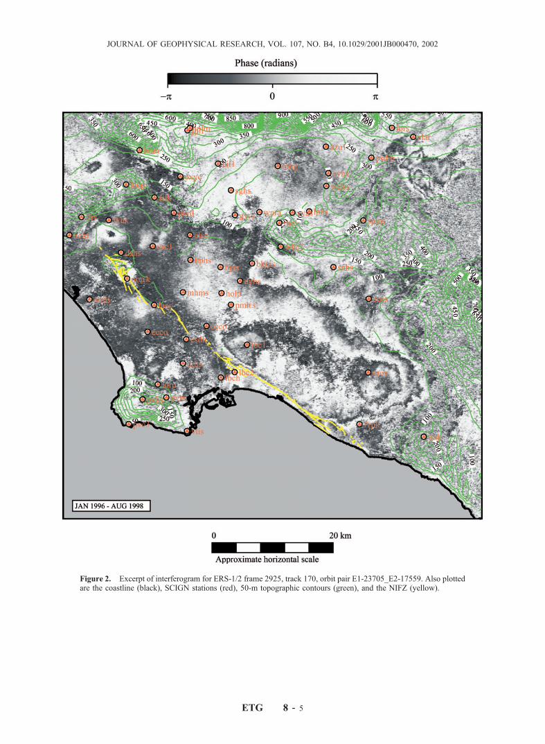
Figure 2. Excerpt of interferogram for ERS-1/2 frame 2925, track 170, orbit pair E1-23705_E2-17559. Also plottedare the coastline (black), SCIGN stations (red), 50-m topographic contours (green), and the NIFZ (yellow).

ETG 8 - 5

JOURNAL OF GEOPHYSICAL RESEARCH, VOL. 107, NO. B4, 10.1029/2001JB000470, 2002

Figure 9. Contour plot of up component least squares fit sinusoidal curve amplitudes (yellow solid lines) in mm andphase (green dashed lines) in years for the SCIGN sites labeled.

ETG 8 - 12

JOURNAL OF GEOPHYSICAL RESEARCH, VOL. 107, NO. B4, 10.1029/2001JB000470, 2002