Satellite Dynamics Toolbox library(SDTlib) - User's Guide - oatao
242
Satellite Dynamics Toolbox library (SDTlib) - User’s Guide D. Alazard & F. Sanfedino ÷ , ÷ : .it#*EE9EEIfTTHE .lt i : : ÷ ÷ - March 18, 2021
-
Upload
khangminh22 -
Category
Documents
-
view
0 -
download
0
Transcript of Satellite Dynamics Toolbox library(SDTlib) - User's Guide - oatao

Satellite Dynamics Toolbox library(SDTlib) - User’s Guide
D. Alazard & F. Sanfedino
÷,
-
i
÷ :
.it#*EE9EEIfTTHE.lt- i .
:. :
. ÷ .
÷
-
March 18, 2021

Document InformationProject: ESA - SDT+ / On board estimator
Area: Modeling of Space Dynamic SystemsElaborated by: Francesco Sanfedino, Daniel AzardReviewed by:
Created at: March 9, 2021
Last RevisionDate Changes/Comentary Reviewed byDate Create Document Author’s Name

Abstract
This user-guide is the catalog of the tutorials and the helps available on-line with the SDTlibpackage. These tutorials aim to train the Space system engineer on the way to use the SDTlib to:
• build LPV (Linear Parameter Varying)models of any kind of open kinematic chain of rigid/flexiblemulti-body systems,
• build linear model of any kind of closed kinematic chain of rigid/flexible multi-body systems,
• take into account in these models some flexible bodies modelled with PATRAN/NASTRAN(NASTRAN/SIMULINK interface) or on-board angular momentums,
• connect these models with the Robust Control toolbox in order to design attitude control systems.

SDTlib User’s Guide CONTENTS
Contents
Get Started 1
1 Tutorial : Introduction 2
2 Tutorial : Spacecraft with Solar Arrays 15
3 Tutorial : Robust Control of a spacecraft 28
4 Tutorial : Solar Arrays imported by NASTRAN 38
5 Tutorial : Short course on TITOP model 44
6 Tutorial : 6 DoFs Robotic Arm 62
7 Tutorial : NASTRAN Multi-Port Model 80
8 Tutorial : Plate Model for Solar Arrays 85
9 Tutorial : Solar Array with 3 Panels 90
10 Tutorial : On-Board Angular Momentum 97
11 Tutorial : The Four-Bar Mechanism 109
12 Tutorial : Simulation of SDT Models 135
13 SDTlib Documentation 14013.1 6 DoFs Bodies . . . . . . . . . . . . . . . . . . . . . . . . . . . . . . . . . . . . . . . . . 140
13.1.1 Multi-Port Rigid Body . . . . . . . . . . . . . . . . . . . . . . . . . . . . . . . . 14113.1.2 One-Port Flexible Body . . . . . . . . . . . . . . . . . . . . . . . . . . . . . . . 14513.1.3 Massless Connection Body . . . . . . . . . . . . . . . . . . . . . . . . . . . . . . 14813.1.4 One-Port NASTRAN Body . . . . . . . . . . . . . . . . . . . . . . . . . . . . . 15013.1.5 NINOP NASTRAN Body . . . . . . . . . . . . . . . . . . . . . . . . . . . . . . 15313.1.6 One-Port Angular Momentum . . . . . . . . . . . . . . . . . . . . . . . . . . . . 15713.1.7 TITOP Flexible Beam . . . . . . . . . . . . . . . . . . . . . . . . . . . . . . . . 16113.1.8 NINOP Flexible Plate . . . . . . . . . . . . . . . . . . . . . . . . . . . . . . . . 16813.1.9 Sloshing 1D Mass-Spring Model . . . . . . . . . . . . . . . . . . . . . . . . . . . 175
13.2 6 DoFs Mechanisms . . . . . . . . . . . . . . . . . . . . . . . . . . . . . . . . . . . . . . 17713.2.1 Revolute Joint TITOP Model . . . . . . . . . . . . . . . . . . . . . . . . . . . . 17813.2.2 Revolute Joint TITOP Model + Angle Configuration . . . . . . . . . . . . . . . 18113.2.3 6 DoFs Local Spring-Damper . . . . . . . . . . . . . . . . . . . . . . . . . . . . 184
13.3 3/6 DoFs DCM . . . . . . . . . . . . . . . . . . . . . . . . . . . . . . . . . . . . . . . . 18713.3.1 3x3 z-Rotation . . . . . . . . . . . . . . . . . . . . . . . . . . . . . . . . . . . . 18813.3.2 3x3 v-Rotation . . . . . . . . . . . . . . . . . . . . . . . . . . . . . . . . . . . . 19013.3.3 6x6 z-Rotation . . . . . . . . . . . . . . . . . . . . . . . . . . . . . . . . . . . . 19213.3.4 6x6 v-Rotation . . . . . . . . . . . . . . . . . . . . . . . . . . . . . . . . . . . . 19413.3.5 3x3 Non-Linear z-Rotation . . . . . . . . . . . . . . . . . . . . . . . . . . . . . 19613.3.6 3x3 Non-Linear v-Rotation . . . . . . . . . . . . . . . . . . . . . . . . . . . . . 19813.3.7 6x6 Non-Linear z-Rotation . . . . . . . . . . . . . . . . . . . . . . . . . . . . . 20013.3.8 6x6 Non-Linear v-Rotation . . . . . . . . . . . . . . . . . . . . . . . . . . . . . 20213.3.9 6x6 DCM . . . . . . . . . . . . . . . . . . . . . . . . . . . . . . . . . . . . . . . 204
13.4 Predefined Subsystems . . . . . . . . . . . . . . . . . . . . . . . . . . . . . . . . . . . . 206
D. Alazard & F. Sanfedino Page i of 237

13.4.1 One-Port Flexible Body + Revolute Joint . . . . . . . . . . . . . . . . . . . . . 20713.4.2 Multi-Port Rigid Body + Revolute Joint . . . . . . . . . . . . . . . . . . . . . . 21013.4.3 TITOP flexible beam + Revolute Joint . . . . . . . . . . . . . . . . . . . . . . 214
14 SDTlib blocks dialog boxes 21814.1 6 DoFs Bodies . . . . . . . . . . . . . . . . . . . . . . . . . . . . . . . . . . . . . . . . . 218
14.1.1 Multi-Port Rigid Body . . . . . . . . . . . . . . . . . . . . . . . . . . . . . . . . 21814.1.2 One-Port Flexible Body . . . . . . . . . . . . . . . . . . . . . . . . . . . . . . . 21914.1.3 Massless Connection Body . . . . . . . . . . . . . . . . . . . . . . . . . . . . . . 22014.1.4 One-Port NASTRAN Body . . . . . . . . . . . . . . . . . . . . . . . . . . . . . 22114.1.5 NINOP NASTRAN Body . . . . . . . . . . . . . . . . . . . . . . . . . . . . . . 22214.1.6 One-Port Angular Momentum . . . . . . . . . . . . . . . . . . . . . . . . . . . . 22314.1.7 NINOP Flexible Plate . . . . . . . . . . . . . . . . . . . . . . . . . . . . . . . . 22414.1.8 TITOP Flexible Beam . . . . . . . . . . . . . . . . . . . . . . . . . . . . . . . . 22514.1.9 Sloshing 1D Mass-Spring Model . . . . . . . . . . . . . . . . . . . . . . . . . . . 226
14.2 6 DoFs Mechanisms . . . . . . . . . . . . . . . . . . . . . . . . . . . . . . . . . . . . . . 22714.2.1 Revolute Joint TITOP Model . . . . . . . . . . . . . . . . . . . . . . . . . . . . 22714.2.2 Revolute Joint TITOP Model + Angle Configuration . . . . . . . . . . . . . . . 22814.2.3 6 DoFs Local Spring-Damper . . . . . . . . . . . . . . . . . . . . . . . . . . . . 229
14.3 3/6 DoFs DCM . . . . . . . . . . . . . . . . . . . . . . . . . . . . . . . . . . . . . . . . 23014.3.1 3x3 z-Rotation . . . . . . . . . . . . . . . . . . . . . . . . . . . . . . . . . . . . 23014.3.2 3x3 v-Rotation . . . . . . . . . . . . . . . . . . . . . . . . . . . . . . . . . . . . 23014.3.3 6x6 z-Rotation . . . . . . . . . . . . . . . . . . . . . . . . . . . . . . . . . . . . 23114.3.4 6x6 v-Rotation . . . . . . . . . . . . . . . . . . . . . . . . . . . . . . . . . . . . 23114.3.5 3x3 Non-Linear z-Rotation . . . . . . . . . . . . . . . . . . . . . . . . . . . . . 23214.3.6 3x3 Non-Linear v-Rotation . . . . . . . . . . . . . . . . . . . . . . . . . . . . . 23214.3.7 6x6 Non-Linear z-Rotation . . . . . . . . . . . . . . . . . . . . . . . . . . . . . 23314.3.8 6x6 Non-Linear v-Rotation . . . . . . . . . . . . . . . . . . . . . . . . . . . . . 23314.3.9 6x6 DCM . . . . . . . . . . . . . . . . . . . . . . . . . . . . . . . . . . . . . . . 234
14.4 Predefined Subsystems . . . . . . . . . . . . . . . . . . . . . . . . . . . . . . . . . . . . 23514.4.1 One-Port Flexible Body + Revolute Joint . . . . . . . . . . . . . . . . . . . . . 23514.4.2 Multi-Port Rigid Body + Revolute Joint . . . . . . . . . . . . . . . . . . . . . . 23614.4.3 TITOP Flexible beam + Revolute Joint . . . . . . . . . . . . . . . . . . . . . . 237
ii

GetStarted file for the SDTLIB.Table of Contents
1. Installation2. Tutorials
1. InstallationThe required MATLAB configuration for the SDTLIB_v1_1:
MATLAB R2020b or later,control_toolbox
robust_toolbox
simulink
simulink_control_design
symbolic_toolbox
Once the folder SDTLIB_V1_1_R2020b folder is unzipped on your computer at: yourDirectory>SDTLIB_V1_1_R202b, you can launch MATLAB and give the path to this folder by navigating to the yourDirectory folder using the Current Folder Toolbar and :
select SDTLIB_V1_1_R202b in the Current Folder Brower and then right-click on Add to path > Selected Folders and Subfolders,or type the following command in the Command Window
addpath(genpath('SDTLIB_V1_1_R2020b'))
You can now navigate to your working directory and open the Simulink Library SDTlibV1:
SDTlibV1
The SDTlibV1 is a SIMULINK library, depicted in the following Figure and is composed of 4 sub-libraries:
6 dof bodies,6 dof mechanisms,3/6 dof DCM,Predefined subsystems,
This library can be used like any SIMULINK libraries: you can select and drag to your current SIMULINK model any blocks available in the sublibraries.
2. TutorialsTo better use the SDTlib, it is recommanded to read and play the various tutorials available in the SDTLIB_V1_1_R2020b subfolders: Tutorial1, Tutorial2, ...
Each tutorial is composed of a live script tutorial1.mlx, tutorial2.mlx, ... and one or several SIMULINK models.
Tutorial1: introduction. Tutorial2: a spacecraft with 2 symmetrical rotating solar arrays ( run) .Tutorial3: robust attitude control design of a spacecraft with 2 symmetrical rotating solar arrays ( run).Tutorial4: a spacecraft with 2 symmetrical rotating solar arrays defined by a NASTRAN model ( run).Tutorial5: a short course on TITOP (Two-Input Two-Output Ports) models.Tutorial6: a 6 dofs robotic arm on a chaser spacecraft ( run).Tutorial7: the cantilevered plate dynamics studied with SDTlib block NINOP Nastran body ( run).Tutorial8: a spacecraft with 2 symmetrical rotating solar arrays defined by a generic plate model ( run).Tutorial9: a solar array with 3 pannels ( run ).Tutorial10: on-board angular momentum ( run).Tutorial11: the 4 bar mechanism ( run)Tutorial12: simulating a SDTlib-based model ( run).
Get Started
1

Tutorial 1: IntroductionTable of Contents
1. Context and objectives........................................................................................................................................ 1First summary.......................................................................................................................................................3
2. One-port dynamic model..................................................................................................................................... 32.1 Illustration in the single-axis case................................................................................................................. 62.2 Six d.o.fs case............................................................................................................................................... 92.3 Revolute joints............................................................................................................................................. 112.4 Summary......................................................................................................................................................13
3. References.........................................................................................................................................................13
by D. Alazard and F. Sanfedino - ISAE-SUPAERO
1. Context and objectivesSDTlib is a SIMULINK library to model multibody systems in the space vehicle engineering context.
The multibody systems considered in the SDTlib are composed of rigid or flexible bodies (or links) ,
connected to each other by single-axis revolute joints or by clamped joints. One can distinguish
chain-like multibody systems (Fig.a), tree-like systems (Fig.b) and closed kinematic chain systems (Fig.c).
Notations:
• is the number of rigid degrees-of-freedom (d.o.f.) and is the geometric
configuration vector. For an open-kinematic system (chain-like or tree-like): , i.e. the
angular configurations of the revolute joints plus the 6 d.o.fs (3 translations and 3 rotations) of the
reference body (anyone particular body among the bodies),
• , is the mechanical parameter vector of each body ; i.e: the vector containing all the
varying, uncertain or to be sized mechanical paremeters of the body (mass, inertia, centering, ...)
1
SDTlib User’s Guide Chapter 1. Tutorial : Introduction
1. Tutorial : Introduction
D. Alazard & F. Sanfedino Page 2 of 237

• for flexible bodies, is the internal deformation d.o.f vector of the flexible body and
is the deformation d.o.f. vector of the whole system.
In all the cases, the objective of the SDTlib is to derive the linear model of the system dynamics for a given
geometric configuration of the rigid d.o.fs and around an equilibrium characterized by:
, , , , and .
Such a model is only valid for small variations ( ) of the d.o.fs around the equilibrium configuration,
small variation rates ( ) and small deformations of the flexible bodies ( , ).
The main interest of the SDTlib is the possibility to build this linear model, named where is the
Laplace variable, of the multibody system fully parameterized according to the:
• geometric configuration: ,
• mechanical parametric configuration: .
The model is computed once and for all and is fully compatible with Matlab robust control
toolbox (it is an uss).
This model is built block by block from the various SDTlib blocks used to model each body and each joint.
It is important to understand that the dynamic model (or the various sub-model) is the transfer
between:
• the external wrenches (forces and torques) which can be applied to any body at any given points and the
driving torques which can be applied inside any revolute joints,
• the acceleration twists (translational and angular accelerations) of bodies at any given points and the
acceleration vector of the d.o.fs: .
Thus:
• since this model works for small motions around a given geometric configuration, it is assumed that
the external wrenches and driving torques are small and null at the equilibrium (indeed: ). Thus
gravitationnal force/acceleration are not taken into account in the SDTlib,• the state vector of is composed of the internal deformation d.o.fs of each flexible body
and their time-derivative: . Thus the dynamic model for a rigid multi-body
system is static (i.e. a direct feed-through). In addition, the double integrator which can be added on
each acceleration component (for instance : , ) to analyse the variations of the positions
( ) and rates ( ) are not included in the model . The user must include these integrators
in the SIMULINK model of the system according to his(her) objective: for instance to model a local
2
SDTlib User’s Guide Chapter 1. Tutorial : Introduction
D. Alazard & F. Sanfedino Page 3 of 237

mechanism or a controller at a revolute joint or to take into account an Attitude and Orbit Control System
(AOCS) on the reference body (that will be highlightd in the various tutorials).
For closed kinematic chain systems, the number of rigid and independent d.o.f.s is reduced due to the loop
closure constraints:
• (on positions),
• (on velocities)
• (on accelerations)
These constraints are non-linear equations and are not solved in the SDTlib and it is assumed that the
user can provide a geometric configuration satisfying these constraints and the equilibrium conditions, i.e.
. Then the SDTlib can be used to build a linear model which is valid for small variations around the
configuration while satisfying the linearized loop closure constraints at the acceleration level:
.
As a consequence, for closed kinematic chain systems, the linear model is only parameterized according to the
mechanical parameter vector: .
Finally, since the model considers only forces and accelerations, its input/output channels are
invertible. In the SDTlib documentation, the model from accelerations (input) to forces/torques (output) is
called the direct dynamic model and is homegenous to mass ( ) and inertia ( ) while the model from
forces/torques (input) to accelerations (output) is called the inverse dynamic model (not to confused with the
terminology "forward dynamics" and "inverse dynamics" commonly used in multi-body dynamics).
First summary
• SDTlib is a tool for linear parametric modelling and for parametric robustness analyses and/or robustcontrol design purposes.
• SDTlib is not a tool for simulation purposes. For the user willing just to simulate a multibody system for a
given mechanical parameter vector , it is recommended to use Simscape/multibody . Nevertheless,
the tutorial 12 : Simulating a SDTlib-based model is proposed to address this topic.
2. One-port dynamic model
3
SDTlib User’s Guide Chapter 1. Tutorial : Introduction
D. Alazard & F. Sanfedino Page 4 of 237

In this section, the general multibody system context is restricted to the case where the system is composed
of a rigid body (the base ) holding various single (rigid or flexible) bodies, called appendages ( ). In the
following Figure, the main body is rigid and holds 2 flexible appendages:
• a solar pannel at point through a revolute joint,
• an antenna at poiint though a clamped joint.
Furthermore, it is assumed that the appendages are only submitted to the interaction wrenches with the main
body.
Notations:
• O, B, are the reference point, the centre of mass and the connection points of the body ,
respectively,
• , are the main body frame and the appendage body frame, respectively,
• is the point on where is applied the 6 component resultant wrench of external forces
(3 components, independent from the considered point since the main body is rigid) and torques
(3 components). This wrench is due to orbital disturbances, AOCS actuators,.... . is also
the point where is considered the 6 component dual acceleration twist composed of the inertial
translational acceleration ( 3 components) of the main body at point and its angular acceleration
( 3components, independent from the considered point since the main body is rigid),
• and are the in-joint driving torque and the relative acceleration of the revolute joint of the
appendage .
4
SDTlib User’s Guide Chapter 1. Tutorial : Introduction
D. Alazard & F. Sanfedino Page 5 of 237

Considering the example of the Figure above, the objective is to find the dynamic model
and/or its inverse between and on one side and and on the other side.
The notation of the model includes the point where is written this model and the frame
where it is projected:
In sections 2.1 and 2.2 the clamped connection of one appendage to a main body is detailed in the single
axis case (academic example on the spring-mass system) and the 6 d.o.fs case, respectively. The proposed
solution is strongly linked to the modal effective mass models used in structural dynamics (see references)
and renamed one port model in this documentation.
In section 2.3, it is shown that taking into account the revolute joint between the main body and the appendage
can be easily solved by working on the direct dynamic model and that the inverse dynamic
model , required to design control laws, can be obtained by a simple inversion operation.
Finally, an on-board angular mometum (due for instance to a reaction wheel system or more generally to a
balanced wheel spinned at a constant angular rate as the appendage depicted in the next Figure) can also
be taken into account as a dynamic appendage using the same formalism. See also the tutorial 10: on-boardangular momentum.
To address the general multibody system depicted in the first Figure of this tutorial, the one port models can be
extented to the TITOP (Two Inputs-Two Outputs Ports) models (or more generally NINOP models: N Inputs-
5
SDTlib User’s Guide Chapter 1. Tutorial : Introduction
D. Alazard & F. Sanfedino Page 6 of 237

N-Ouputs Ports models). See also the tutorial 5: a short course on TITOP (Two-Input Two-Output Ports)models.
2.1 Illustration in the single-axis case
Let us consider the spring-mass system between points P and C depicted in the following Figure. Only
motions along -axis are considered.
k, , are the stiffness, the mass attached to the point P and the mass attached to the point C of the system
, respectively.
The objective is to compute the single input single output transfer function of from the inertial
acceleration prescribed at the point P (input in blue) to the force applied to at the point P (output in
ted).
Only variations around the equilibrium conditions are considered. is the variation of the length of the vector
w.r.t its length at rest. The equilibrium conditions are: , , .
The Newton principle applied on each of the 2 masses leads to:
•
• .
Considering that , a state space representation of , associated to the state vector
, reads:
,
and the transfer function , after some algebra, reads:
6
SDTlib User’s Guide Chapter 1. Tutorial : Introduction
D. Alazard & F. Sanfedino Page 7 of 237

where is the cantilever frequency of when it is cantilevered
at point P.
is composed of 2 terms:
• an effective mass rigidly attached to the point P (where is prescribed the acceleration input),
• an effective mass which is flexible and characterized by the cantilevered frequency .
Of course the DCgain of is the sum of the masss but if the system is "shaked" at the point P with a
frequency largely greater than then the apparent mass seen from the point P is only the mass .
Let us consider now a system where the base , with a mass , holds the spring mass system . An
actuator can apply a force on the base . The inertial acceleration of the base is .
The dynamic model of the base considered alone is simply:
and we will denote the direct dynamic model of the rigid base.
Considering that in the appendage model , the direct dynamic model
of the system is just the sum of the direct dynamic models of and :
.
The output of this model is u and the input is .
The inverse dynamic model , where the input is u and the output is , can be written as:
.
This last formulation shows that the inverse dynamique of is in fact the inverse dynamic model of the in
feedback with the direct dynamic model of and can be represented by the following block diagram where:
• the model of the appendage is detailled with the 3 mechanical parameters , , ,
7
SDTlib User’s Guide Chapter 1. Tutorial : Introduction
D. Alazard & F. Sanfedino Page 8 of 237

• the double integrator are added on to obtain the position variation on the output.
Note that this block-diagram representation is not interesting for simulation purpose since it exhibits an
algebraic loop (represented in red in the previous Figure) which must be solved at each simulation step. The
interest of this block diagram repreentation, which is in fact the core of the SDTlib, is twice:
• first, to have a structured model where each body is represented by its own sub-model depending only
on its own mechanical parameters. Thus parametric variations on each of these mechanical parameter
can be taken into account with a minimal occurence when the uncertain state-space model of the whole
system is computed with, for instance, the function ulinearize,• second, the same approach can be used to "plug" any other spring-system to the base as described
in the following example.
Considering a base holding 3 spring-mass systems , as depicted in the following Figure. Each
appendage is characterized by 3 parameters , , and the effective mass model (or ),
previously defined.
Then the model of the whole system taking account all the dynamic couplings between the sub-systems can be
described by the following block-diagram representation.
8
SDTlib User’s Guide Chapter 1. Tutorial : Introduction
D. Alazard & F. Sanfedino Page 9 of 237

2.2 Six d.o.fs caseThe previous block-diagram-based modelling approach can be directly extended to the 6 d.o.fs case while
taking into account:
• the dynamics coupling between translations and rotations due to the geometry (lever-arm effect),
• the various frames in which are described the various bodies , ,
• the 6 d.o.f.s behavior of the flexible modes of each flexible appendages .
Reconsidering the case of the clamped connection of a fexible appendage on a rigid base at the point P.
The inverse dynamic model of the system at the point and projected in the frame
is described by the feedback loop depicted in the following Figure where the inverse dynamic model of the
base is in feedback with direct effective mass model of the appendage. The feedback loop
contains also:
• the frame change from to to obtain ,
• the transportation from point P to point to obtain .
9
SDTlib User’s Guide Chapter 1. Tutorial : Introduction
D. Alazard & F. Sanfedino Page 10 of 237

In this Figure:
• is the rigid mass model of the body at the point : where B,
and are the centre of mass, the mass and the inertia tensor at B, respectively. See also:
web Docmultiportrigidbody.html -new
•
is the "rigid'' kinematic model between point B and : where is the
skew-symmetric matrix associated to vector from B to .
• is the "rigid'' kinematic model between point P and ,
• is the DCM (Direction Cosine Matrix) from the appendage frame to the main body frame .
See also:
web Doc6dcm.html -new
is the effective mass model of the flexible appendage at the point P:
where:
• , , are, respectively: the modal participation factors at point P, the frequencies and the damping
ratios of the N flexible modes of body ,
10
SDTlib User’s Guide Chapter 1. Tutorial : Introduction
D. Alazard & F. Sanfedino Page 11 of 237

• is the total static mass of the appendage at the point P where A, and
are the centre of mass, the mass and the inertia tensor at A, respectively.
All these data required to build the model can be provided by the user or provided by a NASTRAN output
file (file ***.f06) thanks to a NASTRAN/SIMULINK interface.
The state-space representation and block-diagram representation of the appendage model are detailled
in the help of the block 1 port flexible body. See also:
web Doconeportflexiblebody.html -new
2.3 Revolute joints
In the case where the appendage is connected to the base through a revolute joint, let us denote:
• the direction of the joint axis (unitary vetor)
• the projection of in ,
• the angular configuration of the joint around .
Then, the revolute joint dynamics can be taken into account directly in the previous direct dynamic model
of the appendage by considering that:
• the inertial angular acceleration of the the point P is augmented by the relative acceleration around
,
• the driving torque inside the revolute joint is the projection alond of the interaction torque
applied by on at the point P:
.
is direct dynamic model of the appendage with the revolute joint. Its inputs are the acceleration
twist and . Its outputs are the interaction wrench and .
From a practical point of view, the last channel needs to be inverted. That can be done thanks to the function
invio.
Notation:
11
SDTlib User’s Guide Chapter 1. Tutorial : Introduction
D. Alazard & F. Sanfedino Page 12 of 237

• is the model where the channels numbered in the vector of indexes are inverted. See
also:
web docInvio.html -new
The joint angular configuration is taken into account by the DCM associated to a rotation of
around . can be declared as a varying parameter (using the function ureal) in order to have a linear model
valid for a full revolution of the joint. Then, is a varying matrix, parameterized according to
in order to be represented by an normalized LFT (Linear Fractional Transformation) avec . See also:
web Doc3zurotation.html -new
Finally the inverse dynamic model of the system composed of the main body , the revolute
joint r and the appendage , at the point and projected in the main body frame, can be represented by the
following block-diagram.
In this block-diagram is the DCM between and when .
The appendage and its revolute joint (the blue part in the block-diagram) can also be dissociated and modelled
by the direct dynamic model of the appendage in feedback connection with the TITOP model of a
revolute joint, thus avoiding the 7-th channel inversion. See also the section 2.2 of the tutorial 5: A short course
on TITOP (Two-Input Two-Output Ports) models.
12
SDTlib User’s Guide Chapter 1. Tutorial : Introduction
D. Alazard & F. Sanfedino Page 13 of 237

The sub-library Predefined subsystems of the SDTlib contains the models of bodies taking into account a
revolute joint at the connection point which are used in the various tutorials of the SDTlib .
2.4 Summary
• The SDTlib is based on a highly structured block-diagram representation of the multibody systems.
• The LFT (Linear Fractional Transformation) of the DCM, thanks to the parametrization in , allows
to obtain a linear model valid for any angular configurations of the revolute joints.
• the various dynamic or geometric parameters introduced in the previous sections, except
the DCMs ( ) and the directions of the revolute joint axes ( ), can be declared as
uncertain or varying parameters (using the function ureal). Thus, the mechanical
parameter vector , used in the general model , can be composed of :
.
3. References
• Girard, A.: Modal effective mass models in structural dynamics . In: International Modal Analysis
Conference (IMAC), 9th, Florence, Italy, Apr. 15-18, 1991, Proceedings. Vol. 1 (A93-29227 10-39), p.
45-50
• Alazard, Daniel and Cumer, Christelle and Tantawi, Khalid. Linear dynamic modeling of spacecraft
with various flexible appendages and on-board angular momentums. (2008) In: 7th International
ESA Conference on Guidance, Navigation & Control Systems (GNC 2008), 2 June 2008 - 5 June 2008
(Tralee, Ireland).
• Guy, Nicolas and Alazard, Daniel and Cumer, Christelle and Charbonnel, Catherine. Dynamic modeling
and analysis of spacecraft with variable tilt of flexible appendages. (2014) Journal of Dynamic Systems
Measurement and Control, 136 (2). ISSN 0022-0434
• Cumer, Christelle and Alazard, Daniel and Grynadier, Alain and Pittet, Christelle. Codesign mechanics /
attitude control for a simplified AOCS preliminary synthesis. (2014) In: ESA GNC 2014 - 9th
International ESA Conference on Guidance, navigation & Control Systems, 2 June 2014 - 6 June 2014
(Porto, Portugal).
13
SDTlib User’s Guide Chapter 1. Tutorial : Introduction
D. Alazard & F. Sanfedino Page 14 of 237

Tutorial 1: a spacecraft with 2 symmetrical rotating solar arrays (
run).
Table of Contents
1. Description........................................................................................................................................................... 12. Required data...................................................................................................................................................... 2
Data relative to the main body :.......................................................................................................................... 2Direction Cosine Matrix (DCM):........................................................................................................................... 4Data relative to the solar array :..........................................................................................................................5Data relative to the solar array :..........................................................................................................................7Revolute joint driving mechanism:....................................................................................................................... 7
3. The whole dynamic model................................................................................................................................74. First analyses.......................................................................................................................................................95. Remarks.............................................................................................................................................................12
by D. Alazard and F. Sanfedino - ISAE-SUPAERO
1. DescriptionThe objective is to compute the inverse dynamic model of the spacecraft depicted in the
following Figure.
The spacecraft is composed of:
• the main body with its center of gravity B, its reference point and its body frame ,
1
SDTlib User’s Guide Chapter 2. Tutorial : Spacecraft with Solar Arrays
2. Tutorial : Spacecraft with Solar Arrays
D. Alazard & F. Sanfedino Page 15 of 237

• 2 symmetrical flexible solar arrays and connected to at the points and respectively,
through a revolute joint. , and are the centre of gravity, the reference point and the body frame
of ( ).
The angular configurations of the 2 solar panels are symmetrical: and . In the Figure, and
represent 2 geometric configurations of for the nominal configuration ( ) and for a given angle
.
is the model of the spacecraft at the centre of gravity B of the main body and projected in the
main body frame axes for a given angular configuration , that is the transfer between:
• the resultant external wrench (6 components: 3 forces and 3 torques) applied to at the
point B,
• the dual vector of acceleration of point B (6 components: 3 translations, 3 rotations).
Each revolute joint i adds in the model a SISO (Single-Input Single Ouput) channel between:
• the torque applied by to around inside the revolute joint,
• the relative acceleration of w.r.t. around .
To hold the angular configuration of w.r.t. at the value , the driving mechanism inside the revolute joint
is modeled as a simple stiffness ( ), a viscous friction ( ) and an internal disturbing torque
( ):
.
2. Required data.
Data relative to the main body :
2
SDTlib User’s Guide Chapter 2. Tutorial : Spacecraft with Solar Arrays
D. Alazard & F. Sanfedino Page 16 of 237

All the data are expressed in the body frame :
•geometry (in m): , , ,
• mass: ,
•
3x3 inertia tensor at B: ( ).
This body can be simply modeled with the block multi port rigid body of the sub-library 6 dof bodiesof the SDTlib. The dialog box allows to choose 3 ports (i.e. 3 points, the last port P3 corresponds to the center
of mass B) and to fill all the data:
3
SDTlib User’s Guide Chapter 2. Tutorial : Spacecraft with Solar Arrays
D. Alazard & F. Sanfedino Page 17 of 237

The inline help in the dialog box opens the web browser and describes the mathematical model
of this block (internet connection required). This help is also avalaible by:
web Docmultiportrigidbody.html -new
Direction Cosine Matrix (DCM):
is the DCM
• from the body frame: in the nominal configuration ( )
• to the body frame: .
(That is the matrix of the coordinates of , and expressed in .)
In the same way: .
These DCM can be modeled with the block 6x6 DCM of the sub-library 3/6 dof DCM of the SDTlib:
4
SDTlib User’s Guide Chapter 2. Tutorial : Spacecraft with Solar Arrays
D. Alazard & F. Sanfedino Page 18 of 237

Data relative to the solar array :
All the data are expressed in the body frame :
•geometry (in m): ,
•mass: ,
•
3x3 inertia tensor at : ( ),
• the frequencie and the modal participation factor vector at the connection point of the j-
th solar array flexible mode.
5
SDTlib User’s Guide Chapter 2. Tutorial : Spacecraft with Solar Arrays
D. Alazard & F. Sanfedino Page 19 of 237

• the common damping ratio for the flexible modes .
3 flexible modes are considered for :
The revolute joint along -axis at the connection point can be taken into account using the block 1 port
flexible body + revolute joint of the sub-library predefined subsystems of the SDTlib.
The revolute joint is characterized by:
• the revolute axis direction : ,
• its angular configuration which can be declared as a varying parameter:
ureal('Theta',0,'Range',[-pi,pi]) to have a model valid for a whole turn of the solar array.
The DCM from the frame to the frame is included in the block
and is parameterized according to to be expressed under the LFT (Linear Fractional Transformation)
formalism.
The dialog box of the block 1 port flexible body + revolute joint allows to fill all the data:
6
SDTlib User’s Guide Chapter 2. Tutorial : Spacecraft with Solar Arrays
D. Alazard & F. Sanfedino Page 20 of 237

See also:
web Doconeportflexrevolute.html -new
Data relative to the solar array :
Due to the symmetry this block is identical to the previous one except the revolute axis direction which is now:
.
Revolute joint driving mechanism:
The model , can be directly included in the SIMULINK file by adding 2 integrators
per revolute joint and the gains and for the in-joint stiffness and friction.
Numerical application: , .
3. The whole dynamic modelThe whole model is then described by the following SIMULINK file SCwith2SAs.slx:
7
SDTlib User’s Guide Chapter 2. Tutorial : Spacecraft with Solar Arrays
D. Alazard & F. Sanfedino Page 21 of 237

SCwith2SAs % the SIMULINK lile of the modelGu=ulinearize('SCwith2SAs')
Gu =
Uncertain continuous-time state-space model with 6 outputs, 8 inputs, 16 states. The model uncertainty consists of the following blocks: tan_Theta_div4: Uncertain real, nominal = 0, range = [-1,1], 32 occurrences
Type "Gu.NominalValue" to see the nominal value, "get(Gu)" to see all properties, and "Gu.Uncertainty" to interact with the uncertain elements.
One can check that the model have 8 inputs:
• the external wrench (6 components)
• the torque disturbance inside the revolute joint of ,
8
SDTlib User’s Guide Chapter 2. Tutorial : Spacecraft with Solar Arrays
D. Alazard & F. Sanfedino Page 22 of 237
• the torque disturbance inside the revolute joint of ,
6 outputs: the dual vector of acceleration of point B (6 components),
and 16 states: 8 modes (3 flexible modes + 1 revolute joint mode per appendage).
This model depends on the uncertain parameter (tan_Theta_div4) with 32 occurences.
4. First analysesIt is now possible:
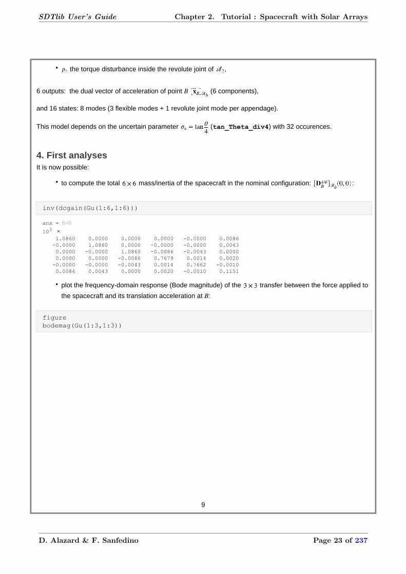
• to compute the total mass/inertia of the spacecraft in the nominal configuration: :
inv(dcgain(Gu(1:6,1:6)))
ans = 6×6
103 × 1.0860 0.0000 0.0000 0.0000 -0.0000 0.0086 -0.0000 1.0860 0.0000 -0.0000 -0.0000 0.0043 0.0000 -0.0000 1.0860 -0.0086 -0.0043 0.0000 0.0000 0.0000 -0.0086 0.7679 0.0014 0.0020 -0.0000 -0.0000 -0.0043 0.0014 0.7662 -0.0010 0.0086 0.0043 0.0000 0.0020 -0.0010 0.1151
• plot the frequency-domain response (Bode magnitude) of the transfer between the force applied to
the spacecraft and its translation acceleration at B:
figurebodemag(Gu(1:3,1:3))
9
SDTlib User’s Guide Chapter 2. Tutorial : Spacecraft with Solar Arrays
D. Alazard & F. Sanfedino Page 23 of 237

• plot the frequency-domain response (Bode magnitude) of the transfer between the torque applied
to the spacecraft at B and its angular acceleration:
figurebodemag(Gu(4:6,4:6))
10
SDTlib User’s Guide Chapter 2. Tutorial : Spacecraft with Solar Arrays
D. Alazard & F. Sanfedino Page 24 of 237

• plot the frequency-domain response (Bode magitude) of the transfer between the disturbance
and the angular accelerations:
figurebodemag(Gu(4:6,7))
11
SDTlib User’s Guide Chapter 2. Tutorial : Spacecraft with Solar Arrays
D. Alazard & F. Sanfedino Page 25 of 237

Obviously, due to symmetry, the transfer from to the angular acceleration around does not depend on the
angular configuration of the solar pannel.
5. Remarks
• one can also dissociate the Revolute joint block (sub-library: 6 dof mechanisms) and the 1-port flexible body (sub-library: 6 dof bodies) . In such a case, the user have to provide the
ouput shaft inertia of the revolute joint,
• for the solar array, it is also possible to use the block 1 Port Nastran body to avoid the declaration
of the flexible mode data (frequency and modal participation factors). Then one have to specify the
Nastran output file name ***.f06 (see tutorial ),
• it is also possible to use the multi-port flexible plate of the sub-library: 6 dof bodies to
model the solar array (see tutorial 4: a spacecraft with 2 symmetrical rotating solararrays defined by a NASTRAN model ).
• In the various blocks of the 6 dof bodies sub-library, the dialog box requires to fill for a given
body : (i) the mass , (ii) the inertia tensor of the body at its center of mass G
and (iii) the vector from a reference point O to the center of mass G. In some application,
the only data available is the total mass/inertia matrix (also called direct dynamic
model) at a reference point O. Then, one can apply the dynamic model transport property:
12
SDTlib User’s Guide Chapter 2. Tutorial : Spacecraft with Solar Arrays
D. Alazard & F. Sanfedino Page 26 of 237

which is valid in any frame to recover the required
data: , , where is the antisymmetric matrix associated to the vector
. That can be easily implemented thanks to the function antisym.m as illustrated in the following
example.
D_CatO=[50 0 0 0 50 0;0 50 0 -50 0 100;0 0 50 0 -100 0;... 0 -50 0 67 0 -100;50 0 -100 0 312 0;0 100 0 -100 0 280]
D_CatO = 6×6 50 0 0 0 50 0 0 50 0 -50 0 100 0 0 50 0 -100 0 0 -50 0 67 0 -100 50 0 -100 0 312 0 0 100 0 -100 0 280
m_C=D_CatO(1,1)
m_C = 50
OG=[D_CatO(2,6);-D_CatO(1,6);D_CatO(1,5)]/m_C
OG = 3×1 2 0 1
J_CatG=D_CatO(4:6,4:6)+m_C*antisym(OG)^2
J_CatG = 3×3 17 0 0 0 62 0 0 0 80
13
SDTlib User’s Guide Chapter 2. Tutorial : Spacecraft with Solar Arrays
D. Alazard & F. Sanfedino Page 27 of 237

Tutorial 3: robust attitude control design of a spacecraft with 2
symmetrical rotating solar arrays ( run).
Table of Contents
1. Description........................................................................................................................................................... 12. The design model................................................................................................................................................23. Design optimization..............................................................................................................................................54. Optimal design analysis.......................................................................................................................................7
by D. Alazard and F. Sanfedino - ISAE-SUPAERO
1. DescriptionThe objective is to design the Attitude Control System of the spacecraft presented in the Tutorial 2: aspacecraft with 2 symmetrical rotating solar arrays.
The SIMULINK model is thus the same except that of relative uncertainty is taken into account on the :
• the mass of the main body : mB,
• the 3 terms on the diagonal of the main body inertia: : IBx, IBy, IBz,
• the frequency of the 3 flexible modes of the solar array (identical for the 2 solar arrays): w1, w2, w3.
SCwith2SAs2Gu=ulinearize('SCwith2SAs2')
Gu =
Uncertain continuous-time state-space model with 6 outputs, 8 inputs, 16 states. The model uncertainty consists of the following blocks: IBx: Uncertain real, nominal = 75, variability = [-20,20]%, 1 occurrences IBy: Uncertain real, nominal = 40, variability = [-20,20]%, 1 occurrences IBz: Uncertain real, nominal = 80, variability = [-20,20]%, 1 occurrences mB: Uncertain real, nominal = 1e+03, variability = [-20,20]%, 3 occurrences tan_Theta_div4: Uncertain real, nominal = 0, range = [-1,1], 32 occurrences w1: Uncertain real, nominal = 5.6, variability = [-20,20]%, 4 occurrences w2: Uncertain real, nominal = 19.3, variability = [-20,20]%, 4 occurrences w3: Uncertain real, nominal = 35.4, variability = [-20,20]%, 4 occurrences
Type "Gu.NominalValue" to see the nominal value, "get(Gu)" to see all properties, and "Gu.Uncertainty" to interact with the uncertain elements.
This tutorial aims to show that the SIMULINK models made with SDTlib are comptible with the robust
control toolbox. The numerical data are given as an example and are not necesseraly representative of a real
application.
We consider the robust design of a 3- axis structured attitude control law to meet:
• (Req1) the pointing requirement (defined by the vector APE) in spite of low frequency orbital
disturbances (characterized by the upper bound on the magnitude Tpert),
1
SDTlib User’s Guide Chapter 3. Tutorial : Robust Control of a spacecraft
3. Tutorial : Robust Control of a spacecraft
D. Alazard & F. Sanfedino Page 28 of 237

• (Req2) stability margins characterized by an upper bound (gamma) on the norm of the input
sensitivity function.
while minimizing (Req3) the variance on the torque applied by the reaction wheel system on the spacecraft
in response to the star sensor and gyrometer noises charcacterized by their PSD (Power Spectral Density
PSD_SST and PSD_GYRO (assumed to be equal for the 3 components).
Numerical application:
% APE (Absolute Pointing Error) requirementAPE=[10 10 50]'*0.001*pi/180; % (rad)
% Orital disturbance magnitude:Tpert=[0.03 0.01 0.02]'; %( Nm)
% PSD of sensor noises:PSD_GYRO=1e-10; %(rd^2/s), PSD_SST=1e-8; % (rd^2.s),
% Upper bound on the input sensitivity functiongamma=1.5;
The value ensures on each of the 3 axes:
• a modulus margin ,
• a gain margin ,
• a phase margin .
The requirements Req1 and Req2 must be met for any values of:
• the mechanical parameter (composed of the 7 parameters: mB, IPx, IBy, IBz w1, w2, w3),
• the geometrical configuration of the solar arrays.
The performance index Req3 is measured on the worst-case parametric configuration in , .
2. The design modelThe design model is the SIMULINK file SC_CL_model.slx depicted in the following Figure.
2
SDTlib User’s Guide Chapter 3. Tutorial : Robust Control of a spacecraft
D. Alazard & F. Sanfedino Page 29 of 237

The model previously computed (Gu) is introduced with an Uncertain State Space from the
Robust Control toolbox sub-library. Since the design will be based on the SIMULINK model and the
Matlab/Simulink slTuner interface, it is very important to specify again Gu in the Linear Analysis >Specify Selected Block Linearization menu (obtained by a right click on the block Gu) according to
he following Figure.
Then the design model is completed with avionics models for:
• the reaction wheel system dynamics: RW. A second order transfer with a damping ratio and a
frequency is assumed on each of the 3 axes,
• the star sensor dynamics: SST. A first order transfer with a cut-off frequency is assumed on each of
the 3 axes,
• the gyrometer dynamics: GYRO. A first order transfer with a cut-off frequency is assumed on each
of the 3 axes,
3
SDTlib User’s Guide Chapter 3. Tutorial : Robust Control of a spacecraft
D. Alazard & F. Sanfedino Page 30 of 237

• a loop delay DELAY. A delay, modelled by a second order Pade approximation, is assumed on
each of the 3 axes.
% Avionics:% RWs: 2nd order low pass at 100 HzRW=tf((200*pi)^2,[1 1.4*200*pi (200*pi)^2])*eye(3);% SST: 1st order low pass at 8 hzSST=tf(8*2*pi,[1 8*2*pi])*eye(3);% GYRO: 1sr order low pass at 200 HzGYRO=tf(400*pi,[1 400])*eye(3);% Loop delaydelay=0.01; %(s) : delay to discretizaton, etc ...[num,den]=pade(delay,2);DELAY=tf(num,den)*eye(3);
The structured attitude controller (ACS) is depicted in the next figure.
4
SDTlib User’s Guide Chapter 3. Tutorial : Robust Control of a spacecraft
D. Alazard & F. Sanfedino Page 31 of 237

It is a decentralised controller composed of a proportional-derivative controller (the 2 gains Kpi and Kvi,
i=x,y,z) with a first order low pass filter (charcaterized by the cut-off frequency wi, i=x,y,z) per axis.
The set of the 9 tunable parameters (Kpi, wi and Kvi, i=x,y,z) is denoted . They are all initialized to 1.
% Tunable parameter initialization:Kp_x=1; Kp_y=1; Kp_z=1;Kv_x=1; Kv_y=1; Kv_z=1;w_x=1; w_y=1; w_z=1;
The inputs and outputs of the closed-loop SIMULINK model SC_CL_model.slx, denoted , are:
• (Torb: 3 component input # 1): the normalized (w.r.t. Tpert) orbital distrubance (adimensional),
• (Dsadm1: 1 component input # 2): the disturbing torque on the SADM # 1 ( ). Not used in the
design,
• (Dsadm2: 1 component input # 3): the disturbing torque on the SADM # 2 ( ). Not used in the
design,
• (Ngyro: 3 component input # 4): the normalized (w.r.t. PSD_GYRO) gyro noise ( ),
• (Nsst: 3 component input # 5): the normalized (w.r.t. PSD_SST) star sensor noise ( ),
• (Torque: 3 component output # 1): the torque applied on the spacecraft by the reactions wheels (
),
• (ape: 3 component output # 2): the normalized (w.r.t. APE) attitude error (adimensional).
denotes the closed-loop transfer from to for a given parametric uncertainty vector
, a given geometric configuration and a given tunable parameter vector . denotes the
closed-loop transfer from the 6 component noise to .
In addition the SIMULINK model has some labelled internal signals: (Sin) is the input disturbance
used to define the input sensitivity function .
3. Design optimizationThe design is made using the MATLAB/SIMULINK interface slTuner by specifying the names of the tunable
blocks and the names of the signals used to express the various requirements:
SC_CL_modelP0=slTuner('SC_CL_model','Kpx','Kvx','wx','Kpy','Kvy','wy','Kpz','Kvz','wz');addPoint(P0,'Torb','Sin','Dsadm1','Dsadm2','Ngyro','Nsst','Torque','ape');
The first requirement or hard contraint Req1 on the pointing error reads:
5
SDTlib User’s Guide Chapter 3. Tutorial : Robust Control of a spacecraft
D. Alazard & F. Sanfedino Page 32 of 237

and the corrsponding MATLAB syntax is:
% Hard requirement on the closed-loop transfert:% The gain from the normalized orbital disturbances to normalized APE:Req1=TuningGoal.Gain('Torb','ape',1);Req1.Name='ape/Spec';
The second requirement or hard constraint Req2 on the input sensitivity function reads:
and the corresponding MATLAB syntax is:
% Hard requirement on the input sensitivity function:Req2=TuningGoal.Gain('Sin','Torque',gamma);Req2.Name='Input sensitivity';
The preformance index or soft constraint Req3 is:
with
and the corresponding MATLAB syntax is:
% Soft requirement on the variance from sensor noises to% the applied torque:Req3=TuningGoal.Variance('Ngyro','Nsst','Torque',1);Req3.Name='Actuator Variance';
The optimization is done thanks to the function systune with 2 random initializations in addition to the
proposed initialization:
% Design optimisation:opt=systuneOptions;opt.RandomStart=2;[Popt,fBest,gBest,Info] = systune(P0,Req3,[Req1,Req2],opt);
Nominal tuning:Design 1: Soft = 0.232, Hard = 0.79502Design 2: Soft = 0.0379, Hard = 0.99983Design 3: Soft = 0.0379, Hard = 0.99988
Robust tuning of Design 3:Soft: [0.0379,Inf], Hard: [1,1.08], Iterations = 163Soft: [0.0415,Inf], Hard: [1,1.09], Iterations = 182Soft: [0.0417,0.0418], Hard: [1,1], Iterations = 161Soft: [0.0418,Inf], Hard: [1,1], Iterations = 190Soft: [0.0418,0.0418], Hard: [1,1], Iterations = 174Final: Soft = 0.0418, Hard = 0.99996, Iterations = 870
Robust tuning of Design 2:Soft: [0.0379,Inf], Hard: [1,1.08], Iterations = 243Soft: [0.0415,Inf], Hard: [1,1.11], Iterations = 194
6
SDTlib User’s Guide Chapter 3. Tutorial : Robust Control of a spacecraft
D. Alazard & F. Sanfedino Page 33 of 237

Soft: [0.0417,0.0418], Hard: [1,1], Iterations = 177Soft: [0.0418,0.0418], Hard: [1,1], Iterations = 176Final: Soft = 0.0418, Hard = 0.99981, Iterations = 790
Robust tuning of Design 1:Soft: [0.232,0.232], Hard: [0.795,0.84], Iterations = 170Soft: [0.232,0.232], Hard: [0.804,0.84], Iterations = 161Final: Soft = 0.232, Hard = 0.80393, Iterations = 331
gBest
gBest = 1×2 1.0000 1.0000
Since the 2 components of gBest are lower than 1, the requirements Req1 and Req2 are met for any
parametric unceratinties and any geometric configuration .
fBest
fBest = 0.0418
fBest gives the worst-case performance index:
Then one can get the optimal tuning of the 9 controller gains :
% Optimal tuning:w_x=getBlockValue(Popt,'wx');w_x=w_x.d;w_y=getBlockValue(Popt,'wy');w_y=w_y.d;w_z=getBlockValue(Popt,'wz');w_z=w_z.d;Kp_x=getBlockValue(Popt,'Kpx');Kp_x=Kp_x.d;Kp_y=getBlockValue(Popt,'Kpy');Kp_y=Kp_y.d;Kp_z=getBlockValue(Popt,'Kpz');Kp_z=Kp_z.d;Kv_x=getBlockValue(Popt,'Kvx');Kv_x=Kv_x.d;Kv_y=getBlockValue(Popt,'Kvy');Kv_y=Kv_y.d;Kv_z=getBlockValue(Popt,'Kvz');Kv_z=Kv_z.d;
4. Optimal design analysisIt is now possible to analyse the frequency-domain responses of 2 constrained transfers (Req1 and Req2) from
random samples in the parametric space and the worst-case identified during the optimization process
(systune):
% Optimal design analysis:PB1=getIOTransfer(Popt,'Torb','ape');PB2=getIOTransfer(Popt,'Sin','Torque');
% Worst-cases identified by systune% Best run:[g,index]=min([Info.g])
g = 0.8039index = 1
% Worst cases identified during the best run:
7
SDTlib User’s Guide Chapter 3. Tutorial : Robust Control of a spacecraft
D. Alazard & F. Sanfedino Page 34 of 237

WCs=Info(index).wcPert;
The first worst-case :
WCs(1)
ans = struct with fields: IBx: 60.0000 IBy: 33.9282 IBz: 78.3873 mB: 936.0938 tan_Theta_div4: -0.4178 w1: 4.7029 w2: 20.3862 w3: 36.5042
The frequency domain response relative to Req1:
% Frequency domain constraints Req1:figureviewGoal(Req1,PB1)hold onsigma(usubs(PB1,WCs(1)),'-r') % worst performancelegend('Principal gain','Max Gain','Worst-case','Location','southwest')
One can check that the hard constraint Req1 is saturated at the null frequency for any values of the parametric
vector and the geometric configuration.
The frequency domain response realtive to Req2:
8
SDTlib User’s Guide Chapter 3. Tutorial : Robust Control of a spacecraft
D. Alazard & F. Sanfedino Page 35 of 237

figureviewGoal(Req2,PB2)hold onsigma(usubs(PB2,WCs(1)),'-r') % worst performance:legend('Principal gain','Max Gain','Worst-case','Location','southeast')
One can check that the worst-case identified by systune saturates the constraint in low frequency and at the
frequency .
It is also possible to analyze the stability margins, axis per axis, on the Nichols frequency-domain responses of
the open-loop transfer function (when the loop is opened on the system input):
% Nichols plot of the open-loop transfer function:% the loop is opened at the system input:L = -getLoopTransfer(Popt,'Torque') ;figurefor ii=1:3 FDBCK=eye(3); FDBCK(ii,ii)=0; % only the loop on channel # ii is opened! BFii=feedback(L,FDBCK); subplot(1,3,ii); nichols(BFii(ii,ii)); ngrid set(gca,'Ylim',[-100 20]);endset(gcf,'Units','normalized','Position',[0 0 1 0.5])
9
SDTlib User’s Guide Chapter 3. Tutorial : Robust Control of a spacecraft
D. Alazard & F. Sanfedino Page 36 of 237

One can check that the axis-per-axis stability margins (gain margins and phase margins) are largely better
than the convervative lower bounds induced from Req2 (gain margin , phase margin
) .
It is now possible to save the optimal closed-loop design Popt as an uncertain state space modelCLu (uss) for simulation purpose. See also the tutorial 12 Simulating a SDTlib-basedmodel .
% Save the optimal closed-loop system as an USS for simulation purpose:CLu=uss(getIOTransfer(Popt,'Torb','Dsadm1','Dsadm2','Ngyro','Nsst','Torque','ape'))
CLu =
Uncertain continuous-time state-space model with 6 outputs, 11 inputs, 43 states. The model uncertainty consists of the following blocks: IBx: Uncertain real, nominal = 75, variability = [-20,20]%, 1 occurrences IBy: Uncertain real, nominal = 40, variability = [-20,20]%, 1 occurrences IBz: Uncertain real, nominal = 80, variability = [-20,20]%, 1 occurrences mB: Uncertain real, nominal = 1e+03, variability = [-20,20]%, 3 occurrences tan_Theta_div4: Uncertain real, nominal = 0, range = [-1,1], 32 occurrences w1: Uncertain real, nominal = 5.6, variability = [-20,20]%, 4 occurrences w2: Uncertain real, nominal = 19.3, variability = [-20,20]%, 4 occurrences w3: Uncertain real, nominal = 35.4, variability = [-20,20]%, 4 occurrences
Type "CLu.NominalValue" to see the nominal value, "get(CLu)" to see all properties, and "CLu.Uncertainty" to interact with the uncertain elements.
save OptimalDesign CLu
10
SDTlib User’s Guide Chapter 3. Tutorial : Robust Control of a spacecraft
D. Alazard & F. Sanfedino Page 37 of 237

Tutorial 4: a spacecraft with 2 symmetrical rotating solar arrays
defined by a NASTRAN model ( run).
Table of Contents
1. Description........................................................................................................................................................... 12. NASTRAN interface.............................................................................................................................................13. Revolute joint....................................................................................................................................................... 23. The whole dynamic model................................................................................................................................34. Parametric association.........................................................................................................................................55. Analyses...............................................................................................................................................................66. Remarks...............................................................................................................................................................6
by D. Alazard and F. Sanfedino - ISAE-SUPAERO
1. Description
This tutorial reconsiders the same example already addressed in the tutorial 1 but the models ,
( ) of 2 the rotating solar flexible solar arrays are now defined by:
• a .f06 file provided be a Nastran analysis assuming that the reference point for this analysis of the
solar array is the connection point with the main body ,
• a revolue joint at the point .
2. NASTRAN interfaceThe simplest interface with NASTRAN is the block 1 port Nastran body of the SDTlib/6 dof bodiessub-library. This bloc requires only the name of .f06 file, the number of flexible modes (ordered by increasing
frequency) to be taken into the block and the common damping ratio for all the considered flexible modes.
In addition, the user can specify a relative uncertainty on the frequency of each of the considered flexible
modes.
The dialog box of this block is depicted in the following figure.
1
SDTlib User’s Guide Chapter 4. Tutorial : Solar Arrays imported by NASTRAN
4. Tutorial : Solar Arrays imported by NASTRAN
D. Alazard & F. Sanfedino Page 38 of 237

The file ff06_plate.f06 specified in the dialog box is proposed as an example. It corresponds to a
square plate of aluminium ( ) and is available in NASTRANfiles sub-library available with
the SDTlib. , and of relative variations are taken into account on the flexible 1, 2 and 3,
respectively, among the 10 flexibles modes extracted from the .f06 file.
The reader is advised to read the inline help available in the dialog box (internet connection required), also
available by:
web Doc1PortNastranBody.html -new
3. Revolute jointThe revolute joint is modeled thanks to the block Revolute joint + configuration on the SDTlib/6dof mechanisms sub-library.
According to the dialog box depicted in the following Figure, this block requires:
• the direction of the revolute axis in the inherit (local) frame,
• the output shat inertia (one can put a very small value when this data is unknown),
• the angular configuration of the joint (the other block, named Revolute joint in the 6 dof
mechanisms sub-library, assumes small angular variations around 0).
2
SDTlib User’s Guide Chapter 4. Tutorial : Solar Arrays imported by NASTRAN
D. Alazard & F. Sanfedino Page 39 of 237

See also:
web DocRevoluteJoint_configuration.html -new
3. The whole dynamic modelThe whole model is then described by the following SIMULINK file SCwith2SAs_bis.slx:
3
SDTlib User’s Guide Chapter 4. Tutorial : Solar Arrays imported by NASTRAN
D. Alazard & F. Sanfedino Page 40 of 237

SCwith2SAs_bis % the SIMULINK lile of the modelGu=ulinearize('SCwith2SAs_bis')
Gu =
Uncertain continuous-time state-space model with 6 outputs, 8 inputs, 44 states. The model uncertainty consists of the following blocks: tan_Theta_div4: Uncertain real, nominal = 0, range = [-1,1], 32 occurrences w_SA1_1: Uncertain real, nominal = 10.2, variability = [-20,20]%, 2 occurrences w_SA1_2: Uncertain real, nominal = 17.3, variability = [-10,10]%, 2 occurrences w_SA1_3: Uncertain real, nominal = 67.4, variability = [-10,10]%, 2 occurrences w_SA2_1: Uncertain real, nominal = 10.2, variability = [-20,20]%, 2 occurrences w_SA2_2: Uncertain real, nominal = 17.3, variability = [-10,10]%, 2 occurrences w_SA2_3: Uncertain real, nominal = 67.4, variability = [-10,10]%, 2 occurrences
4
SDTlib User’s Guide Chapter 4. Tutorial : Solar Arrays imported by NASTRAN
D. Alazard & F. Sanfedino Page 41 of 237

Type "Gu.NominalValue" to see the nominal value, "get(Gu)" to see all properties, and "Gu.Uncertainty" to interact with the uncertain elements.
As in tutorial 1, one can check that the model have 8 inputs:
• the external wrench (6 components)
• the torque disturbance inside the revolute joint of ,
• the torque disturbance inside the revolute joint of ,
6 outputs: the dual vector of acceleration of point B (6 components),
but 44 states: 22 modes (10 flexible modes + 1 revolute joint mode per appendage).
This model depends on :
•the uncertain parameter (tan_Theta_div4) with 32 occurences.
• the uncertainties on the first 3 frequencies of the 2 solar panels (w_SAi_j, i=1,2, j=1,2,3).
4. Parametric associationThe model Gu is fully compatible with the MATLAB Robust Control Toolbox. It is thus possible to
associate the various uncertain parameters or to specify new variations using the function ususbs.
As specified in the dialog box of the 1 port Nastran body, the uncertainties correspond to independant
manufacturing uncertainties on the flexible mode frequencies of the 2 solar pannels. At preliminary design
phase, it is better recommanded to specify design uncertainties. That is to say, the 2 solar pannels are
identical but there are some uncertainties on the solar pannel flexible modes. That can be done by associating
the uncertain parameters of the model Gu to new design uncertain parameters which are the same for the 2
solar panels. The syntax is the following:
w_SA_1=ureal('w_SA_1',10.2,'percent',20);w_SA_2=ureal('w_SA_2',17.3,'percent',20);w_SA_3=ureal('w_SA_3',67.4,'percent',20);Gu_sym=usubs(Gu,'w_SA1_1',w_SA_1,'w_SA2_1',w_SA_1,... 'w_SA1_2',w_SA_2,'w_SA2_2',w_SA_2,... 'w_SA1_3',w_SA_3,'w_SA2_3',w_SA_3)
Gu_sym =
Uncertain continuous-time state-space model with 6 outputs, 8 inputs, 44 states. The model uncertainty consists of the following blocks: tan_Theta_div4: Uncertain real, nominal = 0, range = [-1,1], 32 occurrences w_SA_1: Uncertain real, nominal = 10.2, variability = [-20,20]%, 4 occurrences w_SA_2: Uncertain real, nominal = 17.3, variability = [-20,20]%, 4 occurrences w_SA_3: Uncertain real, nominal = 67.4, variability = [-20,20]%, 4 occurrences
Type "Gu_sym.NominalValue" to see the nominal value, "get(Gu_sym)" to see all properties, and "Gu_sym.Uncertainty" to interact with the uncertain elements.
In this new model the 2 solar pannels are identical for any values of the 3 parameters w_SA_1, w_SA_2,
w_SA_3.
5
SDTlib User’s Guide Chapter 4. Tutorial : Solar Arrays imported by NASTRAN
D. Alazard & F. Sanfedino Page 42 of 237

5. AnalysesAs in tutorial 1, the same kind of analyses can be now performed on this new model, for instance the
frequency-domain response (Bode magnitude) of the transfer between the torque applied to the
spacecraft at B and its angular acceleration:
figurebodemag(Gu_sym(4:6,4:6),0.1 1000)
6. Remarks
• the block 1 Port Nastran body is the simplest interface between the SDT and NASTRAN. If the
user wants to build the model of an array of solar pannels or to model some external loads (wrenches) at
some particular points of the solar pannel, a muti-port model is required and the user is advised to use
the block N Ports Nastran body (see tutorial 7: the cantilevered plate dynamics studied withSDTlib block NINOP Nastran body),
• it is also possible to use the multi-port flexible plate of the sub-library: 6 dof bodies to
model the solar array (see tutorial 8: a spacecraft with 2 symmetrical rotating solar arrays definedby a generic plate model).
6
SDTlib User’s Guide Chapter 4. Tutorial : Solar Arrays imported by NASTRAN
D. Alazard & F. Sanfedino Page 43 of 237
Tutorial 5: a short course on TITOP (Two-Input Two-Output Ports)models
Table of Contents
1. Illustration in the single-axis case....................................................................................................................... 11.1. Elementatry TITOP model of the spring-mass system.................................................................................11.2. Channel (port) inversion............................................................................................................................... 41.3. Assembling open-kinematic chains of spring-mass systems....................................................................... 61.4. Assembling closed-kinematic chains of spring-mass systems..................................................................... 9
2. Six dofs case..................................................................................................................................................... 112.1. Six d.o.fs TITOP model of a flexible body................................................................................................. 112.2 TITOP model of a revolute joint.................................................................................................................. 142.3 Channel (port) inversion.............................................................................................................................. 142.4 Assembling open-kinematic chains with TITOP models..............................................................................152.5 Assembling closed-kinematic chains with NINOP models.......................................................................... 16
3. References.........................................................................................................................................................17
by D. Alazard and F. Sanfedino - ISAE-SUPAERO
1. Illustration in the single-axis case
1.1. Elementatry TITOP model of the spring-mass system
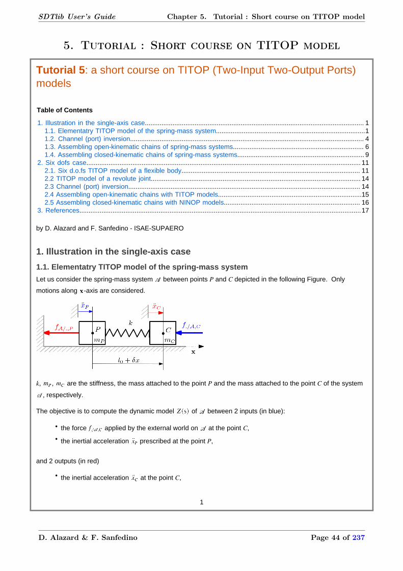
Let us consider the spring-mass system between points P and C depicted in the following Figure. Only
motions along -axis are considered.
k, , are the stiffness, the mass attached to the point P and the mass attached to the point C of the system
, respectively.
The objective is to compute the dynamic model of between 2 inputs (in blue):
• the force applied by the external world on at the point C,
• the inertial acceleration prescribed at the point P,
and 2 outputs (in red)
• the inertial acceleration at the point C,
1
SDTlib User’s Guide Chapter 5. Tutorial : Short course on TITOP model
5. Tutorial : Short course on TITOP model
D. Alazard & F. Sanfedino Page 44 of 237

• the force applied by on the external world at the point P.
Only variations around the equilibrium conditions are considered. is the variation on the length of the vector
w.r.t its length at rest. The equilibrium conditions are: , , .
The Newton principle applied on each of the 2 masses leads to:
•
• .
Considering that , a state space representation of , associated to the state vector
, reads:
,
and the transfer matrix reads:
,
with:
• is the free frequency of ,
• is the cantilever frequency of when it is cantilevered at point P.
The TITOP model can also be represented by a SIMULINK block diagram model, depicted in the next
figure
2
SDTlib User’s Guide Chapter 5. Tutorial : Short course on TITOP model
D. Alazard & F. Sanfedino Page 45 of 237

and embbeded in a masked sub-system:
Numerical application: , , .
MK_elem[a,b,c,d]=linmod('MK_elem');Z=ss(a,b,c,d);
Note that the interest of the block-diagram representation, w.r.t. to the state space or transfer matrix
representation is that the number of occurences of the 3 mechanical parameters of ( k, , ) is minimized:
each parameters is associated to a single gain. Thus the uncertain system which can be derived from this
3
SDTlib User’s Guide Chapter 5. Tutorial : Short course on TITOP model
D. Alazard & F. Sanfedino Page 46 of 237

SIMULINK model considering uncertain parameters for k, , is guarranteed to be mininal in terms of order
and parametric occurences.
1.2. Channel (port) inversion
The open-loop dynamics of the model , i.e. when the 2 inputs ( and ) are null, corresponds to the
clamped at P / free at Cboundary conditions, i.e: the roots of .
Since is a square ( ) system with an invertible direct-freedthrough, it is possible to inverse 1 or 2 input/
output channel(s) :
• the channel # 1 is the channel from to ,
• the channel # 2 is the channel from to .
That can be done thanks to the function invio of the SDTLIB. See also:
web docInvio.html -new
Let us note the model where the channels numbered in the vector of indexes are inverted, then:
•the open-loop dynamics of is the free at P / free at C dynamics: ,
•the open-loop dynamics of is the free at P / clamped at Cdynamics: where
is the cantilever frequency of when it is cantilevered at point C,
•the open-loop dynamics of is the clamped at P / clamped at Cdynamics: .
Indeed:
damp(Z)
Pole Damping Frequency Time Constant (rad/seconds) (seconds) 0.00e+00 + 5.77e-01i 0.00e+00 5.77e-01 Inf 0.00e+00 - 5.77e-01i 0.00e+00 5.77e-01 Inf
damp(invio(Z,2))
Pole Damping Frequency Time Constant (rad/seconds) (seconds) 0.00e+00 + 9.13e-01i 0.00e+00 9.13e-01 Inf 0.00e+00 - 9.13e-01i 0.00e+00 9.13e-01 Inf
damp(inv(Z))
4
SDTlib User’s Guide Chapter 5. Tutorial : Short course on TITOP model
D. Alazard & F. Sanfedino Page 47 of 237

Pole Damping Frequency Time Constant (rad/seconds) (seconds) 0.00e+00 + 7.07e-01i 0.00e+00 7.07e-01 Inf 0.00e+00 - 7.07e-01i 0.00e+00 7.07e-01 Inf
damp(invio(Z,1))
Pole Damping Frequency Time Constant (rad/seconds) (seconds) 0.00e+00 -1.00e+00 0.00e+00 Inf 0.00e+00 -1.00e+00 0.00e+00 Inf
It is surprising and interesting to note that the dyamics of corresponds to a double integrator . Indeed,
the two inputs of are and . Obviously, the steady state response of to 2 independent steps
on these 2 inputs creates infinite outputs (the forces and ). Thus the DCgain of is:
and the state equation for the model reads (obsviously):
,
.
If now it is imposed that the 2 inputs must be equal: , then the 2 integrators must be reduced such
that the transfer from to and is:
.
Indeed, one can recover this resuts using the function minreal (minimal realization):
minreal(invio(Z,1)*[1;1])
2 states removed.
ans = D = u1 y1 3 y2 -2 Static gain.
5
SDTlib User’s Guide Chapter 5. Tutorial : Short course on TITOP model
D. Alazard & F. Sanfedino Page 48 of 237

One can also consider the "dual" property which consists to consider a single output (i.e. the
total force applied to by the external world) in order to recover the quite obvious static model:
:
minreal([1 -1]*invio(Z,1))
2 states removed.
ans = D = u1 u2 y1 3 2 Static gain.
Conclusion: the main interest of the TITOP model is that it can be used to model the system for any
arbitrary boundary conditions at its tips P and C, thanks to simple channel operations.
1.3. Assembling open-kinematic chains of spring-mass systemsThe previous conclusion works not only for clamped or free boundary conditions but also for any dynamical
systems connected to at the point P or at the point C.
Indeed, let us consider the systems depicted in the following Figure and composed of 4 spring-mass sub-
systems , . The objective is to find the model between the input , a force applied to the point
, and the variations of positions of the points ( ) and ( ).
For each sub-system , let us denote:
• , : the 2 points at the tips of ,
• : its 3 mechanical parameters,
• : its TITOP model associated to state vector .
Numerical application:
6
SDTlib User’s Guide Chapter 5. Tutorial : Short course on TITOP model
D. Alazard & F. Sanfedino Page 49 of 237

The model of the whole system can then be defined by the interconnection of the 4 blocks , ,
and according to the following SIMULINK model ( file MK_elem_x4.xls) depicted in the next
Figure and considering the action/re-action relations:
; ; ; ,
and the accelaration constraints: , .
7
SDTlib User’s Guide Chapter 5. Tutorial : Short course on TITOP model
D. Alazard & F. Sanfedino Page 50 of 237

Finally: 2 double integators was added on and to obtain the position outputs and . Note that
one of the 2 double integrators is non-miminal and can be removed considering the geometric constraints
between the outputs and the internal state variables:
• ,
• .
Thus it is recomended to use minreal on the model derived from the SIMULINK model:.
8
SDTlib User’s Guide Chapter 5. Tutorial : Short course on TITOP model
D. Alazard & F. Sanfedino Page 51 of 237

MK_elem_x4[a,b,c,d]=linmod('MK_elem_x4');G=ss(a,b,c,d);G=minreal(G);
2 states removed.
damp(G)
Pole Damping Frequency Time Constant (rad/seconds) (seconds) -5.67e-18 + 6.54e-09i 8.67e-10 6.54e-09 1.76e+17 -5.67e-18 - 6.54e-09i 8.67e-10 6.54e-09 1.76e+17 -3.82e-16 + 4.90e-01i 7.79e-16 4.90e-01 2.62e+15 -3.82e-16 - 4.90e-01i 7.79e-16 4.90e-01 2.62e+15 2.50e-16 + 7.27e-01i -3.44e-16 7.27e-01 -4.00e+15 2.50e-16 - 7.27e-01i -3.44e-16 7.27e-01 -4.00e+15 2.78e-16 + 1.15e+00i -2.42e-16 1.15e+00 -3.60e+15 2.78e-16 - 1.15e+00i -2.42e-16 1.15e+00 -3.60e+15 -1.67e-16 + 1.27e+00i 1.32e-16 1.27e+00 6.00e+15 -1.67e-16 - 1.27e+00i 1.32e-16 1.27e+00 6.00e+15
One of the main interest in the proposed TITOP modeling approach is that the model of a flexible multi-body system is highly structured and based on the interconnection of the TITOP models of the variousflexible bodies. Each TITOP model depends only on its own mechanical parameters. Thus this approachis suitable to derive minimal LFT model when parametric variations are taken into account.
1.4. Assembling closed-kinematic chains of spring-mass systems
Let us consider the system depicted in the following Figure and composed of 3 spring-mass sub-systems
, . Inside the subsytem , a controlled force can be applied between the 2 tips masses. The
objective is to find the model between the input and the variations of acceleration of the point .
Numerical application: , , . Thus , (variable Z in
the workspace).
Such a system is a closed kinematic chain mechanism since: and at any time.
9
SDTlib User’s Guide Chapter 5. Tutorial : Short course on TITOP model
D. Alazard & F. Sanfedino Page 52 of 237

The model of the whole system can then be defined by the interconnection of the 3 blocks , , and
according to the following SIMULINK model ( file MK_elem_cl.xls) depicted in the next Figure and
considering the action/re-action relations:
; ; ,
and the acceleration constraints: , , and .
MK_elem_cl[a,b,c,d]=linmod('MK_elem_cl');G=ss(a,b,c,d);damp(G)
Pole Damping Frequency Time Constant (rad/seconds) (seconds) 5.77e-17 + 6.17e-09i -9.35e-09 6.17e-09 -1.73e+16 5.77e-17 - 6.17e-09i -9.35e-09 6.17e-09 -1.73e+16 -4.90e-18 + 7.38e-01i 6.64e-18 7.38e-01 2.04e+17 -4.90e-18 - 7.38e-01i 6.64e-18 7.38e-01 2.04e+17 6.26e-18 + 8.30e-01i -7.54e-18 8.30e-01 -1.60e+17 6.26e-18 - 8.30e-01i -7.54e-18 8.30e-01 -1.60e+17
10
SDTlib User’s Guide Chapter 5. Tutorial : Short course on TITOP model
D. Alazard & F. Sanfedino Page 53 of 237

The dyamics is characterized by 2 flexible modes (at and ) and 2 eigenvalues around
0. These 2 eigenvalues corresponds to the geometric constraints between the internal state variables to
maintained closed the kinematic chain for any value of the deformation:
• ,
• .
They can be reduced using a minimal realization of the transfer using minreal:
G=minreal(G);
2 states removed.
damp(G)
Pole Damping Frequency Time Constant (rad/seconds) (seconds) 1.11e-16 + 7.38e-01i -1.51e-16 7.38e-01 -9.01e+15 1.11e-16 - 7.38e-01i -1.51e-16 7.38e-01 -9.01e+15 0.00e+00 + 8.30e-01i 0.00e+00 8.30e-01 Inf 0.00e+00 - 8.30e-01i 0.00e+00 8.30e-01 Inf
More complex example of closed-loop mechanism involving 2D plates and several closed kinematic chains or
the 4 bar mechanism are proposed in the tutorial 9 A solar array with 3 pannels and the tutorial 11 the 4 barmechanism.
2. Six dofs caseThe previous TITOP modelling approach can be directly extented to the 6 d.o.fs case while taking into account:
• the dynamics coupling between translations and rotations due to the geometry (lever-arm effect),
• the various frames in which are described the various bodies ,
• the 6 d.o.f.s behavior of the flexible modes of each bodie . The dynamic model of this flexible behavior
can be:
• (i) computed analytically for very simple shaped body: uniform beam, uniform rectangular plate,
• (ii) provided by finite element method softwares. A NASTRAN/SIMULINK interface is available in the
SDTlib. (see also the sub-library 6 dof bodies of the SDTlib and the tutorial 7 Cantileveredplate dynamics studied with SDTlib block NINOP Nastran body).
2.1. Six d.o.fs TITOP model of a flexible body
Let us consider a flexible substructure (link) connected a the parent substructure at the point P and to the
child substructure at point C as depicted in next Figure. is the body frame attached to .
11
SDTlib User’s Guide Chapter 5. Tutorial : Short course on TITOP model
D. Alazard & F. Sanfedino Page 54 of 237

The TITOP (Two-Input Two-Output Port) model is a linear dynamic model between inputs:
•the 6 components in of the wrench applied by the child substructure to
at point C,
•the 6 components in of the acceleration twist (time-derivative of the twist) of the
point P,
and outputs:
•the 6 components in of the acceleration twist of point C,
•the 6 components in of the wrench applied by to the parent substructure
at point P,
and can be represented by the block-diagram depicted in next Figure.
12
SDTlib User’s Guide Chapter 5. Tutorial : Short course on TITOP model
D. Alazard & F. Sanfedino Page 55 of 237

The way to obtain the TITOP model in the general case is detailled in AIAA 2015 and is based on the
modal analysis of the body with the clamped at P - free at Cboundary conditions. Indeed, the Lagrange's
formulation of dynamics leads to the generalized 2-nd order differential equation (all the terms are projected in
the frame , omitted for brivety):
where:
• n is the number of flexible modes of body characterized by the modal coordinates vector , the
frequencies and the damping ratio , ,
• is the identity matrix of size n,
• is the modal participation factor matrix of the body at point P,
• is the projection matrix of the n clamped-free modal shapes on the 6 d.o.fs at point C,
•
is the "rigid'' kinematic model between point C and P: where is the skew-
symmetric matrix associated to vector from C to P,
• is the rigid mass model of the body at point P. where A, and
are the centre of mass, the mass and the inertia tensor at A, respectively.
The acceleration twist at point C reads:
.
These equations can be expressed with a block-diagram representation and thus a SIMULINK model as it is
proposed in the SDTlib. All the required data ( n, , , , , , , , ) can be extracted from the
NASTRAN file of the body (files ***.bdf and ***.f06) thanks to the block N ports Nastran body of
the sub-library 6 DOF bodies.
The reader is advised to reads the help of this block also avalailbale by:
web DocNPortNastranBody.html -new
Finally, the TITOP model of a flexible body can be easily extended to NINOP (N-Input, N-Output Ports) model ,
considering several child points , , ... .
13
SDTlib User’s Guide Chapter 5. Tutorial : Short course on TITOP model
D. Alazard & F. Sanfedino Page 56 of 237

For a uniform beam and a uniform rectangular plate, all the required data are derived analytically from the
geometry and material characteristics in the blocks TITOP flexible beam and NINOP flexible plate.
See also:
web DocBeam.html -newweb DocPlate_joly.html -new
Rigid bodies can also be handled under this formalism thanks to the block Multi-port rigid body. See
also:
web Docmultiportrigidbody.html -new
2.2 TITOP model of a revolute joint
The body can be linked to the parent body at point P through a revoute joint, characterized by the axis
direction (unitary vector expressed in the body frame : ) and an angular configuration . Then, the
TITOP model of the revolute joint depicted in the next Figure can be used during the asssembly of
the multi-body system. This block is a transfer with:
• the TITOP transfer between the wrenches and the accelerations twists at the input shaft (and
thus expressed in the frame ) and at the output shaft (and thus expressed in the frame ). and
are aligned when ,
• the SISO channel from the torque applied inside the revolute joint by a driving mechanism to the
relative acceleration of the output shaft w.r.t. the input shaft.
The angular configuration can be a varyring parameter declared with ureal so that the linear model derived
from the SIMULINK model is valid for any angular configuration .
Revolute joint can be also embedded inside the TITOP model of a rigid body, a flexible body and a flexible
beam as it is proposed in the sub-library Predefined subsystems (see also the tutorial 6: a 6 dofs roboticarm on a chaser spacecraft ).
See also:
web DocRevoluteJoint_configuration.html -new
2.3 Channel (port) inversion
14
SDTlib User’s Guide Chapter 5. Tutorial : Short course on TITOP model
D. Alazard & F. Sanfedino Page 57 of 237

Exactly as it was shown for the spring-mass system in the academic example above, the channels of the TITOP
model of a flexible body can be inverted to take into account boundary conditions:
• clamped at P and clamped at C:
• free at P and free at C:
• free at P and clamped at C:
Remark: single or multiple channel inversions can be performed thanks to the function invio but these
operations are not included in the dialog boxes of the various SDTlib blocks in its current version. But for the
blocks:
• Multi-port rigid body: it is possible to inverse one ( ) channel at one connection point or
port (see: port to be inverted in the Multi-port rigid body block dialog box). Indeed for a
rigid body, it is not possible to precribe 2 independent acceleration twists at 2 different points. Thus only
one port can be inverted for a rigid body,
• multi-port flexible plate: it possible to specify up to 4 parent points , where
independent acceleration twists can be prescribed. See also the tutorial 9: a solar array with 3pannels.
In the general case, for flexible bodies, there is no limits in the number of input/output channel which can be
inverted. It is up to the user to manage these inversions by using the function invio and to create customized
new blocks. See also the tutorial 11: the 4 bar mechanism.
2.4 Assembling open-kinematic chains with TITOP models
The connection of the body in the whole structure between the parent body and the child body can be
modelled by the interconnection of the TITOP models of the various bodies through the DCM (Direction Cosine
15
SDTlib User’s Guide Chapter 5. Tutorial : Short course on TITOP model
D. Alazard & F. Sanfedino Page 58 of 237

Matrix) to manage the projection in the different frames , where are described the bodies ,
and .
In the following Figure, is the dual DCM and is the DCM from frame to frame
, i.e: the matrix where each column is the component vector of each orthogonal unit vector of expressed
in : . See also:
web Doc6dcm.html -new
The bodies and can be also connected to some others bodies at some connection points ( ).
The tutorial 6 a 6 dofs robotic arm on a chaser spacecraft is a representative example of multibody system
composed of a serial connection of several rigid and flexible bodies based on this principle.
Since rigid and flexible bodies can also have several connections points , , and be represented by
NINOP model, it is also possible to model any kind of tree-like structures.
2.5 Assembling closed-kinematic chains with NINOP modelsTo assemble a closed-kinematics chain of bodies it is required to close the loop on a body with 2 parent points
as it was illustrated in the section Section 1.4.. Thus:
• for rigid bodies, since their TITOP model cannot have more than 1 parent points (see remark), it is
not possible to model directly a closed-kinematic chain composed only of rigid bodies. One can then
close the loop using a local stiffness block from the 6 dof mechanism sub-library. This block
introduced states associated to and : the variation and the rate of variation of the stiffness strain
along the 6 d.o.fs (3 translations and 3 rotations). These states can be seen as the Lagrange multipliers
commonly used to take into account kinematics constraints.
16
SDTlib User’s Guide Chapter 5. Tutorial : Short course on TITOP model
D. Alazard & F. Sanfedino Page 59 of 237

• for flexible bodies, it is thus possible to build the model of a closed-kinematic chain mechanism thanks to
the function invio. The user have to be sure that the mechanism have some stiffness on each of the 6
d.o.fs to absorb the closure constraints on the relative acceleration at the closure point ( ).
Finally, although it is possible to derive a linear parametric model (i.e. an uss model) of any open-
kinematic chains of (rigid or flexible) bodies, parameterized according to the geometric configuration (i.e.
the vector of the rigid degrees of freedom of the system), it is not possible for closed-kinematic mechanisms.
Indeed, as mentionned in the introdustion (Tutorial 1), the SDTlib does not solve the non-linear loop closure
constraints ( ). If the user can provide a geometric configuration satisfying these constraints, then
the SDTlib can be used to build a linear model which is valid for small variations around the configuration
while satisfying the loop closure constraints at the acceleration level.
The tutorials dealing with closed-kinematic mechanisms:
• The 4 bar mechanism,
• A solar array with 3 pannels.
3. ReferencesTo learn more on TITOP model:
• Alazard, Daniel and Perez Gonzalez, José Alvaro and Loquen, Thomas and Cumer, Christelle. Two-
input two-output port model for mechanical systems. (2015) In: Scitech 2015 - 53rd AIAA Aerospace
Sciences Meeting, 5 January 2015 - 9 January 2015 (Kissimmee, United States).
• Murali H.H.S., Alazard D., Massotti L., Ankersen F., Toglia C. (2015) Mechanical-Attitude
Controller Co-design of Large Flexible Space Structures. In: Bordeneuve-Guibé J., Drouin A., Roos
C. (eds) Advances in Aerospace Guidance, Navigation and Control. Springer, Cham. https://
doi.org/10.1007/978-3-319-17518-8_38
• Perez Gonzalez, José Alvaro and Pittet, Christelle and Alazard, Daniel and Loquen, Thomas and Cumer,
Christelle. A Flexible Appendage Model for Use in Integrated Control/Structure Spacecraft Design.
(2015) In: 1st IFAC Workshop on Advanced Control and Navigation for Autonomous Aerospace Vehicles
(ACNAAV’15), 10 June 2015 - 12 June 2015 (Séville, Spain).
• Perez Gonzalez, José Alvaro and Alazard, Daniel and Loquen, Thomas and Pittet, Christelle and Cumer,
Christelle. Flexible Multibody System Linear Modeling for Control Using Component Modes Synthesis
and Double-Port Approach. (2016) Journal of Dynamic Systems, Measurement, and Control, 138 (12).
121004. ISSN 0022-0434
• Chebbi, Jawhar and Dubanchet, Vincent and Perez Gonzalez, José Alvaro and Alazard, Daniel.
Linear dynamics of flexible multibody systems : a system-based approach. (2017) Multibody System
Dynamics, 41 (1). 75-100. ISSN 1384-5640
• Sanfedino, Francesco and Alazard, Daniel and Pommier-Budinger, Valérie and Falcoz, Alexandre
and Boquet, Fabrice. Finite element based N-Port model for preliminary design of multibody systems.
(2018) Journal of Sound and Vibration, 415. 128-146. ISSN 0022-460X
• Sanfedino, Francesco and Alazard, Daniel and Pommier-Budinger, Valérie and Boquet, Fabrice and
Falcoz, Alexandre. A novel dynamic model of a reaction wheel assembly for high accuracy pointing
17
SDTlib User’s Guide Chapter 5. Tutorial : Short course on TITOP model
D. Alazard & F. Sanfedino Page 60 of 237

space missions. (2018) In: ASME 2018 Dynamic Systems and Control Conference (DSCC2018), 30
September 2018 - 3 October 2018 (Atlanta, United States).
• Murdoch, Naomi and Alazard, Daniel and Knapmeyer-Endrun, B. and Teanby, N. A. and Myhill, R..
Flexible Mode Modelling of the InSight Lander and Consequences for the SEIS Instrument. (2018)
Space Science Reviews, 214 (117). 1-24. ISSN 0038-6308
• Sanfedino, Francesco, Experimental validation of a high accuracy pointing system, PhD. Thesis,
Université de Toulouse, ISAE-SUPAERO, 25 Avril 2019.
• Alazard, Daniel and Sanfedino, Francesco. Satellite dynamics toolbox for preliminary design phase.
(2020) In: 43rd Annual AAS Guidance and Control Conference, 30 January 2020 - 5 February 2020
(Brechenridge, United States).
18
SDTlib User’s Guide Chapter 5. Tutorial : Short course on TITOP model
D. Alazard & F. Sanfedino Page 61 of 237

Tutorial 6: a 6 dofs robotic arm on a chaser spacecraft ( run).Table of Contents
1. Description........................................................................................................................................................... 12. Required data...................................................................................................................................................... 2
Data relative to the main body :.......................................................................................................................... 2Data relative to each link ....................................................................................................................................4
3. The whole dynamic model.................................................................................................................................. 54. First analyses.......................................................................................................................................................7
Worst-case analysis:............................................................................................................................................ 85. Flexible robotic arm on the chaser......................................................................................................................96. Chaser + flexible robotic arm + flexible target.................................................................................................. 13
First analyzes..................................................................................................................................................... 167. Remark...............................................................................................................................................................18
by D. Alazard and F. Sanfedino - ISAE-SUPAERO
1. DescriptionThe objective is to compute the mass matrix of the system depicted in the
following Figure and composed of:
• the main body (chaser spacecraft) with its center of gravity B, its reference point and its body
frame ,
• a 6 d.o.fs robotic arm , itself composed of 6 links , . For each link i: , , ,
are (i) the reference point, (ii) the center of mass, (iii) the connection point with the parent body, (iv) the
connection with the child body and (v) the joint axis direction (3 components vector ) of the revolute joint
at the point , respectively.
1
SDTlib User’s Guide Chapter 6. Tutorial : 6 DoFs Robotic Arm
6. Tutorial : 6 DoFs Robotic Arm
D. Alazard & F. Sanfedino Page 62 of 237

is the vector of the arm angular configuration.
is the model of the system at the centre of gravity B of the main body and projected in the main
body frame axes for a given angular configuration , that is the gain from:
• the resultant external wrench (6 components: 3 forces and 3 torques) applied to at the
point B,
• 6 component input vector of the local torques applied inside the arm joints,
to
• the dual vector of acceleration of point B (6 components: 3 translations, 3 rotations),
• the vector of the relative acceleration of w.r.t. around
(with ).
This model is static and is reduced to a direct feedthrough. It must be inverted to find the mass matrix
.
2. Required data.
Data relative to the main body :
2
SDTlib User’s Guide Chapter 6. Tutorial : 6 DoFs Robotic Arm
D. Alazard & F. Sanfedino Page 63 of 237

All the data are expressed in the body frame :
•geometry (in m): , ( ),
• mass: ,
•
3x3 inertia tensor at B: ( ).
Exactly as for the tutorial 2, this body can be simply modeled with the block multi port rigid body of the
sub-library 6 dof bodies of the SDTlib. The dialog box allows to choose 2 ports and to fill all the data:
3
SDTlib User’s Guide Chapter 6. Tutorial : 6 DoFs Robotic Arm
D. Alazard & F. Sanfedino Page 64 of 237

The inline help in the dialog box opens the web browser and describes the mathematical model of
this block (internet connection required). This help is also avalaible by:
web Docmultiportrigidbody.html -new
Data relative to each link
First, all the links are assumed to be rigid.
In the nominal configuration ( ), all the data for each link can be easily expressed in the inherit frame
.
Note that all the links : .
Each link and its revolute joint along -axis at the connection point with the link can be taken into
account using the block Multi port rigid body + revolute joint of the sub-library predefinedsubsystems of the SDTlib.
The angular configuration of each joint can be declared as a varying parameter:
ureal('theta_i',0,'Range',[-pi,pi]) to have a model valid for any angular configurations. The
DCM associated with the angular configuration is included in the block and is parameterized according to
to be expressed under the LFT (Linear Fractional Transformation) formalism.
4
SDTlib User’s Guide Chapter 6. Tutorial : 6 DoFs Robotic Arm
D. Alazard & F. Sanfedino Page 65 of 237
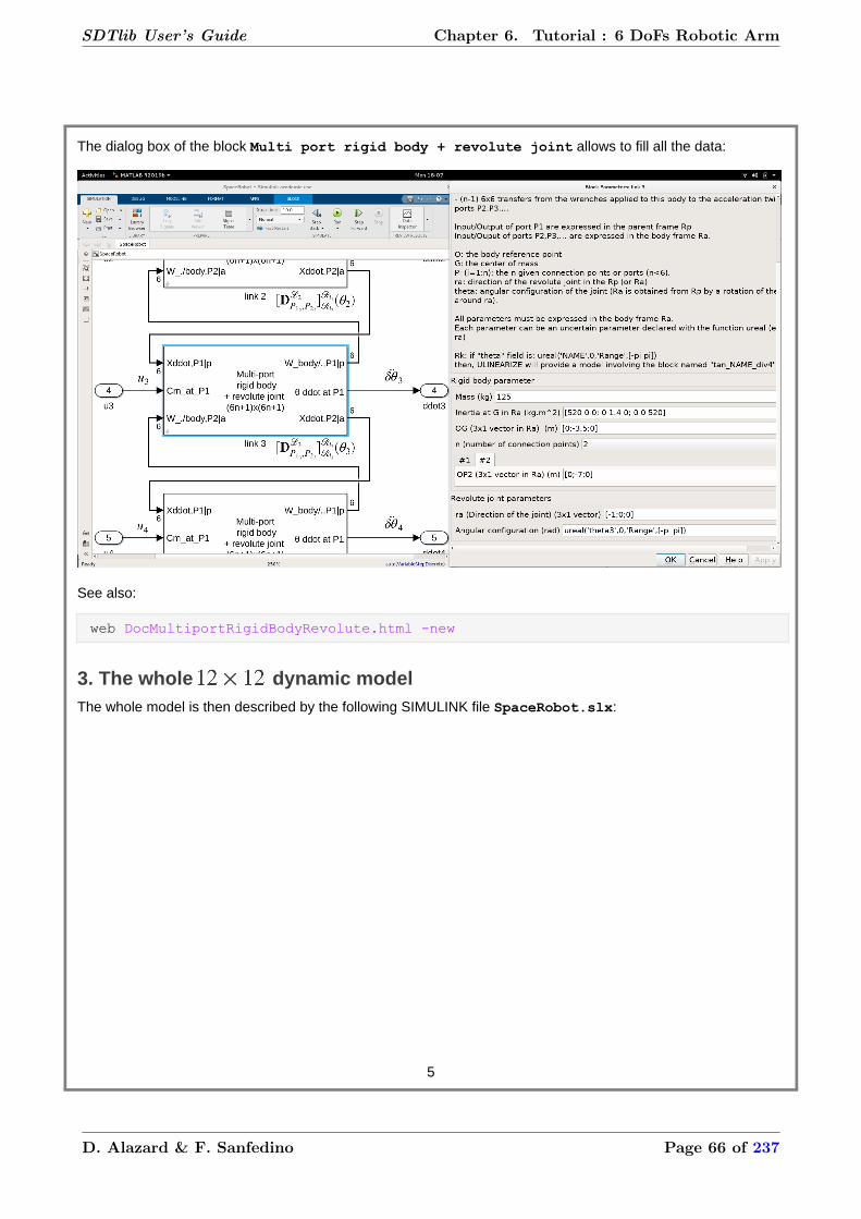
The dialog box of the block Multi port rigid body + revolute joint allows to fill all the data:
See also:
web DocMultiportRigidBodyRevolute.html -new
3. The whole dynamic modelThe whole model is then described by the following SIMULINK file SpaceRobot.slx:
5
SDTlib User’s Guide Chapter 6. Tutorial : 6 DoFs Robotic Arm
D. Alazard & F. Sanfedino Page 66 of 237

SpaceRobot % the SIMULINK lile of the modelGu=ulinearize('SpaceRobot');
6
SDTlib User’s Guide Chapter 6. Tutorial : 6 DoFs Robotic Arm
D. Alazard & F. Sanfedino Page 67 of 237

Mu=inv(Gu) % the mass matrix is the inverse of the model Gu.
Mu =
Uncertain continuous-time state-space model with 12 outputs, 12 inputs, 0 states. The model uncertainty consists of the following blocks: tan_theta1_div4: Uncertain real, nominal = 0, range = [-1,1], 16 occurrences tan_theta2_div4: Uncertain real, nominal = 0, range = [-1,1], 16 occurrences tan_theta3_div4: Uncertain real, nominal = 0, range = [-1,1], 16 occurrences tan_theta4_div4: Uncertain real, nominal = 0, range = [-1,1], 16 occurrences tan_theta5_div4: Uncertain real, nominal = 0, range = [-1,1], 16 occurrences tan_theta6_div4: Uncertain real, nominal = 0, range = [-1,1], 16 occurrences
Type "Mu.NominalValue" to see the nominal value, "get(Mu)" to see all properties, and "Mu.Uncertainty" to interact with the uncertain elements.
This mass matrix depends on 6 uncertain parameters , with an occurence of for each
parameter.
4. First analysesThe mass matrix in the nominal configuration:
M0=Mu.NominalValue
M0 = D = ddot_X_B(1) ddot_X_B(2) ddot_X_B(3) ddot_X_B(4) ddot_X_B(5) ddot_X_B(6) W_.//B,B(1) 1387 0 0 0 566 2953 W_.//B,B(2) 0 1387 -1.252e-12 -566 0 0 W_.//B,B(3) 0 -5.493e-11 1387 -2953 0 0 W_.//B,B(4) 0 -566 -2953 3.557e+04 0 0 W_.//B,B(5) 566 0 0 0 1502 4429 W_.//B,B(6) 2953 0 0 0 4429 3.474e+04 u1 2953 0 0 0 4429 3.408e+04 u2 0 -6.339e-10 2953 -3.408e+04 0 0 u3 0 -2.962e-10 1205 -1.592e+04 0 0 u4 0 -2.443e-11 89.6 -1313 0 0 u5 38.4 0 0 0 57.6 572.2 u6 6.308e-15 0 0 0 -0.34 5.563e-14 ddot1 ddot2 ddot3 ddot4 ddot5 ddot6 W_.//B,B(1) 2953 0 0 0 38.4 1.645e-16 W_.//B,B(2) 0 -1.621e-11 -6.86e-12 -6.228e-13 0 0 W_.//B,B(3) 0 2953 1205 89.6 0 0 W_.//B,B(4) 0 -3.408e+04 -1.592e+04 -1313 0 0 W_.//B,B(5) 4429 0 0 0 57.6 -0.34 W_.//B,B(6) 3.408e+04 0 0 0 572.2 5.9e-17 u1 3.408e+04 0 0 0 572.2 5.9e-17 u2 0 3.408e+04 1.592e+04 1313 0 0 u3 0 1.592e+04 8206 739.6 0 0 u4 0 1313 739.6 112.4 0 0 u5 572.2 0 0 0 33.04 2.204e-19 u6 5.563e-14 0 0 0 7.23e-16 0.34 Static gain.
The mass matrix of the robotic arm when the chaser is clamped on the inertial frame (in the nominal
configuration):
7
SDTlib User’s Guide Chapter 6. Tutorial : 6 DoFs Robotic Arm
D. Alazard & F. Sanfedino Page 68 of 237

M0(7:12,7:12)
ans = D = ddot1 ddot2 ddot3 ddot4 ddot5 ddot6 u1 3.408e+04 0 0 0 572.2 5.9e-17 u2 0 3.408e+04 1.592e+04 1313 0 0 u3 0 1.592e+04 8206 739.6 0 0 u4 0 1313 739.6 112.4 0 0 u5 572.2 0 0 0 33.04 2.204e-19 u6 5.563e-14 0 0 0 7.23e-16 0.34 Static gain.
The mass matrix of the robotic arm when the chaser is free to move (in the nominal configuration):
inv(Gu.NominalValue(7:12,7:12))
ans = D = ddot1 ddot2 ddot3 ddot4 ddot5 ddot6 u1 644.8 0 0 0 12.63 0.02836 u2 0 1212 582.5 48.96 0 0 u3 0 582.5 1022 146 0 0 u4 0 48.96 146 63.28 0 0 u5 12.63 0 0 0 23.32 -0.005118 u6 0.02836 0 0 0 -0.005118 0.3399 Static gain.
Worst-case analysis:The models Gu and Mu are fully compatible with the robust control toolbox. To illustrate worst-case analysis, let
us consider the computation of the angular configuration leading to the maximal inertia seen by the chaser
around its ( ) axis, that is to say, the 5-th input/output chanel of the model Mu:
Obviously, considering the system geometric configuration depicted in the first Figure, the inertia around the (
) axis is maximal for : .
It is a little bit disapointing to see that the function wcgain fails to find this worst-case. Indeed:
[WCG,WCU] = wcgain(Mu(5,5))
WCG = struct with fields: LowerBound: 8.1894e+03 UpperBound: Inf CriticalFrequency: 0WCU = struct with fields: tan_theta1_div4: 0.5985 tan_theta2_div4: 0.6335 tan_theta3_div4: 0.6335 tan_theta4_div4: 0.5619 tan_theta5_div4: 0.2259 tan_theta6_div4: -0.3375
8
SDTlib User’s Guide Chapter 6. Tutorial : 6 DoFs Robotic Arm
D. Alazard & F. Sanfedino Page 69 of 237

One can use the "home-made" function wcpeak to recover (approximatively) the obvious answer:
[WCG,WCU] = wcpeak(Mu(5,5))
WCG = struct with fields: LowerBound: 4.4431e+04 CriticalFrequency: 0 UpperBound: 4.6707e+04WCU = struct with fields: tan_theta1_div4: 0 tan_theta2_div4: 0.4123 tan_theta3_div4: 0.0027 tan_theta4_div4: 0.0027 tan_theta5_div4: 0 tan_theta6_div4: 0
Note that and do not impact this worst-case configuration.
The worst case inertia is:
usubs(Mu(5,5),WCU)
ans = D = ddot_X_B(5) W_.//B,B(5) 4.443e+04 Static gain.
5. Flexible robotic arm on the chaserThe flexibility of links and (with a very long aspect ratio) is now taken into account. They are modelled as
uniform aluminium beams with circular cross section (radius: , thickness: ) to have the same mass/
inertia than the rigid links used in the previous model.
The 6 d.o.f. of a flexible beam is modelled with a TITOP "superelement" embedded in the bock 2 ports
flexible beam of the sub-library 6 dof bodies of the SDTlib and/or in the block TITOP flexiblebeam+revolute joint (which takes into account a revolute joint at one tip of the beam) in the library
Predefined subsystems.
This model is expressed in the local frame of the beam assuming that is along the beam
axis (see next Figure) . This model considers 4 bending modes in the plane ( ), 4 bending modes in the
plane ( ), 1 torsion mode around and one traction mode along .
9
SDTlib User’s Guide Chapter 6. Tutorial : 6 DoFs Robotic Arm
D. Alazard & F. Sanfedino Page 70 of 237

See also:
web DocBeam.html -newweb DocBeamRevolute.html -new
Since and are no more aligned with , the DCM must be taken into account (see
following Figure).
SpaceFlexibleRobotGuf=ulinearize('SpaceFlexibleRobot');Muf=inv(Guf)
Muf =
10
SDTlib User’s Guide Chapter 6. Tutorial : 6 DoFs Robotic Arm
D. Alazard & F. Sanfedino Page 71 of 237

Uncertain continuous-time state-space model with 12 outputs, 12 inputs, 40 states. The model uncertainty consists of the following blocks: tan_theta1_div4: Uncertain real, nominal = 0, range = [-1,1], 16 occurrences tan_theta2_div4: Uncertain real, nominal = 0, range = [-1,1], 16 occurrences tan_theta3_div4: Uncertain real, nominal = 0, range = [-1,1], 16 occurrences tan_theta4_div4: Uncertain real, nominal = 0, range = [-1,1], 16 occurrences tan_theta5_div4: Uncertain real, nominal = 0, range = [-1,1], 16 occurrences tan_theta6_div4: Uncertain real, nominal = 0, range = [-1,1], 16 occurrences
Type "Muf.NominalValue" to see the nominal value, "get(Muf)" to see all properties, and "Muf.Uncertainty" to interact with the uncertain elements.
One can check that the DCgain of the (dynamic) mass matrices are almost the same ones in the rigid case
and in the flexible case (with the rounding errors in the computation of the inertia and mass) for any parametric
configurations (the maximal relative error is around ).
figuresigma(eye(12)-Muf/Mu)
The next Figure compares the frequency domain response (singular values plot) of the mass matrix seen
from arm joints when:
• the chaser is locked on the inertial frame, i.e. when the 6 inputs (blue plot)
• the chaser is free to move, i.e. when the 6 inputs (red plot),
in the nominal configuration.
figure
11
SDTlib User’s Guide Chapter 6. Tutorial : 6 DoFs Robotic Arm
D. Alazard & F. Sanfedino Page 72 of 237

sigma(Muf.NominalValue(7:12,7:12),inv(Guf.NominalValue(7:12,7:12)))
The next figure plots the same response for a set of random parametric confgurations:
figuresigma(Muf(7:12,7:12),inv(Guf(7:12,7:12)))
12
SDTlib User’s Guide Chapter 6. Tutorial : 6 DoFs Robotic Arm
D. Alazard & F. Sanfedino Page 73 of 237

6. Chaser + flexible robotic arm + flexible targetThe previous robotic arm graps now a target which corresponds to the spacecraft (with 2 flexible solar
arrays) studied in the tutorial 1. The end effector of the arm (point ) holds by the point (renamed ) of
the target main body (see tutorial 2) in the configuration described in the following Figure:
13
SDTlib User’s Guide Chapter 6. Tutorial : 6 DoFs Robotic Arm
D. Alazard & F. Sanfedino Page 74 of 237

The DCM from the target frame to the end-effector frame is: .
To model the system composed of the chaser, the robotic arm and the target, one can reuse the SIMULINK
file developed in the tutorial 1 as the subsystem Target in positive feedback on the subsystem Chaser+Armdeveloped in the previous section. The whole block diagram is then depicted in the following Figure:
14
SDTlib User’s Guide Chapter 6. Tutorial : 6 DoFs Robotic Arm
D. Alazard & F. Sanfedino Page 75 of 237

The target model is the direct mass model (with a minus sign) of the target between the
acceleration twist prescribed by the arm end effector at the point (input) and the wrench
applied by the target to the end effector at the point . This model is the same than the model
used in the tutorial 2 but the block multi port rigid body used for the target main body must have now 4
ports P1, P2, P3, P4 corresponding to the points twice (one times to connect the solar array, one times
for the connection with arm end effector), and and the port P1 must be inverted. The subsystem Target
is detailled in the following Figure.
15
SDTlib User’s Guide Chapter 6. Tutorial : 6 DoFs Robotic Arm
D. Alazard & F. Sanfedino Page 76 of 237

SpaceFlexibleRobotLoadGufl=ulinearize('SpaceFlexibleRobotLoad')
Gufl =
Uncertain continuous-time state-space model with 12 outputs, 12 inputs, 56 states. The model uncertainty consists of the following blocks: tan_Theta_div4: Uncertain real, nominal = 0, range = [-1,1], 32 occurrences tan_theta1_div4: Uncertain real, nominal = 0, range = [-1,1], 16 occurrences tan_theta2_div4: Uncertain real, nominal = 0, range = [-1,1], 16 occurrences tan_theta3_div4: Uncertain real, nominal = 0, range = [-1,1], 16 occurrences tan_theta4_div4: Uncertain real, nominal = 0, range = [-1,1], 16 occurrences tan_theta5_div4: Uncertain real, nominal = 0, range = [-1,1], 16 occurrences tan_theta6_div4: Uncertain real, nominal = 0, range = [-1,1], 16 occurrences
Type "Gufl.NominalValue" to see the nominal value, "get(Gufl)" to see all properties, and "Gufl.Uncertainty" to interact with the uncertain elements.
The model order is now ; equal to the chaser+arm model order ( ) plus the target model order ( ). The
model depends on 7 parameters: the 6 arm joint angular configurations and the angular configuration of target
solar arrays.
First analyzesThe next figure plots the pole/zero map for various parametric configurations and for the nominal configuration
(in red):
figurepzmap(Gufl,Gufl.NominalValue)sgrid
16
SDTlib User’s Guide Chapter 6. Tutorial : 6 DoFs Robotic Arm
D. Alazard & F. Sanfedino Page 77 of 237

Although all the modes are badly damped, they are of course always stable for any parametric configurations
since the model is the result of the connection of passive flexible bodies. Nethertheless, it is surprising to see
that (around ), 2 modes are damped up to .
The dynamic couplings between the various bodies and their flexible modes depend on the boundary condition
applied by the joint controller (not still designed). They can be illustrated on the frequency-domain response,
in the nominal configuration, of the transfer between the 3 torques applied on the chaser to
control its attitude and the 3 angular accelerations of the chaser (i.e. the channels 4 to 6 of the
model Gufl):
• when the 6 arm joints are free. The response is in blue in the next Figure,
• when the 6 arm joints are locked. The response is in red in the next Figure. The model when the joints
are locked (i.e.: ) is simply obtained by the inversion of the channel 7 to 12 of the
model Gufl thanks to the function invio.
See also:
web docInvio.html -new
The frequency domain response in the frequency band: :
Gufl_lock=invio(Gufl,7:12);figure
17
SDTlib User’s Guide Chapter 6. Tutorial : 6 DoFs Robotic Arm
D. Alazard & F. Sanfedino Page 78 of 237

bodemag(Gufl.NominalValue(4:6,4:6),Gufl_lock.NominalValue(4:6,4:6),1,1000)
7. Remark
• the SDT is used to compute the linear dynamic model of multi-body systems around a given geometric
configuration. This geometric configuration is considered as a varing parameter. Geometric constraints,
for instance to avoid colision between the arm and the chaser, are not considered in this toolbox.
18
SDTlib User’s Guide Chapter 6. Tutorial : 6 DoFs Robotic Arm
D. Alazard & F. Sanfedino Page 79 of 237

Tutorial 7: Cantilevered plate dynamics studied with SDTlib block:
NINOP Nastran body ( run)
Table of Contents
1. Description........................................................................................................................................................... 12. Importing the NASTRAN model in SDTlib.......................................................................................................... 23. SIMULATION....................................................................................................................................................... 3
by D. Alazard and F. Sanfedino - ISAE-SUPAERO
1. Description(this tutorial has an animation at the end of this live script)
In this tutorial we shown how to directly use the results coming from NATRAN modal analysis to build a NINOP
model in the SDTlib.
A NINOP model of a bending plate is taken as appication example.
Let consider the PATRAN model in the next figure:
A squared plate of 1m size is meshed with 10 elements CQUAD4 per side. See fbdf_plate.bdf file for
details on mechanical properties. The total number of nodes is the 121.
This plate is blocked (all 6 DOF) in the node P. All the other nodes are left free.
NASTRAN SOL 103 routine provides the result of the modal analysis like in the next figure for the first mode:
1
SDTlib User’s Guide Chapter 7. Tutorial : NASTRAN Multi-Port Model
7. Tutorial : NASTRAN Multi-Port Model
D. Alazard & F. Sanfedino Page 80 of 237

2. Importing the NASTRAN model in SDTlibWe want now to build the NINOP model of this structure by recovering the dynamic model at the 9 nodes
showed in the next figure. Note that the corresponding node index (N.B. the indexes are the same as in the
PATRAN mesh).
We introduce the parameters demanded by the block NINOP Nastran body dialog box as done in the
following figure:
2
SDTlib User’s Guide Chapter 7. Tutorial : NASTRAN Multi-Port Model
D. Alazard & F. Sanfedino Page 81 of 237

The reader is advised to read the inline help available in the dialog box (internet connection required), also
available by:
web DocNPortNastranBody.html -new
3. SIMULATIONOnce the NASTRAN NINOP model is ready we can use it for the needed applications. In the next DEMO we
show for instance how to simulate the plate dynamics when subjected to an impulsive force acting at
on the point perpendicular to its face. The last figure depicted the plate deformation acconding to time (it can
take several minutes, be patient...).
T_sim = 3;pulse_width = 2; % Percentage of T_simamp_pulse = 1;dt = 0.01;
% Integrator initial conditions on speed dot_x_0 = zeros(8*6,1);% Integrator initial conditions on position x_0 = [zeros(6,1);... %C1 [.5 0 0 0 0 0]';... %C2
3
SDTlib User’s Guide Chapter 7. Tutorial : NASTRAN Multi-Port Model
D. Alazard & F. Sanfedino Page 82 of 237

[1 0 0 0 0 0]';... %C3 [.5 .5 0 0 0 0]';...%C4 [1 .5 0 0 0 0]';... %C5 [0 1 0 0 0 0]';... %C6 [.5 1 0 0 0 0]';... %C7 [1 1 0 0 0 0]']; %C8
clamped_plate_simulationsim('clamped_plate_simulation')%%N = length(C_x.time);t = C_x.time;X = [C_x.signals.values(:,1:3) zeros(N,1) C_x.signals.values(:,4:end)];Y = [C_y.signals.values(:,1:3) .5.*ones(N,1) C_y.signals.values(:,4:end)];Z = [C_z.signals.values(:,1:3) zeros(N,1) C_z.signals.values(:,4:end)];f = figure;
axis([0 1 0 1 -1e-2 1e-2])[Xs,Ys,Zs] = sphere;
for i = 1:N subplot(2,1,1) tri = delaunay(X(i,:),Y(i,:)); %x,y,z column vectors h = trisurf(tri,X(i,:),Y(i,:),Z(i,:)); colormap(gray) alpha(.5) view(40,30) % set viewpoint axis([0 1 0 1 -max(max(abs(Z)))*1.1 max(max(abs(Z)))*1.1]) hold on plot3(0,.5,0,'.k','MarkerSize',50) if pert.signals.values(i) ~= 0 hold on plot3([1 1],[0 0],[Z(i,5) Z(i,5)-.5e-2],'r-^') hold off end hold off xlabel('x [m]','Interpreter','latex') ylabel('y [m]','Interpreter','latex') zlabel('z [m]','Interpreter','latex')
subplot(2,1,2) plot(t(i),pert.signals.values(i),'.k','MarkerSize',.5) xlabel('t [s]','Interpreter','latex') ylabel('F [N]','Interpreter','latex') hold on axis([0 t(end) -0.2 amp_pulse+.2]) shg refresh(f) pause(1e-5)end
4
SDTlib User’s Guide Chapter 7. Tutorial : NASTRAN Multi-Port Model
D. Alazard & F. Sanfedino Page 83 of 237

5
SDTlib User’s Guide Chapter 7. Tutorial : NASTRAN Multi-Port Model
D. Alazard & F. Sanfedino Page 84 of 237

Tutorial 8: a spacecraft with 2 symmetrical rotating solar arrays
defined by a generic plate model ( run ).
Table of Contents
1. Description........................................................................................................................................................... 12. Plate model..........................................................................................................................................................13. The whole dynamic model................................................................................................................................24. Analyses...............................................................................................................................................................45. Remark.................................................................................................................................................................5
by D. Alazard and F. Sanfedino - ISAE-SUPAERO
1. DescriptionThis tutorial reconsiders the same example already addressed in the tutorial 2 and tutorial 4 but the models
, ( ) of 2 the rotating solar flexible solar arrays are now defined by:
• a generic rectangular uniform plate for each solar array ,
• a revolue joint at the connection point .
2. Plate modelDuring early preliminary design phase, the user could not know:
• neither the flexible mode characteristics (frequencies, modal participation factors, ...) required to fill the
dialog box of the block 1 port flexible body,• nor the NASTAN model required to fill the dialog box of the blocks or 1 port Natran body or Nports Nastran body
to model the solar panels.
To address this situation, a generic Kirchhoff-love model of a uniform rectangular plate was developped. This
model involves flexible modes per plate.
This model is implemented in the block multi-port flexible plate of the SDTlib/6 dof bodies sub-
library. The dialog box (depicted in the following) requires only the geometric data of the plate and the material
characteristics.
WARNING: this block does not support varying or uncertain parameters.
1
SDTlib User’s Guide Chapter 8. Tutorial : Plate Model for Solar Arrays
8. Tutorial : Plate Model for Solar Arrays
D. Alazard & F. Sanfedino Page 85 of 237

The reader is advised to read the inline help available in the dialog box (internet connection required) to have
details on the Kirchhoff-Love model used for the flexible plate, also available by:
web DocPlate_joly.html -new
3. The whole dynamic modelThe whole model is then described by the following SIMULINK file SCwith2SAs_ter.slx:
2
SDTlib User’s Guide Chapter 8. Tutorial : Plate Model for Solar Arrays
D. Alazard & F. Sanfedino Page 86 of 237

SCwith2SAs_ter % the SIMULINK lile of the modelGu=ulinearize('SCwith2SAs_ter')
Gu =
Uncertain continuous-time state-space model with 6 outputs, 8 inputs, 76 states. The model uncertainty consists of the following blocks: tan_Theta_div4: Uncertain real, nominal = 0, range = [-1,1], 32 occurrences
Type "Gu.NominalValue" to see the nominal value, "get(Gu)" to see all properties, and "Gu.Uncertainty" to interact with the uncertain elements.
3
SDTlib User’s Guide Chapter 8. Tutorial : Plate Model for Solar Arrays
D. Alazard & F. Sanfedino Page 87 of 237

As in tutorial 2, one can check that the model have 8 inputs:
• the external wrench (6 components)
• the torque disturbance inside the revolute joint of ,
• the torque disturbance inside the revolute joint of ,
6 outputs: the dual vector of acceleration of point B (6 components),
but 76 states: 38 modes (18 flexible modes + 1 revolute joint mode per appendage).
This model depends on the uncertain parameter (tan_Theta_div4) with 32 occurences.
4. AnalysesAs in tutoroial 2, the same kind of analyses can be now performed on this new model, for instance the
frequency-domain response (Bode magnitude) of the transfer between the torque applied to the
spacecraft at B and its angular acceleration:
figurebodemag(Gu(4:6,4:6),0.1 1000)
4
SDTlib User’s Guide Chapter 8. Tutorial : Plate Model for Solar Arrays
D. Alazard & F. Sanfedino Page 88 of 237

5. Remark
• As the N Ports Nastran body block, this block can be used to build the model of an array of solar
pannels by using additionnal ports to connect the various pannels (see also tutorial 9: a solar arraywith 3 pannels).
5
SDTlib User’s Guide Chapter 8. Tutorial : Plate Model for Solar Arrays
D. Alazard & F. Sanfedino Page 89 of 237

Tutorial 9: a solar array with 3 pannels ( run )
Table of Contents
1. Description........................................................................................................................................................... 12. Model using the SDTlib....................................................................................................................................... 13. Reduction............................................................................................................................................................. 44. Summary..............................................................................................................................................................7
by D. Alazard and F. Sanfedino - ISAE-SUPAERO
1. DescriptionLet us consider a solar array composed of 3 identical pannels , . Each pannel is modelled
by the generic plate model already used in tutorial 8 and corresponds to a quare plate ( ) of
aluminium.
web DocPlate_joly.html -new
The connection points between the 3 pannels are described in the following Figure:
• have 1 parent point and 2 child points and
• have 2 parent points and (where the 2 dual acceleration twists are imposed by ) and 2
child points and ,
• have 2 parent points and (where the 2 dual acceleration twists are imposed by ).
The hinges at the connection points ( , , ) are assumed to be rigid.
2. Model using the SDTlibThe model of the whole array between the acceration twist prescribed at point by the
parent structure and the wrench applied by on this parent structure at point is decribed by the direct
interconnection of the NINOP model of the 3 pannels :
1
SDTlib User’s Guide Chapter 9. Tutorial : Solar Array with 3 Panels
9. Tutorial : Solar Array with 3 Panels
D. Alazard & F. Sanfedino Page 90 of 237

SA_3pannels[a,b,c,d]=linmod('SA_3pannels');M_SA=ss(a,b,c,d);
One can check that the DC gain of this system corresponds (with a minus sign) to the mass/inertia at the point
of a rectangular plate ( ) of aluminium:
L=3;l=1;h=0.01;rho=474;M_SA_G=L*l*h*rho;I_SA_G=M_SA_G/12*diag([l^2 L^2 l^2+L^2]);D_SA_G=[M_SA_G*eye(3) zeros(3);zeros(3) I_SA_G];D_SA_P1=translate_dynamic_model([L/2;l/2;0],[0;l/2;0],D_SA_G)
D_SA_P1 = 6×6 14.2200 0 0 0 0 0 0 14.2200 0 0 0 21.3300 0 0 14.2200 0 -21.3300 0 0 0 0 1.1850 0 0 0 0 -21.3300 0 42.6600 0 0 21.3300 0 0 0 43.8450
-dcgain(M_SA)
ans = 6×6 14.2200 -0.0000 0 0 0 -0.0000 -0.0000 14.2200 0 0 0 21.3300 0 0 14.2200 0.0000 -21.3300 0 0 0 0.0000 1.1851 -0.0000 0
2
SDTlib User’s Guide Chapter 9. Tutorial : Solar Array with 3 Panels
D. Alazard & F. Sanfedino Page 91 of 237

0 0 -21.3300 -0.0000 42.6601 0 -0.0000 21.3300 0 0 0 43.8450
One can also check the dynamics reveals eigenvalues around 0. Exactly as in the acacemic
case presented in Tutorial 5 (in the single axis case) these eigenvalues are due to the kinematics constraints on
the internal states of the model associated to the closed-kinemetic chains.
damp(M_SA)
Pole Damping Frequency Time Constant (rad/seconds) (seconds) 4.73e-04 -1.00e+00 4.73e-04 -2.11e+03 -4.73e-04 1.00e+00 4.73e-04 2.11e+03 7.04e-04 -1.00e+00 7.04e-04 -1.42e+03 -7.04e-04 1.00e+00 7.04e-04 1.42e+03 1.03e-10 + 1.16e-03i -8.81e-08 1.16e-03 -9.75e+09 1.03e-10 - 1.16e-03i -8.81e-08 1.16e-03 -9.75e+09 7.29e-04 + 9.91e-04i -5.92e-01 1.23e-03 -1.37e+03 7.29e-04 - 9.91e-04i -5.92e-01 1.23e-03 -1.37e+03 -7.29e-04 + 9.91e-04i 5.92e-01 1.23e-03 1.37e+03 -7.29e-04 - 9.91e-04i 5.92e-01 1.23e-03 1.37e+03 1.24e-03 -1.00e+00 1.24e-03 -8.08e+02 -1.24e-03 1.00e+00 1.24e-03 8.08e+02 -1.58e-03 + 1.04e+01i 1.52e-04 1.04e+01 6.31e+02 -1.58e-03 - 1.04e+01i 1.52e-04 1.04e+01 6.31e+02 -7.87e-02 + 5.76e+01i 1.37e-03 5.76e+01 1.27e+01 -7.87e-02 - 5.76e+01i 1.37e-03 5.76e+01 1.27e+01 -6.32e-02 + 6.65e+01i 9.50e-04 6.65e+01 1.58e+01 -6.32e-02 - 6.65e+01i 9.50e-04 6.65e+01 1.58e+01 -8.46e-01 + 1.84e+02i 4.61e-03 1.84e+02 1.18e+00 -8.46e-01 - 1.84e+02i 4.61e-03 1.84e+02 1.18e+00 -3.51e-01 + 1.86e+02i 1.89e-03 1.86e+02 2.85e+00 -3.51e-01 - 1.86e+02i 1.89e-03 1.86e+02 2.85e+00 -2.44e+00 + 3.35e+02i 7.29e-03 3.35e+02 4.10e-01 -2.44e+00 - 3.35e+02i 7.29e-03 3.35e+02 4.10e-01 -2.14e+00 + 3.55e+02i 6.04e-03 3.55e+02 4.67e-01 -2.14e+00 - 3.55e+02i 6.04e-03 3.55e+02 4.67e-01 -4.08e+00 + 5.20e+02i 7.83e-03 5.20e+02 2.45e-01 -4.08e+00 - 5.20e+02i 7.83e-03 5.20e+02 2.45e-01 -4.52e+00 + 5.26e+02i 8.60e-03 5.26e+02 2.21e-01 -4.52e+00 - 5.26e+02i 8.60e-03 5.26e+02 2.21e-01 -5.83e+00 + 6.58e+02i 8.87e-03 6.58e+02 1.71e-01 -5.83e+00 - 6.58e+02i 8.87e-03 6.58e+02 1.71e-01 -7.22e+00 + 7.21e+02i 1.00e-02 7.21e+02 1.39e-01 -7.22e+00 - 7.21e+02i 1.00e-02 7.21e+02 1.39e-01 -8.18e+00 + 7.61e+02i 1.07e-02 7.61e+02 1.22e-01 -8.18e+00 - 7.61e+02i 1.07e-02 7.61e+02 1.22e-01 -6.86e+00 + 7.96e+02i 8.61e-03 7.96e+02 1.46e-01 -6.86e+00 - 7.96e+02i 8.61e-03 7.96e+02 1.46e-01 -1.03e+01 + 9.99e+02i 1.03e-02 9.99e+02 9.68e-02 -1.03e+01 - 9.99e+02i 1.03e-02 9.99e+02 9.68e-02 -1.06e+01 + 1.02e+03i 1.04e-02 1.02e+03 9.43e-02 -1.06e+01 - 1.02e+03i 1.04e-02 1.02e+03 9.43e-02 -1.58e+01 + 1.04e+03i 1.51e-02 1.04e+03 6.34e-02 -1.58e+01 - 1.04e+03i 1.51e-02 1.04e+03 6.34e-02 -2.62e+01 + 1.36e+03i 1.93e-02 1.36e+03 3.82e-02 -2.62e+01 - 1.36e+03i 1.93e-02 1.36e+03 3.82e-02 -1.49e+01 + 1.37e+03i 1.09e-02 1.37e+03 6.73e-02 -1.49e+01 - 1.37e+03i 1.09e-02 1.37e+03 6.73e-02 -2.64e+01 + 1.41e+03i 1.87e-02 1.41e+03 3.79e-02
3
SDTlib User’s Guide Chapter 9. Tutorial : Solar Array with 3 Panels
D. Alazard & F. Sanfedino Page 92 of 237

-2.64e+01 - 1.41e+03i 1.87e-02 1.41e+03 3.79e-02 -3.53e+01 + 1.79e+03i 1.97e-02 1.79e+03 2.83e-02 -3.53e+01 - 1.79e+03i 1.97e-02 1.79e+03 2.83e-02 -2.07e+01 + 1.87e+03i 1.11e-02 1.87e+03 4.84e-02 -2.07e+01 - 1.87e+03i 1.11e-02 1.87e+03 4.84e-02 -3.21e+01 + 1.89e+03i 1.69e-02 1.89e+03 3.12e-02 -3.21e+01 - 1.89e+03i 1.69e-02 1.89e+03 3.12e-02 -3.94e+01 + 2.11e+03i 1.87e-02 2.11e+03 2.54e-02 -3.94e+01 - 2.11e+03i 1.87e-02 2.11e+03 2.54e-02 -2.08e+01 + 2.29e+03i 9.10e-03 2.29e+03 4.80e-02 -2.08e+01 - 2.29e+03i 9.10e-03 2.29e+03 4.80e-02 -1.68e+02 + 2.38e+03i 7.06e-02 2.38e+03 5.95e-03 -1.68e+02 - 2.38e+03i 7.06e-02 2.38e+03 5.95e-03 -3.10e+01 + 2.49e+03i 1.24e-02 2.49e+03 3.23e-02 -3.10e+01 - 2.49e+03i 1.24e-02 2.49e+03 3.23e-02 -6.75e+01 + 2.65e+03i 2.55e-02 2.65e+03 1.48e-02 -6.75e+01 - 2.65e+03i 2.55e-02 2.65e+03 1.48e-02 -3.98e+01 + 2.92e+03i 1.36e-02 2.92e+03 2.51e-02 -3.98e+01 - 2.92e+03i 1.36e-02 2.92e+03 2.51e-02 -1.91e+02 + 2.99e+03i 6.36e-02 3.00e+03 5.25e-03 -1.91e+02 - 2.99e+03i 6.36e-02 3.00e+03 5.25e-03 -8.31e+01 + 3.31e+03i 2.51e-02 3.31e+03 1.20e-02 -8.31e+01 - 3.31e+03i 2.51e-02 3.31e+03 1.20e-02 -1.46e+02 + 3.69e+03i 3.95e-02 3.69e+03 6.86e-03 -1.46e+02 - 3.69e+03i 3.95e-02 3.69e+03 6.86e-03 -2.34e+02 + 3.80e+03i 6.16e-02 3.80e+03 4.27e-03 -2.34e+02 - 3.80e+03i 6.16e-02 3.80e+03 4.27e-03 -7.25e+01 + 4.19e+03i 1.73e-02 4.19e+03 1.38e-02 -7.25e+01 - 4.19e+03i 1.73e-02 4.19e+03 1.38e-02 -4.25e+02 + 4.36e+03i 9.72e-02 4.38e+03 2.35e-03 -4.25e+02 - 4.36e+03i 9.72e-02 4.38e+03 2.35e-03 -3.42e+02 + 4.66e+03i 7.32e-02 4.68e+03 2.92e-03 -3.42e+02 - 4.66e+03i 7.32e-02 4.68e+03 2.92e-03 -2.85e+02 + 4.93e+03i 5.78e-02 4.94e+03 3.51e-03 -2.85e+02 - 4.93e+03i 5.78e-02 4.94e+03 3.51e-03 -2.22e+02 + 5.21e+03i 4.26e-02 5.21e+03 4.51e-03 -2.22e+02 - 5.21e+03i 4.26e-02 5.21e+03 4.51e-03 -2.00e+03 + 5.47e+03i 3.44e-01 5.83e+03 4.99e-04 -2.00e+03 - 5.47e+03i 3.44e-01 5.83e+03 4.99e-04 -4.29e+02 + 6.44e+03i 6.64e-02 6.45e+03 2.33e-03 -4.29e+02 - 6.44e+03i 6.64e-02 6.45e+03 2.33e-03 -1.38e+03 + 6.42e+03i 2.09e-01 6.57e+03 7.27e-04 -1.38e+03 - 6.42e+03i 2.09e-01 6.57e+03 7.27e-04 -6.17e+01 + 6.62e+03i 9.32e-03 6.62e+03 1.62e-02 -6.17e+01 - 6.62e+03i 9.32e-03 6.62e+03 1.62e-02 -1.32e+02 + 6.77e+03i 1.95e-02 6.77e+03 7.58e-03 -1.32e+02 - 6.77e+03i 1.95e-02 6.77e+03 7.58e-03 -1.62e+03 + 6.80e+03i 2.32e-01 6.99e+03 6.17e-04 -1.62e+03 - 6.80e+03i 2.32e-01 6.99e+03 6.17e-04 -8.67e+02 + 7.56e+03i 1.14e-01 7.61e+03 1.15e-03 -8.67e+02 - 7.56e+03i 1.14e-01 7.61e+03 1.15e-03 -9.44e+02 + 9.69e+03i 9.70e-02 9.73e+03 1.06e-03 -9.44e+02 - 9.69e+03i 9.70e-02 9.73e+03 1.06e-03 -9.94e+02 + 1.06e+04i 9.35e-02 1.06e+04 1.01e-03 -9.94e+02 - 1.06e+04i 9.35e-02 1.06e+04 1.01e-03 -3.54e+02 + 1.08e+04i 3.28e-02 1.08e+04 2.83e-03 -3.54e+02 - 1.08e+04i 3.28e-02 1.08e+04 2.83e-03 -7.62e+02 + 1.28e+04i 5.92e-02 1.29e+04 1.31e-03 -7.62e+02 - 1.28e+04i 5.92e-02 1.29e+04 1.31e-03
3. Reduction
4
SDTlib User’s Guide Chapter 9. Tutorial : Solar Array with 3 Panels
D. Alazard & F. Sanfedino Page 93 of 237

In this system, there are closed-kinematic chains (1 between and and the other one between
and ). The kinematic contraints on the rigid behavior of a plate (i.e. the 2 translations along -axis and
-axis and the rotation around -axis) are solved inside the bock multi-port flexible plate. But for
the ( ) flexible d.o.f. behaviors (i.e. the 2 rotations around -axis and -axis and the translation along
-axis), the 2 kinematic constraints (one on the position and one on the velocity) per d.o.f. depends on the
boundary conditions at the parent points and child points. In a very general way, it can be checked, that once
the system (or the mechanism) is assembled, the number of eigenvalues at 0 is:
.
Since the model considers the transfer at the point which is not involved in the closed-kinematic
chains, these eigvalues can be reduced using the functions:
• minreal (if it works.., it is not the case in this application since only a few eigenvalues among 12 are
removed),
• red_slow (a dedicated function for this kind of application; see also: help red_slow). This function
plots also the frequency-domain responses (sigma plots) of full and reduced models to check if the
trucature is relevant.
minreal(M_SA);
1 state removed.
M_SAr=red_slow(M_SA,0.9);
12 states removed
5
SDTlib User’s Guide Chapter 9. Tutorial : Solar Array with 3 Panels
D. Alazard & F. Sanfedino Page 94 of 237

Once reduced the model is a -th order model with flexible modes spread between an
.
For control design purpose, such a model can be reduced using a balanced reduction. The following MATLAB
sequence reduced the model to a order model (10 modes) and compare it with full-order model in the
frequency-domain.
M_SArb=balreal(M_SAr);M_SArbr=modred(M_SArb,[21:96]);figuresigma(M_SA,M_SArbr,M_SA-M_SArbr,1,10000)legend('96-th order full model','20-th order reduced model','difference')
6
SDTlib User’s Guide Chapter 9. Tutorial : Solar Array with 3 Panels
D. Alazard & F. Sanfedino Page 95 of 237

4. SummaryThe SDTlib can be used to model complex mechanisms of flexible bodies with closed-kinematic chains. The
obtained model can be a high order model. When reducing it, it is recommended to proceed in 2 steps:
• first reduce eigenvalues around 0 due to kinematic constraints using a modal troncature (function
red_slow) or a minimal realiization (function minreal). The number of eigenvalues to be reduced can
be known by a kinematic analysis of the mechanism,
• second, reduce high frequency flexible modes using a balanced reduction.
7
SDTlib User’s Guide Chapter 9. Tutorial : Solar Array with 3 Panels
D. Alazard & F. Sanfedino Page 96 of 237

Tutorial 10: on-board angular momentum ( run).
Table of Contents
1. Description........................................................................................................................................................... 12. Single on-board angular momentum................................................................................................................... 23. Reaction wheels system......................................................................................................................................54. Remark...............................................................................................................................................................12
by D. Alazard and F. Sanfedino - ISAE-SUPAERO
1. DescriptionThis tutorial aims to show how on-board angular monentums can be taken into account in a SIMULINK model
based on the SDTlib. Indeed the gyroscopic stiffness due to an on-board angular moementum is a linear term
which can be modelled thanks to the block One-port angular momentum of the sub-library 6 dofbodies.
Let is consider a wheel with an inertia , spinning at the angular rate arount the axis in the inherit
frame i.e. the frame of the parent body carrying the wheel at the point P. The direction of in is defined
by the azimuth and the elevation angles:
Assuming that the wheel is balanced , the angular rate is constant and the wheel axis is constant in ,
it is thus possible to derive the direct dynamic model of the spining wheel system at the
connection point P and projected in the inherit frame . This model is detailled in the inline help of the block
One-port angular momentum:
web DocMomentum.html -new
1
SDTlib User’s Guide Chapter 10. Tutorial : On-Board Angular Momentum
10. Tutorial : On-Board Angular Momentum
D. Alazard & F. Sanfedino Page 97 of 237
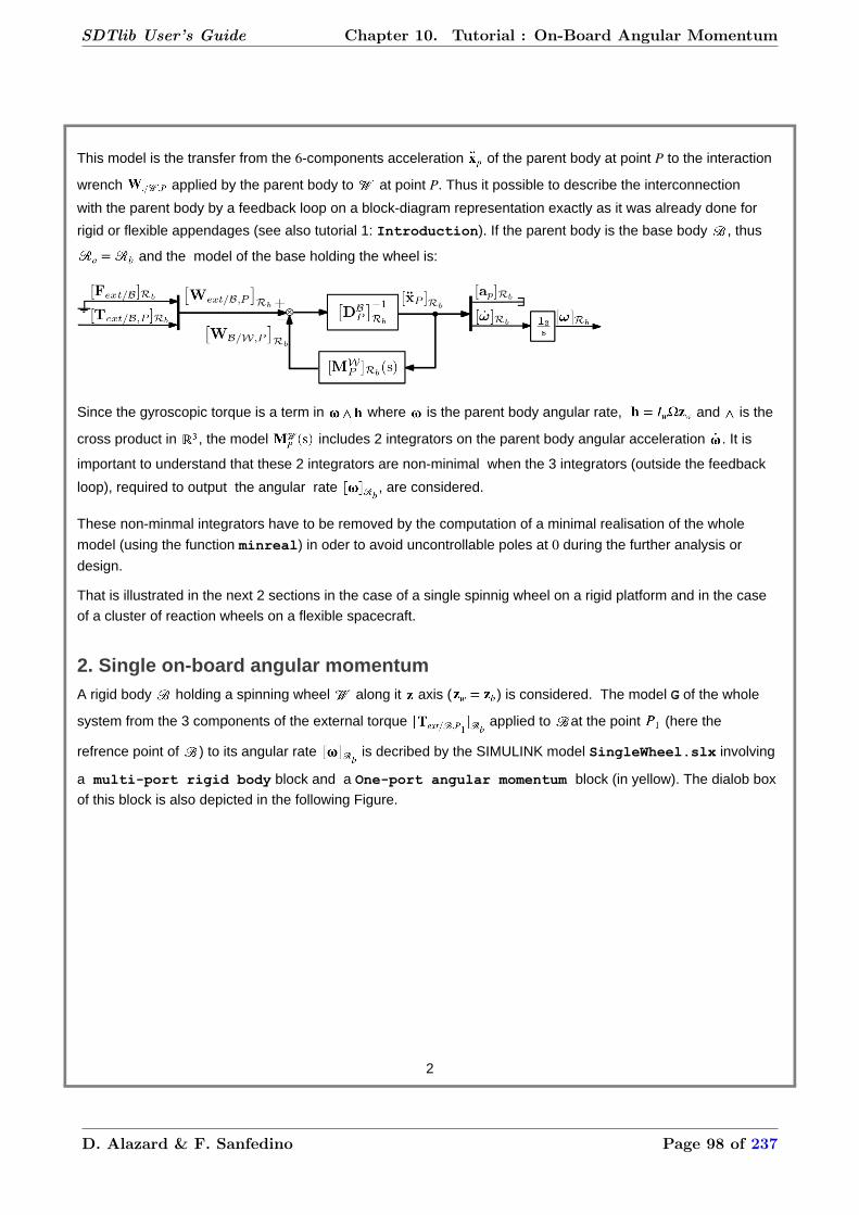
This model is the transfer from the 6-components acceleration of the parent body at point P to the interaction
wrench applied by the parent body to at point P. Thus it possible to describe the interconnection
with the parent body by a feedback loop on a block-diagram representation exactly as it was already done for
rigid or flexible appendages (see also tutorial 1: Introduction). If the parent body is the base body , thus
and the model of the base holding the wheel is:
Since the gyroscopic torque is a term in where is the parent body angular rate, and is the
cross product in , the model includes 2 integrators on the parent body angular acceleration . It is
important to understand that these 2 integrators are non-minimal when the 3 integrators (outside the feedback
loop), required to output the angular rate , are considered.
These non-minmal integrators have to be removed by the computation of a minimal realisation of the whole
model (using the function minreal) in oder to avoid uncontrollable poles at 0 during the further analysis or
design.
That is illustrated in the next 2 sections in the case of a single spinnig wheel on a rigid platform and in the case
of a cluster of reaction wheels on a flexible spacecraft.
2. Single on-board angular momentumA rigid body holding a spinning wheel along it axis ( ) is considered. The model G of the whole
system from the 3 components of the external torque applied to at the point (here the
refrence point of ) to its angular rate is decribed by the SIMULINK model SingleWheel.slx involving
a multi-port rigid body block and a One-port angular momentum block (in yellow). The dialob box
of this block is also depicted in the following Figure.
2
SDTlib User’s Guide Chapter 10. Tutorial : On-Board Angular Momentum
D. Alazard & F. Sanfedino Page 98 of 237

The model directly derived from this SIMULINK model:
SingleWheel[a,b,c,d]=linmod('SingleWheel');G=ss(a,b,c,d);
One can check that the model G have 5 states and thus 5 eigenvalues:
• 2 coming form the One-port angular momentum block, i.e. the 2 integrators which are moved (due
to the feedback loop) to the 2-nd order oscillating gyroscopic mode,
• 3 from the Integrator on the output:
damp(G)
Pole Damping Frequency Time Constant (rad/seconds) (seconds) 0.00e+00 -1.00e+00 0.00e+00 Inf 0.00e+00 -1.00e+00 0.00e+00 Inf 0.00e+00 -1.00e+00 0.00e+00 Inf -8.67e-19 + 1.83e-01i 4.75e-18 1.83e-01 1.15e+18 -8.67e-19 - 1.83e-01i 4.75e-18 1.83e-01 1.15e+18
A minimal realisation of G removes 2 states and more exactly 2 poles at 0:
Gm=minreal(G);
2 states removed.
3
SDTlib User’s Guide Chapter 10. Tutorial : On-Board Angular Momentum
D. Alazard & F. Sanfedino Page 99 of 237

damp(Gm)
Pole Damping Frequency Time Constant (rad/seconds) (seconds) 4.76e-21 -1.00e+00 4.76e-21 -2.10e+20 -3.47e-17 + 1.83e-01i 1.90e-16 1.83e-01 2.88e+16 -3.47e-17 - 1.83e-01i 1.90e-16 1.83e-01 2.88e+16
The frequency-domain response of G:
figurebodemag(Gm,0.001 10)grid
Since the angular momentum is along the -axis of the main body, one can check:
• the gyroscopic stiffness on and axes and the resonnance due to the gyroscopic mode (at
. The distrubance rejection due to the gyroscopic effect is highlighted: a very low
frequency torque (input) on (resp. ) axis does not create an angular rate around the (resp. ) axis.
• this effect is not visible on the transfer around -axis (the angular momentum axis) which is thus free to
move. This transfer exhibits a pole zero cancellation at . Indeed:
zpk(Gm(3,3))
ans =
4
SDTlib User’s Guide Chapter 10. Tutorial : On-Board Angular Momentum
D. Alazard & F. Sanfedino Page 100 of 237

0.012497 (s^2 + 0.03334) ------------------------ s (s^2 + 0.03338) Continuous-time zero/pole/gain model.
3. Reaction wheels systemThe spacecraft model studied in Tutorial t is reconsidered with
• only one rotating SA (Solar Array): is geometric configuration of the SA w.r.t the main body ,
• a reaction wheel systems (RWS) carried by the main body at its center of mass
The reaction wheel system is composed of 4 reaction wheels in a pyramidal configuration described in the
following Figure:
Each wheel has a maximal angular momentum of with a maximal spinning rate of . The
pyramid geometry (azimth and elevation angles) is summarized in the following table:
Note that if all the wheels are spinning at the same angular rate, the total angular momentum is null: .
The objective is to build the model of the whole system between the 3
component torque applied to the main body at the point (by the RWS itself or by orbital
diistrurbances) and the main body angular rate , projected in the frame and fully parameterized
5
SDTlib User’s Guide Chapter 10. Tutorial : On-Board Angular Momentum
D. Alazard & F. Sanfedino Page 101 of 237

according to the SA angular configuration and the 4 spinning rates , of the 4 wheels. Each of
the can vary between , the nominal value being 0.
To model such a reaction wheel systems with 4 reaction wheel subsystems, it is recommanded to user a
massless connection body block from the 6 dof body sub-library. See also:
web DocMassLessBody.html -new
Indeed this block allows to extend the number of connection ports of the multi-port rigid body block
which is limited to 5. Then the reaction wheel system is decribed in the following Figure and is embedded in the
subsystem RWS.
6
SDTlib User’s Guide Chapter 10. Tutorial : On-Board Angular Momentum
D. Alazard & F. Sanfedino Page 102 of 237

7
SDTlib User’s Guide Chapter 10. Tutorial : On-Board Angular Momentum
D. Alazard & F. Sanfedino Page 103 of 237

The subsystem RWS is then connected to the main body like the other appendage (SA) in the SIMULINK file
SCwith1SA_RWs.slx (see next Figure).
The data relative to the reaction wheel system:
wRW=20000*pi/60; % max spinning rate (10000 rpm in rad/s)mRW=0; % Mass (Kg) IrRW=0; % Radial inertia (Kgm^2)IwRW=100/wRW; % Axial inertia (Kgm^2) for a maximal momentum of 100 NmsazimuthRW=[0 90 180 -90]*pi/180; % the list of azimuht angles (rad)elevationRW=[45 -45 45 -45]*pi/180; % the list of elevations angles (rad)wRW1=ureal('RW1',0,'PlusMinus',wRW); % varying spinning rates (rad/s)wRW2=ureal('RW2',0,'PlusMinus',wRW);wRW3=ureal('RW3',0,'PlusMinus',wRW);wRW4=ureal('RW4',0,'PlusMinus',wRW);
The model directly derived from this SIMULINK model:
% the whole modelSCwith1SA_RWs
8
SDTlib User’s Guide Chapter 10. Tutorial : On-Board Angular Momentum
D. Alazard & F. Sanfedino Page 104 of 237

Gu=ulinearize('SCwith1SA_RWs')
Gu =
Uncertain continuous-time state-space model with 3 outputs, 3 inputs, 19 states. The model uncertainty consists of the following blocks: RW1: Uncertain real, nominal = 0, variability = [-1.05e+03,1.05e+03], 2 occurrences RW2: Uncertain real, nominal = 0, variability = [-1.05e+03,1.05e+03], 2 occurrences RW3: Uncertain real, nominal = 0, variability = [-1.05e+03,1.05e+03], 2 occurrences RW4: Uncertain real, nominal = 0, variability = [-1.05e+03,1.05e+03], 2 occurrences tan_Theta_div4: Uncertain real, nominal = 0, range = [-1,1], 16 occurrences
Type "Gu.NominalValue" to see the nominal value, "get(Gu)" to see all properties, and "Gu.Uncertainty" to interact with the uncertain elements.
The model have 19 state variables:
• 3 flexible modes for the solar array (thus 6 states)
• 1 mode for the mechanism between the main body and the solar array (2 states)
• 4 pairs of integrators in the 4 spinning wheels (8 states)
• 3 integrators on the output ( ).
This model depends on 5 varying parameters: RW1, RW2, RW3, RW4: the spinning rates of the wheels and
tan_Theta_div4 ( ): the angular configuration of the solar pannel.
damp(Gu) % poles of the system in the nominal configuration
Pole Damping Frequency Time Constant (rad/seconds) (seconds) 0.00e+00 -1.00e+00 0.00e+00 Inf 0.00e+00 -1.00e+00 0.00e+00 Inf 0.00e+00 -1.00e+00 0.00e+00 Inf 0.00e+00 -1.00e+00 0.00e+00 Inf 0.00e+00 -1.00e+00 0.00e+00 Inf 0.00e+00 -1.00e+00 0.00e+00 Inf 0.00e+00 -1.00e+00 0.00e+00 Inf 0.00e+00 -1.00e+00 0.00e+00 Inf 0.00e+00 -1.00e+00 0.00e+00 Inf 0.00e+00 -1.00e+00 0.00e+00 Inf 0.00e+00 -1.00e+00 0.00e+00 Inf -6.05e-02 + 8.24e+00i 7.34e-03 8.24e+00 1.65e+01 -6.05e-02 - 8.24e+00i 7.34e-03 8.24e+00 1.65e+01 -1.31e-01 + 1.99e+01i 6.60e-03 1.99e+01 7.61e+00 -1.31e-01 - 1.99e+01i 6.60e-03 1.99e+01 7.61e+00 -1.97e-01 + 3.71e+01i 5.32e-03 3.71e+01 5.07e+00 -1.97e-01 - 3.71e+01i 5.32e-03 3.71e+01 5.07e+00 -2.34e+01 + 1.57e+02i 1.47e-01 1.59e+02 4.27e-02 -2.34e+01 - 1.57e+02i 1.47e-01 1.59e+02 4.27e-02
The nomimal model dynamics exhibits 11 poles at 0 since the spinning rates are null for the nominal model (no
gyroscopic stiffness).
A minimal realisation of the model removes 8 states and more exactly 8 poles at 0:
Gum=minreal(Gu);
8 states removed.
9
SDTlib User’s Guide Chapter 10. Tutorial : On-Board Angular Momentum
D. Alazard & F. Sanfedino Page 105 of 237

damp(Gum)
Pole Damping Frequency Time Constant (rad/seconds) (seconds) 2.76e-13 -1.00e+00 2.76e-13 -3.62e+12 -3.30e-13 1.00e+00 3.30e-13 3.03e+12 1.31e-12 -1.00e+00 1.31e-12 -7.64e+11 -6.05e-02 + 8.24e+00i 7.34e-03 8.24e+00 1.65e+01 -6.05e-02 - 8.24e+00i 7.34e-03 8.24e+00 1.65e+01 -1.31e-01 + 1.99e+01i 6.60e-03 1.99e+01 7.61e+00 -1.31e-01 - 1.99e+01i 6.60e-03 1.99e+01 7.61e+00 -1.97e-01 + 3.71e+01i 5.32e-03 3.71e+01 5.07e+00 -1.97e-01 - 3.71e+01i 5.32e-03 3.71e+01 5.07e+00 -2.34e+01 + 1.57e+02i 1.47e-01 1.59e+02 4.27e-02 -2.34e+01 - 1.57e+02i 1.47e-01 1.59e+02 4.27e-02
It is worth to mention that the computation of the minimal realization works on the parameter varying system i.e.
for any value of the parametric configurations.
The frequency-domain response of :
figurebodemag(usample(Gum,50),Gum.NominalValue,0.01 100)grid
The nominal model (red plot) does not exhibit the low frequency resonance due to the gyroscopic stiffness (all
the wheels are not spinning), one can check on the cross coupling terms that the gyrsocopic stiffness increases
axis couplings (by an average level of +40db on the X-Y axis coupling)
On such an "over-actuated" platform, the frequency of the gyroscopic mode can reach approximatively !!
Indeed, on can plot the frequency domain response of the model for the maximal spinnning rates with the good
sign (leading to the stiffest gyroscopic mode, yellow plot):
GumM=usubs(Gum,'RW1',-1000,'RW2',-1000,'RW3',1000,'RW4',1000);hold onbodemag(GumM,0.01 100)legend('$\mathbf G(\mathrm s,\theta,\Omega\_1,\Omega\_2,\Omega\_3,\Omega\_4)$',... '$\mathbf G(\mathrm s,0,0,0,0,0)$',... '$\mathbf G(\mathrm s,\theta,-1000,-1000,1000,1000)$','Interpreter','Latex')
10
SDTlib User’s Guide Chapter 10. Tutorial : On-Board Angular Momentum
D. Alazard & F. Sanfedino Page 106 of 237

Assuming that all the wheels have the same spinning rate (the wheel ones), the gyroscopic effect vanishes
due to the wheel pyramidal configuration:
Gum0=usubs(Gum,'RW2',wRW1,'RW3',wRW1,'RW4',wRW1);Gum0=simplify(Gum0,'full') % still 2 occurences remaining due to numerical burden!!
Gum0 =
Uncertain continuous-time state-space model with 3 outputs, 3 inputs, 11 states. The model uncertainty consists of the following blocks: RW1: Uncertain real, nominal = 0, variability = [-1.05e+03,1.05e+03], 2 occurrences tan_Theta_div4: Uncertain real, nominal = 0, range = [-1,1], 16 occurrences
Type "Gum0.NominalValue" to see the nominal value, "get(Gum0)" to see all properties, and "Gum0.Uncertainty" to interact with the uncertain elements.
figurebodemag(usample(Gum0,50),Gum.NominalValue,0.01 100)
11
SDTlib User’s Guide Chapter 10. Tutorial : On-Board Angular Momentum
D. Alazard & F. Sanfedino Page 107 of 237

4. RemarkIf the wheel is carried by a revolute joint around an axis orthogonal to (also called precssion axis), it is also
possible to model a CMG (Control Moment Gyro). In that case, the obtained linear model is only valid for small
variations of the precession angle which is considered as a geometric configuration variable. But is possible to
derive a linear model of a platform actuated by a cluster of CMGs, parameterized according to the precession
angles.
12
SDTlib User’s Guide Chapter 10. Tutorial : On-Board Angular Momentum
D. Alazard & F. Sanfedino Page 108 of 237

Tutorial 11: the 4 bar mechanism ( run)Table of Contents
1. Description........................................................................................................................................................... 12. Rigid case............................................................................................................................................................ 23. Flexible case........................................................................................................................................................74. The rigid 4 bar mechanism free in 3D-space....................................................................................................175. The flexible 4 bar mechanism free in 3D-space............................................................................................... 226. References.........................................................................................................................................................30
by D. Alazard and F. Sanfedino - ISAE-SUPAERO
1. DescriptionThe objective of this tutorial is to illustrate on the well-known 4 bar mechanism how it is possible to modelclosed kinematic chains of rigid or flexible bodies with the SDTlib. Let us consider the 4 bar mechanismdepicted in the following Figure charcaterized by 3 uniform bars (the 4-th bar being the inertial frame or ground)in the -plane and 4 revolute joints around -axis. Let us conider the particular case where the 4 bars shapea parallelogram.
Indeed, as it is mentionned in the introduction (tutorial 1), such a closed kinematic chain have some non-linearclosure constraints which are not solved in the SDTlib.
is the vector of the 3 d.o.fs but the 2 constraints (due to the coincidence of points and ):
,
(where is the length of the link i) reduce to 1 the number of independent d.o.f.
In the case where and (parralelogram), these constraints can be easily solved:
.
1
SDTlib User’s Guide Chapter 11. Tutorial : The Four-Bar Mechanism
11. Tutorial : The Four-Bar Mechanism
D. Alazard & F. Sanfedino Page 109 of 237

Thus, in this particular case where the closure constraints are solved, it is possible to build the dynamic modelof this mechanism fully parameterized acconding to .
Numerical application: all the links are made of aluminium beams with a square cross section of side. and .
In the next sections the objective is to compute the dynamic model from , the torque applied by anactuator inside the revolute joint between links # 0 and 1 at the point to:
• the angular accelerations , and . Then one can check that the closure constraints are met at the
acceleration level. One can aslo compute the apparent inertia seen from the actuator at point
i.e. the inverse of the DCgain of the transfer ,
• the axial and radial forces , applied to the link 3 at point (along -axis and axis,
respectively),
in the case where the beams are rigid (section 2) and in the case where the beams are flexible (section 3)
In sections 4 and 5, the problem is reconsidered when the link # 0 is also a beam and when the system is freeto move in the 3D space.
2. Rigid caseThe simulink model is described in the SIMULINK file FourRigidBars.slx (see following Figure):
2
SDTlib User’s Guide Chapter 11. Tutorial : The Four-Bar Mechanism
D. Alazard & F. Sanfedino Page 110 of 237
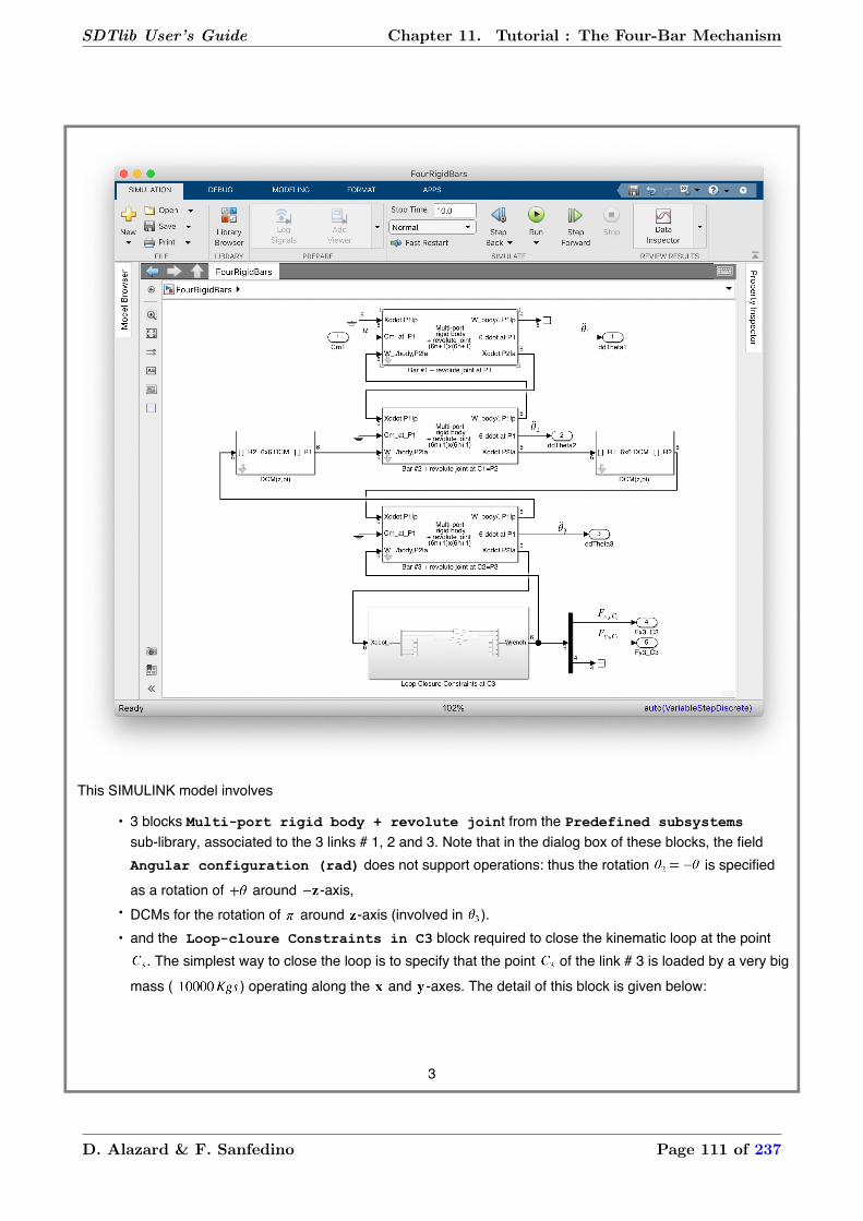
This SIMULINK model involves
• 3 blocks Multi-port rigid body + revolute joint from the Predefined subsystemssub-library, associated to the 3 links # 1, 2 and 3. Note that in the dialog box of these blocks, the fieldAngular configuration (rad) does not support operations: thus the rotation is specifiedas a rotation of around -axis,
• DCMs for the rotation of around -axis (involved in ).• and the Loop-cloure Constraints in C3 block required to close the kinematic loop at the point
. The simplest way to close the loop is to specify that the point of the link # 3 is loaded by a very bigmass ( ) operating along the and -axes. The detail of this block is given below:
3
SDTlib User’s Guide Chapter 11. Tutorial : The Four-Bar Mechanism
D. Alazard & F. Sanfedino Page 111 of 237

The data of the model:
% General data: aluminium beams with square cross section: thickness 1 cmh=0.01; % side of the square cross section (m)rho=2700; % mass density (Kg/m^3)% Bar # 1:l1=0.75; % length (m)m1=rho*l1*h^2; % mass (Kg)I1_G=diag([m1*h^2/6 m1/12*(h^2+l1^2) m1/12*(h^2+l1^2)]); % Inertia matrix at CdG (Kg.m^2)% Bar # 2:l2=1;m2=rho*l2*h^2;I2_G=diag([m2*h^2/6 m2/12*(h^2+l2^2) m2/12*(h^2+l2^2)]);% Bar # 3:l2=1;m2=rho*l2*h^2;I2_G=diag([m2*h^2/6 m2/12*(h^2+l2^2) m2/12*(h^2+l2^2)]);% Bar # 3:l3=l1;m3=rho*l3*h^2;I3_G=diag([m3*h^2/6 m3/12*(h^2+l3^2) m3/12*(h^2+l3^2)]);
4
SDTlib User’s Guide Chapter 11. Tutorial : The Four-Bar Mechanism
D. Alazard & F. Sanfedino Page 112 of 237

% Bar # 4 is the inertial frame
The geometric configuration is varying between 0 and (due to symmetry).
Theta=ureal('theta',pi/2,'Range',[0 pi]);
The SIMULINK model:
FourRigidBarsGu=ulinearize('FourRigidBars')
Gu =
Uncertain continuous-time state-space model with 5 outputs, 1 inputs, 0 states. The model uncertainty consists of the following blocks: tan_theta_div4: Uncertain real, nominal = 0.414, range = [0,1], 16 occurrences
Type "Gu.NominalValue" to see the nominal value, "get(Gu)" to see all properties, and "Gu.Uncertainty" to interact with the uncertain elements.
This model is static.
Gu0=simplify(Gu.d,'full')
Gu0 =
Uncertain matrix with 5 rows and 1 columns. The uncertainty consists of the following blocks: tan_theta_div4: Uncertain real, nominal = 0.414, range = [0,1], 8 occurrences
Type "Gu0.NominalValue" to see the nominal value, "get(Gu0)" to see all properties, and "Gu0.Uncertainty" to interact with the uncertain elements.
The parametric occurrence number can be reduced in such an application with geometric constraints.
Then one can transform it into a matrix, scheduled according to varying by a step of between and. Note that and are singular configurations.
theta=[1:1:179]*pi/180;clear sysLPVfor ii = 1:length(theta), sig4=tan(theta(ii)/4); sysLPV(:,:,ii) = usubs(Gu0,'tan_theta_div4',sig4);end
Then one can plot the apparent inertia and the gains between u and the 2 outputs ,
as functions of .
figuresubplot(2,1,1)plot(theta*180/pi,1./squeeze(sysLPV(1,1,:)))xlabel('$\theta\;(deg)$','Interpreter','Latex','Fontsize',16)ylabel('$I_z,P_1\;(Kg\,m^2)$','Interpreter','Latex','Fontsize',16)set(gca,'Ylim',[0 1])subplot(2,1,2)plot(theta*180/pi,squeeze(sysLPV(4:5,1,:)))
5
SDTlib User’s Guide Chapter 11. Tutorial : The Four-Bar Mechanism
D. Alazard & F. Sanfedino Page 113 of 237

xlabel('$\theta\;(deg)$','Interpreter','Latex','Fontsize',16)ylabel('$(m^-1)$','Interpreter','Latex','Fontsize',16)legend('$F_x_3,C_3/u$','$F_y_3,C_3/u$','Interpreter','Latex',... 'Fontsize',16,'Location','southeast')
It is interesting to note that the apparent inertia at point is constant for any value of i.e; the shape of theparralelogram). It is also true for the radial force .
Finally one can check that the accelerations , and meet the loop closure constraints for any value of :
sysLPV(:,:,[10 45 90 135 170])
ans = ans(:,:,1) =
4.3909 4.3931 4.3903 -3.7801 -0.1111
ans(:,:,2) =
4.3896 4.3897 4.3896 -0.6666 -0.1111
6
SDTlib User’s Guide Chapter 11. Tutorial : The Four-Bar Mechanism
D. Alazard & F. Sanfedino Page 114 of 237

ans(:,:,3) =
4.3895 4.3895 4.3895 -0.0000 -0.1111
ans(:,:,4) =
4.3896 4.3895 4.3894 0.6666 -0.1111
ans(:,:,5) =
4.3909 4.3888 4.3859 3.7801 -0.1111
Indeed the first 3 conponents are always equal: all the revolute joint must have the same angular acceleration tomeet the closure constraints.
3. Flexible caseWhen the links are considered flexible, it possible to specify 2 independent accelerations twists at 2 differentpoints (see also the section 1.4 of tutorial 5). Thus it is possible to meet the closure constraints at theacceleration level with the internal flexible states ( ) of the system.
For that, we need to apply the channel inversion function invio to the TITOP model of the flexible link wherethe loop is closed, here the link # 3 at point .
The matlab function used to compute the TITOP model of a flexible beam in the blocks TITOP flexiblebeam and TITOP flexible beam + revolute joint is the function TwoPOrtBeamFull.m (in theSDTfct/bib_SDT sub-directory):
help TwoPortBeamFull
M=TwoPortBeamFull(ro,s,l,e,g,iz,iy,xi) computes the 2 input/output model M (12x12) of a uniform beam characterized by: * mass density: ro (Kg/m^3), * section: s (m^2), * lenght: l (m), * Young modulus: e (Pascal or N/m^2), * shear modulus: g (Pascal or N/m^2), * second moment of area w.r.t z axis: iz (m^4), * second moment of area w.r.t y axis: iy (m^4), * xi: arbitrary damping ratio for all flexible modes. ^ y(x) | | x=======================x---------> x
7
SDTlib User’s Guide Chapter 11. Tutorial : The Four-Bar Mechanism
D. Alazard & F. Sanfedino Page 115 of 237

/P(x=0) C(x=l) / z The 12 inputs of M are: * the 6 components of the external force/torque vector applied to the beam at point C (in the frame (P,x,y,z)), * the 6 components of the linear/angular acceleration vector at point P (in the frame (P,x,y,z)). The 12 outputs of M are: * the 6 components of the linear/angular acceleration vector at point C (in the frame (P,x,y,z)), * the 6 components of the external force/torque vector applied by the beam at point P (in the frame (P,x,y,z)). Only pure flexion in the plane (P,x,y), in the plane (P,x,z) traction and torsion along (P,x) axis are considered. This fonction supports uncertain parameters (see ureal). See also: MKelemu
Then one can compute the TITOP model of the link # 3 directly from the mechanical parameters:
S=h^2; % beam cross seectio (m^2)E=70e9; % Young module (N/m^2)ni=0.35; % Poison coefficientGG=E/(2*(1+ni));% Shear modulys (N/m^2)Iz=h^4/12; % second mooment of aera arount z-axisIy=Iz; % second mooment of aera arount Y-axisxi=0.001; % common damping ratio% TITOP model of the bar # 3Bar3=TwoPortBeamFull(rho,S,l3,E,GG,Iz,Iy,xi);
This model corresponds to the following block diagram:
The inversion of the channels # 1,2,3,4,5 and 12 allows to specify that:
• channels 1 to 5: the first 5 components of the acceleration twist at point are imposed. These 5
inputs will be set to 0 in this application to meet the closure constraints. The forces , to be
analyzed corresponds to the outputs # 1 and 2,• channel 6: the input # 6 is the torque applied inside the revolute joint between links 3 and 0. It will be
also set to 0. The output is the revolute joint acceleration • channels 7 to 11: the inputs # 7 to 11 are the first 5 components of the acceleration twist imposed by
the link # 2 at point . The outputs are the first 5 component of the wrench applied by the link
# 3 to the link # 2 at point (interaction torque around -axis cannot be applied due to the revolute joint)
8
SDTlib User’s Guide Chapter 11. Tutorial : The Four-Bar Mechanism
D. Alazard & F. Sanfedino Page 116 of 237

• channel 12: the input # 12 is the torque applied inside the revolute joint between links # 2 and 3. It will
be also set to 0. The output is the revolute joint acceleration .
This model, named can be represented by the following block-diagram:
Then the SIMULINK model FourFlexibleBars.slx involves this model with:
• 2 blocks TITOP flexible beam + revolute joint for the links # 1 and 2,• the DCMs associated to the frame rotation .
9
SDTlib User’s Guide Chapter 11. Tutorial : The Four-Bar Mechanism
D. Alazard & F. Sanfedino Page 117 of 237

Let us consider the particular geometric configuration :
Theta=pi/4;FourFlexibleBars[a,b,c,d]=linmod('FourFlexibleBars');G=ss(a,b,c,d); size(G)
State-space model with 5 outputs, 1 inputs, and 60 states.
damp(G)
Pole Damping Frequency Time Constant (rad/seconds) (seconds) -5.52e-13 + 2.10e-05i 2.63e-08 2.10e-05 1.81e+12 -5.52e-13 - 2.10e-05i 2.63e-08 2.10e-05 1.81e+12 2.25e-12 + 4.67e-05i -4.82e-08 4.67e-05 -4.44e+11 2.25e-12 - 4.67e-05i -4.82e-08 4.67e-05 -4.44e+11
10
SDTlib User’s Guide Chapter 11. Tutorial : The Four-Bar Mechanism
D. Alazard & F. Sanfedino Page 118 of 237

5.73e-05 -1.00e+00 5.73e-05 -1.74e+04 -5.73e-05 1.00e+00 5.73e-05 1.74e+04 -9.54e-03 + 5.26e+01i 1.82e-04 5.26e+01 1.05e+02 -9.54e-03 - 5.26e+01i 1.82e-04 5.26e+01 1.05e+02 -6.40e-02 + 9.66e+01i 6.63e-04 9.66e+01 1.56e+01 -6.40e-02 - 9.66e+01i 6.63e-04 9.66e+01 1.56e+01 -2.71e-01 + 1.66e+02i 1.64e-03 1.66e+02 3.68e+00 -2.71e-01 - 1.66e+02i 1.64e-03 1.66e+02 3.68e+00 -3.81e-01 + 2.58e+02i 1.48e-03 2.58e+02 2.62e+00 -3.81e-01 - 2.58e+02i 1.48e-03 2.58e+02 2.62e+00 -3.42e-01 + 2.74e+02i 1.25e-03 2.74e+02 2.92e+00 -3.42e-01 - 2.74e+02i 1.25e-03 2.74e+02 2.92e+00 -5.65e-01 + 3.10e+02i 1.82e-03 3.10e+02 1.77e+00 -5.65e-01 - 3.10e+02i 1.82e-03 3.10e+02 1.77e+00 -8.00e-01 + 5.03e+02i 1.59e-03 5.03e+02 1.25e+00 -8.00e-01 - 5.03e+02i 1.59e-03 5.03e+02 1.25e+00 -8.16e-01 + 5.44e+02i 1.50e-03 5.44e+02 1.23e+00 -8.16e-01 - 5.44e+02i 1.50e-03 5.44e+02 1.23e+00 -1.94e+00 + 5.82e+02i 3.34e-03 5.82e+02 5.15e-01 -1.94e+00 - 5.82e+02i 3.34e-03 5.82e+02 5.15e-01 -1.83e+00 + 8.54e+02i 2.15e-03 8.54e+02 5.46e-01 -1.83e+00 - 8.54e+02i 2.15e-03 8.54e+02 5.46e-01 -3.45e+00 + 1.03e+03i 3.34e-03 1.03e+03 2.90e-01 -3.45e+00 - 1.03e+03i 3.34e-03 1.03e+03 2.90e-01 -3.79e+00 + 1.09e+03i 3.48e-03 1.09e+03 2.64e-01 -3.79e+00 - 1.09e+03i 3.48e-03 1.09e+03 2.64e-01 -3.21e+00 + 1.44e+03i 2.23e-03 1.44e+03 3.11e-01 -3.21e+00 - 1.44e+03i 2.23e-03 1.44e+03 3.11e-01 -3.83e+00 + 1.58e+03i 2.42e-03 1.58e+03 2.61e-01 -3.83e+00 - 1.58e+03i 2.42e-03 1.58e+03 2.61e-01 -1.87e+01 + 2.02e+03i 9.27e-03 2.02e+03 5.35e-02 -1.87e+01 - 2.02e+03i 9.27e-03 2.02e+03 5.35e-02 -2.70e+01 + 2.85e+03i 9.49e-03 2.85e+03 3.70e-02 -2.70e+01 - 2.85e+03i 9.49e-03 2.85e+03 3.70e-02 -2.86e+01 + 3.41e+03i 8.39e-03 3.41e+03 3.50e-02 -2.86e+01 - 3.41e+03i 8.39e-03 3.41e+03 3.50e-02 -3.32e+01 + 3.57e+03i 9.30e-03 3.57e+03 3.02e-02 -3.32e+01 - 3.57e+03i 9.30e-03 3.57e+03 3.02e-02 -4.64e+01 + 3.95e+03i 1.17e-02 3.95e+03 2.16e-02 -4.64e+01 - 3.95e+03i 1.17e-02 3.95e+03 2.16e-02 -5.47e+01 + 4.50e+03i 1.22e-02 4.50e+03 1.83e-02 -5.47e+01 - 4.50e+03i 1.22e-02 4.50e+03 1.83e-02 -6.32e+01 + 5.69e+03i 1.11e-02 5.69e+03 1.58e-02 -6.32e+01 - 5.69e+03i 1.11e-02 5.69e+03 1.58e-02 -7.89e+01 + 6.96e+03i 1.13e-02 6.96e+03 1.27e-02 -7.89e+01 - 6.96e+03i 1.13e-02 6.96e+03 1.27e-02 -1.57e+02 + 7.20e+03i 2.17e-02 7.20e+03 6.39e-03 -1.57e+02 - 7.20e+03i 2.17e-02 7.20e+03 6.39e-03 -9.28e+01 + 7.29e+03i 1.27e-02 7.29e+03 1.08e-02 -9.28e+01 - 7.29e+03i 1.27e-02 7.29e+03 1.08e-02 -3.41e+01 + 1.05e+04i 3.24e-03 1.05e+04 2.94e-02 -3.41e+01 - 1.05e+04i 3.24e-03 1.05e+04 2.94e-02 -6.58e+01 + 1.08e+04i 6.08e-03 1.08e+04 1.52e-02 -6.58e+01 - 1.08e+04i 6.08e-03 1.08e+04 1.52e-02 -5.62e+01 + 1.59e+04i 3.53e-03 1.59e+04 1.78e-02 -5.62e+01 - 1.59e+04i 3.53e-03 1.59e+04 1.78e-02
The order of the model G is (i.e flexible modes by link since the 3D model of a flexible beamincludes 4 bending modes in the -plane, 4 bending modes in the -plane, 1 torsion mode aound the -axis of the beam and 1 traction mode along its -axis). See also:
web DocBeam.html -new
11
SDTlib User’s Guide Chapter 11. Tutorial : The Four-Bar Mechanism
D. Alazard & F. Sanfedino Page 119 of 237

One can also check that 6 poles are around 0 due to the loop closure constraints.
These poles and the out-of- -plane flexible modes can be reduced using the fonction minreal:
Gxy=minreal(G);
30 states removed.
damp(Gxy)
Pole Damping Frequency Time Constant (rad/seconds) (seconds) -2.71e-01 + 1.66e+02i 1.64e-03 1.66e+02 3.68e+00 -2.71e-01 - 1.66e+02i 1.64e-03 1.66e+02 3.68e+00 -3.81e-01 + 2.58e+02i 1.48e-03 2.58e+02 2.62e+00 -3.81e-01 - 2.58e+02i 1.48e-03 2.58e+02 2.62e+00 -5.65e-01 + 3.10e+02i 1.82e-03 3.10e+02 1.77e+00 -5.65e-01 - 3.10e+02i 1.82e-03 3.10e+02 1.77e+00 -1.94e+00 + 5.82e+02i 3.34e-03 5.82e+02 5.15e-01 -1.94e+00 - 5.82e+02i 3.34e-03 5.82e+02 5.15e-01 -3.45e+00 + 1.03e+03i 3.34e-03 1.03e+03 2.90e-01 -3.45e+00 - 1.03e+03i 3.34e-03 1.03e+03 2.90e-01 -3.79e+00 + 1.09e+03i 3.48e-03 1.09e+03 2.64e-01 -3.79e+00 - 1.09e+03i 3.48e-03 1.09e+03 2.64e-01 -1.87e+01 + 2.02e+03i 9.27e-03 2.02e+03 5.35e-02 -1.87e+01 - 2.02e+03i 9.27e-03 2.02e+03 5.35e-02 -2.86e+01 + 3.41e+03i 8.39e-03 3.41e+03 3.50e-02 -2.86e+01 - 3.41e+03i 8.39e-03 3.41e+03 3.50e-02 -3.32e+01 + 3.57e+03i 9.30e-03 3.57e+03 3.02e-02 -3.32e+01 - 3.57e+03i 9.30e-03 3.57e+03 3.02e-02 -4.64e+01 + 3.95e+03i 1.17e-02 3.95e+03 2.16e-02 -4.64e+01 - 3.95e+03i 1.17e-02 3.95e+03 2.16e-02 -7.89e+01 + 6.96e+03i 1.13e-02 6.96e+03 1.27e-02 -7.89e+01 - 6.96e+03i 1.13e-02 6.96e+03 1.27e-02 -9.28e+01 + 7.29e+03i 1.27e-02 7.29e+03 1.08e-02 -9.28e+01 - 7.29e+03i 1.27e-02 7.29e+03 1.08e-02 -3.41e+01 + 1.05e+04i 3.24e-03 1.05e+04 2.94e-02 -3.41e+01 - 1.05e+04i 3.24e-03 1.05e+04 2.94e-02 -6.58e+01 + 1.08e+04i 6.08e-03 1.08e+04 1.52e-02 -6.58e+01 - 1.08e+04i 6.08e-03 1.08e+04 1.52e-02 -5.62e+01 + 1.59e+04i 3.53e-03 1.59e+04 1.78e-02 -5.62e+01 - 1.59e+04i 3.53e-03 1.59e+04 1.78e-02
One can check that the DCgain of this system corresponds to the model obtained in the previous section (for) assuming the beams are rigid:
dcgain(Gxy)
ans = 5×1 4.3896 4.3896 4.3896 -0.6667 -0.1111
sysLPV(:,:,45)
ans = 5×1
12
SDTlib User’s Guide Chapter 11. Tutorial : The Four-Bar Mechanism
D. Alazard & F. Sanfedino Page 120 of 237

4.3896 4.3897 4.3896 -0.6666 -0.1111
Let us consider varying between 0 and
Theta=ureal('theta',pi/2,'Range',[0 pi]);Gu=ulinearize('FourFlexibleBars');Guxy=minreal(Gu)
Guxy =
Uncertain continuous-time state-space model with 5 outputs, 1 inputs, 60 states. The model uncertainty consists of the following blocks: tan_theta_div4: Uncertain real, nominal = 0.414, range = [0,1], 32 occurrences
Type "Guxy.NominalValue" to see the nominal value, "get(Guxy)" to see all properties, and "Guxy.Uncertainty" to interact with the uncertain elements.
Note that the out-of- -plane modes are not reduced with this parameter varying model.
But, as done in the previous section, one can transform the model into an LPV system scheduled according to varying by a step of between and :
theta=[1:1:179]*pi/180;clear sysLPVfor ii = 1:length(theta), sig4=tan(theta(ii)/4); sysLPV(:,:,ii) = minreal(usubs(Gu,'tan_theta_div4',sig4));end
30 states removed.30 states removed.30 states removed.30 states removed.30 states removed.30 states removed.30 states removed.30 states removed.30 states removed.30 states removed.30 states removed.30 states removed.30 states removed.30 states removed.30 states removed.30 states removed.30 states removed.30 states removed.30 states removed.30 states removed.30 states removed.30 states removed.30 states removed.30 states removed.30 states removed.30 states removed.30 states removed.30 states removed.30 states removed.
13
SDTlib User’s Guide Chapter 11. Tutorial : The Four-Bar Mechanism
D. Alazard & F. Sanfedino Page 121 of 237

30 states removed.30 states removed.30 states removed.30 states removed.30 states removed.30 states removed.30 states removed.30 states removed.30 states removed.30 states removed.30 states removed.30 states removed.30 states removed.30 states removed.30 states removed.30 states removed.30 states removed.30 states removed.30 states removed.30 states removed.
sysLPV.SamplingGrid = struct('Crank_configuration',theta);
and check that the reduction works for all the numerical values of .
Then one can plot the frequency-domain responses of the apparent inertia and the gains between u
and the 2 outputs , as functions of .
figuresubplot(2,1,1)sigma(1/sysLPV(1,1,:)) % Apparent inertia at point P_1gridlegend('$I\_z,P\_1(\mathrm s,\theta)\;(Kg\,m^2)$','Interpreter','Latex',... 'Fontsize',16)subplot(2,1,2)sigma(sysLPV(4,1,:)) % transfert from z-torque at P1 to Fx at C3hold onsigma(sysLPV(5,1,:)) % transfert from z-torque at P1 to Fy at C3gridlegend('$F\_x\_3,C\_3/U(\mathrm s,\theta)\;(m^-1)$',... '$F\_y\_3,C\_3/U(\mathrm s,\theta)\;(m^-1)$',... 'Interpreter','Latex','Fontsize',16,'Location','southeast')
16
SDTlib User’s Guide Chapter 11. Tutorial : The Four-Bar Mechanism
D. Alazard & F. Sanfedino Page 122 of 237

Exactly as in the rigid case the DCGAIN of does not depend on .
One of the main interest of ploting the frequency-domain response of the system using its gain-scheduledrepresentation sysLPV instead of its uncertain state-space reprentation Gu is that it is possible to click on aparticular response in the graphic window to read the corresponding parametric configuration. For instance, inthe botton figure, a response of the SISO transfer has a magnitude largely lower than the others: it
corresponds to the configuration . Indeed, for this configuration the axial force in the link 3 is null.
4. The rigid 4 bar mechanism free in 3D-spaceNow the link # 0 is no more the inertial frame (ground) but a real beam and we consider in addition the dynamic model between an external wrench applied to the mechanisim at the point and the
acceleration twist at this point. A new frame attached to the link # 0 at the point is introduced:
17
SDTlib User’s Guide Chapter 11. Tutorial : The Four-Bar Mechanism
D. Alazard & F. Sanfedino Page 123 of 237

For the link # 0, the rigid body and the revolute joint (at point ) are dissociated in the SIMULINK modelin order to model the closure constraints. Furthermore, these constraints cannot be modeled using a "great"mass as it was proposed in section 2 since the model is now free to move in 3D-space. It is thus recommendedto use a local spring-damper system acting on the relative motion between points and and only on thed.o.fs which required to be closed, here the 2 translations in the -plane. Thus, the relative acceleration
needs to be integrated to model the effect of the spring and the damper. The states associated
to these integrators can be seen as the Lagrange multipliers commonly used to take into account kinematicsconstraints.
In the general case of loop closure constraints acting on the 6 d.o.fs, one can also use the block LocalSpring-Samper system from the 6 dof mechanisms sub-library. See also:
web Doc_6DOFs_spring_damper.html -new
Finally the SIMULINK model FourRigidBarsFree.slx is diplayed in the following Figure with the detailled ofthe sub-system: Loop closure constraints at C3.
18
SDTlib User’s Guide Chapter 11. Tutorial : The Four-Bar Mechanism
D. Alazard & F. Sanfedino Page 124 of 237

19
SDTlib User’s Guide Chapter 11. Tutorial : The Four-Bar Mechanism
D. Alazard & F. Sanfedino Page 125 of 237

A stiffness of and a damping of are arbitrary chosen for the spring and the damperon both and axes. The only recommendation is to choose sufficiently high values in order to track thecorresponding eigenvalues in the whole system dynamics once the model is computed, as it is ilustrated below.
The data relative to the link # 0 and the whole model in the configuration :
l0=l2;m0=rho*l0*h^2;I0_G=diag([m0*h^2/6 m0/12*(h^2+l2^2) m0/12*(h^2+l2^2)]);Theta=pi/4;FourRigidBarsFree[a,b,c,d]=linmod('FourRigidBarsFree');G=ss(a,b,c,d);damp(G)
Pole Damping Frequency Time Constant (rad/seconds) (seconds) -7.30e+01 1.00e+00 7.30e+01 1.37e-02 -7.56e+01 1.00e+00 7.56e+01 1.32e-02 -1.31e+03 1.00e+00 1.31e+03 7.64e-04
20
SDTlib User’s Guide Chapter 11. Tutorial : The Four-Bar Mechanism
D. Alazard & F. Sanfedino Page 126 of 237

-3.36e+03 1.00e+00 3.36e+03 2.98e-04
The model G is a 4-th order model between:
• 7 inputs: the 6 components of and u,
• outputs: the 6 components of , , , , and
Due to the feedback loops in the SIMULINK model, the 4 integrators introduced for the loop closure constraintsare moved far in the left-hand side of the complex plane. These poles can be reduced considering the DCgain(low frequency behavior) of the system G:
G0=dcgain(G);
Then one can compute the apparent mass matrix of the system seen from the point and projected in
the frame :
• when the angular configuration of the parrallelogram is free to change: one can check that the apparentmass is diffrent according to the 3 translations:
% Apparent 6x6 mass when the joint #1 is freeG0m1free=invio(ss(G0),1:6);G0m1free(1:6,1:6)
ans = D = u1 u2 u3 u4 u5 u6 y1 0.6694 0.2756 0 0 0 -0.1378 y2 0.2756 0.6694 0 0 0 -0.3347 y3 0 0 0.945 -0.2506 0.7231 0 y4 0 0 -0.2506 0.1139 -0.2392 0 y5 0 0 0.7231 -0.2392 0.747 0 y6 -0.1378 -0.3347 0 0 0 0.3136 Static gain.
• when the parrallelogram is locked in the angular configuration . The apparent mass is the samefor the 3 translations and equal to the total mass of the system :
% Apparent 6x6 mass when the joint #1 is locked at thetaG0m1lock=invio(ss(G0),1:7);G0m1lock(1:6,1:6)
ans = D = u1 u2 u3 u4 u5 u6 y1 0.945 4.705e-16 0 0 0 0.2506 y2 1.622e-15 0.945 0 0 0 -0.7231 y3 0 0 0.945 -0.2506 0.7231 0 y4 0 0 -0.2506 0.1139 -0.2392 0 y5 0 0 0.7231 -0.2392 0.747 0 y6 0.2506 -0.7231 0 0 0 0.8609
21
SDTlib User’s Guide Chapter 11. Tutorial : The Four-Bar Mechanism
D. Alazard & F. Sanfedino Page 127 of 237

Static gain.
m0+m1+m2+m3
ans = 0.9450
One can also recover the result obtained in section 2 just by nulling the first 6 inputs ( ) of the inverse
model G0m1free, i.e.: the link # 0 is clamped on the inertial frame:
% Recovering the result of section 1G0m1free(7:11,7)
ans = D = u1 y1 4.39 y2 4.39 y3 4.39 y4 -0.6667 y5 -0.1111 Static gain.
The folllowing syntax shows how to recover the LPV representation of the system when the link # 0 is clampedon the inertial frame for vaying in (i.e. in the same condition than the section 2):
Theta=ureal('theta',pi/2,'Range',[0 pi]);Gu=ulinearize('FourRigidBarsFree');Gu=simplify(Gu,'full');% DCgain for uss:Gu0=simplify(Gu.d-Gu.c*inv(Gu.a)*Gu.b,'full');% Clamping the bar # 0:Gu0m1=invio(ss(Gu0),1:6);Gu0m1=Gu0m1.d;theta=[1:1:179]*pi/180;clear sysLPVfor ii = 1:length(theta), sig4=tan(theta(ii)/4); sysLPV(:,:,ii) = usubs(Gu0m1(7:11,7),'tan_theta_div4',sig4);end
5. The flexible 4 bar mechanism free in 3D-spaceIn the case the 4 bars are flexible, the SIMULINK model is very simple and composed of:
• 4 bocks TITOP flexible beam + revolute joint blocs associated to the 4 links,• some DCMs associated to the rotation of around -axis, required to specify the vayring angular
configuration as an ureal in the revolute joint dialog boxes (for numerical values of these DCMcan be removed).
22
SDTlib User’s Guide Chapter 11. Tutorial : The Four-Bar Mechanism
D. Alazard & F. Sanfedino Page 128 of 237

Considering the angular configuration :
% Flexible case: free caseTheta=pi/4;FourFlexibleBarsFree[a,b,c,d]=linmod('FourFlexibleBarsFree');G=ss(a,b,c,d);damp(G)
Pole Damping Frequency Time Constant (rad/seconds) (seconds) -3.91e-13 + 6.00e-05i 6.51e-09 6.00e-05 2.56e+12
23
SDTlib User’s Guide Chapter 11. Tutorial : The Four-Bar Mechanism
D. Alazard & F. Sanfedino Page 129 of 237

-3.91e-13 - 6.00e-05i 6.51e-09 6.00e-05 2.56e+12 -5.70e-05 + 3.65e-05i 8.42e-01 6.76e-05 1.76e+04 -5.70e-05 - 3.65e-05i 8.42e-01 6.76e-05 1.76e+04 5.70e-05 + 3.65e-05i -8.42e-01 6.76e-05 -1.76e+04 5.70e-05 - 3.65e-05i -8.42e-01 6.76e-05 -1.76e+04 -8.65e-02 + 1.04e+02i 8.35e-04 1.04e+02 1.16e+01 -8.65e-02 - 1.04e+02i 8.35e-04 1.04e+02 1.16e+01 -3.13e-01 + 1.76e+02i 1.77e-03 1.76e+02 3.19e+00 -3.13e-01 - 1.76e+02i 1.77e-03 1.76e+02 3.19e+00 -3.30e-01 + 1.87e+02i 1.77e-03 1.87e+02 3.03e+00 -3.30e-01 - 1.87e+02i 1.77e-03 1.87e+02 3.03e+00 -2.55e-01 + 2.13e+02i 1.19e-03 2.13e+02 3.93e+00 -2.55e-01 - 2.13e+02i 1.19e-03 2.13e+02 3.93e+00 -5.52e-01 + 2.96e+02i 1.87e-03 2.96e+02 1.81e+00 -5.52e-01 - 2.96e+02i 1.87e-03 2.96e+02 1.81e+00 -5.14e-01 + 3.00e+02i 1.71e-03 3.00e+02 1.94e+00 -5.14e-01 - 3.00e+02i 1.71e-03 3.00e+02 1.94e+00 -8.83e-01 + 3.84e+02i 2.30e-03 3.84e+02 1.13e+00 -8.83e-01 - 3.84e+02i 2.30e-03 3.84e+02 1.13e+00 -8.88e-01 + 4.80e+02i 1.85e-03 4.80e+02 1.13e+00 -8.88e-01 - 4.80e+02i 1.85e-03 4.80e+02 1.13e+00 -1.12e+00 + 5.23e+02i 2.15e-03 5.23e+02 8.90e-01 -1.12e+00 - 5.23e+02i 2.15e-03 5.23e+02 8.90e-01 -1.95e+00 + 5.82e+02i 3.34e-03 5.82e+02 5.14e-01 -1.95e+00 - 5.82e+02i 3.34e-03 5.82e+02 5.14e-01 -2.59e+00 + 6.87e+02i 3.76e-03 6.87e+02 3.87e-01 -2.59e+00 - 6.87e+02i 3.76e-03 6.87e+02 3.87e-01 -1.79e+00 + 8.02e+02i 2.24e-03 8.02e+02 5.58e-01 -1.79e+00 - 8.02e+02i 2.24e-03 8.02e+02 5.58e-01 -2.28e+00 + 8.56e+02i 2.66e-03 8.56e+02 4.39e-01 -2.28e+00 - 8.56e+02i 2.66e-03 8.56e+02 4.39e-01 -3.44e+00 + 1.03e+03i 3.33e-03 1.03e+03 2.91e-01 -3.44e+00 - 1.03e+03i 3.33e-03 1.03e+03 2.91e-01 -4.10e+00 + 1.14e+03i 3.59e-03 1.14e+03 2.44e-01 -4.10e+00 - 1.14e+03i 3.59e-03 1.14e+03 2.44e-01 -4.51e+00 + 1.23e+03i 3.66e-03 1.23e+03 2.22e-01 -4.51e+00 - 1.23e+03i 3.66e-03 1.23e+03 2.22e-01 -4.72e+00 + 1.53e+03i 3.09e-03 1.53e+03 2.12e-01 -4.72e+00 - 1.53e+03i 3.09e-03 1.53e+03 2.12e-01 -1.92e+01 + 2.03e+03i 9.43e-03 2.03e+03 5.22e-02 -1.92e+01 - 2.03e+03i 9.43e-03 2.03e+03 5.22e-02 -2.25e+01 + 2.17e+03i 1.04e-02 2.17e+03 4.44e-02 -2.25e+01 - 2.17e+03i 1.04e-02 2.17e+03 4.44e-02 -2.39e+01 + 2.45e+03i 9.78e-03 2.45e+03 4.18e-02 -2.39e+01 - 2.45e+03i 9.78e-03 2.45e+03 4.18e-02 -4.35e+01 + 3.05e+03i 1.43e-02 3.05e+03 2.30e-02 -4.35e+01 - 3.05e+03i 1.43e-02 3.05e+03 2.30e-02 -3.20e+01 + 3.53e+03i 9.09e-03 3.53e+03 3.12e-02 -3.20e+01 - 3.53e+03i 9.09e-03 3.53e+03 3.12e-02 -4.20e+01 + 3.85e+03i 1.09e-02 3.85e+03 2.38e-02 -4.20e+01 - 3.85e+03i 1.09e-02 3.85e+03 2.38e-02 -2.72e+01 + 3.97e+03i 6.85e-03 3.97e+03 3.68e-02 -2.72e+01 - 3.97e+03i 6.85e-03 3.97e+03 3.68e-02 -4.89e+01 + 3.99e+03i 1.23e-02 3.99e+03 2.05e-02 -4.89e+01 - 3.99e+03i 1.23e-02 3.99e+03 2.05e-02 -6.72e+01 + 4.43e+03i 1.52e-02 4.43e+03 1.49e-02 -6.72e+01 - 4.43e+03i 1.52e-02 4.43e+03 1.49e-02 -4.74e+01 + 4.77e+03i 9.93e-03 4.77e+03 2.11e-02 -4.74e+01 - 4.77e+03i 9.93e-03 4.77e+03 2.11e-02 -8.90e+01 + 5.28e+03i 1.68e-02 5.28e+03 1.12e-02 -8.90e+01 - 5.28e+03i 1.68e-02 5.28e+03 1.12e-02 -8.17e+01 + 6.12e+03i 1.33e-02 6.12e+03 1.22e-02 -8.17e+01 - 6.12e+03i 1.33e-02 6.12e+03 1.22e-02 -7.46e+01 + 6.88e+03i 1.09e-02 6.88e+03 1.34e-02 -7.46e+01 - 6.88e+03i 1.09e-02 6.88e+03 1.34e-02
24
SDTlib User’s Guide Chapter 11. Tutorial : The Four-Bar Mechanism
D. Alazard & F. Sanfedino Page 130 of 237

-1.05e+02 + 7.51e+03i 1.40e-02 7.51e+03 9.52e-03 -1.05e+02 - 7.51e+03i 1.40e-02 7.51e+03 9.52e-03 -1.84e+02 + 7.91e+03i 2.33e-02 7.91e+03 5.42e-03 -1.84e+02 - 7.91e+03i 2.33e-02 7.91e+03 5.42e-03 -2.00e+02 + 9.40e+03i 2.13e-02 9.40e+03 4.99e-03 -2.00e+02 - 9.40e+03i 2.13e-02 9.40e+03 4.99e-03 -5.16e+01 + 1.52e+04i 3.39e-03 1.52e+04 1.94e-02 -5.16e+01 - 1.52e+04i 3.39e-03 1.52e+04 1.94e-02 -1.20e+02 + 1.53e+04i 7.84e-03 1.53e+04 8.31e-03 -1.20e+02 - 1.53e+04i 7.84e-03 1.53e+04 8.31e-03 -6.23e+01 + 1.88e+04i 3.32e-03 1.88e+04 1.60e-02 -6.23e+01 - 1.88e+04i 3.32e-03 1.88e+04 1.60e-02 -5.65e+01 + 2.10e+04i 2.69e-03 2.10e+04 1.77e-02 -5.65e+01 - 2.10e+04i 2.69e-03 2.10e+04 1.77e-02
The whole model G is a 80-th order system with 6 poles around 0 due to the internal constraints requiredto meet the loop closure contraints.
They can be removed using the function minreal but the out-of- -plane flexible modes are not reduced
because they are controllable by and obdservable by .
Gr=minreal(G);
6 states removed.
One can recover the apparent apparent (rigid) mass matrix of the system seen from the point and
projected in the frame :
• when the angular configuration of the parrallelogram is free to change: one can check that the apparentmass is diffrent according to the 3 translations:
Gm1free=invio(Gr,1:6);dcgain(Gm1free(1:6,1:6))
ans = 6×6 0.6694 0.2756 0.0000 0.0000 -0.0000 -0.1378 0.2756 0.6694 0.0000 -0.0000 -0.0000 -0.3347 -0.0000 -0.0000 0.9450 -0.2506 0.7231 0.0000 0.0000 0.0000 -0.2506 0.1139 -0.2392 -0.0000 -0.0000 -0.0000 0.7231 -0.2392 0.7470 0.0000 -0.1378 -0.3347 -0.0000 0.0000 0.0000 0.3136
• when the parrallelogram is locked in the angular configuration . The apparent mass is the samefor the 3 translations and equal to the total mass of the system :
G0m1lock=invio(Gr,1:7);dcgain(G0m1lock(1:6,1:6))
ans = 6×6 0.9450 -0.0000 -0.0000 0.0000 -0.0000 0.2506 0.0000 0.9450 0.0000 -0.0000 0.0000 -0.7231 0.0000 -0.0000 0.9450 -0.2506 0.7231 0.0000 -0.0000 0.0000 -0.2506 0.1139 -0.2392 -0.0000 0.0000 -0.0000 0.7231 -0.2392 0.7470 0.0000 0.2506 -0.7231 -0.0000 0.0000 -0.0000 0.8609
25
SDTlib User’s Guide Chapter 11. Tutorial : The Four-Bar Mechanism
D. Alazard & F. Sanfedino Page 131 of 237

The following sequence considers as a varying parameter and plots the frequency-domain responses of theapparent inertia and the gains between u and the 2 outputs , as functions of , when
the link # 0 is clamped on the inertial frame at the point .. Note that the responses are different than the ones
obtained in section 3 because, although the link # 0 is clamped at point , it is flexible.
Theta=ureal('theta',pi/2,'Range',[0 pi]);Gu=ulinearize('FourFlexibleBarsFree');Gu=simplify(Gu,'full')
Gu =
Uncertain continuous-time state-space model with 11 outputs, 7 inputs, 80 states. The model uncertainty consists of the following blocks: tan_theta_div4: Uncertain real, nominal = 0.414, range = [0,1], 64 occurrences
Type "Gu.NominalValue" to see the nominal value, "get(Gu)" to see all properties, and "Gu.Uncertainty" to interact with the uncertain elements.
% Clamping the bar # 0 at C0=P1:Gu0m1=invio(Gu,1:6);theta=[1:1:179]*pi/180;% Analysis:clear sysLPVfor ii = 1:length(theta), sig4=tan(theta(ii)/4); sysLPV(:,:,ii) = minreal(usubs(Gu0m1(7:11,7),'tan_theta_div4',sig4));end
40 states removed.40 states removed.40 states removed.40 states removed.40 states removed.40 states removed.40 states removed.40 states removed.40 states removed.40 states removed.40 states removed.40 states removed.40 states removed.40 states removed.40 states removed.40 states removed.40 states removed.40 states removed.40 states removed.40 states removed.40 states removed.40 states removed.40 states removed.40 states removed.40 states removed.40 states removed.40 states removed.40 states removed.40 states removed.40 states removed.40 states removed.
26
SDTlib User’s Guide Chapter 11. Tutorial : The Four-Bar Mechanism
D. Alazard & F. Sanfedino Page 132 of 237

40 states removed.40 states removed.40 states removed.40 states removed.40 states removed.40 states removed.40 states removed.40 states removed.40 states removed.40 states removed.40 states removed.40 states removed.40 states removed.40 states removed.40 states removed.40 states removed.40 states removed.40 states removed.
sysLPV.SamplingGrid = struct('Crank_configuration',theta);figuresubplot(2,1,1)sigma(1/sysLPV(1,1,:)) % Apparent inertia at point P_1gridlegend('$I\_z,P\_1(\mathrm s,\theta)\;(Kg\,m^2)$','Interpreter',... 'Latex','Fontsize',16)subplot(2,1,2)sigma(sysLPV(4,1,:)) % transfert from z-torque at P1 to Fx at C3
Warning: The frequency response has poor relative accuracy. This may be because the response is nearly zero or infinite at all frequencies, or because the state-space realization is ill conditioned. Use the "prescale" command to investigate further.
hold onsigma(sysLPV(5,1,:)) % transfert from z-torque at P1 to Fy at C3gridlegend('$F\_x\_3,C\_3/U(\mathrm s,\theta)\;(m^-1)$',... '$F\_y\_3,C\_3/U(\mathrm s,\theta)\;(m^-1)$',... 'Interpreter','Latex','Fontsize',16,'Location','southeast')
29
SDTlib User’s Guide Chapter 11. Tutorial : The Four-Bar Mechanism
D. Alazard & F. Sanfedino Page 133 of 237

6. References• Chebbi, Jawhar and Dubanchet, Vincent and Perez Gonzalez, José Alvaro and Alazard, Daniel.
Linear dynamics of flexible multibody systems : a system-based approach. (2017) Multibody SystemDynamics, 41 (1). 75-100. ISSN 1384-5640
30
SDTlib User’s Guide Chapter 11. Tutorial : The Four-Bar Mechanism
D. Alazard & F. Sanfedino Page 134 of 237

Tutorial 12: simulating a SDTlib-based model ( run).
Table of Contents
1. Description........................................................................................................................................................... 12. From the uss model to LPV model..................................................................................................................... 13. The simulation model.......................................................................................................................................... 2
by D. Alazard and F. Sanfedino - ISAE-SUPAERO
1. Description
As it was mentionned in the introduction (see tutorial 0), the SDTlib is a tool for parametric modelling purpose
and not for simulation purpose. Indeed, the SIMULINK model based on the SDTlib blocks reveals algebraic
loops which can slow down the simulation run time.
Nevertheless, it shown in this tutorial, how it is possible to simulate such a model using a new SIMULINK file
where the model of the mechanical system is implemented using a Linear Parameter Varying
(LPV) Model (from the sub-libray Control system Tooolbox>Linear Parameter Varying.
Indeed, once the model is computed (for instance using the function ulinearize), the algebraic
loops are solved once for all. Then for the simulation, one can freeze the value of the uncertain parameters (for
instance ) and use the known varying parameters (for instance the geometric configuration ) as schedling
variables. That is to say: is evaluated on a N-point grid of the scheduling parameter to obtain
N models , which are linearly interpolated according to the current value of during the
simulation.
The following illustration reconsiders the close-loop model designed in the tutorial 3 Robust attitudecontrol design of a spacecraft with 2 symmetrical rotating solar arrays and saved in the file
OptimalDesign.mat. A whole orbit is simulated and it is assumed that the geometrical configuration of the
solar arrays varies from to during this orbit. The system is submitted to orbital disturbances, internal
SADM disturbances, star sensor and gyrometer noises.
2. From the uss model to LPV model
Let us load the optimal closed-loop model (CLu) previoulsy obtained:
load OptimalDesign
The varying parameter is sampled every between and . The model is evaluted
on this grid to create the LPV model, named sysLPV:
theta=[-pi:pi/180:pi];clear sysLPV
1
SDTlib User’s Guide Chapter 12. Tutorial : Simulation of SDT Models
12. Tutorial : Simulation of SDT Models
D. Alazard & F. Sanfedino Page 135 of 237

for ii = 1:length(theta), sig4=tan(theta(ii)/4); sysLPV(:,:,ii) = usubs(CLu,'tan_Theta_div4',sig4);endsysLPV.SamplingGrid = struct('SA_configuration',theta)
sysLPV =
361x1 array of uncertain continuous-time state-space models. Each model has 6 outputs, 11 inputs, 43 states, and the following uncertain blocks: IBx: Uncertain real, nominal = 75, variability = [-20,20]%, 1 occurrences IBy: Uncertain real, nominal = 40, variability = [-20,20]%, 1 occurrences IBz: Uncertain real, nominal = 80, variability = [-20,20]%, 1 occurrences mB: Uncertain real, nominal = 1e+03, variability = [-20,20]%, 3 occurrences w1: Uncertain real, nominal = 5.6, variability = [-20,20]%, 4 occurrences w2: Uncertain real, nominal = 19.3, variability = [-20,20]%, 4 occurrences w3: Uncertain real, nominal = 35.4, variability = [-20,20]%, 4 occurrences
Type "sysLPV.NominalValue" to see the nominal value, "get(sysLPV)" to see all properties, and "sysLPV.Uncertainty" to interact with the uncertain elements.
Now we can check that sysLPV is array of uss. Each uss model depends only on the uncertain parameters
and no more on .
Let us consider the nominal value of the uncertian parameters:
sysLPV0=sysLPV.NominalValue;
3. The simulation modelThe simulation model SimulationModel.slx is depicted in the follwong Figure:
2
SDTlib User’s Guide Chapter 12. Tutorial : Simulation of SDT Models
D. Alazard & F. Sanfedino Page 136 of 237

The input signals are:
•normalized orbital disturbances ( ) at the orbital frequency,
• harmonic internal disturbances on the 2 SADM ( and ) : magnitude , frequency ,
•the normalised noises on the star tracker ( ) and the gyrometer ( ) are not taken into account
(switch off) since they slow down the simulation over one orbit.
The simulation run time is around to simulate the whole orbit ( ). The responses of the 2 outputs:
• the torque applied to the spacecraft by the reaction wheel system ,
•the normalized pointing error
can then be plotted and analyzed:
% Simulation Orbital periodT=5000; % (s)
SimulationModelSimout=sim('SimulationModel');% Plot the results (with out transcient response)figuresubplot(3,1,1)
3
SDTlib User’s Guide Chapter 12. Tutorial : Simulation of SDT Models
D. Alazard & F. Sanfedino Page 137 of 237

plot(Simout.tout(10000:end),Simout.T.signals.values(10000:end,1))xlabel('time (s)');ylabel('$T_x\,(Nm)$','Interpreter','latex')subplot(3,1,2);plot(Simout.tout(10000:end),Simout.T.signals.values(10000:end,2))xlabel('time (s)');ylabel('$T_y\,(Nm)$','Interpreter','latex')subplot(3,1,3);plot(Simout.tout(10000:end),Simout.T.signals.values(10000:end,3))xlabel('time (s)');ylabel('$T_z\,(Nm)$','Interpreter','latex')
One can check the resonance due to the SADM disturbances and the exchange between and axes
according to the solar array angular configuration .
figuresubplot(3,1,1)plot(Simout.tout,Simout.APE.signals.values(:,1))xlabel('time (s)');ylabel('$\delta\phi/\delta\phi_req\;(\%)$','Interpreter','latex')subplot(3,1,2);plot(Simout.tout,Simout.APE.signals.values(:,2))xlabel('time (s)');ylabel('$\delta\theta/\delta\theta_req\;(\%)$','Interpreter','latex')subplot(3,1,3);plot(Simout.tout,Simout.APE.signals.values(:,3))xlabel('time (s)');ylabel('$\delta\psi/\delta\psi_req\;(\%)$','Interpreter','latex')
4
SDTlib User’s Guide Chapter 12. Tutorial : Simulation of SDT Models
D. Alazard & F. Sanfedino Page 138 of 237

The error is always between of the requirement.
5
SDTlib User’s Guide Chapter 12. Tutorial : Simulation of SDT Models
D. Alazard & F. Sanfedino Page 139 of 237

SDTlib User’s Guide Chapter 13. SDTlib Documentation
13. SDTlib Documentation
6 dof bodies
6 dof mechanisms
3/6 dof DCM
1 port flexible body + revolute joint
Multi port rigid body + revolute joint
TITOP flexible beam +revolute joint
Predefined subsystems
13.1. 6 DoFs Bodies
Multi-port rigid body (6nx6n)
W_./body,P1 Xddot,P1
W_./body,P2 Xddot,P2
W_./body,P3 Xddot,P3
Multi port rigid body
One-portflexiblebody
(6x6)Xddot W_body/.
1 port flexible body
One-port Nastran body
(6x6)Xddot W_body/.
1 port Nastran body
NINOP flexible plate
(6nx6n)
W./body,C1 Xddot,C1
Xddot,P1 Wbody/.,P1
multi-port flexible plate
TITOP flexible beam
(12x12)
W./body,C Xddot,C
Xddot,P Wbody/.,P
2 ports flexible beam
Massless connection body
(6nx6n)
W_body/.,P1Xddot,P1
W_./body,P2 Xddot,P2
W_./body,P3 Xddot,P3
W_./body,P4 Xddot,P4
massless connection body
One-portangularmomemtum
(6x6)Xddot W_body/.
1 port spinning wheel
Sloshing 1D mass-spring model(6x6)
Xddot W_body/.
u_sloshing
NINOP Nastran body
(6(n+1)x6(n+1))
W_./body,C1 Xddot,C1W_./body,C2 Xddot,C2W_./body,C3 Xddot,C3W_./body,C4 Xddot,C4W_./body,C5 Xddot,C5W_./body,C6 Xddot,C6W_./body,C7 Xddot,C7Xddot,P Wbody/.,P
N ports Nastran body
D. Alazard & F. Sanfedino Page 140 of 237

Multiportrigidbody
Multiportrigidbody(6x6)linearmodel.
Itcomputestheinverselinearizeddynamicmodelofarigidbody
at givenpoints,
initsreferenceframe ,thepoint isagenericnameforthereferencepointofthisframe.areunitvectors.
Itresultsina transfermatrix(static)betweenwrenchesappliedatthe pointsandtheaccelerationtwistsatthesepoints.
Remark:the channelassociatedtooneport(onepoint)canbeinverted:thentheinputofthischannelistheaccelerationtwistimposedatthispointandtheoutputisthewrenchappliedbythisbody.Indeed,sincethebodyitassumedtoberigid,onecanonlyimposetheaccelerationatasinglepoint.
Seealso:1portflexiblebody,1portNASTRANflexiblebody,masslessconnectionbody
Contents
Description
Ports
Parameters
Simulinkdiagramunderthemask
Description
TheNewtonEulerequationsappliedtoarigidbody atitscenterofmass reads:
where:
:Externalforces(vector)appliedto .
:Externaltorques(vector)appliedto atpoint .
:massof .
: inertiatensorof atpoint .
:staticdirectdynamicsmodelexpressedatpoint .
:Inertialacceleration(vector)ofbody atpoint .
:Angularspeed(vector)of withrespecttotheinertialframe.
ThelinearizedNewtonEulerequationsassumethat issmall.Thequadratictermscanbeneglected,leadingtotheseequations:
Moreoverletusconsideranotherpoint ontherigidbody .Thevelocityof canbeexpressedasafunctionofthevelocityof andtheangularvelocity :
SDTlib User’s Guide 13.1 6 DoFs Bodies
13.1.1. Multi-Port Rigid Body
D. Alazard & F. Sanfedino Page 141 of 237

Thetimederivationofthisequationgivestheexpressionoftheinertialacceleration(vector)atpoint :
orequivalently:
with:
:theskewsymmetricmatrixassociatedwithvector :
if then .
iscalledthekinematicmodelbetweenpoints and .
Thelinearizedequivalentequationsare:
Itcanalsobeproved,bydefinitionoftorque,that:
Theinversedynamicmodeloftherigidbody initsreferenceframe atdifferentpoints with canbeobtainfollowingthisscheme:
SDTlib User’s Guide 13.1 6 DoFs Bodies
D. Alazard & F. Sanfedino Page 142 of 237

Ports
Thenumberofportsdependsonthenumber ofgivenpointswheretheinversedynamicmodelhastobecomputed.
Inputs:
W_./body,Pi:thewrenches(units: and )appliedtotherigidbody atthe differentpoints with :
Outputs:
Xddot,Pi:theaccelerationtwists(units: and )atthe differentpoints with intherigidbodyframe :
Iftheportnumber isinvertedtocomputethedirectdynamicmodel(withaminussign)atthepoint ,then:
the inputsfrom to are (Xddot,Pi)
the outputsfrom to are (W_body/.,Pi)
(seefollowingFigureinthecase )
Parameters
Allparametersareexpressedinthebodyframe .Eachparametercanbeanuncertainparameterdeclaredwith"ureal".
Themainparametersare:
thebodymass(unit: )
the inertiamatrixofthebodyexpressedatitscenterofmass (unitofeachterm: )
the vector :thepositionofthecenterofmass in (unit: )
SDTlib User’s Guide 13.1 6 DoFs Bodies
D. Alazard & F. Sanfedino Page 143 of 237

thenumberofports(moreexactly,thenumber ofpoints with wheretheinversedynamicmodelhastobecomputed)
eventually,thenumberoftheport(between and )whichmustbeinverted
the vectors , :thepositionsoftheconnectionpoints in (unit: ).
Simulinkdiagramunderthemask
TheSimulinkblockisbuiltbytheinitializationaccordingtotheparametersinthedialogbox.Examples:
Inversedynamicmodelwith2ports:
3portsbodywiththeport#2inverted:
SDTlib User’s Guide 13.1 6 DoFs Bodies
D. Alazard & F. Sanfedino Page 144 of 237

1portflexiblebody
Oneport(6x6)flexiblebodylinearmodel
Itcomputesthe lineardynamicmodelofaflexiblebody betweenaccelerationtwistandwrenchappliedbythisbodytoanother(parent)body
initsbodyframe , isthereferencepointof ,
atthepoint :theconnectionpointwithanother(parent)body
Seealso:1portNASTRANflexiblebody,MultiPort_rigid_body
Contents
Description
Ports
Parameters
REMARK
Seealso
Simulinkdiagramunderthemask
Description
Ifthebodywasrigid,itsdirectdynamicsmodelatpoint wouldreadas(fornotations,seethehelpoftheblockMultiPort_rigid_body):
Incaseofaflexiblebody,thedirectdynamicmodel atpoint isdescribedbyhybridcantilevermodel:
Thismodeldependson:
thefrequencies anddampingration ( )ofthe flexiblemodes,
the matrixofmodalparticipationfactor ,
the"rigid"dynamicmodel ofthebody expressedatpoint .
Astatespacerepresentationofthedirectdynamicmodel is:
with theresidualmassofthebody rigidlycantileveredtotheotherbodyatpoint .
SDTlib User’s Guide 13.1 6 DoFs Bodies
13.1.2. One-Port Flexible Body
D. Alazard & F. Sanfedino Page 145 of 237
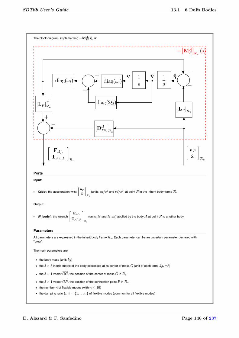
Theblockdiagram,implementing ,is:
Ports
Input:
Xddot:theaccelerationtwist (units: and )atpoint intheinheritbodyframe .
Output:
W_body/.:thewrench (units: and )appliedbythebody atpoint toanotherbody.
Parameters
Allparametersareexpressedintheinheritbodyframe .Eachparametercanbeanuncertainparameterdeclaredwith"ureal".
Themainparametersare:
thebodymass(unit: )
the inertiamatrixofthebodyexpressedatitscenterofmass (unitofeachterm: )
the vector ,thepositionofthecenterofmass in
the vector ,thepositionoftheconnectionpoint in
thenumber offlexiblemodes(with )
thedampingratio offlexiblemodes(commonforallflexiblemodes)
SDTlib User’s Guide 13.1 6 DoFs Bodies
D. Alazard & F. Sanfedino Page 146 of 237

thefrequency ofeachflexiblemode(unit: )
themodalparticipationfactorsatpoint : bothintranslations(unit: )androtations(unit: ),expressedatpoint andinframe .
REMARK:
Theblockinitializationfunctionchecksthattheresidualmass isdefinepositiveforalltheparametric
configurations.Thatmaybetimeconsumingwhenthenumberofparametricuncertaintiesishigh.
Seealso:
Multiportrigidbody
Flexiblebody+revolutejoint
Simulinkdiagramunderthemask
SDTlib User’s Guide 13.1 6 DoFs Bodies
D. Alazard & F. Sanfedino Page 147 of 237
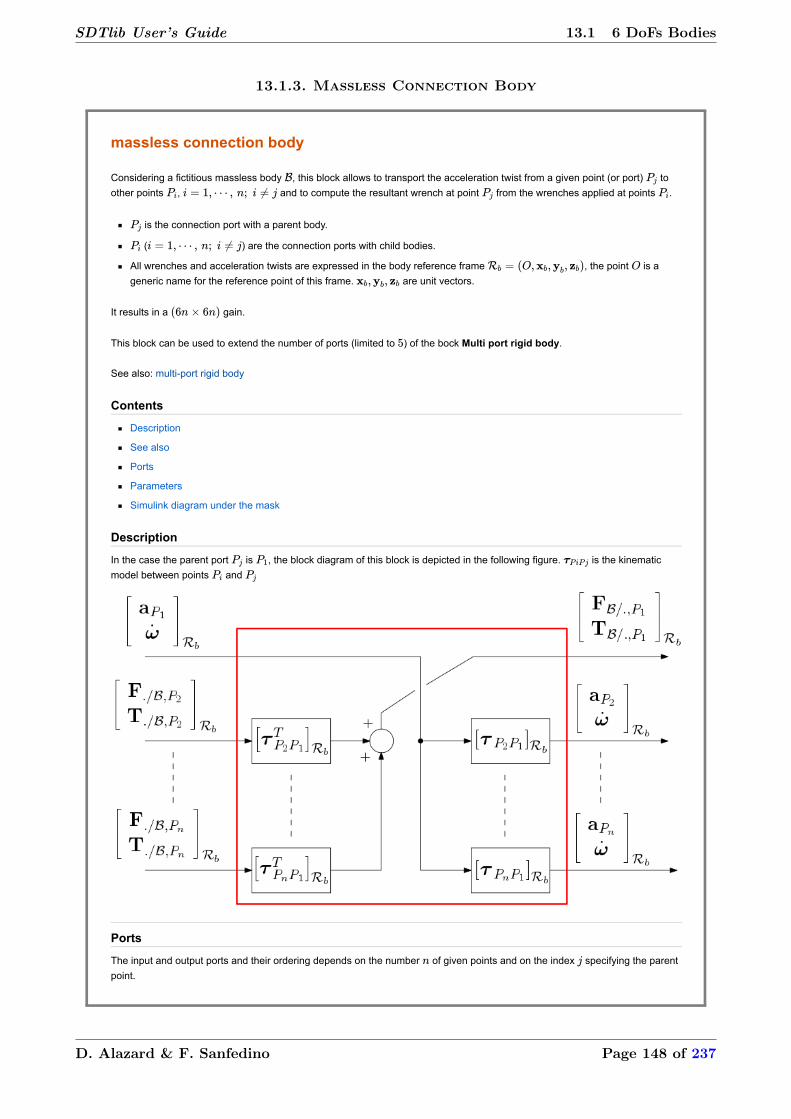
masslessconnectionbody
Consideringafictitiousmasslessbody ,thisblockallowstotransporttheaccelerationtwistfromagivenpoint(orport) tootherpoints , andtocomputetheresultantwrenchatpoint fromthewrenchesappliedatpoints .
istheconnectionportwithaparentbody.
( )aretheconnectionportswithchildbodies.
Allwrenchesandaccelerationtwistsareexpressedinthebodyreferenceframe ,thepoint isagenericnameforthereferencepointofthisframe. areunitvectors.
Itresultsina gain.
Thisblockcanbeusedtoextendthenumberofports(limitedto )ofthebockMultiportrigidbody.
Seealso:multiportrigidbody
Contents
Description
Seealso
Ports
Parameters
Simulinkdiagramunderthemask
Description
Inthecasetheparentport is ,theblockdiagramofthisblockisdepictedinthefollowingfigure. isthekinematicmodelbetweenpoints and
Ports
Theinputandoutputportsandtheirorderingdependsonthenumber ofgivenpointsandontheindex specifyingtheparentpoint.
SDTlib User’s Guide 13.1 6 DoFs Bodies
13.1.3. Massless Connection Body
D. Alazard & F. Sanfedino Page 148 of 237
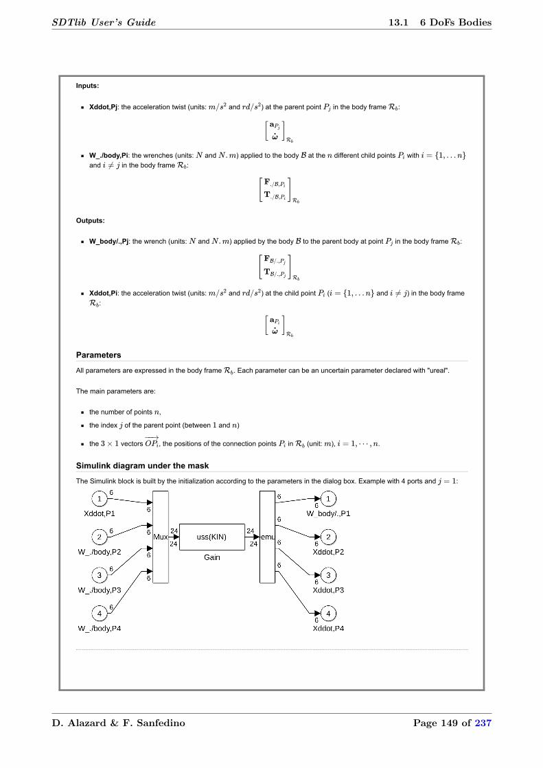
Inputs:
Xddot,Pj:theaccelerationtwist(units: and )attheparentpoint inthebodyframe :
W_./body,Pi:thewrenches(units: and )appliedtothebody atthe differentchildpoints withand inthebodyframe :
Outputs:
W_body/.,Pj:thewrench(units: and )appliedbythebody totheparentbodyatpoint inthebodyframe :
Xddot,Pi:theaccelerationtwist(units: and )atthechildpoint ( and )inthebodyframe:
Parameters
Allparametersareexpressedinthebodyframe .Eachparametercanbeanuncertainparameterdeclaredwith"ureal".
Themainparametersare:
thenumberofpoints ,
theindex oftheparentpoint(between and )
the vectors ,thepositionsoftheconnectionpoints in (unit: ), .
Simulinkdiagramunderthemask
TheSimulinkblockisbuiltbytheinitializationaccordingtotheparametersinthedialogbox.Examplewith4portsand :
SDTlib User’s Guide 13.1 6 DoFs Bodies
D. Alazard & F. Sanfedino Page 149 of 237

1portNastranbody
Oneport(6x6)modelofaNASTRANflexiblebodyfrom.f06file
ThisblockisaNASTRAN/MATLABinterfacetocomputethe lineardynamicmodelofaflexiblebody betweenaccelerationtwistandwrenchappliedbythisbodytoanotherbody.
ThisinterfacereadsthevaluesfromtheNASTRAN/PATRANanalysisoutputfile(filewithextension.f06)tobuildthemodel.Thereaderisadvisedtoreadfirstthehelpof1portflexiblebody.
Theobtainedmodelisexpressed:
initsreferenceframe ,
atthepoint (theconnectionpointwithanotherbody).
Seealso:1portflexiblebody,NportsNASTRANflexiblebody,MultiPort_rigid_body
Contents
Description
Ports
Parameters
Simulinkdiagramunderthemask
Remarks
Description
The modelisdenoted andisdepictedinthefollowingFigure::
SDTlib User’s Guide 13.1 6 DoFs Bodies
13.1.4. One-Port NASTRAN Body
D. Alazard & F. Sanfedino Page 150 of 237

Itdependson:
thefrequencies anddampingratios ( )ofthe flexiblemodes,
the matrixofmodalparticipationfactor ,
theresidualmass ofthebody rigidlycantileveredatpoint .
Theparameters , and arereadfromtheassociatedNastranoutputfiles.Thedampingratioisthesameforalltheflexiblemodes .
Ports
Input:
Xddot:theaccelerationtwist (units: and )atpoint intheinheritbodyframe .
Output:
W_body/.:thewrench (units: and )appliedbythebody atpoint toanotherbody.
Parameters
Nameofthe.f06file(withoutextension):string,
Numberofmodestobeconsidered:integer .Thisintegermustequalorlowerthanthenumberofflexiblemodesinthe.f06file,
Commondampingratio :real(canbedeclaredasanuncertainparameterswithureal),
Uncertainties(%)ontheflexiblemodefrequencies :acommonpositiverealvalueoravectorwith components(inincreasingfrequencyorder).
Simulinkdiagramunderthemask
Remarks:
SDTlib User’s Guide 13.1 6 DoFs Bodies
D. Alazard & F. Sanfedino Page 151 of 237

foreachfrequency ,theassociateduncertainparameterisnamed:'w_name_i'where'name'isthecurrentblockname(withoutspaces).
fortheuserwhowantstotakeintoaccountuncertaintiesonthecomponentsofthemodalparticipationfactormatrix ,2optionsareproposed:
toextractthedatathankstothefunctiongetDataFromNASTRAN1Port.m(see:helpgetDataFromNASTRAN1Port)andthentousethe1portflexiblebodyblock.
tousetheblockaNportsNASTRANflexiblebody(withadummychildport).
SDTlib User’s Guide 13.1 6 DoFs Bodies
D. Alazard & F. Sanfedino Page 152 of 237

NportsNastranbody
NINOPmodelofaNASTRANflexiblebodyfrom.f06and.bdffiles
ThisblockisaNASTRAN/MATLABinterfacetocomputethe lineardynamicmodelofaflexiblebody
.TheN+1portsofthismodelare:
the portsatpoints (for ),i.e.:the channelsfromthewrenchesappliedtothebodyatpoints by
thechildsubstructurestotheaccelerationtwistofpoint ,
theportatpoint ,i.e.:the6channelsfromtheaccelerationtwistofpoint tothewrenchappliedbythebodytothe
parentsubstructureatpoint .
ThisinterfacereadsthevaluesfromtheNASTRAN/PATRANanalysisoutputfiles(fileswithextensions.f06and.bdf)tobuildthemodel.
Theobtainedmodelisexpressedinitsreferenceframe .
Seealso:1portflexiblebody,TITOPmodelofaflexiblebeam,1portNASTRANflexiblebody,MultiPort_rigid_body
Contents
Description
Ports
Parameters
Simulinkdiagramunderthemask
Description
Letusdefine:
:theexternalwrench( )appliedtothebeamatpoint ,expressedin ,
:theaccelerationtwist( )ofthebeamatpoint ,expressedin ,
:theaccelerationtwist( )ofthebeamatpoint ,expressedin ,
:thewrench( )appliedbythebeamatpoint ,expressedin .
TheNINOPmodel oftheflexiblebodyisdescribedbythefollowingblockdiagram:
SDTlib User’s Guide 13.1 6 DoFs Bodies
13.1.5. NINOP NASTRAN Body
D. Alazard & F. Sanfedino Page 153 of 237

ThedetailsofthismodelaredepictedinthefollowingFigure:
Itdependson:
thefrequencies anddampingratios ( )ofthe flexiblemodes,
the matrixofmodalparticipationfactor ,
SDTlib User’s Guide 13.1 6 DoFs Bodies
D. Alazard & F. Sanfedino Page 154 of 237

the projectionmatrix oftheNmodalshapesonthe6d.o.fofpoint ,
the kinematicmodel betweenpoints and ,
theresidualmass ofthebody rigidlycantileveredatpoint .
TheseparametersarereadfromtheassociatedNastranoutputfiles.Itisalsopossibletotakeintoaccountrelativeuncertainties
onthefrequencies,themodalparticipationfactorsandthemodalshapesofeachflexiblemodes.
Ports
Inputs:
W_./body,Ci :6componentsignal(units: and ),
Xddot,P :6componentsignal(units: and ).
Outputs:
Xddot,Ci :6componentsignal(units: and ),
W_body/.,P :6componentsignal(units: and ).
Parameters
Nameofthe.bdffile(withoutextension):string,
Nameofthe.f06file(withoutextension):string,
Gridpointcorrespondingtothepoint (connectionwithparentbody):integer.ThisintegercanbedisplayedinPATRANby
clickingonthenodecorrespondingtotheconnectionpoint andmustbepresentinthe.f06file,
Gridpointscorrespondingtothepoints (connectionwiththechildbodies):vectorofintegers.Thisintegercanbe
displayedinPATRANbyclickingonthenodecorrespondingtotheconnectionpoint andmustbepresentinthe.f06file,
Numberofmodestobeconsidered:integer .Thisintegermustequalorlowerthanthenumberofflexiblemodesinthe
.f06file,
Commondampingratio:real, ,
Percentageofuncertaintyoneachnaturalfrequencies :real,
Percentageofuncertaintyoneachcoefficientofeigenvectorsmatrix( ):real,
Percentageofuncertaintyoneachmodalparticipationfactor( ):real.
Simulinkdiagramunderthemask
TheSimulinkblockisbuiltbytheinitializationaccordingtotheparametersinthedialogbox.Examples:
Dynamicmodelwith8ports:
SDTlib User’s Guide 13.1 6 DoFs Bodies
D. Alazard & F. Sanfedino Page 155 of 237

SDTlib User’s Guide 13.1 6 DoFs Bodies
D. Alazard & F. Sanfedino Page 156 of 237

1portspinningwheel
Oneport(6x6)angularmomentumlinearmodel
Itcomputesthe lineardynamicmodelofabody characterizedbyanonboardangularmomentum(spinningwheel):
i.e.thetransferbetweenaccelerationtwistandwrenchappliedby toanother(parent)body
initsbodyframe , isthereferencepointof ,
atthepoint :theconnectionpointwithanother(parent)body
Seealso:1portNASTRANflexiblebody,1portflexiblebody,MultiPort_rigid_body
Contents
Description
Ports
Parameters
Simulinkdiagramunderthemask
Description
LetusconsiderthespinningwheeldepictedinthefollowingFigureandcharacterizedbythewheelmass ,thewheelaxialand
radialinertia and ,thespinningrate aroundthewheelaxis andthegeometryofthewheelcenterofmass andthe
connectionpoint intheframe .
Underthefollowingassumption:
[H1] and (thespinningrateandthespinaxisofthewheel)areconstantsinframe ,
[H2]thespinningwheelisbalanced:i.e.
thedirectdynamicmodel ofthewheelatpoint inthebodyframe is:
SDTlib User’s Guide 13.1 6 DoFs Bodies
13.1.6. One-Port Angular Momentum
D. Alazard & F. Sanfedino Page 157 of 237

Notethatthewheelframe isattachedtothewheelaxisbutdoesnotspin: ismotionlessin .
Proof:atpoint theNewtonEulerequationsread:
where isthetotalangularmomentumofthebody and istheangularratevectoroftheparentbody
w.r.t.inertialframe.
Thusthedirectdynamicsmodelofthe atpoint ,i.e.the transferfromtheaccelerationtwist tothewrench
appliedby totheparentbody,is:
Inprojectionintheframe , leadstothemodelinequation .
TakingintoaccounttheDCMbetweenframes and : with:
and ,thentransportingthemodel topoint ,weget:
Theblockdiagram,implementing ,is:
SDTlib User’s Guide 13.1 6 DoFs Bodies
D. Alazard & F. Sanfedino Page 158 of 237

Remarks(independentoftheprojectionframeused):
.
Itclearlyappearsthatthemodelofanembeddedangularmomentumappendageisasecondorder modelcontaining
2integrators.These2integratorswereusedtomodeltherotationvector fromtheangularacceleration ,thatisthelast
3inputsofdirectdynamicsmodel.Letusnamed and theparentbodyanditscentreofmass.Whencomputinga
minimalrealizationoftheinversedynamicsmodel augmentedwiththe6integratorsrequiredtocomputethe
speedsfromtheaccelerations,these2previousintegratorsmustberemoved.
Whenconsideringaparentbody fittedwith embeddedangularmomentumappendages , (for
instance,reactionwheels),thedynamicsmodeloftheassembly ,whichisa ordermodel,should
reducetoasecondordermodelbecausethematrix isrank2forallvectors and:
where isthetotalangularmomentumoftheglobalassembly,containingthe spinningtops.
Ports
Input:
Xddot:theaccelerationtwist (units: and )atpoint intheinheritbodyframe .
Output:
W_body/.:thewrench (units: and )appliedbythebody atpoint totheparentbody.
Parameters
Allparametersareexpressedintheinheritbodyframe .Onlythethespinningrate canbeanuncertainparameter
declaredwith"ureal".
Themainparametersare:
thewheelaxis: ,
thewheelmass(Kg): ,
thewheelaxialinertia( ): ,
thewheelradialinertia( ): ,
the vectorpositionof ( ): ,
the vectorpositionof ( ): ,
SDTlib User’s Guide 13.1 6 DoFs Bodies
D. Alazard & F. Sanfedino Page 159 of 237

thespinningrate(rd/s): .
Simulinkdiagramunderthemask
with: .
SDTlib User’s Guide 13.1 6 DoFs Bodies
D. Alazard & F. Sanfedino Page 160 of 237

2portsflexiblebeam
TITOP(TwoInputsTwoOutputsPort),linearandanalyticalmodelofaflexiblebeam.
Thisblockimplementsthe TITOPmodelofaflexiblebeam.The2portsofthismodelare:
theportatpoint ,i.e.:the6channelsfromthewrenchappliedtothebeamatpoint bythechildsubstructuretotheaccelerationtwistof
point ,
theportatpoint ,i.e.:the6channelsfromtheaccelerationtwistofpoint tothewrenchappliedbythebeamtotheparentsubstructureat
point .
Seealso:1portflexiblebody,NportNASTRANflexiblebody,MultiPort_rigid_body
Contents
Description
Ports
Parameters
Simulinkdiagramunderthemask
Seealso
Pureflexiondynamics
Torsiondynamics
Tractiondynamics
TITOPmodelassembly
Description
Consideringabeam describedinthefollowingFigure
Figure1:Aflexiblebeamin3D.
andcharacterizedby
thelocalframe ,
thedimensions: , , and ,
massdensity: ,
Youngmodulus andPoissoncoefficient .
Letusdefine:
:theexternalwrench( )appliedtothebeamatpoint ,expressedin ,
:theaccelerationtwist( )ofthebeamatpoint ,expressedin ,
:theaccelerationtwist( )ofthebeamatpoint ,expressedin ,
:thewrench( )appliedbythebeamatpoint ,expressedin .
SDTlib User’s Guide 13.1 6 DoFs Bodies
13.1.7. TITOP Flexible Beam
D. Alazard & F. Sanfedino Page 161 of 237

Foreachport,the6degreesoffreedom( , , , , , )aresplitinto:
[ ]forwhichthemotionisassumedtobepureflexionintheplane (seealso:Pureflexiondynamics)andcomputed
usinga thorderpolynomialapproximationin ofthedeflection (seealso:(C.Jawharetal.))
[ ]forwhichthemotionisassumedtobepureflexionintheplane andcomputedanalogouslytothepreviouscase,
[ ]forwhichthemotionisassumedtobepuretorsionaround axis(seealso:Torsiondynamics)andcomputedusinga thorder
polynomialapproximationin oftheangulardeflection ,
[ ]forwhichthemotionisassumedtobepuretractionalong axis(seealso:Tractiondynamics)andcomputedusinga thorder
polynomialapproximationin ofthelineardeflection ,
TheTITOPmodeloftheflexiblebeamisdescribedbythefollowingblockdiagram:
Figure2:BlockdiagramoftheTITOPmodel.
Ports
Inputs:
W_./body,C :6componentsignal(units: and ),
Xddot,P :6componentsignal(units: and ).
Outputs:
Xddot,C :6componentsignal(units: and ),
W_./body,C :6componentsignal(units: and ).
Parameters
Theparametersare:
lengthalong (unit: ): ,
crosssection(unit: ): ,
massdensity(unit: ): ,
Youngmodulus(unit: ): ,
secondmomentofareaalongzaxis(unit: ), ,
secondmomentofareaalongyaxis(unit: ), ,
Poissoncoefficient; ,
dampingratio; ,
Simulinkdiagramunderthemask
SDTlib User’s Guide 13.1 6 DoFs Bodies
D. Alazard & F. Sanfedino Page 162 of 237

Seealso:
1portflexiblebody
2portsNASTRANflexiblebody
multiportrigidbody
multiportflexibleplate
LPVDirectionCosineMatrix
Pureflexiondynamicsintheplane( ):
Dynamicsofpureflexionintheplane( )concernsthe2degreesoffreedom ofthebeam.
Figure3:Pureflexionintheplane( ).
Thedeflectionalong ofapointofabscissa isdenoted .Letusdefined:
with: and
Coordinatesandassociatedshapefunctions:
Therigidandflexiblemotioncanbesplitbyintroducingthemotionofthepoint throughtherigidverticaldisplacement( )andthe
rotation( )of :
Theflexiblepart isapproximatedbya thorderpolynomialin :
where isavectorof4elementarymonomials:
suchthat: .
isthevectorofthetimedependentpolynomialcoefficient.
Analogously:
SDTlib User’s Guide 13.1 6 DoFs Bodies
D. Alazard & F. Sanfedino Page 163 of 237

,
.
Thenonecandefinethe matrixofmonomials:
Consideringthe4componentvectorofflexiblecoordinates:
onecanexpressthevectorof timedependentcoefficient asafunctionofthevectorofflexiblecoordinates:
Then,definingthevectorofthe2rigidcoordinates(atpoint ): ,onecanexpress:
Massandstiffnessmatrices
Thekineticenergyisgivenby
withthemassmatrix:
Thered inthematrix,insteadof ,highlightsthattherotationalcontributiontothekineticenergyisneglected.
(Rk: )
Theelasticpotentialenergyisgivenby:
withthestiffnessmatrix:
2portmodel
Letusdenote(seeFigure3):
the2d.o.fwrench(1forceand1torque)appliedbythebeamtotheparentsubstructureatthepoint ,
the2d.o.fwrench(1forceand1torque)appliedtothebeambythechildsubstructureatthepoint .
Thentheworkofthesewrenchesread:
where standsfortherows and ofthevectorormatrix .Thus:
SDTlib User’s Guide 13.1 6 DoFs Bodies
D. Alazard & F. Sanfedino Page 164 of 237

ThusthedynamicmodelobtainedbyLagrangederivationreads:
Usingtheeigenvectormatrix oftheeigenvalueproblem ,onecanintroducethe
dampingmatrix
The2d.o.f.accelerationtwistsatpoints and arewrittenas: and
Then,the2portsmodel( )forthebeam consideringasinputstheaccelerationtwistattheparentnode andthewrenchatthechildnode
isdenoted andcanbedescribedbythefollowingstatespacerepresentation( isrenamed ):
Thismodelrepresentthecaseofabeamclampedat andfreeat .Thankstothefactthatthefeedthroughmatrixconsistsofnonnulltermson
thediagonaltheinversionofthechannelispossible(seealso:invio).Itisthereforepossibletorepresentotherboundaryconditionsbyinversionofoneorseveralchannels.
Pureflexiondynamicsintheplane( ):
TheTITOPmodel forthepureflexionofthebeamintheplane( )canbeobtainedfromthepreviousmodeljust:
changing by inthecomputationofthematrix ,
premultiplyingandpostpultiplyingthe TITOPmodelby (totakeintoaccountthat ).
Torsiondynamics(around axis):
Onlyoneflexiblemodeisconsideredtorepresentthetorsionalong axis.Let theaxialangulardeformationatanypointofabscissa
( )duetoaxialtorques and appliedtothebeamatpoints and ,respectively.Then,itisassumedthat:
thatis,thedeformationat isproportionaltothetotaldeformation ofthebeam.Then,thekineticenergyreads:
with: and .Thepotentialenergyreads:
with: and (shearmodulus).
Thestatespacerepresentationofthe TITOPmodel relativetothetraction/compressiondynamicsalong axistakinginto
accountadampingratio is:
SDTlib User’s Guide 13.1 6 DoFs Bodies
D. Alazard & F. Sanfedino Page 165 of 237

Tractiondynamics(along axis):
Onlyoneflexiblemodeisconsideredtorepresentthetractioncompressionalong axis.Let theaxialdeformationatanypointof
abscissa ( )duetoaxialforces and appliedtothebeamatpoints and ,respectively.Then,itisassumedthat:
thatis,thedeformationat isproportionaltothetotaldeformation ofthebeam.Then,thekineticenergyreads:
with: ,andthepotentialenergyreads:
with: .
Thestatespacerepresentationofthe TITOPmodel relativetothetraction/compressiondynamicsalong axistakinginto
accountadampingratio is:
TITOPmodelassembly:
The TITOPmodel (seeFigure2)ofthebeamisfinallyobtainedbyconcatenatingthe4previousmodelsandreorderingthe
inputsandoutputsusingthepermutationmatrix .Thatis:
SDTlib User’s Guide 13.1 6 DoFs Bodies
D. Alazard & F. Sanfedino Page 166 of 237

SDTlib User’s Guide 13.1 6 DoFs Bodies
D. Alazard & F. Sanfedino Page 167 of 237
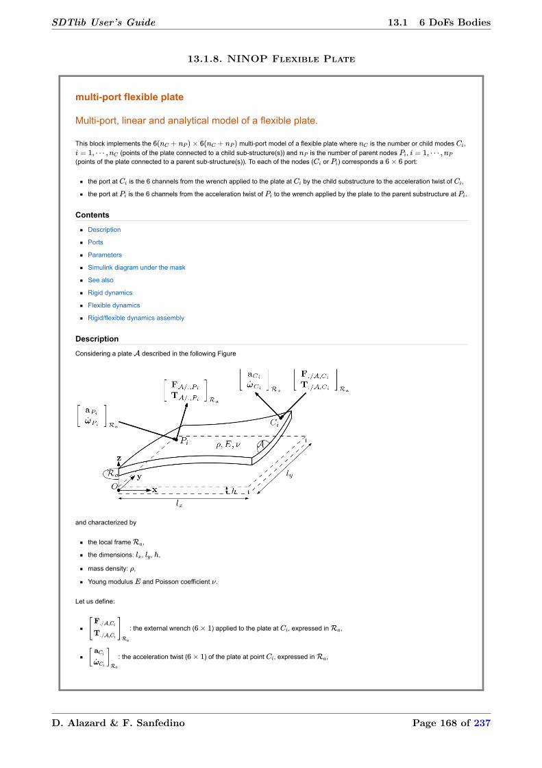
multiportflexibleplate
Multiport,linearandanalyticalmodelofaflexibleplate.
Thisblockimplementsthe multiportmodelofaflexibleplatewhere isthenumberorchildmodes ,
(pointsoftheplateconnectedtoachildsubstructure(s))and isthenumberofparentnodes ,
(pointsoftheplateconnectedtoaparentsubstructure(s)).Toeachofthenodes( or )correspondsa port:
theportat isthe6channelsfromthewrenchappliedtotheplateat bythechildsubstructuretotheaccelerationtwistof ,
theportat isthe6channelsfromtheaccelerationtwistof tothewrenchappliedbytheplatetotheparentsubstructureat .
Contents
Description
Ports
Parameters
Simulinkdiagramunderthemask
Seealso
Rigiddynamics
Flexibledynamics
Rigid/flexibledynamicsassembly
Description
Consideringaplate describedinthefollowingFigure
andcharacterizedby
thelocalframe ,
thedimensions: , , ,
massdensity: ,
Youngmodulus andPoissoncoefficient .
Letusdefine:
:theexternalwrench( )appliedtotheplateat ,expressedin ,
:theaccelerationtwist( )oftheplateatpoint ,expressedin ,
SDTlib User’s Guide 13.1 6 DoFs Bodies
13.1.8. NINOP Flexible Plate
D. Alazard & F. Sanfedino Page 168 of 237

:theaccelerationtwist( )oftheplateatpoint ,expressedin ,
:thewrench( )appliedbytheplateat ,expressedin .
Foreachport,the6degreesoffreedom( , , , , , )aresplitinto:
[ ]forwhichthemotionisassumedtoberigid(seealso:Rigiddynamics)
[ ]forwhichthemotionisflexible(seealso:Flexibledynamics)andcomputedusinga thorderpolynomial
approximationin and ofthedeflection (seealso:FiniteelementbasedNPortmodelforpreliminarydesignof
multibodysystems(F.Sanfedinoetal.)).
Then,inversionchannelfunction(seealso:invio)isusedtoswitchfromchildnodetoparentnode.
Themultiportmodeloftheflexibleplateisdescribedbythefollowingblockdiagram:
Ports
Inputs:
W_./body,Ci :6componentsignal(units: and )for ,
Xddot,Pi :6componentsignal(units: and )for .
Outputs:
Xddot,Ci :6componentsignal(units: and )for ,
W_body/.,Pi :6componentsignal(units: and )for .
Parameters
Theparametersare:
lengthalong (unit: ): ,
widthalong (unit: ): ,
thicknessalong (unit: ): ,
massdensity(unit: ): ,
SDTlib User’s Guide 13.1 6 DoFs Bodies
D. Alazard & F. Sanfedino Page 169 of 237
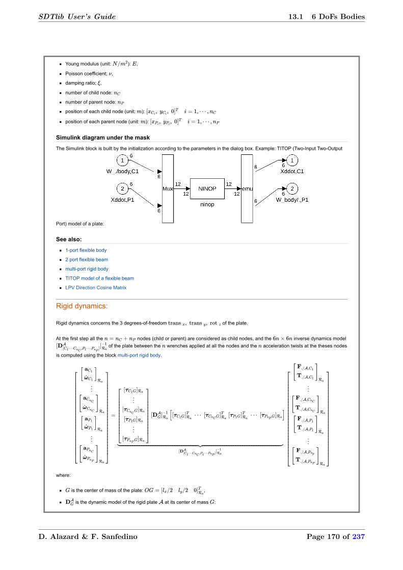
Youngmodulus(unit: ): ,
Poissoncoefficient; ,
dampingratio; ,
numberofchildnode:
numberofparentnode:
positionofeachchildnode(unit: ):
positionofeachparentnode(unit: ):
Simulinkdiagramunderthemask
TheSimulinkblockisbuiltbytheinitializationaccordingtotheparametersinthedialogbox.Example:TITOP(TwoInputTwoOutput
Port)modelofaplate:
Seealso:
1portflexiblebody
2portflexiblebeam
multiportrigidbody
TITOPmodelofaflexiblebeam
LPVDirectionCosineMatrix
Rigiddynamics:
Rigiddynamicsconcernsthe3degreesoffreedom oftheplate.
Atthefirststepallthe nodes(childorparent)areconsideredaschildnodes,andthe inversedynamicsmodel
oftheplatebetweenthe wrenchesappliedatallthenodesandthe accelerationtwistsatthethesesnodes
iscomputedusingtheblockmultiportrigidbody.
where:
isthecenterofmassoftheplate: ,
isthedynamicmodeloftherigidplate atitscenterofmass :
SDTlib User’s Guide 13.1 6 DoFs Bodies
D. Alazard & F. Sanfedino Page 170 of 237
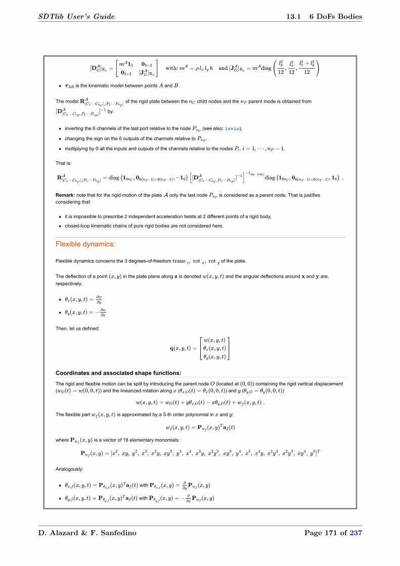
isthekinematicmodelbetweenpoints and .
Themodel oftherigidplatebetweenthe childnodesandthe parentmodeisobtainedfrom
by:
invertingthe6channelsofthelastportrelativetothenode (seealso:invio),
changingthesignonthe6outputsofthechannelsrelativeto .
multiplyingby alltheinputsandoutputsofthechannelsrelativetothenodes , .
Thatis:
Remark:notethatfortherigidmotionoftheplate onlythelastnode isconsideredasaparentnode.Thatisjustifies
consideringthat:
itisimpossibletoprescribe2independentaccelerationtwistsat2differentpointsofarigidbody,
closedloopkinematicchainsofpurerigidbodiesarenotconsideredhere.
Flexibledynamics:
Flexibledynamicsconcernsthe3degreesoffreedom oftheplate.
Thedeflectionofapoint intheplateplanealong isdenoted andtheangulardeflectionsaround and are,
respectively:
Then,letusdefined:
Coordinatesandassociatedshapefunctions:
Therigidandflexiblemotioncanbesplitbyintroducingtheparentnode (locatedat )containingtherigidverticaldisplacement
( )andthelinearizedrotationalong ( )and ( )
Theflexiblepart isapproximatedbya thorderpolynomialin and :
where isavectorof18elementarymonomials:
Analogously:
with
with
SDTlib User’s Guide 13.1 6 DoFs Bodies
D. Alazard & F. Sanfedino Page 171 of 237

Thenonecandefinethe matrixofmonomials:
Consideringthe6points ofcoordinates definedinthefollowingFigure.Then:
Thenonecanexpressthevectorof timedependantcoefficient asafunctionofthevectorofflexiblecoordinates
:
Then,definingthevectorofthe3rigidcoordinates(atpoint ): ,onecanexpress:
Massandstiffnessmatrices
Thekineticenergyisgivenby
withthemassmatrix:
(Rk: )
Theelasticpotentialenergyisgivenby:
Thecurvaturesandtheflexuralrigiditymatrixaregivenby
SDTlib User’s Guide 13.1 6 DoFs Bodies
D. Alazard & F. Sanfedino Page 172 of 237

where istheflexuralstiffnessand isthePoissonratio.Thus with .
2portmodel
Letusdenote:
the3d.o.fwrench(oneforceand2torques)appliedbytheplatetotheparentsubstructureatthepoint
,
the3d.o.fwrench(oneforceand2torques)appliedtotheplateatagivenchildnode .
Thentheworkofthesewrenchesread: or:
Thusthedynamicmodelreads:
Themodalcoordinatesareintroducedbysolvingtheeigenvalueproblem
Applyingthetransformation thesystembecomes:
where: and
Dampingcanbeaddedbyintroducingmatrix .
The3d.o.f.accelerationtwistatchildnode iswrittenas:
The2portsmodel( )fortheplate consideringasinputstheaccelerationtwistattheparentnode andthewrenchatthechild
node isdenoted andcanbedescribedbythefollowingstatespacerepresentation( isrenamed ):
Thismodelrepresentthecaseofaplateclampedat andfreeat .Thankstothefactthatthefeedthroughmatrixhasconsistsof
nonnulltermsonthediagonaltheinversionofthechannelispossible(seealso:invio).Itisthereforepossibletorepresentotherboundaryconditionsbyinversionofoneorseveralchannels.
nportmodel
Considering2childnodes and ,onecaneasilyderivedthe3portmodeloftheplate :
Consideringnowthattheparentnodeisnomore but ,itispossibletocomputethemodel by:
SDTlib User’s Guide 13.1 6 DoFs Bodies
D. Alazard & F. Sanfedino Page 173 of 237

computingthemodel consideringbothnodes and aschildnodes
freeingthenode (nowrenchappliedat )andtransformingthechildnode intoaparentnodebyinvertingthechannels4to9
ofthemodel ,
forgettingthe lastchannels(at )inthemodel,
changingthesignonthe3outputsofthechannelsrelativeto .
Theseoperationscanbesummarizedbythemathematicalexpression:
Inthisexpression:
thenotation standsfortheinversioninthemodel ofthechannelslistedinthevectorofindices ,
thenotation standsfortheselectioninthemodel ofthechannelslistedinthevectorofindices .
Consideringtheplate withthe parentnodesand childmodes,onecaneasilycomputethe portmodelwhichsizeis
( ):
Rigid/flexibledynamicsassembly:
The portmodel (seeFigureabove)oftheplateisfinallyobtainedfromtherigidmodel
byoverwritingthechannelsnumbers3,4and5ofeachofthe portswiththe3channelsofthecorrespondingportofthemodel
.Thatis:
SDTlib User’s Guide 13.1 6 DoFs Bodies
D. Alazard & F. Sanfedino Page 174 of 237

u_sloshing
Sloshing1Dmassspringlinearmodel(6x6)
Itcomputesasimplified dynamicsmodeloflateralsloshingwithaspringmassmodellocatedatpoint (connectionpointwiththehub)alonganydirection.Themodeliswrittenintheinheritbodyframe .
Contents
Description
Ports
Parameters
Simulinkdiagramunderthemask
Description
Itconsistsinwritingtheequationofa springmasssysteminanewframe,wherethe axisisalongagivenspringmass
systemdirection .TheDCMfrom tothisnewframe is: with:
and .
Ports
Input:
Xddot:theaccelerationtwist (units: and )atpoint inthehubframe .
Output:
W_body/.:thewrench (units: and )appliedbythespringmasssystemat .
Parameters
thedirectionvector( ) ofthespringmasssystemexpressedinthe .
thesloshingmass attachedtothespring(unit: )
thefrequency oftheflexiblemode(unit: )
thedampingratio oftheflexiblemode
Eachparametercanbeanuncertainparameterdeclaredwith"ureal".
Simulinkdiagramunderthemask
SDTlib User’s Guide 13.1 6 DoFs Bodies
13.1.9. Sloshing 1D Mass-Spring Model
D. Alazard & F. Sanfedino Page 175 of 237

SDTlib User’s Guide 13.1 6 DoFs Bodies
D. Alazard & F. Sanfedino Page 176 of 237

SDTlib User’s Guide 13.2 6 DoFs Mechanisms
13.2. 6 DoFs Mechanisms
Revolute joint TITOP model
W_./r Xddot_out
Xddot_in W_r/.
Cm θ ddot
Revolute joint
Revolute jointTITOP model
+ angle configuration
W_./r|a Xddot_out|a
Xddot_in|p W_r/.|p
Cm θ ddot
Revolute joint + configuration
Local spring-damper
Xddot,C W./s,C
Xddot,P Ws/.,P
Local Spring-Damper system
D. Alazard & F. Sanfedino Page 177 of 237

Revolutejoint
LinearaugmentedTITOPmodelofarevolutejoint .
Thisblockimplementstheaugmented TITOP(TwoInputTwoOutputPorts)modelofarevolutejoint.The13input
outputchannelsare:
the channelfromthewrenchappliedtotheoutputshaftbythechildbodytotheabsoluteoutputshaftacceleration
twist,
the channelfromtheabsoluteaccelerationtwistoftheinputshafttothewrenchappliedbytheinputshaftonthe
parentbody,
the channelfromthetorqueappliedtotheoutputshaftbytheinputshafttotherelativeangularaccelerationofthe
outputshaftw.r.t.theinputshaft,
Contents
Description
Ports
Parameters
Seealso
Simulinkdiagramunderthemask
Description
Consideringarevolutejoint(seefollowingFigure)atthepoint betweenaparentbody(supportingbodyclampedtheinput
shaft)andthechildbody(loadclampedontheoutputshaft),letusdefine:
:thelocal(inherit)frame,
:thedirectionoftherevolutejointaxisand aunitaryvectoralongthisdirection,
:thedrivingtorquewhichcanbeappliedinsidetherevolutejointbytheinputshafttotheoutputshaft,
:therelativeangularaccelerationoftheoutputshaftw.r.t.totheinputshaft,
:theinertiaoftheoutputshaft,
:theexternalwrench( )appliedtotheoutputshaftbythechildbody,atpoint ,
expressedin ,
:theabsoluteaccelerationtwist( )oftheoutputshaftatpoint ,expressedin ,
:theaccelerationtwist( )oftheinputshaftatpoint ,expressedin ,
:thewrench( )appliedbytheinputshaftontheparentbody,atpoint ,expressedin .
SDTlib User’s Guide 13.2 6 DoFs Mechanisms
13.2.1. Revolute Joint TITOP Model
D. Alazard & F. Sanfedino Page 178 of 237

Then,thedynamicmodelprojectedontherevolutejointaxisreads:
and:
where: standsforthescalarproductofvectors and .
Thecomponents(alongthe5complementaryaxes)ofthewrenchandaccelerationtwistaredirectlytransferredbetweenthe
inputandoutputshafts.
ConsideringtheDCMmatrixmappingtherevolutejointaxisonthethirdaxis:
then,theblockdiagramoftheTITOPmodelofarevolutejointcanbedepictedinthefollowingFigure.
Ports
Inputs:
W_./r,P :6componentsignal(units: and ),
Xddot_in :6componentsignal(units: and ),
Cm :scalarsignal(unit: ).
SDTlib User’s Guide 13.2 6 DoFs Mechanisms
D. Alazard & F. Sanfedino Page 179 of 237

Outputs:
Xddot_out :6componentsignal(units: and ),
W_r/.,P :6componentsignal(units: and ),
Theta_ddot scalarsignal(unit: ).
Parameters
Theinputparametersare:
thedirectionofthejointaxisinthelocalframe(3x1vector): ,
theoutputshaftinertia(unit: ):
Seealso:
Revolutejoint+configuration
1portflexiblebody
Multiportrigidbody
3x3vu_rotation
Simulinkdiagramunderthemask
with: .
SDTlib User’s Guide 13.2 6 DoFs Mechanisms
D. Alazard & F. Sanfedino Page 180 of 237

Revolutejoint+configuration
LinearaugmentedTITOPmodelofarevolutejointaroundagivenangular
configuration.
Thisblockimplementstheaugmented TITOP(TwoInputTwoOutputPorts)modelofarevolutejointlinearizedaround
agivenangularconfiguration.The13inputoutputchannelsare:
the channelfromthewrenchappliedtotheoutputshaftbythechildbodytotheabsoluteoutputshaftacceleration
twist,
the channelfromtheabsoluteaccelerationtwistoftheinputshafttothewrenchappliedbytheinputshaftonthe
parentbody,
the channelfromthetorqueappliedtotheoutputshaftbytheinputshafttotherelativeangularaccelerationofthe
outputshaftw.r.t.theinputshaft,
Contents
Description
Ports
Parameters
Seealso
Simulinkdiagramunderthemask
Description
Consideringarevolutejoint(seefollowingFigure)atthepoint betweenaparentbody(supportingbodyclampedtheinput
shaft)andthechildbody(loadclampedontheoutputshaft),letusdefine:
:theframeattachedtotheoutputshaftorthechildbody,
:theframeattachedtotheinputshaftortheparentbody,
:thedirectionoftherevolutejointaxisand aunitaryvectoralongthisdirection,
:theangularconfigurationoftherevolutejoint: isobtainedfrom byarotationof around ,
:thedrivingtorquewhichcanbeappliedinsidetherevolutejointbytheinputshafttotheoutputshaft,
:therelativeangularaccelerationoftheoutputshaftw.r.t.totheinputshaft,
:theinertiaoftheoutputshaft,
:theexternalwrench( )appliedtotheoutputshaftbythechildbody,atpoint ,
expressedin ,
:theabsoluteaccelerationtwist( )oftheoutputshaftatpoint ,expressedin ,
:theaccelerationtwist( )oftheinputshaftatpoint ,expressedin ,
:thewrench( )appliedbytheinputshaftontheparentbody,atpoint ,expressedin .
SDTlib User’s Guide 13.2 6 DoFs Mechanisms
13.2.2. Revolute Joint TITOP Model + Angle Configuration
D. Alazard & F. Sanfedino Page 181 of 237

Then,thedynamicmodelisbuiltbyusing:
themodelofarevolutejointwithanullangularconfiguration,see:Revolutejoint,
the transformationassociatedtoarotationof aroundagivenaxis ,see:6x6vu_rotationand3x3vu_rotation.
ThemaindifferenceswiththeblockRevolutejointare:
fromtheoutputshaftside,thewrench andtheaccelerationtwist areexpressedin while,fromtheinput
shaftside,thethewrench andtheaccelerationtwist areexpressedin ,
theparameter canbedeclaredasavaryingparameter(ureal)toobtainbyusingulinearizeanLPV(LinearVarying
Parameter)modelvalidforaawholerevolutionofthejoint.
Ports
Inputs:
W_./r,P|a :6componentsignal(units: and ),
Xddot_in|p :6componentsignal(units: and ),
Cm :scalarsignal(unit: ).
Outputs:
Xddot_out|a :6componentsignal(units: and ),
W_r/.,P|p :6componentsignal(units: and ),
Theta_ddot :scalarsignal(unit: ).
Parameters
Theinputparametersare:
thedirectionofthejointaxisinthelocalframe(3x1vector): ,
theoutputshaftinertia(unit: ):
theangularconfiguration (unit: ).
canbeafixedvalueoranvaryingparameterdeclaredwith"ureal"withmode"Range".Example:>>ureal('theta',0,'Range',[pi
pi])
SDTlib User’s Guide 13.2 6 DoFs Mechanisms
D. Alazard & F. Sanfedino Page 182 of 237

Remarks:when"ureal"usused,"ulinearize"ratherthan"linmod"isrecommanded.Thentheuncertainmodelisparameterized
accordingtotherealparameterlabelled"tan_theta_div4".
Seealso:
Revolutejoint
6x6vu_rotation
3x3vu_rotation
1portflexiblebody
Multiportrigidbody
Simulinkdiagramunderthemask
SDTlib User’s Guide 13.2 6 DoFs Mechanisms
D. Alazard & F. Sanfedino Page 183 of 237

6DOFslocalspringdamper
LinearTITOPmodelofaspringdampersysteminthe6d.o.fscase.
Thisblockimplementsthe TITOP(TwoInputTwoOutputPorts)modelofamasslessspringdampersystemlocatedat
thereferencepoint betweenthe points(ports) and ,i.e.thetransferfromthe inputs:
the componentaccelerationtwistatthepoint ,
the componentaccelerationtwistatthepoint ,
tothe outputs:
the componentexternalwrenchappliedtothespringdampersystematthepoint ,
the componentwrenchappliedbythespringdampersystemtooutsideatthepoint .
Contents
Description
Remark
Ports
Parameters
Seealso
Simulinkdiagramunderthemask
Description
Consideringa6d.o.fsspringmasssystemcenteredatthereferencepoint (seefollowingFigure)and2connectionpoints
and withaparentbodyandathechildbody,respectively.Letusdefine:
:thelocal(inherit)frame,
:the stiffnessmatrixatthereferencepoint ,expressedin ,
:the dampingmatrixatthereferencepoint ,expressedin ,
:theinternaldeflectionvector( )ofthespringmasssystematthepoint ,expressedin ,
:theaccelerationtwist( )imposedbythechildbodyatpoint ,expressedin ,
:theaccelerationtwist( )imposedbytheparentbodyatpoint ,expressedin ,
:theexternalwrench( )appliedbythechildbodytothespringdampersystematpoint ,
expressedin ,
:thewrench( )appliedbyspringdampersystemtotheparentbody,atpoint ,
expressedin .
SDTlib User’s Guide 13.2 6 DoFs Mechanisms
13.2.3. 6 DoFs Local Spring-Damper
D. Alazard & F. Sanfedino Page 184 of 237
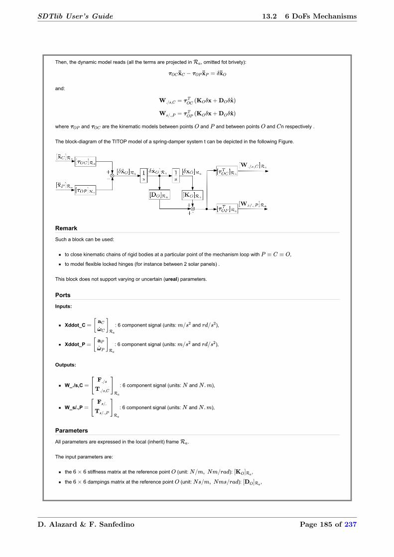
Then,thedynamicmodelreads(allthetermsareprojectedin ,omittedfotbrivety):
and:
where and arethekinematicmodelsbetweenpoints and andbetweenpoints and nrespectively.
TheblockdiagramoftheTITOPmodelofaspringdampersystemtcanbedepictedinthefollowingFigure.
Remark
Suchablockcanbeused:
toclosekinematicchainsofrigidbodiesataparticularpointofthemechanismloopwith ,
tomodelflexiblelockedhinges(forinstancebetween2solarpanels).
Thisblockdoesnotsupportvaryingoruncertain(ureal)parameters.
Ports
Inputs:
Xddot_C :6componentsignal(units: and ),
Xddot_P :6componentsignal(units: and ),
Outputs:
W_./s,C :6componentsignal(units: and ),
W_s/.,P :6componentsignal(units: and ),
Parameters
Allparametersareexpressedinthelocal(inherit)frame .
Theinputparametersare:
the stiffnessmatrixatthereferencepoint (unit: ): ,
the dampingsmatrixatthereferencepoint (unit: ): ,
SDTlib User’s Guide 13.2 6 DoFs Mechanisms
D. Alazard & F. Sanfedino Page 185 of 237

the vectorofthepositionoftheparentpoint (unit: ): ,
the vectorofthepositionoftheparentpoint (unit: ): .
Seealso:
Revolutejoint+configuration
TITOPflexiblebeam+revolutejoint
1portflexiblebody+revolutejoint
Multiportrigidbody+revolutejoint.
Simulinkdiagramunderthemask
SDTlib User’s Guide 13.2 6 DoFs Mechanisms
D. Alazard & F. Sanfedino Page 186 of 237

SDTlib User’s Guide 13.3 3/6 DoFs DCM
13.3. 3/6 DoFs DCM
z-rot3x3[.]_R2 [.]_R1
3x3 z-u_rotation
z-rot6x6[.]_R2 [.]_R1
6x6 z-u_rotation
v-rot3x3[.]_R2 [.]_R1
3x3 v-u_rotation
z-rot3x3
non-lin
[.]_R2
[.]_R1
θ
3x3 z-nl_rotation
z-rot6x6
non-lin
[.]_R2
[.]_R1
θ
6x6 z-nl_rotation
v-rot3x3
non-lin
[.]_R2
[.]_R1
θ
3x3 v-nl_rotation
v-rot6x6
non-lin
[.]_R2
[.]_R1
θ
6x6 v-nl_rotation
6x6 DCM[.]_R2 [.]_R1
6x6 DCM
v-rot6x6[.]_R2 [.]_R1
6x6 v-u_rotation
D. Alazard & F. Sanfedino Page 187 of 237

3x3zu_rotation
Linearparametrizationofthe(3x3)DirectionCosineMatrixassociatedtoarotationaroundthezaxis.
ThisblockimplementstheLFTparametrizationofthe(3x3)directioncosinematrix(DCM)oritstransposedassociatedtotherotationofagivenangle aroundthe axistotransformtheframe intotheframe .
Theparametrizationisintangentofthequarterangle: toderiveLFTwhen isavaryingoranuncertainparameter.
Seealso:6x6zu_rotation,3x3znl_rotation,6x6znl_rotation
Contents
Description
Ports
Parameters
Simulinkdiagramunderthemask
Description
Ifweconsiderthetangentofthehalfangle: ,theDirectionCosineMatrixbecomes:
Astermslike and canbeeasilyrepresentedbyfeedbackloops,arepresentationoftheuncertainornot
DCMmatrixcanbededuced:
SDTlib User’s Guide 13.3 3/6 DoFs DCM
13.3.1. 3x3 z-Rotation
D. Alazard & F. Sanfedino Page 188 of 237

Finally,as:
blocks canbechangedintofeedbackloopswith (seeSimulinkdiagramunderthemask).
If hasafixedvalue, hastoo.If isanuncertainparameterdeclaredwith"ureal",then isalsoanuncertainparameterrepeated times.Moreoverif (awholerevolution), variesin .
Ports
Input:a(3x1)vector intheframe (resp. )
Output:theexpressionofthe(3x1)vector intheframe (resp. ).
(resp. )
Parameters
Theonlyparameteristheangle (unit: ).Itcanalsobeanuncertainparameterdeclaredwith"ureal"withmode"Range".
Example:>>ureal('theta',0,'Range',[pipi])
Remarks:when"ureal"usused,"ulinearize"ratherthan"linmod"isrecommanded.Thentheuncertainmodelisparameterizedaccordingtotherealparameterlabelled"tan_theta_div4".
Acheckboxisproposedtoimplementthetransposed: .
Simulinkdiagramunderthemask
SDTlib User’s Guide 13.3 3/6 DoFs DCM
D. Alazard & F. Sanfedino Page 189 of 237

3x3vu_rotation
Linearparametrizationofthe(3x3)DirectionCosineMatrixassociatedtoarotationaroundanyaxis.
ThisblockimplementstheLFTparametrizationofthe(3x3)directioncosinematrix(DCM)oritstransposedassociatedtotherotationofagivenangle aroundagivenaxis totransformtheframe intotheframe .
Theparametrizationisintangentofthequarterangle: toderiveLFTwhen isavaryingoranuncertainparameter.
DCMisthematrixofthecoordinatesoftherotatedframeaxesintheinitialframe.
Seealso:3x3zu_rotation,6x6vu_rotation,3x3vnl_rotation,6x6vnl_rotation
Contents
Description
Ports
Parameters
Simulinkdiagramunderthemask
Description
Theblocknamed3x3zu_rotationgivesthenonlineardirectioncosinematrix( )associatedtotherotationofagivenangle aroundthe axis.Toexploitthisresult,anintermediateframe isusedsuchthat isalong .Then:
with:
,
,
.
Ports
Input:a(3x1)vector intheframe (resp. ).
Output:theexpressionofthe(3x1)vector intheframe (resp. ).
(resp. )
Parameters
Thetwoparametersare
thecoordinatesofthe(3x1)rotationaxisvector in (or ).
theangle (unit: ).Itcanalsobeanuncertainparameterdeclaredwith"ureal"withmode"Range".
SDTlib User’s Guide 13.3 3/6 DoFs DCM
13.3.2. 3x3 v-Rotation
D. Alazard & F. Sanfedino Page 190 of 237

Example:>>ureal('theta',0,'Range',[pipi])
Remarks:when"ureal"usused,"ulinearize"ratherthan"linmod"isrecommanded.Thentheuncertainmodelisparameterizedaccordingtotherealparameterlabelled"tan_theta_div4".
Acheckboxisproposedtoimplementthetransposed: .
Simulinkdiagramunderthemask
SDTlib User’s Guide 13.3 3/6 DoFs DCM
D. Alazard & F. Sanfedino Page 191 of 237

6x6zu_rotation
Linearparametrizationofthe(6x6)rotationmatrixaroundthezaxis.
Forthe6d.o.f.bodymotion(3translationsand3rotations),thisblockimplementstheLFTparametrizationoftherotationmatrixoritstransposedforagivenangle aroundthe axistotransformtheframe intotheframe .
Theparametrizationisintangentofthequarterangle: toderiveLFTwhen isavaryingoranuncertainparameter(see:3x3zu_rotation)
Seealso:3x3zu_rotation,3x3znl_rotation,,6x6znl_rotation
Contents
Description
Ports
Parameters
Simulinkdiagramunderthemask
Description
Thisblockistheconcatenationoftwoblocks3x3zu_rotation.
Ports
Inputs:a(6x1)vector (3intranslation,3inrotation)intheframe (resp. )
Output:theexpressionofthe(6x1)vector intheframe (resp. )
(resp. )
Parameters
Theonlyparameteristheangle (unit: ).Itcanalsobeanuncertainparameterdeclaredwith"ureal"withmode"Range".
Example:>>ureal('theta',0,'Range',[pipi])
Remarks:when"ureal"usused,"ulinearize"ratherthan"linmod"isrecommanded.Thentheuncertainmodelisparameterizedaccordingtotherealparameterlabelled"tan_theta_div4".
Acheckboxisproposedtoimplementthetransposed: .
Simulinkdiagramunderthemask
SDTlib User’s Guide 13.3 3/6 DoFs DCM
13.3.3. 6x6 z-Rotation
D. Alazard & F. Sanfedino Page 192 of 237

SDTlib User’s Guide 13.3 3/6 DoFs DCM
D. Alazard & F. Sanfedino Page 193 of 237

6x6vu_rotation
Linearparametrizationofthe(6x6)rotationmatrixaroundanyaxis.
Forthe6d.o.f.bodymotion(3translationsand3rotations),thisblockimplementstheLFTparametrizationoftherotationmatrixoritstransposedforagivenangle aroundagivenaxis .
Theparametrizationisintangentofthequarterangle: toderiveLFTwhen isavaryingoranuncertainparameter(see:3x3zu_rotation)
Itisageneralizationofthenonlinearblock"6x6zu_rotation".
Seealso:6x6vnl_rotation,3x3vu_rotation,3x3zu_rotation
Contents
Description
Ports
Parameters
Simulinkdiagramunderthemask
Description
Consideringthe2frames and ,the between and isdefinedasthe matrixwhereeachcolumnisthecomponentvectorofeach orthogonalunitvectorexpressedin .
Inthe6d.o.fscase(3translationsand3rotations),therotationmatrixis:
Thus,thisblockistheconcatenationoftwoblocks3x3vu_rotation.
Ports
Input:a(3x1)vector intheframe (resp. ).
Output:theexpressionofthe(3x1)vector intheframe (resp. ).
(resp. )
Parameters
Thetwoparametersare
thecoordinatesofthe(3x1)rotationaxisvector in (or ).
theangle (unit: ).Itcanalsobeanuncertainparameterdeclaredwith"ureal"withmode"Range".
Example:>>ureal('theta',0,'Range',[pipi])
Remarks:when"ureal"usused,"ulinearize"ratherthan"linmod"isrecommanded.Thentheuncertainmodelisparameterizedaccordingtotherealparameterlabelled"tan_theta_div4".
Acheckboxisproposedtoimplementthetransposed: .
SDTlib User’s Guide 13.3 3/6 DoFs DCM
13.3.4. 6x6 v-Rotation
D. Alazard & F. Sanfedino Page 194 of 237

Simulinkdiagramunderthemask
SDTlib User’s Guide 13.3 3/6 DoFs DCM
D. Alazard & F. Sanfedino Page 195 of 237

3x3znl_rotation
Nonlinear3x3DirectionCosineMatrixassociatedtoarotationaroundthezaxis.
Thisblockimplementsthenonlinear(3x3)directioncosinematrix(DCM)oritstransposedassociatedtotherotationofagivenangle aroundthe axistotransformtheframe intotheframe .
Itisthenonlinearversionofthelinearblockcalled:3x3zu_rotation.
Seealso:3x3zu_rotation,6x6zu_rotation,6x6znl_rotation
Contents
Ports
Parameters
Simulinkdiagramunderthemask
Ports
Inputs:
a(3x1)vector intheframe (resp. )
theangle (unit: ).
Output:theexpressionofthe(3x1)vector intheframe (resp. ).
(resp. )
Parameters
Acheckboxtoimplementthetransposed: .
Simulinkdiagramunderthemask
SDTlib User’s Guide 13.3 3/6 DoFs DCM
13.3.5. 3x3 Non-Linear z-Rotation
D. Alazard & F. Sanfedino Page 196 of 237

with: fordirect , for .
SDTlib User’s Guide 13.3 3/6 DoFs DCM
D. Alazard & F. Sanfedino Page 197 of 237

3x3vnl_rotation
Nonlinear3x3DirectionCosineMatrixassociatedtoarotationaroundanyaxis.
Thisblockimplementsthenonlinear(3x3)directioncosinematrix(DCM)oritstransposedassociatedtotherotationofagivenangle aroundagivenaxis totransformtheframe intotheframe .
Itisthenonlinearversionofthelinearblock3x3vu_rotationandageneralizationofthenonlinearblock3x3znl_rotation.
Seealso:3x3znl_rotation,3x3vu_rotation
Contents
Description
Ports
Parameters
Simulinkdiagramunderthemask
Description
Theblocknamed3x3znl_rotationgivesthenonlineardirectioncosinematrix( )associatedtotherotationofagivenangle aroundthe axis.Toexploitthisresult,anintermediateframe isusedsuchthat isalong .Then:
with:
,
,
.
Ports
Inputs:
a(3x1)vector intheframe (resp. )
theangle (unit: ).
Output:theexpressionofthe(3x1)vector intheframe (resp. ).
(resp. )
Parameters
Theonlyparametersarethecoordinatesofthe(3x1)rotationaxisvector in (or )andacheckboxtoimplementthetransposed: .
Simulinkdiagramunderthemask
SDTlib User’s Guide 13.3 3/6 DoFs DCM
13.3.6. 3x3 Non-Linear v-Rotation
D. Alazard & F. Sanfedino Page 198 of 237

with: fordirect , for and .
SDTlib User’s Guide 13.3 3/6 DoFs DCM
D. Alazard & F. Sanfedino Page 199 of 237

6x6znl_rotation
Nonlinear6x6rotationmatrixaroundthezaxis.
Forthe6d.o.f.bodymotion(3translationsand3rotations),thisblockimplementsthenonlinear(6x6)rotationmatrixoritstransposedforagivenangle aroundthe axistotransformtheframe intotheframe .
Itisthenonlinearversionofthelinearblocknamed6x6zu_rotation.
Seealso:3x3zu_rotation,6x6zu_rotation,3x3znl_rotation
Contents
Description
Ports
Parameters
Simulinkdiagramunderthemask
Description
Thisblockistheconcatenationoftwoblocks3x3znl_rotation.
Ports
Inputs:
a(6x1)vector (3intranslation,3inrotation)intheframe (resp. )
theangle (unit: ).
Output:theexpressionofthe(6x1)vector intheframe (resp. )
(resp. )
Parameters
Acheckboxtoimplementthetransposed: .
Simulinkdiagramunderthemask
SDTlib User’s Guide 13.3 3/6 DoFs DCM
13.3.7. 6x6 Non-Linear z-Rotation
D. Alazard & F. Sanfedino Page 200 of 237

with: fordirect , for .
SDTlib User’s Guide 13.3 3/6 DoFs DCM
D. Alazard & F. Sanfedino Page 201 of 237

6x6vnl_rotation
Nonlinear(6x6)rotationmatrixaroundanyaxis.
Forthe6d.o.f.bodymotion(3translationsand3rotations),thisblockimplementsthenonlinear rotationmatrixoritstransposedassociatedtotherotationofagivenangle aroundagivenaxis totransformtheframe intotheframe .
Itisthenonlinearversionofthelinearblock6x6vu_rotation.
Seealso:3x3vnl_rotation,6x6vu_rotation
Contents
Description
Ports
Parameters
Simulinkdiagramunderthemask
Description
Consideringthe2frames and ,the between and isdefinedasthe matrixwhereeachcolumnisthecomponentvectorofeach orthogonalunitvectorexpressedin .
Inthe6d.o.fscase(3translationsand3rotations),therotationmatrixis:
Thus,thisblockistheconcatenationoftwoblocks3x3vnl_rotation.
Ports
Inputs:
a vector (3intranslation,3inrotation)intheframe (resp. ).
theangle (unit: ).
Output:theexpressionofthe vector intheframe (resp. ).
(resp. ).
Parameters
Theonlyparametersarethecoordinatesofthe(3x1)rotationaxisvector in (or )andacheckboxtoimplementthetransposed: .
Simulinkdiagramunderthemask
SDTlib User’s Guide 13.3 3/6 DoFs DCM
13.3.8. 6x6 Non-Linear v-Rotation
D. Alazard & F. Sanfedino Page 202 of 237

with: fordirect , for .
SDTlib User’s Guide 13.3 3/6 DoFs DCM
D. Alazard & F. Sanfedino Page 203 of 237

6x6DCM
(6x6)rotationmatrixforagiven(3x3)DirectionCosineMatrix(DCM).
Fora6d.o.f.bodymotion(3translationsand3rotations),thisblockimplementsthe rotationmatrixoritstransposefora givendirectioncosinematrix(DCM).
Contents
Description
Ports
Parameters
Simulinkdiagramunderthemask
Description
Consideringthe2frames and ,the between and isdefinedasthe matrixwhereeachcolumnisthecomponentvectorofeach orthogonalunitvectorexpressedin .
Inthe6d.o.fscase(3translationsand3rotations),therotationmatrixis:
Ports
Input:a vector (3intranslation,3inrotation)intheframe (resp. )
Output:theexpressionof intheframe (resp. )
(resp. )
Parameters
Theonlyparametersarethe matrix andacheckboxtoimplementthetransposed: .
Simulinkdiagramunderthemask
SDTlib User’s Guide 13.3 3/6 DoFs DCM
13.3.9. 6x6 DCM
D. Alazard & F. Sanfedino Page 204 of 237

SDTlib User’s Guide 13.3 3/6 DoFs DCM
D. Alazard & F. Sanfedino Page 205 of 237

SDTlib User’s Guide 13.4 Predefined Subsystems
13.4. Predefined Subsystems
One-port flexible body
+ revolute joint (7x7)
Xddot W_body/.
Cm θ ddot
1 port flexible body + revolute joint
Multi-port rigid body
+ revolute joint (6n+1)x(6n+1)
Xddot,P1|p W_body/.,P1|p
Cm_at_P1 θ ddot at P1
W_./body,P2|a Xddot,P2|a
W_./body,P3|a Xddot,P3|a
Multi port rigid body + revolute joint
TITOP flexible beam + revolute joint
(13x13)
W./body,C|a Xddot,C|a
Cm_at_P θ ddot at P
Xddot,P|p W_body/.,P|p
TITOP flexible beam +revolute joint
D. Alazard & F. Sanfedino Page 206 of 237

1portflexiblebody+revolutejoint
Lineardynamicmodelofaflexiblebodyconnectedthrougharevolutejoint( )
Consideringaflexiblebody connectedtoaparentbody througharevolutejointatapoint ,thisblockcomputesthe
dynamicmodelcomposedof:
the channelfromtheabsoluteaccelerationtwistofthepoint tothewrenchappliedbythebody ontheparent
body,expressedintheparentbodyframe ,
the channelfromthedrivingtorqueappliedinsidetherevolutejointtotherelativeaccelerationofthejoint
Contents
Description
Ports
Parameters
REMARK
Seealso
Simulinkdiagramunderthemask
Description
Theflexiblebody connectedtotheparentbody atpoint througharevolutejointisdepictedinthefollowingFigure,letus
define:
:thebodyframeattachedto ,
:thebodyframeattachedto ,
:thedirectionoftherevolutejointaxisand aunitaryvectoralongthisdirection,
:theangularconfigurationoftherevolutejoint: isobtainedfrom byarotationof around ,
and :thereferencepointandthecenterofmassofbody ,
:thedrivingtorquewhichcanbeappliedinsidetherevolutejointbyanexternaldrivingsystem,
:therelativeangularaccelerationofthebodysideshaftw.r.t.totheparentsideshaft,
:theabsoluteaccelerationtwist( )ofpoint ,expressedin ,
:thewrench( )appliedbythebody ontheparentbody,atpoint ,expressedin .
SDTlib User’s Guide 13.4 Predefined Subsystems
13.4.1. One-Port Flexible Body + Revolute Joint
D. Alazard & F. Sanfedino Page 207 of 237

Thedynamicsmodelcanbedenoted (seealsoinvioforthenotation)andcanberepresentedbythe
followingblockdiagram:
Thisblockusesthe2blocks:Oneport_flexible_bodyandRevolutejoint+configuration.
Itsmaininterestare:
itisnotrequiredtospecifytheoutputshaftinertia intherevolutejointblock,
theangularconfiguration oftherevolutejointcanbedeclaredasavaryingparameter.
Ports
Inputs:
Xddot:theaccelerationtwist (units: and )ofpoint intheparentbodyframe
Cm:thejointtorque (unit: )appliedtotheflexiblebodyalongthe revolutionaxis.
Outputs:
W_body/.,P:thewrench (units: and )appliedbythebody atpoint totheparentbody,
expressedintheparentbodyframe
theta_ddot:thejointacceleration (unit: )alongthe revolutionaxis.
Parameters
Allparametersareexpressedinthebodyframe .Eachparameter(except )canbeanuncertainparameterdeclaredwith
"ureal".
Themainparametersare:
thebodymass(unit: )
the inertiamatrixofthebodyexpressedatitscenterofmass (unitofeachterm: )
the vector ,thepositionofthecenterofmass in (unit: )
the vector ,thepositionoftheconnectionpoint in (unit: )
the revolutionaxisdirection :
theangularconfiguration (unit: )
thenumber offlexiblemodes(with )
thedampingratio offlexiblemodes(commonforallflexiblemodes)
thefrequency ofeachflexiblemode(unit: )
themodalparticipationfactorsatpoint : bothintranslations(unit: )and
rotations(unit: ),expressedatpoint andinframe .
SDTlib User’s Guide 13.4 Predefined Subsystems
D. Alazard & F. Sanfedino Page 208 of 237

Remark:if isdeclaredasvaryingparameterwith"ureal"andmode"Range"(ex:ureal('theta',0,'Range',[pipi])),then
"ulinearize"computesaLPVmodelparameterizedaccordingtotherealparameterlabelled"tan_theta_div4".
REMARK:
Theblockinitializationfunctionchecksthattheresidualmass isdefinepositiveforalltheparametric
configurations.Thatmaybetimeconsumingwhenthenumberofparametricuncertaintiesishigh.
Seealso:
Revolutejoint+configuration
1portflexiblebody
Multiportrigidbody
Multiportrigidbody+revolutejoint
TITOPflexiblebeam+revolutejoint
Simulinkdiagramunderthemask
SDTlib User’s Guide 13.4 Predefined Subsystems
D. Alazard & F. Sanfedino Page 209 of 237

Multiportrigidbody+revolutejoint
Dynamicmodelofarigidbodyconnectedthrougharevolutejointatoneportandloadedatotherports
Consideringarigidbody connectedtoaparentbody througharevolutejointatapoint(port) andtochildbodiesat
point ,thisblockcomputesthe dynamicmodelcomposedof:
the channelfromtheabsoluteaccelerationtwistofthepoint tothewrenchappliedbythebody ontheparent
body,expressedintheparentbodyframe ,
the channelfromthedrivingtorqueappliedinsidetherevolutejointtotherelativeaccelerationofthejoint,
the channelsfromthewrenchesappliedto atpoint , bychildbodiestotheabsolute
accelerationtwistofpoints ,expressedinthebodyframe .
Contents
Description
Ports
Parameters
Seealso
Simulinkdiagramunderthemask
Description
Therigidbody connectedtotheparentbody atpoint througharevolutejointandloadedatpoint isdepictedinthe
followingFigure,letusdefine:
:thebodyframeattachedto ,
:thebodyframeattachedto ,
:thedirectionoftherevolutejointaxisand aunitaryvectoralongthisdirection,
:theangularconfigurationoftherevolutejoint: isobtainedfrom byarotationof around ,
and :thereferencepointandthecenterofmassofbody ,
:thedrivingtorquewhichcanbeappliedinsidetherevolutejointbyanexternaldrivingsystem,
:therelativeangularaccelerationofthebodysideshaftw.r.t.totheparentsideshaft,
:theabsoluteaccelerationtwist( )ofpoint ,expressedin ,
:thewrench( )appliedbythebody ontheparentbody,atpoint ,expressedin
,
:theabsoluteaccelerationtwist( )ofpoint ,expressedin ,
:thewrench( )appliedbythebody ontheparentbody,atpoint ,expressedin
.
SDTlib User’s Guide 13.4 Predefined Subsystems
13.4.2. Multi-Port Rigid Body + Revolute Joint
D. Alazard & F. Sanfedino Page 210 of 237

Thedynamicsmodelcanberepresentedbythefollowingblockdiagram:
Thisblockusesthe2blocks:MultiportrigidbodyandRevolutejoint+configuration.
Itsmaininterestare:
itisnotrequiredtospecifytheoutputshaftinertia intherevolutejointblock,
theangularconfiguration oftherevolutejointcanbedeclaredasavaryingparameter.
Ports
Inputs:
Xddot,P1|p:theaccelerationtwist (units: and )ofpoint intheparentbodyframe
Cm:thejointtorque (unit: )appliedtotherigidbodyalongthe revolutionaxis,
W_./body,Pi|a:thewrench (units: and )appliedtothebody atpoint ,expressedinthebody
frame , .
Outputs:
SDTlib User’s Guide 13.4 Predefined Subsystems
D. Alazard & F. Sanfedino Page 211 of 237

W_body/.,P1|p:thewrench (units: and )appliedbythebody atpoint totheparentbody,
expressedintheparentbodyframe
theta_ddot:thejointacceleration (unit: )alongthe revolutionaxis,
Xddot,Pi|a:theaccelerationtwist (units: and )ofpoint inthebodyframe , .
Parameters
Allparametersareexpressedinthebodyframe .Eachparameter(except )canbeanuncertainparameterdeclaredwith
"ureal".
Themainparametersare:
thebodymass(unit: )
the inertiamatrixofthebodyexpressedatitscenterofmass (unitofeachterm: )
the vector ,thepositionofthecenterofmass in (unit: )
thenumberofports
the vectors ,thepositionsoftheconnectionpoints in (unit: ),
the revolutionaxisdirection :
theangularconfiguration (unit: )
Remark:if isdeclaredasvaryingparameterwith"ureal"andmode"Range"(ex:ureal('theta',0,'Range',[pipi])),then
"ulinearize"computesaLPVmodelparameterizedaccordingtotherealparameterlabelled"tan_theta_div4".
Seealso:
Revolutejoint+configuration
Multiportrigidbody
1portflexiblebody+revolutejoint
TITOPflexiblebeam+revolutejoint
1portflexiblebody
Simulinkdiagramunderthemask
SDTlib User’s Guide 13.4 Predefined Subsystems
D. Alazard & F. Sanfedino Page 212 of 237

SDTlib User’s Guide 13.4 Predefined Subsystems
D. Alazard & F. Sanfedino Page 213 of 237

TITOPflexiblebeam+revolutejoint
Dynamicmodelofaflexiblebeamconnectedthrougharevolutejointatonetipandloadedattheothertip
Consideringaflexiblebeam connectedtoaparentbody througharevolutejointatonetip(port) andtoachildbodyat
theothertip ,thisblockcomputesthe dynamicmodelcomposedof:
the channelfromthewrenchesappliedto atpoint bythechildbodytotheabsoluteaccelerationtwistofpoints
,expressedinthebodyframe ,
the channelfromthedrivingtorqueappliedinsidetherevolutejointtotherelativeaccelerationofthejoint,
the channelfromtheabsoluteaccelerationtwistofthepoint tothewrenchappliedbythebody ontheparent
body,expressedintheparentbodyframe .
Contents
Description
Ports
Parameters
Seealso
Simulinkdiagramunderthemask
Description
Theflexiblebeam connectedtotheparentbody atpoint througharevolutejointandloadedatpoint isdepictedin
thefollowingFigure,letusdefine:
:thebodyframeattachedto :itisassumedthatthebeamaxisisalongthe axisof ,
:thebodyframeattachedto ,
:thedirectionoftherevolutejointaxisand aunitaryvectoralongthisdirection,
:theangularconfigurationoftherevolutejoint: isobtainedfrom byarotationof around ,
and :the2tipsofthebeam ,
:thedrivingtorquewhichcanbeappliedinsidetherevolutejointbyanexternaldrivingsystem,
:therelativeangularaccelerationofthebodysideshaftw.r.t.totheparentsideshaft,
:theabsoluteaccelerationtwist( )ofpoint ,expressedin ,
:thewrench( )appliedbythebody ontheparentbody,atpoint ,expressedin ,
:theabsoluteaccelerationtwist( )ofpoint ,expressedin ,
:thewrench( )appliedbythebody ontheparentbody,atpoint ,expressedin .
SDTlib User’s Guide 13.4 Predefined Subsystems
13.4.3. TITOP flexible beam + Revolute Joint
D. Alazard & F. Sanfedino Page 214 of 237

Thedynamicsmodelcanberepresentedbythefollowingblockdiagram:
Thisblockusesthe2blocks:TITOPflexiblebeamandRevolutejoint+configuration.
Itsmaininterestare:
itisnotrequiredtospecifytheoutputshaftinertia intherevolutejointblock,
theangularconfiguration oftherevolutejointcanbedeclaredasavaryingparameter.
Ports
Inputs:
W_./body,C|a:thewrench (units: and )appliedtothebody atpoint ,expressedinthebody
frame .
Cm:thejointtorque (unit: )appliedtotherigidbodyalongthe revolutionaxis,
Xddot,P|p:theaccelerationtwist (units: and )ofpoint intheparentbodyframe
Outputs:
Xddot,C|a:theaccelerationtwist (units: and )ofpoint inthebodyframe , .
theta_ddot:thejointacceleration (unit: )alongthe revolutionaxis,
W_body/.,P|p:thewrench (units: and )appliedbythebody atpoint totheparentbody,
expressedintheparentbodyframe
Parameters
Allparametersareexpressedinthebodyframe .Eachparameter(except )canbeanuncertainparameterdeclaredwith
"ureal".
SDTlib User’s Guide 13.4 Predefined Subsystems
D. Alazard & F. Sanfedino Page 215 of 237

Themainparametersare:
lengthalong (unit: ): ,
crosssection(unit: ): ,
massdensity(unit: ): ,
Youngmodulus(unit: ): ,
secondmomentofareaalongzaxis(unit: ), ,
secondmomentofareaalongyaxis(unit: ), ,
Poissoncoefficient; ,
dampingratio; ,
the revolutionaxisdirection :
theangularconfiguration (unit: )
Remark:if isdeclaredasvaryingparameterwith"ureal"andmode"Range"(ex:ureal('theta',0,'Range',[pipi])),then
"ulinearize"computesaLPVmodelparameterizedaccordingtotherealparameterlabelled"tan_theta_div4".
Seealso:
Revolutejoint+configuration
TITOPflexiblebeam
Multiportrigidbody
Multiportrigidbody+revolutejoint
1portflexiblebody
Simulinkdiagramunderthemask
SDTlib User’s Guide 13.4 Predefined Subsystems
D. Alazard & F. Sanfedino Page 216 of 237

SDTlib User’s Guide 13.4 Predefined Subsystems
D. Alazard & F. Sanfedino Page 217 of 237

SDTlib User’s Guide Chapter 14. SDTlib blocks dialog boxes
14. SDTlib blocks dialog boxes
14.1. 6 DoFs Bodies
14.1.1. Multi-Port Rigid Body
D. Alazard & F. Sanfedino Page 218 of 237

SDTlib User’s Guide 14.1 6 DoFs Bodies
14.1.2. One-Port Flexible Body
D. Alazard & F. Sanfedino Page 219 of 237
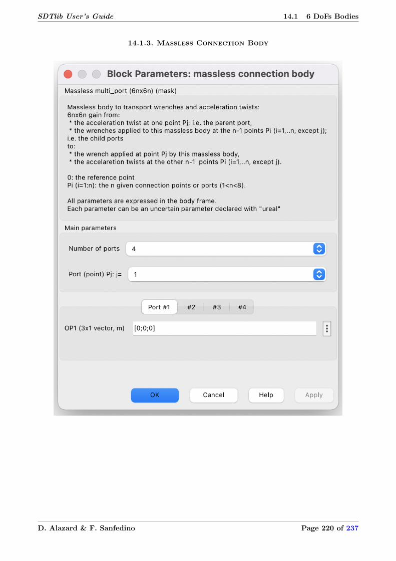
SDTlib User’s Guide 14.1 6 DoFs Bodies
14.1.3. Massless Connection Body
D. Alazard & F. Sanfedino Page 220 of 237

SDTlib User’s Guide 14.1 6 DoFs Bodies
14.1.4. One-Port NASTRAN Body
D. Alazard & F. Sanfedino Page 221 of 237

SDTlib User’s Guide 14.1 6 DoFs Bodies
14.1.5. NINOP NASTRAN Body
D. Alazard & F. Sanfedino Page 222 of 237

SDTlib User’s Guide 14.1 6 DoFs Bodies
14.1.6. One-Port Angular Momentum
D. Alazard & F. Sanfedino Page 223 of 237

SDTlib User’s Guide 14.1 6 DoFs Bodies
14.1.7. NINOP Flexible Plate
D. Alazard & F. Sanfedino Page 224 of 237

SDTlib User’s Guide 14.1 6 DoFs Bodies
14.1.8. TITOP Flexible Beam
D. Alazard & F. Sanfedino Page 225 of 237

SDTlib User’s Guide 14.1 6 DoFs Bodies
14.1.9. Sloshing 1D Mass-Spring Model
D. Alazard & F. Sanfedino Page 226 of 237

SDTlib User’s Guide 14.2 6 DoFs Mechanisms
14.2. 6 DoFs Mechanisms
14.2.1. Revolute Joint TITOP Model
D. Alazard & F. Sanfedino Page 227 of 237

SDTlib User’s Guide 14.2 6 DoFs Mechanisms
14.2.2. Revolute Joint TITOP Model + Angle Configuration
D. Alazard & F. Sanfedino Page 228 of 237

SDTlib User’s Guide 14.2 6 DoFs Mechanisms
14.2.3. 6 DoFs Local Spring-Damper
D. Alazard & F. Sanfedino Page 229 of 237

SDTlib User’s Guide 14.3 3/6 DoFs DCM
14.3. 3/6 DoFs DCM
14.3.1. 3x3 z-Rotation
14.3.2. 3x3 v-Rotation
D. Alazard & F. Sanfedino Page 230 of 237

SDTlib User’s Guide 14.3 3/6 DoFs DCM
14.3.3. 6x6 z-Rotation
14.3.4. 6x6 v-Rotation
D. Alazard & F. Sanfedino Page 231 of 237

SDTlib User’s Guide 14.3 3/6 DoFs DCM
14.3.5. 3x3 Non-Linear z-Rotation
14.3.6. 3x3 Non-Linear v-Rotation
D. Alazard & F. Sanfedino Page 232 of 237

SDTlib User’s Guide 14.3 3/6 DoFs DCM
14.3.7. 6x6 Non-Linear z-Rotation
14.3.8. 6x6 Non-Linear v-Rotation
D. Alazard & F. Sanfedino Page 233 of 237

SDTlib User’s Guide 14.3 3/6 DoFs DCM
14.3.9. 6x6 DCM
D. Alazard & F. Sanfedino Page 234 of 237

SDTlib User’s Guide 14.4 Predefined Subsystems
14.4. Predefined Subsystems
14.4.1. One-Port Flexible Body + Revolute Joint
D. Alazard & F. Sanfedino Page 235 of 237

SDTlib User’s Guide 14.4 Predefined Subsystems
14.4.2. Multi-Port Rigid Body + Revolute Joint
D. Alazard & F. Sanfedino Page 236 of 237

SDTlib User’s Guide 14.4 Predefined Subsystems
14.4.3. TITOP Flexible beam + Revolute Joint
D. Alazard & F. Sanfedino Page 237 of 237