Faculty of Economics and BusinessAmsterdam School of Economics

Requirements thesis MSc in Econometrics.

1. The thesis should have the nature of a scienti�c paper. Consequently the thesis is dividedup into a number of sections and contains references. An outline can be something like (thisis an example for an empirical thesis, for a theoretical thesis have a look at a relevant paperfrom the literature):

(a) Front page (requirements see below)

(b) Statement of originality (compulsary, separate page)

(c) Introduction

(d) Theoretical background

(e) Model

(f) Data

(g) Empirical Analysis

(h) Conclusions

(i) References (compulsary)

If preferred you can change the number and order of the sections (but the order youuse should be logical) and the heading of the sections. You have a free choice how tolist your references but be consistent. References in the text should contain the namesof the authors and the year of publication. E.g. Heckman and McFadden (2013). Inthe case of three or more authors: list all names and year of publication in case of the�rst reference and use the �rst name and et al and year of publication for the otherreferences. Provide page numbers.

2. As a guideline, the thesis usually contains 25-40 pages using a normal page format. All thatactually matters is that your supervisor agrees with your thesis.

3. The front page should contain:

(a) The logo of the UvA, a reference to the Amsterdam School of Economics and the Facultyas in the heading of this document. This combination is provided on Blackboard (inMSc Econometrics Theses & Presentations).

(b) The title of the thesis

(c) Your name and student number

(d) Date of submission �nal version

(e) MSc in Econometrics

(f) Your track of the MSc in Econometrics

1

Sarcasm Detection in Reddit Comments

by

Stepan Svoboda11762616

Masters in Econometrics

Track: Big Data Business Analytics

Supervisor: L. S. Stephan MPhil

Second reader: prof. dr. C.G.H. Diks

August 12, 2018

Statement of Originality

This document is written by student Stepan Svoboda who declares to take full respon-

sibility for the contents of this document.

I declare that the text and the work presented in this document are original and that

no sources other than those mentioned in the text and its references have been used in

creating it.

The Faculty of Economics and Business is responsible solely for the supervision of com-

pletion of the work, not for the contents.

1

UNIVERSITY OF AMSTERDAM

Abstract

Faculty of Economics and Business

Amsterdam School of Economics

Masters in Econometrics

by Stepan Svoboda

This thesis created a new sarcasm detection model which levies existing research in

sarcasm detection field and applies it to a novel data set from an online commenting

platform. It takes several different approaches to extract information from the com-

ments and their context (author’s history and parent comment) and identifies the most

promising approaches. The main contribution is the identification of most promising

features on the large and novel data set which should make the findings robust to noise

in data. The achieved accuracy was 69.5% with the model being slightly better at de-

tecting non-sarcastic than sarcastic comments. The best features, given the hardware

limitations, were found to be the PoS-based ones and lexical-based ones.

Acknowledgements

I would like to thank my supervisor, Sanna Stephan, for all the help and feedback she

provided me during the writing of my thesis. I’m also grateful to my friends Jan, Samuel

and Radim for all their support and help during my studies and work on the thesis.

3

Contents

Statement of Originality 1

Abstract 2

Acknowledgements 3

List of Figures 6

List of Tables 7

Abbreviations 8

Glossary 9

1 Introduction 1

2 Sentiment Analysis and Sarcasm Detection 4

2.1 Sentiment Analysis . . . . . . . . . . . . . . . . . . . . . . . . . . . . . . . 5

2.1.1 Polarity classification . . . . . . . . . . . . . . . . . . . . . . . . . 7

2.1.2 Beyond polarity classification . . . . . . . . . . . . . . . . . . . . . 9

2.2 Sarcasm Detection . . . . . . . . . . . . . . . . . . . . . . . . . . . . . . . 9

2.2.1 Survey of sarcasm detection . . . . . . . . . . . . . . . . . . . . . . 10

2.2.2 Research papers . . . . . . . . . . . . . . . . . . . . . . . . . . . . 11

3 Data description 15

3.1 Sarcasm detection data set . . . . . . . . . . . . . . . . . . . . . . . . . . 15

3.1.1 Authors’ history . . . . . . . . . . . . . . . . . . . . . . . . . . . . 17

4 Methodology 19

4.1 Pre-processing & Feature engineering . . . . . . . . . . . . . . . . . . . . . 19

4.1.1 Bag-of-Words . . . . . . . . . . . . . . . . . . . . . . . . . . . . . . 20

4.1.2 Sentiment-based features . . . . . . . . . . . . . . . . . . . . . . . 22

4.1.3 Lexical-based features . . . . . . . . . . . . . . . . . . . . . . . . . 23

4.1.4 PoS-based features . . . . . . . . . . . . . . . . . . . . . . . . . . . 23

4.1.5 Word similarity-based features . . . . . . . . . . . . . . . . . . . . 24

4.1.6 User embeddings . . . . . . . . . . . . . . . . . . . . . . . . . . . . 25

4.2 Neural network . . . . . . . . . . . . . . . . . . . . . . . . . . . . . . . . . 25

4

Contents 5

4.2.1 Feed-forward Neural network . . . . . . . . . . . . . . . . . . . . . 26

4.2.2 Error Backpropagation . . . . . . . . . . . . . . . . . . . . . . . . . 31

4.3 Evaluation . . . . . . . . . . . . . . . . . . . . . . . . . . . . . . . . . . . . 35

5 Empirical part 38

5.1 Setup . . . . . . . . . . . . . . . . . . . . . . . . . . . . . . . . . . . . . . 38

5.2 Results . . . . . . . . . . . . . . . . . . . . . . . . . . . . . . . . . . . . . . 41

5.2.1 Discussion . . . . . . . . . . . . . . . . . . . . . . . . . . . . . . . . 44

6 Conclusion 48

A Truncated SVD 51

B Neural net optimization 53

B.1 Neural net architecture . . . . . . . . . . . . . . . . . . . . . . . . . . . . . 53

C Used libraries 56

Bibliography 57

List of Figures

4.1 A basic neural net (Bishop, 2006) . . . . . . . . . . . . . . . . . . . . . . . 27

6

List of Tables

5.1 Confusion matrix of the main model . . . . . . . . . . . . . . . . . . . . . 41

5.2 Summary of the performance of individual models . . . . . . . . . . . . . 42

5.3 Confusion matrix of the model using as features: BoW and context . . . . 42

5.4 Confusion matrix of the model using as features: BoW, context and PoS-based features . . . . . . . . . . . . . . . . . . . . . . . . . . . . . . . . . . 43

5.5 Confusion matrix of the model using as features: BoW, context andsimilarity-based features . . . . . . . . . . . . . . . . . . . . . . . . . . . . 43

5.6 Confusion matrix of the model using as features: BoW, context and usersimilarity-based features . . . . . . . . . . . . . . . . . . . . . . . . . . . . 43

5.7 Confusion matrix of the model using as features: BoW, context andsentiment-based features . . . . . . . . . . . . . . . . . . . . . . . . . . . . 44

5.8 Confusion matrix of the model using as features: BoW, context andlexical-based features . . . . . . . . . . . . . . . . . . . . . . . . . . . . . . 44

C.1 Libraries used in this thesis . . . . . . . . . . . . . . . . . . . . . . . . . . 56

7

Abbreviations

BoW Bag-of-Words

CM Confusion Matrix

ML Machine Learning

NLP Natural Language Processing

PCA Principal Component Analysis

PoS Part-of-Speech

TF-IDF Term Frequency-Inverse Document Frequency

SGD Stochastic Gradient Descent

SVD Singular Value Decomposition

w.r.t. with respect to

8

Glossary

k-nearest neighbor Technique which moves all observed data points into n-dimensional

space, where n is the number of features, and finds the k closest points based on

a prespecified distance measure, e.g. Euclidean distance. 11

Amazon’s Mechanical Turk Amazon’s Mechanical Turk is an internet marketplace

for tasks which computers are currently unable to do. Human users can choose

and execute these tasks for money, thereby providing the input for the subsequent

ML process. A typical ML example is acquiring set of predefined labels for a data

set, which can be later used to perform a supervised learning task.. 11, 14

bigram An augmentation of preprocesing of the BoW. Instead of a word a collocation

of two words is in the columns. An example sentence ’I went shopping’ has three

unigrams (’I’, ’went’ & ’shopping’) and 2 bigrams (’I went’, ’went shopping’). 12,

13, 45, 49

BoW This technique is applied directly to all the preprocessed documents (comments)

and creates a matrix with all the words being represented in the columns and

all the documents being represented by the rows. Then each field of this matrix

represents the number of occurences of a specific word in the specific document.

9, 10, 12–14, 20, 21, 24, 38, 42, 45, 49

deep learning Type of ML based on Neural Nets aimed at learning data representa-

tions such as shapes and objects in images. ’Deep’ in the name refers to the large

number of layers. 10, 26

determiner ’A modifying word that determines the kind of reference a noun or noun

group has, e.g. a, the, every’ (Oxford Dictionary). An example are the articles in

9

Glossary 10

the sentence ”The girl is a student”, where both of them are determiners which can

specify the definiteness, i.e. do we know the girl?, and volume of the appropriate

nouns, e.g. indefinite article is not compatible with a plural. 11

feature ML equivalent of explanatory variable. Non-numerical features can be recoded

to numerical state. 2, 3, 9–14, 17, 19, 22, 23, 42, 44

feature set A number of distinctive (yet related) features used together as one set. 2,

10, 11, 13, 19, 27, 41–44, 46

hyperparameter In ML hyperparameter is a parameter whose value is not learned but

is set before the learning begins. 10, 30, 39, 40, 53

lexical clue A specific type of expression in writing, akin to voice inflection and ges-

turing in speech, e.g. emoticons, capital letters and more than one punctuation

mark in a row. 11

online learning This method allows to train a model on data that come in sequentially,

this is commonly used when the data set is too large to handle at once and the

computation is divided into many parts to make them feasible. It is called online

learning since it can handle real-time data. 26, 38

regularized regression Augmented OLS, called Ridge regression or l2 penalty, by an

additional term in the loss function. The rewritten loss function takes follow-

ing form:∑n

i=1(yi −∑k

j=1 xijβj)2 + λ

∑kj=1 β

2j . An alternative versions of reg-

ularization exist such as l1 penalty, or LASSO regression, which takes the form∑ni=1(yi −

∑kj=1 xijβj)

2 + λ∑k

j=1 βj . 13, 14

test set Data set on which the generalization properties of the validated model are

evaluated. The generalization property is the ability of the model to perform well

on previously unseen data. 11, 39

unigram The word in the column of a BoW. 9, 12, 13, 45, 49

validation set Data set which provides evaluation of the generalization properties of

the model and allows hyperparameters to be tuned. 39

Glossary 11

verb morphology Specific form of a verb, e.g. passive tense and infinitive. 11

word embeddings A process in which a word or a phrase is mapped to a vector of

real numbers. It is a general term that can be associated with different methods.

One of them is described briefly in Section 4.1.5. 14, 18

Chapter 1

Introduction

The analysis of unstructured data is a complex and intriguing problem. Unstructured

data are usually comprised mainly from text but other information, such as dates and

numeric values, can be present. Unlike in the case of structured data there is no rigid

and uniform structure such as is common with all structured data, i.e. rows being the in-

stances of the phenomenon and columns being the properties of the individual instances.

The structured data are sometimes also called rectangular due to their structure. Struc-

tured data are commonly saved in the .csv format since that format was created to store

this kind of data. An example of structured data might be list of countries (instances)

with their GDP, area and population represented in the columns. The final table is then

a rectangle which is where the name ‘rectangular data‘ comes from.

The lack of structure in unstructured data makes an analysis difficult since it is usually

highly irregular. An example of unstructured data might be online communication of

the employees, e.g. emails or internal instant messaging platform. Many specialized

techniques are required to retrieve the desired information.

The sheer volume of this data is gigantic. It was estimated in 1998 that somewhere

between 80-90% of all business data are actually in the unstructured form (Grimes), e.g.

anything from an invoice, internal memo to a log of a machine’s performance. This is

only a rule of thumb and no quantitative research has been done but is still a somewhat

accepted ratio and is often cited. This is an incredible amount of information that could

be levied to improve virtually every aspect of the business operations. This ratio is also

1

2

supported by the Computer World magazine’s claims that more than 70-80% of data

are in unstructured form (Chakraborty & Pagolu).

One type of unstructured data analysis is the sentiment analysis which is essentially an

automated way to extract opinions from the text at hand (Oxford Dictionary). The

most common example of extracted opinion is the polarity of a statement, i.e. pos-

itive/negative. A more detailed description follows in the next chapter. This type of

analysis suffers from many drawbacks which are enumerated and discussed in this thesis.

This thesis focuses on one problem specifically, sarcasm presence in the available textual

information. This can easily mislead the sentiment analysis model since taken literally,

sarcastic statements have a meaning different from the one intended. An example is a

statement ’It’s great to be at work when there’s such a nice weather!’, this statement

can seem at first as an honest, and positive, remark since it does not include any typical

signs of a negative comment. But with some background knowledge the hidden meaning,

sarcasm, can be easily seen.

This thesis tries to build on and extend the current sarcasm detection literature and

by combining the best existing features create a working sarcasm detection model. In

the process the distinct features are also compared against each other and the most

beneficial ones are found. The comparison of the features is one of the main extensions

of the current existing literature achieved by this thesis. This goal was achieved in two

stages, in the first one data pre-processing and feature engineering took place and in

the second the found features were used as an input for a neural net, i.e. in this case a

classification algorithm. In the first step several pre-processing approaches were used to

obtain various types of features and in the second step their actual benefit was evaluated.

The benefit brought by the specific feature sets is also compared to the computational

burden and the overall usefulness is evaluated.

The difference between the models in ML and standard econometrics should be high-

lighted since this thesis focuses exclusively on the former. In ML we cannot really derive

the true underlying process and model this process as is common in econometrics and

thus we do not know exact rules that govern the model’s decision process. This lack

of interpretability is a trade-off for overall better prediction power of these ‘black-box‘

models.

3

The thesis is organized as follows, in Chapter 2 sentiment analysis is described as a whole

with special care given to the sarcasm detection and related literature. In Chapter 3 the

used data are described and in Chapter 4 both pre-processing and feature engineering

are discussed in length alongside the description of neural net. Afterwards the results

are presented in Chapter 5 and the thesis ends with some concluding remarks in Chapter

6.

Chapter 2

Sentiment Analysis and Sarcasm

Detection

Sentiment analysis is defined by the Oxford Dictionary as ’the process of computationally

identifying and categorizing opinions expressed in a piece of text, especially in order to

determine the writer’s attitude towards a particular topic or product’. This discipline

based mainly on Natural Language Processing (NLP) and Text Mining is widely used

in many fields, from marketing and spam detection (Peng & Zhong, 2014) to financial

markets forecasting (Xing et al. , 2018). The specific applications and how sentiment

analysis is used in these fields are discussed in the following sections. This chapter is

divided into two sections. First the sentiment analysis is introduced in general and

afterwards sarcasm detection is discussed in detail.

Sarcasm detection is indeed an issue that typically prevents a straightforward sentiment

analysis. The problem sarcastic or ironic (here used interchangeably) comments pose

is they often use different polarity than they express. An example might be a sentence

’Great job!’, which can be meant both sincerely and sarcastically. In both cases the

sentiment seems positive at first sight but the true meaning differs and that can throw

the analysis off.

The other issues are not discussed in depth here and are only briefly mentioned. Different

types of opinions, i.e. regular vs comparative and explicit vs implicit opinions, are

an issue since detecting comparisons or implicit opinions is complicated. Subjectivity

detection is also an issue since many applications of sentiment analysis want to discern

4

5

between a statement without emotional undertone and with some emotional charge. Last

problem sentiment analysis faces is the point of view which can be either the author’s

or the reader’s.

These problems are quite intuitive but some examples are given here nonetheless (Liu,

2012). Regular opinion is stating that Coke is good while comparative is that Coke is

better than Pepsi. Explicit is saying iPhone has bad battery life while implicit is saying

iPhone has shorter battery life than Samsung. Subjective opinion is one expressing not

a fact but my personal opinion, i.e. I like Apple products. Lastly the point of view

matters as well. For example the news of a stock-hike is good for people who own the

stock but bad for people who shorted the stock.

The way in which these problems can mislead the analysis are various. The comparative

opinion requires the researcher to determine whether Coke is better than Pepsi or the

other way around. It must be established what is the relationship between the two

compared things. Implicit opinion suffers from the same problem, the structure of the

sentence must be used to automatically determine which of the two things is compared

to which. If this is not done the sentence can be understood incorrectly. Subjective

and objective opinions depend a lot on specific use cases but differentiating between

emotion-less and emotional statements can be important in removing potential noise

which brings very little to the overall model. The point of view issue is similar to

the problems implicit and comparative opinions pose. The entity which expressed the

opinion must be determined for us to know whether there is some hidden agenda, e.g.

an analyst claiming a stock has bad fundametals might have motivation to damage a

stock since his firm could hold a short position in the stock.

2.1 Sentiment Analysis

Sentiment analysis (sometimes also known as opinion mining) aims to determine the

position of the speaker/writer towards a specific issue. This can be done with respect

to the overall polarity of the analyzed document/paragraph/sentence/... or underlying

emotional response to the analyzed event. There are many slightly different names for

slightly different tasks within this broad category of sentiment analysis or opinion min-

ing such as opinion extraction, sentiment mining, subjectivity analysis, affect analysis,

6

emotion mining and review mining (Liu, 2012). Opinion extraction and sentiment min-

ing are the same and focus only on identifying the existing sentiment/opinion in the given

document. Subjectivity analysis is concerned with discerning between subjective and

objective statements. The possible usage differs per the need of the specific researcher

but common usage is removing the objective sentences before determining polarity to

improve the model’s ability to differentiate between positive and negative statements.

Affect analysis and emotion mining are the same since they aim to detect the expressed

emotional state in the text. Review mining describes all types of sentiment analysis but

used only on one specific type of text, i.e. reviews.

In sentiment analysis both the position of the writer and the specific issue addressed

are of interest since different types of sentiment analysis deal with different problems

arising from the different specifications (Liu, 2012). The position can be expressed in

two ways, either we can describe the stance of a person towards the issue, i.e. positive

or negative, or we can try to describe the emotional response elicited, i.e. sadness,

anger, happiness etc. Beyond the emotional response the subjectivity and aspect-based

measures of the statement/document can be looked at. Aspect-based measures attempt

to find expressed sentiment toward specific entities. A document can be negative toward

one entity and at the same time positive toward another entity, i.e. a review can be

critical to a museum and give an example of a good museum.

Subjectivity analysis aims to find subjective parts of the document in order to differen-

tiate between different types of expressed opinion. Another option is to downgrade the

importance or remove the objective statements to achieve greater accuracy in simple

polarity analysis. The aspect-based sentiment analysis aims to identify the sentiment

expressed towards a specific entity mentioned in the text, which requires to determine

not only the sentiment but also the entities in the text (Liu, 2012). By looking at the

opinions in finer granularity the analysis can be more precise and deliver more informa-

tion.

The subjectivity analysis and aspect-based approach are not discussed here in depth

since they are not of main interest in this thesis and only applications of the polarity

(positive/negative) of opinion or advanced sentiment classification are mentioned later

on.

7

2.1.1 Polarity classification

A few examples of possible applications of the standard sentiment analysis, i.e. polarity

classification, are given in this chapter. The examples include mainly data from social

networks and the tasks using sentiment analysis are various. They range from mar-

keting, e.g. identifying brand sentiment, counting the number of positive and negative

reactions, and using polarity as an input for recommendation systems, e.g. Twitter, to

financial forecasting. A practical example can be Starbucks, they use sentiment analysis

to identify complaints on Twitter and answer all of these negative comments.

The first application discussed is detecting spam or fake reviews. Here the term spam

reviews is used due to the terminology of Peng & Zhong (2014). Users giving false

positive or negative reviews to either boost or ruin a score of a product/store is not

an uncommon issue. Spotting a spam review and removing it can greatly improve

the trustworthiness of a rating site and improve the consumer experience as Peng &

Zhong (2014) discuss. They managed to improve the detection of the spam reviews

by employing a three step algorithm. The first step was computing the sentiment of

the reviews. This was followed by a second step where a set of discriminative rules

was applied to detect unexpected patterns in the text. The third and final step was a

creation of time series based on the reviews and sentiment score to see and detect any

sudden anomalies.

Another possible application is using sentiment analysis as an input for a recommen-

dation system to improve the recommendation precision. Yang et al. (2013) use a

recommendation system based on two main approaches. One is using a location-based

data and the other is using sentiment analysis data to make recommendations. They

use social networks with location data and by using this information in tandem with

the information from sentiment analysis, i.e. sentiment of posts on these social media,

they manage to create and successfully apply a novel recommendation engine. An-

other example worth mentioning is the paper of Gurini et al. (2013) where they ex-

plore the possibility of better friend recommendation systems. They took the standard

content-based similarity measure, cosine similarity, and augmented it by plugging in the

Sentiment-Volume-Objective (SVO) function. SVO is based on the expressed sentiment,

the volume and the subjectivity of the reactions toward a concept by a specific user. The

contribution of the sentiment analysis here is the augmentation of the measure used to

8

recommend the specific users. Thanks to this augmentation the recommendation engine

takes into account more information and knows how similar the attitudes of the two

persons are. By using not only the shared interests but also the sentiment analysis of

the user’s content they managed to create and original model.

In a newer paper Zimbra et al. (2016) decided to use neural nets and Twitter data

to assign a brand a sentiment class in a three- or five-class sentiment system. Here the

sentiment analysis is used to find out the public perception of a certain brand, which can

be very useful for all marketing practitioners. They manually labeled tweets mentioning

Starbucks and used those in their analysis.

Poecze et al. (2018) studied the effectiveness of social media posts based on the metrics

provided by the platform and sentiment analysis of the reactions. The effectiveness was

measured by the number of different reactions, e.g. ’shares’ and ’likes’. They found

out sentiment analysis proved an invaluable complement in evaluating the effectiveness

of certain posts since it was able to look past the standard metrics and determine why

some forms of communication were less popular with the consumer base. The underlying

positive/negative reaction of the base is better measured by the sentiment analysis than

by number of views and reactions alone.

Ortigosa et al. (2014) concentrate solely on Facebook and determining the polarity of the

users’ opinions and the changes in their mood based on the changes of their comments’

polarity. By combining a lexical-based approach and a machine learning-based one they

managed to create a tool that first determines the polarity of a submission and then by

computing the user’s standard sentiment polarity detects significant emotional changes.

Lastly the survey from Xing et al. (2018) focuses on financial forecasting. The natural

language based financial forecasting (NLFF) is a strand of research focused on enhanc-

ing the quality of financial forecasting by including new explanatory variables based on

NLP with sentiment analysis having a prominent place in this area. Among the ana-

lyzed documents are corporate disclosures such as quarterly/annual reports, professional

periodicals such as Financial Times, aggregated news from sources like Yahoo Finance,

message boards activities and social media posts. The texts from these sources can then

be used for different types of sentiment analysis like subjectivity and polarity analysis.

This can be useful for many parties, an obvious example being any trader or hedge fund.

9

Any information signalling possible price movement of a stock is extremely valuable and

can be used in the overall valuation.

2.1.2 Beyond polarity classification

Mohammad (2016) discusses in his work sentiment analysis quite holistically, from stan-

dard polarity and valence of the shown sentiment to emotions. The problems of this

strand of research are discussed alongside some of the underlying theory from psychol-

ogy. One of the main issues is finding labeled data since in emotion analysis we don’t

have just a binary problem, e.g. positive/negative or sarcastic/not sarcastic. The exist-

ing work is summarized in this paper which makes it a good starting point for anyone

interested in this specific area of sentiment analysis.

One of the solutions to the problem of missing labels in data sets can be the emotion

lexicon presented in Staiano & Guerini (2014). It is an earlier work but it can serve as a

good starting point for other emotion lexicons. The authors created a lexicon containing

37 thousand terms and a corresponding emotion score for each of the terms. This can be

an invaluable source for anyone wanting to apply a sentiment analysis that goes beyond

simple polarity.

2.2 Sarcasm Detection

Sarcasm detection has become a topic in sentiment analysis due to the problems it

causes. A statement imparting negative/positive sentiment while seemingly having the

opposite polarity can quite quickly lower the accuracy of sentiment analysis models (Liu,

2012). This gave rise to a specialized field of research – sarcasm detection. Most of the

papers focused on this problem are quite new (less than 10 years old) and the progress

from first attempts using only word lexicons and lexical cues to the current literature

using context, word embeddings and other neural net-based approaches is significant.

This section is divided into two parts, in the first a survey paper is presented as a possible

introduction into this field of research. In the following section actual research papers

are discussed and the evolution of this area of research presented.

10

2.2.1 Survey of sarcasm detection

The most notable paper that concentrates on this topic is from Joshi et al. (2017). The

setup, issues, different kinds of data sets, approaches, their performances and the trends

present in the sarcasm detection literature are discussed. The problems discussed in this

paper are mentioned here but they are not analyzed in depth. In the following section

some papers dealing with sarcasm detection are discussed and when relevant the issues

are highlighted.

The linguistic background is not discussed here and can be found with proper references

in the Joshi et al. (2017) paper alongside the overall problem definition.

The different types of available data are divided based on text length – short, long,

transcripts/dialogue and miscellaneous or mixed, i.e. those that do no fit into previous

categories. The different approaches to the problem of sarcasm detection (illustrated

in the choice of papers in next section) can be divided into rule-based and feature set-

based. A rule-based system is typically a set of {IF : THEN} statements such as

IF ′red′ THEN ′stop′ rule for a car. These rules can be much more complicated and

possibly nested as well. The feature set-based one also comprises of usage of different

algorithms, i.e. standard ML and deep learning ones. The trends are also described in

the next section since the choice of papers is organized along the time axis and nicely

imparts the evolution of the field.

Then the issues with the process of sarcasm classification are discussed. The prominent

issue is the data annotation. Several options are discussed in the next chapter but the

main difference is along the axis self-labeled and annotated by third party. The quality

of these labels is also in question since humans have trouble discerning between sarcastic

and non-sarcastic utterances and no labels from a third-party can be perfect. With self-

labeling the data quality problem lies in selecting users that use the appropriate hashtag

or similar method to announce the use of sarcasm. This is coupled with cases where the

hashtag is used either by accident or in different meaning than intended, e.g. talking

about the usage of #sarcasm. Another issue is the inherent skewness in data since most

comments and tweets are not sarcastic and some measures need to be taken for the data

set to be balanced.

11

Some local/temporal specifics of lexical clue are important as well. These clues are

not constant in time and in different cultures/countries. Usage of emojis and some

abbreviations, e.g. LOL, is a somewhat newer development and is not spread evenly

over the globe. Background knowledge is required for constructing this type of feature

sets.

2.2.2 Research papers

In following paragraphs the progress in the field is illustrated and the changes in overall

approach to classifying sarcasm are shown. Some of the changes are linked to the growth

of computational power, e.g. possibility of using neural network-based methods.

One of the early papers focused on identifying sarcasm is the Carvalho et al. (2009)

paper that attempted to find irony in user-generated content by looking for lexical clues,

specifically detecting irony in sentences containing normally positive words by looking for

oral and gestural clues. Examples of these clues are among others emoticons, laughter

expressions (haha, LOL,...) and number of punctuation marks in a row. They also

found that some more complex linguistic information were quite inefficient in detecting

irony. The more complex linguistic information were constructions such as diminutives,

determiners and verb morphology. Since this research was done mainly on Portuguese

text some of the chosen features were specific to Portuguese and are not transferable to

other languages. The evaluation of their work was done by hand, some comments were

chosen at random and then manually scored with this score being then compared to the

predicted value. Their contribution is showing that the overall sentiment analysis can be

easily improved by using even simple lexical rules to identify some sarcastic comments.

Davidov et al. (2010) use just like Carvalho et al. manually labeled data. They use the

Amazon’s Mechanical Turk to label a large collection of tweets and of Amazon reviews.

This gives rise to the main data set which is then divided into training and test set.

This is the common and correct approach and later on in this section it is assumed

as standard. Only deviations from this approach are highlighted. Each instance is

rated by three independent evaluators which guarantees a high level of reliability. Their

algorithm is based on expressing each observation in training set as a vector based on the

extracted features and then using the k-nearest neighbor technique to match the testing

observations to its most similar vectors in training set based on Euclidean distance.

12

Majority voting was then used to classify the testing observation. Their features included

a separation of the sentences into different patterns identifying so called high-frequency

words and content words. They have pre-existing patterns and look how similar the

review/tweet is to their patterns and each observation gets a score between 0 and 1 for

each pattern. These patterns are then combined with some punctuation based features.

Newer papers include Riloff et al. (2013) that focuses exclusively on Twitter data. Their

data are once again labeled by human annotators and are chosen with special emphasis

on choosing tweets that are sarcastic on its own and not as a reply. By doing this

the context becomes insignificant and one of common problems in sarcasm detection

is solved. They used several feature sets, various existing sentiment lexicons, support

vector machines on BoW (created with unigrams and unigrams & bigrams) and their

own sentiment lexicon created by bootstrapping the key phrases. They have a very

specific case of sarcasm in mind, one where a positive sentiment is followed by negative

sentiment with this incongruity creating the irony, e.g. ’I love being ignored’. Then

they use this assumption to learn positive and negative phrases (using many iterations)

which then serve as their lexicon used to identify the positive and negative sentiment

present. If both are found in tandem then that is taken as evidence of sarcasm being

present. The overall model is more complex but this description is supposed to give only

a very rough overview of the idea.

Wallace et al. (2014) is the first paper mentioned here that talks about the necessity of

using context for detecting sarcasm. It claims that since humans usually need context

to detect sarcasm, machines should as well. They reach this conclusion on Reddit, social

media site described in Chapter 3, data set which is scored by humans and during the

scoring it is recorded whether the annotator asked for additional context. They used a

basic logistic regression with one explanatory dummy variable (asking for context) to

show that in case of an ironic comment the annotators are more likely to ask for context.

Their claim was substantiated also by another model, another logistic regression. They

have shown that their base-line model makes mistakes more often in the cases where

the annotators asked for context, which again points to the intuitive conclusion of both

machines and humans needing context for sarcasm detection.

Bamman & Smith (2015) are also trying to detect sarcasm by leveraging the contextual

information. Another important feature of this paper is the data they are using. They

13

use tweets and they started using self-labeled data, i.e. #sarcasm, #irony, etc., while

taking measures to exclude retweets and other submissions that are not appropriate for

their study. They used many standard approaches to create features such as unigrams

and bigrams (BoW), part of speech tags, capitalizaton, punctuation, tweet sentiment

and tweet word sentiment within one tweet. Then they also extracted features regarding

the authors such as their profile information and historical sentiment, audience features

such as communication between author and addressee and their shared interests. They

found out that combination of the information about author and those contained in the

tweet was nearly on par with the inclusion of all features at hand. They used a basic

regularized regression and managed to reach accuracy of 85%.

A similar avenue was studied by Khattri et al. (2015) who used just like Bamman &

Smith (2015) author’s history but they rather focused on sentiment contrast than many

different text-based features. They implement this idea by creating two models and

then synthesizing them. The first is they find the overwhelming historical sentiment

towards a specific entity and the second is looking at what sentiment is shown towards

the entity in the current tweet. This model using context is then combined with stan-

dard sentiment incongruity within one tweet. They develop specific rules for combining

these models and report a very good overall performance. The performance is based on

standard classification measures descibed in Section 4.3. They also acknowledge some

shortcomings of their approach such as assumption that author’s history contains the

true sentiment and some accounts being deactivated, renamed or otherwise inaccessible.

This accounted for approximately 10% of all authors.

Another paper worth mentioning is from Wallace et al. (2015) which is a follow up of

the paper Wallace et al. (2014) where it was shown that machines do need context for

detecting sarcasm jut like humans. In the newer paper a proper model implementing

the context as a feature is presented. The data set used was presented in the older

paper and here it is only reused. As their features they decided to leverage the detected

sentiment alongside the specific subreddit, which is a specific part of Reddit and is defined

in the beginning of Chapter 3, and so called ’bag-of-NNP’. This bag is constructed in

the same way as standard BoW but only noun phrases (NNP), not unigrams, are taken

into account from each comment. Then by creating an interaction feature set between

the NNP features and subreddits they acquire their fourth feature type. To properly

14

leverage these features they use a specific regularization combining both an l1 and l2

penalty (explained in regularized regression), each levied on a specific subset of features.

Ghosh et al. (2015) focused on somewhat different task, discerning between a literal

and sarcastic usage of a word. They used Twitter data and then employed Amazon’s

Mechanical Turk to crowdsource the labels on specific phrases. The tweets themselves

were self-labeled, i.e. #sarcasm, #sarcastic, ..., and the phrases in the tweets that

were meant sarcastically were labeled by the Turkers, i.e. people who perform tasks

at Amazon’s Mechanical Turk. The Turkers also came up with an alternative way to

say the same message but without sarcasm. This gave rise to a lexicon of phrases with

similar meaning to the original sarcastic utterance. These phrases were then transformed

by word embeddings and used to classify the sarcastic tweets.

Joshi et al. (2016) also worked with word embeddings but in a different fashion than

Ghosh et al. (2015). Instead of using the embeddings themselves as features they use

them to find the word similarity between respective words within comments however

they do not use contextual information in this paper. Only features discussed previ-

ously (lexical, BoW-based, sentiment incongruity, punctuation) on top of the addition

of finding similarity between different words using their word embeddings. Several dif-

ferent pre-trained instances of word embeddings were used and the overall result was

that these features bring significant additional value.

Amir et al. (2016) followed in the direction of Joshi et al. (2016) and used word embed-

dings as well. Their innovation was training user embeddings which contain context and

author’s history. Their overall model is then a neural net with convolutional layers which

processes both user embeddings and content features. They split these features into four

groups – tweet-features, author-features, audience-features and response-features. They

used an existing data set from the paper by Bamman & Smith (2015) and the used

features were also the same with the exception of the user embeddings. The proposed

model seems to be outperforming the original model from Bamman & Smith (2015).

Chapter 3

Data description

In this chapter the used data are presented. Two different data sets were used, one is a

freely available data set created for sarcasm detection tasks and the other is a data set

of authors’ history downloaded from Reddit for this thesis.

Reddit is the self-proclaimed front page of the internet. It is a social-media news ag-

gregation website where each user can post in each Reddit forum (called subreddit) a

comment, link or a video and others comment and react to it in a typical hierarchi-

cal manner. Subreddits range from topics like politics and religion to NBA (highest

US basketball league), NFL (highest US american football league) and all the way to

country-specific subreddits like the Netherlands.

Both data sets are based on Reddit comments which were all in English. Almost all

of Reddit is in English and the prepared data set was curated to include only English

comments.

3.1 Sarcasm detection data set

The main data set used in this thesis is the one prepared by Khodak et al. (2017).

The data are split into training and testing part by the authors already and on top of

that there are two versions – balanced and unbalanced one1. In this thesis the balanced

version is used due to the aim of the thesis and hardware limitations. The balanced

1Balanced data set is a data set where all classes are equally represented while an unbalanced onehas higher prevalence of some classes than other classes

15

16

version contains more than a million comments and that already presents a substantial

computational burden.

The corpus consists of several different variables beside the label. The comment itself, the

parent comment, the subreddit where the comment was published, the author, publish

date and the number of likes and dislikes. Naturally the comment itself and the context

(parent comment and subreddit) hold the most information and are expected to bring a

lot of explanatory power.

The data set is presented and described in quite a length in the original article and here

only the most important aspects are highlighted.

The most important detail that must be mentioned is the way the labels are acquired.

The sarcastic labels are added by Reddit commentators themselves by adding /s at the

end of their comments. The labels are put in during the actual writing of the comment.

They are not added at later date.

Several filters were used to exclude noisy comments, these include filtering comments

which are just URLs and special handling of some comments due to properties of Reddit

conversations, such as replies to sarcastic comments, since these are usually very noisy

according to Khodak et al. (2017).

The raw data set contains 533 million comments, of which 1.3 million are sarcastic, from

January 2009 to April 2017. This set is controlled to include only authors who know the

Reddit sarcasm notation, /s, by excluding people who have not used in the month prior

to their comment the standard notation. These are excluded to minimise the noise by

authors that do not know this notation. This sarcasm notation used on Reddit is known

as self-labeling which means only the author has any influence on the final label of the

comment. Khodak et al. (2017) devote large part of the paper to showing the noise is

minimized and the data are thus appropriate for analysis. They study the proportion of

the sarcastic and non-sarcastic comments, the rate of false positive and negatives and

the overall quality of the corpus for NLP tasks.

For a comment to be eligible for the data set it must pass several quality barriers, i.e.

• the author is familiar with the notation meaning they used the sarcastic label in

the past month prior to the comment,

17

• the comment is not a descendant, direct or indirect, of a comment labeled as

sarcastic due to noise in the labeling following a sarcastic comment,

• due to the sarcasm prevalence in the overall data set being 0.25% only very few

comments can be marked as sarcastic and actually be a reply to sarcastic comment

which was not labeled as one.

The noise from classifying sarcastic comments which were answers to non-labeled sar-

castic comments exists but in the overall scale is minimal. The impact on the overall

performance is negligible but it is important to mention its existence. We are dealing

with real-world data and obtaining proper labeling for every instance is simply impos-

sible, this is as good as it gets.

The authors also performed a manual check on a small subset of the data and arrived at

conclusion that the number of false positives is about 1% while the false negative rate is

about 2%. This is an issue in the unbalanced setting as the sarcasm prevalence is about

0.25% but in the balanced setting of the data set this noise is quite limited. Overall the

manual checks are described in length in the original paper and Khodak et al. (2017)

state the filters are working reasonably well as shown by high overlap percentage with

the manual check. The manual label was created by a majority voting scheme between

human annotators.

Khodak et al. (2017) also explain why Reddit is a better data source for sarcasm

detection than most other commonly used sources. It holds the same advantage as

Twitter in having self-labeled data while being written in non-abbreviated English unlike

Twitter. Thanks to Reddit being organized into subreddits with clear comment structure

and context it is much easier to recover the necessary context features. According to

the authors these are the main advantages which make the data set more realistic and

better suited for this type of research.

The balanced data set used in this thesis has slightly more than one million comments.

3.1.1 Authors’ history

The idea behind the author’s history is to create a typical behavior pattern of a user.

We want to create a benchmark that is relevant in explaining the user’s behavior.

18

The number of authors present in the above-mentioned data set is quite large, approx-

imately quarter of a million. A large majority has only one comment and only a small

number of people has many comments. The largest number of comments per author is

854. Thus the only way to retrieve an author’s history is to download it directly from

Reddit.

In order to create a reasonable representation of user’s behavior on Reddit 100 newest

comments per user were downloaded. These then serve as a benchmark to compare the

comment of interest to the ”standard” way the user expresses themselves. This kind

of information is again targeted at the incongruity within a person’s expressions and is

based on the original idea of Amir et al. (2016).

The specific process is in detail described in Section 4.1.6. These comments were used

to create an equivalent of word embeddings for users. Not a word but a user is mapped

into the high-dimensional vector space.

Chapter 4

Methodology

The methodology description is divided into several parts, firstly the process of feature

selection and text processing is explained and motivated. Secondly neural networks

are described and explained. Thirdly and lastly the approach to model evaluation is

explained and the chosen measures are justified.

4.1 Pre-processing & Feature engineering

Several text processing techniques were used to extract the signal from the available

comments. Context is very important for sarcasm detection for humans and the same

applies for machines as was already shown in the literature (Wallace et al. , 2014). Both

the original comment and its context (parent comment and author’s history) are used

to provide additional information for our modeling. The exact extent to which is this

information used is described for all distinctive feature sets in the following sections.

The used techniques are described in some detail in the following sections. Alongside

the described features a specific form of context is used – a simple variable specifying

the prevalence of sarcasm of the subreddit. The share of sarcastic comments is calculated

by dividing the number of sarcastic comment by the overall number of comments.

19

20

4.1.1 Bag-of-Words

This technique is applied to the text itself, firstly all unnecessary words from all docu-

ments at hand are removed and then the remaining words are used to fill a matrix, i.e.

the BoW. In this matrix the documents represent the rows and the columns represent

the words. Each field in the matrix thus marks how many times a word was used in a

document.

This is a standard NLP method that is widely used due to its strength and predictive

power.

The pre-processing of the text, i.e. removing all unnecessary words, consists of sev-

eral steps to achieve a clean text that can be easily transformed into the BoW. This

was achieved by an algorithm which was implemented using two Python libraries, i.e.

spaCy (Honnibal & Montani, 2017) & NLTK (Bird et al. , 2009), and Python’s built-in

functions. The steps taken to clean the text were:

• all words are converted into lower case letters,

• all words are stemmed – stemming refers to leaving in place only a stem of the

word, e.g. fish, fishing, fisher and fished have all the same stem,

• only words are left in place – numbers, punctuation and special characters are

removed,

• stop words are removed, i.e. words that are too general and carry no specific

meaning such as the, a, and, is etc.,

• one- and two-letter words are also removed.

The algorithm described above was implemented from scratch, meaning only core func-

tions, e.g. transformations to lower case letters and stemming, were used in the process.

The rest of the algorithm was developed specifically for this thesis.

This leaves a significantly smaller vocabulary in the documents and the preprocessed

text is then used to create the BoW. While the first steps seem reasonable even at first

sight, the last step requires some additional justification, removing the one- and two-

leter words. The reason is that many short words can in the end be stemmed to the

21

same letter(s), e.g. the word ’saw’ becomes ’s’. With the large document collection at

hand this can occur often and create a substantial noise which would significantly lower

the overall accuracy of our sarcasm detection model. This applies to all the steps above

and not just the last one.

Last step is the normalization of this matrix known as Term Frequency–Inverse Docu-

ment Frequency (TF-IDF). The goal of this normalization is to down-weigh words that

are present in many documents since that points to the word being a common occurence

and having less predictive power than those present only in a smaller subset of the

documents. This step should improve the overall performance of our sarcasm detection

model.

The TF-IDF measure is denoted as

tf -idf(t, d) = tf(t, d) ∗ idf(t, d) (4.1)

and is dependent on d, the document, and t, the terms/words. The first term, tf(t, d),

is intuitive and presents the number of occurrences of a word in a document while

the second is a bit more complicated. The inverse document frequency is denoted as

idf = log 1+nd1+df(d,t) where nd is the overall number of documents and df(d, t) describes

the number of documents where the term in question appeared. The reason for this

transformation is simple, this normalization helps bring out the more meaningful terms,

those with more influence. The output is a simple BoW with each field not containing the

number of occurrences of word in a document but the normalized equivalent described

in Equation 4.1.

The final step is applying the Truncated Singular Value Decomposition, i.e. a concept

related to PCA, to lower the dimensionality of our matrix. Truncated SVD is now briefly

described.

The Truncated SVD simply produces a low-rank approximation of the matrix in ques-

tion. X ≈ Xk = UkΣkVTk with UkΣk being the transformed training set and having

k components. This is used often due to computational complexity since it does not

calculate the full and exact matrix but only its low-dimensional approximation. The

22

low-dimensional approximation has the same number of rows and only k columns. A

more in-depth explanation can be found in literature, e.g. Bishop (2006), or in Appendix

A. The final output is then a matrix with significantly smaller number of columns and

the same number of rows, with each row still representing a specific document.

This transformation is applied to both the comment of interest and the parent comment.

4.1.2 Sentiment-based features

The sentiment-based features are extracted from both the parent comment and the

comment of interest. The comment’s sentiment and subjectivity alongside the most

positive and negative word and the standard deviation of the polarity of all the words

in the comment is also determined. Sentiment is a continuous measure on scale from −1

to 1 while subjectivity is a continuous measure on scale from 0 to 1. Negative polarity is

associated with negative numbers while positive is associated with the positive part of

the number axis. Objective statements are described by lower numbers while subjective

statements have higher values. This expresses how positive/negative the specific word

is, e.g. ’good’ is not as positive as ’great’. This scale exists so that we can order the

words based on their overall positivity/negativity.

The reasoning behind this choice is based largely on the paper from Joshi et al. (2017)

and his discussion of sarcasm and sentiment. If the comment includes at first sight an

incongruity of sentiment, i.e. one sentence is positive and second negative, it might be

an indication of an unspoken message, i.e. sarcasm. The same applies for the previous

comment, if the parent comment is in stark contrast with the comment in question

we might be able to use it to detect sarcasm. The idea behind including comment’s

subjectivity is also obvious, it is difficult to express sarcasm without using at least some

subjective terms that can carry emotional meaning.

The sentiment retrieval in this thesis was done using the Python library NLTK (Bird

et al. , 2009) and its pre-trained sentiment models. Each word has a specific sentiment

and obejctivity assigned and the pre-trained model is essentially a look-up table from

which the desired value is retrieved. This is a state-of-the-art NLP library widely used

by many researchers.

23

4.1.3 Lexical-based features

Another set of features that might be indicative of sarcasm are features based on the

textual expression of a user. There are some common ways to express sarcasm in the

online world instead of voice inflection, such as usage of punctuation, capital letters and

emojis. All of these options are studied in this thesis.

The number of capital letters divided by length is used to express how prevalent is the

usage throughout the comment, a high value should be indicative of a comment more

likely to be sarcastic. The same is done with words in all capitals, again the higher the

value, the higher the likelihood of the comment being sarcastic based on intuition and

the way people express themselves. This reasoning is used in the case of punctuation as

well, the number of punctuation marks, the number of exclamation and question marks

and the number of ellipsis cases, several dots in a row, are all retrieved and normalized

per comment by its length. Lastly the number of emojis normalized by the comment’s

length is calculated.

These six lexical measures are calculated for both parent and original comment.

The built-in Python library regex was used.

4.1.4 PoS-based features

Another approach to processing the text is using the word types present in the comments.

PoS tagging gives every word within the comment the appropriate tag, e.g. proper noun,

pronoun, adjective, adverb. There are together 34 English word types used in the NLTK

library (Bird et al. , 2009) which was used for this specific task and already mentioned

in the sentiment-based feature engineering section. By extracting all word types from

the comment we might be able to better detect sarcasm since some word types are more

likely to carry the sarcastic meaning than others. It is not easy to express sarcasm

without adjectives and/or adverbs. By exploiting this knowledge we might be able to

uncover some additional signal in the data. This is a novel approach not tried in the

previous literature. The PoS-based features were only scarcely used and usually only as

auxilliary measures and not as main explanatory variables.

24

We implemented this approach by creating the standard BoW with the columns repre-

senting all the word types. Then we used the entire matrix as an input, to see whether

the comment’s structure plays a role or not.

4.1.5 Word similarity-based features

Determining word similarity is an idea dating back decades. Many approaches and

techniques were applied to this problem but since the seminal paper from Mikolov et al.

(2013) and the subsequent research of Mikolov and his team their approach to word

embeddings became the standard. Their algorithm is called word2vec and thanks to

creating a version of BoW, the so-called continuous bag-of-words, and training a shallow

neural net over the continuous BoW, it managed to capture the underlying semantic

meaning much better than all previous attempts. The continuous BoW is based on the

idea of context, each row and column represent a word and a field is filled by the number

of times the word from the column appeared in the context of the word from the row.

Context here represents immediate surrounding of the word from the row, window’s

precise size is not predefined and can change based on the problem at hand. In the end

each word is represented by a vector in a high-dimensional space. Each vector is the

output of the shallow neural net and the dimensionality is determined by the output

parameters of the neural net. The input for the neural net is the continuous BoW. More

detailed explanation can be found in the paper from Mikolov et al. (2013). Similarity

in this kind of setting is determined by calculating the cosine distance between the two

vectors.

The implemented approach used the Python library spaCy (Honnibal & Montani, 2017)

and took advantage of their pretrained word vectors. By using a pretrained model it

is enough to simply extract the underlying vector of each word and then compare the

vectors of interest when necessary.

Joshi et al. (2016) looked as one of the first at this approach to sarcasm detection

and found that just like with sentiment certain semantic incongruity in the text can be

indicative of sarcasm presence. Thus we compare all verbs and nouns within a comment

against each other and find the highest and lowest similarity within these two groups.

This tells us whether the comment is heterogenous or homogenous meaning-wise.

25

Studying the similarities and dissimilarities within a comment can lead to better detec-

tion of sarcasm. If the comment has a comparison of a person being at something ‘as

good as fish at flying‘ then it’s not meant sincerely and the differences in the semantic

meaning can help detect the sarcastic comment. Since ‘fish‘ and ‘flying‘ are dissimilar

the cosine difference would be large.

Lastly the comment of interest and parent comment are compared and their similarity

is calculated using cosine distance as well. This is done internally by the spaCy library

by averaging the vectors within the comment and then calculating the cosine similarity

of these two final vectors.

4.1.6 User embeddings

The last step of the feature engineering process is the creation of a vector representing

a specific user. The user history downloaded from Reddit is used in tandem with the

pretrained word vectors from the spaCy library mentioned in previous section. This idea

is based on the paper from Amir et al. (2016) and takes the past utterances of a user,

i.e. their past comments, and averages the vectors of the words they used. Afterwards

this vector that represents the user is compared to the comment being categorized and

their similarity is calculated using once again the cosine distance.

This feature is meant to identify potential differences from the user’s typical way of

expression. If the user is behaving and writing differently than is common then it might

a sign of insincerity. This is simply another attempt to identify the potential incongruity

present in the text in case of sarcasm.

4.2 Neural network

Neural networks are widely used models based on a collection of connected units (called

neurons) which loosely imitate the way human brain works. The first relevant paper is

from McCulloch & Pitts (1943) and is nowadays considered as the first stepping stone

in the creation of neural nets.

A good description of neural networks is from Kriesel (2007): ”An artificial neural

network is a network of simple elements called artificial neurons, which receive input,

26

change their internal state (activation) according to that input, and produce output

depending on the input and activation. The network forms by connecting the output

of certain neurons to the input of other neurons forming a directed, weighted graph.

The weights as well as the functions that compute the activation can be modified by

a process called learning which is governed by a learning rule.” This is a very brief

and condense explanation although not the most intuitive. A very intuitive explanation

for econometricians, of a neural net used for binary classification, can be found in the

paper from Mullainathan & Spiess (2017) – ”... for one standard implementation [of a

neural net] in binary prediction, the underlying function class is that of nested logistic

regressions: The final prediction is a logistic transformation of a linear combination

of variables (“neurons”) that are themselves such logistic transformations, creating a

layered hierarchy of logit regressions. The complexity of this function class is controlled

by the number of layers, the number of neurons per layer, and their connectivity (that

is, how many variables from one level enter each logistic regression on the next).”

The deep learning approach is often applied on specific type of data, i.e. text, audio

and image, and a different type of neurons is included alongside the already described.

The main idea is to mimic some of the functions of human brain and to give the net the

ability of abstraction such as recognizing patterns in images or in text. Some examples

are automatic translations, image classification and image captioning. It has not been

applied in this thesis and we do not discuss here any longer.

The choice of the neural net as a classifier was largely based on two reasons. The first

reason is the overall strengths of the algorithm. In current applications neural nets are

the go-to algorithm and commonly manage to achieve the best performance if properly

optimized. The second reason is the ability of the classifier to use online learning.

4.2.1 Feed-forward Neural network

Several types of neural nets exist which are meant specifically to tackle image or speech

recognition, text analysis or even standard classification issues such as the one presented

in this thesis. The basic neural network used in this thesis is the one described in the

previous section, essentially a series of logistic regressions. It does not have to be a

series of logistic regressions per se, it can be only a series of binary classifiers where each

neuron acts as a classifier. In the terminology of econometrics and a context of a series

27

Figure 4.1: A basic neural net (Bishop, 2006)

of logistic regressions the link function does need to be the logistic function. The more

complex neural nets with different architectures are not discussed here at length since

they are used to solve different types of problems.

The specific issues and details regarding the way the default parameters of neural net

are set such as the number of layers and its neurons are discussed in the Chapter 5 as

it is an empirical and not a theoretical issue.

For simplicity, we illustrate the procedure with a simplified neural net that simply con-

tains 3 layers: inputs, outputs and an intermediate, so-called ”hidden layer”. The

described architecture is shown in the Figure 4.1. As can be seen in the Appendix B,

much more complicated nets were used for the actual empirical analysis at hand. The

mathematical description that follows is also based on this net to make the explanation

as simple and as informative as possible. The following example is based largely on the

well-known Bishop (2006).

The input, x, for our neural network are the feature sets described in the previous section.

These are thus the results of the application of one or several of the aforementioned pre-

processing techniques.

The output of each final neuron of the neural net can be denoted as

28

y(x,w) = f

M∑j=1

wjφj(x)

(4.2)

where φj(x) depends on parameters and is adjusted alongside the coefficients wj . The

neural network uses the Equation 4.2 as its underlying idea. Each neuron’s output is

a nonlinear transformation of a linear combination of its inputs where the weights, or

adaptive parameters, are the coefficients of the linear combination.

As per the Figure 4.1 M represents the number of hidden neurons and D represents

the number of input variables. This Figure 4.1 is then used as the basis for the overall

idea of the neural network. Firstly we take M linear combinations of the input variables

x1, ..., xD in the form

aj =D∑i=1

w(1)ji xi + w

(1)j0 , (4.3)

where j = 1, ...,M corresponds to the neurons in the hidden layer of the neural net. The

superscript (1) refers to the input layer. The term w(1)ji is referred to as weights and

w(1)j0 as biases. Bias is commonly known in econometrics as intercept. The weights are

randomly initialized, the exact approach is described in this thesis in Chapter 5 and is

taken from the paper from He et al. (2015). The quantity aj is known as activation and

each activation is then transformed by a nonlinear activation function h(·) which leads

to the final neuron output in the shape

zj = h(aj). (4.4)

The idea behind this approach is that the weighted inputs must together pass a certain

threshold to be influential. This naturally depends on the specific activation function.

Then all the neurons together influence the final output which is the threshold that

matters. The output neuron with the ‘strongest signal‘ is then taken as the output per

the one observation.

29

The neurons in the network after the first input layer are known as hidden units and

these quantities correspond to their output. The next layer (output layer in Figure 4.1)

then has output

ak =M∑j=1

w(2)kj zj + w

(2)k0 , (4.5)

where k = 1, ...,K and K represents the number of outputs, in case of binary outcome

K = 2. The output here could be just one neuron, this is not an universal choice and

the preference in the literature varies. The decision is then taken based on which of the

two output neurons has higher final activation value, the one representing sarcastic or

non-sarcastic class. This equation describes the second layer of the network (the output

layer) and the resulting activation is again transformed with a nonlinear activation

function which gives us the set of network outputs yk. The final activation function

value naturally depends on the data set at hand and its structure, for a regression it is

an identity function and for binary classification it can be a standard logistic sigmoid

function in the shape yk = σ(ak) = h(ak) where

σ(a) =1

1 + exp(−a). (4.6)

If all the enumerated steps are combined then the final output of the neural net in our

example can be written down as

yk(x,w) = σ

M∑j=1

w(2)kj h

D∑j=1

w(1)ji xi + w

(1)j0

+ w(2)k0

(4.7)

where all the weight and bias parameters are grouped together in the vector w. This

means the neural net is a nonlinear function from input variables {xi} to output variables

{yk} determined by the weights in the vector w. The process described up to this point

is also known as forward propagation. The choice of the activation functions is done

empirically and is left for Chapter 5 which is focused on the empirical part.

30

The overall training of the neural net happens in two stages, the forward propagation

and backpropagation. The forward propagation was already described and gives us the

exact value of our error function1 and is obtained in the following Equations 4.8 or 4.14.

Given the prediction tn, the error function is non-convex due to the highly nonlinear

nature of the neural net and usually looks like

E(w) =1

2

N∑n=1

{y(xn,w)− tn}2 (4.8)

in the regression setting when tn is the value of the target, i.e. dependent variable in

econometrics, or as

E(w) = −N∑n=1

{tn log yn + (1− tn) log(1− yn)} (4.9)

in the binary classification case when tn ∈ {0, 1}.

The relationship between the forward propagation and backpropagation is quite straight-

forward. The forward propagation returns the value of our error function for the cal-

culated weights and biases. The backpropagation then recalculates these weights and

adjusts them to achieve lower overall error. The specific way how this is done is now

described.

The non-convexity means there are multiple local extrema and finding the global ex-

tremum is difficult and sometimes not necessary. Finding a local extremum that is ‘close

enough‘ is often satisfactory. The problem is we never know what means ‘close enough‘

if we do not know the value of the global maximum. In practice this is done by iter-

ating over many hyperparameters and searching for the values which lead to the best

performance of the neural net on the validation set while controlling for overfitting.

We start with an initial vector w and we look for one that minimizes E(w). The obvious

first approach is to find an analytical solution but sadly in the case of our non-convex

error function this does not exist and we must look for the optimal vector w with a

1Error function is the ML equivalent of the loss function in economentrics.

31

numerical approach. When the vector w is changed to w + δw it causes the error to

change δE ' δwT∇E(w) where ∇E(w) represents the gradient of the error function.

The optimization of such functions is a common problem and is done in several steps.

Usually a starting point is chosen, w(0) and then in each step the weight vector is

updated using

w(τ+1) = w(τ) + ∆w(τ) (4.10)

where τ represents the iteration step. Each algorithm approaches this problem differently

and this problem is not described here at length. The algorithms usually differ in the

way they update the weights at each step and how each step is made, i.e. whether only

the gradient is added or if some other term based on the gradient is added as well. Some

details can be found in Bishop (2006). Every library implementing neural nets includes

these algorithms, including the PyTorch library (Paszke et al. , 2017) used here.

4.2.2 Error Backpropagation

Backpropagation is a method of finding the optimal parameters of the neural net. Before

we can describe the process of backpropagation in detail we must first discuss the overall

approach to training the neural net.

Error backpropagation is an efficient technique for evaluation of the gradient of the error

function E(w). The goal is to evaluate the derivative of the loss function and then move

in the direction of steepest descent as is common in nonlinear optimization. The derived

backpropagation formulas are quite general. Bishop (2006) showed it on a typical error

function of maximum likelihood for a set of i.i.d. data which is denoted as

E(w) =

M∑n=1

En(w). (4.11)

32

The formulas are shown only for the evaluation of ∇En(w) which is enough since se-

quential optimization or batch evaluation can be used. For the explanation of back-

propagation let us use a simple linear model with output yk and input xi in the form

of

yk =∑i

wkixi. (4.12)

This gives rise to the regression error function for the particular input pattern n,

En =1

2

∑k

(ynk − tnk)2, (4.13)

where ynk = yk(xn,w). The binary classification error function takes the form of

En = −∑k

{tnk log ynk + (1− tnk) log(1− ynk)}. (4.14)

We also see the gradient of this error function w.r.t. wji is in case of regression

∂En∂wji

= (ynj − tnj)xni (4.15)

and in case of binary classification the result is almost identical

∂En∂wji

= (tnj − ynj)xni. (4.16)

One can interpret the gradient as a ’local’ computation of the product of the ’error signal’

ynj − tnj associated with the output end of the link wji and the variable xni associated

33

with the input end of the link. This can be easily generalized to setting with multilayer

network. Each unit (neuron) calculates in general a weighted sum of its inputs as

aj =∑i

wjizi (4.17)

where zi is the activation of a neuron, in case of the first layer an input, that sends a

connection to unit j and wji is the appropriate weight. The activation from the Equation

4.17 is also transformed by a nonlinear transformation function h(·) which gives us the

following activation of unit j

zj = h(aj). (4.18)

This can be extended to evaluate the derivative of En w.r.t. wji. The output of various

units in the following equations naturally depends on the particular input pattern n but

it is omitted to achieve uncluttered notation. To get the derivative of En w.r.t. wji we

must apply the chain rule and we get

∂En∂wji

=∂En∂aj

∂aj∂wji

. (4.19)

For cases when the network is somewhat more complex a useful notation is presented

δj ≡∂En∂aj

(4.20)

where the δ’s are commonly known as errors. Now if we use Equation 4.17 we can say

∂aj∂wji

= zi. (4.21)

34

Then we can substitute, as is shown in Bishop (2006), into the Equation 4.19 the Equa-

tions 4.20 and 4.21 and arrive at resulting equation

∂En∂wji

= δjzi. (4.22)

From this equation we can see that the required derivative, to search for optimal solution,

is equal to multiplying the value of the gradient of the unit at the output end, δ, by the

value of the gradient of its input signal, z. This allows us to calculate only δs for all the

hidden and output units in the network which allows for efficient backpropagation.

For the output units δ takes the following form

δk = yk − tk (4.23)

and for hidden units we can write down δ as

δj ≡∂En∂aj

=∑k

∂En∂ak

∂ak∂aj

(4.24)

where the sum runs over all units k to which unit j sends signal. By combining all the

previous equations we can arrive at the final form

δj = h′(aj)∑k

wkjδk (4.25)

which allows us to get the value of δ for any hidden unit by simply propagating δ’s

backwards from the units which precede the unit in question in the network.

The overall process was summed up by Bishop (2006) in 4 simple steps

35

1. Forward propagate the input vector xn through the network to obtain activations

of all hidden and output units using Equations 4.17 & 4.18.

2. Evaluate δk for all the output units using Equation 4.23.

3. Backpropagate δ’s using Equation 4.25 to get δj for each hidden unit in the net-

work.

4. Evaluate the needed derivatives using Equation 4.22.

This 4-step algorithm is repeated until our stopping criterion kicks in.

Naturally this explanation does not cover everything but it is a sufficient introduction

to neural networks for this thesis to be comprehensible without any prior knowledge.

4.3 Evaluation

The evaluation methods presented here are quite straightforward and well known. They

are standard and widely used metrics in the field of classification. The metrics are

accuracy, confusion matrix and F1 score. Firstly we define these terms and then their

choice is discussed. The chosen metrics are also a common sight in the sarcasm detection

literature which is one of the reasons for their selections.

Accuracy (De Bievre, 2012) is a simple ratio of correctly classified instances and all the

instances. This can be written down as

accuracy =true positives+ true negatives

all instances(4.26)

where true positives are correctly classified instances of sarcastic comment and true

negatives are correctly classified instances of not sarcastic comments.

In the case of binary classification confusion matrix is a simple 2x2 table with 4 fields.

These fields are true positives, false positives, false negatives and and true negatives. The

true positive and negative have already been explained. False positives are in our case

non-sarcastic comments which were predicted to be sarcastic while false negatives are

36

sarcastic comments which were tagged as not sarcastic. This gives us more information

than just plain accuracy since we can see where the model makes most mistakes or

whether the model has same prediction strength for both classes. This can be very

helpful especially in a case where the use case is not clear from the beginning and it

is not known how harmful are false positives and false negatives. We can get better

understanding of the model and know how to augment the model to improve it in an

appropriate way.

An example of a situation where false negatives are more harmful might be a case of

a company which is subcontractor for a large automobile company. It has a system in

place which automatically detects flawed pieces of hardware. Their contract states that

they pay hefty fines for all flawed pieces which are delivered, this means that if the flaw

is not found, i.e. the piece of hardware was flagged as without a problem – negative

result, it would hurt the company more than simply discarding a perfectly fine piece

of hardware. With this kind of knowledge the model can be fine tuned to have zero

false negatives and a relatively high number of false positives, i.e. pointlessly discarded

items. Another example might be a system for sarcasm detection. If the firm tracks

the reviews of its products it might falsely believe customers are quite satisfied with its

product even though some of the comments are sarcastic and the product is well bellow

average in the overall rating.

Lastly the F1 score was mentioned which is a simple harmonic mean of the precision

and recall, i.e.

F1 = 2precision ∗ recallprecision+ recall

(4.27)

Precision is defined as

precision =true positives

true positives+ false positives(4.28)

and recall is defined as

37

recall =true positives

true positives+ false negatives. (4.29)

Good F1 score usually means that the model manages to discover most of the instances

of interest, i.e. sarcastic comments, while also being quite precise, meaning it does

not discover these cases by saying that all comments are sarcastic, which would deliver

perfect recall.

In this thesis all these measures are reported so that we get better idea of the underlying

model dynamics. The best way to improve the model in the future is to see where it

does well and where it simply fails to perform at a desirable level.

Chapter 5

Empirical part

In this chapter the empirical part is discussed. This includes the setup, i.e. quick

description of the used tools to obtain the results and discussion of the neural net

tuning, and the actual results achieved. The results concentrate on the added value of

each feature set after the very basic BoW which is taken to be the baseline prediction

set.

5.1 Setup

Several times during the thesis hardware limitations were mentioned. This is caused by

the fact a laptop with an i3 – 1.8GHz CPU and 8GB of RAM (and no graphic card)

was used to train the neural net and do the feature engineering. This lead to many

issues since the limited RAM does not allow the usage of several methods. Example

being any learning algorithm without the online learning option, i.e. random forest or

a dimensionality reduction technique such as PCA/Truncated SVD. The advantage of

online learning lies in the fact that while methods like random forest or PCA need to

work with the whole data set at once, they must take in all the data and then they

output the final results, the models with the online learning option can take the data in

sequentially, e.g. if the data set has one million rows they can process it in ten batches of

hundred thousand observations which are quite easy to process even on slower machines

and after each batch the model parameters are updated.

38

39

Another thing which should be discussed before the results are presented is how the

neural net was tuned. Firstly the high-level overview is given and is followed by the

description of the final net. The chosen approach is quite typical, the data were divided

into train set, validation set and test set. This division affects only the observations, all

features are always kept. The neural net was trained on the train set which accounts

for 70% of the data. The validation set and test set each consist of 15% of the data

and serve their usual role as well. The validation data set is used for finding optimal

hyperparameter values by iterating over different parameters of neural net – learning

rate, regularization, different architectures and different optimizers. The specific details

of this process are discussed in Appendix B and briefly mentioned in the following

paragraphs as well. This hyperparameter tuning is necessary for two reasons, firstly

different architectures of the net create different loss functions and different achievable

performance and secondly since there is no easily found global maximum we must use

numerical procedures to efficiently find some satisfatory maximum of the loss function.

Tuning the appropriate hyperparameters (learning rate, weight decay, etc.) is necessary

to achieve this goal. Then the final results are obtained by applying the best model on

the test set This final result is compared with the retrained net’s performance on the

subsets of all the features and these are reported alongside the overall performance.

Firstly the structure of the net is discussed and then the hyperparameters related to

the learning process are mentioned. All of the chosen hyperparameter of the neural

net were determined using grid search. This is the standard approach in all of ML,

several different combinations of the hyperparameters are tried and the one with the

best performance is chosen. There is no theoretical foundation for these choices, the

best combination is found via computing a large number of models and choosing the

one which fits data the best. The division of the data to the train set, validation set

and test set is there to prevent overfitting. The problem of overfitting is the unknowing

extraction of some of the noise present in the data and assuming it is part of the signal.

This division allows testing of the model on unseen data which tells us whether the

model has generalization property. Whether it can perform at the same level on unseen

data with different noise or whether the model is over-taught on the one specific data

set and incorporated the noise into the model. A brief description of the used neural

net follows now but the grid search and tested architectures are listed in Appendix B.

The neural net used in the end has 3 hidden layers, the first hidden layer has 256

40

neurons, second 128 and third 64 neurons. The dropout applied, i.e. percentage chance

each neuron in the layer is dropped in the training, is 0.25 for the first layer and 0.2 for

all other layers. Dropout is introduced to prevent overfitting of the net. By dropping

random neurons within the layers the model cannot rely solely on a few connections

since those are sometimes removed and must learn to use also other signals in the data.

The activation functions, defined in Equation 4.4, used in the learning were Parametric

Rectified Linear Unit (PReLU) (He et al. , 2015) which can be written down as

f(x) =

x if x ≥ 0

ax otherwise.

(5.1)

The parameter a is then trained alongside the weights of the neural net. The activation

function in the output layer is standard sigmoid which is commonly used in the case

of binary classification. The weight initialization should be mentioned as well, a robust

method from the paper by He et al. (2015) is used. This initialization takes form of a

random draw for each weight from normal distributionN (0, std) where the std =√

21+a2

.

The a being the parameter from the Equation 5.1. Lastly the standard cross-entropy

loss function was used which takes the form of

L(w) = − 1

N

N∑n=1

[yn log yn + (1− yn) log(1− yn)] . (5.2)

The used hyperparameters related to learning are mainly those of the Adam optimizer

(Kingma & Ba, 2014) which is essentially an improved version of the standard SGD.

Its default learning rate of 0.001 is used which when coupled with a multi-step learning

rate scheduler turned out to deliver the best performance. The multi-step learning rate

scheduler is simply an algorithm that decides after how many epochs, an epoch is one

run through the entire training data set, should the learning rate decrease by a factor

of 0.1 so the numerical optimization becomes more precise in later epochs when the

algorithm is already close to the ”good” solutions. The last used hyperparameter was

weight decay which is used as a way of regularizing the network, the best performing

value was 1e−33 .

41

The grid search tried almost 30 different combinations with each run taking at least 2

and up to 3 hours of computation time depending on the overall number of parameters.

Different activation functions were tried (PReLU, ReLU, Leaky ReLU), various levels

of dropout in all layers (from 0.5 to 0.2), different number of hidden layers (1, 2, 3 and

4) with different number of neurons in them (all were some power of two). This was

combined with different optimizers than Adam (Adagrad and SGD), different learning

rates (1e − 3 and its multiples, i.e. times two, one half and one third) and different

weight decays (1e− 3, 1e−32 , 1e−3

3 ).

The neural net was trained and optimized using the PyTorch deep learning framework

(Paszke et al. , 2017).

5.2 Results

The results of the overall model are presented first and are followed by the results of the

specific feature subsets. The results of the partial models are shown and the performance

differences are discussed.

The overall model managed to achieve a decent 69.5% accuracy on the test set. The

benchmark of human performance (average accuracy achieved by three humans) given

with the original data in the paper from Khodak et al. (2017) is 81% accuracy (no

other scores were given), which means that our model performs at a reasonable level

given all the hardware limitations. The F1 score was 0.687 and the confusion matrix

is indicative of a model that is pretty balanced in terms of specificity (true positive

rate/recall) and sensitivity (true negative rate). It is slightly skewed towards sensitivity

but the difference is not major.

Main model’s CMActual value

Sarcasm Not SarcasmPredicted Sarcasm 50760 21231

value Not Sarcasm 25034 54615

Table 5.1: Confusion matrix of the main model

To see what is the impact of individual feature sets the model was applied to some

specific feature sets as well, the studied combinations are as follows:

42

1. All features,

2. BoW and context,

3. BoW, context and PoS-based features,

4. BoW, context and similarity-based features,

5. BoW, context and user similarity-based features,

6. BoW, context and sentiment-based features,

7. BoW, context and lexical-based features.

Model Accuracy F1-score1 69.5% 0.6872 65.7% 0.6393 67.5% 0.6644 66.6% 0.6585 65.9% 0.6416 66.05% 0.6447 67% 0.662

Table 5.2: Summary of the performance of individual models

These 6 different results based on the incomplete feature set are now presented, discussed

and compared to the overall model.

The first partial model, model 2, is the one using the BoW and context alone. Just a

quick reminder, context is the prevalence of sarcasm in the specific subreddit. The final

accuracy of this model on the test set was 65.7% and the F1 score was 0.639. From the

confusion matrix we can see that there is less false positives so our model is better at

recognizing non-sarcastic cases than sarcastic ones but the difference is not large. This

is in line with our expected results based on the main model – worse results overall and

same weaknesses/strengths.

Basic model’s CMActual value

Sarcasm Not SarcasmPredicted Sarcasm 46188 22381

value Not Sarcasm 29606 53465

Table 5.3: Confusion matrix of the model using as features: BoW and context

The second partial model, model 3, is using the PoS-based features alongside the BoW

and context. This set of additional features proved to be the most valuable and brought

43

the maximum explanatory power. The overall accuracy was 67.5% with F1 score of

0.664. The confusion matrix again is very similar to the ones we have seen before. It

is slightly more sensitive than specific which can be also seen in accuracy being higher

than the F1 score. This is also true for all previous cases.

PoS-based model’s CMActual value

Sarcasm Not SarcasmPredicted Sarcasm 48797 22289

value Not Sarcasm 26997 53557

Table 5.4: Confusion matrix of the model using as features: BoW, context and PoS-based features

The next feature set, model number 4, that is discussed is the similarity-based feature

set and it achieved accuracy of 66.6% with F1 score of 0.658. This seems to be the third

most beneficial feature set after the PoS-based and lexical-based features. Considering

the high-dimensionality of the underlying vectors it would be very interesting to see how

other approaches to utilizing the word vectors perform.

Similarity-based model’s CMActual value

Sarcasm Not SarcasmPredicted Sarcasm 48758 23650

value Not Sarcasm 27036 52196

Table 5.5: Confusion matrix of the model using as features: BoW, context andsimilarity-based features

The next feature set, model number 5, is the user similarity-based feature set. It barely

brings any additional explanatory power with accuracy at 65.9% and F1 score at 0.641.

The confusion matrix is very similar to the baseline model and only marginally better.

This is surprising since these features seemed very promising. It would be a good

idea to process these features possibly in a different way although that might be very

computationally intensive and not possible in the case of this thesis.

User similarity-based model’s CMActual value

Sarcasm Not SarcasmPredicted Sarcasm 46258 22219

value Not Sarcasm 29536 53627

Table 5.6: Confusion matrix of the model using as features: BoW, context and usersimilarity-based features

44

Next case, model number 6, is using the sentiment-based features as additional ex-

planatory variable which leads to accuracy 66.05% and F1 score of 0.644. This is an

improvement on the baseline model but it performed worse than the PoS-based set of

features. The confusion matrix follows the same pattern as all the previous ones.

Sentiment-based model’s CMActual value

Sarcasm Not SarcasmPredicted Sarcasm 46666 22349

value Not Sarcasm 29128 53497

Table 5.7: Confusion matrix of the model using as features: BoW, context andsentiment-based features

The lexical-based feature set, model number 7, is studied next and its results are quite

promising. It performs better than the sentiment-based set of features but somewhat

worse than the PoS-based set of features. It obtained accuracy of 67% and F1 score

of 0.662. Once again the confusion matrix shows the model is better at discovering

non-sarcastic remarks than the sarcastic ones.

Lexical-based model’s CMActual value

Sarcasm Not SarcasmPredicted Sarcasm 49129 23385

value Not Sarcasm 26665 52461

Table 5.8: Confusion matrix of the model using as features: BoW, context and lexical-based features

5.2.1 Discussion

Overall the results seem very interesting and bring us many surprising findings. The

PoS-based feature set proved to be by far the most telling which is a very interesting

finding that did not seem likely based on the existing literature. The previously chosen

approaches utilizing PoS-based features were different and varied in the existing litera-

ture but were never the key factor, the reason for the publication of the paper. Perhaps

it might have been the nature of the data set since most of the sarcasm detection studies

have been done using Twitter. Comments from Reddit are more ’English-like’, they

resemble more standard English and are less abbreviated, which might be a reason why

this feature set turned out to be more important than literature suggests.

45

Another interesting observation is the overall strength of the standard BoW. This was

obviously expected since it is an incredibly strong predictive feature used throughout the

NLP literature but it is still nonetheless good to mention it. Also the comparison of BoW

formed from unigram, as was done in this thesis, with a BoW made from bigram/trigrams

would be very interesting. It would be an intriguing comparison that unfortunately was

not done in this thesis since handling the larger BoW (of bigram/trigrams) was not

feasible on the available machine. Another option to improve the overall model would

be to do less restrictive dimension reduction, the BoW was shrinked to 150 columns,

which would preserve more variance and might tell us more. This was not done since

the used machine could not handle the larger final matrix.

The strength of the lexical-based features is also worth mentioning. This set of features

which is a very basic approach, and the oldest, to detecting sarcasm was the second

most useful in tandem with the standard BoW. It can be easily presumed that the way

the comment is written is the most important feature in the final sarcasm detection

since both lexical-based and PoS-based features describe the structure of the comment.

Lexical-based features focus on the specific signs of sarcasm, e.g. ellipsis, and PoS-based

features focus on the overall structure, i.e. what types of words are used and what

patterns of different types of word usage are more indicative of sarcasm or lack of it.

An example is usage of adjective/adverbs, it is very difficult to express sarcasm without

using them.

The third most important set of features is the one based on the word similarity. This is

more or less in line with our expectations since the features obtained from the powerful

word2vec algorithm tend to be strong. Here they might have been overshadowed by the

other features due to some hardware limitations. These vectors tend to be very high-

dimensional (the pre-trained model used here projected the words into 384-dimensional

vector space) and that makes the computations much more difficult. Perhaps using these

vectors in a different way might lead to better results. One use case that comes to mind

is using the whole vector, e.g. the comment vector, and see the result. That is likely

to be very influential but in the case of this thesis not feasible due to computational

complexity.

Very similar reasoning can be applied to the user similarity-based feature set. This set

turned out to be the least influential which was very surprising. The limitation of this

46

feature set might have been the shrinkage of the user vectors to too few dimensions

which may have caused a large loss of information. This could have been prevented by

preserving more of this information, e.g. by using the whole dimension of the vector

space as was suggested in previous paragraph. Unfortunately in this thesis that was not

feasible but that can be easily remedied by having access to a much stronger machine.

The last feature set that was not discussed is the sentiment-based one. This one turned

out to be quite weak predictor. This was not expected but once compared to the stronger

feature sets the explanation offers itself. Both the lexical-based and PoS-based features

describe the structure of the comment and the type of expressions commonly associated

with sarcasm, e.g. ellipsis or high usage of adjectives/adverbs, and similarity-based

measures describe the semantic incongruity within a comment or within the context of

the comment. Both can be often a strong predictor of several types of sarcasm. The

sentiment based feature set can be more often associated with a simple disagreement

than a sarcastic utterance than the three strongest feature sets which might explain the

overall lower predictive power. Polar incongruity can simply be related to a less often

occurring type of sarcasm which would explain the weaker performance very well.

The room for improvement is present and has already been mentioned. The hardware

limitations blocked potential usage of several feature sets. And naturally using wider

data could be very beneficial to the overall results since neural nets tend to perform well

at extracting signal from large data sets. That might be one of the reasons for strong

performance of the PoS-based and lexical-based feature sets since they were complete

and not limited by the lack of computational power. Repeating this analysis with a

better setup and extending it this way is the most obvious possibility for future research.

There are other interesting avenues for future research as well such as studying all the

combinations of the feature sets. That is quite enticing but the time it takes to train a

neural net on a CPU when large data set is in question is quite prohibitive. Last area

of possible improvement connected to hardware limitations is the actual tuning of the

neural net. A grid search approach was used to see which model performed best but

this search is simply not exhaustive and there might exist a better configuration. If a

GPU and enough time is available than better search techniques can be used and better

result could be achieved. Again this is conditional on having a GPU since using only

a CPU (as in case of this thesis) is much slower and makes the optimization extremely

lengthy.

47

Another possible extension, unrelated to hardware limitations, might be using neural

nets on the raw text. There is every possibility that a deeper network could preprocess

the text by itself better than the current existing approaches can. This can be extremely

interesting comparison to see and an exciting area for future research. This approach,

Recurrent neural nets (Hochreiter & Schmidhuber, 1997), is not discussed or explained

here since it is quite a complicated topic.

The last thing discussed are the generalization capabilities of the presented model to

other data sets. The gap between the performance on this and other data sets should

not be high since the large volume of data should ensure quite robust results. The

number of observations is larger by a factor of 10 than the largest comparable studies

and this kind of difference in data set magnitude is indicative of a more robust results.

In combination with the features being quite robust choices which are not sensitive to

small deviations the results should be reliable.

Chapter 6

Conclusion

The findings and the way they were obtained are summarized now alongside a short

discussion about the findings. Firstly the thesis is summarized very shortly, secondly

the goal of the thesis and the actual results achieved are discussed, thirdly some discus-

sion about the limitations and possible future work follows and lastly a few concluding

remarks about the thesis and topic itself are given.

In this thesis the aim was to build on the existing sarcasm detection literature by sum-

marizing it and synthetizing the preferred and most promising approaches to extracting

the information from the text at hand. Several possible ways were identified in the lit-

erature and they were applied here. The goal then was two-fold, finding an overall good

model for this kind of modeling and deciding which feature sets are the most important.

The goal set at the beginning of this thesis was to create a sarcasm classification model

trained on the novel data set from Khodak et al. (2017) and then compare the feature

sets used and see which are the most and least important. This was achieved and a

lengthy discussion of the detailed results can be found in previous section. The results

overall were promising. The accuracy reached was 69.5% slightly skewed towards speci-

ficity, i.e. the model discovers non-sarcastic comments more successfully than sarcastic

ones. The results regarding the impact of the different feature sets were intriguing and

also somewhat distorted by lack of computational power. We arrived at a conclusion that

both PoS-based and lexical-based feature sets are relatively easy to obtain (in terms of

computational power) and deliver substantial improvements while the similarity-based

48

49

measures (based on word2vec algorithm) are weaker, which might be a result of the com-

putational constraints and inability to fully leverage the high-dimensional vectors. Quite

interestingly the sentiment-based features seemed to simply perform badly in compar-

ison with all other feature sets. This cannot be attributed to possible shortcomings in

feature engineering due to computational cost since these features are not transformed

into lower dimensions. All of these feature sets are used in tandem with a standard BoW

formed from unigram, comparing its performance with a BoW from bigram or trigrams

can be beneficial and lead to more surprising insights.

From the short description of the achieved results above some of the limitations and

potential improvements are quite obvious. The computational constraints blocked some

possible improvements of the model, mainly different way of treating the similarity-based

and user similarity-based features due to their high-dimensionality. This is also true for

the possible extensions of BoW – one consisting from either bigram or trigrams. Access

to a machine capable of handling these different BoW’s would be another possible avenue

for exploration. All of these limitations are hardware limitations and the future research

recommendations essentially boil down to using a more powerful machine. There are

naturally other possible extensions such as combining more feature sets and looking for

some interactions among them. This also might be coupled with applying statistical

tests on the predictions and seeing whether one model is outperforming some other or

not. An example of this might the Diebold-Mariano test (Diebold & Mariano, 1995).

The issue of the large data set would have to be addressed, since statistical tests on

large data sets have always low p-values, but it can be an interesting research task to

statistically compare the prediction accuracy. Lastly applying the recurrent neural nets

on raw text, as mentioned at the end of previous chapter, could be quite exciting.

In this thesis it was tried to apply, and possibly improve, many typical approaches to

sarcasm detection and combine them on a novel data set to see the prediction strength

of this model and the different feature sets. This was achieved with a varying degree of

success due to the computational limitations. Some feature sets managed to properly

leverage the information within the data, e.g. the PoS-based and lexical-based feature

sets, while some other were not as successful. These were mainly the word2vec-based

feature sets which most likely underperformed due to loss of too much information by

the transformations of the high-dimensional vectors. This can be remedied by access

50

to more computational power and experimenting with some other forms of representing

these vectors.

Appendix A

Truncated SVD

Truncated SVD is a special version of the standard SVD. The normal SVD is explained

and described and then its augmented version, the truncated SVD, is presented.

The main idea behind the SVD is the factorization of a matrix. It can be thought of as a

generalization of the eigendecomposition of positive semi-definite matrix to an arbitrary

m× n matrix. The SVD can be written down as

M = UΣV∗, (A.1)

where M is the m×n to be factorized, U is m×m matrix, Σ is a diagonal m×n matrix

with non-negative real numbers and V* is an n× n matrix. The main difference of the

SVD from the eigendecomposition of a matrix is that it can be applied to an arbitrary

m× n. The eigendecomposition is limited only to some square matrices.

The truncated SVD is then a simple augmentation of the SVD. It essentially shrinks the

dimensions of the matrices Σ and V* from m×n respectively n×n to m×k respectively

k × k and creates a low rank approximation of the original matrix.

M ≈Mk = UkΣkVTk (A.2)

51

52

The reason for this approximation is purely economical, in terms of memory and com-

putation time. If a matrix is too large to handle properly it can be shrinked by the

truncated SVD while preserving most of the information found in the data. The way

k is chosen is based either on how much variance the approximation explains or by the

savings in terms of computation time and overall feasibility of the calculations.

Appendix B

Neural net optimization

The search for the optimal architecture of the neural net and setting all the hyperpa-

rameters is briefly discussed in the main body of the thesis. More details are presented

here. The search for the optimal architecture is reminiscent of robustness checks and

validation in econometrics. There large differences as ML and econometrics are very

different in spirit but it can serve as a good intuitive explanation.

The tested hyperparameters can be divided into two groups. The first group is the

actual setup of the neural net which includes among other things the number of hidden

layers, number of neurons in each layer and the weight initialization. The second group

are the hyperparameters of the learning algorithm such as learning rate. All of them

were trained on 80 epochs with multi-step scheduler kicking in at epoch 60.

The approach was divided into two stages, firstly the best architecture with default

learning parameters was found and then the best learning parameters were identified.

This choice was based on the idea that we can identify the most promising error function

and then after we find the best one we find the ideal optimization parameters which

should give us the best solution.

B.1 Neural net architecture

Overall 14 different neural net architectures were tried and now they are described. The

best accuracy was 69.5% as reported in the main body of the thesis. With each net

several learning parameters were tried but only the best result per net is reported.

53

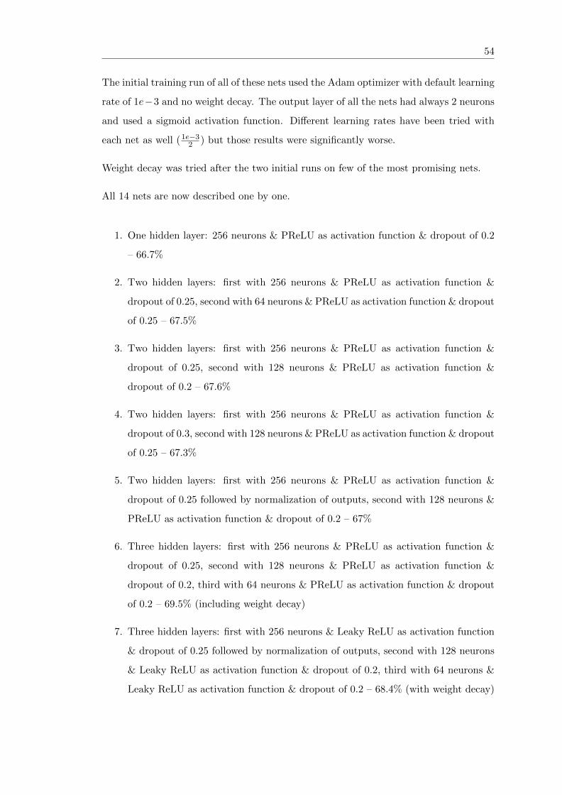
54

The initial training run of all of these nets used the Adam optimizer with default learning

rate of 1e−3 and no weight decay. The output layer of all the nets had always 2 neurons

and used a sigmoid activation function. Different learning rates have been tried with

each net as well (1e−32 ) but those results were significantly worse.

Weight decay was tried after the two initial runs on few of the most promising nets.

All 14 nets are now described one by one.

1. One hidden layer: 256 neurons & PReLU as activation function & dropout of 0.2

– 66.7%

2. Two hidden layers: first with 256 neurons & PReLU as activation function &

dropout of 0.25, second with 64 neurons & PReLU as activation function & dropout

of 0.25 – 67.5%

3. Two hidden layers: first with 256 neurons & PReLU as activation function &

dropout of 0.25, second with 128 neurons & PReLU as activation function &

dropout of 0.2 – 67.6%

4. Two hidden layers: first with 256 neurons & PReLU as activation function &

dropout of 0.3, second with 128 neurons & PReLU as activation function & dropout

of 0.25 – 67.3%

5. Two hidden layers: first with 256 neurons & PReLU as activation function &

dropout of 0.25 followed by normalization of outputs, second with 128 neurons &

PReLU as activation function & dropout of 0.2 – 67%

6. Three hidden layers: first with 256 neurons & PReLU as activation function &

dropout of 0.25, second with 128 neurons & PReLU as activation function &

dropout of 0.2, third with 64 neurons & PReLU as activation function & dropout

of 0.2 – 69.5% (including weight decay)

7. Three hidden layers: first with 256 neurons & Leaky ReLU as activation function

& dropout of 0.25 followed by normalization of outputs, second with 128 neurons

& Leaky ReLU as activation function & dropout of 0.2, third with 64 neurons &

Leaky ReLU as activation function & dropout of 0.2 – 68.4% (with weight decay)

55

8. Three hidden layers: first with 256 neurons & PReLU as activation function &

dropout of 0.3, second with 64 neurons & PReLU as activation function & dropout

of 0.25, third with 16 neurons & PReLU as activation function & dropout of 0.2 –

68.7% (with weight decay)

9. Three hidden layers: first with 256 neurons & ReLU as activation function &

dropout of 0.3, second with 128 neurons & ReLU as activation function & dropout

of 0.25, third with 64 neurons & ReLU as activation function & dropout of 0.2 –

68.7% (with weight decay)

10. Four hidden layers: first with 256 neurons & PReLU as activation function &

dropout of 0.3, second with 128 neurons & PReLU as activation function & dropout

of 0.25, third with 64 neurons & PReLU as activation function & dropout of 0.2,

fourth with 16 neurons & PReLU as activation function & dropout of 0.2 – 67.8%

(with weight decay)

11. Four hidden layers: first with 256 neurons & ReLU as activation function &

dropout of 0.3, second with 128 neurons & ReLU as activation function & dropout

of 0.25, third with 64 neurons & ReLU as activation function & dropout of 0.2,

fourth with 16 neurons & ReLU as activation function & dropout of 0.2 – 67.9%

12. Five hidden layers: first with 256 neurons & PReLU as activation function &

dropout of 0.3, second with 128 neurons & PReLU as activation function & dropout

of 0.25, third with 64 neurons & PReLU as activation function & dropout of 0.2,

fourth with 32 neurons & PReLU as activation function & dropout of 0.2 – 67.1%

13. Five hidden layers: first with 256 neurons & Leaky ReLU as activation function &

dropout of 0.3 followed by normalization, second with 128 neurons & Leaky ReLU

as activation function & dropout of 0.25, third with 64 neurons & Leaky ReLU as

activation function & dropout of 0.2, fourth with 32 neurons & Leaky ReLU as

activation function & dropout of 0.2 – 67.2%

14. Five hidden layers: first with 256 neurons & ReLU as activation function & dropout

of 0.3, second with 128 neurons & ReLU as activation function & dropout of 0.25,

third with 64 neurons & ReLU as activation function & dropout of 0.2, fourth with

32 neurons & ReLU as activation function & dropout of 0.2, fifth with 16 neurons

& ReLU as activation function & dropout of 0.2 – 66.9%

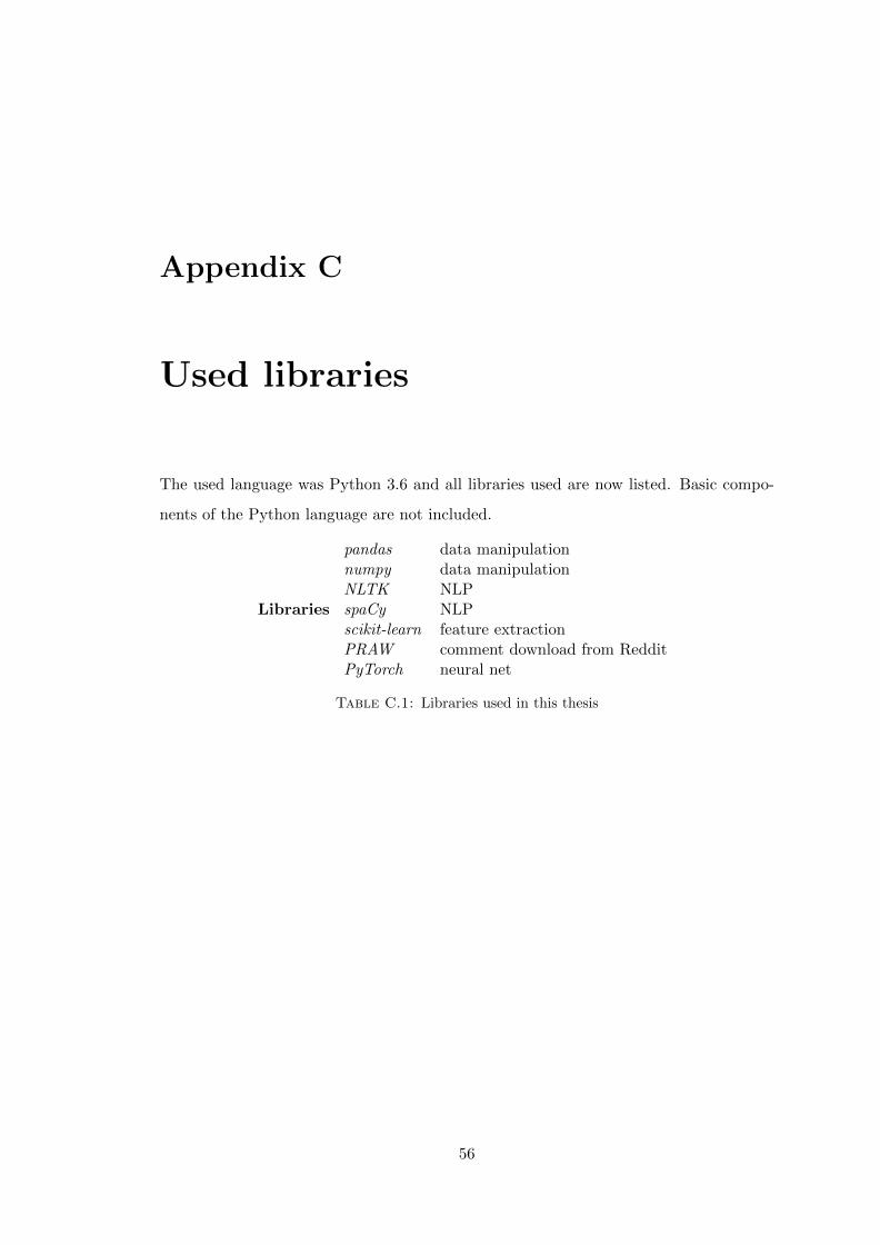
Appendix C

Used libraries

The used language was Python 3.6 and all libraries used are now listed. Basic compo-

nents of the Python language are not included.

Libraries

pandas data manipulationnumpy data manipulationNLTK NLPspaCy NLPscikit-learn feature extractionPRAW comment download from RedditPyTorch neural net

Table C.1: Libraries used in this thesis

56

Bibliography

Amir, Silvio, Wallace, Byron C, Lyu, Hao, & Silva, Paula Carvalho Mario J. 2016.

Modelling context with user embeddings for sarcasm detection in social media. arXiv

preprint arXiv:1607.00976.

Bamman, David, & Smith, Noah A. 2015. Contextualized Sarcasm Detection on Twitter.

Pages 574–577 of: ICWSM.

Bird, Steven, Klein, Ewan, & Loper, Edward. 2009. Natural Language Processing with

Python. 1st edn. O’Reilly Media, Inc.

Bishop, Christopher M. 2006. Pattern Recognition and Machine Learning (Information

Science and Statistics). Berlin, Heidelberg: Springer-Verlag.

Carvalho, Paula, Sarmento, Luıs, Silva, Mario J, & De Oliveira, Eugenio. 2009. Clues

for detecting irony in user-generated contents: oh...!! it’s so easy;-. Pages 53–56 of:

Proceedings of the 1st international CIKM workshop on Topic-sentiment analysis for

mass opinion. ACM.

Chakraborty, Goutam, & Pagolu, Murali Krishna. Analysis of Unstructured Data: Ap-

plications of Text Analytics and Sentiment Mining.

Davidov, Dmitry, Tsur, Oren, & Rappoport, Ari. 2010. Semi-supervised recognition

of sarcastic sentences in twitter and amazon. Pages 107–116 of: Proceedings of the

fourteenth conference on computational natural language learning. Association for

Computational Linguistics.

De Bievre, Paul. 2012. The 2012 International Vocabulary of Metrology: “VIM”. Ac-

creditation and Quality Assurance, 17(2), 231–232.

Diebold, Francis X., & Mariano, Roberto S. 1995. Comparing Predictive Accuracy.

Journal of Business & Economic Statistics, 13(3), 253–263.

57

Bibliography 58

Ghosh, Debanjan, Guo, Weiwei, & Muresan, Smaranda. 2015. Sarcastic or not: Word

embeddings to predict the literal or sarcastic meaning of words. Pages 1003–1012

of: Proceedings of the 2015 Conference on Empirical Methods in Natural Language

Processing.

Grimes, Seth. A Brief History of Text Analytics. http://www.b-eye-network.com/

view/6311. Accessed: 2018-07-03.

Gurini, Davide Feltoni, Gasparetti, Fabio, Micarelli, Alessandro, & Sansonetti,

Giuseppe. 2013. A Sentiment-Based Approach to Twitter User Recommendation.

RSWeb@ RecSys, 1066.

He, Kaiming, Zhang, Xiangyu, Ren, Shaoqing, & Sun, Jian. 2015. Delving deep into rec-

tifiers: Surpassing human-level performance on imagenet classification. Pages 1026–

1034 of: Proceedings of the IEEE international conference on computer vision.

Hochreiter, Sepp, & Schmidhuber, Jurgen. 1997. Long short-term memory. Neural

computation, 9(8), 1735–1780.

Honnibal, Matthew, & Montani, Ines. 2017. spaCy 2: Natural language understanding

with Bloom embeddings, convolutional neural networks and incremental parsing. To

appear.

Joshi, Aditya, Tripathi, Vaibhav, Patel, Kevin, Bhattacharyya, Pushpak, & Carman,

Mark. 2016. Are Word Embedding-based Features Useful for Sarcasm Detection?

arXiv preprint arXiv:1610.00883.

Joshi, Aditya, Bhattacharyya, Pushpak, & Carman, Mark J. 2017. Automatic sarcasm

detection: A survey. ACM Computing Surveys (CSUR), 50(5), 73.

Khattri, Anupam, Joshi, Aditya, Bhattacharyya, Pushpak, & Carman, Mark. 2015.

Your sentiment precedes you: Using an author’s historical tweets to predict sarcasm.

Pages 25–30 of: Proceedings of the 6th Workshop on Computational Approaches to

Subjectivity, Sentiment and Social Media Analysis.

Khodak, Mikhail, Saunshi, Nikunj, & Vodrahalli, Kiran. 2017. A large self-annotated

corpus for sarcasm. arXiv preprint arXiv:1704.05579.

Kingma, Diederik P, & Ba, Jimmy. 2014. Adam: A method for stochastic optimization.

arXiv preprint arXiv:1412.6980.

Bibliography 59

Kriesel, David. 2007. A Brief Introduction to Neural Networks.

Liu, Bing. 2012. Sentiment analysis and opinion mining. Synthesis lectures on human

language technologies, 5(1), 1–167.

McCulloch, Warren S., & Pitts, Walter. 1943. A logical calculus of the ideas immanent

in nervous activity. The bulletin of mathematical biophysics, 5(4), 115–133.

Mikolov, Tomas, Yih, Wen-tau, & Zweig, Geoffrey. 2013. Linguistic regularities in contin-

uous space word representations. Pages 746–751 of: Proceedings of the 2013 Confer-

ence of the North American Chapter of the Association for Computational Linguistics:

Human Language Technologies.

Mohammad, Saif M. 2016. Sentiment analysis: Detecting valence, emotions, and other

affectual states from text. Pages 201–237 of: Emotion measurement. Elsevier.

Mullainathan, Sendhil, & Spiess, Jann. 2017. Machine learning: an applied econometric

approach. Journal of Economic Perspectives, 31(2), 87–106.

Ortigosa, Alvaro, Martın, Jose M, & Carro, Rosa M. 2014. Sentiment analysis in Face-

book and its application to e-learning. Computers in Human Behavior, 31, 527–541.

Paszke, Adam, Gross, Sam, Chintala, Soumith, Chanan, Gregory, Yang, Edward, De-

Vito, Zachary, Lin, Zeming, Desmaison, Alban, Antiga, Luca, & Lerer, Adam. 2017.

Automatic differentiation in PyTorch. In: NIPS-W.

Peng, Qingxi, & Zhong, Ming. 2014. Detecting Spam Review through Sentiment Anal-

ysis. JSW, 9(8), 2065–2072.

Poecze, Flora, Ebster, Claus, & Strauss, Christine. 2018. Social media metrics and sen-

timent analysis to evaluate the effectiveness of social media posts. Procedia Computer

Science, 130, 660–666.

Riloff, Ellen, Qadir, Ashequl, Surve, Prafulla, De Silva, Lalindra, Gilbert, Nathan, &

Huang, Ruihong. 2013. Sarcasm as contrast between a positive sentiment and nega-

tive situation. Pages 704–714 of: Proceedings of the 2013 Conference on Empirical

Methods in Natural Language Processing.

Staiano, Jacopo, & Guerini, Marco. 2014. Depechemood: a lexicon for emotion analysis

from crowd-annotated news. arXiv preprint arXiv:1405.1605.

Bibliography 60

Stevenson, Angus. Oxford Dictionary of English.

Wallace, Byron C, Kertz, Laura, Charniak, Eugene, et al. . 2014. Humans require context

to infer ironic intent (so computers probably do, too). Pages 512–516 of: Proceedings

of the 52nd Annual Meeting of the Association for Computational Linguistics (Volume

2: Short Papers), vol. 2.

Wallace, Byron C, Charniak, Eugene, et al. . 2015. Sparse, contextually informed mod-

els for irony detection: Exploiting user communities, entities and sentiment. Pages

1035–1044 of: Proceedings of the 53rd Annual Meeting of the Association for Compu-

tational Linguistics and the 7th International Joint Conference on Natural Language

Processing (Volume 1: Long Papers), vol. 1.

Xing, Frank Z, Cambria, Erik, & Welsch, Roy E. 2018. Natural language based financial

forecasting: a survey. Artificial Intelligence Review, 1–25.

Yang, Dingqi, Zhang, Daqing, Yu, Zhiyong, & Wang, Zhu. 2013. A sentiment-enhanced

personalized location recommendation system. Pages 119–128 of: Proceedings of the

24th ACM Conference on Hypertext and Social Media. ACM.

Zimbra, David, Ghiassi, Manoochehr, & Lee, Sean. 2016. Brand-related twitter sen-

timent analysis using feature engineering and the dynamic architecture for artificial

neural networks. Pages 1930–1938 of: System Sciences (HICSS), 2016 49th Hawaii

International Conference on. IEEE.