Sandeep Mavadia - Imperial College London
148
The Imperial College of Science, Technology and Medicine Department of Physics Motional Sideband Spectra and Coulomb Crystals in a Penning Trap Sandeep Mavadia Submitted in part fulfilment of the requirements for the degree of Doctor of Philosophy in Physics of Imperial College London, 09/04/2013
-
Upload
khangminh22 -
Category
Documents
-
view
0 -
download
0
Transcript of Sandeep Mavadia - Imperial College London

The Imperial College of Science, Technology and Medicine
Department of Physics
Motional Sideband Spectra
and Coulomb Crystals
in a Penning Trap
Sandeep Mavadia
Submitted in part fulfilment of the requirements for the degree of
Doctor of Philosophy in Physics of Imperial College London,
09/04/2013

Abstract
Laser cooled ions in a Penning trap can be isolated from the environment by placing them
in vacuum and only interacting with them through optical and RF fields. The number
of trapped particles can be varied from a single ion up to thousands. Confinement is
provided by a static homogeneous magnetic field and a quadrupole electric potential. In
the natural frame of the ions, this appears as a 3D simple harmonic potential. Therefore
three dimensional structures can be formed in the absence of any additional RF field which
may lead to heating as is the case with RF traps. There are 3N different motional modes
for N particles. I present an analysis of the motion of a single particle showing that the
energy levels for all three modes are equally spaced. I also describe the interaction between
a trapped two level atom and an optical field.
During my time in the lab the laser and computer control of the experiment has been
significantly improved. In addition, an existing trap was modified to provide greater optical
access and fluorescence collection. This allowed the vibrational levels superimposed on
the internal states of a single 40Ca+ ion to be resolved via a narrow linewidth, electric
quadrupole transition. This is the first observation of magnetron and modified cyclotron
sidebands on an optical transition.
When more than one calcium ion is laser cooled, and their temperature reduced below
5mK, they form a Coulomb crystal. The locations of the ions minimise the total potential
energy which is comprised of the Coulomb repulsion and trap potential. The fluorescence
collection optics have been arranged to resolve individual ions in these crystals. Informa-
tion about the motion of the ions is deduced by comparing photos from the experiment to
numerical simulations. Previously, only two ions have ever been aligned along the mag-
netic field in a Penning trap. I present strings of up to 29 particles and suggest the only
limitation, apart from the electrode structure, is the overlap of the laser beams with the
ions.
2

Acknowledgements
Thanks goes to all the people I have worked with during my time in the Lab: Dan, Sean,
Shailen, Graham and Joe without whom none of the work presented here would have been
possible. Special thanks to Dan, not just for his talents useful across the whole lab and
incredible ability to just make things work but also for his enthusiasm and drive to try new
ideas. Thanks especially to Sean for his companionship during the time when we were in
both working in the lab.
Thanks also goes to my supervisors. Richard for always making time for me and explaining
theory when I invariably became stuck. And to Danny for a constant supply of optimism
when I had occasionally run out.
I gratefully thank Brian for his work in the mechanical workshop; for those jobs where ab-
solute precision was required. And also Bandu whose technical knowledge seemed endless.
A thank you to everyone in the CCM for the good friendship for the past few years, it was
great to feel part of a larger group.
3

Declaration
I declare that this thesis is my own work. Where I have used the work of others the sources
are appropriately referenced and acknowledged.
4

Contents
1 Introduction 8
1.1 Description of thesis . . . . . . . . . . . . . . . . . . . . . . . . . . . . . . . 10
2 Ion Traps 12
2.1 Penning Traps . . . . . . . . . . . . . . . . . . . . . . . . . . . . . . . . . . 13
2.1.1 Classical Motion . . . . . . . . . . . . . . . . . . . . . . . . . . . . . 13
2.1.2 Quantum motion . . . . . . . . . . . . . . . . . . . . . . . . . . . . . 19
3 Ion-Light Interaction 21
3.1 Interaction with internal states . . . . . . . . . . . . . . . . . . . . . . . . . 22
3.1.1 Geometry . . . . . . . . . . . . . . . . . . . . . . . . . . . . . . . . . 28
3.1.2 Radiation emission patterns . . . . . . . . . . . . . . . . . . . . . . . 29
3.1.3 Polarisation coefficients . . . . . . . . . . . . . . . . . . . . . . . . . 31
3.1.4 Optimum Polarisation . . . . . . . . . . . . . . . . . . . . . . . . . . 31
3.2 Interaction with external states . . . . . . . . . . . . . . . . . . . . . . . . . 32
3.3 Broadening Mechanisms . . . . . . . . . . . . . . . . . . . . . . . . . . . . . 37
3.3.1 Doppler Broadening . . . . . . . . . . . . . . . . . . . . . . . . . . . 37
3.3.2 Laser linewidth . . . . . . . . . . . . . . . . . . . . . . . . . . . . . . 38
3.4 Laser cooling . . . . . . . . . . . . . . . . . . . . . . . . . . . . . . . . . . . 38
3.4.1 Doppler Cooling . . . . . . . . . . . . . . . . . . . . . . . . . . . . . 39
3.4.2 Resolved sideband cooling . . . . . . . . . . . . . . . . . . . . . . . . 47
5

Contents Contents
4 Experimental Setup 52
4.1 Calcium II level structure . . . . . . . . . . . . . . . . . . . . . . . . . . . . 52
4.1.1 J quantum number magnetic mixing . . . . . . . . . . . . . . . . . . 52
4.2 Diode Lasers . . . . . . . . . . . . . . . . . . . . . . . . . . . . . . . . . . . 54
4.3 Laser Locking . . . . . . . . . . . . . . . . . . . . . . . . . . . . . . . . . . . 55
4.3.1 Pound-Drever-Hall lock theory . . . . . . . . . . . . . . . . . . . . . 56
4.3.2 Dither lock . . . . . . . . . . . . . . . . . . . . . . . . . . . . . . . . 59
4.3.3 Doppler cooling lasers dither lock . . . . . . . . . . . . . . . . . . . . 60
4.3.4 Doppler cooling lasers transfer cavity lock . . . . . . . . . . . . . . . 61
4.4 Repumping lasers . . . . . . . . . . . . . . . . . . . . . . . . . . . . . . . . . 64
4.4.1 Multiple transition repumping . . . . . . . . . . . . . . . . . . . . . . 64
4.4.2 Repumping lasers transfer cavity lock . . . . . . . . . . . . . . . . . 66
4.5 Stabilised 729 nm Laser . . . . . . . . . . . . . . . . . . . . . . . . . . . . . 67
4.5.1 ULE high finesse cavity . . . . . . . . . . . . . . . . . . . . . . . . . 68
4.5.2 Laser & Locking electronics . . . . . . . . . . . . . . . . . . . . . . . 69
4.6 Optical setup . . . . . . . . . . . . . . . . . . . . . . . . . . . . . . . . . . . 73
4.7 Trap configuration . . . . . . . . . . . . . . . . . . . . . . . . . . . . . . . . 75
4.8 Loading Ions . . . . . . . . . . . . . . . . . . . . . . . . . . . . . . . . . . . 79
4.9 FPGA and computer control . . . . . . . . . . . . . . . . . . . . . . . . . . 80
4.9.1 Computer front-end . . . . . . . . . . . . . . . . . . . . . . . . . . . 82
4.9.2 FPGA memory interface . . . . . . . . . . . . . . . . . . . . . . . . . 82
4.9.3 Mains Trigger . . . . . . . . . . . . . . . . . . . . . . . . . . . . . . . 85
4.9.4 RF electronics . . . . . . . . . . . . . . . . . . . . . . . . . . . . . . 85
5 Coulomb Crystals 87
5.1 Centre of Mass Oscillations . . . . . . . . . . . . . . . . . . . . . . . . . . . 90
5.2 Magnetron mode instability . . . . . . . . . . . . . . . . . . . . . . . . . . . 90
5.3 Motion in a Rotating Frame . . . . . . . . . . . . . . . . . . . . . . . . . . . 92
5.3.1 Laser beam torque . . . . . . . . . . . . . . . . . . . . . . . . . . . . 93
6

Contents Contents
5.4 Linear Ion Chains . . . . . . . . . . . . . . . . . . . . . . . . . . . . . . . . . 94
5.5 Higher dimensional Coulomb crystals . . . . . . . . . . . . . . . . . . . . . . 95
5.6 Larger Crystals . . . . . . . . . . . . . . . . . . . . . . . . . . . . . . . . . . 101
5.6.1 Effect of quantum J-state mixing in Coulomb crystals . . . . . . . . 102
6 Motional Sideband Spectroscopy 105
6.1 Pulse sequence . . . . . . . . . . . . . . . . . . . . . . . . . . . . . . . . . . 106
6.1.1 Mains triggering . . . . . . . . . . . . . . . . . . . . . . . . . . . . . 107
6.1.2 Doppler Cooling . . . . . . . . . . . . . . . . . . . . . . . . . . . . . 108
6.1.3 State preparation . . . . . . . . . . . . . . . . . . . . . . . . . . . . . 108
6.1.4 729 nm pulse . . . . . . . . . . . . . . . . . . . . . . . . . . . . . . . 109
6.1.5 State detection . . . . . . . . . . . . . . . . . . . . . . . . . . . . . . 109
6.2 Magnetic field components of the 729 nm transition . . . . . . . . . . . . . . 112
6.3 Cavity Drift . . . . . . . . . . . . . . . . . . . . . . . . . . . . . . . . . . . . 113
6.4 Axial Spectrum . . . . . . . . . . . . . . . . . . . . . . . . . . . . . . . . . . 115
6.5 Radial spectrum . . . . . . . . . . . . . . . . . . . . . . . . . . . . . . . . . 122
7 Discussion 127
A Clebsch-Gordon Coefficients 130
B Polarisation Coefficients 134
B.1 Dipole transitions . . . . . . . . . . . . . . . . . . . . . . . . . . . . . . . . . 135
B.2 Quadrupole transitions . . . . . . . . . . . . . . . . . . . . . . . . . . . . . . 137
Bibliography 141
7

Chapter 1Introduction
Charged particles are easily trapped using either a high-frequency oscillating electrical po-
tential (RF trap) or an homogeneous magnetic field and a static quadratic electric potential
(Penning trap). If these particles are confined in vacuum, they can be stored for many
hours, even months in some cases.
In atomic physics, usually singly charged ions are used for experiments. A few elements in
this state have a simple enough valence electron energy level structure to allow closed cycle
interactions with lasers and RF fields. These species can be laser cooled to a temperature
which is not possible by any other means. When the temperature of the ions is reduced
sufficiently, quantum mechanics must be used to describe the motion of the ions rather
than classical mechanics. Using lasers it is possible to engineer and exploit quantum
entanglement between the internal electronic state of the valence electron and motional
state of the ion.
At low temperatures the particles form stable structures. They find equilibrium posi-
tions where the potential energy associated with the Coulomb repulsion from all the other
trapped particles and the confining potential is minimised. The ratio of the Coulomb repul-
sion between these particles to their thermal energy can be made high enough so that the
ions occupy fixed equilibrium positions forming so called Coulomb crystal. Plasma physics
and astro-physics researchers also use this idea. They use charged dust or micro-particles
to study conditions that are expected to exist in outer space. Their particles are much
heavier than individual ions and the oscillation frequencies are in a regime where they need
only consider classical physics.
Ion traps are used for many different purposes; one of the most common is for high res-
olution measurements in frequency metrology and mass spectrometry. In these types of
experiments it is often beneficial to isolate the particles from the background. By reducing
8

Chapter 1
the number of trapped particles, collisional effects which might obscure the results are
decreased. In fact, individual ions are routinely trapped for mass spectroscopy or optical
frequency standard measurements. To achieve the highest precision in these experiments,
the motion of the ions is reduced so that they occupy only a small volume. Where laser
cooling is available, this can even be the quantum mechanical harmonic oscillator ground
state. The techniques initially designed for this field have been adapted for use in quan-
tum information processing since the initial proposal by Cirac and Zoller in 1995 [1]. Much
progress has been made in this field. For example, a string of ions can be cooled to the
ground state of motion and entangled [2] or used in quantum gates [3]. However, in many
groups it has been accepted that any trapped ion system designed to perform quantum
algorithms will need to have the ability to move ions around and be adaptable to different
operations. A list of the key requirements are laid out in the DiVincenzo criteria [4].
In 1982, Richard Feynman suggested designing one quantum system to simulate another
quantum system [5]. He showed that a classical computer would find it exponentially more
difficult to calculate the state of a quantum system as the number of particles increased.
More recently, there has been interest in using arrays of trapped ions to simulate other
quantum systems which are harder to access and control [6, 7].
Only a single ion, or linear strings of ions, can be cooled to the quantum ground state
across all the motional modes in an RF trap; away from the RF null ions are susceptible to
RF heating. Penning traps do not suffer from this limitation, and more interesting two and
three dimensional structures could, potentially, be cooled to the ground state. Proposals
where a large number of particles need to be coupled together or where the experiment
requires a two or three dimensional potential surface are more suited to Penning traps.
However, there are technical challenges which make some aspects of performing experiments
in Penning traps less attractive than using an RF trap. Also, the benefits outlined above
are only useful in certain circumstances. Therefore, until very recently, there were only two
research groups1 working on laser cooled ions in Penning traps compared to tens of groups
using RF traps. A lot of the work described in this thesis will show that in principle, much
of the work performed in one dimension in a RF trap is feasible in two or three dimensions
in a Penning trap.
I will show that we can form and manipulate Coulomb crystals in a Penning trap. The
work in this thesis will also demonstrate the first steps towards ground state cooling these
ions. Specifically, we observe motional sidebands on an optical transition. These are
worthwhile aims in themselves merely because they have not been demonstrated previously.
However, after these goals have been achieved, experiments that require controlled coherent
interactions between larger numbers of particles than is possible in a RF trap may also be
1The other group is headed by John Bollinger and is based at NIST in Boulder, Colorado.
9

Chapter 1 Description of thesis
performed.
1.1 Description of thesis
The motion of an ion in a Penning trap can be calculated without any approximations. In
chapter 2, the equations of motion are solved and show that the trap potential is simply a
three-dimensional harmonic oscillator. By forming the appropriate ladder operators, these
oscillators can be quantised in the standard way. These energy levels are superimposed on
to the internal states of the ion.
A single ion with the appropriate atomic energy level structure can be approximated as
a two level system. The interactions between light and a free two level atom and also
between light and a trapped ion are analysed in chapter 3. The dependence of the relevant
matrix element on geometric factors i.e. angle of incidence and polarisation relative to
the quantisation axis are thoroughly explained. This information is useful to see which
transitions are can be stimulated with our limited optical access.
Doppler laser cooling in a Penning trap is more complicated than in an RF trap because the
potential energy in the plane perpendicular to magnetic field decreases as the magnitude
of the orbit increases. Here, simply using a laser beam detuned to a lower frequency than
the atomic resonance would lead to unstable motion. Instead, in chapter 3, a method for
reducing the amplitude of motion for all three modes using a laser beam intensity gradient
is described.
The vast majority of the time during my degree has been spent building, and improving,
the equipment used to trap and laser cool 40Ca+ ions to Coulomb crystals of tens or hun-
dreds of ions. A concise description of the apparatus is given in chapter 4. This includes
the laser locking techniques, and the optical layout. Daniel Crick, Sean Donnellan and I
designed a method for economically repumping eight magnetic field split metastable levels
which remove 40Ca+ ions from the cooling cycle; the details of this are also included. Dur-
ing my time in the lab we also implemented several improvements to the general apparatus
including a computerised control system and optical modulators for repetitive high speed
pulsed spectroscopy; an optical fibre connection to a reliable wavemeter in an adjacent lab;
a photoionisation loading scheme using a high power, pulsed, frequency doubled, Nd:YAG
laser and a method for atomic species and isotope purification inside the trap. In addition,
I modified a trap originally built by Shailen Bharadia to allow greater optical access. The
imaging system and opto-mechanics around the trap were entirely replaced, this produced
a completely fibre coupled trap which could be wheeled around while still observing atomic
fluorescence when operated as a RF trap. One key aspect of the experiment, built exclu-
sively by Daniel Crick, was a narrow linewidth diode laser. Nonetheless, I have described
10

Chapter 1 Description of thesis
its operation and provide an overview of its locking system. This laser was essential to
perform the spectroscopy described in chapter 6.
When the temperature of ions is reduced below 5mK they form well ordered Coulomb
crystals. In chapter 5 the shapes of these crystals are analysed to determine information
about the trap parameters, including the frequency of rotation. By comparing a photo of
a string of ions to their theoretically predicted position, it can also be shown that the trap-
ping potential is well approximated by a quadratic function over at least several hundred
micrometres. Photos show that single ions in Coulomb crystals are clearly resolved. Even
for large crystals, where the number of ions cannot be directly counted, which is otherwise
done by aligning them in a string along the magnetic field; we can still extract information
about the ratio of the trap frequencies and the number of ions by comparison to a computer
simulation. This shows significant progress compared to previous experiments. Coulomb
crystals in a Penning trap have previously been formed of thousands or hundreds of ions
in two or three dimensional structures [8] with the exception of a single experiment where
a two ion crystal was imaged [9]. The results in this thesis fill the middle ground; with the
observation of Coulomb crystals from a few ions up to several hundred ions.
In chapter 6, the pulse sequence used to stimulate and measure the shelving probability
of a single ion via a narrow linewidth quadrupole transition is described. At the end of
this chapter I show preliminary data of sideband spectroscopy of the vibrational modes
of a single ion. Finally, I discuss the results presented in this this thesis and give a brief
outlook for the future.
11

Chapter 2Ion Traps
Ion traps can be used to almost perfectly isolate charged particles from the environ-
ment while still allowing controlled external interactions via narrowband laser light or
microwaves. Ideally we can produce an harmonic trapping potential for the ions. The two
common methods, described briefly below, both have the same ideal electrode geometry,
as shown in figure 2.1. These electrodes should be formed of hyperboloids of revolution
where z is the symmetry axis denoted as the axial direction in this thesis. The other two
dimensions are degenerate and henceforth collectively described as the radial direction.
r
z
Figure 2.1: Cross section of the ideally shaped trap electrodes. The axes in the z and r
directions have equal scaling. The electrodes are formed of hyperboloids of revolution. Theelectrodes on the top and bottom of the figure are called endcaps and the single electrodein the centre of the figure is normally called the ring.
There are two commonly used methods for trapping.
1. RF Trap - by quickly alternating the polarity of the electric field applied to electrodes
12

Chapter 2 Penning Traps
a time averaged harmonic potential can be created in the centre of the trap where
an RF null is formed. In a variation of this type of trap, called a linear RF trap, the
RF null is extended to a 1D line.
2. Penning Trap - a homogeneous magnetic field is imposed along the trap axis pro-
ducing a cyclotron orbit in the plane perpendicular to the field. The ion is trapped
along the trap axis using a static quadrupole electric potential generated by applying
a DC potential to the electrodes.
In this thesis I shall only describe experiments in a Penning trap. There are many good
references for information on RF traps including from one of the inventors, Wolfgang
Paul [10].
2.1 Penning Traps
2.1.1 Classical Motion
In a Penning trap the confinement in the radial plane is provided by a homogeneous mag-
netic field. In this plane the particle travels in cyclotron loops. To provide trapping in
the remaining, axial, dimension a DC harmonic potential is imposed. However, to satisfy
Laplace’s equation the electric field produces an anti-trapping potential in the radial plane
which partially counteracts the confinement from the magnetic field. This makes the effec-
tive radial potential from the magnetic field shallower and reduces the cyclotron frequency,
to what is now called the modified cyclotron frequency. Secondly, the combination of these
two fields leads to a third mode, called the magnetron mode, arising from the E×B drift.
This should be obvious when considering that crossed electric and magnetic fields are often
used as velocity filters for charged particles.
The physical effect of this force can be seen by first considering the motion of a charged
particle in a constant electric field perpendicular to a constant magnetic field. Figure 2.2
shows that there is a differential velocity for a particle on one side of the orbit relative to
the other side leading to a drift in the E×B direction. Extending this to a radial electric
field, shown in figure 2.3, the E× B drift precesses around the magnetic field in the same
direction as the cyclotron motion.
The explanation of the motion of an ion in this section is based on the description given
in [11] and [12]. It is easier when solving a problem dependent on magnetic and electrostatic
fields to consider a generalised potential including both a scalar potential, φ and vector
potential, A. The potential of a constant magnetic field, B = Bz, can be written as
φ = 0, A = (B × r) /2 = (−yB, xB, 0) /2 and an electrostatic potential as φ = φ, A = 0.
13

Chapter 2 Penning Traps
a
b
c
d
E
B
E ×B
Figure 2.2: A positively charged particle travels in cyclotron loops in a magnetic field.When a perpendicular uniform electric field is added, the particle has a higher speed atpoint b rather than point d. The net effect is a drift in the E × B direction. In this casethe cyclotron motion no longer from closed loops.
In a Penning trap φ =(k/4)×(2z2 − x2 − y2
), where k is a constant dependent on the
applied potential and the electrode geometry. In an ideal Penning trap the electrodes are
made up of hyperboloids of revolution as shown in figure 2.1, which follow the equations
r2
r20− z2
z20= ±1. (2.1)
In equation 2.1 the positive sign relates to the central ring electrode and the negative sign
to the two endcaps; r0 and z0 are the closest approaches of the electrodes to the centre of
the trap in the radial and axial dimensions respectively. In this case k = 4U/(2z20 + r20
)
where U is the applied potential. To trap positively charged ions, the potential applied to
the endcaps should be positive relative to the ring voltage.
The generalised electromagnetic potential V = q (φ− r ·A), written in Cartesian coordi-
nates, is
V =1
4qk(2z2 − x2 − y2
)− q
2B (yx− xy) . (2.2)
Writing down the Lagrangian for this system
L =m
2
(x2 + y2 + z2
)− 1
4qk(2z2 − x2 − y2
)+q
2B (yx− xy) , (2.3)
14

Chapter 2 Penning Traps
a
b
c
d
EB
E ×B
Figure 2.3: Electric field points out from the centre of the trap which leads to an E × B
drift which rotates around the magnetic field in the same direction as the cyclotron motion.
and solving Lagrange’s equations we find that
mx =1
2qkx+ qBy, (2.4a)
my =1
2qky − qBx, (2.4b)
mz = −qkz. (2.4c)
The motion in the z-direction is obviously just simple harmonic motion. Solving this in
the standard way the motion can be described by
z (t) = Z cos (ωzt+ δz) , (2.5)
where the axial frequency is
ωz =√qk/m . (2.6)
The phase, δz, and amplitude of the oscillation, Z, depend on the initial conditions.
Solving the radial motion is made easier by substituting the complex variable s = x + ıy
into the two coupled equations for x and y, and reducing them to the single equation
s =qk
2ms− ı
qB
ms. (2.7)
15

Chapter 2 Penning Traps
Equation 2.7 has two solutions with frequencies,
ω± =1
2
qBm
±
√(qB
m
)2
− 2qk
m
, (2.8)
which can be found by substituting the trial solution s = e−ıωt. Defining the cyclotron
frequency
ωc =qB
m, (2.9)
the oscillation frequency without the imposition of an external electric field, and using the
axial frequency from equation 2.6 we can write equation 2.8 more succinctly as
ω± =1
2
(ωc ±
√ω2c − 2ω2
z
). (2.10)
These frequencies are the modified cyclotron frequency, ω+, and the magnetron frequency,
ω−. We can also define the frequency
ω1 =√ω2c − 2ω2
z /2, (2.11)
which will be useful in subsequent chapters of this thesis. In normal operation ωc ≈ ω+ ≫ωz ≫ ω−.
The discriminant in equation 2.8 must remain positive so that the oscillation frequencies
are real. This is the condition for stable trapping. In anharmonic traps where the frequency
of motion is not constant with distance from the trap centre the entire volume which the
ion samples must obey this criterion rather than just the trap centre. This is especially
difficult for planar Penning traps which are anharmonic in the extreme, see reference [13]
for a discussion on maximising trap depth in such situations.
Having calculated the oscillation frequencies in the radial plane we can write down the
general solution to equation 2.7
s = R+e−ı(ω+t+δ+) +R−e
−ı(ω−t+δ−) (2.12)
where the radii of the modified cyclotron and magnetron motions, R+ and R−, and the
phases, δ+ and δ−, of the two motions depend on the initial conditions.
Converting this complex co-ordinate back to a Cartesian system we find
x = R+ cos (−ω+t+ δ+) +R− cos (−ω−t+ δ−) (2.13a)
y = R+ sin (−ω+t+ δ+) +R− sin (−ω−t+ δ−) . (2.13b)
16

Chapter 2 Penning Traps
Figure 2.4 shows an example of the motion of a single ion in a Penning trap by plotting
equations 2.5 and 2.13. Squaring and adding these equations gives the amplitude of the
z
x y
z
Figure 2.4: Example of the motion of a single ion in a Penning trap (ωz = ωc/2). Motionin three dimensions is above a projection of the radial motion. The amplitudes and initialphases of the three modes are chosen arbitrarily for clarity (Z = 2R−, R− = 2R+, δz =δ− = δ+ = 0).
motion in the radial plane.
r2 = x2 + y2 = R2+ +R2
− + 2R+R− cos[(ω− − ω+) t+ (δ− − δ+)
], (2.14)
hence |R+ −R−| < r < |R+ +R−|. We can also separate the total kinetic and potential
energy so that
EKin =mv2
2=m
2
[R2
−ω2− +R2
+ω2+
+2R−R+ω−ω+ cos (ω−t− ω+t+ δ− − δ+) + Z2ω2z sin
2 (ωzt+ δa)], (2.15a)
EPot =qV =mω2
z
2
[−(R2
− +R2+
)/2−R−R+ cos (ω−t− ω+t+ δ− + δ+)
+Z2 cos2 (ωzt+ δz)], (2.15b)
noting that ω2z = 2ω+ω−, and summing these two terms we can find the total energy,
ETot = EKin +EPot =m
2
[Z2ω2
z + (ω+ − ω−)(ω+R
2+ − ω−R
2−
)]. (2.16)
In chapter 6 it will be shown that by probing the motion using narrow linewidth spec-
troscopy we can directly measure the time averaged kinetic energy of the particle, given
17

Chapter 2 Penning Traps
by
⟨EKin,z
⟩=mZ2ω2
z/4, (2.17a)⟨EKin,+
⟩=mR2
−ω2−/2, (2.17b)
⟨EKin,−
⟩=mR2
+ω2+/2. (2.17c)
The motion in the axial direction is oscillatory whereas the modified cyclotron and mag-
netron motions are orbits with fixed amplitudes. Therefore the average kinetic energy in
the axial direction is half of its maximum value whereas the kinetic energy in the radial
modes is constant.
To separate the total energy associated with each mode of motion it is necessary to solve
the Hamiltonian for a charged particle in an electromagnetic field,
H (r,p, t) =(p− qA)2
2m+ qφ (r, t) (2.18)
=p2
2m− ωc
2
(pyx− pxy
)+m
8
(x2 + y2
)ω21 +
m
2z2ω2
z . (2.19)
The Hamiltonian includes coupled terms in the radial plane because Cartesian coordinates
are not natural to the system. To decouple equation 2.19 we can make the canonical
transformation
q± =1√2
(Cx∓ py
C
), (2.20a)
p± =1√2
(±Cy + px
C
), (2.20b)
where C =√mω1/2 . The axial motion is already decoupled from the motion in the
radial plane but to keep its form similar to that in equations 2.20 we can scale the axial
coordinates with the parameters
qz = z√mωz (2.21a)
pz =p′z√mωz
. (2.21b)
Substituting these transformations into equation 2.19 leads to an uncoupled Hamiltonian
2H = ω+
(q2+ + p2+
)− ω−
(q2− + p2−
)+ ωz
(q2z + p2z
). (2.22)
The negative sign before the second term shows that the magnetron motion is unstable.
However, the frequency associated with the magnetron motion is low enough that the decay
period, via synchrotron radiation, is theoretically in the order of years [14].
18

Chapter 2 Penning Traps
2.1.2 Quantum motion
The Hamiltonian in equation 2.22 has the form of three harmonic oscillators where the
variables qi & pi, (i = +,−, z), are now variables for which we can construct standard
quantum mechanical raising and lowering ladder operators. Our Hamiltonian in equation
2.22 has already been simplified by removing mass and other constants. The arguments
in this section are similar to those given in reference [11]. Using the commutation relation
[qi, pi] = ı~, the appropriate ladder operators can be written as
ai =qi√2~
+ıpi√2~
, (2.23a)
a†i =qi√2~
− ıpi√2~
(2.23b)
where ai and a†i are the standard lowering and raising operators for an harmonic oscillator.
Now we can write the Hamiltonian using just ladder operators instead of conjugate position
and momentum operators,
H = ~ω+
(a†+a+ +
1
2
)− ~ω−
(a†−a− +
1
2
)+ ~ωz
(a†zaz +
1
2
). (2.24)
This is analogous to the classical case in equation 2.22 with the quantum corrections for zero
point energy and discretised energy levels. If we label energy eigenstates with the notation
|n+, n−, nz〉 for the three different motions, Schrödinger’s equation can be written as
H |n+, n−, nz〉 = (E+ − E− + Ez) |n+, n−, nz〉 , (2.25)
where Ei =(ni + 1/2
)~ωi. The raising and lowering operators can also be used to trans-
form the eigenstates as well as calculate the energy of the system. For example, applying
them to the axial motion would have the effect
az |n+, n−, nz〉 =√nz |n+, n−, nz − 1〉 , (2.26a)
a†z |n+, n−, nz〉 =√nz + 1 |n+, n−, nz + 1〉 , (2.26b)
with the caveat that there is no lower state than |0, 0, 0〉. The ground state wavefunction
in Cartesian co-ordinates is
|0, 0, 0〉 =exp
[− z2
2Z20
− x2 + y2
2R20
]
R0
√Z0
(2π3)1/4 , (2.27)
19

Chapter 2 Penning Traps
where Z0 =√
~/(2mωz) and R0 =√
2~/[m(ω+ − ω−)] [15]. Operating on the states with
the raising and lowering operators increases and lowers the energy eigenstate by ~ωi for
the different modes of motion e.g.
Haz |n+, n−, nz〉 = (E+ − E− + Ez − ~ωz)√nz |n+, n−, nz − 1〉 . (2.28)
By comparing, equations 2.16 and 2.24 we can find a simple relation between quantum
occupation numbers and classical amplitudes of motion
1
4
(Z
Z0
)2
≈(nz +
1
2
), (2.29a)
(R−
R0
)2
≈(n− +
1
2
), (2.29b)
(R+
R0
)2
≈(n+ +
1
2
). (2.29c)
Figure 2.5 shows the energy levels of a trapped particle in a Penning trap including the
ladder of states imposed by motion. The energy levels discussed so far are only those
n = 0
n = 1
n = 2
n = 0
n = 1
n = 2
n = 0
n = 1
n = 2
~ω+
~ω−
~ωz
E
Figure 2.5: Energy level diagram showing the relative energy spacing of the different modesof motion for a single ion (not to scale).
imposed by motion in the trap. These are convolved with all the internal electronic states
of the particle.
20

Chapter 3Ion-Light Interaction
The Hamiltonian for the ion-light interaction is different depending on which type of tran-
sition is being stimulated e.g. electric dipole, magnetic quadrupole, etc. Here I will only de-
scribe the interaction for electric dipole and electric quadrupole transitions for 40Ca+ ions.
The majority of theoretical implementations of trapped ion quantum gates work via cou-
pling the motional states of an ion to their internal levels. In these approaches, the ion
usually must start off in a well known quantum state. This is normally done by first
laser cooling with a high bandwidth transition, conventionally an electric dipole transi-
tion with a scattering rate of the order of 10MHz. After this, a second stage of cooling
can be undertaken where individual quanta of energy can be removed from the trapped
particle by selectively stimulating transitions between motional states. This requires a
transition which has a scattering rate less than the motional frequency. Normally an elec-
tric quadrupole [16] or an off-resonant Raman two-photon process [17] is used for this step.
See section 3.4 for more details.
It is advantageous to use long-lived states to store quantum information as spontaneous
decay destroys any coherent operation that may have been performed. However, while
using a narrower linewidth transition may be better from the point of view of decoherence,
maintaining phase lock between an atom and a laser for more than 1 sec is very difficult.
Individual ion addressing is also a very powerful tool which has been shown to change
the state of a single ion, in a group of ions cooled to a stable linear configuration. This
requires a highly focusable source which is possible with optical wavelengths [18] or near
field microwaves [19]. Alternatively, a magnetic field gradient can be applied to a Coulomb
crystal to allow single ion addressing without a focused electromagnetic field [20].
In this chapter the interaction between light and an atom in the low intensity regime
and then a method for cooling an ion in a Penning trap to the ground state of motion is
21

Chapter 3 Interaction with internal states
described.
3.1 Interaction with internal states
Atoms have multi-level electronic structures which complicates their spectra. In this section
only two electronic levels are considered labelled by j the total angular momentum quantum
number and m the magnetic angular momentum quantum number, |1〉 = |jm〉 and |2〉 =|j′m′〉. The derivation given in the first part of this section is based on references [21–23].
Using Schrödinger’s equation
ı~∂Ψ
∂t= (H0 +HI)Ψ, (3.1)
where H0 is the atomic part of the Hamiltonian and HI is the interaction with the light
field, the evolution of the population in different states coupled by the electromagnetic
field can be calculated. The wavefunction can be written as a superposition of the two
different eigenstates
Ψ = c1Ψ1 + c2Ψ2 (3.2)
where c1 & c2 are time dependent coefficients. By substituting equation 3.2 into equation
3.1 and cancelling the part due to the atomic Hamiltonian on both sides we are left with
HI (c1Ψ1 + c2Ψ2) = ı~
(Ψ1
∂c1∂t
+Ψ2∂c2∂t
). (3.3)
Each wavefunction has a time dependence, Ψ1 = ψ1e−ıE1t/~ and Ψ2 = ψ2e
−ıE2t/~, where
E1 and E2 are the energies of states ψ1 and ψ2 relative to the ground state. In a two level
system the unperturbed solutions to equation 3.1 are
H0ψ1 = E1ψ1, (3.4a)
H0ψ2 = E2ψ2. (3.4b)
Multiplying equation 3.3 from the left by Ψ∗1 and Ψ∗
2 and integrating, two coupled equations
relating the populations in each of the eigenstates can be written as
c1〈1|HI|1〉+ c2〈1|HI|2〉e−ı(E2−E1)t/~ = ı~∂c1∂t
(3.5a)
c2〈2|HI|2〉+ c1〈2|HI|1〉eı(E2−E1)t/~ = ı~∂c2∂t
(3.5b)
where |1〉 = ψ1 and |2〉 = ψ2. Here we are concerned with electric dipole and electric
quadrupole transitions where the final state labelled with quantum numbers j′ and m′ are
not the same as the initial quantum numbers, hence by definition 〈1|HI|1〉 = 〈2|HI|2〉 = 0.
22

Chapter 3 Interaction with internal states
Defining the energy difference between states |1〉 and |2〉, E2 − E1 = ~ω0, equations 3.5
can be written as
c2〈2|HI|1〉e−ıω0t = ı~∂c1∂t
, (3.6a)
c1〈1|HI|2〉eıω0t = ı~∂c2∂t
. (3.6b)
To find the matrix element between two states the form of the interaction Hamiltonian
must be calculated. Expanding out equation 2.18, the Hamiltonian for an electron in an
electromagnetic potential can be written as
H =p2
2m+ qφ (r, t) +
q
2m
(p ·A (r, t) +A (r, t) · p
)+q2A2 (r, t)
2m. (3.7)
The Hamiltonian can be separated into three parts, the unperturbed energy, H0, the low
intensity interaction with the electromagnetic field, HI, and the nonlinear interactions,
HNL:
H0 =p2
2m+ qφ (r, t) (3.8a)
HI =q
2m
(p ·A (r, t) +A (r, t) · p
)(3.8b)
HNL =q2A2 (r, t)
2m. (3.8c)
From now on HNL is neglected as it is only relevant at high intensities [21]. Replacing the
momentum operator with p = −ı~∇ and using the product rule we can see that the first
term of HI operating on any scalar function, f , can be written as
q
2m
(p · (Af)
)=
q~
ı2m(A · ∇f + f∇ ·A) . (3.9)
However, in the Coulomb gauge
∇ ·A = 0. (3.10)
Substituting equations 3.9 and 3.10 into equation 3.8b the interaction Hamiltonian can be
written as
HI =q~
ımA (r, t) · ∇ (3.11)
=q
mA (r, t) · p. (3.12)
Using Ehrenfest’s theorem
p =m
ı~[r,H0] , (3.13)
23

Chapter 3 Interaction with internal states
the interaction Hamiltonian can be simplified to
HI =q
ı~A · [r,H0] . (3.14)
The vector potential for a plane wave can be written as
A =A0
2ǫ ·(eı(k·r−ωLt) + e−ı(k·r−ωLt)
)(3.15)
where ǫ is the unit vector describing the polarisation and ωL is the laser frequency. We
can write the Hamiltonian as two parts 〈2|HI|1〉 = 〈2|H+I |1〉+ 〈2|H−
I |1〉, where
H+I =
qA0
2ı~ǫ · [r,H0] e
−ı(k·r−ωLt) (3.16a)
H−I =
qA0
2ı~ǫ · [r,H0] e
ı(k·r−ωLt). (3.16b)
Substituting equation 3.16a into the matrix element above we find that
〈2|H+I |1〉 = qA0
2ı~ǫ · 〈2| [r,H0] e
−ık·r|1〉eıωLt. (3.17)
Usually, the size of a wavefunction is much smaller than the wavelength of any incident
light (except for x-rays). In this case the amplitude of the electromagnetic field can be
written as a Taylor expansion. To the lowest order, eık·r ≈ e−ık·r ≈ 1. This is called the
dipole approximation and is only relevant for electric dipole (E1) transitions. Using this
approximation in equation 3.17 we find
〈2|H+I |1〉E1 =
qA0
2ı~ǫ ·(〈2|rH0|1〉 − 〈2|H0r|1〉
)eıωLt (3.18a)
=qA0
2ı~ǫ ·(E1〈2|r|1〉 − E2〈2|r|1〉
)eıωLt (3.18b)
=ıqA0ω0
2ǫ · 〈2|r|1〉eıωLt. (3.18c)
Similarly for the other electric dipole matrix elements
〈2|H−I |1〉E1 =
ıqA0ω0
2ǫ · 〈2|r|1〉e−ıωLt, (3.19)
〈1|H+I |2〉E1 = − ıqA0ω0
2ǫ · 〈1|r|2〉eıωLt, (3.20)
〈1|H−I |2〉E1 = − ıqA0ω0
2ǫ · 〈1|r|2〉e−ıωLt. (3.21)
Including the next term in the expansion of the field eık·r ≈ 1+ ik ·r and e−ık·r ≈ 1− ik ·r
24

Chapter 3 Interaction with internal states
and inserting the second term into equations 3.16, we find
〈2|H+I |1〉 = 〈2|H+
I |1〉E1 +qA0
2meıωLt〈2|ı (ǫ · p) (k · r) |1〉 (3.22a)
= 〈2|H+I |1〉E1 +
qA0
2meıωLt
(ı
2ǫ · 〈2| (pr − rp) · k|1〉
+ı
2ǫ · 〈2| (pr + rp) · k|1〉
). (3.22b)
This expansion has been split into two parts, the asymmetric part refers to magnetic dipole
transitions and the symmetric term refers to electric quadrupole transitions. Information
about calculating the matrix element for magnetic dipole transitions can be found in ref-
erence [21]. Using equation 3.13 the matrix element for electric quadrupole transitions can
be written as
〈2|H+I |1〉E2 = −qA0
2m
ı
2ǫ · 〈2|pr + rp|1〉 · keıωLt (3.23a)
= −qA0
2~
1
2ǫ ·(〈2| [r,H0] r|1〉 + 〈2|r [r,H0] |1〉
)· keıωLt (3.23b)
= −qA0
2~
1
2ǫ ·(〈2|rrH0|1〉 − 〈2|H0rr|1〉
)· keıωLt (3.23c)
=qA0ω0
4ǫ · 〈2|rr|1〉 · keıωLt (3.23d)
=qA0ω0ωL
4cnǫ · 〈2|rr|1〉eıωLt, (3.23e)
where k = ωn/c. Similarly for the other electric quadrupole matrix elements
〈2|H−I |1〉E2 = −qA0ω0ωL
4cnǫ · 〈2|rr|1〉e−ıωt, (3.24a)
〈1|H+I |2〉E2 = −qA0ω0ωL
4cnǫ · 〈1|rr|2〉eıωt, (3.24b)
〈1|H−I |2〉E2 =
qA0ω0ωL
4cnǫ · 〈1|rr|2〉e−ıωt. (3.24c)
Equations 3.6 can be rewritten by substituting the matrix elements above and neglecting
terms which oscillate at frequency ω0 + ωL, we find
dc1dt
=c22ΩE1, E2e
ı(ωL−ω0)t, (3.25a)
dc2dt
=c12ΩE1, E2e
−ı(ωL−ω0)t, (3.25b)
25

Chapter 3 Interaction with internal states
where
ΩE1 =qA0ω0
~ǫ · 〈1|r|2〉, (3.26a)
ΩE2 =qA0ω0ωL
2~cnǫ · 〈1|rr|2〉, (3.26b)
are called Rabi frequencies for electric dipole and electric quadrupole transitions. Differen-
tiating equation 3.25, the decoupled second order equations describing the two level system
are
d2c1dt2
− ı (ωL − ω0)dc1dt
+
∣∣∣∣ΩE1, E2
2
∣∣∣∣2
c1 = 0, (3.27a)
d2c2dt2
+ ı (ωL − ω0)dc2dt
+
∣∣∣∣ΩE1, E2
2
∣∣∣∣2
c2 = 0. (3.27b)
Using the trial solution c2 = βept, the general solution to equation 3.27b is
c2 = exp
[− ı (ωL − ω0) t
2
]β1 exp
[ıδt
2
]+ β2 exp
[− ıδt
2
], (3.28)
where δ =√
(ωL − ω0)2 + |ΩE1, E2|2 . Using the initial condition c2 (t = 0) = 0, equation
3.28 reduces to
c2 = β exp
[− ı (ωL − ω0) t
2
]sin
(δt
2
). (3.29)
Substituting equation 3.29 into equation 3.25a and using the initial condition c1 (t = 0) = 1
we find β = ΩE1, E2/δ and the amplitudes of the quantum states can be written as
c1 = exp
[(ωL − ω0) t
2
][cos
(δt
2
)− ı (ωL − ω0)
δsin
(δt
2
)], (3.30a)
c2 =ΩE1, E2
δexp
[− ı (ωL − ω0) t
2
]sin
(δt
2
). (3.30b)
Hence the probabilities of finding the system in states ψ1 and ψ2 are
|c1|2 = cos2(δt
2
)+
(ωL − ω0)2
δ2sin2
(δt
2
), (3.31a)
|c2|2 =Ω2
δ2sin2
(δt
2
). (3.31b)
These well known results assume only coherent population transfer from one state to an-
other. Spontaneous decay is not included, and becomes important when the laser intensity
is around or below the saturation intensity. In practice, electric dipole and quadrupole
transitions are used for different purposes. Electric dipole transitions are used for Doppler
26

Chapter 3 Interaction with internal states
cooling where spontaneous decay is useful and quadrupole transitions are used for coherent
manipulation or sideband cooling.
To calculate the Rabi frequencies in equations 3.26
|ΩE1| =∣∣∣∣qA0ω21
2~
⟨1 |ri| 2
⟩ǫi
∣∣∣∣ , (3.32)
|ΩE2| =∣∣∣∣qA0ω21ωL
4~c
⟨1∣∣rirj
∣∣ 2⟩ǫinj
∣∣∣∣ , (3.33)
where ri and rj are summed over repeated indices i and j where i, j = x, y, z.
Transforming from Cartesian tensors to irreducible tensors, the matrix element is split
between transitions which couple different changes in magnetic quantum number m,
⟨1 |ri| 2
⟩ǫi =
1∑
q=−1
⟨1∣∣∣rC(1)
q
∣∣∣ 2⟩c(q)i ǫi (3.34)
⟨1∣∣rirj
∣∣ 2⟩ǫinj =
2∑
q=−2
⟨1∣∣∣r2C(2)
q
∣∣∣ 2⟩c(q)ij ǫinj (3.35)
where Ckq = Ykq
√4π/ (2k + 1) , are the renormalised spherical harmonics and c
(q)i are
normalised spherical basis vectors. The second order tensors for quadrupole transitions
can be calculated by using the following relation
cqij =
√10
3(−1)q
1∑
m1,m2=−1
1 1 2
m1 m2 −q
c
(m1)i c
(m2)j . (3.36)
As with all matrices, the first index (i) refers to columns and the second (j) to rows. These
tensors are listed explicitly in the appendix of reference [24].
Using the Wigner-Eckart theorem any dependence on angular momentum and magnetic
quantum numbers can be removed from the matrix element and placed in a 3-j symbol (or
Clebsch-Gordan coefficient).
⟨1 |ri| 2
⟩ǫi =
⟨1∥∥∥rC(1)
q
∥∥∥ 2⟩ 1∑
q=−1
j 1 j′
−mj q m′j
c
(q)i ǫi (3.37)
⟨1∣∣rirj
∣∣ 2⟩ǫinj =
⟨1∥∥∥r2C(2)
q
∥∥∥ 2⟩ 2∑
q=−2
j 2 j′
−mj q m′j
c
(q)ij ǫinj. (3.38)
One of the rules for 3-j symbols is that(−mj
)+m′
j + q = 0. This can be used to produce
table 3.1. The Clebsch-Gordan coefficients for the transitions relevant to Ca+ ions are
27

Chapter 3 Interaction with internal states
Transition q
π 0σ+ -1σ− 1δ+ -2δ− 2
Table 3.1: q values for different transitions.
listed in appendix A. The relation between Clebsch-Gordan coefficients and 3-j symbols is
given by j1 j2 j
m1 m2 m
≡ (−1)j1−j2−m
√2j + 1
〈j1j2m1m2|j1j2jm〉 [25]. (3.39)
3.1.1 Geometry
Optical access in a Penning trap is highly restricted by the presence of the magnet. This
section shows how the interaction between light and atoms depends on the geometry of
the situation; the angle of incidence between the laser light and quantisation axis of the
atom and also the polarisation of that light field.
The polarisation of a laser beam can be described exactly by a point on the surface of
a Poincaré sphere as shown in figure 3.1(a). For a laser beam travelling in the positive
z-direction, vectors describing the laser unit vector and polarisation are given by
k =
0
0
1
, (3.40)
ǫ =
cos (β)
eiγ sin (β)
0
. (3.41)
For linear polarisation, β is the angle between the polarisation and the magnetic field,
which has the bounds 0 ≤ β ≤ π/2 and is multiplied by 2 to find a position on the Poincaré
sphere. The ellipticity of the polarisation is a function of γ. When the laser beam is
rotated around the axis coming out of the page, the y-axis (see figure 3.1(b)), the vectors
in equations 3.40 and 3.41 are also rotated. This gives vectors for the laser angle and
28

Chapter 3 Interaction with internal states
γ
2β
(a)
α
B
k
xy
z
(b)
Figure 3.1: The three angles α, β and γ describe the direction and polarisation of the laserbeam, where α gives the angle between the laser wavevector and the magnetic field.
polarisation of the light at arbitrary angles of incidence
k′= Ry · k =
cos (α) 0 − sin (α)
0 1 0
sin (α) 0 cos (α)
·
0
0
1
=
− sin (α)
0
cos (α)
, (3.42)
ǫ′ = Ry · ǫ =
cos (α) 0 − sin (α)
0 1 0
sin (α) 0 cos (α)
·
cos (β)
eiγ sin (β)
0
=
cos (α) cos (β)
eiγ sin (β)
sin (α) cos (β)
. (3.43)
3.1.2 Radiation emission patterns
We can determine the angular distributions of emitted radiation. These are exactly the
same as for a classical oscillating dipole or quadrupole and are simply listed in table 3.2,
plotted in figure 3.2 and are rigorously derived in reference [26].
The normalisation condition means that the sum of emission patterns for the 3 dipole or
the 5 quadrupole transitions are spherically symmetric.
29

Chapter 3 Interaction with internal states
0.290
135
180
225
270
315
0
45
(a) Dipole ∆m = 0
0.290
135
180
225
270
315
0
45
(b) Dipole ∆m = ±1
0.290
135
180
225
270
315
0
45
(c) Quadrupole ∆m = 0
0.290
135
180
225
270
315
0
45
(d) Quadrupole ∆m = ±1
0.290
135
180
225
270
315
0
45
(e) Quadrupole ∆m = ±2
Figure 3.2: Radiation emission patterns for dipole and quadrupole transitions as a functionof angle relative to the quantisation axis for different values of ∆m. The quantisation axisis set vertically.
30

Chapter 3 Interaction with internal states
|∆m|Multipole 0 1 2
Dipole3
8πsin2 α
3
16π
(1 + cos2 α
)
Quadrupole15
8πsin2 α cos2 α
5
16π
(1− 3 cos2 α+ 4cos4 α
) 5
16π
(1− cos4 α
)
Table 3.2: List of radiation emission patterns for different transitions.
3.1.3 Polarisation coefficients
The last two or three terms in equations 3.37 and 3.38 respectively require summing after
matrix multiplication. The moduli of these expressions
∣∣∣f (q)∣∣∣ =
∣∣∣c(q)i ǫi
∣∣∣ =√(
c(q)i ǫi
)(c(q)i ǫi
)∗, (3.44a)
∣∣∣g(q)∣∣∣ =
∣∣∣c(q)ij ǫinj
∣∣∣ =√(
c(q)ij ǫinj
)(c(q)ij ǫinj
)∗, (3.44b)
are then substituted into equations 3.32 and 3.33. A list of these functions for the 3 dipole
transitions and 5 quadrupole transitions are shown in appendix B.
3.1.4 Optimum Polarisation
The optimum polarisation to stimulate a transition at any given angle, α, is identical
to the polarisation of light emitted through spontaneous decay from those transitions.
This quantity would be useful to identify because the laser propagation angle is often
constrained by trap and magnet geometry which restricts optical access. The emitted
polarisation pattern can be calculated from classical electromagnetic theory. They are
also listed explicitly in reference [27], unfortunately in a different co-ordinate system. In
reference [27] polarisation is described in non-normalised spherical polar co-ordinates, r,
θ & φ with unit vectors r0, θ0 & φ0. These coordinates are based in real space using
imaginary numbers to represent phase difference between the components, rather than
using a Poincaré sphere which gives a normalised description of the polarisation using only
real numbers, but which cannot be directly mapped on to real space.
It is possible to convert between the two representations using the equations
β = atan
( |φ||θ|
),
γ = 90° iff ℑφ × θ > 0,
γ = 270° iff ℑφ × θ < 0.
31

Chapter 3 Interaction with external states
The optimum polarisations in both coordinate systems are listed in table 3.3.
Transition Polar coordinates β γ = 90° γ = 270°
Dipole & Quadrupole
π θ0 0° N/A N/A
Dipole
σ+ cos (α) θ0 + iφ0 arctan
(1
|cos(α)|
)0 < α < π/2 π/2 < α < π
σ− cos (α) θ0 − iφ0π/2 < α < π 0 < α < π/2
Quadrupole
σ+ cos (2α) θ0 + i cos (α)φ0
arctan
(|cos(α)||cos(2α)|
) 0 < α < π/4 π/4 < α < π/2π/2 < α < 3π/4 3π/4 < α < π
σ− cos (2α) θ0 − i cos (α)φ0
π/4 < α < π/2 0 < α < π/43π/4 < α < π π/2 < α < 3π/4
δ+ cos (α) θ0 + iφ0 arctan
(1
|cos(α)|
)0 < α < π/2 π/2 < α < π
δ− cos (α) θ0 − iφ0π/2 < α < π 0 < α < π/2
Table 3.3: The optimal laser polarisation for stimulating an atomic transition at a specificangle is the same as the polarisation for
3.2 Interaction with external states
Up until this point we have only considered a free atom, now we shall consider an ion
trapped in a harmonic potential with angular oscillation frequency, ω. In this treatment
only one set of harmonic oscillator levels will be considered. This situation can be realised,
for example, if the laser beam is aligned parallel to the axial motion. A similar argument
can be made for the radial direction with the modified cyclotron and magnetron motion
but in this case two different eigenmodes must be considered simultaneously. When the
ion oscillates in the trap, its transition frequency is modulated in the laboratory frame,
producing sidebands, just as classical phase modulation can produce sidebands on RF
and laser light. However, in this case, the motion of the ion must be treated quantum
mechanically.
The Hamiltonian with the trapping potential can be written as
H0 =1
2
[p2
m+mω2x2 + ~ω0σz
], (3.45)
HI =~Ω
2
[eı(kx−ωLt+φ)σ+ + e−ı(kx−ωLt)σ−
], (3.46)
where σz = |e〉 〈e| − |g〉 〈g| , σ+ = |e〉 〈g| and σ− = |g〉 〈e| (|g〉 and |e〉 are the ground and
32

Chapter 3 Interaction with external states
excited electronic states respectively). Using equations 2.23 in the x and p basis
x =
√~
2ωm
(a+ a†
), (3.47a)
p = ı
√~mω
2
(a† − a
). (3.47b)
We can rewrite the Hamiltonian using the commutation relation [a, a†] = 1 so that
H0 = ~ω
(a†a+
1
2
), (3.48)
HI =~Ω
2
eı[
η(a+a†)−ωIt]
σ+ + e−ı
[
η(a+a†)−ωIt]
σ−
, (3.49)
where the Lamb-Dicke parameter, η = k√
~
2ωm , is proportional to the ratio of the photon
recoil to the trap oscillation frequency. Now we can transform into the interaction picture
where part of the time dependence is taken into the operators so that a˜= ae−ıωt and a
˜† =
a†eıωt. The Hamiltonian in this case can be written as H˜ I = e
ıH0t
2 HIe−
ıH0t
2 . Expanding
this out, we find that
HI =~Ω
2
[σ+e
ıη(
a˜+a˜†)
e−ı∆t + σ−e−ıη
(
a˜+a˜†)
eı∆t
], (3.50)
where ∆ = ωL − ω0. In the case where the detuning is zero, the carrier transition is
stimulated but when ∆ = δn × ω where δn is an integer, a motional sideband will be
excited instead. To maintain energy conservation the ion will either gain or lose δn phonons
in the process. Applying Schroedinger’s equation, to the coherent superposition Ψ =∑
n
(cn |S, n〉+ dn |D,n〉
), where S and D are internal states and n labels the occupation
of external states, the two coupled equations describing the evolution of the system can be
written as
cn = −ı1−|δn|eı(ω0−δnω)tΩn′,n
2dn′ , (3.51a)
dn′ = −ı1+|δn|eı(ω0−δnω)tΩn′,n
2cn, (3.51b)
where the modified Rabi frequency between motional states is
Ωn′,n = Ω⟨n′∣∣ eıη(a+a†) |n〉 . (3.52)
Solving equations 3.51 in a similar way to equations 3.25 we once again find an oscillation of
amplitude between the two states at the modified Rabi frequency. This kind of interaction
allows the ladder of states described in section 2.1.2 to be convolved with the electronic
33

Chapter 3 Interaction with external states
transitions in section 3.1. Coupling the internal and external states in this way has been
crucial for many implementations of trapped ion quantum information processing [1] and
is essential for sideband cooling [28]. The solution to the matrix element in equation 3.52
is
Ωn′,n = Ω
[n<!
n>!
]1/2η|δn|e−
η2/2L|δn|n<
(η2), (3.53)
where n< (n>) is the lesser (greater) of n and n′ and L|δn|n<
(η2)
is an associated Laguerre
polynomial [29]. In the Lamb-Dicke regime, η (2n+ 1) ≪ 1, a simpler expression can be
obtained by taking a Taylor expansion of the exponential in equation 3.52. After Doppler
cooling which is explained in more detail in section 3.4.1 the ion is left in a thermal state.
Decomposing this into Fock or number states the normalised population distribution is
given by
P (n) =nn
(n+ 1)n+1 , (3.54)
where n is the mean vibrational quantum number. All the experiments in this thesis
were done in this situation. To calculate the predicted Rabi oscillation, the thermal state
probability must be multiplied by equation 3.31b at zero detuning and summed over all
number states using
Pe (t) =1
n+ 1
∞∑
n = 0n′ = 0
(n
n+ 1
)n
sin2(Ωn′,nt
2
). (3.55)
We can simulate how the motional sideband spectrum should appear as a function of time.
This is most easily done for the axial spectrum because the laser can be orientated to
only interact with the motion parallel to the magnetic field. We assume that the ion has
been cooled to the Doppler limit in a Penning trap, n = γ/4ωz [15]. The population
distributions are shown in figure 3.3 and Rabi oscillation induced on the carrier and first
order sidebands are shown in figure 3.4 for two different trap parameters. The experiments
carried out in this thesis were done in a 1.85T magnetic field at a range of axial frequencies
from 30–200 kHz. It is clear that even when the trap frequency is set at 200 kHz, more than
the first sidebands will be visible (for 40Ca+ ions in a 200 kHz trap stimulated on a 729 nm
transition η = 0.22). By calculating the Rabi oscillations for higher order sidebands and
plotting the excitation probability at different times we can see how the spectrum should
evolve. We are in the high temperature limit and some features of the spectrum can be
described classically. This is simply an illustration of the correspondence principle. The
sidebands should be resolved because the ion is oscillating at a fixed frequency, however,
the amplitude of individual sidebands is dependent on the thermal state distribution. This
population distribution and the value of η which determines the coupling strength to
34

Chapter 3 Interaction with external states
0
0.02
0.04
0.06
0.08
0.1
0.12
0
0.2
0.4
0.6
0.8
1
Pop
ula
tion
dis
trib
ution
Ωn′,n
Ω
ω = 2π × 700 kHz
ω = 2π × 200 kHz
Carrier 1st 2nd 3rd 4th
0
0.02
0.04
0.06
0.08
0.1
0 30 60 90 120 1500
0.2
0.4
0.6
0.8
n
Pop
ula
tion
dis
trib
ution
Ωn′,n
Ω
ω = 2π × 700 kHz
ω = 2π × 200 kHz
Carrier 1st 2nd 3rd 4th
Figure 3.3: The population distributions in a trap decomposed into number states with a700 kHz (200 kHz) axial frequency in the top (bottom) plot cooled to n = γ/(4ωz) (blacklines). The continuous lines are the coupling strengths on the carrier and 1st to 4th bluesideband transitions. The red sidebands are not shown for clarity only.
35

Chapter 3 Interaction with external states
0
0.2
0.4
0.6
0.8
1
Pe (t)
t/Ω0,0 δn
ω = 2π × 700 kHz
ω = 2π × 200 kHz
δn = 0 :
δn = +1 :
δn = −1 :
0
0.2
0.4
0.6
0.8
0π 4π 8π 12π 16π 20π
Pe (t)
t/Ω0,0 δn
ω = 2π × 700 kHz
ω = 2π × 200 kHz
δn = 0 :
δn = +1 :
δn = −1 :
0
0.2
0.4
0.6
0.8
1
Pe (t)
t/Ω0,0 δn
ω = 2π × 700 kHz
ω = 2π × 200 kHz
δn = 0 :
δn = +1 :
δn = −1 :
-10 -5 0 5 100
0.2
0.4
0.6
0.8
Pe (t)
t/Ω0,0 δn
ω = 2π × 700 kHz
ω = 2π × 200 kHz
δn = 0 :
δn = +1 :
δn = −1 :
Figure 3.4: Predicted Rabi oscillations on carrier (drawn in green) and first red (δn = −1)and blue sidebands (δn = +1) for a mode with ω = 2π × 700 kHz and 2π × 200 kHzoscillation frequencies cooled to n = γ/4ωz. The predicted sideband spectrum for Ωt = 20πis substituted into equation 3.55 and shown by calculating all Rabi oscillations to ±10sidebands.
36

Chapter 3 Broadening Mechanisms
different sidebands as a function of occupation number and sets the envelope which contains
the sidebands. In the case of a classical thermal state, we expect a Gaussian envelope just
as we would for Doppler broadening in a transition without resolved sidebands. In the case
where the population is distributed over a small range of number states, the excited state
population oscillates between 0 and 1 but would eventually reach a steady state excited
population of 0.5. In the intermediate regime between a classical and quantum system,
the Rabi oscillations for each sideband must be calculated individually as shown in figure
3.4.
3.3 Broadening Mechanisms
During spectroscopy, the recorded linewidth is often broader than the linewidth that would
be predicted by the Einstein A coefficient. The final lineshape is formed from a convo-
lution of both the natural Lorentzian and the lineshapes from the different broadening
mechanisms.
3.3.1 Doppler Broadening
For an atomic gas with the thermal velocity distribution, there is a Doppler shift depending
on whether the atoms are moving towards or away from the laser. This shift leads to a
broadening of the atomic transition, with a Gaussian profile. In a situation where the
Doppler shift is small compared to the natural linewidth, we should expect a predominantly
Lorentzian profile. It is simple to calculate the effect of Doppler broadening. The derivation
in this section closely follows that in reference [30]. The atom can absorb light with a
frequency
ω = ω0 + kv (3.56)
where ω0 is the transition frequency at rest in the lab frame, k is the wavevector and v is
the atom’s velocity in the lab frame. Here we only consider a thermal distribution with
the fraction of atoms in a velocity range dv, i.e.
f(v)dv =1
u√π
exp
(−v
2
u2dv
), (3.57)
where u =√
2kBT/m . Substituting equation 3.56 into equation 3.57 we can find the
lineshape from this broadening mechanism,
G(ω) =c
uω0√π
exp
[−(c
u
)2(ω − ω0
ω0
)2]
. (3.58)
37
Chapter 3 Laser cooling
This derivation is based on an ensemble of atoms with a Maxwell-Boltzmann distribution
of energies. However, it also applies to a single particle where the population is a thermal
distribution of number states.
3.3.2 Laser linewidth
Another source of spectral broadening which has not been mentioned until now is the laser
linewidth. This is another factor, which convolves with the natural linewidth to give the
eventual lineshape. If during the interrogation time the laser linewidth is of the same order,
or even broader than the natural linewidth, this effect is clearly noticeable.
If a pulsed laser scheme is used, in the frequency domain the laser is broadened simply
due to the time-bandwidth theorem. If the laser is on for 1ms, the minimum linewidth is
approximately 1 kHz. Also if the pulse is turned on and off in a top-hat style, then in the
frequency domain it has the form of a sinc function. To produce the narrowest linewidth
the pulse should have a Gaussian temporal profile.
Electric dipole transitions usually have scattering rate of approximately 10MHz and, over
short time scales, lasers with linewidths one tenth of this are commonly commercially
available. It is usually not difficult to set up an optical system so that the laser linewidth
is negligible in this case. However, stabilising a laser so that it does not broaden an
electric quadrupole transition, which tend to have a natural linewidth in the 1Hz range,
is extremely technically challenging.
3.4 Laser cooling
Laser cooling was first demonstrated in 1978 on magnesium ions in a Penning trap [31]
and in the same year on barium ions in an RF trap [32]. In 1989 laser cooling to the
ground state of a bound potential was achieved for the first time, on this occasion, using a
mercury ion in a Paul trap [16]. However, no groups have ground state cooled or previously
performed optical motional sideband spectroscopy on a particle in a Penning trap. The
negative energy in the magnetron motion and large magnetic field required for trapping
lead to several complications in the laser cooling of ions in a Penning trap. I received have
many hours of help from one of my supervisors, Prof. Richard Thompson, to help me
understand the theoretical basis of laser cooling in a Penning trap.
38

Chapter 3 Laser cooling
3.4.1 Doppler Cooling
Doppler cooling is used in the regime where the motional sidebands are not resolved, i.e.
ω < γ. By only scattering photons when the atom has a particular velocity, light pressure
exerted on a particle can be used to cool the particle’s thermal motion [33]. This technique
is used in our experiment to reduce the ion’s equivalent temperature by 5–6 orders of
magnitude from approximately 500K down to around 1mK.
This form of cooling works well with the axial and the modified cyclotron motion because
the magnitude of the orbit decreases as the energy of the particle is reduced. However,
to contract the magnetron motion, the energy of the mode must be increased. Hence,
simply tuning the laser frequency below the atomic transition resonance would lead to an
uncontrolled expansion of the orbit. To counter this, a laser beam with a lower frequency
than the atomic transition and which has a non-uniform intensity profile across the radial
motion of the ion is used. The modified cyclotron mode is cooled as normal. The Doppler
shift brings the laser in to resonance with the atomic transition. In addition, more photons
are scattered in the part of the motion where the laser beam intensity is higher. This is
arranged such that there is a greater scattering rate in the part of the magnetron motion
which moves in parallel to the wave vector of the laser beam. This way the energy of the
magnetron mode is increased and therefore the ion becomes localised in the centre of the
trap. The radial modes can only be treated using this simple method when they have a
relatively large frequency difference and there is a sufficient intensity gradient across the
radial orbit. From this point onwards I will abuse the term cooling to mean a reduction in
the size of an orbit even if this requires that the energy of the magnetron mode is increased.
For a quantitative analysis we will closely follow the arguments in reference [15]. We start
with equations 2.5, 2.13a and 2.13b and their time derivatives at time t and t′. This
corresponds to immediately before and after an interaction with a photon. Using the
assumption that the velocity changes instantaneously but the position does not, we can
39

Chapter 3 Laser cooling
produce the set of simultaneous equations:
Z cos (ωzt+ δz) = Z ′ cos(ωzt
′ + δ′z), (3.59a)
−ωzZ sin (ωzt+ δz) + ∆vz = −ωzZ′ sin
(ωzt
′ + δ′z), (3.59b)
R+ cos (ω+t+ δ+)+R− cos (ω−t+ δ−)
= R′+ cos
(ω+t
′ + δ′+)+R′
− cos(ω−t
′ + δ′−), (3.59c)
−ω+R+ sin (ω+t+ δ+)−ω−R− sin (ω−t+ δ−) + ∆vx
= −ω+R′+ sin
(ω+t
′ + δ′+)− ω−R
′− sin
(ω−t
′ + δ′−), (3.59d)
−R+ sin (ω+t+ δ+)−R− sin (ω−t+ δ−)
= −R′+ sin
(ω+t
′ + δ′+)−R′
− sin(ω−t
′ + δ′−), (3.59e)
−ω+R+ cos (ω+t+ δ+)−ω−R− cos (ω−t+ δ−) + ∆vy
= −ω+R′+ cos
(ω+t
′ + δ′+)− ω−R
′− cos
(ω−t
′ + δ′−). (3.59f)
Calculating (3.59a × ωz)2 + (3.59b)2 directly leads to the equation
∆Z2 = Z ′2 − Z2 =
(∆vzωz
)2
− 2∆vzZ
ωzsin (ωzt+ δz) , (3.60)
which gives the change in the magnitude of the axial motion for one scattering event. The
equations that relate to the radial motion need to be treated slightly more carefully to
uncouple the two different modes. Initially, equations 3.59c and 3.59e are multiplied by
ω+ and ω− in the 4 possible combinations. Then these equations are added or subtracted
with equations 3.59d and 3.59f to produce the four simultaneous equations
−2ω1R+ cos (ω+t+ δ+) + ∆vy = −2ω1R′+ cos
(ω+t
′ + δ′+), (3.61a)
2ω1R− cos (ω−t+ δ−) + ∆vy = 2ω1R′− cos
(ω−t
′ + δ′−), (3.61b)
−2ω1R+ sin (ω+t+ δ+) + ∆vx = −2ω1R′+ sin
(ω+t
′ + δ′+), (3.61c)
2ω1R− sin (ω−t+ δ−) + ∆vx = 2ω1R′− sin
(ω−t
′ + δ′−), (3.61d)
where 2ω1 = ω+ − ω−. Now, calculating (3.61a)2 + (3.61c)2 and (3.61b)2 + (3.61d)2 we
find
∆R2− = R′2
− −R2− =
∆v2x +∆v2y4ω2
1
+R−
ω1
[∆vx sin (ω−t+ δ−) + ∆vy cos (ω−t+ δ−)
],
(3.62)
∆R2+ = R′2
+ −R2+ =
∆v2x +∆v2y4ω2
1
− R+
ω1
[∆vx sin (ω+t+ δ+) + ∆vy cos (ω+t+ δ+)
].
(3.63)
40

Chapter 3 Laser cooling
We can calculate the change in velocity and energy for a particular scattering event, using
simple conservation of energy and momentum equations,
∆v = v′ − v =
~ (k− ks)
m(3.64)
∆E =m
2
(v′2 − v
2)=
~2 (k− ks)
2
2m+ ~ (k− ks) · v, (3.65)
where an atom initially travelling with velocity v is accelerated to velocity v′ after absorbing
a photon with wave vector k and emitting a photon with wavevector ks. When the change
in energy per scattering event is split into vector components i = x, y, z, we can write
equation 3.65 as
∆Ei =~2 (ki − ksi)
2
2m+ ~ (ki − ksi) vi. (3.66)
Averaging over scattering directions we find 〈∆E〉s = 2R + ~k · v where R = (~k)2 /2m is
the recoil energy. The time averaged power loss (gain) depends on the energy change per
scattering event, the cross section and, in the low intensity limit, the photon frequency,
I/~ωL. The cross section depends on the velocity of the atom and the natural linewidth
so that
σ (ω, v) =σ0(γ/2)2
(ω0 + k · v+R/~− ωL
)2+(γ/2)2 , (3.67)
where ωL and ω0 are the laser and atomic resonance frequencies respectively and σ0 is
related to the coefficients that were calculated in section 3.1.
To calculate a minimum temperature that can be reached using this method, we can
assume that cooling has already taken place so that the transition linewidth is dominated
by the spontaneous decay rather than Doppler broadening. In this limit the cross section
in equation 3.67 can be simplified. Also, we can ignore the term R/~ in the denominator
of equation 3.67 which is small compared to the natural linewidth, R/~γ = 1.5× 10⁻³ for
the 397 nm Doppler cooling transition in 40Ca+. In this case, we can write equation 3.67
as
σ (ω, v) ≈ σ0(γ/2)2
(ω0 − ωL)2 + 2 (ω0 − ωL)k · v +
(γ/2)2 (3.68a)
=σ0(γ/2)2
(ω0 − ωL)2 +
(γ/2)2
1
1 +2 (ω0 − ωL)k · v
(ω0 − ωL)2 +
(γ/2)2
(3.68b)
≈ σ0(γ/2)2
(ω0 − ωL)2 +
(γ/2)2
1− 2 (ω0 − ωL)k · v
(ω0 − ωL)2 +
(γ/2)2
, (3.68c)
41

Chapter 3 Laser cooling
where only the first order terms of the Taylor expansion, in the final step, have been
included. The first term in the parenthesis of equation 3.68c refers to the DC light pressure
and the term linearly dependent on velocity term relates to laser cooling (heating), which
is maximised at ω0 − ωL = γ/2 (ω0 − ωL = −γ/2). The rate of energy change, induced
by a single laser, averaged over a particular velocity distribution, in vector components is
given bydEi
dt=
I
~ωL〈σ (ωL, v)
[~kivi +R (fi + fsi)
]〉v, (3.69)
where fi = k2i and fsi =∫Ps(ks)k
2sidΩ and where the functions Ps(ks) are listed in table
3.2. It can be shown that it is not possible to cool all three modes of motion with a
single uniform intensity laser beam [15]. In this treatment I will consider a non-uniform
beam, with maximum intensity I1, incident perpendicular to the magnetic field and another
uniform beam, with intensity I2, parallel to the magnetic field. This is the situation which
is used in the experiments later on in this thesis. It is assumed that when the ion is cooled,
the amplitude of the motion in the radial plane, is much smaller than the width of the
laser beam so that a Gaussian intensity profile
I (y) =1
b√2π
exp
[−(y − a)2
2b2
](3.70)
can be approximated by the linear function I (y) ≈ I0(1 + y/y0
)where y0 = b at the point
of maximum intensity gradient on the Gaussian profile. Figure 3.5 shows how these two
functions compare.
I0
−y0 0
I(y)
y
Figure 3.5: Linear approximation to Gaussian beam at the point of maximum gradient.
42

Chapter 3 Laser cooling
In this case, the equations describing the evolution of the amplitude of motion can be
written as
d⟨i2⟩
dt=
I1~ωL1
⟨(1 +
y
y0
)σ1 (ωL1, v)∆i
⟩+
I2~ωL2
⟨σ2 (ωL2, v)∆i
⟩, (3.71)
where i = Z,R+, R− [15]. Using the approximation in equation 3.68 the three rate equa-
tions describing the change in amplitude of the three different modes can be written as
d⟨Z2⟩
dt=− 2γs2~k
22 (ω0 − ωL2)
⟨Z2⟩
m[(γ/2)2
+ (ω0 − ωL2)2] +
γs2~2k22
[1 +
(1 + γs1/γs2
)fsz
]
m2ω2z
, (3.72a)
d⟨R2
−
⟩
dt=− γs1~k1
⟨R2
−
⟩
2my0ω1+
γs1~k21ω− (ω0 − ωL1)
⟨R2
−
⟩
mω1
[(γ/2)2
+ (ω0 − ωL1)2]
+γs1~
2k21
[1 +
(1 + γs1/γs2
) (fsx + fsy
)]
4m2ω1, (3.72b)
d⟨R2
+
⟩
dt=+
γs1~k1⟨R2
+
⟩
2my0ω1− γs1~k
21ω− (ω0 − ωL1)
⟨R2
+
⟩
mω1
[(γ/2)2
+ (ω0 − ωL1)2]
+γs1~
2k21
[1 +
(1 + γs1/γs2
) (fsx + fsy
)]
4m2ω1. (3.72c)
To ensure that the lasers cool the radial motion rather than heat, the sum of the first two
terms of equations 3.72b and 3.72c must be negative. This limits the value of y0 within
the range
ω− <
(γ/2)2
+ (ω0 − ωL1)2
2k1y0 (ω0 − ωL1)< ω+. (3.73)
These limits are plotted alongside trap frequencies in figure 3.6, as a function of the max-
imum stable trapping voltage. It is clear that y0 can take a wider range of values and still
lead to cooling both the magnetron and cyclotron motions at lower trap voltages. This is
directly a consequence of the relatively large frequency difference between the two modes.
This difference allows simple velocity selection (Doppler) cooling for the modified cyclotron
motion and only a small amount of heating of the magnetron motion. Simultaneously, the
intensity gradient can also impart energy to the magnetron mode. This energy transfer
reduces the amplitude of the magnetron motion while not having too great a heating effect
on the modified cyclotron mode. The cooling limits
43

Chapter 3 Laser cooling
0
0.2
0.4
0.6
0.8
1
0 0.2 0.4 0.6 0.8 10
20
40
60
80
100
ω/ωc y0 /arb
V/Vmax
Stable y0ωz/ωcω+/ωcω−/ωc
Figure 3.6: Trap frequencies and the range of laser intensity gradients which lead to stablelaser cooling as a function of trap bias. The frequencies are in units of ωc and the laserintensity gradient is calculated at a detuning of γ/2 at the Ca+ Doppler cooling wavelength.For 40Ca+ions the optimal intensity gradient as a function of magnetic field is y0/ |B| =3.5µmT.
⟨Z2⟩=
~[(γ/2)2 + (ω0 − ωL2)
2] [
1 + (1 + γs1/γs2)fsz]
2mω2z(ω0 − ωL2)
, (3.74a)
⟨R2
−
⟩=
~k1y0[1 + (1 + γs2/γs1)(fsx + fsy)
]
2mω1
[1− 2k1y0(ω0 − ωL1)ω−
(γ/2)2 + (ω0 − ωL1)2
] , (3.74b)
⟨R2
+
⟩=
~k1y0[1 + (1 + γs2/γs1)(fsx + fsy)
]
2mω1
[k1y0(ω0 − ωL1)ω+
(γ/2)2 + (ω0 − ωL1)2− 1
] , (3.74c)
can be derived by setting equations 3.72 equal to zero and rearranging them to find the
44

Chapter 3 Laser cooling
mean squared amplitudes. Setting the detuning to γ/2 minimises these amplitudes,
⟨Z2⟩
min=
9~γ
10mω2z
, (3.75a)
⟨R2
−
⟩min
=11~γ
20mω1ω−
(γ
2k1y0ω−− 1
) , (3.75b)
⟨R2
+
⟩min
=11~γ
10mω1ω+
(1− γ
k1y0ω+
) , (3.75c)
where we have assuming that both lasers address the same |∆m| = 1 transitions, where
fsz = 4/10 and fsx = fsy = 3/10 (this is essential to do laser cooling parallel to the
applied magnetic field as we do). Equations 3.75 clearly show that the mode amplitudes
are dependent on trap frequencies, which in turn are dependent on the trap bias and the
magnetic field. Figure 3.7 shows the amplitudes of the three different modes for typical trap
and laser parameters as a function of the maximum stable trap bias. Using equations 2.29
0
2
4
6
8
10
0 0.2 0.4 0.6 0.8 1
Mode
amplitu
de
/µm
V/Vmax
Z:
A+:
A−:
Vcrit/Vmax:
Vcrit
Vmax
Figure 3.7: The absolute amplitude of motion for the three different modes at the Dopplercooling limit and the critical voltage where the magnetron mode becomes unstable, i.e.heating from laser light detuned to a lower frequency than the atomic resonance is greaterthan cooling due to the intensity gradient. The plot is for 397 nm laser cooling on a 40Ca+
ion, parameters assumed are: |B| = 1.85T and y0 = 12µm.
45

Chapter 3 Laser cooling
we can determine the average occupation numbers for the different modes at the Doppler
cooling limit for the trapping parameters given in figure 3.7. These limits are plotted as a
function of trap voltage in figure 3.8. We can calculate the kinetic energy in each of these
0
20
40
60
80
100
0 0.2 0.4 0.6 0.8 1
n
V/Vmax
nz:
n+:
n−/10:
Vcrit/Vmax:
Vcrit
Vmax
Figure 3.8: The value of n as a function of maximum stable trap bias. Assumed trapparameters are the same as figure 3.7.
modes by using equations 2.17. The kinetic energy in the three cases is
〈KEz〉 =9~γ
40, (3.76a)
〈KE−〉 =11~γω−
40ω1
(γ
2k1y0ω−− 1
) , (3.76b)
〈KE+〉 =11~γω+
20ω1
(1− γ
k1y0ω+
) . (3.76c)
These modes show different behaviour: the kinetic energy of the axial motion is a constant
and not affected by trap bias whereas the other modes increase their kinetic energy as
a function of trap voltage. The magnetron kinetic energy is initially very small but still
becomes unstable for a particular value of y0. Close to this trap potential the kinetic
energy becomes very large because the denominator in equation 3.76b approaches zero.
46

Chapter 3 Laser cooling
3.4.2 Resolved sideband cooling
The Doppler cooling limit derived in the previous section is not fundamental and the kinetic
energy of the ion can be reduced further. To date, two methods have been used to cool a
trapped ion the ground state of motion: resolved sideband cooling either via direct optical
excitation [16] or Raman transitions [17] and Stark shift tuned electromagnetic induced
transparency cooling [34].
Once an ion has been cooled to the ground state of motion, the population distribution
is described by a number state (specifically n = 0). An ion in this state will display
full contrast Rabi oscillations. Ground state cooled ions are a useful resource for many
applications:
1. Arbitrary superpositions of quantum states.
2. A starting point for complicated quantum computations and simulations.
3. Reduced Doppler shifts for atomic clocks & high resolution spectroscopy.
4. Potentially, higher resolution mass measurements.
The coherent motion of a trapped ion modulates the atomic spectrum. This frequency
modulation produces sidebands on the carrier transition; in the resolved-sideband regime
where γ < ω, these sidebands can be optically resolved. In a Penning trap the energy levels
in figure 2.5 are superimposed on the internal states. To simplify the situation, we only
consider a pseudo-two-level atom (ion) modulated by the axial motion. A method of cooling
|2〉
|1〉
n = 0
n = 1
n = 2
Figure 3.9: Axial motional states superimposed on two internal energy levels, |1〉 and |2〉.The solid arrows represent stimulation on the red sideband followed by decay on carriertransitions, drawn with wavy arrows.
that exploits these ideas was initially investigated for a Penning trap in reference [35].
By selectively stimulating a sideband with frequency lower than the transition carrier,
47

Chapter 3 Laser cooling
the motional state of the ion is reduced. Figure 3.9 shows a schematic diagram of how
this proceedure could be used to reduce the energy of the axial motion of an ion in a
Penning trap. In the Lamb-Dicke regime, defined by η(2n + 1) < 1, the decay happens
predominantly on the carrier transition without a change in occupation number. However,
it is clear from figure 3.4, that it is very difficult to achieve this regime in a Penning trap
by merely Doppler cooling without a low mass ion e.g. Be+, a high magnetic field >10T
and a beam profile with a region of large intensity gradient (this could be either a tight
focus or higher order Laguerre-Gaussian beam) with y0 ∼ 1µm. This is challenging to
achieve given the restricted optical access in Penning traps.
Theoretical papers have proposed efficient sideband cooling from outside the Lamb-Dicke
regime [36]. This method has not been demonstrated experimentally to this date. However,
a simpler technique where the laser is initially tuned to the second red sideband, on average
removing two quanta of energy per scattering event, as a pre-cooling step to reach the
Lamb-Dicke regime, has been shown to work. This step was followed by the standard
sideband cooling procedure, to reach the ground motional state in reference [37].
To calculate the cooling rate for this laser cooling method, we need to treat the motion of
the ion quantum mechanically. The analysis in section we closely follow the arguments in
reference [35]. We start by writing the down the rate equation
d 〈ni〉dt
=Im~ωm
∑
ni,j
P(ni,l)σ(ni,l → ni,f
) (ni,f − ni,l
), (3.77)
where i = +,−, z, P(ni,l)
is the initial population distribution, ni,j and ni,f are the
intermediate and final vibrational level respectively, and σ(ni,l → ni,f
)is the cross section
from ni,l to ni,f for laser m. The cross section is now written as
σ(ni,l → ni,f
)=
σ0γ2
4
∫ ∣∣∣∣∣∣
∑
ni,j
⟨ni,f
∣∣exp (−ıks · r)∣∣ni,j
⟩ ⟨ni,j
∣∣exp (ıkm · r)∣∣ni,l
⟩
ω0 − ωm +(ωi,j − ωi,l
)− ıγ/2
∣∣∣∣∣∣
2
Ps
(ks
)dΩ. (3.78)
It can be shown that equation 3.78 can be written as
d 〈ni〉dt
=Imσ0~ω0
∫I ′dω
∑
ni,l,ni,j
P(ni,l)[βifsi + ni,j − ni,l
] ∣∣∣⟨ni,j
∣∣exp (ıkm · r)∣∣ni,l
⟩∣∣∣2
1 +
2
γ
[ω0 − ωm +
(ωi,j − ωi,l
)] ,
(3.79)
48

Chapter 3 Laser cooling
where
βi =
(kr0)
2 /4 if i = c or m
(kz0)2 if i = z,
fsi =
fsx + fsy if i = c or m
fsz if i = z[35]. (3.80)
The physical meanings of the terms in equation 3.79 are explained in table 3.4. In general
Imσ0/~ω0 The on-resonance scattering rate.
∫I ′dω The integral takes into account the spectral purity of the
laser relative to the transition linewidth. The integral isnormalised to unity.
βifsi The photon recoil frequency relative to the trap frequency,this is the change in occupation number which occurs ondecay.
ni,j − ni,l The change in occupation number which occurs in stimu-lated excitation. For cooling, this term must be less thanzero.
⟨ni,j
∣∣exp (ıkm · r)∣∣ni,l
⟩The Rabi frequency between levels ni,j and ni,l.
2
γ
[ω0 − ωm +
(ωi,j − ωi,l
)]Takes into account the detuning from the resonance of asideband.
Table 3.4: Physical meanings of terms in equation 3.79.
solving equation 3.79 can be quite complicated, however, if somehow the atom has already
been cooled to the Lamb-Dicke regime, where only transitions on the carrier and first order
sidebands need to be considered, the absorption and decay rates in equation 3.52 can be
well approximated by simple polynomial functions. In this case, the Rabi frequencies on
the carrier, first red and first blue sidebands are proportional to 1 − η2 (n+ 1) /2, η√n
and η√n+ 1 respectively. These Rabi frequencies can then be used to calculate equation
3.55.
If an ion is placed in both the ground electronic and motional states there is no level to
which it can be excited with a laser tuned to the first red sideband. Hence, the excitation
probability at this laser frequency tends to zero as n approaches zero. In this regime, the
mean vibrational level can be directly calculated from
n =PRSBe
PBSBe − PRSB
e
, (3.81)
where PRSBe and PRSB
e are the excitation probability of the first red and blue sidebands
49
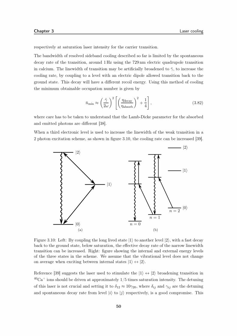
Chapter 3 Laser cooling
respectively at saturation laser intensity for the carrier transition.
The bandwidth of resolved sideband cooling described so far is limited by the spontaneous
decay rate of the transition, around 1Hz using the 729 nm electric quadrupole transition
in calcium. The linewidth of transition may be artificially broadened to γ, to increase the
cooling rate, by coupling to a level with an electric dipole allowed transition back to the
ground state. This decay will have a different recoil energy. Using this method of cooling
the minimum obtainable occupation number is given by
nmin ≈(γ
2ω
)2[(
ηdecay
ηabsorb
)2
+1
4
], (3.82)
where care has to be taken to understand that the Lamb-Dicke parameter for the absorbed
and emitted photons are different [38].
When a third electronic level is used to increase the linewidth of the weak transition in a
2 photon excitation scheme, as shown in figure 3.10, the cooling rate can be increased [39].
|0〉
|1〉
|2〉
(a)
|1〉
|0〉
|2〉
n = 0
n = 1
n = 2
(b)
Figure 3.10: Left: By coupling the long lived state |1〉 to another level |2〉, with a fast decayback to the ground state, below saturation, the effective decay rate of the narrow linewidthtransition can be increased. Right: figure showing the internal and external energy levelsof the three states in the scheme. We assume that the vibrational level does not changeon average when exciting between internal states |1〉 ↔ |2〉.
Reference [39] suggests the laser used to stimulate the |1〉 ↔ |2〉 broadening transition in40Ca+ ions should be driven at approximately 1/5 times saturation intensity. The detuning
of this laser is not crucial and setting it to δ12 ≈ 10γ20, where δij and γij are the detuning
and spontaneous decay rate from level |i〉 to |j〉 respectively, is a good compromise. This
50

Chapter 3 Laser cooling
is still effectively a two level system because the decay from |2〉 is extremely fast compared
to the spontaneous decay rate γ10. For this pseudo two level system the effective decay
rate,
γ =Ω212/2[
(γ20 + γ21) /2]2
+ δ212γ20, (3.83)
depends quadratically on the Rabi frequency of the transition used to increase the sponta-
neous decay rate and linearly on the decay rate of state |2〉 to the ground state. A simpler,
more intuitive way of thinking of the combined linewidth is 1/τ where τ is the time re-
quired for a single closed cooling cycle. However, it is important to remember that when
broadening the weak transition, the resolved sideband condition, γ < ω, must remain true
to perform sideband cooling.
It is clear from figure 3.8 that resolved sideband cooling the magnetron motion is always
going to tricky, not only because n at the Doppler cooling limit is very high but also because
the oscillation frequency is so low that a compromise must be made between broadening
the weak transition to increase the cooling rate and still resolving motional sidebands.
51

Chapter 4Experimental Setup
4.1 Calcium II level structure
The atomic energy level structure of 40Ca+ ions can be seen in figure 4.1. All the transitions
marked in figure 4.1 are dipole allowed transitions except for the 729 nm S1/2 ↔ D5/2
transition, which is electric quadrupole allowed, with a natural lifetime of approximately
1 s [40].
The two S1/2 ↔ P1/2 transitions are used for Doppler cooling. On approximately 1/15th of
occasions the ion decays from the P1/2 state to the D3/2 state [28]. This state needs to be
repumped to maintain a closed cooling cycle. In a Penning trap the Zeeman splitting of
the P1/2 ↔ D3/2 transitions is much larger than the natural and laser linewidths. Therefore,
to repump the D3/2 levels we phase modulate the repumping laser field with an electroptic
modulator (EOM); see section 4.4.1 for details.
These laser beams are sent via polarisation maintaining (PM) optical fibres to the trap.
Fluorescence from the ions in the trap is collected, imaged onto multimode optical fibres
and detected on photomultiplier tubes, or an amplified camera.
4.1.1 J quantum number magnetic mixing
Spin and orbital angular momentum couple together in the absence of an external field
to form J , the total angular momentum. This interaction can be thought of as being
due to the magnetic field caused by the nucleus and electronic core orbiting the valence
electron, interacting with the electron magnetic moment, in the frame of reference where
52

Chapter 4 Calcium II level structure
4S1/2
4P1/2
4P3/2
3D3/2
3D5/2
397 nm
866 nm
729 nm
854 nm
mj = 1/2
mj = 1/2
mj = -1/2
mj = -1/2
mj = 3/2
mj = 3/2
mj = -3/2
mj = -3/2
mj = 5/2
mj = -5/2
...
...
...
Figure 4.1: Relevant Zeeman split energy levels for 40Ca+ ions, in the low magnetic fieldregime (not to scale).
the electron is stationary. The Hamiltonian has the form
H = f (r)(J2 − L2 − S2
), (4.1)
where f(r) depends on the principal quantum number and several other factors. Here the
good quantum numbers to use are J , L, S & mJ .
Applying a small magnetic field splits each J level linearly into 2J +1 states, with energy
proportional to mJ , so that
∆EZeeman = µBgJmJB, (4.2)
where gJ is the Landé g-factor and µB is the Bohr magnetron.
In calcium the fine structure splitting between the metastable D-states is approximately
1.1THz, whereas the Zeeman splitting is of the order of 10GHz T−1. It is clear that at a
53

Chapter 4 Diode Lasers
trapping field of 1.85T, we are in a regime where the spin-orbit coupling dominates.
It is possible to modify the eigenstates to take account of the applied magnetic field [41].
In the weak applied field regime, the obvious basis to use is J & mJ . The effect of the
magnetic field is to mix levels with the same L and mJ [41], i.e. the P1/2,±1/2 and P3/2,±1/2
states mix and D3/2,−3/2···3/2 and D5/2,−3/2···3/2 states also mix together. The magnetically
mixed state makes some of the highly forbidden P1/2 ↔ D5/2 transitions allowed, with a
small electric dipole amplitude.
This process can be seen experimentally during Doppler cooling. When the ion is excited
to the P1/2 level instead of always decaying to the S1/2 or D3/2 levels, the ion occasionally
decays to the D5/2 level which removes it from the standard cooling cycle. The rate at
which this decay happens can be calculated with first order perturbation theory. It can be
shown thatγ(P1/2 → D5/2
)
γ(P1/2 → S1/2
) ≈ 4.2 × 10⁻⁷ T−2, (4.3)
where γ(P1/2 → D5/2
)and γ
(P1/2 → S1/2
)are partial spontaneous decay rates from the
P1/2 state [42]. In a 1.85T magnetic field approximately 7.0× 10⁵ photons will be emitted
on average before shelving to the metastable state. On average an ion will only scatter
photons for 54ms before shelving to the D5/2 level when the cooling transition is saturated.
In order to remove this problem, we apply a laser at 854 nm to drive the D5/2 ↔ P3/2
transitions and to return the ion to the cooling cycle. The required repumping rate is
much slower than all the other Doppler cooling transitions, so only a very small amount of
power is needed in this laser, or alternatively, the laser can be detuned by a few hundred
megahertz and still remain useful.
4.2 Diode Lasers
The two lasers we use for main 397 nm laser cooling transitions are GaN laser diodes1.
They are used to stimulate the S1/2,1/2 ↔ P1/2,−1/2 and S1/2,1/2 ↔ P1/2,−1/2 transitions which
have a 69GHz frequency splitting in a 1.85T magnetic field. They are housed in TuiOptic
(now called Toptica) commercial extended cavity diode laser (ECDL) systems with Littrow
feedback. These lasers are locked to low finesse tunable cavities via feedback to the diode
current and a piezoelectric element on to which the diffraction grating is mounted. These
cavities are in turn locked to a reference HeNe laser with a home-made spectrum analyser
to produce a pair of 2–3MHz linewidth lasers over several hours.
1NDV4814T laser diode from Nichia Corporation.
54

Chapter 4 Laser Locking
The light from these lasers that is not used for frequency stabilisation is then double passed
through acousto-optic modulators (AOMs) to allow high speed switching with extinction
>36 dB. The laser beams are then combined on a 50/50 non-polarising beam splitter and
sent, via polarisation maintaining (PM) optical fibres, to the optical breadboard on which
the trap rests. See section 4.6 for details.
The repumping lasers at 866 nm and 854 nm and the narrow linewidth spectroscopy laser
at 729 nm are home made ECDL setups. The design of these are all based around a
commercial mirror mount with a piezo stack and ruled diffraction grating mounted 1.5–2
cm from the laser diode. The angle of the grating is set to send the -1 diffraction order back
into the laser. A schematic design of these laser heads is shown in figure 4.2. Choosing the
blaze angle of the grating is a trade off between power out of the laser and the fraction of
light sent back to the the laser to stabilise its frequency. Our lasers use different feedback
proportions but we found in general that the anti-reflection coated IR diodes required less
feedback (15%–20%) to lase single mode compared to standard laser diodes which required
about 30% feedback.
α
Laserdiode
Aspheric lens
Diffraction grating
Piezo stack
Figure 4.2: A schematic diagram of the ECDL used for the repumping lasers and narrowlinewidth 729 nm spectroscopy laser. The design is based around a commercial mirrormount with laser diode and aspheric collimating lenses in a threaded tube. The diffractionangle is tuned so that sinα = λ/ (2d) where d is the diffraction grating line spacing and λis the laser wavelength.
4.3 Laser Locking
A number of different locking schemes are used for the various lasers employed in the
experiment. This section covers the background required to understand these systems.
Common feedback mechanisms in ECDLs are:
55

Chapter 4 Laser Locking
• To the piezoelectric element on which the diffraction grating is mounted.
• Directly to the laser current.
• To an external acousto-optic (AOM) or electro-optic (EOM) modulator.
Feedback to the piezo allows large frequency correction although it usually has a maximum
bandwidth of about 1 kHz, limited by the mechanical resonance and capacitance of the
system. Feedback to the laser diode current can occur on significantly shorter time-scales;
however in this case, the servo electronics have to be designed carefully not to introduce
external noise. Feedback to the laser current has two effects: at lower frequencies, there
is a thermal effect which changes the material refractive index and has a negative df/dI
coefficient. However, at times shorter than around 1µs this process becomes less important
and another effect related to the carriers in the diode with a positive df/dI coefficient
becomes dominant [43]. These two competing mechanisms with their associated phase
responses make it difficult to design and build a servo system with a bandwidth higher
than a few megahertz. To use an acousto-optic or electro-optic modulator the carrier
RF frequency is modulated by the feedback signal. Bandwidth limits on AOMs, usually
around 1MHz, are simply determined by the speed of sound in the crystal. Alternatively, an
external EOM has the highest possible modulation bandwidth of all the methods discussed
here and is only limited by the capacitance of the crystal. Modulators exist that have
extremely wide bandwidths. For example, in section 4.4.1 I will discuss using an EOM
with 20GHz bandwidth which could also be used inside a feedback loop.
4.3.1 Pound-Drever-Hall lock theory
The Pound-Drever-Hall (PDH) locking scheme between a laser and an optical cavity allows
high bandwidth feedback. The laser is coupled to the cavity and the reflected light is
detected on a photodiode. The PDH locking technique compares the light leaking out from
the cavity and the light that is promptly reflected from the input coupling mirror. This
produces clear benefits over the side-of-fringe technique [43]. The side-of-fringe technique
operates by stabilising the power transmitted through a cavity to some set point; usually
half the maximum transmission. The error signal in this case forms an odd function without
requiring any external electronics, making it much easier to set up, although with some
limitations. Two of the most obvious benefits of a PDH lock compared to a side-of-fringe
scheme are:
1. The bandwidth of the lock can be higher than the linewidth of the cavity.
2. The error signal is insensitive to laser amplitude noise to first order.
56

Chapter 4 Laser Locking
When a laser is coupled to a Fabry-Perot cavity on resonance, there is a dip in the intensity
of the reflected signal. If the laser shifts frequency the amount of reflected light increases
but there is no discrimination between a positive or negative frequency shift. To produce
an odd function which has a zero point at the cavity resonance, the laser is modulated
and the reflected sidebands and carrier are mixed on a photodiode where they interfere to
produce an error signal. The error signal is then amplified in a loop filter and fed back
to the laser. The design of the loop filter and reduction of external noise sources is often
where the experimental skill is required. A schematic diagram of a PDH locking system
for a laser diode is shown in figure 4.3.
EOM
Laserdiode
LoopFilter
Low-pass filter Mixer
∆φ
Local oscillator
Phase shifter
Faraday isolator Optical isolator Fabry-Perot cavity
Photo-diode
Figure 4.3: Key components of a laser diode PDH locking scheme. Here the phase mod-ulation is imposed on the light using an EOM but sidebands could also be produced bymodulating the laser diode current directly.
For a quantitative description, we follow the method in reference [44]. The first step is to
phase modulate the laser beam such that the light incident on the cavity can be written
as
Einc = E0eı[ωt+β sin(Ωt)] (4.4)
= E0
[J0 (β) e
ıωt + J1 (β) eı(ω+Ω)t − J1 (β) e
ı(ω−Ω)t], (4.5)
where the sinusoidally varying phase has been expanded in terms of Bessel functions with
modulation index β and frequency Ω. The modulation index should be kept low so that
J0+2J1 ≃ 1. We now drop the modulation index from the equations but it is implied. For
a symmetric, lossless, Fabry-Perot cavity the reflected light can be calculated from Eref =
57

Chapter 4 Laser Locking
F (ω)Einc where the incident light is multiplied by the frequency dependent reflection
coefficient
F (ω) =r(eıω/ωFSR − 1
)
1− r2eıω/ωFSR, (4.6)
r is the reflection amplitude of one mirror and ω/ωFSR is the optical phase which is an
integer multiple of 2π at resonance. The amplitude of the reflected light can be written as
Eref = E0
[F (ω)J0e
ıωt + F (ω +Ω)J1eı(ω+Ω)t − F (ω − Ω)J1e
ı(ω−Ω)t]. (4.7)
The photodiode only detects the reflected power, not the amplitude, so we should calculate
Pref = |Eref|2. Using Euler’s formula and the identities (x+ ıy) + (x+ ıy)∗ = 2ℜx+ ıyand (x+ ıy)− (x+ ıy)∗ = 2ℑx+ ıy we can write
Pref =PC |F (ω) |2 + PS
|F (ω +Ω) |2 + |F (ω +Ω) |2
+ 2√PCPS
ℜ[F (ω)F ∗ (ω +Ω)− F ∗ (ω)F (ω − Ω)
]cosΩt
+ℑ[F (ω)F ∗ (ω +Ω)− F ∗ (ω)F (ω − Ω)
]sinΩt
+ 2Ω terms, (4.8)
where PC and PS is the power in the carrier and first order sidebands. We are only
interested in the second and third terms of 4.8 because they contain information about the
mixed carrier and sidebands. The DC and 2Ω terms can be removed by AC coupling the
photodiode and putting a low pass filter in series with the signal respectively.
Which of the remaining terms is dominant depends on the size of the modulation frequency
relative to the cavity bandwidth. In the PDH scheme, the sidebands are almost completely
reflected, i.e.
F (ω +Ω) ≈ F (ω − Ω) ≈ −1. (4.9)
Then the term inside the square brackets in 4.8 can be written as
F (ω)F ∗ (ω +Ω)− F ∗ (ω)F (ω − Ω) ≈−[F (ω)− F ∗ (ω)
]
=− ı2ℑ[F (ω)
]. (4.10)
Only the sin term remains in 4.8 after this substitution. By adjusting the phase of signal
and multiplying it by the modulation on a mixer, the error signal,
ǫ = −2√PCPS ℑ
[F (ω)F ∗ (ω +Ω)− F ∗ (ω)F (ω − Ω)
], (4.11)
58

Chapter 4 Laser Locking
can be extracted. Figure 4.4 shows an example error signal. Within the cavity linewidth,
the error signal is approximately a linear function proportional to the displacement from
resonance. However, the capture range (the range over which the signal remains positive
to the right of the central feature or remains negative to the left) extends all the way to the
sideband resonance. Fundamentally, the laser locking bandwidth is limited to the sideband
−1
−0.6
−0.2
0.2
0.6
1
−0.1 −0.06 −0.02 0.02 0.06 0.1
Err
or/2√PcPs
Laser frequency /free spectral range
Figure 4.4: Calculated PDH error signal as a laser is scanned around resonance for a cavityfinesse of 1000 and a laser modulation of approximately 40 cavity linewidths.
frequency. However, as this can be made arbitrarily large using an EOM, the limiting
factors are usually the feedback mechanism and loop filter electronics which amplifies the
error signal. We use a PDH lock to reduce the linewidth of the 729 nm laser used to
interrogate the quadrupole S1/2 ↔ D5/2 transitions. Section 4.5 describes technical details
about this locking system.
4.3.2 Dither lock
If the cavity used for laser locking has a broad resonance relative to the modulation fre-
quency the features in figure 4.4 at the sideband resonances are no longer distinct. The
name of the laser lock in this regime is called a dither lock. Hence, in a dither lock the
approximation in equation 4.9 no longer holds true. In this regime we can approximate
59

Chapter 4 Laser Locking
the reflection coefficients at the sidebands as,
F (ω − Ω) ≈ F (ω)− dF (ω)
dωΩ. (4.12)
Hence the term
F (ω)F ∗ (ω +Ω)− F ∗ (ω)F (ω − Ω) ≈ 2ΩℜF (ω)
dF ∗ (ω)
dω
(4.13)
only contains real components. The phase of the signal must be modified so that a cosine
modulation appears at the mixer and the error signal
ǫ ≈ 2√PCPS
d|F (ω) |2dω
Ω (4.14)
is demodulated, amplified through the loop filter and fed back to the laser.
4.3.3 Doppler cooling lasers dither lock
The two 397 nm Doppler cooling lasers are dither locked to two different re-entrant design
tunable cavities with Zerodur spacers. The cavities are described in more detail in reference
[45]. However, in brief, they have finesses of approximately 40 and 60, and a 1.5GHz free
spectral range. The cavities are housed inside a large vacuum chamber with float glass
windows at a pressure less than 10−1 mbar. The injection current to the lasers is directly
modulated to produce sidebands approximately 10MHz from the carrier. The optical and
electronic setup is shown in figure 4.5.
The error signal is amplified and fed back to laser current using a loop filter similar to
the circuit described in reference [43]. In order that the laser does not hop to another
longitudinal laser mode with a large DC current offset, the error signal is digitally integrated
and fed back to the piezo as well. The microcontroller controlling feedback to the piezo also
has an input from the transmission of the locking cavities. This ensures that if the laser
becomes unlocked or the beam is blocked, the piezo is not suddenly pushed to a voltage
rail.
The bandwidth of this lock is 0.5–1MHz, easily removing any acoustic noise that is present.
However, higher frequency noise from the lock broadens the short term linewidth of each
laser to approximately 2MHz. This is equivalent to locking to approximately 1/20th of the
cavity linewidth.
Figure 4.6 shows an oscilloscope trace of one of the locking cavities scanning over resonance
with one of the Doppler cooling lasers. The error signal is fit to equation 4.14 and the
60

Chapter 4 Laser Locking
Laser diode
Adder
Loopfilter
Oscillator
AmplifierMixer
Piezo Fabry-Perot λ/4
PBS
PM fibre
Photodiode
µ-controller
Figure 4.5: Schematic diagram of the dither lock for one of the 397 nm Doppler coolinglasers. Solid lines are electrical signals, dashed lines are light and the short dashed line isa PM fibre to take the light to the cavity setup. The DC laser diode current and piezovoltage supplies are not shown for clarity. See text for details.
best fit parameters suggest a cavity finesse of 50. However, if we measure the width of
the transmission peak, the finesse is only 30. The difference is due to the imperfect peak
shape. This can be attributed to dirt on the mirrors. Despite being housed in a vacuum
chamber, they have been removed occasionally and were originally purchased more than a
decade ago. The finesse of one of the cavities was significantly improved by intentionally
snapping a mirror off the spacer and cleaning it before re-gluing it to the spacer.
4.3.4 Doppler cooling lasers transfer cavity lock
The cavities used in section 4.3.2 drift due to temperature variation such that they need
to be adjusted several times an hour to maintain a constant fluorescence rate from the
trapped ions. In order to remove any long term drift, the lasers are locked to a polarisation–
stabilised HeNe laser via a home-made spectrum analyser. The essence of the lock is to
keep the time difference from the HeNe to the Doppler cooling laser resonances constant,
as the spectrum analyser is scanned over one free spectral range.
The cavity and electronics were built by Joe Goodwin and Daniel Crick. In this thesis
an overview of the technical set up is provided but more information can be found in
reference [46]. The cavity is built around a brass spacer with internal threading. Brass
mirror holders with external threading fit onto the ends of the spacer. The mirrors have
dielectric coatings for 633 nm and 397 nm. The cavity finesses at the different wavelengths
are roughly 400 at 633 nm and 65 at 397 nm. The cavity has a single disc piezo attached
61

Chapter 4 Laser Locking
−4
−2
0
2
4
−100 −50 0 50 100
Err
orsi
gnal
/V
Cavity Scan /MHz
Figure 4.6: The loop filter amplified error signal of one of the Doppler cooling lasers as theFabry-Perot cavity is scanned over a resonance (black circles). The error signal is fitted toequation 4.14 (black line).
to one mirror for scanning over slightly more than one free spectral range. A stacked disc
piezo is attached to the other mirror and is used to compensate for thermal variations and
to select a particular free spectral range with a suitable peak splitting.
In this section the HeNe laser will be referred to as the master and Doppler cooling lasers
as slaves. Light from both slaves emerges from a PM optical fibre, is overlapped with the
master on a dichroic mirror and coupled to the spectrum analyser. The cavity is 150mm
long and aligned to be confocal. The cavity is scanned with a sinusoidal drive voltage
over one free spectral range of the master at approximately 2 kHz using a synthesised
signal generator and a home-made amplifier. The free spectral range of the slaves is
λ397/λ633 = 0.63 times that of the master; so normally we observe 3 peaks from the Doppler
cooling lasers within one free spectral range of the master. Two of these peaks are from one
slave laser and one peak from the other. The transmitted light is split on a dichroic mirror.
The master is detected on a photodiode and the slaves are coupled to a 600µm multimode
optical fibre and detected by a photomultiplier tube (PMT) with a simple transimpedance
amplifier.
High speed analogue peak detectors convert the amplified photodiode signals to 5V digital
62

Chapter 4 Laser Locking
pulses. The peak detector only triggers when the differential of the photodiode signal
goes through zero and when the absolute signal is above an adjustable threshold. After
T1
T2
T3
T4
Scan voltage
Masterpeaks
Slavepeaks
Time
Trigger
Figure 4.7: Order of peaks received by the microprocessor and the relevant times measuredin clock cycles, from the trigger received from the signal generator. See text for details.
this point the pulses can be dealt with digitally. An inexpensive Arduino microcontroller
measures the number of clock cycles from the start of the scan to several different pulses.
The pulses and times that are measured by the microprocessor are shown schematically
in figure 4.7. If the temperature in the lab varies, the length of the cavity spacer and
the pressure and refractive index of air in the lab change. T1 will get longer or shorter
depending on the optical path in the cavity. To keep a whole free spectral range of the
master inside the scan range, a voltage is fed back to the piezo stack. We assume that the
scan frequency is stable but thermal variation of the amplifier may cause the amplitude of
the scan to vary over time. This would appear like an effective frequency shift of the lasers.
To avoid this, the microcontroller measures the time between the master peaks within one
free spectral range, T4. It then feeds back to the voltage controlled amplitude input of the
signal generator to stabilise the scan amplitude.
The differences between T2 and T3 during a particular scan, and their values when the lock
is initialised are the effective error signals which are used as feedback to the lasers. These
error signals are digitally integrated and fed back to the low-finesse dither-lock cavities
through an aggressive low pass filter to avoid digitisation noise. The lasers are locked to
these cavities via high bandwidth feedback to the laser diode current and ECDL grating
piezo.
63

Chapter 4 Repumping lasers
The measurements of T1 to T4 are made during one half of the sinusoidal scan. This
type of scan was used after it was observed that harmonics in a triangle wave scan excited
mechanical resonances in the cavity. On the return half of the scan, the feedback parame-
ters are calculated using a look up table to compute arcsin (this removes non-linearities in
the peak displacement). This error signal outputs via 16-bit, parallel digital-to-analogue
converters (DACs)2.
The set point of the lock is held as a digital variable in the Arduino memory. There is
an external input which is used use to alter this variable. The lasers can then be tuned
around resonance with 100 kHz resolution as long as the slave peaks in figure 4.7 do not
overlap.
4.4 Repumping lasers
4.4.1 Multiple transition repumping
In section 4.1.1 it was mentioned that we need to repump not only the four D3/2 but also
four of the D5/2 levels. The gJ values which determine the energy splitting of these levels,
as a function of magnetic field, are shown in table 4.1.
State gJ Splitting /(GHz T−1)
S1/2 2 27.992
P1/2 2/3 9.331
P3/2 4/3 18.662
D3/2 4/5 11.197
D5/2 6/5 16.795
Table 4.1: The gJ values and low-field Zeeman splittings for the relevant levels in 40Ca+.
12/15
2/15
18/15
D3/2 ↔ P1/2
D5/2 ↔ P3/2
Figure 4.8: The splitting of the transitions between metastable D-states and P-statesrelative to the transitions in no magnetic field, in units of µBB.
2Linear Technology LTC1597
64

Chapter 4 Repumping lasers
Fortuitously, the energy splittings of the 854 nm and 866 nm transitions have a simple
integer relationship. Figure 4.8 shows the magnetic field split D3/2 ↔ P1/2 and D5/2 ↔ P3/2
transitions at 866 nm and 854 nm. We modulate the phase of the laser light with an
EOM to produce sidebands. The modulation frequency is να = 6µBB/15 and we set
the modulation index to maximise the second order sidebands. When the second order
sidebands are maximised, we also have a considerable amount of light in the third order
sidebands, at the centre of the sigma D5/2 ↔ P3/2 transitions. Then we also modulate the
light by νβ = µBB/15 to maximise the first order sidebands at this frequency using the
same EOM. By combining both laser and microwave sources before sending them to the
same EOM we obtain a whole array of sidebands. Figure 4.9 shows the optimal intensity
we expect in the resonant sidebands relative to the total power out from the EOM. We have
to remember that only the D5/2,−3/2...3/2 are populated via quantum J-state mixing. Hence
this arrangement repumps all the relevant magnetic sub-levels for closed cycle Doppler
cooling. We note that while the frequency splitting of the sidebands on the 854 nm laser
is accurate, the carrier wavelength may drift by several hundred megahertz over a day
because it is not included in the transfer cavity lock.
0
0.02
0.04
0.06
0.08
0.1
-24 -16 -8 0 8 16 24
Sid
eban
din
tensi
ty/
I 0
Sideband splitting from carrier / µBB/15
Sidebands resonant with the 866 nm transition
Sidebands resonant with the 854 nm transition
Figure 4.9: The lasers are modulated to maximise the second order sideband at 6/15µBBand the first order sideband at 1/15µBB. The optimum sideband intensities relative to thetotal power out of the EOM is plotted. The remainder of the power is in the non-resonantsidebands (not shown).
65

Chapter 4 Repumping lasers
The microwave frequencies that we use are derived from different sources so they are in-
coherent. For an analysis of using coherent microwave sources with controllable phase
differences to optimise the relevant sideband amplitudes, and also a proposal to stimu-
late all the magnetic field split D5/2 ↔ P3/2, D3/2 ↔ P3/2 and D3/2 ↔ P1/2 transitions
in 40Ca+ using one EOM, two microwave frequencies and four lasers, see chapter six of
reference [41].
To implement our scheme the lasers are combined on an angle tuned dielectric filter3. The
same filter also attenuates 854 nm amplified stimulated emission (ASE) in the 866 nm laser
by 36 dB. This is useful because during spectroscopy of the S1/2 ↔ D5/2 quadrupole tran-
sition we need to apply laser pulses in the absence of any 854 nm light. These lasers are
then coupled into the fibre pigtailed, waveguide EOM4. The modulator has approximately
40% transmission due to imperfect mode-matching between the input (and output) fibre
and the waveguide. The microwaves are derived from a synthesised CW generator5 at
10.4000GHz and a voltage controlled oscillator6 (VCO) at 1.7365GHz. The signal genera-
tor can be attenuated in 0.1 dB steps but the power of the VCO, nominally 7 dBm, can only
be altered in 1 dB steps with fixed, inline, attenuators. These sources are then combined
on a resistive power splitter7 and amplified using a wideband amplifier8 with 26 dB gain.
The setup is shown in figure 4.10.
The fibre-pigtailed EOM that we use couples light from the input polarisation-maintaining
fibre into a LiNbO3 waveguide. The waveguide has a similar width to the input and output
fibre, which allows the electrodes, which are either side, to produce a high electric field
for a relatively small input voltage. The RF input power is then dumped into an internal
50Ω terminator, with a maximum power rating of +27 dBm. The electric field can also
be applied over the entire length of the waveguide to allow a high modulation index. We
characterised the modulation index as a function of RF voltage; figure 4.11 shows the
intensities of sidebands after the modulator when driven at 16.8GHz. We have observed
it is possible to maximise the 4th order sideband at this frequency, limited by the internal
terminator.
4.4.2 Repumping lasers transfer cavity lock
The transfer cavity lock for the repumping lasers works in a similar way to the one described
in section 4.3.4 with a few minor changes. The cavity is the same design and uses the same
3Semrock LP02-980RS-254EOSPACE PM-0K5-20-PFA-PFA-8505HP 8650L6Mini-Circuits ZX95-2600-S+7Mini-Circuits ZFRSC-183-S+8Mini-Circuits ZVA-213-S+
66

Chapter 4 Stabilised 729 nm Laser
866 nm
854 nm
Microwave source VCOSemi-rigidcable
-15 dBattenuator
-7 dB
+26dB
Fibre EOM
Modulatedlight
Dichoric filter
Figure 4.10: Experimental apparatus for repumper laser modulation.
master laser as a reference. The mirrors are also custom made with finesses of roughly
50 at 633 nm and 866 nm. We only lock the 866 nm laser using this method, while the
854 nm laser is left unlocked, since the repumping rate required from this laser is very
low. Transmission through this cavity at the relevant wavelengths is much higher than
the spectrum analyser described in section 4.3.4 therefore the transmitted light is simply
detected on photodiodes with transimpedance amplifiers.
This cavity is scanned at 200Hz with a triangle wave and instead of feeding back to the
function generator to maintain a constant scan amplitude we divide all the variables by
the time required to scan a free spectral range of the cavity at 633 nm.
The feedback from the transfer lock is applied directly to the ECDL grating piezo; there
is no other high bandwidth locking system involved with the 866 nm laser. We attempt
to heavily saturate the D3/2 ↔ P1/2 transition so small variations of the laser frequency do
not significantly alter the repumping rate.
4.5 Stabilised 729 nm Laser
The vast majority of work to stabilise the 729 nm laser diode to the reference cavity was
done by Daniel Crick with some minor help from Sean Donnellan and myself. Some of the
technical details of the locking system are described here for completeness only. For more
67

Chapter 4 Stabilised 729 nm Laser
0
0.1
0.2
0.3
0.4
0.5
0 0.4 0.8 1.2 1.6 2
Sid
eban
dIn
tensi
ty/I
0
Applied Voltage /V
Carrier
1st order sideband
2nd order sideband
3rd order sideband
4th order sideband
Figure 4.11: Sideband intensities measured on an optical spectrum analyser after the fibreEOM at a 16.8GHz modulation frequency. The intensities have been fitted to Besselfunctions and normalised to the output carrier intensity with no modulation. The inputRF voltage was set on a microwave source and then connected to the fibre EOM using ahomemade semi-rigid cable with unknown S-parameters, so the applied voltage must bemultiplied by some factor less than unity.
general information, reference [43] is an excellent introduction into locking ECDLs to high
finesse cavities via the PDH scheme.
We lock a diode laser9 to a high finesse cavity with a spacer made of ultra-low expansion
(ULE) glass to reduce its linewidth. If the trap was perfectly stable, the ion would act
as an extremely high-Q oscillator to which the laser could be compared. However, it is
unknown whether the width of the sidebands in section 6 is predominantly from laser phase
noise or magnetic field fluctuations.
4.5.1 ULE high finesse cavity
The cavity was placed inside an ultra-high vacuum chamber and evacuated with a turbo
molecular pump. The vacuum chamber was valved off after a few days with an all metal
angle valve and any remaining pumping done with an ion pump. The ion pump current
9Optnext HL7301MG
68

Chapter 4 Stabilised 729 nm Laser
supply suggests a vacuum pressure between 10−7–10−8 mbar. The vacuum ensures that
there is no pressure change inside the cavity, maintaining a constant optical path length. To
shield the laser system and locking optics from air currents and variations in temperature
the entire system is enclosed inside a wooden box lined with foam. The temperature of
the vacuum chamber is also stabilised and the recorded error signal showed a maximum
deviation of approximately 0.5mK while the box enclosing the laser stabilisation setup
remained closed. The vacuum chamber also provides thermal isolation of the cavity from
the environment.
ULE glass is designed so that it has a very small expansion coefficient which goes through
zero at a temperature near 20C. Above the turning point the glass expands with in-
creasing temperature whereas below the turning point the glass contract with increasing
temperature. The manufacturer is not able to control the temperature of the turning point
from batch to batch. It is therefore necessary for users to identify the turning point by
making their own measurements. The results in this thesis were taken while the cavity was
temperature stabilised but not at the thermal turning point.
The cavity linewidth (and finesse) can be found by first locking the laser to the cavity and
then quickly shifting the laser off resonance. The cavity mode decays as light leaks out
through the mirrors. The rate of decay of the intensity of light incident on the transmission
photodiode should be directly related to the cavity linewidth. This technique is commonly
named cavity ring-down spectroscopy. The data in figure 4.12 is fitted to an exponential
decay and suggests that the cavity has a linewidth of 25.3 kHz (or a finesse of 59300).
4.5.2 Laser & Locking electronics
The vast majority of the electronics for this laser were home built by Daniel Crick. The
commercial alternatives that were initially used were found to add noise to the laser light.
DC current supply
The laser diode has a 75mA operating current and a 100mA absolute maximum rating
and a 2.5V diode voltage drop. The DC supply is provided by ten 10V voltage references
and 1 kΩ low thermal coefficient shunt resistors in parallel. The circuit diagram is shown
in figure 4.13.
Voltage references provide an extremely low drift supply with very low noise. The noise is
attenuated further when used in parallel as shown in figure 4.13. These are both properties
that make them ideal for a low noise current supply. However, we still found it useful to
employ a high-capacity, trickle charged, 12V battery as the power supply. This reduced
69

Chapter 4 Stabilised 729 nm Laser
0.1
1
0 5 10 15 20
Tra
nsm
issi
onP
hot
odio
de
/Arb
Time /µs
Figure 4.12: Light detected on a photodiode recording transmission through the highfinesse cavity after the laser was quickly removed from lock (black circles). This data isfit to an exponential decay function to measure the decay time for the cavity mode (blackline). Data obtained by Daniel Crick.
the residual mains noise on the laser.
Feedback electronics
The electronic servo system should be designed not to limit the bandwidth of the lock. The
loop filter should provide enough electronic gain to the laser diode to reduce the frequency
fluctuations to less than the linewidth of the reference oscillator. The phase margin (the
phase shift from 180 at the frequency where the amplifier gain falls below unity) should be
at least 45 to avoid oscillation [43]. This usually means that the transfer function should
not be steeper than -20 dB per decade or equivalent to 1/f slope at unity gain. However,
ideally there should be very large gains at low frequencies because the suppression of noise
at a particular frequency is approximately the inverse of the gain at that frequency.
A high finesse cavity acts as a frequency discriminator at frequencies lower than the cavity
bandwidth, but like an integrator at higher frequency. This adds a pole to the transfer
function of the feedback at the cavity bandwidth. The transfer function of the loop filter
70

Chapter 4 Stabilised 729 nm Laser
Common
Common
Vout
Vout
Vin
Vin
1 kΩ
1 kΩ 100Ω
On/OffPowersupply
× 10 in parallel
Laserdiode
REF102
REF102
Figure 4.13: Laser diode DC current supply using voltage references. The supply has verylow drift and allows the current to be varied between 68mA and 75mA assuming a 2.5Vpotential difference across the laser diode.
is designed to take into account this effect. The loop filter has several TTL switches to
change the transfer function between a full integrator at low frequency to merely a very
high gain amplifier.
A diagram of the locking system is shown in figure 4.14. The loop filter has two offsets
that must be set manually to maintain a good lock. First is the input offset; this is a DC
offset on the error signal which can be nulled by summing the error signal from the mixer
with a DC voltage. The second is the output offset, which keeps the voltage at the output
with no gain on the amplifier the same as the laser diode voltage drop. This means that
when the lock is engaged the laser frequency is not disturbed.
An Arduino microcontroller controls several TTL operated analogue switches inside the
loop filter. This controller takes an input from a photodiode placed after the reference
cavity to measure transmission. This signal is compared to approximately half of that
which is expected when the laser is locked. When the auto-relock switch is engaged, and
this comparator gives a low signal, the error signal is replaced with a slow (approximately
150Hz) triangle wave at the input of the loop filter to scan the laser frequency. When
transmission through the cavity increases again, and the laser is on resonance with the
cavity, the standard locking system is re-engaged.
71

Chapter 4 Stabilised 729 nm Laser
Loop filter
0 dB
Full integrator
Auto-relock
Errorsignal
Outputoffset
Summingamplifier
Servo control
Functiongenerator
Functiongenerator
µ-controller
µ-controller DAC
Offset
Comparator
Comparator
Laser diode
DC current
Piezo feedback
Transfer function
Variablegain
Vlock/2 Lock engaged?
Engagelock
Engagelock
Engage fullintegrator
Scan
Mixer
Figure 4.14: Schematic block diagram of the high bandwidth laser locking scheme for thequadrupole spectroscopy 729 nm laser. Solid lines are analogue signals, dotted lines aredigital signals and dashed lines are light. Not all the details are show for clarity, see textfor more information.
72

Chapter 4 Optical setup
The loop filter provides an error monitor before the variable gain stage. This is sent to a
separate control system for the piezo feedback, increasing the low frequency gain. Inside
the piezo controller, the error signal is compared to ground to detect whether the error
signal is positive or negative. The microprocessor then increments the piezo voltage via a
16-bit, high speed, low glitch, parallel DAC10.
Additionally, the piezo controller takes an input from the servo controller to instantly
freeze the piezo voltage and avoid the laser frequency moving too far from resonance if the
laser becomes unlocked. The piezo feedback is restored when the transmission photodiode
measures that the lock has been restored.
4.6 Optical setup
The overall optical setup of the experiment is separated into two parts. The first is the
optical tables with the associated laser locking and switching apparatus. Fibre optics at
the end of this chain then transfer the laser light to an optical breadboard on which the
experimental vacuum chamber sits. The breadboard includes optics for combining different
wavelength light and focusing it onto the ion.
Light from all the laser diodes used have different widths in the vertical and horizontal
directions because the diodes themselves physically have an aspect ratio of roughly 3:1.
We initially shape these beams using either anamorphic prisms or single axis Keplerian
telescopes composed of cylindrical lenses. The lenses are tilted slightly to avoid back
reflections to the diodes. The light then passes through Faraday isolators to reduce feedback
from optical elements further down the beam line. After the isolators, half wave plates and
polarising beam splitters are used to split the light into two paths, one for laser locking
and wavelength determination and the other for the laser cooling in the experiment.
For the Doppler cooling lasers some light is picked off the laser locking beam path, and
then sent to the dither lock cavities described in section 4.3.3 via PM fibres. The remainder
of this light, from the two lasers, is combined on a 50:50 non-polarising beam splitter cube.
The mixed light from one of the output ports of the beam splitter goes to the transfer
cavity lock described in section 4.3.4 via a PM optical fibre. The light from the other
output port is sent to a Fizeau interferometer wavemeter11 in an adjacent laboratory12,
via an approximately 60m long single mode fibre.
The light that is sent to the experiment after the isolator first travels through double passed
10Linear Technology LTC159711High Finesse WS-612Use of the wavemeter is kindly provided by Centre for Cold Matter at Imperial College.
73

Chapter 4 Optical setup
AOMs13 before being combined on a non polarising beam splitter cube. The beams from
the two outputs act as a pair of cooling beams, one sent along the axis of the trap (axial
cooling beam) and one sent along the radial plane (radial cooling beam).
Of the repumping lasers, only the 854 nm laser has an AOM in its path. The 866 nm laser
is left on continuously. These two laser beams are combined on a dielectric filter and pass
through the high frequency EOM described in section 4.4.1. The combined repumping
light is then split on a 80/20 plate beam splitter with 80% to the radial repumping beam
and 20% to the axial repumping beam via PM optical fibres. The narrow linewidth laser
at 729 nm is combined with the axial or radial repumping light after the EOM. A diagram
showing the major features of the layout is shown in figure 4.15.
Cooling beam
Repumping beam
729 nm beam
Faraday isolator
λ/2 retarder
λ/4 retarder
Dichroic mirror
Beam sampler
Polarisingbeam splitterNon-polarisingbeam splitterAnamorphicprisms
Cylindricallenses
Polarisationmaintaining fibreSingle modefibre
AOM
Doppler cooling lasers
Dither lock
Transfer cavitylock
Transfer cavitylock
Wavemeter
Wavemeter
From 729 nmlaser
Fibre EOM
Breadboard
Breadboard
Breadboard
Repumping lasers
Figure 4.15: Optical table layout (beam steering mirrors are not shown). The labels onthe diagram show where the fibres end. See text for details.
All the light required for laser cooling is coupled into PM fibres and sent to the breadboard
13Isomet 1206C-833
74

Chapter 4 Trap configuration
holding the trap apparatus. On the breadboard, one set of repumping laser beams and one
set of cooling laser beams are overlapped to form the axial laser beam, using a dichroic
beam splitter. Similarly, the other set of repumping and cooling beams are combined to
form the radial laser beam. These beams are then focused onto the trap centre. The
axial beam uses a f = 400mm lens and the radial beam, a f = 500mm focal length lens
which give 1/e2 diameter spot sizes of 85µm and 105µm respectively. The radial beam
exits the trap and is reflected back down to the breadboard, passes through a glass colour
filter and hits a quadrant photodiode. The vertical beam exits through a window on the
top of the vacuum chamber, passes through a dielectric beam splitter and a glass colour
filter before hitting another quadrant photodiode. We use these detectors and a simple
computer program to monitor the position of the laser beams.
For trap loading, photoionisation is performed via non-resonant multi-photon excitation
at 532 nm using light from a pulsed, frequency-doubled Nd:YAG laser. This laser sits on a
separate small table bolted to the superconducting magnet cryostat. The output from this
pulsed laser cannot be coupled into a fibre because the instantaneous pulse power is too
high. The light counter-propagates along the axial laser cooling path with a focusing lens
just before the window above the trap. There are more details of the loading procedure in
section 4.8. A diagram of the optical setup on the breadboard can be seen in figure 4.16.
4.7 Trap configuration
The trap that we use for the experiments was originally built by Shailen Bharadia and
described in reference [47]. Here, I provide a brief description of the trap and and the
changes made to the optical access to perform the experiments in this thesis.
We use a solenoid superconducting magnet, operating at 1.85 T, to provide the radial
confinement. The trap is inside a vacuum system pumped by a 40 ls−1 ion pump and a
non-evaporable getter pump14 which is especially good for low mass particles. The pressure
inside the vacuum system is less than 10−9 mbar.
The trap electrodes are cylindrical and machined from oxygen-free high conductivity cop-
per. They have a 21.6mm inner diameter. This means that they are much less sensitive
to misalignment than in a miniature ion traps. The ring electrode is split vertically in to 4
segments, to allow a rotating dipole RF field to be applied to the ion [48]. Precise dimen-
sions for all the electrodes are given in reference [47]. There is also a 4mm diameter hole
drilled in each of the ring segments. Two of these apertures are used for laser beam access
and the other two are used for fluorescence collection. The electrodes are kept electrically
14SAES Getters CapaciTorr D 400
75

Chapter 4 Trap configuration
Coolingbeam
Repumpingbeam
Combinedbeams
Aperture to alternativeimaging setup
Fluorescence
Fluorescence
Photodiode
Dichroicmirror
Viewport Periscopemirror
PM fibre
f = 500mm
f = 400mm
Axial beam
Radial beam
Multimodefibre
Axial beam
Radial beam Fluorescence
To vacuumpumps
Breadboard
Magnet cryostat edge
104.5mm
CF40 to CF16zero length
reducer
Chamber containingtrap electrodes
Figure 4.16: Top: simplified diagram of the vacuum chamber and laser beam paths seenfrom the side. The mirror that directs the axial beam vertically is inside the vacuum cham-ber, see section 4.7. Bottom: top down view of the optical and vacuum setup. Only partof the vacuum chamber is shown (light gray). All the laser light arrives at the breadboardvia PM fibres. The first mirror after the radial beam focusing lens is a computer controlledpiezo motor mount.
76

Chapter 4 Trap configuration
isolated either using small sapphire balls or macor rings. The trap electrodes are mounted
on four copper rods which attach to a mounting plate. The mounting plate is bolted onto a
vacuum flange which also has three 4-pin feedthroughs welded onto it. The vacuum flange
is also fitted with a CF16 viewport.
Optical access has been increased since reference [47] to allow laser beam access along the
trap axis. A window was installed on the vacuum system at the same level as the optical
breadboard optics to allow laser access. A custom, fixed, mirror holder is bolted to the
inside of the vacuum chamber. A mirror here allows laser light to be directed vertically
upwards. Figure 4.17 shows a CAD rendering of the mirror holder and the vertical laser
beam. The holder mounts into two threaded holes in a CF40 to CF16 zero length reducer.
There is an 397 nm anti-reflection coated CF16 viewport15 on the other side of the reducer.
This window is used to send the laser light into and out of the trap. We use a Semrock
Maxmirror in the vacuum which has high reflectivity for all polarisations and wavelengths
from 350 nm to 1100 nm.
Mirror
Laser beam
Mounting holes
Figure 4.17: Mirror mount which allows vertical optical access. The holder is mounted inthe vacuum chamber on CF40 to CF16 zero length reducer as shown on figure 4.16.
To allow unobstructed optical access vertically along the trap, we have removed the electron
bombardment filament used for the experiments in reference [47]. The effusive calcium oven
has also been shifted to below the trap and off-axis. Figure 4.18 shows the current setup
of the trap with laser beams, fluorescence detection optics and electrodes displayed.
Apertures in the ring segments through which fluorescence is collected limit the detection
solid angle. The combination of both 4mm diameter apertures, 10.8mm from centre of
the trap allow, at most, the collection of 1.5% of the spontaneously emitted light. The
light is channelled along two paths, through 14mm gaps, between the vacuum chamber
and the edge of the magnet bore before it can be detected.
15Torr Scientific VPZ16VAR-LN
77

Chapter 4 Trap configurationreplacemen
Lens 1
Mirror 1
Lens 2 Lens 5
Lens 3
Lens 6
Lens 4
PMT
Lens 1
Mirror 1
Mirror 2
Lens 2
Lens 3
Lens 4
Lens 5
Lens 6
Oven
B
Best form f = 20mm
Singlet f = 100mm
Singlet f = 100mm
Best form f = 20mm
Achromat f = 200mm
Aspheric f = 20mm
Elliptical 1/2” mirror
Elliptical 1/2” mirror
200µmmultimode
fibre
Mirror 2
EMCCD or200µm multimode fibre
& PMT
21.6mm
Endcap
Ring
Compensationelectrode
Figure 4.18: Trap and fluorescence detection setup. The trap electrodes are shown in or-ange along with the support structure which is also made of copper. The support structureis comprised of a pair of end plates and four copper rods. A pair of copper lens holders areattached to the rods near the centre of the trap. The central electrode is the ring which isradially split into 4 segments. Each segment has a 4mm aperture. The fluorescence, shownin light-purple, exits through two apertures and is nominally collimated by lenses inside thevacuum chamber. Above and below the ring are a pair of compensation electrodes. Aboveand below the compensation electrodes are the endcaps. Above and below the endcaps areanother pair of electrodes not used in this work and which are internally grounded. Theinner electrodes are separated by small sapphire balls, shown in light-blue, and the largerelectrodes by macor rings, shown in beige. The laser beams propagate vertically, shownby the purple arrow, and radially shown by the circle with a cross inside at the centre ofthe trap. The oven is below the electrode and displaced from the trap axis.
78

Chapter 4 Loading Ions
Photomultiplier tubes are susceptible to the fringe field of the magnet; they need to be
at least 1m from the base of the magnet to operate properly. To avoid long-distance free
space optics, we permanently couple one of the paths into a 200µm, 0.22NA, solarization-
resistant optical fibre. These optical fibres do not have anti-reflection coated ends and
a bulk attenuation of around 1.5%/m. The end of the fibre is fixed with an adapter
approximately 2mm from the detection face of the PMTs. The other path can be swapped
between a similar multimode fibre or an amplified camera16 for imaging.
4.8 Loading Ions
To load 40Ca+ ions into the trap we follow a three step procedure. Initially, we resistively
heat a 2 cm long calcium filled tantalum tube with a hole in one side pointing towards the
centre of the trap. Once this tube, which we call the oven, begins to glow dimly a small
amount of calcium starts to effuse out of the hole and some of it is sent towards the trapping
region. After the oven has been heated like this for 30–60 s we pulse the Nd:YAG laser17
5–50 times in a short burst lasting a few seconds. The laser has an average pulse power
of 1–10MW during its approximately 5 ns pulses. A non-linear non-resonant three-photon
process ionises some of the atoms. The process is not isotope selective and the loading rate
is greatly variable. These atoms are ionised over the length of the 532 nm beam which may
not overlap with the centre of the trap. This creates ions out at large radii and with large
axial displacements. Figure 4.19 shows fluorescence from 40Ca+ ions cooling into the centre
of the trap from large orbits over several seconds after we have stopped pulsing the high
power laser. This behaviour can continue for several minutes. This is highly undesirable
if we wish to perform experiments with a single ion or a well defined number of ions. We
have developed a method to control the number of ions loaded which is described below.
Penning traps have no micromotion and the ions are not heated when they are away from
the centre of the trap. Furthermore Penning traps are stable for ions with a large range
of charge to mass ratios. Hence, our loading process can produce many undesirable ions.
The laser cooling acts quickly on the correct isotope of calcium but non-resonant ions can
remain trapped in large orbits which occasionally interfere with the experiment. To remove
the unwanted ions we simply turn off the electrostatic trapping field for 10–20µs. During
this time the cooled ions in the trap undergo a Coulomb explosion. The ions in large orbits
are lost from the trap altogether. After the trapping field is restored the calcium ions that
were initially in the centre of the trap are quickly cooled again. To reduce the number of
ions in the trap we repeat the same procedure but when the required number of ions have
16Andor Luca R.17Continuum Surelite II
79

Chapter 4 FPGA and computer control
500
1000
1500
2000
2500
3000
3500
4000
4500
5000
5500
0 5 10 15 20 25 30 35
Phot
onco
unt
rate
/Hz
Time /s
Figure 4.19: PMT count data after loading using the non-resonant pulsed Nd:YAG laser.Dashed lines are marked where ions cool to the centre of the trap. The initial count atapproximately 800Hz is scattered background light from the lasers.
been re-cooled to the centre of the trap we turn off the trap again in an attempt to eject
any remaining 40Ca+ ions still in larger orbits. Using this technique we can load between
one and roughly 30 ions at will.
4.9 FPGA and computer control
The S1/2 ↔ D5/2 electric quadrupole transition in 40Ca+ has a spontaneous decay rate
of roughly 1Hz. This makes standard fluorescence or absorption spectroscopy infeasible.
Instead we use the high bandwidth S1/2 ↔ P1/2 transition as a diagnostic as to whether
the ion has been shelved in metastable D5/2 state. The procedure is to Doppler cool an
ion for a few milliseconds, then turn off a particular 397 nm laser for around a hundred
microseconds. This leaves the ion in a thermal state, optically pumped into one of the
magnetic sub-levels of the S1/2 states. The 729 nm spectroscopy laser is then pulsed on for
a few milliseconds. This is again followed by a few milliseconds of Doppler cooling. The
ion will not fluoresce during this final stage if the 729 nm laser has excited the ion to the
long-lived D5/2 state. This technique produces a digital signal (i.e. is the ion fluorescing or
80

Chapter 4 FPGA and computer control
not) which must be repeated many times at each laser frequency to calculate a shelving
probability. Once this is done, the laser frequency can be changed and the whole procedure
repeated to build up a spectrum.
During my time in the laboratory, we installed AOMs in the beam lines to allow repetitive
pulsed spectroscopy to be carried out. Also, previously, photons detected by PMTs were
counted using a fast EG & G Ortec multichannel scaler card. This computer card only has
8192 channels and was reliant on a computer with an ISA interface, which is now an obsolete
standard. To overcome these limitations we decided to build a more future-proof system
based around a modern PC and a field programmable gate array (FPGA) development
board. The system was developed by two MSci project students, Shamim Patel and Stefan
Zeeman, with supervision from Daniel Crick and myself. More information can be found
in references [49, 50].
A standard experiment starts at a particular frequency, and carries out many pulse se-
quences to detect the state of the ion after applying the 729 nm laser to the ion. The
FPGA then records the number of photons detected by the PMTs. See section 6.1 for
more details. The data for that frequency are sent back to the computer and analysed
to build up a spectrum of the transition. The computer then tells the function generator
to change frequency and the FPGA repeats the pulse sequences. Eventually, the FPGA
reaches a stop command, a signal is sent back to the computer and the experiment ends.
The control system should be able to perform all the laser pulses and gated photon counting
described in section 6.1. We also require an efficient communication protocol between the
PC and FPGA. Figure 4.20 shows the network of computer controlled apparatus in the
experiment and the communication between these items.
FPGAs are made up of logical elements. Each logical element can be configured to imitate
different digital gates. These gates can be configured in different orders to perform different
tasks. Hence, FPGAs can be considered as software programmable hardware. This direct
hardware manipulation of inputs to give certain outputs is inherently faster than using a
standard microprocessor because the processing is done by optimised discrete elements.
One area of the device can be configured to deal with a certain task and another area can
perform a completely different task. These operations can then be synchronised exactly.
This is in contrast to executing a list of instructions in a serial fashion which is what
happens on a microprocessor. For example, the signal to switch several AOMs on or off
can be sent at exactly the same time, measured to within the resolution of our 300MHz
oscilloscope18, as well as doing several other tasks simultaneously. The timing resolution
of these operations is set by the clock speed of the FPGA: 50MHz for our development
board.
18Tektronix TDS3032B
81

Chapter 4 FPGA and computer control
Computer
FunctionGenerator
PulseSequence
PhotonCounts FPGA
RF switch
AOM for729 nm laser
3×VCOs for cooling lasers
3×RF switches
3×AOMs for cooling lasers
PMT 1
PMT 2
GPIB
Figure 4.20: The interaction between the apparatus used to automate pulsed spectroscopy.
The FPGA19 that we use employs an internal 3.3V TTL voltage. To interface with 5V
signals in other parts of the system we step the voltages up and down using digital buffers20.
These are extremely fast, 13 ns propagation delay according to the data sheet, and provide
no discernible delay on the signals.
4.9.1 Computer front-end
The program which interfaces with the FPGA and the function generator was written in-
house by the masters students mentioned in section 4.9. This computer interface provides a
simple way of setting up an experiment. The program compiles the experimental sequence
into the binary format which the FPGA expects and uploads it. This program also tells a
GPIB interface card21 what data to send to the signal generator. In addition, the computer
program receives data from the FPGA, saves it in a suitable text file, and performs several
simple handshaking requirements. Figure 4.21 shows a screenshot of the control program.
4.9.2 FPGA memory interface
The FPGA development board that we use has 3 types of memory available:
• Synchronous dynamic random access memory (SDRAM) - 8MB: this is similar to
memory on PCs. It has a relatively fast access rate and is large enough to hold a
significant amount of data. This type of memory is volatile; if the FPGA is switched
19ALTERA - DK-CYCII-2C20N - KIT, FPGA, CYCLONE II DEVELOPMENT203-State quad buffer MM74HC125N21National Instruments PCI-GPIB
82

Chapter 4 FPGA and computer control
Figure 4.21: The user interface of the program we use to setup the experiments andcommunicate with the FPGA and function generator.
off, the data stored in the SDRAM will be lost. Writing or reading to this type of
memory takes up to 2 or 3 clock cycles. We use this type of memory to store the
pulse sequence.
• Static random-access memory (SRAM) - 512 kB: not conventionally used in consumer
electronics because it is relatively expensive, SRAM has several advantages over other
types of memory e.g. SDRAM. For our purpose the main benefit is the speed of
access: reading and writing to SRAM happens well within one clock cycle. From
now on we will consider this as virtually instantaneous. This is where we store the
PMT count data and laser lock information.
• Flash memory - 4MB: This type of memory is the slowest of all those present on the
development board. The memory is non-volatile, i.e. the data is not lost when the
power is turned off. Flash memory has some limitations which make it unreliable for
our purpose. Only a finite number of programming cycles can be implemented on
the same memory bits before they become corrupted. Often the number of stable
programming cycles is as high as 1,000,000 but because we repetitively change the
pulse instructions and PMT data, we avoid using this memory chip.
83

Chapter 4 FPGA and computer control
There is much more detail that could be written about these different types of memory
technologies. Many of the integrated devices are now so small that they utilise quantum
tunnelling effects for their operation.
The compiled pulse sequence is received from the computer via a USB-to-TTL interface
cable22. These data are uploaded to the SDRAM via the FPGA. The baud rate is deliber-
ately kept low to avoid corrupted data as there are no error correction bits included in the
data. The SDRAM can only be accessed in 16-bit words. Each pulse operation is stored as
two of these words which are henceforth referred to as a phrase. Each phrase is split into
three parts, 24-bits of timing data, allowing pulse lengths between 0 s and 0.335544300 s
in 20 ns steps; 5-bits of laser data, these are essentially TTL outputs to RF switches and
other devices; the remaining three bits are to tell the FPGA what operations to run during
the pulse. These are:
• Mains wait - Leaves the lasers that were set on until the mains trigger is received
and then moves onto the next laser pulse setting, see section 4.9.3.
• Normal - This setting turns on the lasers that are instructed to do so for the time
set in the control software.
• Count - Turns the lasers on as requested and counts PMT photons saving the data
along with a laser lock error code, which report if any of the lasers became accidentally
unlocked in this interval, in the SRAM. This latter feature allows us to tag any data
taken with the lasers unlocked so that it can be discarded in post-processing.
• Send Data - This flushes the data from the SRAM into the computer, which stores
it in a text file. The transfer takes place via the USB-to-TTL cable.
• Function generator wait - This sends a signal to the computer to step the function
generator frequency to the next value and waits for approximately 0.25 s for this to
happen. The lasers are set to Doppler cool the ion during this period
• Start loop - This tell the FPGA that the instructions following this command and
before the end loop command are to be repeated. The number of repetitions is stored
in the timing data.
• End loop - This command marks the end of the internal hardware loop.
• Stop experiment - The FPGA sends a signal to the computer to say that the experi-
ment has finished. After this point the Doppler cooling lasers are left on permanently.
22Future Technology Devices International Ltd. TTL-232R-3V3 USB to TTL Serial Converter Cable
84

Chapter 4 FPGA and computer control
We can store up to 8MB/32-bit = 262144 phrases in the memory. However, using the
hardware loop command we can send a standard set of instructions that has 1000 frequency
steps in around only 500 commands.
4.9.3 Mains Trigger
The pulse sequence used for spectroscopy of the quadrupole transition is phase locked to
the mains cycle to avoid ambient magnetic field fluctuations that would affect the atomic
transition frequency, and voltage fluctuations in the electronic equipment. The trigger
works by first stepping down mains voltage to 20V amplitude on a small transformer.
Then this signal is compared to ground on a simple LM311 voltage comparator. The
output signal from this stage is shown in figure 4.22.
Time
Stepped down mains
5V signal to FPGA
Figure 4.22: The trigger provides a high TTL signal when the mains voltage is above zeroand a low signal when the mains voltage is below zero.
This signal is sent to the FPGA so that pulse sequences starts at a specific phase relative
to the mains. The signal from the comparator is digitally filtered. If the output from the
trigger changes, the FPGA waits to see if the signal is consistent for 3 clock cycles (60 ns)
before acknowledging the trigger.
4.9.4 RF electronics
The RF electronics which control the Doppler cooling AOMs all have similar setups. For
each setup a sinusoidal signal comes from a VCO23 which passes through fixed attenuators,
a homemade RF switch based on an Analog Devices ADG918 IC and a homemade voltage
controlled amplifier based on a National Semiconductors LMH6505MA IC. The signals are
amplified with a CATV amplifier24 before being sent to the AOMs. The AOMs in the
23Minicircuits ZOS-100 for the 854 nm laser beam AOM, Minicircuits ZX95-200 of the 397 nm laser beamAOMs
24Amplifier Solutions Corporation ASC2832
85

Chapter 4 FPGA and computer control
Doppler cooling laser beam paths operate at a 110MHz central frequency and the AOM
in the 854 nm laser beam path operates at a 80MHz central frequency.
The 729 nm laser is controlled from a stable, 1Hz resolution function generator via a GPIB
interface. This allows computer control of both the frequency and amplitude. The signal
is sent to a high extinction RF switch25 and RF amplifier26 before going to the AOM.
The AOM has a 250MHz central frequency and approximately a 40 MHz tuning range.
However, the power in the first order deflected beam coupled to the PM optical fibre can
reduce to half over that range.
The TTL signals from the FPGA activate the RF switches; the homemade switches have
an RF isolation between 28–35 dB and a 5–10 ns rise/fall time. The commercial RF switch
for the 729 nm laser has a specified 100 dB isolation with a similar rise/fall time.
25Mini Circuits ZASWA-2-50DR+26Mini Circuits ZHL-1-2W
86

Chapter 5Coulomb Crystals
Coulomb crystals are formed when more than one ion is cooled to the solid phase. In
this case the average thermal energy of the ions is much less than the energy required
to overcome the Coulomb barrier for individual ions to swap positions. This is usually
parametrised in the literature by the Coulomb coupling parameter, Γ = e2/(4πǫ0akBT );
where a is the Wigner-Seitz radius defined by 4πa3/3 = n−10 , where n0 is the number
density of ions and kB is the Boltzmann constant [51]. Different studies have shown that
solid phase crystals are formed in large plasmas when Γ > 172 − 178 [52–56].
In this phase, the ions behave in a similar way to a rigid body, with the same centre of mass
oscillation frequency common to all ions. Higher order motional modes are characterised
by small vibrations around their equilibrium positions. The shape of these crystals is only
controlled by the ratio of trapping frequencies in the axial and radial directions. In the
case of a simple Penning trap, with no additional electric fields, there is no particular
orientation in the radial plane and the crystal rotates. The rotation frequency for more
than one ion is not fixed, and can vary anywhere between the magnetron and modified
cyclotron frequency for a single ion in the same electric and magnetic fields [57]. Typically
the Coulomb crystal will settle into a particular steady state rotation frequency dependent
upon the parameters of the laser cooling. The rotation frequency and the number density
of the particles in the crystal are related through the equation
n0 =2mǫ0ω
′r
(ωc − ω′
r
)
q2, (5.1)
where ω′r is the rotation frequency in the laboratory frame [58]. This relation can be
calculated by substituting the electric potential into Poisson’s equation where the charge
density is defined as ρ = n0q. Previously, two different methods have shown that it is
87

Chapter 5
possible to externally vary the rotation frequency; first by a laser induced torque [59]
and later by applying a rotating quadrupole electric field [60, 61], colloquially called the
rotating wall technique. The rotating wall technique distorts the radial trapping potential
and phase locks the crystal rotation to a RF drive.
Forming a coupled array of particles like a Coulomb crystal in an ion trap is relatively
simple when for example compared to an optical lattice. Here the ions need only to be
laser cooled to around 5mK to produce these configurations, whereas, in an optical lattice
micropotentials must be formed via differential AC stark shifts in a standing wave. In
the limit where the number of particles in a crystal is large, the ions become regularly
spaced. For linear chains, the ions are equally spaced in a row and in 2-dimensions, planar
arrays with six-fold rotational symmetry are formed [6]. In three dimensions, the picture is
more complicated; crystals can form many different shapes from elongated spirals through
concentric shells, to layers of planar arrays [62]. As the crystals become smaller, edge
effects have to be taken into account and ion-ion spacing is no longer constant.
Coulomb crystals are not restricted to singly charged ions, they have also been observed
in dusty plasmas [63] (with Coulomb coupling parameters as high as 20700 [64]). These
crystals are formed of multiply charged, micron sized, clusters but form similar shaped
arrays. In an astrophysical context, most of the matter in the universe is either plasma
or dust particles. These crystals may help in the understanding of structures seen by
telescopes, for a good review see reference [65].
Coulomb crystals have been instrumental in certain recent atomic physics experiments.
Transverse optical cavity modes have been mapped out using both single ions [66] and
large elongated crystals [67]. In the case of a single ion, the transverse mode was in-
vestigated by shifting the ion along the cavity mode and monitoring fluorescence. This
allowed information about the light intensity to be gathered on a sub-wavelength scale.
Cavity QED experiments in the strong coupling regime also become accessible with large
Coulomb crystals using standard, macroscopic, mirrors. The coupling between the ions in
the cavity and the cavity mode is proportional to√N , where N is the number of particles
interacting with the cavity mode [68].
Another use of Coulomb crystals is to couple the internal states and collective motional
modes of several ions. The Coulomb interaction allows excitation of the collective modes of
the crystal via optical sidebands. This has been a key method in some of the experiments
implementing quantum entanglement. In reference [2], a 14-ion linear Coulomb crystal in
a RF trap is first cooled to the ground state of the centre of mass mode and then entan-
gled using a narrowband laser beam. The ions were placed in a superposition of the form
(|0 . . . 0〉+ |1 . . . 1〉)/√2 . It is possible to confirm that the particles are entangled by mea-
suring the off diagonal (i.e. ρ0...0,1...1 and ρ1...1,0...0) elements of the density matrix [38]. An
88

Chapter 5
engineered quantum state of this type is commonly know as a Greenberger-Horne-Zeilinger
(GHZ) state. One example application of this type of state is to increase sensitivity in spec-
troscopy experiments [69]. This procedure only works because the coupling between the
ions is fast enough to produce collective oscillation modes. However, linear RF traps are
limited to using chains of ions for this purpose. Any ions displaced from the trap axis are
subject to micromotion at the RF drive frequency and are heated well above the quantum
ground state. Currently this limits the number of ions that can be entangled, in a single
crystal, in a RF trap.
Alternatively, using a Penning trap, both 2 and 3 dimensional crystals can be formed with-
out any micromotion. These crystals can theoretically be cooled to the ground state for all
motional modes. The readily available, harmonically confined, two and three dimensional
arrays of coupled particles present a useful system for performing quantum simulation ex-
periments [6]. As a starting point, entanglement between spin and motional states of several
hundred particles in a planar two dimensional array is exploited to measure the tempera-
ture of the different modes transverse to the plane of the crystal in reference [70]. Initially
the ions are placed in a superposition of all possible spin states (i.e. ⊗Nj=1(
∣∣↑j⟩+∣∣↓j⟩)/√2 ,
where the N particles are labelled by the indices j), with a microwave pulse. A travel-
ling wave, with angular frequency ωODF, produced from two laser fields which has a net
wavevector transverse to the plane of ions is tuned close to the frequency of the different
motional modes. The optical dipole force from the travelling wave induces decoherence of
the spin state dependant on the temperature of the mode being investigated. The temper-
ature of different modes can be determined by fitting the magnitude of the decoherence as
ωODF is varied.
During my time in the lab we have improved our trap and laser setup to allow the produc-
tion of small Coulomb crystals. Here proof of principle evidence that we can manipulate
and image these crystals is reported. The work presented in this thesis will concentrate on
small numbers of ions where all the ion-ion interactions can be numerically calculated on a
standard computer. When the number of ions increases, the system must be approximated
as a one component plasma [51] or large shell structure crystal [71] both of which have
been investigated in Penning traps for many years.
In this chapter the spacing of ions, in a linear chain, in our trap, are compared to the values
predicted in reference [24]. Linear chains of up to 29 ions are presented; previously only
chains of up to 2 ions have been “crystallised” along the magnetic field axis in a Penning
trap [9], although linear crystals have been seen in RF trap since 1987 [72]. If a linear
chain is held in a trap and the axial frequency is increased, there comes a point where it is
energetically favourable for the chain to develop kinks, taking up a zigzag formation. This
is a well known effect which is routinely seen in for ion chains in linear RF traps, though
89

Chapter 5 Centre of Mass Oscillations
it has never previously been observed in a Penning trap. I will compare photographs to
computer simulations and infer the radial trap frequency. This information is used to
examine the linear-zigzag configuration transition as a function of the number of trapped
ions. Then using photos of 15 ions at a range of different trap voltages and their comparison
to computer simulations it will be shown that it is possible to determine the radial trap
frequency with a certain error bound. It will also be shown that this is also possible for
intermediate sized crystals containing a few hundred ions as long as individual ions are
still resolved. Finally, I investigate the effect of quantum J-state mixing on larger crystals
of hundreds of ions.
5.1 Centre of Mass Oscillations
There are 3N oscillation modes for N ions. For a string of ions aligned along the trap
axis, the centre of mass (COM) motion is always the lowest frequency axial mode and
is independent of particle number. This oscillation frequency can be found by applying a
small RF drive to one of the electrodes along the trap axis, varying its frequency and looking
for a blurring of the image of a crystal on a camera as shown in figure 5.1. This occurs
when the oscillating potential resonates with the crystal COM mode. Using a camera is
a more sensitive detection technique than simply looking for a reduction in fluorescence
using a PMT. With high enough magnification, large oscillations of the ions around their
equilibrium positions can be imaged while the ions remain crystallised.
By changing the trap bias, and measuring the COM oscillation frequency we can calculate
the constant of proportionality κ in the equation ωz = 2πκ√V where V is the trap bias.
The data plotted in figure 5.1 shows that κ = 26.36 ± 0.03 kHzV−1/2.
5.2 Magnetron mode instability
Section 3.4.1 shows that there is a maximum magnetron frequency, for a single ion, before
the Doppler cooling lasers with a particular intensity gradient start to heat the magnetron
motion. By measuring the diameter of the magnetron orbit using an amplified camera we
can estimate the laser frequency relative to the atomic transition. We assume that the
amplitude of the radial motion is dominated by the magnetron mode. The cooling lasers
probably over saturate the transition by a factor of 2 - 5 (Isat = 440µW mm−2). In this
case the interaction between laser beam and the ions is now a saturated Gaussian and
not just determined by the laser beam profile which is a standard Gaussian. A saturated
Gaussian can have a higher intensity gradient. Assuming that the intensity gradient is now
y0 ≈ 15µm (y0 is defined in figure 3.5), compared to 25µm which should be the case when
90

Chapter 5 Magnetron mode instability
0
100
200
300
400
500
600
700
0 50 100 150 200 250 300 350
Osc
illa
tion
freq
uen
cy/k
Hz
Applied trap bias /V
Centre of mass oscillation frequencies
ωz/2π
ω+/2π
ω−/2π
50µm
Figure 5.1: Measured axial oscillation frequency as a function of trap bias for a linear 3-ioncrystal. The inferred modified cyclotron and magnetron frequencies are also shown. Theaxial COM motion is damped by the laser cooling and therefore accuracy in the frequencymeasurements is limited to around ±200Hz. Insert shows example data. Left: a phototaken when the RF drive is off resonance. Right: photo taken when RF drive resonateswith the COM axial mode.
the transition is not saturated, we should only expect good agreement between the fit and
the data till the oscillation extends to around this diameter. The solid line in figure 5.2 is
only fit to the data where the diameter of the magnetron motion extends to a maximum of
15µm (= y0) and is consistent with the cooling lasers being detuned by approximately half
a natural linewidth. Alternatively if we include all the data up to 130V we find a different
fit (dashed-dot line). This fit does not follow the data as well for low voltages but is more
consistent with the data around the region where the orbit expands dramatically. In this
case the fit suggests that the laser detuning is 1–2 times the natural linewidth. These result
is inferred from the data, rather than a measurement from an absolute frequency reference.
The wavemeter that we use to initially set the laser frequencies is only accurate to a few
hundred megahertz. When the diameter of the oscillation is greater than y0, radial cooling
is reduced and can no longer be approximated by equation 3.71. When the amplitude of
the oscillation reaches around 100µm the ion samples the entire width of the beam and
the size of the orbit reaches some stable equilibrium.
91

Chapter 5 Motion in a Rotating Frame
0
10
20
30
40
50
60
70
80
0 50 100 150 200 250 300 350
Dia
met
erof
mag
net
ron
mot
ion
/µm
Trap bias /V
Fit of data up to 2R− = y0
Fit of all data up to 130V
Figure 5.2: The amplitude of the radial motion of a single ion (×) fit against equation 3.74bfor different data ranges (see text for details). The diameter of the motion is measured usingan amplified camera at different trap bias settings. The imaging magnification (3 ± 0.1)and pixel size (8µm), limit the accuracy of the measurement to an error of around ±1µm.
5.3 Motion in a Rotating Frame
The laboratory frame is not the natural frame in which to consider the motion of an ion in
a Penning trap. If instead we move into a frame rotating at ωc/2 the circular motion which
couples the two radial co-ordinates, x and y, is removed and a simple harmonic motion in
only one co-ordinate is retained. However, as is shown below, when there are two or more
ions present they can rotate even in this frame. The standard result for the acceleration
of a rigid body in a rotating frame, at a constant frequency, is
sr = s− 2Ω× s− |Ω|2 s, (5.2)
where sr and s are accelerations in the rotating and lab frames and Ω is the rotation
frequency. The penultimate term in equation 5.2 relates to the Coriolis force and the final
term relates to the centripetal force. If we substitute equation 2.7 and Ω = ωc/2 into
92

Chapter 5 Motion in a Rotating Frame
equation 5.2 we find,
sr = −(ω2c
4− ω2
z
2
)s = −ω2
1s. (5.3)
This transformation has removed any rotation due to the magnetic field and essentially
turned this system into a harmonic potential in 3-dimensions where the trapping frequen-
cies in the x and y directions are degenerate. We can rewrite the potential energy of the
system in the rotating frame as
V =m
2
N∑
n=1
[ω2zz
2n + ω2
1
(x2n + y2n
)]+
e2
8πǫ0
∑
n,m6=n
1
rnm, (5.4)
where the Coulomb repulsion of N ions has now been included. The indices n and m
sum over the number of ions, and rnm =√(xn − xm)2 + (yn − ym)2 + (zn − zm)2 is the
interparticle spacing. The directions xn and yn are arbitrary in the case of a Penning trap
with no perturbing electric fields. If the crystal rotates in this frame at ωr we can move
into another frame where the ions are now stationary. To relate the frame where the ions
are stationary and the laboratory frame, we can use the simple conversion, ω′r = ωc/2−ωr,
where ω′r is the rotation frequency in the laboratory frame; this assumes that the rotation
frequency in the laboratory frame is always less than ωc/2. The radial trap frequency can
be written as
ω2T = ω2
1 − ω2r (5.5)
which can be derived by considering the total energy of the system in the two different
frames. Now the potential energy for the system can be written as
V =m
2
N∑
n=1
[ω2zz
2n + ω2
T
(x2n + y2n
)]+
e2
8πǫ0
∑
n,m6=n
1
rnm. (5.6)
When ωr 6= 0, or equivalently ωT < ω1, the maximum voltage at which the configuration
is stable is reduced toVmax
V0= 1−
(1− 2ωr/ωc
)2, where V0 is the maximum stable bias for
a single ion in a Penning trap with the same magnetic field.
5.3.1 Laser beam torque
The axial COM oscillation frequency, ωz, is set directly by the trap potential. In our
experiment the rotation frequency is set by the radial laser cooling beam which essentially
applies a torque to the crystal. We do this by offsetting the laser beam from the centre
of the Coulomb crystal. This method has been shown to vary the rotation frequency of a
large non-neutral plasma from ω− to ω+ [57].
93

Chapter 5 Linear Ion Chains
As the crystal becomes smaller, the torque that can be applied to the ions, which is
proportional to distance between the centre of rotation and the laser beam, is reduced.
When the diameter of the crystal in the radial plane is less than the width of the laser
beam, a torque can be applied via an intensity gradient. This situation becomes very similar
to laser cooling of a single ion described in section 3.4.1. Now the rotation frequency is
not fixed and depends on unstable laser parameters such as intensity, frequency and beam
position. The work in this thesis depends on the radial cooling beam to set the rotation
frequency, hence the radial trap frequency.
5.4 Linear Ion Chains
By relaxing the axial trapping potential in a Penning trap with a fixed magnetic field, the
ions form linear Coulomb crystals aligned along the trap axis. For small numbers of ions
the infinite range 1/r Coulomb repulsion leads to a non-linear ion-ion spacing. By solving
the N coupled simultaneous equations 5.4, we can predict their positions. These equations
can be solved analytically for chains of up to 3 ions however for larger numbers of ions the
equations must be solved numerically [24]. The solutions are tabulated in reference [24]
for up to 10 ions.
The right-hand-side of figure 5.3 is a collage of photos of 1 to 9 ions aligned along the
trap axis. The numerical solution to equations 5.4 have also been plotted as circles. The
experimental data fit these theoretical points well, suggesting that the harmonic trapping
term is dominant. We can also cool larger strings of ions. The left-hand-side of figure 5.3,
shows a photo of a 29 ion crystal. Previously only two-ion linear crystals have been shown
to align along the axis of a Penning trap [9]. The ions at the edges of the 29 ion chain,
which is 505± 15µm long, appear less intense than the central ions. If the axial beam was
not aligned properly it may not have good enough a spatial overlap to saturate the laser
cooling transitions for the outer ions. Also, as ions are held further from the centre of the
trap, they become more susceptible to electrical noise on the electrodes. This may also
induce oscillations in the crystals shown in figure 5.3.
The radial cooling beam width (1/e2 diameter is approximately 100µm) is too small to
provide any laser cooling at the edges of the long string of ions in figure 5.3. The axial
cooling beam heats the radial motion of the ions through photon recoil. In cases where
the crystal is made to extend even further along the trap axis, it is possible to see a larger
radial motion of the end ions compared to the ions in the centre of the crystal.
94

Chapter 5 Higher dimensional Coulomb crystals
0
0.2
0.4
0.6
0.8
1
B
Figure 5.3: Right: collage of linear crystals of 1–9 ions. The trap bias is set at 8.95Vfor all of the photos. Each photo is an accumulation of twenty 1 second exposures andthe maximum intensity in each photo is normalised to unity. Each pixel is equivalent to2.65 ± 0.15µm in the centre of the trap. The circles around the ions are the theoreticallycalculated positions, from reference [24], and not from a fit to the data. Left: a chain of 29ions and their intensity profile. The ions at the end of the chain are less bright than thecentre ions probably because they are not as well overlapped with the laser beams. Thebars at the bottom of the photos both represent a length of 50µm.
5.5 Higher dimensional Coulomb crystals
The shape of two and three ion crystals in a Penning trap is determined analytically in
references [73,74]. However, only numerical analysis is possible for larger numbers of ions.
To progress further, I wrote a simple script in the Matlab programming language to find
the equilibrium positions for the ions. The same program also displays an image which
should be similar to what we see on the camera after a long exposure.
The magnetic field, number of ions and axial (ωz) and radial (ωT ) trap frequencies are
input into the program. The ions are originally given random positions in space for the
three dimensions. The random positions should help avoid any unstable equilibria which
the simulation may find. For the first ion, the net force due to the Coulomb repulsion from
all the other ions and the trap potential is found. This is repeated for all the other ions
to find the magnitude and direction of the net force. Now the program takes a small time
step. The position of each ion is moved in the same direction as the force from the previous
step. The magnitude of the force determines how far to move a particular ion. The new
positions are then used as starting points and the process is iterated several thousand times
95

Chapter 5 Higher dimensional Coulomb crystals
to find the equilibrium positions.
At the end of this process, each ion has a position in three dimensional space where the
total force on all the ions is minimised. The script could easily be optimised to stop looping
if the total force on all the ions drops below a certain threshold but this modification has
not been implemented to produce the results in this thesis.
In the laboratory frame, the crystallised ions are rotating around the trap axis. When we
take a photograph in the experiment, fluorescence from the ions appears to be smeared
out because the exposure is much longer than a single rotation period. The ions are cooled
to a few milli-Kelvin and hence have fixed relative positions so their orbits are circular.
When this motion is projected onto the plane imaged by the camera, it is easy to see that
an ion appears to spend more time at the extrema of its apparently sinusoidal motion. We
can simulate what kind of an image we expect to see, assuming that the fluorescence rate
is constant, by applying the formula
I ∝ arcsin
(X +∆X/2
r
)− arcsin
(X −∆X/2
r
), (5.7)
where I is the intensity incident on a particular pixel on the camera, X is the position
of the pixel relative to the centre of the image, ∆X is the width of a pixel and r is the
radius of motion for a particular ion [9]. The image can be simulated by summing the
fluorescence we expect to observe from each individual ion, assuming that they all interact
equally with the cooling lasers. This assumption may be flawed but it is used anyway. For
example, if the orbit of an ion has a radius of 10µm we expect the Doppler shift of the
cooling transitions, when the rotation frequency in the lab frame equals ωc/2, to be
∆f =
(ωc/2
)× 10µm
cf0
≈ 55MHz, (5.8)
where c is the speed of light and f0 is the frequency of the cooling transitions (approximately
755THz).
The image is then filtered with a Gaussian point spread function commensurate with our
imaging system. This is simple using the functions provided by Matlab. Figure 5.4 shows
an example of an image we would expect to observe when seven ions are formed in to a
linear string, a zigzag if there was no rotation and a zigzag when rotation in the radial
plane is taken into account.
By maintaining the same axial frequency (which is solely dependent on the trap bias) but
altering the radial frequency input to the computer code to match photographs from the
experiment and images from the simulation, we can find the rotation frequency, ωr, of the
96

Chapter 5 Higher dimensional Coulomb crystals
BBB
0
0.2
0.4
0.6
0.8
1
Figure 5.4: Simulated images for seven ions. Left: when the ions form a string, theyappear in a line from our point of view even though they are rotating. Centre: when theaxial frequency is increased the ions form a zigzag shape. If the camera we used to imagethese ions could be gated in phase with the crystal rotation we would observe an imagesimilar to the one shown in the centre. Right: a simulated image for the ions in a zigzagconfiguration taking into account the fact that we are viewing the crystal while it rotates.
crystal.
The first non-linear shape which we observe is a zigzag geometry. Reference [75] determines
the ratio of axial and radial trapping frequencies where the linear to zigzag transition takes
place. By calculating this ratio for a wide range of ion string lengths, an empirical scaling
law to predict the the transition is inferred.
In a linear chain, all the ions lie along the trap axis. However, from simple arguments
we can see that if there is a zigzag pattern none of the ions can lie along the trap axis.
As proof, consider the case where only a few central ions lie off axis. The transverse
electrostatic repulsive forces from these ions in the chain may balance perfectly for a single
ion further along the chain. However, the next ion along has a different forces acting on it
because the Coulomb repulsion is a function of distance. Hence, we can see that it would
be impossible for a few ions to be off axis in the centre of the chain and the remainder to
lie exactly along the trap axis [76].
97

Chapter 5 Higher dimensional Coulomb crystals
0.55
0.6
0.65
0.7
0.75
0.8
0.85
0.9
0.95
1
3 4 5 6 7 8 9 10
ωT/(ωc/2)
atlinea
rto
zigz
agtr
ansi
tion
Number of ions
Experimental data
ωr/(ωc/2) = 0
ωr/(ωc/2) = 0.66
Figure 5.5: By measuring the trap bias when a linear to zigzag transition occurs we canpredict the radial trap frequency. This figure shows the frequency ωT inferred from theexperimental data. These data are consistent with ωr = 0.66 ± 0.05. The frequency ωT
is also calculated at the transition between linear and zigzag crystal configurations for thetheoretical case where ωr = 0.
Here, the radial trap frequency, ωT , is determined from the linear to zigzag configuration
transition voltages and comparison to computer simulation. We input the axial oscillation
frequency, where the transition was observed, which is fixed by the trap bias and the radial
frequency is varied in the program until the linear to zigzag transition is found. Figure
5.5 shows the radial trap frequencies at the zigzag transition and the predicted frequencies
if the crystal was stationary in the frame rotating at ωc/2. However, the data is more
consistent with the crystals consisting of different numbers of ions rotating at angular
frequency ωr/(ωc/2) = 0.66 ± 0.05.
We can also compare photos of a fixed number of ions, at various trap biases, to computer
simulations. Figure 5.6 shows a continuum of images for 15 ions from a linear string to
a flat two dimensional rotating pentagon-decagon structure. The images are titled with
axial trapping frequency in units of ωz/(√2 ωc/2). For a single ion, all the stable axial
trap frequencies, in these dimensionless units, are within the range zero to one. They are
compared to the closest matching simulations with a variable radial trap frequency, ωT .
98

Chapter 5 Higher dimensional Coulomb crystals
B
100µm
0.106 0.110 0.112 0.118 0.129 0.149 0.167 0.183 0.198 0.211
0.224 0.236 0.248 0.259 0.269 0.279 0.289 0.299 0.312 0.334
0.3590.366 0.392 0.409 0.425
0.438 0.452 0.471 0.487
0.528 0.578 0.6250.646 0.668
0.688 0.708
0.728 0.746 0.783 0.800 0.806
0.809 0.818 0.826 0.835 0.851
Figure 5.6: Left: photographs of 15 ion Coulomb crystals. Right: the closest matchingcomputer simulations. The images are titled with axial trapping frequency in units ofωz/(
√2 ωc/2). In all the images, the magnetic field is in the vertical direction and the
horizontal and vertical scales are equal and given by the bar on the right hand side. Themaximum intensity in all the photographs is normalised to 1 and come from an accumu-lation 40 exposures each with a 1 s shutter time. The magnification in all the images is3.0± 0.1. The colour scale is the same as in figure 5.3.
99

Chapter 5 Higher dimensional Coulomb crystals
To find the closest matching simulation to the photos in figure 5.6, the radial trap frequency
was manually optimised. The axial frequency and the deduced radial trapping frequency,
ωT , are plotted against each other in figure 5.7 for the images shown in figure 5.6. By
fitting these data to (2
ωc
)2[ω2T +
ω2z
2
]= 1−
(ωr
ωc/2
)2
, (5.9)
we should be able to find ωr, the rotation frequency in the frame rotating at ωc/2. Equation
5.9 can be derived by substituting equation 5.5 into equation 2.11. This is the same
equation as a circle in suitably scaled coordinates.
0
0.2
0.4
0.6
0.8
1
0 0.2 0.4 0.6 0.8 1
ωT/(ωc/2)
ωz/(√2 ωc/2)
15 ion crystal data
ωr = 0.50 × (ωc/2)
ωr = 0.25 × (ωc/2)
ωr = 0
Figure 5.7: For each of the images in figure 5.6 the axial trapping frequency is plottedagainst the radial trapping frequency used to produce the simulated images. This is essen-tially the stability diagram for a Penning trap. Lines of constant rotation frequency, ωr,are plotted for comparison. The error bars are derived from how accurately the radial trapfrequency can be determined by comparison to computer simulations.
Figure 5.7 shows that the rotation frequency of the crystals, ωr, appears to decrease to-
wards higher axial trap frequencies from around 0.5 × ωc/2 to 0.25 × ωc/2. However, is
100

Chapter 5 Larger Crystals
it much harder to deduce rotation frequencies when the crystal is in one of the two ex-
treme configurations. The radial trap frequency has no effect on a linear chain and the
axial frequency has very little effect on an oblate ellipsoid (pancake) shape crystal. The
configuration of the crystals changes much less in the range 0.5 < ωr/(ωc/2) < 1 than the
range 0 < ωr/(ωc/2) < 0.5. This can be seen graphically in figure 5.7. The area of the
sector enclosed by the lines ωr/(ωc/2) = 0.5 and ωr/(ωc/2) = 0 is much less than the area
from the origin to the line where ωr/(ωc/2) = 0.5.
5.6 Larger Crystals
The strong coupling between ions in a Coulomb crystal and the broad laser beam profile
in our experiment allows us to crystallise larger numbers of ions than previously discussed
in this chapter. As the numbers of ions increases more intermediate configurations become
possible. However, what appeared as configuration transitions for small numbers of ions,
are no longer so clear. For example, a three ion zigzag shape crystal transforms to a triangle
rotating in the radial plane when ωz = ωT . However, for large numbers of ions the first
shape after a zigzag is a spiral of varying aspect ratio, followed by a shell configuration,
without any kind of layered structure, until the regime where ωz ≫ ωT is reached.
B
50µm
0
0.2
0.4
0.6
0.8
1
Figure 5.8: A photo of a large Coulomb crystal and a simulation of a similar shaped crystal.The simulated image is for 174 ions where ω2
z/(2ω2T ) = 0.146.
101

Chapter 5 Larger Crystals
Figure 5.8 shows a photograph of a larger crystal in our trap as a demonstration that we
can crystallise and clearly image larger numbers of ions. It is not possible, with just a
single side-on photograph, to determine the exact number of ions in a three dimensional
Coulomb crystal of this size. The simulations suggest that the crystal in the photograph
contains 174 ± 4 ions in a trap potential where ω2z/2ω
2T = 0.146 ± 0.010. If the number
of ions and ratio of trap frequencies is varied within the errors provided, the simulated
crystal maintains the correct gross structure (number of planes of ions, number of central
ions, etc.) and the correct aspect ratio. By altering either of these parameters further,
it is possible to observe a clear deviation from the crystal in the photo. This is roughly
the limit for the numbers of ions that can be simulated by my simple Matlab code. It is
unfavourable to increase the number of ions further as the number of calculations required
scales with the square of the number of particles. Much more sophisticated molecular
dynamics codes exist if larger crystals are being investigated. For example, a computer
program called Protomol can compute the interaction between 100000 ions, including ions
of different species [77].
It is difficult to align more than 50 ions along the axis of the trap because it would require
the ratio of the axial and radial trap frequencies, ω2z/(2ω
2T ), to approach zero. In this
case, the crystal would become susceptible to melting during collisions with background
gas molecules and noise on the electrodes which may couple to vibrational modes of the
crystal.
5.6.1 Effect of quantum J-state mixing in Coulomb crystals
In the frame where the crystal is stationary the radial cooling beam rotates around at
ωc/2 − ωr. However, the axial cooling beam has a definite angle of incidence relative to
the trap axis (it is parallel). Therefore, when the ions are fluorescing there is a net force
imparted on the crystal proportional to the number of photons scattered from the axial
cooling beam. If some ions decay to a non-fluorescing dark state and no longer interact
with the axial laser cooling beam, they are not affected by the light pressure. This is clearly
a state dependent force. We can engineer a situation like this by blocking the repumping
laser which stimulates the D5/2 ↔ P3/2 transition. Now, any ions that are shelved in the
D5/2 level, via quantum J-state mixing, see section 4.1.1, remain dark for approximately 1 s
before decaying to the ground state and returning to the cooling cycle. The axial cooling
beam pushes the fluorescing ions in the same direction as the laser light. This can be
directly observed by taking a time averaged photo of a Coulomb crystal with the 854 nm
laser beam blocked.
Figure 5.9 shows a photo of a large Coulomb crystal with and without 854 nm laser light to
repump the D5/2 state. The bright ions are pushed by the axial laser beam. The crystalline
102

Chapter 5 Larger Crystals
B
100µm
0
0.2
0.4
0.6
0.8
1
Figure 5.9: The effect of quantum J-state mixing is clearly shown on this Coulomb crystal.The photo on the left shows a Coulomb crystal when the D5/2 state is repumped andthe photo on the right is taken when the repumping laser is blocked. The photos areaccumulations of 60 × 0.5 s exposures, long enough for the ions to spontaneously decayback to the ground state around 30 times on average.
structure is still clearly visible suggesting that the dark ions are sympathetically cooled to
the solid phase.
Far above saturation we expect the ion to have a γ/2 fluorescence rate, for a two level
system. By including the whole level system including two S1/2, two P1/2 and four D3/2
states we should only expect a γ/4 fluorescence rate. Including another factor of 1/2
because the laser cooling frequency is detuned below the atomic resonance we should
expect γ/8 ≈ 1.7 × 10⁷ photons s−1 to be emitted. Using the theory in reference [78] we
should expect 7.1 × 10⁵ photons before decaying to the D5/2 state on average. Therefore
the ratio of fluorescence when the 854 nm laser is blocked and unblocked is given by
7.1/170
1.2 + 7.1/170= 0.034, (5.10)
where 1.2 s is the lifetime of the D5/2 state. The ratio of the fluorescence in the two photos
in figure 5.9 when corrected for background laser scatter is 0.23. One possible explanation
for the discrepancy is that the D5/2 level is repumped by amplified stimulated emission
in the 866 nm laser. However this seems unlikely because the dichroic mirror combining
103

Chapter 5 Larger Crystals
the two repumping lasers has 36 dB attenuation (measured) for 854 nm light in the 866 nm
laser beam. An alternative view might be that the photograph on the left hand side of
figure 5.9 is not fluorescing at the rate predicted above. This could be because axial beam
does not saturate ions throughout the whole crystal, only the central 100µm. The radial
beam may not interact with the outer ions either due to the Doppler shift. The ions in the
outer shell are approximately r = 100µm from the centre of rotation in the radial plane.
Assuming the crystal rotates at ω = 2π × 100 kHz in the lab frame, this should shift the
laser cooling frequencies by ±ωrf0/c ≈ 160MHz. The shift for the repumping lasers is
approximately 72MHz. This could reduce the fluorescence rate at the left and right of the
image and be the main reason why the outer most shell of ions is not clearly visible apart
from at the top and bottom of the crystal.
104

Chapter 6Motional Sideband Spectroscopy
The motion of a Doppler laser cooled ion in a Penning trap can be well approximated by
an harmonic oscillator. It can be shown that the quantum energy levels in such a confining
potential are equally spaced. Motional sidebands can be observed when the trap frequency
is greater than the linewidth of a probe optical or RF atomic transition. The energy level
structure in 40Ca+ ions has an electric quadrupole allowed transition between the S1/2 and
the metastable D5/2 levels with a natural linewidth of approximately 1Hz [40]. In this
chapter I will show that we have observed both axial and radial motional sidebands using
this 729 nm narrow linewidth transition in a single calcium ion in a Penning trap.
Motional sidebands on atomic transitions have been observed in several systems. They were
first detected, via microwave spectroscopy, in a cloud of He+ ions stored in a quadrupole RF
trap [79]. The first observation of optical sidebands was performed using a single Hg+ ion
at NIST [80]. Since then, optical sidebands have been observed in neutral atoms stored in
an optical lattice [81] and a micromechanical oscillator [82]. For reference, the temperature
of the centre of mass mode and several higher order modes in a 2 dimensional Coulomb
crystal in a Penning trap has been measured by tuning lasers to induce an optical dipole
force resonant with a motional mode [70]. For many experimental groups, the observation
of motional sidebands quickly leads to resolved sideband cooling. Again, this was first
demonstrated at NIST with a single Hg+ ion [16].
A theoretical framework for the interaction between laser light and the external states is
described in section 3.2. By fitting the shelving probability of the sidebands to equation
3.55 we can estimate the temperature or, more generally, the population distribution of the
trapped ion. In the Lamb-Dicke regime, the average motional state can be calculated by
the approximation n = P−1/(P+1−P−1), where P−1 and P+1 are the shelving probabilities
of the first lower and upper sidebands, assuming these transitions are not saturated.
105

Chapter 6 Pulse sequence
Resolved sideband cooling has allowed significant progress in atomic frequency references
and quantum computing using trapped ions. Sideband cooling often increases the occu-
pation of the ground state of motion to greater than 99% probability. Doppler shifts are
then reduced so that they are no longer the dominant sources of error in atomic frequency
standards [83].
Many quantum computing algorithms or quantum simulation protocols require that the
motional state of the particles is initially prepared with a well defined distribution. For
example to perform high contrast Rabi oscillations a trapped particle must be prepared
in a Fock or number state. Many other well defined coherent superposition states have
been created, but always starting from a ground state cooled ion, for some examples see
reference [84].
This chapter will first describe the experimental procedure used to perform spectroscopy on
the S1/2 ↔ D5/2 transition. It will also illuminate some of the challenges to determining the
internal state of the ion due to quantum J-state mixing. Finally, the preliminary spectra
of the axial and radial motions of a single 40Ca+ ion in a Penning trap are displayed.
The quality of the data limits the accuracy of the measurement of the average motional
occupation number, n to no better than a factor of 2 or 3.
6.1 Pulse sequence
The control hardware and software repeatedly pulses different lasers on and off to a well
defined sequence to build up a spectrum of the transition. The spectrum includes vibra-
tional sidebands around the carrier so the frequency range that must be scanned is many
times that of the transition linewidth.
The pulse sequence used to measure a spectrum is shown in figure 6.1. Each pulse performs
a certain task.
• Mains wait: Takes over when the previous pulse sequence has finished and carries
on Doppler cooling until the mains voltage increases above ground. This is to ensure
that the pulse sequence is phase locked to the mains cycle.
• Doppler Cooling: Standard laser cooling with both 397 nm Doppler cooling lasers
and the two repumping lasers. The detuning and power of the lasers in this pulse
determines the ion temperature for the spectroscopy run.
• State preparation: Optical pumping into one of the S1/2 magnetic sub-levels.
Achieved by simply turning off one of the 397 nm lasers.
106

Chapter 6 Pulse sequence
• 729 nm pulse: Creates a superposition of the S1/2 ground state and the metastable
D5/2 state.
• Detection: All the standard Doppler cooling lasers, except for the 854 nm laser, are
turned on again to stimulate atomic fluorescence and determine whether the ion has
been shelved or remains in the ground state.
Mainswait
Dopplercooling
Statepreparation
729 nmpulse Detection
397 nm A
397 nm B
729 nm
854 nm
866 nm
PMT gate
Mains cycle
Figure 6.1: Pulse sequence used in spectroscopy of the S1/2 ↔ D5/2 transition. Statepreparation is achieved by optical pumping into one of the magnetic field split groundstates. This is achieved by simply turning off one of the Doppler cooling lasers, either397 nm A or 397 nm B, depending on which magnetic sub-level is required. The boxes arenot drawn to scale. See text for details.
6.1.1 Mains triggering
All the electronic equipment in the lab, with the exception of the DC current source and
photodiode for locking the narrow linewidth 729 nm laser and the superconducting magnet,
are powered from the mains supply. This induces noise on lots of equipment in phase with
each other and creates ambient AC magnetic field fluctuations. In order to remove this
modulation from our results we phase lock the laser pulse cycle to the mains. First, we step
107

Chapter 6 Pulse sequence
down mains voltage and then compare the signal to ground on a simple voltage comparator.
The resulting signal is a square wave which can be used as a digital input to the FPGA.
For more details on the mains trigger hardware, see section 4.9.3.
6.1.2 Doppler Cooling
In this section only technical aspects related to Doppler cooling during the spectroscopy
experiment will be presented. For more theoretical information see section 3.4.1.
The Doppler cooling part of the pulse sequence ensures that the ion is at the same temper-
ature each time it is interrogated by the 729 nm laser. The broad bandwidth of Doppler
cooling ensures that any heating from the environment is quickly removed.
A single ion is robustly confined in our trap with a total depth of roughly 50 eV. This is
the maximum energy, summed over all the motional modes, that an ion can have and still
remain trapped. However, to increase the orbit of an ion beyond the width of our laser
beams (around 100µm) only requires roughly 5meV. Occasionally, there are collisions
with background gas molecules (background gas pressure is of the order of 10−8 Pa) which
imparts this much energy to the ion. When a collision like this takes place, the ion no longer
interacts strongly with the laser light. We believe background gas may also sporadically be
ionised by the violet Doppler cooling laser beams. The Coulomb interaction with these ions
disrupts the experiment. Also rare, but possible, are chemical reactions between hydrogen
molecules and the trapped calcium ions [85]. Normally, the ion is returned to the original
fluorescence rate in a fraction of a second. However, ions are stable in very large orbits
and can potentially take several minutes to return to the centre of the trap.
We count the number of photons received during the Doppler cooling part of the pulse
sequence to diagnose any problems with the experiment. If we notice the ion has become
dark for a prolonged period, we can pause the experiment and attempt to remedy the
situation. However, if the perturbation was too short for us to observe visually, the data is
discarded during post processing. The data from a pulse sequence is only included if the
number of photons we have detected during the cooling phase is above a set threshold.
6.1.3 State preparation
Optical pumping can be achieved simply by turning off one of the 397 nm Doppler cool-
ing lasers, since the large Zeeman splitting allows the individual transitions to be easily
addressed in the frequency domain. In a RF trap, where two transitions are split by less
than their natural linewidth, the correct circularly polarised light must be used for state
initialisation. This is one advantage of a Penning trap compared to an RF trap; state
108

Chapter 6 Pulse sequence
preparation can be done with potentially higher fidelity.
6.1.4 729 nm pulse
After the Doppler cooling and state preparation parts of the pulse sequence, the ion should
have a thermal population distribution. The excitation from the 729 nm laser places the
ion in a superposition of the S1/2 and D5/2 levels. To model the resulting excited state
population, all vibrational levels must be taken into account, see section 3.2 for more
details. The 729 nm laser is narrow enough to resolve vibrational sidebands. However, the
remaining observed S1/2 ↔ D5/2 transition linewidth is dominated by the short term laser
linewidth. The laser pulses in the experiment are turned on and off in a top hat fashion.
If desired, the laser linewidth can be artificially increased by reducing the laser pulse time.
The 729 nm laser frequency is scanned to build up a spectrum. The laser frequency is
varied using a double passed AOM and high resolution signal generator. The 729 nm light
to the trap is turned on and off using the same AOM, see figure 4.20 for more details.
6.1.5 State detection
We analyse the photomultiplier counts recorded by the FPGA during the detection phase
of the pulse sequence to determine the internal state of the ion. The fluorescence from
the whole spectrum is collated and the data are plotted as a histogram with respect to
the number of photons detected. An example of the data we collect is shown in figure
6.2: it clearly has a bimodal structure. When the ion is shelved in the D5/2 state only a
few photons are counted in the detection period, corresponding to the lower peak. The
lower peak has a non-zero mean value because both scattered light from the laser beams
and thermionic emission from the PMT photocathode are also counted. The higher peak,
when more photons are counted, relates to the superposition of the two atomic energy
levels collapsing to the S1/2 state after interacting with the Doppler cooling lasers.
By setting a threshold between these two distributions, the internal state of the ion can be
determined with high probability. A complication arises with calcium ions in a Penning
trap, due to quantum J-state mixing, see section 4.1.1 for more details. If initially during
the detection period we observe fluorescence, on average after 54ms (if the transition is
saturated), in our magnetic field, the ion will shelve in the D5/2 state. This is similar to
any random decay process, with an exponential dependence on time. Hence, the highest
decay rate occurs when we initially turn on the detection lasers. If the shelving event
happens before the control system has counted enough photons to recognise that the ion
was initially bright, we record a false shelving event. In effect, this reduces the fidelity of
state detection.
109

Chapter 6 Pulse sequence
0
200
400
600
800
1000
1200
1400
0 10 20 30 40 50
Num
ber
ofob
serv
atio
ns
Photons in detection period
Double Poisson with J-state mixing
Double Poisson
Spectroscopy run data
Figure 6.2: Histogram of photon counts in a 5ms detection period. The number of photonscounted in a particular bin are quantised and shown by ×. The functions that are fit tothis data assume a double Poissonian distribution with and without a plateau betweenthe two peaks to simulate quantum J-state mixing. The vertical dotted line is set atthe minimum of the double Poisson fit. The solid and dashed-dot vertical lines are at 3standard deviations from the mean of the lower peak and 2 standard deviations from themean of the higher peak for the different fit models. The mean values for the lower andupper peaks are approximately 1.5 and 25 respectively for a detection time of 5ms. Seetext for details.
Figure 6.2 shows a histogram of the data collected during one particular spectroscopy
run. In the absence of quantum J-state mixing the data should follow a double Poisson
distribution of the formABke−B
k!+CDke−D
k!, (6.1)
where A and C are the amplitudes and B and D are the mean values for the lower and
upper peaks respectively. In the double Poisson fit on figure 6.2, these distributions are
clearly separated. When this is the case then a threshold placed where the vertical dotted
line is located would work well to discriminate between fluorescing and non-fluorescing
events. However, the data does not follow this fit in the region between the two peaks. If
we assume that the quantum J-state mixing decay period is at least 5–10 times longer than
the detection period, we can approximate the exponential decay with a straight line. In
110

Chapter 6 Pulse sequence
this regime, the photon count histogram should include an approximately flat distribution
of events between the mean values B & D. To take account of this effect, the data was
fitted to the equation
ABke−B
k!+CDke−D
k!+E
2
[erf
(k −B√2B
)− erf
(k −D√2D
)], (6.2)
where E is the amplitude of the plateau between the two peaks. This fit follows the data
more closely closer over the entire range of the histogram. An error function is used because
it has the same shape as is required here and not for any fundamental reason.
In order to remove some of the quantum J-state mixing events from mistakenly being
counted as shelving events, the threshold is set as close to B as possible. On figure 6.2 the
two vertical lines, relating to the two different fit models (equations 6.1 & 6.2), close to the
lower peak are set at 3 standard deviations above B. At this point, a large fraction of the
false shelving events are removed while still counting the majority of real shelving events.
We also count the number of photons received in the cooling period before the 729 nm
pulse. A second threshold is set to make sure that the ion is cold and localised, e.g. has
not just collided with a background gas molecule. This threshold is set at two standard
deviations below D.
The two models have very different behaviour in the region between the two peaks. How-
ever, they have very similar mean values B and D. Hence, the difference between the
thresholds shown by the solid and dashed-dot lines in figure 6.2 is often inconsequential.
There are several more sophisticated techniques to determine the difference between an ion
that is fluorescing, shelved or undergoes quantum J-state mixing during detection. One
method studied in detail in reference [86], named maximum likelihood detection, which
may increase the fidelity of this readout stage, and would be required at higher magnetic
fields where quantum J-state mixing will have a larger affect. Alternatively, the average
number of photons scattered during the detection process could be increased before shelv-
ing to the D5/2 state by selectively repumping the magnetic field split D5/2,−3/2...3/2 levels.
However, this limits the transitions which can be stimulated during the 729 nm pulse to
S1/2,1/2 ↔ D5/2,5/2 and S1/2,−1/2 ↔ D5/2,−5/2. The emission patterns of these transitions show
that it would no longer be possible to stimulate axial motional sidebands with these par-
ticular∣∣∆mj
∣∣ = 2 transitions when confined by our current optical access. In the end,
there is only so much information that can be extracted from so few photons. To increase
the detection fidelity further the only option would be to increase the light gathering effi-
ciency. This is difficult with most Penning traps due to limited optical access. For example
in our set up, the fluorescence must be channelled along a 14.2± 0.5mm gap, between the
vacuum chamber and magnet bore, for a minimum of 30 cm before it can be imaged. Per-
111

Chapter 6 Magnetic field components of the 729 nm transition
haps, progress could be made by using a trap where transparent electrodes coated with
indium-tin-oxide are also shaped as light collecting optics [87]. This would be particularly
applicable to a Penning trap where only static fields are required. Alternatively, the collec-
tion efficiency could be increased by forgoing bulk optics altogether and using just optical
fibres close to the ions [88].
6.2 Magnetic field components of the 729 nm transition
The large magnetic field used for confinement splits the S1/2 ↔ D5/2 transitions by many
gigahertz. To stimulate these different transitions, the laser must be unlocked from the
cavity and its wavelength altered.
The ∆mj = 0 transitions cannot be stimulated because they require light incident at
approximately 45 to the magnetic field, where we have no optical access. The∣∣∆mj
∣∣ = 1
transitions can be stimulated with different strengths both parallel and perpendicular to
the magnetic field and∣∣∆mj
∣∣ = 2 transitions can only be stimulated perpendicular to the
magnetic field. See section 3.1.2 for details.
In a 1.85T magnetic field the separation of the transitions is far greater than the tuning
range of our AOM. In order to lock the 729 nm laser for use with a given transition we first
have to find the atomic resonance, this is done by manually varying the laser frequency
while still using the pulse sequence outlined in section 6.1. Next we attempt to identify a
TEM mode of the ULE cavity which has a similar frequency. The laser is locked to this
mode and AOM frequency is set compensate for any discrepancy between the cavity and
atomic resonances.
To tune between the atomic transitions once the different frequencies are known the laser is
first unlocked from the cavity and the the ECDL piezo is altered to the correct wavelength
according to the wavemeter. The wavemeter can drift by a maximum of a few hundred
megahertz but is always accurate enough to determine to which free spectral range of
the cavity the laser needs to be locked. The laser is then locked to the cavity mode
previously recorded. Note that the linewidth of the cavity is narrow enough to resolve
the difference between perpendicular modes which are split by roughly 100 kHz. Finally
the AOM frequency is set. The first positive diffracted order from the modulator is used,
increasing the frequency of the light by twice the input RF frequency in our double pass
setup.
Table 6.1 lists all the transitions that we have observed and the AOM offset frequency
relative to the cavity mode. There is no absolute frequency measurement because we did
not have access to a narrow linewidth absolute frequency reference.
112

Chapter 6 Cavity Drift
Transition Wavemeter reading Transverse AOM frequency shiftS1/2 ↔ D5/2 /THz Cavity Mode /MHz
−1/2 ↔ −5/2 410.9892 0, 2 430−1/2 ↔ −5/2 410.9892 0, 11 550−1/2 ↔ −5/2 410.9892 0, 21 520−1/2 ↔ −3/2 411.0205 0, 18 532−1/2 ↔ 1/2 411.0829 0, 4 5101/2 ↔ −3/2 410.9685 0, 6 5201/2 ↔ −1/2 410.9995 0, 2 5101/2 ↔ 3/2 411.0619 0, 13 510
Table 6.1: Table showing which S1/2 ↔ D5/2 transitions have been stimulated in our Penningtrap. The AOM frequency shift column is twice the frequency applied to the AOM fromthe signal generator.
Magnetic field dependence GHzT−1
Transition Minimum Maximum
π 5.595 5.595σ 11.205 22.395δ 28.005 39.195
Table 6.2: Magnetic field dependence of the different 729 nm transitions. Pi transitions arethe least sensitive to magnetic field fluctuations.
Stimulating π transitions would minimise sensitivity to magnetic field fluctuations. That
would require light incident at 45 relative to the quantisation axis (see figure 3.2(c)).
Unfortunately, the current setup does not have optical access from this direction. Table
?? lists the magnetic field dependence of the different 729 nm transitions.
6.3 Cavity Drift
Cavity drift limits the accuracy of the spectra presented in this chapter to tens of kHz over
an hour or so. Ultra-low-expansion glass has a very small thermal expansion coefficient
over a wide range of temperatures but can be minimised at only one specific temperature.
We can calculate the fractional change in length of the cavity that would correspond to a
1 kHz shift in laser frequency,
∆L
L=
103 × λ
c∼= 2.4× 10⁻¹², (6.3)
which is equivalent to 2.4× 10⁻¹³ m for our 10 cm long cavity or approximately 1/200th of
a Bohr radius!
113

Chapter 6 Cavity Drift
0
0.1
0.2
0.3
0.4
0.5
150 160 170 180 190 200 210
Shel
vin
gP
robab
ility
AOM frequency shift -498 MHz /kHz
Initial scan
+20 minutes
Figure 6.3: Two scans over an axial sideband with a magnetron sideband either side takentwenty minutes after each other. Data recorded by Joe Goodwin.
The effect of the temperature drift was empirically measured by repeatedly scanning over a
single axial sideband with sub-sidebands at the magnetron frequency. The laser frequency
was incremented in 500Hz steps and the 729 nm pulse length was set to 6ms. The data
in figure 6.3 was taken when the temperature of the ULE cavity high-finesse cavity used
to stabilise the 729 nm spectroscopy laser was set to around 26C. See section 6.4 for more
detail on how spectra of the axial motion were obtained. Figure 6.3 shows that twenty
minutes after the initial scan, the central peak had drifted 4.2± 0.5 kHz. We can see that
the cavity is drifting at different rates in the two scans because the magnetron sidebands
are separated by different amounts even though the trap bias was held constant. Cavity
drift can be significant even during a single experimental sequence; each scan in figure 6.3
would take around 12 minutes to complete.
To determine the temperature dependence of the cavity length we stimulated the S1/2,1/2 ↔D5/2,−1/2 transition from the axial direction with the reference cavity locked to several
different temperatures. Figure 6.4 shows that the centre frequency of the transition shifts
0.43MHzK−2 relative to the turning point predicted by the data at 21.1 C. If further
measurements continue to follow this trend the AOM frequency shift required will be
488± 0.5MHz. The in loop measurement of the cavity temperature suggested a maximum
114

Chapter 6 Axial Spectrum
480
490
500
510
520
530
540
550
16 18 20 22 24 26 28 30 32
AO
Mfr
equen
cysh
ift
/MH
z
Cavity temperature /C
Figure 6.4: The S1/2,1/2 ↔ D5/2,−1/2 transition frequency relative to the 0,2 transverse cavitymode as the temperature is changed in 2 C steps from 26.0C to 32.0 C. The data is fitto a quadratic curve.
variation of approximately 0.5mK. We can put a measured value on the cavity temperature
variation. If the cavity resonance was to drift a maximum of 10 kHz at 26C, we find the
temperature variation of 10/(430 × 5) = 5mK.
Unfortunately we could not the lock the reference cavity to a temperature lower than 26 C
because only a heater was used for the feedback mechanism. Work is currently under way
to lock the cavity temperature using a continuously cooled thermo-electric peltier element
which should allow a spectrum to be recorded with significantly less drift.
6.4 Axial Spectrum
The spectroscopy and repumping laser beams are overlapped on the optical table. These
beams are then coupled into a polarisation-maintaining fibre and sent to the experiment
breadboard. The light propagates through the trap approximately parallel to the trap axis.
In this configuration, only σ transitions can be stimulated. The laser was tuned close to
the S1/2,1/2 ↔ D5/2,−1/2 transition and scanned in steps of 5 kHz. The laser pulse sequence
was repeated 200 times at each frequency. The shelving probability was calculated from
115

Chapter 6 Axial Spectrum
the fraction of these interrogations where the number of photons that were recorded was
less than a set threshold. The pulse sequence used to obtain the spectrum in figure 6.5 is
shown in table 6.3. The spectrum obtained in figure 6.5 took around 3 hours to complete.
Laser state Pulse time /ms
Mains phase wait N/ADoppler cooling 5
State preparation0.4
σ− - off, σ+ - on729 nm pulse 9
Detection 5
Table 6.3: Pulse sequence used to produce sideband spectrum in figure 6.5. The total pulsetime is less than the mains cycle so that sequence is repeated at 50Hz.
The spectrum in figure 6.5 shows sidebands around the carrier. Many sidebands are present
making it difficult to identify one in particular as the carrier. The sidebands are separated
by the axial trap frequency. Some of the central peaks are surrounded by sub-sidebands
separated by the magnetron frequency. The transition is clearly saturated because there
are many sidebands which reach around 0.5 shelving probability. This is the shelving
probability we expect for an ion in thermal distribution which is well saturated, see section
3.2 for more details. However, the sidebands in the saturated region of the spectrum do
not show equal shelving probabilities. There are several possible explanations for this:
1. Shot noise: After the 729 nm laser pulse, the internal state of the ion is a coherent
superposition of both S1/2,1/2 and D5/2,−1/2 levels. When the transition is saturated
we can assume that the amplitudes of these two states are roughly equal. We detect
the state of the ion with Doppler cooling light, producing a digital signal subject
to Poisson statistics. Hence, we would expect a standard deviation of 0.05 in the
shelving probability for 100 repetitions.
2. Quantum J-state mixing: During the state detection period, quantum J-state
mixing leads to the ion shelving in the D5/2 state. Occasionally this appears as an
additional shelving event increasing the shelving probability. This effect should also
be present if the 729 nm laser is blocked. We found that this added an additional
0.01–0.05 to the shelving probability. This is equivalent to a DC offset on the data
and is independent of the 729 nm laser frequency.
3. Under-sampling: The sideband linewidth is dominated by the laser linewidth. If
the short term laser linewidth is less than the frequency step, the sidebands would
not be sampled accurately. This is clearly true because usually there are only 2 or 3
frequency steps in resonance with any particular sideband.
116

Chapter 6 Axial Spectrum
0
0.1
0.2
0.3
0.4
0.5
0.6
0.7
507 508 509 510 511 512 513
Shel
vin
gP
robab
ility
AOM frequency shift /MHz
Figure 6.5: Axial spectrum of the S1/2,1/2 ↔ D5/2,−1/2 transition. The peaks are separatedby the axial trap frequency; some central sidebands are flanked by peaks separated by themagnetron frequency. See text for details.
4. Cavity Drift: During the time required to complete the pulse sequences for a
particular point on the spectrum, the length of the reference cavity can drift. This
shifts the laser frequency, altering the shelving probability even though the frequency
of the sine wave sent to the AOM has not been changed. If the cavity drifts at a
similar rate to the frequency scan in the experiment, the sidebands are broadened.
The double peaked features towards the higher frequency end of the spectrum are
attributed to this affect.
Combining these effects, the shelving probability could reach approximately 0.6 but no
higher which is in good agreement with the observed spectrum.
After Doppler cooling, the ion should be in a thermal state with occupation probability
P (n) = nn/ (1 + n)n+1. The Doppler cooling limit for the axial motion in our trap is
n = 26, at optimised laser frequencies and intensities, assuming that γ/2π = 21MHz and
ωz/2π = 200 kHz. In this case, and at higher temperatures, the sideband peaks should
follow a Gaussian profile due to Doppler broadening. However, in figure 6.5 the 729 nm
laser pulse saturates the transition and now there are at least two free parameters that
need to be fit to the spectrum: the temperature of the ion and the degree of saturation.
117

Chapter 6 Axial Spectrum
This assumes that the ion temperature in each of the interrogations was similar. Drift in
the Doppler cooling laser frequencies while the 729 nm laser was scanned across the range
of the spectrum means that this is almost certainly not true.
The error on the height of the peaks in figure 6.5 could easily be 0.05 for the reasons outlined
above. So instead of trying to fit the data to what we should expect theoretically, figure
6.6 shows three cases with different ion temperatures and saturation parameters. From
figure 6.6 the best estimate that can be drawn from the data for the occupation number
is n = 100+100−50 . The predicted spectra shown in figure 6.6 shows that for 50 < n < 200
the data and the simulations agree moderately well. However, when the mean occupation
number of the ion in the simulation is increased to n = 500, there is significant deviation
from the observed data. In order to keep the predicted spectrum with n = 500 roughly
as narrow as the data, the interaction time must be reduced and the shelving probability
does not agree with the data.
The spectrum in figure 6.5 is clearly not symmetric, and does not follow the overall shape
of the predicted sidebands in figure 6.6, especially in the AOM frequency shift range from
511.5MHz to 512.5MHz. This could correspond to a change in the Doppler cooling tem-
perature over the time that the spectrum took to measure (approximately 3 hrs). The
temperature of the ion before the 729 nm pulse is only set by the Doppler cooling laser
intensities and detunings. The transfer cavity lock described in section 4.3.4 keeps the
two Doppler cooling lasers locked to 5–10MHz. However, drift of this magnitude is large
enough to affect the laser detuning from the atomic transition and varies ion temperature.
There are 24 sidebands in figure 6.5 between the peaks at 507.085MHz and 511.835MHz.
By calculating the average spacing between these peaks we measure an axial frequency
of ωz/2π = 198 ± 10 kHz. The spectrum was recorded at a trap bias of 52.2V. Section
2.1.1 shows that ωz/2π = κ√V , where κ is a constant of proportionality and V is the
trap bias. This data implies κ = 27.4 ± 1.5 kHzV−1/2. This value agrees with the results
in section 5.1, where it was measured that κ = 26.36 ± 0.03 kHzV−1/2, within the range
of the error bars. The sideband spectrum in figure 6.5 also shows that the laser beam is
aligned along a direction with components of both the axial and magnetron motions. We
can see this clearly in figure 6.7 where sub-sidebands which are separated from the main
peaks by the magnetron frequency are shown. Using equation 2.8, and assuming a 1.85T
magnetic field, we expect that the magnetron frequency will be 26.3 kHz. Measuring the
frequency difference between the sub-sidebands on 5 of the clearest peaks gives a splitting
of 26.5± 2.0 kHz which shows good agreement with the calculation.
Since the magnetron motion is in the radial plane, it is not immediately obvious that
magnetron sidebands should be seen in the axial spectrum. There are at least two reasons
why magnetron sidebands are visible in the axial spectrum in figure 6.5:
118

Chapter 6 Axial Spectrum
n = 50, t = 8000π n = 100, t = 306π
n = 200, t = 13.5π n = 500, t = 2.4π
Shel
vin
gP
robab
ility
Sideband number
n = 50, t = 8000π n = 100, t = 306π
n = 200, t = 13.5π n = 500, t = 2.4π
Shel
vin
gP
robab
ility
Sideband number
n = 50, t = 8000π n = 100, t = 306π
n = 200, t = 13.5π n = 500, t = 2.4π
Shel
vin
gP
robab
ility
Sideband number
n = 50, t = 8000π n = 100, t = 306π
n = 200, t = 13.5π n = 500, t = 2.4π
Shel
vin
gP
robab
ility
Sideband number
0
0.1
0.2
0.3
0.4
0.5
0.6
0
0.1
0.2
0.3
0.4
0.5
0.6
−10 −5 0 5 10 −10 −5 0 5 10
Figure 6.6: The Axial spectrum is fitted to different ion temperatures and saturationparameters given in the title of each plot. The solid lines are predicted shelving probabilitiesfrom equation 3.55. The filled curves are the data from peaks in figure 6.5 with the pointssimply joined and a ±0.05 error margin. A 0.05 offset is also subtracted from the data totake into account the additional shelving due to quantum J-state mixing.
119

Chapter 6 Axial Spectrum
0
0.1
0.2
0.3
0.4
0.5
0.6
400 500 600 700 800 900 1000
Shel
vin
gP
robab
ility
AOM frequency shift -508MHz /kHz
Figure 6.7: Section of the axial spectrum showing magnetron sidebands around axial side-bands.
• The magnetic field and trap axis are not aligned properly. Now the E × B force,
which manifests as the magnetron motion, is no longer solely in the radial plane.
This modifies the magnetron frequency from the simple derivation in chapter 2.
• The laser is not aligned along the trap axis. This is certainly true. There is a blemish
at the centre of the exit viewport above the trap which requires the laser beams to
be skewed relative to the trap axis to avoid excessive background laser scatter.
Most likely, both of these effects contribute to the results.
The magnetron sidebands appear in the spectrum with a shelving probability of up to 0.35.
This is artificially higher than would be expected naively, due to saturation effects.
We can perform several diagnostics on the experimental setup using the ion as a probe.
The laser was scanned over a frequency range known to contain a sideband both with and
without locking to the mains. We assume that when we are not locked to the mains cycle,
there are many unresolved 50Hz sidebands present. The spectroscopy laser was scanned
across a single sideband in 1 kHz steps. The 729 nm laser pulse length was 0.5ms. Figure 6.8
shows a sideband as a single peak when the pulse sequence is locked to the mains cycle and
a double peak when free running. It is clear from figure 6.8 that the probability for shelving
120

Chapter 6 Axial Spectrum
the ion is both broadened over a larger frequency range, and reduced in amplitude, when
the mains wait is not included in the pulse sequence. If we assume that the modulation
in figure 6.8 is due to ambient magnetic field in the laboratory, it is possible to calculate
the magnitude of the fluctuations. The Zeeman splitting for the S1/2 ↔ D−1/2 transition is
22GHzT−1. Hence, a 5 kHz modulation suggests magnetic field fluctuations on the order
of 2× 10⁻⁷ T.
0
0.1
0.2
0.3
0.4
−8 −6 −4 −2 0 2 4 6 8
Shel
vin
gpro
bab
ility
Laser frequency shift /kHz
With mains triggering
Without mains triggering
Figure 6.8: A scan over a single sideband with and without synchronising to the mains.The sidebands have been centred on top of each other to give a clear view of the difference.An offset due to the reference cavity drift has been removed in post-processing.
State preparation in our set-up is very fast. Due to the Clebsch-Gordon coefficients, decay
preferentially occurs from the P1/2 level via σ polarised light, see appendix A. Therefore,
on average, between only 1 and 2 spontaneous decay events are required to optically pump
to the correct state for the start of the experiment. To test the length of time this takes,
we stimulated the quadrupole transition with and without the state preparation stage. In
the case where there is no state preparation the shelving probability should be halved. The
results in table 6.4 show that an optical pumping pulse of only 500 ns is long enough to
prepare the correct state.
121

Chapter 6 Radial spectrum
State preparation Shelvingtime /µs probability
0 0.14 ± 0.020.5 0.21 ± 0.02200 0.23 ± 0.02
Table 6.4: Shelving probability to the D1/2 level as a function of state preparation time.
6.5 Radial spectrum
Thus far the quadrupole transition spectra presented have been obtained by excitation
using a 729 nm laser beam aligned so that predominantly the axial sidebands are detected.
In order to observe modified cyclotron and strong magnetron sidebands excitation along
the radial plane is required. Switching between the two is very simple. The 729 nm laser
light is now combined with radial repumper beam on the optical table and coupled into
the same polarisation maintaining optical fibre. This beam is then overlapped with the
radial cooling beam on the experimental breadboard.
It is clear from chapter 2.1 that motion in the radial plane in a Penning trap is more
complicated than that in the axial direction. In the lab frame the magnetron and modified
cyclotron motions are superimposed upon each other. However, they can still be thought of
as two harmonic oscillators and we can still write them in the standard quantum mechanical
form as shown in equation 2.24.
The modified cyclotron motion behaves in a similar way to axial motion where stimulating a
sideband with lower energy than the carrier transition leads to a reduction in the magnitude
of the orbit. This sideband disappears in the limiting case, n = 0. For the magnetron
motion, the opposite is true. Stimulating a motional sideband of the magnetron mode
with higher energy than the carrier corresponds to a reduction in the magnitude of the
orbit.
During the experiment to measure a radial spectrum, the trap bias was set to 30.00±0.02V.
For a magnetic field of 1.85T the oscillation frequencies for a 40Ca+ ion should be, ωz/2π =
144.4 kHz, ω+/2π = 690.0 kHz & ω−/2π = 15.1 kHz. The relationship between the axial
motional frequency and the trap bias measured in section 5.1 is used to calculate these
values. To record the spectrum we stimulated the S1/2,1/2 ↔ D5/2,−1/2 transition, the same
as in figure 6.5. However, the cavity temperature was lower to reduce the cavity drift.
This is the reason why there is an absolute frequency difference of approximately 8MHz
between the axial and radial spectra.
The pulse sequence in table 6.5 was repeated 100 times at each frequency to record the
results shown in figure 6.9. The laser frequency was incremented in 400Hz steps to make
122

Chapte
r6
Rad
ialsp
ectrum
0.00
0.05
0.10
0.15
0.20
0.25
0.30
0.35
0.40
0.45
0.5 1 1.5 2 2.5 3 3.5 4 4.5
Shel
vin
gP
robab
ility
AOM frequency shift -498MHz /MHz
Figure 6.9: Vibrational spectrum of the radial modes using the S1/2,1/2 ↔ D5/2,−1/2 electric quadrupole transition. Each cluster ofclosely spaced lines (magnetron sidebands) belong to a single modified cyclotron sideband. Due to time constraints only a portion ofthe entire spectrum was recorded showing 7 modified cyclotron sidebands. See text and table 6.5 for details.
123

Chapter 6 Radial spectrum
Laser state Pulse time /ms
Mains phase wait N/ADoppler cooling 7
State preparation0.4
σ− - off, σ+ - on729 nm pulse 5
Detection 7
Table 6.5: Pulse sequence in this table was repeated 100 times at each frequency step toproduce radial sideband spectrum in figure 6.9.
sure that sidebands usually consisted of more than a single point in the spectrum. The
729 nm laser pulse length was 5ms, which is equivalent to a 400 Hz time-bandwidth limited
laser linewidth. For a better measurement of the shelving probability, there should be at
least 3 or 4 frequency steps over this range. However, the laser linewidth is much less than
the modified cyclotron frequency so it was necessary to tune the AOM to many different
frequencies to resolve the entire spectrum displayed in figure 6.9.
0
0.1
0.2
0.3
0.4
400 450 500 550 600 650 700
Shel
vin
gP
robab
ility
AOM frequency shift -500 MHz /kHz
Figure 6.10: Magnetron sidebands around a single modified cyclotron sideband.
The spectrum in figure 6.9 took approximately 9 hours, between 9 pm and 6 am, to
complete. This led to drift in several parameters. Most important to cooling the radial
motion in a Penning trap are the Doppler cooling laser frequencies and beam positions [15,
124

Chapter 6 Radial spectrum
89]. Ideally these parameters would remain fixed so that the 729 nm laser could interrogate
an ion with the same temperature each time the pulse sequence is repeated. However,
this was not the case and it was clear during the experiment that the running average
fluorescence rate varied by around one third. Some possible explanations for this drift
include:
• Temperature change in the lab and thermal drift on the optical mounts for the laser
beams going into the trap.
• Laser frequency drift on the Doppler cooling lasers of 5–10 MHz as mentioned for the
axial spectrum.
• Other factors such as a change in the amplitude of mains voltage as the load in the
physics department at Imperial College changed throughout the day.
Figure 6.9 shows 7 modified cyclotron sidebands each with up to 30 magnetron sidebands
around them. Figure 6.10 shows a zoomed in version of one of the modified cyclotron
sidebands. Here, even by eye, it is clear that magnetron sidebands are very close to
equally spaced. The magnetron frequency of ω−/2π = 14.2±1.0 kHz is measured from the
average sideband spacing in figure 6.9. This value is in good agreement with the predicted
frequency, 15.1 kHz. Magnetron sidebands may appear to have different frequency splitting
at different points in the spectrum due to cavity drift, hence why there is a relatively large
error associated with this measurement. Many more motional sidebands are present in
figure 6.9 than in figure 6.5. In the ions frame of reference the laser is modulated far more
and therefore has a lower spectral purity. Hence, we now record an unsaturated spectrum
where none of the sidebands observed have an excitation probability greater than one half.
It is interesting to note that the cluster of magnetron sidebands around each modified
cyclotron sideband are well separated. This also shows that the energy spread of the
magnetron mode is small compared to the axial and modified cyclotron modes. From first
inspection, the magnetron mode appears to have an equivalent temperature in the tens
to hundreds of micro-Kelvin range. It must be noted that this is only a probe of the
kinetic energy of the system. Further analysis similar to that in section 3.2 is required to
explain this behaviour; with the caveat that now two motional modes need to be considered
simultaneously.
By measuring the spacing between modified cyclotron sidebands and adding this to the
magnetron frequency, the true cyclotron frequency can be measured. The magnetic field
can then be calculated directly from equation 2.9. The measured frequency difference
between the first and sixth modified cyclotron sideband is 3.39± 0.05MHz, which implies
ω+/2π = 679± 25 kHz. Using these data, and the measured magnetron frequency, we can
125

Chapter 6 Radial spectrum
calculate the magnetic field in the trap. The motional frequencies suggest B = 1.82±0.03T,
this is in good agreement with the Doppler cooling laser frequencies and the magnetic
field components of the S1/2 ↔ D5/2 transitions, which both suggest a magnetic field of
1.84±0.01T. The majority of the error comes from poor sampling of sidebands and cavity
drift over the spectrum time period.
126

Chapter 7Discussion
In this thesis I have shown that, in principle, many of the experiments performed in
RF traps can also be done in a Penning trap. Vibrational sidebands of all the motional
modes can be clearly resolved via spectroscopy of a narrow linewidth electric quadrupole
transition. This is despite the large ratio between the magnetron and modified cyclotron
frequencies.
We can resolve motional sidebands which are only a separated by a few kilohertz. The
obvious next step would be to reduce the intensity of the narrow linewidth laser to avoid
saturation and measure a spectrum to determine the Doppler cooling temperature of an
ion. Resolved sideband cooling the axial and cyclotron modes for a single ion should be
relatively simple after this point. The transition can be broadened to enhance the cooling
rate by coupling the D5/2 and P3/2 levels. The minimum temperature that can be reached
now depends on at least two factors:
1. Off resonant sideband exciation i.e. stimulating the carrier when sideband cooling.
2. The ratio of the Lamb-Dicke factor for absorption and spontaneous decay when the
narrow linewidth transition is artificially broadened.
For example, the minimum obtainable occupation number in a trap with a 200 kHz (30 kHz)
motional frequency and a 20 kHz cooling bandwidth is approximately 0.01 (0.4). While
resolved sideband cooling the magnetron mode is obviously possible, the low motional
frequency may suggest that Doppler cooling via the 729 nm transition is preferable [90].
Perhaps a more efficient method of cooling the magnetron mode would be to couple it to
the axial mode [91] or the modified cyclotron mode [92], although care would have to be
taken not to add noise to the electrodes and heat the ions. Ground state cooling or at
least near ground state cooling in a Penning trap has never been achieved before.
127

Chapter 7
When there is more than one ion in the trap the radial motional frequencies can vary,
even if the trap bias is kept constant, and hence the sideband spacing would not be fixed.
To measure sidebands from more than one ion will require significant alteration to the
apparatus. In particular, by separating the ring electrode into 6 or 8 segments to impose
an asymmetric radial potential on any trapped particles. This would fix the Coulomb
crystal rotation frequency to a variable RF drive.
We can also cool many ions into a Coulomb crystal. Then, by careful control of the
trap potentials, the shape of the crystal can be manipulated. The two extreme shapes:
linear chains and two dimensional discs are clearly observed. By comparison to computer
simulations we have learnt much about these structures.
Previously, the longest linear ion chain that had been imaged in a Penning trap only
consisted of two particles [9]. This number has been increased in this work to 29, producing
a string which measures around 0.5mm in length. It is obvious now, as suspected in
reference [78], that the absence of laser cooling parallel to the magnetic field was the
limiting factor in that experiment. It is likely that the ion chain could be extended by 2–5
times this length with the current trap configuration. The new limit would depend on the
overlap between the radial laser cooling beam and the ions at the extrema of the chain.
This could be improved by simply moving the focal position of the beam laterally away
from the centre of the trap.
Coulomb crystals that extend into both two and three dimensions can be formed without
any micromotion. This is one of the key benefits to using a Penning trap. I have shown a
series of side-on images for a crystal made of 15 ions. By comparison to simple computer
simulations, it is possible to deduce the rotation frequency. It may also be possible to
find the rotation frequency via correlation of the photon arrival times at the detector [93].
However, this would be difficult to detect because the radial extent of the crystals is small
and they are rotationally symmetric. Hence, we expect the modulation of fluorescence to
be extremely weak.
Ground state cooling has only ever been performed on a single ion or a one dimensional
string of ions previously. If the radial trap frequency was stabilised using the rotating wall
technique we could use the narrow linewidth laser to do the first ground state cooling of
the centre of mass mode of a two or three dimensional crystal. From this state, there are
many possible experiments that have been proposed which require coupling many quantum
particles together, for example see reference [94] and the references therein.
In our trap, we can also form larger crystals. Figure 5.8 shows an image of around 174
ions. This is the interesting intermediate regime where the shape can be determined from
neither simple symmetry arguments nor Bravais lattice structures where edge effects do
not have to be taken into account.
128

Chapter 7
Although this thesis has concentrated on single ions and small to intermediate sized
Coulomb crystals it is clear that, one of the key benefits to using a Penning trap is their
stability over large volumes in the absence of micromotion. The trap volume is only set
by the homogeneity of the magnetic field and size of the electrodes; no large RF voltages
are required. The group headed by John Bollinger at NIST has long taken advantage of
this and recently performed quantum simulation experiments with hundreds of ions [6], far
more that currently being considered with RF traps.
One improvement which could easily be made to the current apparatus, would be to in-
crease the confining magnetic field. The magnet that we use can potentially provide a field
of around 2.4–2.5T. If this change was implemented the cyclotron frequency would increase
from 705 kHz to roughly 930 kHz. This would lead to lower initial Doppler cooling occu-
pation numbers for the axial and cyclotron modes. However, this gain pales in comparison
to the increase in the motional frequency that could be obtained by using a lower mass
atomic species such as beryllium which would oscillate at 4.5 times higher frequency in the
same magnitude magnetic field. The laser cooling frequencies for beryllium are different
from those used to cool calcium and would have previously required the use of dye lasers.
However, laser technology has improved significantly in the recent years and reference [88]
reports a 750mW all solid state laser system that produces narrowband 313 nm light for
cooling beryllium ions.
One slightly more involved but very useful improvement would be to implement an optical
system which could image the radial plane. Combining this with a high speed imager, such
as a position sensitive photomultiplier, a great deal more information about the motion
of a crystal could be obtained. Then, if motional spectroscopy was performed on a two
dimensional disc of many ions in parallel, data about which particles had been excited could
be obtained rather than just the fraction of ions that had been excited. This information
could be used to determine the laser beam profile or in the longer term to create mesoscopic
Schrödinger cat states [95].
129

Appendix AClebsch-Gordon Coefficients
Using the the notation |1〉 = |jm〉, |2〉 = |j′m′〉. With the standard form for the coefficients
as in [25].
〈j1j2m1m2|j1j2jm〉 = 〈j′km′q|j′kjm〉= (−1)j1+j2−j 〈j2j1m1m2|j2j1jm〉 (A.1)
where k is the order of the transition, k = 1 for dipole transitions and k = 2 for quadrupole
transitions and q denotes the change in magnetic quantum number as denoted in table 3.1.
Transition m m′ CG coefficient1√
2j + 1
S1
2
→P1
2
397nm
−1
2−1
2−√
1
3 √1
2−1
2
1
2
√2
31
2−1
2
√2
31
2
1
2−√
1
3
S1
2
→P3
2
393nm
−1
2−3
2
√1
2
√1
2
−1
2−1
2−√
1
3
−1
2
1
2
√1
6
130

Chapter A
Transition m m′ CG coefficient1√
2j + 1
1
2−1
2
√1
61
2
1
2−√
1
31
2
3
2
√1
2
P3
2
→S1
2
393nm
−3
2−1
21
1
2
−1
2−1
2
√2
3
−1
2
1
2
√1
31
2−1
2
√1
31
2
1
2
√2
31
2
3
21
P1
2
→D3
2
866nm
−1
2−3
2
√1
2
√1
2
−1
2−1
2−√
1
3
−1
2
1
2
√1
61
2−1
2
√1
61
2
1
2−√
1
31
2
3
2
√1
2
D3
2
→P1
2
866nm
−3
2−1
21
1
2
−1
2−1
2
√2
3
−1
2
1
2
√1
31
2−1
2
√1
31
2
1
2
√2
31
2
3
21
131

Chapter A
Transition m m′ CG coefficient1√
2j + 1
D3
2
→P3
2
850nm
−3
2−3
2−√
3
5
1
2
−3
2−1
2
√2
5
−1
2−3
2−√
2
5
−1
2−1
2−√
1
15
−1
2
1
2
√8
151
2−1
2−√
8
151
2
1
2
√1
151
2
3
2
√2
53
2
1
2−√
2
53
2
3
2
√3
5
D5
2
→P3
2
854nm
−5
2−3
21
√1
6
−3
2−3
2
√2
5
−3
2−1
2
√3
5
−1
2−3
2
√1
10
−1
2−1
2
√3
5
−1
2
1
2
√3
101
2−1
2
√3
101
2
1
2
√3
51
2
3
2
√1
103
2
1
2
√3
53
2
3
2
√2
55
2
3
21
132

Chapter A
Transition m m′ CG coefficient1√
2j + 1
P3
2
→D5
2
854nm
−3
2−5
2
√2
3
√1
6
−3
2−3
2−√
4
15
−3
2−1
2
√1
15
−1
2−3
2
√2
5
−1
2−1
2−√
2
5
−1
2
1
2
√1
51
2−1
2
√1
51
2
1
2−√
2
51
2
3
2
√2
53
2
1
2
√1
153
2
3
2−√
4
153
2
5
2
√2
3
S1
2
→D5
2
729nm
−1
2−5
2
√1
3
√1
2
−1
2−3
2−√
4
5
−1
2−1
2
√1
5
−1
2
1
2−√
2
15
−1
2
3
2
√1
151
2−3
2
√1
151
2−1
2−√
2
151
2
1
2
√1
51
2
3
2−√
4
151
2
5
2
√1
3
133

Appendix BPolarisation Coefficients
As the polarisation of the light used to stimulate transitions between internal states is
altered the Rabi frequency between the two levels varies. This chapter quantifies the change
that occurs at different polarisations. The co-ordinates are defined in figure 3.1. Below
I list the functions |f (q) (α, β, γ) |, −1 ≤ q ≤ 1 for dipole transitions and |g(q) (α, β, γ) |,−2 ≤ q ≤ 2 for quadrupole transitions (see also section 3.1.3). The problem with displaying
these functions is that they contain 3 independent variables. To show the most useful cases
I have taken specific values of α and used a 2D contour plot to show the probability of
exciting to the upper level, i.e. Rabi frequency squared,∣∣∣f (q) (β, γ)
∣∣∣2
and∣∣∣g(q) (β, γ)
∣∣∣2
as
a function of β and γ.
For σ and δ transitions only plots for positive changes in magnetic quantum number are
shown, i.e. q = −1,−2. For negative changes in magnetic quantum number these graphs
can be reflected along the line γ = 180°.
These square plots are meant to describe the surface of sphere so they show some slightly
peculiar behaviour which is noted below.
• When β = 0 or β = 90 the polarisation vector points to the poles of the Poincaré
sphere where γ has no impact on the polarisation of the field.
• As the laser beam propagates along the z-axis, there is no way for the polarisation
to be parallel to the quantisation axis and all linear polarisations are equivalent.
• Common polarisations that show a maximum are explained below:
βγ
=
0°
all
= linear polarisation ‖ B
134

Chapter B Dipole transitions
βγ
=
90°
all
= linear polarisation ⊥ B
βγ
=
45°
90°
= righthand circular polarisation along k
βγ
=
45°
270°
= lefthand circular polarisation along k
B.1 Dipole transitions
B.1.1 q = 0
∣∣∣c(0)i ǫi
∣∣∣ =[sin (α) cos (β)
] 12 (B.1)
The π transitions have no dependence γ so the function can be shown on one plot, figure
B.1.
180
150
120
90
60
30
0
9075604530150
1.0
0.8
0.6
0.4
0.2
0.0
α
β
Figure B.1: Plot showing the probability of stimulating a π transition. Angle between thelaser beam and quantisation axis, α, on the y-axis and angle between laser polarisationand quantisation axis, β, on the x-axis.
Here it is clear that there is only a reduction in 10% in the probability of stimulating a
transition for up to ±15° differences in both laser angle α and polarisation angle β from
the optimal.
B.1.2 q = −1
∣∣∣c(−1)i ǫi
∣∣∣ =1√2
[cos2 (α) cos2 (β) + sin2 (β)− cos (α) sin (β) sin (γ)
] 1
2
(B.2)
135

Chapter B Dipole transitions
360
300
240
180
120
60
0
9075604530150
1.0
0.8
0.6
0.4
0.2
0.0
α = 0
β
γ
(a)
360
300
240
180
120
60
0
9075604530150
0.5
0.4
0.3
0.2
0.1
0.0
α = 90
β
γ
(b)
360
300
240
180
120
60
0
9075604530150
1.0
0.8
0.6
0.4
0.2
0.0
α = 180
β
γ
(c)
Figure B.2: Contour plots showing the probability of stimulating an electric dipole σ+
transition to a different state. Angle between polarisation and quantisation axis, β, on thex-axis and ellipticity, γ, on the y-axis. The titles of the individual plots give the anglebetween the laser beam and quantisation axis.
Figure B.2 shows that it is possible to be twice as efficient at stimulating a transition by co-
propagating or counter-propagating the laser beam with the quantisation axis, compared
to when the laser beam is incident perpendicular to the magnetic field (k ⊥ B). There is
a wide range of polarisations around circular which are good at stimulating the transition
for co- and counter-propagating beams. When linear polarisation is used perpendicular to
the magnetic field γ can only vary by ±15 to maintain high efficiency at stimulating the
transition.
B.1.3 q = 1
∣∣∣c(1)i ǫi
∣∣∣ =1√2
[cos2 (α) cos2 (β) + sin2 (β) + cos (α) sin (β) sin (γ)
] 1
2
(B.3)
136

Chapter B Quadrupole transitions
B.2 Quadrupole transitions
B.2.1 q = 0
∣∣∣c(−1)i ǫinj
∣∣∣ =1
2
[sin2 (2α) cos2 (β)
] 1
2
(B.4)
The quadrupole π transition requires linear polarisation parallel to the magnetic field no
matter what angle the light is incident. This is in common with the dipole π transitions.
Figure B.3 shows that the only way of stimulating quadrupole π transitions is by propagat-
180
150
120
90
60
30
0
9075604530150
0.25
0.20
0.15
0.10
0.05
0.00
α
γ
Figure B.3: Plot showing the probability of stimulating a π transition. Angle between thelaser beam and quantisation axis, α, on the y-axis and angle between laser polarisationand quantisation axis, β, on the x-axis.
ing the laser beam at roughly 45° to the quantisation axis. The tolerance on the laser for
quadrupole π transitions is much narrower rather than dipole π transitions, only a range
of ±5° still gives high Rabi frequencies.
B.2.2 q = −1
∣∣∣c(−1)i ǫinj
∣∣∣ =1√6
[cos2 (β) cos2 (2α) + sin2 (β) cos2 (α)
− sin (γ) sin (β) cos (2α) cos (α)
]1
2
(B.5)
The polarisation required to stimulate quadrupole σ transitions changes rapidly with laser
angle so it is more important that this is set correctly.
Figure B.4 shows that along the axis circular polarisation is required. When α = 45° the
137

Chapter B Quadrupole transitions
360
300
240
180
120
60
0
9075604530150
0.30
0.25
0.20
0.15
0.10
0.05
0.00
α = 0
β
γ
(a)
360
300
240
180
120
60
0
9075604530150
80
60
40
20
0
x10-3
α = 45
β
γ
(b)
360
300
240
180
120
60
0
9075604530150
0.16
0.14
0.12
0.10
0.08
0.06
0.04
0.02
0.00
α = 90
β
γ
(c)
360
300
240
180
120
60
0
9075604530150
80
60
40
20
0
x10-3
α = 135
β
γ
(d)
360
300
240
180
120
60
0
9075604530150
0.30
0.25
0.20
0.15
0.10
0.05
0.00
α = 180
β
γ
(e)
Figure B.4: Contour plots showing the probability of stimulating an electric quadrupoleσ+ transition to a different state. The angle between polarisation and quantisation axis,β, is displayed on the x-axis and ellipticity, γ, on the y-axis. The titles of the individualplots give the angle between the laser angle and quantisation axis.
138

Chapter B Quadrupole transitions
polarisation required is linear perpendicular to z-axis and rotates through circular to linear
polarisation parallel to the magnetic field when α = 90°.
B.2.3 q = 1
∣∣∣c(−1)i ǫinj
∣∣∣ =1√6
[cos2 (β) cos2 (2α) + sin2 (β) cos2 (α)
+ sin (γ) sin (β) cos (2α) cos (α)
]1
2
(B.6)
B.2.4 q = −2
∣∣∣c(−2)i ǫinj
∣∣∣ =1√6sin (α)
[cos2 (α) cos2 (β) + sin2 (β)
+ cos (α) sin (2β) sin (γ)
] 1
2
(B.7)
The δ transitions have no equivalent among the dipole transitions since they induce a
change in magnetic quantum number by 2.
Figure B.5 shows the Rabi frequency that can be stimulated is maximum when the light is
incident perpendicular to the magnetic field although changing α by 45° has only a small
effect on the maximum Rabi frequency.
B.2.5 q = 2
∣∣∣c(2)i ǫinj
∣∣∣ =1√6sin (α)
[cos2 (α) cos2 (β) + sin2 (β)
− cos (α) sin (2β) sin (γ)
] 1
2
(B.8)
139

Chapter B Quadrupole transitions
360
300
240
180
120
60
0
9075604530150
10
8
6
4
2
0
α = 0
β
γ
(a)
360
300
240
180
120
60
0
9075604530150
0.14
0.12
0.10
0.08
0.06
0.04
0.02
0.00
α = 45
β
γ
(b)
360
300
240
180
120
60
0
9075604530150
0.16
0.14
0.12
0.10
0.08
0.06
0.04
0.02
0.00
α = 90
β
γ
(c)
360
300
240
180
120
60
0
9075604530150
0.14
0.12
0.10
0.08
0.06
0.04
0.02
0.00
α = 135
β
γ
(d)
360
300
240
180
120
60
0
9075604530150
10
8
6
4
2
0
α = 180
β
γ
(e)
Figure B.5: Contour plots showing the probability of stimulating a δ+ transition. The anglebetween polarisation and quantisation axis, β, is displayed on the x-axis and ellipticity, γ,on the y-axis. The titles of the individual plots give the angle between the laser angle andquantisation axis. It is not possible to stimulate delta transitions by using a laser beamparallel to the quantisation axis, hence the first and last plots all show zero.
140

Bibliography
[1] J. I. Cirac and P. Zoller, “Quantum Computations with Cold Trapped Ions,” Phys.
Rev. Lett., vol. 74, pp. 4091–4094, May 1995.
[2] T. Monz, P. Schindler, J. T. Barreiro, M. Chwalla, D. Nigg, W. A. Coish, M. Harlan-
der, W. Hänsel, M. Hennrich, and R. Blatt, “14-Qubit Entanglement: Creation and
Coherence,” Phys. Rev. Lett., vol. 106, p. 130506, Mar 2011.
[3] T. Monz, K. Kim, W. Hänsel, M. Riebe, A. S. Villar, P. Schindler, M. Chwalla,
M. Hennrich, and R. Blatt, “Realization of the Quantum Toffoli Gate with Trapped
Ions,” Phys. Rev. Lett., vol. 102, p. 040501, Jan 2009.
[4] D. DiVincenzo et al., “The physical implementation of quantum computation,” arXiv
preprint quant-ph/0002077, 2000.
[5] R. Feynman, “Simulating physics with computers,” International Journal of Theoret-
ical Physics, vol. 21, pp. 467–488, 1982.
[6] J. W. Britton, B. C. Sawyer, A. C. Keith, C.-C. J. Wang, J. K. Freedricks, H. Uys,
M. J. Biercuk, and J. J. Bollinger, “Engineered two-dimensional Ising interactions in a
trapped-ion quantum simulator with hundreds of spins,” Nature, vol. 484, pp. 489–492,
April 2012.
[7] B. P. Lanyon, C. Hempel, D. Nigg, M. Müller, R. Gerritsma, F. Zähringer,
P. Schindler, J. T. Barreiro, M. Rambach, G. Kirchmair, M. Hennrich, P. Zoller,
R. Blatt, and C. F. Roos, “Universal Digital Quantum Simulation with Trapped Ions,”
Science, vol. 334, no. 6052, pp. 57–61, 2011.
[8] W. M. Itano, J. J. Bollinger, J. N. Tan, B. Jelenković, X.-P. Huang, and D. J.
Wineland, “Bragg Diffraction from Crystallized Ion Plasmas,” Science, vol. 279,
no. 5351, pp. 686–689, 1998.
141

Bibliography Bibliography
[9] D. R. Crick, H. Ohadi, I. Bhatti, R. C. Thompson, and D. M. Segal, “Two-ion Coulomb
crystals of 40Ca+ in a Penning trap,” Opt. Express, vol. 16, pp. 2351–2362, Feb 2008.
[10] W. Paul, “Electromagnetic traps for charged and neutral particles,” Rev. Mod. Phys.,
vol. 62, pp. 531–540, Jul 1990.
[11] P. K. Ghosh, Ion Traps. Oxford University Press, 1995.
[12] C. Gignoux and B. Silvestre-Brac, Solved Problems in Lagrangian and Hamiltonian
Mechanics. Springer, 2009.
[13] J. Goldman and G. Gabrielse, “Optimized planar Penning traps for quantum-
information studies,” Phys. Rev. A, vol. 81, p. 052335, May 2010.
[14] L. S. Brown and G. Gabrielse, “Geonium theory: Physics of a single electron or ion
in a Penning trap,” Rev. Mod. Phys., vol. 58, pp. 233–311, Jan 1986.
[15] W. M. Itano and D. J. Wineland, “Laser cooling of ions stored in harmonic and
Penning traps,” Phys. Rev. A, vol. 25, pp. 35–54, Jan 1982.
[16] F. Diedrich, J. C. Bergquist, W. M. Itano, and D. J. Wineland, “Laser Cooling to the
Zero-Point Energy of Motion,” Phys. Rev. Lett., vol. 62, pp. 403–406, Jan 1989.
[17] C. Monroe, D. M. Meekhof, B. E. King, S. R. Jefferts, W. M. Itano, D. J. Wineland,
and P. Gould, “Resolved-Sideband Raman Cooling of a Bound Atom to the 3D Zero-
Point Energy,” Phys. Rev. Lett., vol. 75, pp. 4011–4014, Nov 1995.
[18] F. Schmidt-Kaler, H. Häffner, M. Riebe, S. Gulde, G. P. T. Lancaster, T. Deuschle,
C. Becher, C. F. Roos, J. Eschner, and R. Blatt, “Realization of the Cirac-Zoller
controlled-NOT quantum gate,” Nature, vol. 422, pp. 408–411, March 2003.
[19] C. Ospelkaus, U. Warring, Y. Colombe, K. Brown, J. Amini, D. Leibfried, and
D. Wineland, “Microwave quantum logic gates for trapped ions,” Nature, vol. 476,
pp. 181–184, 2011.
[20] M. Johanning, A. Braun, N. Timoney, V. Elman, W. Neuhauser, and C. Wunderlich,
“Individual Addressing of Trapped Ions and Coupling of Motional and Spin States
Using rf Radiation,” Phys. Rev. Lett., vol. 102, p. 073004, Feb 2009.
[21] M. Weissbluth, Atoms and Molecules. Academic Press, 1978.
[22] R. Loudon, The Quantum Theory of Light. Oxford Science Publications, Oxford
University Press, third ed., 2000.
142

Bibliography Bibliography
[23] G. K. Woodgate, Elementary Atomic Structure. Oxford Science Publications, Oxford
University Press, second ed., 1986.
[24] D. James, “Quantum dynamics of cold trapped ions with application to quantum
computation,” Applied Physics B: Lasers and Optics, vol. 66, pp. 181–190, 1998.
[25] M. Weissbluth, Atoms and Molecules, p. 31. Academic Press Inc, student edition ed.,
1981.
[26] J. D. Jackson, Classical Electrodynamics. Wiley, 1998.
[27] E. Condon and S. G.H., The Theory of Atomic Spectra, pp. 91–95. Cambridge Uni-
versity Press, 1970.
[28] C. Roos, T. Zeiger, H. Rohde, H. C. Nägerl, J. Eschner, D. Leibfried, F. Schmidt-Kaler,
and R. Blatt, “Quantum State Engineering on an Optical Transition and Decoherence
in a Paul Trap,” Phys. Rev. Lett., vol. 83, pp. 4713–4716, Dec 1999.
[29] D. Wineland, C. Monroe, W. Itano, B. King, D. Leibfried, D. Meekhof, C. My-
att, and C. Wood, “Experimental Primer on the Trapped Ion Quantum Computer,”
Fortschritte der Physik, vol. 46, no. 4-5, pp. 363–390, 1998.
[30] C. J. Foot, Atomic Physics. oxford master series in atomic, optical and laser physics,
Oxford University Press, 2005.
[31] D. J. Wineland, R. E. Drullinger, and F. L. Walls, “Radiation-Pressure Cooling of
Bound Resonant Absorbers,” Phys. Rev. Lett., vol. 40, pp. 1639–1642, Jun 1978.
[32] W. Neuhauser, M. Hohenstatt, P. Toschek, and H. Dehmelt, “Optical-Sideband Cool-
ing of Visible Atom Cloud Confined in Parabolic Well,” Phys. Rev. Lett., vol. 41,
pp. 233–236, Jul 1978.
[33] T. Hänsch and A. Schawlow, “Cooling of gases by laser radiation,” Optics Communi-
cations, vol. 13, no. 1, pp. 68 – 69, 1975.
[34] C. F. Roos, D. Leibfried, A. Mundt, F. Schmidt-Kaler, J. Eschner, and R. Blatt, “Ex-
perimental Demonstration of Ground State Laser Cooling with Electromagnetically
Induced Transparency,” Phys. Rev. Lett., vol. 85, pp. 5547–5550, Dec 2000.
[35] D. J. Wineland, W. M. Itano, J. C. Bergquist, and R. G. Hulet, “Laser-cooling limits
and single-ion spectroscopy,” Phys. Rev. A, vol. 36, pp. 2220–2232, Sep 1987.
[36] G. Morigi, J. I. Cirac, M. Lewenstein, and P. Zoller, “Ground-state laser cooling
beyond the Lamb-Dicke limit,” EPL (Europhysics Letters), vol. 39, no. 1, p. 13, 1997.
143

Bibliography Bibliography
[37] G. Poulsen, Y. Miroshnychenko, and M. Drewsen, “Ground state sideband cooling of
an ion in a room temperature trap with a sub-Hertz heating rate,” ArXiv e-prints,
2012.
[38] D. Leibfried, R. Blatt, C. Monroe, and D. Wineland, “Quantum dynamics of single
trapped ions,” Rev. Mod. Phys., vol. 75, pp. 281–324, Mar 2003.
[39] I. Marzoli, J. I. Cirac, R. Blatt, and P. Zoller, “Laser cooling of trapped three-level ions:
Designing two-level systems for sideband cooling,” Phys. Rev. A, vol. 49, pp. 2771–
2779, Apr 1994.
[40] P. A. Barton, C. J. S. Donald, D. M. Lucas, D. A. Stevens, A. M. Steane, and D. N.
Stacey, “Measurement of the lifetime of the 3d2D5/2 state in 40Ca+,” Phys. Rev. A,
vol. 62, p. 032503, Aug 2000.
[41] S. Donnellan, Towards Sideband Cooling of a Single 40Ca+ Ion in a Penning Trap.
PhD thesis, Imperial College London, 2011.
[42] D. R. Crick, S. Donnellan, D. M. Segal, and R. C. Thompson, “Magnetically induced
electron shelving in a trapped Ca+ ion,” Phys. Rev. A, vol. 81, p. 052503, May 2010.
[43] R. W. Fox, C. W. Oates, and L. W. Hollberg, “Stabilizing diode lasers to high-finesse
cavities,” in Cavity-Enhanced Spectroscopies (R. D. van Zee and J. P. Looney, eds.),
vol. 40 of Experimental Methods in the Physical Sciences, pp. 1 – 46, Academic Press,
2003.
[44] E. D. Black, “An introduction to Pound–Drever–Hall laser frequency stabilization,”
American Journal of Physics, vol. 69, no. 1, pp. 79–87, 2001.
[45] E. Philips, Controlled Dynamics of Laser-Cooled Ions in a Penning Trap. PhD thesis,
University of London, 2004.
[46] J. Goodwin, “Development of a Fast Scanning Cavity for Laser Frequency Stabilisation
and Locking,” Master’s thesis, Imperial College London, 2010.
[47] S. Bharadia, Towards Laser Spectroscopy of Highly Charged Ions: Dynamics of 40Ca+
Ions in a Penning Trap. PhD thesis, Imperial College London, 2011.
[48] S. Bharadia, M. Vogel, D. Segal, and R. Thompson, “Dynamics of laser-cooled Ca+
ions in a Penning trap with a rotating wall,” Applied Physics B: Lasers and Optics,
vol. 107, pp. 1105–1115, 2012. 10.1007/s00340-012-4871-6.
[49] S. Patel, “FPGA Controlled Pulse Spectroscopy of 40Ca+ Ions,” Master’s thesis, Im-
perial College London, 2012.
144

Bibliography Bibliography
[50] S. Zeeman, “FPGA-based Laser control for spectroscopy measurements in Ion Traps,”
Master’s thesis, Imperial College London, 2012.
[51] J. J. Bollinger and D. J. Wineland, “Strongly Coupled Nonneutral Ion Plasma,” Phys.
Rev. Lett., vol. 53, pp. 348–351, Jul 1984.
[52] M. D. Jones and D. M. Ceperley, “Crystallization of the One-Component Plasma at
Finite Temperature,” Phys. Rev. Lett., vol. 76, pp. 4572–4575, Jun 1996.
[53] G. S. Stringfellow, H. E. DeWitt, and W. L. Slattery, “Equation of state of the one-
component plasma derived from precision Monte Carlo calculations,” Phys. Rev. A,
vol. 41, pp. 1105–1111, Jan 1990.
[54] R. T. Farouki and S. Hamaguchi, “Thermal energy of the crystalline one-component
plasma from dynamical simulations,” Phys. Rev. E, vol. 47, pp. 4330–4336, Jun 1993.
[55] D. H. E. Dubin, “First-order anharmonic correction to the free energy of a Coulomb
crystal in periodic boundary conditions,” Phys. Rev. A, vol. 42, pp. 4972–4982, Oct
1990.
[56] W. L. Slattery, G. D. Doolen, and H. E. DeWitt, “n dependence in the classical one-
component plasma Monte Carlo calculations,” Phys. Rev. A, vol. 26, pp. 2255–2258,
Oct 1982.
[57] J. J. Bollinger, D. J. Heinzen, F. L. Moore, W. M. Itano, D. J. Wineland, and D. H. E.
Dubin, “Electrostatic modes of ion-trap plasmas,” Phys. Rev. A, vol. 48, pp. 525–545,
Jul 1993.
[58] L. R. Brewer, J. D. Prestage, J. J. Bollinger, W. M. Itano, D. J. Larson, and D. J.
Wineland, “Static properties of a non-neutral 9be+-ion plasma,” Phys. Rev. A, vol. 38,
pp. 859–873, Jul 1988.
[59] D. J. Heinzen, J. J. Bollinger, F. L. Moore, W. M. Itano, and D. J. Wineland, “Rota-
tional equilibria and low-order modes of a non-neutral ion plasma,” Phys. Rev. Lett.,
vol. 66, pp. 2080–2083, Apr 1991.
[60] X.-P. Huang, J. J. Bollinger, T. B. Mitchell, and W. M. Itano, “Phase-Locked Rotation
of Crystallized Non-neutral Plasmas by Rotating Electric Fields,” Phys. Rev. Lett.,
vol. 80, pp. 73–76, Jan 1998.
[61] T. Hasegawa, M. J. Jensen, and J. J. Bollinger, “Stability of a Penning trap with a
quadrupole rotating electric field,” Phys. Rev. A, vol. 71, p. 023406, Feb 2005.
145

Bibliography Bibliography
[62] J. N. Tan, J. J. Bollinger, B. Jelenkovic, and D. J. Wineland, “Long-Range Order
in Laser-Cooled, Atomic-Ion Wigner Crystals Observed by Bragg Scattering,” Phys.
Rev. Lett., vol. 75, pp. 4198–4201, Dec 1995.
[63] J. H. Chu and L. I, “Direct observation of Coulomb crystals and liquids in strongly
coupled rf dusty plasmas,” Phys. Rev. Lett., vol. 72, pp. 4009–4012, Jun 1994.
[64] H. Thomas, G. E. Morfill, V. Demmel, J. Goree, B. Feuerbacher, and D. Möhlmann,
“Plasma Crystal: Coulomb Crystallization in a Dusty Plasma,” Phys. Rev. Lett.,
vol. 73, pp. 652–655, Aug 1994.
[65] P. K. Shukla, “A survey of dusty plasma physics,” Physics of Plasmas, vol. 8, no. 5,
pp. 1791–1803, 2001.
[66] G. R. Guthöhrlein, M. Keller, K. Hayasaka, W. Lange, and H. Walther, “A single ion
as a nanascopic probe of an optical field,” Nature, vol. 414, pp. 49–51, November 2001.
[67] A. Dantan, M. Albert, J. P. Marler, P. F. Herskind, and M. Drewsen, “Large ion
Coulomb crystals: A near-ideal medium for coupling optical cavity modes to matter,”
Phys. Rev. A, vol. 80, p. 041802, October 2009.
[68] P. F. Herskind, A. Dantan, J. P. Marler, M. Albert, and M. Drewsen, “Realization
of collective strong coupling with ion Coulomb crystals in an optical cavity,” Nature
Physics, vol. 5, pp. 494–498, June 2009.
[69] V. Giovannetti, S. Lloyd, and L. Maccone, “Quantum-Enhanced Measurements: Beat-
ing the Standard Quantum Limit,” Science, vol. 306, no. 5700, pp. 1330–1336, 2004.
[70] B. C. Sawyer, J. W. Britton, A. C. Keith, C.-C. J. Wang, J. K. Freericks, H. Uys,
M. J. Biercuk, and J. J. Bollinger, “Spectroscopy and Thermometry of Drumhead
Modes in a Mesoscopic Trapped-Ion Crystal Using Entanglement,” Phys. Rev. Lett.,
vol. 108, p. 213003, May 2012.
[71] S. L. Gilbert, J. J. Bollinger, and D. J. Wineland, “Shell-Structure Phase of Magnet-
ically Confined Strongly Coupled Plasmas,” Phys. Rev. Lett., vol. 60, pp. 2022–2025,
May 1988.
[72] D. J. Wineland, J. C. Bergquist, W. M. Itano, J. J. Bollinger, and C. H. Manney,
“Atomic-Ion Coulomb Clusters in an Ion Trap,” Phys. Rev. Lett., vol. 59, pp. 2935–
2938, Dec 1987.
[73] R. Thompson and D. Wilson, “The motion of small numbers of ions in a Penning
trap,” Zeitschrift für Physik D Atoms, Molecules and Clusters, vol. 42, pp. 271–277,
1997.
146

Bibliography Bibliography
[74] S. Fishman, G. De Chiara, T. Calarco, and G. Morigi, “Structural phase transitions
in low-dimensional ion crystals,” Phys. Rev. B, vol. 77, p. 064111, Feb 2008.
[75] D. G. Enzer, M. M. Schauer, J. J. Gomez, M. S. Gulley, M. H. Holzscheiter, P. G.
Kwiat, S. K. Lamoreaux, C. G. Peterson, V. D. Sandberg, D. Tupa, A. G. White, R. J.
Hughes, and D. F. V. James, “Observation of Power-Law Scaling for Phase Transitions
in Linear Trapped Ion Crystals,” Phys. Rev. Lett., vol. 85, pp. 2466–2469, Sep 2000.
[76] R. Thompson. Personal Communication.
[77] “Protomol.” http://protomol.sourceforge.net/.
[78] D. Crick, Manipulation of Laser Cooled Ca+ Ions in Penning Traps. PhD thesis,
Imperial College, University of London, July 2009.
[79] H. S. Lakkaraju and H. A. Schuessler, “Motional side-band resonances in the microwave
spectrum of stored ions,” Journal of Applied Physics, vol. 53, no. 6, pp. 3967–3974,
1982.
[80] J. C. Bergquist, W. M. Itano, and D. J. Wineland, “Recoilless optical absorption and
doppler sidebands of a single trapped ion,” Phys. Rev. A, vol. 36, pp. 428–430, Jul
1987.
[81] S. E. Hamann, D. L. Haycock, G. Klose, P. H. Pax, I. H. Deutsch, and P. S. Jessen,
“Resolved-Sideband Raman Cooling to the Ground State of an Optical Lattice,” Phys.
Rev. Lett., vol. 80, pp. 4149–4152, May 1998.
[82] A. Schliesser, R. Rivière, G. Anetsberger, O. Arcizet, and T. J. Kippenberg, “Resolved-
sideband cooling of a micromechanical oscillator,” Nature Physics, vol. 4, pp. 415–419,
April 2008.
[83] T. Rosenband, D. B. Hume, P. O. Schmidt, C. W. Chou, A. Brusch, L. Lorini, W. H.
Oskay, R. E. Drullinger, T. M. Fortier, J. E. Stalnaker, S. A. Diddams, W. C. Swann,
N. R. Newbury, W. M. Itano, D. J. Wineland, and J. C. Bergquist, “Frequency Ratio
of Al+ and Hg+ Single-Ion Optical Clocks; Metrology at the 17th Decimal Place,”
Science, vol. 319, no. 5871, pp. 1808–1812, 2008.
[84] D. M. Meekhof, C. Monroe, B. E. King, W. M. Itano, and D. J. Wineland, “Gener-
ation of Nonclassical Motional States of a Trapped Atom,” Phys. Rev. Lett., vol. 76,
pp. 1796–1799, Mar 1996.
[85] N. Kimura, K. Okada, T. Takayanagi, M. Wada, S. Ohtani, and H. A. Schuessler,
“Sympathetic crystallization of CaH+ produced by a laser-induced reaction,” Phys.
Rev. A, vol. 83, p. 033422, Mar 2011.
147

Bibliography Bibliography
[86] A. Burrell, High Fidelity Readout of Trapped Ion Qubits. PhD thesis, Oxford Univer-
sity, 2010.
[87] A. M. Eltony, S. X. Wang, G. M. Akselrod, P. F. Herskind, and I. L. Chuang, “Trans-
parent ion trap with integrated photodetector,” ArXiv e-prints, December 2012.
[88] A. Wilson, C. Ospelkaus, A. VanDevender, J. Mlynek, K. Brown, D. Leibfried, and
D. Wineland, “A 750-mw, continuous-wave, solid-state laser source at 313 nm for
cooling and manipulating trapped 9be+ ions,” Applied Physics B, vol. 105, pp. 741–
748, 2011.
[89] R. C. Thompson and J. Papadimitriou, “Simple model for the laser cooling of an ion
in a Penning trap,” Journal of Physics B: Atomic, Molecular and Optical Physics,
vol. 33, no. 17, p. 3393, 2000.
[90] R. J. Hendricks, J. L. Sørensen, C. Champenois, M. Knoop, and M. Drewsen, “Doppler
cooling of calcium ions using a dipole-forbidden transition,” Phys. Rev. A, vol. 77,
p. 021401, Feb 2008.
[91] E. A. Cornell, R. M. Weisskoff, K. R. Boyce, and D. E. Pritchard, “Mode coupling
in a Penning trap: π pulses and a classical avoided crossing,” Phys. Rev. A, vol. 41,
pp. 312–315, Jan 1990.
[92] H. F. Powell, D. M. Segal, and R. C. Thompson, “Axialization of Laser Cooled Mag-
nesium Ions in a Penning Trap,” Phys. Rev. Lett., vol. 89, p. 093003, Aug 2002.
[93] K. Dholakia, G. Horvath, D. Segal, and R. Thompson, “Photon Correlation Measure-
ment of Ion Oscillation Frequencies in a Combined Trap,” Journal of Modern Optics,
vol. 39, no. 11, pp. 2179–2185, 1992.
[94] R. Blatt and D. Wineland, “Entangled states of trapped atomic ions,” Nature, vol. 453,
pp. 1008–1015, June 2008.
[95] C. A. Sackett, D. Kielpinski, B. E. King, C. Langer, V. Meyer, C. J. Myatt, M. Rowe,
Q. A. Turchette, W. M. Itano, D. J. Wineland, and C. Monroe, “Experimental entan-
glement of four particles,” Nature, vol. 404, pp. 256–259.
148