DOI: 10.1127/0340 – 269X/2009/0039– 0377 0340 – 269X/09/0039 – 0377 $ 5.40© 2009 Gebrüder Borntraeger, D-14129 Berlin · D-70176 Stuttgart

Phytocoenologia, 39 (4), 377–388Berlin – Stuttgart, December 30, 2009

Sampling effort and factors infl uencing the precision of estimates of tree species abundance in a tropical forest stand

by Roque CIELO-FILHO, Mario Antonio GNERI and Fernando Roberto MARTINS, Campinas, Brazil

with 3 fi gures and 4 tables

Abstract. Stand inventories are indispensable in community and population studies, diversity and conservation assessments, and pattern search, representing the fi rst step towards understanding distribution and abundance varia-tion of species in space. As species abundance descriptors are estimated through sampling, the precision of the esti-mates is important to assess data scope. In a 6.5-ha area of a semideciduous Atlantic forest, SE Brazil, we randomly located 100 plots of 10 10 m to sample trees with DBH 5 cm. We calculated the sampling error of estimates of density, frequency, dominance, and importance value index (IVI) for species with fi ve or more adult individuals, and determined the number of plots necessary not to exceed sampling errors of 20 %. Esenbeckia leiocarpa (Rutaceae), the most abundant species, was the only species for which sampling errors did not exceed 20 %. The most appropri-ate criterion for evaluation of the sampling suffi ciency for the inventory of the stand as a whole was the one based on the general sampling error of a set of the most abundant species. The estimates of density, frequency and IVI were infl uenced by the aggregation of individuals. The estimate of dominance had a greater infl uence of the basal area variation among individuals. Frequency had the greatest precision, dominance had the smallest, and density and IVI had intermediate precision.

Keywords: Multiple plot sampling method, phytosociology, sampling design, semideciduous Atlantic forest, spatial autocorrelation, vegetation survey.

Introduction

In quantitative inventories of forest stands the main descriptors of tree species abundance are density (number of trees per unit area), frequency (propor-tion of sampling units with the species present), dom-inance (basal area of the species per unit area), and the sum of their relative values, the importance value index IVI (Mueller-Dombois & Ellenberg 1974). In general, a quantitative inventory of a stand is made through sampling, in which the trees are counted, measured and identifi ed in a set of sampling units. Most researchers use a plot of a predefi ned area as the sampling unit, the so called multiple plot sampling method (Daubenmire 1968) being the most fre-quently used. The estimated values of the abundance descriptors are then obtained for each species. The precision of the estimates can be assessed through the sampling error, which is frequently defi ned as the ratio of the half range of the confi dence interval to the average, expressed in percentage (Zar 1999). The larger the sample size the greater the precision of the estimates should be (Greig-Smith 1983). The sample size is usually viewed as the number of individuals of a given species included in the sample. The single plot sampling method, which uses a unique big plot, has been applied to increase sample sizes in tropical for-est inventories; we refer to Condit (1998) for a com-prehensive account on this method. Concerning the widely used multiple plot sampling method (Caiafa & Martins 2007), the sample size is affected by two

factors: plot size and the number of plots used, which is called the sampling effort. The increase of both plot size and number can lead to a larger sample size. In this paper we are concerned only with the latter factor. For the relation between plot size and sam-ple size/abundance estimates precision we refer to Bormann (1953), Bellehumeur et al. (1997), Clark et al. (1999) and Vieira & Couto (2001). In spite of the importance of those two factors, we recognize that the sample size will be primarily defi ned by the species abundance. In any tropical forest stand inven-tory a considerable proportion of the species – the rare species – will present small sample sizes even if a huge sampling effort is applied. Low species abun-dances and consequently low sample sizes are intrin-sic properties of highly diversifi ed tropical forests.

The expression “sampling suffi ciency” can be used to express the sampling effort needed to yield a sam-pling error not greater than an a priori defi ned value. Kenkel et al. (1989) argued that sampling suffi ciency is a relative matter, and suggested the use of different criteria to assess the sampling suffi ciency according to the objectives of the work. For instance, in vege-tation surveys – the search for composition patterns in vegetation – bootstrap resampling-based techniques were devised in order to evaluate the stability of mul-tivariate analysis outcomes, which was considered as a criterion to assess sampling suffi ciency (Pillar 1998, 1999a, 1999b). In this context it is argued that sampling suffi ciency can be attained by adding new stands to the data matrix until the among-species cor-

eschweizerbartxxx ingenta

378 R. Cielo-Filho et al.

relation structure of the data is stabilized (Kenkel et al. 1989, Pillar 2004). On the other hand, increas-ing sampling effort in individual stand inventories can also help stabilize the outcome of multivariate analysis, as it will contribute to diminish sampling error of abundance descriptors and so the noise in correlation structures (Gauch 1982). In vegetation surveys a compromise should be reached between inventorying more stands with smaller sampling ef-fort applied in each inventory and inventorying more accurately fewer stands, which will demand larger sampling effort in each inventory. However, because of the intense forest fragmentation observed in wide regions around the world (Schelhas & Greenberg 1996, Laurance & Bierregaard 1997, Wade et al. 2003), the sampling effort to be used in inventories of the few remaining undisturbed stands, and not the number of stands to be inventoried, may be the key decision to be taken.

In a stand inventory there are as many estimates (and respective sampling errors) as the number of species times the number of abundance descriptors to be assessed. Therefore, we need a general crite-rion to defi ne a unique sampling error and deter-mine a unique sampling suffi ciency for the inven-tory of the stand. Two general criteria described by Morais & Scheuber (1997) are evaluated here: sam-pling suffi ciency based on the largest sampling error in the community (generally the sampling error of the rarest species); and sampling suffi ciency based on the sampling error of the most abundant species or on the general sampling error of a set of the most abun-dant species. By using the fi rst criterion we can assure that, if sampling suffi ciency is attained for the species with the largest sampling error, then all the other spe-cies will automatically be sampled with suffi ciency. It is obvious, however, that such a criterion is more laborious and expensive to implement. On the other hand, the second criterion demands a much smaller sampling effort, but the precision will be attained only for the species selected. Considering this trade-off can assist in the choice of the most appropriate criterion to assess sampling suffi ciency in quantita-tive stand inventories.

Because of the different natures of the abundance descriptors, the precision of their estimates may be infl uenced by different factors. Whereas the estimates of all the descriptors can be infl uenced by the aggre-gation of individuals of the species, only estimates of dominance and IVI can be directly infl uenced by the size variation among individuals. Hence, some descriptors may be estimated more precisely than others with the same sampling effort. Therefore, it is important to test the infl uence of these factors on the precision of the estimates of different abundance descriptors and to determine which of them can have the greatest precision in a given sample.

Considering a random sample taken from a tropi-cal forest stand, our goals are: a) to assess the pre-cision and the sampling suffi ciency for estimates of abundance descriptors; b) to evaluate different criteria

of sampling suffi ciency determination; c) to investi-gate the infl uence of spatial pattern and size variation in the precision of the estimates; and d) to compare abundance descriptors in relation to the precision of their estimates.

The question of the precision of estimates in tropi-cal forests has been considered in the literature con-cerning the estimation of demographic parameters such as mortality rates (Condit et al. 1995), edaphic preferences (Clark et al. 1999), abundance distribu-tion (Green & Plotkin 2007), and above ground biomass (Clark & Clark 2000, Chave et al. 2004). However, the precision of estimates of tree species abundance descriptors has received much less atten-tion.

Study Area

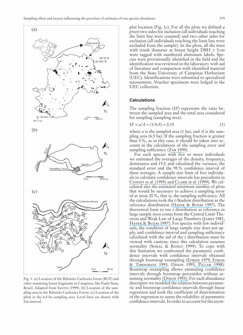
This work was carried out in the Ribeirão Cacho-eira forest, a 245-ha tropical forest fragment (22 º50’ S, 46 º55’ W, 630–760 m above sea level) in a region where forest cover was highly fragmented in Campi-nas municipality, São Paulo State, Southeast Brazil (Fig. 1a). The regional climate is Koeppen’s Cwa (Köppen 1948), with summer rains and mild win-ter. A warm-humid period of average temperature between 22 and 24 oC and 1057 mm rainfall extends from October to March, whereas a dry period from April to September presents average temperature be-tween 18 and 22 oC and 325 mm rainfall (Ortolani et al. 1995). The relief is mountainous, with 10–45 % slopes (Instituto Geológico 1993), and the soil is Red-Yellow Argisol (Prado 2003). The vegetation is seasonal semideciduous tropical forest, dominated by phanerophytes up to 30 m in height, and ca. 20–30 % of the highest trees shed their leaves in the dry season (Veloso 1992).

Methods

We did a previous reconnaissance with the aid of an aerial photograph in scale 1:25,000 and by walking in the forest, and selected a 6.5-ha homogeneous stand with uniform topography and phytophysiognomy in the southern portion of the fragment, at the left margin of the Cachoeira stream (Fig. 1b). We avoided abrupt topographic irregularities and the presence of large gaps in the forest. The stand selected had a cano-py height of 15–18 m, with isolated emergent trees up to 30 m high, and no indications of recent disturbanc-es. The sampling area is located on a slope of approxi-mately 270 m length with 40 m of difference between the altitudes of the lowest and highest points, and an average steepness of 15 %. In this area one hundred 10 m 10 m permanent plots were randomly located according with the unrestricted randomization tech-nique proposed by Greig-Smith (1983). In a map of the sampling area we used a system of coordinated axes to draw random number pairs corresponding to

eschweizerbartxxx ingenta

Sampling effort and factors infl uencing the precision of estimates of tree species abundance 379

plot location (Fig. 1c). For all the plots we defi ned apriori two sides for inclusion (all individuals touching the limit line were counted) and two other sides for exclusion (all individuals touching the limit line were excluded from the sample). In the plots, all the trees with trunk diameter at breast height DBH 5 cm were tagged with numbered aluminum labels. Spe-cies were provisionally identifi ed in the fi eld and the identifi cation was reviewed in the laboratory with aid of literature and comparison with identifi ed material from the State University of Campinas Herbarium (UEC). Identifi cations were submitted to specialized taxonomists. Voucher specimens were lodged in the UEC collection.

Calculations

The sampling fraction (SF) represents the ratio be-tween the sampled area and the total area considered for sampling (sampling area):

SF = a/A = (1/6.5) = 0.15 (1)

where a is the sampled area (1 ha), and A is the sam-pling area (6.5 ha). If the sampling fraction is greater than 5 %, as in this case, it should be taken into ac-count in the calculations of the sampling error and sampling suffi ciency (Zar 1999).

For each species with fi ve or more individuals we estimated the averages of the density, frequency, dominance and IVI; and calculated the variance, the standard error and the 95 % confi dence interval of these averages. A sample size limit of fi ve individu-als to calculate confi dence intervals has precedents in Condit et al. (1995) and Clark et al. (1999). We cal-culated also the estimated minimum number of plots that would be necessary to achieve a sampling error of at most 20 %, that is, the sampling suffi ciency. All the calculations took the t-Student distribution as the reference distribution (Hayek & Buzas 1997). The theoretical basis to use t distribution as reference in large sample sizes comes from the Central Limit The-orem and Weak Law of Large Numbers (James 1981, Hayek & Buzas 1997). For species with few individ-uals, the condition of large sample size does not ap-ply, and confi dence interval and sampling suffi ciency calculated with the aid of the t distribution must be viewed with caution, since this calculation assumes normality (Sokal & Rohlf 1999). To cope with this limitation we confronted the parametric confi -dence intervals with confi dence intervals obtained through bootstrap resampling (Efron 1979, Efron & Tibshirani 1993, Dixon 1993, Pillar 1998). Bootstrap resampling allows estimating confi dence intervals through bootstrap percentiles without as-suming normality (Dixon 1993). For each abundance descriptor we modeled the relation between paramet-ric and bootstrap confi dence intervals through linear regression and took the coeffi cient of determination of the regression to assess the reliability of parametric confi dence intervals. In order to account for the asym-

Fig. 1. (a) Location of the Ribeirão Cachoeira forest (RCF) and other remaining forest fragments in Campinas, São Paulo State, Brazil. Adapted from Santin (1999). (b) Location of the sam-pling area in the Ribeirão Cachoeira Forest. (c) Location of the plots in the 6.5-ha sampling area. Level lines are drawn with 5 m interval.

eschweizerbartxxx ingenta

380 R. Cielo-Filho et al.

metry of the bootstrap confi dence intervals (Dixon 1993) we performed the regression with both lower and upper limits. We calculated bootstrap percentiles confi dence intervals through 9,999 iterations for each species using the software Multiv (Pillar 2006).

The following formulas were used:

D = N/q (2)

DO = G/q (3)

where D is the species average density, N is the total number of individuals of the species; q is the number of plots; DO is the species average dominance; and G is the species total basal area in the sample. The standard error of both the species average density and dominance (S–

x) was calculated as:

S–x = [(s2/q)(1 – SF)]0.5 (4)

where s2 is the sample variance and SF is the sampling fraction (Zar 1999).

The estimated frequency of the species (FR) was given by:

FR = Y/q (5)

where Y is the number of plots in which the species occurs. Taking several random samples of plots with replacement from the same community, the number of plots in which a species occurs will have a binomial distribution (Greig-Smith 1983). This allows con-sidering FR obtained from a unique random sample as an estimate of the average of a population of FR values obtained from a large random sample set. As the variance of FR is estimated by FR(1 – FR)(q – 1) and is a variance of averages, it is possible to estimate FR standard error (SFR) through (Zar 1999):

SFR = [ FR(1 – FR)(q – 1) (1 – SF)]0.5

(6)

To calculate the IVI average and variance we used the method of fragmented relative values (Morais & Scheuber 1997), in which the IVI of each species in a plot is composed by the sum of the relative fragmented values of density, dominance and frequency of the species in this plot:

FRDk = (nk/TN) 100 (7)

FRDOk = (gk/TG) 100 (8)

FRFRk = (vk/TV) 100 (9)

FIVIk = FRDk + FRDOk + FRFRk (10)

where FRDk is the fragmented relative density of the species in the plot k, nk is the number of individuals of the species in the plot k, TN is the total number of individuals in the sample considering all the spe-cies, FRDOk is the fragmented relative dominance of the species in the plot k, gk is the species basal area in the plot k, TG is the total basal area in the sample considering all the species, FRFRk is the fragmented relative frequency of the species in the plot k, vk is the species presence or absence in the plot k (1 or 0,

respectively), TV is the sum of presences of all the species in all the plots, and FIVIk is the fragmented IVI of the species in the plot k. To calculate the aver-age, variance and the standard error of the FIVI, we did not use any transformation in order to avoid the infl uence of transformations upon the variance of the variables (Freeman & Tukey 1950, Mosteller & Youtz 1961). The average of the FIVI was calculated as:

FIVI =

q

k = 1 FIVIk

q (11)

where FIVI is the species average FIVI. To calculate the variance and standard error of FIVI, we followed the same procedure as for density and dominance.

Once obtained the standard error of the estimated averages for all abundance descriptors of a given spe-cies, we calculated the half range of confi dence inter-vals (Zar 1999). The sampling error of the estimate was obtained through the ratio of the half range of the confi dence interval to the average, expressed in percentage. The number of plots required to obtain a sampling error of at most 20 %, that is, the sampling suffi ciency, considering a sampling fraction smaller than 5 % (qest), was iteratively calculated as (Zar 1999):

qest = s2 t2(2)d.f./(0.2x)2 (12)

where x is the average value, and t (2)d.f. is the bilateral value of the t-Student distribution for an level of 0.05 and degrees of freedom (d.f.) initial value equal to q-1. The estimate of the number of plots necessary to yield a maximum sampling error of at most 20 %, with correction for a sampling fraction greater than 5 % (Qest), was calculated as (Zar 1999):

Qest = qest

1+(qest – 1)/Z (13)

where Z = sampling area/plot area ratio, that is, the number of plots that would fi ll in the whole sampling area. To calculate the general sampling error and sam-pling suffi ciency of the set of the most abundant spe-cies we used the arithmetic mean of the averages and variances of these species, and applied the same pro-cedure described above.

To evaluate the infl uence of the species spatial pat-tern on the sampling error of the estimates, we calcu-lated Morisita’s Ig aggregation index (Morisita 1971, Hurlbert 1990):

Ig = q q

k = 1 [nk(nk – 1)]/[N(N – 1)] (14)

Ig varies from less than one to q (number of plots); if greater than one, the spatial pattern is aggregated; if equal to one, the spatial pattern is random; and if smaller than one, the spatial pattern is regular (Greig-Smith 1983). We calculated Ig only for the species with more than one individual in at least one plot. The probability associated to the departures from randomness was verifi ed in a table of F for 0.05-

level, following Greig-Smith (1983).

eschweizerbartxxx ingenta

Sampling effort and factors infl uencing the precision of estimates of tree species abundance 381

For each abundance descriptor we calculated the Spearman correlation coeffi cient (rs) between the ag-gregation index of the species and the sampling er-ror of the descriptor estimate. The same correlation coeffi cient was calculated between the coeffi cient of variation (CV - ratio of the standard deviation to the mean) of the species basal area – on an individual ba-sis – and the sampling error of the estimates of domi-nance and IVI, in order to investigate the infl uence of size variation among individuals on the sampling error.

In order to compare the four abundance descrip-tors in relation to the precision of their estimates, we calculated for each descriptor the interquartile range – the distance between the fi rst and third quartiles – of the distribution of sampling errors among species (Zar 1999). These interquartile ranges were repre-sented through a box plot. The interquartile range was also calculated for the distributions of the species coeffi cients of variation of basal area and aggregation index among species, in order to assist in compari-sons between species.

Results

In the whole 1-ha sample we found 119 species in 1080 individuals. The 39 species with fi ve or more in-dividuals summed up 914 trees. Esenbeckia leiocarpa was the most abundant species considering the four abundance descriptors. The parametric and boot-strap confi dence intervals showed a good agreement, with coeffi cients of determination above 99 % for all abundance descriptors (Table 1). This confi rms the validity of using parametric confi dence intervals in our study.

Precision and sampling suffi ciency determined by different criteria

Density: Esenbeckia leiocarpa had the smallest sam-pling error (20 %), whereas Aegiphila sellowiana, the greatest (120 %). Sampling suffi ciency for these spe-cies would be obtained with 101 and 560 plots (15.6 % and 86.5 % of the sampling area), respectively (Table 2).

Frequency: Esenbeckia leiocarpa had the smallest sampling error (14 %), whereas Aegiphila sellowi-ana and Lonchocarpus muehlbergianus, the largest (90 %). It would be necessary 56 and 506 plots (8.6 %

and 78 % of the sampling area), respectively, to reach sampling suffi ciency for these species (Table 2).

Dominance: The smallest sampling error was ob-tained for Esenbeckia leiocarpa (26 %) and the largest for Lonchocarpus muehlbergianus (172 %). Sampling suffi ciency for these species would require 153 and 602 plots (23.6 % and 93 % of the sampling area), re-spectively (Table 3).

IVI: Esenbeckia leiocarpa had the smallest sampling error (20 %) and Lonchocarpus muehlbergianus, the largest (121 %). Sampling suffi ciency for these specieswould be obtained with 97 and 561 plots (15 % and 86 % of the sampling area), respectively (Table 3).

With the actual sampling effort used (100 plots, 10 m x 10 m each), the only species for which sam-pling suffi ciency was attained was Esenbeckia leio-carpa, with sampling errors of about 20 % for den-sity and IVI and 14 % for frequency. No species was suffi ciently sampled for dominance, and this was the descriptor with the largest sampling error for all the species.

Only Esenbeckia leiocarpa had confi dence inter-vals that did not overlap with those of other species for density, frequency, dominance, and IVI. Follow-ing this species, Savia dictyocarpa, Astronium gra-veolens and Aspidosperma polyneuron occupied the fi rst four positions in the abundance rank of all the abundance descriptors. The species occupying lower positions of the abundance rank varied depending on the descriptor considered. Because of this, we consid-ered those four species to assess sampling suffi ciency through the criterion of the general sampling error of a set of the most abundant species. The application of this criterion to other data might also be based on the consistence of the position of the most abundant spe-cies across the abundance rank of different descrip-tors. By applying this criterion, we obtained a gen-eral sampling error of 26.2 % for density, 20.0 % for frequency, 44.7 % for dominance and 27.5 % for IVI. So, it would be necessary to sample 24 % of the sam-pling area (153 plots) to reach sampling suffi ciency for density, 15 % (101 plots) for frequency, 47 % (306 plots) for dominance and 25 % (165 plots) for IVI.

Factors infl uencing the precision of abundance descriptor estimates

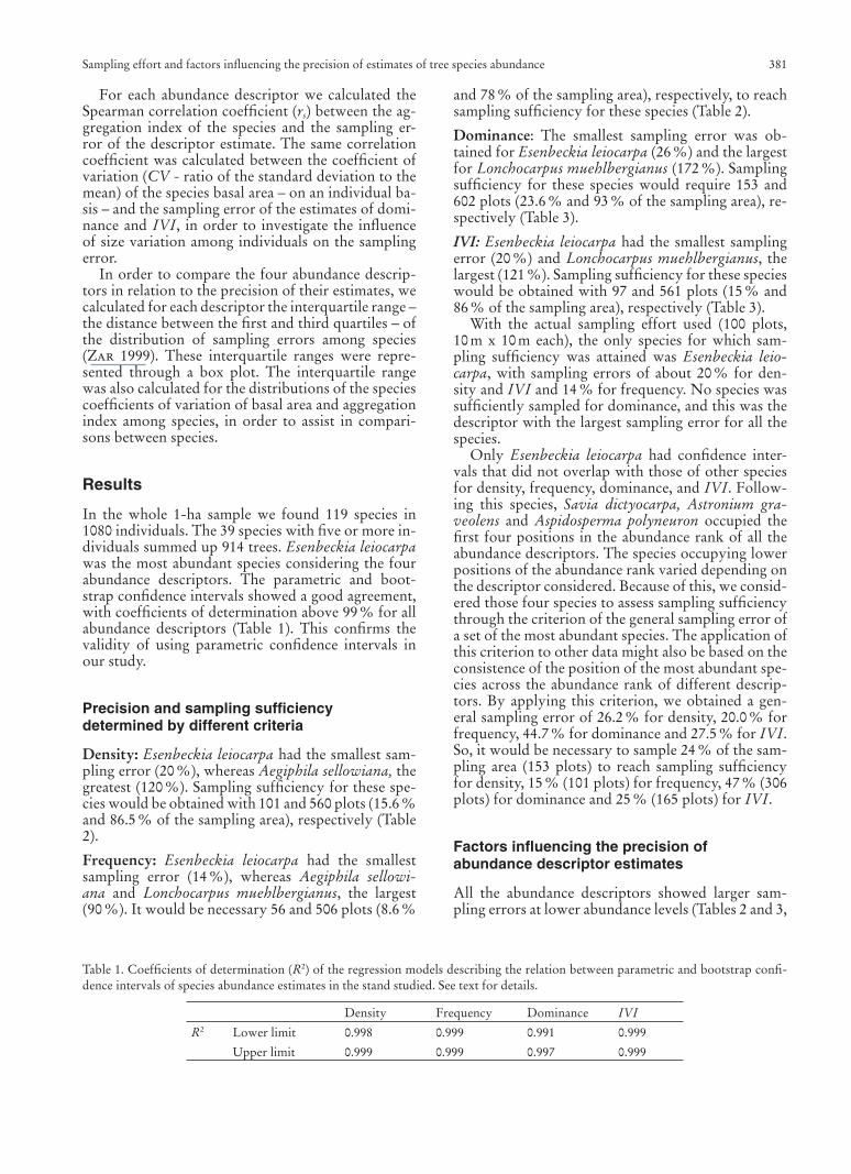
All the abundance descriptors showed larger sam-pling errors at lower abundance levels (Tables 2 and 3,

Table 1. Coeffi cients of determination (R2) of the regression models describing the relation between parametric and bootstrap confi -dence intervals of species abundance estimates in the stand studied. See text for details.

Density Frequency Dominance IVI

R2 Lower limit 0.998 0.999 0.991 0.999

Upper limit 0.999 0.999 0.997 0.999

eschweizerbartxxx ingenta

382 R. Cielo-Filho et al.

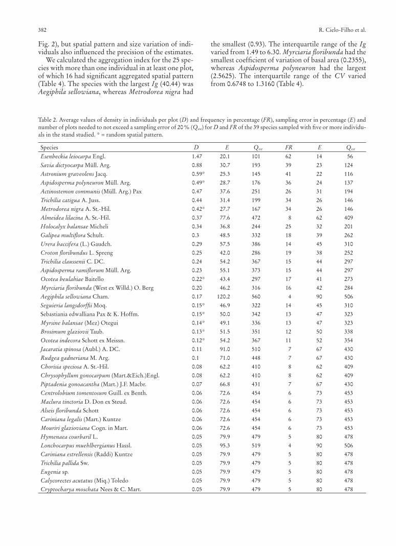
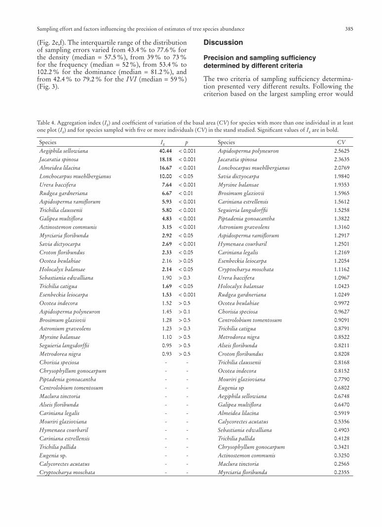
Fig. 2), but spatial pattern and size variation of indi-viduals also infl uenced the precision of the estimates.

We calculated the aggregation index for the 25 spe-cies with more than one individual in at least one plot, of which 16 had signifi cant aggregated spatial pattern (Table 4). The species with the largest Ig (40.44) was Aegiphila sellowiana, whereas Metrodorea nigra had

the smallest (0.93). The interquartile range of the Ig varied from 1.49 to 6.30. Myrciaria fl oribunda had the smallest coeffi cient of variation of basal area (0.2355), whereas Aspidosperma polyneuron had the largest (2.5625). The interquartile range of the CV varied from 0.6748 to 1.3160 (Table 4).

Table 2. Average values of density in individuals per plot (D) and frequency in percentage (FR), sampling error in percentage (E) and number of plots needed to not exceed a sampling error of 20 % (Qest) for D and FR of the 39 species sampled with fi ve or more individu-als in the stand studied. * = random spatial pattern.

Species D E Qest FR E Qest

Esenbeckia leiocarpa Engl. 1.47 20.1 101 62 14 56

Savia dictyocarpa Müll. Arg. 0.88 30.7 193 39 23 124

Astronium graveolens Jacq. 0.59* 25.3 145 41 22 116

Aspidosperma polyneuron Müll. Arg. 0.49* 28.7 176 36 24 137

Actinostemon communis (Müll. Arg.) Pax 0.47 37.6 251 26 31 194

Trichilia catigua A. Juss. 0.44 31.4 199 34 26 146

Metrodorea nigra A. St.-Hil. 0.42* 27.7 167 34 26 146

Almeidea lilacina A. St.-Hil. 0.37 77.6 472 8 62 409

Holocalyx balansae Micheli 0.34 36.8 244 25 32 201

Galipea multifl ora Schult. 0.3 48.5 332 18 39 262

Urera baccifera (L.) Gaudch. 0.29 57.5 386 14 45 310

Croton fl oribundus L. Spreng 0.25 42.0 286 19 38 252

Trichilia claussenii C. DC. 0.24 54.2 367 15 44 297

Aspidosperma ramifl orum Müll. Arg. 0.23 55.1 373 15 44 297

Ocotea beulahiae Baitello 0.22* 43.4 297 17 41 273

Myrciaria fl oribunda (West ex Willd.) O. Berg 0.20 46.2 316 16 42 284

Aegiphila sellowiana Cham. 0.17 120.2 560 4 90 506

Seguieria langsdorffi i Moq. 0.15* 46.9 322 14 45 310Sebastiania edwalliana Pax & K. Hoffm. 0.15* 50.0 342 13 47 323Myrsine balansae (Mez) Otegui 0.14* 49.1 336 13 47 323

Brosimum glaziovii Taub. 0.13* 51.5 351 12 50 338

Ocotea indecora Schott ex Meissn. 0.12* 54.2 367 11 52 354

Jacaratia spinosa (Aubl.) A. DC. 0.11 91.0 510 7 67 430

Rudgea gadneriana M. Arg. 0.1 71.0 448 7 67 430

Chorisia speciosa A. St.-Hil. 0.08 62.2 410 8 62 409

Chrysophyllum gonocarpum (Mart.&Eich.)Engl. 0.08 62.2 410 8 62 409

Piptadenia gonoacantha (Mart.) J.F. Macbr. 0.07 66.8 431 7 67 430

Centrolobium tomentosum Guill. ex Benth. 0.06 72.6 454 6 73 453

Maclura tinctoria D. Don ex Steud. 0.06 72.6 454 6 73 453

Alseis fl oribunda Schott 0.06 72.6 454 6 73 453

Cariniana legalis (Mart.) Kuntze 0.06 72.6 454 6 73 453

Mouriri glazioviana Cogn. in Mart. 0.06 72.6 454 6 73 453

Hymenaea courbaril L. 0.05 79.9 479 5 80 478

Lonchocarpus muehlbergianus Hassl. 0.05 95.3 519 4 90 506

Cariniana estrellensis (Raddi) Kuntze 0.05 79.9 479 5 80 478

Trichilia pallida Sw. 0.05 79.9 479 5 80 478

Eugenia sp. 0.05 79.9 479 5 80 478

Calycorectes acutatus (Miq.) Toledo 0.05 79.9 479 5 80 478

Cryptocharya moschata Nees & C. Mart. 0.05 79.9 479 5 80 478

eschweizerbartxxx ingenta

Sampling effort and factors infl uencing the precision of estimates of tree species abundance 383

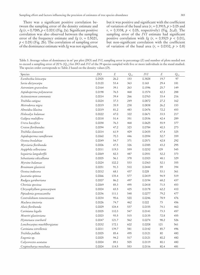
There was a signifi cant positive correlation be-tween the sampling error of the density estimate and Ig (rs = 0.7085, p < 0.001) (Fig. 2a). Signifi cant positive correlation was also observed between the sampling error of the frequency estimate and Ig (rs = 0.5021, p < 0.05) (Fig. 2b). The correlation of sampling error of the dominance estimate with Ig was not signifi cant,

but it was positive and signifi cant with the coeffi cient of variation of the basal area (rs = 0.3915, p > 0.05 and rs = 0.3338, p < 0.05, respectively) (Fig. 2c,d). The sampling error of the IVI estimate had signifi cant positive correlation with Ig (rs = 0.5523 p < 0.01), but non-signifi cant correlation with the coeffi cient of variation of the basal area (rs = 0.0332, p > 0.8)

Table 3. Average values of dominance in m2 per plot (DO) and IVI, sampling error in percentage (E) and number of plots needed not to exceed a sampling error of 20 % (Qest) for DO and IVI of the 39 species sampled with fi ve or more individuals in the stand studied. The species order corresponds to Table 2 based on the density values (D).

Species DO E Qest IVI E Qest

Esenbeckia leiocarpa 0.0505 26.2 153 0.3828 19.7 97

Savia dictyocarpa 0.0120 53.4 363 0.165 29.4 181

Astronium graveolens 0.0164 39.1 263 0.1596 25.7 149

Aspidosperma polyneuron 0.0198 76.5 468 0.1574 42.3 288

Actinostemon communis 0.0014 39.4 266 0.0763 33.4 216

Trichilia catigua 0.0024 37.3 249 0.0872 27.2 162

Metrodorea nigra 0.0019 35.9 238 0.0838 26.2 153

Almeidea lilacina 0.0019 81.2 483 0.0476 72.2 453

Holocalyx balansae 0.0022 47.0 322 0.0671 33.5 217

Galipea multifl ora 0.0018 51.4 351 0.0536 42.4 289

Urera baccifera 0.0058 76.3 468 0.0625 55.9 377

Croton fl oribundus 0.0094 47.2 323 0.0784 40.3 273

Trichilia claussenii 0.0014 61.9 409 0.0435 47.4 325

Aspidosperma ramifl orum 0.0060 70.3 446 0.0594 52.7 359

Ocotea beulahiae 0.0049 54.7 371 0.0571 42.8 292

Myrciaria fl oribunda 0.0006 47.5 326 0.0385 43.2 295

Aegiphila sellowiana 0.0011 119.3 559 0.0232 109 545

Seguieria langsdorffi i 0.0069 82.3 487 0.0551 52.2 373

Sebastiania edwalliana 0.0005 56.1 378 0.0303 48.1 329

Myrsine balansae 0.0024 102.2 533 0.0363 52.1 355

Brosimum glaziovii 0.0051 91.3 510 0.0444 59 394

Ocotea indecora 0.0012 68.1 437 0.028 53.1 361

Jacaratia spinosa 0.0066 135.4 577 0.0419 94.9 519

Rudgea gardneriana 0.0007 86.2 497 0.0194 68.2 437

Chorisia speciosa 0.0069 85.3 495 0.0418 71.5 453

Chrysophyllum gonocarpum 0.0004 65.5 425 0.0178 62.2 410

Piptadenia gonoacantha 0.0036 111.1 548 0.0277 79.2 477

Centrolobium tomentosum 0.0034 95.6 520 0.0246 78.9 476

Maclura tinctoria 0.0026 74.7 462 0.022 73 456

Alseis fl oribunda 0.0009 104.4 537 0.0155 74.1 460

Cariniana legalis 0.0005 110.3 547 0.0141 73.3 457

Mouriri glazioviana 0.0003 93.5 515 0.0135 72.8 455

Hymenaea courbaril 0.0047 121.7 562 0.0274 98.2 526

Lonchocarpus muehlbergianus 0.0032 172.1 602 0.0208 121 561

Cariniana estrellensis 0.0011 139.7 581 0.0142 85.7 496

Trichilia pallida 0.0005 85.4 495 0.0121 80 480

Eugenia sp. 0.0005 94.2 517 0.0121 80.2 480

Calycorectes acutatus 0.0004 89.1 505 0.0119 80.1 480

Cryptocharya moschata 0.0004 114.5 553 0.0116 80.4 481

eschweizerbartxxx ingenta

384 R. Cielo-Filho et al.

Fig. 2. Dependency of the sampling error of the species abundance estimates on the number of individuals, aggregation index (Ig) and coeffi cient of variation of basal area (CV). Values of Ig and CV are proportional to the size of the symbols.

eschweizerbartxxx ingenta

Sampling effort and factors infl uencing the precision of estimates of tree species abundance 385

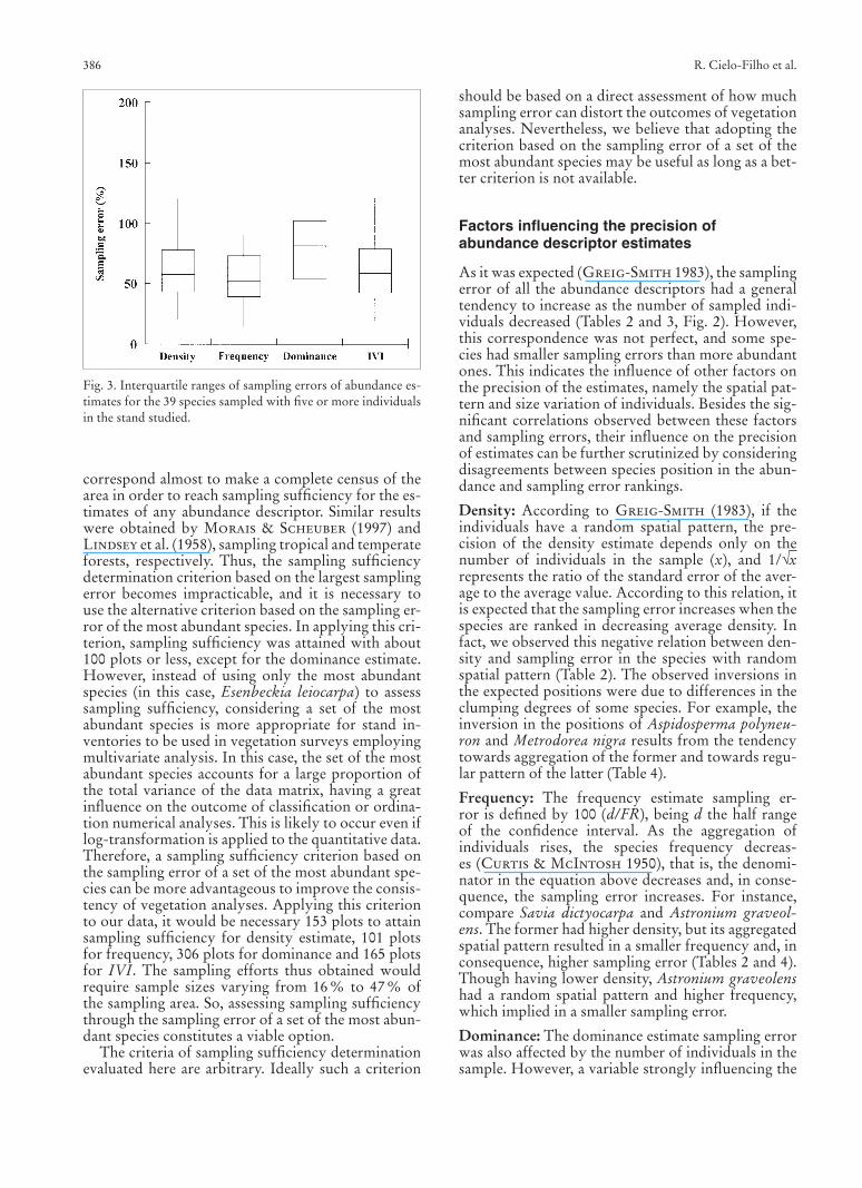
(Fig. 2e,f). The interquartile range of the distribution of sampling errors varied from 43.4 % to 77.6 % for the density (median = 57.5 %), from 39 % to 73 % for the frequency (median = 52 %), from 53.4 % to 102.2 % for the dominance (median = 81.2 %), and from 42.4 % to 79.2 % for the IVI (median = 59 %) (Fig. 3).

Discussion

Precision and sampling suffi ciency determined by different criteria

The two criteria of sampling suffi ciency determina-tion presented very different results. Following the criterion based on the largest sampling error would

Table 4. Aggregation index (Ig) and coeffi cient of variation of the basal area (CV) for species with more than one individual in at least one plot (Ig) and for species sampled with fi ve or more individuals (CV) in the stand studied. Signifi cant values of Ig are in bold.

Species Ig p Species CV

Aegiphila sellowiana 40.44 < 0.001 Aspidosperma polyneuron 2.5625

Jacaratia spinosa 18.18 < 0.001 Jacaratia spinosa 2.3635

Almeidea lilacina 16.67 < 0.001 Lonchocarpus muehlbergianus 2.0769

Lonchocarpus muehlbergianus 10.00 < 0.05 Savia dictyocarpa 1.9840

Urera baccifera 7.64 < 0.001 Myrsine balansae 1.9353

Rudgea gardneriana 6.67 < 0.01 Brosimum glaziovii 1.5965

Aspidosperma ramifl orum 5.93 < 0.001 Cariniana estrellensis 1.5612

Trichilia claussenii 5.80 < 0.001 Seguieria langsdorffi i 1.5258

Galipea multifl ora 4.83 < 0.001 Piptadenia gonoacantha 1.3822

Actinostemon communis 3.15 < 0.001 Astronium graveolens 1.3160

Myrciaria fl oribunda 2.92 < 0.05 Aspidosperma ramifl orum 1.2917

Savia dictyocarpa 2.69 < 0.001 Hymenaea courbaril 1.2501

Croton fl oribundus 2.33 < 0.05 Cariniana legalis 1.2169

Ocotea beulahiae 2.16 > 0.05 Esenbeckia leiocarpa 1.2054

Holocalyx balansae 2.14 < 0.05 Cryptocharya moschata 1.1162

Sebastiania edwalliana 1.90 > 0.3 Urera baccifera 1.0967

Trichilia catigua 1.69 < 0.05 Holocalyx balansae 1.0423

Esenbeckia leiocarpa 1.53 < 0.001 Rudgea gardneriana 1.0249

Ocotea indecora 1.52 > 0.5 Ocotea beulahiae 0.9972

Aspidosperma polyneuron 1.45 > 0.1 Chorisia speciosa 0.9627

Brosimum glaziovii 1.28 > 0.5 Centrolobium tomentosum 0.9091

Astronium graveolens 1.23 > 0.3 Trichilia catigua 0.8791

Myrsine balansae 1.10 > 0.5 Metrodorea nigra 0.8522

Seguieria langsdorffi i 0.95 > 0.5 Alseis fl oribunda 0.8211

Metrodorea nigra 0.93 > 0.5 Croton fl oribundus 0.8208

Chorisia speciosa - - Trichilia claussenii 0.8168

Chrysophyllum gonocarpum - - Ocotea indecora 0.8152

Piptadenia gonoacantha - - Mouriri glazioviana 0.7790

Centrolobium tomentosum - - Eugenia sp 0.6802

Maclura tinctoria - - Aegiphila sellowiana 0.6748

Alseis fl oribunda - - Galipea multifl ora 0.6470

Cariniana legalis - - Almeidea lilacina 0.5919

Mouriri glazioviana - - Calycorectes acutatus 0.5356

Hymenaea courbaril - - Sebastiania edwalliana 0.4903

Cariniana estrellensis - - Trichilia pallida 0.4128

Trichilia pallida - - Chrysophyllum gonocarpum 0.3421

Eugenia sp. - - Actinostemon communis 0.3250

Calycorectes acutatus - - Maclura tinctoria 0.2565

Cryptocharya moschata - - Myrciaria fl oribunda 0.2355

eschweizerbartxxx ingenta

386 R. Cielo-Filho et al.

correspond almost to make a complete census of the area in order to reach sampling suffi ciency for the es-timates of any abundance descriptor. Similar results were obtained by Morais & Scheuber (1997) and Lindsey et al. (1958), sampling tropical and temperate forests, respectively. Thus, the sampling suffi ciency determination criterion based on the largest sampling error becomes impracticable, and it is necessary to use the alternative criterion based on the sampling er-ror of the most abundant species. In applying this cri-terion, sampling suffi ciency was attained with about 100 plots or less, except for the dominance estimate. However, instead of using only the most abundant species (in this case, Esenbeckia leiocarpa) to assess sampling suffi ciency, considering a set of the most abundant species is more appropriate for stand in-ventories to be used in vegetation surveys employing multivariate analysis. In this case, the set of the most abundant species accounts for a large proportion of the total variance of the data matrix, having a great infl uence on the outcome of classifi cation or ordina-tion numerical analyses. This is likely to occur even if log-transformation is applied to the quantitative data. Therefore, a sampling suffi ciency criterion based on the sampling error of a set of the most abundant spe-cies can be more advantageous to improve the consis-tency of vegetation analyses. Applying this criterion to our data, it would be necessary 153 plots to attain sampling suffi ciency for density estimate, 101 plots for frequency, 306 plots for dominance and 165 plots for IVI. The sampling efforts thus obtained would require sample sizes varying from 16 % to 47 % of the sampling area. So, assessing sampling suffi ciency through the sampling error of a set of the most abun-dant species constitutes a viable option.

The criteria of sampling suffi ciency determination evaluated here are arbitrary. Ideally such a criterion

should be based on a direct assessment of how much sampling error can distort the outcomes of vegetation analyses. Nevertheless, we believe that adopting the criterion based on the sampling error of a set of the most abundant species may be useful as long as a bet-ter criterion is not available.

Factors infl uencing the precision of abundance descriptor estimates

As it was expected (Greig-Smith 1983), the sampling error of all the abundance descriptors had a general tendency to increase as the number of sampled indi-viduals decreased (Tables 2 and 3, Fig. 2). However, this correspondence was not perfect, and some spe-cies had smaller sampling errors than more abundant ones. This indicates the infl uence of other factors on the precision of the estimates, namely the spatial pat-tern and size variation of individuals. Besides the sig-nifi cant correlations observed between these factors and sampling errors, their infl uence on the precision of estimates can be further scrutinized by considering disagreements between species position in the abun-dance and sampling error rankings.

Density: According to Greig-Smith (1983), if the individuals have a random spatial pattern, the pre-cision of the density estimate depends only on the number of individuals in the sample (x), and 1/ x represents the ratio of the standard error of the aver-age to the average value. According to this relation, it is expected that the sampling error increases when the species are ranked in decreasing average density. In fact, we observed this negative relation between den-sity and sampling error in the species with random spatial pattern (Table 2). The observed inversions in the expected positions were due to differences in the clumping degrees of some species. For example, the inversion in the positions of Aspidosperma polyneu-ron and Metrodorea nigra results from the tendency towards aggregation of the former and towards regu-lar pattern of the latter (Table 4).

Frequency: The frequency estimate sampling er-ror is defi ned by 100 (d/FR), being d the half range of the confi dence interval. As the aggregation of individuals rises, the species frequency decreas-es (Curtis & McIntosh 1950), that is, the denomi-nator in the equation above decreases and, in conse-quence, the sampling error increases. For instance, compare Savia dictyocarpa and Astronium graveol-ens. The former had higher density, but its aggregated spatial pattern resulted in a smaller frequency and, in consequence, higher sampling error (Tables 2 and 4). Though having lower density, Astronium graveolens had a random spatial pattern and higher frequency, which implied in a smaller sampling error.

Dominance: The dominance estimate sampling error was also affected by the number of individuals in the sample. However, a variable strongly infl uencing the

Fig. 3. Interquartile ranges of sampling errors of abundance es-timates for the 39 species sampled with fi ve or more individuals in the stand studied.

eschweizerbartxxx ingenta

Sampling effort and factors infl uencing the precision of estimates of tree species abundance 387

dominance sampling error was the variation of the individual size, which implied a variation of the basal area among the plots. The variation of the individual size does not directly affect the precision of density or frequency estimates, but sometimes it alone infl u-ences the sampling error of the dominance, some-times it strengths the effect of the aggregated spatial pattern. For example, the basal area of Aspidospermapolyneuron had the largest coeffi cient of variation and, although having a random spatial pattern, the sampling error was greater than that of Actinostemoncommunis, with similar number of individuals in the sample, signifi cantly aggregated spatial pattern, but lower coeffi cient of variation of the basal area (Tables 3 and 4). On the other hand, species with a high aggregation index and highly variable basal areas, such as Jacaratia spinosa and Lonchocarpus muehl-bergianus, also had the largest dominance estimate sampling errors. This suggests a synergic effect of aggregation and basal area variation on the sampling error of the dominance estimates.

IVI: As it is the sum of the relative values of density, frequency and dominance, the IVI estimate should have its precision affected by the same variables af-fecting these descriptors. However, only the number of individuals in the sample and their spatial pattern affected the IVI estimate precision. Thus, when the species are ranked in order of decreasing density, there is a tendency towards increasing sampling error of the IVI. Moreover, species with low basal area variation but high aggregation index, such as Almeidea lilacina and Aegiphila sellowiana, had greater sampling error than species with similar number of individuals in the sample, greater basal area variation, but smaller ag-gregation index (Tables 3 and 4). This confi rms the prevalent effect of the spatial aggregation on the sam-pling error of IVI estimates.

The sampling error of all the abundance descrip-tors is, therefore, infl uenced by the number of in-dividuals in the sample. The estimate of the density, frequency and IVI was additionally infl uenced by the spatial aggregation, whereas the dominance estimate was mainly infl uenced by the variation of basal area. In fact, in the presence of spatial autocorrelation, sam-pling methods in general, including the multiple plots sampling method, perform poorly (Goslee 2006). We found that the descriptor with the greatest preci-sion was the frequency, followed by density (Fig. 3). On the other hand, the dominance estimate had the smallest precision (Fig. 3). Similar results were ob-tained by Lindsey et al. (1958), thus demonstrating the inadequacy of the multiple plot sampling method to estimate dominance.

Almost 50 % of the species had smaller IVI sam-pling errors than those of density and dominance, and the distribution of sampling errors of IVI esti-mates showed a median and interquartile range simi-lar to those of density and much smaller values than those of dominance. That was an unexpected result, since IVI is a combination of the two latter descrip-

tors plus frequency, and so should be infl uenced by a greater number of factors and should present a lower precision in its estimates. Moreover, as mentioned above, the estimation of IVI is not affected by size variation among individuals. These two related fi nd-ings can be interpreted as a result of the interaction of single error terms in the sum that gives rise to the IVI. As the relative values of the three components of the IVI (density, frequency and dominance) are rarely entirely correlated, the sampling error of the sum of these components is smaller than each of the individ-ual sampling errors of the summands. This property of the IVI makes its use advantageous from the pre-cision viewpoint when inventorying stands through the multiple plots sampling method. Moreover, the synthetic nature of IVI – which allows encompass-ing three different aspects of the abundance into a unique fi gure – can enhance the describing appeal of the IVI. The use of IVI, however, can mask variations in the individual parameters (Daubenmire 1968, Martins 1993), which may lead to the establishment of misleading fl oristic-structural relationships among stands, thus precluding correct ecological interpre-tations in vegetation surveys. We suggest, therefore, that the use of frequency and density along with IVI should always be assessed when data of stand inven-tories are handled, through multivariate numerical techniques, for the purpose of vegetation surveys.

Acknowledgements: We thank Conselho Nacional de Desen-volvimento Científi co e Tecnológico – CNPq for the grants for the fi rst author; Valério De Patta Pillar, John Du Vall Hay, Miguel Petrere Junior and Kikyo Yamamoto for suggestions on the earlier version of the manuscript; and Eunice Reis Batista and Fabiano Chiste for fi eld assistance.

References

Bellehumeur, C., Legendre, P. & Marcotte, D. (1997): Variance and spatial scales in a tropical rain forest: changing the size of sampling units. – Plant Ecology 130:89–98.

Bormann, F.H. (1953): The statistical effi ciency of sample plot size and shape in forest ecology. – Ecology 34: 474–487.

Caiafa, A.N. & Martins, F.R. (2007): Taxonomic identifi cation, sampling methods, and minimum size of the tree sampled: implications and perspectives for studies in the Brazilian At-lantic Rainforest. – Functional Ecosystems and Communi-ties 1: 95–104.

Chave, J., Condit, R., Aguilar, S., Hernandez, A., Lao, S. & Per-ez, R. (2004): Error propagation and scaling for tropical forest biomass estimates. – Phil. Trans. R. Soc. Lond. 359: 409–420.

Clark, D.B. & Clark, D.A. (2000): Landscape-scale variation in forest structure and biomass in a tropical rain forest. – Forest Ecology and Management 137: 185–198.

Clark, D.B., Palmer, M.W. & Clark, D.A. (1999): Edaphic fac-tors and the landscape-scale distributions of tropical rain forest trees. – Ecology 80: 2662–2675.

Condit, R. (1998): Tropical forest census plots: methods and re-sults from Barro Colorado Island, Panama and a comparison with other plots. – Springer-Verlag, Berlin.

eschweizerbartxxx ingenta

388 R. Cielo-Filho et al.

Condit, R., Hubbell, S.P. & Foster, R.B. (1995): Mortality rates of 205 neotropical tree and shrub species and the impact of a severe drought. – Ecological Monographs 65: 419–439.

Curtis, J.T. & Mcintosh, R.P. (1950): The interelations of certain analytic and synthetic phytosociological characters. – Ecol-ogy 31: 434–455.

Daubenmire, R.F. (1968): Plant communities: a text book of plant synecology. – Harper and How, New York.

Dixon, P.M. (1993): The bootstrap and the jackknife: describ-ing the precision of ecological indices. – In: S.M. Schein-er & J. Gurevitch (eds.): Design and analysis of ecological experiments, pp. 290–318. – Chapman and Hall, New York.

Efron, B. (1979): Bootstrap methods: another look at the jack-knife. – The Annals of Statistics 7: 1–25.

Efron, B. & Tibshirani, R. (1993): An introduction to the boot-strap. – Chapman and Hall, London.

Freeman, M.F. & Tukey, J.W. (1950): Transformations related to the angular and square root. – Ann. Math. Statist. 21: 607–611.

Gauch, H.G. (1982): Multivariate analysis in community ecol-ogy. – Cambridge University Press, Cambridge.

Goslee, S.C. (2006): Behavior of vegetation sampling methods in the presence of spatial autocorrelation. – Plant Ecology 187: 203–212.

Green, J.L. & Plotkin, J.B. (2007): A statistical theory for sam-pling species abundances. – Ecology Letters 10: 1037–1045.

Greig-Smith, P. (1983): Quantitative plant ecology. – Blackwell, Oxford.

Hayek, L.A.C. & Buzas, M.A. (1997): Surveying natural popu-lations. – Columbia University Press, New York.

Hurlbert, S.H. (1990): Spatial distribution of the montane uni-corn. – Oikos 58: 257–271.

Instituto Geológico (1993): Subsídios do meio físico e geológico ao planejamento do município de Campinas. – Secretaria de Planejamento e Meio Ambiente, Prefeitura Municipal de Campinas, Campinas.

James, B.R. (1981): Probabilidade: um curso em nível inter-mediário. – Projeto Euclides, IMPA, Rio de Janeiro.

Kenkel, N.C., Juhász-Nagy, P. & Podani, J. (1989): On sam-pling procedures in population and community ecology – Vegetatio 83: 195–207.

Köppen, W.P. (1948): Climatologia: con un estudio de los climas de la tierra. – Fondo de Cultura Economica, Mexico.

Laurance, W.F. & Bierregaard, R.O. (1997): Tropical forest rem-nants: ecology, management, and conservation of fragmented communities. – The University of Chicago Press, Chicago.

Lindsey, A.A., Barton, J.D. & Miles, R. (1958): Field effi ciency of forest sampling methods. – Ecology 39: 428–444.

Martins, F.R. (1993): Estrutura de uma Floresta Mesófi la. – Edi-tora da Universidade Estadual de Campinas, Campinas.

Mosteller, F. & Youtz, C. (1961): Tables of the Freeman-Tukey transformations for the binomial and Poisson distribu-tions. – Biometrika 48: 433–440.

Morais, R. & Scheuber, M. (1997): Statistical precision in phy-tosociological surveys. – In: J. Imaña-Encinas & C. Kleinn (eds.): Assessment and monitoring of forests in tropical dry regions with special reference to gallery forests, pp. 135–145. – University of Brasilia, Brasilia.

Morisita, M. (1971): Composition of the Ig index. – Res. Pop. Ecol. 13: 1–27.

Mueller-Dombois, D. & Ellenberg, H. (1974): Aims and meth-ods of vegetation ecology. – John Wiley and Sons, New York.

Ortolani, A.A., Camargo, M.B.P. & Pedro-Junior, M.J. (1995): Normais climatológicas dos postos meteorológicos do Insti-tuto Agronômico: 1. Centro Experimental de Campinas. – Campinas Agronomic Institute technical bulletin No. 155, Campinas.

Pillar, V.D. (1998): Sampling suffi ciency in ecological surveys. – Abstr. Bot. 22: 37–48.

– (1999a): How sharp are classifi cations? – Ecology 80: 2508–2516.

– (1999b): The bootstrapped ordination re-examined. – J. Veg. Sci. 10: 895–902.

– (2004): Sufi ciência amostral. – In: C.E. de M. Bicudo, & D. de C. Bicudo (eds.): Amostragem em Limnologia, pp. 25–43. – RiMa Editora, São Carlos.

– (2006): Multiv: multivariate exploratory analyses, random-ization testing and bootstrap resampling. User’s Guide v. 2.4. – Universidade Federal do Rio Grande do Sul, Porto Alegre.

Prado, H. (2003): Solos do Brasil: gênese, morfologia, classifi -cação, levantamento, manejo agrícola e geotécnico. Author’s publishing, Piracicaba.

Santin, D.A. (1999): A Vegetação remanescente do município de Campinas (SP): mapeamento, caracterização fi sionômica e fl orística, visando a conservação. – Doctorate thesis, Depart-ment of Botany, Campinas State University, Campinas.

Schelhas, J. & Greenberg, R. (1996): Forest patches in tropical landscapes. – Island Press, Washington.

Sokal, R.R. & Rohlf F.J. (1999): Biometry: The principles and practice of statistics in biological research. – W. H. Freeman, New York.

Veloso, H.P. (1992): Sistema fi togeográfi co. – In: IBGE: Manual técnico da vegetação brasileira, pp. 9–38. – Instituto Brasil-eiro de Geografi a e Estatística, Rio de Janeiro.

Vieira, M.G.L. & Couto, H.T.Z. (2001): Estudo do tamanho e número de parcelas na Floresta Atlântica do Parque Estadual de Carlos Botelho, SP. – Scientia Forestalis 60: 11–20.

Wade, T.G., Riitters, K.H., Wickham, J.D. & Jones, K.B. (2003): Distribution and causes of global forest fragmentation. – Conservation Ecology 7: 7. (online) URL: http://www.con-secol.org/vol7/iss2/art7

Zar, J.H. (1999): Biostatistical analysis. – Prentice Hall, New Jersey.

Addresses of the authors:Dr. Roque Cielo-Filho Plant Biology Graduate Course, Inst. of Biology, P.O. Box 6109, University of Campinas – UNI-CAMP, 13083–970 Campinas, SP, BrazilCurrent address: Forest Institute, Caixa postal 1322, São Paulo 02377–000, SP, Brazil.Dr. Mario Antonio Gneri, Dep. of Statistics, Inst. of Mathemat-ics, Statistics and Computer Science, P.O. Box 6065, University of Campinas – UNICAMP, 13083–970 Campinas, SP, Brazil.Dr. Fernando Roberto Martins*, Dep. of Botany, Inst. of Bi-ology, P.O. Box 6109, University of Campinas – UNICAMP, 13083–970 Campinas, SP, Brazil.*Author for correspondence, e-mail: fmartins@unicamp.br

eschweizerbartxxx ingenta