i

Rural Credit Markets in Assam- A Study of Lower Brahmaputra Valley

A Dissertation Submitted to the Sikkim University (A Central University)

in Partial Fulfillment of the Requirements for the Award of the Degree of

DOCTOR OF PHILOSOPHY

IN

ECONOMICS

BY

TIKEN DAS

DEPARTMENT OF ECONOMICS

SCHOOL OF SOCIAL SCIENCES

SIKKIM UNIVERSITY (A CENTRAL UNIVERSITY)

GANGTOK-737102

November 2016

ii

DEDICATED

TO

ALL UNDERPRIVILEGED RURAL

BORROWERS

iii

Department of Economics Date: School of Social Sciences Sikkim University 6th Mile, Tadong, Gangtok Sikkim- 737102

CERTIFICATE This is to certify that Tiken Das has carried out the PhD work embodied in the present

dissertation entitled, “Rural Credit Markets in Assam- A Study of Lower Brahmaputra

Valley ” for the partial fulfillment of the degree of the Doctor of Philosophy in Economics under

my supervision. I declare to the best of my knowledge that no part of this dissertation was earlier

submitted for any other degree, diploma, associate-ship and fellowship. All the assistance and

help received during the course of the investigation have been duly acknowledged by him.

Dr. Komol Singha Dr. Manesh Choubey

HEAD SUPERVISOR

Department of Economics Department of Economics

iv

DECLARATION

I, Tiken Das, hereby declare that the research embodied in this dissertation entitled, “Rural

Credit Markets in Assam- A Study of Lower Brahmaputra Valley” is carried out by me

under the supervision of Dr. Manesh Choubey, Associate Professor, Department of

Economics, in partial fulfillment of the requirement for the award of the Doctor of Philosophy in

Economics from the Sikkim University.

I declare to the best of my knowledge that no part of this dissertation was earlier submitted for

the award of any other degree of this university or any other university.

Date: (TIKEN DAS)

Place: Roll No. 13PDEC02

Registration No. 13/Ph.D/ECN/02

v

Acknowledgements

I am especially indebted to my supervisor Dr. Manesh Choubey for his support and

valuable comments during my study period. Particularly, I am much grateful to him for giving

me scholarly freedom to explore ideas as per my interest. In addition, I am greatly thankful to

Dr. Pradyut Guha for his all kinds of support throughout my doctoral candidature.

I am thankful to all of my friends in the campus for making my campus life enjoyable

throughout the study period. They have also helped me tremendously in completing this piece of

work by giving lots of encouragement and valuable suggestions. Special mentions in this regard

are made of Hemant, Babar, Suman, Angshuman, Amit, Jayanta, Samuzal, Paresh, Abdula, and

Rakibul. I convey my heartiest thanks to all the teaching and non-teaching staffs of the Dept. of

Economics, Sikkim University for providing their kind support during my research work.

I am very much grateful to my family members for providing all kind of support in

completing my research work. Particularly, I express sincere gratitude to my younger brother

Diganta for his continued encouragement throughout the study period. Finally, I would like to

put on record my sincere gratitude to my friend Manashi who has always been a great source of

inspiration for me. I am very grateful to her for staying with me in my joyous as well as in sad

moments.

Tiken Das

vi

Contents Page No. List of Tables Viii-X List of Abbreviation Xi-Xiii Abstract Xiv-Xv CHAPTER ONE: INTRODUCTION 1-8 1.1. Background of the Study 1-3 1.2. Theoretical Outlook of Rural Credit Market 3-5 1.3. Objectives and Research Questions 5-6 1.4. Materials and Methods 6-8 1.5. Layout of the Thesis 8 CHAPTER TWO: REVIEW OF LITERATURE 9-30 2.1. Introduction 9-91 2.2. Rural Credit: Contradiction between Providers and Demanders 9-12 2.3. Does Coexistence of Formal and Informal Sources Favorable for Rural Poor? 12-14 2.4. Informal Credit: Contradictory Thoughts 14-17 2.5. What Determines Credit in Emerging Market? 18-19 2.6. Whether Microfinance Programme Become Successful? Conflicting Views 20-22 2.7. Issues of Repayment Performance of Rural Credit 22-24 2.8. Nature and Scope of Rural Credit in India’s North East 24-27 2.9. Issues Find Out from above Discussion 27-30 CHAPTER THREE: RURAL FINANCIAL SCENARIO OF ASSAM 31-91 3.1. Introduction 31-32 3.2. Socio-Economic Profile of Assam by Focusing Study Districts 32-36 3.3. Depth of Financial Exclusion in Assam 36-65 3.4. Contradiction between Socio-Economic and Banking Parameters 65-66 3.5. Sampling Design and Data Collection Tool 66-70 3.6. Social Background of the Household Respondent’s 70-72 3.7. Occupational Background of the Respondent Households 72-73 3.8. Land Holding Pattern of Households 73-74 3.9. Banking Profile of Respondent Households 75-83 3.10. Basic Profile of Surveyed SHGs 84-86 3.11. Socio- Economic Background of Surveyed SHGs Members 87-90 3.12. Conclusion 91 CHAPTER FOUR: DEMAND, AWARENESS AND USE OF FINANCIAL SERVICES IN RURAL AREAS OF ASSAM

92-131

4.1. Introduction 92-94 4.2. Operational Framework 95-98 4.3. Description of Variables and Descriptive Statistics 98-102 4.4. Econometric Estimation of Loan Demand 103-114 4.5. Awareness and Use of Credit Sources: Some Existing Studies 115 4.6. Econometric Model Building for Awareness and Use of Credit Sources 115-118 4.7. Description of Variables and Descriptive Statistics for Awareness and Use of Credit Sources

118-120

4.8. Awareness and Use of Credit Sources in Study Area 120-122 4.9. Empirical Estimation of Awareness and Use of Credit Sources 122-130

vii

4.10. Conclusion 130-131 CHAPTER FIVE: VARIATION OF INTEREST RATE AND REPAYMENT PERFORMANCE AMONG DIFFERENT CREDIT SOURCES IN RURAL AREAS OF ASSAM

132-148

5.1. Introduction 132-133 5.2. Determinants of Repayment: Some Existing Studies 133-135 5.3. Repayment Models 135-136 5.4. Econometric Formulation of Double Hurdle Model 136-137 5.5. Econometric Formulation of Instrumental Variable Probit Model 137 5.6. Description of Variables and Descriptive Statistics 138-140 5.7. Credit Source-Wise Repayment Performance 140-141 5.8. Credit Source-Wise Determinants of Repayment 142-148 5.9. Conclusion 148 CHAPTER SIX: SEMIFORMAL CREDIT AND ITS IMPACT ON INCOME POVERTY AND LIFE SATISFACTION IN RURAL AREAS OF ASSAM

149-201

6.1. Introduction 149-151 6.2. Description of Variables and Descriptive Statistics 152-154 6.3. Econometric Formulation 154-162 6.4. Distribution of Income by Different Equivalent Factors 162-163 6.5. Identification of Instrumental Variable for Second-Stage Heckit Procedure 164-165 6.6. Second-Stage Heckit Procedure: Impact of Credit Programme Involvement on Household’s Income

165-167

6.7. Identification of Instrumental Variable for Two Stage Tobit Selection 167 6.8. Heckit Procedure for a Tobit Selection Equation: Impact of Borrowing Programme Participation on Household’s Income

167-169

6.9. Impact of Rural Credit on Poverty Reduction 170-174 6.10. Determinants of Life Satisfaction: Some Existing Studies 174-176 6.11. Description of Variables and Descriptive Statistics for Life Satisfaction of Borrowers

176-182

6.12. Econometric Model Building for Life Satisfaction 182 6.13. Evaluation of Non-Monetary Effect of Credit Access 182-189 6.14. Group Sustainability: Some Existing Facts 190-191 6.15. Organizational Sustainability of SHGs 191-192 6.16. Managerial Sustainability of SHGs 192-194 6.17. Financial Sustainability of SHGs 194-196 6.18. Construction of MDSISHG 197 6.19. Status of Group Sustainability 197-199 6.20. Conclusions 199-201 CHAPTER SEVEN: CONCLUSION AND POLICY IMPLICATIONS 202-206 APPENDIX 207-262 REFERENCES 263-286

viii

List of Tables

Table Name Page No. Table 3.1 Net State Domestic Product at Factor Cost by Industry of Orig in, Assam (at Constant price: 2004-05 Price) (₹ in Lakh)

31

Table 3.2 Demography Profile of Study Districts 32 Table 3.3 District Wise Per Capita Income at Constant Prices for the Year 2011-12 at Constant Prices (₹ in Lakh)

33

Table 3.4 Main and Marginal Workers as a Percentage of Total Population, Assam 35 Table 3.5 Human Development Indicators of Assam 35 Table 3.6 Urbanization in Assam 35 Table 3.7 Literacy Rate in Assam 36 Table 3.8 Infant Mortality Rate of Assam (Per 1000 Live Births) 36 Table 3.9 Banking Profile of Assam in the Year 2013-14 (₹ in Lakh) 37 Table 3.10 Population Group-Wise Distribution of Banking Statistics in Assam 39 Table 3.11 Distribution of Households Having Bank Account, Post Office Account, Other Deposit Account, Kisan Credit Card and Amount of Credit Received from Kisan Credit Card per Household Having KCC as on 30.06.12 (per 1000 No. of Households)

40

Table 3.12 District-wise Proportion of Households Availing Banking Serv ices in Assam 40 Table 3.13 Deposits and Credit Accounts per 100 Adult Populations 41 Table 3.14 Criteria for Measuring Status of Financial Inclusion 42 Table 3.15: FII across States (Overall, Rural and Urban) and their Ranks and Status using Six Indicators of Banking Outreach

44

Table 3.16 Self Help Groups Financed by Banks in Assam (₹ in Lakh) 45 Table 3.17 Microfinance Programme in Assam 46 Table 3.18 Proportion of NPAs Out of Total Public Sector Bank Loan Outstanding Against SHGs 46 Table 3.19 Per Cap ita Loan Disbursed to SHGs and Per Cap ita Saving of SHGs with Public Sector Commercial Banks (Amount in ₹)

47

Table 3.20 District Wise Physical Achievements under SGSY in Assam, 2011-12 47 Table 3.21 Break-up of Institutional and Non-Institutional Rural Credit (%) 49 Table 3.22 Outstanding Cash Debt of Assam in Different years (AIDIS 1961-62, 1971-72, 1981-82, 1991-92 & 2001-02) - Credit Agency Wise (%)

51

Table 3.23 Number o f Households Reporting Cash Loans Outstanding as on 30.06.02 per 1000 Households Over Credit Agency for each Household Assets Holding Class

52

Table 3.24 Average Loan Size Per Rural Household by Asset Class in Assam and India 53 Table 3.25 per 1000 Number of Rural Households, Average Value of Assets per Household and Amount of Cash Loan per Household as on 30.06.12 by Household Asset Holding Class (Amount in ₹)

54

Table 3.26 per 1000 Number of Rural Households, Average Value of Assets per Household and Amount of Cash Loan per Household as on 30.06.12 by Household Type (Amount in ₹)

55

Table 3.27 Percentage Distribution of Loans by Purpose in Assam and India 55 Table 3.28 District-Wise Distribution of Aggregate Deposit and Gross Bank Cred it of A ll Scheduled Commercial Banks in Assam (₹ in Crore)

56

Table 3.29 Average Population per Branch Office of All Scheduled Commercial Banks of Assam as on December, 2013

57

Table 3.30 Average Population per Branches of Commercial Banks in Rural Areas of Assam as on March 2009

57

Table 3.31 Per Cap ita Credit of All Scheduled Commercial Banks of Assam as on December, 2013 (Amount in Millions)

58

Table 3.32 Per Cap ita Deposit of All Scheduled Commercial Banks of Assam as on December, 2013 (Amount in Millions)

58

Table 3.33 Advances Outstanding Under Priority Sector in Assam (₹ in Crore) 59 Table 3.34 Target Achievement under Annual Credit Plan fo r Advancing to Priority Sector in Study District

59

Table 3.35: Region and District-wise Distribution of Banking Performance Index Value in Assam 62 Table 3.36 Demand Side FII (fo r Formal, Semiformal and In formal) in Three Selected Districts of 65

ix

Assam Table 3.37 Social Profile of Respondent Households 71 Table 3.38 Educational Profile of Respondent Households 72 Table 3.39 Type of Dwelling of Respondent Households 72 Table 3.40 Main Occupation of Respondent Households 73 Table 3.41 Land Hold ing Pattern of Respondent Households 74 Table 3.42 Respondent Households Borrowed Money from Formal Sources 77 Table 3.43 Primary Purpose of Borrowing Formal Money 79 Table 3.44 Respondent Households Borrowed Money from Semiformal Sources 80 Table 3.45 Primary Purpose of Borrowing Semiformal Money 81 Table 3.46 Respondent Households Borrowed Money from Informal Sources 82 Table 3.47 Primary Purpose of Informal Money Borrowed 83 Table 3.48 Profile of Studied SHGs 85 Table 3.48.1 Profile of Studied SHGs 86 Table 3.49 Descriptive Statistics of Variables 87 Table 3.50 Social Profile of SHGs Members 88 Table 3.51 Educational Status of SHGs Members 89 Table 3.52 Family Income of Members Per Month (p/m) (Amount in 000’) 90 Table 4.1 Variab les Included in Regression for Heckman’s Two Stage Procedure and Type Three Tobit Model

99

Table 4.2 Credit Source-Wise Descript ive Statistics of Variables (Amount in ₹) 101 Table 4.3 Distribution of Households across the Purposes of Borrowing 102 Table 4.4 Loan Demand Estimated Using Total Loans and Type Three Tobit Method 106 Table 4.5 Loan Demand Estimated Using Formal Loans and Type Three Tobit Method 109 Table 4.6 Loan Demand Estimated Using Semi-Formal Loans and Type Three Tobit Method 112 Table 4.7 Loan Demand Estimated Using Informal Loans and Type Three Tobit Method 114 Table 4.8 Variab les Included in Regression for Probit and Mult inomial Logit Model 119 Table 4.9 Credit Source-Wise Descript ive Statistics of Variables (Amount in ₹) 120 Table 4.10 Distribution of Households across Awareness 121 Table 4.11 Distribution of Households across Uses Conditioning Awareness 122 Table 4.12 Marginal Effects of Probability that a Source of Credit is considered in a Consideration Set using a Normal Distribution

124

Table 4.13 Odd Ratios of Multinomial Logit with Sample Select ion and Consideration Set 125 Table 4.14 Probability that a Source of Credit is considered in a Consideration Set (Awareness) using a Normal Distribution

129

Table 4.15 Multinomial Log it (Use) with Sample Selection and Consideration Set 130 Table 5.1 Variab les Included in the Regression for Double Hurd le and Instrumental Variable Prob it Models

139

Table 5.2 Descriptive Statistics of Credit Amount (₹) and Interest Rate (p/a) 140 Table 5.3 Credit Source-Wise Descript ive Statistics of Variables (Amount in ₹) 140 Table 5.4 Repayment Performance by Cred it Source-Wise and Household Activity-Wise 141 Table 5.5 Determinants of Credit Amount of Formal, Semiformal and Informal Sources Obtained by Tobit Model

143

Table 5.6 Determinants of Repayment Estimated by the Double Hurdle Model 145 Table 5.7 Determinants of Repayment Estimated by the Instrumental Variable Probit Model 147 Table 6.1 Variab les Included in Different Regression Models 153 Table 6.2 Credit Source-Wise Descript ive Statistics of Variables (Amount in ₹) 154 Table 6.3 Proportion of Household’s under Categorical Variables 154 Table 6.4: Intra-Household Distribution of Income by Different Equivalent Factors 163 Table 6.5 Identify ing Instrumental Variable for Second Stage Heckit Procedure 164 Table 6.6 Distances to Main Market Place as an Indentifying Instrumental Variab le for Second Stage Heckit Procedure

164

Table 6.7 Impact of Borrowing Programme Participation on Household’s Income (Heckit Two Stage Procedure)

166

Table 6.8 Determin ing Instruments for the Two Stage Tobit Select ion Equation 167 Table 6.9 Impact of Borrowing Programme Participation on Household’s Income by Two Stage Tobit 169

x

Selection Equation Table 6.10 Income Poverty amongst Credit Programme Part icipants 171 Table 6.11 MPI amongst Cred it Programme Participants 171 Table 6.12 Distribution of Households Deprived Under Different Indicators for Calculat ion of MPI 172 Table 6.13 Effect of Rural Credit Programme Participation on the Probability of Staying in Poverty 173 Table 6.14 Effect of Rural Credit Programme Participation on the Probability of Staying in MPI Poverty

173

Table 6.15 Variables Included in the Regression For OLS, Ordered Probit , and Propensity Score Approach

178

Table 6.16 Credit Source-Wise Descriptive Statistics of Variables (Amount in ₹) 179 Table 6.17 Proportion of Household’s Under Categorical Variables 179 Table 6.18 Credit Source-Wise Distribution of Households under Different Life Satisfaction Scores 180 Table 6.19 Nonparametric tests (Wilcoxon Signed-Rank) on differences in life satisfaction and income between groups

180

Table 6.20 Marginal Effects of Ordered Probit Model for Determination of Life Satisfaction for Rural Borrowers

188

Table 6.21 Result of Propensity Score Approach 189 Table 6.22 Criterion for Examining the Nature of Organizat ional, Managerial, Financial and Multidimensional Sustainability of SHGs

191

Table 6.23 Distribution of Groups under Organizational Sustainability Indicator 192 Table 6.24 Indicators for Measuring Managerial Sustainability 193 Table 6.25 Distribution of Groups under Various Managerial Sustainability Indicators 194 Table 6.26 Indicators of Financial Sustainability 195 Table 6.27 Distribution of Groups under Various Financial Sustainability Indicators 196

xi

List of Abbreviation

RRBs Regional Rural Banks NABARD National Bank for Agriculture and Rural Development

PACS Primary Agricultural Credit Societies NBFCs Non-Bank Finance Companies NER North East Region SHGs Self Help Groups SMEs Small and Medium Enterprises NEDFi North Eastern Development Finance Corporation Ltd RIDF Rural Infrastructure Development Fund SIDBI Small Industrial Development Bank of India

CD Credit Deposit Ratio KCC Kisan Credit Card SDFII Supply Driven Financial Inclusion Index MFIs Micro Finance Institutions

DCCBs District Central Cooperative Bank NPAs Non Performing Assets SGSY Swarnajayanti Gram Swarojgar Yojana PCLD Per Capita Loan Disbursed PCS Per Capita Saving

APMAS Andhra Pradesh Mahila Abhivruddhi Society SHPA Self Help Promoting Agencies NGOs Non Governmental Organizations AIDIS All India Debt and Investment Survey NSSO National Sample Survey Organization AIRCS All India Rural Credit Survey BSR Banking Statistical Returns RBI Reserve Bank of India

CGAP Consultative Group to Assist the Poor APPO Average Population per Branch Office SBI State Bank of India

APPB average rural population per branches of commercial banks PCAC Per Capita Credit of All Scheduled Commercial Banks PCAD Per Capita Deposit of All Scheduled Commercial Banks ASCB All Scheduled Commercial Bank AACB All Assam Cooperative Bank APPBO Average Population per Bank Offices

APPRBO Average Population per Rural Bank Offices ADPBO Average Deposit per Bank Offices ACPBO Average Credit per Bank Offices

ACOPCA Average Credit Outstanding Per Credit Accounts NCAPTP No. of Credit Account per Thousand Populations

PCCO Per Capita Credit Outstanding ADPTDA Average Deposit per Thousand Deposit Accounts

PCD Per Capita Deposit

xii

ADPTDARA Average Deposit per Thousand Deposit Accounts in Rural Areas PCDARA Per Capita Deposit Amount in Rural Areas

CDR Credit Deposit Ratio HABS Households Availing Banking Services

RHABS Rural Households Availing Banking Services BAK Baksa BAR Barpeta BON Bongaigaon CAC Cachar CHI Chirang

DARR Darrang DHE Dhemaji DIBR Dibrugarh GOAL Goalpara GOL Golaghat HAIL Hailakandi JOR Jorhat KAM Kamrup

KAM (M) Kamrup Metropolitan KA Karbi Anglong

KAR Karimganj KOK Kokrajhar

LAKH Lakhimpur MOR Morigaon NAG Nagaon NAL Nalbari NCH North Cachar Hills SIB Sibsagar SON Sonitpur TIN Tinsukia UDA Udalguri TNA Total North Assam TLA Total Lower Assam TUA Total Upper Assam

THBV Total Hills and Barak Valley DDFII Demand Driven Financial Inclusion Index HDI Human Development Index SC Scheduled Caste ST Scheduled Tribe

OBC Other Backward Classes D Districts T Total

GT Grand Total ND Name of Districts NG Name of SHG NM No. of Members

xiii

DE Date of Establishment RR Rate of Repayment

RIM Rate of Interest (Members) RIO Rate of Interest (Outsiders) CM Contribution from Members EG Retained Earnings

TLG Loan Outstanding TSG Total Saving of Group TBG Total Borrowing of Group ML Manual Labor PE Private Sector Employed BA Businessman

DOG Households who have Gold WBOS Borrowed from other Sources apart from Studied Sources

L Land AL Agricultural Land

AGVB Assam Gramin Vikash Bank ONB Other Nationalized Bank PB Private Bank SGs Saving Groups MLs Money Lenders IVP Instrumental Variable Probit

MDSISHG Multidimensional Sustainability Index of SHGs 2SLS Two-Stage Least Squares MPI Multidimensional Poverty Index PC Planning Commission WB World Bank PL Poverty Line

ATT Average Treatment Effect on the Treated NCAER National Council of Applied Economic Research MSISHG Managerial Sustainability Index FSISHG Financial Sustainability Index

xiv

Abstract

It has been broadly recognized that wide financial services have a positive impact on growth and

welfare. The literature on credit has found that limited access to formal financial services could

encourage the development of informal financial institutions which could act as a complement or

substitute to the formal sector. However, credit demand estimations are often biased and

incompetent because of data truncation, and utilization of data on individual and single loan

sizes. Moreover, a vital demand-access component of credit is awareness of credit institutions.

Nevertheless, though awareness is the first step towards use, not much has been explored about

the determinants of awareness of credit sources and their use. The present study was

concentrated in rural Assam to know and estimate credit demand by covering all three sources of

credit- formal, semiformal and informal. Moreover, the study made an attempt for having an

understanding about the paradox, whether awareness of credit sources leads to their use by

analyzing the determinants of awareness and use of different credit sources. Further, the study

tried to evaluate the effect of rural credit on income poverty and life satisfaction of the people in

the study area. The result argued that borrowers and lenders-specific variables are more

important determinants of the decision to borrow. In general, rural household participation in the

credit market is influenced by the ability and capacity to work, the life cycle effect of the

borrower as well as some other exogenous factors. But the direction of causality of the factors

influencing household participation in the rural credit market is remarkably different among all

three credit sources. We find evidence that suggests that the awareness of credit sources is a

necessary, but not sufficient requirement for their use. Besides, broadly formal, semiformal and

informal sources attend different segments of the population and it is also obvious from the

diverse nature of the impact of the different factors on awareness and uses among all three

sources. In addition, formal credit sources are more effective at reducing the number of poor

households but only by lifting those who were closest to the poverty line, with low impacts on

the poverty gap. However, semiformal and informal sources are more effective in reaching the

extreme poor, but by doing so, they report low, insignificant effects on the overall incidence,

bringing the extreme poor closer to the poverty line. The study pointed that the formal clients

have on average a significantly higher level of life satisfaction than other clients. In addition, the

study confirmed the positive relation of life satisfaction with borrowings. Moreover, the study

observed that, in general, rural borrower’s life satisfaction is influenced by the ability and

xv

capacity to work, the value of physical assets of the borrower as well as some other exogenous

factors. But the direction of causality of the factors influencing borrower’s life satisfaction is

remarkably different among all three credit sources. It was argued that 95 per cent of SHGs be

positioned within the range of ‘High’ and ‘Moderate’ MDSISHG status, and may maintain their

function well over a long period of time.

1

CHAPTER- ONE INTRODUCTION

1.1. Background of the Study For poor people entrance to financial markets is imperative. Low-income households and

microenterprises can benefit from the credit, saving, and insurance services like all economic

agents. These services facilitate to deal with risk and to smooth consumption and assist people to

acquire gain of advantageous business opportunities and augment their earnings potential.

Further, for removing poverty and improving the living standard of people credit is useful.

However, the conventional banking systems, often serve up poor people shoddily as rural poor

people do not have enough traditional forms of collateral such as physical assets to offer. In

addition, transaction costs are often high relative to the small loans usually demanded by poor

people. Nevertheless, in areas where population density is low, physical entrance to banking

services can be extremely tough. Moreover, due to Information Asymmetry the bank faces two

types of risk- Voluntary and Involuntary1 for delivering credit services to rural poor people.

These risks build the reception of collateral indispensable for the lenders. Those peoples who are

living below poverty line have tiny or no asset to be provided as collateral and this makes them

debarred from the traditional credit markets. However, the situation of informal financial

institutions such as village moneylenders, relatives and friends, professional moneylenders etc.

are different as they have broader alternatives to acknowledge as collaterals such as labor of the

borrowers. Moreover, the informal money lenders have rather more information about the

clients, since their lending business usually stipulated in neighboring areas. Therefore, the poor

normally excluded from the formal financial institutions and have to depend on informal sources.

Since independence the government of India has been taking various policies like nationalization

of banks in 1969 & 1980, establishment of Regional Rural Banks (RRBs) in 1975, National

Bank for Agriculture and Rural Development (NABARD) in 1982, Lead Bank Scheme (1969),

formulation of District Credit Plans, Service Area Credit Plans at village level, Service Area

Management Information System, innovations like Micro-finance, Rural Infrastructure

1 Concept of both terms has been discussed in the following section.

2

Development Fund, Kisan Credit Card (1998-99), General Credit Card (2005), no-frill accounts

etc. India has over 32,000 rural branches of commercial banks (generally public sector

commercial banks) and RRBs,14,000 cooperative bank branches, 98,000 Primary Agricultural

Credit Societies (PACS), thousands of mutual fund sellers, numerous non-bank finance

companies (NBFCs), and a huge post office network with 154,000 outlets that are required to

focus on deposit mobilization and money transfers (Basu, 2006). However, the enormous

majority of India’s rural poor still does not have access to formal finance. According to Rural

Finance Access Survey (2003), 70% of marginal/landless farmers do not have a bank account

and 87% have no entrance to credit from formal sources. The Report of the ‘Task Force on

Credit Related Issues of Farmers’ (GoI, 2010) submitted to the Ministry of Agriculture had

looked into the issue of a large number of farmers, who had taken loans from private

moneylenders. In these perspectives, the present study was motivated by the necessity to analyze

the nature and scope of credit demand in rural areas. Moreover, an effort has also been made to

realize the direction of the relation between credit access and economic and social improvement

and life satisfaction of rural people.

Assam is situated in the North East Region (NER) of India- bordering seven states viz.

Arunachal Pradesh, Manipur, Meghalaya, Mizoram, Nagaland, Tripura and West Bengal and two

countries viz. Bangladesh and Bhutan. With a geographical area of 78,438 sq. km i.e., about

2.4% of the country’s total geographical area Assam provides shelter to 3, 11, 69,272 (Census,

2011) i.e., 2.58% population of the country. The state comprises 27 districts, 2202 blocks, and

26395 villages. With the objective to bring as many as people within the bank coverage, the

banking network has been increased by opening new branches in the state. Consequently, the

number of reporting bank offices of all scheduled commercial banks in Assam has been

increased to 1940 in the year 2013-14. Despite the fact that more than 95% of the household is

financially excluded from the formal sources in the NER. The bulk of these excluded households

belonged to the small and marginal farmers. At a disaggregated level the condition is much more

sensitive to more than 70% of the districts in Assam having an exclusion which ranges from

96.1% – 98.5 % (Report of the Committee Financial Inclusion, 2008). Nevertheless, from

literature, it was found the dominance of informal finance and traditional community-based

3

organization in NER of India. With these contexts, the present study was conducted in Assam2.

Although, some studies3 have been done relating to this area in Assam but, none of the studies

addressed the above-mentioned issues in a systematic and scientific way4.

1.2. Theoretical Outlook of Rural Credit Market5 Economic activities are spread out over time as the adoption of a new technology or a new crop

requires investment today, with the payoffs coming in later. Even ongoing productive activity

needs inputs in advance, with revenues accrued at afterward. Besides, this is particularly factual

because casual labor or the self-employed income streams may fluctuate, and such fluctuations

will be transmitted to consumption unless they are strengthened through some form of credit

(Ray, 2010). Conversely, it becomes challenging with two features of the rural credit market.

First, it is very difficult to scrutinize exactly what is being done with a loan. A loan may be taken

for a seemingly productive purpose, but may be used for other needs such as consumption which

cannot be easily altered into monetary repayment. Then again, a loan may be put into a

hazardous productive activity that may fail to pay off and that creates the problem of inability to

repay or involuntary default at which point there is little that a lender can do to get his money

back. Secondly, there is the problem of voluntary or strategic default, in which the borrower can

repay the loan, in principle, but merely does not find it in his interest to do so.

The demand for credit or capital created with three grounds. First, capital is needed for new

startups or a substantial spreading out of existing production lines and is called the market for

fixed capital. In contrast, credit is also wanted for ongoing production activity that occurs due to

the considerable lag between the outlays required for normal production and sales receipts and

this is called the market for working capital. Lastly, there is consumption credit, which in general

is demanded by poor individuals who are strapped for cash, either due to an unexpected decline

in their production, or an unexpected drop in the price of what they sell, or maybe because of an

2 Detailed behind selection of Assam has discussed in Chapter-Three 3 Studies are reviewed in Chapter-Two. 4 Research gaps are explained thoroughly in Chapter-Two and other Chapters where respective objectives are analyzed. 5The relevant literature (theoretical and empirical) on the issues mentioned in this section has been reviewed broadly in Chapter-Two.

4

enhance in their consumption needs caused by illness, death, or festivities such as a wedding and

this underline the demand for insurance.

Now the question arises who provides rural credit? There are the formal or institutional lenders:

government banks, commercial banks, credit bureaus, and so on. However, the main difficulty

with formal lenders is that they often do not have personal knowledge about the characteristics

and activities of their clients. Often, these agencies cannot accurately observe how the loans are

used. Therefore institutional credit agencies frequently insist on collateral before advancing a

loan. A farmer may have a small quantity of land that he is willing to mortgage, but a bank may

not find this acceptable collateral, simply because the cost of selling the land in the event of a

default is too high. Nevertheless, no bank will recognize labor as collateral. Accordingly, the

right sort of informal moneylender may be willing to accept collateral in these forms. Therefore,

it is no surprise to find that formal banks cannot successfully reach out to poor borrowers, while

informal moneylenders- the landlord, the shopkeeper, the trader- do a much better job.

In addition, the rural credit market has some special characteristics. Like in the case of any

commodity, there would be a demand curve for credit and a subsequent supply curve of credit,

and the intersection of the curves would determine the volume of credit and its equilibrium price

as well, which is simply the interest rate. However, unfortunately, rural credit markets are pretty

far removed from perfect competition and the fundamental feature that creates imperfections in

credit markets is informational constraints. The second characteristic of the rural credit market is

its tendency towards segmentation and many credit relationships are personalized and take the

time to build up. Furthermore, a third feature, which may be considered an extension of the

second, is the existence of what we might explain as interlinked credit transactions. Given a

segmented market, it perhaps won’t come as a surprise to learn that landlords tend to give credit

mostly to their tenants or farm workers while traders favor lending to clients from whom they

also purchase grain. Similarly, informal interest rates on loans exhibit immense variation, and the

rates vary by geographical location, the source of funds, and the characteristics of the borrower.

Moreover, informal credit markets are characterized by widespread rationing that is upper limits

on how much a borrower receives from a lender. In this sense credit rationing is a puzzle: if the

borrower would like to borrow strictly more than what he gets, there is some surplus here that the

moneylenders can grab by simply raising the rate of interest a wee bit more. This process should

5

continue until the price (interest rate) is such that the borrower is borrowing just what he wants at

that rate of interest. Thus, why does rationing in this sense persist? Therefore, as a special case,

rationing includes the complete exclusion of some potential borrowers from credit transactions

with some lenders. However, one explanation for the very high rates of interests that are

sometimes observed is that the lender has exclusive monopoly power over his clients and can

hence charge a much higher price for loans than his opportunity cost. Apart from that, a common

feature of many loan transactions in developing countries is that credit is linked with dealings in

some other market, such as the market for labor, land, or crop output. On the basis of these

contentious theoretical backgrounds, the present study was conducted by focusing the above-

stated issues.

1.3. Objectives and Research Questions On the basis of the existing literature and the apparent gap in research in the circumstance of

Assam, the specific objectives of the study were articulated as the following.

To analyze the structure and position of rural finance in Assam by comparing with India

as a whole.

To estimate the loan demand, awareness and use of formal, semiformal, and informal

finance in the study area.

To analyze the variation and determinant of repayment performance and interest rates of

formal, semiformal and informal credit sources in the study area.

To evaluate the effect of semiformal credit on income poverty and life satisfaction of the

people relative to formal and informal credit in the study area.

These objectives were used to find out the answer to the following research questions:

What is the nature and scope of formal, semiformal and informal credit market in rural

areas of Lower Brahmaputra Valley of Assam?

Are rural people aware about the use of different credit sources in the study area?

What are the determinants of variation of interest rate charges by formal, semiformal and

informal credit sources?

6

Are semiformal financial institutions successful for reducing income poverty and

improving life satisfaction of people relative to formal and informal credit sources in the

study area?

1.4. Materials and Methods 1.4.1. Source of Data Secondary information from sources such as the Statistical Handbook of Assam- 2012, Census of

India- 2011, Directorate of Economics and Statistics- Assam, Assam Human Development

Report- 2003, Annual Health Survey- 2010-11 and 2014, Statistical Handbook of Assam - 2012,

Banking and Statistical Returns of RBI- 2013, Various Reports of State Level Bankers

Committee- Assam, Various Reports of Status of Microfinance Programme in India- NABARD,

All India Rural Credit Survey (1954), All India Debt and Investment Survey- 1961-62, 1971-72,

1981-82, 1991-92 & 2001-2002, 59th and 70th Round of AIDIS, NSSO. The secondary data,

however, provided only an idea about overall credit market scenario of Assam. Moreover, these

sources had also been utilized to know the socio-economic profile of Assam vis-a-vis studied

districts. Besides, the secondary sources were not sufficient to fulfill the remaining objectives of

the study. Hence, primary data had to be collected to fulfill the objectives.

The locations for field investigation were limited only to the Lower Brahmaputra Valley of

Assam6. For collecting primary data, a multi-stage sampling design was adopted. In the first

stage, three districts namely- Barpeta, Baksa, and Nalbari were selected purposively among eight

districts of the region- one district from each of high, average and low performing districts7. In

the second stage, two development blocks from each district were selected. Since all the three

districts have more or less equal numbers of blocks (Barpeta: 11, Baska: 7 and Nalbari: 8),

therefore, equal numbers of blocks has been chosen from each district. Hence, altogether six

development blocks have been chosen for study. In selecting blocks some of the factors such as

populations, locations etc. has been taken care to avoid the heterogeneous characters of blocks.

In the third stage, from each block, two villages were chosen to keep in view representation of

variations in socio-economic conditions. Therefore, twelve villages were chosen to undertake the 6Because literatures discussed in Chapter Two indicates the high concentration of informal microfinance setups besides semiformal financial institutions in this region. The rational behind selection of study state and region have been discussed in Chapter-Three. 7Detailed selection criteria have been discussed in Chapter-Three.

7

study. In the fourth stage, from each village, 6 to 9 percent of household were selected at random

for study, and so per village twenty households chosen for the interview. In this way, a sample of

240 households was interviewed.

Further, since from existing literature and six group discussion conducted in the selected districts

on the month of August 2014, found the rising role of semiformal institutions, therefore, one

questionnaire was prepared to survey the Self Help Groups (SHGs) of chosen villages to validate

the present study. As it was believe that strong programs, rather than weak ones are most

relevant to assessing the potential of the SHG movement, therefore SHGs were selected on the

basis of their age, saving amount, loan amount, the number of times loan taken and their

activities. Therefore, altogether sixty SHGs were chosen five from each village for study.

1.4.2. Methodology With regard to the first objective, after documenting the financial scenario of Assam vis-a-vis

respective districts, the socio-economic background of the same has also been analyzed relating

with various banking parameters. This is supplemented with the information about the surveyed

household characteristics. The main analytical challenge of the study, however, lied in dealing

with the objectives from two to fourth. The second objective builds a theoretical framework of

household participation in rural credit markets. Here loan demand is estimated in four-fold viz.

households participate in all forms of credit sources8, majority amount of loan taken from formal

sources9, majority amount of loan taken from semiformal sources10 and majority amount of loan

taken from informal sources11. For analyzing one group of household, other sets are taken as

control households. The present objective also calculated loan demand by constructing

Consideration Set Formation for awareness of sources of credit. The third objective presented a

comparative analysis of variation and determinant of repayment rate among formal, semiformal

and informal credit sources by separating households in four-fold like objective two. Objective

fourth evaluated the impact of credit access on economic and social improvement and life

satisfaction of borrowers and provided a comparative picture among above mentioned three

8State Bank of India, Assam Grameen Bikash Bank, Other Nationalized Bank, Private Bank, SHGs, MFIs, Money Lenders and Private Saving Groups 9State Bank of India, Assam Grameen Bikash Bank, Other Nationalized Bank and Private Bank 10SHGs and MFIs 11Money Lenders and Private Saving Groups

8

types of households. Furthermore, to validate the impact study the present objective measured

group sustainability by taking organizational, managerial and financial indicators.

1.4.3. Tools Used Besides diagrammatical explanation, the first objective was analyzed by constructing Financial

Composite Indexes separately for state, region and district level. For estimating loan demand in

objectives two we used Heckman Two-Step Model, Type Three Tobit, Probit and Conditional

Multinomial Logit Model. Double Hurdle and Instrumental Variable Probit Model were used in

objective third for explaining repayment rate. To make an impact analysis in objective fourth

tools like Second Stage Heckit Procedure, Second Stage Tobit Selection Equation, Probit,

Ordered Probit Model, and Propensity Score Matching had been used. Further, to measure group

sustainability we have constructed one Multidimensional Sustainability Index of SHGs. The

relevant modeling and other related materials have been elaborated in chapters two, three and

fourth where we have made use of the above tools.

1.5. Layout of the Thesis The study has been organized into seventh chapters. The relevant theoretical and empirical

literature on the topic under study has been discussed in chapter two. The third chapter discusses

banking market scenario of Assam vis-a-vis study districts basic profile. Moreover, respondent’s

socio-economic profiles are also underlined in chapter three. Chapter fourth traces out the

estimation of loan demand. An estimation of loan demand is also carried out by constructing

Consideration Set Formation of awareness in chapter fourth. Chapter fifth is a comparative

discussion of the repayment rate of various sources of credit. Impacts of credit access on the

economic and social enhancement of people have been analyzed in chapter sixth. Chapter sixth

also elaborates the impact of credit access on life satisfaction of borrowers. In same chapter we

have constructed one Multidimensional Sustainability Index of SHGs to validate our impact

study. The concluding chapter (chapter seventh) of the thesis contains the summary of the main

findings of the study. It also contains the implications of the study and suggestions on policy

measures to be taken up.

9

CHAPTER- TWO

REVIEW OF LITERATURE

2.1. Introduction

It is repeatedly argued that the formal and informal financial sectors in developing countries have

botched to serve the poorer segment of the society. Collateral, credit rationing, a choice for high-

income clients and big loans, and long bureaucratic procedures of delivering loans keep poor

people outside the boundary of the formal sector financial institutions in developing countries. At

the same time, the informal financial sources have also reluctant to facilitate the poor.

Monopolistic power, horribly high-interest rates, and exploitation via the undervaluation of

collateral have constrained the informal financial sector in providing credit to poor people for

income generating and poverty mitigation purposes. The disadvantages of both financial sectors

in providing financial services, particularly credit, have motivated microcredit programs to

evolve. These programs were attempted with the intention of providing poor people with tiny

credit without collateral. The strict discipline in providing credit and collecting repayments, the

harmonies among group members and care of borrower’s activities in the microcredit system

have abolished the stipulation of collateral. However, this group based programmes has also

been criticized in various time because of charging the high interest rate, skewed spread among

different regions, low quality of self help groups, un-sustainability of groups, giving loans

irrespective of purpose etc. Thus, this chapter made an attempt to understand rural credit market

and its contesting theories and divergent facts

2.2. Rural Credit: Contradiction between Providers and Demanders

The accessibility of inexpensive financial capital has long been acknowledged as a central factor

in economic development, besides other factors, which Mosher (1971) named as "the element of

a progressive rural structure". Patrick (1966) argued that in developing countries, a competent

system of financial intermediaries is a necessary and sufficient condition for the growth of

different financial assets and liabilities and for economic development. Moreover, the financial

system transfers rising volumes of purchasing power from depositors with restricted deposit

opportunities to borrowers with superior productive options (Gonzalez-Vega 1989). However, by

analyzing large-scale household level survey data from India, Pal & Pal (2012) argued that the

10

extent of financial exclusion is quite severe in India, particularly among the poor households.

Even so, the significant proportion of rich households is also found to be financially excluded in

both rural and urban sectors. As the percentage of financially included households is lower in

rural sectors, income related inequality in financial inclusion is higher in urban sectors. On the

other hand, the outcome of their study indicated that an increase in the level of financial

inclusion can have the differential consequence on income related inequality in financial

inclusion across sectors.

Over the past four decades, rural financial markets have been at the centre of policy interventions

in developing countries. Several governments, supported by multilateral and bilateral aid

agencies, have committed substantial capital to provide economical credit to farmers in a myriad

of institutional settings (Hoff & Stiglitz, 1990). However, this importance on credit need has not

been free of problems. The majority these programmes have needed huge subsidies and loan

recovery has repeatedly been unsatisfactory. Moreover, the rural poor has had obscurity in

getting admission to these cheap loans, and in addition, it is not understandable that large

increases in formal lending have accelerated growth and development. Even more notably,

numerous financial intermediaries conducting these programmes are not self-sustaining (Adams

& Meyer, 1989). Further, Braverman & Guasch (1986) by presenting the evidence of

government intervention in rural credit markets of LDCs in the past three decades showed a

significant failure of subsidized credit programs either to achieve an increase in agricultural

output cost-effectively or to improve rural income distribution and alleviate poverty. In addition,

many of the financial institutions that were created to channel rural credit have been shown to be

inept and lacking accountability. Atieno (2001) however, by assessing the role of institutional

lending policies among formal and informal credit institutions in determining the access of

small-scale enterprises to credit in Kenya showed that the limited use of credit reflects the lack of

supply, resulting from the rationing behavior of both formal and informal lending institutions.

Furthermore, Ramachandran & Swaminathan (2001) described and evaluated rural credit policy

in India over the last three decades and examine its effects on rural workers at the level of a

single village. In their study, they showed that share of the formal sector in the principal

borrowed by landless labour households increased from 17% in the green revolution phase to

80% in the Integrated Rural Development Programme phase and fell to 22% in the liberalization

11

phase. Apart from that, the share of production and business-related loans in the proximate

purposes for which all loans were taken by landless labour households was 23.8% in 1977, rose

to 44.2% in 1985 and fell sharply to 22.6% in 1999.

There have been major advances in theoretical understanding of the workings of rural credit

markets in the past decade. These advances have evolved from a paradigm that emphasizes the

problems of imperfect information and imperfect enforcement. However, Udry (1990) by

reporting result from a comprehensive survey of 198 households in northern Nigeria argued that

since almost all loans are transacted within a village or kinship group, therefore, information

asymmetries within such groups are irrelevant. In addition, the author evaluated the quantitative

insignificance of collateral and contractual inter-linkage. According to the author, credit

contracts play a direct role in pooling risk among households in the survey area.

By analyzing demand side problem through survey data from 209 banks in 62 countries Beck et

al. (2008) has developed a new indicator of barriers to access and use of banking services around

the world and showed that barriers such as minimum account and loan balances, account fees,

and required documents are linked with lower levels of banking outreach, whereas country

characteristics associated with financial depth, such as the effectiveness of creditor rights,

contract enforcement mechanisms, and credit information systems, are weakly correlated with

barriers. However, strong relations are noticed between barriers and measures of restrictions on

bank activities and entry, bank disclosure practices and media freedom, and expansion of

physical infrastructure. In addition, by using a unique proprietary data set on third-party

guaranteed loans in China, Dybvig et al. (2011) investigated interaction between guarantors and

lending banks in issuing guaranteed loans to Small and Medium Enterprises (SMEs), and their

main result was that guarantors and banks disagree on the appraisal of loan risk. To present an

explanation to this puzzling fact, the study associated the risk measure given by guarantors and

banks to collateralization, as insufficient collateral is regarded as the key rationale for the use of

loan guarantees. Moreover, the study argued that loan rate charged by banks is positively linked

with collateralization and is predictive of loan default. In contrast, guarantor’s risk measure is

negatively related with collateralization and has no predictive power on default.

12

Thus, from above discussion, we can get a paradox between providers and demander’s problem

for delivering formal credit to rural poor people. But in an attempt to find solution to this

paradox Gonzalez-Vega (1989) argued that financial system should offer high-quality financial

services as a farmer is not interested in obtaining sufficient purchasing power from a loan; he

also wants the funds to be timorously disbursed, the loan procedure to be easy and flexible, the

amortization schedule to correspond adequately to his cash flow, and the loan period to be

sufficiently long. Moreover, Dasgupta (2009) proposed an alternative lending mechanism for

banks and emphasized on an incentive based pricing mechanism. He argued that higher growth

path can be achieved by small enterprises when banks distinguish between high and low-risk

firms and set the price accordingly. Furthermore, Atieno (2001) emphasized that given the

established network of formal credit institutions, improving lending terms and conditions in

favor of small-scale enterprises would provide an important avenue for facilitating poor rural

people access to credit.

2.3. Does Coexistence of Formal and Informal Sources Favorable for Rural Poor? Constructive informal financing is prevalent in regions where access to bank loans is extensive

while its role in supporting firm growth decreases with the availability of bank loans and similar

relations exist in much large or fast-growing emerging economy. Empirical results not only

reconcile the contradictory evidence in the existing literature on the role of informal financing

but also suggest formal and informal financing can be complements as well as substitutes (Allen

et al. 2013). By presenting an in-depth overview of rural financial markets in developing

countries, Spio & Groenewald (1997) argued that rural financial markets in developing countries

should be seen as a system comprising of formal and informal sectors. The authors also gave

importance to the role of financial markets in the development process, approaches to rural

finance in developing countries, and formal and informal financial markets. Moreover, Floro &

Ray (1997) examined the vertical linkages between the formal and informal sector in the

Philippine rural financial market to study a policy that expands formal credit to informal lenders,

in the hope that this will improve loan terms for borrowers who are shut out of the formal sector.

The authors indicated that the effects of stronger vertical links depend on the form of lender

competition, and however if the relationship between lenders is one of strategic cooperation, an

expansion of formal credit may worsen the terms faced by informal borrowers.

13

Srivastava (1992) has been taken a fresh look at the question as to whether or not the formal and

informal credit markets in India are interlinked, and in addition, he also evaluated the relevance

to the Indian economy of financial repression models, McKinnon (1973) and Shaw (1975) and of

the neostructuralist models of underdeveloped financial sectors. The study could not reject the

assumption of lack of inter-linkage between formal and informal credit markets. Further, the

resultant attenuation of one transmission mechanism implies the weakening of monetary policy

in the presence of the informal credit markets, and the money-output causality implied by the

financial repression and neostructuralist models were strongly rejected for the Indian data.

Additionally, Gine tried to understand the mechanism underlying access to credit in Thailand

(2001) by explaining two important aspects of rural credit markets viz., moneylenders and other

forms of informal financing coexist with formal lending institutions such as government or

commercial banks, and more recently, micro-lending institutions and second, potential borrowers

face sizeable transaction costs obtaining external credit. The author showed large disparities

between access to formal and informal credit. While for some households the cost of accessing a

formal institution can be as large as the average amount borrowed, the transaction costs of credit

from informal sources are negligible for everyone. Ngalawa & Viegi (2010) investigated the

interaction of formal and informal financial markets and their impact on economic activity in

quasi-emerging market economies by using a four-sector dynamic stochastic general equilibrium

model with asymmetric information in the formal financial sector and the authors come up with

three fundamental findings. First, it demonstrated that formal and informal financial sector loans

are complementary in the aggregate, suggesting that an increase in the use of formal financial

sector credit creates additional productive capacity that requires more informal financial sector

credit to maintain equilibrium. Second, it is shown that interest rates in the formal and informal

financial sectors do not always change together in the same direction. Third, the model showed

that the risk factor (probability of success) for both high and low-risk borrowers plays an

important role in determining the magnitude by which macroeconomic indicators respond to

shocks.

Weak legal institutions, in particular, poor creditor protection, explain the coexistence of formal

and informal financial sectors in developing credit markets. However, informal finance emerges

as a response to the formal sectors inability to perfectly enforce its claims. Within this

14

framework, the theory incorporates for the possibility of a credit-rationed informal sector

indicating that entrepreneurial and informal sector assets are either complements or substitutes

(Madestam 2005).

Thus, we observed contradictory results regarding the coexistence of formal and informal

sources in the rural credit market. To remove this dilemma (Bell 1990) proposed five measures-

improve the decennial surveys, use the knowledge of informal lenders in the formal sector,

interlink institutional credit with marketing and supply, do not restrict the trader-moneylender,

and use direct measures to raise incomes in undeveloped areas.

2.4. Informal Credit: Contradictory Thoughts Informal credit markets had proved to be important in the functioning of the contemporary

economy. "Indigenous-style bankers," belonging to particular ethnic communities and castes,

formerly provided the full range of banking services to their clients. However, with the rise of

modern, western-style banking the indigenous bankers either has transformed them to serve

sectors, such as wholesale trade, not well served by the modern sector or provide services which

the modern bankers cannot provide. Though any estimate is very approximate, it seems that

informal credit markets account for as much as 20% of commercial credit outstanding in the

various markets in India. The literature revealed that a wide range of ethnic groups was now

involved in informal credit markets, and the more meaningful differentiation was now functional

rather than ethnic. The study indicated three important functional categories: full-service

indigenous bankers who took deposits and made loans; commercial financiers who lent primarily

their own resources; and brokers who connected potential lenders and borrowers (Timberg &

Aiyar 1984).

Informal financial services exist not only in rural but also in peri-urban areas, and their

popularity is ascribed to their flexibility in meeting the needs of the clients. Informal financial

services do not require conventional collateral, and they charge low or no interest. Moreover,

they have adequate information about their clients and have developed innovative ways of

reducing transaction costs. Borrower prefers informal financial service mainly because of quick

service, i.e. the loan is readily available to the client, while the empirical results indicated that

age, level of education, type of occupation and marital status are important determinants of the

15

choice of a specific informal financial service whereas gender does not play a significant role in

this Kgowedi (2002). The persistence of informal finance may be traced to four complementary

reasons––the limited supply of formal credit, limits in state capacity to implement its policies,

the political and economic segmentation of local markets, and the institutional weaknesses of

many microfinance programs. It is recommended that informal finance is not simply a

manifestation of weaknesses in the formal financial system, but also, a product of local political,

institutional, and market interactions (Tsai 2004).

Similarly, to create a better understanding of how the informal segment of the market operates

and how it differs from the formal segment, Aryeetey (1994) attempted to put together a

comprehensive set of data on the characteristics of the segment, analyzed by types of institutions,

and by interregional and rural-urban variations. He, however, showed clearly that informal

financial agents operate in relatively confined segments, and are thus unable to make much

impact on production agents that require a large dose of capital. While their assets and liabilities

are short terms, the scope for their involvement in term lending is extensively limited without a

change in their current structures. Despite that, firms choose to finance their fixed asset

investments by informal credit. The empirical analysis argued the financial constraints as the

source of informal credit use. Equally, firm size, owners’ gender, and location are important firm

level factors affecting firms’ reliance on informal credit (Yaldiz et al. 2011).

In addition, Srivastava (1993) by using macro search costs and trading externalities highlighted

the underdeveloped nature of the informal financial markets in India. The author depicted an

equilibrium with aggregate credit demand determined, to show that the supply curve of

(potential) credit may be horizontal in the presence of these markets, analogously to Lewis'

(1974) unlimited supply of labor in dual economics. Further, the empirical analysis argued a

negative impact on informal sector output on money demand in addition to the usual scale effect.

Moreover, Dasgupta (2009) in a dynamic general equilibrium framework with heterogeneous

firms showed that informal loans reduce the cost of credit constraints under regulated regime for

small loans and foster growth by 1.1%, and this higher growth rate can be attributed to the ability

of the informal market to separate the high risk from the low-risk firms due to their informational

advantage.

16

Furthermore, Allen et al. (2013) explored various sources of informal financing based on their

mechanisms to deal with asymmetric information and enforcement and examined their role in

supporting firm growth. Constructive informal financing such as trade credits and family

borrowings that rely on information advantages or an altruistic relationship is associated good

firm performance while underground financing such as money lenders who use violence for

enforcement is not associated with firm growth.

An economically significant link between participation in rotating savings and credit associations

and durables accumulation of households was suggested by Besley & Levenson (1996) in

Taiwan. In addition, the study presented preliminary evidence of the importance of informal

finance, even in an economy that has undergone significant modernization, and underlines the

notion that the informal sector can be productive, which permits individuals to reap gains from

inter-temporal trade, and that leads to enlarged capital accumulation. Besides, Ayyagari et al.

(2008 & 2010) made an attempt to closer look at firm financing patterns and growth using a

database of 2,400 Chinese firms. The authors found that a relatively small percentage of firms in

the sample utilize formal bank finance with a much greater reliance on informal sources.

However, the results suggested that despite its weaknesses, financing from the formal financial

system is associated with faster firm growth, but fund raising from alternative channels is not. In

an attempt to examine the availability and importance of relationship-based informal credit for

small firms De & Singh (2012) used a unique dataset combining panel data of reported financial

information in India with data from a survey of the same firms regarding the role of relationships

in the supply of inter-firm credit. The study examined that, firms that are unsuccessful in

generating internal funds or bank loans appear to have better access to relationship-based credit.

However, it was also found that, persistent evidence of rationing of relationship-based credit,

including credit driven by business relationships as well as social relationships.

Bhende (1986) by analyzing aspects of rural financial markets in three villages of three agro-

climatic zones of peninsular South India found that in Andhra Pradesh village private

moneylenders are an important source of credit; whereas in Maharashtra village cooperative

societies and land development banks play an important role. Moreover, institutional credit is

concentrated in the richer households having the large farm and family size, and headed by more

educated, older heads. On the other hand, those households who farmed more land but were less

17

educated, and had fewer livestock and more irrigated area relied more heavily on informal credit.

The largest defaulters are those households who have borrowed most from institutional sources.

In addition, relatively, households with larger families and higher dependency ratios are more

prone to default. The author argued that it was not easy to explain the variation in use of credit

across households. It pointed out that, those households who farmed more land, were less

educated, had fewer livestock, and had more irrigated area relied more on informal credit.

By presenting an analysis of smallholders’ access to rural credit and the cost of borrowing from

Pakistan, Amjad & Hasnu (2007) pointed that, the tenure status, family labor, literacy status, off-

farm income, value of non-fixed assets and infrastructure quality are found to be the most

important variables in determining access to formal credit. On the other hand, the total operated

area, family labor, literacy status and off-farm income are found to be the most important factors

in determining the credit status of the smallholders from informal sources. The results showed

that the cost of borrowing from formal sources falls as the size of holding increases. Apart from

that, the analysis confirmed the importance of informal credit, especially to the smallest of the

smallholders and tenant cultivators.

Safavian & Wimpey (2007) tested the hypothesis that enterprises may forgo formal finance in

lieu of informal credit by choice and found that the likelihood of enterprises preferring to only

use informal finance is inversely related to the quality of the regulatory environment, particularly

the quality of tax administration and overall governance. Moreover, the authors found that when

an enterprise has been asked for bribes by tax inspectors, it is 17% more likely to prefer informal

finance.

Thus, we can get conflicting views concerning informal sources to deliver financial services to

needy people. Timberg & Aiyar (1984) however, argued that the existence of these markets is

that more credit is provided to activities such as wholesale trade and smaller-scale industry than

otherwise, and their activities can be correspondingly expanded. Similarly, Aryeetey (1994)

favored for changing the current structure of informal sources for their involvement in term

lending. Nevertheless, financial development level in the country has significant impacts on

decreasing informal credit use (Yaldiz et al. 2011)

18

2.5. What Determines Credit in Emerging Market?

Rural household involvement augmented in the organized loan market, in which interest rates

were higher relative to the unorganized money market, which reported sizeable interest-free

loans. Besides, literature not only established the comparatively low cost of borrowing in the

informal credit market but also a low size of informal borrowing compared to formal credit-

taking (Elhiraika 1999).

Credit demand (both whether individuals apply for credit and the volume of credit they apply

for) can be fairly well modeled using socio-economic characteristics of households, even though

a large number of people who did not apply for credit did so because they had little expectation

of obtaining it. Conversely, on the supply side, the issue is not as clear, once people apply for

credit since so few people who apply are completely refused such credit (Okurut et al. 2004).

By testing leading theories of low demand for financial services in emerging markets, clubbing

novel survey confirmation from Indonesia and India with a field experiment, Cole et al. (2009)

found a strong correlation between financial literacy and behavior. However, a financial

education program has modest effects, and increasing demand for bank accounts only for those

with low levels of education or financial literacy. On the contrary, small subsidies greatly

increase demand, and in addition, these payments are more than two times extra cost-effective

than the financial literacy training, while this calculation does not take into account any ancillary

benefits of financial education. While investigating the determinants of the size of formal and

informal financing and the circumstances of entrance to formal bank loans among private firms

in China, Tanaka & Molnar (2008) pointed that formal banks focus on past evidence of the firm,

such as credit rating, earlier tax payments, and credit history, as well as the size of the firm and

manufacturing activities, however informal institutions put a moderately higher weight on

current operations. They argued that amount of receivables is a very important determinant of the

size of the loan extended. Further, informal sources explore the information on past borrowing

from the formal banking sector to cut down monitoring costs and hence indicated the definite

worth of integration of formal and informal finance.

Mohamed & Temu (2009) conducted a study in order to determine the gender characteristics of

the determinants of rural households' access to credit in the formal credit markets of Unguja and

19

Pemba Island and showed that male and female heads as credit constrained are influenced by a

diverse set of factors. They argued that degree of market integration, as well as the wealth and

risk-bearing indicators (value of productive assets owned and household income level), are

significant indicators in determining whether a household is a credit constrained for male headed

households. Similarly, for female-headed households, simply the income level was found to be a

significant factor for a household being credit constrained. Furthermore, the results suggested

that human capital (education) and wealth and risk-bearing factors (maintaining financial

account, worth of productive resources owned, the level of household income) are important

factors in determining the strength of use of formal credit among male-headed households. On

the contrary, the worth of productive resources owned and the headship status is factors that

significantly influence the strength of using formal credit among female-headed households.

In an attempt to identify the social and economic factors that explain the farmers’ credit

constraint and stimulate farmers’ decisions to transfer from informal to formal credit markets

Tang et al. (2010) had argued that the credit demand is significantly influenced by household’s

production capability as supported by the fact that household size, land size, household head

education all significantly boost household’s chance to borrow, but the impact of these factors

varies considerably by credit market. Apart from that, transaction costs have a significant,

negative effect on formal credit demand. Likewise, the credit constraints study recommended

that off-farm employment, land size and the cost of the credit are the three key important factors

that boost the chance of being constrained.

By employing simultaneous equation technique Nwaru et al. (2011) examined the determinants

of credit demand and supply in informal credit markets among food crop farmers in the Akwa

Ibom State of Nigeria. The study indicated that farm income, profit, education, and interest

amount determined demand while liquidity, experience in lending and interest amount

determined supply. Moreover, the authors pointed that education is a key factor influencing

credit demand and use; hence, scheming suitable educational packages for farmers, equally

formal and informal such as evening schools and adult education programmes will be helpful.

They recommended that government and financial institutions should make sure that credit

intended for farming are utilized for farming by putting in place actions to check misuse.

20

Moreover, Kgowedi et al. (2007) identified factors influencing the choice of informal financial

service providers in the peri-urban areas of South Africa. The results showed that personal

characteristics such as age, education, occupation and marital status explain the choice of

moneylenders. However, gender is not a distinguishing factor, implying that both male and

female have the same choice pattern. The study argued that clients choose certain services due to

low interest, quick service and the fact that they are acquaintances. In addition, monthly income,

rather than other, also explained the choice of moneylenders over non-moneylenders.

Thus, there is the different set of factors which determine credit among different credit sources,

between genders, among countries and among various income groups.

2.6. Whether Microfinance Programme Become Successful? Conflicting Views One of the key microfinance approaches in India is the Self Help Group- Bank Linkage

Programme. By formulating a quasi-experimental design Chowdhury (2008) has been found that,

the poverty of borrowing household’s decreases with the increase in microcredit program

membership duration and microcredit loan size in countries like Bangladesh and Philippines.

However, the author showed the negative relationship between microcredit program participation

and poverty of borrowing households is not linear in both the countries. Moreover, Hermes

(2014) examined a negative association between the measure of microfinance intensity and the

level of income inequality by conducting a cross-sectional regression study for a sample of 70

developing countries for the phase of 2000 to 2008. While the analysis recommended that in

countries where microfinance involvement is higher income inequality is usually lower, but, the

author also indicated that the effects of microfinance on declining income inequality are tiny.

Micro-borrowing has indeed reduced borrowing from informal sources, thereby demonstrating

microfinance as an effective alternative source of finance to the poor. Additionally, micro-

borrowing is also found to increase voluntary savings, thus assuring that a suitable facility can

enhance household savings even in a poor country such as Bangladesh. However, impacts of

microfinance vary by the gender of borrowers. It was pointed that, savings outcome of micro-

borrowing is more distinct for women than for men. In contrast, the informal finance impact is

more pronounced for men than for women (Khandker 2000). Likewise, Coleman (1999) has

presented results on the impact of a women’s village bank group-lending program in Northeast

21

Thailand by using a unique survey designed and indicated that program loans are having modest

impact even though ‘‘naive’’ calculates of impact that not succeed to account for self-selection

and endogenous program assignment significantly overvalue impact.

In an attempt to show how microfinance works, by using group lending methodology for

dropping poverty and how it influences the livelihood standard (saving, income etc.) of the poor

people in Bangladesh Khan & Rahaman (2007) found that microfinance influences positively on

the standard of living of the underprivileged people and on their lifestyle. Moreover, it has not

only helped the deprived people to come out from the poverty line but has also helped them to

empower themselves. In spite of the dispute regarding higher interest rate, MFIs are serving not

only in alleviating the poverty and augmenting the living standards of the poor people but also in

giving wide human development programs in Bangladesh. Demont (2010) used a standard

adverse selection framework to show the benefit of group lending as solitary innovative lending

tools, and then to appraise how the spirit of this new type of lenders might alter the equilibria on

rural credit markets, taking into account the response of conventional lenders. The study argued

that two opponent effects on the interest rate can act together: a typical competition effect and a

more delicate composition effect whereas, the comparative weights of the two effects depend on

the market structure, the risk heterogeneity of the population and the actual distance between

lending tools. By using a large household survey, Deininger & Liu (2009) has assessed the

financial and societal impacts of the creation of self-help groups in India, and established

optimistic influences on empowerment and nutritional intake in program areas overall, whereas

heterogeneity of impacts between members of pre-existing and recently created groups, as well

as non-involvement. Moreover, irrespective of involvement status, female social and economic

empowerment in program areas has augmented, indicating positive externalities.

Furthermore, Ghatak (1999) analyzed how group lending programs use joint liability to utilize

local information that borrowers have concerning each other activities through self-selection of

group members in the group creation phase. The author showed that by exploiting an intangible

resource, specifically local information, that is embodied in definite social networks the

association of joint liability based group lending can ease credit market failures, and it serves the

objectives of both efficiency and equity by helping the poor break away from the trap of poverty

by financing small-scale productive activities.

22

It is more expensive to reach the poorest of the poor than reaching other segments of the market

even though when there are no fixed lending costs and that leverage may be much tougher to

attain for MFOs that target the ‘‘low-end’’ of the market. While this seems to be a reality amply

held to be true by most practitioners but that donors and policymakers have, as of late, been

reluctant to accept (Conning 1999).

However, Banerjee et al. (2013) presented on the first randomized assessment of the impact of

launching the standard microcredit group-based lending product in a fresh market in Hyderabad,

India, and found no changes in any of the development outcomes that are often believed to be

affected by microfinance, including health, education, and women’s empowerment. If the

amount that a successful borrower owes for his defaulting colleague is optimally determined, and

the punishment is allowed to vary across group members, then even in the absence of any social

sanctions or cross-reporting, expected borrower welfare is strictly higher with group lending

when both group lending and individual lending are feasible and group lending is feasible for a

greater range of opportunity cost of capital (Bhole & Ogden 2010). The literature suggested that

success of microfinance in countries like Bangladesh and Guatemala may be replicated in

societies where social connectedness and the ability to impose social sanctions are low.

Thus, to some extent, we can argue the positive and influential role of microfinance on the well-

being of rural people. However, the literature recommended that, if SHG Bank Linkage is to be

scaled-up to present mass entrance to finance for the rural poor, then much more concentration

will require being paid towards the endorsement of high-quality SHGs that are sustainable, clear

targeting of customers, and ensuring that banks connected to SHGs price loans at cost-covering

levels. In addition, in an economy as huge and diverse as India’s, there is scope for varied

microfinance approaches to work together. While microfinance can, at the minimum, serve up as

a rapid mode to convey finance to the poor, the medium-term strategy to scale-up access to

finance for the poor should be to ‘graduate’ microfinance customers to formal financial

institutions (Basu & Srivastava 2005).

2.7. Issues of Repayment Performance of Rural Credit Abula et al. (2013) assessed that volume of loan borrowed, annual household income and size of

farm affected repayment by beneficiaries of Microfinance Banks in Kogi State, Nigeria. The

23

mean loan repayment performance of respondents for all the agricultural enterprises was found

to be 88.96%, and the authors argued that to achieve a better repayment performance, group

lending, and credit delivery method now a common feature of microfinance credit delivery

should be encouraged and sustained.

Similarly, in an attempt to examine whether repayment frequency affects loan default and

delinquency, Field & Pande (2008) pointed that any observed differences in default patterns

across clients on the weekly and monthly repayment schedule are attributable to features of the

repayment schedule. The study found that switching from weekly to monthly installments did not

affect client repayment capacity. Likewise, delinquency rates were low and not statistically

different across clients on weekly and monthly repayment schedules. Besley & Coate (1993) by

investigating the impact on repayment rates of lending to groups which are made jointly liable

for repayment, and suggested that such schemes have both positive and negative effects on

repayment rates. The positive effect is that successful group members may have an incentive to

repay the loans of group members whose projects have yielded the insufficient return to make

repayment worthwhile. However, the negative effect arises when the whole group defaults, even

when some members would have repaid under individual lending. The authors have also shown

how group lending may harness social collateral, which serves to mitigate its negative effect.

By analyzing the repayment rates of 128 credit groups belonging to three group-based credit

programmes in Bangladesh, Sharma & Zeller (1997) tested the hypothesized determinants of

group size, the size of loans, the degree of loan rationing, enterprise mix within groups,

demographic characteristics, social ties and status, and occurrence of idiosyncratic shocks. The

study concluded that if basic principles of prudential banking are adhered to, repayment rates can

be good even in poor and remote communities.

Likewise, Duy (2013) compared the repayment performance of farmers and non-farmers who

borrow credit in individual and group-based schemes from formal banks in the Mekong Delta in

Vietnam and showed that among the borrowers, farmers have a statistically significant higher

repayment performance than non-farmers. In addition, repayment in group schemes seems to be

positively affected by educational level and by loans to farmers, and negatively by the loan

24

amount, while repayment by independent borrowers is positively affected by the loan amount,

farmers as borrowers, and the gender of borrowers.

Silwal (2003) examined the repayment performance of nine village banks in Nepal and found

results that are both corroborate and contradict from previous results of microfinance institutions.

It corroborated previous results in that; these village banks have had no defaults – irrecoverable

loans – in their roughly three-year life-span. The author argued that using default rates to

represent repayment performance is misleading since they can mask delinquencies – delayed

payments – which are much more frequent than default rates.

The literature highlighted that, regular monitoring and audits, high repayment frequency,

consumption smoothing support through rice credit, and having group savings deposited with the

lender all significantly increase repayment rates. According to the study, estimated magnitudes

of their effects vastly exceed those of member’s socio-economic characteristics (Deininger & Liu

2009).

The literature recommended that credit institutions or lending agencies should look out for that

socio-economic characteristic that significantly influences loan repayment before granting loans

and advances to the small-scale farmer to reduce the incidence of loan delinquencies and defaults

(Abula et al. 2013). Moreover, their findings suggested that a slight variation of the traditional

micro-finance model could allow MFIs to reach up to four times as many clients without hiring

additional collection officers, and thereby significantly expand operations without incurring a

loss. Apart from that, the authors argued, among micro-finance clients who are willing to borrow

at either weekly or monthly repayment schedules, a more flexible schedule can significantly

lower transaction costs without increasing client default (Field & Pande 2008). Furthermore, the

important thing for financial institutions is to tailor services such that it becomes worthwhile for

the poor to establish a profitable long-term association. In addition, more freedom to members in

the process of group formation is recommended (Sharma & Zeller 1997).

2.8. Nature and Scope of Rural Credit in India’s North East For all the efforts of past and present governments, the North East region remains a classic case

of financial exclusion. Despite the professed aim of providing universal access to finance,

25

supply-driven approaches have failed to increase outreach. Key indicators remain clearly are

much lower than the national average. With the exception of just two districts of the North East,

the credit per capita is lower than the national average: some districts have a credit per capita of

₹200 compared to the national average of ₹12, 500. Apart from that, several key indicators are

moving in the wrong direction, for example, in contrast to the rest of the country, there has been

a rapid withdrawal of banks from offering/ maintaining “small accounts” (₹25, 000) in the

region. In addition, the current best practice models (such as joint liability, group-based systems)

can indeed be replicated in the areas, (typically the plains and valleys) with a cash-based

economy (Sharma 2011). Moreover, the author made an attempt to understand the processes of

community-based traditional financial institutions in the north eastern region of India and tried to

inform the formal sector either in developing linkages or modify products and processes of these

institutions. In order to capture the information more vividly, the study has restricted itself to

looking at only six districts covering Lower Assam. The study revealed that the life cycle lump

sum needs of households were mostly used for diseases, education for children, marriages, social

functions and house building and repair. Besides the above, another set of requirements is

generated from the seasonality of income and expenditure and the mismatch that occurs between

them over the entire year. However, given the lack of availability of financial instruments to

meet their needs, they often seize opportunities available to them, mostly in the informal sector

through either savings or credit. Whatever may be the product, the poor would use it only if it is

flexible, reliable and convenient. It should be easily accessible with minimum transaction cost.

The study indicated that most of these set of requirements are fulfilled by the informal sector

institutions and hence they dominate the rural financial landscapes in Lower Assam and among

the various informal institutions ‘XONCHOIS’ are the most used informal institution.

Singh (2009 & 2011) tried to identify some of the important issues relating to the formal finance

and ‘MARUP’ for the economic development of rural areas of Manipur. The author conducted

this study purely based on the primary data collected from 135 rural households from all the nine

districts of Manipur, four in the valley and five in the hills, fifteen households from each district

through purposive sampling. The author argued that the present day developed formal financial

practices cannot wipe off traditional systems known as MARUP which is the age old one in

Manipur. Quite interestingly, informal rural savings and its investment in MARUP’s by the

26

selected rural households are found to be not depended on any variables like rural occupations,

income from rural occupations, the level of educational qualifications or income from

government salary and forestry. However, saving and its investment in MARUP’s by the rural

households were almost found to be related to the customary or social phenomenon which is not

related to one’s income or source of income. In addition, rich or poor, educated or uneducated,

young or old, rural households are more or less inclined towards MARUP’s, irrespective of their

income levels. The author justified that MARUP’s system of informal finance in Manipur is an

age-old method of depending on friends for their financial needs and requirements.

Likewise, Das (2010) documented the organizational structure, operation and functions of both

informal and semi-formal Private Savings Societies, and examined how these financial providers

have responded to the credit demand in two districts of lower Assam namely Nalbari and Baska.

The study concluded that these saving societies perform a necessary and useful role in areas

where banking facilities are not available. In fact, these societies have become part of villagers’

lives, creating a place that is convenient and safe to keep their money. Moreover, these saving

societies have achieved a very high growth rate, in terms of deposit mobilization and loan

disbursements. Their client base has also multiplied repeatedly over a very short time span.

By explaining the importance of savings services for the clients in the north east region of India,

Moulick (2009) noted that the poor do save, but that they often lose their savings in the absence

of any formal source. It reviewed the savings mechanisms adopted by the poor, some of which,

in the case of the formal sector, are not in line with their needs. The author found that, the poor

uses semiformal systems such as SHGs and MFIs, and informal mechanisms such as savings at

home, with NBFCs, ROSCAs, and ASCAs. Additionally, the author recommended four savings

products based on various attributes: security, accessibility, returns and other key preferences of

low-income people.

Furthermore, Sharma & Mathews (2009) provided an overview of the village financial systems

in north east India, highlighting the security, flexibility and the multiple needs met by

Accumulating Savings and Credit Associations. The authors pointed out that, globally, ASCAs

generally operate within the range of 6-12 months. However, in the present study, none operated

27

for less than 12 months. There were 8 indefinite ‘XONCHOIS’ ranging from 36 to 130 months

old. None of these had identified a specific breaking date.

Thus, we can understand the informal nature of rural credit in the north east region of India. The

literature pointed out that due to drawbacks in many areas, the amount of money, though small,

in the hands of the people are not circulating in a judicious manner. There is a need to recognize

the informal sector in order to design products and delivery mechanism. Moreover, the facilities

for training of the people involved in the informal system, awareness programmes of the

financial linkage system, easy and transparent government regulation, etc. are required for

streamlining the contribution of informal sector finance in the economic and development

mainstream (Singh 2009). However, Sharma (2011) recommended that in order to make

microfinance institutions sustainable, and also to meet the wide variety of unmet needs in these

areas, a wider market segment than the traditional poor microfinance clientele must be served.

2.9. Issues Find Out from Above Discussion

Does the rural financial market in developing countries should be seen as a system,

comprising of formal and informal sectors?

It was argued that efficient system of financial intermediaries is a necessary and

sufficient condition for the growth of various financial assets and liabilities and for

economic development.

Whether the cost of borrowing from formal sources falls as the size of holding increases?

It has been pointed out that the barriers such as minimum account and loan balances,

account fees, and required documents are associated with lower levels of banking

outreach.

It was further argued that significant proportion of rich households is also financially

excluded in both rural and urban sectors.

28

Most of the researchers argued that why firms choose to finance their fixed asset

investments by informal credit.

Whether the formal sector can also achieve the same advantage like informal sector if

they follow an incentive based pricing mechanism.

The review suggested that informal finance is not simply a manifestation of weaknesses

in the formal financial system, but also, a product of local political, institutional, and

market interactions.

The study argued that the effects of stronger vertical links between formal and informal

sector depend on the form of lender competition. Moreover, it is pointed out that, if the

relationship between lenders is one of strategic cooperation, an expansion of formal

credit may worsen the terms faced by informal borrowers

It demonstrated that formal and informal financial sector loans are complementary in the

aggregate, suggesting that an increase in the use of formal financial sector credit creates

additional productive capacity that requires more informal financial sector credit to

maintain equilibrium. In addition, it is shown that interest rates in the formal and informal

financial sectors do not always change together in the same direction.

Whether the weak legal institutions, in particular, poor creditor protection, explain the

coexistence of formal and informal financial sectors in developing credit markets?

Why demand for formal financial services low in emerging markets?

It was highlighted that, while formal banks focus on past performance of the firm, such as

credit rating, previous tax payments, and credit history, as well as the size of the firm and

manufacturing activities, informal institutions put a relatively higher weight on current

operations.

It was showed that the negative relationship between microcredit program participation

and poverty of borrowing households is not linear.

29

Whether the optimistic expectations about the effectiveness of microfinance in reducing

income inequality are justified?

It was highlighted the potential importance of the link between capital accumulation and

the availability of financial institutions.

The study showed that micro-borrowing has indeed reduced borrowing from informal

sources, thereby demonstrating microfinance as an effective alternative source of finance

to the poor.

There is an argument that the interest rate of microfinance institutions is high, but

interestingly the study traced that most of the participants did not agree on this issue and

found it to be reasonable.

The study found no changes in any of the development outcomes that are often believed

to be affected by microfinance, including health, education, and women’s empowerment.

The review suggested that despite its weaknesses, financing from the formal financial

system is associated with faster firm growth, whereas fund raising from alternative

channels is not.

The study found that the likelihood of enterprises preferring to only use informal finance

is inversely related to the quality of the regulatory environment, particularly the quality of

tax administration and overall governance.

The review argued that reaching the poorest of the poor is more costly than reaching

other segments of the market even when there are no fixed lending costs and that

leverage may be much harder to achieve for microfinance organizations that target the

‘‘low-end’’ of the market.

The study found evidence that membership of cooperative societies provides part of the

explanation for the increase in household income because there was a significant positive

relationship between membership of the cooperative and an increase in household

income.

30

The researchers argued that to achieve a better repayment performance, group lending

and credit delivery method now a common feature of microfinance credit delivery should

be encouraged and sustained.

Whether repayment frequency affects loan default and delinquency?

It was investigated the impact on repayment rates of lending to groups which are made

jointly liable for repayment.

It was argued by researchers that, if basic principles of prudential banking are adhered to,

repayment rates can be good even in poor and remote communities.

The study showed that, among the borrowers, farmers have a statistically significant

higher repayment performance than non-farmers. In addition, repayment in group

schemes seems to be positively affected by educational level and by loans to farmers, and

negatively by the loan amount, while repayment by independent borrowers is positively

affected by the loan amount, farmers as borrowers, and the gender of borrowers.

The author argued that the present day developed formal financial practices cannot wipe

off traditional systems known as ‘MARUP’ which is the age old one in Manipur.

It was showed the vast numbers of community-based traditional financial institutions

besides semiformal Private Saving Societies are working in rural areas of the north

eastern region of India.

31

CHAPTER- THREE

RURAL FINANCIAL SCENARIO OF ASSAM

3.1. Introduction

Assam is situated in the North East region of India- bordering seven states viz. Arunachal

Pradesh, Manipur, Meghalaya, Mizoram, Nagaland, Tripura and West Bengal and two countries

viz. Bangladesh and Bhutan. With a geographical area of 78,438 sq. km i.e., about 2.4% of the

country’s total geographical area Assam provides shelter to 3, 11, 69,272 (Census, 2011) i.e.,

2.58% population of the country. Almost 85.91% of the total population inhabit in 26,395 nos. of

villages (Census, 2011). The literacy rate is 73.18%, out of which male 78.81% and female

67.27% and the rural literacy rate is 70.44% (Census, 2011). The economy of the state of Assam

has been primarily agricultural although in recent years services sector is slowly emerging as the

dominant sector. Agriculture sector continues to support more than 75% population of the state

directly or indirectly providing employment of more than 53% of the total workforce.

Table 3.1 Net State Domestic Product at Factor Cost by Industry of Origin, Assam (at Constant price: 2004-05 Price) (₹ in Lakh)

Industry 2014-15

Total % Primary Sector 1935283 21

Secondary Sector 1250272 21 Tertiary Sector 4553849 58

Total NSDP 7739404 100 Per capita NSDP (₹) 23968 --

Source: Economic Survey, Assam, 2014-15

Tea is one of the important cash crops but is mostly restricted to Upper Assam areas, although, a

few of them are also present in the study region of Lower Assam. Sericulture is another

important activity and gives employment to a large number of people. Most of these are located

in Lower Assam. The largest Silk cluster in Assam which is involved in the production of both

yarn and cloth is located near Guwahati in a place called Sualkuchi. The state of Assam can be

divided into four broad categories from the geographical point of view. They are- the North

Assam, the Lower Bahmaputra Valley of Assam, the Upper Assam, and the Hills and Barak

Valley. However, the study area comprising of the three districts namely Baksa, Barpeta and

Nalbari which are located in the valley areas of river Brahmaputra. Hence, this chapter tried to

32

focus banking scenario vis- a- vis socio economic profile of assam. Moreover, socio-economic

profile of unit of observations has also presented in this chapter.

3.2. Socio-Economic Profile of Assam by Focusing Study Districts Like all over India, Assam is the most densely populated area, even though the decadal variation

in population declines during the period of 2001-2011 in compare to 1991-2001 (Table 3.2 &

Figure 3.1). However, unfortunately, the population density of Assam is higher than country

level, and even the population density is higher than national level in all the study districts and it

is highest in Nalbari district among the study districts.

Table 3.2 Demography Profile of Study Districts

District Area (sq. km.) Population Population Density Sex Ratio Baksa 2007.50 953773 475 967

Barpeta 2677.33 1693190 632 951 Nalbari 1009.57 769919 763 945 Assam 78438.08 31169272 397 954 India 3,287,240 1210193422 382 940

Source: Census of India, 2011

This high density has been large because of the high growth of population especially 1941

onwards which continued up to 1991. The population growth has come down only in 1991-2001

which can be seen from the Figure 3.1. This high growth has been fueled largely by the influx of

population from Bangladesh and erstwhile East Pakistan into the study area which has also been

the reason for the political turmoil in the state from the 1980s onwards. Unlike other study

districts, in Barpeta district, the decadal variation in population expands during the period 2001-

11 in compare to 1991-2001(Table 3.2 & Figure 3.1).

33

Figure 3.1 Decadal Percentage Variations in Population Since 1901

Source: Census of India, 2011

Furthermore, Table 3.2 indicates that sex ratio of Assam is in better position than all over India

as well as Barpeta and Nalbari districts. Among the study districts, it is worst in Nalbari district

followed by Barpeta while Baksa district is performing well even in compare to Assam also. The

high growth of population coupled with low resource base has made the study districts poor in

most socio-economic parameters compared to the Assam as a whole. For example, unlike

Nalbari district, the per capita income is lower for both Barpeta and Baksa districts in compare to

Assam (Table 3.3). This low per capita income is primary because of low resource base coupled

with low labour productivity and the absence of any significant modern industrial sector to

absorb the excess labour.

Table 3.3 District Wise Per Capita Income at Constant Prices for the Year 2011-12 at Constant Prices (₹ in Lakh)

Districts Net District Domestic Product Per Capita Income (₹) Baksa 106973 10967

Barpeta 163962 11202 Nalbari 118753 16457 Assam 4643249 15857

Source: Directorate of Economics and Statistics, Assam

Now the question arises why Nalbari district is doing well in case of per capita income, unlike

Barpeta and Baksa districts. Unlike Barpeta and Baksa districts, all of these have contributed to

the growth of the micro-enterprise sector in the rural non-farm sector of lower Assam, and most

of these are in the service sector. As it is clearly evident from Figure 3.2, in Nalbari district the

34

contribution of the service sector is higher than Assam as well as other two study districts. These

consist mainly of petty business and micro enterprises taken up to lift their living as the

productivity of agriculture is low. However, interestingly, the contribution of secondary sector is

higher in both Barpeta and Baksa districts in compare with all over Assam and Nalbari district

(Figure 3.2). Does really the manufacturing sector is growing well in Barpate and Baksa district?

If it so, why per capita income of these two districts is not satisfactory, even away from all over

Assam.

Figure 3.2 District-Wise and Sector Wise Distribution of the Economy for the Year 2011-12

(at Current Price)

Source: Directorate of Economics and Statistics, Assam

Considerably, one significant point which can be seen from Table 3.4 that the workforce

participation rate is lower for both Barpeta and Nalbari districts in compares to all over Assam,

besides higher proportion of marginal workers in the study districts. This result highlights the

high dependency ratio of study districts in compare to all over Assam.

35

Table 3.4 Main and Marginal Workers as a Percentage of Total Population, Assam

Districts

Workforce Participation Rate

(Per 1000 Population)

Main Workers

Marginal Workers

Persons Persons Male Female Persons Male Female Baksa -- -- -- -- -- -- --

Barpeta 31.4 24.87 42.91 5.70 20.86 10.25 59.33 Nalbari 33.7 25.27 41.44 8.00 25.02 14.27 55.71 Assam 35.9 26.59 42.35 9.68 9.29 7.58 11.12

Source: Census of India, 2011

It is also assessed from Table 3.4 that a large portion of the female workers is in the marginal

category. Not only is the income small, it is also unpredictable and unreliable given the type of

activities the households are engaged in. It is, therefore, clear that the levels of poverty are much

higher in the study districts as compared to the state.

In terms of the other parameters too, the study districts are much poorer than the rest of the state.

In terms of Human Development Index (Table 3.5), both the districts are much lower than the

state average. Similarly, the urbanization rate (Table 3.6) is much lower for these districts. In

Baksa district, only 1.28% of the population is living in urban followed by 8.70% in Barpeta

district, whereas among the study districts Nalbari districts performing well.

Table 3.5 Human Development Indicators of Assam Districts HDI value Income Index Education Index Health Index Baksa -- -- -- --

Barpeta 0.396 0.385 0.527 0.279 Nalbari 0.343 0.076 0.641 0.314 Assam 0.407 0.286 0.595 0.343

Source: Assam Human Development Report, 2003

Besides economic factors, the study district except Nalbari is also much below the state in social

indicators like literacy rate and Infant Mortality Rate etc which can be seen from Tables 3.7 &

3.8.

Table 3.6 Urbanization in Assam Districts No. of towns Urban Area (sq. km.) Urban Population % of Urban

Population Baksa 02 --- 12173 1.28

Barpeta 09 --- 147289 8.70 Nalbari 11 --- 82551 10.72 Assam 214 --- 4388756 14.08 India 7,935 --- 377000000 31.34

Source: Census of India, 2011

36

As we can see from Table 3.7 that the literacy rate of Nalbari district is much higher than the

other two study districts, even though it is higher than all over Assam and India. The position of

Barpeta district is much worst followed by Baksa district.

Table 3.7 Literacy Rate in Assam Districts Male Female Total

Baksa 77.03 61.27 69.25 Barpeta 69.29 58.06 63.81 Nalbari 84.36 72.57 78.63 Assam 78.81 67.27 73.18 India 80.9 64.6 74.04

Source: Census of India, 2011

However, the picture is complete difference in the case of infant mortality rate which can be seen

from Table 3.8. Here Barpeta district is outperforming both Nalbari district and all over Assam

numbers whiles the picture is worst in Nalbari district followed by all over Assam.

Table 3.8 Infant Mortality Rate of Assam (Per 1000 Live Births) Districts Infant mortality rate

Baksa 44 Barpeta 48 Nalbari 64 Assam 60

Source: Annual Health Survey, 2010-11

Thus, it is clear that the study districts, as well as Assam, are far away from the country level

position in most of the socio-economic parameters. Consequently, one interesting point is that

Nalbari district is performing well among all other study districts and in some cases overcoming

entire Assam and all over India position. In Nalbari district service sector is contributing more in

net state domestic product, but at the same time in Barpeta and Baksa districts, manufacturing

sector is contributing more. This is one of the conflicting results because of the fact that the per

capita income of Nalbari district is higher than the Barpeta and Baksa Districts.

3.3. Depth of Financial Exclusion in Assam Not only is the region very poor both economically and socially, it is also poor in banking

parameters too. In this section, we have discussed the status of formal banking in Assam.

Moreover, the dominance of semiformal and informal sources has also been investigated and

tried to support Assam as a study state.

37

3.3.1 Formal Banking Profile of Assam Banks are playing an important role in sustaining economic development by mobilizing deposits

and credits. With the objective to bring as many as people within the bank coverage, the banking

network has been increased by opening new branches in the state. Consequently, the number of

reporting bank offices of all scheduled commercial banks in Assam has been increased to 1940

in the year 2013-14 as can be seen from Table 3.9. As it is indicated in Table 3.9 the aggregate

advances of all scheduled commercial banks in the year 2013-14 is ₹3694049.64 Lakh and

among these

Table 3.9 Banking Profile of Assam in the Year 2013-14 (₹ in Lakh) Profile Comm. Bank RRBs Co-op Banks NEDFi & RIDF & MIDC

& SIDBI Total

Branch Network 1432 441 67 0 1940 Aggregate Deposit 7144637.08 646634.82 182313.21 0 7973585.11

Aggregate Advances 3096396.19 371331.69 68924.62 157397.14 3694049.64 Credit Utilize 210420.88 0 0 0 210420.88

CD Ratio 43.34 57.43 37.81 46.33 Priority Sector

Advances 1453663.73 315919.39 25643.51 157397.14 1952623.77

% to Total Advances 50.37 85.08 37.21 23.28 52.86 Adv. To Agriculture 484971.11 138234.38 7396.07 90956.14 721557.7 % to Total Advances 16.8 37.23 10.73 13.45 19.53 Adv. To SSI Sector 375575.93 28945.64 706.24 66441 471668.81

% to Total Advances 13.01 7.8 1.02 9.83 12.77 Recovery % of Priority Sector

Advances 57 73 42 0 59

Overdues % of Priority Sector

Advances 43 27 58 0 41

Source: Reports of State Level Bankers Committee, Assam, 2014 52.86% is directed to priority sector, whereas out of total priority sector advances 19.53% goes

to the agricultural sector. The share of the small-scale industrial sector which dominating the

rural economy of Assam is only 12.33%. This raises concern over the distribution of credit in

rural Assam, actually who is benefiting from formal rural credit. Moreover, at the same time, the

recovery rate of priority sector is only 59%. This figure highlights the problem of nonperforming

assets in rural areas of Assam and consequently one of the factors hindering formal rural credit.

In addition, we can point out that the credit deposit ratio of regional rural banks is much higher

than the commercial banks which are a good indication due to the fact that the regional rural

banks are basically concentrated for providing banking facilities to agriculture and allied

activities.

38

Table 3.10 indicates the sequential changes in the different banking parameters in Assam during

2001 to 2011. It can be argued from the Table 3.10 that all the rural parameters, except for CD

ratio, have underperformed in contrast to the parameters of other population-group. The number

of bank branches in rural areas, in fact, came down during the period 2001-2011 while during the

same period the number of urban branches approximately doubled. Assam experienced an

overall augment of 265 branches out of which 148 were urban branches and 133 semi-urban

branches but rural branches came down to 802 from 818 during the period of study. The

compound growth rate between 2001 to 2011 demonstrate that rural deposits have grown at the

lowest rate of 16.1 per cent in comparison to urban deposits (22.2%) and total deposits (19.6%).

Likewise, the annual growth rate of rural credit was also the lowest, although the gap among

other population-groups was less than that of rural deposits. The CD ratio of rural bank branches

was consistently higher during 2003-11 among all population-groups.

39

Table 3.10 Population Group-Wise Distribution of Banking Statistics in Assam year Offices Deposits Credit CD Ratio

Rural Semi-Urban Urban Total Rural Semi-Urban Urban Total Rural Semi-Urban Urban Total Rural Semi-Urban Urban Total 2001 818 257 164 1239 2323 3432 4109 9864 800 778 1615 3193 34.4 22.7 39.3 32.4 2002 809 259 164 1232 2776 4071 4705 11552 922 941 1764 3627 33.2 23.1 37.5 31.4 2003 792 260 164 1216 3141 4323 5458 12922 1032 1059 1604 3695 32.9 24.5 29.4 28.6 2004 792 261 168 1221 3305 5044 6421 14770 1292 1288 2027 4607 39.1 25.5 31.6 31.2 2005 788 269 178 1235 3907 6458 7715 18080 1768 1955 2497 6220 45.3 30.5 32.4 34.4 2006 782 260 192 1234 4260 6999 9612 20871 2278 2469 4016 8763 53.5 35.3 41.8 42 2007 778 273 211 1262 4671 8476 12611 25758 2712 3606 4836 11154 58.1 42.5 38.3 43.3 2008 775 296 246 1317 5301 9899 16466 31666 3171 3946 5940 13057 59.8 39.9 36.1 41.2 2009 784 316 269 1369 6702 12109 20616 39427 3278 4702 7135 15115 48.9 38.8 34.6 38.3 2010 791 357 286 1434 8263 15430 25852 49545 3942 5586 8783 18311 47.7 36.2 34 37 2011 802 390 312 1504 10317 18326 30457 59100 4672 6137 10244 21053 45.3 33.5 33.6 35.6

CAGR -0.2 4.26 6.64 1.96 16.08 18.24 22.18 19.61 19.3 22.94 20.29 20.76 2.79 3.97 -1.55 0.95 Source: Authors’ estimation based on Basic Statistical Returns of SCBs in India, RBI; Quarterly Statistics on Deposits and Credit of SCBs, RBI; Economic

Survey, Assam

40

Table 3.11 Distribution of Households Having Bank Account, Post Office Account, Other Deposit Account, Kisan Credit Card and Amount of Credit Received from Kisan Credit

Card per Household Having KCC as on 30.06.12 (per 1000 No. of Households) Rural

State Bank Account

Post Office Account

Other Deposit Account

Kisan Credit Card

Amount of Credit Received from KCC in 365 Days per HH Having KCC (Amount

in ₹ ) Assam 586 (58.6) 193 (19.3) 67 (6.7) 27 (2.7) 16321

All India 688 (68.8) 140 (14) 92 (9.2) 71 (7.1) 46711 Urban

Assam 789 (78.9) 182 (18.2) 101(10.1) 5 (0.5) 6886 All India 795 (79.5) 124 (12.4) 108 (10.8) 7 (0.7) 61778

Source: Household Assets and Liabilities, NSS 70th Round Note: Figures in the parentheses represent per cent of households

Table 3.11 shows that per 1000 number of households in rural areas 58.6% households have

bank account while in 68.8% in India as a whole. Similarly, 2.7% received KCC in Assam but

7.1% at national level. However, households having post office account larger in Assam (19.3%)

in comparison to India as a whole (14%).

Table 3.12 District-wise Proportion of Households Availing Banking Services in Assam

District Rural Urban Total Household Rank Household Rank Household Rank

Baksa 33.3 22 58.2 25 33.6 25 Barpeta 33.4 21 70.7 18 36.9 21

Bongaigaon 54.3 3 81.6 3 58.9 3 Cachar 35 17 66.9 22 41 15 Chirang 34.8 18 62.7 24 36.9 20 Darrang 34.5 19 64.1 23 36.5 22 Dhemaji 32.7 23 69 19 35.7 23 Dhubri 19.3 27 56.8 26 23.3 27

Dibrugarh 46.2 8 80.4 5 53 6 Dima Hasao 37.2 13 82.5 2 51.3 7

Goalpara 30 26 52.7 27 33.3 26 Golaghat 47.2 7 77.6 9 50.2 9

Hailakandi 69.7 1 78 8 70.3 2 Jorhat 49.9 5 78.4 6 56.2 4

Kamrup 42.9 10 66.9 21 45.4 12 Kamrup Metropolitan 58.4 2 83.7 1 80 1

Karbi Anglong 36.7 14 73.3 16 41.7 14 Karimganj 33.5 20 75.4 14 37.5 18 Kokrajhar 30.4 25 80.9 4 33.7 24 Lakhimpur 43.9 9 76.8 10 47.4 11 Morigaon 42.1 11 76.3 12 45.1 13 Nagaon 32.3 24 70.7 17 37.8 17 Nalbari 53.2 4 76.2 13 55.8 5

Sivasagar 48 6 76.4 11 51 8 Sonitpur 36.3 15 78.1 7 40.7 16 Tinsunia 41.6 12 75.4 15 49 10 Udalguri 35.3 16 68.9 20 37 19

All Assam 38.3 75.2 44.1 Source: Census of India, 2011

41

Table 3.12 depicts that the number of households availing banking services varies extensively

across the districts. Kamrup Metro, Hailakandi, Bongaigaon, Jorhat and Nalbari top the list with

half of their households having a bank account, both in rural and urban areas. Dibrugarh, Dima

Hasao, Sivasagar, Golaghat, Tinsukia, Lakhimpur, Kamrup and Morigaon are districts which

have a higher proportion of households with a bank account compared with All Assam average.

Dhubri, Goalpara, Kokrajhar and Dhemaji are the bottom five in terms of both total households

and rural households availing banking services. It also shows the wide-spread rural-urban

disparities in availing banking services, both at the state level and district level. As more than

three-fourth urban households have a bank account, less than two-fifth rural households hold a

bank account in Assam (Table 3.12).

Table 3.13 Deposits and Credit Accounts per 100 Adult Populations

Year

Deposit Accounts Credit Accounts Assam All India Assam All India

1981 11.6 28.9 1.4 6.2 1991 34.9 60.3 7 13.9 2001 39.4 55 4.5 9.7 2005 39.1 59.3 5.9 13.3 2011 47.3 66.9 5.3 10

Source: Authors, estimation based on Basic Statistical Returns of SCBs in India, RBI, 2011

Table 3.13 which illustrates the advancement in the number of deposits accounts per 100 adult

populations in Assam and all India level during 1981-2011 and indicates an enormous gap

between the two. In 2011, as against All India figure of 67 deposits accounts per 100

populations, in Assam it was 47 deposits accounts. Similarly, the credit accounts per 100 adult

population in Assam is also lower than the national average, representing lower percentage of

population availing credit facility in Assam as compared to the national level. In the following

section, we have undertaken an interstate analysis as a rationale behind the selection of Assam.

3.3.2 Credit Providers- An Interstate Analysis The present section provided an analysis by covering availability and accessibility elements of

banks to a large extent among Indian states. We have constructed one Supply Driven Financial

Inclusion Index (SDFII) for the same and used following six indicators.

Number of deposit accounts per person (as access or penetration or outreach)

Number of credit accounts per person (as access or penetration or outreach)

42

Number of offices of scheduled commercial banks per one lakh population (as

availability)

Average saving amount per deposit account (as usage/depth of the financial system)

Average credit amount per credit account (as usage/depth of the financial system)

Average credit amount per credit account of small borrower (as usage/depth of the

marginalized groups)

Here first three indicators are normalized by population size and the remaining three indicators

normalized by their respective numbers of accounts. We used distance-from-average method for

constructing SDFII. First, for each indicator, the actual value is divided by the overall average of

that indicator.

Iq = Yt qs / Yt qs*,

Where,

Yt qs is the value of indicator q for the state s at time t

Yt qs* is the mean value of indicator q for all the states at time t

q = 1, 2,……., 6

Subsequently, the average of all the indicators gives us the proposed supply driven composite

index- SDFII,

SDFII = (∑q Iq) /6 In addition, after calculation of index value, we applied one criterion for measuring the status of

financial inclusion in the respective states and districts as mentioned in Table 3.14.

Table 3.14 Criteria for Measuring Status of Financial Inclusion Criteria Status

1 ≤ Index Value Top Performer 0.75 ≤ Index Value ≤ 1 Average Performer

0.75 ≥ Index Value Low Performer Source: Authors’ own development

As the distance from an average method has been used to construct the supply driven index

(Table 3.15), the average or India as a whole value of the index will be unity. Consequently, the

actual value of indicators will give us a clear picture of the overall country (Appendix A, B and

C for overall, rural and urban respectively).

43

The study indicates an uneven development of financial system within India. It is apparent from

the fact that the SDFII of banking outreach value of the top state (Chandigarh) is more than five

times that of the bottom state (Bihar). In rural areas, the difference between the top (Chandigarh)

and bottom (Daman & Diu) is close to thirteen times and in urban areas the difference between

the top (Chandigarh) and bottom (Manipur) is nearly three times. As comparing the economic

development of the state (in terms of per capita income) vis-à-vis the outreach of the banking

services, it is observed that states Chandigarh, Delhi, Punjab, Haryana, Sikkim, Goa, Karnataka,

Kerala, Tamil Nadu, Pondicherry have performed better on both the parameters. This reflects a

larger spread of services among people in the states which are better developed. In outreach of

financial services from banks, one observes wide disparity between rural and urban areas with

the latter performing better in almost all the cases. Compared to other states Chandigarh, Delhi,

Sikkim, Goa, and Lakshadweep is performing better in rural areas in compare to urban areas. In

some situations, it has been observed that the outreach of financial service is concentrated among

a smaller segment of the population.

44

Table 3.15: FII across States (Overall, Rural and Urban) and their Ranks and Status using Six Indicators of Banking Outreach

States Overall States Rural Urban Index Rank Status Index Rank Status Index Rank Status

Haryana 1.14 6 TOP 0.87 8 AVERAGE 1.18 7 TOP Himachal Pradesh 1.04 10 TOP 1.01 7 TOP 1.42 3 TOP

Jammu & Kashmir 0.82 17 AVERAGE 0.72 11 LOW 0.86 21 AVERAGE

Punjab 1.19 5 TOP 1.01 7 TOP 1.19 6 TOP Rajasthan 0.76 19 AVERAGE 0.56 18 LOW 0.89 19 AVERAGE

Chandigarh 2.81 1 TOP 4.74 1 TOP 1.95 1 TOP Delhi 2.49 2 TOP 3.21 3 TOP 1.73 2 TOP

Arunachal Pradesh 0.73 21 LOW 0.75 10 AVERAGE 0.87 20 AVERAGE

Assam 0.59 27 LOW 0.41 26 LOW 0.93 17 AVERAGE Manipur 0.56 28 LOW 0.48 23 LOW 0.58 30 LOW

Meghalaya 0.74 20 LOW 0.61 17 LOW 0.93 17 AVERAGE Mizoram 0.78 18 AVERAGE 0.67 12 LOW 0.67 29 LOW Nagaland 0.69 23 LOW 0.49 22 LOW 0.76 26 AVERAGE Tripura 0.65 24 LOW 0.56 18 LOW 0.72 28 LOW Bihar 0.48 29 LOW 0.38 27 LOW 0.79 24 AVERAGE

Jharkhand 0.6 26 LOW 0.44 25 LOW 0.75 27 AVERAGE Odisha 0.7 22 LOW 0.51 21 LOW 0.98 14 AVERAGE Sikkim 1.07 8 TOP 4.22 2 TOP 1.15 8 TOP

West Bengal 0.82 17 AVERAGE 0.48 23 0.97 15 AVERAGE Andaman &

Nicobar Islands

0.96 14 AVERAGE 0.84 9 AVERAGE 0.9 18 AVERAGE

Chhattisgarh 0.69 23 LOW 0.44 25 LOW 0.89 19 AVERAGE Madhya Pradesh 0.7 22 LOW 0.51 21 LOW 0.81 22 AVERAGE

Uttar Pradesh 0.62 25 LOW 0.47 24 LOW 0.78 25 AVERAGE Uttarakhand 0.97 13 AVERAGE 0.62 16 LOW 1.01 13 TOP

Goa 1.9 3 TOP 1.76 5 TOP 1.18 7 TOP Gujarat 0.96 14 AVERAGE 0.64 14 LOW 0.95 16 AVERAGE

Maharashtra 1.03 11 TOP 0.53 20 LOW 1.33 4 TOP Dadra &

Nagar Haveli 0.87 16 AVERAGE 0.63 15 LOW 0.78 25 AVERAGE

Daman & Diu 1.03 11 TOP 0.36 28 LOW 0.8 23 AVERAGE Andhra Pradesh 0.99 12 AVERAGE 0.65 13 LOW 1.1 11 TOP

Karnataka 1.08 7 TOP 0.65 13 LOW 1.12 10 TOP Kerala 1.05 9 TOP 0.53 20 LOW 1.22 5 TOP

Tamil Nadu 1.22 4 TOP 0.75 10 AVERAGE 1.13 9 TOP Lakshadweep 1.07 8 TOP 2.14 4 TOP 0.72 28 LOW Pondicherry 1.22 4 TOP 1.02 6 TOP 0.89 19 AVERAGE

All India 0.9 15 AVERAGE 0.55 19 LOW 1.03 12 TOP Source: Calculated from RBIs Banking Statistical Returns of Scheduled Commercial Bank in India 2012-

13 and Census of India, 2011 This is evident from the number of deposit and credit accounts being very low than the average,

but the average deposit and credit amount per account being substantially higher than the

average, for instance, Assam, Bihar, Jharkhand, Odisha, for credit and Arunachal Pradesh,

Meghalaya, Goa for deposit. Furthermore, Sikkim is the fairly better performer than other north

45

eastern states in terms of some of the supply driven indicators like higher density of bank offices

and the high average amount of deposit per account mainly due to relatively better performance

in its rural areas.

Thus, from the above discussion of SDFII we can recognize the disappointing performance of

states like Assam, Manipur, Meghalaya, Mizoram, Nagaland and Bihar among all Indian states.

However, among all these low performing states Assam has some special characteristics which

we have discussed subsequently.

3.3.3. Self Help Groups Finance in Assam Due to the failure of formal banks to finance rural people directly, the semiformal institutions

particularly the self help group bank linkage program has emerged widely in rural Assam. As can

be seen from Table 3.16 that total numbers of bank linked, deposit linked and credit linked self

help groups are increasing over time in Assam. This is not a surprising result because of the fact

that it is natural to increase the numbers of SHGs and their amount of credit and deposit over

time.

Table 3.16 Self Help Groups Financed by Banks in Assam (₹ in Lakh)

Year Total Bank Linked SHGs Deposit Linked Credit Linked Number Amount Number Amount Number Amount

2004-05 122304 20975.75 79592 3409.05 42712 17566.7 2005-06 269917 48239.13 175565 9846.77 94352 38392.36 2006-07 230902 58040.52 121474 5261.61 109428 52778.91 2007-08 257863 57417.7 142147 6044.72 115716 51372.98 2008-09 305132 77365.49 166740 7485.51 138392 69879.98 2009-10 374745 92724.79 210890 9123.46 163855 83601.33 2010-11 433954 118051.2 240032 11195.29 193922 106855.9 2011-12 499183 139741 272822 10928 226361 128813 2012-13 540566 164138.86 281018 12228.9 259548 151909.96 2013-14 589268 175686.05 319417 15092.27 269851 160593.78

Source: Various Reports of State Level Bankers Committee, Assam According to Sa-Dhan (2008), the total demand for microfinance services in north region was

estimated at ₹2600 crore out of which Assam’s share was around ₹1700 crore. The demand for

these services in 2012 has gone up to ₹9000 crore while the current supply chain is merely able

to serve 20-22 per cent of the total demand Sa-Dhan (2013). Originally, MFIs movement in

Assam was primarily driven by development financial institutions like NEDFi and SIDBI.

Presently private banks as well as public sector banks have also joins hand in the microfinance

movement. The position of microfinance programme in the state is stated in Table 3.17.

46

Table 3.17 Microfinance Programme in Assam Parameters Particulars

Total No. of MFIs Operating in the State 6 No. of MFIs Having HQ in the State 5

Banks Providing Microfinance Services 18 (Public Banks= 14, RRBs= 2, DCCBs= 1) Total No. of SHGs under SBLP in the State 276565

Total Savings - Client Outreach 3871910 Total SHG - Savings with Banks (in Lakh) 9845.98

Total Credit - Client Outreach 2556427 (MFIs=907101, Banks=1649326 ) Total Portfolio Outstanding (in Lakh) 162378.79 (MFIs=99357.15, Banks=63021.64)

No. of Districts Served by MFI 24 Out of Which No. of Poorest Districts 11

Source: Sa-Dhan Website (2014)

However, it can be seen from Table 3.18 that the proportion of NPAs out of total loan

outstanding in Assam is higher than all over India in almost all the years. Moreover, in the case

of the percentage of NPAs out of total loan outstanding under SGSY, Assam is overcoming all

over India position in almost all the years. Thus, even though the amount of saving the balance of

SHGs with banks and amount of loan disbursed to SHGs by banks was lower in Assam in

compare with all over India which is natural, but the share of NPAs to total loans outstanding

was higher here. This raises concern over self help group bank linkage program in Assam.

Table 3.18 Proportion of NPAs Out of Total Public Sector Bank Loan Outstanding Against

SHGs

Year % of NPA Out of Total Loan Outstanding % of NPAs Out of Total Loan Outstanding Under

SGSY Assam India Assam India

2007-08 11.4 2.1 15.8 3.7 2008-09 13.2 2.4 8.7 4.47 2009-10 5.77 2.6 5.16 4.95 2010-11 7.6 4.8 7.1 7.4 2011-12 5.5 6.48 11.19 8.75 2012-13 11.34 8.39 7.54 9.9 2013-14 10.04 7.02 7.63 9.62 2014-15 16.12 8.02 18.51 9.43

Source: Various Reports of Status of Microfinance Programme in India, NABARD We can get the similar picture from per capita loan disbursed to SHGs and per capita saving of

SHGs with public sector commercial banks that can be indicated in Table 3.19. The per capita

loan disbursed to SHGs by public sector commercial banks in Assam is lower than all over India

though the situation is worst in the year 2011-12 and 2012-13. The similar is the condition in

case of per capita savings of SHGs with public sector commercial banks in Assam, and it is

worst in the year 2012-13 (Table 3.19). Therefore, it also underlines question mark in the success

story of self help group bank linkage programme in Assam.

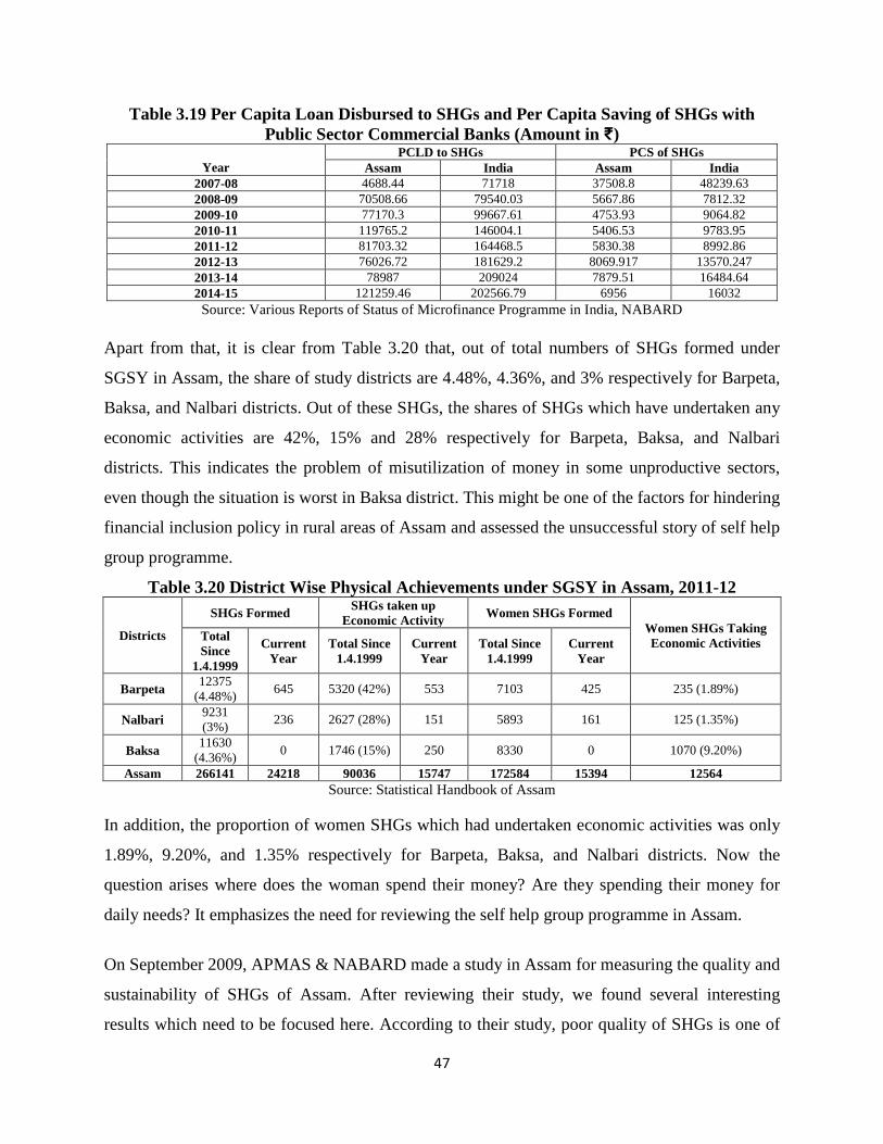
47

Table 3.19 Per Capita Loan Disbursed to SHGs and Per Capita Saving of SHGs with Public Sector Commercial Banks (Amount in ₹)

Year

PCLD to SHGs PCS of SHGs Assam India Assam India

2007-08 4688.44 71718 37508.8 48239.63 2008-09 70508.66 79540.03 5667.86 7812.32 2009-10 77170.3 99667.61 4753.93 9064.82 2010-11 119765.2 146004.1 5406.53 9783.95 2011-12 81703.32 164468.5 5830.38 8992.86 2012-13 76026.72 181629.2 8069.917 13570.247 2013-14 78987 209024 7879.51 16484.64 2014-15 121259.46 202566.79 6956 16032 Source: Various Reports of Status of Microfinance Programme in India, NABARD

Apart from that, it is clear from Table 3.20 that, out of total numbers of SHGs formed under

SGSY in Assam, the share of study districts are 4.48%, 4.36%, and 3% respectively for Barpeta,

Baksa, and Nalbari districts. Out of these SHGs, the shares of SHGs which have undertaken any

economic activities are 42%, 15% and 28% respectively for Barpeta, Baksa, and Nalbari

districts. This indicates the problem of misutilization of money in some unproductive sectors,

even though the situation is worst in Baksa district. This might be one of the factors for hindering

financial inclusion policy in rural areas of Assam and assessed the unsuccessful story of self help

group programme.

Table 3.20 District Wise Physical Achievements under SGSY in Assam, 2011-12

Districts

SHGs Formed SHGs taken up Economic Activity Women SHGs Formed

Women SHGs Taking Economic Activities Total

Since 1.4.1999

Current Year

Total Since 1.4.1999

Current Year

Total Since 1.4.1999

Current Year

Barpeta 12375 (4.48%) 645 5320 (42%) 553 7103 425 235 (1.89%)

Nalbari 9231 (3%) 236 2627 (28%) 151 5893 161 125 (1.35%)

Baksa 11630 (4.36%) 0 1746 (15%) 250 8330 0 1070 (9.20%)

Assam 266141 24218 90036 15747 172584 15394 12564 Source: Statistical Handbook of Assam

In addition, the proportion of women SHGs which had undertaken economic activities was only

1.89%, 9.20%, and 1.35% respectively for Barpeta, Baksa, and Nalbari districts. Now the

question arises where does the woman spend their money? Are they spending their money for

daily needs? It emphasizes the need for reviewing the self help group programme in Assam.

On September 2009, APMAS & NABARD made a study in Assam for measuring the quality and

sustainability of SHGs of Assam. After reviewing their study, we found several interesting

results which need to be focused here. According to their study, poor quality of SHGs is one of

48

the basic reasons for the backwardness of the microfinance program in the region. Out of the 109

sample SHGs in Assam, 2 are ‘A’ grade groups, 67 are ‘B’ grade groups and 40 are ‘C’ grade

groups. Consequently, these grades imply that the quality of groups in the state is very poor.

Likewise, lack of member’s awareness is one of the basic factors for the backwardness of the

microfinance program in Assam. According to their report, though 62 groups said that the

purpose of the group was to save; only 18% groups said providing loans as their purpose. Apart

from that, they also reviewed that, only 62% of groups heard about grading, 58 groups know that

their groups were graded, but 38 groups do not know grade they got. These raises question over

the quality improvement programme and training programme undertaken by NABARD in

various time over the year. Moreover, integration of two incompatible programs, i.e. SHG-

Banking Program and SGSY program, has been hindering the microfinance programme in

Assam. The SHG-Banking Program aimed at financial inclusive, i.e. proving financial services,

hitherto un-reached and un-bankable sections, designed to run purely on commercial terms.

Whereas the SGSY program is aimed at poverty alleviation through the promotion of

entrepreneurship and self-employment with the capital subsidy, runs on state subsidy.

Widespread corruption in SGSY program is affecting adversely the repayment to the banks,

which in turn is affecting adversely the SHG-Banking Program. In this way, the integration has

vitiated the SHG movement in the state. Furthermore, all the stakeholders including primary

stakeholders have got limited and, in many instances, inappropriate capacity building inputs.

Funds shortage and non-availability of quality capacity building inputs, especially on the

institutional building are major problems at SHG and Self Help Promoting Agencies (SHPA)

level. Among NGOs, big NGOs got very good training and exposure from national and state

level institutions, but small NGOs have to content with local capacity building inputs.

Thus, it is clear that, although self help group programme has been helping the poor to provide

financial facilities since the decade, but it is not successful to deliver their services as per

expectation, and there are some underline factors which are hindering the programme in rural

Assam. Now the question arises, where the rural people go to fulfill their financial needs. In the

following section, we had outlined the dominance of informal finance in continuation of our

discussion regarding special features of rural credit markets of Assam.

49

3.3.4. Dominance of Informal Finance in Assam Due to the failure of formal and semiformal financial institutions to provide credit facilities to

rural people, a vast portion of rural people is depending on informal finance. In this section, we

have discussed the dominance of informal finance in India through special emphasis on Assam

by taking different sets of AIDIS undertaken by RBI and NSSO.

3.3.4.1 Informal Finance in All India Level Although India inherited a basic network of credit cooperatives from the colonial era, the

Reserve Banks first decennial All India Rural Credit Survey (AIRCS) 1951-52 (RBI, 1954)

found that 92.8% of rural household relied on the informal financial sector (Table 3.21). During

1951-52, an increase in debt was recorded in all the 75 investigated districts of India. The

moneylenders continued dominance at the beginning of plan period (around 70% of rural credit)

despite all measures to control them, suppress or supplant had led to the suggestion that ‘any

realistic system of rural credit should seek to incorporate him in itself rather than compete with

him or wishfully expect to eliminate him’ (RBI, 1954). Loans from relatives (virtually interest-

free) accounted for 14% of the reported borrowings of cultivators. About 6% of the total

borrowings of cultivators were from traders and commission agents. The combined contribution

of government and cooperatives was about 6% of the total rural credit, each accounting for about

3%. As for commercial banks, 1 % represented the insignificant part played by them in the direct

financing of the cultivator.

Table 3.21 Break-up of Institutional and Non-Institutional Rural Credit (%) Sources 1951 1961 1971 1981 1991 2002 2013

Institutional Agencies 7.2 14.8 29.2 61.2 64.0 57.1 56 Government 3.3 5.3 6.7 4.0 5.7 2.3 1.2

Co-op. Society/bank 3.1 9.1 20.1 28.6 18.6 27.3 24.8 Commercial bank incl. RRBs 0.8 0.4 2.2 28.0 29.0 24.5 25.1

Insurance -- -- 0.1 0.3 0.5 0.3 0.3 Provident Fund -- -- 0.1 0.3 0.9 0.3 --

Other institutional agencies -- -- -- -- 9.3 2.4 4.6 Non-Institutional Agencies 92.8 85.2 70.8 38.8 36.0 42.9 44

Landlord 1.5 0.9 8.6 4.0 4.0 1.0 0.7 Agricultural Moneylender 24.9 45.9 23.1 8.6 6.3 10.0 33.2 Professional Moneylender 44.8 14.9 13.1 8.3 9.4 19.6 --

Traders and Commission Agencies 5.5 7.7 8.7 3.4 7.1 2.6 0.1 Relatives and Friends 14.2 6.8 13.8 9.0 6.7 7.1 8.5

Others 1.9 8.9 2.8 4.9 2.5 2.6 1.4 Total 100 100 100 100 100 100 100

Source: All India Rural Credit Survey (1954); All India Debt and Investment Survey, Various Issues; Note: Other Institutional Agencies includes financial corporation/institution, financial company and other institutional agencies.

50

AIRCS (RBI, 1954) pointed out that ‘agricultural prices during the survey year witnessed a

stagnation followed by a steep decline for the first time in a period of ten years’. However, a

large part of the working funds borrowed by subsistence farmers seems to be related to

consumption rather than production. The problem turned into more complicated one due to the

socio-economic structure of the village with its characteristics of caste and inequality. Other

factors that might have aided to the trend towards an increase in debt were relatively large

incidence of drought, famine and inclement seasonal credit.

All India Rural Debt and Investment Survey 1961-62 In this second survey by Reserve Bank, the outstanding loans owed to agriculturist moneylenders

accounted for about 46% of the aggregate outstanding of all rural households, nearly double the

share compared to the first survey. The share of outstanding loans owing to professional

moneylenders was next highest though their share declined to constitute 15% of the aggregate

outstanding. As per the survey findings on the all-India basis (Table 3.21), the share of

cooperatives was at 9.1%, ‘others’ at 8.9%, traders and commission agents at 7.7%, relatives at

6.8% and government at 5.3% in the total outstanding debt. The shares of landlords and

commercial banks in the aggregate outstanding were negligible at 9.0% and 0.4%, respectively.

This fact signifies the continuance of informal finance in rural India that might have prompted

the nationalization of commercial banks in 1969 in the first phase.

One of the important reasons for continued dependence on moneylenders is that the formal credit

delivery structure has not stretched to the villages despite its penetration. The formal credit

delivery channels also lack the personal bonds that moneylenders enjoy with the borrowers.

Borrowers obtain their loans more promptly from non-institutional sources (Pradhan, 2013).

From Table 3.21, it can be assessed that the informal/non-institutional finance was gradually

declining during the 1960s, was very nearly broken during the 1970s, with the institutional

agencies making steady inroads into the rural scene. The share of institutional credit agencies in

the outstanding cash dues of the rural households at the all-India level increased from 29% in

1971 to 61% in 1981 and then the pace of increase was arrested rising to 64% in 1991. During

the following decade, the share declined by about 7% points and reached 57% in 2002. It seems

that credit cooperatives, commercial banks, and other formal financial sector programmes in

51

rural areas have not displaced informal sources of credit, altogether. The 2002 All India Debt and

Investment Survey (AIDIS) revealed that 43% of rural households continue to rely on informal

finance, which includes professional moneylenders, agricultural moneylenders, traders, relatives

and friends, and others.

3.3.4.2. Persistence of Informal Credit in Rural Assam- AIDIS Surveys

Since the district wise data are not available in AIDIS surveys, we have taken all over Assam

data as a proxy of study districts. From Table 3.22, it can be observed that the share of

government in total outstanding cash debt in rural areas of Assam was 15.5% in 1961-62 and it

increases to 23.5% in 1971-72. But its share is negligible during the period 1981-82 and 1991-

92, and further increases to 15.4 in 2001-02. Likewise, the share of cooperatives increases from

8.3% in 1961-62 to 15.5% in 1991-92 but declines to 5.2% in 2001-02. The share of the

commercial bank was nil during the period 1971-72 but increases to 23.0% in 2001-02.

Table 3.22 Outstanding Cash Debt of Assam in Different years (AIDIS 1961-62, 1971-72, 1981-82, 1991-92 & 2001-02) - Credit Agency Wise (%)

Credit Agency 1961-62 1971-72 1981-82 1991-92 2001-02 Government 15.5 23.5 2.0 5.6 15.4 Cooperatives 8.3 10.6 6.0 15.5 5.2

Commercial Banks -- 0.0 16.0 9.1 23.0 Insurance -- -- 0.0 -- 0.1

Provident Fund -- -- 6.0 -- 7.3 Financial Institution -- -- -- -- 2.2 Financial Company -- -- -- -- 0.8

Other Institutional Agency -- -- -- -- 3.9 Landlords & Traders 6.7 11.6 2.0 35.9 1.6

Moneylenders (Agr. & Prof.) 50.1 19.7 6.0 25.8 26.2 Relatives & Friends 11.9 27.0 34.0 4.8 12.4

Others 7.6 7.6 28.0 3.3 1.9 Total 100.0 100.0 100.0 100.0 100.0

Source: All India Debt and Investment Survey- 1961-62, 1971-72, 1981-82, 1991-92 & 2001-2002 Note: Data’s are edited by author

Among the non-institutional credit agencies, moneylenders (agri. & prof.) dominating the

position (50.1%) in 1961-62, and its share was negligible during the period 1981-82 and further

increases to 26.2% in 2001-02. The share of relatives and friends was very significant during the

period 1971-72 and 1981-82 with 27.0% and 34.0% respectively.

It can be accessed from Table 3.22 that the most remarkable performance was that of the

commercial banks while the share of cooperatives was declining in recent years. It appears that a

large number of branches that was set up by various commercial banks in the 1970s and the

52

subsequent introduction of rural banking schemes have driven the commercial banks to assume

the role of principal credit agency in rural areas. As a whole, in Assam, among the institutional

credit agencies, the commercial banks and government were the two most important agencies in

the rural sector. These two agencies together accounted for 38.4% of outstanding cash debt

during the year 2001-02. As a whole, among the non-institutional agencies, moneylenders were

the main source of credit followed by relatives and friends. The gradual increase in the share of

formal institutional credit in agriculture witnesses some reversal during 1991-2002 mainly

because of a pull back by commercial banks. Thus likewise all over India, in Assam also, we can

get a continuance dominance of informal sectors in recent time (Table 3.22). There is another

large segment of supplier under the informal sector in Lower Assam called the Xonchois which

are missing in AIDIS report. They dominate the financial landscapes in most parts of the region.

One of the reasons could be that Xonchois are constituted of friends and relatives. Hence, it

might be possible that they have been included under the generic category of Friends and

Relatives (Sharma, 2011).

It is important to mention here, not only is the informal sector dominant but also this dominance

is found to be much more pervasive across different income classes. Amongst the poor classes,

its dominance is almost 100% as compared to the national average of around 80% (Table 3.23

and Table 3.25). This dominance of informal sector continues across most of the higher asset

classes. In other words, the informal sector is much more widespread in the state as compared to

the country.

Table 3.23 Number of Households Reporting Cash Loans Outstanding as on 30.06.02 per

1000 Households Over Credit Agency for each Household Assets Holding Class

Asset Holding Class (Rs. 000)

Assam All India

Institutional Agencies

Non Institutional Agencies Total Institutional

Agencies

Non Institutional

Agencies Total

0-15 2(3.3) 58(96.7) 60 36(24.0) 120(80.0) 150 15-30 3(3.3) 87(96.7) 90 62(32.6) 139(73.2) 190 30-60 11(12.2) 80(88.9) 90 87(34.5) 177(70.2) 252

60-100 10(11.9) 74(88.1) 84 109(41.1) 177(66.8) 265 100-150 20(27.8) 51(70.8) 72 136(47.1) 179(61.9) 289 150-200 6(17.1) 28(80.0) 35 146(50.9) 171(59.6) 287 200-300 13(25.5) 38(74.5) 51 162(56.4) 157(54.7) 287 300-450 48(51.6) 45(48.4) 93 187(65.2) 132(46.0) 287 450-800 96(68.1) 46(32.6) 141 220(71.0) 130(41.9) 310

800 & above 58(69.9) 25(30.1) 83 267(81.2) 103(31.3) 329 All 16(21.3) 59(78.7) 75 134(50.6) 155(58.5) 265

Source: 59th Round of AIDIS, NSSO; Note: Figures in the parentheses represent per cent to total

53

Another important characteristic of non-institutional informal finance in Assam is the nature of

extremely small loan sizes. Table 3.24 shows that the average loan size of Assam is less than half

of the national average. Not only the average size is small, this smallness persists across all the

asset classes in the state. Even in the case of the richest class, the loan size in Assam is only

22.56% of the loan size of the country as a whole. It is extremely difficult for formal institutions

like banks to meet the demand of extremely small loans as it is not sustainable for them.

Table 3.24 Average Loan Size Per Rural Household by Asset Class in Assam and India

Household Asset Holding Class (Rs.000) Assam India % of Loan Size in Assam from all over India Loan Size

0-15 159 1423 11.2 15-30 315 2243 14 30-60 248 3153 7.9

60-100 635 4301 14.8 100-150 518 5299 9.8 150-200 274 5696 4.8 200-300 429 7058 6.1 300-450 2232 9857 22.6 450-800 3578 15090 23.7

800 & above 1868 33414 5.6 All 643 1423 45.2

Source: 59th Round of AIDIS, NSS, 2002

54

Table 3.25 per 1000 Number of Rural Households, Average Value of Assets per Household and Amount of Cash Loan per Household as on 30.06.12 by Household Asset Holding Class

(Amount in ₹) State Asset Holding

Class Per 1000 No. of

Households Avg. Value of Assets

per HHs Avg. Value of Cash Loan

per HHs

Assam

1 103 28896 1312 (13.52) 2 102 87793 1601(18.15) 3 115 154346 2388 (17.29) 4 98 227361 1915 (12.22) 5 132 329053 2457 (13.07) 6 149 459948 5979 (25.51) 7 110 635192 6551(22.77) 8 103 903674 6176 (16.40) 9 66 1516865 20637 (36.42) 10 22 3457939 25247 (22.56) All 1000 503499 5256 (16.16)

India

1 100 25071 9705 2 100 89593 8819 3 100 151460 13811 4 100 227415 15673 5 100 325385 18800 6 100 454192 23441 7 100 635506 28770 8 100 922870 37662 9 100 1548889 56658 10 100 5689385 111884 All 1000 1006985 32522

Source: Household Assets and Liabilities, NSS 70th Round; Note: Household asset holding class refers to the 10 deciles classes of the all-India distribution (estimated distribution) of households by asset holding size. In the tables, the different deciles classes are referred to simply as 1 (lowest deciles class), 2, 3 …9, 10; Figure in the parentheses

represent per cent of loan size in Assam from all over India loan size

In the present context when the prime objective of the banks are in improving their bottom lines,

they would try to avoid this segment due to the high costs and restrict themselves in meeting the

requirements of much larger loans. The average size of the loan of the formal banking industry in

Assam is ₹112174/- (BSR, RBI, 2008). Even in the case of rural areas the average loan size

financed by the formal banking sector in the state is 56852/-(BSR, RBI, 2008) which is way

above the demand of ₹5256/- only for the rural households as cited in the Table 3.24. This is one

of the major reasons why the rural households in Assam rely mostly on the informal financial

sector to meet their credit requirements.

55

Table 3.26 per 1000 Number of Rural Households, Average Value of Assets per Household and Amount of Cash Loan per Household as on 30.06.12 by Household Type (Amount in ₹)

State Household Type Avg. Value of Assets per HHs Avg. Value of Cash Loan per HHs

Assam

Self Employed in Agriculture 625913 4748 (12.21) Self Employed in Non-Agriculture 476910 5396 (10.34)

Regular Wage/Salary Earnings 471853 12038 (30.39) Casual Labour in Agriculture 309483 542 (3.36)

Casual Labour in Non-Agriculture 220088 901 (4.73) Others 468568 2854 (19.02)

All 503499 5256 (16.16)

India

Self Employed in Agriculture 1573731 38888 Self Employed in Non-Agriculture 928712 52162

Regular Wage/Salary Earnings 981390 39617 Casual Labour in Agriculture 304104 16141

Casual Labour in Non-Agriculture 374876 19030 Others 554341 15001

All 1006985 32522 Source: Household Assets and Liabilities, NSS 70th Round; Note: Figure in the parentheses represent per cent of

loan size in Assam from all over India loan size Table 3.26 outlines the small size of average loan of Assam vis-à-vis India in household

category-wise. The average loan size is low in case of casual labour in agriculture and which is

only 3.36% of national level.

In addition, most of the loans are spending for consumption purpose in Assam as can be seen

from Table 3.27. Basically, during the lean income period, a large segment of the loans are

borrowed so that the households can meet their expenditure during this period. This frees up

capital for production activities which otherwise would be needed for daily living expenses,

especially during the lean times (CGAP Annual Report, 2005). .

Table 3.27 Percentage Distribution of Loans by Purpose in Assam and India

Assam

Exp in Farm Business Exp in Non Farm Total for Production 13.7 8.1 21.8

HH Exp Other Exp Total for Non business HH Exp 58.9 18.6 77.4

Total 100

India

Exp in Farm Business Exp in Non Farm Total for Production 32.7 7.2 39.9

HH Exp Other Exp Total for Non business HH Exp 56.7 9.1 64.9

Total 100 Source: 59th Round of AIDIS, NSS, 2002

This borrowing also reduces risk and vulnerabilities of the poor and hence used very extensively

as a survival strategy by them. However, the nature of such loans is such that they need to be

disbursed very quickly to the recipient. This can only be done by financial intermediaries who

are residing in the vicinity of the clients and know them intimately; thus reducing problems of

56

information asymmetry leading to adverse selection and moral hazard formal sector in the rural

areas of Assam.

On the basis of the above background, we have chosen Assam as a study state among all other

low performing states. In the next section, we have discussed the banking profile vis-à-vis

rationale behind the selection of study districts.

3.3.5. Banking Profile of Study Districts Among the study districts, most of the scheduled commercial bank branches are concentrated in

Barpeta district (Table 3.28) which is a good indicator because of the fact that, in Barpeta district

large numbers of the population are living, unlike other study districts. It is interesting to see

from Table 3.28 that, the credit-deposit ratio of all study districts are much higher than all over

Assam which underlines the better position of formal credit in the study districts while among

the study districts, credit deposit ratio is lowest in Baksa district and it is highest in Nalbari

district. Thus, Nalbari district is healthier than other study districts in case of credit deposit ratio.

Table 3.28 District-Wise Distribution of Aggregate Deposit and Gross Bank Credit of All Scheduled Commercial Banks in Assam (₹ in Crore)

Districts

As on March 2013 As on March 2014 No. of

Reporting Offices Deposit Credit CD ratio

No. of reporting offices Deposit Credit CD ratio

Barpeta 66 1606 710 44.20 72 1873 847 45.22 Nalbari 49 1097 522 47.54 52 1202 595 49.50 Baska 27 386 194 50.25 29 534 219 41.01 Assam 1682 77730 28575 36.79 1861 85070 31714 37.28

Source: Statistical Handbook of Assam, 2014 Likewise, Table 3.29 also indicated that unlike Nalbari district, the average population per

branch office of all scheduled commercial banks is higher in both study districts namely Baksa

and Barpeta in compare to Assam, while the situation is worst in Baksa district. However, the

situation is most horrible in all the three districts as well as of Assam if we compare it with all

India level. This focuses the problem of the thin spread of bank branches generally in Assam

and particularly for Baksa and Barpeta districts. Thus, we can get a poorly developed banking

structure of Assam in compare with all over India, but the status is relatively superior in Nalbari

district among the study districts.

57

Table 3.29 Average Population per Branch Office of All Scheduled Commercial Banks of Assam as on December, 2013

Districts SBI & its Associates (offices)

Nationalized Bank (offices)

Foreign Banks

(offices)

RRB (offices)

OPB (offices)

NPB (offices)

Total (offices) APPO

Baksa 4 15 -- 9 -- -- 28 34063 Barpeta 11 35 -- 17 -- 6 69 24538 Nalbari 8 24 -- 17 -- 3 52 14806 Assam 301 922 2 408 16 141 1790 17413 India 21469 55920 301 17524 6199 10365 111778 10825

Source: BSR, RBI and Census of India, 2011

Similarly, if we look at the picture of average rural population per branches of commercial

banks, we can get the same situation as earlier. Here also, average rural population per branches

of commercial banks is higher in both Barpata and Baksa district in compare to Assam and all

over India (Table 3.30), whereas Nalbari district is relatively performing well in compare to all

over Assam. Thus, one can get a point here why Nalbari district is doing well in case of rural

bank branch expansion in Assam, unlike other study districts.

Table 3.30 Average Population per Branches of Commercial Banks in Rural Areas of Assam as on March 2009

Districts Rural Branches Rural Population APPB Baksa 22 941600 42800

Barpeta 38 1545901 40681 Nalbari 30 687368 22912 ASSAM 786 26780516 34071

India 31695 833000000 26281 Source: BSR, RBI and Census of India, 2011

In a similar way, the average per capita credit (Table 3.31) and average per capita deposit (Table

3.32) also indicates severe financial exclusion in the study districts as well as all over Assam in

compare to overall India. As we can point out from Table 3.31 that average per capita credit of

all scheduled commercial banks is much lower in Assam in compare to all over India, while the

situation is worst in Baksa district. Although Nalbari district is performing well among all study

districts, but unable to overcome all over Assam situation. This raises a question why Nalbari

district unable to overcome all over Assam in spite of his impressive bank branch expansion.

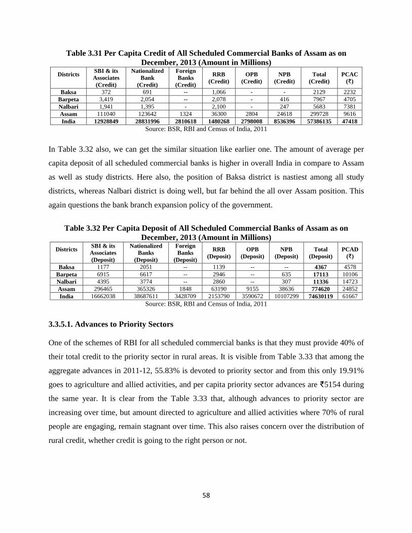
58

Table 3.31 Per Capita Credit of All Scheduled Commercial Banks of Assam as on December, 2013 (Amount in Millions)

Districts

SBI & its Associates (Credit)

Nationalized Bank

(Credit)

Foreign Banks

(Credit)

RRB (Credit)

OPB (Credit)

NPB (Credit)

Total (Credit)

PCAC (₹)

Baksa 372 691 -- 1,066 - - 2129 2232 Barpeta 3,419 2,054 -- 2,078 - 416 7967 4705 Nalbari 1,941 1,395 - 2,100 - 247 5683 7381 Assam 111040 123642 1324 36300 2804 24618 299728 9616 India 12928849 28831996 2810618 1480268 2798008 8536396 57386135 47418

Source: BSR, RBI and Census of India, 2011

In Table 3.32 also, we can get the similar situation like earlier one. The amount of average per

capita deposit of all scheduled commercial banks is higher in overall India in compare to Assam

as well as study districts. Here also, the position of Baksa district is nastiest among all study

districts, whereas Nalbari district is doing well, but far behind the all over Assam position. This

again questions the bank branch expansion policy of the government.

Table 3.32 Per Capita Deposit of All Scheduled Commercial Banks of Assam as on

December, 2013 (Amount in Millions) Districts

SBI & its Associates (Deposit)

Nationalized Banks

(Deposit)

Foreign Banks

(Deposit)

RRB (Deposit)

OPB (Deposit)

NPB (Deposit)

Total (Deposit)

PCAD (₹)

Baksa 1177 2051 -- 1139 -- -- 4367 4578 Barpeta 6915 6617 -- 2946 -- 635 17113 10106 Nalbari 4395 3774 -- 2860 -- 307 11336 14723 Assam 296465 365326 1848 63190 9155 38636 774620 24852 India 16662038 38687611 3428709 2153790 3590672 10107299 74630119 61667

Source: BSR, RBI and Census of India, 2011

3.3.5.1. Advances to Priority Sectors One of the schemes of RBI for all scheduled commercial banks is that they must provide 40% of

their total credit to the priority sector in rural areas. It is visible from Table 3.33 that among the

aggregate advances in 2011-12, 55.83% is devoted to priority sector and from this only 19.91%

goes to agriculture and allied activities, and per capita priority sector advances are ₹5154 during

the same year. It is clear from the Table 3.33 that, although advances to priority sector are

increasing over time, but amount directed to agriculture and allied activities where 70% of rural

people are engaging, remain stagnant over time. This also raises concern over the distribution of

rural credit, whether credit is going to the right person or not.

59

Table 3.33 Advances Outstanding Under Priority Sector in Assam (₹ in Crore) Sectors 2004-

05 2005-06 2006-07 2007-08 2008-09 2009-10 2010-11 2011-12 2012-13 2013-14

Aggregate Advances

6497.59 9811.15 12989.4

4 16081.4

3 17750.9

9 20910.9

7 23843.6

2 30363.2

2 32825.1

1 37902.9

2

Total Priority Sector

Advance

3119.99

(48.02)

4248.21 (43.30)

6148.70 (47.34)

8322.25 (51.75)

10705.50

(60.31)

11314.92

(54.11)

13242.59

(55.54)

16080.72

(55.83)

19429.10

(59.19)

21645.83

(57.11)

Agriculture & Allied Activities

616.15 (9.48)

1212.84 (12.36)

1596.74 (12.29)

2158.80 (13.42)

2345.86 (13.22)

3868.37 (18.50)

4557.40 (19.11)

5733.91 (19.91)

6614.39 (20.15)

7497.58 (19.78)

Industries 515.87 (7.94)

685.52 (6.99)

1018.13 (7.84)

1281.63 (7.97)

1460.25 (8.23)

2054.15 (9.82)

2490.30 (10.44)

2819.38 (9.79)

4326.50 (13.18)

5158.53 (13.61)

Per Capita Priority Sector

Advances (₹)

1170 1594 2307 3122 4016 4245 4968 5154

6226

6938

Source: Various Reports of State Level Bankers Committee, Assam However, we can get a very worst picture if we look at the situation of target achieved for

advancing to priority sectors in the study districts (Table 3.34). As it can be indicated from Table

3.34, on 25.02.2014 in Baksa district the scheduled commercial banks only fulfill 6.32% of their

target. The same is the position in case of regional rural banks. The status of Nalbari district is

relatively better in compare to other two districts which can be shown from Table 3.34.

Table 3.34 Target Achievement under Annual Credit Plan for Advancing to Priority Sector

in Study District Bank Type Year Target Achieved in Different Priority Sector in Study Districts (%)

Baksa Barpeta Nalbari A

SCB

2009

88 14

2010 32 41 17 2011 18 19 7 2012 -- -- -- 2013 8.2 15 14.4 2014 6.32 24.08 27.93

RR

B

2009 -- 81 81 2010 37 70 52 2011 2 71 14 2012 -- -- -- 2013 6.28 29.38 15.6 2014 5.95 35.97 29.58

AA

CB

2009 -- 51 3 2010 58 19 0 2011 46 13 2 2012 -- -- -- 2013 1.2 2.1 -- 2014 2.4 5.35 --

Source: Various Reports of SLBC, Assam

60

Thus, the failure of achieving the target of priority sector lending where the majority of rural

people are engaging indicates the severe financial exclusion in rural areas of Assam, and

consequently, it points out that most of the credits are actually concentrated among the small

portion of rich people. Although in most of the cases the position of Nalbari district is superior in

compared to other study districts as well as Assam, but it is horrible in compare with all over

India. This highlights the serious financial exclusion in rural areas of Assam which forcing the

rural people to informal financial institutions. However, the introduction of group-based

approach in 1979, although it is adopted later in Assam, has somewhat improved the situation. In

the subsequent section, we provided an analysis by focusing demand side of credit in the study

area for validating our study districts.

3.3.6. District/Region Level Financial Inclusion Index To rationalize the selection of study region and districts we have constructed one financial

inclusion index separately across districts and regions in Assam by using fourteen indicators as

mentioned below-

Average Population per Bank Offices (APPBO)

Average Population per Rural Bank Offices (APPRBO)

Average Deposit per Bank Offices (ADPBO) (in Million)

Average Credit per Bank Offices (ACPBO) (in Million)

Average Credit Outstanding Per Credit Accounts (ACOPCA) (in thousands)

No. of Credit Account per Thousand Population (NCAPTP)

Per Capita Credit Outstanding (PCCO) (in thousands)

Average Deposit per Thousand Deposit Account (ADPTDA) (in Million)

Per Capita Deposit (PCD) (in thousands)

Average Deposit per Thousand Deposit Account in Rural Areas (ADPTDARA) (in

Million)

Per Capita Deposit Amount in Rural Areas (PCDARA) (in thousands)

Credit Deposit Ratio (CDR) (%)

Households Availing Banking Services (HABS) (%)

Rural Households Availing Banking Services (RHABS) (%)

61

As in state level index, we have used same method and criteria for constructing and measuring

the status of financial inclusion here.

62

Table 3.35: Region and District-wise Distribution of Banking Performance Index Value in Assam Regions IND 1 IND 2 IND 3 IND 4 IND 5 IND 6 IND 7 IND 8 IND 9 IND 10 IND 11 IND 12 IND 13 IND 14 Index Value Status

NORTH ASSAM UDA 0.46 0.64 0.64 1.09 0.30 0.98 0.48 0.44 0.46 0.59 0.47 1.55 0.82 0.87 0.70 LOW

DARR 0.89 0.74 0.71 0.94 0.42 0.87 0.60 0.61 0.64 0.53 0.33 1.29 0.81 0.85 0.73 LOW SON 1.15 1.13 0.87 1.04 0.87 1.04 1.49 0.82 0.99 0.79 0.68 1.16 0.90 0.90 0.99 AVERAGE NAG 0.84 0.87 1.06 1.04 0.42 0.98 0.67 0.73 0.85 0.63 0.59 1.00 1.00 1.04 0.84 AVERAGE MOR 0.83 0.78 0.58 0.96 0.35 0.95 0.55 0.43 0.53 0.43 0.43 1.44 1.05 1.09 0.74 LOW

TNA (A) 0.83 0.83 0.77 1.01 0.47 0.96 0.76 0.60 0.69 0.59 0.50 1.29 0.92 0.95 0.80 AVERAGE LOWER ASSAM

DHU 0.25 0.04 0.78 0.77 0.36 0.53 0.31 0.64 0.49 0.66 0.34 0.88 0.52 0.48 0.50 LOW KOK 0.50 0.24 1.32 0.86 0.43 0.65 0.46 0.87 0.93 0.83 0.49 0.65 0.83 0.83 0.71 LOW BON 1.10 0.74 0.97 0.96 0.56 0.86 0.79 0.89 1.10 0.82 0.52 0.90 1.31 1.35 0.92 AVERAGE

GOAL 0.77 0.92 0.74 0.71 0.38 0.67 0.42 0.65 0.64 0.88 0.63 0.93 1.14 0.92 0.74 LOW BAK 0.52 1.09 0.56 0.65 0.34 0.43 0.24 0.44 0.36 0.83 0.84 0.99 0.74 0.82 0.63 LOW CHI 0.79 1.05 1.29 1.01 0.45 0.71 0.53 0.86 1.03 1.70 1.73 0.71 0.82 0.86 0.97 AVERAGE BAR 0.84 0.91 0.80 0.99 0.43 0.77 0.54 0.64 0.70 0.88 0.86 1.09 0.82 0.83 0.79 AVERAGE NAL 1.21 1.31 0.74 0.88 0.41 1.21 0.81 0.68 0.98 0.87 0.12 1.19 0.84 0.80 0.86 AVERAGE KAM 1.13 1.36 0.63 0.98 1.18 1.66 3.20 0.71 0.96 1.24 1.81 1.01 1.25 1.24 1.31 TOP

KAM M) 1.81 1.75 2.80 2.61 1.53 2.70 6.76 5.11 1.78 4.12 5.94 0.80 1.01 1.06 2.84 TOP TLA (A) 0.89 0.94 1.06 1.04 0.61 1.02 1.40 1.15 0.90 1.28 1.33 0.92 0.93 0.92 1.03 TOP

UPPER ASSAM LAKH 1.06 1.10 0.64 1.06 0.40 1.14 0.75 0.60 0.72 0.71 0.74 1.48 0.75 0.75 0.85 AVERAGE DIBR 1.47 1.34 1.67 1.20 0.64 1.51 1.58 1.71 2.88 1.19 1.27 0.77 1.17 1.14 1.40 TOP DHE 0.48 0.36 0.74 1.14 0.38 0.91 0.56 0.57 0.50 0.73 0.50 1.56 0.79 0.81 0.72 LOW TIN 1.37 1.20 1.10 0.97 0.70 0.91 1.04 1.23 1.72 1.05 0.81 0.87 1.09 1.03 1.08 TOP SIB 1.27 1.22 1.08 1.10 0.05 1.20 0.11 1.00 1.44 1.04 1.18 1.07 1.13 1.19 1.01 TOP JOR 1.40 1.27 1.33 1.32 0.61 1.48 1.48 1.23 2.01 0.96 1.13 1.04 1.56 1.73 1.33 TOP GOL 1.24 1.35 0.93 0.86 0.38 1.22 0.76 0.72 0.95 0.88 1.07 1.13 0.74 0.74 0.93 AVERAGE

TUA (A) 1.19 1.12 1.07 1.09 0.45 1.20 0.89 1.01 1.46 0.94 0.96 1.13 1.03 1.06 1.04 TOP HILLS AND BARAK VALLEY

NCH 1.41 1.58 0.74 0.43 0.46 0.74 0.56 1.20 0.15 1.42 1.59 0.49 1.24 1.32 0.95 AVERAGE KA 1.17 1.35 0.61 0.59 0.48 0.36 0.28 0.92 0.95 0.62 0.69 0.69 1.77 1.45 0.85 AVERAGE

CAC 1.18 1.12 1.34 1.07 0.59 1.01 0.97 1.41 1.67 1.14 1.15 0.84 0.91 0.87 1.09 TOP HAIL 0.85 0.54 0.89 0.75 0.35 0.84 0.49 0.72 0.08 0.68 0.45 0.82 1.11 1.17 0.70 LOW KAR 0.84 0.91 1.13 0.75 0.49 0.66 0.53 0.82 0.79 0.86 0.76 0.72 0.92 0.91 0.79 AVERAGE

THBV(A) 1.09 1.10 0.94 0.72 0.48 0.72 0.56 1.01 0.73 0.94 0.93 0.71 1.19 1.14 0.88 AVERAGE ASSAM 1.18 1.07 1.30 1.26 0.67 1.03 1.08 1.34 1.71 0.92 0.86 0.90 0.98 0.95 1.09 TOP Source: Authors’ estimation based on Basic Statistical Returns of SCBs in India, RBI, 2015; Quarterly Statistics on Deposits and Credit of SCBs, March 2015;

Census of India, 2011; Note: BAK= Baksa, BAR= Barpeta, BON= Bongaigaon, CAC= Cachar, CHI= Chirang, DARR= Darrang, DHE= Dhemaji, DIBR= Dibrugarh, GOAL= Goalpara, GOL= Golaghat, HAIL= Hailakandi, JOR= Jorhat, KAM= Kamrup, KAM (M) = Kamrup Metropolitan, KA= Karbi Anglong,

KAR= Karimganj, KOK= Kokrajhar, LAKH= Lakhimpur, MOR= Morigaon, NAG= Nagaon, NAL= Nalbari, NCH= North Cachar Hills, SIB= Sibsagar, SON= Sonitpur, TIN= Tinsukia, UDA= Udalguri, TNA= Total North Assam, TLA= Total Lower Assam, TUA= Total Upper Assam, THBV= Total Hills and Barak

Valley; INDj= Indicator 1……….14; Value of IND 1 and IND 2 are subtracted by ‘2’ to make it same direction with other indicators.

63

Table 3.35 reveals a skewed expansion of the financial system across districts and regions within

Assam. It is apparent from the fact that the financial inclusion index of the banking outreach

value of the top district (Kamrup Metro) is more than four times that of the bottom district

(Dhubri). The same picture is evident from the absolute figure of each indicator (Appendix D

and Appendix E). Moreover, only 25.93% districts are the top performer while 40.74% are the

average performer. Thus between two Top performer regions we have selected Lower Assam as

a study region because literature agrued the higher concentration of microfinance setup besides

several informal community based organizations in this region. Similarly, among ten districts in

this region we have selected Nalbari, Barpeta and Baksa as a study districts from each of Top,

Average and Low performer districts.

3.3.7. Demand Driven Financial Inclusion in Study Districts

Prior to depth study in the subsequent chapters, here we presented an investigation by

constructing one Demand Driven Financial Inclusion Index (DDFII) in order to validate of our

study districts. We used household level data for the same12. Indeed, for constructing DDFII, we

used three indicators for formal sector- proportion of people having formal credit, proportion of

people having formal saving and proportion of people having formal insurance.

DDFII F

= (∑q Yt qs) /3

Where,

Yt qs is the value of indicator q for the district/village at time t

q = formal saving, credit and insurance

However, for semiformal and informal sectors we used two indicators- proportion of people

having semiformal/informal credit and proportion of people having semiformal/informal saving.

DDFII S

= (∑q Yt qs) /2

Where,

Yt qs is the value of indicator q for the district/village at time t

q = semiformal saving and credit

DDFII I = (∑q Yt

qs) /2

Where,

Yt qs is the value of indicator q for the district/village at time t

q = informal saving and credit 12 Detailed of data collection has been discussed in subsequent section.

64

Here formal sector includes all scheduled commercial banks operating in the respective districts.

Likewise, the semiformal sector includes Self Help Groups linked with banks and Microfinance

institutions basically BANDHAN even though, it now got bank license, and informal sector

includes money lenders and various private saving groups exist in the village. Moreover,

informal saving includes savings of people with various Chit Fund Company though people lost

their money because of Chit Fund Scam.

As the indicators are all in percentages, they are already normalized with a minimum of zero and

maximum of hundred. We used an equally weighted average of the indicators to calculate

DDFII, separately for formal, semiformal and informal sources. The index is the average of these

three components (in the case of formal sources) and the average of two components – saving

and credit only (in the case of semiformal and informal sources), which indicates the status of

availed financial services. It serves as a proxy of demand for these services.

While Table 3.36 indicates that in Baksa district the dominance of all the three sources is found

to be smallest, whereas in Barpeta district all three are doing well. In Baksa district access to

formal sources is one out of every three households, one out of every two households in case of

both semiformal and informal sources. However, the indicator-wise indexes are mentioned in

Appendix F, Appendix G and Appendix H. Indeed, in Barpeta district access to formal sources is

one out of every three households, while all households are engaged in semiformal sources. But,

access to informal sources is one out of every two households. Thus, we can get a very poor

picture of financial inclusion in Baksa district and this raises question where do the rural people

go for their financial needs.

65

Table 3.36 Demand Side FII (for Formal, Semiformal and Informal) in Three Selected Districts of Assam

Dist/Vill DDFII (Formal) DDFII (Semiformal) DDFII (Informal) Baksa 0.36 0.43 0.41

Jengrengpara 0.32 0.35 0.15 Bunmajhar Pam 0.52 0.45 0.45

Bagariguri 0.47 0.45 0.4 Salbari 0.15 0.48 0.63

Barpeta 0.46 0.72 0.59 Bamundi 0.45 0.73 0.65

Bamunkuchi 0.57 0.65 0.43 Garemari 0.48 0.7 0.73

Bhare Gaon 0.35 0.8 0.58 Nalbari 0.45 0.64 0.52

Bar Makhibaha 0.45 0.8 0.6 Namati 0.47 0.63 0.4

Bamunbari 0.48 0.45 0.28 Baralkuchi 0.4 0.65 0.8

Total 0.42 0.59 0.51 Source: Calculated from Primary Survey conducted in Assam, 2014

Since Baksa district is a conflict prone area, this also raises concern over the interrelation

between conflict and financial exclusion. Apart from that, the dominance of all the three sources

in Barpeta district indicates the integration of formal, semiformal and informal sources in rural

areas. In all the three districts dominance of semiformal sector is found to be attractive followed

by the informal sector. Nevertheless, on an average presence of semiformal sector is found to be

prominent followed by the informal sector. Thus, we can point out that semiformal institutions

are successful for replacing the informal institutions in rural areas. In the same way, the

performance of the formal sector is found to be most ineffective in Baksa district followed by

Nalbari district. However, among the three indicators of the formal sector, the first indicator

proportion of people having formal credit is lowest, whereas the saving of the people with formal

institutions is found to be striking. This indicates the mounting saving behavior of rural people.

Equally, the dominance of semiformal and informal institutions is found to be high in Barpeta

district followed by Nalbari district. Here one can get an important point why Nalbari district

could not successful in overcoming Barpeta district despite its impressive development

indicators like high Per Capita Income, Literacy Rate, and Work Rate Participation etc.

3.4. Contradiction between Socio-Economic and Banking Parameters

From above discussion it has been argued that despite lower decadal variation of population

during 2001-11 and higher density of population in compare to country as a whole, in Assam the

66

banking parameters like number of deposit and credit account per person, number of offices of

scheduled commercial banks per lakh population etc. were far behind from national level.

Moreover, we could found the pessimistic relation between some social and economic indicators

and banking parameters. Despite lagging banking parameters, in all study districts and Assam,

sex ratio is privileged in compare to India as a whole. Even among all study districts, sex ratio is

highest in Baksa- the lowest performer of banking parameter, while it is lowest in Nalbari- the

highest performer of banking parameters. Likewise, the peak performer in banking parameters

Nalbari district has lowest HDI among all study districts. Similarly, Barpeta has lowest infant

mortality rate, but lower per capita income, lower banking performance, and worst performer in

some economic variables, while Nalbari district has highest infant mortality rate, but higher per

capita income, higher banking penetration, and highest performer in some other economic

variables.

Furthermore, we have observed similar kind of relation in urbanization and literacy where the

good performer in banking parameters Nalbari district has the highest proportion of the urban

population and literacy rate among all study districts, and the reverse is the situation in Baksa

and Barpeta. In addition, more proportion of women SHGs have undertaken economic activities

in Baksa district, while reverse circumstances have been observed in Nalbari district and it

indicated the existence of SHGs domination where formal banks unable to catch up.

In the course of the study, it became imperative to undertake a field study either to fulfill some of

the objectives and research questions or to verify some of the observations derived from

secondary information. It is thought that objectives on demand, awareness, and use of credit

sources, repayment rate, and the monetary and social impact of rural credit could be better

understood and analyzed from the household’s point of view. In addition, it was thought to

conduct SHGs level study too to intensify the study. The methodological aspects of the sample

survey have been outlined in the following section.

3.5. Sampling Design and Data Collection Tool This study is basically based on primary data collected during September-December, 2014. As

mentioned in the first chapter, a multi-stage sampling technique has been adopted to select the

67

field study locations. Figure 3.3 presents a map of Assam showing the study districts and

development blocks. In the first stage, three districts namely- Barpeta, Baksa and Nalbari were

selected purposively among eight districts of the region. In the second stage, two development

blocks from each district were selected. Hence, altogether six development blocks have been

chosen for study. In the third stage, from each block, two villages were chosen to keep in view

representation of variations in socio-economic conditions. Therefore, twelve villages were

chosen to undertake the study. In the fourth stage, from each village, 6 to 9 percent of household

were selected at random for study, and so per village twenty households chosen for the

interview. In this way, a sample of 240 households was interviewed. Figure 3.4 shows the

selection process of the household’s sample. As discussed in chapter one, for rationalizing the

study we surveyed sixty SHGs in the same procedure like respondent households. Figure 3.5

shows the selection procedure of the SHGs sample.

68

Figure 3.3: Study Area Showing the Sample Districts and Development Blocks in Assam

69

Figure 3.4: Selection Process of the Households Sample

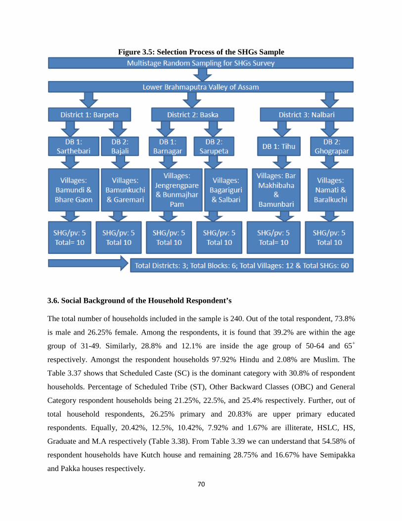
70

Figure 3.5: Selection Process of the SHGs Sample

3.6. Social Background of the Household Respondent’s The total number of households included in the sample is 240. Out of the total respondent, 73.8%

is male and 26.25% female. Among the respondents, it is found that 39.2% are within the age

group of 31-49. Similarly, 28.8% and 12.1% are inside the age group of 50-64 and 65+

respectively. Amongst the respondent households 97.92% Hindu and 2.08% are Muslim. The

Table 3.37 shows that Scheduled Caste (SC) is the dominant category with 30.8% of respondent

households. Percentage of Scheduled Tribe (ST), Other Backward Classes (OBC) and General

Category respondent households being 21.25%, 22.5%, and 25.4% respectively. Further, out of

total household respondents, 26.25% primary and 20.83% are upper primary educated

respondents. Equally, 20.42%, 12.5%, 10.42%, 7.92% and 1.67% are illiterate, HSLC, HS,

Graduate and M.A respectively (Table 3.38). From Table 3.39 we can understand that 54.58% of

respondent households have Kutch house and remaining 28.75% and 16.67% have Semipakka

and Pakka houses respectively.

71

Table 3.37 Social Profile of Respondent Households D

Villages Total Households Male Female 20-25 26-30 31-49 50-64 65+ Hindu Muslim GEN OBC SC ST

Bak

sa

Bagariguri 20 12 (60) 8 (40) 2 (10) 2 (10) 6 (30) 6 (30) 4 (20) 20

(100) 0 0 20 (100) 0 0

Jengrengpara 20 19 (95) 1 (5) 1 (5) 2 (10) 6 (30) 8 (40) 3 (15) 20

(100) 0 0 20 (100) 0 0

Salbari 20 14 (70) 6 (30) 2 (10) 2 (10) 11

(55) 5 (25) 0 20 (100) 0 0 0 9 (45) 11

(55) Bunmajhar

Pam 20 12 (60) 8 (40) 6 (30) 3 (15) 6 (30) 19

(95) 0 17 (85) 3 (15) 3 (15) 0 0 17 (85)

T

4 80 57 (71.3)

23 (28.75)

11 (13.8)

9 (11.3)

29 (36.3)

38 (47.5) 7 (8.8) 77

(96.25) 3 (3.75) 3 (3.75)

40 (50)

9 (11.3) 28 (35)

Bar

peta

Bamundi 20 16 (80) 4 (20) 2 (10) 2 (10) 14

(70) 0 2 (10) 20 (100) 0 0 0 20

(100) 0

Bamunkuchi 20 14 (70) 6 (30) 2 (10) 2 (10) 6 (30) 7 (35) 3 (15) 20

(100) 0 20 (100) 0 0 0

Bhare Gaon 20 16 (80) 4 (20) 4 (20) 6 (30) 8 (40) 2 (10) 0 20

(100) 0 0 0 0 20 (100)

Garemari 20 14 (70) 6 (30) 2 (10) 2 (10) 8 (40) 2 (10) 6 (30) 20

(100) 0 0 0 20 (100) 0

T

4 80 60 (75) 20 (25) 10

(12.5) 12

(15) 36

(45) 11

(13.8) 11

(13.8) 80

(100) 0 20 (25) 0 40

(50) 20(25)

Nal

bari

Namati 20 11 (55) 9 (45) 0 4 (20) 6 (30) 5 (25) 5 (25) 20

(100) 0 6 (30) 14 (70) 0 0

Bar Makhibaha 20 11

(55) 9 (45) 0 0 9 (45) 4 (20) 7 (35) 20 (100) 0 20

(100) 0 0 0

Baralkuchi 20 20 (100) 0 (0) 0 0 6 (30) 13

(65) 1 (5) 18 (90) 2 (10) 2 (10) 0 15 (75) 3 (15)

Bamunbari 20 18 (90) 2 (10) 0 0 8 (40) 12

(60) 0 20 (100) 0 10

(50) 0 10 (50) 0

T

4 80 60 (75) 20 (25) 0 4 (5) 29

(36.3) 34

(42.5) 13

(16.3) 78

(97.5) 2 (2.5) 38 (47.5)

14 (17.5)

25 (31.3) 3 (3.75)

GT

12 240 177 (73.8)

63 (26.25)

21 (8.75)

25 (10.4)

94 (39.2)

69 (28.8)

31 (12.1)

235 (97.92) 5 (2.08) 61

(25.4) 54

(22.5) 74

(30.8) 51 (21.25)

Source: Field Survey, 2014; Note: Here D= Districts, T= Total, GT= Grand Total; Figures within parentheses represent percentages of households

72

Table 3.38 Educational Profile of Respondent Households

Districts Villages Graduate HS HSLC Illiterate M.A Primary Upper Primary Total

Baksa

Bagariguri 2 (10.5) 2 (8) 0 4 (8.16) 0 6 (9.5) 6 (12) 20 Jengrengpara 0 4 (16) 3 (10) 4 (8.16) 0 4 (6.35) 5 (10) 20

Salbari 2 (10.5) 1 (4) 0 14 (28.6) 0 3 (4.76) 0 20 Bunmajhar

Pam 6 (31.6) 1 (4) 6 (20) 1 (2.04) 0 3 (4.76) 3 (6) 20

Total 4 10 (52.6) 8 (32) 9 (30) 23 (46.9) 0 16 (25.4) 14 (28) 80

Barpeta

Bamundi 0 2 (8) 6 (20) 4 (8.16) 0 6 (9.5) 2 (4) 20 Bamunkuchi 4 (21.1) 5 (20) 5 (16.7) 0 2 (50) 2 (3.2) 2 (4) 20 Bhare Gaon 0 2 (8) 2 (6.67) 4 (8.16) 2 (50) 6 (9.5) 4 (8) 20 Garemari 2 (10.5) 2 (8) 4 (13.3) 0 0 2 (3.2) 10 (20) 20

Total 4 6 (31.6) 11 (44) 17 (56.7) 8 (16.33) 4 (100) 16 (25.4) 18 (36) 80

Nalbari

Namati 0 0 2 (6.67) 2 (4.08) 0 11 (17.5) 5 (10) 20 Bar

Makhibaha 3 (15.8) 2 (8) 2 (6.67) 6 (12.24) 0 2 (3.2) 5 (10) 20

Baralkuchi 0 0 0 8 (16.32) 0 12 (19.0) 0 20 Bamunbari 0 4 (16) 0 2 (4.08) 0 6 (9.52) 8 (16) 20

Total 4 3 (15.8) 6 (24) 4 (13.33) 18 (36.7) 0 31 (49.2) 18 (36) 80 Grand Total 12 19 (7.9) 25 (10.4) 30 (12.5) 49 (20.4) 4 (1.7) 63 (26.3) 50 (20.8) 240

Source: Field Survey, 2014; Note: Figures within parentheses represent percentages of households

Table 3.39 Type of Dwelling of Respondent Households Districts Villages Kutch House Pakka House Semi-Pakka Total

Baksa

Bagariguri 12 (9.16) 2 (5) 6 (8.69) 20 Bunmajhar Pam 12 (9.16) 5 (12.5) 3 (4.35) 20

Jengrengpara 15 (11.45) 3 (7.5) 2 (2.90) 20 Salbari 14 (10.69) 2 (5) 4 (5.80) 20

Total 4 53 (40.46) 12 (30) 15 (21.74) 80

Barpeta

Bamundi 12 (9.16) 4 (10) 4 (5.80) 20 Bamunkuchi 5 (3.82) 6 (15) 9 (13.04) 20 Bhare Gaon 16 (12.21) 2 (5) 2 (2.90) 20 Garemari 10 (7.63) 2 (5) 8 (11.59) 20

Total 4 43 (32.82) 14 (35) 23 (33.33) 80

Nalbari

Bar Makhibaha 8 (6.11) 4 (10) 8 (11.59) 20 Baralkuchi 12 (9.16) 2 (5) 6 (8.69) 20 Bamunbari 8 (6.11) 6 (15) 6 (8.70) 20

Namati 7 (5.34) 2 (5) 11 (15.94) 20 Total 4 35 (26.72) 14 (35) 31 (44.93) 80

Grand Total 12 131 (54.58) 40 (16.67) 69 (28.75) 240 Source: Field Survey, 2014; Note: Figures within parentheses represent percentages of households

3.7. Occupational Background of the Respondent Households Out of the total number of respondent households, 30% respondents have the main occupation of

farming. Similarly, 19.17% has manual labour, 7.92% small business, 6.67% government

pension holders, 9.17% government job, 5.42% artisan, 3.75% private sector employee and

4.17% shopkeeper (Table 3.40). Interestingly, 66.25% of respondents have the secondary

73

occupation, and out of that, 28.30% has the farmer, 16.98% manual labour and 8.18%

shopkeeper13.

Table 3.40 Main Occupation of Respondent Households

Activities Name of Districts Total Baksa Barpeta Nalbari

Agriculture and Allied Activities 0 3 (60) 2 (40) 5 (2.08) Artisan 1 (7.69) 8 (61.54) 4 (30.77) 13 (5.42)

Chicken Farm 0 2 (100) 0 2 (0.83) Councilor 0 0 2 (100) 2 (0.83)

Councilor, Panchayat Member 0 0 2 (100) 2 (0.83) Farmer 28 (38.89) 24 (33.33) 20 (27.78) 72 (30.0)

Gaon Bura 0 2 (40) 3 (60) 5 (2.08) Government/Public Employee 10 (45.45) 4 (18.18) 8 (36.36) 22 (9.17)

Housewife 5 (71.43) 2 (28.57) 0 7 (2.92) Manual Labour 19 (41.30) 14 (30.43) 13 (28.26) 46 (19.17)

Government Pension Holders 1 (6.25) 7 (43.75) 8 (50) 16 (6.67) Priest 0 1 (100) 0 1 (0.42)

Private Sector Employee 3 (33.33) 5 (55.56) 1 (11.11) 9 (3.75) Shop keeper and Agriculture 0 0 4 (100) 4 (1.67)

Shopkeeper 0 2 (20) 8 (80) 10 (4.17) Small Business 9 (47.37) 6 (31.58) 4 (21.05) 19 (7.92)

Student 3 (100) 0 0 3 (1.25) Temporary Teacher 1 (50) 0 1 (50) 2 (0.83)

Total 80 80 80 240 Source: Field Survey, 2014; Note: Figures within parentheses represent percentages of households

3.8. Land Holding Pattern of Households

Table 3.41 shows that out of 240 respondent households, 8.75% have land holdings of one

Bigha, 6.67% half Bigha, 8.75% two Bigha, 5.42% three Bigha, 7.92% four Bigha, 6.67% five

Bigha, 7.92% six Bigha and 6.25% seven Bigha. Similarly, out of total respondent, 65.42% have

agricultural land, and from that, 19.11% has agricultural land of two Bigha, 22.93% three Bigha,

8.92% four Bigha and 12.74% has five Bigha14.

13 Relevant Table has been attached in Appendix I 14 Relevant Table has been attached in Appendix J

74

Table 3.41 Land Holding Pattern of Respondent Households Amount of Land (in Bigha) Name of Districts Total Baksa Barpeta Nalbari

1.5 0 2 (33.33) 4 (66.67) 6 (2.5) 1.03 2 (50) 2 (50) 0 4 (1.67)

1 3 (14.29) 14 (66.67) 4 (19.05) 21 (8.75) 0.5 6 (37.5) 4 (25) 6 (37.5) 16 (6.67) 10 3 (75) 0 1 (25) 4 (1.67) 11 1 (14.29) 6 (85.71) 0 7 (2.92) 12 0 2 (100) 0 2 (.83) 16 1 (50) 0 1 (50) 2 (.83) 17 2 (28.57) 3 (42.86) 2 (28.57) 7 (2.92) 18 0 2 (100) 0 2 (.83) 19 2 (100) 0 0 2 (.83) 2.5 3 (42.86) 2 (28.57) 2 (28.57) 7 (2.92)

2.03 0 0 4 (100) 4 (1.67) 2 8 (38.09) 4 (19.05) 9 (42.86) 21 (8.75)

2.05 1 (100) 0 0 1 (.42) 2.03 2 (50) 0 2 (50) 4 (1.67) 2.3 0 0 2 (100) 2 (.83) 0.1 1 (33.33) 2 (66.67) 0 3 (1.25) 20 2 (50) 2 (50) 0 4 (1.67) 21 1 (100) 0 0 1 (.42) 22 2 (100) 0 0 2 (.83) 23 0 2 (100) 0 2 (.83) 25 2 (100) 0 0 2 (.83) 3.5 0 0 4 (100) 4 (1.67) 3 7 (53.85) 4 (30.77) 2 (15.39) 13 (5.42)

3.05 0 4 (100) 0 4 (1.67) 3.2 1 (100) 0 0 1 (.42) 3.4 1 (100) 0 0 1 (.42)

0.15 1 (100) 0 0 1 (.42) 37 0 2 (100) 0 2 (.83) 4.5 0 2 (100) 0 2 (.83) 4 8 (42.11) 3 (15.79) 8 (42.11) 19 (7.92) 5 4 (25) 7 (43.75) 5 (31.25) 16 (6.67)

52 2 (100) 0 0 2 (.83) 6.5 0 0 2 (100) 2 (.83) 6 5 (26.32) 2 (10.53) 12 (63.16) 19 (7.92) 7 4 (26.67) 7 (46.67) 4 (26.67) 15 (6.25) 8 2 (33.33) 0 4 (66.67) 6 (2.5)

0.4 0 0 2 (100) 2 (.83) 84 0 2 (100) 0 2 (.83) 9 3 (100) 0 0 3 (1.25)

Grand Total 80 80 80 240 Source: Field Survey, 2014; Note: 1 Bigha= 0.3305785 Acre, Figures within parentheses represent percentages of

households

75

3.9. Banking Profile of Respondent Households Figure 3.6 indicates that out of total respondents 86.25% (207) have the formal bank account.

Out of their respective respondents in Barpeta and Nalbari districts 36.71% (76) have the bank

accout but in Baksa 26.57% (55) respondent have the bank accout. Furthermore, among total

respondents 62.5% (150) has saved money in formal bank account, whereas, in Barpeta 39.33%

(59) and in Nalbari 25.33% (38) (Fig. 3.7). Likewise, 40.83% (98) respondent enjoyed life

insurance facility. In study districts it is 24.49% (24), 38.77% (38) and 36.73% (36) respectively

for Baksa, Barpeta and Nalbari (Fig. 3.8).

Figure 3.6 Proportions of Households Having Bank Account

Source: Field Survey, 2014

Figure 3.7 Proportions of Households Save Money

Source: Field Survey, 2014

76

Figure 3.8 Proportions of Households Having Life Insurance

Source: Field Survey, 2014

Figure 3.9 Proportions of Households Experience Income Remittances

Source: Field Survey, 2014

Figure 3.9 indicates the proportion of household’s experiences income remittances from any

sources of borrowed money, and accordingly, in total 39.17% (94) households practice income

remittances. However, in Barpeta district highest 37.23% (35) observe the same among all three

districts and in Baksa districts lowest 27.66% (26) view the same. In addition, among total respondent households, 30% (70) borrowed money from formal sources.

The percentages are 27.78% (20), 13.89% (10) and 36.25% (29) respectively for Baksa, Barpeta

and Nalbari districts (Table 3.42).

77

Table 3.42 Respondent Households Borrowed Money from Formal Sources

Districts Villages Borrow Money from Formal

Sources Total No Yes

Baksa

Bagariguri 14 (8.33) 6 (8.33) 20 Bunmajhar Pam 14 (8.33) 6 (8.33) 20

Jengrengpara 14 (8.33) 6 (8.33) 20 Salbari 18 (10.71) 2 (2.78) 20

Total 4 60 (35.71) 20 (27.78) 80

Barpeta Bamundi 14 (8.33) 6 (8.33) 20

Bamunkuchi 15 (8.93) 5 (6.94) 20 Bhare Gaon 18 (10.71) 2 (2.78) 20 Garemari 10 (5.95) 10 (13.89) 20

Total 4 57 (33.93) 23 (31.94) 80

Nalbari Bar Makhibaha 9 (5.36) 11 (15.28) 20

Baralkuchi 17 (10.12) 3 (4.17) 20 Bamunbari 10 (5.95) 10 (13.89) 20

Namati 15 (8.93) 5 (6.94) 20 Total 4 51 (30.36) 29 (36.25) 80

Grand Total 12 168 (70) 72 (30) 240 Source: Field Survey, 2014; Note: Figures within parentheses represent percentages of households

Again Table 3.43 shows that out of formal money borrowed respondent, 38.89% (28) borrowed

primarily for agriculture purpose, 34.7% (25) for house construction and 5.6% (4) for buying

cows and business. Interestingly, 19.44% (14) respondent have the secondary purpose of

borrowing formal money, and out of that, 35.71% (5) borrowed for house construction, and

21.43% (3) for agriculture15.

Table 3.44 reveals that out of total respondent households, 54.58% (131) had borrowed from

semiformal sources. Among study districts, in Nalbari highest 40.46% (53) respondents

borrowed from semiformal sources. The percentages of Barpeta and Baksa districts are 39.69%

(52) and 19.85% (26) respectively. Among the borrowers of the semiformal loan, 35.11% (46)

borrowed money for daily needs, 16.79% (22) for illness and 10.69% (14) borrowed for farming

(Table 3.45). Likewise, from the semiformal borrowers, 30.53% (40) of the respondent has

multiple purposes of borrowing money, and among them, 37.5 (15) borrowed for daily needs and

32.5% (13) for illness16.

Out of total respondent, 57.5% (138) borrowed money informal sources, and the percentages are

36.96% (51), 33.33% (46) and 29.71% (41) respectively for Nalbari, Barpeta and Baksa (Table

3.46). Among informal borrowers, 23.9% (33) borrowed money for farming, 21.01% (29) for

15 Appropriate Table has been attached in Appendix L 16 See Appendix M

78

daily needs, and 16.67% (23) borrowed for business and the percentage is same for illness too

(Table 3.47). Moreover, 18.84% (26) borrowers has multiple purpose of informal borrowing, and

among them, 42.31% (11) borrowed for illness, 26.92% (7) for daily needs and 23.08% (6)

borrowed informal money for education purpose17.

17 See Appendix N

79

Table 3.43 Primary Purpose of Borrowing Formal Money

Districts Villages Agriculture Daily Needs Education Fishery Business Buying

Cows Girl

Marriage House

Construction Total

Baksa

Bagariguri 3 (10.71) 0 0 1 (25) 0 0 0 2 (8) 6 (8.3) Bunmajhar Pam 0 0 0 3 (75) 0 0 0 3 (12) 6 (8.3)

Jengrengpara 1 (3.57) 0 1 (100) 0 1 (25) 1 (25) 0 2 (8) 6 (8.3) Salbari 0 0 0 0 0 0 0 2 (8) 2 (2.8)

Total 4 4 (14.29) 0 1 (100) 4 (100) 1 (25) 1 (25) 0 9 (36) 20 (27.8)

Barpeta

Bamundi 2 (7.14) 2 (66.7) 0 0 0 0 0 2 (8) 6 (8.3) Bamunkuchi 2 (7.14) 1 (33.3) 0 0 1 (25) 0 1 (33.3) 0 5 (6.9) Bhare Gaon 2 (7.14) 0 0 0 0 0 0 0 2 (2.8) Garemari 4 (14.29) 0 0 0 0 0 0 6 (24) 10 (13.9)

Total 4 10 (35.71) 3 (100) 0 0 1 (25) 0 1 (33.3) 8 (32) 23 (31.9)

Nalbari

Bar Makhibaha 4 (14.29) 0 0 0 2 (50) 3 (75) 0 2 (8) 11 (15.3) Baralkuchi 3 (10.71) 0 0 0 0 0 0 0 3 (4.7) Bamunbari 4 (14.29) 0 0 0 0 0 0 6 (24) 10 (13.9)

Namati 3 (10.71) 0 0 0 0 0 2 (66.7) 0 5 (6.9) Total 4 14 (50) 0 0 0 2 (50) 3 (75) 2 (66.7) 8 (32) 29 (40.3)

Grand Total 12 28 (38.89) 3 (4.2) 1 (1.4) 4 (5.6) 4 (5.6) 4 (5.6) 3 (4.2) 25 (34.7) 72 (100) Source: Field Survey, 2014; Note: Figures within parentheses represent percentages of households

80

Table 3.44 Respondent Households Borrowed Money from Semiformal Sources Districts Villages Borrow Money from Semiformal Sources Total No Yes

Baksa

Bagariguri 16 (14.68) 4 (3.05) 20 Bunmajhar Pam 14 (12.84) 6 (4.58) 20

Jengrengpara 14 (12.84) 6 (4.58) 20 Salbari 10 (9.17) 10 (7.63) 20

Total 4 54 (49.54) 26 (19.85) 80

Barpeta

Bamundi 10 (9.17) 10 (7.63) 20 Bamunkuchi 8 (7.34) 12 (9.16) 20 Bhare Gaon 4 (3.67) 16 (12.21) 20 Garemari 6 (5.50) 14 (10.69) 20

Total 4 28 (25.69) 52 (39.69) 80

Nalbari

Bar Makhibaha 5 (4.59) 15 (11.45) 20 Baralkuchi 1 (0.92) 19 (14.50) 20 Bamunbari 10 (9.17) 10 (7.63) 20

Namati 11 (10.09) 9 (6.87) 20 Total 4 27 (24.77) 53 (40.46) 80

Grand Total 12 109 (45.42) 131 (54.58) 240 Source: Field Survey, 2014; Note: Figures within parentheses represent percentages of households

81

Table 3.45 Primary Purpose of Borrowing Semiformal Money

Districts Villages Daily Needs Education Farming Festival Girls

Marriage Home

Construction Illness Job Land Weaving Total

Baksa

Bagariguri 2 (4.4) 0 0 0 0 0 0 4 (100) 0 0 6 (4.6) Bunmajhar Pam 4 (8.7) 0 1 (7.1) 1 (50) 0 0 0 0 0 0 6 (4.6)

Jengrengpara 3 (6.5) 0 2 (14.3) 1 (50) 0 0 0 0 0 0 6 (4.6) Salbari 6 (13.0) 3 (60) 0 0 0 0 0 0 1 (100) 0 10 (7.6)

Total 4 15 (32.6) 3 (60) 3 (21.4) 2 (100) 0 0 0 4 (100) 1 (100) 0 28 (21.4)

Barpeta

Bamundi 6 (13.0) 0 2 (14.3) 0 0 0 0 0 0 0 10 (7.6) Bamunkuchi 0 0 0 0 0 2 (50) 2 (7.7) 0 0 0 10 (7.6) Bhare Gaon 2 (4.4) 2 (40) 6 (42.9) 0 0 0 4 (18.2) 0 0 0 16 (12.2) Garemari 2 (4.4) 0 0 0 2 (100) 0 8 (36.4) 0 0 0 14 (10.7)

Total 4 10 (21.7) 2 (40) 8 (57.1) 0 2 (100) 2 (50) 14 (53.9) 0 0 0 50 (38.2)

Nalbari

Bar Makhibaha 2 (4.4) 0 2 (14.3) 0 0 2 (50) 8 (36.4) 0 0 1 (100) 15 (11.5) Baralkuchi 10 (21.7) 0 1 (7.1) 0 0 0 0 0 0 0 19 (14.5) Bamunbari 2 (4.4) 0 0 0 0 0 2 (9.1) 0 0 0 10 (7.6)

Namati 7 (15.2) 0 0 0 0 0 0 0 0 0 9 (6.8) Total 4 21 (45.7) 0 3 (21.4) 0 0 2 (50) 10 (45.5) 0 0 1 (100) 53 (40.5)

Grand Total 12 46 (`35.1) 5 (3.8) 14 (10.7) 2 (1.5) 2 (1.5) 4 (10.7) 26 (19.9) 4 (10.7) 1 (0.8) 1 (0.8) 131 (100)

Source: Field Survey, 2014; Note: Figures within parentheses represent percentages of households

82

Table 3.46 Respondent Households Borrowed Money from Informal Sources Districts Villages Borrow Money from Informal Sources Total No Yes

Baksa

Bagariguri 12 (11.76) 8 (5.80) 20 Bunmajhar Pam 8 (7.84) 12 (8.70) 20

Jengrengpara 17 (16.67) 3 (2.17) 20 Salbari 2 (1.96) 18 (13.04) 20

Total 4 39 (38.23) 41 (29.71) 80

Barpeta

Bamundi 10 (9.80) 10 (7.25) 20 Bamunkuchi 14 (13.73) 6 (4.35) 20 Bhare Gaon 8 (7.84) 12 (8.70) 20 Garemari 2 (1.96) 18 (13.04) 20

Total 4 34 (33.33) 46 (33.33) 80

Nalbari

Bar Makhibaha 9 (8.82) 11 (7.97) 20 Baralkuchi 0 20 (14.49) 20 Bamunbari 10 (9.80) 10 (7.24) 20

Namati 10 (9.80) 10 (7.25) 20 Total 4 29 (28.43) 51 (36.96) 80

Grand Total 12 102 (42.5) 138 (57.5) 240 Source: Field Survey, 2014; Note: Figures within parentheses represent percentages of households

83

Table 3.47 Primary Purpose of Informal Money Borrowed

Districts Villages Business Daily Needs Education Child Farming Tractor Girl

Marriage Home

Construction Illness Job Land Total

Baksa

Bagariguri 2 (8.7) 4 (13.8) 0 0 0 0 0 2 (22.2) 0 0 0 8 (5.8) Bunmajhar

Pam 0 4 (13.8) 1 (12.5) 0 2 (6.1) 1 (100) 0 2 (22.2) 2 (8.7) 0 0 12 (8.7)

Jengrengpara 0 1 (3.5) 0 0 2 (6.1) 0 0 0 0 0 0 3 (2.2) Salbari 1 (4.4) 10 (34.5) 0 0 1 (3.0) 0 0 0 3 (13.0) 2 (50) 1 (33.3) 18 (13.0)

Total 4 3 (13.0) 19 (65.5) 1 (12.5) 0 5 (15.2) 1 (100) 0 4 (44.4) 5 (21.7) 2 (50) 1 (33.3) 41 (29.7)

Barpeta

Bamundi 2 (8.7) 2 (6.9) 0 0 4 (12.1) 0 0 0 0 0 2 (66.7) 10 (7.3) Bamunkuchi 2 (8.7) 0 0 1 (100) 0 0 0 3 (33.3) 0 0 0 6 (4.4) Bhare Gaon 2 (8.7) 2 (6.9) 0 0 6 (18.2) 0 0 0 2 (8.7) 0 0 12 (8.7) Garemari 4 (17.4) 0 0 0 4 (12.1) 0 2 (50) 2 (22.2) 4 (17.4) 2 (50) 0 18 (13.0)

Total 4 10 (43.5) 4 (13.8) 0 1 (100) 14 (42.4) 0 2 (50) 5 (55.6) 6 (26.1) 2 (50) 2 (66.6) 46 (33.3)

Nalbari

Bar Makhibaha 0 0 5 (62.5) 0 0 0 2 (50) 0 4 (17.4) 0 0 11 (7.9)

Baralkuchi 6 (26.1) 2 (6.9) 0 0 12 (36.4) 0 0 0 0 0 0 20 (14.5) Bamunbari 4 (17.4) 0 2 (25) 0 0 0 0 0 4 (17.4) 0 0 10 (7.3)

Namati 0 4 (13.8) 0 0 2 (6.1) 0 0 0 4 (17.4) 0 0 10 (7.3) Total 4 10 (43.5) 6 (20.7) 7 (87.5) 0 14 (42.4) 0 2 (50) 0 12 (52.2) 0 0 51 (36.9)

Grand Total 12 23 (16.7) 29 (21.0) 8 (5.8) 1 (0.7) 33 (23.9) 1 (0.7) 4 (2.9) 9 (6.5) 23 (16.7) 4 (2.9) 3 (2.2) 138

Source: Field Survey, 2014; Note: Figures within parentheses represent percentages of households

84

3.10. Basic Profile of Surveyed SHGs Table 3.48 reveals that 58.3% (35) SHGs has group members 10, and 20% (12) of them has

group members 12. Moreover, 16.7% (10) of SHGs are nine year old, 15% (9) are seven year

old and 11.7% (7) are only two year old. 70% (42) SHGs enjoyed 100% repayment rate, and

3.3% experienced 80% repayment rate. In addition, 41.7% (25) SHGs charged 36% interest

rate per annum for members and 35% (21) SHGs 60%. Interestingly, 71.7% (43) SHGs didn’t

provide loan outsiders. Among them who provided the loan to outsiders, 18.3% (11) charged

60% interest rate per annum, and 5% (3) charge 120%.

Furthermore, contribution from members is ₹6000 per annum for 15% (9) SHGs, 13.3% (8)

have ₹12000, 11.7% (7) ₹4800, 10% (6) 14400, 8.3% (5) ₹7200 and 6.7% ₹24000. 18.3%

(11) of SHGs don’t have any retained earnings, 13.3% (8) SHGs earned ₹10000 per annum,

8.3% (5) ₹50000, 6.7% (4) ₹5000, 5% (3) ₹80000, 5% (3) ₹30000, 5% (3) ₹25000 and 5%

(3) earned ₹20000 per annum. 30% (18) SHGs doesn’t have any outstanding loan, 8.3% (5)

SHGs ₹8000, 6.7% (4) ₹4000, and 5% (3) ₹50000. Besides, 8.3% (5) SHGs has the saving of

₹5000 till date, 6.7% (4) has ₹6000 and 6.7% (4) ₹4000. Accordingly, 28.9% (17) SHGs

hasnot borrowed any money from banks, 11.7% (7) borrowed ₹10000, 8.3% (5) SHGs

borrowed ₹210000, 6.7% (4) ₹225000, 6.7% (4) ₹25000 and 5% (3) borrowed ₹30000

(Table 3.48.1).

85

Table 3.48 Profile of Studied SHGs ND NV NG NM DE RR (%) RIM (p/a) RIO (p/a)

Bak

sa

Jangapara Rangdhali 10 2011 100 36 60 Jangapara Sanghamitra 10 2007 100 60 60 Jangapara Atma Niyojan Samiti 10 2000 100 36 36 Jangapara Ramdhenu 10 2012 100 24 24 Jangapara Aai Asomi 10 2013 100 36 --

Salbari Salbari Nzwra Affat 10 2008 90 60 60 Salbari Golden 12 2006 100 60 60 Salbari Pakhila 10 2005 100 60 60 Salbari Udashri 10 2011 100 60 120 Salbari Rupashree 12 2004 100 60 60

Bunmaja 11 Star 11 2009 -- -- -- Bunmaja Narikallari 10 2012 -- -- -- Bunmaja Jonmoni 10 2008 100 60 -- Bunmaja Rangjali 12 2013 -- -- -- Bunmaja Baishagi 10 2006 100 60 120

Bagariguri Jonmoni 11 2009 -- -- -- Bagariguri Nari Mukti 10 2012 -- -- -- Bagariguri Jonmoni 10 2008 100 60 -- Bagariguri Rangjali 12 2013 -- -- -- Bagariguri Baishagi 10 2006 100 60 120

Bar

peta

Bamundi Jai Shiv 10 2013 100 24 -- Bamundi Maa Kali 11 2008 100 36 -- Bamundi Maa Kamakhya 10 2014 100 24 -- Bamundi Sarachati 10 2013 100 36 -- Bamundi Rupjyoti 10 2012 100 36 --

Bhare Gaon Shudamsri 11 2010 100 60 60 Bhare Gaon Hainashree Mahila 10 2008 100 36 48 Bhare Gaon Jayamoti 11 2006 100 36 60 Bhare Gaon Maina 14 2008 -- -- -- Bhare Gaon Mousumi 12 2006 100 36 -- Garemari Bowari 10 2011 100 60 -- Garemari Jaganath 13 2007 80 60 -- Garemari Akha 15 2007 100 60 -- Garemari Jibita 15 2007 100 60 60 Garemari Bhogirothi 12 2008 100 60 60

Bamunkuchi Pragati 12 2003 100 24 -- Bamunkuchi Sarachati 10 2006 -- 60 -- Bamunkuchi Pragati 10 2007 100 36 -- Bamunkuchi Meghali 12 2014 -- -- -- Bamunkuchi Lakhimi 10 2004 100 36 --

Nal

bari

Bar Makhibaha Lakhimi 10 2003 100 36 -- Bar Makhibaha Puwali 10 2002 -- 36 -- Bar Makhibaha Milan 10 2012 100 36 -- Bar Makhibaha Nilachal 10 2008 80 36 -- Bar Makhibaha pragatishil 11 2003 100 36 --

Baralkuchi Milijuli 12 2002 100 36 -- Baralkuchi Ramdhenu 10 2013 -- 48 -- Baralkuchi Shiv Shankar 12 2011 -- 60 -- Baralkuchi Jontona 12 2010 100 60 -- Baralkuchi Lakhimi 8 2006 100 60 -- Bamunbari Maa Kamakhya 10 2002 100 36 -- Bamunbari Udiyaman 10 2006 100 36 -- Bamunbari Nabmilan 10 2002 100 36 60 Bamunbari Kapili 10 2013 -- 48 -- Bamunbari Mayamoni 12 2011 -- 60 --

Namati Pragati 10 2006 75 36 -- Namati Rangdhali 11 2008 100 36 -- Namati Nab Jyoti 10 2006 100 36 -- Namati Abala 11 2005 100 36 -- Namati Niyor 10 2002 100 36 --

Source: Field Survey, 2014; Note: ND= Name of Districts, NG= Name of SHG, NM= No. of Members, DE= Date of Establishment, RR= Rate of Repayment, RIM= Rate of Interest (Members), RIO= Rate of Interest

(Outsiders)

86

Table 3.48.1 Profile of Studied SHGs ND NV NG CM (p/a) EG TLG TSG TBG

Bak

sa

Jangapara Rangdhali 4800 1500 7000 2226 -- Jangapara Sanghamitra 2400 -- 17000 115000 225000 Jangapara Atma Niyojan Samiti 4800 50000 -- 32000 237000 Jangapara Ramdhenu 9600 8000 20000 2500 15000 Jangapara Aai Asomi 24000 2000 12000 700 10000

Salbari Salbari Nzwra Affat 12000 80000 70000 14500 210000 Salbari Golden 3600 70000 39000 12500 150000 Salbari Pakhila 2400 60000 5500 -- 5000 Salbari Udashri 6000 5000 13000 8000 -- Salbari Rupashree 14400 10000 -- 12000 10000

Bunmaja 11 Star 5280 -- -- 20000 -- Bunmaja Narikallari 6000 -- -- 12000 -- Bunmaja Jonmoni 6000 10000 -- 4200 30000 Bunmaja Rangjali 14400 -- -- 1500 -- Bunmaja Baishagi 4800 10000 -- 5000 5000

Bagariguri Jonmoni 5280 -- -- 20000 -- Bagariguri Nari Mukti 6000 -- -- 12000 -- Bagariguri Jonmoni 6000 10000 -- 4200 30000 Bagariguri Rangjali 14400 -- -- 1500 -- Bagariguri Baishagi 4800 10000 -- 5000 5000

Bar

peta

Bamundi Jai Shiv 1440 8000 36000 9000 25000 Bamundi Maa Kali 5280 30000 80000 1500 75000 Bamundi Maa Kamakhya 4800 -- 7500 4000 15000 Bamundi Sarachati 2400 2000 50000 11000 65000 Bamundi Rupjyoti 5760 20000 60000 9000 40000

Bhare Gaon Shudamsri 14520 25000 22000 22000 -- Bhare Gaon Hainashree Mahila 12000 20000 100000 3000 5000 Bhare Gaon Jayamoti 2640 80000 40000 106000 210000 Bhare Gaon Maina 4200 -- -- 2500 -- Bhare Gaon Mousumi 2880 -- -- 142000 210000 Garemari Bowari 6000 5000 5000 6000 40000 Garemari Jaganath 3900 25000 1000 4500 -- Garemari Akha 7200 105000 40000 7000 -- Garemari Jibita 7200 50000 30000 15000 -- Garemari Bhogirothi 14400 30000 8000 4000 30000

Bamunkuchi Pragati 5760 50000 -- 5000 125000 Bamunkuchi Sarachati 4800 50000 -- 4400 14000 Bamunkuchi Pragati 2400 25000 8000 5000 10000 Bamunkuchi Meghali 7200 -- -- 1600 -- Bamunkuchi Lakhimi 6000 40000 42000 10000 10000

Nal

bari

Bar Makhibaha Lakhimi 24000 180000 -- 39000 215000 Bar Makhibaha Puwali 12000 36000 9000 9300 225000 Bar Makhibaha Milan 6000 10000 27000 3675 10000 Bar Makhibaha Nilachal 12000 43200 50000 2400 225000 Bar Makhibaha pragatishil 5280 250000 5000 3150 120000

Baralkuchi Milijuli 14400 500 4500 6000 -- Baralkuchi Ramdhenu 12000 500 8000 4000 -- Baralkuchi Shiv Shankar 7200 5000 4000 24000 10000 Baralkuchi Jontona 14400 10000 20000 35000 25000 Baralkuchi Lakhimi 4800 50000 6000 3500 25000 Bamunbari Maa Kamakhya 24000 100000 2000 6000 210000 Bamunbari Udiyaman 12000 10000 4000 7359 125000 Bamunbari Nabmilan 6000 12000 4000 5000 25000 Bamunbari Kapili 12000 500 8000 4000 -- Bamunbari Mayamoni 7200 5000 4000 24000 10000

Namati Pragati 3600 30000 70000 106200 225000 Namati Rangdhali 6600 40000 8000 9000 20000 Namati Nab Jyoti 12000 20000 10000 8000 20000 Namati Abala 3960 80000 50000 108000 320000 Namati Niyor 24000 100000 2000 6000 210000

Source: Field Survey, 2014; Note: CM= Contribution from Members, EG= Retained Earnings, TLG= Loan Outstanding, TSG= Total Saving of Group, TBG= Total Borrowing of SHG

87

3.11. Socio- Economic Background of Surveyed SHGs Members

Out of 647 members in 60 SHGs, 97.2% (629) are Hindu members, 2.8% (28) Muslim.

Moreover, among members 26.4% (171) belongs to General category and the percentages of

OBC, SC and ST are 23.2% (150), 31.4% (203) and 17.2% (111) respectively (Table 3.50).

Similarly, among members, 24% (153) are illiterate, 37.4% (238) primary school passed,

21.5% (137) upper primary school passed, 10.4% (66) HSLC, 4.7% (30) HS and 1.7% (11)

graduate (Table 3.51).

Further, 21.8% (139) members remain within the income range of ₹1000-3000 per month.

Likewise, 21.5% (136) have income of ₹4000-6000, 16.8% (107) ₹7000-9000, 15.9% (101)

have income of ₹10000-12000 per month (Table 3.52).

Table 3.49 Descriptive Statistics of Variables Districts Statistics NM CM EG TLG TSG TBG RIM

(p/a) RIO (p/a)

Overall Mean 10.78 8353 31236.67 16808.33 17848.5 63766.67 45.23 66.75

Minimum 8 1440 0 0 0 0 24 24 Maximum 15 24000 250000 100000 142000 320000 60 120

Baksa Mean 10.5 7848 16325 9175 14241.3 46600 52.29 70.91

Minimum 10 2400 0 0 0 0 24 24 Maximum 12 24000 80000 70000 115000 237000 60 120

Barpeta Mean 11.4 6039 28250 26475 18625 43700 43.33 57.6

Minimum 10 1440 0 0 1500 0 24 48 Maximum 15 14520 105000 100000 142000 210000 60 60

Nalbari Mean 10.45 11172 49135 14775 20679.2 101000 42 60

Minimum 8 3600 500 0 2400 0 36 60 Maximum 12 24000 250000 70000 108000 320000 60 60

Source: Authors estimation based on field survey, 2014

88

Table 3.50 Social Profile of SHGs Members ND NV NG NM Religion Caste

Hindu Muslim General OBC SC ST

Bak

sa

Jangapara Rangdhali 10 10 0 0 6 4 0 Jangapara Sanghamitra 10 10 0 1 5 4 0 Jangapara Atma Niyojan Samiti 10 10 0 2 4 4 0 Jangapara Ramdhenu 10 10 0 0 3 7 0 Jangapara Aai Asomi 10 10 0 3 5 2 0

Salbari Salbari Nzwra Affat 10 10 0 0 0 0 10 Salbari Golden 12 12 0 0 2 0 10 Salbari Pakhila 10 10 0 1 6 0 3 Salbari Udashri 10 10 0 0 0 0 10 Salbari Rupashree 12 12 0 0 3 2 7

Bunmaja 11 Star 11 0 11 11 0 0 0 Bunmaja Narikallari 10 3 7 7 3 0 0 Bunmaja Jonmoni 10 10 0 0 0 0 10 Bunmaja Rangjali 12 12 0 0 0 0 12 Bunmaja Baishagi 10 10 0 0 0 0 10

Bagariguri Jonmoni 11 11 0 2 0 9 0 Bagariguri Nari Mukti 10 10 0 0 3 7 0 Bagariguri Jonmoni 10 10 0 1 6 3 0 Bagariguri Rangjali 12 12 0 0 2 10 0 Bagariguri Baishagi 10 10 0 3 4 3 0

Bar

peta

Bamundi Jai Shiv 10 10 0 0 0 10 0 Bamundi Maa Kali 11 11 0 0 2 9 0 Bamundi Maa Kamakhya 10 10 0 0 0 10 0 Bamundi Sarachati 10 10 0 0 0 10 0 Bamundi Rupjyoti 10 10 0 0 4 6 0

Bhare Gaon Shudamsri 11 11 0 0 0 0 11 Bhare Gaon Hainashree Mahila 10 10 0 0 0 0 10 Bhare Gaon Jayamoti 11 11 0 0 0 0 11 Bhare Gaon Maina 14 14 0 10 4 0 0 Bhare Gaon Mousumi 12 12 0 5 2 5 0 Garemari Bowari 10 10 0 5 2 3 0 Garemari Jaganath 13 13 0 3 2 8 0 Garemari Akha 15 15 0 4 2 9 0 Garemari Jibita 15 15 0 5 6 4 0 Garemari Bhogirothi 12 12 0 1 10 0 0

Bamunkuchi Pragati 12 12 0 10 2 0 0 Bamunkuchi Sarachati 10 10 0 8 2 0 0 Bamunkuchi Pragati 10 10 0 5 5 0 0 Bamunkuchi Meghali 12 12 0 5 1 6 0 Bamunkuchi Lakhimi 10 10 0 7 3 0 0

Nal

bari

Bar Makhibaha Lakhimi 10 10 0 10 0 0 0 Bar Makhibaha Puwali 10 10 0 10 0 0 0 Bar Makhibaha Milan 10 10 0 5 2 3 0 Bar Makhibaha Nilachal 10 10 0 10 0 0 0 Bar Makhibaha pragatishil 11 11 0 2 5 4 0

Baralkuchi Milijuli 12 12 7 5 0 0 0 Baralkuchi Ramdhenu 10 10 3 0 0 7 0 Baralkuchi Shiv Shankar 12 12 0 0 0 12 0 Baralkuchi Jontona 12 12 0 0 0 5 7 Baralkuchi Lakhimi 8 8 0 0 0 8 0 Bamunbari Maa Kamakhya 10 10 0 5 0 5 0 Bamunbari Udiyaman 10 10 0 3 2 5 0 Bamunbari Nabmilan 10 10 0 8 0 2 0 Bamunbari Kapili 10 10 0 6 4 0 0 Bamunbari Mayamoni 12 12 0 2 5 5 0

Namati Pragati 10 10 0 0 10 0 0 Namati Rangdhali 11 11 0 2 7 1 0 Namati Nab Jyoti 10 10 0 0 5 5 0 Namati Abala 11 11 0 4 6 1 0 Namati Niyor 10 10 0 0 5 5 0

3 12 60 647 629 (97) 28 (2.8) 171 (26.4) 150 (23.2) 203 (31.4) 111 (17.2) Source: Field Survey, 2014; Note: Figures within parentheses represent percentages of members

89

Table 3.51 Educational Status of SHGs Members ND NV NG NM Illiterate Primary Upper

Primary HSLC HS B.A M.A

Bak

sa

Jangapara Rangdhali 10 5 3 2 0 0 0 0 Jangapara Sanghamitra 10 3 5 1 1 0 0 0 Jangapara Atma Niyojan Samiti 10 2 7 1 0 0 0 0 Jangapara Ramdhenu 10 1 5 3 1 0 0 0 Jangapara Aai Asomi 10 4 3 2 0 1 0 0

Salbari Salbari Nzwra Affat 10 1 4 3 1 1 0 0 Salbari Golden 12 3 5 2 1 0 0 0 Salbari Pakhila 10 0 6 2 2 0 0 0 Salbari Udashri 10 2 4 3 1 0 0 0 Salbari Rupashree 12 4 4 3 1 0 0 0

Bunmaja 11 Star 11 2 4 2 1 1 1 0 Bunmaja Narikallari 10 5 2 3 0 0 0 0 Bunmaja Jonmoni 10 0 4 2 2 2 0 0 Bunmaja Rangjali 12 2 3 3 2 1 1 0 Bunmaja Baishagi 10 3 3 2 2 0 0 0

Bagariguri Jonmoni 11 3 5 2 1 0 0 0 Bagariguri Nari Mukti 10 0 6 2 2 0 0 0 Bagariguri Jonmoni 10 2 4 3 1 0 0 0 Bagariguri Rangjali 12 4 4 3 1 0 0 0 Bagariguri Baishagi 10 2 4 2 1 1 1 0

Bar

peta

Bamundi Jai Shiv 10 2 5 2 1 0 0 0 Bamundi Maa Kali 11 3 4 1 1 1 1 0 Bamundi Maa Kamakhya 10 4 4 2 0 0 0 0 Bamundi Sarachati 10 2 3 2 2 1 0 0 Bamundi Rupjyoti 10 1 4 2 1 1 1 0

Bhare Gaon Shudamsri 11 3 3 2 2 1 0 0 Bhare Gaon Hainashree Mahila 10 4 4 2 0 0 0 0 Bhare Gaon Jayamoti 11 3 3 1 1 1 1 0 Bhare Gaon Maina 14 4 3 3 2 2 0 0 Bhare Gaon Mousumi 12 5 3 2 1 1 0 0 Garemari Bowari 10 3 5 1 1 0 0 0 Garemari Jaganath 13 3 7 2 1 0 0 0 Garemari Akha 15 3 5 3 1 1 0 0 Garemari Jibita 15 4 3 5 2 1 0 0 Garemari Bhogirothi 12 1 4 3 1 1 1 0

Bamunkuchi Pragati 12 3 5 2 2 0 0 0 Bamunkuchi Sarachati 10 0 6 2 2 0 0 0 Bamunkuchi Meghali 12 4 4 3 1 0 0 0 Bamunkuchi Lakhimi 10 2 4 2 1 1 0 0

Nal

bari

Bar Makhibaha Lakhimi 10 5 2 3 1 1 0 0 Bar Makhibaha Puwali 10 0 4 2 2 2 0 0 Bar Makhibaha Milan 10 2 3 3 2 0 0 0 Bar Makhibaha Nilachal 10 3 3 2 2 0 0 0 Bar Makhibaha pragatishil 11 3 5 2 1 0 0 0

Baralkuchi Milijuli 12 0 6 4 2 0 0 0 Baralkuchi Ramdhenu 10 2 4 3 1 0 0 0 Baralkuchi Shiv Shankar 12 4 4 3 1 0 0 0 Baralkuchi Jontona 12 3 4 2 1 1 1 0 Baralkuchi Lakhimi 8 2 5 1 0 0 0 0 Bamunbari Maa Kamakhya 10 3 4 1 1 1 0 0 Bamunbari Udiyaman 10 4 4 2 0 0 0 0 Bamunbari Nabmilan 10 2 3 2 2 1 0 0 Bamunbari Kapili 10 1 4 2 1 1 1 0 Bamunbari Mayamoni 12 3 3 2 2 1 1 0

Namati Pragati 10 4 4 2 0 0 0 0 Namati Rangdhali 11 3 3 2 1 1 1 0 Namati Nab Jyoti 10 4 3 3 0 0 0 0 Namati Abala 11 2 2 5 1 1 0 0 Namati Niyor 10 1 4 3 1 1 0 0

3 12 60 637 153 (24) 238 (37.4)

137 (21.5)

66 (10.4)

30 (4.7)

11 (1.7) 0

Source: Field Survey, 2014; Note: Figures within parentheses represent percentages of members

90

Table 3.52 Family Income of Members Per Month (p/m) (Amount in 000’) ND NV NG NM 1-3 4- 6 7- 9 10-12 13-15 16-18 19-21 21+

Bak

sa

Jangapara Rangdhali 10 1 5 2 1 1 0 0 0 Jangapara Sanghamitra 10 0 3 3 2 1 1 0 0

Jangapara Atma Niyojan Samiti 10 2 2 3 2 1 0 0 0

Jangapara Ramdhenu 10 0 3 2 2 1 1 1 0 Jangapara Aai Asomi 10 3 1 3 1 1 0 0 0

Salbari Salbari Nzwra Affat 10 1 3 2 3 0 1 0 0

Salbari Golden 12 2 2 1 2 2 2 1 0 Salbari Pakhila 10 0 5 1 3 1 0 0 0 Salbari Udashri 10 2 3 3 2 0 0 0 0 Salbari Rupashree 12 4 2 1 2 1 1 1 0

Bunmaja 11 Star 11 1 1 5 3 1 0 0 0 Bunmaja Narikallari 10 2 2 3 0 3 0 0 0 Bunmaja Jonmoni 10 3 3 2 1 1 0 0 0 Bunmaja Rangjali 12 2 2 3 2 2 1 0 0 Bunmaja Baishagi 10 1 4 2 1 1 1 0 0

Bagariguri Jonmoni 11 4 2 2 1 1 1 0 0 Bagariguri Nari Mukti 10 3 1 3 2 1 0 0 0 Bagariguri Jonmoni 10 2 1 2 1 1 1 1 1 Bagariguri Rangjali 12 2 2 1 2 1 1 1 2 Bagariguri Baishagi 10 4 2 2 2 0 0 0 0

Bar

peta

Bamundi Jai Shiv 10 3 1 2 1 1 1 1 0 Bamundi Maa Kali 11 2 2 1 2 1 2 1 0 Bamundi Maa Kamakhya 10 3 2 2 1 1 0 0 2 Bamundi Sarachati 10 1 2 4 2 1 0 0 0 Bamundi Rupjyoti 10 2 1 1 1 1 1 2 1

Bhare Gaon Shudamsri 11 2 2 1 2 2 2 0 0 Bhare Gaon Hainashree Mahila 10 2 0 0 3 2 1 0 2 Bhare Gaon Jayamoti 11 2 1 2 1 2 1 2 0 Bhare Gaon Maina 14 3 2 1 2 1 2 2 1 Bhare Gaon Mousumi 12 2 1 1 3 2 2 1 0 Garemari Bowari 10 3 0 0 2 0 3 0 2 Garemari Jaganath 13 2 5 3 2 1 0 0 0 Garemari Akha 15 4 2 2 1 2 3 1 0 Garemari Jibita 15 2 5 2 3 2 1 0 0 Garemari Bhogirothi 12 5 2 1 2 2 0 0 0

Bamunkuchi Pragati 12 3 5 2 2 0 0 0 0 Bamunkuchi Sarachati 10 2 2 2 2 1 1 0 0 Bamunkuchi Meghali 12 2 3 2 1 0 1 2 1 Bamunkuchi Lakhimi 10 3 3 2 1 1 0 0 0

Nal

bari

Bar Makhibaha Lakhimi 10 4 1 1 2 1 0 1 0 Bar Makhibaha Puwali 10 2 1 2 1 2 0 1 1 Bar Makhibaha Milan 10 1 4 2 0 1 1 1 0 Bar Makhibaha Nilachal 10 2 3 2 2 1 0 0 0 Bar Makhibaha pragatishil 11 3 2 1 2 2 1 0 0

Baralkuchi Milijuli 12 3 2 1 1 2 2 1 0 Baralkuchi Ramdhenu 10 2 2 1 2 1 1 1 0 Baralkuchi Shiv Shankar 12 2 0 0 3 2 1 1 2 Baralkuchi Jontona 12 2 1 2 1 2 1 2 1 Baralkuchi Lakhimi 8 3 2 1 2 0 0 0 0 Bamunbari Maa Kamakhya 10 2 1 1 3 2 1 0 0 Bamunbari Udiyaman 10 3 0 0 2 0 3 0 2 Bamunbari Nabmilan 10 2 5 3 0 0 0 0 0 Bamunbari Kapili 10 4 2 2 1 0 0 1 0 Bamunbari Mayamoni 12 2 5 2 3 0 0 0 0

Namati Pragati 10 5 2 1 2 0 0 0 0 Namati Rangdhali 11 3 5 2 1 0 0 0 0 Namati Nab Jyoti 10 2 2 2 2 1 1 0 0 Namati Abala 11 2 3 2 1 0 1 2 0 Namati Niyor 10 3 3 2 1 1 0 0 0

3 12 60 637 139 (21.8)

136 (21.5)

107 (16.8)

101 (15.9)

62 (9.7)

45 (7.1)

28 (4.4)

18 (2.8)

Source: Field Survey, 2014; Note: Figures within parentheses represent percentages of members

91

3.12. Conclusion Thus, we can summarize that the position of Assam is behind from all over India position in

most of the socio-economic characteristics, and in some cases it is far away from mainland

India. Although, branch expansion policy of government of India has somewhat improved the

situation, but in almost all of the banking parameters, Assam is far behind from all over India,

whereas if we compare the all over India position with study districts we can get the worst

picture, even though Nalbari district is performing well by overcoming mainland India

position in few parameters. While it was expected that the introduction of group-based

approach, although it comes later in Assam will able to provide financial facilities to rural

people, but here also Assam is far behind from the mainland India position. Consequently,

the continuous dominance of informal finance has found, although in recent time its share

decline. However, the informal sector is much more widespread in the state as compared to

the country.

92

CHAPTER- FOUR DEMAND, AWARENESS AND USE OF FINANCIAL SERVICES

IN RURAL AREAS OF ASSAM

4.1. Introduction

The accessibility of inexpensive financial capital has long been acknowledged as a central

factor in economic development, besides other factors, which Mosher (1971) named as "the

element of a progressive rural structure". It has been broadly recognized that wide financial

services have a positive impact on growth and welfare (Claessens, 2006; Demirgüç-Kunt and

Levine, 2008; Clarke, Xu, and Zou, 2003; Honohan, 2004; Dehejia and Lleras-Muney, 2007;

Levine, 2005). The literature on credit has found that limited access to formal financial

services could encourage the development of informal financial institutions which could act

as a complement or substitute to the formal sector (Eswaran and Kotwal, 1989; Braverman

and Stiglitz, 1989; Kiiza and Pederson, 2002). Patrick (1966) argued that in developing

countries, a competent system of financial intermediaries is a necessary and sufficient

condition for the growth of different financial assets and liabilities and for economic

development. Moreover, the financial system transfers rising volumes of purchasing power

from depositors with restricted deposit opportunities to borrowers with superior productive

option (Gonzalez-Vega 1989). However, by analyzing large-scale household level survey

data from India, Pal & Pal (2012) argued that the extent of financial exclusion is quite severe

in India, particularly among the poor households.

In developing countries, numerous studies have projected credit demand, but the estimates

are often misleading because of data truncation, non-determination of supply and demand

factors and non-division of production and consumption decisions among rural households

(David, 1979; David and Meyer, 1980; Iqbal, 1983). Accordingly, Singh, Squire and Strauss

(1989) described the ‘new household economics’ framework by using econometric models

such as Heckman’s method, Truncated or Censoring and Switching Regression to deal with

these problems. Nevertheless, estimates of credit demand are often ambiguous due to the fact

that they are generally estimated either by Continuous Regression Models that don’t correct

for Selectivity Bias or use data that usually record single credit transactions. E.g. Ubogu

(1988) obtained a positive relationship between the cost and amount of mortgage loans by

Ordinary Least Squares. The author ascribed this theoretically contradicting result to poor

quality data. Indeed, the above dilemma may be due to the inappropriate definition used for

93

credit demand and exclusion of data censoring problems. Likewise, Olufemi (1983) estimated

credit demand using individual loans. Moreover, Nagarajan et al. (1998) and Elhiraika and

Ahmed (1998) estimated agricultural loan demand by using only formal and informal

sources. Although the underlying relationship between the loan amounts and explanatory

variables were theoretically correct, the model fit was not good due to an inappropriate

definition of loan demand.

In the existence of data censoring, credit and quantity rationing and non-fulfillment of the

borrower’s credit necessities by single credit transaction, then the above mention estimates

produced misleading results. In reality, non-borrowers, loan quantity, and loan size rationing

are prevalent in rural financial markets18. Moreover, rural borrowers often take multiple loans

from diverse credit sources offering different types of contracts. Economic theory provides

tools to observe the credit demand derived by a utility maximizing borrower without any

supply constraints19.

In fact, when supply constraints and multiple credits are observed, estimates based on single

loan transactions do not measure the quantity demanded. Unless individual credit transactions

are aggregated by households, we cannot use the same to estimate a demand function when

multiple loans are present. Hence, it is vital to build up a definition of credit demand and get

data so that all credits obtained throughout a reference period can be calculated. This will aid

in obtaining theoretically conceivable and empirically robust estimates of credit demand.

Though credit demand is generally unobservable, under certain behavioral margins it can be

obtained by aggregating individual loans received from different types of lenders. Thus,

credit demand can be anticipated consistently and efficiently from surveys that cautiously

collect data on all loans. The present chapter emphasises to know and estimate credit demand

by covering all three sources of credit- formal, semiformal and informal20 as structured in

Figure 4.1. The novelty of the present chapter lies (a) to disentangle the effect of households,

lenders and locality characteristics on estimation of different types of credit demand, (b) to

provide a theoretical and econometric framework of estimating credit demand by data

18Credit quantity rationing arises when probable borrowers are deprived of credit while credit size rationing arises when borrowers are supplied loans smaller than demanded. 19Gourieroux et al. 1980; Drazen, 1980) argued that total demand is synonymous with Walrasian demand derived under no supply constraint. 20Formal Sources: State Bank of India, Assam Grameen Bikash Bank, Canara Bank, Syndicate Bank, ICICI Bank, Punjab National Bank, United Bank of India, UCO Bank, Union Bank, Indusben Bank, Central Bank, Allahabad Bank and Apex Bank; Semiformal Sources: SHGs and MFIs (BANDHAN and ASOMI); Informal Sources: Money Lenders and Private Saving Groups.

94

censoring, identifying of supply and demand factors, and dividing of production and

consumption decisions and (c) to correct selectivity bias of estimating credit demand.

However, a vital demand-access component of credit is awareness of credit institutions. It is

not easy for rural people to ask for a loan in an institution that they do not recognize.

Claessens (2006) argued that in case of the demand side of the market, individuals are

voluntarily debarred of the credit market if they are not aware of the service, do not want the

service, or assume rejection, and therefore, he points that in order to have entrance to the

credit market peoples should choose to be aware of the services. Moreover, Beck and de la

Torre (2006) argued to differentiate between access and use when discussing financial sector

outreach and found that the actual demand for credit can be lower due to lack of access

because of reasons such as financial illiteracy or lack of awareness. Nevertheless, though

awareness is the first step towards use, not much has been explored about the determinants of

awareness of credit sources and their use. Therefore the present chapter has also tried to

examine the use of credit institutions conditioning on their awareness. Hence, the novelty of

the present chapter has also lies (a) to disentangle the effect of households, lenders and

locality characteristics on awareness and use of different types of credit, (b) to understand the

importance of knowing the specific channel through which different variables affect access to

credit sources and (c) to differentiate those households that are aware of credit sources but

decide not to participate from those that are not aware of credit sources.

95

Figure 4.1 Types of Loan Demand across Treatment and Control Groups

4.2. Operational Framework

4.2.1. Construction of Theoretical Framework for Estimating Credit Demand

Suppose a single lender develops the loan offer schedule, Cs* by offering a single contract to

maximize his utility function. The tangency point of the iso-expected utility curves of the

borrower and the lender will give the loan demand CD* with an unimpeded loan supply at an

interest rate ‘r’. Conversely, both loan quantity and loan size rationing are likely outcomes

when there is constrained supply. Due to incomplete and asymmetric information, restrictions

on interest rates and liquidity, the supply of credit is often constrained. Thus, the total loan

size, CD×, derived by matching demand and supply schedules can be presented as follows;

CD* = if 0<Cd*<Cs*: No Rationing CD

× = CS* = if 0<Cs*<Cd*: Loan Size Rationing CS* = 0 if Cs*≤0 and Cd*>0: Loan Quantity Rationing CD* = 0 if Cd*≤0: No Demand However, there may exist some unfulfilled credit demand under a single lender. When

individuals have access to non-exclusive loan contracts from multiple lenders, it can be

fulfilled by borrowing from more than one lender. Suppose borrowers maximize their

96

expected utility and obtain their loan demand, CE*, given the terms and conditions of an

available marginal contract. Hence, the credit demand is fulfilled at the margin. A borrower

has a contract opportunity set ‘Ω’ that consists of two non-exclusive contracts from two

lenders (1 and 2) such that Ω1 is from lender 1 and Ψ2 is from lender 2. In addition, there is no

credit size rationing from either one of the lenders. In this situation total loan CE˟ can be

fulfilled by taking the offer from either one of the lenders (C1× or C2˟) or from both lenders

(C1× + C2˟). Thus the total loan size CE˟ can be expressed as;

CE* = C1

× if 0<CE*<CS1* : Ω = Ω1 CE˟ = CE* = C2˟ if 0< CE*<CS2

* : Ψ = Ψ2 CE* = C1

× + C2˟ if 0<CE*<CS1* and 0<CE*<CS2* : Ψ = Ω1, Ψ2

Where, Ω1 and Ψ2 are the credit contracts and CS1* and CS2

* are the supply of credits from

lender 1 and lender 2 respectively; C1× and C2˟ are the individual loans from lender 1 and

lender 2, respectively.

Suppose, lender 1 may not always satisfy the loan demand and may credit ration the

borrowers, and hence, be the infra-marginal lender. On the other hand, lender 2 be the

marginal lender and always satisfies the credit demand of a borrower. Let Ψ2 be the marginal

contract from lender 2 and suppose the infra-marginal lender, lender 1 rationed the loan size.

With the terms and conditions of Ω1, the infra-marginal lender supplies loan up to C1 such

that C1 is less than CE*. Hence, the borrowers total loan size, CE˟ and loan demand, CE* can

either be the sum of maximum loan supplied by lender 1 and the rest from lender 2 or all

loans taken from lender 2 only. It can be expressed as;

CE* = CS1* + C2˟ if CE*>CS1* and 0<CE*<CS2* : Ψ = Ω1, Ψ2

CE˟ = CE* = C2˟ if CE*>CS1* and 0<CE*<CS2* : Ψ = Ψ2

The above discussion provides an understanding of loan demand from the individual loans

taken from different sources that are often supply constrained. This theoretical explanation of

loan demand can be applied to validate the empirical estimates.

4.2.2. Econometric Model Building for Estimation of Credit Demand On the basis of the theoretical explanation, it indicates that the observed borrowing can be

obtained by matching the demand for and supply of credits, which is related to determinants

of loan demand and determinants of loan supply. We can get total borrowing through field

surveys by calculating the total amount of credit obtained by a household over some period of

time. Since field data indicates multiple borrowing per household and supply constraints,

97

therefore, loan size rationing from an infra-marginal lender may be assumed leading to

multiple borrowings. It indicates that households with only one credit choose the marginal

lender to satisfy their whole credit demand.

Therefore, the structural model consisting of credit demand and credit supply can be written

as;

CE* = α + α1L + α2 r + u1 --------------------------------------- (4.1) CS

* = β + β1N + β2 r + u2 ---------------------------------------- (4.2) CE* = CS

* ------------------------------------------ (4.3) E (Lu1) = E (Nu2) = 0; [E (ru1) = E (ru2)] ≠ 0 Where, L and N include sets of observed exogenous variables that affect credit demand and

supply, respectively. Indeed, L and N are asymptotically uncorrelated with the stochastic

residuals u1 and u2. The interest rate r is endogenously determined by the clearance condition

and is correlated with u1 and u2. It is obvious as the observed interest rates in rural financial

markets are usually lender and borrower-specific and are associated with the credit size.

While the censored nature of data because of the presence of non-borrowers in a sample leads

to bias and inconsistent Ordinary Least Squares/Two Stage Ordinary Least Squares or

Limited Information Maximum Likelihood estimates, a Tobit model that can produce

consistent and efficient estimates on censored samples needs to be applied. Moreover, the

Tobit model can be derived from a utility maximization structure, consistent with the

theoretical model used in this study.

Thus, the credit demand equation (CE*) can be calculated consistently using Tobit models

from the observed total credit size (CD×). The basic single equation Tobit model requires to

be extended to contain simultaneous estimations as interest rates are intended only for

positive credit sizes.

Therefore, following Amemiya's (1985) extension of the Type Three Tobit Model, we can

state the model as;

B* = X1iβ1 + u1i ------------------------------------------ (4.4) r* = X2iβ2 + u2i ------------------------------------------- (4.5) CE* = CE

˟ = X3iβ3 + r* + u3i if CE*>0 ------------------ (4.6) = 0 if CE*≤0 B× = 1 if CE*>0 and CS

*>0 = 0 if CE*≤0 and CS

*≤0 r× = r* if CE*>0 and CS

*>0 or B˟ = 1 = 0 if CE*≤0 and CS

*≤0 or B× = 0

98

Where, B* is the likely index that affects the decision to borrow, and B× is the observed index

that shows the matching of the borrower's decision to borrow with the lender's decision to

offer loans. CE* is the demand for credits and CE˟ is the total credit size; r* is the interest rate

related to the credit demand whereas r× is the observed interest rate. X1 and X2 are vectors or

exogenous variables affecting both the demand and supply, and X3 is a vector of exogenous

variables that only affect the demand.

Here X1 and X2 are obtained by combining L and N and X3 is obtained from L. Furthermore,

Heckman's two stage procedure can be used to estimate equation 4.4 and equation 4.5 and to

get the predicted value of interest rate. In addition, the predicted value of interest rate can be

used to estimate loan demand (equation 4.6) by using Tobit.

4.3. Description of Variables and Descriptive Statistics Based on the literature and theoretical considerations, a set of explanatory factors is derived

for estimating loan demand. Table 4.1 presents the description of the variables, hypothesized

relation, and the definition behind choosing the particular variable. The descriptive statistics

of stated variables and the distribution of households under categorical variables are

mentioned in Table 4.2. It indicates approximately in all borrowers, lenders and location-

specific characteristics, formal borrowers are in the superior position with respect to

semiformal and informal borrowers.

99

Table 4.1 Variables Included in Regression for Heckman’s Two Stage Procedure and Type Three Tobit Model Dependent Variable-Probit (Dichotomous): Whether Household Borrowed Money from any Sources in Last Three Years (Separately for Formal, Semiformal and Informal);

Dependent Variable-Selection Equation (Pooled Demand): Weighted Interest Rate (Formal weight: 1, semiformal: 4.50, Informal: 6) of Formal, Semiformal and Informal Sources; Dependent Variable- Selection Equation (Separately for Formal, Semiformal and Informal): Un-weighted Interest Rate (Separately for Formal, Semiformal and Informal)

Dependent Variable- Type Three Tobit Model: Total Borrowing of Households in Last three Years (Separately for Formal, Semiformal, and Informal)

Explanatory Variables Notation Definition Hypothesized Relation

Borrower’s Characteristics Age of Household Head AHHi It measures the working ability of the household head +

Occupation GJi Dummy: Whether the main income source of household is government job; D=1 if it is govt. job and 0, otherwise +/- Family Members NFMi Number of family members in the households +/- Family Income FIi Household income per annum -

Spends on Subsistence ISSi Household income spends on subsistence per annum + Spends on medical ISMi Household income spends on medical per annum +

Spends on Investment ISIi Household income spent on agriculture and any other productive activities per annum + Son/Daughter Earn Income SDIi Dummy: Whether son/daughter earn income in the family; D= 1 if so and 0, otherwise +/-

Dependent Members NDMi No of dependent members who do not earn any income in the family + Negative Shocks DNSi Dummy: Whether family face any negative shocks in the last three years; D= 1 if so and 0, otherwise +

Save Money DSMi Dummy: Whether family saves any money; D= 1 if so and 0, otherwise - Physical Assets VPAi The Value of physical assets of the households: it may measure the collateral value of the households +/-

Age2 AGESQi The Square of the age of the household head: it may measure the life cycle effects. +/- Household Head Male HHMi Dummy: Whether the household head is male; D= 1 if so and 0, otherwise +/-

Education ENSi Numbers of schooling year of household head. Only for Heckman's Two-Stage Procedure Lender’s Characteristics

Formal Sources DFSi Distance to formal bank branch from the respondent’s house +/-

Majority Money Borrowed MFi, MSFi & MIi

Credit Source Dummy: from which sources maximum loan taken, i.e. formal, semiformal and informal (only for total credit demand and Heckman's Two- Stage Procedure); therefore, MFi= 1 if formal and 0, otherwise; MSFi= 1

if semiformal and 0, otherwise; MIi= 1 if informal and 0, otherwise

Majority from Regional Rural Banks WRRBi

Dummy: Whether the majority borrowed from regional rural banks (only for formal sector and Heckman's Two- Stage Procedure): therefore, D= 1 if so, and 0, otherwise

Majority from SHGs WMSi Dummy: Whether the majority borrowed from SHGs (only for semiformal sector and Heckman's Two-Stage

Procedure): therefore, D= 1 if so, and 0, otherwise

Majority from moneylenders WMMi Dummy: Whether the majority borrowed from moneylenders (only for Informal sector and Heckman's Two- Stage

Procedure): therefore, D= 1 if so, and 0, otherwise

Interest Rate ri The Predicted interest rate calculated from selection equation. Only used in Type Three Tobit - Location Specific Characteristics

District Dummy LBi & LNi Dummy: to test for variations in loan demand and the interest rate across districts, Here Baksa district is taken as a

base category; therefore, LB= 1 if Barpeta and 0, otherwise; LN= 1 if Nalbari and 0, otherwise +/-

Living in Village HLVi How many years living in the village by the household head/their earlier generations: reputation of borrowers + Distance to Market Place DMPi It measures the effect of market linkage on credit and unit of measurement is kilometers -

100

Using the above explanatory variables (Table 4.1), the credit demand and supply equations can

be presented as follows:

Demand (CSIZE) = α + α1 ri + α2 AHHi + α3 MPi + α4 GJi + α5 NFMi + α6 FIi + α7 ISSi + α8 ISMi + α9 ISIi + α10 SDIi + α11 NDMi + α12 DNSi + α13 DSMi + α14 VPAi + α15 AGESQi + α16 DFSi + α17 LBi + α18 LNi Supply (CSIZE) = β + β1 ri + β2 AHHi + β3 HHMi + β4 HLVi + β5 GJi + β6 ENSi + β7 VPAi + β8 SDIi + β9 DSMi + β10 ISIi + β11 MSFi + β12 MIi + β13 LBi + β14 LNi

101

Table 4.2 Credit Source-Wise Descriptive Statistics of Variables (Amount in ₹) Variables Pooled Formal Semiformal Informal

Mean Value AHHi 46.4 53.14 44.85 45.8

AGESQi 2358.1 3065.9 2222.4 2286.4 DMPi 6.4 6.8 6.6 6.8 NFMi 5.55 6.3 5.4 5.63

FIi 127000.2 230166.7 110015.3 109270.1 ISSi 52000.65 67583.33 49923.7 51591.24 ISMi 1000.6 2526.4 1573.3 1409.5 ISIi 22000.36 39550 20574.1 16826.3

DFSi 7.42 7.3 7.6 8.3 VPAi 343000.92 679861 334198.5 242408.7591 NDMi 3.42 4.03 3.25 3.55 ENSi 6.6 9.3 6.2 5.7 HLVi 78.81 65.22 55.52 67.24

Li (in Bigha*) 7.8 11.5 7.0 4.9 ALi (in Bigha) 5.87 9.2 5.2 3.2

Credit Amounti 73982.55 172508.3 12974.81 11416.06 Interest Ratei (P/A) 53.92+ 11.33 49.95 67.53

Proportion of Households Under Categorical Variables GJi 20 48.6 14.5 16.1 MLi 19.17 2.8 20.6 23.4 PEi 4.75 0 6.1 1.5 BAi 7.92 20.8 22.1 25.5 SDIi 40.4 51.4 39.7 39.4

DOGi 32.9 50 29 19.7 DNSi 57.5 59.7 58.8 66.4 DSMi 62.5 87.5 64.1 62 HHMi 73.8 74.6 73.5 75.8 MSFi -- -- 42.45 -- MIi -- -- -- 33.49

WRRBi -- 36.11 -- -- WMSi -- -- 83.08 -- WMMi -- -- -- 64.96

WBOSFi -- 65.3 71 73 Kutch Housei 54.58 25 58.8 62

Semi Pakka Housei 28.75 33.3 28.2 28.5 Pakka Housei 16.67 41.7 13 9.5 Land Holdersi 99.01 97.2 98.5 97.1

Face Negative Shocksi 61.15 59.72 58.02 65.7 Bank Accounti 86.25 95.8 90.1 86.9

Insurance Facilityi 40.83 66.7 38.9 38 Income Remittancesi 39.17 63.9 33.6 37.2 Total Observations 240 72 131 137

Source: Authors’ Estimation Based on Field Survey; Note: ML= Manual Labor, PE= Private Sector Employed, BA= Businessman, DOG= Households who have Gold, WBOS: Borrowed from other Sources apart from Studied

Sources, L= Land, AL= Agricultural Land; *1 Bigha= 0.3305785 Acre; + Weighted Interest Rate

102

Table 4.3 Distribution of Households across the Purposes of Borrowing Distribution of Households across the Purposes of Borrowing Formal Credit

Agriculture Daily Needs Education Fishery Business Buying Cows Girl Marriage Home Construction -- -- -- 28 (38.89) 3 (4.2) 1 (1.4) 4 (5.6) 4 (5.6) 4 (5.6) 3 (4.2) 25 (34.7) -- -- --

Distribution of Households across the Purposes of Borrowing Semiformal Credit

Daily Needs Education Agriculture Festival Girl Marriage

Home Construction Illness Job Land Weaving --

46 (`35.1) 5 (3.8) 14 (10.7) 2 (1.5) 2 (1.5) 4 (10.7) 26 (19.9) 4 (10.7) 1 (0.8) 1 (0.8) -- Distribution of Households across the Purposes of Borrowing Informal Credit

Business Daily Needs Education Child Agriculture Tractor Girl Marriage Home Construction Illness Job Land 23 (16.7) 29 (21.0) 8 (5.8) 1 (0.7) 33 (23.9) 1 (0.7) 4 (2.9) 9 (6.5) 23 (16.7) 4 (2.9) 3 (2.2)

Source: Field Survey; Note: Figures in the parentheses represent % of households

103

4.4. Econometric Estimation of Loan Demand

For estimating credit demand, the Type Three Tobit model is applied following the procedure

discussed in section 4.2. Indeed, formal, semiformal and informal credit demand functions have

been fitted separately on the grounds that the terms and conditions of loan contracts might be

significantly different among the three segments of the credit market. The estimates for formal,

semiformal and informal loan demand are reported in Table 4.5, Table 4.6 and Table 4.7

respectively. To further test the validity of these separate regressions, pooled sample regression

results for loan demand are given in Table 4.4. In all cases, several regressions were run, but

only the most statistically sound one is presented and discussed here. We can assume a good

model fit through significant log-likelihood functions for measuring credit demand in four folds

and expect that results are consistent with the theoretical framework.

Further, although the Type Three Tobit incorporates information on non-borrowers to estimate

the credit demand using pooled credits and provides consistent and efficient estimates, the model

fit is not as good compared to the estimates reported using loans separately for formal,

semiformal and informal sources, and this is confirmed by the better Pseudo R value.

4.4.1. Econometric Estimation of Pooled Loan Demand

Table 4.4 presents the estimated pooled credit demand. The empirical result reveals that credit

demand is elastic with the interest rate, and is positively affected by the ability and capacity of

the borrower to focus on productive activities. The negative effect of predicted interest rate

indicates the availability of alternative credit sources in the study area. This finding is in line

with the findings of Nagarajan et al. (1998) and Elhiraika and Ahmed (1998), although they

studied only agricultural loan demand of Philippine and Sudan respectively, by using merely

formal and informal sources. Moreover, it hints multiple borrowing as the borrower may reduce

the borrowing from the current sources because of higher interest rate, and starts to borrow from

other credit sources. Likewise, the nature of the effect of the age of household head refers the

creation of credit demand with respect to working abilities of the household head. Hence, it

indicates the positive relation between employment and self-employment with credit demand,

and we can assume the positive relation of agriculture and credit.

104

Credit demand is significantly and negatively affected by life cycle effects, and by supporting the

findings of Nagarajan et al. (1998) present study argues that as the household head gets older in

their activities, their credit demand decline. They may manage their activities through dissaving,

however unfortunately, altogether only 62.5% households save any money per month. The

negative and significant coefficient for distance to market place refers the necessity of market

linkages for an investment of credit in the productive sector. Thus, credit demand is associated

with proper market linkages, and may be probable cause for stopping artisan activities in rural

areas.

In addition, the negative and significant effect of government job indicates the limited access to

formal sources in rural areas. Moreover, it also points that most of the rural credit demand comes

from non-government job holders because only 9.17% respondent household’s main occupation

is the government job. Furthermore, the negative and significant effect of family income reveals

the linkages between employment and borrowing and financing of basic needs through

borrowing. It also shows as people become richer their credit demand decline, and this is usual

since rich people in rural areas are only government job holders whose numbers is negligible, as

almost 91% respondent household’s are engaging in the unorganized sector.

Indeed, the positive and significant effects of family income spent on subsistence, medical and

investment shows the financing of daily needs, social expenditure, and agriculture by borrowing.

The nature of their (subsistence and medical expenditure) relationship with credit refers that

credit demand of a family augments with daily expenses. Thus, borrowers use their credit money

in unproductive activities. Nevertheless, the pattern of association between investment

expenditure and credit demand, argues the financing of unorganized employment by borrowing

since households generally invest their credit money in unorganized sectors like artisan

activities, agriculture, small business, etc., which have an uncertain outcome.

The negative sign of SDI indicates the decline of credit demand with the expansion of earning

members in a family as the majority of credit demand comes from daily needs, medical

expenses, and agricultural investment. Nonetheless, regrettably only 40.4% household’s

son/daughter earns any income. Moreover, we can get a significant and positive effect of

negative shocks on borrowing, which reveals the financing of household’s shocks through

105

borrowing. Thus, this result also argues the spending of credit money for medical purposes

because 50% household’s nature of negative shocks is illness and people died in serious illness.

Further, the negative impact of DSM indicates that as the majority of credit demand comes from

daily needs, medical expenses, and agriculture, therefore their credit demand drops with savings.

However, sadly, although 86.25% households have the formal bank account, only 62.5%

respondent households save any money. Similarly, the positive and significant effect on the

value of physical assets analogous to the result of Nagarajan et al. (1998) reveals the enjoying of

rural credit by asset holding households. However, Elhiraika and Ahmed (1998) in their study

have found the negative relationship between them. The present study indicates that rural credit

demand increases with collateral as 62% households have agricultural land which is a popular

form of collateral in rural areas.

106

Table 4.4 Loan Demand Estimated Using Total Loans and Type Three Tobit Method Variables Borrowing Decision (Probit1) Interest Rate (Selection Equation2) Loan Demand (Tobit3) Constant -0.67** (4.76) 65.20*** (21.81) 10.96** (8.66)

ri4 --- ---- -27.04*** (5.01)

AHHi -0.23* (0.17) 0.11** (0.78) 3.35* (5.60) AGESQi -0.84** (2.78) 0.02*** (0.09) -09** (0.61)

DMPi -0.08*** (0.76) 1.22 (0.73) -04.07* (0.29) GJi -2.02* (1.40) -7.69** (6.01) -07.23** (6.19)

NFMi 0.57*** (0.38) -2.19 (1.58) 0.27 (0.52) FIi -2.01* (6.55) -0.92 (0.78) -0.65** (0.11)

ISSi 0.92* (3.25) 1.29* (7.46) 0.01** (0.46) ISMi 6.78*** (9.45) 2.83** (0.75) 25.40** (6.11) ISIi 0.25** (4.56) -9.08* (0.00) 1.33*** (0.36) SDIi -1.55* (1.36) -5.11*** (5.61) -2.71** (1.03)

NDMi 0.93 (0.40) 0.09 (1.92) 7.53 (5.07) DNSi 1.15** (0.58) 0.63** (3.65) 9.62* (5.3) DSMi -1.30* (0.75) -0.75 (4.41) -0.09** (0.55) VPAi 8.35** (1.12) -2.77*** (5.15) 0.08** (0.02) DFSi -0.05*** (0.10) -0.54** (0.64) -3.34* (5.53) LBi -1.48** (1.09) -17.75** (5.02) -7.25** (1.92) LNi 1.39* (0.95) -17.85* (5.17) 9.85*** (3.52)

HMFi 0.11 (0.89) -6.03 (4.13) -- HLVi 0.01 (0.01) -0.01*** (0.05) --

HHENi 0.11** (0.11) -1.34** (0.50) -- MSFi 10.49** (6.36) 9.12* (4.93) -- MIi 11.74** (3.47) 25.36** (5.21) --

Log Likelihood -23.64 --- -247.61 Pseudo R 0.73 --- 0.34

Wald Chi2 -- 116.72 --- Rho --- 0.36 ---

Number of Observations 240 240 240 Censored Observations -- 28 28

Uncensored Observations -- 212 212 Note: Figures in the parentheses represent Standard Errors; *Significance at 10%, **Significance at 5% and

***Significance at 1%; 1= Model is estimated using all explanatory variables affecting both credit demand and supply; 2= Explicit interest rates estimated as a selection equation using all explanatory variables affecting credit

demand and supply; 3= Total credit size of a household estimated using variables affecting credit demand; 4= Shows predicted value of interest rates

Identically, the negative and significant impact of DFS refers the importance of expansion of

formal bank branches in rural areas, and this result is in line with Elhiraika and Ahmed (1998)

study. This is because of the fact that the majority of rural people borrows from semiformal and

informal sources as only 30% households borrow from formal sources. Compared to Nagarajan

et al. (1998) study, the present study fails to produce significant results for a number of family

members on credit demand.

4.4.2. Econometric Estimation of Formal Loan Demand

The econometric estimation of formal loan demand is presented in Table 4.5. Like pooled credit

demand the result reveals that formal credit demand is elastic with respect to predicted formal

interest rate. As anticipated, predicted formal interest rate has a negative effect on formal credit

107

demand, but only 30% respondent households borrow from formal sources. The study of

Elhiraika and Ahmed (1998) also found the negative relation, but failed to make its significance.

Poor people obtained formal loans in terms of the Kishan Credit Card and for purchasing cows as

data indicated 38.89% households borrow formal loans for agricultural purposes, and 5.6% of

purchasing cows (Table 4.3). Thus, they may shift to other credit sources if they realize

regarding interest rate hike because 65.3% households borrow from other sources apart from

formal sources. The relatively rich people generally borrow formal money for house construction

as 34.7% households borrow formal money for house construction, and they are mostly

government job holder family (Table 4.3).

Similarly, the positive influence of age of household head, which measures working ability

indicates that borrowers who have achieved success in their activities competent to take the

formal loan. Correspondingly, the formal credit demand is negatively influenced by the square of

the age of household head which measures life cycle effect. It might be because of the fact that

people do not borrow money when they become older because the majority of formal borrowers

are government job holders, and, therefore, they may dissave their money for any emergency as

87.5% formal loan taking households save any money. Besides, the nature of the negative effect

of distance to main market place shows the prevention of agricultural production as data reveal

that 38.89% household’s main purpose of borrowing formal loan is agriculture (Table 4.3).

Unlike pooled credit demand, formal credit demand is positively influenced by GJ, SDI, and FI

which assumes rich people are receiving the benefits of formal sources. Formal loans are

generally borrowed by rich people as data shows that 45% formal loan borrowed households

have the government job and pensions. Thus, it indicates discrimination of formal loan against

the poor, landless and jobless peoples. Indeed, the positive relation of SDI with formal credit

demand also emphasizes the same, while only 51.4% formal loan borrowed household’s

son/daughter earns any income.

Further, contrasting pooled credit demand, formal credit demand is negatively affected by ISS

and ISM, and similar to total credit demand positively influenced by ISI. The positive effect of

ISI indicates the financing formal credit in productive sectors as only 9.2% households borrow

for daily needs, and the remaining 91% households borrow for some productive purposes, and

hence most probably for agriculture since 97.2% formal money borrowed households have their

108

own land and average agricultural land holding is 5.2 Bigha. Moreover, among formal

borrowers, nobody spends credit money for medical purposes.

As expected, similar to pooled credit demand, DFS also influences formal demand negatively

and discourages people to borrow from formal branches. Therefore, they may try to look some

alternative credit source, while 65.3% formal borrowers borrow some money from other sources.

In addition, like overall credit demand, the positive influence of DSM and VPA on formal credit

indicates the enjoying of the benefit of formal credit by asset holding peoples. This result

contrasts with Elhiraika and Ahmed (1998) findings as they observed the negative relation

between assets and formal credit demand. Furthermore, contrasting total credit demand, the

volume of formal credit demand increases in Barpeta and declines in Nalbari with the expansion

of formal loan borrowing households in comparison with Baksa.

109

Table 4.5 Loan Demand Estimated Using Formal Loans and Type Three Tobit Method Variables Borrowing Decision

(Probit1) Interest Rate (Selection

Equation2) Loan Demand (Tobit3)

Constant -0.28** (3.43) 9.67*** (2.33) -31.92* (8.25) ri

4 --- --- -28.56** (7.28) AHHi -0.28** (0.14) -0.03* (0.6) 0.35* (0.25)

AGESQi 0.04* (0.01) 5.45* (2.01) -10.97* (05.51) DMPi -0.10 (0.08) 0.11 (0.06) -2.59** (9.07) GJi 9.77* (6.66) -0.19** (0.42) 12.37* (5.57)

NFMi -0.42 (0.22) 0.09 (0.11) -2.06 (9.88) FIi 10.02** (3.68) -2.65 (2.33) 0.48** (0.30)

ISSi -9.38* (4.56) 10.07 (8.25) -6.95* (2.24) ISMi -20.08* (13.26) 6.20 (43.22) -89.56* (16.90) ISIi 15.20** (34.87) -20.60* (5.50) 2.58** (1.44) SDIi 0.35*** (1.06) -0.80* (0.56) 15.67* (21.51)

NDMi -0.79 (0.32) 0.14 (0.16) -6.68 (4.06) DNSi -04.27** (3.45) 0.12 (0.37) -4.54 (2.93) DSMi 0.69 (0.63) -0.74* (0.47) 70.60** (62.25) VPAi 4.15*** (6.72) -6.18*** (3.20) 0.25* (0.06) DFSi -0.15 (0.09) 0.08 (0.05) -3.51** (8.89) LBi -1.11* (0.74) -1.21** (0.44) 32.5* (7.1) LNi 0.51** (0.74) 1.64* (0.38) -3.07** (5.9)

HMFi 0.26** (0.54) -0.36 (0.35) --- HLVi 0.03 (0.06) -0.02** (0.04) ---

HHENi 0.26** (0.10) -0.07* (0.05) --- WRRBi 10.85** (6.56) -0.29* (0.60) ---

Log Likelihood -28.59 --- -939.31 Pseudo R 0.81 --- 0.49

Wald Chi2 -- 108.31 --- Rho --- 0.66 ---

Number of Observations 240 240 240 Censored Observations -- 168 168

Uncensored Observations -- 72 72 Note: Figures in the parentheses represent Standard Errors; *Significance at 10%, **Significance at 5% and

***Significance at 1%; 1= Model is estimated using all explanatory variables affecting both formal credit demand and supply; 2= Explicit formal interest rates estimated as a selection equation using all explanatory variables

affecting formal credit demand and supply; 3= Total formal credit size of a household estimated using variables affecting formal credit demand; 4= Shows predicted value of formal interest rates

4.4.3. Econometric Estimation of Semiformal Loan Demand Table 4.6 outlined the empirical results of semiformal loan demand. Like pooled and formal

credit demand, the result demonstrates that semiformal loan demand is also elastic with respect

to the interest rate. As presumed, the negative effect of predicted interest rate on semiformal

credit demand indicates a decline of semiformal loan demand with higher interest rate, and data

also point that 71% semiformal borrowing households are also borrowed from other credit

sources. Similarly, akin to total and formal credit demand, the semiformal credit demand is

positively influenced by the age of household head, and thus refers expansion of loan demand

with the working ability of the household head. Hence, semiformal loan demand is created by

110

productive economic activities, but unfortunately, only 10.7% semiformal borrower’s main

purpose of borrowing is farming.

Moreover, unlike pooled and formal credit demand, the square of the age of household head

influences semiformal credit positively and shows people borrow till their older age. It indicates

poorness of semiformal borrowers as their average family income is only ₹110015.3, and merely

64.1% borrower households save any money. Similar to total and formal credit demand, distance

to main market place negatively affect semiformal credit demand, and hence indicates the

reduction of the volume of semiformal credit with an increase in distance to the market place.

Thus, it shows the positive relation between lack of market linkages and decline of semiformal

loan demand. Therefore, it may force borrowers to stop their productive activities in rural areas.

Further, contrasting formal demand and akin to total credit demand, GJ influences semiformal

credit demand negatively, indicates a decline of the volume of semiformal credit with an increase

in government job holder borrower households in comparison with other households. It shows

the unorganized nature of occupation of semiformal borrowers as only 4.6% are government job

holders.

NFM, which was not significant for total and formal credit demand affects semiformal credit

negatively and shows the reduction of the volume of semiformal credit with the expansion of

family members. It may happen because the earning capacity of the family increases with the

expansion of household members, and, therefore, credit demand decline although they are mostly

engaged in the unorganized sector. Additionally, unlike total and similar to formal credit

demand, FI influences semiformal credit demand positively, indicates expansion of semiformal

credit demand with the upliftment of family income.

Furthermore, dissimilar to formal demand and analogous to total credit demand, ISS and ISM

influence semiformal credit positively, highlights financing semiformal credit in daily needs and

social sectors. Nevertheless, contrasting total and formal credit demand, there is a negative

relationship between ISI and semiformal credit demand indicates the reduction of productive

investment with an increase in the volume of semiformal credit. This is obvious because 35.1%

semiformal borrower’s main purpose of borrowing is daily needs. While 19.9% borrows for

illness, and only 10.7% households for farming (Table 4.3).

111

Likewise, NDM affects semiformal credit demand positively which was not significant for

pooled and formal credit demand. Thus, the demand of semiformal credit, boost with an increase

in a number of dependent members of a family. We can support this result with respect to the

proportion of semiformal borrower households borrow for daily needs. Besides, divergent from

formal and akin to total credit demand, DNS effects semiformal credit demand positively,

indicates financing of negative shocks by semiformal borrowing. Data shows that households

finance their uncertain negative shocks through semiformal borrowing since 58.8% semiformal

borrowing household’s experiences negative shocks and among them 36.85% households in the

form of illness.

Indeed alike pooled and formal credit demand, DSM influences semiformal credit demand

positively, shows expansion of semiformal credit with an increase in borrower households who

save any money. However, unfortunately, although 90.1% households have a bank account, but

only 64.1% of them saves any money. Likewise, divergent to pooled and formal credit demand,

there is a positive relation between DFS and semiformal credit demand. It indicates the creation

of semiformal loan demand with non-availability of formal branches in rural areas as the average

distance to formal sources is 7.6 km.

112

Table 4.6 Loan Demand Estimated Using Semi-Formal Loans and Type Three Tobit Method

Variables Borrowing Decision (Probit1) Interest Rate (Selection Equation2) Loan Demand (Tobit3) Constant -12.88** (56.67) 133.90*** (18.85) -70.68* (57.30)

ri4 --- --- -88.68** (38.58)

AHHi -0.89* (0.41) -2.19** (0.76) 4.19* (5.93) AGESQi 0.01** (0.04) 0.02* (0.01) 6.29*** (5.78)

DMPi 10.34*** (23.76) 0.12 (0.69) -0.52** (0.60) GJi -0.48* (3.47) 14.08*** (6.35) -8.18* (4.12)

NFMi 2.76 (1.38) 0.41 (1.61) -14.96 (4.26) FIi -4.50** (2.54) -0.12* (0.60) 0.02** (0.03)

ISSi 0.34* (0.25) -0.90** (0.80) 0.25*** (0.09) ISMi 8.20* (5.26) 0.02* (0.02) 0.71* (1.21) ISIi 0.50*** (0.20) 0.66* (1.25) -0.34** (0.08) SDIi -7.66* (3.27) -5.80 (4.86) -6.41 (8.32)

NDMi 3.39 (1.39) 3.05 (1.92) 2.49*** (1.93) DNSi 0.81* (1.28) -0.92** (3.03) 4.80* (8.65) DSMi -5.71** (2.51) -1.35*** (4.45) 0.7** (5.57) VPAi -9.75* (3.49) -8.16 (6.14) -0.01 (3.64) DFSi 0.90 (0.37) 0.36 (0.57) 10.75** (0.46) LBi 20.13** (8.89) -25.72** (4.61) 3.43** (9.65) LNi 23.38*** (10.02) -28.03* (5.48) 1.19* (0.74)

HMFi -1.75* (1.62) 1.63*** (3.45) --- HLVi 0.01 (0.01) -0.03** (.04) ---

HHENi 0.11** (0.16) -1.88* (0.43) --- WMSHGi 37.11*** (15.11) -14.62** (7.39) ---

Log Likelihood -17.52 --- -190.98 Pseudo R 0.89 --- 0.47

Wald Chi2 -- 120.91 --- Rho -- 0.34 --

Number of Observations 240 240 240 Censored Observations -- 111 111

Uncensored Observations -- 129 129 Note: Figures in the parentheses represent Standard Errors; *Significance at 10%, **Significance at 5% and

***Significance at 1%; 1= Model is estimated using all explanatory variables affecting both semiformal credit demand and supply; 2= Explicit semiformal interest rates estimated as a selection equation using all explanatory

variables affecting semiformal credit demand and supply; 3= Total semiformal credit size of a household estimated using variables affecting semiformal credit demand; 4= Shows predicted value of semiformal interest rates

4.4.4. Econometric Estimation of Informal Loan Demand

The empirical estimation of informal loan demand is presented in Table 4.7. Similar to total,

formal and semiformal credit demand, the result reveals that informal loan demand is also elastic

with respect to the interest rate. Thus, borrowers may move to alternative credit sources because

of the higher interest rate as data shows that 73% informal borrowers borrowed from other credit

sources apart from informal sources. Further, divergent of the pooled, formal and semiformal

credit demand, the age of household head negatively influences informal credit demand and

therefore, informal credit demand decline with the working ability of the household head. Thus,

the borrower’s use informal credit when they remain idle, but once they become richer; they may

start borrowing from other sources i.e. from formal and informal sources.

113

Moreover, like semiformal and contrasting pooled and formal credit demand, life cycle effect

influences informal credit demand positively, hints that borrowers cannot make the success in

their activities, and remain poor until their older age. The negative effect of DMP on informal

credit demand akin to total, formal and semiformal credit demand shows a reduction of the

volume of informal credit with the increase in distance to main market place. We can argue in

line with semiformal credit because similar to semiformal borrowers, the majority of informal

borrowers is also engaged in unproductive activities, and this may be due to unavailability of the

suitable market among informal borrowers.

Similarly, unlike formal and akin to pooled and semiformal credit demand, GJ influences

informal credit demand negatively, refers lessening volume of informal credit with the expansion

of government job holder borrowing households in comparison with other households.

Moreover, it also points that bulk of informal credit demand comes from unorganized activities

as only 10.2% respondent’s household’s main occupation is the government job, and this could

be realized since average schooling years of informal borrowers is only 5.7. In line with the

study of Desai and Mellor, 1993, in the present study NFM influences informal credit demand

positively by contrasting semiformal credit and shows enlargement of informal credit with an

expansion of family members. Thus, households earning capacity does not amplify with a

number of family members and this can be observed as the majority of households are engaged

in an unproductive and unorganized sector.

As well, unlike formal and similar to pooled and semiformal credit demand, variables like ISS

and ISM influences informal credit demand positively. This can be visible from data that 21%

and 16.7% informal borrowers spend their credit money in daily needs and medical purposes

respectively. Indeed, we have found the negative relationship between ISI and informal credit

demand, argues investment of informal credit in unproductive sectors by contrasting both total

and formal credit demand, and similar to semiformal credit demand. Similarly, like semiformal

credit demand, NDM has the positive effect on informal credit demand. Thus, demand for

informal credit raises with enlargement of dependent members in a family.

Further, unlike formal demand and like pooled and semiformal demand, the positive influence of

DNS on informal credit demand shows financing negative shocks by informal borrowing. As

data indicates 66.4% informal borrowers experience any kind of negative shocks, and among

114

them 33.33% faced in the form of illness. Moreover divergent to the pooled, formal and

semiformal credit demand DSM influences informal credit demand negatively and argues

household manages their emergency needs by dissaving. Contrasting to the findings of Elhiraika

and Ahmed (1998), the present study found the positive relation between the value of physical

assets and informal credit demand indicating the rise of credit demand with collateral.

Additionally, divergent to pooled and formal credit demand and similar to semiformal credit

demand, DFS has the positive impact on informal credit demand, indicates non-availability of

formal sources leads to informal loan in rural areas as the average distance to formal branches is

8.3 km which is highest among all three credit sources.

Table 4.7 Loan Demand Estimated Using Informal Loans and Type Three Tobit Method Variables Borrowing Decision (Probit1) Interest Rate (Selection Equation2) Loan Demand (Tobit3) Constant -5.82** (1.85) 30.83*** (28.89) -13.87*** (5.93)

ri4 --- --- -43.90** (71.02)

AHHi 0.02** (0.07) 0.28** (0.89) -69.15*** (74.52) AGESQi -0.28* (0.01) -0.60* (0.01) 22.75** (5.90)

DMPi 0.04*** (0.07) 2.52 (1.03) -7.64* (6.35) GJi -1.56* (0.66) -21.04* (6.84) -0.88** (8.41)

NFMi 0.29** (0.16) 0.38 (1.78) 01.22** (1.16) FIi -5.29* (3.12) -0.80** (0.98) -0.04 (0.21)

ISSi 5.57** (10.71) 0.67** (0.65) 0.01** (0.09) ISMi 26.22*** (16.11) 0.04* (0.02) 1.85*** (1.46) ISIi 4.32* (9.93) -3.87** (1.87) -0.18* (0.08) SDIi -0.52 (0.49) -10.36 (5.99) -31.17 (8.97)

NDMi 0.09** (0.17) 2.11 (2.14) 2.26*** (5.50) DNSi 0.47*** (0.32) 1.08** (4.26) 13.97** (37.01) DSMi 0.63 (0.39) -1.85 (4.80) -0.85*** (1.61) VPAi 3.91* (5.39) -0.74** (8.95) 0.01** (0.01) DFSi 0.22** (0.06) 0.78** (0.91) 7.21*** (5.94) LBi 0.60** (0.46) -34.28* (5.38) 07.25* (4.07) LNi 1.94** (0.52) -21.53** (7.27) 29.39** (9.44)

HMFi 1.12 (0.40) -10.49 (4.99) --- HLVi 20.43** (78.85) - 0.12* (0.05) ---

HHENi 0.02** (0.04) -1.07** (0.55) --- WMMi 4.93** (0.81) 41.39*** (8.86) ---

Log Likelihood -56.03 --- -159.08 Pseudo R 0.66 --- 0.55

Wald Chi2 -- 116.73 --- Rho --- 0.97 ---

Number of Observations 240 240 240 Censored Observations -- 103 103

Uncensored Observations -- 137 137 Note: Figures in the parentheses represent Standard Errors; *Significance at 10%, **Significance at 5% and

***Significance at 1%; 1= Model is estimated using all explanatory variables affecting both informal credit demand and supply; 2= Explicit informal interest rates estimated as a selection equation using all explanatory variables

affecting informal credit demand and supply; 3= Total informal credit size of a household estimated using variables affecting informal credit demand; 4= Shows predicted value of informal interest rates

115

4.5. Awareness and Use of Credit Sources: Some Existing Studies In reference to the use of credit, entrance to formal, semiformal and informal credit sources have

been investigated so far as a choice process in which the person or household decides whether to

use or not a particular source. Besley and Levenson (1996) and Anderson and Baland (2002)

studied involvement in Roscas in Taiwan and Kenya respectively with a one-stage probit.

Moreover, the demand side of the use of credit sources has also been analyzed by using

multinomial models. Bendig et al. (2009) calculated the demand for savings products, loans, and

insurances in Ghana through multinomial probit. Further, using a multinomial logit, Wydick et

al. (2011) assess the extent to which social networks find the use of diverse sources of credit in

Guatemala. Furthermore, to examine the demand for formal and informal credit in China, Tang

et al. (2010) apply a multinomial product model. Besides, use of credit has also been calculated

by using two-stage models. Univariate probit models can be applied to observe how a person and

the household’s characteristics and events might affect the possibility of a person asking for

credit and being granted such credit (Zeller, 1994). The author projected the model

independently for the formal and informal sources, to observe the discrepancy between formal

and informal sources of credit. In addition Pal (2002) estimated the possibility that a family

demands informal or formal credit through multinomial logit and then, examined the demand on

informal credits conditional on having one formal loan to investigate the existence of any formal

credit rationing in rural India. Nevertheless, these studies do not account the fact that no

anticipation/use could be due to lack of consciousness of the credit sources that are considered.

In the following section we presented the econometric model building for analysising the

awareness and use of credit sources in study area.

4.6. Econometric Model Building for Awareness and Use of Credit Sources With reference to earlier studies stated in section 4.5, choosing which options to consider when

making a judgment is pertinent because a preference might be made when the options are not

physically available, for the reason that clients must be familiar with what they are looking for or

because households lack the enthusiasm to locate and examine multiple options (Andrews and

Srinivasan, 1995). Moreover, consumers create consideration sets with specific characteristics,

they prefer to create a consideration set of alternatives that are easy to compare or that have a

high likelihood of containing their optimal alternative. Borrowers can use their past knowledge

116

to narrow down their awareness set which is called screening criteria and it is used when clients

countenance a large set of options in order to diminish the number of options they will choose

among.

However, there is a selection bias in the sample that uses financial services as we only observe

the decision to ask for credit for those individuals that are aware of a specific source and that

individuals choose which sources to know. To overcome this difficulty we examine the demand

for credit as a two-stage decision process in which persons first choose which type of sources

they want to take as possible lenders and then choose among them. We estimate the first stage

through a model of credit use with consideration set formation (Andrews and Srinivasan,

1995)21. Rather than focusing on a specific credit source, the estimation approach uses all the

information about household’s awareness on all probable credit sources. In addition, it allows us

to investigate information on households that are barred from the formal, semiformal and

informal or all three credit sources for the reason that they are not aware of the sources, rather

than focusing simply on the households that are already participating in the credit market. As

given the household’s choice set formed in the first stage, we model the decision process as a

multinomial logit in the second stage estimation.

In our study, altogether there are eight diverse sources that offer loans: S = SBI, AGVB, Other

Nationalized Bank, Private Bank, SHGs, MFIs, Money Lenders, Village Saving Groups22.

Within formal sector, there are four different sources that supply loans: S= SBI, AGVB, Other

Nationalized Bank, Private Bank. Likewise, in the semiformal sector, there have two different

sources that provide loans: S= SHGs, MFIs and in the informal sector as well, there are two

sources that provide loans: S= Money Lenders, Village Saving Groups. We examine the

use/non-use of a particular source simply, if the household knows the source. A household (i)

knows a source (s) if ysi* = 1 (ys

i >0),

Where

21Andrews and Srinivasan (1995) build the model to investigate the demand with consideration set formation for scanner data. Consideration set formation is the procedure in which the persons decide which alternatives they want to consider when making a choice. 22SBI= State Bank of India, AGVB= Assam Gramin Vikash Bank, ONB= Other Nationalized Bank (Canara Bank, Syndicate Bank, Punjab National Bank, United Bank of India, UCO Bank, Union Bank, Central Bank, Allahabad Bank and Apex Bank), PB= Private Bank (ICICI Bank and Induslen Bank), SHGs= Self Help Groups, MFIs= Mince Finance Institutions (BANDHAN and ASOMI), MLs= Money Lenders and SGs= Village Saving Groups.

117

ysi = βXis + αZis + μis

Where, μis ~ N [0, 1], βXis indicates to household characteristics and αZis is a set of variables for

being conscious of a source and that are not directly associated with the use of a lending source.

Therefore, for every household, we have a consideration set Di ˟ M, determined by ysi*s

8 = 1,

and M is the set of all probable subsets of set S (lending sources) excluding the empty set.

Suppose, in addition to the sources that the household decides to consider (households ‘i'

consideration set), the households preference set (Ci ˟ Ψ) also includes the alternative not asking

for a loan, i.e. Ci = Di U not asking loan. Thus, the set of probable choice sets is Ψ = UDi ˟ M

Di U not asking loan. Hence, in the second stage the household prefers to apply for a loan or

not, taking as given its choice set Ci. The household maximizes its utility and solves:

Max uiss˟Ci

Where uis = Xisб + ʎ svi + ˟is ~ GEV (Generalized Extreme Value Distribution), vi ~ N [0, 1] is a

random parameter that confine the unobserved factors through which sample selection operates.

Following Greene (2006) the likelihood that household ‘i' choose option s ˟ Ci follows the

multinomial logit model with sample selection:

P (s/Ci, Xis, vi) = e (Xisб + ʎ svi)/ Σn˟Cie(Xinб + ʎ nvi) if s ˟ Ci

Or 0 if s ¢ Ci

Here the data are characteristics of the individual rather than attributes of the choices, then the

coefficients are renormalized. Furthermore, in the second stage (use) ‘not asking for a loan’ has

been used as the baseline group and subsequently all the coefficient should be interpreted with

respect to it. To keep away from the possible endogeneity between the first stage decisions and

the second stage, we permit for correlation between the error terms of the first and second step:

(μis, vi) ~ N [(0, 1), (1, ρs, 1)]. By joint normality f (μis/ vi) = N [ρvi, (1- ρ2)]. The parameters ʎ s

and ρ will correct for the endogeneity between the second and first stage.

To build the maximum likelihood p(s) we require the chance of choosing institution s given that

the household has choice set Ci: p (s/Ci) and the likelihood of being conscious of the sources

belonging to the set Ci: p (Ci): The latter probability is calculated as:

118

P (Ci/ βXis, αZis, vi) = ∏ p (yni* > 0) ∏ [(1- p (yn

i* > 0)];

(For ∏ → n ˟ Ci and ∏ → n ¢ Ci respectively)

= [∏ £ (βXin + αZin + ρn/ 1- ρ2) ∏ £ (-βXin + αZin + ρn/ 1- ρ2)];

(For ∏ → n ˟ Ci and ∏ → n ¢ Ci respectively)

Here, vi is not identified, a random variable that captures the ignored heterogeneity. Therefore, to

calculate the maximum likelihood function, we need to incorporate over the distribution of vi.

We assume that household heterogeneity vi is the same among households and is independent

across households. Then, the chance of observing the demand for credit in source‘s’ is:

R = p(s) = ( p(s/Ci, βXis, αZis) p (Ci/ βXis, αZis) f (vi) dvi

4.7. Description of Variables and Descriptive Statistics for Awareness and Use of Credit Sources Based on the literature and theoretical considerations, a set of explanatory factors is derived for

awareness and use of credit sources. Table 4.8 presents the description of the variables,

hypothesized relation, and the definition behind choosing the particular variable. The credit

source-wise summary statistics of variables are presented in Table 4.9. It indicates that average

family income of formal borrowers (₹230166.7) higher than the semiformal (₹110015.3) and

informal borrowers (₹109270.1). As expected the percentages of government job holder

households is greater among formal borrowers (48.6%) followed by informal borrowers (16.1%).

Likewise, the average years of schooling of household head are 9.3 among formal borrowers,

followed by 6.2 years in semiformal borrowers. Indeed, 66.4% informal borrowers experience

any negative shocks followed by 59.7% households among formal borrowers. Alike, heads of

formal borrower’s households were relatively older than those of semiformal and informal

borrower’s household. Hence, approximately in all borrowers, lenders and location-specific

characteristics, formal borrowers are in the superior position with respect to semiformal and

informal borrowers.

119

Table 4.8 Variables Included in Regression for Probit and Multinomial Logit Model Dependent Variable- Probit Model: Whether the household head knows any source of credit (SBI, AGVB, Other Nationalized

Bank, Private Bank, SHG, MFIs, Money Lenders, Village Saving Groups/ Formal, Semiformal, and Informal) Dependent Variable- Multinomial Logit: Whether the household takes credit from any sources (SBI, AGVB, Other Nationalized

Bank, Private Bank, SHG, MFIs, Money Lenders, Village Saving Groups/ Formal, Semiformal and Informal): Here 0= not asking loan, 1= SBI, 2= AGVB, 3= Other Nationalized Bank, 4= Private Bank, 5= SHGs, 6= MFIs, 7= Money lenders and 8=

village saving groups/ For formal, semiformal and informal: 0= not asking for loan, 1= Formal, 2= Semiformal and 3= Informal)

Explanatory Variables Notation Definition Hypothesized Relation

Borrower’s Characteristics Age of Household Head AHHi It measures the working ability of the household head +

Occupation GJi

Main Occupation Dummy: Whether the main income source of household is government job; D=1 if it is government job and

0, otherwise +

Family Income FIi Household income per annum +

Dependent Members NDMi No of dependent members who do not earn any income in the

family +/-

Negative Shocks DNSi

Adverse Shocks Dummy: Whether family face any negative shocks in the last three years; D= 1 if so and 0, otherwise. Here negative shocks are in the form of the car accident, failure of

agriculture, flood, house damage in rain, illness, girl marriage, family members died, cows died, fishery lost and land lost.

+

Physical Assets VPAi The Value of physical assets of the households: it may measure

the collateral value of the households +

Age2 AGESQi The Square of the age of household head: it may measure the

life cycle effects. +/-

Household Head Male HHMi Household Head Dummy: Whether household head is male; D=

1 if so and 0, otherwise +/-

Education ENSi Number of schooling years of household head +/- Spouse Education HHSi Number of schooling years of household head spouse +/-

Member of Socio-Economic Organizations WMSEi

Organization Dummy: Whether household head is a member of any socio-economic organization in the village or outside; D= 1

if so and 0, otherwise +

Experiences any Income Remittance WEIRi

Remittance Dummy: Whether family experiences any income remittances in the last three years; D= 1 if so and 0, otherwise +

Family Members NFMi Number of family members in the respondent households +/- Lender’s Characteristics

Formal Sources DFSi Distance to formal bank branches from the households +/- Location Specific Characteristics

Districts LBi and LNi

District-Wise Variation Dummy: To test for variations of awareness and use across districts. Here Baksa district is taken as base district; therefore, LB= 1 if Barpeta and 0, otherwise;

LN= 1 if Nalbari and 0, otherwise

+/-

Living in Village HLVi

How many years living in the village by the household head/their earlier generations: it measures the reputation of

borrowers +

Distance to Market Place DMPi It measures the effect of market linkage on use and awareness

of credit sources -

Instruments: To avoid identification problems (must fulfilled two conditions- first, that instruments are strongly correlated with awareness and second, that they are uncorrelated with use of credit)

Transportation is Good WTGi

Instrument Dummy 1: Whether transportation facility in the locality is good; D= 1 if so and 0, otherwise. Only used for

probit. +

Change in Infrastructure WICi

Instrument Dummy 2: Whether any improvement of infrastructure occurred in your locality in last three years. Only

used for probit. +

120

Table 4.9 Credit Source-Wise Descriptive Statistics of Variables (Amount in ₹) Variables Formal Semiformal Informal

Mean Value AHHi 53.14 44.85 45.8

AGESQi 3065.9 2222.4 2286.4 DMPi 6.8 6.6 6.8 NFMi 6.3 5.4 5.63

FIi 230166.7 110015.3 109270.1 HLVi 65.22 55.52 67.24 HHSi 6.5 4.2 3.5 DFSi 7.3 7.6 8.3 VPAi 679861 334198.5 242408.7591 NDMi 4.03 3.25 3.55 ENSi 9.3 6.2 5.7

Proportion of Households Under Categorical Variables GJi 48.6 14.5 16.1

HHMi 74.6 73.5 75.8 DNSi 59.7 58.8 66.4 LBi 31.94 39.69 33.58 LNi 40.28 40.46 37.23

WTGi 62.5 36.25 57.5 WMSEi 17.5 21.25 21.25 WEIRi 55.5 23.75 11.25 WICi 50 32.5 27.5

Source: Field Survey, 2014

4.8. Awareness and Use of Credit Sources in Study Area Table 4.10 and Table 4.11 indicate the awareness and use of credit sources respectively. Table

4.10 presents the number of credit sources those households in the sample aware, and which is

the cardinality of their consideration set. While it can be observed, altogether only 0.42% of the

households in the sample do not aware any of the ‘eight’ sources of credit considered in the

study, thus their consideration set is empty. However, if we look at credit source-wise, then

15.4% households consideration set is empty as they do not know any formal sources, and the

percentages are 18.3% and 10.8% respectively for semiformal and informal sources respectively.

Moreover, it reveals that out of total respondent households, 99.58% households know at least

‘one’ source of credit, however among them, 88.70% borrow money from any stated credit

sources. Moreover, a bulk of households (63%) aware about ‘three’ credit sources followed by

‘four’ (60%). Similarly, 84.6% households know at least ‘one’ formal credit source, though

among them just 35.47% borrow money from these sources. Besides, the majority of households

(45.81%) aware about ‘one’ formal credit source followed by ‘two’ (39.90%).

It also shows that 81.7% households know at least ‘one’ semiformal credit sources, and out of

them simply 66.84% borrow money from these sources. In addition, 63.78% and 36.22%

121

households know ‘one’ and ‘both’ semiformal sources respectively. Indeed, 89.2% households

know at least ‘one’ informal source, but among them merely 64.02% borrow from these sources.

Additionally, 81.78% and 18.22% households know ‘one’ and ‘both’ informal sources

respectively.

Table 4.10 Distribution of Households across Awareness Awareness of Credit Sources

Known Sources Over All Baksa Barpeta Nalbari At least One 239 (99.58) 79 (98.75) 80 (100) 80 (100)

One 12 (5) 6 (7.6) 2 (2.5) 4 (5) Two 39 (16.3) 13 (16.5) 11 (13.8) 15 (18.8)

Three 63 (26.4) 29 (36.7) 15 (18.8) 19 (23.8) Four 60 (25.1) 20 (25.3) 21 (26.3) 19 (23.8) Five 37 (15.5) 5 (6.3) 17 (21.3) 15 (18.8) Six 19 (7.9) 6 (7.6) 7 (8.8) 6 (7.5)

Seven 7 (2.9) 0 5 (6.3) 2 (2.5) Eight 2 (0.8) 0 2 (2.5) 0

Awareness of Formal, Semiformal and Informal Credit Sources Formal

Known Sources Over All Baksa Barpeta Nalbari At least One 203 (84.6) 62 (77.5) 74 (92.5) 67 (83.8)

One 93 (45.81) 21 (33.87) 40 (54.05) 32 (47.76) Two 81 (39.90) 34 (54.84) 16 (21.62) 31 (46.26)

Three 23 (11.33) 4 (6.45) 15 (20.27) 4 (5.97) Four 6 (2.96) 3 (4.84) 3 (4.05) 0

Semiformal At least One 196 (81.7) 65 (81.3) 69 (86.3) 62 (77.5)

One 125 (63.78) 64 (98.46) 32 (46.38) 29 (46.77) Two 71 (36.22) 1 (1.54) 37 (53.62) 33 (53.23)

Informal At least One 214 (89.2) 69 (86.3) 77 (96.3) 68 (85)

One 175 (81.78) 58 (84.06) 63 (81.82) 54 (79.41) Two 39 (18.22) 11 (15.94) 14 (18.18) 14 (20.59)

Awareness of Different Formal, Semiformal and Informal Credit Sources Formal

Known Sources Over All Baksa Barpeta Nalbari SBI 154 (75.86) 51 (82.26) 48 (64.86) 55 (82.09)

AGVB 99 (48.77) 43 (69.35) 50 (67.57) 6 (8.96) Other Nationalized Bank 88 (43.35) 15 (24.19) 28 (37.84) 45 (67.16)

Private Bank 8 (3.94) 5 (8.06) 3 (4.05) 0 Semiformal

SHGs 196 (100) 65 (100) 69 (100) 62 (100) MFIs 71 (36.22) 1 (1.54) 37 (53.62) 33 (53.23)

Informal Moneylenders 185 (86.45) 62 (89.86) 77 (100) 46 (67.65) Saving Groups 70 (32.71) 18 (26.09) 14 (18.18) 38 (55.88)

Source: Field Survey, 2014; Note: Figures in the parentheses represent % of households

122

Table 4.11 Distribution of Households across Uses Conditioning Awareness Credit Source-wise Borrowed Households Conditioning Awareness

Borrowed Sources Over All Baksa Barpeta Nalbari At Least One Source 212 ( 88.70) 64 (81.01) 72 (90) 76 (95)

Formal 72 (35.47) 20 (32.26) 23 (31.08) 29 (43.28) Semiformal 131 (66.84) 26 (40) 52 (75.36) 53 (85.48)

Informal 137 (64.02) 41 (59.42) 46 (59.74) 51 (75) Households Borrowed from Different Formal, Semiformal and Informal Sources Conditioning Awareness

Formal Borrowed Sources Over All Baksa Barpeta Nalbari

SBI 57 (37.01) 15 (29.41) 15 (31.25) 27 (49.09) AGVB 13 (13.13) 5 (11.63) 6 (12) 2 (33.33)

Other Nationalized Bank 3 (3.41) 0 3 (10.71) 0 Private Bank 0 0 0 0

Semiformal SHGs 127 (64.80) 26 (40) 50 (72.46) 51 (82.26) MFIs 24 (33.80) 1(100) 9 (24.32) 14 (42.42)

Informal Moneylenders 95 (51.35) 33 (53.23) 41 (53.25) 21 (45.65) Saving Groups 52 (74.29) 7 (38.89) 9 (64.29) 36 (94.74)

Majority Money Borrowed from Different Sources Conditioning Awareness of at least One Credit Source Majority Borrowed Sources Over All Baksa Barpeta Nalbari

Formal 60 (29.56) 19 (30.65) 19 (25.68) 22 (32.84) SBI 45 (29.22) 13 (25.49) 11 (22.92) 21 (38.18)

AGVB 15 (15.15) 5 (11.63) 7 (14) 3 (50) Other Nationalized Bank 3 (3.41) 0 3 (10.71) 0

Private Bank 0 0 0 0 Semiformal 84 (42.86) 15 (23.08) 36 (52.17) 33 (53.22)

SHGs 66 (33.67) 15 (23.08) 30 (43.48) 21 (33.87) MFIs 17 (23.94) 0 5 (13.51) 12 (36.36)

Informal 67 (31.31) 29 (42.03) 17 (22.08) 21 (30.88) Moneylenders 42 (22.70) 25 (40.32) 12 (15.58) 5 (10.87) Saving Groups 23 (32.86) 6 (33.33) 3 (21.43) 14 (36.84)

Source: Field Survey, 2014; Note: Figures in the parentheses represent % of households Furthermore, among households familiar and takes a loan from at least ‘one’ credit source,

29.56% households borrowed the maximum amount of money from formal sources. Similarly,

42.86% household’s borrowed majority money from semiformal sources while 31.31%

households borrowed the bulk amount of money from informal sources. The Tables has also

explained awareness and use of credit individually within broad sources and observe the similar

pattern of relation.

4.9. Empirical Estimation of Awareness and Use of Credit Sources

Table 4.12 indicates the results for consciousness and Table 4.13 the results for use conditional

on awareness23. Here awareness and use of the eight sources are calculated simultaneously. We

estimate the standard errors using clusters to control for possible error correlation inside 23Maximum likelihood estimation of awareness and use of credit sources are presented in Appendix O and Appendix P.

123

localities. For interpretation of the results, the first step outlined in Table 4.12 (awareness) is

modeled by using a normal distribution. Thus, the coefficients can be analyzed as the change in

the predicted probability that the source of credit is part of the household’s consideration set or

the chance that the households are conscious of it when there is a change in one of the exogenous

variables keeping everything else constant24. Table 4.12 presents the marginal effects at the

mean. The outcome in Table 4.13 is calculated from the information on the consideration set of

each household and they outline the effect of each variable on conditional use corrected for

selection. ‘Not asking for a loan’ is the base category in the estimation in Table 4.13; therefore,

all the results in this table interpreted with reference to this variable. The extent of the

coefficients in ‘use’ can be interpreted as coefficients of a standard multinomial logit model by

using odds ratios.

The age of household head, which measures the working ability of the household head, has the

positive effect on awareness of formal sources SBI, AGVB, ONB, and PB. However, except

AGVB for other formal sources, it affects negatively on the use of them. These results are in line

with the argument of Campero and Kaiser (2013) although they studied only formal and informal

sources. This may be because older people are more likely to be aware of these sources, but out

of the ones that are aware of them the younger ones are the ones that use them. Similarly, it has

the positive effect on the awareness of semiformal sources SHGs, but effect negatively on

awareness of MFIs. Moreover, it has the positive impact on the use of SHGs and affect

negatively on MFIs while influences negatively on both awareness and use of informal sources.

The employment dummy GJ has the positive effect on awareness of all formal sources, but

unlike SBI and ONB it has the negative effect on the use of AGVB. This could be explained

because having a formal job make it easier for the household members to show that they have a

stable job and income which is necessary to get a loan from formal sources. But it affects

negatively on both awareness and use of semiformal sources. Akin to semiformal sources, GJ has

the positive effect on the awareness of informal sources MLs. Thus, this also emphasizes the

discrimination of formal credit against poor people.

24The interpretation of these coefficients is the same as the interpretation of probit regression. Hence, awareness of each source of credit is modeled as a probit.

124

Our estimation provides information on the segmentation of the credit market when analyzing

how income affects the demand of different credit sources. Results show that the effect of

income is different among all sources for both awareness and use of credit. Family Income has

the positive effect on the probability of knowing formal sources studied here, and the using

formal sources SBI and ONB; however, it has a negative effect on the use of the credit of

AGVB. Moreover, family income influences negatively for knowing and using all semiformal

and informal sources. This provides evidence of what has been mentioned in past literature about

income having a positive impact on

Table 4.12 Marginal Effects of Probability that a Source of Credit is considered in a Consideration Set using a Normal Distribution

Variables/Sources SBI AGVB ONB PB SHGs MFIs MLs SGs Households Characteristics

AHHi 0.01* 0.01* 0.03* 0.006** 0.01** -0.02** -0.01 -0.05** GJi 0.11 0.27** 0.05** 0.08** -0.18* -0.06* 0.11** -0.22 FIi 0.07** 0.09* 0.08*** 0.06* -0.096* 0.088** -0.090* -0.05*

NDMi 0.06*** 0.02*** -0.02* -0.08 -0.01 0.08* 0.02* -0.056 DNSi 0.03* 0.11* 0.05** -0.056 0.02 -0.09** 0.13** 0.07** VPAi 0.070* 0.064 0.0053*** 0.042* 0.096** -0.083 -0.071* -0.048

AGESQi 0.086 -0.09 0.003* -0.056** -0.06 0.056** 0.07* 0.08** HHMi -0.08 0.07 0.022* 0.09 -0.03 -0.02 -0.05 0.09 ENSi 0.09* 0.02** 0.01 0.060** -0.056 -0.02** -0.01 -0.05** HHSi 0.005 0.02* 0.02 -0.062 -0.02 0.01 0.01 -0.09*

WMSEi -0.076 0.29** -0.09 0.08 0.16* 0.14 0.14*** 0.15** WEIRi -0.043 0.09 -0.12 0.070* 0.08 -0.05* -0.05 0.08 NFMi 0.09 1.03* 0.33 1.27 1.09*** 0.92* 0.02** 1.09**

Lender’s Characteristics DFSi 0.08** -0.02 0.01 -0.050** 0.01 -0.01 0.06 0.02*

Location Specific Characteristics LBi -0.21 -0.01* 0.10 -0.043 0.03 0.57* 0.22 -0.08 LNi 0.07 -0.66 0.43 -- -0.06 0.46 -0.25 0.23

HLVi 0.067 0.045 0.06* -0.017 0.09*** 0.054** -0.032 0.032***

DMPi -0.02* -0.01* 0.01 0.043** -0.02*** -0.04* -0.01** -0.011*

Instruments WTGi 0.41* -0.34 -0.09** -0.03** 0.01* -0.41* -0.11 -0.12**

WICi -0.19 -0.02** 0.09* 0.01** 0.04** 0.53** 0.09** 0.20*

Observations 240 240 240 240 240 240 240 240 Note: Marginal effects are estimated at the mean; *Significance at 10%, **Significance at 5% and ***Significance

at 1%

125

Table 4.13 Odd Ratios of Multinomial Logit with Sample Selection and Consideration Set Variables/Sources SBI AGVB ONB PB SHGs MFIs MLs SGs

Households Characteristics AHHi 0.92** 2.05** 0.47** -- 3.05** 0.92** 0.92* 0.94

GJi 1.03* 0.79* 8.05* -- 0.28* 0.11* 2.09 0.98** FIi 1.28*** 0.38 3.07** -- 7.08 0.87* 0.06*** 0.14*

NDMi 0.05 0.08* 0.78* -- 0.79* 0.01 2.08** 2.02*** DNSi 0.04 0.07*** 0.08** -- 2.04*** 0.93** 3.08*** 2.09* VPAi 3.06* 4.04* 6.09** -- 0.01* 0.92 4.05* 4.09

AGESQi 2.08** 0.06*** 0.02** -- 0.10 0.45* 3.80* 1.06 HHMi 1.68 1.29 10.08* -- 3.07 3.05 1.43 3.07** ENSi 3.04** 0.79* 2.06* -- 0.86 0.96** 0.83* 0.97** HHSi 0.85 0.03 5.04 -- 0.87 0.92 0.99 0.85*

WMSEi 5.07* 7.03*** 1.08 -- 1.02** 7.07 2.05*** 2.04** WEIRi 2.08 4.02 5.04 -- 0.06 0.14 0.13* 1.05 NFMi 0.82 0.68 0.03** -- 1.07* 4.06* 4.84** 2.02*

Lender’s Characteristics DFSi 1.07* 1.08* 1.02* -- 2.01* 2.01** 2.09 1.04*

Location Specific Characteristics LBi 2.07 0.77 11.06 -- 3.06 3.06* 0.71* 1.02 LNi 5.05 2.08* 7.09* -- 5.04 4.04 0.90 5.09

HLVi 1.08** 1.02 1.03** -- 1.06** 1.02* 1.01** 0.46* DMPi 1.08** 0.98** 2.01* -- 0.57* 0.57*** 0.68** 0.55*

Note: An odds ratio of 1.05 means the variable makes it 5% more likely to ‘ask for a credit’ at that source than ‘not ask for a credit’; *Significance at 10%, **Significance at 5% and ***Significance at 1%

access to credit from formal institutions while some sources of informal and semiformal credit

attend the residual demand, which includes households with lower income (Beck and de la Torre,

2007; Eswaran and Kotwal, 1989; Braverman and Stiglitz, 1989; Kiiza & Pederson, 2002). As

Peachey and Roe (2004) explain, this could be happening because lower income households ask

for small credit transactions unprofitable for formal financial service providers or because poor

households have a lack of income stability or collateral.

The variable number of dependent member’s influences positively on knowing formal sources

SBI and AGVB, while affecting negatively on ONB. Nevertheless, it has the negative impact on

the use of formal sources studied here as they may try to get some loan for any activities, but

unable to obtain it because of non-availability of organized employment. Equally, it has a

positive impact on knowing semiformal sources MFI and informal sources ML, even though it is

insignificant in SHGs and SG. However, it has the positive impact on the use of both informal

sources, and negative impact on the use of semiformal sources SHGs.

Likewise, negative shocks experienced by households have the positive impact on awareness of

formal sources SBI, AGVB, and ONB, however, affects negatively on the use of studied formal

sources. It indicates that poor people may not get the loan from formal sources during their

126

emergencies. While negative shocks have a positive effect on knowing semiformal sources

SHGs, it affects negatively on MFIs and positive impact on knowing both informal sources.

However, interestingly except MFIs, it has the positive impact of using all semiformal and

informal sources. This result recommends that the semiformal and informal sector also acts as a

complement of the formal sector. This is consistent with the literature that explains that informal

networks are used as a way of sharing risk and as funds when dealing with an enterprise or

family emergency due to its flexibility and rapid lending procedures (Pearlman, 2010).

As expected value of physical assets which has been used as collateral have the positive impact

on both awareness and use of all studied formal sources. This finding is analogous to the result of

Nagarajan et al. (1998) reveals the enjoying of rural credit by asset holding households25.

Nonetheless, it has the negative effect of knowing semiformal source SHGs and informal source

ML. Similarly, it has the negative impact on using semiformal source SHGs and positive

influence on ML, even though it is insignificant in MFIs and SGs.

In addition, the square of the age of household head, which measures the life cycle effect has the

positive impact on awareness of ONB whereas effect negatively on PB, and thus consistent with

the study of Campero and Kaiser (2013). As well, it has the positive effect on the use of SBI, and

negative effect on the use of AGVB and ONB. Thus, this indicates that people borrow money till

their older age. In addition, it has also the positive impact on knowing semiformal sources MFIs

and informal sources MLs and SGs. Although it affects negatively on using MFI loan, but the

chance of using ML is expanded with the same.

Additionally, by supporting the results of Campero and Kaiser (2013), the number of schooling

years of the household head has the positive effect on awareness of all formal sources. In

addition, except AGVB, for all formal sources, uses of credit are also positively related to a

number of schooling years of household head, and hence contrasting the findings of Campero

and Kaiser (2013) where they argued the insignificant impact of this variable. Nevertheless, for

awareness of semiformal source MFIs and informal source SGs, it affects negatively. Similarly,

it affects negatively for using all semiformal and informal sources, except SHGs where it is

insignificant.

25They estimated credit demand irrespective of awareness.

127

Further, no of family members is not significant for knowing formal sources, except AGVB in

which it influences positively. However, its effects negatively for using formal sources ONB,

whereas for other formal sources it is insignificant. This also emphasizes the nonavailability of

formal loan for unemployed and unorganized sector employees. Nevertheless, in all semiformal

and informal sources, it effects positively for knowing and using them. This could be explained

by assuming that the household head or spouse have more members to support, they need more

resources in their daily expenses and therefore, they get loans from semiformal and informal

sources since these sources can lend smaller amounts in little time.

Distance to formal sources is insignificant for knowing formal sources, except SBI where it

affects positively indicates the positive relation between distance to formal sources and its access

by rich people. However, its effects negatively for using all other formal sources, and divergent

to the results of Campero and Kaiser (2013) where they found the insignificant effect of this

variable. Likewise, it has the positive impact of knowing semiformal source SHGs and informal

source MLs. Moreover, except MLs, it influences positively for using all other semiformal and

informal sources and contradict with Campero and Kaiser (2013) as they found the negative

relation between the availability of formal sources and use of money lenders. This indicates the

command of semiformal and informal sources for the reason that the nonavailability of formal

branches in rural areas. This also provides evidence for the fact that substitution between formal

and informal sources of credit exists.

The variable number of year’s household heads is living in the village which measures the

reputation of the borrowers has the positive impact of knowing formal sources ONB, while in all

other formal sources it is insignificant. As expected, it affects positively for using formal sources

SBI and ONB. Correspondingly, the variable has the positive impact of knowing all semiformal

and informal sources, except ML where it is insignificant. Moreover, it has also the positive

impact of using all semiformal and informal sources, except SGs where it affects negatively.

Furthermore, distance to the market place has the negative impact on awareness of formal

sources SBI and AGVB while its effects positively on awareness of ONB and PB. In addition, it

has the positive impact on the use of SBI and ONB, and negative effect on AGVB. This indicates

that rich people borrow formal credit without any proper market linkage. However, interestingly

128

distance to main market place has the negative effect on both awareness and use of all

semiformal and informal sources, and this also indicates the nonavailability of the market is the

one indicator of lack of credit demand in rural areas.

4.9.1. Robustness Check

To gain statistical efficiency and confirm our results we grouped the credit sources in formal,

semiformal and informal. Results are presented in Table 4.14 and Table 4.15. We find that some

of the general results presented still hold, however, other results disappear because of contrary

effects that some variables have within formal, semiformal or informal sources. No of family

members still affects uses of semiformal and informal sources positively, but no longer its

awareness, although it was significant for all the four semiformal and informal sources. We still

get that households with a large value of physical assets are more likely to be aware and use of

formal sources and that years of schooling and government employment variables have a

positive effect on awareness of formal sources. Grouping all credit sources can be misleading.

For example, we find that no of dependent members in a family affects awareness of only

informal sources and it would seem like no of dependent members does not have an effect on the

use of any type of credit source.

129

Table 4.14 Probability that a Source of Credit is considered in a Consideration Set (Awareness) using a Normal Distribution

Variables/Sources Formal Semiformal Informal Households Characteristics

AHHi 0.32** (0.14) 0.04* (0.05) -0.01 (0.06) GJi 3.34* (0.65) -0.68** (0.41) -0.37** (0.42) FIi 0.87* (8.90) -9.09* (1.64) -3.10* (1.74)

NDMi -0.12 (0.14) -0.05 (0.06) -0.90*** (0.07) DNSi -0.32 (0.39) -0.11** (0.25) -0.17* (0.27) VPAi 3.64** (1.17) 9.10 (4.17) -6.50** (2.97)

AGESQi 0.08* (0.01) 0.65** (1.33) 0.65* (0.43) HHMi 0.49* (0.46) -0.17 (0.26) 0.10* (0.32) ENSi 0.50** (0.12) -0.01** (0.04) -0.02 (0.05) HHSi -0.12* (0.08) -0.07** (0.04) 0.02 (0.05)

WMSEi -0.97*** (0.76) 1.02* (0.38) 0.36** (0.37) WEIRi 1.06 (0.65) 0.40* (0.32) 0.44 (0.37) NFMi -0.34* (0.03) -0.05* (0.04) -0.11* (0.56)

Lender’s Characteristics DFSi -0.20* (0.12) 0.03* (0.05) 0.10* (0.05)

Location Specific Characteristics LBi -0.14*** (0.55) 0.14*** (0.31) 0.62** (0.42) LNi 0.94* (0.72) -0.25* (0.34) -0.54* (0.41)

HLVi 0.06* (0.01) 0.09* (0.07) 0.87** (0.96) DMPi 0.24** (0.16) 0.08*** (0.06) -0.05* (0.05)

Instruments WTGi -0.06** (0.49) 0.03* (0.31) -0.91*** (0.37) WICi 0.36* (0.59) 0.18** (0.37) 1.17** (0.43)

Constant 6.11*** (3.14) 0.66* (1.43) 1.83* (1.74) Observations 240 240 240

Note: Figures in the parentheses represent Robust Standard Errors; *Significance at 10%, **Significance at 5% and ***Significance at 1%

130

Table 4.15 Multinomial Logit (Use) with Sample Selection and Consideration Set Variables/Sources Formal Semiformal Informal

Households Characteristics AHHi -0.03* (0.16) 0.11 (0.15) -0.09** (0.15)

GJi -2.56** (1.27) -1.99* (1.37) -1.21** (1.31) FIi 1.43* (5.08) -7.36** (5.87) -7. 06* (5.47)

NDMi 0.81 (0.34) -0.21 (0.33) 0.39 (0.31) DNSi 1.49 (0.69) 0.45** (0.61) 1.37* (0.62) VPAi 1.59** (1.18) 1.64 (1.24) 3.43** (1.34)

AGESQi -0.43 (0.23) -0.64 (0.05) -0.21 (0.04) HHMi 0.49** (0.71) 0.86* (0.64) 1.14* (0.67) ENSi 0.02* (0.11) -0.14** (0.09) -0.08* (0.09) HHSi 0.12** (0.11) -0.08* (0.09) -0.07* (0.09)

WMSEi 0.02 (0.55) 0.52** (4.06) 0.06** (9.07) WEIRi 0.23* (0.86) -0.88*** (0.81) -0.71* (0.84) NFMi -0.58 (0.28) 0.09* (0.24) 0.07** (0.23)

Lender’s Characteristics DFSi -0.20** (0.11) 0.22*** (0.11) 0.34*** (0.11)

Location Specific Characteristics LBi 0.31* (0.84) 1.84* (0.75) 0.12** (0.75) LNi 2.27** (0.89) 3.22** (0.87) 1.83* (0.88)

HLVi 0.01*** (0.02) 0.34* (0.69) 0.01*** (0.03) DMPi -0.08** (0.11) -0.29** (0.13) -0.26** (0.13)

Constant -4.54* (4.33) 4.09*** (3.86) 0.84* (3.85) Log Likelihood -214.26 -- --

Pseudo R2 0.33 -- -- Observations 240 240 240

Note: Figures in the parentheses represent Robust Standard Errors; *Significance at 10%, **Significance at 5% and ***Significance at 1%

Also, when looking at the square of the age of the household head variable, we view that it has a

positive effect on awareness of formal, semiformal and informal sources and that it has no effect

on the use of neither of the sources. Thus, these findings would lead to conclude that formal,

semiformal and informal sources are acting similarly in the square of the age of household head,

but in Table 4.14 and Table 4.15 we have not seen that.

4.10. Conclusion Rural credit demand estimations are often biased and incompetent because of data truncation,

and utilization of data on individual and single loan sizes which suffer from non-identifiability of

aggregate demand and supply components. The present chapter attempted to stipulate and

estimate an implicit loan demand function by presenting a framework to relate the sum of all

loans with the loan demand of a household and applies a Type Three Tobit model to fit separate

loan demand functions for household involved in the formal, semiformal and informal credit

markets. The study contains both non-borrowers and borrowers. The latter type of respondents

also included formal, semiformal and informal borrowers, and has indicated some multiple loan

131

transactions. The three estimates were compared, and the robustness of the separate estimates

further tested by running an overall sample regression for all credit sources. This regression

argues that pooling formal, semiformal and informal credit produces biased results. The result

argues that borrowers and lenders-specific variables are more important determinants of the

decision to borrow. In general, rural household participation in the credit market is influenced by

the ability and capacity to work, the life cycle effect of the borrower as well as some other

exogenous factors. But the direction of causality of the factors influencing household

participation in the rural credit market is remarkably different among all three credit sources.

Moreover, the present chapter has also tried to know and answer the paradox, whether awareness

of credit sources leads to their use by using a model of consideration set formation and correcting

for selection. As it was thought that the first step for using a particular credit source is being

aware of it, hence it is imperative to consider the selection problem when investigating the use of

credit. Moreover, the fact is that different households’ aware different sources of credit through

the formation of the household’s consideration set in the estimation. We find evidence that

suggests that the awareness of credit sources is a necessary, but not sufficient requirement for

their use. Besides, broadly formal, semiformal and informal sources attend different segments of

the population and it is also obvious from the diverse nature of the impact of the different factors

on awareness and uses among all three sources. The employment dummy ‘whether the

household's main occupation is a government job’ has the positive effect on awareness of all

formal sources, but it affects negatively on both awareness and use of semiformal sources.

Furthermore, even individually within broad sources the direction of the impact of factors,

diverse and capture different segments of populations. While adverse shocks dummy ‘whether

family experiences any negative shocks in last three years’ has the positive impact on both

knowing and using semiformal source SHGs, however in another semiformal source MFIs it

effects negatively. The next chapter supplemented the present chapter by analyzing one of the

supply component of rural credit i.e. repayment performance.

132

CHAPTER- FIVE

VARIATION OF INTEREST RATE AND REPAYMENT PERFORMANCE AMONG DIFFERENT CREDIT SOURCES IN RURAL AREAS OF ASSAM

5.1. Introduction

Microcredit has been acknowledged as playing a potentially considerable task in sinking

household poverty levels (Lashley, 2004; Chowdhury et al., 2005; Brau and Woller, 2004;

Ahmad, 2002; Navajas et al., 2000). This is because it addresses the lack of credit that poor

households experience (Duy, 2013). Consequentially, households’ wellbeing assessed by

income, expenditure, asset levels and empowerments was found to be affected by credit

stipulation (Khandker, 1998). However, credit provision in rural areas is a risky business for a

lender since it may be negatively affected by the duplicitous and opportunistic behavior of the

borrowers (Duy, 2013), and it frequently suffers from the lack of reliable information about the

borrower and the use of the credit26.

Manove et al. (2001) argued that lenders typically have modest knowledge of the investment

projects that borrowers would like to take on, whereas lenders require to be able to evaluate risk

and possible repayment default. In order to be beneficial repayment performance is of key

importance for the lenders. Default problems can unfavorably affect lending chance when

repayment performance decreases, transforming lenders into welfare agencies instead of viable

financial institutions. Further, credit non-payment may lead to lenders avoiding fresh applicant’s

loan since cash flow management problems, boost in direct proportion to enlarge in non-payment

problems (Hunte, 1996). Moreover, Bhatt and Tang (2002) argued that higher repayment rates

reflect the competence of the financial institutions services to customers’ want and limit the need

for cross subvention of the borrowers.

The present chapter emphasises to examine the repayment performance of borrowers. Moreover,

the variation of interest rate among different credit sources has also been underlined. Hence, the

novelty of the present chapter lies to analyze (a) the way credit provision is structured by

26 More hazard due to asymmetric information.

133

comparing repayment of formal, semiformal and informal lending and (b) the major occupation

of the borrowers by comparing organized with unorganized.

Though repayment performances have been studied by others (Afolabi, 2010; Ugbomeh et al.,

2008; Oladeebo and Oladeebo, 2008; Oke et al., 2007; Hamza, 2007), the present study effort to

add to the existing literature by combining both the effects of the loan delivery and the lending to

rural households27. In addition, a double hurdle approach is attempted to tackle selection bias on

lending. Moreover, to check the robustness of the findings, an instrumental variable probit (IVP)

model is calculated which controls the potential endogeneity of the loan amount taken out.

5.2. Determinants of Repayment: Some Existing Studies

By combining fractions of the principal sum and interest in each payment, repayment, usually

takes the form of periodic payments. Each installment is typically estimated as the principal sum

and interest due, divided by the number of installments. Otherwise, at maturity, a lump sum with

interest is repaid. Credit institutions will attempt to safe repayment by customer selection,

monitoring or requesting for collateral or joint liability. The causes of non-repayment can be

classified into three main categories (Derban et al., 2005). First, it makes doubtful that the credit

will be repaid because of the intrinsic characteristics of borrowers and their business. Second, it

creates trouble for borrowers due to the characteristics of the credit institutions and the

appropriateness of the credit product to the borrowers. Third, borrowers face risks from outer

factors, e.g. economic, political and business environment, which may affect the borrowers’

operations and performance.

It was argued that the loan repayment performance of rural borrowers is largely influenced by

farmers’ characteristics, e.g. years of farming experience and their level of education (Oke et al.,

2007; Oladeebo and Oladeebo, 2008; Afolabi, 2010). Credit repayment is found to be affected

via social relations, responsibilities of the borrowers besides credit characteristics such as interest

rates and the quantity of money borrowed (Ugbomeh et al., 2008; Afolabi, 2010). Additionally,

Hamza (2007) pointed that the level of livelihood diversification with the relative importance of

non-farm and off-farm income of farm households seems to be essential for the loan repayment

of rural borrowers. Besides, the credit repayment rate of the rural households was considerably

27But in Assam very limited numbers of study highlights repayment performance of rural borrowers.

134

influenced by the agroecology, total land holding, total livestock holding, knowledge in the use

of agricultural extension services, get in touch with extension agents and income from off-farm

activities (Brehanu and Fufa, 2008). Moreover, market characteristics, such as stability of the

agricultural commodity prices, are found to affect repayment of credit in rural areas (Ugbomeh et

al., 2008).

Laffont and N'Guessan (2000) and Ghatak (2000) recommended that repayment rates of group-

based credit may be higher than those of individual borrowers. This is primarily examined

through the fact that in a group-based credit the tasks of monitoring, screening, and enforcement

of credit repayment are to a large extent shifted from the bank’s agent to the group of the credit

taker. Indeed, borrowers have more information on each other, can observe each other’s

investment activity more simply, and may be capable of imposing effective non-pecuniary social

sanctions at low cost. The hazard of non-payment by one member will be uniformly shared by

the whole group even if the loans are officially obtained individually by each member of the

group.

Koopahi and Bakhshi (2002) pointed that repayment performance in individual lending to

farmers was affected by socio-economic features of the borrower (e.g. income, education,

farming experience), and loan characteristics (e.g. transaction costs, quantity of loan obtained,

length of repayment period, bank direction of loan use, waiting time for loan reception). Further,

physical capital (e.g. the use of machinery), and community characteristics (e.g. occurrence of

natural adversity, cyclic and risky activities) has found to be momentous. Likewise, the

repayment rate of group liability contracts depends on the honest exposure of each group

member to the accomplishment of the peers' projects (Rai and Sjostrom, 2004). In addition, the

group lending repayment rate has found to be influenced by the weekly sales and distance among

the members (Wydick, 1999; Karlan, 2007), gender diversity and cultural uniformity (Kevane

and Wydick, 2001; Bhatt and Tang, 2002; Armendariz and Morduch, 2005; Karlan, 2007), the

task of group office bearer, peer monitoring, social ties, and group size (Madajewicz, 2005;

Hermes et al., 2005).

Furthermore, Impavido (1998) argued that group size influences both the ability to provide

punishments and level of monitoring. According to him, big groups are more difficult to handle

than smaller ones. However, conversely, Madajewicz (2005) observed that a lending institution

135

gains more from lending to bigger groups, even if these contain a risk of low repayment rates. It

is also suggested that group liability and social collateral by borrowers are not a universal

remedy to safe repayment. Indeed, it has revealed that joint liability alone cannot lessen an ex-

ante moral hazard dilemma (Chowdhury, 2005). By using a household bargaining model Van

Tassel (2004) analyzed that a group member can invest the loan amount in risky business

projects beyond his or her capacity to pay back the credit despite the fact that other members are

also accountable for repaying the debts. The motivation of the borrower may be that he/she

thinks the other members would be willing to pay back the credit in order to save their future

credits.

5.3. Repayment Models To examine the determinants of repayment, a number of econometric models have been used.

Oke et al. (2007) and Afolabi (2010) analyzed the determinants of repayment performance by

multiple regression models. The dependent variable in these models for individual repayment

was recognized as the proportion of the loan repaid. Vigenina and Kritikos (2004) used a dummy

variable for repayment performance and estimate a probit model. Here the dummy variable

indicated whether or not repayments of monthly installments were made according to schedule

time. Likewise, Kohansal and Mansoori (2009) implemented a logit model to study whether

farmers were delayed in repaying.

However, approximately all studies have not identified the possible endogeneity of the credit

amount on repayment, nor have they accounted for the likely selection bias of borrowing.

Therefore, the present study has used two different models to avoid these problems. The first

model is a double hurdle model, through the choice of taking out a credit considered as the first

hurdle, whereas repaying is the second hurdle. Here, the first hurdle (credit amount) is

instrumented in the second hurdle (repayment model). Subsequently, an instrumented probit

model is calculated which has the benefit that two equations in the models are calculated

concurrently.

136

Here, the dependent variable is a dummy variable with a value of one if the borrower repaid the

loan and interest within loan maturity and zero if otherwise28. Studies like Ugbomeh et al. (2008)

and Afolabi (2010), established that the credit size has an effect on repayment performance.

Nevertheless, possibly this credit size is endogenous to repayment routine, since borrowers with

good repayment routine may also borrow bigger amounts. Therefore, an anticipated credit

amount resulting from a tobit model is supplemented to the model together with household,

community and program characteristics.

5.4. Econometric Formulation of Double Hurdle Model

In our study, double hurdle model consists of tobit and probit models. Tobit model is used for

censored data (Tobin, 1957). The credit size is taken to be censored to the left (zero credit

amounts for non-borrowers). Taking out a credit (credit amount > 0) is undertaken as the first

hurdle. Suppose there is an unobservable (i.e. latent) variable Ci* which linearly depends on Mi

via parameters αi. The observable variable Ci* for borrower ‘i' is expressed as follows:

Ci* = αiMi + Ui

The random errors Ui are supposed to be independent and normally distributed. The calculated

credit amount is saved and introduced as an independent variable in the probit model of credit

repayment, which is the second hurdle analyzed.

A Probit model is used to examine the repayment routine of the borrowers. The household’s

choice to repay the credit is assumed to be affected by household, location, credit and economic

characteristics. The probit Model can be written as:

Hi* = ΨiNi + ΩCi

^ + Vi

Here Hi* is a dummy that a household repays the loan and it indicates the probability that a

household ‘i' has repaid the loan to the financial institutions within specified criteria. Ni is a

vector of exogenous household, location and loan variables that have an effect on Hi*. Ci

^ is the

expected loan size estimated from Tobit model. Ψi and Ω are the subsequent parameters of Ni

28For semiformal and informal- whether the borrowers repaid last two year loan and interest amount in current year i.e. in the third year. Because there do not have any loan maturity period and specific time limit for repayment in both sources. Therefore, this definition of repayment will assist to understand borrower’s burden of loans and interest amount, and aid to identify how they handle these burdens.

137

and Ci^. The variable Hi

* is not observed, however, we observe if the household has repaid the

installments within maturity or not, where Hi* =1 if Hi

* >0 and Hi* =0 if Hi

* ≤0.

5.5. Econometric Formulation of Instrumental Variable Probit Model

Instrumental variable probit is a maximum-likelihood estimation substitute to facilitate models

with dichotomous dependent variables and endogenous explanatory variables (Newey, 1987).

Assume a linear statistical model in which the continuous dependent variable will be called H*1i

but it is not directly observed. The model can be defined as:

H*1i = αiH2i + £iZi + Ui

H*2i = Ψ1Zi + Ψ2Ki + Vi

Where ‘i’ = 1, 2, 3, 4……..n; H*1i is a dichotomous dependent variable; H2i is a vector of

endogenous variables; Zi is a vector of exogenous variables; Vi is the vector of instruments that

satisfy conditions of instrumental endogeneity and relevance; αi and £i are vectors of structural

parameters; Ψ1 and Ψ2 are matrices of reduced form parameters. The H*2i equation is written in

reduced form and both equations are estimated simultaneously using maximum-likelihood

alternatives. As a discrete choice model, H*1i is not observed because the model instead fits H1i

for H*1i > 0 and H1i =0 for H*1i < 0.

Here, the IVP model is constructed under the assumption that credit reimbursement decisions

may be undertaken at the same time when the credit size is obtained. Therefore, the expected

credit size variable is incorporated in the estimating equation as an instrumented variable. The

model can be constructed as follows:

H*1i = α0 + α In (loansizei) + £Zi + Ui

In (loansizei) = Ψ1Zi + Ψ2Ki + Vi

Where H*1i is the same binary dependent variable like in the above equation. ln (loansizei) the

instrumental variable (H*2i) in this model, is the log transformation of the credit amount variable;

Zi is the set of variables comprising household, location, and loan characteristics as introduced

above; Ki is the set of variables associated with socioeconomic characteristics of households.

138

5.6. Description of Variables and Descriptive Statistics

Based on the literature and theoretical considerations, a set of explanatory factors is derived for

repayment and use of credit sources. Table 5.1 presents the description of the variables,

hypothesized relation, and the definition behind choosing the particular variable. The credit

source-wise summary statistics of variables are presented in Table 5.2 and Table 5.3. Table 5.2

points that the average amount of money borrowed from all sources is ₹73982.6 and the overall

weighted interest rate is 53.92% per annum. Similarly, the average amounts of loan for formal,

semiformal and informal sources are ₹172508, ₹12974.8 and ₹11416.1 respectively, and the

interest rates of the same are 11.33%, 49.95% and 67.53% per annum respectively. Thus, we can

understand the tiny loan size and higher interest rate in semiformal and informal sources.

Further, Table 5.3 indicates that average family income of formal borrowers (₹230166.7) higher

than the semiformal (₹110015.3) and informal borrowers (₹109270.1). Similarly, average family

income spends on subsistence, medical and productive activities are also higher among formal

borrowers in comparison with semiformal and informal borrowers.

As expected the percentages of government job holder households is greater among formal

borrowers (48.6%) followed by informal borrowers (16.1%). Likewise, the average years of

schooling of household head are 9.3 among formal borrowers, followed by 6.2 years in

semiformal borrowers. Indeed, 66.4% informal borrowers experience any negative shocks

followed by 59.7% households among formal borrowers. While 87.5% formal borrowers’

household saves any money, the percentages are 64.1 and 62 respectively for semiformal and

informal borrowers. Alike, heads of formal borrower’s households were relatively older than

those of semiformal and informal borrower’s household. Hence, approximately in all borrowers,

lenders and location-specific characteristics, formal borrowers are in the superior position with

respect to semiformal and informal borrowers.

139

Table 5.1 Variables Included in the Regression for Double Hurdle and Instrumental Variable Probit Models Dependent Variable for Probit: Dichotomous: Whether borrowed money from different sources (separately for formal, semiformal and informal) paid within maturity period;

Dependent Variable for Tobit: Amount of borrowed money from different sources (separately for formal, semiformal and informal); Dependent Variable for IVP (first equation): Dichotomous: Whether borrowed money from different sources (separately for formal, semiformal and informal) paid within maturity period; Dependent Variable for IVP

(Instrumented): Log of money borrowed from different sources (separately for formal, semiformal and informal)

Explanatory Variables Notation Definition Hypothesized Relation

Borrower’s Characteristics Formal Borrowed Money FBMi Log of the amount of money borrowed from formal sources in last three years +

Semiformal Borrowed Money SBMi Log of the amount of money borrowed from semiformal sources in last three years - Informal Borrowed Money IMBi Log of the amount of money borrowed from informal sources in last three years -

Age of Household Head AHHi It measures the working ability of the household head

Occupation GJi Dummy: Whether the main income source of household is government job; D=1 if it is govt. job and 0,

otherwise +

Family Members NFMi Number of family members in the respondent households +/- Family Income FIi Household income per annum +

Spends on Subsistence ISSi Household income spends on subsistence per annum +/- Spends on medical ISMi Household income spends on medical per annum +/-

Spends on Investment ISIi Household income spends on agriculture and any other productive activities per annum +/- Son/Daughter Earn Income SDIi Dummy: Whether son/daughter earn income in the family; D= 1 if so and 0, otherwise +

Dependent Members NDMi No of dependent members who do not earn any income in the family - Negative Shocks DNSi Dummy: Whether family face any negative shocks in the last three years; D= 1 if so and 0, otherwise -

Save Money DSMi Dummy: Whether family saves any money; D= 1 if so and 0, otherwise + Physical Assets VPAi The Value of physical assets of the households: it may measure the collateral value of the households +/-

Age2 AGESQi The Square of the age of household head: it may measure the life cycle effects. + Other Loan OLi Dummy: Whether loan taken from others apart from studied sources; D=1 if so and 0, otherwise +

Household Head Male HHMi Dummy: Whether household head is male; D=1 if so and 0, otherwise +/- Education HHEDi Education of the household head in terms of the numbers of years of schooling +

Lenders Characteristics Distance to Formal Sources DFSi Distance to formal bank branch from the households house -

Formal Interest Rate Rfi Interest rate of formal loan per annum - Semiformal Interest Rate Rsfi Interest rate of semiformal loan per annum -

Informal Interest Rate RIi Interest rate of informal loan per annum - Duration of Formal Loan DFLi Duration of repayment of loan borrowed from formal sources + Predicted Formal Loan PFLi The Predicted value of formal loan borrowed: Calculated from Tobit model +

Predicted Semiformal Loan PSFLi The Predicted value of semiformal loan borrowed: Calculated from Tobit model - Predicted Informal Loan PILi The Predicted value of informal loan borrowed: Calculated from Tobit model -

Location Specific Characteristics

District Dummy LBi and LNi

Dummy: To test variations across districts; Here Baksa district is taken as base category; therefore, LB= 1 if Barpeta and 0, otherwise; LN= 1 if Nalbari and 0, otherwise +/-

Distance to Market Place DMPi It measures the effect of market linkage on money borrowing and repayment -

140

Table 5.2 Descriptive Statistics of Credit Amount (₹) and Interest Rate (p/a)

Statistics

Over all Formal Semiformal Informal

Amount Interest rate (%) Amount Interest

rate (%) Amount Interest rate (%) Amount Interest

rate (%) Mean 73982.55 53.92 172508.3 11.33 12974.81 49.95 11416.06 67.53

Standard Deviation 155792.26 29.51 226322 1.501 14674.92 22.223 19463.44 28.143

Observations 212 (88.33) 212 72 (33.96) 72 131 (61.79) 131 137 (64.62) 137

Source: Field Survey; Note: Figures in the parentheses represent % of households

Table 5.3 Credit Source-Wise Descriptive Statistics of Variables (Amount in ₹) Variables Formal Semiformal Informal

Mean Value AHHi 53.14 44.85 45.8

AGESQi 3065.9 2222.4 2286.4 DMPi 6.8 6.6 6.8 NFMi 6.3 5.4 5.63

FIi 230166.7 110015.3 109270.1 ISSi 67583.33 49923.7 51591.24 ISMi 2526.4 1573.3 1409.5 ISIi 39550 20574.1 16826.3

DFSi 7.3 7.6 8.3 VPAi 679861 334198.5 242408.7591 NDMi 4.03 3.25 3.55

HHEDi 9.3 6.2 5.7 DFLi 5.4 -- --

Proportion of Households Under Categorical Variables GJi 35 (48.6) 19 (14.5) 22 (16.1)

HHMi 47 (74.6) 61 (73.5) 50 (75.8) SDIi 37 (51.4) 52 (39.7) 54 (39.4) DNSi 43 (59.7) 77 (58.8) 91 (66.4)

WOABi 16 (22.2) 13 (9.8) 53 (38.6) DSMi 63 (87.5) 84 (64.1) 85 (62) OLi 47 (65.3) 93 (71) 101 (73) LBi 23 (31.94) 52 (39.69) 46 (33.58) LNi 29 (40.28) 53 (40.46) 51 (37.23)

Source: Field Survey; Note: Figures in the parentheses represent % of households; WOAB: Economic condition worse off after borrowing

5.7. Credit Source-Wise Repayment Performance

Table 5.4 presents the repayment performance by type of households and borrowers in the study.

It reveals that in formal sources, altogether 54.2% households repaid the money within maturity

period, and 68.6% and 40.5% respectively for the government job (organized employs) and non-

government job holder (unorganized employs) households. In general, the percentage is higher in

Nalbari district (55.2%) and lowest in Baksa (55.0%). Although, among government job holder

formal borrowers, the percentage is highest in Nalbari (76.5%) and lowest in Baksa (55.6%), but

amongst unorganized employs the percentage is lower in Nalbari (25%) and maximum in Baksa

(54.5%).

141

Moreover, it indicates that overall among semiformal borrower households, 50.4% households

repaid the last two years borrowed money in the third year with interest amount, and the

percentages are 63.2 and 48.2 respectively for government and non-government job holder

households. The percentage is highest in Baksa (57.7%) and lowest in Barpeta (46.2%).

Similarly, for government and non-government job holder households the percentage is higher in

Baksa (75% and 54.5%, respectively), and lowest in Barpeta (50% and 45.8% respectively).

Furthermore, in informal sources in general 42.3% households repaid the loan amount within a

specified time, and the percentages are 50 and 41.7 for government and non-government job

holder borrowers respectively. In general, the percentage is maximum in Baksa (65%) and

lowest in Barpeta (30.4%). However, among government and non-government job holder

households, the percentage is higher in Baksa (100% and 58.8%, respectively) and lowest in

Nalbari (20%) and Barpeta (27.5%) respectively.

Thus, repayment performance is superior among formal borrowers, followed by semiformal and

informal borrowers. While occupation-wise it is prominent among organized employs, but

among three districts, it is relatively enhanced in Baksa.

Table 5.4 Repayment Performance by Credit Source-Wise and Household Activity-Wise

Districts Formal

Overall Govt. Job (Organized)

Non-govt. job (Unorganized)

Overall (Observations)

Govt. Job (Observations)

Non-govt. Job (Observations)

Overall 39 (54.2) 24 (68.6) 15 (40.5) 72 35 37 Baksa 11 (55.0) 5 (55.6) 6 (54.5) 20 9 11

Barpeta 12 (52.2) 6 (66.7) 6 (42.9) 23 9 14 Nalbari 16 (55.2) 13 (76.5) 3 (25.0) 29 17 12

Semiformal Overall 66 (50.4) 12 (63.2) 54 (48.2) 131 19 112 Baksa 15 (57.7) 3 (75.0) 12 (54.5) 26 4 22

Barpeta 24 (46.2) 2 (50.0) 22 (45.8) 52 4 48 Nalbari 27 (50.9) 7 (63.6) 20 (47.6) 53 11 42

Informal Overall 58 (42.3) 11 (50.0) 48 (41.7) 136 22 115 Baksa 26 (65.0) 6 (100) 20 (58.8) 40 6 34

Barpeta 14 (30.4) 3 (50.0) 11 (27.5) 46 6 40 Nalbari 18 (35.3) 2 (20.0) 17 (41.5) 50 10 41

Source: Authors’ Estimation from Field Survey; Note: Figures in the parentheses represent % of households

142

5.8. Credit Source-Wise Determinants of Repayment The repayment performance is expected to be influenced by a set of household, location and

credit program variables. The loan amount obtained by households is modeled by a Tobit model

(Table 5.5) and the repayment performance is estimated in the probit and IVP models (Table 5.6

and Table 5.7 respectively). The results of the Tobit model in Table 5.5 show that the loan size is

influenced by household characteristics (i.e. age of household’s head, square of the age of

household head, the main occupation of the households, number of family members, family

income, household spend income on subsistence and medical, etc.), asset endowment (value of

physical assets and households spend income on productive activities), and location of the

household (distance to formal bank, distance to main marketplace, experience any negative

shocks and living district of households). Nevertheless, the direction of causality of the factors

influencing household participation in the rural credit market is remarkably different among all

three credit sources.

Table 5.6 and Table 5.7 estimated the coefficients of the determinants of repayment performance

by type of borrowers as calculated from a probit model (double hurdle model) and an IPV model

respectively. From these results, we observe that rise in the interest rate has the negative impact

on the probability of repaying a formal and semiformal loan on specified time, however, its

effects positively on the probability of repaying the informal credit. Thus, informal borrowers

need to repay the borrowed money within a specified time irrespective of interest rate.

Sometimes they forced to sell their property and home assets for repayment of an informal loan.

As field data shows that 38.6% informal borrowers acknowledged worsening economic

condition after borrowing while 9.8% and 22.2% respectively for semiformal and formal sources

(Table 5.3). In addition, farmers seem to have taken out relatively smaller loans, with a short

duration and high interest rates. This would typically involve loans used to buy inputs such as

seed, fertilizers, and pesticides; hence small investments of relatively low risk. Additionally, for

farmers, but also for other households, good repayment performance is a guarantee to receive

future loans (Desai and Mellor, 1993).

143

Table 5.5 Determinants of Credit Amount of Formal, Semiformal and Informal Sources Obtained by Tobit Model

Variables

Formal Semiformal Informal Coefficient t Statistics Coefficient t Statistics Coefficient t Statistics

AHHi 11.01** (7.32) -1.54 17.78** (5.72) -3.14 -11.73** (7.01) -2.38 AGESQi 8.37* (2.67) 2.28 17.15* (5.68) 3.02 15.59* (6.19) 2.51

DMPi 3.67 (1.06) 1.27 -5.31** (7.85) -0.86 12.57 (1.89) 0.21 GJi 3.48** (1.87) -0.64 -6.82*** (1.02) -0.43 -6.44** (5.13) 1.42

NFMi -5.34 (8.87) -3.45 -7.61* (4.15) -0.62 4.64*** (1.74) 0.15 FIi 1.28* (0.24) 5.31 -0.08** (0.02) -3.22 -0.02** (0.02) -0.80

ISSi -0.83** (1.07) -0.77 0.15*** (0.09) 1.75 0.22** (0.09) 2.31 ISMi -6.83* (2.45) -3.76 2.95** (1.19) 2.48 0.41** (1.40) 0.29 ISIi 2.35** (0.74) 3.16 -0.16*** (0.08) -2.15 -0.26** (0.08) -3.07 SDIi 8.07** (4.12) -1.61 1.61 (1.80) 0.58 -6.71 (1.14) -1.12

NDMi 1.57 (2.10) 3.79 4.87** (8.12) 0.62 8.28 (4.87) 2.04 DNSi -5.22** (6.53) -0.71 6.56** (1.56) 0.73 9.27** (8.43) 1.87 DSMi 4.90*** (6.88) 2.80 7.54 (4.48) 3.18 -7.33** (1.92) 0.91 VPAi 0.12* (0.04) 2.78 0.01 (0.00) 1.85 0.01 (0.00) -1.15 DFSi -10.61** (3.63) -1.84 3.51 (5.18) -0.79 8.52** (3.53) 0.54 LBi 4.5* (3.35) -2.19 6.63** (2.43) 3.92 3.49*** (5.36) 0.93 LNi -0.2** (0.45) 1.23 2.97*** (4.91) 5.02 9.2** (4.36) 3.16

Constant -9.6** (9.3) -0.48 61.53** (10.7) 1.89 49.60** (7.22) 0.16 Sigma 96.5 (42.14) --- 92.43 (10.05) --- 18.31 (8.58) ---

Pseudo R2 0.49 --- 0.32 --- 0.55 --- Log

Likelihood -48.89 --- -115.08 --- -182.74 ---

Censored 168 109 103 Uncensored 72 131 137 Observations 240 --- 240 --- 240 --- Note: Figures in the parentheses represent Standard Errors; *Significance at 10%, **Significance at 5% and

***Significance at 1%

The age of the household head, which measures the working ability has a positive impact on the

probability of repaying the formal money in time while in the semiformal and informal loan it

effects negatively. This result indicates the unorganized and the unstable income stream among

semiformal and informal borrowers. The data also indicate that 32.1% and 21.7% semiformal

borrowers the main occupation is farming and manual labor respectively. Similarly, the

percentages are 27 and 23.2 respectively, for informal borrowers (Appendix Q). The square of

the age of household head, which measures life cycle effects, shows the insignificant result for

all credit sources. This is because of the fact that household head may repay all borrowed money

prior to an older age (as their economic activities become mature or profitable) or might be

repaid by their relatives and spouse.

Equally, the variable distance to main market place influences negatively on the probability of

repaying the informal credit, on the other hand, it shows insignificant for formal and semiformal

sources. This result highlights that the lack of market linkage or unprofitable and unorganized

market is one of the factors of loan default by informal borrowers. Moreover, the insignificant

144

result among formal and semiformal borrowers argues the nature of unproductive investment by

rural borrowers, whilst data shows that 38.89% formal borrowers use credit money on

agriculture. In addition, 35.1% and 19.1% semiformal borrowers spend their loan money in daily

needs and illness respectively. Similarly, among informal borrowers, 23.9% and 21% uses their

credit money in agriculture and daily needs respectively.

The occupational dummy GJ has the positive influence on the probability of repaying all sources

of credit within a specified criterion in comparison with the probability of other unorganized

employs households. Our result is divergent with the findings of Duy (2013), where he has found

the positive relation between repayment performance and farming activities. As data also argue

that the repayment rate of government job holder households are 68.6%, 63.2% and 50%

respectively for formal, semiformal and informal credit sources (Table 5.4). Fernaldo (2008)

argued that returns in agriculture are not only more volatile, but also generally lower than those

in more rural commercial and non-farm activities. In addition, Raghunathan et al. (2011)

recommended that loans for agriculture have poorer repayment rates, because many loans are

being provided for small businesses as opposed to agricultural purposes.

145

Table 5.6 Determinants of Repayment Estimated by the Double Hurdle Model Variables

Formal Semiformal Informal

Coefficient Z Statistics Coefficient Z Statistics Coefficient Z

Statistics Rfi -0.24* (0.17) -1.39 -- -- -- -- Rsfi -- -- -0.01** (0.01) 1.17 -- -- Rii -- -- -- -- 0.01* (0.01) 1.48

AHHi 0.11** (0.09) 1.24 -0.11** (0.07) 1.53 -0.03** (0.06) 0.51 AGESQi -0.01 (0.02) -0.89 -0.03 (0.02) -1.75 -0.09 (0.05) -0.28

DMPi 0.09 (0.07) 1.27 0.02 (0.05) 0.51 -0.14** (0.05) 2.89 GJi 0.58* (0.50) 1.16 1.77** (0.66) 2.68 0.61* (0.48) 1.28

NFMi -0.05 (0.14) -0.37 0.30 (0.14) 2.17 0.09** (0.11) 0.86 FIi 9.98** (2.20) 0.05 1.04** (2.53) -0.04 5.61* (1.91) -0.29

SDIi -- -- 0.72* (0.46) -1.54 0.60** (0.41) -1.49 NDMi -0.14** (0.17) 0.83 -0.55* (0.19) -2.86 -0.19** (0.14) -1.42 DNSi -0.54** (0.51) 1.07 -0.42** (0.27) -1.53 -0.87 (0.28) 3.03 VPAi 1.05* (3.58) -0.29 1.27* (3.62) -0.35 1.09** (6.18) -1.77 LBi 0.27* (0.52) -0.52 -0.22** (0.41) 0.54 0.86** (0.37) -2.40 LNi 0.42** (0.64) 0.66 -0.31* (0.54) 0.58 0.59* (0.39) -1.49 OLi -0.47*** (0.45) -1.05 -0.65* (0.32) -2.01 0.10** (0.31) -0.33

DFLi 0.02** (0.14) 0.17 -- -- -- -- HHMi -0.24* (0.46) -0.54 -0.99** (0.32) -3.08 0.59** (0.33) -1.80 HHEDi 0.05** (0.07) 0.76 -0.02* (0.04) -0.47 -0.01** (0.04) 0.36

PFLi 3.22* (8.67) 0.37 -- -- -- -- PSFLi -- -- -0.08** (0.04) -1.10 -- -- PILi -- -- -- 2.36* (0.00) 0.20

Constant -2.11* (3.16) -0.67 -0.98* (1.90) -0.51 -1.68** (1.68) -1.00 Log

Likelihood -41.16 -- -69.05 -- -71.98 --

Pseudo R2 0.45 -- 0.50 -- 0.52 -- Observations 72 -- 131 -- 137 --

Note: Figures in the parentheses represent Standard Errors; *Significance at 10%, **Significance at 5% and ***Significance at 1%

Indeed, the number of family members has the positive influence on the probability of repaying

informal credit within specified time, while for other two sources it is insignificant. This may be

because the earning capacity of the family increases with the expansion of the family members.

As expected family income has the positive impact on the probability of repaying borrowed

money within a specified time for all credit sources and the effect is highest among formal

borrowers followed by informal borrowers. Moreover, the son/daughter earning family has the

higher probability of repaying borrowed money within specified criteria in comparison with non-

earning households, and here the effect is positive for semiformal and informal credit sources.

However, unfortunately, only 39.7% and 39.4% borrower’s household’s son/daughter earn any

income among semiformal and informal borrowers respectively (Table 5.3). Alike, no of

dependent members have the negative influence on the probability of repaying for all credit

sources and the effect is greatest on semiformal sources followed by informal sources.

146

Household’s experiences any negative shocks have more chance to default with respect to

households without any negative shocks. Here the effect is significant and negative for formal

and semiformal sources, but insignificant among informal borrowers. Thus, a majority of

borrower’s repayment rate turns down because of illness and expansion of medical expenditure

since data refers that 32.56%, 36.84%, and 33.33% households face negative shocks in the form

of illness among formal, semiformal and informal borrowers respectively (Appendix R).

Similarly, as expected, the value of physical assets which measures collateral has the positive

effect on the probability of repaying for all credit sources. This finding is consistent with the

result of Zeller et al. (2001), Okurut (2006), and Duy (2013) where they argued total land owned

is an important determinant of access to credit and repayment. It reveals that poor people are

more defaulters with respect to rich and asset holding peoples because they do not have assets or

have very limited physical assets to provide as collateral. While the average value of physical

assets with formal borrowers is ₹679861 but, the values are only ₹334198.5 and ₹242408.76

respectively for semiformal and informal borrowers (Table 5.3).

Further, the district dummy LB and LN has the positive effect on the probability of repaying

formal and informal credit within specified time, while the negative effect on semiformal credit

in comparison with the probability of Baksa district. However, data demonstrate that repayment

performance of Baksa district is moderately healthier than other two studied districts (Table 5.4).

Furthermore, the dummy OL has the negative effect on the probability of repaying the formal

and semiformal credit, while it affects positively on informal credit. This result indicates that

multiple borrowing hinders the repayment performance among rural borrowers, but the negative

effect on informal credit suggests the repayment of the informal loan from alternative sources

because of the stress accomplished by informal lenders. Data shows that 73% borrowers have

taken credit from other sources apart from informal sources (Table 5.3).

Households with a male household head has a negative effect on probability of repaying formal

and semiformal loan in comparing with the households of women's household head, but in

informal sources its effect positively. This argues that women borrowers are more credit worth

by comparing to men, and in line with the findings of Roslan and Mohd Zaini (2009) and Sharma

and Zeller (1997). Women are generally considered to be better borrowers because they are less

147

likely to spend the loans on non-productive expenditure (e.g. cigarettes or alcohol), they tend to

be less mobile (e.g. risk to disappear with the money) and they are more likely to spend the

money on the well-being of the households (e.g. food and education). Lending to women may

open more opportunities for them to handle the household’s income-generating activities and

lead to their economic empowerment.

Table 5.7 Determinants of Repayment Estimated by the Instrumental Variable Probit Model

Variables

Formal Semiformal Informal Reduced

Form (1st)

Endogenous Regressors

(2nd)

Reduced Form (1st)

Endogenous Regressors

(2nd)

Reduced Form (1st)

Endogenous Regressors

(2nd) VPA 1.19* (7.89) -- 1.04** (0.09) -- 1.69** (1.53) -- FBMi -- 1.05** (1.96) -- -- -- -- SBMi -- -- -- 0.11** (1.68) -- -- IBMi -- -- -- -- -- -1.29** (1.86)

HHEDi 0.02** (0.01) -- -0.02* (0.01) -- -0.02** (0.01) -- Rfi, Rsfi, Rii -0.02*** (0.04) -0.22** (0.17) -0.01* (0.00) 0.01** (0.01) 0.05* (0.20) 0.01** (0.01)

AHHi 0.02* (0.02) 0.09 (0.08) -0.04* (0.02) 0.08 (0.09) -0.05** (0.02) -0.02* (0.09) AGESQi -0.04 (0.06) -0.09** (0.20) 0.06* (0.40) -0.20* (0.00) 0.70 (0.30) 0.60* (0.00)

DMPi 0.01 (0.01) 0.10 (0.07) -0.05 (0.01) 0.02 (0.09) -0.02** (0.01) 0.09 (0.06) GJi 0.23** (0.11) 0.40** (0.63) 0.28** (0.16) 1.67** (0.72) 0.28** (0.12) 0.81** (0.65)

NFMi 0.05 (0.03) -0.14** (0.16) -0.04 (0.04) 0.24** (0.16) 0.03** (0.03) 0.12 (0.13) FIi 4.79** (5.08) 6.53*** (2.08) 4.08* (7.87) -1.18** (1.85) 1.34* (4.66) 5.07** (2.93)

SDIi -- -- 0.03** (0.13) -0.54 (0.48) 0.09** (0.11) -0.55** (0.44) NDMi -0.01** (0.04) 0.15** (0.17) -0.01** (0.04) -0.52 (0.20) -0.05** (0.03) -0.22** (0.16) DNSi -0.22* (0.11) 0.75** (0.73) -0.02** (0.08) -0.46** (0.30) -0.07** (0.07) 0.98** (0.33) LBi 0.24** (0.12) -0.48* (0.73) -0.01* (0.12) 0.20* (0.42) 0.13* (0.10) -0.67* (0.42) LNi 0.24*** (0.13) 0.24** (0.57) -0.18* (0.13) -0.09** (0.51) 0.07** (0.11) -0.35** (0.43) OLi -0.15* (0.09) -0.39* (0.44) -- -- 0.70** (0.08) -0.13** (0.33)

DFLi 0.25*** (0.03) -0.26** (0.55) -- -- -- -- HHMi -0.05* (0.10) -0.21** (0.45) 0.21** (0.09) -1.03* (0.47) 0.09** (0.09) -0.71* (0.33)

Constant 3.05*** (0.69) -5.06*** (7.35) 5.70** (0.55) -0.50** (8.85) 4.75* (0.46) 3.89** (8.40) R2 0.84 -- 0.33 -- 0.35 --

Wald Chi2 -- 13.63 -- 22.94 -- 27.06 Observations 72 72 131 131 137 137

Note: Figures in the parentheses represent Standard Errors; *Significance at 10%, **Significance at 5% and ***Significance at 1%

By contrasting with the results of Eze and Ibekwe (2007), Bhatt and Tang (2002) and Duy

(2013), the variable household heads education has the negative impact on the probability of

repaying the semiformal and informal credit, while its effect is positive on repayment of the

formal loan. This may be because borrowers provide less importance on informal credit and try

to concentrate on formal credit with their educational level.

Additionally, predicted loan amount has positive effect on the probability of repaying formal and

informal credit, while its effect is negative on probability of repaying semiformal credit. This

result is consistent with the result of Duy (2013), even though the author only studied repayment

148

determinants of farmers and nonformers in Vietnam. Indeed, smaller loans are more likely to be

repaid in time in group-based schemes, while larger loans are repaid in time by individual

borrowers. This may be explained by the difference in the social-economic position of the

borrowers in the different sources. Group-based borrowers are poorer in line with the targeting of

lending institutions. The repayment of small loans seems for them easier than repaying large

loans. Individual borrowers are relatively better endowed and have higher income levels. We can

assume that the larger loans are used for more expensive projects and that increases their

probability to take out credit in the future.

5.9. Conclusion

Credit repayment estimations are often biased and incompetent because of not identifiability of

possible endogeneity of the credit amount on repayment, nor have accounted for the likely

selection bias of borrowing. The present chapter attempted to stipulate and estimate the

repayment performance of rural borrowers and tried to have an understanding about the paradox,

whether heterogeneous determinants of repayment affect differently across credit sources by

applying a double hurdle approach and instrumental variable probit model. The study contains

borrowers of formal, semiformal and informal sources. The study observed better repayment

performance among formal borrowers, followed by semiformal and informal borrowers. Whilst

occupation-wise it is prominent among organized employs, but among three districts, it is

relatively enhanced in Baksa. In general, household characteristics (occupation, educational level

of the household head, family income, physical assets, etc.), loan characteristics (expected loan

amount, interest rate, and distance to formal sources) and location-specific characteristics

(district dummy and distance to main market place) significantly affect repayment performance.

However, the nature of causality of the factors influencing repayment performance in the rural

credit market is remarkably different among all three credit sources. The subsequent chapter

supplemented current chapter by testing the hypothesis that credit access has influenced on

poverty diminution in the rural framework

149

CHAPTER- SIX

SEMIFORMAL CREDIT AND ITS IMPACT ON INCOME POVERTY AND LIFE SATISFACTION IN RURAL AREAS OF ASSAM

6.1. Introduction In the course of economic development and poverty alleviation, the importance of credit is an

issue of continuing debate. During the earlier period, by assuming a trickle-down effect that

would eventually help the poor, it was frequent for the state to interfere in those strategic sectors

that had complexity in accessing capital. Within this framework, numerous state banking

institutions were built in different developing countries in the middle 1940s and early 1950s

under quasi- Keynesian ideology of financial oppression intended to augment investment.

However, this thought has been intensely criticized by the Ohio School for augmenting

inefficiencies in the financial sector and enhancing the troubles of moral hazard and adverse

selection (Zarazua, 2007). While in the late 1970s and early 1980s, an innovation recognized at

present as microfinance were advanced through institutions like the Bangladeshi Grameen Bank,

the Unit Desa System of the Bank Rakyat in Indonesia and the Bolivian BancoSol which made

supportive for institutional lenders to lessen informational costs associated with the screening,

incentive, and enforcement problems, and for the poor to entrance institutional credit. Even

though microfinance institutions have turned out to be the arguably subsidy-recipients proved as

more successful channels to attain the poor, the hypothesis that it has influenced on poverty

diminution has not been sufficiently analyzed in most of the cases, mainly in the rural

framework, with a few exceptions, e.g. Morduch and Haley (2002), Coleman (1999), Pitt and

Khandker (1998), Hulme and Mosley (1996). The present chapter concentrated to evaluate the

impact of the use of credit institutions on income and multidimensional poverty. Moreover, the

novelty of the present chapter lies (a) To provide an econometric framework which controls the

troubles of endogeneity and self-selection, (b) To assess the probable differences among formal,

semiformal and informal lending technology concerning poverty impacts as structured in Box

6.1.

However, development projects which save beneficiaries from marginalization and offer

entrance to opportunities would go ahead of the stipulation of monetary possessions as they end

up healing in beneficiary wounded associations with themselves by restoring dignity and self-

150

esteem and with other members of the society through social recognition and reputation.

Alongside many credit institutions point that lending to the uncollateralized poor living near to

the poverty line has an impact which goes beyond the simple money recognition (Becchetti and

Conzo 2011). Indeed, the World Relief Organization claims that ‘The world of microfinance

opens the door of opportunity for the poor – providing the dignity and satisfaction that comes

from working to support one’s family. Microfinance is about much more than just money. It

helps create stability at home, teaches individuals how to thrive, and fosters self-respect and

community well-being. Once empowered, men and women are able to support their families for

a lifetime – not just a few days or weeks. It’s the difference between a hand up and a hand out’.

To answer these claims, it is obligatory to widen the scope of credit access impact examination

through considering among performance variables not only standard economic but also non-

pecuniary wellbeing indicators.

According to Becchetti and Conzo (2013), this enhanced focus is vital for at least four reasons.

First, the argument on the association between subjective and objective wellbeing measures and,

more particularly, between income and happiness has been always more at the core of the

economic debate and is pertinent not only for highly industrialized countries but also in

developing countries. This emergent thought can be examined by the rising consciousness that

social sustainability, local empowerment and active participation in development projects are

basic for their accomplishment. Second, as they are competent to capture the effect of pertinent

omitted factors on individual wellbeing results from life satisfaction estimates may be a good

complement to standard impact analyzes. The argument is more imperative in rural credit where

a credit to an uncollateralized borrower may protect him from social exclusion. With this

argument, we may envisage the capability of an individual to contribute to social life and to

make economic life as an ‘iceberg’. The minor visible part is its visible contribution to the

creation of economic value in the society and its visible productivity, whereas the larger hidden

part made of dignity, self-esteem, and social recognition is actually the invisible pillar of the

former. Third, supplementary enthusiasm may come from the fact that the life satisfaction

literature has initiated to investigate the role of financial capabilities in high-income countries

too. Taylor et al. (2009) articulated in their empirical study on the British Household Panel

Survey that financial competence has a significant and positive impact on life satisfaction and

health dropping by 15 per cent of the likelihood that an individual experience from anxiety or

151

depression. Fourth in the overall effect of microfinance on life satisfaction may be its impact on

trust and trustworthiness. Therefore, the present chapter has also attempted to evaluate the non-

monetary effect of credit access. Here, we tried (a) To provide an econometric framework which

controls the troubles of selectivity bias, (b) To assess the probable differences among formal,

semiformal and informal lending technology concerning non-monetary impacts as arranged in

Box 6.1.

Further, to gain continual benefit from Self Help Groups (SHGs) in financial intermediation,

group sustainability is having a wider concern in donor agencies, practitioners, policy makers

and academicians. Group sustainability both at the institutional and financial level is a

prerequisite condition for the wider impact of rural credit on poor (Shetty & Madheswaran,

2008). This is because if the SHGs are not able to maintain their performance both at the

institutional and financial level, then they may further loss support from the self-help promoting

institutions and donor agencies in the long run. Therefore, the issue of group sustainability is

required to be examined to ensure a continued and positive impact of rural credit on the poor.

Hence, the novelty of the present chapter has also lies to measure group sustainability by

constructing one Multidimensional Sustainability Index of SHGs (MDSISHG). Here, we have

estimated group sustainability by combining organizational, managerial and financial indices,

while the existing literatures so far has concentrated upon only the individual measurement of

organizational and financial sustainability.

152

Box 6.1 Types of Borrowers across Treatment and Control Groups

6.2. Description of Variables and Descriptive Statistics

Based on the literature and theoretical considerations, a set of explanatory factors is derived from

an impact study. Table 6.1 presents the description of the variables, hypothesized relation, and

the definition behind choosing the particular variable. The credit source-wise summary statistics

of variables are presented in Table 6.2 and Table 6.3. Hence, approximately in all borrowers,

lenders and location-specific characteristics, formal borrowers are in the superior position with

respect to semiformal and informal borrowers. However, semiformal and informal borrowers are

in a better position in the variable dependency ratio and distance to main market place.

153

Table 6.1 Variables Included in Different Regression Models Identifying Instrumental Variable for Second Stage Heckit Procedure: Dependent Variable- Log of Equivalent One Per Capita Income (LEOI) and Log of Maximum amount of

Credit was taken (LMCT) [Separately Formal (LMFC), Semiformal (LMSFC) and Informal (LMIC)] Identifying Instrumental Variable for Second Stage Tobit Selection Equation: Dependent Variable- Log of Equivalent One Per Capita Income (LEOI) and Log of Maximum amount

of Last Credit Cycle (LMLCC) as a proxy for rural credit participation [Separately Formal (LMLFCC), Semiformal (LMLSFCC) and Informal (LMLICC)] Second Stage Heckit Procedure, Second Stage Tobit Selection Equation, OLS to confirm Second Stage Heckit Procedure and Tobit Selection Equation: Dependent Variable-

Log of Per Capita Income (LPI), Log of Equivalent One Per Capita Income (LEOI) and Log of Equivalent Two Per Capita Income (LETI) Probit: Dependent Variable- Binary: Whether households, equivalent one per capita income less than an identified poverty line; HBP=1 if so and 0, otherwise

Explanatory Variables Notation Definition Expected Sign

Agricultural Land ALMOAj Instrumental (Heckit Procedure) Dummy: Whether household among the specified borrowed sources has

agricultural land more than one acre; D=1 if it is so and 0, otherwise +

Distance to Market Place DMPj Instrumental (Heckit and Tobit); Distance is measured in Kilometers. - Dependency Ratio DRj The dependency ratio is measured: no. of dependent members/no. of total family members ˟ 100 -

Age of Household Head AHHj It measures the working ability of Household Head + Household Head Male HHMj Dummy: Whether household head is male; D=1 if so and 0, otherwise +/-

Education HHEDj Education of the household head in terms of numbers of years of schooling + Marital Status MSj Dummy: Whether household head is married; D=1 if it is so and 0, otherwise +/-

Occupation GJj Dummy: Whether the main income source of household is job; D=1 if it is govt. job and 0, otherwise + Dwelling Pakka DPj Dummy: Whether household have pakka house; D=1 if it is so and 0, otherwise +

Occupation Engagement EMOj Numbers of years, the household head are engaging with the main occupation + Son/Daughter Earn Income SDIj Dummy: Whether son/daughter earn income in the family; D= 1 if so and 0, otherwise + Participate in Rural Credit,

the Maximum amount Borrowed from Formal,

Semiformal and Informal

WPRCj, WMABFj,

WMABSFj & WMABIj

Dummy: Whether the particular households participate in rural credit programmes (separately for formal, semiformal and informal, but here, whether the households maximum amount of credit borrowed from specified

source); D=1 if it is so and 0, otherwise +/-

Borrowed from Formal, Semiformal & Informal

WBFj, WBSFj & WBIj

Dummy: Whether households borrowed from formal, Whether households borrowed from semiformal l& Whether households borrowed from informal; D=1 if so and 0, otherwise +/-

Majority of Regional Rural Banks WRRBj

Dummy: Whether the majority borrowed from regional rural banks (only for formal sector): therefore, D= 1 if so, and 0, otherwise +/-

Majority from SHGs WMSj Dummy: Whether the majority borrowed from SHGs (only for semiformal sector): therefore, D= 1 if so, and 0,

otherwise +

Majority from moneylenders WMMj Dummy: Whether the majority borrowed from moneylenders (only for Informal sector): therefore, D= 1 if so,

and 0, otherwise -

Relationship with Lenders RLj Instrumental (Tobit); Average numbers of years of relationship with lenders (Separately for formal, semiformal

and informal). +

Log Maximum Last Credit

LMLCCj, LMLFCCj,

LMLSFCCj & LMLICCj

Log of the maximum amount of loan taken from all sources in the last transaction (separately for formal,

semiformal and informal loan in last credit cycle) +/-

Log of Maximum Credit

LMCTj, LMFCj,

LMSFCj & LMICj

Log of Maximum amount of Credit taken from all Sources as a proxy for rural credit participation (Separately Formal, Semiformal and Informal- Households majority of credit amount taken from specified source)

+/-

154

Table 6.2 Credit Source-Wise Descriptive Statistics of Variables (Amount in ₹) Variables Statistics Overall Formal Semiformal Informal

LPIj M 4.17 4.51 4.04 4.06 SD 0.38 0.5 0.19 0.24

LEOIj M 4.25 4.62 4.12 4.12 SD 0.43 0.49 0.33 0.33

LETIj M 4.35 4.73 4.2 4.26 SD 0.48 0.45 0.41 0.44

DRj M 0.67 0.75 0.58 0.74 SD 0.47 0.44 0.5 0.44

AHHj M 46.41 51.97 41.77 45.59 SD 14.33 15.33 12.25 14.23

LMCTj, LMFCj, LMSFCj & LMICj M 3.71 4.78 3.76 3.82 SD 1.56 0.85 0.55 0.72

DMPj M 6.4 6.92 6.01 6.35 SD 2.99 3.66 2.57 2.85

LMLCCj, LMLFCCj, LMLSFCCj & LMLICCj M 3.68 4.71 3.46 3.76 SD 1.49 0.79 0.65 0.61

RLj M 5.52 12.2 3.72 5.32 SD 4.62 6.88 1.5 2.07

HHEDj M 6.6 9.3 5.82 5.21 SD 4.8 4.35 4.49 4.86

EMOj M 15.3 16.6 13.4 14.8 SD 6.31 6.25 5.15 6.23

Source: Authors’ estimation based on field survey; Note: M= Mean, SD= Standard Deviation

Table 6.3 Proportion of Household’s under Categorical Variables Variables Overall Formal Semiformal Informal

HHMj 177 (73.8) 47 (74.6) 61 (73.5) 50 (75.8) MSj 209 (87.1) 57 (90.5) 69 (83.1) 57 (86.4) GJj 48 (20) 30 (47.6) 4 (4.8) 10 (15.2) DPj 109 (45.4) 48 (76.2) 29 (34.9) 19 (28.8) SDIj 97 (40.4) 31 (49.2) 29 (34.9) 25 (37.9)

WPRCj 212 (88.3) -- -- -- WBFj 72 (30) -- -- --

WBSFj 131 (54.6) -- -- -- WBIj 137 (57.1) -- -- --

ALMOAj 125 (52.1) 50 (79.4) 30 (36.1) 28 (42.4) WMABFj -- 63 (26.3) -- --

WMABSFj -- -- 83 (34.6) -- WMABIj -- -- -- 66 (27.5) WRRBj -- 20 (31.7) -- -- WMSj -- -- 66 (79.5) -- WMMj -- -- -- 41 (62.1)

Source: Authors’ estimation based on field survey; Note: Figures in the parentheses represent per cent of households

6.3. Econometric Formulation

Suppose household ‘j' makes a decision to involve in a borrowing programme to finance any

particular activity. The quantity of capital provided is exogenously determined by the lender ‘C’,

who constructs this utmost threshold on the basis of the level of involvement in the programme.

155

Besley and Coate (1995), Hoff and Stiglitz (1990) and Akerlof (1970) argued that the creditor is

anticipated to exploit various screenings, incentive and enforcement strategy to handle the

difficulty of moral hazard and adverse selection which are associated with borrowers activities.

With the specific environment in underdeveloped financial markets, the demand for credit is

assumed to be rationed by the creditor (Stiglitz & Weiss, 1981). Since the main purpose of the

study is to calculate the effect of credit on the outcome to be investigated, that is examined by

the income variable. Therefore, we can undertake the following model:

Zj = Mj£ + PjΨ + Uj --------------------------------------------------------------- (6.1)

Where Mj is a vector of exogenous family characteristics and Pj is a dichotomous variable with

value P =1 if household ‘j’ is a programme participant, P=0 otherwise. It calculates the effect of

programme involvement by the coefficient of the parameter estimate, Ψ. Pj cannot be undertaken

as exogenous with the assumption of the possible problem of selection bias29. Thus, we express

the specification equation in the following form:

Z1j = M1j£1 + PjΨ + U1j (Credit Programme Participants) --------------------------- (6.2)

Z2j = M2j£2 + U2j (Credit Programme Non-Participants) --------------------------- (6.3)

P1* = K1Ω1 – Ƹ 1 ----------------------------------------------------------------------------- (6.4)

P2* = K2Ω2 – Ƹ 2 ------------------------------------------------------------------------------ (6.5)

Here we defined Pj by two parts: P1* indicates the decision of a household of whether or not to

involve in a credit programme, and P2* indicates the decision of the credit officer, group

members and individual lenders on whether or not to accept such applicants. With this

framework:

P1 =1 if household j decides to involve in the borrowing programme

P1 = 0, Otherwise

P2 =1 if household j is accepted by group members, credit officer and individual lenders

P2 = 0, Otherwise

The problem emerges here when we cannot examine households who decide either to involve or

not, and households who are either accepted or discarded by credit officers, group members and

individual lenders, i.e. P = P1 + P2, but simply as a single indicator P = P1. P2. Hence, what we 29Selection bias occurs if the choice of a family of whether or not to involve in the borrowing programme depends not only on the effort, abilities, preferences and attitudes towards risk which engender person self-selection, what we indicate a demand-related bias but also on the selectivity unfairness made by borrowing programmes, designated to as a supply-related bias.

156

examine is household ‘j’ self-selecting to involve in the borrowing programme and being

accepted by the creditor. Therefore, we can only identify the distribution of families who have

been accepted to involve in the programme (P2*) and then calculate the parameter Ω2, if these

households have previously self-selected (P1 =1). Our calculation approach thus centered on

households who have fulfilled the situation P = P1. P2.

Maddala (1999) argued to examine P2

* over the whole population, i.e. recognizes families with

their activity or living in the same locality, and then estimate the model from the truncated

sample where the parameters Ω1 and Ω2 can be calculated by maximizing a likelihood function,

e.g. probit or tobit. The point is, Maddala argues that in principle P2* exists even for the non-

applicants. Hence, the observed Zj can be stated as Zj = Z1j if Pj = 1, and Zj = Z2j if Pj = 0, where

the involvement choice function is given by Pj* = ZjΩ = Ƹ j. Besides, Maddala (1999) defines the

covariance matrix as follows:

Cov (U1j, U2j, Ƹ j) = ---------------------------------------------------- (6.6)

It helps us to assess the impact of programme involvement on the outcome of interest, through

comparing the likely outcome for treatment and control groups. Thus, we can follow the model

as:

Z1j = M1j£1 + U1j (Treatment Group) ------------------------------------------------- (6.7)

Z2j = M2j£2 + U2j (Control Group) ----------------------------------------------------- (6.8)

6.3.1. Heckman Process with Pj as Endogenous Regressors In spite of the fact that we consider that our sample strategy addresses the difficulty of self-

selectivity, we can still encounter a trouble of endogeneity in the model of programme

involvement if the explanatory variable Pj is associated with unobservable factors which are

relegated to the random error term Uj. To avoid the probable endogeneity problem, we pursue a

heckit calculation process (Heckman, 1979) through an identifying instrumental variable (IV).

Thus, the maximum likelihood approach has the following model:

Zj = Mj£z + PjΨ + Ujz ----------------------------------------------------------- (6.9)

Pj = Mj£I + KjΩ + UjI -------------------------------------------------------------- (6.10)

157

Where, Mj is a 1 x K vector of household characteristics. We initiate an exogenous regressor Kj

in equation (6.10) as the identifying instrument which has not been included in the equation

(6.9). Kj is an observable variable different from those in Mj that affects Pj but not the outcome

of interest Zj conditional on Pj.

The heckit process permits us to check for the assumption of no self-selectivity by calculating

the inverse Mills ratio, λ (.) ≡ φ(.)/Φ(.), resulting from the relationship between the density of the

distribution function, φ (.), and the cumulative distribution function of the standard normal, Φ(.).

Heckman (1979) indicated that we can calculate consistently the parameters £I and Ω by

exploiting the properties of the first stage probit estimation and then get the calculated inverse

Mills ratio, λ^. In the second stage, we attain the parameters £z and Ψ from ordinary least squares

through inverse Mills ratio incorporated to the regressor as:

Zj = Mj£z + Njψ+ PjΨ + λH + Ujz ----------------------------------------------------- (6.11)

Here we have also incorporated Nj i.e. a 1 x K vector of credit market features that captures the

effect of formal, semiformal and informal credit agents. The justification behind including these

variables into Nj relies on the assumption that if we do not control for the effect of other

intermediaries on the outcome of interest Zj, then the parameter Ψ that captures the effect of

programme involvement may be inconsistent.

The two-stage least squares (2SLS) method produces consistent results in the parameter of

interest Ψ where H and λ are the inverse Mills ratio and its parameter estimate, respectively

(Wooldridge, 2002). The simple technique of testing for self-selectivity is with the null

hypothesis of no selection bias, H0: λ = 0, using the usual 2SLS ‘t’ statistic.

The point is that the calculation process aware us with information on the impact of credit

programme involvement at the mean of the dependent variable; but, it does not provide us to

what extent those participants are really poor (Zarazua, 2007). Additionally, we can observe that

the parameter Ψ examines the average impact of credit programme participation on Zj;

nevertheless, it does not capture the effect of borrowing over time. Treatment families with just

one or two years of association are likely to account a lower impact than those households with

158

say five years of membership. To address this issue, we broaden the heckman process to a Tobit

selection equation.

6.3.2. Heckit Procedure for a Tobit Selection Equation We substitute the treatment dichotomous variable Pj in equation (6.10) by a continuous variable

Gj, that measures the maximum amount of money borrowed during the last credit cycle. We

believe that Gj is exogenously determined by the creditor N, who identifies this maximum

threshold with reference to the level of involvement in the programme. Therefore, the equation

can be written as follows:

Gj* = Mj£G + KjΩ + Uj

G ----------------------------------------------------- (6.12)

Where

Gj = Max (0, Gj*), i.e. ---------------------------------------------------------------- (6.13)

Gj = Gj* if Gj

*>0 (Treatment Group) ------------------------------------------------- (6.14)

Gj = 0 if Gj*≤0 (Control Group) ------------------------------------------------------ (6.15)

Here,

Uj | Mj ~ Normal (0, σ2)

Accordingly Gj takes a maximum value and a lower threshold zero in the form of a censored

tobit model (Tobin, 1958) with a Gj>0 for treatment groups and Gj = 0 for control groups.

In this way, we believe to be capturing a more precise measure of the impact of programme

participation by using Gj in the reduced form equation, where Ψ now measures the impact of

credit per additional unit of capital borrowed. Here, the use of OLS for the sub-sample for which

Gj will produce inconsistent estimators of £G and Ω since we are using only the data on

uncensored observations (Wooldridge, 2002), causing a downward bias result (Greene, 2003).

Thus, the tobit model implies that the probability of observing Gj>0 and Gj = 0 are ɸ (.) and

p(Gj<0) = Ǿ(0), respectively, where ɸ (.) and Ǿ(0) denote the same density function and the

cumulative density function of the standard normal. These assumptions are very similar to those

implied in the probit selection equation, but now the log-likelihood function takes the form:

In C = ∑Gj>0 [- In σ + In ɸ (Gj- Mj£G/ σ)] + ∑Gj=0In [1- Ǿ (Mj£G/ σ)] -------------- (6.16)

159

We are particularly interested in looking at the conditional mean function of the observed

dependent variable Gj that is censored at zero for control groups and has disturbances normally

distributed. Therefore, we can estimate now a credit function for the level of programme

participation, which is determined by the marginal effects of the independent variables on the

maximum amount of capital borrowed during the last credit cycle, Gj as follows:

Gj = βG + Mj£G + KjΩ + NjψG + UjG ------------------------------------- (6.17)

Where Mj is a 1 x K vector of household characteristics; Kj is a set of observable variables

distinct from those in Mj that affects Gj, but not the outcome of interest Zj conditional on Gj that

plays the role of the identifying instruments; Nj is a vector of financial market characteristics; βG,

£G, Ω and ψG are the intercept and the unknown parameters, respectively whereas UjG is the error

term that captures unmeasured household characteristics that determine borrowing levels.

The function for the outcome of interest Zj, i.e. income, conditional on the level of programme

participation Gj takes the form:

Zj = βZ + Mj£Z + NjψZ + GjΨ + UjZ ---------------------------------------------- (6.18)

Where βZ, £Z, ψZ, and Ψ are the intercept and the unknown parameters respectively, whilst Uj

Z is

the error term reflecting unmeasured determinants of Zj that vary from household to household.

Given that we are including Gj as the explanatory variable in the equation (6.18), we may expect

some level of endogeneity emerging now from the lender’s policy-specifics that affect the upper

limit of credit available and not only the accessibility to it.

Instrumental variable enables us to estimate a 2SLS tobit procedure, the type of method that

Amemiya (1984) has referred to as Type III Tobit model. We derive this estimation equation as

follows:

Zj = βZ + Mj£Z + NjψZ + GjΨ + Ejƿ + ej ------------------------------------ (6.19)

Where Ej and ƿ are the predicted tobit residuals and its parameter estimate, respectively, and ej ≡

UjZ – E (Uj

Z|Ej), where (ej, Ej), are assumed to be independent of Mj, i.e. E (ej|Mj, Ej) = 0. The

predicted residuals from the tobit equation are estimated when Gj>0 in (6.17) and then included

as another regressor in (6.19) to yield consistent and efficient estimators (Wooldridge, 2002).

The null of no selection bias is tested in the similar fashion as the heckit procedure; however, we

160

now use the 2SLS heteroskedasticity-robust ‘t’ statistic on the predicted residuals: when ƿ ≠ 0

we encounter a selection problem.

However, since we are interested in examining poverty impacts, we can expect larger effects

from credit amongst those households who are better off. We examine this particular issue

through probit model by looking at the relationship between the severity of deprivation and

poverty impacts from the three credit sources.

6.3.3. Econometric Model Building for Probit Estimation Here, we ran a probit estimation equation in the form:

HBPj = βj + GjΨ + Uj ---------------------------------------------------------- (6.20)

Where, the dependent variable HBPj is a binary variable that takes the values

HBPj = 1 if jth household is below the poverty lines and value of multidimensional poverty

greater than the specified criteria and 0, Otherwise and Gj is the same continuous variable in the

equation (6.19) that measures the maximum amount of credit borrowed in logarithmic form. We

have run (6.20) with adopting different poverty lines and using by default the definition of

income per adult equivalent one30. For comparative purposes, we have also run equation (6.20)

with Pj as a substitute for Gj where Pj is the dichotomous variable previously defined with value

P =1 for treatment households and P = 0 for control groups.

By estimating the marginal effects of Gj, we were able to capture in Ψ the impact of a relative

change in the amount of capital borrowed by a poor household on the probability of staying

below the poverty line. Alternatively, if we included Pj in the probit equation, we were able to

capture in Ψ the impact of the individual choice of a poor household to participate in a credit

programme on the probability of staying in poverty.

6.3.4. Stated Poverty Line

We proceed to calculate the incidence of poverty and the poverty gap amongst households’ by

computing two different monetary thresholds of income deprivation and one threshold in social

context.

30Poverty lines and income per adult equivalent are explained in the subsequent section.

161

a) India's planning commissions’ (PC) poverty line (PL1), in 2014: ₹972 (US$15) a month

in rural areas for food expenditure.

b) World Bank (WB) international poverty line (PL2): $1.78 per day (₹96) on 2011 PPP

basis31.

c) To divert our attention from income poverty, we have used one criterion-

Multidimensional Poverty Index (MPI) in the social context32.

6.3.5. Criteria for Determining Per Capita Income

For empirical estimation, we have used the income per capita and two diverse definitions of

income per adult equivalent. Utilization of adult equivalence scales is usually justified because of

the fact that children, in general, have lower consumption expenses than adults and so they

should be specified a smaller weight (Zarazua, 2007). Dreze and Srinivasan (1997)

recommended that additional adults should be weighted less than the first adult after taking into

account economies of scale. It is argued that poverty rates can be responsive to equivalence

scales and hence, alter the conclusions reached on the impact of rural credit on poverty lessening

(Zarazua, 2007). With this perception, it becomes imperative to look at this specific issue.

In developing countries there have been fresh attempts to add weights to the distribution of

income and wealth by conveying adult equivalencies to family members with reference to their

age and sex (Posel & May, 1995; Hentschel & Lanjouw, 1995; Zarazu, 2007). However, we

decided to use the equivalence factors adopted by Rothbarth (1943).

The equivalence factor takes the form Eh = (Bh + ɸ Nh)θ, where Eh is the equivalence factor for

household h, Bh is the number of adults (age 18 to 65) and Nh is the number of children in

household h. The parameter θ is equal to 1 and ɸ has different values corresponding to the age

and sex of every child. With this framework, boys in the range 0-5 years have a ɸ value of 0.661

whereas girls have one of 0.609; boys in the range of 6 to 12 years have a parameter ɸ of 0.750

whilst girls have one of 0.664; young men in the range of 13 to 18 years have a parameter of

31Dollars are converted at ₹58.5 per dollar- average exchange rate of 2014-15 32The Global Multidimensional Poverty Index (MPI) was developed in 2010 by the Oxford Poverty & Human Development Initiative and the United Nations Development Programme and uses different factors to determine poverty beyond income based lists. The dimension and indicators of MPI has been discussed in Appendix S. For more detail visit- http://www.ophi.org.uk/policy/multidimensional-poverty-index/.

162

0.633 at the same time young women in the same range of age have a weight of 0.635. Lastly

elderly men and women (65 years of age and older) were attached values of 0.553 and 0.570,

respectively. In our study, we have referred to this measurement as equivalence factor one.

Furthermore, we also incorporate other equivalence factors to perform a sensitivity analysis.

Therefore, we pursue the adult equivalence scales developed by Wagstaff and Van Doorslaer

(1998) where it is specified the parameters ɸ and θ a value equal to 0.75 and children are

indicated as those aged less than 14 years. We entitle this measurement as the equivalent factor

two. In addition, we have included income per capita as an additional proxy for distribution of

household income and wealth for comparative purposes. But, for empirical purposes, we have

concentrated on the equivalent factor one.

6.4. Distribution of Income by Different Equivalent Factors

As we were expecting, after taking into account distributional factors, the level of individual

welfare was influenced by equivalent factors, with Income per capita being the measurement that

most overstated the level of deprivation (Table 6.4).

163

Table 6.4: Intra-Household Distribution of Income by Different Equivalent Factors Figures in ₹ Overall Formal Semiformal Informal

Control Treatment Control Treatment Control Treatment Control Treatment Average Household Income Per Month 8017.86 10943.4 7338.98 19769.84 12547.78 6921.69 11750 7575.76

Household Income as a per cent of Treatment Group 73.27 100.0 37.12 100.0 181.28 100.0 155.09 100.0 Average Monthly Per Capita Income 1813.09 1989.87 1473.51 3362.02 2273.72 1393.31 2173.67 1430.3

Per Capita Income as a per cent Treatment Group 91.12 100.0 43.83 100.0 163.19 100.0 151.97 100.0 Equivalent One Per Capita Income Per month 1966.79 2195.87 1624.07 3700.51 2488.88 1564.33 2402.54 1553.81

Equivalent One Per Capita Income as a per cent of Treatment Group 89.57 100.00 43.89 100.0 159.1 100.0 154.62 100.0

Equivalent Two Per Capita Income Per Month 2620.18 3089.65 2214.18 5340.66 3515.73 2125.31 3369.12 2153.68 Equivalent Two Per Capita Income as a per cent of Treatment

Group 84.81 100.0 41.46 100.0 165.42 100.0 156.44 100.0

Source: Authors’ estimation based on field survey

164

6.5. Identification of Instrumental Variable for Second-Stage Heckit Procedure

The present study investigated instruments used by other researchers to choose the instrumental

variable. For example, Pitt and Khandker (1998) have identified a specific exogenous rule that

institutions such as the Grameen Bank and BRAC in Bangladesh have set up to control

programme involvement in non-poor families. This particular exogenous rule is associated with

land ownership, and has been referred as families owning more than half an acre of land. Zarazua

(2007) pointed that given the existence of credit rationing in the market, it is realistic to presume

that the level of programme involvement is exogenously identified by the creditor. Therefore, the

author liked to focus on the supply side to recognize the instrument. Here, we have used

households having agricultural land more than one acre (dummy) as an instrumental variable.

Table 6.5 Identifying Instrumental Variable for Second Stage Heckit Procedure Coefficients Overall Formal Semiformal Informal

ALMOAj (For Equation: 8.10) -0.03** (0.07) 0.62** (0.24) -0.81* (0.24) 0.12*** (0.25) ALMOAj (For Equation: 8.11) 0.04* (0.03) 0.06** (0.03) 0.06* (0.03) 0.06 (0.03)

R2 (For Equation: 8.10) 0.91 0.46 0.33 0.15 R2 (For Equation: 8.11) 0.62 0.57 0.57 0.58

Observations 212 63 83 66 Note: *Significance at 10 per cent, **Significance at 5 per cent and ***Significance at 1 per cent; Figures in the

parentheses represent standard errors; while the study incorporated other explanatory variables, but here we discussed the relevant one.

Table 6.6 Distances to Main Market Place as an Indentifying Instrumental Variable for Second Stage Heckit Procedure

Coefficients Overall Formal Semiformal Informal DMPj (For Equation: 8.10) -0.02** (0.01) 0.03* (0.04) -0.03*** (0.04) -0.50** (0.04) DMPj (For Equation: 8.11) 0.05 (0.20) 0.01 (0.03) 0.01 (0.02) 0.06 (0.04)

R2 (For Equation: 8.10) 0.91 0.47 0.33 0.15 R2 (For Equation: 8.11) 0.62 0.58 0.58 0.57

Observations 212 63 83 66 Note: *Significance at 10 per cent, **Significance at 5 per cent and ***Significance at 1 per cent; Figures in the

parentheses represent standard errors; while the study incorporated other explanatory variables, but here we discussed the relevant one.

From Table 6.5 we can get that the instrumental variable households having agricultural land

more than one acre influenced the equivalent one per capita income for overall, formal and

semiformal credit sources. Therefore, we cannot take it as an instrumental variable, and need to

go for some other variables. Hence, we have taken one new instrumental variable- distance to the

main market place from respondent’s home.

165

In Table 6.6 we observe that the instrumental variable DMP has not influenced the equivalent

one per capita income for all credit sources. Thus, we can take distance to main market place as

the identifying instrument for the heckit procedure.

6.6. Second-Stage Heckit Procedure: Impact of Credit Programme Involvement on Household’s Income Now we turn to the outcome of the calculation of the effect of credit programme involvement on

household income indicated in Table 6.7. The coefficient of the inverse Mills ratio indicated no

confirmation of selection bias permitting us to focus on the OLS estimation. If we encountered

endogeneity problems, we should have concentrated on the heckit estimation.

The parameter calculates Ψ of the impact variable; Pj reveals the difference in the mean log

income per adult equivalent of treatment households relative to the control group. The slope

coefficients show, as expected, a positive sign for each of the three credit programmes; however,

the coefficients were only statistically significantly different from zero in the case of overall and

formal credit source. The reasons for examining the significant levels of Ψ were to observe the

degree to which it might be related to the severity of deprivation amongst families (Zarazua,

2007). Indeed, a number of scholars have investigated that very poor debtors are more possibly

to present low income impacts not only because they are occupied in low-return self-

employment activities (Hulme & Mosley, 1996; Wood & Shariff, 1997; Zarazua, 2007; Zaman,

2004), but also due to the course of decision making under uncertainty is driven by risk-averse

behavior, mainly at low levels of income (Ravallion, 1988; Sinha & Lipton, 1999).

166

Table 6.7 Impact of Borrowing Programme Participation on Household’s Income (Heckit Two Stage Procedure) Endogenous Explanatory Variable ( Pj): LMCTj (or LMFCj, LMSFCj & LMICj)@

Dependent Variables Coefficient Overall Formal Semiformal Informal

OLS Heckit OLS Heckit OLS Heckit OLS Heckit

Dependent Variable: LPIj

(Equation. 8.11)

LMCTj (or LMFCj, LMSFCj & LMICj)

0.04** (0.01) 0.14* (0.07) 0.04* (0.01)

0.11*** (0.04)

0.03

(0.03) 0.31 (0.26) 0.02 (0.03) 0.46 (1.13)

Mills -- -0.69 (1.38) -- -0.16 (0.13) -- -0.40 (0.26) -- 0.66 (1.77) R2 0.60 -- 0.61 -- 0.56 -- 0.57 --

Pseudo R2 -- 0.09 -- 0.49 -- 0.31 -- 0.13

Dependent Variable: LEOIj (Equation. 8.11)

LMCTj (or LMFCj, LMSFCj & LMICj)

0.04* (0.01) 0.16** (0.05) 0.04** (0.01) 0.09* (0.04) 0.01 (0.03) 0.34 (0.27) 0.03

(0.03) 0.44 (1.09)

Mills -- -0.50 (0.99) -- -0.16 (0.12) -- -0.42 (0.28) -- 0.63 (1.70) R2 0.61 -- 0.62 -- 0.57 -- 0.58 --

Pseudo R2 -- 0.09 -- 0.49 -- 0.31 -- 0.13

Dependent Variable: LETIj (Equation. 8.11)

LMCTj (or LMFCj, LMSFCj & LMICj)

0.04*** (0.01)

0.17*** (0.06)

0.05* (0.01) 0.12** (0.04) 0.02 (0.03) 0.30 (0.24) 0.02

(0.03) 0.48 (1.20)

Mills -- -0.54 (1.07) -- -0.17 (0.12) -- -0.38 (0.25) -- 0.69 (1.87) R2 0.62 -- 0.64 -- 0.58 -- 0.59 --

Pseudo R2 -- 0.09 -- 0.49 -- 0.31 -- 0.13 Censored Observations -- 28 -- 177 -- 157 -- 174

Uncensored Observations -- 212 -- 63 -- 83 -- 66 Observations 212 240 63 240 83 240 66 240

Note: *Significance at 10 per cent, **Significance at 5 per cent and ***Significance at 1 per cent; @The Heckman procedure transforms LMCTj (or LMFCj, LMSFCj & LMICj) into a dummy variable for treatment group = 1 if Pj > 0; Robust standard errors in parentheses; Although the study incorporated other

explanatory variables, but here we discussed only credit programme participation.

167

Nevertheless, the study experienced a degree of variability in the coefficient of Pj when various

criteria of income per adult equivalent were incorporated; indicating that the impact study of

credit might be responsive to the intra-household distribution of welfare, and consistent with the

result of Zarazua (2007) (Table 6.7).

6.7. Identification of Instrumental Variable for Two Stage Tobit Selection In order to identify the additional instrument contained in Kj, we explored the incentive devices

employed by the different credit sources that could affect Gj but not the outcome of interest Zj.

The selected identifying instrument was the relationship with the lenders. This variable was

assumed to be related to progressive lending, an incentive device exploited by credit sources to

deal with the problem of moral hazard and reduce operational costs in the long run.

Table 6.8 Determining Instruments for the Two Stage Tobit Selection Equation Equations Coefficients Overall Formal Semiformal Informal

Equation: 8.17 DMPj -0.01** (0.02) 0.02*** (0.03) -0.08* (0.03) -0.01** (0.03) RLj 0.22* (0.02) 0.23** (0.01) 0.49** (0.05) 0.36* (0.04) R2 0.45 0.74 0.48 0.36

Equation: 8.19 DMPj 0.01 (0.00) 0.03 (0.02) 0.04 (0.03) 0.02 (0.01) RLj 0.05 (0.04) 0.07 (0.05) 1.28 (0.45) 2.01 (0.60) R2 0.62 0.63 0.58 0.58

Observations 212 63 83 66 Note: *Significance at 10 per cent, **Significance at 5 per cent and ***Significance at 1 per cent; Standard errors in parentheses; while the study incorporated other explanatory variables, but here we discussed the relevant one. Table 6.8 reveals that when we estimated equation (6.17) with distance to main market place and

relationship with lenders as the identifying instruments contained in vector Kj , the p-values of

the t statistic for the coefficient Ω for each of the credit sources rejected the null of H0 : Ω = 0 ,

i.e. it reflected the statistically significance correlation between the maximum level borrowing,

and the two instruments contained in Kj; however, when we included Kj in equation (6.19), the

parameter estimate Ω accepted the null of no correlation against the outcome of interest Zj. As a

result, we were able to use them as identifying instruments for the Tobit selection procedure.

6.8. Heckit Procedure for a Tobit Selection Equation: Impact of Borrowing Programme Participation on Household’s Income It is shown in Table 6.9 that the predicted residuals from the second-stage Tobit selection

equation report statistically insignificant levels in the parameter estimates ƿ, confirming, as in

the heckit procedure, the assumption of no selectivity. It is possible to argue thus that the

168

decision process that involves increasing levels of borrowing is largely a function of the policy

specifics that are exogenously determined, and linearly correlated to progressive lending

(captured by the length of relationship with lenders).

The parameter estimate Ψ of the impact variable, Gj, reported a positive sign for each of the three

credit sources; however, the coefficients were only significantly different from zero in the case

of overall and formal credit sources (Table 6.9). This result is important for two reasons: First, it

confirms that our findings are in line with the statistically significant impacts that we reported in

equation (6.11); however, by substituting Gj for Pj we were able to discount the effects that older

borrowers have on the average impact of programme participation, allowing us to obtain a more

accurate estimation. Second, our results confirm the findings of other researchers (Morduch,

1998; Coleman, 1999; Zarazua, 2007) in relation to the small (or insignificant) effects that credit

has on the level of individual income.

169

Table 6.9 Impact of Borrowing Programme Participation on Household’s Income by Two Stage Tobit Selection Equation Endogenous Explanatory Variable ( Gj): LMLCCj (or LMLFCCj, LMLSFCCj & LMLICCj)

Dependent Variables Coefficient Overall Formal Semiformal Informal

OLS 2S-Tobit OLS 2S-Tobit OLS 2S-Tobit OLS 2S-Tobit

LPIj: (Equation

8.19)

LMLCCj (or LMLFCCj, LMLSFCCj & LMLICCj)

0.04** (0.01) 0.07** (0.02) 0.04* (0.01)

0.06** (0.03)

0.11 (0.09)

0.15 (0.10)

0.09 (0.05)

0.14 (0.10)

R2 0.60 -- 0.61 -- 0.57 -- 0.58 -- Log Likelihood -- -323.32 -- -322.03 -- -378.99 -- -385.94

Alpha -- -0.05 (0.02) -- -0.03 (0.02) -- -0.00

(0.02) -- -0.02 (0.02)

LEOIj: (Equation

8.19)

LMLCCj (or LMLFCCj, LMLSFCCj & LMLICCj)

0.06* (0.05) 0.09** (0.06) 0.07** (0.04)

0.09* (0.07)

0.15 (0.10)

0.17

(0.12) 0.10

(0.05) 0.16

(0.11) R2 0.60 -- 0.62 0.57 0.57 --

Log Likelihood -- -319.52 -- -315.60 -- -373.69 -- -379.35

Alpha -- -0.04 (0.02) -- -0.03 (0.02) -- -0.00

(0.02) -- -0.02 (0.02)

LETIj: (Equation

8.19)

LMLCCj (or LMLFCCj, LMLSFCCj & LMLICCj)

0.07*** (0.03)

0.10*** (0.07)

0.09* (0.05)

0.11** (0.09)

0.12 (0.08)

0.19 (0.15)

0.11 (0.07)

0.17 (0.09)

R2 0.62 -- 0.64 0.58 0.58 -- Log Likelihood -- -313.86 -- -307.52 -- -370.16 -- -376.71

Alpha -- -0.04 (0.02) -- -0.04 (0.02) -- -0.01

(0.02) -- -0.02

Observations 212 240 63 240 83 240 66 240 Note: *Significance at 10 per cent, **Significance at 5 per cent and ***Significance at 1 per cent; Robust standard errors in parentheses; although the study

incorporated other explanatory variables, but here we discussed only credit programme participation.

170

6.9. Impact of Rural Credit on Poverty Reduction

The estimation of the incidence of poverty and poverty gap is presented in Table 6.10. The

incidence of poverty has been computed as the percentage of programme participants whose

income per adult equivalent one was below the selected poverty line. The study also estimated

the poverty gap by estimating the mean aggregate income per adult equivalent one shortfall

relative to the poverty line across the sample. Likewise, MPI among credit programme

participants is presented in Table 6.11. Moreover, Table 6.12 stated the distribution of deprived

households under different indicators for construction of MPI.

171

Table 6.10 Income Poverty amongst Credit Programme Participants PL

Concept Overall Formal Semiformal Informal

Sample Control Treatment Sample Control Treatment Sample Control Treatment Sample Control Treatment

Overall 240 28 (11.67) 212 (88.33) 212 177

(83.49) 63 (29.72) 212 157 (74.06) 83 (39.15) 212 174

(82.07) 66 (54.55)

PC

LEOI ≤PL1 50

(20.83) 9 (32.14) 41 (19.34) 50 (23.58) 46 (26) 4 (6.3) 50

(23.58) 32 (20.4) 18 (21.7) 50 31 (17.8) 19 (28.8)

Poverty Gap 7.82 10.61 5.03 4.59 6.89 2.29 5.21 6.75 3.66 6.83 4.28 9.38 Depth of

Poverty (in ₹) 287.06 321.26 252.85 303.96 257.77 350.14 243.04 322.05 164.02 275.1 233.69 316.51

WB

LEOI ≤PL2 188

(78.33) 26 (92.9) 162 (76.4) 188 (88.68)

162 (91.5) 26 (41.3) 188

(88.68) 111 (70) 77 (92.8) 188 (88.68)

129 (74.1) 59 (89.4)

Poverty Gap 47.42 54.89 39.94 34.13 50.04 18.22 42.92 37.59 48.24 44.33 38.45 50.20 Depth of

Poverty (in ₹) 53.47 56.75 50.18 47.44 52.48 42.39 50.91 51.89 49.93 51.86 49.78 53.94

Source: Authors’ estimation based on field survey; Note: Figures in parentheses represent per cent of households

Table 6.11 MPI amongst Credit Programme Participants

Concept Overall Formal Semiformal Informal

Sample Control Treatment Sample Control Treatment Sample Control Treatment Sample Control Treatment

Overall 240 28 (11.67) 212 (88.33) 212 177

(83.49) 63 (29.72) 212 157 (74.06) 83 (39.15) 212 174

(82.07) 66 (54.55)

MPI≥33 (Poor)

106 (44.2) 12 (42.9) 94 (44.3) -- 96 (54.2) 10 (15.9) -- 60 (38.2) 46 (55.4) -- 68 (39.1) 38 (57.6)

MPI

H= 44.2 (0.44) A= 59.02 (0.59)

MPI= (0.44 ᵡ 0.59)= 0.26 (25.96)

H= 15.9 (0.16) A= 51.40 (0.51)

MPI= (0.16 ᵡ 0.51)= 0.08 (8.16)

H= 55.4 (0.55) A= 57.52 (0.58)

MPI= (0.55 ᵡ 0.58)= 0.32 (31.9)

H= 57.6 (0.58) A= 61.87 (0.62)

MPI= (0.58 ᵡ 0.62)= 0.36 (35.96) Source: Authors’ estimation based on field survey; Notes: Here, H: Percentage of people who are MPI poor (Incidence of Poverty) and A: Average intensity of

MPI poverty across the poor (per cent); Figures in parentheses represent per cent of households

172

Table 6.12 Distribution of Households Deprived Under Different Indicators for Calculation of MPI

Dimension Indicators Overall Formal Semiformal Informal

Health Child Mortality 20 (48) 20.6 (13) 15.7 (13) 19.7 (13) Nutrition 47.1 (113) 22.2 (14) 59 (49) 56.1 (37)

Education Years of Schooling 18.8 (45) 4.8 (3) 24.1 (20) 25.7 (17) School Attendance 8.3 (20) 1.6 (1) 13.3 (11) 6.1 (4)

Living Standards

Cooking Fuel 45 (108) 15.9 (10) 57.8 (48) 56.1 (37) Toilet 64.2 (154) 38.1 (24) 77.1 (64) 75.8 (50) Water 20.4 (49) 3.2 (2) 10.8 (9) 45.5 (30)

Electricity 32.9 (79) 7.9 (5) 44.6 (37) 39.4 (26) Floor 54.6 (131) 23.8 (15) 65.1 (54) 71.2 (47) Assets 47.9 (115) 25.4 (16) 59 (49) 56.1 (37)

Source: Authors’ estimation based on field survey; Note: Figures in parentheses represent per cent of households We observed a larger incidence of poverty amongst treatment households at semiformal and

informal than at formal when PL1 and PL2 were employed. The estimated poverty gap was also

higher in informal sources followed by semiformal sources. Poor borrowers at formal sources

had to cover, on average, an income shortfall of ₹350.14 per month in order to cross the PL1,

whereas poor borrowers at semiformal and informal had to cover only ₹164.02 and ₹316.51,

respectively.

Equally, we can get the similar picture from MPI scores. Treatment households of semiformal

and informal sources are more multidimensionally poor than formal sources (see Table 6.11).

However, in informal sources, we observed largest MPI poor treatment households among all

three sources. For both semiformal and informal borrowers the status of MPI is severely

multidimensionally poor, however, for formal sources borrowed households are deprived but not

near- multidimensionally poor.

Now we might have the case here where some credit sources (formal) are more effective at

reducing the number of poor households but only by lifting those who were closest to the poverty

line, with low impacts on the poverty gap. Other sources (semiformal and informal) might be

more effective in reaching the extreme poor, but by doing so, they report low, insignificant

effects on the overall incidence, bringing the extreme poor closer to the poverty line. One way to

find out whether our assumptions are correct is by estimating the marginal effects of borrowing

across the poverty lines. We presented the results of probit in Table 6.13 and Table 6.14

respectively, for income poverty and MPI.

173

Table 6.13 Effect of Rural Credit Programme Participation on the Probability of Staying in Poverty LEOI

1≤Specified Poverty Line

Variables

Overall Formal Semiformal Informal

LMLCCj (Cj)

WPRCj (Pj)

LMLFCCj (Cj)

WMABFj (Pj)

LMLSFCCj (Cj)

WMABSFj (Pj)

LMLICCj (Cj)

WMABIj (Pj)

Planning Commission Poverty Line

Coefficient -0.20 (0.06) -0.40 (0.27) -0.21 (0.06) -0.88 (0.27) -0.01* (0.05) -0.05** (0.19) 0.08* (0.05) 0.36** (0.20) Marginal effects -0.06 (0.02) -0.13 (0.09) -0.06 (0.02) -0.20 (0.05) -0.003** (0.01) -0.01* (0.06) 0.02** (0.01) 0.11* (0.06)

Pseudo R2 0.04 0.01 0.06 0.05 0.00 0.00 0.01 0.07 Log Likelihood -117.33 -121.70 -114.85 -116.31 -122.79 -122.79 -121.72 -121.15

World Bank Poverty Line

Coefficient -0.56* (0.11) -0.75** (0.37) -0.36* (0.04) -1.59** (0.21) -0.23 (0.06) -0.91 (0.23) 0.14** (0.06) 0.60** (0.23) Marginal effects -0.14** (0.02) -0.16* (0.06) -0.09** (0.01) -0.50* (0.07) -0.06 (0.02) -0.22 (0.05) 0.04* (0.02) 0.15* (0.05)

Pseudo R2 0.16 0.02 0.29 0.25 0.07 0.07 0.02 0.03 Log Likelihood -105.48 -123.01 -88.61 -94.07 -116.80 -116.50 -122.36 -121.78

Observations 240 240 240 240 240 240 240 240 Note: *Significance at 10 per cent, **Significance at 5 per cent and ***Significance at 1 per cent; Figures in parentheses represent robust standard errors

Table 6.14 Effect of Rural Credit Programme Participation on the Probability of Staying in MPI Poverty

Variables

Overall Formal Semiformal Informal LMLCCj

(Cj) WPRCj

(Pj) LMLFCCj

(Cj) WMABFj

(Pj) LMLSFCCj

(Cj) WMABSFj

(Pj) LMLICCj

(Cj) WMABIj

(Pj)

MPI≥33 (poor)

Coefficient -0.15** (0.06) -0.04* (0.25) -0.26** (0.05) -1.11** (0.21) 0.11** (0.04) 0.44** (0.17) 0.09** (0.05) 0.47** (0.18) Marginal effects -0.06* (0.02) -0.01** (0.09) -0.10* (0.02) -0.38* (0.06) 0.04* (0.02) 0.17* (0.07) 0.06* (0.02) 0.18* (0.07)

Pseudo R2 0.02 0.00 0.11 0.09 0.02 0.02 0.01 0.02 Log Likelihood -161.06 -164.71 -146.25 -149.62 -161.67 -161.47 -162.64 -161.41

Observations 240 240 240 240 240 240 240 240 Note: *Significance at 10 per cent, **Significance at 5 per cent and ***Significance at 1 per cent; Figures in parentheses represent robust standard errors

174

As expected, the slope coefficient reported negative signs for the overall, formal and semiformal

sample when PL2 included as dependent variables, but they only showed statistically significant

levels when we estimated the probit equation for programme participants at overall and formal

sources. For informal lenders, it is showing a statistically significant positive relationship.

However, in the case of PL1 the overall and formal samples indicate negative sign, but are not

statistically significant. Indeed, the slope coefficient reported negative sign for the semiformal

sample when PL1 included as a dependent variable, but are not significant in the case of PL2.

Thus, we could not find statistical evidence to confirm a poverty impact from the formal and the

overall sample at the lowest point of deprivation, where the extreme poor were grouped. This

might confirm our hypothesis with regard to the idea that some lenders are more effective at

having poverty impacts, but just at the upper limits of deprivation, where they can take those

who are closest to the poverty line out of poverty. Likewise, the slope coefficient reported

negative signs for overall and formal sample and the positive sign for semiformal and informal

when MPI≥33 included as the dependent variable (Table 6.14).

6.10. Determinants of Life Satisfaction: Some Existing Studies The well-known Easterlin (1974) paradox pointed the decoupling between the dynamics of per

capita income and happiness in the post-war USA. Further, in general, and ahead of the

aggravation of the paradox, the attention in this strand of the literature arises from the wish to

experiment empirically the undemonstrated assumptions regarding the shape of utility functions

which are at the basis of economic models once a broad array of large databases including

information on self-confirmed life satisfaction has become accessible.

Life satisfaction empirical literature has studied the relationship between happiness and

numerous determinants such as income (Easterlin 1995, 2001; Winkelmann and Winkelmann

1998; Frey and Stutzer 2000; Ravallion and Lokshin 2001; Ferrer-i-Carbonell and Frijters 2004;

Ferrer-i- Carbonell 2005; Di Tella et al. 2005; Clark and Lelkes 2005) , employment position

(Winkelmann and Winkelmann 1998), marital status (Argyle 1999; Johnson and Wu 2002; Frey

and Stutzer 2002a, 2006b; Blanchflower and Oswald 2004), unemployment and inflation (Clark

and Oswald 1994; Gallie and Russell 1998; Di Tella et al. 2001; Di Tella and MacCulloch 2003),

relational goods (Becchetti et al. 2011b), natural capital (Engelbrecht 2011) and several other

175

factors. Moreover, life satisfaction analysis are also of practical attention as they indicate

themselves extremely helpful for calculating with approaches like the compensating surplus, the

shadow value of various non-marketable goods such as air quality and pollution (Welsch 2006,

2002), airport noise (Van Praag and Baarsma 2005), terrorism (Frey et al. 2007), the fear of

crime (Moore and Shepherd 2006), marriage (Johnson and Wu 2002; Blanchflower and Oswald

2004; Frey and Stutzer 2006) and unemployment (Clark and Oswald 1994; Gallie and Russell

1998; Di Tella et al. 2001).

As of a methodological point of view, life satisfaction has been calculated either as a short run

response to daily events (momentary effect) with the diary method (Kahneman and Krueger

2006) or as a wide-ranging long-run evaluation of one’s own satisfaction regarding life. The

major ingredient of empirical contributions has followed this second direction, allowing that a

clearer assessment of one’s own satisfaction requires the role of an inner resounding of living

experiences. The exercise of interview-based information on respondent’s valuation concerning

the overall quality of their life is not free of methodological evils well explained in this literature

– i.e. the signal on the inner state of the respondent assorted with the noise created by the current

effect (Schwarz and Strack 1999), the inter-comparability of ordinal scales across diverse

cultures, etc. Despite these difficulties, there is considerable confirmation that life satisfaction

conceded a series of validation checks (Frey and Stutzer 2002b).

A good number of empirical studies examine determinants of life satisfaction in high-income

countries, whereas research on the effects of development projects in low-income countries, not

simply on economic indicators but also on wider concepts of wellbeing and life satisfaction, is

still lagging behind. However, in the last decade, different authors (e.g. Narayan et al. 2000a, b;

Ravallion and Lokshin 2002a, b; Herrera et al. 2006) have attempted to bridge this gap by

arguing that the mixture of quantitative and qualitative wellbeing indicators can yield vital extra

insights also in the case of development studies. More purposively, as inclusion processes

undertake essential noneconomic effects (on self-esteem, dignity, social recognition), whereas

varies in economic conditions have indirect effects on population cultures and habits, and hence,

the wider wellbeing effect of development policies does not overlap with the conventionally

calculated economic ones.

176

In addition, life satisfaction indicators may assist to calculate shadow values of nonmarket goods

for the affected populations and the authentic distribution of the fruits of a given policy program

among various stakeholders. With this framework, Rojas (2008) studies the intra-household

allocation of health satisfaction and investigates in this way gender inequalities that can be

because of cultural discrimination and bargaining in family arrangements. Herrera et al. (2006)

compare Madagascar and Peru and point that the correlation between subjective well-being and

income is stronger in poorer environments. Becchetti et al. (2011a) obtained similar results by

comparing the life satisfaction effect of affiliation fair trade in two areas with markedly diverse

standard of living. Likewise, Becchetti and Castriota (2010) demonstrate how exogenous shocks

on income, such as the negative lottery of the tsunami, and the successive project to recapitalize

microfinance institutions, find out changes in the life satisfaction of the borrowers hit by the

catastrophe that emerge stronger than those experiential with parallel exogenous shocks in rich

countries (Gardner and Oswald 2004; Frijters et al. 2004a, b).

Besides, the second peculiarity of determinants of life satisfaction in developing countries is that

we usually view a more optimistic response to income inequality than in high-income countries

because wellbeing improvements by peers are interpreted as amplified opportunities for social

mobility (Herrera et al. 2006). This is consistent with what pragmatic in transition countries, in

which the Hirschman’s (1973) tunnel effect usually prevails over the negative impact of

inequality (Senik 2004). The subsequent section described about data and variables used in

empirical investigation.

6.11. Description of Variables and Descriptive Statistics for Life Satisfaction of Borrowers

Based on the literature and theoretical considerations, a set of explanatory factors is derived for

an impact study. Table 6.15 presents the description of the variables, hypothesized relation, and

the definition behind choosing the particular variable. The credit source-wise summary statistics

of variables are presented in Table 6.16 and Table 6.17. Hence, approximately in all borrowers,

lenders and location-specific characteristics, formal borrowers are in the superior position with

respect to semiformal and informal borrowers.

177

Moreover, Table 6.18 (or Figure 1 to Figure 4) reveals the credit source-wise distribution of

households under different life satisfaction scores. Overall, 32.5 per cent (78) households scored

‘five’ in their life satisfaction, while 23.3 per cent (56) ‘eight’, 14.2 per cent (34) ‘six’ and 12.5

per cent (30) scored ‘three’ in their life satisfaction. However, in formal sector, 49.2 per cent (31)

scored ‘eight’, 19 per cent (12) ‘seven’, 12.7 per cent (8) ‘six’ and 7.9 per cent (5) scored ‘three’

in their life satisfaction. Similarly, in semiformal sector, 54.2 per cent (45) scored ‘five’, 14.5 per

cent (12) ‘six’, 10.8 per cent (9) ‘seven’ and 9.6 per cent (8) scored ‘eight’ in their life

satisfaction. Equally, in the informal sector, 22.7 (15) of households scored ‘three’ and ‘eight’

respectively, in their life satisfaction, while 33.3 per cent (22) scored ‘five’ and 16.7 per cent

(11) scored ‘six’ in their life satisfaction.

178

Table 6.15 Variables Included in the Regression For OLS, Ordered Probit, and Propensity Score Approach Dependent Variable for OLS and Ordered Probit Model: Life Satisfaction Ranges from 0-10

Explanatory Variables Notation Definition Hypothesized Relation

Whether Non-Borrowers WNBj Dummy: Whether the household didn’t borrow money in last three years, but borrow money prior to that; D=1 if

so and 0, otherwise -

Sick Members WSMj Dummy: Whether there have any major sick members of the households; D=1 if so and 0, otherwise - Dwelling Pakka WDPj Dummy: Whether the household has pakka dwelling; D=1 if so and 0, otherwise +

Age of Household Head AHHi It measures the working ability of Household Head + Occupation GJi Dummy: Whether the main income source of household is govt. job; D=1 if it is govt. job and 0, otherwise +

Family Members NFMi Number of family members in the respondent households +/- Family Income FIi Household income per annum +

Spends on Subsistence ISSi Household income spends on subsistence per annum +/- Access to Health Care WAHCj Dummy: Whether the household can access to basic health care facility; D=1 if so and 0, otherwise +

Good Sanitation WGSj Dummy: Whether the household has pakka sanitation facility; D=1 if so and 0, otherwise + No of Son/Daughter NSDj Numbers of son and daughter of household head +/- Dependent Members NDMi No of dependent members who don’t earn any income in the family -

Improvement In Occupation WIOj Dummy: Whether any improvement in occupation of household in last five years + Cover Expenditure WCEj Dummy: Whether the household income covers day to day expenditure; D=1 if so and 0, otherwise +

Physical Assets VPAi The value of physical assets of the households: it may measure the collateral value of the households + Own Livestock WOLj Dummy: Whether the household owns any livestock; D=1 if so and 0, otherwise +/-

Other Loan OLi Dummy: Whether loan taken from others apart from studied sources; D=1 if so and 0, otherwise - Household Head Male HHMi Dummy: Whether household head is male; D=1 if so and 0, otherwise +/-

Education HHEDi Education of the household head in terms of numbers of years of schooling +/- Amount Save ASj The Amount of money, saves by households per annum +/-

Married HHMj Dummy: Whether the household head is married; D=1 if so and 0, otherwise +/- Distance to Market Place DMPi It measures the effect of market linkage on money borrowing -

Borrowers WBj Dummy: Whether borrow money from any sources; D=1 if so and 0, otherwise. This variable is only used in

propensity score matching. +/-

Majority Formal WMFj Dummy: Whether majority borrowed from formal sources; D=1 if so and 0, otherwise. This variable is only used

in propensity score matching. +/-

Majority Semiformal WMSFj Dummy: Whether the majority borrowed from semiformal sources. This variable is only used in propensity

score matching. +/-

Majority Informal WMIFj Dummy: Whether the majority borrowed from informal sources. This variable is only used in propensity score

matching. +/-

179

Table 6.16 Credit Source-Wise Descriptive Statistics of Variables (Amount in ₹) Variables Statistics Pooled Formal Semiformal Informal

AHHj M 46.41 51.97 41.77 45.59 SD 14.33 15.33 12.25 14.23

DMPj M 6.4 5.92 6.01 6.35 SD 2.99 3.66 2.57 2.85

NFMj M 5.55 6.22 4.81 5.92 SD 2.47 2.67 1.56 3.2

FIj M 127225 237238.1 83060.24 90909.09 SD 123788.1 160001.4 67137.53 76195.04

ISSj M 52650 68095.24 43807.23 49636.36 SD 26714.25 30654.01 19671.98 25051.11

NDMj M 3.42 4.02 2.81 3.79 SD 1.99 2.32 1.25 2.42

VPAj M 343916.7 726984.1 211325.3 187575.76 SD 543460.6 825785.3 348077.55 176922.94

ENSj M 6.6 9.3 5.82 5.21 SD 4.8 4.35 4.45 4.86

NSDj M 2.22 2.41 2.01 2.24 SD 1.39 1.15 1.44 1.51

ASj M 1405.83 3780.95 606.02 374.24 SD 3278.34 5348.29 974.35 483.68

Observations 240 63 83 66 Source: Authors’ estimation based on field survey; Note: M= Mean, SD= Standard Deviation

Table 6.17 Proportion of Household’s Under Categorical Variables

Variables Pooled Formal Semiformal Informal WNBj 28 (11.7) -- -- -- HHMj 177 (73.8) 47 (74.6) 61 (73.5) 50 (75.8)

GJj 48 (20.0) 30 (47.6) 4 (4.8) 10 (15.2) WSMj 84 (35.0) 29 (46.0) 21 (25.3) 23 (34.8) WDPj 109 (45.4) 48 (76.2) 29 (34.9) 19 (28.8)

WAHCj 108 (45.0) 41 (65.1) 27 (32.5) 21 (31.8) WGSj 86 (35.8) 39 (61.9) 19 (22.9) 16 (24.2) WIOj 96 (40.0) 38 (60.3) 30 (36.1) 20 (30.3) WCEj 149 (62.1) 55 (87.3) 41 (49.4) 44 (66.7) WOLj 143 (59.6) 42 (66.7) 43 (51.8) 42 (63.6) HHMj 209 (87.1) 57 (90.5) 69 (83.1) 57 (86.4)

OLj -- 41 (65.1) 55 (66.3) 37 (56.1) Observations 240 63 83 66

Source: Authors’ estimation based on field survey; Note: Figures in the parentheses represent per cent of households

180

Table 6.18 Credit Source-Wise Distribution of Households under Different Life Satisfaction Scores

Scores Pooled Formal Semiformal Informal 0 1 (0.4) 0 0 0 1 2 (0.8) 0 1 (1.2) 0 2 3 (1.3) 0 0 0 3 30 (12.5) 5 (7.9) 5 (6.0) 15 (22.7) 4 8 (3.3) 1 (1.6) 3 (3.6) 0 5 78 (32.5) 4 (6.3) 45 (54.2) 22 (33.3) 6 34 (14.2) 8 (12.7) 12 (14.5) 11 (16.7) 7 26 (10.8) 12 (19.0) 9 (10.8) 3 (4.5) 8 56 (23.3) 31 (49.2) 8 (9.6) 15 (22.7) 9 2 (0.8) 2 (3.2) 0 0

10 0 0 0 0 Observations 240 63 83 66

Source: Authors’ estimation based on field survey; Note: Figures in the parentheses represent per cent of households

Table 6.19 Nonparametric tests (Wilcoxon Signed-Rank) on differences in life satisfaction and income between groups

H0 = Two Distributions are the Same, i.e. X1 ∼ X2

Comparison Life Satisfaction Income (p/a)

Z- stat. p -value Z- stat. p -value Pooled versus Formal Sample -5.06 0.00 -4.73 0.00

Pooled versus Semiformal Sample -1.84 0.04 0.75 0.05 Pooled versus Informal Sample -1.72 0.05 -0.02 0.03

Formal versus Semiformal Sample 4.98 0.00 6.05 0.00 Formal versus Informal Sample 4.32 0.00 5.10 0.00

Semiformal versus Informal Sample -0.45 0.05 -1.46 0.01 Source: Authors’ estimation based on field survey

181

0.1

.2.3

.4K

erna

l Den

sity

2 4 6 8 10Values (0-10)

Kernel density estimateNormal density

kernel = epanechnikov, bandwidth = 0.5826

Fig. 2: Distribution of Life Satisfaction for Formal Sample

0.2

.4.6

.8K

erna

l Den

sity

0 2 4 6 8Values (0-10)

Kernel density estimateNormal density

kernel = epanechnikov, bandwidth = 0.2757

Fig. 3: Distribution of Life Satisfaction for Semiformal Sample

.05

.1.1

5.2

.25

Ker

nal D

ensi

ty

2 4 6 8 10Values (0-10)

Kernel density estimateNormal density

kernel = epanechnikov, bandwidth = 0.5772

Fig. 4: Distribution of Life Satisfaction for Informal Sample

The Wilcoxon nonparametric test documents that formal clients have on average a significantly

higher level of life satisfaction than pooled clients. Moreover, average life satisfaction of pooled

0.1

.2.3

Ker

nal D

ensi

ty

0 2 4 6 8 10Values (0-10)

Kernel density estimateNormal density

kernel = epanechnikov, bandwidth = 0.4459

Fig. 1: Distribution of Life Satisfaction for Overall Sample

182

clients is significantly greater than semiformal clients. As well, average life satisfaction of

pooled clients is greater than informal clients, formal clients are greater than semiformal and

informal clients, and informal clients are greater than semiformal clients (see Figure 5 and Table

6.19).

6.12. Econometric Model Building for Life Satisfaction

To study the effect of rural credit participation on life satisfaction, we calculate the following

econometric arrangement:

Life Satisfactionj = α0 + α1WNBj + α2WSMj + α3WDPj + α4AHHj + α5GJj + α6NFMj + α7FIj +

α8ISSj + α9WAHCj + α10WGSj + α11NSDj + α12NDMj + α13WIOj + α14WCEj + α15VPAj +

α16WOLj + α17OLj + α18HHMj + α19HHEDj + α20ASj + α21HHMj + α22DMPj

We calculate the model for the pooled, formal, semiformal and informal borrowers separately.

Life satisfaction is considered as a categorically ordered variable based on the reply to the

question ‘How satisfied are you with your life, all things considered?’ The replies are rated from

0 (totally dissatisfied) to 10 (totally satisfied). As the dependent variable points on an ordinal

scale, life satisfaction regressions are usually calculated with an ordered probit or logit.

However, Van Praag and Ferrer-i-Carbonell (2006, 2007) demonstrate that the simple linear

models are as good as the probit and logit model, but computationally much easier. Therefore,

we put forward both ordinary least squares (OLS) and ordered probit (OPROBIT) estimates in

order to confirm the robustness to estimating techniques of each model specification.

6.13. Evaluation of Non-Monetary Effect of Credit Access

The maximum likelihood and OLS estimation of the ordered probit model is presented in

Appendix T. The calculation of the marginal effect of a change in a regressor on the probability

of declaring oneself very happy in the ordered probit estimate is obtained by the following

formula:

Δ Pr (Highest Satisfied) = N (AS + Δ AS – Hc) – N (AS - Hc)

183

Where ‘N’ is the cumulative normal distribution, ‘AS’ the predicted average satisfaction level

and ‘Hc’ the highest cut point. We interpreted coefficients with this result and presented in Table

6.20.

By applying this formula, we find that in pooled sample a unit change in the non-borrower

households leads to 0.002 per cent lower probability of declaring the highest life satisfaction

score in comparison to borrower households. Thus, this highlights the positive relation of life

satisfaction with borrowings and consistent with the result of Taylor et al. (2009) in which they

have found the positive relation between financial capabilities and life satisfaction through

reduction of anxiety and depression.

The average age of the household’s head, which measures the working ability of the household,

had the positive impact on life satisfaction of pooled and formal borrowers; however it has the

negative influence on semiformal and informal borrowers. This may be because earning capacity

and working abilities of formal borrowers expand with the increase in their age, unlike

semiformal and informal borrowers. In addition, semiformal and informal borrowers generally

invest their credit in unproductive activities, so they unable to accrue more benefit with the

expansion of their age and working abilities. Accordingly, because of that, they may remain in

stress for repayment of their credit which is difficult due to unprofitable investment.

Likewise, distance to market place has the negative influence on life satisfaction of pooled and

semiformal borrowers; conversely, for formal and informal sources it is insignificant. This may

be for the reason of the reduction of potential demand of the borrower’s economic activity.

Nevertheless, the insignificant result of formal and informal borrowers indicates the irrelevance

of a market for their activities as the majority of formal borrowers used their credit in house

construction while informal borrowers spend their credit on the daily needs and medical

purposes.

In addition, a number of family members have a positive effect on life satisfaction of pooled,

formal and informal borrowers, but it affects negatively on semiformal borrowers. This may be

due to nonavailability of basic essential goods and services among semiformal borrowers with

the increase of their family members. Equally, in the same empirical finding life satisfaction of

184

borrower declines with the augment in numbers of son/daughter in the family and probability of

declaring the highest level of life satisfaction declines by 0.09 per cent and 0.08 per cent

respectively, for semiformal and informal borrowers, while for formal borrowers it increases by

0.065 per cent.

As expected family income has the positive effect on life satisfaction of pooled, formal and

informal borrowers, however, it is not significant for semiformal borrowers. This finding

supported the puzzle since the empirical life satisfaction literature has provided plenty evidence

of the fact that such variables should be significant for the happiness of the poor (Di Tella and

MacCulloch 2008). In order to avoid the risk that the income variable is misinterpreted (or that

household income is a poor proxy for permanent income and/or monetary pleasure which are

anticipated to affect more directly life satisfaction) the study adds the total value of physical

assets among regressors. However, the variable is strongly significant in the model estimated for

all credit sources. Our interpretation of the income puzzle is that family income is just one of the

factors influencing permanent income and monetary pleasure. Other factors include government

job, the amount of saving, households borrowed from other credit sources, improvement in

present occupation and even the marital status which may capture economic as well as an

effective component.

Household expenditure on subsistence has the negative effect on life satisfaction of pooled,

semiformal and informal borrowers while insignificant for formal borrowers. The negative effect

may be because of the fact if they spend their credit money on daily expenses, they may get

satisfied in the short run, however, faced difficulty and harassed at times of repayment of credit

in the long run.

Further, HHM has the negative impact on life satisfaction of formal borrowing households,

whereas for other sources it is insignificant. This may be for the reason that women borrowers

are more creditworthy, and they can spend money in the most proper way by scrutinizing the

purpose of borrowing.

Additionally, household’s life satisfaction is positively related to the numbers of schooling years

of the household head for pooled, formal and informal borrowers, while for semiformal

185

borrowers it affects negatively. A conceivable interpretation is that, as it is well known,

education raises expectations and this may have a counterbalancing (negative) effect on life

satisfaction with respect to the projected positive one. The point is well resumed by Frey and

Stutzer (2002a) claiming that the level of education, as such, bears little relationship to

happiness. Education is decidedly associated with income. Education may indirectly contribute

to pleasure by allowing a better adaptation to altering environments. But it also tends to raise

aspiration levels. Further, it has been found that the well educated are more anxious than the less

educated when they are hit by unemployment (Clark and Oswald 1994).

Moreover, WDP has the positive impact on life satisfaction of pooled and formal borrowers.

However, for semiformal and informal borrowers the probability declines by 0.032 per cent and

0.04 per cent respectively. The negative effect is may be due to the fact that if the borrowers

utilize their loan in house constructions which do not have any direct economic gain and returns,

they faced difficulty in repayment because of higher interest rate charged by semiformal and

informal organizations.

Likewise, borrowers with access to health care facilities have the positive impact on life

satisfaction of pooled, formal and informal borrowers, while for semiformal borrowers it is

insignificant. Furthermore, good sanitation facility has the positive impact on the probability of

declaring the highest level of life satisfaction score by 0.028 per cent and 0.087 per cent

respectively for overall and semiformal borrowers with respect to the borrowers who doesn’t

have sanitation facility, while for formal and informal borrowers it is not showing significant.

These results can be supported by the ‘happy slave paradox’: if individuals are so deprived of

their rights, they may be in a circumstance of not even wish their emancipation and, therefore,

remain pleased with their state of slavery (Sen 2005). The sufficient empirical literature,

however, indicates that happy slave paradoxes are irrelevant when drawing inferences from large

samples which always reveal a strong positive correlation between life satisfaction and

capabilities (Frey and Stutzer 2002b).

The probability of declaring the highest level of life satisfaction score declines by 0.005 per cent

and 0.13 per cent, respectively, for semiformal and informal borrowers with the families who

own any kind of livestock in comparison with the family who do not have livestock. However,

186

for overall borrowers, it boosts by 0.009 per cent. The negative effect may be because of non-

availability of market, lack of demand, need more manpower, and high cost of maintaining their

activities.

As well, the probability of declaring highest life satisfaction score declines by 0.057 per cent

with the increase in the amount of saving among formal borrowers, while for other borrowers it

is not showing significant. The negative effect may be because borrowers save money by

reducing their present consumption of entertainment and some luxurious activities which may

directly be related to their life satisfaction.

Indeed, the probability of declaring the highest level of life satisfaction scores turn down by

0.039 per cent, 0.004 per cent and 0.04 per cent, respectively, for pooled, semiformal and

informal borrowers with the increasing numbers of the household head who got married in

comparison with the non-married household head. However, for formal borrowers, it increases

by 0.087 per cent. This result is contradictory to the result of Becchetti and Conzo (2013) in

which they found the positive relation between life satisfaction and marital status for

microfinance organization borrowers.

Life satisfaction of borrower’s increases with the expansion of household who have borrowed

money from other sources apart from studied sources. This variable indicates that borrowers may

meet their unfulfilled desire by borrowing from other sources apart from studies sources.

Sometimes they may face difficulty because of multiple borrowings, and is generally happening

in the case of informal borrowers as they need to pay higher interest rate without any economic

return from borrowed money.

Apparently, the arrangement calculated in columns 3 and 4 under formal sources (see Appendix

T) is fully subject to selection bias which is particularly severe in rural credit studies. Do the

nexus between life satisfaction and the borrower status driven by involvement with rural credit or

is it pre-existent and because of heterogeneous characteristics between treatment and control

sample? In this second circumstance, a reverse causality nexus applies: individuals endowed

with specific personality traits (insolence, friendliness, etc.) are both happier and more likely to

be successful in their jobs and activities. Such individuals are thus more prone to receive a loan

187

and, by considering them as the treatment group, the impact of rural credit participation might be

overestimated. As well the presence of a selection bias, through overestimating the influence of

the treatment on the treated, leads to wrong policy conclusions on its effectiveness. Essentially,

the argument for the endogeneity between income and happiness applies also to the relationship

between life satisfaction and rural borrower status. As a partial solution to the heterogeneity

problem among treatment and control sample undertake nevertheless that control sample

individuals are chosen among those as other sources customers and few are non-borrowers.

They, therefore, live in the same villages, have income which falls into the category of potential

rural borrowers and can start an economic activity.

A problem which prevents us from interpreting our result in the second arrangement as a

causality nexus is the survivorship bias. What we examine are merely successful borrowers

(those for which the loan, the ex-post economic performance and, seemingly, life satisfaction are

positively associated) of the studied source. However, the initial pool of borrowers incorporated

also those who abortive at a given credit cycle and, therefore, terminated their relationship with

the studied lenders. This second group of initial borrowers is more likely to register a non-

positive nexus between the rural credit participation, economic success, and life satisfaction. In

order to have an evaluation of the impact of rural credit, which mitigates survivorship bias, we

estimated it separately for semiformal and informal sources (see Appendix T, columns 6 and 8).

Moreover, as a third specification, in order to reduce heterogeneity between treatment and

control group we estimated the model in the treatment group by using one variable- whether

households borrowed from other sources apart from studying sources.

A typical objection which may be raised in a survey measuring the effects of rural credit on

happiness is that borrowers may feel obliged to declare higher happiness levels if they figure that

the credit institutions may in some way check their answers. The study, however, find that our

result is robust to the inclusion of estimation separately for all three credit sources.

188

Table 6.20 Marginal Effects of Ordered Probit Model for Determination of Life Satisfaction for Rural Borrowers

Variables Pooled Formal Semiformal Informal WNBj -0.002** -- -- -- AHHj 0.091* 0.0016*** -0.010 -0.09***

DMPj -0.004*** -0.060 -0.050*** 0.22 NFMj 0.003* 0.053* -0.080* 0.11*

FIj 0.04** 0.027*** 0.055 0.096***

ISSj -0.093*** 0.008 -0.030* -0.011*

NDMj -0.008 -0.076 -0.09* -0.06 VPAj 0.013* 0.0037** 0.0050*** 0.0038**

HHMj -0.05 -0.073** -0.09 -0.27 GJj 0.008*** 0.0077* -0.01 -0.25***

HHEDj 0.0067* 0.078* -0.019* 0.007*

WSMj -0.009 -0.026 -0.056 -0.04

WDPj 0.007** 0.01** -0.032*** -0.04*

WAHCj 0.028*** 0.052* 0.09 0.13** WGSj 0.104* 0.0075 0.087* -0.29

NSDj 0.060 0.065* -0.090** -0.08***

WIOj 0.001 0.073*** 0.05 0.06

WCEj 0.050* 0.097 0.007* 0.21*

WOLj 0.009*** -0.080 -0.005*** -0.13**

ASj -0.207 -0.057*** -0.052 0.0076*

HHMj -0.039* 0.087* -0.004* -0.04**

OLj -- 0.095*** 0.043*** -0.03***

Note: *Significance at 10 per cent, **Significance at 5 per cent and ***Significance at 1 per cent

6.13.1. Robustness of Ordered Probit Model and Propensity Score Approach

The estimated results may be potentially subject to other types of selection bias. From

descriptive statistics, we observe that formal borrowers are, on average richer and lives closer to

the main market place. In principle, if formal borrowers living nearer to the main road run a

healthier business this could feel them happier and, consequently, create a downward bias in our

findings. Conversely, the interpretation can go the other way round since it might be

hypothesized that individuals with activity nearer to the main marketplace can be more stressed

by overwork. In such situation, we have an upward bias. The problem is only partly taken into

explanation in our estimation when we control for the distance from the main market place.

An additional potential downward bias in our results arises if non-borrowers and borrowers of

other sources apart from studies sources overstate their happiness levels in sort to present good

signals about their quality as likely borrowers of the sources estimated. Hence, if the reasoning

applies the significance of our results should be stronger. Evidently, too this bias could work in

the contradictory direction (borrowers may have the incentive to demonstrate themselves joyful

toward interviewers).

189

Given these considerations, the main hazard which can generate an upward bias with the danger

of invalidating our results is a confounder which associates positively with the treatment, the

outcome, and assortment into the treatment. These confounder can be for example the

unobservable skills and enterprising ability which guide both to higher success in economic

activities and superior capability in finding the entrance to financing sources or, alternatively, the

observable distance from the main market place which implies less stress from overwork and so

associates positively both with the outcome (happiness) and selection in the treatment (majority

borrowed from estimated sources).

To address the potential selection bias, we exercise the propensity score approach and assess the

Average Treatment Effect on the Treated (ATT) of the rural borrowers (separately for overall,

formal, semiformal and informal borrowers) on the probability of announcing the highest level of

life satisfaction. The propensity score is calculated by using the following probit specification:

[Pr (Overall Borrowers), Pr (Formal Borrowers), Pr (Semiformal Borrowers) & Pr

(Informal Borrowers)] = α0 + α1WBj + α2WSMj + α3WDPj + α4AHHj + α5GJj + α6NFMj + α7FIj

+ α8ISSj + α9WAHCj + α10WGSj + α11NSDj + α12NDMj + α13WIOj + α14WCEj + α15VPAj +

α16WOLj + α17WMFj + α18HHMj + α19HHEDj + α20ASj + α21HHMj + α22DMPj + α23WMSFj +

α24WMIFj + Uj

Table 6.21 Result of Propensity Score Approach Outcome Variable: Life Satisfaction; Treatment Dependent Variable: WBj, WMFj, WMSFj and WMIFj; Estimator: Propensity Score Matching

Sources ATET Coefficient Z- test Observations Pooled WBj 2.05*** (1.06) 1.94 240 Formal WMFj 1.41** (0.66) 2.13 240

Semiformal WMSFj 0.70* (0.41) 1.72 240 Informal WMIFj 0.56** (0.39) 1.43 240

Note: *Significance at 10 per cent, **Significance at 5 per cent and ***Significance at 1 per cent; Figures in the parentheses represent standard errors

The estimated ATET is 2.05 and is significant supporting the hypothesis of the positive effect of

borrowers on life satisfaction. Similarly, for formal, semiformal and informal sources estimated

ATET are 1.41, 0.70 and 0.56 respectively, and they are significant, indicating the positive effect

of all credit sources on life satisfaction in compared to their respective control samples.

190

6.14. Group Sustainability: Some Existing Facts The term ‘sustainability’ in rural credit is defined as the repeating performance in the future.

Such permanency requires a flexible organization and a structure of incentives to maintain

performance in spite of changes in the environment (Schreiner, 1997). In addition, sustainability

of SHGs refers to the ability of the group to maintain internal integrity without breaking up as it

climbs through to higher order financial services (Srinivasan, 2008). Further, group sustainability

implies the acquisition of skills and knowledge necessary to ensure that group is financially and

institutionally sustainable.

To attain the institutional sustainability, groups need to independently manage and handle their

group activities, whereas the financial sustainability of the group is studied through the ability of

the group to meet its costs through resources mobilized (Shetty & Madheswaran 2008).

Sustainability of SHGs can also be defined as the levels of skills and confidence of the group to

approach the local institutions in order to mobilize resources at its own command (Rajasekhar,

2002). Hulme and Mosley (1996) distinguish between the “intended beneficiary school and

“intermediary school” where the former is concerned with the impact of micro finance on the

intended beneficiary individuals or households and later with the institutional outreach and

institutional sustainability. Moreover, Mayoux (1998) provides three contrasting, but overlapping

paradigms of financial self-sustainability, poverty alleviation and feminist empowerment.

Apprehensions have been expressed whether the groups could be on their own managing their

affairs once NGOs withdraw from the scene (Srinivasan, 2008), otherwise federation need to

serve the purpose of undertaking those roles that can not be performed well by individual SHGs

on their own (Reddy, 2008; Nair, 2005). Christen & Ivatury (2007) however makes the point that

if federations are to contribute the long term viability of SHG they must not only provide critical

services, but must do so in a manner that is sustainable.

There are a good number of literatures available regarding the issue of the sustainability of SHGs

(Tankha, 2002; Christen & Ivatury, 2007; Shetty & Madheswaran, 2008; Srinivasan, 2008;

Meenai, 2003; Roy & Gummadi, 2010), even though, very limited research has been done on

measuring the group sustainability. Therefore, in present chapter we test the hypothesis that

whether the SHGs can able to sustain their performance in the long run by constructing one

191

MDSISHG. For doing so, we test the same separately for organizational, managerial and financial

sustainability through their respective indicators.

6.15. Organizational Sustainability of SHGs

Organizational sustainability is a pillar for making a sound platform for the SHGs for becoming

managerially and financially viable entities. However, very few studies are carried out on the

measurement of organizational sustainability of SHGs. The study made by the National Council

of Applied Economic Research (NCAER) (2008) attempts to measure the organizational

sustainability of SHGs in terms of dropout rate of the members. The present chapter tried to

measure the organizational sustainability of SHGs by following the methodology of NCAER

(2008).

Dropout Rate =

However, there is one difference with the methodology followed by NCAER (2008) and the

present study. NCAER (2008) has not defined any criteria for examining the nature of group

sustainability at the organizational level, but our study has developed a criterion for examining

the nature of organizational sustainability (Table 6.22).

Table 6.22 Criterion for Examining the Nature of Organizational, Managerial, Financial and Multidimensional Sustainability of SHGs

Organizational Sustainability Dropout Rate Nature of Sustainability

0 Score: 0; Nature: Highest 0< Dropout Rate ≤5 Score: 25; Nature: High

6≤ Dropout Rate ≤ 11 Score: 50; Nature: Medium 12≤ Dropout Rate ≤ 17 Score: 75; Nature: Low

More than 17 Score: 100; Nature: Lowest Managerial and Financial Sustainability

MSISHG and FSISHG Value Nature of Sustainability MSISHG and FSISHG= 3 Score: 0; Nature: Highest

2.5 ≤ MSISHG and FSISHG ≤ 2.9 Score: 25; Nature: High 2 ≤ MSISHG and FSISHG ≤ 2.4 Score: 50; Nature: Medium 1.1≤ MSISHG and FSISHG ≤1.9 Score: 75; Nature: Low

MSISHG and FSISHG =1 Score: 100; Nature: Lowest Multidimensional Sustainability

MDSISHG Value Nature of MDSISHG 0 ≤ MDSISHG ≤ 10 Highest

11 ≤ MDSISHG ≤ 20 High 21 ≤ MDSISHG ≤ 30 Medium 31 ≤ MDSISHG ≤ 40 Low 41≤ MDSISHG ≤ 50 Lowest

Source: Authors’ development

192

Out of total 647 SHG members, 45 (6.96 per cent) have dropped out from groups. In addition, 21

(35 per cent) SHGs have experienced dropout while among all dropout members, 15 (33.33 per

cent) members main reason for dropout is unable to deposit compulsory saving in groups (Table

6.23). However, NCAER (2008) found that the most important reason for members dropping out

(44 per cent) was the lack of benefits from SHGs. The distribution of groups across dropout rate

is presented in Appendix U.

Table 6.23 Distribution of Groups under Organizational Sustainability Indicator Total Dropout SHGs 21 (35)

No. of Dropout Members 45 (6.96) Average No. of Dropout Members 2.14

Average Dropout Ratio 2.35 Dropout Members Because of Unable to Save 15 (33.33)

Total SHGs 60 Total SHG Members 647

Source: Authors estimation based on field survey; Note: Figures in the parentheses represent per cent 6.16. Managerial Sustainability of SHGs

Managerial sustainability of SHGs can be defined as the managing and handling of the group

activities and resolving various internal or external conflicts associated with the group

functioning independently and efficiently. It implies that groups will become managerially

sustainable once they are able to manage their activities and resolve the conflicts successfully

without the intervention of their promoter agency or any other organization. Managerial un-

sustainability may lead to the dropping out of members of the group. The indicators for

measuring managerial sustainability are stated in Table 6.24.

193

Table 6.24 Indicators for Measuring Managerial Sustainability Sl. No Indicators Options Score Weight

1 Frequency of the Group Meeting (FM) Weekly 3

0.20 Fortnightly 2 Monthly 1

2 Attendance of the Members in the Meeting (AM) Over 90per cent 3

0.20 70per cent-90per cent 2 Less than 70per cent 1

3 Maintenance of Group Records (MGR) Group Members 3

0.20 Promoter Agency 2 Others 1

4 Decision Making Process (DMP) Consensus 3

0.20 Group Leader 2 Promoter Agency 1

5 Rotation of Group Leadership (RGL) Half Yearly 3

0.10 Annually 2 Not Rotating 1

6 Conflict Resolve Capacity of the Group (CRC) Extremely Efficient 3

0.10 Efficient 2 Poor 1

Source: Authors’ development

After assigning the scores to the various indicators of the managerial sustainability of SHGs, a

weighted average is taken to calculate the Managerial Sustainability Index for each SHG

(MSISHG). Thus, MSISHG is a weighted average of all the indicators of managerial sustainability

at the group level.

6.16.1. Construction of MSISHG

Let Zij denote the value of the ‘j’th indicator of managerial sustainability for the ‘i’th SHG and Wj

be the weights given to the various indicators of managerial sustainability. Then the general form

of MSISHG can be expressed as;

; 1≤

Where,

MSI SHG = Managerial Sustainability Index of SHGs

Wj = 0.20 for j = 1, 2, 3 and 4

= 0.10 for j = 5 and 6

The value of MSISHG ranges between ‘1’ and ‘3’. When all the indicators of managerial

sustainability of SHGs take the lowest number, the value of MSISHG becomes ‘1’ whereas with

194

all the indicators taking the highest figure, the value of MSISHG will be ‘3’. It indicates that when

all the indicators of group sustainability at managerial level show the highest level of

performance, MSISHG value will be ‘3’ and when they show the lowest performance level, the

MSISHG value will be ‘1’. The MSISHG value not only measures the managerial sustainability of

SHGs but also examines its nature. The criteria used for examining the nature of managerial

sustainability of SHGs on the basis of MSISHG value are shown in Table 6.22.

The distribution of groups across various managerial sustainability indicators being presented in

Table 6.25 (or Appendix V) reveals that among all groups majority (56.7 per cent) have

conducted monthly group meetings. About 70-90 per cent attendance of members at the meeting

was found in 65 per cent of the group. Moreover, maintenance of group records by group

members has been found in 63.3 per cent of groups among all groups. Again in the decision-

making processes, all members’ participation was observed in 43.3 per cent of the group.

Further, group leadership was not rotated by 73.3 per cent of the group. In 71.1 per cent of the

group, the conflict resolving capacity is extremely efficient.

Table 6.25 Distribution of Groups under Various Managerial Sustainability Indicators Managerial Options Proportion

FMi Weekly 43.3

Fortnightly 0 Monthly 56.7

AMi Over 90per cent 35 70-90per cent 65

Less than 70per cent 0

MGRi Groups Members 63.3 Promoter Agency 20

Others 16.7

DMPi Consensus 43.3

Group Leader 38.3 Promoter Agency 18.3

RGLi Half Yearly 6.7

Annually 20 Not Rotating 73.3

CRCi Extremely Efficient 71.1

Efficient 21.7 Poor 6.7

Source: Authors’ estimation based on field survey 6.17. Financial Sustainability of SHGs

If the SHGs are to play the intended role, then it is important that such groups must emerge as

sustainable entities - not only organizationally and managerially but also financially. The

indicators for examining the financial sustainability of groups are mentioned in Table 6.26.

195

Table 6.26 Indicators of Financial Sustainability Sl. No Indicators Options Score Weight

1 Total Savings of the SHGs (TSG) More than ₹ 10000 3

0.13 ₹ 5000- ₹ 10000 2 Less than ₹ 5000 1

2 Total Borrowing of the SHGs (TBG) More than ₹ 100000 3

0.13 ₹ 50000- ₹ 100000 2 Less than ₹ 50000 1

3 Repayment of Loan by the SHGs (RLG) Over 90 per cent 3

0.13 70per cent-90 per cent 2 Less than 70 per cent 1

4 Total Lending of the SHGs (TLG) More than ₹ 10000 3

0.13 ₹ 5000- ₹ 10000 2 Less than ₹ 5000 1

5 Repayment of Loan by the SHGs Members (RLM) Over 90 per cent 3

0.13 70per cent-90 per cent 2 Less than 70 per cent 1

6 Provision of Loan for Productive Purposes (PPP) Over 90 per cent 3

0.13 70per cent-90 per cent 2 Less than 70 per cent 1

7 Utilization of Loan by the SHG Members for the Productive Purposes (UMPP)

Fully 3 0.13 Partially 2

Other Purposes 1

8 Dependence of SHG Members on Informal Sources (MDIL)

None 3 0.13 Less than 10 per cent 2

More than 10 per cent 1 Source: Authors’ development

As the scores are assigned to the various indicators of financial sustainability of SHGs, a

weighted average is taken to calculate the Financial Sustainability Index for each SHG (FSISHG).

Thus, FSISHG is a weighted average of all the indicators of financial sustainability at the group

level.

6.17.1. Construction of FSISHG

Let Zij denote the value of the ‘j’th indicator of financial sustainability for the ‘i’th SHG and Wj be

the weights given to the various indicators of financial sustainability. Then the general form of

FSISHG can be expressed as;

Where

FSISHG = Financial Sustainability Index of SHGs

= 1

Wj = 0.13 for j=1, 2….8

196

The value of FSISHG ranges between ‘1’ and ‘3’. The nature of interpretation of the value ‘1’ and

‘3’ is same as in managerial sustainability and follow similar criteria (Table 6.22).

Table 6.27 (or Appendix W) indicates the distribution of groups across various financial

sustainability indicators. The estimate shows that among all SHGs, 36.7 per cent of the group has

a total savings of less than ₹5000 while 70 per cent of the group have total borrowing of less

than ₹50000 and 46.51 per cent of groups repaid less than 70 per cent of their loan. Lending

amount less than ₹5000 was found amongst the 43.3 per cent of SHGs and out of total borrowed

money by SHG members, in the case of 45.24 per cent of groups less than 70 per cent of the

money was repaid. Over 90 per cent of the money was lent for the provision of productive

purposes in case of 38.09 per cent of the group. The loans being partially utilized for productive

purpose among 48.84 per cent of members. More than 10 per cent of SHGs members are relying

on informal lenders in case of 80 per cent of SHGs among all.

Table 6.27 Distribution of Groups under Various Financial Sustainability Indicators

Indicators Options Proportion

TSGi More than ₹10000 33.3 ₹5000- ₹10000 30 Less than ₹5000 36.7

TBGi More than ₹100000 26.7 ₹50000- ₹100000 3.3 Less than ₹50000 70

RLGi Over 90 per cent 13.95 70-90 per cent 39.53

Less than 70 per cent 46.51

TLGi More than ₹10000 35 ₹5000- ₹10000 21.7 Less than ₹5000 43.3

RLMi Over 90 per cent 21.43 70-90 per cent 33.33

Less than 70 per cent 45.24

PPPi Over 90 per cent 38.09 70-90 per cent 35.71

Less than 70 per cent 26.19

UMPPi Fully 23.26

Partially 48.84 Other Purposes 27.91

MDILi None 10

Less than 10 per cent 10 More than 10 per cent 80

Source: Authors’ estimation based on field survey

197

6.18. Construction of MDSISHG

Let Zij denote the value of the ‘j’th indicator of multidimensional sustainability for the ‘i’th SHG

and Wj be the weights given to the various indicators of multidimensional sustainability. Then the

general form of MDSISHG can be expressed as;

Where,

MDSISHG = Multidimensional Sustainability Index of SHGs

j = Organizational, Managerial and Financial Sustainability Index respectively

Wj = 0.1 for Managerial Sustainability and 0.2 for both Organizational and Financial

Sustainability.

Zij = Sustainability Score of jth for ith SHGs

i = SHGs from 1 to 60

Thus, we have constructed MDSISHG by combining organizational, managerial and financial

sustainability indices of SHGs. It signifies that when all the indicators of multidimensional

sustainability show the highest level of performance, MDSISHG value will be ‘0’ and when they

show the lowest performance level, the MDSISHG value will be ‘50’. Besides, the criterion for

examining the nature of MDSISHG is attached in Table 6.22.

6.19. Status of Group Sustainability

Among all SHGs, 65 per cent (39) groups having organizational sustainability score of ‘0’, while

33.3 per cent (20) had secured ‘25’. Thus, almost all (98.03 per cent) SHGs are situated within

the range of ‘Highest’ and ‘High’ organizational sustainability status (Figure 6). This may be

because of their similar socioeconomic status, and trust and coordination among group members.

198

Figure 6: Proportion of Groups under Different Sustainability Score

Source: Authors estimation based on field survey

Moreover, it shows that amongst all groups, 50 per cent (30) had secured managerial

sustainability score ‘50’, whereas, 43.3 per cent (26) ‘75’, and the remaining 6.7 per cent (40)

have secured ‘25’. Thus, unlike organizational sustainability, the majority of SHGs (93.3 per

cent) is placed in the managerial sustainability status of ‘Medium’ and ‘Low’ (Figure 6). The

data also highlight that only 43.3 per cent of SHGs conducted the group meeting weekly, 65 per

cent of SHGs attendance of members in group meeting lies within 70-90 per cent, in 38.3 per

cent of SHGs the group leader takes all decisions, and in 73.3 per cent of SHGs group leadership

does not rotate. However, surprisingly, conflict resolution capacity is extremely efficient for 71.1

per cent of SHGs (Table 6.25).

Similarly, 50 per cent (30) SHGs has secured the financial sustainability score ‘75’, 25 per cent

(15) ‘100’, and 21.7 per cent (13) ‘50’. Thus, like managerial sustainability, the majority of the

SHGs (75 per cent) are positioned within the range of ‘Low’ and ‘Lowest’ financial

sustainability status (Figure 6). This is obvious because data show that 36.7 per cent of the SHGs

total saving amount is less than ₹5000, 46.51 per cent of the SHGs repayment rate of bank loan

is less than 70 per cent, and more interestingly in the case of 80 per cent of SHGs, more than 10

per cent of SHGs members borrow from informal money lenders (Table 6.27). In addition the

sustainability score of organizational, managerial and financial sustainability are presented in

Appendix X.

199

Figure 7: Proportion of SHGs under Different MDSISHG Status

Source: Authors’ estimation based on field survey

From Figure 7 we reveal that 1.7 per cent (1) SHGs has received ‘Highest’ MDSISHG status, 36.7

per cent (22) ‘High’, 58.3 per cent (35) ‘Moderate’, and 3.3 per cent (2) ‘Low’33. However,

under ‘Lowest’ MDSISHG none of the SHGs was found. Hence, the majority of SHGs (95 per

cent) was found within the range of ‘High’ and ‘Moderate’ MDSISHG status, and may continue to

function well over a long period of time. Although the present study is more or less first attempt

to construct MDSISHG, however, our results are in line with Parida & Sinha (2010) where they

argued that only female SHGs are sustainable, and the factors that determine the sustainability

include recovery of loans, per capita savings, and linkage with an SHG federation. Moreover,

some other studies such as Nair (2005), Moyle et al. (2006), and Chakrabarti (2004) has assessed

that SHG federations play a critical role in improving the sustainability of SHGs through

financial and organizational support. Nevertheless, in our case SHGs are constructed by

members themselves, and some of them are promoted by banks.

6.20. Conclusions

An important number of impact studies have attempted to evaluate the effect of credit on

poverty; but, many of these studies have not paid sufficient attention to the problems of

endogeneity and selection bias. In present chapter we attempted to provide an econometric

framework that controls the troubles of endogeneity and self-selection, and to assess the probable

differences among formal, semiformal and informal lending technology concerning poverty

33The details construction of MDSISHG is stated in Appendix Y. Moreover, group-wise status of MDSISHG is presented in Appendix Z.

200

impacts by using a model of heckit procedure, tobit selection equation and probit. To lessen

possible selection problems, the present chapter conducted a quasi-experiment household survey

in four folds. Moreover, the study used income poverty line of the Planning Commission of India

and World Bank while Multidimensional Poverty Index was utilized as social context. Further,

for empirical estimation the study employed the logarithm of income per capita and two diverse

definitions of income per adult equivalent. The study observed that the level of individual

welfare was influenced by equivalent factors, with income per capita being the measurement that

most overstated the level of deprivation. In addition, it was observed a larger incidence of

poverty amongst treatment households at semiformal and informal than at formal borrowers. The

estimated poverty gap was also higher in informal sources followed by semiformal sources. The

chapter argued that the formal credit sources are more effective at reducing the number of poor

households but only by lifting those who were closest to the poverty line, with low impacts on

the poverty gap. However, semiformal and informal sources are more effective in reaching the

extreme poor, but by doing so, they report low, insignificant effects on the overall incidence,

bringing the extreme poor closer to the poverty line.

In addition, lending to the uncollateralized poor living near to the poverty line has an impact

which goes beyond the simple money recognition. The present chapter has also attempted to

provide an econometric framework that controls the troubles of selectivity bias, and to evaluate

the possible variations among formal, semiformal and informal credit sources concerning non-

monetary impacts by using a model of the ordered probit and propensity score approach. We find

evidence that suggests that the formal clients have on average a significantly higher level of life

satisfaction than other clients. In addition, the chapter confirmed the positive relation of life

satisfaction with borrowings. Moreover, the study observed that, in general, rural borrower’s life

satisfaction is influenced by the ability and capacity to work, the value of physical assets of the

borrower as well as some other exogenous factors. But the direction of causality of the factors

influencing borrower’s life satisfaction is remarkably different among all three credit sources.

Further, the propensity score approach also indicates the positive effect of all credit sources on

life satisfaction of borrowers in compared to their respective control samples.

Furthermore, in the present chapter we measured the status of group sustainability for

roubustness of the impact study.The present chapter attempted to examine the status of group

201

sustainability by constructing one Multidimensional Sustainability Index of Self Help Groups.

We estimated group sustainability by combining organizational, managerial and financial

indicators, whereas the existing literature so far has concentrated on only the individual

measurement of organizational and financial sustainability. The study examined that almost all

SHGs are situated within the range of ‘Highest’ and ‘High’ organizational sustainability status.

In addition, unlike organizational sustainability, the majority of SHGs is placed in the managerial

sustainability status of ‘Medium’ and ‘Low’, whereas 75 per cent of the SHGs are positioned

within the range of ‘Low’ and ‘Lowest’ financial sustainability status. However, it was argued

that 95 per cent of SHGs be positioned within the range of ‘High’ and ‘Moderate’ MDSISHG

status, and may maintain their function well over a long period of time.

202

CHAPTER- SEVEN

CONCLUSION AND POLICY IMPLICATIONS

In the preceding chapters, the standpoint of the rural credit market with reference to the Lower

Brahmaputra Valley of Assam has been presented. A detailed account of this is found in chapters

3 to 6, which deal with banking market scenario, estimation of loan demand, awareness and use

of credit, repayment rate of various sources of credit, impacts of credit access on the economic

and social enhancement of people, and Multidimensional Sustainability Index of SHGs

respectively.

Chapter three summarizes that the position of Assam is behind from all over India position in

most of the socio-economic characteristics, and in some cases it is far away from mainland India.

Although, branch expansion policy of government of India has somewhat improved the situation,

but in almost all of the banking parameters, Assam is far behind from all over India, whereas if

we compare the all over India position with study districts we can get the worst picture, even

though Nalbari district is performing well by overcoming mainland India position in few

parameters. While it was expected that the introduction of group-based approach, although it

comes later in Assam will able to provide financial facilities to rural people, but here also Assam

is far behind from the mainland India position. Consequently, the continuous dominance of

informal finance has found, although in recent time its share decline. However, the informal

sector is much more widespread in the state as compared to the country.

Chapter four argues that the rural credit demand estimations are often biased and incompetent

because of data truncation, and utilization of data on individual and single loan sizes which

suffer from non-identifiability of aggregate demand and supply components. The chapter

attempted to stipulate and estimate an implicit loan demand function by presenting a framework

to relate the sum of all loans with the loan demand of a household and applies a Type Three

Tobit model to fit separate loan demand functions for household involved in the formal,

semiformal and informal credit markets. The three estimates were compared, and the robustness

of the separate estimates further tested by running an overall sample regression for all credit

sources. This regression argues that pooling formal, semiformal and informal credit produces

biased results. The result argues that borrowers and lenders-specific variables are more important

203

determinants of the decision to borrow. In general, rural household participation in the credit

market is influenced by the ability and capacity to work, the life cycle effect of the borrower as

well as some other exogenous factors. But the direction of causality of the factors influencing

household participation in the rural credit market is remarkably different among all three credit

sources. The chapter recommends that by specifying a correct theoretical and econometric

framework, and also through representing the necessity of cautiously collecting data on all credit

sources, it is possible to provide an efficient credit demand estimate by incorporating all

potential factors.

Moreover, in the same chapter we attempted to know and answer the paradox, whether

awareness of credit sources leads to their use by using a model of consideration set formation

and correcting for selection. The chapter emphasizes that the awareness of credit sources is a

necessary, but not sufficient requirement for their use. Besides, broadly formal, semiformal and

informal sources attend different segments of the population and it is also obvious from the

diverse nature of the impact of the different factors on awareness and uses among all three

sources. The employment dummy ‘whether the household's main occupation is a government

job’ has the positive effect on awareness of all formal sources, but it affects negatively on both

awareness and use of semiformal sources. Furthermore, even individually within broad sources

the direction of the impact of factors, diverse and capture different segments of populations.

While adverse shocks dummy ‘whether family experiences any negative shocks in last three

years’ has the positive impact on both knowing and using semiformal source SHGs, however in

another semiformal source MFIs it effects negatively. The chapter recommends that the

semiformal and informal sector acts as a complement of the formal sector due to its

characteristics, such as flexibility and quick approval of loans. Additionally, there might be

complement role played by each other’s individually within each of the respective sources.

Chapter fifth reveals that credit repayment estimations are often biased and incompetent because

of not identifiability of possible endogeneity of the credit amount on repayment, nor have

accounted for the likely selection bias of borrowing. The chapter attempted to stipulate and

estimate the repayment performance of rural borrowers and tried to have an understanding about

the paradox, whether heterogeneous determinants of repayment affect differently across credit

sources by applying a double hurdle approach and instrumental variable probit model. The

204

chapter observed better repayment performance among formal borrowers, followed by

semiformal and informal borrowers. Whilst occupation-wise it is prominent among organized

employs, but among three districts, it is relatively enhanced in Baksa. In general, household

characteristics (occupation, educational level of the household head, family income, physical

assets, etc.), loan characteristics (expected loan amount, interest rate, and distance to formal

sources) and location-specific characteristics (district dummy and distance to main market place)

significantly affect repayment performance. However, the nature of causality of the factors

influencing repayment performance in the rural credit market is remarkably different among all

three credit sources. It was recommended for ensuring productive opportunities and efficient

market linkages in rural areas so that borrowers can invest their credit money in the right way for

gainful returns. It will be useful for better repayment performance and to reduce default rates

among unorganized employs of semiformal and informal borrowers.

An important number of impact studies have attempted to evaluate the effect of credit on

poverty; but, many of these studies have not paid sufficient attention to the problems of

endogeneity and selection bias. Chapter sixth provided an econometric framework that controls

the troubles of endogeneity and self-selection, and to assess the probable differences among

formal, semiformal and informal lending technology concerning poverty impacts by using a

model of heckit procedure, tobit selection equation and probit. To lessen possible selection

problems, the chapter conducted a quasi-experiment household survey in four folds. Moreover,

the study used income poverty line of the Planning Commission of India and World Bank while

Multidimensional Poverty Index was utilized as social context. Further, for empirical estimation

the study employed the logarithm of income per capita and two diverse definitions of income per

adult equivalent. The chapter observed that the level of individual welfare was influenced by

equivalent factors, with income per capita being the measurement that most overstated the level

of deprivation. In addition, it was observed a larger incidence of poverty amongst treatment

households at semiformal and informal than at formal borrowers. The estimated poverty gap was

also higher in informal sources followed by semiformal sources. The chapter argued that the

formal credit sources are more effective at reducing the number of poor households but only by

lifting those who were closest to the poverty line, with low impacts on the poverty gap.

However, semiformal and informal sources are more effective in reaching the extreme poor, but

205

by doing so, they report low, insignificant effects on the overall incidence, bringing the extreme

poor closer to the poverty line.

It was argued that the lending to the uncollateralized poor living near to the poverty line has an

impact which goes beyond the simple money recognition. Therefore, the same chapter provided

an econometric framework that controls the troubles of selectivity bias, and to evaluate the

possible variations among formal, semiformal and informal credit sources concerning non-

monetary impacts by using a model of the ordered probit and propensity score approach. We find

evidence that suggests that the formal clients have on average a significantly higher level of life

satisfaction than other clients. In addition, the study confirmed the positive relation of life

satisfaction with borrowings. The study observed that, in general, rural borrower’s life

satisfaction is influenced by the ability and capacity to work, the value of physical assets of the

borrower as well as some other exogenous factors. But the direction of causality of the factors

influencing borrower’s life satisfaction is remarkably different among all three credit sources.

Further, the propensity score approach also indicates the positive effect of all credit sources on

life satisfaction of borrowers in compared to their respective control samples.

To gain continual benefit from SHGs in financial intermediation, group sustainability is having a

wider concern in donor agencies, practitioners, policy makers and academicians. Group

sustainability both at the institutional and financial level is a prerequisite condition for the wider

impact of rural credit on poor. This is because if the SHGs are not able to maintain their

performance both at the institutional and financial level, then they may further loss support from

the self-help promoting institutions and donor agencies in the long run. Therefore, to validate the

impact study in chapter sixth we tried to measure group sustainability by constructing one

Multidimensional Sustainability Index of SHGs. Here, we have estimated group sustainability by

combining organizational, managerial and financial indices, while the existing literatures so far

has concentrated upon only the individual measurement of organizational and financial

sustainability. The study examined that almost all SHGs are situated within the range of

‘Highest’ and ‘High’ organizational sustainability status. In addition, unlike organizational

sustainability, the majority of SHGs is placed in the managerial sustainability status of ‘Medium’

and ‘Low’, whereas 75 per cent of the SHGs are positioned within the range of ‘Low’ and

‘Lowest’ financial sustainability status. However, it was argued that 95 per cent of SHGs be

206

positioned within the range of ‘High’ and ‘Moderate’ MDSISHG status, and may maintain their

function well over a long period of time. Thus, the chapter recommended for enlargement of

semi-formal financial institutions in rural areas of Assam.

207

Appendix A: Indicators of Banking Outreach and their Ranks across States (Overall) States Deposit

a/c/ pp Rank Credit a/c/pp Rank Ave Deposit

per a/c Rank Ave Credit per a/c Rank Ave credit per a/c

Small borrower Rank No of offices per lakh Population Rank

Haryana 0.93 14 0.08 11 61848 13 585019 6 73204 2 11.92 13 Himachal Pradesh 1.09 7 0.09 10 51042 22 252678 16 58729 11 16.98 5

Jammu & Kashmir 0.81 16 0.05 14 49287 24 246552 19 63157 6 9.55 19

Punjab 1.17 6 0.08 11 53331 20 585987 5 66320 5 15.69 6 Rajasthan 0.52 27 0.06 13 41824 30 322679 15 62908 7 7.19 26

Chandigarh 2.46 2 0.26 2 151943 2 1690910 2 78928 1 34.41 2 Delhi 1.81 3 0.21 5 225652 1 1830166 1 42705 26 17.17 4

Arunachal Pradesh 0.53 26 0.05 14 79020 8 193591 24 62604 8 3.53 35

Assam 0.53 26 0.06 13 40032 32 142668 32 44961 24 5.26 33 Manipur 0.29 33 0.03 16 52456 21 138500 33 62562 9 3.45 36

Meghalaya 0.47 29 0.05 14 79465 7 192952 25 49633 20 7.99 23 Mizoram 0.45 30 0.07 12 68770 10 161345 29 55500 13 10.17 17 Nagaland 0.36 32 0.05 14 80080 6 144685 31 55307 14 5.45 32 Tripura 0.65 21 0.09 10 43887 28 96235 34 35000 33 7.38 25

Bihar 0.39 31 0.05 14 34780 33 85882 36 38537 29 4.48 34 Jharkhand 0.54 25 0.05 14 48974 25 174108 28 34998 34 6.61 29

Odisha 0.63 23 0.09 10 46923 26 160605 30 37402 31 7.91 24 Sikkim 0.73 19 0.06 13 90525 4 348894 12 68047 3 14.64 8

West Bengal 0.69 20 0.05 14 58756 15 513681 9 38292 30 6.64 27 Andaman &

Nicobar Islands 0.96 12 0.08 11 54964 18 241718 20 67409 4 12.14 12

Chhattisgarh 0.49 28 0.04 15 53904 19 341419 13 44355 25 6.25 30 Madhya Pradesh 0.56 24 0.05 14 41128 31 239296 21 61713 10 6.62 28

Uttar Pradesh 0.64 22 0.05 14 33886 34 175456 27 47655 22 6.06 31 Uttarakhand 0.94 13 0.08 11 59145 14 250803 17 54721 15 14.33 9

Goa 2.65 1 0.17 7 94301 3 423185 10 51234 18 35.73 1 Gujarat 0.79 17 0.06 63866 12 557526 7 49051 21 9.19 20

Maharashtra 0.89 15 0.23 4 15243 35 553064 8 20008 36 8.55 21 Dadra & Nagar

Haveli 0.99 9 0.02 17 46429 27 598250 3 31600 35 11.66 15

Daman & Diu 1.21 5 0.02 17 69742 9 595333 4 35666 32 13.99 10 Andhra Pradesh 0.93 14 0.18 6 43623 29 247145 18 46535 23 9.84 18

Karnataka 0.98 10 0.14 8 68449 11 333822 14 51274 17 11.68 14 Kerala 1.08 8 0.21 5 5555 36 216246 22 52180 16 14.99 7

Tamil Nadu 0.96 12 0.3 1 57344 17 213235 23 42507 27 10.59 16 Lakshadweep 0.98 10 0.09 10 89730 5 91500 35 56000 12 18.75 3 Puducherry 1.22 4 0.25 3 50802 23 177977 26 49757 19 13.75 11

All india 0.75 18 0.11 9 57902 16 366994.97 11 41849 28 8.33 22 Source: Calculated from RBIs Banking Statistical Returns of Scheduled Commercial Bank in India 2012-13 and Census of India, 2011

208

Appendix B: Indicators of Banking Outreach and their Ranks across States (Rural) States Deposit a/c per

person Rank Credit a/c per person Rank Ave Deposit

per a/c Rank Ave Credit per a/c Rank Ave credit per a/c

Small borrower Rank No of offices per lakh Population Rank

Haryana 0.35 17 0.04 11 30453 16 312602 32 81131 1 5.66 15 Himachal Pradesh 0.89 6 0.08 7 36859 9 169935 29 58608 10 13.86 6

Jammu & Kashmir 0.51 11 0.03 12 30909 15 159887 28 61463 6 6.89 12

Punjab 0.53 10 0.04 11 39185 8 388873 33 75534 2 8.29 11 Rajasthan 0.23 25 0.03 12 19262 28 112740 20 67375 4 3.8 26

Chandigarh 6.14 1 0.38 2 107275 1 1418363 34 70500 3 82.76 2 Delhi 2.33 5 0.05 10 50103 4 2886684 35 53700 14 18.85 5

Arunachal Pradesh 0.36 16 0.03 12 51294 3 131500 24 58409 11 5.07 19

Assam 0.31 20 0.03 12 13789 35 66092 5 39541 28 3.05 31 Manipur 0.11 29 0.01 14 28010 19 102640 19 57631 12 2.42 34

Meghalaya 0.28 23 0.03 12 40060 7 100050 18 43164 26 5.53 16 Mizoram 0.31 20 0.05 10 30159 17 90370 13 46130 22 11.05 7 Nagaland 0.12 28 0.02 13 28390 18 96875 17 53076 15 2.91 32 Tripura 0.39 14 0.07 8 24938 20 58679 4 30303 33 4.98 20

Bihar 0.21 26 0.03 12 17670 31 46349 1 35343 30 2.76 33 Jharkhand 0.32 19 0.04 11 20892 24 54210 2 27937 34 4.33 22

Odisha 0.42 13 0.06 9 17871 30 57580 3 32884 32 5.19 18 Sikkim 5.62 2 0.48 1 45190 5 220636 30 61428 7 130.43 1

West Bengal 0.38 15 0.04 11 20055 27 77819 11 34211 31 4.08 24 Andaman &

Nicobar Islands 0.64 8 0.06 9 33980 11 147642 26 59300 9 9.28 10

Chhattisgarh 0.3 21 0.03 12 18243 29 67438 7 38834 29 3.77 27 Madhya Pradesh 0.25 24 0.03 12 15164 33 96336 16 62114 5 3.51 29

Uttar Pradesh 0.39 14 0.04 11 14410 34 68106 8 44461 25 3.53 28 Uttarakhand 0.58 9 0.06 9 31470 13 124962 22 4969 35 9.79 8

Goa 2.4 4 0.11 6 55874 2 222344 31 54775 13 36.59 4 Gujarat 0.29 22 0.04 11 33087 12 129612 23 51233 17 4.96 21

Maharashtra 0.23 25 0.03 12 23910 22 138729 25 45385 24 3.85 25 Dadra & Nagar

Haveli 0.34 18 0.01 14 34967 10 158000 27 52000 16 6.01 14

Daman & Diu 0.07 30 0 24000 21 0 3.33 30 Andhra Pradesh 0.39 14 0.12 5 13463 36 67224 6 43150 27 4.96 21

Karnataka 0.44 12 0.08 7 17507 32 95089 15 48184 20 6.4 13 Kerala 0.14 27 0.03 12 31234 14 123159 21 49357 19 2 35

Tamil Nadu 0.44 12 0.13 4 20868 25 77490 10 50448 18 5.43 17 Lakshadweep 2.83 3 0.21 3 42525 6 85666 12 59666 8 57.14 3 Puducherry 0.76 7 0.21 3 21546 23 71535 9 48063 21 9.62 9

All india 0.34 18 0.05 10 20248 26 92547 14 45804 23 4.31 23 Source: Same as Appendix A

209

Appendix C: Indicators of Banking Outreach and their Ranks across States (Urban) States Deposit a/c

per person Rank Credit a/c per person Rank Ave Deposit

per a/c Rank Ave Credit per a/c Rank Ave credit per a/c

Small borrower Rank No of offices per lakh Population

Rank

Haryana 2.21 8 0.15 14 65675 20 729872 5 68067 4 23.6 7 Himachal Pradesh 2.75 4 0.18 11 92524 10 565295 11 59310 12 44.79 1

Jammu & Kashmir 1.59 21 0.11 18 65055 21 318424 22 65075 6 16.6 21

Punjab 2.73 5 0.15 48232 31 700366 6 61167 11 27.95 5 Rajasthan 1.68 18 0.14 15 44827 32 475222 14 58947 14 17.47 17

Chandigarh 2.35 7 0.25 6 155237 2 1709155 2 79613 2 33.04 3 Delhi 3.54 1 0.22 8 116724 4 1824516 1 42650 30 17.09 19

Arunachal Pradesh 1.08 29 0.12 17 109968 7 250947 26 66952 5 13.25 30

Assam 1.89 13 0.21 9 66325 19 214533 29 51433 21 18.67 12 Manipur 0.7 31 0.08 21 60389 23 151880 32 63239 7 6.23 35

Meghalaya 1.22 26 0.12 17 115304 5 297855 24 59244 13 17.82 15 Mizoram 0.57 32 0.09 20 88132 12 196833 30 61657 8 9.28 33 Nagaland 0.97 30 0.13 16 95408 9 167000 31 56403 15 11.73 32 Tripura 1.38 24 0.17 12 58860 25 138612 34 40707 31 14.15 28 Bihar 1.99 11 0.16 13 44607 33 148181 33 44428 28 17.9 14

Jharkhand 1.32 25 0.09 20 67872 18 335378 18 48099 25 13.8 29 Odisha 1.71 17 0.2 10 82214 14 320602 21 45611 27 21.49 8 Sikkim 1.21 27 0.09 20 153166 3 560266 12 81142 1 18.83 11

West Bengal 1.88 14 0.08 21 59787 24 950326 3 43294 29 12.12 31 Andaman &

Nicobar Islands 1.49 22 0.13 16 69864 17 298263 23 74083 3 16.78 20

Chhattisgarh 1.13 28 0.09 20 85752 13 620033 8 51870 20 14.43 26 Madhya Pradesh 1.67 19 0.12 17 43861 34 327861 19 61415 9 14.74 25

Uttar Pradesh 1.89 13 0.1 19 40865 36 326574 20 53056 17 14.86 24 Uttarakhand 1.78 15 0.13 16 80068 15 377907 17 61210 10 24.96 6

Goa 2.8 2 0.2 10 114301 6 34283 36 50065 23 35.17 2 Gujarat 2.09 10 0.1 19 49938 29 756978 4 47784 26 14.86 24

Maharashtra 2.79 3 0.46 2 105646 8 586929 10 17874 36 14.24 27 Dadra & Nagar

Haveli 1.74 16 0.04 23 48964 30 638428 7 26250 35 18.01 13

Daman & Diu 1.59 21 0.03 24 70371 16 593333 9 34000 34 17.49 16 Andhra Pradesh 2.56 6 0.31 4 43636 35 383053 16 49454 24 19.63 10

Karnataka 2.56 6 0.24 7 63099 22 460968 15 53211 16 20.05 9 Kerala 2.11 9 0.41 3 57351 27 224037 27 52436 18 29.21 4

Tamil Nadu 1.9 12 0.48 1 54993 28 253314 25 39931 32 16.09 22 Lakshadweep 0.48 33 0.06 22 164625 1 97000 35 52000 19 8 34 Puducherry 1.43 23 0.26 5 58055 26 218502 28 50497 22 15.59 23

All india 1.64 20 0.24 7 88772 11 492697 13 39800 33 17.2 18 Source: Same as Appendix A

210

Appendix D: District-Wise Absolute Numbers of Banking Performance Parameters in Assam Districts IND 1 IND 2 IND 3 IND 4 IND 5 IND 6 IND 7 IND 8 IND 9 IND 10 IND 11 IND 12 IND 13 IND 14

APPBO APPRBO ADPBO ACPBO ACOPCA NCAPTP PCCO ADPTDA PCD ADPTDARA PCDARA CDR HABS RHABS BAK 25677.70 25346.83 188.67 87.21 76.57 29.76 2.27 12.73 5.61 12.73 5.68 41.01 33.6 33.3 BAR 20162.16 30319 268.29 132.33 96.38 54.08 5.21 18.54 10.96 13.44 5.80 45.22 36.9 33.4 BON 15719.23 34944.11 326.14 128.93 126.35 59.84 7.56 25.55 17.31 12.61 3.53 37.47 58.9 54.3 CAC 14234.56 24502.63 449.02 143.31 132.35 70.31 9.30 40.81 26.2 17.47 7.79 35 41 35 CHI 20963.56 26283.82 432.73 135.56 101.91 49.81 5.07 24.84 16.25 25.97 11.68 29.59 36.9 34.8

DARR 19343.75 34920.24 237.37 126.52 95.12 60.60 5.76 17.47 10.13 8.10 2.24 53.76 36.5 34.5 DHE 26389.73 45560.57 247.730 152.65 84.92 63.23 5.37 16.55 7.89 11.25 3.35 65.02 35.7 32.7 DHU 30457.15 54548.65 261 103.48 80.41 36.77 2.95 18.59 7.71 10.09 2.31 36.78 23.3 19.3 DIBR 9210.65 18349.23 557.24 161.03 143.29 105.77 15.15 49.26 45.33 18.22 8.55 31.96 53 46.2 GOAL 21450.70 30004.17 247.40 95.91 85.10 46.96 3.99 18.79 10.11 13.46 4.28 38.75 51.3 37.2 GOL 13171.45 17947.25 310.65 114.86 85.31 84.92 7.24 20.89 14.96 13.46 7.25 47.01 33.3 30 HAIL 19978.66 40743.73 298.18 101.03 79.40 58.63 4.65 20.83 1.20 10.39 3.02 34.28 50.2 47.2 JOR 10402.43 20272.60 445.85 177.17 136.75 103.44 14.14 35.55 31.69 14.72 7.63 43.46 70.3 69.7 KAM 15175.42 17859.06 211.95 131.26 264.20 116.20 30.70 20.51 15.18 18.92 12.25 42.06 56.2 49.9

KAM (M) 3317.29 6997.64 936.75 350.08 343.70 188.49 64.78 147.42 28.00 63.06 40.12 33.36 45.4 42.9 KA 14489.59 17943.55 202.71 79.60 107.97 24.81 2.67 26.57 15.00 9.57 4.66 28.72 80 58.4

KAR 20142.39 30242.86 376.45 100.81 110.70 45.98 5.09 23.60 12.46 13.15 5.11 30.05 41.7 36.7 KOK 26092.41 48953 443.17 116.02 96.79 45.17 4.37 25.10 14.59 12.8 3.31 26.92 37.5 33.5

LAKH 16283.39 25021.15 215.37 142.51 90.24 79.31 7.15 17.42 11.38 10.86 5.02 61.73 33.7 30.4 MOR 20370.70 34004.80 193.40 129.21 78.90 66.33 5.23 12.40 8.32 6.58 2.89) 59.98 47.4 43.9 NAG 20169.77 31464.53 353.56 139.80 94.26 68.14 6.42 21.06 13.35 9.71 4.01 41.73 45.1 42.1 NAL 13779.26 19136.36 246.78 117.46 91.51 84.50 7.73 19.68 15.50 13.29 0.78 49.5 37.8 32.3 NCH 10195.33 11662.53 247.80 57.71 103.34 51.83 5.35 34.62 2.42 21.74 10.75 20.57 55.8 53.2 SIB 12648.90 21686.54 361.19 147.08 12.09 84.13 1.01 28.97 22.64 15.99 7.97 44.41 51 48 SON 14800.84 24309.23 292.22 139.31 195.27 72.92 14.24 23.55 15.51 12.09 4.57 48.12 40.7 36.3 TIN 10974.61 22149.70 366.40 130.54 156.37 63.73 9.96 35.35 27.09 16.12 5.45 36.21 49 41.6 UDA 26828 37814 215.32 145.93 67.33 68.76 4.63 12.58 7.25 9.02 3.16 64.58 37 35.3

ASSAM 14177.90 25751.23 435.15 168.91 149.59 71.72 10.39 38.71 26.86 14.08 5.83 37.28 44.1 38.3 Source: Authors’ estimation based on Basic Statistical Returns of SCBs in India, RBI, 2015; Quarterly Statistics on Deposits and Credit of SCBs, March 2015;

Census of India, 2011; Note: BAK= Baksa, BAR= Barpeta, BON= Bongaigaon, CAC= Cachar, CHI= Chirang, DARR= Darrang, DHE= Dhemaji, DIBR= Dibrugarh, DHU= Dhubri, GOAL= Goalpara, GOL= Golaghat, HAIL= Hailakandi, JOR= Jorhat, KAM= Kamrup, KAM (M) = Kamrup Metropolitan, KA=

Karbi Anglong, KAR= Karimganj, KOK= Kokrajhar, LAKH= Lakhimpur, MOR= Morigaon, NAG= Nagaon, NAL= Nalbari, NCH= North Cachar Hills, SIB= Sibsagar, SON= Sonitpur, TIN= Tinsukia, UDA= Udalguri; INDj= Indicator 1……….14.

211

Appendix E: District-Wise Distribution of Rank of Absolute Numbers of Banking Performance Parameters in Assam Districts APPBO APPRBO ADPBO ACPBO ACOPCA NCAPTP PCCO ADPTDA PCD ADPTDARA PCDARA CDR HABS RHABS

BAK 24 14 28 26 26 27 27 26 26 17 12 14 25 23 BAR 19 19 16 13 15 20 18 22 19 13 11 9 21 22 BON 14 23 12 17 9 18 10 10 8 18 20 16 3 3 CAC 10 12 3 8 8 11 8 3 6 6 7 20 16 18 CHI 22 16 7 12 13 22 20 12 9 2 3 25 21 19

DARR 16 22 22 18 16 17 14 23 20 27 27 5 22 20 DHE 26 26 19 5 22 16 15 25 23 20 21 1 23 24 DHU 28 28 17 22 23 26 25 21 24 23 26 18 27 28 DIBR 2 6 2 4 6 3 3 2 1 5 5 23 6 8 GOAL 23 17 20 25 21 23 24 20 21 12 18 15 7 14 GOL 7 5 13 21 20 5 11 16 14 11 9 8 26 27 HAIL 17 25 14 23 24 19 21 17 28 22 24 21 9 7 JOR 4 8 4 2 7 4 5 5 2 9 8 11 2 1 KAM 13 3 25 14 2 2 2 18 12 4 2 12 4 5

KAM (M) 1 1 1 1 1 1 1 1 3 1 1 22 12 10 KA 11 4 26 27 11 28 26 9 13 25 16 26 1 2

KAR 18 18 8 24 10 24 19 13 17 15 14 24 15 15 KOK 25 27 5 20 14 25 23 11 15 22 27 19 21

LAKH 15 13 23 9 19 8 12 24 18 21 15 3 24 26 MOR 21 21 27 16 25 14 17 28 22 28 25 4 11 9 NAG 20 20 11 10 17 13 13 15 16 24 19 13 13 11 NAL 8 7 21 19 18 6 9 19 11 14 28 6 18 25 NCH 3 2 18 28 12 21 16 7 27 3 4 28 5 4 SIB 6 9 10 6 28 7 28 8 7 8 6 10 8 6 SON 12 11 15 11 3 9 4 14 10 19 17 7 17 16 TIN 5 10 9 15 4 15 7 6 4 7 13 19 10 12 UDA 27 24 24 7 27 12 22 27 25 26 23 2 20 17

ASSAM 9 15 6 3 5 10 6 4 5 10 10 17 14 13 Source: Same as Appendix D; Note: Follow Appendix D

212

Appendix F: Demand Side Indicators of Formal Sources in Three Selected Districts of Assam

Dist/Vill Iq (Credit) Iq (Saving) Iq (Insurance) FII D Baksa 0.24 0.46 0.39 0.36

Jengrengpara 0.25 0.45 0.25 0.32 Bunmajhar Pam 0.35 0.6 0.6 0.52

Bagariguri 0.25 0.55 0.6 0.47 Salbari 0.1 0.25 0.1 0.15

Barpeta 0.29 0.7 0.4 0.46 Bamundi 0.25 0.65 0.45 0.45

Bamunkuchi 0.4 0.8 0.5 0.57 Garemari 0.35 0.7 0.4 0.48

Bhare Gaon 0.15 0.65 0.25 0.35 Nalbari 0.34 0.65 0.36 0.45

Bar Makhibaha 0.5 0.6 0.25 0.45 Namati 0.25 0.8 0.35 0.47

Bamunbari 0.45 0.65 0.35 0.48 Baralkuchi 0.15 0.55 0.5 0.4

Total 0.29 0.6 0.38 0.42 Source: Calculated from field survey conducted in Assam

Appendix G: Demand Side Indicators of Semiformal Sources in Three Selected Districts of Assam

Dist/Vill Iq (Credit) Iq (Saving) FII D Baksa 0.36 0.5 0.43

Jengrengpara 0.35 0.35 0.35 Bunmajhar Pam 0.3 0.6 0.45

Bagariguri 0.35 0.55 0.45 Salbari 0.45 0.5 0.48

Barpeta 0.67 0.76 0.72 Bamundi 0.6 0.85 0.73

Bamunkuchi 0.65 0.65 0.65 Garemari 0.65 0.75 0.7

Bhare Gaon 0.8 0.8 0.8 Nalbari 0.64 0.63 0.64

Bar Makhibaha 0.75 0.85 0.8 Namati 0.65 0.6 0.63

Bamunbari 0.35 0.55 0.45 Baralkuchi 0.8 0.5 0.65

Total 0.56 0.63 0.59 Source: Same as Appendix D

213

Appendix H: Demand Side Indicators of Informal Sources in Three Selected Districts of Assam

Dist/Vill Iq (Credit) Iq (Saving) FII D Baksa 0.54 0.28 0.41

Jengrengpara 0.2 0.1 0.15 Bunmajhar Pam 0.7 0.2 0.45

Bagariguri 0.45 0.35 0.4 Salbari 0.8 0.45 0.63

Barpeta 0.6 0.59 0.59 Bamundi 0.6 0.7 0.65

Bamunkuchi 0.4 0.45 0.43 Garemari 0.8 0.65 0.73

Bhare Gaon 0.6 0.55 0.58 Nalbari 0.56 0.48 0.52

Bar Makhibaha 0.5 0.7 0.6 Namati 0.45 0.35 0.4

Bamunbari 0.45 0.1 0.28 Baralkuchi 0.85 0.75 0.8

Total 0.57 0.45 0.51 Source: Same as Appendix D

Appendix I: Secondary Occupation of Respondent Households

Activities Name of Districts Total Baksa Barpeta Nalbari Agriculture and Allied Activities 0 5 (23.81) 16 (76.19) 21 (13.21)

Agriculture and Fishery 0 0 2 (100) 2 (1.26) Agriculture and Manual Labour 0 0 2 (100) 2 (1.26)

Agricultural Laborer 0 2 (100) 0 2 (1.26) Artisan 1 (10) 2 (20) 7 (70) 10 (6.29)

Big Business 0 0 2 (100) 2 (1.26) Cook, Priest and Manual Labour 0 2 (100) 0 2 (1.26)

Dairy 0 1 (100) 0 1 (0.63) Farmer 16 (35.56) 19 (42.22) 10 (22.22) 45 (28.30)

Govt/Public Employee 0 8 (88.89) 1 (11.11) 9 (5.67) Manual Labour 7 (25.93) 6 (22.22) 14 (51.85) 27 (16.98)

Government Pension Holders 2 (100) 0 0 2 (1.26) Private Sector Employee 0 4 (57.14) 3 (42.86) 7 (4.40)

Shop keeper and Agriculture 0 2 (50) 2 (50) 4 (2.51) Shopkeeper 2 (15.38) 7 (53.85) 4 (30.77) 13 (8.18)

Small Business 4 (50) 3 (13.5) 3 (37.5) 10 (6.03) Total 32 (20.13) 61 (38.36) 66 (41.51) 159 (66.25)

Source: Field Survey, 2014; Note: Figures within parentheses represent percentages of households

214

Appendix J: Agricultural Land Holding Pattern of Respondent Households Amount of Land (in Bigha) Name of Districts Total Baksa Barpeta Nalbari

1 2 (50) 0 2 (50) 4 (2.55) 11 0 2 (100) 0 2 (1.27) 12 1 (100) 0 0 1 (0.64) 14 2 (25) 4 (50) 2 (25) 8 (5.09) 15 2 (50) 1 (25) 1 (25) 4 (2.55) 16 0 2 (100) 0 2 (1.27) 18 2 (100) 0 0 2 (1.27) 2 11 (36.67) 7 (23.33) 12 (40) 30 (19.11) 20 3 (100) 0 0 3 (1.91) 22 0 2 (100) 0 2 (1.27) 23 2 (100) 0 0 2 (1.27) 3 12 (33.33) 10 (27.78) 14 (38.89) 36 (22.93) 30 0 2 (100) 0 2 (1.27) 4 2 (14.29) 10 (71.43) 2 (14.29) 14 (8.92) 40 2 (100) 0 0 2 (1.27) 5 6 (30) 2 (10) 12 (60) 20 (12.74) 6 3 (30) 2 (20) 5 (50) 10 (6.37) 7 2 (100) 0 0 2 (1.27) 8 3 (50) 2 (33.33) 1 (16.67) 6 (3.82) 80 0 2 (100) 0 2 (1.27) 9 1 (33.33) 2 (66.67) 0 3 (1.91)

Total 56 (35.67) 50 (31.85) 51 (32.48) 157 (65.42) Source: Field Survey, 2014; Note: Figures within parentheses represent percentages of households; 1

Bigha= 0.3305785 Acre

Appendix K: Nature of Negative Shocks Faced by Borrowers Shocks % of Households

Car Accident 11 (8.7) Cows Died 6 (4.8)

Failure of Agriculture 10 (7.9) Fishery Lost 2 (1.6)

Flood 14 (11.1) Home Demage in Rain 7 (5.6)

Illness 43 (34.1) Girl Marriage 6 (4.8)

Lost Land 5 (4) People Died 20 (15.9)

Problem from Village People 2 (1.6) Total 126 (59.43)

Source: Field Survey, 2014; Note: Figures within parentheses represent percentages of households

215

Appendix L: Secondary Purpose of Borrowing Formal Money

Districts Villages Agriculture Fishery House Construction

Purchase Bike

Tractor Loan Total

Baksa

Bagariguri 0 2 (100) 1 (20) 0 1 (100) 4 (28.6) Bunmajhar Pam 1 (33.3) 0 0 1 (33.3) 0 2 (14.3)

Jengrengpara 0 0 0 0 0 0 Salbari 0 0 0 0 0 0

Total 4 1 (33.3) 2 (100) 1 (20) 1 (33.3) 1 (100) 6 (42.9)

Barpeta

Bamundi 0 0 0 0 0 0 Bamunkuchi 0 0 2 (40) 0 0 2 (14.3) Bhare Gaon 0 0 2 (40) 0 0 2 (14.3) Garemari 0 0 0 0 0 0

Total 4 0 0 4 (80) 0 0 4 (28.6)

Nalbari

Bar Makhibaha 2 (66.7) 0 0 0 0 2 (14.3) Baralkuchi 0 0 0 0 0 0 Bamunbari 0 0 0 2 (66.7) 0 2 (14.3)

Namati 0 0 0 0 0 0 Total 4 2 (66.7) 0 0 2 (66.7) 0 4 (28.6)

Grand Total 12 3 (21.4) 2 (14.3) 5 (35.7) 3 (21.4) 1 (7.1) 14 (19.4)

Source: Field Survey, 2014; Note: Figures within parentheses represent percentages of households

Appendix M: Secondary Purpose of Borrowing Semiformal Money Districts Villages Business Daily Needs Education Home

Construction Illness Total

Baksa

Bagariguri 0 0 0 0 0 0 Bunmajhar Pam 0 0 0 0 0 0

Jengrengpara 0 0 0 0 0 0 Salbari 0 0 0 0 0 0

Total 0 0 0 0 0 0

Barpeta

Bamundi 0 0 0 0 0 0 Bamunkuchi 0 5 (33.33) 0 2 (50) 0 7 (17.5) Bhare Gaon 0 6 (40) 0 2 (50) 0 8 (20) Garemari 0 2 (13.33) 0 0 0 2 (5)

Total 0 13 (86.67) 0 4 (100) 0 17 (42.5)

Nalbari

Bar Makhibaha 2 (50) 0 4 (100) 0 0 6 (15) Baralkuchi 2 (50) 2 (13.33) 0 0 7 (53.9) 11 (27.5) Bamunbari 0 0 0 0 6 (46.2) 6 (15)

Namati 0 0 0 0 0 0 Total 4 (100) 2 (13.33) 4 (100) 0 13 (100) 23 (57.5)

Grand Total Total 4 (10) 15 (37.5) 4 (10) 4 (10) 13 (32.5) 40 (30.5)

Source: Field Survey, 2014; Note: Figures within parentheses represent percentages of households

216

Appendix N: Secondary Purpose of Informal Money Borrowed Districts Villages Daily Needs Education Fishery Illness Total

Baksa

Bagariguri 0 0 0 0 0 Bunmajhar Pam 0 0 0 1 (9.09) 1 (3.85)

Jengrengpara 0 0 0 0 0 Salbari 0 6 (100) 0 0 6 (23.08)

Total 4 0 6 (100) 0 1 (9.09) 7 (26.92)

Barpeta

Bamundi 0 0 0 0 0 Bamunkuchi 0 0 0 0 0 Bhare Gaon 2 (28.57) 0 0 0 2 (7.69) Garemari 0 0 0 0 0

Total 4 2 (28.57) 0 0 0 2 (7.69)

Nalbari

Bar Makhibaha 0 0 0 3 (27.27) 3 (11.54) Baralkuchi 5 (71.43) 0 2 (100) 5 (45.45) 12 (46.15) Bamunbari 0 0 0 2 (18.18) 2 (7.69)

Namati 0 0 0 0 0 Total 4 5 (71.43) 0 2 (100) 10 (90.91) 17 (65.38)

Grand Total 12 7 (26.92) 6 (23.08) 2 (7.69) 11 (42.31) 26 (18.84) Source: Field Survey, 2014; Note: Figures within parentheses represent percentages of households

217

Appendix O: Awareness of Different Credit Sources Correcting for Selection Probability that a Source of Credit is Considered in a Consideration Set using a Normal Distribution

Dependent Variable: Awareness of Sources of Credit Variables/Sources SBI AGVB ONB PB SHGs MFIs ML SG

Households Characteristics

AHHi 0.04** (0.06)

4.03** (1.05)

0.08** (0.05)

0.43* (0.26)

0.04* (0.05)

-0.09** (0.06)

-0.06* (0.06)

-0.16** (0.05)

GJi 0.33* (0.46)

0.73* (0.45)

0.14*** (0.33)

0.55* (0.99)

-0.68** (0.41)

-0.27*** (0.38)

0.55** (0.38)

-1.07 (0.46)

FIi 3.13*** (2.19)

1.07*** (1.45)

2.07** (1.38)

2.67** (4.52)

-9.09*** (1.64)

2.92* (1.76)

-2.09** (1.51)

-3.77** (2.29)

NDMi 0.19* (0.07)

0.05* (0.96)

-0.06*** (0.05)

-0.28 (0.25)

-0.05 (0.06)

0.02* (0.06)

0.10* (0.06)

-0.01 (0.06)

DNSi 0.09** (0.24)

0.31** (0.25)

0.09** (0.20)

-0.66 (0.74)

0.11* (0.25)

-0.36** (0.23)

0.57** (0.24)

0.25* (0.23)

VPAi 8.41* (4.37)

4.91* (2.87)

4.18*** (2.65)

2.11** (5.36)

-9.10** (4.17)

-1.20 (3.55)

-1.58** (2.81)

-1.96* (5.77)

AGESQi 0.56

(2.65) -1.20 (0.80)

0.45** (0.63)

-0.01*** (0.05)

-0.78 (2.50)

0.80** (0.25)

0.75* (0.30)

0.88** (0.70)

HHMi -0.27** (0.27)

0.23** (0.27)

0.66** (0.24)

1.60* (0.97)

-0.17** (0.26)

-0.08* (0.27)

-0.21 (0.26)

0.34 (0.26)

ENSi 0.28* (0.05)

0.06* (0.04)

0.02* (0.03)

0.13* (0.11)

-0.01 (0.04)

-0.01** (0.04)

-0.06 (0.04)

-0.06** (0.04)

HHSi 0.52*** (0.94)

0.07** (0.04) 0.06 (0.03) -0.06**

(0.12) -0.07** (0.04)

0.03 (0.04)

-0.05 (0.42)

-0.01** (0.04)

WMSEi -0.69* (0.35)

0.80*** (0.33)

-0.27* (0.27) 0.39 (0.94) 1.02*

(0.38) 0.52

(0.33) 0.78** (0.32)

0.49* (0.31)

WEIRi -0.97** (0.30)

0.26* (0.32)

-0.34 (0.25)

0.77** (0.94)

0.39** (0.32)

-0.23** (0.28)

-0.19*** (0.30)

0.29*** (0.28)

NFMi 1.02

(0.19) 0.69**

(0.02) -0.48 (0.11)

-0.09 (0.12)

0.22***

(0.02) 1.06*

(0.26) 0.05** (0.08)

2.05*

(1.06) Lender’s Characteristics

DFSi 2.35* (0.84)

-0.07 (0.04) 0.02 (0.04) -0.06**

(0.10) 0.33 (0.05) -0.03* (0.04)

0.01* (0.04)

0.06* (0.04)

Location Specific Characteristics

LBi -0.62*** (0.32)

-0.03** (0.28)

0.27* (0.26)

-0.40*** (0.66)

0.14** (0.31)

1.97** (0.44)

1.11** (0.38)

-0.30*** (0.29)

LNi 0.23* (0.33)

-3.06** (0.52)

1.17* (0.29)

2.45** (1.76)

-0.25*** (0.34)

1.61* (0.46)

-0.92* (0.33)

0.75* (0.32)

HLVi 0.64

(0.73) 0.50

(3.40) 0.76*** (0.65)

-0.01* (0.01)

0.64* (2.50)

0.37** (0.09)

-0.55* (0.03)

0.76** (0.80)

DMPi -3.05** (0.05)

-0.02*** (0.04)

0.03* (0.04)

0.04** (0.08)

-0.08** (0.06)

-0.01* (0.06)

-0.05*** (0.04)

-0.01** (0.04)

Instrument

WTGi 1.30* (0.35)

-1.05* (0.28)

-0.24** (0.28)

-0.42*** (0.75)

0.03** (0.31)

-1.69*** (0.48)

-0.49* (0.32)

-0.43*** (0.32)

WICi -0.55* (0.38)

-0.06** (0.37)

0.26* (0.32)

1.19* (0.78)

0.18* (0.37)

1.78* (0.52)

0.46** (0.36)

0.65** (0.36)

Constant -2.57*** (1.47)

-1.00** (1.36)

0.38*** (1.21)

-10.45** (5.23)

0.66* (1.43)

0.46** (1.52)

3.82*** (1.57)

2.44* (1.37)

Observations 240 240 240 240 240 240 240 240 Note: Figures in the parentheses represent Robust Standard Errors; *Significance at 10%, **Significance at 5% and

***Significance at 1%

218

Appendix P: Use of Different Credit Sources Conditional on Awareness Correcting for Selection

Multinomial Logit with Sample Selection and Consideration Set Dependent Variable: Use of Sources of Credit

Variables/Sources SBI AGVB ONB PB SHGs MFIs MLs SGs Households Characteristics

AHHi -0.08** (0.18)

0.02** (0.26) -1.47 (8.89) -- 0.01**

(0.17) -0.02** (0.27)

-0.08* (0.16)

-0.06 (0.20)

GJi 1.96* (1.27)

-3.79* (2.11)

12.52* (9.01)

-- -1.93* (1.41)

-22.11* (1.16)

0.19 (1.31)

-1.98** (1.67)

FIi 0.66*** (5.05)

-0.62 (0.22)

0.57** (0.02)

-- 6.58 (5.76)

-6.87* (0.90)

-4.55** (5.05)

-0.86* (0.44)

NDMi -0.39 (0.34)

-0.65* (0.49)

-4.79* (0.42)

-- -0.21* (0.34)

-0.91 (0.58)

0.48** (0.33)

0.04*** (0.37)

DNSi -0.39 (0.79)

-2.47*** (1.07)

-6.48* (7.53)

-- 0.34*** (0.62)

-0.07** (0.94)

0.88*** (0.65)

0.59* (0.76)

VPAi 1.96* (1.30)

2.68* (1.90)

7.06** (0.67)

-- -2.61* (1.33)

-4.92 (4.34)

1.65* (1.47)

2.49 (2.38)

AGESQi 0.98** (0.20)

-8.06*** (1.76)

-0.02** (0.95)

-- -0.89 (0.50)

-0.55* (0.76)

2.20* (0.02)

0.76 (0.02)

HHMi 0.68* (0.81)

0.71** (1.13)

8.88*** (5.40)

-- 0.73* (0.68)

1.03*** (1.05)

0.43** (0.71)

1.75** (1.01)

ENSi 0.34** (0.16)

-0.21* (0.17) 3.29* (0.72) -- -0.14

(0.11) -0.04** (0.18)

-0.17* (0.11)

-0.03** (0.15)

HHSi -0.15* (0.13)

-0.43** (0.18)

3.34** (1.79)

-- -0.13** (0.10)

-0.08* (0.16)

-0.01 (0.11)

-0.15* (0.14)

WMSEi 19.37* (6.88)

4.30*** (0.88) 0.48 (0.28) -- 0.24**

(0.88) 5.27

(1.88) 0.08*** (0.09)

0.34** (0.06)

WEIRi 0.68

(1.03) 1.22** (1.21)

1.68** (2.82)

-- -1.86 (0.89)

-1.86 (0.89)

-1.13* (0.91)

0.50 (1.03)

NFMi -0.13** (0.31)

-0.28 (0.38)

-1.99** (5.38)

-- 0.06* (0.26)

1.16* (0.58)

0.26** (0.26)

0.25* (0.29)

Lender’s Characteristics

DFSi -0.07* (0.13)

-0.18* (0.16)

-0.52* (1.67)

-- 0.31* (0.12)

0.31** (0.12)

0.39 (0.12)

0.42* (0.15)

Location Specific Characteristics

LBi 0.76*** (1.07)

-0.23** (1.23)

13.86*** (4.97)

-- 1.69*** (0.79)

1.69* (0.79)

-0.29* (0.81)

0.72** (1.12)

LNi 4.45* (1.18)

0.78* (1.67) 5.06* (6.22) -- 2.64*

(0.95) 2.64*** (0.95)

-0.10* (1.06)

3.99** (1.18)

HLVi 0.80** (0.01)

0.02 (0.01)

0.04** (0.45)

-- 0.86** (0.01)

0.22* (0.01)

0.01** (0.01)

-0.54* (0.01)

DMPi 0.08** (0.14)

-0.02** (0.17) 0.16* (0.72) -- -0.43*

(0.14) -0.43*** (0.14)

-0.32** (0.14)

-0.45* (0.19)

Constant -7.13*** (5.40)

-7.48*** (7.19)

-23.60*** (1.86)

-- 3.06*** (4.28)

-23.43* (2.64)

2.56*** (4.21)

-1.14*** (5.48)

Log Likelihood -258.96 -- -- -- -- -- -- --

Pseudo R2 0.42 -- Observations 240 240 240 240 240 240 240 240 Note: Figures in the parentheses represent Robust Standard Errors; *Significance at 10%, **Significance at 5% and

***Significance at 1%

219

Appendix Q: Credit Source-Wise Main Occupation of Households Occupation Formal Semiformal Informal

Both Agriculture and Allied 2 (2.8) 3 (2.3) 4 (2.9) Artisan 2 (2.8) 7 (5.3) 11 (8)

Member of Panchayat 2 (2.8) 4 (3) 4 (3) Only Farming 17 (23.6) 42 (32.1) 37 (27) Gaon Bura* 1 (1.4) 2 (1.5) 2 (1.5)

Government Job 18 (25) 6 (4.6) 14 (10.2) Manual Labor 2 (2.8) 31 (21.7) 34 (23.2)

Government Pension Holder 14 (19.4) 6 (4.6) 2 (1.5) Priest 1 (1.4) -- 1 (0.7)

Both Shopkeeper and Agriculture 2 (2.8) 2 (1.5) 4 (2.9) Only Shopkeeper 4 (5.6) 6 (4.6) 6 (4.4)

Small Business 7 (9.1) 11 (7.9) 15 (10.9) Poultry -- 2 (1.5) --

Private Employ -- 8 (6.1) 2 (1.5) Temporary Teacher -- 1 (0.8) 1 (0.7)

Source: Field Survey; Note: Figures in the parentheses represent % of households; *Gaon Bura= Village Head

Appendix R: Credit Source-Wise Nature of Negative Shocks Shocks Formal Semiformal Informal

Car Accident 4 (9.30) 4 (5.26) 9 (10) Failure of Agriculture 4 (9.30) 9 (11.84) 8 (8.89)

Flood 4 (9.30) 7 (9.21) 9 (10) Home Damage in Rain 5 (11.63) 4 (5.26) 7 (7.78)

Illness 14 (32.56) 28 (36.84) 30 (33.33) Girl Marriage 2 (4.65) 6 (7.89) 3 (3.33)

Family Members Died 8 (18.60) 9 (11.84) 11 (12.22) Problems from Village People 2 (4.65) -- --

Cows Died -- 4 (5.26) 6 (6.67) Fishery Lost -- 2 (2.63) 2 (2.22) Land Lost -- 3 (3.95) 5 (5.56)

Source: Field Survey; Note: Figures in the parentheses represent % of households

220

Appendix S: Dimension and indicators of Multi-Dimensional Poverty Index (MPI) Dimension Indicators Deprived Weight

Health

Child Mortality If there was a child death in the household within last 5 years from the date of the survey, or to a woman of age 35 or less 1/6

Nutrition If at least one of the two following conditions are satisfied: (a) There is a child, 0-59 months of age,

who is shorter for the age (height-for-age z score) according to the WHO standards, and (b) There is an adult (15 or older) with the Body Mass Index (BMI) <18.5.

1/6

Education

Years of Schooling If no one in the household has 6 years or more of education among those who are old enough to have achieved 6 years of education. 1/6

School Attendance If at least one child of age between the primary school entering age +1 and the primary school entering age +8 is not attending school 1/6

Living Standards

Cooking Fuel If not uses solid fuel for cooking and heating 1/18 Toilet If has not accessed to improve sanitation (MDG indicator 7.9) 1/18

Water If has not accessed to improve drinking water sources (MDG indicator 7.8) which is less than 30- minute walk from home 1/18

Electricity If has not accessed to electricity 1/18 Floor If has not a finished floor (Here we have taken proxy: Whether household has pakka house) 1/18

Assets

(a) Allow access to information (radio, TV, telephone) (b) Support mobility (bike, motorbike, car, truck, animal cart, motorboat) (c) Support livelihood (refrigerator, own agricultural land, own livestock)

A household is not deprived in assets if it has at least one asset from group (a) and at least one asset

from groups (b) or (c).

1/18

Definition of Poverty States

A. A household is considered Multi- dimensionally poor if the total of weighted deprivations is equal to 1/3 or more. B. A household is considered severely Multi-dimensionally poor if the deprivation score is 1/2 or more.

C. A household is considered near- Multi-dimensionally poor if the deprivation score is 1/5 or more but less than 1/3. D. A household is considered deprived but not near- Multi-dimensionally poor if the deprivation score is positive but less than 1/5.

E. If a household is deprived, then all its members are deprived.

221

Appendix T: Determinant of Life Satisfaction for Borrowers in Rural Areas Variables Pooled Sample Formal Sample Semiformal Sample Informal Sample

OLS OPROBIT OLS OPROBIT OLS OPROBIT OLS OPROBIT

WNBj -1.18** (0.28)

-0.96** (0.24) -- -- -- -- -- --

AHHj 0.04* (0.01)

0.05** (0.01)

0.05* (0.02)

0.33** (0.08)

0.02 (0.02) 0.02 (0.02) -0.02**

(0.02) -0.04** (0.03)

DMPj -0.02*** (0.03)

-0.01*** (0.03) 0.06 (0.05) 0.57 (0.27) -0.09*

(0.06) -0.18** (0.08) 0.03 (0.07) 0.05 (0.08)

NFMj 0.12* (0.08)

0.10** (0.07)

0.08** (0.10)

0.27** (0.37)

-0.57** (0.21)

-0.81* (0.26) 0.15* (0.20) 0.17*

(0.25)

FIj 2.75** (1.83)

3.48* (1.69)

7.06* (2.32)

2.03* (8.36)

3.23 (4.23) 1.89 (5.94) 8.18**

(4.80) 2.05*** (2.01)

ISSj -5.94* (5.69)

-6.73*** (5.00) 5.87 (0.04) -3.00

(0.80) -5.03*** (0.34)

-2.06** (0.05)

-0.09*** (0.50)

-0.70* (0.09)

NDMj -0.11** (0.09)

-0.06* (0.07)

-0.12** (0.13)

-1.69** (0.65)

-0.21** (0.16)

-0.37* (0.20)

-0.05** (0.21)

-0.01** (0.26)

VPAj 2.27*** (2.55)

3.93* (2.74)

2.47*** (2.97)

4.88* (1.18)

1.70** (7.65)

4.25*** (1.18)

6.60** (1.17)

8.39* (1.30)

HHMj 0.27 (0.21) 0.32 (0.18) -0.03* (0.38)

-0.72*** (1.38)

0.03 (0.29) 0.02 (0.36) 1.23 (0.54) 1.76 (0.63)

GJj 0.02** (0.33)

0.23** (0.29)

0.05** (0.47)

1.17* (1.24)

0.92 (0.82) 0.24 (1.07) -0.78***

(0.66) -1.53** (0.81)

HHEDj 0.04* (0.03)

0.03* (0.02)

0.19** (0.06)

1.69*** (0.39)

-0.03** (0.04)

-0.01** (0.04)

0.04** (0.05)

0.07** (0.06)

WSMj 0.19 (0.20) 0.16 (0.17) 0.19 (0.34) 2.31 (0.98) -0.26** (0.33)

-0.34* (0.38) 0.51 (0.38) 0.74 (0.44)

WDPj 0.64** (0.25)

0.56*** (0.22)

2.02** (0.41)

9.62** (2.09)

-0.52** (0.41)

-1.04** (0.50)

-0.49** (0.51)

-0.71*** (0.62)

WAHCj 0.11** (0.23)

0.03* (0.20)

0.03** (0.52)

0.40* (1.23)

-0.20 (0.36) -0.17 (0.45) 1.79* (0.72) 2.45*

(0.95)

WGSj 0.04*** (0.28)

0.02** (0.23)

-1.03 (0.67)

-6.55 (1.71)

0.65** (0.50)

0.71*** (0.60) -1.26 (0.67) -1.84

(0.82)

NSDj -0.03 (0.09)

-0.01 (0.08)

0.56** (0.21)

5.86*** (1.34)

-0.19** (0.16)

-0.35** (0.20)

-0.80*** (0.19)

-0.03*** (0.23)

WIOj 0.77** (0.21)

0.66*** (0.18)

0.18** (0.35)

3.91* (1.27)

0.79** (0.34)

1.39** (0.46)

0.14** (0.59)

0.06** (0.70)

WCEj 0.59** (0.22)

0.45* (0.18) 0.78 (0.56) -3.48

(1.72) 0.62*** (0.32) 0.51* (0.42) 1.30* (0.43) 1.70*

(0.55)

WOLj 0.16* (0.18)

0.10** (0.16) 0.84 (0.39) 10.43

(2.29) -0.26** (0.29)

-0.67** (0.37)

-0.97** (0.40)

-1.32** (0.46)

ASj 0.07 (0.20) 0.20 (0.06) -0.30** (0.50)

-0.45** (0.60)

-0.06 (0.05) 0.09 (0.05) 0.25 (0.60) 0.60*

(0.40)

HHMj -0.09** (0.30)

-0.03** (0.25)

0.99** (0.61)

4.26* (1.77)

-1.00** (0.38)

-1.26** (0.49)

-0.87** (0.92)

-1.07** (1.05)

OLj -- -- 0.23** (0.33)

1.62** (0.73)

0.15** (0.27)

0.18*** (0.32)

-0.36*** (0.33)

-0.45** (0.37)

Constant 3.67** (0.50) -- 1.66 (1.24) -- 5.00***

(0.89) -- 2.31** (1.20) --

Observations 240 240 63 63 83 83 66 66

R2 0.52 -- 0.77 -- 0.56 -- 0.71 -- Pseudo R2 -- 0.23 -- 0.69 -- 0.34 -- 0.44

Log Likelihood -- -325.16 -- -29.14 -- -77.57 -- -54.23

Note: *Significance at 10 per cent, **Significance at 5 per cent and ***Significance at 1 per cent; Figures in the parentheses represent standard errors

222

Appendix U: Distribution of Groups across Dropout Rate ND NV NG NM ND DR

Bak

sa

Jangapara Rangdhali SHG 10 0 0.00 Jangapara Sanghamitra SHG 10 0 0.00 Jangapara Atma Niyojan Samiti 10 6 6.60 Jangapara Ramdhenu SHG 10 0 0.00 Jangapara Aai Asomi SHG 10 1 1.10

Salbari Salbari Nzwra Affat SHG 10 0 0.00 Salbari Golden SHG 12 0 0.00 Salbari Pakhila SHG 10 0 0.00 Salbari Udashri SHG 10 0 0.00 Salbari Rupashree SHG 12 2 2.17

Bunmaja 11 star SHG 11 0 0.00 Bunmaja Narikallari SHG 10 0 0.00 Bunmaja Jonmoni SHG 10 0 0.00 Bunmaja Rangjali SHG 12 0 0.00 Bunmaja Baishagi SHG 10 0 0.00

Bagariguri Jonmoni SHG 11 0 0.00 Bagariguri Nari Mukti SHG 10 0 0.00 Bagariguri Jonmoni SHG 10 0 0.00 Bagariguri Rangjali SHG 12 0 0.00 Bagariguri Baishagi SHG 10 0 0.00

Bar

peta

Bamundi Jai Shiv SHG 10 0 0.00 Bamundi Maa Kali SHG 11 0 0.00 Bamundi Maa Kamakhya SHG 10 0 0.00 Bamundi Sarachati SHG 10 0 0.00 Bamundi Rupjyoti SHG 10 0 0.00

Bhare Gaon Shudamsri 11 0 0.00 Bhare Gaon Bhare Gaon Hainashree Mahila SHG 10 2 2.20 Bhare Gaon Jayamoti SHG 11 0 0.00 Bhare Gaon Maina SHG 14 2 2.14 Bhare Gaon Mousumi SHG 12 0 0.00 Garemari Bowari SHG 10 0 0.00 Garemari Jaganath SHG 13 3 3.23 Garemari Akha SHG 15 0 0.00 Garemari Jibita SHG 15 0 0.00 Garemari Bhogirothi SHG 12 0 0.00

Bamunkuchi Pragati SHG 12 0 0.00 Bamunkuchi Sarachati SHG 10 3 3.30 Bamunkuchi Pragati SHG 10 0 0.00 Bamunkuchi Meghali SHG 12 0 0.00 Bamunkuchi Lakhimi SHG 10 1 1.10

Nal

bari

Bar Makhibaha Lakhimi SHG 10 1 1.10 Bar Makhibaha Puwali SHG 10 3 3.30 Bar Makhibaha Milan SHG 10 2 2.20 Bar Makhibaha Nilachal SHG 10 2 2.20 Bar Makhibaha pragatishil SHG 11 1 1.09

Baralkuchi Milijuli SHG 12 0 0.00 Baralkuchi Ramdhenu SHG 10 0 0.00 Baralkuchi Shiv Shankar SHG 12 0 0.00 Baralkuchi Jontona SHG 12 0 0.00 Baralkuchi Lakhimi SHG 8 4 4.50 Bamunbari Maa Kamakhya SHG 10 2 2.20 Bamunbari Udiyaman SHG 10 2 2.20 Bamunbari Nabmilan SHG 10 2 2.20 Bamunbari Kapili SHG 10 0 0.00 Bamunbari Mayamoni SHG 12 0 0.00

Namati Pragati SHG 10 1 1.10 Namati Rangdhali SHG 11 2 2.18 Namati Nab Jyoti SHG 10 1 1.10 Namati Abala SHG 11 0 0.00 Namati Niyor SHG 10 2 2.20

Note: ND= Name of District, NG= Name of Groups, NM= No. of Members, ND= No. of Dropout, DR= Dependency Ratio

223

Appendix V: Status of Groups under Managerial Sustainability Indicators ND NV NG FM AM (%) MGR DMP RGL CRC

Bak

sa

Jangapara Rangdhali Weekly 100 Own members Consensus Not rotating Extremely efficient Jangapara Sanghamitra Monthly 90 Own members Group leaders Not rotating Extremely efficient Jangapara Atma Niyojan Samiti Weekly 90 Own members Group leaders Not rotating Extremely efficient Jangapara Ramdhenu Weekly 95 Others Group leaders Not rotating Extremely efficient Jangapara Aai Asomi Weekly 100 Own members Group leaders Not rotating Extremely efficient

Salbari Salbari Nzwra Affat Monthly 95 Banks Consensus Not rotating Extremely efficient Salbari Golden Monthly 90 Banks Consensus Not rotating Extremely efficient Salbari Pakhila Monthly 80 Own members Consensus Not rotating Extremely efficient Salbari Udashri Monthly 100 Own members Promoter agency Not rotating Extremely efficient Salbari Rupashree Monthly 90 Own members Group leaders Not rotating Extremely efficient

Bunmaja 11 star Monthly 99 Others Group leaders Not rotating Extremely efficient Bunmaja Narikallari Weekly 100 Banks Group leaders Not rotating Extremely efficient Bunmaja Jonmoni Monthly 80 Banks Group leaders Annually Extremely efficient Bunmaja Rangjali Weekly 100 Own members Group leaders Annually Extremely efficient Bunmaja Baishagi Weekly 85 Own members Consensus Annually Extremely efficient

Bagariguri Jonmoni Monthly 90 Own members Consensus Annually Efficient Bagariguri Nari Mukti Weekly 85 Own members Promoter agency Not rotating Efficient Bagariguri Jonmoni Monthly 75 Others Promoter agency Not rotating Efficient Bagariguri Rangjali Weekly 100 Others Promoter agency Not rotating Efficient Bagariguri Baishagi Weekly 100 Others Consensus Not rotating Efficient

Bar

peta

Bamundi Jai Shiv Weekly 100 Banks Consensus Not rotating Extremely efficient Bamundi Maa Kali Weekly 99 Banks Consensus Not rotating Extremely efficient Bamundi Maa Kamakhya Weekly 90 Own members Group leaders Not rotating Extremely efficient Bamundi Sarachati Weekly 95 Own members Group leaders Not rotating Extremely efficient Bamundi Rupjyoti Weekly 85 Own members Group leaders Not rotating Extremely efficient

Bhare Gaon Shudamsri Monthly 80 Own members Group leaders Not rotating Extremely efficient Bhare Gaon Hainashree Mahila Monthly 75 Own members by consensus Annually Extremely efficient Bhare Gaon Jayamoti Monthly 70 Banks by consensus Annually Extremely efficient Bhare Gaon Maina Monthly 100 Banks by consensus Annually Extremely efficient Bhare Gaon Mousumi Monthly 99 Banks by consensus Annually Extremely efficient Garemari Bowari Weekly 90 Own members by consensus Annually Efficient Garemari Jaganath Monthly 85 Own members by consensus Not rotating Efficient Garemari Akha Weekly 80 Own members Consensus Not rotating Efficient Garemari Jibita Weekly 90 Own members Consensus Not rotating Efficient Garemari Bhogirothi Weekly 90 Own members Consensus Not rotating Efficient

Bamunkuchi Pragati Weekly 90 Own members Promoter agency Half yearly Extremely efficient Bamunkuchi Sarachati Monthly 80 Own members Promoter agency Not rotating Efficient Bamunkuchi Pragati Monthly 85 Own members Consensus Not rotating Efficient Bamunkuchi Meghali Monthly 90 Others Consensus Not rotating Efficient Bamunkuchi Lakhimi Monthly 80 Others Consensus Not rotating Extremely efficient

Nal

bari

Bar Makhibaha Lakhimi Weekly 85 Own members Consensus Not rotating Extremely efficient Bar Makhibaha Puwali Weekly 85 Own members Group leaders Not rotating Extremely efficient Bar Makhibaha Milan Weekly 85 Own members Group leaders Not rotating Extremely efficient Bar Makhibaha Nilachal Monthly 90 Own members Group leaders Half yearly Extremely efficient Bar Makhibaha pragatishil Weekly 95 Own members Group leaders Half yearly Extremely efficient

224

Baralkuchi Milijuli Monthly 95 Others Promoter agency Half yearly Extremely efficient Baralkuchi Ramdhenu Monthly 100 Others Promoter agency Annually Extremely efficient Baralkuchi Shiv Shankar Monthly 100 Banks Promoter agency Annually Extremely efficient Baralkuchi Jontona Monthly 100 Own members Consensus Annually Extremely efficient Baralkuchi Lakhimi Monthly 95 Own members Consensus Not rotating Poor Bamunbari Maa Kamakhya Monthly 90 Own members Consensus Not rotating Poor Bamunbari Udiyaman Monthly 80 Own members Consensus Not rotating Poor Bamunbari Nabmilan Weekly 80 Own members Consensus Not rotating Poor Bamunbari Kapili Monthly 85 Others Group leaders Not rotating Extremely efficient Bamunbari Mayamoni Monthly 85 Banks Group leaders Not rotating Extremely efficient

Namati Pragati Monthly 80 Banks Group leaders Not rotating Extremely efficient Namati Rangdhali Monthly 90 Own members Promoter agency Not rotating Extremely efficient Namati Nab Jyoti Weekly 90 Own members Promoter agency Not rotating Extremely efficient Namati Abala Weekly 90 Own members Consensus Not rotating Extremely efficient Namati Niyor Monthly 90 Own members Consensus Not rotating Extremely efficient

225

Appendix W: Status of Groups under Financial Sustainability Indicators ND NV NG TSG TBG RLG (%) TLG RLM (%) PPP (%) UMPP MDIL (%)

Bak

sa

Jangapara Rangdhali 2226 0 -- 7000 70 90 Partially 30.00 Jangapara Sanghamitra 115000 225000 80 17000 75 80 Partially 20.00 Jangapara Atma Niyojan Samiti 32000 237000 75 0 -- -- Fully 40.00 Jangapara Ramdhenu 2500 15000 50 20000 90 85 Other purposes 20.00 Jangapara Aai Asomi 700 10000 40 12000 95 50 Partially 0.00

Salbari Salbari Nzwra Affat 14500 210000 90 70000 80 30 Partially 30.00 Salbari Golden 12500 150000 80 39000 75 70 Other purposes 33.33 Salbari Pakhila 0 5000 70 5500 50 75 Other purposes 50.00 Salbari Udashri 8000 0 -- 13000 20 90 Partially 60.00 Salbari Rupashree 12000 10000 20 0 -- -- -- 0.00

Bunmaja 11 star 20000 0 -- 0 -- -- -- 0.00 Bunmaja Narikallari 12000 0 -- 0 -- -- -- 10.00 Bunmaja Jonmoni 4200 30000 67 0 -- -- -- 20.00 Bunmaja Rangjali 1500 0 -- 0 -- -- -- 25.00 Bunmaja Baishagi 5000 5000 90 0 -- -- -- 40.00

Bagariguri Jonmoni 20000 0 -- 0 -- -- -- 45.45 Bagariguri Nari Mukti 12000 0 -- 0 -- -- -- 0.00 Bagariguri Jonmoni 4200 30000 30 0 -- -- -- 0.00 Bagariguri Rangjali 1500 0 -- 0 -- -- -- 0.00 Bagariguri Baishagi 5000 5000 20 0 -- -- -- 10.00

Bar

peta

Bamundi Jai Shiv 9000 25000 85 36000 30 100 Partially 10.00 Bamundi Maa Kali 1500 75000 90 80000 35 86 Partially 18.18 Bamundi Maa Kamakhya 4000 15000 75 7500 40 87 Partially 30.00 Bamundi Sarachati 11000 65000 70 50000 45 90 Fully 30.00 Bamundi Rupjyoti 9000 40000 70 60000 50 100 Partially 30.00

Bhare Gaon Shudamsri 22000 0 -- 22000 20 100 Partially 36.36 Bhare Gaon Hainashree Mahila 3000 5000 100 100000 25 100 Partially 40.00 Bhare Gaon Jayamoti 106000 210000 100 40000 30 95 Fully 36.36 Bhare Gaon Maina 2500 0 -- 0 -- -- -- 21.43 Bhare Gaon Mousumi 142000 210000 40 0 -- -- -- 16.67 Garemari Bowari 6000 40000 50 5000 35 95 Other purposes 50.00 Garemari Jaganath 4500 0 -- 1000 40 90 Other purposes 46.15 Garemari Akha 7000 0 -- 40000 23 60 Partially 46.67 Garemari Jibita 15000 0 -- 30000 90 65 Partially 60.00 Garemari Bhogirothi 4000 30000 35 8000 95 78 Partially 25.00

Bamunkuchi Pragati 5000 125000 45 0 -- -- -- 16.67 Bamunkuchi Sarachati 4400 14000 50 0 -- -- -- 20.00 Bamunkuchi Pragati 5000 10000 60 8000 99 89 Partially 20.00 Bamunkuchi Meghali 1600 0 -- 0 -- -- -- 8.33 Bamunkuchi Lakhimi 10000 10000 70 42000 100 90 Fully 10.00

Nal

bari

Bar Makhibaha Lakhimi 39000 215000 77 0 -- -- -- 20.00 Bar Makhibaha Puwali 9300 225000 89 9000 100 30 Partially 30.00 Bar Makhibaha Milan 3675 10000 90 27000 89 56 Fully 30.00 Bar Makhibaha Nilachal 2400 225000 95 50000 90 50 Partially 40.00 Bar Makhibaha pragatishil 3150 120000 100 5000 95 38 Fully 36.36

226

Baralkuchi Milijuli 6000 0 -- 4500 87 95 Other purposes 33.33 Baralkuchi Ramdhenu 4000 0 -- 8000 85 100 Other purposes 50.00 Baralkuchi Shiv Shankar 24000 10000 10 4000 78 97 Partially 41.67 Baralkuchi Jontona 35000 25000 15 20000 75 96 Other purposes 50.00 Baralkuchi Lakhimi 3500 25000 25 6000 90 90 Other purposes 37.50 Bamunbari Maa Kamakhya 6000 210000 30 2000 100 100 Fully 20.00 Bamunbari Udiyaman 7359 125000 50 4000 93 96 Fully 20.00 Bamunbari Nabmilan 5000 25000 30 4000 67 97 Partially 20.00 Bamunbari Kapili 4000 0 -- 8000 30 95 Other purposes 10.00 Bamunbari Mayamoni 24000 10000 50 4000 35 30 Other purposes 41.67

Namati Pragati 106200 225000 60 70000 67 50 Other purposes 50.00 Namati Rangdhali 9000 20000 90 8000 90 70 Partially 45.45 Namati Nab Jyoti 8000 20000 95 10000 100 72 Partially 60.00 Namati Abala 108000 320000 100 50000 20 98 Fully 54.55 Namati Niyor 6000 210000 87 2000 60 100 Fully 20.00

227

Appendix X: Sustainability Score of Groups ND NV NG SSDR SSMI SSFI

Baksa Jangapara Rangdhali 0 25 75 Baksa Jangapara Sanghamitra 0 75 50 Baksa Jangapara Atma Niyojan Samiti 50 50 75 Baksa Jangapara Ramdhenu 0 50 75 Baksa Jangapara Aai Asomi 25 50 75 Baksa Salbari Salbari Nzwra Affat 0 50 50 Baksa Salbari Golden 0 75 50 Baksa Salbari Pakhila 0 50 75 Baksa Salbari Udashri 0 75 75 Baksa Salbari Rupashree 25 75 75 Baksa Bunmaja 11 star 0 75 100 Baksa Bunmaja Narikallari 0 50 100 Baksa Bunmaja Jonmoni 0 75 100 Baksa Bunmaja Rangjali 0 25 100 Baksa Bunmaja Baishagi 0 25 100 Baksa Bagariguri Jonmoni 0 50 100 Baksa Bagariguri Nari Mukti 0 75 100 Baksa Bagariguri Jonmoni 0 75 100 Baksa Bagariguri Rangjali 0 75 100 Baksa Bagariguri Baishagi 0 50 100

Barpeta Bamundi Jai Shiv 0 50 50 Barpeta Bamundi Maa Kali 0 50 75 Barpeta Bamundi Maa Kamakhya 0 50 75 Barpeta Bamundi Sarachati 0 50 50 Barpeta Bamundi Rupjyoti 0 50 75 Barpeta Bhare Gaon Shudamsri 0 75 75 Barpeta Bhare Gaon Hainashree Mahila 25 50 75 Barpeta Bhare Gaon Jayamoti 0 75 25 Barpeta Bhare Gaon Maina 25 50 100 Barpeta Bhare Gaon Mousumi 0 50 75 Barpeta Garemari Bowari 0 50 75 Barpeta Garemari Jaganath 25 75 100 Barpeta Garemari Akha 0 50 75 Barpeta Garemari Jibita 0 50 75 Barpeta Garemari Bhogirothi 0 50 75 Barpeta Bamunkuchi Pragati 0 50 100 Barpeta Bamunkuchi Sarachati 25 75 100 Barpeta Bamunkuchi Pragati 0 75 75 Barpeta Bamunkuchi Meghali 0 75 100 Barpeta Bamunkuchi Lakhimi 25 75 50 Nalbari Bar Makhibaha Lakhimi 25 50 75 Nalbari Bar Makhibaha Puwali 25 75 50 Nalbari Bar Makhibaha Milan 25 50 75 Nalbari Bar Makhibaha Nilachal 25 50 50 Nalbari Bar Makhibaha pragatishil 25 25 50 Nalbari Baralkuchi Milijuli 0 75 75 Nalbari Baralkuchi Ramdhenu 0 75 75 Nalbari Baralkuchi Shiv Shankar 0 75 75 Nalbari Baralkuchi Jontona 0 50 75 Nalbari Baralkuchi Lakhimi 25 50 75 Nalbari Bamunbari Maa Kamakhya 25 75 50 Nalbari Bamunbari Udiyaman 25 75 50 Nalbari Bamunbari Nabmilan 25 50 75 Nalbari Bamunbari Kapili 0 75 75 Nalbari Bamunbari Mayamoni 0 75 75 Nalbari Namati Pragati 25 75 75 Nalbari Namati Rangdhali 25 75 75 Nalbari Namati Nab Jyoti 25 50 50 Nalbari Namati Abala 0 50 25 Nalbari Namati Niyor 25 50 50

Note: SSDR= Sustainability Score of Dependency Ratio, SSMI= Sustainability Score of Managerial Indicators and SSFI= Sustainability Score of Financial Indicators

228

Appendix Y: Construction of Multidimensional Sustainability Index of SHGs ND NV NG Organizational Managerial Financial MDSISHG

Baksa Jangapara Rangdhali 0 2.5 15 17.5 Baksa Jangapara Sanghamitra 0 7.5 10 17.5 Baksa Jangapara Atma Niyojan Samiti 10 5 15 30 Baksa Jangapara Ramdhenu 0 5 15 20 Baksa Jangapara Aai Asomi 5 5 15 25 Baksa Salbari Salbari Nzwra Affat 0 5 10 15 Baksa Salbari Golden 0 7.5 10 17.5 Baksa Salbari Pakhila 0 5 15 20 Baksa Salbari Udashri 0 7.5 15 22.5 Baksa Salbari Rupashree 5 7.5 15 27.5 Baksa Bunmaja 11 star 0 7.5 20 27.5 Baksa Bunmaja Narikallari 0 5 20 25 Baksa Bunmaja Jonmoni 0 7.5 20 27.5 Baksa Bunmaja Rangjali 0 2.5 20 22.5 Baksa Bunmaja Baishagi 0 2.5 20 22.5 Baksa Bagariguri Jonmoni 0 5 20 25 Baksa Bagariguri Nari Mukti 0 7.5 20 27.5 Baksa Bagariguri Jonmoni 0 7.5 20 27.5 Baksa Bagariguri Rangjali 0 7.5 20 27.5 Baksa Bagariguri Baishagi 0 5 20 25

Barpeta Bamundi Jai Shiv 0 5 10 15 Barpeta Bamundi Maa Kali 0 5 15 20 Barpeta Bamundi Maa Kamakhya 0 5 15 20 Barpeta Bamundi Sarachati 0 5 10 15 Barpeta Bamundi Rupjyoti 0 5 15 20 Barpeta Bhare Gaon Shudamsri 0 7.5 15 22.5 Barpeta Bhare Gaon Hainashree Mahila 5 5 15 25 Barpeta Bhare Gaon Jayamoti 0 7.5 5 12.5 Barpeta Bhare Gaon Maina 5 5 20 30 Barpeta Bhare Gaon Mousumi 0 5 15 20 Barpeta Garemari Bowari 0 5 15 20 Barpeta Garemari Jaganath 5 7.5 20 32.5 Barpeta Garemari Akha 0 5 15 20 Barpeta Garemari Jibita 0 5 15 20 Barpeta Garemari Bhogirothi 0 5 15 20 Barpeta Bamunkuchi Pragati 0 5 20 25 Barpeta Bamunkuchi Sarachati 5 7.5 20 32.5 Barpeta Bamunkuchi Pragati 0 7.5 15 22.5 Barpeta Bamunkuchi Meghali 0 7.5 20 27.5 Barpeta Bamunkuchi Lakhimi 5 7.5 10 22.5 Nalbari Bar Makhibaha Lakhimi 5 5 15 25 Nalbari Bar Makhibaha Puwali 5 7.5 10 22.5 Nalbari Bar Makhibaha Milan 5 5 15 25 Nalbari Bar Makhibaha Nilachal 5 5 10 20 Nalbari Bar Makhibaha pragatishil 5 2.5 10 17.5 Nalbari Baralkuchi Milijuli 0 7.5 15 22.5 Nalbari Baralkuchi Ramdhenu 0 7.5 15 22.5 Nalbari Baralkuchi Shiv Shankar 0 7.5 15 22.5 Nalbari Baralkuchi Jontona 0 5 15 20 Nalbari Baralkuchi Lakhimi 5 5 15 25 Nalbari Bamunbari Maa Kamakhya 5 7.5 10 22.5 Nalbari Bamunbari Udiyaman 5 7.5 10 22.5 Nalbari Bamunbari Nabmilan 5 5 15 25 Nalbari Bamunbari Kapili 0 7.5 15 22.5 Nalbari Bamunbari Mayamoni 0 7.5 15 22.5 Nalbari Namati Pragati 5 7.5 15 27.5 Nalbari Namati Rangdhali 5 7.5 15 27.5 Nalbari Namati Nab Jyoti 5 5 10 20 Nalbari Namati Abala 0 5 5 10 Nalbari Namati Niyor 5 5 10 20

229

Appendix Z: Nature of MDSISHG of Various Groups ND NV NG

0-10 (Highest)

11-- 20 (High)

21-- 30 (Medium)

31-- 40 (Low)

41-- 50 (Lowest)

Baksa Jangapara Rangdhali -- Yes -- -- -- Baksa Jangapara Sanghamitra -- Yes -- -- -- Baksa Jangapara Atma Niyojan Samiti -- - Yes -- -- Baksa Jangapara Ramdhenu -- Yes -- -- -- Baksa Jangapara Aai Asomi --

Yes -- --

Baksa Salbari Salbari Nzwra Affat -- Yes -- -- -- Baksa Salbari Golden -- Yes -- -- -- Baksa Salbari Pakhila -- Yes -- -- -- Baksa Salbari Udashri -- -- Yes -- -- Baksa Salbari Rupashree -- -- Yes -- -- Baksa Bunmaja 11 star -- -- Yes -- -- Baksa Bunmaja Narikallari -- -- Yes -- -- Baksa Bunmaja Jonmoni -- -- Yes -- -- Baksa Bunmaja Rangjali -- -- Yes -- -- Baksa Bunmaja Baishagi -- -- Yes -- -- Baksa Bagariguri Jonmoni -- -- Yes -- -- Baksa Bagariguri Nari Mukti -- -- Yes -- -- Baksa Bagariguri Jonmoni -- -- Yes -- -- Baksa Bagariguri Rangjali -- -- Yes -- -- Baksa Bagariguri Baishagi -- -- Yes -- --

Barpeta Bamundi Jai Shiv -- Yes -- -- -- Barpeta Bamundi Maa Kali -- Yes -- -- -- Barpeta Bamundi Maa Kamakhya -- Yes -- -- -- Barpeta Bamundi Sarachati -- Yes -- -- -- Barpeta Bamundi Rupjyoti -- Yes -- -- -- Barpeta Bhare Gaon Shudamsri -- -- Yes -- -- Barpeta Bhare Gaon Hainashree Mahila -- -- Yes -- -- Barpeta Bhare Gaon Jayamoti -- Yes -- -- -- Barpeta Bhare Gaon Maina -- -- Yes -- -- Barpeta Bhare Gaon Mousumi -- Yes -- -- -- Barpeta Garemari Bowari -- Yes -- -- -- Barpeta Garemari Jaganath -- -- -- Yes -- Barpeta Garemari Akha -- Yes -- -- -- Barpeta Garemari Jibita -- Yes -- -- -- Barpeta Garemari Bhogirothi -- Yes -- -- -- Barpeta Bamunkuchi Pragati -- -- Yes -- -- Barpeta Bamunkuchi Sarachati -- -- -- Yes -- Barpeta Bamunkuchi Pragati -- -- Yes -- -- Barpeta Bamunkuchi Meghali -- -- Yes -- -- Barpeta Bamunkuchi Lakhimi -- -- Yes -- -- Nalbari Bar Makhibaha Lakhimi -- -- Yes -- -- Nalbari Bar Makhibaha Puwali -- -- Yes -- -- Nalbari Bar Makhibaha Milan -- -- Yes -- -- Nalbari Bar Makhibaha Nilachal -- Yes -- -- -- Nalbari Bar Makhibaha pragatishil -- Yes -- -- -- Nalbari Baralkuchi Milijuli -- -- Yes -- -- Nalbari Baralkuchi Ramdhenu -- -- Yes -- -- Nalbari Baralkuchi Shiv Shankar -- -- Yes -- -- Nalbari Baralkuchi Jontona -- Yes -- -- -- Nalbari Baralkuchi Lakhimi -- -- Yes -- -- Nalbari Bamunbari Maa Kamakhya -- -- Yes -- -- Nalbari Bamunbari Udiyaman -- -- Yes -- -- Nalbari Bamunbari Nabmilan -- -- Yes -- -- Nalbari Bamunbari Kapili -- -- Yes -- -- Nalbari Bamunbari Mayamoni -- -- Yes -- -- Nalbari Namati Pragati -- -- Yes -- -- Nalbari Namati Rangdhali -- -- Yes -- -- Nalbari Namati Nab Jyoti -- Yes -- -- -- Nalbari Namati Abala Yes -- -- -- -- Nalbari Namati Niyor -- Yes -- -- --

3 12 60 1 (1.7) 22 (36.7) 35 (58.3) 2 (3.3) 0

230

Appendix Z.1

Rural Credit Markets in Assam- A Study of Lower Brahmaputra Valley Questionnaire for Household Interview

Questionnaire No--------------------------------- Date: General Household Information

1. Name of village Village name

2. Name of block Block name

3. Name of district District name

4. Name of respondent:

5. Age of respondent 01. 0-10 yrs 02. 11-19 yrs 03. 20-25 yrs 04. 26-30 yrs 05. 31-49 yrs 06. 50-64 yrs 07. 65+ yrs 6. Sex of respondent

01. Male 02. Female 03. Others (Specify)

7. Religion of the respondent

01. Hindu 02. Muslim 03. Sikh 04. Christen 05. Others (Specify)

8. Caste of the respondent

01. ST 02. SC 03. OBC 04. GEN 05. Others (Specify)

9. Marital Status

01. Below Age 02. Bachelor 03. Married 04. Divorced 05. Widowed

231

10. How many years are you living in the village? 01. 0-5 yrs 02. 6-10 yrs 03. 11-15 yrs 04. 16-20 yrs 05. 21-25 yrs 06. 26-30 yrs 07. 31+ yrs 11. How much Distance to market centre from your home? 01. Less than 1km 02. 1-3km 03. 4-6km 04. 7-9km 05. 10-12km 06. 13-15km 07. 16-20km 08. 21-30km 09. 31km and more 12. Do you have any membership of socio-economic organization in the locality? 01. Yes 02. No 13. If yes, mention the name of the organization

14. Occupation of the respondent

01. Landlord 02. Agricultural Labourer 03. Artisan 04. Merchant/trader 05. Govt/Public Employee 06. Private Sector Employee 07. Farmer 08. Unemployed 09. Others (Specify) 15. How many years you are engaging with this occupation? 01. 0-3 yrs 02. 4-7 yrs 03. 8-12 yrs 04. 13-17 yrs 05. 18-22 yrs 06. 23-27 yrs 07. 28-32 yrs 08. 33-37 yrs 09. 38+ yrs 16. Do you experience any changes in your occupations over the last five years (i.e. size of livestock kept, farm size, business, use of labour, etc)?

17. Education of the respondent

01. Illiterate 02. Primary School 03. Upper Primary School 04. HSLC 05. HS 06. Graduate 07. Others (Specify)

232

18. Education of the respondent spouse

01. Illiterate 02. Primary School 03. Upper Primary School 04. HSLC 05. HS 06. Graduate 07. Others (Specify) 19. Number of Members in the Family 01. One 02. Two 03. Three 04. Four 05. Five 06. Six 07. Seven 08. Eight 09. Nine 10. Others (Specify) 20. Number of son/daughters in the Family 01. One 02. Two 03. Three 04. Four 05. Five 06. Six 07. Seven 08. Others 21. Number of Male and Female Children’s in the Family

22. Male Children’s Education

01. Illiterate 02. Primary School 03. Upper Primary School 04. HSLC 05. HS 06. Graduate 07. Below Age 08. Others (Specify)

23. Female Children’s Education

01. Illiterate 02. Primary School 03. Upper Primary School 04. HSLC 05. HS 06. Graduate 07. Below Age 08. Others (Specify)

24. Does no one in the household have 6 years or more of education among those who are old enough to achieve 6 years of education?

01. Yes 02. No

25. Does at least one child of age between the primary school entering age +1 and the primary

school entering age +8 is not attending school?

01. Yes 02. No

M

F

Sl. No.

Sl. No.

233

26. Distribution of Family Members across Age Groups

Age Groups No. of Family Members Approximate Average Height

Approximate Average Weight

65 and Older Females 65 and Older Males

13-18 Females 13-18 Males 6-12 Females 6-12 Males

0-5 Girl Child 0-5 boy Child

19-64 27. Health, sanitation and fuel 01. Access to the health center 02. Access to family planning programme 03. Access to clean/good drinking water 04. Good sanitation 05. Access to electricity 06. Cooking gas 28. Was there a child death in the household within last 5 years to a woman

of age 35 or less?

01. Yes 02. No

29. Type of Dwelling 01. Apartment 02. Village House 03. Rural House 04. Separate Room 05. Informal Housing 06. Others (Specify) 30. Possession of Dwelling 01. Owned 02. Rented 03. Furnished and Rented 04. With Job 05. Squattered 06. Others (Specify) 31. Family Income per Month (Rs.)

32. Total Family expenses per month (Rs.)

234

33. Does the household income meet family needs? Assess over a period of five years. 01. Yes 02. No 34. How households do spend their incomes per month?

Item Subsistence: food, clothing, shelter

School fees, Medicare, transport

Investment (specify: farming, livestock, business, etc)

Entertainment/festival Others (specify)

Amount (Rs)

35. Number of household members at work 01. One 02. Two 03. Three 04. Four 05. Five 06. Six 07. Eight 08. None 36. Do your son/daughters earn money? 01. Yes 02. No 37. If Yes, What is the source of their Income? 01. Service 02. Farmer 03. Manual Labour 04. Others (Specify) 05. Not Applicable 38. Son/daughters income per month (Rs.) 39. Number of dependent members in the family 01. One 02. Two 03. Three 04. Four 05. Five 06. Six 07. Eight 08. None 40. Approximate value of physical assets inherited by household

Sl. No.

Sl. No.

235

41. Assets of the Households Asset Types If Yes (Put Tick Mark)

Radio TV

Telephone Bike Car

Truck Animal Cart Refrigerator

42. Do you own land? 01. Yes 02. No 43. If Yes, How much? 01. Less than 1bighas 02. 1 -3 bighas 03. More than 3 – 8 bighas 04. More than 8 -12 bighas 05. More than 12- 15 bighas 06. More than 15- 25 bighas 07. Others (Specify) 44. Homestead Land 01. Less than 1bighas 02. 1 -3 bighas 03. More than 3 – 8 bighas 04. More than 8 -12 bighas 05. More than 12- 15 bighas 06. More than 15- 25 bighas 07. Others (Specify) 45. Agricultural Land 01. Less than 1bighas 02. 1 -3 bighas 03. More than 3 – 8 bighas 04. More than 8 -12 bighas 05. More than 12- 15 bighas 06. More than 15- 25 bighas 07. Others (Specify) 46. How many members engaged in farming in your land? 47. What type of crops do you grow?

236

48. What are the objectives of growing these crops? 01. Commercial 02. Subsistence 03. Habit 04. Don’t know 05. Others (specify) 49. What is the approximate value of your production per annum? 50. How much you spend per annum for production of crops? 51. What is the pattern of land ownership of household? 52. Do you own any livestock? 01. Yes 02. No 53. If yes, specify the name 54. What is their approximate value? 55. Do you own any gold? 01. Yes 02. No 56. If yes, How much? 57. Do you face any negative shock during last five years? 01. Yes 02. No 58. If yes, mention the nature of negative shock

237

59. What is the status of public transport in your locality? 60. Do you experience any change in infrastructure in your locality during last five years? 61. Do you have a bank account? 01. Yes 02. No

62. If yes, name the type of account.

01. Savings 02. Current 03. Cheque 04. Transmission 05. Other (specify) 63. Do you lend any money to someone? 01. Yes 02. No 64. If yes, to whom you lend money? 65. How much you lend in last three years? 66. What is the interest rate you charge? 67. Do you save money per month? 01. Yes 02. No

238

68. If yes, Where? 69. How much money you save per month? 01. Less than Rs. 500 02. Rs. 500-1000 03. More than Rs. 1000-1500 04. More than Rs. 1500-2000 05. More than Rs. 2000-2500 06. More than Rs. 2500 and Above

70. Do you have insurance policy? 01. None 02. Education plan 03. Life cover 04. Investment 05. Annuity 06. All of the above 71. What is the monthly premium? 72. Any income remittances from any source for the last five years? (Specify where possible) 73. Do you satisfy in your life? 01. Zero 02. One 03. Two 04. Three 05. Four 06. Five 07. Six 08. Seven 09. Eight 10. Nine 11. Ten

239

Borrowing from Formal Sources

1. Do you know any formal sources or place where you can borrow or ask for a credit?

01. Yes 02. No

2. If yes, mention their names

3. Do you borrow any money from these formal sources? 01. Yes 02. No 4. If yes, Does the borrower is women? 01. Yes 02. No 5. Is she married? 01. Yes 02. No 6. If yes, mention the name of sources from where you borrowed money 7. Do you have any branch of these formal credit sources in your locality? 01. Yes 02. No 8. How much money you borrowed from them in last three years? 9. Mention the source-wise amount of borrowed money Source

Amount (Rs.)

240

10. What is the purpose of borrowing formal sector loan? 11. How you spend the borrowed money?

Items Consumption Education Production including

agricultural

Health Emergency Others (Specify)

Amount (Rs)

12. Do you have any written contract with them? 01. Yes 02. No 13. What is the time taken from date of application to receipt of credit? 01. one week 02. One month 03. Six month 04. One year 05. Others (Specify) 14. Minimum money requirement for opening an account 01. Rs. 200 02. Rs. 500 03. Rs. 1000 04. None 05. Others (Specify) 15. Mention the requirements for obtaining the loan 01. Membership 02. No other loans 03. Trustworthiness 04. Others (Specify)

16. What is the amount of the last loan you asked? 17. What is the amount of the last loan you received? 18. What is the duration of loan? 19. How many years you have relationship with the lenders?

241

20. What is the distance to banks and other formal credit sources from your house? 21. How much money you spend for borrowing money in last three years? 22. What is the interest rate per annum? 23. How much interest rate you paid per annum? 24. Do you repay the all borrowed money within the maturity period? 01. Yes 02. No 25. If yes, how much money you repay out of total borrowed money? 26. What is the amount of the last installment you paid? 27. What is the nature of periodicity of loan collection? 01. Weekly 02. Monthly 03. Quarterly 04. Half yearly 05. Yearly 06. Others (Specify) 28. What was the monthly installment? 29. Do you surrender of title to lender? 01. Yes 02. No 30. Do you mortgage any land for credit? 01. Yes 02. No

242

31. Collateral, in the form of 01. Money/Property 02. Land 03. Bank account 04. Trust 05. Other 06. None 32. Compulsory savings 01. Required (please mention how much) 02. Not required 03. Required with conditions (please mention) 33. Entrance fee 01. Required (please mention how much) 02. Not required 03. Required with conditions (please mention) 04. Not applicable 34. Do you face any sanction/punishment if the borrowed money is not repaid in time? 01. Yes 02. No 35. If yes, mention the nature of sanction/punishment 01. Fines 02. Cultural/social sanction 03. Other (please mention) 36. Do ever your loan application was rejected? 01. Yes 02. No 37. If yes, mention the reasons of rejection 38. Do you face any problem in repaying the borrowed money? 39. What are the reasons for involvement in formal rural credit programme?

243

40. Institutional problems in accessing formal rural credit 01. Lack of access due to unstable/low income 02. Lack of collateral 03. Lack of access due to live in remote areas 04. Lack of access due to high debt of previous loan 05. Lack of access due to unable to repay the loan (high interest rates) 06. Others (Specify) 41. Administrative problems in accessing formal rural credit 01. Long procedure 02. Too many fee 03. Poor management 04. Others

(Specify) 42. What is your understanding about formal rural credit scheme available in your area?

43. What is the role of local government and central government in facilitating formal rural credit programme in your area? 44. Why did you choose that credit source? 45. Do you have any suggestion for formal credit sources?

244

46. Reasons of not borrowing from formal sector 47. How do you rate and compare your farming and household economic conditions before involved in formal rural credit programme and after involved in formal rural credit programme? 01. Worse-off 02. The same 03. Better-off

245

Borrowing from Semiformal Sources 1. Do you know any semiformal sources or place where you can borrow or ask for a credit?

01. Yes 02. No

2. If yes, mention their names

3. Do you borrow any money from these Semiformal sources? 01. Yes 02. No 4. If yes, Does the borrower is women? 01. Yes 02. No 5. Is she married? 01. Yes 02. No 6. If yes, mention the name of sources from where you borrowed money 7. Do the semiformal organizations are located in your locality? 01. Yes 02. No 8. How much money you borrowed from them in last three years? 9. Mention source-wise amount of borrowed money

Source

Amount (Rs.)

246

10. What is the purpose of borrowing semiformal sector loan? 11. How you spend the borrowed money?

Items Consumption Education Production including

agricultural

Health Emergency Others (Specify)

Amount (Rs.)

12. Do you have any written contract with them? 01. Yes 02. No 13. Mention the requirements for obtaining the loan 01. Membership 02. No other loans 03. Trustworthiness 14. What is the amount of the last loan you asked? 15. What is the amount of the last loan you received? 16. What is the duration of loan? 17. How many years you have relationship with the lenders? 18. What is the distance to these semiformal credit sources from your house? 19. What is the time taken from date of application to receipt of credit? 01. One week 02. One month 03. Six month 04. One year 05. Others (Specify) 20. How much money you spend for borrowing money in last three years?

247

21. What is the interest rate per annum? 22. How much interest rate you paid per annum? 23. Do you repay the last two years borrowed money in current year? 01. Yes 02. No 24. If yes, how much money you paid out of total loan amount? 25. If no, are you a previous member of these credit sources? 01. Yes 02. No 26. What is the amount of the last installment you paid? 27. What is the nature of periodicity of loan collection? 01. Weekly 02. Monthly 03. Quarterly 04. Half yearly 05. Yearly 06. Others (Specify) 28. Do you have compulsory meetings in semiformal credit sources? 01. Yes 02. No 29. Do you surrender of title to lender? 01. Yes 02. No 30. Do you mortgage any land for credit? 01. Yes 02. No

248

31. Do you face any problem in repaying the borrowed money? 32. Collateral, in the form of 01. Money/Property 02. Land 03. Bank account 04. Trust 05. Other 06. None 33. Compulsory savings 01. Required (please mention how much) 02. Not required 03. Required with conditions (please mention) 34. Entrance fee 01. Required (please mention how much) 02. Not required 03. Required with conditions (please mention) 04. Not applicable 35. Do you face any sanction/punishment if the borrowed money is not repaid in time? 01. Yes 02. No 36. If yes, mention the nature of sanction/punishment 01. Fines 02. Cultural/social sanction 03. Other (please mention) 37. Do ever you loan application was rejected? 01. Yes 02. No 38. If yes, mention the reasons of rejection 39. How many times you have taken loan from these sources? 01. One time 02. Two times 03. Three times 04. Four times 05. Five times 06. Six times 07. Seven times 08. Eight times 09. Others (Specify)

249

40. How many members were there? 41. Is the qualification for membership determined by one or more of the following criteria? 01. Age 02. Kinship 03. Ethnic affiliation 04. Locality 05. Occupation 06. Education 07. Religious affiliation 08. Place of work 42. How is the composition of the membership? 01. Women only 02. Men only 03. Mostly women 04. Mostly men 05. Both men and women 43. How often is the member allowed to be granted a loan? 01. Once 02. Twice 03. Thrice 04. As many as possible 05. As long as you have a good record 44. How often do you meet? 01. Monthly 02. Once in six months 03. In times of need 45. What is your monthly/weekly contribution? 46. What do you discuss in a meeting? 01. General issues 02. How to make more money 03. Problems 47. How do you decide who should receive the first payment? 01. Alphabetical order of surnames 02. Order of the date’s members joined 03. Drafted list 48. How much does an individual receive? 49. Is a party thrown when a member receives a purse? 01. Yes 02. No 50. If there are officials or organizers what are their functions? 01. Chair and secretary 02. Chair, secretary and treasurer 03. No officials

250

51. By what criteria are they selected? 01. Hard work 02. Trustworthiness 03. None 04. Voting 52. Is there a constitution or a set of formal rules? 01. Yes 02. No 53. What is the term of office of the officials or committee? 54. Give the problems that you are encountering in your association 01. Absenteeism 02. Poor repayment 03. Others (Specify) 55. What are the reasons for involvement in semiformal rural credit programme? 56. Reasons of not borrowing from semiformal sector 57. What is your understanding about semiformal rural credit scheme available in your area?

58. What is the role of local government and central government in facilitating semiformal rural credit programme in your area?

251

59. What are the disadvantages/problems to be involved in semiformal rural credit programme? Please mention 60. Do you have any suggestion for semiformal credit sources? 61. How do you rate and compare your farming and household economic conditions before involved in semiformal rural credit programme and after involved in semiformal rural credit programme? 01. Worse-off 02. The same 03. Better-off

252

Borrowing from Informal Sources 1. Do you know any informal sources or place where you can borrow or ask for a credit? 01. Yes 02. No 2. If yes, mention their names

3. Do you borrow any money from these informal sources? 01. Yes 02. No 4. If yes, does the borrower is women? 01. Yes 02. No 5. Is she married? 01. Yes 02. No 6. If yes, mention the name of sources from where you borrowed money 7. Do the informal credit sources are located in your locality? 01. Yes 02. No 8. If no, from where they are coming? 9. How much money you borrowed from them in last three years?

253

10. Mention source-wise loan taken Source Amount (Rs.)

11. What is the purpose of borrowing informal sector loan? 12. How you spend the borrowed money?

Items Consumption Education Production including

agricultural

Health Emergency Others (Specify)

Amount (Rs.)

13. Mention the requirements for obtaining the loan 01. Membership 02. No other loans 03. Trustworthiness 14. Do you have any written contract with them? 01. Yes 02. No 15. What is the amount of the last loan you asked? 16. What is the amount of the last loan you received? 17. What is the duration of loan? 18. How many years you have relationship with the lenders? 19. What is the distance to these informal credit sources from your house?

254

20. How much money you spend for borrowing money from these informal credit sources in last three years? 21. What is the interest rate per annum? 22. How much interest rate you paid per annum? 23. Do you repay the last two years borrowed money in current year? 01. Yes 02. No 24. If yes, how much money you repaid out of total borrowed amount? 25. What is the amount of the last installment you paid? 26. How long was the time expected for repayment of that loan (in months)? 27. What do you think would have happened to you if you could have failed to repay the loan? 01. Property repossessed 02. Arrested 03. Beated 04. Confiscation of ID & bank card 28. Do you face any sanction/punishment if the borrowed money is not repaid in time? 01. Yes 02. No 29. If yes, mention the nature of sanction/punishment 01. Fines 02. Cultural/social sanction 03. Other (please mention) 30. Do ever you loan application was rejected? 01. Yes 02. No

255

31. If yes, mention the reasons of rejection

32. What is the nature of periodicity of loan collection? 01. Weekly 02. Monthly 03. Quarterly 04. Half yearly 05. Yearly 06. Others (Specify) 33. Do you surrender of title to lender? 01. Yes 02. No 34. Do you mortgage any land for credit? 01. Yes 02. No 35. Collateral, in the form of 01. Money/Property 02. Land 03. Bank account 04. Trust 05. Other 06. None

36. Do you face any problem in repaying the borrowed money? 37. Is the interest rate reasonable? 01. Yes 02. No 38. Was the loan used for its intended purpose? 01. Yes 02. No 39. If no, what was its intended purpose? 40. What was your monthly/weekly payment of the loan?

256

41. How long did it take for your loan to be approved? 01. Hours 02. Weeks 03. Days 42. How often do you borrow money from them? 01. Every month 02. Once in two months 03. Once in six months 04. Once a year 43. Is the informal lender running his business from his office or house? 01. Office 02. House 44. Did the interest rate of that particular informal lender change in the past months? 01. Increased 02. Decreased 03. Constant 04. Don’t know 45. Specify the amount (in %) by which it has changed e.g. 30% to 25% 46. Why do you think that informal lenders are better than formal banks? 47. Did you ever experience a problem with informal lenders? 01. Yes 02. No 48. If yes, explain the nature of the problem 49. Do you think that you can survive without the help of the informal lenders? 01. Yes 02. No

257

50. If no, explain why you can’t survive 51. How did you know about the informal lenders?

52. Reasons for involvement in informal rural credit programme 53. Reasons of not borrowing from informal sector 54. What are the disadvantages/problems to be involved in informal rural credit programme? Please mention 55. How do you rate and compare your farming and household economic conditions before involved in informal rural credit programme and after involved in informal rural credit programme? 01. Worse-off 02. The same 03. Better-off 56. Do you have any suggestion for informal credit sources? Date Name of Interviewer Place Signature

258

Appendix Z.2

Rural Credit Markets in Assam- A Study of Lower Brahmaputra Valley Questionnaire for SHGs Survey

1. Name of village Village name

2. Name of block Block name

3. Name of district District name

4. Name of respondent:

5. Do the respondent an office bearer of the SHGs?

01. Yes 02. No

6. Name of SHGs: 7. Composition of Members: a. Male Members b. Female Members

8. Date of Establishment:

9. Distribution of Members across Religion and Caste

Religion/Caste No. of Members Hindu

Muslim General

SC ST

OBC

259

10. Distribution of Members across Educational Status

Educational Status No. of Members Illiterate Primary

Upper Primary HSLC

HS Graduation Master’s

11. Distribution of Members across Family Income Category (p/m)

Income Category No. of Members 1000-3000 4000-6000 7000-9000

10000-12000 13000-15000 16000-18000 19000-21000

More than 21000 12. Current contribution frequency: Amount per member:

13. No. of members (Previous): a. Male No. b. Female No.

14. No. of new members added: a. Male No. b. Female No.

15. Shares added to same households:

16. No. of dropouts:

a. Current term: i. Deaths ii. Others

b. Previous term i. Deaths ii. Others

17. Previous contributions frequency: Amount per month:

18. How much money you lend per month?

260

19. What is the maximum amount of loan you sanctioned?

20. What is the minimum amount of loan you sanctioned?

21. Frequency of loan repayment

22. Mode of repayment

23. Repayment rate

24. Loan outstanding

25. Members presently having loan

26. Rate of interest for members (p/a)

27. Rate of interest for outsiders (p/a)

28. In what purpose you lend money to them?

29. Mention the requirements for obtaining the loan

261

30. Collateral, in the form of

31. Do you have any sanction/punishment if the borrowed money is not repaid in time?

01. Yes 02. No

32. If yes, mention the nature of sanction/punishment

33. How often is the member allowed to be granted a loan? 34. Managerial and Financial Factors of SHGs

Factors Options Put Tick Mark

Frequency of the Group Meeting Weekly Fortnightly Monthly

Attendance of the Members in the Meeting Over 90per cent 70per cent-90per cent Less than 70per cent

Maintenance of Group Records Group Members Promoter Agency Others

Decision Making Process Consensus Group Leader Promoter Agency

Rotation of Group Leadership Half Yearly Annually Not Rotating

Conflict Resolve Capacity of the Group Extremely Efficient Efficient Poor

Provision of Loan for Productive Purposes Over 90 per cent 70per cent-90 per cent Less than 70 per cent

Utilization of Loan by the SHG Members for the Productive Purposes

Fully Partially Other Purposes

Dependence of SHG Members on Informal Sources None Less than 10 per cent More than 10 per cent

262

35. Financial Information

Contribution

from

members

Retained

earnings

Total

Borrowing of

SHGs

Loan

Outstanding

Total

Saving

of

SHGs

Cash

in

hand

Recurring

deposit in

bank

Fixed

deposit

in bank

Total

Lending

of the

SHGs

36. Suggestion for improvement of semiformal credit sources for rural poor

Date Signature Place Name of Interviewer

263

References

Abdelkhalek, Touhami, Arestoff, Florence, Freitas, Najat El Mekkaoui de & Mage, Sabine

(2010): “A Micro Econometric Analysis of Household Savings Determinants in Morocco”,

African Review of Money Finance and Banking, Vol 34 (4), pp. 7-27

Abula, M., Otitolaiye, J.O. & Orebiyi, J.S. (2013): “Repayment Performance of Rural Farmers

Loan Beneficiaries of Microfinance Banks in Kogi State, Nigeria (2005 – 2010)”, International

Journal of Farming and Allied Sciences, Vol., 2 (5), pp. 104-110

Afolabi, J. A. (2010): “Analysis of Loan Repayment among Small Scale Farmers in Oyo State”,

Journal of Social Sciences, Vol 22 (2), pp. 115-119.

Ahmad, M. M. (2002): “Who Cares? The Personal and Professional Problems of NGO

Fieldworkers in Bangladesh”, Development in Practice, Vol 12 (2), pp. 177-191.

Akerlof, G. (1970): “The Market for Lemons: Quality Uncertainty and the Market Mechanism”,

The Quarterly Journal of Economics, Vol 84 (3), pp. 488-500.

Allen, Franklin, Qian, Meijun & Xie, Jing (2013): “Understanding Informal Financing”, NUS

Business School, National University of Singapore, and Wharton Financial Institutions Center

Amemiya, T. (1984): “Tobit Models: A Survey”, Journal of Econometrics, Vol 24 (2), pp. 3-61.

Amemiya, T. (1985): “Advanced Econometrics”, Cambridge Harvard University Press.

Amjad, Shehla & Hasnu, Saf (2007): “Smallholders’ Access to Rural Credit: Evidence from

Pakistan”, The Lahore Journal of Economics, Vol 12 (2), pp. 1-25

Anderson, S., & Baland, J.M. (2002): “The Economics of Roscas and Intra-Household Resource

Allocation”, The Quarterly Journal of Economics, Vol 117(3), pp. 963-995.

264

Andrews, R., & Srinivasan, T.C. (1995): “Studying Consideration Effects in Empirical Choice

Models Using Scanner Panel Data”, Journal of Marketing Research, Vol 32 (1), pp. 30-41.

Argyle, M. (1999): Causes and Correlates of Happiness. In D. Kahneman, E. Diener, & N.

Schwarz (Eds.), Well-being: The Foundations of Hedonic Psychology (pp. 353–73). New York:

Russell Sage.

Armendariz, B. A., & Morduch, J. (2005): “The Economics of Microfinance”, The MIT Press:

Cambridge.

Aryeetey, Ernest (1994): “Financial Integration and Development in Sub-Saharan Africa: A

Study of Informal Finance in Ghana”, Overseas Development Institute, Regent's College, Inner

Circle, Regent's Park, London NW14NS, Working Paper 78

Atieno, Rosemary (2001): “Formal and Informal Institutions Lending Policies and Access to

Credit by Small-Scale Enterprises in Kenya: An Empirical Assessment”, AERC Research Paper

111

Ayyagari, Meghana, Kunt, Asli Demirgüc & Maksimovic, Vojislav (2008): “Formal versus

Informal Finance: Evidence from China”, Policy Research Working Paper 4465, the World

Bank; Development Research Group, Finance and Private Sector Team

Ayyagari, Meghana, Kunt, Asli Demirgüç & Maksimovic, Vojislav (2010): “Formal versus

Informal Finance: Evidence from China”, the Review of Financial Studies, Vol. 23(8), pp. 3048-

3097

Banerjee, Abhijit, Duflo, Esther, Glennerster, Rachel & Kinnan, Cynthia (2013): “The Miracle of

Microfinance? Evidence from a Randomized Evaluation”, Institute for Financial Management

and Research, Centre for Micro Finance, Working Paper 5993

Basu, Priya & Srivastava, Pradeep (2005): “Scaling-up Microfinance for India’s Rural Poor”,

World Bank Policy Research Working Paper 3646

265

Basu, Priya (2006): “Improving Access to Finance for India’s Rural Poor”, The World Bank,

Working Paper 36448

Becchetti, L., & Castriota, S. (2010): “The Effects of a Calamity on Income and Wellbeing of

Poor Microfinance Borrowers: The Case of the (2004) Tsunami Shock”, Journal of Development

Studies, Vol 46 (2), pp. 211–33.

Becchetti, L., & Conzo, P. (2011): “Credit Access and Life Satisfaction: Evaluating the

Nonmonetary Effects of Micro Finance”, Applied Economics, Vol 45 (9), pp. 1201–1217.

Becchetti, L., & Conzo, P. (2011): “Enhancing Capabilities through Credit Access:

Creditworthiness as a Signal of Trustworthiness under Asymmetric Information”, Journal of

Public Economics, Vol 95 (3-4), pp. 265–78.

Becchetti, L., Castriota, S., & Solferino, N. (2011a): “Development Projects and Life

Satisfaction: An Impact Study on Fair Trade Handicraft Producers”, Journal of Happiness

Studies, Vol 12 (1), pp. 115–38.

Becchetti, L., Trovato, G., & Londono Bedoya, D. A. (2011b): “Income, Relational Goods and

Happiness”, Applied Economics, Vol 43 (3), pp. 273–90.

Becchetti, Leonardo & Conzo, Pierluigi (2010): “Enhancing Capabilities through Credit Access:

Creditworthiness as A Signal of Trustworthiness under Asymmetric Information”, Journal of

Public Economics, Vol. 95 (3-4), pp. 265-278

Becchetti, Leonardo & Conzo, Piertuigi (2011): “Credit Access and Life Satisfaction: Evaluating

the Nonmonetary Effects of Micro Finance”, Applied Economics, Vol. 45 (9), pp. 1201-1217

Beck, T., & de la Torre, A. (2006): “The Analytics of Access to Financial Services”, World Bank

Policy Research Working Paper 4026.

266

Beck, Thorsten, Kunt, Asli Demirguc & Peria, Maria Soledad Martinez (2008): “Banking

Services for Everyone? Barriers to Bank Access and Use around the World”, the World Bank

Economic Review, Vol. 22 (3), pp. 397–430

Bendig, M., Giesbert, l., & Stainer S. (2009): “Savings, Credit and Insurance: Household

Demand for Formal Financial Services in Rural Ghana”, GIGA Working Paper 94.

Besley, T., & Coate, S. (1995): “Group Lending, Repayment Incentives and Social Collateral”,

Journal of Development Economics, 46 (1), pp. 1-18.

Besley, T., & Levenson, A.R. (1996): “The Anatomy of an Informal Financial Market: Rosca

Participation in Taiwan”, Journal of Development Economics, 51 (1), pp. 45-68.

Besley, Timothy & Coate, Stephen (1995): “Group Lending, Repayment Incentives and Social

Collateral”, Journal of Development Economics, Vol. 46 (1), pp. 1-18

Bhatt, N., & Tang, S. Y., (2002): “Determinants of Repayment in Microcredit: Evidence from

Programs in the United States”, International Journal of Urban and Regional Research, Vol 26

(6), pp. 360-376.

Bhende, M. J. (1986): “Credit Markets in Rural South India”, Economic and Political Weekly,

Vol. 21 (38/39), pp. 119-124

Bhole, Bharat & Ogden, Sean (2010): “Group Lending and Individual Lending with Strategic

Default”, Journal of Development Economics, Vol. 91 (2), pp. 348–363

Blanchflower, D., & Oswald, A. J. (2004): “Well-being over time in Britain and the USA”,

Journal of Public Economics, Vol 88 (7-8), pp. 1359–86.

Brau, J., Woller, G. M., (2004): “Microfinance: A Comprehensive Review of the Existing

Literature”, Journal of Entrepreneurial Finance and Business Ventures Vol 9 (1), pp. 1-26.

267

Braverman, A., & Stiglitz, J.E., (1989): Credit Rationing, Tenancy, Productivity, and The

Dynamics of Inequality. In P. Bardhan (Ed.), the Economic Theory of Agrarian Institutions (pp.

185-202). New York: Oxford University Press.

Braverman, Avishay & Guasch, J. Luis (1986): “Rural Credit Markets and Institutions in

Developing Countries: Lessons for Policy Analysis from Practice and Modern Theory”, World

Development, Vol 14 (10/11), pp. 1253-1267

Brehanu, A., Fufa, B., (2008): “Repayment Rate of Loans from Semi-Formal Financial

Institutions among Small Scale Farmers in Ethiopia: Two Limit Tobit Analysis”, The Journal of

Socio-Economics Vol 37 (6), pp. 2221-2230.

Campbell, D., & Stanley, J. (1966): Experimental and Quasi-Experimental Designs for Research.

In N.L. Gage (Ed.), Handbook of Research on Teaching (pp. 1-76). Chicago: Rand McNally.

Campero, A., & Kaiser, K. (2013): “Access to Credit: Awareness and Use of Formal and

Informal Credit Institutions”, Banco de Mexico Working Paper 2013-07.

Census of India (2011): Ministry of Home Affairs. Chakrabarti, R. (2004). The India Microfinance Experience: Accomplishments and Challenges in

B. Debroy and A. U. Khan (ed.), Integrating the Rural Poor into Markets, pp 32-67, New Delhi:

Academic Foundation.

Chaudhuri, Sarbajit (2000): “Interactions between two Informal Sector Lenders and Interest Rate

Determination in the Informal Credit Market: A Theoretical Analysis”, Indian Economic Review,

Vol 35 (2), pp. 155-174

Chowdhury, M. J. A., Ghosh, D., Wright, R. E., (2005): “The Impact of Micro-Credit on

Poverty: Evidence from Bangladesh”, Progress in Development Studies Vol 5 (4), pp. 298-309.

268

Chowdhury, M. Jahangir Alam (2008): “Poverty and Microfinance: An Investigation into the

Role of Microcredit in Reducing the Poverty Level of Borrowing Households in Bangladesh and

the Philippines”, the Whitehead Journal of Diplomacy and International Relations, Vol 9 (2), pp.

19-35

Christen, P. B., & Ivatury, G. (2007): “Sustainability of Self-Help Groups in India: Two

Analyses”, Occasional Paper 12, Washington, DC: CGAP.

Claessens, S. (2006): “Access to Financial Services: A Review of the Issues and Public Policy

Objectives”, the World Bank Research Observer, Vol 21 (2), pp. 207-240.

Clark, A. E., & Oswald, A. J. (1994): “Unhappiness and Unemployment”, the Economic Journal,

Vol 104 (424), pp. 648–59.

Clark, A., & Lelkes, O. (2005): “Deliver us from Evil: Religion as Insurance”, Working Paper

43, Paris: Paris School of Economics.

Clarke, G., Xu, L. C., & Zou, H. (2003): “Finance and Income Inequality: Test of Alternative

Theories”, Working Paper 2984: World Bank Policy Research.

Cole, Shawn, Sampson, Thomas & Zia, Bilal (2009): “Financial Literacy, Financial Decisions,

and the Demand for Financial Services: Evidence from India and Indonesia”, Working Paper

117, Harvard Business School

Cole, Shawn, Sampson, Thomas & Zia, Bilal (2009): “Prices or Knowledge? What Drives

Demand for Financial Services in Emerging Markets?” Working Paper 117, Harvard Business

School

Coleman, B. (1999): “The Impact of Group Lending in Northeast Thailand”, Journal of

Development Economics, Vol 60 (1), pp. 105-141.

Conning, Jonathan (1999): “Outreach, Sustainability and Leverage in Monitored and Peer-

Monitored Lending”, Journal of Development Economics, Vol 60 (1), pp. 51–77

269

Das, D. (2011). Informal microfinance in Assam: Empirical evidence from Nalbari and Baksa

districts, Centre for Micro Finance, IFMR, Chennai.

David, Cristina C. (1979): "Conceptual Issues in Analyzing Impact and Demand for Agricultural

Credit", ESO No. 610, the Ohio State University, Columbus.

David, Cristina C., Richard L.M (1980): "Measuring the Farm Level Impact of Agricultural

Loans", in Borrowers and Lenders, eds. J.Howell: Overseas Development Institute, London, pp.

201-222.

De, Sankar & Singh, Manpreet (2012): “Credit Rationing in Informal Markets: The Case of

Small Firms in India” Centre for Analytical Finance, Indian School of Business, Hyderabad

Dehejia, R., & Lleras-Muney, A. (2007): “Financial Development and Path-Ways of Growth:

State Branching and Deposit Insurance Laws in the United States, from 1900 to1940”, Journal of

Law and Economics, Vol 50 (2), pp. 239-272.

Deininger, Klaus & Liu, Yanyan (2009): “Determinants of Repayment Performance in Indian

Micro-Credit Groups”, Policy Research Working Paper 4885, the World Bank Development

Research Group Sustainable Rural and Urban Development Team.

Deininger, Klaus & Liu, Yanyan (2009): “Economic and Social Impacts of Self-Help Groups in

India”, Policy Research Working Paper 4884, the World Bank Development Research Group,

Sustainable Rural and Urban Development Team

Demirgüç-Kunt, A., & Levine, R. (2008): Finance and Economic Opportunity, Working Paper

4468, World Bank Policy Research.

Demont, Timothée (2010): “The Impact of Microfinance on the Informal Credit Market: An

Adverse Selection Model”, Working Paper 5, CRED, Namur University

Derban, W. K., Binner, J. M., Mullineux, A., (2005): “Loan Repayment Performance in

Community Development Finance Institutions in the UK”, Small Business Economics, Vol 25

(4), pp. 319-332.

270

Desai, B. M., and J. W. Mellor (1993): “Institutional Finance for Agricultural Development- An

Analytical Survey of Critical Issues”, International Food Policy Research Institute, Washington,

D.C.

Di Tella, R., & MacCulloch, R. (2003): “The Macroeconomics of Happiness”, Review of

Economics and Statistics, Vol 85 (4), pp. 809–27.

Di Tella, R., & MacCulloch, R., J. P. (2008): “Happiness Adaptation to Income beyond and

Basic Needs” Working Paper 14539, Cambridge: National Bureau of Economic Research, Inc.

Di Tella, R., MacCulloch, R., & Haisken-DeNew, J. P. (2005): “Happiness Adaptation to Income

and to Status in an Individual Panel”, Working Paper 13159, Harvard: Harvard Business School.

Di Tella, R., MacCulloch, R., & Oswald, A. (2001): “Preferences over Inflation and

Unemployment: Evidence from Surveys of Happiness”, American Economic Review, Vol 91 (1),

pp. 335–41.

Drazen, A. (1980): "Recent Developments in Macroeconomic Disequilibrium Theory",

Econometrica, Vol 48 (2), pp. 283-306.

Drèze, J., & Srinivasan, P.V. (1997): “Widowhood and Poverty in Rural India: Some Inferences

from Household Survey Data”, Journal of Development Economics, Vol 54 (2), pp. 217-234.

Duy, V.Q., (2013): “Is the Repayment Performance of Farmers Better Than That of Non-

Farmers? A Case Study of Borrowers of Formal Bank Credit in the Mekong Delta, Vietnam”,

Discussion Paper 88, CAS.

Easterlin, A. (1974): Does Economic Growth Improve the Human Lot? In P.A. David, & M.W.

Reder (Eds.), Nations and Households in Economic Growth: Essays in Honour of Moses

Abramovitz (pp. 89–125). New York: Academic Press Inc.

Easterlin, R. A. (1995): “Will Raising the Incomes of all Increase the Happiness of All”? Journal

of Economic Behavior and Organization, Vol 27 (1), pp. 35–48.

271

Easterlin, R. A. (2001): “Income and Happiness: Towards a Unified Theory”, the Economic

Journal, Vol 111 (473), pp. 465–84.

Elhiraika, A.B., Ahmed, S.A. (1998): “Agricultural Credit Under Economic Liberalization and

Islamization in Sudan”, AERC Research Paper 79, Nairobi, Kenya.

Elhiraika, Adam B. (1999): “An Econometric Analysis of Farm Household Participation in the

Rural Credit Market in Sudan”, Savings and Development, Vol. 23 (2), pp. 193-213

Engelbrecht, H.-J. (2011): “Some Empirics of the Bivariate Relationship between Average

Subjective Well-Being and the Sustainable Wealth of Nations”, Applied Economics, Vol 41 (5),

pp. 1–18.

Eswaran, M., & Kotwal, A. (1989): Credit and Agrarian Class Structure. In P. Bardhan (Ed.), the

economic theory of agrarian institutions (pp. 166-184). New York: Oxford University Press.

Eze, C. C., Ibekwe, U. C., (2007): “Determinants of Loan Repayment under the Indigenous

Financial System in Southeast, Nigeria”, the Social Sciences Vol 2 (2), pp. 116-120.

Fernaldo, N. A., (2008): “Managing Microfinance Risks: Some Observations and Suggestions”,

Asian Development Bank, Mandaluyong City, Philippines.

Ferrer-i-Carbonell, A. (2005): Income and Well-Being: An Empirical Analysis of the

Comparison Income Effect, Journal of Public Economics, Vol 89 (5-6), pp. 997–1019.

Ferrer-i-Carbonell, A., & Frijters, P. (2004): How Important is Methodology for the Estimates of

the Determinants of Happiness? Economic Journal, Vol 114 (497), pp. 641–59.

Field, Erica & Pande, Rohini (2008): “Repayment Frequency and Default in Microfinance:

Evidence from India”, Journal of the European Economic Association, Vol. 6 (2/3), pp. 501-509

Floro, Maria Sagrario & Ray, Debraj (1997): “Vertical Links between Formal and Informal

Financial Institutions”, Review of Development Economics, Vol 1 (1), pp. 34-56

272

Frey, B. S., & Stutzer, A. (2000): “What are the Sources of Happiness?” Working Paper 27,

Austria: Department of Economics, Johannes Kepler University.

Frey, B. S., & Stutzer, A. (2002a): “Happiness and Economics: How the Economy and

Institutions Affect Well-Being”, Princeton: Princeton University Press.

Frey, B. S., & Stutzer, A. (2002b): “What Can Economists Learn From Happiness Research?”

Journal of Economic Literature, Vol 40 (2), pp. 402–35.

Frey, B. S., & Stutzer, A. (2006): “Does Marriage Make People Happy or Do Happy People Get

Married?” Journal of Socio-Economics, Vol 35 (2), pp. 326–47

Frey, B. S., Benesch, C., & Stutzer, A. (2007): “Does Watching TV Make Us Happy?” Journal

of Economic Psychology, Vol 28 (3), pp. 283–313.

Frijters, P., Shields, M. A., & Haisken-DeNew, J. P. (2004a): “Money Does Matter! Evidence

from Increasing Real Incomes in East Germany Following Reunification”, American Economic

Review, Vol 94 (3), pp. 730–41.

Frijters, P., Shields, M. A., & Haisken-DeNew, J. P. (2004b): “Changes in the Pattern and

Determinants of Life Satisfaction in Germany Following Reunification”, Journal of Human

Resources, Vol 39 (3), pp. 649–74.

Gallie, D., & Russell, H. (1998): “Unemployment and Life Satisfaction: A Cross-Cultural

Comparison”, Archives Europeennes de Sociologie, Vol 41 (2), pp. 248–80.

Gardner, J., & Oswald, A. (2004): “How is Mortality Affected by Money, Marriage and Stress?”

Journal of Health Economics, Vol 23 (6), pp. 1181–207.

Ghatak, M., (2000): “Screening by the Company You Keep: Joint Liability Lending and the Peer

Selection Effect”, Economic Journal, Vol 110 (465), pp. 601-631.

Ghatak, Maitreesh (1999): “Group Lending, Local Information and Peer Selection”, Journal of

Development Economics, Vol. 60 (1), pp. 27–50

273

Gine, Xavier & Yang, Dean (2009): “Insurance, Credit, and Technology Adoption: Field

Experimental Evidence from Malawi”, Journal of Development Economics, Vol. 89, pp. 1–11

Gine, Xavier (2011): “Access to Capital in Rural Thailand: An Estimated Model of Formal vs.

Informal Credit”, Journal of Development Economics, Vol 96 (1), pp. 16-29

Gonzalez-Vega, C. (1989): “Deepening Rural Financial Markets: Macroeconomic, Policy and

Political Dimensions”, the Ohio State University, Columbus.

Gourieroux, C., J.J. Laffont and A. Monfort (1980): "Disequilibrium Econometrics in

Simultaneous Equations Systems" Econometrica, Vol 48 (1), pp. 75-96.

Greene, W. (2003): “Econometric Analysis”, Prentice Hall: USA.

Hamza, R., (2007): “Non-Agricultural Rural Activities Preliminary Results from Selected Area

of Syria”, Working Paper 28, Ministry of Agriculture and Agrarian Reform, National

Agricultural Policy Center.

Heckman, J. (1979): “Sample Selection Bias as a Specification Error”, Econometrica, Vol 46 (1),

pp. 153-61.

Hentschel, J., & Lanjouw, J. (1995): “Combining Census and Survey Data to Trace the Spatial

Dimensions of Poverty: A Case Study of Ecuador”, World Bank Economic Review, Vol 4 (1), pp.

147-165.

Hermes, N., Lensink, R., Mehrteab, H.T., (2005): “Peer Monitoring, Social Ties and Moral

Hazard in Group Lending Programmes: Evidence from Eritrea”, World Development, Vol 33 (1),

pp. 149–69.

Hermes, Niels (2014): “Does Microfinance Affect Income Inequality?” Applied Economics, Vol

46 (9), pp. 1021-1034

274

Herrera, J., Razafindrakoto, M., & Roubaud, F. (2006): “The Determinants of Subjective

Poverty: A Comparative Analysis in Madagascar and Peru”, Working Paper No DT/2006/01,

Paris: DIAL.

Hirschman, A. (1973): “The Changing Tolerance for Income Inequality in The Course Of

Economic Development”, Quarterly Journal of Economics, Vol 87 (4), pp. 544–66.

Hoff, K., & Stiglitz, J. (1990): “Introduction: Imperfect Information and Rural Markets –Puzzles

and Policy Perspectives”, World Bank Economic Review, Vol 4 (3), pp. 235-249.

Honohan, P. (2004): “Financial Sector Policy and the Poor: Selected Findings and Issues”,

Working Paper 43, the World Bank: Washington

Hulme, D., & Moseley, P. (1996): “Finance against Poverty”, London: Routledge.

Hunte, K. C., (1996): “Controlling Loan Default and Improving the Lending Technology in

Credit Institutions”, Savings and Development, Vol 20 (1), pp. 23-34.

Impavido, G., (1998): “Credit Rationing, Group Lending and Optimal Group Size”, Annals of

Public and Cooperative Economics, Vol 69 (2), pp. 243-260.

Iqbal, F. (1983): "The Demand for Funds by Agricultural Households", Journal of Development

Studies, Vol 20 (1), pp. 69-86.

Johnson, D. R., & Wu, J. (2002): “An Empirical Test of Crisis, Social Selection, and Role

Explanations of the Relationship between Marital Disruption and Psychological Distress: A

Pooled Time-Series Analysis of Four Wave Panel Data”, Journal of Marriage and the Family,

Vol 64 (1), pp. 211–24.

Kahneman, D., & Krueger, A. B. (2006): “Developments in the Measurement of Subjective

Well-Being”, Journal of Economic Perspectives, Vol 20 (1), pp. 3–24.

Karlan, D.S., (2007): “Social Connections and Group Banking”, Economic Journal, Vol 117

(517), pp. 52-84.

275

Kevane, M., Wydick, B., (2001): “Microenterprise Lending to Female Entrepreneurs: Sacrificing

Economic Growth For Poverty Alleviation?” World Development, Vol 29 (7), pp. 1225-1236.

Kgowedi, Matome John (2002): “Informal Financial Services in a Peri-Urban Setting. A Case

Study of Moletji District in the Northern Province”, Magister Institutionis Agrariae, In the

Faculty of Natural and Agricultural Sciences University of Pretoria, Pretoria

Kgowedi, MJ, Makhura, MN & Coetzee, GK (2007): “Factors Distinguishing the Choice of

Money Lenders and Non-Moneylenders in Moletji District”, Working paper 2002-07,

Department of Agricultural Economics, Extension and Rural Development, University of

Pretoria, South Africa

Khan, Mohammad Arifujjaman & Rahaman, Mohammed Anisur (2007): “Impact of

Microfinance on Living Standards, Empowerment and Poverty Alleviation of Poor People: A

Case Study on Microfinance in the Chittagong District of Bangladesh”, Master Thesis Submitted

in Umeå School of Business, Department of Business Administration

Khandker, S.R., (1998): “Fighting Poverty with Microcredit: Experience in Bangladesh”, Oxford

University Press, New York.

Khandker, Shahidur R. (2000): “Savings, Informal Borrowing, and Microfinance”, the

Bangladesh Development Studies, Vol. 26 (2/3), pp. 49-78

Kiiza, B., & Pederson, G. (2002): “Household Financial Savings Mobilization: Empirical

Evidence from Uganda”, Journal of African Economies, Vol 10 (4), pp. 390-409.

Kohansal, M.R., Mansoori, H., (2009): “Factors Affecting on Loan Repayment Performance of

Farmers in Khorasan-Razavi Province of Iran”, Conference on International Research on Food

Security, Natural Resource Management and Rural Development.

Koopahi, M., Bakhshi, M. R., (2002): “Factors Affecting Agricultural Credit Repayment

Performance: Case Study in Birjand District”, Iranian Journal of Agricultural Sciences, Vol 24

(2), pp. 11-19.

276

Laffont, J.J., NGuessan, T., (2000): “Group Lending With Adverse Selection”, European

Economic Review, Vol 44 (4-6), pp. 773-784.

Lashley, J. G., (2004): “Microfinance and Poverty Alleviation in the Caribbean: A Strategic

Overview”, Journal of Microfinance, Vol 6 (1), pp. 83-94.

Levine, R. (2005): Finance and Growth: Theory and Evidence. Handbook of Economic Growth.

In: P. Aghion & S. Durlauf (Ed.), Handbook of Economic Growth (pp. 865-934), Elsevier.

Madajewicz, M., (2005): “Capital for the Poor: The Effect of Wealth on the Optimal Credit

Contract”, Unpublished Master’s Thesis: Columbia University.

Maddala, G. (1999): “Limited Dependent and Qualitative Variables in Econometrics”,

Econometric Society Monographs, Cambridge University Press, UK.

Madestam, Andreas (2005): “Informal Finance: A Theory of Moneylenders”, Department of

Economics, Stockholm School of Economics, Sweden.

Manove, M., Padilla, A. J., Pagano, M., (2001): “Collateral vs. Project Screening: A Model of

Lazy Banks”, RAND Journal of Economics, Vol 32 (4), pp. 726-744.

May, C., & Posel, D. (1995): “The Composition and Persistence of Poverty in Rural South

Africa: An Entitlements Approach”, Land and Agriculture Policy Centre: Johannesburg

Mayoux, L. (1998): “Women’s Empowerment and Micro Finance Programmes: Approaches,

Evidence and Ways Forward”, Working Paper 41: Development Policy and Practice, Faculty of

Technology, the Open University, Walton Hall.

Meenai, Z. (2003): “Empowering Rural Women: An Approach to Empowering Women through

Credit-Based Self Help Groups”, Aakar Books, Delhi

Mobarek, Asma & Kalonov Alovaddin (2013): “Comparative Performance Analysis between

Conventional and Islamic Banks: Empirical Evidence from OIC Countries”, Applied Economics,

Vol 46 (3), pp. 253-270

277

Mohamed, Khalid S. & Temu, Andrew E. (2009): “Gender Characteristics of the Determinants

of Access to Formal Credit in Rural Zanzibar”, Savings and Development, Vol 33 (2), pp. 95-111

Mohieldin Mahmoud S. & Wright Peter W. (2000): “Formal and Informal Credit Markets in

Egypt”, Economic Development and Cultural Change, Vol 48 (3), pp. 657-670

Mohieldin, Mahmoud & Wright, Peter (1994): “Formal and Informal Credit Markets in Egypt”,

Working Paper 9415, Economic Research Forum, Egypt

Moore, S. C., & Shepherd, J. P. (2006): “The Cost of Fear: Shadow Pricing The Intangible Costs

Of Crime”, Applied Economics, Vol 38 (3), pp. 293–300.

Morduch, J. (1998): “Does Microfinance Really Help the Poor: New Evidence from Flagship

Programs in Bangladesh”, Unpublished paper, Department of Economics and HIID, Harvard

University and Hoover Institution, Stanford University.

Morduch, J., & Haley, B. (2002): “Analysis of the Effects of Microfinance on Poverty

Reduction”, Wagner Working Paper 1014, New York University.

Mosher, A.T. (1971): “To Create a Modern Agriculture”, Agriculture Development Council Inc,

New York.

Moulick, Madhurantika (2009): “Savings Behaviour of Poor People in the North East of India”,

Market-led solutions for financial services, MicroSave

Moyle, T., Dollard, M., & Biswas, S. N. (2006): “Personal and Economic Empowerment in

Rural Indian Women: A Self-Help Group Approach”, International Journal of Rural

Management, Vol 2 (2), pp. 245–66.

Nagarajan, G., Meyer R.L and Hushak, L.J. (1998): “Demand for Agricultural Loans: A

Theoretical and Econometric Analysis of the Philippine Credit Market”, Savings and

Development, Vol 22 (3), pp. 349-363.

278

Nagarajan, G., Meyer R.L., & Hushak, L.J. (1998): “Demand for Agricultural Loans: A

Theoretical and Econometric Analysis of the Philippine Credit Market”, Savings and

Development, Vol 22 (3), pp. 349-363.

Nair, A. (2005): “Sustainability of Microfinance Self Help Group in India: Would Federating

Help?” Policy Research Working Paper 3516, the World Bank, Washington.

Narayan, D., Chambers, R., Shah, M. K., & Petesch, P. (2000a): “Voices of the poor: Crying out

for Change”, Oxford University Press, New York

Narayan, D., Patel, R., Schafft, K., Rademacher, A., & Koch-Schulte, S. (2000b): “Voices of the

Poor: Can Anyone Hear Us?” Oxford University Press, New York

National Council of Applied Economic Research (2008): “Impact and Sustainability of SHG

Bank Linkage Programme”, Report Submitted to: GTZ-NABARD.

Navajas, S., Schreiner, M., Meyer, R.L., Gonzalez-Vega, C., Rodriguez-Meza, J., (2000):

“Microcredit and the Poorest of the Poor: Theory and Evidence from Bolivia”, World

Development, Vol 28 (2), pp. 333-346.

Newey, W.K., (1987): “Specification Tests for Distributional Assumption in the Tobit Model”,

Journal of Econometrics, Vol 34 (33), pp. 125-145.

Ngalawa, Harold P.E. & Viegi, Nicola (2010): “Interaction of Formal and Informal Financial

Markets in Quasi-Emerging Market Economies”, ERSA working paper 326, South Africa

Nwaru, Jude C., Essien, Ubon Asuquo & Onuoha, Robert Enyeribe (2011): “Determinants of

Informal Credit Demand and Supply among Food Crop Farmers in Akwa Ibom State, Nigeria”,

Nwaru Journal of Rural and Community Development, Vol 6 (1), pp. 129–139

Oke, J.T.O., Adeyemo, R., Agbonlahor, M. U., (2007): “An Empirical Analysis of Microcredit

Repayment in Southwestern Nigeria”, Humanity and Social Sciences Journal, Vol 2 (1), pp. 63-

74.

279

Okurut, F.N., (2006): “Access to Credit by the Poor in South Africa: Evidence from Household

Survey Data 1995 and 2000”, Stellenbosch Economic Working Papers 13/06, University

of Stellenbosch

Okurut, Nathan, Schoombee, Andrie & Berg, Servaas Van Der (2004): “Credit Demand and

Credit Rationing in the Informal Financial Sector in Uganda”, Paper to the DPRU/Tips /Cornell

conference on African Development and Poverty Reduction: The Macro-Micro Linkage

Oladeebo, J.O., Oladeebo, O.E., (2008): “Determinants of Loan Repayment among Smallholder

Farmers in Ogbomoso Agricultural Zone of Oyo State, Nigeria”, Journal Social Science, Vol 17

(1), pp. 59-62.

Oladeji, S.I. & Ogunrinola, I. O. (2001): “Determinants of Informal Savings in South-Western

Nigeria”, Savings and Development, Vol 25 (2), pp. 225-251

Oludimu, O. (1983): "The Demand for Institutional Credit in the Rural Sector of Nigeria: Some

Considerations", Savings and Development, Vol 7(2), pp. 139-148.

Oluyombo, Onafowokan O. (2012): “The Role of Cooperatives in Rural Finance: Evidence from

Ogun State, Nigeria”, Unpublished Thesis Submitted to De Montfort University, Leicester, UK

Pal, Rama & Pal, Rupayan (2012): “Income Related Inequality in Financial Inclusion and Role

of Banks: Evidence on Financial Exclusion in India”, WP-2012-013, Indira Gandhi Institute of

Development Research, Mumbai

Pal, S. (2002): “Household Sectorial Choice and Effective Demand for Rural Credit in India”,

Applied Economics, Vol 34 (14), pp. 1743-1755.

Parida, P. C., & Sinha, A. (2010): “Performance and Sustainability of Self-Help Groups in India:

A Gender Perspective”, Asian Development Review, Vol 27 (1), pp. 80–103.

Patrick, H.T. (1966): “Financial Development and Economic Growth in Underdeveloped

Countries”, Economic Development and Cultural Change, Vol 14 (2), pp. 174-189.

280

Peachey, S., & Roe, A. (2004): “Access to Finance”, World Savings Bank Institute, Oxford

Policy Management.

Pearlman, S. (2010): “Flexibility Matters: Do More Rigid Loan Contracts Reduce Demand for

Microfinance?” Working paper 10, CAF.

Pitt, M., & Khandker, S. (1998): “Household and Intra-Household Impact of The Grameen Bank

And Similar Targeted Credit Programs in Bangladesh”, Journal of Political Economy, Vol 106

(5), pp. 558-596.

Raghunathan, U.K., Escalante, C. L., Dorfman, J. H., Ames, G. C. W., Houston, J. E., (2011):

The Effect of Agriculture on Repayment Efficiency: A Look At MFI Borrowing Groups,

Agricultural Economics, Vol 42 (4), pp. 465-474.

Rai, A.S., Sjostrom, T., (2004): “Is Grameen Lending Efficient? Repayment Incentives and

Insurance in Village Economies”, Review of Economic Studies, Vol 71 (1), pp. 217-234.

Rajasekhar, D. (2002): Impact of Micro Finance Programmes on Poverty and Gender Equality:

Some Evidences from Indian NGOs in S Ravazi (ed.), Shifting Burdens: Gender and Agrarian

Change under Neoliberalism, pp. 151–196, USA: Kumarian Press.

Ramachandran, V. K. & Swaminathan, Madhura (2001): “Does Informal Credit Provide

Security? Rural Banking Policy in India”, International Labor Office, Geneva

Rangarajan, C. (2008): “Report on the Committee on Financial Inclusion”, Government of India. Ravallion, M. (1988): “Expected Poverty under Risk-Induced Welfare Variability”, Economic

Journal, Vol 98 (393), pp. 1171-1182.

Ravallion, M., & Lokshin, M. (2001): “Identifying Welfare Effects from Subjective Questions”,

Economica, Vol 68 (271), pp. 335–57.

Ravallion, M., & Lokshin, M. (2002a): “Self-Rated Economic Welfare in Russia”, European

Economic Review, Vol 46 (8), pp. 1453–73.

281

Ravallion, M., & Lokshin, M. (2002b): “Rich and Powerful? Subjective Power and Welfare in

Russia”, Working Paper 2854, the World Bank, Washington.

Reddy, C. S. (2008): Emerging SHG Federations and Challenges in K.G. Karamakar (ed.), Micro

Finance in India, pp 146-147, Sage Publication, New Delhi.

Rojas, M. (2008): “Intra-Household Arrangements and Health” Research Paper 57, World

Institute for Development Economic Research, Paris.

Roslan, A.H., Mohd Zaini, A.K., (2009): “Determinants of Microcredit Repayment in Malaysia:

The Case of Agro Bank”, Humanity and Social Sciences Journal Vol 4 6), pp. 45-52.

Rothbarth, E. (1943): Note on a Method of Determining Equivalent Income for Families of

Different Composition. In C. Madge (Ed.), War-Time Pattern Of Saving And Spending (pp.

1255–1289). Cambridge: Cambridge University Press.

Roy, M., & Sridevi, G. (2010): “Sustainability of Self-Help Groups: Concepts, Indicators and

Measurement Related Issues”, Working Paper 1, Department of Economics, Hyderabad

University.

Safavian, Mehnaz & Wimpey, Joshua (2007): “When Do Enterprises Prefer Informal Credit”?

WPS 4435, the World Bank Financial and Private Sector Development Enterprise Analysis Unit

Saqware, Abdallah Naniyo (2012): “Micro Insurance in Tanzania: Demand Perspectives”,

Unpublished PhD Thesis, University of Central Lancashire

Schreiner, M. (1997): “A Framework for the Analysis of the Performance and Sustainability of

Subsidized Microfinance Organizations with Application to BancoSol of Bolivia and Grameen

Bank of Bangladesh”, Unpublished PhD Thesis, the Ohio State University, Columbus.

Schwarz, N., & Strack, F. (1999): Reports of subjective well-being: Judgmental processes and

their methodological implications. In D. Kahneman, E. Diener, & N. Schwarz (Eds.), Well-

being: The Foundations of Hedonic Psychology (pp. 61–84). Sage: New York

Sen, A. K. (2005): “Happiness and capabilities”, (Mimeo), Milano Bicocca: Keynote speech.

282

Senik, C. (2004): “Relativizing Relative Income”, Working Paper 2004-17, DELTA, Michigan.

Shanmugam, Bala (1991): “Socio-Economic Development through the Informal Credit Market”,

Modern Asian Studies, Vol 25 (2), pp. 209-225

Sharma, A. (2011): “An Exploratory Study on Traditional Financial Institutions of Lower

Assam”, Centre for Microfinance Research, Bankers’ Institute of Rural Development and Indian

Institute of Bank Management, Guwahati.

Sharma, A., & Matthews, B. H. (2009): “Village Financial Systems in North East India”, Focus

Note 21, MicroSave, Lucknow

Sharma, Abhijit (2008): “Reaching Remote Areas – A Case for North East India”, MicroSave,

Market-led solutions for financial services

Sharma, Manohar & Zeller, Manfred (1997): “Repayment Performance in Group-Based Credit

Programs in Bangladesh: An Empirical Analysis”, World Development, Vol 25 (10), pp. 1742-

1742

Sharma, Shishir & Chamala, S. (1998): “Moneylender and Banker in Rural India- The Images

from Below”, Savings and Development, Vol 22 (1), pp. 107-130

Shehzad, C.T, Haan J. De & Scholtens (2012): “The Relationship between Size, Growth and

Profitability of Commercial Banks”, Applied Economics, Vol 45 (13), pp. 1751-1765

Shetty, K. N., & Madheswaran, S. (2008): “Whether Micro Finance Groups are Sustainable?

Evidence from India”, A Seminar Paper Presented in The Conference of The All India

Econometric Society Took Place in University of Hyderabad.

Siamwalla, Ammar (1990): “The Thai Rural Credit System: Public Subsidies, Private

Information, and Segmented Markets”, the World Bank Economic Review, Vol. 4 (3), pp. 271-

195

Silwal, Ani Rudra (2003): “Repayment Performance of Nepali Village Banks”, Public Policy

Thesis Presented in Partial Fulfillment of The Honors Program at Swarthmore College.

283

Singh, E. N. (2011): “Rural Savings and Its Investment in Manipur: A Case Study of Formal

Finance vis-à-vis Marups”, Management Convergence, Vol 2 (2), pp. 10-30.

Singh, I., Lyn, S. and John, S. (1986): “Agricultural Household Models”, John Hopkins Press,

Baltimore, MD.

Singh, W. C. (2009): “Informal Financial Sector: The Case of State of Manipur”, International

Review of Business Research Papers, Vol 5 (5), pp. 160‐168.

Sinha, S., & Lipton, M. (1999): “Damaging Fluctuations, Risk and Poverty: A Review”,

Background Paper for the World Development Report 2000/2001

Spio, Kojo & Groenewald, Jan A. (1997): “Rural Financial Markets: An Overview”, Agrekon,

Vol 36 (2), pp. 121-138

Srinivasan, N. (2008): Sustainability of SHGs in India in K.G. Karamakar (ed.), Micro Finance

in India, pp 177-178, Sage Publication: New Delhi

Srivastava, Pradeep (1992): “Are Formal and Informal Credit Markets in India Interlinked?”

Economic and Political Weekly, Vol (41), pp. 2241-2245

Srivastava, Predeep (1993): “Informal Credit Markets and Financial Underdevelopment:

Evidence from Money Demand in India”, Indian Economic Review, Vol 28 (2), pp. 141-156

State Level Banker Committee, Assam (2014): Background Paper Quarterly

Stiglitz, J.E., & Weiss, A. (1981): Credit Rationing in Markets with Imperfect Information,

American Economic Review, Vol 71 (3), pp. 393-410.

Tanaka, Kensuke & Molnar, Margit (2008): “What is Different about Informal Finance?

Financing of Private Firms in China”, Revue Économique, Vol 59 (6), pp. 1131-1143

284

Tang, Sai, Guan, Zhengfei & Jin, Songqing (2010): “Formal and Informal Credit Markets and

Rural Credit Demand in China”, Selected Paper Prepared for Presentation at the Agricultural &

Applied Economics Association 2010 AAEA, CAES, & WAEA Joint Annual Meeting, Denver,

Colorado

Tankha, A. (2002): “Self-help Groups as Financial Intermediaries in India: Cost of Promotion,

Sustainability and Impact”, Sa-Dhan, New Delhi

Taylor, M., Jenkins, S.P., & Sacker, A. (2009): “Financial Capability and Wellbeing: Evidence

from the BHPS”, Occasional Paper 34, Financial Services Authority, London

Timberg, Thomas A. & Aiyar, C. V. (1984): “Informal Credit Markets in India”, Economic

Development and Cultural Change, Vol 33 (1), pp. 43-59

Tobin, J. (1958): “Estimation of Relationships for Limited Dependent Variables”, Econometrica,

Vol 26 (1), pp. 24-36.

Tobin, J., (1957): “Liquidity Preference as Behavior towards Risk”, Review of Economic Studies,

Vol 25 (2), pp. 65-86.

Tsai, Kellee S. (2004): “Imperfect Substitutes: The Local Political Economy of Informal Finance

and Microfinance in Rural China and India”, World Development, Vol 32 (9), pp. 1487–1507

Ubogu, Ronald E., (1988): "Demand for Mortgage Finance in Nigeria: A Cross-Sectional

Analysis" Savings and Development, Vol 12 (3), pp. 271 -286.

Udry, Christopher (1990): “Credit Markets in Northern Nigeria: Credit as Insurance in a Rural

Economy”, the World Bank Economic Review, Vol 4 (3), pp. 251-269

Ugbomeh, G.M.M., Achoja, F. O., Ideh, V., Ofuoku, A. U., (2008): “Determinants of Loan

Repayment Performance Among Women Self Help Groups in Bayelsa State, Nigeria”,

Agriculture Conspectus Scientificus Vol 73 (3), pp. 189-195.

285

Van Praag, B. M. S., & Baarsma, B. E. (2005): “Using Happiness Surveys to Value Intangibles:

The Case of Airport Noise”, Economic Journal, Vol 115 (500), pp. 224–46.

Van Praag, B.M.S., & Ferrer-i-Carbonell, A. (2006): “An Almost Integration-Free Approach to

Ordered Response Models”, Discussion Paper 06-047/3, Tinbergen Institute, Netherlands

Van Praag, B.M.S., & Ferrer-i-Carbonell, A. (2007): “Happiness Quantified: A Satisfaction

Calculus Approach”, Catalogue No. 9780199226146, Oxford University Press, UK.

Van Tassel, E., (2004): “Household Bargaining and Microfinance”, Journal of Development

Economics 74 (2), pp. 449-468.

Vigenina, D., Kritikos, A. S., (2004): “The Individual Micro-Lending Contract: Is It A Better

Design than Joint-Liability?” Economic Systems, Vol 28 (2), pp. 155-176.

Wagstaff, A., & Doorslaer, E.V. (1998): “Income-Related Inequalities in Health: Some

International Comparisons”, Journal of Health Economics, Vol 16 (1), pp. 93- 112.

Welsch, H. (2002): “Preferences over Prosperity and Pollution: Environmental Valuation Based

On Happiness Surveys”, Kyklos, Vol 55 (4), pp. 473–94.

Welsch, H. (2006): “Environment And Happiness: Valuation of Air Pollution Using Life

Satisfaction Data”, Ecological Economics, Vol 58 (4), pp. 801–13.

Winkelmann, L., & Winkelmann, R. (1998): “Why Are The Unemployed So Unhappy?

Evidence from Panel Data”, Economica, Vol 65 (257), pp. 1–15.

Wood, G., & Sharrif, S. (1997): “Credit Where Credit is Due?” UPL and Zed Press, Dhaka and

London

Wooldridge, J. (2002): “Econometric Analysis of Cross Section and Panel Data”, MIT Press,

London

286

Wydick, B., (1999): “Can Social Cohesion Be Harnessed To Repair Market Failures? Evidence

from Group Lending in Guatemala”, Economic Journal, Vol 109 (457), pp. 463-475.

Wydick, B., Hayes, H. K., & Kempf, S.H. (2011): “Social Networks, Neighborhood Effects, and

Credit Access: Evidence from Rural Guatemala”, World Development, Vol 39 (6), pp. 974-982.

Yaldiz, Elma, Altunbas, Yener & Bazzana, Flavio (2011): “Determinants of Informal Credit

Use: A Cross Country Study”, Annual Meeting Paper, Midwest Finance Association

Zaman, H. (2004): “Assessing the Poverty and Vulnerability Impact of Microcredit in

Bangladesh: A Case Study of BRAC”, Unpublished Mimeo, the World Bank.

Zarazua, M.N. (2007): “The Impact of Credit on Income Poverty in Urban Mexico- An

Endogeneity Corrected Estimation”, MPRA Paper 2367.

Zeller, M. (1994): “Determinants of Credit Rationing: “A Study of Informal Lenders and Formal

Credit Groups in Madagascar”, World Development, Vol 22 (12), pp. 1895-1907.

Zeller, M., Sharma, M., Henry, C., Lapenu, C., (2001): “An Operational Tool for Evaluating

Poverty Outreach of Development Policies and Projects”, Discussion Paper 111, 45, Food

Consumption and Nutrition Division, International Food Policy Research Institute, Washington