Rupture process of the 1964 Prince William Sound, Alaska, earthquake from the combined inversion of...

Rupture process of the 1964 Prince William Sound, Alaska,

earthquake from the combined inversion of seismic, tsunami,

and geodetic data

Gene Ichinose,1,2 Paul Somerville,1 Hong Kie Thio,1 Robert Graves,1 and Dan O’Connell3

Received 1 September 2006; revised 26 January 2007; accepted 7 February 2007; published 10 July 2007.

[1] Four great earthquakes (1952, 1960, 1964, and 2004) have occurred since seismicmonitoring began and only two since the installation of a global seismic network.A reexamination of the 1964 (M 9.2) Prince William Sound (PWS), Alaska, earthquake istimely due to the 2004 Sumatra earthquake because it adds constraints to the potentialrange of source parameters for these types of infrequent events and aids in the ability topredict the ground motions for other subduction zone including Cascadia. We firstmeasured the durations of high-frequency energy radiation from teleseismic P wave codasrecorded by short-period World Wide Standardized Seismographic Network (WWSSN SP)instruments to put constraints on the earthquake rupture length. The durations rangedbetween 250 and 600 s and are shorter in time between azimuths of 190! and 260!.The fault length is estimated to range from 540 to 740 km, rupturing at average speeds of1.4–2 km/s in a 220!–238! direction. We developed a multiple time windowkinematic rupture model for the PWS earthquake from the least squares inversion ofteleseismic P waves, tsunami tide gauge records, and geodetic leveling surveyobservations based on the Green’s function technique. We assume three major faultsegments for the subduction zone dipping 6-12! based on geologic data. The subfault sizeon the megathrust was set to 50 ! 50 km. The Patton Bay fault (PBF) imbricate thrustwas assigned a 60 dip with a subfault size of 20 ! 20 km. We estimated a seismicmoment of 5.52 ! 1022 N m (Mw9.12). We identified three areas of major moment release,on the PWS segment near Montague and Middleton Islands extending out tothe trench, beneath the Portlock anticline on the Cook segment between 58!N fracturezone and the Kodiak-Bowie seamount chain and finally on the Katmai segment off thecoast of Kodiak Island extending to the trench. Our preferred rupture model has a peak slipof 14.9 m along the megathrust and 17.4 m along the PBF. The addition of the PBFresulted in an 8% improvement in residuals and also had a significant effect on the overallslip distribution. Moment release occurred as deep as 50 km depth slab contour near the350!C isotherm and mantle fore-arc wedge, which is about 10–20 km deeper thanprevious coupling depths.

Citation: Ichinose, G., P. Somerville, H. K. Thio, R. Graves, and D. O’Connell (2007), Rupture process of the 1964 Prince WilliamSound, Alaska, earthquake from the combined inversion of seismic, tsunami, and geodetic data, J. Geophys. Res., 112, B07306,doi:10.1029/2006JB004728.

1. Introduction

[2] The great 1964 Prince William Sound, Alaska, earth-quake highlights the potential impact of an (M 9+) mega-thrust subduction zone earthquake that can cause massiveuplifts, landslides, lateral spreading, severe ground shakingand a destructive ocean wide tsunami. Anchorage, Alaska,was heavily damaged, including Turnagain Heights, a

suburb that suffered major damage from lateral spreading.A strong tsunami was generated by this earthquake, whichinundated Alaskan cities and ports at Seaward and Kodiak,as well as distant places including Hilo, Hawaii, andCrescent City, California. An earthquake triggered subma-rine landslide is believed to have caused anomalously largewaves (31.7 m) at Whittier, Alaska [National Academy ofSciences, 1972].[3] A detailed reexamination of this earthquake is

significant for characterizing the seismogenic behavior ofsubduction zones, quantifying the seismic hazard ofAlaska–Pacific Northwest and for understanding tsunamigeneration; yet the infrequency of M > 9 earthquakes limitsthe ability of geophysicists and engineers to predict their

JOURNAL OF GEOPHYSICAL RESEARCH, VOL. 112, B07306, doi:10.1029/2006JB004728, 2007ClickHere

for

FullArticle

1URS Group Inc., Pasadena, California, USA.2Now at MTC Technologies, Inc., Patrick AFB, Florida, USA.3U.S. Bureau of Reclamation, Denver, Colorado, USA.

Copyright 2007 by the American Geophysical Union.0148-0227/07/2006JB004728$09.00

B07306 1 of 21

http://dx.doi.org/10.1029/2006JB004728

effects. Until the recent Mw 9.3 Sumatra-Andaman islandsearthquake [e.g., Ammon et al., 2005; Lay et al., 2005] therange of source parameters and ground motions fromgreat megathrust earthquakes including the 1952 (M 9)Kamchatka, 1960 (M 9.5) Chile, and 1964 (M 9.2) Alaskaearthquakes were relatively unconstrained because only thelast two events were recorded by a global seismic network.The source parameters for ground motion simulations,including risetime, slip distribution and rupture velocity,can be estimated from the reexamination of historicalearthquakes [e.g., Wald et al., 1992]. These source param-eters can improve scenario ground motion simulations morethan from using completely unphysical stochastic methods.Geodetic data are very useful for providing spatial con-straints on slip distribution but do not provide informationabout rupture dynamics or offshore slip. Typically, seismicor tsunami data provide additional constraints to inversionsof geodetic data. Other historical earthquakes along theAlaskan-Aleutian trench have been analyzed with tsunamiand seismic data based on the Green’s function techniqueincluding the 1938 (Mw 8.2) Alaskan earthquake [Johnsonand Satake, 1994] and the 1946 (Mw 8.2) Aleutian earth-quake [Johnson and Satake, 1997], both of which havecontributed to the mapping of seismic moment release andseismic gaps.[4] We estimate a multiple time window kinematic rup-

ture model that best fits all available geophysical dataincluding teleseismic, tsunami and geodetic observationsbased on the Green’s function technique. Previous studieshave only inverted tsunami and geodetic data or seismicdata alone, but a full time-dependent rupture model basedon the inversion of all combined data sets does not yet exist.We also independently examine the duration of high-frequency P wave coda radiation to estimate the lengthand speed of the rupture, which are two fundamentalparameters that remain unresolved for the 1964 earthquake.

2. Background

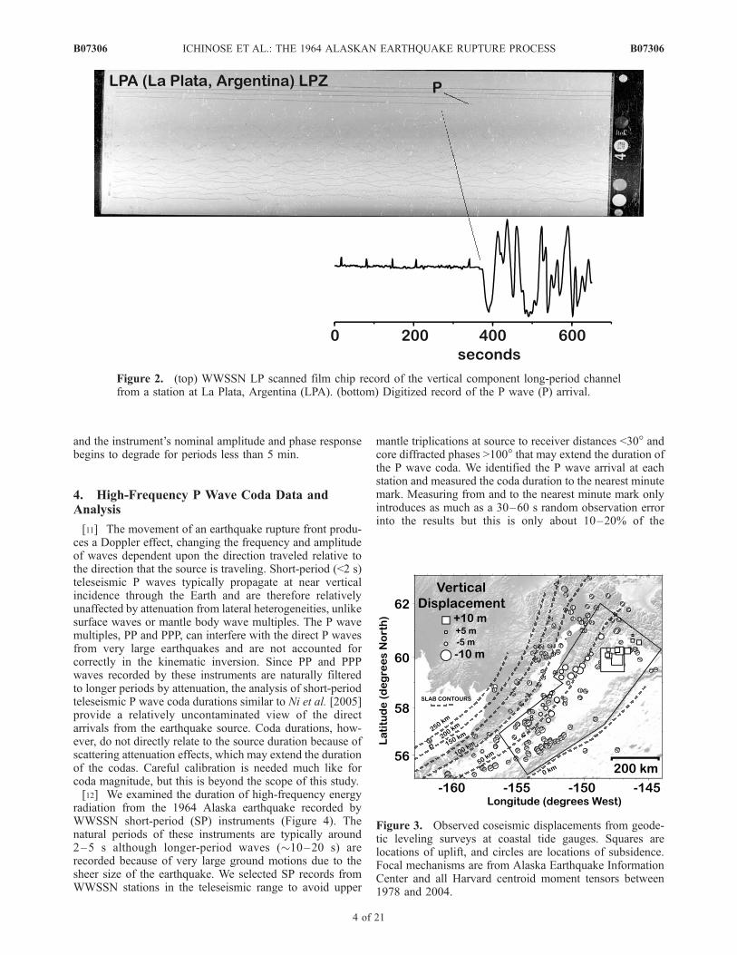
[5] The 28 March 1964 Prince William Sound (PWS),Alaska, earthquake ruptured about 600–800 km startingfrom near Valdez and Anchorage (epicenter at 61!N,147.73!W [Sherburne et al., 1964]), traveling in about aS50!W direction across the Kenai Peninsula, and finallyending at the western side of Kodiak Island. The ruptureprimarily occurred along the subduction zone interface ormegathrust between the Pacific and North American plates[e.g., Hastie and Savage, 1970; Brocher et al., 1994] withsecondary splay faulting observed at Montague and Mid-dleton islands [Plafker, 1965, 1972] causing approximately140,000 to 200,000 km2 of ground deformation, withthe majority of the deformation occurring offshore. Thetotal seismic moment was estimated by Kanamori [1970] at"8 ! 1022 N m (Mw 9.2).[6] The rupture mechanism was initially poorly con-

strained [e.g., Harding and Algermissen, 1969; Stauderand Bollinger, 1966] but was believed to have occurredalong the megathrust. However, sparse first motion polari-ties were used to constrain only the auxiliary plane. Theaddition of geodetic data supported the previous hypothesisthat the main moment release occurred along the megathrust[e.g., Hastie and Savage, 1970]. Kanamori [1970] reex-

amined the radiation pattern of long-period surface waves(R4 and G4) and he found that the earthquake rupturedalong a shallow northwest dipping thrust fault. Ruff andKanamori [1983] inverted attenuated outer-core diffractedP phases from long-period World Wide StandardSeismograph Network (WWSSN LP) records and inferredthat the earthquake ruptured smoothly for the first 120 sacross the Kenai and PWS regions. Other studies identifiedareas of high slip along imbricate thrusts at Montague Island[Plafker, 1965, 1972], and complex rupture [e.g., Wyss andBrune, 1967; Kikuchi and Fukao, 1987] with at least sixsubevents within the first 100 s identified in short-periodseismograms (WWSSN SP). Christensen and Beck [1994]inverted WWSSN LP teleseismic P waves to estimate therough distribution of seismic moment release. They con-firmed that the moment release was initially strong in thePWS region but also identified a second region of largemoment release near Kodiak Island beginning at about180 s. Johnson et al. [1996] inverted tsunami and geodeticdata based on a fault model constructed by Holdahl andSauber [1994] and confirmed that the Kodiak Island regionof large moment release was a robust feature.[7] The plate motion of the Pacific plate relative to the

North American plate is 5–7 cm/yr in a N17!W direction[e.g., DeMets and Dixon, 1999]. This plate motion isaccommodated along a well defined but complex plateinterface [e.g., Brocher et al., 1994] with Wadati-Benioffzone seismicity extending down to approximately 200 kmdepth [e.g., Engdahl et al., 1998]. In the northern Gulf ofAlaska and Prince William Sound there are two majoraccreted terranes: the Prince William terrane and Yakutatterrane. The Yakutat terrane lies under the Prince Williamterrane and both appear to be subducted into the megathrustover the Pacific plate in an oceanic-continental type colli-sion along the slope magnetic anomaly (SMA). Brocher etal. [1994] identified the interface in this region that rupturedin 1964 as the discontinuity between the Yakutat terrane andthe Pacific plate. Only the Prince William terrane overliesthe Pacific plate along the subduction zone from SMA toKodiak Island [von Huene et al., 1999]. In addition to upperplate complexity and trench sediment thickness, von Hueneet al. [1999] also identified several seamounts on the Pacificplate at the latitude of Kodiak Island along the trench, whichmay influence the locking of the two plates over the seismiccycle, including the Kodiak-Bowie seamount chain (Ksm).Zweck et al. [2002] estimated the distribution of platecoupling, fraction of relative plate rate, based on theinversion of GPS data over the last decade. They identifiedtwo locked zones (high coupling > 0.6) off the coast ofKodiak Island and also beneath the Prince William Sound.They also identified a creeping zone (negative coupling)along the Cook Inlet and northern Kenai Peninsula consis-tent with observations of continued 1964 postseismic slipby Freymueller et al. [2000]. There is also an area of lowcoupling between the two locked zones. The locked zonesare coincident with areas of high seismicity along themegathrust and in the upper plate off the coast of KodiakIsland and beneath PWS and low seismicity over zones oflow plate coupling [e.g., Doser et al., 2002; Zweck et al.,2002]. Doser et al. [2002, 2006] also observed differentseismicity patterns between the PWS and KI locked zones.The PWS exhibits down dip migration of seismicity but the

B07306 ICHINOSE ET AL.: THE 1964 ALASKAN EARTHQUAKE RUPTURE PROCESS

2 of 21

B07306

KI region does not exhibit down dip seismicity perhaps dueto the differences in subducted terranes. They estimate themoment release in the KI region since 1964 is also about 5 to10 times higher than in the PWS region. The conditionalprobability for another great earthquake in the PWS area islow (<1%) over the period of 1988–2008 but is slightlyhigher at 11–14% for the Kodiak Island region [Nishenkoand Jacob, 1990] for a 233-year recurrence time. On thebasis of geology and seismicity, the Kodiak ‘‘Katmaisegment’’ should be treated differently from the PWSsegment. Nishenko and Jacob [1990] noted a factor of2 difference in recurrence times between uplifted terraces(1020 years) and submerged forests (425–800 years). Theyhypothesized that the difference may indicate anotherimminent earthquake that would account for the disparity,but remain indistinguishable in the geologic record. Overthe past 40 years, such an earthquake has not yet occurredso a detailed 1964 slip distribution and analysis of post-seismic and aseismic slip may help resolve these differencesin recurrence times.

3. Data

[8] We digitized and skew-corrected World Wide Stan-dard Seismograph Network seismograms [Powell and Fries,1964] scanned from microfiche film chips into gray scalebitmap images (Figures 1 and 2). The records consist oflong-period (LP) ("30–100 s) three component (LPZ,LPN, and LPE) seismograms and short-period (SP) seismo-grams. We collected 35 P waves with the best quality and asmuch as 100 to 200 s duration out of the 575 WWSSN filmchips. We used the GNU software package Engauge todigitize the bitmap images automatically, but the poorquality of most film or paper records required manualcorrections. The records selected were recorded between

40! and 120! epicentral distance. Besides contamination fromPP and PPP arrivals, many P waves were clipped or lost inoverlying and overlapping traces before 270 s; thereforeadditional constraints from tsunami and geodesy were nec-essary to construct a more complete picture of the ruptureprocess.[9] In an effort to revise the tidal datum planes and charts

a survey was made by the Coast and Geodetic Survey torecord the tidal datum plane changes resulting from the1964 earthquake (Figure 3). Out of the 49 sites, 11 siteswere reoccupied in 1964, and 26 locations were reoccupiedin 1965, typically for a duration of 2 months [Small andWharton, 1969]. Sitka, Alaska, was the nearest control tidegauge unaffected by the earthquake. The tidal observationswere reduced to mean values by simultaneous comparisonwith the Sitka control station. There was significant post-seismic deformation observed at two sites, and four sitesindicated insignificant postseismic deformation, while20 stations showed moderate postseismic deformation.Vertical ground displacements are most sensitive to thelocation and amount of dip slip. Therefore we focus onlyon leveling data to make the amount of data and inversionsmanageable and to avoid data coverage duplications.[10] The Pacific Tsunami Warning System consists of

analog tide gauge instruments located around the PacificOcean. The tsunami was well recorded across the Pacificand as far as New Zealand and Chile. We selected an evendistribution of nine stations closest to the source region. Wecorrected digitized tide gauge data for lunar tides by firstfitting a polynomial to a data window of interest and thensubtracting the polynomial from the data. Any other tran-sients with periods greater than several hours were Fourierfiltered from the residual time series. The records werearbitrarily decimated at 2-min intervals because tide gaugeinstruments usually record at a rate of 1 to 2 min per sample

Figure 1. Map of World Wide Standard Seismograph Network (WWSSN) and tide gauge stations usedin this analysis of the 1964 Prince William Sound, Alaska, earthquake.


3 of 21

B07306

and the instrument’s nominal amplitude and phase responsebegins to degrade for periods less than 5 min.

4. High-Frequency P Wave Coda Data andAnalysis

[11] The movement of an earthquake rupture front produ-ces a Doppler effect, changing the frequency and amplitudeof waves dependent upon the direction traveled relative tothe direction that the source is traveling. Short-period (<2 s)teleseismic P waves typically propagate at near verticalincidence through the Earth and are therefore relativelyunaffected by attenuation from lateral heterogeneities, unlikesurface waves or mantle body wave multiples. The P wavemultiples, PP and PPP, can interfere with the direct P wavesfrom very large earthquakes and are not accounted forcorrectly in the kinematic inversion. Since PP and PPPwaves recorded by these instruments are naturally filteredto longer periods by attenuation, the analysis of short-periodteleseismic P wave coda durations similar to Ni et al. [2005]provide a relatively uncontaminated view of the directarrivals from the earthquake source. Coda durations, how-ever, do not directly relate to the source duration because ofscattering attenuation effects, which may extend the durationof the codas. Careful calibration is needed much like forcoda magnitude, but this is beyond the scope of this study.[12] We examined the duration of high-frequency energy

radiation from the 1964 Alaska earthquake recorded byWWSSN short-period (SP) instruments (Figure 4). Thenatural periods of these instruments are typically around2–5 s although longer-period waves ("10–20 s) arerecorded because of very large ground motions due to thesheer size of the earthquake. We selected SP records fromWWSSN stations in the teleseismic range to avoid upper

mantle triplications at source to receiver distances <30! andcore diffracted phases >100! that may extend the duration ofthe P wave coda. We identified the P wave arrival at eachstation and measured the coda duration to the nearest minutemark. Measuring from and to the nearest minute mark onlyintroduces as much as a 30–60 s random observation errorinto the results but this is only about 10–20% of the

Figure 3. Observed coseismic displacements from geode-tic leveling surveys at coastal tide gauges. Squares arelocations of uplift, and circles are locations of subsidence.Focal mechanisms are from Alaska Earthquake InformationCenter and all Harvard centroid moment tensors between1978 and 2004.

Figure 2. (top) WWSSN LP scanned film chip record of the vertical component long-period channelfrom a station at La Plata, Argentina (LPA). (bottom) Digitized record of the P wave (P) arrival.


4 of 21

B07306

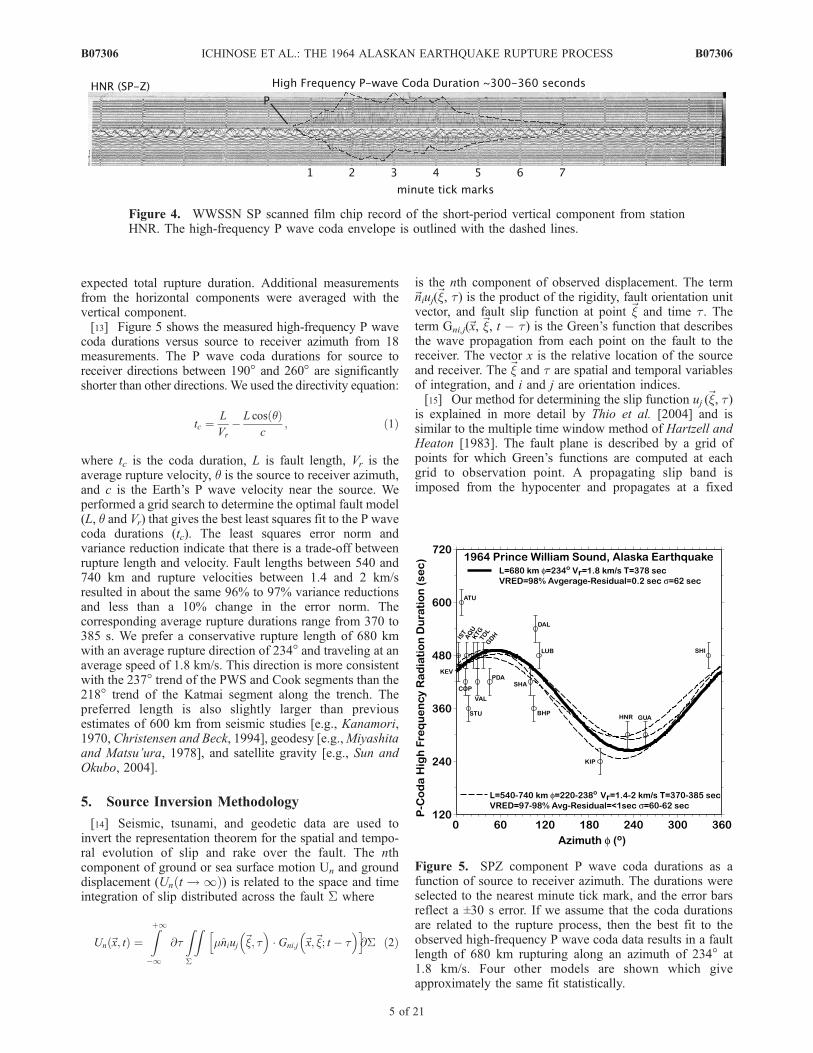
expected total rupture duration. Additional measurementsfrom the horizontal components were averaged with thevertical component.[13] Figure 5 shows the measured high-frequency P wave

coda durations versus source to receiver azimuth from 18measurements. The P wave coda durations for source toreceiver directions between 190! and 260! are significantlyshorter than other directions. We used the directivity equation:

tc #L

Vr$ L cos q% &

c; %1&

where tc is the coda duration, L is fault length, Vr is theaverage rupture velocity, q is the source to receiver azimuth,and c is the Earth’s P wave velocity near the source. Weperformed a grid search to determine the optimal fault model(L, q and Vr) that gives the best least squares fit to the P wavecoda durations (tc). The least squares error norm andvariance reduction indicate that there is a trade-off betweenrupture length and velocity. Fault lengths between 540 and740 km and rupture velocities between 1.4 and 2 km/sresulted in about the same 96% to 97% variance reductionsand less than a 10% change in the error norm. Thecorresponding average rupture durations range from 370 to385 s. We prefer a conservative rupture length of 680 kmwith an average rupture direction of 234! and traveling at anaverage speed of 1.8 km/s. This direction is more consistentwith the 237! trend of the PWS and Cook segments than the218! trend of the Katmai segment along the trench. Thepreferred length is also slightly larger than previousestimates of 600 km from seismic studies [e.g., Kanamori,1970, Christensen and Beck, 1994], geodesy [e.g.,Miyashitaand Matsu’ura, 1978], and satellite gravity [e.g., Sun andOkubo, 2004].

5. Source Inversion Methodology

[14] Seismic, tsunami, and geodetic data are used toinvert the representation theorem for the spatial and tempo-ral evolution of slip and rake over the fault. The nthcomponent of ground or sea surface motion Un and grounddisplacement (Un t ! 1% &) is related to the space and timeintegration of slip distributed across the fault S where

Un ~x; t% & #Z

'1

$1

@tZ

S

Z

mniuj ~x; t! "

( Gni;j ~x;~x; t $ t! "h i

@S %2&

is the nth component of observed displacement. The term~niuj(~x, t) is the product of the rigidity, fault orientation unitvector, and fault slip function at point ~x and time t. Theterm Gni,j(~x,~x, t $ t) is the Green’s function that describesthe wave propagation from each point on the fault to thereceiver. The vector x is the relative location of the sourceand receiver. The~x and t are spatial and temporal variablesof integration, and i and j are orientation indices.[15] Our method for determining the slip function uj (~x, t)

is explained in more detail by Thio et al. [2004] and issimilar to the multiple time window method of Hartzell andHeaton [1983]. The fault plane is described by a grid ofpoints for which Green’s functions are computed at eachgrid to observation point. A propagating slip band isimposed from the hypocenter and propagates at a fixed

Figure 4. WWSSN SP scanned film chip record of the short-period vertical component from stationHNR. The high-frequency P wave coda envelope is outlined with the dashed lines.

Figure 5. SPZ component P wave coda durations as afunction of source to receiver azimuth. The durations wereselected to the nearest minute tick mark, and the error barsreflect a ±30 s error. If we assume that the coda durationsare related to the rupture process, then the best fit to theobserved high-frequency P wave coda data results in a faultlength of 680 km rupturing along an azimuth of 234! at1.8 km/s. Four other models are shown which giveapproximately the same fit statistically.


5 of 21

B07306

number of time steps. This slip band is characterized by twoparameters, maximum rupture velocity and risetime. Gridpoints that are contained within a slip band, at each timestep, are combined and cast into a set of normal equations ofthe form Ax = b, where A contains the Green’s functionsfrom every grid point to every station, x is the solutionvector containing the slip value at every grid point, and b isthe vector containing all the data. The normal equation issolved simultaneously using a least squares solver with apositivity constraint to prohibit reverse slip [Lawson andHanson, 1974]. Regularization and spatial smoothing areapplied to prevent wildly oscillating solutions. This isachieved by imposing a smoothing condition in which theamplitude of slip at one point is forced to be equal to itsneighbors. Lower smoothing will lead to models withvarying complexity and larger values of smoothing willlead to models with uniform slip.[16] Thio et al. [2004] allow for variable rake, in which

case every original rake is split into two conjugate vectorswhere the new rake angles are different from the original by±45! so that the same positivity constraint can be used. Thefinal rake vector is the vector summation of the twoindividual rake vectors. Allowing for variable rake thusleads to a doubling of the number of unknowns, so we needto regularize the two slip vectors to prevent strong, unphys-ical variation in rake. This is achieved in a manner analo-gous to the spatial smoothing, where instead of forcing theamplitude of a slip vector to be equal to its neighbors, weforce it to be equal to its conjugate slip vector. In this case, astrong smoothing constraint will cause the two conjugatevectors to become equal, and thus yield the orientation ofthe initial single rake vector.[17] We imposed a weighting scheme that uses overall

weight per data type and, within each group, an automaticweighting based on the absolute amplitude and number ofpoints [e.g., Thio et al., 2004]. This was made to prevent thecontribution of one data set from dominating the solution,especially in the case of greatly varying amplitudes andsample lengths. Many of the inversion weighting parame-ters, including those for slip and rake smoothing, wereselected on the basis of trial and error.[18] The teleseismic body wave Green’s functions are

computed using the Haskell propagator matrix methoddescribed by Bouchon [1976] and Haskell [1960, 1962].We account for attenuation using a t* of 1 s for P waves andt* of 4 s for S waves [Langston and Helmberger, 1975]. Theattenuation operator t* = t/Q, where t is traveltime and Q isquality factor, integrated over the travel path. We digitized

the three-component displacement seismograms recordedby WWSSN LP 15–90 s electrodynamic seismographs. Theinstrument responses were convolved into the Greens func-tions to avoid instabilities resulting from deconvolution ofdigitized data. We used the calibrated PS-9 velocity model(Table 1) with layered P and S wave velocities and densitiesoriginally developed for the Pacific Northwest based on theanalysis of teleseismic P waves [e.g., Baker and Langston,1987], which was later modified by Ichinose et al. [2006]using regional body waves in an iterative waveform inver-sion method [e.g., Ichinose et al., 2005].[19] The vertical coseismic displacement Green’s func-

tions for the inversion of the leveling data were computedusing a frequency–wave number summation method and aone-dimensional layered Earth model [Zeng and Anderson,1995]. The calibrated PS-9 model, which was used for thesource region in the calculation of the teleseismic P waveGreen’s functions, was also used here. Typically, a half-space is used to compute surface coseismic displacements,but using a layered model is more realistic because thedisplacements are usually larger due to lower velocities nearthe surface, higher velocities at the source, and the interac-tion of the waves from a multilayered model [e.g., Wald andGraves, 2001].[20] The tsunami Green’s functions were computed using

the staggered grid finite difference (FD) method to solve forthe nonlinear hydrodynamic wave equation [Satake, 1995].The FD method was modified to include a nested variablegrid refinement. We selected a large region of the northernPacific just encompassing the earthquake and tide gaugelocations using a 2 ! 2 arc min ("3.7 km) bathymetry grid.We refined the bathymetry to 30 ! 30 arc sec ("0.93 km)for a 1 ! 1! area surrounding the tide gauge stations. Forcomparison, Johnson et al. [1996] used a 5 ! 5 arc min gridfor the open ocean and 1 ! 1 arc min grid for the tide gaugesites.[21] The FD calculations were performed for each of the

97 subfaults assuming a base slip and scalar seismicmoment at each station. The computational time step wasset to 1 s and the Green’s function time length was 9 hours.The vertical deformation from each subfault was firstcomputed using the equations of Okada [1992] for elastichalf-space and then used as input in the FD calculations asthe initial sea surface height changes. The Green’s functionswere low-pass filtered to simulate the response of ananalog tide gauge instrument and then arbitrarily decimatedto 120 s.[22] Figure 6 shows the root mean square of tsunami

amplitudes calculated from the Green’s function time his-tories for a unit response equivalent to an Mw 5.8 event oneach subfault at four different tide gauge stations. TheYakutat station just south and east of the rupture zone ismost sensitive to slip along the continental shelf and slopeportion of the PWS and Cook segments. The Sitka station issouth of Yakutat is also most sensitive to slip along similarareas although it has high sensitivity to slip along theKatmai segment. Avila Beach in central California has mostof its sensitivity to slip along the Katmai segment particu-larly along the sedimentary wedge. Kauai is not as sensitiveto slip distribution as the other stations because of itsposition relative to the tsunami radiation pattern. Sitesfurther to the east including Adak, Unalaska and Hilo also

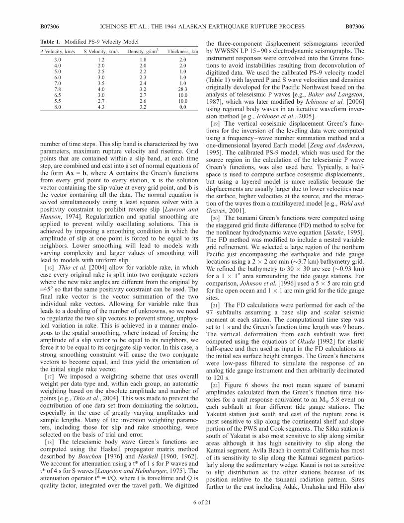
Table 1. Modified PS-9 Velocity Model

P Velocity, km/s S Velocity, km/s Density, g/cm3 Thickness, km

3.0 1.2 1.8 2.04.0 2.0 2.0 2.05.0 2.5 2.2 1.06.0 3.0 2.3 1.07.0 3.5 2.4 1.07.8 4.0 3.2 28.36.5 3.0 2.7 10.05.5 2.7 2.6 10.08.0 4.3 3.2 0.0


6 of 21

B07306

have a similar response that is dependent more upon siteconditions and best for measuring tsunami magnitudes butnot slip distributions. The tsunami energy propagates mostlyperpendicular to the direction of fault strike so that nearly all

of its energy is directed to the Pacific west coast of Alaska,Canada, and California. The pattern of these unit responsesare also somewhat sensitive to water depth above the source

Figure 6. Root-mean-square of tsunami amplitudes from the Green’s function time histories for a unitresponse equivalent to a Mw 5.8 event on each subfault at four different tide gauge stations.

Figure 7. We developed a two-segment fault model, the Prince William Sound and Kodiak Islandsegments. The segments are composed of subfaults with dimensions of 50 by 50 km. See Table 2 forsubfault descriptions.


7 of 21

B07306

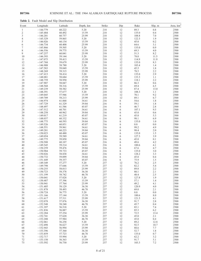
Table 2. Fault Model and Slip Distribution

Event Longitude Latitude Depth, km Strike Dip Rake Slip, m Area, km2

1 $144.779 60.222 5.20 218 12 89.3 0.8 25002 $145.484 60.492 15.59 218 12 135.0 0.4 25003 $146.201 60.757 25.99 218 12 108.8 7.0 25004 $145.329 59.865 5.20 218 12 122.3 1.9 25005 $146.026 60.134 15.59 218 12 45.0 0.2 25006 $146.734 60.400 25.99 218 12 64.6 3.1 25007 $145.866 59.505 5.20 218 12 135.0 0.9 25008 $146.556 59.775 15.59 218 12 69.3 4.0 25009 $147.257 60.041 25.99 218 12 51.3 8.2 250010 $146.393 59.144 5.20 218 12 78.0 11.5 250011 $147.075 59.413 15.59 218 12 114.9 11.9 250012 $147.768 59.679 25.99 218 12 135.0 8.3 250013 $146.908 58.780 5.20 218 12 103.4 1.4 250014 $147.583 59.049 15.59 218 12 45.5 1.8 250015 $148.269 59.315 25.99 218 12 78.5 2.2 250016 $147.413 58.414 5.20 218 12 135.0 2.9 250017 $148.081 58.684 15.59 218 12 133.3 1.1 250018 $148.759 58.950 25.99 218 12 118.1 2.2 250019 $147.907 58.047 5.20 218 12 86.3 0.6 250020 $148.568 58.316 15.59 218 12 69.4 6.5 250021 $149.239 58.582 25.99 218 12 87.4 13.0 250022 $148.391 57.677 5.20 218 12 108.3 1.1 250023 $149.045 57.946 15.59 218 12 70.1 9.2 250024 $149.709 58.213 25.99 218 12 89.1 6.7 250025 $146.974 61.068 34.61 216 6 54.6 1.8 250026 $147.729 61.329 39.84 216 6 59.1 1.8 250027 $148.497 61.586 45.07 216 6 46.7 2.8 250028 $147.512 60.701 34.61 216 6 107.1 9.5 250029 $148.258 60.962 39.84 216 6 45.0 0.6 250030 $149.017 61.219 45.07 216 6 45.0 5.3 250031 $148.037 60.332 34.61 216 6 98.1 6.9 250032 $148.775 60.593 39.84 216 6 135.0 1.0 250033 $149.526 60.851 45.07 216 6 0.0 0.0 250034 $148.551 59.961 34.61 216 6 99.2 4.9 250035 $149.281 60.223 39.84 216 6 98.4 2.0 250036 $150.023 60.480 45.07 216 6 135.0 1.5 250037 $149.054 59.589 34.61 216 6 127.3 3.9 250038 $149.775 59.850 39.84 216 6 45.0 0.1 250039 $150.508 60.107 45.07 216 6 49.6 4.2 250040 $149.545 59.214 34.61 216 6 100.6 4.1 250041 $150.259 59.476 39.84 216 6 67.6 4.7 250042 $150.984 59.733 45.07 216 6 135.0 3.0 250043 $150.026 58.838 34.61 216 6 128.2 3.3 250044 $150.732 59.099 39.84 216 6 45.0 0.4 250045 $151.449 59.357 45.07 216 6 75.9 1.5 250046 $149.349 57.277 5.20 237 12 76.2 2.5 250047 $149.798 57.646 15.59 237 12 82.2 5.4 250048 $150.255 58.013 25.99 237 12 89.8 2.2 250049 $150.723 58.378 36.38 237 12 80.1 2.1 250050 $151.199 58.742 46.78 237 12 48.4 2.5 250051 $150.041 57.028 5.20 237 12 127.8 1.9 250052 $150.487 57.396 15.59 237 12 57.1 1.4 250053 $150.941 57.764 25.99 237 12 49.2 4.1 250054 $151.405 58.129 36.38 237 12 120.9 4.0 250055 $151.878 58.493 46.78 237 12 69.0 2.1 250056 $150.724 56.775 5.20 237 12 0.0 0.0 250057 $151.166 57.144 15.59 237 12 100.6 8.0 250058 $151.617 57.511 25.99 237 12 121.5 4.1 250059 $152.078 57.876 36.38 237 12 91.7 2.8 250060 $152.548 58.240 46.78 237 12 45.7 0.4 250061 $151.397 56.518 5.20 237 12 85.1 7.4 250062 $151.836 56.887 15.59 237 12 85.3 6.2 250063 $152.284 57.254 25.99 237 12 72.5 13.4 250064 $152.741 57.620 36.38 237 12 45.0 2.1 250065 $153.208 57.984 46.78 237 12 45.0 0.4 250066 $152.061 56.258 5.20 237 12 89.2 12.8 250067 $152.498 56.627 15.59 237 12 92.5 10.7 250068 $152.943 56.994 25.99 237 12 88.6 7.7 250069 $153.396 57.360 36.38 237 12 52.7 1.8 250070 $153.859 57.723 46.78 237 12 135.0 0.7 250071 $152.717 55.994 5.20 237 12 62.2 3.2 250072 $153.150 56.363 15.59 237 12 91.7 5.1 250073 $153.592 56.730 25.99 237 12 103.3 7.2 2500


8 of 21

B07306

although radiation pattern is the most significant and isconsidered in weighting of the data in the inversion.

6. Fault Model and Rupture Parameters

[23] We constructed a four-segment fault model for the1964 PWS earthquake using a subfault dimension of 50 !50 km. The up dip portion of the subduction zone isassigned a dip of 12!. The portion of the PWS segmentunderlain by the Yakutat terrane appears to have a shallowerdip, which we assign as 6! [e.g., Brocher et al., 1994]. We

placed the transition along the Montague Islands andincluded the Patton Bay imbricate thrust fault between thetwo subduction zone segments assuming a dip of 60![Plafker, 1965, 1972]. The Katmai or Kodiak segment wasassigned a dip of 12!. The Prince William Sound and KodiakIsland segments are made up of 85 subfaults and have acombined area of 212,500 km2 (Figure 7). The Patton Bayimbricate thrust consists of 7 subfaults with dimensions of20 by 20 km along a 140 km length. The depth andorientation of this fault model were constrained to theapproximate slab contours estimated by Gudmundsson and

Table 2. (continued)

Event Longitude Latitude Depth, km Strike Dip Rake Slip, m Area, km2

74 $154.042 57.096 36.38 237 12 98.1 3.5 250075 $154.501 57.460 46.78 237 12 0.0 0.0 250076 $153.363 55.727 5.20 237 12 63.9 2.6 250077 $153.793 56.096 15.59 237 12 83.6 5.8 250078 $154.232 56.463 25.99 237 12 77.1 4.7 250079 $154.679 56.829 36.38 237 12 45.0 2.2 250080 $155.135 57.193 46.78 237 12 130.7 0.4 250081 $154.000 55.457 5.20 237 12 0.0 0.0 250082 $154.428 55.825 15.59 237 12 0.0 0.0 250083 $154.863 56.193 25.99 237 12 84.2 0.5 250084 $155.307 56.558 36.38 237 12 127.9 0.2 250085 $155.759 56.922 46.78 237 12 135.0 0.9 250086 $147.011 60.394 8.66 218 60 65.0 2.6 40087 $147.232 60.251 8.66 218 60 45.0 4.4 40088 $147.452 60.107 8.66 218 60 83.0 2.6 40089 $147.669 59.963 8.66 218 60 48.5 9.9 40090 $147.884 59.819 8.66 218 60 124.4 17.4 40091 $148.098 59.675 8.66 218 60 127.6 5.6 40092 $148.309 59.530 8.66 218 60 117.5 4.0 40093 $148.519 59.385 8.66 218 60 55.4 1.3 40094 $148.727 59.239 8.66 218 60 76.8 2.1 40095 $148.934 59.093 8.66 218 60 118.8 0.8 400

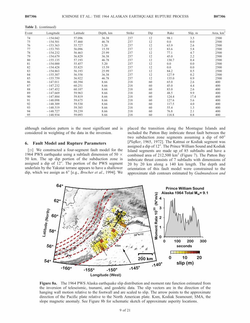
Figure 8a. The 1964 PWS Alaska earthquake slip distribution and moment rate function estimated fromthe inversion of teleseismic, tsunami, and geodetic data. The slip vectors are in the direction of thehanging wall motion relative to the footwall and are scaled to slip. The arrow points to the approximatedirection of the Pacific plate relative to the North American plate. Ksm, Kodiak Seamount; SMA, theslope magnetic anomaly. See Figure 8b for schematic sketch of approximate asperity locations.


9 of 21

B07306

Sambridge [1998] from International Seismological Centre(ISC) catalogs and relocated seismicity by Engdahl et al.[1998]. Relocation of earthquakes locally by Ratchkovskiand Hansen [2002] and Flores and Doser [2005] suggestthat the slab contours are shifted by 50 km for the Kodiakregion and by100 km for the PWS region. The slab contourby Plafker [1972] puts the slab interface about 10 kmshallower in the PWS region. The detailed fault model islisted in detail in Table 2.[24] For the kinematic rupture model parameters we used

54 time windows at 5 s increments. The risetime can varyfrom 5 to 25 s, so a particular subfault can rupture from 1 to 5time windows after the passage of the rupture front. The slipat each time step is summed using a triangle slip functionwith 5 s rise and 5 s fall. The range of risetime and trianglefunction duration was chosen based on making the best fit tothe frequency content of the teleseismic data recorded byWWSSN LP instruments and on the subfault dimension. Therupture velocity is limited to less than 2.7 km/s. This upperlimit appears reasonable because the analysis of the 2004Sumatra earthquake by Guilbert et al. [2005] suggests arupture velocity between 2.7 and 2 km/s using hydroacousticdata.Additionally, in section 5, the analysis of high-frequencyP wave coda of the 1964 Alaska earthquake suggests anaverage between 1.8 and 2 km/s. We do not include subfaultdynamics in the Green’s functions because of the poor

quality of data and lack of near source strong ground motiondata.

7. Results

[25] We inverted 24 teleseismic P waves, 9 tsunami tidegauge records, and 49 leveling observations for the spatialand temporal distribution of slip and rake. We first invertedall of the data sets simultaneously to make a preferredrupture model (Figure 8a). We will discuss the sensitivity ofthe inversion results with only 1 or 2 data sets in theDiscussion section. The hypocenter is fixed from the ISCcatalog and placed on the nearest subfault (60.7!N,147.512!W), which is at a depth of 35 km. We obtain atotal seismic moment of 5.52 ! 1022 N m for the preferredrupture model (Table 3). The peak slip is about 15 m alongthe megathrust and the PBF has a peak slip of 17.4 m nearthe location of the largest uplift ("10 m) observed byPlafker [1965, 1972] on the western edge of MontagueIsland. Overall the average slip is about 5 m.[26] We identify three regions of major seismic moment

release or asperities (i.e., regions of high fault slip) definedin Table 3 as subfaults with slip equal to or more than twicethe average. The first region has about 11 m of slip andextends about 5000 km2 across the PWS segment (M1 inFigure 8b). The asperity starts about 50 km offshore from

Figure 8b. Schematic sketch of the asperity map for Figure 8a. We identify three asperities M1, M2,and M3. The earthquake ruptured three subduction zone fault segments, the Prince William Sound(PWS), Cook, and Katmai. Rupture did not extend into the Semidi segment. P wave arrivals identified byWyss and Brune [1967] are labeled (A, B, C, X, Y, and Z). The slip vectors are in the direction of thehanging wall motion relative to the footwall and are scaled to slip. The arrow points to the approximatedirection of the Pacific plate relative to the North American plate. Ksm, Kodiak-Bowie Seamount chain;SMA, the approximate location of the slope magnetic anomaly. The subducting slab is contoured at 50 kmintervals.


10 of 21

B07306

Montague Island, passes beneath Middleton Island andextends to the sedimentary wedge. The area of this asperityappears correlated with the slope magnetic anomaly, wherethe Yakutat and Prince William terranes are subductingtogether above the Pacific plate [e.g., Brocher et al.,1994]. The second asperity is confined to the Cook segment(M2 in Figure 8b) and is located beneath a raised portion ofthe continental slope along the Portlock anticline extendingto about only 50 km from the trench. The area is alsoapproximately 5000 km2 and has a slip between 10 and13 m. The location of this asperity appears to be on the slabwhere the 58!N fracture zone and Kodiak-Bowie seamountchain intersect. The third asperity is located off the southerncoast of Kodiak Island on the Katmai segment and extendstoward the trench (M3 in Figure 8b). The area ranges from7500 km2 for 13 m slip included in a broader area ofapproximately encompassing 22500 km2 with 9 m of slip.These 3 major asperities are all located shallower than the50 km depth contour and collocated with zones of 1-dayaftershock activity (M > 4) after the 1964 earthquake fromthe ISC catalog. The moment rate function (Figure 8a)shows that our estimate of the rupture duration for the firstasperity (M1) is about 160 s, compared to the 120 s durationestimated by Ruff and Kanamori [1983] and Christensenand Beck [1994].[27] The slip vectors (Figures 8a and 8b) or the motion of

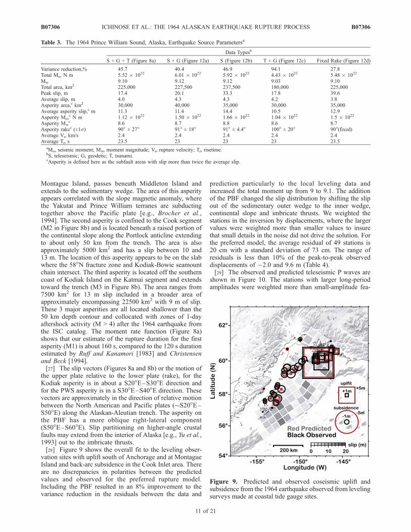
the upper plate relative to the lower plate (rake), for theKodiak asperity is in about a S20!E–S30!E direction andfor the PWS asperity is in a S30!E–S40!E direction. Thesevectors are approximately in the direction of relative motionbetween the North American and Pacific plates ("S20!E–S50!E) along the Alaskan-Aleutian trench. The asperity onthe PBF has a more oblique right-lateral component(S50!E–S60!E). Slip partitioning on higher-angle crustalfaults may extend from the interior of Alaska [e.g., Yu et al.,1993] out to the imbricate thrusts.[28] Figure 9 shows the overall fit to the leveling obser-

vation sites with uplift south of Anchorage and at MontagueIsland and back-arc subsidence in the Cook Inlet area. Thereare no discrepancies in polarities between the predictedvalues and observed for the preferred rupture model.Including the PBF resulted in an 8% improvement to thevariance reduction in the residuals between the data and

prediction particularly to the local leveling data andincreased the total moment up from 9 to 9.1. The additionof the PBF changed the slip distribution by shifting the slipout of the sedimentary outer wedge to the inner wedge,continental slope and imbricate thrusts. We weighted thestations in the inversion by displacements, where the largervalues were weighted more than smaller values to insurethat small details in the noise did not drive the solution. Forthe preferred model, the average residual of 49 stations is20 cm with a standard deviation of 73 cm. The range ofresiduals is less than 10% of the peak-to-peak observeddisplacements of $2.0 and 9.6 m (Table 4).[29] The observed and predicted teleseismic P waves are

shown in Figure 10. The stations with larger long-periodamplitudes were weighted more than small-amplitude fea-

Figure 9. Predicted and observed coseismic uplift andsubsidence from the 1964 earthquake observed from levelingsurveys made at coastal tide gauge sites.

Table 3. The 1964 Prince William Sound, Alaska, Earthquake Source Parametersa

Data Typesb

S + G + T (Figure 8a) S + G (Figure 12a) S (Figure 12b) T + G (Figure 12c) Fixed Rake (Figure 12d)

Variance reduction,% 45.7 40.4 46.9 94.1 27.8Total Mo, N m 5.52 ! 1022 6.01 ! 1022 5.92 ! 1022 4.43 ! 1022 5.48 ! 1022

Mw 9.10 9.12 9.12 9.03 9.10Total area, km2 225,000 227,500 237,500 180,000 225,000Peak slip, m 17.4 20.1 33.3 17.8 39.6Average slip, m 4.0 4.3 4.3 4.2 3.8Asperity area,c km2 30,000 40,000 35,000 30,000 35,000Average asperity slip,c m 11.3 11.4 14.4 10.5 12.9Asperity Mo,

c N m 1.12 ! 1022 1.50 ! 1022 1.66 ! 1022 1.04 ! 1022 1.5 ! 1022

Asperity Mwc 8.6 8.7 8.8 8.6 8.7

Asperity rakec (±1s) 90! ± 27! 91! ± 18! 91! ± 4.4! 100! ± 20! 90!(fixed)Average Vr, km/s 2.4 2.4 2.4 2.4 2.4Average Tr, s 23.5 23 23 23 23.5

aMo, seismic moment; Mw, moment magnitude; Vr, rupture velocity; Tr, risetime.bS, teleseismic; G, geodetic; T, tsunami.cAsperity is defined here as the subfault areas with slip more than twice the average slip.


11 of 21

B07306

tures. This was done to avoid fitting small-scale featuresthat are probably strongly dependent on fine details of Earthstructure, which were not adequately modeled. The dataweighting and smoothing features were balanced so thepredictions best fit data and yet produced a solution that isrelatively smooth in slip and rake.[30] We performed two inversions: (1) with linear shallow

water Green’s functions and (2) with nonlinear shallow anddeep water Green’s functions. The linear Green’s functionsdo not include complex nearshore shoaling and onshorerunup effects. In this case we also did not refine thebathymetric resolution near the tide gauge stations. Theinversions performed with nonlinear Green’s functionsincluded moving land-water boundary conditions and gridrefinement near the stations.

[31] The observed and predicted tsunami tide gaugerecords were fit poorly at Yakutat and Sitka when usingthe course grid and linear Green’s function calculations(Figure 11). Low-resolution bathymetric and topographicgrids result in an incorrect location and water depth for thereceiver relative to its true reported position for these twocases. The linear calculations also tend to over predict theamplitudes and shift wave energy to longer periods for thenearshore zone because water-land boundary conditions areunrealistically fixed. A course grid was adequate for Adakand Avila Beach due to more simple coastal geometries.Using a high-resolution grid for the entire simulation area isinefficient since the higher resolution is only needed nearthe tide gauge site. Therefore we used a nested gridrefinement approach to calculate the Green’s functions in

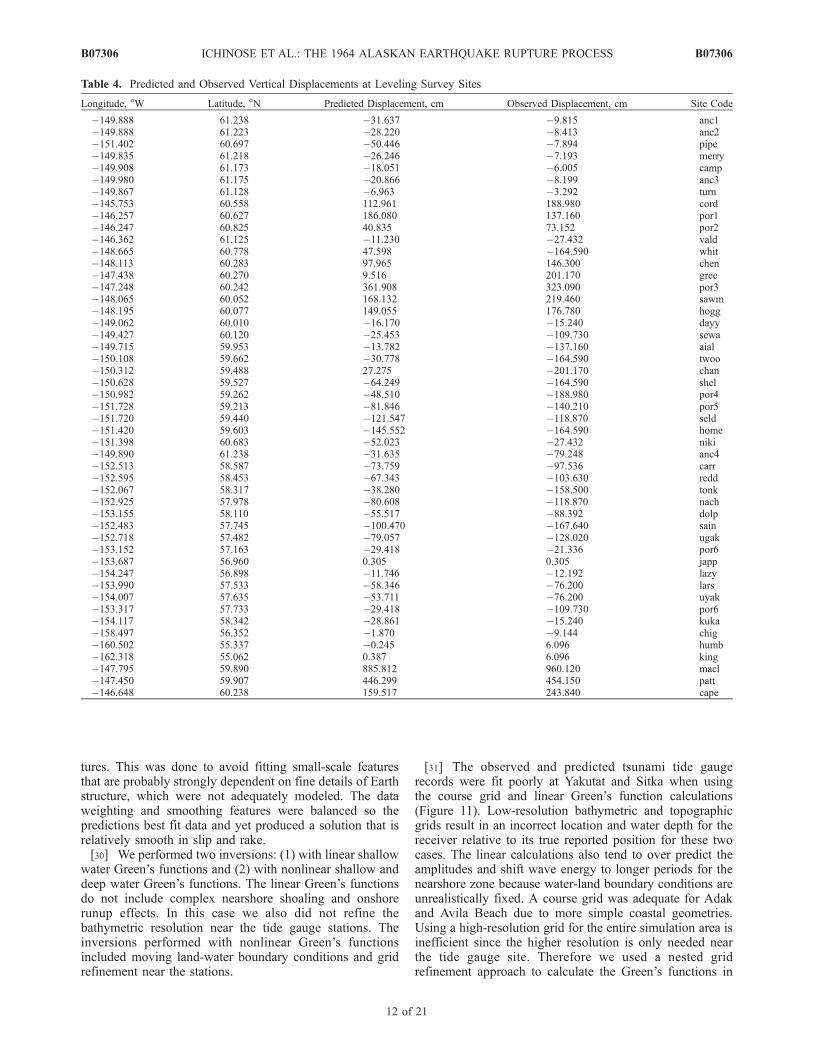
Table 4. Predicted and Observed Vertical Displacements at Leveling Survey Sites

Longitude, !W Latitude, !N Predicted Displacement, cm Observed Displacement, cm Site Code

$149.888 61.238 $31.637 $9.815 anc1$149.888 61.223 $28.220 $8.413 anc2$151.402 60.697 $50.446 $7.894 pipe$149.835 61.218 $26.246 $7.193 merry$149.908 61.173 $18.051 $6.005 camp$149.980 61.175 $20.866 $8.199 anc3$149.867 61.128 $6.963 $3.292 turn$145.753 60.558 112.961 188.980 cord$146.257 60.627 186.080 137.160 por1$146.247 60.825 40.835 73.152 por2$146.362 61.125 $11.230 $27.432 vald$148.665 60.778 47.598 $164.590 whit$148.113 60.283 97.965 146.300 chen$147.438 60.270 9.516 201.170 gree$147.248 60.242 361.908 323.090 por3$148.065 60.052 168.132 219.460 sawm$148.195 60.077 149.055 176.780 hogg$149.062 60.010 $16.170 $15.240 dayy$149.427 60.120 $25.453 $109.730 sewa$149.715 59.953 $13.782 $137.160 aial$150.108 59.662 $30.778 $164.590 twoo$150.312 59.488 27.275 $201.170 chan$150.628 59.527 $64.249 $164.590 shel$150.982 59.262 $48.510 $188.980 por4$151.728 59.213 $81.846 $140.210 por5$151.720 59.440 $121.547 $118.870 seld$151.420 59.603 $145.552 $164.590 home$151.398 60.683 $52.023 $27.432 niki$149.890 61.238 $31.635 $79.248 anc4$152.513 58.587 $73.759 $97.536 carr$152.595 58.453 $67.343 $103.630 redd$152.067 58.317 $38.280 $158.500 tonk$152.925 57.978 $80.608 $118.870 nach$153.155 58.110 $55.517 $88.392 dolp$152.483 57.745 $100.470 $167.640 sain$152.718 57.482 $79.057 $128.020 ugak$153.152 57.163 $29.418 $21.336 por6$153.687 56.960 0.305 0.305 japp$154.247 56.898 $11.746 $12.192 lazy$153.990 57.533 $58.346 $76.200 lars$154.007 57.635 $53.711 $76.200 uyak$153.317 57.733 $29.418 $109.730 por6$154.117 58.342 $28.861 $15.240 kuka$158.497 56.352 $1.870 $9.144 chig$160.502 55.337 $0.245 6.096 humb$162.318 55.062 0.387 6.096 king$147.795 59.890 885.812 960.120 macl$147.450 59.907 446.299 454.150 patt$146.648 60.238 159.517 243.840 cape


12 of 21

B07306

Figure 10. Teleseismic P waves.


13 of 21

B07306

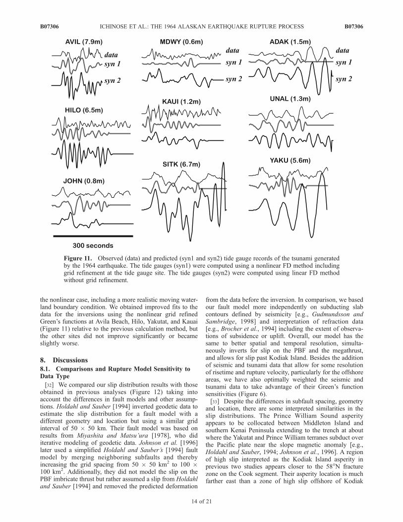
the nonlinear case, including a more realistic moving water-land boundary condition. We obtained improved fits to thedata for the inversions using the nonlinear grid refinedGreen’s functions at Avila Beach, Hilo, Yakutat, and Kauai(Figure 11) relative to the previous calculation method, butthe other sites did not improve significantly or becameslightly worse.

8. Discussions8.1. Comparisons and Rupture Model Sensitivity toData Type

[32] We compared our slip distribution results with thoseobtained in previous analyses (Figure 12) taking intoaccount the differences in fault models and other assump-tions. Holdahl and Sauber [1994] inverted geodetic data toestimate the slip distribution for a fault model with adifferent geometry and location but using a similar gridinterval of 50 ! 50 km. Their fault model was based onresults from Miyashita and Matsu’ura [1978], who diditerative modeling of geodetic data. Johnson et al. [1996]later used a simplified Holdahl and Sauber’s [1994] faultmodel by merging neighboring subfaults and therebyincreasing the grid spacing from 50 ! 50 km2 to 100 !100 km2. Additionally, they did not model the slip on thePBF imbricate thrust but rather assumed a slip from Holdahland Sauber [1994] and removed the predicted deformation

from the data before the inversion. In comparison, we basedour fault model more independently on subducting slabcontours defined by seismicity [e.g., Gudmundsson andSambridge, 1998] and interpretation of refraction data[e.g., Brocher et al., 1994] including the extent of observa-tions of subsidence or uplift. Overall, our model has thesame to better spatial and temporal resolution, simulta-neously inverts for slip on the PBF and the megathrust,and allows for slip past Kodiak Island. Besides the additionof seismic and tsunami data that allow for some resolutionof risetime and rupture velocity, particularly for the offshoreareas, we have also optimally weighted the seismic andtsunami data to take advantage of their Green’s functionsensitivities (Figure 6).[33] Despite the differences in subfault spacing, geometry

and location, there are some interpreted similarities in theslip distributions. The Prince William Sound asperityappears to be collocated between Middleton Island andsouthern Kenai Peninsula extending to the trench at aboutwhere the Yakutat and Prince William terranes subduct overthe Pacific plate near the slope magnetic anomaly [e.g.,Holdahl and Sauber, 1994; Johnson et al., 1996]. A regionof high slip interpreted as the Kodiak Island asperity inprevious two studies appears closer to the 58!N fracturezone on the Cook segment. Their asperity location is muchfarther east than a zone of high slip offshore of Kodiak

Figure 11. Observed (data) and predicted (syn1 and syn2) tide gauge records of the tsunami generatedby the 1964 earthquake. The tide gauges (syn1) were computed using a nonlinear FD method includinggrid refinement at the tide gauge site. The tide gauges (syn2) were computed using linear FD methodwithout grid refinement.


14 of 21

B07306

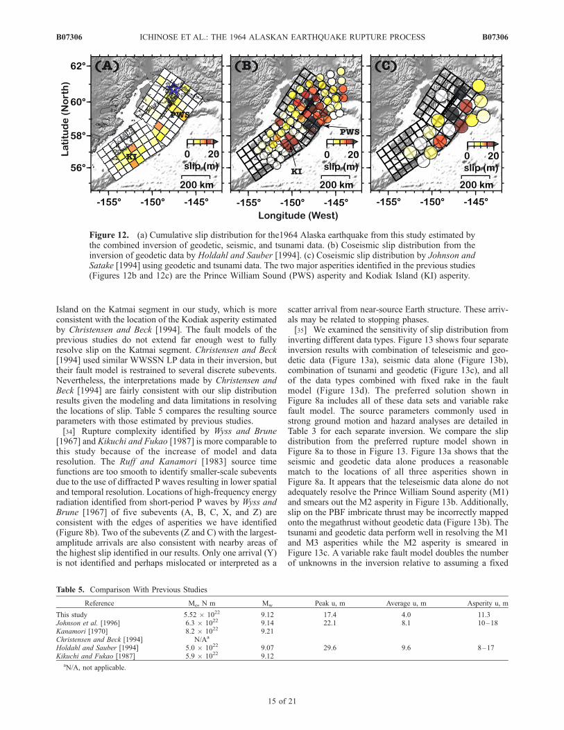
Island on the Katmai segment in our study, which is moreconsistent with the location of the Kodiak asperity estimatedby Christensen and Beck [1994]. The fault models of theprevious studies do not extend far enough west to fullyresolve slip on the Katmai segment. Christensen and Beck[1994] used similar WWSSN LP data in their inversion, buttheir fault model is restrained to several discrete subevents.Nevertheless, the interpretations made by Christensen andBeck [1994] are fairly consistent with our slip distributionresults given the modeling and data limitations in resolvingthe locations of slip. Table 5 compares the resulting sourceparameters with those estimated by previous studies.[34] Rupture complexity identified by Wyss and Brune

[1967] and Kikuchi and Fukao [1987] is more comparable tothis study because of the increase of model and dataresolution. The Ruff and Kanamori [1983] source timefunctions are too smooth to identify smaller-scale subeventsdue to the use of diffracted P waves resulting in lower spatialand temporal resolution. Locations of high-frequency energyradiation identified from short-period P waves by Wyss andBrune [1967] of five subevents (A, B, C, X, and Z) areconsistent with the edges of asperities we have identified(Figure 8b). Two of the subevents (Z and C) with the largest-amplitude arrivals are also consistent with nearby areas ofthe highest slip identified in our results. Only one arrival (Y)is not identified and perhaps mislocated or interpreted as a

scatter arrival from near-source Earth structure. These arriv-als may be related to stopping phases.[35] We examined the sensitivity of slip distribution from

inverting different data types. Figure 13 shows four separateinversion results with combination of teleseismic and geo-detic data (Figure 13a), seismic data alone (Figure 13b),combination of tsunami and geodetic (Figure 13c), and allof the data types combined with fixed rake in the faultmodel (Figure 13d). The preferred solution shown inFigure 8a includes all of these data sets and variable rakefault model. The source parameters commonly used instrong ground motion and hazard analyses are detailed inTable 3 for each separate inversion. We compare the slipdistribution from the preferred rupture model shown inFigure 8a to those in Figure 13. Figure 13a shows that theseismic and geodetic data alone produces a reasonablematch to the locations of all three asperities shown inFigure 8a. It appears that the teleseismic data alone do notadequately resolve the Prince William Sound asperity (M1)and smears out the M2 asperity in Figure 13b. Additionally,slip on the PBF imbricate thrust may be incorrectly mappedonto the megathrust without geodetic data (Figure 13b). Thetsunami and geodetic data perform well in resolving the M1and M3 asperities while the M2 asperity is smeared inFigure 13c. A variable rake fault model doubles the numberof unknowns in the inversion relative to assuming a fixed

Table 5. Comparison With Previous Studies

Reference Mo, N m Mw Peak u, m Average u, m Asperity u, m

This study 5.52 ! 1022 9.12 17.4 4.0 11.3Johnson et al. [1996] 6.3 ! 1022 9.14 22.1 8.1 10–18Kanamori [1970] 8.2 ! 1022 9.21Christensen and Beck [1994] N/Aa

Holdahl and Sauber [1994] 5.0 ! 1022 9.07 29.6 9.6 8–17Kikuchi and Fukao [1987] 5.9 ! 1022 9.12

aN/A, not applicable.

Figure 12. (a) Cumulative slip distribution for the1964 Alaska earthquake from this study estimated bythe combined inversion of geodetic, seismic, and tsunami data. (b) Coseismic slip distribution from theinversion of geodetic data by Holdahl and Sauber [1994]. (c) Coseismic slip distribution by Johnson andSatake [1994] using geodetic and tsunami data. The two major asperities identified in the previous studies(Figures 12b and 12c) are the Prince William Sound (PWS) asperity and Kodiak Island (KI) asperity.


15 of 21

B07306

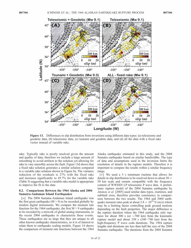
rake. Typically rake is poorly resolved given the amountand quality of data; therefore we include a large amount ofsmoothing to avoid artifacts to the solution yet allowing forrake to vary smoothly across the fault. Figure 13d shows thata fixed rake solution generates a similar solution comparedto a variable rake solution shown in Figure 8a. The variancereduction of the residuals is 27% with the fixed rakeand increases significantly to 45.7% for the variable rake(Table 3) suggesting that a variable rake model is appropriateto improve the fit to the data.

8.2. Comparisons Between the 1964 Alaska and 2004Sumatra-Andaman Island Earthquakes

[36] The 2004 Sumatra-Andaman Island earthquake wasthe first great earthquake (M > 9) to be recorded globally bymodern digital instruments. We compare the moment ratefunction for the 1964 earthquake, the first M > 9 earthquaketo be recorded by a network of global analog instruments, tothe recent 2004 earthquake to characterize these events.These earthquakes are so large that they are unique to allother known earthquake characteristics, so it is of interest torelate them to earthquake scaling models. Figure 14 showsthe comparison of moment rate functions between the 1964

Alaska earthquake estimated in this study, and the 2004Sumatra earthquake based on similar bandwidths. The typeof data and assumptions used in the inversion limits theresolution of details in the rupture models. Therefore it isimportant to compare the results within a similar frequencyrange.[37] We used a 5 s minimum risetime that allows for

details in slip distribution to be resolved down to about 50 !50 km scale and remain compatible with the frequencycontent of WWSSN LP teleseismic P wave data. A prelim-inary rupture model of the 2004 Sumatra earthquake byAmmon et al. [2005] used similar data types, risetimes, andsubfault sizes, therefore provides consistency in compari-sons between the two results. The 1964 and 2004 earth-quake moment rates peak at about 3.8 ! 1020 N (m/s) whichmay be a limiting factor controlling peak ground motionsdepending on the fault properties. The major difference isthe rupture duration where the 1964 earthquake only rup-tures for about 300 s (or "700 km) from the kinematicrupture model and about 350 s (540–740 km) from thehigh-frequency P wave coda durations. The 1964 rupturelengths and durations are less than half the size of the 2004Sumatra earthquake. The durations from the 2004 Sumatra

Figure 13. Differences in slip distribution from inversions using different data types: (a) teleseismic andgeodetic data, (b) teleseismic data, (c) tsunami and geodetic data, and (d) all the data with a fixed rakevector instead of variable rake.


16 of 21

B07306

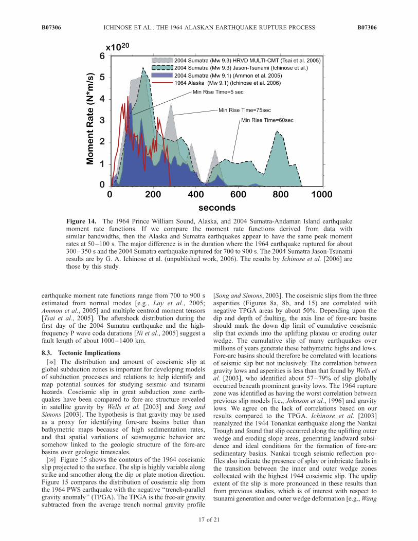
earthquake moment rate functions range from 700 to 900 sestimated from normal modes [e.g., Lay et al., 2005;Ammon et al., 2005] and multiple centroid moment tensors[Tsai et al., 2005]. The aftershock distribution during thefirst day of the 2004 Sumatra earthquake and the high-frequency P wave coda durations [Ni et al., 2005] suggest afault length of about 1000–1400 km.

8.3. Tectonic Implications

[38] The distribution and amount of coseismic slip atglobal subduction zones is important for developing modelsof subduction processes and relations to help identify andmap potential sources for studying seismic and tsunamihazards. Coseismic slip in great subduction zone earth-quakes have been compared to fore-arc structure revealedin satellite gravity by Wells et al. [2003] and Song andSimons [2003]. The hypothesis is that gravity may be usedas a proxy for identifying fore-arc basins better thanbathymetric maps because of high sedimentation rates,and that spatial variations of seismogenic behavior aresomehow linked to the geologic structure of the fore-arcbasins over geologic timescales.[39] Figure 15 shows the contours of the 1964 coseismic

slip projected to the surface. The slip is highly variable alongstrike and smoother along the dip or plate motion direction.Figure 15 compares the distribution of coseismic slip fromthe 1964 PWS earthquake with the negative ‘‘trench-parallelgravity anomaly’’ (TPGA). The TPGA is the free-air gravitysubtracted from the average trench normal gravity profile

[Song and Simons, 2003]. The coseismic slips from the threeasperities (Figures 8a, 8b, and 15) are correlated withnegative TPGA areas by about 50%. Depending upon thedip and depth of faulting, the axis line of fore-arc basinsshould mark the down dip limit of cumulative coseismicslip that extends into the uplifting plateau or eroding outerwedge. The cumulative slip of many earthquakes overmillions of years generate these bathymetric highs and lows.Fore-arc basins should therefore be correlated with locationsof seismic slip but not inclusively. The correlation betweengravity lows and asperities is less than that found byWells etal. [2003], who identified about 57–79% of slip globallyoccurred beneath prominent gravity lows. The 1964 rupturezone was identified as having the worst correlation betweenprevious slip models [i.e., Johnson et al., 1996] and gravitylows. We agree on the lack of correlations based on ourresults compared to the TPGA. Ichinose et al. [2003]reanalyzed the 1944 Tonankai earthquake along the NankaiTrough and found that slip occurred along the uplifting outerwedge and eroding slope areas, generating landward subsi-dence and ideal conditions for the formation of fore-arcsedimentary basins. Nankai trough seismic reflection pro-files also indicate the presence of splay or imbricate faults inthe transition between the inner and outer wedge zonescollocated with the highest 1944 coseismic slip. The updipextent of the slip is more pronounced in these results thanfrom previous studies, which is of interest with respect totsunami generation and outer wedge deformation [e.g.,Wang

Figure 14. The 1964 Prince William Sound, Alaska, and 2004 Sumatra-Andaman Island earthquakemoment rate functions. If we compare the moment rate functions derived from data withsimilar bandwidths, then the Alaska and Sumatra earthquakes appear to have the same peak momentrates at 50–100 s. The major difference is in the duration where the 1964 earthquake ruptured for about300–350 s and the 2004 Sumatra earthquake ruptured for 700 to 900 s. The 2004 Sumatra Jason-Tsunamiresults are by G. A. Ichinose et al. (unpublished work, 2006). The results by Ichinose et al. [2006] arethose by this study.


17 of 21

B07306

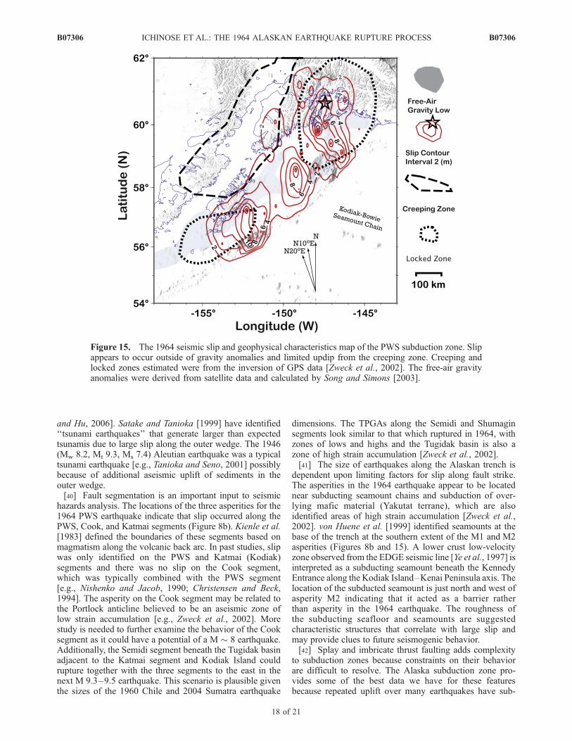
and Hu, 2006]. Satake and Tanioka [1999] have identified‘‘tsunami earthquakes’’ that generate larger than expectedtsunamis due to large slip along the outer wedge. The 1946(Mw 8.2, Mt 9.3, Ms 7.4) Aleutian earthquake was a typicaltsunami earthquake [e.g., Tanioka and Seno, 2001] possiblybecause of additional aseismic uplift of sediments in theouter wedge.[40] Fault segmentation is an important input to seismic

hazards analysis. The locations of the three asperities for the1964 PWS earthquake indicate that slip occurred along thePWS, Cook, and Katmai segments (Figure 8b). Kienle et al.[1983] defined the boundaries of these segments based onmagmatism along the volcanic back arc. In past studies, slipwas only identified on the PWS and Katmai (Kodiak)segments and there was no slip on the Cook segment,which was typically combined with the PWS segment[e.g., Nishenko and Jacob, 1990; Christensen and Beck,1994]. The asperity on the Cook segment may be related tothe Portlock anticline believed to be an aseismic zone oflow strain accumulation [e.g., Zweck et al., 2002]. Morestudy is needed to further examine the behavior of the Cooksegment as it could have a potential of a M " 8 earthquake.Additionally, the Semidi segment beneath the Tugidak basinadjacent to the Katmai segment and Kodiak Island couldrupture together with the three segments to the east in thenext M 9.3–9.5 earthquake. This scenario is plausible giventhe sizes of the 1960 Chile and 2004 Sumatra earthquake

dimensions. The TPGAs along the Semidi and Shumaginsegments look similar to that which ruptured in 1964, withzones of lows and highs and the Tugidak basin is also azone of high strain accumulation [Zweck et al., 2002].[41] The size of earthquakes along the Alaskan trench is

dependent upon limiting factors for slip along fault strike.The asperities in the 1964 earthquake appear to be locatednear subducting seamount chains and subduction of over-lying mafic material (Yakutat terrane), which are alsoidentified areas of high strain accumulation [Zweck et al.,2002]. von Huene et al. [1999] identified seamounts at thebase of the trench at the southern extent of the M1 and M2asperities (Figures 8b and 15). A lower crust low-velocityzone observed from the EDGE seismic line [Ye et al., 1997] isinterpreted as a subducting seamount beneath the KennedyEntrance along the Kodiak Island–Kenai Peninsula axis. Thelocation of the subducted seamount is just north and west ofasperity M2 indicating that it acted as a barrier ratherthan asperity in the 1964 earthquake. The roughness ofthe subducting seafloor and seamounts are suggestedcharacteristic structures that correlate with large slip andmay provide clues to future seismogenic behavior.[42] Splay and imbricate thrust faulting adds complexity

to subduction zones because constraints on their behaviorare difficult to resolve. The Alaska subduction zone pro-vides some of the best data we have for these featuresbecause repeated uplift over many earthquakes have sub-

Figure 15. The 1964 seismic slip and geophysical characteristics map of the PWS subduction zone. Slipappears to occur outside of gravity anomalies and limited updip from the creeping zone. Creeping andlocked zones estimated were from the inversion of GPS data [Zweck et al., 2002]. The free-air gravityanomalies were derived from satellite data and calculated by Song and Simons [2003].


18 of 21

B07306

merged or exposed islands [e.g., Plafker, 1965, 1972] fromwhich coseismic and interseismic deformation can be mea-sured. Recently, marine geophysical data, multibeam sonarand seismic reflection, have revealed that splay and imbri-cate thrusts occur in many subduction zones including theSunda Trench which ruptured in the 2004 Sumatra earth-quake. The largest slip in 1964 occurred along one of thesesplay faults, with "17.4 m along the PBF. Although slipoccurs along the splay fault, it also appears to be colocatedwith large slip on the mega thrust extending out to the trenchalong the M1 asperity (Figures 8a and 15). The relationbetween splay faulting and outer wedge deformation isuncertain, but analysis by von Huene et al. [1999] indicatesthat upper plate shortening occurs out to the Alaskan trenchalong TACT transect. This could indicate that for someportions of the plate interface, active deformation is occur-ring within the outer wedge, which has implications towardtsunami generation [Satake and Tanioka, 1999]. Analogsoccur on land such as the 1999 Chi-Chi, Taiwan [e.g., Lee etal., 2001; Kelson et al., 2001] and 1971 San Fernando,California, earthquakes where slip extended updip to thesedimentary wedge [e.g., Allen et al., 2000]. Wang and Hu[2006] provided some new theories using mechanicalmodels based on stress changes over many earthquakecycles, suggesting that the actively deforming outer wedgemay resist coseismic slip due to velocity strengtheningresulting in splay faulting or postseismic slip.[43] The landward limit of coseismic slip along the

megathrust is an important unknown and has implicationsin strong ground motion hazards along populated coastalcities. Many studies [e.g., Hyndman et al., 1997; Oleskevichet al., 1999] have identified the limit as the location of thefore-arc mantle, which is approximately 45–55 km beneathKodiak Island. Another indicator is the 350!C isotherm atabout 55–65 km depth, although the thermal behaviorbetween warm and cold slabs is different. Zweck et al.[2002] have also identified a creeping zone beneath theCook Inlet that also coincides with the landward limit ofcoseismic slip shown in Figure 15. We estimated the depthextent of the 1964 rupture (Figures 8a and 8b) and foundthat the coupling depth for megathrust earthquakes canreach 50 km, exceeding the previous maximum couplingdepth estimated for southern Alaskan trench by about 10 to15 km [Tichelaar and Ruff, 1993]. The one constrainingevent for southern Alaska used by Tichelaar and Ruff[1993] was the 4 September 1965 Kodiak Island earthquake(Mw 6.9), which is mislocated to the southwest by 15 kmrelative to relocations by Engdahl et al. [1998] and Doser etal. [2002]. The mislocation may be due to changes betweentraveltimes through fast oceanic and slow continental lith-osphere, thereby erroneously shifting subduction earthquakelocations toward the slower continent side. Our revisedcoupling depth is deeper than previously estimated and isone of the deepest globally, only comparable to theHokkaido triple junction at 55 km [Tichelaar and Ruff,1993]. If we use the slab contours from Plafker [1972]rather than from Gudmundsson and Sambridge [1998], thenthe disparity is probably insignificant and our estimateswould be in line with previous studies. A deeper couplingdepth or currently ongoing postseismic slip may helpexplain for the absence of episodic tremor and slow slip

events for the southern Alaskan trench that is found else-where in Cascadia and Japan [e.g., Dragert et al., 2001].

9. Conclusion

[44] The 1964 Prince William Sound, Alaska, earthquakewas one of four M > 9 subduction zone earthquakes to haveoccurred since the beginning of global earthquake monitor-ing era. The sheer size and complexity of these earthquakescan yield very unique rupture characteristics. Unfortunatelytheir infrequency limits our ability to examine them indetail. Reanalysis of historical earthquakes provides con-straints on rupture characteristics important for strongground motion prediction and tectonic studies.[45] We estimated the spatial and temporal distribution of

slip and rake for the 1964 PWS earthquake. We collectedand digitized WWSSN LP and SP teleseismic P waves,tsunami tide gauge records, and vertical coseismic displace-ments from leveling surveys. We were not able to use theshort-period data for the inversion but were able to measurethe duration of the P wave coda to estimate roughly theduration, length and speed of the rupture front. We notedthat the P coda durations were related to source directivitybecause durations were significantly shorter at stations inone direction of fault strike relative to opposite direction.Because of trade-offs in rupture duration or length andspeed we found a range of rupture models that fit the dataequally well. The fault lengths range from 540 to 740 kmrupturing at a speed of 1.4–2 km/s in a 220!–238!direction. Given the effect of scattering attenuation nearthe site that extended the P coda durations, the measure-ments should be viewed as maximum values. The 1964PWS Alaska earthquake appeared to have ruptured about680 km and not more than 740 km, slightly more than thatpredicted by on-scale strain seismograms recorded inHawaii and Pasadena, by satellite gravity, and from analysesof previous seismic or geodetic studies. This estimateprovides an independent constraint on rupture length andis not affected by P wave multiples which are problematic inkinematic rupture models.[46] We assumed three major fault segments for the

subduction zone dipping 6! to 12! based on geologic andgeodetic observations including earthquake locations. Thesubfault size was set to 50 ! 50 km. The Patton Bay faultimbricate thrust was assigned a 60! dip with a subfault sizeof 20 ! 20 km. Our preferred kinematic rupture modelhas a total seismic moment of 5.52 ! 1022 N m (Mw 9.1)Slip is shallower than 50 km depth slab contour constrainedmostly by subsidence observed in the leveling surveys. Weidentify three areas of major moment release, first nearMontague and Middleton islands along the slope magneticanomaly extending out to the trench, the second beneath theshelf and slope between the 58!N fracture zone and theKodiak seamount chain, and the third off the coast ofKodiak Island extending to the trench. Our preferred rupturemodel has a peak slip of 14.9 m along the megathrust and17.4 m along the PBF and average slip of 4.9 m, which isabout half of that estimated in previous studies.[47] The depth limit of rupture or coupling depth is

typically 20 to 55 km worldwide based on earthquakelocations, geochemical and geothermal constraints. Weestimated the depth extent of the 1964 rupture and found


19 of 21

B07306

that the coupling depth for megathrust earthquakes canreach 50 km, exceeding the previous maximum couplingdepth estimated for Alaskan trench by about 10 to 15 km[Tichelaar and Ruff, 1993]. This places the Alaskan trenchas having one of the deepest coupling depths comparable tothe Hokkaido triple junction at 55 km. A deeper couplingdepth or currently ongoing postseismic slip may helpexplain for the absence of episodic tremor and slow slipevents for the southern Alaskan trench that is found else-where in Cascadia and Japan [e.g., Dragert et al., 2001].

[48] Acknowledgments. We thank Bob Hutt and Leo Sandoval at theU. S. Geological Survey Albuquerque Seismology Laboratory for access totheir WWSSN film chip laboratory. Funding was provided by the RUPTUproject of the U. S. Bureau of Reclamation Dam Safety Research Program.

ReferencesAmmon, C. J., et al. (2005), Rupture process of the great 2004 Sumatra-Andaman earthquake, Science, 308, 1133–1139.

Baker, G. E., and C. A. Langston (1987), Source parameters of the 1949magnitude 7.1 south Puget Sound, Washington, earthquake as determinedfrom long-period body waves and strong motions, Bull. Seismol. Soc.Am., 77, 1530–1557.

Bouchon, M. (1976), Teleseismic body wave radiation from a seismicsource in a layered medium, Geophys. J. R. Astron. Soc., 47, 515–530.

Brocher, T. M., G. S. Fuis, M. A. Fisher, G. Plafker, M. J. Moses, J. J.Taber, and N. I. Christensen (1994), Mapping the megathrust beneath thenorthern Gulf of Alaska using wide-angle seismic data, J. Geophys. Res.,99, 11,663–11,685.

Christensen, D. H., and S. L. Beck (1994), The rupture process and tectonicimplications of the great 1964 Prince William Sound earthquake, PureAppl. Geophys., 142, 29–53.

DeMets, C., and T. H. Dixon (1999), A new kinematic models for Pacific–North America motion from 3 Ma to present: 1. Evidence for steadymotion and biases in the NUVEL-1A model, Geophys. Res. Lett., 26,1921–1924.

Doser, D. I., W. A. Brown, and M. Velasquez (2002), Seismicity of theKodiak Island region (1964–2001) and its relation to the 1964 GreatAlaskan earthquake, Bull. Seismol. Soc. Am., 92, 3269–3292.

Doser, D. I., A. M. Veilleux, C. Flores, and W. A. Brown (2006), Changesin seismic-moment rates along the rupture zone of the 1964 great Alaskanearthquake, Bull. Seismol. Soc. Am., 96(4A), 1545–1550, doi:10.1785/0120050194.

Dragert, H., K. Wang, and T. S. James (2001), A silent slip event on thedeeper Cascadia subduction zone interface, Science, 292, 1525–1528,doi:10.1126/science.1060152.

Engdahl, E. R., R. van der Hilst, and R. Buland (1998), Global teleseismicearthquake relocation with improved travel times and procedures fordepth determination, Bull. Seismol. Soc. Am., 88, 722–743.

Flores, C., and D. Doser (2005), Shallow seismicity of the Anchorage,Alaska, region (1964–1999), Bull. Seismol. Soc. Am., 95(5), 1865–1879.

Freymueller, J. T., S. C. Cohen, and H. J. Fletcher (2000), Spatial variationsin present-day deformation, Kenai Peninsula, Alaska, and their implica-tions, J. Geophys. Res., 105, 1801–8079.

Gudmundsson, O., and M. Sambridge (1998), A regionalized upper mantle(RUM) seismic model, J. Geophys. Res., 103, 7121–7136.

Guilbert, J., J. Vergoz, E. Schissele, A. Roueff, and Y. Cansi (2005), Use ofhydroacoustic and seismic arrays to observe rupture propagation andsource extent of the Mw 9 Sumatra earthquake, Geophys. Res. Lett., 32,L15310, doi:10.1029/2005GL022966.

Harding, S. T., and S. T. Algermissen (1969), Focal mechanism of thePrince William Sound, Alaska earthquake of March 28, 1964, Bull. Seis-mol. Soc. Am., 59, 799–811.

Hartzell, S. H., and T. H. Heaton (1983), Inversion of strong ground motionand teleseismic waveform data for the fault rupture history of the 1979Imperial Valley, California earthquake, Bull. Seismol. Soc. Am., 73,1553–1583.

Haskell, N. A. (1960), Crustal reflection of plane SH waves, J. Geophys.Res., 65, 4147–4150.

Haskell, N. A. (1962), Crustal reflection of plane P and SV waves,J. Geophys. Res., 67, 4751–4767.

Hastie, L. M., and J. C. Savage (1970), A dislocation model for the 1964Alaska earthquake, Bull. Seismol. Soc. Am., 60, 1389–1392.

Holdahl, S. R., and J. Sauber (1994), Coseismic slip in the 1964 PrinceWilliam Sound Earthquake: A new geodetic inversion, Pure Appl. Geo-phys., 142, 55–82.

Hyndman, R. D., M. Yamano, and D. A. Oleskevich (1997), The seismo-genic zone of subduction thrust faults, Isl. Arc, 6, 244–260.

Ichinose, G. A., H. K. Thio, P. G. Somerville, T. Sato, and T. Ishii (2003),Rupture process of the 1944 Tonankai earthquake (Ms 8.1) from theinversion of teleseismic and regional seismograms, J. Geophys. Res.,108(B10), 2497, doi:10.1029/2003JB002393.

Ichinose, G. A., P. Somerville, H. K. Thio, S. Matsushima, and T. Sato(2005), Rupture process of the 1948 Fukui earthquake (M 7.1) from thejoint inversion of seismic waveform and geodetic data, J. Geophys. Res.,110, B05301, doi:10.1029/2004JB003437.

Ichinose, G. A., H. K. Thio, and P. G. Somerville (2006), Moment tensorand rupture model for the 1949 Olympia, Washington, earthquake andscaling relations for Cascadia and global intraslab earthquakes, Bull.Seismol. Soc. Am., 96(3), 1029–1037, doi:10.1785/0120050132.

Johnson, J. M., and K. Satake (1994), Rupture extent of the 1938 Alaskanearthquake as inferred from tsunami waveforms, Geophys. Res. Lett.,21(8), 733–736.

Johnson, J. M., and K. Satake (1997), Estimation of seismic momentand slip distribution of the April 1, 1946, Aleutian tsunami earthquake,J. Geophys. Res., 102, 11,765–11,774.

Johnson, J. M., K. Satake, S. R. Holdahl, and J. Sauber (1996), The 1964Prince William Sound earthquake: Joint inversion of tsunami and geode-tic data, J. Geophys. Res., 101, 523–532.

Kanamori, H. (1970), The Alaska earthquake of 1964: Radiation of long-period surface waves and source mechanism, J. Geophys. Res., 75,5029–5040.

Kelson, K. I., K.-H. Kang, W. D. Page, C.-T. Lee, and L. S. Cluff (2001),Representative styles of deformation along the Chelungpu fault from the1999 Chi-Chi (Taiwan) Earthquake: Geomorphic characteristics andresponses of man-made structures, Bull. Seismol. Soc. Am., 91, 930–952.

Kienle, J., S. E. Swanson, and H. Pulpan (1983), Magmatism and subduc-tion in the eastern Aleutian arc, in Arc Volcanism: Physics and Tectonics,edited by D. Shimozuru and I. Yokoyama, pp. 191–224, Terra Sci.,Tokyo.

Kikuchi, M., and Y. Fukao (1987), Inversion of long period P-waves fromgreat earthquakes along subduction zones, Tectonophysics, 144, 231–247.

Langston, C. A., and D. V. Helmberger (1975), A procedure for modelingshallow dislocation sources, Geophys. J. R. Astron. Soc., 42, 117–130.

Lawson, C. L., and R. J. Hanson (1974), Solving Least Squares Problems,Prentice-Hall, Englewood Cliffs, N. J.

Lay, T., et al. (2005), The great Sumatra-Andaman earthquake of26 December 2004, Science, 308, 1127–1133.

Lee, J.-C., Y.-G. Chen, K. Sieh, K. Mueller, W.-S. Chen, H.-T. Chu, Y.-C.Chan, C. Rubin, and R. Yeats (2001), A vertical exposure of the 1999surface rupture of the Chelungpu fault at Wufeng, western Taiwan: Struc-tural and paleoseismic implications for an active thrust fault, Bull. Seis-mol. Soc. Am., 91, 914–929.

Miyashita, K., and M. Matsu’ura (1978), Inversion analysis of static dis-placement data associated with the Alaska earthquake of 1964, J. Phys.Earth, 26, 333–349.

National Academy of Sciences (1972), A study of the source mechanism ofthe Alaska earthquake and tsunami of March 27, 1964, in Seismologyand Geodesy on the Great Alaska Earthquake of 1964, pp. 249–258,Natl. Acad. of Sci., Washington D. C.

Ni, S., H. Kanamori, and D. Helmberger (2005), Energy radiation from theSumatra earthquake, Nature, 434, 582.

Nishenko, S. P., and K. H. Jacob (1990), Seismic potential of the QueenCharlotte-Alaska-Aleutian seismic zone, J. Geophys. Res., 95, 2511–2532.

Okada, Y. (1992), Internal deformation due to shear and tensile faults in ahalf space, Bull. Seismol. Soc. Am., 82, 1018–1040.

Oleskevich, D. A., R. D. Hyndman, and K. Wang (1999), The updip anddowndip limits to great subduction earthquakes: Thermal and structuralmodels of Cascadia, south Alaska, SW Japan, and Chile, J. Geophys.Res., 104, 14,965–14,992.

Plafker, G. (1965), Tectonic deformation associated with the 1964 Alaskaearthquake, Science, 148, 1675–1687.

Plafker, G. (1972), Alaskan earthquake of 1964 and Chilean earthquake of1960: Implications for arc tectonics, J Geophys. Res., 77(5), 901–925.

Powell, T., and D. Fries (1964), Handbook: World Wide Standard Seismo-graph Network, Acoust. and Seismics Lab., Inst. of Sci. and Technol.,Univ. of Michigan, Ann Arbor.

Ratchkovski, N. A., and R. Hansen (2002), New evidence for segmentationof the Alaska subduction zone, Bull. Seismol. Soc. Am., 92, 1754–1765.

Ruff, L., and H. Kanamori (1983), The rupture process and asperity dis-tribution of three great earthquakes from long period diffracted P-waves,Phys. Earth Planet. Inter., 31, 202–230.

Satake, K. (1995), Linear and nonlinear computations of the 1992 Nicar-agua earthquake Tsunami, Pure Appl. Geophys., 144, 455–470.


20 of 21

B07306

Satake, K., and Y. Tanioka (1999), Sources of tsunami and tsunamigenicearthquakes in subduction zones, Pure Appl. Geophys., 154, 467–483.

Sherburne, R. W., S. T. Algermissen, and S. T. Harding (1964), Hypocenter,origin time, and magnitude of the Prince William Sound earthquake ofMarch 28, 1964, in Seismology and Marine Geology, vol. II-B-C, U.S.Coast and Geod. Surv., Washington, D. C.

Small, J. B., and L. C. Wharton (1969), Vertical displacements determinedby surveys after the Alaska earthquake of March 28, 1964, the PrinceWilliam Sound earthquake of 1964 and aftershocks, vol. III, U.S. Coastand Geod. Surv., Washington, D. C.

Song, T. A., and M. Simons (2003), Large trench-parallel gravity variationspredict seismogenic behavior in subduction zones, Science, 301, 630–633.

Stauder, W., and G. A. Bollinger (1966), The focal mechanism of the Alaskaearthquake of March 28, 1964, and its aftershock sequence, J. Geophys.Res., 71, 5283–5295.

Sun, W., and S. Okubo (2004), Coseismic deformations detectable bysatellite gravity missions: A case study of Alaska (1964, 2002) andHokkaido [2003] earthquakes in the spectral domain, J. Geophys. Res.,109, B04405, doi:10.1029/2003JB002554.

Tanioka, Y., and T. Seno (2001), Detailed analysis of tsunami waveformsgenerated by the 1946 Aleutian tsunami earthquake, Nat. Hazards EarthSyst. Sci., 1, 171–175.

Thio, H. K., R. W. Graves, P. G. Somerville, T. Sato, and T. Ishii (2004), Amultiple time window rupture model for the 1999 Chi-Chi earthquakefrom a combined inversion of teleseismic, surface wave, strongmotion, and GPS data, J. Geophys. Res., 109, B08309, doi:10.1029/2002JB002381.

Tichelaar, B. W., and L. J. Ruff (1993), Depth of seismic coupling alongsubduction zones, J. Geophys. Res., 98, 2017–2037.

Tsai, V. C., M. Nettles, G. Ekstrom, and A. Dziewonski (2005), MultipleCMT source analysis of the 2004 Sumatra earthquake, Geophys. Res.Lett., 32, L17304, doi:10.1029/2005GL023813.

von Huene, R., D. Klaeschen, and J. Fruehn (1999), Relation between thesubducting plate and seismicity associated with the great 1964 Alaskaearthquake, Pure Appl. Geophys., 154, 575–591.

Wald, D., and R. W. Graves (2001), Resolution analysis of finite faultsource inversion using one- and three-dimensional Green’s functions:

2. Combining seismic and geodetic data, J. Geophys. Res., 106, 8767–8788.

Wald, D. J., and P. G. Somerville (1994), Variable-slip rupture model ofthe great 1923 Kanto, Japan earthquake: Geodetic and body-waveformanalysis, Bull. Seismol. Soc. Am., 85, 159–177.

Wang, K., and Y. Hu (2006), Accretionary prisms in subduction earthquakecycles: The theory of dynamic Coulomb wedge, J. Geophys. Res., 111,B06410, doi:10.1029/2005JB004094.

Wells, R. E., R. J. Blakely, Y. Sugiyama, D. W. Scholl, and P. A. Dinterman(2003), Basin-centered asperities in great subduction zone earthquakes: Alink between slip, subsidence, and subduction erosion?, J. Geophys. Res.,108(B10), 2507, doi:10.1029/2002JB002072.

Wyss, M., and J. N. Brune (1967), The Alaska earthquake of 28 March1964: A complex multiple rupture, Bull. Seismol. Soc. Am., 57, 1017–1023.

Ye, S., E. R. Flueh, D. Klaeschen, and R. von Huene (1997), Crustalstructure along the EDGE transect beneath the Kodiack shelf off Alaskaderived from OBH seismic refraction data, Geophys. J. Int., 130, 283–302.

Yu, G., S. G. Wesnousky, and G. Ekstrom (1993), Slip partitioning alongmajor convergent plate boundaries, Pure Appl. Geophys., 140, 183–210.

Zeng, Y., and J. G. Anderson (1995), A method for direct computation ofthe differential seismogram with respect to the velocity change in alayered elastic media, Bull. Seismol. Soc. Am., 85, 300–307.

Zweck, C., J. T. Freymueller, and S. C. Cohen (2002), Three-dimensionalelastic dislocation modeling of the postseismic response to the 1964Alaska earthquake, J. Geophys. Res., 107(B4), 2064, doi:10.1029/2001JB000409.

$$$$$$$$$$$$$$$$$$$$$$$R. Graves, P. Somerville, and H. K. Thio, URS Group Inc., 566 El

Dorado St., 2nd Floor, Pasadena, CA 91101-2560, USA.G. Ichinose, MTC Technologies, Inc., AFTAC/TTR/MTC, 1030 S. Hwy

A1A, Patrick AFB, FL 32925-3002, USA. ([email protected])D. O’Connell, U.S. Bureau of Reclamation, P.O. Box 25007 (D-8330),

Denver, CO 80225-0007, USA. ([email protected])


21 of 21

B07306

Rupture process of the 1964 Prince William Sound, Alaska, earthquake from the combined inversion of...

Documents

Transcript of Rupture process of the 1964 Prince William Sound, Alaska, earthquake from the combined inversion of...