RUNNING COSTS OF MOTOR VEHICLES AS AFFECTED BY ...

NATIONAL COOPERATIVE HIGHWAY RESEARCH PROGRAM 111 REPORT

RUNNING COSTS OF MOTOR VEHICLES AS AFFECTED BY

ROAD DESIGN AND TRAFFIC

HIGHWAY RESEARCH BOARD NATIONAL RESEARCH COUNCIL

NATIONAL ACADEMY OF SCIENCES- NATIONAL ACADEMY OF ENGINEERING

HIGHWAY RESEARCH BOARD 1971

Officers

CHARLES E. SHUMATE, Chairman ALAN M. VOORHEES, First Vice Chairman WILLIAM L. GARRISON, Second Vice Chairman W. N. CAREY, JR., Executive Director

Executive Committee

F. C. TURNER, Federal Highway Administrator, U. S. Department of Transportation (ex officio) A. E. JOHNSON, Executive Director, American Association of State Highway Officials (ex officio) ERNST WEBER, Chairman, Division of Engineering, National Research Council (ex officio) OSCAR T. MARZKE, Vice President, Fundamental Research, U. S. Steel Corporation (ex officio, Past Chairman, 1969) D. GRANT MICKLE, President, Highway Users Federation for Safety and Mobility (ex officio, Past Chairman, 1970) CHARLES A. BLESSING, Director, Detroit City Planning Commission HENDRIK W. BODE, Professor of Systems Engineering, Harvard University JAY W. BROWN, Director of Road Operations, Florida Department of Transportation W. J. BURMEISTER, State Highway Engineer, Wisconsin Department of Transportation HOWARD A. COLEMAN, Consultant, Missouri Portland Cement Company HARMER E. DAVIS, Director, institute of Transportation and Traffic Engineering, University of California WILLIAM L. GARRISON, Professor of Environmental Engineering, University of Pittsburgh GEORGE E. HOLBROOK, E. I. du Pont de Nemours and Company EUGENE M. JOHNSON, President, The Asphalt institute A. SCHEFFER LANG, Department of Civil Engineering, Massachusetts institute of Technology JOHN A. LEGARRA, State Highway Engineer and Chief of Division, California Division of Highways WILLIAM A. McCONNELL, Director, Operations Office, Engineering Staff, Ford Motor Company JOHN J. McKETTA, Department of Chemical Engineering, University of Texas J. B. McMORRAN, Consultant JOHN T. MIDDLETON, Acting Commissioner, National Air Pollution Control Administration R. L. PEYTON, Assistant State Highway Director, State Highway Commission of Kansas MILTON PIKARSKY, Commissioner of Public Works, Chicago, Illinois CHARLES E. SHUMATE, Executive Director-Chief Engineer, Colorado Department of Highways DAVID H. STEVENS, Chairman, Maine State Highway Commission ALAN M. VOORHEES, Alan M. Voorhees and Associates

NATIONAL COOPERATIVE HIGHWAY RESEARCH PROGRAM

Advisory Committee

CHARLES E. SHUMATE, Colorado Department of Highways (Chairman) ALAN M. VOORHEES, Alan M. Voorhees and Associates WILLIAM L. GARRISON, University of Pittsburgh F. C. TURNER, U. S. Department of Transportation A. E. JOHNSON, American Association of State Highway Officials ERNST WEBER, National Research Council OSCAR T. MARZKE, United States Steel Corporation

GRANT MICKLE, Highway Users Federation for Safety and Mobility W. N. CAREY, JR., Highway Research Board

General Field of Administration Area of Economics Advisory Panels A 2-5, A2-5A, and A2-7

JOHN W. HOSSACK, Barton-Aschman Associates (Chairman) R. C. BLENSLY, Oregon State University W. L. GARRISON, University of Pittsburgh

L. GRANT, Stanford University RUDOLF HESS, California Division of Highways D. S. JOHNSON, Connecticut Department of Transportation T. F. MORF, illinois Division of Highways ROBLEY WINFREY, Consultant K. E. COOK, Highway Research Board

Program Staff

W. HENDERSON, JR., Program Director M. MAcGREGOR, Administrative Engineer

W. C. GRAEUB, Projects Engineer J. R. NOVAK, Projects Engineer H. A. SMITH, Projects Engineer

W. L. WILLIAMS, Projects Engineer HERBERT P. ORLAND, Editor ROSEMARY S. MAPES, Editor CATHERINE B. CARLSTON, Editorial Assistant

COpy IiIGij WAYS

NATIONAL COOPERATIVE HIGHWAY RESEARCH PROGRAM 111 REPORT



PAUL J. CLAFFEY

PAUL J. CLAFFEY AND ASSOCIATES

POTSDAM, NEW YORK

RESEARCH SPONSORED BY THE AMERICAN ASSOCIATION

OF STATE HIGHWAY OFFICIALS IN COOPERATION

WITH THE FEDERAL HIGHWAY. ADMINISTRATION

SUBJECT CLASSIFICATION:

TRANSPORTATION ECONOMICS

HIGHWAY RESEARCH BOARD DIVISION OF ENGINEERING NATIONAL RESEARCH COUNCIL

NATIONAL ACADEMY OF SCIENCES- NATIONAL ACADEMY OF ENGINEERING 1971


Systematic, well-designed research provides the most ef-fective approach to the solution of many problems facing highway administrators and engineers. Often, highway problems are of local interest and can best be studied by highway departments individually or in cooperation with their state universities and others. However, the accelerat-ing growth of highway transportation develops increasingly complex problems of wide interest to highway authorities. These problems are best studied through a coordinated program of cooperative research.

in recognition of these needs, the highway administrators of the American Association of State Highway Officials initiated in 1962 an objective national highway research program employing modern scientific techniques. This program is supported on a continuing basis by funds from participating member states of the Association and it re-ceives the full cooperation and support of the Federal Highway Administration, United States Department of Transportation.

The Highway Research Board of the National Academy of Sciences-National Research Council was requested by the Association to administer the research program because of the Board's recognized objectivity and understanding of modern research practices. The Board is uniquely suited for this purpose as: it maintains an extensive committee structure from which authorities on any highway transpor-tation subject may be drawn; it possesses avenues of com-munications and cooperation with federal, state, and local governmental agencies, universities, and industry; its rela-tionship to its parent organization, the National Academy of Sciences, a private, nonprofit institution, is an insurance of objectvity; it maintains a full-time research correlation staff of specialists in highway transportation matters to bring the findings of research directly to those who are in a position to use them.

The program is developed on the basis of research needs identified by chief administrators of the highway depart-ments and by committees of AASHO. Each year, specific areas of research needs to be included in the program are proposed to the Academy and the Board by the American Association of State Highway Officials. Research projects to fulfill these needs are defined by the Board, and qualified research agencies are selected from those that have sub-mitted proposals. Administration and surveillance of re-search contracts are responsibilities of the Academy and its Highway Research Board.

The needs for highway research are many, and the National Cooperative Highway Research Program can make significant contributions to the solution of highway transportation problems of mutual concern to many re-sponsible groups. The program, however, is intended to complement rather than to substitute for or duplicate other highway research programs.

NCHRP Report 111

Project 2-5, 2-5A, and 2-7 FY '64, '65, '67 ISBN 0-309-01901-X L. C. Card No. 70-610443

Price: $5.20

This report is one of a series of reports issued from a continuing research program conducted under a three-way agreement entered into in June 1962 by and among the National Academy of Sciences-National Research Council, the American Association of State High-way Officials, and the Federal Highway Administration. Individual fiscal agreements are executed annually by the Academy-Research Council, the Federal Highway Administration, and participating state highway departments, members of the American Association of State Highway Officials.

This report was prepared by the contracting research agency. It has been reviewed by the appropriate Advisory Panel for clarity, docu-mentation, and fulfillment of the contract. It has been accepted by the Highway Research Board and published in the interest of effective dissemination of findings and their application in the for-mulation of policies, procedures, and practices in the subject problem area.

The opinions and conclusions expressed or implied in these reports are those of the research agencies that performed the research. They are not necessarily those of the Highway Research Board, the Na-tional Academy of Sciences, the Federal Highway Administration, the American Association of State Highway Officials, nor of the individual states participating in the Program.

Published reports of the


are available from:

Highway Research Board National Academy of Sciences 2101 Constitution Avenue Washington, D.C. 20418

(See last pages for list of published titles and prices)

FOREWORD Information on the running costs of cars and trucks given in this report may be readily applied to the economic analysis of highway improvements by highway

By Staff planners, economists, traffic engineers, and design engineers. Reliable running costs

Highway Research Board based on field tests of motor vehicles are presented as broken down into the cost categories of fuel, oil, tire wear, maintenance, depreciation, and accident costs. Relationships between the cost categories and highway grades, operating speeds, roadway surface, horizontal alignment, and traffic volumes are provided to facilitate the calculation of automobile and truck fuel and tire costs for free-flowing volumes. Included in the report are detailed examples illustrating typical problems that can be solved by use of the information presented. Annotated bibliographies are included on the subjects of motor-vehicle operating costs and on relationships between highway accident costs and highway design.

This report presents the combined research results of NCHRP Projects 2-5 and 2-5A, "Running Costs of Motor Vehicles as Affected by Highway Design and Traffic," and NCHRP Project 2-7, "Road User Costs in Urban Areas." Additional documentation of the first year of research on passenger-car fuel and tire costs and the design of a photoelectronic fuelmeter are presented in NCHRP Report 13,

"Running Cost of Motor Vehicles as Affected by Highway Design—Interim Report." Because highway location, geometric design, and traffic operations affect the

cost of operating motor vehicles, highway engineers strive to obtain the minimum transportation cost that considers both the highway cost and the vehicle running cost. Alternate possibilities of highway location and design are analyzed on the basis of their relative effect on the operation of vehicles. This analysis requires that vehicle running cost items be determined and evaluated as a function of the range of speeds normally encountered in traffic, the conditions of traffic found on all highway systems, and various elements of highway design. It was with these thoughts that this project was initiated during the summer of 1963 and extended through 1969 to include conduct of field tests with vehicles, theoretical development, and a search of the literature to assemble reliable running costs of motor vehicles under

real-life operating conditions. In a comprehensive and well-documented study, the consulting firm of Paul

Claffey and Associates has provided a major contribution to the development of relationships among vehicle operating costs, highway location, geometric design, and traffic control. The precise measurements and street survey controls that were

employed have made possible more accurate data than those from any previous study. The effects that variations in gradient, road surface, speed change frequency, and traffic volumes have on the running costs of passenger cars, pickup trucks, two-axle six-tire trucks, and tractor-trailer combinations are included and new information is provided on the following items of operating expense: fuel and oil consumption, maintenance and depreciation costs, tire wear, and accident costs. Condensed graphs of the findings of the fuel consumption and tire wear studies are presented for convenience in applying the research results. Each graph is designed to provide fuel and tire wear cost for various combinations of road design elements and speed change conditions for a given running speed. Also included are families of curves of fuel consumption and tire wear for the eleven test vehicles used in the study and data on the maintenance costs of passenger cars and trucks relative to travel distance, together with average oil consumption rates for operation on dust-free pavements in free-flowing traffic, on dusty roads in free-flowing traffic, and on high-type pavements under restrictive traffic conditions.

CONTENTS

1 SUMMARY

PART I

3 CHAPTER ONE Introduction

Running Costs

Effects of Road Design

Effects of Traffic Conditions

6 CHAPTER TWO Research Approach

Research Technique

Fuel Consumption Measurements

Tire Wear Measurements

Determination of Maintenance Costs

Determination of Vehicle Oil Consumption

Determination of Unit Depreciation Cost per Mile

Determination of Accident Costs Relative to Road Design

Presentation of Results

16 CHAPTER THREE Findings: Passenger-Car Fuel Consumption

Fuel Consumption of the Composite Passenger Car

21 CHAPTER FOUR Findings: Truck Fuel Consumption

Fuel Consumption of Composite Pickup Truck

Fuel Consumption of Composite Two-Axle Six-Tire Truck

Fuel Consumption of Composite Tractor Semi-Trailer Truck Combination

31 CHAPTER FIVE Findings: Passenger-Car Tire Wear Cost

Tire Wear Cost for the Composite Passenger Car

33 CHAPTER SIX Findings: Truck Tire Wear Costs

Tire Wear Costs for Pickup Trucks and Two-Axle Six-Tire Trucks

35 CHAPTER SEVEN Findings: Maintenance Costs of Motor Ve- hicles

37 CHAPTER EIGHT Findings: Vehicle Oil Consumption

38 CHAPTER NINE Findings: Motor-Vehicle Depreciation

39 CHAPTER TEN Vehicle Accident Costs

40 CHAPTER ELEVEN Interpretation of Findings

Fuel Consumption of Passenger Cars in Gently Rolling Terrain

Effect of Vertical Curves on Fuel Consumption Predictions

Representativeness of the Reported Tire • Wear Costs for Passenger-Car Tire Wear in General

Tire Wear of Passenger Cars at High Speed

41 CHAPTER TWELVE Application of Findings

Distribution of Basic Truck Types by Highway System

Vehicle Speeds for Running Cost Computations

Fuel Corrections for Passenger-Car Weight and Engine Size and for the Effects of Environmental Conditions

Sample Problem One

Sample Problem Two

46 CHAPTER THIRTEEN Conclusion

Suggested Further Research

46 REFERENCES

PART II

47 APPENDIX A Graphical Representation of the Fuel (Gasoline) Consumption Rates of Each Test Vehicle for Uniform Increments of Road and Traffic Factors

62 APPENDIX B Graphical Representation of the Effect on Passenger-Car Fuel Consumption of Air Temperature, Altitude, Engine Size, and Vehicle Weight, Age, and Accumulated Mileage

64 APPENDIX C Graphical Presentation of the Relationship of Tire Wear to Road and Traffic Factors

67 APPENDIX D A Comparative Analysis of the Fuel Consump- tion Rates of Diesel and Gasoline Trucks

70 APPENDIX E Annotated Bibliography of Highway Motor- Vehicle Operating Costs, 1950-1970

83 APPENDIX F Special Projects

ACKNOWLEDGMENTS

The research reported herein was performed under NCHRP Projects 2-5 and 2-7 by the Department of Civil Engineering, The Catholic University of America, and also under NCHRP Project 2-5A by Paul J. Claffey and Associates, Consulting Engineers, all with Dr. Paul J. Claffey as Principal Investigator. For part of the work of Projects 2-5 and 2-7, the facilities of the Department of Civil Engineering, The Catholic University of America, were used.

The Motor Vehicle Running Cost Study could not have been carried out successfully without the cooperation and assistance of many people. Particularly important to the conduct of this research were the contributions of the following:

Joseph C. Michalowicz, formerly Head, Department of Electrical Engineering, Catholic University, who developed the electronic fuelmeter.

Frank A. Biberstein, formerly Head, Department of Civil Engineering, and Dale C. Braungart, Associate Professor of Biology, Catholic University, who conducted experiments to evaluate the use of radioisotopes for tire wear measurements.

Hoy Stevens, formerly Automotive Research Specialist, U.S. Bureau of Public Roads, whose advice on vehicle maintenance and oil consumption research was invaluable.

Dr. William E. Corgill, recent doctoral candidate at Catholic University, who assisted in a comprehensive study of motor vehicle user accident costs.

Dr. Philip L. Brach, recent doctoral candidate, Fergus Biber-stein, Assistant Professor of Civil Engineering, and Jerome Steffens, Associate Professor of Mechanical Engineering, Catho-lic University, who supervised much of the field research activities.



SUMMARY Development of the Fuelmeter and the Use of Radioisotopes for Tire Wear Measurement

A series of research investigations into the effects that road design and traffic condi-tions have on vehicle operating costs were completed between 1965 and 1969 for NCHRP Projects 2-5 and 2-7. As part of this research, an entirely new fuelmeter, specifically designed for motor vehicle fuel consumption research, was successfully developed and tested, first as a prototype model and later as a production model. Also included in the research were the development and testing of a technique for using a radioisotope to measure tire wear. However, radioisotopes were found to be unsatisfactory for this purpose because of changes that occur in tire surface mate-rial as wear progresses. Development of the fuelmeter and research into the use of radioisotopes for tire wear measurement are described in Appendix F.

Fuel Consumption and Tire Wear Measurement

Fuel consumption and tire wear were measured for a wide variety of vehicle types, road designs, traffic volumes and operating speeds (speed changes). Families of curves of fuel consumption and tire wear developed from test measurements for 11 individual test vehicles for various road and traffic conditions appear in Appendices A and C. The tables and graphs of findings for fuel consumption and tire wear of Part I, however, show average fuel consumption and tire wear values only for com-posite or representative vehicles in each of four categories: (1) passenger cars, (2) pickup trucks, (3) two-axle six-tire trucks, and (4) tractor semi-trailer truck combinations.

The distribution of vehicle types and weights in each category for U.S. highways was found from information in the literature or from direct observation. For exam-ple, the distribution of passenger-car types was established by observation of more than 35,000 cars on the highways of 11 states as follows: standard-size cars, 65 per-cent; large cars, 20 percent; compact cars, 10 percent; and small cars, 5 percent.

In the case of passenger cars, detailed fuel consumption data developed for each of four different types of passenger-car test vehicle are presented in Appendix A. However, only a single schedule of fuel consumption data made up of average values weighted according to the distribution of car types found on U.S. highways is shown in the tables and graphs of findings for passenger cars in Part I.

Simplified Graphs of Fuel Consumption Rates and Tire Cost

Several simplified graphs, each showing rates of vehicle fuel consumption (or tire cost) as affected by various combinations of gradients, curves, road surfaces, and speed changes, are provided in Part I for convenience in the use of study results.

Simplified graphs of fuel consumption rates are given for passenger cars (Figs. 1 1A, 1 1B, and 1 1C), pickup trucks (Figs. 12A and 12B), two-axle six-tire trucks (Figs. 13A and 13B), and tractor semi-trailer truck combinations (Figs. 14A and 14B). Similarly, simplified graphs of tire cost are given for passenger cars (Figs. 1 5A, 1 5B, and 1 SC) and for pickup trucks (Figs. 1 6A and 1 6B).

Examples of How the Simplified Graphs May Be Used To Determine Fuel Consumption Rates

Given a section of two-lane paved rural highway on a 40 curve graded at 4 percent with free-flowing traffic. For average speeds of 30 mph, 0.5 stop per mile, and three 10-mph slowdown cycles per mile, the average fuel consumption rate (gpm) for upgrade operation for the four composite vehicles may be read from the simplified graphs as follows:

COMPOSITE VEHICLE FIG. NO. GPM

Passenger car 1 1A 0.098 Pickup truck 12A 0.100 Two-axle six-tire truck 1 3A 0.222 Tractor semi-trailer truck 14A 0.800

Maintenance Costs

The average total maintenance cost for those vehicle parts affected by travel (engine, transmission, wheels, steering, and suspension, for example) is 1.15 cents per mile for passenger cars and 1.42 cents per mile for pickup trucks. In addition, it costs 0.12 cents per stop cycle for passenger-car stops from 25-mph running speeds.

Oil Consumption Rates

Oil consumption of motor vehicles takes place because (1) oil becomes contami-nated and must be replaced, and (2) oil is lost through combustion and leakage and must be replenished. Chapter Eight gives rates of oil consumption arising from contamination, and Table 27, from combustion and leakage.

Depreciation

Depreciation as a motor-vehicle running cost is discussed in Chapter Nine. The principal finding is that as highways improve, vehicles travel farther and faster, re-sulting in greater lifetime mileage and lower depreciation cost per mile. It was not practicable, however, to develop numerical relationships between particular types of highway improvements and the corresponding effects on unit depreciation cost.

Accident Costs

An analytical study of motor-vehicle accident cost as a user operating cost based on 1958 accident cost data (Special Project 5) was carried out as part of the research conducted for NCHRP Project 2-5. This study and the results achieved are de-scribed in Appendix F. Passenger-car accident cost per million miles of travel of all vehicles (cars, trucks, and buses) is $1,673 on rural non-freeway routes, $4,287 on urban non-freeway routes, $734 on rural freeways, and $1,430 on urban free-ways (1958 dollars).

3

Illustrative Problems Showing Practical Application of Study Results

Two problems, worked out in detail in Chapter Twelve, ifiustrate the use of the tables of findings and the simplified graphs of fuel consumption rates and tire costs for determination of operating costs. These problems are illustrated.

Annotated Bibliography of Motor Vehicle Operating Costs

An annotated bibliography of all literature references on motor-vehicle operating costs (except accidents) is provided in Appendix E. A similar bibliography of acci-dent costs only is given in Appendix F (Special Project 6). Both bibliographies

include all pertinent literature items published since 1950, listed in chronological

order by subject area. All pertinent entries were personally reviewed by the Prin-cipal Investigator, who eliminated all those not directly relevant in motor-vehicle operating cost analyses. Annotations for all items, basically brief summaries of content, were prepared by the Principal Investigator.

Fuel Corrections for Environmental Factors

Corrections for the effect of air temperature and elevation above sea levelon motor-vehicle fuel consumption are given in Appendix B. These corrections provide the means for adjusting the fuel consumption data given in this report for air tempera-tures of 80° to 90° F and elevations above sea level up to approximately 1,700 ft, for situations where air temperatures and/or elevations differ substantially from

these values.

CHAPTER ONE

I NTRODUCTION

RUNNING COSTS

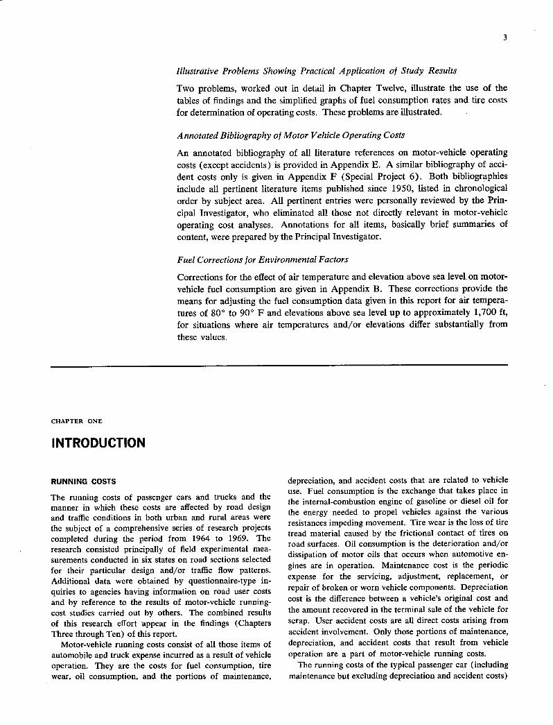
The running costs of passenger cars and trucks and the manner in which these costs are affected by road design and traffic conditions in both urban and rural areas were the subject of a comprehensive series of research projects completed during the period from 1964 to 1969. The research consisted principally of field experimental mea-surements conducted in six states on road sections selected for their particular design and/or traffic flow patterns. Additional data were obtained by questionnaire-type in-quiries to agencies having information on road user costs and by reference to the results of motor-vehicle running-cost studies carried out by others. The combined results of this research effort appear in the findings (Chapters Three through Ten) of this report.

Motor-vehicle running costs consist of all those items of automobile and truck expense incurred as a result of vehicle operation. They are the costs for fuel consumption, tire wear, oil consumption, and the portions of maintenance,

depreciation, and accident costs that are related to vehicle use. Fuel consumption is the exchange that takes place in the internal-combustion engine of gasoline or diesel oil for the energy needed to propel vehicles against the various resistances impeding movement. Tire wear is the loss of tire tread material caused by the frictional contact of tires on road surfaces. Oil consumption is the deterioration and/or dissipation of motor oils that occurs when automotive en-gines are in operation. Maintenance cost is the periodic expense for the servicing, adjustment, replacement, or repair of broken or worn vehicle components. Depreciation cost is the difference between a vehicle's original cost and the amount recovered in the terminal sale of the vehicle for scrap. User accident costs are all direct costs arising from accident involvement. Only those portions of maintenance, depreciation, and accident costs that result from vehicle operation are a part of motor-vehicle running costs.

The running costs of the typical passenger car (including maintenance but excluding depreciation and accident costs)

4

are approximately 30 percent of the total of all costs of car ownership and operation during the first 5 years of a car's life and about 35 percent of these costs over the life of the car, as shown by Winfrey (1, p. 310), using hypothetical values selected to accurately reflect typical automobile costs. All car costs other than running costs, depreciation, and accident costs (licensing, garaging, tolls, taxes, insurance, interest, and parking) constitute about 40 percent of the total of car ownership and operation costs each year throughout a car's service life. Depreciation makes up the remaining 25 to 30 percent of passenger-car ownership and operating costs.

For trucks in line-haul service, running costs (including maintenance costs and driver wages but excluding depre-ciation and accident costs) constitute a much higher portion of total ownership and operating costs than is the case for cars-60 percent for 40-kip trucks compared to 30 to 35 percent for cars (2). This is due largely to inclusion of driver wages and subsistence as running costs for trucks. Depreciation and non-running costs equal about 40 percent of truck ownership and operating costs.

Fuel consumption is a, larger element of running cost (fuel and oil consumption, tire wear, maintenance costs and, for trucks, driver wages) for passenger cars than for trucks-60 percent for the passenger cars under 5 years compared to 13 percent for the 40-kip truck (1, 2). Main-tenance and lubrication costs are about 30 percent and tire costs about 8 percent of running costs for both trucks and automobiles.

Fuel consumption is by far the most important of motor-vehicle running costs involved in the research reported on herein. It not only is a major expense, accounting for 8 to 18 percent of all costs of vehicle ownership and operation, but is far more sensitive to variation in road design and traffic conditions than are any of the other items of vehicle expense. Because it is the consumption or burning of fuel that produces the energy to overcome resistances, variations in road design (or traffic conditions) that increase or decrease resistance (steepening or flattening a grade, for example) are directly associated with a corresponding increase or decrease in vehicle fuel consumption.

Tire wear, also an important item of motor-vehicle running cost (constituting 3 and 5 percent of the total ownership and operating costs of passenger cars and trucks, respectively), is second only to fuel consumption in sensi-tivity to variation in road and traffic conditions. Tires form the surface of vehicle contact with road pavements and serve to transfer propulsion and control forces. Variations in these forces arising from vehicle operation on roads of different designs and/or traffic conditions have a pro-nounced effect on the frictional wear of tires at the contact surface.

Maintenance and lubrication costs are also important items of motor-vehicle cost (often as high as 18 percent of total ownership and operating costs for trucks, for ex-ample). Maintenance of vehicle appearance and main-tenance procedures to insure future dependability are not a part of running costs. The running-cost element of maintenance costs is affected primarily by road design

changes that increase or decrease travel distance, alter the frequency of stop-and-go operations, or change road surface conditions.

Total depreciation (the difference between a vehicle's original cost new and its terminal salvage value) is, by definition, not a running cost, because it is unaffected by vehicle use. However, it becomes a running cost when evaluated on a cost-per-mile basis because of the effect vehicle use has on lifetime mileage accumulation. Life-time mileage accumulation, in turn, is affected by average operating speeds, route lengths, and road surface conditions.

Accident costs are running costs when involvement in an accident occurs during vehicle operation. Accidents occur-ring when a vehicle is garaged or parked are not included.

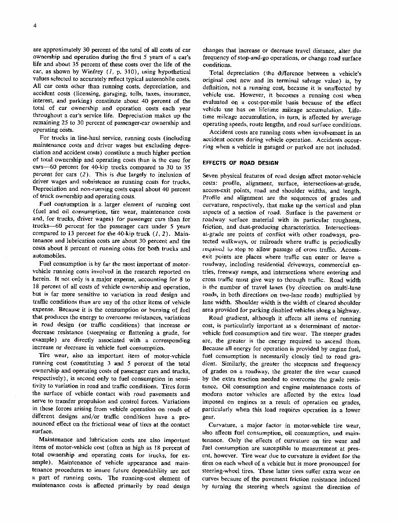
EFFECTS OF ROAD DESIGN

Seven physical features of road design affect motor-vehicle costs: profile, alignment, surface, intersections-at-grade, access-exit points, road and shoulder widths, and length. Profile and alignment are the sequences of grades and curvature, respectively, that make up the vertical and plan aspects of a section of road. Surface is the pavement or roadway surface material with its particular roughness, friction, and dust-producing characteristics. Intersections-at-grade are points of conflict with other roadways, pro-tected walkways, or railroads where traffic is periodically icquited to stop to allow passage of cron traffic Access-exit points are places where traffic can enter or leave a roadway, including residential driveways, commercial en-tries, freeway ramps, and intersections where entering and cross traffic must give way to through traffic. Road width is the number of travel lanes (by direction on multi-lane roads, in both directions on two-lane roads) multiplied by lane width. Shoulder width is the width of cleared shoulder area provided for parking disabled vehicles along a highway.

Road gradient, although it affects all items of running cost, is particularly important as a determinant of motor-vehicle fuel consumption and tire wear. The steeper grades are, the greater is the energy required to ascend them. Because all energy for operation is provided by engine fuel, fuel consumption is necessarily closely tied to road gra-dient. Similarly, the greater the steepness and frequency of grades on a roadway, the greater the tire wear caused by the extra traction needed to overcome the grade resis-tance. Oil consumption and engine maintenance costs of modern motor vehicles are affected by the extra load imposed on engines as a result of operation on grades, particularly when this load requires operation in a lower gear.

Curvature, a major factor in motor-vehicle tire wear, also affects fuel consumption, oil consumption, and main-tenance. Only the effects of curvature on tire wear and fuel consumption are susceptible to measurement at pres-ent, however. Tire wear due to curvature is evident for the tires on each wheel of a vehicle but is more pronounced for steering-wheel tires. These latter tires suffer extra wear on curves because of the pavement friction resistance induced by turning the steering wheels against the direction of

5

vehicle motion to develop the necessary turning force. The extra fuel consumed on curves provides the additional energy needed to propel the vehicle against this induced pavement friction.

Road surface conditions have an important bearing on fuel consumption, tire wear, oil consumption, and main-tenance. Extra energy (and, therefore, extra fuel consump-tion) is needed on rough gravel or loose stone surfaces either to force wheels up and over the stones or to push the stones aside. Extra fuel is needed on loose sand and earth surfaces either to force wheels out of depressions or to push sand or soil particles aside to form ruts. Tires are subject to extra wear either on loose stone or on slip-resistant surfaces where they are subject to the deteriorating effects of heavy buffeting, in the case of stone roads, or excessive friction wear, in the case of abrasive pavements. Oil consumption is affected by the dust-producing charac-teristics of road surfaces: the more dusty the surface, the greater the frequency of engine oil changes. Maintenance is related to road surface principally through the effects rough roads have on vehicle suspension systems and dusty roads have on the wear of cylinder walls, piston rings, and bearing surfaces.

Intersections-at-grade as an element of road design are responsible for a considerable share of motor-vehicle fuel consumption, tire wear, oil consumption, and maintenance costs through their action in causing vehicle stops and slowdowns. Extra fuel is needed to accelerate vehicles back to running speed after they have been stopped or slowed. Tire wear occurs when vehicles stop and start up again, both because of the frictional wear during braking and the traction slip during acceleration. Oil consumption is increased by stops due to the effect of speed changes on oil contamination rate. Maintenance is amplified by stops both because of brake wear during deceleration and because of transmission wear during acceleration.

Access-exit points are locations where, because of enter-ing and/or leaving cars or trucks, through vehicles often are required to slow down momentarily. The change from an initial speed to a lower speed followed by resumption of the initial speed is reflected principally in the additional fuel needed for the acceleration to regain speed.

Road lane widths, together with the number of lanes and the width of shoulders, affect motor-vehicle running costs through their effect on vehicle speeds and road capacity. For a given traffic flow rate, an insufficient number of travel lanes (over-all road width) may cause interference among vehicles, resulting in frequent vehicle speed changes. These speed changes (speed reductions followed by resump-tion of speed) induce extra fuel and oil consumption, tire wear, and maintenance cost. Because this item of road design affects running costs most during times of heavy traffic volumes, it is essentially a factor of road capacity and traffic conditions and is considered in the following.

Length is the travel distance along a particular route between two trip end points. A realignment of the route that reduces this distance does away with all vehicle run-ning costs, including depreciation and accident costs, for the length of road eliminated.

EFFECTS OF TRAFFIC CONDITIONS

Traffic conditions on both urban and rural routes affect motor-vehicle running costs only where traffic volumes interfere with the uniformity of speeds on individual ve-hicles. The influence of traffic on motor-vehicle running costs, therefore, is a combined effect of road design factors which determine capacity (particularly gradient, curvature, road width, intersections-at-grade, and access-exit points) and traffic volumes. Where traffic volumes are low relative to road capacity at a particular location, vehicles may move at uniform speeds, and traffic conditions have little effect on running costs. But, where traffic volumes are high relative to road capacity, vehicles interfere with each other and, in jockeying for position, develop erratic pat-terns of speed change that have an effect on all elements of running cost. Where traffic volumes are particularly high (equal to or approaching capacity) such as often occurs on high-volume expressways near busy access-exit points, vehicles may be slowed to a stop, or even to a series of stops of uncertain duration, with a corresponding increase in the running costs associated with stops and slowdowns: fuel and oil consumption, tire wear, and maintenance:

The only traffic condition for which meaningful relation-ships between traffic volume and running costs can be established readily are medium-to-heavy traffic flows below route capacity on road sections having uniform design characteristics throughout their length. At low volumes, vehicle fuel consumption is only slightly affected by traffic conditions; and, at volumes equal to or approaching ca-pacity, running costs depend on a variety of factors which can not be predicted (traffic composition, frequency of congestion stops, duration of such stops, driver response to congestion situations, racing of engines to promote engine cooling, and the duration of congestion periods). Uni-formity of road design provides a definite relationship between traffic volume and road design details for a section of road. A road section that might pass a given volume of traffic if design details are uniform might become congested at the same traffic volume near a point of non-uniformity (an exit or access point on a freeway, for example, where traffic is slowed by leaving or entering vehicles).

Traffic conditions severe enough to be a factor in motor-vehicle fuel consumption (without being bad enough to cause congestion stops) will usually also induce lower average speeds as the normally faster vehicles get trapped behind slower vehicles. A driver attempting to travel in heavy traffic at a certain speed will find that he not only will have to change speeds frequently in trying to maintain this speed but also will inexorably suffer a reduction in average running speed. For many ranges of speeds the lower average speed forced by traffic conditions partially or entirely compensates for the extra fuel consumption caused by traffic-induced speed changes.

On sections of access-controlled multi-lane highways and urban freeways where traffic is not affected by such inter-ruptions as entering vehicles at an access ramp, free-flowing conditions prevail at volumes up to nearly 800 vehicles per hour (vph) per lane. Here frequent congestion stops (forced flow) occur at capacity volumes of about 2,000

r;i

vph per lane (3). The relationship of fuel consumption rates to traffic conditions is especially meaningful for the range of traffic volumes from approximately 800 to 1,800 vph per lane (service levels B through D).

Free-flowing traffic conditions are found on sections of two-lane rural roads for traffic volumes up to 400 vph (both directions) where there is no interference activity, such as is associated with adjacent service stations, for example (3). Congestion stops on these .roads occur at two-way volumes of about 1,800 vph or more. The rela-tionship of vehicle fuel consumption and traffic flow on such roads is particularly significant for two-way volumes of about 500 to 1,700 vph (service levels B through D).

In urban areas the three principal types of non-freeway routes are residential streets, major street arterials, and central business district (CBD) streets. Traffic flows on

residential streets, by the nature of such streets, are essen-tially low-volume and slow. They normally affect fuel consumption only through the traffic control devices (stop signs and yield signs) needed for the safety of vehicle users and pedestrians at intersections, and through the slow-downs that occur when turning corners and crossing other streets at uncontrolled intersections. On arterials and CBD streets, however, irregular traffic interruptions due to inter-sections-at-grade (traffic signals), curb parking, double-parked vehicles, and pedestrian movements have a pro-nounced effect on vehicle fuel consumption that varies with traffic volumes even at low volumes. Motor-vehicle fuel consumption rates on these latter two types of urban route can be predicted for specific traffic conditions and selected combinations of traffic signal stops and traffic volumes.

CHAPTER TWO

RESEARCH APPROACH

RESEARCH TECHNIQUE

information on the effect of road design and traffic condi-tions on running costs was secured by direct experiment, analyses of user cost records, personal and written inquiries to those likely to have particular information in the area of user costs, and reviews of motor-vehicle cost data developed in studies conducted by others. Direct experiments con-sisted of field measurements of elements of running cost for actual road and traffic conditions. Analysis of user cost records involved computations to structure data from such records, particularly vehicle maintenance records, for run-ning cost studies. Personal and written inquiries were made to operators of fleets of vehicles, vehicle manufacturers and vehicle research engineers to obtain information otherwise unavailable. Motor-vehicle cost data developed by other researchers in the field were reviewed for their particular applicability in the study of running costs.

Field measurements were especially important for de-veloping data on fuel and oil consumption and tire wear costs. Because these items are uniquely sensitive to changes in road and traffic conditions, detailed information on the effect that road design and traffic conditions have on fuel consumption, oil consumption, and tire wear were needed. Available data were severely limited in scope and range of applicability. Adequate field data on fuel consumption were lacking, principally because a suitable fuelmeter had not been available for use in previous studies. Tire wear and oil consumption data were lacking because there had not been sufficient interest earlier to warrant the relatively high cost of conducting the necessary field studies.

Road user cost records submitted in reply to inquiries addressed to agencies having particular information on vehicle operating costs were used to secure data on vehicle maintenance. Some direct experiments were employed to obtain data on this subject (the effect of stop-and-go opera-tions on brake wear, for example) but most data were generated by analyzing user cost records.

FUEL CONSUMPTION MEASUREMENTS

Fuel consumption measurements were recorded for each of several representative types of vehicles operating on each of several road test sections. Each test section exhibited a particular design throughout, with operations conducted either at a series of uniform speeds, through specified speed change sequences, or with the speed patterns resulting when drivers attempt to travel at certain speeds as part of a moving traffic stream for various traffic volumes. Fuel consumption was also measured for each vehicle with the vehicle stationary and the engine idling.

Data for each test vehicle were obtained by driving the vehicle at a specified speed condition (uniform speed or speed change pattern) over a measured distance on each test section. The time to travel the measured distance in seconds (nearest 0.1 sec) and the fuel consumed in gallons (nearest unit of about 0.001 gal.) were recorded for each test run in each direction. A minimum of three test runs were made in each direction. If the values recorded for these runs varied appreciably, additional test runs were made until stable values of run time and fuel consumption were established. Average speed for each test run was

computed from the measured test section length and the elapsed time measurement.

Fuel measurements were made for five different pas-senger-car models, five types of truck (including a diesel-operatcd truck), and a bus. The passenger car test vehicles represented the full range of cars from the small foreign import to the large Chrysler New Yorker. The trucks ranged from a pickup truck to a 2-S2 tractor semi-trailer truck combination. Only one bus was used, however, it was a typical urban transit bus.

The five passenger-car test vehicles are described in Table 1. Only the empty (or tare) weight is given in the table, because three of the vehicles were tested at more than one loaded (road) weight. Each vehicle was operated with a carried load of 200 lb. In addition, the Chevrolet sedan was operated with carried loads of 600 and 1,000 lb, and the Chrysler sedan was operated with a carried load of 600 lb. The wheel radius for each car was determined as the average measured distances from the centers of the four wheels to a flat pavement for a carried load of 200 lb.

The Chevrolet sedan test car in Table I is shown in Figure 1. This automobile was the principal test vehicle used in the operating cost study. It was purchased new for NCHRP Projects 2-5 and 2-7 in February 1964 and was used for fuel and oil consumption test measurements, tire wear measurements, maintenance measurements, and mea-surements of the effects of environmental conditions on

7

Figure 1. /964 Chevrolet sedan test vehicle.

fuel consumption rates, as well as for each of two special projects described in Appendix F. It has been operated on test projects for a total distance of over 60,000 miles.

The test trucks and bus are described in Table 2. Again, tare weights rather than road weights are given because two of the vehicles, the pickup truck and the bus, were operated at more than one road weight, as shown in the findings of this report. Wheel radii are averages of the measured distances from wheel centers to pavement for each vehicle when loaded to road weight. For the pickup

TABLE 1

DESCRIPTION OF PASSENGER-CAR TEST VEHICLES

iTEM CHRYSLER PLYMOUTH' CHEVROLET FALCON VOLKSWAGEN

Model 4-door sedan 4-door sedan 4-door-sedan 2-door 2-door Model year 1966 1968 1964 1965 1965 Tare weight (lb) 4,200 4,200 3,800 2,800 1,900 Speedometer reading:

Beginning of study 18,000 6,000 0 16,000 32,000 End of study 22,000 8,000 60,000 20,000 36,000

Frnntal area (sq ft) 76 26 26 26 24 Wheel base (in.) 121.5 119.5 119.0 117.0 94.5 Wheel rolling radius (in.) 13.0 13.5 12.0 11.5 11.5 Tire size (in.) 8.25 x 14 8.55 x 14 7.50X 14 6.50X 13 5.6X 15 Tire pressure (psi) 32 32 30 30 20 Engine:

No. of cylinders 8 8 8 6 4 Compression ratio 10:1 9.2:1 9.2:1 9.2:1 7.0:1 Displacement (cu in.) 440 383 283 200 72 Net horsepower 350 290 195 120 42 Engine speed (rpm) 4,400 4,400 4,800 4,400 3,900 Carburetor 4B 2B 2B 2B 2B Gasoline Prem. Reg. Reg. Reg. Reg. Oil capacity (qt) S 5 5 5 2.6 Bore-stroke (in.) 4.32-3.75 4.25-3.375 3.875-3.0 3.68-3.13 3.03 1-2.52

Transmission: Type Auto. Auto. Auto. Auto. Man. Ratio in first 2.45:1 2.45:1 1.82:1 2.46:1 3.08:1 Ratio in second 1.45:1 1.45:1 1.00:1 1.46:1 2.06:1 Ratio in third 1.00:1 1.00:1 - 1.00:1 1.32:1 Ratio in fourth - - - - 0.89:1

Rear-axle ratio 2.76: 1 2.76:1 3.08: 1 2.88:1 4.375:1 Steering ratio 15.7:1 15.7:1 24.0:1 22.0:1 -

'A one-axle travel trailer was used with this vehicle on certain runs. It had a cross section of 65.0 sq ft and weighed 3,000 lb

TABLE 2

DESCRIPTION OF TRUCK AND BUS TEST VEHICLES

ITEM

PICKUP TRUCK, 2-AXLE 4-TIRE

SINGLE-UNIT TRUCK, 2-AXLE 6-iiRE 1

SINGLE-UNIT TRUCK, 2-AXLE 6-TIRE

TRACTOR TRANSIT SEMI-TRALER BUS, TRUCK, 2-AXLE 2-S2 6-TIRE

Body type Box Van Van Flat 31-passenger Model year 1967 1965 1962 1960 1960 Tare weight (ib) 4,500 8,600 10,000 20,000 12,500 Speedometer reading:

Beginning of study 15,000 12,000 86,000 92,000 70,000 End of study 21,000 16,000 90,000 96,000 73,000

Frontal area (sq ft) 32 90 88 58 80 Dimensions:

Height (ft) 6.0 11.3 11.0 8.0 10.0 Width (ft) 6.0 8.0 8.0 8.0 8.0

Wheel rolling radius (in.) 14.0 16.5 16.5 16.5 16.5

Tire size (in.) 7x17.5 8.25x20 8.25x20 8.25x20 8.25x20 Engine:

No. of cylinders 6 6 6 6 6 Displacement

(Cu in.) 250 351/477 305 386 270 Net horsepower 125 142/135 142 175 124 Engine speed

(100 rpm) 38 38/32 38 32 32 Fuel Gas. Gas/dies. Gas. Gas. Gas Oil capacity (qt) 5 6 6 8 6

Transmission: Tvoe Man. Man. Man. Man. Auto. Ratio inflrst 7.06:1 7.06:1 6.68:1 1.88:1 3.82:1 Ratio in second 3.58:1 3.58:1 3.24:1 4.68:1 2.63:1 Ratio in third 1.72:1 1.72:1 1.68:1 2.84:1 1.45:1 Ratio in fourth 1.00:1 1.00:1 1.00:1 1.68:1 1.00:1 Ratio in fifth - - - 1.00:1 -

Rear-axleratio 4.57:1 5.83:1 6.17:1 6.14:1 6.71:1 8.37:1

1 Two single-unit trucks are represented. They are identical in every way except one is gasoline-operated, has a cylinder displacement of 351 cu in. and a net horsepower of 142 at 3,800 rpm; the other is diesel-operated, has a cylinder displacement of 477 cu in. and a net horsepower of 135 at 3,200 rpm.

truck and the bus, wheel radii are for the lightest road weights.

There actually were two 1965 two-axle six-tire trucks (Col. 3, Table 2), one gasoline-operated and one diesel-operated. The vehicles were identical except for the differ-ences in type of fuel, engine displacement, net horsepower, and engine speed, as given in the table. These two vehicles were put through identical test programs to establish the relationship of vehicle fuel use for gasoline and diesel trucks as described in Appendix D.

The test bus is shown in Figure 2. Two of the test trucks, the two-axle six-tire truck and the 2-S2 tractor semi-trailer truck combination, are shown in Figures 3 and 4, respectively. A sign on the side of each vehicle identifies its loaded (road) weight and indicates whether it is gaso-line- or diesel-operated.

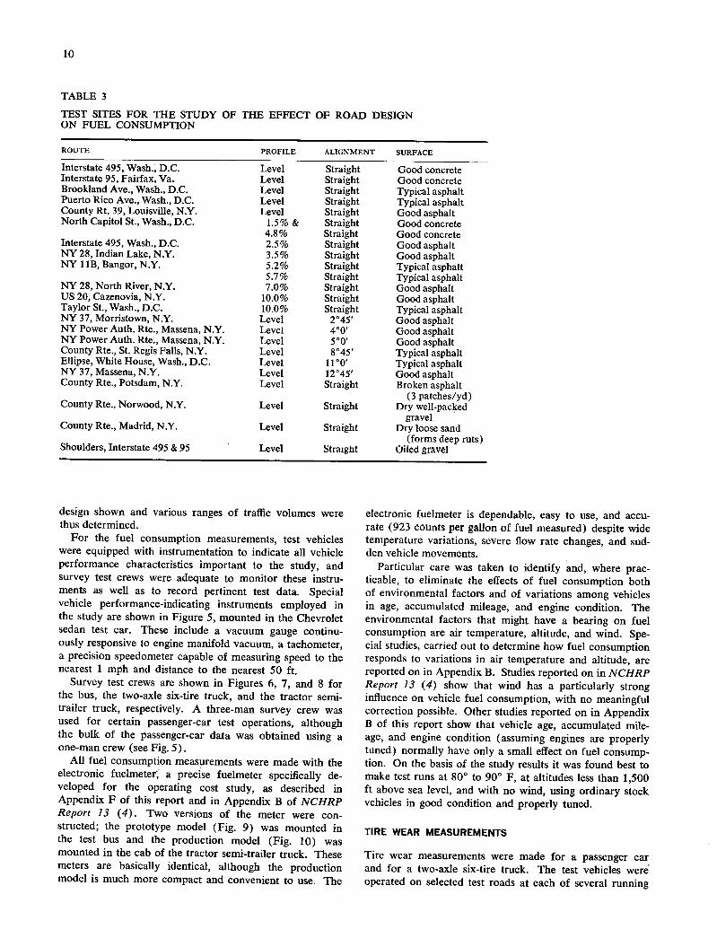
Measurements of the fuel consumption of motor vehicles as affected by road design were made on each of the 22 sections of road described in Table 3. Each test section exhibited a particular combination of grade, alignment, and surface condition. Data were collected first for operation at various constant speeds on roads with the basic design

condition: level, straight roads with good pavement. Then, operations were carried out on test sections where two of the design factors were the same but where the third was changed so that the effects on fuel consumption of varying individual road design factors could be determined. Traffic volumes on the test roads were negligible at the time the test runs were made.

Test operations to determine the effect on fuel consump-tion of speed changes, particularly stop-and-go and slow-down speed change cycles, were made on those test sections of Table 3 with the basic conditions: level profile, straight alignment, and good pavement. The additional fuel con-sumption due to cycles of speed change were found by subtracting the fuel consumption for uniform speed test runs from the fuel consumption for corresponding runs which involved a speed change.

Measurements of the fuel consumption of motor vehicles as affected by traffic conditions were made on each of the 13 road sections described in Table 4. Test operations were conducted on each section at times when each of several levels of traffic volume prevailed. The effects on test-vehicle fuel consumption of the different types of road

TE5TJ-N

Figure 2. Transit bus test vehicle.

Figure 3. Two-axle six-tire truck test vehicle.

9

Figure 4. 2-S2 tractor scnzi-i railer truck coin bination test vehicle.

10

TABLE 3

TEST SITES FOR THE STUDY OF THE EFFECT OF ROAD DESIGN ON FUEL CONSUMPTION

ROUTE PROFILE ALIGNMENT SURFACE

Interstate 495, Wash., D.C. Level Straight Good concrete Interstate 95, Fairfax, Va. Level Straight Good concrete Brookiand Ave., Wash., D.C. Level Straight Typical asphalt Puerto Rico Ave., Wash., D.C. Level Straight Typical asphalt County Rt. 39, Louisville, N.Y. Level Straight Good asphalt North Capitol St., Wash., D.C. 1.5% & Straight Good concrete

4.8% Straight Good concrete Interstate 495, Wash., D.C. 2.5% Straight Good asphalt NY 28, Indian Lake, N.Y. 3.5% Straight Good asphalt NY 1 IB, Bangor, N.Y. 5.2% Straight Typical asphalt

5.7% Straight Typical asphalt NY 28, North River, N.Y. 7.0% Straight Good asphalt US 20, Cazenovia, N.Y. 10.0% Straight Good asphalt Taylor St., Wash., D.C. 10.0% Straight Typical asphalt NY 37, Morristown, N.Y. Level 2°45' Good asphalt NY Power Auth. Rte., Massena, N.Y. Level 4°0' Good asphalt NY Power Auth. Rte., Massena, N.Y. Level 5°0' Good asphalt County Rte., St. Regis Falls, N.Y. Level 8°45' Typical asphalt Ellipse, White House, Wash., D.C. Level 11,01 Typical asphalt NY 37, Massena, N.Y. Level 1245' Good asphalt County Rte., Potsdam, N.Y. Level Straight Broken asphalt

(3 patches/yd) County Rte., Norwood, N.Y. Level Straight Dry well-packed

gravel County Rte., Madrid, N.Y. Level Straight Dry loose sand

(forms deep ruts) Shoulders, Interstate 495 & 95 Level Straight Oiled gravel

design shown and various ranges of traffic volumes were thus determined.

For the fuel consumption measurements, test vehicles were equipped with instrumentation to indicate all vehicle performance characteristics important to the study, and survey test crews were adequate to monitor these instru-ments as well as to record pertinent test data. Special vehicle performance-indicating instruments employed in the study are shown in Figure 5, mounted in the Chevrolet sedan test car. These include a vacuum gauge continu-ously responsive to engine manifold vacuum, a tachometer, a precision speedometer capable of measuring speed to the nearest 1 mph and distance to the nearest 50 ft.

Survey test crews are shown in Figures 6, 7, and 8 for the bus, the two-axle six-tire truck, and the tractor semi-trailer truck, respectively. A three-man survey crew was used for certain passenger-car test operations, although the bulk of the passenger-car data was obtained using a one-man crew (see Fig. 5).

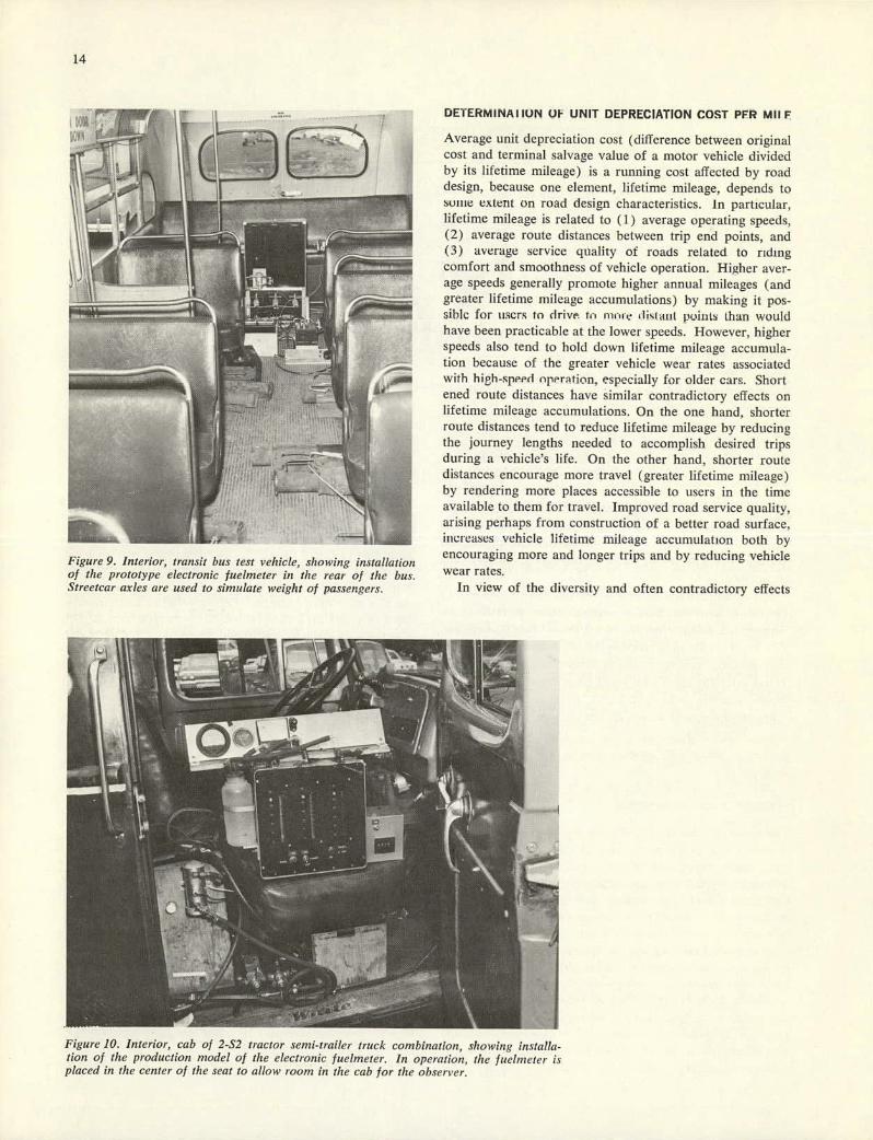
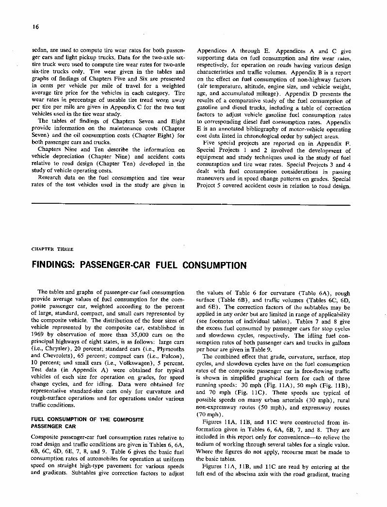
All fuel consumption measurements were made with the electronic fuelmeter; a precise fuelmeter specifically de-veloped for the operating cost study, as described in Appendix F of this report and in Appendix B of NCHRP Report 13 (4). Two versions of the meter were con-structed; the prototype model (Fig. 9) was mounted in the test bus and the production model (Fig. 10) was mounted in the cab of the tractor semi-trailer truck. These meters are basically identical, although the production model is much more compact and convenient to use. The

electronic fuelmeter is dependable, easy to use, and accu-rate (923 counts per gallon of fuel measured) despite wide temperature variations, severe flow rate changes, and sud-den vehicle movements.

Particular care was taken to identify and, where prac-ticable, to eliminate the effects of fuel consumption both of environmental factors and of variations among vehicles in age, accumulated mileage, and engine condition. The environmental factors that might have a bearing on fuel consumption are air temperature, altitude, and wind. Spe-cial studies, carried out to determine how fuel consumption responds to variations in air temperature and altitude, are reported on in Appendix B. Studies reported on in NCHRP Report 13 (4) show that wind has a particularly strong influence on vehicle fuel consumption, with no meaningful correction possible. Other studies reported on in Appendix B of this report show that vehicle age, accumulated mile-age, and engine condition (assuming engines are properly tuned) normally have only a small effect on fuel consump-tion. On the basis of the study results it was found best to make test runs at 800 to 90° F, at altitudes less than 1,500 ft above sea level, and with no wind, using ordinary stock vehicles in good condition and properly tuned.

TIRE WEAR MEASUREMENTS

Tire wear measurements were made for a passenger car and for a two-axle six-tire truck. The test vehicles were operated on selected test roads at each of several running

11

TABLE 4

TEST SITES FOR THE STUDY OF THE EFFECT OF TRAFFIC CONDITIONS ON FUEL CONSUMPTION

INTERSECTION

ROUTE LANES CONTROL PROFILE/ALIGNMENT

(a) Freeways and expressways—divided—access controlled

Baltimore Expressway, Wash., D.C. 6 Separated 1.5% /straight Eisenhower Expressway, Chicago 6 Separated Level/straight Southern Expressway, Long Island 6 Separated Level/straight Kenilworth Ave., Wash., D.C. 6 Separated Level/straight

(b) Urban arterials—undivided—no control of access

North Capitol St., Wash., D.C. 6 Signals 1.5% /straight Michigan Ave., Wash., D.C. 4 Signals 1.5 % /straight Wisconsin Ave., Wash., D.C. 4 Signals 1% to 4% with

minor curvature Roosevelt Ave., Chicago 4 Signals Level/straight Independence Ave., Wash., D.C. 4 Signals Level/straight Constitution Ave., Wash., D.C. 8 Signals Level/straight

(c) CBD streets—undivided—no control of access

G St., Wash., D.C. 4 Signals Level/straight 34th St., N.Y. City 4 Signals Level/straight 42nd St., N.Y. City 6 Signals Level/straight

speeds and for certain speed change patterns. Tire wear was established by noting the loss in tire weight occurring during a test operation. Tire wear values (weight loss in grams) per unit travel distance (mile) were developed at each of several speeds (or speed change patterns) for operation on each of several surface types and degrees of curvature.

The Chevrolet sedan described in Table 1 was used for the passenger-car tire wear study, and the two-axle six-tire truck (Col. 3, Table 2) was used for the tire wear measure-ments of the two-axle six-tire truck. The passenger car was operated at a gross vehicle weight of 4,000 lb on 7.50-by 14-in, two-ply tires and was considered to develop tire wear patterns typical of lightweight vehicles (passenger cars and pickup trucks) varying in weight from 2,000 to 5,000 lb. The two-axle six-tire truck was operated on 8.25- by 20-in. 10-ply truck tires at axle loads of 12,000 lb (rear) and 4,000 lb (front). The tire wear patterns of this vehicle were assumed to represent typical patterns for all two-axle six-tire trucks. No tire wear measurements were made for tractor semi-trailer truck combinations.

Tire wear data were recorded for operation at the ten test sites given in Table 5. Four surface types are repre-sented: good concrete, good asphalt, typical asphalt, and dry well-packed gravel. For the road surface described as typical asphalt, test sites for each of six different curve patterns were included. One major street urban arterial route is also included among these test sites.

Tire wear was measured by weighing after it had been established through a special study (reported in Appendix F) that this procedure was the most appropriate for the accurate determination of tire wear. A tire to be weighed was removed from its rim, cleaned thoroughly, and in-spected before being placed on the scales in the exact

center of the weighing plate. Two independent weighings were made before a tire weight was recorded to detect any error that might arise through failure to balance the scales properly or from incorrect placement of the tire on the weighing plate.

The total weight of tread material available for wear was recorded for each size of tire: 1,500 gm for the pas-senger-car tire, and 4,500 gm for the truck tire.

DETERMINATION OF MAINTENANCE COSTS

Limited data on the effects of road design and traffic condi-tions on vehicle maintenance costs were obtained by direct experiment, by questionnaire inquiry to agencies that oper-ate large fleets of vehicles, and from published research data. The information developed by experiment was the maintenance cost of brake systems due to vehicle stops. The Chevrolet test car in Table 1 was operated through a sequence of 15,000 stop cycles at 25 mph immediately after installation of new brake shoes and wheel cylinders. The difference in brake-shoe weight before and after the test operations and the seal deterioration and brake fluid loss occurring during the test were evaluated in terms of brake cost per stop cycle.

Information on the maintenance cost of parts of pas-senger cars and pickup trucks subject to wear as a result of vehicle operation was obtained as cost per mile of travel by questionnaire inquiry, without regard to specific road designs. Questionnaires were sent to each of the Bureau of Public Roads' Division Engineers and to each of the Chief Engineers of the state highway departments—a dis-bursement of 100 inquiries. Twenty percent of the in-quiries were returned with information on the over-all

12

Figure 5. Interior, 1964 Chevrolet sedan test vehicle, showing survey speedometer, tach-ometer, vacuum gauge, oil and fuel pressure gauges, am,neter, and water temperature indicator.

mileage repair costs of individual parts of 1,350 passenger cars and 15 piLkup tiucks.

Two reference works (2, 5) containing good research data on the cost of operating large line-haul trucks were relied on for data on the effect of travel on truck main-tenance costs. The information in these references is based on large-scale reviews of the operating costs of truck fleets. For example, Stevens (2) reports on data for 611 compan-ies (23,000 vehicles).

jT

A.

I is:ure ó..urve•v crew and vehicle, transit hn.s ,ctucjy.

DETERMINATION OF VEHICLE OIL CONSUMPTION

Motor oil is consumed in vehicle operation in three ways: (1) contamination by impurities, (2) dissipation by com-bustion and evaporation, and (3) leakage. Contamination of oil with combustion remnants (water and acid-forming sludge) and with dust particles from dusty roads does not cause appreciable loss of volume but, because the oil has to he replaced to protect the engine, contamination is a true element of oil consumption. A measurable amount of

13

Figure 7. Two survey crews and vehicle—two-axle six-tire truck study.

oil is dissipated through combustion and evaporation and through leakage, especially at high operating speeds. Oil consumption through contamination is promoted by low speeds and frequent stops (travel on urban streets) when combustion remnants cannot be burned off, and by travel on dusty roads. Oil consumption through dissipation and leakage is accelerated by travel on high-speed freeways and expressways.

Oil consumption data were developed by two means: (I) reviews of manufacturers' recommendations regarding con-ditions that define when engine oil should be replaced, and (2) experiments to determine the oil dissipation and leak-age resulting from operation at various uniform speeds, on urban arterials, and for stop-and-go cycles of speed change. Shop manuals were purchased from General Motors, Chrysler, Ford, and Volkswagen motor companies to facili-

tate the review of vehicle manufacturers' oil change recom-mendations.

Experiments to determine the effect on engine oil con-sumption of different uniform speeds, urban arterial travel, and stop-and-go travel were carried out using the Chevrolet sedan described in Table I and the two-axle six-tire truck described in Col. 3, Table 2. The differences in weight of engine oil and filter before and after test runs were care-fully determined, using the precision scales acquired for the tire wear measurements. Oil temperature and viscosity were recorded each time oil weights were determined. Oil consumption data in relation to speed were obtained for operation at 35, 45, 55, and 60 mph, for a series of 15,000 stop cycles at 25 mph (passenger car only) and for travel on an urban arterial at an attempted speed of 25 to 35 mph for the passenger car and 20 to 25 mph for the two-axle six-tire truck.

r g 1

Figure 8. Survey crew and vehicle.-2-S2 tractor semi-ira i/er truck co,nbjnation study.

14

iLT

T1N \\O_ ru

Figure 9. Interior, transit bus test vehicle, showing installation of the prototype electronic fuelmeter in the rear of the bus. Streetcar aries are used to simulate weight of passengers.

DETERMINAII0N OF UNIT DEPRECIATION COST PFR MIIF

Average unit depreciation cost (difference between original cost and terminal salvage value of a motor vehicle divided by its lifetime mileage) is a running cost affected by road design, because one element, lifetime mileage, depends to soiiie extent on road design characteristics. In particular, lifetime mileage is related to (I) average operating speeds,

average route distances between trip end points, and average service quality of roads related to riding

comfort and smoothness of vehicle operation. Higher aver-age speeds generally promote higher annual mileages (and greater lifetime mileage accumulations) by making it pos-ibIc for users to drive to moie ,lktiil poilils than would

have been practicable at the lower speeds. However, higher speeds also tend to hold down lifetime mileage accumula-tion because of the greater vehicle wear rates associated with high-specl operation, especially for older cars. Short ened route distances have similar contradictory effects on lifetime mileage accumulations. On the one hand, shorter route distances tend to reduce lifetime mileage by reducing the journey lengths needed to accomplish desired trips during a vehicle's life. On the other hand, shorter route distances encourage more travel (greater lifetime mileage) by rendering more places accessible to users in the time available to them for travel. Improved road service quality, arising perhaps from construction of a better road surface, increases vehicle lifetime mileage accumulation both by encouraging more and longer trips and by reducing vehicle wear rates.

In view of the diversity and often contradictory effects

Figure 10. Interior, cab of 2-52 tiactor semi-trailer truck combination, showing installa-tion of the production model of the electronic fuelmeter. In operation, the fuelmeter is placed in the center of the seat to allow room in the cab for the observer.

15

TABLE 5

TEST SITES FOR THE STUDY OF THE EFFECT OF ROAD DESIGN AND TRAFFIC ON TIRE WEAR

ROUTE SURFACE DESIGN FEATURE

Interstate 495, Wash., D.C., Beltway Good concrete Four-lane divided Interstate 81, N.Y. State Good asphalt Four-lane divided Town road system, N.Y. State Dry well-packed gravel Two lanes Crosstown route, Wash., D.C. Good concrete Urban arterial Ellipse, White House, Wash., D.C. Typical asphalt 11° curve Shirlington Circle, Arlington, Va. Typical asphalt 18° curve Traffic Circle, Massena, N.Y. Typical asphalt 12° curve Sherman Circle, Wash., D.C. Typical asphalt 31° curve Parking lot, Catholic Univ., Wash., D.C. Typical asphalt 570 curve Runway, Bolling Air Force Base, D.C. Typical asphalt 900 curve

that road design improvements have on the lifetime mileage accumulations of motor vehicles, it was determined that the research approach most appropriate for this aspect of the user cost evaluation study was a review of the literature, supplemented with a limited field investigation of the rela-tionship between used-car prices and vehicle mileage ac-cumulation, including data for recently scrapped vehicles. Particularly useful discussions of motor vehicle deprecia-tion costs are given by Winfrey (1, p. 347) and by De Weille (6, p. 59).

DETERMINATION OF ACCIDENT COSTS RELATIVE TO

ROAD DESIGN

The study of motor-vehicle accident costs in relation to road design was conducted as a special project (Special Project 5). This investigation was an analytical develop-ment of automobile and truck accident costs relative to type of road, frequency of intersections, and degree of curvature, based on the results of the motor-vehicle acci-dent cost studies conducted in Massachusetts, Illinois, Utah, and the District of Columbia, together with data from various sources in the literature. A description of Special Project 5, along with analysis results, appears in Appen-dix F.

PRESENTATION OF RESULTS

The principal results of the study are presented in Part I of this report as compact tables of fuel consumption, tire wear, maintenance, and oil consumption and as text presen-tations of depreciation and accident costs. The tables of findings for fuel consumption and tire wear are supple-mented with graphical presentations of the fuel consump-tion and tire wear for combinations of road design condi-tions at typical running speeds. Research results developed in the study in support of the material presented in the tables and graphs of findings of Part I, as well as an annotated bibliography of motor-vehicle operating costs, are included in Appendices A through F. The tables and graphs of findings of passenger-car fuel consumption, truck fuel consumption, passenger-car tire wear, truck tire wear, vehicle maintenance, and vehicle oil consumption are given

in Chapters Three, Four, Five, Six, Seven, and Eight, re-spectively. Presentations of depreciation and accident costs of cars and trucks are given in Chapters Nine and Ten, respectively.

The findings of this report are average values for broad categories of vehicle types weighted according to the distri-bution of vehicle types and sizes within each category. Specific measurements of fuel consumption and tire wear for individual test vehicles are given in Appendices A and C, respectively. Only the weighted average fuel con-sumption rates and tire wear rates for the distribution of vehicle types in each category are given in the tables and graphs of findings of Part I.

Passenger-car fuel consumption data were developed for five vehicle types: Chrysler, Plymouth, Chevrolet, Falcon, and Volkswagen. However, in the tables and graphs of findings (Chapter Three) only a weighted average of the fuel consumption rates for the five vehicles is reported. Values for the individual test vehicles appear in Appendix A.

In the tables and graphs of findings of fuel consumption for trucks, Chapter Four, three basic truck categories are recognized: pickup and panel trucks, two-axle six-tire trucks, and tractor semi-trailer truck combinations. Average fuel consumption values are given for the typical distri-butions of trucks in each category in the tables and graphs of findings. Fuel consumption data for the pickup and panel truck category were developed for a pickup truck at each of two gross vehicle weights: 4,800 lb and 5,800 lb. Data for the two-axle six-tire truck were obtained using three vehicles—one operating at 8,000 lb, one at 16,000 lb and one at 24,000 lb. Data for the tractor semi-trailer truck combinations were taken from the published results of Sawhill's 1959 study of the fuel consumption rates of 42,000- and 50,000-lb tractor semi-trailer truck com-binations (7). Fuel consumption results for the individual test trucks are given in Appendix A.

Similarly, in the tables and graphs of findings of Chapters Five and Six, tire wear for passenger cars and trucks, respectively, are given for the same categories of vehicles as described previously for the tables and graphs of findings for fuel consumption. However, in the case of tire wear measurements, data for a single vehicle, the Chevrolet

16

sedan, are used to compute tire wear rates for both passen-ger cars and light pickup trucks. Data for the two-axle six-tire truck were used to compute tire wear rates for two-axle six-tire trucks only. Tire wear given in the tables and graphs of findings of Chapters Five and Six are presented in cents per vehicle per mile of travel for a weighted average tire price for the vehicles in each category. Tire wear rates in percentage of useable tire tread worn away per tire per mile are given in Appendix C for the two test vehicles used in the tire wear study.

The tables of findings of Chapters Seven and Eight provide information on the maintenance costs (Chapter Seven) and the oil consumption costs (Chapter Eight) for both passenger cars and trucks.

Chapters Nine and Ten describe the information on vehicle depreciation (Chapter Nine) and accident costs relative to road design (Chapter Ten) developed in the study of vehicle operating costs.

Research data on the fuel consumption and tire wear rates of the test vehicles used in the study are given in

Appendices A through E. Appendices A and C give supporting data on fuel consumption and tire wear rates, respectively, for operation on roads having various design characteristics and traffic volumes. Appendix B is a report on the effect on fuel consumption of non-highway factors (air temperature, altitude, engine size, and vehicle weight, age, and accumulated mileage). Appendix D presents the results of a comparative study of the fuel consumption of gasoline and diesel trucks, including a table of correction factors to adjust vehicle gasoline fuel consumption rates to corresponding diesel fuel consumption rates. Appendix E is an annotated bibliography of motor-vehicle operating cost data listed in chronological order by subject areas.

Five special projects are reported on in Appendix F. Special Projects 1 and 2 involved the development of equipment and study techniques used in the study of fuel consumption and tire wear rates. Special Projects 3 and 4 dealt with fuel consumption considerations in passing maneuvers and in speed change patterns on grades. Special Project 5 covered accident costs in relation to road design.

CHAPTER THREE

FINDINGS: PASSENGER-CAR FUEL CONSUMPTION

The tables and graphs of passenger-car fuel consumption provide average values of fuel consumption for the com-posite passenger car, weighted according to the percent of large, standard, compact, and small cars represented by the composite vehicle. The distribution of the four sizes of vehicle represented by the composite car, established in 1969 by observation of more than 35,000 cars on the principal highways of eight states, is as follows: large cars (i.e., Chrysler), 20 percent; standard cars (i.e., Plymouths and Chevrolets), 65 percent; compact cars (i.e., Falcon), 10 percent; and small cars (i.e., Volkswagen), 5 percent. Test data (in Appendix A) were obtained for typical vehicles of each size for operation on grades, for speed change cycles, and for idling. Data were obtained for representative standard-size cars only for curvature and rough-surface operations and for operations under various traffic conditions.

FUEL CONSUMPTION OF THE COMPOSITE PASSENGER CAR

Composite passenger-car fuel consumption rates relative to road design and traffic conditions are given in Tables 6, 6A, 613, 6C, 6D, 6E, 7, 8, and 9. Table 6 gives the basic fuel consumption rates of automobiles for operation at uniform speed on straight high-type pavement for various speeds and gradients. Subtables give correction factors to adjust

the values of Table 6 for curvature (Table 6A), rough surface (Table 613), and traffic volumes (Tables 6C, 6D, and 6E). The correction factors of the subtables may be applied in any order but are limited in range of applicability (see footnotes of individual tables). Tables 7 and 8 give the excess fuel consumed by passenger cars for stop cycles and slowdown cycles, respectively. The idling fuel con-sumption rates of both passenger cars and trucks in gallons per hour are given in Table 9.

The combined effect that grade, curvature, surface, stop cycles, and slowdown cycles have on the fuel consumption rates of the composite passenger car in free-flowing traffic is shown in simplified graphical form for each of three running speeds: 30 mph (Fig. llA), 50 mph (Fig. llB), and 70 mph (Fig. liC). These speeds are typical of possible speeds on many urban arterials (30 mph), rural non-expressway routes (50 mph), and expressway routes (70 mph).

Figures 1 1A, 1 1B, and 1 1C were constructed from in-formation given in Tables 6, 6A, 6139 7, and 8. They are included in this report only for convenience—to relieve the tedium of working through several tables for a single value. Where the figures do not apply, recourse must be made to the basic tables.

Figures hA, 11B, and 11C are read by entering at the left end of the abscissa axis with the road gradient, tracing

17 TABLE 6

AUTOMOBILE FUEL CONSUMPTION AS AFFECTED BY SPEED AND GRADIENT-STRAIGHT HIGH-TYPE PAVEMENT AND FREE-FLOWING TRAFFIC'

UNIFORM GASOLINE CONSUMPTION (GPM) ON GRADES OF SPEED (MPH) LEVEL 1% 2% 3% 4% 5% 6% 7% 8% 9% 10%

Plus grades

10 0.072 0.080 0.087 0.096 0.103 0.112 0.121 0.132 0.143 0.160 0.179 20 0.050 0.058 0.070 0.076 0.086 0.094 0.104 0.116 0.128 0.144 0.160 30 0.044 0.051 0.060 0.068 0.078 0.087 0.096 0.110 0.124 0.138 0.154 40 0.046 0.054 0.062 0.070 0.078 0.087 0.096 0.111 0.124 0.140 0.156 50 0.052 0.059 0.070 0.076 0.083 0.093 0.104 0.118 0.130 0.145 0.162 60 0.058 0.067 0.076 0.084 0.093 0.102 0.112 0.126 0.138 0.152 0.170 70 0.067 0.075 0.084 0.093 0.102 0.111 0.122 0.135 0.148 0.162 0.180

Minus grades

10 0.072 0.060 0.045 0.040 0.040 0.040 0.040 0.040 0.040 0.040 0.040 20 0.050 0.040 0.027 0.022 0.021 0.021 0.021 0.021 0.021 0.021 0.021 30 0.044 0.033 0.022 0.016 0.014 0.013 0.013 0.013 0.013 0.013 0.013 40 0.046 0.035 0.025 0.018 0.014 0.012 0.012 0.012 0.012 0.012 0.012 50 0.052 0.041 0.030 0.025 0.021 0.018 0.014 0.013 0.010 0.010 0.008 60 0.058 0.048 0.036 0.037 0.030 0.027 0.022 0.018 0.014 0.011 0.008 70 0.067 0.058 0.048 0.043 0.039 0.036 0.031 0.027 0.022 0.016 0.013

1 The composite passenger car represented here reflects the following vehicle distribution: Large cars, 20 per-cent; standard cars, 65 percent; compact cars, 10 percent; small cars, 5 percent.

TABLE 6B

CORRECTION FACTORS TO ADJUST THE VALUES OF TABLE 6 FOR ROUGH SURFACE'

CORRECTION FACTORS BY ROAD SURFACE: UNIFORM SPEED OF AUTOMOBILES HIGH-TYPE CONCRETE BADLY BROKEN AND DRY WELL-PACKED LOOSE (MPH) OR ASPHALT PATCHED ASPHALT GRAVEL SAND

10 1.00 1.01 1.09 1.23 20 1.00 1.05 1.13 1.28 30 1.00 1.20 1.26 1.40 40 1.00 1.34 1.56 1.73 50 1.00 1.50 1.70 2.00

1 Correction factors determined for standard-size U.S. cars represented by Chevrolet sedan at 4,400 lb G.V.W They apply on grades up to 3 percent. For grades greater than 3 percent see Fig. A-13.

TABLE 6A

CORRECTION FACTORS TO ADJUST THE VALUES OF TABLE 6 FOR CURVATURE'

DEGREE OF

CORRECTION FACTORS BY UNIFORM SPEED OF AUTOMOBILES (MPH):

CURVE 10 20 30 40 50 60 70

0 1.000 1.000 1.000 1.000 1.000 1.000 1.000 1 1.000 1.001 1.005 1.015 1.025 1.040 1.060 2 1.001 1.002 1.010 1.031 1.054 1.080 1.120 3 1.002 1.003 1.016 1.048 1.090 1.132 1.182 4 1.002 1.004 1.022 1.065 1.120 1.200 1.300 5 1.003 1.005 1.028 1.082 1.180 1.300 - 6 1.004 1.006 1.034 1.120 1.250 1.400 - 7 1.005 1.007 1.040 1.170 1.430 1.900 - 8 1.005 1.008 1.080 1.230 1.610 - - 9 1.006 1.010 1.140 1.340 1.820 - - 10 1.008 1.030 1.200 1.480 2.070 - - 11 1.010 1.070 1.280 1.620 2.200 - - 12 1.020 1.110 1.360 1.800 2.500 - - 90 1.130 2.000 - - - - -

1 Correction factors determined for standard-size U.S. cars (65 percent of vehicle population) represented by Plymouth and Chevrolet sedans at 4,400 lb G.V.W. They apply on grades up to 3 percent. For grades greater than 3 percent, refer to Figs. A-il and A-12.

TABLE 6C

CORRECTION FACTORS TO ADJUST THE VALUES OF TABLE 6 FOR TRAFFIC VOLUME- SIX-LANE EXPRESSWAY'

CORRECTION FACTORS BY ATTEMPTED ONE-WAY SPEED OF AUTOMOBILES (MPH): TRAFFIC VOLUME (VPH) 45 50 55 60

0-2400 (Level of service A= f ree-flowing traffic) 2400-2800 1.000 1.000 1.010 1.020 2800-3200 1.000 1.005 1.015 1.025 3200-3600 1.000 1.010 1.020 1.030 3600-4000 1.000 1.015 1.030 1.045 4000-4400 1.001 1.020 1.040 1.060 4400-4800 1.002 1.030 1.050 1.070 4800-5200 1.003 1.032 1.060 1.078 5200-5600 1.004 1.036 1.070 1.085 5600-6000 1.005 1.040 1.080 1.090 6000+ (Level of service E=unstable flow)

1 Correction factors determined for standard-size U.S. cars represented by Chevrolet sedan at 4,400 lb G.V.W.

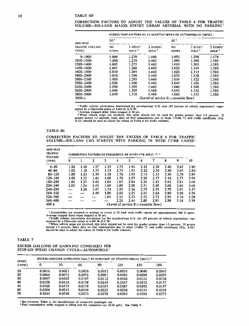
18 TABLE 6D

CORRECTION FACTORS TO ADJUST THE VALUES OF TABLE 6 FOR TRAFFIC VOLUME-SIX-LANE MAJOR STREET URBAN ARTERIAL WITH NO PARKING 1

CORRECTION FACTORS BY ATTEMPTED SPEED OF AUTOMOBILES (MPH):

30 2 402 ONE-WAY TRAFFIC VOLUME NO 1 STOP! 2 STOPS! NO I STOP! 2 STOPS! (VPH) STOPS MILE MILE STOPS MILE MILE

0-1000 1.000 1.270 1.460 1.000 1.298 1.578 1000-1200 1.000 1.270 1.460 1.000 1.300 1.580 1200-1400 1.005 1.275 1.460 1.010 1.305 1.580 1400-1600 1.005 1.280 1.460 1.020 1.310 1.580 1600-1800 1.010 1.285 1.460 1.020 1.315 1.580 1800-2000 1.010 1.290 1.460 1.030 1.318 1.580 2000-2200 1.010 1.295 1.460 1.030 1.322 1.580 2200-2400 1.020 1.300 1.460 1.040 1.326 1.580 2400-2600 1.030 1.305 1.460 1.040 1.380 1.580 2600-2800 1.040 1.305 1.460 1.050 1.332 1.580 2800-3000 1.050 1.310 1.460 1.060 1.333 1.580 3000+ (Level of service E=unstable flow)

1 Traffic volume corrections determined for standard-size U.S. cars (65 percent of vehicle population) represented by a Chevrolet sedan at 4,400 lb G.V.W.

2 Average stopped delay when stopped is 30 sec. 3 When vehicle stops are involved, this table should not be used for grades greater than 1.5 percent. If

grades exceed 1.5 percent, basic data on fuel consumption due to stops (Table 7) and traffic conditions (Fig. A-23) should be used to adjust the values of Table 6 for traffic volumes.

TABLE 6E

CORRECTION FACTORS TO ADJUST THE VALUES OF TABLE 6 FOR TRAFFIC VOLUME-SIX-LANE CBD STREETS WITH PARKING IN BOTH CURB LANES1

ONE-WAY TRAFFIC CORRECTION FACTORS BY FREQUENCY OF STOPS PF.R MILF.: 2, 3

VOLUME -- (vPH) 0 1 2 3 4 5 6 7 8 9 10

0-40 1.00 1.18 1.37 1.55 1.73 1.91 2.12 2.30 2.40 2.65 2.80 40-80 1.00 1.18 1.37 1.55 1.73 1.91 2.12 2.30 2.40 2.65 2.80 80-120 1.00 1.21 1.39 1.58 1.76 1.95 2.14 2.33 2.50 2.70 2.89

120-160 1.00 1.22 1.41 1.60 1.78 1.97 2.20 2.37 2.56 2.75 2.94 160-200 1.01 1.23 1.42 1.64 1.85 2.04 2.24 2.42 2.61 2.81 3.00 200-240 1.02 1.24 1.43 1.69 1.89 2.08 2.31 2.49 2.68 2.86 3.06 240-280 - 1.26 1.47 1.74 1.95 2.16 2.39 2.55 2.70 2.91 3.17 280-320 - - 1.49 1.80 2.02 2.23 2.45 2.64 2.80 3.00 3.26 320-360 - - - 1.84 2.11 2.33 2.52 2.73 2.93 3.10 3.28 360-400 - - - - 2.21 2.44 2.68 2.85 2.98 3.18 3.39 400+ (Level of service E=unstable flow)

1 Automobiles are assumed to attempt to travel at 25 mph with traffic signals set approximately 500 ft apart. Average stopped delay when stopped is 30 sec.

Traffic volume corrections determined for the standard-size U.S. car (65 percent of vehicle population) represented by a Chevrolet sedan at 4,400 lb G.V.W.

When vehicle stops are involved, this table should not be used for grades greater than 1.5 percent. If grades exceed 1.5 percent, basic data on fuel consumption due to stops (Table 7) and traffic conditions (Fig. A-24) should be used to adjust the values of Table 6 for traffic volumes. -

TABLE 7

EXCESS GALLONS OF GASOLINE CONSUMED PER STOP-GO SPEED CHANGE CYCLE-AUTOMOBILE1

SPEED EXCESS GASOLINE CONSUMED (GAL) BY DURATION OF STOPPED DELAY (5EC) :

(MPH) 0 30 60 90 120 150 180

10 0.0016 0.0021 0.0026 0.0031 0.0035 0.0040 0.0045 20 0.0066 0.0071 0.0076 0.0081 0.0085 0.0090 0.0095 30 0.0097 0.0102 0.0107 0.0112 0.0116 0.0121 0.0126 40 0.0128 0.0133 0.0138 0.0143 0.0147 0.0152 0.0157 50 0.0168 0.0173 0.0178 0.0183 0.0187 0.0192 0.0197 60 0.0208 0.0213 0.0218 0.0223 0.0228 0.0233 0.0238 70 0.0243 0.0248 0.0253 0.0258 0.0263 0.0268 0.0273

1 See footnote, Table 6, for identification of composite passenger car. 2 Fuel consumption while stopped is idling fuel for composite car (0.58 gph). See Table 9

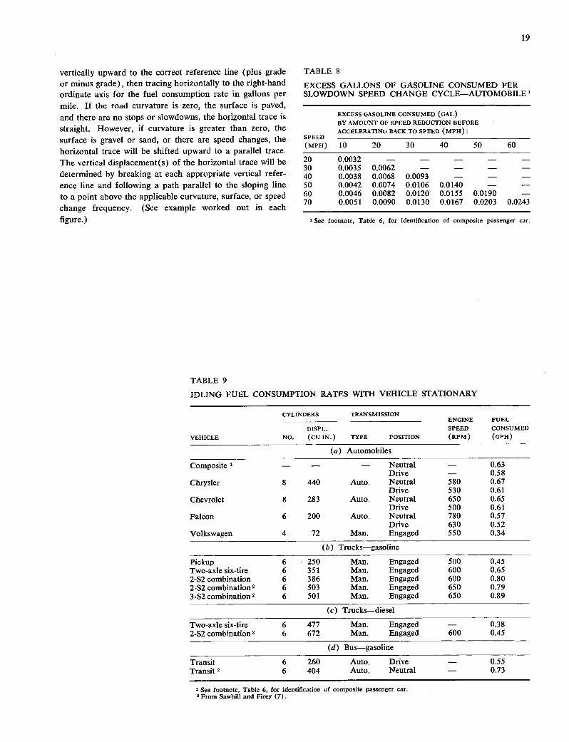
19

vertically upward to the correct reference line (plus grade or minus grade), then tracing horizontally to the right-hand ordinate axis for the fuel consumption rate in gallons per mile. If the road curvature is zero, the surface is paved, and there are no stops or slowdowns, the horizontal trace is straight. However, if curvature is greater than zero, the surface is gravel or sand, or there are speed changes, the horizontal trace will be shifted upward to a parallel trace. The vertical displacement(s) of the horizontal trace will be determined by breaking at each appropriate vertical refer-ence line and following a path parallel to the sloping line to a point above the applicable curvature, surface, or speed change frequency. (See example worked out in each figure.)

TABLE 8

EXCESS GALLONS OF GASOLINE CONSUMED PER SLOWDOWN SPEED CHANGE CYCLE-AUTOMOBILE'

EXCESS GASOLINE CONSUMED (GAl.) BY AMOUNT OF SPEED REDUCTION BEFORE ACCELERATING BACK TO SPEED (MPH):

SPEED (MPH) 10 20 30 40 50 60

20 0.0032 - - - - - 30 0.0035 0.0062 - - - - 40 0.0038 0.0068 0.0093 - - - 50 0.0042 0.0074 0.0106 0.0140 - - 60 0.0046 0.0082 0.0120 0.0155 0.0190 - 70 0.0051 0.0090 0.0130 0.0167 0.0203 0.0243

1 See footnote, Table 6, for identification of composite passenger car.

TABLE 9

IDLING FUEL CONSUMPTION RATES WITH VEHICLE STATIONARY

CYLINDERS TRANSMISSION ENGINE FUEL

DISPL. SPEED CONSUMED

VEHICLE NO. (CU IN.) TYPE POSITION (RPM) (GPH)

(a) Automobiles

Composite - - - Neutral - 0.63 Drive - 0.58

Chrysler 8 440 Auto. Neutral 580 0.67 Drive 530 0.61

Chevrolet 8 283 Auto. Neutral 650 0.65 Drive 500 0.61

Falcon 6 200 Auto. Neutral 780 0.57 Drive 630 0.52

Volkswagen 4 72 Man. Engaged 550 0.34

(b) Trucks-gasoline

Pickup 6 250 Man. Engaged 500 0.45 Two-axle six-tire 6 351 Man. Engaged 600 0.65 2-S2 combination 6 386 Man. Engaged 600 0.80 2-S2 combination 2 6 503 Man. Engaged 650 0.79 3-S2 combination 2 6 501 Man. Engaged 650 0.89

Trucks-diesel

Two-axle six-tire 6 477 Man. Engaged - 0.38 2-S2 combination 2 6 672 Man. Engaged 600 0.45

Bus-gasoline

Transit 6 260 Auto. Drive - 0.55 Transit' 6 404 Auto. Neutral - 0.73

1 See footnote, Table 6, for identification of composite passenger car. 'From Sawhill and Firey (7).

30

30

30 0

30

8

I

N.sv.1 30 Second Siop. 104WI Slowdown Grade (5) - Q,sts (.) .f.o. $p..d thong. Cps1.. Fur *1.

Figure hA. Automobile fuel consumption, free-flowing traffic volumes-30-mph running speed.

• III!UO 111111 Jim ___iIUiIIIIIIIIUIi oulniulil_ uiuumuiiuiiiioiiiii [INuOMIN!ir;ii I-I-- —

Example

Grade t-±1 -'- t•' - t I N. Stops

M,s 0.11011snsIb*1.

:!±i --44

±

I I -

Hit. 4J LJHi TL .41.......

H: 17

L T / I

b 246510 0 24 6 NI

os1 30 S.c.d Stops 10-I S1.pd.s

i.fics Sps.d thong. C1., For Nil.

Figure 11C. Automobile fuel consumption, free-flowing traffic volumes-70-mph running speed.

0 assev.1 30 Soosen Stps 10-W S1,s

só. Olevetwe C.) Oivf.cs Speed Qisngs C7s1.s Per *1.

Figure 1IB. Automobile fuel consumption, free-flowing traffic volumes—SO-mph running speed.

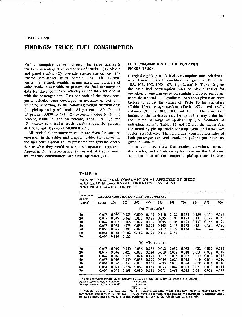
CHAPTER FOUR

FINDINGS: TRUCK FUEL CONSUMPTION

21

Fuel consumption values are given for three composite trucks representing three categories of trucks: (1) pickup and panel trucks, (2) two-axle six-tire trucks, and (3) tractor semi-trailer truck combinations. The extreme variations in truck weights, engine sizes, and numbers of axles made it advisable to present the fuel consumption data for three composite vehicles rather than for one as with the passenger car. Data for each of the three com-posite vehicles were developed as averages of test data weighted according to the following weight distributions: (1) pickup and panel trucks, 85 percent, 4,800 lb, and 15 percent, 5,800 lb (8); (2) two-axle six-tire trucks, 50 percent, 8,000 lb, and 50 percent, 16,000 lb (1); and (3) tractor semi-trailer truck combinations, 50 percent, 40,000 lb and 50 percent, 50,000 lb (1).

All truck fuel consumption values are given for gasoline operation in the tables and graphs. Tables for converting the fuel consumption values presented for gasoline opera-tion to what they would be for diesel operation appear in Appendix D. Approximately 35 percent of tractor semi-trailer truck combinations are diesel-operated (9).

FUEL CONSUMPTION OF THE COMPOSITE PICKUP TRUCK

Composite pickup truck fuel consumption rates relative to road design and traffic conditions are given in Tables 10, bA, lOB, bC, 1013, bE, 11, 12, and 9. Table 10 gives the basic fuel consumption rates of pickup trucks for operation at uniform speed on straight high-type pavement for various speeds and gradients. Subtables give correction factors to adjust the values of Table 10 for curvature (Table bA), rough surface (Table lOB), and traffic volumes (Tables bC, 10D, and lOB). The correction factors of the subtables may be applied in any order but are limited in range of applicability (see footnotes of individual tables). Tables 11 and 12 give the excess fuel consumed by pickup trucks for stop cycles and slowdown cycles, respectively. The idling fuel consumption rates of both passenger cars and trucks in gallons per hour are given in Table 9.

The combined effect that grades, curvature, surface, stop cycles, and slowdown cycles have on the fuel con-sumption rates of the composite pickup truck in free-

TABLE 10

PICKUP TRUCK FUEL CONSUMPTION AS AFFECTED BY SPEED AND GRADIENT-STRAIGHT HIGH-TYPE PAVEMENT AND FREE-FLOWING TRAFFIC'

UNIFORM SPEED

GASOLINE CONSUMPTION (6PM) ON GRADES OF:

(MPH) LEVEL 1% 2% 3% 4% 5% 6% 7% 8% 9% 10%

Plus grades2

10 0.058 0.070 0.083 0.090 0.100 0.110 0.129 0.134 0.150 0.174 0.197 20 0.047 0.057 0.068 0.077 0.086 0.095 0.105 0.121 0.137 0.147 0.156 30 0.047 0.057 0.068 0.077 0.086 0.095 0.105 0.121 0.137 0.156 0.174 40 0.053 0.063 0.073 0.083 0.094 0.103 0.113 0.132 0.151 0.164 0.180 50 0.065 0.075 0.085 0.095 0.106 0.117 0.128 0.144 0.164 - - 60 0.081 0.092 0.102 0.112 0.123 0.133 0.144 - - - - 70 0.099 0.110 0.122 - - - - - -. - -

Minus grades

10 0.058 0.049 0.040 0.036 0.032 0.032 0.032 0.032 0.032 0.032 0.032 20 0.047 0.036 0.027 0.022 0.020 0.019 0.018 0.018 0.018 0.018 0.018 30 0.047 0.036 0.028 0.024 0.020 0.017 0.015 0.013 0.012 0.012 0.012 40 0.053 0.046 0.039 0.033 0.028 0.024 0.020 0.015 0.010 0.010 0.010 50 0.065 0.060 0.054 0.047 0.041 0.035 0.030 0.024 0.018 0.014 0.010 60 0.081 0.077 0.074 0.067 0.059 0.053 0.047 0.037 0.027 0.019 0.011 70 0.099 0.098 0.098 0.089 0.081 0.073 0.065 0.053 0.041 0.028 0.015

1 The composite pickup truck represented here reflects the following vehicle distribution: Pickup trucks at 4,800 lb G.V.W. 85 percent Pickup trucks at 5,800 lb G.V.W. 15 percent

100 percent 2 Vehicle operation is in high gear (No. 4) whenever possible. When necessary (on steep grades and/or at

low speed) operation is in gear No. 3. When vehicle approach speed exceeds the maximum sustainable speed on plus grades, speed is reduced to this maximum as soon as the vehicle gets on the grade.

TABLE 1OA

CORRECTION FACTORS TO ADJUST THE VALUES OF TABLE 10 FOR CURVATURE '

DEGREE OF

CORRECTION FACTORS BY UNIFORM SPEED OF PICKUP TRUCKS (MPH)

CURVE 10 20 30 40 50 60 70

0 1.000 1.000 1.000 1.000 1.000 1.000 1.000 1 1.000 1.000 1.000 1.000 1.001 1.002 1.005 2 1.000 1.000 1.001 1.003 1.004 1.005 1.010 3 1.000 1.001 1.002 1.004 1.005 1.010 1.020 4 1.000 1.001 1.003 1.007 1.010 1.020 1.050 5 1.000 1.002 1.008 1.026 1.050 1.080 - 6 1.000 1.005 1.020 1.050 1.100 1.140 - 7 1.000 1.010 1.040 1.100 1.170 - - 8 1.000 1.020 1.080 1.160 1.240 - - 9 1.000 1.040 1.120 1.220 1.330 - -

10 1.000 1.080 1.160 1.260 1.360 - - 11 1.000 1.100 1.210 1.320 1.430 - - 12 1.000 1.130 1.260 1.380 1.500 - -

1 Correction factors determined for vehicle distribution given in the foot-note, Table 10. They apply to grades up to 3 percent. For grades greater than 3 percent refer to Figs. A-31, A-32, and A-33.

TABLE 1OC

CORRECTION FACTORS TO ADJUST THE VALUES OF TABLE 10 FOR TRAFFIC VOLUME-SIX-LANE EXPRESSWAY 1

ONE-WAY

(vpH) TRAFFIC VOLUME

CORRECTION FACTORS BY ATFEMPTED SPEED OF PICKUP TRUCKS (MPH):

45 50 55 60

0-2400 (Level of service A=free-flowing traffic) 2400-2800 1.000 1.000 1.008 1.015 2800-3200 1.000 1.004 1.012 1.020 3200-3600 1.000 1.008 1.018 1.025 3600-4000 1.000 1.012 1.028 1.040 4000-4400 1.000 1.018 1.036 1.050 4400-4800 1.001 1.028 1.040 1.060 4800-5200 1.002 1.030 1.050 1.066 5200-5600 1.003 1.032 1.060 1.072 5600-6000 1.004 1.036 1.080 1.080 6000+ (Level of service E=unstable flow)

1 Correction factors determined for the pickup truck by adjusting the correction factors of Table 6C for passenger cars. The adjustments were proportioned to the ratios of the excess fuel consumption for the truck and passenger car for 10-mph speed change cycles.

TABLE lOB


CORRECTION FACTORS BY ROAD SURFACE:

UNIFORM SPEED HIGH-TYPE CONCRETE BADLY BROKEN AND DRY WELL-PACKED LOOSE OF PICKUPS (MPH) OR ASPHALT PATCHED ASPHALT GRAVEL SAND

10 1.00 1.00 1.07 1.33 20 1.00 1.00 1.09 1.49 30 1.00 1.01 1.16 1.67 40 1.00 1.06 1.27 2.02 50 1.00 1.16 1.34 -

1 Correction factors determined for truck distribution of Footnote 1, Table 10. They apply on grades up to 3 percent. For grades greater than 3 percent, see Fig. A-34.

TABLE 1OD

CORRECTION FACTORS TO ADJUST THE VALUES OF TABLE 10 FOR TRAFFIC VOLUME-SIX-LANE MAJOR STREET URBAN ARTERIAL WITH NO PARKING 1

CORRECTION FACTORS BY ATFEMPTED SPEED OF PICKUP TRUCKS (MPH):

ONE-WAY 302 402

TRAFFIC VOLUME NO 1 STOP! 2 STOPS! NO I STOP! 2 STOPS! (VPii) STOPS MILE 3 MILE 3 STOPS MILE 3 MILE 3

0-1000 1.000 1.253 1.506 1.000 1.272 1.540 1000-1200 1.000 1.253 1.506 1.000 1.272 1.540 1200-1400 1.004 1.258 1.506 1.008 1.285 1.540 1400-1600 1.006 1.265 1.506 1.016 1.287 1.540 1600-1800 1.008 1.267 1.506 1.018 1.289 1.540 1800-2000 1.010 1.268 1.506 1.020 1.291 1.540 2000-2200 1.012 1.269 1.506 1.026 1.293 1.540 2200-2400 1.016 1.271 1.506 1.032 1.294 1.540 2400-2600 1.020 1.273 1.506 1.036 1.295 1.540 2600-2800 1.032 1.275 1.506 1.040 1.296 1.540 2800-3000 1.038 1.278 1.506 1.050 1.297 1.540 3000+ (Level of service E=unstable flow)

1 Traffic volume corrections determined for the pickup truck by adjusting the corrections for the passenger car. The adjustments were proportioned to the ratios of the excess fuel consumption for the truck and passenger car for 10-mph speed change cycles.

stopped delay when stopped is 30 sec. 3 When vehicle Stops are involved, this table should not be used for grades greater than 1.5 percent. If grades

exceed 1.5 percent, basic data on fuel consumption due to stops (Table 11) and traffic conditions (Fig. A-23) should be used to adjust the values of Table 10 for traffic volumes.

F

23

TABLE IOE

CORRECTION FACTORS TO ADJUST THE VALUES OF TABLE 10 FOR TRAFFIC VOLUME-SIX-LANE CBD STREETS WITH PARKING IN BOTH CURB LANES 1

ONE-WAY TRAFFIC VOLUME

CORRECTION FACTORS BY FREQUENCY OF STOPS PER MILE: 2,3

(vPH) 0 1 2 3 4 5 6 7 8 9 10

0-40 1.00 1.22 1.43 1.65 1.87 2.11 2.33 2.54 2.76 2.98 3.20 40-80 1.00 1.22 1.43 1.65 1.87 2.11 2.33 2.54 2.76 2.98 3.20 80-120 1.00 1.23 1.45 1.67 1.89 2.12 2.34 2.56 2.78 3.01 3.22

120-160 1.00 1.23 1.45 1.68 1.91 2.13 2.35 2.57 2.79 3.01 3.23 160-200 1.00 1.24 1.46 1.70 1.92 2.15 2.37 2.59 2.82 3.04 3.27 200-240 1.01 1.25 1.48 1.72 1.94 2.17 2.42 2.62 2.85 3.07 3.30 240-280 - 1.27 1.49 1.75 1.99 2.21 2.46 2.67 2.87 3.10 3.33 280-320 - - 1.50 1.78 2.02 2.25 2.49 2.72 2.93 3.13 3.36 320-360 - - - 1.80 2.07 2.31 2.53 2.77 2.98 3.19 3.42 360-400 - - - - 2.13 2.38 2.62 2.85 3.01 3.25 3.49 400+ (Level of service E=unstable flow)

1 Traffic volume corrections determined for the pickup truck by adjusting the corrections for the passenger car. The adjustments were proportioned to the ratios of the excess fuel consumption for the truck and passenger car for 10-mph speed change cycles.

2 Pickup trucks are assumed to attempt to travel at 25 mph with traffic signals set approximately 500 It apart. Average stopped delay is 30 sec.

3 When vehicle stops are invioved, this table should not be used for grades greater than 1.5 percent. If grades exceed 1.5 percent, basic data on fuel consumption due to stops (Table 11) and traffic conditions (Fig. A-24) should be used to adjust the values of Table 10 for traffic volumes.

TABLE 11

EXCESS GALLONS OF GASOLINE CONSUMED PER STOP-GO SPEED CHANGE CYCLE-PICKUP TRUCK

SPEED EXCESS GASOLINE CONSUMED (GAL) BY DURATION OF STOPPED DELAY (5EC): 2

(MPH) 0 30 60 90 120 150 180

10 0.0016 0.0054 0.0092 0.0130 0.0168 0.0206 0.0244 20 0.0048 0.0086 0.0124 0.0162 0.0200 0.0238 0.0276 30 0.0081 0.0119 0.0157 0.0195 0.0233 0.0271 0.0309 40 0.0106 0.0144 0.0182 0.0220 0.0258 0.0296 0.0334 50 0.0132 0.0170 0.0208 0.0246 0.0285 0.0322 0.0360 60 0.0157 0.0195 0.0233 0.0271 0.0309 0.0347 0.0385

1 See Footntc I, Table 10, for identification of composite pickup truck. 2 Fuel consumption while stopped is idling fuel for pickup truck (0.45 gph). See Table 9.

TABLE 12

EXCESS GALLONS OF GASOLINE CONSUMED PER SLOWDOWN SPEED CHANGE CYCLE-PICKUP TRUCK 1

EXCES GASOLINE CONSUMED (GAL) BY AMOUNT OF SPEED REDUCTION BEFORE ACCELERATING BACK TO SPEED (MPH):

SPEED (MPH) 10 20 30 40 50

20 0.0031 - - - - 30 0.0037 0.0064 - - - 40 0.0034 0.0060 0.0090 - - 50 0.0027 0.0056 0.0082 0.0125 - 60 0.0021 0.0049 0.0075 0.0100 0.0147

1 See Footnote 1, Table 10, for identification of composite pickup truck.

flowing traffic is shown in simplified graphical form for each of two running speeds: 30 mph (Fig. 12A) and 50 mph (Fig. 12B). These speeds are typical of possible speeds on many urban arterials (30 mph) and rural routes (50 mph).

Figures 12A and 12B are read in the same manner as explained in the last paragraph of Chapter Three for Figures 11A, 11B, and 11C.

FUEL CONSUMPTION OF COMPOSITE TWO-AXLE SIX-TIRE TRUCK

Composite two-axle six-tire truck fuel consumption rates relative to road design and traffic conditions are given in Tables 13, 13A, 13B, 13C, 13D, 13E, 14, 15, and 9. Table

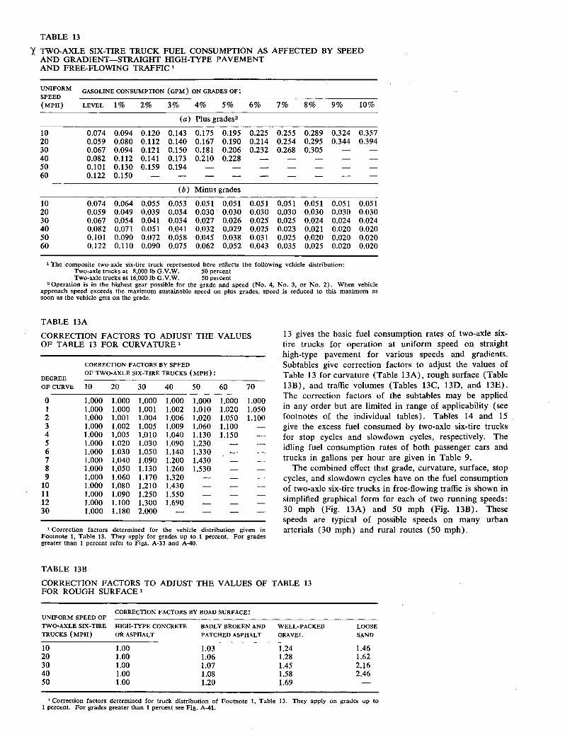
TABLE 13

X TWO-AXLE SIX-TIRE TRUCK FUEL CONSUMPTION AS AFFECTED BY SPEED AND GRADIENT-STRAIGHT HIGH-TYPE PAVEMENT AND FREE-FLOWING TRAFFIC'

UNIFORM SPEED

GASOLINE CONSUMPTION (GPM) ON GRADES OF:

(MPH) LEVEL 1% 2% 3% 4% 5% 6% 7% 8% 9% 10%

Plus grades2

10 0.074 0.094 0.120 0.143 0.175 0.195 0.225 0.255 0.289 0.324 0.357 20 0.059 0.080 0.112 0.140 0.167 0.190 0.214 0.254 0.295 0.344 0.394 30 0.067 0.094 0.121 0.150 0.181 0.206 0.232 0.268 0.305 - - 40 0.082 0.112 0.141 0.173 0.210 0.228 - - - - - 50 0.101 0.130 0.159 0.194 - - - - - - - 60 0.122 0.150 - - - - - - - - -

Minus grades

10 0.074 0.064 0.055 0.053 0.051 0.051 0.051 0.051 0.051 0.051 0.051 20 0.059 0.049 0.039 0.034 0.030 0.030 0.030 0.030 0.030 0.030 0.030 30 0.067 0.054 0.041 0.034 0.027 0.026 0.025 0.025 0.024 0.024 0.024 40 0.082 0.071 0.051 0.041 0.032 0.029 0.025 0.023 0.021 0.020 0.020 50 0.101 0.090 0.072 0.058 0.045 0.038 0.031 0.025 0.020 0.020 0.020 60 0.122 0.110 0.090 0.075 0.062 0.052 0.043 0.035 0.025 0.020 0.020

1 The composite two-axle six-tire truck represented here reflects the following vehicle distribution: Two-axle trucks at 8,000 lb G.V.W. 50 percent Two-axle trucks at 16,000 lb G.V.W. 50 percent

Operation is in the highest gear possible for the grade and speed (No. 4, No. 3, or No. 2). When vehicle approach speed exceeds the maximum sustainable speed on plus grades, speed is reduced to this maximum as soon as the vehicle gets on the grade.

TABLE 13A


CORRECTION FACTORS BY SPEED

nrr.pr' OF TWO-AXLE SIX-TIRE TRUCKS (MPH):

OF CURVE 10 20 30 40 50 60 70

0 1.000 1.000 1.000 1.000 1.000 1.000 1.000 1 1.000 1.000 1.001 1.002 1.010 1.020 1.050 2 1.000 1.001 1.004 1.006 1.020 1.050 1.100 3 1.000 1.002 1.005 1.009 1.060 1.100 - 4 1.000 1.005 1.010 1.040 1.130 1.150 - 5 1.000 1.020 1.030 1.090 1.230 - - 6 1.000 1.030 1.050 1.140 1.330 - - 7 1.000 1.040 1.090 1.200 1.430 - -. 8 1.000 1.050 1.130 1.260 1.530 - - 9 1.000 1.060 1.170 1.320 - - -

10 1.000 1.080 1.210 1.430 - - - 11 1.000 1.090 1.250 1.550 - - - 12 1.000 1.100 1.300 1.690 - - - 30 1.000 1.180 2.000 - - - -

1 Correction factors determined for the vehicle distribution given in Footnote 1, Table 13. They apply for grades up to 1 percent. For grades greater than 1 percent refer to Figs. A-33 and A-40.

13 gives the basic fuel consumption rates of two-axle six-tire trucks for operation at uniform speed on straight high-type pavement for various speeds and gradients. Subtables give correction factors to adjust the values of Table 13 for curvature (Table 13A), rough surface (Table 13B), and traffic volumes (Tables 13C, 13D, and 13E). The correction factors of the subtables may be applied in any order but are limited in range of applicability (see footnotes of the individual tables). Tables 14 and 15 give the excess fuel consumed by two-axle six-tire trucks for stop cycles and slowdown cycles, respectively. The idling fuel consumption rates of both passenger cars and trucks in gallons per hour are given in Table 9.

The combined effect that grade, curvature, surface, stop cycles, and slowdown cycles have on the fuel consumption of two-axle six-tire trucks in free-flowing traflic is shown in simplified graphical form for each of two running speeds: 30 mph (Fig. 13A) and 50 mph (Fig. 13B). These speeds are typical of possible speeds on many urban arterials (30 mph) and rural routes (50 mph).

TABLE 13B

CORRECTION FACTORS TO ADJUST THE VALUES OF TABLE 13 FOR ROUGH SURFACE 1

CORRECTION FACTORS BY ROAD SURFACE: UNIFORM SPEED OF TWO-AXLE SIX-TIRE HIGH-TYPE CONCRETE BADLY BROKEN AND WELL-PACKED LOOSE TRUCKS (MPH) OR ASPHALT PATCHED ASPHALT GRAVEL SAND

10 1.00 1.03 1.24 1.46 20 1.00 1.06 1.28 1.62 30 1.00 1.07 1.45 2.16 40 1.00 1.08 1.58 2.46 50 1.00 1.20 1.69 -

1 Correction factors determined for truck distribution of Footnote I, Table 13. They apply on grades up to 1 percent. For grades greater than 1 percent see Fig. A-41.

Figures 13A and 13B are read in the same manner as explained in the last paragraph of Chapter Three for Figures 11A,'l1B, and 11C.

FUEL CONSUMPTION OF THE COMPOSITE TRACTOR SEMI-TRAILER TRUCK COMBINATION

Composite tractor semi-trailer truck fuel consumption rates relative to road design and traffic conditions are given in Tables 16, 16A, 16B, 16C, 16D, 16E, 17, 18, and 9. Table 16 gives the basic fuel consumption rates of tractor semi-trailer truck combinations for operation at uniform speed on straight high-type pavement for various speeds and gradients. Subtables give correction factors to adjust the values of Table 16 for curvature (Table 16A), rough surface (Table 16B), and traffic volumes (Tables 16C, 16D, and 16E). The correction factors of the subtables may be applied in any order but are limited in range of applicability (see footnotes of individual tables). Tables 17 and 18 give the excess fuel consumed by tractor semi-trailer combinations for stop cycles and slowdown cycles, respectively. The idling fuel consumption rates of both passenger cars and trucks in gallons per hour are given in Table 9.

The combined effect that grade, curvature, surface, stop cycles, and slowdown cycles have on the fuel consumption of tractor semi-trailer combinations is shown in simplified graphical form for each of two running speeds: 30 mph (Fig. 14A) and 50 mph (Fig. 14B). These speeds are typical of possible speeds on many urban arterials (30 mph) and rural routes (50 mph).

Figures 14A and 14B are read in the same manner as explained in the last paragraph of Chapter Three for Figures 11A, 1IB, and lIC.

25

TABLE 13C

CORRECTION FACTORS TO ADJUST THE VALUES OF TABLE 13 FOR TRAFFIC VOLUME- SIX-LANE EXPRESSWAY'

CORRECTION FACTORS BY ATTEMPTED SPEED OF TWO-AXLE SIX-TIRE TRUCKS

ONE-WAY (MPH): TRAFFIC VOLUME (vPH) 45 50

0-2400 (Level of service A=free-flowing traffic) 2400-2800 1.000 1.000 2800-3200 1.000 1.004 3200-3600 1.000 1.008 3600-4000 1.000 1.012 4000-4400 1.000 1.018 4400-4800 1.001 1.028 4800-5200 1.002 1.030 5200-5600 1.003 1.032 5600-6000 1.004 1.034 6000+ (Level of service E=unstable flow)

'Correction factors determined for a two-axle six-tire truck at 24,000 lb. G.V.W. for an attempted speed of 45 mph. For an attempted speed of 50 mph passenger-car correction factors of Table 6C were adjusted in pro-portion to the ratios of the excess fuel consumption for 10-mph slowdown speed change cycles of two-axle six-tire trucks and passenger cars.

TABLE 13D

CORRECTION FACTORS TO ADJUST THE VALUES OF TABLE 13 FOR TRAFFIC VOLUME-FOUR-LANE MAJOR STREET URBAN ARTERIAL WITH NO PARKING'

ONE-WAY TRAFFIC VOLUME (vPH)

CORRECTION FACTORS BY FREQUENCY OF STOPS-TWO-AXLE SIX-TIRE TRUCKS 2

NONE ONE/MILE 3 TWO/MILE

0-500 1.000 1.300 1.600 500-600 1.000 1.300 1.600 600-700 1.000 1.300 1.605 700-800 1.010 1.300 1.620 800-900 1.020 1.310 1.630 900-1000 1.030 1.320 1.650

1000-1 100 1.040 1.325 1.700 1100-1200 1.050 1.330 1.660 1200-1300 1.060 1.335 1.665 1300-1400 1.070 1.340 1.670 1400-1500 1.080 1.350 1.680 1500+ (Level of service E=unstable flow)

1 Traffic volume correction factors determined for the two-axle six-tire truck at 24,000 lb G.V.W. 2 Vehicle operation at 25 mph attempted. Average stopped delay when stopped is 30 sec. 3 When vehicle stops are involved, this table should not be used for grades greater than 1 percent. If grades

exceed 1 percent, basic data on fuel consumption due to stops (Table 14) and traffic conditions (Fig. A-44) should be used to adjust the values of Table 13 for traffic volumes.

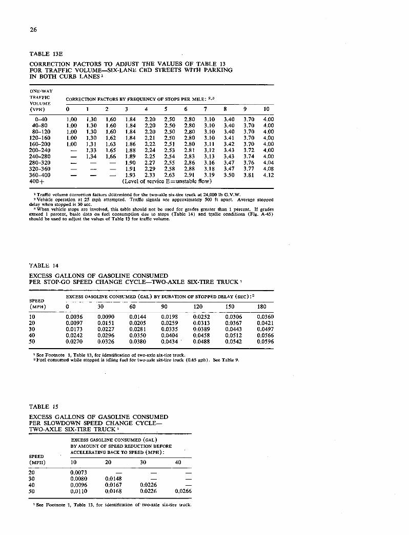
26

TABLE 13E

CORRECTION FACTORS TO ADJUST THE VALUES OF TABLE 13 FOR TRAFFIC VOLUME-SIX-LANE CBD STREETS WITH PARKING IN BOTH CURB LANES 1



(vPH) 0 1 2 3 4 5 6 7 8 9 10

0-40 1.00 1.30 1.60 1.84 2.20 2.50 2.80 3.10 3.40 3.70 4.00 40-80 1.00 1.30 1.60 1.84 2.20 2.50 2.80 3.10 3.40 3.70 4.00 80-120 1.00 1.30 1.60 1.84 2.20 2.50 2.80 3.10 3.40 3.70 4.00

120-160 1.00 1.30 1.62 1.84 2.21 2.50 2.80 3.10 3.41 3.70 4.00 160-200 1.00 1.31 1.63 1.86 2.22 2.51 2.80 3.11 3.42 3.70 4.00 200-240 - 1.33 1.65 1.88 2.24 2.53 2.81 3.12 3.43 3.72 4.00 240-280 - 1.34 1.66 1.89 2.25 2.54 2.83 3.13 3.43 3.74 4.00 280-320 - - - 1.90 2.27 2.55 2.86 3.16 3.47 3.76 4.04 320-360 - - - 1.91 2.29 2.58 2.88 3.18 3.47 3.77 4.08 360-400 - - - 1.93 2.33 2.63 2.91 3.19 3.50 3.81 4.12 400+ (Level of service E=unstable flow)

1 Traffic volume correction factors determined for the two-axle six-tire truck at 24,000 lb G.V.W. 2 Vehicle operation at 25 mph attempted. Traffic signals are approximately 500 ft apart. Average stopped

delay when stopped is 30 sec. When vehicle stops are involved, this table should not be used for grades greater than 1 percent. If grades

exceed 1 percent, basic data on fuel consumption due to stops (Table 14) and traffic conditions (Fig. A-45) should be used to adjust the values of Table 13 for traffic volume.

TABLE 14

EXCESS GALLONS OF GASOLINE CONSUMED PER STOP-GO SPEED CHANGE CYCLE-TWO-AXLE SIX-TIRE TRUCK 1

SPEED EXCESS GASOLINE CONSUMED (GAL) BY DURATION OF STOPPED DELAY (5EC) :2

(MPH) 0 30 60 90 120 150 180

10 0.0036 0.0090 0.0144 0.0198 0.0252 0.0306 0.0360 20 0.0097 0.0151 0.0205 0.0259 0.0313 0.0367 0.0421 30 0.0173 0.0227 0.0281 0.0335 0.0389 0.0443 0.0497 40 0.0242 0.0296 0.0350 0.0404 0.0458 0.0512 0.0566 50 0.0270 0.0326 0.0380 0.0434 0.0488 0.0542 0.0596

1 See Footnote 1, Table 13, for identification of two-axle six-tire truck. Fuel consumed while stopped is idling fuel for two-axle six-tire truck (0.65 gph). See Table 9

TABLE 15

EXCESS GALLONS OF GASOLINE CONSUMED PER SLOWDOWN SPEED CHANGE CYCLE-TWO-AXLE SIX-TIRE TRUCK 1

EXCESS GASOLINE CONSUMED (GAL) BY AMOUNT OF SPEED REDUCTION BEFORE ACCELERATING BACK TO SPEED (MPH):

SPEED (MPH) 10 20 30 40

20 0.0073 - - - 30 0.0080 0.0148 - - 40 0.0096 0.0167 0.0226 - 50 0.0110 0.0168 0.0226 0.0266

1 See Footnote 1, Table 13, for identification of two-axle six-tire truck

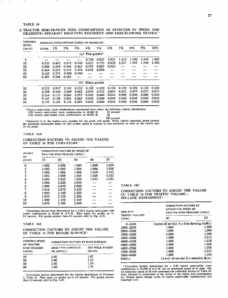
TABLE 16

)t TRACTOR SEMI-TRAILER FUEL CONSUMPTION AS AFFECTED BY SPEED AND GRADIENT-STRAIGHT HIGH-TYPE PAVEMENT AND FREE-FLOWING TRAFFIC'

UNIFORM GASOLINE CONSUMPTION (cPM) ON CRADS OF: SPEED (MsIi) LEVEL 1% 2% 3% 4% 5% 6% 7% 8% 9% 10%

Plus grades2

5 - - - - 0.720 0.825 0.925 1.115 1.290 1.440 1.605 10 0.355 0.405 0.475 0.540 0.615 0.735 0.858 1.027 1.195 1.340 1.490 20 0.208 0.289 0.364 0.462 0.555 0.685 0.813 - - - - 30 0.164 0.253 0.342 0.474 0.618 0.800 - - - - - 40 0.163 0.275 0.390 0.560 - - - - - - 50 0.195 0.344 0.485 - - - - - - - -

Minus grades

10 0.355 0.247 0.145 0.132 0.120 0.120 0.120 0.120 0.120 0.120 0.120 20 0.208 0.140 0.069 0.062 0.055 0.055 0.055 0.055 0.055 0.055 0.055 30 0.164 0.115 0.066 0.053 0.040 0.040 0.040 0.040 0.040 0.040 0.040 40 0.163 0.128 0.091 0.065 0.040 0.040 0.040 0.040 0.040 0.040 0.040 50 0.195 0.164 0.131 0.095 0.040 0.040 0.040 0.040 0.040 0.040 0.040

'Tractor semi-trailer truck combinations represented here reflect the following vehicle distribution: 2-S2 tractor semi-trailer truck combinations at 40,000 lb 50 percent 3-S2 tractor semi-trailer truck combinations at 50,000 lb 50

100 percent 2 Operation is in the highest gear possible for the grade and speed. When vehicle approach speed exceeds

the maximum sustainable speed on plus grades, speed is reduced to this maximum as soon as the vehicle gets on the grade.

TABLE 16A


CORRECTION FACTORS BY SPEED OF DEGREE TRACTOR SEMI-TRAILER (MPH): OF CURVE 10 20 30 40 50

27

0 1.000 1.000 1.000 1.000 1.000 1 1.000 1.002 1.004 1.006 1.008 2 1.000 1.006 1.008 1.010 1.012 3 1.002 1.008 1.010 1.020 1.022 4 1.004 1.010 1.020 1.022 1.024 5 1.006 1.020 1.040 - - 6 1.008 1.040 1.080 - - 7 1.010 1.070 1.150 - - 8 1.020 1.100 1.220 - - 9 1.030 1.120 1.280 - -

10 1.040 1.130 1.340 - - 30 1.050 1.300 2.000 - -

1 Correction factors were determined for a 2-Si-2 tractor semi-trailer full trailer combination at 50,000 lb G.V.W. They apply for grades up to 0.5 percent. For grades greater than 0.5 percent refer to Fig. A-Si.

TABLE 16B


UNIFORM SPEED CORRECTION FACTORS BY ROAD SURFACE: OF TRACTOR SEMI-TRAILERS HIGH-TYPE CONCRETE DRY WELL-PACKED (MPH) OR ASPHALT GRAVEL

10 1.00 1.07 20 1.00 1.27 30 1.00 1.59 40 1.00 1.75

1 Correction factors determined for the vehicle distribution of Footnote 1, Table 16. They apply on grades up to 0.5 percent. For grades greater than 0.5 percent refer to Fig. A-41.

TABLE l6C

CORRECTION FACTORS TO ADJUST THE VALUES OF TABLE 16 FOR TRAFFIC VOLUME- SIX-LANE EXPRESSWAY1

CORRECTION FACTORS BY ATItMPTED SPEED OF

ONE-WAY TRACTOR SEMI-TRAILERS (MPH): TRAFFIC VOLUME (vPH) 45 50

0-2400 (Level of service A=free-flowing traffic) 2400-2800 1.000 1.000 2800-3200 1.000 1.004 3200-3600 1.000 1.008 3600-4000 1.000 1.012 4000-4400 1.000 1.018 4400-4800 1.000 1.028 4800-5200 1.000 1.030 5200-5600 1.000 1.032 5600-6000 1.000 1.034 6000+ (Level of service E=unstable flow)

1 Correction factors determined for a 2-S2 tractor semi-trailer truck combination at 50,000 lb G.V.W. for an attempted speed of 45 mph. For an attempted speed of 50 mph passenger-car correction factors of Table 6C were adjusted in proportion to the ratios of the excess fuel consumption for 10-mph speed change cycles of tractor semi-trailer combinations and passenger cars.

28

TABLE 16D

CORRECTION FACTORS TO ADJUST THE VALUES OF TABLE 16 FOR TRAFFIC VOLUME-FOUR-LANE MAJOR STREET URBAN ARTERIAL WITH NO PARKING 1

CORRECTION FACTORS BY FREQUENCY OF STOPS- ONE-WAY TRACTOR SEMI-TRAILERS: TRAFFIC VOLUME (VPH)

NONE ONE/MILE 1 TWO/MILE 3 THREE/MILE 3

0-500 1.000 1.390 1.780 2.180 500-600 1.000 1.390 1.780 2.180 600-700 1.000 1.390 1.780 2.180 700-800 1.000 1.390 1.780 2.180 800-900 1.000 1.390 1.780 2.180 900-1000 1.000 1.390 1.780 2.180

1000-1100 1.000 1.400 1.820 2.200 1100-1200 1.010 1.420 1.830 2.220 1200-1300 1.010 1.430 1.850 2.230 1300-1400 1.020 1.450 1.870 2.240 1400-1500 1.030 1.460 1.890 2.270 1500+ (Level of service E=unstable flow)

1 Traffic volume correction factors determined for a 2-S2 tractor semi-trailer combination at 50,000 lb G.V.W.

a Vehicle operation at 25 mph attempted. Average stopped delay when stopped is 30 sec. When vehicle stops are involved, this table should not be used for grades greater . than 0.5 percent. If

grades exceed 0.5 percent, basic data on fuel consumption due to stops (Table 17) and traffic conditions (Fig. A-47) should be used to adjust the values of Table 16 for traffic volume.

TABLE 16E

CORRECTION FACTORS TO ADJUST THE VALUES OF TABLE 16 FOR TRAFFIC VOLUME-SIX-LANE CBD STREETS WITH PARKING IN BOTH CURB LANES1



(vpH) 0 1 2 3 4 5 6 7 8 9 10

0-40 1.00 1.39 1.78 2.18 2.57 2.96 3.35 3.75 4.14 4.53 4.93 40-80 1.00 1.39 1.78 2.18 2.57 2.96 3.35 3.75 4.14 4.53 4.93 80-120 1.00 1.39 1.78 2.18 2.57 2.96 3.35 3.75 4.14 4.53 4.93

120-160 1.00 1.39 1.78 2.18 2.57 2.96 3.35 3.75 4.14 4.53 4.93 160-200 - - 1.78 2.18 2.57 2.96 3.35 3.75 4.14 4.53 4.93 200-240 - - 1.78 2.18 2.57 2.96 3.35 3.75 4.14 4.53 4.95 240-280 - - - - 2.60 2.99 3.38 3.78 4.18 4.58 4.98 280-320 - - - - 2.62 3.03 3.42 3.80 4.20 4.60 5.00 320-360 - - - - - - 3.45 3.83 4.22 4.62 5.03 360-400 - - - - - - 3.48 3.86 4.24 4.64 5.05 400+ (Level of service E=unstable flow)

1 Traffic volume correction factors determined for a 2-S2 tractor semi-trailer combination at 50,000 lb G.V.W. Vehicle operation at 25 mph attempted with traffic signals set approximately 500 ft apart. Average stopped

delay when stopped is 30 sec. 3 When vehicle stops are involved, this table should not be used for grades greater than 0.5 percent. If

grades exceed 0.5 percent, basic data on fuel consumption due to stops (Table 17) and traffic conditions (Fig. A-54) should be used to adjust the value of Table 16 for traffic volume.

TABLE 17

EXCESS GALLONS OF GASOLINE CONSUMED PER STOP-GO SPEED CHANGE CYCLE-TRACTOR SEMI-TRAILER TRUCK'

EXCESS GASOLINE CONSUMED (GAL) BY DURATION OF STOPPED DELAY (sEC) :2 SPEED (MPH) 0 30 60 90 120 150 180

10 0.015 0.022 0.029 0.036 0.043 0.050 0.057 20 0.047 0.054 0.061 0.068 0.075 0.082 0.089 30 0.085 0.092 0.099 0.106 0.113 0.120 0.127 40 0.133 0.140 0.147 0.154 0.161 0.168 0.175 50 0.205 0.212 0.219 0.226 0.233 0.240 0.247

1 See Footnote 1, Table 16, for identification of tractor semi-trailers. Fuel consumption while stopped is idling fuel for 2-S2 combination (0.80 gph). See Table 9.

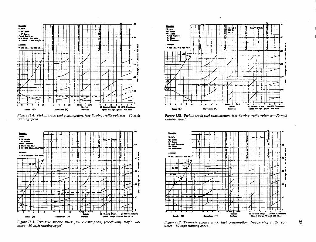
sds (5) (•)

0 0 1 2 3 02 4 30 P.co..d Stops 10-4 S1ons Speed Q.snp. cyoles For *1.

246 10 0 4 B 12 0 1 2 3 0 2 40 30 S.c.d Stops 10-lI S1s

Ws Cs) O.iovst. () Surt.00 Spssd Q.ngs C7c1.. P., Ills

Figure 12A. Pickup truck fuel consumption, free-flowing traffic volumes-30-mph running speed.

Figure 12B. Pickup truck fuel consumption, free-flowing traffic volumes-50-mph running speed.

1F] 11•1 .JHIMMIINIL •••uu•F ....i.I. _ILU_ UUUUUNLI• uu•uuuwau U•flIU!4UUl

......... our No LI W Is M

M! 10M 0 NMI

ruuuu•u• mu..u..•u ••UUdUU 30 Q cord Stops 10-Un SLOUNIVEnG

(5) b5 (.) Speed Chengs cycl.s IS, tale

Figure 13A. Two-axle six-tire truck fuel consumption, free-flowing traffic vol-umes-30-mph running speed.

.Jiuuiinii!iiiiuim EIIN IN;!i1IP!IItJII!!iI UUU 91UI 'A•UIUIUU ••uuiuuu•uau•uu' rurmuii•iuuu•' . uuus dd

pu•umuiiuiu ..ua..•uuu uuU• vuu..Uuiula.

ON .0 uau 1W UI

ON MIS ral"Em WE I WI S 0 raj.E.I. I III I I I I I 'I kwo .1• ;p l Gravel 30 5sc tsps Lu-11 wenewerts

Graft (5) (°) aiisO. Spssd Q.snqs c1c1.. P.. *19

Figure 13B. Two-axle six-tire truck fuel consumption, free-flowing traffic vol-umes-50-mph running speed.

30

$uOT1 - U011d%1UO3 TId

MELLO kjk

flhguIIIrnhm!IgpkI ...a

ii-

MMEEME MOWN

=IIIiIII1IiIIIIIIi1i oil

194

B N

a

i .

fEXCESS

TABLE 18

GALLONS OF GASOLINE CONSUMED PER SLOWDOWN SPEED CHANGE CYCLE—TRACTOR SEMI-TRAILER TRUCK 1

EXCESS GASOLINE CONSUMED (GAL) BY AMOUNT OF SPEED REDUCTION BEFORE ACCELERATING BACK TO SPEED (MPH):

SPEED (MPH) 10 20 30 40

20 0.040 - - - 30 0.040 0.065 - - 40 0.050 0.077 0.110 - 50 0.065 0.107 0.157 0.227

B 'See Footnote 1, Table 16, for identification of tractor semi-trailer

combinations.

— • B

4 I

8TV 44d •uoj - ..o;5du0 5S51

if

I

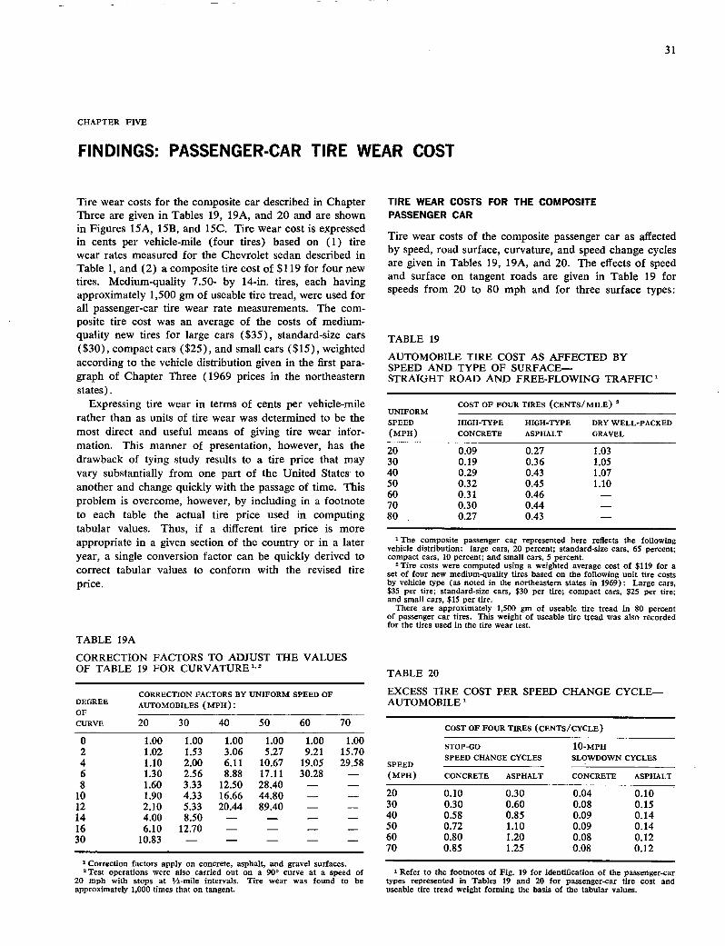
CHAPTER FIVE

FINDINGS: PASSENGER-CAR TIRE WEAR COST

31

Tire wear costs for the composite car described in Chapter Three are given in Tables 19, 19A, and 20 and are shown in Figures 15A, 15B, and 15C. Tire wear cost is expressed in cents per vehicle-mile (four tires) based on (1) tire wear rates measured for the Chevrolet sedan described in Table 1, and (2) a composite tire cost of $119 for four new tires. Medium-quality 7.50- by 14-in, tires, each having approximately 1,500 gm of useable tire tread, were used for all passenger-car tire wear rate measurements. The com-posite tire cost was an average of the costs of medium-quality new tires for large cars ($35), standard-size cars ($30), compact cars ($25), and small cars ($15), weighted according to the vehicle distribution given in the first para-graph of Chapter Three (1969 prices in the northeastern states).

Expressing tire wear in terms of cents per vehicle-mile rather than as units of tire wear was determined to be the most direct and useful means of giving tire wear infor-mation. This manner of presentation, however, has the drawback of tying study results to a tire price that may vary substantially from one part of the United States to another and change quickly with the passage of time. This problem is overcome, however, by including in a footnote to each table the actual tire price used in computing tabular values. Thus, if a different tire price is more appropriate in a given section of the country or in a later year, a single conversion factor can be quickly derived to correct tabular values to conform with the revised tire price.

TABLE 19A

CORRECTION FACTORS TO ADJUST THE VALUES OF TABLE 19 FOR CURVATURE"2

TIRE WEAR COSTS FOR THE COMPOSITE PASSENGER CAR

Tire wear costs of the composite passenger car as affected by speed, road surface, curvature, and speed change cycles are given in Tables 19, 19A, and 20. The effects of speed and surface on tangent roads are given in Table 19 for speeds from 20 to 80 mph and for three surface types:

TABLE 19

AUTOMOBILE TIRE COST AS AFFECTED BY SPEED AND TYPE OF SURFACE- STRAIGHT ROAD AND FREE-FLOWING TRAFFIC1

COST OF FOUR TIRES (CENTS/MILE) 2

UNIFORM SPEED

HIGH-TYPE HIGH-TYPE DRY WELL-PACKED (MPH) CONCRETE ASPHALT GRAVEL

20 0.09 0.27 1.03 30 0.19 0.36 1.05 40 0.29 0.43 1.07 50 0.32 0.45 1.10 60 0.31 0.46 - 70 0.30 0.44 - 80 0.27 0.43 -

composite passenger car represented here reflects the following vehicle distribution: large cars, 20 percent; standard-size cars, 65 percent; compact cars, 10 percent; and small cars, 5 percent.

'Tire costs were computed using a weighted average cost of $119 for a set of four new medium-quality tires based on the following unit tire costs by vehicle type (as noted in the northeastern states in 1969): Large cars, $35 per tire; standard-size cars, $30 per tire; compact cars, $25 per tire; and small cars, $15 per tire.

There are approximately 1,500 gm of useable tire tread in 80 percent of passenger car tires. This weight of useable tire tread was also recorded for the tires used in the tire wear test.

TABLE 20

CORRECTION FACTORS BY UNIFORM SPEED OF EXCESS TIRE COST PER SPEED CHANGE CYCLE- DEGREE AUTOMOBILES (MPH): AUTOMOBILE' OF CURVE 20 30 40 SO 60 70 COST OF FOUR TIRES (CENTS/CYCLE)

0 1.00 1.00 1.00 1.00 1.00 1.00 2 1.02 1.53 3.06 5.27 9.21 15.70 4 1.10 2.00 6.11 10.67 19.05 29.58 6 1.30 2.56 8.88 17.11 30.28 - 8 1.60 3.33 12.50 28.40 - -

10 1.90 4.33 16.66 44.80 - - 12 2.10 5.33 20.44 89.40 - - 14 4.00 8.50 - - - - 16 6.10 12.70 - - - - 30 10.83 - - - - -

1 Correction factors apply on concrete, asphalt, and gravel surfaces. 'Test operations were also carried out on a 90° curve at a speed of

20 mph with stops at ½-mile intervals. Tire wear was found to be approximately 1,000 times that on tangent.

STOP-GO 10-MPH SPEED CHANGE CYCLES SLOWDOWN CYCLES

SPEED (MPH) CONCRETE ASPHALT CONCRETE ASPHALT

20 0.10 0.30 0.04 0.10 30 0.30 0.60 0.08 0.15 40 0.58 0.85 0.09 0.14 50 0.72 1.10 0.09 0.14 60 0.80 1.20 0.08 0.12 70 0.85 1.25 0.08 0.12

'Refer to the footnotes of Fig. 19 for identification of the passenger-car types represented in Tables 19 and 20 for passenger-car tire cost and useable tire tread weight forming the basis of the tabular values.

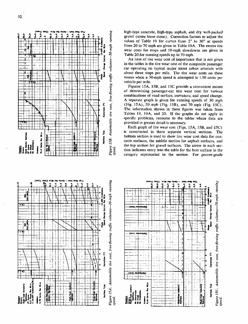
(lulL a4) •1 Old '1103 - 1003 Ol

(lulL ft°d) film sod 'W'D - 1103 ZV 10Th

UUk1 •UI MU1i11 ii U P . r & Vii ii 'thiiñri 1 ii

JUS

1111mlimfflww In

loom

ii.mi .uu • .i..

- - - Miss on 4 0iR0

a

(uij ) •l 4 fl103 - 8I3 I o e 0 0 0 0 0 0 0

high-type concrete, high-type asphalt, and dry well-packed gravel (some loose stone). Correction factors to adjust the values of Table 19 for curves from 2° to 30° at speeds from 20 to 70 mph are given in Table 1 9A. The excess tire wear costs for stops and 10-mph slowdowns are given in Table 20 for running speeds up to 70 mph.

An item of tire wear cost of importance that is not given E in the tables is the tire wear cost of the composite passenger

car operating on typical major street urban arterials with

a about three stops per mile. The tire wear costs on these routes when a 30-mph speed is attempted is 1.50 cents per vehicle per mile.

CIO Figures 15A, 15B, and 15C provide a convenient means

of determining passenger-car tire wear cost for various combinations of road surface, curvature, and speed change. A separate graph is given for running speeds of 30 mph (Fig. 15A), 50 mph (Fig. 15B), and 70 mph (Fig. 15C). The information shown in these figures was taken from Tables 19, 19A, and 20. If the graphs do not apply in specific problems, recourse to the tables where data are provided in greater detail is necessary.

Each graph of tire wear cost (Figs. 15A, 15B, and 15C) is constructed in three separate vertical sections. The bottom section is used to show tire wear cost data for concrete surfaces, the middle section for asphalt surfaces, and the top section for gravel surfaces. The arrow in each sec-

to 14) tion indicates entry into the table for the best surface in the category represented in the section. For poorer-grade

32

33

surfaces, entry should be made higher on the road sur-face reference line (but within the section) at a point selected by judgment as being appropriate for the surface conditions relative to the best surface.

After entry into the figure by surface type is determined (at the arrows for the best surface surfaces-somewhat above for poorer surfaces), tire wear cost is found by tracing horizontally to the right scale where tire wear cost

is read in cents per mile per vehicle. If curvature is zero and there are no stops or slowdowns, the trace is straight. However, if curvature exists and there are stops or slow-downs the horizontal trace is displaced upward by breaking at the appropriate reference lines (R.L.) and tracing parallel to the sloping lines to points directly above the appropriate curvature, stop frequency or slowdown fre-quency. (See the examples worked on each figure.)

CHAPTER SIX

FINDINGS: TRUCK TIRE WEAR COSTS

Detailed tire wear costs for the composite pickup truck described in Chapter Four are given in Tables 21, 21A, and 22 and shown in Figures 16A and 16B. Limited tire wear cost information for the two-axle six-tire truck is given in Table 23. Tire wear costs are given in cents per mile per vehicle (four tires) for the pickup truck and in cents per mile per axle for the two-axle six-tire truck. No tire wear data for the tractor semi-trailer truck combination are provided in this report.

The rate of tire'wear for the pickup truck was assumed to be the same as for the passenger car for speeds up to 50 mph. There are two bases for this assumption. First, the undercarriages, power delivery systems, and brake systems of pickup trucks are similar to those of passenger

TABLE 21

PICKUP TRUCK TIRE COST AS AFFECTED BY SPEED AND TYPE OF SURFACE- STRAIGHT ROAD AND FREE-FLOWING TRAFFIC1' 2

COST OF FOUR TIRES (CENTS/MILE) UNIFORM SPEED HIGH-TYPE HIGH-TYPE DRY WELL-PACKED (MPH) CONCRETE ASPHALT GRAVEL

20 0.10 0.32 1.22 30 0.22 0.42 1.24 40 0.34 0.51 1.26 50 0.38 0.53 1.30

'The typical pickup truck represented here has an average weight of 5,000 lb (85 percent of pickup trucks weigh 4,800 lb and 15 percent weigh 5,800 lb). Eecause this weight is less than that of a large automobile with three adults aboard, and because wheel rigging is similar for the two vehicle types, it was assumed that the rate of tire wear was the same for the pickup truck as for the passenger car for speeds up to 50 mph. (At speeds greater than 50 mph aerodynamic effects on tire wear are appre-ciably different for passenger cars and pickup trucks.)

2 The pickup truck carries a heavier, more expensive tire than does the typical automobile. In the northeastern states in 1969 the average medium-grade pickup truck tire cost $40 ($160 per vehicle) and had an average of 1,700 gm of useable tire tread available for wear before recapping was necessary.

cars, including coiled springs and shock absorbers at all four wheels, wheel bases of about 120 in., and independent suspensions at each front wheel. Power is delivered to the rear wheels through a transmission, drive shaft, and differential gearing for both vehicle types. Braking of both vehicle types is accomplished by manually operated hydraulic brake systems with drum-type brakes. Second, the average pickup truck weighs about 5,000 lb, about the weight of a large car with three adults aboard (the empty weight of the 3%-ton pickup truck is only 4,400 lb-the same as the 1966 Chrysler Newport with driver).

However, the pickup truck and passenger car exhibit markedly different tire wear patterns at speeds greater than 50 mph, because of the effect vehicle shape has on aero-dynamic forces. Many passenger cars have hoods that slope downward to the front so that moving air at high speed tends to press these vehicles downward, giving wheels greater traction and less tire wear-inducing slippage. Pickup

TABLE 21A

CORRECTION FACTORS TO ADJUST THE VALUES OF TABLE 21 FOR CURVATURE1

DEGREE

CURvE OF

CORRECTION FACTORS BY UNIFORM SPEED OF PICKUP TRUCK (MPH):

20 30 40 50

0 1.00 1.00 1.00 1.00 2 1.02 1.53 3.06 5.27 4 1.10 2.00 6.11 10.67 6 1.30 2.56 8.88 17.11 8 1.60 3.33 12.50 28.40

10 1.90 4.33 16.66 44.80 12 2.10 5.33 20.44 89.40 14 4.00 8.50 - - 16 6.10 12.70 - - 30 10.83 - - -

Correction factors apply on concrete, asphalt, and gravel surfaces.

34 TABLE 22

EXCESS TIRE COST PER SPEED CHANGE CYCLE—PICKUP TRUCK'

COST OF FOUR TIRES (CENTS/CYCLE)

STOP-GO 10-MPH SPEED CHANGE CYCLES SLOWDOWN CYCLES

SPEED (MPH) CONCRETE ASPHALT CONCRETE ASPHALT

20 0.12 0.36 0.05 0.11 30 0.36 0.71 0.09 0.17 40 0.69 1.00 0.10 0.17 50 0.85 1.30 0.10 0.17

1 Refer to the footnotes of Figure 21 for identification of the weight distribution of pickup trucks represented in Tables 21 and 22 and for pickup truck tire cost and useable tire tread weight forming the basis of the tabular values. As noted in Footnote I, Table 21, the rate of pickup truck tire wear is assumed the same as that for passenger cars.

TABLE 23

TIRE WEAR COST—TWO-AXLE SIX-TIRE TRUCK'

TYPE OF OPERATION AND ROAD SURFACE

TIRE WEAR COSTS (CENTS/MILE/AXLE)

REAR AXLE— FRONT AXLE— FOUR TIRES TWO TIRES (12,000 LB) (4,000 LB)

Uniform speed of 45 mph on high-type concrete 0.40 0.10 25-30 mph on four-lane major street urban ar-

terial with high-type concrete surface (3 to 4 stops per mile) 1.96 0.28

25 mph on 30° curve with high-type surface 10.80 1.30 25 mph on 60° curve with high-type surface 108.00 9.20

1 Tire wear costs based on a cost of $120 per tire for a medium-quality 10-ply 8.25X20 transport tire (1970 price in the northeastern states). Each tire has approximately 4,500 gm of useable tread before recapping is necessary. Value of the tire carcass when recapped was assumed to be $20.

t•-u -"a -Lin --

88 - •.'cJ zeft —IS (9St5j anal) •jpq 44U - a.

0 n;j

00000000000 0000

1r1

- \ (re)

I j ----— -4-

tr

UIIIII -

IH 1 DI EE IU IIFIFT

---....---f-- --

iid1!f I J jt-J4 T TFIIk

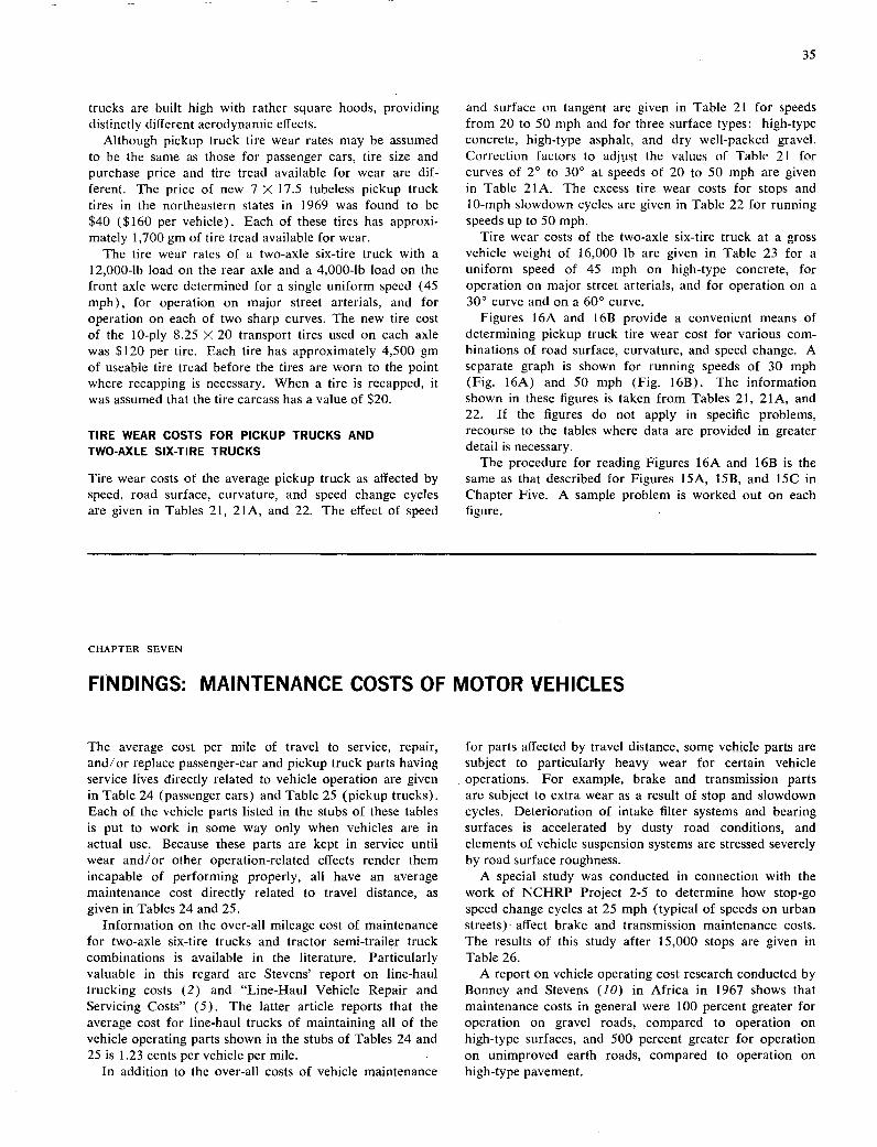
35

trucks are built high with rather square hoods, providing distinctly different aerodynamic effects.

Although pickup truck tire wear rates may be assumed to be the same as those for passenger cars, tire size and purchase price and tire tread available for wear are dif-ferent. The price of new 7 >< 17.5 tubeless pickup truck tires in the northeastern states in 1969 was found to be $40 ($160 per vehicle). Each of these tires has approxi-mately 1,700gm of tire tread available for wear.

The tire wear rates of a two-axle six-tire truck with a 12,000-lb load on the rear axle and a 4,000-lb load on the front axle were determined for a single uniform speed (45 mph), for operation on major street arterials, and for operation on each of two sharp curves. The new tire cost of the 10-ply 8.25 X 20 transport tires used on each axle was $120 per tire. Each tire has approximately 4,500 gm of useable tire tread before the tires are worn to the point where recapping is necessary. 'When a tire is recapped, it was assumed that the tire carcass has a value of $20.

TIRE WEAR COSTS FOR PICKUP TRUCKS AND TWO-AXLE SIX-TIRE TRUCKS

Tire wear costs of the average pickup truck as affected by speed, road surface, curvature, and speed change cycles are given in Tables 21, 21A, and 22. The effect of speed

and surface on tangent are given in Table 21 for speeds from 20 to 50 mph and for three surface types: high-type concrete, high-type asphalt, and dry well-packed gravel. Correction factors to adjtist the values of Table 21 for curves of 2° to 30° at speeds of 20 to 50 mph are given in Table 21A. The excess tire wear costs for stops and 10-mph slowdown cycles are given in Table 22 for running speeds up to 50 mph.

Tire wear costs of the two-axle six-tire truck at a gross vehicle weight of 16,000 lb are given in Table 23 for a uniform speed of 45 mph on high-type concrete, for operation on major street arterials, and for operation on a 30° curve and on a 60° curve.

Figures 16A and 16B provide a convenient means of determining pickup truck tire wear cost for various com-binations of road surface, curvature, and speed change. A separate graph is shown for running speeds of 30 mph (Fig. 16A) and 50 mph (Fig. 16B). The information shown in these figures is taken from Tables 21, 21A, and 22. If the figures do not apply in specific problems, recourse to the tables where data are provided in greater detail is necessary.

The procedure for reading Figures 16A and 16B is the same as that described for Figures 15A, 15B, and 15C in Chapter Five. A sample problem is worked out on each figure.

CHAPTER SEVEN

FINDINGS: MAINTENANCE COSTS OF MOTOR VEHICLES

The average cost per mile of travel to service, repair, and/or replace passenger-car and pickup truck parts having service lives directly related to vehicle operation are given in Table 24 (passenger cars) and Table 25 (pickup trucks). Each of the vehicle parts listed in the stubs of these tables is put to work in some way only when vehicles are in actual use. Because these parts are kept in service until wear and/or other operation-related effects render them incapable of performing properly, all have an average maintenance cost directly related to travel distance, as given in Tables 24 and 25.

Information on the over-all mileage cost of maintenance for two-axle six-tire trucks and tractor semi-trailer truck combinations is available in the literature. Particularly valuable in this regard are Stevens' report on line-haul trucking costs (2) and "Line-Haul Vehicle Repair and Servicing Costs" (5). The latter article reports that the average cost for line-haul trucks of maintaining all of the vehicle operating parts shown in the stubs of Tables 24 and 25 is 1.23 cents per vehicle per mile.

In addition to the over-all costs of vehicle maintenance

for parts affected by travel distance, some vehicle parts are subject to particularly heavy wear for certain vehicle operations. For example, brake and transmission parts are subject to extra wear as a result of stop and slowdown cycles. Deterioration of intake filter systems and bearing surfaces is accelerated by dusty road conditions, and elements of vehicle suspension systems are stressed severely by road surface roughness.

A special study was conducted in connection with the work of NCHRP Project 2-5 to determine how stop-go speed change cycles at 25 mph (typical of speeds on urban streets) affect brake and transmission maintenance costs. The results of this study after 15,000 stops are given in Table 26.

A report on vehicle operating cost research conducted by Bonney and Stevens (10) in Africa in 1967 shows that maintenance costs in general were 100 percent greater for operation on gravel roads, compared to operation on high-type surfaces, and 500 percent greater for operation on unimproved earth roads, compared to operation on high-type pavement.

NO. OF VEHICLES FOR WHICH DATA WERE AVAILABLE

TRAVEL DISTANCE BEFORE REPAIRS ARE NECESSARY (1,000 MILES)

COST OF REPAIRS

($)

AVG.

VEHICLE PART RANGE AVG. RANGE

AVG. COST (cENTs! MILE)

TABLE 24 AVERAGE MAINTENANCE COST AS AFFECTED BY TRAVEL DISTANCE-STANDARD-SIZE PASSENGER CARS 1

TRAVEL DISTANCE NO. OF BEFORE REPAIRS ARE VEHICLES NECESSARY COST OF REPAIRS FOR WHICH (1,000 MILES) ($) AVG. COST

VEHICLE DATA WERE (cENTs! PART AVAILABLE RANGE AVG. RANGE AVG. MILE)

Automatic transmission 850 54-103 66 100-255 178 0.27

Engine block 395 50-90 70 65-130 93 0.13 Shock absorbers 1350 30-60 44 28-51 37 0.08 Brake system 1350 40-77 54 40-5 8 41 0.08 Distributor 1050 10-21 14 5-20 12 0.08 Exhaust 1350 30-56 39 18-33 26 0.07 Carburetor 1050 32-60 45 21-40 29 0.06 Universal 1050 30-54 44 20-31 28 0.06 Rear axle 50 100-113 106 54-75 66 0.06 Generator 1050 42-60 52 18-40 32 0.06 Water pump 1050 34-55 43 18-30 24 0.06 Springs 50 40-100 68 28-46 40 0.06 Fuel pump 50 44-64 52 12-20 15 0.03 Oil pump 50 92-138 109 16-28 21 0.02 Radiator 50 66-96 76 10-25 16 0.02 Fan belt 1050 40-68 51 3-6 4 0.01

Total 1.15

1 Based on responses to an inquiry submitted to the Chief Engineers of the highway departments of each of the 50 states and to each of the Division Engineers of the Bureau of Public Roads.

TABLE 25 AVERAGE MAINTENANCE COST AS AFFECTED BY TRAVEL DISTANCE-PICKUP TRUCK 1

15 77-78 77 - 40 0.05 15 75-92 81 250-350 300 0.37 15 25-50 29 23-42 31 0.11 15 50-75 60 75-100 91 0.15 15 50-70 65 14-25 20 0.03 15 15-25 22 21-40 30 0.14 15 25-50 36 10-20 16 0.04 15 50-82 66 15-23 19 0.03 15 75-115 94 70-100 85 0.09 15 30-50 38 15-35 22 0.06 15 30-50 43 15-25 21 0.05 15 50-75 62 80-100 90 0.14 15 - 50 8-15 23 0.04 15 - 106 11-12 11 0.01 15 75-95 85 75-80 76 0.09 15 50-55 52 - 10 0.02

1.42

Manual transmission

Engine block Shock absorbers Brake system Distributor Exhaust Carburetor Universal Rear axle Generator Water pump Springs Fuel pump Oil pump Radiator Fan belt

Total

1 Based on responses to an inquiry submitted to the Chief Engineers of the highway departments of each of the 50 states and to each of the Division Engineers of the Bureau of Public Roads.

TABLE 26 EFFECT OF STOP-GO CYCLES ON BRAKE SYSTEM WEAR AND TRANSMISSION FLUID LOSS-PASSENGER CAR OPERATING AT 25 MPH

NO. OF STOPS BEFORE REPAIRS SERVICE PRICE COST/STOP

ITEM ARE NECESSARY NEEDED ($) (cENIs)

Brake shoes 5,000 Adjustment 2.50 0.05 Brake fluid 15,000 Add 0.5 in. - - Brake lining 60,000 Replace 41.00 0.07 Trans. fluid - - - - Total cost/stop 0.12

CHAPTER EIGHT

FINDINGS: VEHICLE OIL CONSUMPTION

37

Motor-vehicle oil consumption arises from (1) the need for periodically replacing oil to remove destructive con-taminants, and (2) the need for continuous replacement of oil lost by burning, evaporation, and leakage. The magnitude of the oil consumed to replace contaminated oil depends in part on whether operation is at high sustained speed with engines properly warmed up (long trips), so that sludge is burned away, or at low speed on short trips with frequent stops when unburned combustion remnants are able to accumulate. Oil replacement because of contami-nation is also accelerated by operation on dusty roads when some dust particles get by filters to form an abrasive oil contaminant.

The amount of oil needed to replace oil lost by burning, evaporation, and leakage varies with speed and frequency of stop-go cycles. More oil is lost by sustained high freeway speeds, for example, than on rural highways in general. Each time a vehicle goes through a stop-go cycle some oil is lost due to engine conditions associated with speed change.

Motor-vehicle manufacturers' recommendations regard-ing oil change intervals to control oil contamination based on their knowledge of engine design should be followed by

motor-vehicle users, because engine design has an important effect on how oil contaminants are handled by the engine. On the basis of these recommendations for each of the types of vehicle investigated in this study, it was determined that on dust-free roads with free-flowing traffic, oil con-sumption to remove contaminants is 0.70, 0.60, and 2.50 qt per 1,000 miles for the composite passenger car, the pickup truck, and the two-axle six-tire truck, respectively. On dusty roads (gravel and sand surfaces) in free-flowing traffic, oil consumption to remove contaminants is 4.00 qt per 1,000 miles for passenger cars and pickup trucks, and 5.00 qt per 1,000 miles for two-axle six-tire trucks. On CBD streets with restricted traffic flow, it is 2.0 qt per 1,000 miles for passenger cars, 1.33 qt per 1,000 miles for pickup trucks, and 1.66 qt per 1,000 miles for two-axle six-tire trucks. Similar information for tractor semi-trailer truck combinations is not reported.

Oil consumed by motor vehicles as a result of burning, evaporation, and/or leakage is given in Table 27 for the composite passenger car, the pickup truck, and the two-axle six-tire truck. These values were determined through re-search conducted for NCHRP Project 2-5.

The oil consumption rate to use for a particular problem

TABLE 27

ENGINE OIL ADDITIONS BETWEEN OIL CHANGES TO MAKE UP THAT LOST BY LEAKAGE AND COMBUSTIONI

TRACTOR SEMI- COMPOSITE TWO-AXLE TRAILER TRUCK

5PEEt) PASSENGER PICKUP SIN-TIRE (MPH) CAR 2 TRUCK 2 TRUCK 3 2-S2 3-S2

(a) Free-flowing traffic (qt/ 1,000 miles)

30 0.27 0.27 0.27 - - 35 0.27 0.27 0.27 - - 40 0.42 0.42 0.34 - - 45 0.58 0.58 0.50 - - 50 0.75 0.75 0.66 - - 55 0.94 0.94 0.83 - - 60 1.08 1.08 1.00 - -

(b) Major street urban arterial (qt/ 1,000 miles)

20-25 - - 1.55 - - 25-35 0.45 - - - -

(c) Excess per stop-go cycle (qt/ 1,000 stops)

25 0.09 - - - - 1 Minimum trip length = 10 miles.

Both the composite passenger car and the pickup truck are represented by an eight-cylinder Chevrolet sedan (engine displacement = 283 cu in.)

3 The two-axle six-tire truck is represented by a two-axle six-tire truck with six cylinders (engine displace-ment = 351 cu in.) weighing 16,000 lb.

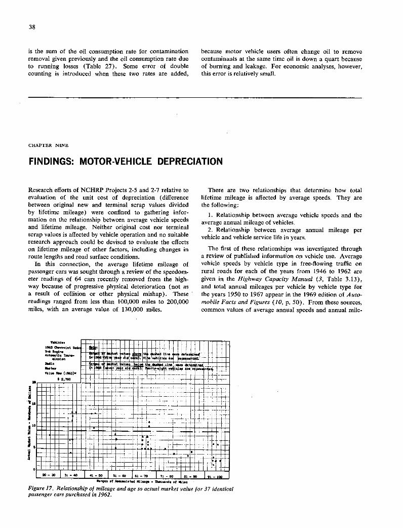
5

38

is the sum of the oil consumption rate for contamination removal given previously and the oil consumption rate due to running losses (Table 27). Some error of double counting is introduced when these two rates are added,

because motor vehicle users often change oil to remove contaminants at the same timc oil is down a quart because of burning and leakage. For economic analyses, however, this error is relatively small.

CHAPTER NINE

FINDINGS: MOTOR-VEHICLE DEPRECIATION

Research efforts of NCHRP Projects 2-5 and 2-7 relative to evaluation of the unit cost of depreciation (difference between original new and terminal scrap values divided by lifetime mileage) were confined to gathering infor-mation on the relationship between average vehicle speeds and lifetime mileage. Neither original cost nor terminal scrap values is affected by vehicle operation and no suitable research approach could be devised to evaluate the effects on lifetime mileage of other factors, including changes in route lengths and road surface conditions.

In this connection, the average lifetime mileage of passenger cars was sought through a review of the speedom-eter readings of 64 cars reecntly removed from the high-way because of progressive physical deterioration (not as a result of collision or other physical mishap). These readings ranged from less than 100,000 miles to 200,000 miles, with an average value of 130,000 miles.

There are two relationships that determine how total lifetime mileage is affected by average speeds. They are the following:

Relationship between average vehicle speeds and the average annual mileage of vehicles.

Relationship between average annual mileage per vehicle and vehicle service life in years.

The first of these relationships was investigated through a review of published information on vehicle use. Average vehicle speeds by vehicle type in free-flowing traffic on rural roads for each of the years from 1946 to 1962 are given in the Highway Capacity Manual (3, Table 3.13), and total annual mileages per vehicle by vehicle type for the years 1950 to 1967 appear in the 1969 edition of Auto-mobile Facts and Figures (10, p. 50). From these sources, common values of average annual speeds and annual mile-

!lIIIlg F4GII!!!!.. H-- U..... uu•ii••u• u•

iiiiiI'jIjjJ'jiJ' iETii11 N 0

IN 0 OMEN

IN 1111MEW

on ...n ng.s of Mu1.t.d IQIQaga - Thsands of1si

Figure 17. Relationship of mileage and age to actual market value for 37 identical passenger cars purchased in 1962.

39

ages for passenger cars were found for the years 1950 to 1962. Fitting a straight line to the plots of annual mileages for corresponding average speeds indicates the following relationship: passenger cars develop an average total annual mileage of 9,150 miles when the average speed on rural roads in free-flowing tralllc is 50 mph. This mileage increases to 9,360 at 52 mph, and to 9,560 at 54 mph, implying that users travel farther per year when possible speeds are increased through highway improvement.

The second relationship of importance in determining how average speeds affect vehicle lifetime mileage, the relationship between average annual mileage and total vehicle service life in years, was investigated for passenger cars through a study of patterns of change in an auto-mobile's value occurring during its service life. Figure 17 shows the market values of a particular model passenger car (a 1962 Chevrolet sedan) after the first 5 years of service life (data above the dashed line) and at 7 years of service life (data below the dashed line). Ranges of market

value data are plotted according to ranges of accumulated mileage noted on vehicle speedometers at the time market values were established through actual negotiation.

Assuming the pattern of market value changes during a vehicle's life is a reasonable measure of the time rate at which a vehicle's value is approaching terminal scrap value, Figure 17 suggests that increases in annual mileage, have little effect in accelerating the time rate of vehicle deterio-ration during the early years of a vehicle's service life.

The results of this study are inconclusive because of the limited number of vehicles for which depreciation infor-mation is available. However, the conclusion seems inescapable that as highways are improved, the average road user travels faster and farther with a relatively small reduction in the service life of his vehicle. Average depreciation cost per mile goes down as roads are improved because total depreciation is distributed over a greater mileage.

CHAPTER TEN

FINDINGS: VEHICLE ACCIDENT COSTS

The cost of accidents that take place when vehicles are operated on roads and streets is a motor-vehicle running cost, because it is an expenditure individuals can avoid by not using their vehicles. Although erratic and haphazard in its impact, accident cost nevertheless is a tangible user expense directly associated with vehicle operation. A spe-cial analytical study of motor-vehicle accident cost as a user operating cost based on 1958 accident cost data was carried out in connection with the research for NCHRP Project 2-5. This study is described as Special Project 5 and is reported in Appendix F.

Table F-7 indicates that passenger-car accident cost per million miles of travel of all vehicle types (passenger cars, buses, and trucks) is $1,673 on rural non-freeway routes,

$4,287 on urban non-freeway routes, $734 on rural free-ways, and $1,430 on urban freeways (1958 dollars).

Table F-8 gives information on the cost of accidents as affected by curves and intersections. Passenger cars suffer an average of $2,419 per million miles of travel of all vehicle types on curves greater than 10° but only $1,814 per million miles of travel of all vehicle types on curves of 3° to 6°. Passenger cars have accident costs of $5,796 per million miles of travel of all vehicle types on roads with 0.8 intersection per mile but only $2,520 per million miles of travel of all vehicle types on roads with only 0.3 intersection per mile. Similar data for trucks appear in Appendix F.

40

CHAPTER ELEVEN

INTERPRETATION OF FINDINGS

Special interpretative comments are unnecessary for most of the material presented in this report. Fuel consumption, tire wear cost, maintenance cost, oil consumption, depre-ciation, and accident costs are presented in relation to highway design and traffic to the extent these items could be identified with and evaluated for specific road design elements and traffic conditions. Although the variety of factors involved in road user cost research complicates the presentation of report data, most of the subject matter is easily understood. The few exceptions are discussed in the following sections.

FUEL CONSUMPTION OF PASSENGER CARS IN GENTLY ROILING TERRAIN

In Table 6, where the fuel consumption of passenger cars is given relative to speed and gradient, fuel consumption is greater for level roads than for successive equal-length grades that are alternately plus and minus (grades less than 4 percent). This would seem to indicate an error in the data, because the level road is generally considered to be most economical for operation when there is a zero over-all change in elevation. This apparent aberration of the data was noted early in the study and numerous check test runs were made on the 31/2 -percent test grade and on the level test road. Invariably it was found that the sum of the fuel consumed operating up and down the 31/2 -percent grade a given distance was a little less than that for oper-ating twice the distance on a level road. Table 6 is not in error. It is slightly more economical at medium speed to operate passenger cars up and down equal-length grades up to about 30 than to operate continually on level roads.

EFFECT OF VERTICAL CURVES ON FUEL CONSUMPTION PREDICTIONS

A frequently voiced concern regarding the interpretation of the findings of fuel consumption is the possibility of error in fuel consumption predictions at grade breaks due to the vertical curves that normally connect successive gradients. A special study was undertaken to determine how much error in fuel consumption predictions would be introduced by assuming that grades change abruptly at the point of grade-line intersection rather than gradually by means of a vertical curve. This study was carried out after all fuel consumption data for operation on specific grades had been collected and analyzed.

A section of New York State Route 30 between Tupper Lake and Long Lake was selected for the vertical curve study because of the succession of severe grade changes provided in a relatively short distance (6,500 ft). The road had a good concrete surface and consisted of a se-quence of grades (northbound) as follows: —1.08 percent, +4.1 percent, +2.4 percent, +5.4 percent, —1.0 percent,

+7.0 percent, and —4.2 percent. The grades were con-nected by vertical curves having a typical rate of grade change of 1.0 percent per 100 ft. The fuel consumption of the Chevrolet and Plymouth test cars in Table 1 were predicted for operation in each direction on this test sec-tion, assuming the grade-lines intersected without vertical curves. The predicted values of fuel consumption were then compared with fuel consumption actually measured for operation over the test section. It was found that the predicted values agreed almost exactly with the measured values. Fuel consumption measurements for a few of the test runs varied from the predicted values but none with an error greater than 5 percent. The error introduced by ignoring vertical curves connecting successive grades is, therefore, small and need not be a concern in the analysis of vehicle costs.

REPRESENTATIVENESS OF THE TIRE WEAR COSTS REPORTED HEREIN FOR PASSENGER-CAR TIRE WEAR IN GENERAL

Passenger-car tire wear rates on which the findings of Chapter Five are based were determined using medium-quality 7.50 x 14 tires and a 1964 Chevrolet sedan. Cer-tain check tire wear measurements were also made to sub-stantiate these results using good-quality 8.55 X 14 tires and a large car (Plymouth sedan at 4,200 lb with 383-cu-in. engine) - These vehicles represent 65 percent of the pas-senger cars on U.S. highways (see Chapter Three).

However, it must be recognized that tire wear rates are sensitive to many factors that vary with vehicle design and tire details. For example, aerodynamic forces that tend to press down on cars at high speeds for vehicles with certain body configurations may tend to lift cars with a different shape. Different body suspension systems that vary in their response to road roughness also affect forces holding tires to the road. These factors affect tire wear principally at speeds greater than 50 mph.

The values of tire wear cost given in Chapter Five are accurate for most cars of the standard- and large-size cate-gories for speeds up to 50 mph. For specialty cars and small cars like the Volkswagen and for speeds greater than 50 mph, when body shape affecting aerodynamic forces becomes a factor in tire wear, report values can still be used but are most accurate the closer vehicles resemble the Chevrolet sedan test vehicle (Fig. 1).

TIRE WEAR OF PASSENGER CARS AT HIGH SPEED

In Table 19, tire wear cost drops off at speeds greater than 50 mph. It is surprising that this is so, inasmuch as traction forces necessarily increase at high speeds to overcome increased air resistance. Still, this feature of tire wear was

41

noticed in the field, where it was supported with repeated check measurements. The reason for the fall-off in tire wear at high speed is probably the aerodynamic down pressure imposed on the car by its shape—especially the downward sloping front hood. This downward pressure increases tire friction and reduces wheel slippage at high speed. Because wheel slippage is a major cause of tire wear, the reduction of wheel slippage at high speed is the apparent cause of reduced tire wear at these speeds.

The importance of wheel slippage as the cause of tire wear is suggested by information on the effect of surface on tire friction given by De Vinney (12). De Vinney notes that portland cement concrete surfaces exhibit an appre-

ciably higher coefficient of friction than dense asphalt pavements for all speeds. Tire wear, however, is much less on concrete pavements than on asphalt, indicating that tire wear is reduced with greater friction because of less wheel slippage.

It is worth noting also that the Volkswagen, for which tire wear rates are particularly low, has a pronounced downward sloping front hood. This feature of body design enables the Volkswagen to take advantage of aerodynamic forces to minimize wheel slippage at relatively low speeds.

The drop-off in tire wear at high speeds noted for the test car is probably applicable for all modern cars because most have somewhat downward sloping front hoods.

CHAPTER TWELVE

APPLICATION OF FINDINGS

The research findings of NCHRP Projects 2-5 and 2-7 provide a comprehensive display of operating cost data for a composite passenger car and each of three composite trucks: (1) a pickup truck, (2) a two-axle six-tire truck, and (3) a tractor semi-trailer truck combination. Tables in Chapters Three and Four provide information on fuel consumption rates; Chapters Five and Six, tire wear costs; Chapter Seven, maintenance costs; Chapter Eight, oil con-sumption costs; Chapter Nine, depreciation information; and Chapter Ten, accident costs. These findings are in-tended for use by highway planners, administrators, engi-

neers, economists, and others who find it necessary in the course of their work to evaluate motor-vehicle running costs for particular road and traffic conditions.

DISTRIBUTION OF BASIC TRUCK TYPES

BY HIGHWAY SYSTEM

To make full use of the tables and graphs of findings for trucks to establish the average cost of truck operations on a given section of highway, the applicable distribution of pickup trucks, two-axle six-tire trucks, and tractor semi-trailer trucks should be known. Only by knowing this

TABLE 28

TYPICAL DISTRIBUTION OF TRUCK TYPES BY HIGHWAY SYSTEM1

DISTRIBUTION OF TRUCKS (%)

TRACTOR SEMI- TRAILER

FEDERAL-AID TWO-AXLE COMBINA- HIGHWAY SYSTEM PICKUP SIX-TIRE TIONS OTHERS TOTAL

Rural Interstate 32 15 49 4 100 Urban Interstate 39 23 35 3 100 Rural F.-A. Primary 42 25 30 3 100 Urban F.-A. Primary 48 25 24 3 100 Rural F.-A. Secondary 56 28 13 3 100 Urban F.-A. Secondary 57 26 14 3 100 Ruralnon-F.-A. 57 27 13 3 100 Urbannon-F.-A. 63 25 10 2 100

1 Data developed from Ref. 9 (Table Ii) updated to 1967 with information from Ref. 13 (Table 12, Fig. 2)

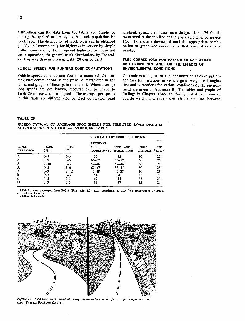
42

distribution can the data from the tables and graphs of findings be applied accurately to the truck population by truck type. The distribution of truck types can be obtained quickly and conveniently for highways in service by simple traffic observations. For proposed highways or those not yet in operation, the general truck distributions by Federal-aid Highway System given in Table 28 can be used.

VEHICLE SPEEDS FOR RUNNING COST COMPUTATIONS

Vehicle speed, an important factor in motor-vehicle run-ning cost computations, is the principal parameter in the tables and graphs of findings in this report. Where average spot speeds are not known, recourse can be made to Table 29 for passenger-car speeds. The average spot speeds in this table are differentiated by level of service, road

gradient, speed, and basic route design. Table 29 should be entered at the top line of the applicable level of service (Col. 1), moving downward until the appropriate combi-nation of grade and curvature at that level of service is reached.

FUEL CORRECTIONS FOR PASSENGER CAR WEIGHT AND ENGINE SIZE AND FOR THE EFFECTS OF ENVIRONMENTAL CONDITIONS

Corrections to adjust the fuel consumption rates of passen-ger cars for variations in vehicle gross weight and engine size and corrections for various conditions of the environ-ment are given in Appendix B. The tables and graphs of findings in Chapter Three are for typical distributions of vehicle weight and engine size, air temperatures between

TABLE 29

SPEEDS TYPICAL OF AVERAGE SPOT SPEEDS FOR SELECTED ROAD DESIGNS AND TRAFFIC CONDITIONS—PASSENGER CARS 1

SPEED (MPH) BY BASIC ROUTE DESIGN:

FREEWAYS LEVEL GRADE CURVE AND TWO-LANE URBAN CBD OF SERVICE (%) (°) EXPRESSWAYS RURAL ROADS ARTERIALS 2 STS. 2

A 0-3 0-3 60 53 30 25 A 3-7 0-3 60-52 53-52 30 25 A 7-10 0-3 52-46 52-46 30 25 A 0-3 3-6 60-47 53-47 30 25 A 0-3 6-12 47-38 47-38 30 25 B 0-3 0-3 54 50 25 20 C 0-3 0-3 49 44 25 20 D 0-3 0-3 45 37 25 20

1 Tabular data developed from Ref. 3 (Figs. 3.26, 3.27, 3.28y supplemented with field observations of speeds on grades and curves.

2 Attempted speeds.

Lk

'7 1

/1 /

Figure 18. Two-lane rural road showing views before and after major improvement (see "Sample Problem One").

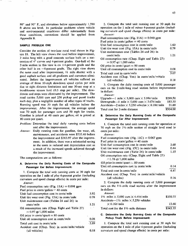
43

800 and 90° F, and elevations below approximately 1,700 ft above sea level. In particular problems where vehicle and environmental conditions differ substantially from these conditions, corrections should be applied from Appendix B.

SAMPLE PROBLEM ONE

Consider the section of two-lane rural road shown in Fig-ure 18. The left view shows the road before improvement, 2 miles long with a good concrete surface built on a suc-cession of 4° curves and 4-percent grades. One-half of the 2-mile section in this view is on +4-percent grade and the other half is on -4-percent grade. The right view shows the same road after improvement, ½ mile shorter with a good asphalt surface and all gradients and curvature elimi-nated. Before the improvement all vehicles suffered an average of three 10-mph slowdown speed cycles per mile due to sight distance limitations and one 30-sec stop at a troublesome stream ford (0.5 stop per mile). The slow-downs and stops were eliminated by the improvement. The road carries 5,000 cars and 250 pickup and panel trucks each day, plus a negligible number of other types of trucks. Running speed was 30 mph for all vehicles before the improvement. After the improvement, the average speed was 70 mph for passenger cars and 50 mph for trucks. Gasoline is priced at 40 cents per gallon; oil is priced at 80 cents per quart.

Problem: Determine the total daily running costs before and after the improvement.

Answer: Daily running costs for gasoline, tire wear, oil, maintenance, and accidents were $535.40 before the improvement and $363.97 after the improve-ment. In addition, there was a substantial saving to the users in reduced unit depreciation cost as a result of the increased speeds achieved through the improvement.

The computations are as follows:

A. Determine the Daily Running Costs of the Composite

Passenger Car Before Improvement:

1. Compute the total unit running costs at 30 mph for operation on the I mile of plus 4-percent grades (including curvature and speed change effects) in cents per mile:

Answer: Fuel consumption rate (Fig. hA) = 0.098 gpm Fuel price in cents! gallon = 40 cents Unit fuel consumption cost in cents/mile 3.92 Unit tire wear cost (Fig. 15A) in cents/mile 0.78 Unit maintenance cost (Tables 24 and 26) in

cents/mile 1.21 Oil consumption rate (Chap. Eight and Table 27)

= 0.97 qt/ 1,000 miles Oil price in cents/quart = 80 cents Unit oil consumption cost in cents/mile 0.08

Total unit cost in cents/mile 5.99 Accident cost (Chap. Ten) in cents/ mile/ vehicle

(all vehicles) 0.18

Compute the total unit running cost at 30 mph for operation on the 1 mile of minus 4-percent grades (includ-ing curvature and speed change effects) in cents per mile:

A nswer: Fuel consumption rate (Fig. 1 1A) = 0.040 gpm Fuel price in cents/ gallon = 40 cents Unit fuel consumption cost in cents/mile 1.60 Unit tire wear cost (Fig. iSA) in cents/mile 0.78 Unit maintenance cost (Tables 24 and 26) in




(all vehicles) 0.18

Compute the daily running costs of 5,000 passenger cars on the 2-mile-long road section before improvement in dollars:

Answer: Upgrade-i mile X 5,000 cars X 5.99/mi1e $299.50 Downgrade-i mile X 5,000 cars X 3.67/mile 183.50 Accidents-2 miles X 5,250 vehicles X 0.18/mile 21.00

Total cost for 2-mile distance $504.00

B. Determine the Daily Running Costs of the Composite

Passenger Car After Improvement:

Compute the total unit running costs for operation at 70 mph on the 11/2 -mile section of straight level road in cents per mile:

Answer: Fuel consumption rate (Fig. 1 1C) = 0.067 gpm Fuel price in cents/gallon = 40 cents Unit fuel consumption cost in cents/mile 2.68 Unit tire wear cost (Fig. 15C) in cents/mile 0.44 Unit maintenance cost (Table 24) in cents/mile 1.15 Oil consumption rate (Chap. Eight and Table 27)

=1.78 qt/ 1,000 miles Oil price in cents/quart = 80 cents Unit oil consumption cost in cents/mile 0.14


(all vehicles) 0.16

Compute the daily running costs of 5,000 passenger cars on the 11/2 -mile road section after the improvement in dollars:

Answer: 11/2 miles X 5,000 cars X 4.41/miIe $330.75 Accidents-i ½ miles X 5,250 vehicles

X 0.16/mile 12.60

Total cost for the 11/2 -mile distance $343.35

C. Determine the Daily Running Costs of the Composite

Pickup Truck Before Improvement:

1. Compute the total unit running cost at 30 mph for operation on the 1 mile of plus 4-percent grades (including curvature and speed change effects) in cents per mile:

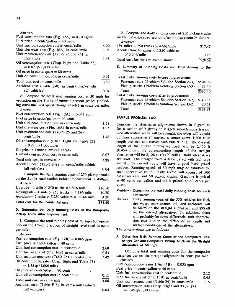
44

An wer: Fuel consumption rate (Fig. 12A) = 0.100 gpm Fuel price in cents! gallon = 40 cents Unit fuel consumption cost in cents/mile 4.00 Unit tire wear cost (Fig. 16A) in cents/mile 1.05 Unit maintenance cost (Tables 25 and 26) in


= 0.87 qt/ 1,000 miles Oil price in cents/quart = 80 cents Unit oil consumption cost in cents/mile 0.07 Total unit cost in cents/mile 6.60 Accident cost (Table F-8) in cents/ mile/ vehicle

(all vehicles) 0.04

Compute the total unit running cost at 30 mph for operation on the 1 mile of minus 4-percent grades (includ-ing curvature and speed change effects) in cents per mile:

Answer: Fuel consumption rate (Fig. 12A) = 0.042 gpm Fuel price in cents! gallon = 40 cents Unit fuel consumption cost in cents/mile 1.68 Unit tire wear cost (Fig. 16A) in cents/mile 1.05 Unit maintenance cost (Tables 25 and 26) in



(all vehicles) 0.04 Compute the daily running costs of 250 pickup trucks

on the 2-mile road section before improvement in dollars: Answer:

Upgrade-I mile X 250 trucks X6.60/mile $16.50 Downgrade-i mile X 250 trucks X 4.28/mile 10.70 Accidents-2 miles X 5,250 vehicles X 0.04! mile 4.20 Total cost for the 2-mile distance $31.40

D. Determine the Daily Running Costs of the Composite

Pickup Truck After Improvement:

1. Compute the total running cost at 50 mph for opera-tion on the 11/2 -mile section of straight level road in cents per mile:

Answer: Fuel consumption rate (Fig. 12B) = 0.065 gpm Fuel price in cents! gallon = 40 cents Unit fuel consumption cost in cents/mile 2.60 Unit tire wear cost (Fig. 16B) in cents/mile 0.53 Unit maintenance cost (Table 25) in cents/mile 1.42 Oil consumption rate (Chap. Eight and Table 27)


(all vehicles) 0.04

2. Compute the daily running costs of 250 pickup trucks on the 11/2 -mile road section after improvement in dollars:

Answer: 11/2 miles X 250 trucks X 4.66/mile $17.47 Accidents-11/2 miles >< 5,250 vehicles

X 0.04! mile 3.15 Total cost for the 11/2 -mile distance $20.62

E. Summary of Running Costs and Final Answer to the Problem:

Total daily running costs before improvement: Passenger cars (Problem Solution Section A-3) $504.00 Pickup trucks (Problem Solution Section C-3) 31.40 Total $535.40

Total daily running costs after improvement: Passenger cars (Problem Solution Section B-2) $343.35 Pickup trucks (Problem Solution Section D-2) 20.62 Total $363.97

SAMPLE PROBLEM TWO

Consider the alternative alignments shown in Figure 19 for a section of highway in rugged mountainous terrain. One alternative route will be straight; the other will consist of three successive 80 curves, a center curve 1,200 ft in length and two end curves each 600 ft long. The over-all length of the curved alternative route will be 2,400 ft (0.454 mile); the corresponding length of the straight alternative will be 2,126 ft (0.403 mile). Both alternatives are level. The straight route will be paved with high-type asphalt; the curved route will have a good hard gravel surface. Running speeds of 50 mph may be assumed for each alternative route. Daily traffic will consist of 500 passenger cars and 50 pickup trucks. Gasoline is priced at 40 cents per gallon and oil is priced at 80 cents per quart.

Problem: Determine the total daily running costs for each alternative.

Answer: Daily running costs of the 550 vehicles for fuel, tire wear, maintenance, oil, and accidents will be $8.95 on the straight alternative and $98.68 on the curved alternative. In addition, there will probably be some differential unit deprecia-tion cost due to the difference in length and surface conditions of the alternatives.

The computations are as follows:

A. Determine Unit Running Costs of the Composite PasS

senger Car and Composite Pickup Truck on the Straight Alternative at 50 mph:

1. Compute total unit running costs for the composite passenger car on the straight alignment in cents per mile:

Answer: Fuel consumption rates (Fig. 1 iB) = 0.053 gpm Fuel price in cents! gallon = 40 cents Unit fuel consumption cost in cents/mile 2.12 Unit tire wear cost (Fig. 15B) in cents/mile 0.45 Unit maintenance cost (Table 24) in cents/mile 1.15 Oil consumption rate (Chap. Eight and Table 27)

= 1.45 qt/ 1,000 miles

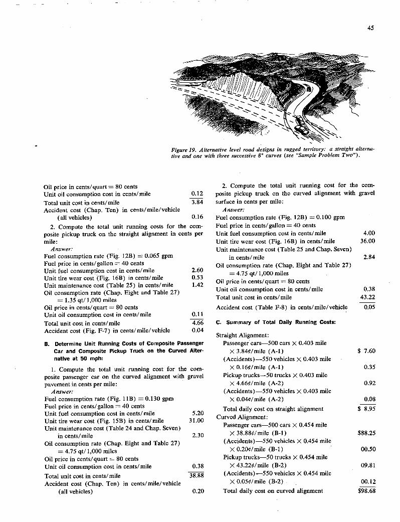
45

Figure 19. Alternative level road designs in rugged territory: a straight alterna-tive and one with three successive 8° curves (see "Sample Problem Two").

Oil price in cents! quart = 80 cents Unit oil consumption cost in cents/mile 0.12

Total unit cost in cents/mile 3.84 Accident cost (Chap. Ten) in cents!mile!vehicle

(all vehicles) 0.16

2. Compute the total unit running costs for the composite pickup truck on the straight alignment in cents per mile:

Answer: Fuel consumption rate (Fig. 1 2B) = 0.065 gpm Fuel price in cents! gallon = 40 cents Unit fuel consumption cost in cents/mile 2.60 Unit tire wear cost (Fig. 16B) in cents/mile 0.53 Unit maintenance cost (Table 25) in cents/mile 1.42 Oil consumption rate (Chap. Eight and Table 27)


Total unit cost in cents/mile 466 Accident cost (Fig. F-7) in cents/ mile/ vehicle 0.04

B. Determine Unit Running Costs of Composite Passenger Car and Composite Pickup Truck on the Curved Alter-

native at 50 mph:

1. Compute the total unit running cost for the composite passenger car on the curved alignment with gravel pavement in cents per mile:

Answer: Fuel consumption rate (Fig. 1 1B) = 0.130 gpm Fuel price in cents! gallon = 40 cents Unit fuel consumption cost in cents/mile 5.20 Unit tire wear cost (Fig. 15B) in cents/mile 31.00 Unit maintenance cost (Table 24 and Chap. Seven)

in cents/mile 2.30 Oil consumption rate (Chap. Eight and Table 27)



(all vehicles) 0.20

2. Compute the total unit running cost for the composite pickup truck on the curved alignment with gravel surface in cents per mile:

Answer:

Fuel consumption rate (Fig. 1 2B) = 0.100 gpm Fuel price in cents! gallon = 40 cents Unit fuel consumption cost in cents/mile 4.00 Unit tire wear cost (Fig. 16B) in cents/mile 36.00 Unit maintenance cost (Table 25 and Chap. Seven)

in cents! mile 2.84 Oil consumption rate (Chap. Eight and Table 27)

= 4.75 qt/ 1,000 miles Oil price in cents/quart = 80 cents Unit oil consumption cost in cents/mile 0.38 Total unit cost in cents! mile 43.22

Accident cost (Table F-8) in cents/ mile/ vehicle 0.05

C. Summary of Total Daily Running Costs:

Straight Alignment: Passenger cars-500 cars X 0.403 mile

X 3.84!mi1e (A-i) $ 7.60 (Accidents)-550 vehicles X 0.403 mile

X 0.16!miIe (A-i) 0.35 Pickup trucks-SO trucks X 0.403 mile

X 4.66!mile (A-2) 0.92 (Accidents)-550 vehicles X 0.403 mile

X 0.04!mi1e (A-2) 0.08

Total daily cost on straight alignment $ 8.95 Curved Alignment:

Passenger cars-500 cars X 0.454 mile X 38.88/mile (B-i) $88.25

(Accidents)-550 vehicles)< 0.454 mile X 0.20!mile (B-I) 00.50

Pickup trucks-SO trucks X 0.454 mile X 43.22/mile (B-2) 09.81

(Accidents) -550 vehicles X 0.454 mile X 0.05!mi1e (B-2) 00.12

Total daily cost on curved alignment $98.68

46

CHAPTER THIRTEEN

CONCLUSION

The findings presented in this report constitute a broad array of operating cost data relative to road design and traffic conditions for each of four composite vehicles rep-resenting (1) passenger cars, (2) pickup and panel trucks, (3) two-axle six-tire trucks, and (4) tractor semi-trailer truck combinations. Although they are incomplete for tire wear, maintenance, oil consumption, accidents and depre-ciation, the findings, nevertheless, provide a wealth of material needed to evaluate motor-vehicle running costs for the road and traffic conditions encountered on modern highways.

SUGGESTED FURTHER RESEARCH

Although the amount of operating cost data available for highway economy analyses is now substantial, further re-search of this subject is needed (1) to organize the existing data for computer application, including development of suitable computer programs, and (2) to extend study data to cover gaps in existing data. Specifically, further research into the subject of motor-vehicle operating costs is recom-mended as follows:

Organization of existing operating cost data for mechanical storage and ease of acquisition.

Development of computer programs for carrying out the calculations of road user costs for a variety of problem types.

Detailed evaluation of the effects that levels of traffic service have on motor-vehicle operating costs.

A review of the effects that motor-vehicle anti-air-pollution devices have on fuel consumption, especially while vehicles are stopped with the engine idling or while vehicles are running slowly in traffic.

An investigation into the rates of motor-vehicle in-volvement in accidents and the costs of such involvements by road design feature and by type of vehicle.

A clarification of certain aspects of motor-vehicle depreciation, especially those relative to the effect of road design, speed, speed changes, and annual vehicle mileage.

Detailed consideration of the effects of speed, grades, speed changes, and rough surface on truck maintenance costs.

A study of tire wear for pickup trucks and tractor semi-trailer truck combinations as tire wear is affected by road surface, curvature, and, if possible, by gradient.

Further inquiry into the effects of environment and altitude on motor-vehicle fuel consumption, especially en-vironmental conditions of snow and ice and altitude con-ditions encountered at more than 4,000 ft above sea level.

A study of passenger-car design and aerodynamic factors relative to tire wear at high speed.

Further fuel consumption research, especially for vehicles not adequately represented in this report: large diesel-operated as well as gasoline-operated tractor semi-trailer and full-trailer combinations, 3-axle single-unit trucks, small U.S. cars (Gremlin, for example), and recrea-tion vehicles (motor houses, pickup trucks with camper, and cars pulling travel trailers).

REFERENCES

WINFREY, R., Economic Analysis for Highways. International Textbook Co., Scranton, Pa. (1969) 923 pp. STEVENS, H., "Line-Haul Trucking Costs Upgraded, 1964." Hwy. Res. Record No. 127 (1966) pp. 1-21. "Highway Capacity Manual." HRB Spec. Rep. 87 (1965). CLAFFEY, P. J., "Running Cost of Motor Vehicles as Affected by Highway Design—Interim Report." NCHRP Report 13 (1965) 43 pp. "Line-Haul Vehicle Repair and Servicing Costs." Commercial Car J., Vol. 100, No. 4 (Dec. 1960).

DE WEILLE, J., Quantification of Road User Savings. International Bank for Reconstruction and Develop-ment (1966). SAWHILL, R. B., and FIREY, J. C., "Motor Transport Fuel Consumption Rates and Travel Time." HRB Bull. 276 (1960) pp. 35-91. MESSER, R. T., Chief, Current Planning Division, Bureau of Public Roads. Letter to P. J. Claffey, Potsdam, N.Y. (Oct. 29, 1969). "Supplementary Report of the Highway Cost Alloca-tion Study." House Document No. 124, 89th Cong., lstSess. (1965).

47

BONNEY, R. S. P., and STEVENS, N. F., "Vehicle Operating Costs on Bituminous, Gravel and Earth Roads in East and Central Africa." Road Research Laboratory Report 76 (1967). 1969 Automobile Facts and Figures. Automobile Manufacturers Assn., Detroit (1969).

DE VINNEY, W. E., "Factors Affecting Tire Trac-tion." SAE Trans., Vol. 76, Sec. 3 (1967). "The Guide for Forecasting Traffic on the Interstate System-1970." Highway Planning Program Manual, Vol. 4, Chap. VII, App. A, Bureau of Public Roads (Jan. 1969).

APPENDIX A

GRAPHICAL PRESENTATION OF THE FUEL (GASOLINE) CONSUMPTION RATES OF EACH TEST VEHICLE FOR UNIFORM INCREMENTS OF ROAD AND TRAFFIC FACTORS

Fuel consumption rates in gallons per mile, as determined for each of the test vehicles used in the study, are shown in Figures A-i through A-54. Fuel consumption informa-tion is shown in Figures A-i through A-24 for passenger cars, in Figures A-25 through A-37 for pickup trucks, in Figures A-38 through A-45 for two-axle six-tire trucks, in Figures A-46 through A-48 for the transit bus, and in Figures A-49 through A-54 for tractor semi-trailer truck combinations. Each figure shows fuel consumption rates relative to a particular road design or traffic condition for one test vehicle. All test operations were conducted under calm wind conditions with air temperatures between 800 and 90° F.

EFFECT OF GRADE

The effect of gradient on passenger-car fuel consumption is shown in Figures A-i through A-9 for operation in high gear and in Figure A-10 for operation in low gear. The effect of gradient on the fuel consumption of pickup trucks is shown in Figures A-25 through A-27 for operation in high gear and in Figures A-28 through A-30 for operation in low gear. The effects of gradient on the fuel consump-tion of two-axle six-tire trucks, transit buses, and tractor semi-trailer truck combinations are shown in Figures A-38 and A-39, Figure A-46, and Figures A-49 and A-50, respectively. In each of these figures, values for operation at various uniform speeds on plus grades are shown in the upper section of the figure; those for operation on minus grades are shown in the lower section. The floating speed for each test vehicle on each minus grade is the speed corresponding to the low point of the appropriate minus grade curve.

EFFECT OF CURVATURE

Fuel consumption on curves is shown in Figures A-il and A-12 for passenger cars, in Figures A-31 through A-33 for pickup trucks, in Figure A-40 for the two-axle six-tire truck,

and in Figure A-5 1 for the tractor semi-trailer truck com-binations. In each of these figures data on the fuel con-sumed while operating at uniform speed on curves of different degrees of curvature are given in the upper part of the figure. The corresponding front-wheel slip angles are shown in the lower part, except for two-axle six-tire trucks (Fig. A-40) and tractor semi-trailer combinations (Fig. A-51).

EFFECT OF SURFACE

Fuel consumption rates for operation on gravel roads, badly patched asphalt surfaces, and loose sand (as well as on good paved road surfaces) are shown in Figure A-1 3 for passenger cars, in Figure A-34 for pickup trucks, and in Figure A-41 for both two-axle six-tire trucks and tractor semi-trailer truck combinations.

EFFECT OF SPEED CHANGE

The effects of speed changes on the fuel consumption of passenger cars are shown in Figures A-14 through A-21. Similarly, the fuel consumption rates of trucks as affected by speed changes are shown in Figures A-35 through A-37 for pickup trucks, in Figure A-42 for the two-axle six-tire truck, and in Figure A-52 for tractor semi-trailer truck combinations. The fuel consumption curves in each of these figures show the fuel consumed per mile for each of several speed change situations: (1) no speed change, (2) one stop cycle per mile, (3) one 10-mph slowdown cycle per mile, (4) one 20-mph slowdown cycle per mile, and (5) one 30-mph slowdown cycle per mile. The excess fuel consumption for a particular speed change cycle can be found by subtracting the fuel consumption per mile for no speed change from the corresponding fuel consumption per mile for the speed change cycle.

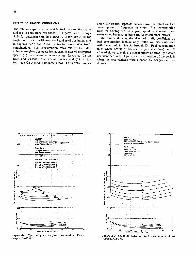
48

EFFECT OF TRAFFIC CONDITIONS and CBD streets, separate curves show the effect on fuel consumption of frequency of stops Fuel cnnsiimption

The relationships between vehicle fuel consumption rates rates for no-stop runs at a given speed vary among these and traffic conditions are shown in Figures A-22 through street types because of basic traffic interference effects. A-24 for passenger cars, in Figures A-43 through A-45 for The curves showing the effect of traffic conditions on

single-unit trucks, in Figures A-47 and A-48 for buses, and fuel consumption include only traffic volumes associated in Figures A-53 and A-54 for tractor semi-trailer truck with Levels of Service A through D. Fuel consumption combinations. Fuel consumption rates relative to traffic rates when Levels of Service E (unstable flow) and F volume are given for operation at each of several attempted (forced flow) prevail are substantially affected by factors speeds (1) on six-lane expressways and freeways, (2) on not identified in the figures, such as duration of the periods four- and six-lane urban arterial routes, and (3) on the when the test vehicles were stopped by congestion con- four-lane CBD streets of large cities. For arterial routes ditions.

_.__..._:H.......... v.hisl -- l96GVdlko.g.n (t.o door) Four cOliodoro72 cu. in. dispilc000nt

.3 nTran.missioñ -.

.Conditgnn.. ---•- etgflt-roat------...........

Good icn.d ourf ate •. .2 ----•--------- _._._.._______•__.__._•._ ....

80° -gO° F.

dient vs. C.ó Fsition

- 4 Lee ijeod 3.sr 3 .2 ----------- -

-1 All sp..ds t.sr 2

0 10 :0 50 60 70

Figure A-i. Effect of grade on fuel consumption—Volks-wagen, 2,100 lb.

Yahici., Falcon

Sin cylt,ei, 200 en. in. disploc.atnt Auton,atic tflnomlosion

Cooditiva, Straight road Good pseed surface Cal,, clod eo°gg-p........

.015

-r-- -

0.1 - -. - • -------- --

Sps.d In iHiss P.r Hour

Figure A-2. Effect of grade on fuel consumption—Ford Falcon, 3,000 lb.

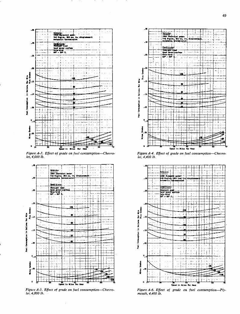
..•.•-••. I -••--i............ i hick. - . ............. ••.• I ......- d•n............

4 CU. IN 411p1sCaI.t

.... . .; . ......

+ -

.

L

..

o t ---

-I.. -4--- -- ;.Hi_

ff'± FItjTh 9 U,hnl- -I--I-- .3)

ition, . WIhd . Ce -

20

-.-- •

.3

.2

.1 .1

.1

S

I

S

49

4 1n., U3 C*M tn..dkMwn AiitiI.iC tC..lsHiun

OCod 0$vsd iufas

- .. .. -I.

q1'

- _

EH-- . ...

Figure A-3. Effect of grade on fuel consumption—Chevro-let, 4,000 lb.

Ll - ....•- --.!!L.j -i-:.... _LJ._ _j-_.._-.

I Qis4r43.t .. V.4.E,1to - 3!cu n4.dI1U4U.

- .... I

.L.

- t-1--------• - -..

----------- ftCU -- - 80-901 . - -----. Al . '.-4-----4— - .............. - .-..-+-+ :- -------------- --

4 t1 j_

S,.d in *1.o Pip H

Figure A-4. Effect of grade on fuel consumption—Chevro-let, 4,400 lb.

.3

.3

.2

Spied in Igloo per How

Figure A-5. Effect of grade on fuel consumption—Chevro- Figure A-6. Effect of grade on fuel consumption—Ply- let, 4,800 lb. mouth, 4,400 lb.

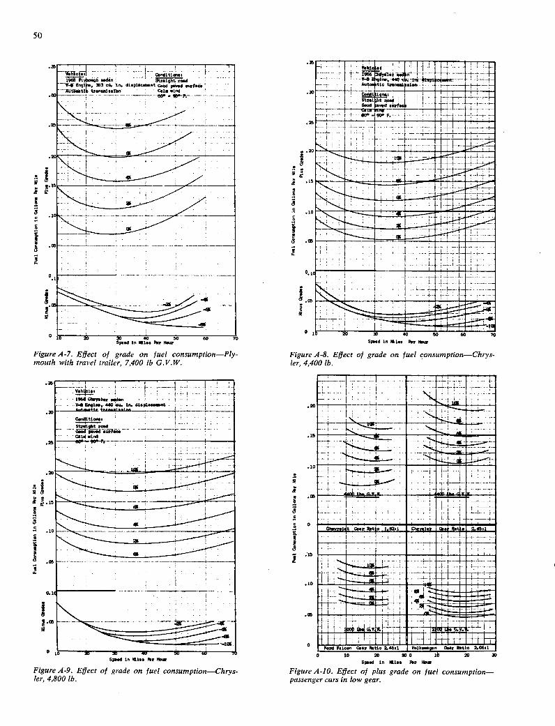
.20

.10

.10

.1!! - OREM=—

rBtwLa

I1UUNIEI MR 7"

IIIIflhIUIIifliflL.11 r-

1 -,

50

tj

1968 1$no,9h sodln Stx.ight fled - - - V4 Ençi., 20 ed ..

3. n. dtsp1cnt ooni pm.d .u1ai. 86tt1b transMi*sft,n . Cei. wird so-

.25

.10

° IJ S.d in 81.. Pr

Figure A-7. Effect of grade on fuel consumption—Ply-mouth with travel trailer, 7,400 lb G.V.W.

-.-.- -8 ,. •1, tt

3'

25

20

is

10

05

. . .

S.d in WIss Per Hm

Figure A-S. Effect of grade on fuel consumption—Chrys-ler, 4,400 lb.

Se.d in 1.s P.r i

Figure A-9. Effect of grade on fuel consumption—Chrys-ler, 4,800 lb.

Figure A-JO. Effect of plus grade on fuel consumption—passenger cars in low gear.

010 20 20 40 50 - dO 70 Speed in 181.e P.c

Figure A-12. Effect of curvature on fuel consumption—Plymouth, 4,400 lb G.V.W.

.30

.21

.21

.0

II

.01

0

HOMES

W-om miuu•uuia..m

Oi!EII!I! ..........

mom Now-iiiII ........... ••uuuu•uu iuui•i•iii ..........

UIIIIIIIIiH!! !! . .m....0 ......... MMEMOSM

ii11!!1iu.,i.i.u,.....i.......ui on ME ..1...

23MEMEEMMEMEMEMEMS

own N~ ,momiIIEE...MEMEMOMM ...WRIMEMERHEME .....1.1.MEMENS..... on

a

.31

. 05

Speed in Miles P.c HDW

Figure A-Il. Effect of curvature on fuel consumption—Chevrolet, 4,400 lb G.V.W.

51

h1 lei

164 %18

loden L lnLr 3 .u.-4os-IepisssN-it

I

. Mtl•itiC *,ssisa, . - .

---.----

- ---

- _

---'-

i8i8h_jy--Ly - - ------- -

-

1.ujnd T -H------ .............

---+-

—, ts ar .. . .

.

kd 1y bcon ild .pet 0avel With 1f1 osto LJ/4

4 ary iooee eetd ieyclr, ots t4 4i .

.iH--------

-

_-..................

1906 Vo1ksapen (Goe d,)

20 -

Gonditior,. -

St.iit i.n.1 cold — - -

- Good pored sofas. 800 - 900 F.

Si..d Change Cycles. -. ..

1, . 10 WH eilon pernu.

15 2.01W2 F pe .-

ii.,

0

Speed in Idles P.c los. Speed in 1111ae For Hiner

Figure A-13. Effect of surface on fuel consumption— Figure A-14. Effect of speed change on fuel consumption— Chevrolet, 4,400 lb G.V.W. Volkswagen, 2,100 lb G.V.W.

0 10 20 20 - 40 50 6u 70 Spied in i146 Its linux

Figure A-16. Effect of speed change on fuel consumption—Chevrolet, 4,000 lb G.V.W.

.21

TT TT L!

Qmvnolpt sedan TA Engine1 cii. in. 4UCiIi1I

ip1n..nt . I - - I-

____ h .

nd

L.. .....

-ï ---- -•4•t--- -F---F--H•

: 4 L Wr.iou..n

0i1fl$r21ita 4r !.I too LI -

4_ .L.f

----i --t--- - : '-- -- --

..

± i fii 4 i

-H-]— 4

. --t'•-±--

f

-i---f-•t-1 ---

....

LIT

T 1

T

' —

T--

+HT - 4 T__j_ 1 1 1 1 1 1 1 1 1 1

2.0., I0 MR1010dS. pu*uils - L F t 320 sen

.r prio .i—j r

4. 40 di iiTp —

V j IT

-. .1

F_ ... t 1 L4_1_ —4----- __________________ 0 20 a, mu 50-

20

.05

0

52

-- _— uu•u --

_______________

•• _i u•u••m

Iuui--_-9=I mine — Hsi

0-1 PIN

u---rnam......—..

Spud in MiI.0 . Hmar

Figure A-15. Effect of speed change on fuel consumption—Ford Falcon, 3,000 lb G.V.W.

Spuid in MU•s P.r H.ur Spied in mi.. P.r Ilnec

Figure A-17. Effect of speed change on fuel consumption— Figure A-18. Effect of speed change on fuel consumption— Chevrolet, 4,400 lb G.V.W. Chevrolet, 4,800 lb G.V.W.

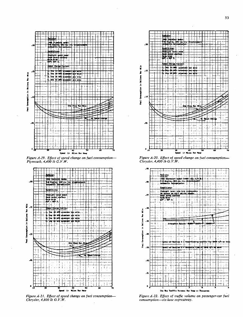
00 1 2 .3 4 5 6 s IIIy TnsHic Vel,s Ip Hm in 15,uuundn

Figure A-22. Effect of traffic volume on passenger-car fuel consumption—six-lane expressway.

010 20 30 40 50 60 70 Scud in Idles

Figure A-20. Effect of speed change on fuel consumption—Chrysler, 4,400 lb G.V.W.

.09

.09

I! .0:

.20

09

.01

09

01

...,,w...s...uasuu..ai•ia••u • • U •• •••• •••• U as. u U5iiuUM•iMUs.UUU•5iUs.0

s.•MulSUMUUUs.U••s.U5s.0 .astimiusa...••u....0

ai UUUUR

poll IN

...u.uas.ua•.•.as..••asus.as 5idN•aibUi•uRs.•

UIiiIUII:B1II:IHII

immmaiilmm=mom

mmmmmmiimm

UU1lIIL.. #____

Ii:!IIIIr!!! OIIIE!iI! .I!hIIIhhhIII!IIIIIU

zj.H I' + --.

St.sØs440 IG.L -$ F. 4.; . tic,tr4nn. -L1 1

91ti.fls* 4_4__ $1.t.Isvi1.s$.i.u41 09uc.Is Or• t

*a. .. .iy .

............... _______ _______

Cffir-IM 0 V7117~1I

TfE th± ±L 1L j - -! -I

-I--i--

1 1 -

._ - - -1- - -•-----

4

H- H-H- =

.30

.15

.05

0

0 t0 2o 30 40 50 60 70 S..d in idles Fier Now

Figure A-19. Effect of speed change on fuel consumption—Plymouth, 4,400 lb G.V.W.

.0

1

11 _____ u..u•i.u.u.0

ElmEmmoommoommmm IN milmmmmmmmmmommom ••auuu•u•uu

am RjAr

mmmmmmmommmo !UUIU••UU uuuuuu•u•u

OhlUIllI ...............

lli uuu•uu••u•u• MMMOMMMME

............... ..............,

Mk AM

Mm~mmmmmmmEm6=mm

mmmmmmmmommm

u••••u•uu•uau smimmmmmmmo

lllinommmonommmommmm u..............

..riumuuu•u

..u...auuiuuuu.0

uua uu•uuama as.. .as_._..s._...s.as.

Iown L.,: i.

9 WAR .18~0-;Rp-.POWN OR

RM

-Ihu- I-- .d in idles Per 09n

Figure A-21. Effect of speed change on fuel consumption—Chrysler, 4,800 lb G.V.W.

53

54

i•VSi fr(*21t1 * I . 1. ........ fiosInr5.j

sit.......... - -F. - I •---r- 10 SIP.D.1hr In to

Sto ; To all 4H<J-4- 44à.!s [' f! .. .eT: •-1 . is . 14

H

TT--± _ ,

.... _.

I O4 '4-i' hI C aboUt i0 vrIiis *b0' ajfjj.bbt4OO4 ion,.

J 1 I44: . ............

H.08

' .07

1

.obH —

. -:4AP 1j44 Palo JiR---P---'. _!I' R - --

tiLl- ITT. V483.jn.j nDiK - . Attic tre flion j.-. ._. .. ..--. -r .qpt1wI

s4nskgit'i.n. S&n-i• n ara .. I

—* -f - Tntraffic s*g*1sp --t rfring -i--'-i--- - .. God PAIMS - ---- -f--H- 'H c41n4nd

01

at re E uI1is fle, a

1fH

r I;

One y lost? IC V.i,. PIr New in ThoosaMs

Figure A-23. Effect of traffic volume on passenger-car fuel consumption—six-lane urban arterial.

196 3/4.too isIorsi.t toack .. Sin y*I,iósos0 0 .1lsa!sflt Fasa.sps.d s1 tosnsai$.

'l'°°'............... S*nsght ooad

—T-_hOodt —_0*T -- -.-.--•- .- ...2

...... -°-l- °• I -

2 - -' 1-_

.15

. .4 . ............ ....... .

SØsd In flOss Per Hoo

Figure A-25. Effect of grade on fuel consumption—pickup truck at 4,800 lb G.V.W. in high gear.

UM ooy Trait IC VOi(• PIn Hinm in Iirsds

Figure A-24. Effect of traffic volume on passenger-car fuel consumvtion—lour-lane CRD Streets.

_L!I!...... f: HTTi+iLIiiiLiLTr _9tJW4 thnQo4.tp4. 1%41k .

Cy1iM. 0 cm in. dIsi.,t . 70o&, iisidmiai tisr.aisUioj, .30 ---T-1----- co,it1QM. - I

41

.05

- .. —... -•-----.-------

:j 20 ; k Figure A-26. Effect of grade on fuel consumption—pickup truck at 7,200 lb G.V.W. in high gear.

15

.10

.30 I

0

-I

I I 8

I

.30

10 T 4-4-

1 L :.; TI 10

1i4

1j

H - 0 1

': , Sps.d in 301.. P.r P..0

Figure A-27. Effect of grade on fuel consumption—pickup truck at 8,000 lb G.V.W. in high gear.

55

.30

.30

.20

H' i -jiiii

iITii - -

JL1E :1 ---1 - - --

r- iiiI. G.ar 3 Gar R.tio 1.72,1 Ci30 2 Gssr R.tio 3.58.1

10 20 20 400 10 20 30 Sp..d in 161.; P.r H.ur

Figure A-28. Effect of grade on fuel consumption—pickup truck at 4,800 lb G.V.W. in low gear.

.30

.30

S0..d 'in Who P.x How - - - Sp..d in 161•s For H.ur

Figure A-29. Effect of grade on fuel consumption—pickup Figure A-30. Effect of grade on fuel consumption—pickup truck at 7,200 lb G.V.W. in low gear. truck at 8,000 lb G.V.W. in low gear.

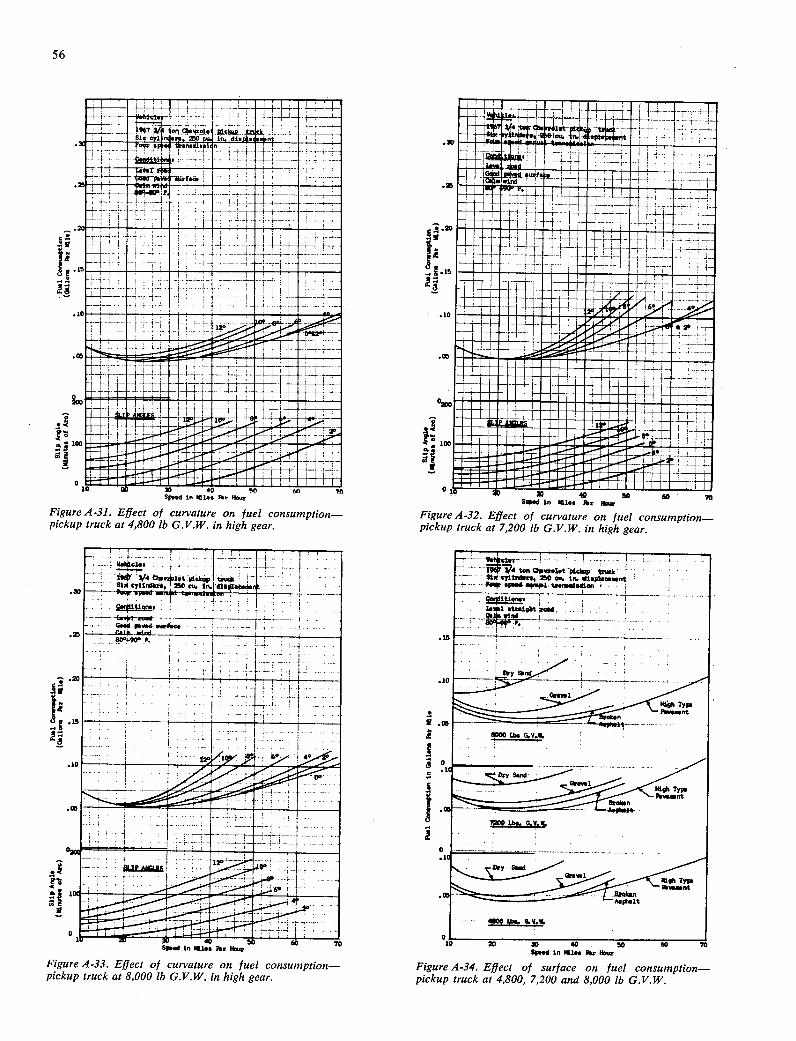
10

AaP*lt

56

MEMNON m

------

Ij ! 1jjj --I- I'm M-- Im m -iiil

• I iuI M:m OWN

I.m..w..!LddSIM w OPINION

,. .ii., •S

Figure A-31. Effect of curvature on fuel consumption—pickup truck at 4,800 lb G.V.W. in high gear.

IOC -

In

S..d In MIl..

Figure A-33. Effect of curvature on fuel consumption—pickup truck at 8,000 lb G.V.W. in high gear.

U..

1 .MEN

U •• .y. p_

11 NMI m .m.

L - U.U•U

- uuu:mU..u. .

S.d in MIll. lr I Figure A-32. Effect of curvature on fuel consumption—pickup truck at 7,200 lb G.V.W. in high gear.

Sp..d in *1.. ftr I Figure A-34. Effect of surface on fuel consumption—pickup truck at 4,800, 7,200 and 8,000 lb G.V.W.

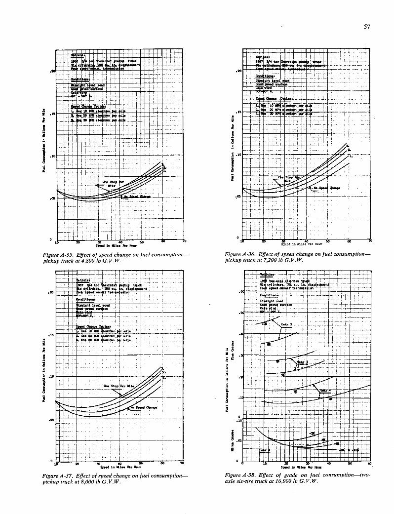
. 21

0

.20

.10

.05

0

sn. in. Us ..•I_ . ..j...! .

.44

7

. 1

.0

:1i

- 57

2

i.. ti

++ FJ .

r±..t.i +Ji

ttri HJIt.:

±1i L** j'1I .J_

15

1 oadden is

L. H-'- 3P

tJiT.

t

-1-1-1-- - —r----1•- i I _______

10

j

ti ....

:P1r

—

I II —1 40 30

Sps.d in False P.c P.

Figure A-35. Effect of speed change on fuel consumption—pickup truck at 4,800 lb G.V.W.

EL!

1eif. __ GsSd we .

I+1i1c ±io-rs TLiLi1;Lp ......

.: . L1

L.. I .

. ___ 2. .

ON

iI! II

i. - ..

.n. Spned in Miles Pe HO,r

Figure A -36. Effect of speed change on fuel consumption—pickup truck at 7,200 lb G.V.W.

S.d in miles For HOSU Spsd in Idles P.r Mona

Figure A-37. Effect of speed change on fuel consumption— Figure A-38. Effect of grade on fuel consumption—two- pickup truck at 8,000 lb G.V.W. axle six-tire truck at 16,000 lb G.V.W.

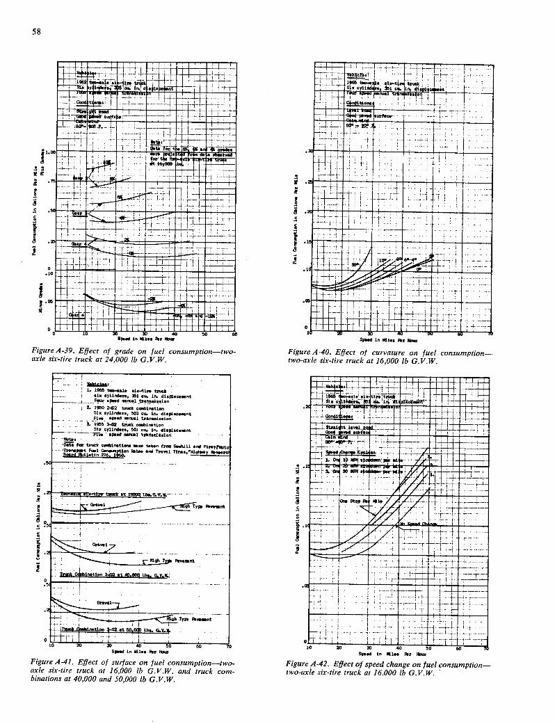
58

ItT • -VtMc . 1-- J-;- - -

c4 ic !f

- :-- -.

- iIIItI - -

'-- .-

--L- -;___________________________

- -

-

.25

-I - -r

.2 - -.

HE

n.

• __ UP!iJ!Ilui—__i:II

ihIu_ Speed in Miss Par linux

Figure A-39. Effect of grade on fuel consumption—two-axle six-tire truck at 24,000 lb G.V.W.

Sp..d in 561.s For linux

Figure A-40. Effect of curvature on fuel consumption—two-axle six-tire truck at 16,000 lb G.V.W.

L 1966 si.in. truck - .. ... sin cyii.ru, 301 cu, in. displacement

-Four P!l !!!'° 10 2-62 truck cin.ti,n

S CYLI ndfre, 503 cx. in. dlspl.c.nunt Flu, •jxd menual trsn,nl,,jon 1665 34 truck cinmtion Six GYiindSrs, 501 cx, in. dispisossint

Wv. SF566 665055 t5t$n168160

for truck cothtn,tjsn, nunm, tnb.n from, Sinful and Fiu,y F1 Cenmpt1os Sit.. und Ineusi Tin..,"Higt..y P..ums .S66rd 96ilitin 216. 1960.

...................

at St00QtGZ -................. .

tens'

RI gh nsns t

muck Cnthinatipn 2.= at io.00q Lb.. 0.v.li.

l i

'- ji'ns SIns.nt Txp ( Inutfcn.at 20,tX2 Lbs. G.V.. .

10 20 - 30 40 50 60 70

Figure A 41. Effect of surface on fuel consumption—two-axle six-tire truck at 16,000 lb G.V.W. and truck com-binations at 40,000 and 50,000 lb G.V.W.

i:t, Li - ±— -:ii::t

'-4

- i—+-I I

102031D i -rt

Figure A-42. Effect of speed change on fuel consumption—two-axle six-tire truck at 16.000 lb G.V.W.

3

o

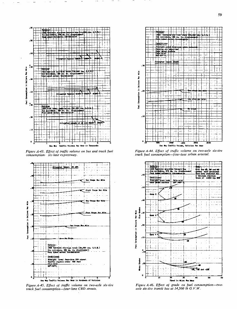
.30

.3C

ctl

L .. Lin mCi

U..

H ................... __

.3D 1I1 :

CO

C_

0 0 In RI RI 40 '10

One y Tr.tf IC Vo1ss For Hour in Thnn..flds

Figure A-43. Effect of traffic volume on bus and truck fuel consumption—sir-lane expressway.

59

MOMOM uuuuuu .Mr MMIHIM I...

U.-.

L its U. U

iioui•iu— MM

IUhIEbiN' UiiIII!IIINIIIIt- 10500 i0005( 20 00

One Way Traffic Vol, V.hlnln. Per Hnnr

Figure A-44. Effect of traffic volume on two-axle six-tire truck fuel consumption—f our-lane urban arterial.

One 1by TrsIf IC Vn1. For Hour in *.nnd$ of Vehick.. Sp,.d in Pales In ftm

Figure A-45. Effect of traffic volume on two-axle six-tire Figure A-46. Effect of grade on fuel consumption—two-

truck fuel consumption—four-lane CBD streets. axle six-tire transit bus at 14,500 lb G.V.W.

ii!HIHIE!i!!II!N!EIO! .00

0 5CC 1000 1500 2000 00 . Soy Trsfftc - V.Mcl.. Soi How

Figure A-47. Effect of traffic volume on transit bus fuel consumption—four-lane urban arterial.

Fl

••.•.iiãi..uiuu••• .....I

IlU.Ur..NEENSOMMENluR.murnua :I!iiii!!IIiIi ir'u

no

Iu•UF'r

MEMO iU•••iI

001111111111110

MOM I.....MEN1 uuI

MUMMEN MEN

mom 1010PE MEMINEINIM-=0 e.•.uuiaau :son::u:IlIIIIIIIIINhi1iI

u MINIMUM OMEN MEN

WMM

w ri EEfl1E1E

P.IIIiiiiPii!i IMMUNE

0 0

Mom 1 2 3 4 5 6

One Soy Traffic Vo1-ltrndrad. of V.hici.s P.r It.0

Figure A-48. Effect of traffic volume on transit bus fuel consumption—four-lane CBD streets.

60

.41

.81

.15

10

00

1.5

--:- ............. r six cy1nd cu .rs, 003. Tn. dii1Sv.o.flt

-1--- 1_: I Q6i*1toflu ...............

1•

...........-.-

7-1

.... t4t.n h It,ii- . Fi_ *.o2. .... - ....... Soi_ Ti.. I$isny SoIsrci !oSx

1.0 .. ..: So1i.tIn 270.isoo.! data f$x 113, gxsd.s

oj.et.d fr data f. d.1od f 0960 2•S2 i_ti_ Soighin

I -I

.20

............ 'H0

-----

- so

-r -?jI 3.00i

-I-

1p1496it .

4 1 ____ I f V.d lq 2.90.1 -r

I T1

4.111 *n 0 4oat6t4j

1y 4 Sot.1 fan

In.t

H and b.ve

Co

:-j

.VTTT

f!

Silud in Adles FOr Sow 8p,.d in *1.. Per It.

Figure A-49. Effect of grade on fuel consumptjon-242 Figure A-50. Effect of grade on fuel consumption-342 truck combination at 40,000 lb G.V.W. tractor semi-trailer truck combination at 50,000 lb G.V.W.

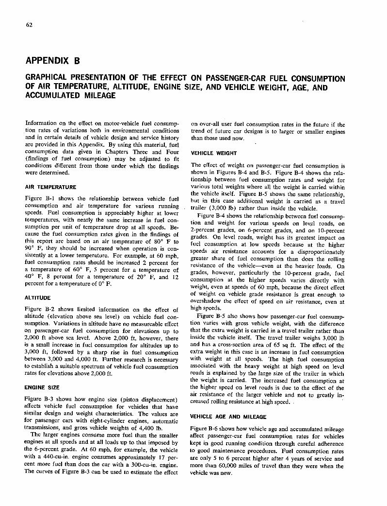
62

APPENDIX B

GRAPHICAL PRESENTATION OF THE EFFECT ON PASSENGER-CAR FUEL CONSUMPTION OF AIR TEMPERATURE, ALTITUDE, ENGINE SIZE, AND VEHICLE WEIGHT, AGE, AND ACCUMULATED MILEAGE

Information on the effect on motor-vehicle fuel consump-tion rates of variations both in environmental conditions and in certain details of vehicle design and service history are provided in this Appendix. By using this material, fuel consumption data given in Chapters Three and Four (findings of fuel consumption) may be adjusted to fit conditions different from those under which the findings were determined.

AIR TEMPERATURE

Figure B-i shows the relationship between vehicle fuel consumption and air temperature for various running speeds. Fuel consumption is appreciably higher at lower temperatures, with nearly the same increase in fuel con-sumption per unit of temperature drop at all speeds. Be-cause the fuel consumption rates given in the findings of this report are based on an air temperature of 800 F to 900 F, they should be increased when operation is con-sistently at a lower temperature. For example, at 60 mph, fuel consumption rates should be increased 2 percent for a temperature of 60° F, 5 percent for a temperature of 400 F, 8 percent for a temperature of 20° F, and 12 percent for a temperature of 0° F.

ALTITUDE

Figure B-2 shows limited information on the effect of altitude (elevation above sea level) on vehicle fuel con-sumption. Variations in altitude have no measureable effect on passenger-car fuel consumption for elevations up to 2,000 ft above sea level. Above 2,000 ft, however, there is a small increase in fuel consumption for altitudes up to 3,000 ft, followed by a sharp rise in fuel consumption between 3,000 and 4,000 ft. Further research is necessary to establish a suitable spectrum of vehicle fuel consumption rates for elevations above 2,000 ft.

ENGINE SIZE

Figure B-3 shows how engine size (piston displacement) affects vehicle fuel consumption for vehicles that have similar design and weight characteristics. The values are for passenger cars with eight-cylinder engines, automatic transmissions, and gross vehicle weights of 4,400 lb.

The larger engines consume more fuel than the smaller engines at all speeds and at all loads up to that imposed by the 6-percent grade. At 60 mph, for example, the vehicle with a 440-cu-in, engine consumes approximately 17 per-cent more fuel than does the car with a 300-cu-in, engine. The curves of Figure B-3 can be used to estimate the effect

on over-all user fuel consumption rates in the future if the trend of future car designs is to larger or smaller engines than those used now.

VEHICLE WEIGHT

The effect of weight on passenger-car fuel consumption is shown in Figures B-4 and B-S. Figure B-4 shows the rela-tionship between fuel consumption rates and weight for various total weights where all the weight is carried within the vehicle itself. Figure B-S shows the same relationship, but in this case additional weight is carried as a travel trailer (3,000 lb) rather than inside the vehicle.

Figure B-4 shows the relationship between fuel consump-tion and weight for various speeds on level roads, on 2-percent grades, on 6-percent grades, and on 10-percent grades. On level roads, weight has its greatest impact on fuel consumption at low speeds because at the higher speeds air resistance accounts for a disproportionately greater share of fuel consumption than does the rolling resistance of the vehicle—even at the heavier loads. On grades, however, particularly the 10-percent grade, fuel consumption at the higher speeds varies directly with weight, even at speeds of 60 mph, because the direct effect of weight on vehicle grade resistance is great enough to overshadow the effect of speed on air resistance, even at high speeds.

Figure B-S also shows how passenger-car fuel consump-tion varies with gross vehicle weight, with the difference that the extra weight is carried in a travel trailer rather than inside the vehicle itself. The travel trailer weighs 3,000 lb and has a cross-section area of 65 sq ft. The effect of the extra weight in this case is an increase in fuel consumption with weight at all speeds. The high fuel consumption associated with the heavy weight at high speed on level roads is explained by the large size of the trailer in which the weight is carried. The increased fuel consumption at the higher speed on level roads is due to the effect of the air resistance of the larger vehicle and not to greatly in-creased rolling resistance at high speed.

VEHICLE AGE AND MILEAGE

Figure B-6 shows how vehicle age and accumulated mileage affect passenger-car fuel consumption rates for vehicles kept in good running condition through careful adherence to good maintenance procedures. Fuel consumption rates are only S to 6 percent higher after 4 years of service and more than 60,000 miles of travel than they were when the vehicle was new.

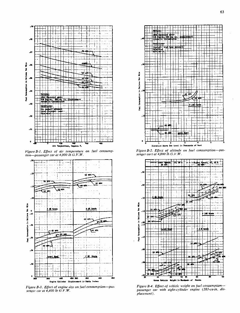
0 0 I 440 +60 490

Air T..09rst., 0.gr..s F.

Figure B-i. Effect of air temperature on fuel consump-tion—vassen2er car at 4.000 lb G.V.W.

.02

.01

.09

.07

09 uuu•a•u •

MOORE !I!II!IiIIiIiIIlII _U

SOME

1

i 0 W

sawn

riNiIiP"__

PERM

Il..UMENEM

.UU•MEN

II..U..l..U.i::iNaII___. U•

I......••.......MEMENEEEMEEEEEmmm

....'....

IUUIUUUIflI.lUUU..U.Um...

63

0

Engine Cylind.r Dtepiic.,ant In Cubic Inch,.

Figure B-3. Effect of engine size on fuel consumption—pas-senger car at 4,400 lb G.V.W.

riiiiiiiiiiiiii.............. .••MUU••U••UUUUUl•UU••l•UUU • • • I U uiPUui•U•.•UUUU.UUUIUUIU _____

....U...U.U..U.U.URU•UUUU••a IU•UUUR•UU••••••U•SUUUU .....u....u.uumu.mU.UUlIR

.....uuuuu...uu.Iu...I.uuuuR .u...•..u.I.u.a..I..u.Ua ..•.iu.uuu...u.iu...uua .u...i.u....u.uu..u..._____ .....•UUUU•.N.UU••••UU U....UUU.UUUU.UUU••UUUU .......U...U.UUW•U•UlUUU ..au.a.a...uuII.IUUUUU

.u.u..m..U...UUWJIRU•• .ua.uiauuuuN•UtT!UUUUU u...u•.U..krd4U...0 Is

uERu...iI: Ia.HIMEMO

MONSOON

i iIOIO i••.uU•à.aN

lilml

E1.nction Aboni Sri L.ncl in Thncsand. of Fist

Figure B-2. Effect of altitude on fuel consumption—pas-senger cars at 4,000 lb G.V.W.

uINOhIIllh!jIa!L- • •

UPOPE ' EUi1iiiNMI

911111111

MEN No mmimmmmmmmiiim=mi

••U••i••••••l•U . d u••uu•••Uuu•iNU••dUUU ..•••u•u•.. uuuuua•••

••••• ' U U U • •••••••••

MEMPER ••. U••

MOOSE

••.••Ill,..R•..

U. .dUl•UU iTU &T!i••UU

u•UUUU•UUUUUI ME •

t1 IlILLU UUUUUUSUUUUU

boss Vshicl. Walght in rhamined. of 1bws

Figure B-4. Effect of vehicle weight on fuel consumption—passenger car with eight-cylinder engine (283-cu-in. dis-placement).

H

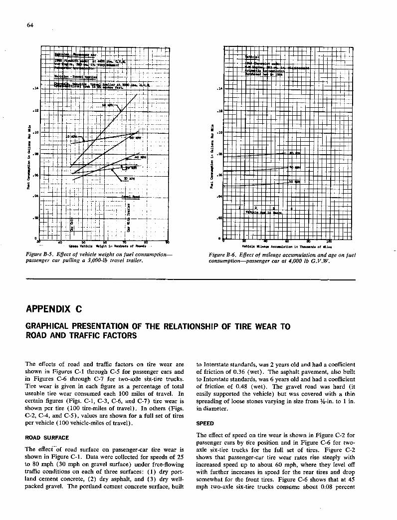
64

ti4lT.,ji1 14 '!1:

H - .12

_

.10 '

.00

.06 Th -i

Itr.--

-H-

fJ1iL: o ,

OS$ Y.hiol. Idat,t in Iozsdo of Fbwndo

Figure B-5. Effect of vehicle weight on fuel consumption—passenger car pulling a 3,000-lb travel trailer.

14

9 V.140i. 1411oage Accdation in Tho,.u,s of mi.s

Figure B-6. Effect of mileage accumulation and age on fuel consumption—passenger car at 4,000 lb G.V.W.

APPENDIX C

GRAPHICAL PRESENTATION OF THE RELATIONSHIP OF TIRE WEAR TO ROAD AND TRAFFIC FACTORS

The effects of road and traffic factors on tire wear are shown in Figures C-i through C-5 for passenger cars and in Figures C-6 through C-7 for two-axle six-tire trucks. Tire wear is given in each figure as a percentage of total useable tire wear consumed each 100 miles of travel. In certain figures (Figs. C-i, C-3, C-6, and C-i) tire wear is shown per tire (100 tire-miles of travel). In others (Figs. C-2, C-4, and C-5), values are shown for a full set of tires per vehicle (100 vehicle-miles of travel).

ROAD SURFACE

The effect of road surface on passenger-car tire wear is shown in Figure C-i. Data were collected for speeds of 25 to 80 mph (30 mph on gravel surface) under free-flowing traflic conditions on each of three surfaces: (1) dry port-land cement concrete, (2) dry asphalt, and (3) dry well-packed gravel. The portland cement concrete surface, built

to Interstate standards, was 2 years old and had a coefficient of friction of 0.36 (wet). The asphalt pavement, also built to Interstate standards, was 6 years old and had a coefficient of friction of 0.48 (wet). The gravel road was hard (it easily supported the vehicle) but was covered with a thin spreading of loose stones varying in size from 1/4-in. to 1 in. in diameter.

The effect of speed on tire wear is shown in Figure C-2 for passenger cars by tire position and in Figure C-6 for two-axle six-tire trucks for the full set of tires. Figure C-2 shows that passenger-car tire wear rates rise steeply with increased speed up to about 60 mph, where they level off with further increases in speed for the rear tires and drop somewhat for the front tires. Figure C-6 shows that at 45 mph two-axle six-tire trucks consume about 0.08 percent

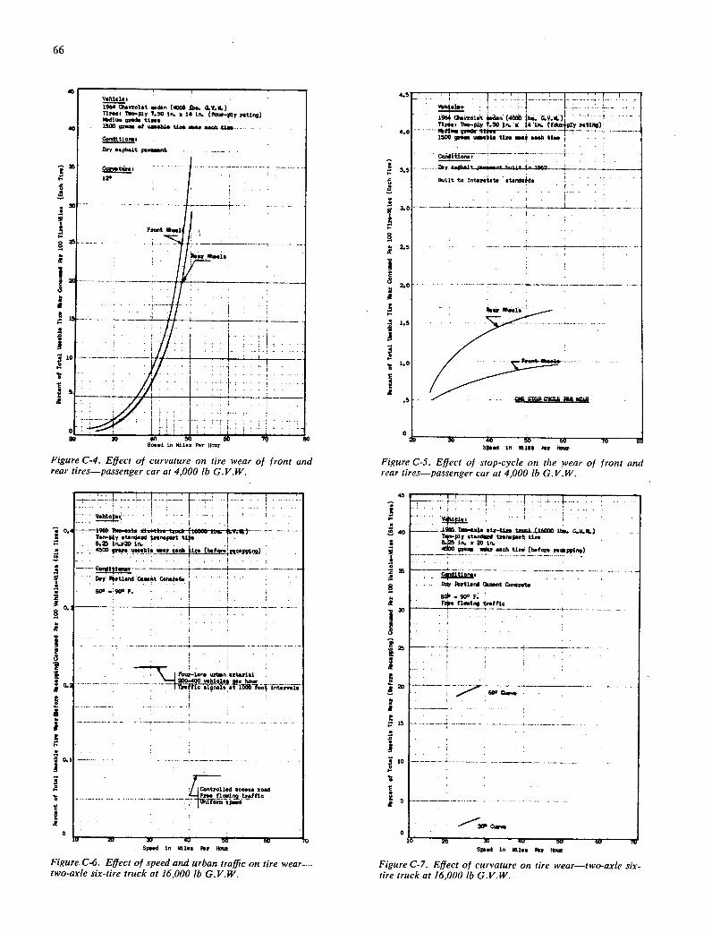
S I

V.htcli, 1964 Qseerel.t ..dsn (4000 b. 0.0.0.) Tie.., IWo..ply 1.50 in. s 14 in. (four-ply biting) idiu.n ged. tines 1500 grane Is uas.Uasnea. .olOU Conditions, Dry e.pAait piesneM...................-. . -

10.tUbl5 120

------4-

.j--:- ). ----*94& -P,1t, 4100. t.,.J. (16000 1!... -VS-) - -

Ten-ply stardsed zsn.pm,t tl$e-

F 'P!L 10

y Prt1a, c.,,.ht Ccs,cg. ..........................

.......... ffj

son,.rt.rtl1 50O-400vehici.4 .an i,.n 42 ig lOin nnalest lowfoo' int.rv.1.

1.1 -.-.- .......................-.----.---...---- .....

ControhlId ace.;. bold .............- . Pr.. f1ov1ntr.fftc

iO4d in esice I.e now

Figure C-S. Effect of stop-cycle on the wear of front and rear tires—passenger car at 4,000 lb G.V.W.

45•

, 40

8

j30

25 LP

50

I

15

10

66

obese ifl fuse, fer flour

Figure C-4. Effect of curvature on tire wear of front and rear tires—passenger car at 4,000 lb G.V.W.

Sp,.d in lOi.s Per Indsr Spied in aOl,, Ps Pear

Figure C-6. Effect of speed and urban traffic on tire wear— Figure C-7. Effect of curvature on tire wear—two-axle six- two-axle six-tire truck at 16,000 lb G.V.W. tire truck at 16,000 lb G.V.W.

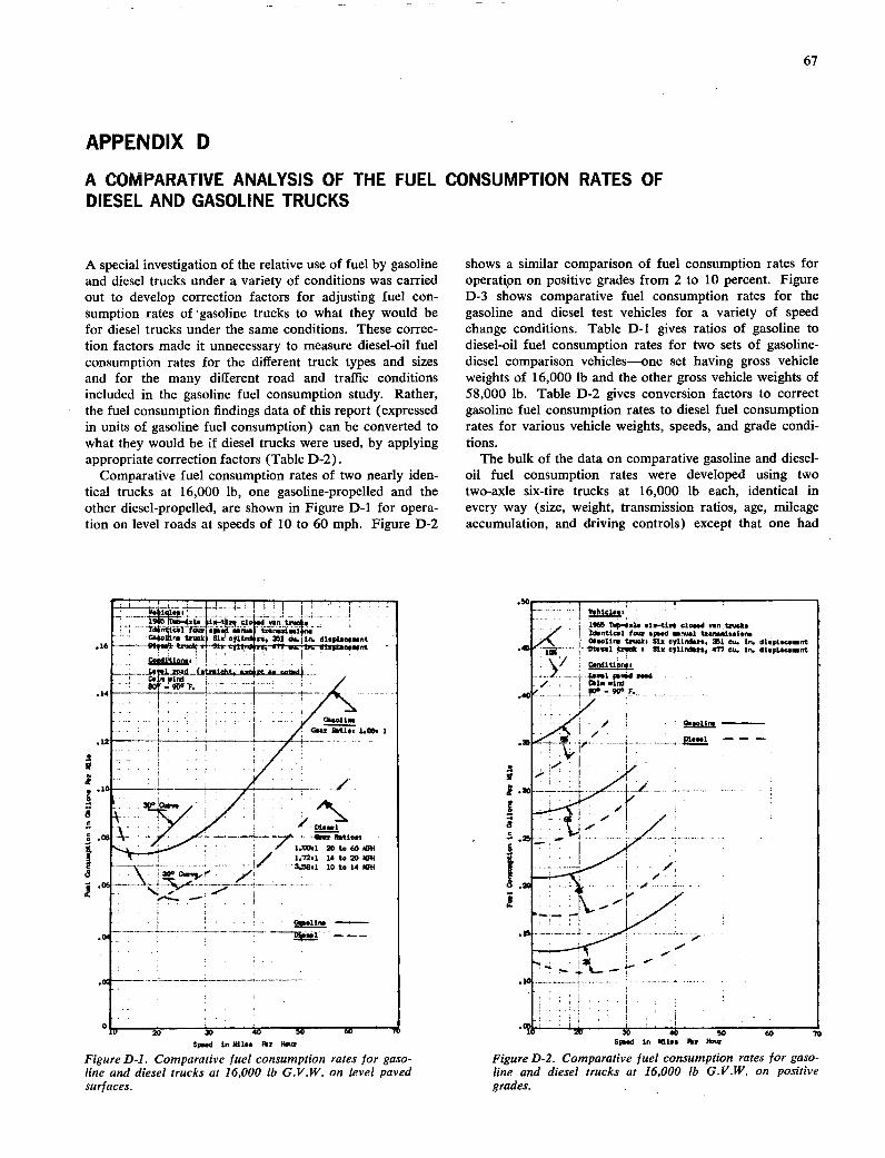
APPENDIX D

A COMPARATIVE ANALYSIS OF THE FUEL CONSUMPTION RATES OF DIESEL AND GASOLINE TRUCKS

67

A special investigation of the relative use of fuel by gasoline and diesel trucks under a variety of conditions was carried out to develop correction factors for adjusting fuel con-sumption rates of gasoline trucks to what they would be for diesel trucks under the same conditions. These correc-tion factors made it unnecessary to measure diesel-oil fuel consumption rates for the different truck types and sizes and for the many different road and traffic conditions included in the gasoline fuel consumption study. Rather, the fuel consumption findings data of this report (expressed in units of gasoline fuel consumption) can be converted to what they would be if diesel trucks were used, by applying appropriate correction factors (Table D-2).

Comparative fuel consumption rates of two nearly iden-tical trucks at 16,000 lb, one gasoline-propelled and the other diesel-propelled, are shown in Figure D-1 for opera-tion on level roads at speeds of 10 to 60 mph. Figure D-2

shows a similar comparison of fuel consumption rates for operatipn on positive grades from 2 to 10 percent. Figure D-3 shows comparative fuel consumption rates for the gasoline and diesel test vehicles for a variety of speed change conditions. Table D-1 gives ratios of gasoline to diesel-oil fuel consumption rates for two sets of gasoline-diesel comparison vehicles—one set having gross vehicle weights of 16,000 lb and the other gross vehicle weights of 58,000 lb. Table D-2 gives conversion factors to correct gasoline fuel consumption rates to diesel fuel consumption rates for various vehicle weights, speeds, and grade condi-tions.

The bulk of the data on comparative gasoline and diesel-oil fuel consumption rates were developed using two two-axle six-tire trucks at 16,000 lb each, identical in every way (size, weight, transmission ratios, age, mileage accumulation, and driving controls) except that one had

'n.$oLln trucip Six C1 xx, Si5 sx..in. displscI.snt 16 D14.i • Si , OTT .. in. .p...cansnt -

C0.4itions, -

—:.---- j - 1.00.1 2D to 60 Mn.

*" 1.72,1 14 to

,1 10 to 14 60M

.00 .-.-

ftoline

01.

H H - 'C

40 50 60 S.d in Silos %V iSia

Figure D-1. Comparative fuel consumption rates for gaso-line and diesel trucks at 16,000 lb G.V.W. on level paved surfaces.

1966 Tic-sals sio-ti$ cio..d vOn trucks / Id.nticai box s96id 0.tn,11 transmission.

/\

Gasoline truck, 51. cyiindsrs, Zi Cu. in. dispi.csnt .44 -Duo.! tr1ck , Six cjiinSizs, 477 Cu. in. dispi*o.ent

- \•/ C..4ition$. - ImnoL 9m5.4 00.4

7. a1a mind .40

Gasoline . . Dt.ss1

000

.30

1.2

S

_•. ...............

.0'i iI

W So au 50 60 11

Sps.d in Silas Per Si.

Figure D-2. Comparative fuel consumption rates for gaso-line and diesel trucks at 16,000 lb G.V.W. on positive grades. -

H'

in. Iip~acjwni.

to '!L

- .101h

LU 1iL T _L i

to , 3-

T

:

-

onis , ItHsL,.4 per all. -

i.* all *. one ,

S.d in Igloo Figure D-3. Comparative fuel consumption rates for gaso-line and diesel trucks at 16,000 lb G.V.W. for stop and slowdown cycles.

68

a gasoline engine and the other had a diesel engine. The engine in each vehicle had six cylinders but necessarily differed in piston displacement and horsepower. The gasoline engine had a displacement of 351 cu in., com-pared to 477 cu in. for the diesel engine. The gasoline and diesel engines had net horsepower capabilities of 142 at 3,800 rpm and 135 at 3,200 rpm, respectively.

Fuel consumption data for both of these trucks were obtained for operation on a level road at speeds of 10 to 60 mph and on a series of grades at appropriate speeds. In addition, test data were obtained for both test vehicles for operation through a variety of speed changes. The data from these test operations are shown in Figures D-1 through D-3 and are given in the top portion of Table D-1.

Data on the fuel consumption rates of gasoline and diesel trucks weighing 58,000 lb developed by Sawhill at the University of Washington in 1959 were used to expand the study results to cover a broad band of vehicle weights (16,000 to 58,000 lb). The ratios computed from Sawhill's study are given in the bottom section of Table D-1 and are reflected, along with data developed for the 16,000-lb trucks, in Table D-2.

The conversion factors of Table D-2 agree with conver-sion factors based on comparative gasoline and diesel fuel consumption rates reported by Kent in 1960 (1). Using

TABLE D-1

RATIOS OF DIESEL FUEL CONSUMPTION RATES TO GASOLINE FUEL CONSUMPTION RATES FOR TWO PAIRS OF TEST VEHICLES

RATIOS BY ROAD DESIGN AND OPERATING CONDITIONS:

UNIFORM SPEED ON GRADES ONE SPEED CHANGE CYCLE/MILE

SPEED STOP 10 20 30 (MPH) LEVEL 2% 4% 6% 8% 10% MPH MPH MPH

(a) Two-axle single-unit trucks (16,000 lb G.V.W.) 10 1.32 0.94 0.83 0.88 0.90 0.90 - - - -

15 0.94 0.86 0.80 0.88 0.90 0.90 - - - -

20 0.73 0.80 0.80 0.89 0.90 0.76 0.76 - -

25 0.70 0.78 0.78 0.90 0.90 0.72 0.70 - -

30 0.64 0.74 0.77 0.90 - 0.72 0.68 0.67 -

35 0.65 0.72 0.80 - - 0.70 0.64 0.65 -

40 0.65 0.73 - - - 0.67 0.64 0.63 0.63 45 0.65 ----- 0.67 0.63 0.63 0.62 50 0.67 ----- 0.67 0.63 0.63 0.62 55 0.69 - - - - - - - - -

60 0.70 - - - - - - - -

(b) 2-S2 tractor semi-trailer truck combinations (58,000 lb G.V.W.) 1

10 0.71 0.82 0.80 0.72 - - - -

15 0.70 0.82 0.67 0.60 - - - - - -

20 0.68 0.70 0.60 - - - - - - -

25 0.66 0.67 - - - - - - - -

30 0.62 0.62 - - - - - - - -

35 0.68 0.60 - - - - - - - -

40 0.70 - - - - - - - - -

45 0.73 - - - - - - - - -

SO 0.74 - - - - - - - - -

1 Source: Sawhill and Firey (2)

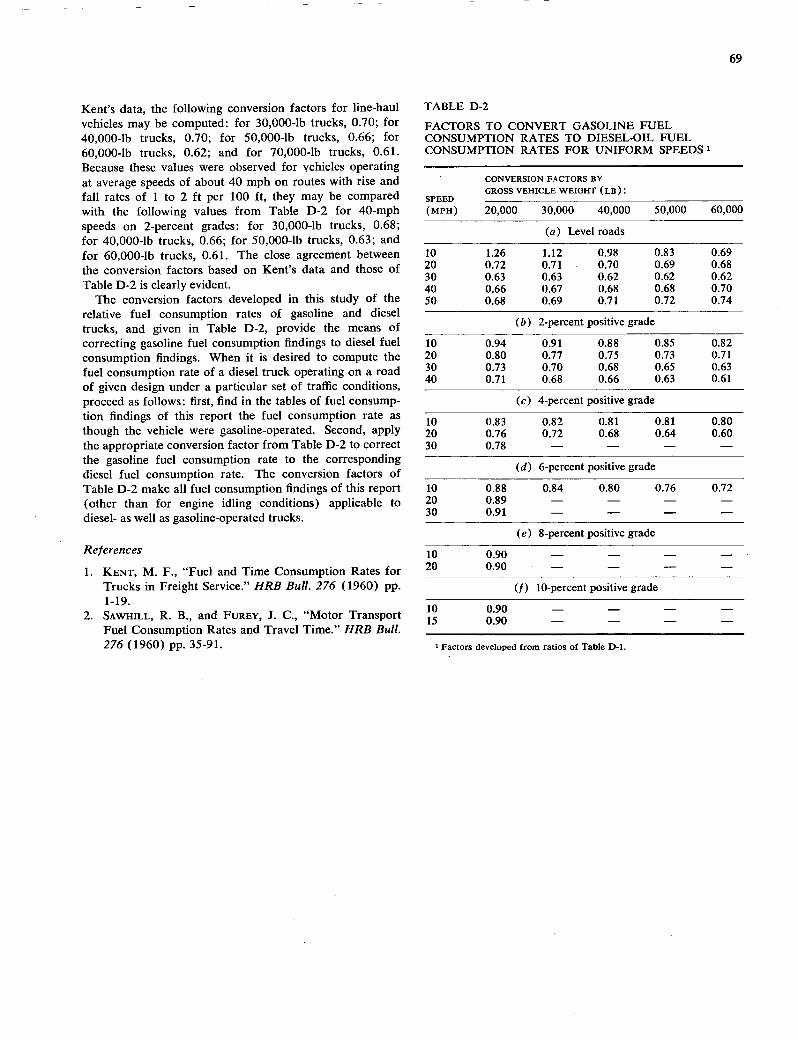
69

Kent's data, the following conversion factors for line-haul TABLE D-2

vehicles may be computed: for 30,000-lb trucks, 0.70; for FACTORS TO CONVERT GASOLINE FUEL 40,000-lb trucks, 0.70; for 50,000-lb trucks, 0.66; for CONSUMPTION RATES TO DIESEL-OIL FUEL 60,000-lb trucks, 0.62; and for 70,000-lb trucks, 0.61. CONSUMPTION RATES FOR UNIFORM SPEEDS 1

Because these values were observed for vehicles operating at average speeds of about 40 mph on routes with rise and CONVERSION FACTORS BY

fall rates of 1 to 2 ft per 100 ft, they may be compared SPEED GROSS VEHICLE WEIGHT (LB):

with the following values from Table D-2 for 40-mph (MPH) 20,000 30,000 40,000 50,000 60,000

speeds on 2-percent grades: for 30,000-lb trucks, 0.68; (a) Level roads for 40,000-lb trucks, 0.66; for 50,000-lb trucks, 0.63; and for 60,000-lb trucks, 0.61. The close agreement between 10 1.26 1.12 0.98 0.83 0.69

the conversion factors based on Kent's data and those of 20 0.72 0.71 0.70 0.69 0.68 30 0.63 0.63 0.62 0.62 0.62

Table D-2 is clearly evident. 40 0.66 0.67 0.68 0.68 0.70 The conversion factors developed in this study of the 50 0.68 0.69 0.71 0.72 0.74

relative fuel consumption rates of gasoline and diesel trucks, and given in Table D-2, provide the means of (b) 2-percent positive grade

correcting gasoline fuel consumption findings to diesel fuel 10 0.94 0.91 0.88 0.85 0.82 consumption findings. When it is desired to compute the 20 0.80 0.77 0.75 0.73 0.71

fuel consumption rate of a diesel truck operating on a road 30 0.73 0.70 0.68 0.65 0.63

of given design under a particular set of traffic conditions, 40 0.71 0.68 0.66 0.63 0.61

proceed as follows: first, find in the tables of fuel consump- (c) 4-percent positive grade tion findings of this report the fuel consumption rate as 10 0.83 0.82 0.81 0.81 0.80 though the vehicle were gasoline-operated. Second, apply 20 0.76 0.72 0.68 0.64 0.60 the appropriate conversion factor from Table D-2 to correct 30 0.78 - - - - the gasoline fuel consumption rate to the corresponding diesel fuel consumption rate. The conversion factors of

(d) 6-percent positive grade

Table D-2 make all fuel consumption findings of this report 10 0.88 0.84 0.80 0.76 0.72 (other than for engine idling conditions) applicable to 20 0.89 - - - - diesel- as well as gasoline-operated trucks. 30 0.91 - - - -

(e) 8-percent positive grade

References 10 0.90 - - - - 1. KENT, M. F., "Fuel and Time Consumption Rates for 20 0.90 - - - -

Trucks in Freight Service." HRB Bull. 276 (1960) Pf (f) 10-percent positive grade 1-19.

2. SAWHILL, R. B., and FUREY, J. C., "Motor Transport 10 15

0.90 - - -

0.90 - - - - Fuel Consumption Rates and Travel Time." HRB Bull. 276 (1960) pp. 3591. 1 Factors developed from ratios of Table D-l.

70

APPENDIX E

ANNOTATED BIBLIOGRAPHY OF HIGHWAY MOTOR-VEHICLE OPERATING COSTS, 1950-1970

The following items provide a full coverage of references that contain research data on fuel and oil consumption, tire wear, and maintenance applicable in road user cost analyses. Except for four important works on road user cost analysis listed in the Special category, all of the items are research reports of motor-vehicle operation investiga-tions. Where a given research project is reported in more than one publication, only the principal reference is given. The items are listed chronologically by subject area.

FUEL CONSUMPTION

1950-1955

LAUTZENHISER, F. B., "Diesel Compared With Gaso-line Engine." SAE I., Vol. 58, No. 6, p. 72 (June 1950).

An early study of the comparable use of fuel by gasoline and diesel trucks showed that heavy diesel trucks used only about 67 percent as much fuel as comparable gasoline trucks for long hauls. For short hauls, however, the fuel consumption rates of gasoline and diesel trucks were about the same. SAAL, C., "Time and Gasoline Consumption in Motor Truck Operation." HRB Spec. Rep. 9A (1950) 73 pp.

Seven trucks, varying in size from the two-axle six-tire truck to the tractor semi-trailer full-trailer truck combination, were operated at a variety of loads on the Pennsylvania Turnpike and parallel U.S. 30. Each route was divided into definite sections, each having a given rate of rise and fall. Test runs were made at normal truck speeds, about 50 mph on level sections, and somewhat less on grades, with momentum used to assist ve-hicle operation on upgrades. Fuel consumption was recorded by test section for each vehicle at each weight.

Fuel consumption values are presented in graphical form by gross vehicle weight and aver-age rate of rise and fall. Separate graphs show fuel consumption for particular rates of rise and fall and for various percentages of total rise and fall that is rise. "Test of Road Vehicles Under Controlled Conditions." Transport Research Quart., No. 5, pp. 33-44 (Oct. 1951).

The fuel consumption rates of two British trucks (one gasoline-operated weighing 12,000 lb and the other diesel-operated weighing 36,000 lb) were determined for operation on nearly level roads at various uniform speeds and for cycles of stop-go operation. Ambient air temperatures

during test operations fell between 54° F and 78° F.

The fuel consumption rate of the 12,000-lb truck in gallons per mile was 0.07 at speeds of 15 to 25 mph and 0.09 at 35 mph. Similarly, the fuel consumption rate of the 36,000-lb truck was 0.09 gpm at 20 to 25 mph and 0.11 gpm at 30 mph.

The excess fuel consumption for stop-go cycles at 25 mph was found to be 0.14 gal. for the 12,000-lb vehicle and 0.17 gal. for the 36,000-lb vehicle. BONE, A. J., "Travel Time and Gasoline Consumption Studies in Boston." Proc. HRB, Vol. 31 (1952) pp. 440-456.

In connection with the "before" part of a "before and after" investigation of time and fuel consumption rates on Boston arterial streets rela-tive to the impact of the Boston Central Artery, the fuel consumption of a 1951 sedan was mca-sured for trips on several streets. With the thought that a sufficiently close relationship be-tween average speed in traffic and the correspond-ing fuel consumption rates could be established for estimating fuel consumption from time con-sumption data, a mass of fuel and time consump-tion data for travel on Boston streets was accumu-lated and analyzed. However, there was far too great a scatter of fuel consumption rates for a given travel speed for the concept to be useful.

Only a limited amount of over-all fuel con-sumption data for travel over the length of test sections on certain Boston streets are given in the findings tables of this report. "Petrol Consumption on Gravel and Bituminous Roads." Commonwealth Eng. (Australia), Vol. 40, No. 6, p. 245 (Jan. 1953).

Research of the Department of Main Roads shows fuel consumption is about 11/2 times greater on good gravel roads than on good bituminous roads for speeds up to 50 mph. This agrees well with results of a similar study for passenger cars conducted for NCHRP Project 2-5. MITZELFELD, T. H., "Large Low-Speed Engine Eco-nomical." SAEJ., Vol. 61, No. 5, p. 126 (May 1953).

A carefully controlled test was carried out to determine the relative fuel consumption of differ-ent size engines for the same operating condi-tions. Two cars exactly alike were equipped with identical 331-cu-in, engines. One was left alone. The other, however, was converted to a 248-cu-in. engine by changing the piston stroke and

71

modifying the crankshaft. The rear axle of this car was changed to produce rear-axle torques in operation equal to that of the car with the un-changed engine.

The two vehicles were operated extensively under the same road and traffic conditions. It was found that fuel consumption was approxi-mately the same for both vehicles. Everything else being the same, engine size has little effect on fuel consumption rates.

7. WHITE, H. S., ENOCH, 0., and HAYNES, A. L., "Gaso-line Economy Depends on the Driver Too." SAE I., Vol. 61,No. 8, pp. 61-63 (Aug. 1953).

This article reports on engine fuel economy studies conducted by the Ford Motor Company Engineering Research Department in 1952. Among numerous items of useful information developed, it was found that maximum conver-sion of the fuel energy into useful work is accom-plished at a median speed range, about 2,000 rpm. Brake specific fuel consumption drops with increasing engine speed at low speeds but in-creases at speeds greater than about 2,000 rpm because of greater internal engine friction at the higher speeds.

Smaller engines run somewhat more efficiently than large engines when the relative size is on the order of two to one. However, for operation at speeds near the optimum and for median loads, fuel consumption is about the same for all engine sizes.

An important item of information noted in this research is that, when coasting downhill with closed throttle, fuel consumption is the same regardless of speed. Further, coasting fuel con-sumption with closed throttle is less than fuel consumption while stopped with engine idling, because no fuel energy is needed to turn the en-gine crankshaft. This aspect of vehicle fuel consumption was also noted in NCHRP Project 2-5 studies. LISTER, R. D., and KEMP, R. N., "Some Traffic and Driving Conditions Which Influence Petrol Consump-tion." Road Abstracts, Vol. 21, No. 12, p. 186 (Dec. 1954).

The fuel consumption rates of three vehicles (a small car, a large car, and a 3-ton truck) were measured for operation (1) at a uniform speed of 30 mph on a level paved road at three traffic volume levels (zero, light, and heavy), (2) while accelerating from 0 to 40 mph on a level road with no traffic, (3) while traveling up a 4-percent grade at 30 mph, and (4) while travel-ing on a 100-ft-radius curve. Fuel consumption rates were found to be 35 percent greater in light traffic and 100 percent greater in heavy traffic compared to operation in zero traffic, 100 percent greater on the 4-percent grade compared to oper-ation on the level road, and about 21/2 times greater for acceleration to 40 mph or for opera-

tion around a 100-ft circle compared to uniform speed at 30 mph on a tangent.

The test results developed in this study agree well with study results of NCHRP Project 2-5 for acceleration, grade, and curve operations. Whether agreement exists for operation in light and heavy traffic could not be determined because traffic details of the Lister-Kemp study were not given (frequencies of slowdowns and traffic stops, for example).

The authors of this article observed that the most consistent and useful running cost data could be obtained only by operating over a defi-nite test section of known length. MATSON, T. M., SMITH, WILBUR, and HURD, F. W., TratjIc Engineering. McGraw-Hill, pp. 26-34 (1955).

This textbook in traffic engineering outlines in detail the various resistances encountered in the operation of motor vehicles. Rolling resistance on good pavement was reported as 20 to 27 lb per ton of gross weight. Air resistance was re-ported as equalling 0.0008 times the product of the frontal area in square feet and the square of the speed in miles per hour, about 60 lb at 55 mph for the typical U.S. sedan. Impact resistance on rough roads can increase rolling resistance by 30 percent. SAAL, C., "Operating Characteristics of a Passenger Car on Selected Routes." HRB Bull. 107 (1955) pp. 1-34.

The fuel consumption of a 1951 model stan-dard-type passenger car for operation on each of several freeway-type roads and parallel non-free-way routes is reported. Over-all fuel consumption rates for the long test sections of the comparison routes, however, are not differentiated by gradi-ent, curvature, surface condition or traffic vol-umes. It is worth noting that the test operations were carried out by attempting to travel at certain speeds, even when traffic conditions imposed slower actual speeds.

Limited studies of passenger-car fuel consump-tion as affected by gradient and acceleration rates are also given. NORTHCUTT, J. P., "Cost Per Hour." Mass Trans., Vol. 51,No. 12, p. 45 (Dec. 1955).

In 1954 a study of diesel bus operation in CBD's developed the following fuel consumption rates for the given stop frequencies: 0.239 gpm for four stops per mile (17 mph), 0.321 gpm for eight stops per mile (12 mph), and 0.413 gpm at 12 stops per mile (9mph).

1956-1960

NAGLER, L. H., BURKE, C. E., LUNDSTROM, L. C., and ASSOCIATES, "Where Does All the Power Go?" SAEJ., Vol. 65, pp. 54-63 (Apr. 1957).

The research reported in this article was developed for typical passenger cars of 1956. It describes the magnitude under a variety of con-

72

ditions of the various power-consuming items needed to operate these cars. The power require-ments for each of the following items are consid-ered: (1) generator, (2) fan, (3) power steering, (4) automatic transmission, (5) rear axle, (6) rolling tire on pavement, (7) still air, and (8) wind. At 60 mph about 50 percent of the rated gross brake horsepower of the engine (nominal power) is available at the traction surfaces of the rear wheels to propel the vehicle.

Air temperature affects power needs appreci-ably. Power requirements increase at a rate of ½ percent per degree F temperature drop from 70° F to 30° F at 60 mph.

Horsepower requirement is about 40 percent greater on loose gravel roads than on good rigid pavement.

These values agree in general with the corre-sponding effects of surface conditions and tem-perature on fuel consumption as determined for NCHRP Project 2-5.

13. MILLER, J. C., "Prime Factors Affecting Diesel Fuel Economy." SAE J., Vol. 65, No. 11, p. 68 (Oct. 1957).

Engine speed is a major determinant of fuel consumption for diesel trucks. For example, a 48,000-lb diesel tractor-trailer combination uses 21.5 lb of fuel per hour at 1,500 rpm (35 mph) on a level road. However, it uses 51.0 lb of fuel per hour at 2,000 rpm (50 mph). Thus, a 33-percent increase in engine speed results in 137-percent increase in fuel use. If the engine were operated at 2,500 rpm instead of 2,000 rpm at 50 mph (use of lower gear), fuel consumption would have been 57.0 lb per hour instead of 51.0 lb—an increase of 12 percent due to increased engine speed alone.

The diesel engine is relatively inefficient at low road speeds with the gear position set for high engine speed. Thus, heavy diesel trucks may have a particularly high fuel consumption rate when operating in congested traffic in low speed with much changing of gears.

This agrees with the data recorded for NCHRP Project 2-5 in that fuel consumption rates are greater for diesel than for gasoline trucks of the same weight when operating at speeds of less than 15 mph on level roads.

14 CLAFFEY, P. J., "Time and Fuel Consumption for Highway User Benefit Studies." HRB Bull. 276 (1960) pp. 20-34.

Fuel consumption measurements were made for a passenger-car sedan, a pickup truck, and a two-axle six-tire truck for operation at constant speds of 15 to 55 mph on level roads, both paved and gravel surfaces. Fuel consumption measure-ments were also made for stop-go and 10-mph slowdown cycles. The passenger car was operated at a gross vehicle weight of 3,850 lb, the pickup at 3,860 lb (empty) and 5,340 lb (loaded), and

the two-axle six-tire truck at 10,200 lb (empty) and 15,300 lb (half-loaded).

The fuel consumption data are shown graphi-cally both as absolute values and as savings re-sulting from improvement of a road from gravel to paved surface, elimination of stop cycles, and elimination of slowdown cycles. CROOKS, L. E., "Consumers Union Test Data Rate Compact Performance." SAE I., Vol. 68, No. 8, p. 128 (Aug. 1960).

Consumer's Union conducted an investigation into the relative fuel consumption of large (i.e., Chrysler), compact (i.e., Falcon), and small (i.e., Volkswagen) cars. All operations were carried out on level roads at constant speed with no wind. It was found that at 50 mph the fuel economy of large, compact, and small cars was 20, 25, and 40 miles per gallon, respectively.

The values given in this report agree with those of NCHRP Project 2-5 for large and com-pact cars. However, the small car achieves a fuel economy of 40 mpg only at 30 mph. At 50 mph, its rate of fuel consumption is the same as that for the compact car. CLEVELAND, A. E., and Bisi-iop, I. N., "Fuel Eco-nomy." SAE J., Vol. 68, No. 8, p. 27 (Aug. 1960),

This article explains the various energy losses in an automobile engine from heat losses via cylinder walls to energy losses in metering fuel. It covers the reasons only about 22 percent of the heat energy of fuel is available for propelling motor vehicles against road and air resistances. This paper is chiefly useful to the highway economist in defining the variability of the factors that affect fuel consumption between firing of the fuel in the cylinders and the use of the resulting energy forces at the traction wheels. Examples of items affecting energy realization in cars are magnitude of heat loss in cylinders, ratio of cylinder bore to stroke, accelerator pump fric-tion, air friction entering cylinders, and engine oil viscosity. KENT, M. F., "Fuel and Time Consumption Rates for Trucks in Freight Service." HRB Bull. 276 (1960) pp. 1-19.

Fuelmeters were mounted in line-haul trucks operating in regular service between Baltimore and Richmond on the east coast, between Cleve-land and Columbus and Detroit and Lansing in the mid-west, and between Seattle and other Washington cities in the far west. Fuel consump-tion and gross vehicle weight per trip were re-corded for each truck, diesel or gasoline, on each test route. In addition, fuel consumption measure-ments and speed changes greater than 3 mph were recorded during each trip by identified road sections. For example, fuel consumption and speed change on urban extensions were dif-

73.

ferentiated from those on rural road sections. Speeds were those normally used by drivers and essentially matched those of the general traffic. Fuelmeters measured fuel consumption to the nearest 1/so of a gallon.

Over-all fuel consumption rates by gross vehicle weight, road type, frequency of speed change, and type of fuel are presented in graphi-cal and tabular form. Research results are explicit in showing the relative use of fuel by gasoline and diesel trucks.

At 50,000 lb gross vehicle weight, diesel trucks in normal service consume about 66 percent as much fuel as do gasoline trucks. This agrees with data developed for NCHRP Project 2-5. SAWHILL, R. B., and FIREY, J. C., "Motor Transport Fuel Consumption Rates and Travel Time." HRB Bull.276, (1960) pp. 35-91.

Nine tractor-trailer combinations and three buses, some of which were, gasoline-propelled and some diesel-propelled, were operated at various constant speeds on level paved road sections, on paved grades of 1.53, 2.79, 4.00, and 5.96 percent, and on level gravel road sections. In addition, each test vehicle was operated through test sequences of stop and go cycles and 10-mph slowdown cycles.

The fuel consumption rates of the test vehicles are shown as a function of speed in a series of graphs for operation on paved roads of various gradients, on level gravel roads, and for stop-go and slowdown cycles.

This report served as a major source of re-search information for NCHRP Project 2-5.

1961-1965

MITCHELL, B. J., RANSOM, G. P., and REED, H. E., "Effect of Engine RPM on MEP and Fuel Economy." SAE J., Vol. 69, No. 3, p. 87 (Mar. 1961).

The relationships between the mean effective cylinder pressure, horsepower, and fuel consump-tion of a V-8 engine with 371-cu-in, capacity were studied under controlled conditions in a laboratory. It was found that mean effective pressure is maximum at about 3,000 rpm, drop-ping off at both higher and lower speeds.

Horsepower output of the engine was found to increase almost in a straight line with increases in engine speed for the range from 1,000 to 4,000 rpm. However, engine friction also in-creases with speed, although at a lesser rate. At 4,000 rpm engine friction consumed nearly 100 hp, whereas total output was about 280 hp.

Fuel consumption in pounds of fuel per horse-power-hour remained constant for engine speeds of 1,000 to 4,000 rpm. That is, fuel consump-tion is proportional to horsepower production for this range of engine speed. Because lost horse-power due to engine friction increases with speed,

the net horsepower output per pound of fuel decreases with increased speed. KENT, M. F., "AASHO Road Test Vehicle Operating Costs Related to Gross Weight." HRB Spec. Rep. 73 (1962) pp. 149-165.

Records of rates of fuel and oil consumption, tire wear, and maintenance were kept for all vehicles during the operation of the test trucks on the nearly level AASHO test loops in Ottawa, Ill., in i959. Operations were conducted on two test loops, each consisting of two parallel straight roads, several thousand feet in length, connected at each end by nearly 30° curves about equal in length to the tangents. The test trucks were operated at a uniform speed of 35 mph on the tangents and 25 mph on the loops.

Average over-all fuel consumption rates were found to be 0.07, 0.08, 0.22, and 0.26 gpm for the pickup (4,200 lb), the two-axle six-tire truck (8,200 lb), the 2-S1 truck (40,000 lb), and the 3-S2 truck (50,000 lb), respectively. These values are somewhat higher than those measured in NCHRP Project 2-5 for operation of these types and weights of trucks on level tangents. This, of course, reflects the effect of the tight end-loop sections on fuel consumption of the test trucks. SAWHILL, R. B., and FIREY, J. C., "Predicting Fuel Consumption and Travel Time of Motor Transport Vehicles." HRB Bull. 344 (1962) pp. 27-46.

The fuel consumption rates of two gasoline-operated and two diesel-operated tractor semi-trailer trailer combination trucks were determined for specific operating conditions (1) by actual fuel measurement, and (2) by calculation using basic energy relationships. Due to variations in the thermal efficiency of the engines, however, considerable differences were found between cal-culated and measured fuel consumption rates. For fuel consumption prediction formulas to give results of acceptable accuracy they become highly complex and require formulae inputs that them-selves are difficult to evaluate. SAWHILL, R. B., "Fuel Consumption of Transport Vehicles on Horizontal Curves." Univ. of Wash. Traffic and Operations Series Research Report No. 5, Seattle (June 1962) 12 pp.

A 2-Si -2 tractor semi-trailer trailer combination was operated around a series of circles at each of three gross vehicle weights: empty at 32,100 lb, half-loaded at 53,500 lb, and fully loaded at 64,200 lb. The circles were nearly flat (an air-port runway) with radii of 90 ft, 150 ft, and 210 ft. Tests were made at speeds of 7 to 25 mph in regular 5-mph increments.

The curves had an appreciable effect on fuel consumption. For example, at 25 mph, fuel con-sumption rates of the empty vehicle were 0.18, 0.23, 0.25, and 0.30 gpm on tangents, 210-ft radius curves, 150-ft radius curves, and 90-ft radius curves, respectively.

74

SAWHILL, R. B., "Fuel Consumption of Transport Vehicles on Grades." Univ. of Wash. Traffic and Operations Series Research Report No. 6, Seattle (June 1962) 11 pp.

To determine the effect on truck fuel consump-tion on upgrades when approach speeds exceed maximum on-grade crawl speeds (momentum grades) two trucks (one gasoline and the other diesel) were operated up a 4-percent and a nearly 6-percent grade at approach speeds up to 50 mph. Each truck was investigated at each of three gross vehicle weights: empty at about 33,000 lb, half-loaded at about 54,000 lb, and fully loaded at 65,000 lb. At the lower speeds, the trucks were able to complete the trip up the grades without changing speed; but above the crawl speeds the grades forced the speed down to crawl speed. In the latter case appreciable on-grade distance was covered on momentum.

It was found that fuel consumption on the grades dropped off appreciably on momentum grades for the gasoline vehicles but only slightly for the diesel truck. STONEX, K. A., "How Cars Have Changed in 30 Years." SAE J., Vol. 70, No. 10, pp. 33-36 (Oct. 1962).

The research information presented in this article and applicable in user cost studies is the road distance required for passing maneuvers of passenger cars. Most passings from 40 mph re-quire from 750 to 850 ft of passing distance. LIEDER, N., "Passenger Car Fuel Consumption Rates." Public Roads, Vol. 32, No.5, p. 113 (Dec. 1962).

This article reports on a study of over-all fuel consumption relative to vehicle and weather fac-tors. It does not distinguish fuel consumption according to road design elements.

Fuel consumption is approximately 10 percent greater in winter than in summer for most auto-mobiles.

Passenger-car fuel consumption rates change very little over time. In 1960, cars of a particular type that were 10 years old consumed about the same amount of fuel as new cars of the same type and design.

These values agree with those developed for NCHRP Project 2-5. CLAFFEY, P. J., "Running Cost of Motor Vehicles as Affected by Highway Design—Interim Report." NCHRP Report 13 (1965) 43 pp.

NCHRP Report 13 is an interim report on Project 2-5 covering fuel consumption of the standard-type passenger car. Fuel consumption rates of this vehicle on level roads, grades, certain curves, and on several different road surfaces are given.

The photo-electronic fuelmeter is described in Appendix B.

The impact on vehicle fuel consumption of

wind, variations among drivers, and differences among fuel types is reported on in detail.

Patterns of tire wear and the magnitude of wire wear for operation on a curve of 65-ft radius are also given.

1966.1970

JOYNER, J. A., "Factors Affecting Fuel Economy in Diesel-Powered Vehicles." SAE Trans., Vol. 74, p. 341 (1966).

The fuel consumption rates of diesel trucks were investigated for highway operation under controlled conditions. It was found that the brake specific fuel consumption per horsepower- hour was relatively high for light loads (low brake horsepower) but dropped to a minimum at approximately 160 hp before increasing at loads greater than 160 hp. It was evident from the results of this study that fuel economy in diesel truck operation is best when the truck is over-coming a substantial resistance.

These results tend to agree with information developed for NCHRP Project 2-5 which showed that at low speeds diesel trucks operating on level roads consumed fuel at a higher rate than on a 1-percent grade at the same speed. CORNELL, J. J., "Car Size Chiefly Responsible for Low MPG at High MPH." SAE I., Vol. 74, No. 4, p. 37 (Apr. 1966).

Passenger-car fuel consumption for operation on level roads at high speeds, 70 to 80 mph, is determined principally by the dimensions of the car (rather than vehicle weight or engine size). This results from the overriding effect of air resistance on fuel consumption at high speed.

The standard U.S. six-cylinder car has a rolling resistance of about 80 lb at 50 mph and 90 lb at 80 mph. The rolling resistance of compact cars is about 12 percent less than that of the standard-type car, whereas the large car rolling resistance is about 12 percent greater than that of the standard car.

The fuel consumption rates of three cars of the same size and weight, but with different size engines, was determined for level road operation at 30 and 80 mph. At 30 mph, fuel consumption rates were different due to the effect of engine size (0.034, 0.038, and 0.040 gpm.) However, at 80-mph speeds, the strong effect of air re-sistance produced the same fuel consumption rate for each vehicle (0.067 gpm) because each car had the same dimensions.

The reduction of the effect of engine size on fuel consumption rates at the higher speeds was noted in the research for NCHRP Project 2-5, but only for the larger engines. SCHEFFLER, C. E., and NIEPOTH, G. W., "Tests Show Fuel Economy Effects of Car Design and Driver Factors." SAE I., Vol. 74, No. 10, p. 46 (Oct. 1966).

Fuel consumption rates are significantly af-

75

fected by ambient temperatures. After traveling about 10 miles so that the engine is at normal operating temperature, fuel economy is about 90 percent of maximum economy at 700 F ambi-ent temperature and II percent of maximum economy at 10° F ambient temperature.

Passenger-car weight affects fuel consumption by causing approximately 25 percent increase in fuel consumption for a 1,000-lb increase in weight. These are approximately the results found in the NCHRP Project 2-5 study. BONNEY, R. S. P., and STEVENS, N. F., "Vehicle Operating Costs on Bituminous, Gravel and Earth Roads in East and Central Africa." Road Research Laboratory Report 76 (1967) 43 pp.

A study was conducted on selected African roads to determine the effects of road surface on the cost of operation for vehicles in regular service. Each of the 65 commercial vehicles for which data were developed in the study (46 buses and 19 trucks) normally operated on a route with the same road surface type for most of its length. Road grades were light and vehicle weights were about the same from vehicle to vehicle.

It was found that operating on a good grade of gravel surface rather than on a paved bituminous surface had little effect on fuel consumption at normal operating speeds. However, operation on unimproved earth roads resulted in a 20-percent increase in fuel consumption. KESSLER, J. C., and WALLIS, S. B., "Aerodynamic Test Techniques." SAE Trans., Vol. 75, Sec. 3, p. 12 (1967).

This paper reports on an extensive investiga-tion into the basic resistances encountered in automobile operation: rolling resistance (road friction, tire deflection, wheel bearing friction, and differential gear friction) and air resistance. A typical mid-1960's model U.S. sedan was used for the study. Lubrication of the vehicle and tire pressures were according to manufacturer's re-commendations.

The test car with its transmission disconnected was pulled by a second vehicle while a strain gauge mounted in the coupling measured the drag of the test car. Operations were at various uniform speeds from 10 to 80 mph on level, straight, high-type pavements when wind condi-tions were calm.

Rolling resistance was determined as follows: a box large enough to completely enclose the test car was mounted over the test car on sepa-rate dollies. The box had long skirts reaching to the road surface in all directions. The drive car pulled both the box (on its dollies) and the test car with the coupling for the test car passing through a hole in the front of the box. Test data with the box in place were measurements of the

rolling resistances, only without the effect of air resistance.

Air resistance was determined by repeating the test runs without the box in place, recording the drag due to both rolling and air resistances, and subtracting to find air resistance.

Rolling resistance (with the transmission dis-connnected) was found to be about 55 lb for all speeds from 10 to 60 mph, increasing gradually to about 65 lb at 80 mph. Rolling resistance at rest is about 75 lb. Because the typical car weighs about 2 tons, rolling resistance is about 27 lb per ton on high-type level pavement.

Air resistance is about zero at 10 mph, 55 lb (equal to rolling resistance) at 55 mph, and in-creases generally as the square of the speed. EVERALL, P. F., "The Effect of Road and TraflIc Conditions on Fuel Consumption." Road Research Laboratory Report LR 226 (1968) 71 pp.

Six test vehicles varying from a small passenger car to a 22-ton diesel tractor semi-trailer truck combination were operated over a 154-mile test road (1) at normal speeds, (2) at highest prac-tical speeds, and (3) at speeds designed to maxi-mize economy. The test road was divided into 154 separate marked-off test sections (0.1 to 3.5 miles in length), each of which had a specific known speed limit, grade, and cross-section de-sign. Fuel and time consumption for operation over each test section at times of light, medium, and heavy traffic flows were recorded for each vehicle type for the various traffic flows and for each of the attempted speed conditions. Un-fortunately, traffic volumes encountered on the various road sections are not reported.

It was found that the fuel consumption of passenger cars is least at a uniform speed of about 35 mph and is particularly high in low-speed traffic (10-mph traffic speeds). Fuel con-sumption on expressway is 10 to 20 percent less than on rural highways in general. Five-per-cent grades produce about 14 percent more fuel consumption (averaged uphill and downhill) than do level roads.

The fuel consumption of trucks is particularly affected by grades, being 125 percent greater on 61/4 -percent grades (again averaged uphill and downhill) than on level roads. PELENSKY, E., BLUNDEN, W. R., and MUNRO, R. D.,

"Operating Costs of Cars in Urban Areas." Proc., Fourth Conference, A ustralian Road Research Board, Vol.4, Part 1, pp. 475-504 (1968).

Fuel consumption measurements of a passenger car at 3,200 lb gross vehicle weight were made on each of 39 urban routes in Sidney and on each of 8 urban routes in Melbourne. The 47 route sec-tions for which fuel data were recorded were typical of urban routes; some were in the central business districts, some were on major arterials, and some were on expressways. Sections were

relatively long (ito 9 miles in length) and each incorporated a variety of grades, traffic condi-tions, and road types. Even on sections identified as level, there were rates of rise and fall as great as 4.38.ft per 100 ft. Traffic volumes were not recorded. Test drivers were instructed to drive with the traffic.

From the measurements of fuel consumption made for this study, together with relationships developed between fuel consumption rates and urban travel speeds, tables of fuel consumption for typical English cars in cents per mile are presented as functions of 'travel speed on urban routes. OGLESBY, C. H., and ALTENHOFEN, M. J., "Economics of Design Standards for Low-Volume Rural Roads." NCHRP Report 63 (1969) pp. 55-76.

Appendix D of this report contains important user operating cost data for travel on low-volume two-lane roads of various widths. Operating costs of passenger cars when meeting and passing other vehicles are given in a series of graphs as func-tions of road widths. As roads of ample width lead to roads of ever-decreasing width, conflicts of meeting and passing vehicles become amplified and result in speed changes and shoulder running which add to operating costs. All of the effects that operation on low-volume secondary roads have on vehicle operating costs are explored. SAWHILL, R. B., MATTESON, J. H., and HALL, J. W., Vehicle Characteristics of Fuel and Travel Time on Urban Arterials and Freeways." Univ. of Wash. Traffic and Operations Series Research Report No. 14A, Seattle (Jan. 1970) 44 pp.

A "before and after" study of fuel and time consumption rates was conducted on four nearly parallel arterial routes and a parallel freeway before the freeway was built (1962) and after the freeway had been in operation some time (1968). One set of five test vehicles (a compact, a stan-dard-type sedan, a pickup truck, a two-axle six-tire truck, and a diesel tractor-trailer combination truck) was used in the "before" study. A similar set was used for the "after" study. Some difficulty was suffered in calibrating the different "before" and "after" vehicles.

"Before" and "after" fuel and time consump-tion values were developed for the operation of each vehicle in both directions on all test routes during peak hours and during off-peak hours.

TIRE WEAR

1950-1955

SPROWLS, G. - M., "Impediments to Tire Longevity." SAE I., Vol. 58, No. ii, p. 40 (Nov. 1950).

Heat and abrasion are the principal causes of tire failure. Heat causes a deterioration of tire material and may lead to a dangerous failure and probably results in a shortened over-all tire life.

Abrasion is the loss of tread due to friction between tires and pavement. Abrasion gradually wears away tire material until a tire tread is too thin for safety. Tire wear measurements are measurements of tire abrasion.

Tires wear or abrasion results from stop-go operations, speed, accelerations, grades (upgrade and downgrade), and rough surface. Tire wear on winding mountain roads is about 66 percent greater than on straight level routes. Surface wear is least where particles of pavement mate-rial are rounded and smooth, even though the surface may be "bumpy" or "lumpy." However, on an apparently smooth surface, if particles are sharp-angled and striated, tire wear will be high (harsh surface). "Factors Affecting Tire Mileage." Commercial Carl., Vol. 81, No. 2, pp. 120121 (Apr. 1951).

Truck tire studies in 1950 developed informa-tion to show that tire wear at a constant speed of 50 mph is about twice what it would be for constant-speed operation at 20 mph. Tire wear at normal speeds on loose gravel surface is ap-proximately double the tire wear on a good paved surface at the same speed. These results agree well with similar tire wear studies conducted for NCHRP Project 2-5. STECHERT, D. G., and BOLT, T. D., "Evaluation of Tread Wear." Analytical Chemistry, Vol. 23, No. 11, p. 1641 (Nov. 1951).

A technique is presented for measuring the effect on tire wear of road design that is of inter-est for tire wear cost studies. The technique was considered for use in NCHRP Project 2-5 but was discarded because assurance of satis-factory results was lacking.

This technique for tire wear measurement is as follows: on the basis of 21/2 years of study, it was established that the log-log graph of tread depth versus mileage is a straight line. Thus, it is possible to predict tire mileage to baldness for a given set of running conditions if tread depth is measured at two values of travel mileage during the time mileage is accumulated for the given conditions. The mileage for total consump-tion of tire tread to baldness for these conditions can be estimated on the basis of a very limited amount of travel.

A major deterrent to the use of this technique is the inaccuracy inherent in tread depth measure-ment. STIEHLER, R. D., STEEL, M. N., and MANDEL, J., "Factors Influencing the Road Wear of Tyres." Engineering, Vol. 173, No. 4499, pp. 218-222 (Feb. 15, 1952).

This article deals principally with the chemis-try of tires—the relative amounts of rubber and black needed for tire durability. However, the research developed the following information of use in operating cost studies:

76

34

77

Measurement of tire wear should be made by tire weight rather than by tread depth. Laboratory studies show that tread depth de-creases much more rapidly during the first few years of life than during the latter years for the same conditions of use. Weight loss relative to wear, however, is nearly the same throughout the life of a tire.

The rate of wear of a 6.00 X 16 passenger-car tire is 0.03 and 0.05 gm per mile at 30 and 50 mph, respectively. This is substantially the same as that found in NCHRP Project 2-5 for the 7.50 >< 14 tire.

For straight normal operation, tire wear on the rear wheels is much greater than on the front wheels.

1956-1960

PATTERSON, P. D., "The Tire on the Road." Road International, No. 21, pp. 28-33, 56 (Summer 1956).

This is a report on a review of general tire wear considerations in different countries, alti-tudes, types of road surfaces, and speeds.

A particular point was made that even when running conditions do not cause great wear, high temperature may shorten life of tires by interior deterioration (where temperature is highest). In desert areas, for example, tire life is prolonged by using an extra-thin tread to promote interior cooling of the tire on the hot sand. HERSHEY, M. P., "Tire Degradation." SAE J., Vol. 65, No. 7, p. 85 (July 1957).

Tires deteriorate rapidly at sustained high speeds because of the elevated temperatures as-sociated with such speeds. High temperature causes a degradation of tire rubber, resulting in chunking and! or essential separation of tire tread from casing. Such tire temperatures do not cause appreciable tread wear or weight loss. Rather, temperature shortens life through tire deterioration.

A tire with a tread life of 33,000 miles at 60-mph sustained speeds will have a tread life, as a result of heat degradation, of only 14,000 miles if a speed of 90 mph is maintained. GOUGH, V. E., "Cornering Can Wear Tires Rapidly." SAE J., Vol. 66, No. 1, pp. 28-29 (Jan. 1958).

This article describes in detail and with dia-grams how front-wheel tires wear on curves. A cornering force that deflects the vehicle into a curved path is developed by turning the steering wheels a certain angle (slip angle) beyond the direction the wheels are actually moving relative to the road. The resultant slippage produces the force needed to turn the car, while greatly ac-celerating tire wear.

Pneumatic tires are of particular value in motor-vehicle operation because they can produce

a large cornering force with a relatively small slip angle.

Tire wear on curves is quite large. For ex-ample, steering-wheel tires are worn more by turning a 90° angle at a certain speed than they are by three full stop-go cycles at that speed.

The work performed in turning a vehicle is measured by the area under the curve of corner-ing force versus lateral movement and is devel-oped chiefly under the rear half of the pavement contact area.

It is interesting to note that at slip angles greater than about 3° (with normal automobile loads) cornering force can be more than doubled with practically no driver effort (loss of driver feel). Tire wear has little relationship to steering-wheel torque at greater than 3° of slip angle. RIEHL, T. A., "Treadwear Life Down 18 Percent." SAE J., Vol. 66, No. 6, p. 56 (June 1958).

The results of tire wear studies conducted by tire manufacturers in 1958 show for 50 mph that one stop every 5 miles reduces tire life to 50 percent of what it would be at a uniform speed of 50 mph. This agrees with findings of NCHRP Proj- ect 2-5.

Findings on the effect of constant speeds, age of car, and tire rubber composition are also reported in this article.

1961-1965

KENT, M. F., "AASHO Road Test Vehicle Operating Costs Related to Gross Weight." HRB Spec. Rep. 73 (1962) pp. 149-165.

Records of rates of fuel and oil consumption, tire wear, and maintenance were kept for all vehicles during the operation of the test trucks on the nearly level AASHO test loops in Ottawa, Ill., in 1959. Operations were conducted on two test loops, each consisting of two parallel straight roads, several thousand feet in length, connected at each end by nearly 30° curves about equal in length to the tangents. The test trucks were operated at a uniform speed of 35 mph on the tangents and 25 mph on the loops.

Tire wear costs were found to be 0.05 cents per tire-mile for the pickup and two-axle six-tire trucks, and 0.15 cents per tire-mile for the tractor semi-trailer combinations.

The tire wear rates recorded by Kent approxi-mate the results obtained in the NCHRP Project 2-5 study for the same conditions. MERNAGH, L. R., "Tyres at Speed." Rubber Develop-ments, Vol. 15, No. 1, pp. 2-5 (1962).

Under laboratory test conditions of constant load, tire life decreases for all speeds up to 100 mph. Expected tire life at sustained 100-mph operation is about 15 percent of that for 40-mph operation.

Heat build-up at high speed shortens tire life.

78

A temperature rise to greater than 2000 F de-teriorates tire rubber, thus shortening tire life.

46 "Tyre Abrasion Testing on the Road." Rubber De-velopments, Vol. 15, No. 4, pp. 102-104 (1962).

Development of a specially constructed trailing vehicle for measurement of tire wear due to abrasion is described in this article. Only one value of tire wear rate is given: a tire operating continuously at a 10 slip angle will consume about 1 percent of its useable tire tread each 100 miles. This approximates findings in NCHRP Project 2-5 for operation on a 10 curve at 60 mph (about a 1° slip angle).

47 NORDEEN, D. L., and CORTESE, A. D., "Large Differ-ences in Vehicle Handling." SAE I., Vol. 71, No. 7, pp. 83-89 (July 1963).

This article reports on detailed research into the interplay of forces between motor-vehicle steering wheels and road surfaces. The pertinent information developed relative to tire wear study is a graph showing how wheel load (normal force), slip angle, and cornering force (lateral force at zero camber angle) are interrelated when a vehicle traverses a curve.

For slip angles of 2° or less, cornering force is independent of normal force (wheel load). How-ever, for slip angles greater than 2°, cornering forces increase with increases in normal force at an increasing rate.

For tire wear purposes it can be noted that vehicles having heavy loads will develop the needed cornering force at a lesser slip angle than the lighter vehicle. This tends to reduce tire wear by holding down slip angle. However, this is offset by the higher cornering force necessary to change the direction of the greater mass of the heavier vehicle. "Tires." Product Eng., p. 53 (Nov. 23, 1964).

Studies of the Firestone Tire and Rubber Com-pany show how horsepower loss due to rolling resistance varies with speed and how cornering force varies with steering angle. The rolling re-sistance horsepower loss of conventional tires is about 0.5 at 10 mph, 2.2 at 50 mph, and 3.9 at 80 mph. The cornering force developed at 1° turning angle is 160 lb; at 30, 295 lb; and at 6°, 420 lb.

1966-1970

BONNEY, R. S. P., and STEVENS, N. F., "Vehicle Operating Costs on Bituminous, Gravel and Earth Roads in East and Central Africa." Road Research Laboratory Report 76 (1967) 43 pp.

A study was conducted on selected African roads to determine the effects of road surface on the cost of operation for vehicles in regular ser-vice. Each of the 65 commercial vehicles for

which data were developed in the study (46 buses and 19 trucks) normally operated on a route with the same road surface type for most of its length. Road grades were light and Ve-hicle weights were about the same from vehicle to vehicle.

It was found that operating on a good grade of gravel surface rather than on a paved bituminous surface increased tire costs by about 10 percent. However, operation on an unimproved earth road resulted in a 50-percent increase in tire costs, compared to operation on a bituminous surface.

50. Da VINNEY, W. E., "Factors Affecting Tire Trac-tion." SAE Trans., Vol. 76, Sec. 3, p. 1649 (1967).

The coefficient of friction between the traction tires of cars and the pavement they travel on for various tire conditions, surface types, surface textures, and operating speeds were studied under actual operating conditions. The following infor-mation was developed:

The coefficient of friction of new tires drops off rapidly with increased speed on a given sur-face, being about 0.20 at 60 mph compared to 0.34 at 20 mph on fine-textured asphalt surfaces.

The coefficient of friction is substantially more. for portland cement concrete than for dense asphalt at all speeds.

The coefficient of friction is as much as eight times as great on coarse-textured surfaces as on fine-textured surfaces.

The coefficient of friction of smooth tires is low, about 0.10 on good fine-textured surfaces, and does not change appreciably with speed.

These research results show how friction is related to road surfaces and speed. Conditions where friction is low induce traction wheel slip-page with resultant tire wear, such as that noted for increasing speeds (up to about 60 mph), and for operation on asphalt compared to concrete surfaces.

51. LOWNE, R., "The Effect of Road Surface Texture on Tyre Wear." Road Research Laboratory Report LR 265 (1969) 19pp.

An investigation of tire wear as affected by road surface was conducted by operating an automobile on various surfaces and measuring tire wear for operation on each surface through weight determination before and after each trip.

Specific tire wear rates as a function of surface type were not given in the report. However, it was stated that mere lumpiness of surface (such as that where small rounded pebbles project through the surface material) had little effect on tire wear. However, any surface, lumpy or smooth, doubled or tripled tire wear if the road surface particles themselves had an abrasive or scratchy surface.

79

MAI NTENANCE

1950-1960

72, JACKSON, H. R,, "Laboratory Testing and Field Wear Tests Using Radioactive Tracers." SAE Trans., Vol. 61, pp. 233-236 (1953).

Early research on the wear-resistant character-istics of cylinders' bores shows that 1952 pas-senger-car cylinders wore at the rate of 0.002 in. per 10,000 miles. Because a wear of 0.016 in. required an engine overhaul, car engines needed new rings and overhaul at 80,000 miles. Inter-vening developments in engine design and oil composition have greatly reduced this wear rate (1970).

Jackson also used radioactive top rings to study the effect on engine wear of adding detergents to oil. He found that at cylinder jacket temperatures up to 100° F (such as develop with short hauls, light loads, and low speed), engine life was three to four times longer with high-detergent oils than with low-detergent oils. At high engine tempera-tures, detergents have little effect on cylinder wear. Detergent additives are, therefore, prin-cipally effective in reducing corrosion in cylinders. KUNC, J. F., MCARTHUR, D. S., and MooDy, L. S., "How Engines Wear." SAE Trans., Vol. 61, pp. 221-223 (1953).

This article reports on an extensive study of the cylinder wear of 1952 model cars. It was found that corrosion caused the most wear for low-temperature operation (less than 100° F jacket temperatures) and abrasion for high-tem-perature operation. Low-temperature operation is typical of short trips, cold-weather operation, and low speed. High temperatures are associated with toll-road or expressway speeds.

At present (1970), improved cylinder mate-rials, ring designs, and oil composition have greatly reduced the effects of corrosion as a factor in engine wear. Furthermore, improved oil and air filters now minimize abrasive wear by keeping abrasive particles out of the engine. JACKSON, H. R., "Why Does Your Car Wear Out." SAE Preprint No. 57, pp. 1-6 (1957).

This article reports on an extensive study of the effects of air temperature and mileage be-tween oil changes on passenger-car engine cylin-der wear for certain oils and engine designs.

Graphs are presented that show cylinder wear to be much greater at low ambient air tempera-tures than at temperatures greater than 50° F to 60° F, and that cylinder wear is greatest just before oil changes. This demonstrates the effect of the corrosion that takes place in engines before they are heated up to a suitable temperature. It also shows that accumulations of abrasives in oil

take their toll in cylinder wear after prolonged use of the same oil without change.

55. PONTIUS, R. L., "Higher Power Output Accentuates Wear Problems." SAE J., Vol. 66, No. 7, p. 120 (July 1958).

Observations of the cylinder walls, ring and piston surfaces, and valve seats of motor-vehicle engines used in various types of service show that engine wear is accelerated by each of the follow-ing:

Frequent stop-go operations. Sustained high speeds (toll-road operation). Heavy engine load (operation on long, steep

grades).

The need for an improved engine oil that would protect engines against the strain of modern high-way travel was recognized at this time (1958) when an engine life comparable to that of over-all car life was set as a goal of oil research and engine development. The high cost of engine oil in 1970 partially reflects the cost of oil improve-ment to reduce engine wear.

56. ROBBINS, B. A., PiNorrI, P. L., and JONES, D. R., "Radiotracers Measure Wear Effects of Fuel Varia-bles". SAE I., Vol. 67, No. 10, p. 64 (Oct. 1959).

The research reported in this study shows that diesel-engine cylinder wear is largely unaffected either by engine forces (brake mean effective pressure) or by engine speed (rpm). This re-search covers only diesel engines, but the results also apply generally to gasoline engines.

57. "Line-Haul Vehicle Repair and Servicing Costs." Commercial Car I., Vol. 100, No. 4, p. 106 (Dec. 1960).

The costs of maintaining component operating parts of line-haul trucks in inter-city service were developed from a broad survey of truck repair costs in the United States. The average costs nationwide (in cents per mile) of main-taining truck parts are as follows: engine, 0.40; electrical system, 0.14; transmission, 0.14; dif-ferential, 0.12; clutch, 0.10; brakes, 0.08; cooling system, 0.08; lubrication system (oil pump), 0.08; fuel system (fuel pump), 0.07; and rear axle, 0.02. The total is 1.23 cents per vehicle-mile. This agrees well with similar information developed for the passenger car and pickup truck in NCHRP Project 2-5---1.15 cents per vehicle-mile for the passenger car and 1.42 cents per vehicle-mile for the pickup truck.

However, the line-haul repair costs reported here are less than the repair costs published in certain other articles (such as Stevens' "Line-Haul Trucking Costs Upgraded, 1964," for example) which include total vehicle repair costs—not just those affected by vehicle operation.

80

1961-1970

BONNEY, R. S. P., and STEVENS, N. F., "Vehicle Operating Costs on Bituminous, Gravel and Earth Roads in East and Central Africa." Road Research Laboratory Report 76 (1967) 43 pp.

A study was conducted on selected African roads to determine the effects of road surface on the cost of operation for vehicles in regular service. Each of the 65 commercial vehicles for which data were developed in the study (46 buses and 19 trucks) normally operated on a route with the same road surface type for most of its length. Road grades were light and vehicle weights were about the same from vehicle to vehicle.

It was found that operating on a good grade of gravel surface rather than on a paved bituminous surface increased maintenance costs by 100 per-cent. Operation on unimproved earth roads re-sulted in a 500-percent increase in maintenance costs. Truck Costs, A Comparison of Private Ownership and Full-Service Leasing. Univ. Research Center, Chicago (1968) 41 pp.

An investigation of the operating costs of more than 7,000 trucks owned and operated by more than 1,300 companies was carried out to establish both the fixed and variable costs of typical two-axle six-tire trucks and tractor semi-trailer com-binations.

Good data on truck maintenance and oil consumption costs are presented in tabular form for easy reference.

OIL CONSUMPTION

1950-1960

GEORGI, C. W., Motor Oils and Lubrication. Reinhold, pp. 276-309 (1950).

Oil consumption of automotive engines results from worn engine condition, high vehicle running speeds, and high engine temperatures. The prin-cipal elements of engine wear that allow leakage are (1) worn ring grooves, (2) loss of tension or freedom of movement in rings, (3) worn and! or eroded cylinder walls, (4) worn valve guides, (5) worn or loose bearings, (6) leaking gaskets, and (7) leaks in the diaphragm of the fuel pump. High vehicle speeds throw excessive oil against cylinder walls and reduce opportunities for oil to drain from cylinder walls. High engine temperatures (resulting from the imposition of heavy engine loads) cause a thinning or loss of viscosity in oil, permitting oil to escape more easily around pistons.

Engine oil consumption through deterioration results from the formation and disposition of col-lected impurities or sludge. Sludge plugs oil pas-sages, causes valve and ring sticking, lowers en-gine efficiency, forms deposits on gears and other

engine parts, and erodes cylinder walls. Major engine overhauls will be necessary if sludge for-mation is not controlled through frequent oil changes.

Sludge is formed principally through low-speed operation, frequent short trips, stop-go operations; and other vehicle operations that do not develop adequate engine temperatures. A particularly serious sludge condition problem arises when a vehicle operates at low speed (low temperature) long enough for a soft sludge to be formed and this situation is followed by operation at high speed (high temperatures) when sludge becomes baked on sensitive engine parts. LANE, P. S., "Controlling Oil Consumption in Pas-senger Cars." SAE J., Vol. 58, No. 11, p. 18 (Nov. 1950).

This article, prepared on the basis of engine designs and oil compositions used in 1950, notes that at high speed oil consumption increases dra-matically, partly because of higher crankcase pressure and partly because of oil thinning at the high temperatures associated with high speed. Considerable oil is also lost at high temperature due to vaporization. In 1950 the average car consumed about 1.25 qt of oil per 1,000 miles at 30 mph and 2.50 qt per 1,000 miles at 60 mph.

Improved engine designs and materials and oil additives have greatly reduced oil consumption rates from those of 1950. However, the research results of the early oil consumption studies are useful today in showing how oil consumption tends to react both to engine conditions and to types of vehicle operations. Engines with worn cylinder bores and/or oils with additives burned out with excessive use will consume oil much like the cars of 1950. FRASER, D., KLINGEL, A. R., and TUPA, R. C., "Fric-tion and Combustion Characteristics of Motor Oils." Industrial and Eng. Chemistry, Vol. 45, No. 10, pp. 2336-2342 (Oct. 1953).

This article reports on a thorough investigation of the advantages of using polymers in motor oils to reduce friction. All good oils now have poly-mers, so the principal results of the study are not applicable to road user cost studies.

However, useful information is provided on the increase in engine friction associated with higher temperatures and the relationship of engine speed to engine friction.

1961-1970

STARKMAN, E. S., "A Radioactive Tracer Study of Lubricating Oil Consumption." SAE Trans., Vol. 69, pp. 86-90 (1961).

The oil consumption characteristics of a gaso-line engine were examined by introducing a radioactive substance (tritium) into the engine oil and observing the level of radioactivity of the exhaust, crankcase breather, and blow-by gases.

81

It was found that oil consumption rates in gallons per hour of operation increased with both engine load and engine speed. The oil consump-tion rate at full load is approximately double that at half load for the middle range of normal engine speed. At full load it is about 50 percent greater at normal rates of engine speed as compared to that for minimum full-load engine speeds. Oil consumption is definitely a function of piston travel. KALINOWSKI, M. L., and AssocIATEs, "When Should Oil be Changed." SAE J., Vol. 70, No. 3, p. 73 (Mar. 1962).

This report describes specific engine designs that minimize oil contamination and identifies oil characteristics for maximum drain periods. Oil should be changed regardless of mileage before detergent additive has been depleted by 75 per-cent. Because mileage rate of detergency loss varies with engine design (location of baffle plates to keep oil from hot spots, for example), engine manufacturer's recommendations for maximum oil drain periods should be followed. KENT, M. F., "AASHO Road Test Vehicle Operating Costs Related to Gross Weight." HRB Spe. Rep. 73 (1962) pp. 149-165.

Records of rates of fuel and oil consumption, tire wear, and maintenance were kept for all ve-hicles during the operation of the test trucks on the nearly level AASHO test loops in Ottawa, Ill., in 1959. Operations were conducted on two test loops, each consisting of two parallel straight roads, several thousand feet in length, connected at each end by nearly 30° curves about equal in length to the tangents. The test vehicles were operated at a uniform speed of 35 mph on the tangents and at 25 mph on the loops.

The oil-added rates expressed in quarts per 1,000 miles were found to be 0.51 for the pickup, 0.30 for the two-axle six-tire truck, and 0.13 for the 40,000- and 50,000-lb combination vehicles. These results are similar to those found for NCHRP Project 2-5. DIMITROFF, E., and QUILLIAN, J., "Low Temperature Engine Sludge—What, Where, How." SAE Trans., Vol. 75,p. 55(1966).

Sludge is formed in engines operating at low temperatures, such as for short trips of up to about 5 miles in length and/or for frequent stops and slow driving. This sludge contains oxygen and salts that corrode and eventually ruin interior engine surfaces.

Sludge is formed of insolubles in engine oil caused by liquid oxidation products, salts, and polymerized organic compounds. These form sludge binders that make it possible for inorganic substances (sulphur, carbonyls, inorganic salts, and water) to be deposited as sludge. Essentially, sludge is made up of acidic water, oxidized car-bons, and unburned fuel.

Engine temperatures at low speed and for short trips do not rise high enough to burn off the binders that permit sludge to form.

Use of an oil with an additive dispersant to offset action of the binders greatly reduces sludge formation. However, such oil additives are slowly lost out of oil, and the oil must be regularly re-placed if the anti-sludge formation effect is to be maintained. BAME, J. L., and CooN, J. S., "Performance of Multi-grade Oils in Heavy-Duty Diesel and Gasoline En-gines." SAE Trans., Vol. 76, Sec. 4, p. 3248 (1967).

This article describes the effects that diesel truck operation has on oil consumption. Diesel trucks do not develop much sludge or water in the lubricating oil for low-speed, stop-go opera-tions, as is the case for gasoline engines. How-ever, excessive amounts of soot (unburned diesel oil) do accumulate in the oil. The net effect is that in both diesel and gasoline engines contami-nants accumulate in the oil at low-speed stop-go short-haul operations.

Diesels in long-haul operations burn off con-taminants at normal running speeds on long hauls —customarily averaging about 17,000 miles be-tween oil changes. BONNEY, R. S. P., and STEVENS, N. F., "Vehicle Operating Costs on Bituminous, Gravel and Earth Roads in East and Central Africa." Road Research Laboratory Report 76 (1967) 43 pp.

Operation on a good grade of gravel surface rather than on a paved surface had little effect on oil consumption. However, operation on an un-improved earth surface resulted in a 50-percent increase in oil use.

MISCELLANEOUS

1950-1970

GLAZE, C. K., and VAN MIEGHAN, G., "Washington Motor Vehicle Operating Cost Survey." Proc. HRB (1957) Vol. 36, pp. 51-60.

Information on average over-all motor-vehicle running costs, as well as on all other vehicle costs, were obtained for representative vehicle types in the State of Washington by directly interviewing vehicle owners and operators. Appropriate sam-ples of vehicle owners and operators were con-tacted and their records of motor-vehicle expense were reviewed. Average over-all costs in cents per mile for gasoline and oil consumption, tire wear, maintenance, and depreciation, as well as for all non-running items of expense, are pre-sented in tabular and graphical form.

Of particular interest are passenger-car main-tenance costs. These were reported as 1.69 cents per mile; in NCHRP Project 2-5 they were re-ported as 1.15 cents per mile. The discrepancy stems from the inclusion of all car maintenance costs (even body hardware repairs) in the Wash-

82

ington State value, whereas only maintenance costs of items affected by vehicle operation are included in the NCHRP Project 2-5 value. STEVENS, H., "Line-Haul Trucking Costs Upgraded, 1964." Hwy. Res. Record No. 127 (1966) pp. 1-21.

This report provides average over-all line-haul truck operating costs in cents per vehicle-mile for fuel consumption, oil consumption, tire wear, and depreciation, as well as for driver wages for both gasoline and diesel truck combinations at price levels applicable in 1964 (trucks in normal operat-ing service). COPE, E. L., and LISTON, L. L., Automobile Operating Costs. Federal Highway Administration (Jan. 1968)

9 pp. The average costs of passenger-car ownership

in cents per mile were computed, assuming a car purchased for $2,806 in May 1967 is kept 10 years and operated a total of 100,000 miles. The average costs in cents per mile were estimated to be as follows: fuel, 1.50; oil, 0.23; tires, 0.23; grease, 0.08; maintenance, 1.76; depreciation, 2.81; insurance, 1.42; and other (garaging, etc.), 1.80. This is a total of 9.83 cents per mile. PELENSKY, E., BLUNDEN, W. R., and MUNRO, R. D., "Operating Costs of Cars in Urban Areas." Proc., Fourth Conference, A ustralian Road Research Board, Vol. 4, Part 1, pp. 475-504 (1968).

Operating costs for other than fuel consumption were obtained from a sample of 80 Public Works Department cars that were operated only in urban areas. Department records of repairs and depre-ciation were used to evaluate maintenance, tire, and depreciation costs of passenger cars. From these records non-fuel operating costs could be related to fuel consumption rates in such a way that, given vehicle fuel consumption rates on urban streets, total operating costs could be roughly estimated.

From the measurements of fuel consumption made for this study, together with relationships developed between fuel consumption rates and urban travel speeds, tables of fuel consumption rates for typical English cars in cents per mile are presented as functions of travel speed in urban areas. From the relationship of fuel consumption and operating costs described previously, tables of operating costs as functions of urban travel speed were also developed and presented in a series of tables.

SPECIAL

1950-1970

Road User Benefit Analysis for Highway Improve-ment. American Association of State Highway Offi-cials (1960) 151 pp.

Motor-vehicle operating cost data from re-search conducted prior to 1950 were used to de-velop graphs and tables of vehicle running costs in relation to road design for highway economy analyses. However, the supporting data of this work were obtained between 1930 and 1950 for the road and vehicle conditions of that period and are of limited value today. The format for pres-entation of running cost data for road user cost studies and the techniques of applying these data for economy analyses given in this publication, however, are still worthy of careful consideration. "Supplementary Report of the Highway Cost Alloca-tion Study." House Document No. 124, 89th Cong., lstSess. (1965) pp. 53-55 and 212-290.

Information developed for the Federal High-way Cost Allocation Study on the average distri-bution of passenger cars, pickup trucks, two-axle six-tire trucks, and tractor semi-trailer trucks on the various highway systems of the United States is given on pages 53 to 55.

Certain operating cost values accumulated for the Differential Benefit Study are given; this in-cludes information on the relative use of fuel by gasoline and diesel trucks on page 216 and acci-dent cost data on pages 220 and 229. DE WEILLE, J., Quantification of Road User Savings. International Bank for Reconstruction and Develop-ment (1966) 93 pp.

Important information on road user operating costs from many sources has been compiled in this book in a form readily useable for highway economy studies. The material on pages 59 to 67 dealing with the evaluation of depreciation for vehicle operating cost analysis is particularly valuable. WINFREY, R., Economic Analysis for Highways. In-ternational Textbook Co., Scranton, Pa. (1969) 923

pp. This book contains excellent material on motor-

vehicle operating costs in a form for maximum utility in highway economy studies. It reflects the latest research information available on road user costs in relation to highway design as of 1969.

Chapters 12, 13, and 14, covering vehicle per-formance, operating cost factors, and running cost values, respectively, provide a broad cover-age of current information on vehicle costs. Tables of specific costs for fuel, oil, maintenance, tire wear, and depreciation for various road de-signs and vehicle operations appear in Appen-dix A.

Chapter 14 gives a comprehensive explanation of the place of accident costs in user cost studies and identifies the specific relationships that exist between road designs and accident costs as these are known in 1969.

APPENDIX F

83

SPECIAL PROJECTS

Several special projects were carried out in connection with the activities of NCHRP Projects 2-5 and 2-7. The primary objectives of these special projects were development of the equipment needed to achieve over-all project goals and determination of the effects that certain operating maneu-vers have on operating costs. In addition, a special project was carried out to determine the effect that road design has on vehicle accident costs insofar as this is possible using research data available in public references.

Two items of specialized equipment were required to achieve over-all project objectives: a fuelmeter capable of measuring fuel consumption with acceptable service char-acteristics as well as suitable accuracy capability, and a reasonably convenient device for making highly precise tire wear measurements. Because this equipment was of fundamental importance to the study, special projects to determine the most suitable fuelmeter (Special Project 1) and the best means of measuring tire wear (Special Project 2) were carried out before any field studies were under-taken.

Speed changes have a definite effect on fuel consumption. Special Projects 3 and 4 were conducted to determine how speed changes affect fuel consumption for particular situa-tions. In Special Project 3 the effects that the speed changes associated with passing maneuvers have on fuel consumption were investigated. In Special Project 4 the effects that speed changes have on fuel consumption for operation on grades were studied. Special Project 5 was a limited investigation of the effects that road design and traffic conditions have on motor-vehicle accident costs.

SPECIAL PROJECT 1—DEVELOPMENT OF EQUIPMENT FOR THE MEASUREMENT OF VEHICLE FUEL CONSUMPTION

Fuelmeter Requirements

An accurate and dependable fuelmeter capable of making precise measurements of the fuel consumption of both gasoline and diesel engines for broad ranges of tempera-ture, flow rate, and operating conditions was a prerequisite for the large-scale investigations of vehicle fuel consump-tion contemplated in the study of motor-vehicle operating costs. A high degree of precision was necessary to detect differences in fuel consumption arising from variations in road design elements such as the difference in fuel con-sumed on a curved instead of a straight road section of identical length, gradient, and surface condition. The meter had to be highly dependable, essentially immune to capricious failure in the field, in order that every advantage could be taken of all opportunities afforded by weather conditions and vehicle and test-site availability to make fuel measurements. Accuracy, particularly avoidance of erroneous readings, was of paramount importance because

the magnitude of the over-all test program precluded the making of more than two or three repetitions of individual test operations. The meter had to function properly for air temperatures from —20° F to +100° F because test readings would be taken for operation at temperatures throughout this range. It had to handle flow ratesvarying from those associated with the idling of a small automobile to those encountered in operating a 50,000-lb truck up a 10-percent grade at maximum speed. Finally, the meter had to operate regardless of how or where the vehicle was being operated, including sudden start-stop operations and operations on sharp curves and on rough road surfaces.

Need for Development of a New Fuelmeter

It was necessary to develop an entirely new fuelmeter for this investigation because the meters available at the time the project activities were initiated (1963) did not meet the requirements noted previously. Test operations had been attempted earlier (1959) with the FM200 fuelmeter developed by the University of Washington, the British-developed Petrometa, a fuelmeter developed by the Ford Motor Company, and the meter produced by the Service Manufacturing Company. Although each of these devices functioned satisfactorily under certain conditions, all failed to provide the service characteristics needed for the operat-ing cost study. Each of these meters was of the volumetric-displacement type and depended on a small cylinder filling and emptying fuel in accordance with demand. These cylinders, with piston or diaphragm movements, were very sensitive to temperature conditions. For example, at air temperatures greater than 80° F it was necessary to pack ice about moving parts of the Ford meter in an attempt to keep it functioning. Service availability of the FM200 fuelmeter depended heavily on maintenance of air at a definite pressure and on the condition of certain "0" rings that were not commercially available. The Petrometa tended to stop functioning after constant use of 1 to 2 hr, probably because of piston expansion from friction-induced heat. The Service Company's fuelmeter suffered from lack of precision because it was designed to read only to the nearest io of a gallon.

In addition to operation of these four fuelmeters under actual test conditions, a fifth meter, developed by General Motors, was observed in operation at the company's Warren, Mich., Proving Grounds. This meter depends for its operation on fuel discharging from one side of a "U" tube to the other on demand and did not provide the level of precision needed for the operating cost study.

Finally, to ensure that no suitable fuelmeter was over-looked, a questionnaire was sent to 52 persons throughout the world, who are well known for their interest in motor-

84

vehicle operating cost studies, asking for suggestions as to the best fuelmeter to use for a large-scale operating cost study. Although all questionnaires were returned, no fuel-meters other than those discussed previously were sug-gested.

Development of the New Fuelmeter

A new fuelmeter was developed for the operating cost study by Dr. J. C. Michalowicz, Head of the Electrical Engineer-ing Department at Catholic University, Washington, D.C. It is basically a three-tube buret-type meter with the posi-tion of the fuel surface in each tube (identified by an opaque float) monitored by photoconductive cells. Elec-trically operated valves controlled the filling and emptying of the tubes, and an electrically operated counter noted each 4 cu cm of fuel delivered from the buret tubes to the engine. The photoconductive cells, the valves, and the counter were interconnected electrically to function con-tinuously without any action by the observer other than to record fuel consumption in units of 4 cu cm, as displayed by the counter. The meter and its component parts are described in NCHRP Report 13.

In addition to the electronic fuelmeter, a companion device to be used with the fuelmeter for the measurement of the fuel consumption of diesel engines was also devel-oped. The fuel system of a diesel engine differs radically from that of a gasoline engine. Where all fuel delivered to the gasoline engine is consumed in the cylinders, only a portion of the diesel fuel delivered to the diesel engine is consumed in the cylinders, with the remainder recircu-lating back to the fuel tank. The device developed for handling this problem in diesel-fuel-consumption measure-ments consists of a common reservoir accepting diesel fuel both from the vehicle's fuel tank (after passing through the electronic fuelmeter) and from the recirculating fuel line, and discharging fuel to the engine. A float on the reservoir fuel surface maintains a constant surface level by interrupting a light beam to a photoconductive cell set at the proper surface level. The cell is connected electri-cally to the filling valve controlling the fuel from the vehi-cle's fuel tank that has passed through the fuelmeter and has been measured. Thus, the electronic fuelmeter in this case measures only new fuel coming from the vehicle's fuel tank and feeding into the complex of the engine and the re-circulating fuel lines.

Both the electronic fuelmeter and the companion device for handling the recirculating fuel of the diesel engine were fully developed as part of NCHRP Projects 2-5 and 2-7. It was necessary both to build the component parts of these devices and to assemble the components into properly functioning units. In addition, many hours of research were expended in testing and evaluating the suit-ability of materials, fuel-line layouts, and electrical circuitry to ensure that the meter would provide all the service characteristics identified previously as needed for a fuel-meter to be used in the operating cost study.

One example of the time-consuming research involved in developing a new and sophisticated fuelmeter is the extensive research involved in selecting material for the buret floats. Each float had to float almost submerged in

gasoline, be completely opaque, be impervious to gasoline, and have an outside diameter only slightly less than the inside diameter of the buret tubes. It was only after trying more than 15 materials that a satisfactory float (consisting of a section of plastic tubing with a cork insert) was discovered.

Two electronic fuelmeters were constructed for NCHRP Projects 2-5 and 2-7; these were identical in all basic design concepts but exhibited superficial differences, prin-cipally in over-all size and convenience of component arrangement. The first meter (essentially an experimental model) measured nearly 3 ft in height and 18 in. by 12 in. in plan; it consisted of three items: (1) buret tubes with valves and photoconductive cells, (2) the stepper switch box, and (3) the programmer box. This meter can be mounted in an automobile only with difficulty by removing the front seat and substituting a bucket seat on the driver's side. Its size and unwieldy shape make it impractical for use in the cab of a truck, although it can be used satisfactorily in a bus.

The second meter, however, is a small compact unit (11 in. high, 18 in. long, and 11 in. wide) with all com-ponent parts in a single chassis. It can be placed on the floor of the front seat of any vehicle (including a small car, such as the Volkswagen) or on the front seat next to the driver, if more convenient. This meter is equipped with a separate control panel that can be placed on the seat next to the driver, regardless of where the meter is placed, and operated by the driver without assistance. Pressing one switch button starts the meter counting, pressing another stops the count, and pressing a third zeros the counter. Fuel can be directed through the fuel-meter or through a bypass line by flipping a switch handle. With this equipment, test operations can be conducted by the driver with no one else in the test vehicle.

Capability of the Electronic Fuelmeter

The electronic fuelmeter has adequate precision for motor-vehicle operating cost studies. It counts 923 times per gal-lon of fuel consumed (each unit count measures 0.001082 gal of fuel). Even under conditions of very low fuel con-sumption (a Volkswagen operating at 30 mph on a level paved road, for example), a reasonable count of fuel con-sumption can be detected-25 counts per mile for the Volkswagen in the example. For heavier vehicles, speeds other than 30 mph, speed changes, and grade, curve, or rough-surface operations, fuel consumption is higher. In general, a test section of 2,000 to 2,500 ft is long enough for most fuel consumption measurements. Test sections of this length are relatively easy to find.

The dependability of the electronic fuelmeter has been demonstrated in actual service as a research instrument during the 6 years it has been available. It has been used intensively during the warm-weather months, and less in-tensively during the rest of the year, for each of the 6 years. Normal shop maintenance is limited to one overhaul per year; this involves replacing some photoconductive cells, replacing electronic tubes, and checking the operation of

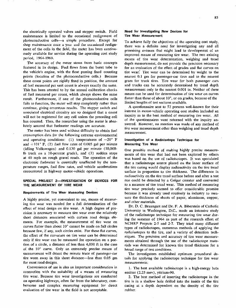
85

the electrically operated valves and stepper switch. Field maintenance is limited to the occasional realignment of photoconductive cells—a simple procedure. Except for shop maintenance once a year and Ihe uccasiojial realign-ment of the cells in the field, the meter has been continu-ously available for service during the operating cost study period, 1964-1969.

The accuracy of the meter stems from basic concepts featured in its design. Fuel flows from the buret tube to the vehicle's engine, with the float passing fixed counting points (location of the photoconductive cells.) Because these count points are rigidly fixed in position, the amount of fuel measured per unit count is always exactly the same. This has been attested to by the annual calibration checks of fuel measured per count, which always shows the same result. Furthermore, if one of the photoconductive cells fails to function, the meter will stop completely rather than continue, giving erroneous results. The stepper switch and associated electrical circuitry are so designed that a count will not be registered for any cell unless the preceding cell has counted. Thus, the researcher using the meter is abso-lutely assured that fuelmeter readings are accurate.

The meter has been used without difficulty to obtain fuel consumption data for the following extreme environmental and operating conditions: (1) temperatures of —20° F and +1010 F, (2) fuel flow rates of 0.005 gal per minute (idling Volkswagen) and 0.130 gal per minute (50,000-lb truck on a 10-percent grade), and (3) sudden stops at 40 mph on rough gravel roads. The operation of the electronic fuelmeter is essentially unaffected by the tem-perature ranges, fuel flow rates, and vehicle accelerations encountered in highway motor-vehicle operations.

SPECIAL PROJECT 2—INVESTIGATION OF DEVICES FOR

THE MEASUREMENT OF TIRE WEAR

Requirements of Tire Wear Measuring Devices

A highly precise, yet convenient to use, means of measur-ing tire wear was needed for a full determination of the effect of road design on tire wear. A high degree of pre-cision is necessary to measure tire wear over the relatively short distances associated with certain road design ele-ments. For example, the measurement of tire wear on curves flatter than about 10° cannot be made on full circles because few, if any, such circles exist. For these flat curves, the effect of the curvature on tire wear can be determined only if tire wear can be measured for operation on a por-tion of a circle, a distance of less than 4,000 ft in the case of the 100 curve. Only an extremely precise means of measurement will detect the minute trace of passenger-car tire worn away in this short distance—less than 0.05 gm for most road designs.

Convenience of use is also an important consideration in connection with the suitability of a means of measuring tire wear. Because tire wear investigations are conducted on operating highways, often far from the laboratory, cum-bersome and complex measuring equipment for direct evaluation of tire wear in the field is not acceptable.

Need for Investigating New Devices for

Tire Wear Measurement

To achieve fully the objectives of the operating cost study, there was a definite need for investigating any and all promising avenues that might lead to development of an improved means of measuring tire wear. The two existing means of tire wear determination, weighing and tread depth measurement, do not provide the precision necessary for an evaluation of the effect of grades and flat curves on tire wear Tire wear can be determined by weight to the nearest 0.1 gm for passenger-car tires and to the nearest gram for truck tires. Tire wear for both passenger cars and trucks can be accurately determined by tread depth measurement only to the nearest 0.001 in. Neither of these means can be used for determination of tire wear on curves flatter than those of about 100, or on grades, because of the limited lengths of test sections available.

A questionnaire sent to 52 persons well-known for their interest in motor-vehicle operating cost studies included an inquiry as to the best method of measuring tire wear. All of the questionnaires were returned with the inquiry an-swered. However, no mention was made of any method of tire wear measurement other than weighing and tread depth measurement.

Investigation of a Radioisotope Technique for

Measuring Tire Wear

One possible method of making highly precise measure-ments of tire wear that had not been explored by others was based on the use of radioisotopes. It was speculated that a radioisotope source placed on the inner surface of the tire casing would display radioactivity on the tire tread surface in proportion to tire thickness. The difference in radioactivity on the tire tread surface before and after a test run could be detected by a Geiger counter and converted to a measure of tire tread wear. This method of measuring tire wear precisely seemed to offer considerable promise because it was already used routinely in industry to mea-sure the thickness of sheets of paper, aluminum, copper, and other materials.

Dr. D. C. Braungart and Dr. F. A. Biberstein of Catholic University in Washington, D.C., made an intensive study of the radioisotope technique for measuring tire wear dur-ing the summer of 1964 as part of the research effort of NCHRP Projects 2-5 and 2-7. They tried many different types of radioisotopes, numerous methods of applying the radioisotopes to the tire, and a variety of detection tech-niques. The precision and accuracy of tire wear measure-ments obtained through the use of the radioisotope mate-rials was determined for known tire tread thickness for a broad range of test conditions.

The investigators established optimum procedural de-tails for applying the radioisotope technique for tire wear measurements:

The best available radioisotope is a high-energy beta emitter (2.25 mev), yttrium-90.

The best method of inserting the radioisotope in the tire is in a shallow hole drilled into the inside of the tire casing at a depth dependent on the density of the tire rubber.

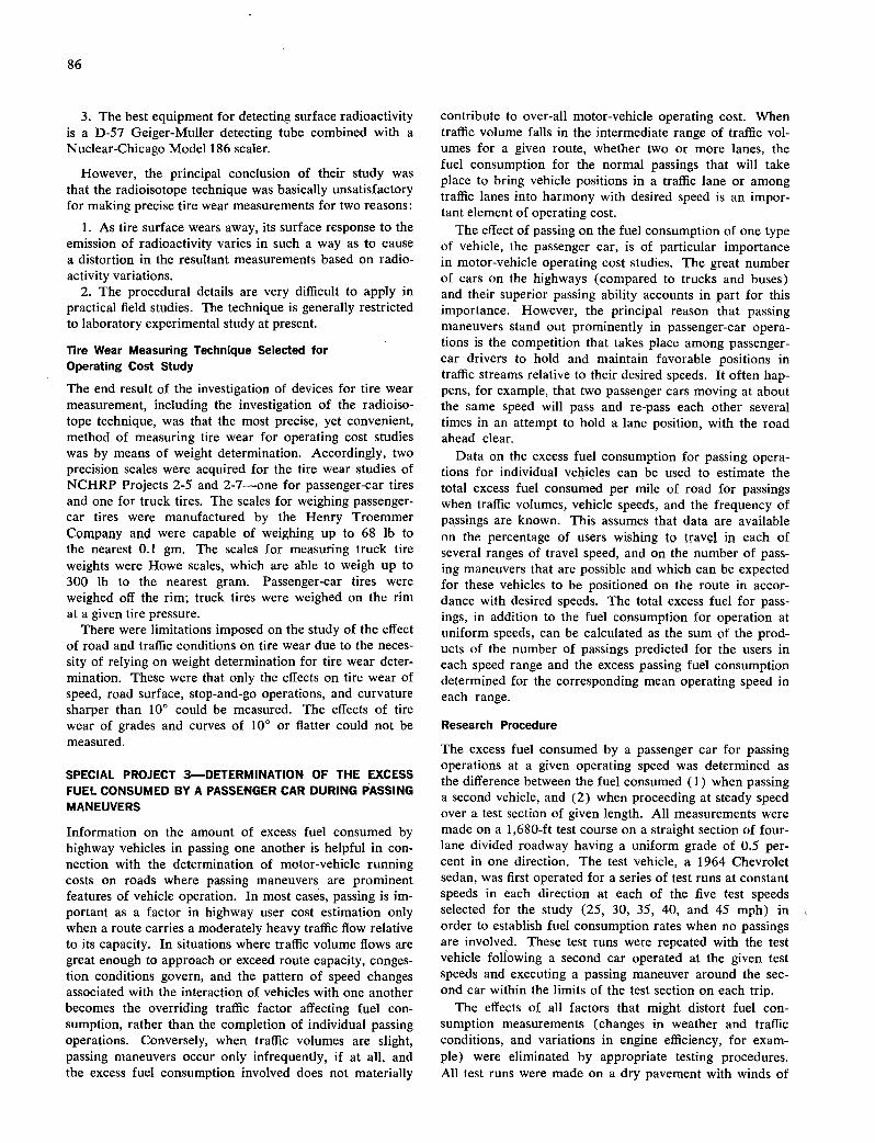
86

The best equipment for detecting surface radioactivity is a D-57 Geiger-Muller detecting tube combined with a Nuclear-Chicago Model 186 scaler.

However, the principal conclusion of their study was that the radioisotope technique was basically unsatisfactory for making precise tire wear measurements for two reasons:

As tire surface wears away, its surface response to the emission of radioactivity varies in such a way as to cause a distortion in the resultant measurements based on radio-activity variations.

The procedural details are very difficult to apply in practical field studies. The technique is generally restricted to laboratory experimental study at present.

Tire Wear Measuring Technique Selected for Operating Cost study

The end result of the investigation of devices for tire wear measurement, including the investigation of the radioiso-tope technique, was that the most precise, yet convenient, method of measuring tire wear for operating cost studies was by means of weight determination. Accordingly, two precision scales were acquired for the tire wear studies of NCHRP Projects 2-5 and 2-7--one for passenger-car tires and one for truck tires. The scales for weighing passenger-car tires were manufactured by the Henry Troemmer Company and were capable of weighing up to 68 lb to the nearest 0.1 gm. The scales for measuring truck tire weights were Howe scales, which are able to weigh up to 300 lb to the nearest gram. Passenger-car tires were weighed off the rim; truck tires were weighed on the rim at a given tire pressure.

There were limitations imposed on the study of the effect of road and traffic conditions on tire wear due to the neces-sity of relying on weight determination for tire wear deter-mination. These were that only the effects on tire wear of speed, road surface, stop-and-go operations, and curvature sharper than 10° could be measured. The effects of tire wear of grades and curves of 10° or flatter could not be measured.

SPECIAL PROJECT 3—DETERMINATION OF THE EXCESS FUEL CONSUMED BY A PASSENGER CAR DURING PASSING MANEUVERS

Information on the amount of excess fuel consumed by highway vehicles in passing one another is helpful in con-nection with the determination of motor-vehicle running costs on roads where passing maneuvers are prominent features of vehicle operation. In most cases, passing is im-portant as a factor in highway user cost estimation only when a route carries a moderately heavy traffic flow relative to its capacity. In situations where traffic volume flows are great enough to approach or exceed route capacity, conges-tion conditions govern, and the pattern of speed changes associated with the interaction of vehicles with one another becomes the overriding traffic factor affecting fuel con-sumption, rather than the completion of individual passing operations. Conversely, when traffic volumes are slight, passing maneuvers occur only infrequently, if at all, and the excess fuel consumption involved does not materially

contribute to over-all motor-vehicle operating cost. When traffic volume falls in the intermediate range of traffic vol-umes for a given route, whether two or more lanes, the fuel consumption for the normal passings that will take place to bring vehicle positions in a traffic lane or among traffic lanes into harmony with desired speed is an impor-tant element of operating cost.

The effect of passing on the fuel consumption of one type of vehicle, the passenger car, is of particular importance in motor-vehicle operating cost studies. The great number of cars on the highways (compared to trucks and buses) and their superior passing ability accounts in part for this importance. However, the principal reason that passing maneuvers stand out prominently in passenger-car opera-tions is the competition that takes place among passenger-car drivers to hold and maintain favorable positions in traffic streams relative to their desired speeds. It often hap-pens, for example, that two passenger cars moving at about the same speed will pass and re-pass each other several times in an attempt to hold a lane position, with the road ahead clear.

Data on the excess fuel consumption for passing opera-tions for individual vehicles can be used to estimate the total excess fuel consumed per mile of road for passings when traffic volumes, vehicle speeds, and the frequency of passings are known. This assumes that data are available on the percentage of users wishing to trav1 in each of several ranges of travel speed, and on the number of pass-ing maneuvers that are possible and which can be expected for these vehicles to be positioned on the route in accor-dance with desired speeds. The total excess fuel for pass-ings, in addition to the fuel consumption for operation at uniform speeds, can be calculated as the sum of the prod-ucts of the number of passings predicted for the users in each speed range and the excess passing fuel consumption determined for the corresponding mean operating speed in each range.

Research Procedure

The excess fuel consumed by a passenger car for passing operations at a given operating speed was determined as the difference between the fuel consumed (1) when passing a second vehicle, and (2) when proceeding at steady speed over a test section of given length. All measurements were made on a 1,680-ft test course on a straight section of four-lane divided roadway having a uniform grade of 0.5 per-cent in one direction. The test vehicle, a 1964 Chevrolet sedan, was first operated for a series of test runs at constant speeds in each direction at each of the five test speeds selected for the study (25, 30, 35, 40, and 45 mph) in order to establish fuel consumption rates when no passings are involved. These test runs were repeated with the test vehicle following a second car operated at the given test speeds and executing a passing maneuver around the sec-ond car within the limits of the test section on each trip.

The effects of all factors that might distort fuel con-sumption measurements (changes in weather and traffic conditions, and variations in engine efficiency, for exam-ple) were eliminated by appropriate testing procedures. All test runs were made on a dry pavement with winds of

87

3 mph or less and with temperatures ranging between 40° F and 550 F. Traffic volumes on the test section were relatively light at all times. Nevertheless, to assure that traffic conditions did not affect data, test runs were made only between 10:00 A.M. and 4:00 P.M. when interference by traffic was negligible. The combustion efficiency char-acteristics of the test vehicle's engine were determined by use of an exhaust gas analyzer with the vehicle on a dyna-mometer. Data on engine efficiency at the time of the tests were compared to corresponding values that had been established when the vehicle was new; this established the stability of engine efficiency at the time of the tests. Uni-formity of fuel energy characteristics was secured through use of fuel from a single source. Finally, tire pressures were maintained at constant pressure (28 psi), engine vacuum readings were kept steady for constant-speed runs, and the same driver operated the test vehicle for all test runs in any speed range.

All measurements. of fuel consumption were for opera-tion of the test vehicle from one end of the test course to the other. In the case of constant-speed runs, fuel con-sumption measurements were made for travel at a given uniform speed from a flag indicating one end of the test course to the flag indicating the other end of the course. For the passing runs, a second vehicle, also a passenger car, was used. It proceeded at a given constant speed for the full length of the test course while the test vehicle executed a passing maneuver around it. For these runs the test vehicle followed the second vehicle into the test section, moving at the same speed, and spaced behind it in a posi-tion considered by the driver to be close enough for passing without being dangerously close. Shortly after the test vehicle entered the test section the driver accelerated past the second vehicle and returned to the run lane as quickly as possible. The test vehicle was then allowed to slow to the given run speed (speed of the passed vehicle) without applying braking effort. Fuel consumption mea-surements for each test run, both constant speed and passing runs, were made with the electronic fuelmeter.

A minimum of 30 test runs were made in each direction for each run speed selected for the study (25, 30, 35, 40, and 45 mph) both for constant-speed runs and for passing runs, for a total of more than 600 runs. A full set of test data was obtained for each direction in order that the excess fuel consumption for passing could be computed for each direction (and thus reflect the effect of the 0.5-percent gradient) as well as for the combination of both directions to develop values for passings on a nearly level route.

In addition to a record of the fuel consumption of the test vehicle and the speed of the passed vehicle during each test run, a careful record was made of all the elements of the passing maneuver that are related in any way to vehicle fuel consumption. These included the elapsed time for the passing operation, the length of road over which the pass-ing operation took place, the maximum rates of speed and acceleration during passing operations, and the speed of the passing vehicle just as it returns to the travel lane after completion of the passing maneuver. The elapsed time during passing was established by starting a stopwatch as a

passing maneuver was begun and stopping the watch when the passing vehicle returned to the travel lane. The distance traversed during passing was found by noting the points along the road, both where each passing operation began and where it ended, and measuring the distance between these points. This was greatly facilitated by setting markers with identifying numbers at 15-ft intervals for the full length of the test course. The numbers on the markers could be read from the moving vehicle. The maximum rate of acceleration during passing was determined by watching a calibrated direct-reading accelerometer and noting the maximum reading. Vehicle speeds, both the maximum speed during passing and the speed on returning, to the travel lane, were read on a calibrated survey-type speed-ometer.

In summary, the principal elements of data obtained in the field for this study consisted of run times and fuel con-sumption rates for the test vehicle, both for test runs where the test vehicle traveled at constant speed and for test runs where the test vehicle passed a second vehicle traveling at constant speed. In each case, more than 30 test runs were made in each direction at each of five run speeds used for the constant-speed runs. A complete record was made of all pertinent information for each passing maneuver.

The primary analysis of the data involved determination of the average increase in the fuel consumption of the test vehicle for runs when it was used to pass a second vehicle, compared to runs when it proceeded at constant speed for each of the five run speeds used in the study. Three values of the excess fuel consumption for passing were computed for each run speed: (1) in the direction up the 0.5-percent grade, (2) in the direction down the 0.5-percent grade, and (3) for the combined direction where the 0.5-percent grade is upgrade and downgrade for equal distances. The value for the combined directions is essentially that for opera-tion on a level road.

Associated analyses included determination of the aver-age length of road transversed during passing operations, the average time consumed in passing, maximum accelera-tion rates and speeds achieved in passing, and average speeds of vehicles when returning to the travel lane on com-pletion of passing maneuvers.

Data and Analysis

Fuel consumption data obtained for this study are given in Table F-i by run speed and by direction of travel, including the combined values for both directions. Because the mag-nitude of these values of fuel consumption is small, cubic centimeters rather than gallons are used as units of volume measurement. Confidence ranges on the 95-percent level and variances are given, as well as mean fuel consumption values. The mean fuel consumption values given in Col. 2 are for constant-speed operation; those in Col. 5 are for runs when passing maneuvers were executed. Those in Col. 8 are the excess fuel consumption values for passing.

Data on several aspects of the passing maneuvers for which fuel consumption data were obtained are given in Table F-2. Data in this table are maximum accelerations and speeds during passing, elapsed times and route dis-

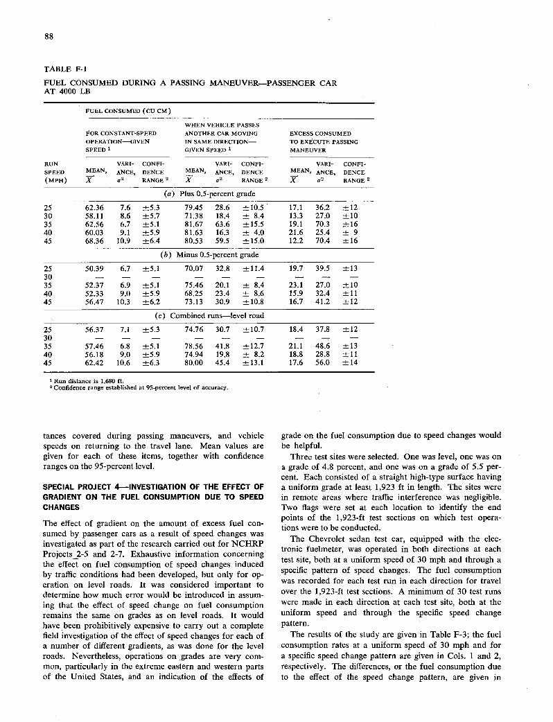
88

TABLE F-i

FUEL CONSUMED DURING A PASSING MANEUVER-PASSENGER CAR AT 4000 LB

FUEL CONSUMED (CU CM)

WHEN VEHICLE PASSES FOR CONSTANT-SPEED ANOTHER CAR MOVING EXCESS CONSUMED OPERATION-GIVEN IN SAME DIRECTION- TO EXECUTE PASSING SPEED 1 GIVEN SPEED 1 MANEUVER

RUN VARI- CONFI- VARI- CONFI- VARI- CONFI- SPEED MEAN, ANCE, DENCE MEAN, ANCE, DENCE MEAN, ANCE, DENCE (MPH) X a2 RANGE 2 X a2 RANGE 2 X 0-2 RANGE 2

(a) Plus 0.5-percent grade

25 62.36 7.6 ±5.3 79.45 28.6 ± 10.5 17.1 36.2 ±12 30 58.11 8.6 ±5.7 71.38 18.4 ± 8.4 13.3 27.0 ±10 35 62.56 6.7 ±5.1 81.67 63.6 ±15.5 19.1 70.3 ±16 40 60.03 9.1 ±5.9 81.63 16.3 ± 4.0 21.6 25.4 ± 9 45 68.36 10.9 ±6.4 80.53 59.5 ±15.0 12.2 70.4 ±16

(b) Minus 0.5-percent grade

25 50.39 6.7 ±5.1 70.07 32.8 ±11.4 19.7 39.5 ±13 30 - - - - - - - - - 35 52.37 6.9 ±5.1 75.46 20.1 ± 8.4 23.1 27.0 ±10 40 52.33 9.0 ±5.9 68.25 23.4 ± 8.6 15.9 32.4 ±11 45 56.47 10.3 ±6.2 73.13 30.9 ±10.8 16.7 41.2 ±12

(c) Combined runs-level road

25 56.37 7.1 ±5.3 74.76 30.7 ±10.7 18.4 37.8 ±12 30 - - - - - - - -,- - 35 57.46 6.8 ±5.1 78.56 41.8 ±12.7 21.1 48.6 ±13 40 56.18 9.0 ±5.9 74.94 19.8 ± 8.2 18.8 28.8 ±11 45 62.42 10.6 ±6.3 80.00 45.4 ±13.1 17.6 56.0 ±14

'Run distance is 1,680 ft. 2 Confidence range established at 95-percent level of accuracy

tances covered during passing maneuvers, and vehicle speeds on returning to the travel lane. Mean values are given for each of these items, together with confidence ranges on the 95-percent level.

SPECIAL PROJECT 4-INVESTIGATION OF THE EFFECT OF GRADIENT ON THE FUEL CONSUMPTION DUE TO SPEED CHANGES

The effect of gradient on the amount of excess fuel con-sumed by passenger cars as a result of speed changes was investigated as part of the research carried out for NCHRP Projects 2-5 and 2-7. Exhaustive information concerning the effect on fuel consumption of speed changes induced by traffic conditions had been developed, but only for op-eration on level roads. It was considered important to determine how much error would be introduced in assum-ing that the effect of speed change on fuel consumption remains the same on grades as on level roads. It would have been prohibitively expensive to carry out a complete field investigation of the effect of speed changes for each of a number of different gradients, as was done for the level roads. Nevertheless, operations on grades are very com-mon, particularly in the extreme eastern and western parts of the United States, and an indication of the effects of

grade on the fuel consumption due to speed changes would be helpful.

Three test sites were selected. One was level, one was on a grade of 4.8 percent, and one was on a grade of 5.5 per-cent. Each consisted of a straight high-type surface having a uniform grade at least 1,923 ft in length. The sites were in remote areas where traffic interference was negligible. Two flags were set at each location to identify the end points of the 1,923-ft test sections on which test opera-tions were to be conducted.

The Chevrolet sedan test car, equipped with the elec-tronic fuelmeter, was operated in both directions at each test site, both at a uniform speed of 30 mph and through a specific pattern of speed changes. The fuel consumption was recorded for each test run in each direction for travel over the 1,923-ft test sections. A minimum of 30 test runs were made in each direction at each test site, both at the uniform speed and through the specific speed change pattern.

The results of the study are given in Table F-3; the fuel consumption rates at a uniform speed of 30 mph and for a specific speed change pattern are given in Cols. 1 and 2, respectively. The differences, or the fuel consumption due to the effect of the speed change pattern, are given in

89

TABLE F-2

MAGNITUDE OF VARIOUS ELEMENTS OF THE PASSING MANEUVER OF A PASSENGER CAR THAT MAY AFFECT FUEL CONSUMPTION OF THE PASSING VEHICLE

ROAD DISTANCE

MAX. ACCELERATION MAX. SPEED ELAPSED TIME TRAVERSED

DURING PASSING DURING PASSING DURING PASSING DURING PASSING

(MPH/SEc) (MPH) (sEC) (FT)

RUN CONFI- CONFI- CONFI- CONFI-

SPEED MEAN, DENCE MEAN, DENCE MEAN, DENCE MEAN, DENCE

(MPH) X RANGE 1 X MNGE 1 X RANGE 1 X RANGE'


25 3.0 ±1 40 ±7 12.0 ±3 664 ±209 30 2.6 ±1 42 ±5 11.3 ±3 649 ±314 35 3.0 ±1 50 ±5 11.4 ±2 780 ±147 40 2.5 ±1 52 ±2 12.3 ±3 - - 45 2.3 ±1 56 ±7 12.8 ±3 1024 ± 50

(b) Minus 0.5-percent grade

25 2.8 ±1 40 ±4 11.4 ±3 623 ±160 30 - - - - - - - - 35 2.9 ±1 50 ±5 11.4 ±2 785 ±200 40 2.2 ±1 51 ±4 12.9 ±3 992 ±400 45 2.1 ±1 55 ±4 13.5 ±3 - -

(c) Combined runs-level road

25 2.9 ±1 40 ±5 11.7 ±3 643 ±185 30 - - - - - - - - 35 2.9 ±1 50 ±5 11.4 ±2 782 ±175 40 2.4 ±1 52 ±5 13.1 ±3 - - 45 2.2 ±1 55 ±5 13.3 ±3 - -

'Confidence range established at 95-percent level of accuracy

Col. 3. The percentage differences in excess fuel consump-tion due to speed changes for operation on level roads and on grades are given in Col. 3, both for the 4.8-percent grades and for the 5.5-percent grades.

The excess fuel consumption due to the speed change pattern is only 6 percent different for operation on positive grades, compared to operation on level roads. However, it is 13 percent different for operation on negative grades, compared to operation on level roads. The discrepancy of 6 percent in the value of fuel consumption for speed changes on plus grades is not serious because the over-all project accuracy allows for discrepancies of as much as 5 percent. However, fuel consumption due to speed changes on down grades should be estimated at at least 10 percent greater than the fuel consumption for the same speed changes on the level road.

SPECIAL PROJECT 5-MOTOR-VEHICLE ACCIDENT COSTS

RELATIVE TO ROAD DESIGN

A special study was undertaken with the assistance of Dr. W. E. Corgill to review available research data on motor-vehicle accidents and their costs in order to develop rea-sonable estimates of the effects that various road designs have on user accident costs.

Two items of information are needed to evaluate high-way user accident costs in relation to road design: (1) accident rates as affected by highway design details (curves, grades, and intersections, for example) and (2) average motor-vehicle user costs per accident. For this information to be applicable in accident cost analysis, however, the two items-accident rates and accident costs -should be compatible or developed on the same basis so they can be combined to obtain accident costs as func-tions of road design.

Unfortunately, most existing accident research data have not been developed with compatible accident frequency and accident cost rates. Good information on accident rates relative to road design is available-but only for reported accidents. Unreported accidents are not repre-sented and, in most cases, the number and type of vehicles involved in accidents are not given. On the other hand, accident cost information is available only by vehicle in-volvement. Although sometimes aggregated as cents per accident cost per vehicle-mile of over-all travel, accident costs per accident or per reported accident are not available.

This data incompatibility arises naturally. Information on accident frequency in relation to road design is found by examining historical records of accidents occurring at

90

TABLE F-3

EFFECT OF GRADIENT ON THE EXCESS FUEL CONSUMPTION CAUSED BY SPEED CHANGES-PASSENGER CAR

FUEL CONSUMPTION (GPM)

UNIFORM SPEED' SPEED CHANGES' EXCESS DUE TO SPEED CHANGES ITEM (1) (2) (C0L. 2-COL. 1) (3)


On grade 0.0830 0.0997 0.0167 On level 0.0486 0.0642 0.0156 Difference 0.0344 0.0355 0.0011 % difference 6

(b) Plus 5.5-percent grade


(c) Minus 4.8-percent grade


(d) Minus 5.5-percent grade


'Uniform speed is 30 mph. 'Speed change pattern adhered to is as follows: 30 mph for 210 ft; followed by a decrease in speed from

30 to 20 mph in 207 ft; followed by constant-speed operation at 20 mph for 281 ft; followed by increase in speed from 20 to 35 mph in 280 ft; followed by constant-speed operation at 35 mph for 267 ft; followed by a decrease in speed from 35 to 25 mph in 147 ft; followed by constant-speed operation at 25 mph for 272 ft; followed by an increase in speed from 25 to 30 mph in 259 ft. Tolal test distance was 1,923 ft.

road locations having particular design characteristics. Such records are often lacking in detail, so that the investigator must be content with a simple count of acci-dents, without knowing the number or types of vehicles involved. On the other hand, accident costs are determined in the present by interviewing people who have been involved in accidents. This provides accident cost informa-tion per vehicle involved per accident, without including all vehicles involved in any given accident. Except for single-vehicle accidents, cost per accident involvement is only part of the cost per accident.

The problem of using existing accident cost research data for evaluating user accident costs is further compli-cated by disagreement among researchers as to what should be included in computing accident involvement cost. Some include only costs for reported accident involvements, whereas others develop composite costs for reported and unreported accident involvements. A few researchers com-pute involvement costs based on including in fatal accident costs evaluations of the present worth of the future earn-ings of the deceased, had they lived. Usually, however, neither this cost item nor funeral expenses is included as direct accident cost.

Procedure for Evaluating Total Accident Costs per Reported Accident

A solution to the problem of estimating the cost of acci-dents in relation to road design, despite the basic incom-patibility of accident frequency and accident cost data, was worked out for NCHRP Project 2-5. It consisted essentially in using existing accident cost information to develop factors equal to the average cost of passenger-car accidents and factors equal to the average cost of truck accidents for each reported accident. Because information on the frequency of accidents by road design is given as reported accidents per unit of exposure (million vehicle-miles of travel, usually), these factors can be multiplied by accident frequency rates to obtain passenger-car and truck accident costs for the given unit of exposure.

Most existing accident cost data give the average cost of an accident involvement, including both reported and unreported accidents. Therefore, the first step in the development of the average cost factors for reported accidents was to compute the average number of total accidents for each reported accident by type of road. The second step was to determine the number of involvements

91

for each accident, both reported and unreported. The products of these two sets of values are the ratios of num-ber of vehicle involvements to number of reported acci-dents by type of road.

The third step was to compute the average direct cost of a motor-vehicle accident involvement for (1) passenger cars and (2) trucks, based on the average costs of both reported and unreported involvements (excluding funeral costs and future earnings for fatal accidents).

The fourth step was to determine the percentage of vehicle involvement in the average accident that are passenger cars and the percentage that are trucks, on the basis of exposure—namely, the relative vehicle-miles of travel for each vehicle classification. The products of these percentages and the ratios of number of involvements to number of reported accidents by type of road (found as described in Steps 1 and 2) give ratios of involvements to reported accidents by vehicle type (passenger cars and trucks) as well as by type of road.

The fifth step was to combine the ratios of number of involvements to number of reported accidents with the average direct costs of accident involvement by vehicle type and road type. The results were two series of factors by type of road, one equal to the average costs of passenger-car accidents and the other equal to the average cost of truck accidents for each reported accident.

These two series of factors, one for passenger cars and one for trucks, may be multiplied by accident rates ex-pressed as number of reported accidents per million vehicle-miles of travel to obtain accident costs by vehicle type per million vehicle-miles of travel. For example, where the average accident rate per million vehicle-miles on a given road type is known, it can be multiplied by the cost factor for passenger cars and by the cost factor for trucks to obtain the average cost of passenger-car and truck acci-dents per million vehicle-miles of travel on the given road type.

The end products of this analysis procedure are average accident costs for passenger cars and for trucks per unit of over-all travel mileage (usually million vehicle-miles of travel). That is, the procedure does not give passenger-car accident costs per million vehicle-miles of passenger car travel nor truck accident costs per million vehicle-miles of truck travel. Rather, it gives passenger-car accident costs and truck accident costs per million vehicle-miles of combined travel of passenger cars and trucks.

Evaluation of Passenger-Car and Truck Accident Costs per

Reported Accident

Ratios developed for Steps 1 and 2 of the procedure are given in Table F-4 for each of the four principal route categories: non-freeway urban, non-freeway rural, freeway urban, and freeway rural. Ratios of total accidents to reported accidents (Col. 2) were established from ratios of total to reported accidents determined for California in 1964 and given by Smith and Tamburri according to class of accident severity (1). California's ratios of total to reported accidents, expressed as percentages, are the following:

PERCENTAGE OF TOTAL ACCIDENTS REPORTED

PROPERTY DAMAGE

AREA FATAL INJURY ONLY

Rural 100 92 41 Urban 100 95 34

These ratios (percentages) were reduced to two (one for urban areas, and one for rural areas) by computing aver-ages weighted according to total number of fatal, injury, and property-damage-only accidents listed in Accident Facts for 1968 (2). The number of fatal, injury, and property-damage-only accidents for 1968 is as follows:

TABLE F-4

RATIOS OF TOTAL ACCIDENTS TO REPORTED ACCIDENTS, AND OF ACCIDENT INVOLVEMENTS BOTH TO TOTAL ACCIDENTS AND TO REPORTED ACCIDENTS

RATIO

TOTAL ACCIDENTS ACCIDENT INVOLVE- ACCIDENT INvOLvE-

TO REPORTED MENTS TO TOTAL MENTS TO REPORTED

ROAD TYPE ACCIDENTS' ACCIDENTS 2 ACCIDENTS

(1) (2) (3) (4)

Non-freeway: Rural 2.08 1.61 3.34 Urban 2.56 1.91 4.89

Freeway: Rural 2.08 1.55 3.22 Urban 2.56 1.81 4.63

1 Computed from data on accident severity given in Accident Facts (2. p. 45) and from data on the relation-ships of reported to total accidents in California as given by Smith and Tamburri (1, p. 15). I Data for California highways as given by Smith and Tamburri (1, p. 13). 3 Product of values in Cols. 2 and 3.

92

NUMBER OF ACCIDENTS IN 1968-NATIONWIDE

PROPERTY DAMAGE AREA FATAL INJURY ONLY

Rural 30,600 520,000 3,700,000 Urban 16,200 780,000 9,600,000

The weighted average ratios of reported to total acci-dents were found to be 0.48 for rural areas and 0.39 for urban areas. The reciprocals of these values, 2.08 and 2.56, respectively, are the ratios of total accidents to reported accidents developed for NCHRP Project 2-5. They are given in Col. 2, Table F-4.

The ratios of accident involvements to total accidents (Col. 3, Table F-4) are averages of the number of vehicles involved per accident on non-freeway rural, non-freeway urban, freeway rural, and freeway urban routes. Each of the ratios is the direct average of the ratios given by Smith and Tamburri for fatal, injury, and property-damage-only accidents, based on California's experience in 1964 (1).

The ratios of number of accident involvements to num-ber of reported accidents are given in Col. 4, Table F-4. These were computed by multiplying the values of Cols. 2 and 3, Table F-4.

The average costs of accident involvements, including both reported and unreported accidents, for passenger cars and trucks are given in Table F-5. The average cost of a passenger-car involvement is $196 and of a truck involve-ment is $141, based on price levels of 1955-1958. These values are averages of those determined for the accident cost studies conducted in Massachusetts, Utah, and Illinois during the period from 1953 to 1958.

The average cost of an accident involvement for reported and unreported accidents in Massachusetts was given by McCarthy as $200 for passenger cars and $143 for trucks (3). Similarly, the average cost of an accident involvement for reported and unreported accidents in

TABLE F-5

AVERAGE DIRECT COST OF REPORTED AND UNREPORTED ACCIDENT INVOLVEMENTS-PASSENGER CARS AND TRUCKS'

AVERAGE COSTS

($)

PASS. SOURCE STUDY CARS TRUCKS

Massachusetts accident cost study (1953)2 200 143 Utah accident cost study (1957) 191 138 Illinois accident cost study (1958) 196 141 Average 196 141

1 Costs based on price levels of 1955-1958. "From McCarthy (3, Fig. 2, P. 26),

From Ref. 5. Computed from given percentages of accidents falling in each of several ranges of accident cost.

4 From Billingsley and Jorgenson (4, Table 2, p. 52).

Illinois was given by Billingsley and Jorgenson as $196 for passenger cars and $141 for trucks (4).

The average costs of accident involvements for reported and unreported accidents in Utah were computed from the following distribution of passenger-car and truck accident involvement costs given in the published results of the Utah study (5):

PASSENGER CARS

COST RANGE PERCENT

TRUCKS

COST RANGE PERCENT

$ 0-9.9 3.2 $ 0-4.9 12.7 10-29.9 9.8 5-24.9 10.8 30-49.9 12.0 25-44.9 19.0 50-99.9 24.6 45-94.9 21.8

100-199.9 18.8 95-194.9 16.2 200-299.9 9.6 195-294.9 4.4 300-399.9 5.1 295-394.9 2.6 400-499.9 3.6 395-494.9 2.2 500+ 13.3 495+ 10.3

Total 100.0 Total 100.0

Average cost, assuming Average cost, assuming mid-point of upper range mid-point of upper range of cost is $600, = $191 of cost is $595, = $138

The results of the more recent Washington-area motor-vehicle accident cost study (6, data for 1965) are not included in the averages given in Table F-S for two rea-sons: (1) the Washington accident cost analysis differ-entiated costs by vehicle type only for reported accidents-not for reported and unreported accidents together, and (2) only the Washington study included future earnings of deceased persons in fatal-accident cost computations-an amount equal to about 25 percent of the total reported accident costs. The Washington study results-$527 per reported accident and $74 per unreported accident-can be adjusted for comparison with the results of the other studies by reducing the reported accident cost by 25 percent to remove the fatality's future earnings factor and by averaging the reported and unreported accident costs weighted according to their relative frequency, one reported accident for every 1.8 unreported accidents. The adjust-ment gives a single accident cost value of $189 per acci-dent, reported and unreported, for passenger cars and trucks. This value is very nearly the same as the average of those found in the Massachusetts, Illinois, and Utah studies for passenger cars.

The average distributions of passenger cars and trucks in accidents on rural and urban routes are given in Col. 2, Table F-6. These were established equal to the correspond-ing distribution of vehicle-miles of travel for passenger cars and trucks on the theory that vehicle involvements in accidents are proportional to exposure to accidents as measured by travel mileage. Annual miles of travel by passenger cars and trucks are given in the "Supplementary Report of the Highway Cost Allocation Study" (7, Table 11).

93

TABLE F-6

DISTRIBUTION OF PASSENGER CARS AND TRUCKS BY ROAD TYPE, TOGETHER WITH PASSENGER-CAR AND TRUCK ACCIDENT INVOLVEMENTS AND COSTS PER REPORTED ACCIDENT

ACCIDENT INVOLVE- ACCIDENT COSTS DISTRIBUTION OF MENTS PER PER REPORTED VEHICLE TYPES' REPORTED ACCIDENT' ACCIDENT ($)

(2)

(3)

(4)

ROAD TYPE PASS. PASS. PASS. (1) CARS TRUCKS CARS TRUCKS CARS TRUCKS

Non-freeway: Rural 0.77 0.23 2.57 0.77 504 109 Urban 0.85 0.15 4.16 0.73 815 103

Freeway: Rural 0.77 0.23 2.48 0.74 486 104 Urban 0.85 0.15 3.93 0.70 770 99

'See Ref. 7, Table 11, p. 55. 2 Product of Col. 2, this table, and Col. 4, Table F-4. 'Product of Col. 3, this table, and average accident costs of Table F-5

Accident involvements per reported accident by vehicle type are given in Col. 3, Table F-6. These were found by multiplying the vehicle distributions given in Col. 2, Table F-6, by the ratios of accident involvements to reported accidents given in Col. 4, Table F-4.

Average accident costs per reported accident by vehicle type are given in Col. 4, Table F-6. These were computed by multiplying accident involvements per reported accident (Col. 3, Table F-6) by the average cost of accidents—$196 for passenger cars and $141 for trucks (Table F-5).

Accident Costs per Million Vehicle-Miles of Travel

Rates of reported accidents per million vehicle-miles of over-all travel are given in Col. 2 of Table F-7 for non-freeway and freeway, rural and urban routes, and in Col. 2 of Table F-8 for various sharpness of curvature and frequencies of intersections on non-freeway rural routes. The rates of reported accidents by route type (Table F-7)

were taken from "The Federal Role in Highway Safety" (8, Fig. 4, p. 58). The rates of reported accidents by sharpness of curvature and frequencies of intersections were taken from Raff's study of Interstate Highway acci-dents (9).

The average costs of passenger-car accidents and truck accidents per million vehicle-miles of over-all travel (com-bined car and truck travel) are given in Col. 3 of Tables F-7 and F-8 for the given road types and design charac-teristics. These costs were found by multiplying the acci-dent rates of Col. 2, Tables F-7 and F-8, by the correspond-ing values in Col. 4 of Table F-6. Table F-7 gives passenger-car and truck accident costs for every million vehicle-miles of travel by road type.

Table F-8 gives accident costs for travel on non-freeway rural routes having sharp curvature and frequent inter-sections.

TABLE F-7

RATES OF REPORTED ACCIDENTS AND RATES OF TOTAL ACCIDENT COSTS BY VEHICLE TYPE FOR FREEWAY AND NON-FREEWAY ARTERIAL ROUTES

REPORTED ACCIDENTS PER MILLION VEHICLE-MILES

OF COMBINED TRAVEL ROAD TYPE (PASS. CARS AND TRUCKS) (1) (2)

TOTAL ACCIDENT COSTS PER MILLION VEHICLE-MILES

OF COMBINED TRAVEL ($)' (3)

PASS. CARS TRUCKS

Non-freeway: Rural 3.32 1,673 362 Urban 5.26 4,287 541

Freeway: Rural 1.51 734 157 Urban 1.86 1,430 184

'From Ref. 8, p. 58. 2 Product of Col. 2, this table, and Col. 4, Table F-6

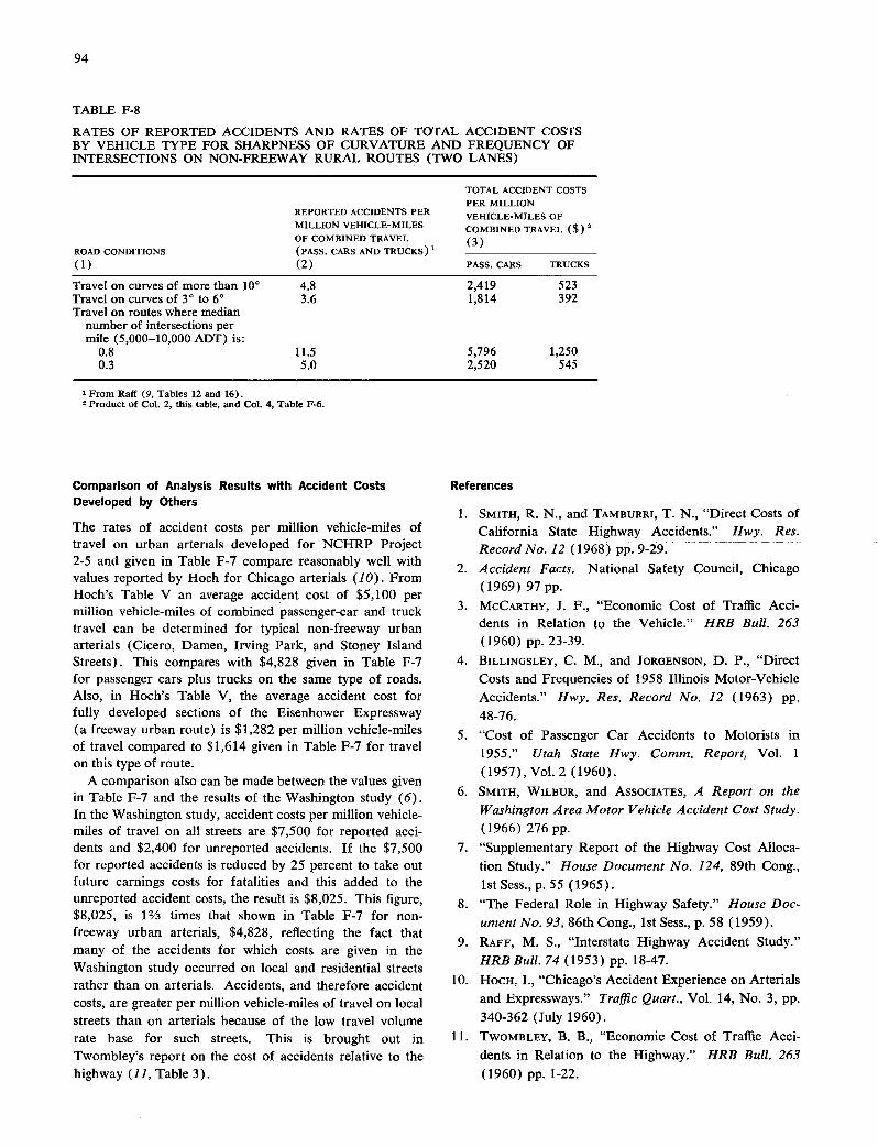
94

TABLE F-8

RATES OF REPORTED ACCIDENTS AND RATES OF TOTAL ACCIDENT COSTS BY VEHICLE TYPE FOR SHARPNESS OF CURVATURE AND FREQUENCY OF INTERSECTIONS ON NON-FREEWAY RURAL ROUTES (TWO LANES)

TOTAL ACCIDENT COSTS

REPORTED ACCIDENTS PER PER MILLION VEHICLE-MILES OF

MILLION VEHICLE-MILES COMBINED TRAVEL ($) 2 OF COMBINED TRAVEL (3)

ROAD CONDITIONS (PASS. CARS AND TR' (1) (2) PASS. CARS TRUCKS

Travel on curves of more than 100 4.8 2,419 523 Travel on curves of 30 to 6° 3.6 1,814 392 Travel on routes where median

number of intersections per mile (5,000-10,000 ADT) is:

0.8 11.5 5,796 1,250 0.3 5.0 2,520 545

1 From Raff (9, Tables 12 and 16). Product of Col. 2, this table, and Col. 4, Table F-6.

Comparison of Analysis Results with Accident Costs References

Developed by Others SMITH, R. N., and TAMBURRI, T. N., "Direct Costs of

The rates of accident costs per million vehicle-miles of California State Highway Accidents." Hwy. Res. travel on urban arterials developed forNCHRP Project Record No. 12 (1968) pp.9-29. 2-5 and given in Table F-7 compare reasonably well with

Accident Facts. National Safety Council, Chicago values reported by Hoch for Chicago arterials (10). From

(1969) 97 pp. Hoch's Table V an average accident cost of $5,100 per million vehicle-miles of combined passenger-car and truck MCCARTHY, J. F., "Economic Cost of Traffic Acci-

travel can be determined for typical non-freeway urban dents in Relation to the Vehicle." HRB Bull. 263

arterials (Cicero, Damen, Irving Park, and Stoney Island (1960) pp. 23-39.

Streets). This compares with $4,828 given in Table F-7 BILLINGSLEY, C. M., and JORGENSON, D. P., "Direct

for passenger cars plus trucks on the Same type of roads. Costs and Frequencies of 1958 Illinois Motor-Vehicle Also, in Hoch's Table V, the average accident cost for Accidents." Hwy. Res. Record No. 12 (1963) pp. fully developed sections of the Eisenhower Expressway 48-76. (a freeway urban route) is $1,282 per million vehicle-miles "Cost of Passenger Car Accidents to Motorists in of travel compared to $1,614 given in Table F-7 for travel 1955." Utah State Hwy. Comm. Report, Vol. 1 on this type of route.

(1957), Vol.2 (1960). A comparison also can be made between the values given

in Table F-7 and the results of the Washington study (6). SMITH, WILBUR, and ASSOCIATES, A Report on the

In the Washington study, accident costs per million vehicle- Washington Area Motor Vehicle Accident Cost Study.

miles of travel on all streets are $7,500 for reported acci- (1966) 276 pp.

dents and $2,400 for unreported accidents. If the $7,500 "Supplementary Report of the Highway Cost Alloca- for reported accidents is reduced by 25 percent to take out tion Study." House Document No. 124, 89th Cong., future earnings costs for fatalities and this added to the lstSess., p.SS (1965). unreported accident costs, the result is $8,025. This figure, "The Federal Role in Highway Safety." House Doc- $8,025, is 12/3 times that shown in Table F-7 for non- ument No. 93, 86th Cong., 1st Sess., p. 58 (1959). freeway urban arterials, $4,828, reflecting the fact that many of the accidents for which costs are given in the

RAFF, M. S., "Interstate Highway Accident Study."

Washington study occurred on local and residential streets HRB Bull. 74 (1953) pp. 18-47.

rather than on arterials. Accidents, and therefore accident HOCH, I., "Chicago's Accident Experience on Arterials

costs, are greater per million vehicle-miles of travel on local and Expressways." Traffic Quart., Vol. 14, No. 3, pp.

streets than on arterials because of the low travel volume 340-362 (July 1960).

rate base for such streets. This is brought out in TWOMBLEY, B. B., "Economic Cost of Traffic Acci-

Twombley's report on the cost of accidents relative to the dents in Relation to the Highway." HRB Bull. 263

highway (11, Table 3). (1960) pp. 1-22.

95

SPECIAL PROJECT 6—ANNOTATED BIBLIOGRAPHY OF RELATIONSHIPS BETWEEN ACCIDENT COSTS AND ROAD DESIGN, 1950-1970

The following items providc a full coverage of references containing research data on motor-vehicle accident costs relative to road design that are applicable in road user cost analyses. The items are listed in chronological order.

GLANvILLE, W. H., Road Safety and Road Research. Royal Society of Arts, London (1951) 51 pp.

This report includes data on accident rates on curves on non-freeway roads in England. On curves greater than 4°, accident rates range up-ward from 3.5 accidents per million vehicle-miles of travel. Kipp, 0. L., "Minnesota Roadwide Survey. Progress Report on Accident, Access Point and Advertising Sign Study in Minnesota." HRB Bull. 38 (1951) pp. 68-72.

This article contains brief information on acci-dent rates noted in Minnesota. It was found that accident rates per million vehicle-miles of travel on curves were approximately 11/3, 21/2 ,

and 4 for 3°, 4°, and more than 4°, respectively. BELMONT, D. M., "Effect of Average Speed and Volume on Motor Vehicle Accidents on Two-Lane Tangents." Proc. HRB, Vol. 32 (1953) pp. 383-395.

Accidents on two-lane roads under both opti-mum and restrictive conditions. RAFF, M. S., "Interstate Highway-Accident Study." HRB Bull. 74(1953) pp. 18-47.

This article reports on a comprehensive in-vestigation of the frequency of accidents on primary rural highways having particular design characteristics. It does not give rates of vehicle accident involvement by type of vehicle, an important consideration for road user cost evalua-tion.

A series of tables gives accident rates per million vehicle-miles of travel by road cross-section design, traffic volume, frequency and sharpness of curvature, frequency of intersections, frequency of commercial and residential access points, and frequency of grades. BITZEL, I. F., "Effect of Motorway Design on Acci-dents in Germany." Roads and Roads Construction, Vol. 35, No. 409, p. 17 (Jan. 1957).

A comprehensive study of accident rates on German freeways as affected by design details and traffic. Information on the effect of combina-tions of grade and curvature on accidents rates provided in this article is particularly valuable for user accident cost studies. "The Federal Role in Highway Safety." House Doc-ument No. 93, 86th Cong., 1st Sess. (1959) 232 pp.

This report contains numerous tables and graphs depicting accident frequencies for a variety of operating conditions. Of particular use in road user cost analyses is Figure 12, page 81, which shows rates of accident involvement by

vehicle type based on the results of a broad study of accidents covering nearly 4 billion vehicle-miles of travel and 10,000 vehicles. "Cost of Passenger Car Accidents to Motorists in 1955." Utah State Hwy. Comm. Report, Vol. 1 (1957), Vol. 2 (1960).

This report provides accident involvement costs for passenger cars and trucks registered in Utah in 1957 without distinction as to the design characteristics of the road where the accidents occurred. The percentages of accident involve-ments that took place on one-way, two-way, and divided roadways by number of lanes and on both Federal-aid primary and Federal-aid second-ary routes are given. However, because the relationships between accident involvements and traffic volumes are not given, these percentages cannot be used for road user cost analysis.

The average cost of reported and unreported accident involvement costs in Utah in 1957 was $191 for passenger cars and $138 for trucks (assuming $600 as the mid-point cost value for the top cost range designated as "over $500"). These values agree well with those developed in Massachusetts ($200 for passenger cars and $143 for trucks) and in Illinois ($196 for passenger cars and $141 for trucks.) HOCH, I., "Chicago's Accident Experience on Arterials and Expressways." Traffic Quart., Vol. 14, No. 3, pp. 340-362 (July 1960).

In 1958 accident costs on Chicago's arterial streets and on its Congress Expressway were evaluated using accident frequencies for these streets and expressway and using average cost of accident involvements as determined in Mas-sachusetts in 1953. Results of interest in user cost accident analysis are given in Table V, page 354. MCCARTHY, J. F., "Economic Cost of Traffic Acci-dents in Relation to the Vehicle." HRB Bull. 263 (1960) pp. 23-39.

The data on accident involvement costs of both reported and unreported accident involvements developed in the Massachusetts study (1953 and 1955) are reported by vehicle type. Of particular value for road user cost analysis is Figure 2, page 26, which shows the average cost of accident involvement for all accidents as $200 for pas-senger cars and $143 for trucks. BILLINGSLEY, C. M., and JORGENSON, D. P., "Direct Costs and Frequencies of 1958 Illinois Motor-Vehicle Accidents." Hwy. Res. Record No. 12 (1963) pp. 48-76.

This Illinois study developed average accident costs per involvement for passenger cars, single-unit trucks, and truck combinations based on a sample of all Illinois accidents in 1958, both reported and unreported. Table 15, page 70, is of particular interest for user cost studies. The average cost of an accident involvement, based

96

on both reported and unreported accidents, is $196 for passenger cars, $122 for single-unit trucks, and $253 for truck combinations ($141 for all trucks.)

11 MARCELLIS, J. C., "An Economic Evaluation of Traffic Movement at Various Speeds." Hwy. Res. Record No. 35 (1963) pp. 18-40.

This is a report of a comprehensive analysis of running costs in relation to vehicle speed using data from the literature. It is particularly val-uable for an analysis of accident involvement costs in relation to type of road and vehicle speeds shown in Figures 7, 8, and 13. For ex-ample, daytime passenger-car accident involve-ment cost at 50 mph is about 2.5 cents per mile, compared to 1.5 cents per mile on four-lane divided rural highways.

12. Traffic Control and Roadway Elements. Automotive Safety Foundation (1963) 124 pp. (including supple-ments).

Numerous sources having information on the impact that elements of road design and various traffic control devices have on vehicle operation were searched to develop data on the effects that these factors have on accident frequency and severity. The search included not only pub-lished reports available in the libraries of the Bureau of Public Roads, Yale, and the University of California, but also unpublished material avail-able from the highway departments of the vari-ous states. The results of the search are presented in terms of accident rates (rather than involve-ment rates) in 42 figures and 30 tables.

13 SOLOMON, D., Accidents on Main Rural Highways Related to Speed, Driver, and Vehicle. Bureau of Public Roads (1964).

This publication provides comprehensive in-formation on the frequency of accident involve-ments on primary rural highways. These values can be used with information on accident costs per involvement to develop needed accident cost values for road user cost analyses.

Accident involvement rates are given for two-lane and four-lane rural roads (with and without medians) on road sections where there are no intersections and on sections with intersections at various spacings.

Emphasis is given to the factor of speed, partic-ularly the relatively high accident involvement rates of slow-speed drivers on roads where aver-age speeds are 50 to 60 mph.

14. "Supplementary Report of the Highway Cost Alloca-tion Study." House Document No. 124, 89th Cong., lstSess. (1965) pp. 212-290.

Information developed for the Differential Benefit Study of value in user cost analyses ap-pears on pages 212 to 290. Data on the frequency and cost of accident involvements by highway system and vehicle type, based on the results of studies conducted in Massachusetts, Utah, New

Mexico, and Illinois, appear on pages 220 and 229. SMITH, WILBUR, and ASSOCIATES, A Report on the Washington Area Motor Vehicle Accident Cost Study. (1966) 276 pp.

Reported and unreported accidents in the Washington, D.C., metropolitan area were in-vestigated to determine the costs to road users of involvements in accidents. The average direct costs of reported accident involvements of all kinds are shown for passenger cars, taxicabs, and trucks in Figure 16, page 71. In addition, re-ported accident involvement costs of all vehicle classes by type of intersection are shown in Figure 14, page 64; by type of roadway, in Figure 13, page 62; and by type of traffic control, in Figure 15, page 66. KIHLBERG, J. K., and THARP, K. J., "Accident Rates as Related to Design Elements of Rural Highways." NCHRP Report 47 (1968) 173 pp.

The frequencies of accidents occurring on state highways in Ohio, Florida, and Connecticut during the period from 1962 through 1964 were analyzed relative to the effect of number of lanes, control of access, presence of median, curvature, grades, intersections, structures, and traffic vol-times. Number of lanes was either two or four: control of access was none, partial, or full; a median was either present or not present; curva-ture was any curve of 4° or greater; grade was any grade of 4 percent or greater; and inter-sections were either present or not present. The principal findings table, Table B-is, gives the number of accidents by severity for every possible combination of the control items noted pre-viously. Accident frequencies in accidents per. million vehicle-miles are given in a series of tables for selected highway and traffic conditions.

Figure C-7, page 170, shows that curvature and grades have a minimal effect on accident frequency. In the use of these values in road user cost studies it must be recognized that only data for roads in relatively flat terrain (Connecti-cut, Florida, and Ohio) are used, and curvature and gradients are identified only as being equal to or greater than 4° (curvature) and 4 percent (grades).

Use of the results of this study for road user cost analysis is further complicated by the ex-pression of results in terms of accidents rather than in terms of accident involvements. SMITH, R. N., and TAMBURRI, T. N., "Direct Costs of California State Highway Accidents." Hwy. Res. Record No. 225 (1968) pp.9-29.

Estimates of the direct costs of accidents in California were developed using accident cost data from the 1958 Illinois accident cost study plus data on both the number of vehicle involve-ments per accident and the relative fraction of

97

reported and unreported accidents determined for California in 1964.

The average number of vehicle involvements (all vehicles) per accident in California in 1964 was 1.61 on rural non-freeway routes, 1.55 on rural freeways, 1.91 on urban non-freeway routes, and 1.81 on urban freeways. This is an average of 13/4 vehicles per accident.

The percentages of total fatal, injury, and property-damage-only accidents for which acci-dent reports were filed in California in 1965 were 100 percent (fatal), 94 percent (injury), and 37 percent (property damage only).

18 Accident Facts. National Safety Council, Chicago (1969) 97 pp.

Numerous tables and figures of accident statis-

tics are provided in this annual publication of the National Safety Council. It is helpful in road user accident cost analysis by providing accident rates separately for urban and rural routes and by giving accident rates for urban routes by size of city (see page 45).

19. WINFREY, R., Economic Analysis for Highways. International Textbook Co., Scranton, Pa. (1969)

923 pp. This book contains excellent material on motor-

vehicle accident costs (Chapter 15) applicable in user cost analyses. The latest research informa-tion on motor-vehicle accident rates and costs is presented along with techniques of applying acci-dent cost data in road user cost analyses.

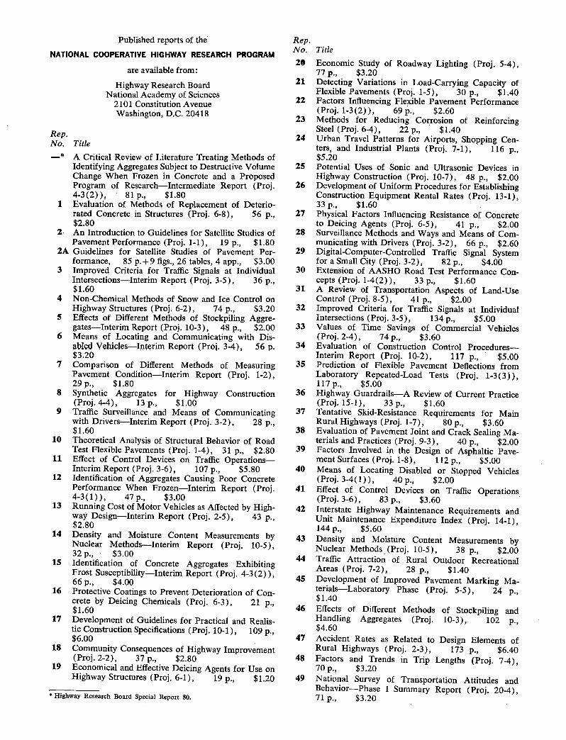
Published reports of the


are available from:

Highway Research Board National Academy of Sciences

2101 Constitution Avenue Washington, D.C. 20418

Rep. No. Title

-* A Critical Review of Literature Treating Methods of Identifying Aggregates Subject to Destructive Volume Change When Frozen in Concrete and a Proposed Program of Research—Intermediate Report (Proj. 4-3(2)), 81p., $1.80

1 Evaluation of Methods of Replacement of Deterio- rated Concrete in Structures (Proj. 6-8), 56 p., $2.80

2 An Introduction to Guidelines for Satellite Studies of Pavement Performance (Proj. 1-1), 19 p., $1.80

2A Guidelines for Satellite Studies of Pavement Per- formance, 85 p.+9 figs., 26 tables, 4 app., $3.00

3 Improved Criteria for Traffic Signals at Individual Intersections—Interim Report (Proj. 3-5), 36 p., $1.60

4 Non-Chemical Methods of Snow and Ice Control on Highway Structures (Proj. 6-2), 74 p., $3.20

5 Effects of Different Methods of Stockpiling Aggre-gates—Interim Report (Proj. 10-3), 48 p., $2.00

6 Means of Locating and Communicating with Dis-abled Vehicles—Interim Report (Proj. 3-4), 56 p. $3.20

7 Comparison of Different Methods of Measuring Pavement Condition—Interim Report (Proj. 1-2), 29 p., $1.80

8 Synthetic Aggregates for Highway Construction (Proj. 4-4), 13 p., $1.00

9 Traffic Surveillance and Means of Communicating with Drivers—Interim Report (Proj. 3-2), 28 p., $1.60

10 Theoretical Analysis of Structural Behavior of Road Test Flexible Pavements (Proj. 1-4), 31 p., $2.80

11 Effect of Control Devices on Traffic Operations— Interim Report (Proj. 3-6), 107 p., $5.80

12 Identification of Aggregates Causing Poor Concrete Performance When Frozen—Interim Report (Proj. 4-3(1)), 47p., $3.00

13 Running Cost of Motor Vehicles as Affected by High- way Design—Interim Report (Proj. 2-5), 43 p., $2.80

14 Density and Moisture Content Measurements by Nuclear Methods—Interim Report (Proj. 10-5), 32 p., $3.00

15 Identification of Concrete Aggregates Exhibiting Frost Susceptibility—Interim Report (Proj. 4-3(2)), 66 p., $4.00

16 Protective Coatings to Prevent Deterioration of Con- crete by Deicing Chemicals (Proj. 6-3), 21 p., $1.60

17 Development of Guidelines for Practical and Realis- tic Construction Specifications (Proj. 10-1), 109 p., $6.00

18 Community Consequences of Highway Improvement (Proj. 2-2), 37 p., $2.80

19 Economical and Effective Deicing Agents for Use on Highway Structures (Proj. 6-1), 19 p., $1.20

* Highway Research Board Special Report 80.

Rep. No. Title

20 Economic Study of Roadway Lighting (Proj. 5-4), 77 p., $3.20

21 Detecting Variations in Load-Carrying Capacity of Flexible Pavements (Proj. 1-5), 30 p., $1.40

22 Factors Influencing Flexible Pavement Performance (Proj. 1-3(2)), 69 p., $2.60

23 Methods for Reducing Corrosion of Reinforcing Steel (Proj. 6-4), 22 p., $1.40

24 Urban Travel Patterns for Airports, Shopping Cen- ters, and Industrial Plants (Proj. 7-1), 116 p., $5.20

25 Potential Uses of Sonic and Ultrasonic Devices in Highway Construction (Proj. 10-7), 48 p., $2.00

26 Development of Uniform Procedures for Establishing Construction Equipment Rental Rates (Proj. 13-1), 33 p., $1.60

27 Physical Factors Influencing Resistance of Concrete to Deicing Agents (Proj. 6-5), 41 p., $2.00

28 Surveillance Methods and Ways and Means of Com- municating with Drivers (Proj. 3-2), 66 p., $2.60

29 DigitalComputer-Controlled Traffic Signal System for a Small City (Proj. 3-2), 82 p., $4.00

30 Extension of AASHO Road Test Performance Con- cepts (Proj. 1-4(2)), 33 p., $1.60

31 A Review of Transportation Aspects of Land-Use Control (Proj. 8-5), 41 p., $2.00

32 Improved Criteria for Traffic Signals at Individual Intersections (Proj. 3-5), 134 p., $5.00

33 Values of Time Savings of Commercial Vehicles (Proj. 2-4), 74p., $3.60

34 Evaluation of Construction Control Procedures— Interim Report (Proj. 10-2), 117 p., $5.00

35 Prediction of Flexible Pavement Defiections from Laboratory Repeated-Load Tests (Proj. 1-3(3)), 117p., $5.00

36 Highway Guardrails—A Review of Current Practice (Proj. 15-1), 33 p., $1.60

37 Tentative Skid-Resistance Requirements for Main Rural Highways (Proj. 1-7), 80 p., $3.60

38 Evaluation of Pavement Joint and Crack Sealing Ma- terials and Practices (Proj. 9-3), 40 p., $2.00

39 Factors Involved in the Design of Asphaltic Pave- ment Surfaces (Proj. 1-8), 112 p., $5.00

40 Means of Locating Disabled or Stopped Vehicles (Proj. 3-4(1)), 40 p., $2.00

41 Effect of Control Devices on Traffic Operations (Proj. 3-6), 83 p., $3.60

42 Interstate Highway Maintenance Requirements and Unit Maintenance Expenditure Index (Proj. 14-1), 144 p., $5.60

43 Density and Moisture Content Measurements by Nuclear Methods (Proj. 10-5), 38 p., $2.00

44 Traffic Attraction of Rural Outdoor Recreational Areas (Proj. 7-2), 28 p., $1.40

45 Development of Improved Pavement Marking Ma- terials—Laboratory Phase (Proj. 5-5), 24 p., $1.40

46 Effects of Different Methods of Stockpiling and Handling Aggregates (Proj. 10-3), 102 p., $4.60

47 Accident Rates as Related to Design Elements of Rural Highways (Proj. 2-3), 173 p., $6.40

48 Factors and Trends in Trip Lengths (Proj. 7-4), 70 p., $3.20

49 National Survey of Transportation Attitudes and Behavior—Phase I Summary Report (Proj. 20-4), 71 p., $3.20

Rep. No. Title 50 Factors Influencing Safety at Highway-Rail Grade

Crossings (Proj. 3-8), 113 p., $5.20 51 Sensing and Communication Between Vehicles (Proj.

3-3), 105 p., $5.00 52 Measurement of Pavement Thickness by Rapid and

Noiidestruetive Methods (Proj. 10-6), 82 p., $3.80

53 Multiple Use of Lands Within Highway Rights-of- Way (Proj. 7-6), 68 p., $3.20

54 Location, Selection, and Maintenance of Highway Guardrails and Median Barriers (Proj. 15-1(2)), 63 p., $2.60

55 Research Needs in Highway Transportation (Proj. 20-2), 66 p., $2.80

56 Scenic Easements—Legal, Administrative, and Valua- tion Problems and Procedures (Proj. 11-3), 174 p., $6.40

57 Factors Influencing Modal Trip Assignment (Proj. 8-2), 78 p., $3.20

58 Comparative Analysis of Traffic Assignment Tech-niques with Actual Highway Use (Proj. 7-5), 85 p., $3.60

59 Standard Measurements for Satellite Road Test Pro- gram (Proj. 1-6), 78 p., $3.20

60 Effects of Illumination on Operating Characteristics of Freeways (Proj. 5-2) 148 p., $6.00

61 Evaluation of Studded Tires—Performance Data and Pavement Wear Measurement (Proj. 1-9), 66 p., $3.00

62 Urban Travel Patterns for Hospitals, Universities, Office Buildings, and Capitols (Proj. 7-1), 144 p., $5.60

63 Economics of Design Standards for Low-Volume Rural Roads (Proj. 2-6), 93 p., $4.00

64 Motorists' Needs and Services on Interstate Highways (Proj. 7-7), 88 p., $3.60

65 One-Cycle Slow-Freeze Test for Evaluating Aggre-gate Performance in Frozen Concrete (Proj. 4-3(1)), 21p., $1.40

66 Identification of Frost-Susceptible Particles in Con- crete Aggregates (Proj. 4-3(2)), 62 p., $2.80

67 Relation of Asphalt Rheological Properties to Pave- ment Durability (Proj. 9-1), 45 p., $2.20

68 Application of Vehicle Operating Characteristics to Geometric Design and Traffic Operations (Proj. 3- 10), 38 p., $2.00

69 Evaluation of Construction Control Procedures—Aggregate Gradation Variations and Effects (Proj. 10-2A), 58 p., $2.80

70 Social and Economic Factors Affecting Intercity Travel (Proj. 8-1), 68 p., $3.00

71 Analytical Study of Weighing Methods for Highway Vehicles in Motion (Proj. 7-3), 63 p., $2.80

72 Theory and Practice in Inverse Condemnation for Five Representative States (Proj. 11-2), 44 p., $2.20

73 Improved Criteria for Traffic Signal Systems on Urban Arterials (Proj. 3-5/1), 55 p., $2.80

74 Protective Coatings for Highway Structural Steel (Proj. 4-6), 64 p., $2.80

74A Protective Coatings for Highway Structural Steel— Literature Survey (Proj. 4-6), 275 p., $8.00

74B Protective Coatings for Highway Structural Steel— Current Highway Practices (Proj. 4-6), 102 p., $4.00

75 Effect of Highway Landscape Development on Nearby Property (Proj. 2-9), 82 p., $3.60

Rep. No. Title 76 Detecting Seasonal changes in Load-Carrying Ca-

pabilities of Flexible Pavements (Proj. 1-5(2)), 37 p., $2.00

77 Development of Design Criteria for Safer Luminaire Supports (Proj. 15-6), 82 p., $3.80

78 Highway loise—Measurement, Simulation, and Mixed Reactions (Proj. 3-7), 78 p., $3.20

79 Development of Improved Methods for Reduction of Traffic Accidents (Proj. 17-1), 163 p., $6.40

80 Oversize-Overweight Permit Operation on State High- ways (Proj. 2-10), 120 p., $5.20

81 Moving Behavior and Residential Choice—A Na- tional Survey (Proj. 8-6), 129 p., $5.60

82 National Survey of Transportation Attitudes and Behavior—Phase II Analysis Report (Proj. 20-4), 89 p., $4.00

83 Distribution of Wheel Loads on Highway Bridges (Proj. 12-2), 56 p., $2.80

84 Analysis and Projection of Research on Traffic Surveillance, Communication, and Control (Proj. 3-9), 48 p., $2.40

85 Development of Formed-in-Place Wet Reflective Markers (Proj. 5-5), 28 p., $1.80

86 Tentative Service Requirements for Bridge Rail Sys- tems (Proj. 12-8), 62 p., $3.20

87 Rules of Discovery and Disclosure in Highway Con- demnation Proceedings (Proj. 11-1(5)), :28 p., $2.00

88 Recognition of Benefits to Remainder Property in Highway Valuation Cases (Proj. 11-1(2)), 24 p., $2.00

89 Factors, Trends, and Guidelines Related to Trip Length (Proj. 7-4), 59 p., $3.20

90 Protection of Steel in Prestressed Concrete Bridges (Proj. 12-5), 86 p., $4.00

91 Effects of Deicing Salts on Water Quality and Biota —Literature Review and Recommended Research (Proj. 16-1), 70 p., $3.20

92 Valuation and Condemnation of Special Purpose Properties (Proj. 11-1(6)), 47 p., $2.60

93 Guidelines for Medial and Marginal Access Control on Major Roadways (Proj. 3-13), 147 p., $6.20

94 Valuation and Condemnation Problems Involving Trade Fixtures (Proj. 11-1(9)), 22 p., $1.80

95 Highway Fog (Proj. 5-6), 48 p., $2.40 96 Strategies for the Evaluation of Alternative Trans-

portation Plans (Proj. 8-4), ill p., $5.40 91 Analysis of Structural Behavior of AASHO Road

Test Rigid Pavements (Proj. 1-4(1)A), 35 p., $2.60

98 Tests for Evaluating Degradation of Base Course Aggregates (Proj. 4-2), 98 p. $5.00

99 Visual Requirements in Night Driving (Proj. 5-3), 38 p., $2.60

100 Research Needs Relating to Performance of Aggre- gates in Highway Construction (Proj. 4-8), 68 p., $3.40

101 Effect of Stress on Freeze-Thaw Durability of Con- crete Bridge Decks (Proj. 6-9), 70 p., $3.60

102 Effect of Weldments on the Fatigue Strength of Steel Beams (Proj. 12-7), 114 p., $5.40

103 Rapid Test Methods for Field Control of Highway Construction (Proj. 10-4), 89 p., $5.00

104 Rules of Compensability and Valuation Evidence for Highway Land Acquisition (Proj. 11-1), 77 p., $4.40

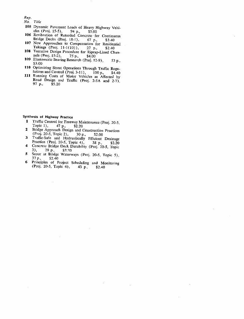
Rep. No. Title

105 Dynamic Pavement Loads of Heavy Highway Vehi- cles (Proj. 15-5), 94 p., $5.00

106 Revjbratjon of Retarded Concrete for Continuous Bridge Decks (Proj. 18-1), 67 p., $3.40

107 New Approaches to Compensation for Residential Takings (Proj. 11-1(10)), 27 p., $2.40

108 Tentative Design Procedure for Riprap-Lined Chan- nels (Proj. 15-2), 75 p., $4.00

109 Elastomeric Bearing Research (Proj. 12-9), 53 p., $3.00

110 Optimizing Street Operations Through Traffic Regu- lations and Control (Proj. 3-11), 100 p., $4.40

111 Running Costs of Motor Vehicles as Affected by Road Design and Traffic (Proj. 2-5A and 2-7), 97 p., $5.20

Synthesis of Highway Practice 1 Traffic Control for Freeway Maintenance (Proj. 20-5,

Topic 1), 47 p., $2.20 2 Bridge Approach Design and Construction Practices

(Proj. 20-5, Topic 2), 30 p., $2.00 3 Traffic-Safe and Hydraulically Efficient Drainage

Practice (Proj. 20-5, Topic 4), 38 p., $2.20 4 Concrete Bridge Deck Durability (Proj. 20-5, Topic

3), 28 p., 5 Scour at Bridge Waterways (Proj. 20-5, Topic 5),

37 p., $2.40 6 Principles of Project Scheduling and Monitoring

(Proj. 20-5, Topic 6), 43 p., $2.40

THE NATIONAL ACADEMY OF SCIENCES is a private, honorary organiza-tion of more than 700 scientists and engineers elected on the basis of outstanding contributions to knowledge. Established by a Congressional Act of Incorporation signed by President Abraham Lincoln on March 3, 1863, and supported by private and public funds, the Academy works to further science and its use for the general welfare by bringing together the most qualified individuals to deal with scientific and technological problems of broad significance.

Under the terms of its Congressional charter, the Academy is also called upon to act as an official—yet independent—adviser to the Federal Government in any matter of science and technology. This provision accounts for the close ties that have always existed between the Academy and the Government, although the Academy is not a governmental agency and its activities are not limited to those on behalf of the Government.

THE NATIONAL ACADEMY OF ENGINEERING was established on December 5, 1964. On that date the Council of the National Academy of Sciences, under the authority of its Act of Incorporation, adopted Articles of Organization bringing the National Academy of Engineering into being, independent and autonomous in its organization and the election of its members, and closely coordinated with the National Academy of Sciences in its advisory activities. The two Academies join in the furtherance of science and engineering and share the responsibility of advising the Federal Government, upon request, on any subject of science or technology.

THE NATIONAL RESEARCH COUNCIL was organized as an agency of the National Academy of Sciences in 1916, at the request of President Wilson, to enable the broad community of U. S. scientists and engineers to associate their efforts with the limited membership of the Academy in service to science and the nation. Its members, who receive their appointments from the President of the National Academy of Sciences, are drawn from academic, industrial and government organizations throughout the country. The National Research Council serves both Academies in the discharge of their responsibilities.

Supported by private and public contributions, grants, and contracts, and volun-tary contributions of time and effort by several thousand of the nation's leading scientists and engineers, the Academies and their Research Council thus work to serve the national interest, to foster the sound development of science and engineering, and to promote their effective application for the benefit of society.

THE DIVISION OF ENGINEERING is one of the eight. major Divisions into which the National Research Council is organized for the conduct of its work. Its membership includes representatives of the nation's leading technical societies as well as a number of members-at-large. Its Chairman is appointed by the Council of the Academy of Sciences upon nomination by the Council of the Academy of

Engineering.

THE HIGHWAY RESEARCH BOARD, organized November 11, 1920, as an agency of the Division of Engineering, is a cooperative organization of the high-way technologists of America operating under the auspices of the National Research Council and with the support of the several highway departments, the Federal Higiiway Administration, and many other organizations interested in the develøpment of trans-portation. The purpose of the Board is to advance knowledge concerning the nature and performance of transportation systems, through the stimulation of research and

dissemination of information derived therefrom.

HIGHWAY RESEARCH BOARD NATIONAL ACADEMY OF SCIENCES—NATIONAL RESEARCH COUNCIL 2101 Constitution Avenue Washington, 0. C. 20415

ADDRESS CORRECTION REQUESTED

NON-PROFIT ORG.

U.S. POSTAGE

PAID

WASHINGTON, D.C. PERMIT NO. 42970

I -

/1

1YLIp Z3 - I

DEPT. OF HGH1//ys

000015 LIBRARY

IDAHO DEPT OF p 0 BOX 7129 ao I SE

HIGHWAYS

ID 83707

RUNNING COSTS OF MOTOR VEHICLES AS AFFECTED BY ...

Documents

Transcript of RUNNING COSTS OF MOTOR VEHICLES AS AFFECTED BY ...