Ruminant Eructation and a Long-Run Environmental Kuznets' Curve for Enteric Methane in New Zealand:...
37
Electronic copy available at: http://ssrn.com/abstract=1806701 1 Department of Economics University of Victoria Econometrics Working Paper EWP0306 ISSN 1485-6441 Ruminant Eructation and a Long-Run Environmental Kuznets’ Curve for Enteric Methane in New Zealand: Conventional and Fuzzy Regression Analysis David E.A. Giles & Carl A. Mosk Department of Economics, University of Victoria Victoria, B.C., Canada V8W 2Y2 June, 2003 ABSTRACT This paper examines the very long-run relationship between income and emissions of enteric methane in New Zealand, over the period 1895 to 1996. Controlling the emissions of this particular greenhouse gas is of crucial importance if that country is to meet its obligations as a signatory to the Kyoto Protocol. We use standard parametric regression, nonparametric regression, and a new nonlinear regression estimator based on fuzzy clustering analysis, to estimate ‘environmental Kuznets’ curves’ for CH 4 in New Zealand. Our results appear to be the first to support the existence of some form of ‘inverted-U’ curve for this pollutant, and the ‘double-hump’ relationship that emerges from our fuzzy modeling is consistent with certain theoretical results. Methane pollution is maximized at a level of real per capita GDP that is consistent with those reported for other pollutants in the literature. JEL Classifications: C14; C49; C51; O1; Q2 Keywords: Environmental Kuznets’ curve; fuzzy regression; greenhouse gas; Kyoto Protocol; methane emissions; sheep Author Contact: Professor David E.A. Giles, Department of Economics, University of Victoria, P.O. Box 1700, STN CSC, Victoria, B.C., Canada V8W 2Y2; email: [email protected]; Voice: (250) 721-8540; FAX: (250) 721-6214
Transcript of Ruminant Eructation and a Long-Run Environmental Kuznets' Curve for Enteric Methane in New Zealand:...
Electronic copy available at: http://ssrn.com/abstract=1806701
1
Department of Economics University of Victoria Econometrics Working Paper EWP0306 ISSN 1485-6441
Ruminant Eructation and a Long-Run Environmental Kuznets’ Curve for Enteric Methane in New Zealand: Conventional and
Fuzzy Regression Analysis
David E.A. Giles &
Carl A. Mosk
Department of Economics, University of Victoria Victoria, B.C., Canada V8W 2Y2
June, 2003
ABSTRACT
This paper examines the very long-run relationship between income and emissions of enteric
methane in New Zealand, over the period 1895 to 1996. Controlling the emissions of this
particular greenhouse gas is of crucial importance if that country is to meet its obligations as a
signatory to the Kyoto Protocol. We use standard parametric regression, nonparametric
regression, and a new nonlinear regression estimator based on fuzzy clustering analysis, to
estimate ‘environmental Kuznets’ curves’ for CH4 in New Zealand. Our results appear to be the
first to support the existence of some form of ‘inverted-U’ curve for this pollutant, and the
‘double-hump’ relationship that emerges from our fuzzy modeling is consistent with certain
theoretical results. Methane pollution is maximized at a level of real per capita GDP that is
consistent with those reported for other pollutants in the literature.
JEL Classifications: C14; C49; C51; O1; Q2 Keywords: Environmental Kuznets’ curve; fuzzy regression; greenhouse gas; Kyoto Protocol; methane emissions; sheep Author Contact:
Professor David E.A. Giles, Department of Economics, University of Victoria, P.O. Box 1700, STN CSC, Victoria, B.C., Canada V8W 2Y2; email: [email protected]; Voice: (250) 721-8540; FAX: (250) 721-6214

Electronic copy available at: http://ssrn.com/abstract=1806701
2
1. Introduction
Globally, methane (CH4) is an important greenhouse gas (GHG), estimated by the International
Panel on Climate Control (IPCC) to account for 20% of the global radiative forcing due to
increases in atmospheric concentrations of GHG’s since 1750. In current terms, it is the second
most important GHG, after carbon dioxide. New Zealand is a ‘small player’ in the international
pollution arena, producing less than 0.5% of the world’s CH4, but it has a unique GHG emissions
profile among developed countries.1 Specifically, over 50% of New Zealand’s recent
anthropogenic emissions are attributable to CH4, in terms of CO2-equivalent units. Moreover, in
this country of 45.7 million sheep, 4.4 million dairy cattle, and 4.6 million beef cattle (and 3.7
million people, 1999 figures) enteric CH4 accounts for 88% of all methane emissions, and 99% of
CH4 emissions from just the agricultural sector.2 New Zealand’s economic history has been
dominated by sheep since the establishment of the first sheep station in that country in 1844.
While only recently of public concern, emissions of CH4 have existed, and have inhibited wool
and meat production since then, and they warrant a long-term analysis.
New Zealand is a signatory to the United Nations Framework Convention on Climate Change
(FCCC), and to the Kyoto Protocol. Accordingly, it has a commitment to prepare accurate
inventories of its sources and sinks for all GHG’s, and during the period 2008-2012 New Zealand
is also committed to limiting its levels of GHG’s to their 1990 level.3 Not surprisingly, therefore,
the role of enteric CH4 is crucial to these calculations and to the associated environmental policy
debate in that country. Enteric methane production is the output of CH4 from ruminants – sheep,
dairy cows, beef cattle and farmed deer and goats in the case of New Zealand. It is essentially a
by-product of the rumen fermentation process, and the methane is released into the atmosphere
primarily when these animals engage in eructation (i.e., they belch excessively)!
Recent agricultural research in New Zealand has focused on obtaining direct, ‘on the farm’
measurements of this interesting activity, and also on the role and relative importance of pasture
type, climatic and seasonal factors. Consequently, several mitigation options have been isolated,
these focusing on the manipulation of enteric bacteria by various means. The objective is not only
to reduce total CH4 emissions, but also to improve animal productivity – enteric methane
production requires energy that can otherwise be used by the animal to produce meat, wool or
milk.4

3
The following developments are among those that are pertinent to the GHG problem in New
Zealand. CO2 emissions have grown by about 20% since 1990, primarily in association with
growth in the electricity generation and transportation sectors. By way of partial compensation,
although the annual planting rate of forest sinks decreased during the 1990’s, it has now returned
to about its 1990 rate. Sheep numbers declined steadily from a peak of 70.3 million in 1982 to
approximately 57.9 million in 1990, and by 21% between 1990 and 1999. In contrast, however,
dairy and beef cattle numbers have increased by 25%, and 1% respectively since 1990, and the
number of farmed deer has risen by 72%. These significant changes in the both the numbers and
the ‘mix’ of ruminants, coupled with their vastly different CH4 emission rates, complicate the task
that New Zealand scientists and policy-makers face in order to meet their Kyoto Protocol
obligations.5
Our objective is to explore the very long-run relationship between income and enteric CH4
emissions in New Zealand. Specifically, we ask, ‘Is there an environmental Kuznets’ curve’ for
this particular GHG in New Zealand?’ Given the mixed international empirical evidence
associated with environmental Kuznets’ curves, and the special role of methane in New Zealand,
there is a strong case for analyzing this individual GHG, rather than considering a more general
index of pollutants. It is estimated that the agricultural sector contributes approximately 17% of
New Zealand’s GDP.6 In 1999 44.1% of that country’s export revenues were ‘pastoral based’ and
hence dependent on ruminants.7 ‘Solving’ the GHG problem, and meeting the Kyoto Protocol
targets simply by dramatically reducing the numbers of these animals is not a viable option from
an economic perspective for reasons that we discuss in detail below. A better understanding of the
trade-off between methane emissions and economic output is certainly helpful to the current
environmental policy debate in New Zealand, and elsewhere. In the next section we summarize
some of the relevant literature relating to research on environmental Kuznets’ curves. Section 3
deals with data construction issues associated with our use of time-series spanning just over a
century; and in section 4 we outline the modelling techniques that we use. The main empirical
results, which include strong new evidence of an environmental Kuznets’ curve for enteric
methane, are presented in section 5; and section 6 discusses the role of trade and some policy
implications. The paper concludes with a section that summarizes our principal findings.

4
2. Environmental Kuznets’ Curves
Kuznets (1955) proposed that there is an ‘inverted-U’ relationship between income inequality and
a country’s level of output. The basis for this was that if income inequality between high
productivity and low productivity sectors in the economy is higher than inequality within each
sector, then income inequality should rise, at first, as people moved between sectors. Then it
should fall as this flow of labour ended, or when returns to the factors of production were
balanced across the sectors. He supported this hypothesis with the analysis of time-series data for
the United Kingdom, the U.S.A. and Germany. Numerous studies have since explored Kuznets’
proposal, with rather mixed results. In particular, the empirical results that have been obtained
have depended to some degree on the overall level of development of the countries in question,
the type of data (namely, time-series or cross-country) that have been used, and the extent to
which other factors have been taken into account. With the availability of larger and richer data-
sets, the more recent literature has generally discounted Kuznets’ hypothesis (e.g., Deininger and
Squire, 1998).8 It should also be emphasized that even when a statistically robust Kuznets’
relationship can be established, it does not imply anything about causality from inequality to
income, or vice versa. It simply suggests that rising income is associated with a worsening, and
then an improvement, in income inequality.
There is now a well-established literature, dating back at least to the World Bank (1992) and
Grossman and Krueger (1991, 1995), that explores the possibility of a so-called ‘environmental
Kuznets curve’ (EKC) – that is, an ‘inverted-U’ shaped relationship between environmental
pressure and per capita income.9 There is a certain amount of theoretical support in favour of the
existence of an EKC – that is, a worsening and then an improvement in pollution as income rises.
For example, Andreoni and Levinson (1998) present a static model that shows that an EKC can
be derived from the technological link between consumption of a desired good and the abatement
of its undesirable by-product. Pfaff et al. (2001) provide a theoretical framework at the household
level, and by focusing on the linkage between income and household choices that impact upon the
environment, they show how household-level EKC’s can arise. Other theoretical contributions
include those of Selden and Song (1995) and Stokey (1998). For example, the former authors
note that among the factors that lead to an initial increase, and subsequent downturn in pollution
as income grows are: (i) positive income elasticities for environmental quality; (ii) changes in the
composition of production and consumption; (iii) increasing levels of education and awareness;
(iv) more open political systems.10 On the other hand, Bousquet & Favard (2000) develop a

5
public good model of the provision of environmental quality with ‘bell-shaped’ income
inequality, and they show that their model generates an ‘environmental camel curve’ – a curve
with ‘two humps’.
Interestingly, this last theoretical result is consistent with the recent empirical results of Taskin
and Zaim (2000). Using nonparametric production frontier methods and aggregate data for 52
countries over 16 years, they estimate an EKC for CO2 emissions with a peak, followed by a
trough, as real per capita GDP increases. Their results are also quite compatible with those of
Dijkgraaf and Vollebergh (2001). They use a panel of data for OECD countries between 1960 and
1997, and for certain countries the CO2 data follow the pattern established by Taskin and Zaim, a
point to which we will return below. As a result of their econometric analysis they conclude that
it is unlikely that the overall income-emission relationship is of the ‘inverted-U’ type. The
(relatively) early results of Selden and Song (1994) uncovered EKC’s for SO2, CO, oxides of
nitrogen (NOx) and suspended particulate matter (SPM). Other early contributions include those
of Shafik (1994), Shafik and Bandyopadhyay (1992) and Holtz-Eakin and Selden (1995), and
Hilton and Levinson (1998) provide a tabular summary of the various results that favour the
EKC.
The EKC hypothesis has been widely criticized both on conceptual grounds and empirically (e.g.,
Ekins, 1997, and Stern et al., 1997). Although there appears to be some evidence of EKC’s for
certain pollutants with short term effects and low abatement costs (e.g., SO2), the same is not true
in general for pollutants with more global and longer-term effects, and higher abatement costs
(e.g., CO2). In many studies where an EKC is apparently uncovered the levels of real per capita
income, above which pollution begins to decline, are exceedingly high relative to actual current
levels. In addition, the clarity of many EKC results diminishes once covariates other than real per
capita income are taken into consideration. A further issue that has, to the best of our knowledge,
been taken into account in the empirical EKC literature only by Egli (2001), is the fact that many
of the studies have been based on time-series data that are undoubtedly non-stationary. As noted
above, the research reported by Jacobsen and Giles (1998) clearly indicates the importance of
taking account of unit roots and cointegration in the data when estimating Kuznets’ curves.
Indeed, the more recent empirical evidence is not especially favourable towards ‘literal’ EKC
relationships. Harbargh et al. (2000) re-examine the earlier World Bank and Grossman-Krueger
data and find that the evidence that the latter authors presented in favour of EKC’s for SO2,

6
smoke and total suspended particulates are actually very sensitive to the sample period and to
controlling for other factors. On balance, they reject the simple EKC for these emissions. Among
the more positive recent results are those of Hilton and Levinson (1998), who examine emissions
of lead as a result of gasoline consumption in 48 countries over a 20-year period. They consider
various functional forms and find an EKC with a statistically significant peak at a real (1990) per
capita income of around US$11,000, when only post-1983 data are used. The many other recent
contributions to this literature include three that are of particular interest to us here - those of
Roca et al. (2001) and Egli (2001), and Utt et al. (2001). The first two of these studies appear to
be the only ones to date that attempt to estimate an EKC explicitly for methane. Roca et al.
consider Spanish data for the emissions of six atmospheric pollutants – CO2 (for the period 1972
to 1996) and SO2, N2O, CH4, NOx and non-methanic volatile organic compounds (NMVOC) for
the period 1980 to 1996. With the exception of SO2 they fail to find satisfactory econometric
relationships to support EKC’s for any of these pollutants. Using German time-series data for the
period 1966 to 1998, Egli considers emissions of eight pollutants – NOx, NH3, SO2, CH4, CO,
CO2, NMVOC and SPM. He uncovers standard EKC relationships for the first two of these.
When the non-stationarity of the data are taken into account and a modified error-correction
model is estimated, there is mild evidence to support a long-run EKC for methane emissions. Utt
et al. estimate an EKC for total per capita equivalent-CO2 for the U.S.A., using data for 1922 to
1996. Not only is the length of their sample much greater than is usual in such studies, and more
in keeping with our own, but their calculation of equivalent-CO2 includes an allowance CH4 and
other GHG’s.11 They use a quartic polynomial to estimate an EKC that has local maxima at
US$8,000 and US$28,000, and a local minimum at about US$20,000.12
3. Data Issues
One of the distinguishing features of this study is its use of a very long-term set of data.13
Moreover, we are fortunate to have access to data of very high quality. The data for enteric
methane emissions have been constructed by multiplying animal numbers, as reported by the
New Zealand Ministry of Agriculture and Forestry (2003), by the methane emission rates used by
Clarke (1999) in the preparation of that country’s national GHG inventory.14 These rates are
given in Table 1 for each type of ruminant farmed in New Zealand, with low (L) and high (H)
estimates given for 1990 and 1999.15 The four emission rate estimates give rise to four series for
total enteric CH4, which we denote CH490L, CH490H, CH499L and CH499H in Figure 1, for the
period 1895 to 1996.16 This allows us to check the sensitivity of our results to assumptions about
7
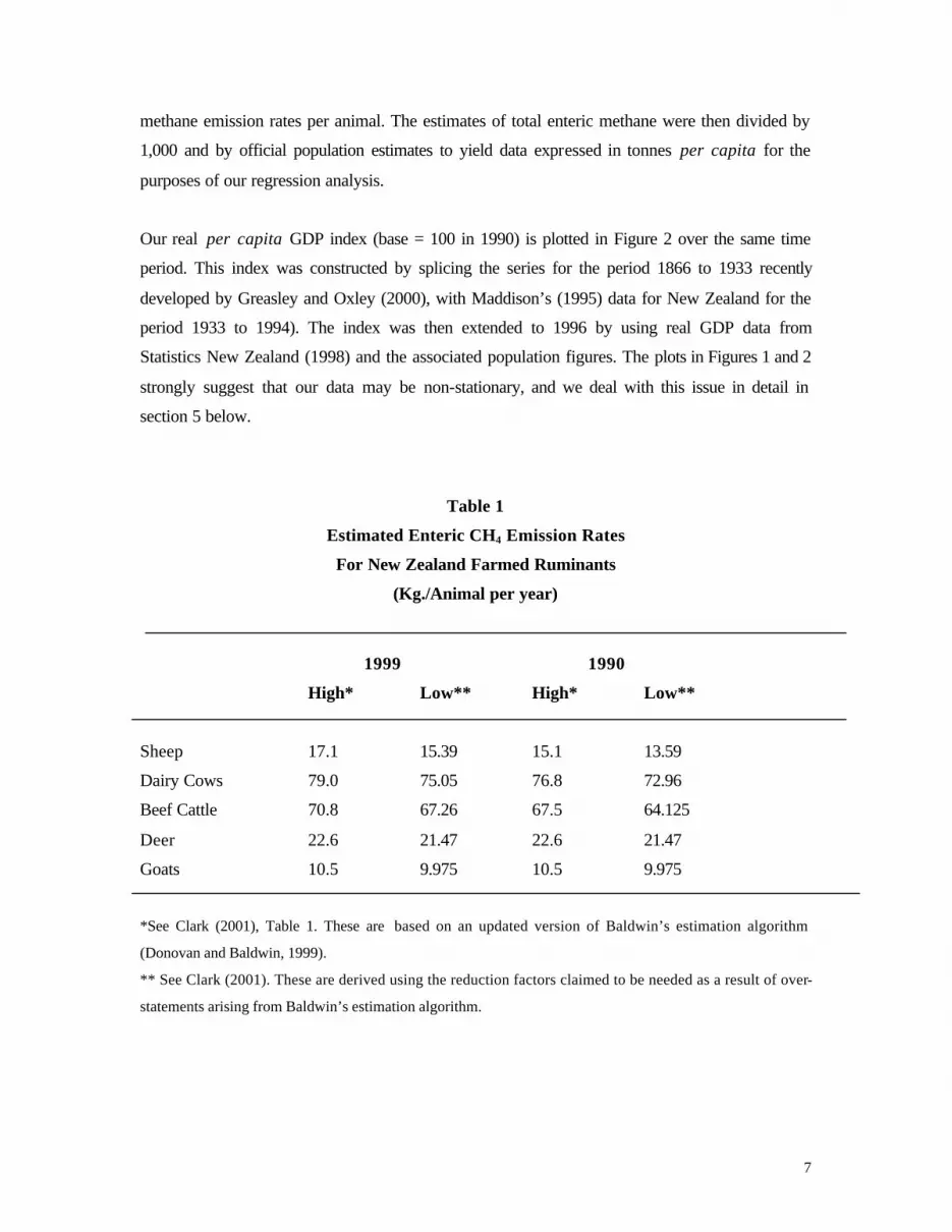
methane emission rates per animal. The estimates of total enteric methane were then divided by
1,000 and by official population estimates to yield data expressed in tonnes per capita for the
purposes of our regression analysis.
Our real per capita GDP index (base = 100 in 1990) is plotted in Figure 2 over the same time
period. This index was constructed by splicing the series for the period 1866 to 1933 recently
developed by Greasley and Oxley (2000), with Maddison’s (1995) data for New Zealand for the
period 1933 to 1994). The index was then extended to 1996 by using real GDP data from
Statistics New Zealand (1998) and the associated population figures. The plots in Figures 1 and 2
strongly suggest that our data may be non-stationary, and we deal with this issue in detail in
section 5 below.
Table 1
Estimated Enteric CH4 Emission Rates
For New Zealand Farmed Ruminants
(Kg./Animal per year)
1999 1990
High* Low** High* Low**
Sheep 17.1 15.39 15.1 13.59
Dairy Cows 79.0 75.05 76.8 72.96
Beef Cattle 70.8 67.26 67.5 64.125
Deer 22.6 21.47 22.6 21.47
Goats 10.5 9.975 10.5 9.975
*See Clark (2001), Table 1. These are based on an updated version of Baldwin’s estimation algorithm
(Donovan and Baldwin, 1999).
** See Clark (2001). These are derived using the reduction factors claimed to be needed as a result of over-
statements arising from Baldwin’s estimation algorithm.

8
Figure 1 Enteric Methane Emissions (1895 - 1996)
300
500
700
900
1100
1300
1500
1700
1900
1890 1900 1910 1920 1930 1940 1950 1960 1970 1980 1990 2000
Year
Th
ou
san
ds
of
To
nn
es
1990-Low
1999-Low
1999-High
Figure 2Real Per Capita GDP Index (1990=100)
0
20
40
60
80
100
120
1890 1900 1910 1920 1930 1940 1950 1960 1970 1980 1990 2000
Year
GD
P In
dex

9
4. Modelling and Estimation Strategies
Typically, attempts to establish the existence of an EKC have been based on regression models in
which the level of the pollutant in question is ‘explained’ in terms of real income, or some simple
polynomial of the latter. These models sometimes include additional regressors to control for
other relevant factors, and some of them allow for dynamic effects through the inclusion of a
lagged value of the dependent variable. EKC’s have been estimated from cross-country data,
time-series data, or ‘pooled’ data Regrettably, many of the studies that use the latter two types of
data do not allow for the possibility that these data are non-stationary, and this brings the
relevance of their results into question in view of the fact that some are undoubtedly based on
‘spurious regressions’.17 Among the few EKC studies that attempt to take at least some account of
unit roots in the data are those of Stern and Common (2001), Egli (2001), Roca et al. (2001), but
none of these test for multivariate cointegration.
Almost without exception, the models in these studies are parametric, and the use of an explicit
functional form places crucial constraints on the results that can be obtained. As an obvious
example of this, if the regressors include GDP and its squared value (but no higher powers of
GDP), then the partial relationship between the amount of pollution and GDP simply has to be ‘U
shaped’ or ‘inverted-U shaped’, depending on the signs of the estimated coefficients. It cannot
have more than one turning point.18 In practice, estimated EKC’s have been found to be quite
sensitive to the type of pollutant under study, to changes in the type and sample of data used, and
to the specification of the model’s functional form.
One obvious way to deal with this last type of sensitivity is to avoid placing any parametric
constraints on the model at all, and to use nonparametric kernel regression. Somewhat
surprisingly, it seems that this option has been pursued in only one previous EKC study. Taskin
ad Zaim (2000) compare nonparametric regression with simple parametric polynomial
specifications in the case of CO2 emissions for 52 countries over the period 1975 to 1990. Their
nonparametric results suggest a relationship that is broadly similar in appearance to a cubic one.
An alternative to nonparametric regression is to use splines (piecewise continuous, usually simple
polynomial, functions). One application of this idea in the context of the EKC is the study by
Schmalensee et al. (1998) who find a clear ‘inverted-U’ EKC for CO2 when simple spline
analysis is used in conjunction with national-level panel data for the period 1950 to 1990.
Similarly, Hilton and Levinson (1998) include some basic (linear) spline regression analysis in
10
their study and they also find a significant EKC, in their case for lead arising from the use of
gasoline.
In the present study not only do we consider the usual polynomial specifications that are common
in the empirical EKC (and ‘regular’ Kuznet’s curve) literature, and nonparametric kernel
regression, but we also use a new and very flexible regression modelling procedure that has been
developed by Giles and Draeseke (2003).19 This ‘fuzzy regression’ approach involves using fuzzy
clustering techniques (from the pattern recognition literature) to partition the data into sub-
samples over which separate parametric regressions are then fitted. A weighted average of the
sub-sample results is then formed, using the ‘degrees of membership’ for each data point and
each cluster as weights. As these weights vary continuously from one data point to another, we
are able to capture complex non-linearities very successfully.20 In a range of different modelling
applications, Giles and Draeseke (2003) demonstrate that this methodology out-performs
nonparametric kernel regression, and standard parametric regression, often quite dramatically. As
this fuzzy regression framework is not yet widely known, we present some details here.21
Fuzzy set theory originated with Zadeh (1965).22 In conventional set theory, items either belong
to some particular set or they do not. That is, the ‘degree of membership’ of an element with
respect to any particular set is either unity or zero. The boundaries of the sets are ‘sharp’, or
‘crisp’. In the case of fuzzy sets, the degree of membership may be any value between zero and
unity, and every item is associated with all of the sets. Usually this association will involve
different degrees of membership for each item (data point) with each of the fuzzy sets.
In order to implement our fuzzy regression analysis we use the so-called ‘fuzzy c-means’ (FCM)
algorithm that is widely used in the pattern recognition literature, together with some basic
concepts from fuzzy logic.23 The FCM algorithm, which is described in the appendix, enables us
to partition the data into a fixed number of clusters, based on the values of the regressor(s). These
clusters have ‘fuzzy’ boundaries, in the sense that each data value belongs to every cluster to
some degree or other. The FCM algorithm determines the cluster mid-points, the associated
membership functions and degrees of membership for all of the data-points. Separate regressions
are fitted over each of the clusters, and the degrees of membership provide the basis for
combining the separate results into one prediction for the conditional mean of the dependent
variable in the model.
11
5. A Long-Run EKC for Enteric CH4 in New Zealand
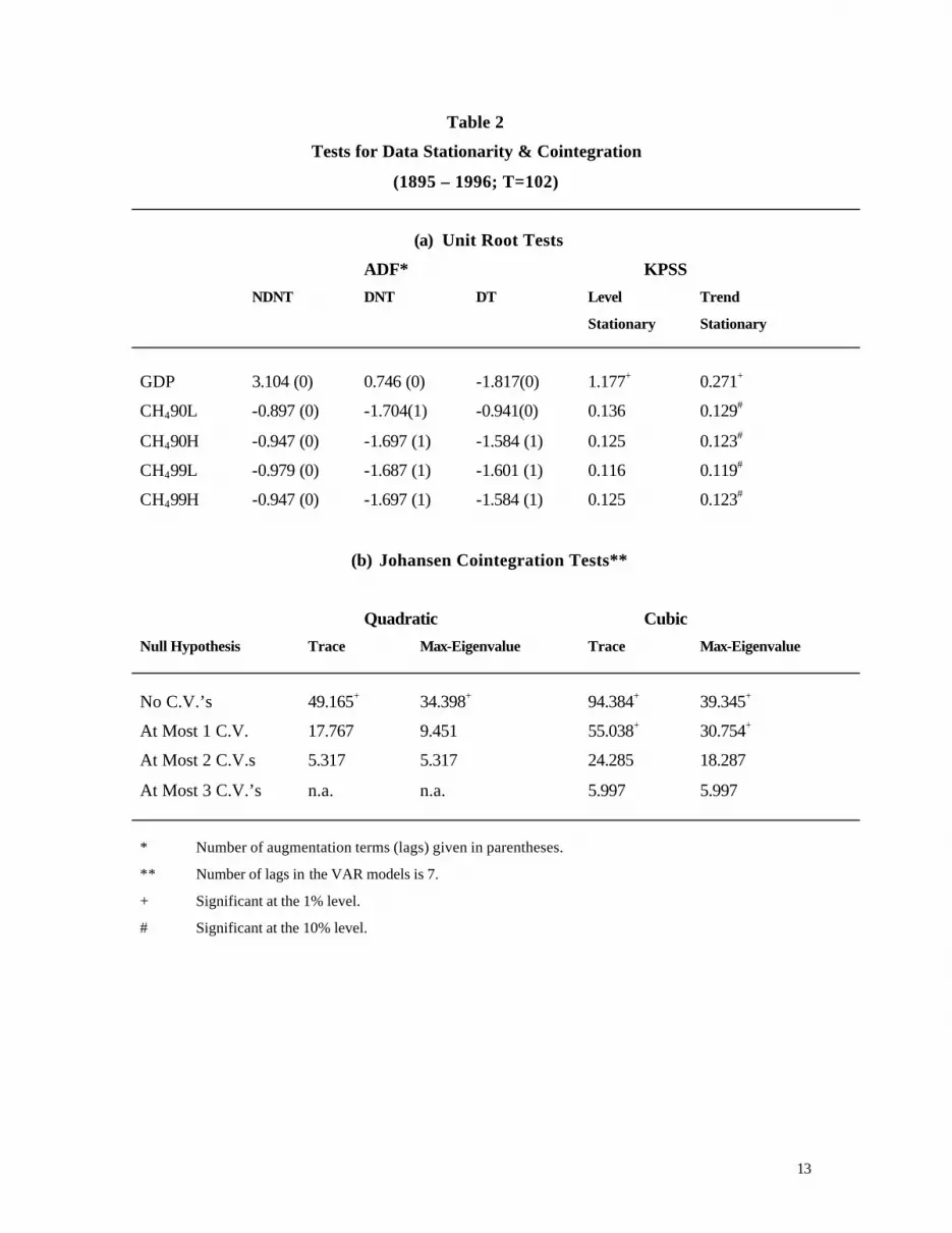
The time-series data that we use in our modeling have first been tested for stationarity using both
the ‘augmented’ Dickey-Fuller (ADF) tests and the tests proposed by Kwiatovsky et al. (KPSS)
(1992). For the ADF ‘t-tests’ (Dickey and Fuller, 1979, 1981; Dickey and Said, 1981) the null
hypothesis is that the series has a unit root and the alternative hypothesis is that it is stationary.
The null and alternative hypotheses are reversed for the KPSS tests. In the case of the ADF tests
we have considered the usual three cases for the Dickey-Fuller regressions: including a drift
(constant term) and a linear trend (DT); including a drift but no trend (DNT); and no drift or trend
(NDNT). The number of augmentation terms for the ADF tests was determined by using the
Schwarz information criterion (Schwarz, 1978). In the case of the KPSS tests we consider the
usual two variants of the null hypothesis, namely level stationarity and trend stationarity. Our
results, obtained with the EViews (2002) econometrics package and based on the full time-period,
1895 to 1996, appear in part (a) of Table 2. It is well known that these unit root tests lack power
in finite samples, so in practice it is often wise to adopt a relatively conservative significance
level such as 10%. Using the exact finite-sample critical values for the ADF test given by
MacKinnon (1991), and those for the KPSS test given by Hornok and Larsson (2000), we find
that all of our series have a unit root (i.e., they are I(1)).24
Given the close similarity between the characteristics of each of the four enteric methane series,
as evidenced in Figure 1 and Table 1, all of the following discussion and the results that are
presented below are based only CH490L. This provides the most conservative estimates of
methane emissions, and it uses animal emission rate estimates that are based on scientific data as
far from the end-point(s) of our sample as are available.25
In part (b) of Table 2 we present the results of testing for multivariate cointegration between
CH490L, GDP, GDP2 and GDP3, using Johansen’s (1988, 1995) likelihood-based procedures. As
data exhibit a trend, following the suggestion of Franses (2001) we include a drift and trend in the
cointegrating equation, and a drift but no trend in the VAR models when applying Johansen's
procedure. This corresponds to ‘case 4’ in the EViews (2002) econometrics package. The lag
lengths for the VAR models were determined using the Schwarz information criterion and
Akaike’s (1973) information criterion. As can be seen from Table 2, the results of both the trace
tests and the max.-eigenvalue tests clearly indicate the presence of cointegration (with at most
one or two cointegrating vectors (CV’s)) between the variables in question. This is particularly

12
important as it determines the appropriate way to estimate the EKC. In fact, we have two
legitimate choices – we can either model a short-run dynamic relationship by estimating an
‘error-correction model’; or we can fit the model in terms of the levels (not the differences) of the
data and determine the long-run equilibrating relationship. It is the latter that is relevant in the
case of an EKC. Moreover, OLS estimation will yield ‘super-consistent’ estimates of the model’s
parameters.26
Table 3 presents the results obtained when we estimate some basic parametric EKC’s for enteric
methane emission in New Zealand, using OLS estimation. These are based on both quadratic and
cubic specifications, explaining per capita methane in terms of real per capita GDP. Several
summary statistics and diagnostic test results are included in Table 3. The usual (asymptotic)
Lagrange multiplier test statistic for serial independence of the errors (against the alternative
hypothesis of a simple AR(i) or MA(i) process) is denoted LMi (i = 1, 2). The Jarque and Bera
(1980) test for normality of the errors is denoted JB; and FREi (i = 1, 2, 3) denotes the ‘FRESET’
test for mis-specification of functional form and/or omitted regressors proposed by DeBenedictis
and Giles (1998, 1999).27
The significance of the estimated coefficients is quite apparent, and the t-value associated with
GDP3 confirms that a cubic specification is preferred over the more restrictive quadratic
relationship. However, in the two static models the tests for serial independence, and several of
the FRESET test results, suggest that the formulation of the model requires further consideration.
Estimating simple dynamic models that include a lagged value of the dependent variable yields
more robust results. The estimated static and (long-run) dynamic relationships are shown in
Figures 3(a) and (b) respectively.28 We see that classic ‘inverted U’ curves emerge when a
quadratic relationship is fitted, with the location of the maximum essentially unaffected by
allowing for dynamics in the specification of the EKC. The (preferred) cubic EKC’s attain a
maximum at a higher level of GDP than do the quadratic ones, but again the general conclusions
are insensitive to the dynamics of the model. Based on the cubic specification, these rather
restrictive and conventional parametric regression results suggest that the EKC for enteric
methane emissions in New Zealand peaked at a GDP level of approximately NZ$11,000
(US$8,777) per capita , in real 1990 dollar terms.
13
Table 2
Tests for Data Stationarity & Cointegration
(1895 – 1996; T=102)
(a) Unit Root Tests
ADF* KPSS
NDNT DNT DT Level Trend
Stationary Stationary
GDP 3.104 (0) 0.746 (0) -1.817(0) 1.177+ 0.271+
CH490L -0.897 (0) -1.704(1) -0.941(0) 0.136 0.129#
CH490H -0.947 (0) -1.697 (1) -1.584 (1) 0.125 0.123#
CH499L -0.979 (0) -1.687 (1) -1.601 (1) 0.116 0.119#
CH499H -0.947 (0) -1.697 (1) -1.584 (1) 0.125 0.123#
(b) Johansen Cointegration Tests**
Quadratic Cubic
Null Hypothesis Trace Max-Eigenvalue Trace Max-Eigenvalue
No C.V.’s 49.165+ 34.398+ 94.384+ 39.345+
At Most 1 C.V. 17.767 9.451 55.038+ 30.754+
At Most 2 C.V.s 5.317 5.317 24.285 18.287
At Most 3 C.V.’s n.a. n.a. 5.997 5.997
* Number of augmentation terms (lags) given in parentheses.
** Number of lags in the VAR models is 7.
+ Significant at the 1% level.
# Significant at the 10% level.

14
Table 3
Parametric Regression Results*,+
Static (OLS) Dynamic (OLS)
Quadratic Cubic Quadratic Cubic
Constant 0.3299 0.5857 0.0223 0.1007
(18.03) (12.34) (1.19) (2.52)
GDP 0.3772*10-2 -0.0101 0.7064*10-3 -0.2363*10-2
(5.86) (-4.05) (1.99) (-1.65)
GDP2 -0.2879*10-4 0.1953*10-3 -0.5876*10-5 0.4528*10-4
(-5.90) (4.96) (-1.47) (1.94)
GDP3 -0.1112*10-5 -0.2601*10-6
(-5.72) (-2.21)
CH490L-1 0.9066 0.8531
(18.38) (15.77)
R2 0.260 0.445 0.838 0.846
LM1 8.715 [0.00] 8.377 [0.00] 2.313 [0.01] 2.517 [0.01]
LM2 7.035 [0.00] 6.002 [0.00] 0.395 [0.35] 0.266 [0.40]
JB 2.013 [0.37] 1.547 [0.46] 0.152 [0.93] 0.093 [0.96]
FRE1 2.729 [0.07] 0.267 [0.77] 0.580 [0.56] 0.945 [0.39]
FRE2 9.440 [0.00] 2.050 [0.09] 0.299 [0.88] 0.623 [0.65]
FRE3 6.698 [0.00] 1.680 [0.14] 0.295 [0.94] 0.505 [0.80]
Max. 9.17 11.00 8.41 10.74
(NZ$’000)
Max. 6.79 8.77 6.80 7.65
(US$’000)#
Year 1958 1965 1950 1967
* t-ratios appear in parentheses.
+ p-values appear in brackets.
# Converted using the ratio (‘Y’) of real per capita GDP for New Zealand to that of the U.S.A.,
from the Penn World Table, 5.6 (Summers and Heston, 1995), for each year in question.

15
Figure 3(a)Empirical Kuznets' Curves: Static Model, OLS
0.34
0.36
0.38
0.40
0.42
0.44
0.46
0.48
0.50
0.52
20 30 40 50 60 70 80 90 100 110 120
Ral per capita GDP Index (1990 =100)
Met
hane
(Ton
nes
per
capi
ta)
Actual Data
Quadratic
Cubic
Figure 3(b)Empirical Kuznets' Curves: Dynamic Model, OLS
0.34
0.36
0.38
0.40
0.42
0.44
0.46
0.48
0.50
0.52
20 30 40 50 60 70 80 90 100 110 120
Real per capita GDP Index (1990 = 100)
Met
hane
(Ton
nes
per
capi
ta)
Actual Data
Quadratic
Cubic
16
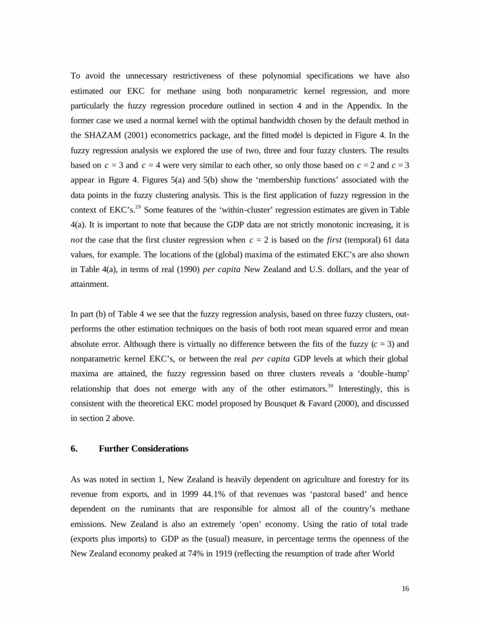
To avoid the unnecessary restrictiveness of these polynomial specifications we have also
estimated our EKC for methane using both nonparametric kernel regression, and more
particularly the fuzzy regression procedure outlined in section 4 and in the Appendix. In the
former case we used a normal kernel with the optimal bandwidth chosen by the default method in
the SHAZAM (2001) econometrics package, and the fitted model is depicted in Figure 4. In the
fuzzy regression analysis we explored the use of two, three and four fuzzy clusters. The results
based on c = 3 and c = 4 were very similar to each other, so only those based on c = 2 and c = 3
appear in Figure 4. Figures 5(a) and 5(b) show the ‘membership functions’ associated with the
data points in the fuzzy clustering analysis. This is the first application of fuzzy regression in the
context of EKC’s.29 Some features of the ‘within-cluster’ regression estimates are given in Table
4(a). It is important to note that because the GDP data are not strictly monotonic increasing, it is
not the case that the first cluster regression when c = 2 is based on the first (temporal) 61 data
values, for example. The locations of the (global) maxima of the estimated EKC’s are also shown
in Table 4(a), in terms of real (1990) per capita New Zealand and U.S. dollars, and the year of
attainment.
In part (b) of Table 4 we see that the fuzzy regression analysis, based on three fuzzy clusters, out-
performs the other estimation techniques on the basis of both root mean squared error and mean
absolute error. Although there is virtually no difference between the fits of the fuzzy (c = 3) and
nonparametric kernel EKC’s, or between the real per capita GDP levels at which their global
maxima are attained, the fuzzy regression based on three clusters reveals a ‘double -hump’
relationship that does not emerge with any of the other estimators.30 Interestingly, this is
consistent with the theoretical EKC model proposed by Bousquet & Favard (2000), and discussed
in section 2 above.
6. Further Considerations
As was noted in section 1, New Zealand is heavily dependent on agriculture and forestry for its
revenue from exports, and in 1999 44.1% of that revenues was ‘pastoral based’ and hence
dependent on the ruminants that are responsible for almost all of the country’s methane
emissions. New Zealand is also an extremely ‘open’ economy. Using the ratio of total trade
(exports plus imports) to GDP as the (usual) measure, in percentage terms the openness of the
New Zealand economy peaked at 74% in 1919 (reflecting the resumption of trade after World
17
Figure 4Empirical Kuznets' Curves: Fuzzy & Nonparametric Estimation
0.34
0.36
0.38
0.40
0.42
0.44
0.46
0.48
0.50
0.52
20 30 40 50 60 70 80 90 100 110 120
Real per capita GDP Index (1990 = 100)
Met
hane
(Ton
nes
per c
apita
)
Actual Data
Nonparametric
Fuzzy (c=2)
Fuzzy (c=3)

18
War I) and at 71% in 1952 (reflecting the Korean War Boom).31 The median openness rate over
the period 1918 to 1998 was 48%, and the figures for 1918, 1958 and 1998 were 58%, 48% and
46% respectively. By way of comparison, the corresponding figures for the U.S.A. in these three
years were only 12%, 7% and 18%; for the United Kingdom they were 38%, 39% and 41%; and
for Australia they were 39%, 31% and 34%. For Canada, the openness figure ranged from 33% in
1926 to 22% and 47% in 1958 and 1998 respectively.32 The New Zealand economy is heavily
reliant on trade, and in particular it is (and always has been) heavily dependent on exports of such
‘pastoral-based’ products as wool, lamb and mutton, live sheep, butter and cheese, skimmed milk
powder, and more recently venison and deer antler ‘velvet’.33 Given the intimate connection
between the production of these exports and the generation of enteric CH4 emissions, one obvious
question that arises is whether or not the associated EKC is at least partially determined by the
(relative) price of exports. Given the pivotal role of sheep in New Zealand, both in terms of
exports and in terms of methane emissions, wool prices may be of special relevance. This is
reinforced by New Zealand’s continued standing as a top international producer of this product –
still the third largest in the world in 2000/2001.34
We have experimented with various versions of our EKC models by including values of the wool
price index (deflated either by the consumer price index, or by the export price index for New
Zealand). To take account of the time delay likely to be associated with reductions (increases) in
sheep stocks as farmers respond to rises (falls) in the relative price of wool, we also considered
lagged values of the deflated wool price index in the models. However, we were unable to find
any specifications with a significant and positive price effect. Indeed, in most cases the wool
price variable had an insignificant negative coefficient, which is not surprising in view of the
negative sample correlations between CH490L and the two real wool price series.35 It seems clear
that New Zealand’s methane emission problems are not responsive to the associated international
prices.
As can be seen in Figure 2, real per capita output has followed a strong upward trend in New
Zealand since the Great Depression, and Giles et al. (1992) have established the existence of
significant (Granger) causality from exports of certain goods and services to real GDP in that
country. In the context of our EKC results, this suggests that it would be a mistake for New
Zealand’s policy-makers to look to livestock (and hence exports) reduction as a means of
achieving their Kyoto Protocol commitments with respect to methane emissions. Moreover, were
19
they to do so (such as through a reinstatement of sheep retention subsidies), the effects of the
associated trade diversion could result in net increase in worldwide emissions of enteric CH4. For
example, assuming no change in the international demand for wool and sheep meats, but with the
New Zealand supply diminished, prices for these products would rise on international markets
and other countries would increase their sheep stocks. The countries most likely to respond in this
way are ones (such as China, Argentina, Uruguay and South Africa) with lower real per capita
GDP than New Zealand.36 To the extent that our EKC results for methane apply internationally,
this would lead to a net increase in enteric methane emissions. Relatively high income countries
have a comparative advantage in finding technological solutions for pollution problems such as
methane emissions, and from a global perspective policy-makers in New Zealand are correct in
pursuing their current scientific efforts to reduce CH4 emission rates per animal.
The agricultural research base in that country is exceptionally strong, and recently there has been
intensive research into methods of measuring and reducing methane emission rates among
ruminants (especially sheep and cattle). On-the-farm measurements of enteric methane emissions
in New Zealand date from 1996, with the development of a micro-meteorological method of
measuring net methane emissions from flocks of free-ranging sheep, taking into account the
oxidation or consumption of methane by soil bacteria.37 Dietary intake is an important
determinant of enteric CH4 emissions. For example, Ulyatt et al. (2002) report on the extent to
which these emissions can be reduced by modifying the type of pasture to include sub-tropical
kikuyu grass (Pennisetum clandestinum). Other research indicates that emission rates fall as the
condensed tannin content of the food is increased. Such research is not limited to New Zealand.
For example, experiments at the Institut National de la Recherche Agronomique in France have
involved lambs, born by caesarian section, being reared in a sterile environment. The animals
have been inoculated with all the usual bacteria from the rumen of ordinary sheep, except for the
methane-producing bacteria. The results to date indicate that the elimination of the bacteria does
not affect the growth or productive capabilities of the sheep. Related research in Australia has
resulted in experimental trials of a vaccine that discourages Methanogenic archae, the organisms
which inhabit the animal’s digestive system and produce methane by breaking down feed.

20
Table 4
Fuzzy and Nonparametric Regression Results
(a) Fuzzy Regression Sub-Model Results
c Fuzzy T Cluster Slope Intercept
Cluster Centre (t-value) (t-value)
2 1 61 39.032 0.2767*10-3 0.4182
(1.06) (39.25)
2 41 89.826 -0.1529*10-2 0.5722
(-4.07) (17.15)
3 1 49 35.291 0.1291*10-2 0.4702
(2.23) (22.31)
2 24 64.117 0.1689*10-2 0.4147
(3.33) (12.79)
3 29 95.786 -0.4938*10-2 0.9839
(-7.41) (15.49)
(b) Comparative Model Performances*
OLS Fuzzy Nonparametric
Quadratic Cubic c = 2 c = 3
RMSE 0.0565 0.0517 0.0244 0.0201 0.0228
MAE 0.0321 0.0254 0.0201 0.0168 0.0179
Max. 8.41 10.74 9.74 11.28 11.28
(NZ$’000)
Max. 6.80 7.65 7.70 8.14 8.14
(US$’000)*
Year 1950 1967 1959-1961 1970 1970
* Converted using the ratio (‘Y’) of real per capita GDP for New Zealand to that of the U.S.A.,
from the Penn World Table, 5.6 (Summers and Heston, 1995), for each year in question.

21
Figure 5(a) Fuzzy Clustering Membership Functions (c = 2)
0.0
0.1
0.2
0.3
0.4
0.5
0.6
0.7
0.8
0.9
1.0
1.1
20 30 40 50 60 70 80 90 100 110 120
Real per Capita GDP Index (1990 = 100)
Mem
bers
hip
Val
ue
Mu1
Mu2
Figure 5(b) Fuzzy Clustering Membership Functions (c = 3)
0
0.1
0.2
0.3
0.4
0.5
0.6
0.7
0.8
0.9
1
1.1
20 30 40 50 60 70 80 90 100 110 120
Real per capita GDP Index (1990 = 100)
Mem
bers
hip
Val
ue
Mu1
Mu2
Mu3

22
7. Conclusions
In this paper we have studied the relationship between enteric methane emissions and real per
capita GDP in New Zealand, using traditional and new techniques to estimate an environmental
Kuznets’ curve for this GHG. Among the noteworthy features of this research are: our use of data
spanning more than a century; the application of new ‘fuzzy regression’ techniques to unearth the
nonlinear characteristics of the relationship in a flexible manner; and the focus on a little-studied
GHG that is of primary concern to this major wool-producing country in meeting its obligations
as a signatory to the Kyoto Protocol.
It is not the purpose of this paper to offer a theoretical basis for the relationship between methane
emissions and income, but our empirical results indicate that there is an environmental Kuznets’
curve for CH4 in New Zealand. Our preferred results, based on ‘fuzzy regression’ methods
suggest that the curve has a ‘double -hump’, with a maximum at a GDP level of just over
US$8,000 per capita , in real 1990 dollar terms. This general shape for the EKC is consistent with
the results of Taskin and Zaim (2000) and Dijkgraaf and Vollebergh (2001) for CO2, and is
suggested by the theoretical model of Bousquet & Favard (2000). Our nonparametric kernel
regression results suggests a curve with a single maximum at the same level of income, while
levels of the order of US$7,000-US$7,500 are implied by our standard quadratic and cubic
regressions. These turning point levels are very consistent with the results of other studies relating
to various GHG emissions internationally, as is evidenced by the discussions in Grossman and
Krueger (1995) and Hilton and Levinson (1998).
Lowering enteric methane emissions by reducing livestock numbers is not a viable option for
New Zealand, given its dependence on pastoral-based exports, and the established causality
between its exports and GDP. Our positive findings with respect to an environmental Kuznets’
curve for CH4 suggest that this economic ‘fact of life’ may be fortuitous – it seems that any
significant reduction in real GDP from its recent levels would lead to an increase in the emissions
of this GHG. With its relatively high per capita GDP, New Zealand has always invested heavily
(and successfully) in agricultural research. A number of positive recent scientific developments
suggest that methane emissions in that country will be curtailed (and livestock productivity will
be increased) through vaccinations and dietary changes. Our findings with respect to an
environmental Kuznets’ curve suggest that there will also be a reinforcing effect as enhanced
exports have a positive impact on real output.

23
Appendix Fuzzy Econometric Modelling
The Fuzzy c-Means Algorithm The FCM algorithm provides a method for dividing up the ‘n’ data-points into ‘c’ fuzzy clusters
(where c < n), while also locating the centres of these clusters. The metric that forms the basis for
the usual FCM algorithm is usually ‘squared error distance’, though the use of an ‘absolute error
distance’ can be used to deal with outliers in the data. (See Stroomer and Giles, 2003). The
mathematical details of the algorithm are as follows. Let xk be the k th (possibly vector) data-point
(k = 1, 2, ...., n). Let vi be the centre of the ith (fuzzy) cluster (i = 1, 2, ....., c). Let dik = || xk - vi || be
the distance between xk and vi , and let uik be the ‘degree of membership’ of data-point ‘k’ in
cluster ‘i’, where :
The objective is to partition the data-points into the ‘c’ clusters, locate the cluster centers, and
also determine the associated ‘degrees of membership’, so as to minimize the functional
While there is no explicit basis for choosing the value of the parameter ‘m’, which must satisfy 1
< m < ∞, with m = 1 corresponding to ‘hard clustering’. In practice m = 2 is a common choice,
and is the one that we adopt here. The FCM algorithm requires that the number of clusters, c, be
specified in advance, and in view of the sample size in our study (and the empirical findings of
Giles and Draeseke, 2003) we have considered c = 2, 3 and 4. The algorithm then comprises the
following steps:
1. Select the initial locations of the cluster centres.
2. Generate a (new) partition of the data by assigning each data-point to its closest cluster
centre.
3. Calculate new cluster centres from the revised partition of the data.
4. If the cluster partition is stable then stop. Otherwise go to step 2 above.
J U v u dk
n
iki
cm
ik( , ) ( ) ( ) .===
∑∑11
2
( ) .uiki
c
==∑ 1
1

24
In the case of fuzzy the memberships, the Lagrange multiplier technique generates the following
expression for the membership values to be used at step 2 above:
If the memberships of data-points to clusters are ‘crisp’ then
uik = 0 ; ≤ i ! j,
ujk = 1 ; j s.t. djk = min.{dik, i = 1, 2, ...., c}.
The updating of the cluster centres at step 3 above is obtained via the expression
The fixed-point nature of this problem ensures the existence of a solution in a finite number of
steps. When the centres of the fuzzy clusters have been determined, each of the n data-points can
be allocated to the cluster whose center it is closest to.
Fuzzy Regression Analysis
To begin with, consider the simple case where there is a single regressor (other than, perhaps, a
constant intercept). The fuzzy relationship to be estimated is of the form:
where the form of the functional relationship remains unspecified (but will typically involve
unknown parameters), and e is a random disturbance term. There is no need to make any
distributional assumptions about the latter. If the disturbance has a zero mean, the fuzzy function
represents the conditional mean of the dependent variable, y. To this extent, the framework is the
same as that which is adopted in non-parametric kernel regression.
The identification and estimation of the fuzzy model then proceeds according to the following
steps:
u d dik ikj
n
jkm=
=
−∑1 2
1
2 1 1/ [( ) / ( ) ]{ }./( )
v u x u i ci ikm
k
n
k ikm
k
n
= == =
∑ ∑[ ( ) ]/ [ ( ) ] ; , ,...., .1 1
1 2
y f x= +( ) ε

25
Step 1: Partition the sample observations for x into c fuzzy clusters, using the FCM
algorithm. This generates the membership values for each x-value with respect to
each cluster, and also defines a corresponding partition of the data for y.
Step 2: Using the data for each fuzzy cluster separately, fit the models:
In particular, if the chosen estimation procedure is parametric least squares, then
Step 3: Model and predict the conditional mean of y using:
where uik is the degree of membership of the k th value of x in the i’th. fuzzy
cluster, and bim is the least squares estimator of bim (m = 0, 1) obtained using the
ith fuzzy partition of the sample.
The fuzzy predictor of the conditional mean of y is a weighted average of the linear predictors
based on the fuzzy partitioning of the explanatory data, with the weights (membership values)
varying continuously through the sample. This latter feature enables non-linearities to be
modelled effectively. In addition, it can be seen that the separate modelling over each fuzzy
cluster involves the use of fuzzy logic of the form “IF the input data are likely to lie in this
region, THEN this is likely to be the predictor of the output variable”, etc.. The derivative of the
conditional mean with respect to the input variable also has this weighted average structure, and
the same potential for non-linearity.
Note that this modelling strategy is essentially a semi-parametric one. The parametric
assumptions could be relaxed further by using kernel estimation to fit each of the cluster sub-
models at Step 2 above, in which case the estimated derivatives (rather than coefficients) would
be weighted at Steps 3 and 4, instead of the parameter estimates. However, some experimentation
with this variation of the modelling methodology was undertaken by Giles and Draeseke (2003),
and was found not to perform well.
y f x j n i cij i ij ij i= + = =( ) ; ,...., ; ,....,ε 1 1
y x j n i cij i i ij ij i= + + = =β β ε0 1 1 1; ,...., ; ,....,
[ ]$ ( ) / ; ,....,y b b x u u k nki
c
i i k iki
c
ik= +
=
= =∑ ∑
10 1
1
1

26
More generally we will be interested in models that have more than one regressor:
Assuming a linear least squares basis for the analysis for expository purposes, the steps in the
above fuzzy modelling procedure are extended as follows :
Step 1': Separately partition the n sample observations for each xr into cr fuzzy clusters
(where r = 1, 2, ....,p), using the FCM algorithm. This generates the membership
values for each observation on each x variable with respect to each cluster.
Step 2': Consider all c possible combinations of the fuzzy clusters associated with the p
input variables, where
and discard any for which the intersections involve negative degrees of freedom
(nr < p). Let the number of remaining cluster combinations be c'.
Step 3': Using the data for each of these c' fuzzy clusters separately, fit the models:
Step 4': Model and predict the conditional mean of y by using:
where
y x x x j n i cij i i ij i ij ip pij ij i= + + + + + = =β β β β ε0 1 1 2 2 1 1LL ; ,...., ; ,...., '
y f x x xp= +( , ,......., )1 2 ε
c crr
p
==
∏1
[ ]$ ( ) / ; ,....,'
y b b x b x w w k nki
c
i i k ip pk iki
c
ik= + + +
=
= =∑ ∑
10 1 1
1
1LL
w u i ci kr
p
ij rjk= ==
∏1
1δ ; , , 'LL

27
Here, dij is a ‘selector’ that chooses the membership value for the j th fuzzy cluster
(for the rth input variable) if that cluster is associated with the ith cluster
combination (i = 1, 2, …., c'); and bim is the least squares estimator of bim
obtained by using the ith fuzzy partition of the sample.
Comparing these steps with those in the case of a single input variable, it is clear that the
computational burden associated with the fuzzy modelling increases at the same rate as in the
case of multiple linear regression as additional explanatory variables are added to the model.
Under some very mild conditions, it can be shown that the fuzzy regression estimator is weakly
consistent, and more importantly its rate of convergence is the same as that for the least squares
estimator. That is, we have T1/2 convergence under standard assumptions. In contrast,
nonparametric kernel regression suffers from the well-known ‘curse of dimensionality’ – it
converges in probability increasingly slowly as the number of regressors grows. (Strictly
speaking, this is true only if all of the regressors are continuous, rather than discrete, variables –
see Racine and Li, 2003, for details.)

28
References
Akaike, H. (1973), “Information Theory and an Extension of the Maximum Likelihood
Principle”, in B. N. Petrov and F. Csáki (eds.), 2nd International Symposium on
Information Theory (Akadémiai Kiadó, Budapest), 267-281.
Andreoni, J. and A. Levinson (1998), “The Simple Analytics of the Environmental Kuznets
Curve”, NBER Working Paper 6739, National Bureau of Economic Research, Cambridge
MA.
Bousquet, A. and P. Favard (2000), “Does S. Kuznets’ Belief Question the Environmental
Kuznets Curve?”, mimeo., Université des Sciences Sociales Toulouse.
Clark, H. (2001), “Ruminant Methane Emissions: A Review of the Mrhodology Used for
National Inventory Estimations”, A Report Prepared for the Ministry of Agriculture and
Forestry, New Zealand.
DeBenedictis, L.F. and D.E.A. Giles (1998), “Diagnostic Testing in Econometrics: Variable
Addition, RESET, and Fourier Approximations”, in A. Ullah and D.E.A. Giles (eds.),
Handbook of Applied Economic Statistics (Marcel Dekker, New York), 383-417.
DeBenedictis, L.F. and D.E.A. Giles, 1999, “Robust Specification Testing in Regression: The
FRESET Test and Autocorrelated Disturbances”, Journal of Quantitative Economics, 15,
67-75.
De Bruyn, S. M., J. C. J. M. van den Bergh and J. B. Opschoor (1998), “Economic Growth and
Emissions: Reconsidering the Empirical Basis of Environmental Kuznets Curves”,
Ecological Economics, 25, 161-175.
Deininger, K. and L. Squire (1998), “New Ways of Looking at Old Issues”, Journal of
Development Economics, 57, 259-87.
Dijkgraaf, E. and H. R. J. Vollebergh (2001), “A Note on Testing for Environmental Kuznets
Curves”, OCFEB Research Memorandum 0102, Research Center for Economic Policy,
Erasmus University Rotterdam.
Dickey, D. A. and W. A. Fuller (1979), “Distribution of the Estimators for Autoregressive Time
Series With a Unit Root”. Journal of the American Statistical Association, 74, 427-31.
Dickey, D. A. and W. A. Fuller (1981), “Likelihood Ratio Statistics for Autoregressive Time
Series With a Unit Root”. Econometrica, 49, 1057-72.
Dickey, D. A. and S. E. Said (1981), “Testing ARIMA(p,1,q) Against ARMA(p+1,q)”.
Proceedings of the Business and Economic Statistics Section, American Statistical
Association, 28, 318-22.

29
Donovan, K. and L. Baldwin (1999), “Results of the AAMOLLY Model Runs for the Enteric
Fermentation Model”, mimeo., University of California, Davis.
Egli, H. (2001), “Are Cross-Country Studies of the Environmental Kuznets Curve Misleading?
New Evidence From Time Series Data for Germany”, Discussion Paper 10/2001, Ernst-
Moritz-Arndt University of Greifswald.
Ekins, (1997), “The Kuznets Curve for the Environment and Economic Growth: Examining the
Evidence”, Environment and Planning A, 29, 805-830.
Eviews (2002), Eviews 4.1, User’s Guide. (Quantitative Micro Software, Irvine, CA.)
Franses, P. H. (2001), “How to Deal With Intercept and Trend in Practical Cointegration
Analysis?”, Applied Economics, 33, 577-579.
Giles, D. E. A. (2001), “Output Convergence and International Trade: Time-Series and Fuzzy
Clustering Evidence for New Zealand and Her Trading Partners, 1950-1992”,
Econometrics Working Paper EWP0102, Department of Economics, University of
Victoria.
Giles, D. E. A. (2002), “Spurious Regressions With Time-Series Data: Some Further Asymptotic
Results”, Econometrics Working Paper EWP0203, Department of Economics, University
of Victoria.
Giles, D. E. A. and R. Draeseke (2003), “Econometric Modelling Using Pattern Recognition via
the Fuzzy c-Means Algorithm”, in D. E. A. Giles (ed.), Computer-Aided Econometrics
(Marcel Dekker, New York), 407-450.
Giles, D. E. A. and H. Feng (2003), “Testing for Convergence in Measures of ‘Well-Being’ in
Industrialized Countries”, Econometrics Working Paper EWP0303, Department of
Economics, University of Victoria.
Giles, D. E. A., J. A. Giles and E. B. M. McCann (1992), “Causality, Unit Roots and Export-Led
Growth: The New Zealand Experience”, Journal of International Trade and Economic
Development, 2, 195-218.
Granger, C. W. J. and P. Newbold (1974), “Spurious Regressions in Econometrics, Journal of
Econometrics, 2, 111-120.
Greasley, D. and L. Oxley (2000), Measuring New Zealand’s GDP 1865-1933: A Cointegration-
Based Approach”, Review of Income and Wealth , 46, 351-368.
Grossman G. M. and A. B. Krueger (1993), “Environmental Impacts of a North American Free
Trade Agreement”, in P. Garber (ed.), The U.S.-Mexico Free Trade Agreement. MIT
Press, Cambridge MA, 165-177.

30
Grossman, G. M. and A. B. Krueger (1995), “Economic Growth and the Environment”, Quarterly
Journal of Economics, 110, 353-357.
Harbargh, W., A. Levinson and D. Wilson (2002), “Reexamining the Empirical Evidence for an
Environmental Kuznets Curve”, Review of Economics and Statistics, 84, 541-551.
Hilton, F. G. H. and A. Levinson (1998), “Factoring the Environmental Kuznets Curve: Evidence
From Automotive Lead Emissions”, Journal of Environmental Economics and
Management, 35, 126-141.
Holtz-Eakin, H. and T. M. Selden (1995), “Stoking the Fires? CO2 Emissions and Economic
Growth”, Journal of Public Economics, 57, 85-101.
Hornok, Attila and Larsson, Rolf. “The Finite Sample Distribution of the KPSS Test.”
Econometrics Journal 3 (2000): 108-21.
Jacobsen, P. W. F. and D. E. A. Giles (1998), “Income Distribution in the United States: Kuznets’
Inverted-U Hypothesis and Data Non-Stationarity”, Journal of International Trade and
Economic Development, 7, 405-423.
Jarque, C. and A. Bera (1980), “Efficient Tests for Normality, Homoskedasticity and Serial
Independence of Regression Residuals, Economics Letters, 6, 255-259.
Johansen, S. (1988), “Statistical Analysis of Cointegration Vectors”, Journal of Economic
Dynamics and Control, 12, 231-254.
Johansen, S. (1995), Likelihood-Based Inference in Cointegrated Vector Autoregressive Models
(Oxford University Press, Oxford).
Kuznets, S. (1955), “Economic Growth and Income Inequality”, American Economic Review, 45,
1-28.
Kwiatkowski, D., P. C. B. Phillips, P. Schmidt, and Y. Shin (1992), “Testing the Null
Hypothesis of Stationarity Against the Alternative of a Unit Root.” Journal of
Econometrics, 54, 91-115.
MacKinnon, J. G. (1991), “Critical Values for Co-integration Tests”, in R. F. Engle and C. W. J.
Granger (eds.), Long-Run Economic Relationships (Cambridge University Press,
Cambridge), 267-276.
Maddison, A. (1995), Monitoring the World Economy, 1820-1992 (Organisation for Economic
Co-operation and Development, Paris).
Mosk, C. A. (2003), Bound for Distant Lands: Trade and Migration in the Modern World , book
manuscript.
New Zealand Ministry of Agriculture and Forestry (2000), International Trade Statistics,
Wellington, New Zealand.
31
New Zealand Ministry of Agriculture and Forestry (2002), Agriculture, Forestry and Horticulture
in Brief, Wellington, New Zealand.
New Zealand Ministry of Agriculture and Forestry (2003), Livestock Data, as reported on the
internet at <http://www.maf.govt.nz/statistics/primaryindustries/livestock/>
New Zealand National Institute of Water and Atmospheric Research (2003), Environmental
Performance Indicators Program, as reported on the internet at
<www.environment.govt.nz/indicators/climate/methane.html>
Ogwang, T. (1994), “Economic Development and Income Inequality: A Nonparametric
Investigation of Kuznets’ U-Curve Hypothesis”, Journal of Quantitative Economics, 10,
139-153.
Perman, R. and D. I. Stern (1999), “The Environmental Kuznets Curve: Implications of Non-
Stationarity”, Working Papers in Ecological Economics 9901, Centre for Resource and
Environmental Studies, Australian National University, Canberra.
Pfaff, A. S. P., S. Chaudhuri and H. L. M. Nye (2001), “Why Might One Expect Environmental
Kuznets Curves? Examining the Desirability and Feasibility of Substitution”, mimeo.,
Columbia University.
Phillips, P. C. B. (1986), “Understanding Spurious Regressions in Econometrics, Journal of
Econometrics, 33, 311-340.
Racine, J. and Q. Li (2003), “Nonparametric Estimation of Regression Functions With Both
Categorical and Continuous Data”, forthcoming in Journal of Econometrics.
Ruspini, E. (1970), “Numerical Methods for Fuzzy Clustering”, Information Science, 2, 319-350.
Roca, J., E. Padilla, M. Farré and V. Galletto (2001), “Economic Growth and Atmospheric
Pollution in Spain: Discussing the Environmental Kuznets’ Curve Hypothesis”,
Ecological Economics, 39, 85-99.
Schmalensee, R., T. M. Stoker and R. A. Judson (1998), “World Carbon Dioxide Emissions:
1950-2050”, Review of Economics and Statistics, 80, 15-27.
Schwarz, G. (1978), “Estimating the Dimension of a Model”, Annals of Statistics, 6, 461-464.
Selden, T., and D. Song (1994), “Environmental Quality and Devlopment: Is There a Kuznets
Curve for Air Pollution Emissions?”, Journal of Environmental Economics and
Management, 28, 147-162.
Selden, T, and D. Song (1995), “Neoclassical Growth, the J-Curve for Abatement, and the
Inverted U-Curve for Pollution”, Journal of Environmental Economics and Management,
29, 162-168.

32
Shafik, N. (1994), “Economic Development and Environmental Quality: An Econometric
Analysis”, Oxford Economic Papers, 46, 757-773.
Shafik, N. and S. Bandyopadhyay (1992), Economic Growth and Environmental Quality: Time
Series and Cross Country Evidence. Background paper for World Development Report
1992, World Bank, Washington, DC.
SHAZAM (2001), SHAZAM Econometrics Package, User's Guide, Version 9 (Northwest
Econometrics, Vancouver, B.C..)
Shepherd, D. and F. K. C. Shi (1998), “Economic Modelling With Fuzzy Logic”, paper presented
at the CEFES ’98 Conference, Cambridge, U.K..
Statistics New Zealand (1998), Hot Off the Press (June Quarter), available on the internet at
<http://www.stats.govt.nz/domino/external/pasfull/pasfull.nsf/web/Hot+Off+The+Press
+Gross+Domestic+Product+June+1998+quarter?open>
Stern, D. I. and M. S. Common (2001), “Is There an Environmental Kuznets Curve for Sulfur?”,
Journal of Environmental Economics and Management, 41, 162-178.
Stern, D. I., M. S. Common and E. B. Barbier (1997), “Economic Growth and Environmental
Degradation: The Environmental Kuznets Curve and Sustainable Development”, World
Development, 24, 1151-1160.
Stock, J. H. (1987), “Asymptotic Properties of Least-Squares Estimators of Co-integrating
Vectors”, Econometrica, 55, 1035-1056.
Stokey, N. L. (1998), “Are There Limits to growth?”, International Economic Review, 39, 1-31.
Stroomer, C., and D. E. A. Giles (2003), “Income Convergence and Trade Openness: Fuzzy
Clustering and Time Series Evidence”, Econometric Working Paper EWP0304,
Department of Economics, University of Victoria.
Summers, R. and A. Heston (1995), The Penn World Table, Version 5.6 (National Bureau of
Economic Research: Cambridge MA).
Taskin, F. and O. Zaim (2000), “Searching for a Kuznets Curve in Environmental Efficiency
Using Kernel Estimation”, Economics Letters, 68, 217-223.
Ulyatt, M. J., K. R. Lassey, I. D. Shelton and C. F. Walker (2002), “Methans Emission From
Dairy Cows and Wether Sheep Fed Subtropical Grass-Dominant Pastures in Midsummer
in New Zealand”, New Zealand Journal of Agricultural Research, 45, 227-234.
Utt, J. A., W. W. Hunter and R. E. McCormick (2001), “On the Relation Between Net Carbon
Emissions and Income. Carbon Sinks Global Warming: Are Rich People Cool?”.
Mimeo., Department of Economics, Washington State University.
World Bank (1992), World Development Report 1992. Oxford University Press, New York.

33
Zadeh, L. A. (1965), “Fuzzy Sets”, Information and Control, 8, 338-353.
Zadeh, L. A. (1987), Fuzzy Sets and Applications: Selected Papers. Wiley, New York.

34
Footnotes
* We are extremely grateful to Dr Harry Clark (AgResearch Ltd., New Zealand) and Dr
Gerald Rys (Ministry of Agriculture and Forestry, New Zealand) for helpful
correspondence and the provision of data and technical information relating to the
scientific research program into enteric methane emissions in that country.
1. Total atmospheric methane concentrations in New Zealand rose from 1669.5 ppb in 1990
to 1736.3 ppb in 2000 (in terms of Gg of CO2-equivalent units). See New Zealand
National Institute of Water and Atmospheric Research (2003).
2. See Clark, 2001.
3. This level was just over 73 million CO2-equivalent tonnes.
4. Some of this research has been undertaken in collaboration with other scientific teams in
Australia and France.
5. See Table 1 below for details of the different enteric methane emission rates associated
with the different animal types.
6. See New Zealand Ministry of Agriculture and Forestry (2000).
7. See New Zealand Ministry of Agriculture and Forestry (2002). This represented a
reduction from over 48% in 1992. Agriculture as a whole accounted for 53.8% of the
value of New Zealand’s exports in 1999, and forestry products accounted for
approximately an additional 11% of export dollars.
8. It also seems likely that the results of some of the earlier studies, using time-series data,
may have been affected by a failure to take account of the fact that these data were non-
stationary. For some evidence on this point, see Jacobsen and Giles (1998) Perman and
Stern (1999), and Stern and Common (2001).
9. Special issues of Ecological Economics (in 1995 and 1998), and Environment and
Development Economics (1996) have been devoted to the environmental Kuznets curve.
10. See Selden and Song (1995, p.147).
11. Each GHG has its own ‘global warming potential’, set by the Intergovernmental Panel on
Climate Control (IPCC). In the case of methane this is 21 (c.f., CO2 = 1) for a 100-year
time-horizon.
12. These are constant 1999 dollars.
13. Although Stern and Common (2001) have data for sulfur emissions for the period 1850
to 1990, their EKC study is based on models estimated for 1960 to 1990 due to
constraints on the availability of PPP-adjusted international GDP data.
35
14. Our data for livestock numbers end in 1996, due to a change in the reporting method.
Official Ministry of Agriculture and Fisheries (now Forestry) figures for the period prior
to 1971 are taken from the annual New Zealand Yearbooks.
15. Recent confidential work by Clarke and Ulyatt deals with updates to these estimates. No
emission rate estimates are available for the period prior to 1990, the latter year being the
‘base year’ for New Zealand’s Kyoto Protocol obligations. In our calculations, in the
absence of contrary evidence, we assume a constant emission rate for each animal type
over time.
16. The series using the ‘1990-High’ and ‘1999-Low’ emission estimates are visually
indistinguishable.
17. A ‘spurious regression’ arises when the data are non-stationary, but are not cointegrated,
and the associated results are meaningless (and increasingly so as the sample size
increases). See Granger and Newbold (1974), Phillips (1986) and Giles (2002) for more
details.
18. It is understood, of course, that this turning point may occur at a level of output that is
outside the range of the sample values, so it may not be ‘observed’.
19. Their modelling framework is based, in turn, on the earlier contribution of Shephard and
Shi (1998).
20. It should be emphasized that while this technique may appear to be similar to spline
analysis, in fact it is quite different, and is much more flexible. In spline analysis the join-
points (or ‘knots’) for the continuous sections of the function are taken as known and are
specified in advance. In fuzzy regression, the FCM algorithm determines the partition of
the data into the clusters on the basis of the sample values. Moreover, in fuzzy regression
the different estimated cluster results are ‘mixed’ by using the estimated degrees of
membership, whereas in spline analysis the separate functional sections are simply
abutted to one another.
21. The following discussion is taken essentially from Giles and Draeseke (2003, pp.412-
419). For some additional applications of fuzzy clustering in economic applications, see
Giles (2001), Giles and Feng (2003) and Stroomer and Giles (2003).
22. For a more complete discussion of this topic, see Zadeh (1987).
23. The FCM algorithm is usually attributed to Ruspini (1970), though there are now many
variants of it in use.

36
24. Applying the tests to the differenced data confirmed that none of the series are I(2). In
addition, allowing for the possibility of structural breaks in the trends of the data did not
affect our conclusions.
25. Details of the results obtained by using each of the other three methane series are
available from the authors on request. The results that we present here are completely
insensitive to the choice of the CH4 series.
26. If ‘T’ denotes the sample size, a super-consistent estimator is one that converges to the
true parameter value at a rate ‘T’, rather than the usual rate of ‘T1/2’. See Stock (1987).
27. The FRESET test of Debenedictis and Giles (1998, 1999) is similar to Ramsey’s RESET
test, but a Fourier series approximation is used in its construction, rather than a
polynomial approximation. This use of a global (rather than local) approximation
increases the power of test markedly, even in the context of contamination from serial
correlation. The FRESET test can be conducted with the DIAGNOS command in the
SHAZAM econometrics package.
28. In Figure 3(a) we present the ‘fitted values’ from the OLS regressions, plotted against
GDP. The relationships shown in Figure 3(b) are obtained when we solve for the long-
run estimated relationship, as follows. If the model is of the generic form,
yt = a + b xt + c yt-1 + ut, then y* = (a* + b* x)/(1 – c*), where an asterisk denotes an
estimated value.
29. Giles and Draeseke (2003) estimate a conventional Kuznets’ curve for the U.S.A. using
fuzzy regression, as one of their illustrative examples. Nonparametric (kernel) estimates
of Kuznets’ curves are surprisingly unusual. For conventional Kuznets’ curves see
Ogwang (1994) and Jacobsen and Giles (1998); and for the only nonparametric EKC that
we are aware of, see Taskin and Zaim (2000).
30. The same is true when the fuzzy analysis is conducted with c = 4. In this case the higher
of the two maxima occurs at a real (1990 dollars) per capita output level of NZ$11,680
(US$8,433), which corresponds to the year 1971 in our sample. Of course it may also be
possible to achieve a ‘double-hump’ EKC with a higher-order polynomial specification,
but we have not pursued this further.
31. The New Zealand economy boomed during the Korean War, largely as a result of the
increased demand for its coarse-grade wool.
32. See Mosk (2003) for further details.
33. The export of live sheep is to countries in the Middle East, so that religious customs may
be observed during slaughtering.

37
34. New Zealand’s production was 258 kilo-tonnes of fleece and skin wool (greasy wool
equivalent). The productions of Australia and China were 652 and 291 kilo-tonnes
respectively. See the British Wool Marketing Board’s site on the internet at
<http://www.britishwool.org.uk/a-factsheet4.asp>
35. The simple correlations with CH490L are –0.026 and –0.018 when wool prices are
deflated by the CPI and by export prices respectively.
36. Using Penn World Table data, the real (1990 dollars) per capita GDP’s for New Zealand,
China, South Africa and Uruguay in 2000 were approximately $16,750, $3,200, $6,700
and $8,600. Our preferred EKC peaks at approximately $8,140.
37. This research has been undertaken primarily by the LandcareResearch, Agresearch and
HortResearch organizations. For more information on the internet, see
<http://www.landcareresearch.co.nz/research/greenhouse/climatechange/methane.asp>