
Routing and wavelength allocation in WDM optical networks
208
Routing and wavelength allocation in WDM optical networks Stefano Baroni Submitted to the University of London for the degree of Ph.D. UCL Department of Electronic and Electrical Engineering University College London May 1998
-
Upload
khangminh22 -
Category
Documents
-
view
0 -
download
0
Transcript of Routing and wavelength allocation in WDM optical networks

Routing and wavelength allocation in WDM optical networks
Stefano Baroni
Submitted to the University of London for the degree of Ph.D.
UCLDepartment of Electronic and Electrical Engineering
University College London May 1998

ProQuest Number: U643721
All rights reserved
INFORMATION TO ALL USERS The quality of this reproduction is dependent upon the quality of the copy submitted.
In the unlikely event that the author did not send a complete manuscript and there are missing pages, these will be noted. Also, if material had to be removed,
a note will indicate the deletion.
uest.
ProQuest U643721
Published by ProQuest LLC(2016). Copyright of the Dissertation is held by the Author.
All rights reserved.This work is protected against unauthorized copying under Title 17, United States Code.
Microform Edition © ProQuest LLC.
ProQuest LLC 789 East Eisenhower Parkway
P.O. Box 1346 Ann Arbor, Ml 48106-1346


To my parents Domenico and Isabella
To Federica


Abstract
This thesis investigates routing and wavelength allocation (RWA) in wavelength-division-
multiplexed {WDM), wavelength-routed optical networks {WRONs).
WRONs represent the most promising solution for high-capacity transport applica
tions, providing efficient way to satisfy the increasing demand for bandwidth require
ment and network flexibility. The most critical parameter in WRONs is the network
physical topology onto which traffic demand has to be mapped, since it determines
RWA, and, hence, resource and WDM transmission requirements.
Although numerous investigations have addressed RWA problems in WRONs, little
attention has been paid to the role of physical topology. It is, therefore, the focus of this
thesis to investigate relationship between physical topology and network performance,
the results being crucial to enable optimal network design.
First, single-fibre WRONs are systematically analysed with uniform traffic demand,
the figure of merit being the wavelength requirement N \. A new integer linear program
{ILP) formulation is proposed for the exact solution of the RWA problem. Lower bounds
on N \ are discussed, and RWA heuristic algorithms proposed. The results quantify the
relationship between N \ and physical connectivity a, and highlights the negligible ben
efit achievable with wavelength conversion, or interchange (W/), in the optical cross
connects {OXCs). It is shown that WRONs allow large wavelength reuse, resulting in
large network throughput with a moderate number of wavelengths N \, even in weakly-
connected topologies. The comparison with regular networks shows that arbitrarily-
connected WRONs provide scalability and flexibility, whilst maintaining similar wave
length requirements.
The consequence of link failure restoration is then assessed. The results demonstrate
the key role of physical topology on the increase in N \, and the limited improvement
achievable with WI.
WDM transmission is studied by considering physical limitations imposed by wave

length-dependent gain characteristic of erbium-doped fibre amplifiers (EDFAs). A sim
ple algorithm for the absolute-wavelength assignment is proposed to compensate for
gain non-uniformities in EDFA cascades, under condition of lightpath add/drop. In ad
dition, a WDM optical amplifier configuration providing self-regulating properties is
proposed to reduce management complexity in large-scale resilient WRONs.
The design of multi-fibre WRONs is then investigated, by introducing the maxi
mum number of wavelengths per fibre, PF, as a parameter. Fibre requirement. Ft , and
resource utilisation are derived under different network conditions, including provision
ing of basic demand, restoration, and traffic growth. Different restoration strategies are
studied and compared. It is shown that the increase in Ft to provide for restoration is
governed by network physical connectivity a. The analysis of traffic growth identifies
the relationship between network size and connectivity, wavelength multiplicity W , and
relative merits of WI.
The presented algorithms and results can be used in the analysis and optimisation of
WRONs.

Acknowledgements
This dissertation is the result of (a bit more than) three years’ work, and I owe many
people gratitude for their help over that time. First and most importantly, I would like
to thank my supervisor Dr. Polina Bayvel for her continuous support, guidance, and
encouragement throughout the course of this work. Most of the problems analysed in
this thesis originated from discussions with her.
I would like to express my gratitude to Prof. John E. Midwinter for his support and
interest in my work, and to Prof. Frank P. Kelly (Statistical Laboratory, University of
Cambridge) for numerous ideas and helpful directions in the first part of my research.
The lower bounds presented in Chapter 3 were suggested to me by him.
I would like to thank Nortel Technology Ltd for the financial support which enabled
me to carry out this research, and, in particular, I would like to mention Drs. Paul A.
Kirkby, Nigel Baker, and Daniel V. McCaughan.
Part of the results in Chapter 6 were obtained during my internship in Lucent Tech
nologies, Holmdel, during the summer of 1996. I would like to thank Dr. Steve K.
Korotky for offering me the opportunity to experience those fast-changing months in
Lucent.
I would like to thank Dr. Richard I. Gibbens (Statistical Laboratory, University of
Cambridge) for working with me in deriving the ILP formulations presented in Chapters
3, 4, and 6. I will always be grateful to him for everything he could teach me.
I really enjoyed working with Dr Fabrizio Di Pasquale, Christophe Marand, and
Ricardo Olivares. Thanks to them I was able to understand a little more about the
limitations imposed by the physical transmission media. The joint work led to the results
of Chapter 5.
I would like to thank Drs. Richard J. Gibbens and Robert Killey to take the time to
read my thesis.
I would like to acknowledge the members of the Optical Networks Group, the people
7

in room 808, and all the other people with whom I shared my time, with discussions and
pizzas: Paolo, Derek, Neil, Jason, Farah, Martin, Cyrille, and the list could continue for
lines and lines. Most of them should be Drs by now!
Finally, I would like to thank my fiancée Federica for her patience and support dur
ing these years. The fact that she was able to tolerate me and my life in this period gives
me great hope for our future together.
Stefano BaroniDepartment o f Electronic and Electrical Engineering University College London May 1998

Contents
1 Introduction 29
2 W D M optical networks 33
2.1 Introduction...................................................................................................... 33
2.2 Wavelength-routed optical n e tw o rk s ............................................................ 34
2.3 Open issues in single-hop W R O N s............................................................... 38
2.3.1 Wavelength requ irem en t.................................................................. 38
2.3.2 OXCs functionality: reconfigurability and wavelength conversion 40
2.3.3 Optical re s to ra tio n ............................................................................ 43
2.3.4 WDM transmission in WRONs ..................................................... 44
2.3.5 Wavelength multiplicity and traffic l o a d ........................................ 45
2.4 C onclusions...................................................................................................... 47
3 W avelength requirem ent in single-fibre W RO Ns 49
3.1 In troduction...................................................................................................... 49
3.2 Network m o d e l ................................................................................................ 50
3.3 Lightpath allocation: ILP form ulations........................................................ 52
3.3.1 WIXC c a s e ......................................................................................... 53
3.3.2 W SXC c a s e .................................................................................................. 54
3.4 Lightpath allocation: lower bounds............................................................... 56
3.4.1 Distance b o u n d .................................................................................. 56
3.4.2 Partition b o u n d .................................................................................. 57
3.5 Lightpath allocation: upper b o u n d ............................................................... 58
3.6 Lightpath allocation: heuristic a lg o rith m s .................................................. 59
3.7 R esults............................................................................................................... 60
3.7.1 Real networks...................................................................................... 60
9
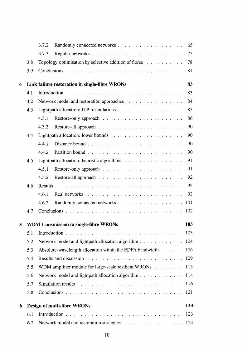
3.7.2 Randomly connected netw orks......................................................... 65
3.7.3 Regular netw orks............................................................................... 75
3.8 Topology optimisation by selective addition of f i b r e s ............................... 78
3.9 C onclusions...................................................................................................... 81
4 L ink failure restoration in single-fibre W RO Ns 83
4.1 In troduction ...................................................................................................... 83
4.2 Network model and restoration approaches ............................................... 84
4.3 Lightpath allocation: ILP form ulations......................................................... 85
4.3.1 Restore-only a p p ro a c h ..................................................................... 86
4.3.2 Restore-all a p p ro a c h ........................................................................ 90
4.4 Lightpath allocation: lower boun d s............................................................... 90
4.4.1 Distance b o u n d .................................................................................. 90
4.4.2 Partition b o u n d .................................................................................. 90
4.5 Lightpath allocation: heuristic a lg o rith m s .................................................. 91
4.5.1 Restore-only a p p ro a c h ..................................................................... 91
4.5.2 Restore-all a p p ro a c h ........................................................................ 92
4.6 R esults ................................................................................................................ 92
4.6.1 Real netw orks..................................................................................... 92
4.6.2 Randomly connected netw orks.............................................................101
4.7 C onclusions..........................................................................................................102
5 W D M transm ission in single-fibre W RO Ns 103
5.1 In troduction ..........................................................................................................103
5.2 Network model and lightpath allocation algorithm .........................................104
5.3 Absolute-wavelength allocation within the EDFA b a n d w id th ..................... 106
5.4 Results and d is c u s s io n ...................................................................................... 109
5.5 WDM amplifier module for large-scale resilient W R O N s............................113
5.6 Network model and lightpath allocation algorithm .........................................114
5.7 Simulation re su lts ................................................................................................ 116
5.8 C onclusions..........................................................................................................121
6 D esign o f m ulti-fibre W R O N s 123
6.1 In troduction ..........................................................................................................123
6.2 Network model and restoration strategies ......................................................124
10

6.2.1 Edge-disjoint path restoration with reserved c a p a c ity ...................... 125
6.2.2 Edge-disjoint path re s to ra tio n ............................................................ 126
6.2.3 Path restoration ...................................................................................... 127
6.2.4 Link restoration...................................................................................... 127
6.3 Lightpath allocation: ILP form ulations............................................................128
6.3.1 WIXC c a s e .............................................................................................129
6.3.2 WSXC c a s e .............................................................................................131
6.4 Lightpath allocation: lower bou n d s.................................................................. 133
6.4.1 Distance b o u n d ...................................................................................... 134
6.4.2 Partition b o u n d ...................................................................................... 134
6.5 Comparison of restoration s tra teg ie s ...............................................................136
6.6 Influence of physical connectivity on restoration c ap a c ity ...........................144
6.6.1 Lightpath allocation: heuristic a lgo rithm s..........................................145
6.6.2 R e s u l t s ................................................................................................... 146
6.7 Analysis of traffic g ro w th .................................................................................. 151
6.7.1 Transport capacity and utilisation g a in ............................................... 151
6.7.2 R e s u l t s ................................................................................................... 153
6.8 C onclusions......................................................................................................... 159
7 C onclusions and future work 161
A P artition bound evaluation: heuristic algorithm 169
B L ightpath allocation: heuristic algorithm s 173
B.l Active lightpaths allocation in single-fibre W R O N s .....................................173
B.2 Restore-only approach in single-fibre W R O N s...............................................176
B.3 Active lightpaths allocation in multi-fibre WRONs .....................................178
B.4 Restoration lightpaths allocation in multi-fibre W R O N s...........................182
C R C N s generation m ethod 191
11


List of Tables
2.1 Some of the commercially available WDM point-to-point systems. W ,
number of wavelengths transmitted (wavelength multiplicity)........................ 33
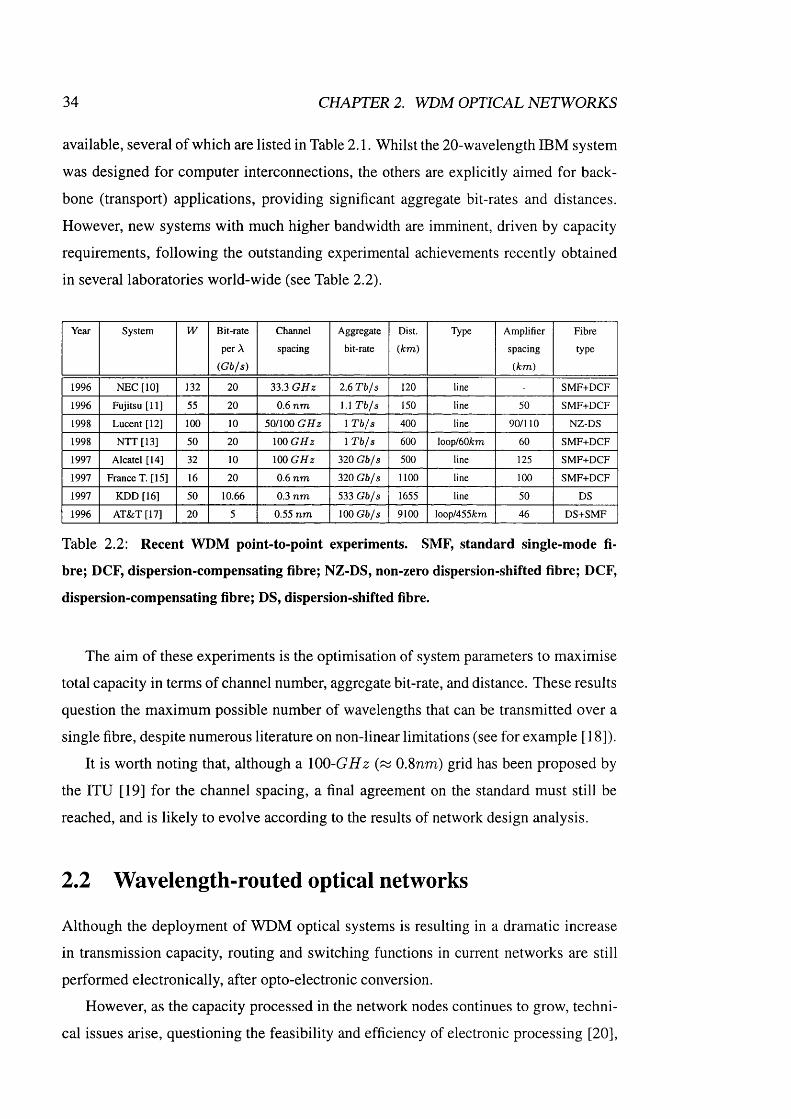
2.2 Recent WDM point-to-point experiments. SMF, standard single-mode
fibre; DCF, dispersion-compensating fibre; NZ-DS, non-zero dispersion-
shifted fibre; DCF, dispersion-compensating fibre; DS, dispersion-shifted
fibre................................................................................................................................. 34
2.3 WRON experiments.................................................................................................... 37
3.1 Topological parameters of existing or planned network topologies. The
dotted lines represent the limiting cuts. Æ, number of nodes; L, number of
links; Sminy ^max- minimum and maximum nodal degree; a, physical con
nectivity; H, average inter-nodal distance; D , network diameter (longest
path within the network); \C\, number of links in the limiting cut; |C"|,
number of links in the limiting cut when single link failure is considered
(see Chapter 4)............................................................................................................. 61
3.2 Results for existing or planned network topologies. P = N . { N —l) /2 , total
number of bi-directional lightpath allocated within the networks (network
throughput Tp = 2 .P.i?5, with Rf, bit-rate per channel); W d b , distance
bound; W p b , partition bound (marked by if obtained by inspection); e,
extra number of hops allowed to the active lightpaths; a dash is shown
where the ILP failed to give any result after one day of computation on
a UNIX workstation; N\y wavelength requirements. The results which
achieved the lower bounds are highlighted........................................................... 62
13

3.3 Computational complexity of I L P formulations, e, extra number of hops
allowed to the active lightpaths; ç, average size of active sets, Az,e’, Ny,
number of variables; Nc, number of constraints; W, maximum number
of wavelengths per fibre, fixed in the W S X C . The formulations which
were successfully carried out are highlighted....................................................... 63
3.4 Number of bi-directional lightpaths transiting the WRNs and WRN size
for the heuristic WIXC case, e, extra number of hops allowed to the ac
tive lightpaths. The node-numbers with the largest (max) and smallest
(min) transit traffic are in parentheses to identify their positions within
the graphs of Table 3.1............................................................................................... 65
3.5 Topological parameters for several RCNs with N = 14, a = 0.23 {L = 21).
The dotted lines represent the limiting cuts, rii, number of network nodes
with degree ô = i. ômax = 4, as for NSFNet......................................................... 67
3.6 Results for several RCNs with N — 14, a = 0.23 (L = 21). A dash is
shown where the ILP failed to give any result in acceptable time; the re
sults for the heuristic WIXC and WSXC cases are in the same column
since they were equal; e, extra number of hops allowed to the active light
paths. The results which achieved the lower bounds are highlighted. . . . 68
3.7 Topological parameters and results for the analysed ShuffleNet topologies.
The nodal degree of a SN{ô, k) is equal to 5. The results which achieved
the lower bounds are highlighted............................................................................ 76
3.8 Topological parameters and results for the analysed de Bruijn topologies.
The nodal degree of a deB{6, D) is equal to 8. The results which achieved
the lower bounds are highlighted. When the calculation of the partition
bound was not terminated, the largest result achieved was recorded and is
marked b y * ................................................................................................................ 78
4.1 Computational complexity of I L P formulations for RO approach, a, ex
tra number of hops allowed to the restoration lightpaths; b, average size of
the restoration sets P p j y , Ny, number of variables; Nc, number of con
straints; W , maximum number of wavelengths per fibre, fixed in W S X C
case. The formulations which were successfully carried out are high
lighted. [For the EURO-Core WIXC case, only the formulation with a = 0
was performed, as it reached the lower b o u n d .] ............................................... 93
14

4.2 Results of failure restoration in link (8,9) in NSFNet (heuristic algorithms).
number of lightpaths re-routed; number of terminals involved;
new wavelength requirement. = 11, distance bound; =
17, partition bound..................................................................................................... 94
4.3 Link failure restoration requirements for NSFNet. N^r, average number
of lightpaths re-routed per link failure; Nt, average number of terminals
involved per link failure; N", new wavelength requirement. = 11,
distance bound; Wp^ = 17, partition bound....................................................... 95
4.4 Results for real network topologies. W pp obtained by inspection are marked
by ; for each case, the smallest N'J achieved is presented, and the corre
sponding value of a in restoration sets a is in parentheses; a dash is
shown where the ILP failed to give any result after one day of computation
on a UNIX workstation; The results which achieved the lower bounds are
highlighted..................................................................................................................... 97
4.5 Results for the analysed RCNs with TV = 14, L = 21. The smallest N'
achieved is presented, and the corresponding value of a is given in paren
theses only when different from zero.......................................................................... 101
5.1 Lightpaths dropped and added in the intermediate OXCs of the network’s
longest path. The bold numbers in brackets are the distances the light
paths have travelled within the network up to that point...................................... 110
5.2 Lightpaths dropped and added in the intermediate OXCs of path l\ (San
Diego - Atlanta) for the normal operation mode......................................................117
5.3 Lightpaths dropped and added in the intermediate OXCs of path l\ (San
Diego - Atlanta) for the restoration mode..................................................................118
5.4 Lightpaths dropped and added in the intermediate OXCs of path I2 (Seat
tle - College Park) for the normal operation mode..................................................119
5.5 Lightpaths dropped and added in the intermediate OXCs of path I2 (Seat
tle - College Park) for the restoration mode..........................................................120
6.1 Network configurations identified. The configurations analysed are high
lighted................................................................................................................................. 128
15

6.2 Computational complexity of ILP formulations without link failure restora
tion for the 5-node, 7-link topology. Extra number of hops allowed for the
active lightpaths e = 0. maximum number of wavelengths per fibre;
Nyy number of variables; Nc, number of constraints..............................................136
6.3 Computational complexity of W I X C DLP formulation with link failure
restoration for the 5-node, 7-link topology, b, size of restoration sets
The number of extra constraints for the edge-disjoint path restoration
case is in parentheses...................................................................................................... 137
6.4 Computational complexity of W S X C ELP formulation with link failure
restoration for the 5-node, 7-link topology. W , maximum number of wave
lengths per fibre; b, size of restoration sets The number of extra
constraints for the edge-disjoint path restoration case is in parentheses. . . 138
6.5 Results for the 5-node, 7-link topology without link failure restoration.
Extra number of hops allowed for the active lightpaths e = 0. Fdb^i^',
distance bound; Fpb^/^, partition bound; Fp^^ , total number of fibres
obtained with ILP formulations. The results which achieved the lower
bounds are highlighted...................................................................................................139
6.6 Results for the 5-node, 7-link topology with link failure restoration. Fd b / ,
distance bound; Fp b ^/ , partition bound; b, size of restoration sets F p j y ,
Ft / , total number of fibres obtained with ILP formulations. DI, DSA,
DSF, PI, PSA, PSF, LI, LSF are defined in Table 6.1. The results which
achieved the lower bounds are highlighted............................................................... 139
6.7 Results for the 8-node, 13-link topology without link failure restoration.
Extra number of hops allowed to the active lightpaths e = 0. Fdb^/„^
distance bound; Fpp^/^, partition bound; total number of fibres
obtained with ILP formulations. The results which achieved the lower
bounds are highlighted................................................................................................... 141
16

6.8 Results obtained for the 8-node, 13-link topology with link failure restora
tion. Extra number of hops allowed to the active lightpaths e = 0. ,
distance bound; partition bound; total number of fibres
obtained with ILP formulations. When the ILP was not completed after
one day of computation on a UNIX workstation, the best results achieved
was recorded and is marked with a *. Lower bounds derived from ILP
computation are in parentheses. The results which achieved the lower
bounds are highlighted............................................................................................... 142
B .l Results for two 8-node networks. versus W for both WIXC and
WSXC cases obtained with I L P and heurist ic algorithms..................................182
B.2 Results for the ring 8-node network. Fp ^ versus W for WIXC, WSXC-
A, and WSXC-F cases obtained with I L P and heurist ic algorithms, with
link failure restoration (path restoration strategy). Size of restoration sets
is 6 = 1. When the ILP failed was not completed after one day of compu
tation on a UNIX workstation, the best results achieved was recorded and
is marked with a * ............................................................................................................188
B.3 Results for the mesh 8-node network shown in Fig. 6.4(b). Ft / versus W
obtained with I L P and heurist ic algorithms, considering with link failure
restoration. WIXC with path restoration (PI).............................................................. 188
B .4 Results for the mesh 8-node network shown in Fig. 6.4(b). Ft^ versus W
obtained with I L P and heurist ic algorithms, considering with link failure
restoration. WSXC-A with path restoration (PSA)..................................................... 188
B.5 Results for the mesh 8-node network shown in Fig. 6.4(b). Fp versus W
obtained with I L P and heurist ic algorithms, considering with link failure
restoration. WSXC-F with path restoration (PSF)......................................................189
17

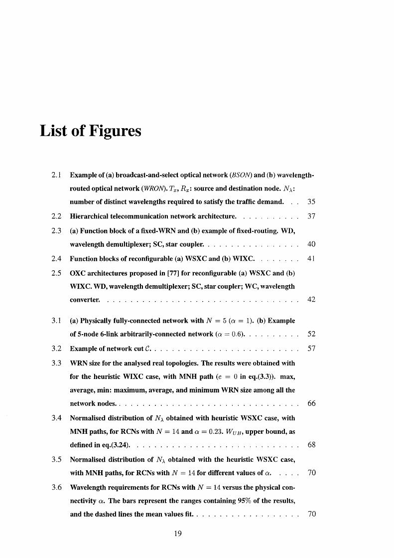
List of Figures
2.1 Example of (a) broadcast-and-select optical network (BSOM) and (b) wavelength-
routed optical network (WROM). Tx, Rx- source and destination node. N \ i
number of distinct wavelengths required to satisfy the traffic demand. . . 35
2.2 Hierarchical telecommunication network architecture...................................... 37
2.3 (a) Function block of a fixed-WRN and (b) example of fixed-routing. WD,
wavelength demultiplexer; SC, star cou p ler....................................................... 40
2.4 Function blocks of reconfigurable (a) WSXC and (b) WIXC........................... 41
2.5 OXC architectures proposed in [77] for reconfigurable (a) WSXC and (b)
WIXC. WD, wavelength demultiplexer; SC, star coupler; WC, wavelength
converter. ................................................................................................................... 42
3.1 (a) Physically fully-connected network with N = b (a = 1). (b) Example
of 5-node 6-link arbitrarily-connected network (a = 0.6)................................ 52
3.2 Example of network cut C.......................................................................................... 57
3.3 WRN size for the analysed real topologies. The results were obtained with
for the heuristic WIXC case, with MNH path (e = 0 in eq.(3.3)). max,
average, min: maximum, average, and minimum WRN size among all the
network nodes.............................................................................................................. 66
3.4 Normalised distribution of N \ obtained with heuristic WSXC case, with
MNH paths, for RCNs with TV = 14 and a = 0.23. W u b upper bound, as
defined in eq.(3.24)...................................................................................................... 68
3.5 Normalised distribution of N \ obtained with the heuristic WSXC case,
with MNH paths, for RCNs with TV = 14 for different values of a ................. 70
3.6 Wavelength requirements for RCNs with TV = 14 versus the physical con
nectivity a. The bars represent the ranges containing 95% of the results,
and the dashed lines the mean values fit................................................................ 70
19

3.7 Mean values of N \ for RCNs versus physical connectivity a, as a function
of the number of nodes N........................................................................................... 71
3.8 Mean values of N \ versus physical connectivity a, as a function of the
number of nodes N...................................................................................................... 71
3.9 Number of wavelengths {upper bound) for 95% of the RCNs versus physical
connectivity a , as a function of the number of nodes N..................................... 72
3.10 Minimum values {lower bound) of N \ for RCNs versus physical connectiv
ity a , as a function of the number of nodes N....................................................... 73
3.11 Normalised distribution of average inter-nodal distance: (left) jV = 14,
a = 0.23, and (right) N = 20, a = 0.20................................................................. 73
3.12 Minimum values of the mean inter-nodal distance, Hminy versus physical
connectivity o;, as a function of the number of nodes N..................................... 74
3.13 Minimum values of N \ for RCNs and asymptotic lower bound de
rived in [101] versus physical connectivity a ........................................................ 75
3.14 (a) ShuffleNet SN{2,2) . (h) Corresponding network considered {N = 8,
L = 12)........................................................................................................................... 76
3.15 (a) de Bruijn deB{2,3). (b) Corresponding network considered {N = 8,
L = 13)........................................................................................................................... 77
3.16 Number of wavelengths N \ versus physical connectivity a for regular net
works ShuffleNet and de Bruijn............................................................................... 79
3.17 Distribution of link congestion in EON and ARPANet. The most loaded
links in each network are listed to identify them in the graphs of Table 3.1. 80
3.18 Wavelength saving Ws versus percentage fibre added A F / L . The solid
line represents the savings achievable with non-selective duplication of all
network links................................................................................................................ 80
4.1 Example of centralised network management system........................................ 84
4.2 Average number of lightpaths re-routed, Nir lP {% ), per link failure, for
different restoration techniques versus the additional number of hops a. . 95
4.3 Average number of terminals involved, Nt / N{ %) , per link failure, for dif
ferent restoration techniques versus the additional number of hops a. . . . 96
4.4 Extra number of wavelengths required for restoration versus the number
of links in the network limiting cut \C\. RA-approach: (left) WIXC, and
(right) WSXC............................................................................................................... 99
20

4.5 Extra number of wavelengths required for restoration versus the number
of links in the network limiting cut \C\. RO-approach: (left) WIXC, and
(right) WSXC................................................................................................................ 99
4.6 OXC size for the analysed topologies. The results are for the heuristic
WIXC case with MNH path. The increase in the average OXC size in
comparison to the results of Fig. 3.3 are reported............................................... 100
5.1 Example of WRON with extra constraint {C4)......................................................104
5.2 EON network considered. The distances between the nodes are in km.
Only the cities involved in the worst path (Lisbon - Athens) are indicated. . 107
5.3 Congestion (load) distribution in the EON links....................................................... 107
5.4 Optical SNR for the 24 channels propagating together along 5200 km, with
and without FWM. The allocation of the wavelength-numhers within the
EDFA bandwidth is also shown (e.g. the longest lightpath with wavelength-
number Ai is assigned the channel u (absolute-wavelength 1551 nm) which
has the largest value of the SNR).................................................................................108
5.5 Optical power spectrum and SNR at the input of each OXC in the analysed
path, Lisbon-Athens, total length of 5200 km (inter-amplifier span 40 km). 111
5.6 Optical SNR spectrum at Athens for two random absolute-wavelength al
locations. Note that the channels at 1541.5 nm are actually dropped at
Zagreb.................................................................................................................................112
5.7 Schematic diagram of the transmission system between two OXCs.................... 112
5.8 Schematic diagram of the NSF network. Only the cities involved in the
two worst paths li (San Diego - Atlanta), I2 (Seattle - College Park) are
indicated.............................................................................................................................116
5.9 Optical power spectrum and SNR at the input and output of each after
each OXC in the normal operation mode for path l\ (□ SNR, O Total
Noise Power (ASE and Crosstalk), • ASE Power)................................................... 118
5.10 Optical power spectrum and SNR at the input of each OXC under link
failure restoration for p a th /i....................................................................................... 119
5.11 Optical power spectrum and SNR at the input of each OXC without (top)
and with (bottom) link failures for path I2 ................................................................ 120
6.1 Example of edge-disjoint path restoration (with and without reserved ca
pacity)............................................................................................................................. 125
21
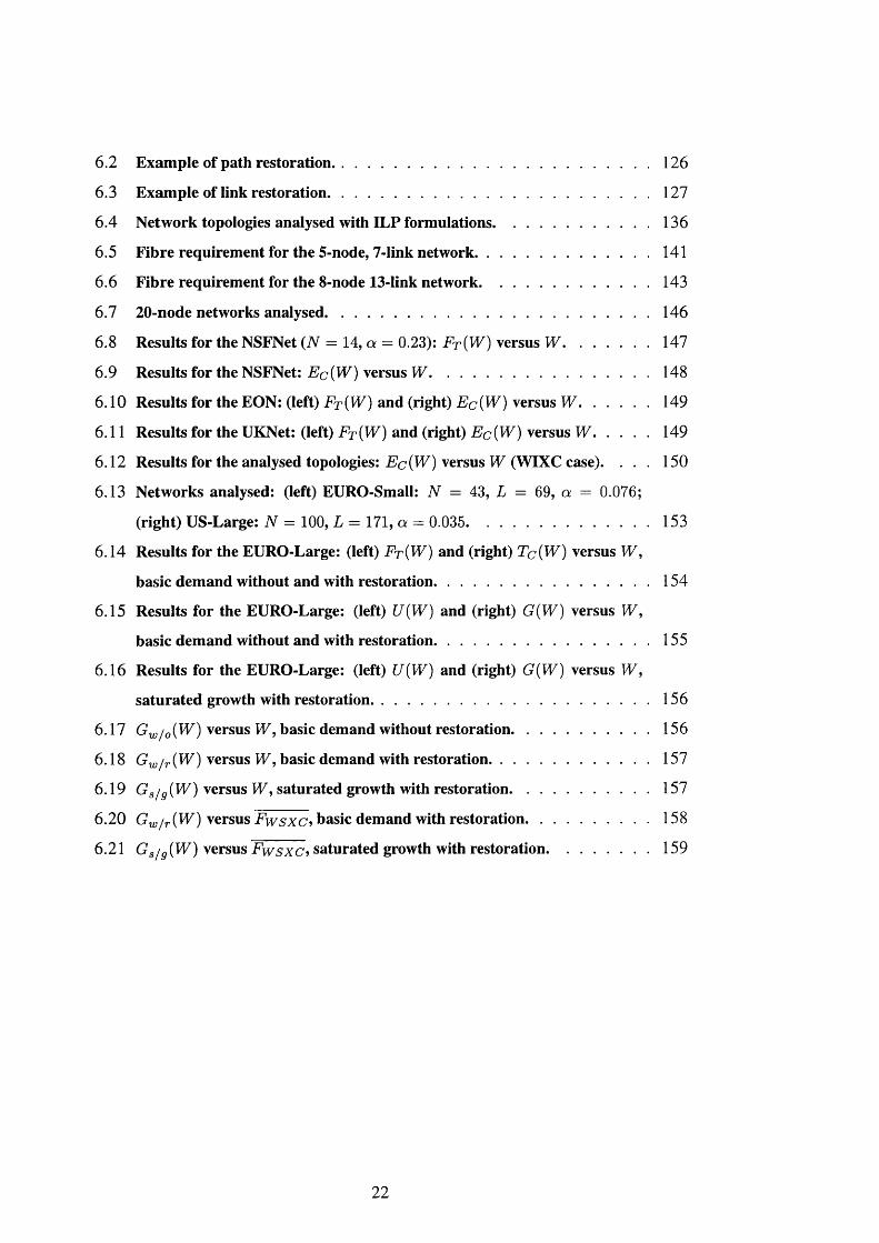
6.2 Example of path restoration......................................................................................... 126
6.3 Example of link restoration.......................................................................................... 127
6.4 Network topologies analysed with ILP formulations..............................................136
6.5 Fibre requirement for the 5-node, 7-link network...................................................141
6.6 Fibre requirement for the 8-node 13-link network................................................. 143
6.7 20-node networks analysed........................................................................................... 146
6.8 Results for the NSFNet {N = 14, a = 0.23): Ft {W) versus W ...........................147
6.9 Results for the NSFNet: E c { W ) versus W ...............................................................148
6.10 Results for the EON: (left) Ft {W) and (right) E c { W ) versus W ...................... 149
6.11 Results for the UKNet: (left) Ft {W) and (right) E c { W ) versus W ...................149
6.12 Results for the analysed topologies: Ec7(l^) versus PF (WIXC case). . . . 150
6.13 Networks analysed: (left) EURO-Small: N = 43, L = 69, a = 0.076;
(right) US-Large: N = 100, L = 171, a = 0.035................................................. 153
6.14 Results for the EURO-Large: (left) Ft {W) and (right) T c { W ) versus W ,
basic demand without and with restoration..............................................................154
6.15 Results for the EURO-Large: (left) U[ W) and (right) G{ W) versus W,
basic demand without and with restoration..............................................................155
6.16 Results for the EURO-Large: (left) U{ W) and (right) G{ W) versus W,
saturated growth with restoration...............................................................................156
6.17 Gyj joiW) versus W, basic demand without restoration.........................................156
6.18 Gyj i r{W) versus W, basic demand with restoration...........................................157
6.19 Gs/ g(W) versus W, saturated growth with restoration..................................... 157
6.20 Gyj j r{W) versus F w s x c i basic demand with restoration.....................................158
6.21 Gs/ g{W) versus F w s x c i saturated growth with restoration............................... 159
22

List of symbols
a network physical connectivity
à nodal degree
àjnax maximum degree among the network nodes
àmin minimum degree among the network nodes
77 network efficiency
A possible wavelength for restoration lightpaths
A* wavelength assigned to restoration lightpath
a extra number of links allowed to restoration paths
A set of network arcs (links)
Az set of paths connecting z with m(z) length
Az^e set of paths connecting z with length at most m(z) + e
ASE amplified spontaneous emission
h size of the restoration sets
h average size of the restoration sets
BSON broadcast-and-select optical network
C network cut
\C\ number of links in cut C, without link failure restoration
\C'\ number of links in cut C, with link failure restoration
D network diameter
Dc number of lightpaths traversing cut C
DCF dispersion-compensating fibre
DI edge-disjoint path restoration, with WIXC
DS dispersion-shifted fibre
DSA edge-disjoint path restoration, with WSXC-A
DSF edge-disjoint path restoration, with WSXC-F
e extra number of links allowed to active paths
23

E c
EDFA
A F
f j
Ej
FcF DB■w! o
F D ^ w / r
FpB,
'PBw / r
Fj
Fj
F t
w / o
w / r
FwsxcFWM
G w/ o
G w/r
G s / g
H
ILP
jI
L
Ls
L pc
LAN
LI
LSA
LSF
m{z)
{z)
MAN
extra capacity required to provide for restoration
erbium-doped fibre amplifier
number of fibres added
number of fibres in link j
set of possible active lightpaths using arc j
number of fibres required to satisfy traffic across cut C
distance bound on Ftw / o
distance bound on Fp^^
partition bound on Ft^^
partition bound on Ft^^
total number of network fibres
total number of network fibres, without link failure restoration
total number of network fibres, with link failure restoration
average number of fibres per link for the WSXC-A case
four-wave mixing
network graph
utilisation gain, without link failure restoration
utilisation gain, with link failure restoration
utilisation gain, saturated growth with restoration
average inter-nodal distance
integer linear program
network link (arc)
average length (in number of links) of a possible active path
number of network links
inter-amplifier span
number of network links in a physically fully-connected network
local area network
link restoration, with WIXC
link restoration, with WSXC-A
link restoration, with WSXC-F
minimum distance for node pair z
minimum distance for node pair z, with failure in link j
metropolitan area network
24

MNH minimum number-of-hops (links) distance for node pair 2
W set of network nodes
N number of network nodes
N \ wavelength requirement, without link failure restoration
AA^a expected increase in wavelength requirement due to link
failure restoration
wavelength requirement, with addition of fibres
N ” wavelength requirement, with link failure restoration
N l wavelength requirement, with failure in link j
Nc number of constraints in ILP formulation
Nd number of destination-nodes
Nij. number of lightpaths re-routed for a failure in link j
Nir average number of lightpaths re-routed per link failure
N} number of terminals involved in failure of link j
N t average number of terminals involved per link failure
Ns number of source-nodes
Nti number of lightpaths transiting a WRN
Ny number of variables in ILP formulation
NZ-DS non-zero dispersion-shifted fibre
OXC optical-cross connect
p possible active path
p* assigned active path
P total number of network node-pairs
PI path restoration, with WIXC
PR permutation routing
PSA path restoration, with WSXC-A
PSF path restoration, with WSXC-F
q average size of active sets Az,e, or Az
r possible restoration path
r* assigned restoration path
Rb channel bit-rate
Rp j^a set of possible restoration paths for active lightpath p when
link j fails, length at most m^{z) 4- a
25

set of b shortest possible restoration paths for active lightpath p when
link j fails
Rx destination node
RA reroute-all approach
RCN randomly connected network
RI edge-disjoint path restoration with reserved capacity, with WIXC
RO reroute-only approach
RSA edge-disjoint path restoration with reserved capacity, with WSXC-A
RSF edge-disjoint path restoration with reserved capacity, with WSXC-F
RWA routing and wavelength allocation
SC star couple
SMF standard single-mode fibre
SNR optical signal-to-noise ratio
T ' capacity utilised by active lightpaths, with saturated growth
Tc network transport capacity
network transport capacity, without link failure restoration
network transport capacity, with link failure restoration
Tmin capacity utilised by active lightpaths, uniform traffic demand
Tp network throughput
Tx source node
Uyj jo resource utilisation, without link failure restoration
JJ^ jj. resource utilisation, with link failure restoration
JJ jg resource utilisation, saturated growth with link failure restoration
w possible wavelength for active lightpaths
w* wavelength assigned to active lightpath
W wavelength multiplicity
Wc number of wavelengths required to satisfy traffic across cut C
W db distance bound on N \
W'jjQ distance bound on N'^
distance bound on N ”
WC wavelength converter
WD wavelength demultiplexer
WDM wavelength division multiplexing
26

WDM-XC
WI
WIXC
WIXC-RA
WIXC-RO
^ L B
W'l b
%
WpB
WRN
WRON
wsxcWSXC-A
WSXC-F
WSXC-RA
WSXC-RO
WuB
— (-2 11 2 )
z
wavelength division multiplexing cross-connect
wavelength conversion, or interchange
wavelength interchanging cross-connect
wavelength interchanging cross-connect, reroute-all approach
wavelength interchanging cross-connect, reroute-only approach
lower bound on N \
lower bound on N'^
lower bound on N'{
partition bound on N \
partition bound on
partition bound on
wavelength-routing node
wavelength-routed optical network
wavelength saving
wavelength selective cross-connect
wavelength selective cross-connect, with wavelength-agility
wavelength selective cross-connect, with fixed restoration wavelengths
wavelength selective cross-connect, reroute-all approach
wavelength selective cross-connect, reroute-only approach
upper bound on N \
node-pair
set of node-pairs in Q (A/*, A)
27

Chapter 1
Introduction
The deployment of erbium-doped fibre amplifiers (EDFAs) has dramatically boosted
optical communications. EDFAs enable compensation for fibre loss over several tens of
nanometers of optical bandwidth (equivalent to 4-8 THz) , resulting in feasible and eco
nomic transmission of multiple wavelength-division-multiplexed {WDM), high-capacity
optical channels, transparently, over hundreds of kilometres [1],
This unprecedented potential has been immediately recognised by network opera
tors world-wide, always looking for effective ways to satisfy their increasing capacity
requirements, and promote new and more bandwidth-demanding applications, such as
internet access and multimedia services.
WDM systems have already been deployed in numerous point-to-point links of sev
eral long-distance carriers, to increase capacity without installing more fibre or higher-
speed transmission equipment [2].
However, the greatest advantage of WDM is the increased network flexibility achiev
able with wavelength-routing [3], which allows to provide network node-pairs with end-
to-end optical channels [4], known as lightpaths [5]. The intermediate optical cross
connects {OXCs) route the lightpaths from sources to destinations [6], simplifying net
work management and processing compared to routing in digital cross-connected sys
tems [7]. Significant operational advantages are also expected by performing optical
restoration in the case of link failures [8].
This scenario will dramatically enhance the role of optical fibre technology within
telecommunication networks, from simply providing point-to-point physical transport
capabilities to creating an optical networking layer, where high-level networking func
tions are performed. To fully exploit WDM wavelength-routing, efficient optical net-
29

30 CHAPTER 1. INTRODUCTION
work architectures must be deployed, which are affected by numerous network param
eters, primarily physical topology, node functionalities, and traffic configuration.
In this thesis, rigorous models are developed for the analysis of WDM wavelength-
routed optical transport networks (WRONs), to study the impact of network parameters
on WRON performance, vital for optimal network design.
First, Chapter 2 presents an overview of WDM systems and networks, and discusses
crucial issues in WRONs currently under investigation.
Chapter 3 studies the wavelength requirements, N \, in single-fibre, arbitrarily-con
nected WRONs, characterised by the physical connectivity parameter a. A new integer
linear program (ILP) formulation is proposed for the exact solution of the lightpath allo
cation. Lower bounds on the wavelength requirement are discussed, and heuristic light
path allocation algorithms described. Several existing or planned fibre network infras
tructures are analysed together with a large number of randomly generated, arbitrarily-
connected topologies. The benefit achievable with wavelength conversion in OXCs is
analysed. Regular topologies are then compared to arbitrarily-connected networks in
terms of wavelength requirement and network scalability. Finally, a simple method for
the selective addition of multiple fibres in heavily loaded links is proposed for network
optimisation.
Chapter 4 deals with link failure restoration in single-fibre WRONs. Two restora
tion approaches are considered. First, only the interrupted lightpaths are re-routed along
alternative physical paths, whereas, in the second, all the network lightpaths are reas
signed within the resultant topology. The ILP formulation proposed in Chapter 3 is
extended for the optimal allocation of restoration lightpaths. Lower bounds on the new
wavelength requirement are presented, and heuristic lightpath allocation algorithms pro
posed. The role played by network critical cuts on the increase in Nx is ascertained, and
the benefit of wavelength conversion analysed.
In Chapter 5, WDM transmission in single-fibre WRONs is studied, considering
physical limitations imposed by the wavelength-dependent gain characteristic in ED
FAs. A simple algorithm for the assignment of absolute-wavelengths to the lightpaths
is initially proposed to compensate for gain non-uniformities in EDFA cascades under
condition of lightpath add/drop. However, this technique is effective only in the case
of static traffic. Therefore, a new WDM optical amplifier configuration providing self
regulating properties is proposed to reduce management complexity in the large-scale
resilient WRONs.

31
In Chapter 6 , the design of multi-fibre WRONs is investigated, introducing the max
imum number of wavelengths per fibre, W , as a parameter. ILP formulations and
heuristic algorithms are proposed for lightpath allocation, aiming at minimising the to
tal number of fibres. Ft , or capacity, required. Lower bounds on Ft are also discussed.
Capacity requirement and resource utilisation are derived under different network condi
tions, including provisioning of basic demand, restoration, and traffic growth. Different
restoration strategies are considered and compared. The analysis of network evolution
quantifies the relationship between network size and connectivity, wavelength multi
plicity W , traffic condition, and relative merits of wavelength conversion.
Chapter 7 presents a summary of the main conclusions of the research, and provides
suggestions for future work.


Chapter 2
WDM optical networks
2.1 Introduction
Optical fibre is now widely recognised as the most effective medium for high-capacity
long-distance transmission, due to the combination of high bandwidth and low loss [ 1 ].
Since the maximum bit-rate at which each user can transmit is limited by electronic
speed, multiplexing techniques are required to make efficient use of the optical band
width [9].
The recent development of erbium-doped fibre amplifiers (EDFAs) enables the trans
mission of numerous high-capacity, wavelength-division-multiplexed (WDM) optical
channels, transparently, over long distances [1 ], providing the most efficient solution
to the need for increased transmission capacity [2 ].
Year System W Mux/Demux Bit-rate
per A
(G6/&)
Channel
spacing
Aggregate
bit-rate
Dist.
(km)
1995 IBM 20 Free Space Grating 0.2 1 n m 4 G b / s 50
1995 Pirelli 4 Power Comb./ Interfer. Filter 2.5 200 G H z \ O G b j s 550
1995 Lucent 8 AWG 2.5 100 G H z 20 G b / s 360
1996 Ciena 16 Power Comb./ Fibre Grating 2.5 100 G H z 40 G b / s 600
1997 Ciena 40 Power Comb./ Fibre Grating 2.5 50 G H z 100 G b / s 500
Table 2.1 : Some of the commercially available WDM point-to-point systems. W , number
of wavelengths transmitted (wavelength multiplicity).
To date, the WDM potential has only partially been exploited in point-to-point ap
plications, as witnessed by numerous products which recently became commercially
33
34 CHAPTER 2. WDM OPTICAL NETW ORKS
available, several of which are listed in Table 2.1. Whilst the 20-wavelength IBM system
was designed for computer interconnections, the others are explicitly aimed for back
bone (transport) applications, providing significant aggregate bit-rates and distances.
However, new systems with much higher bandwidth are imminent, driven by capacity
requirements, following the outstanding experimental achievements recently obtained
in several laboratories world-wide (see Table 2.2).
Year System W Bit-rate
per A
( Gb / s )
Channel
spacing
Aggregate
bit-rate
Dist.
(km)
Type Amplifier
spacing
( km)
Fibre
type
1996 NEC [10] 132 20 33.3 G H z 2.6 T b / s 120 line - SMF+DCF
1996 Fujitsu [11] 55 20 0.6 n m 1.1 T b / s 150 line 50 SMF+DCF
1998 Lucent [12] 100 10 50/100 G H z 1 T b / s 400 line 90/110 NZ-DS
1998 NTT [13] 50 20 \ O O G H z I T b / s 600 loop/60A:m 60 SMF4-DCF
1997 Alcatel [14] 32 10 100 G H z 320 G b / s 500 line 125 SMF-kDCF
1997 France T. [15] 16 20 0.6 n m 320 G b / s 1100 line 100 SMF+DCF
1997 KDD [16] 50 10.66 0.3 n m 533 G b / s 1655 line 50 DS
1996 AT&T [17] 20 5 0.55 n m 100 G b / s 9100 loop/455/cm 46 DS+SMF
Table 2.2: Recent WDM point-to-point experiments. SMF, standard single-mode fi
bre; DCF, dispersion-compensating fibre; NZ-DS, non-zero dispersion-shifted fibre; DCF,
dispersion-compensating fibre; DS, dispersion-shifted fibre.
The aim of these experiments is the optimisation of system parameters to maximise
total capacity in terms of channel number, aggregate bit-rate, and distance. These results
question the maximum possible number of wavelengths that can be transmitted over a
single fibre, despite numerous literature on non-linear limitations (see for example [ 18]).
It is worth noting that, although a \00-G H z (% O.Snm) grid has been proposed by
the ITU [19] for the channel spacing, a final agreement on the standard must still be
reached, and is likely to evolve according to the results of network design analysis.
2.2 Wavelength-routed optical networks
Although the deployment of WDM optical systems is resulting in a dramatic increase
in transmission capacity, routing and switching functions in current networks are still
performed electronically, after opto-electronic conversion.
However, as the capacity processed in the network nodes continues to grow, techni
cal issues arise, questioning the feasibility and efficiency of electronic processing [2 0 ],

2 .2 . WAVELENGTH-ROUTED OPTICAL NETWORKS 35
Tx Kx
1 2 3 4 5 6
- - - 1 1
Traffic demand
(in number of lightpaths)
I
2
3
4
5
6
(a) B S0N(Nj^-5) (b) WRON (N,=2)
Figure 2.1: Example of (a) broadcast-and-select optical network (BSON) and (b)
wavelength-routed optical network {WRON). T , Rx- source and destination node. Nx".
number of distinct wavelengths required to satisfy the traffic demand.
leading towards the need for all-optical networks [21][22], where signals remain en
tirely optical from sources to destinations, without any electronic processing in inter
mediate nodes.
Broadcast-and-select optical netM’orks (BSONs) were originally proposed and anal
ysed, given their conceptual simplicity [23]-[25]. In BSONs, a direct physical path
exists between each node-pair (see Fig. 2.1(a)), since passive optical couplers are used
as combiners and splitters, thus the transmission from each node is broadcast to all the
others. At each destination-node, the desired signal is filtered from the entire WDM
signal by an optical filter.
Since the network optical signals share the fibre infrastructure, the number of distinct
wavelengths required, N \ , is equal to the number of channels established, which is
typically as large as the number of network nodes, N , [25], as shown in Fig. 2.1(a).
Moreover, as N increases, stability requirements for lasers and filters become critical,
since the selected channels have to be filtered at the receiving-end. Also, the fraction
of the transmitted power which is received decreases with increasing N , because of
the inherent 1 / N power split. Therefore, the implementation of BSONs is likely to
be constrained to local or metropolitan environments {LANs, MANs) , where a limited
number of nodes can be physically interconnected [26].
In the case of wide-area transport networks (VFAMv), the high fibre installation costs
result in weakly-connected physical topologies, where network nodes are arbitrarily-
connected by point-to-point fibre links (see Fig. 2 .1 (b)). In these conditions, the greatest
advantage of W DM is achieved by implementing wavelength-routing within the nodes.

36 CHAPTER 2. WDM OPTICAL NETW ORKS
as firstly suggested in [3] [4], enabling to route the high-capacity optical signals on a
wavelength-by-wavelength basis [6 ] (see section 2.3.2), without any opto-electronic
conversion or processing.
This leads to simplified management and processing compared to routing in digital
cross-connected systems [27], and significant saving of electronic-equipment [28].
Even more important, wavelength-routing allows to provide the network node-pairs
with end-to-end optical channels [7], known as wavelength-channels, or lightpaths [5],
resulting in the fundamental advantage of protocol transparency [29].
The nodes are referred to as wavelength-routing nodes {WRNs) [5], or optical cross
connects iPXCs) [6 ].
Single-hop logical topology [30] is obtained if each connection request is satisfied
by a dedicated lightpath, which is established from source to destination and maintained
for the time period required for data transmission (which can be days, or even months,
in transport applications).
This approach eliminates the processing required in multihop logical topology [31],
where, for example because of a limited number of wavelength-channels, it is not pos
sible to dedicate an entire lightpath to all the node-pairs requiring a connection, and,
hence, processing is necessary to share the available optical channels.
In WRONs, lightpaths are not broadcast, but follow selected paths within the net
work, thus the same wavelengths can be used in different parts of the network, that is,
wavelength reuse is achievable, resulting in reduction of Nx (see Fig. 2.1(b)). Further
more, the 1 / N power split of BSONs is eliminated, and the filtering problem reduced,
as only specified channels reach destination-nodes.
Significant operational advantages can be obtained by performing optical restora
tion [8 ] in the case of link failure. In fact, wavelength-routing enables to achieve full
restoration by reallocating a small number of high-capacity channels, without the need
to reconfigure a large number of low-bandwidth circuits, as in digital networks, reduc
ing restoration time and complexity [6 ][7]. In mesh physical topologies, this approach
will also allow to share and, therefore, reduce, restoration capacity [7].
Therefore, wavelength-routed optical networks (WRONs) are key to implement a
nation-wide optical transport layer, where high-level networking functions are performed
in the optical domain, as proposed and discussed in [32]-[35].
This layer interconnects numerous LANs and MANs, generating a hierarchical net
work architecture, as shown in see Fig. 2.2 [2][35].

2 .2 . WAVELENGTH-ROUTED OPTICAL NETWORKS 37
O ptical transport layer
M etropolitan area netw ork s
□ op tica l term inal <= O X C A V R N
L oca l area n etw ork s
Figure 2.2: Hierarchical telecommunication network architecture.
Year System Ns Nd W Bit-rate
per A
Channel
spacing
Dist
(km)
1991 BT [36] 1 3 3 622 M b / s 12 n m 90
1993 MWTN [33] 4 4 4 622 M b / s 4 n m -
1995 ONTO [37] 5 5 4 155 M b / s 4 n m 150
1995 Bellcore (Ring) [38] 8 8 8 2.5-10 G b / s 200 G H z -
1996 NTT (Ring) [39] 3 3 8 0.622-2.5 G b / s 200 G H z 198
1995-99 MONET [40] 4 4 8 W G b / s 200 G H z up to 2000
Table 2.3: WRON experiments.
The highest layer mainly consists of broadcast-and-select optical LANs where con
nections are established and taken down by users, sharing limited sets of wavelengths.
The middle layer consists of metropolitan area networks interconnecting multiple LANs,
and providing wavelength reuse by means of WRNs. Also electrical LANs (shown as a
dark tree in Fig. 2.2) and single users can directly access this layer via optical terminals.
The optical transport layer mainly interconnects MANs and has a quasi-static traffic pat
tern, with high-capacity lightpaths established and maintained for long periods of time.
As shown in the figure, single users requiring high bandwidth can have direct access, as
suggested in [40].
The growing interest in WRONs is reflected in the large number of experiments
carried out in the last few years, where technical and economic feasibility of WDM
wavelength-routing was demonstrated (see Table 2.3). It is important to note, however,
that none of these experiments was aimed to achieve optimal or full network logical
interconnection.
Single-hop WRONs for wide-area transport applications is the focus of the research

38 CHAPTER 2. WDM OPTICAL NETW ORKS
described in this thesis. Open issues are reviewed in the next section.
2.3 Open issues in single-hop WRONs
The enormous potential of wavelength-routing is witnessed by the exceptionally large
number of papers recently published in this field, in specialised conferences and jour
nals (see for example [41]-[45]). These works aimed at identifying theoretical and ex
perimental issues related to WRON implementation, and address possible solutions.
However, numerous problems are still open, which are now reviewed.
2.3.1 Wavelength requirement
Much analysis recently carried out on single-hop WRONs has focused on conditions of
dynamic traffic, where lightpath requests arrive at random, or in a probabilistic manner
(for example, described as Poisson arrival probability, with exponential holding time),
and, hence, need to be established and released on demand [46]-[51]. This is by analogy
with call-by-call routing in circuit-switched telecommunication networks [52], where
the network capacity is fixed, and the aim is to minimise the number of connections
which are blocked.
However, this is not relevant for the case of high-capacity transport networks con
sidered here, where lightpaths provide quasi-static high-capacity pipes (with bit-rate
Rb > 2.bGh/s), and, hence, no blocking is allowed.
Therefore, one of the crucial issues in single-hop transport WRONs is the number of
wavelengths, N \, required to interconnect the network nodes and satisfy a given traffic
demand, as N \ directly determines network design parameters and device complexity.
The wavelength requirement Nx can be derived by solving the routing and wave
length assignment, or allocation (RWA) problem, that is how to optimally route and
assign wavelengths to a given set of connection requests onto a given physical topology,
firstly addressed in [5]. In this work, the RWA problem was demonstrated to be NP-
complete, that is, no exact solution can be obtained in polynomial time [53], implying
that only small-size networks can be optimally designed, subject to available computing
resources.
Therefore, several approaches have recently been proposed for its solution, namely,
analytical methods [54]-[58], integer linear program (ILP) formulations [31], [59]-[63],

2.3. OPEN ISSUES IN SINGLE-HOP WRONS 39
and efficient near-optimal heuristic algorithms [5],[61][62], [64]-[72].
In the last few years theoretical lower and upper bounds on N \ have been derived for
the permutation routing {PR) problem [54]-[56]. In PR networks, each node is equipped
with one wavelength-tunable transmitter and receiver and is therefore the origin and des
tination of one session at any time. Although deriving important information-bounds,
these analyses did not consider constraints imposed by network physical topology, which
are key in calculating tighter bounds on N \, necessary for practical network design.
By far the most critical parameter in WRONs is the network physical topology onto
which the traffic demand has to be mapped, since it directly determines RWA, and,
hence, wavelength requirement and complexity of the OXCs.
In [59], [61]-[65], mesh physical network topologies were analysed in conditions of
static traffic, aiming, respectively, at maximising the number of carried connections for
a given network capacity, and minimising wavelength requirement Nx-
These works provided invaluable insight for the solution of the RWA problem in
WRONs, proposing formal description and efficient solution methods. In particular,
ILP formulations for the exact solution of RWA were presented in [59], [61][62]. These
formulation were shown to be computationally complex, as will be discussed in sec
tion 3.3, and, hence, efficient, near-optimal heuristic algorithms were proposed (see
also [64]-[65]).
However, very few physical topologies were analysed, aimed at verifying the ac
curacy of the heuristic algorithms, and little attention was paid to studying the role of
network physical topology on N \.
Where physical topology has been investigated, this has always been regularly-
connected, such as ring [67]-[69], or regular mesh topologies [70]-[72],
Ring topologies will most likely be the first architectures to implement WDM wave
length-routing, given their relatively easy design and management implementation, fol
lowing successful operation as SONET/SDH topologies [73]. However, the analysis of
their wavelength requirement N \, performed in [67]-[69], showed that only limited-size
single-fibre rings are feasible, that is, they are more appropriate for LAN environments.
The study of regular mesh topologies, such as ShuffleNet, de Bruijn graphs, torus,
and grid, performed in [70]-[72] followed the analysis originally carried out in pho
tonic switching [74], where regular multihop logical topologies enabled simple routing
strategies [75] [76].
Whilst the results in [70]-[72] can be considered as theoretical limits, they are diffi-

40 CHAPTER 2. WDM OPTICAL NETWORKS
F ix edR d uiin g M ux
SCWD
(a) (b)
Figure 2.3: (a) Function block of a fixed-WRN and (b) example of fixed-routing. WD,
wavelength demultiplexer; SC, star coupler.
cult to apply to real transport networks whose physical topologies, determined by cost
and operational constraints, are neither fully nor regularly connected. Therefore, a sys
tematic analysis of arbitrarily-connected WRONs is essential, to investigate relation
ship between wavelength requirement and physical topology, necessary for the optimal
network design. Much of the analysis carried out in this thesis focuses on answering
these questions (Chapters 3 and 4), which have not been previously addressed.
2.3.2 OXCs functionality: reconfigurability and wavelength con
version
As shown in Fig. 2.1(b), in weakly-connected WRONs, the lightpaths may travel via
intermediate optical cross-connects, or wavelength-routing nodes. A WRN usually has
several input and output fibres, or ports. Each input port receives signals at distinct
wavelengths. The function of the WRN is to route a lightpath coming in at a given input
port and wavelength to an output port, independently of the signals at other wavelengths.
The routing may be fixed or dynamic.
When the W RNs are not reconbgurable, each channel always follows the same path
within each WRN, and hence within the network, leading to fixed-routing approach.
In this case, the W RNs are caWtd fixed-WRNs, and the corresponding network non-
reconfigurable or switchless [54]. 3'he function block of a hxed-WRN is shown in
Fig. 2.3(a). The incoming lightpaths are firstly wavelength demultiplexed, then routed
following a fixed path, and finally re-multiplexed onto the output fibres. As shown in
the example of Fig. 2.3(b), any two signals at the same wavelength incoming from two

2 .3 . OPEN ISSUES IN SINGLE-HOP WRONS 41
(a)
' Ih H '
2 h 4 - hDem ux S p jc c
Sw itch ing M ux D em ux W avclcnglliCiiiivcrsKin
SpaceSw iichinu
M ux
M 1!h — J M M h
(b)
Figure 2.4: Function blocks of reconfigurable (a) WSXC and (b) WIXC.
different fibres cannot be routed to the same output fibre. In principle this wavelength
collision problem can be overcome by wavelength conversion, or interchange of one of
the two signals before multiplexing.
However, when routing is fixed, the advantage achievable by introducing wavelength
conversion is expected to be small, as collisions can be solved a-priori, by a Judicious
assignment of the paths and wavelengths to lightpaths.
With dynamic routing, it is possible to change the routing at different times, for ex
ample in response to a change in the network traffic pattern, or to provide link failure
restoration. This can be achieved by introducing optical space-switches between the
Demux/Mux. The corresponding networks are called reconfigurahle [54]. The OXCs
are referred to as wavelength selective cross-connects (VF5'XCv) when wavelength con
version is not included, and wavelength interchanging cross-connects (WIXCs) when
wavelength conversion is available (see Fig. 2.4). In contrast to WSXCs, where only
space-switching is performed, WIXCs allow cross-connection in both space and wave
length domains. Thus, any wavelength on any input fibre can be routed to any output
fibre on any output wavelength (with the only limitation given by the wavelengths al
ready used at the output fibre).
The need for reconfigurable OXCs was first demonstrated in [54], considering the
permutation routing (PR) problem. The results showed that a large saving in wavelength
requirement N \ can be achieved by introducing reconfigurability within the OXCs, even
for the simple traffic patterns derived by the PR configurations. Similar conclusions
were obtained in [59], where the aim was to derive upper bounds on the number of car
ried connections on a given network. The results showed that fixed-routing is efficient
only when the traffic demand is known and not changing, implying that the most impor
tant advantage of reconfigurable OXCs is to make the network adaptable to unknown
traffic patterns rather than to provide a higher wavelength reuse.
Reconfigurable OXCs are expected to be key in transport WRONs, enabling efficient

42 CHAPTER 2. WDM OPTICAL NETWORKS
(a)
IE
W D W D W C
(b)
Figure 2.5: OXC architectures proposed in [77] for reconfigurable (a) WSXC and (b)
WIXC. WD, wavelength demultiplexer; SC, star coupler; WC, wavelength converter.
lightpath restoration in the case of link failures [6][8], as the latter result in significant
variations in lightpath allocation. Several reconfigurable architectures have recently
been proposed for both W SXC and WIXC (see for example [77]-[80], and Fig. 2.5),
to provide OXCs which are strictly non-blocking in the spatial domain and scalable to
support traffic growth. Hence, the ability to add a variable number of input and output
fibres and wavelengths per fibre to the OXC (i.e. fibre and wavelength modularity) is a
crucial feature [77]. Moreover, the space-switch fabric must be the smallest possible to
reduce physical OXC size [80].
The drawback of the WIXC configuration is the large number of wavelength con
verters required, equal to the product of the number of input fibres and number of wave
lengths per fibre ( M x W in Fig. 2.5). All-optical wavelength converters are currently
under development [81], and commercial products use opto-electronic conversion. The
latter are bit-rate dependent, i.e. not format transparent, and relatively expensive. More
over, wavelength converters require an additional management overhead which may be
extremely complex and expensive. Therefore their utilisation can be justified only if
significantly better network performances, such as reduction in wavelength or capacity
requirement, can be achieved.
Although numerous investigations have been carried out to appraise the value of
wavelength interchange, varied conclusions have been reported, and, to date, no consen
sus has been reached [82]. However, it is important to note that the initial assumption
that full-range wavelength conversion in every network node would be essential in guar
anteeing optimal network performance has been disproved by recent results [58],[61]-
[65], and most of the current research focuses on determining the real need and optimal

2.3. OPEN ISSUES IN SINGLE-HOP WRONS 43
location of wavelength interchange capabilities within a network [82].
In [57][58], worst case traffic analyses of ring networks were carried out, that is the
traffic was characterised only by the maximum number of lightpaths, or congestion, in
the network links. Although the initial results in [57] showed that wavelength inter
change is crucial to build large WDM ring networks, the analysis in [58], demonstrated
that limited wavelength conversion in a subset of the network nodes is sufficient to sat
isfy any possible traffic requirement for a given maximum congestion. However, in the
process of planning a network, more information on the traffic demand than the worst
case is desirable, as it may lead to different conclusions, as shown in [69]. Here, the
analysis of WDM rings with static uniform traffic showed that optimal lightpath allo
cation could be achieved with WSXC, and no reduction in the wavelength requirement
Nx was attainable by introducing wavelength conversion within the OXCs.
Similar results were obtained in the analysis of mesh WRONs topologies. In [83] [84],
it was shown that the availability of wavelength conversion in a very small subset of
nodes could greatly reduce capacity and wavelength requirement, respectively. How
ever, whilst the accuracy of the heuristic algorithm utilised in [83] was only partially
demonstrated, the analysis in [84] considered a worst-case physical topology.
As discussed in section 2.3.1, ILP formulations and near-optimal heuristic algo
rithms were utilised in [61]-[65], to calculate wavelength requirement in WRON mesh
topologies. It was shown that, in all the cases considered, a negligible improvement at
tainable with wavelength conversion. However, as discussed in section 2.3.1, very few
network were considered, and, thus, the influence of network physical topology on the
benefit achievable with wavelength interchange was not addressed.
Therefore, a systematic investigation of the usefulness of wavelength conversion
in arbitrarily-connected WRONs was carried out and is described in this thesis (Chap
ters 3, 4, and 6 ).
2.3.3 Optical restoration
Link failures due to cable cuts have been widely recognised to have the most signifi
cant impact on the network performance [2][7], thus WRON architectures have to be
deployed to enable efficient optical restoration [8 ].
The restoration strategy is key in reducing spare wavelength or capacity require
ments, necessary to cope with re-routing traffic as a result of link failures. Although

44 CHAPTER 2. WDM OPTICAL NETW ORKS
several restoration approaches have been identified [85], limited analyses of restoration
requirements have been performed to date.
In [65] heuristic algorithms were proposed for the allocation of active and restora
tion lightpaths in single-fibre WSXC and WIXC networks. In the WSXC case, two
restoration scenarios were considered, where, respectively, for each restoration light
path, the wavelength (a) must be the same (fixed-wavelength case) or (b) could be
different {wavelength-agility case) from the active lightpath. It was observed that the
wavelength requirements for WIXC and WSXC(b) cases were quite similar (also shown
in [62]), whereas a much larger N \ was necessary for the WSXC(a), implying that, in
WSXC case, wavelength-agility is vital for network optimisation.
The spare capacity required to build restorable WIXC networks was analysed in [63],
where different restoration strategies were studied and compared.
However, in all these analyses, limited results were obtained, so that no general
conclusions could be derived. In particular, to date, the influence of physical topology
on restoration requirements has not been identified, in comparison to strategies avail
able at the higher network layers, such as SONET/SDH [8 ]. Therefore, in this work,
a detailed investigation was carried out to analyse optical restoration methods and the
corresponding wavelength, or capacity, requirement in WRONs (Chapters 4 and 6 ).
2.3.4 WDM transmission in WRONs
The feasibility of WRONs is also dependent on the ability to transmit the network light
paths through cascades of WDM optical amplifiers and OXCs, without complex network
control.
The theoretical study of WDM transmission (see for example [43]) has always been
limited to point-to-point systems, and therefore separated from the RWA problem anal
ysis. The former focuses on the optimisation of transmission parameters such as EDFA
design and inter-amplifier spacing, dispersion map, channel spacing, and power per
channel, to maximise the number of channels and distance. This analysis has, however,
recognised the critical limitations imposed by the wavelength-dependent gain charac
teristic of existing EDFAs, which leads to different gain and performances for channels
propagating along a EDFA cascade, according to their position within the EDFA band
width, referred to as gain-peaking effect [8 6 ] [87]. Several approaches have recently
been investigated trying to improve the EDFA gain flatness [8 8 ]; however, further de-
2 .3 . OPEN ISSUES IN SINGLE-HOP WRONS 45
velopment is crucial for the design of large WRONs.
Although several near optimal lightpath allocation algorithms have recently been
reported [5][59][65] [62], these have not considered the assignment to the lightpaths of
absolute-wavelengths within the EDFA bandwidth, key to minimising penalties associ
ated with gain-peaking. This is particularly important in large-scale networks, where
channels are added and dropped in intermediate OXCs, and an incorrect wavelength
assignment can result in severe transmission limitations.
Therefore, the combined analysis of RWA and WDM transmission is vital in study
ing network transmission performances.
The variations in the number of channels traversing network links, as a result of
link failure restoration, can lead to large power excursions at the input of the EDFAs,
impairing multi-wavelength transmission [89].
Two possible protection schemes have recently been proposed. In [90], the pump
power, and therefore the gain of the EDFAs, were varied as a function of the input chan
nels to limit power excursions of surviving channels. However, this fast control mech
anism would be required in each EDFA within the network, resulting in an increased
management complexity and cost. In [91], a link protection method was proposed,
where a control channel (at a wavelength within the EDFA bandwidth) was added at the
beginning of each link to maintain the power along that link. This technique reduced
the management complexity, as the protection was performed link by link. However,
the maximum achievable dynamic range was not determined.
It is, therefore, key to develop efficient WDM optical amplifier configurations, pro
viding significant self-regulating properties, to enable the design of large-scale WRONs.
WDM transmission was analysed within this thesis, with the aim of proposing prac
tical solutions to these critical limitations (Chapter 5).
2.3.5 Wavelength multiplicity and traffic load
As shown in section 2.1, WDM point-to-point systems are moving towards a very
large number of wavelengths {wavelength multiplicity, W ) transmitted over a single
fibre, to reduce transmission cost and satisfy the ever increasing traffic requirement.
In WRONs, this is expected to result in different network performances depending on
whether WIXCs or WSXCs are employed.
Consider the WIXC and WSXC configurations shown in Fig. 2.5, and assume that

46 CHAPTER 2. W DM OPTICAL NETW ORKS
the number of lightpaths entering the OXCs is fixed and equal to R, that is M input
and output fibres, each carrying W wavelengths (R = M x W ). Reducing W results
in increasing M , hence minimising the difference between WIXC and WSXC perfor
mance, since the space-switching part of the OXCs becomes more important than the
wavelength-switching part. In the extreme case of ly = 1 (i? input and output fi
bres), the two OXCs are the same, as only space-switching is performed, and both OXC
configurations are assumed to provide the same space-switching performance (strictly
non-blocking). However, as W increases, the number of fibres M decreases and the
wavelength-switching function becomes dominant. The WSXC can be seen as W OXCs
in parallel, each cross-connecting M signal only in the space domain. Thus, increasing
W , a larger number of disconnected layers are generated, and wavelength-blocking [46]
may occur when the same wavelength is not available in both input and output fibres,
due to wavelength continuity constraint.
However, in the WIXC case, blocking results only when no one wavelength is free in
either of the considered input and output fibres. Therefore the performance gain achiev
able by using WIXC, i.e. wavelength-conversion gain [92], is expected to increase with
W .
This was analytically proven, in condition of dynamic traffic, in [50] [92] [93] where
blocking performances were calculated in a multi-link path. Similar results were ob
served in the analysis of average blocking performance in a mesh network [93]. The
relationship between gain and W is also influenced by the traffic load. As shown
in [49] [92], a large gain is obtained for low traffic load, as wavelength-blocking dom
inates. However, as the traffic load, and, therefore, the network blocking probability,
increase, the gain decreases, since network performances are increasingly dominated by
capacity blocking [92] [94].
In the case of transport applications, the initial knowledge of the static traffic con
figuration can be expected to lead to near-optimal lightpath allocation and wavelength
utilisation in both WIXC and WSXC cases, for any value of W , thus resulting in a
limited gain, as shown in [66][72]. However, conditions of link failure restoration and
traffic growth may lead to different conclusions.
Surprisingly, these analyses have attracted little attention, and, to date, the study of
transport network evolution is still missing in the literature. Therefore, the relationship
between network physical topology, wavelength multiplicity, and traffic conditions was
the focus of detailed analysis (Chapter 6 ).

2 .4 . CONCLUSIONS 47
2.4 Conclusions
Wavelength-routed optical networks represent the most promising solution for future
wide-area transport network applications. The greatest operational advantage of WRONs
is achieved when the network node-pairs requiring a connection are dedicated high-
capacity wavelength-channels, resulting in single-hop logical topology. The intermedi
ate OXCs route the lightpaths from sources to destinations, simplifying network man
agement and processing compared to the routing in digital cross-connected systems.
Significant operational advantages are expected by performing optical restoration in the
case of link failure.
However, as discussed in section 2.3, numerous issues are still under debate. The
work carried out in this thesis attempts to address and give answers to those, as their
outcome is expected to greatly affect future WRON design and optimisation.

Chapter 3
Wavelength requirement in single-fibre
WRONs
3.1 Introduction
As discussed in section 2.3.1, the feasibility of single-hop logical topology in WRONs
is critically dependent on the number of wavelengths N \ required to interconnect the
network nodes, and satisfy a given traffic demand. N \ determines device and network
design parameters, such as wavelength stability, channel spacing, EDFA bandwidth, and
OXC size. This is particularly crucial in single-fibre WRONs, where all the lightpaths
transmitted between a pair of physically connected nodes propagate together along a
single bi-directional fibre.
In this chapter, the allocation of active lightpaths in arbitrarily-connected single
fibre WRONs is studied, and wavelength requirement N \ is derived as a function of
the physical topology. The relative merits of wavelength interchanging functionality in
WRNs are also addressed.
A new integer linear program {ILP) formulation is proposed for the exact solution
of the routing and wavelength allocation {RWA) problem [95]. Lower bounds are dis
cussed, and new heuristic lightpath allocation algorithms described [96].
Several existing or planned fibre network infrastructures are studied first, to analyse
the computational complexity of IL P formulations and verify the accuracy of heuristic
algorithms. A systematic analysis of a large number of randomly-generated WRONs,
referred to as randomly-connected networks {RCNs), is then performed, aimed at quan
tifying the relationship between N \ and physical connectivity a [97].
49

50 CHAPTER 3. WAVELENGTH REQUIREMENT IN SINGLE-FIBRE WRONS
The wavelength requirement of regular network topologies, which, as discussed in
section 2.3.1, have recently been proposed for their simple routing strategies, is then
compared to that of RCNs, to verify possible improvement in N \.
Finally, the selective addition of multiple fibres in heavily loaded links is studied as
a method to reduce wavelength requirement in sub-optimal network topologies.
3.2 Network model
The analysis carried out in Chapters 3 ,4 , 6 is based on the network model described in
this section.
The network consists of N nodes arbitrarily-connected by L links. It is assumed
that each link consists of a single bi-directional fibre. This is the worst case for the
wavelength requirement, as multiple fibres per link result in a larger number of disjoint
physical paths and, therefore, smaller N \. The consequence of removing this constraint
and selectively adding fibres is addressed in section 3.8, whilst the design of multi-fibre
WRONs is described in Chapter 6 .
It is assumed that {Cl) any two subsets of the network nodes are connected by
at least two links [96]. This is a fundamental requirement for network reliability, so
that in the case of single link failure, the network remains connected, and restoration
lightpaths can be established along alternative physical paths. As a consequence, (C2)
the minimum number of fibre incoming and outgoing any node, referred to as nodal
degree, is ômin — 2. The analysis of single link failure restoration is described in
Chapter 4.
A new parameter, referred to as network physical connectivity, is introduced to char
acterise the physical topology [96]:
^ 2.L
a is defined as the normalised number of bi-directional links with respect to a physically
fully-connected network of the same size {Lpc = N .{N — l) /2 ). Due to the high fibre
installation costs, any network node is connected to only a few other nodes even in very
large networks. As a result L = 0 { N ) , and, hence, a = 0{N ~^). Therefore, in real
networks, a is expected to decrease with N .
Each node consists of an end-node, or terminal, and a wavelength-routing node
(WRN). The end-nodes emit and terminate the lightpaths, whilst the WRNs route the
3 .2 . NETW ORK MODEL 51
lightpaths from sources to destinations.
The network has a single-hop logical topology, that is, each node-pair request is sat
isfied by a dedicated end-to-end lightpath, and simple wavelength-routing is performed
in the intermediate WRNs.
A uniform traffic demand is considered, where all the P = N . { N — l ) /2 node-pairs
are assigned a bi-directional lightpath. However, the number of simultaneously active
lightpaths depends on the number of transmitters and receivers at each end-node. If
each end-node is equipped with N — 1 transmitters and receivers, it can simultaneously
transmit to all the others, and all the P lightpaths are active in the network. In this case,
the transmitters and receivers can be fixed in wavelength, as each lightpath has a prede
fined wavelength. Similarly, since each lightpath always follows the same path, there is
no need for reconfigurable optical cross-connects, and the WRNs can be fixed. No co
ordination is necessary between the network nodes, resulting in a reduced management
overhead. This is the case assumed in this chapter. As in [70], the network efficiency rj
is defined as the ratio between the maximum number of lightpaths that can be simulta
neously established and the total number of lightpaths the network can support. In this
case 7] = 1, and the network throughput is Tp = N . ( N - l ) .Rb = 2.P.Rb, where R^ is
the bit-rate per channel.
In the case of one transmitter and receiver per end-node (permutation routing case [54]-
[56], see section 2.3.1), only one channel can be transmitted and received at a time.
Therefore, each end-node will communicate to the other W - 1 in different time inter
vals. Given that the different lightpaths transmitted and received at any end-node may
be assigned different wavelengths, wavelength-tunable devices are required. Clearly
network co-ordination is necessary between the nodes to schedule transmission. The
network efficiency is 77 = 1/(W — 1), and the maximum throughput Tp = N.Rb. In this
case, the wavelength requirement N \ can be determined by analysing all the possible
N \ different traffic permutations together with the physical topology.
Each end-node is assumed directly connected to the corresponding WRN, so that
any transmitted wavelength can directly access any of the output fibres (and vice versa
for any received wavelength). Consider the 5-node fully-connected network shown in
Fig. 3.1(a). Each node is connected to the other N — 1 = 4 nodes by a bi-directional
fibre, and therefore each node-pair has a unique physical path, disjoint from the other
node-pairs. The same wavelength can be used for all the lightpaths, so that, in a fully-
connected networks (a = 1), only one wavelength is necessary (Nx = 1 ).

52 CHAPTER 3. WAVELENGTH REQUIREMENT IN SINGLE-FIBRE WRONS
1
5 4
W R N I Iend-node
1
5
(a) (b)
Figure 3.1: (a) Physically fully-connected network with N = b {a = I), (b) Example of
5-node 6-link arbitrarily-connected network (a = 0.6).
In arbitrarily-connected networks (see for example Fig. 3.1(b)), the reduced number
of links {a < 1 ) results in multiple lightpaths sharing common physical links, leading
to larger wavelength requirement {N\ > 1). It is the aim of this chapter to study the
relationship between N \ and physical connectivity a, to derive network design rules.
3.3 Lightpath allocation: ILP formulations
In this section, an integer linear program {ILP) formulation is developed for the ex
act solution of the routing and wavelength allocation problem in single-fibre WRONs,
aiming at minimising wavelength requirement [95].
ILP problems are optimisation problems involving a finite number of integer vari
ables, in which a linear function is minimised, or maximised, subject to a set of linear
equations, or constraints, on the variables [98]. Exact solution to ILP formulations can
be achieved by using general-purpose ILP solvers, such as CPLBX© [99], used in this
work, which utilises branch&bound technique [98].
It is well known that ILP formulations of RWA problems are computationally diffi
cult [100], given the large number of variables Ny and constraints Nc required. How
ever, ILP formulations are necessary to provide formal description of the problems, and
propose efficient solutions.
In [61], an ILP formulation was proposed for WIXC networks only. However, the
model, based on the^ow formulation, was shown to be computationally expensive, and
pruning techniques were implemented.
As described in [62], path formulation allows to impose constraints on the set of

3.3. LIGHTPATH ALLOCATION: ILP FORMULATIONS 53
possible paths for any node-pair, and, therefore, is used to limit the complexity of the
problem. Although both WIXC and WSXC networks were analysed, only the allocation
of active lightpaths was studied.
In this section, a unified framework of LLPs based on path formulation is presented.
These allow to address all possible network configurations, including the use of WIXCs
and WSXCs, and conditions of link failure restoration, as shown in section 4.3.
Let G = Q (A f,A ) be the network graph consisting of arcs (links), j G A , with
1^1 = L, and nodes, AA = { 1 ,2 , . . . , \J\f\}, with |W| = N . A path p C ^ is a connected
series of arcs, written p : s{p) —)■ d{p), from source node s(p) to destination node d(p)
not including any cycles. Let i (p) be the length of the path as measured by the number
of arcs. Define I ( j e p) = 1 if j is an arc of path p and / ( j G p) = 0 otherwise.
Represent the set of node-pairs in the graph A ) by
Z = {(zi, Z2 ) G W X A/" I zi < Z2 } . (3.2)
Define Vz = (zi, Z2 ) G Z , M N H (z i, Z2 ,G{Af, A ) ) = m {z) to be the minimum dis
tance (in number of links) between zi and zg, and for e = 0 , 1 ,...
A z , e = {p : Zi Z2 I f (p ) < M N H { z i , Z 2, G { A f , A ) ) + e = m( z ) + e } (3.3)
to be the set of paths connecting the node-pair z with length at most the minimum length
m(z) plus constant e. By setting the value of the constant e it is possible to control the
size of sets Az,e, and, therefore, the complexity of the formulation (as shown below).
3.3.1 WIXC case
If wavelength conversion is available within the WRNs, a lightpath can be identified
only by the path p, as the wavelengths can be assigned locally in each link. Therefore,
the network wavelength requirement N \ is determined by the number of lightpaths in
the most congested link.
Set, Mz e Z and Vp G Az,e,
. 1 if p is selected as active lightpath for z= 1 . (3-4)
I 0 otherwise.
Given that uniform traffic is considered, one lightpath is assigned to each node-pair z.
Thus, the following must be satisfied:
Z V z e Z . (3.5)peAz,e

54 CHAPTER 3. WAVELENGTH REQUIREMENT IN SINGLE-FIBRE WRONS
This problem minimises the number of wavelengths Nx within the network, subject
to there being an active lightpath for each node-pair; each lightpath requiring any one
wavelength with at most N \ wavelengths per fibre:
min Nx
subject to
5^^ > 0, integer, Vz e Z , Vp e (3.6)
E = 1. V z e Z (3.7)p e Az , e
E E C - f O 'e p ) < N ,, \ / j e A . (3.8)z E Z pe A z , e
In this formulation, the number of variables is = 1 + P.q, where P is the total
number of node-pairs, and q is the average size of the sets Az,e^ determined by the value
of e. The number of constraints is Nc = P.q -I P L, specifically P.q constraints of
type (3.6), P of type (3.7), and L of type (3.8). The complexity of this formulation
depends only on network size and connectivity, and additional links e, whereas it is
independent of the wavelength requirement Nx.
In arbitrarily-connected networks, the number of possible paths interconnecting a
node-pair can be exponential with the number of nodes or links [59], that is Ny = Nc =
O ( e ^ ) . However, in this formulation, the average size q of sets Az,e is controlled by
fixing the value of the variable e. In particular, for small values of e (for example 0 or 1 ),
q is restricted to be very small (a few units) and therefore Ny = Nc = 0 {P ) = 0 ( N ‘).
This is an efficient method to limit the complexity of the problem, which otherwise
could become intractable even for extremely small networks.
3.3.2 WSXC case
In WSXC case, the absence of wavelength conversion results in any lightpath being
identified by the path p and wavelength w, which is fixed end-to-end. Therefore, the
wavelength requirement Nx is determined by the total number of distinct wavelengths
utilised within the network by at least one lightpath.
Assume that W wavelengths are available on each fibre, and, Vz G Z , Vp G Az,e,
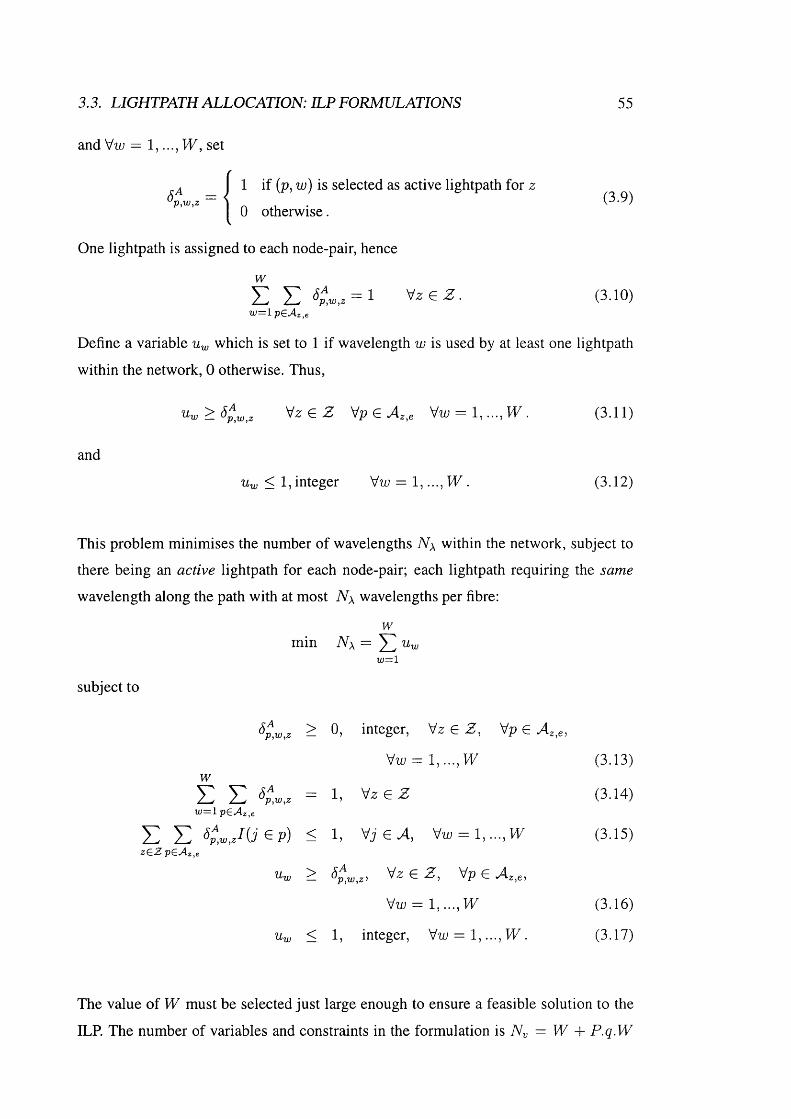
3.3. LIGHTPATH ALLOCATION: TLP FORMULATIONS 55
and Vw = 1 , W , set
1 if (p, w) is selected as active lightpath for z ^
0 otherwise.= <
One lightpath is assigned to each node-pair, hence
wE E = 1 V z e Z . (3.10)
VJ = l p e A z , e
Define a variable which is set to 1 if wavelength w is used by at least one lightpath
within the network, 0 otherwise. Thus,
M z e Z Vp e A ,e Vu; = 1 , VK. (3.11)
and
Uu; < 1, integer Vu; = 1,..., TV . (3.12)
This problem minimises the number of wavelengths N \ within the network, subject to
there being an active lightpath for each node-pair; each lightpath requiring the same
wavelength along the path with at most N \ wavelengths per fibre:
wmin N x =
w—l
subject to
> 0, integer, Vz G Z , Vp G
Vu; = 1 ,..., W (3.13)w
= 1, M z e Z (3.14)10 = 1 p e A z , e
E E <5pE,U (iep) < 1, V j e A Vw = i , . . . . i y (3.15)zÇiZ p E A z , e
Vz G Z , Vp G ^z,e,
Vu; = 1,..., W (3.16)
Uw < 1, integer, Vu; = 1 ,..., IV . (3.17)
The value of W must be selected just large enough to ensure a feasible solution to the
ILP. The number of variables and constraints in the formulation is = W 3- P .q.W

56 CHAPTER 3. WAVELENGTH REQUÏÏŒMENT IN SINGLE-FIBRE WRONS
and Nc = + P + + +VF, respectively. In this case, the complexity of
the formulation depends not only on network size and connectivity, and value of e, but
also on the wavelength requirement A ; , as VF must exceed N \. This makes the WSXC
case more computationally expensive, as it will be shown in section 3.7.1.
3.4 Lightpath allocation: lower bounds
In this section, lower bounds on the optimal solution are developed. These have the
advantage of reduced computational complexity compared to the ILPs previously de
scribed.
Two lower bounds on the wavelength requirement N \ can be defined for a given
network topology. Since in calculating these, no constraints on wavelength continuity
are imposed, these limits define lower bounds for the WIXC case. However, they can
also be used for comparison with the WSXC case.
3.4.1 Distance bound
The minimum total number of links occupied by all the network lightpaths is
and the average inter-nodal distance is
I ) '
An ideal allocation of the lightpaths, evenly distributed over the L links, would lead to
a wavelength requirement equal to [70]:
VF,D BLT
L(3.20)
where \x] represents the lowest integer greaUer than or equal to x.
This lower limit is referred to as distance bound [101], throughout the thesis.
W db can be easily derived once the mimimum-number-of-link (or physical hop),
MNH, distance for all the node-pairs is obtaiined, for example by using Dijkstra algo
rithm [53].

3.4. LIGHTPATH ALLOCATION: LOWER BOUNDS 57
IV\S
Figure 3.2: Example of network cut C.
3.4.2 Partition bound
Consider a network cut, that is a set of links j e C C A (C ^ (f), A ), whose elimination
results in two disjoint subsets of nodes, S and A f\S , respectively (see Fig. 3.2). The
total number of lightpaths traversing the cut C is
D c = Y : d(z)zGjiC)
(3.21)
where d{z) is the demand, in number of bi-directional lightpaths, for the node-pair
z , and 7 ( C ) = { ( z i , Z 2 ) G Z | z% G <S, Z 2 G A^\<5}. In the case of uniform traffic
considered here, eq.(3.21) can be written simply as Dc = |<S|.|Af\5|. The minimum
number of distinct wavelengths necessary to satisfy the traffic demand across the cut C
is, therefore:
Wc =Dc|C|
(3.22)
where \C\ is the number of links in the cut C. The different cuts C within the net
work result in different values of Wc, with the largest one determining the lower bound
WpB [96]:\ \ s \ . \ u \ s \ ^
(3.23)WpB = max Wc = max CC-4 C c A |C|
The network cut C which sets the lower limit W pb is referred to as the limiting cut.
This bound was independently proposed in [65], and is referred to as partition
bound [101].
For a network topology with N nodes, enumerating all the network cuts to find W pb
is 0 ( 2 ^ “ ^), which is practical only for small size networks.
Therefore, a heuristic algorithm was developed, to identify the network limiting cut,
and calculate the parition bound W pb (see Appendix A). However, as discussed in
Appendix A, in the case of several network topologies where two or more cuts, for

58 CHAPTER 3. WAVELENGTH REQUIREMENT IN SINGLE-FIBRE WRONS
example, C\ and C2 , required similar number of wavelengths to satisfy the traffic across
them, Wc^ % Wc^ ~ the algorithm was observed to oscillate between these cuts,
failing to produce a valid result.
However, since in most of the networks only one cut determines the partition bound,
it was relatively easy to identify the limiting cut from the network plot, and derive W p b -
For a given topology, the largest value between WpB and W pb determines the actual
lower bound W lb on the wavelength requirement, that is W l b =^^'^{W d b , W p b ).
It will be shown in section 3.7.1 that, in real networks, the partition bound sets the
lower limit on N \. Conversely, in random networks with size 77 —)■ 00 , the lower limit
is governed by W d b , as proved in [101] and discussed in section 3.7.2.
The calculation of the lower bounds does not provide information on routing of the
lightpaths to achieve these limits. In fact, WpB may not be achieved if routing rules
(such as constraints on path length, as discussed in section 3.6, and wavelength conti
nuity in WSXC case) are imposed. However, these bounds provide useful indication of
the minimum N \, to verify the accuracy of the heuristic lightpath allocation algorithms
described in section 3.6.
3.5 Lightpath allocation: upper bound
For any network topology with N nodes, an upper bound on N \ can be derived as fol
lows. The constraint (C7) in section 3.2 imposes that any two subsets of nodes are
connected by at least two links. Therefore the worst case in terms of 77 is obtained
when two subsets, each consisting of N /2 nodes, are connected by just two links, re
sulting in W lb = W pb = [77^/8].^ At the same time, it is expected that no more
than wavelengths are necessary, as this 2-link cut determines a wavelength re
quirement Wc much larger than any other cut in the network. Therefore, for any given
network of size A , an upper bound can be defined as:
^ if 77 even
,N o d d .
For odd values of N, the worst case is with {N — 1)/2 nodes in one side and {N -h 1)/2 nodes in the
other, resulting in W l b = [(77 - 1)/S].

3.6. LIGHTPATH ALLOCATION: HEURISTIC ALGORITHMS 59
Similarly to the lower bound, this limit can be exceeded if routing rules are imposed,
as discussed in section 3.7.2.
3.6 Lightpath allocation: heuristic algorithms
As will be shown in section 3.7.1, the ILP formulations are computationally expensive,
and can only be used to analyse relatively small networks. For the case of large net
works, heuristic algorithms are developed to construct good (although not necessarily
optimal) solutions. The algorithms developed in this work for the allocation of the ac
tive lightpaths solves the routing and wavelength assignment sub-problems separately,
simplifying algorithm design [96].
First, the physical paths are assigned to all node-pairs. The minimum-number-of-
hops (MNH) algorithm is considered (hence e = o in active sets Az,e defined in eq.(3.3),
as, in this case, each lightpath utilises the minimum number of physical links and OXCs,
minimising the total and average transit traffic, and hence OXC size. This is also key to
minimising crosstalk penalties associated with physical limitations of OXCs. However,
in the cases where the lower bound is not achieved, longer paths may be considered
(e > 0 in eq.(3.3)), to enable more efficient lightpath allocation, and, hence, reduce Nx,
as shown in section 3.7.1.
In a network with N nodes, there exist P node-pairs and therefore P\ different ways
in which they can be ordered and assigned paths. In the proposed algorithm, node-pairs
with the largest MNH are assigned paths first. Since sets Az,e usually consist of several
paths, a certain degree of freedom is available to allocate, as evenly as possible, the
lightpaths among the network links, minimising link congestion.
In the WSXC case, wavelengths are then assigned to the paths. There exist P !
different ways in which the paths can be ordered and assigned wavelengths. Here, the
paths are ranked by decreasing length, and the longest ones are assigned wavelength
first, as, intuitively, long paths are harder to allocate since a unique free wavelength
must be found on more links, as discussed in [5]. The highest wavelength assigned
amongst all node-pairs determines the network wavelength requirement N \.
For the WIXC case, no wavelength assignment is performed, since the wavelengths
can be allocated link by link, and the wavelength requirement N \ is equal to the number
of lightpaths in the most congested link.
A formal description of the algorithms is given in Appendix B. 1.
60 CHAPTER 3. WAVELENGTH REQUIREMENT IN SINGLE-FIBRE WRONS
The accuracy of the proposed heuristic algorithms was verified by comparing their
results with lower bounds and exact results obtained with ILP formulations, as described
in section 3.7.
3.7 Results
3.7.1 Real networks
Several existing or planned fibre network infrastructures were first analysed, to eval
uate their topological parameters for WRON applications (see Table 3.1, with the net
works ranked in increasing value of a).
The considered topologies are examples of US and pan-European networks. The
BURO-Core [83] is an example of a possible first optical pan-European network [102],
which may evolve to include more and more nodes to form a larger topology such as
EON proposed in [103],^ and EURO-Large. Similarly, NSFNet [60] and ARPANet [59]
may be used for first WRON deployment in the US, evolving to the USNet. A UK
topology approximating the current BT-network [104] was also considered.
As shown, the networks’ sizes vary from 11 to 46 nodes. Since, as discussed in
section 3.2, the maximum nodal degree, ômax, is relatively constant and does not scale
with N (see ômax in Table 3.1), a increases as N decreases, ranging between 0.07 and
0.45. This is the range which will be considered in this analysis, as most of real transport
networks have comparable values of a . An increase in a leads to a more connected
network, and a decrease in the average inter-nodal distance H and diameter D (defined
as the longest path within the network). For the analysed networks, H varies between
1.58 and 4.4, and D is between 3 and 11, typical for real transport networks.
The dotted lines in the graphs identify the limiting cuts which determine Wpb, as
discussed in section 3.4. In the UKNet the central cut Ci determines the partition bound
WpB, whilst the upper cut C2 determines the partition bound W p^ when single link
failure restoration is considered, as discussed in section 4.6.1. The number of links \C\
in the limiting cut is also reported. [For all the networks, except for the UKNet, the
same cut sets the partition bound for both configurations without and with link failure
restoration, thus the number of links in the limiting cut under condition of single link
^With respect to the topology presented in [103], a link between the node 7 and 8 has been added to
satisfy constraints (Cl) and (C2).

3 . 7. RESULTS
N e t w o r k
USNet 0.07 4.4
(2.5) 3.6EURO-Large
(2,4) 0.16 2.81ARPANet [59]
2.51UKNet [104] (2,7) 0.19
EON [103] (2.7) 0.2
(2.4) 0.23 2.14NSFNet [60]
EURO-Core [83] 0.45 1.58
Table 3.1: Topological parameters of existing or planned network topologies. The dotted
lines represent the limiting cuts. N, number of nodes; L, number of links; ô.,aini 3/nax-
minimum and maximum nodal degree; a, physical connectivity; H, average inter-nodal
distance; D, network diameter (longest path within the network); |C|, number of links
in the limiting cut; \C"\, number of links in the limiting cut when single link failure is
considered (see Chapter 4).

62 CHAPTER 3. WAVELENGTH REQUIREMENT IN SINGLE-FIBRE WRONS
N e t w o r k P W d b W p B e
NxI L P Heuristic
W I X C W S X C W I X C W S X C
USNet 1035 60 103t 0 - - 108 108
1 103 108
EURO-Large 903 37 66^ 0 - - 88 88
1 66 68
ARPANet 190 18 33 0 33 - 33 33
UKNet 210 14 19 0 21 - 21 21
1 19 19 20
EON 190 12 18 0 18 18 18 18
NSFNet 91 10 13 0 13 13 13 13
EURO-Core 55 4 4 0 4 4 4 4
Table 3.2: Results for existing or planned network topologies. P = N.{N - l)/2 , to
tal number of bi-directional lightpath allocated within the networks (network throughput
Tp = 2.P.Rb, with Rb bit-rate per channel); WoBi distance bound; Wp b , partition bound
(marked by if obtained by inspection); e, extra number of hops allowed to the active
lightpaths; a dash is shown where the ILP failed to give any result after one day of compu
tation on a UNIX workstation; N \, wavelength requirements. The results which achieved
the lower bounds are highlighted.
failure is \C”\ = \C\ — 1 (see section 4.6.1).]
The results, including lower bounds, are presented in Table 3.2. As expected, an
increase in a leads to a reduction of the distance bound W b e -
For the USNet and EURO-Large, the partition bound was derived by inspection,
and the values were then confirmed by the results of N \ obtained by the heuristic algo
rithms. For all the other topologies, W pb was obtained by both enumerating the network
cuts and using the heuristic algorithm described in Appendix A, except for the UKNet,
where the heuristic was observed to oscillate between two network cuts, as discussed in
section 3.4.2.
As shown, for all the networks, excluding the EURO-Core, the partition bound W pb
is much larger than the distance bound W d b , and, therefore, determines the lower bound
FFlb on the wavelength requirement. There are two operational reasons for this: the
distribution of nodes over a given geographical area, and the cost of deploying the
fibre infrastructure, which determines that each node is most likely connected to its
neighbouring nodes, resulting in elongated topologies, where a particular cut becomes

3.7. RESULTS 63
N e t w o r k e Q W I X C WSXC
Ny Nc W Ny Nc
EURO-Large 0 2.67 2,411 3,403 90 233,370 475,653
ARPANet 0 1.48 282 502 34 9,588 20,386
UKNet
0 1.92 405 653 22 8,910 18,866
1 7.40 1,555 1,803 22 34,210 69,466
2 19.06 4,003 4,251 22 88,066 177,178
3 31.78 6,674 6,922 22 146,828 294,702
EON 0 2.01 383 611 18 6,894 14,662
NSFNet 0 1.29 118 229 14 1,652 3,675
EURO-Core 0 1.69 94 173 5 470 1,115
Table 3.3: Computational complexity of IL P formulations, e, extra number of hops al
lowed to the active lightpaths; q, average size of active sets, Az,e’y Tly, number of variables;
Nc, number of constraints; W, maximum number of wavelengths per fibre, fixed in the
W S X C . The formulations which were successfully carried out are highlighted.
significant. However, in more uniformly-connected topologies (see for example EURO-
Core), W db can be equal or even larger than W p b , setting the network lower limit. This
is the case for very large random networks, as demonstrated in [101] and discussed in
section 3.7.2.
Table 3.2 also shows the results for N \ calculated with both I L P formulations and
heuristic algorithms. For EURO-Core, NSFNet, and EON topologies, the lower bound
was achieved by both I L P s and heuristics algorithms utilising MNH paths (e = 0).
The same results were obtained for WIXC and WSXC cases, showing that wavelength
conversion within the OXCs does not lead to a reduction in Nx- In fact, the wavelength
requirement is determined by physical connectivity and topology, i.e. limiting cut.
The number of variables and constraints in the ILP formulations are shown in Ta
ble 3.3 for all real networks, except for the USNet. Consider the EURO-Core. For the
WIXC case, Ny = 94 and Nc = 173, whereas the complexity is larger, although still
tractable, for WSXCs {Ny = 470 and Nc = 1,115, with W = 5). As shown, Ny and
Nc increase with network size N , particularly in the WSXC case, resulting in longer
running time. For example, for the ARPANet with e = 0, Ny = 405 and Nc = 653 with
WIXCs, and Ny = 8,910 and Nc = 18,866 with WSXCs (W = 34), the latter resulting
in extremely long running time. For UKNet and ARPANet, only WIXC ILP calculation
time was feasible, whereas the WSXC case failed to yield any results after at least one

64 CHAPTER 3. WAVELENGTH REQUIREMENT IN SINGLE-FIBRE WRONS
day of computation on a UNIX workstation (dashes in Table 3.2). However, it was not
possible to extend ILP formulations to the analysis of EURO-Large and USNet, given
the extremely large number of variables and constraints. In these cases, the results of
Nx obtained with the heuristic algorithms were confirmed by the lower bounds.
It is worth noting the importance of e in determining the ILP complexity. As shown
for the UKNet, small values of e (for example e = 0 or 1) enables to limit the average
size q of the active sets Az,e, resulting in limited number of variables and constraints.
However, as e is increased (see for example e = 2 or 3), Ny and Ny dramatically
increase, especially in the WSXC case, making the problem intractable.
The UKNet, EURO-Large, and USNet were also analysed with lightpaths one hop
longer than MNHs (see rows with e = 1 in Table 3.2). For the UKNet, this allowed
to achieve the lower bound with both ILP and heuristic WIXC case, whereas it was not
achieved by the heuristic WSXC case (even with e > 2). For the EURO-Large and
USNet, the heuristic for the WIXC case achieved the lower bound, whereas a few extra
wavelengths were required for the WSXC case, although the difference was negligible.
This confirmed the negligible improvements achievable with wavelength conversion,
even in large topologies.
As expected, the wavelength requirement N \ increases as the physical connectivity
a decreases. However, for all networks, the wavelength requirement N \ is much smaller
than the number of bi-directional lightpaths P established, highlighting the large wave
length reuse achievable in WRONs (a factor of 10 in most of the topologies). Thus, even
in weakly-connected topologies, a relatively small N \ can satisfy a very large traffic de
mand, providing large network throughput, Tp = 2.P.Rb.
Finally, it is worth noting the accuracy of the heuristic algorithms, which were ob
served to produce results always equal or very close to the lower bounds or exact solu
tion of the ILPs.
Table 3.4 shows the number of bi-directional lightpaths transiting (and not terminat
ing into) the WRNs, Nu, and WRN-sizes, obtained with the heuristic WIXC case. [The
actual size of the OXCs is double, as the lightpaths are bi-directional.] As shown, Nu
and, hence, the WRN size increase as the network size increases. Moreover, as N in
creases, the average transit traffic becomes much larger than the number of bi-directional
lightpaths terminating at the corresponding end-node, equal to Æ — 1 (almost as large
as 3 times for the USNet). These results indicate that, in the case of large networks
with large traffic demand (in number of lightpaths), wavelength-routing is key, as it en-
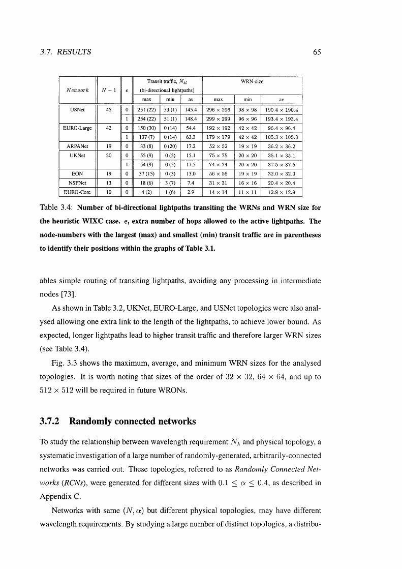
3.7. RESULTS 65
N e t w o r k N - I e
Transit traffic, Nti
(bi-directional lightpaths)
WRN-size
max min av max min av
USNet 45 0 251 (22) 53(1) 145.4 296 X 296 98 X 98 190.4 X 190.4
1 254(22) 51 (1) 148.4 299 X 299 96 X 96 193.4 X 193.4
EURO-Large 42 0 150(30) 0(14) 54.4 192 X 192 42 X 42 96.4 X 96.4
1 137 (7) 0(14) 63.3 179 X 179 42 X 42 105.3 X 105.3
ARPANet 19 0 33 (8) 0(20) 17.2 52 X 52 19 X 19 36.2 X 36.2
UKNet 20 0 55 (9) 0(5 ) 15.1 75 X 75 20 X 20 35.1 X 35.1
1 54 (9) 0 (5 ) 17.5 74 X 74 20 X 20 37.5 X 37.5
EON 19 0 37(15) 0(3) 13.0 56 X 56 19 X 19 32.0 X 32.0
NSFNet 13 0 18(6) 3(7) 7.4 31 X 31 16 X 16 20.4 X 20.4
EURO-Core 10 0 4(2) 1 (6) 2.9 14 X 14 11 X 11 12.9 X 12.9
Table 3.4: Number of bi-directional lightpaths transiting the WRNs and WRN size for
the heuristic WIXC case, e, extra number of hops allowed to the active lightpaths. The
node-numbers with the largest (max) and smallest (min) transit traffic are in parentheses
to identify their positions within the graphs of Table 3.1.
ables simple routing of transiting lightpaths, avoiding any processing in intermediate
nodes [73].
As shown in Table 3.2, UKNet, EURO-Large, and USNet topologies were also anal
ysed allowing one extra link to the length of the lightpaths, to achieve lower bound. As
expected, longer lightpaths lead to higher transit traffic and therefore larger WRN sizes
(see Table 3.4).
Fig. 3.3 shows the maximum, average, and minimum WRN sizes for the analysed
topologies. It is worth noting that sizes of the order of 32 x 32, 64 x 64, and up to
512 X 512 will be required in future WRONs.
3.7.2 Randomly connected networks
To study the relationship between wavelength requirement N \ and physical topology, a
systematic investigation of a large number of randomly-generated, arbitrarily-connected
networks was carried out. These topologies, referred to as Randomly Connected Net
works {RCNs), were generated for different sizes with 0.1 < a < 0.4, as described in
Appendix C.
Networks with same {N, a ) but different physical topologies, may have different
wavelength requirements. By studying a large number of distinct topologies, a distribu-

66 CHAPTER 3. WAVELENGTH REQUIREMENT IN SINGLE-FIBRE WRONS
512x512- 0 — 0 max■— fl average O Omin256x256 -
0)~ 128x128-
zccg
64x64 -
32x32 -
16x16-increasing N
E u No -C NSF^Net . e 6 nl e t , EON UKN et A R PA N et ElNetwork topology
Figure 3.3: WRN size for the analysed real topologies. The results were obtained with
for the heuristic WIXC case, with MNH path (e = 0 in eq.(3.3)). max, average, min:
maximum, average, and minimum WRN size among all the network nodes.
tion of Nx was obtained. It was observed that a few thousand such distinct topologies
generated defined and stable distributions of N \.
Figs. 3.4 shows the normalised distribution of N \ obtained with heuristic WSXC
case, with MNH paths, for RCNs with = 14 and a = 0.23. The position of the
NSFNet (Nx = 13) within the distribution is also presented.
As shown, the distribution assumes a wide range of values, and is bimodal with
peaks centred, respectively, around Nx = 14: and 17. The average value is A a = 14.2
and the range 11 < A a < 20 contains 95% of the results. A few of these topologies
are presented in Table 3.5. They are ordered for increasing wavelength requirement Nx,
and the letter identifies their position within the distribution of Fig. 3.4.
These topologies are good representations of real fibre network infrastructures, con
firming the validity of the method used to generate the RCNs (given in Appendix C).
The average inter-nodal distance, H, slightly increases moving from the top to the
bottom of Table 3.5, whereas the diameter D appears unrelated to Nx, as, for example,
D = 5 for both topologies C and N, which have a large difference in the wavelength
requirement. Similarly, the nodal degree distribution (ri2 , ris, in the table) appears not
^The normalisation is performed with respect to the total number of analysed networks, i.e. the total area of the histogram is 1.

3 . 7. RESULTS 67
N e t w o r k
2.12
2.14
2.34
2.24
2.25
2.29
2.46
2.45
2.58
2.41
2.59
2.71
2.57
2.61
Table 3.5; Topological parameters for several RCNs with N = 14, a = 0.23 (L — 21). The
dotted lines represent the limiting cuts. 74%, number of network nodes with degree = i.
5rnax ~ 4, as for NSFNet.

68 CHAPTER 3. WAVELENGTH REQUIREMENT IN SINGLE-FIBRE WRONS
■s
N S F N e t
\
e 10 1 2 14^ 1 6 I S 2 0 2 2 2 4 2 6 2 8 3 0 3 2 3 4 3 6 3 8 4 0 N u m b e r o f W a v e l e n g t h s ( N ^ )
Figure 3.4: Normalised distribution of N \ obtained with heuristic WSXC case, with MNH
paths, for RCNs with N = 14 and a = 0.23. Wu b , upper hound, as defined in eq.(3.24).
Net iuork ^VpB W p B e
Nx
I L P Heuristic
W I X C W S X C W I X C , H 'S A 'C
A 10 10 0 10 10 10
B 10 12 0 12 12 12
C 11 13 0 13 13 13
D 10 13 0 14 14 14
1 13 13 13
E 10 13 0 15 15 15
1 13 - 13
F 10 17 0 17 17 17
G 11 20 0 20 - 20
H 11 23 0 23 - 23
I 12 25 0 25 - 25
J 11 23 0 27 - 27
1 23 23
K 12 23 0 31 - 31
1 23 23
L 12 25 0 37 - 37
1 25 25
M 12 25 0 38 - 38
1 25 25
N 12 25 0 39 - 39
1 30 30
2 25 25
Table 3.6: Results for several RCNs with = 14, a = 0.23 (L = 21). A dash is shown
where the ILP failed to give any result in acceptable time; the results for the heuristic
WIXC and WSXC cases are in the same column since they were equal; e, extra number
of hops allowed to the active lightpaths. The results which achieved the lower hounds are
highlighted.
3.7. RESULTS 69
to have any effect on As shown, it is the number of links \C\ in the limiting cut, and
its position within the network, which governs the wavelength requirement. Consider
the limiting cut and partition bound W p b , the latter shown in Table 3.6. As the number
of links \C\ decreases, and the limiting cut moves towards the centre of the network,
the partition bound increases, given that the two generated subsets of nodes become
approximately of the same size (equal to N /2) with fewer links connecting them. [For
all the networks, except for topologies C and D, the same cut set the partition bound
without and with link failure restoration, thus \C”\ = |C| - 1, as will be discussed in
section 4.6.2.]
Similarly to the real networks in section 3.7.1, the partition bound was always ob
served to be larger than the distance bound, and defined the lower bound, i.e. W lb =
WpB- The only exception was the uniformly-connected topology A, in which, simi
larly to the EURO-Core in section 3.7.1, all network cuts consisted of a large number
of links, and the partition bound is equal to the distance bound. As shown, the largest
lower bound is Wpp = 25, equal to the upper bound discussed in section 3.5.
As expected, the I L P formulation for the WSXC case produced results up to a
given value of N \ (networks A-F in Table 3.6), after which the formulation became
computationally intractable. As shown, IL P s and heuristic algorithms, the latter for
both WIXC and WSXC, always produced the same results, and, always, the lower bound
was achieved, that is the availability of wavelength conversion did not results in any
reduction of N \. However, for the networks D, E, J-N, one or two extra hops were
required to evenly distribute the lightpaths among the network links, and achieve W l b -
In the distribution of Fig. 3.4, with only MNH paths, only a small fraction of the
RCNs required more wavelengths than the upper bound W ub — 25, and the analysis of
the example networks J to N (Table 3.6) showed that one or two extra hops allowed to
achieve the corresponding lower bound. Therefore, it is expected that a small fraction
of RCNs would benefit from using paths longer than MNHs.
The analysis of numerous topologies for different (A , a) showed wavelength re
quirement for WIXC and WSXC heuristic algorithms always equal or very close to the
lower bound, implying that significant reduction in N \ was attainable by the introduc
tion of wavelength conversion, confirming the initial results obtained in [62] [65].
Therefore, hereafter, on]y the results obtained with WSXC heuristic, with MNH
paths, will be presented.
The distribution of the observed N \ for RCNs, with = 14 and different values

70 CHAPTER 3. WAVELENGTH REQUIREMENT IN SINGLE-FIBRE WRONS
o c = 0 . 1
12 14 16 10 20 22 24 26 28 30 32 34 36 38 40N um ber of W ave len gth s (N. )
o c = 0 . 2 9
0.30
0.20
0.006 8 1 0 1 2
N um ber_ 14 16 18 20 22 24
Num ber of W a v e le n g th s (N J
0.70
. 8 0.60
r g 0.50 ;
"cOQ 0.40 -
W 0.30 -IIg 0.20 E 0.10
O 00 —
o t = 0 . 3 5
a4 5 6 7 8 9 10 11 12 13N u m ber of W a v e le n g th s (N J
0.70
0.60
0.50
0.40
0.30
0.20
0 . 1 0
0.00
o c = 0 . 4 j
Q4 5 6 7 8 9 10 11 12 13N um ber of W a v e le n g th s (N,)
Figure 3.5: Normalised distribution of N \ obtained witb tbe heuristic WSXC case, with
MNH paths, for RCNs with = 14 for different values of a.
4 -
Co nne ct iv i ty (cx)
Figure 3.6: Wavelength requirements for RCNs with = 14 versus the physical connec
tivity a. The bars represent the ranges containing 95% of the results, and the dashed lines
the mean values fit.

3 . 7. RESULTS 71
M 20
■sf -
ARPANet
U K N e t
E O N
-V N = 50
N S F N e t
: U R O - C o r
Tectivity (<x)
Figure 3.7: Mean values of N \ for RCNs versus physical connectivity a, as a function of
the number of nodes N.
20
A R P A N e t
U K N e t
E O N
N S F N e t
C o m p l e t e a n a l y s i s (N = S. N = G)
: U RO -Coro-—
O 0.1 0 .2 0 .3 0 .4 0 .5 0 .5 O.T 0 .8 0 .9Connectiv ity (<x)
"T
Figure 3.8: Mean values of N \ versus physical connectivity a , as a function of the number
of nodes N.
of a are plotted in Fig. 3.5. As expected, an increase in a leads to a decrease in N \ ,
since the lightpaths can be mapped over a larger number of links. Consequently, the
distribution shifts towards lower values and becomes narrower. In Fig. 3.6 the mean
values and the ranges containing 95% of the results for R C N s with N = 14 are plotted
versus the physical connectivity a. As discussed, both the mean values and the ranges
decrease with increasing connectivity.
The same analysis was performed for RCNs with different network sizes in the range
20 < 77 < 50, and the results showed similar behaviour to the case with N = 14, that
is, wavelength requirements driven by limiting cuts and limited improvement achievable
with wavelength conversion.
In Fig. 3.7 the mean values of the distributions for all the considered values of N are
plotted versus a. It is interesting to note that the mean values of N \ are independent of
the network size N . [Similarly, for a given cv, the 95% ranges for different N were found

72 CHAPTER 3. WAVELENGTH REQUIREMENT IN SINGLE-FIBRE WRONS
C o n n e c t iv i ty (tx)
Figure 3.9: Number of wavelengths (upper houncl) for 95% of the RCNs versus physical
connectivity a, as a function of the number of nodes N.
to be comparable.] A clear trade-off exists between mean values of N \ and physical
connectivity a , and their relationship is quantified by the results shown in Fig. 3.7.
On average, RCNs can satisfy the uniform traffic demand with a moderate number of
wavelengths. For example, no more than 32, 16 and 8 wavelengths are necessary for
Q > 0.15, 0.2, and 0.3, respectively.
The results of several real networks are also shown. It can be seen that UKNet, EON,
NSFNet, and EURO-Core match well the average wavelength requirements of RCNs,
whereas the ARPANet requires a larger N \ , given its sub-optimal topology resulting
from its limiting cut (consisting of only 3 links, located in the middle of the topology,
as shown in Table 3.1).
A complete analysis of all the possible topologies was performed for networks with
N = 3 and 6. The range of possible values of physical connectivity is a > Ü.5 and 0.4,
respectively, as derived in eq.(C.2). Given these large values of a, narrow distributions
of N \ were obtained. The mean values, plotted in Fig. 3.8, show that as a increases
the wavelength requirement decreases reaching N \ = I for a = 1, as expected. These
results correspond exactly with those obtained for RCNs, confirming the validity of the
RCNs modelling results.
Fig. 3.9 shows the values of N \ below which 95% of the RCNs lie, defining an upper
hound of the observed wavelength requirements. It should be noted that, for example,
for a > 0.2 and 0.3, 95% of all the generated networks require less than 32 and 16
wavelengths, respectively.
In Fig. 3.10 the minimum values of the distributions of h \ (representing the ob
served lower bound) for RCNs are plotted versus a . Similarly to the mean values of

3 . 7. RESULTS 73
RCMs <: Complet© An alys is
- : 40 .0 0.1 0 .2 0 .3 0 .4 0 .5 0 .6 0 .7 0 .8 0 .0 1 .0
C onnect iv ity <cx)
Figure 3.10: Minimum values (lower bound) of N \ for RCNs versus physical connectivity
O', as a function of the number of nodes N.
N=14. «%=0.23
2.3 2.4 2.5 2.6 2.7 2.8 2.9 3.0Average Intornodal Distance
N = 2 0 . i x = 0 . 2
l l L l u i2.2 2.3 24 2.5
Average Internodal Distance
Figure 3.11: Normalised distribution of average inter-nodal distance: (left) N = 14, a =
0.23, and (right) N = 20, o = 0.20.
Fig. 3.8, they depend only on cv, and are independent of the network size N . The fol
lowing equation:k
(3.25)
provides a good fit for this curve with /c = 3 for 0.1 < a < 0.4, and k = 2 for a > 0.4.
By using eqs.(3.1) and (3.19), the distance bound W ob defined in eq.(3.20) can be
written as a function of a\
N . { N - l ) l i L r c . H H(3.26)
2.T I
where H is the average inter-nodal distance. It can be seen that, for a = 1, 77 = 1 and
the distance bound is achieved (Nx^,^ = li oB = !)•
The distributions of 77 for all the RCNs were analysed, and for a given (Ay a ) a
normal distribution was found to be a good fit (see Fig. 3.11 ). In Fig. 3.12 the minimum
values of these distributions, Hmin, are plotted versus physical connectivity a. For a

74 CHAPTER 3. WAVELENGTH REQUIREMENT IN SINGLE-FIBRE WRONS
11
C onn ect iv i ty (tx)
Figure 3.12: Minimum values of the mean inter-nodal distance, Hmim versus physical
connectivity a , as a function of the number of nodes N.
given N , an increase in a results in a decrease of as expected. As shown, for low
values of a (<a < 0.3), Hmin decreases with an increase of A . However, the influence of
the network size decreases with an increase in a, and for cv > 0.3, Hmin is almost inde
pendent of N . From these results, it is not possible to define a quantitative relationship
between Hmin and a , independently of N . Nevertheless, the results of Fig. 3.12 can be
used in eq.(3.26) to calculate the minimum distance bound, WoBmin- example for
27 = 28 and a = 0.25, Hmin = 1 9 , and from eq.(3.26) WoB„^^n = " 6. From eq.(3.25),
for a = 0.25, = 10. This difference results from an uneven distribution of the
lightpaths among the network links. In fact, as discussed in sections 3.7.1 and 3.7.2, Nx
is governed by the limiting cut and the corresponding partition bound W p ^ .
However, as the physical connectivity a increases, this difference decreases. For
example, for a = 0.4, Hmin = 1-6 (independent of N), hence WoBm^n — "1- Fi'om
eq.(3.25), for a = 0.4, = 5.5. This confirms that by increasing a , the number
of the links in the network cuts becomes more uniform, and W pp approaches W pp-
The availability of more alternative paths for each node-pair results in an even lightpath
distribution and efficient link utilisation, leading to a reduction of N \ which approaches
W d b .
It is worth noting that asymptotic lower bounds on wavelength requirement N \ were
analytically derived in [101] for random networks, with size 27 — oo and diameter
D < 2. It was proved that, in these topologies, the partition bound is 11 = 1 /a
and the distance bound is VF5b = 2 / a — 1, which determines the lower bound. Several
optimal finite-size topologies, achieving the lower bound W p p , were proposed in [105].
However, only selected values of N were feasible, and for all of them D = 2, as re-

3 . 7. RESULTS 75
Connectiv ity (tx>
Figure 3.13: Minimum values of N \ for RCNs and asymptotic lower bound derived
in [101] versus physical connectivity a.
quired.
In Fig. 3.13, the minimum values of the observed N \ for RCNs and the optimal lower
bound H a r e plotted against the physical connectivity a. As shown, the results are
in very good agreement for a > 0.4, with a slight difference for 0.1 < cv < 0.4. This
difference mainly results from the sub-optimality of the generated RCNs, whose diame
ter was always D > 2, the condition required to achieve the lower bound 11/*/ j . Taking
into account this main topological difference, the analytical lower bound confirms the
validity of the results obtained in this analysis.
3.7.3 Regular networks
As discussed in section 2.3.1, regular network topologies have recently attracted signif
icant interest [70]-[72], following photonic switching analysis, where regular multihop
logical topologies were key to enable simple routing [75][76].
In this work, regular physical topologies were compared to arbitrarily-connected
networks in terms of wavelength requirements Nx- The topologies considered are the
de Bruijn graph and ShuffleNet.
Shuffle-net topology.
The (3, A:)-ShuffleNet [106] consists of N = k.6^ nodes, arranged in A; columns with 6^
nodes per column, as shown in Fig. 3.14(a) for (5 = 2 and k — 2. Adjacent columns
are connected in a perfect 3-shuffle with direct links. The column is connected
back to the first column, also in a perfect 3-shuffle. Both the in- and out-degree of a
(3, A:)-ShuffleNet are 3, and the diameter is D = 2A: — 1.
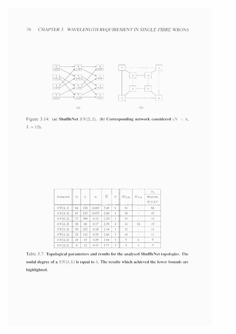
76 CHAPTER 3. WAVELENGTH REQUIREMENT IN SINGLE-FIBRE WRONS
l . (K)(),()()
0.01
1 . 1 00.10
(a) (b)
Figure 3.14: (a) ShuffleNet SN{2,2) . (b) Corresponding network considered (TV = 8,
L = 12).
N e t w o r k N L a H D W p B
Va
Heuristic
W S X C
S N (2 ,4 ) 64 128 0.063 3.42 6 54 - 68
S7V(3,3) 81 243 0.075 2 80 4 38 - 45
6W (6,2) 72 396 0.15 2.20 3 15 - 18
S N (2 ,3 ) 24 48 0.17 2.39 4 14 18 19
g7V(5,2) 50 225 0.18 2.14 3 12 - 15
S N { 4 , 2 ) 32 112 0.23 2.06 3 10 - 11
S N (3 ,2 ) 18 45 0.29 1.94 3 7 6 7
5 N (2 ,2 ) 8 12 0.43 1.71 3 4 4 5
Table 3.7: Topological parameters and results for the analysed ShuffleNet topologies. The
nodal degree of a 57/(5, A;) is equal to Ô. The results which achieved the lower bounds are
highlighted.

3.7. RESULTS 11
n
n(a) (b)
Figure 3.15: (a) de Bruijn cfeB(2,3). (b) Corresponding network considered {N = 8 ,
L — 13).
In the ShuffleNet topologies considered here, single directed links were replaced by
bi-directional ones, as shown in Fig. 3.14(b). The main topological parameters and the
results obtained with the heuristic WSXC case, with MNH paths, are shown in Table 3.7,
with the networks ranked for increasing values of a.
As expected, the average inter-nodal distance H, distance bound W ^ b , and wave
length requirement N \, decrease with an increase in a. For large networks, the calcu
lation of the partition bound was not feasible. When W pb was determined, the lower
bound W lb was obtained, and N \ was found equal or very close to it. In the other
cases, N \ was still relatively close to the distance bound (the difference was at most
25%). However, for these networks the partition bound is expected to be larger than
W db and, therefore, closer to N \, confirming the accuracy of the results.
de Bruijn graphs.
For any positive integer ô > 2 and D > 1, the de Bruijn graph deB{ô, D) [47] is a di
rected graph with set of nodes {0, 1 , 2 ,..., and an edge from node (ai, U2 , -, cld)
to node (&i,6 2 , if, and only if, 6 * = a^+i, for 1 < i < D - 1 , as shown in
Fig. 3.15(a) for 5 = 2 and D = 3. The de Bruijn graph deB(ô, D) has N = 6^ nodes,
diameter D, and the in-degree and out-degree equal to 6 for every node.
In this analysis, modified de Bruijn graphs were considered, with single directed
links replaced by bi-directional ones, and self-loops deleted, as shown in Fig. 3.15(b).
The main topological parameters and results are shown in Table 3.8, with the networks
ranked for increasing values of a. These results can be analysed in the same way as for
‘a link starting and terminating in the same node is referred to as self-loop.

78 CHAPTER 3. WAVELENGTH REQUIREMENT IN SINGLE-FIBRE WRONS
N e t w o r k N L a H D W d b W p B
Nx
Heuristic
W S X C
d e B (3 ,4 ) 81 237 0.07 2.83 4 39 - 47
d e B ( 5 ,3) 125 610 0.079 2.47 3 32 - 38
d e B { 2 , b ) 32 61 0.12 2.75 5 23 - 30
d e B ( 4 ,3) 64 246 0.12 2.32 3 20 - 23
d e B {3 , 3) 27 75 0.21 2.08 3 10 10* 12
d e B { 2 , 4 ) 16 29 0.24 2.14 4 9 11 12
d e B { 8 , 2 ) 64 476 0.24 1.76 2 8 - 10
d e B { 7 , 2 ) 49 315 0.27 1.73 2 7 - 9
d e B { 6 , 2 ) 36 195 0.31 1.69 2 6 - 8
d e B { 5 , 2 ) 25 110 0.37 1.63 2 5 5* 6
d e B { 4 , 2 ) 16 54 0.45 1.55 2 4 4 4
d e B { 2 , 3 ) 8 13 0.46 1.64 3 4 6 6
d e B { 3 , 2 ) 9 21 0.58 1.42 2 3 3 3
Table 3.8: Topological parameters and results for the analysed de Bruijn topologies. The
nodal degree of a deB{0, D) is equal to 8. The results which achieved the lower bounds are
highlighted. When the calculation of the partition bound was not terminated, the largest
result achieved was recorded and is marked by *
the ShuffleNet.
In Fig. 3.16 the wavelength requirements N \ are plotted versus a. These results lie
close to the curve describing the mean values of N \ for RCNs (Fig. 3.8), confirming
that arbitrarily-connected networks have similar topological features of regular topolo
gies [107] and, hence, similar wavelength requirement. As already discussed, the main
advantage of regular topologies is the simplicity of routing, which is the same for all
the network nodes. However, regular networks can be grown only by discrete steps, in
which a fixed number of nodes and links must be added, limiting the network scala
bility. Therefore these results lead to the important conclusion that, whilst arbitrarily-
connected networks have similar wavelength requirement that regular topologies, they
also have the added advantages of flexibility required for practical network evolution.
3.8 Topology optimisation by selective addition of fibres
Given the growth of opto-electronic technology, WRONs requiring 8 or 16 wavelengths
could be implemented in the near future [2][108]. As shown in section 3.7, in single-
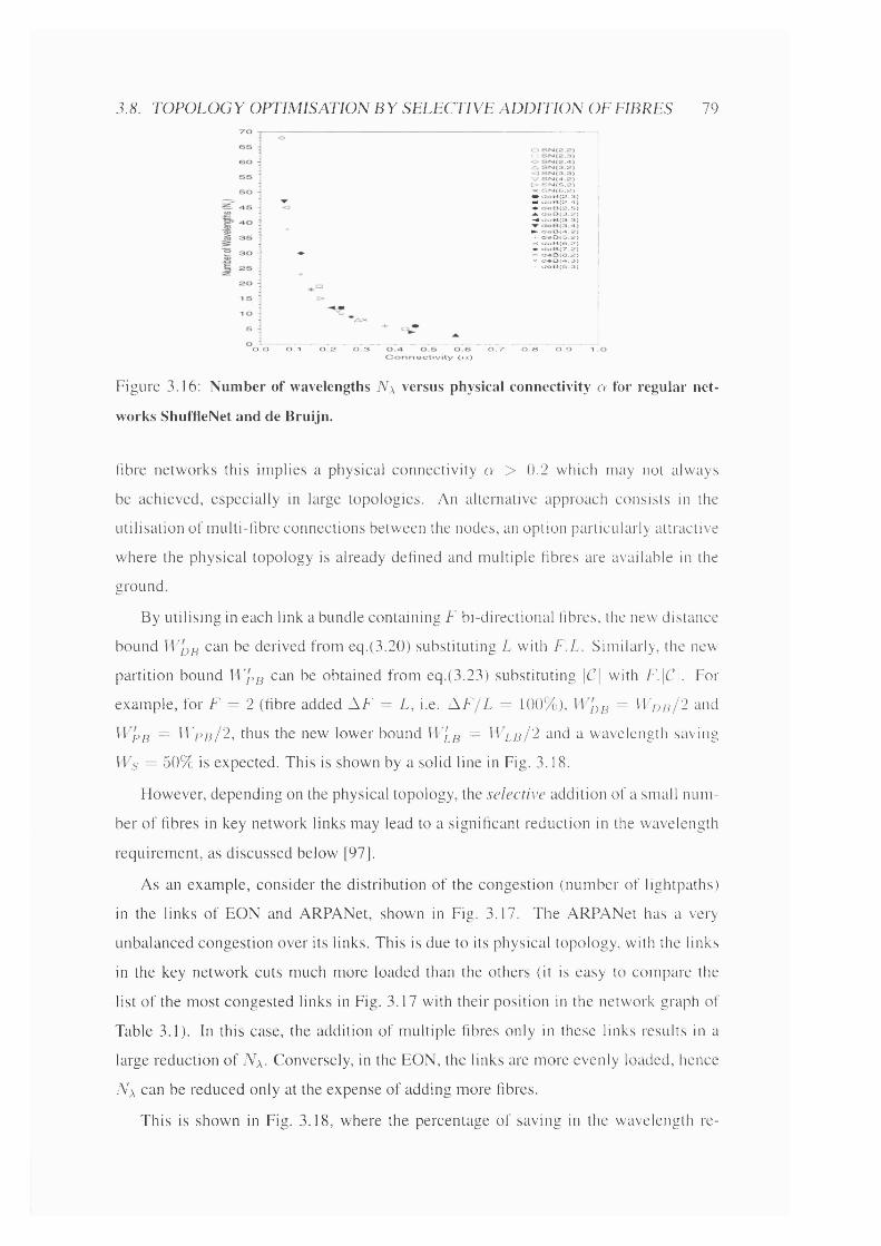
3.8. TOPOLOGY OPTIMISATION B Y SELECTIVE ADDITION OE FIBRES 79
Srsi<s.2) X srg<6.2)« d©B(2.3) M d € 3 B ( 2 . ^ )♦ c J e B ( 2 . S ) ▲ cJaB(3.2) ^ cJoB(3.3)
► d e B ( 4 . 2 ) I cloB(&.2) X cJoB(6.2)• deB(7.2) n cJeB(8.2) V deB(4.3) -> UoB(S.3)
0.0 0.1 0.2 0.3activity <<x)
0.7 0.8 0.9
Figure 3.16: Number of wavelengths N \ versus physical connectivity a for regular net
works ShuffleNet and de Bruijn.
fibre networks this implies a physical connectivity a > 0.2 which may not always
be achieved, especially in large topologies. An alternative approach consists in the
utilisation of multi-fibre connections between the nodes, an option particularly attractive
where the physical topology is already dehned and multiple fibres are available in the
ground.
By utilising in each link a bundle containing F bi-directional hbres, the new distance
bound W qj can be derived from eq.(3.20) substituting L with F.L. Similarly, the new
partition bound IFp^ can be obtained from eq.(3.23) substituting \C\ with F.\C\. For
example, for F = 2 (fibre added A F = L, i.e. N F / L = 100%), IT pp = TFpp/2 and
IT pp = TFpp/2, thus the new lower bound TF[p = TT p p /2 and a wavelength saving
IFp = 50% is expected. This is shown by a solid line in Fig. 3.18.
However, depending on the physical topology, the selective addition of a small num
ber of fibres in key network links may lead to a significant reduction in the wavelength
requirement, as discussed below [97].
As an example, consider the distribution of the congestion (number of lightpaths)
in the links of EON and ARPANet, shown in Fig. 3.17. The ARPANet has a very
unbalanced congestion over its links. This is due to its physical topology, with the links
in the key network cuts much more loaded than the others (it is easy to compare the
list of the most congested links in Fig. 3.17 with their position in the network graph of
Table 3.1). In this case, the addition of multiple fibres only in these links results in a
large reduction of Nx- Conversely, in the EON, the links are more evenly loaded, hence
N \ can be reduced only at the expense of adding more hbres.
This is shown in Eig. 3.18, where the percentage of saving in the wavelength re-

80 CHAPTER 3. WAVELENGTH REQUIREMENT IN SINGLE-FIBRE WRONS
1 4 16 18 20 22 24 C h a n n e l s p e r l ink
ECNA R R A fS le t
Figure 3.17: Distribution of link congestion in EON and ARPANet. The most loaded links
in each network are listed to identify them in the graphs of Table 3.1.
n ; = 8N \ = 8 ^
(/) 3 5SQ 3 0
n ; = i 6 * ....... ^ ARPANetA - - A UKNet
EON ▼------▼ N S FN etm 10
0 10 20 30 40 50 60 70 80 90 1 0011 01 201 30 1 40Fibre added, A F /L (%)
Figure 3.18: Wavelength saving Ws versus percentage fibre added AF/ L . The solid line
represents the savings achievable with non-selective duplication of all network links.
3.9. CONCLUSIONS 81
quirement, defined as
(3.27)
with N'x equal to the new wavelength requirement, is plotted as a function of fibres added
A F /L . For the ARPANet, setting F = 2 in 6 links (corresponding to A F / L = 19%)
allows to achieve = 22 {Ws = 33%). To obtain a wavelength requirement less
or equal to 16 {N'^ = 15 and Ws = 54%), it is sufficient to set F = 3 in the 4 links
carrying 32 or 33 lightpaths, and F = 2 in the 8 links carrying 17-to-30 channels (total
fibre added of only A F / L = 48%). As shown, this curve has a very steep slope and
lies well above the solid line, confirming that, for this topology, the selective addition
of fibres results in a significant reduction of N\.
For the UKNet, EON and NSFNet, a wavelength requirement = 16 or 8 can be
practically achieved by adding fibre. For example, in the EON, N'^ = 16 is obtained
by setting F = 2 in the 5 most loaded links (A F /L = 13%), and = 8 with F = 3
in these links, and F = 2 in the 24 links carrying 9-to-16 channels (A F /L = 87%).
However, for all these topologies, reductions in N \ are achieved at the cost of larger
additional fibre compared to ARPANet, as witnessed by the less steep slope of their
curves (close to the solid line).
As already discussed, an optimised topology must have the fibres loaded as evenly as
possible (with W lb = ^ d b )-> since uneven distribution results in increased wavelength
requirement. These results show that, according to the physical topology, the installation
of multiple fibres in heavily loaded links is an efficient way to optimise the topology.
3.9 Conclusions
This chapter studied the wavelength requirement of arbitrarily-connected, single-fibre
WRONs as a function of the physical topology. A new ILP formulation was proposed
for the exact solution of the routing and wavelength assignment problem. Lower bounds
were discussed and heuristic algorithms proposed.
The ILPs were shown to be computationally complex, because of the large num
ber of variable and constraints required. The accuracy of the heuristic algorithms was
demonstrated by comparison with lower bounds.
The results showed that WRONs allow a large wavelength reuse, resulting in large
network throughput with a moderate number of wavelengths N \, even in weakly-connec-

82 CHAPTER 3. WAVELENGTH REQUIREMENT IN SINGLE-FIBRE WRONS
ted topologies. The benefit achievable by the availability of wavelength interchange
within the OXCs was found to be negligible.
It was proven that the wavelength requirement strongly depends on the physical
topology. In particular, the relationship between N \ and physical connectivity a was
quantified, in excellent agreement with analytical lower bounds.
The network cuts were observed to be crucial in determining the network perfor
mance. In sub-optimal (i.e. non uniformly loaded) topologies, the selective addition of
fibres in heavily loaded links resulted in significant reduction in N \.
The comparison with regular topologies showed that arbitrarily-connected WRONs
provide the key advantage of network scalability whilst maintaining similar wavelength
requirement.

Chapter 4
Link failure restoration in single-fibre
WRONs
4.1 Introduction
In transport applications blocking is not permitted, thus a network must be designed not
only to provide the active lightpaths, but also to restore the traffic in the case of failures
which can affect any of the network components, i.e. end-nodes, OXCs, and fibres.
Failures in end-nodes and OXCs can be locally resolved, by providing extra hardware
within the nodes. Similarly, if a fibre becomes faulty, for example, due to a problem in
EDFAs, spare fibres in the same link can be used to solve the problem locally. However,
fibre failures due to cable cuts cannot be locally resolved, and, thus, a network-wide
strategy is required to perform restoration. As discussed in section 2.3.3, link failures
have been recognised to have the most significant impact on the network performance,
therefore an accurate analysis of the number of spare wavelengths required is crucial for
optimal network design.
In this chapter, the additional wavelengths required to provide for restoration in the
case of single link failure are analysed, considering several existing or planned network
topologies. Two possible restoration approaches are studied and compared [109]. First,
for any link failure, only the interrupted lightpaths are re-routed along alternative phys
ical paths, whereas, in the second, all the network lightpaths are reassigned within the
resultant topology.
The ILP formulations of section 3.3 are extended for the exact solution of the RWA
problem with restoration [95]. Lower bounds are presented, and new heuristic lightpath
83

84 CHAPTER 4. LINK FAILURE RESTORATION IN SINGLE-EIBRE WRONS
NM S
OXCTenninal ^ Z 7
Routing tables
Figure 4.1 : Example of centralised network management system.
allocation algorithms proposed [110].
The influence of physical topology on the increase in wavelength requirement is
analysed [111], and the importance of wavelength interchange within the OXCs ad
dressed [97].
4.2 Network model and restoration approaches
The network model is similar to the one discussed in section 3.2, where constraints {Cl )
and (C2) imposed on the physical topology represent the basis of the analysis carried
out in this chapter.
A centralised network management system {NMS), directly connected to all the end-
nodes and OXCs, is assumed [110] (see Fig. 4.1 ). In the case of a link failure, equivalent
to a cable cut (see for example link j in Fig. 4.1), both the unidirectional fibres are as
sumed dysfunctional. Since the interconnected OXCs stop receiving power from the
failed fibres, a fault-signal is transmitted to the NMS, which sends a command to all the
end-nodes and OXCs to switch to the restoration mode for that particular link failure,
resulting in new lightpath allocation and new input-output routing functions performed
by the OXCs, according to pre-planned routing tables stored in the nodes. The P bi
directional lightpaths are now allocated over the incomplete network topology, leading
to a new wavelength requirement > N \ . Different link failures will result in dif
ferent values of N^, the largest of which determining the wavelength requirement with
restoration, that is N'-/ = n m x N i .
When static traffic is considered, as in Chapter 3, the network performs fixed-
routing, thus fixed-WRNs and fixed-wavelength transmitters and receivers are sufficient.

4.3. LIGHTPATH ALLOCATION: ILP FORMULATIONS 85
However, in the presence of changing traffic, reconfigurability in the routing nodes is
desirable. In fact, as discussed in section 2.3.2, different network performances are ex
pected in the two cases of fixed-WRNs and reconfigurable OXCs. Therefore, the latter
are assumed here, as the comparison between fixed and reconfigurable OXCs is outside
the scope of this analysis.
From the point of view of the end-nodes, two cases must be considered. In the
WIXC case, the transmitters/receivers can still be fixed in wavelength, as wavelength
conversion can be performed within the OXCs, thus N — 1 fixed-wavelength transmit
ters/receivers per end-node suffice. In the WSXC case, wavelength-agility is assumed
within the terminal [110], that is, for each node-pair, active and restoration lightpaths
can be assigned different wavelengths. This can be achieved by either considering N — I
wavelength-tunable transmitters/receivers per end-node, or adding extra transceivers
within the end-nodes. [The analysis of WSXCs with fixed restoration wavelengths, i.e.
fixed-wavelength transmitters/receivers, was carried out for multi-fibre WRONs, and is
presented in Chapter 6.]
Two restoration approaches are compared. In the first one, only the interrupted light
paths on the failed link are re-routed along alternative physical paths. This is most likely
to be implemented in transport applications, as it does not affect the surviving traffic,
and is referred to as restore-only, or RO approach. In this case, several restoration strate
gies are possible (see section 6.2). Here, end-to-end path restoration is considered, that
is, for each interrupted lightpath, any path from source to destination which is not using
the failed link may be considered for restoration.
The second solution is to re-allocated all the network lightpaths, since in the first
scenario the new lightpath allocation is clearly sub-optimal. This will be referred to as
restore-all, or RA approach.
4.3 Lightpath allocation: ILP formulations
In this section ILP formulations are developed for the exact solution of the RWA prob
lem considering single link failure restoration [95].

86 CHAPTER 4. LINK FAILURE RESTORATION IN SINGLE-FIBRE WRONS
4.3.1 Restore-only approach
The ILPs described in section 3.3 are extended here with the aim of minimising the
number of wavelengths required to satisfy the uniform traffic demand, guaranteeing full
restoration in the case of any single link failure.
According to the definition of section 3.3, Z is the set of node-pairs z in graph Ç (VV, A ) ,
and Az,e is the set of paths connecting a given node-pair z with length at most the min
imum length m(z) plus constant e.
Define Vj G A
Tj = { p \ 3z e Z, p e Az,e, j ^ p } (4.1)
as the set of active lightpaths that might potentially use arc j e A, and Vp : z% -4 Z2 G
J^j, let for a = 0 , 1, . . .
= {r : Zi ^ Z2 I i{r) < M N H { z i ,Z 2 , {;})) -f a = m-^(z) -f a} (4.2)
be the set of potential restoration paths r for active lightpath p when link j fails, with
length at most equal to the new MNH length between z% and Z2 , W (z) plus constant a.
The average size of sets IZp,j,a will be referred to as b, and is controlled by selecting the
value of the constant a (as shown below).
WIXC caseIn the WIXC case, the network wavelength requirement N \ is determined by the number
of lightpaths in the most congested link considering all the possible link failure restora
tions.
As discussed in section 3.3, Vz G Z and Vp G A z , e , ^ p , z is 1 if p is selected as active
lightpath for z, 0 otherwise. Moreover, Vz G Z , ^ = 1, given that one lightpathp e A z , e
is assigned to each node-pair z. Furthermore, let Vr G K p j ^ a
p 1 if active lightpath p is restored to lightpath r when j fails= L . (4.3)
I 0 otherwise.
So, to ensure that each selected active lightpath p is restored by precisely one restoration
lightpath, it is required that
Z ^r,v,j = V p€.F ,-. (4.4)fE'R-pJ a

4.3. LIGHTPATH ALLOCATION: ILP FORMULATIONS 87
This problem assigns the minimum number of wavelengths N " within the network,
subject to there being an active lightpath for each node-pair and a restoration lightpath
for every active lightpath interrupted by any link failure; each lightpath requiring any
one wavelength with at most N'- wavelengths per fibre:
min
subject to
(5 > 0, integer, Vz e Z , Vp e (4.5)
E C = 1- V z e Z (4.6)peAz.e
E E O O 'ep) < M', V j e . 4 (4.7)ZEZ pÇiAz,e
> 0, integer, Vj e A , Vp €
Vr G IZp,j,a (4.8)
E E i p J U e p ) +zez peAz.e-p^y ji
+ Z Z % . y A 7 G r ) < V j G ^ , (4.10)pe:Fj,
Eq.(4.10) quantifies the consequence on link j of restoring a failure in link j ' . The
first term is the total number of active lightpaths using link j but not j ' , to take into
account capacity that is released on link j by lightpaths that, in the case of failure of j ' ,
are restored and no-longer use link j . The second term is the total number of lightpaths
that, when link / fails, are restored by a path using j . As previously discussed, the sum
of these terms must be at most equal to the maximum number of wavelengths N'^.
In this formulation, the number of variables is Ny = l + P.q-\-P.qJI), where P is the
total number of node-pairs, q is the average size of the sets Az^e, ^ is the average length
(in number of links) of a possible active path p, and b is the average size of restoration
sets The number of constraints is Nc = P.q + P + L-\-P.q.I.bpP.q.I-{-L.{L — l).
As shown, also with link failure restoration, the complexity of WIXC formulation is in
dependent of the wavelength requirement N ”.

88 CHAPTER 4. LINK FAILURE RESTORATION IN SINGLE-FIBRE WRONS
WSXC caseIn the WSXC case, the wavelength requirement N \ is determined by the total number
of distinct wavelengths used within the network by at least one lightpath, considering
all the possible link failures.
According to the definitions in section 3.3, W wavelengths are available on each fibre,
and Vz G Z , Vp E Az,e, and \/w = = 1 if (p, w) is selected as activew
lightpath for z, 0 otherwise. Moreover, Vz G Z , ^ ^ = 1.W = l p e A z , e
Furthermore, let Vr G and VA = 1,..., kF
^ J 1 if active lightpath (p, w) is restored to lightpath (r, A) when j fails
I 0 otherw ise.(4.11)
To ensure that each selected active lightpath (p, w) is restored by precisely one restora
tion lightpath, it is required that
wE E ^r,x,p,wj = V i e .4 VpeJF, 'iw = l , . . . , W . (4.12)A=1 T&'R-pJ
In this case, there is no restriction on the restoration wavelength which can be any of
the W available wavelengths, as wavelength-agility is assumed in the end-nodes. [The
case with fixed restoration wavelengths will be presented in section 6.3, for multi-fibre
WRONs.]
Define a variable which is set to 1 if wavelength w is used by at least one lightpath
within the network, 0 otherwise. Thus
Uw > ôp yj,z Vz G Z Vp G A ,e Vw = 1 , I F. (4.13)
and
“A > irXp,w,j Vj e .4 Vp G (F, Vr E
= VA = l , . . . , kF. (4.14)
and
Wu; < 1 ,integer \fw = l , . . . , W . (4.15)
This problem assigns the minimum number of wavelengths N ” within the network,
subject to there being an active lightpath for each node-pair and a restoration lightpath

4.3. LIGHTPATH ALLOCATION: ILP FORMULATIONS 89
for every active lightpath interrupted by any link failure; each lightpath requiring the
same wavelength along the path with at most N ” wavelengths per fibre:
wmin N ” =
w=l
subject to
> 0, integer, Vz E Z , Vp G
\/w = 1, W (4.16)w
E ^p,w,z = 1, Vz E Z (4.17)p e A z , e
E E < 1> Vi 6 .4, Vw = l,...,W^ (4.18)zÇiZ pÇ.Az,e
:A^ G Z , Vp E
Vw = 1,..., W (4.19)
> 0, integer, V; E Vp E ,
^ VW = 1, ..., IV,
VA = 1,...,M7 (4.20)w
^ ^r ,X,p ,w, j ^p,w, {s{p) ,d{p) )^ ^ ^ ^ j iA=1 r G%p,i,a
\/w = 1, ..., IV (4.21)
V i eA, Vp e
Vr E Vw = 1,..., M/,
VA = l , . . . , f y (4.22)
Y K , w , z H j ^ p ) +z e z p e A z , e ' p ^ : F j ,
wE E E G r ) < 1, Vi G A , V;' ^ j e A ,x - i p e J ^ j i r e U p j t
Vw = l , . . . ,4y (4.23)
u-w < 1, integer, Vw = 1,..., 14 . (4.24)
Eq.(4.23) guarantees that, on each link j , each wavelength w is used at most once,
between all possible active lightpaths which utilise link j but not j ' , and all possible
restoration lightpaths which are restored on link j when j ' fails.
The value of W must be selected just large enough to ensure a feasible solution to
the ILP. The number of variables and constraints in the formulation are Ny = W -\-

90 CHAPTER 4. LINK FAILURE RESTORATION IN SINGLE-FIBRE WRONS
P.q.W + P.q.I.b.W^ and Nc = P.q.W 4-P -\-L .W P.q.W + P.q.I.b.W^ -\- P .q I .W +
P.ql.b.W'^ L.{L — I) W W , respectively.
4.3.2 Restore-all approach
As previously described, when a link failure occurs, in the RA approach all the network
lightpaths are reallocated within the resultant network topology obtained by eliminat
ing the failed link. Therefore, in this case, the I L P formulations of section 3.3 have
to be written for all L cases obtained by eliminating a link at a time, and the largest
wavelength requirement determines the new wavelength requirement with restoration
The ILP formulations are not presented here, as they are the same of section 3.3.
4.4 Lightpath allocation: lower hounds
Similar to section 3.4, two lower bounds on the wavelength requirement N ” can be
defined.
4.4.1 Distance bound
Given the original network topology, eliminate link j G A, and by using MNH routing
calculate the minimum distance (in number of links) for each node-pair, m^{z). The
total number of links occupied by all the connections is ^ m^{z) and therefore
at least =
follows;L - l wavelengths are required. The distance bound can be written as
(4.25)W'Âpi = maxWrjB = max j e A j e A L - l
4.4.2 Partition bound
As shown in eq.(3.22), any network cut C requires a minimum number of wavelengths
Wc to interconnect the nodes within the two generated subsets S and A f \S . In the case
of single link failure restoration, Wc becomes larger, as the same number of lightpaths
must be routed over fewer links. Therefore, the partition bound can be derived from
4.5. LIGHTPATH ALLOCATION: HEURISTIC ALGORITHMS 9 1
eq.(3.23) by replacing \C\ with \C\ — 1:
[ \S \. \A f\S \l(4.26)Wpf, = max
C C A \ C \ - 1
Similarly to the case without link failure restoration (section 3.4.2), the partition
bound Wpp was calculated using different approaches according to the analysed net
work topology, i.e. enumerating all network cuts, using heuristic algorithm, or by in
spection.
The lower bound Wpp is determined by the maximum between and Wpp, the
latter being the limiting factor for real networks.
If the new partition bound Wpp results from the same cut which determines Wpp,
as for most of the real network topologies (see section 4.6.1), from eqs.(3.23) and (4.26)
it follows that Wpp = W pp.{l + j ^ ^ ) , and an increment
A N , = | 4 ^ % (4.27)
in the wavelength requirement is expected, dependent on the number of links \C\ in
the limiting cut. As a consequence, the original limiting cut and all the network cuts
C whose Wc ~ Wpp must consist of as many links as possible to minimise the extra
wavelengths required for restoration [110].
4.5 Lightpath allocation: heuristic algorithms
As it will be shown in section 4.6.1, I L P formulations with link failure restoration are
feasible only for the analysis of small networks {N < 15), and only for the WIXC case.
Heuristic algorithms were therefore designed [109], to analyse the networks considered
in Chapter 3.
4.5.1 Restore-only approach
The network is assumed to be in the normal operation state determined by the lightpath
allocation algorithms described in section 3.6. Each link j e A i s randomly eliminated
in turn and the node-pairs whose active lightpaths have been interrupted are ranked in
order of decreasing length of the new MNH path, m^(z). For each of those node-pairs,
the restoration path, and wavelength in the WSXC case, are assigned to minimise the

92 CHAPTER 4. LIN K FAILURE RESTORATION IN SINGLE-FIBRE WRONS
number of wavelengths required for restoration as follows: among all of the possible
restoration paths r G 'Kp,j,a, the one which has the lowest maximum congestion (WIXC
case), or which requires the lowest wavelength (WSXC case), is assigned. For each link
failure, the highest congestion among the network links (WIXC case), or the highest
wavelength assigned among all the restored node-pairs (WSXC case), determines the
wavelength requirement for that link failure, N{. The largest N{ among all the network
link failures determines the new wavelength requirement N ”.
A formal description of the algorithms is given in Appendix B.2.
4.5.2 Restore-all approach
The network is assumed to be in the normal operation state determined by the lightpath
allocation algorithms described in section 3.6. In the case of a link failure, all the P
lightpaths are reallocated by re-applying the same heuristic algorithms to the resultant
network topology. It is expected that many more lightpaths are re-routed compared to
the RO approach.
The formal description of the heuristics for the RA approach are not presented here,
as they are similar to the ones in section 3.6, with the only difference that, for each link
failure, the network consists of A — 1 links.
The accuracy of the proposed heuristic algorithms will be verified in the next sec
tion by comparing their results with lower bounds and exact results obtained with ILP
formulations.
4.6 Results
4.6.1 Real networks
The network topologies described in section 3.7.1 were analysed first.
The ILP formulations for the RA-approach were not performed given the extremely
large number of calculations required (one per each link failure, for each network).
The number of variables and constraints for the ILP formulations for RO approach
are given in Table 4.1 for EURO-Core, NSFNet, and EON topologies. Consider the
EURO-Core for a = 0. The increase in and Nc with respect to the case without
restoration (shown in Table 3.3) is quite significant. In particular the WSXC case be-

4.6. RESULTS 93
N e t w o r k a b W I X C WSXC
Ny Nc W Ny Nc
EON 0 2.58 2,880 6,089 36 3,746,268 303,824,836
NSFNet 0 1.70 574 1,373 18 149,868 9,076,356
1 4.08 1,211 2,010 18 356,256 20,634,084
0 2.81 586 1,440 6 18,276 1,241,032
EURO-Core 1 12.27 2.242 3,096 6 77,892 3,864,136
2 26.08 4,658 5,512 6 164,868 7,691,080
Table 4.1: Computational complexity of IL P formulations for RO approach, a, extra
number of hops allowed to the restoration lightpaths; b, average size of the restoration
sets R p jy , Ny, number of variables; Nc, number of constraints; W, maximum number
of wavelengths per fibre, fixed in W S X C case. The formulations which were successfully
carried out are highlighted. [For the EURO-Core WIXC case, only the formulation with
a = 0 was performed, as it reached the lower bound.]
comes intractable even for this very small topology.
The average size b of the restoration sets 'Rpj^a increases considerably as the number
of extra hops a increases, resulting in larger Ny and Nc- For the EURO-Core WIXC
case, only the formulation with a = 0 was performed, as it allowed to reach the lower
bound, as discussed below.
As shown, the complexity also increases rapidly with an increase in the network size
N , determining longer running time. For example, the analysis of EON for the WIXC
case (Ny = 2, 880 and Nc = Q, 089) failed to give any result after at least one day of
computation on a UNIX workstation. Therefore, the ILP RO approach was performed
only for the two smallest topologies (EURO-Core and NSFNet), for WIXCs. In all the
other cases, only heuristic algorithms were utilised to calculate N ”, and their results
were then confirmed by lower bounds.
In the following discussion, a lightpath is considered re-routed when its path changes
(WIXC case), or when the path and/or wavelength change (WSXC case). As an exam
ple, consider link (8,9) in the limiting cut of NSFNet (see Table 3.1). From the results of
section 3.7.1, Nfi^ = 13 bi-directional lightpaths transiting over this link, and Nt = 10
terminals are involved, in both WIXC and WSXC cases.
The results of restoration analysis for this link failure, obtained with the heuristic al
gorithms, are shown in Table 4.2. Increasing values of a were considered until the best
possible new wavelength requirement N^^ was achieved. With RO approach, in both

94 CHAPTER 4. LIN K FAILURE RESTORATION IN SINGLE-HBRE WRONS
RO approach RA approach
Resource WIXC WSXC WIXC WSXC
a = 0 a = 1 a = 0 a = 1 a = 0 a = 1 a = 0
^ 89 13 13 13 13 20 88 88
14.3 14.3 14.3 14.3 22.0 9 6.7 96.7^ 8 9 10 10 10 10 12 14 14
n P / n {%) 71.4 71.4 71.4 71.4 85.7 100.0 100.0
N89 18 17 19 18 17 18 17
Table 4.2; Results of failure restoration in link (8,9) in NSFNet (heuristic algorithms).
number of lightpaths re-routed; number of terminals involved; new wave
length requirement. = 11, distance bound; = 17, partition bound.
WIXC and WSXC, the number of lightpaths re-routed is equal to the number of transit
ing lightpaths, that is N f^ = = 13 (14.3% of the total network lightpaths, P = 91),
and = 10 terminals are involved (71.4% of the total network nodes). These values
are independent of the number of additional hops a allowed to the restoration paths.
In the RA approaches, more lightpaths are re-routed and terminals involved, as ex
pected. In the WIXC case, Nf^ = 20 (22.0%) and N f = 12 (85.7%). For the WSXC
case, Nir is very large (almost 100%), as most of the lightpaths have their path or
wavelength changed during the optimisation process, and all the end-nodes are involved
(W«9 = 100%).
The last row in the table shows the new wavelength requirement . The new
distance bound is = 11, and partition bound is = 17. The new lower bound
is achieved by both the WIXC cases, and by the WSXC RA approach. For the WSXC
RO approach, the best result = 18 is obtained for a = 1, and no improvements
were observed with further increase of a.
All possible link failures in the NSFNet were analysed with the heuristic algorithms,
and the results are presented in Table 4.3. For the RO approaches, the average number of
lightpaths re-routed was Nir % 10%, with about N t = 63% of the terminals involved.
For the WISX RA approach, on average 15 — 20% of the lightpaths were re-routed,
whereas for the WSXC RA approach Nir ~ 90%. In the RA cases, on average 90 —
100% of the terminals are involved.
The new lower limit on wavelength requirement is W'l^ = WpQ = 17, determined
by the same cut which set the partition bound in the case without link failure restoration
(see \C\ and \C\” for NSFNet in Table 3.1). Therefore, the expected increase in the

4.6. RESULTS 95
Resource
RO approach RA approach
WIXC WSXC WIXC WSXC
a = 0 a = 1 a = 0 a = 1 a — 2 a — 3 a = 4 a - 0 a = 1 a = 0 a = 1
Nir 9.3 9.3 9.3 9.3 9.3 9.3 9.3 1.3 211 80.9 83.4
10.2 10.2 10.2 10.2 10.2 10.2 10.2 16.3 23.2 88.9 91.6
N t 8.9 8.x 8.8 8.8 8.9 8.9 8.9 II.6 13 14 14
63.6 62.9 62.9 63.6 63.6 63.6 63.6 82.9 93 100 100
/V- 21 18 21 20 20 20 19 20 17 20 17
Table 4.3: Link failure restoration requirements for NSFNet. N[j., average number of
lightpaths re-routed per link failure; Nt, average number of terminals involved per link
failure; N ”, new wavelength requirement. = 11, distance bound; — 17, parti
tion bound.
WSXC-RA
WIXC-RAA ----- ▲ N S F N eto - - o U S N et
« EONo ------ O UKNetM ----- 4 EURO-LargeV V ARP A N et► -- -► E U R O -C o r e
2 3
Addit ional hop s (a)
Figure 4.2: Average number of lightpaths re-routed, Nir/P{%), per link failure, for dif
ferent restoration techniques versus the additional number of hops a.
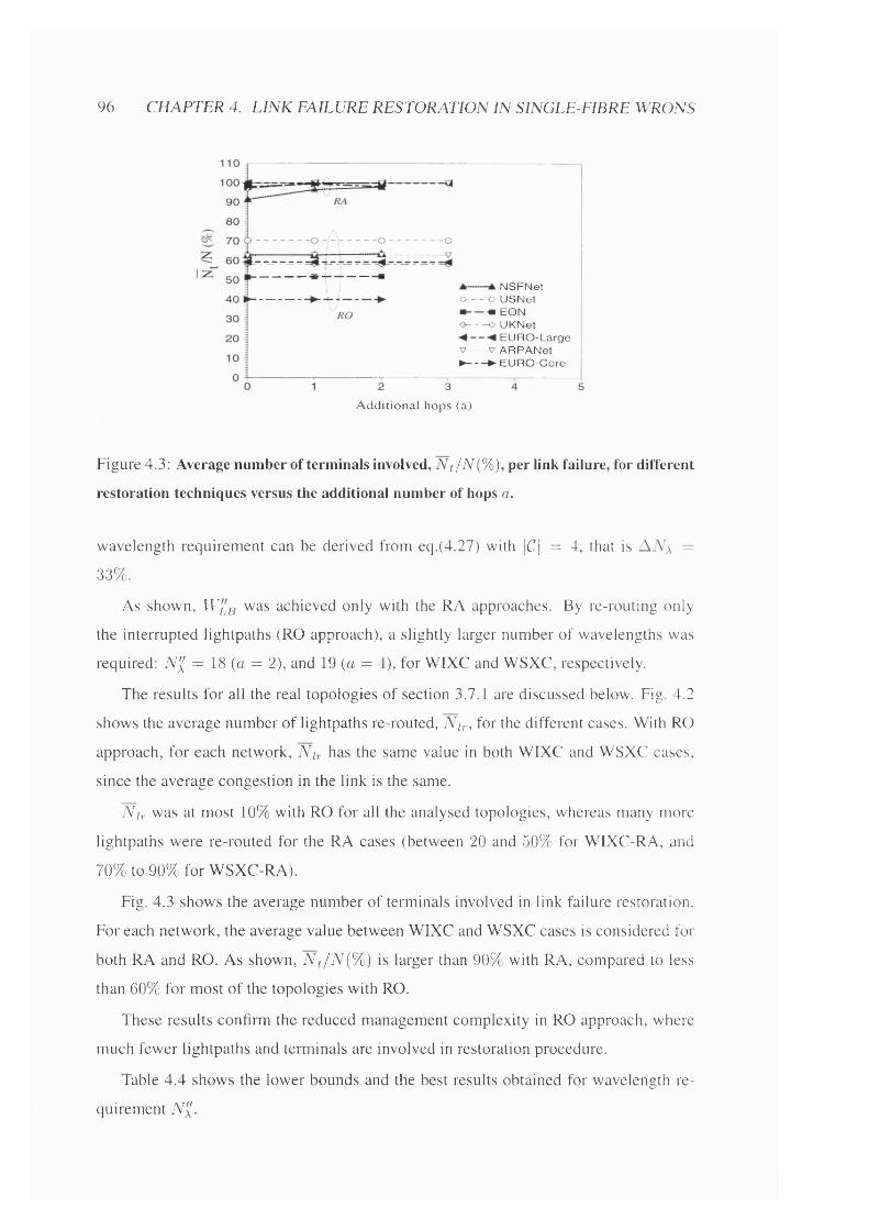
96 CHAPTER 4. LINK FAILURE RESTORATION IN SINGLE-FIBRE WRONS
N S F N et o - - o U S N et m- — « EONO O UKNet
EURO-Large V V ARPANet ►— - —► EU R O-C ore
2 3
A d dit io n a l hops (a)
Figure 4.3: Average number of terminals involved, Nt / N{%) , per link failure, for different
restoration techniques versus the additional number of hops a.
wavelength requirement can be derived from eq.(4.27) with \C\ = 4, that is =
33%.
As shown, Wj Q was achieved only with the RA approaches. By re-routing only
the interrupted lightpaths (RO approach), a slightly larger number of wavelengths was
required: N'^ = 18 (a = 2), and 19 (a = 4), for WIXC and WSXC, respectively.
The results for all the real topologies of section 3.7.1 are discussed below. Fig. 4.2
shows the average number of lightpaths re-routed, Nir, for the different cases. With RO
approach, for each network, Nir has the same value in both WIXC and WSXC cases,
since the average congestion in the link is the same.
N ir was at most 10% with RO for all the analysed topologies, whereas many more
lightpaths were re-routed for the RA cases (between 20 and 50% for WIXC-RA, and
70% to 90% for WSXC-RA).
Fig. 4.3 shows the average number of terminals involved in link failure restoration.
For each network, the average value between WIXC and WSXC cases is considered for
both RA and RO. As shown, N t / N { % ) is larger than 90% with RA, compared to less
than 60% for most of the topologies with RO.
These results confirm the reduced management complexity in RO approach, where
much fewer lightpaths and terminals are involved in restoration procedure.
Table 4.4 shows the lower bounds and the best results obtained for wavelength re
quirement N ”.

4.6. RESULTS 91
N e t w o r k ^ D B
N -
RO approach RA approach
I L P Heuristic Heuristic
W I X C W S X C W I X C W S X C W I X C i v g x c
USNet 64 129t - - 129 156 129 141
(6) (4) (2) (2)
EURO-Large 38 77+ - - 91 95 77 82
(3) (4) (2) (3)
ARPANet 20 50 - - 50 50 50 50
(1) (2) (1) (1)
UKNet 15 27 - - 27 29 27 27
(3) (2) (1) (1)
EON 13 36 - - 36 36 36 36
(0) (0) (0) (0)
NSFNet II 17 17 - 18 19 17 17
(1) (2) (4) (1) (1)
EURO-Core 4 5 5 - 5 5 5 5
(0) (2) (2) (0) (0)
Table 4.4: Results for real network topologies. Wp^ obtained by inspection are marked
by 1 ; for each case, the smallest N ” achieved is presented, and the corresponding value of a
in restoration sets Rpj^a is in parentheses; a dash is shown where the ILP failed to give any
result after one day of computation on a UNIX workstation; The results which achieved
the lower bounds are highlighted.
98 CHAPTER 4. LIN K FAILURE RESTORATION IN SINGLE-FIBRE WRONS
For all network topologies, except for the UKNet, the limiting cut in the case with
out link failure restoration also set the partition bound with restoration. Therefore, the
number of links in the limiting cut with restoration is \C”\ = \C\ — 1, and the expected
increase in the wavelength requirement can be derived from eq.(4.27).
However, in the case of UKNet, two different cuts set the lower bound in the cases
without and with link failure restoration (see Ci and C2 in UKNet in Table 3.1). In fact,
although the central cut Ci determined Wpb {Wpb = Wc^ = 19 > Wc^ = 18), in the
case with restoration, W p^ was set by the upper cut C2 , given the many fewer links it
consists of (W'^B = = 27 > = 22).
Consider the EURO-Core topology. With the ILP formulation for the WIXC RO
approach, the lower bound WpQ = 5 was achieved with MNH paths, i.e. a = 0 in
the restoration sets 77.pj,a defined in eq.(4.2). With heuristic algorithms, N'l = 5 was
achieved for a = 2 and a = 0 with the RO and RA approaches, respectively. The results
for the NSFNet were previously discussed (see N ” in Table 4.3).
The results for the other networks are also reported in Table 4.4. The lower bound is
achieved or approached in most of the cases, even with the RO approaches, with slight
differences for EURO-Large and USNet topologies. This implies that a very limited
reduction in N ” can be achieved by re-routing all the lightpaths, at the cost of more
complex management requirement.
A negligible difference is shown between the WIXC and WSXC cases for the RA
approach. Similarly, the difference is quite limited between the RO approaches: the
reduction in N " achievable with WIXCs is about 20% for the USNet, whereas it is
less than 8% for all the other topologies. Thus, when wavelength-agility is provided
within the end-nodes, the benefit achievable with wavelength interchange in OXCs is
very small, even with restoration, as the new wavelength requirement N'l is ultimately
determined by physical topology.
Figs. 4.4-4.5 show the extra wavelengths required to provide for restoration as a
function of the number of links \C\ in the network limiting cut (see Table 3.1). The
results obtained with the RA and RO heuristic algorithms, WIXC and WSXC, for dif
ferent values of a are reported. The LB variation curve is the expected increase in the
wavelength requirement, from eq.(4.27).
Fig. 4.4(left) demonstrates that lower bound can always be achieved in the WIXC-
RA case. [In the EURO-Core (|C| = 8), the difference with respect to the LB curve
results from the granularity of N\.] For EURO-Large and USNet topologies, paths

4.6. RESULTS 99
Number of links in the limiting cut (ICI) Number of links in the limiting cut (ICI)
Figure 4.4: Extra number of wavelengths required for restoration versus the number of
links in the network limiting cut \C\. RA-approach: (left) WIXC, and (right) WSXC.
Number of links in the limiting cut (ICI) Number of links in the limiting <
Figure 4.5: Extra number of wavelengths required for restoration versus the number of
links in the network limiting cut \C\. RO-approach: (left) WIXC, and (right) WSXC.

100 CHAPTER 4. LINK FAILURE RESTORATION IN SINGLE-FIBRE WRONS
CDN'(/)OXo
512x512-
256x256 -
^ 128x128
64x64
32x32
16x16-
O O max
+17.8
6 .1%
increasing N
E U fIo -C N SF^N et. EÔN UK^'Jet A R P > N etE U riO -L U S k e te t , EON U KN et A R PA N etE LNetwork topology
Figure 4.6: OXC size for the analysed topologies. The results are for the heuristic WIXC
case with MNH path. The increase in the average OXC size in comparison to the results of
Fig. 3.3 are reported.
longer than MNH (a = 2) are required to achieve the limit.
Consider the EON. Since the limiting cut consists of |C| = 2 links, the number
of wavelengths doubles when restoration is considered. However, for the EURO-Large,
only 16.7% extra wavelengths are required, given that the limiting cut consists of |C| = 7
links, and therefore, in the case of a link failure, the interrupted lightpaths can be re
routed over the surviving 6 links. These results clearly demonstrate the importance of
\C\ on the extra wavelengths required to provide for restoration.
For the WSXC-RA approach. Fig. 4.4(right), a larger N ” is required for the EURO-
Large and USNet topologies, although the difference is very small (about 8%).
Fig. 4.5(left) shows that, when wavelength interchange is available within the OXCs,
wavelength requirements equal or very close to the bounds are achieved also by re
routing only the interrupted channels. [The only exception is for the EURO-Large, but
the difference is relatively small (about 18%).] In these cases, restoration paths longer
than MNH (a as large as 6 for the USNet) are necessary to improve sharing of restoration
wavelengths. However, in WSXC case. Fig. 4.5(right), increasing a beyond 4 does not
lead to any significant improvement for any of the analysed topologies, since it is harder
to find a unique free wavelength over longer paths. Therefore a trade-off exists between
a and wavelength continuity constraint.

4.6. RESULTS 101
N etw ork AT-
WIXC-RO
N'>
WSXC-RO
A 14 14
(2)
18
B 24 24 24
C 2 4 2 4 24
D 24 24 24
E 17 18
(3)
23
F 3 4 3 4 34
G 4 0 4 0 40
H 45 45 45
I 4 9 49 49
L 4 5 45 45
M 4 5 45 45
N 4 9 4 9 49
O 4 9 49 49
F 4 9 49 49
Table 4.5: Results for the analysed RCNs with N = 14, L = 21. The smallest achieved
is presented, and the corresponding value of a is given in parentheses only when different
from zero.
Fig. 4.6 shows the OXC sizes for the analysed topologies. Compared to the results
shown in Fig. 3.3, it can be noted that the increase in the average OXC size to provide for
restoration was about 30% for most of the networks. Where the restoration wavelengths
were better shared, such as in the well-connected EURO-Core and in the large USNet,
a smaller increase was observed (about 17%), whereas the increase was about 40% for
the sub-optimal ARPANet.
4.6.2 Randomly connected networks
The 14-node 21-link RCNs selected and analysed in section 3.7.2 were also studied
considering condition of link failure restoration.
The partition bound and results obtained with the RO heuristic algorithms are pre
sented in Table 4.5. For each network, the smallest N'l achieved is presented, and the
corresponding value of a is given in parentheses only when different from zero.
Similar to the UKNet, in the cases of topologies C and D, two different cuts deter
mined WpB and W pB‘ However, for all the other networks, the same cut set the partition

102 CHAPTER 4. LINK FAILURE RESTORATION IN SINGLE-FIBRE WRONS
bound in both cases without and with link failure restoration.
As shown, the networks requiring the smallest Nx to provide active lightpaths (A,
B, C, D, E), due to the large number of links \C\ in the limiting cut (see Table 3.5), are
also the ones to have the smallest increase in the wavelength requirement to provide for
restoration. Therefore, these results show that an optimised topology for active lightpath
allocation (i.e. large \C\) also results in increased robustness against link failure.
4.7 Conclusions
The requirements given by single link failure restoration in WRONs were analysed. Two
possible approaches were considered and compared in terms of the trade-off between
the extra wavelengths required for restoration and the number of lightpaths re-routed
and nodes involved. It was shown that the reallocation of only the interrupted lightpaths
results in a slightly larger wavelength requirement compared to the case where all the
lightpaths are re-assigned within the resultant network. However, fewer lightpaths and
nodes are involved, simplifying network management complexity.
The results demonstrated that the increase in wavelength requirement is strongly
influenced by the physical topology, and that wavelength interchange within the OXCs
results in limited improvement.
It was shown that a large number of links in the limiting cuts enables optimal alloca
tion of both active and restoration lightpaths, resulting in optimised network topology.

Chapter 5
WDM transmission in single-fibre
WRONs
5.1 Introduction
The feasibility of WRONs depends not only on the number of wavelengths required to
satisfy a given traffic demand, but also on the ability to propagate the lightpaths through
cascades of WDM optical amplifiers and OXCs, without complex network control.
As discussed in section 2.3.4, the theoretical study of WDM transmission has al
ways been limited to point-to-point analyses, without considering network condition of
lightpath add/drop, key in determining network transmission performances.
In these analyses, the wavelength-dependent gain characteristic of existing EDFAs
has been recognised as one of the limiting factors in WDM transmission, leading to
different performances for the propagating channels, according to their position within
the EDFA bandwidth. This effect is referred to as gain-peaking [86] [87]. Several ap
proaches have recently been studied to improve the EDFA gain flatness [88]. However,
further development is necessary for the design of large WRONs.
The judicious assignment to the lightpaths of absolute-wavelengths within the EDFA
bandwidth can be used to minimise gain-peaking effect, and improve transmission per
formance. However, although several near-optimal lightpath allocation algorithms have
recently been proposed [5][59][65][62], this issue has not been considered to date.
In the first part of this chapter, a simple algorithm for the assignment of absolute-
wavelengths to the lightpaths is proposed to compensate for the gain non-uniformities
in the EDFA cascades under add/drop conditions [112]. The algorithm is used in com-
103

104 CHAPTER 5. WDM TRANSMISSION IN SINGLE-FIBRE WRONS
different ^ wavelengths
OXC
end-node
Figure 5.1: Example of WRON with extra constraint (C4).
bination with the heuristic lightpath allocation algorithm of section 3.6 which defines
the add/drop requirements in the network OXCs. The WDM channel propagation is
studied by considering physical limitations imposed by gain-peaking, four-wave mix
ing (FWM), and the accumulation of amplifier spontaneous emission (ASE).
However, with this technique, the design of EDFAs requires a constant number of
channels travelling in each link, which is, therefore, applicable only to static traffic
conditions. An alternative approach is necessary when variations in link’s congestion
occur, for example as a consequence of link failure restoration, because of the large
power excursions at the input of the WDM amplifiers [89].
Two possible solutions have recently been proposed (see section 2.3.4). However,
the increased management complexity and limited dynamic range of these may limit
their applications to small-size networks.
As a solution, a new WDM optical amplifier configuration, based on EDFAs, gain
equalising filters, and arrays of integrated waveguide amplifiers is proposed, and a net
work example is analysed under critical condition of link failure restoration [113].
5.2 Network model and lightpath allocation algorithm
In the analysis of WDM transmission, it is important to distinguish between the wavelength-
numbers assigned to the lightpaths (for example, within the algorithms of sections 3.6
and 4.5), and their absolute-wavelengths within the EDFA bandwidth. There is, of
course, a one-to-one correspondence between them, and it is the scope of the first part
of this chapter to proposes an accurate algorithm to assign absolute-wavelength to the

5.2. NETW ORK MODEL AN D LIGHTPATH ALLOCATION ALGORITHM 105
lightpaths, to minimise gain-peaking effect.
The network model is the one introduced in section 3.2. However, approximated
distances (in km) were considered for the links of the analysed networks.
In the first part of the chapter, (C3) each end-node is assumed connected to the
corresponding OXC by a single bi-directional fibre, as shown in Fig. 5.1. This extra
constraint is introduced for comparison with the results of Chapter 3. The OXCs do not
include wavelength conversion, i.e. WSXCs are considered.
A uniform traffic demand is assumed, with each end-node equipped with N —1 trans
mitters and receivers. Since the A — 1 lightpaths transmitted by each terminal are mul
tiplexed onto a unique fibre to reach the corresponding OXC, the wavelength-numbers
assigned to these lightpaths must be different (see for example node 1 in Fig. 5.1). A
similar situation appears at the receiving-end, where the A — 1 lightpaths are multi
plexed onto the same fibre to reach the destination end-node. This implies an additional
constraint on the lightpath allocation algorithm, that is, a given wavelength-number not
only can be assigned at most once on a given link, but also can be transmitted and
received at most once by any end-node [114].
The lightpath allocation is performed according to the heuristic algorithm described
in section 3.6 (see Appendix B .l), using only MNH paths (i.e. e = 0 in set Az,e defined
in eq.(3.3)). The only difference is in the allocation of the wavelength-numbers (Phase
IV), where the lightpaths, before being assigned wavelength-numbers, are ranked by de
creasing length of their path considering real distance (in km) and not number of links.
Moreover, the additional constraint (03) in the nodes is considered. The details of Phase
IV utilised here are given below.
Phase IV: wavelength-number assignment
1. Determine a list P of all node-pairs z sorted by decreasing length (in km) of their
assigned paths p*
2. Set the list of wavelength-numbers used in each link to be the empty set (Aj = 0,
Vj C X)
3. Set the list of wavelength-numbers used by each node to be the empty set (A^ = 0,
k = 1,..., N )

106 CHAPTER 5. W DM TRANSMISSION IN SINGLE-FIBRE WRONS
4. Select first z = (^i, >2 ) from P
5. Consider the path p* assigned to z
6. Determine w* as the lowest wavelength-number not used in p*, and by the nodes
zi and Z2 , w* = | U UA'^J. Assign w* to z = 1), and addjep*
w* to the set of used wavelength-numbers in all links in p*, and by the nodes
{Aj = Aj Vj G p*, and A = A;^ and A = A [j{w*})
7. If there is a further source-destination pair in P not yet considered, select it as
new z and go to 5
8. A a = I U AjIj e A
The total number of distinct wavelength-numbers assigned among all the node-pairs
determines the network wavelength requirement N \. Step 1 results in longest lightpaths
having the smallest wavelength-numbers, i.e. wavelength-number increases (from to
as the length of the corresponding lightpath decreases.
5.3 Absolute-wavelength allocation within the EDFA band
width
To optimise the allocation of wavelength-number within the EDFA bandwidth, the fol
lowing algorithm is proposed [112]: lightpaths which travel the longest distances within
the network are assigned absolute-wavelengths within the EDFA bandwidth with the
highest SNRs. This is performed by ^ ranking the lightpaths for decreasing length,
i.e. considering the wavelength-numbers from Ai to Aat , and analysing the network
optical SNR differential, as described below.
As an example, the EON topology described in section 3.7.1 was considered (see
Fig. 5.2). (0 First, the lightpaths were allocated within the network according to the al
gorithm described in section 5.2. The obtained wavelength requirement was N \ = 24,
with the longest lightpaths assigned the smallest wavelength-numbers. The distribution
of the congestion in the EON links is presented in Fig. 5.3. The most congested links
carry 18 channels, over a total distance of about 7000/cm. 26% of the network links
^The wavelength requirement N\ = 24 is larger than in section 3.7.1 {N\ = 18) as a result of the
additional constraint (Ci).

5.3. ABSOLUTE-WAVELENGTH ALLOCATION WITHIN THE EDFA BANDWIDTHIOI
Figure 5.2: EON network considered. The distances between the nodes are in krn. Only
the cities involved in the worst path (Lisbon - Athens) are indicated.
1 6
1 s1 4 1 3 1 2 1 1
1 o9a7654321O O ____ c C
4 6 8 1 0 1 2 1 4 1 6 1 8 2 0INlumber of c h a n n e l s
Figure 5.3: Congestion (load) distribution in the EON links.

108 CHAPTER 5. WDM TRANSMISSION IN SINGLE-FIBRE WRONS
30
20
CQ
^ 10z000
-10
4 6• • •
511.
20*21,
2^
1718 19
7 • 12 10
• •14 15 16
With FWM Without FWM
.23
a b o d e f g h i j k l m n o p q r s t u v w x
1540 1542 1544 1546 1548 1550 1552 1554Wavelength (nm)
Figure 5.4: Optical SNR for the 24 channels propagating together along 5200 km, with and
without FWM. The allocation of the wavelength-numbers within the EDFA bandwidth is
also shown (e.g. the longest lightpath with wavelength-number Ai is assigned the channel
u (absolute-wavelength 1551 mn) which has the largest value of the SNR).
(corresponding to about 15000 k m ) are loaded with 16 channels. It is worth noting that
the shape of this distribution is different from that in Fig. 3.17, since the total length in
km,, and not the normalised number of links, is reported in the Y-axis.
The lightpath Lisbon-London-Berlin-Vienna-Zagreb-Athens (see Fig. 5.2) was ob
served to be the longest one with 5200 k m , with its links being loaded with 18, 17, 17,
16 and 16 channels, respeetively. As a result the wavelength Ai was assigned to this
lightpath.
To allocate the N \ = 24 wavelength-numbers within the EDFA bandwidth, the SNR
differential was caleulated for the 24 channels propagating together along the path from
Lisbon to Athens.
The W DM transmission was analysed following ref. [86], and the design of the ED
FAs along this path was optimised for the amplification of 18 channels, with an output
power of —10 d B m per channel. The EDFAs were two-stage amplifiers pumped at
980 nm , including an optical isolator, and ASE filter to attenuate the spontaneous emis
sion around 1532 nm . The inter-amplifier span was L s = 40 Ann, and the fibre losses
0 A 4 d B / k m and 0.22 d B / km,, respectively, for the dispersion eompensating (disper

5.4. RESULTS AN D DISCUSSION 109
sion —95ps/{km .nm )) and standard single mode p s / {km.nm)) fibres used in
each span. Gain equalising filters were introduced every 4 EDFAs to reduce the spectral
gain non-uniformities.
The analysis included a semi-analytical model for FWM non-linear interaction and
a realistic spectrally-resolved numerical description of the EDFA [115].
The channels were equally spaced from 1541 to 1552.5 nm (0.5 nm channel spac
ing), and the power/channel was set to —10 dBm . Since no channels were added
and dropped, this propagation represents the worst case in terms of SNR performance.
Fig. 5.4 shows the optical SNR spectral distribution calculated at the end of the 5200 km
with and without considering FWM crosstalk. The results indicate that little impairment
was generated by FWM, the latter being efficiently suppressed through the use of the
dispersion map described in [8 6 ]. The main system limitation was gain-peaking, as the
SNR of a given channel strongly depends on its position within the EDFA bandwidth.
As shown, channels u, t, and s had the largest SNR (of about 25 dB), and a, x, and b the
smallest. Several channels had SNR below the minimum required value of 15 dB [116].
(ii) The wavelength-numbers were then assigned absolute-wavelengths within EDFA
bandwidth as follows: Ai,...,A2 4 were assigned channels a,...,x in order of decreasing
value of SNR. For example, Ai, Ag, and A3 (which were assigned to the longest light
paths) were allocated the channels u, t, and s. At the other extreme, wavelength-number
A2 4 was allocated to channel a whose SNR was the worst.
However, in real network operation, the 24 channels would not travel together over
such large distances, but lightpaths would be added and dropped, resulting in high SNR
even for lightpaths whose wavelength-numbers are allocated in the worst EDFA chan
nels, since these would be transmitted over short distances only.
5.4 Results and discussion
To test the proposed algorithm for absolute-wavelength allocation, the WDM transmis
sion was studied for EON topology with realistic conditions of lightpath add/drop.
The dropping of a lightpath at the OXCs was modelled by considering ideal filtering,
i.e. by setting to zero signal and noise powers in the corresponding channel [117] (the
resolution of the model was 0.125 nm).
When a lightpath is added, the powers of signal and ASE noise depend on the num
ber of EDFAs this lightpath has travelled through, and the congestion of the path. To

110 CHAPTER 5. W DM TRANSMISSION IN SINGLE-FIBRE WRONS
O X C Channels
dropped
Channels
added (distance, k m )
Lisbon e(0), f(0), h(0), i(0), j(0), k(0), 1(0), m(0), n(0),
0(0), p(0), q(0), r(0), s(0), t(0), u(0), v(0), w(0)
London e, f, h, j, 1, m, n,
0, p, V, w
e(0), g(640), h(0),j(0), 1(0),
m(640), o(0), v(640), w(1600), x(0)
Berlin g, h, 1, q, r, s,
t, V, W, X
b(1040), g(1480), h(840), 1(840), p(1600),
q(1040), r(1600), s(1040), t(1140), v(0)
Vienna b. e, g, k, m,
p. V
a(0), b(0), k(440), m(1880),
n(0), p(440).
Zagreb a, b, i, k, 1, 0,
q .r
c(880), d(0), k(3520), 1(2920), o(2040),
r(2840), v(1880), w(1840)
Table 5.1: Lightpaths dropped and added in the intermediate OXCs of the network’s
longest path. The bold numbers in brackets are the distances the lightpaths have travelled
within the network up to that point.
consider the worst case with respect to SNR, these powers were chosen as if all 24
lightpaths propagated together through this number of EDFAs.
Consider the propagation of the lightpaths along the network longest path (Lisbon-
London-Berlin-Vienna-Zagreb-Athens). Table 5.1 shows the lightpath add/drop config
urations in the intermediate OXCs, as derived from the combination of the lightpaths
and absolute-wavelength allocation algorithms. For example, 11 lightpaths are dropped
and 10 are added in the OXC corresponding to London.
Fig. 5.5 shows optical power spectrum and SNR at the source node (Lisbon) and at
the input of each intermediate OXC along the path. Good performances are obtained
throughout the path, with SNR greater than 19.5 dB and SNR variation below 6.2 dB.
These results guarantee acceptable performance network-wide, even for the lightpaths
assigned at the edges of the EDFA bandwidth.
Two random allocations of absolute-wavelengths were also studied considering the
same network path. Fig. 5.6 shows the optical SNR spectral distribution calculated
at the final node (Athens). [The channels at 1541.5 nm are actually dropped at Za
greb. However, they are added to the graph to show their inadequate SNR.] It is clearly
demonstrated that the allocation of the longest lightpaths (for example the ones using
wavelengths Ai and A2 ) at the extreme of the EDFA bandwidth results in unacceptable
SNR (below 15 dB) and SNR variation (larger than 15 dB).
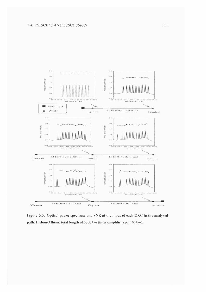
5.4. RESULTS AND DISCUSSION
lul__544 1546 1548 1550 1552 1554
Wavelength (nm)
e n t l - n o c i e
W R i s i I ^ i . s b o n
1 548 1 550 1 552 1 554Wavelength (nm)
47 E D F A s ( 1 K40Km)
alangth (nm>
I ^ o n c l o M32 E D F A s ( 1 2S()K.m)
B ei l i n15 E D F A s (bOOKin)
V ie n n a
1548 1550
14 E D F A s (5<S()K:m) 23 E D F A s ( V2()K.in)V ie n n a Z agreb
Figure 5.5: Optical power spectrum and SNR at the input of each OXC in the analysed
path, Lisbon-Athens, total length of 5200 km (inter-amplifier span 40 km).

12 CHAPTER 5. WDM TRANSMISSION IN SINGLE-FIBRE WRONS
CO 15
Inadequate SNR
1540 1542 1544 1546 1548 1550 1552 1554 Wavelength (nm)
Figure 5.6: Optical SNR spectrum at Athens for two random absolute-wavelength alloca
tions. Note that the channels at 1 5 4 1 . 5 n m are actually dropped at Zagreb.
ASEh l iA n filter
> I - VSMF DCF
EDFA notchI FILTER
#4
1 Er/YbASE Waveguides
FILTERÀI
EDFA NOTCH4 FILTER
hSMF DCF
S L Ù
EDFA
Figure 5.7: Schematic diagram of the transmission system between two OXCs.
This confirms the key role played by the absolute-wavelength allocation scheme
in compensating for EDFA gain non-uniformity, under network add/drop conditions.
However, this approach is feasible only when the configuration of the lightpaths within
the network is fixed, as the EDFA design strongly depends on the number of channels
travelling through them. Therefore this solution is optimal only in the case of static traf
fic, whereas alternative techniques are necessary every time a variation in the lightpaths
configuration, and therefore in the links congestion, occurs.
5.5. W DM AMPLIFIER MODULE FOR LARGE-SCALE RESILIENT WRONS 113
5.5 WDM amplifier module for large-scale resilient WRONs
As discussed in Chapter 4, in the presence of a link failure, the network logical con
nectivity must be fully restored by re-routing the interrupted lightpaths along alternative
physical paths. This leads to a variation in the number of channels propagating through
some of the network links, and, inevitable, large power excursions at the input of WDM
amplifiers, impairing multi-wavelength transmission [89].
If simple EDFAs are employed, acceptable performances can be achieved only by
introducing a control protection scheme. Two possible solutions, namely fast pump [90]
and link [91] control protection have recently been proposed (see section 2.3.4). How
ever, with these techniques, the maximum number of channels which can be added and
dropped on a link has not been determined, and also an increased management com
plexity is expected.
In this work, an alternative approach, based on a new WDM optical amplifier con
figuration, was proposed and studied [113].
The amplifier configuration consisted of EDFAs, optical filters, and arrays of inte
grated waveguide amplifiers, as shown in Fig. 5.7 between a pair of OXCs.
The EDFAs were pumped in both co- and counter-propagating directions and in
cluded an optical isolator [86]. The ASE filter was used to eliminate ASE power gener
ated below 1543 nm, and the notch filter, centred at 1550.5 n m (with 3 dB bandwidth of
3 nm, and peak attenuation of -1 .2 dB), was introduced to improve EDFA gain flatness.
The inter-amplifier span considered was Ls = 45 km. As discussed in section 5.3,
dispersion management was applied in each span to reduce FWM non-linear interaction.
A power level compensator was periodically introduced every four amplifier stages.
It consisted of an array of E r /Y h co-doped silica waveguide amplifiers placed in paral
lel between a pair of concave planar gratings acting, respectively, as a demultiplexer and
multiplexer. These arrays were successfully fabricated and used in fibre transmission ex
periments [118], and modelled by using finite-element code [119] [120]. A waveguide
length of 10 cm was considered, with input pump power for each amplifier of 25 m W
at 980 nm [120]. The number of waveguides in each module must be at least equal to
the maximum number of channels carried by the link where the module is introduced,
considering the network configurations deriving from all possible link failure scenar
ios. The deployment of more waveguides could be considered to guarantee network
scalability and flexibility. Note that an array of waveguides was also inserted in the

114 CHAPTER 5. W DM TRANSMISSION IN SINGLE-FIBRE WRONS
amplification stage within each OXC (not shown in Fig. 5.7).
The grating demultiplexer and multiplexer were considered with rectangular band
width of 0.5 nm , centred at signal wavelengths, and with insertion loss of 2 dB.
The total noise in the system was modelled as the sum of ASE generated along the
amplifier cascade, and grating-induced crosstalk, including the filtering effect of the
input/output gratings [103]. The crosstalk generated in the grating demultiplexer (m-
terband crosstalk) was computed at each channel by considering the two neighbouring
channels and assuming an isolation of —35dB [117]. The intraband crosstalk, gener
ated by other channels at the same wavelength (from other fibres) during the mux/demux
process in the OXCs, was neglected. In the analysis carried out in this work, this as
sumption is acceptable because the interband crosstalk is expected to be much larger
than the intraband crosstalk, as each channel travels many more waveguides than OXCs.
During the transmission, the WDM channels were amplified together in EDFAs,
mostly to compensate for span losses, and separately by waveguide amplifiers to reduce
non-uniformities in the EDFA gain spectrum: signals with high power experienced less
gain than signals at low power levels. This simple mechanism provided the desired self
regulating properties necessary to reduce power excursion in EDFA, in the case of link
failure restoration.
This WDM amplifier configuration removed the need for the absolute-wavelength
allocation algorithm described in section 5.3, since all the lightpaths were expected to
experience limited power excursion, and therefore similar SNR at destination. Therefore
the wavelength-numbers Ai, A2 ,... could be allocated absolute-wavelengths in order,
starting from 1545 n m every 0.5 nm, as discussed in section 5.7.
Therefore, no distinction was considered here between wavelength-numbers and
absolute-wavelengths, both referred simply to as wavelengths.
The adding and dropping of a channel were modelled as in section 5.4.
5.6 Network model and lightpath allocation algorithm
The network model is the one discussed in section 3.2, with each end-node directly con
nected to the corresponding OXC, that is, the constraint (C5) introduced in section 5.2
is not considered here. The OXCs are considered reconfigurable without wavelength in
terchange functionality, that is WSXCs are assumed, and wavelength-agility is provided
within the end-nodes (see section 4.2).

5.6. NETW ORK MODEL AN D LIGHTPATH ALLOCATION ALGORITHM 115
In the normal operation mode, all the node-pairs were assigned lightpaths according
to the heuristic algorithm described in section 3.6 (see Appendix B .l), with only MNH
paths, to limit length of the lightpaths.
In the restoration mode, each single link failure was analysed in turn, and only the
interrupted lightpaths were reallocated. The WSXC RO approach algorithm described
in section 4.5 (see Appendix B.2) was modified as follows: among all possible restora
tion paths, the shortest one (in km), and not the one requiring the lowest restoration
wavelength, was selected. This was crucial in guaranteeing acceptable network perfor
mances, as it allowed to limit the distances travelled by restoration lightpaths, even at
the cost of a few extra wavelengths. The differences with respect to the WSXC RO
approach of Appendix B.2 are as follows:
Restoration lightpaths assignment
1. Set AJt = Ak, \/k e A
2. Randomly select first link j ^ A (supposed faulty)
3. Set Ak = A^, \/k Ç: A
4. For each node-pair z whose active path p* is using link j , determine the shortest
restoration path r* (in km)
5. Determine a list, P, of all node-pairs z considered in step 4 sorted by decreasing
length of their restoration paths r*
6. Select first z from P
7. Delete active lightpath (p*,w*) previously assigned to z: delete w* from the set of
used wavelengths in all the links in p* (A^ = A \ {w*}, VA; G p*)
8. If there is a further node-pair in P not yet considered select it as new z and go to
7
9. Select first z from P
10. Consider restoration path r* and determine A* as the lowest wavelength not used
in r * (A* = I U A^|. Assign path r * and wavelength A* to node pair z ,p* ,w* jkEr*
1), and add A* to the set of used wavelengths in all links in r* (A^ = A t
VA: G r*)

116 CHAPTER 5. W DM TRANSMISSION IN SINGLE-FIBRE WRONS
Ann Arbour 630
Seattle 20702565 31^C f ^ p a ig n P ittsb i/g h1125 Salt Lake
City 945945 945
630 9451710 ' 315630675 945 1801260 ,
San D iego 1935 1935C ollege ParkHouston
1125Atlanta
Figure 5.8: Schematic diagram of the NSF network. Only the cities involved in the two
worst paths l\ (San Diego - Atlanta), I2 (Seattle - College Park) are indicated.
11. If there is a further node-pair in P not yet considered select it as new z and go to
10
12. Determine the new wavelength requirement = I (J A^|k e A
13. If set Ar;' = N i
14. If there is a further link not yet considered select it as new j and go to 3
5.7 Simulation results
In this analysis, the NSFNet topology described in section 3.7.1 was studied consider
ing approximated distances (in km) for the links (see Fig. 5.8). In the normal operation
mode an optimal wavelength requirement Nx = 13 was obtained (see section 3.7.1).
When single link failure restoration was considered, the wavelength requirement in
creased to N'^ = 23. This is slightly larger than the value obtained in section 4.6 for the
WSXC case with MNH restoration paths {N'x = 21), because of the different algorithm
utilised (shortest restoration path assigned to each interrupted node-pair), as discussed
in section 5.6.
As previously discussed, the wavelength-numbers Ai,...,A2 s were assigned absolute-
wavelengths within the EDFA bandwidth in order, from the first channel-slot at 1545 n m
to the last at 1556 nm.
The proposed WDM amplifier configuration was tested by analysing the network
performances in terms of the optical SNR, as in section 5.4. Two critical network paths

5.7. SIMULATION RESULTS 117
O X C Channels
dropped
Channels
added (distance, km )
San Diego 1(0), 2(3060), 5(0), 6(3870),
8(1935), 10(0)
Seattle 1,2, 6, 8 1(0), 2(0), 3(1125), 4(1125), 6(2070)
7(1125), 8(0), 9(0), 11(0)
Champaign 3, 5, 6 ,7 , 8, 10, 11 3(945), 5(945), 6(0), 7(0), 8(945),
10(0), 11(0), 12(0), 13(0)
Pittsburgh 1,2, 3, 4, 5, 6 ,7 ,
8 ,9 , 11, 12, 13
1(0), 2(1305), 3(0), 4(360)
5(0), 6(360), 7(0)
Table 5.2: Lightpaths dropped and added in the intermediate OXCs of path (San Diego
- Atlanta) for the normal operation mode.
were identified, considering estimated length, number of WDM channels in each link,
and variation in the congestion induced by link failure restoration procedures.
The first was the longest path which could be used within the network: San Diego
— Seattle — Champaign — Pittsburgh — Atlanta (/i in Fig. 5.8). It was 6165/cm-long
and represented the restoration lightpath between San Diego and Atlanta in the case of
failure in link Houston — Atlanta. The number of channels per link was 6, 11, 13 and 8,
respectively, during the normal operation mode and 7, 15, 20 and 13 under link failure
restoration.
The second was the path with the largest excursion in the number of WDM channels:
Seattle — San Diego — Houston - College Park {I2 in Fig. 5.8). It was 5580A:m-long
and consisted of heavily loaded links (6, 13, and 13 channels respectively, in the normal
operation mode). By re-routing the lightpaths passing via the link Salt Lake City — Ann
Arbour, assumed faulty, the number of channels in the links became, respectively, 6, 17,
and 23.
Tables 5.2 and 5.3 show the list of lightpaths added and dropped at the OXCs of
path li during, respectively, the normal operation mode and link failure restoration. The
distances that the channels have travelled before being added are given in brackets.
Fig. 5.9 shows optical power spectrum and SNR obtained along this path, in the
normal operation mode. The power difference of up to 5 dB among the WDM signals
at the input of each link (top row in the figure) was reduced to less than 2 dB at the end of
each link (bottom row), by the self-regulating properties of the amplifier configuration,
which provided an automatic gain control mechanism. Moreover, the SNR was kept

18 CHAPTER 5. WDM TRANSMISSION IN SINGLE-FIBRE WRONS
O X C Channels
dropped
Channels
added (distance, krn)
San Diego 1(0), 5(0), 6(3870),
8(1935), 10(0), 14(0), 20(0)
Seattle 1 ,6 .8 1(0), 2(0), 3(1125), 4(1125), 6(2070)
7(1125), 8(0), 9(0), 11(0), 16(1125), 17(0)
Champaign 3, 5, 6, 7, 8. 10, 11 3(945), 5(945), 6(0), 7(0), 8(945), 10(0), 11(0),
12(0), 13(0), 15(1620), 18(945), 19(1620)
Pittsburgh I.2 , 3 .4 . 5. 6. 8. 9.
II, 12, 13, 14, 15
2(1305), 4(360), 5(0), 6(360), 9(540),
14(3150), 15(2475)
Table 5.3: Lightpaths dropped and added in the intermediate OXCs of path /i (San Diego
- Atlanta) for the restoration mode.
i.AO - -S43 1547 1551 1555 1543 1547 1551 1555
Wavelength [nm]
Seattle Champaign Pittsburgh Atlanta38 stages 57 stages 21 stages 21 stages
(1710 Km) (2565 Km) (945 Km) (945 Km)
Wavelength [nm
Figure 5.9: Optical power spectrum and SNR at the input and output of each after each
OXC in the normal operation mode for path li (□ SNR, O Total Noise Power (ASE and
Crosstalk), • ASE Power).
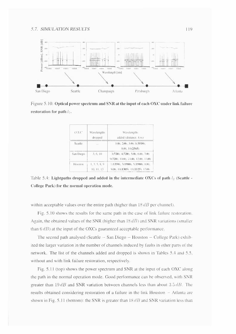
5.7. SIMULATION RESULTS
Wavelength [nm]
♦San Diego Seattle Champaign Pittsburgh Atlanta
Figure 5.10: Optical power spectrum and SNR at the input of each OXC under link failure
restoration for path l\.
O A C Wavelengths
dropped
Wavelengths
added (distance, k m)
Seattle 1(0), 2(0), 3(0). 6(3510),
8(0), 10(2565)
San Diego 3,6 , 10 3(720), 4(720), 5(0), 6(0), 7(0)
9(720), 10(0), 11(0), 12(0). 13(0)
Houston 1 3 3 8 ,9
10, 11, 13
1(1350), 3(1980), 5(1980), 8(0).
9(0), 10(1305), 11(1125). 13(0)
Table 5.4: Lightpaths dropped and added in the intermediate OXCs of path I2 (Seattle -
College Park) for the normal operation mode.
within acceptable values over the entire path (higher than 18 d B per channel).
Fig. 5.10 shows the results for the same path in the case of link failure restoration.
Again, the obtained values of the SNR (higher than 18 dB) and SNR variations (smaller
than 6 d B ) at the input of the OXCs guaranteed acceptable performance.
The second path analysed (Seattle - San Diego - Houston — College Park) exhib
ited the larger variation in the number of channels induced by faults in other parts of the
network. The list of the channels added and dropped is shown in Tables 5.4 and 5.5,
without and with link failure restoration, respectively.
Fig. 5.11 (top) shows the power spectrum and SNR at the input of each OXC along
the path in the normal operation mode. Good performance can be observed, with SNR
greater than 19 d B and SNR variation between channels less than about 3 .o d B . The
results obtained considering restoration of a failure in the link Houston — Atlanta are
shown in Fig. 5.11 (bottom): the SNR is greater than 18 d B and SNR variation less than

120 CHAPTER 5. WDM TRANSMISSION IN SINGLE-FIBRE WRONS
O X C Wavelengths
dropped
Wavelengths
added (distance, km)
Seattle 1(0), 2(0), 3(0), 6(3510),
8(0), 10(2565)
San Diego 3,6 , 10 3(720), 4(720), 5(0), 6(0), 7(0)
9(720), 10(0), 11(0), 12(0), 13(0)
16(0), 17(720), 18(720), 21(720)
Houston 1,3, 5. 8 ,9
10, 11, 13
1(1350), 3(1980), 5(1980), 8(0),
9(0), 10(1305), 11(1125), 13(0)
14(1305), 15(0), 19(1305),
20(1980), 22(1980), 23(1980),
Table 5.5: Lightpaths dropped and added in the intermediate OXCs of path L (Seattle
College Park) for the restoration mode.
E
i - 5 4 3 1 5 4 7 1 5 5 1
Seattle > ■ #- 38 stages
1 5 4 3 1 6 4 7 1 5 5 1 1 5 6 5
\ Wavelength [nm] \
J San Diego j Houston^ ____________43 stages ^ __________43 stages
College Park
(1710 Km) (1935 Km) (1935 Km)
>-41 5 5 1 1 5 5 5 1 5 5 1 1 5 5 5
Wavelength [nm]
Figure 5.11: Optical power spectrum and SNR at the input of each OXC without (top)
and with (bottom) link failures for path L.

5.8. CONCLUSIONS 121
about 5.9 dB.
It is important to note that this approach does not require any protection mechanism
in the EDFAs, avoiding the need for a fast network control. The periodic insertion of
power level compensators allows to use the same EDFA design throughout the network.
Although the gain in the EDFAs strongly depends on the number of input channels, the
signal power excursions are automatically compressed by the saturating behaviour of
the waveguide amplifiers in the power level compensators.
Finally, it is worth noting that the performance of this WDM amplifier configuration
strongly relies on the performance of the grating mux/demux at each array of waveg
uides. The numerical calculation showed that the crosstalk generated in the gratings
limits the SNR, as it accumulates along the paths. Therefore gratings with very high
crosstalk isolation (of the order of —35 dB, or even more) are crucial in the design of
large-scale WRONs.
5.8 Conclusions
In this chapter, WDM transmission was analysed in combination with routing and wave
length allocation, to include condition of lightpath add/drop, key in determining network
transmission performances.
A simple algorithm for the allocation of the absolute-wavelengths within the EDFA
bandwidth was proposed to compensate for gain non-uniformities in EDFA cascades
under lightpath add/drop condition. The results showed that absolute-wavelength allo
cation is crucial to ensure acceptable performances throughout the network. However,
the use of simple EDFAs is feasible only in the case of static traffic, whereas a differ
ent approach is required when links’ congestion is expected to change significantly, for
example in the case of link failure restoration
A new WDM optical amplifier cascade, based on EDFAs, gain equalising filters,
and arrays of integrated waveguide amplifiers was proposed and a network example
studied under critical condition of link failure restoration. The results demonstrated
that the self-regulating properties of this WDM amplifier configuration ensure network
robustness against link failure without the need for a complex network control.


Chapter 6
Design of multi-fibre WRONs
6.1 Introduction
The analyses of Chapters 3, 4 and 5 assumed single-fibre link networks, with each fibre
carrying as many wavelengths as required to satisfy the traffic demand. The study of
section 3.8 showed that the availability of multiple fibres per link allows to limit the
number of channels per fibre.
In real WRON applications, the maximum number of wavelengths (wavelength mul
tiplicity), W , carried by each fibre may be limited by technological constraints, such as
EDFA bandwidth, and non-linear limitations in WDM transmission. As discussed in
section 2.3.5, the recent trend in point-to-point systems is towards larger values of W ,
to reduce transmission cost and solve the problem of fibre exhaust faced by network
operators world-wide.
In the process of planning a network, the choice of W is critically governed by
physical topology, fibre availability, and actual and forecast traffic demand. The choice
of a large W may be justified if the initially deployed excess capacity is accessible for
future traffic growth.
Another key question concerns the potential benefit of wavelength interchange within
the OXCs. The results of Chapters 3 and 4 showed that little benefit is achievable in the
case without link failure restoration, and also with restoration when wavelength-agility
is available within the end-nodes. However, a static, uniform, traffic demand was as
sumed, which is not the case when network evolution is to be considered.
In this chapter, capacity requirements and resource utilisation for WIXC and WSXC
networks are compared under different traffic conditions, including provisioning of ba-
123
124 CHAPTER 6. DESIGN OF MULTI-FIBRE WRONS
sic demand, restoration, and growth [121]. The maximum number of wavelengths per
fibre, W , is explicitly introduced as a parameter, resulting in multiple fibres allocated
within the network.
A new ILP formulation is proposed for the exact solution of the routing and wave
length allocation problem in multi-fibre networks. The ILP allows to study and compare
different restoration strategies, for WIXC and WSXC networks, the latter with and with
out wavelength-agility in the terminals.
Lower bounds on the minimum number of fibres required are discussed, and new
heuristic algorithms proposed.
Numerous network topologies are considered, to evaluate the influence of physical
connectivity on restoration capacity [ 1 2 2 ].
Network evolution is analysed to study the importance of wavelength conversion as
a function of network size and connectivity, traffic demand, and wavelength multiplicity
IV [121].
6.2 Network model and restoration strategies
The network model considered here is the same of section 3.2.
In the first part of this analysis, a uniform traffic demand is assumed. The study of
network traffic growth will be presented in section 6.7.
The network end-nodes are equipped with the sufficient number of transmitters and
receivers to provide and restore the initial uniform traffic demand, and also to allocate
further growth, that is, no blocking occurs because of lack of transceivers in the termi
nals. Both reconfigurable WIXC and WSXC configurations are considered as optical
cross-connects. In the WSXC case, both conditions with and without wavelength-agility
in the end-nodes are analysed.
It is assumed that (C4) each link consists of a bundle carrying at least one fibre: if
f j defines the number of fibres in link j G A , then f j > l,V j G yl.
Each fibre, as well as its associated in-line equipment (such as optical amplifiers and
WDM multiplexers), are limited to carry up to W wavelengths, where W is referred to
as wavelength multiplicity [1 2 1 ].
Since the maximum number of wavelengths per fibre W is fixed, multiple fibres may
be required in the network links to satisfy the traffic requirement. Given the high cost of
installing and managing the fibres, the aim is to satisfy the traffic demand minimising

6.2. NETW ORK MODEL AN D RESTORATION STRATEGIES 125
oxccn d -n o d e
— a c tiv e lig h tp a th (p ) Cresto ra tio n lig h tp a th (r)
Figure 6.1: Example of edge-disjoint path restoration (with and without reserved capac
ity).
the total number of fibres, that is
min F t = XI f j j e A
As in section 4.2, all the network end-nodes and OXCs are assumed directly con
nected to a centralised network management system (NMS). In the case of link failure,
the NMS orders new lightpath allocation to the node-pairs, and new input-output routing
functions performed by the OXCs. A larger Ft is expected to provide for link failure
restoration.
In this analysis, it is assumed that only the interrupted lightpaths are re-routed along
alternative physical paths, whereas the surviving traffic is maintained (i.e. RO approach
according to the definition of section 4.2). Different restoration strategies can be imple
mented, namely edge-disjoint path restoration with and without reserved capacity, path
restoration, and link restoration. In this work they were compared in terms of the extra
number of fibres required to provide for restoration.
6.2.1 Edge-disjoint path restoration with reserved capacity
Each node-pair is assigned an active lightpath and a edge-disjoint restoration lightpath
(see p i, r i and p 2 , V2 in Fig. 6.1). For each node-pair, the capacity required for both the
lightpaths is reserved, determining 1 0 0 % capacity redundancy.^
If any of the links in the active lightpath fails, the lightpath is always re-routed along
the same pre-assigned restoration lightpath. This is an end-to-end restoration process,
since both source and destination nodes are involved. Not only the capacity in the fibres,
but also the OXC ports are reserved along the restoration lightpaths, therefore, when a
^This is similar to the 1+1 protection scheme in SONET/SDH ring [73].

126 CHAPTER 6. DESIGN OF MULTI-FIBRE WRONS
(a) (b) (c)
Figure 6.2: Example of path restoration.
failure occurs, the switching is performed only in the OXCs connected to the source and
destination terminals (see arrows in Fig. 6.1), whereas no switching is performed in the
OXCs along the restoration lightpaths.
Since both active and restoration lightpaths are reserved, there is no sharing of
restoration capacity between edge-disjoint active lightpaths. For example, in link C-
D in Fig. 6.1, the capacity required for both restoration lightpaths ri and r 2 is reserved
separately, and it is not shared between the edge-disjoint active lightpaths pi and p 2 .
This restoration scheme is therefore characterised by: (i) for all the node-pairs, ac
tive and restoration lightpaths do not share any links, (ii) two edge-disjoint active light
paths do not share capacity in their restoration lightpaths, and (iii) this is an end-to-end
process.
6.2.2 Edge-disjoint path restoration
Similar to the approach in section 6.2.1, active and restoration lightpaths are edge-
disjoint. However, in this case, the restoration capacity is not reserved, but can be
shared for restoration of edge-disjoint lightpaths, by performing switching also in the
OXCs along the restoration path. Moreover, similarly to the approach in section 6.2.1,
this is an end-to-end process.
In Fig. 6 .1, therefore, the two restoration lightpaths r i and r 2 can share the same
wavelength-slot in the link C-D in the WIXCs case, and also in the WSXCs case if the
same wavelength is assigned to both restoration lightpaths. [The lightpaths pi and p 2
cannot be interrupted simultaneously, as single link failure is assumed.]
The main feature of this restoration strategy is that: (i) for all the node-pairs, the
active and restoration paths do not share any links, and (ii) this is an end-to-end process.

6 2 . NETW ORK MODEL AN D RESTORATION STRATEGIES 127
(a) (b) (0
Figure 6.3: Example of link restoration.
6.2.3 Path restoration
With this approach, for each interrupted lightpath during a link failure, any path from
source to destination which is not using the failed link may be considered for restoration.
Therefore, the restoration lightpath may be different according to which link has failed
in the active lightpath, as shown in Fig. 6.2.
This approach is characterised by: (i) for each node-pair, active and restoration paths
may share some links, and (ii) this is an end-to-end process.
However, in particular cases, source and destination nodes may not be involved (for
example in Fig. 6.2(b) for WSXCs with fixed-wavelength transmitters/receivers, i.e.
fixed restoration wavelengths, and WIXCs), resulting in a localised restoration.
6.2.4 Link restoration
In the case of a link failure, the restoration is achieved by re-routing the interrupted
lightpath around the failed link {circumventing the failed link), whilst maintaining the
rest of the path (see Fig. 6.3).
For the cases of WSXCs with fixed-wavelength transceivers and WIXCs, this pro
cess does not involved the source and destination nodes, but only the OXCs around the
failed link. Therefore, in these cases, link restoration is not an end-to-end strategy, but is
resolved locally. However, in the WSXC case, wavelength-agility can be exploited only
by involving the source and destination end-nodes, resulting in an end-to-end process.
If the failed link carries more than one lightpath (Fig 6.3(a)), these can be re-routed
together over one circumventing path only (Fig 6.3(b)), or over multiple circumventing
paths (Fig 6.3(c)). Only the second approach will be considered in this work, as it is
expected to better share restoration fibres around each link, and therefore reduce the
total extra capacity required for restoration.

128 CHAPTER 6. DESIGN OF MULTI-FIBRE WRONS
Restoration
strategy WIXC
WSXC
wavelength-agility fixed-wavelength
Edge-disjoint
path restoration
with reserved capacity
RI RSA RSF
Edge-disjoint
path restoration DI DSA DSF
Path restoration PI PSA PSF
Link restoration LI LSA LSF
Table 6.1: Network configurations identified. The configurations analysed are highlighted.
With this approach, (i) for all the node-pairs, active and restoration lightpaths do
share links^, and (ii) this may be a localised process.
According to the restoration approach, and capabilities provided within OXCs and ter
minals, several configurations can be identified, as shown in Table 6.1. In this analysis,
only the configurations highlighted will be studied and compared.
Edge-disjoint path restoration with reserved capacity is not studied here, as it re
sults in restoration capacity requirements similar to SONET/SDH rings, and hence does
not lead to the capacity saving expected by performing optical restoration in mesh
WRONs [8 ]. Link restoration with WSXC and wavelength-agility in the end-nodes
(LSA in Table 6.1) is not considered, as it does not provide a localised solution.
6.3 Lightpath allocation: ILP formulations
In this section, an ILP formulation is developed for the exact solution of the RWA prob
lem without and with link failure restoration. Both WIXC and WSXC cases, the latter
with and without wavelength-agility in the terminals, are considered with the objective
of minimising the total number of fibres Ft [1 2 2 ].
Compared to sections 3.3 and 4.3, the maximum number of wavelength per fibre
W is fixed in both WIXC and WSXC cases. Therefore w = 1 , VL is the set of
wavelengths available on each fibre. Moreover, here, only MNH paths are considered
for active lightpaths (e = 0 in eq.(3.3)), hence, hereafter the active sets will be referred
^The only exception is for adjacent node-pairs, where the active path consists of one link and is therefore disjoint from the restoration path.

6.3. LIGHTPATH ALLOCATION: ILF FORMULATIONS 129
simply to as Az-
As discussed in section 4.3, by selecting the value of a, it is possible to control the
size of the restoration sets 'Rp,j,a- However, every time a is increased by one, a large
variation in the size of the sets occurs (see average size of restoration sets b, in
Table 4.1).
Therefore the restoration sets assumed here, have a fixed size |7^p,j,6| = b,
and consist of the b shortest possible restoration paths. Respect to the sets defined
in eq.(4.2), they are constructed as follows. For a given value 6 = 1 ,2 ,...
• if 3a such that \'JZp,j,a\ = b, then the set IZpj^b = ^p,j,a,
• otherwise consider a such that \'Rpj,a\ > b > \IZpj^a-i\- Randomly select b —
paths from the set 7^pj,a \ T^p,j,a-i to form the set Q. Now set TZpj^b =
'J^p,j,a-l U Q..
For path restoration approach, the restoration paths r to form set 72. 5 are se
lected from all the paths connecting the node-pair z and not using link j . However, the
sets 7^p,j,6 are further constrained depending on the restoration strategy. For instance,
for edge-disjoint path restoration strategy it is required that p D r = 0 (see Fig. 6.1),
whereas with link restoration p O r = p \ { j} (see Fig. 6.3).
6.3.1 WIXC case
Wavelength routingThis problem assigns the minimum number of fibres within the network, subject
to there being an active lightpath for each node-pair; each lightpath requiring any one
wavelength with at most W wavelengths per fibre:
= E f jj e A
subject to
f j > 1, integer, e A (6.1)
> 0, integer, Vz G Z , Vp G A (6.2)
= I, V z e Z (6.3)peAz
E E ' ^ p V ü e p ) < w . f , , \ f j e A . (6.4)zez peAz

130 CHAPTER 6. DESIGN OF MULTI-FIBRE WRONS
Eq.(6.1) is introduced to impose the selected physical topology, that is at least one
fibre is assumed in every link of a given network, as discussed in section 6.2.
The number of variables and constraints in the formulation \s Ny = L + P.q and
Nc =: L A P.q A P + L, respectively, where P is the total number of node-pairs, and
q is the average size of the sets Therefore, Ny and are independent of W . As
shown, the complexity of this formulation is of the same order of the single-fibre case
described in section 3.3.1.
Wavelength routing and restorationThis problem assigns the minimum number of fibres within the network, sub
ject to there being an active lightpath for each node-pair and a restoration lightpath for
every active lightpath interrupted by any link failure; each lightpath requiring any one
wavelength with at most W wavelengths per fibre:
min F r ./ . = E f jjeA
subject to
fj > 1, integer, Vj G A (6.5)
> 0, integer, Vz G Z , Vp G Az (6.6)
E < .peAz
- - 1, Vz G Z (6.7)
E E G p)zez peAz
< (6.8)
> 0, integer. Vj G Vp G Fj,
Vr G Ppj^b (6.9)
E —xAP,{s{p),d{p)) V; G V p G ^ (6.10)
E E ^pA U ^ p ) +z e z peAz-.p^J^j/
+ Z Z G r) < TV./j, V; G X, V / / j G (6.11)peTj,
As previously discussed, the possible restoration paths included in the restoration sets
Tip,j,b are selected according to the restoration strategy.
In the case of edge-disjoint path restoration, for a given active path p, =
IZpji,b, Vj, y G p. In this case, the same restoration lightpath is utilised for all the
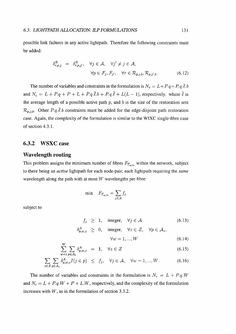
6.3. LIGHTPATH ALLOCATION: ILP FORMULATIONS 131
possible link failures in any active lightpath. Therefore the following constraints must
be added:
G A, y f ^ j e A,
\fp ^ J-j, J - j i Vr G R-p,j,bi 'T p,j',b • (6.12)
The number of variables and constraints in the formulation is Ny = L + P.q + P.qJ.b
and Nc = L 3- P.q + P + L 4- P.qI.b + P.q.I + L{L — 1), respectively, where I is
the average length of a possible active path p, and b is the size of the restoration sets
Pp,j,b- Other P.qI.b constraints must be added for the edge-disjoint path restoration
case. Again, the complexity of the formulation is similar to the WIXC single-fibre case
of section 4.3.1.
6.3.2 WSXC case
Wavelength routingThis problem assigns the minimum number of fibres within the network, subject
to there being an active lightpath for each node-pair; each lightpath requiring the same
wavelength along the path with at most W wavelengths per fibre:
m i" =jeA
subject to
f j > 1, integer, \fj e A (6.13)
^p,w,z > 0, integer, Vz G Z , Vp G A ,
\/w — 1,..., W (6.14)wE E VzEZ (6 .15)w=i peAz
E E Gp) < f j , y j e A , Vw = l,...,V K . (6.16)z^ Z pÇ.Az
The number of variables and constraints in the formulation is Ny = L L P.q.W
and Nc = L 3- P.q.W P L L .W , respectively, and the complexity of the formulation
increases with VF, as in the formulation of section 3.3.2.

132 CHAPTER 6. DESIGN OF MULTI-FIBRE WRONS
Wavelength routing and restorationThis problem assigns the minimum number of fibres within the network, subject
to there being an active lightpath for each node-pair and a restoration lightpath for ev
ery active lightpath interrupted by any link failure; each lightpath requiring the same
wavelength along the path with at most W wavelengths per fibre.
Consider the case with wavelength-agility in the terminals:
min ^ / ,jeA
subject to
f j > 1, integer, e A (6.17)
^ p , w , z > 0 , integer, Vz G Z , Vp G A ,
\/w = 1,..., W (6.18)wE E = 1. V z e Z (6.19)
w = i p e A z
< f i < V j e A = (6 .2 0 )z e z p e A z
^tX p,wj > 0. integer, Vj € X, Vp S
Vr G 7^pj,6, Vw = 1,..., W,
VA = l , . . . , l f (6.21)w
^ ^r ,X,P,w, j ~ ^p,w, { s {p) ,d{p) )^ '^7 ^ A^ Vp G Fj,A = i f ' e ' R ' p j ^ b
Vw = 1,..., W (6.22)
^p,w,zHj C p) + z e z p e A z - p ^ ^ j i
w+ E E E ^T, w, p . Ki ' I ( j e r) < f j , V i G A , Vi' A j e A ,
X=lpeTj, reTlp ji f,
Similar to the WIXC case, additional constraints must be added for edge-disjoint path
restoration:
V i G A , V i' j ^ j e A , Vp G r j , j ^ j f ,
Vr G 7 ^ p j , 6 , V w = 1, ...,I f , VA = 1, ...,1V.(6.24)
The number of variables and constraints in the formulation is, similarly to the WSXC
single-fibre case of section 4.3.1, = L F P.q.W -{-P.ql.b.W^ and A = L f P .q.W F

6.4. LIGHTPATH ALLOCATION: LOWER BOUNDS 133
P + L .W + F.q.I.b.W'^ + P.q.I.W + L{L — 1).W, respectively. Other P.qI.b.
constraints must be added for the edge-disjoint path restoration case.
When fixed-wavelength transmitters and receivers are considered, the wavelength of
any active lightpath must be maintained in the restoration lightpath. Therefore eqs.(6.21)-
(6.23) must be replaced by the following:
^T,w,P,w,j > 0, integer, Vj 6 .4, Vp e
Vr e Vw = 1,..., fK (6.25)
r,w,p,w,j ~ ^p,w,{s{p),d{p)) ^ '^P ^
Vît = 1,..., ly (6.26)
^ p , w , z H i ^ P) +zez peAz:p^Tji
+ 12 £ ’■) ^ /)- Vj e .4, y f ^ j e A ,pe^j'
\/w = 1 , . . . ,W . (6.27)
For edge-disjoint path restoration, eq.(6.24) must be replaced by the following:
^r,w,p,w,j ~ ^r,w,p,w,j'i ^ J ^ Vp G
Vr G Pp,j,b, ^p,j',b, Vu; = 1,..., VF . (6.28)
In this case, the number of variables and constraints in the formulation is Ny =
L -f P.q.W 4- P.q.I.b.W and Nc = L P P.q.W + P P L .W P P .q l .b .W P P.q.I.W P
L{L — 1).W, respectively. Other P.q.I.b.W constraints must be added for the edge-
disjoint path restoration case.
6.4 Lightpath allocation: lower hounds
Two lower bounds on the total number of fibres Ft can be defined in both cases without
and with link failure restoration. Since in calculating these no constraints on wavelength
continuity are imposed, these limits define lower bounds for the WIXC case. However,
they can also be used for comparison with the WSXC case.
Furthermore, the bounds with link failure restoration do not consider any constraints
on the restoration paths with respect to the active paths. Therefore they represent real
bounds for the path restoration case, whereas larger Ft may be required for edge-
disjoint path restoration and link restoration, because of the limitation imposed on the
restoration paths.
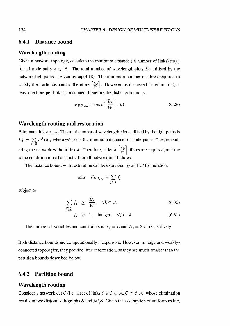
134 CHAPTER 6. DESIGN OF MULTI-FIBRE WRONS
6.4.1 Distance bound
Wavelength routingGiven a network topology, calculate the minimum distance (in number of links) m{z)
for all node-pairs z e Z . The total number of wavelength-slots L t utilised by the
network lightpaths is given by eq.(3.18). The minimum number of fibres required to
satisfy the traffic demand is therefore . However, as discussed in section 6.2, at
least one fibre per link is considered, therefore the distance bound is
Lt
W,L ) (6.29)
Wavelength routing and restorationEliminate link k e A . The total number of wavelength-slots utilised by the lightpaths is
L t = m*(z), where m^(z) is the minimum distance for node-pair z e Z , consid-
ering the network without link k. Therefore, at least fibres are required, and the
same condition must be satisfied for all network link failures.
The distance bound with restoration can be expressed by an ILP formulation:
min Fdb„/, = E / j jeA
subject to
/ j > \/k c A (6.30)j € A :j/fc
f j > 1, integer, Vj G ^ . (6.31)
The number of variables and constraints is = L and Nc = 2.L, respectively.
Both distance bounds are computationally inexpensive. However, in large and weakly-
connected topologies, they provide little information, as they are much smaller than the
partition bounds described below.
6.4.2 Partition bound
Wavelength routingConsider a network cut C (i.e. a set of links j £ C C A , C ^ (j), A ) whose elimination
results in two disjoint sub-graphs S and N \ S . Given the assumption of uniform traffic,

6.4. LIGHTPATH ALLOCATION: LOWER BOUNDS 135
the total number of lightpaths traversing the cut C is Dc = |5|.|AA\5|. Therefore, the
minimum number of fibres necessary to satisfy the traffic demand across the cut C is
DcF r = (6.32)
W
This constraint must be satisfied by all the network cuts. Therefore the partition bound
can be formulated as follows:
min = E f jjeA
subject to
E f j > V C C . 4 (6.33)jec
f j > 1, integer, V j e ^ . (6.34)
In this formulation the number of variable is quite small, Ny = L. However, the
number of constraints is very large, being determined by the number of network cuts,
which is 0 (2 ^"^ ), as discussed in section 3.4. Therefore, as the network size increases,
the computational complexity dramatically increases, and no advantages is gained com
pared to the exact ILP formulations.
In contrast to Chapters 3 and 4, no heuristic algorithm was designed for the calcu
lation of given its complexity. Moreover, here, the partition bound cannot be
derived from the network plot, as Fpb^^ is not generated by a single network cut, as
for single-fibre WRONs.
Wavelength routing and restorationWhen link failure restoration is considered, the partition bound can also be expressed
by an ILP formulation, as follows:
min FpB^i, = Y , f i jeA
subject to
Y f i > V k e C , y C c A (6,35)j e C : ^
f j > 1, integer, ^ j e A . (6.36)
Here, the number of constraints is even larger than the case without restoration, as,
for each network cut C, multiple equations must be written (one for each link in the cut).

136 CHAPTER 6. DESIGN OF MULTI-FIBRE WRONS
(b) N=8, L=13,a =0.46(a) N=5, L=7, a =0.70
Figure 6.4: Network topologies analysed with ILP formulations.
w WIXC WSXC
Ny Nc Ny Nc
1 21 38 21 38
2 21 38 35 59
3 21 38 49 80
Table 6.2: Computational complexity of ILP formulations without link failure restoration
for the 5-node, 7-link topology. Extra number of hops allowed for the active lightpaths
e = 0. W , maximum number of wavelengths per fibre; Ny, number of variables; Nc,
number of constraints.
For a given topology, in both cases without and with link failure restoration, the
largest value between F db and Fpb determines the actual lower bound on the network
fibre requirement, that is Fl b = ^^^{F d b , Fp b ).
However, as previously discussed, whilst from one side the distance bounds do not
produce significant values, from the other, the partition bounds are computationally
expensive. Therefore their utility is limited to small network topologies.
6.5 Comparison of restoration strategies
The restoration strategies described in section 6.2 were studied for two small topologies
(see Fig. 6.4), and compared in terms of the number of fibres required to provide for
restoration.
Uniform traffic demand was assumed, and the ILP formulations presented in sec
tion 6.3 were used for the calculation of Fp.
Tables 6.2-6.4 illustrate the complexity of the ILP formulations for the 5-node 7-link
network without and with link failure restoration. Consider the case without restoration

6.5. COMPARISON OF RESTORATION STRATEGIES 137
b Ny Nc
] 42 122
(+21)
2 63 143
(+42)
3 84 164
(+63)
4 105 185
(+84)
Table 6.3: Computational complexity of W I X C TLP formulation with link failure restora
tion for the 5-node, 7-link topology, b, size of restoration sets Rpj,b' The number of extra
constraints for the edge-disjoint path restoration case is in parentheses.
(Table 6.2). As discussed in section 6.3, in the WIXC case, Ny and Nc are indepen
dent of the wavelength multiplicity, whereas they increase with W in the WSXC case.
However, in both cases, the complexity of the formulation is very small.
When restoration is considered, the complexity increases with an increase in the
size of the restoration sets b, as many more paths are analysed as possible restoration
path, for each link failure in any active path. However, in the WIXC case (Table 6.3),
Ny and Nc are still relatively small, even for edge-disjoint path restoration, where extra
constraints are required (shown in parentheses).
In the WSXC case (Table 6.4), the computational complexity increases with both W
and b, and Ny and Nc may become very large, particularly in the case of wavelength-
agility. For example, for PF = 5 and 6 = 4, = 2,177 and Nc = 2, 537, and other
2,100 constraints are added for the edge-disjoint path restoration case. These values
demonstrate that ILP formulations can be applied effectively only to the analysis of
small topologies, whereas efficient heuristic algorithms are required for the analysis of
large networks.
Tables 6.5 and 6.6 show the results for the 5-node 7-link network without and with
link failure restoration, respectively. Lower bounds, and fibre requirements are reported.
In the ILP formulations, the extra number of hops allowed to the active lightpaths is
e = 0.
Consider the case without link failure restoration (Table 6.5). For each W analysed,
the distance and partition bounds assumed the same value, i.e. = Fp b^/^- As
shown, the bounds were achieved by the exact ILP solutions only for VF = 1, and 3,

138 CHAPTER 6. DESIGN OF MULTI-FIBRE WRONS
w b wavelength-agility fixed-wavelength
Ny Nc Ny Nc
1 42 122
(+21)
42 122
(+21)
]
2 63 143
(+42)
63 143
(+42)
3 84 164
(+63)
84 164
(+63)
4 105 185
(+84)
105 185
(+84)
1 119 269
(+84)
77 227
(+42)
22 203 353
(+168)
119 269
(+84)
3 287 437
(+252)
16! 311
(+126)
4 371 521
(+336)
203 353
(+168)
1 238 458
(+189)
112 332
(+63)
3
2 427 647
(+378)
175 395
(+126)
3 616 836
(+567)
238 458
(+189)
4 805 1,025
(+756)
301 521
(+252)
] 399 689
(+336)
147 437
(+84)
4
2 735 1,025
(+672)
231 521
(+168)
3 1,071 1,361
(+1.008)
315 605
(+252)
4 1407 1697
(+1,344)
399 689
(+336)
1 602 962
(+525)
182 542
(+105)
5
2 1,127 1,487
(+1,050)
287 647
(+210)
3 1,652 2,012
(+1,575)
392 752
(+315)
4 2,177 2,537
(+2,100)
497 857
(+420)
Table 6.4: Computational complexity of W S X C I L P formulation with link failure restora
tion for the 5-node, 7-link topology. W , maximum number of wavelengths per fibre; b,
size of restoration sets The number of extra constraints for the edge-disjoint path
restoration case is in parentheses.

6.5. COMPARISON OF RESTORATION STRATEGIES 139
w^T^/o
W IX C W S X C
1 13 13 13 13
2 7 7 8 8
3 7 7 7 7
Table 6.5: Results for the 5-node, 7-link topology without link failure restoration. Extra
number of hops allowed for the active lightpaths e = 0. distance bound; Fpb^^^,
partition bound; total number of fibres obtained with ILP formulations. The results
which achieved the lower bounds are highlighted.
W ^ P B ^ / r
^T^/ rDI, DSA,
PI, PSA
DSF,
PSF LI LSF
h = 1 2 6 = 1 2 3 6 = 1 2 3 6 = 1 2 3 4
1 17 21 23 21 23 21 21 26 22 22 26 22 22 22
2 9 11 12 11 13 12 11 14 12 11 14 12 12 11
3 7 9 10 9 10 9 9 11 10 9 12 10 10 10
4 7 7 7 7 9 8 8 7 7 7 9 9 8 8
5 7 7 7 7 7 7 7 7 7 7 7 7 7 7
Table 6.6: Results for the 5-node, 7-link topology with link failure restoration. FpB^/^y
distance bound; Fp b ^/ , partition bound; b, size of restoration sets R p j y , Fp^^ , total
number of fibres obtained with ILP formulations. DI, DSA, DSF, PI, PSA, PSF, LI, LSF
are defined in Table 6.1. The results which achieved the lower bounds are highlighted.

140 CHAPTER 6. DESIGN OF MULTI-FIBRE WRONS
whereas an extra fibre was required for 14 = 2. [By allowing one extra hop to the
active lightpaths (e = 1) no improvement was observed.] For each W , the same value
was achieved with both WIXCs and WSXCs, implying that wavelength conversion does
not reduce fibre requirement. As shown, for VF = 3 one fibre per link sufficed, that is
Ft^^o = L = 7. Given the condition (C4) in section 6.2, a further increase in W did not
reduce
A larger number of fibres was required to guarantee link failure restoration, as shown
in Table 6.6. In this case, for W < 3, the partition bound was larger than the distance
bound, and set the lower bound on the fibre requirements. However, for larger values of
W (W > 4), Fdb^/, = FpB^/, = L.
In the calculation of for each value of W , the ILP formulations were
analysed considering increasing value of b, until no improvements in fibre requirement
were achieved.
Different results were achieved for the different restoration strategies. Edge-disjoint
path restoration and path restoration led to the same results for any given W and b,
and therefore they are grouped in common columns in Table 6.6. [This results from
the well-connected topology considered here, although, in general, path restoration is
expected to give better sharing, and therefore reduction, of restoration capacity.] In
these cases, the lower bound was always achieved with WIXCs (DI, PI), and also with
WSXCs with wavelength-agility (DSA, PSA). Similar results were also obtained with
fixed-wavelength transceivers (DSF, PSF) by allowing larger values of b, except for
W = 4, where one extra fibre was required. This small penalty for DSF and PSF results
from the large connectivity of this topology, whereas a significant difference is expected
in the case of real networks.
When wavelength conversion was available within the OXC, the lower limits were
also achieved, in most of the cases, with link restoration (LI). A small difference was
observed only for fF = 1. Finally, LSF was observed to be the worst approach in terms
of fibre requirement, as expected, given the constraints on the restoration paths and
wavelength continuity. However, also in this case, the difference was relatively small.
These results are summarised in Fig. 6.5, where for each restoration strategy, the
smallest Ft { W ) from Tables 6.5 and 6.6 is plotted versus the wavelength multiplicity
W , for both cases without and with link failure restoration. As previously discussed, an
increase in W results in a decrease of the fibre requirement, until the minimum value
F t = L = 7 is reached. The limited differences between the restoration strategies are

6.5. COMPARISON OF RESTORATION STRATEGIES 14126
24O ' O L S F
22 ^ D S F . P S FD I . D S A . P I . P S A W I X C . W S X C20
1 e1 6
1 4
1 2
w i t h o u t876
4 '
W a v e l e n g t h m u l t i p l i c i t y . W
Figure 6.5: Fibre requirement for the 5-node, 7-link network.
Pt w/oU' WIXC WSXC
1 46 46 46 46
2 23 24 23 23
3 16 16 16 16
4 13 14 14 14
5 13 14 14 14
6 13 13 13 13
Table 6.7: Results for the 8-node, 13-link topology without link failure restoration. Extra
number of hops allowed to the active lightpaths e = 0. , distance bound; ,
partition bound; Fp^^ , total number of fibres obtained with ILP formulations. The results
which achieved the lower bounds are highlighted.
evident in this graph.
Another small randomly-generated topology was analysed (8-node 13-link network
shown in Fig. 6.4(b)). In the ILP formulations utilised to calculate Fp, the extra number
of links allowed to the active lightpaths was e = 0. Moreover, in the case with link
failure restoration, for each W , three values of b were considered {b = 1, 2, and 10),
and the smallest Fp achieved was recorded.
Consider the case without link failure restoration (Table 6.7). As shown, in most
of the cases, the partition bound was larger than the distance bound, and set the lower
bound on the fibre requirement. The limits were achieved by the exact ILP solutions
for all values of W considered, except for IT = 2. The same values were obtained for
WIXCs and WSXCs, implying that no improvements were attainable by introducing

142 CHAPTER 6. DESIGN OF MULTI-FIBRE WRONS
wPI PSA PSF DI DSA DSF LI LSF
1 53 64 65* 65* 65* 66*(> 65) 66* 66* 71 71
2 27 32 33 33 35* 35* 35* 36* 38*(> 36) 38*
3 18 23 23 25* 27* 23 26* 27* 27*(> 24) 29*
4 14 16 18*(> 17) 18* 24* 18*(> 17) 20* 24* 20* (> 18) 25*
5 13 16 16 16 21* 16 16 21* 16 23*
6 13 15 15 15 17* 15 15 18* 15 20*
7 13 15 15 15 15 15 15 16* 15 18*
8 13 13 13 13 13 13 13 13 13 13
Table 6.8: Results obtained for the 8-node, 13-link topology with link failure restoration.
Extra number of hops allowed to the active lightpaths e = 0. distance bound;
partition bound; total number of fibres obtained with ILP formulations.
When the ILP was not completed after one day of computation on a UNIX workstation,
the best results achieved was recorded and is marked with a *. Lower bounds derived
from ILP computation are in parentheses. The results which achieved the lower bounds
are highlighted.
wavelength conversion in the OXCs. As shown, for W = 6 one fibre per link sufficed,
that is Ftw / o L = 13.
A larger number of fibres was required to provide for link failure restoration (Ta
ble 6.8). As shown, the partition bound Fpb^/^ was always larger than the distance
bound Fb b ^/^, except for W = S, for which one fibre per link sufficed.
When the ILPs utilised to calculate Ft^^ were not completed after one day of com
putation on a UNIX workstation, the smallest results achieved at that point were retained
(marked with a star in Table 6.8). This was observed to be particularly critical in the
fixed-wavelength case, where longer time was required to achieve the optimal solution.
However, confidence can be placed in the accuracy of these results, since these val
ues, once reached, remained constant for many hours of calculation.
In some cases, for a given restoration strategy, it was possible to derive, during
the ILP computation,^ a lower bound on Ft^^ larger than Fp b ^^^. These limits were
recorded and are shown in parentheses in Table 6.8 to verify the accuracy of the sub-
optimal result. For example, for W = 4, although the partition bound is Fpp w / r 16,
^This was achieved by specifying uppercutoff values to the ILP, to “cut-off” large sets of nodes in the
branch&bound tree whose fractional values were larger than the supplied cutoff value [99].
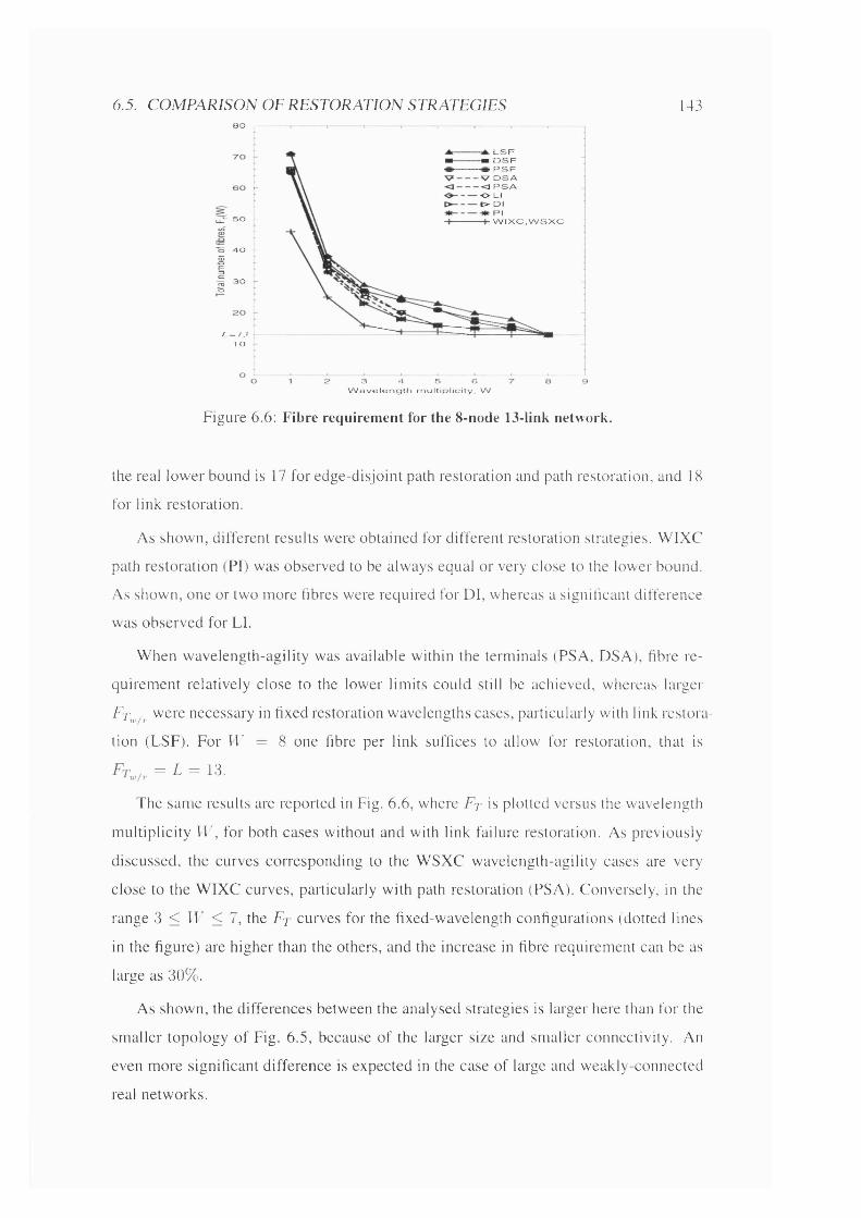
6.5. CO M P A R ISO N OF R E S T O R A T IO N STRATEGIES80
143
llT 50
S 40
I -/ . = y .î
1 o
1 _ S F - K D S F
P S F V D S A < 1 P S A O LI O - DI
W I X C , W S X C
2 3 4 5 6W a v e l e n g t h m u l t i p l i c i t y , W
Figure 6.6: Fibre requirement for the 8-node 13-link network.
the real lower bound is 17 for edge-disjoint path restoration and path restoration, and 18
for link restoration.
As shown, different results were obtained for different restoration strategies. WIXC
path restoration (PI) was observed to be always equal or very close to the lower bound.
As shown, one or two more fibres were required for DI, whereas a significant difference
was observed for LI.
When wavelength-agility was available within the terminals (PSA, DSA), fibre re
quirement relatively close to the lower limits could still be achieved, whereas larger
Ci\^/r were necessary in fixed restoration wavelengths cases, particularly with link restora
tion (LSF). For ]V = 8 one fibre per link suffices to allow for restoration, that is
= L = 13.
The same results are reported in Fig. 6.6, where F r is plotted versus the wavelength
multiplicity W , for both cases without and with link failure restoration. As previously
discussed, the curves corresponding to the WSXC wavelength-agility cases are very
close to the WIXC curves, particularly with path restoration (PSA). Conversely, in the
range 3 < W < 7, the F r curves for the fixed-wavelength configurations (dotted lines
in the figure) are higher than the others, and the increase in fibre requirement can be as
large as 30%.
As shown, the differences between the analysed strategies is larger here than for the
smaller topology of Fig. 6.5, because of the larger size and smaller connectivity. An
even more significant difference is expected in the case of large and weakly-connected
real networks.

144 CHAPTER 6. DESIGN OF MULTI-FIBRE WRONS
6.6 Influence of physical connectivity on restoration ca
pacity
The results of section 6.5 showed that path restoration determines the lowest increase
in fibre requirement to provide for restoration, and a limited difference was observed
between PSA and PI. However, only small networks were analysed given the complexity
of the ILP formulations.
In this section, the analysis is extended to large networks, to study the role played
by physical topology on restoration requirement, in comparison to restoration strategies
available at higher network layers, as discussed in section 2.3.3.
In particular, the extra capacity required to provide for restoration, defined as [122]:
Ft (W)
is investigated as a function of the physical connectivity a.
In this analysis, only path restoration strategy is utilised, and the different configu
rations PI, PSA, and PSF of Table 6.1 will be referred simply to as WIXC, WSXC-A,
and WSXC-F, respectively.
To extend the analysis to large networks, heuristic algorithms (which provide good
but not necessarily optimal solutions) were developed, as described in the next section.
As discussed in section 6.4.2, the computational complexity of the ILP formulations
utilised to calculate the partition bound increases significantly with the network size N.
For example, more than 1,000 and 4,000 constraints are required to calculate
for the EURO-Core and NSFNet, respectively, whereas Nc is much larger when link
failure restoration is considered. Therefore, the calculation of the partition bound was
not feasible for the networks analysed in this section. Moreover, the distance bound
failed to produce any meaningful result.
Therefore, the accuracy of the results obtained in this analysis was verified in two
ways. First, by considering small network topologies, and comparing the results ob
tained by heuristic algorithms with exact ILP solutions (see Appendices B.3 and B.4).
Second, in the case of large real networks, by comparing the results obtained here with
both results available in the literature and results obtained in the single-fibre case of
Chapter 3, as shown in section 6.6.2.

6.6. INFLUENCE OFPHYSICAL CONNECTIVITY ON RESTORATION CAPACITYl 45
6.6.1 Lightpath allocation: heuristic algorithms
(a) Active lightpath allocationIn the WIXC case, the wavelengths can be assigned locally, fibre by fibre, therefore only
path allocation is required, whereas, for WSXC, both paths and wavelengths must be
allocated.
Initially, for all the node-pairs z E Z , a random list Az of MNH paths is generated,
as defined in eq.(3.3) with e = 0. Only MNH paths are considered for active lightpaths
as they minimise the number of wavelength-slots utilised, and therefore help minimising
the total number of fibres, Ft {W) .
In a network with N nodes, there exist P node-pairs and therefore P! different ways
in which they can be ordered and assigned paths. In the proposed algorithm, the node-
pairs with the largest MNH are assigned lightpaths first. Since, for each node-pair z,
the set Az usually consists of several paths p, a certain degree of freedom is available
and is used to minimise the total number of fibres as follows: the path p (WIXC case),
or path p and wavelength w (WSXC case), that require the fewest fibres to be added are
assigned.
Fibres are added during the process, as all the node-pairs are considered in turn.
Thus, the total number of fibres allocated at the end. Ft , , is influenced by the order
in which the node-pairs are considered. To achieve the best possible solution, a subse
quent optimisation procedure is performed where node-pairs may have their lightpaths
changed if this allows to reduce the total number of fibres. This procedure is repeated
until no reduction in Ft^^ is possible.
A formal description of the algorithms and the analysis of their accuracy are given
in Appendix B.3.
(b) Restoration lightpath allocationWhen link failure restoration is considered, two cases are possible for the WSXC con
figuration, that is with and without wavelength-agility in the end-nodes, WSXC-A and
WSXC-F, respectively.
For the WIXC and WSXC-A cases, the network is assumed in the normal opera
tion state determined by, respectively, the WIXC and WSXC algorithms described in
(a). Each link j G A is randomly eliminated in turn, and the node-pairs whose active
lightpaths have been interrupted are ranked in order of decreasing length of the new

146 CHAPTER 6. DESIGN OF MULTI-FIBRE WRONS
L = 4 5 , cx = 0 .2 3
Figure 6.7: 20-node networks analysed.
MNH path, m ^ r ) . For each of those node-pairs, the restoration lightpath is assigned
to minimise the total number of fibres as follows: the path r (WIXC), or path r and
wavelength A (WSXC-A), that require the fewest fibres to be added are selected from
all the possible restoration paths r G and available wavelengths. This is repeated
for all the interrupted node-pairs, and fibres are added while node-pairs are considered.
This is repeated for all the possible link failures, and at the end the new total number of
fibres is calculated.
In the WSXC-F case, for each node-pair, the same wavelength is used in the active
and restorations lightpaths. In the proposed heuristic algorithm, the paths and wave
lengths are assigned separately.
First, active and restoration paths are assigned by using the two WIXC heuristics
described in (a) and (b). The wavelengths are then assigned to paths. Here the paths
are ranked for decreasing length of their active paths, and the longest ones are assigned
wavelengths first. For each node-pair, the wavelength that requires the fewest fibres to
be added along both the active and restoration paths is selected. At the end, the new
total number of fibres Ft^^ is calculated.
A formal description of the algorithms and the analysis of their accuracy are given
in Appendix B.4.
6.6.2 Results
Most of the real networks described in section 3.7.1 were studied. For comparison,
four 20-node topologies with different physical connectivities a were also considered

6.6. INFLUENCE OFPHYSICAL CONNECTIVITY ON RESTORATION CAPACITY147
W a v e le n g t h multiplicity. W
Figure 6.8: Results for the NSFNet (N = 14, a- = 0.23): Fr{W ) versus W.
(see Fig. 6.7). The heuristic algorithms of section 6.6.1 were used to calculate libre
requirement, with MNH-long active lightpaths (e = 0), and restoration sets TZp j b with
size b = 10 (the reason for this large value of b is discussed in Appendix B.4). [Please
note that path restoration strategy was utilised.]
Fig. 6.8 shows the total number of fibres Ft {W ) required for NSFNet to satisfy the
uniform traffic, without and with link failure restoration, versus IF. Consider the curves
without restoration. Similar to the results of section 6.5, the total number of fibres
decreases with IF , and for IF = 16 one fibre per link sufficed, that is T^7„./„(1F) =
L = 21. Given the condition (C4) in section 6.2, a further increase in IF did not lead
to any reduction in F t ^ ^ ^ ( W ) . A s shown, the difference between WIXC and WSXC
was negligible. [In Fig. 6.8, modular values of IF are plotted. However, it is important
to note that fibre requirement Ft^^^^{W) = L = 21 was obtained for all IF > 13, for
both WIXC and WSXC, in agreement with the results obtained in section 3.7.1, that is,
A \ = 13 wavelengths are sufficient to allocate active lightpaths in the case of single
fibre NSFNet.]
A larger number of fibres was required to make the network resilient to single link
failures. Ft^^^{W) also decreased with IF, and reaches the value 21 for IF = 32. [A
fibre requirement Ft^^^^{W) = 21 was achieved for IF > 18 and IF > 19, for WIXC
and WSXC-A, respectively, confirming the results obtained in the single-fibre case, as
discussed in section 4.6.1.]
A different behaviour was seen for the two W SXC cases. If wavelength-agility was
provided (WSXC-A), the difference with respect to WIXC was very small. However,
a larger Ft^^^{IV) was needed if, for each node-pair, the same wavelength was used in
both active and restoration lightpaths (WSXC-F).

148 CHAPTER 6. DESIGN OF MULTI-EIBRE WRONS
W avelength» multiplicity. W
Figure 6.9: Results for the NSFNet: E c {W ) versus W.
This is illustrated in Fig. 6.9, where the extra capacity required for restoration E c i^ V )
is plotted versus wavelength multiplicity IT. In the WIXC case, for IT < 8, E c % 40%.
However, increasing IT in a modular way, increased the installed excess capacity de
ployed at the outset, which could be used for restoration, reducing the extra number
of fibres to be added during the allocation of restoration lightpaths. Thus, for IT > 8,
E c ( IT ) decreased, reaching the value E c = 0 for IT = 32 (for which one bi-directional
fibre per link resulted in sufficient capacity for both active and restoration lightpaths).
As previously described, W SXC-A results in a similar behaviour, and, therefore, the
difference in the excess capacity E c { W ) was very small (less than 8% for all values of
III.
For the W SXC-F case, E c ( W ) initially increased with IT and approached values as
large as 95% for IT = 8. Again, for IT > 8, E c ( W ) decreased to zero for IT = 32.
As shown, the difference in the extra capacity between WSXC-A and WSXC-F could
be as large as 40%. [It is worth noting that in [65], a topologically similar single-fibre
network was studied to calculate the wavelength requirement N \ , without and with link
failure restoration. Several traffic patterns were considered, and, in the case of link
failure restoration, the difference in N \ between W SXC-A and WSXC-F was shown to
be comparable.]
The results for EON and UKNet are shown in Figs. 6.10 and 6.11. Both networks
exhibited behaviour similar to the NSFNet, with little difference between the WIXC
and W SXC-A cases. For these topologies, the difference in E c { W ) between WSXC-A
and W SXC-F could be as large as 45%. [In [63], a pan-European network similar to
the EON was studied, considering uniform traffic, to calculate the capacity required to
provide for restoration. Only the WIXC case was analysed with IT = 8. The result

6.6. INFLUENCE OEPHYSICAL CONNECTIVITY ON RESTORATION CAPACITY] 49
800
O OW IXC▼— v w s x c■ - - • W S X C - A A - - -A W SXC-F
700
5 600
m 500
Ô 400withrestoration
E 300
200
withoutrestoration100
02 4 8 16 32 64
110
W avelength multiplicity, W
Co 100
^ 90
uj“ 80
.2 702o 60
A - - - A W SXC-F ■ - - ■ W S X C - A O OW IXC
1i - 40
S. 30
I 20
S 10
32W avelength multiplicity, W
Figure 6.10: Results for the EON: (left) F t { W ) and (right) Ec{W) versus W.
900
O OW IXCV— v w s x c■ - - « W S X C - A A - - -A W SXC-F
800
700
. 600
500
withrestoration0) 400
i 300
SO 200
withoutrestoration100
032 641 2 4 8 16
W avelength multiplicity, W
110
100 A - - -A W SXC-F \ ■ - - ■ W SXC-A \ O OW IXC
90580
70
1 60
50o
UJ
W avelength multiplicity, W
Figure 6 .1 1 : Results for the UKNet: (left) F t [ W ) and (right) Ec{W) versus VF.

150 CHAPTER 6. DESIGN OE MULTI-FIBRE WRONS
100 f — # B ing (N =20, , .= 0 .1 1 )Q - E ] M esh (N =20, u = 0 .1 3 )
A R P A N et (N =20, ix=0.16) ■ A EO N (N =20, « = 0 .2 )
UK N el (N =21. « = 0 .1 9 ) N S F N e l (N =14, « = 0 .2 3 ) M esh (N =20, « = 0 23)M esh (N =20, « = 0 .2 9 ) E U R O -C o re (N = 1 1, « = 0 45 )
2 4 8 16 32 64W avelength m ultip lic ity, W
Figure 6.12: Results for the analysed topologies: Ec{W) versus W (WIXC case).
showed extra capacity E c ( W ) = 62%, in perfect agreement with the result obtained in
this work.]
Similar results were obtained for all the analysed network topologies, confirming
that wavelength-agility in the end-nodes is crucial to minimise the extra capacity for
restoration when wavelength conversion is not available within the OXCs, confirming
the initial results reported in [65].
In Fig. 6.12, the extra capacity E c ( W ) is plotted versus the wavelength multiplic
ity IF , for W IXC case, for all the analysed topologies. As expected, a ring network,
required about 100% extra capacity, since no sharing of restoration capacity was attain
able. For large values of W ( W > 128 in this case), the available spare capacity sufhced
to provide for restoration, and hence E c { W ) decreased to zero.
However, in the case of more connected networks, multiple edge-disjoint active
lightpaths could share restoration capacity with their restoration lightpaths. Therefore,
as the physical connectivity a increased, the extra capacity E c ( W ) decreased. For ex
ample, for the 20-node mesh with a = 0.13 (see Fig. 6.7), Ec { I V) was about 80%. For
the ARPANet, EON, and UKNet ( a % 0.2), E c { W ) decreased to about 50 - 60%. If
the physical connectivity was increased even further, E c { W ) could become as small as
40%, or even 30% for the well-connected EURO-Core.
These results highlight the influence of physical connectivity on the extra capacity
required for restoration, and quantify this relationship. Moreover, it is demonstrated
that mesh W RON architectures can achieve considerable capacity saving compared to

6.7. ANALYSIS OF TRAFFIC GROWTH 151
strategies available at higher network layers, such as in SONET/SDH ring, where 100%
spare capacity is required for restoration.
It is worth noting that, as expected, the value of W after which E c { W ) started
decreasing also decreased with an increase of a.
6.7 Analysis of traffic growth
The previous results demonstrated the little difference in fibre requirement Ft {W)
between WIXC and WSXC networks, and also with restoration between WIXC and
WSXC-A. However, static traffic was assumed, not taking into account traffic growth,
which, however, must be considered for the optimal design of “future-proof” networks.
In this section, traffic growth is analysed, to evaluate the influence of physical topol
ogy and wavelength multiplicity W on the performance difference between WIXC and
WSXC-A networks [121]. Wavelength-agility is assumed here, since it was shown to
be key when wavelength interchange is not available within OXCs.
6.7.1 Transport capacity and utilisation gain
The network transport capacity is defined as the product of wavelength multiplicity and
sum total of fibres [121]:
T c ( W ) = W . F r i W ) = W. y ] / j (6.38)j e A
T c { W ) represents the total number of wavelength-slots provided by the network, and,
hence, is a measure of the transport infrastructure deployment costs.
The results of sections 6.5 and 6.6.2 showed that as W increases, Ft {W) decreases.
However, the network transport capacity T c { W ) increases with W , and, as previously
discussed, for a given large W the spare capacity deployed during active lightpath al
location can be sufficient also for restoration. A further increase in W results in excess
capacity being deployed within the network, and it is the aim of this analysis to verify
its accessibility for future traffic growth.
Consider uniform traffic without restoration. The number of wavelength-slots utilised
by the active lightpaths is Tmin = N . { N - l ) .H /2 , where H is the average inter-nodal
distance between the node-pairs, determined by network topology and routing algo
rithm. If the same constraints are imposed on the routing strategies for both WIXC and

152 CHAPTER 6. DESIGN OF MULTI-FIBRE WRONS
WSXC (for example MNH paths), the same value of Tmin is obtained, independent of
W .
The actual utilisation of the deployed capacity, referred to as resource utilisation, is
therefore [121]:
where Tc^^^{W) is calculated from eq.(6.38), without considering link failure restora
tion.
As shown in sections 6.5 and 6.6.2, different values of and therefore
Tc,^/o (W ) and Uw/o{W), may be obtained for WIXC and WSXC. To assess the benefit
introduced by wavelength interchange, the utilisation gain is introduced [121]:
^ ^ [Uwlo{W)]wixc ^ [ F t „ , A W ) \ w s x c
\fJwlo{W)]wSXC [ F t ^ i ^ { W ) \ w I X C
Gw/o{W) represents the increment in the resource utilisation U^/oiW) achievable by
introducing wavelength conversion within the OXC, for the uniform traffic without
restoration. Gyj/o{W) can also be seen as the increment in network capacity (i.e. num
ber of fibres) required to satisfy traffic demand when wavelength interchange is not
available within OXCs.
As discussed in the previous sections, when link failure restoration is considered, a
larger number of fibres is necessary, that is Ft^^^{W) > Ft^^^{W). Therefore, the
transport capacity, Tc,^f^{W), increases, whereas the resource utilisation Uyjir{W) de
creases, as Tmin is constant. In the case of link failure restoration, the utilisation gain
is:„ _ [UwIt { W ) ] w i x c _ [Ft ^ , S ^ ) ] w s x c - a
\ U y , / r i W ) \ w S X C - A [Ft„ i ^ { W ) ] w IXC
As previously discussed, as W increases, the excess capacity deployed becomes larger.
To identify its accessibility, additional lightpaths between randomly selected node-pairs
were allocated, to simulate traffic growth [121].
The total number of attempts was equal to the original demand of P = N .{N —\) /2
bi-directional lightpaths. An additional lightpath was set up if, and only if, a restoration
path can be found for it, and the restoration of all the previously assigned lightpaths was
guaranteed. The total traffic (original + new) which could be accommodated in this way
is referred to as saturated growth.

6.1. ANALYSIS OF TRAFFIC GROWTH 153
Figure 6.13: Networks analysed: (left) EURO-Small: N — A3, L — Q9, a = 0.076; (right)
US-Large: N = 100, L — 171, a — 0.035.
The total number of wavelength-slots occupied by active lightpaths at the end of this
process, T '{W ), depends on the number of lightpaths which are successfully added.
Since the network capacity is fixed, and equal to (fF), the new resource utilisation
is:
Us/ç{W) = (6.42)
It is expected that a different number of lightpaths will be added for WIXC and
WSXC-A cases, resulting in different values of resource utilisation. The utilisation gain
gives, therefore, a measure of how much better the capacity initially deployed can be
accessed if wavelength conversion is available within the OXC:
[Us/g{W)]wiXC _ [r(F F )]
6.7.2 Results
Most of the real networks described in section 3.7.1 were studied. For comparison,
two other large topologies were also considered (see EURO-Small and US-Large in
Fig. 6.13). The heuristic algorithms of section 6.6.1 were used to calculate fibre re
quirement, and hence transport capacity, and resource utilisation without and with link
failure restoration. MNH-long active lightpaths (e = 0), and restoration sets with
size 5 = 10 were assumed. As in section 6.6, only path restoration was considered.
Moreover, for the WSXC case, only WSXC-A was assumed, given the worse perfor
mance provided by WSXC-F. Therefore, hereafter, the WSXC-A case will be referred
simply to as WSXC.
The allocation of the additional lightpaths was performed as follows [121]. A node
pair z was randomly selected. All the paths connecting the node-pair z with length
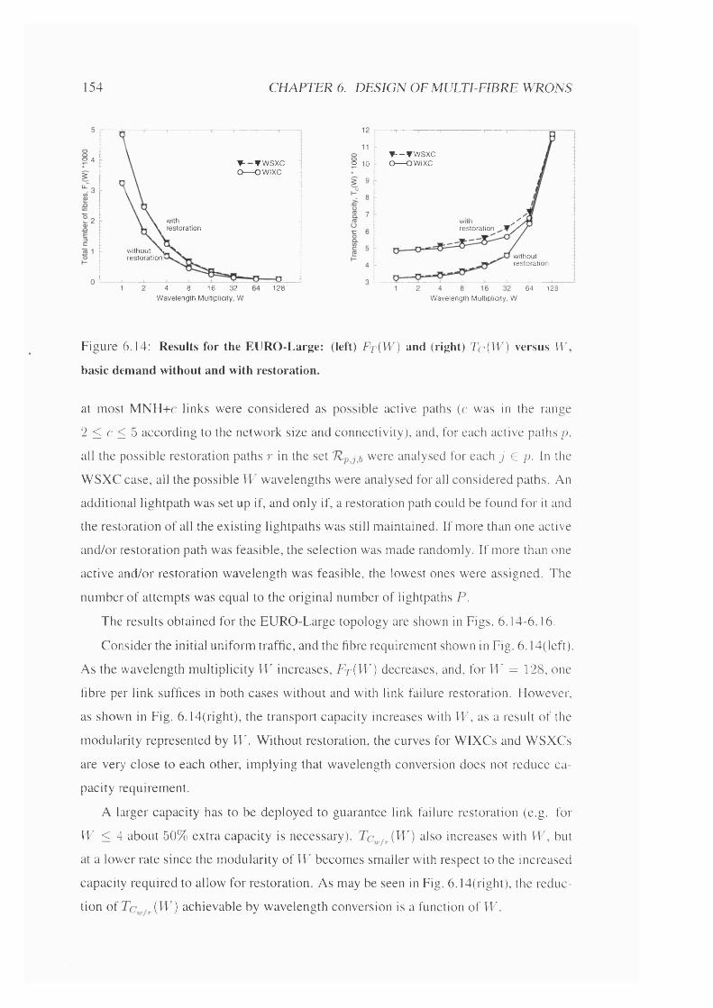
54 CHAPTER 6. DESIGN OF MULTI-FIBRE WRONS
0 4 ▼ --▼ W S X C O O W IXC
withrestoration
without \ res to ra tio n '
4 8 16 32W aveleng th Multiplicity. W
128
▼ --▼ W S X C O OW IXCo 10
WIlll /resto ration y
withoutresto ra tion
64 128W avelength Multiplicity, W
Figure 6.14: Results for the EURO-Large: (left) Ft { W) and (right) Tc{W) versus W,
basic demand without and with restoration.
at most M NH+c links were considered as possible active paths (c was in the range
2 < c < 5 according to the network size and connectivity), and, for each active paths /;,
all the possible restoration paths r in the set were analysed for each j G p. In the
W SXC case, all the possible IF wavelengths were analysed for all considered paths. An
additional lightpath was set up if, and only if, a restoration path could be found for it and
the restoration of all the existing lightpaths was still maintained. If more than one active
and/or restoration path was feasible, the selection was made randomly. If more than one
active and/or restoration wavelength was feasible, the lowest ones were assigned. The
number of attempts was equal to the original number of lightpaths P.
The results obtained for the EURO-Large topology are shown in Figs. 6.14-6.16.
Consider the initial uniform traffic, and the fibre requirement shown in Fig. 6 . 14(left).
As the wavelength multiplicity W increases, F t ( W ) decreases, and, for IF = 128, one
fibre per link suffices in both cases without and with link failure restoration. However,
as shown in Fig. 6 .14(right), the transport capacity increases with IF , as a result of the
modularity represented by W. Without restoration, the curves for W IXCs and W SXCs
are very close to each other, implying that wavelength conversion does not reduce ca
pacity requirement.
A larger capacity has to be deployed to guarantee link failure restoration (e.g. for
II" < 4 about 50% extra capacity is necessary). (IF) also increases with IF, but
at a lower rate since the modularity of IF becomes smaller with respect to the increased
capacity required to allow for restoration. As may be seen in Fig. 6 .14(right), the reduc
tion of (IF) achievable by wavelength conversion is a function of IF.

6.7. ANALYSIS OF TRAFFIC GROWTH 55
100
90 withoutrestoration
§ 703d 60
I 50 with ^ restoration3
Q)O O W IXC▼ --▼ W S X C
128W avelength Multiplicity, W
withrestoration
withoutrestoration
0.91 2 8 16 32 64 1284
W avelength Multiplicity, W
Figure 6.15: Results for the EURO-Large: (left) U{W) and (right) G{W) versus W, basic
demand without and with restoration.
For small values of W (lU < 4), no difference is observed between WIXC and
WSXC, as expected, since the blocking characteristics of the two OXCs conhgurations
are practically the same. However, within the range 4 < IF < 64, an appreciable
difference is obtained - the result of reduced blocking in WIXCs (as discussed in sec
tion 2.3.5).
No difference was observed for II ' = 128, as the capacity allocated is much larger
than required, for both OXC configurations. This is clearly shown in Fig. 6.15(left),
where the resource utilisation is plotted versus IT'. Consider the curves without restora
tion. For IT' = 1, the capacity deployed is entirely used for active lightpaths, thus
= 100%. However, as IT' increases, U { W ) decreases, since the granularity of IT
results in a larger transport capacity deployed. When the capacity to provide for restora
tion is added, the resource utilisation decreases (Uu,/r = 70% for IT = 1). However, as
shown, the difference between U^fo ^nd V\,/r decreases with IT'.
The utilisation gain is shown in Fig. 6.15(right). As previously discussed, a very
limited gain is observed for the case without restoration, whereas, with restoration,
assumes appreciable values (of up to 10%) for intermediate values of IT.
Traffic growth was then simulated, and the results are depicted in Fig. 6.16. As
shown, for IT > 32, the increase in resource utilisation achievable with WIXCs is
much larger than WSXCs, and the difference increases with IT. Therefore, the gain
with saturated growth increases with IT', and, as shown in Fig. 6.16, can be as large as
4(19% for TT = 1S!8.
This implies that WIXCs allow the access to the originally deployed excess capacity
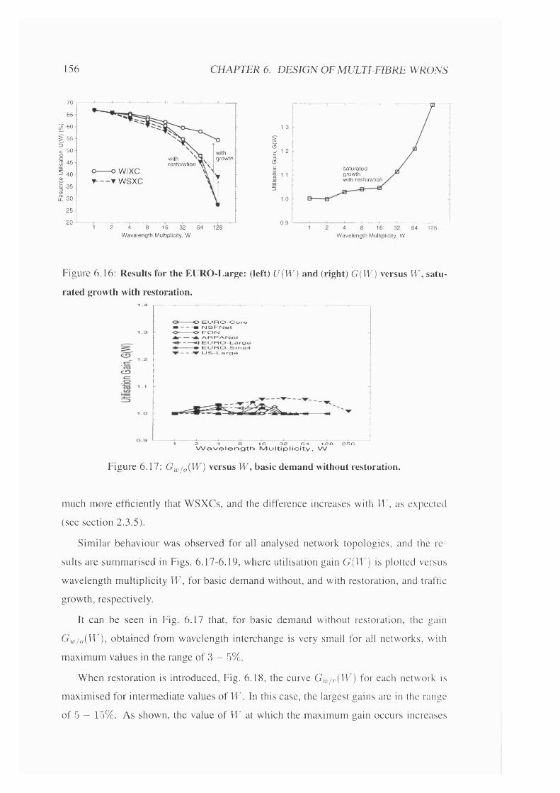
156 CHAPTER 6. DESIGN OF MULTI-FIBRE WRONS
70
65
g 60S 55
I »I 455 40g0 35
1 30
25
20
withresto ra tion »» \
VV
growth
o WIXCr-— ▼ WSXC
2 4 8 16 32 64W aveleng th Multiplicity. W
128
1.3
1 ’-§% 1-1
sa tu ra te dgrowthwith restoration
31.0
0.9128
W avelength Multiplicity, W
Figure 6.16: Results for the EURO-Large: (left) U{W) and (right) G{W) versus W, satu
rated growth with restoration.
O E L J F tO - O o r ô m M S R IM o t— O E O N ^ A F tF > A N © t- — — < 3 E L _ J P t O * L a r g e m E U R O - S m a l l V U S - E a r g a
2 4 a 1 6 3 2 6 4 1 2 8 2 5 6W a v o l o n g t h I V l u l t i p l i c i t y . W
Figure 6.17: G^j/oiW) versus W, basic demand without restoration.
much more efficiently that WSXCs, and the difference increases with W , as expected
(see section 2.3.5).
Similar behaviour was observed for all analysed network topologies, and the re
sults are summarised in Figs. 6.17-6.19, where utilisation gain G(fU) is plotted versus
wavelength multiplicity W , for basic demand without, and with restoration, and traffic
growth, respectively.
It can be seen in Fig. 6.17 that, for basic demand without restoration, the gain
G ^ / o ( W) , obtained from wavelength interchange is very small for all networks, with
maximum values in the range of 3 — 5%.
When restoration is introduced. Fig. 6.18, the curve Gw/ri^^ ) for each network is
maximised for intermediate values of IF. In this case, the largest gains are in the range
of 5 — 15%. As shown, the value of IF at which the maximum gain occurs increases

6.7. ANALYSIS OF TRAFFIC GROWTH 157
O ELJ FtCZ>-Oore m rSISFNet— O E O N ARRANot- - —<3 E U R O - L a r g e m - E U R O - S m a l l V U S - L a r g e
Figure 6.
1 2 4 8 16 3 2 6 4 1 2 8 2 5 6W a v e l e n g t h I V l u l t i p l i c i t y . W
8: G^,/r{W) versus W, basic demand with restoration.
E U R O - L a r g e
2W avele
4 a 16 W avelengtri IVlultiplicity, WWti ityP
Figure 6.19: Gs/g{W) versus VF, saturated growth with restoration.

158 CHAPTER 6. DESIGN OF MULTI-EIBRE WRONS
1 .3
1.2
oc' CT3O
• I 1.1
Q------- O E U R O -C o r e■ m N S F N c io --------o E O NA------- ▲ A R P A N c l<3 — - 4 E U F^ O -L argc* --------• E U R O -S m a ll▼-------▼ U S -L a r g e
A v e r a g e F ib r e s p e r L in k , F W S X C
Figure 6.20: Gyj/r{W) versus Fwsxc^ basic demand with restoration.
with an increase in the network size N (or with a decrease in the physical connectivity
a ) . For example, in the NSFNet, the peak gain occurs for \V = 8, after which the
gain decreases, given that the capacity allocated becomes larger than required, in both
WIXC and W SXC cases. However, for the larger and less-connected EURO-Small,
IF = 8 wavelengths per fibre results in a very large number of fibres allocated
within the network. Therefore little difference is shown between WIXCs and WSXCs
(which have similar blocking performance), leading to a negligible gain. As shown, for
this topology, the peak gain occurs for W = 64.
When traffic growth is considered, Fig. 6.19, the utilisation gain Gs/g(lU) increases
with W , and reaches values greater than 20% for the majority of the networks. As
shown, the value of W at which the curves start rising increases with an increase in
the network size. Also, the value of VV for which a given gain G,, /g(W) is obtained
increases with an increase of the network size. For example, in the NSFNet, the gain
is about 20% for IF = 16, whereas Gs/g(W) % 16% for IF = 128 in the case of the
EURO-Small.
The relationship between utilisation gain, wavelength multiplicity, and physical topol
ogy is clearly illustrated in Figs. 6.20 and 6.21, where G{\V) is plotted versus the av
erage number of fibres per link for the W SXC case, F w s x c ^ for basic demand with
restoration and traffic growth, respectively.
Consider the case with restoration (Fig. 6.20). As discussed in section 2.3.5, when
the average number of fibres per link is large, the space-switching part of the OXC dom-

6.8. CONCLUSIONS 59
oc ' c3 O c o
E U R O -C o r cN S F N c iE O NA R P A N c lE U R O -L a r g eE U R O -S in a llU S -L a r g c
I -1 .3
M1. 2
1.1
1 . ( )
o.y] ( ) ( ) I o I
A v e r a g e F ib r e s p e r L in k , F
Figure 6.21 : Gs/y{W) versus F w s x c j saturated growth with restoration,
inates, and, hence, WIXCs and WSXCs have similar blocking performances. Therefore,
as shown, the gain is negligible for F\ .ysxc > 5. However, as F w s x c decreases (due
to an increase of IT), wavelength-blocking is introduced in WSXCs and, therefore, the
utilisation gain increases. As shown, for all the topologies, the maximum gain occurs
when the average number of fibres per link is approximately F y s x c = 2. As previously
discussed, a further increase in IT (i.e. decrease in F w s x c ) results in allocated capacity
much larger than required for the uniform traffic demand; thus, the gain decreases to
zero.
However, this does not hold when saturated growth is considered, since for small
values of F w s x c , the two OXC configurations provide different blocking performances
to the random attempts, resulting in a large gain, as shown in Fig. 6.21.
These results show that the improvement achievable with wavelength conversion
is strongly related to network size and connectivity, traffic condition, and wavelength
multiplicity. In particular, the larger N and lower a, the larger is the required IT and
the traffic to be allocated, to see significant gain with WIXCs.
6 .8 Conclusions
This chapter studied multi-fibre WRONs, where the maximum number of wavelengths
per fibre, IT, was introduced as a parameter. Different traffic conditions were consid
ered, including provisioning of uniform traffic demand, without and with link failure

160 CHAPTER 6. DESIGN OF MULTI-FIBRE WRONS
restoration, and growth. Three restoration strategies were considered and compared.
A new ILP formulation was proposed for the exact solution of the RWA problem, ap
plicable to WIXC and WSXC networks, the latter with and without wavelength-agility
in the end-nodes. Lower bound were discussed and heuristic algorithms proposed.
The analysis of two small topologies demonstrated the best restoration performance
provided by path restoration approach.
The study of numerous topologies showed that little benefit was achieved with
WIXCs, in the case without restoration and also with restoration if wavelength-agility
was provided within the terminals.
It was shown that network physical connectivity has great importance in determining
the extra capacity required for restoration. Moreover, it was demonstrated that mesh
WRONs can achieve considerable capacity saving with respect to restoration approaches
utilised at higher network layers, such as SONET/SDH.
In the case of traffic growth, wavelength conversion could improve resource utilisa
tion. However, the results demonstrated that the benefit strongly depends on network
size and connectivity, and wavelength multiplicity.

Chapter 7
Conclusions and future work
Routing and wavelength allocation has been studied in WDM, single-hop, wavelength-
routed optical transport networks (WRONs). The role played by the physical topology
on the network performance has been identified as vital to enable optimal WRON de
sign. An algorithm for absolute-wavelength allocation in the EDFA bandwidth, and a
WDM amplifier configuration have been proposed to enable efficient WDM channel
transmission.
The systematic analysis of a large number of arbitrarily-connected single-fibre WRONs
with static uniform traffic enabled to quantify the relationship between wavelength re
quirement N \ and physical connectivity a. It was shown that large network throughput
can be achieved with relatively small N \, as wavelength-routing results in large wave
length reuse, even in weakly-connected networks. On average, no more than 32, 16 and
8 wavelengths were necessary for a > 0.15, 0.2, and 0.3, respectively.
N \ was observed to be governed by critical network cuts, and, for sub-optimal
topologies, the selective addition of multiple fibres in heavily loaded links resulted in
significant reduction of N \.
The comparison with regular network topologies showed that arbitrarily-connected
WRONs can provide the advantages of scalability and fiexibility, with similar wave
length requirements.
The analysis of link failure restoration showed that key network cuts must consist of
as many links as possible to reduce the extra wavelengths required for restoration.
Therefore, an optimised topology for active lightpath allocation (i.e. large number
of links in the limiting cut) also resulted in increased robustness against link failure.
161

162 CHAPTER?. CONCLUSIONS AN D FUTURE W ORK
The obtained values of N \ are comparable to, or even smaller than, the number
of wavelengths transmitted over a single fibre in current point-to-point WDM systems.
Therefore, these results indicate that wavelength requirement is not a limiting factor in
the deployment of arbitrarily-connected wide-area WRONs.
The analysis showed that, for static traffic, the benefit achievable by introducing wave
length conversion within the OXCs is very small, in the case without restoration, and
also with restoration, when wavelength-agility is provided within the network end-
nodes.
The study of link failure restoration demonstrated that, although the reallocation of only
the interrupted lightpaths leads to slightly larger increase in wavelength requirement,
it guarantees the reallocation of far fewer lightpaths and nodes, resulting in simplified
network management, crucial in transport applications.
In real WRONs, the maximum number of wavelengths carried in each fibre (wavelength
multiplicity W ) is likely to be limited by technological constraints, and, hence, multiple
fibres may be deployed in the network links to satisfy the traffic demand. A large W
can be considered if the excess capacity initially deployed is accessible by future traffic
growth. Therefore, the analysis of multi-fibre WRONs was carried out introducing W
as a parameter, and considering conditions of network evolution.
The analysis of initial static uniform traffic demonstrated the better restoration per
formance provided by path restoration approach. It was shown that wavelength-agility
in the terminals is key to minimise restoration capacity, if wavelength conversion in not
available within the OXCs. The network physical connectivity was observed to have
great importance on the extra capacity required for restoration. It was demonstrated
that mesh WRON architectures can lead to considerable capacity saving compared to
strategies available at higher network layers, such as SONET/SDH.
In the case of traffic growth, wavelength conversion could improve the utilisation
of the excess capacity initially deployed. However, the benefit was strongly dependent
on network size and connectivity, and wavelength multiplicity. In particular, increasing
N and reducing a, increases the value of W , and the traffic to be allocated required
to obtain significant gain with WIXCs. In the case of large and weakly-connected real
networks (for example, EURO-Small, TV % 50, a < 0.1), extremely large values of

163
wavelength multiplicity are necessary (W > 128) to justify the need for wavelength
conversion.
Although WDM point-to-point systems with extremely large values of W have been
experimentally demonstrated, it will be some time before their practical implementation.
Therefore, these results indicate that the need for WIXCs is quite unlikely.
The analysis of WDM transmission in WRONs showed the critical limitation imposed
by wavelength-dependent gain in EDFAs. However, the judicious assignment to the
lightpaths of absolute-wavelengths within the EDFA bandwidth was shown to guarantee
acceptable performances throughout the network, under condition of lightpath add/drop.
The proposed WDM optical amplifier configuration was observed to ensure network
robustness against link failure, without the need for a complex network control.
The results achieved in this work answered many open questions, but also raised a num
ber of new issues representing important topics for further research.
Firstly, the analysis of network scalability is extremely important given the rapid
pace at which current telecommunication networks are growing. The study of efficient
algorithms enabling the addition of single nodes or connections, without disturbing ex
isting lightpaths, is crucial for the design of “future-proof” WRON architectures. More
over, the development of near-optimal algorithms to provide efficient network intercon
nections is seen to be very important.
In the analysis of link failure restoration, a centralised management system was as
sumed. Although this approach may be easily implemented in small-size networks,
practical complexity may emerge in wide-area applications due to the long propaga
tion time of control signals, caused by large distances between nodes and centralised
management. It is therefore important to investigate alternative distributed management
approaches, and study the consequence on signalling requirement.
The proposed WDM amplifier configuration was analysed by using a steady-state
model. However, time domain analysis would provide invaluable information about
restoration time, critical in transport applications given the high-capacity signals carried
by the lightpaths.
The ILP formulations were shown to be efficient only in the case of small network
topologies. When the integrality constraint was relaxed, the formulations failed to pro
duce any meaningful results.

164 CHAPTER?. CONCLUSIONS AND FUTURE W ORK
In the study of single-fibre WRONs (Chapters 3 and 4), lower bounds were eas
ily attainable by analysing key network cuts, used to verify the accuracy of proposed
heuristic algorithms. However, in the analysis of multi-fibre WRONs (Chapter 6), the
lower bounds were computationally expensive, and therefore not feasible in the case of
large networks. Thus, the proposed heuristic algorithms were verified only for small
network topologies, and by comparing results available in the literature.
An alternative approach is necessary to derive exact results in the case of large
topologies. The implementation of cutting-plane techniques, in which LP solutions are
iterated to derive tight LP-relaxation lower bounds, as proposed and discussed in [100],
may prove to very effective, as shown in [123]. This is expected to efficiently extend
ILP formulations to the analysis of real network topologies.
The original contributions included in this thesis are:
• A unified framework of integer linear program (ILP) formulations, which allow
to address all possible network configurations, including the use of WIXC and
WSXC, and different link failure restoration strategies, for single-fibre [95] and
multi-fibre [122] networks.
• Meaningful lower bounds on the wavelength [95] and fibre requirement.
• Design of accurate heuristic algorithms, to enable efficient allocation of active and
restoration lightpaths in single-fibre [96][110], and multi-fibre WRONs [121][122]
• The systematic analysis of a large number of arbitrarily-connected single-fibre
WRONs, which enabled to identify the key role played by topological parameters
on the network performance [111]. In particular:
- the relationship between wavelength requirement and physical connectivity
was quantified [96] [114];
- the importance of critical network cuts on wavelength and restoration require
ment was highlighted [96][97][110];
- the study of restoration strategies showed the limited performance penalties
resulting from re-routing only the intermpted lightpaths, whilst keeping the
surviving traffic unchanged, as required in transport applications [109].

165
• By analysing a large number of different topologies, the limited benefit achievable
with wavelength conversion in both cases without [96] [97], and with link failure
restoration when wavelength-agility is available within the end-nodes [95] [110]
was demonstrated in the case of static traffic.
• An efficient algorithm for the allocation to the network lightpaths of absolute-
wavelengths within the EDFA bandwidth, to compensate for gain non-uniformities
in the EDFA cascades under network add/drop conditions [112].
• A new WDM amplifier configuration that guarantees network robustness against
link failure without the need for a complex network control [113].
• Study of network evolution in multi-fibre topologies. The influence of phys
ical connectivity a on the extra capacity required for restoration was quanti
fied [122], and the relationship between network topology, wavelength multiplic
ity W , and benefit of wavelength conversion in condition of traffic growth was
identified [121].


List of publications
The following is a list of publications arising from the work in this thesis at the time
of submission, in chronological order, including conference presentations, letters, and
papers:
S. Baroni, R Bayvel, J. E. Midwinter, “Influence of physical connectivity on the number
of wavelengths in dense wavelength-routed optical networks”, in Proc. OFC’96, pp.
25-26, San Jose, CA, Feb. 1996.
S. Baroni, P. Bayvel, “Analysis of restoration requirements in wavelength-routed optical
networks”, in Proc. NOC’96, vol.Ill, pp.56-63, Heidelberg, Germany, June 1996.
S. Baroni, P. Bayvel, J. E. Midwinter, “Wavelength Requirements in Dense Wavelength-
Routed Optical Transport Networks with Variable Physical Connectivity”, lEE Elec
tronic Letters, vol.32, no.6, pp. 575-576, 1996.
S. Baroni, P. Bayvel, “Key topological parameters for the wavelength-routed optical
networks design”, in Proc. ECOC’96, vol.2, pp.277-280, Oslo, Norway, Sept. 1996.
C. Marand, S. Baroni, F. Di Pasquale, P. Bayvel, “Design of wavelength-routed op
tical networks with optimised channel allocation in the EDFA bandwidth”, in Proc.
ECOC’96, vol.2, pp.273-276, Oslo, Norway, Sept. 1996.
S. Baroni, P. Bayvel, “Link failure restoration in WDM optical transport networks and
the effect of wavelength conversion”, in Proc. OEC’97, pp. 123-124, Dallas, TX, Feb.
1997.
167

s. Baroni, P. Bayvel, “Wavelength Requirements in Arbitrarily Connected Wavelength-
Routed Optical Networks”, lEEE/OSA Journal o f Lightwave Technology, vol. 15, no.2,
pp.242-251,Feb. 1997.
S. Baroni, S. K. Korotky, P. Bayvel, “Wavelength interchange in multi-wavelength op
tical transport networks”, in Proc. ECOC’97, vol.3, pp. 164-167, Edinburgh, Scotland,
Sept. 1997.
S. Baroni, P. Bayvel, and R. J. Gibbens, “On the Number of Wavelengths in Arbitrarily-
Connected Wavelength-Routed Optical Networks”, University of Cambridge, Statistical
Laboratory Research Report 1998-7 (http://www.statslab.cam.ac.uk/Reports/), also to
be published on OSA Trends in Optics and Photonics Series (TOPS) vol.20 on Optical
Networks and Their Applications, 1998. [Invited contribution]
R. Olivares, S. Baroni, F. Di Pasquale, P. Bayvel, F. A. Fernandez, “A New WDM
Amplifier Cascade for Improved Performance in Wavelength-Routed Optical Transport
Networks”, accepted for publication on Optical Fiber Technology, 1998.
S. Baroni, P. Bayvel, R. J. Gibbens, “Restoration capacity for resilient wavelength-
routed optical transport networks”, paper TuC2 to be presented at lEEE/LEOS Summer
Topical Meeting “Broadband Optical Networks and Technologies: An Emerging Reali
ty”, Monterey, CA, 20-22 July, 1998.
168

Appendix A
Partition bound evaluation: heuristic
algorithm
As discussed in section 3.4.2, for a network topology with N nodes, enumerating all the
network cuts to find W pb is 0 ( 2 ^ “ ^), which is feasible only for small size networks.
Therefore, the following heuristic algorithm was developed, to identify the network
limiting cut, and calculate the partition bound W p b -
Phase I: setup
1. For each node-pair z = (zi, Z2 ) G Z determine a random list Az,e of paths be
tween zi and Z2 with length at most m{z) + e, as defined in eq.(3.3)
2. Determine a list P with all node-pairs z G Z sorted by decreasing length of their
MNH distance m (z), with ties broken randomly
3. Set cost Sj = 0, V j G A
Phase II: initial path assignment
1. Set congestion Cj = 0, Vj G A
2. Set COS"!; = 0 0 , Vz G Z
3. Set = 0, Vp G A ,e , Vz G Z
4. Select first z from P
169

170APPENDIXA. PARTITION BOUND EVALUATION: HEURISTIC ALGORITHM
5. Select first path p from Az,e
6. Determine C O S T as the sum of the cost of all links in p (C O S T = ^ sj)j^p
7. If (COS'T < COS"?;), setp* = p, COS'T, = COS'T
8. If there is a further path in Az,e not yet considered select it as new p and go to 6
9. Assign path p* to node pair z (set 6 .^ = 1), and increase the congestion of all
the links in p* (cj = + 1, Vj G p*)
10. If there is a further node-pair in P not yet considered, select it as new z and go to
5
Phase III: subsequent optimisation
1. Set = (5 , Vp G Az,e, Vz G Z
2. Calculate the list P of all node-pairs z sorted by decreasing length of their MNH
distance m (z), with ties broken randomly
3. Select first z from P
4. Delete path p* previously assigned to z (set 5 * . = 0), and decrease the conges
tion along p* (cj = Cj - 1, Vj G p*)
5. Select first path p from Az,e
6. Set C O N G m a x oo
7. Determine C O S T as the sum of the cost of all links in p (C O S T = Y. Sj),j^p
and C O N G as the maximum congestion among all links in p (C O N G = max cj)j^p
8. If ((COS-T = = cos'll:) && (COAC = = COAC^Ax), setp* = p, COAC^Ax
COAC
9. If there is a further path in Az,e not yet considered select it as new p and go to 7
10. Assign path p* to node pair z (set 6A = 1), and increase the congestion of all
the links in p* (Cj = Cj P 1, Vj G p*)

171
11. If there is a further node-pair in P not yet considered, select it as new z and go to
4
12. If there exists at least one node-pair z e Z and a path p G Az,e such that /
go to 1
Phase IV: cost increase
1. Determine j as the most congested link (j | Cj > c^, V/c G .4), and increase its
cost ( S j = Sj + 1)
Phases II, III, and IV are repeated until a subset of links j e C C A is observed
to have their cost significantly increased. This is the limiting cut that determines the
partition bound W p b , whose value is obtained from eq.(3.22).
Initially, for each node-pair z, the set of all paths connecting z, with length at most
the minimum length m(z) plus constant e, is generated. Large values of e, as large as
4, depending on network size and connectivity, were considered, to generate large sets
Az^C'
The node-pairs are then ranked by decreasing length of their minimum-number-of-
hops, or physical links, {MNH) distance, as longest paths are considered first. The cost
of each link j is set to zero.
In Phase II, each node-pair is assigned the first cheapest lightpath available, accord
ing to the values of the links’ cost Sj.
To evenly distribute the lightpaths along the network links, and reduce the maximum
congestion. Phase III is performed. Here, for each node-pair, the previously assigned
cheapest path is replaced by another cheapest path if the maximum congestion among
all the links is reduced. This is repeated until no improvements are possible.
In principle, this may lead to an oscillating state. However, this problem was not
observed in any of the analysed networks.
If an even distribution of the paths is achieved, the congestion of the links within the
limiting cut is the largest among all the network links. Therefore, the cost of the most
congested link is increased in Phase IV. If more than one link has the same maximum
value of the congestion, the cost of only one link, randomly selected, is increased.

\12APPEN D IXA. PARTITION BOUND EVALUATION: HEURISTIC ALGORITHM
This procedure is repeated until a subset of links is observed to have their cost sig
nificantly increased, identifying the limiting cut. The partition bound W pb is then cal
culated from eq.(3.22).
The heuristic algorithm was observed to be accurate in deriving the partition bound
WpB for a large number of topologies.
However, for networks (such as the UKNet described in section 3.7.1) where two or
more cuts, for example, C\ and C2 , required similar number of wavelengths to satisfy
the traffic across them, Wc^ ~ Wc2 ~ W pb, the algorithm was observed to oscillate
between these cuts, failing in producing a valid result.
In these cases, W pb was derived by inspection, identifying the limiting cut from the
network plot.
Appendix B
Lightpath allocation: heuristic
algorithms
B.l Active lightpaths allocation in single-fibre WRONs
This section presents a formal description of the algorithms utilised for the allocation of
active lightpaths in single-fibre WRONs (section 3.6).
Input dataGiven:
1. Network of N nodes and L links
2. Additional number of hops e allowed to the active lightpaths
Phase I: setup
1. For each node-pair z = {zi, Z2 ) G Z determine a random list Az,e of paths be
tween zi and Z2 with length at most 7 7 1 (2 :) -f e, as defined in eq.(3.3)
2. Determine a list P with all node-pairs z e Z sorted by decreasing length of their
MNH distance m{z), with ties broken randomly
Phase II: initial path assignment
1. Set congestion Cj = 0, Vj G A
173

174 APPENDIX B. LIGHTPATH ALLOCATION: HEURISTIC ALGORITHMS
2. Set 6^^ = 0, Vp G Az^e, Vz G Z
3. Select first z from P
4. Set M A X lo a d = oo and P A T H lo a d = oo
5. Select first path p from Az^e
6. Determine M l o a d as the maximum congestion among all the links in p ( M l o a d =
m axc,), and P l o a d as the sum of the congestion of all links in p { P l o a d =j^pE c j )j^p
7. If { { M l o a d < M A X l o a d ) or { { M l o a d = = M A X l o a d ) and { P l o a d <
P A T H l o a d ) ) ) , set p* = p, M A X l o a d = M l o a d , and P A T E l o a d = P l o a d
8. If there is a further path in Az^e not yet considered select it as new p and go to 6
9. Assign path p* to node pair z (set — 1), and increase the congestion of all
the links in p* {cj = Cj + 1, Vj G p*)
10. If there is a further node-pair in P not yet considered, select it as new z and go to
4
Phase III: subsequent optimisation
1. Set Vp G Az,e, Vz G Z
2. Calculate the list P of all node-pairs z sorted by decreasing length of their MNH
distance m (z), with ties broken randomly
3. Select first z from P
4. Delete path p* previously assigned to z (set 6^^ = 0), and decrease the conges
tion along p* {Cj = Cj - 1, Vj G p*)
5. Repeat all the steps 4-9 of Phase II
6. If there is a further node-pair in P not yet considered, select it as new z and go to
4
7. If there exists at least one node-pair z G Z and a path p G Az,e such that
go to 1
B .L ACTIVE LIGHTPATHS ALLOCATION IN SINGLE-FIBRE WRONS 175
8. N \{ W I X C ) = n g x Cj
Phase IV: wavelength assignment (WSXC case)
1. Determine a list P of all node-pairs z sorted by decreasing length of their assigned
paths p*, with ties broken randomly
2. Set the list of wavelengths used in each link to be the empty set (Aj = 0, Vj e A)
3. Select first z from P
4. Consider the path p* assigned to z
5. Determine w* as the lowest wavelength not used among the all the links in p*
{w* = I U AjI + 1). Assign w* to z (set (5 = 1), and add w* to the set ofjep*
used wavelengths in all links in p* {Aj = Aj Vj G p*)
6. If there is a further node-pair in P not yet considered, select it as new z and go to
4
7. AA(iyS'AC) = I U A,.|j^A
In Phase II, each node-pair z is assigned the cheapest path according to the values
of the links congestion Cj when z is considered. Therefore, different solutions are ob
tained for different ordered lists P. To achieve the best possible allocation of the paths,
independently of the order in list P , Phase III is performed. Here, each node-pair is con
sidered at a time, and the path p* previously assigned is replaced by a different one if,
and only if, the maximum congestion along the new path is smaller than the maximum
congestion in the previously assigned path. Phase III is repeated until no improvements
are possible. In principle, this may lead to an oscillating state. However, this problem
was not observed in any of the analysed networks.
As previously discussed, in the WIXC case. Phase IV was not performed, and
N x i W I X C ) was equal to the maximum congestion among all the network links.
However, in the WSXC case, the wavelengths are then assigned to the paths, ranked
by decreasing length. The total number of distinct wavelengths assigned amongst all
node-pairs determines the network wavelength requirement N \{ W S X C ) .

176 APPENDIX B. LIGHTPATH ALLOCATION: HEURISTIC ALGORITHMS
B.2 Restore-only approach in single-fibre WRONs
This section present a formal description of the algorithms utilised for the allocation
of restoration lightpaths in single-fibre WRONs, for the restore-only approach (sec
tion 4.5.1).
Input dataGiven:
1. Network of L links and N nodes
2. Allocation of the active lightpaths (6^ for the WIXC, and for the WSXC)
determined by the algorithm in section 3.6 (Appendix B .l), and:
WIXC case: The congestion C j , Vj G A
WSXC case: The list of wavelengths used Aj, \fj G A
3. Original wavelength requirement N \
WIXC case: N \ = max Cjj e A ^
WSXC case: TVa = | U A4
4. Additional number of hops a allowed to the restoration paths
Restoration lightpaths assignment
1. Set Ik = Ck and = A^, VA; G
2. Randomly select first link j G A (supposed faulty)
3. Set Ck = Ik 3.nd Ak = A^, VA; G ^
4. For each node-pair z whose active path p* is using link j , determine the list T^p.
of potential restoration paths with length at most equal to the new MNH, distance,
m^{z), plus a
5. Determine a list, P, of all node-pairs z considered in step 4 sorted by decreasing
length of their distance m^{z), with ties broken randomly
6. Select first z from P

B.2. RESTORE-ONLY APPROACH IN SINGLE-FIBRE WRONS 177
7. Delete active lightpath previously assigned to z (p* for WIXC, (p*,w*) for WSXC):
WIXC case: Decrease by 1 the congestion of all the links in p* {Ck = — I,
\/k G p * )
WSXC case: Delete w* from the set of used wavelengths in all the links in p*
{Ak = Ak\ {w*},^k e p*)
8. If there is a further node-pair in P not yet considered select it as new z and go to
7
9. Select first z from P
10. Set M A X load oo
11. Select first path r from IZp*
12. WIXC case: Determine M l q a d as the maximum link congestion among all the
links in r { M l q a d = maxc^)k £ r
WSXC case: Determine M l q a d as the lowest wavelength not used among all
the links in r { M l q a d = \ U A^| -h 1)k e r
13. If { M l o a d < M A X l o a d ) , set r * = r , and M A X l o a d = M l o a d
14. If there is a further path in Pp*j,a not yet considered, select it as new r and go to
12
15. WIXC case: Assign restoration lightpath r* to node pair z (set p. j = 1), and
increase the congestion in all the links in r* (c t = + 1, V/c G r*)
WSXC case: Assign restoration lightpath {r*, A*), with A* = M A X l o a d to
node pair z (set ^ , v * ~ Add A* to the set of used wavelengths in
all the links in r * {Ak = Ak U{A*}, VA: G r * )
16. If there is a further node-pair in P not yet considered select it as new z and go to
10
17. Determine the new wavelength requirement N{\
WIXC case: NÎ = max Ck keAWSXC case: NÎ = \ (J Ak\
keA

178 APPENDIX B. LIGHTPATH ALLOCATION: HEURISTIC ALGORITHMS
18. If 77 =
19. If there is a further link not yet considered select it as new j and go to 3
B.3 Active lightpaths allocation in multi-fihre WRONs
This section presents a formal description of the algorithms utilised for the allocation of
active lightpaths in multi-fibre WRONs (section 6.6.1(a)).
WIXC case
Input dataGiven:
1. Network of N nodes and L links
2. Maximum number of wavelengths per fibre W
Phase I: setup
1. For each node-pair z = (z%, Z2 ) G Z determine a random list Az of paths be
tween zi and Z2 with length at most m{z), as defined in eq.(3.3) with e = 0
2. Determine a list P with all the node-pairs z e Z sorted by decreasing length of
their MNH distance m{z), with ties broken randomly
Phase II: initial assignment
1. Set congestion Cj = 0, and number of fibres f j = l , Vj G A
2. Set = 0, V p G Az,e, V z G Z
3. Select first z from P
4. Set M A X pjB jiE — 0 0
5. Select first path p from Az

B.3. ACTIVE LIGHTPATHS ALLOCATION IN MULTI-FIBRE WRONS 179
6. Determine M f i b r e as the number of fibres to be added if p is selected as active
lightpath { M f i b r e = # links j e p\cj%W = = 0)
7. If ( M f i b r e < M A X f i b r e ) setp* = p, and M A X f i b r e = M f i b r e
8. If there is a further path in Az not yet considered select it as new p and go to 6
9. Assign lightpath p* to node pair z (set 6^ = 1), increase the number of fibres
where required (Vj E p*, if (Cj%W == 0), set Jj = f j + 1), and the congestion
of all the links in p* (cj = cj A 1, Vj G p*)
10. If there is a further node-pair in P not yet considered, select it as new z and go to
4
Phase III: subsequent optimisation
1. Set = 0 ^ , Vp G Az,e, Vz G Z
2. Calculate the list P of all node-pairs z sorted by decreasing length of their MNH
distance m (z), with ties broken randomly.
3. Select first z from P
4. Delete lightpath p* previously assigned to z (set = 0) and decrease the con
gestion along p* (Cj = Cj — 1, Vj G p*), and the number of fibres where possible
(V; G p \ if (c,% iy = = 0), set - 1)
5. Repeat all the steps 4-9 of Phase II
6. If there is a further node-pair in P not yet considered, select it as new z and go to
4
7. If there exists at least one node-pair z G Z, and a path p G Az,e, such that
% f go to 1
8. Ft^ J W I X C ) = E f ijeA

180 APPENDIX B. LIGHTPATH ALLOCATION: HEURISTIC ALGORITHM S
WSXC case
Input dataGiven:
1. Network of N nodes and L links
2. Maximum number of wavelengths per fibre W
Phase I: setup
1. For each node-pair z = (zi, Z2 ) G Z determine a random list Az of paths be
tween Zi and Z2 with length at most m {z), as defined in eq.(3.3) with e = 0
2. Determine a list P with all the node-pairs z G Z sorted by decreasing length of
their MNH distance m {z), with ties broken randomly
Phase II: initial assignment
1 . Set number of fibres f j = 1, Vj G A , and set frecy jj = 1, Vu; =
Vj G A
2. Set = 0, Vp G Az,e, Vw = 1 , W ,y z e Z
3. Select first z from P
4. Set M AX pjB RE — 0 0
5. Select first path p from ^ 2
6. Select first wavelength, u; — 1
7. Determine M fib r e as the number of fibres to be added if (p, w) is selected as
active lightpath { M f i b r e = # links j G p \ fr e e ^ j == 0)
8. If { M f i b r e < M A X f i b r e ) , setp* = p,w* = w, and M A X r i b r e ’ M f i b r e
9. If u; < W , w = w -\-l and go to 7
10. If there is a further path in Az not yet considered select it as new p and go to 6
B.3. ACTIVE LIGHTPATHS ALLOCATION IN MULTI-FIBRE WRONS 181
11. Assign lightpath (p*,w*) to node pair z (set = 1), increase the number
of fibres where required (Vj G p*, if (free^* j == 0), set f j = / j + 1, and
frec y jj = f r e e ^ j + 1, Vru = 1 , W ), and decrease the wavelength availability
( / r e e ^ . j = - 1, Vj G p*)
12. If there is a further node-pair in P not yet considered, select it as new z and go to
4
Phase III: subsequent optimisation
Set 2 ^ A ,e , Vw = 1, Vz G Z
2. Calculate the list P of all node-pairs z sorted by decreasing length of their MNH
distance m (z), with ties broken randomly.
3. Select first z from P
4. Delete lightpath {p*,w*) previously assigned to z (set = 0), increase the
wavelength availability ( / r e e ^ 'j = fr e e ^ ^ j 4- 1, Vj G p * ) and decrease the
number of fibres where possible (Vj G p*, if Vw = 1 ,..., W , {frecyjj > 0), set
f j = f j - 1 , and f r e e ^ j = f r e e ^ j - l ,\ /w = 1, ...,W )
5. Repeat all the steps 4-11 of Phase II
6. If there is a further node-pair in P not yet considered, select it as new z and go to
4
7. If there exists at least one node-pair z G Z and a path p G Az,e and a wavelength
w = l , . . .W such that f „ go to 1
8. Ft^,^{W SXC)= E fjjeA
To verify the accuracy of the proposed heuristic algorithms, the fibre requirement of two
8-node networks (a ring, and the 8-node 13-link shown in Fig. 6.4(b)) was determined
with both ILF and heuristic algorithms (see Table B .l). As shown, for both topologies,
the heuristics achieved the optimal results of ILPs for all the values of W considered,
confirming the accuracy of their design.

182 APPENDIX B. LIGHTPATH ALLOCATION: HEURISTIC ALGORITHMS
wRings MeshS
WIXC WSXC WIXC WSXC
I L P I L P I L P I L P
1 64 64 64 64 46 46 46 46
2 34 34 34 34 25 25 25 25
4 18 18 18 18 14 14 14 14
6 15 15 15 15 13 13 13 13
8 10 10 10 10 13 13 13 13
10 8 8 8 8 13 13 13 13
Table B. 1 : Results for two 8-node networks. versus W for both WIXC and WSXC
cases obtained with IL P and heuristic algorithms.
B.4 Restoration lightpaths allocation in multi-fihre WRONs
This section presents a formal description of the algorithms utilised for the allocation of
restoration lightpaths in multi-fibre WRONs (section 6.6.1(b)).
WIXC case
Input dataGiven:
1. Network of L links and N nodes
2. Allocation of the active lightpaths (6^ _) determined by the algorithm in sec
tion 6.6.1 (a)-WIXC case (Appendix B.3-WIXC case), and the congestion Cj and
number of fibres f j , ^ j e A
3. Original total number of fibres = E f jjeA
4. Maximum number of wavelengths per fibre W
5. Size b of the restoration sets
Restoration lightpaths assignment
1. Set Ik = Ck, y k e A
2. Randomly select first link j e A (supposed faulty)
3. Set Ck = Ik y k e A

BA. RESTORATION LIGHTPATHS ALLOCATION IN MULTI-FIBRE W R O N S m
4. For each node-pair z whose active lightpath p* is using link j , determine the list
'Rp*,j,b of potential restoration lightpaths, as defined in section 6.3
5. Determine a list, P, of all node-pairs z considered in step 4 sorted by decreasing
length of their distance m^{z), with ties broken randomly
6. Select first z from P
1. Consider active lightpath p* previously assigned to z: decrease by 1 the conges
tion of all the links in p* (c^ = — 1, V/c G p*)
8. If there is a further node-pair in P not yet considered select it as new z and go to
7
9. Select first z from P
10. Set M AX.FJBRE — oo
11. Select first path r from 'Rp*j,b
12. Determine M fib r e as the number of fibres to be added if r is selected as restora
tion lightpath { M f i b r e = # links k e r\ck%W == 0)
13. If { M f i b r e < M A X f i b r e )^ set r* = r , and M A X f i b r e = M f i b r e
14. If there is a further path in 'Rp*j,b not yet considered, select it as new r and go to
12
15. Assign restoration lightpath r* to node pair z (set . = 1 ) , and increase the
number of fibres where required ( V / c G r* , if {Ck%W = = 0 ) , set fk = f k P I),
and increase the congestion of all the links in r * (cjt = + 1, V /c G r* )
16. If there is a further node-pair in P not yet considered select it as new z and go to
10
17. If there is a further link not yet considered select it as new j and go to 3
18. The new total number of fibres with restoration is {W IX C ) = ^ f jjeA

184 APPENDIX B. LIGHTPATH ALLOCATION: HEURISTIC ALGORITHMS
WSXC case with wavelength-agility in the terminals (WSXC-A)
Input dataGiven:
1. Network of L links and N nodes
2. Allocation of the active lightpaths determined by the algorithm in sec
tion 6.6.1(a)-WSXC case (Appendix B.3-WSXC case), the wavelength availabil
ity fr e e w j,y w = 1 , W , Vj e A , and number of fibres f j , Vj G A
3. Original total number of fibres S X C ) = ^ f jjeA
4. Maximum number of wavelengths per fibre W
5. Size b of the restoration sets
Restoration lightpaths assignment
1. Set avails,k = f'f'G^w,k, Vw = 1 , W ,y k e A
2. Randomly select first link j E A (supposed faulty)
3. Set free^^k = availyj^k^ Vw = 1 , W ,\fk e A
4. For each node-pair z whose active lightpath (p*, w*) is using link j , determine the
list of potential restoration lightpaths, as defined in section 6.3
5. Determine a list, P, of all node-pairs z considered in step 4 sorted by decreasing
length of their distance m^{z), with ties broken randomly
6. Select first z from P
1. Consider active lightpath (p*,w*) previously assigned to z: increase the wave
length availability (freeyj*^k = fTeew*^k + 1, V/c G p*)
8. If there is a further node-pair in P not yet considered select it as new z and go to
7

B.4. RESTORATION LIGHTPATHS ALLOCATION IN MULTI-FIBRE W RONSl 85
9. Select first z from P
10. Set M AXpiQjiE = o o
11. Select first path r from Pp*j,b
12. Select first wavelength, A = 1
13. Determine M p jb re as the number of fibres to be added if (r, A) is selected as
active lightpath (M p jbre = # links k E r\freex,k == 0)
14. If (MpiBRE < ^ - ^ ^ f ib r e ) - ! set r* = r , \* = A, and M A X p jb r e = A Ipjbre
15. If A < VT, A = A + 1 and go to 13
16. If there is a further path in 'Rp*j,b not yet considered select it as new r and go to
12
17. Assign restoration lightpath (r*, A*) to node pair z (set = 1), increase
the number of fibres where required (V/c e r*, if (freex*,k == 0), set fk =
f k P I, and freex,k = + 1, VA = 1,..., W ), and decrease the wavelength
availability {freex*,k = freex*,k - 1, V/c G r*)
18. If there is a further node-pair in P not yet considered, select it as new z and go to
10
19. If there is a further link not yet considered select it as new j and go to 3
20. The new total number of fibres with restoration is (W S X C — A) = fjjeA
WSXC case with fixed restoration wavelength (WSXC-F)
Input dataGiven:
1. Network of L links and N nodes
2. Allocation of the active and restoration paths and % p. j ) determined by the
algorithms in section 6.6.1-WIXC case (Appendices B.3 and B.4-WIXC case),
and number of fibres f j , Vj e A

186 APPENDIX B. LIGHTPATH ALLOCATION: HEURISTIC ALGORITHMS
3. Total number of fibres { W IX C ) = ^ f jjeA
4. Maximum number of wavelengths per fibre W
Restoration lightpaths assignment
1. Set frecyj^k = = I, e A
2. Determine a list, P, of all node-pairs z sorted by decreasing length of their as
signed active paths p*, with ties broken randomly
3. Select first z from P
4. Set M AXpfBRE — oo
5. Select first wavelength, w = 1
6. Determine M f i b r e as the number of fibres to be added in active and restoration
path if wavelength w is selected (for each link j in the active path p*, the maxi
mum number of simultaneous lighpaths using link j with wavelength w must be
calculated, considering the restoration of all network link failures, and compare
with the number of fibres in link j \ for each link k in the restoration path r*,
the maximum number of simultaneous lighpaths using link k with wavelength w
must be calculated, considering the restoration of all links in active path p* , and
compare with the number of fibres in link k)
7. If ( M f i b r e < M A X f i b r e ) ^ set w* = w, and M A X f i b r e = M f i b r e
8. If w < W , w w + 1 and go to 6
9. Assign wavelength w* to the active and restoration lightpaths of node pair z (set
^p*,w\z = 1’ = 1’ G P*), adding fibres where required, along
the active and restoration paths
10. If there is a further node-pair in P not yet considered, select it as new z and go to
4
11. The new total number of fibres with restoration is (W S X C — F) = Y. f jjeA

BA. RESTORATION LIGHTPATHS ALLOCATION IN MULTI-FIBRE WRONSl 87
To verify the accuracy of the proposed heuristics, the fibre requirement of two 8-node
networks (a ring, and the 8-node 13-link shown in Fig. 6.4(b)) was determined with both
ILP and heuristic algorithms (see Tables B.2-B.5).
In a ring network, each active lightpath has only one restoration lightpath, which is
edge-disjoint. Therefore, all the restoration sets have size 6 = 1 . When the ILP was
not completed after one day of computation on a UNIX workstation, the best results
achieved was recorded and is marked with a *. However, confidence can be placed in
the accuracy of these results, since these values, once reached, remained constant for
many hours of calculation.
As shown, in Table B.2, the optimal solutions of the ILPs were always achieved or
approached for all the considered values of W .
For the mesh network, each configuration was studied for three different values of
the size of restoration sets, 6 = 1, 2, and 10, respectively. [As discussed in section 6.5,
in some cases, for a given restoration strategy, it was possible to derive, during the ILP
computation, a lower bound on larger than Fpb^/^- These limits were recorded
and are shown in parentheses in Tables B.3, B.4 and B.5, to verify the accuracy of the
sub-optimal result.]
Consider path restoration with WIXC (PI) in Table B.3. An increase in b results in
a larger number of possible restoration paths, and, hence, a better optimisation of the
restoration lightpath allocation. As a consequence, decreases as b increases. As
shown, with ILP, a great reduction in Fp^^^ is achieved when b changes from 1 to 2,
as the number of possible solutions increases significantly. A limited improvement is
then obtained when b is further increased to 10, However, for the heuristic algorithm, a
large number of possible restoration paths is required for each node-pair, to achieve or
approach the optimal solution.
As shown, the difference between the heuristic results and the optimal ILP solutions
is very small for all values of W considered (less than 10%).
Similar results were obtained for the WSXC-A (PSA) and WSXC-F (PSF) configu
rations, confirming the accuracy of the heuristic algorithms (Tables B.4 and B.5).

188 APPENDIX B. LIGHTPATH ALLOCATION: HEURISTIC ALGORITHMS
w W IX C (PI) W SX C -A (PSA) W SX C -F (PSF)
I L P He ur i s t i c I L P Heur i s t i c I L P H eur i s t i c
1 128 128 128 128 128 128
2 64 64 64 64 64 64
4 32 32 32 32 32 32
6 24 24 24 24 24 24
8 16 16 16 16 16 16
10 16 16 16 16 16 16
12 16 16 16 16 16 16
16 8 8 8 8 15» 16
24 8 8 8 8 12* 13
26 8 8 8 8 1 1 , 11
28 8 8 8 8 8 8
Table B.2: Results for the ring 8-node network. versus W for WIXC, WSXC-A, and
WSXC-F cases obtained with I L P and heuristic algorithms, with link failure restoration
(path restoration strategy). Size of restoration sets is 6 = 1. When the ILP failed was not
completed after one day of computation on a UNIX workstation, the best results achieved
was recorded and is marked with a *.
W
(W IX C (PI))
6 = 1 6 = 2 6 = 10
I L P He ur i s t i c I L P H eur i s t i c I L P H eur i s t i c
1 74 76 67 75 65* ( > 6 4 ) 68
2 39 42 34 40 33 36
4 22 27 18 23 I 8 * ( > 1 7 ) 19
6 15 15 15 15 15 15
8 13 13 13 13 13 13
Table B.3: Results for the mesh 8-node network shown in Fig. 6.4(b). versus W
obtained with IL P and heuristic algorithms, considering with link failure restoration.
WIXC with path restoration (PI).
(W SX C-A (PSA ))
W 6 = 1 6 = 2 6 = 10
I L P H eur i s t i c I L P H eur i s t i c I L P H eur i s t i c
1 74 76 67 75 65* ( > 6 4 ) 68
2 39 42 34 40 33 36
4 23* ( > 2 2 ) 26 18 23 1 8 * ( > 1 7 ) 20
6 15 17 15 17 15 16
8 13 14 13 13 13 13
Table B.4: Results for the mesh 8-node network shown in Fig. 6.4(b). Ft^ versus W
obtained with I L P and heuristic algorithms, considering with link failure restoration.
WSXC-A with path restoration (PSA).

B.4. RESTORATION LIGHTPATHS ALLOCATION IN MULTI-FIBRE W R O N S m
w
(W SX C-F (PSF))
6 = 1 6 = 2 6 = 10
I L P He ur i s t i c I LP He ur i s t i c I L P Heur i s t i c
1 74 76 67 75 65* ( > 6 4 ) 68
2 39 45 36 42 35* 39
4 24 28 24 27 24* 26
6 18* 21 17* 21 17* 20
8 15* 15 13 15 13 13
Table B.5: Results for the mesh 8-node network shown in Fig. 6.4(b). Ft versus W
obtained with I L P and heuristic algorithms, considering with link failure restoration.
WSXC-F with path restoration (PSF).


Appendix C
RCNs generation method
This section describes the method utilised to generate the randomly connected networks
(RCNs) analysed in section 3.7.2
Given N nodes there exist
\
/
^ L f c
V := L fc different network configurations with 1
link, Lpc2
different network configurations with 2 links,...,L f c ^
L fc= 1 network
configuration with L fc links, that is the physically fully-connected one. Therefore, for
a given N , the total number of distinct topologies ritop which can be generated is:
V N+
'^top —
/ r \J^FC
N + l
' L f c ^ L f c \+ +
1 y 2 )
+ ... - f -( T \^FC — 2^FC
K )
^ L f c ^
N - 1+
N . ( N - l )- 1 (C .l)
To satisfy the two constraints (Cl) and (C2) described in section 3.2, at least N
links are required (in the ring topology), hence the first line of the eq.(C.l) is a list of
topologies not acceptable. Moreover, even with L > N , a. topology must verify the two
constraints to be valuable.
If Smin is the minimum nodal degree in a given topology, the number of links in the
network is L > ômin-Lf/2, thus a > ômin/(N - 1). Similarly, if ômax is the maximum
nodal degree, L < ômax-Lf/2, and a < ôm ax/{^ — 1). As previously stated, for a
network with N nodes, al least N links are required in the ring configuration (ômin = 2),
and at most L fc = N .{N — l) /2 links are possible in the fully-connected network
191

TV = 14 and a = 0.23 (L = 21), there existV
10^ distinct\ 2 1 /
192 APPENDIX C. RCNS GENERATION METHOD
i^max = N — 1). Therefore, given N , the possible range of a is:
^ < « < 1 (C.2)
As N increases, the range of a increases and very small values become possible.
As shown in eq.(C.l), ritop = 0 (2^^), hence the total number of possible topologies
is enormous, even for small values of N (for example Utop ~ 10® for A = 7), making
it impractical to analyse all of them. Furthermore, as N increases, also the analysis of
all the possible topologies for a single {N, a) becomes intractable. For example, for
L fc
Ltopologies.
The approach followed in this work was to analyse for a given (N, a) a sample
consisting of a few thousand distinct topologies, and derive general results from them.
Given N and a, a randomly selected link was added at a time until the value of a
was achieved. A uniform probability distribution was considered, such that each of the
L fc links had the same probability to be selected. A new link was accepted only if
it was not already present and the nodal degree of both the interconnecting nodes was
smaller than a previously defined maximum degree, ômax whose value was determined
by N and a , as described below. To verify that this random process did not result in
unconnected networks, a following step was performed to ascertain the constraints (CJ)
and (C2), and only the connected networks were analysed.
To ensure that the sample contained only distinct topologies, a vector consisting of
several topological parameters was assigned to each of them:
y = (ri2 , 713, 724, ..., , 722.D, TIs.D-U .u D , H)
where 72% represents the total number of nodes with degree 5 = i, and 72%j the total
number of node-pairs both with degree 5 = i, and j links away from each other. Having
different vectors is a sufficient condition for two networks to be topologically different,
hence any new generated network was accepted only if its vector was different with
respect to the previous ones.
For a given (77, a ), the average nodal degree is:
- ^ ^ 2 ^ ^ N . { N - l ) . a (C-3)
Without limiting the nodal degree, a large number of RCNs were generated for dif
ferent values of N and a , and the nodal degree distribution was found to be normally
193
distributed centred around (5, with standard deviation a dependent on N and a. In par
ticular, for a given N , a increased with an increase of a (up to a = 0.5). Similarly for
a given a, a increased with an increase of N . Typical values of a were between 1.5
and 3. To retain over 95% of the possible topologies, the maximum nodal degree was
therefore defined as:A — Ô + 2 ( 7 (C.4)
However, when (TV, a) was equal to that of a real network, the same value of ômax was
imposed to the RCNs (for example, ômax = 4 for TV = 14 and a = 0.23, as for the
NSFNet).


Bibliography
[1] A. E. Willner, “Mining the optical bandwidth for a terabit per second”, IEEE
Spectrum, vol.34, no.4, Apr. 1997, pp.32-41.
[2] R. K. Butler, D. R. Poison, “Wave-Division Multiplexing in the Sprint Long Dis
tance Network”, IEEE Communications Magazine, Feb. 1998, pp.52-55.
[3] G . R. Hill, “A wavelength routeing approach to optical communication network
s’’, BT Technol. J., vol.6, no.3, July 1988, pp.24-31.
[4] H. Kobrinski, “Crossconnection of WDM high-speed channels”, lEE Electron.
Lett., vol.23, no. 18, Aug. 1987, pp.974-976.
[5] I. Chlamtac, A. Ganz, G. Karmi, “Purely Optical Networks for Terabit Commu
nication”, Proc. IEEE INFOCOM’89, pp.887-896.
[6] M. Young, H. Laor, B. J. Fontenot, “First In-Service Network Application of
Optical Cross-Connects”, Proc. OFC’98, PD23.
[7] E. D. Lowe, P. Botham, I. Hawker, “An Upgrade Route for Core Transport Net
works”, Proc. Globecom’96, pp.338-342.
[8] O. Gerstel, “Opportunities for optical protection and restoration”, Proc. OFC’98,
pp.269-270.
[9] D. J. Mestdagh, “Multiple Access Techniques for Fiber-Optic Networks”, Optical
Fiber Technology, vol.2, no.l, Jan. 1996, pp.7-54.
[10] Y. Yano, T. Ono, K. Fukuchi, T. Ito, H. Yamazaki, M. Yamaguchi, K. Emura,
“2.6 Terabit/s WDM Transmission Experiment using Optical Duobinary Cod
ing”, Proc. ECOC’96, vol.5, pp 3-6.
195

196 BIBLIOGRAPHY
[11] H. Onaka, H. Miyata, G. Ishikawa, K. Otsuka, H. Ooi, Y. Kai, S. Kinoshita,
M. Seino, H. Nishimoto, T. Chikama, “ 1.1 Tb/s WDM Transmission over a
150Km 1.3mum Zero-Dispersion Single-Mode Fiber”, Proc. OFC’96, paper PD-
19.
[12] A. K. Srivastava, Y. Sun, J. W. Sulhoff, C. Wolf, M. Zirngibl, R. Monnard,
A. R. Chraplyvy, A. A. Abramov, R. P. Espindola, T. A. Strasser, J. R. Pedraz-
zani, A. M. Vengsarkar, J. L. Zyskind, J. Zhou, D. A. Ferrand, P. F. Wysocki,
J. B. Judkins, Y. P.Li, “ 1 Tb/s Transmission of 100 WDM lOGb/s Channels Over
400 km of TrueWave^^ Fiber, in Proc. OFC’98, PDIO, 1998.
[13] S. Aisawa, T. Sakamoto, M. Fukui, J. Kani, M. Jinno, K. Oguchi, “Ultra-
wide band, long distance WDM transmission demonstration: 1 Tb/s (50 x 20
Gb/s), 600 km transmission using 1550 and 1580 nm wavelegth bands”, in Proc.
OFC’98, P D ll, 1998.
[14] S. Bigo, A. Bertaina, M. Chbat, S. Gurib, J. Da Laura, J-C. Jacquinot, J. Hervo,
P. Bousselet, S. Borne, D. Bay art, L. Gasca, J-L. Beylat, “320 Gbit/s WDM trans
mission over 500 km of conventional single-mode fibre with 125-km amplifier
spacing”, Proc. ECOC’97, vol.5, pp. 17-20.
[15] D. Le Guen, F. Favre, M. L. Moulinard, M. Henry, F. Devaux, T. Georges,
“320 Gbit/s soliton WDM transmission over 1100 km with 100 km dispersion-
compensated spans of standard fibre”, Proc. ECOC’97, vol.5, pp.25-28.
[16] H. Taga, T. Miyakawa, K. Murashige, N. Edagawa, M. Suzuki, H. Tanaka,
K. Goto, S. Yamamoto, “ A Half Tbit/s (50xl0.66Gbit/s), Over 1600km
Transmission Experiment Using Widely Gain-flattened EDFA Chain”, Proc.
ECOC’97, vol.5,pp.l3-16.
[17] N. S. Bergano, C. R. Davidson, D. L. Wilson, F. W. Kerfoot, M. D. Trem
blay, M. D. Levonas, J. P. Morreale, J. D. Evankow, P. C. Corbett, M. A. Mills,
G. A. Ferguson, A. M. Vengsarkar, J. R. Pedrazzani, J. A. Nagel, J. L. Zyskind,
J. W. Sulhoff, “ 100 Gb/s Error Free Transmission over 9100 Km using Twenty 5
Gb/s WDM Data Channels”, Proc. OFC’96, paper PD-23.

BIBLIOGRAPHY 197
[18] A. R. Chraplyvy, “Limitations on Lightwave Communications Imposed by
Optical-Fibre Nonlinearities”, lEEE/OSA J. Lightwave Technol, vol.8, no. 10,
Oct. 1990, pp.1548-1557.
[19] S. F. Habiby, M. J. Soulliere, “WDM Standards: A First Impression”, Proc. WDM
Components Conf.’96, SPIE Vol. 2690, pp.97-108.
[20] J. Y. Hui, K.-W. Cheung, “Optical Versus Electronic Switching for Broadband
Networks”, IEEE Network, vol.10, no.6, Nov./Dec. 1996, pp.21-25.
[21] P. B. Jr. Green, Fiber Optic Networks, Prentice Hall, New Jersey, 1993
[22] M. Sabry, J. B. Midwinter, “Towards an optical ether”, lEE Proc. Optoelec.,
vol. 141, no.5, October 1994, pp.327-335.
[23] G. R. Hill, “Wavelength Domain Optical Network Techniques”, Proc. IEEE,
vol.78, no.l, Jan. 1990, pp. 121-132.
[24] C. A. Brackett,“Dense Wavelength Division Multiplexing Networks: Principles
and Applications”, IEEE J. Select. Areas Commun., vol.8, no.6, Aug. 1990,
pp.948-964.
[25] R. Ramaswami, “Multiwavelength Lightwave Networks for Computer Commu
nication”, IEEE Communication Magazine, vol.31, no.2, February 1993, pp.78-
88 .
[26] P. S. Henry, “High-Capacity Lightwave Local Area Networks”, IEEE Communi
cation Magazine, vol.27, no. 10, Oct. 1989, pp.20-26.
[27] P. B. Jr. Green, “Optical Networking Update”, IEEE J. Select. Areas Commun.,
vol. 14, no.5, June 1996, pp.746-779.
[28] P. Roorda, C.-Y. Lu, T. Boutilier, “Benefits of all-optical routing in transport
networks,” Proc. OFC'95, pp. 164-165, 1995.
[29] O. Gerstel, “On The Future of Wavelength Routing Networks”, IEEE Network,
vol. 10, no.6, Nov./Dec. 1996, pp. 14-20.
[30] B. Mukherjee, “WDM-Based Local Lightwave Networks Part I: Single-Hop Sys
tems”, IEEE Network, vol.6, no.5. May 1992, pp. 12-27.
198 BIBLIOGRAPHY
[31] M. H. M. Nizam, D. K. Hunter, D. G. Smith, “A Dynamic Reconfiguring Tool
For Improving Multiwavelength Transport Network Robustness”, Proc. IC C ’97,
pp.246-250
[32] S. Johansson, M. Lindblom, R Granestrand, B. Lagerstrom, L. Thylèn, ’’Optical
Cross-Connect System in Broad-Band Networks: System Concept and Demon
strators Description”, lEEE/OSA J. Lightwave Technol, vol.l 1, no.5/6. May/June
1993, pp.688-694.
[33] G. R. Hill, P. J. Chidgey, F. Kaufhold, T. Lynch, O. Sahlen, M. Janson, B. Lager
strom, G. Grasso, R Meli, S. Johansson, J. Ingers, L. Fernandez, S. Rotolo,
A, Antonielli, S. Tebaldini, E. Vezzoni, R. Cadeddu, N. Caponio, F Testa,
A. Scavennec, M. J. O’Mahony, J. Zhou, A. Yu, W. Solher, U. Rust, H. Herrmann,
‘A Transport Network Layer Based on Optical Network Elements”, lEEE/OSA
J. Lightwave Technol, vol.l 1, no.5/6. May/June 1993, pp.667-679.
[34] S. B. Alexander, R. S. Bondurant, D. Byrne, V. W. S. Chan, S. G. Finn,
R. Gallager, B. S. Glance, H. A. Haus, P. Humblet, R. Jain, I. P. Kaminov,
M. Karol, R. S. Kennedy, A. Kirkby, H. Q. Le, A. A. M. Saleh, B. A. Schofield,
J. H. Shapiro, N. K. Shankaranarayanan, R. E. Thomas, R. C. Williamson,
R. W. Wilson, ‘A Precompetitive Consortium on Wide-Band All-Optical Net
works”, lEEE/OSA J. Lightwave Technol, vol.l 1, no.5/6, May/June 1993,
pp.714-735.
[35] I. P. Kaminow, C. R. Doerr, C. Dragone, T. Koch, U. Koren, A. A. M. Saleh,
A. J. Kirkby, C. M. Ozveren, B. Schofield, R. E. Thomas, R. A. Barry,
D. M. Castagnozzi, V. W. S. Chan, B. R. Hemenway, D. Marquis, S. A. Parikh,
M. L. Stevens, F. A. Swanson, S. G. Finn, R. G. Gallager, “A Wideband All-
Optical WDM Network”, lEEE/OSA J. Lightwave Technol, vol. 14, no.5, June
1996, pp.780-799.
[36] H. J. Westlake, P. J. Chidgey, G. R. Hill, P. Granestrand, L. Thylèn, G. Grasso,
F. Meli, “Reconfigurable wavelength routed optical networks: a field demonstra
tion”, Proc. ECOC’91, pp.753-756.

BIBLIOGRAPHY 199
[37] G. -K. Chang, G. Ellinas, J. K, Gamelin, M. Z. Iqbal, C. A. Brackett, “Multi-
wavelength Reconfigurable WDM/ATM/SONET Network Testbed”, lEEE/OSA
J. Lightwave Technol, vol. 14, no.6, June 1996, pp. 1320-1340.
[38] R. S.Vodhanel, F. Shehadeh, J.-C. Chiao, G.-K. Chang, C. Gibbons, T. Suzaki,
“Performance of an 8-Wavelength 8-Node WDM Ring Network Experiment with
80 Gb/s capacity”, Proc. OFC’96, paper PD-28.
[39] M. Fukui, K. Oda, K. Shimano, A. Umeda, T. Sakamoto, M. Fukutotu, “Field
experiment of all-optical WDM ring network up to 70 Gb/s capacity employing
198 Km installed dispersion shifted fiber”, Proc. ECOC’96, vol.5, pp.33-36.
[40] R. E. Wagner, R. C. Alferness, A. A. M. Saleh, M. S. Goodman, “MONET:
Multiwavelength Optical Networking”, lEEE/OSA J. Lightwave Technol, vol. 14,
no.6, June 1996, pp. 1349-1355.
[41] Special Issue on Broad-Band Optical Networks, edited by M. J. Karol, G. R. Hill,
C. Lin, K. Nosu, lEEE/OSA J. Lightwave Technology, vol.l 1, no.5/6. May/June
1993, pp.665-1124.
[42] See Proceedings of Optical Fibre Communication Conferences, OFC’94-
OFC’98, and Proceedings of European Conference on Optical Communication,
ECOC’94-ECOC’97.
[43] Special Issue on System and Network Applications of Optical Amplifiers, edited
by C. R. Giles, M. Newhouse, J. Wroght, K. Hagimoto, lEEE/OSA J. Lightwave
Technology, vol. 13, no.5. May 1995, pp.701-946.
[44] Special Issue on Multiwavelength Optical Technology and Networks, edited by
M. Fujiwara, M. S. Goodman, M. J. O’Mahony, O. K. Tonguz, A. E. Willner,
lEEE/OSA J. Lightwave Technology, vol. 14, no.6, June 1996, pp.932-1454 and
Special Issue on Optical Networks, edited by R. L.Cruz, G. R. Hill, A. K. Kellner,
R. Ramaswami, G. H. Sasaki, Y. Yamabayashi, IEEE J. Sel Area in Commun.,
vol. 14, no.5, June 1996, pp.761-1056.
[45] Special Issue on Optical Networks, edited by R. Barry, IEEE Network, vol. 10,
no.6, Nov./Dec. 1996, pp.6-36.
200 BIBLIOGRAPHY
[46] E. D. Lowe, M. J. O’Mahony, “Wavelength contention blocking in circuit
switched WDM optical networks”, Proc. ECOC’94, pp.889-892.
[47] K. N. Sivarajan, R. Ramaswami, “Lightwave Networks Based on de Bruijn
Graphs”, lEEE/ACM Trans, on Networking, vol.2, no.l, February 1994, pp.70-
79.
[48] M. Kovacevic, A. Acampora, “On Wavelength Translation in All-Optical Net
works”, Proc. IEEEINFOCOM ’95, pp.413-422.
[49] S. Subramaniam, M. Azizoglu, A. K. Somani, “Connectivity and Sparse Wave
length Conversion in Wavelength-Routed Networks”, Proc. IEEEINFOCOM’96,
pp .148-155.
[50] G. Jeong, E. Ayanoglu, “Comparison of Wavelength-Interchanging and
Wavelength-Selective Cross-Connects in Multiwavelength All-Optical network
s’’, Proc. IEEE INFOCOM’96, pp. 156-163.
[51] E. Buillet, K. Bala, “The Benefit of Wavelength Interchange in WDM Rings”,
P rac ./C C ’97, pp.411-415.
[52] A. Girard, Routing and Dimensioning in Circuit-Switched Networks, Addison-
Wesley, 1990.
[53] M. Gondran, M. Minoux, Graphs and algorithms, John Wiley & Sons, 1986.
[54] A. Aggarwal, A. Bar-Noy, D. Coppersmith, R. Ramaswami, B. Schieber, M. Su-
dan,“Efficient Routing and Scheduling Algorithms for Optical Networks”, Proc.
5th Annual ACM-SIAM Symp. on Discrete Algorithms, Jan. 1994, pp 412-23.
[55] R. A. Barry, Wavelength Routing fo r All-Optical Networks, PhD thesis. Dept, of
Electrical Engineering and Computer Science, MIT, August 1993.
[56] R. K. Pankaj, R. G. Gallager, “Wavelength Requirements of All-Optical Net
works”, lEEE/ACM Trans, on Networking, vol.3, pp.269-280, June 1995.
[57] O. Gerstel, S. Kutten, “Dynamic Wavelength Allocation in All-Optical Ring Net
works”, Proc. IC C ’97, pp.432-436.

BIBLIOGRAPHY 201
[58] R. Ramaswami, G. H. Sasaki, “Multiwavelength Optical Networks with Limited
Wavelength Conversion”, Proc. IEEE INFOCOM’97.
[59] R. Ramaswami, K. N. Sivarajan, “Routing and Wavelength Assignment in All-
Optical Networks”, lEEE/ACM Trans, on Networking, vol.3, no.5, Oct. 1995,
pp.489-500.
[60] R. Ramaswami, K. N. Sivarajan, “Design of Logical Topologies for Wavelength-
Routed All-Optical Networks”, Proc. IEEE INFOCOM’95, pp. 1316-1325.
[61] D. Banerjee, B. Mukherjee, “A Practical Approach for Routing and Wavelength
Assignment in Large Wavelength-Routed Optical Networks”, IEEE J. Select. Ar
eas Commun., vol. 14, no.5, June 1996, pp.903-908.
[62] N. Wauters, P. Demeester, “Design of the Optical Path Layer in Multiwavelength
Cross-Connected Networks”, IEEE J. Select. Areas Commun., vol. 14, no.5, June
1996, pp.881-892.
[63] B. Van Caenegem, N. Wauters, P. Demeester, “Spare Capacity Assignment for
Different Restoration Strategies in Mesh Survivable Networks”, Proc. ICC’97,
pp.288-292.
[64] I. Chlamtac, A. Ganz, G. Karmi, “Lightpath Communications: An Approach to
High Bandwith Optical WAN’s”, IEEE Trans, on Commun., vol.40, no.7, July
1992, pp.1171-1182.
[65] N. Nagatsu, Y. Hamazumi, K.-I. Sato, “Optical Path Accommodation Designs
Appliable to Large Scale Networks”, lEICE Trans, on Commun., vol.E-78, no.4,
Apr. 1995, pp.597-607.
[66] N. Nagatsu, S. Okamoto, K.-I. Sato, “Optical Path Cross-Connect System Scale
Evaluation Using Path Accommodation Design for Restricted Wavelength Mul
tiplexing”, IEEE J. Select. Areas on Commun., vol. 14, no.5, June 1996, pp.893-
902.
[67] M. N. Huber, R. Osborne, “Architecture of an all-optical ring network”, Proc.
E F O C kN ’94, pp. 1-4.

202 BIBLIOGRAPHY
[68] L. Wuttisittikulkij, M. J. O’Mahony, “Multiwavelength Self-Healing Ring Trans
parent Networks”, Proc. Globecom’95, pp.45-49.
[69] D. K. Hunter, D. Marcenac, “Optimal mesh routing in four-fibre WDM rings”,
lE E Electronic Letters, vol.34, no.8, pp. 796-797, 1998.
[70] M. Ajmone Marsan, A. Bianco, E. Leonardi, F. Neri, “Topologies for
Wavelength-Routing All-Optical Networks”, lEEE/ACM Trans, on Networking,
vol.l, no.5, October 1993, pp.534-546.
[71] H. A. Jager, “WDM-Gridconnect as a Transport Structure”, IEEE Phot. Techn.
Letter, vol.7, no.5. May 1995, pp.576-578.
[72] D. K. Hunter, E. D. Lowe, I. Andonovic, “Modelling of Routing in Multi-Fibre
WDM Grid Networks”, in Proc. lEE Colloquium on “WDM technology and ap
plications ”, London, Fdb. 1997.
[73] T. H. Wu, R. C. Lau, “A Class of Self-Healing Ring Architectures for
SONET Network Applications”, IEEE Trans, on Communications, vol.40, no.l 1,
pp. 1746-1756, Nov. 1992.
[74] J. E. Midwinter, Ed., Photonic in Switching. Volume II: Systems, Academic
Press, 1993.
[75] A. S. Acampora, M. J. Karol, “An Overview of Lightwave Packet Networks”,
IEEE Network, vol.3, no.l, Jan. 1989, pp.29-40.
[76] B. Mukherjee, “WDM-Based Local Lightwave Networks Part II: Multihop Sys
tems”, IEEE Network, vol.6, no.7, July 1992, pp.20-32.
[77] A. Watanabe, S. Okamoto, K.-I. Sato, “Optical Path Cross-Connect Node Archi
tecture with High Modularity for Photonic Transport Networks”, lEICE Trans,
on Commun., vol.E77-B, no. 10, Oct. 1994, pp. 1220-1229.
[78] W. De Zhong, J. P. R. Lacey, R. S. Tucker, “Multiwavelength Cross-Connects
for Optical Transport Networks”, lEEE/OSA J. Lightwave Technol, vol. 14, no.7,
July 1996, pp. 1613-1620.

BIBLIOGRAPHY 203
[79] E. lannone, R. Sabella, “Optical Path Technologies: A Comparison Among Dif
ferent Cross-Connect Architectures”, IEEE/OS A J. Lightwave Technol, vol. 14,
no.10, Oct. 1996, pp.2184-2196.
[80] O. Ishida, N. Takachio, K.-I. Sato, “Modular Cross-Connect System for WDM
Optical-Path Networks”, Proc. ECOC’97, vol.3, pp.63-66.
[81] S. J. B. Yoo, “Wavelength Conversion Technologies for WDM Network Applica
tions”, lEEE/OSA J. Lightwave Technol, vol. 14, no.6, June 1996, pp.955-966.
[82] C. A. Brackett, “Is There an Emerging consensus on WDM Networking”,
lEEE/OSA J. Lightwave Technology, vol. 14, no.6, June 1996, pp.936-941
[83] M. Garnot, M. Sotom, F. Masetti, “Routing Strategies for Optical Paths in WDM
Networks”, Proc. ICC’97, pp.422-426.
[84] W. Van Parys, B. Van Caenegem, B. Vandenberge, P. Demeester,“Meshed
wavelength-division multiplexed networks partially equipped with wavelength
convertors”, Proc. OFC’98, pp.359-360.
[85] L. Nederlof, M. Garnot, F. Masetti, “A Comparison of Survivability Methods for
Optical Networks”, Proc. NO C’97, pp. 103-110.
[86] W. Zeiler, F. Di Pasquale, P. Bayvel, J.E. Midwinter, “Modelling of four-wave-
mixing and gain peaking in amplified WDM optical communication systems and
networks”, lEEE/OSA J. Lightwave Technology, vol. 14, pp. 1933-1942, Septem
ber 1996.
[87] A. E. Willner, S.-M. Hwang, “Transmission of Many WDM Channels Through a
Cascade of EDFA’s in Long-Distance Links and Ring Networks”, lEEE/OSA J.
Lightwave Technol, vol. 13, no.5. May 1995, pp.802-816.
[88] M. Nishimura,“Gain-flattened erbium-doped amplifiers for WDM transmission”,
Proc. G FC’97, pp. 127.
[89] J. L. Zyskind, Y. Sun, A. K. Srivastava, J. W. Sulhoff, A. J. Lucero, C. Wolf,
R. W. Tkach, “Fast power transients in optically amplified multiwavelength opti
cal networks”, in Proc. OFC’96, PD31, 1996.
204 BIBLIOGRAPHY
[90] A. K. Srivastava, Y. Sun, J. L. Zyskind, J. W. Sulhoff, C. Wolf, R. W. Tkach,
“Fast gain control in erbium-doped fibers amplifiers”, in Proc. OAA’96, pp.24-
27, 1996.
[91] J. L. Zyskind, A. K. Srivastava, Y. Sun, J. C. Eilson, G. W. Newsome,
R. W. Tkach, A. R. Chraplyvy, J. W. Sulhoff, T. A. Strasser, J. R. Pedrazzani,
C. Wolf, “Fast link control protection for surviving channels in multiwavelength
optical networks”, in Proc. ECOC’96, vol.5, pp.49-52, 1996.
[92] R. A. Barry, P. A. Humblet, “Models of Blocking Probability in All-Optical Net
works With and Without Wavelength Changer”, IEEE J. Select. Areas Commun.,
vol. 14, no.5, June 1996, pp.858-867.
[93] N. Wauters, P. Demeester, “Wavelength translation in optical multi-wavelength
multi-fibre transport networks”. Int. J. o f Optoelectronics, vo.l 1, no.l, Jan. 1997,
pp.53-70.
[94] E. Karasan, E. Ayanoglu, “Effects of Wavelength Routing and Selection Al
gorithms on Wavelength Conversion Gain in WDM Optical Networks”, Proc.
Globecom’96, pp.299-305.
[95] S. Baroni, P. Bayvel, R. J. Gibbens, “On the Number of Wave
lengths in Arbitrarily-Connected Wavelength-Routed Optical Networks”,
University of Cambridge, Statistical Laboratory Research Report 1998-7
(http://www.statslab.cam.ac.uk/Reports/), also to be published on OSA Trends
in Optics and Photonics Series (TOPS), vol.20 on Optical Networks and Their
Applications, 1998.
[96] S. Baroni, P. Bayvel, J. E. Midwinter, “Influence of physical connectivity on
the number of wavelengths in dense wavelength-routed optical networks”, Proc.
OFC’96, pp. 25-26.
[97] S. Baroni, P. Bayvel, “Wavelength requirements in arbitrarily connected
wavelength-routed optical networks”, lEEE/OSA J. Lightwave Techn., vol. 15,
no.2, Feb. 1997, pp.242-251.
[98] T. C. Hu, Integer Programming and Networks Flows, Addison Wesley, 1970.
[99] See CPLEX web page at http://www.cplex.com/

BIBLIOGRAPHY 205
[100] D. Bienstock, O. Günlük, “Computational experience with a difficult mixed-
integer multicommodity flow problem”, Mathematical Programming, vol.68,
pp.213-237, 1995.
[101] D. J. Wischik, “Routing and wavelength assignment in optical networks”. Part III
Mathematics Tripos, University of Cambridge, May 1996.
[102] See UUNet web page at http://www.uu.net/
[103] M. J. O ’Mahony, D. Simeonidou, A. Yu, J. Zhou, “The Design of a European Op
tical Network”, lEEE/OSA J. Lightwave Techn., vol.13, pp.817-828, May 1995.
[104] S. Appleby, S. Steward, “Mobile software agents for control in telecommunica
tions networks”, BT Technol J., vol. 12, pp. 104-116, April 1994.
[105] C. Jagger, A. Thomason, “Efficient optical networks for wavelength routing”,
submitted to lEEE/ACM Trans, on Networking.
[106] M. G. Hluchyj, M. J. Karol, “Shufflenet: An application of generalized per
fect shuffles to multihop lightwave networks”, lEEE/OSA J. Lightwave Technol,
vol.9, no. 10, October 1991, pp.1386-1397.
[107] C. Rose, “Mean Internodal Distance in Regular and Random Multihop Network
s’’, IEEE Trans, on Communications, vol.40, pp.1310-1318, August 1992.
[108] R. Alferness, P. Kaiser, 2nd International Workshop on Optical Networking,
OFC’96, March 1, 1996.
[109] S. Baroni, P. Bayvel, “Analysis of restoration requirements in wavelength-routed
optical networks”, Proc. NOC’96, vol.Ill, pp.56-63.
[110] S. Baroni, P. Bayvel, “Link failure restoration in WDM optical transport networks
and the effect of wavelength conversion”, Proc. OFC’97, pp. 123-124.
[111] S. Baroni, P. Bayvel, “Key topological parameters for the wavelength-routed op
tical networks design”, in Proc. ECOC’96, vol.2, pp.277-280, Oslo, Norway,
September 1996.
[112] C. Marand, S. Baroni, F. Di Pasquale, P. Bayvel, “Design of wavelength-routed
optical networks with optimised channel allocation in the EDFA bandwidth”, in
Proc. ECOC’96, vol.2, pp.273-276, Oslo, Norway, September 1996.

206 BIBLIOGRAPHY
[113] R. Olivares, S. Baroni, R Di Pasquale, P. Bayvel, F. A. Fernandez, “A New
WDM Amplifier Cascade for Improved Performance in Wavelength-Routed Op
tical Transport Networks”, accepted for publication on Optical Fiber Technology,
1998.
[114] S. Baroni, P. Bayvel, J. E. Midwinter, “Wavelength Requirements in Dense
Wavelength-Routed Optical Transport Networks with Variable Physical Connec
tivity”, lEE Electronic Letters, vol.32, no.6, pp. 575-576, 1996.
[115] F. Di Pasquale, M. Montagna, M. Zoboli, G. Grasso, F. Meli, “Theoretical and
experimental characterization of erbium-doped fibre amplifiers”, Proc. FOTON-
ICA’93.
[116] D. Marcuse, “Derivation of Analytical Expressions for the Bit-Error Probability
in Lightwave Systems with Optical Amplifiers”, lEEE/OSA J. Lightwave Tech
nol., vol.8, no. 12, December 1990, pp. 1816-1823.
[117] E. G. Churin, P. Bayvel, J. E. Midwinter, A. M. Hill, “The influence of aperture
size and shape on crosstalk level in free-space grating demultiplexers for WDM
networks”, IEEE Photon. Technol. Lett., vol. 8, pp.1337-1339, October 1996.
[118] J. M. P. Delavaux, S. Granlund, O. Mizuhara, L. D. Tzeng, D. Barbier, M. Rat-
tay, F. Saint André, A. Kevorkian, “Integrated optics erbium-ytterbium amplifier
system in 10-Gb/s fiber transmission experiment”, IEEE Photon. Technol. Lett.,
vol.9, pp.247-249, February 1997.
[119] M. Federighi, F. Di Pasquale, “The effect of pair-induced energy transfer on the
performance of silica waveguide amplifiers with high E r / Y b concentration”,
IEEE Photon. Technol. Lett., vol. 7, pp.303-305, March 1995.
[120] M. Goebel, F. Di Pasquale, M. Federighi, “Design of multiwavelength optical
communication systems based on an integrated waveguide amplifier compen
sator”, IEEE Photon. Technol. Lett., vol. 8, pp.446-448, March 1996.
[121] S. Baroni, S. K. Korotky, P. Bayvel, “Wavelength interchange in multi
wavelength optical transport networks”, in Proc. ECOC’97, vol.3, pp. 164-167,
Edinburgh, Scotland, September 1997.

BIBLIOGRAPHY 207
[122] S. Baroni, P. Bayvel, R. J. Gibbens, “Restoration capacity for resilient
wavelength-routed optical transport networks”, paper TuC2 to be presented at
IEEE/LEGS Summer Topical Meeting “Broadband Optical Networks and Tech
nologies: An Emerging Reality”, Monterey, CA, 20-22 July, 1998.
[123] R. M. Krishnaswamy, K. N. Sivarajan, ‘Design of Logical Topologies: a Linear
Formulation for Wavelength-Routed All-Optical Networks with no Wavelength
Changers”, Proc. IEEE INFOCOM’98.