Route choice dynamics after a link restoration

Route choice dynamics after a link restoration1

Carlos Carrion∗ David Levinson †2

August 1, 20123

Abstract4

(1) studied the bridge choice behavior of commuters before and after a new bridge opened to the5

public. This bridge replaced the previously collapsed I-35W bridge in the metro area of Minneapolis-St.6

Paul. The original I-35W bridge collapsed on August 1st 2007, and the replacement bridge opened to the7

public on September 18th 2008. This study extends (1) by considering explicitly the day-to-day behavior8

of travelers, and by also considering the previously excluded subjects that are transitioning between9

bridge alternatives not including the I-35W bridge. The primary results indicate that the subjects react to10

day-to-day travel times on a specific route according to thresholds. These thresholds help discriminate11

whether a travel time is within an acceptable margin or not, and travelers may decide to abandon the12

chosen route depending on the frequency of travel times within acceptable margins. The secondary13

results indicate that subjects previous experience, and perception of the alternatives also influence their14

decision to abandon the chosen route.15

Keywords: GPS, route choice, I-35W bridge, duration, hazard, survival.16

Word Count: 5,94617

Word Count incl. figures and tables: 7,44618

∗Corresponding Author, University of Minnesota, Department of Civil Engineering, [email protected]†RP Braun-CTS Chair of Transportation Engineering; Director of Network, Economics, and Urban Systems Research Group;

University of Minnesota, Department of Civil Engineering, 500 Pillsbury Drive SE, Minneapolis, MN 55455 USA, [email protected], http://nexus.umn.edu

1

file:[email protected]



http://nexus.umn.edu

1 Introduction1

The most basic wisdom of travel behavior is that travelers adapt to their circumstances according to their2

own knowledge inside the road network. This knowledge is the outcome of human-environment interaction3

related to the act of traveling. Travelers refine their movements in their surroundings through spatial, and4

temporal information acquisition. This information is connected to two guiding processes: navigation, and5

wayfinding. Navigation describes the actions required for unobstructed movement by linking locations of6

places, and trajectories between places. Wayfinding is about selecting routes connecting an origin-destination7

pair of interest to the traveler. In short, travelers learn about some of the places connected by the transporta-8

tion system. Travelers learn about some of the distinct alternatives (i.e. mode, route) to navigate in the9

transportation system. Travelers learn about some of the states (e.g. peak hour congestion) of the trans-10

portation system at specific times during the day, week, month, and in some cases even year. Furthermore,11

travelers’ may exercise any combination of several possible responses available to them that vary according12

to timing. In the short term, travelers potential responses include: rescheduling trips to earlier or later times;13

switching routes; canceling trips; and others. In the long term, travelers potential responses include: auto14

ownership; finding alternative location of activities; moving to a new residential and/or work location; and15

others. It is important to realize that travelers choose a proper bundle of potential responses depending on16

the characteristics of the travelers themselves, and of the physical environment. In essence, the travelers17

perceive the characteristics of the physical environment, and the travelers extract the relevant information18

according to their own criteria. This information is processed also according to their own criteria, and a19

bundle of possible responses is chosen. Lastly, this selection process is dynamic; it receives feedback (e.g.20

past experience) from the travelers’ previous decisions (2, 3, 4, 5, 6).21

22

This study focuses on uncovering the dynamics of travel behavior, more specifically, the dynamics of bridge23

choice behavior after a large-scale disruption. It investigates the day-to-day behavior of commuters after24

the opening of the replacement bridge for the previously collapsed I-35W bridge in the Minneapolis-St.25

Paul metropolitan region. The original I-35W bridge collapsed on August 1st 2007, and the replacement26

bridge opened to the public on September 18th 2008. The primary objective of this study is to identify27

the factors that influence the day-to-day subjects’ decision to stay or abandon their current chosen bridge,28

and in addition to determine the possible relationships between these factors. For this purpose, this study29

analyzes data collected of commuters recruited from a previous research effort (1). This data consists of30

Global Positioning System (GPS) points, and web-based surveys. This data was collected before and after31

the replacement bridge opened. The GPS data of the subjects contains geographical points between the last32

weeks of August 2008, and the first weeks of December 2008.33

34

The study is organized as follows: literature review of the relevant research to the topic at hand; data (de-35

scription, and methodology); econometric models (specification, and estimation); discussion and results; and36

conclusions.37

2 Literature Review38

Typically, transportation research in route choice behavior has focused on three categories: traveler’s knowl-39

edge of alternative routes; decision processes of travelers; and the influence of attributes of the traveler-road40

network system in travelers’ route preferences. The first consists of analyzing the criteria travelers adopt to41

include routes in their set of possible routes. The second focuses in the rules followed by the travelers to42

select their final decisions. The third examines the effect of attributes in travelers’ route preferences (6).43

44

2

Most of the early research found travel time and travel distance as the main explanatory attributes for trav-1

eler’s route preferences (7, 8, 9, 10, 11, 12). However, research has shown that route choice behavior is2

not entirely encapsulated by travel time and travel distance. Other factors are also linked to the explanation3

of this phenomenon. These other factors include but are not limited to: travel time variability/reliability4

(13, 14, 15, 16); travel cost (13, 14, 15, 16); aesthetics of scenery (17); traffic information (17, 18); and5

others (19).6

7

Travel time reliability is closely linked to the unpredictable variations due to the uncertainty of travel time.8

This uncertainty has been divided in three elements by (20): variation between seasons and days of the9

week; variation by changes in travel conditions because of weather and crashes or incidents; and variations10

attributed to each travelers perception. (21) lists also the components of uncertainty as variations in the link11

flows and variations in the capacity. Therefore, the unpredictable variations trace their source at both the12

demand side (e.g. traveler’s heterogeneous behavior) and supply side (e.g. traffic signal failure) of a trans-13

portation system. This implies that travelers must choose routes under an uncertain transportation network14

as they may not predict their exact travel time before departing from their origins to their destinations. More-15

over, travel time reliability is considered interchangeable with travel time variability in the transportation16

research literature. Thus, travel time is seen as a probability distribution. This means that travel time is17

associated with two dimensions: frequency, and magnitude.18

19

Most route choice studies in the transportation literature have focused on the estimation of the value of travel20

time reliability. This value refers to the marginal rate of substitution between travel cost, and increases in the21

reliability (i.e. reducing the variability) of travel time. The dominant method for the estimation of the value of22

travel time reliability is discrete choice analysis typically within the Random Utility framework (22, 23, 24).23

The estimation has mostly been done using stated preference data from hypothetical choice experiments.24

These choice experiments present scenarios with myriad of presentations to travelers. The main concern25

with these scenarios is whether the subjects understand the representations of travel time variability being26

presented to them. A secondary concern is whether subjects can perceive the situation on the hypothetical27

experiment as similar to actual experiences in the actual transportation network. There are few studies28

using revealed preference data because of few examples of experimental settings with significant travel time29

variation across at least two alternatives (e.g. high occupancy toll lanes); difficulties with measuring travel30

time data; costs associated with planning (e.g. methodology of experiment) and deployment (e.g. surveys,31

devices to measure travel time) of revealed preference studies; and others. Furthermore, the stated choice32

experiments are far more common than collected revealed preference observations for the measurement of33

values of travel time reliability. In addition, revealed preference studies are using measured travel time34

distributions as obtained from a device (e.g. loop detector, GPS device). Thus, the perception error of35

travelers with regards to travel time has been largely ignored.36

37

Travel time reliability has been incorporated in route choice studies as different measures of variability of the38

travel time distribution. These measures are generally centered on two theoretical frameworks: Centrality-39

Dispersion (or Mean-Variance) proposed by (25); and Scheduling delays under uncertainty proposed by40

(26, 27). The first is based on the idea that the travel time unreliability (or variability) is concentrated in a41

statistical measure of the dispersion of the travel time distribution. The second assumes that travelers have42

a specified time of arrival, and any expected late arrivals or expected early arrivals incurs disutilities. These43

disutilities are asymmetric in contrast to the Centrality-Dispersion framework that assumes all disutilities44

(due to unreliability) are weighted equally. It should be noted that expected refers to the first statistical45

moment of schedule delays due to late arrivals or early arrivals over the travel time distribution. Readers46

may refer to (28) for an extensive review on the value of travel time reliability1

3

2.1 Limitations and discussion2

In the transportation research literature, models that incorporate travel time reliability are static models,3

and Random Utility models (see (22, 23, 24) for details about Random Utility Theory). The models are4

static, because they only consider trade-offs of statistical measures on travel time distributions of a set of5

alternatives (e.g. routes, bridges). The travel time distributions may be hypothetical (stated preference data)6

or day-to-day travel times (revealed preference data). In stated preference studies, the travel time distribution7

of each alternative is generated by the researchers. In addition, the researchers are familiar with the value of8

different statistical measures (e.g. mean, median), based on the previous theoretical frameworks of the travel9

time distribution of each alternative. Thus, subjects simply observe a set of attributes of each alternative10

that are abstractions of the concept of travel time reliability/variability, and of expected travel time. These11

abstractions depend on different presentations (e.g. numbers and/or visual aid), and in cases may include the12

travel time distributions of the alternatives such as in the case of histograms in the stated choice questions. On13

the other hand, revealed preference studies produce travel time distributions for an alternative by aggregating14

travel times of different days of the alternative. Statistical measures are computed on these day-to-day travel15

times, and it is assumed that these measures represent the experience of the subjects with regards to the16

travel time reliability/variability, and the expected travel time for each alternative. In essence, the dynamic17

behavior of the travelers have been neglected to favor an assumption that subjects, at the aggregate level,18

settle for a particular alternative. However, this assumption neglects that subjects may be exercising their19

decisions at a day to day level. In addition, the subjects may only consider a subset of the day to day travel20

times for each alternative, and that this subset of day to day travel times is updated every few days. In other21

words, subjects may consider adding to the set day-to-day travel times according to their perception, and the22

subjects may discard day-to-day travel times according to their limited memory. Furthermore, the models23

are Random Utility models, and thus they are bound by the assumption that travelers as utility-maximizers24

know the expected travel time, and the travel time variability of each alternative. Travelers are informed with25

regards to the attributes related to travel time (i.e. means, standard deviation) for each alternative. This is a26

fundamental assumption in Random Utility models based on the theory of rational choice presented in (29).27

It is possible to include only the travel times known for certain alternatives, but this implicitly assumes that28

the travel times of the alternatives, that excludes them, are of the highly unlikely value of zero. This is also29

a questionable assumption. In fact, questions arise about whether a subject truly knows of the travel time of30

his other alternatives, or a subject only knows the travel time obtained from past accumulated experience.31

In addition, questions arise about the modus operandi of a subject to choose whether to stay or abandon the32

current chosen alternative based on its day to day travel times. In light of this discussion, researchers must33

ask whether stated preference studies are presenting a decision-making situation that is realistic, and whether34

revealed preference studies with travel time distributions obtained by aggregating day to day travel times are35

simplistic. Lastly, it may be argued that the few studies with dynamic Random Utility models (a revealed36

preference example is (16)) are not able to overcome discussed issues satisfactorily. Stated preference studies37

with multiple choice situations are considered more likely to be cases of unobserved heterogeneity rather than38

dynamics. Revealed preference studies (for example (16)) are able to include the dynamics by calculating39

the statistical measures on day-to-day travel time distributions that are updated during each choice situation40

of a decision-maker. This update is accomplished by including the new travel times for each choice situation.41

Unfortunately, it requires significant data collection by the researchers of trips of subjects on each alternative,42

and the assumption that subjects are informed, and always remember all past travel times are still present. It43

should be noted that these concerns are similar to those put forward in a more general setting by (30) (i.e.44

bounded rationality).1

4

3 Data2

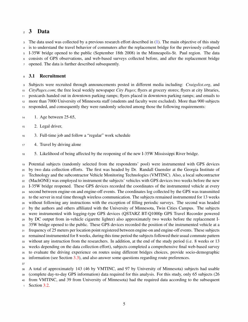
The data used was collected by a previous research effort described in (1). The main objective of this study3

is to understand the travel behavior of commuters after the replacement bridge for the previously collapsed4

I-35W bridge opened to the public (September 18th 2008) in the Minneapolis-St. Paul region. The data5

consists of GPS observations, and web-based surveys collected before, and after the replacement bridge6

opened. The data is further described subsequently.7

3.1 Recruitment8

Subjects were recruited through announcements posted in different media including: Craigslist.org, and9

CityPages.com; the free local weekly newspaper City Pages; flyers at grocery stores; flyers at city libraries,10

postcards handed out in downtown parking ramps; flyers placed in downtown parking ramps; and emails to11

more than 7000 University of Minnesota staff (students and faculty were excluded). More than 900 subjects12

responded, and consequently they were randomly selected among those the following requirements:13

1. Age between 25-65,14

2. Legal driver,15

3. Full-time job and follow a “regular” work schedule16

4. Travel by driving alone17

5. Likelihood of being affected by the reopening of the new I-35W Mississippi River bridge.18

Potential subjects (randomly selected from the respondents’ pool) were instrumented with GPS devices19

by two data collection efforts. The first was headed by Dr. Randall Guensler at the Georgia Institute of20

Technology and the subcontractor Vehicle Monitoring Technologies (VMTINC). Also, a local subcontractor21

(MachONE) was employed to instrument the subjects’ vehicles with GPS devices two weeks before the new22

I-35W bridge reopened. These GPS devices recorded the coordinates of the instrumented vehicle at every23

second between engine-on and engine-off events. The coordinates log collected by the GPS was transmitted24

to the server in real time through wireless communication. The subjects remained instrumented for 13 weeks25

without following any instructions with the exception of filling periodic surveys. The second was headed26

by the authors and others affiliated with the University of Minnesota, Twin Cities Campus. The subjects27

were instrumented with logging-type GPS devices (QSTARZ BT-Q1000p GPS Travel Recorder powered28

by DC output from in-vehicle cigarette lighter) also approximately two weeks before the replacement I-29

35W bridge opened to the public. These GPS devices recorded the position of the instrumented vehicle at a30

frequency of 25 meters per location point registered between engine-on and engine-off events. These subjects31

remained instrumented for 8 weeks, during this time period the subjects followed their usual commute pattern32

without any instruction from the researchers. In addition, at the end of the study period (i.e. 8 weeks or 1333

weeks depending on the data collection effort), subjects completed a comprehensive final web-based survey34

to evaluate the driving experience on routes using different bridges choices, provide socio-demographic35

information (see Section 3.3), and also answer some questions regarding route preferences.36

37

A total of approximately 143 (46 by VMTINC, and 97 by University of Minnesota) subjects had usable38

(complete day-to-day GPS information) data required for this analysis. For this study, only 65 subjects (2639

from VMTINC, and 39 from University of Minnesota) had the required data according to the subsequent40

Section 3.2.1

5

3.2 Methodology2

The data analysis process can be divided in three phases:3

1. Identification of morning commute trips per subject from GPS data on the bridges of interest (see4

Figure 1);5

2. Information extraction (e.g. travel time) of commute trips per subject from GPS and survey data;6

3. Specification and estimation of econometric models using the extracted information from GPS and7

from survey data.8

The first phase uses the coordinates (latitude and longitude) of the trips per subject, and the TLG network9

in order to identify the trips crossing bridges, and the bridges crossed. The TLG network refers to a digital10

map maintained by the Metropolitan Council and The Lawrence Group (TLG). It covers the entire 7-county11

Minneapolis-St. Paul Metropolitan Area and is the most accurate GIS map of this network to date. The12

TLG network contains 290,231 links, and provides an accurate depiction of the entire Minneapolis-St. Paul13

network at the street level. The identification is done by spatial matching the coordinates of each bridge14

of interest to the coordinates of each set of trips for each subject. Also, subjects’ trips must start at their15

home/work and end at their work/home locations in order to be considered commute trips (only direct com-16

mute trips). The distance tolerance between origins (destinations) to home (work) locations was set to 60017

meters. The home and work locations are geocoded (transformed into latitude and longitude coordinates)18

from the actual addresses provided by the subjects on the web-based surveys. The origin and destination19

pair of each trip is obtained by mapping the coordinate points into trajectories of engine-on and engine-off20

events. Moreover, inaccurate points due to GPS “noise”, and out-of-town trips (e.g. during Thanksgiving)21

were excluded. Also, only the trips after September 18th are considered as this is the date the new I-35W22

Bridge opened to the public at 5 AM. Lastly, only morning trips (those between 4 AM and 11 AM) are23

considered, because it is likely that subjects are not able to gather information from other non-commute trips24

during the morning, especially when the subjects drive directly from home to work without any side stops.25

26

The second phase extracts usable information from the matched trips such as: statistics of travel time distri-27

bution of all trips (e.g. mean, standard deviation, and others) for each subject from GPS data. This process28

is performed for home to work trips. This is further explained in section 4.29

30

The third phase is explained in section 4.1

6

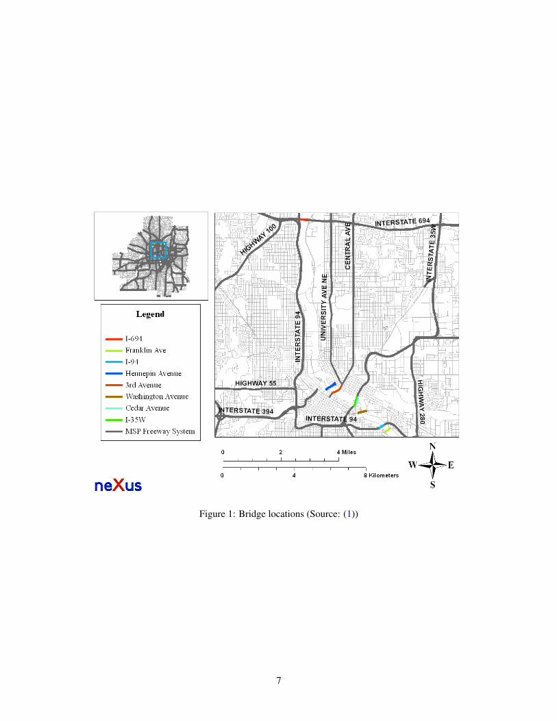
Figure 1: Bridge locations (Source: (1))

7

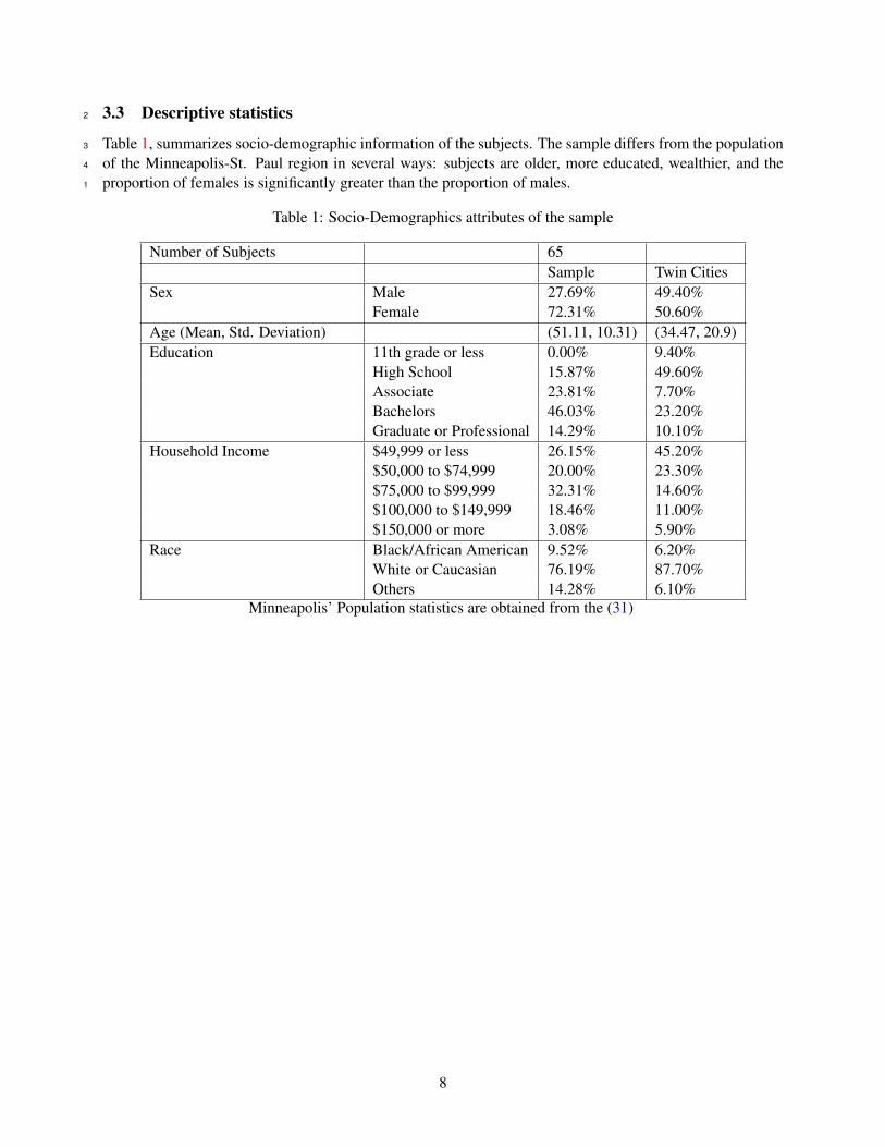
3.3 Descriptive statistics2

Table 1, summarizes socio-demographic information of the subjects. The sample differs from the population3

of the Minneapolis-St. Paul region in several ways: subjects are older, more educated, wealthier, and the4

proportion of females is significantly greater than the proportion of males.1

Table 1: Socio-Demographics attributes of the sample

Number of Subjects 65Sample Twin Cities

Sex Male 27.69% 49.40%Female 72.31% 50.60%

Age (Mean, Std. Deviation) (51.11, 10.31) (34.47, 20.9)Education 11th grade or less 0.00% 9.40%

High School 15.87% 49.60%Associate 23.81% 7.70%Bachelors 46.03% 23.20%Graduate or Professional 14.29% 10.10%

Household Income $49,999 or less 26.15% 45.20%$50,000 to $74,999 20.00% 23.30%$75,000 to $99,999 32.31% 14.60%$100,000 to $149,999 18.46% 11.00%$150,000 or more 3.08% 5.90%

Race Black/African American 9.52% 6.20%White or Caucasian 76.19% 87.70%Others 14.28% 6.10%

Minneapolis’ Population statistics are obtained from the (31)

8

4 Econometric models2

In this study, the data set is analyzed through duration analysis (also know as failure time analysis in op-3

erations research; hazard analysis in insurance and accident theory; and survival analysis in biostatistics)4

(32, 33, 34). The dependent variable is the single-spell duration per subject. This duration is defined as the5

date and time elapsed from September 18th 5:00 AM until the date and time a subject consistently leaves his6

current bridge choice for any other of those in figure 1 (transition is observed), or the date and time until the7

GPS device is retrieved from the subject, and the subject has not left his current bridge choice (transition8

is not observed). The term current bridge choice refers to the subject’s bridge choice at or after September9

18th 5:00 AM. The term consistently refers to a subject’s transition from his current bridge choice to another10

bridge at least two times consecutively. The term single-spell duration refers to modeling only one single11

transition from the current bridge choice to any other of those in figure 1. This single transition is only the12

first transition observed in the subjects’ GPS data. In the data set, there are only 65 subjects, and only 6513

single-spell transitions (one single-spell observation per subject). There are 835 observations, and on average14

12.84 observations per subject. In addition, subjects are observed on average for 32.06 days, and 34 subjects15

are observed to consistently transition from their current bridge choice to another bridge of those in figure 1.16

Also, the order of the events (i.e. different observed days and times of subjects’ trips) of the single-spell17

duration per subject is known to the minute (year, month, day, hour, and minutes).18

4.1 Duration models19

4.1.1 Cox Proportional Hazard model20

Duration models, similar to other econometric models, may have nonparametric, semi-parametric, and/or21

parametric models for the dependent variable. The Cox Proportional Hazard (hereafter referred as Cox22

PH) model is a semi-parametric model that assumes the hazard function (conditional on the parameters and23

covariates; h(t|β, x)) is factored into two separate functions (proportional hazards assumption).24

h(t|β, x) = h0(t)φ(x, β) (1)

h0(t) is known as the baseline hazard, and φ(x, β) is known as the relative hazard. The baseline hazard is25

a function of the date, and time of transition, and its functional form is left unspecified. The shape of the26

baseline hazard function depends on the data, and it is not assumed as in fully parametric models. The base-27

line hazard function is estimated using a nonparametric product limit estimator similar to the Kaplan-Meier28

estimator (32, 34). This is further explained in section 4.1.4. The relative hazard is a nonnegative function29

(i.e. hazard rates cannot be negative) that is fully specified by the researcher. The common functional form30

of φ(x, β) is the exponential (φ(x, β) = eβT x; β is a vector of coefficients, and x are the vectors of covariates31

in the regressors matrix). The relative hazard is estimated by maximizing a Partial Likelihood function. This32

is further explained in section 4.1.4. For this study, the hazard rate is33

h(t|β, x) = h0(t)eβT x (2)

The basic assumption of the Cox PH’s hazard function is that all subjects have the same baseline hazard34

function (h0(t)), and the relative hazard (φ(x, β)) has a multiplicative effect on the baseline hazard depending35

on the values of the covariates. In other words, one subject’s hazard function is a multiplicative version of36

another subject’s hazard function. This is the proportional hazards assumption, and it is statistically tested37

for the data set of this study. This is further explained in section 4.1.3 along with other statistical tests.38

9

Furthermore, the Cox PH model may be adjusted to consider: tied observations; and censorship of single-1

spell durations. The tied observations refer to the lack of information with regards to the order of the subjects2

that transition at the same date, and time in the data set. The order matters as it is required for the estimation3

of Cox PH model. In this study, there are no ties as the order of the events (i.e. different observed days and4

times of subjects’ trips) of the single-spell duration per subject is known to the minute (year, month, day,5

hour, and minutes). The censorship (or more precisely right-censorship) of single-spell durations refer to6

the researchers not observing the transition of the subjects. An observed transition is defined as a subject7

consistently leaving his current bridge choice for any other of those in figure 1. A unobserved transition8

is a subject not leaving his current bridge choice before the GPS device is retrieved from the subject. In9

other words, the study ends before a transition is observed. Readers should remember that the term current10

bridge choice refers to the subject’s bridge choice at or after September 18th 5:00 AM. In this study, there11

are 34 subjects (out of a total of 65 subjects) are observed to consistently transition (i.e. at least two times12

consecutively) from their current bridge choice to another bridge of those in figure 1. In contrast, there are13

31 subjects with unobserved transition. It is assumed that the censorship mechanism is independent from14

the single-spell duration of the subjects. This is a fair assumption given that the time that a GPS device is15

retrieved from a subject did not depend on whether a subject changed bridge choices or not, but rather on the16

fixed time duration of the study (i.e. 8 or 13 weeks depending on the data collection effort; see section 3.1).17

4.1.2 Relative hazard: covariates18

The selection of the covariates in the relative hazard function is based on two major groups: characteristics19

of the subjects; and travel time measures. The characteristic of the subjects are obtained from web-based20

survey data, and GPS data. The travel time measures are calculated on travel times obtained from GPS data.21

Readers may refer to section 3.2 for details. In addition, there are two types of covariates: time-invariant (y);22

and time-dependent (z(t)). Thus, the relative hazard is given by23

φ(y, z(t);βx, βz) = eβTy y+β

Tz z(t) (3)

βy, and βz are vector of coefficients to be estimated. y is a vector of time-invariant covariates (only change24

across subjects, and not across subjects’ day-to-day morning commute trips). z(t) is a vector of time-25

dependent covariates (the values vary across subjects’ day-to-day morning commute trips).26

The time-invariant covariates (x) are:27

• y1: Past bridge diversity.28

• y2: Gender.29

• y3: Income.30

• y4: Ratio of bridge distances (current bridge choice to previous bridge choice).31

• y5: Fear of driving on the I-35W bridge and other bridges in the vicinity.32

Past bridge diversity (y1)33

34

The number of distinct alternatives (bridges) a subject used for his morning commute trip before September35

18th 5:00 AM. This covariate is an indication of a subject’s knowledge of alternative bridges before traveling36

each day from September 18th 5:00 AM until the subject decided to change to another bridge alternative.37

10

1

Gender (y2)2

3

It is a binary variable; 1 = Male; 0 = Female.4

Income (y3)5

6

It is a set of two three binary variables: Low income (($0, $49, 999]), Medium income (($50, 000, $99, 999]).7

and High income (($100, 000,∞+)]). The first category is the base case (2008 US dollars).8

9

Ratio of bridge distances (current bridge choice to previous bridge choice; y4)10

11

It is the ratio of Euclidean distances. The numerator is the Euclidean distance from a subject’s home location12

to the centroid of the current bridge choice, and from this centroid to the subject’s work location. The denom-13

inator is the euclidean distance from a subject’s home location to the centroid of the previous bridge choice,14

and from this centroid to the subject’s work location. The term current bridge choice refers to the subject’s15

bridge choice at or after September 18th 5:00 AM. The term previous bridge choice refers to the subject’s16

bridge choice with the highest number of trips before September 18th 5:00 AM. This covariate measures a17

relative impedance of distance between the current bridge, and an alternative bridge highly preferred in the18

past by the subject.19

20

Fear of driving on the I-35W bridge and other bridges in the vicinity (y5)21

22

It is a binary variable. This variable identifies the subjects that admitted they avoid bridges (including the23

I-35W bridge, Washington Ave bridge, and 10th Street bridge), because of fear of bridge collapse or any24

other reason in the web-based surveys.25

26

The time-dependent covariates (z(t)) are the following travel time measures:27

• z1(t): Fixed thresholds28

• z2(t): Moving thresholds29

• z3(t): Travel times from the previous most used bridge30

Travel time measures31

32

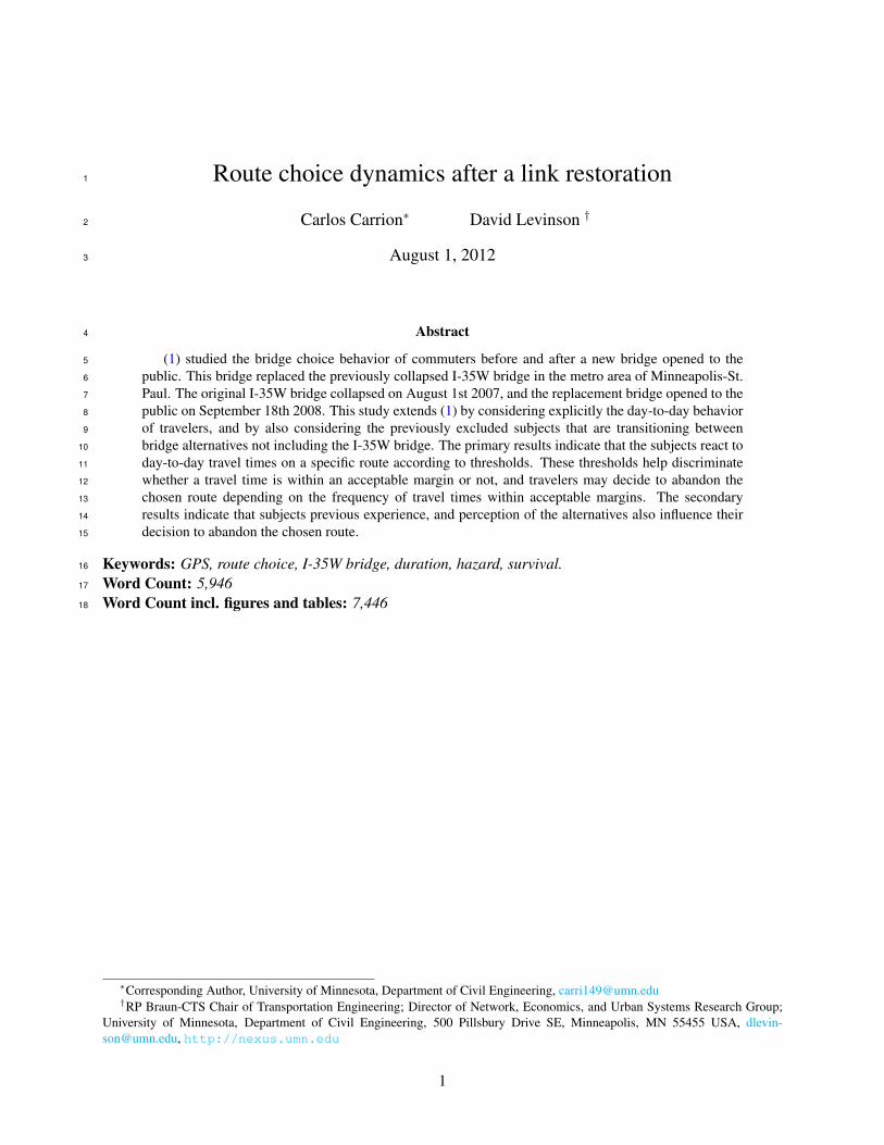
In this study, the authors hypothesize that the subjects only consider a subset of their travel times, and that33

the subjects only recall every few days a portion of the travel times in this subset. In addition, the travel34

times in this subset are continuously updated according to thresholds set by the subjects. Figure 2a presents35

the day to day travel times of a subject in the sample. A (epanechnikov; 5.29 bandwidth) kernel weighted36

local polynomial smoother with its 95% confidence interval (see (32)) is fitted to the day to day travel times37

to further elucidate the trend across days. The smoother indicates that the travel times are constantly in flux38

until they finally increase significantly. Therefore, it must be asked how do travelers react to the trend and39

volatility of the observed travel time time series. It is reasonable given the perception of travelers that only40

certain travel times have weight in influencing the choices of travelers. In other words, travel times across41

days that are closely similar (e.g. 20 minutes, and 24 minutes) may not be as noticeable to the traveler in42

comparison to travel times across days that are quite dissimilar (e.g. 20 minutes and 35 minutes). Thus,43

11

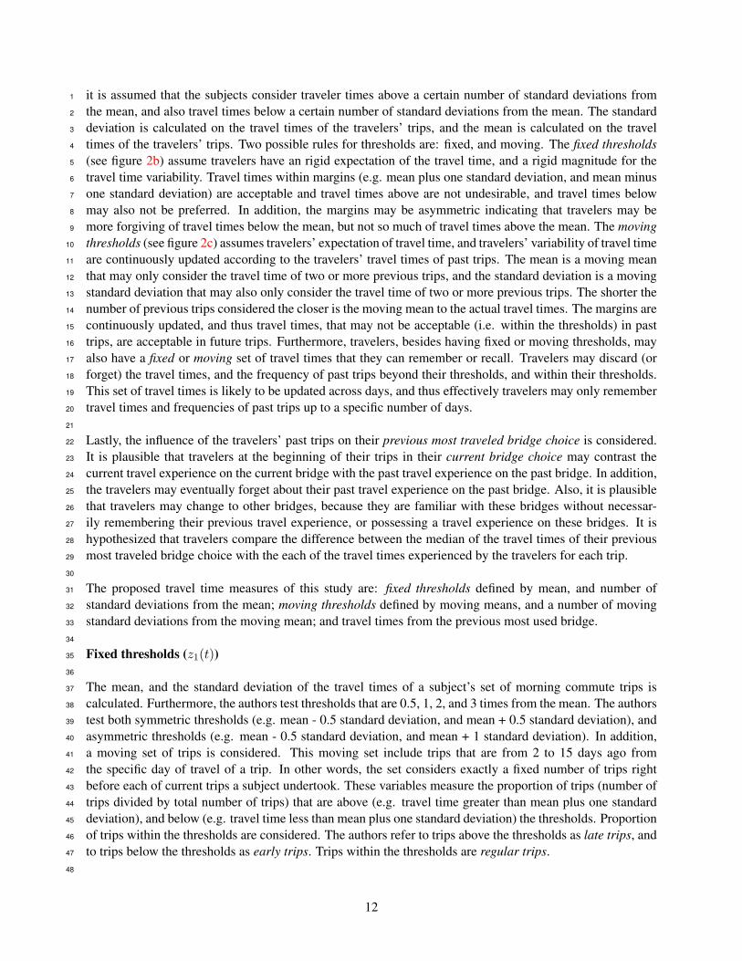
it is assumed that the subjects consider traveler times above a certain number of standard deviations from1

the mean, and also travel times below a certain number of standard deviations from the mean. The standard2

deviation is calculated on the travel times of the travelers’ trips, and the mean is calculated on the travel3

times of the travelers’ trips. Two possible rules for thresholds are: fixed, and moving. The fixed thresholds4

(see figure 2b) assume travelers have an rigid expectation of the travel time, and a rigid magnitude for the5

travel time variability. Travel times within margins (e.g. mean plus one standard deviation, and mean minus6

one standard deviation) are acceptable and travel times above are not undesirable, and travel times below7

may also not be preferred. In addition, the margins may be asymmetric indicating that travelers may be8

more forgiving of travel times below the mean, but not so much of travel times above the mean. The moving9

thresholds (see figure 2c) assumes travelers’ expectation of travel time, and travelers’ variability of travel time10

are continuously updated according to the travelers’ travel times of past trips. The mean is a moving mean11

that may only consider the travel time of two or more previous trips, and the standard deviation is a moving12

standard deviation that may also only consider the travel time of two or more previous trips. The shorter the13

number of previous trips considered the closer is the moving mean to the actual travel times. The margins are14

continuously updated, and thus travel times, that may not be acceptable (i.e. within the thresholds) in past15

trips, are acceptable in future trips. Furthermore, travelers, besides having fixed or moving thresholds, may16

also have a fixed or moving set of travel times that they can remember or recall. Travelers may discard (or17

forget) the travel times, and the frequency of past trips beyond their thresholds, and within their thresholds.18

This set of travel times is likely to be updated across days, and thus effectively travelers may only remember19

travel times and frequencies of past trips up to a specific number of days.20

21

Lastly, the influence of the travelers’ past trips on their previous most traveled bridge choice is considered.22

It is plausible that travelers at the beginning of their trips in their current bridge choice may contrast the23

current travel experience on the current bridge with the past travel experience on the past bridge. In addition,24

the travelers may eventually forget about their past travel experience on the past bridge. Also, it is plausible25

that travelers may change to other bridges, because they are familiar with these bridges without necessar-26

ily remembering their previous travel experience, or possessing a travel experience on these bridges. It is27

hypothesized that travelers compare the difference between the median of the travel times of their previous28

most traveled bridge choice with the each of the travel times experienced by the travelers for each trip.29

30

The proposed travel time measures of this study are: fixed thresholds defined by mean, and number of31

standard deviations from the mean; moving thresholds defined by moving means, and a number of moving32

standard deviations from the moving mean; and travel times from the previous most used bridge.33

34

Fixed thresholds (z1(t))35

36

The mean, and the standard deviation of the travel times of a subject’s set of morning commute trips is37

calculated. Furthermore, the authors test thresholds that are 0.5, 1, 2, and 3 times from the mean. The authors38

test both symmetric thresholds (e.g. mean - 0.5 standard deviation, and mean + 0.5 standard deviation), and39

asymmetric thresholds (e.g. mean - 0.5 standard deviation, and mean + 1 standard deviation). In addition,40

a moving set of trips is considered. This moving set include trips that are from 2 to 15 days ago from41

the specific day of travel of a trip. In other words, the set considers exactly a fixed number of trips right42

before each of current trips a subject undertook. These variables measure the proportion of trips (number of43

trips divided by total number of trips) that are above (e.g. travel time greater than mean plus one standard44

deviation), and below (e.g. travel time less than mean plus one standard deviation) the thresholds. Proportion45

of trips within the thresholds are considered. The authors refer to trips above the thresholds as late trips, and46

to trips below the thresholds as early trips. Trips within the thresholds are regular trips.47

48

12

Moving thresholds (z2(t))1

The moving mean, and the moving standard deviation of the travel times with distinct thresholds that are2

0.5, 1, 2, and 3 times from the moving mean are considered. The moving mean, and the moving standard3

deviation are calculated on a moving set that includes trips that are from 2 to 15 days ago from the specific day4

of travel of a trip. The moving set considers exactly a fixed number of trips right before each of current trips a5

subject undertook. These variables measure the proportion of trips (number of trips divided by total number6

of trips) that are above (e.g. travel time greater than moving mean plus one moving standard deviation),7

and below (e.g. travel time less than moving mean plus one moving standard deviation) the thresholds.8

Proportion of trips within the thresholds are considered. The authors refer to trips above the thresholds as9

late trips, and to trips below the thresholds as early trips. Trips within the thresholds are regular trips.10

11

Travel times from the previous most used bridge (z3(t))12

The bridge with the highest number of trips before September 18th 5:00 AM is identified. The median of13

the travel times of the different days a traveler used the bridge is calculated. The difference between this14

median, and each of the days travel times is computed. Furthermore, it is assumed that the coefficient of this15

time-dependent covariate is also time-dependent. Basically, the coefficient for the first week of travel of a16

subject in the current bridge choice is different from the coefficient after the first week of travel in the current17

bridge choice.18

19

4.1.3 Hypothesis testing and goodness of fit20

There are two hypothesis tests that are considered for the duration models in this study. For the nested21

models, the Wald tests are used as they only depend on the covariance matrix of the unrestricted models, and22

do not require estimation of the restricted models. These tests are asymptotically equivalent to the likelihood23

ratio tests. For the nonnested models, the Akaike information criterion (AIC), and Bayesian information24

criterion (BIC) are used in order to compare the statistical fit of the duration models with the different travel25

time measures proposed in section 4.1.2. See (35, 36, 37) for more details.26

27

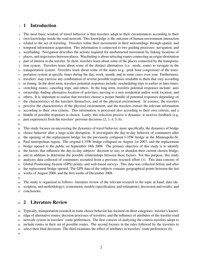
The goodness of fit of the models are checked with residual analysis (32). The Schoenfeld residuals (38, 39)28

are computed to test the proportional hazards assumption required for the Cox PH model, and the Deviance29

residuals (40) are examined to check the model accuracy, and identification of outliers.30

4.1.4 Estimation31

The estimation of the Cox PH model is done in two steps. The first step is the maximization of a Partial32

Likelihood function to obtain estimates of the coefficients, and the covariance matrix for the coefficients in33

the relative hazard function. The second is the maximization of a product limit estimator to obtain the hazard34

rate contributions given the estimates of the relative hazard. This estimator is a nonparametric Likelihood35

function. A thorough treatment is presented in (32, 34).36

37

The Partial Likelihood function for this study is38

L(βy, βz) =k∏j=1

eβTy yj+β

Tz zj(t)∑

m∈R(tj)eβ

Ty ym+βTz zm(t)

(4)

39

The k is the number of single-spell durations, and thus of subjects in this sample. There is an order of these40

single-spell durations (i.e. t1 < t2 < ... < tk). This order is present in the set R(tj). This is the set1

13

Figure 2: Thresholds-based behavior of travelers

(a) Day to day (GPS) travel times of a subject30

30

3035

35

3540

40

4045

45

4550

50

50Travel time (minutes)

Trav

el t

ime

(min

utes

)

Travel time (minutes)0

0

020

20

2040

40

4060

60

6080

80

80100

100

100Days after September 18th 2008

Days after September 18th 2008

Days after September 18th 200895% CI

95% CI

95% CIKernel Smoother: Travel time

Kernel Smoother: Travel time

Kernel Smoother: Travel timeTravel time (line)

Travel time (line)

Travel time (line)Travel time (scatter)

Travel time (scatter)


(b) Fixed thresholds30

30

3035

35

3540

40

4045

45

4550

50


Trav

el t

ime

(min

utes

)


0

020

20

2040

40

4060

60

6080

80

80100

100



Days after September 18th 2008Mean - 0.5 Std Dev

Mean - 0.5 Std Dev

Mean - 0.5 Std DevMean + 0.5 Std Dev

Mean + 0.5 Std Dev

Mean + 0.5 Std DevMean

Mean

MeanTravel time (line)

Travel time (line)




(c) Moving thresholds30

30

3035

35

3540

40

4045

45

4550

50


Trav

el t

ime

(min

utes

)


20

2040

40

4060

60

6080

80

80100

100



Days after September 18th 2008Mean - 0.5 Std Dev

Mean - 0.5 Std Dev

Mean - 0.5 Std DevMean + 0.5 Std Dev

Mean + 0.5 Std Dev

Mean + 0.5 Std DevMean (moving - 5)

Mean (moving - 5)

Mean (moving - 5)Travel time (line)

Travel time (line)




14

of single-spell durations that have transitioned at the order j, and that have not transitioned at the order j2

excluding those that already transitioned before the order j. Mathematically, this is R(tj) = {l : tl ≥ tj}.3

4

The nonparametric Likelihood function for this study is5

L(α; β̂y, β̂z) =k∏j=1

(α−eβ̂Ty yj+β̂

Tz zj(t)

j − 1)∏

m∈R(tj)

α−eβ̂Ty ym+β̂Tz zm(t)

j

(5)

6

The 1 − αj are the baseline hazard rate contributions at the order j. This nonparametric Likelihood func-7

tion allow the estimation of the Survivor function, and the contributions may be used to obtained a kernel8

smoothing function of the hazard rate function. This estimator is similar to the Kaplan-Meier estimator, but9

adjusted for the value of relative hazard’s covariates.10

11

The models are estimated using STATA (41). The plots are also obtained using STATA (42).12

5 Discussion and results13

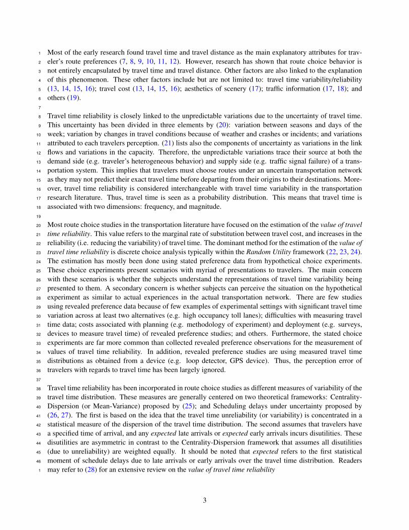
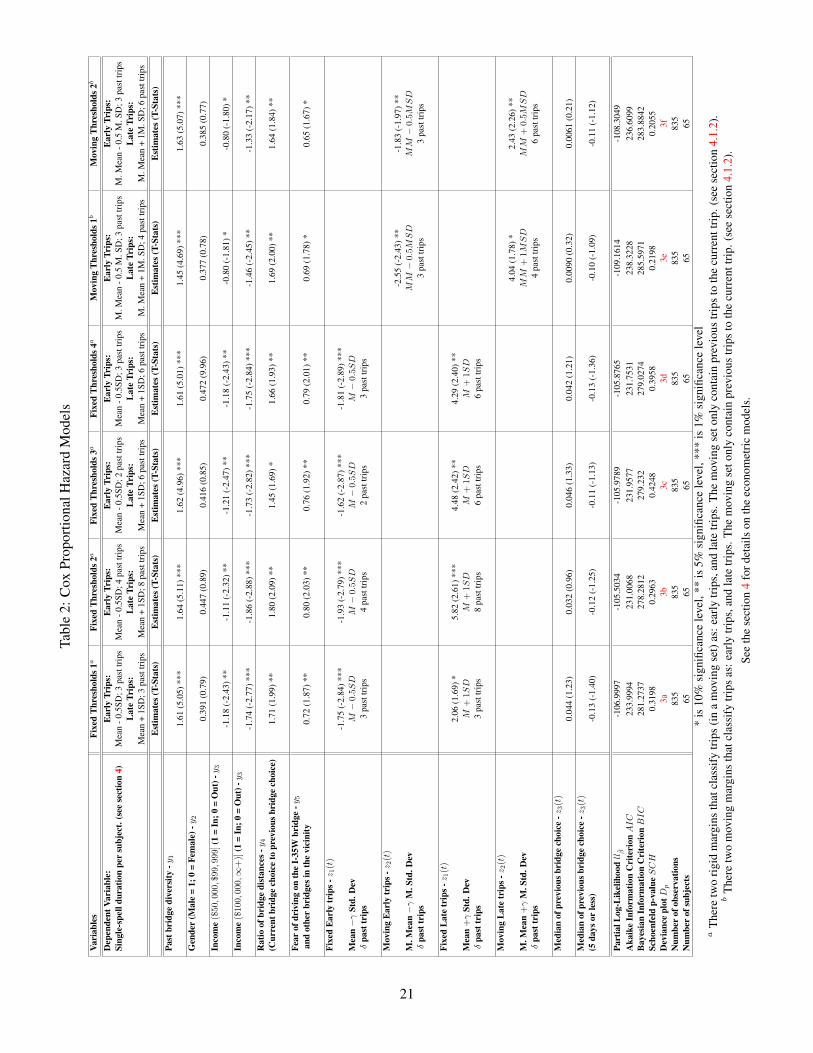
Table 2 presents the estimates of the relative hazard functions of the models, and figures 4a, 4b, and 4c14

present the estimates of the baseline cumulative hazard, baseline hazard rate function, and baseline survivor15

function for the Fixed Thresholds 2 model. There are two types of models: Fixed Thresholds, and Moving16

Thresholds. The Fixed Thresholds models assume subjects have a rigid expectation with regards to their17

travel times, and also have a rigid magnitude of the travel time variability. Subjects classify their experience18

trips whether they fall into the margins (i.e. regular trip, fall above the margins (i.e. late trip), and below19

the margins (early trip). The Moving Thresholds models assume subjects continuously update their margins20

based on previous past trips. Similar to the Fixed Thresholds models, subjects classify their experience trips21

whether they fall into the margins (i.e. regular trip, fall above the margins (i.e. late trip), and below the22

margins (early trip). Readers should refer to see section 4.1.2 for details. In addition, both Fixed Thresholds23

and Moving Thresholds assume that subjects have a moving set of travel times. The moving set of travel24

times refer to which travel times of past trips the subjects are able to recall. Furthermore, readers should25

remember that the dependent variable of the model is the single-spell duration (as defined in section 4) of26

the subjects in their current bridge until they decide to switch to another bridge or until their GPS devices27

are collected from their vehicles.28

29

For the models (Fixed Thresholds and Moving Thresholds), several combinations of distinct levels of stan-30

dard deviations (or moving standard deviations) from the mean (or moving mean), and of past trips in the31

moving set of travel times were tested. The results that were statistically significant are summarized in ta-32

ble 2. All the models find that the number of past trips for classifying early trips are less than four past trips.33

In contrast, the number of past trips for classifying late trips is greater than 3 past trips, and most of the time34

its value was found to be 6 past trips. This indicates that subjects were found to recall further in time travel35

experiences of greater travel times with respect to the mean (or moving mean) in comparison to travel experi-36

ences of smaller travel times with respect to the mean (or moving mean). In addition, 0.5 standard deviation37

(or moving standard deviation) from the mean (or moving mean) were found to be statistically significant38

at least 5% level for the margins classifying early trips. For the margins classifying late trips, 1 standard39

deviation (or moving standard deviations) from the mean (or moving mean) were found to be statistically40

significant at least 5%. This implies subjects have asymmetric margins for classifying a trip to be late or41

early. Also, subjects consider trips not too far below the mean (or moving mean) as early, but trips farther42

above the mean are considered as late. Thus, subjects are tolerate travel times that are above, but close to the1

15

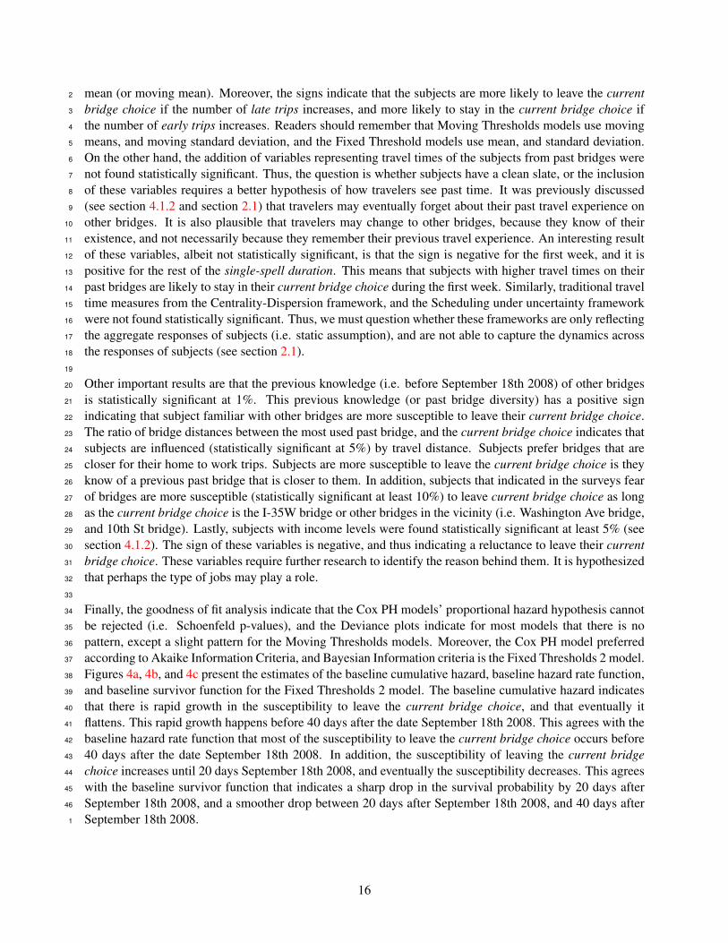
mean (or moving mean). Moreover, the signs indicate that the subjects are more likely to leave the current2

bridge choice if the number of late trips increases, and more likely to stay in the current bridge choice if3

the number of early trips increases. Readers should remember that Moving Thresholds models use moving4

means, and moving standard deviation, and the Fixed Threshold models use mean, and standard deviation.5

On the other hand, the addition of variables representing travel times of the subjects from past bridges were6

not found statistically significant. Thus, the question is whether subjects have a clean slate, or the inclusion7

of these variables requires a better hypothesis of how travelers see past time. It was previously discussed8

(see section 4.1.2 and section 2.1) that travelers may eventually forget about their past travel experience on9

other bridges. It is also plausible that travelers may change to other bridges, because they know of their10

existence, and not necessarily because they remember their previous travel experience. An interesting result11

of these variables, albeit not statistically significant, is that the sign is negative for the first week, and it is12

positive for the rest of the single-spell duration. This means that subjects with higher travel times on their13

past bridges are likely to stay in their current bridge choice during the first week. Similarly, traditional travel14

time measures from the Centrality-Dispersion framework, and the Scheduling under uncertainty framework15

were not found statistically significant. Thus, we must question whether these frameworks are only reflecting16

the aggregate responses of subjects (i.e. static assumption), and are not able to capture the dynamics across17

the responses of subjects (see section 2.1).18

19

Other important results are that the previous knowledge (i.e. before September 18th 2008) of other bridges20

is statistically significant at 1%. This previous knowledge (or past bridge diversity) has a positive sign21

indicating that subject familiar with other bridges are more susceptible to leave their current bridge choice.22

The ratio of bridge distances between the most used past bridge, and the current bridge choice indicates that23

subjects are influenced (statistically significant at 5%) by travel distance. Subjects prefer bridges that are24

closer for their home to work trips. Subjects are more susceptible to leave the current bridge choice is they25

know of a previous past bridge that is closer to them. In addition, subjects that indicated in the surveys fear26

of bridges are more susceptible (statistically significant at least 10%) to leave current bridge choice as long27

as the current bridge choice is the I-35W bridge or other bridges in the vicinity (i.e. Washington Ave bridge,28

and 10th St bridge). Lastly, subjects with income levels were found statistically significant at least 5% (see29

section 4.1.2). The sign of these variables is negative, and thus indicating a reluctance to leave their current30

bridge choice. These variables require further research to identify the reason behind them. It is hypothesized31

that perhaps the type of jobs may play a role.32

33

Finally, the goodness of fit analysis indicate that the Cox PH models’ proportional hazard hypothesis cannot34

be rejected (i.e. Schoenfeld p-values), and the Deviance plots indicate for most models that there is no35

pattern, except a slight pattern for the Moving Thresholds models. Moreover, the Cox PH model preferred36

according to Akaike Information Criteria, and Bayesian Information criteria is the Fixed Thresholds 2 model.37

Figures 4a, 4b, and 4c present the estimates of the baseline cumulative hazard, baseline hazard rate function,38

and baseline survivor function for the Fixed Thresholds 2 model. The baseline cumulative hazard indicates39

that there is rapid growth in the susceptibility to leave the current bridge choice, and that eventually it40

flattens. This rapid growth happens before 40 days after the date September 18th 2008. This agrees with the41

baseline hazard rate function that most of the susceptibility to leave the current bridge choice occurs before42

40 days after the date September 18th 2008. In addition, the susceptibility of leaving the current bridge43

choice increases until 20 days September 18th 2008, and eventually the susceptibility decreases. This agrees44

with the baseline survivor function that indicates a sharp drop in the survival probability by 20 days after45

September 18th 2008, and a smoother drop between 20 days after September 18th 2008, and 40 days after46

September 18th 2008.1

16

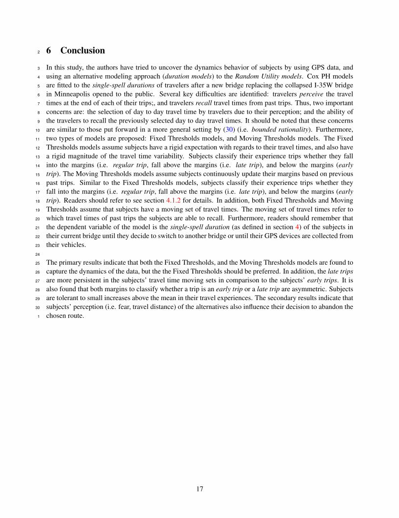
6 Conclusion2

In this study, the authors have tried to uncover the dynamics behavior of subjects by using GPS data, and3

using an alternative modeling approach (duration models) to the Random Utility models. Cox PH models4

are fitted to the single-spell durations of travelers after a new bridge replacing the collapsed I-35W bridge5

in Minneapolis opened to the public. Several key difficulties are identified: travelers perceive the travel6

times at the end of each of their trips;, and travelers recall travel times from past trips. Thus, two important7

concerns are: the selection of day to day travel time by travelers due to their perception; and the ability of8

the travelers to recall the previously selected day to day travel times. It should be noted that these concerns9

are similar to those put forward in a more general setting by (30) (i.e. bounded rationality). Furthermore,10

two types of models are proposed: Fixed Thresholds models, and Moving Thresholds models. The Fixed11

Thresholds models assume subjects have a rigid expectation with regards to their travel times, and also have12

a rigid magnitude of the travel time variability. Subjects classify their experience trips whether they fall13

into the margins (i.e. regular trip, fall above the margins (i.e. late trip), and below the margins (early14

trip). The Moving Thresholds models assume subjects continuously update their margins based on previous15

past trips. Similar to the Fixed Thresholds models, subjects classify their experience trips whether they16

fall into the margins (i.e. regular trip, fall above the margins (i.e. late trip), and below the margins (early17

trip). Readers should refer to see section 4.1.2 for details. In addition, both Fixed Thresholds and Moving18

Thresholds assume that subjects have a moving set of travel times. The moving set of travel times refer to19

which travel times of past trips the subjects are able to recall. Furthermore, readers should remember that20

the dependent variable of the model is the single-spell duration (as defined in section 4) of the subjects in21

their current bridge until they decide to switch to another bridge or until their GPS devices are collected from22

their vehicles.23

24

The primary results indicate that both the Fixed Thresholds, and the Moving Thresholds models are found to25

capture the dynamics of the data, but the the Fixed Thresholds should be preferred. In addition, the late trips26

are more persistent in the subjects’ travel time moving sets in comparison to the subjects’ early trips. It is27

also found that both margins to classify whether a trip is an early trip or a late trip are asymmetric. Subjects28

are tolerant to small increases above the mean in their travel experiences. The secondary results indicate that29

subjects’ perception (i.e. fear, travel distance) of the alternatives also influence their decision to abandon the30

chosen route.1

17

References2

[1] C. Carrion and D. Levinson. A model of bridge choice across the mississippi river in minneapolis.3

In D. Levinson, H. Liu, and M. Bell, editors, Network Reliability in Practice: Selected papers from4

the fourth international symposium on transportation network reliability, chapter 8, pages 115–129.5

Springer, 2012.6

[2] R.G. Golledge and R.J. Stimson. Spatial behavior. Guilford Press, New York, 1997.7

[3] R. Golledge. Human wayfinding and cognitive maps. In Wayfinding Behavior: Cognitive Mapping and8

Other Spatial Processes, pages 5–45. John Hopkins, 1999.9

[4] R. Golledge. Place recognition and wayfinding: Making sense of space. Geoforum, 23:199–214, 1992.10

[5] P. Bovy and E. Stern. Route Choice: Wayfinding in Transport Networks. Kluwer Academic Publishers,11

Netherlands, 1990.12

[6] M. Ben-Akiva, MJ Bergman, AJ Daly, and R. Ramaswamy. Modelling inter urban route choice be-13

haviour. In Proceedings of the Ninth International Symposium on Transportation and Traffic Theory,14

Delft, the Netherland, pages 299–330, 1984.15

[7] D. L. Trueblood. Effect of travel time and distance on freeway usage. Highway Research Board, (61):16

18–37, 1952.17

[8] R. D. Michaels. Attitudes of drivers toward alternative highways and their relation to route choice.18

Highway Research Record, (122):50–74, 1966.19

[9] K. J. Kansky. Travel patterns of urban residents. Transportation Science, 1(4):261–285, 1967.20

[10] L. E. Haefner and L. V. Dickinson. Preliminary analysis of disaggregate modeling in route choice.21

Transportation Research Record, (527):66–72, 1974.22

[11] R. Hamerslag. Investigation into factors affecting the route choice in rijnstreek-west with the aid of a23

disaggregate logit model. Transportation, 10(4):373–391, 1981.24

[12] M. Vaziri and T. N. Lam. Perceived factors affecting driver route decisions. Journal of Transportation25

Engineering, 109(2):297311, 1983.26

[13] N. Tilahun and D. Levinson. A moment of time: Reliability in route choice using stated preference.27

Journal of Intelligent Transportation Systems, 14(3):179 –187, 2010.28

[14] K.A. Small, C. Winston, and J. Yan. Uncovering the distribution of motorists’ preferences for travel29

time and reliability. Econometrica, 73(4):1367–1382, 2005.30

[15] K.A. Small, C. Winston, and J. Yan. Differentiated road pricing, express lanes, and carpools: Exploiting31

heterogeneous preferences in policy design. Brookings-Wharton Papers on Urban Affairs, 7:53–96,32

2006.33

[16] C. Carrion and D. Levinson. Value of reliability: High occupancy toll lanes, general purpose lanes,34

and arterials. In Conference Proceedings of 4th International Symposium on Tranportation Network35

Reliability in Minneapolis, MN (USA), 2010.36

[17] L. Zhang and D. Levinson. Determinants of route choice and the value of traveler information: A field37

experiment. Transportation Research Record: Journal of the Transportation Research Board, 2086:38

81–92, 2008.1

18

[18] M.A. Abdel-Aty, R. Kitamura, and P.P. Jovanis. Using stated preference data for studying the effect2

of advanced traffic information on drivers’ route choice. Transportation Research Part C, 5(1):39–50,3

1997.4

[19] A. Pal. Modeling of commuter’s route choice behavior. Master’s thesis, The University of Toledo5

(USA), 2004.6

[20] HK Wong and JM Sussman. Dynamic travel time estimation on highway networks. Transportation7

Research, 7:355–370, 1973.8

[21] A. Nicholson and ZP Du. Degradable transportation systems: an integrated equilibrium model. Trans-9

portation Research Part B, 31(3):209–223, 1997.10

[22] K. Train. Discrete choice methods with simulation. Cambridge University Press, 2nd edition, 2009.11

[23] J. Ortuzar and L. Willumsen. Modelling Transport. Wiley, 4th edition, 2011.12

[24] M. Ben-Akiva and S. Lerman. Discrete choice analysis: theory and application to travel demand. MIT13

Press, 1985.14

[25] W. Jackson and J Jucker. An empirical study of travel time variability and travel choice behavior.15

Transportation Science, 16(4):460–475, 1982.16

[26] K.A. Small. The scheduling of consumer activities: Work trips. American Economic Review, 72(3):17

467–479, 1982.18

[27] RB Noland and KA Small. Travel-time uncertainty, departure time choice, and the cost of morning19

commutes. Transportation Research Record, 1493:150–158, 1995.20

[28] C. Carrion and D. Levinson. Value of reliability: A review of the current evidence. Transportation21

Research Part A, 46(4):720–741, 2012.22

[29] T. Domencich and D. McFadden. Urban Travel Demand-A Behavioral Analysis. North Holland., 1975.23

[30] H. Simon. Models of bounded rationality: empirically grounded economic reason, volume 3. MIT24

Press, 1997.25

[31] 2006-2008 american community survey 3-year estimates, minneapolis-st. paul-bloomington, mn-wi26

metropolitan statistical area, retrieved november 25, 2009. URL http://factfinder.census.27

gov/.28

[32] A. C. Cameron and P. K. Trivedi. Microeconometrics: Methods and Applications. Cambridge Univ.29

Press, 2005.30

[33] J. Wooldridge. Econometric Analysis of Cross Section and Panel Data. MIT Press, 2nd edition, 2010.31

[34] J. Kalbfleisch and R. Prentice. The statistical analysis of failure time data. Wiley, 2nd edition, 2002.32

[35] J. Johnston and J. DiNardo. Econometric methods. McGraw-Hill, 1997.33

[36] W. Greene. Econometric Analysis. Prentice-Hall, 7th edition, 2012.34

[37] J. Cramer. Econometric applications of Maximum Likelihood methods. Cambridge Univ. Press, 1986.1

19

http://factfinder.census.gov/



[38] P. Grambsch and T. Therneau. Proportional hazards tests and diagnostics based on weighted residuals.2

Biometrika, 81:515–526, 1994.3

[39] D. Schoenfeld. Partial residuals for the proportional hazards regression model. Biometrika, 69:239–4

241, 1982.5

[40] D. Collett. Modelling Survival Data in Medical Research. Chapman and Hall, 2nd edition, 2003.6

[41] M. Cleves, R. Gutierrez, W. Gould, and Y. Marchenko. An Introduction to Survival Analysis using7

STATA. Stata Press, 3rd edition, 2010.8

[42] M. Mitchell. A Visual Guide to STATA Graphics. Stata Press, 2nd edition, 2008.631

20

Tabl

e2:

Cox

Prop

ortio

nalH

azar

dM

odel

s

Vari

able

sFi

xed

Thr

esho

lds1

aFi

xed

Thr

esho

lds2

aFi

xed

Thr

esho

lds3

aFi

xed

Thr

esho

lds4

aM

ovin

gT

hres

hold

s1b

Mov

ing

Thr

esho

lds2

b

Dep

ende

ntVa

riab

le:

Ear

lyTr

ips:

Ear

lyTr

ips:

Ear

lyTr

ips:

Ear

lyTr

ips:

Ear

lyTr

ips:

Ear

lyTr

ips:

Sing

le-s

pell

dura

tion

per

subj

ect.

(see

sect

ion

4)M

ean

-0.5

SD;3

past

trip

sM

ean

-0.5

SD;4

past

trip

sM

ean

-0.5

SD;2

past

trip

sM

ean

-0.5

SD;3

past

trip

sM

.Mea

n-0

.5M

.SD

;3pa

sttr

ips

M.M

ean

-0.5

M.S

D;3

past

trip

sL

ate

Trip

s:L

ate

Trip

s:L

ate

Trip

s:L

ate

Trip

s:L

ate

Trip

s:L

ate

Trip

s:M

ean

+1S

D;3

past

trip

sM

ean

+1S

D;8

past

trip

sM

ean

+1S

D;6

past

trip

sM

ean

+1S

D;6

past

trip

sM

.Mea

n+

1M.S

D;4

past

trip

sM

.Mea

n+

1M.S

D;6

past

trip

sE

stim

ates

(T-S

tats

)E

stim

ates

(T-S

tats

)E

stim

ates

(T-S

tats

)E

stim

ates

(T-S

tats

)E

stim

ates

(T-S

tats

)E

stim

ates

(T-S

tats

)Pa

stbr

idge

dive

rsity

-y1

1.61

(5.0

5)**

*1.

64(5

.11)

***

1.62

(4.9

6)**

*1.

61(5

.01)

***

1.45

(4.6

9)**

*1.

63(5

.07)

***

Gen

der

(Mal

e=

1;0

=Fe

mal

e)-y

2

0.39

1(0

.79)

0.44

7(0

.89)

0.41

6(0

.85)

0.47

2(9

.96)

0.37

7(0

.78)

0.38

5(0

.77)

Inco

me

($50,0

00,$

99,9

99](

1=

In;0

=O

ut)-y 3

-1.1

8(-

2.43

)**

-1.1

1(-

2.32

)**

-1.2

1(-

2.47

)**

-1.1

8(-

2.43

)**

-0.8

0(-

1.81

)*-0

.80

(-1.

80)*

Inco

me

($10

0,00

0,∞

+)]

(1=

In;0

=O

ut)-y 3

-1.7

4(-

2.77

)***

-1.8

6(-

2.88

)***

-1.7

3(-

2.82

)***

-1.7

5(-

2.84

)***

-1.4

6(-

2.45

)**

-1.3

3(-

2.17

)**

Rat

ioof

brid

gedi

stan

ces-y 4

(Cur

rent

brid

gech

oice

topr

evio

usbr

idge

choi

ce)

1.71

(1.9

9)**

1.80

(2.0

9)**

1.45

(1.6

9)*

1.66

(1.9

3)**

1.69

(2.0

0)**

1.64

(1.8

4)**

Fear

ofdr

ivin

gon

the

I-35

Wbr

idge

-y5

and

othe

rbr

idge

sin

the

vici

nity

0.72

(1.8

7)**

0.80

(2.0

3)**

0.76

(1.9

2)**

0.79

(2.0

1)**

0.69

(1.7

8)*

0.65

(1.6

7)*

Fixe

dE

arly

trip

s-z 1

(t)

-1.7

5(-

2.84

)***

-1.9

3(-

2.79

)***

-1.6

2(-

2.87

)***

-1.8

1(-

2.89

)***

Mea

n−γ

Std.

Dev

M−

0.5SD

M−

0.5SD

M−

0.5SD

M−

0.5SD

δpa

sttr

ips

3pa

sttr

ips

4pa

sttr

ips

2pa

sttr

ips

3pa

sttr

ips

Mov

ing

Ear

lytr

ips-z 2

(t)

-2.5

5(-

2.43

)**

-1.8

3(-

1.97

)**

M.M

ean−γ

M.S

td.D

evMM−

0.5M

SD

MM−

0.5M

SD

δpa

sttr

ips

3pa

sttr

ips

3pa

sttr

ips

Fixe

dL

ate

trip

s-z 1

(t)

2.06

(1.6

9)*

5.82

(2.6

1)**

*4.

48(2

.42)

**4.

29(2

.40)

**M

ean

+γ

Std.

Dev

M+

1SD

M+

1SD

M+

1SD

M+

1SD

δpa

sttr

ips

3pa

sttr

ips

8pa

sttr

ips

6pa

sttr

ips

6pa

sttr

ips

Mov

ing

Lat

etr

ips-z 2

(t)

4.04

(1.7

8)*

2.43

(2.2

6)**

M.M

ean

+γ

M.S

td.D

evMM

+1M

SD

MM

+0.

5MSD

δpa

sttr

ips

4pa

sttr

ips

6pa

sttr

ips

Med

ian

ofpr

evio

usbr

idge

choi

ce-z

3(t

)0.

044

(1.2

3)0.

032

(0.9

6)0.

046

(1.3

3)0.

042

(1.2

1)0.

0090

(0.3

2)0.

0061

(0.2

1)M

edia

nof

prev

ious

brid

gech

oice

-z3(t

)(5

days

orle

ss)

-0.1

3(-

1.40

)-0

.12

(-1.

25)

-0.1

1(-

1.13

)-0

.13

(-1.

36)

-0.1

0(-

1.09

)-0

.11

(-1.

12)

Part

ialL

og-L

ikel

ihoo

dllβ̂

-106

.999

7-1

05.5

034

-105

.978

9-1

05.8

765

-109

.161

4-1

08.3

049

Aka

ike

Info

rmat

ion

Cri

teri

onAIC

233.

9994

231.

0068

231.

9577

231.

7531

238.

3228

236.

6099

Bay

esia

nIn

form

atio

nC

rite

rion

BIC

281.

2737

278.

2812

279.

232

279.

0274

285.

5971

283.

8842

Scho

enfe

ldp-

valu

eSCH

0.31

980.

2963

0.42

480.

3958

0.21

980.

2055

Dev

ianc

epl

otDp

3a3b

3c3d

3e3f

Num

ber

ofob

serv

atio

ns83

583

583

583

583

583

5N

umbe

rof

subj

ects

6565

6565

6565

*is

10%

sign

ifica

nce

leve

l,**

is5%

sign

ifica

nce

leve

l,**

*is

1%si

gnifi

canc

ele

vel

aT

here

two

rigi

dm

argi

nsth

atcl

assi

fytr

ips

(in

am

ovin

gse

t)as

:ear

lytr

ips,

and

late

trip

s.T

hem

ovin

gse

tonl

yco

ntai

npr

evio

ustr

ips

toth

ecu

rren

ttri

p.(s

eese

ctio

n4.

1.2)

.b

The

retw

om

ovin

gm

argi

nsth

atcl

assi

fytr

ips

as:e

arly

trip

s,an

dla

tetr

ips.

The

mov

ing

seto

nly

cont

ain

prev

ious

trip

sto

the

curr

entt

rip.

(see

sect

ion

4.1.

2).

See

the

sect

ion

4fo

rdet

ails

onth

eec

onom

etri

cm

odel

s.

21

Figure 3: Deviance residuals plots

(a) Deviance Plot - Fixed Thresholds 1-2

-2

-2-1

-1

-10

0

01

1

12

2

2Deviance residual

Devi

ance

resid

ual

Deviance residual0

0

02

2

24

4

46

6

6Natural log of Hazard rate contributions

Natural log of Hazard rate contributions

Natural log of Hazard rate contributions(b) Deviance Plot - Fixed Thresholds 2

-2

-2

-2-1

-1

-10

0

01

1

12

2

2Deviance residual

Devi

ance

resid

ual

Deviance residual0

0

02

2

24

4

46

6




(c) Deviance Plot - Fixed Thresholds 3-2

-2

-2-1

-1

-10

0

01

1

12

2

2Deviance residual

Devi

ance

resid

ual

Deviance residual0

0

02

2

24

4

46

6



Natural log of Hazard rate contributions(d) Deviance Plot - Fixed Thresholds 4

-2-2

-2-1-1

-100

011

122

2Deviance residualDe

vian

ce re

sidua

lDeviance residual0

0

02

2

24

4

46

6




(e) Deviance Plot - Moving Thresholds 1-2

-2

-2-1

-1

-10

0

01

1

12

2

2Deviance residual

Devi

ance

resid

ual

Deviance residual0

0

02

2

24

4

46

6



Natural log of Hazard rate contributions(f) Deviance Plot - Moving Thresholds 2

-2

-2

-2-1

-1

-10

0

01

1

12

2

2Deviance residual

Devi

ance

resid

ual

Deviance residual1

1

12

2

23

3

34

4

45

5

56

6




22

Figure 4: Baseline functions

(a) Baseline cumulative hazard - Fixed Thresholds 20

0

0.2

.2

.2.4

.4

.4.6

.6

.6.8

.8

.8Cumulative Baseline Hazard

Cum

ulat

ive

Base

line

Haza

rd

Cumulative Baseline Hazard0

0

020

20

2040

40

4060

60

6080

80

80100

100



Days after September 18th 2008(b) Smoothed baseline hazard function - Fixed Thresholds 2

0

0

0.005

.005

.005.01

.01

.01.015

.015

.015.02

.02

.02Smoothed Baseline Hazard Function

Smoo

thed

Bas

elin

e Ha

zard

Fun

ctio

n

Smoothed Baseline Hazard Function10

10

1020

20

2030

30

3040

40

4050

50

5060

60




(c) Baseline survivor function - Fixed Thresholds 2.5

.5

.5.6

.6

.6.7

.7

.7.8

.8

.8.9

.9

.91

1

1Baseline Survival Probability

Base

line

Surv

ival

Pro

babi

lity

Baseline Survival Probability0

0

020

20

2040

40

4060

60

6080

80

80100

100




23

Route choice dynamics after a link restoration

Documents

Transcript of Route choice dynamics after a link restoration