J. Fluid Mech. (2014), vol. 741, R5, doi:10.1017/jfm.2013.668

Rotne–Prager–Yamakawa approximation fordifferent-sized particles in application tomacromolecular bead models

P. J. Zuk1, E. Wajnryb2, K. A. Mizerski3 and P. Szymczak1,†

1Institute of Theoretical Physics, Faculty of Physics, University of Warsaw, Hoza 69, 00-681Warsaw, Poland2Department of Mechanics and Physics of Fluids, Institute of Fundamental and TechnologicalResearch, Polish Academy of Sciences, Pawinskiego 5B, 02-106 Warsaw, Poland3Department of Magnetism, Institute of Geophysics, Polish Academy of Sciences,ul. Ksiecia Janusza 64, 01-452 Warsaw, Poland

(Received 23 October 2013; revised 4 December 2013; accepted 13 December 2013)

The Rotne–Prager–Yamakawa (RPY) approximation is a commonly used approach tomodel the hydrodynamic interactions between small spherical particles suspended ina viscous fluid at a low Reynolds number. However, when the particles overlap, theRPY tensors lose their positive definiteness, which leads to numerical problems in theBrownian dynamics simulations as well as errors in calculations of the hydrodynamicproperties of rigid macromolecules using bead modelling. These problems can beavoided by using regularizing corrections to the RPY tensors; so far, however, thesecorrections have only been derived for equal-sized particles. Here we show howto generalize the RPY approach to the case of overlapping spherical particles ofdifferent radii and present the complete set of mobility matrices for such a system.In contrast to previous ad hoc approaches, our method relies on the direct integrationof force densities over the sphere surfaces and thus automatically provides the correctlimiting behaviour of the mobilities for the touching spheres and for a completeoverlap, with one sphere immersed in the other one. This approach can then be usedto calculate hydrodynamic properties of complex macromolecules using bead modelswith overlapping, different-sized beads, which we illustrate with an example.

Key words: complex fluids, computational methods, low-Reynolds-number flows, mathematicalfoundations, suspensions

†Email address for correspondence: piotrek@fuw.edu.pl

c© Cambridge University Press 2014

741 R5-1

P. J. Zuk, E. Wajnryb, K. A. Mizerski and P. Szymczak

1. Introduction

The dynamics of particles suspended in a viscous fluid is governed by thehydrodynamic interactions. Owing to their multi-body and nonlinear nature,hydrodynamic interactions are hard to take into account in their full complexity.Instead, one must resort to various approximations in order to make the computationsmore tractable. One of the most popular approaches is the Rotne–Prager–Yamakawa(RPY) approximation, based on the following idea. When a force (or torque) isapplied to particle i, that particle begins to move, inducing flow in the bulk of thefluid. The effect of this flow on the translational and rotational velocities of anotherparticle (j) is then calculated using Faxen’s laws (Kim & Karrila 1991). In that way,one neglects not only the multi-body effects (involving three and more particles)but also the higher-order terms in two-particle interactions (e.g. the impact of themovement of particle j back on particle i). The RPY tensor is by far the most popularmethod of accounting for hydrodynamic interactions in soft matter modelling (Nägele2006). In comparison, the very accurate multipole method employs the multiplescattering expansion, which involves summing up the infinite number of reflectionsof the Stokes flow between all of the particles. The reflected flows include also thehigher-order singular and regular solutions of the Stokes equation which are generatedduring successive reflections. In this framework, the RPY approximation correspondsto a single scattering only, and thus involves pairs of particles and never larger groups.

Notably, the RPY tensor is divergence-free, which considerably simplifies theapplication of the Brownian dynamics algorithm (Ermak & McCammon 1978).However, when one goes beyond the RPY approximation and includes many-bodyeffects in hydrodynamic interactions, the divergence of the mobility matrix becomesnon-zero and needs to be taken into account in Brownian dynamics simulationschemes (Wajnryb, Szymczak & Cichocki 2004). The RPY is a far-field approximationwith the corrections decaying at least as fast as the inverse fourth power of theinterparticle distances; but it is less accurate at smaller distances. In particular, whenthe particles overlap, the hydrodynamic tensors calculated based on RPY may becomenon-positive definite, which causes a problem in the Brownian dynamics simulationswhere the square root of the mobility matrix is needed. To avoid this problem, oneusually uses a regularizing correction for Rij < ai + aj, which is not singular atRij = 0 and positive definite for all the particle configurations. For the translationalcomponents of the mobility matrix of equal-sized spherical particles, such a correctionhas already been derived by Rotne & Prager (1969). In a recent paper (Wajnryb et al.2013) we have rederived the original RPY tensor using direct integration of forcedensities over the sphere surfaces and we used this approach to derive the regularizingcorrections for rotational and dipolar components of the generalized mobility matrix.Here we show how to use this method to derive the RPY tensors for the particles ofdifferent sizes, both non-overlapping and overlapping. The latter case is of particularinterest, since the regularizing corrections for unequal overlapping particles havenot been derived previously, even for the translational degrees of freedom. Instead,a number of ad hoc formulae have been used, such as the Zipper–Durchschlagcorrection (Zipper & Durchschlag 1997), which lack continuity and do not have theproper limiting behaviour.

The calculation of hydrodynamic tensors for overlapping particles is importantfor bead–spring models of macromolecules, both rigid and flexible. These modelsallow for calculation of the dynamic properties of macromolecules, such as thediffusion coefficient and intrinsic viscosity (Kirkwood & Riseman 1948; Bloomfield,

741 R5-2

Rotne–Prager–Yamakawa approximation for different-sized particles

Dalton & Van Holde 1967; Antosiewicz & Porschke 1989; Carrasco & de la Torre1999). In the case of flexible molecules, one can also track the internal motionsand global conformational changes using the Brownian dynamics. The overlappingbead models are particularly often used in coarse-grained models of proteins, inwhich each amino acid is represented as a number of beads that interact viaeffective force fields (Tozzini 2005; Clementi 2008; Hills & Brooks 2009). Inthe simplest version, there is just a single bead per amino acid, usually centredon the position of the Cα atom (which is the carbon atom to which the side chainof the amino acid is attached), whereas more complex models involve additionalbeads representing side chains as well. By tuning the diffusion coefficient of aprotein as a whole to the experimental data, Szymczak & Cieplak (2007) found thehydrodynamic radius of the amino acids to be a ≈ 4.1 Å. Other authors have usedsimilar values of a in their models: e.g. a = 5.1 Å (Antosiewicz & Porschke 1989),a = 3.6 Å (Hellweg et al. 1997), a = 4.5 Å (Banachowicz, Gapinski & Patkowski2000) and a= 5.3 Å (Frembgen-Kesner & Elcock 2009). However, since the distancebetween successive Cα atoms along the protein backbone is 3.8 Å, in all of thesemodels some of the beads representing amino acids overlap.

In fact, the non-overlapping bead models (a < 1.9 Å) were found to performunsatisfactorily in protein modelling (de la Torre, Huertas & Carrasco 2000). Thisreflects the facts that: (i) the interior of the protein is densely packed; (ii) the sidechains of amino acids are usually longer than 1.9 Å; and (iii) the protein is coveredby a hydration layer of tightly bound water molecules. On the other hand, differentamino acids are of different sizes, and a more appropriate protein model would bethat of unequal-sized beads. However, the lack of a theoretically sound formulationfor hydrodynamic interactions in this case has prevented the wider use of suchmodels (Byron 1997; de la Torre et al. 2000). Our paper seeks to fill this gap byshowing how to construct the hydrodynamic tensors in the RPY approximation fordifferent-sized overlapping beads. Importantly, the use of this formalism is not limitedto proteins only; in principle, any complex shape of a macromolecule would be morefaithfully represented by the collection of unequal-sized beads rather than same-sizedones.

We demonstrate that, for rigidly connected overlapping spheres, the hydrodynamicproperties calculated using the virtually exact multipole method are surprisinglywell reproduced by the corrected RPY model. Additionally, the RPY method isshown to work in the regime where the standard multipole approach cannot be used(corresponding to the situations where the centre of one sphere is inside another).

It is important to realize that the two aforementioned techniques (the multipolemethod and RPY approximation) are designed with different applications in mind.The multipole technique is a very accurate, although numerically expensive, methodof evaluating the hydrodynamic interactions of suspensions of spherical particles. Onthe other hand, the RPY method is often used for fast simulations of Stokesian andBrownian dynamics of bead-and-spring models of soft-matter systems, where theapproximation involved in treating the system as a collection of beads is usuallymore severe than the fact that not all of the terms in the hydrodynamic interactionshave been taken into account.

2. The Rotne–Prager–Yamakawa approximation

We consider a suspension of N spherical particles of different radii ai, in anincompressible fluid of viscosity η at a low Reynolds number, in a linear shear flow

741 R5-3

P. J. Zuk, E. Wajnryb, K. A. Mizerski and P. Szymczak

v∞(r)= K∞ · r, (2.1)

where K∞ is the velocity gradient matrix. Owing to the linearity of the Stokesequations, the forces and torques exerted on the fluid by the particles (Fj and Tj)depend linearly on the translational and rotational velocities of the particles (Ui andΩi). This relation defines the friction matrices ζ ,

(Fj

Tj

)=−

∑i

(ζ tt

ji ζ trji ζ td

ji

ζ rtji ζ rr

ji ζ rdji

)· v∞(Ri)−Ui

ω∞(Ri)−Ωi

E∞

, (2.2)

where ζ pq (with p= t, r and q= t, r, d) are the Cartesian tensors and the superscriptst, r and d indicate the translational, rotational and dipolar components, respectively.The tensor E∞ is the symmetric part of K∞ and ω∞ = 1

2∇× v∞(Ri)= 12ε :K∞ is the

vorticity of the incident flow. Finally, Ri is the position of particle i. The reciprocalrelation giving the velocities of particles moving under external forces and torques inexternal flow v∞ is determined by the generalized mobility matrix (Dhont 1996)(

Ui

Ωi

)=(

v∞(Ri)

ω∞(Ri)

)+∑

j

[(µtt

ij µtrij

µrtij µrr

ij

)·(Fj

Tj

)]+(

C ti

Cri

): E∞, (2.3)

where the elements of the shear disturbance tensor C are defined as

C ti =∑

j

µtdij , Cr

i =∑

j

µrdij . (2.4a)

Finally, the single-particle mobility matrices have the form

µttii =

1ζ tt

i1, µrr

ii =1ζ rr

i1, µtr

ii =µrtii =µtd

ii =µrdii = 0, (2.5)

with friction coefficients for a spherical particle ζ tti = 6πηai and ζ rr

i = 8πηa3i .

Relation (2.3) can be rewritten in a more concise form by introducing the so-calledsuper-vector notation:(

UΩ

)=(

v∞ω∞

)+(µtt µtr

µrt µrr

)·(FT

)+(

C t

Cr

): E∞. (2.6)

Here F= (F1,F2, . . . ,FN) is the 3N-dimensional vector of external forces acting onthe particles, and analogously for T, U and Ω . Because of the neglect of inertia, theexternal forces and torques acting on the particles are equal (and opposite) to thoseexerted by the fluid on the particles. Finally v∞ = (v∞(R1), v∞(R2), . . . , v∞(RN)) andanalogously for ω∞. Note that the mobility matrices µpq (p, q= t or d) are then 3N×3N Cartesian tensors. Finally, the whole 6N × 6N matrix in (2.6) comprising µtt, µtr,µrt and µrr is called the N-particle mobility matrix.

In order to make the subsequent analysis more concise, we also introduce thetensors (Wajnryb et al. 2013)

wti(r)=

14πa2

i1 δ(ρi − ai), wr

i (r)=3

8πa3iε · ρi δ(ρi − ai), (2.7)

741 R5-4

Rotne–Prager–Yamakawa approximation for different-sized particles

where ρj= r−Rj is the distance from the centre of sphere j and [ε · ρj]αβ = εαβγ [ρj]γ .The above tensors multiplied by force wt ·F and torque wr · T have the interpretationof surface force densities on the surface of the sphere due to the force and torqueacting on the sphere. Using this notation, the RPY tensor can be convenientlyexpressed as (Wajnryb et al. 2013)

µpqij = 〈wp

i |T0|wqj 〉 =

∫∫dr′ dr′′ [wp

i (r′)]T · T0(r′, r′′) ·wqj (r′′), (2.8)

with p, q= r, t and superscript T denoting tensor transposition. In the above, T0(r′, r′′)is the Green’s function for the Stokes flow given by the Oseen tensor (Kim & Karrila1991)

T0(r)= 18πηr

(1+ rr). (2.9)

In an analogous manner, one can express the elements of the shear disturbancetensor. First, one observes that the contribution to the surface force density due tothe straining fluid motion is equal to 3ηδ(ρj− aj)E∞ · ρj, which defines the additionaltensor wc(r) by

wc(r) : E∞ = 3ηδ(ρj − aj)E∞ · ρj. (2.10)

Next, in analogy to (2.8), for the dipolar components of the mobility matrix one gets

µtdij : E∞ = 〈wt

i|T0|wcj 〉 : E∞ (2.11)

andµrd

ij : E∞ = 〈wri |T0|wc

j 〉 : E∞. (2.12)

3. The explicit form of RPY tensors

Below, we present the analytical expressions for the full set of mobility matricesdefined by (2.8)–(2.12). In the following formulae Rij = Ri − Rj is the interparticledistance, a> (a<) denotes the radius of the larger (smaller) particle in the pair i, j,and Θ(x) is the Heaviside function.

The integration of (2.8) gives the following form of the translational–translationalmobility matrix:

µttij =

(1+ a2

i + a2j

6∇2

)T0(Rij)

= 18πηRij

[(1+ a2

i + a2j

3R2ij

)1+

(1− a2

i + a2j

R2ij

)RijRij

], ai + aj < Rij,

16πηaiaj

[16R3

ij(ai + aj)− ((ai − aj)2 + 3R2

ij)2

32R3ij

1

+ 3((ai − aj)2 − R2

ij)2

32R3ij

RijRij

], a> − a< < Rij 6 ai + aj,

16πηa>

1= 1ζ tt>

1, Rij 6 a> − a<,

(3.1)

741 R5-5

P. J. Zuk, E. Wajnryb, K. A. Mizerski and P. Szymczak

whereas the rotational–rotational mobility matrix is given by

µrrij =

−1

4∇2T0(Rij)= 1

16πηR3ij(3RijRij − 1), ai + aj < Rij,

18πηa3

i a3j(A 1+BRijRij), a> − a< < Rij 6 ai + aj,

18πηa3

>1= 1

ζ rr>

1, Rij 6 a> − a<,

(3.2)

with

A =5R6

ij − 27R4ij(a

2i + a2

j )+ 32R3ij(a

3i + a3

j )− 9R2ij(a

2i − a2

j )2 − (ai − aj)

4(a2i + 4ajai + a2

j )

64R3ij

(3.3)

and

B = 3((ai − aj)2 − R2

ij)2(a2

i + 4ajai + a2j − R2

ij)

64R3ij

. (3.4)

The rotational–translational part of the mobility matrix simply reads

µrtij =

12∇×

(1+ a2

j

6∇2

)T0(Rij)= 1

2∇× T0(Rij)= 1

8πηR2ijε · Rij, ai + aj < Rij,

116πηa3

i aj

(ai − aj + Rij)2(a2

j + 2aj(ai + Rij)− 3(ai − Rij)2)

8R2ij

ε · Rij,

a> − a< < Rij 6 ai + aj,

θ(ai − aj)Rij

ζ rriε · Rij, Rij 6 a> − a<.

(3.5)

Owing to the symmetry (Kim & Karrila 1991), the translational–rotational mobilitymatrix is of the same form as µrt

ij but with interchanged ai and aj (note that inequation (3.16) of Wajnryb et al. (2013) it was erroneously stated that µrt

ij is thetranspose of µtr

ij ).Finally, the dipolar components of the mobility matrix are of the form

µtdij =

56

aj

[−2(5a2

i a2j + 3a4

j )

5R4ij

1Rij +a2

j (5a2i + 3a2

j − 3R2ij)

R4ij

RijRijRij

], ai + aj < Rij,

56

aj[C 1Rij +DRijRijRij], a> − a< < Rij 6 ai + aj,

−θ(aj − ai)Rij1Rij, Rij 6 a> − a<

(3.6)

with

C = 10R6ij − 24aiR5

ij − 15R4ij(a

2j − a2

i )+ (aj − ai)5(ai + 5aj)

40aiajR4ij

, (3.7)

D = ((ai − aj)2 − R2

ij)2((ai − aj)(ai + 5aj)− R2

ij)

16aiajR4ij

(3.8)

741 R5-6

Rotne–Prager–Yamakawa approximation for different-sized particles

and

µrdij =

−5

2

[aj

Rij

]3

(ε · Rij)Rij, ai + aj < Rij,

− 53a3

iB(ε · Rij)Rij, a> − a< < Rij 6 ai + aj,

0, Rij 6 a> − a<,

(3.9)

where [1Rij]αβγ = δαβ[Rij]γ . Several remarks are in order here. First, for non-overlapping particles, the integrals defined in (2.8) can be conveniently expressedin terms of the differential operators acting on T0, as detailed in the formulae(3.1)–(3.5) (upper row). For the dipolar components, the analogous formulae read

µtd : E∞ = 203

πηa3j

[(1+ 5a2

i + 3a2j

30∇2

)T0(Rij)

]←−∇: E∞ (3.10)

andµrd : E∞ = 10

3πηa3

j [∇× T0(Rij)]←−∇ : E∞, (3.11)

where ∇ is a differential operator with respect to Rij and [T0(Rij)←−∇ ]αβγ = ∂γT0 αβ(Rij).

Note that µtd and µrd are not determined uniquely, since they define only thesymmetric and traceless parts of the mobility matrix. Given this freedom, in (3.6)–(3.9)we write the matrices in the simplest algebraic form, following the convention ofWajnryb et al. (2013).

Next, the self-mobilities of the particles in the RPY approximation can be recoveredby taking the limit Rij→ 0 in (3.1)–(3.9) and they read (for ai > aj)

µttii = lim

Rij→0µtt

ij =1ζ tt

i1, µrr

ii = limRij→0

µrrij =

1ζ rr

i1, (3.12)

whereas

µtrii =µrt

ii =µtdii =µrd

ii = 0. (3.13)

Note that the above correspond simply to the single-particle mobilities, since withinthe RPY approximation the hydrodynamic effects do not enter at this level.

Importantly, the formulae (3.1)–(3.9) reproduce the single-particle mobilities also inthe case when the smaller sphere is completely immersed in the larger one. This is tobe expected, since in such a case only the external sphere interacts hydrodynamicallywith the outside world. Note, however, that the phenomenological formulae proposedfor the RPY tensors for unequal overlapping spheres (Zipper & Durchschlag 1997;Carrasco, de la Torre & Zipper 1999; Arya, Zhang & Schlick 2006) do not have thisproperty. These issues are discussed in more detail in the next section.

Additionally, one notes that there is no simple correspondence between the RPYformulae for the equal-sized spheres and those for different-sized ones. The notableexception is the translational part of the mobility matrix for non-overlapping particles,which can be obtained from the corresponding formulae for identical spheres by thesubstitution a→[(a2

i + a2j )/2]1/2, as already noted by de la Torre & Bloomfield (1977).

Unfortunately, such a simple mapping ceases to work as soon as the particles beginto overlap.

741 R5-7

P. J. Zuk, E. Wajnryb, K. A. Mizerski and P. Szymczak

Finally, let us stress that the RPY approximation can be generalized to anyboundary conditions and corresponding propagators (e.g. in the vicinity of a wallor in periodic boundary conditions), as detailed in (Wajnryb et al. 2013). Importantly,the regularizing corrections (corresponding to the extra terms that need to be added tothe RPY tensors derived for the non-overlapping case to obtain those for overlappingparticles) turn out to be independent of the specific form of the propagator. Thusone can use the above-derived result to construct the RPY approximation for unequalparticles with different conditions at the boundaries of the system.

4. Other forms of RPY tensors for overlapping spheres

Several ansätze have previously been proposed in the literature to account for thedifferent sphere radii in RPY tensors. All of them have employed the original RPYformulae for equal spheres, replacing the sphere radius by an effective radius aeff ,defined as some function of ai and aj. Arguably, the most popular is the ansatz dueto Zipper & Durchschlag (1997), where

aeff = [(a3i + a3

j )/2]1/3, (4.1)

motivated by the fact that in this case the volume of the two spheres of radius aeff isthe same as that of the pair ai and aj. Such an effective radius is then inserted intothe RPY formula for overlapping equal-sized spheres, i.e. (according to (3.1))

µttij =

16πηaeff

[(1− 9Rij

32aeff

)1+ 3Rij

32aeffRijRij

], Rij < ai + aj, (4.2)

whereas for the non-overlapping spheres the formula (3.1) (upper row) is used, i.e.

µttij =

18πηRij

[(1+ a2

i + a2j

3R2ij

)1+

(1− a2

i + a2j

R2ij

)RijRij

], Rij > ai + aj. (4.3)

On the other hand, Carrasco et al. (1999) have analysed the model in which aeff inthe overlapping region is a simple arithmetic mean of ai and aj, i.e.

aeff = (ai + aj)/2, (4.4)

whereas, in the non-overlapping region, (4.3) is again used. Finally, Arya et al. (2006)have proposed to use

aeff = [(a2i + a2

j )/2]1/2, (4.5)

which reproduces the correct formula for the translational mobility matrix for non-overlapping spheres. Below, we analyse the predictions of these models and comparethem with that of the previously derived (3.1)–(3.9).

As an example, let us calculate the translational mobility of a pair of particles witha2= a1/2 as a function of the distance between their centres. Owing to the symmetryof the problem, the mobility tensor µtt

12 is then of the form

µtt12 =µ‖(R12)R12R12 +µ⊥(R12)(1− R12R12) (4.6)

with the components µ‖(R12) and µ⊥(R12) presented in figure 1 for a number ofdifferent mobility models:

741 R5-8

Rotne–Prager–Yamakawa approximation for different-sized particles

1.0

1.5

2.0

0 0.2 0.4 0.6 0.8 1.0 1.2

1.0

1.2

1.4

1.6

1.8

2.0

0 0.2 0.4 0.6 0.8 1.0 1.2

0.98 1.00 1.02

0.87

0.900.98 1.00 1.02

1.19

1.28

ACZDCCCRPYCRPYSTK(a () b)

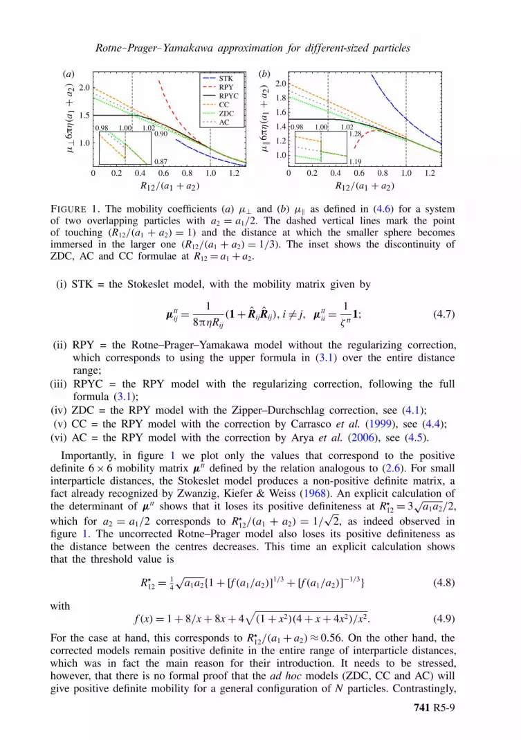
FIGURE 1. The mobility coefficients (a) µ⊥ and (b) µ‖ as defined in (4.6) for a systemof two overlapping particles with a2 = a1/2. The dashed vertical lines mark the pointof touching (R12/(a1 + a2) = 1) and the distance at which the smaller sphere becomesimmersed in the larger one (R12/(a1 + a2) = 1/3). The inset shows the discontinuity ofZDC, AC and CC formulae at R12 = a1 + a2.

(i) STK = the Stokeslet model, with the mobility matrix given by

µttij =

18πηRij

(1+ RijRij), i 6= j, µttii =

1ζ tt

1; (4.7)

(ii) RPY = the Rotne–Prager–Yamakawa model without the regularizing correction,which corresponds to using the upper formula in (3.1) over the entire distancerange;

(iii) RPYC = the RPY model with the regularizing correction, following the fullformula (3.1);

(iv) ZDC = the RPY model with the Zipper–Durchschlag correction, see (4.1);(v) CC = the RPY model with the correction by Carrasco et al. (1999), see (4.4);

(vi) AC = the RPY model with the correction by Arya et al. (2006), see (4.5).

Importantly, in figure 1 we plot only the values that correspond to the positivedefinite 6× 6 mobility matrix µtt defined by the relation analogous to (2.6). For smallinterparticle distances, the Stokeslet model produces a non-positive definite matrix, afact already recognized by Zwanzig, Kiefer & Weiss (1968). An explicit calculation ofthe determinant of µtt shows that it loses its positive definiteness at R?12 = 3

√a1a2/2,

which for a2 = a1/2 corresponds to R?12/(a1 + a2) = 1/√

2, as indeed observed infigure 1. The uncorrected Rotne–Prager model also loses its positive definiteness asthe distance between the centres decreases. This time an explicit calculation showsthat the threshold value is

R?12 = 14

√a1a21+ [f (a1/a2)]1/3 + [f (a1/a2)]−1/3 (4.8)

withf (x)= 1+ 8/x+ 8x+ 4

√(1+ x2)(4+ x+ 4x2)/x2. (4.9)

For the case at hand, this corresponds to R?12/(a1+ a2)≈ 0.56. On the other hand, thecorrected models remain positive definite in the entire range of interparticle distances,which was in fact the main reason for their introduction. It needs to be stressed,however, that there is no formal proof that the ad hoc models (ZDC, CC and AC) willgive positive definite mobility for a general configuration of N particles. Contrastingly,

741 R5-9

P. J. Zuk, E. Wajnryb, K. A. Mizerski and P. Szymczak

0.70

0.75

0.80

0.85

0.90

0.95

1.00

0.70

0.75

0.80

0.85

0.90

0.95

1.00

2 4 6 8

0.66

0.71

0.780 0.33 1 1.2

0 2 4 6 8 10

0.66

0.69

0.720 0.33 1 1.2

MLTPRPYC

010

(a () b)

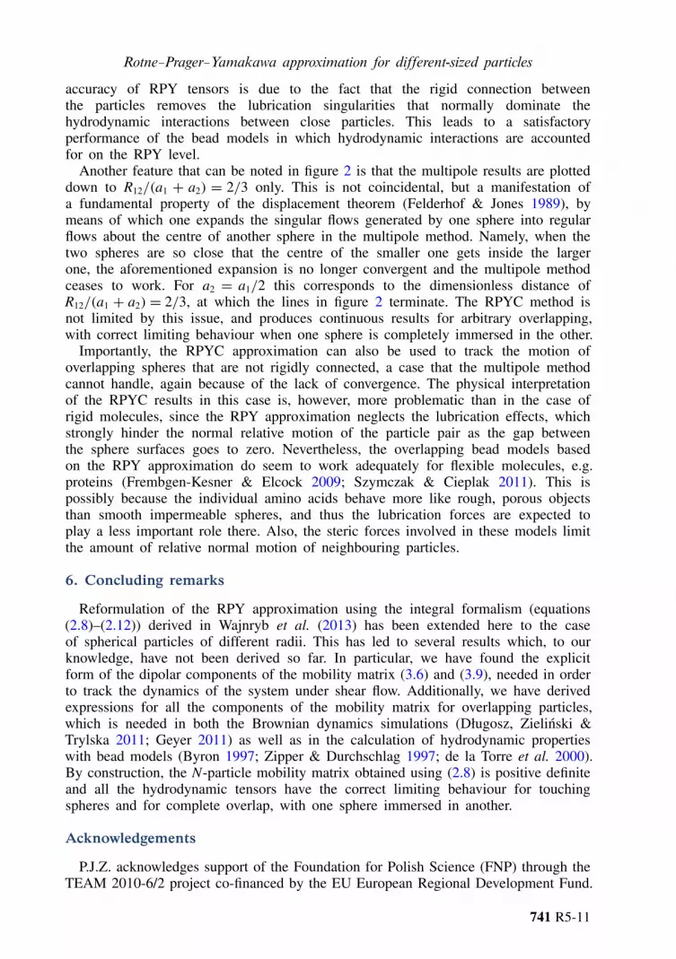
FIGURE 2. The friction coefficients for a snowman-shaped particle comprising two rigidlyconnected, overlapping spheres with a2 = a1/2. The panels present the (a) transversefriction coefficient ζ⊥ and (b) longitudinal friction coefficient ζ‖ calculated using theRPYC formulae (solid) and the multipole expansion (dashed). The inset shows themagnification of the small R12 region.

the RPYC model derived here is positive definite by construction, as it arises from theaction of a positive definite operator T0 on the vectors wq (cf. (2.8)–(2.12); see alsothe discussion in Cichocki et al. (2000) and Wajnryb et al. (2013)).

The analysis of figure 1 shows further that the ad hoc models are not continuous atthe point of touching, i.e. a1+ a2=R12. Such a discontinuity in mobility, albeit small,can lead to numerical artifacts in the Brownian dynamics simulations. In particular, itwill affect the resulting shape of the pair distribution function of close particles. Anadditional negative aspect of the ad hoc corrections is their behaviour in the completeoverlap region, i.e. when R12 < a> − a<. As already mentioned, the mobility matricesin this region should become independent of R12 and reduce to those of the larger(external) particle. Such a behaviour is indeed observed for RPYC tensors, but not inthe case of other corrections.

5. Bead models of macromolecules

The overlapping bead models can be used for the calculation of hydrodynamicproperties of complex-shaped macromolecules, both rigid and flexible. To illustratethis, we consider a simple example of a snowman-like molecule, formed by tworigidly connected overlapping particles of radii a1 and a2 = a1/2. The recent adventof microassembly techniques allows such structures to be relatively easily fabricated(Duguet et al. 2011). Figure 2 presents the longitudinal and transverse frictioncoefficients for such a snowman, defined in analogy to (4.6). These are obtainedby inverting the N-particle mobility matrix of (2.6) and then projecting the resultingfriction matrix on the rigid-body motion of the snowman as a whole. This is comparedwith the friction coefficients calculated using the (virtually) exact multipole seriesexpansion method (MLTP) (Cichocki et al. 1994; Zurita-Gotor, Bławzdziewicz &Wajnryb 2007).

The data presented in figure 2 show that, even though the RPY approach isformally a far-field expansion, it works surprisingly well also for very small distancesbetween the particles, including the case of overlap. The transverse component isunderestimated by the RPYC approximation by no more than ∼1 %, whereas thelongitudinal component is underestimated by no more than ∼2 %. Such a good

741 R5-10

Rotne–Prager–Yamakawa approximation for different-sized particles

accuracy of RPY tensors is due to the fact that the rigid connection betweenthe particles removes the lubrication singularities that normally dominate thehydrodynamic interactions between close particles. This leads to a satisfactoryperformance of the bead models in which hydrodynamic interactions are accountedfor on the RPY level.

Another feature that can be noted in figure 2 is that the multipole results are plotteddown to R12/(a1 + a2) = 2/3 only. This is not coincidental, but a manifestation ofa fundamental property of the displacement theorem (Felderhof & Jones 1989), bymeans of which one expands the singular flows generated by one sphere into regularflows about the centre of another sphere in the multipole method. Namely, when thetwo spheres are so close that the centre of the smaller one gets inside the largerone, the aforementioned expansion is no longer convergent and the multipole methodceases to work. For a2 = a1/2 this corresponds to the dimensionless distance ofR12/(a1 + a2) = 2/3, at which the lines in figure 2 terminate. The RPYC method isnot limited by this issue, and produces continuous results for arbitrary overlapping,with correct limiting behaviour when one sphere is completely immersed in the other.

Importantly, the RPYC approximation can also be used to track the motion ofoverlapping spheres that are not rigidly connected, a case that the multipole methodcannot handle, again because of the lack of convergence. The physical interpretationof the RPYC results in this case is, however, more problematic than in the case ofrigid molecules, since the RPY approximation neglects the lubrication effects, whichstrongly hinder the normal relative motion of the particle pair as the gap betweenthe sphere surfaces goes to zero. Nevertheless, the overlapping bead models basedon the RPY approximation do seem to work adequately for flexible molecules, e.g.proteins (Frembgen-Kesner & Elcock 2009; Szymczak & Cieplak 2011). This ispossibly because the individual amino acids behave more like rough, porous objectsthan smooth impermeable spheres, and thus the lubrication forces are expected toplay a less important role there. Also, the steric forces involved in these models limitthe amount of relative normal motion of neighbouring particles.

6. Concluding remarks

Reformulation of the RPY approximation using the integral formalism (equations(2.8)–(2.12)) derived in Wajnryb et al. (2013) has been extended here to the caseof spherical particles of different radii. This has led to several results which, to ourknowledge, have not been derived so far. In particular, we have found the explicitform of the dipolar components of the mobility matrix (3.6) and (3.9), needed in orderto track the dynamics of the system under shear flow. Additionally, we have derivedexpressions for all the components of the mobility matrix for overlapping particles,which is needed in both the Brownian dynamics simulations (Długosz, Zielinski &Trylska 2011; Geyer 2011) as well as in the calculation of hydrodynamic propertieswith bead models (Byron 1997; Zipper & Durchschlag 1997; de la Torre et al. 2000).By construction, the N-particle mobility matrix obtained using (2.8) is positive definiteand all the hydrodynamic tensors have the correct limiting behaviour for touchingspheres and for complete overlap, with one sphere immersed in another.

Acknowledgements

P.J.Z. acknowledges support of the Foundation for Polish Science (FNP) through theTEAM 2010-6/2 project co-financed by the EU European Regional Development Fund.

741 R5-11

P. J. Zuk, E. Wajnryb, K. A. Mizerski and P. Szymczak

E.W. and K.M. acknowledge the support of the Polish National Science Centre (grantno. 2012/05/B/ST8/03010). P.S. acknowledges the support of the Polish Ministry ofScience and Higher Education (grant no. N N202 055440).

References

ANTOSIEWICZ, J. & PORSCHKE, D. 1989 Volume correction for bead model simulations of rotationalfriction coefficients of macromolecules. J. Phys. Chem. 93, 5301–5305.

ARYA, G., ZHANG, Q. & SCHLICK, T. 2006 Flexible histone tails in a new mesoscopicoligonucleosome model. Biophys. J. 91, 133–150.

BANACHOWICZ, E., GAPINSKI, J. & PATKOWSKI, A. 2000 Solution structure of biopolymers: a newmethod of constructing a bead model. Biophys. J. 78, 70–78.

BLOOMFIELD, V., DALTON, W. O. & VAN HOLDE, K. E. 1967 Frictional coefficients of multisubunitstructures. I. Theory. Biopolymers 5, 135–148.

BYRON, O. 1997 Construction of hydrodynamic bead models from high-resolution X-raycrystallographic or nuclear magnetic resonance data. Biophys. J. 72, 408–415.

CARRASCO, B. & DE LA TORRE, G. J. 1999 Hydrodynamic properties of rigid particles: comparisonof different modeling and computational procedures. Biophys. J. 76, 3044–3057.

CARRASCO, B., DE LA TORRE, J. G. & ZIPPER, P. 1999 Calculation of hydrodynamic properties ofmacromolecular bead models with overlapping spheres. Eur. Biophys. J. 28, 510–515.

CICHOCKI, B., FELDERHOF, B. U., HINSEN, K., WAJNRYB, E. & BłAWZDZIEWICZ, J. 1994 Frictionand mobility of many spheres in Stokes flow. J. Chem. Phys. 100, 3780–3790.

CICHOCKI, B., JONES, R. B., KUTTEH, R. & WAJNRYB, E. 2000 Friction and mobility for colloidalspheres in Stokes flow near a boundary: the multipole method and applications. J. Chem.Phys. 112, 2548–2561.

CLEMENTI, C. 2008 Coarse-grained models of protein folding. Curr. Opin. Struct. Biol. 18, 10–15.DHONT, J. K. G. 1996 An Introduction to Dynamics of Colloids. Elsevier Science.DłUGOSZ, M., ZIELINSKI, P. & TRYLSKA, J. 2011 Brownian dynamics simulations on CPU and

GPU with BD BOX. J. Comput. Chem. 32, 2734–2744.DUGUET, E., DÉSERT, A., PERRO, A. & RAVAINE, S. 2011 Design and elaboration of colloidal

molecules: an overview. Chem. Soc. Rev. 40, 941–960.ERMAK, D. L. & MCCAMMON, J. A. 1978 Brownian dynamics with hydrodynamic interactions. J.

Chem. Phys. 69, 1352–1360.FELDERHOF, B. U. & JONES, R. B. 1989 Displacement theorems for spherical solutions of the

linear Navier–Stokes equations. J. Math. Phys. 30, 339–342.FREMBGEN-KESNER, T. & ELCOCK, A. H. 2009 Striking effects of hydrodynamic interactions on

the simulated diffusion and folding of proteins. J. Chem. Theory Comput. 5, 242–256.GEYER, T. 2011 Many-particle Brownian and Langevin dynamics simulations with the Brownmove

package. BMC Biophys. 4, 7.HELLWEG, T., EIMER, W., KRAHN, E., SCHNEIDER, K. & MÜLLER, A. 1997 Hydrodynamic

properties of nitrogenase – the MoFe protein from Azotobacter vinelandii studied by dynamiclight scattering and hydrodynamic modelling. Biochem. Biophys. Acta 1337, 311–318.

HILLS, R. D. JR. & BROOKS, C. L. III 2009 Insights from coarse-grained Go models for proteinfolding and dynamics. Intl J. Mol. Sci. 10, 889–905.

KIM, S. & KARRILA, S. J. 1991 Microhydrodynamics: Principles and Selected Applications.Butterworth-Heinemann.

KIRKWOOD, J. G. & RISEMAN, J. 1948 The intrinsic viscosities and diffusion constants of flexiblemacromolecules in solution. J. Chem. Phys. 16, 565–573.

NÄGELE, G. 2006 Brownian dynamics simulations. In Computational Condensed Matter Physics, vol.B4:1 (ed. S. Blügel, G. Gompper, E. Koch, H. Müller-Krumbhaar, R. Spatschek & R. G.Winkler), Forschungszentrum Jülich.

ROTNE, J. & PRAGER, S. 1969 Variational treatment of hydrodynamic interaction in polymers. J.Chem. Phys. 50, 4831–4837.

SZYMCZAK, P. & CIEPLAK, M. 2007 Proteins in a shear flow. J. Chem. Phys. 127, 155106.

741 R5-12

Rotne–Prager–Yamakawa approximation for different-sized particles

SZYMCZAK, P. & CIEPLAK, M. 2011 Hydrodynamic effects in proteins. J. Phys.: Condens. Matter23, 033102.

DE LA TORRE, J. G. & BLOOMFIELD, V. A. 1977 Hydrodynamic properties of macromolecularcomplexes. I. Translation. Biopolymers 16, 1747–1763.

DE LA TORRE, G. J., HUERTAS, M. L. & CARRASCO, B. 2000 Calculation of hydrodynamicproperties of globular proteins from their atomic-level structure. Biophys. J. 78, 719–730.

TOZZINI, V. 2005 Coarse-grained models for proteins. Curr. Opin. Struct. Biol. 15 (2), 144–150.WAJNRYB, E., MIZERSKI, K. A., ZUK, P. J. & SZYMCZAK, P. 2013 Generalization of the Rotne–

Prager–Yamakawa mobility and shear disturbance tensors. J. Fluid Mech. 731, R3.WAJNRYB, E., SZYMCZAK, P. & CICHOCKI, B. 2004 Brownian dynamics: divergence of mobility

tensor. Physica A 335, 339–358.ZIPPER, P. & DURCHSCHLAG, H. 1997 Calculation of hydrodynamic parameters of proteins from

crystallographic data using multibody approaches. Prog. Colloid. Polym. Sci. 107, 58–71.ZURITA-GOTOR, M., BłAWZDZIEWICZ, J. & WAJNRYB, E. 2007 Motion of a rod-like particle between

parallel walls with application to suspension rheology. J. Rheol. 51, 71–97.ZWANZIG, R., KIEFER, J. & WEISS, G. H. 1968 On the validity of the Kirkwood–Riseman theory.

Proc. Natl Acad. Sci. USA 60, 381–386.

741 R5-13