Robust and Accurate Algorithm for Structure and Motion Factorization

Robust and Accurate Structure from Motion of

Rigid and Nonrigid Objects

by

Guanghui Wang

A thesispresented to the University of Waterloo

in fulfilment of thethesis requirement for the degree of

Doctor of Philosophyin

Systems Design Engineering

Waterloo, Ontario, Canada, 2014

c©Guanghui Wang 2014

I hereby declare that I am the sole author of this thesis. This is a true copy of thethesis, including any required final revisions, as accepted by my examiners.

I understand that my thesis may be made electronically available to the public.

Guanghui Wang

iii

Abstract

As a central theme in computer vision, the problem of 3D structure and motionrecovery from image sequences has been widely studied during the past threedecades, and considerable progress has been made in theory, as well as in prac-tice. However, there are still several challenges remaining, including algorithmrobustness and accuracy, especially for nonrigid modeling. The thesis focuses onsolving these challenges and several new robust and accurate algorithms havebeen proposed.

The first part of the thesis reviews the state-of-the-art techniques of structureand motion factorization. First, an introduction of structure from motion andsome mathematical background of the technique is presented. Then, the generalidea and different formulations of structure from motion for rigid and nonrigidobjects are discussed.

The second part covers the proposed quasi-perspective projection model andits application to structure and motion factorization. Previous algorithms arebased on either a simplified affine assumption or a complicated full perspectiveprojection model. The affine model is widely adopted due to its simplicity,whereas the extension to full perspective suffers from recovering projectivedepths. A quasi-perspective model is proposed to fill the gap between thetwo models. It is more accurate than the affine model from both theoreticalanalysis and experimental studies. More geometric properties of the model areinvestigated in the context of one- and two-view geometry. Finally, the modelwas applied to structure from motion and a framework of rigid and nonrigidfactorization under quasi-perspective assumption is established.

The last part of the thesis is focused on the robustness and three new al-gorithms are proposed. First, a spatial-and-temporal-weighted factorizationalgorithm is proposed to handle significant image noise, where the uncertaintyof image measurement is estimated from a new perspective by virtue of repro-jection residuals. Second, a rank-4 affine factorization algorithm is proposedto avoid the difficulty of image alignment with erroneous data, followed by arobust factorization scheme that can work with missing and outlying data. Third,

v

the robust algorithm is extended to nonrigid scenarios and a new augmentednonrigid factorization algorithm is proposed to handle imperfect tracking data.

The main contributions of the thesis are as follows: The proposed quasi-perspective projection model fills the gap between the simplicity of the affinemodel and the accuracy of the perspective model. Its application to structureand motion factorization greatly increases the efficiency and accuracy of thealgorithm. The proposed robust algorithms do not require prior information ofimage measurement and greatly improve the overall accuracy and robustness ofprevious approaches. Moreover, the algorithms can also be applied directly tostructure from motion of nonrigid objects.

vi

Acknowledgements

I would like to thank my supervisor Dr. John Zelek for his extensive support,encouragement, and motivating discussions during my study. I am deeply gratefulto Dr. Jonathan Wu for his invaluable guidance and support throughout my entireacademic experience in Canada. I would also like to thank Dr. Ruzena Bajcsy forher insightful advice and kind help during my visit at the University of California,Berkeley.

Many thanks to all members of my committee, Dr. David Clausi, Dr. AlexanderWong, Dr. Richard Mann, Dr. Zhou Wang, and Dr. John Barron for their helpfuland insightful comments and suggestions to the thesis.

I would like to extend my gratitude to all faculty and staff members at theDepartment of Systems Design Engineering for their readiness to help at all times.I am especially grateful to Vicky Lawrence for her helpful support.

Furthermore, I owe thanks to the staff members at the Centre for TeachingExcellence, Centre for Career Action, and the Student Success Office of theUniversity of Waterloo for their support to my study and career development. Iwould also like to thank my friends, including Adel Fakih, Dong Li, Jinfu Yang,Dibyendu Mukherjee, Xiangru Li, and many more, who made my experience atWaterloo more fruitful and enjoyable.

In addition, I have been very privileged to get several scholarships to supportmy study. I convey special acknowledgement to NSERC CGS Scholarship, NSERCCGS-MSFSS, President’s Graduate Scholarship of the University of Waterloo, andthe Ontario Graduate Scholarship in Science and Technology.

Last but not least, I owe my thanks to my family for their infinite love andsupport throughout everything. Thank you with all my heart.

vii

Dedication

To my wife Junfeng and daughter Nina.

ix

Table of Contents

Author’s Declaration iii

Abstract v

Acknowledgements vii

Dedication ix

Table of Contents xi

List of Tables xv

List of Figures xvii

1 Introduction 11.1 Problem Definition of SfM . . . . . . . . . . . . . . . . . . . . . . . . . 11.2 Challenges in SfM . . . . . . . . . . . . . . . . . . . . . . . . . . . . . . 41.3 Thesis Contributions . . . . . . . . . . . . . . . . . . . . . . . . . . . . . 51.4 Thesis Organization . . . . . . . . . . . . . . . . . . . . . . . . . . . . . 6

2 Background 92.1 Literature Review . . . . . . . . . . . . . . . . . . . . . . . . . . . . . . . 9

2.1.1 Factorization for rigid objects and static scenes . . . . . . . 92.1.2 Factorization for nonrigid objects and dynamic scenes . . . 102.1.3 Robust structure and motion factorization . . . . . . . . . . 11

2.2 Structure and Motion Recovery of Rigid Objects . . . . . . . . . . . 122.2.1 Rigid factorization under affine projection . . . . . . . . . . 122.2.2 Rigid factorization under perspective projection . . . . . . . 15

2.3 Structure and Motion Recovery of Nonrigid Objects . . . . . . . . . 162.3.1 Bregler’s deformation model . . . . . . . . . . . . . . . . . . . 172.3.2 Nonrigid factorization under affine assumption . . . . . . . 18

xi

2.3.3 Nonrigid factorization under perspective projection . . . . 222.3.4 Nonrigid factorization in trajectory space . . . . . . . . . . . 24

2.4 Discussion . . . . . . . . . . . . . . . . . . . . . . . . . . . . . . . . . . . 25

3 Quasi-Perspective Projection Model 273.1 Introduction . . . . . . . . . . . . . . . . . . . . . . . . . . . . . . . . . . 273.2 Affine Projection Model . . . . . . . . . . . . . . . . . . . . . . . . . . . 283.3 Quasi-Perspective Projection Model . . . . . . . . . . . . . . . . . . . 31

3.3.1 Quasi-perspective projection . . . . . . . . . . . . . . . . . . . 313.3.2 Error analysis of different models . . . . . . . . . . . . . . . . 34

3.4 Experimental Evaluations . . . . . . . . . . . . . . . . . . . . . . . . . . 373.4.1 Imaging errors . . . . . . . . . . . . . . . . . . . . . . . . . . . . 383.4.2 Influence of imaging conditions . . . . . . . . . . . . . . . . . 39

3.5 Conclusion . . . . . . . . . . . . . . . . . . . . . . . . . . . . . . . . . . . 39

4 Properties of Quasi-Perspective Model 414.1 Introduction . . . . . . . . . . . . . . . . . . . . . . . . . . . . . . . . . . 414.2 One-View Geometrical Property . . . . . . . . . . . . . . . . . . . . . . 424.3 Two-View Geometrical Property . . . . . . . . . . . . . . . . . . . . . . 45

4.3.1 Fundamental matrix . . . . . . . . . . . . . . . . . . . . . . . . 454.3.2 Plane induced homography . . . . . . . . . . . . . . . . . . . . 484.3.3 RANSAC computation . . . . . . . . . . . . . . . . . . . . . . . 50

4.4 3D Structure Reconstruction . . . . . . . . . . . . . . . . . . . . . . . . 514.5 Evaluations on Synthetic Data . . . . . . . . . . . . . . . . . . . . . . . 53

4.5.1 Fundamental matrix and homography . . . . . . . . . . . . . 544.5.2 Outlier removal . . . . . . . . . . . . . . . . . . . . . . . . . . . 554.5.3 Reconstruction result . . . . . . . . . . . . . . . . . . . . . . . . 56

4.6 Evaluations on Real Images . . . . . . . . . . . . . . . . . . . . . . . . 574.6.1 Test on stone dragon images . . . . . . . . . . . . . . . . . . . 574.6.2 Test on Medusa head images . . . . . . . . . . . . . . . . . . . 58

4.7 Conclusion . . . . . . . . . . . . . . . . . . . . . . . . . . . . . . . . . . . 59

5 SfM Based on Quasi-Perspective Projection Model 615.1 Introduction . . . . . . . . . . . . . . . . . . . . . . . . . . . . . . . . . . 615.2 Background on Factorization . . . . . . . . . . . . . . . . . . . . . . . 625.3 Quasi-Perspective Rigid Factorization . . . . . . . . . . . . . . . . . . 64

5.3.1 Euclidean upgrading matrix . . . . . . . . . . . . . . . . . . . 655.3.2 Algorithm outline . . . . . . . . . . . . . . . . . . . . . . . . . . 71

5.4 Quasi-Perspective Nonrigid Factorization . . . . . . . . . . . . . . . . 725.4.1 Problem formulation . . . . . . . . . . . . . . . . . . . . . . . . 725.4.2 Euclidean upgrading matrix . . . . . . . . . . . . . . . . . . . 73

xii

5.5 Evaluations on Synthetic Data . . . . . . . . . . . . . . . . . . . . . . . 755.5.1 Evaluations of rigid factorization . . . . . . . . . . . . . . . . 755.5.2 Evaluations of nonrigid factorization . . . . . . . . . . . . . . 78

5.6 Evaluations on Real Image Sequences . . . . . . . . . . . . . . . . . . 795.6.1 Test on fountain base sequence . . . . . . . . . . . . . . . . . 795.6.2 Test on Franck sequence . . . . . . . . . . . . . . . . . . . . . . 80

5.7 Conclusion . . . . . . . . . . . . . . . . . . . . . . . . . . . . . . . . . . . 81

6 Spatial-and-Temporal-Weighted Factorization 836.1 Introduction . . . . . . . . . . . . . . . . . . . . . . . . . . . . . . . . . . 836.2 Background on Structure and Motion Factorization . . . . . . . . . 846.3 Weighted Factorization . . . . . . . . . . . . . . . . . . . . . . . . . . . 86

6.3.1 Feature uncertainty modeling . . . . . . . . . . . . . . . . . . 866.3.2 Spatial-and-temporal-weighted factorization . . . . . . . . . 896.3.3 Implementation details . . . . . . . . . . . . . . . . . . . . . . 92

6.4 Evaluations on Synthetic Data . . . . . . . . . . . . . . . . . . . . . . . 936.4.1 Recovery of spatial and temporal errors . . . . . . . . . . . . 936.4.2 Weighted factorization under affine model . . . . . . . . . . 956.4.3 Weighted factorization under perspective projection . . . . 996.4.4 Computational complexity . . . . . . . . . . . . . . . . . . . . 99

6.5 Evaluations on Real Sequences . . . . . . . . . . . . . . . . . . . . . . 1016.5.1 Test on garden sequence . . . . . . . . . . . . . . . . . . . . . 1016.5.2 Test on tree trunk sequence . . . . . . . . . . . . . . . . . . . . 1046.5.3 Test on statue sequence . . . . . . . . . . . . . . . . . . . . . . 104

6.6 Conclusion . . . . . . . . . . . . . . . . . . . . . . . . . . . . . . . . . . . 105

7 Robust SfM of Rigid Objects 1077.1 Introduction . . . . . . . . . . . . . . . . . . . . . . . . . . . . . . . . . . 1077.2 Background on Structure and Motion Factorization . . . . . . . . . 1087.3 Rank-4 Structure from Motion . . . . . . . . . . . . . . . . . . . . . . 109

7.3.1 Rank-4 affine factorization . . . . . . . . . . . . . . . . . . . . 1107.3.2 Euclidean upgrading matrix . . . . . . . . . . . . . . . . . . . 1107.3.3 Algorithm of rank-4 affine factorization . . . . . . . . . . . . 112

7.4 Alternative and Weighted Factorization . . . . . . . . . . . . . . . . . 1127.4.1 Alternative factorization algorithm . . . . . . . . . . . . . . . 1127.4.2 Alternative weighted factorization . . . . . . . . . . . . . . . 114

7.5 Outlier Detection and Robust Factorization . . . . . . . . . . . . . . . 1157.5.1 Outlier detection scheme . . . . . . . . . . . . . . . . . . . . . 1157.5.2 Parameter estimation . . . . . . . . . . . . . . . . . . . . . . . . 119

7.6 Evaluations on Synthetic Data . . . . . . . . . . . . . . . . . . . . . . . 121

xiii

7.6.1 Influence of image centroid . . . . . . . . . . . . . . . . . . . . 1217.6.2 Performance evaluation . . . . . . . . . . . . . . . . . . . . . . 122

7.7 Evaluations on Real Sequences . . . . . . . . . . . . . . . . . . . . . . 1257.8 Conclusion . . . . . . . . . . . . . . . . . . . . . . . . . . . . . . . . . . . 126

8 Robust SfM of Nonrigid Objects 1298.1 Introduction . . . . . . . . . . . . . . . . . . . . . . . . . . . . . . . . . . 1298.2 Background of Nonrigid Factorization . . . . . . . . . . . . . . . . . . 1308.3 Augmented Affine Factorization . . . . . . . . . . . . . . . . . . . . . . 131

8.3.1 Rank-(3k+ 1) affine factorization . . . . . . . . . . . . . . . . 1318.3.2 Euclidean upgrading matrix . . . . . . . . . . . . . . . . . . . 1328.3.3 Alternative factorization with missing data . . . . . . . . . . 1338.3.4 Alternative weighted factorization . . . . . . . . . . . . . . . 134

8.4 Outlier Detection and Robust Factorization . . . . . . . . . . . . . . . 1348.4.1 Outlier detection scheme . . . . . . . . . . . . . . . . . . . . . 1358.4.2 Implementation details . . . . . . . . . . . . . . . . . . . . . . 1368.4.3 Parameter estimation . . . . . . . . . . . . . . . . . . . . . . . . 137

8.5 Evaluations on Synthetic Data . . . . . . . . . . . . . . . . . . . . . . . 1398.5.1 Influence of image centroid . . . . . . . . . . . . . . . . . . . . 1408.5.2 Performance of the robust algorithm . . . . . . . . . . . . . . 141

8.6 Evaluations on Real Sequences . . . . . . . . . . . . . . . . . . . . . . 1428.7 Conclusion . . . . . . . . . . . . . . . . . . . . . . . . . . . . . . . . . . . 144

9 Conclusion and Future Work 1479.1 Contributions and Conclusion . . . . . . . . . . . . . . . . . . . . . . . 1479.2 Future Work . . . . . . . . . . . . . . . . . . . . . . . . . . . . . . . . . . 149

Bibliography 151

xiv

List of Tables

1.1 Classification of structure from motion . . . . . . . . . . . . . . . . . 4

4.1 The entry number and degrees of freedom . . . . . . . . . . . . . . . 494.2 The number of trials . . . . . . . . . . . . . . . . . . . . . . . . . . . . . 514.3 Reprojection error under different models . . . . . . . . . . . . . . . 57

5.1 The average computation time . . . . . . . . . . . . . . . . . . . . . . 775.2 Camera parameters and reprojection errors . . . . . . . . . . . . . . 81

6.1 Real computation time of different algorithms . . . . . . . . . . . . 1016.2 Reprojection errors by different algorithms . . . . . . . . . . . . . . . 104

7.1 Real computation time of different algorithms . . . . . . . . . . . . 123

8.1 Real computation time of different algorithms . . . . . . . . . . . . 142

xv

List of Figures

1.1 Four frames from the dinosaur sequence . . . . . . . . . . . . . . . . 31.2 Tracked features of the dinosaur sequence . . . . . . . . . . . . . . . 5

2.1 The structure of a jellyfish . . . . . . . . . . . . . . . . . . . . . . . . . 172.2 Four female face models . . . . . . . . . . . . . . . . . . . . . . . . . . 17

3.1 Imaging process of different models . . . . . . . . . . . . . . . . . . . 303.2 Imaging process of a camera . . . . . . . . . . . . . . . . . . . . . . . . 323.3 Evaluation on projective depth . . . . . . . . . . . . . . . . . . . . . . 373.4 Evaluation of the imaging errors . . . . . . . . . . . . . . . . . . . . . 383.5 Evaluation on quasi-perspective model . . . . . . . . . . . . . . . . . 39

4.1 The imaging process and relationship . . . . . . . . . . . . . . . . . . 434.2 Histogram distribution of the epipolar residuals . . . . . . . . . . . 534.3 Histogram distribution of reprojection errors . . . . . . . . . . . . . 544.4 Result of outlier removal . . . . . . . . . . . . . . . . . . . . . . . . . . 554.5 Average computation time . . . . . . . . . . . . . . . . . . . . . . . . . 564.6 Evaluation on 3D reconstruction . . . . . . . . . . . . . . . . . . . . . 574.7 Reconstruction result of stone dragon images . . . . . . . . . . . . . 584.8 Histogram distribution of the epipolar residuals . . . . . . . . . . . 594.9 Reconstruction result of Medusa head images . . . . . . . . . . . . . 60

5.1 Evaluation on the accuracy . . . . . . . . . . . . . . . . . . . . . . . . . 765.2 The mean reconstruction error . . . . . . . . . . . . . . . . . . . . . . 775.3 Reconstruction results of nonrigid factorization . . . . . . . . . . . . 785.4 Evaluation of nonrigid factorization . . . . . . . . . . . . . . . . . . . 795.5 Reconstruction results of fountain base sequence . . . . . . . . . . . 805.6 Histogram distributions of the reprojection errors . . . . . . . . . . 815.7 Reconstruction of different facial expressions . . . . . . . . . . . . . 82

6.1 Illustration of feature uncertainties . . . . . . . . . . . . . . . . . . . 86

xvii

6.2 Spatial and temporal distribution of features . . . . . . . . . . . . . 876.3 Illustration of the normalized noise . . . . . . . . . . . . . . . . . . . 886.4 Outline of the proposed method . . . . . . . . . . . . . . . . . . . . . 926.5 The real values of the added noise . . . . . . . . . . . . . . . . . . . . 946.6 Error of the synthetic sequence . . . . . . . . . . . . . . . . . . . . . . 956.7 The spatial and temporal noises . . . . . . . . . . . . . . . . . . . . . 966.8 The spatial and temporal noises . . . . . . . . . . . . . . . . . . . . . . 976.9 The spatial and temporal noises . . . . . . . . . . . . . . . . . . . . . . 986.10 The reprojection variation . . . . . . . . . . . . . . . . . . . . . . . . . 1006.11 Reconstruction of the garden sequence . . . . . . . . . . . . . . . . . 1026.12 Reconstruction of the tree trunk sequence . . . . . . . . . . . . . . . 1036.13 Reconstruction of the head statue sequence . . . . . . . . . . . . . . 105

7.1 Illustration of the normalized noise . . . . . . . . . . . . . . . . . . . 1177.2 The outline of the method . . . . . . . . . . . . . . . . . . . . . . . . . 1187.3 Histogram distribution of the noise . . . . . . . . . . . . . . . . . . . 1207.4 The mean reprojection variance . . . . . . . . . . . . . . . . . . . . . . 1227.5 The mean reprojection variance . . . . . . . . . . . . . . . . . . . . . . 1237.6 Reconstruction of the fountain base sequence . . . . . . . . . . . . . 1247.7 Histogram distribution of the residual matrix . . . . . . . . . . . . . 1257.8 Reconstruction of the Hearst Gym sequence . . . . . . . . . . . . . . 127

8.1 Illustration of the normalized noise . . . . . . . . . . . . . . . . . . . 1358.2 The outline of the proposed approach . . . . . . . . . . . . . . . . . . 1368.3 Histogram distribution of the added noise . . . . . . . . . . . . . . . 1388.4 Two simulated space cubes . . . . . . . . . . . . . . . . . . . . . . . . . 1398.5 The mean reprojection variance . . . . . . . . . . . . . . . . . . . . . . 1408.6 The mean reprojection variance . . . . . . . . . . . . . . . . . . . . . . 1418.7 Test results of the dinosaur sequence . . . . . . . . . . . . . . . . . . 1438.8 Histogram distribution of the residual matrix . . . . . . . . . . . . . 1448.9 Test results of the face sequence . . . . . . . . . . . . . . . . . . . . . 145

xviii

Chapter 1

Introduction

Making computers see and understand the world are the main tasks of computervision. As a central theme in computer vision, the problem of 3D structure andmotion recovery from images or video sequences has been widely studied duringthe past three decades [72].

The classical method for 3D reconstruction is stereo vision using two or threeimages. Once the correspondences between these images have been established,the 3D structure can be calculated via triangulations. For a sequence of manyimages, the typical approach is the structure and motion factorization algorithm,which was first proposed by Tomasi and Kanade [74]. The factorization methodis based on a bilinear formulation that decomposes image measurements directlyinto the structure and motion components. The algorithm assumes that thetracking matrix of an image sequence is available and deals uniformly with thedata from all images. Thus, it is more robust and more accurate than the methodsthat use only two images [17][42][57][65][77].

In recent years, considerable progress has been made in theory and practice,resulting in many successful applications in robot navigation and map building,industrial inspection, medical image analysis, reverse engineering, autonomousvehicles, and digital entertainment. However, the problem still remains far frombeing solved.

In this chapter, the definition and classification of structure from motion (SfM)is presented, followed by the challenges of structure and motion recovery. Then,the contributions of this thesis are summarized.

1.1 Problem Definition of SfM

In projective geometry, a point is normally denoted in homogeneous form. Sup-pose X j = [x j , y j , z j]T is a 3D space point, which is projected to a 2D image point

1

xi j = [ui j , vi j]T in the i-th frame. Their corresponding homogeneous forms aredenoted as X j = [X j , 1]T and xi j = [xi j , 1]T , respectively.

Under a full perspective projection model, a 3D point is projected to an imagepoint by the following equation.

λi jxi j = PiX j = Ki[Ri , ti]X j (1.1)

where λi j is a nonzero depth scale; Pi is a 3× 4 projection matrix of the i-thcamera; Ri and ti are the corresponding rotation matrix and translation vector ofthe camera with respect to the world system; and Ki is the camera calibrationmatrix. When the object is far away from the camera with relatively small depthvariation, one may safely assume a simplified affine camera model as below toapproximate the perspective projection.

xi j = AiX j + ti (1.2)

where Ai is a 2× 3 affine projection matrix; the image point xi j and the spacepoint X j are denoted in nonhomogeneous form. Under affine projection model,the mapping from space to the image becomes linear since the unknown depthscalar λi j in (1.1) is eliminated. If all image points of each frame are registeredto the centroid of that image and a relative image coordinate system is adopted,the translation term ti will vanish. Thus, the affine projection Equation (1.2) isfurther simplified to

xi j = AiX j . (1.3)

Suppose we have an image sequence of m frames and a set of n feature pointstracked across the sequence. The coordinates of the tracked features are denotedas xi j =

ui jvi j

|i = 1, ..., m, j = 1, ..., n, we can arrange these tracking data into acompact matrix as

W= frames

y

points︷︸︸︷

x11 · · · x1n...

. . ....

xm1 · · · xmn

2m×n

=

u11

v11

· · ·

u1n

v1n

.... . .

...

um1

vm1

· · ·

umn

vmn

(1.4)

where W is called the tracking or measurement matrix, which is a 2m× n matrixcomposed of all tracked features across the sequence.

Under the perspective projection (1.1), the tracking data can be denoted in

2

66 4 Introduction to Structure and Motion Factorization

Fig. 4.1 Four consecutive frames from the dinosaur sequence. Where 115 tracked features areoverlaid on the images in the second row, the white lines denote the relative disparities betweenframes. Courtesy of Andrew Fitzgibbon and Andrew Zisserman.

the image point xi j = [ui j,vi j]T is expressed in non-homogeneous form. For all these

features, we can arrange them into a compact single matrix form as:

W = frames

????y

pointsz | 264

x11 · · · x1n...

. . ....

xm1 · · · xmn

375

2m£n

=

2666664

∑u11v11

∏· · ·∑

u1nv1n

∏

.... . .

...∑um1vm1

∏· · ·∑

umnvmn

∏

3777775

(4.4)

where W is called the tracking or measurement matrix, a 2m£n matrix composedof all tracking information across the sequence. Under perspective projection (4.1),if we include the depth scale, the tracking data can be denoted in homogeneous formas follows.

W =

264

l11x11 · · · l1nx1n...

. . ....

lm1xm1 · · · lmnxmn

375

3m£n

=

26666666664

l11

24

u11v111

35 · · · l1n

24

u1nv1n1

35

.... . .

...

lm1

24

um1vm11

35 · · · lmn

24

umnvmn1

35

37777777775

(4.5)

We call W the projective-depth-scaled or weighted tracking matrix. The depthscale li j is normally unknown.

Fig. 4.1 gives an example of the feature tracking result for a dinosaur sequence.The sequence contains 36 frames which are taken evenly around a turn table. Theimages and tracking data were downloaded from the Visual Geometry Group ofOxford University. Fig. 4.1 shows 4 consecutive images with 115 tracked points.

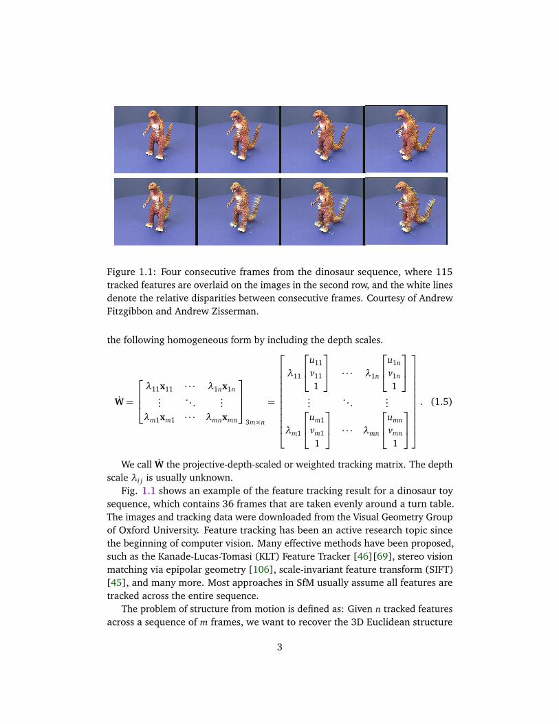
Figure 1.1: Four consecutive frames from the dinosaur sequence, where 115tracked features are overlaid on the images in the second row, and the white linesdenote the relative disparities between consecutive frames. Courtesy of AndrewFitzgibbon and Andrew Zisserman.

the following homogeneous form by including the depth scales.

W=

λ11x11 · · · λ1nx1n...

. . ....

λm1xm1 · · · λmnxmn

3m×n

=

λ11

u11

v11

1

· · · λ1n

u1n

v1n

1

.... . .

...

λm1

um1

vm1

1

· · · λmn

umn

vmn

1

. (1.5)

We call W the projective-depth-scaled or weighted tracking matrix. The depthscale λi j is usually unknown.

Fig. 1.1 shows an example of the feature tracking result for a dinosaur toysequence, which contains 36 frames that are taken evenly around a turn table.The images and tracking data were downloaded from the Visual Geometry Groupof Oxford University. Feature tracking has been an active research topic sincethe beginning of computer vision. Many effective methods have been proposed,such as the Kanade-Lucas-Tomasi (KLT) Feature Tracker [46][69], stereo visionmatching via epipolar geometry [106], scale-invariant feature transform (SIFT)[45], and many more. Most approaches in SfM usually assume all features aretracked across the entire sequence.

The problem of structure from motion is defined as: Given n tracked featuresacross a sequence of m frames, we want to recover the 3D Euclidean structure

3

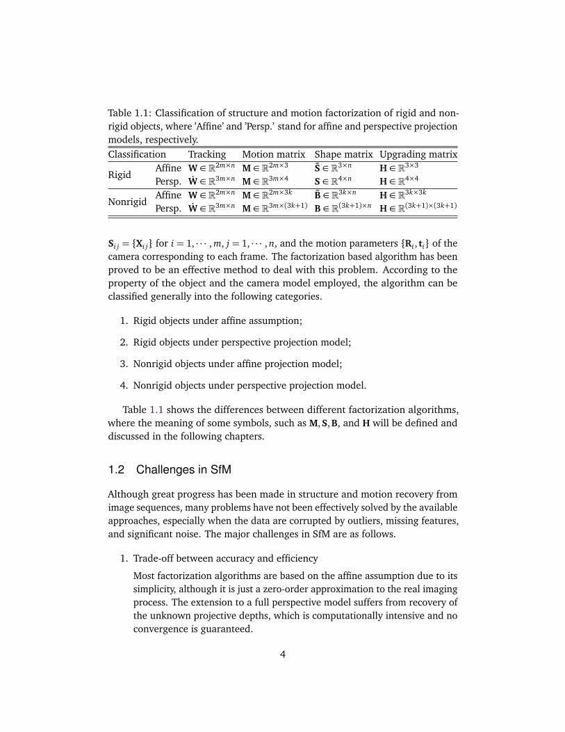
Table 1.1: Classification of structure and motion factorization of rigid and non-rigid objects, where ’Affine’ and ’Persp.’ stand for affine and perspective projectionmodels, respectively.Classification Tracking Motion matrix Shape matrix Upgrading matrix

Affine W ∈ R2m×n M ∈ R2m×3 S ∈ R3×n H ∈ R3×3Rigid

Persp. W ∈ R3m×n M ∈ R3m×4 S ∈ R4×n H ∈ R4×4

Affine W ∈ R2m×n M ∈ R2m×3k B ∈ R3k×n H ∈ R3k×3kNonrigid

Persp. W ∈ R3m×n M ∈ R3m×(3k+1) B ∈ R(3k+1)×n H ∈ R(3k+1)×(3k+1)

Si j = Xi j for i = 1, · · · , m, j = 1, · · · , n, and the motion parameters Ri , ti of thecamera corresponding to each frame. The factorization based algorithm has beenproved to be an effective method to deal with this problem. According to theproperty of the object and the camera model employed, the algorithm can beclassified generally into the following categories.

1. Rigid objects under affine assumption;

2. Rigid objects under perspective projection model;

3. Nonrigid objects under affine projection model;

4. Nonrigid objects under perspective projection model.

Table 1.1 shows the differences between different factorization algorithms,where the meaning of some symbols, such as M,S,B, and H will be defined anddiscussed in the following chapters.

1.2 Challenges in SfM

Although great progress has been made in structure and motion recovery fromimage sequences, many problems have not been effectively solved by the availableapproaches, especially when the data are corrupted by outliers, missing features,and significant noise. The major challenges in SfM are as follows.

1. Trade-off between accuracy and efficiency

Most factorization algorithms are based on the affine assumption due to itssimplicity, although it is just a zero-order approximation to the real imagingprocess. The extension to a full perspective model suffers from recovery ofthe unknown projective depths, which is computationally intensive and noconvergence is guaranteed.

4

100 200 300 400 500 600 700

0

100

200

300

400

500100 200 300 400 500 600 700

0

100

200

300

400

500

(a) (b)

Figure 1.2: The tracked features of the dinosaur sequence, where the consecutivetracked features are connected by colorful lines. (a) The features being trackedin more than four consecutive frames; and (b) the features being tracked in morethan eight consecutive frames.

2. Accurate solution in presence of significant noise

General factorization methods usually assume error-free tracking data,however, the performance will degenerate in the presence of significantnoise or errors. Researchers proposed to use weighted factorization tohandle noisy and erroneous data, however, the weight matrix is hard toretrieve and usually unavailable in many situations.

3. Robust algorithm in presence of outlying and missing data

Outliers and missing data are inevitable during the process of featuretracking. Figure 1.2 shows an example of the missing features in tracking.Existing approaches usually adopt RANSAC or other hypothesis-and-testalgorithms to detect outliers. However, these methods are computationallyintensive and can only be applied to rigid factorization. Few reports in theliterature can handle outliers for nonrigid factorization.

1.3 Thesis Contributions

The thesis is endeavored to solve the challenges of accuracy and robustnessfor SfM. It is not only academically significant, but also significant to manyapplications in 3D modeling, such as robot navigation, motion analysis, andvisual surveillance. Below are the major contributions of the thesis.

5

First, we propose a quasi-perspective projection model and a structure andmotion factorization framework based on that model. Previous algorithms areeither based on a simplified affine assumption or a complicated full perspectiveprojection model. The affine model is widely adopted due to its simplicity,whereas its extension to full perspective suffers from recovering projective depths.The proposed quasi-perspective model fills the gap between the simplicity of theaffine model and the accuracy of the perspective model. It is more accurate thanthe affine model from both theoretical analyses and experimental studies. Thegeometric properties of the model are investigated in the context of one- andtwo-view geometry. Finally, the model is applied to the SfM framework of rigidand nonrigid objects.

Second, three robust SfM algorithms are proposed to handle the data that arecorrupted by outliers, missing features, and significant noise: (i) a spatial-and-temporal-weighted factorization algorithm is designed to handle significant noisecontained in the tracking data, where the uncertainty of image measurementis estimated from a new perspective by virtue of reprojection residuals; (ii) anaugmented affine factorization algorithm is proposed to handle outlying andmissing data for rigid scenarios. As a new addition to previous affine factorizationfamily based on rank-3 constraint, the algorithm avoids the difficulty of imagealignment; and (iii) the augmented affine factorization algorithm is successfullyextended to nonrigid scenarios in the presence of imperfect tracking data.

1.4 Thesis Organization

The rest of this thesis is organized as follows.Chapter 2 presents the state-of-the-art techniques for the problem of structure

from motion, including a brief introduction of different formulations of structureand motion factorization under different projection models.

Chapter 3 describes the affine approximation of a full perspective projectionmodel, and proposes a quasi-perspective projection model under the assumptionthat the camera is far away from the object with small lateral rotations.

In Chapter 4, the geometrical properties of the quasi-perspective projectionmodel are investigated in the context of one- and two-view geometry, includingquasi-perspective projection matrix, fundamental matrix, plan induced homo-graph, and quasi-perspective reconstruction.

Chapter 5 discusses a quasi-perspective-model-based algorithm for structureand motion recovery of both rigid and nonrigid objects, and establishes a frame-work of rigid and nonrigid factorization under quasi-perspective assumption.Furthermore, the computation details on how to upgrade the solutions to theEuclidean space are presented in this chapter.

6

In Chapter 6, a spatial-and-temporal-weighted factorization algorithm isproposed to handle significant noise contained in the tracking data. In thealgorithm, the error distribution is estimated from a new perspective by virtueof reprojection residuals, and the image errors are modeled both spatially andtemporally to cope with different kinds of uncertainties.

Chapter 7 describes a robust structure from motion algorithm for rigid objects.First, a rank-4 augmented affine factorization algorithm is proposed to overcomethe difficulty in image alignment for imperfect data. Then, a robust structure andmotion factorization scheme is proposed to handle outlying and missing data.

The robust algorithm is further extended to nonrigid scenarios in Chapter 8,where the outliers can be detected directly from image reprojection residualsof nonrigid factorization. A new augmented nonrigid factorization algorithmis proposed in this chapter, followed by a robust scheme to handle imperfecttracking data of nonrigid image sequence.

Chapter 9 summarizes the thesis conclusion and presents a discussion ofpotential research work for future study.

7

Chapter 2

Background

In this chapter, the state-of-the-art techniques for the problem of structure frommotion are presented, followed by a brief introduction of different formulationsof structure and motion factorization, including the factorization algorithms ofrigid and nonrigid objects based on different camera models.

2.1 Literature Review

In this section, we will present a review of the structure and motion factorizationalgorithms, including the factorization of rigid objects and static scenes, nonrigidobjects and dynamic scenes, and robust algorithms.

2.1.1 Factorization for rigid objects and static scenes

The original factorization algorithm assumes an orthographic projection modeland works only for rigid objects and static scenes [74]. The main idea of thealgorithm is to decompose the tracking matrix into the motion and structurecomponents simultaneously by Singular Value Decomposition (SVD) with low-rank approximation. It was extended to weak perspective and paraperspectiveprojection by Poelman and Kanade [62]. The orthographic, weak perspective,and paraperspective projections can be generalized with the affine camera model,which is a zero order (for weak-perspective) or first order (for paraperspective)approximation of a full perspective projection [34][62][65].

More generally, Christy and Horaud [15] extended the algorithm to a perspec-tive camera model by incrementally performing the factorization under affineassumption. The method is an affine approximation to full perspective projection.Triggs and Sturm [71][77] proposed a full projective reconstruction method viarank-4 factorization of a scaled tracking matrix, where the unknown depth scales

9

were recovered from pairwise epipolar geometry. The method was further studiedin Heyden et al. [37] and Mahamud and Hebert [47], and different iterativeschemes were proposed to recover the projective depths by minimizing reprojec-tion errors. Recently, Oliensis and Hartley [56] provided a complete theoreticalconvergence analysis for the iterative extensions. Unfortunately, no iteration hasbeen shown to converge sensibly, and they proposed a simple extension, calledCIESTA, to give a reliable initialization to other algorithms.

Almost all factorization algorithms are limited in handling the tracking dataof point features. Alternatively, Quan and Kanade [64] proposed an analogousfactorization algorithm for line features under affine assumption. The algorithmdecomposes the whole structure and motion into three substructures which canbe solved linearly via factorization of appropriate measurement matrix. Theline-based factorization requires at least seven lines in three views. Whereas thepoint-based algorithm only needs a minimum of four points in three frames.

2.1.2 Factorization for nonrigid objects and dynamic scenes

In real world, many scenarios are nonrigid or dynamic, such as articulated motion[58], human faces carrying different expressions, lip movements, hand gesture,and moving vehicles, etc. In order to deal with these situations, many extensionsstemming from the factorization algorithm were proposed to relax the rigidityconstraint.

Costeira and Kanade [16] first discussed how to recover the motion and shapeof several independent moving objects via factorization using orthographic pro-jection. Bascle and Blake [8] proposed a method for factorizing facial expressionsand poses based on a set of preselected basis images. Recently, Li et al. [44]proposed to segment multiple rigid-body motions from point correspondences viasubspace separation. Yan and Pollefeys [97][98] proposed a factorization-basedapproach to recover the structure and kinematic chain of articulated objects.Zelnik-Manor and Irani [101][102] analyzed the problem of multi-sequence fac-torization of multiple objects by both temporal synchronization of sequences andspacial matching across sequences. Del Bue and Agapito [20] proposed a schemefor nonrigid stereo factorization. Taylor et al. [73] proposed a framework tosolve unknown body deformation under orthography by introducing a constraintof locally-rigid motion.

In the seminal work by Bregler et al. [11], it is demonstrated that the 3Dshape of a nonrigid object can be expressed as a weighted linear combination ofa set of shape bases. Then, the shape bases and camera motions are factorizedsimultaneously for all time instants under the rank constraint of the tracking ma-trix. Following this idea, the method was extensively investigated and developed

10

by many researchers, such as Brand [9][10], Del Bue et al. [21][18], Torresaniet al. [75][76], and Xiao et al. [95][96]. Recently, Rabaud and Belongie [66]relaxed the Bregler’s assumption [11] by assuming that only small neighborhoodsof shapes are well-modeled by a linear subspace; and proposed a novel approachto solve the problem by adopting a manifold-learning framework. He et al. [36]proposed an prior-free approach for nonrigid structure and motion recovery,where no extra prior knowledge about the nonrigid scene or the camera motionswere assumed.

Most nonrigid factorization methods are based on affine camera model dueto its simplicity. It was extended to perspective projection in [96] by iterativelyrecovering the projective depths. The perspective factorization is more compli-cated and does not guarantee its convergence to the correct depths, especially fornonrigid scenarios [32]. Vidal and Abretske [78] proposed that the constraintsamong multiple views of a nonrigid shape consisting of k shape bases can bereduced to multilinear constraints. They presented a closed form solution to thereconstruction of a nonrigid shape consisting of two shape bases. Hartley andVidal [34] proposed a closed form solution to the nonrigid shape and motionwith calibrated cameras or fixed intrinsic parameters.

Since the factorization is only defined up to a nonsingular transformationmatrix, many researchers adopt metric constraints to recover the matrix and up-grade the factorization results to the Euclidean space [9][11][18][76]. However,the rotation constraint may cause ambiguity in the combination of shape bases.Xiao et al. [95] proposed a basis constraint to solve the ambiguity and provide aclosed-form solution to the problem.

2.1.3 Robust structure and motion factorization

Most factorization methods usually assume all features are reliably tracked acrossthe sequence. In the presence of missing data, SVD factorization can not beused directly, and some researchers have proposed to solve the motion andshape matrices alternatively while maintaining the other matrix fixed, suchas the alternative factorization [49], power factorization [33][79][82], andfactor analysis [29]. In practice, outlying data are inevitable during the processof feature tracking; as a consequence, the performance of the algorithm willdegenerate. The most popular strategy in the computer vision field for solvingthis type of problem is RANSAC (RANdom SAmple Consensus) [26], LeastMedian of Squares (LMedS) [32], and similar hypothesise-and-test frameworks[14][52][67]. However, these methods are preliminary designed for two or threeviews, they are not suitable for long sequence factorization due to its highlyintensive computational cost.

11

In recent years, the problem of robust factorization has received a lot ofattention, and some practical methods have been proposed to handle noisy anderroneous data [100]. Aguitar and Moura [3] proposed a scalar-weighted SVDalgorithm by minimizing the weighted square errors. Anandan and Irani [7]proposed a covariance-weighted factorization to factorize noisy correspondenceswith a high degree of directional uncertainty. Gruber and Weiss [29] formulatedthe problem as a factor analysis and derived an Expectation Maximization (EM)algorithm to incorporate prior knowledge and enhance the robustness to miss-ing data and uncertainties. Zelnik-Manor et al. [103] defined a new type ofmotion consistency based on temporal consistency; and applied it to multi-bodyfactorization with directional uncertainty.

Zaharescu and Horaud [100] introduced a Gaussian mixture model and in-corporated it with the EM algorithm, an approach that is resilient to outliers.Huynh et al. proposed an iterative approach to correct the outliers with ’pseudo’observations. Ke and kanade [41] proposed a robust algorithm to handle outliersby minimizing the L1 norm of the reprojection errors. Eriksson and Hengel[23] introduced the L1 norm minimization to the Wiberg algorithm to handlemissing data and outliers. Buchanan and Fitzgibbon [12] presented a comprehen-sive comparison on a number of factorization algorithms. Their study stronglysupports second order nonlinear optimization strategy.

Okatani et al. [55] proposed to incorporate a damping factor into the Wibergmethod to solve the problem. Yu et al. [99] presented a quadratic program(QP) formulation for robust multi-model fitting of geometric structures in visiondata. Wang et al. [92] proposed an adaptive kernel-scale weighted hypotheses(AKSWH) to segment multiple-structure data even in the presence of a largenumber of outliers. Paladini et al. [60] proposed an alternating bilinear approachto solve nonrigid SfM by introducing a globally optimal projection step of themotion matrices into the manifold of metric constraints. Additional studies arereferenced in Aanæs et al. [1] and Okatani and Deguchi [54].

2.2 Structure and Motion Recovery of Rigid Objects

In this section, we will introduce the structure and motion factorization algorithmfor rigid objects under affine and perspective camera models.

2.2.1 Rigid factorization under affine projection

Suppose the image points in each frame are registered to the correspondingcentroid. Under affine projection model, the imaged points in the i-th frame are

12

formulated as

[xi1, xi2, · · · , xin] = Ai[X1, X2, · · · , Xn], ∀ i = 1, · · · , m. (2.1)

Stacking the equations (2.1) for all frames together, we can obtain

x11 · · · x1n...

. . ....

xm1 · · · xmn

︸︷︷︸

W2m×n

=

A1...

Am

︸︷︷︸

M2m×3

X1, · · · , Xn

︸︷︷︸

S3×n

. (2.2)

The above equation can be written concisely as W=MS, which is called thegeneral factorization expression under affine projection assumption. Supposethe tracking data across the sequence of m frames are available, i.e. the trackingmatrix W is given, our purpose is to recover the motion matrix M and the rigidshape matrix S.

SVD decomposition with rank constraint

The tracking matrix is a 2m×n matrix with highly rank-deficiency. From the rightside of (2.2), we can easily find that the rank of the tracking matrix is at most 3for noise-free data since both M and S are at most of rank 3. However, when thedata is corrupted by image noise, the rank of W will be greater than 3. Here weuse the concept of SVD decomposition to obtain the rank-3 approximation andfactorize the tracking matrix into the motion and shape matrices.

Without loss of generosity, we assume 2m≥ n and perform SVD decompositionon the tracking matrix.

W= U2m×nΣn×nVTn×n (2.3)

where Σ = diag(σ1,σ2, · · · ,σn) is a diagonal matrix with all diagonal entriescomposed by the singular values of W and arranged in descending order asσ1 ≥ σ2 ≥ · · · ≥ σn ≥ 0; and U and V are 2m× n and n× n orthogonal matricesrespectively. Thus, UT U= VT V= In with In an n× n identical matrix. It is notedthat the assumption 2m≥ n is not crucial, we can obtain a similar decompositionwhen 2m< n by simply taking a transpose of the tracking matrix.

In ideal case, W is of rank 3, which is equivalent to σ4 = σ5 = · · · = σn = 0.However, when the data is contaminated by noise, the rank of W is definitelygreater than 3. Actually, the rank may also be greater than 3 even for noise freedata since the affine camera model is just an approximation of the real imagingprocess. We will now seek a rank-3 matrix W′ that can best approximate thetracking matrix. Let us partition the matrices U,Σ, and V as follows:

U = [U′2m×3|U′′2m×(n−3)],

13

Σ =

Σ′3×3 00 Σ′′(n−3)×(n−3)

, (2.4)

V = [V′n×3|V′′n×(n−3)].

Then, the SVD decomposition (2.3) can be written as

W= U′Σ′V′T︸︷︷︸

W′

+U′′Σ′′V′′T︸︷︷︸

W′′

(2.5)

where Σ′ = diag(σ1,σ2,σ3) contains the first three greatest singular values ofthe tracking matrix, U′ is the first three columns of U, and V′T is the first threerows of VT . It is easy to prove that W′ = U′Σ′V′T is the best rank-3 approximationof W in the Frobenius norm. Now let us define

M = U′Σ′12 (2.6)

S = Σ′12 V′T (2.7)

where M is a 2m× 3 matrix and S is a 3× n matrix. Then, we have W′ = MS,a similar form of the factorization expression (2.2). In fact, M and S are oneset of the maximum likelihood affine reconstruction of the tracking matrix W.Obviously, the decomposition is not unique since it is defined up to a nonsingularlinear transformation matrix H ∈ R3×3 as MS = (MH)(H−1S). If we can find atransformation matrix H that can make

M= MH (2.8)

exactly corresponds to a metric motion matrix as in (2.2), then the structureS = H−1S will be upgraded from affine to the Euclidean space. We call thetransformation H an upgrading matrix, which can be recovered through a metricconstraint by enforcing orthogonality on the rotation matrix.

Euclidean stratification and reconstruction

Let us assume a simplified camera model with only one parameter, i.e. the focallength f . Suppose the upgrading matrix is H, which upgrades the matrix Min (2.6) to the Euclidean motion matrix as in (2.2). Then, the motion matrixcorresponding to frame i can be written as

f rT1i

f rT2i

=Mi = MiH=

mT1i

mT2i

H (2.9)

which leads to

mT1i

mT2i

HHT

m1i|m2i

= f 2

rT1i

rT2i

r1i| r2i

= f 2

1 00 1

. (2.10)

14

Let us define Q= HHT , which is a 3× 3 symmetric matrix with 6 unknowns.The following constraints can be obtained from (2.10).

¨

mT1iQm1i =mT

2iQm2i

mT1iQm2i =mT

2iQm1i = 0. (2.11)

The constraints (2.11) are called metric or rotation constraints, which yielda set of over-constrained equations for all frames i = 1, · · · , m. Thus, Q canbe calculated linearly via least squares and the upgrading matrix H is thenextracted from Q using Cholesky decomposition [32]. Finally, the correct metricmotion and structure matrices are obtained by applying the upgrading matrix asM= MH, S= H−1S, and the rotation matrices corresponding to each frame arethen extracted from M.

It is noted that the above solution is defined only up to an arbitrary rotationmatrix since the choice of the world coordinate system is free. In practice, wecan simply choose the first frame as a reference, i.e. setting R1 = I3, and registerall other frames to it.

The implementation details of the above factorization algorithm are summa-rized as follows.

1. Register all image points in each frame to their centroid and construct thetracking matrix;

2. Perform rank-3 SVD decompozation on the tracking matrix to obtain asolution of M and S from (2.6) and (2.7);

3. Compute the upgrading matrix H from (2.11);

4. Recover the metric motion matrix M= MH and shape matrix S= H−1S;

5. Retrieve the rotation matrix of each frame from M.

2.2.2 Rigid factorization under perspective projection

Many previous studies on rigid factorization adopt an affine camera model due toits simplicity. However, the assumption is valid only when the objects have smalldepth variation and are far away from the cameras. Otherwise, the algorithmmay fail or yield poor results.

Christy and Horaud [15] extended the above methods to a perspective cameramodel by incrementally performing the factorization under affine assumption.The method is an affine approximation to full perspective projection. Sturm [71]and Triggs and Sturm[77] proposed a full projective reconstruction method viarank-4 factorization of a scaled tracking matrix with projective depths recovered

15

from pairwise epipolar geometry. The method was further studied in [37][47],where different iterative schemes were proposed to recover the projective depthsby minimizing image reprojection errors.

Under the perspective projection (1.1), all imaged points in the i-th frame areformulated as

[λi1xi1,λi2xi2, · · · ,λinxin] = Pi[X1,X2, · · · ,Xn], ∀ i = 1, · · · , m. (2.12)

Thus, we can obtain the general perspective factorization expression bygathering the equation (2.12) for all frames as follows.

λ11x11 · · · λ1nx1n...

. . ....


︸︷︷︸

W3m×n

=

P1...

Pm

︸︷︷︸

M3m×4

X1, · · · , Xn

︸︷︷︸

S4×n

. (2.13)

Compared with the affine factorization (2.2), the main differences lie inthe dimension and entries of the tracking matrix, as well as the dimension ofthe motion and shape matrices. Given a set of consistent projective scales λi j,the rank of the weighted tracking matrix is at most 4, since the rank of eitherthe motion matrix M or the shape matrix S is not greater than 4. For noisecontaminated data, rank(W) > 4. We can adopt a similar SVD decompositionprocess as in (2.4) to obtain a best rank-4 approximation of the scale-weightedtracking matrix and factorize it into a 3m× 4 motion matrix M and a 4× n shapematrix S.

Obviously, this factorization corresponds to a projective reconstruction, whichis defined up to a 4× 4 transformation matrix H. Therefore, we need to upgradethe solution from the projective to the Euclidean space. Through the above anal-ysis, we can see that there are essentially two indispensable steps in perspectivefactorization. One is the computation of the projective depths, the other is therecovery of the upgrading matrix.

2.3 Structure and Motion Recovery of Nonrigid Objects

We assumed rigid objects and static scenes in the last section. In the real world,however, many objects do not have fixed structures, such as human faces withdifferent expressions, torsos, and animals bodies, etc. In this section, we willextend the factorization algorithm to the nonrigid and deformable objects. Fig.2.1 shows the deformable structure of a jellyfish at different time instance.

16

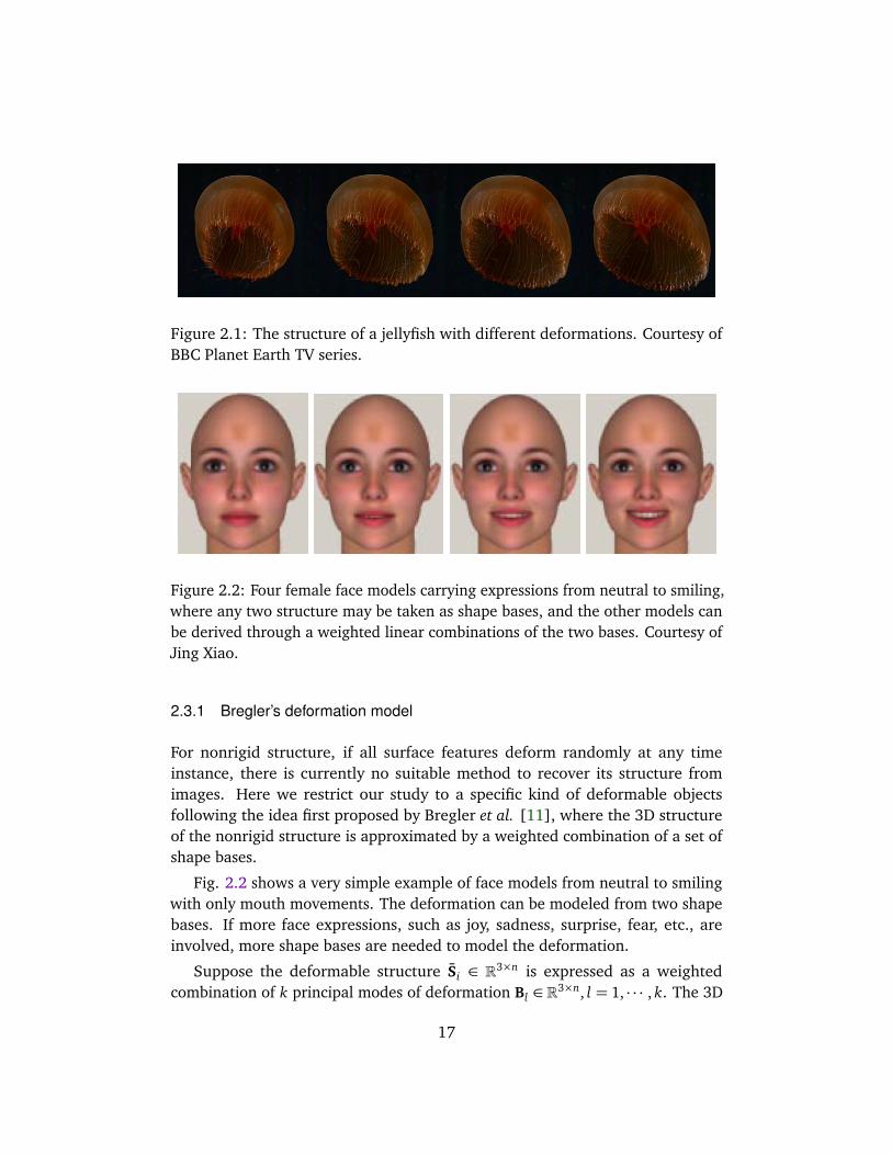
Figure 2.1: The structure of a jellyfish with different deformations. Courtesy ofBBC Planet Earth TV series.

Figure 2.2: Four female face models carrying expressions from neutral to smiling,where any two structure may be taken as shape bases, and the other models canbe derived through a weighted linear combinations of the two bases. Courtesy ofJing Xiao.

2.3.1 Bregler’s deformation model

For nonrigid structure, if all surface features deform randomly at any timeinstance, there is currently no suitable method to recover its structure fromimages. Here we restrict our study to a specific kind of deformable objectsfollowing the idea first proposed by Bregler et al. [11], where the 3D structureof the nonrigid structure is approximated by a weighted combination of a set ofshape bases.

Fig. 2.2 shows a very simple example of face models from neutral to smilingwith only mouth movements. The deformation can be modeled from two shapebases. If more face expressions, such as joy, sadness, surprise, fear, etc., areinvolved, more shape bases are needed to model the deformation.

Suppose the deformable structure Si ∈ R3×n is expressed as a weightedcombination of k principal modes of deformation Bl ∈ R3×n, l = 1, · · · , k. The 3D

17

model can be expressed as

Si =k∑

l=1

ωilBl (2.14)

where ωil ∈ R is the deformation weight for base l at frame i. A perfect rigidobject corresponds to the situation of k = 1 and ωil = 1. Suppose all imagefeatures are registered to their centroid in each frame, then, we have the followingformulation under orthographic projection.

Wi = [xi1, xi2, · · · , xin] = RAi

k∑

l=1

ωilBl

=

ωi1RAi , · · · ,ωikRAi

B1...

Bk

, ∀ i = 1, · · · , m (2.15)

where RAi stands for the first two rows of the rotation matrix corresponding tothe i-th frame. Then, we can obtain the factorization equation of the trackingmatrix by stacking all instances of equations (2.15) frame by frame as

x11 · · · x1n...

. . ....

xm1 · · · xmn

︸︷︷︸

W2m×n

=

ω11RA1 · · · ω1kRA1...

. . ....

ωm1RAm · · · ωmkRAm

︸︷︷︸

M2m×3k

B1...

Bk

︸︷︷︸

B3k×n

. (2.16)

The above equation can be written in short as W =MB, which is similar asthe rigid factorization (2.2). The only difference lies in the form and dimensionof the motion and shape matrices. From the right side of (2.16), it is easy to findthat the rank of the nonrigid tracking matrix is at most 3k (usually 2m and n areboth larger than 3k). The goal of nonrigid factorization is to recover the motionand the deformable structure corresponding to each frame.

2.3.2 Nonrigid factorization under affine assumption

Following the same idea of rigid factorization, we perform SVD decompositionon the nonrigid tracking matrix and impose the rank-3k constraint, W canbe factorized into a 2m × 3k matrix M and a 3k × n matrix B. However, thedecomposition is not unique as any nonsingular linear transformation matrixH ∈ R3k×3k can be inserted into the factorization which leads to an alternativeresult W= (MH)(H−1 ¯B). If we have a transformation matrix H that can resolvethe affine ambiguity and upgrade the solution to the Euclidean space, the shapebases are then easily recovered from B = H−1B, while the rotation matrix RAi and

18

the weighting coefficient ωi j can be decomposed from M = MH by Procrustesanalysis [9][11][76].

Similar to the rigid situation, the upgrading matrix can be recovered byimposing metric constraint to the motion matrix. In the following section, wewill briefly review some typical methods to deal with this problem.

Metric constraints

To recover the upgrading matrix, many researchers apply metric constraints tothe rotation matrix. Bregler et al. [11] first introduced the nonrigid factorizationframework and proposed a sub-block factorization algorithm to recover therotation matrix RAi and deformation weights ωil by decomposing every two-rowsub-blocks of the motion matrix M.

In (2.16), each two-row sub-block is given by

Mi =

ωi1RAi , · · · ,ωikRAi

(2.17)

which can be rearranged as a k× 6 matrix M′i as follows.

M′i =

ωi1rT1i | ωi1rT

2i...

...ωikrT

1i | ωikrT2i

k×6

=

ωi1...ωik

rT1i|r

T2i

(2.18)

where rT1i and rT

2i are the first and second rows of the rotation matrix, respectively.Clearly, the deformation weight ωil and the rotation matrix can be easily derivedvia the SVD factorization of M′i with rank-1 constraint. However, such recoveredrotation matrix

RAi =

rT1i

rT2i

is usually not an orthonormal matrix, thus, an orthonormality process is requiredto find the rotation matrix RAi [74].

Concerning the recovery of the upgrading matrix, Xiao et al. [95] presenteda block computation method via metric constraints. Suppose the l-th columntriples of H is Hl , l = 1, · · · , k, which is independent of each other since H isnonsingular. Then, we have

MHl =

ω1lRA1...

ωmlRAm

(2.19)

19

and

MHlHTl MT =

ω211RA1RT

A1 ∗ · · · ∗∗ ω2

2lRA2RTA2 · · · ∗

......

. . ....

∗ ∗ · · · ω2mlRAmRT

Am

(2.20)

where ′∗′ stands for nonzero entries. Let Ql = HlHTl , which is a 3k×3k symmetric

matrix with 12k(9k+ 1) unknowns. Since RAi is an orthonormal rotation matrix,

from each diagonal block in (2.20), we have

M2i−1:2iQlMT2i−1:2i =ω

2il

1 00 1

(2.21)

where M2i−1:2i stands for the i-th two-row of M. Thus, we have the followinglinear constraints on Ql .

¨

M2i−1QlMT2i = 0

M2i−1QlMT2i−1− M2iQlM

T2i = 0

, ∀ i = 1, · · · , m. (2.22)

Therefore, Ql may be computed linearly via least squares from (2.22) givensufficient frames, then, Hl is recovered from Ql via Cholesky decomposition.

In sub-block factorization, it is assumed that all configurations concerning thecamera motion and deformation weights are contained in the initially factorizedmatrix M. Nevertheless, the initial decomposition may yield random solutionfor M and B, and result in a bad estimation of the rotation matrix [9][19]. Toovercome the limitation of sub-block factorization, Torresani et al. [76] proposeda tri-linear approach to solving Bl ,ωil , and RAi alternatively by minimizing thefollowing cost function.

f (Bl ,ωil ,RAi) =

Wi −RAi

k∑

l=1

ωilBl

2

F,∀ i = 1, · · · , m. (2.23)

The iterative algorithm that solves the cost function is initialized by the rigidassumption solution, and a rigid factorization [74] on the nonrigid trackingmatrix is performed to obtain an average shape (mean shape) matrix Sri g anda rigid rotation matrix RAi , i = 1, · · · , m, for each frame; while the deformationweights are initialized randomly. The algorithm is performed iteratively throughthe following three steps:

1. Estimate the shape bases B from RAi and ωil ;

2. Update the deformation weight ωil from B and RAi;

20

3. Update the rotation matrix RAi from B and ωil .

The procedure is simpler than the general nonlinear method and usuallyconverges to a proper solution. However, the algorithm does not preserve thereplicated block structure of the motion matrix (2.16) during iterations [19].

Similar to the tri-linear technique, Wang et al. [82] proposed a rotationconstrained power factorization technique by combining the orthonormality ofthe rotation matrix into a power factorization algorithm. In Addition, Brand [9]proposed a flexible factorization technique to compute the upgrading matrix andrecover the motion parameters and deformation weights using an alternativeorthonormal decomposition algorithm.

Basis constraints

One main problem of using a metric constraint to recover the upgrading ma-trix lies in its ambiguity. Given the same tracking data, different motion anddeformable shapes may be found, since any nonsingular linear transformationmatrix can be inserted into the factorization process and, as a result, lead todifferent sets of eligible shape bases.

On the other hand, when we use the constraints (2.22) to recover the matrixQl , it appears that if we have enough features and frames, the upgrading matrixcan be solved linearly by exploring all the constraints in (2.22). Unfortunately,using only the rotation constraints may be insufficient when the object deformsat varying speed, since most of the constraints are redundant. Xiao et al. [96]proposed a basis constraint to solve this ambiguity.

The main idea is based on the assumption that there exists k frames whichinclude independent shapes that can be treated as a set of bases. Suppose thefirst k frames are independent of each other. Then, their corresponding weightingcoefficients can be set as

ωil =

¨

1 if i, l = 1, ..., k and i = l0 if i, l = 1, ..., k and i 6= l

. (2.24)

Let us define Ω = (i, j)|i = 1, · · · , k, j = 1, · · · , m, i 6= l, then, from (2.20) we

21

can obtain the following basis constraint.

M2i−1QlMT2 j−1 =

¨

1, i = j = l0, (i, j) ∈ Ω

M2iQlMT2 j =

¨

1, i = j = l0, (i, j) ∈ Ω

M2i−1QlMT2 j =

¨

0, i = j = l0, (i, j) ∈ Ω

M2iQlMT2 j−1 =

¨

0, i = j = l0, (i, j) ∈ Ω

. (2.25)

Altogether we have 4m(k− 1) linear basis constraints. Using both the metricconstraints (2.22) and the basis constraints (2.25), Xiao et al. [96] derived alinear close form solution to the nonrigid factorization by dividing the probleminto k linear systems. However, the method deals with each column-triplesMi separately. Thus, the repetitive block structure of the entire motion matrixis not observed during computation. In addition, the solution is dependanton the selection of shape bases, which are treated as prior information of thedeformation, but such a selection may be difficult in some situations. Followingthis idea, Brand [10] proposed a modified approach based on the deviation ofthe solution from metric constraints. The approach explores a weak constraint tothe independent shape bases.

2.3.3 Nonrigid factorization under perspective projection

In this section, we will discuss the perspective reconstruction method proposedin [96]. From perspective projection (1.1), we can obtain the following equationsystem by stacking the projection of each frame.

W=

λ11x11 · · · λ1nx1n...

. . ....


=

P1S1...

PmSm

(2.26)

where Si is a 4× n matrix which denotes the 3D structure corresponding to thei-th frame in homogeneous form. For rigid objects, the shape does not changewith time, thus, S1 = · · · = Sm. Following Bregler’s deformation model (2.14), wehave

PiSi =k∑

l=1

ωilP(1:3)i Bl

+ P(4)i 1T (2.27)

where P(1:3)i and P(4)i denote the first three columns and the last column of Pi,

respectively; and 1T is a n-vector with unit entries. From equations (2.26) and

22

(2.27), we obtain the following expression for perspective nonrigid factorization.

W=

ω11P(1:3)1 · · · ω1kP(1:3)

1 P(4)1...

. . ....

...ωm1P(1:3)

m · · · ωmkP(1:3)m P(4)m

︸︷︷︸

M3m×(3k+1)

B1...

Bk

1T

︸︷︷︸

B(3k+1)×n

(2.28)

where M ∈ R3m×(3k+1) and B ∈ R(3k+1)×n are the motion matrix and shape bases,respectively. All nonrigid structures of one object share the same set of shapebases, and both M and B are of full rank. Therefore, the rank of the scale-weighted tracking matrix is no more than min((3k+ 1), 3m, n). In practice, thepoint and frame numbers are usually larger than the shape bases number, so therank of W is at most 3k+ 1. This is consistent with that of rigid factorization,where k = 1 and the rank is no more than 4.

Suppose the projective depth scales in W are available, then, a projectivesolution of M and B can be obtained through SVD decomposition of the weightedtracking matrix with rank-(3k+ 1) constraint. Obviously, the solution is definedup to a nonsingular transformation matrix H ∈ R(3k+1)×(3k+1). Similar to the rigidcase, the upgrading matrix can be recovered using both the metric constraints andthe basis constraints. Then, the Euclidean motion parameters and deformationstructures are recovered from the matrices M and B. Please refer to Xiao andKanade [96] for computation details.

As for the recovery of the projective depths, a similar iteration method as in[31] and [47], based on the rank constraint on W, is adopted. The algorithmstarts with weak perspective assumption by setting λi j = 1, then, the depth scalesare optimized iteratively by minimizing the following cost function

J(λi j) =min‖W− MB‖2F . (2.29)

The minimizing process is achieved iteratively by first factorizing W into MBwith the given depth scales and then updating the depth scales through backprojection. In deformation case, the rank of the tracking matrix is 3k+ 1 andthe dimension of M and B follows the Equation (2.28). In order to avoid trivialsolutions of λi j = 0, the following constraints are enforced alternatively duringthe computation to ensure that the depth scales of all points in any frame or asingle point in all images have unit norms. As a result, the minimization of (2.29)is converted to a simple eigenvalue problem [96].

23

2.3.4 Nonrigid factorization in trajectory space

Bregler’s assumption [11] represents the nonrigid structure in shape space as alinear combination of shape bases. Most recently, Akhter et al. [4] [5] proposed adual representation of nonrigid objects in trajectory space, where the evolving 3Ddeformable structure is described in the trajectory space by a linear combinationof some basis trajectories.

Suppose the structure of a nonrigid object is represented as follows by anm× 3n matrix.

S∗ =

X11 · · · X1n Y11 · · · Y1n Z11 · · · Z1n...

. . ....

.... . .

......

. . ....

Xm1 · · · Xmn Ym1 · · · Ymn Zm1 · · · Zmn

m×3n

. (2.30)

The row space of S∗ spans the shape space, while the column space of S∗

corresponds to the trajectories of the points, all of which form the trajectoryspace. Since both the row and column spaces have the same dimension, thetrajectory of the points can also be denoted by k trajectory bases. Let us writethe trajectory as

T( j) = [TTx ( j),T

Ty ( j),T

Tz ( j)]

T (2.31)

where

TTx ( j) = [X i j , · · · , Xmj], TT

y ( j) = [Yi j , · · · , Ymj], TTz ( j) = [Zi j , · · · , Zmj] (2.32)

are the j-th trajectory in the three coordinates directions. Each trajectory can bedenoted by k trajectory bases as follows.

TTx ( j) =

k∑

l=1

ωx l( j)θl , TT

y ( j) =k∑

l=1

ωyl( j)θl , TT

z ( j) =k∑

l=1

ωzl( j)θl (2.33)

whereωx l( j),ωyl( j), andωzl( j) are the coefficients; and θ l = [θ l1, · · · ,θ l

m]T ∈ Rm

is a trajectory basis vector. Expending (2.33) yields

X11 · · · X1n

Y11 · · · Y1n

Z11 · · · Z1n

X21 · · · X2n

Y21 · · · Y2n

Z21 · · · Z2n... · · ·

...Xm1 · · · Xmn

Ym1 · · · Ymn

Zm1 · · · Zmn

︸︷︷︸

S3m×n

=

θ T1θ T

1θ T

1...

......

θ Tmθ T

mθ T

m

︸︷︷︸

Θ3m×3k

ω1x1 ω1

x2 · · · ω1xn

......

......

ωkx1 ωk

x2 · · · ωkxn

ω1y1 ω1

y2 · · · ω1yn

......

......

ωky1 ωk

y2 · · · ωkyn

ω1z1 ω1

z2 · · · ω1zn

......

......

ωkz1 ωk

z2 · · · ωkzn

︸︷︷︸

Ω3k×n

(2.34)

24

where θ Tj = [θ

1j , · · · ,θ k

j ]T . Thus, the nonrigid trajectory can be written concisely

as follows.S3m×n =Θ3m×3kΩ3k×n. (2.35)

Under orthographic projection, the mapping from 3D space to 2D image canbe written as

W=MS= (MΘ)Ω= ΛΩ (2.36)

where

M=

R1. . .

Rm

(2.37)

with R j the j-th 2× 3 orthographic projection matrix; and Λ=MΘ is a 3m× 3kmatrix. It is clear that the factorization in trajectory space (2.36) is a dualexpression of the nonrigid factorization in shape space (2.16).

Like in shape space, the rank of (2.36) is at most 3k, the factorization can beeasily obtained via SVD decomposition, however, the solution is not unique anda similar metric constraint can be used to upgrade the solution from perspectiveto the Euclidean space by an invertible upgrading matrix H ∈ R3k×3k.

An advantage of the trajectory based algorithm lies in the fact that the trajec-tory bases can be predefined independently of the tracking data. The key pointhere is how to select the trajectory bases. Some available candidates includeDiscrete Sine/Cosine transformation, discrete Wavelet transformation, Hadamardtransform basis, etc. In [5], it was demonstrated that DCT basis was suitable torepresent human motions. The method was used to reconstruct the 3D trajectoryof a moving point from 2D projections [61]. Gotardo and Martinez furtherstudied the approach [27] and applied a kernel trick in the standard nonrigidSfM [28].

2.4 Discussion

In the literature, most algorithms assume affine camera model due to its simplicity,while the extension to full perspective model is computational intensive andno convergence is guaranteed. To bridge the gap between the two model, aquasi-perspective projection model is proposed in Chapter 3. The model isshowed to be more accurate than the affine assumption and more computationalefficient than the full perspective model. The geometric properties of the quasi-perspective model are investigated in Chapter 4 in the context of one- andtwo-view geometry. Finally, a structure from motion framework for both rigidand nonrigid objects is established in Chapter 5. Theoretical analyses and

25

experimental studies demonstrate the advantages of the proposed model overthe previous affine and perspective projection models.

Robustness is another important issue of SfM because the tracking data areusually corrupted by outliers, missing features, and significant noise. The maindifficulty of the robust algorithm lies in the estimation of feature uncertainties,which has not been effectively solved in the literature. In this thesis, the un-certainties are modeled from a new perspective by virtue of the fact that theuncertainties associated with image features are largely in proportion to thereprojection residuals.

A spatial-and-temporal-weighted factorization algorithm is proposed in Chap-ter 6, where the image uncertainties are modeled both spatially and temporallyto address different kinds of errors. An augmented affine factorization algorithmis proposed in Chapter 7 to circumvent the problem of image registration inaffine factorization in the presence of outlying and missing data. Based on thenew formulation, a robust factorization scheme is presented in the chapter tohandle outliers in rigid factorization. In Chapter 8, the idea is successfully ex-tended to nonrigid scenarios with imperfect tracking data. Unlike other existingrobust algorithms, the proposed technique requires no prior information of theerror distributions of the tracked features. Extensive experiments validate itsadvantages and effectiveness.

26

Chapter 3

Quasi-Perspective Projection Model

The chapter focuses on the approximation of a full perspective projection model.We first present a review on the affine camera model, including orthographicprojection, weak-perspective projection, and paraperspective projection. Then,under the assumption that the camera is far away from the object with smalllateral rotations, we show that the imaging process can be modeled by quasi-perspective projection. Geometrical analysis and experimental study show thatthe proposed model is more accurate than the affine model.

3.1 Introduction

The modeling of imaging formation is an important issue for many computervision applications, such as structure from motion, object recognition, pose es-timation, etc. Geometrically, a camera maps data from 3D space to 2D imagespace. The general camera model used in computer vision is modeled by per-spective projection. This is an ideal and accurate model for a wide range ofexisting cameras. However, the resulting equations from perspective projectionare complicated and nonlinear due to the unknown scaling factor [56]. To sim-plify computation, researchers have proposed many approximations to the fullperspective projection.

The most common approximation includes weak-perspective projection, or-thographic projection, and paraperspective projection [6]. These approximationsare generalized as affine camera model [51] [68]. Faugeras [24] studied theproperties of projective cameras. Hartley and Zisserman [32] presented a compre-hensive survey and in-depth analysis of different camera models. Affine camerais a zero-order (for weak-perspective) or a first-order (for paraperspective) ap-proximation of full perspective projection [15]. It is valid only when the depthvariation of the object is small compared to the distance from camera to the

27

object. Kanatani et al. [40] analyzed a general form of symmetric affine cameramodel to mimic perspective projection and provided the minimal requirements fororthographic, weak perspective, and para-perspective simplification. The modelcontains two free variables that can be determined through self-calibration.

In structure from motion, the affine assumption is widely adopted due toits simplicity. In this chapter, we try to make a trade-off between the simplicityof the affine model and the accuracy of the full perspective projection model.By assuming that the camera is far away from the object with small lateralrotations, which is similar to affine assumption and is easily satisfied in practice,we propose a quasi-perspective projection model and present an error analysisof different projection models [83]. The proposed model is shown to be moreaccurate than the affine approximation. In Chapters 4 and 5 of this thesis, we willfurther analyze the geometrical properties of the model [85] and its applicationto structure and motion factorization. Part of this chapter was published inInternational Journal of Computer Vision [86].

The remaining part of the chapter is organized as follows. The affine projec-tion model is reviewed in Section 3.2. The proposed quasi-perspective modeland error analysis are elaborated in Section 3.3. Some experimental evaluationson synthetic data are given in Section 3.4.

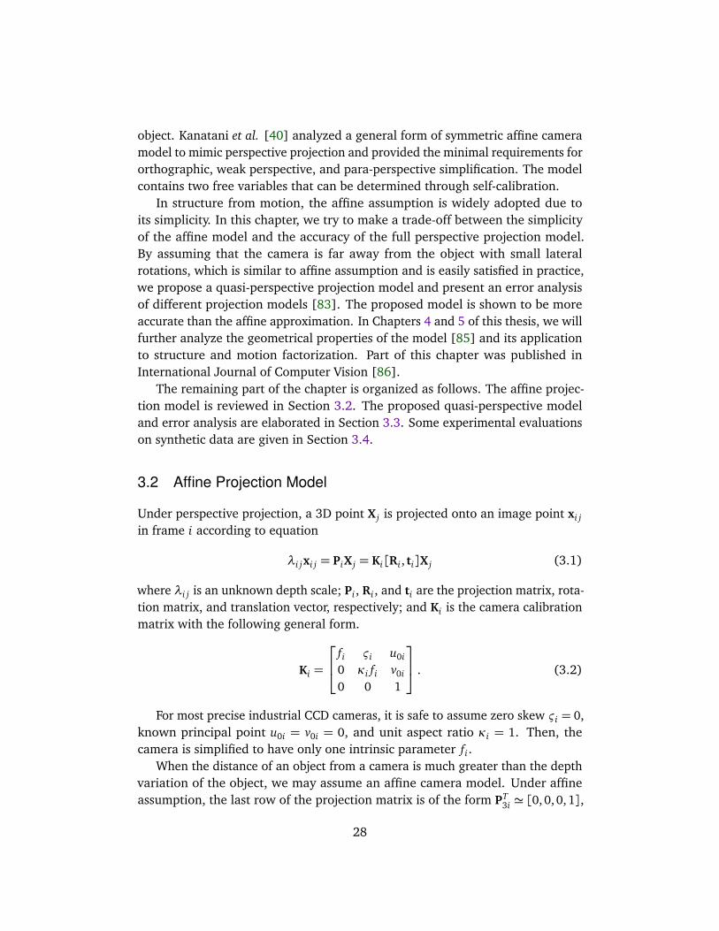
3.2 Affine Projection Model

Under perspective projection, a 3D point X j is projected onto an image point xi j

in frame i according to equation

λi jxi j = PiX j = Ki[Ri , ti]X j (3.1)

where λi j is an unknown depth scale; Pi, Ri, and ti are the projection matrix, rota-tion matrix, and translation vector, respectively; and Ki is the camera calibrationmatrix with the following general form.

Ki =

fi ςi u0i

0 κi fi v0i

0 0 1

. (3.2)

For most precise industrial CCD cameras, it is safe to assume zero skew ςi = 0,known principal point u0i = v0i = 0, and unit aspect ratio κi = 1. Then, thecamera is simplified to have only one intrinsic parameter fi.

When the distance of an object from a camera is much greater than the depthvariation of the object, we may assume an affine camera model. Under affineassumption, the last row of the projection matrix is of the form PT

3i ' [0, 0, 0, 1],

28

where ’'’ denotes equality up to scale. Thus, a general affine projection matrixfor the i-th view can be written as

PAi =

p11 p12 p13 p14

p21 p22 p23 p24

0 0 0 1

=

Ai ti

0T 1

(3.3)

where Ai ∈ R2×3 is composed by the upper-left 2 × 3 submatrix of Pi, ti is atranslation vector. Under affine assumption, the imaging process (3.1) can besimplified by removing the unknown scale factor λi j.

xi j = AiX j + ti . (3.4)

Under the affine projection (3.4), the mapping from space to the image islinear. One attractive attribute of the affine camera model is that the mapping isindependent of the translation term if relative coordinates are employed in bothspace and image coordinate frames.

Suppose Xr is a reference point in space and xir is its image in the i-th frame.Then, we have xir = AiXr + ti. Let us denote

x′i j = xi j − xir , X′j = X j − Xr

as the relative image and space coordinates. We can immediately obtain asimplified affine projection equation in terms of relative coordinates.

x′i j = AiX′j . (3.5)

The translation term ti is actually the image of the world origin. It is easy toverify that the centroid of a set of space points is projected to the centroid of theirimages. In practice, we can simply choose the centroid as the reference point, thenthe translation term vanishes if all the image points in each frame are registeredto the corresponding centroid. The affine matrix Ai has six independent variableswhich encapsulate both intrinsic and extrinsic parameters of the affine camera.According to RQ decomposition [32], matrix Ai can be uniquely decomposedinto the following form.

Ai = KAiRAi =

α1i ζi

α2i

rT1i

rT2i

(3.6)

where KAi is the intrinsic calibration matrix. In accordance with the cameramatrix of perspective projection, α1i and α2i are the scaling factors of the twoimage axes and α1i/α2i is defined as the aspect ratio, ζi is the skew factor ofthe affine camera. For most CCD cameras, we usually assume unit aspect ratio

29

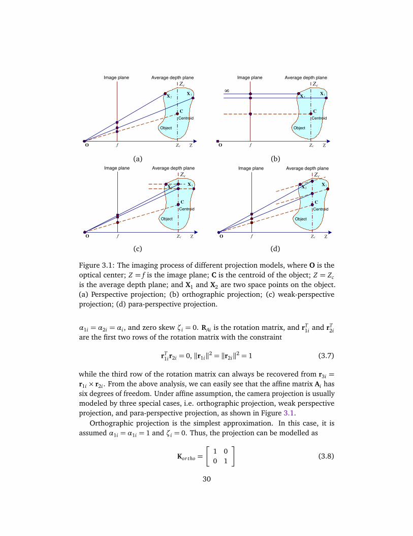
8

C

Zc

ZO f Zc

Image plane Average depth plane

Centroid

Object

X1X2

C

Zc

ZO f Zc


Centroid

Object

X1X2

(a) (b)

C

Zc

ZO f Zc


Centroid

Object

X1X2

C

Zc

ZO f Zc


Centroid

Object

X1X2

(c) (d)

Figure 3.1: The imaging process of different projection models, where O is theoptical center; Z = f is the image plane; C is the centroid of the object; Z = Zc

is the average depth plane; and X1 and X2 are two space points on the object.(a) Perspective projection; (b) orthographic projection; (c) weak-perspectiveprojection; (d) para-perspective projection.

α1i = α2i = αi, and zero skew ζi = 0. RAi is the rotation matrix, and rT1i and rT

2iare the first two rows of the rotation matrix with the constraint

rT1ir2i = 0, ‖r1i‖2 = ‖r2i‖2 = 1 (3.7)

while the third row of the rotation matrix can always be recovered from r3i =r1i × r2i. From the above analysis, we can easily see that the affine matrix Ai hassix degrees of freedom. Under affine assumption, the camera projection is usuallymodeled by three special cases, i.e. orthographic projection, weak perspectiveprojection, and para-perspective projection, as shown in Figure 3.1.

Orthographic projection is the simplest approximation. In this case, it isassumed α1i = α1i = 1 and ζi = 0. Thus, the projection can be modelled as

Kor tho =

1 00 1

(3.8)

30

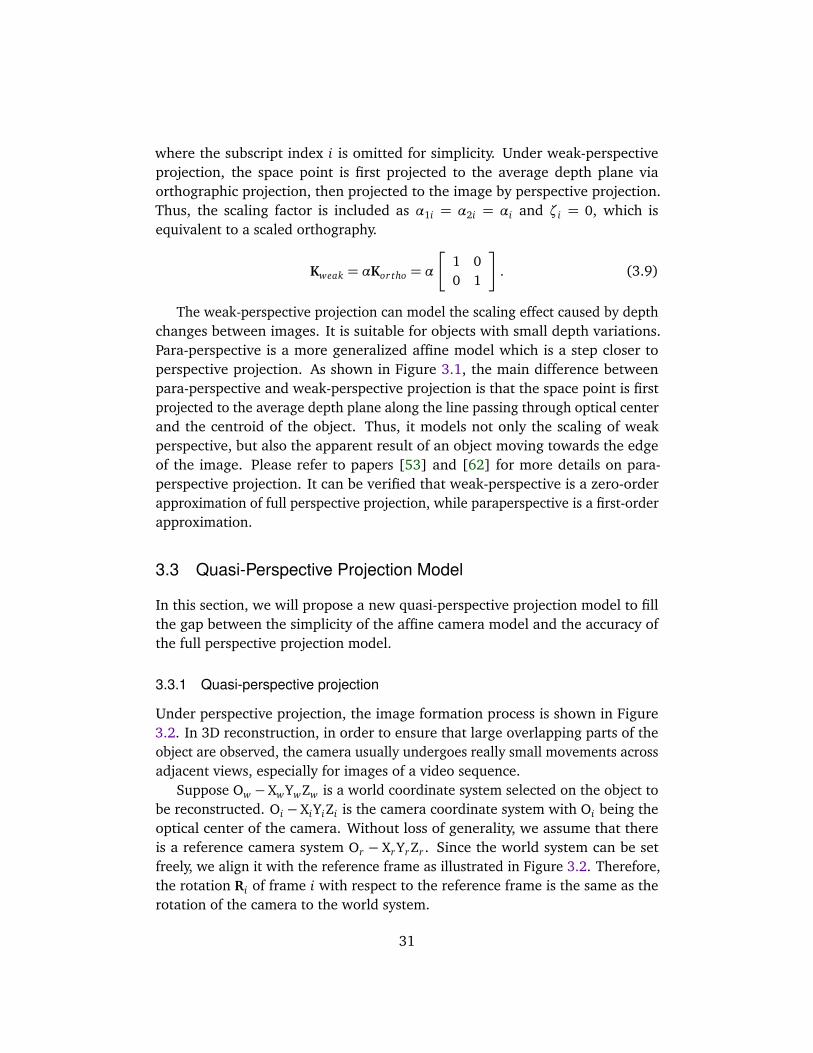
where the subscript index i is omitted for simplicity. Under weak-perspectiveprojection, the space point is first projected to the average depth plane viaorthographic projection, then projected to the image by perspective projection.Thus, the scaling factor is included as α1i = α2i = αi and ζi = 0, which isequivalent to a scaled orthography.

Kweak = αKor tho = α

1 00 1

. (3.9)

The weak-perspective projection can model the scaling effect caused by depthchanges between images. It is suitable for objects with small depth variations.Para-perspective is a more generalized affine model which is a step closer toperspective projection. As shown in Figure 3.1, the main difference betweenpara-perspective and weak-perspective projection is that the space point is firstprojected to the average depth plane along the line passing through optical centerand the centroid of the object. Thus, it models not only the scaling of weakperspective, but also the apparent result of an object moving towards the edgeof the image. Please refer to papers [53] and [62] for more details on para-perspective projection. It can be verified that weak-perspective is a zero-orderapproximation of full perspective projection, while paraperspective is a first-orderapproximation.

3.3 Quasi-Perspective Projection Model

In this section, we will propose a new quasi-perspective projection model to fillthe gap between the simplicity of the affine camera model and the accuracy ofthe full perspective projection model.

3.3.1 Quasi-perspective projection

Under perspective projection, the image formation process is shown in Figure3.2. In 3D reconstruction, in order to ensure that large overlapping parts of theobject are observed, the camera usually undergoes really small movements acrossadjacent views, especially for images of a video sequence.

Suppose Ow − XwYwZw is a world coordinate system selected on the object tobe reconstructed. Oi − XiYiZi is the camera coordinate system with Oi being theoptical center of the camera. Without loss of generality, we assume that thereis a reference camera system Or − XrYrZr . Since the world system can be setfreely, we align it with the reference frame as illustrated in Figure 3.2. Therefore,the rotation Ri of frame i with respect to the reference frame is the same as therotation of the camera to the world system.

31

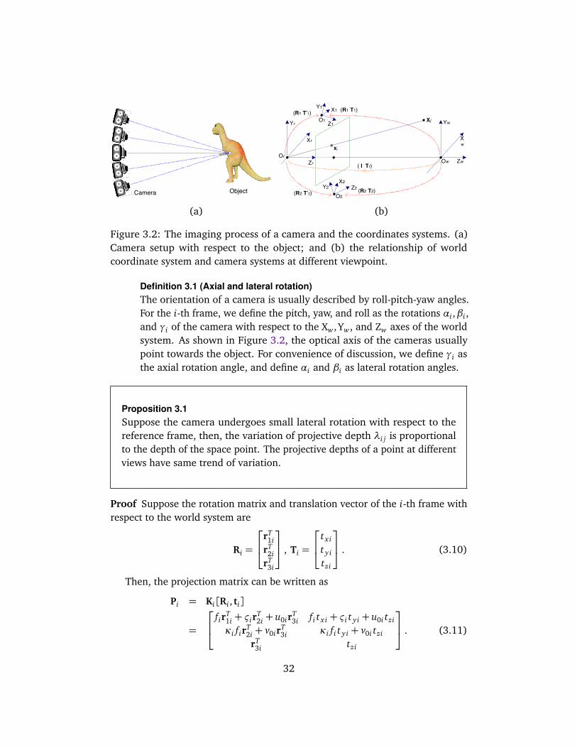
O1

Or

O2

Ow

Z1

Zr

Z2

Zw

X1

Xr

X2

Xw

Y1

Yr

Y2

YwXj

xj

(R1 T1)

(R2 T2)

(R1 T’1)

(R2 T’2)

( I Tr)

ObjectCamera

(a) (b)

Figure 3.2: The imaging process of a camera and the coordinates systems. (a)Camera setup with respect to the object; and (b) the relationship of worldcoordinate system and camera systems at different viewpoint.

Definition 3.1 (Axial and lateral rotation)The orientation of a camera is usually described by roll-pitch-yaw angles.For the i-th frame, we define the pitch, yaw, and roll as the rotations αi ,βi,and γi of the camera with respect to the Xw , Yw, and Zw axes of the worldsystem. As shown in Figure 3.2, the optical axis of the cameras usuallypoint towards the object. For convenience of discussion, we define γi asthe axial rotation angle, and define αi and βi as lateral rotation angles.

Proposition 3.1Suppose the camera undergoes small lateral rotation with respect to thereference frame, then, the variation of projective depth λi j is proportionalto the depth of the space point. The projective depths of a point at differentviews have same trend of variation.

Proof Suppose the rotation matrix and translation vector of the i-th frame withrespect to the world system are

Ri =

rT1i

rT2i

rT3i

, Ti =

t x i

t yi

tzi

. (3.10)

Then, the projection matrix can be written as

Pi = Ki[Ri , ti]

=

firT1i + ςir

T2i + u0ir

T3i fi t x i + ςi t yi + u0i tzi

κi firT2i + v0ir

T3i κi fi t yi + v0i tzi

rT3i tzi

. (3.11)

32

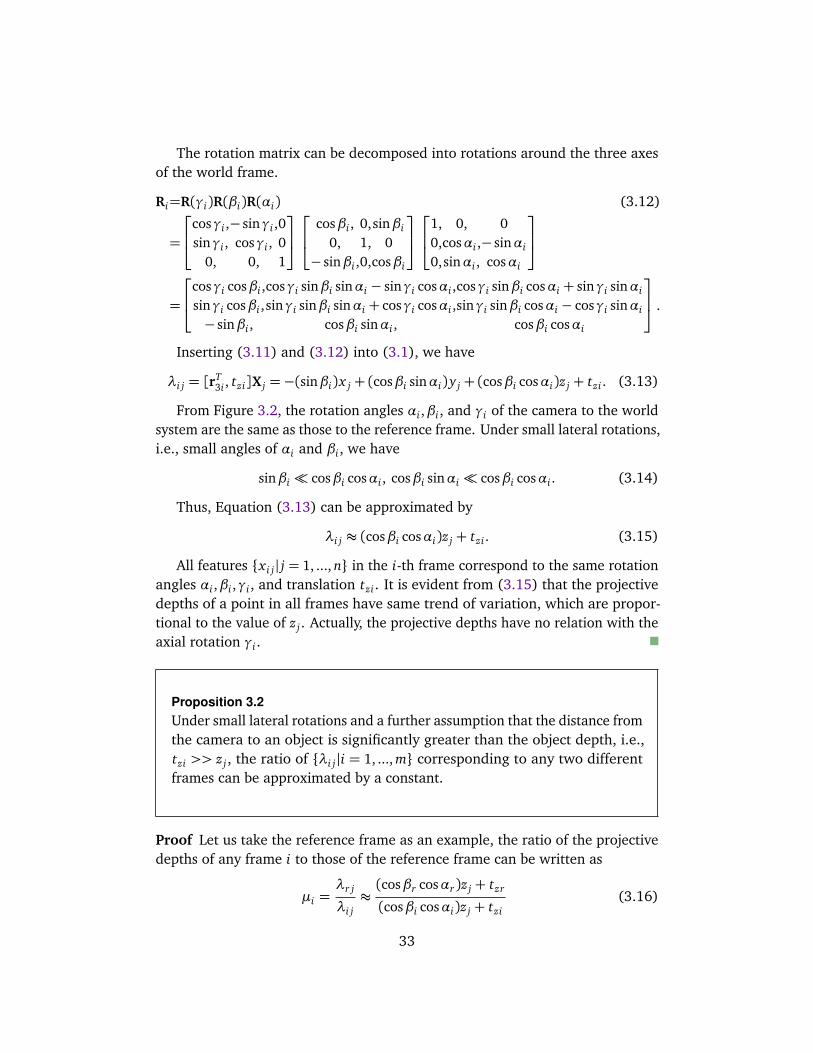
The rotation matrix can be decomposed into rotations around the three axesof the world frame.

Ri=R(γi)R(βi)R(αi) (3.12)

=

cosγi ,− sinγi ,0sinγi , cosγi , 0

0, 0, 1

cosβi , 0,sinβi

0, 1, 0− sinβi ,0,cosβi

1, 0, 00,cosαi ,− sinαi

0,sinαi , cosαi

=

cosγi cosβi ,cosγi sinβi sinαi − sinγi cosαi ,cosγi sinβi cosαi + sinγi sinαi

sinγi cosβi ,sinγi sinβi sinαi + cosγi cosαi ,sinγi sinβi cosαi − cosγi sinαi

− sinβi , cosβi sinαi , cosβi cosαi

.

Inserting (3.11) and (3.12) into (3.1), we have

λi j = [rT3i , tzi]X j =−(sinβi)x j + (cosβi sinαi)y j + (cosβi cosαi)z j + tzi . (3.13)

From Figure 3.2, the rotation angles αi ,βi, and γi of the camera to the worldsystem are the same as those to the reference frame. Under small lateral rotations,i.e., small angles of αi and βi, we have

sinβi cosβi cosαi , cosβi sinαi cosβi cosαi . (3.14)

Thus, Equation (3.13) can be approximated by

λi j ≈ (cosβi cosαi)z j + tzi . (3.15)

All features x i j| j = 1, ..., n in the i-th frame correspond to the same rotationangles αi ,βi ,γi, and translation tzi. It is evident from (3.15) that the projectivedepths of a point in all frames have same trend of variation, which are propor-tional to the value of z j. Actually, the projective depths have no relation with theaxial rotation γi.

Proposition 3.2Under small lateral rotations and a further assumption that the distance fromthe camera to an object is significantly greater than the object depth, i.e.,tzi >> z j, the ratio of λi j|i = 1, ..., m corresponding to any two differentframes can be approximated by a constant.

Proof Let us take the reference frame as an example, the ratio of the projectivedepths of any frame i to those of the reference frame can be written as

µi =λr j

λi j≈(cosβr cosαr)z j + tzr

(cosβi cosαi)z j + tzi(3.16)

33

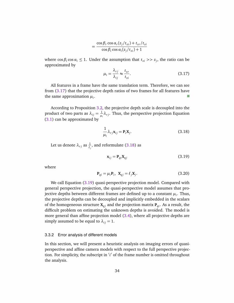
=cosβr cosαr(z j/tzi) + tzr/tzi

cosβi cosαi(z j/tzi) + 1

where cosβi cosαi ≤ 1. Under the assumption that tzi >> z j, the ratio can beapproximated by

µi =λr j

λi j≈

tzr

tzi. (3.17)

All features in a frame have the same translation term. Therefore, we can seefrom (3.17) that the projective depth ratios of two frames for all features havethe same approximation µi.

According to Proposition 3.2, the projective depth scale is decoupled into theproduct of two parts as λi j =

1µiλr j. Thus, the perspective projection Equation

(3.1) can be approximated by

1

µiλr jxi j = PiX j . (3.18)

Let us denote λr j as 1` j

, and reformulate (3.18) as

xi j = PqiXq j (3.19)

where

Pqi = µiPi , Xq j = ` jX j . (3.20)

We call Equation (3.19) quasi-perspective projection model. Compared withgeneral perspective projection, the quasi-perspective model assumes that pro-jective depths between different frames are defined up to a constant µi. Thus,the projective depths can be decoupled and implicitly embedded in the scalarsof the homogeneous structure Xq j and the projection matrix Pqi. As a result, thedifficult problem on estimating the unknown depths is avoided. The model ismore general than affine projection model (3.4), where all projective depths aresimply assumed to be equal to λi j = 1.

3.3.2 Error analysis of different models

In this section, we will present a heuristic analysis on imaging errors of quasi-perspective and affine camera models with respect to the full perspective projec-tion. For simplicity, the subscript in ′i′ of the frame number is omitted throughoutthe analysis.

34

Suppose the intrinsic parameters of the cameras are known, and all imagesare normalized by the cameras as K−1

i xi j → xi j. Then, the projection matricesunder different projection models can be written as

P=

rT1 t x

rT2 t y

rT3 tz

, rT

3 = [− sinβ , cosβ sinα, cosβ cosα] (3.21)

Pq =

rT1 t x

rT2 t y

rT3q tz

, rT3q = [0,0, cosβ cosα] (3.22)

Pa =

rT1 t x

rT2 t y

0T tz

, 0T = [0,0, 0] (3.23)

where P is the projection matrix of full perspective projection, Pq is that of quasi-perspective assumption, and Pa is that of affine projection. Obviously, the maindifference between the above projection matrices lies only in the last row. For aspace point X = [x , y, z]T , its projected images under different camera modelsare given by

m= P

X1

=

uv

rT3 X+ tz

(3.24)

mq = Pq

X1

=

uv

rT3qX+ tz

(3.25)

ma = Pa

X1

=

uvtz

(3.26)

where

u= rT1 X+ t x , v = rT

2 X+ t y (3.27)

rT3 X=−(sinβ)x + (cosβ sinα)y + (cosβ cosα)z (3.28)

rT3qX= (cosβ cosα)z (3.29)

and the nonhomogeneous image points can be denoted as

m=1

rT3 X+ tz

uv

(3.30)

35

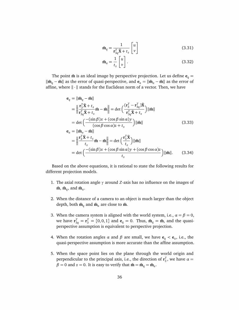
mq =1

rT3qX+ tz

uv

(3.31)

ma =1

tz

uv

. (3.32)

The point m is an ideal image by perspective projection. Let us define eq =‖mq − m‖ as the error of quasi-perspective, and ea = ‖ma − m‖ as the error ofaffine, where ‖ · ‖ stands for the Euclidean norm of a vector. Then, we have

eq = ‖mq − m‖

=

rT3 X+ tz

rT3qX+ tz

m− m

= det(rT

3 − rT3q)X

rT3qX+ tz

‖m‖

= det−(sinβ)x + (cosβ sinα)y

(cosβ cosα)z+ tz

‖m‖ (3.33)

ea = ‖ma − m‖

=

rT3 X+ tz

tzm− m

= detrT

3 X

tz

‖m‖

= det−(sinβ)x + (cosβ sinα)y + (cosβ cosα)z

tz

‖m‖. (3.34)

Based on the above equations, it is rational to state the following results fordifferent projection models.

1. The axial rotation angle γ around Z-axis has no influence on the images ofm, mq, and ma.

2. When the distance of a camera to an object is much larger than the objectdepth, both mq and ma are close to m.

3. When the camera system is aligned with the world system, i.e., α= β = 0,we have rT

3q = rT3 = [0,0,1] and eq = 0. Thus, mq = m, and the quasi-

perspective assumption is equivalent to perspective projection.

4. When the rotation angles α and β are small, we have eq < ea, i.e., thequasi-perspective assumption is more accurate than the affine assumption.

5. When the space point lies on the plane through the world origin andperpendicular to the principal axis, i.e., the direction of rT

3 , we have α =β = 0 and z = 0. It is easy to verify that m= mq = ma.

36

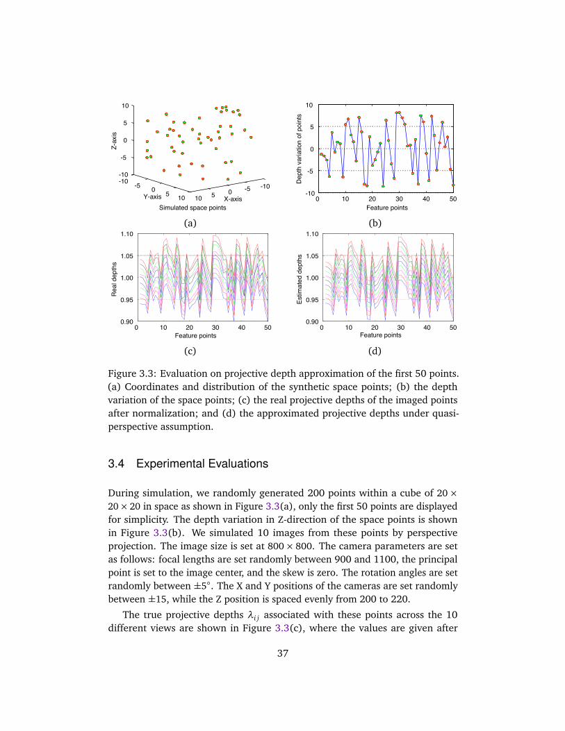
-10 -5 0 5 10-10-50510

-10

-5

0

5

10

Simulated space points

Z-ax

is

X-axisY-axis 0 10 20 30 40 50-10

-5

0

5

10

Feature points

Dep

th v

aria

tion

of p

oint

s

(a) (b)

Feature points

Estim

ated

dep

ths

0 10 20 30 40 500.90

0.95

1.00

1.05

1.10

Rea

l dep

ths

Feature points0 10 20 30 40 50

0.90

0.95

1.00

1.05

1.10

(c) (d)

Figure 3.3: Evaluation on projective depth approximation of the first 50 points.(a) Coordinates and distribution of the synthetic space points; (b) the depthvariation of the space points; (c) the real projective depths of the imaged pointsafter normalization; and (d) the approximated projective depths under quasi-perspective assumption.

3.4 Experimental Evaluations

During simulation, we randomly generated 200 points within a cube of 20×20× 20 in space as shown in Figure 3.3(a), only the first 50 points are displayedfor simplicity. The depth variation in Z-direction of the space points is shownin Figure 3.3(b). We simulated 10 images from these points by perspectiveprojection. The image size is set at 800× 800. The camera parameters are setas follows: focal lengths are set randomly between 900 and 1100, the principalpoint is set to the image center, and the skew is zero. The rotation angles are setrandomly between ±5. The X and Y positions of the cameras are set randomlybetween ±15, while the Z position is spaced evenly from 200 to 220.

The true projective depths λi j associated with these points across the 10different views are shown in Figure 3.3(c), where the values are given after

37

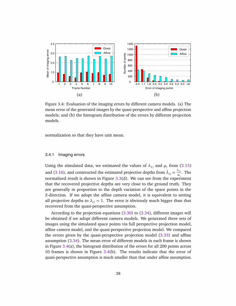
Error of imaging points

Num

ber o

f poi

nts

0.4 1.1 1.8 2.5 3.2 3.9 4.6 5.3 6.0 >60

200

400

600

800

1000

1200

1400

QuasiAffine

Frame Number

Mea

n of

imag

ing

erro

rs

1 2 3 4 5 6 7 8 9 100

1.0

2.0

3.0

4.0QuasiAffine

(a) (b)

Figure 3.4: Evaluation of the imaging errors by different camera models. (a) Themean error of the generated images by the quasi-perspective and affine projectionmodels; and (b) the histogram distribution of the errors by different projectionmodels.

normalization so that they have unit mean.

3.4.1 Imaging errors

Using the simulated data, we estimated the values of λ1 j and µi from (3.15)

and (3.16), and constructed the estimated projective depths from λi j =λ1 j

µi. The

normalized result is shown in Figure 3.3(d). We can see from the experimentthat the recovered projective depths are very close to the ground truth. Theyare generally in proportion to the depth variation of the space points in theZ-direction. If we adopt the affine camera model, it is equivalent to settingall projective depths to λi j = 1. The error is obviously much bigger than thatrecovered from the quasi-perspective assumption.

According to the projection equations (3.30) to (3.34), different images willbe obtained if we adopt different camera models. We generated three sets ofimages using the simulated space points via full perspective projection model,affine camera model, and the quasi-perspective projection model. We comparedthe errors given by the quasi-perspective projection model (3.33) and affineassumption (3.34). The mean error of different models in each frame is shownin Figure 3.4(a), the histogram distribution of the errors for all 200 points across10 frames is shown in Figure 3.4(b). The results indicate that the error ofquasi-perspective assumption is much smaller than that under affine assumption.

38

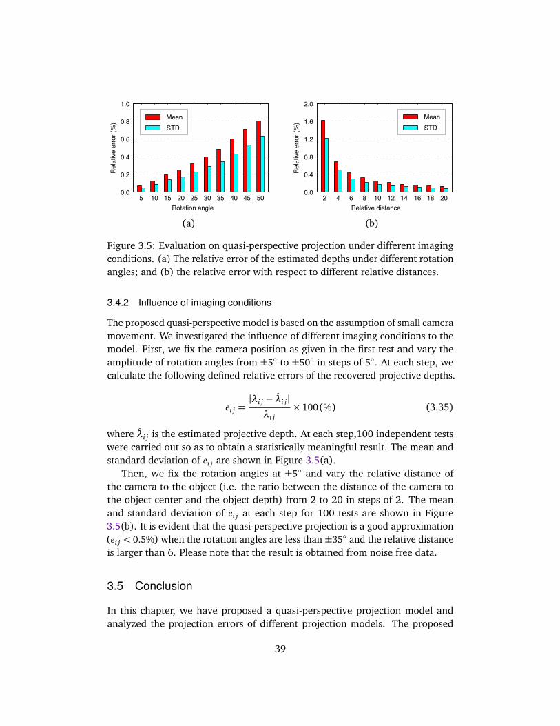
Rotation angle

Rel

ativ

e er

ror (

%)

5 10 15 20 25 30 35 40 45 500.0

0.2

0.4

0.6

0.8

1.0

MeanSTD

Relative distance

Rel

ativ

e er

ror (

%)

2 4 6 8 10 12 14 16 18 200.0

0.4

0.8

1.2

1.6

2.0

MeanSTD

(a) (b)

Figure 3.5: Evaluation on quasi-perspective projection under different imagingconditions. (a) The relative error of the estimated depths under different rotationangles; and (b) the relative error with respect to different relative distances.

3.4.2 Influence of imaging conditions

The proposed quasi-perspective model is based on the assumption of small cameramovement. We investigated the influence of different imaging conditions to themodel. First, we fix the camera position as given in the first test and vary theamplitude of rotation angles from ±5 to ±50 in steps of 5. At each step, wecalculate the following defined relative errors of the recovered projective depths.

ei j =|λi j − λi j|λi j

× 100 (%) (3.35)

where λi j is the estimated projective depth. At each step,100 independent testswere carried out so as to obtain a statistically meaningful result. The mean andstandard deviation of ei j are shown in Figure 3.5(a).

Then, we fix the rotation angles at ±5 and vary the relative distance ofthe camera to the object (i.e. the ratio between the distance of the camera tothe object center and the object depth) from 2 to 20 in steps of 2. The meanand standard deviation of ei j at each step for 100 tests are shown in Figure3.5(b). It is evident that the quasi-perspective projection is a good approximation(ei j < 0.5%) when the rotation angles are less than ±35 and the relative distanceis larger than 6. Please note that the result is obtained from noise free data.

3.5 Conclusion

In this chapter, we have proposed a quasi-perspective projection model andanalyzed the projection errors of different projection models. The proposed

39

model is a trade-off between the affine assumption and the perspective projection.It is computationally efficient with better accuracy than the affine approximation.

The proposed model is suitable for structure and motion factorization of ashort sequence with small camera motions. It should be noted that the smallrotation assumption of the proposed model is not a limiting factor and is usuallysatisfied in many real-world applications. During image acquisition of an objectto be reconstructed, we tend to control the camera movement so as to guaranteelarge overlapping part, which also facilitates the feature tracking process. Somegeometrical properties of the model in one-view and two-view [85] will be pre-sented in Chapter 4. The application details to structure and motion factorization[86] will be discussed in Chapter 5.

40

Chapter 4

Properties of Quasi-Perspective Model

This chapter investigates the geometrical properties of the quasi-perspectiveprojection model in one- and two-view geometry. The main results are as follows:(i) Quasi-perspective projection matrix has nine degrees of freedom, and theparallelism along the X and Y directions in world system are preserved in images;(ii) quasi-fundamental matrix can be simplified to a special form with only sixdegrees of freedom. The fundamental matrix is invariant to any non-singular pro-jective transformation; (iii) plane induced homography under quasi-perspectivemodel can be simplified to a special form defined by six degrees of freedom. Thequasi-homography may be recovered from two pairs of corresponding points withknown fundamental matrix; and (iv) any two reconstructions in quasi-perspectivespace are defined up to a non-singular quasi-perspective transformation.

4.1 Introduction

Stereo vision and structure from motion algorithms are based on certain as-sumption of camera models, including the perspective projection model, affineprojection model, and the quasi-perspective projection model proposed in Chap-ter 3. Different models have different geometrical properties.

The fundamental matrix is an important concept in stereo vision as it en-capsulates the underlying epipolar geometry between images. Classical lineartechniques for fundamental matrix estimation are sensitive to noise. Hartley[35] analyzed the problem and proposed a normalized eight-point algorithmto improve the stability and accuracy of computation. Zhang and Kanade[107]provided a good review on fundamental matrix estimation and uncertainty anal-ysis. Hu et al. [38] proposed to use evolutionary agents for epipolar geometryestimation. The RANdom SAmple Consensus (RANSAC) paradigm [26] wasoriginated for robust parameter estimation in presence of outliers that severely

41

affect least-squares based techniques. Torr et al. [59] proposed to adopt RANSACto estimate fundamental matrix. Cheng and Lai [13] proposed a consensussampling technique to increase the probability of sampling inliers. Dellaert et al.[22] also proposed a robust method to reject outliers and reconstruct 3D scenegeometry.

The concept of affine camera and affine fundamental matrix were well estab-lished in [51] [68] as a generalization of orthographic, weak perspective, andparaperspective projections. Zhang and Xu [108] presented a general expressionof fundamental matrix for both projective and affine cameras. Wolf and Shashua[94] investigated the recovery of affine fundamental matrix and structure ofmultiple planes moving relatively to each other under pure translation betweentwo cameras.

Mendonca and Cipolla [48] investigated the trifocal tensor for an affinetrinocular rig. Guilbert et al. [30] presented a batch algorithm to recover theEuclidean camera motion from sparse data for affine cameras. Lehmann et al.[43] proposed an integral projection approach to determine affine fundamentalmatrix directly from two sets of features without any correspondence or explicitconstraint on the data. Shimshoni et al. [70] presented a geometric interpretationfor weak-perspective motion from two and three images. Zhang et al. [105]investigated the problem of structure reconstruction by the combination ofperspective and weak-perspective images.

The quasi-perspective projection model was originally proposed for factor-ization based structure recovery from image sequences [86]. In this chapter, wewill further investigate some geometrical properties of the model in one- andtwo-view geometry. Part of this chapter was published in Pattern RecognitionJournal [85].

The remainder of this chapter is organized as follows. Properties of the quasi-perspective projection matrix are given in Section 4.2. The two-view geometryof the model is elaborated in Section 4.3. Some properties on quasi-perspectivereconstruction are presented in Section 4.4. Extensive experimental evaluationson synthetic and real images are reported in Section 4.5 and 4.6 respectively.

4.2 One-View Geometrical Property

In Chapter 3, under the assumption that the camera is far away from the objectwith small lateral rotations and translation, we proved that the variation ofprojective depth λi j is mainly proportional to the depth of the correspondingspace point, and the projective depths between different frames can be definedup to a constant. Thus, the projective depths may be decoupled and implicitlyembedded in the scalars of the homogeneous structure and the projection matrix.

42

O1

O2

Z1

Z2

X1

X2

Y1

Y2

Xi

xi

RR

O Z

X

Y

Figure 4.1: The imaging process and relationship of the world coordinate systemwith respect to the camera system at different positions.

Consequently, the imaging process is simplified to the following quasi-perspectiveprojection model.

xi = PqXqi (4.1)

where Pq is the quasi-perspective projection matrix and Xqi is scale weighted spacepoint in homogeneous form. In this section, we will present some geometricalproperties of the model.

Proposition 4.1The quasi-perspective projection matrix has nine degrees of freedom, andits last row is of the form PT

3 ' [0,0,∗,∗], where ′∗′ stands for a nonzeroentry.

Proof As shown in Figure 4.1, let us take the coordinate system O1− X1Y1Z1 offirst camera as a reference frame. Without loss of generality, we assume that theworld coordinate system O−X Y Z is aligned with the reference system. Then, thecamera rotation R with respect to the reference frame is the same as the rotationwith respect to the world system.

Suppose the rotation and translation of the second view are R = [r1, r2, r3]T =R(γ)R(β)R(α) and T = [t1, t2, t3]T , where α,β , and γ are the rotation anglesalong the three axes X , Y , and Z , respectively. Then, the last row of the projectionmatrix can be written as

PT3 = [r

T3 , t3] = [− sinβ , cosβ sinα, cosβ cosα, t3]. (4.2)

Under quasi-perspective assumption of small rotations, we have

sinα, sinβ , sinγ → 0, cosα, cosβ , cosγ → 1 (4.3)

43

which results to sinβ cosβ cosα ≤ 1, and cosβ sinα cosβ cosα ≤ 1. Thus,the last row (4.2) can be approximated by

PT3 ' [0, 0, cosβ cosα, tz] = [0,0,∗,∗]. (4.4)

As a consequence, the quasi-perspective projection matrix Pq has only tennonzero entries and nine degrees of freedom since it is defined up to a globalscale. The matrix Pq can be linearly solved from a minimum of 41

2space to image

correspondences. In comparison, at least 512

correspondences are required forthe recovery of a full perspective projection matrix, and four pairs of matches forthe affine model.

Proposition 4.2Under quasi-perspective projection, parallel lines along X and Y directionsof the world system are mapped to parallel lines in the image.

Proof In projective geometry, parallel lines in 3D space intersect at a point atinfinity, which is also called ideal point in P3. The intersection of the parallel linesalong X and Y directions can be written in canonical form as Vx = [1,0,0,0]T ,Vy = [0,1, 0,0]T . Then, their images are obtained as

vx = PqVx =

∗∗0

, vy = PqVy =

∗∗0

. (4.5)

Obviously, both vx and vy locate at infinity, and the parallelism is preservedalong the X and Y directions.

In a similar way, we can verify that parallel lines on the O− X Y coordinateplane or any other parallel planes also project to parallel lines in the image.However, the parallel relationship is not preserved in the Z-direction. This isdifferent with respect to affine camera model where the parallelism is invariant.

When the space points are coplanar, we assume that the plane is Z = 0 withoutloss of generality, then, the quasi-perspective projection (4.1) is simplified to

xi ' Hπ

X i

Yi

1

=

h11 h12 h13

h21 h22 h23

0 0 h33

X i

Yi

1

(4.6)

44

where Hπ ∈ R3×3 is called homography or perspectivity. There are six degrees offreedom in the perspectivity, so Hπ can be recovered from three non-collinearspace points with known positions. The form of the perspectivity in (4.6) isthe same as that under affine model. In contrast, a general homography underperspective model has eight degrees of freedom and at least four points arerequired for computation.

4.3 Two-View Geometrical Property

In this section, More geometrical properties of quasi-perspective projection areintroduced in the context of two views.

4.3.1 Fundamental matrix

Epipolar geometry is the intrinsic projective geometry between a pair of stereoimages, and the intrinsic geometry between two images can be encapsulated as

x′T Fx= 0 (4.7)

where F ∈ R3×3 is called fundamental matrix; and x and x′ are a pair of corre-sponding points between the images. If the camera parameters are calibratedand the images are normalized as y= K−1x, y′ = K′−1x′, we have an analogousrelation as y′T Ey = 0, where E is named as essential matrix. The fundamentaland essential matrices are related by

Eq = K′T FqK. (4.8)

Both the fundamental matrix and the essential matrix are rank-2 homoge-neous matrices defined up to scales. Thus, they have only seven degrees offreedom.

Proposition 4.3Both the fundamental matrix and the essential matrix under quasi-perspective projection can be simplified to the form of

0 ∗ ∗∗ 0 ∗∗ ∗ ∗

,

which is defined by five degrees of freedom.

45

Proof Given the rotation R= R(γ)R(β)R(α) and the translation t= [t1, t2, t3]T

between two views, the essential matrix can be computed from

Eq = [t]×R=

e11 e12 e13

e21 e22 e23

e31 e32 e33

(4.9)

where

[t]× =

0 t3 −t2

−t3 0 t1

t2 −t1 0

,

e11 = t3 sinγ cosβ + t2 sinβ ,

e21 = −t3 cosγ cosβ − t1 sinβ ,

e12 = t3(cosγ cosα+ sinγ sinβ sinα)− t2 cosβ sinα,

e22 = t3(sinγ cosα− cosγ sinβ sinα) + t1 cosβ sinα.

Using Equation (4.3), we can see that e11, e22 → 0. Therefore, the essentialmatrix is simplified to

Eq =

0 e12 e13

e21 0 e23

e31 e32 e33

=

0 ∗ ∗∗ 0 ∗∗ ∗ ∗

. (4.10)

Suppose the camera parameters are fixed as

K= K′ =

f1 0 u0

0 f2 v0

0 0 1

(4.11)

then, the quasi-fundamental matrix can be obtained from

Fq = K′−T EqK−1 =

e11/ f 21 e12/( f1 f2) ∗

e21/( f1 f2) e22/ f 22 ∗

∗ ∗ ∗

=

0 f12 f13

f21 0 f23

f31 f32 f33

=

0 ∗ ∗∗ 0 ∗∗ ∗ ∗

. (4.12)

Both Eq and Fq have the same form with seven entries. The two matrices aredefined up to scales, subjected to an additional rank-2 constraint. Therefore, Eq

and Fq have only five degrees of freedom.

46

To address the rank-2 constraint, the quasi-fundamental matrix may be pa-rameterized as follows.

Fq =

0 f12 k2 f12

f21 0 k1 f21

f31 f32 k1 f31+ k2 f32

. (4.13)

The quasi-essential matrix can also be parameterized in a similar way. Thereare only six entries in (4.13), and the fundamental matrix can be estimated vianonlinear iterations. Under the above parametrization, the epipole in the secondimage is given by e′ = [−k1,−k2, 1]T . It should be noted that the parametriza-tion (4.13) degenerates when e′ lies at infinity or the camera undergoes puretranslation. In these cases, it is easy to verify that f12 = f21 = 0. Thus, the firsttwo columns of Fq are linearly dependent.

Proposition 4.4Given two quasi-perspective camera matrices Pq and P′q, the fundamentalmatrix between the two views can be recovered from Fq = [e′]×P′qP+q , whereP+q denotes the pseudo-inverse of Pq. The fundamental matrix is invariantto any non-singular projective transformation H ∈ R4×4. i.e. Fq remains thesame if we set Pq← PqH and P′q← P′qH.

Proof Similar to the case of perspective projection as in [107], it is easy to obtainthe following relationship.

Fq = [e′]×P′qP+q . (4.14)

Suppose a space point Xi is projected to xi and x′i via the projection matricesPq and P′q respectively. If we apply a non-singular projective transformation H tothe world system, i.e. Pq ← PqH, P′q ← P′qH, and Xi ← H−1Xi. It is easy to verifythat the transformation does not change the images xi and x′i. Thus, the camerapairs Pq,P′q and PqH,P′qH correspond to the same fundamental matrix as:

Fq = [e′]×P′qP+q = [e

′]×(P′qH)(PqH)+ (4.15)

which indicates that the quasi-fundamental matrix is invariant to the transforma-tion H. Specifically, we can choose a certain transformation matrix to register thefirst camera to the world system and obtain the following projection matrices:

Pq = K[ I |0 ], P′q = K′[R | t ]. (4.16)

47

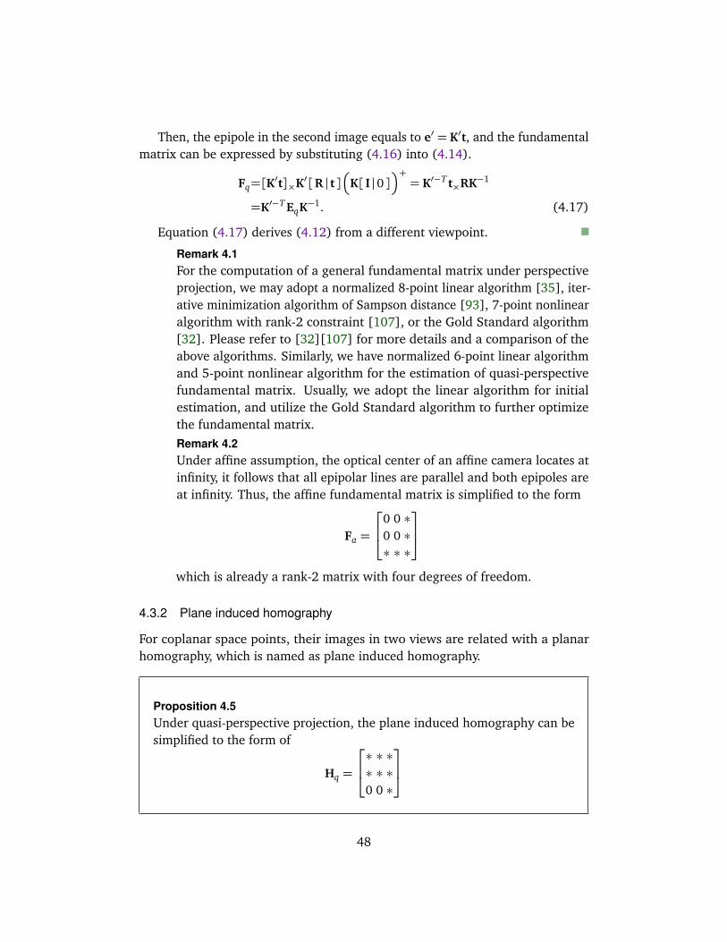
Then, the epipole in the second image equals to e′ = K′t, and the fundamentalmatrix can be expressed by substituting (4.16) into (4.14).

Fq=[K′t]×K′[R | t ]

K[ I |0 ]+= K′−T t×RK−1

=K′−T EqK−1. (4.17)

Equation (4.17) derives (4.12) from a different viewpoint.

Remark 4.1For the computation of a general fundamental matrix under perspectiveprojection, we may adopt a normalized 8-point linear algorithm [35], iter-ative minimization algorithm of Sampson distance [93], 7-point nonlinearalgorithm with rank-2 constraint [107], or the Gold Standard algorithm[32]. Please refer to [32][107] for more details and a comparison of theabove algorithms. Similarly, we have normalized 6-point linear algorithmand 5-point nonlinear algorithm for the estimation of quasi-perspectivefundamental matrix. Usually, we adopt the linear algorithm for initialestimation, and utilize the Gold Standard algorithm to further optimizethe fundamental matrix.Remark 4.2Under affine assumption, the optical center of an affine camera locates atinfinity, it follows that all epipolar lines are parallel and both epipoles areat infinity. Thus, the affine fundamental matrix is simplified to the form

Fa =

0 0 ∗0 0 ∗∗ ∗ ∗

which is already a rank-2 matrix with four degrees of freedom.

4.3.2 Plane induced homography

For coplanar space points, their images in two views are related with a planarhomography, which is named as plane induced homography.

Proposition 4.5Under quasi-perspective projection, the plane induced homography can besimplified to the form of

Hq =

∗ ∗ ∗∗ ∗ ∗0 0 ∗

48

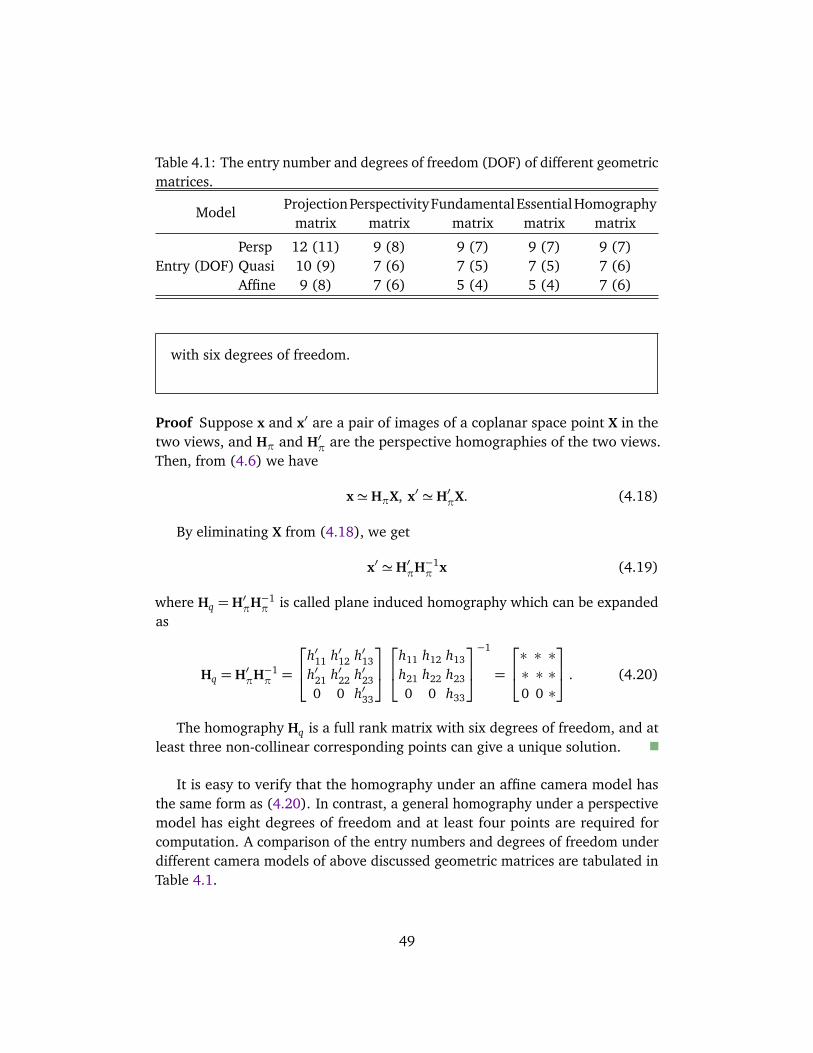
Table 4.1: The entry number and degrees of freedom (DOF) of different geometricmatrices.

ProjectionPerspectivityFundamentalEssentialHomographyModelmatrix matrix matrix matrix matrix

Persp 12 (11) 9 (8) 9 (7) 9 (7) 9 (7)Entry (DOF) Quasi 10 (9) 7 (6) 7 (5) 7 (5) 7 (6)

Affine 9 (8) 7 (6) 5 (4) 5 (4) 7 (6)

with six degrees of freedom.

Proof Suppose x and x′ are a pair of images of a coplanar space point X in thetwo views, and Hπ and H′π are the perspective homographies of the two views.Then, from (4.6) we have

x' HπX, x′ ' H′πX. (4.18)

By eliminating X from (4.18), we get

x′ ' H′πH−1π x (4.19)

where Hq = H′πH−1π is called plane induced homography which can be expanded

as

Hq = H′πH−1π =

h′11 h′12 h′13h′21 h′22 h′230 0 h′33

h11 h12 h13

h21 h22 h23

0 0 h33

−1

=

∗ ∗ ∗∗ ∗ ∗0 0 ∗

. (4.20)

The homography Hq is a full rank matrix with six degrees of freedom, and atleast three non-collinear corresponding points can give a unique solution.

It is easy to verify that the homography under an affine camera model hasthe same form as (4.20). In contrast, a general homography under a perspectivemodel has eight degrees of freedom and at least four points are required forcomputation. A comparison of the entry numbers and degrees of freedom underdifferent camera models of above discussed geometric matrices are tabulated inTable 4.1.

49

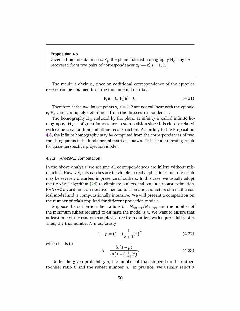
Proposition 4.6Given a fundamental matrix Fq, the plane induced homography Hq may berecovered from two pairs of correspondences xi ↔ x′i , i = 1, 2.

The result is obvious, since an additional correspondence of the epipolese↔ e′ can be obtained from the fundamental matrix as

Fqe= 0, FTq e′ = 0. (4.21)

Therefore, if the two image points xi , i = 1, 2 are not collinear with the epipolee, Hq can be uniquely determined from the three correspondences.

The homography H∞ induced by the plane at infinity is called infinite ho-mography. H∞ is of great importance in stereo vision since it is closely relatedwith camera calibration and affine reconstruction. According to the Proposition4.6, the infinite homography may be computed from the correspondences of twovanishing points if the fundamental matrix is known. This is an interesting resultfor quasi-perspective projection model.

4.3.3 RANSAC computation

In the above analysis, we assume all correspondences are inliers without mis-matches. However, mismatches are inevitable in real applications, and the resultmay be severely disturbed in presence of outliers. In this case, we usually adoptthe RANSAC algorithm [26] to eliminate outliers and obtain a robust estimation.RANSAC algorithm is an iterative method to estimate parameters of a mathemat-ical model and is computationally intensive. We will present a comparison onthe number of trials required for different projection models.

Suppose the outlier-to-inlier ratio is k = Noutl ier/Ninl ier , and the number ofthe minimum subset required to estimate the model is n. We want to ensure thatat least one of the random samples is free from outliers with a probability of p.Then, the trial number N must satisfy

1− p =

1− (1

k+ 1)nN (4.22)

which leads to

N =ln(1− p)

ln

1− ( 1k+1)n

. (4.23)

Under the given probability p, the number of trials depend on the outlier-to-inlier ratio k and the subset number n. In practice, we usually select a

50

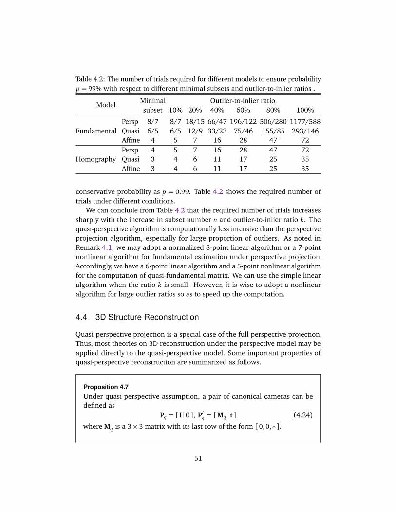
Table 4.2: The number of trials required for different models to ensure probabilityp = 99% with respect to different minimal subsets and outlier-to-inlier ratios .

Minimal Outlier-to-inlier ratioModelsubset 10% 20% 40% 60% 80% 100%

Persp 8/7 8/7 18/15 66/47 196/122 506/280 1177/588Fundamental Quasi 6/5 6/5 12/9 33/23 75/46 155/85 293/146

Affine 4 5 7 16 28 47 72Persp 4 5 7 16 28 47 72

Homography Quasi 3 4 6 11 17 25 35Affine 3 4 6 11 17 25 35

conservative probability as p = 0.99. Table 4.2 shows the required number oftrials under different conditions.

We can conclude from Table 4.2 that the required number of trials increasessharply with the increase in subset number n and outlier-to-inlier ratio k. Thequasi-perspective algorithm is computationally less intensive than the perspectiveprojection algorithm, especially for large proportion of outliers. As noted inRemark 4.1, we may adopt a normalized 8-point linear algorithm or a 7-pointnonlinear algorithm for fundamental estimation under perspective projection.Accordingly, we have a 6-point linear algorithm and a 5-point nonlinear algorithmfor the computation of quasi-fundamental matrix. We can use the simple linearalgorithm when the ratio k is small. However, it is wise to adopt a nonlinearalgorithm for large outlier ratios so as to speed up the computation.

4.4 3D Structure Reconstruction

Quasi-perspective projection is a special case of the full perspective projection.Thus, most theories on 3D reconstruction under the perspective model may beapplied directly to the quasi-perspective model. Some important properties ofquasi-perspective reconstruction are summarized as follows.

Proposition 4.7Under quasi-perspective assumption, a pair of canonical cameras can bedefined as

Pq = [ I |0 ], P′q = [Mq | t ] (4.24)

where Mq is a 3× 3 matrix with its last row of the form [0, 0,∗ ].

51

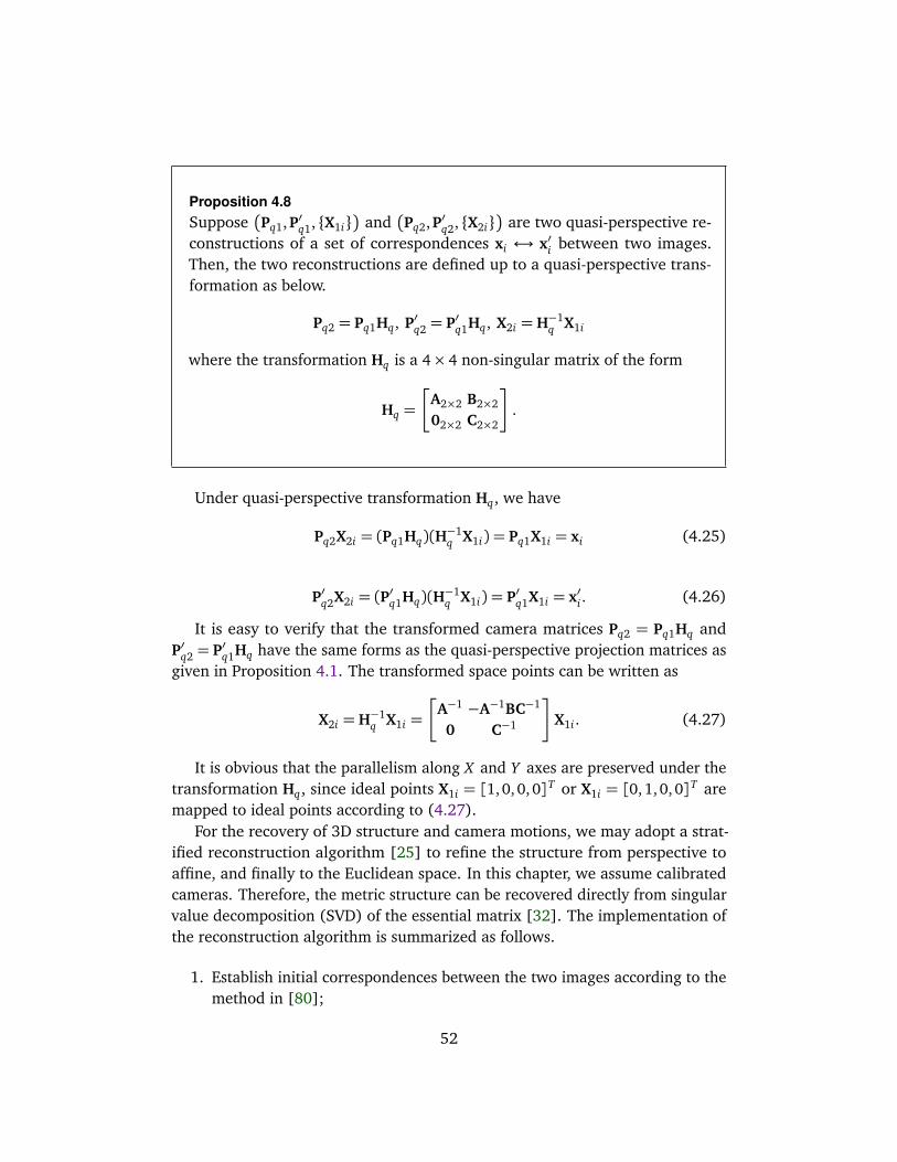
Proposition 4.8Suppose

Pq1,P′q1, X1i

and

Pq2,P′q2, X2i

are two quasi-perspective re-constructions of a set of correspondences xi ↔ x′i between two images.Then, the two reconstructions are defined up to a quasi-perspective trans-formation as below.

Pq2 = Pq1Hq, P′q2 = P′q1Hq, X2i = H−1q X1i

where the transformation Hq is a 4× 4 non-singular matrix of the form

Hq =

A2×2 B2×2

02×2 C2×2

.

Under quasi-perspective transformation Hq, we have

Pq2X2i = (Pq1Hq)(H−1q X1i) = Pq1X1i = xi (4.25)

P′q2X2i = (P′q1Hq)(H

−1q X1i) = P′q1X1i = x′i . (4.26)

It is easy to verify that the transformed camera matrices Pq2 = Pq1Hq andP′q2 = P′q1Hq have the same forms as the quasi-perspective projection matrices asgiven in Proposition 4.1. The transformed space points can be written as

X2i = H−1q X1i =

A−1 −A−1BC−1

0 C−1

X1i . (4.27)

It is obvious that the parallelism along X and Y axes are preserved under thetransformation Hq, since ideal points X1i = [1,0,0,0]T or X1i = [0,1,0,0]T aremapped to ideal points according to (4.27).

For the recovery of 3D structure and camera motions, we may adopt a strat-ified reconstruction algorithm [25] to refine the structure from perspective toaffine, and finally to the Euclidean space. In this chapter, we assume calibratedcameras. Therefore, the metric structure can be recovered directly from singularvalue decomposition (SVD) of the essential matrix [32]. The implementation ofthe reconstruction algorithm is summarized as follows.

1. Establish initial correspondences between the two images according to themethod in [80];

52

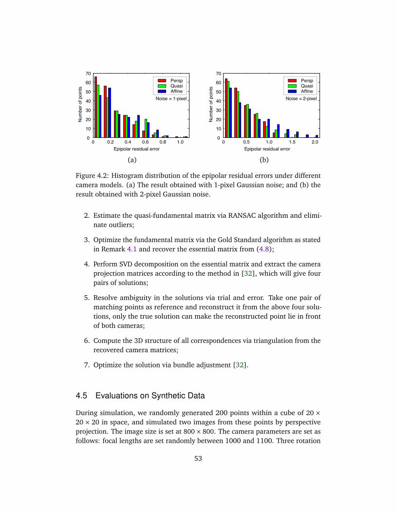
0 0.2 0.4 0.6 0.8 1.00

10

20

30

40

50

60

70

Epipolar residual error

Num

ber o

f poi

nts

Noise = 1-pixelAffineQuasiPersp

0 0.5 1.0 1.5 2.00

10

20

30

40

50

60

70

Epipolar residual error

Num

ber o

f poi

nts

Noise = 2-pixelAffineQuasiPersp

(a) (b)

Figure 4.2: Histogram distribution of the epipolar residual errors under differentcamera models. (a) The result obtained with 1-pixel Gaussian noise; and (b) theresult obtained with 2-pixel Gaussian noise.

2. Estimate the quasi-fundamental matrix via RANSAC algorithm and elimi-nate outliers;

3. Optimize the fundamental matrix via the Gold Standard algorithm as statedin Remark 4.1 and recover the essential matrix from (4.8);

4. Perform SVD decomposition on the essential matrix and extract the cameraprojection matrices according to the method in [32], which will give fourpairs of solutions;

5. Resolve ambiguity in the solutions via trial and error. Take one pair ofmatching points as reference and reconstruct it from the above four solu-tions, only the true solution can make the reconstructed point lie in frontof both cameras;

6. Compute the 3D structure of all correspondences via triangulation from therecovered camera matrices;

7. Optimize the solution via bundle adjustment [32].

4.5 Evaluations on Synthetic Data

During simulation, we randomly generated 200 points within a cube of 20×20× 20 in space, and simulated two images from these points by perspectiveprojection. The image size is set at 800× 800. The camera parameters are set asfollows: focal lengths are set randomly between 1000 and 1100. Three rotation

53

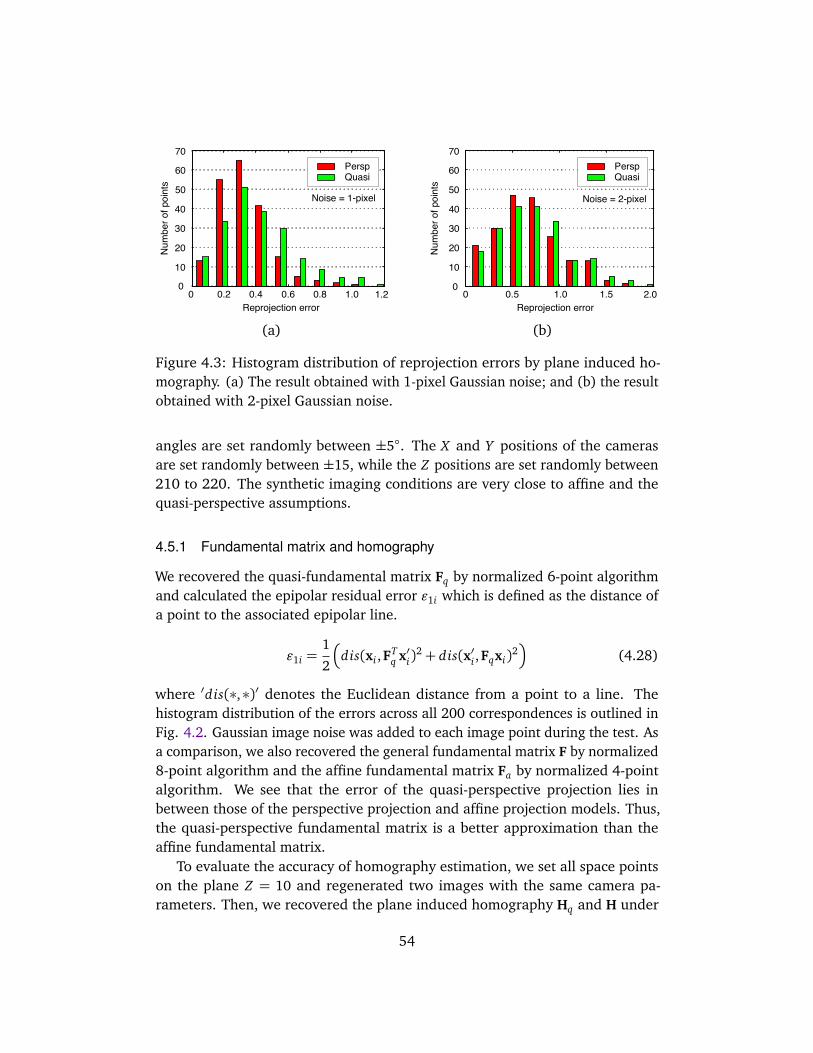
0 0.5 1.0 1.5 2.00

10

20

30

40

50

60

70

Num

ber o

f poi

nts

Reprojection error

QuasiPersp

Noise = 2-pixel

Reprojection error

Num

ber o

f poi

nts

0 0.2 0.4 0.6 0.8 1.00

10

20

30

40

50

60

70

1.2

QuasiPersp

Noise = 1-pixel

(a) (b)

Figure 4.3: Histogram distribution of reprojection errors by plane induced ho-mography. (a) The result obtained with 1-pixel Gaussian noise; and (b) the resultobtained with 2-pixel Gaussian noise.

angles are set randomly between ±5. The X and Y positions of the camerasare set randomly between ±15, while the Z positions are set randomly between210 to 220. The synthetic imaging conditions are very close to affine and thequasi-perspective assumptions.

4.5.1 Fundamental matrix and homography

We recovered the quasi-fundamental matrix Fq by normalized 6-point algorithmand calculated the epipolar residual error ε1i which is defined as the distance ofa point to the associated epipolar line.

ε1i =1

2

dis(xi ,FTq x′i)

2+ dis(x′i ,Fqxi)2

(4.28)

where ′dis(∗,∗)′ denotes the Euclidean distance from a point to a line. Thehistogram distribution of the errors across all 200 correspondences is outlined inFig. 4.2. Gaussian image noise was added to each image point during the test. Asa comparison, we also recovered the general fundamental matrix F by normalized8-point algorithm and the affine fundamental matrix Fa by normalized 4-pointalgorithm. We see that the error of the quasi-perspective projection lies inbetween those of the perspective projection and affine projection models. Thus,the quasi-perspective fundamental matrix is a better approximation than theaffine fundamental matrix.

To evaluate the accuracy of homography estimation, we set all space pointson the plane Z = 10 and regenerated two images with the same camera pa-rameters. Then, we recovered the plane induced homography Hq and H under

54

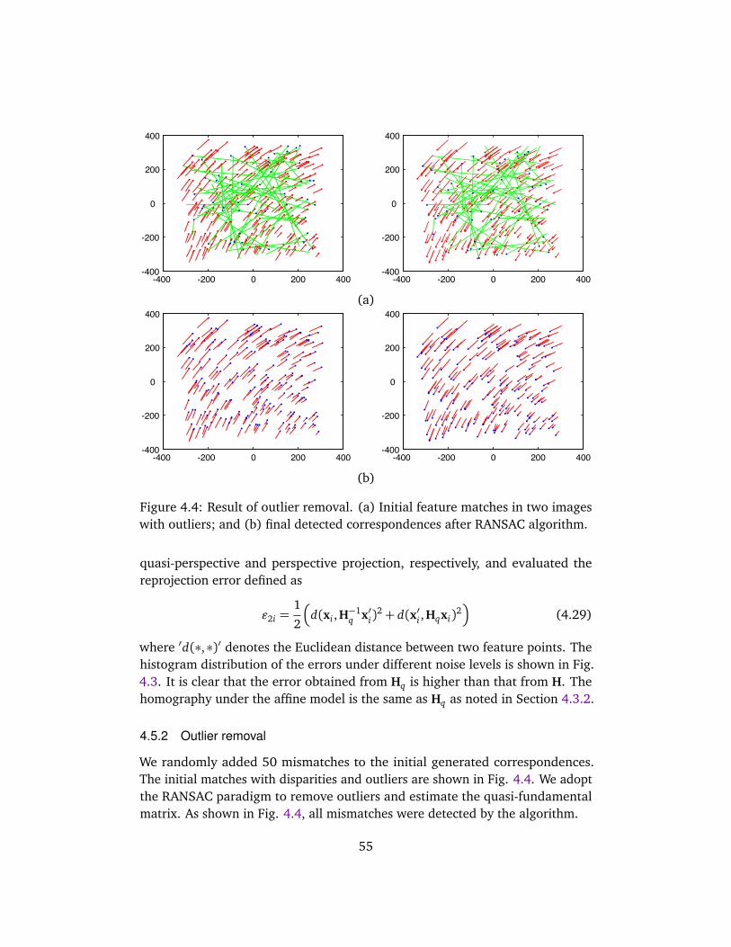
-400 -200 0 200 400-400

-200

0

200

400

-400 -200 0 200 400-400

-200

0

200

400

(a)

-400 -200 0 200 400-400

-200

0

200

400

-400 -200 0 200 400-400

-200

0

200

400

(b)

Figure 4.4: Result of outlier removal. (a) Initial feature matches in two imageswith outliers; and (b) final detected correspondences after RANSAC algorithm.

quasi-perspective and perspective projection, respectively, and evaluated thereprojection error defined as

ε2i =1

2

d(xi ,H−1q x′i)

2+ d(x′i ,Hqxi)2

(4.29)

where ′d(∗,∗)′ denotes the Euclidean distance between two feature points. Thehistogram distribution of the errors under different noise levels is shown in Fig.4.3. It is clear that the error obtained from Hq is higher than that from H. Thehomography under the affine model is the same as Hq as noted in Section 4.3.2.

4.5.2 Outlier removal

We randomly added 50 mismatches to the initial generated correspondences.The initial matches with disparities and outliers are shown in Fig. 4.4. We adoptthe RANSAC paradigm to remove outliers and estimate the quasi-fundamentalmatrix. As shown in Fig. 4.4, all mismatches were detected by the algorithm.

55

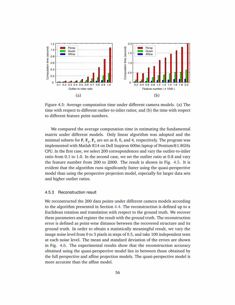
0.2 0.4 0.6 0.8 1.0 1.2 1.4 1.6 1.8 2.00

0.5

1.0

1.5

2.0

AffineQuasiPersp

Feature number ( X 1000 )

Com

puta

tion

time

(sec

ond)

0.1 0.2 0.3 0.4 0.5 0.6 0.7 0.8 0.9 1.00

0.2

0.4

0.6

0.8

1.0

1.2

AffineQuasiPersp

Com

puta

tion

time

(sec

ond)

Outlier to inlier ratio

(a) (b)

Figure 4.5: Average computation time under different camera models. (a) Thetime with respect to different outlier-to-inlier ratios; and (b) the time with respectto different feature point numbers.

We compared the average computation time in estimating the fundamentalmatrix under different models. Only linear algorithm was adopted and theminimal subsets for F, Fq, Fa are set as 8, 6, and 4, respectively. The program wasimplemented with Matlab R14 on Dell Inspiron 600m laptop of Pentium®1.8GHzCPU. In the first case, we select 200 correspondences and vary the outlier-to-inlierratio from 0.1 to 1.0. In the second case, we set the outlier ratio at 0.8 and varythe feature number from 200 to 2000. The result is shown in Fig. 4.5. It isevident that the algorithm runs significantly faster using the quasi-perspectivemodel than using the perspective projection model, especially for larger data setsand higher outlier ratios.

4.5.3 Reconstruction result

We reconstructed the 200 data points under different camera models accordingto the algorithm presented in Section 4.4. The reconstruction is defined up to aEuclidean rotation and translation with respect to the ground truth. We recoverthese parameters and register the result with the ground truth. The reconstructionerror is defined as point-wise distance between the recovered structure and itsground truth. In order to obtain a statistically meaningful result, we vary theimage noise level from 0 to 3 pixels in steps of 0.5, and take 100 independent testsat each noise level. The mean and standard deviation of the errors are shownin Fig. 4.6. The experimental results show that the reconstruction accuracyobtained using the quasi-perspective model lies in between those obtained bythe full perspective and affine projection models. The quasi-perspective model ismore accurate than the affine model.

56

Noise level (pixel)

Mea

n of

reco

nstru

ctio

n er

ror

0 0.5 1.0 1.5 2.0 2.5 3.00

0.51.01.52.02.53.03.54.0

AffineQuasiPersp

0 0.5 1.0 1.5 2.0 2.5 3.00

0.51.01.52.02.53.03.54.0

AffineQuasiPersp

Noise level (pixel)

STD

of r

econ

stru

ctio

n er

ror

(a) (b)

Figure 4.6: Evaluation on 3D reconstruction accuracy by different models. (a)The mean of the reconstruction errors at different noise levels; and (b) thecorresponding standard deviation.

Table 4.3: The reprojection error under different projection models.Model Persp Quasi Affine

Stone dragon 0.72 0.80 0.86ErrorMedusa head 0.97 1.04 1.13

4.6 Evaluations on Real Images

4.6.1 Test on stone dragon images

We tested and compared different models on many real images and we report tworesults here. The correspondences in the tests were established by a matching sys-tem based on SIFT and the epipolar constraint [80], and the camera parameterswere calibrated offline via the method in Zhang [104].

The stone dragon images were captured by a Canon G3 camera in ChungChi College of the Chinese University of Hong Kong. The image resolution is1024× 768, and 4261 reliable features were established by the system [80]. Werecover the fundamental matrix via Gold Standard algorithm and reconstructedthe 3D Euclidean structure according to the process in Section 4.4. Figure 4.7shows the matched features, reconstructed VRML model with texture, and thecorresponding wireframe model viewed from different viewpoints. The structureof the dragon is correctly recovered using the quasi-perspective model. Thedistributions of epipolar residual errors using the three models are compared inFigure 4.8, and the reprojection errors are listed in Table 4.3.

57

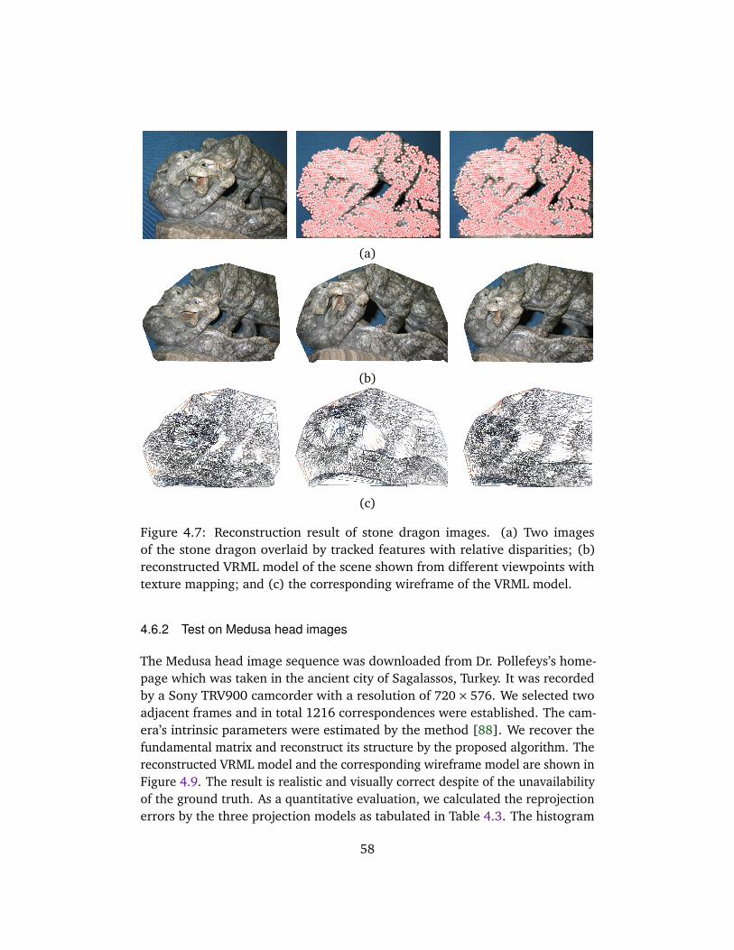
(a)

(b)

(c)

Figure 4.7: Reconstruction result of stone dragon images. (a) Two imagesof the stone dragon overlaid by tracked features with relative disparities; (b)reconstructed VRML model of the scene shown from different viewpoints withtexture mapping; and (c) the corresponding wireframe of the VRML model.

4.6.2 Test on Medusa head images

The Medusa head image sequence was downloaded from Dr. Pollefeys’s home-page which was taken in the ancient city of Sagalassos, Turkey. It was recordedby a Sony TRV900 camcorder with a resolution of 720× 576. We selected twoadjacent frames and in total 1216 correspondences were established. The cam-era’s intrinsic parameters were estimated by the method [88]. We recover thefundamental matrix and reconstruct its structure by the proposed algorithm. Thereconstructed VRML model and the corresponding wireframe model are shown inFigure 4.9. The result is realistic and visually correct despite of the unavailabilityof the ground truth. As a quantitative evaluation, we calculated the reprojectionerrors by the three projection models as tabulated in Table 4.3. The histogram

58

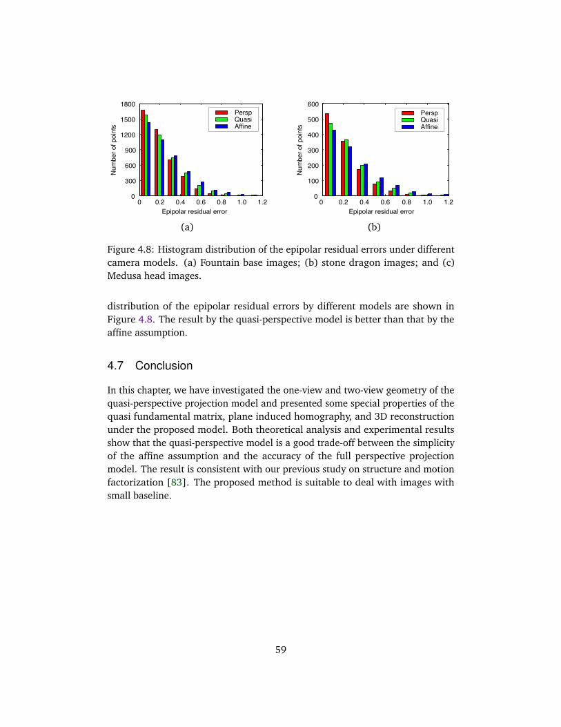
Num

ber o

f poi

nts

Epipolar residual error0 0.2 0.4 0.6 0.8 1.0 1.2

0

100

200

300

400

500

600

AffineQuasiPersp

Num

ber o

f poi

nts

Epipolar residual error0 0.2 0.4 0.6 0.8 1.0 1.2

0

300

600

900

1200

1500

1800

AffineQuasiPersp

(a) (b)

Figure 4.8: Histogram distribution of the epipolar residual errors under differentcamera models. (a) Fountain base images; (b) stone dragon images; and (c)Medusa head images.

distribution of the epipolar residual errors by different models are shown inFigure 4.8. The result by the quasi-perspective model is better than that by theaffine assumption.

4.7 Conclusion

In this chapter, we have investigated the one-view and two-view geometry of thequasi-perspective projection model and presented some special properties of thequasi fundamental matrix, plane induced homography, and 3D reconstructionunder the proposed model. Both theoretical analysis and experimental resultsshow that the quasi-perspective model is a good trade-off between the simplicityof the affine assumption and the accuracy of the full perspective projectionmodel. The result is consistent with our previous study on structure and motionfactorization [83]. The proposed method is suitable to deal with images withsmall baseline.

59

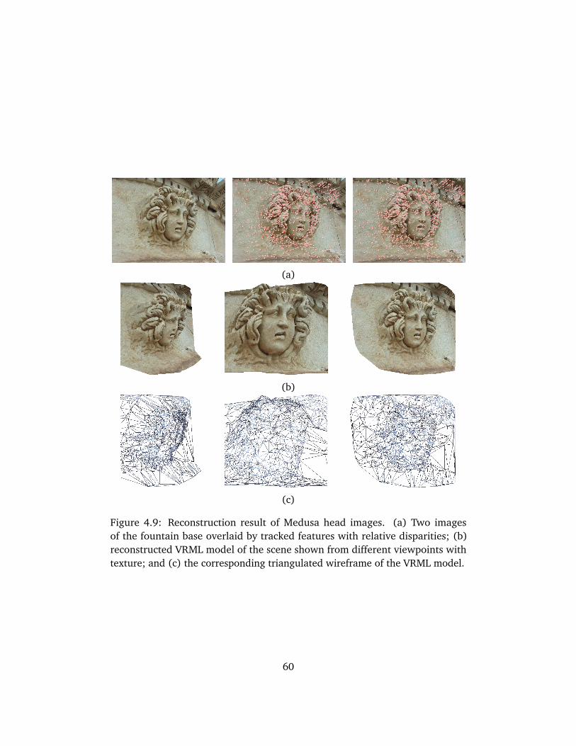
(a)

(b)

(c)

Figure 4.9: Reconstruction result of Medusa head images. (a) Two imagesof the fountain base overlaid by tracked features with relative disparities; (b)reconstructed VRML model of the scene shown from different viewpoints withtexture; and (c) the corresponding triangulated wireframe of the VRML model.

60

Chapter 5

SfM Based on Quasi-Perspective Pro-jection Model

Previous studies on structure and motion factorization are either based on asimplified affine assumption or a general perspective projection model. The affineapproximation is widely adopted due to its simplicity, whereas the extension toperspective model suffers from difficulties in projective depth recovery. To fill thegap between simplicity of affine and accuracy of perspective model, we proposea quasi-perspective model based algorithm for structure and motion recovery ofboth rigid and nonrigid objects. In this chapter, we first establish a frameworkof rigid and nonrigid factorization under quasi-perspective assumption. Then,we propose an extended Cholesky decomposition to recover the rotation part ofthe Euclidean upgrading matrix. Finally, we prove that the last column of theupgrading matrix corresponds to a global scale and translation of the camera thusmay be set freely. The proposed algorithm is validated and evaluated extensivelyon synthetic and real image sequences.

5.1 Introduction

The factorization algorithm is a powerful and efficient method for structure andmotion recovery. Since Tomasi and Kanade [74] first introduced the algorithmin the early 90’s, numerous extensions and generalizations have been proposed.Most early studies on the problem assume a rigid object and an affine cameramodel [62][65]. The main difficulty of its extension to perspective projectionlies in the recovery of depth scales. One method is to estimate the depths in apair-wise fashion via epipolar constraint [71][77], which may be unstable dueto possible error accumulation. Another method is based on nonlinear iteration

61

by minimizing reprojections [47]. These methods rely on the accuracy of initialaffine solution. Oliensis and Hartley [56] recently proved that no iterationconverges sensibly. Wang and Wu [88] proposed a hybrid method to initializethe depth scales via a projective reconstruction.

In recent years, many extensions stemming from the factorization algorithmwere proposed to relax the rigidity constraint to multiple moving objects [16][44]and articulated objects [97][98]. Bregler et al. [11] firstly established the frame-work of nonrigid factorization using shape bases. The method was extensivelyinvestigated and developed under the affine assumption [10][21][75][95]. Ithas been extended to perspective projection in [81][96]. Rabaud and Belongie[66] relaxed the Bregler’s assumption and proposed to solve the problem by amanifold-learning framework. Wang et al. [82] introduced a rotation constrainedpower factorization algorithm. Hartley and Vidal [34] proposed a closed formsolution to the nonrigid shape and motion with known camera constraints.

The affine camera model is widely adopted in factorization due to its sim-plicity. However, the accuracy of this approximation is not satisfactory in manyapplications. Perspective projection based algorithms are computationally in-tensive and thus convergence is not guaranteed. In this chapter, we apply thequasi-perspective projection model [83] to both a rigid and a nonrigid factoriza-tion framework. This is a trade-off between the simplicity of the affine and theaccuracy of the full perspective projection. It is demonstrated to be more accu-rate than affine approximation since the projective depths in quasi-perspectiveprojection are implicitly embedded in the motion and shape matrices. Thus, thedifficult problem of depth recovery in perspective factorization is circumvented.Part of this chapter was published in International Journal of Computer Vision[86].

The remaining part of this chapter is organized as follows. The factorizationalgorithm is briefly reviewed in Section 5.2. The proposed quasi-perspectivefactorization algorithm for rigid objects is detailed in Section 5.3. The nonrigidfactorization under quasi-perspective projection is presented in Section 5.4. Someexperimental evaluations on synthetic and real image sequences are reported inSection 5.5 and 5.6 respectively.

5.2 Background on Factorization

We already introduced the rigid and nonrigid factorization under the affineand perspective projection models in previous chapters. For convenience ofdiscussion, we present a brief review in this section on the expressions of differentfactorization algorithms.

Under perspective projection, a 3D point X j is imaged at xi j in the i-th frame

62

according to equation

λi jxi j = PiX j = Ki[Ri , ti]X j . (5.1)

If we adopt affine projection model and register all image points to thecentroid. Then, the projection process (5.1) is simplified to the form

xi j = AiX j . (5.2)

Given n tracked features of an object across a sequence of m frames. The struc-ture and motion factorization under affine assumption (5.2) can be expressed as

x11 · · · x1n...

. . ....

xm1 · · · xmn

︸︷︷︸

W2m×n

=

A1...

Am

︸︷︷︸

M2m×3

X1, · · · , Xn

︸︷︷︸

S3×n

. (5.3)

The factorization is usually performed by SVD decomposition of the trackingmatrix W with rank-3 constraint. When the perspective projection model (5.1) isadopted, the factorization can be modeled as

λ11x11 · · · λ1nx1n...

. . ....


︸︷︷︸

W3m×n

=

P1...

Pm

︸︷︷︸

M3m×4

X1, · · · , Xn

1, · · · , 1

︸︷︷︸

S4×n

. (5.4)

The rank of the projective depth-scaled tracking matrix W is at most 4 if aconsistent set of scalars are present.

When an object is nonrigid, we follow Bregler’s assumption [11] to model thenonrigid structure by a linear combination of some shape bases.

Si =∑k

l=1ωilBl . (5.5)

With this assumption, the nonrigid factorization under affine camera model isexpressed as

x11 · · · x1n...

. . ....

xm1 · · · xmn

︸︷︷︸

W2m×n

=

ω11A1 · · · ω1kA1...

. . ....

ωm1Am · · · ωmkAm

︸︷︷︸

M2m×3k

B1...

Bk

︸︷︷︸

B3k×n

(5.6)

63

and the rank of the nonrigid tracking matrix is at most 3k. Similarly, the factor-ization under perspective projection can be formulated as follows [96].

λ11x11 · · · λ1nx1n...

. . ....


︸︷︷︸

W3m×n

=

ω11P(1:3)1 · · · ω1kP(1:3)

1 P(4)1...

. . ....

...ωm1P(1:3)

m · · · ωmkP(1:3)m P(4)m

︸︷︷︸

M3m×(3k+1)

B1...

Bk

1T

︸︷︷︸

B(3k+1)×n

. (5.7)

The rank of the correctly scaled tracking matrix in (5.7) is at most 3k+1. Justas its rigid counterpart, the most difficult issue for perspective factorization is todetermine the projective depths that are consistent with (5.1).

5.3 Quasi-Perspective Rigid Factorization

Under the assumption that the camera is far away from the object with smalllateral rotations, we proposed a quasi-perspective projection model to simplifythe imaging process as follows.

xi j = PqiXq j = (µiPi)(` jX j). (5.8)

In quasi-perspective projection (5.8), the projective depths are implicitlyembedded in the scalars of the homogeneous structure Xq j and the projectionmatrix Pqi. Thus, the difficult problem of estimating the unknown depths iscircumvented. The model is more general than the affine projection model(5.2), where all projective depths are simply assumed to be equal. Under thequasi-perspective assumption, the factorization equation of a tracking matrix isexpressed as

x11 · · · x1n...

. . ....

xm1 · · · xmn

=

µ1P1...

µmPm

[`1X1, · · · ,`nXn] (5.9)

which can be written concisely as

W3m×n =M3m×4S4×n. (5.10)

The form is similar to perspective factorization (5.4). However, the projectivedepths in (5.9) are embedded in the motion and shape matrices, hence there is noneed to estimate them explicitly. By performing SVD on the tracking matrix andimposing the rank-4 constraint, W may be factorized as M3m×4S4×n. However,like all other factorization algorithms, the decomposition is not unique since it is

64

defined up to a nonsingular linear transformation H4×4 as M = MH and S = H−1S.Due to the special form of (5.9), the upgrading matrix has some special propertiescompared to that under affine and perspective projection. We will present thecomputational details in the following subsections.

5.3.1 Euclidean upgrading matrix

We adopt the metric constraints to compute the upgrading matrix H4×4. Let usdecompose the matrix into two parts as

H= [Hl |Hr] (5.11)

where Hl denotes the first three columns, and Hr denotes the fourth column.Suppose Mi is the i-th triple rows of M, we have

MiH= [MiHl |MiHr] (5.12)

where

MiHl = µiP(1:3)i = µiKiRi (5.13)

MiHr = µiP(4)i = µiKiti (5.14)

where P(1:3)i and P(4)i denote the first three columns and the fourth column of Pi.

In the following, we will show how to compute Hl and Hr .

Recovering Hl

Let us denote Q = HlHTl , which is a 4 × 4 symmetric matrix. As in previous

factorization studies [31][65], we adopt a simplified camera model with onlyone parameter as Ki = diag( fi , fi , 1). Then, from

Ci = MiQMTi =

MiHl

MiHlT = (µiKiRi)(µiKiRi)

T

= µ2i KiK

Ti = µ

2i

f 2i

f 2i

1

(5.15)

we obtain the following constraints.

Ci(1, 2) = Ci(2, 1) = 0Ci(1, 3) = Ci(3,1) = 0Ci(2, 3) = Ci(3,2) = 0Ci(1, 1)−Ci(2,2) = 0

(5.16)

65

Since the factorization (5.9) can be defined up to a global scalar as W =MS = (εM)(S/ε), we set µ1 = 1 to avoid the trivial solution of Q = 0. Thus, wehave 4m+ 1 linear constraints in total on the ten unknowns of Q, which can besolved via least squares. Ideally, Q is a positive semidefinite symmetric matrix,the matrix Hl can be recovered from Q via extended Cholesky decomposition asfollows.

Definition 5.1 (Vertical extended upper triangular matrix)Suppose U is a n× k (n> k) matrix. We call U a vertical extended uppertriangular matrix if it is of the form

Ui j =

¨

ui j if i ≤ j+ (n− k)0 if i > j+ (n− k)

(5.17)

where Ui j denotes the (i, j)-th element of U, and ui j is a scalar. Forexample, a n× (n− 1) vertical extended upper triangular matrix can bewritten explicitly as

U=

u11 u12 · · · u1(n−1)u21 u22 · · · u2(n−1)

u32 · · · u3(n−1). . .

...un(n−1)

. (5.18)

Proposition 5.1 (Extended Cholesky Decomposition)Suppose Qn is a n× n positive semidefinite symmetric matrix of rank k (k <n). Then, it can be decomposed as Qn = HkHT

k , where Hk is a n×k matrix ofrank k. Furthermore, the decomposition can be written as Qn = ΛkΛ

Tk with

Λk, a n×k vertical extended upper triangular matrix. The degree-of-freedomof the matrix Qn is nk− 1

2k(k− 1), which is the number of unknowns in Λk.

Proof Since A is a n× n positive semidefinite symmetric matrix of rank k, it canbe decomposed by SVD as

A= UΣUT = U

σ1. . .σk

0. . .

0

UT (5.19)

66

where U is a n× n orthogonal matrix, and Σ is a diagonal matrix with σi thesingular value of A. Consequently we get

Hk = U(1:k)

pσ1

. . .pσk

=

Hku

Hkl

(5.20)

such that A = HkHTk , where U(1:k) denotes first k columns of U, Hku denotes upper

(n− k)× k submatrix of Hk, and Hkl denotes lower k× k submatrix of Hk. Byapplying RQ-decomposition to Hkl , we have Hkl = ΛklOk, where Λkl is an uppertriangular matrix, and Ok is an orthogonal matrix.

Let us denote Λku = HkuOTk and construct a n× k vertical extended upper

triangular matrix

Λk =

Λku

Λkl

. (5.21)

Then, we have

Hk = ΛkOk, A= HkHTk = (ΛkOk)(ΛkOk)

T = ΛkΛTk . (5.22)

It is easy to verify that the matrix A has nk− 12k(k− 1) degrees of freedom,

which is just the number of unknowns in Λk.

The proposition can be taken as an extension of the Cholesky Decomposition tothe case of positive semidefinite symmetric matrix, while Cholesky Decompositioncan only deal with positive definite symmetric matrix. From the above proposition,we obtain the following result.

Corollary 5.2The matrix Q recovered from (5.16) is a 4×4 positive semidefinite symmetricmatrix of rank 3. It can be decomposed as Q = HlH

Tl , where Hl is a 4× 3

rank 3 matrix. The decomposition can be further written as Q= Λ3ΛT3 with

Λ3 a 4× 3 vertical extended upper triangular matrix.

In practice, the matrix Hl can be easily computed as follows. Suppose theSVD decomposition of Q is U4Σ4UT

4 , where U4 is a 4 × 4 orthogonal matrix,Σ4 = diag(σ1,σ2,σ3, 0) is a diagonal matrix with σi the singular value of Q.Thus, we have

Hl = U(1:3)

pσ1 p

σ2 pσ3

. (5.23)

67

Then, the vertical extended upper triangular matrix Λ3 can be constructedfrom Hl as in (5.21). From the number of unknowns in Λ3, we know that Q isonly defined up to nine degrees of freedom.

In Corollary 5.2, we claim that the symmetric matrix Q can be decomposedinto Λ3Λ

T3 . In practice, we can simply decompose the matrix into HlH

Tl as shown

in (5.23), it is unnecessary to recover Λ3 since the upgrading matrix (5.11) is notunique. However, when the data is corrupted by noise, the recovered matrix Qmay be negative definite and the decomposition of (5.23) is impossible. In suchcase, we suggest the following alternative estimation method.

Let us denote

Λ3 =

h1 h2 h3h4 h5 h6

h7 h8h9

(5.24)

and substitute the matrix Q in (5.15) with Λ3ΛT3 . Then, a best estimation of Λ3

in (5.24) can be obtained via minimizing the following cost function

J1 =min(Λ3)

1

2

m∑

i=1

C2i (1,2) +C2

i (1,3) +C2i (2, 3) + (Ci(1, 1)−Ci(2,2))2

. (5.25)

The minimization scheme can be solved using any nonlinear optimizationtechniques, such as gradient descent or Levenberg-Marquardt (LM) algorithm. Byintroducing the vertical extended upper triangular matrix (5.24), we can reducethree unknowns in matrix Q.

Recovering Hr

In this section we recover the right part Hr of the upgrading matrix (5.11). Fromquasi-perspective equation (5.8), we have

xi j = (µiP(1:3)i )(` jX j) + (µiP

(4)i )` j . (5.26)

For all features in the i-th frame, we take a summation of their coordinates asbelow.

n∑

j=1

xi j = µiP(1:3)i

n∑

j=1

(` jX j) +µiP(4)i

n∑

j=1

` j (5.27)

where µiP(1:3)i can be recovered from MiHl , µiP

(4)i = MiHr . Since the world

coordinate system can be chosen freely, we may set the origin of the world systemat the gravity center of the scaled space points as

n∑

j=1

(` jX j) = 0. (5.28)

68

On the other hand, we may simply set

n∑

j=1

` j = 1 (5.29)

since the reconstruction is defined up to a global scalar. Thus, Equation (5.27) issimplified to

MiHr =n∑

j=1

xi j =

∑

j ui j∑

j vi j

n

(5.30)

which provides three linear constraints on the four unknowns of Hr . Therefore,we obtain 3m equations from the sequence and Hr can be recovered via linearleast squares.

From the above analysis, we note that the solution of Hr is not unique as it isdependant on the selection of the world origin

∑nj=1(` jX j) and the global scalar

∑nj=1 ` j. Actually, Hr may be set freely as shown in the following proposition.

Proposition 5.3Suppose Hl in (5.11) is already recovered. Let us choose an arbitrary fourdimensional vector Hr that is independent of the three columns of Hl , andconstruct a matrix as

H= [Hl |Hr].

Then, H must be a valid upgrading matrix. i.e., M = MH is a valid Euclideanmotion matrix, and S = H−1S corresponds to a valid Euclidean shape matrix.

Proof Suppose the correct transformation matrix is H= [Hl |Hr], then, from

S= H−1S=

`1X1, · · · , `nXn

`1, · · · , `n

(5.31)

we obtain a correct Euclidean structure [X1, · · · , Xn] of the object under a certainworld coordinate frame by dehomogenizing the shape matrix S. The arbitraryconstructed matrix H = [Hl |Hr] and the correct matrix H are defined up to a4× 4 invertible matrix G as

H= HG, G=

I3 g0T s

(5.32)

69

where I3 is a 3× 3 identity matrix, g is a 3-vector, 0 is a zero 3-vector, and s is anonzero scalar. Under the transformation matrix H, the motion M and shape Sare transformed to

M = MH= MHG−1 =M

I3 −g/s0T 1/s

(5.33)

S = H−1S= (HG−1)−1S= G(H−1S)

= s

`1(X1+ g)/s · · · `n(Xn+ g)/s`1 · · · `n

. (5.34)

As shown in (5.34), the new shape S is actually the original structure thatundergoes a translation g and a scale 1/s, which does not change the Euclideanstructure. From (5.33), we have M(1:3) = M(1:3), which indicates that the first-three-columns of the new motion matrix (rotation term) do not change. While thelast column, which corresponds to translation factor, is modified in accordancewith the translation and scale changes of the structure.

Therefore, the constructed matrix H is a valid transformation matrix that canupgrade the factorization from projective space to the Euclidean space.

According to Proposition 5.3, the value of Hr can be set randomly as any4-vector that is independent of Hl . A practical selection method may be asfollows.

Suppose the SVD decomposition of Hl is

Hl = U4×4Σ4×3VT3×3 = [u1,u2,u3,u4]

σ1 0 00 σ2 00 0 σ3

0 0 0

[v1,v2,v3]T (5.35)

where U and V are two orthogonal matrices, and Σ is a diagonal matrix composedof the three singular values. Let us choose an arbitrary value σr between thebiggest and the smallest singular values of Hl , then we may set

Hr = σru4, H= [Hl ,Hr]. (5.36)

Such a kind of construction guarantees that H is invertible and has the samecondition number as Hl , so that we can obtain a good precision in computing theinverse H−1.

After recovering the Euclidean motion and shape matrices, the intrinsic param-eters and pose of the camera associated with each frame can be easily computedas follows.

µi =

M(1:3)i(3)

(5.37)

70

fi =1

µi

M(1:3)i(1)

=1

µi

M(1:3)i(2)

(5.38)

Ri =1

µiK−1

i M(1:3)i , Ti =

1

µiK−1

i M(4)i (5.39)

where M(1:3)i(t) denotes the t-th row of M(1:3)

i . The result is obtained under quasi-perspective assumption, which is a close approximation to the general perspectiveprojection. The solution may be further optimized to perspective projection byminimizing the image reprojection residuals.

J2 = min(Ki ,Ri ,Ti ,µi ,X j)

1

2

m∑

i=1

n∑

j=1

xi j − xi j

2(5.40)

where xi j denotes the reprojected image point computed via perspective projec-tion (5.1). The minimization process is termed as bundle adjustment, which isusually solved via Levenberg-Marquardt (LM) iterations [32].

5.3.2 Algorithm outline

Given the tracking matrix W ∈ R3m×n across a sequence with small cameramovements. The implementation of the quasi-perspective rigid factorizationalgorithm is summarized as follows.

1. Balance the tracking matrix via point-wise and image-wise rescalings, as in[71], to improve its numerical stability;

2. Perform rank-4 SVD decomposition on the tracking matrix to obtain a setof solution of M and S;

3. Compute the left part of upgrading matrix Hl according to (5.23), or (5.25)for negative definite matrix Q;

4. Construct Hr and H according to (5.36);

5. Recover the Euclidean motion matrix M= MH and shape matrix S= H−1S;

6. Estimate the camera parameters and pose from (5.37) to (5.39);

7. Optimize the solution via bundle adjustment (5.40).

In the above analysis, as well as in other factorization algorithms, we usu-ally assume one-parameter-camera model as in (5.15) so that we can use thisconstraint to recover the upgrading matrix H. In real applications, we may take

71

the solution as an initial value and optimize the camera parameters via Kruppaconstraints that arise from pairwise images [88].

The essence of quasi-perspective factorization (5.10) is to find a rank-4 approx-imation MS of the tracking matrix by minimizing the Frobenius norm ‖W−MS‖2F .Most studies adopt a SVD decomposition of W and truncate it to the desiredrank. However, when the tracking matrix is not complete, such as when somefeatures are missing in some frames due to occlusions, it is hard to performSVD decomposition. In case of missing data, we adopt the power factorizationalgorithm [33][84] to obtain a least squares solution of M and S. The solutionis then upgraded the solution to the Euclidean space according to the proposedscheme.

5.4 Quasi-Perspective Nonrigid Factorization

5.4.1 Problem formulation

For nonrigid factorization, we follow Bregler’s assumption (5.5) to representa nonrigid shape by weighted combination of k shape bases. Under quasi-perspective projection, the structure is expressed in homogeneous form withnonzero scalars. Let us denote the scale-weighted nonrigid structure associatedwith the i-th frame and the l-th scale weighted shape basis as

Si = [`1X1, · · · ,`nXn], Bl = [`1Xl1, · · · ,`nXl

n]. (5.41)

Then from (5.5), we have

Xi =k∑

l=1

ωil Xli , ∀ i = 1, · · · , n. (5.42)

Let us multiply a weight scale ì on both sides as

ìXi = ì

k∑

l=1

ωil Xli =

k∑

l=1

ωil(ìXli) (5.43)

then, we can immediately have the following result.

Si =

Si

`T

=

∑kl=1ωilBl

`T

. (5.44)

We call (5.44) extended Bregler’s assumption in homogeneous case. Un-der this extension, the quasi-perspective projection of the i-th frame can beformulated as

Wi = (µiPi)Si = [µiP(1:3)i ,µiP

(4)i ]

∑kl=1ωilBl

`T

(5.45)

72

= [ωi1µiP(1:3)i , · · · ,ωikµiP

(1:3)i ,µiP

(4)i ]

B1

· · ·Bk

`T

.

Thus, the nonrigid factorization under quasi-perspective projection can beexpressed as

W3m×n =

ω11µ1P(1:3)1 · · · ω1kµ1P(1:3)

1 µ1P(4)1...

. . ....

...ωm1µmP(1:3)

m · · · ωmkµmP(1:3)m µmP(4)m

B1...

Bk

`T

(5.46)

or represented concisely in matrix form as

W3m×n =M3m×(3k+1)B(3k+1)×n. (5.47)

The factorization expression is similar to (5.7). However, the difficulties inestimating the projective depths are circumvented.


The rank of the tracking matrix is at most 3k+ 1, and the factorization is definedup to a transformation matrix H ∈ R(3k+1)×3k+1). Suppose the SVD factorizationof a tracking matrix with rank constraint is W = MB. Similar to the rigid case, weadopt the metric constraint to compute the upgrading matrix. Let us denote thematrix into k+ 1 parts as

H= [H1, · · · ,Hk|Hr] (5.48)

where Hl ∈ R(3k+1)×3(l = 1, · · · , k) denotes the l-th triple columns of H, and Hr

denotes the last column of H. Then, we have

MiHl =ωilµiP(1:3)i =ωilµiKiRi (5.49)

MiHr = µiP(4)i = µiKiti . (5.50)

Similar to (5.15) in the rigid case, Let us denote Cii′ = MiQlMTi′ with Ql =

HlHTl , we obtain

Cii′ = MiQlMTi′ = (ωilµiKiRi)(ωi′ lµi′Ki′Ri′)

T

= ωilωi′ lµiµi′Ki(RiRi′)KTi′ (5.51)

73

where i and i′ (= 1, · · · , m) correspond to different frame numbers, l = 1, · · · , kcorresponds to different shape bases. Assuming a simplified camera model withonly one parameter as Ki = diag( fi , fi , 1), we have

Cii = MiQlMTi =ω

2ilµ

2i

f 2i

f 2i

1

(5.52)

from which we obtain following four constraints.

f1(Ql) = Cii(1, 2) = 0f2(Ql) = Cii(1, 3) = 0f3(Ql) = Cii(2, 3) = 0f4(Ql) = Cii(1, 1)−Cii(2,2) = 0

. (5.53)

The above constraints are similar to (5.16) in the rigid case. However, thematrix Ql in (5.52) is a (3k + 1) × (3k + 1) symmetric matrix. According toProposition 5.1, Ql has 9k degrees of freedom, since it can be decomposed into theproduct of (3k+1)×3 vertical extended upper triangular matrix. Given m frames,we have 4m linear constraints on Ql . It appears that if we have enough featuresand frames, the matrix Ql can be solved linearly by stacking all constraints in(5.53). Unfortunately, only the rotation constraints may be insufficient when anobject deforms at varying speed, since most of these constraints are redundant.Xiao et al. [96] proposed a basis constraint to solve this ambiguity.

The main idea of basis constraint is to select k frames that include indepen-dent shapes and treat them as a set of bases. Suppose the first k frames areindependent of each other, then their corresponding weighting coefficients canbe set as

ωil =

¨

1 if i, l = 1, ..., k and i = l0 if i, l = 1, ..., k and i 6= l

. (5.54)

From (5.51) we obtain following basis constraint.

Cii′ =

0 0 00 0 00 0 0

if i = 1, ..., k, i′ = 1, ..., m, and i 6= l. (5.55)

Given m images, (5.55) can provide 9m(k−1) linear constraints to the matrixQl (some of the constraints are redundant since Ql is symmetric). By combiningthe rotation constraint (5.53) and the basis constraint (5.55) together, the matrixQl can be computed linearly. Then, Hl , l = 1, · · · , k may be decomposed from Ql

according to following Proposition.

74

Proposition 5.4The matrix Ql is a (3k+1)× (3k+1) positive semidefinite symmetric matrixof rank 3. It can be decomposed as Q = HlH

Tl , where Hl is a (3k+ 1)× 3

rank-3 matrix. The decomposition can be further written as Q= Λ3ΛT3 with

Λ3 being a (3k+ 1)× 3 vertical extended upper triangular matrix.

The result can be easily derived from Proposition 5.1. It is easy to verifythat the Proposition 5.3 is still valid for the nonrigid case. Thus, the vector Hr

in (5.48) can be set as an arbitrary (3k + 1)-vector that is independent of allcolumns in Hl, l = 1, · · · , k. After recovering the Euclidean upgrading matrix,the camera parameters, motions, shape bases, and weighing coefficients can beeasily decomposed from the upgraded motion and shape matrices.

M= MH, B= H−1B. (5.56)


In this section, the proposed rigid and nonrigid factorization algorithms areevaluated using synthetic data in terms of accuracy and efficiency.

5.5.1 Evaluations of rigid factorization

During simulations, we randomly generated 200 points within a cube of 20×20×20 in space and simulated 10 images from these points by perspective projection.The image size is set at 800× 800. The camera parameters are set as follows: thefocal lengths are set randomly between 900 and 1100, the principal point is setat the image center, and the skew is zero. The rotation angles are set randomlybetween ±5. The X and Y positions of the cameras are set randomly between±15, while the Z positions are set evenly from 200 to 220. The imaging conditionis very close to quasi-perspective assumption.

We add Gaussian white noise to the initially generated 10 images (i.e., alltracked features in the tracking matrix), and vary the noise level (the standarddeviation of the Gaussian noise) from 0 to 3 units with steps of 0.5. At eachnoise level, we reconstruct the 3D structure of the object which is defined up to asimilarity transformation with the ground truth. We register the reconstructedmodel with the ground truth and calculate the reconstruction error, which isdefined as mean point-wise distance between the reconstructed structure and the

75

0

0.5

1.0

1.5

2.0AffineQuasiPerspAffine+LMQuasi+LMPersp+LM

0 0.5 1.0 1.5 2.0 2.5 3.0Noise level

Stan

dard

dev

iatio

n

0

0.5

1.0

1.5

2.0

2.5

3.0

3.5AffineQuasiPerspAffine+LMQuasi+LMPersp+LM

0 0.5 1.0 1.5 2.0 2.5 3.0Noise level

Mea

n of

erro

rs

(a) (b)

Figure 5.1: Evaluation on the accuracy of rigid factorization. (a) The mean ofreconstruction errors by different algorithms at different noise levels; and (b) thecorresponding standard deviation of reconstruction errors.

ground truth. The mean and standard deviation of the errors on 100 independenttests are shown in Figure 5.1.

The proposed algorithm (Quasi) is compared with [62] under the affineassumption (Affine) and [31] under the perspective projection (Persp). We alsoperform a bundle adjustment optimization scheme through Levenberg-Marquardt(LM) algorithm to upgrade the solution to the perspective projection. It is evidentthat the proposed method performs much better than that of affine, and theoptimized solution (Quasi+LM) is very close to the perspective projection withoptimization (Persp+LM).

The proposed model is based on the assumption of large relative camera-to-object distance and small camera rotations. We studied the influence of these twofactors to different camera models. In the first case, we vary the relative distancefrom 4 to 18 in steps of 2. At each relative distance, we generate 20 images withthe following parameters. The rotation angles are confined between ±5, the Xand Y positions of the camera are set randomly between ±15. We recover thestructure and compute the reconstruction error for each group of images. Themean reconstruction error by different methods is shown in Figure 5.2. In thesecond case, we increase the rotation angles to the range of ±20, and retainother camera parameters the same as in the first case. The mean reconstructionerror is given in Figure 5.2. These results are evaluated on 100 independencetests with 1-unit Gaussian noise.

Based on experimental evidence we have the following Conclusion. (i) Theerror by the quasi-perspective projection is consistently less than that by the affine,especially at small relative distances; (ii) both reconstruction errors by the affineand the quasi-perspective projection increase greatly when the relative distance

76

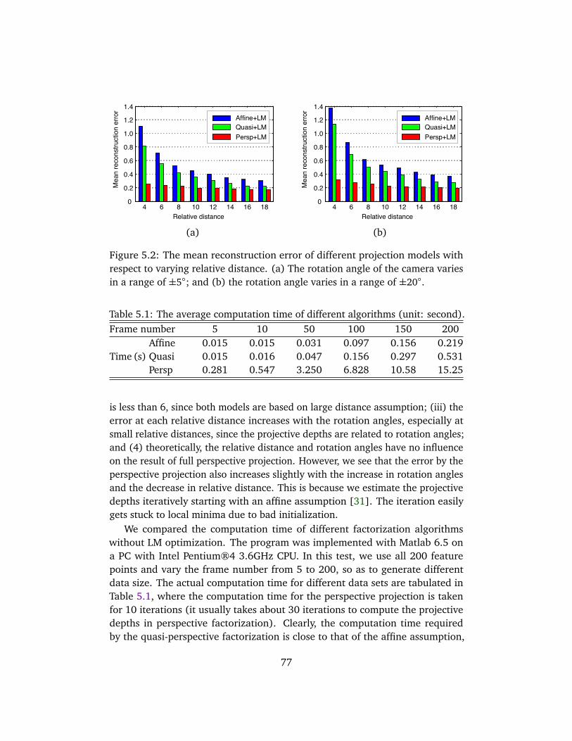
4 6 8 10 12 14 16 180

0.2

0.4

0.6

0.8

1.0

1.2

1.4Affine+LMQuasi+LMPersp+LM

Relative distance

Mea

n re

cons

truct

ion

erro

r

Relative distance4 6 8 10 12 14 16 18

0

0.2

0.4

0.6

0.8

1.0

1.2

1.4Affine+LMQuasi+LMPersp+LM

Mea

n re

cons

truct

ion

erro

r

(a) (b)

Figure 5.2: The mean reconstruction error of different projection models withrespect to varying relative distance. (a) The rotation angle of the camera variesin a range of ±5; and (b) the rotation angle varies in a range of ±20.

Table 5.1: The average computation time of different algorithms (unit: second).Frame number 5 10 50 100 150 200

Affine 0.015 0.015 0.031 0.097 0.156 0.219Time (s) Quasi 0.015 0.016 0.047 0.156 0.297 0.531

Persp 0.281 0.547 3.250 6.828 10.58 15.25

is less than 6, since both models are based on large distance assumption; (iii) theerror at each relative distance increases with the rotation angles, especially atsmall relative distances, since the projective depths are related to rotation angles;and (4) theoretically, the relative distance and rotation angles have no influenceon the result of full perspective projection. However, we see that the error by theperspective projection also increases slightly with the increase in rotation anglesand the decrease in relative distance. This is because we estimate the projectivedepths iteratively starting with an affine assumption [31]. The iteration easilygets stuck to local minima due to bad initialization.

We compared the computation time of different factorization algorithmswithout LM optimization. The program was implemented with Matlab 6.5 ona PC with Intel Pentium®4 3.6GHz CPU. In this test, we use all 200 featurepoints and vary the frame number from 5 to 200, so as to generate differentdata size. The actual computation time for different data sets are tabulated inTable 5.1, where the computation time for the perspective projection is takenfor 10 iterations (it usually takes about 30 iterations to compute the projectivedepths in perspective factorization). Clearly, the computation time requiredby the quasi-perspective factorization is close to that of the affine assumption,

77

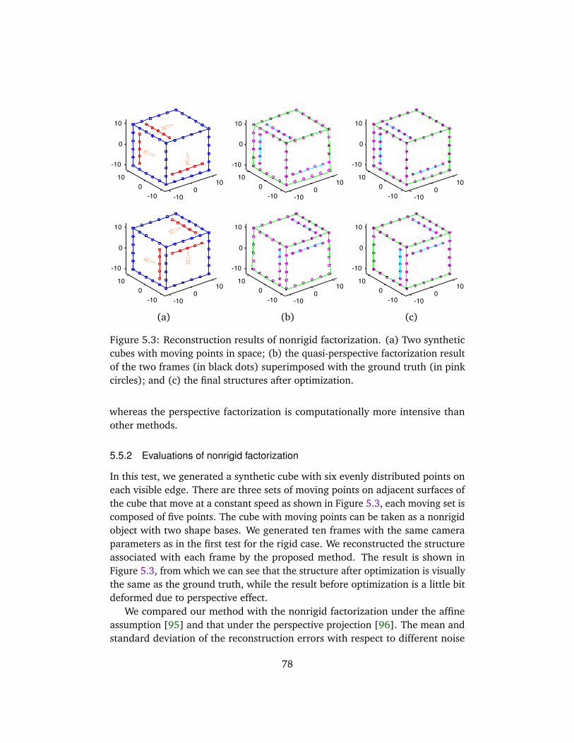
-100

10

-100

10

-10

0

10

-100

10

-100

10

-10

0

10

-100

10

-100

10

-10

0

10

-100

10

-100

10

-10

0

10

-100

10

-100

10

-10

0

10

-100

10

-100

10

-10

0

10

(a) (b) (c)

Figure 5.3: Reconstruction results of nonrigid factorization. (a) Two syntheticcubes with moving points in space; (b) the quasi-perspective factorization resultof the two frames (in black dots) superimposed with the ground truth (in pinkcircles); and (c) the final structures after optimization.

whereas the perspective factorization is computationally more intensive thanother methods.

5.5.2 Evaluations of nonrigid factorization

In this test, we generated a synthetic cube with six evenly distributed points oneach visible edge. There are three sets of moving points on adjacent surfaces ofthe cube that move at a constant speed as shown in Figure 5.3, each moving set iscomposed of five points. The cube with moving points can be taken as a nonrigidobject with two shape bases. We generated ten frames with the same cameraparameters as in the first test for the rigid case. We reconstructed the structureassociated with each frame by the proposed method. The result is shown inFigure 5.3, from which we can see that the structure after optimization is visuallythe same as the ground truth, while the result before optimization is a little bitdeformed due to perspective effect.

We compared our method with the nonrigid factorization under the affineassumption [95] and that under the perspective projection [96]. The mean andstandard deviation of the reconstruction errors with respect to different noise

78

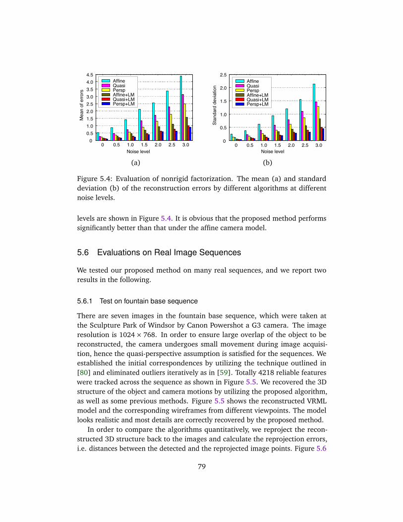
0 0.5 1.0 1.5 2.0 2.5 3.00

0.5

1.0

1.5

2.0

2.5

Noise level

Stan

dard

dev

iatio

n

AffineQuasiPerspAffine+LMQuasi+LMPersp+LM

0 0.5 1.0 1.5 2.0 2.5 3.00

0.51.01.52.02.53.03.54.04.5

Noise level

Mea

n of

erro

rsAffineQuasiPerspAffine+LMQuasi+LMPersp+LM

(a) (b)

Figure 5.4: Evaluation of nonrigid factorization. The mean (a) and standarddeviation (b) of the reconstruction errors by different algorithms at differentnoise levels.

levels are shown in Figure 5.4. It is obvious that the proposed method performssignificantly better than that under the affine camera model.

5.6 Evaluations on Real Image Sequences

We tested our proposed method on many real sequences, and we report tworesults in the following.

5.6.1 Test on fountain base sequence

There are seven images in the fountain base sequence, which were taken atthe Sculpture Park of Windsor by Canon Powershot a G3 camera. The imageresolution is 1024× 768. In order to ensure large overlap of the object to bereconstructed, the camera undergoes small movement during image acquisi-tion, hence the quasi-perspective assumption is satisfied for the sequences. Weestablished the initial correspondences by utilizing the technique outlined in[80] and eliminated outliers iteratively as in [59]. Totally 4218 reliable featureswere tracked across the sequence as shown in Figure 5.5. We recovered the 3Dstructure of the object and camera motions by utilizing the proposed algorithm,as well as some previous methods. Figure 5.5 shows the reconstructed VRMLmodel and the corresponding wireframes from different viewpoints. The modellooks realistic and most details are correctly recovered by the proposed method.

In order to compare the algorithms quantitatively, we reproject the recon-structed 3D structure back to the images and calculate the reprojection errors,i.e. distances between the detected and the reprojected image points. Figure 5.6

79

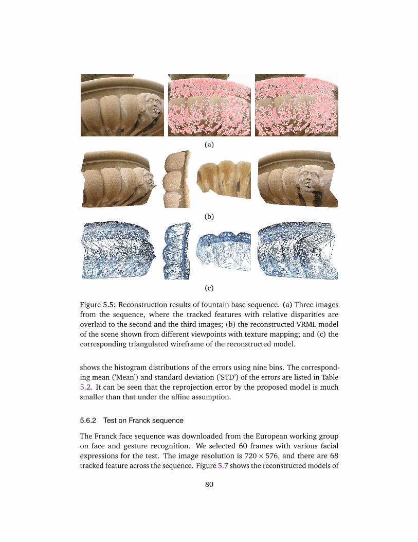
(a)

(b)

(c)

Figure 5.5: Reconstruction results of fountain base sequence. (a) Three imagesfrom the sequence, where the tracked features with relative disparities areoverlaid to the second and the third images; (b) the reconstructed VRML modelof the scene shown from different viewpoints with texture mapping; and (c) thecorresponding triangulated wireframe of the reconstructed model.

shows the histogram distributions of the errors using nine bins. The correspond-ing mean (’Mean’) and standard deviation (’STD’) of the errors are listed in Table5.2. It can be seen that the reprojection error by the proposed model is muchsmaller than that under the affine assumption.

5.6.2 Test on Franck sequence

The Franck face sequence was downloaded from the European working groupon face and gesture recognition. We selected 60 frames with various facialexpressions for the test. The image resolution is 720× 576, and there are 68tracked feature across the sequence. Figure 5.7 shows the reconstructed models of

80

0.1 0.4 0.7 1.0 1.3 1.6 1.9 2.2 2.50

400

800

1200

1600

2000

2400

Reprojection error (pixel)

Num

ber o

f poi

nts

Persp+LMQuasi+LMAffine+LM

Figure 5.6: The histogram distributions of the reprojection errors by differentalgorithms in the test of fountain base sequence.

Table 5.2: Camera parameters of the first four frames and reprojection errors inreal sequence test.Method f1 f2 f3 f4 Mean STD Erep

Quasi+LM 2140.5 2143.6 2139.4 2142.8 0.418 0.285 2.473Affine+LM 2153.4 2155.7 2151.2 2153.1 0.629 0.439 3.189Persp+LM 2131.7 2135.3 2131.2 2134.5 0.240 0.168 1.962

two frames utilizing the proposed nonrigid factorization method. Different facialexpressions are correctly recovered. As a comparison, the relative reprojectionerror Erep generated from different methods are listed in Table 5.2. All testsillustrate that the accuracy by the proposed method is fairly close to that of fullperspective projection, and considerably better than the affine assumption.

5.7 Conclusion

In this chapter, we have proposed a quasi-perspective factorization algorithm forboth rigid and nonrigid objects and elaborated the computation details of the Eu-clidean upgrading matrix. The proposed method avoids the difficulties associatedwith computation of the projective depths under the perspective factorization.It is computationally simple with better accuracy than the affine approximation.The proposed model is suitable for structure and motion factorization of shortsequences with small camera motions. Experiments demonstrates improvementsof our algorithm over the existing techniques. For a long image sequences taken

81

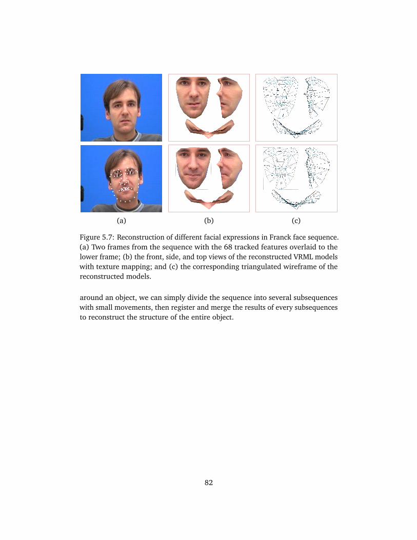
(a) (b) (c)

Figure 5.7: Reconstruction of different facial expressions in Franck face sequence.(a) Two frames from the sequence with the 68 tracked features overlaid to thelower frame; (b) the front, side, and top views of the reconstructed VRML modelswith texture mapping; and (c) the corresponding triangulated wireframe of thereconstructed models.

around an object, we can simply divide the sequence into several subsequenceswith small movements, then register and merge the results of every subsequencesto reconstruct the structure of the entire object.

82

Chapter 6

Spatial-and-Temporal-Weighted Factor-ization

In this chapter, a spatial-and-temporal-weighted factorization algorithm is pro-posed to handle significant noise contained in the tracking data. The mainnovelties and contributions of the proposed algorithm include: (i) The imagereprojection residual of a feature point is demonstrated to be generally propor-tional to the error magnitude associated with the image point; (ii) the errordistributions are estimated from a new perspective, the reprojection residuals.The image errors are modeled both spatially and temporally to cope with dif-ferent kinds of uncertainties. Previous studies have considered only the spatialinformation; and (iii) based on the estimated error distributions, a spatial-and-temporal-weighted factorization algorithm is proposed to improve the overallaccuracy and robustness of traditional approaches. Unlike existing approaches,the proposed technique does not require prior information of image measure-ment and is easy to implement. Extensive experiments on synthetic data and realimages validate the proposed method.

6.1 Introduction

Most factorization methods usually assume error-free tracking data. The perfor-mance will degenerate in the presence of outliers or significant noise. In recentyears, the problem of robust factorization has been a concern, and some practicalmethods have been proposed to handle noisy and erroneous data [100].

Aguitar and Moura [3] proposed a scalar-weighted SVD algorithm by mini-mizing the weighted square errors. Anandan and Irani [7] proposed a covariance-weighted factorization to factorize noisy correspondences with a high degree of

83

directional uncertainty. Gruber and Weiss [29] formulated the problem as a factoranalysis and derived an expectation maximization (EM) algorithm to incorporateprior knowledge and enhance the robustness to missing data and uncertainties.Zelnik-Manor et al. [103] defined a new type of motion consistency based ontemporal consistency, and applied it to multi-body factorization with directionaluncertainty. Zaharescu and Horaud [100] introduced a Gaussian/uniform mix-ture model and incorporated it with the EM algorithm. Buchanan and Fitzgibbon[12] presented a comprehensive comparison on a number of factorization al-gorithms. Their study strongly supports second order nonlinear optimizationstrategy.

Previous methods of robust factorization are either based on isotropic ordirectional assumption of the feature uncertainties, which may be recoveredduring the stage of feature detection and matching. Unfortunately, this infor-mation is hard to retrieve in practice, and unavailable in many situations. Byanalyzing the image reprojection residuals, we find that the errors associatedwith image features are closely related to the reprojection residuals. Based onthis observation, the image uncertainties are modeled spatially and temporally,and a spatial-and-temporal-weighted factorization algorithm is proposed in thischapter. Experiments show that the proposed method improves the accuracy androbustness of the classical affine factorization algorithm. A preliminary work onthis research was published in IEEE Trans. on Circuits and Systems for VideoTechnology [89].

The remainder of this chapter is organized as follows. Some preliminarybackground on structure and motion factorization is offered in Section 6.2. Theproposed spatial-and-temporal-weighted factorization is elaborated in Section6.3. Experimental evaluations and comparisons on synthetic and real images aredescribed in Section 6.4 and 6.5, respectively. Finally, a short conclusion is drawnin Section 6.6.

6.2 Background on Structure and Motion Factorization

In this section, a brief introduction to structure and motion factorization ispresented to facilitate understanding of the discussed problem in this chapter.

Under a simplified affine camera model, if the imaged points in each imageare registered to the centroid and relative image coordinates are employed, the

84

imaging process of an image sequence can be modeled as

x11 · · · x1n...

. . ....

x f 1 · · · x f n

︸︷︷︸

Wm×n

=

A1...

A f

︸︷︷︸

Mm×3

X1, · · · , Xn

︸︷︷︸

S3×n

(6.1)

where f is the frame number. Please note that, for the convenience of discussion,we use f to denote the frame number in this chapter, and let m= 2 f . Equation(6.1) is usually written concisely as:

Wm×n =Mm×3S3×n (6.2)

where the matrix

W= xi j=

u11

v11

· · ·

u1n

v1n

.... . .

...

u f 1

v f 1

· · ·

u f n

v f n

m×n

(6.3)

is called the tracking matrix or measurement matrix. Suppose the tracking matrixW is available, the purpose of structure and motion factorization is to recover themotion matrix M and the shape matrix S as shown in (6.1).

The classical factorization algorithms utilize all image measurements and givethem equal consideration. Thus, the problem is equivalent to minimizing thefollowing error function:

Err(M,S) = argminM,S

‖W−MS‖2F (6.4)

where ‖ · ‖F stands for the Frobenius norm of a matrix. The above algorithmmay yield poor results in the presence of significant noise or outliers. In order tohandle these challenging situations, researchers proposed a robust factorizationapproach to increase the robustness of the algorithm. One common practice is tointroduce a weight matrix into the cost function in (6.4) as below:

Err(M,S) = argminM,S

‖(W−MS)⊗Σ‖2F (6.5)

where ′⊗′ denotes the Hadamard product, which is an element-by-elementmultiplication of two matrices; and Σ = σi j is the uncertainty matrix whoseentries are weights derived from the confidence of the image measurements[3][7]. However, the weight matrix is usually unavailable and is hard to retrieve.

85

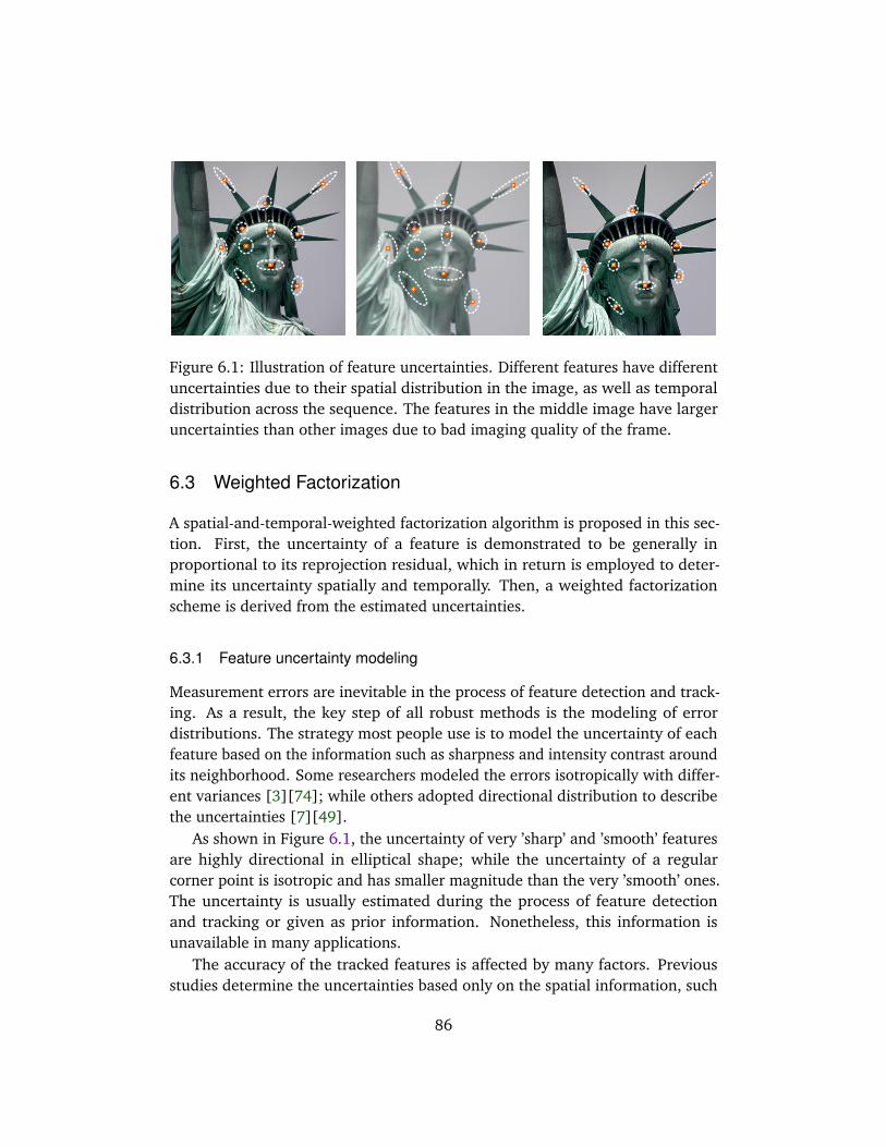
Figure 6.1: Illustration of feature uncertainties. Different features have differentuncertainties due to their spatial distribution in the image, as well as temporaldistribution across the sequence. The features in the middle image have largeruncertainties than other images due to bad imaging quality of the frame.

6.3 Weighted Factorization

A spatial-and-temporal-weighted factorization algorithm is proposed in this sec-tion. First, the uncertainty of a feature is demonstrated to be generally inproportional to its reprojection residual, which in return is employed to deter-mine its uncertainty spatially and temporally. Then, a weighted factorizationscheme is derived from the estimated uncertainties.

6.3.1 Feature uncertainty modeling

Measurement errors are inevitable in the process of feature detection and track-ing. As a result, the key step of all robust methods is the modeling of errordistributions. The strategy most people use is to model the uncertainty of eachfeature based on the information such as sharpness and intensity contrast aroundits neighborhood. Some researchers modeled the errors isotropically with differ-ent variances [3][74]; while others adopted directional distribution to describethe uncertainties [7][49].

As shown in Figure 6.1, the uncertainty of very ’sharp’ and ’smooth’ featuresare highly directional in elliptical shape; while the uncertainty of a regularcorner point is isotropic and has smaller magnitude than the very ’smooth’ ones.The uncertainty is usually estimated during the process of feature detectionand tracking or given as prior information. Nonetheless, this information isunavailable in many applications.

The accuracy of the tracked features is affected by many factors. Previousstudies determine the uncertainties based only on the spatial information, such

86

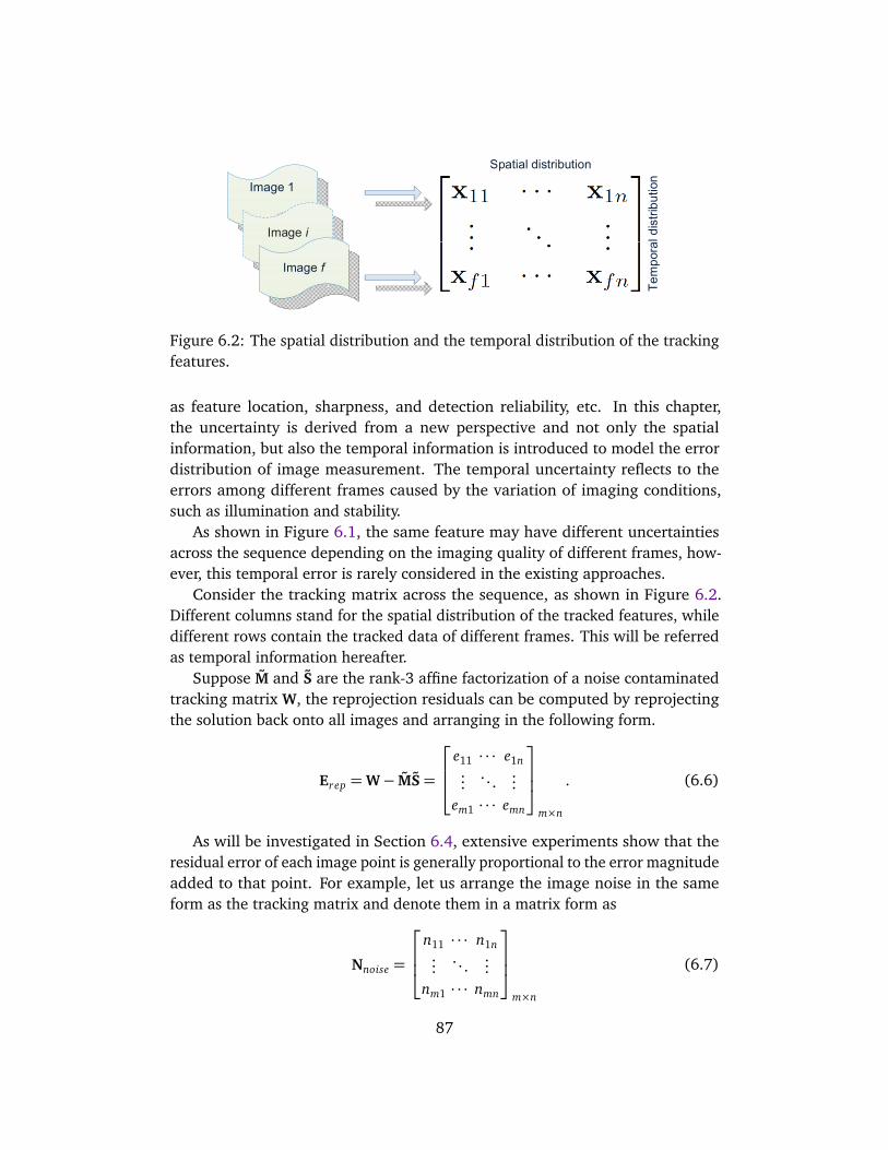
Image 1

Image i

Image f

Spatial distribution

Tem

pora

l dis

tribu

tion

Figure 6.2: The spatial distribution and the temporal distribution of the trackingfeatures.

as feature location, sharpness, and detection reliability, etc. In this chapter,the uncertainty is derived from a new perspective and not only the spatialinformation, but also the temporal information is introduced to model the errordistribution of image measurement. The temporal uncertainty reflects to theerrors among different frames caused by the variation of imaging conditions,such as illumination and stability.

As shown in Figure 6.1, the same feature may have different uncertaintiesacross the sequence depending on the imaging quality of different frames, how-ever, this temporal error is rarely considered in the existing approaches.

Consider the tracking matrix across the sequence, as shown in Figure 6.2.Different columns stand for the spatial distribution of the tracked features, whiledifferent rows contain the tracked data of different frames. This will be referredas temporal information hereafter.

Suppose M and S are the rank-3 affine factorization of a noise contaminatedtracking matrix W, the reprojection residuals can be computed by reprojectingthe solution back onto all images and arranging in the following form.

Erep =W− MS=

e11 · · · e1n...

. . ....

em1 · · · emn

m×n

. (6.6)

As will be investigated in Section 6.4, extensive experiments show that theresidual error of each image point is generally proportional to the error magnitudeadded to that point. For example, let us arrange the image noise in the sameform as the tracking matrix and denote them in a matrix form as

Nnoise =

n11 · · · n1n...

. . ....

nm1 · · · nmn

m×n

(6.7)

87

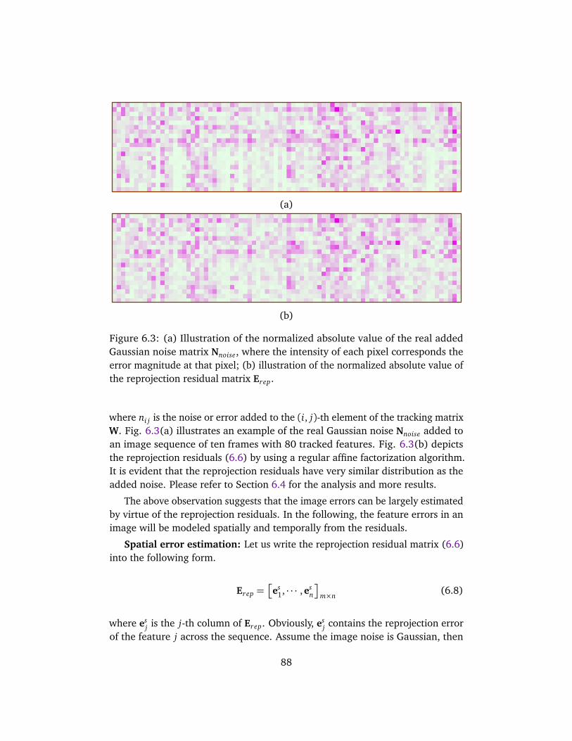
(a)

(b)

Figure 6.3: (a) Illustration of the normalized absolute value of the real addedGaussian noise matrix Nnoise, where the intensity of each pixel corresponds theerror magnitude at that pixel; (b) illustration of the normalized absolute value ofthe reprojection residual matrix Erep.

where ni j is the noise or error added to the (i, j)-th element of the tracking matrixW. Fig. 6.3(a) illustrates an example of the real Gaussian noise Nnoise added toan image sequence of ten frames with 80 tracked features. Fig. 6.3(b) depictsthe reprojection residuals (6.6) by using a regular affine factorization algorithm.It is evident that the reprojection residuals have very similar distribution as theadded noise. Please refer to Section 6.4 for the analysis and more results.

The above observation suggests that the image errors can be largely estimatedby virtue of the reprojection residuals. In the following, the feature errors in animage will be modeled spatially and temporally from the residuals.

Spatial error estimation: Let us write the reprojection residual matrix (6.6)into the following form.

Erep =

es1, · · · ,es

n

m×n(6.8)

where esj is the j-th column of Erep. Obviously, es

j contains the reprojection errorof the feature j across the sequence. Assume the image noise is Gaussian, then

88

the average noise level of esj can be embodied by its standard deviation

δsj =

s

1

m

m∑

i=1

(ei j −µsj)

2 (6.9)

where

µsj =

1

m

m∑

i=1

ei j (6.10)

is the mean of the error vector esj. Stacking the noise levels δs

j of every featuresinto a vector form yields

Es =

δs1, · · · ,δs

n

T. (6.11)

As discussed above, Es can actually reflect the average noise distributionamong different features. Therefore, it is named as spatial error of the trackingdata. Equation (6.11) provides a new perspective in recovering the spatial errorsfrom available data.

Temporal error estimation: Let us rewrite the residual matrix (6.6) into thefollowing from.

Erep =

et1...

etm

m×n

(6.12)

where eti = [ei1, · · · , ein] is the reprojection residuals of all features in the i-th

frame. Similarly, the noise level of the i-th frame is reflected by the standarddeviation of et

i as shown below.

δti =

s

1

n

n∑

i=1

ei j −1

n

n∑

i=1

ei j

2. (6.13)

Similar to the definition of (6.11), the temporal error is defined by stackingδt

i for every frames.

Et =

δt1, · · · ,δt

m

T. (6.14)

Evidently, Et embodies the average noise distribution at different time instantsacross the sequence. The temporal information was rarely considered in previousstudies.

6.3.2 Spatial-and-temporal-weighted factorization

Based on the above estimated spatial and temporal errors, an uncertainty matrixof the tracking data is calculated and applied to the weighted factorization (6.5).

89

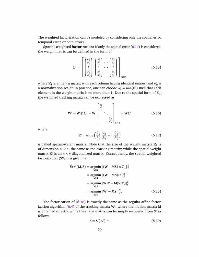
The weighted factorization can be modeled by considering only the spatial error,temporal error, or both errors.

Spatial-weighted factorization: If only the spatial error (6.11) is considered,the weight matrix can be defined in the form of

Σ1 =

δs0

δs1...δs

0

δs1

δs0

δs2...δs

0

δs2

· · ·· · ·· · ·

δs0

δsn...δs

0

δsn

m×n

(6.15)

where Σ1 is an m× n matrix with each column having identical entries; and δs0 is

a normalization scalar. In practice, one can choose δs0 =min(Es) such that each

element in the weight matrix is no more than 1. Due to the special form of Σ1,the weighted tracking matrix can be expressed as

Ws =W⊗Σ1 =W

δs0

δs1

. . .δs

0

δsn

n×n

=WΣs (6.16)

where

Σs = diagδs

0

δs1

,δs

0

δs2

, · · · ,δs

0

δsn

(6.17)

is called spatial-weight matrix. Note that the size of the weight matrix Σ1 isof dimension m× n, the same as the tracking matrix; while the spatial-weightmatrix Σs is an n× n diagonalized matrix. Consequently, the spatial-weightedfactorization (SWF) is given by

Errs(M,S) = argminM,S

‖(W−MS)⊗Σ1‖2F

= argminM,S

‖(W−MS)Σs‖2F

= argminM,S

‖WΣs −M(SΣs)‖2F

= argminM,S

‖Ws −MSs‖2F . (6.18)

The factorization of (6.18) is exactly the same as the regular affine factor-ization algorithm (6.4) of the tracking matrix Ws, where the motion matrix Mis obtained directly, while the shape matrix can be simply recovered from Ss asfollows.

S= Ss(Σs)−1. (6.19)

90

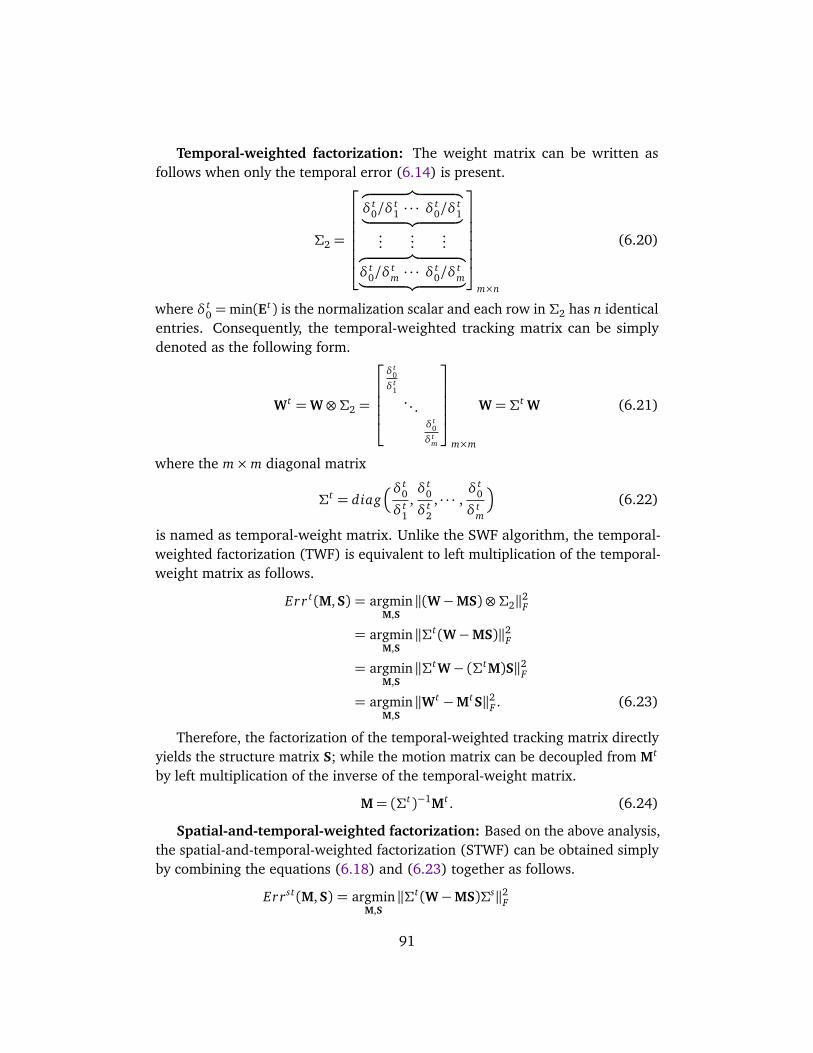
Temporal-weighted factorization: The weight matrix can be written asfollows when only the temporal error (6.14) is present.

Σ2 =

︷︸︸︷

δt0/δ

t1 · · · δ

t0/δ

t1

︸︷︷︸

......

...︷︸︸︷

δt0/δ

tm · · · δ

t0/δ

tm

︸︷︷︸

m×n

(6.20)

where δt0 =min(Et) is the normalization scalar and each row in Σ2 has n identical

entries. Consequently, the temporal-weighted tracking matrix can be simplydenoted as the following form.

Wt =W⊗Σ2 =

δt0

δt1

. . .δt

0

δtm

m×m

W= Σt W (6.21)

where the m×m diagonal matrix

Σt = diagδt

0

δt1

,δt

0

δt2

, · · · ,δt

0

δtm

(6.22)

is named as temporal-weight matrix. Unlike the SWF algorithm, the temporal-weighted factorization (TWF) is equivalent to left multiplication of the temporal-weight matrix as follows.

Err t(M,S) = argminM,S

‖(W−MS)⊗Σ2‖2F

= argminM,S

‖Σt(W−MS)‖2F

= argminM,S

‖ΣtW− (ΣtM)S‖2F

= argminM,S

‖Wt −MtS‖2F . (6.23)

Therefore, the factorization of the temporal-weighted tracking matrix directlyyields the structure matrix S; while the motion matrix can be decoupled from Mt

by left multiplication of the inverse of the temporal-weight matrix.

M= (Σt)−1Mt . (6.24)

Spatial-and-temporal-weighted factorization: Based on the above analysis,the spatial-and-temporal-weighted factorization (STWF) can be obtained simplyby combining the equations (6.18) and (6.23) together as follows.

Errst(M,S) = argminM,S

‖Σt(W−MS)Σs‖2F

91

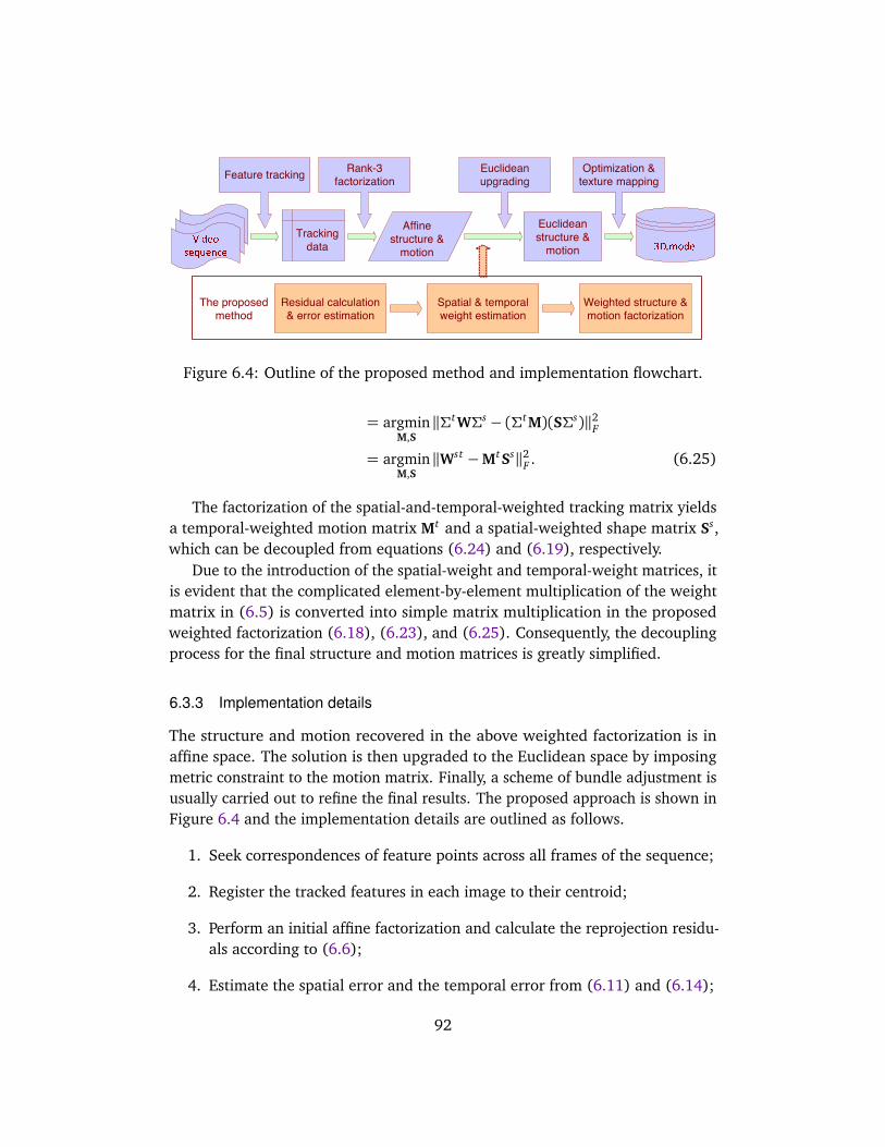
Trackingdata

Euclideanstructure &

motion

Affinestructure &

motion

Spatial & temporalweight estimation

Weighted structure &motion factorization

Residual calculation& error estimation

The proposedmethod

Feature tracking Optimization &texture mapping

Rank-3factorization

Euclideanupgrading

Figure 6.4: Outline of the proposed method and implementation flowchart.

= argminM,S

‖ΣtWΣs − (ΣtM)(SΣs)‖2F

= argminM,S

‖Wst −MtSs‖2F . (6.25)

The factorization of the spatial-and-temporal-weighted tracking matrix yieldsa temporal-weighted motion matrix Mt and a spatial-weighted shape matrix Ss,which can be decoupled from equations (6.24) and (6.19), respectively.

Due to the introduction of the spatial-weight and temporal-weight matrices, itis evident that the complicated element-by-element multiplication of the weightmatrix in (6.5) is converted into simple matrix multiplication in the proposedweighted factorization (6.18), (6.23), and (6.25). Consequently, the decouplingprocess for the final structure and motion matrices is greatly simplified.

6.3.3 Implementation details

The structure and motion recovered in the above weighted factorization is inaffine space. The solution is then upgraded to the Euclidean space by imposingmetric constraint to the motion matrix. Finally, a scheme of bundle adjustment isusually carried out to refine the final results. The proposed approach is shown inFigure 6.4 and the implementation details are outlined as follows.

1. Seek correspondences of feature points across all frames of the sequence;

2. Register the tracked features in each image to their centroid;

3. Perform an initial affine factorization and calculate the reprojection residu-als according to (6.6);

4. Estimate the spatial error and the temporal error from (6.11) and (6.14);

92

5. Construct the spatial-weight matrix (6.17) and the temporal-weight matrix(6.22);

6. Perform the spatial-and-temporal-weighted factorization according to (6.25);

7. Recover the motion matrix and the shape matrix from (6.24) and (6.19);

8. Determine the metric upgrading matrix and upgrade the solution to theEuclidean space;

9. Refine the solution via bundle adjustment if necessary.


The proposed technique was validated and evaluated extensively on syntheticdata and compared with the previous algorithms. During the simulation, 100space points were randomly generated within a cube of 40 × 40 × 40, and asequence of 50 images were produced from these points by the affine projection.The following settings were used in the test: image resolution: 800× 800; focallengths varying randomly from 500 to 550; rotation angles randomly between−60 and +60; camera positions randomly inside a sphere with a diameterof 40; average distance from the cameras to the object: 600. These imagingconditions were very close to the assumption of affine projection.

6.4.1 Recovery of spatial and temporal errors

For the generated images, Gaussian white noise was added to the imaged pointsand the standard deviation of the noise levels was set at 3. First, the rank-3 affinefactorization of the tracking matrix was performed to recover the initial motionand shape matrices. Then, the solution was reprojected back onto the imagesand the reprojection residual matrix was calculated via (6.6). Fig. 6.5 shows theactual reprojection residuals of the first 50 points in one images. It is evidentthat the variational trend of the reprojection residuals and the real added noiseare similar to each other and their magnitudes are largely in proportion.

From the reprojection residuals, the spatial error (6.11) and the temporalerror (6.14) of the entire sequence were recovered. As shown in Fig. 6.6, fromwhich we can see that the two errors recovered by the proposed technique arevery close to the ground truth of the noise added to the images.

In the above tests, the images were generated via affine projection model,which is the first-order approximation of the full perspective projection model.In practice, the images are actually formulated by a full perspective model.

93

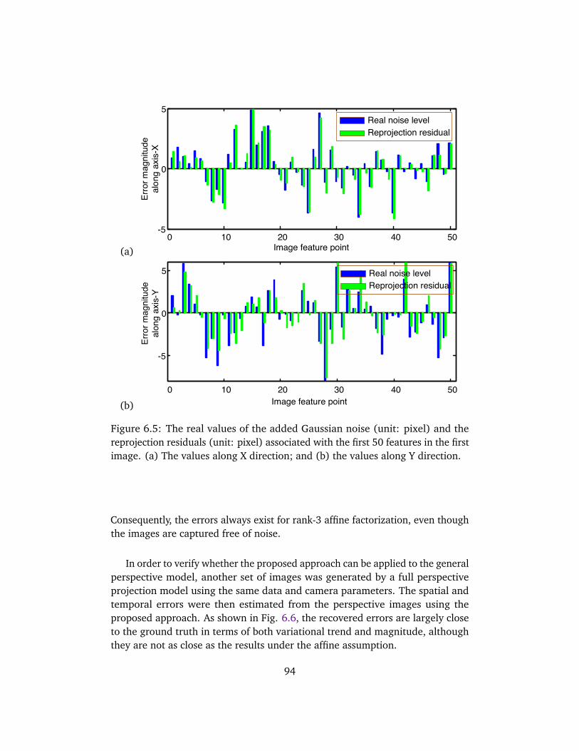
(a)0 10 20 30 40 50

-5

0

5

Image feature point

Erro

r mag

nitu

deal

ong

axis

-X

Real noise levelReprojection residual

(b)

0 10 20 30 40 50

-5

0

5

Image feature point

Erro

r mag

nitu

deal

ong

axis

-Y

Real noise levelReprojection residual

Figure 6.5: The real values of the added Gaussian noise (unit: pixel) and thereprojection residuals (unit: pixel) associated with the first 50 features in the firstimage. (a) The values along X direction; and (b) the values along Y direction.

Consequently, the errors always exist for rank-3 affine factorization, even thoughthe images are captured free of noise.

In order to verify whether the proposed approach can be applied to the generalperspective model, another set of images was generated by a full perspectiveprojection model using the same data and camera parameters. The spatial andtemporal errors were then estimated from the perspective images using theproposed approach. As shown in Fig. 6.6, the recovered errors are largely closeto the ground truth in terms of both variational trend and magnitude, althoughthey are not as close as the results under the affine assumption.

94

(a)

Spat

ial e

rror

Spatial index0 10 20 30 40 50-1.5

-1.0

-0.5

0

0.5

1.0

1.5

Real noise

Spatial-A

Spatial-P

(b)

Tem

pora

l erro

r

0 10 20 30 40 50-1.0

-0.5

0

0.5

1.0

1.5

Real noise

Temporal-A

Temporal-P

Temporal index

Figure 6.6: (a) The spatial error of the synthetic sequence; (b) the temporal errorof the synthetic sequence. Where only the first 50 values are plotted; ’Real noise’stands for the real added noise; ’Spatial-A’ and ’Temporal-A’ denote the spatialand temporal errors under affine model; and ’Spatial-P’ and ’Temporal-P’ denotethe spatial and temporal errors under perspective projection model.

6.4.2 Weighted factorization under affine model

The proposed factorization algorithm was evaluated and compared using theaffine generated images in the following with respect to three different kinds ofadded noise to the images.

Spatial noise: In this case, significant spatial noise was added to the images,i.e., the magnitude of the added noise mainly varied with respect to the features;while the inter-frame noise variation was insignificant, as shown in Fig. 6.7(a).Using the noisy data, the structure and motion were recovered by the proposedSWF, TWF, and STWF algorithms. As a comparison, three benchmark algorithms,i.e. the regular rank-3 affine factorization without uncertainty weight [87], thescalar-weighted factorization [3], and the covariance-weighted factorization [1],were also implemented. Since the above factorizations are in affine space, their

95

(a)

(b)

Figure 6.7: (a) The spatial and temporal noises (unit: pixel) added to the images,where the temporal noise is insignificant; (b) the reprojection variation (unit:pixel) obtained using different algorithms with respect to different noise levels.

performances are evaluated and compared by means of the reprojection variance,which is defined as follows:

Erv =1

mn‖W0− MS‖2F (6.26)

where W0 is the noise-free tracking matrix; M and S are the estimated motionand shape matrices, respectively. In order to obtain a statistically meaningfulcomparison, the temporal noise level (i.e., the standard deviation of the noise)was varied from 1 to 3 pixels in steps of 0.5 during the test, and 100 independenttests were performed at each noise level; while the spatial noise level was set atfour times of the temporal noise level. The mean reprojection variances (6.26)obtained by different algorithms are shown in Fig. 6.7(b).

Based on this test results, the following Conclusion can be drawn: (i) theSWF and STWF algorithms perform similarly, and the accuracy of the solutionis significantly improved by the two algorithms; (ii) the TWF algorithm has

96

(a)

(b)

Figure 6.8: (a) The spatial and temporal noises (unit: pixel) added to the images,where the spatial noise is insignificant; (b) the reprojection variation (unit: pixel)obtained using different algorithms with respect to different noise levels.

only a minor effect since the temporal error is insignificant; (iii) the scalar-weighted factorization does not make big improvement, because the algorithmassumes orthographic camera model and isotropic uncertainty; and (iv) thecovariance-weighted algorithm assumes directional uncertainty and has compa-rable performance as the STWF in this case.

Temporal noise: In this test, a significant temporal noise was added to theimages over minor spatial noise. As shown in Fig. 6.8(a), the noise variationamong different features is insignificant. Similar to the test in the first case, thereprojection variance recovered by different algorithms were evaluated. Themean errors at different noise levels are shown in Fig. 6.8(b).

It is evident from Fig. 6.8 that both the TWF and STWF algorithms significantlyoutperform the regular affine factorization, as well as the scalar-weighted and thecovariance-weighted algorithms. The SWF algorithm shows minor improvementsdue to the insignificance of the spatial error. The performance of the scalar-

97

(a)

(b)

Figure 6.9: (a) The spatial and temporal noises (unit: pixel) added to the images,where both noises are present significantly; (b) the reprojection variation (unit:pixel) obtained using different algorithms with respect to different noise levels.

weighted and the covariance-weighted algorithms lie in between the regularaffine factorization and the proposed STWF, since they only model the noisespatially without explicitly consideration of the influence of temporal noise. Theproposed TWF and the STWF are specifically designed to deal with the temporalnoise, it is not surprising that both of them exhibit the best performance in thisexperiment.

Spatial noise + temporal noise: All algorithms were evaluated under ageneral situation, where a significant spatial noise was applied among differentfeatures and an equivalent amount of temporal noise was applied across thesequence, as shown in Fig. 6.9(a). Using the noise contaminated date, the meanreprojection variances of different algorithms with respect to varied noise levelsare plotted in Fig. 6.9(b).

It can be concluded from this test that (i) the STWF performs the best overother approaches since it can handle both kinds of errors simultaneously. How-

98

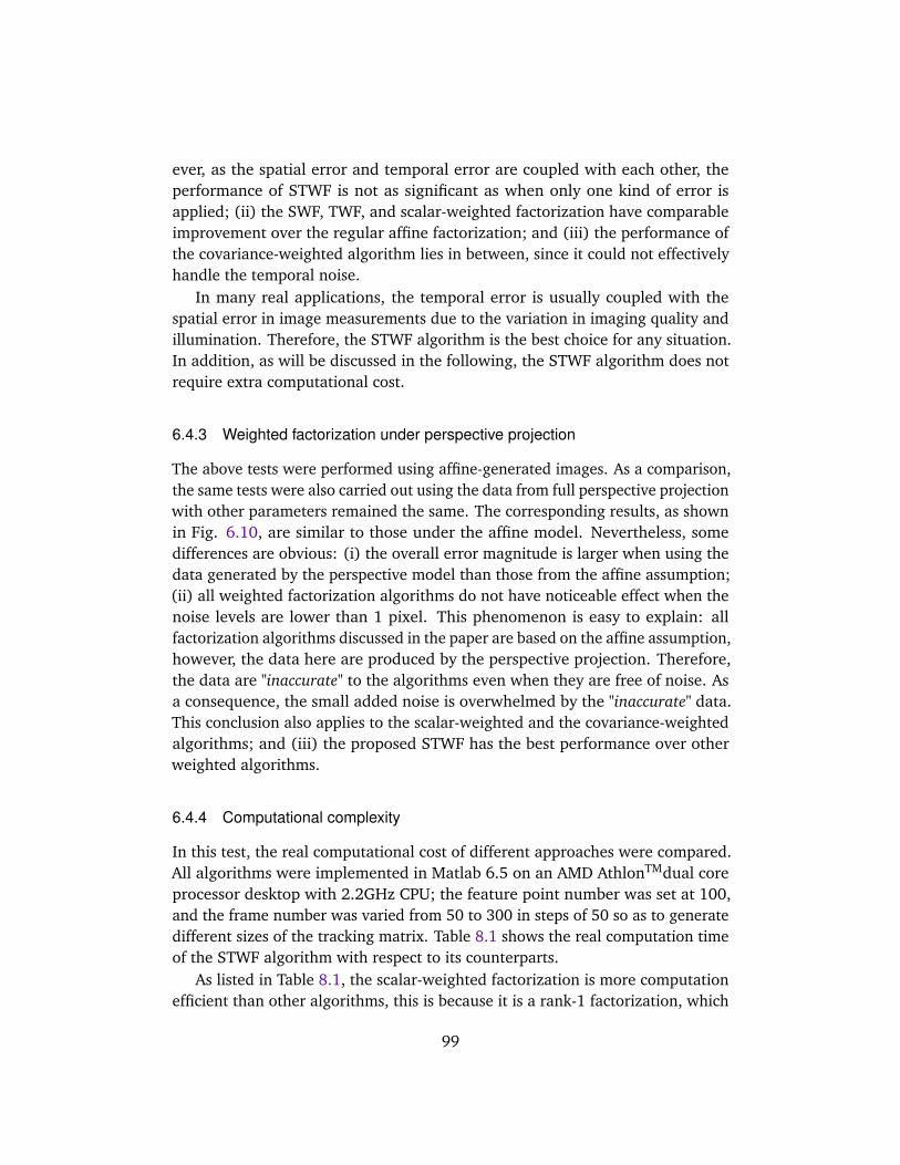
ever, as the spatial error and temporal error are coupled with each other, theperformance of STWF is not as significant as when only one kind of error isapplied; (ii) the SWF, TWF, and scalar-weighted factorization have comparableimprovement over the regular affine factorization; and (iii) the performance ofthe covariance-weighted algorithm lies in between, since it could not effectivelyhandle the temporal noise.

In many real applications, the temporal error is usually coupled with thespatial error in image measurements due to the variation in imaging quality andillumination. Therefore, the STWF algorithm is the best choice for any situation.In addition, as will be discussed in the following, the STWF algorithm does notrequire extra computational cost.

6.4.3 Weighted factorization under perspective projection

The above tests were performed using affine-generated images. As a comparison,the same tests were also carried out using the data from full perspective projectionwith other parameters remained the same. The corresponding results, as shownin Fig. 6.10, are similar to those under the affine model. Nevertheless, somedifferences are obvious: (i) the overall error magnitude is larger when using thedata generated by the perspective model than those from the affine assumption;(ii) all weighted factorization algorithms do not have noticeable effect when thenoise levels are lower than 1 pixel. This phenomenon is easy to explain: allfactorization algorithms discussed in the paper are based on the affine assumption,however, the data here are produced by the perspective projection. Therefore,the data are "inaccurate" to the algorithms even when they are free of noise. Asa consequence, the small added noise is overwhelmed by the "inaccurate" data.This conclusion also applies to the scalar-weighted and the covariance-weightedalgorithms; and (iii) the proposed STWF has the best performance over otherweighted algorithms.

6.4.4 Computational complexity

In this test, the real computational cost of different approaches were compared.All algorithms were implemented in Matlab 6.5 on an AMD AthlonTMdual coreprocessor desktop with 2.2GHz CPU; the feature point number was set at 100,and the frame number was varied from 50 to 300 in steps of 50 so as to generatedifferent sizes of the tracking matrix. Table 8.1 shows the real computation timeof the STWF algorithm with respect to its counterparts.

As listed in Table 8.1, the scalar-weighted factorization is more computationefficient than other algorithms, this is because it is a rank-1 factorization, which

99

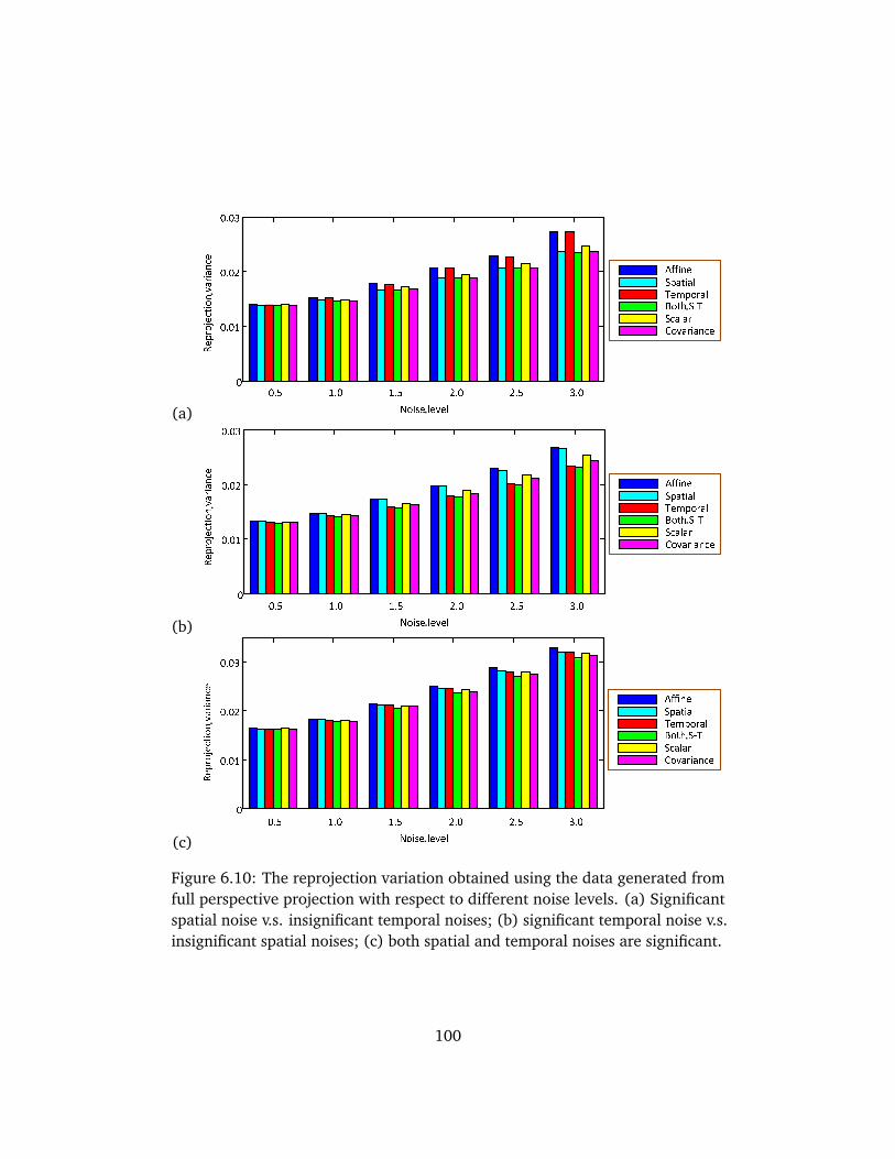
(a)

(b)

(c)

Figure 6.10: The reprojection variation obtained using the data generated fromfull perspective projection with respect to different noise levels. (a) Significantspatial noise v.s. insignificant temporal noises; (b) significant temporal noise v.s.insignificant spatial noises; (c) both spatial and temporal noises are significant.

100

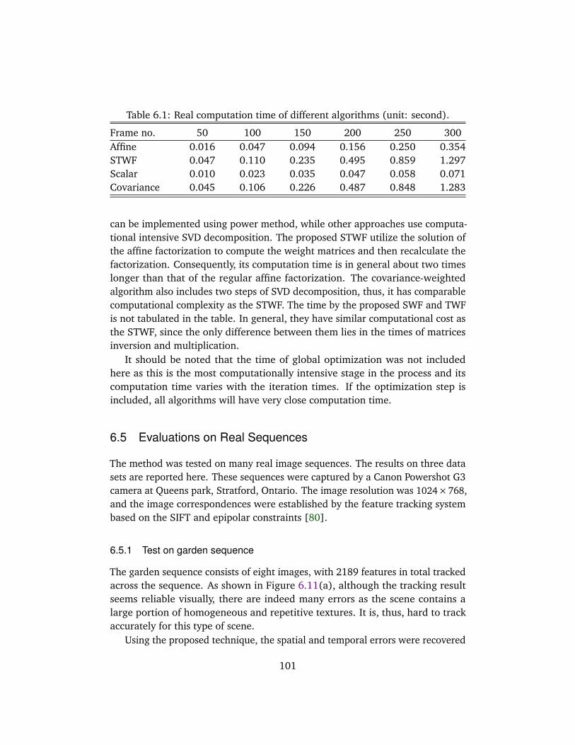
Table 6.1: Real computation time of different algorithms (unit: second).

Frame no. 50 100 150 200 250 300Affine 0.016 0.047 0.094 0.156 0.250 0.354STWF 0.047 0.110 0.235 0.495 0.859 1.297Scalar 0.010 0.023 0.035 0.047 0.058 0.071Covariance 0.045 0.106 0.226 0.487 0.848 1.283

can be implemented using power method, while other approaches use computa-tional intensive SVD decomposition. The proposed STWF utilize the solution ofthe affine factorization to compute the weight matrices and then recalculate thefactorization. Consequently, its computation time is in general about two timeslonger than that of the regular affine factorization. The covariance-weightedalgorithm also includes two steps of SVD decomposition, thus, it has comparablecomputational complexity as the STWF. The time by the proposed SWF and TWFis not tabulated in the table. In general, they have similar computational cost asthe STWF, since the only difference between them lies in the times of matricesinversion and multiplication.

It should be noted that the time of global optimization was not includedhere as this is the most computationally intensive stage in the process and itscomputation time varies with the iteration times. If the optimization step isincluded, all algorithms will have very close computation time.

6.5 Evaluations on Real Sequences

The method was tested on many real image sequences. The results on three datasets are reported here. These sequences were captured by a Canon Powershot G3camera at Queens park, Stratford, Ontario. The image resolution was 1024×768,and the image correspondences were established by the feature tracking systembased on the SIFT and epipolar constraints [80].

6.5.1 Test on garden sequence

The garden sequence consists of eight images, with 2189 features in total trackedacross the sequence. As shown in Figure 6.11(a), although the tracking resultseems reliable visually, there are indeed many errors as the scene contains alarge portion of homogeneous and repetitive textures. It is, thus, hard to trackaccurately for this type of scene.

Using the proposed technique, the spatial and temporal errors were recovered

101

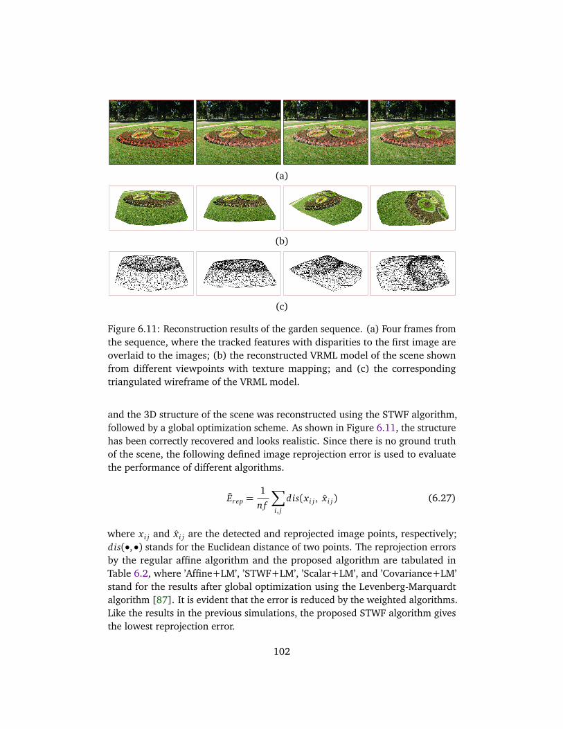
(a)

(b)

(c)

Figure 6.11: Reconstruction results of the garden sequence. (a) Four frames fromthe sequence, where the tracked features with disparities to the first image areoverlaid to the images; (b) the reconstructed VRML model of the scene shownfrom different viewpoints with texture mapping; and (c) the correspondingtriangulated wireframe of the VRML model.

and the 3D structure of the scene was reconstructed using the STWF algorithm,followed by a global optimization scheme. As shown in Figure 6.11, the structurehas been correctly recovered and looks realistic. Since there is no ground truthof the scene, the following defined image reprojection error is used to evaluatethe performance of different algorithms.

Erep =1

nf

∑

i, j

dis(x i j , x i j) (6.27)

where x i j and x i j are the detected and reprojected image points, respectively;dis(•,•) stands for the Euclidean distance of two points. The reprojection errorsby the regular affine algorithm and the proposed algorithm are tabulated inTable 6.2, where ’Affine+LM’, ’STWF+LM’, ’Scalar+LM’, and ’Covariance+LM’stand for the results after global optimization using the Levenberg-Marquardtalgorithm [87]. It is evident that the error is reduced by the weighted algorithms.Like the results in the previous simulations, the proposed STWF algorithm givesthe lowest reprojection error.

102

(a)

(b)

(c)

Figure 6.12: Reconstruction results of the tree trunk sequence. (a) Four framesfrom the sequence overlaid with the tracked features with disparities to thefirst image; (b) the reconstructed VRML model of the trunk shown from differ-ent viewpoints with texture mapping; and (c) the corresponding triangulatedwireframe of the VRML model.

103

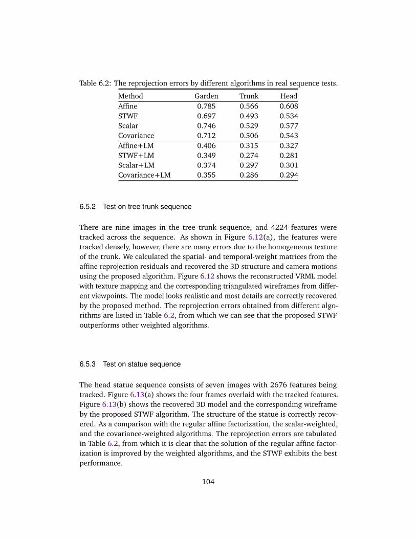
Table 6.2: The reprojection errors by different algorithms in real sequence tests.

Method Garden Trunk HeadAffine 0.785 0.566 0.608STWF 0.697 0.493 0.534Scalar 0.746 0.529 0.577Covariance 0.712 0.506 0.543Affine+LM 0.406 0.315 0.327STWF+LM 0.349 0.274 0.281Scalar+LM 0.374 0.297 0.301Covariance+LM 0.355 0.286 0.294

6.5.2 Test on tree trunk sequence

There are nine images in the tree trunk sequence, and 4224 features weretracked across the sequence. As shown in Figure 6.12(a), the features weretracked densely, however, there are many errors due to the homogeneous textureof the trunk. We calculated the spatial- and temporal-weight matrices from theaffine reprojection residuals and recovered the 3D structure and camera motionsusing the proposed algorithm. Figure 6.12 shows the reconstructed VRML modelwith texture mapping and the corresponding triangulated wireframes from differ-ent viewpoints. The model looks realistic and most details are correctly recoveredby the proposed method. The reprojection errors obtained from different algo-rithms are listed in Table 6.2, from which we can see that the proposed STWFoutperforms other weighted algorithms.

6.5.3 Test on statue sequence

The head statue sequence consists of seven images with 2676 features beingtracked. Figure 6.13(a) shows the four frames overlaid with the tracked features.Figure 6.13(b) shows the recovered 3D model and the corresponding wireframeby the proposed STWF algorithm. The structure of the statue is correctly recov-ered. As a comparison with the regular affine factorization, the scalar-weighted,and the covariance-weighted algorithms. The reprojection errors are tabulatedin Table 6.2, from which it is clear that the solution of the regular affine factor-ization is improved by the weighted algorithms, and the STWF exhibits the bestperformance.

104

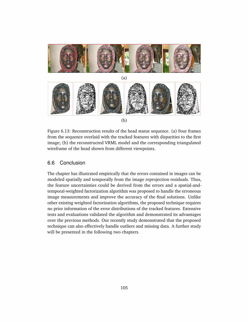
(a)

(b)

Figure 6.13: Reconstruction results of the head statue sequence. (a) Four framesfrom the sequence overlaid with the tracked features with disparities to the firstimage; (b) the reconstructed VRML model and the corresponding triangulatedwireframe of the head shown from different viewpoints.

6.6 Conclusion

The chapter has illustrated empirically that the errors contained in images can bemodeled spatially and temporally from the image reprojection residuals. Thus,the feature uncertainties could be derived from the errors and a spatial-and-temporal-weighted factorization algorithm was proposed to handle the erroneousimage measurements and improve the accuracy of the final solutions. Unlikeother existing weighted factorization algorithms, the proposed technique requiresno prior information of the error distributions of the tracked features. Extensivetests and evaluations validated the algorithm and demonstrated its advantagesover the previous methods. Our recently study demonstrated that the proposedtechnique can also effectively handle outliers and missing data. A further studywill be presented in the following two chapters.

105

Chapter 7

Robust SfM of Rigid Objects

The chapter presents a robust structure from motion algorithm for rigid objects.First, a rank-4 augmented affine factorization algorithm is proposed to overcomethe difficulty in image alignment for imperfect data. Then, a robust structureand motion factorization scheme is proposed to handle outlying and missingdata. The novelty and main contribution of the paper are as follows: (i) Therank-4 factorization algorithm is a new addition to previous affine factorizationfamily using rank-3 constraint; (ii) it is demonstrated that image reprojectionresiduals are in general proportional to the error magnitude in the trackingdata. Thus, the outliers can be detected directly from the distribution of imagereprojection residuals, which are then used to estimate the weight matrix ofinlying measurement; and (iii) the robust factorization scheme is demonstratedempirically to be more efficient and accurate than other robust algorithms.Extensive experiments on synthetic data and real images validate the proposedapproach.

7.1 Introduction

Most factorization methods usually assume all features are tracked across thesequence. In the presence of missing data, SVD factorization can not be useddirectly. Some approaches propose to solve the motion and shape matricesalternatively, such as the alternative factorization [41], power factorization[33], and factor analysis [29]. In practice, outlying data are inevitable duringthe process of feature tracking, and as a consequence, the performance of thealgorithm will degenerate. The most popular strategy in computer vision field isRANSAC, Least Median of Squares [32], and other similar hypothesis-and-testframeworks [67]. However, these methods are usually designed for two or threeviews.

107

In recent years, the problem of robust factorization has received a lot ofattention [2][63][100]. Aguitar and Moura [3] proposed a scalar-weightedSVD algorithm that minimizes the weighted square errors. Gruber and Weiss[29] formulated the problem as a factor analysis and derived an ExpectationMaximization (EM) algorithm to enhance the robustness to missing data anduncertainties. Zelnik-Manor et al. [103] defined a new type of motion consistencybased on temporal consistency, and applied it to multi-body factorization withdirectional uncertainty. Zaharescu and Horaud [100] introduced a Gaussianmixture model and incorporate it with the EM algorithm. Huynh et al. [39]proposed an iterative approach to correct the outliers with ’pseudo’ observations.

Ke and kanade [41] proposed a robust algorithm to handle outliers by mini-mizing a L1 norm of the reprojection errors. Eriksson and Hengel [23] introducedthe L1 norm to the Wiberg algorithm to handle missing data and outliers. Okataniet al. [55] proposed to incorporate a damping factor into the Wiberg method tosolve the problem. Yu et al. [99] presented a Quadratic Program formulation forrobust multi-model fitting of geometric structures. Wang et al. [92] proposedan adaptive kernel-scale weighted hypotheses to segment multiple-structuredata even in the presence of a large number of outliers. Paladini et al. [60]proposed an alternating bilinear approach to solve nonrigid SfM by introducinga globally optimal projection step of the motion matrices onto the manifold ofmetric constraints. Wang et al. [89] proposed a spatial-and-temporal-weightedfactorization approach to handle significant noise in the measurement.

In this chapter, the outlying data are detected from a new viewpoint viaimage reprojection residuals by exploring the fact that the reprojection residualsare in general proportional to measurement errors of the tracking data. Thischapter first proposes an augmented rank-4 factorization algorithm to circumventthe problem of image registration in the presence of missing and outlying data.Then, an alternative weighted factorization algorithm is presented to handle themissing features and image uncertainty. Finally, a robust factorization scheme isproposed to handle outliers. A preliminary work on this research was publishedat the WACV conference [91].

7.2 Background on Structure and Motion Factorization

Under affine projection model, a 3D point X j = [x j , y j , z j]T is projected onto animage point xi j = [ui j , vi j]T in frame i according to the imaging equation

xi j = AiX j + ci (7.1)

where the matrix Ai is a 2× 3 affine projection matrix; and ci is a translationterm of the frame. Under the affine projection, the mapping from space to the

108

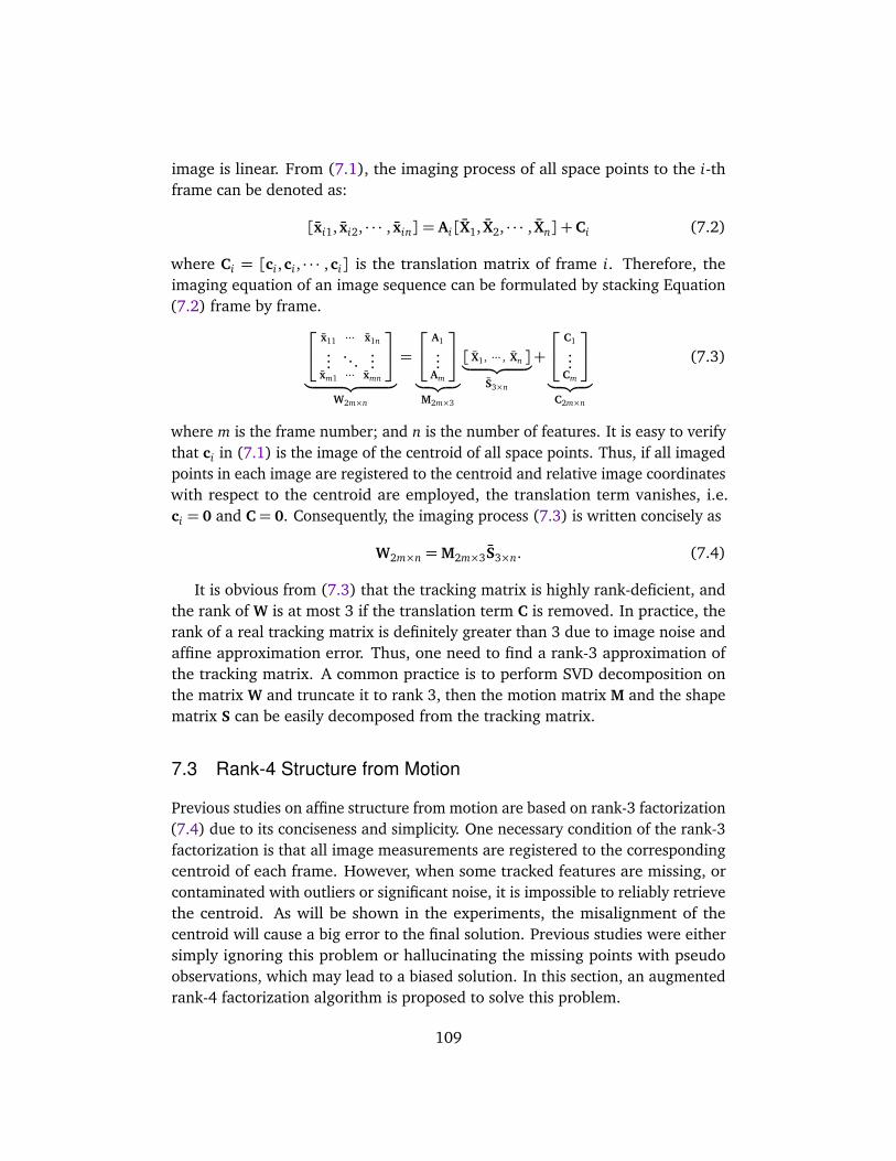
image is linear. From (7.1), the imaging process of all space points to the i-thframe can be denoted as:

[xi1, xi2, · · · , xin] = Ai[X1, X2, · · · , Xn] +Ci (7.2)

where Ci = [ci ,ci , · · · ,ci] is the translation matrix of frame i. Therefore, theimaging equation of an image sequence can be formulated by stacking Equation(7.2) frame by frame.

x11 ··· x1n

......

...xm1 ··· xmn

︸︷︷︸

W2m×n

=

A1

...Am

︸︷︷︸

M2m×3

[ X1, ··· , Xn ]︸︷︷︸

S3×n

+

C1

...Cm

︸︷︷︸

C2m×n

(7.3)

where m is the frame number; and n is the number of features. It is easy to verifythat ci in (7.1) is the image of the centroid of all space points. Thus, if all imagedpoints in each image are registered to the centroid and relative image coordinateswith respect to the centroid are employed, the translation term vanishes, i.e.ci = 0 and C = 0. Consequently, the imaging process (7.3) is written concisely as

W2m×n =M2m×3S3×n. (7.4)

It is obvious from (7.3) that the tracking matrix is highly rank-deficient, andthe rank of W is at most 3 if the translation term C is removed. In practice, therank of a real tracking matrix is definitely greater than 3 due to image noise andaffine approximation error. Thus, one need to find a rank-3 approximation ofthe tracking matrix. A common practice is to perform SVD decomposition onthe matrix W and truncate it to rank 3, then the motion matrix M and the shapematrix S can be easily decomposed from the tracking matrix.

7.3 Rank-4 Structure from Motion

Previous studies on affine structure from motion are based on rank-3 factorization(7.4) due to its conciseness and simplicity. One necessary condition of the rank-3factorization is that all image measurements are registered to the correspondingcentroid of each frame. However, when some tracked features are missing, orcontaminated with outliers or significant noise, it is impossible to reliably retrievethe centroid. As will be shown in the experiments, the misalignment of thecentroid will cause a big error to the final solution. Previous studies were eithersimply ignoring this problem or hallucinating the missing points with pseudoobservations, which may lead to a biased solution. In this section, an augmentedrank-4 factorization algorithm is proposed to solve this problem.

109

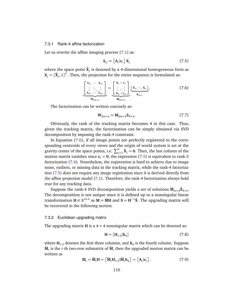
7.3.1 Rank-4 affine factorization

Let us rewrite the affine imaging process (7.1) as:

xi j =

Ai|ci

X j (7.5)

where the space point X j is denoted by a 4-dimensional homogeneous form asX j = [X j , 1]T . Then, the projection for the entire sequence is formulated as:

x11 ··· x1n

......

...xm1 ··· xmn

︸︷︷︸

W2m×n

=

A1 | c1

... |...

Am | cm

︸︷︷︸

M2m×4

[ X1, ··· , Xn ]︸︷︷︸

S4×n

. (7.6)

The factorization can be written concisely as:

W2m×n =M2m×4S4×n. (7.7)

Obviously, the rank of the tracking matrix becomes 4 in this case. Thus,given the tracking matrix, the factorization can be simply obtained via SVDdecomposition by imposing the rank-4 constraint.

In Equation (7.6), if all image points are perfectly registered to the corre-sponding centroids of every views and the origin of world system is set at thegravity center of the space points, i.e.

∑nj=1 X j = 0. Then, the last column of the

motion matrix vanishes since ci = 0, the expression (7.5) is equivalent to rank-3factorization (7.4). Nonetheless, the registration is hard to achieve due to imagenoise, outliers, or missing data in the tracking matrix, while the rank-4 factoriza-tion (7.5) does not require any image registration since it is derived directly fromthe affine projection model (7.1). Therefore, the rank-4 factorization always holdtrue for any tracking data.

Suppose the rank-4 SVD decomposition yields a set of solutions Mm×4S4×n.The decomposition is not unique since it is defined up to a nonsingular lineartransformation H ∈ R4×4 as M = MH and S = H−1S. The upgrading matrix willbe recovered in the following section.


The upgrading matrix H is a 4× 4 nonsingular matrix which can be denoted as:

H= [H1:3|h4] (7.8)

where H1:3 denotes the first three columns, and h4 is the fourth column. SupposeMi is the i-th two-row submatrix of M, then the upgraded motion matrix can bewritten as

Mi = MiH=

MiH1:3|Mih4

=

Ai|ci

. (7.9)

110

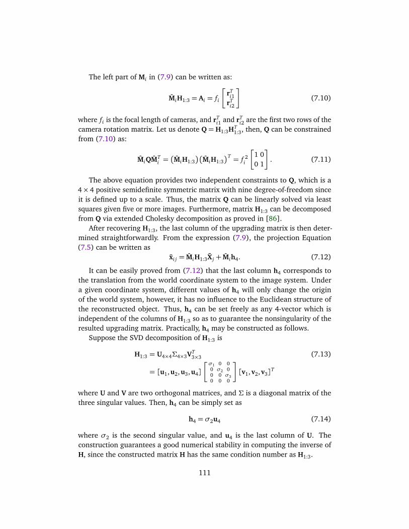
The left part of Mi in (7.9) can be written as:

MiH1:3 = Ai = fi

rTi1

rTi2

(7.10)

where fi is the focal length of cameras, and rTi1 and rT

i2 are the first two rows of thecamera rotation matrix. Let us denote Q= H1:3HT

1:3, then, Q can be constrainedfrom (7.10) as:

MiQMTi =

MiH1:3

MiH1:3T = f 2

i

1 00 1

. (7.11)

The above equation provides two independent constraints to Q, which is a4× 4 positive semidefinite symmetric matrix with nine degree-of-freedom sinceit is defined up to a scale. Thus, the matrix Q can be linearly solved via leastsquares given five or more images. Furthermore, matrix H1:3 can be decomposedfrom Q via extended Cholesky decomposition as proved in [86].

After recovering H1:3, the last column of the upgrading matrix is then deter-mined straightforwardly. From the expression (7.9), the projection Equation(7.5) can be written as

xi j = MiH1:3X j + Mih4. (7.12)

It can be easily proved from (7.12) that the last column h4 corresponds tothe translation from the world coordinate system to the image system. Undera given coordinate system, different values of h4 will only change the originof the world system, however, it has no influence to the Euclidean structure ofthe reconstructed object. Thus, h4 can be set freely as any 4-vector which isindependent of the columns of H1:3 so as to guarantee the nonsingularity of theresulted upgrading matrix. Practically, h4 may be constructed as follows.

Suppose the SVD decomposition of H1:3 is

H1:3 = U4×4Σ4×3VT3×3 (7.13)

= [u1,u2,u3,u4]

σ1 0 00 σ2 00 0 σ30 0 0

[v1,v2,v3]T

where U and V are two orthogonal matrices, and Σ is a diagonal matrix of thethree singular values. Then, h4 can be simply set as

h4 = σ2u4 (7.14)

where σ2 is the second singular value, and u4 is the last column of U. Theconstruction guarantees a good numerical stability in computing the inverse ofH, since the constructed matrix H has the same condition number as H1:3.

111

7.3.3 Algorithm of rank-4 affine factorization

The above proposed rank-4 affine factorization algorithm is summarized asfollows.

Algorithm 1: Rank-4 Affine Factorization

Input: tracking matrix W1. Perform SVD decomposition on the tracking matrix;

2. Obtain a set of rank-4 solutions of M and S;3. Recover the Euclidean upgrading matrix matrix H;4. Compute the Euclidean structure and camera motion

parameters from H−1S and MH.

Output: the Euclidean structure and motion parameters

7.4 Alternative and Weighted Factorization

SVD decomposition is a convenient way of structure and motion factorization,however, SVD only works when all features are tracked across the sequence. Inpractice, missing data are inevitable since some features may be missing duringthe process of tracking due to occlusion or other factors. Researchers proposeddifferent alternative factorization approaches to handle missing data [33]. Inthis section, a two-step alternative and weighted factorization algorithms areintroduced to handle missing data and image uncertainties.

7.4.1 Alternative factorization algorithm

The essence of structure and motion factorization (7.6) is equivalent to findingrank-4 matrices M and S by minimizing the following Frobenious norm.

argminM,S

‖W−MS‖2F (7.15)

subject to: M ∈ R2m×4,S ∈ R4×n.

The basic idea of the two step factorization is to minimize the cost function(7.15) over S and M alternatively until convergence, while leaving the other onefixed, i.e.,

f (S) = argminS‖W−MS‖2F (7.16)

112

f (M) = argminM‖W−MS‖2F . (7.17)

Each cost function of the algorithm is indeed a convex function, so a globalminimum can always be found. The algorithm converges fast if the trackingmatrix is close to rank-4, even with a random initialization. This idea wasadopted in several papers [33] [39] [41].

Different with SVD decomposition, the minimization process is carried out byleast squares. Let us rewrite the cost function (7.16) with respect to each featureas follows.

f (s j) = argmins j

‖w j −Ms j‖2F (7.18)

where w j is the j-th column of W, and s j is the j-th column of S. Thus, the leastsquares solution of S can be given as

s j =M†w j , j = 1, · · · , n (7.19)

where M† = (MT M)−1MT is the Moore-Penrose pseudoinverse of matrix M. Thesolution (7.19) can easily handle the missing data in the tracking matrix. Forexample, if some entries in w j are unavailable, one can simply delete thoseelements in w j and the corresponding columns in M†, or just set those entriesin w j as zeros, then, s j can be solved from (7.19) using the available entries vialeast squares.

Similarly, the second cost function (7.17) can be rewrite as

f (mTi ) = argmin

mTi

‖wTi −mT

i S‖2F (7.20)

which yields the following least-square solution of the motion matrix M.

mTi =wT

i S†, i = 1, · · · , m (7.21)

where the pseudoinverse S† = ST (SST )−1, mTi and wT

i denote the i-th row of thematrices M and W, respectively. In case of missing elements, one can simply resetthose entries in wT

i as zeros.The alternative algorithm is summarized as follows.

Algorithm 2: Alternative Factorization Algorithm

Input: matrix W and matrix MRepeat the following two steps until convergence

1. Updata shape matrix via (7.19)

2. Updata motion matrix via (7.21)

Output: matrices M and S

113

7.4.2 Alternative weighted factorization

Measurement errors are inevitable in the process of feature detection and tracking.If prior knowledge about distribution of the errors is available, then all elementsof the approximation error can be weighted by taking account of the errordistribution so as to increase the robustness and accuracy of the algorithm.The basic idea is to give each image measurement a weight according to itsuncertainty. Reliable features get higher weights, while unreliable features areassigned lower weights. The weighted rank-4 factorization is formulated asfollows.

argminM,S

‖Σ⊗ (W−MS)‖2F (7.22)

subject to: M ∈ R2m×4,S ∈ R4×n

where ′⊗′ denotes the Hadamard product, which is an element-by-elementmultiplication of two matrices; Σ= σi j is an 2m× n uncertainty matrix whoseentries are weights derived from the confidence of the image measurements.

The general weighted factorization could not be solved analytically in termsof the singular value decomposition. Many researchers have proposed differentschemes to solve the problem [3][7][100]. In this section, the solution of (7.22)will be obtained using the alternative factorization algorithm by solving S and Malternatively as follows.

f (S) = argmins j

‖Σ j ⊗ (w j −Ms j)‖2F (7.23)

f (M) = argminmT

i

‖ΣTi ⊗ (w

Ti −mT

i S)‖2F (7.24)

where Σ j denotes the j-th column of Σ, and ΣTi the i-th row of Σ. The close-form

solutions of the shape and motion matrices can be obtained by least squares.

s j =

diag(Σ j)M†

diag(Σ j)w j

, j = 1, · · · , n (7.25)

mTi =

wTi diag(ΣT

i )

Sdiag(ΣTi )†

, i = 1, · · · , m (7.26)

where (•)† denotes the pseudoinverse of a matrix, and ′diag(•)′ stands for thediagonal matrix generated by a vector. Equations (7.25) and (7.26) give theleast-square solutions of S and M. Similar to the alternative factorization, whenthere are any missing data in the tracking matrix, one can simply set those entriesin w j as zeros.

The alternative weighted factorization algorithm is summarized as follows,where the initial values of the motion matrix M and weight matrix Σ will bediscussed in next section.

114

Algorithm 3: Alternative Weighted Factorization

Input: matrices W, M, and ΣRepeat the following two steps until convergence

1. Updata shape matrix S via (7.25)

2. Updata motion matrix M via (7.26)

Output: matrices M and S

7.5 Outlier Detection and Robust Factorization

Based on the rank-4 factorization algorithm proposed in the foregoing sections.A fast and practical scheme for outlier detection is proposed in this section.

7.5.1 Outlier detection scheme

Outlying data are inevitable in the process of feature tracking. The most popularstrategy in computer vision field is RANSAC (RANdom SAmple Consensus) [26],Least Median of Squares (LMedS), and some other similar techniques in thefamily [14]. However, all these methods are computationally intensive. Anotherclass of robust algorithm that can work with outliers is based on L1 factorizationby minimizing the L1 norm of the reprojection errors [41].

The RANSAC approach initiates a model from a minimal set of data and thenscores the model by the number of feature points within a given threshold. It candeal with data having more than 50% outliers. However, since the inlying dataare also contaminated by noise, the initiated model using minimal data may bebiased.

Both the SVD-based and the alternative factorization-based algorithms yielda set of least-square solutions. The best fit model is obtained by minimizingthe sum of the squared residuals between the observed data and the fittedvalues provided by the model. Extensive experiments show that the least-squarealgorithms usually yield reasonable solutions even in the presence of certainamount of outliers and the reprojection residuals of these outlying data areusually much larger than those associated with inliers.

Suppose M and S are a set of solutions of the rank-4 factorization of a trackingmatrix W, the reprojection residuals can be computed by reprojecting the set of

115

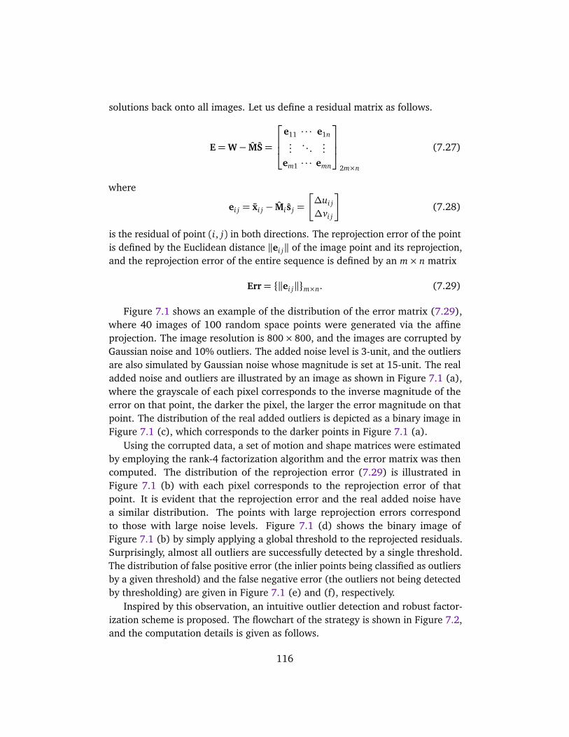
solutions back onto all images. Let us define a residual matrix as follows.

E=W− MS=

e11 · · · e1n...

. . ....

em1 · · · emn

2m×n

(7.27)

where

ei j = xi j − Mi s j =

∆ui j

∆vi j

(7.28)

is the residual of point (i, j) in both directions. The reprojection error of the pointis defined by the Euclidean distance ‖ei j‖ of the image point and its reprojection,and the reprojection error of the entire sequence is defined by an m× n matrix

Err= ‖ei j‖m×n. (7.29)

Figure 7.1 shows an example of the distribution of the error matrix (7.29),where 40 images of 100 random space points were generated via the affineprojection. The image resolution is 800× 800, and the images are corrupted byGaussian noise and 10% outliers. The added noise level is 3-unit, and the outliersare also simulated by Gaussian noise whose magnitude is set at 15-unit. The realadded noise and outliers are illustrated by an image as shown in Figure 7.1 (a),where the grayscale of each pixel corresponds to the inverse magnitude of theerror on that point, the darker the pixel, the larger the error magnitude on thatpoint. The distribution of the real added outliers is depicted as a binary image inFigure 7.1 (c), which corresponds to the darker points in Figure 7.1 (a).

Using the corrupted data, a set of motion and shape matrices were estimatedby employing the rank-4 factorization algorithm and the error matrix was thencomputed. The distribution of the reprojection error (7.29) is illustrated inFigure 7.1 (b) with each pixel corresponds to the reprojection error of thatpoint. It is evident that the reprojection error and the real added noise havea similar distribution. The points with large reprojection errors correspondto those with large noise levels. Figure 7.1 (d) shows the binary image ofFigure 7.1 (b) by simply applying a global threshold to the reprojected residuals.Surprisingly, almost all outliers are successfully detected by a single threshold.The distribution of false positive error (the inlier points being classified as outliersby a given threshold) and the false negative error (the outliers not being detectedby thresholding) are given in Figure 7.1 (e) and (f), respectively.

Inspired by this observation, an intuitive outlier detection and robust factor-ization scheme is proposed. The flowchart of the strategy is shown in Figure 7.2,and the computation details is given as follows.

116

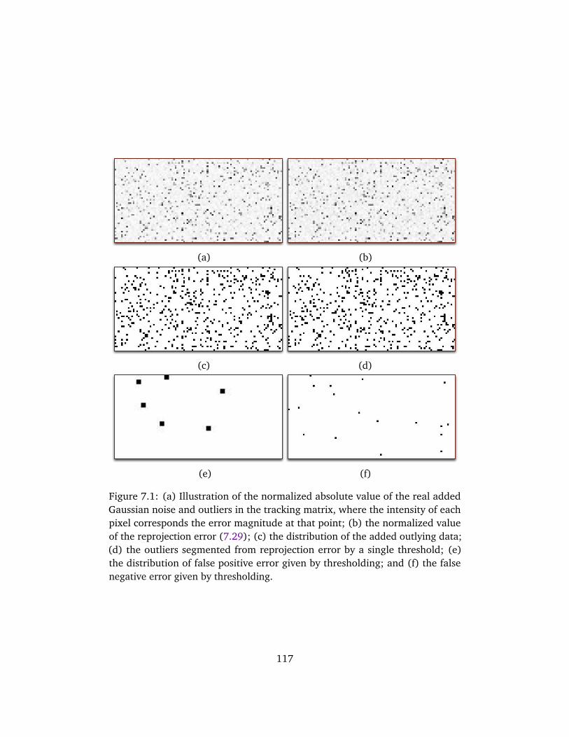
(a) (b)

(c) (d)

(e) (f)

Figure 7.1: (a) Illustration of the normalized absolute value of the real addedGaussian noise and outliers in the tracking matrix, where the intensity of eachpixel corresponds the error magnitude at that point; (b) the normalized valueof the reprojection error (7.29); (c) the distribution of the added outlying data;(d) the outliers segmented from reprojection error by a single threshold; (e)the distribution of false positive error given by thresholding; and (f) the falsenegative error given by thresholding.

117

Tracking Data

Final 3D model

Outlier detection

&Uncertainty estimation

Image sequenceImage

sequenceImage

sequenceInitial

structure & motion

Euclidean structure &

motion

Refined structure &

motion

Featuretracking

Alternativefactorization

Back-projection

Weightedfactorization

Euclideanupgrading

Globaloptimization

Figure 7.2: The outline and flowchart of the robust structure from motion

Algorithm 4: Robust Structure and Motion Factorization

Input: the tracking matrix W1. Balance the tracking matrix via point-wise and image-wise rescalings,

as in [71], to improve numerical stability.

2. Perform rank-4 affine factorization on the tracking matrix to

obtain a set of solutions of M and S.

3. Estimate the reprojection residuals and determine the outlier

threshold.

4. Eliminate the outliers and recalculate the matrices M and S using

the inlying data via Algorithm 2.

5. Estimate the uncertainty of each inlying feature.

6. Refine the solutions by weighted factorization algorithm.

7. Recover the Euclidean upgrading matrix H and upgrade the solutions

to the Euclidean space as M= MH and S= H−1S.

8. Perform a global optimization via bundle adjustment if necessary.

Output: the 3D structure and camera motion parameters recovered from

S and M respectively.

In the above algorithm, steps 3 and 4 can be repeated once to ensure a morerefined inlying data and solutions, but in practice, the repetition does not makemuch difference to final results. During computation, Algorithms 2 and 3 areemployed to deal with missing data. Normally, the alternative algorithm canwork with random initialization, however, since an initial set of solutions havebeen obtained in the previous steps, these solutions can be used as initial valuesin the iteration so as to speed up the convergence.

118

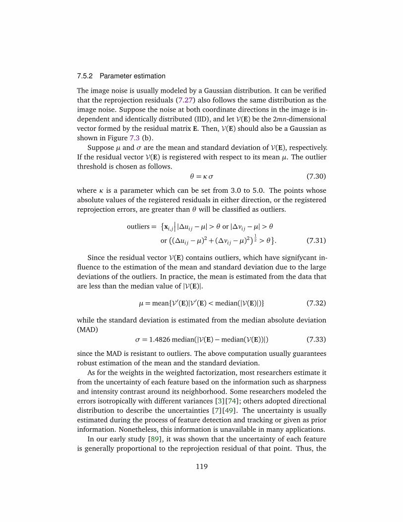
7.5.2 Parameter estimation

The image noise is usually modeled by a Gaussian distribution. It can be verifiedthat the reprojection residuals (7.27) also follows the same distribution as theimage noise. Suppose the noise at both coordinate directions in the image is in-dependent and identically distributed (IID), and let V(E) be the 2mn-dimensionalvector formed by the residual matrix E. Then, V(E) should also be a Gaussian asshown in Figure 7.3 (b).

Suppose µ and σ are the mean and standard deviation of V(E), respectively.If the residual vector V(E) is registered with respect to its mean µ. The outlierthreshold is chosen as follows.

θ = κσ (7.30)

where κ is a parameter which can be set from 3.0 to 5.0. The points whoseabsolute values of the registered residuals in either direction, or the registeredreprojection errors, are greater than θ will be classified as outliers.

outliers=

xi, j

|∆ui j −µ|> θ or |∆vi j −µ|> θ

or

(∆ui j −µ)2+ (∆vi j −µ)2

12 > θ

. (7.31)

Since the residual vector V(E) contains outliers, which have signifycant in-fluence to the estimation of the mean and standard deviation due to the largedeviations of the outliers. In practice, the mean is estimated from the data thatare less than the median value of |V(E)|.

µ=meanV ′(E)|V ′(E)<median(|V(E)|) (7.32)

while the standard deviation is estimated from the median absolute deviation(MAD)

σ = 1.4826 median(|V(E)−median(V(E))|) (7.33)

since the MAD is resistant to outliers. The above computation usually guaranteesrobust estimation of the mean and the standard deviation.

As for the weights in the weighted factorization, most researchers estimate itfrom the uncertainty of each feature based on the information such as sharpnessand intensity contrast around its neighborhood. Some researchers modeled theerrors isotropically with different variances [3][74]; others adopted directionaldistribution to describe the uncertainties [7][49]. The uncertainty is usuallyestimated during the process of feature detection and tracking or given as priorinformation. Nonetheless, this information is unavailable in many applications.

In our early study [89], it was shown that the uncertainty of each featureis generally proportional to the reprojection residual of that point. Thus, the

119

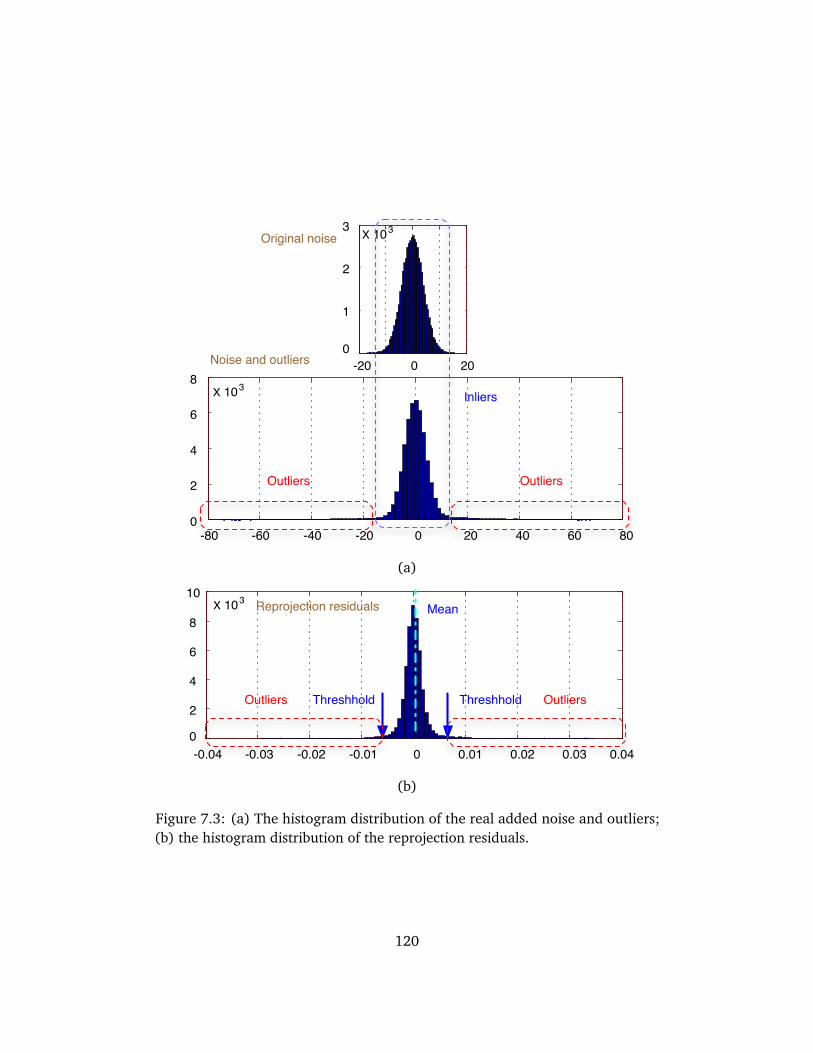
-80 -60 -40 -20 0 20 40 60 800

2

4

6

83X 10

-20 0 20

1

2

3 3X 10

0

Original noise

Noise and outliers

Inliers

OutliersOutliers

(a)

10

-0.04 -0.03 -0.02 -0.01 0 0.01 0.02 0.03 0.040

2

4

6

8

3X 10 Reprojection residuals Mean

Threshhold Threshhold OutliersOutliers

(b)

Figure 7.3: (a) The histogram distribution of the real added noise and outliers;(b) the histogram distribution of the reprojection residuals.

120

weight of each point can be estimated from the residual value obtained fromthe data after eliminating outliers. The point with higher residual value haslarger uncertainty and thus gets lower weight. The weight of each point at eachcoordinate direction is determined as follows in a shape like normal distribution.

ωi j =1

N exp

−E2

i j

2σ2

!

(7.34)

where the standard deviation σ is estimated from Equation (7.33), Ei j is the(i, j)-th element of the residual matrix (7.27), and N is a normalization scale.Clearly, one point may have different weights at the two image directions basedon the residual value at each direction. For the missing data and outliers, thecorresponding weights are set as ωi j = 0.


The proposed technique was validated and evaluated extensively on syntheticdata and compared with other similar algorithms. During the simulation, 100space points were randomly generated within a cube of 40 × 40 × 40, and asequence of 50 images were produced from these points by the affine projection.The following settings were used in the test: image resolution: 800× 800 pixel;focal lengths varying randomly from 500 to 550; rotation angles randomlybetween −60 and +60; camera positions randomly inside a sphere with adiameter of 40; average distance from the cameras to the object: 600. Theseimaging conditions are very close to the assumption of the affine projection.

7.6.1 Influence of image centroid

The proposed rank-4 factorization algorithm was compared with its rank-3counterpart with respect to different image centroid. For the generated images,Gaussian white noise was added to the images and the centroid of each imagewas deviated with a displacement, then, all imaged points were registered to thedeviated centroid. This is a simulation of the situation when the centroid couldnot be reliably recovered due to the missing and outlying data.

Using the misaligned data, the motion and shape matrices were recovered bySVD factorization with the rank-4 and rank-3 constraints, then, the solution wasreprojected back onto the images and the reprojection residuals was calculated.The performance of different algorithms were evaluated and compared by meansof the mean reprojection variance, which is defined as:

Erv =1

mn‖W0− MS‖2F (7.35)

121

!"#$%&'()"%%&%)*+,

!"#$%&"'&()"*+,($%-#&,#$*"

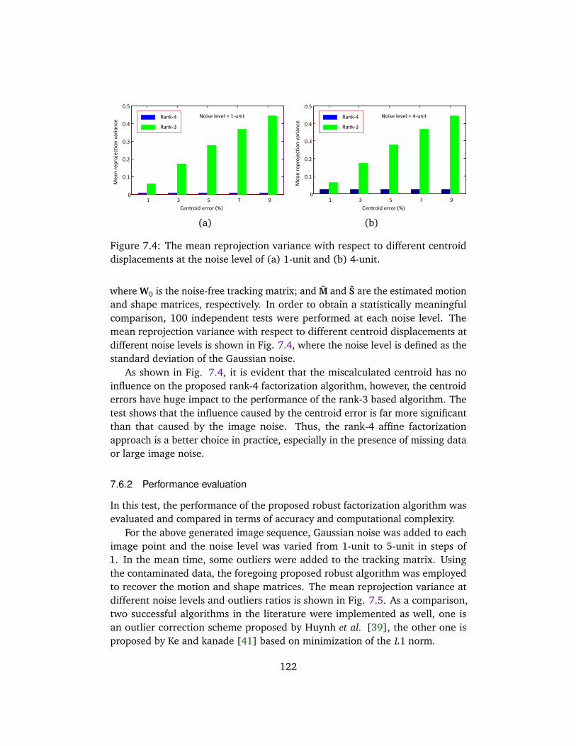
- . / 0 1

2

23-

234

23.

235

23/

67#895

67#89.

:&';")<"="<)>)59?#'$

!"#$%&'()"%%&%)*+,

!"#$%&"'&()"*+,($%-#&,#$*"

- . / 0 1

2

23-

234

23.

235

23/

67#895

67#89.

:&';")<"="<)>)-9?#'$

(a) (b)

Figure 7.4: The mean reprojection variance with respect to different centroiddisplacements at the noise level of (a) 1-unit and (b) 4-unit.

where W0 is the noise-free tracking matrix; and M and S are the estimated motionand shape matrices, respectively. In order to obtain a statistically meaningfulcomparison, 100 independent tests were performed at each noise level. Themean reprojection variance with respect to different centroid displacements atdifferent noise levels is shown in Fig. 7.4, where the noise level is defined as thestandard deviation of the Gaussian noise.

As shown in Fig. 7.4, it is evident that the miscalculated centroid has noinfluence on the proposed rank-4 factorization algorithm, however, the centroiderrors have huge impact to the performance of the rank-3 based algorithm. Thetest shows that the influence caused by the centroid error is far more significantthan that caused by the image noise. Thus, the rank-4 affine factorizationapproach is a better choice in practice, especially in the presence of missing dataor large image noise.

7.6.2 Performance evaluation

In this test, the performance of the proposed robust factorization algorithm wasevaluated and compared in terms of accuracy and computational complexity.

For the above generated image sequence, Gaussian noise was added to eachimage point and the noise level was varied from 1-unit to 5-unit in steps of1. In the mean time, some outliers were added to the tracking matrix. Usingthe contaminated data, the foregoing proposed robust algorithm was employedto recover the motion and shape matrices. The mean reprojection variance atdifferent noise levels and outliers ratios is shown in Fig. 7.5. As a comparison,two successful algorithms in the literature were implemented as well, one isan outlier correction scheme proposed by Huynh et al. [39], the other one isproposed by Ke and kanade [41] based on minimization of the L1 norm.

122

!"#$%&$'$&%()*+,-

!"#$%&"'&()"*+,($%-#&,#$*"

!"#$%&$'$&%()*+,-

!"#$%&"'&()"*+,($%-#&,#$*"

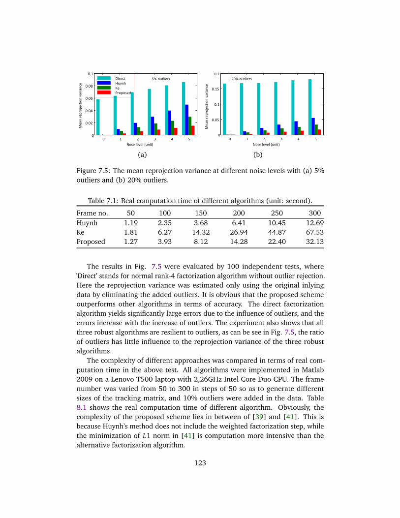
. / 0 1 2 3

.

.4.3

.4/

.4/3

.40

. / 0 1 2 3

.

.4.0

.4.2

.4.5

.4.6

.4/

7+8$9,

:);*<

=$

>8"?"#$@

3A%"),&+$8# 0.A%"),&+$8#

(a) (b)

Figure 7.5: The mean reprojection variance at different noise levels with (a) 5%outliers and (b) 20% outliers.

Table 7.1: Real computation time of different algorithms (unit: second).

Frame no. 50 100 150 200 250 300Huynh 1.19 2.35 3.68 6.41 10.45 12.69Ke 1.81 6.27 14.32 26.94 44.87 67.53Proposed 1.27 3.93 8.12 14.28 22.40 32.13

The results in Fig. 7.5 were evaluated by 100 independent tests, where’Direct’ stands for normal rank-4 factorization algorithm without outlier rejection.Here the reprojection variance was estimated only using the original inlyingdata by eliminating the added outliers. It is obvious that the proposed schemeoutperforms other algorithms in terms of accuracy. The direct factorizationalgorithm yields significantly large errors due to the influence of outliers, and theerrors increase with the increase of outliers. The experiment also shows that allthree robust algorithms are resilient to outliers, as can be see in Fig. 7.5, the ratioof outliers has little influence to the reprojection variance of the three robustalgorithms.

The complexity of different approaches was compared in terms of real com-putation time in the above test. All algorithms were implemented in Matlab2009 on a Lenovo T500 laptop with 2,26GHz Intel Core Duo CPU. The framenumber was varied from 50 to 300 in steps of 50 so as to generate differentsizes of the tracking matrix, and 10% outliers were added in the data. Table8.1 shows the real computation time of different algorithm. Obviously, thecomplexity of the proposed scheme lies in between of [39] and [41]. This isbecause Huynh’s method does not include the weighted factorization step, whilethe minimization of L1 norm in [41] is computation more intensive than thealternative factorization algorithm.

123

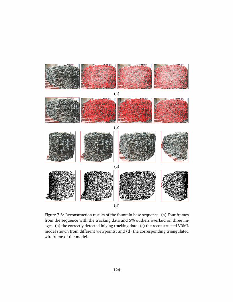
(a)

(b)

(c)

(d)

Figure 7.6: Reconstruction results of the fountain base sequence. (a) Four framesfrom the sequence with the tracking data and 5% outliers overlaid on three im-ages; (b) the correctly detected inlying tracking data; (c) the reconstructed VRMLmodel shown from different viewpoints; and (d) the corresponding triangulatedwireframe of the model.

124

!"#$ !"#"% " "#"% "#$

"

"#%

$

$#%

&

'($"

)

*+,-./+012.3(-+4256784

!"#$%&$'()*+

!) !& " & )

"

&

)

9

'($"

)

*+,-./+012.3(-+4256784

!"#$%&$'()*+

:;-+4;;.85 :;-+4;;.85

(a) (b)

Figure 7.7: The histogram distribution of the residual matrix of the fountain basesequence before (a) and after (b) outlier rejection.


The method was tested on many real image sequences. The results on two datasets are reported here. The resolution of each image is 1024× 768, and thefeature correspondences are established by the feature tracking system based onSIFT and epipolar constraints [80].

The first test is on a fountain base sequence captured at downtown SanFrancisco. The sequence consists of 10 images and 5648 features were trackedacross the sequence. Since the images have a large portion of homogeneous andrepetitive textures, it is thus hard to track accurately for this type of scene, butvisually only a few features were obviously mismatched. In order to test thealgorithm, an additional 5% outliers were added to the tracking data, as shownin Figure 7.6 (a). After rejecting the outliers by the proposed approach, theremaining inlying features with disparities to the first image are shown in Figure7.6 (b), the outliers were successfully rejected. Then, the alternative weightedalgorithm was employed to recover the motion and structure matrices. Finally,the solution was upgraded to the Euclidean space. As shown in Figure 7.6 (c)and (d), the structure looks realistic and most details are correctly recovered.

The histogram distribution of the reprojection residual matrix with outliers isshown in Figure 7.7 (a). The residuals are largely conform to the assumptionof normal distribution. It can be seen from the distribution that the outliers canbe obviously distinguished from inliers, the computed threshold is shown in thefigure. The histogram distribution of the residuals of the detected inlying data isshown in Figure 7.7 (b). Obviously, the residual error was reduced significantlyafter rejecting the outliers. The final reprojection error is 0.426, as a comparison,the reprojection errors by the algorithms of ’Huynh’ and ’Ke’ are 0.736 and 0.597,

125

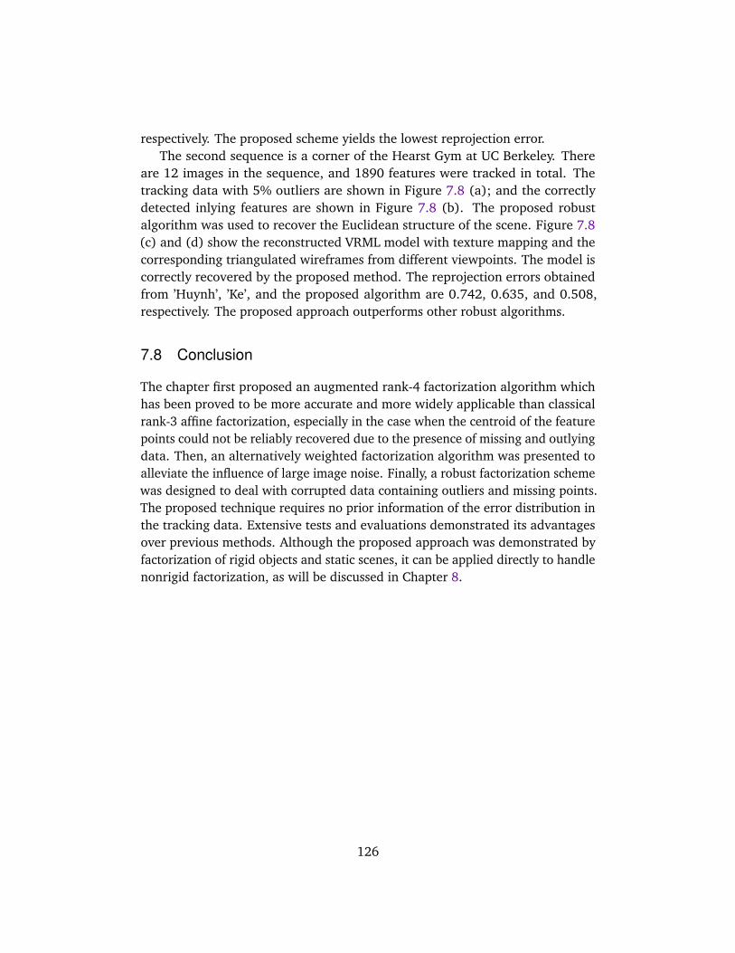
respectively. The proposed scheme yields the lowest reprojection error.The second sequence is a corner of the Hearst Gym at UC Berkeley. There

are 12 images in the sequence, and 1890 features were tracked in total. Thetracking data with 5% outliers are shown in Figure 7.8 (a); and the correctlydetected inlying features are shown in Figure 7.8 (b). The proposed robustalgorithm was used to recover the Euclidean structure of the scene. Figure 7.8(c) and (d) show the reconstructed VRML model with texture mapping and thecorresponding triangulated wireframes from different viewpoints. The model iscorrectly recovered by the proposed method. The reprojection errors obtainedfrom ’Huynh’, ’Ke’, and the proposed algorithm are 0.742, 0.635, and 0.508,respectively. The proposed approach outperforms other robust algorithms.

7.8 Conclusion

The chapter first proposed an augmented rank-4 factorization algorithm whichhas been proved to be more accurate and more widely applicable than classicalrank-3 affine factorization, especially in the case when the centroid of the featurepoints could not be reliably recovered due to the presence of missing and outlyingdata. Then, an alternatively weighted factorization algorithm was presented toalleviate the influence of large image noise. Finally, a robust factorization schemewas designed to deal with corrupted data containing outliers and missing points.The proposed technique requires no prior information of the error distribution inthe tracking data. Extensive tests and evaluations demonstrated its advantagesover previous methods. Although the proposed approach was demonstrated byfactorization of rigid objects and static scenes, it can be applied directly to handlenonrigid factorization, as will be discussed in Chapter 8.

126

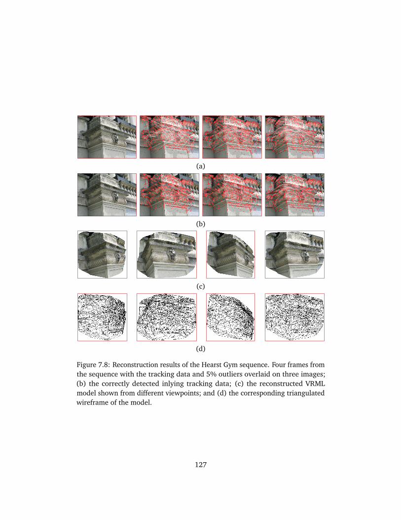
(a)

(b)

(c)

(d)

Figure 7.8: Reconstruction results of the Hearst Gym sequence. Four frames fromthe sequence with the tracking data and 5% outliers overlaid on three images;(b) the correctly detected inlying tracking data; (c) the reconstructed VRMLmodel shown from different viewpoints; and (d) the corresponding triangulatedwireframe of the model.

127

Chapter 8

Robust SfM of Nonrigid Objects

This chapter is an extension of the robust algorithm of Chapter 7 to nonrigidscenarios, and it is presented in a similar style. An augmented nonrigid factoriza-tion algorithm is first proposed to circumvent the difficulty of image alignmentfor imperfect data, followed by a robust scheme to handle outlying and missingdata in nonrigid structure and motion recovery. The contributions of this chapterare as follows: (i) as a new addition to previous nonrigid structure from motion,the proposed factorization algorithm can perfectly handle imperfect trackingdata; (ii) it is demonstrated that the outliers can be detected directly from imagereprojection residuals of nonrigid factorization; and (iii) the robust factoriza-tion scheme is proved empirically to be more efficient and more accurate thanother robust algorithms. The proposed approach is validated and evaluated byextensive experiments on synthetic data and real image sequences.

8.1 Introduction

The factorization algorithm was extended to nonrigid SfM by assuming that the3D shape of a nonrigid object can be modeled as a weighted linear combinationof a set of shape bases [11]. Thus, the shape bases and camera motions arefactorized simultaneously for all time instants under a rank-3k constraint of thetracking matrix. The method has been extensively investigated and developed in[9], [75], and [66].

In recent years, the problem of robust factorization has received a lot ofattention [50] [103] [100]. Aguitar and Moura [3] proposed a scalar-weightedSVD algorithm that minimizes the weighted square errors. Gruber and Weiss[29] formulated the problem as a factor analysis and derived an ExpectationMaximization (EM) algorithm to enhance the robustness to missing data and

129

uncertainties. Huynh et al. [39] proposed an iterative approach to correct the out-liers with ’pseudo’ observations. Ke and Kanade [41] designed a robust algorithmto handle outliers by minimizing a L1-norm of the reprojection errors. Wanget al. [89] proposed a spatial-and-temporal-weighted factorization approach tohandle significant noise in the measurement. The problem is further studied anddifferent robust algorithms have been proposed [23] [55] [99] [92] [60].

Most of the above robust algorithms are initially designed for SfM of rigidobjects. To the best of our knowledge, few studies have been carried out fornonrigid scenarios. In this chapter, we will extend the robust factorizationapproach of Chapter 7 to the nonrigid scenarios.

This chapter first proposes an augmented rank-(3k+1) factorization algorithmto circumvent the difficulty of image registration for imperfect data, followed byan alternative weighted factorization algorithm to handle the missing features andimage uncertainty. Then, the outlying data are detected from a new viewpoint viaimage reprojection residuals by exploring the fact that the reprojection residualsare largely proportional to the measurement errors. Finally, a robust factorizationscheme is proposed to deal with outliers. A preliminary work on this researchwas published at the CRV conference [90].

8.2 Background of Nonrigid Factorization

Under the affine projection model, a 3D point X j is projected onto xi j in frame iaccording to the imaging equation

xi j = AiX j + ci (8.1)

where Ai is a 2×3 affine projection matrix; and the translation term ci is the imageof the centroid of all space points. Let Si = [Xi1, · · · , Xin] be the 3D structureassociated with frame i, the structure may be different at different instants. Innonrigid SfM, we usually follow Bregler’s assumption that Si =

∑kl=1ωilBl , where

the nonrigid structure is assumed to be a linear combination of a set of rigidshape bases Bl [11]. Under this assumption, the imaging process of one imagecan be modeled as

Wi = [xi1, · · · , xin] = AiSi + [ci , · · · ,ci]

=

ωi1Ai , · · · ,ωikAi

B1

...Bk

+ [ci , · · · ,ci].

It is easy to verify that if all image points in each frame are registered tothe centroid and relative image coordinates are employed, the translation term

130

vanishes, i.e., ci = 0. Consequently, the nonrigid factorization under affinecamera model is expressed as

x11 ··· x1n

......

...xm1 ··· xmn

︸︷︷︸

W2m×n

=

ω11A1 ··· ω1kA1

......

...ωm1Am ··· ωmkAm

︸︷︷︸

M2m×3k

B1

...Bk

︸︷︷︸

B3k×n

. (8.2)

Structure from motion is an ill-posed problem. Suppose the tracking matrixW is available, our purpose is to recover the camera motion parameters and the3D structure from the shape matrix. It is obvious from (8.2) that the rank of thetracking matrix W is at most 3k. Previous studies on nonrigid SfM are based onthe rank-3k constraint due to its simplicity, and the factorization can be easilyobtained via SVD decomposition by truncating its rank to 3k.

8.3 Augmented Affine Factorization

One critical condition for Equation (8.2) is that all image measurements areregistered to the corresponding centroid of each frame. When the tracking matrixcontains outliers and/or missing data, it is impossible to reliably retrieve thecentroid. As will be shown in the experiments, the miscalculation of the centroidswill cause significant errors to the final solutions. Previous studies were eitherignoring this problem or hallucinating the missing points with pseudo observa-tions, which may lead to a biased estimation. In this section, an augmented affinefactorization algorithm based on rank-(3k+ 1) constraint is proposed to solvethis problem.

8.3.1 Rank-(3k+ 1) affine factorization

Let us formulate the affine imaging process (8.1) in the following form

xi j =

Ai|ci

X j (8.3)

where X j = [XTj , t j]T is a 4-dimensional homogeneous expression of X j. Then,

the imaging process of frame i can be written as

Wi = [xi1, · · · , xin] =

Ai|ci

∑k

l=1ωilBl

tTi

=

ωi1Ai , · · · ,ωikAi ,ci

B1

...BktTi

.

131

Thus, the structure and motion factorization for the entire sequence is formu-lated as follows.

x11 ··· x1n

......

...xm1 ··· xmn

︸︷︷︸

W2m×n

=

ω11A1 ··· ω1kA1 c1

......

......

ωm1Am ··· ωmkAm cm

︸︷︷︸

M2m×(3k+1)

B1

...BktTi

︸︷︷︸

B(3k+1)×n

. (8.4)

Obviously, the rank of the tracking matrix becomes 3k+ 1 in this case. Giventhe tracking matrix, the factorization can be easily obtained via SVD decompo-sition with rank-(3k+ 1) constraint. Unlike the affine factorization (8.2), theaugmented expression (8.4) does not require any image registration. Thus, it canwork with outlying and missing data.

Both factorization algorithms (8.2) and (8.4) can be equivalently denoted asthe following minimization scheme.

f (M,S) = argminM,S

‖W−MS‖2F . (8.5)

By enforcing different rank constraints, the Frobenius norm of (8.5) corre-sponding to the algorithms (8.2) and (8.4) would be

E3k =N∑

i=3k+1

σ2i , E3k+1 =

N∑

i=3k+2

σ2i (8.6)

where σi , i = 1, · · · , N are singular values of the tracking matrix in descendingorder, and N =min(2m, n). Clearly, the error difference by the two algorithm isσ2

3k+1. For noise free data, if all image points are registered to the centroid, then,σi = 0,∀i > 3k, the equations (8.2) and (8.4) are actually equivalent. However,in the presence of outlying and missing data, the image centroid could not beaccurately recovered, the rank-3k algorithm (8.2) will yield a big error sinceσ3k+1 does not approach to zero in this situation.


Suppose W = MB is a set of factorization result of (8.4). Obviously, the de-composition is not unique since it is only defined up to a nonsingular linearH ∈ R(3k+1)×(3k+1) as M = MH and S = H−1S. The recovery of the upgradingmatrix is different with that in the rank-3k factorization.

Let us write the (3k+ 1)× (3k+ 1) upgrading matrix in the following form.

H= [H1, · · · ,Hk|h3k+1] (8.7)

132

where Hl ∈ R(3k+1)×3(l = 1, · · · , k) denotes the l-th triple columns of H, and h3k+1

denotes the last column of H. Suppose Mi is the i-th two-row submatrix of M,then the upgraded motion matrix can be written as

Mi = MiH= [MiH1, · · · , MiHk|Mih3k+1]. (8.8)

Comparing the above equation with (8.4), we have

MiHl =ωilAi =ωil fi

rTi1

rTi2

(8.9)

where fi is the focal length of the camera, rTi1 and rT

i2 are the first two rows of therotation matrix. Denote Ql = HlH

Tl , then, Ql can be constrained from (8.9) as

MiQlMTi =

MiHl

MiHlT =ω2

il f 2i

1 00 1

. (8.10)

The matrix Ql has 9k degree-of-freedom since it is a (3k+1)×(3k+1) positivesemidefinite symmetric matrix defined up to a scale. The above equation providestwo constraints to Ql , thus, it can be linearly solved via least squares by stackingthe constraints (8.10) frame by frame. Furthermore, the submatrix Hl can bedecomposed from Ql via extended Cholesky decomposition [86].

From equations (8.4) and (8.8), it is easy to prove that the last column of theupgrading matrix h3k+1 only influences the translation from the world coordinatesystem to the image system. Under a given coordinate system, different values ofh3k+1 will only alter the origin of the world system, however, it does not changethe Euclidean structure of the reconstructed points. Therefore, h3k+1 can be setfreely as any (3k+ 1)-dimensional vector that is independent of the columns ofHl , l = 1, · · · , k such that the resulted upgrading matrix is nonsingular.

After recovering the Euclidean upgrading matrix, the camera parameters,motions, shape bases, and deformation weights can be easily decomposed fromthe upgraded motion matrix MH and shape matrix H−1B.

8.3.3 Alternative factorization with missing data

SVD decomposition could not directly work with missing data. If some featuresare missing in the tracking data, we can adopt a similar alternative factorizationalgorithm as in Chapter 7. The basic idea is to minimize the cost function (8.5)over S and M alternatively until convergence, while leaving the other one fixedat each step, i.e.,

f (S) = argminS‖W−MS‖2F (8.11)

133

f (M) = argminM‖W−MS‖2F . (8.12)

As discussed in Chapter 7, each cost function of the algorithm is indeed aconvex function thus a global minimum can be found. The algorithm convergesvery fast if the tracking matrix is close to rank-(3k + 1) even with a randominitialization.

In the alternative factorization, the minimization process of each cost functionis carried out by least squares. Thus, in case of missing elements, one can simplyeliminate those entries in the equation and still obtain a least-square solution ofthe motion and structure matrices.

8.3.4 Alternative weighted factorization

When the uncertainty of image measurement is available, a weighted factorizationstrategy can be adopted to alleviate the influence of unreliable features. Theweighted factorization is formulated as follows.

f (M,S) = argminM,S

‖Σ⊗ (W−MS)‖2F (8.13)

where ′⊗′ denotes the Hadamard product of element-by-element multiplication;and Σ = σi j is the weight matrix whose entries are derived from the confidenceof the image measurements. Similar to Chapter 7, the solution of (8.13) isobtained using the alternative factorization algorithm.

f (S) = argmins j

Σ j ⊗ (w j −Ms j)

2F (8.14)

f (M) = argminmT

i

ΣTi ⊗ (w

Ti −mT

i S)

2F (8.15)

where Σ j and ΣTi denote the j-th column and i-th row of Σ, respectively. The al-

gorithm alternatively updates the shape and motion matrices using least squaresuntil convenience. In case of missing data, one can simply delete the correspond-ing elements in the equations.

8.4 Outlier Detection and Robust Factorization

Based on the foregoing proposed factorization algorithm, a fast and practicalscheme for outlier detection is discussed in this section.

134

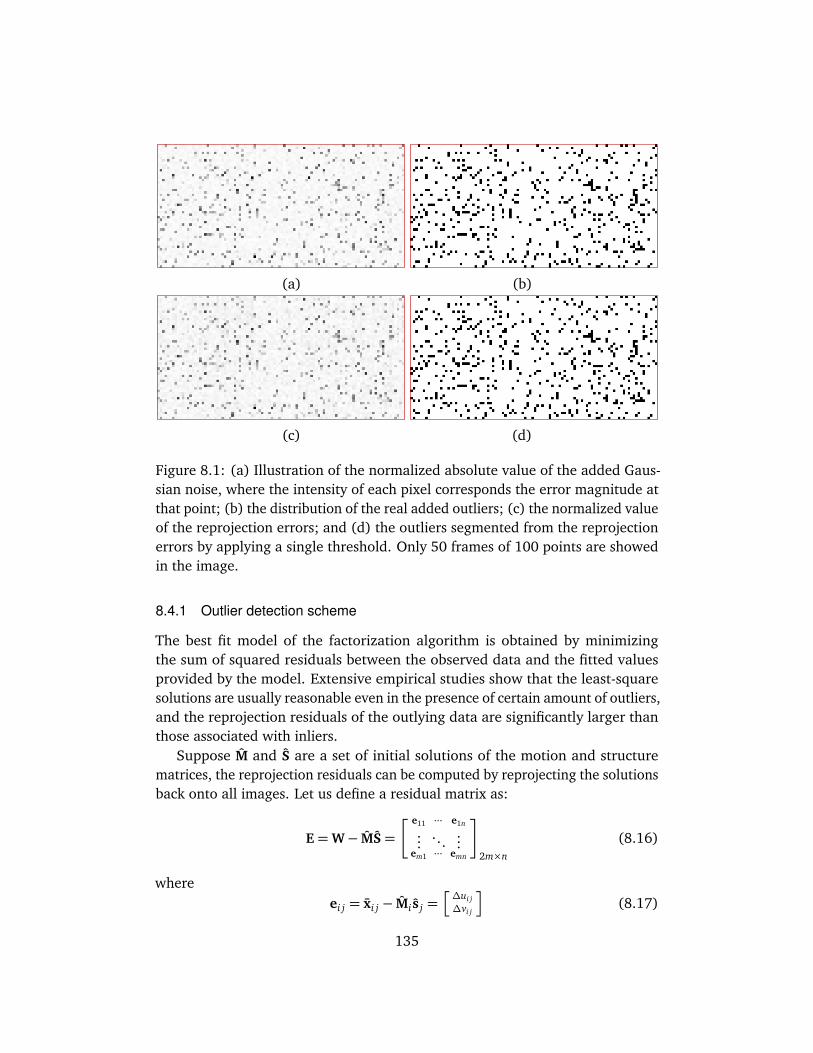
(a) (b)

(c) (d)

Figure 8.1: (a) Illustration of the normalized absolute value of the added Gaus-sian noise, where the intensity of each pixel corresponds the error magnitude atthat point; (b) the distribution of the real added outliers; (c) the normalized valueof the reprojection errors; and (d) the outliers segmented from the reprojectionerrors by applying a single threshold. Only 50 frames of 100 points are showedin the image.

8.4.1 Outlier detection scheme

The best fit model of the factorization algorithm is obtained by minimizingthe sum of squared residuals between the observed data and the fitted valuesprovided by the model. Extensive empirical studies show that the least-squaresolutions are usually reasonable even in the presence of certain amount of outliers,and the reprojection residuals of the outlying data are significantly larger thanthose associated with inliers.

Suppose M and S are a set of initial solutions of the motion and structurematrices, the reprojection residuals can be computed by reprojecting the solutionsback onto all images. Let us define a residual matrix as:

E=W− MS=

e11 ··· e1n

......

...em1 ··· emn

2m×n

(8.16)

whereei j = xi j − Mi s j =

h

∆ui j∆vi j

i

(8.17)

135

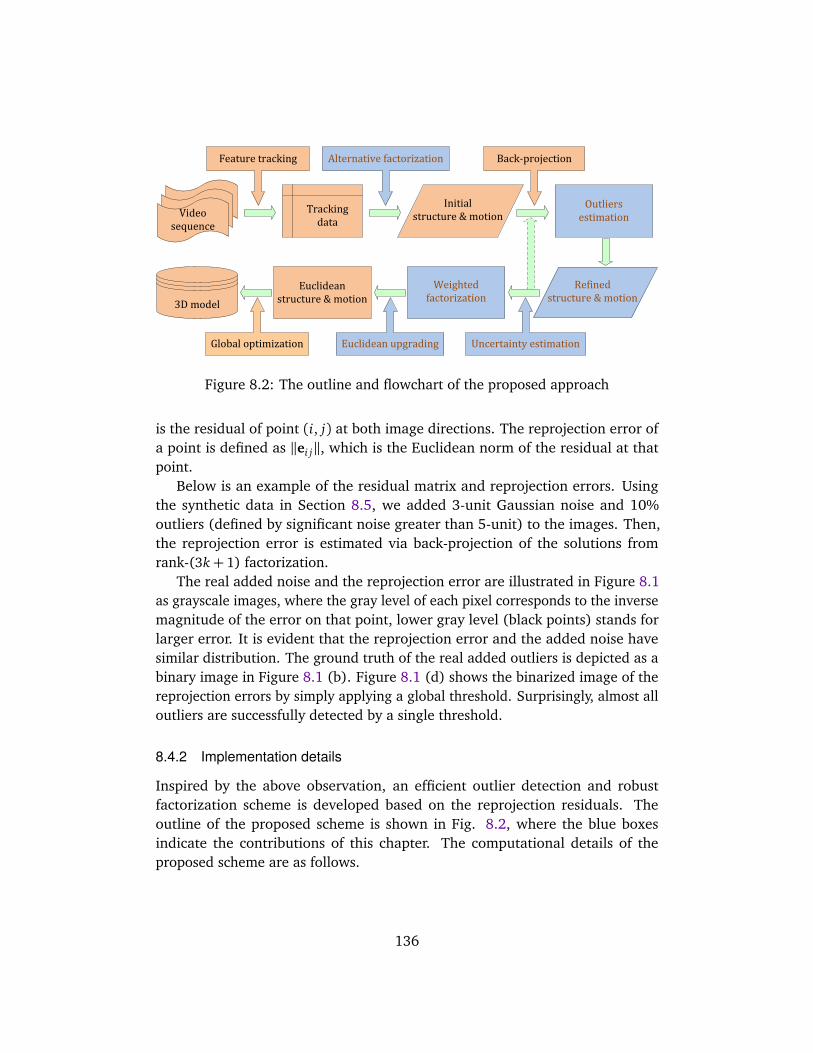
Videosequence

Trackingdata

3Dmodel

Featuretracking

Globaloptimization

Initialstructure&motion

Refinedstructure&motion

UncertaintyestimationEuclideanupgrading

Alternativefactorization Back-projection

Outliersestimation

Euclideanstructure&motion

Weightedfactorization

Figure 8.2: The outline and flowchart of the proposed approach

is the residual of point (i, j) at both image directions. The reprojection error ofa point is defined as ‖ei j‖, which is the Euclidean norm of the residual at thatpoint.

Below is an example of the residual matrix and reprojection errors. Usingthe synthetic data in Section 8.5, we added 3-unit Gaussian noise and 10%outliers (defined by significant noise greater than 5-unit) to the images. Then,the reprojection error is estimated via back-projection of the solutions fromrank-(3k+ 1) factorization.

The real added noise and the reprojection error are illustrated in Figure 8.1as grayscale images, where the gray level of each pixel corresponds to the inversemagnitude of the error on that point, lower gray level (black points) stands forlarger error. It is evident that the reprojection error and the added noise havesimilar distribution. The ground truth of the real added outliers is depicted as abinary image in Figure 8.1 (b). Figure 8.1 (d) shows the binarized image of thereprojection errors by simply applying a global threshold. Surprisingly, almost alloutliers are successfully detected by a single threshold.

8.4.2 Implementation details

Inspired by the above observation, an efficient outlier detection and robustfactorization scheme is developed based on the reprojection residuals. Theoutline of the proposed scheme is shown in Fig. 8.2, where the blue boxesindicate the contributions of this chapter. The computational details of theproposed scheme are as follows.

136

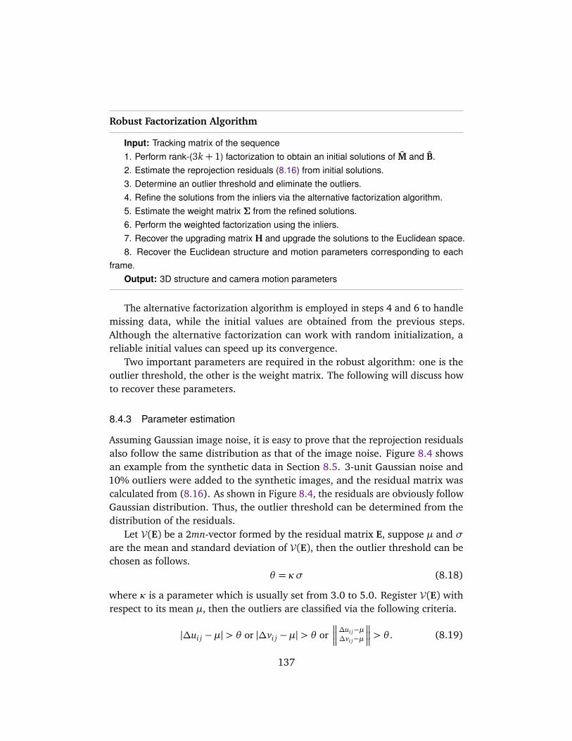
Robust Factorization Algorithm

Input: Tracking matrix of the sequence1. Perform rank-(3k+ 1) factorization to obtain an initial solutions of M and B.2. Estimate the reprojection residuals (8.16) from initial solutions.3. Determine an outlier threshold and eliminate the outliers.4. Refine the solutions from the inliers via the alternative factorization algorithm.5. Estimate the weight matrix Σ from the refined solutions.6. Perform the weighted factorization using the inliers.7. Recover the upgrading matrix H and upgrade the solutions to the Euclidean space.8. Recover the Euclidean structure and motion parameters corresponding to each

frame.Output: 3D structure and camera motion parameters

The alternative factorization algorithm is employed in steps 4 and 6 to handlemissing data, while the initial values are obtained from the previous steps.Although the alternative factorization can work with random initialization, areliable initial values can speed up its convergence.

Two important parameters are required in the robust algorithm: one is theoutlier threshold, the other is the weight matrix. The following will discuss howto recover these parameters.

8.4.3 Parameter estimation

Assuming Gaussian image noise, it is easy to prove that the reprojection residualsalso follow the same distribution as that of the image noise. Figure 8.4 showsan example from the synthetic data in Section 8.5. 3-unit Gaussian noise and10% outliers were added to the synthetic images, and the residual matrix wascalculated from (8.16). As shown in Figure 8.4, the residuals are obviously followGaussian distribution. Thus, the outlier threshold can be determined from thedistribution of the residuals.

Let V(E) be a 2mn-vector formed by the residual matrix E, suppose µ and σare the mean and standard deviation of V(E), then the outlier threshold can bechosen as follows.

θ = κσ (8.18)

where κ is a parameter which is usually set from 3.0 to 5.0. Register V(E) withrespect to its mean µ, then the outliers are classified via the following criteria.

|∆ui j −µ|> θ or |∆vi j −µ|> θ or

∆ui j−µ∆vi j−µ

> θ . (8.19)

137

-50 0 500

2000

4000

6000

8000

10000

12000

Outliers

Noise and outliers Inliers

Outliers

(a)

-50 0 500

2000

4000

6000

8000

10000

Mean

Threshhold Threshhold

Reprojection residuals

(b)

Figure 8.3: (a) Histogram distribution of the real added noise and outliers; (b)histogram distribution of the reprojection residuals.

Since the outliers have heavily influence to the estimation of the mean andstandard deviation due to their large deviations, the mean is practically estimatedfrom the data that are less than the median value of |V(E)|.

µ=meanV ′(E)|V ′(E)<median(|V(E)|) (8.20)

while the standard deviation is estimated from the median absolute deviation(MAD)

σ = 1.4826 median(|V(E)−median(V(E))|). (8.21)

The above computation is resistant to outliers and thus guarantees a robustestimation of the mean and standard deviation of the residuals.

The weight matrix is determined from the uncertainty of each feature basedon the information such as sharpness and intensity contrast around its neigh-borhood [3][74]. The uncertainty is usually estimated during the process offeature detection and tracking or given as prior information. Nonetheless, thisinformation is unavailable in many applications. In our early study [89], it was

138

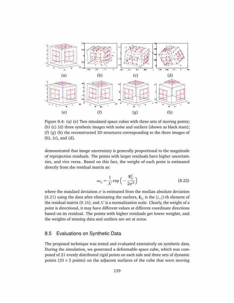
-400 -300 -200 -100 0

-200

-100

0

100

-300 -200 -100 0 100

0

100

200

300

400

-300 -200 -100 0-200

-100

0

100

200

-100

10

-10

0

10

-10

-5

0

5

10

(a) (b) (c) (d)

-100

10

-50

510

-10

-5

0

5

10

15

-100

10

-10

0

10

-10

-5

0

5

10

-10

0

10

-10

0

10

-10

0

10

-10

0

10

-10

0

10

-10

0

10

(e) (f) (g) (h)

Figure 8.4: (a) (e) Two simulated space cubes with three sets of moving points;(b) (c) (d) three synthetic images with noise and outliers (shown as black stars);(f) (g) (h) the reconstructed 3D structures corresponding to the three images of(b), (c), and (d).

demonstrated that image uncertainty is generally proportional to the magnitudeof reprojection residuals. The points with larger residuals have higher uncertain-ties, and vice versa. Based on this fact, the weight of each point is estimateddirectly from the residual matrix as:

ωi j =1

N exp

−E2

i j

2σ2

(8.22)

where the standard deviation σ is estimated from the median absolute deviation(8.21) using the data after eliminating the outliers, Ei j is the (i, j)-th element ofthe residual matrix (8.16), andN is a normalization scale. Clearly, the weight of apoint is directional, it may have different values at different coordinate directionsbased on its residual. The points with higher residuals get lower weights, andthe weights of missing data and outliers are set at zeros.


The proposed technique was tested and evaluated extensively on synthetic data.During the simulation, we generated a deformable space cube, which was com-posed of 21 evenly distributed rigid points on each side and three sets of dynamicpoints (33× 3 points) on the adjacent surfaces of the cube that were moving

139

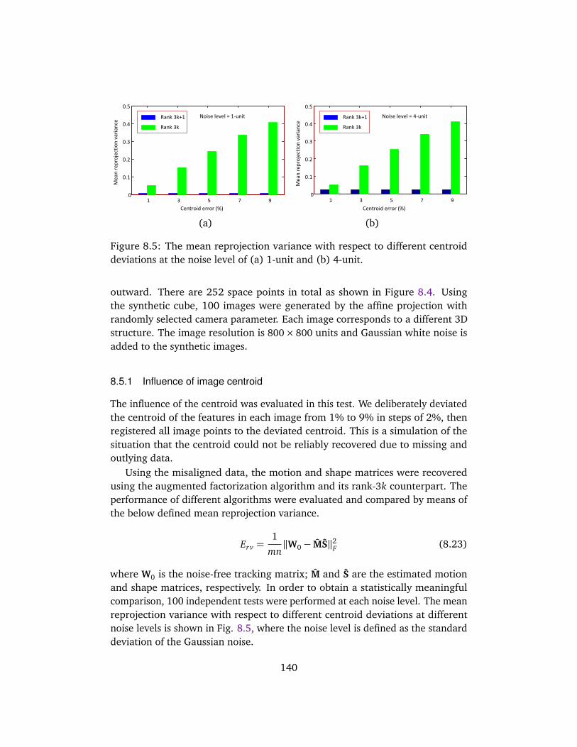
Centroid error (%)

Me

an

re

pro

jecti

on

va

ria

nce

1 3 5 7 90

0.1

0.2

0.3

0.4

0.5

Rank 3k+1

Rank 3k

Noise level = 4-unit

Centroid error (%)

Me

an

re

pro

jecti

on

va

ria

nce

1 3 5 7 90

0.1

0.2

0.3

0.4

0.5

Rank 3k+1

Rank 3k

Noise level = 1-unit

(a) (b)

Figure 8.5: The mean reprojection variance with respect to different centroiddeviations at the noise level of (a) 1-unit and (b) 4-unit.

outward. There are 252 space points in total as shown in Figure 8.4. Usingthe synthetic cube, 100 images were generated by the affine projection withrandomly selected camera parameter. Each image corresponds to a different 3Dstructure. The image resolution is 800× 800 units and Gaussian white noise isadded to the synthetic images.

8.5.1 Influence of image centroid

The influence of the centroid was evaluated in this test. We deliberately deviatedthe centroid of the features in each image from 1% to 9% in steps of 2%, thenregistered all image points to the deviated centroid. This is a simulation of thesituation that the centroid could not be reliably recovered due to missing andoutlying data.

Using the misaligned data, the motion and shape matrices were recoveredusing the augmented factorization algorithm and its rank-3k counterpart. Theperformance of different algorithms were evaluated and compared by means ofthe below defined mean reprojection variance.

Erv =1

mn‖W0− MS‖2F (8.23)

where W0 is the noise-free tracking matrix; M and S are the estimated motionand shape matrices, respectively. In order to obtain a statistically meaningfulcomparison, 100 independent tests were performed at each noise level. The meanreprojection variance with respect to different centroid deviations at differentnoise levels is shown in Fig. 8.5, where the noise level is defined as the standarddeviation of the Gaussian noise.

140

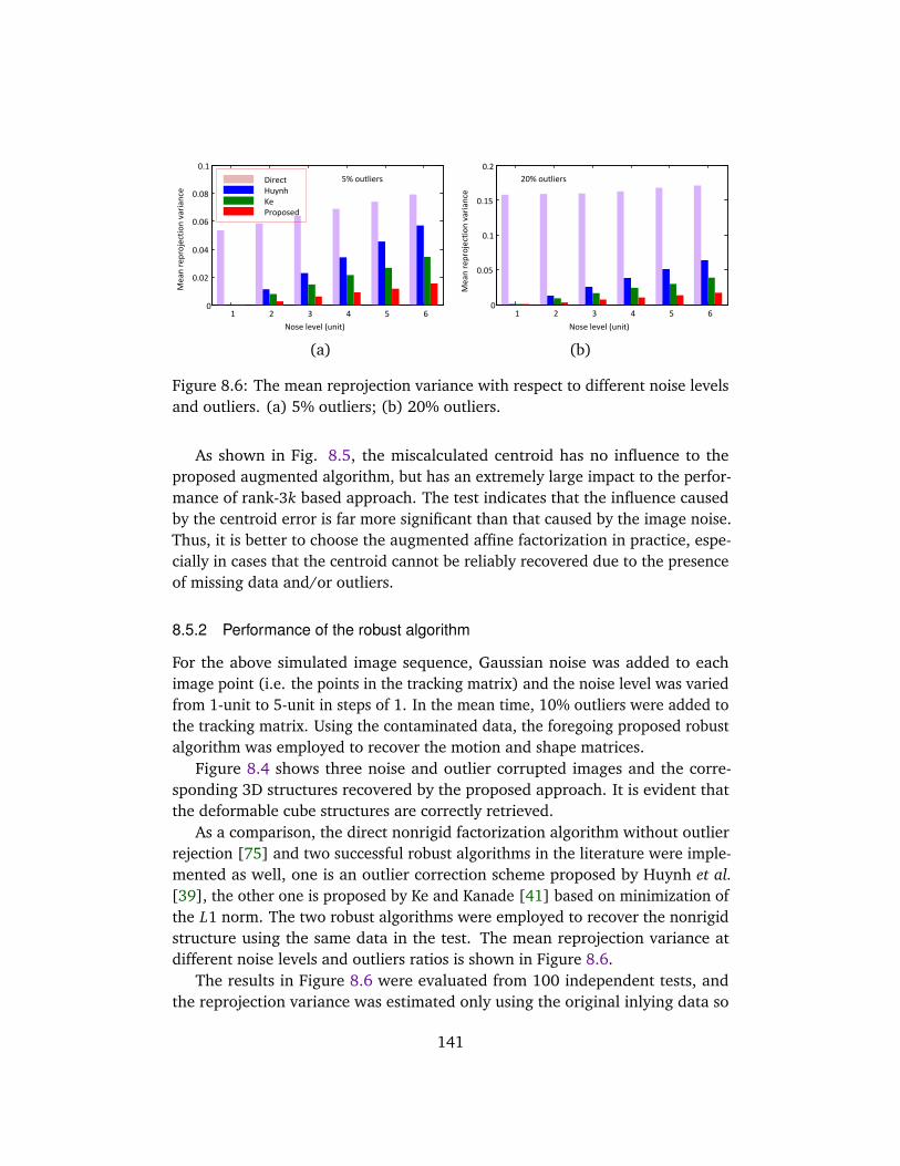
1 2 3 4 5 60

0.05

0.1

0.15

0.2

1 2 3 4 5 60

0.02

0.04

0.06

0.08

0.1

Nose level (unit)

Me

an

re

pro

jecti

on

va

ria

nce

Nose level (unit)

Me

an

re

pro

jecti

on

va

ria

nce

5% outliers 20% outliersDirect

Huynh

Ke

Proposed

(a) (b)

Figure 8.6: The mean reprojection variance with respect to different noise levelsand outliers. (a) 5% outliers; (b) 20% outliers.

As shown in Fig. 8.5, the miscalculated centroid has no influence to theproposed augmented algorithm, but has an extremely large impact to the perfor-mance of rank-3k based approach. The test indicates that the influence causedby the centroid error is far more significant than that caused by the image noise.Thus, it is better to choose the augmented affine factorization in practice, espe-cially in cases that the centroid cannot be reliably recovered due to the presenceof missing data and/or outliers.

8.5.2 Performance of the robust algorithm

For the above simulated image sequence, Gaussian noise was added to eachimage point (i.e. the points in the tracking matrix) and the noise level was variedfrom 1-unit to 5-unit in steps of 1. In the mean time, 10% outliers were added tothe tracking matrix. Using the contaminated data, the foregoing proposed robustalgorithm was employed to recover the motion and shape matrices.

Figure 8.4 shows three noise and outlier corrupted images and the corre-sponding 3D structures recovered by the proposed approach. It is evident thatthe deformable cube structures are correctly retrieved.

As a comparison, the direct nonrigid factorization algorithm without outlierrejection [75] and two successful robust algorithms in the literature were imple-mented as well, one is an outlier correction scheme proposed by Huynh et al.[39], the other one is proposed by Ke and Kanade [41] based on minimization ofthe L1 norm. The two robust algorithms were employed to recover the nonrigidstructure using the same data in the test. The mean reprojection variance atdifferent noise levels and outliers ratios is shown in Figure 8.6.

The results in Figure 8.6 were evaluated from 100 independent tests, andthe reprojection variance was estimated only using the original inlying data so

141

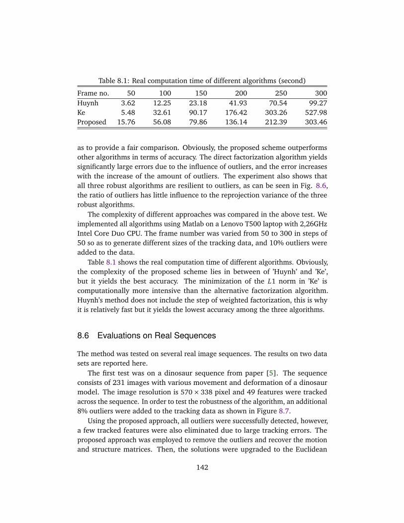
Table 8.1: Real computation time of different algorithms (second)

Frame no. 50 100 150 200 250 300Huynh 3.62 12.25 23.18 41.93 70.54 99.27Ke 5.48 32.61 90.17 176.42 303.26 527.98Proposed 15.76 56.08 79.86 136.14 212.39 303.46

as to provide a fair comparison. Obviously, the proposed scheme outperformsother algorithms in terms of accuracy. The direct factorization algorithm yieldssignificantly large errors due to the influence of outliers, and the error increaseswith the increase of the amount of outliers. The experiment also shows thatall three robust algorithms are resilient to outliers, as can be seen in Fig. 8.6,the ratio of outliers has little influence to the reprojection variance of the threerobust algorithms.

The complexity of different approaches was compared in the above test. Weimplemented all algorithms using Matlab on a Lenovo T500 laptop with 2,26GHzIntel Core Duo CPU. The frame number was varied from 50 to 300 in steps of50 so as to generate different sizes of the tracking data, and 10% outliers wereadded to the data.

Table 8.1 shows the real computation time of different algorithms. Obviously,the complexity of the proposed scheme lies in between of ’Huynh’ and ’Ke’,but it yields the best accuracy. The minimization of the L1 norm in ’Ke’ iscomputationally more intensive than the alternative factorization algorithm.Huynh’s method does not include the step of weighted factorization, this is whyit is relatively fast but it yields the lowest accuracy among the three algorithms.


The method was tested on several real image sequences. The results on two datasets are reported here.

The first test was on a dinosaur sequence from paper [5]. The sequenceconsists of 231 images with various movement and deformation of a dinosaurmodel. The image resolution is 570× 338 pixel and 49 features were trackedacross the sequence. In order to test the robustness of the algorithm, an additional8% outliers were added to the tracking data as shown in Figure 8.7.

Using the proposed approach, all outliers were successfully detected, however,a few tracked features were also eliminated due to large tracking errors. Theproposed approach was employed to remove the outliers and recover the motionand structure matrices. Then, the solutions were upgraded to the Euclidean

142

(a)

(b)

(c)

Figure 8.7: Test results of the dinosaur sequence. (a) Four frames from thesequence overlaid with the tracked features (red circles) and added outliers (bluestars); (b) the corresponding 3D VRML models from different viewpoints; and(c) the associated wireframes of the reconstructed models.

space. Figure 8.7 shows the reconstructed structure and wireframe at differentviewpoints. It can be seen from the results that the deformed structure has beencorrectly recovered from the corrupted data, and the reconstructed VRML modelis visually realistic.

The histogram distribution of the reprojection residual matrix (8.16) withoutliers is shown in Figure 8.8. The residuals largely conform to the assumption ofnormal distribution. As can be seen from the histogram, the outliers are obviouslydistinguished from inliers, the computed threshold is shown in the figure. Afterrejecting outliers, the histogram distribution of the residuals produced by thefinal solutions is also shown in Figure 8.8. Obviously, the residual error is reducedsignificantly by the proposed approach. The final mean reprojection error givenby the proposed approach is 0.597. In comparison, the reprojection errors by thealgorithms of ’Huynh’ and ’Ke’ are 0.926 and 0.733, respectively. The proposedscheme outperforms other approaches.

The second test was on a face sequence with different facial expressions. Thesequence was downloaded from FGnet, and 200 images from the sequence wereused in the test. The image resolution is 720×576 with 68 automatically trackedfeature points using the active appearance model (AAM). For test purpose, 8%

143

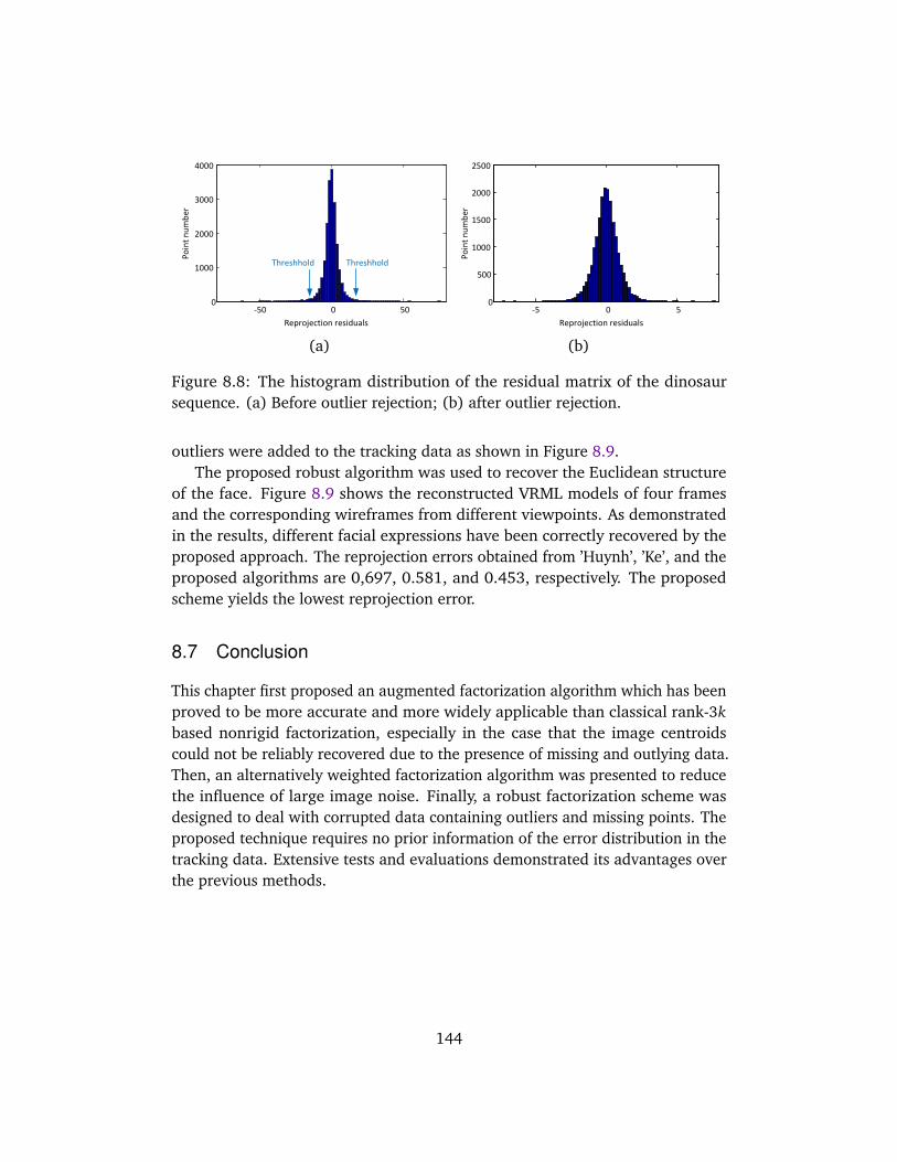
-5 0 50

500

1000

1500

2000

2500

-50 0 500

1000

2000

3000

4000


Po

int

nu

mb

er


Po

int

nu

mb

er

Threshhold Threshhold

(a) (b)

Figure 8.8: The histogram distribution of the residual matrix of the dinosaursequence. (a) Before outlier rejection; (b) after outlier rejection.

outliers were added to the tracking data as shown in Figure 8.9.The proposed robust algorithm was used to recover the Euclidean structure

of the face. Figure 8.9 shows the reconstructed VRML models of four framesand the corresponding wireframes from different viewpoints. As demonstratedin the results, different facial expressions have been correctly recovered by theproposed approach. The reprojection errors obtained from ’Huynh’, ’Ke’, and theproposed algorithms are 0,697, 0.581, and 0.453, respectively. The proposedscheme yields the lowest reprojection error.

8.7 Conclusion

This chapter first proposed an augmented factorization algorithm which has beenproved to be more accurate and more widely applicable than classical rank-3kbased nonrigid factorization, especially in the case that the image centroidscould not be reliably recovered due to the presence of missing and outlying data.Then, an alternatively weighted factorization algorithm was presented to reducethe influence of large image noise. Finally, a robust factorization scheme wasdesigned to deal with corrupted data containing outliers and missing points. Theproposed technique requires no prior information of the error distribution in thetracking data. Extensive tests and evaluations demonstrated its advantages overthe previous methods.

144

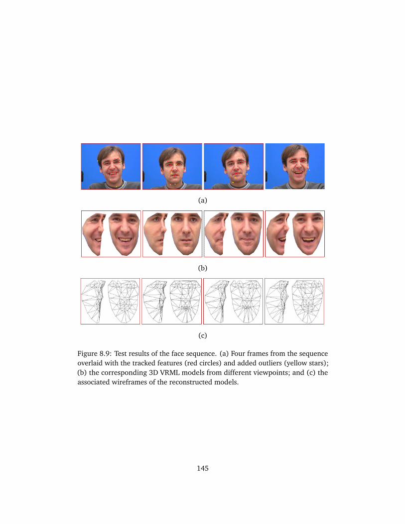
(a)

(b)

(c)

Figure 8.9: Test results of the face sequence. (a) Four frames from the sequenceoverlaid with the tracked features (red circles) and added outliers (yellow stars);(b) the corresponding 3D VRML models from different viewpoints; and (c) theassociated wireframes of the reconstructed models.

145

Chapter 9

Conclusion and Future Work

This thesis started with an introduction to the state-of-the-art techniques of struc-ture from motion and some challenges the field was facing. Then, we proposedseveral new algorithms to increase the accuracy, efficiency, and robustness of theprevious approaches. This chapter revisits the contributions and conclusion ofthe thesis, followed by a discussion of potential research topics for future study.

9.1 Contributions and Conclusion

This thesis focused on the accuracy and robustness for the problem of structurefrom motion. The major contributions and conclusion are as follows.

The first part of the thesis discussed the accuracy and efficiency of structurefrom motion. First, a quasi-perspective projection model was proposed in Chapter3 under the assumption that the camera was far away from the object with smalllateral rotations. As a trade-off for the simplified affine assumption and thecomplicated full perspective projection model, the quasi-perspective model filledthe gap between the two popular models. The proposed model was demonstratedtheoretically and experimentally to be more accurate than the affine model.

More special geometric properties of the model were investigated in Chapter4 in the context of one- and two-view geometry, including the quasi-fundamentalmatrix, plane induced homography, and quasi-perspective 3D reconstruction.Theoretical analysis and experimental study showed that the quasi-perspectivemodel was a good trade-off between the simplicity and the accuracy of previousprojection models.

Finally, the quasi-perspective model was applied to the problem of SfM, and astructure and motion factorization framework of both rigid and nonrigid objectswas presented in Chapter 5. The new framework avoided the difficulty of com-

147

puting projective depths under perspective factorization. It was computationallyefficient with better accuracy than affine approximation.

The proposed model is suitable for structure and motion factorization of ashort sequence with small camera motions. It should be noted that the smallrotation assumption of the proposed model is not a limiting factor and is usuallysatisfied in many real-world applications. For a long image sequence takenaround an object, we can simply divide the sequence into several subsequenceswith small movements, then register and merge the results of each subsequenceto reconstruct the structure of the entire scene.

The second part of the thesis focused on the robustness of SfM algorithms.First, a spatial-and-temporal-weighted factorization algorithm was proposed inChapter 6 to handle significant noise contained in the tracking data, where theuncertainty of image measurement was estimated directly from the reprojectionresiduals. Unlike other existing weighted factorization algorithms, the proposedtechnique didn’t require any prior information of the error distributions of thedata, and the errors could be easily modeled both spatially and temporally tocope with different measurement uncertainties.

In Chapter 7, an augmented rank-4 affine factorization algorithm was pro-posed to handle outlying and missing data in rigid SfM. As a new addition to theprevious affine factorization family, the new formulation is more accurate andmore widely applicable than classical rank-3 affine factorization, since it avoidsthe difficulty of image alignment for erroneous data. Based on the distribution ofreprojection residuals, a robust factorization scheme was designed to deal withcorrupted data with outliers.

The robust algorithm of Chapter 7 was further extended to nonrigid scenariosin Chapter 8. A new augmented nonrigid factorization algorithm was firstproposed to rout the difficulty in image alignment. Then, it was demonstratedthat the outliers could be detected directly from the image reprojection residualsof nonrigid factorization. Thus, a similar robust scheme as rigid factorization wasdesigned to handle outlying and missing data in nonrigid structure and motionrecovery. The proposed technique was demonstrated empirically to be moreefficient and more accurate than other robust algorithms.

The study in this thesis is not only academically significant, but also urgentlyneeded by automotive and robotic industries for autonomous navigation andenvironment modeling. The study provides a new perspective for accurate androbust modeling of both rigid and nonrigid objects.

It should be noted that the proposed robust algorithms are based on the affinecamera model. However, if the camera undergoes small lateral movements, wecan adopt the quasi-perspective model in these robust algorithms. As studied inChapter 5, the quasi-perspective model is more accurate than the affine model.

148

Thus, more accurate solutions are expected by assuming the quasi-perspectiveassumption.

9.2 Future Work

3D environment modeling and motion estimation using visual sensors are twomain functions of autonomous robots. As a central theme in computer vision,the problem of 3D structure and motion recovery from image sequences hasbeen widely studied during the past three decades and considerable progress hasbeen made in theory and applications. Unfortunately, the problem remains farfrom being solved. One critical challenge is how to recover the 3D structure ofdynamic natural scenes with rigid, nonrigid, articulated, and moving objects. Theproblem is very complex and has, thus, seldom been addressed in the literature.Some potential research topics in this field are as follows.

1. Structure and motion recovery of dynamic scenes

Previous study on structure from motion dealt only with simple objectsor scenes, however, a natural environment is more complex; it may becoupled with rigid, nonrigid, moving, and articulated objects. The 3Dreconstruction of such a dynamic environment is still an open problem incomputer vision. A possible approach is to solve this problem in trajectoryspace by introducing some constraint to the 3D trajectory of the scene.

2. Visual SLAM in dynamic environments

The SfM of dynamic scenes has many potential applications. One directapplication is the vision based simultaneous localization and mapping(SLAM) of mobile robots in dynamic environments. Another application is3D reconstruction in video surveillance; the 3D information is very helpfulfor objects recognition and event detection from a dynamic surveillancevideo. If the problem of dynamic modeling is solved, we can directly useall information in the video, including moving and nonrigid objects. Thus,a faster and more reliable result is expected.

3. Robust algorithm for structure from motion

Robustness is a well-known bottleneck of many computer vision applica-tions, because outliers and missing data are inevitable during the processof feature tracking. This thesis provides a partial solution to the problemby virtue of the reprojection residuals, however, the problem has not beencompletely solved, especially for 3D modeling of dynamic environments.More efforts have to be addressed to this research.

149

Bibliography

The numbers at the end of each entry list pages where the reference was cited.In the electronic version, they are clickable links to the pages.

[1] H. Aanæs, R. Fisker, K. Åström, and J. M. Carstensen. Robust factorization.IEEE Trans. Pattern Anal. Mach. Intell., 24(9):1215–1225, 2002. 12, 95

[2] A. K. Agrawal and R. Chellappa. Robust ego-motion estimation and 3-Dmodel refinement using surface parallax. IEEE Transactions on ImageProcessing, 15(5):1215–1225, 2006. 108

[3] P. M. Q. Aguiar and J. M. F. Moura. Rank 1 weighted factorization for3D structure recovery: Algorithms and performance analysis. IEEE Trans.Pattern Anal. Mach. Intell., 25(9):1134–1049, 2003. 12, 83, 85, 86, 95,108, 114, 119, 129, 138

[4] I. Akhter, Y. Sheikh, S. Khan, and T. Kanade. Nonrigid structure frommotion in trajectory space. In NIPS, pages 41–48, 2008. 24

[5] I. Akhter, Y. Sheikh, S. Khan, and T. Kanade. Trajectory space: A dualrepresentation for nonrigid structure from motion. IEEE Trans. PatternAnal. Mach. Intell., 33(7):1442–1456, 2011. 24, 25, 142

[6] J. Y. Aloimonos. Perspective approximation. Image and Vision Computing,8(3):177–192, 1990. 27

[7] P. Anandan and M. Irani. Factorization with uncertainty. InternationalJournal of Computer Vision, 49(2-3):101–116, 2002. 12, 83, 85, 86, 114,119

[8] B. Bascle and A. Blake. Separability of pose and expression in facial tracingand animation. In Proc. of the International Conference on Computer Vision,pages 323–328, 1998. 10

151

[9] M. Brand. Morphable 3D models from video. In Proc. of IEEE Conferenceon Computer Vision and Pattern Recognition, volume 2, pages 456–463,2001. 11, 19, 20, 21, 129

[10] M. Brand. A direct method for 3D factorization of nonrigid motion ob-served in 2D. In Proc. of IEEE Conference on Computer Vision and PatternRecognition (2), volume 2, pages 122–128, 2005. 11, 22, 62

[11] C. Bregler, A. Hertzmann, and H. Biermann. Recovering non-rigid 3Dshape from image streams. In Proc. of IEEE Conference on Computer Visionand Pattern Recognition, volume 2, pages 690–696, 2000. 10, 11, 17, 19,24, 62, 63, 129, 130

[12] A. M. Buchanan and A. W. Fitzgibbon. Damped newton algorithms formatrix factorization with missing data. In Proc. of IEEE Conference onComputer Vision and Pattern Recognition (2), pages 316–322, 2005. 12, 84

[13] C.-M. Cheng and S.-H. Lai. A consensus sampling technique for fast androbust model fitting. Pattern Recognition, 42(7):1318–1329, 2009. 42

[14] S. Choi, T. Kim, and W. Yu. Performance evaluation of ransac family. InBMVC, 2009. 11, 115

[15] S. Christy and R. Horaud. Euclidean shape and motion from multipleperspective views by affine iterations. IEEE Trans. Pattern Anal. Mach.Intell., 18(11):1098–1104, 1996. 9, 15, 27

[16] J. Costeira and T. Kanade. A multibody factorization method for indepen-dent moving objects. 29(3):159–179, September 1998. 10, 62

[17] D. J. Crandall, A. Owens, N. Snavely, and D. P. Huttenlocher. SfM withMRFs: Discrete-continuous optimization for large-scale structure frommotion. IEEE Trans. Pattern Anal. Mach. Intell., 35(12):2841–2853, 2013.1

[18] A. Del Bue, F. Smeraldi, and L. Agapito. Non-rigid structure from motionusing nonparametric tracking and non-linear optimization. In IEEE Work-shop in Articulated and Nonrigid Motion ANM04, held in conjunction withCVPR2004, pages 8–15, June 2004. 11

[19] A. Del Bue. Deformable 3-D modelling from uncalibrated video sequences.PhD Thesis, Queen Mary, University of London, 2007. 20, 21

[20] A. Del Bue and L. Agapito. Non-rigid stereo factorization. InternationalJournal on Computer Vision, 66(2):193–207, 2006. 10

152

[21] A. Del Bue, X. Lladó, and L. de Agapito. Non-rigid metric shape andmotion recovery from uncalibrated images using priors. In Proc. of IEEEConference on Computer Vision and Pattern Recognition (1), volume 1,pages 1191–1198, 2006. 11, 62

[22] F. Dellaert, S. M. Seitz, C. E. Thorpe, and S. Thrun. Structure from motionwithout correspondence. In Proc. of the IEEE Conference on ComputerVision and Pattern Recognition, pages 2557–2564, 2000. 42

[23] A. Eriksson and A. van den Hengel. Efficient computation of robust low-rank matrix approximations in the presence of missing data using the l1norm. In CVPR, pages 771–778, 2010. 12, 108, 130

[24] O. Faugeras. Three-Dimensional Computer Vision: A Geometric Viewpoint.MIT Press, 1993. 27

[25] O. Faugeras. Stratification of 3-D vision: projective, affine, and metricrepresentations. Journal of the Optical Society of America A, 12:46548–4,1995. 52

[26] M. A. Fischler and R. C. Bolles. Random sample consensus: A paradigmfor model fitting with applications to image analysis and automated car-tography. Communications of the ACM, 24(6):381–395, 1981. 11, 41, 50,115

[27] P. F. U. Gotardo and A. M. Martinez. Computing smooth time trajectoriesfor camera and deformable shape in structure from motion with occlusion.IEEE Trans. Pattern Anal. Mach. Intell., 33(10):2051–2065, 2011. 25

[28] P. F. U. Gotardo and A. M. Martinez. Kernel non-rigid structure frommotion. In ICCV, pages 802–809, 2011. 25

[29] A. Gruber and Y. Weiss. Multibody factorization with uncertainty andmissing data using the EM algorithm. In CVPR (1), pages 707–714, 2004.11, 12, 84, 107, 108, 129

[30] N. Guilbert, A. Bartoli, and A. Heyden. Affine approximation for directbatch recovery of Euclidian structure and motion from sparse data. Inter-national Journal of Computer Vision, 69(3):317–333, 2006. 42

[31] M. Han and T. Kanade. Creating 3D models with uncalibrated cameras.In proc. of IEEE Computer Society Workshop on the Application of ComputerVision (WACV2000), December 2000. 23, 65, 76, 77

153

[32] R. Hartley and A. Zisserman. Multiple View Geometry in Computer Vision.Cambridge University Press, ISBN: 0521540518, second edition, 2004.11, 15, 27, 29, 48, 52, 53, 71, 107

[33] R. Hartley and F. Schaffalizky. Powerfactorization: 3D reconstruction withmissing or uncertain data. In proc. of Australia-Japan Advanced Workshopon Computer Vision, 2003. 11, 72, 107, 112, 113

[34] R. Hartley and R. Vidal. Perspective nonrigid shape and motion recovery.In Proc. of European Conference on Computer Vision (ECCV) (1), volume5302 of Lecture Notes in Computer Science, pages 276–289. Springer, 2008.9, 11, 62

[35] R. Hartley. In defense of the eight-point algorithm. IEEE Trans. PatternAnal. Mach. Intell., 19(6):580–593, 1997. 41, 48

[36] M. He, H. Li, and Y. Dai. A simple prior-free method for non-rigid structure-from-motion factorization. 2013 IEEE Conference on Computer Vision andPattern Recognition, 0:2018–2025, 2012. 11

[37] A. Heyden, R. Berthilsson, and G. Sparr. An iterative factorization methodfor projective structure and motion from image sequences. Image VisionComput., 17(13):981–991, 1999. 10, 16

[38] M. Hu, K. McMenemy, S. Ferguson, G. Dodds, and B. Yuan. Epipolargeometry estimation based on evolutionary agents. Pattern Recognition,41(2):575–591, 2008. 41

[39] D. Q. Huynh, R. Hartley, and A. Heyden. Outlier correction in imagesequences for the affine camera. In ICCV, pages 585–590, 2003. 108, 113,122, 123, 130, 141

[40] Y. Sugaya K. Kanatani and H. Ackermann. Uncalibrated factorization usinga variable symmetric affine camera. IEICE Transactions on Information andSystems, E90-D(5):851–858, 2007. 28

[41] Q. Ke and T. Kanade. Robust L1 norm factorization in the presence ofoutliers and missing data by alternative convex programming. In CVPR(1), pages 739–746, 2005. 12, 107, 108, 113, 115, 122, 123, 130, 141

[42] B. Klingner, D. Martin, and J. Roseborough. Street view motion-from-structure-from-motion. In Proc. of IEEE International Conference on Com-puter Vision, 2013. 1

154

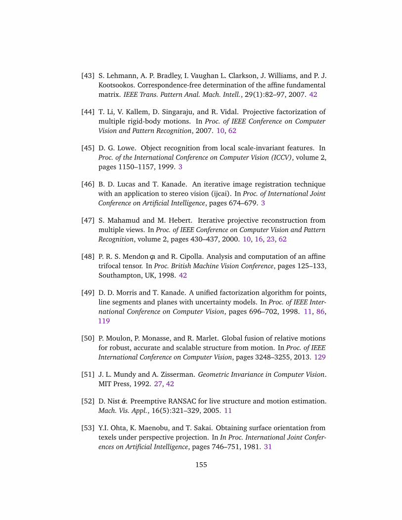
[43] S. Lehmann, A. P. Bradley, I. Vaughan L. Clarkson, J. Williams, and P. J.Kootsookos. Correspondence-free determination of the affine fundamentalmatrix. IEEE Trans. Pattern Anal. Mach. Intell., 29(1):82–97, 2007. 42

[44] T. Li, V. Kallem, D. Singaraju, and R. Vidal. Projective factorization ofmultiple rigid-body motions. In Proc. of IEEE Conference on ComputerVision and Pattern Recognition, 2007. 10, 62

[45] D. G. Lowe. Object recognition from local scale-invariant features. InProc. of the International Conference on Computer Vision (ICCV), volume 2,pages 1150–1157, 1999. 3

[46] B. D. Lucas and T. Kanade. An iterative image registration techniquewith an application to stereo vision (ijcai). In Proc. of International JointConference on Artificial Intelligence, pages 674–679. 3

[47] S. Mahamud and M. Hebert. Iterative projective reconstruction frommultiple views. In Proc. of IEEE Conference on Computer Vision and PatternRecognition, volume 2, pages 430–437, 2000. 10, 16, 23, 62

[48] P. R. S. Mendonça and R. Cipolla. Analysis and computation of an affinetrifocal tensor. In Proc. British Machine Vision Conference, pages 125–133,Southampton, UK, 1998. 42

[49] D. D. Morris and T. Kanade. A unified factorization algorithm for points,line segments and planes with uncertainty models. In Proc. of IEEE Inter-national Conference on Computer Vision, pages 696–702, 1998. 11, 86,119

[50] P. Moulon, P. Monasse, and R. Marlet. Global fusion of relative motionsfor robust, accurate and scalable structure from motion. In Proc. of IEEEInternational Conference on Computer Vision, pages 3248–3255, 2013. 129

[51] J. L. Mundy and A. Zisserman. Geometric Invariance in Computer Vision.MIT Press, 1992. 27, 42

[52] D. Nistér. Preemptive RANSAC for live structure and motion estimation.Mach. Vis. Appl., 16(5):321–329, 2005. 11

[53] Y.I. Ohta, K. Maenobu, and T. Sakai. Obtaining surface orientation fromtexels under perspective projection. In In Proc. International Joint Confer-ences on Artificial Intelligence, pages 746–751, 1981. 31

155

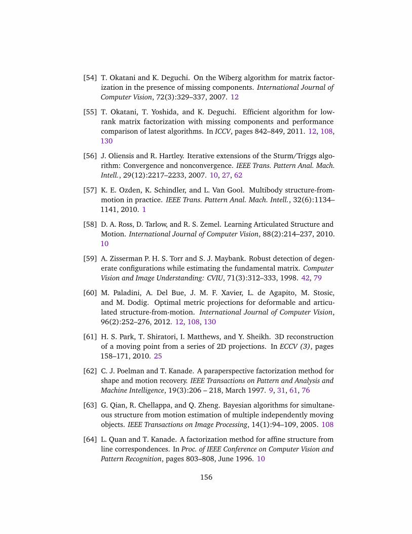
[54] T. Okatani and K. Deguchi. On the Wiberg algorithm for matrix factor-ization in the presence of missing components. International Journal ofComputer Vision, 72(3):329–337, 2007. 12

[55] T. Okatani, T. Yoshida, and K. Deguchi. Efficient algorithm for low-rank matrix factorization with missing components and performancecomparison of latest algorithms. In ICCV, pages 842–849, 2011. 12, 108,130

[56] J. Oliensis and R. Hartley. Iterative extensions of the Sturm/Triggs algo-rithm: Convergence and nonconvergence. IEEE Trans. Pattern Anal. Mach.Intell., 29(12):2217–2233, 2007. 10, 27, 62

[57] K. E. Ozden, K. Schindler, and L. Van Gool. Multibody structure-from-motion in practice. IEEE Trans. Pattern Anal. Mach. Intell., 32(6):1134–1141, 2010. 1

[58] D. A. Ross, D. Tarlow, and R. S. Zemel. Learning Articulated Structure andMotion. International Journal of Computer Vision, 88(2):214–237, 2010.10

[59] A. Zisserman P. H. S. Torr and S. J. Maybank. Robust detection of degen-erate configurations while estimating the fundamental matrix. ComputerVision and Image Understanding: CVIU, 71(3):312–333, 1998. 42, 79

[60] M. Paladini, A. Del Bue, J. M. F. Xavier, L. de Agapito, M. Stosic,and M. Dodig. Optimal metric projections for deformable and articu-lated structure-from-motion. International Journal of Computer Vision,96(2):252–276, 2012. 12, 108, 130

[61] H. S. Park, T. Shiratori, I. Matthews, and Y. Sheikh. 3D reconstructionof a moving point from a series of 2D projections. In ECCV (3), pages158–171, 2010. 25

[62] C. J. Poelman and T. Kanade. A paraperspective factorization method forshape and motion recovery. IEEE Transactions on Pattern and Analysis andMachine Intelligence, 19(3):206 – 218, March 1997. 9, 31, 61, 76

[63] G. Qian, R. Chellappa, and Q. Zheng. Bayesian algorithms for simultane-ous structure from motion estimation of multiple independently movingobjects. IEEE Transactions on Image Processing, 14(1):94–109, 2005. 108

[64] L. Quan and T. Kanade. A factorization method for affine structure fromline correspondences. In Proc. of IEEE Conference on Computer Vision andPattern Recognition, pages 803–808, June 1996. 10

156

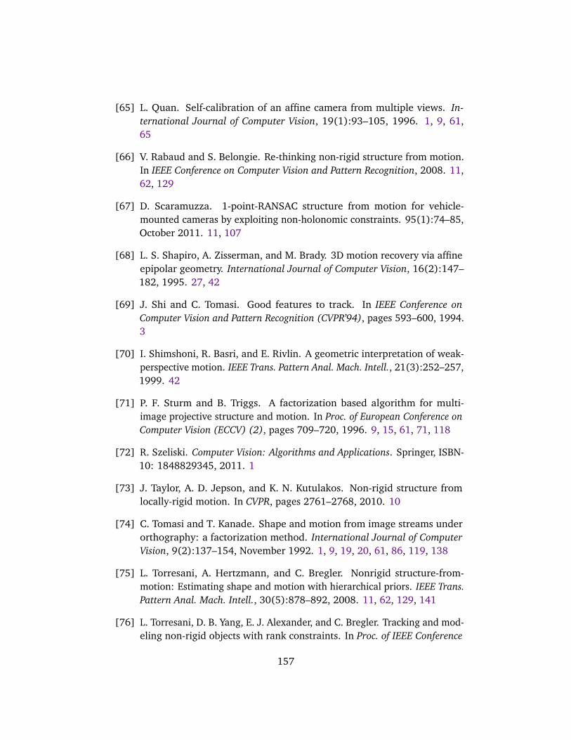
[65] L. Quan. Self-calibration of an affine camera from multiple views. In-ternational Journal of Computer Vision, 19(1):93–105, 1996. 1, 9, 61,65

[66] V. Rabaud and S. Belongie. Re-thinking non-rigid structure from motion.In IEEE Conference on Computer Vision and Pattern Recognition, 2008. 11,62, 129

[67] D. Scaramuzza. 1-point-RANSAC structure from motion for vehicle-mounted cameras by exploiting non-holonomic constraints. 95(1):74–85,October 2011. 11, 107

[68] L. S. Shapiro, A. Zisserman, and M. Brady. 3D motion recovery via affineepipolar geometry. International Journal of Computer Vision, 16(2):147–182, 1995. 27, 42

[69] J. Shi and C. Tomasi. Good features to track. In IEEE Conference onComputer Vision and Pattern Recognition (CVPR’94), pages 593–600, 1994.3

[70] I. Shimshoni, R. Basri, and E. Rivlin. A geometric interpretation of weak-perspective motion. IEEE Trans. Pattern Anal. Mach. Intell., 21(3):252–257,1999. 42

[71] P. F. Sturm and B. Triggs. A factorization based algorithm for multi-image projective structure and motion. In Proc. of European Conference onComputer Vision (ECCV) (2), pages 709–720, 1996. 9, 15, 61, 71, 118

[72] R. Szeliski. Computer Vision: Algorithms and Applications. Springer, ISBN-10: 1848829345, 2011. 1

[73] J. Taylor, A. D. Jepson, and K. N. Kutulakos. Non-rigid structure fromlocally-rigid motion. In CVPR, pages 2761–2768, 2010. 10

[74] C. Tomasi and T. Kanade. Shape and motion from image streams underorthography: a factorization method. International Journal of ComputerVision, 9(2):137–154, November 1992. 1, 9, 19, 20, 61, 86, 119, 138

[75] L. Torresani, A. Hertzmann, and C. Bregler. Nonrigid structure-from-motion: Estimating shape and motion with hierarchical priors. IEEE Trans.Pattern Anal. Mach. Intell., 30(5):878–892, 2008. 11, 62, 129, 141

[76] L. Torresani, D. B. Yang, E. J. Alexander, and C. Bregler. Tracking and mod-eling non-rigid objects with rank constraints. In Proc. of IEEE Conference

157

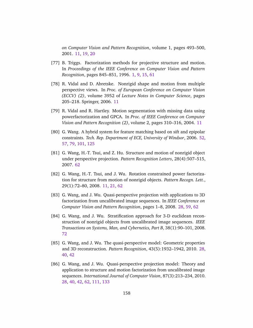
on Computer Vision and Pattern Recognition, volume 1, pages 493–500,2001. 11, 19, 20

[77] B. Triggs. Factorization methods for projective structure and motion.In Proceedings of the IEEE Conference on Computer Vision and PatternRecognition, pages 845–851, 1996. 1, 9, 15, 61

[78] R. Vidal and D. Abretske. Nonrigid shape and motion from multipleperspective views. In Proc. of European Conference on Computer Vision(ECCV) (2), volume 3952 of Lecture Notes in Computer Science, pages205–218. Springer, 2006. 11

[79] R. Vidal and R. Hartley. Motion segmentation with missing data usingpowerfactorization and GPCA. In Proc. of IEEE Conference on ComputerVision and Pattern Recognition (2), volume 2, pages 310–316, 2004. 11

[80] G. Wang. A hybrid system for feature matching based on sift and epipolarconstraints. Tech. Rep. Department of ECE, University of Windsor, 2006. 52,57, 79, 101, 125

[81] G. Wang, H.-T. Tsui, and Z. Hu. Structure and motion of nonrigid objectunder perspective projection. Pattern Recognition Letters, 28(4):507–515,2007. 62

[82] G. Wang, H.-T. Tsui, and J. Wu. Rotation constrained power factoriza-tion for structure from motion of nonrigid objects. Pattern Recogn. Lett.,29(1):72–80, 2008. 11, 21, 62

[83] G. Wang, and J. Wu. Quasi-perspective projection with applications to 3Dfactorization from uncalibrated image sequences. In IEEE Conference onComputer Vision and Pattern Recognition, pages 1–8, 2008. 28, 59, 62

[84] G. Wang, and J. Wu. Stratification approach for 3-D euclidean recon-struction of nonrigid objects from uncalibrated image sequences. IEEETransactions on Systems, Man, and Cybernetics, Part B, 38(1):90–101, 2008.72

[85] G. Wang, and J. Wu. The quasi-perspective model: Geometric propertiesand 3D reconstruction. Pattern Recognition, 43(5):1932–1942, 2010. 28,40, 42

[86] G. Wang, and J. Wu. Quasi-perspective projection model: Theory andapplication to structure and motion factorization from uncalibrated imagesequences. International Journal of Computer Vision, 87(3):213–234, 2010.28, 40, 42, 62, 111, 133

158

[87] G. Wang, and J. Wu. Guide to Three Dimensional Structure and MotionFactorization. Springer-Verlag, ISBN: 978-0-85729-045-8, 2011. 95, 102

[88] G. Wang, and J. Wu. Perspective 3D euclidean reconstruction with varyingcamera parameters. IEEE Transactions on Circuits and Systems for VideoTechnology, 19(12):1793–1803, 2009. 58, 62, 72

[89] G. Wang, J. Zelek, and J. Wu. Structure and motion recovery based onspatial-and-temporal-weighted factorization. IEEE Trans. Circuits Syst.Video Techn., 22(11):1590–1603, 2012. 84, 108, 119, 130, 138

[90] G. Wang, J. Zelek, and J. Wu. Robust structure from motion of nonrigidobjects in the presence of outlying and missing data. In CRV, pages159–166, 2013. 130

[91] G. Wang, J. Zelek, J. Wu, and R. Bajcsy. Robust rank-4 affine factorizationfor structure from motion. In WACV, pages 180–185, 2013. 108

[92] H. Wang, T.-J. Chin, and D. Suter. Simultaneously fitting and segmentingmultiple-structure data with outliers. IEEE Trans. Pattern Anal. Mach.Intell., 34(6):1177–1192, 2012. 12, 108, 130

[93] J. Y. Weng, T. S. Huang, and N. Ahuja. Motion and structure from twoperspective views: Algorithms, error analysis, and error estimation. IEEETrans. Pattern Anal. Mach. Intell., 11(5):451–476, 1997. 48

[94] L. Wolf and A. Shashua. Affine 3-D reconstruction from two projectiveimages of independently translating planes. In Proc. of the InternationalConference on Computer Vision, pages 238–244, 2001. 42

[95] J. Xiao, J. X. Chai, and T. Kanade. A closed-form solution to non-rigidshape and motion recovery. International Journal of Computer Vision,67(2):233–246, April 2006. 11, 19, 62, 78

[96] J. Xiao, and T. Kanade. Uncalibrated perspective reconstruction of de-formable structures. In Proc. of the International Conference on ComputerVision, volume 2, pages 1075–1082, 2005. 11, 21, 22, 23, 62, 64, 74, 78

[97] J. Yan and M. Pollefeys. A factorization-based approach to articulatedmotion recovery. In IEEE Conference on Computer Vision and PatternRecognition (2), pages 815–821, 2005. 10, 62

[98] J. Yan and M. Pollefeys. A factorization-based approach for articulatednonrigid shape, motion and kinematic chain recovery from video. IEEETrans. Pattern Anal. Mach. Intell., 30(5):865–877, 2008. 10, 62

159

[99] J. Yu, T.-J. Chin, and D. Suter. A global optimization approach to robustmulti-model fitting. In CVPR, pages 2041–2048, 2011. 12, 108, 130

[100] A. Zaharescu and R. Horaud. Robust factorization methods using a Gaus-sian/uniform mixture model. International Journal of Computer Vision,81(3):240–258, 2009. 12, 83, 84, 108, 114, 129

[101] L. Zelnik-Manor and M. Irani. Degeneracies, dependencies and theirimplications in multi-body and multi-sequence factorizations. Proc. of theIEEE Conference on Computer Vision and Pattern Recognition, 2:287, 2003.10

[102] L. Zelnik-Manor and M. Irani. On single-sequence and multi-sequencefactorizations. International Journal of Computer Vision, 67(3):313–326,2006. 10

[103] L. Zelnik-Manor, M. Machline, and M. Irani. Multi-body factorizationwith uncertainty: Revisiting motion consistency. International Journal ofComputer Vision, 68(1):27–41, 2006. 12, 84, 108, 129

[104] Z. Zhang. A flexible new technique for camera calibration. IEEE Trans.Pattern Anal. Mach. Intell., 22(11):1330–1334, 2000. 57

[105] Z. Zhang, P. Anandan, and H.-Y. Shum. What can be determined from afull and a weak perspective image? In Proc. of International Conference onComputer Vision, pages 680–687, 1999. 42

[106] Z. Zhang, R. Deriche, O. Faugeras, and Q.-T. Luong. A robust technique formatching two uncalibrated images through the recovery of the unknownepipolar geometry. Artificial Intelligence, 78(1-2):87–119, 1995. 3

[107] Z. Zhang and T. Kanade. Determining the epipolar geometry and itsuncertainty: A review. International Journal of Computer Vision, 27(2):161–195, 1998. 41, 47, 48

[108] Z. Y. Zhang and G. Xu. A general expression of the fundamental matrixfor both projective and affine cameras. In Proc. of International JointConference on Artificial Intelligence, pages 1502–1507, 1997. 42

160

Robust and Accurate Algorithm for Structure and Motion Factorization

Documents

Transcript of Robust and Accurate Algorithm for Structure and Motion Factorization