No. 2006/04

Risk Transfer with CDOs and Systemic Risk in Banking

Jan Pieter Krahnen and Christian Wilde

Center for Financial Studies

The Center for Financial Studies is a nonprofit research organization, supported by an association of more than 120 banks, insurance companies, industrial corporations and public institutions. Established in 1968 and closely affiliated with the University of Frankfurt, it provides a strong link between the financial community and academia.

The CFS Working Paper Series presents the result of scientific research on selected topics in the field of money, banking and finance. The authors were either participants in the Center´s Research Fellow Program or members of one of the Center´s Research Projects.

If you would like to know more about the Center for Financial Studies, please let us know of your interest.

Prof. Dr. Jan Pieter Krahnen Prof. Volker Wieland, Ph.D.

* We are grateful for financial support by Deutsche Forschungsgemeinschaft (DFG) and by Frankfurt University’s Center for Financial Studies (CFS). This paper is part of CFS’ project on the Economics of Credit Risk Transfer. In developing the basic question of this paper, we owe a lot to mini workshops with Günter Franke as well as Dennis Hänsel and Thomas Weber. We also thank seminar participants at the 2005 Meeting of the German Finance Association in Augsburg and the 2005 Annual meeting of the Verein für Socialpolitik in Bonn.

1 Finance Department, Goethe-University, Center for Financial Studies (CFS), Frankfurt, and CEPR.

Correspondence: CFS, Mertonstraße 17-21, 60325 Frankfurt(Main), Germany, Email: krahnen@wiwi.uni-frankfurt.de 2 Finance department, Goethe-University, Frankfurt. Correspondence: Mertonstrasse 17-21 (PF 88), 60054 Frankfurt, Germany,

Email: wilde@finance.uni-frankfurt.de

CFS Working Paper No. 2006/04

Risk Transfer with CDOs and Systemic Risk in Banking*

Jan Pieter Krahnen1 and Christian Wilde2

March 1, 2006

Abstract: Large banks often sell part of their loan portfolio in the form of collateralized debt obligations (CDO) to investors. In this paper we raise the question whether credit asset securitization affects the cyclicality (or commonality) of bank equity values. The commonality of bank equity values reflects a major component of systemic risks in the banking market, caused by correlated defaults of loans in the banks’ loan books. Our simulations take into account the major stylized fact of CDO transactions, the non-proportional nature of risk sharing that goes along with tranching. We provide a theoretical framework for the risk transfer through securitization that builds on a macro risk factor and an idiosyncratic risk factor, allowing an identification of the types of risk that the individual tranche holders bear. This allows conclusions about the risk positions of issuing banks after risk transfer. Building on the strict subordination of tranches, we first evaluate the correlation properties both within and across risk classes. We then determine the effect of securitization on the systematic risk of all tranches, and derive its effect on the issuing bank’s equity beta. The simulation results show that under plausible assumptions concerning bank reinvestment behaviour and capital structure choice, the issuing intermediary’s systematic risk tends to rise. We discuss the implications of our findings for financial stability supervision. JEL Classification: G28 Keywords: Risk Transfer, Systematic Risk, Systemic Risk

1 IntroductionSecuritization of loan assets has become a common instrument of bank risk man-agement. According to [10], a survey published by the European Central Bankin 2004, about 8-15% of overall assets of large, international banks, have beensubject to a securitization transaction. Many observers, such as J.P. Morgan(2004), believe the market for asset backed securities (ABS) to grow rapidlyin the next couple of years. What is the impact of securitizations on the riskexposure of the issuing institutions? In particular, how are commercial banksaffected that hold large volumes of loans on their balance sheets and that engagein securitizing them?The answers to these questions are not obvious at all. According to Green-

baum and Thakor (1987), credit securitization allows a bank to reduce its riskexposure, and to increase diversification in the economy. In the model of Duffieand Gârleanu (2001), securitizations improve liquidity and induce a positiveoverall market value effect. However, the effective risk transfer from a bank’sbalance sheet is limited by moral hazard problems. Allen and Gale (2004) ar-gue that, for incomplete markets, credit risk transfer may in fact increase riskconcentration rather than risk diversification, thereby raising overall systemicrisk. While risk transfer has often been cited as a major driver of ABS marketdevelopment, we will show below that in a typical CLO and CDO transaction(i.e. collateralized loan obligations, collateralized debt obligations), risk transferis rather limited, irrespective of the impressive size of the issues. The key tounderstanding risk transfer in structured transactions, such as ABS and CDOs,lies in the non-proportional sharing of risk. The tranching of claims, and theapplication of the subordination principle, lead to a reshuffling of risk in theportfolio. Typically, tail risk is being transfered, while non-tail risk is retainedby the issuing bank. This is particularly true for asset pools that are subjectto moral hazard, such that retention of the most junior tranche, the first losspiece, serves as a bonding and signaling device (DeMarzo, 2005). Tranchingand securitization therefore alters, or may alter, three aspects of the issuer’srisk position. First, it truncates the loss rate distribution. Second, it affectsthe correlation between on-balance sheet assets and, third, it may change thesystematic risk of the company, its exposure against market-wide risk factors.In this paper we address all three consequences of asset securitization. We

model a bank that repeatedly securitizes its loan portfolio, while retaining thefirst loss piece, and that reinvests the proceeds by lending to customers. Giventhe risk characteristics of the loan portfolio, how does securitization change thebasic properties of the bank’s remaining loan book, i.e. its loss rate distribution?what are the correlations between the retained asset portions and the remainingasset on the balance sheet? Furthermore, how can the risks be characterizedthat are transfered off the balance sheet, and on to the buyers’ books? Are theymostly systematic or rather company-specific, i.e. of an unsystematic nature?Finally, how is the dependence of bank equity values on a macroeconomic factoraffected, does it increase or decrease?Our analysis is of major importance for investors and for regulators. In line

2

with Das et al. (2004), investors will price structured finance products, likesenior or mezzanine tranches of a CDO transaction, by looking at the amountof systematic default risk that they carry. For this purpose, systematic defaultrisk has to be estimated. For regulators, risk shifting between banks and capitalmarkets is relevant since it may affect the required capital base of individualbanks and, even more importantly, it may affect the exposure of the bankingsystem at large vis-à-vis macroeconomic risks, see Andersen et al. (2004).The analysis relies on a two-stage procedure: First, the loss distribution of

the underlying portfolio has to be determined. Subsequently, the loss distribu-tion is allocated to tranches, representing claims of different seniority on theunderlying portfolio. We apply a Monte Carlo simulation to model the lossdistributions for portfolios of bank loans. For tranching, we apply cut-off valuesrepresented by maximum default probabilities allowed for each tranche. In prac-tice, these values are indicated by rating agencies. The data are then used todescribe the correlation property between tranches of different seniority and/ordifferent underlying asset pools. Our asset value model allows to disentangle theeffects of an economy-wide risk factor from risks associated with an industry, ora particular company.The results show that, among tranches of different transactions with the

same credit quality (intra-rating correlations), the most senior tranches havethe highest correlation coefficient.Second, the correlation between tranche performance and the realization of

the macro factor is monotonically related to the degree of subordination. Inparticular, senior tranches have a low systematic risk, while junior tranchesshow high systematic risk.These findings allow to asses the effect of securitizations on the systematic

risk of bank equity and, ultimately, on the systemic risk of the banking industryas a whole. We argue that, as the banks apply themselves to the securitizationof individual loan books, they will most likely increase their systemic expo-sure, rather than reduce it. This, in turn, will contribute to an increase in theprobability of banking crises.The paper is structured as follows: First, we describe how CDOs can be

modeled. We present the model setup, based on a firm-value model, and dis-cuss the implementation based on Monte Carlo simulation. Second, we look at asingle transaction and investigate which risks are transfered from the underlyingloan portfolio to tranches as part of securitization. Third, we turn to the levelof individual institutions. We infer the consequences of securitization for therisk positions of typical banks and examine the benefits of loan portfolio diver-sification in the context of securitization. We also derive how bank equity betaschange after banks securitize their loan portfolios. Fourth, at the level of theoverall economy, we examine the interaction of banks and the consequences ofsecuritization for systemic risk. In the concluding section we discuss the impli-cations of our findings for financial stability supervision and risk management.

3

2 Modeling CDOsIn this section we will analyze the risk charactristics of asset backed securitiesand related financial instruments1. We construct a simple tool that allows usto portray the loss distribution of asset portfolios, and of any tranche that isderived from the same underlying portfolio.

2.1 Model setup

We apply a firm-value model to capture the occurrence of obligor default. Moreprecisely, we apply a structural one-factor correlated default model. The drivingfactor is a market factor, and company value is modeled as the interplay of themarket factor and a company specific, idiosyncratic risk factor. This marketmodel approach is the model of choice in most corporate finance applications.We model company value Vn,t of each obligor n ∈ {1, 2, ..., N} at any timet before maturity as being driven by a generalized macroeconomic factor YM

t

that is common to all securities, and an idiosyncratic component n,t:

Vn,t =qρMn YM

t +q1− ρMn n,t (1)

with YMt ∼ Φ (0, 1), and n,t ∼ Φ (0, 1). Thereby, we obtain correlated

asset values of obligors. In case the sensitivitiespρMn of firm values to the

macroeconomic risk factor are the same for all obligors n, then ρMn correspondsto the mutual correlation coefficient for all assets.2

Obligor n is assumed to default if at any time t the value Vn,t of its assetslies below the exogenously given default boundary Dn, i.e. Vn,t < Dn. Vn,t isassumed to be normally distributed and is standardized such that Vn,t ∼ Φ (0, 1).There is a simple relation linking every default boundary Dn to a particular

default probability pn:

Dn = Φ−1 (pn) . (2)

1Asset backed securities are structured financial instruments that share two basic features:the pooling of underlying financial claims, and their tranching into a set of bonds, differentiatedby the degree of subordination. See Jorion or Fabozzi for institutional details.

2A more general model setup allowing for both inter- and intra-industry correlationcould include, besides the market factor, orthogonal industry factors Y j

t for industriesj ∈ {1, 2, ..., J}. The company value of each obligor in industry j can be modeled as:

V jn,t =

pρMn YM

t +

qρjnY

jt +

q1− ρMn − ρjn n,t, with YM

t ∼ Φ (0, 1), Y jt ∼ Φ (0, 1), and

tn ∼ Φ (0, 1). We assume that securities within industries are driven by a factor Y j

t that is

orthogonal to YMt and specific for that particular industry, i.e. Cov

³Y it , Y

jt

´= 0 for i 6= j.

Thereby, we obtain correlated asset values of obligors within the same industry, with corre-lation coefficient ρjn for industry j. The chosen representation also allows for inter-industrycorrelations, captured by ρMn . This approach is quite general and accounts both for bothinter- and intra-industry correlations. Its structure encompasses the approaches commonlyapplied by major rating agencies, which rely on a one factor model for each industry and zerointer-industry correlation. Thus, it reduces to the classical market model if industry-specificrisk is zero, while it reduces to the agency model if only the industry-specific component hasexplanatory power.

4

Usually, a fraction of the notional amount can be recovered in case of default.Let ψn denote the recovery rate and θn the exposure size of security n. Portfolioloss is given as the sum of individual loan losses. We define the portfolio defaultrate PDR as the present value of portfolio loss divided by the net present valueof all promised payments until maturity:

PDR =

PNn=1 1{Tn>τn} · θn ·

¡Fn · (1− ψn) · e−rτn + Cn,τn,Tn · e−rTn

¢PNn=1 θn · (Fn + Cn,0,Tn) · e−rTn

, (3)

where 1{Tn>τn} is an indicator function taking the value one if securityn defaults during its lifetime and zero otherwise. Tn represents maturity ofsecurity n, and τn is the time of default. Fn denotes the redemption valueand Cn,sn,tn represents the present value at time tn of all coupon payments forsecurity n paid in the time interval [sn, tn]. All payoffs are discounted withinterest rate r.The applied firm value model (Eq. 1) is suitable for a simulation exercise.

2.2 Model implementation

In the implementation, we do not need to apply simplifying assumptions to de-termine the loss distribution of the underlying portfolio. Instead, we are able tofully profit from the Monte Carlo Simulation procedure. Analytical approachesoften rely on limiting assumptions, e.g. that the portfolio is composed of an infi-nite number of securities with identical characteristics. Thus, analytical modelsto some extent may be suitable for sensitivity analyses, but Monte Carlo Simu-lation is more appropriate for real-world applications. All individual securitiesin the portfolio can be accounted for by their specific exposure size, recoveryrate, default probability, and maturity. Furthermore, Monte Carlo Simulationallows to differentiate between obligors and individual securities. The occur-rence of joint obligor defaults is modeled by accounting for the sensitivity ofeach individual obligor to the common factor.The loss distribution is simulated in 5 steps: First, a realization of the macro

factor is simulated until maturity. Subsequently, default scenarios are generatedfor all individual obligors in the portfolio. Default occurs, if the simulated firmvalue of an obligor, based on realizations of the macro factor and an idiosyncraticterm, falls below the default boundary. The default boundaries correspond tocut-off values denoting the maximum default probability allowed for a trancheof a particular seniority. In the third step, individual loan losses are obtainedby applying a recovery rate to loan default. Fourth, portfolio loss is given asthe sum of realized individual loan losses. This corresponds to one realizationin the simulation. Fifth, many simulation runs yield the loss distribution of theentire portfolio.The loss distribution depends on various input factors that may be grouped

into three categories: Individual loan components, portfolio components, andadditional CDO features. Individual loan components comprise maturity, credit

5

quality, and credit migration probability, and expected recovery rate at default.Portfolio components comprise the sensitivities of the individual loans to thecommon factor, portfolio diversification, and individual obligor concentration.Furthermore, in practice, CDO loan portfolios present additional complicationsas they are dynamic portfolios with various restrictions concerning asset replen-ishment over the lifetime of the issue. The implementation applied in this paperaccounts for single issuer default as well as portfolio characteristics, which arethe focus of the investigation.

3 Risk allocation to tranches

3.1 Individual tranche characteristics

We now investigate the nature of risk transfer from the underlying portfolioto tranches. This is at the heart of structured finance products, pooling ofindividual risks in order to reallocate these risks to investors. The transfer ofrisks is non-proportional, or non-linear, due to the principle of subodination oftranches. To estimate the resulting risk allocation we rely on a Monte Carlosimulation. Let us consider a reference portfolio with 10’000 loans. All securi-ties have the same characteristics: identical exposure size, 6% coupon, 1 year tomaturity, 20% default probability, 47.5% recovery rate, and identical exposureto the macro factor, corresponding to a correlation of ρMn = 0.3 between allsecurities. All cash flows are discounted with a constant interest rate of 4%.The evolution of individual-loan credit quality over time is simulated at annualfrequency. Figure 1 shows the loss distribution obtained by Monte Carlo Sim-ulation with 50’000 simulation runs. The loss distribution has a typical shapefor portfolios subject to credit risk, as it has a substantial positive skewness.The sensitivity of the individual loans to the macro factor is an important inputparameter determining the shape of the distribution. The higher it is, the moreprobability mass is shifted from the middle to the tails of the distribution andvice versa.Subsequently, the portfolio is split into seven tranches of strict subordination.

Note that all results reported below remain essentially unchanged if the numberof tranches is changed to, say 5 or to 9 tranches. In practice, the tranchesare associated with different ratings by rating agencies. For given maturitiesof the tranches, the ratings in turn correspond to specific default probabilities.We define the tranches by a maximum default probability, which is fixed atthe 1%, 2%, 5%, 10%, 20%, and 30% quantile of the loss rate distribution.Threshold probabilities are round numbers for convenience only. We numberthe tranches from 1 to 7, with the seventh tranche being the first loss piece, orequity piece, which covers the residual loss. Tranche no.1, at the other end ofthe spectrum, refers to the most senior tranche. All remaining tranches, nos.2-6, are mezzanine tranches.Tranching is done with the intention of minimizing the size of the first loss

piece, given the number of different layers and their respective threshold values.

6

Figure 1: Loss distribution of a loan portfolio

This diagram presents the loss distribution of a loan portfolio at maturity. The underlying portfolio

consists of 10’000 securities from different obligors. All securities have the same characteristics:

identical exposure size, 6% coupon 1 year to maturity, 20% default probability, 47.5 % recovery

rate, and identical exposure to the macro factor (ρn,M = 0.3). All cash flows are discounted with a

constant interest rate of 4%. The evolution of individual-loan credit quality over time is simulated

at annual frequency. The calculations are performed with 50’000 simulation runs. The horizontal

axis shows the loss rate; the vertical axis shows the observed frequency.

0%

1%

2%

3%

4%

5%

6%

7%

0% 5% 10% 15% 20% 25% 30% 35% 40% 45% 50% 55% 60%

7

Table 1: Summary statistics for tranches

This table presents summary statistics for the seven tranches, representing claims of strict subordi-

nation on the underlying portfolio. The statistics indicate the allocation of losses of the underlying

portfolio to the individual tranches. The cut-off values for a particular tranche is determined by

the default probability allowed for that tranche as indicated in the fifth column. The most junior

tranche (tranche number 7) corresponds to the first loss piece. It bears all losses not covered by

the other, more senior, tranches. The columns present, from left to right, the tranche number, the

tranche size, mean loss, loss standard deviation, default probability, and loss given default. The

last row displays the statistics for the underlying portfolio.

82.29%30.000%41.15%24.69%3.93%6

99.996%

99.996%

20.000%

10.000%

5.000%

2.000%

1.000%

Default probability

11.07%8.93%11.07%100.00%Total

60.97%34.28%60.96%14.06%7

72.66%32.79%14.53%6.02%5

72.30%24.25%7.23%5.14%4

66.48%16.46%3.32%5.54%3

73.92%11.35%1.48%3.70%2

6.68%0.84%0.07%61.61%1

LGDLoss stdMean lossTranche size

Tranches

82.29%30.000%41.15%24.69%3.93%6

99.996%

99.996%

20.000%

10.000%

5.000%

2.000%

1.000%

Default probability

11.07%8.93%11.07%100.00%Total

60.97%34.28%60.96%14.06%7

72.66%32.79%14.53%6.02%5

72.30%24.25%7.23%5.14%4

66.48%16.46%3.32%5.54%3

73.92%11.35%1.48%3.70%2

6.68%0.84%0.07%61.61%1

LGDLoss stdMean lossTranche size

Tranches

Applying the loss distribution of the total portfolio leads to the following tranchesizes starting from the most senior tranche: 0.6161, 0.0370, 0.0554, 0.0514,0.0602, 0.0393, and 0.1406 for the equity piece. Further summary statisticsfor the tranches are provided in Table 1. Graphical representations of the lossdistributions for different tranches (senior tranche, mezzanine tranche, and firstloss piece) are given in Figure 2.In Table 1, the senior tranche is by far the largest part of the entire trans-

action, making up 61.61% of the transaction. The expected loss rate is only 7basis points, while expected loss given a default event is 668 basis points. Themean loss rate is monotonously increasing in the degree of subordination. Itsmaximum value is 60.96% for the equity piece. The default probability of theequity piece is almost 100%, as there were only 2 out of 50’000 runs in thesimulation that came out with a zero loss rate for the entire portfolio.

The numbers for the senior tranche are particularly striking, as they showa very low loss given default rate, despite its large size. Figure 2 explains whythis is the case. Realized portfolio losses that surpass the capacities of the

8

Figure 2: Loss distribution of tranches

This diagram presents the loss distribution of three tranches (from left to right): the first loss piece

(tranche 7), a mezzanine tranche (tranche 6), and the senior tranche (tranche 1). The calculations

are performed with 50’000 simulation runs. The horizontal axis shows the loss rate; the vertical

axis shows the observed frequency, truncated at 30%, 1%, and 0.2%, respectively. There are several

values surpassing these thresholds: For the first loss piece, 100% loss occurs at a frequency of 30%.

For the mezzanine tranche, zero loss occurs at a frequency of 70%, and 100% loss occurs at a

frequency of 20%. For the senior tranche, zero loss occurs at a frequency of 99%.

0%

5%

10%

15%

20%

25%

30%

0% 20% 40% 60% 80% 100%0.0%

0.5%

1.0%

0% 20% 40% 60% 80% 100%0.0%

0.1%

0.2%

0% 20% 40% 60% 80% 100%

more subordinate tranches cluster at the low end of possible loss rates, withoutany observation exceeding a 25% loss rate in the simulation runs. Clearly, thedistribution of losses in this tranche is sensitive to the extreme-value propertiesof the underlying risk factors3 .As can be seen from Figure 2, the most subordinate mezzanine tranche,

no. 6, displays a broad tendency of a downward sloping distribution func-tion throughout its domain. While the loss rate distributions for all mezzaninetranches are downward sloping, their slope decreases with the degree of seniorityof the tranche in question for standard portfolio loss distributions and standardcut-off values for tranches.The distribution of the first loss piece, depicted in Figure 2, is single peaked

in the interior of its domain, abstracting from the spike at its upper boundary.This follows from the fact that the lowest tranche comprises two thirds of thecumulative loss rate distribution, comprising the peak of the aggregate loss ratedistribution.From the simulation exercise we obtain a couple of insights. By tranching,

the risks of the underlying portfolio are allocated in a non-proportional wayto the tranches. The loan portfolio is transformed into several securities withentirely different risk characteristics. The tranches or only a selection of them,as is often intended, can subsequently be sold independently to investors. Thesenior tranche has the highest quality in all categories. The probability of defaultis lowest, with no loss in 99% of all cases in this example. In addition, mean loss,loss standard deviation, and loss given default are lowest among all tranches.

3This points at a natural extension of our analysis, which uses fat-tailed distributions tomodel the loss rate distribution of the underlying loan portfolio.

9

Furthermore, the senior tranche is by far the largest of all tranches, with a claimon 61.61% of the volume of the underlying portfolio. In contrast to the seniortranche, the first loss piece suffers a loss rate of 100% with a large probability of30%. Furthermore, while low losses occur at low frequency, higher losses occurwith an increasing likelihood, peaking at a loss of 22%. Overall, the FLP has thehighest expected loss of all tranches. Finally, the presented statistics illustratethat even reference portfolios of relatively bad quality (20% default probabilityover 1 year for all loans in this case) can be divided into one large tranche ofthe highest quality, a couple of mezzanine tranches, and a relatively small firstloss piece in which the major proportion of credit risk is concentrated.

3.2 Tranche interdependencies

In this section, we use the data generated in the simulation exercise in orderto investigate the correlation between tranches. Since the underlying structuralmodel differentiates between macoeconomic and idiosyncratic risk, we will nowuse the risk model presented in the pevious section in order to identify theexposure of single tranches to the macroeconomic risk factor. The analysisshows that non-proportional risk sharing allocates macro risk primarily to juniortranches. In a first step, the correlation between tranches of a single issue isanalyzed, e.g, the correlation between the first loss piece that is retained on thebank’s balance sheet and a mezzanine or a senior tranche of the issue. In a secondstep, we look at tranches of different issues, e.g. the correlation between twofirst loss pieces, or two senior tranches with distinct underlying asset portfolios.Since we control the data generating process, we can trace the effect of changesin the underlying asset correlations to the resulting tranche correlations.Table 2 displays the bilateral correlations of all CDO tranches (ranging from

senior tranche to the first loss piece). The results indicate that tranches of simi-lar credit quality, or seniority, have higher correlation values than tranches withdifferent credit quality. The correlation between tranches of a given transaction(CDO 1 in Table 2) decreases monotonically with the distance of quality of twotranches (or tranche numbers, for that purpose). The correlation of tranche #1,the senior tranche, with the most junior tranche #7, the equity piece, is 0.0907.This shows that senior tranches are almost orthogonal to junior tranches, in par-ticular to the equity piece. Note that even lower correlations can be attainedby increasing the distance of tranches, e.g. by decreasing the maximum defaultprobability allowed for the senior tranche.In Table 3, the tranche-correlations of two CDOs with identical characteris-

tics are displayed. The correlation values are the higher the more similar are thetranches with respect to seniority. The highest correlation values are obtainedfor tranches with the same credit quality. These values are close to one. Cor-respondingly, the lowest bilateral correlation values are obtained for the mostsenior and the most junior tranches (0.0906). Note that for large portfolios, thecorrelation pattern converges in the limit to that of same-issue tranches (seeTable 2). Correspondingly, if the reference portfolios have less obligors, thetranche correlations of different issues are much lower.

10

Table 2: Bilateral correlations of all tranches from one CDO issue

This table displays the bilateral correlations of all CDO tranches ranging from tranche number 1

(most senior tranche) to tranche number 7 (first loss piece). The reference portfolio consists of

10’000 loans, and all of them have a default probability of 20%, 1 year maturity, 47.5% recovery

rate, and 6% coupon. All loans are assumed to have a default correlation of 0.3. All cash flows

are discounted with a constant interest rate of 4%. The loss distribution is calculated with 50’000

simulations.

1.0000Tranche 7

0.68321.0000Tranche 6

0.50470.81111.0000Tranche 5

0.33960.54570.77721.0000Tranche 4

0.23000.36970.52650.77291.0000Tranche 3

0.14830.23840.33950.49840.76521.0000Tranche 2

0.09070.14580.20760.30480.46800.69141.0000Tranche 1CDO 1

Tranche 7Tranche 6Tranche 5Tranche 4Tranche 3Tranche 2Tranche 1

CDO 1

1.0000Tranche 7

0.68321.0000Tranche 6

0.50470.81111.0000Tranche 5

0.33960.54570.77721.0000Tranche 4

0.23000.36970.52650.77291.0000Tranche 3

0.14830.23840.33950.49840.76521.0000Tranche 2

0.09070.14580.20760.30480.46800.69141.0000Tranche 1CDO 1

Tranche 7Tranche 6Tranche 5Tranche 4Tranche 3Tranche 2Tranche 1

CDO 1

11

Table 3: Bilateral correlations of tranches from two different CDO issues

This table displays the bilateral correlations of all tranches from two different CDO issues ranging

from tranche number 1 (most senior tranche) to tranche number 7 (first loss piece). Both CDOs

have similar characteristics: The reference portfolios consist of 100 loans, and all of them have an

initial rating of BB, 1 year maturity, 47.5% recovery rate, and 6% coupon. All loans are assumed

to have a default correlation of 0.3. All cash flows are discounted with a constant interest rate of

4%. The loss distribution is calculated with 50’000 simulations.

0.9991Tranche 7

0.68240.9978Tranche 6

0.50410.81130.9982Tranche 5

0.33920.54590.77640.9976Tranche 4

0.22980.36980.52600.77180.9972Tranche 3

0.14820.23850.33920.49770.76380.9964Tranche 2

0.09060.14580.20740.30440.46720.68960.9977Tranche 1CDO 1

Tranche 7Tranche 6Tranche 5Tranche 4Tranche 3Tranche 2Tranche 1

CDO 2

0.9991Tranche 7

0.68240.9978Tranche 6

0.50410.81130.9982Tranche 5

0.33920.54590.77640.9976Tranche 4

0.22980.36980.52600.77180.9972Tranche 3

0.14820.23850.33920.49770.76380.9964Tranche 2

0.09060.14580.20740.30440.46720.68960.9977Tranche 1CDO 1

Tranche 7Tranche 6Tranche 5Tranche 4Tranche 3Tranche 2Tranche 1

CDO 2

12

According to these simulations, the results confirm that portfolio risk istransferred to tranches in a non-linear way. In particular, the risk associatedwith senior tranches is only to a minor extent correlated with the risk thatremains on the bank’s balance sheet, given the retention of the first loss piece.This raises the question to what extent this result depends on the diversificationamong the assets in the underlying loan portfolio. We turn to this question next.

3.3 Estimating the systematic risk of tranches

The objective of the analysis is to trace the effect of macroeconomic risk tothe risk exposure of individual tranches, structured according to the principleof subordination. This section has an important result: under quite general as-sumptions about tranching, the most subordinate tranche has the largest macro-factor dependency. Tranching therefore tends to increase an issuers systematicequity risk, provided the most junior tranche is retained, a wide-spread industrypractice. To capture the impact of systematic risk on tranches, we consider abond that only depends on the macroeconomic factor and does not exhibit anyidiosyncratic risk. This bond, which we call a macro bond, is assumed to haveotherwise identical characteristics to the bonds in the portfolio, i.e. 1 year tomaturity, 6% coupon, 20% default rate, and 47.5% recovery rate. The macrobond allows us to estimate directly the relationship between the macro risk fac-tor and the realizations of particular tranches of an underlying loan portfolio.In our setting of normally distributed realizations, the default rate of 20% cor-responds to a default boundary of -0.8416 according to the distribution functionof (macro bond) value realizations Vn,t in Eq. (1), where ρMn is set equal to one.Table 4 summarizes the results, comparing joint default events of the tranchesand the macro bond. The second column reports the unconditional default ratesof the tranches, as specified for the simulation in this paper. The third columnreports the default rate of the tranche conditional on the default of the macrobond. This conditional tranche default rate is monotonic in the tranche quality,leading to the highest value of 100% for the most junior tranche, and to 4.95%for the most senior tranche. Note that these conditional default probailities arealmost four times higher than the unconditional probabilities for tranches 1 to5.The fourth column specifies the conditional macro bond default rate, i.e. the

probability of a macro bond default, given the default of a particular tranche.This conditional default rate is 100% for all senior tranches, and graduallydecreases for junior tranches. For the first loss piece, the conditional defaultrate is lowest, with a value of 20.15% in our simulation.The results in Table 4 show that the impact of macro risk on the default

rates of tranches varies systematically with the rating quality of the tranche.According to the last column, the more senior a tranche is, the more likely isits default accompanied by a negative realization of the macro risk factor.Figure 3 relates tranche losses to realizations of the macro factor. The first

loss piece suffers losses even for very good realizations of the macro factor. Thecapacity of the first loss piece is exhausted already for macro factor realizations

13

Table 4: The effect of systematic risk on tranches

This table presents the effect of systematic risk on tranches. All loans are assumed to have a default

correlation of 0.3, a default probability of 20%, 1 year maturity, 47.5% recovery rate, and 6% coupon.

All cash flows are discounted with a constant interest rate of 4%. The calculations are performed

with 50’000 simulation runs. The first column shows the tranches considered, ranging from 1 (most

senior tranche) to 7 (first loss piece). The second column reports the unconditional default rates of

the tranches. The third column reports the default rate of each tranche conditional on the default

of a bond only sub ject to macroeconomic risk. The fourth column specifies the probability of a

macro bond default, given the default of a particular tranche.

100.00%

100.00%

30.00%

20.00%

10.00%

5.00%

2.00%

1.00%

Pd(tranche)

100.00%

100.00%

100.00%

98.42%

49.61%

24.80%

9.92%

4.95%

Pd(tranche | macro)

20.15%Total portfolio

20.15%7

67.21%6

99.22%5

100.00%4

100.00%3

100.00%2

100.00%1

Pd(macro | tranche)Tranche

100.00%

100.00%

30.00%

20.00%

10.00%

5.00%

2.00%

1.00%

Pd(tranche)

100.00%

100.00%

100.00%

98.42%

49.61%

24.80%

9.92%

4.95%

Pd(tranche | macro)

20.15%Total portfolio

20.15%7

67.21%6

99.22%5

100.00%4

100.00%3

100.00%2

100.00%1

Pd(macro | tranche)Tranche

around the 30 percent quantile. For lower realizations, the losses of the firstloss piece are truncated at its share of the reference portfolio, corresponding toa loss of 100 percent. In constrast to the first loss piece, the senior tranche onlysuffers losses in the case of extremely bad realizations of the macro factor. Notethat the senior tranche even in the worst case only suffers minor losses althoughit has by far the largest size of all tranches. This is due to the recovery thattruncates losses of the senior tranche.We now turn to the estimation of a central measure of tranche interdepen-

dency on a market, which is beta, the systematic risk of individual tranches.This measure of risk is used in portfolio theory to capture the degree of pro-cyclicality of two random variables. A beta value larger (smaller) than onecharacterizes a return series that exhibits more (less) cyclical variation then thebenchmark index. In calculating tranche betas we take the macro factor Y t

M asthe benchmark index. Table 5 shows the sensitivity of the individual tranchesto the macro risk factor. In particular, the realized tranche returns obtained inthe simulation runs are regressed on the macro risk factor. The estimated betasincrease monotonically with the level of subordination, indicating that the firstloss piece has a high sensitivity to the macro risk factor while the most seniortranche almost has none. Thus, with tranches being exposed to different degreesof systematic risk, also the exposure of the issuing institution to systematic riskchanges in the practically relevant case that not all tranches are sold.

14

Figure 3: Tranche sensitivity to macro factor

This figure shows the sensitivity of individual tranches to realizations of the macro factor. The

tranche numbers range from 1 (senior tranche) to 7 (equity piece). The vertical axis shows the loss

rate with respect to the reference portfolio. The vertical axis shows the quantiles of macro factor

realizations. High quantiles indicate good states of the economy.

0.0

0.2

0.4

0.6

0.0 0.1 0.2 0.3 0.4 0.5 0.6 0.7 0.8 0.9

1234567

15

Table 5: Tranche beta

This table presents the results from a regression relating tranche returns to the corresponding

realizations of the macroeconomic factor. All loans are assumed to have a default correlation of 0.3,

a default probability of 20%, 1 year maturity, 47.5% recovery rate, and 6% coupon. All cash flows

are discounted with a constant interest rate of 4%. The calculations are performed with 50’000

simulation runs. The first column shows the tranches considered, ranging from 1 (most senior

tranche) to 7 (first loss piece). The second column reports the alpha values and the third column

reports beta values of the regression r = α+ β ∗ YM + .

0.8895

0.4030

0.7558

0.8562

0.9285

0.9670

0.9854

0.9994

αtranche

0.0847

0.3175

0.3070

0.2217

0.1341

0.0722

0.0363

0.0016

βtranche

Total portfolio

7

6

5

4

3

2

1

Tranche

0.8895

0.4030

0.7558

0.8562

0.9285

0.9670

0.9854

0.9994

αtranche

0.0847

0.3175

0.3070

0.2217

0.1341

0.0722

0.0363

0.0016

βtranche

Total portfolio

7

6

5

4

3

2

1

Tranche

16

4 Implications for Bank RiskIn this section, we investigate the risk position of a bank that issues a CDO,assuming that it retains the first loss piece, the most junior tranche. We makethis assumption since it is believed to be common practice among internationalbanks. We have no direct evidence supporting this assumption and thereforerefer to survey results (See ECB 2004 and Bundesbank 2004). This section showsthat under fairly general assumptions concerning bank reinvestment behavior,risk transfer will simultaneously decrease its exposure vis-à-vis extreme risksand increase its overall macro-factor dependence. We therefore predict issuingbanks to increase their equity beta.

4.1 Securitization and reinvestment

We now investigate the risk position of a bank that issues CDOs. Typically,a bank is exposed to various types of risk, in particular market risk, creditrisk, and operational risk. Market risk is often defined as outcomes from po-sition taking (stock, interest-sensitive securities, foreign exchange) as well ascustomer-related activities (fees and provision). Credit risk incurs from lendingwhich generates fees and interest income. Finally, operational risk as definedby the Basle Committee are losses due to external events and failure of internalprocesses, people, or systems. The distributions of all mentioned sources of riskhave distinct characteristics. Market risk is typically assumed to have a sym-metric distribution with a high variance, operational risk is typically assumedto have a very thin distribution with large tails, and credit risk is assumed tohave a skewed distribution with limited gains, but unlimited loss potential. Onaverage, the banks’ exposure to credit risk is about 6.5 times higher than tomarket risk, as obtained by [19], and thus the distribution of credit risk hasa dominating impact on the overall risk distribution of a bank. What is theresulting risk position of a bank that actively securitizes its loan portfolio?The impact of securitization on overall bank risk crucially depends on how

the proceeds are reinvested. The resulting effect is not obvious as there is a wholerange of possiblilties. In the extreme case on the one side, the balance sheetof the bank risk is levered, either by distributing the proceeds to shareholdersor by entering new investments with similar risk characteristics as the retainedjunior tranche. In the other extreme, overall bank risk also can decrease witha securitization transaction. This is the case when the proceeds are invested innew projects with lower risk. Thus, depending on the new risk position followingsecuritization and re-investment, a bank will have to hold more or less equityaccording the capital accords of the Basle committee. Seen from a dynamicperspective, the bank will either be exposed more or less to the fluctuations ofthe overall economy. Thus, while the Basle 2 accords have pro-cyclical effects,securitization (and re-investment) allows to influence a bank’s risk sensitivity tothe overall economy and thereby the capital requirements. Thus, securitizationallows banks to pursue its lending business independently of the state of theeconomy, in spite of cyclical effects imposed by the Basle 2 regulation.

17

Figure 4: Loss distribution of a loan portfolio after repeated securitizations andreinvestments

This figure shows the loss distribution of a loan portfolio after repeated securitizations and rein-

vestments. The original portfolio is securitized by retaining a first loss piece of 14.06 percent. The

proceeds obtained from the securitized portion (85.94 percent of the initial portfolio) amount to

94.26 percent of the total portfolio value as obtained with a one-factor asset pricing model. This

amount is reinvested in a new portfolio consisting of identical loans. Loss distributions are shown

for several iterations ranging from zero (the original portfolio is kept) to infinity (the limit case).

The horizontal axis shows the loss incurred with respect to the initial portfolio value, determined

with a one-factor asset pricing model. Negative values indicate excess returns. The vertical axis

shows the frequency of relative losses.

0%

5%

10%

15%

20%

25%

30%

35%

-200% -100% 0% 100%

01210lim

18

To determine the resulting risk position of a bank that actively securitizesits loan portfolio, we investigate the special case of a bank that repeatedlysecuritizes its loan portfolio and reinvests the proceeds. It turns out that abank that repeatedly securitizes its loan portfolio and reinvests the proceedswill have an entirely different risk position after these transactions. With eachiteration, the bank increases its leverage. Figure 4 shows the credit risk exposureof a bank that repeatedly securitizes its loan portfolio, retains the first loss pieceand reinvests the proceeds in loans of the same quality characteristics in termsof loss distribution. We start out from a simulated loss distribution obtained fora benchmark portfolio with 10’000 individual loans and 1 year to maturity. Thedefault probability of the loans in the portfolio is 20%, and the recovery ratein case of default is 47.5%. Applying the Monte Carlo Simulation technique tothis portfolio leads to the distribution of the original portfolio. The obtainedaverage loss rate is 11.07% with a standard deviation of 8.93%.After every round of securitizing and reinvesting, the resulting relative loss

distribution of the bank changes with the number of iterations and takes a dis-tinct shape, differing from that traditionally assumed for credit risk exposures.This has important implications for firm-wide risk management of the bank.Repeated securitization and reinvestment uniformly increases the return vari-ance of the securitizing bank and the value-at-risk. The special case of identicalloss rate distribution for the initial loan portfolio and all new (reinvested) loanportfolios has a simple limit result: the loss distribution of the portfolio withrepeated reinvestment converges to that of the original first loss piece. However,even a small number of iterations transforms the bank’s loss rate distributionsubstantially, reducing its skewness and increasing its mean value. Already afterone round, mean loss rate and standard deviation increase substantially and takethe values 18.09% and 12.07%, respectively. The limit distribution has a meanloss rate of 60.96% and a standard deviation of 34.28%, while the probabilityof a complete asset loss is 30% (compared to 0.00% in the original portfolio).This latter number is also the probability that the bank goes bankrupt providedthat it is completely equity financed and has no additional income from sourcesother than lending. The results are important for bank risk management andregulation likewise.

4.2 Estimating the effect of granularity

In this section, we investigate the effect of increasing granularity on the standarddeviation of the asset portfolio. We will trace the effect of diversification on theaverage correlation by varying the number of assets (loans) in the underlyingpool. We carry out this basic test, because we are interested in the effect ofsecuritization on diversification. One hypothesis advanced in the literature isthat a bank that engages in the transfer of risk through tranching increasesthe diversification in its asset base. The reason is that the proceeds from asecuritization can be reinvested in new loans, thereby increasing the granularityof the loan book.We consider a reference portfolio with a varying number of loans. All loans

19

Table 6: The effect of portfolio diversification

This table presents, for three correlation scenarios, the standard deviation of losses for different

numbers of loans. The numbers in parentheses indicate the reduction factor of the standard de-

viation obtained when increasing the number of loans in the portfolio by the factor 10. In the

three correlation scenarios, all loans are assumed to have a default correlation of 0.0, 0.15, and 0.3,

respectively. All loans have a default probability of 20%, 1 year to maturity, 47.5% recovery rate,

and 6% coupon. All cash flows are discounted with a constant interest rate of 4%. The calculations

for the different portfolios are performed with 50’000 simulation runs each.

6.16%(1.007)

6.21%(1.051)

6.52%(1.399)

9.12%(2.432)

22.19%

Corr=0.15

10000

1000

100

10

1

Number of loans

0.22%(3.163)

0.70%(3.167)

2.21%(3.178)

7.04%(3.146)

22.13%

Corr=0.0

Standard deviation

8.95%(1.004)

8.98%(1.023)

9.19%(1.198)

11.01%(2.017)

22.20%

Corr=0.30

6.16%(1.007)

6.21%(1.051)

6.52%(1.399)

9.12%(2.432)

22.19%

Corr=0.15

10000

1000

100

10

1

Number of loans

0.22%(3.163)

0.70%(3.167)

2.21%(3.178)

7.04%(3.146)

22.13%

Corr=0.0

Standard deviation

8.95%(1.004)

8.98%(1.023)

9.19%(1.198)

11.01%(2.017)

22.20%

Corr=0.30

have a default probability of 20%, 1 year to maturity, 47.5% recovery rate, and6% coupon. Table 6 presents the standard deviation of losses after accountingfor the number of loans. All loans are assumed to have a default correlationof 0.0 and 0.3, respectively. The calculations for the different portfolios areperformed with 50’000 simulation runs each.

The results suggest that even a small number of loans in a portfolio is enoughto diversify away the major part of idiosyncratic default risk. Consider thefirst column. The asset base is assumed to consist of uncorrelated risks, andthe idiosyncratic risk (standard deviation) is 22.13%. If the number of loansincreases, the standard deviation of the portfolio loss rates is rapidly decreasing,approaching zero. For example, with an asset base of 1000 loans, the resultingportfolio standard deviation is reduced by 1 − 0.7

22.13 = 96.84 percent, relativeto the original level, the standard deviation of the loss rate distribution of asingle loan. As can be seen from columns 2 and 3, the decrease in standarddeviation is a function of the bi-variate correlation between assets. For instance,if the correlation is 0.3, an asset base of 1000 loans reduces portfolio standarddeviation to 8.98% of its original level. This number, however, is numericallyclose to portfolio standard deviation that can be reached when the asset baseis decreased by a factor of 10. In this case, the resulting standard deviationis 9.19%, i.e. increases the standard deviation by a factor of 1.023 (+2.3%).Put differently, increasing the granularity of a portfolio has only a minor effect

20

on portfolio standard deviation, provided the number of loans in the initialportfolio exceeds 100. This exponential phasing out of the granularity effecthappens earlier (i.e. with a small number of loans in the initial portfolio) ifthe bi-variate loan correlation is high. For lower correlations, the phasing outhappens at higher degrees of granularity, but the overall effect is already closeto complete with merely 100 assets. The exception is a bi-variate correlation of0.0, where the reduction of standard deviation for each increase of the numberof loans by the factor 10, can be approximated by a constant factor, 3.1 in oursimulations.Overall, the results demonstrate that the diversification benefits are rapidly

decreasing with the number of securities in the portfolio. Typically, banks holdvery large loan portfolios and the securitization of a bank’s loan book will onlymarginally increase asset granularity. Thus, contrary to what is often believed,securitizing a bank loan portfolio with subsequent reinvestment in new loanswill only have minor additional diversification benefits for banks.

4.3 Implications for bank beta

We now examine the effect of securitization on the exposure of banks to system-atic risk. In particular, how does bank equity beta change in connection with asecuritization transaction? For simplicity, we assume that a bank is only pursu-ing a lending business and that it has no other assets than its loan portfolio. Onthe other hand, the liabilities comprise equity and debt. We now examine howa bank’s beta changes with securitization, assuming that the bank securitizesits entire loan portfolio.In line with the results obtained in Table 5, we assume that there is a

monotonous relation between the beta of a tranche and its seniority, and thatthe following inequality holds:

βFLP > βorigPF = βorigassets,

where βFLP is the beta of the first loss piece and βorigPF is the beta of the original

reference portfolio.4

Generally, a bank’s asset- and equity-beta can be related by the followingequation:

βassets = βdebt · d+ βequity · e, (4)

where βassets, βdebt, and βequity are the betas of the assets, debt, and equity,respectively. The debt ratio is denoted by d, and the equity ratio is denoted bye.The relation between original and new bank equity beta can be expressed in

a general way by using Eq. 4:

4Our simulation results show that the monotonous relation between the beta of a trancheand its seniority applies in all practically relevant cases. However, at this point, a formal proofof this assumption is left to the reader.

21

∆βequity = βnewequity − βorigequity

=βnewassets

enew− βorigassets

eorig− βnewdebt · dnew

enew+

βorigdebt · dorigeorig

, (5)

where eorig (dorig) is the original and enew (dnew) is the new equity (debt)ratio after securitization.The new asset beta βnewassets depends on how the securitization proceeds are

reinvested, i.e. which sensitivities the new securities have to the macroeconomicrisk factor. Let s denote the securitization proceeds in percent of the originalportfolio. Correspondingly, the percentage of the retained first loss piece isequal to 1− s. Reinvestment also implies the possibility to pay out part of thesecuritization proceeds to equity- or debtholders. Let the ratio of total payoutto total assets be represented by h. Thus, the new proportion of funds to bereinvested is s∗ ≡ s−h

1−h , while the proportion of the first loss piece in the newportfolio is 1 − s∗ ≡ 1−s

1−h . Accounting for possible payout to equity- or debt-holders, the new ratio s∗ of reinvested funds. The new asset beta is then givenby:

βnewassets = (1− s∗) · βFLP + s∗ · βreinvest. (6)

By combining Eq. 5 and 6, we obtain a general formula for the relationbetween original and new bank equity beta after securitization5:

∆βequity =(1− s∗) · βFLP + s∗ · βreinvest

enew−β

origassets

eorig−β

newdebt · dnewenew

+βorigdebt · dorig

eorig,

(7)Thus, magnitude and direction of equity beta change depend on bank lever-

age before and after securitization as well as the beta of the reinvestment al-ternative chosen. Figure 5 shows in two panels the change in bank equity betaafter a securitization transaction. The left diagram shows how equity betachanges in response to different leverage, given a constant beta of reinvestedassets βreinvest = βorigassets. The plot shows that, for constant leverage, for in-creasing leverage, and even for to some extent decreasing leverage, βnewequity islarger than βorigequity. The right diagram shows how equity beta changes in re-sponse to different beta of reinvested assets, given a constant equity ratio of 0.1which is typical in the banking sector. The plot shows that equity beta risesin most cases and only decreases if the beta of reinvested assets is substantiallybelow the beta of the original portfolio. Thus, we conclude that equity beta mayrise or fall in response to a securitization transaction, but in most practicallyrelevant cases, it will rise.

5Note that payouts may have any effect on firm leverage, ranging from an increase to adecrease, depending on how the payouts are distributed between equity- and debt-holders.Equally, firm leverage may also change without any payouts due to balance sheet restructur-ings.

22

Figure 5: Bank equity beta change after securitization

This figure shows change of bank equity beta after securitization for various values of firm leverage

(panel a) and beta of reinvested assets (panel b). The beta of debt is set to zero. The first loss

piece has a share of 14.06 percent of the total portfolio. The beta of the original portfolio as well

as the reinvested securities is 0.0846, the beta of the first loss piece is 0.3200, the original and the

new equity ratios are 0.1, corresponding to typical values for banks. In panel a, the new equity

ratio is varied (vertical axis), in panel b, the beta of the reinvested securities is varied (x-axis). In

panel a, there is a positive (negative) change in equity beta for equity ratios smaller (larger) than

0.139. In panel b, there is a positive (negative) change in equity beta for a weighted average beta

of reinvested securities larger (smaller) than 0.046. Leaving both firm leverage and portfolio beta

of reinvested securities constant, the resultung equity beta change of the bank is 0.3310.

-1

-0.5

0

0.5

1

0.0 0.1 0.2 0.3 0.4 0.5 0.6 0.7 0.8 0.9 1.0

-0.6

-0.4

-0.2

0

0.2

0.4

0.6

0.8

1

0.00 0.05 0.10 0.15 0.20

It is worth noting that there is a substantial difference between synthetic andtrue sale transactions with respect to the change in equity beta. The argumentas outlined above, i.e. that beta may rise or fall in response to a securitizationtransaction, holds for true sale transactions. In the case of synthetic transac-tions, however, the argument changes: Since all claims are settled at maturity,there are no immediate cash flows from the transaction that can be reinvestedin new securities or distributed to equity- or debt-holders. Consequently, in thecase of synthetic transactions, there will always be an increase in equity beta.The analysis presented in this paper builds on a one-factor macroeconomic

risk model. In extended versions with several independent risk factors, theresults remain essentially unchanged. There are only more sensitivities andbeta changes that have to be considered, each likewise represented by Eq. 7.

5 Systemic RiskIn the last section we have established that under certain conditions relating tothe retention of first loss pieces, the securitization of a loan portfolios by a bankwill lead to an increase in its exposure to market risk. We found the increaseof the issuing institution’s systematic risk to be positively related to the size ofthe retained equity piece, and to the reinvestment beta of the issue proceeds.Beta always increases for synthetic issues, since there are no issue proceeds.

23

All these claims pertain to the individual bank. What do they imply forthe banking sector as a whole? On the basis of the simple risk transfer modelintroduced in this paper, we now estimate the correlation of defaults. Thiscorresponds to a widely used definition of systemic risk, the likelihood of aconcurrent failure of several banks, see Kaufman (2000) or Lehar (2005).6 Forany given joint loss rate distribution, one can determine the cumulative densityof a certain number n or more banks defaulting simultaneously. This will beour approach to capture system-wide default risks, and we will investigate therelationship between systematic risk exposure on the level of the individual bankand its contribution to the risk of multiple bank failures.

5.1 How securitization affects joint default probabilities

The previous section has concluded that the securitization of a bank’s loanportfolio combined with the retention of a junior claim on the asset pool, tendsto raise the bank’s equity beta. Therefore one may ask: What is the marginaleffect of such a beta rise on the likelihood of multiple bank failure? To answerthis question we run a Monte Carlo simulation with many banks, all modeled asin section 4. We let one bank securitize its loan portfolio, tranching the portfolioaccording to the rules outlined in section 3, selling all tranches except the mostsubordinate one, and reinvesting the proceeds in assets of a similar quality asthe securitized loan portfolio7.Table 7 shows, for a market consisting of 5 banks, the probability that a

certain number of banks default. In the base case of no securitization, i.e. allbanks holding on to their original loan portfolios, the probability of at least onebank defaulting amounts to 42.13% while the probability that all banks defaultamounts to 39.88%. Thus, in the majority of all cases, either all banks or nobank will default.8

Table 7 compares the performance of banks and shows the probabilities ofat least 1, 2, ..., 5 banks defaulting simultaneously. The numbers reportedare cumulative probabilities. The first column shows the base case, when nobank securitizes its loan portfolio. In this case, the probability of just one bank

6Kaufman (2000) surveys the many different definitions of systemic risk used in the liter-ature. These definitions have received considerable attention, probably because the contain-ment of systemic risk is one of the core justifications for banking supervision, and for centralbank interventions in financial markets.

7The assumption that new loans have similar characteristics as the old loans is for ease ofexposition only. In section 4, it was shown that the change in macro factor exposure has thepredicted same sign as long as the reinvestment beta is not too much smaller than the betaof the original loan portfolio. So, for instance, the re-investment of ABS proceeds in risklessgovernment bonds could actually lower the issuing banks equity beta. If this is the case, theeffect on systemic risk is the other way around.

8Note that the number of bank defaults is dominated by the realization of the macro factorin this example. The dominance of macro factor realizations is due to (1) the large size of theloan portfolios with 10000 loans each and (2) the rather high correlation assumption of 0.3between all loans. However, our calculations for more realistic average correlations show thatthe numbers do not change much. Still, realizations of the macro factor dominate the results,i.e. in the majority of all cases, either all banks or no bank default.

24

defaulting is 42,13%, in line with the high individual default probability assumedin these simulations (see section 4 for details). Changing the individual defaultprobabilities will downshift the numbers in column 1 as well. The second columnreports the effect of one securitizing bank on the joint default probabilities of1,...,5 banks. There is a uniform increase in system-wide joint default probabilityfor the different levels of joint default in Table 7. The third column assumesthat all five banks engage in one round of asset securitization. The numbersin the table indicate that securitization increases the risk of joint bank defaultsat each level, represented by the minimum number of banks jointly defaulting.While the probability that at least one bank defaults is 42.13% if all banks holdon to the original loan portfolio, the default probability increases to 56.05% if allbanks sell off their loan portfolios, retaining the first-loss piece, and reinvest theproceeds in new loans. Similar increases can be observed for all other levels ofsystemic risk, i.e. that at least 2, 3, 4, or 5 banks default. Correspondingly, theprobability of a joint default of all five banks rises by 14.15 percentage pointsin comparison to the base case of no securitization and reaches 54.03%.The results reported in Table 7 support the claim that asset securitization

may increase the systematic risk exposure of these banks. Furthermore, the risktransfer by even a single financial institution will contribute to an increase ofthe systemic risk of the banking sector. Note that the source of systemic risk inour model is not contagion, or any other inter-bank liability, but the impact ofa common macroeconomic factor in the return generating process9 . The reasonwhy securitization levers macroeconomic risk has been shown in this and theprevious section: it is the influence that securitization (or structured funding ingeneral) exerts on the systematic risk of the bank’s asset composition. In oursimulations, this influence is due to a) the retention of the most subordinatetranche, and b) to the characteristics of the reinvestment decision concerningthe generated new funds.Overall, these results show how the mechanics of tranching and securitization

relate to systemic risk, providing a framework for more precise regulation.

5.2 Inferring systemic risk from market betas

In the previous section, we have shown that by the use of collateralized debtobligations, based on the mechanics of tranching and securitization, banks mayincrease their systematic risk, and thereby may raise the stability risk of thefinancial system at large. We have captured the bank’s macro factor exposureby beta, the bank return’s standardized covariance with the volatility of themarket index. We now turn our approach on its head and analyze whether ornot a change of a bank’s equity beta is an indicator of an increased systemicbanking risk. This question is important, since an affirmative answer would giveus an easy-to-use instrument at hand that allows the monitoring of joint bankdefault rates, or synonymously, systemic risk. On the other hand, the question

9 In the recent literature on systemic bank risk, there is an emphasis on inter-bank financialrelationships as the main source of systemic risk, see De Bandt and Hartmann (2002) for asurvey.

25

Table 7: Multiple bank defaults

This table shows the probability of multiple bank defaults. The examined market consists of 5

banks holding loan portfolios from different obligors, but with otherwise identical characteristics.

The given numbers are probabilities that at least a certain number of banks in the market default.

The default probabilities are given for three scenarios: (1) no bank securitizes, i.e. all banks hold

on to their original loan portfolios, (2) one bank securitizes its loan portfolio, retaining the first-loss

piece and reinvesting the proceeds, and (3) all banks securitize their loan portfolios.

40.00%

40.69%

41.27%

42.01%

55.04%

One bank securitizes

54.03%39.88%5

54.60%40.49%4

55.05%40.98%3

55.46%41.47%2

56.05%42.13%1

All banks securitize

No bank securitizes

Minimum numberof bank defaults

40.00%

40.69%

41.27%

42.01%

55.04%

One bank securitizes

54.03%39.88%5

54.60%40.49%4

55.05%40.98%3

55.46%41.47%2

56.05%42.13%1

All banks securitize

No bank securitizes

Minimum numberof bank defaults

is not trivial, because it is conceivable that a) securitizations lead to increasedsystematic and systemic risk, as shown in sections 4 and 5, and b) both effectsare actually a consequence of the bank retaining the highly risky first loss pieceof the securitization. Thus, the increase in systemic risk reported earlier, maybe due to the specific risk allocation achieved in structured finance, but it maynot be caused by an increase in beta itself. To put it differently, in this sectionwe will analyze whether an increase in beta will always increase the joint defaultprobability of banks, independent of the reason for the shift in beta.Table 7 reports the results of a Monte Carlo simulation with five banks, all

of which have the same characteristics (equity ratio of 10%, default probabilityof 10%, and equal betas). However, in contrast to earlier simulations, we do notassume anything about securitization and reinvestment. Instead, we model thebank as a return generating entity with a given macro risk exposure, summarizedby its beta value. We look at three distinct scenarios. In the first scenario, allbanks have a zero macro factor exposure, i.e. each individual beta is equal tozero. Results are in col.1 of Table 7.We find a rapid decay in the probability of joint bank defaults for higher

numbers of banks involved. Thus, the probability of one bank or more failingis 40.55%, while it is 7.96% for two or more and 0.05% for 4 or 5 banks failingjointly. If we increase beta uniformly to the level of 1, the probabilities formore than one bank failure is rising for all levels of systemic crisis, relative tothe base case in col.1. Only the probability of just one bank failure is reduced,indicating that probability mass is shifted from independent default occurrenceto joint defaults. If beta is increased further, to the uniform level of 2, we find

26

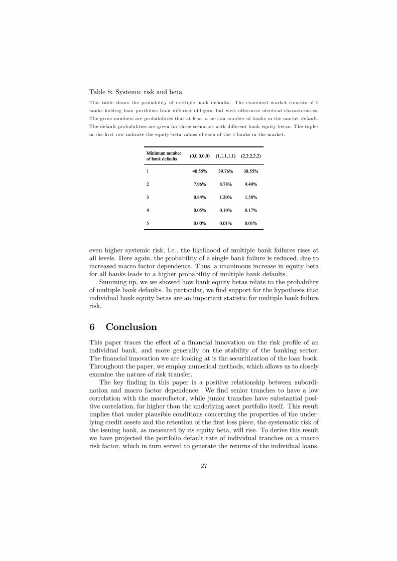
Table 8: Systemic risk and beta

This table shows the probability of multiple bank defaults. The examined market consists of 5

banks holding loan portfolios from different obligors, but with otherwise identical characteristics.

The given numbers are probabilities that at least a certain number of banks in the market default.

The default probabilities are given for three scenarios with different bank equity betas. The tuples

in the first row indicate the equity-beta values of each of the 5 banks in the market.

0.00%

0.05%

0.84%

7.96%

40.55%

(0,0,0,0,0)

0.01%

0.10%

1.20%

8.78%

39.76%

(1,1,1,1,1)

0.01%5

0.17%4

1.58%3

9.49%2

38.55%1

(2,2,2,2,2)Minimum numberof bank defaults

0.00%

0.05%

0.84%

7.96%

40.55%

(0,0,0,0,0)

0.01%

0.10%

1.20%

8.78%

39.76%

(1,1,1,1,1)

0.01%5

0.17%4

1.58%3

9.49%2

38.55%1

(2,2,2,2,2)Minimum numberof bank defaults

even higher systemic risk, i.e., the likelihood of multiple bank failures rises atall levels. Here again, the probability of a single bank failure is reduced, due toincreased macro factor dependence. Thus, a unanimous increase in equity betafor all banks leads to a higher probability of multiple bank defaults.Summing up, we we showed how bank equity betas relate to the probability

of multiple bank defaults. In particular, we find support for the hypothesis thatindividual bank equity betas are an important statistic for multiple bank failurerisk.

6 ConclusionThis paper traces the effect of a financial innovation on the risk profile of anindividual bank, and more generally on the stability of the banking sector.The financial innovation we are looking at is the securitization of the loan book.Throughout the paper, we employ numerical methods, which allows us to closelyexamine the nature of risk transfer.The key finding in this paper is a positive relationship between subordi-

nation and macro factor dependence. We find senior tranches to have a lowcorrelation with the macrofactor, while junior tranches have substantial posi-tive correlation, far higher than the underlying asset portfolio itself. This resultimplies that under plausible conditions concerning the properties of the under-lying credit assets and the retention of the first loss piece, the systematic risk ofthe issuing bank, as measured by its equity beta, will rise. To derive this resultwe have projected the portfolio default rate of individual tranches on a macrorisk factor, which in turn served to generate the returns of the individual loans,

27

together with an idiosyncratic risk factor. We also show that the risk positionof a bank that securitizes its loan portfolio and reinvests the proceeds differssubstantially from commonly used credit loss distributions. Furthermore, wesimulate the dependency between tranches of different transactions, but withthe same risk rating. The correlation coefficients tend to be highest for themost senior tranches. The reason for this is the joint dependency on the marketinterest rate, or the term structure of interest rates, but not their dependencyon the macro risk factor (which was shown earlier to be negligible).The interpretation of the macro risk factor as market risk invites an empir-

ical test of our hypothesis, namely that credit securitizations contribute to anincrease in the systematic risk of banks10. If confirmed, this would imply thatthe banking industry increases its dependence on the macro risk factor by secu-ritizing its asset pool. From the point of view of a regulator, an increased macrorisk dependence of individual banks also raises the probability of joint defaults.This, however, raises the likelihood of observing a banking crisis - many finan-cial intermediaries failing at the same time. In our setting, the commonality isdue to a high dependency of banks on general macroeconomic conditions, whichimplies that banks tend to suffer large loan losses at the same time.Our simulations suggest that credit backed securitizations render banks more

vulnerable against adverse movements of the macroeconomic factor. This con-clusion is subject to the retention of the first loss piece, while mezzanine andsenior tranches are sold to outside investors. A more aggressive risk acquisitionby issuing banks would make our results even stronger, see Acharya (2001) andInstefjord (2005).Note that the increased dependency of first loss banks (i.e. banks that keep

securitizing their loan portfolio while retaining the first loss piece) on macrorisks goes hand in hand with an effective transfer of extreme systematic risks.These latter risks are realized if several banks fail at the same time, and theseverity of these losses is then borne by the holders of the senior tranches. Thetransfer of extreme systematic risk stabilizes the banking system, while thebanks’ systematic risk rise nevertheless.Doesn’t the new rules known as Basel II solve the problem of systematic

risk increase through an increase in minimum equity capital? Under Bael IIregulation, the holder of an equity tranche has to hold 100% equity againstthis position. One can therefore conclude that as long as the minimum capitalrequirement is binding, an increase in asset beta through securitization will bebalanced off by a lower debt ratio. However, empirically we observe a trend forbanks in many countries, and in particular for internationally active banks, toincrease their effective equity capital far above the minimum capital requirement(see Allen et al., 2005, for a survey and an explanation of this development),thereby rendering the above formulation invalid: when minimum capital re-quirement is not binding, then the issue of credit backed securities (retainingthe junior tranche) will most likely increase bank equity beta.Furthermore, as worked out in section 5, the increase of systematic bank

10This is the subject of a companion paper, Hänsel/Krahnen (in preparation).

28

equity risk in the wake of risk transfer through securitized loan assets affectsthe correlation among different financial institutions. The joint dependency iswhat beta is intended to capture after all. Therefore, we have concluded thatsecuritization not only raises systematic bank risk, but it also raises systemicrisk of the entire banking sector. There are three questionable assumptionsthat underlie our conclusion. First, why should the most subordinate trancheof a securitization transaction be retained? Second, are there any compensat-ing effects in other segments of the financial system that offset the increase insystemic risk? Third, are beta values truly useful if one wants to forecast thestability of a financial system vis-à-vis exogenous macroeconomic shocks? Wewill deal with these questions in turn.Equity piece retention is widely observed in the industry, according to sur-

vey evidence published by the Bundesbank (2004), and by the European CentralBank (2004). What is the economic function of the retention of first loss pieces?The question has been analyzed in the theoretical literature by Plantin (2004),and by DeMarzo (2005). These authors show that the retention of a first losspiece serves the purpose of a deductible in insurance markets, aligning the incen-tives of the issuing bank with the interests of the buyers of the senior tranches.Thus, first loss piece retention is all the more important, the stronger is the roleof relationship lending in the pool of securitized assets. Arm’s length lending, incontrast, is less likely to require any deductible in order to be sold on the marketplace. Thus, we expect our line of argument from securitization to systemic riskto be notably relevant for commercial banks with large midcap industry loansand private relationship lending.The second question really describes an open research question. If securi-

tizations in the banking sector raise average beta of the sector, there must bea compensating effect elsewhere in the economy, since average beta equals oneby construction. The relevant question is therefore whether the offsetting effecthappens within the financial system, or outside of the system. The latter casemay be due to a decreasing beta of household assets, which were bank bondsbefore securitization, and are senior CDO tranches afterwards. There are clearlya great many possible compensating effects that need further study.There may be additional reasons to believe that a bank that securitizes

its liabilities will end up increasing asset risk. One powerful argument hasbeen made by Acharya (2001), who endogenizes the choice of correlation riskby banks. Acharya (2001) shows that depending on the capital requirementsimposed on banks, they may find it attractive to increase correlation risk, dueto moral hazard. A good example is a pertinent bank regulation that focuseson the individual default risk of banks (Value at Risk, for example), neglectingcorrelation risk. In such a case, banks will become creative in order to raise theunpriced correlation risk. Of course, and as shown before, one way of achievingincreased correlation risk is through securitizing assets. The current reform ofbanking regulation, Basel II, does not address the correlation risk, and thereforeillustrates well the point raised by Acharya (2001).What are the lessons for financial stability supervision? First, the effect

of credit risk transfer on banks’ systematic risk can be estimated using either

29

numerical models, or using empirical data. In both cases regulators will wantto hold average bank beta at level compatible with banks’ capital reserves.Since non-proportional risk sharing is increasingly used not only in the bank-

ing industry, but also in corporate finance and in the reinsurance industry, weexpect our analysis to have relevance even beyond the field of credit risk man-agement. Overall, the analysis stresses the importance for both investors, banks,and regulators to better understand the risk allocation in securitization trans-actions.

References[1] Acharya, V. (2001). Theoy of systemic risk and design od prudential bank

regulation, working paper, London Business School.

[2] Allen, F., E. Carletti, and R. Marquez (2005). Credit market competitionand capital regulation, working paper.

[3] Allen, F., D. Gale (2005). Systemic risk and regulation, NBER woking pa-per, forthcoming: The Risks of Financial Institutions, edited by M. Careyand R. Stulz, University of Chicago Press.

[4] Andersen, T., T. Bollerslev, F. Diebold, and P. Christoffersen (2004). Prac-tical volatility and correlation modeling for financial market risk manage-ment, working paper, October.

[5] Deutsche Bundesbank (2004). Instrumente zum Kreditrisikotransfer: Ein-satz bei deutschen Banken und Aspekte der Finanzstabilität, Monats-bericht April, 24-45.

[6] Das, S.R., L. Freed, G. Geng, and N. Kapadia (2004). Correlated defaultrisk, working paper, June.

[7] De Bandt, O., P. Hartmann (2002). Systemic risk: A survey, in Financialcrisis, contagion and the lender of last resort: A book of readings, ed byC.A.E. Goodhart and G. Illing, Oxford University Press, London, 249-298.

[8] DeMarzo, P. (2005). The pooling and tranching of securities: a model ofinformed intermediation, Review of Financial Studies 18, 1-35.

[9] Duffie, D., N. Gârleanu (2001). Risk and valuation of collateralized debtobligations, Financial Ananlysts Journal 57, January-February, 41-59.

[10] European Central Bank (2004). Credit risk transfer by EU banks: activities,risks, and risk management. Report, May.

[11] Franke, G., J. P. Krahnen (2005). Default risk sharing between banks andmarkets: the contribution of collateralized debt obligations, NBER work-ing paper, forthcoming: The Risks of Financial Institutions, edited by M.Carey and R. Stulz, University of Chicago Press.

30

[12] Greenbaum, S., A. Thakor (1987). Bank funding modes: securitizationversus deposits, Journal of Banking and Finance 11, 379-392.

[13] Hänsel, D., J.P. Krahnen (2005). An empirical investigation of capital mar-ket reactions to CDO transactions, in preparation.

[14] Instefjord, N. (2005), Risk and hedging: do credit derivatves increase bankrisk?, Journal of Banking and Finance 29, 333—345.

[15] J.P. Morgan (2004). Global ABS/CDO Weekly Market Snapshot, GlobalStructured Finance Research, JP Morgan New York, June 10.

[16] Kaufman, G.G. (2000). Banking and currency crises and systemic risk: Ataxonomy and review, Financial Markets, Institutions & Instruments, 9, 2,May.

[17] Lehar, A. (2005), Measuring systemic risk: A risk management approach,Journal of Banking and Finance 29, 2577-2603.

[18] Plantin, G. (2004). Tranching, working paper, London School of Economics.

[19] Rosenberg, J.V., T. Schuermann (2004). A general approach to integratedrisk management with skewed, fat-tailed risks, Federal Bank of New York,staff report no. 185, May.

31

CFS Working Paper Series:

No. Author(s) Title

2006/04 Jan Pieter Krahnen Christian Wilde

Risk Transfer with CDOs and Systemic Risk in Banking

2006/03 Panos Parpas Berc Rustem Volker Wieland Stan Zakovic

Mean Variance Optimization of Non–Linear Systems and Worst–case Analysis

2006/02 Christoffer Carroll Miles S. Kimball

Precautionary Saving and Precautionary Wealth

2006/01 M. Hashem Pesaran Market Efficiency Today

2005/33 Fulvio Corsi Uta Kretschmer Stefan Mittnik Christian Pigorsch

The Volatility of Realized Volatility

2005/32 Sumit Agarwal Souphala Chomsisengphet Chunlin Liu Nicholas S. Souleles

Do Consumers Choose the Right Credit Contracts?

2005/31 Guenter W. Beck Axel A. Weber

Inflation Rate Dispersion and Convergence in Monetary and Economic Unions: Lessons for the ECB

2005/30 Axel A. Weber Guenter W. Beck

Price Stability, Inflation Convergence and Diversity in EMU: Does One Size Fit All?

2005/29 Luigi Guiso Tullio Jappelli

Awareness and Stock Market Participation

2005/28 Tullio Jappelli Luigi Pistaferri

Intertemporal Choice and Consumption Mobility

Copies of working papers can be downloaded at http://www.ifk-cfs.de