Bank Competition and Credit Risk in Euro Area Banking - MDPI
28
Journal of Risk and Financial Management Article Bank Competition and Credit Risk in Euro Area Banking: Fragmentation and Convergence Dynamics Maria Karadima 1, * and Helen Louri 1,2 1 Department of Economics, Athens University of Economics and Business, 76 Patission Street, GR-10434 Athens, Greece; [email protected] 2 European Institute/Hellenic Observatory, London School of Economics, Houghton Street, London WC2A 2AE, UK * Correspondence: [email protected] Received: 9 February 2020; Accepted: 12 March 2020; Published: 16 March 2020 Abstract: Consolidation in euro area banking has been the major trend post-crisis. Has it been accompanied by more or less competition? Has it led to more or less credit risk? In all or some countries? In this study, we examine the evolution of competition (through market power and concentration) and credit risk (through non-performing loans) in 2005–2017 across all euro area countries (EA-19), as well as core (EA-Co) and periphery (EA-Pe) countries separately. Using Theil inequality and convergence analysis, our results support the continued existence of fragmentation as well as of divergence within and/or between core and periphery with respect to competition and credit risk, especially post-crisis, in spite of some partial reintegration trends. Policy measures supporting faster convergence of our variables would be helpful in establishing a real banking union. Keywords: banking competition; credit risk; NPLs; Theil index; convergence analysis JEL Classification: C23; G21 1. Introduction Financial integration has been one of the major goals of the European Union (EU) because of its significant capability to offer more opportunities for risk sharing, better allocation of capital, and higher economic growth (Baele et al. 2004). Financial integration may be defined as “a situation whereby there are no frictions that discriminate between economic agents in their access to—and their investment of—capital, particularly on the basis of their location” (European Central Bank, ECB 2003). A related concept is financial fragmentation, which is often used to indicate some forms of imperfect integration (Claessens 2019). Fragmentation generally refers to financial markets, which fragment either by type of product/participant or geographically (Financial Stability Board, FSB 2019). From the establishment of the European Monetary Union (EMU) up to the outbreak of the global financial crisis, the euro area witnessed a rapidly growing financial integration, which was evident in terms of both volume and prices (De Sola Perea and Van Nieuwenhuyze 2014). Financial integration was also expected to promote competition in the euro area banking sector (Casu and Girardone 2009), due inter-alia to increased disintermediation and cross-border competition (De Bandt and Davis 2000). Nevertheless, the financial crisis of 2008 reversed some advances in competitive pressure, which had been achieved until then (Maudos and Vives 2019). Financial fragmentation peaked during the euro area debt crisis (2011–2012) and declined afterwards due to the measures taken by the ECB. According to Al-Eyd and Berkmen (2013), the unconventional monetary policy undertaken by the ECB was instrumental in reducing the overall degree of financial market fragmentation. Berenberg-Gossler and Enderlein (2016) confirm that after J. Risk Financial Manag. 2020, 13, 57; doi:10.3390/jrfm13030057 www.mdpi.com/journal/jrfm
-
Upload
khangminh22 -
Category
Documents
-
view
0 -
download
0
Transcript of Bank Competition and Credit Risk in Euro Area Banking - MDPI
Journal of
Risk and FinancialManagement
Article
Bank Competition and Credit Risk in Euro AreaBanking: Fragmentation and Convergence Dynamics
Maria Karadima 1,* and Helen Louri 1,2
1 Department of Economics, Athens University of Economics and Business, 76 Patission Street,GR-10434 Athens, Greece; [email protected]
2 European Institute/Hellenic Observatory, London School of Economics, Houghton Street,London WC2A 2AE, UK
* Correspondence: [email protected]
Received: 9 February 2020; Accepted: 12 March 2020; Published: 16 March 2020�����������������
Abstract: Consolidation in euro area banking has been the major trend post-crisis. Has it beenaccompanied by more or less competition? Has it led to more or less credit risk? In all or somecountries? In this study, we examine the evolution of competition (through market power andconcentration) and credit risk (through non-performing loans) in 2005–2017 across all euro areacountries (EA-19), as well as core (EA-Co) and periphery (EA-Pe) countries separately. Using Theilinequality and convergence analysis, our results support the continued existence of fragmentation aswell as of divergence within and/or between core and periphery with respect to competition and creditrisk, especially post-crisis, in spite of some partial reintegration trends. Policy measures supportingfaster convergence of our variables would be helpful in establishing a real banking union.
Keywords: banking competition; credit risk; NPLs; Theil index; convergence analysis
JEL Classification: C23; G21
1. Introduction
Financial integration has been one of the major goals of the European Union (EU) because of itssignificant capability to offer more opportunities for risk sharing, better allocation of capital, and highereconomic growth (Baele et al. 2004). Financial integration may be defined as “a situation whereby thereare no frictions that discriminate between economic agents in their access to—and their investmentof—capital, particularly on the basis of their location” (European Central Bank, ECB 2003). A relatedconcept is financial fragmentation, which is often used to indicate some forms of imperfect integration(Claessens 2019). Fragmentation generally refers to financial markets, which fragment either by typeof product/participant or geographically (Financial Stability Board, FSB 2019).
From the establishment of the European Monetary Union (EMU) up to the outbreak of the globalfinancial crisis, the euro area witnessed a rapidly growing financial integration, which was evident interms of both volume and prices (De Sola Perea and Van Nieuwenhuyze 2014). Financial integrationwas also expected to promote competition in the euro area banking sector (Casu and Girardone 2009),due inter-alia to increased disintermediation and cross-border competition (De Bandt and Davis 2000).Nevertheless, the financial crisis of 2008 reversed some advances in competitive pressure, which hadbeen achieved until then (Maudos and Vives 2019).
Financial fragmentation peaked during the euro area debt crisis (2011–2012) and declinedafterwards due to the measures taken by the ECB. According to Al-Eyd and Berkmen (2013), theunconventional monetary policy undertaken by the ECB was instrumental in reducing the overalldegree of financial market fragmentation. Berenberg-Gossler and Enderlein (2016) confirm that after
J. Risk Financial Manag. 2020, 13, 57; doi:10.3390/jrfm13030057 www.mdpi.com/journal/jrfm

J. Risk Financial Manag. 2020, 13, 57 2 of 28
the ECB announcement of the Outright Monetary Transactions (OMT) program in 2012 there was agradual, but often fragile, decline of financial fragmentation across all markets. After a temporarycorrection between late 2015 and 2016, the aggregate post-crisis reintegration trend in the euro arearesumed with respect to prices. In contrast, the post-crisis reintegration trend with respect to quantitiesstalled in 2015, partly due to the supply of excess reserves from the ECB, which had reduced the needfor counterparties to trade across borders (ECB 2018).
In this study, we test the hypothesis of the existence of fragmentation in the euro area (EA) as awhole (EA-19 group—19 countries of the Euro Area from 1 January, 2015), as well as in core countries(EA-Co group) and periphery countries (EA-Pe group), with respect to bank competition (throughmarket power and concentration) and credit risk over the period 2005–2017. The group of core countriesincludes eleven countries (Austria, Belgium, Estonia, Germany, Finland, France, Latvia, Lithuania,Luxembourg, Netherlands, and Slovakia), while the periphery group includes eight countries (Cyprus,Greece, Ireland, Italy1, Malta, Portugal, Slovenia, and Spain). The periphery countries were hit by the2008 financial crisis more severely than the core countries, while some of them (namely, Cyprus, Greece,Ireland, Slovenia, and Spain) received state aid through various impaired asset measures or directstate recapitalization. The classification of countries into each group is based on a prior identificationfrom the European Commission of distinct groups of EU Member States, according to their levels ofnon-performing loans (NPLs) (Magnus et al. 2017). More specifically, the hypothesis of the existence offragmentation is tested through the investigation of inequalities among the country-members of eachgroup, as well as between EA-Co and EA-Pe, with respect to bank competition, bank concentrationand credit risk. In total, four types of inequality—with respect to a given variable—are considered:(a) inequality between banks in a given country (within-country inequality), (b) inequality betweenbanks of different countries belonging to the same group (between-country inequality), (c) inequalitybetween banks or countries in a given group (within-group inequality), and (d) inequality betweenbanks or countries of different groups (between-group inequality).
A second hypothesis, which is tested in this study, refers to the presence of β-convergence andσ-convergence2 among the country-members of each group, with respect to bank competition, bankconcentration, and credit risk. It should be noted, however, that a possible convergence of the variablesunder examination is only a necessary but not a sufficient condition for the achievement of financialintegration in the euro area.
The Lerner index for market power, used in our study as an inverse proxy for bank competition,has been calculated following the innovative stochastic frontier estimator of market power, suggestedby Kumbhakar et al. (2012). Bank concentration, which also indicates the degree of competitivepressure, is measured by the Herfindahl–Hirschman Index (HHI) and the market share of the five largestbanks (CR5). Credit risk is approximated by non-performing loans (NPLs). Finally, we use the Theilinequality index for the four variables to examine the evolution of inequality either within/betweencountries or within/between groups.
To the best of our knowledge, this is the first time in the empirical literature that the evolutionand convergence of bank competition, concentration and credit risk are examined across EA-19, EA-Coand EA-Pe to test for continued fragmentation and converging or diverging trends. Our analysis,which employs a panel dataset of euro area banks from 2005 to 2017, extends beyond the periodof financial crisis, thereby taking into account the non-standard measures adopted by the ECB tosupport further integration. By using data from all the 19 euro area countries, which have a common
1 While Italy should in principle be considered as a core country since it has been one of the EU founding members, itis classified in this study as a periphery country because of its high levels of NPLs during the crisis. A classification ofItaly as a periphery country has also been made in other studies (see Al-Eyd and Berkmen 2013; Anastasiou et al. 2019;Louri and Migiakis 2019).
2 In the case of competition, for example, β-convergence would apply if countries with lower levels of competition werefound to tend to catch up with countries characterized by higher levels of competition, while σ-convergence would apply ifthe dispersion of competition levels across countries showed a tendency to decline over time.

J. Risk Financial Manag. 2020, 13, 57 3 of 28
currency and a single bank supervisory mechanism, a possible bias that might stem from the use ofeither heterogeneous data or data coming from only a subset of euro area countries was eliminated.In addition to uncovering the evolution of financial integration a major aim of our study was to providesubstantiated clues to policy makers about the progress of integration and underline the need forfurther measures required to achieve a real banking union.
The use of an alternative measure of credit risk, such as the loan loss provisions (LLPs), wasprohibited by the lack of non-available comparable data. In addition, the lack of bank-level data ontotal assets and NPLs did not facilitate the breakdown of total inequality in both bank concentrationand credit risk into their within-country and between-country components, an issue that remainsopen for future research. Finally, since a limitation of this study is that countries with possiblydifferent characteristics form a group on the basis of a priori classification, future research could usenovel methods (e.g., Phillips and Sul 2007) to identify groups of countries that exhibit convergence(“convergence clubs”).
The rest of the study is organized as follows. Section 2 describes the evolution of competitiveconditions in EU banking. Sections 3–5 examine the evolution of bank competition, concentration andcredit risk, respectively. Section 6 investigates the Theil inequality for bank competition, concentrationand credit risk. Section 7 displays the convergence analysis, while Section 8 concludes.
2. Evolution of Competitive Conditions in EU Banking
2.1. Before the Introduction of the Euro
We classify the literature review on the evolution of competition in the European Union into threegroups, according to the period examined by each study: (1) before the introduction of the euro in1999, (2) around the introduction of the euro, and (3) after the introduction of the euro. The aboveclassification has been made in order to facilitate the comparison of the results.
The first group of studies examines the degree of competition before the introduction of the euroin 1999. The major milestones of this period were: (1) the adoption of the Second Banking Directive(Directive 89/646/ European Economic Community (EEC) of 15 December, 1989), which entered intoforce on 1 January, 1993, providing a “passport” to European banks, which allowed a bank licensed inan EU country to establish branches or provide financial services in any of the other Member States,while the prudential supervision of a bank remained the responsibility of the home Member State;(2) the start of Stage One (1990–1993) of the EMU on 1 July, 1990, a date on which the restrictions onthe free movement of goods, persons, capital and services between the EMU Member States wereremoved; (3) the establishment of the European Union with the signing of the Treaty on the EuropeanUnion (the “Maastricht Treaty”) on 7 February, 1992; and (4) the start of Stage Two (1994–1998) of theEMU on 1 January, 1994, with the establishment of the European Monetary Institute (EMI), whose taskwas to coordinate monetary policy among the central banks of the Member States and make all thenecessary preparations for the introduction of the euro in Stage Three, starting from 1 January, 1999.
Bikker and Haaf (2002) examine the competitive conditions and concentration in 23 European andnon-European industrialized countries over the period 1988–1998. Using the H-statistic, they find thatall the banking markets under examination were characterized by monopolistic competition. Perfectcompetition could not be excluded for a number of European large-bank markets, while competitionappeared to be higher in Europe than in Canada, Japan and the US. De Bandt and Davis (2000)investigate the effects of the EMU on the competitive conditions in France, Germany and Italy overthe period 1992–1996. The H-statistic indicates that large banks in Germany and France operated inan environment of monopolistic competition, in contrast to small banks, which seemed to have somemonopoly power. In Italy, both large and small banks operated under monopolistic competition. TheH-statistic, calculated for the same period on a sample of US banks, indicates that the US bankingsystem was more competitive than those of France, Germany and Italy.

J. Risk Financial Manag. 2020, 13, 57 4 of 28
Some other studies of this group use cross-country data from the EU area only. Fernandez deGuevara et al. (2007) investigate the progress of financial integration in 15 EU countries. The studyreveals the existence of convergence in interest rates during the period 1993–2001, which is attributedto the convergence of inflation rates and the decrease in nominal interest rates. By examining theevolution of the levels of competition, measured by the Lerner index, they find that market powerincreased about 10% on average in 10 of the 15 countries during the period 1993–2000. They alsoconstructed a Theil inequality index for the Lerner index, which helped them to identify an increase inmarket power inequality in the 15 countries under examination. The decomposition of the Theil indexinto a within-country and a between-country component suggests that the main part of the marketpower inequality was within countries themselves (within-country inequality).
The rest of the studies in this group examine the case of one EU country only. Hondroyiannis et al.(1999) assess the competitive conditions in Greece over the period 1993–1995. The results, based onthe use of the H-statistic, indicate that Greek banks operated in an environment characterized bymonopolistic competition. These competitive conditions were formed as a result of the enactment ofthe EU Second Banking Directive, the lifting of controls on foreign exchange, and the liberalizationof capital movements. Angelini and Cetorelli (2003) examine the banking competitive conditions inItaly over the period 1984–1997. Using the Lerner index for each of five geographical banking marketsin Italy (i.e., Nationwide, North-East, North-West, Center, and South), they find that competitiveconditions across the five areas remained relatively unchanged until 1992, before starting to improvethereafter as a result of the implementation of the EU Second Banking Directive in 1993. Anotherfinding is that the large-scale bank consolidation in Italy during the 1990s not only did not worsencompetitive conditions, but actually improved banks’ efficiency. Coccorese (2004) examines the bankingcompetitive conditions in Italy during the period 1997–1999. Using the H-statistic, he finds that banksoperated under conditions of monopolistic competition at a national level. When banks are classifiedinto four macro-regions (North-West, North-East, Center, and South and Islands), the results indicatethat banks in both the North-West and the North-East regions operated in an environment characterizedby perfect competition.
The conclusion that can be drawn from the first group of studies is that euro area banks operatedunder conditions of monopolistic competition during the pre-EMU period, while contradictory resultshave been derived regarding the sign of the change in competition levels.
2.2. Around the Introduction of the Euro
The second group of studies examines the competitive conditions in the EU during a periodincluding a few years both before and after the introduction of the euro, which was introduced in1999 but entered into circulation in 2002. For this reason, some studies (Apergis et al. 2016; Sun 2009)consider 2000 as the end year of the pre-EMU period and 2001 as the start year of the after-EMU period.
Some of the studies of this group employ data not only from the EU area but also from othergeographical regions for comparison purposes. Bikker and Spierdijk (2008) examine the developmentsin bank competition in 101 countries worldwide during the period 1986–2004. Using the H-statistic,they find that the EU-15 (15 EU Member States from 1 January, 1995) experienced a major breakin competitive conditions around 2001–2002, followed by a decrease of about 60% in competition.In contrast, nine Eastern European countries that have joined the EU since 2004 experienced a modestdecrease of about 10% in competition during the years 1994–2004. Sun (2009) assesses the degree ofbank competition in the US, the UK and 10 euro area countries over the period 1995–2009. The resultsof the study indicate that the euro area experienced convergence of competition levels across membercountries, as well as a decrease in competition, measured by the H-statistic, after the introduction of theEMU (period 2001–2007). Competition also decreased during the crisis period (2008–2009), especiallyin countries where large credit and housing booms had been observed pre-crisis.
Some other studies of this group examine countries belonging to the EU area only, makingin some cases a comparison between euro area and non-euro area countries. Staikouras and

J. Risk Financial Manag. 2020, 13, 57 5 of 28
Koutsomanoli-Filippaki (2006) assess the competitive conditions in the EU-15 and EU-10 (10 EUMember States that joined in 2004) countries over the period 1998–2002. The results of the study,based on three different H-statistic specifications, indicate that banks in both the EU-15 and the EU-10countries operated in an environment of monopolistic competition. Goddard et al. (2013) examinethe convergence of bank profits in eight EU countries (Belgium, Denmark, France, Germany, Italy,Netherlands, Spain and the UK) over the period 1992–2007. They find that the average profitabilitywas lower for banks that had a higher capital level, while banks that were more efficient and diversifiedwere characterized by higher average profitability. Another finding is that excess profit presentedweaker persistence during the years 1999–2007 than in the previous period 1992–1998, indicatingthat the introduction of the EU financial integration, especially with the adoption of the euro andthe implementation of the Financial Services Action Plan (FSAP), intensified bank competition.Apergis et al. (2016) assess the level of bank competition across three EU economic blocks (EU-27—27EU Member States from 1 January, 2007; EA-17—17 EA Member States from 1 January, 2011; and theremaining 12 EU countries) over the period 1996–2011. The H-statistic, calculated on the basis of threealternative specifications of both scaled and unscaled reduced-form revenue equations, indicates thepresence of conditions of monopolistic competition across all the above economic blocks. Competitionlevels seemed to be lower in the EA-17 countries than in the EU-27 countries, which could be due to theincreasing mergers and acquisitions in the EA-17 countries. The results also show that the competitionlevel in the EA-17 countries decreased slightly in the post-EMU period (2001–2007), compared to thepre-EMU period (1996–2000), while the competition levels in the EA-17 countries showed a slightdecline during the post-crisis period (2008–2011). The development of banking competition policy inthe EU area, as well as the trends in bank competition and concentration, during the 25-year period1992–2017, are examined by Maudos and Vives (2019). They find that the recent global financial crisisinterrupted the process of normalization of the banking competition policy in the EU, which hadstarted in the 1980s, and reversed the advances that had been made in competitive pressures due tothe implementation of the Single Market initiative and the introduction of the euro. After the crisis,competition policy in the EU focused on limiting the distortions in competition created by the massivestate aid granted to banks. They also find that the crisis accelerated the pace of bank concentrationin the countries that had been hit most severely by the crisis and whose banking systems had beensubject to restructuring.
Regarding studies that examine the case of only one country, Gischer and Stiele (2008) examinethe banking competitive conditions in Germany over the period 1993–2002. Using the H-statistic on adataset of more than 400 cooperative banks (Sparkassen), they find that these banks operated underconditions of monopolistic competition. In addition, the H-statistic for small cooperative banks waslower than for large cooperative banks, suggesting that smaller cooperative banks seemed to enjoymore market power than larger ones.
In summary, the second group of studies suggests that banks in the euro area operated underconditions of monopolistic competition during the period around the introduction of the euro. Theresults regarding the impact of the introduction of the euro on bank competition are contradictory,with most studies suggesting a decline in competition during the post-EMU period.
2.3. After the Introduction of the Euro
The third group of studies examines the evolution of competition well after the introduction of theeuro. Some of these studies examine the case of more than one EU country. Casu and Girardone (2009)assess the effects of the EU deregulation and competition policies on bank concentration and competitionin the five largest EU banking markets (France, Germany, Italy, Spain, and the UK) over the period2000–2005. Using the HHI and CR5 concentration indices, they observe an increasing degree of bankconcentration during the period under examination, with the exception of Spain. Furthermore, thevalues of concentration indices vary significantly across countries. Their findings are confirmed when asub-sample of only commercial banks is taken into account. The use of the Lerner index did not provide

J. Risk Financial Manag. 2020, 13, 57 6 of 28
any evidence that competition increased until 2005, while the results derived from the estimationof H-statistics indicate conditions of monopolistic competition in all five countries. Weill (2013)investigates whether economic integration in the European Union banking industries has favored bankcompetition over the period 2002–2010, by following two different approaches. First, he examines theevolution of competition in the EU-27 countries, as measured by the Lerner index and the H-statistic.The results do not confirm a general improvement of bank competition over the entire period underexamination. In contrast, a small increase of the Lerner index was observed during the pre-crisis period,which, however, slowed down after the outbreak of the global financial crisis, in particular in the caseof the twelve new EU member countries. Second, he employs β-convergence and σ-convergence testson the Lerner index and the H-statistic, which suggest that during the period 2002–2010 the leastcompetitive banking systems had experienced a greater improvement in competition than the mostcompetitive banking systems, while the disparity in competition levels among the EU-27 countrieswas reduced. The impact of the 2008 global crisis on the fragmentation of the banking system in 11euro area countries over the period 1999–2011 was examined by Lucotte (2015) who uses ten differentharmonized banking indicators covering the areas of concentration and competition, efficiency, stability,development, and activity. Using a hierarchical cluster analysis, he indicates the existence of largedissimilarities since the creation of the euro area between Greece and Italy on the one hand, and theother nine countries on the other. The nine countries were split after 2008 into two different clusters withlarge dissimilarities. The first cluster comprises Austria, Belgium, Finland, France, and Germany, whileIreland, Netherlands, Portugal, and Spain belong to the other. Cruz-Garcia et al. (2017) investigate theimpact of financial market integration on the evolution of disparities among European banks’ marketpower. They use bank-specific data for the EA-12 countries (12 EA Member States from 1 January, 2001)over the period 2000–2014, and find that the Lerner index of bank market power increased in 10 of the12 countries. Using a Theil inequality index for the Lerner index, they find that while the differences inmarket power between European banks decreased significantly over the period 2000–2014, significantand persistent differences in market power existed between banks in the same country.
Regarding studies of this group that examine the case of only one country, Moch (2013) investigatesthe competition conditions in Germany over the period 2001–2009. Using the H-statistic on a datasetcomprising data from 1888 private, savings and cooperative banks, the study finds that interpretationsabout competitive conditions that are based on H-statistic calculated at a national level can be distortedwhen the banking market is fragmented, as in Germany. When examining separately the three bankingpillars in Germany (i.e., private, savings, and cooperative banks), the hypothesis for the presenceof monopoly power in any of these pillars was definitely rejected. Savings and cooperative banksseemed to operate either under monopolistic conditions in a long-run equilibrium or under long-runcompetitive conditions with flat average cost functions, while the private banks operated in a long-runcompetitive equilibrium.
In summary, the third group of studies suggests that monopolistic competition has been thedominant form of bank competition in the euro area after the introduction of the euro. The resultsregarding the evolution of competition are either inconclusive or suggest a decrease in competitionlevels after the 2008 global financial crisis.
A conclusion that can be drawn from all the studies presented in this section is that there is generalagreement in the literature that banks in the euro area operated under conditions of monopolisticcompetition during the last 25 years. On the other hand, contradictory results are obtained regardingthe impact of the introduction of the euro on the level of bank competition. This lack of consensus maybe due to differences in the competition measures used, as well as to differences in the data employedwith respect to geographical and time coverage.

J. Risk Financial Manag. 2020, 13, 57 7 of 28
3. Bank Competition in the Euro Area
3.1. Measuring Bank Competition through Market Power
The literature on the measurement of competition follows two major approaches: the structuraland the non-structural. The structural approach, which has its roots in the traditional IndustrialOrganization theory, embraces the Structure-Conduct-Performance (SCP) paradigm and the EfficiencyStructure Hypothesis (ESH). The SCP paradigm states that a higher degree of concentration is likely tocause collusive behavior among the larger banks, resulting in superior market performance. Because oftheir ability to capture structural features of a market, concentration ratios are often used to proxy forcompetition. The most frequently used concentration ratios are the Herfindahl-Hirschman Index (HHI)and the k-bank concentration ratios (CRk). The HHI index is the sum of the squares of the marketshares in total banking assets of all banks in a banking system, while the CRk concentration ratio is thesum of the shares of the k largest banks. The Efficiency Structure Hypothesis (ESH) investigates therelationship between the efficiency of larger banks and their performance. A widely used ESH indicatoris the Boone indicator (Boone 2008), which is calculated as the elasticity of profits or market share tomarginal costs. The idea underlying the Boone indicator is that competition improves the performanceor market share of efficient firms and weakens the performance or market share of inefficient ones.
The non-structural approach developed on the basis of the New Empirical Industrial Organization(NEIO) theory assesses the competitive behavior of firms without having to rely on information aboutthe structure of the market. The H-statistic, developed by Panzar and Rosse (1987), and the Lernerindex, developed by Lerner (1934), are the most well-known non-structural measures of competition.The Panzar and Rosse’s model employs firm-level data to investigate the degree to which a changein input prices is reflected in equilibrium revenues. This model uses the H-statistic, which takes anegative value to indicate a monopoly, a value between 0 and 1 to indicate monopolistic competitionand the value 1 to indicate perfect competition. The Lerner index is a direct measure of a bank’s marketpower. It represents the markup of prices over marginal cost and its value theoretically ranges between0 (perfect competition) and 1 (pure monopoly). In practice, however, negative values may be observedfor banks that face problems.
In our study, bank market power is measured by the Lerner index (L), which identifies the degreeof monopoly power as the difference between the price (P) of a firm and its marginal cost (MC) at theprofit-maximizing rate of output:
L =P−MC
P(1)
A zero value of the Lerner index indicates competitive behavior, while a bigger distance betweenprice and marginal cost is associated with greater market power.
In contrast to P, the value of MC is not directly observable, so we derive its value from theestimation of the following translog cost function:
lnTCit = α0 + αQlnQit + 0.5αQQ(lnQit)2 +
3∑k=1
αklnWk,it +3∑
k=1αQklnQitlnWk,it
+0.53∑
j=1
3∑k=1
α jklnW j,itlnWk,it + αElnEit + 0.5αEE(lnEit)2 +
3∑k=1
αEklnEitlnWk,it
+αEQlnEitlnQit + αTT + 0.5αTTT2 + αTQTlnQit +3∑
k=1αTkTlnWk,it + εit
(2)
where TC is total cost (sum of total interest and non-interest expenses), Q is total assets (proxy for bankoutput), W1 is the ratio of other operating expenses to total assets (proxy for input price of capital), W2
is the ratio of personnel expenses to total assets (proxy for input price of labor), W3 is the ratio of totalinterest expenses to total funding (proxy for input price of funds), T is a time trend variable, E is totalequity and εit is the error term. The subscripts i and t denote bank i and year t, respectively.

J. Risk Financial Manag. 2020, 13, 57 8 of 28
The time trend (T) has been included in (2) to account for advances in banking technology. Wehave also included in (2) the level of Total Equity (E), since it can be used in loan funding as a substitutefor deposits or other borrowed funds.
Symmetry conditions have been applied to the translog portion of (2), while the restriction oflinear homogeneity in input prices is imposed by dividing in (2) both total cost and input prices by oneof the input prices.
ln(
TCitW3,it
)= α0 + αQlnQit + 0.5αQQ(lnQit)
2 +2∑
k=1αk ln
(Wk,itW3,it
)+
2∑k=1
αQklnQit ln(
Wk,itW3,it
)+ 0.5
2∑j=1
2∑k=1
α jk ln(
W j,itW3,it
)ln
(Wk,itW3,it
)+αElnEit + 0.5αEE(lnEit)
2 +2∑
k=1αEklnEit ln
(Wk,itW3,it
)+ αEQlnEitlnQit
+αTT + 0.5αTTT2 + αTQTlnQit +2∑
k=1αTkTln
(Wk,itW3,it
)+ εit
(3)
3.2. Calculation of a Lerner Index Using a Stochastic Frontier Methodology
The traditional approach of first estimating Equation (3) and then using the derived coefficientvalues to calculate marginal cost (MC) is based on the unrealistic assumption that all firms are profitmaximizers. This approach may also produce negative values for the Lerner index, although this shouldnormally be expected to be non-negative. These problems can be solved by employing the innovativeprocedure suggested by Kumbhakar et al. (2012) who draw on a stochastic frontier methodology fromthe efficiency literature to estimate the mark-up for each observation.
Starting from the fact that a profit-maximizing behavior of a bank i at time t requires that
Pit ≥MCit ≡∂TCit∂Qit
(4)
where P is defined as the ratio of total revenues (total interest and non-interest income) to total assets,and after doing some mathematics, we arrive at the following equation:
TRitTCit
=∂lnTCit∂lnQit
+ vit + uit (5)
where TR denotes the total revenues, vit is a symmetric two-sided noise term, which is included in (5) tocapture the possibility that the total revenue share in total cost might by affected by other unobservedvariables, and uit is a non-negative term, which captures the mark-up. This way, Equation (5) becomesa stochastic frontier function, where
∂lnTCit∂lnQit
+ vit
represents the stochastic frontier of TRit/TCit, i.e., the minimum level that TRit/TCit can reach.Taking the partial derivative in (3), we get:
∂lnTCit∂lnQit
= αQ + αQQlnQit +2∑
k=1
αQk ln(
Wk,it
W3,it
)+ αEQlnEit + αTQT (6)
Substituting (6) into (5), we get:
TRitTCit
= αQ + αQQlnQit +2∑
k=1
αQk ln(
Wk,it
W3,it
)+ αEQlnEit + αTQT + vit + uit (7)

J. Risk Financial Manag. 2020, 13, 57 9 of 28
Using the maximum likelihood method, Equation (7) is estimated separately for each country inorder to account for different banking technologies per country. The estimation procedure is based onthe distributional assumption that the non-negative term uit is independently half-normally distributedwith mean 0 and variance σu
2, while vi is independently normally distributed with mean 0 and varianceσv
2. The estimation of (7) also allows to calculate the Jondrow et al. (1982) conditional mean estimatorof uit.
The estimated parameters from (7) are substituted into (6) to calculate (∂lnTCit)/(∂lnQit) and, afteromitting vit from (5) and doing some calculations, we finally get:
Pit −MCitMCit
= uit1
∂lnTCit∂lnQit
(8)
The left part of (8) contains a definition of mark-up, labelled by Kumbhakar et al. (2012) as Θit,
where the distance between price and marginal cost is a fraction of the marginal cost. Then, the Lernerindex is calculated from Θit as follows:
Lit =Θit
1 + Θit(9)
3.3. Evolution of the Lerner Index of Bank Market Power
The evolution of the Lerner index, which is calculated using an unbalanced panel datasetcontaining 13,890 observations from the unconsolidated balance sheets of 1442 commercial, savings,and mortgage banks from all euro area countries, is presented in Table 1 and in Figure 1. The datahave been collected from the Orbis BankFocus (BankScope) Database provided by Bureau van Dijk.J. Risk Financial Manag. 2020, 13, x FOR PEER REVIEW 10 of 26
Figure 1. Evolution of the Lerner index of market power. Source: BankScope database, own calculations.
The country-level reported values have been obtained by taking the weighted average of the Lerner index values of individual banks, using as weights the country-level shares of individual banks in terms of total assets3. The total assets of banks per country and year have been obtained from the ECB Statistical Data Warehouse (ECB 2019a).
As shown in Table 1 and in Figure 1, the weighted average of market power in EA-19 initially followed a decreasing path arriving at a minimum value in 2008. Afterwards it started increasing, reaching a peak in 2015. It started falling in 2016, reaching in 2017 a value that is close to its corresponding value for 2005. On the other hand, the row-wise and column-wise coefficients of variation4 in Table 1 show that there are significant disparities in market power not only between countries for each year but also between different years for the same country. In Ireland, market power increased between 2005 and 2017 by about 16 percentage points, while the biggest decrease of about 5 percentage points was observed in Belgium.
Regarding the other two country groups under examination, the weighted average of market power in EA-Pe has been persistently higher, also presenting more fluctuation, than market power in EA-Co during almost all years of the period under study. From 2009 onwards, as it is shown in Table 1 and in Figure 2, the disparities between EA-Co countries, measured by the coefficient of variation, have been moving almost in parallel with those between EA-Pe countries, both fluctuating between 30% and 40%.
3 Ιn this study, we preferred the weighted euro area averages to unweighted ones, because it is only the
weighted averages that can take into account the large differences between euro area countries with regard to total banking assets.
4 The coefficient of variation is defined as the ratio of the standard deviation to the mean. It shows the degree of variability in relation to the mean.
Figure 1. Evolution of the Lerner index of market power. Source: BankScope database, own calculations.
The country-level reported values have been obtained by taking the weighted average of theLerner index values of individual banks, using as weights the country-level shares of individual banksin terms of total assets3. The total assets of banks per country and year have been obtained from theECB Statistical Data Warehouse (ECB 2019a).
3 In this study, we preferred the weighted euro area averages to unweighted ones, because it is only the weighted averagesthat can take into account the large differences between euro area countries with regard to total banking assets.

J. Risk Financial Manag. 2020, 13, 57 10 of 28
Table 1. Evolution of the Lerner index of market power.
Country 2005 2006 2007 2008 2009 2010 2011 2012 2013 2014 2015 2016 2017 TotalChange
Coeff.Var (%)
Euro Area Core Countries (EA-Co)
Austria 0.142 0.112 0.096 0.096 0.117 0.128 0.125 0.116 0.139 0.133 0.150 0.136 0.189 0.047 18.9Belgium 0.194 0.213 0.129 0.099 0.113 0.159 0.153 0.112 0.135 0.123 0.170 0.146 0.147 −0.047 22.6Estonia 0.107 0.133 0.201 0.110 0.046 0.090 0.114 0.137 0.223 0.167 0.205 0.240 0.242 0.135 40.4Finland 0.129 0.165 0.135 0.124 0.225 0.255 0.220 0.257 0.199 0.209 0.285 0.321 0.174 0.045 29.7France 0.185 0.177 0.119 0.100 0.190 0.154 0.138 0.168 0.162 0.137 0.178 0.200 0.141 −0.044 18.7
Germany 0.111 0.085 0.085 0.071 0.100 0.113 0.131 0.128 0.121 0.118 0.115 0.108 0.108 −0.003 16.5Latvia 0.211 0.182 0.166 0.158 0.183 0.163 0.165 0.196 0.218 0.215 0.232 0.243 0.185 −0.026 14.4
Lithuania 0.164 0.162 0.128 0.097 0.121 0.118 0.071 0.108 0.137 0.178 0.112 0.193 0.186 0.022 27.3Luxembourg 0.160 0.175 0.143 0.145 0.245 0.250 0.215 0.260 0.296 0.298 0.329 0.287 0.253 0.093 26.5Netherlands 0.084 0.088 0.121 0.100 0.101 0.166 0.153 0.091 0.153 0.155 0.108 0.071 0.068 −0.016 30.3
Slovakia 0.116 0.126 0.109 0.105 0.137 0.157 0.168 0.118 0.126 0.128 0.146 0.174 0.080 −0.036 20.3Coeff. Var (%) 27.8 28.0 24.7 22.3 41.9 32.7 28.5 38.7 31.4 32.0 39.3 39.5 37.1
EA-Co average 0.140 0.130 0.107 0.091 0.142 0.144 0.142 0.145 0.149 0.139 0.154 0.153 0.128 −0.012 13.4
Euro Area Periphery Countries (EA-Pe)
Cyprus 0.102 0.236 0.233 0.103 0.146 0.167 0.103 0.154 0.184 0.295 0.331 0.318 0.216 0.114 40.4Greece 0.159 0.127 0.086 0.085 0.091 0.075 0.101 0.119 0.056 0.067 0.080 0.111 0.128 −0.031 29.2Ireland 0.036 0.016 0.016 0.068 0.153 0.224 0.209 0.140 0.217 0.224 0.285 0.141 0.194 0.158 60.1
Italy 0.142 0.138 0.109 0.098 0.110 0.117 0.109 0.129 0.126 0.145 0.142 0.103 0.138 −0.004 13.5Malta 0.178 0.192 0.215 0.209 0.217 0.196 0.161 0.237 0.219 0.224 0.212 0.251 0.166 −0.012 12.9
Portugal 0.163 0.193 0.147 0.128 0.154 0.179 0.118 0.109 0.088 0.130 0.192 0.159 0.233 0.070 25.9Slovenia 0.120 0.128 0.142 0.074 0.121 0.158 0.145 0.172 0.156 0.154 0.122 0.145 0.106 −0.014 19.4
Spain 0.207 0.202 0.181 0.143 0.237 0.295 0.207 0.251 0.187 0.240 0.264 0.202 0.231 0.024 18.1Coeff. Var (%) 38.1 44.4 50.3 40.8 32.9 37.7 30.9 32.5 38.7 39.7 42.5 41.5 27.9EA-Pe average 0.150 0.144 0.122 0.111 0.163 0.196 0.155 0.174 0.151 0.181 0.196 0.145 0.179 0.030 16.4
All Euro Area Countries (EA-19)
Coeff. Var (%) 31.4 35.1 37.6 30.7 37.2 34.5 28.7 35.2 33.8 35.0 40.0 39.3 32.6EA-19 average 0.143 0.134 0.112 0.097 0.149 0.160 0.146 0.154 0.150 0.151 0.166 0.151 0.142 −0.001 13.3
Notes: Total change is the difference between the value for 2017 and the value for 2005. Coeff. Var (%) stands for the percent Coefficient of Variation measure. All average values areweighted by total banking assets. Source: BankScope database, own calculations.
J. Risk Financial Manag. 2020, 13, 57 11 of 28
As shown in Table 1 and in Figure 1, the weighted average of market power in EA-19 initiallyfollowed a decreasing path arriving at a minimum value in 2008. Afterwards it started increasing,reaching a peak in 2015. It started falling in 2016, reaching in 2017 a value that is close to itscorresponding value for 2005. On the other hand, the row-wise and column-wise coefficients ofvariation4 in Table 1 show that there are significant disparities in market power not only betweencountries for each year but also between different years for the same country. In Ireland, market powerincreased between 2005 and 2017 by about 16 percentage points, while the biggest decrease of about5 percentage points was observed in Belgium.
Regarding the other two country groups under examination, the weighted average of market powerin EA-Pe has been persistently higher, also presenting more fluctuation, than market power in EA-Coduring almost all years of the period under study. From 2009 onwards, as it is shown in Table 1 and inFigure 2, the disparities between EA-Co countries, measured by the coefficient of variation, have beenmoving almost in parallel with those between EA-Pe countries, both fluctuating between 30% and 40%.J. Risk Financial Manag. 2020, 13, x FOR PEER REVIEW 11 of 26
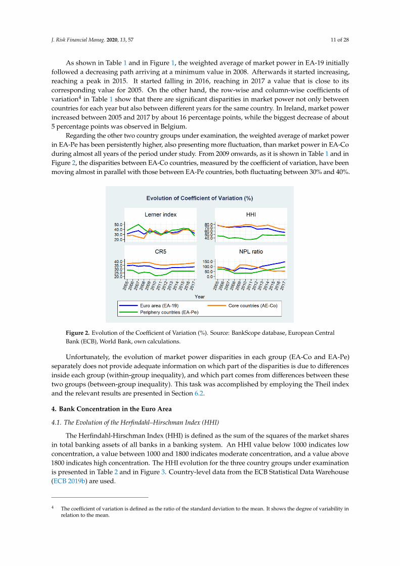
Figure 2. Evolution of the Coefficient of Variation (%). Source: BankScope database, European Central Bank (ECB), World Bank, own calculations.
Unfortunately, the evolution of market power disparities in each group (EA-Co and EA-Pe) separately does not provide adequate information on which part of the disparities is due to differences inside each group (within-group inequality), and which part comes from differences between these two groups (between-group inequality). This task was accomplished by employing the Theil index and the relevant results are presented in Section 6.2.
4. Bank Concentration in the Euro Area
4.1. The Evolution of the Herfindahl–Hirschman Index (HHI)
The Herfindahl-Hirschman Index (HHI) is defined as the sum of the squares of the market shares in total banking assets of all banks in a banking system. An HHI value below 1000 indicates low concentration, a value between 1000 and 1800 indicates moderate concentration, and a value above 1800 indicates high concentration. The HHI evolution for the three country groups under examination is presented in Table 2 and in Figure 3. Country-level data from the ECB Statistical Data Warehouse (ECB 2019b) are used.
The weighted average of HHI in EA-19 peaked in 2014, when it started following a decreasing path arriving in 2017 at a value that is 56 points bigger than the HHI value for 2005. The weighted average of HHI in EA-Co reached a peak in 2011, and started declining thereafter, in contrast to the EA-Pe countries whose weighted average of HHI followed an increasing path reaching a peak in 2017.
On the other hand, the row-wise and column-wise coefficients of variation in Table 2 show that there are significant disparities among the HHI values not only between countries within each year but also between different years for the same country. The biggest decline in HHI values was observed in Belgium, Estonia, and Finland, in contrast to Cyprus and Greece, which presented the biggest increase in HHI values during the period under examination.
Figure 2. Evolution of the Coefficient of Variation (%). Source: BankScope database, European CentralBank (ECB), World Bank, own calculations.
Unfortunately, the evolution of market power disparities in each group (EA-Co and EA-Pe)separately does not provide adequate information on which part of the disparities is due to differencesinside each group (within-group inequality), and which part comes from differences between thesetwo groups (between-group inequality). This task was accomplished by employing the Theil indexand the relevant results are presented in Section 6.2.
4. Bank Concentration in the Euro Area
4.1. The Evolution of the Herfindahl–Hirschman Index (HHI)
The Herfindahl-Hirschman Index (HHI) is defined as the sum of the squares of the market sharesin total banking assets of all banks in a banking system. An HHI value below 1000 indicates lowconcentration, a value between 1000 and 1800 indicates moderate concentration, and a value above1800 indicates high concentration. The HHI evolution for the three country groups under examinationis presented in Table 2 and in Figure 3. Country-level data from the ECB Statistical Data Warehouse(ECB 2019b) are used.
4 The coefficient of variation is defined as the ratio of the standard deviation to the mean. It shows the degree of variability inrelation to the mean.

J. Risk Financial Manag. 2020, 13, 57 12 of 28
Table 2. Evolution of concentration (Herfindahl–Hirschman Index, HHI).
Country 2005 2006 2007 2008 2009 2010 2011 2012 2013 2014 2015 2016 2017 TotalChange
Coeff.Var (%)
Euro Area Core Countries (EA-Co)
Austria 560 534 527 454 414 383 423 395 405 412 397 358 374 −186 18.9Belgium 2112 2041 2079 1881 1622 1439 1294 1061 979 981 998 1017 1102 −1010 22.6Estonia 4039 3593 3410 3120 3090 2929 2613 2493 2483 2445 2409 2406 2419 −1620 40.4Finland 3130 3010 2970 3490 3480 3830 3880 3250 3410 3630 3160 2300 1700 −1430 29.7France 727 726 679 681 605 610 600 545 568 584 589 572 574 −153 18.7
Germany 174 178 183 191 206 301 317 307 266 300 273 277 250 76 16.5Latvia 1176 1270 1158 1205 1181 1005 929 1027 1037 1001 1033 1080 1235 59 14.4
Lithuania 1838 1913 1827 1714 1693 1545 1871 1749 1892 1818 1939 1938 2189 351 27.3Luxembourg 373 333 316 309 310 343 346 345 357 330 321 260 256 −117 26.5Netherlands 1796 1822 1928 2167 2034 2049 2067 2026 2105 2131 2104 2097 2087 291 30.3
Slovakia 1076 1131 1082 1197 1273 1239 1268 1221 1215 1221 1250 1264 1332 256 20.3Coeff. Var (%) 77.8 73.0 72.9 74.3 75.7 79.5 78.5 73.9 75.9 78.1 73.1 67.3 65.0
EA-Co average 711 714 733 757 713 742 767 713 705 746 724 695 663 −48 3.8
Euro Area Periphery Countries (EA-Pe)
Cyprus 1029 1056 1089 1017 1085 1125 1030 1007 1645 1445 1443 1366 1962 933 40.4Greece 1096 1101 1096 1172 1183 1214 1278 1487 2136 2195 2254 2332 2307 1211 29.2Ireland 600 600 700 661 714 700 645 630 671 673 672 636 658 58 60.1
Italy 230 220 328 307 298 410 407 410 406 424 435 452 519 289 13.5Malta 1330 1171 1177 1236 1250 1181 1203 1313 1458 1648 1620 1602 1599 269 12.9
Portugal 1154 1134 1098 1114 1150 1207 1206 1191 1197 1164 1215 1181 1220 66 25.9Slovenia 1369 1300 1282 1268 1256 1160 1142 1115 1045 1026 1077 1147 1133 −236 19.4
Spain 487 442 459 497 507 528 596 654 719 839 896 937 965 478 18.1Coeff. Var (%) 46.0 45.4 39.6 40.6 40.0 35.8 35.9 38.4 49.4 48.6 47.9 48.7 48.0EA-Pe average 480 462 520 526 540 594 604 626 681 726 754 765 812 332 18.6
All Euro Area Countries (EA-19)
Coeff. Var (%) 77.2 73.5 71.3 72.8 72.2 74.1 73.2 66.5 66.6 67.9 63.4 58.9 56.6EA-19 average 647 640 669 685 657 696 717 686 698 740 733 714 703 56 4.5
Notes: Total change is the difference between the value for 2017 and the value for 2005. Coeff. Var (%) stands for the percent Coefficient of Variation measure. All average values areweighted by total banking assets. Source: ECB, own calculations.

J. Risk Financial Manag. 2020, 13, 57 13 of 28
J. Risk Financial Manag. 2020, 13, x FOR PEER REVIEW 12 of 26
Table 2. Evolution of concentration (Herfindahl–Hirschman Index, HHI).
Country 2005 2006 2007 2008 2009 2010 2011 2012 2013 2014 2015 2016 2017 Total Change Coeff. Var (%) Euro Area Core Countries (EA-Co)
Austria 560 534 527 454 414 383 423 395 405 412 397 358 374 −186 18.9 Belgium 2112 2041 2079 1881 1622 1439 1294 1061 979 981 998 1017 1102 −1010 22.6 Estonia 4039 3593 3410 3120 3090 2929 2613 2493 2483 2445 2409 2406 2419 −1620 40.4 Finland 3130 3010 2970 3490 3480 3830 3880 3250 3410 3630 3160 2300 1700 −1430 29.7 France 727 726 679 681 605 610 600 545 568 584 589 572 574 −153 18.7
Germany 174 178 183 191 206 301 317 307 266 300 273 277 250 76 16.5 Latvia 1176 1270 1158 1205 1181 1005 929 1027 1037 1001 1033 1080 1235 59 14.4
Lithuania 1838 1913 1827 1714 1693 1545 1871 1749 1892 1818 1939 1938 2189 351 27.3 Luxembourg 373 333 316 309 310 343 346 345 357 330 321 260 256 −117 26.5 Netherlands 1796 1822 1928 2167 2034 2049 2067 2026 2105 2131 2104 2097 2087 291 30.3
Slovakia 1076 1131 1082 1197 1273 1239 1268 1221 1215 1221 1250 1264 1332 256 20.3
Coeff. Var (%) 77.8 73.0 72.9 74.3 75.7 79.5 78.5 73.9 75.9 78.1 73.1 67.3 65.0
EA-Co average 711 714 733 757 713 742 767 713 705 746 724 695 663 −48 3.8 Euro Area Periphery Countries (EA-Pe)
Cyprus 1029 1056 1089 1017 1085 1125 1030 1007 1645 1445 1443 1366 1962 933 40.4 Greece 1096 1101 1096 1172 1183 1214 1278 1487 2136 2195 2254 2332 2307 1211 29.2 Ireland 600 600 700 661 714 700 645 630 671 673 672 636 658 58 60.1
Italy 230 220 328 307 298 410 407 410 406 424 435 452 519 289 13.5 Malta 1330 1171 1177 1236 1250 1181 1203 1313 1458 1648 1620 1602 1599 269 12.9
Portugal 1154 1134 1098 1114 1150 1207 1206 1191 1197 1164 1215 1181 1220 66 25.9 Slovenia 1369 1300 1282 1268 1256 1160 1142 1115 1045 1026 1077 1147 1133 −236 19.4
Spain 487 442 459 497 507 528 596 654 719 839 896 937 965 478 18.1
Coeff. Var (%) 46.0 45.4 39.6 40.6 40.0 35.8 35.9 38.4 49.4 48.6 47.9 48.7 48.0
EA-Pe average 480 462 520 526 540 594 604 626 681 726 754 765 812 332 18.6 All Euro Area Countries (EA-19)
Coeff. Var (%) 77.2 73.5 71.3 72.8 72.2 74.1 73.2 66.5 66.6 67.9 63.4 58.9 56.6
EA-19 average 647 640 669 685 657 696 717 686 698 740 733 714 703 56 4.5
Notes: Total change is the difference between the value for 2017 and the value for 2005. Coeff. Var (%) stands for the percent Coefficient of Variation measure. All average values are weighted by total banking assets. Source: ECB, own calculations.
Figure 3. Evolution of bank concentration. Source: ECB, own calculations. Figure 3. Evolution of bank concentration. Source: ECB, own calculations.
The weighted average of HHI in EA-19 peaked in 2014, when it started following a decreasingpath arriving in 2017 at a value that is 56 points bigger than the HHI value for 2005. The weightedaverage of HHI in EA-Co reached a peak in 2011, and started declining thereafter, in contrast to theEA-Pe countries whose weighted average of HHI followed an increasing path reaching a peak in 2017.
On the other hand, the row-wise and column-wise coefficients of variation in Table 2 show thatthere are significant disparities among the HHI values not only between countries within each year butalso between different years for the same country. The biggest decline in HHI values was observed inBelgium, Estonia, and Finland, in contrast to Cyprus and Greece, which presented the biggest increasein HHI values during the period under examination.
As it is shown in Table 2 and in Figure 2, the disparities in HHI values between EA-Co countries,measured by the coefficient of variation, reached a peak of about 80% in 2010. Afterwards theyremained at high levels (74%–79%) until 2015 when they started decreasing, arriving at a minimumof 65% in 2017. In contrast, the disparities between EA-Pe countries, started increasing in 2011, afterhaving followed a decreasing path since 2005. In 2013, the disparities between EA-Pe countries reacheda peak of 50%, staying very close to this level thereafter. The decomposition of the HHI disparitiesinto within-group and between-group components, using the Theil inequality index, is presented inSection 6.3.
4.2. The Evolution of the CR5 Concentration Ratio
The CR5 concentration ratio is the sum of the shares of the five largest banks in a banking system.The CR5 evolution for the three country groups under examination is presented in Table 3 and inFigure 3. The weighted average of CR5 in EA-19 peaked in 2014, when it started following a decreasingpath arriving in 2017 at a value that is 4.5% bigger than the CR5 value for 2005. The weighted averageof CR5 in EA-Co reached a peak in 2011, and started declining thereafter, in contrast to EA-Pe whoseweighted average of CR5 followed an increasing path since 2007.
On the other hand, the row-wise and column-wise coefficients of variation in Table 3 show thatthere are significant disparities among the CR5 values not only between countries for each year but alsobetween different years for the same country. The biggest positive evolution for CR5 was observed inGreece, Cyprus, and Spain, in contrast to Belgium and Finland, which presented the biggest decreasein the CR5 value between 2005 and 2017.

J. Risk Financial Manag. 2020, 13, 57 14 of 28
Table 3. Evolution of concentration (market share of the five largest banks, CR5).
Country 2005 2006 2007 2008 2009 2010 2011 2012 2013 2014 2015 2016 2017 TotalChange
Coeff.Var (%)
Euro Area Core Countries (EA-Co)
Austria 0.450 0.438 0.428 0.390 0.372 0.359 0.384 0.365 0.367 0.368 0.358 0.345 0.361 −0.089 8.8Belgium 0.853 0.844 0.834 0.808 0.771 0.749 0.708 0.663 0.640 0.658 0.655 0.662 0.688 −0.165 10.9Estonia 0.981 0.971 0.957 0.948 0.934 0.923 0.906 0.896 0.897 0.899 0.886 0.880 0.903 −0.078 3.6Finland 0.871 0.868 0.861 0.877 0.875 0.892 0.869 0.859 0.871 0.897 0.880 0.805 0.735 −0.136 5.0France 0.519 0.523 0.518 0.512 0.472 0.474 0.483 0.446 0.467 0.476 0.472 0.460 0.454 −0.065 5.5
Germany 0.216 0.220 0.220 0.227 0.250 0.326 0.335 0.330 0.306 0.321 0.306 0.314 0.297 0.081 16.8Latvia 0.673 0.692 0.672 0.702 0.693 0.604 0.596 0.641 0.641 0.636 0.645 0.665 0.735 0.062 6.0
Lithuania 0.806 0.825 0.809 0.813 0.805 0.788 0.847 0.836 0.871 0.857 0.868 0.871 0.901 0.095 4.0Luxembourg 0.345 0.315 0.306 0.297 0.293 0.311 0.312 0.331 0.337 0.320 0.313 0.276 0.262 −0.083 7.5Netherlands 0.845 0.851 0.863 0.867 0.851 0.842 0.836 0.821 0.838 0.850 0.846 0.847 0.838 −0.007 1.4
Slovakia 0.677 0.669 0.682 0.716 0.721 0.720 0.722 0.707 0.703 0.707 0.723 0.727 0.745 0.068 3.1Coeff. Var (%) 37.3 37.9 38.1 38.8 38.7 36.5 35.4 35.4 36.3 36.4 36.9 37.5 38.3
EA-Co average 0.442 0.447 0.454 0.452 0.445 0.468 0.477 0.459 0.457 0.472 0.464 0.460 0.447 0.005 2.4
Euro Area Periphery Countries (EA-Pe)
Cyprus 0.598 0.639 0.649 0.638 0.647 0.642 0.607 0.626 0.641 0.634 0.675 0.658 0.842 0.244 9.2Greece 0.656 0.663 0.677 0.696 0.692 0.706 0.720 0.795 0.940 0.941 0.952 0.973 0.970 0.314 16.7Ireland 0.478 0.490 0.504 0.503 0.526 0.499 0.467 0.464 0.478 0.476 0.459 0.443 0.455 −0.023 4.9
Italy 0.268 0.262 0.331 0.312 0.310 0.398 0.395 0.397 0.396 0.410 0.410 0.430 0.434 0.166 16.6Malta 0.753 0.709 0.702 0.728 0.728 0.713 0.720 0.744 0.765 0.815 0.813 0.803 0.809 0.056 5.6
Portugal 0.688 0.679 0.678 0.691 0.701 0.709 0.708 0.699 0.703 0.692 0.723 0.712 0.731 0.043 2.3Slovenia 0.630 0.620 0.595 0.591 0.597 0.593 0.593 0.584 0.571 0.556 0.592 0.610 0.615 −0.015 3.3
Spain 0.420 0.404 0.410 0.424 0.433 0.443 0.481 0.514 0.544 0.583 0.602 0.618 0.637 0.217 17.3Coeff. Var (%) 28.6 28.3 24.4 25.8 25.4 21.5 21.7 23.2 27.4 27.4 27.3 27.3 27.3EA-Pe average 0.398 0.395 0.424 0.425 0.432 0.467 0.473 0.486 0.502 0.519 0.526 0.537 0.549 0.151 11.3
All Euro Area Countries (EA-19)
Coeff. Var (%) 34.7 35.1 33.8 34.5 33.9 31.2 30.5 30.4 32.0 32.0 32.3 32.6 33.1EA-19 average 0.431 0.433 0.446 0.445 0.442 0.469 0.477 0.469 0.472 0.487 0.483 0.483 0.476 0.045 4.4
Notes: Total change is the difference between the value for 2017 and the value for 2005. Coeff. Var (%) stands for the percent Coefficient of Variation measure. All average values areweighted by total banking assets. Source: ECB, own calculations.

J. Risk Financial Manag. 2020, 13, 57 15 of 28
As it is shown in Table 3 and in Figure 2, the disparities in CR5 values between EA-Co countries,measured by the coefficient of variation, reached a peak of about 39% in 2008, after a continuousincrease from 2005. After a temporary decrease during 2010–2012, they remained at levels rangingbetween 36 and 38%. After having followed a decreasing path since 2005, the disparities betweenEA-Pe countries increased in 2013, remaining afterwards close to 27%. The decomposition of theCR5 disparities into within-group and between-group components, using the Theil inequality index,is presented in Section 6.3.
5. Credit Risk in the Euro Area
Although several years have passed since the onset of the global financial crisis of 2008, manyeuro area banks still have high levels of non-performing loans (NPLs) on their balance sheets. Thenon-performing loans to total gross loans ratio (NPL ratio) reached 3.4% in September 2019 for the euroarea as whole (ECB 2020), following a downward trend after 2012, when it reached an all-time highof around 8%. However, despite this positive evolution for the euro area in total, large dispersionsremain across euro area countries (ratios between 0.9% and 37.4%). Such a large stock of NPLs putsserious constraints on many banks’ lending capacity and their ability to build further capital buffers,thus exerting a strong negative influence on economic growth through the reduction of credit supply.
Bank competition is one of the factors that have been extensively investigated in the pastas one of the major determinants of credit risk, as well as of bank risk in general. In a recentstudy, Karadima and Louri (2019) reached the conclusion that competition exerts a statisticallysignificant and positive impact on NPLs, supporting the “competition-stability” view in banking. Thismotivated us to extend the scope of the present study, by investigating the evolution and convergenceof NPLs in the euro area during the period 2005–2017. The investigation is based on country-level datacollected mainly from the World Bank (2019a, 2019b).
The evolution of NPL ratios for the three country groups under examination is presented inTable 4 and in Figure 4. The weighted average of the NPL ratio in EA-19 peaked in 2013, when it startedfollowing a decreasing path arriving in 2017 at a value 1.6% higher than that of 2005. The weightedaverage of the NPL ratio in EA-Co reached a maximum of 3.4% in 2009 and 2013, and started decliningthereafter, reaching in 2017 a value 0.9% smaller than that of 2005. In contrast, after a very sharp andcontinuous increase, which started in 2008, the weighted average of NPL ratio in EA-Pe reached amaximum of 15.6% in 2014, when it started decreasing arriving in 2017 at a value 8.5% higher than thatof 2005.
J. Risk Financial Manag. 2020, 13, x FOR PEER REVIEW 15 of 26
Country 2005 2006 2007 2008 2009 2010 2011 2012 2013 2014 2015 2016 2017 Total change Coeff. Var (%) Euro area periphery countries (EA-Pe)
Cyprus 7.10 5.40 3.40 3.59 4.51 5.82 9.99 18.37 38.56 44.97 47.75 48.68 40.17 33.07 89.5 Greece 6.30 5.40 4.60 4.67 6.95 9.12 14.43 23.27 31.90 33.78 36.65 36.30 45.57 39.27 75.7 Ireland 0.48 0.53 0.63 1.92 9.80 13.05 16.12 24.99 25.71 20.65 14.93 13.61 11.46 10.98 75.6
Italy 7.00 6.57 5.78 6.28 9.45 10.03 11.74 13.75 16.54 18.03 18.06 17.12 14.38 7.38 39.5 Malta 8.21 6.47 5.31 5.01 5.78 7.02 7.09 7.75 8.95 9.05 6.77 5.32 4.07 −4.14 23.2
Portugal 1.50 1.30 2.85 3.60 5.13 5.31 7.47 9.74 10.62 11.91 17.48 17.18 13.27 11.77 67.7 Slovenia 2.50 2.50 2.50 4.22 5.79 8.21 11.81 15.18 13.31 11.73 9.96 5.07 3.20 0.70 61.7
Spain 0.79 0.70 0.90 2.81 4.12 4.67 6.01 7.48 9.38 8.45 6.16 5.64 4.46 3.67 60.4
Coeff. Var (%) 75.9 72.5 58.9 33.7 33.3 35.4 34.2 44.7 58.4 66.2 75.5 85.5 97.0
EA-Pe average 3.58 3.22 3.05 4.15 7.14 8.07 9.95 12.71 15.32 15.56 14.86 14.08 12.03 8.45 51.6 All euro area countries (EA-19)
Coeff. Var (%) 93.4 91.7 75.6 55.9 87.4 82.6 72.7 84.1 103.7 113.6 126.0 134.6 147.3
EA-19 average 3.27 2.80 2.51 2.98 4.59 4.72 5.35 6.23 7.02 6.72 6.26 5.76 4.90 1.63 32.0
Notes: Total change is the difference between the value for 2017 and the value for 2005. Coeff. Var (%) stands for the percent Coefficient of Variation measure. All average values are weighted by total banking assets. Source: World Bank, own calculations.
Figure 4. Evolution of the NPL ratio. Source: World Bank, own calculations.
On the other hand, the row-wise and column-wise coefficients of variation in Table 4 show that there are significant disparities among the NPL ratios not only between countries within each year but also between different years for the same country. The biggest decline in NPL ratio values was observed in Germany and Malta, in contrast to Cyprus and Greece, which presented the biggest increase in NPL ratios during the period under examination.
After having followed a decreasing path until 2008, as it is shown in Table 4 and Figure 2, the disparities between EA-Co countries, measured by the coefficient of variation, increased sharply in 2009 to a level of about 117%. They started decreasing thereafter, arriving a minimum of 55% in 2017; thus, presenting a clear tendency to converge to lower levels. After having followed a decreasing path until 2011, in 2012 the disparities between EA-Pe countries started increasing continuously, arriving at an all-time peak of 97% in 2017; thus, not showing, in contrast to EA-Co, any sign of convergence to lower levels. By employing the Theil inequality index (see Section 6.4), more information on which part of the disparities is due to differences inside each group (within-group inequality), and which part comes from differences between these two groups (between-group inequality) is provided.
Figure 4. Evolution of the NPL ratio. Source: World Bank, own calculations.

J. Risk Financial Manag. 2020, 13, 57 16 of 28
Table 4. Evolution of credit risk (non-performing loan (NPL) ratio).
Country 2005 2006 2007 2008 2009 2010 2011 2012 2013 2014 2015 2016 2017 Totalchange
Coeff.Var (%)
Euro area core countries (EA-Co)
Austria 2.60 2.74 2.24 1.90 2.25 2.83 2.71 2.81 2.87 3.47 3.39 2.70 2.37 −0.23 16.3Belgium 2.00 1.28 1.16 1.65 3.08 2.80 3.30 3.74 4.24 4.18 3.79 3.43 2.92 0.92 36.6Estonia 0.20 0.20 0.50 1.94 5.20 5.38 4.05 2.62 1.47 1.39 0.98 0.87 0.70 0.50 92.6Finland 0.30 0.20 0.30 0.40 0.60 0.60 0.50 0.50 0.67 1.30 1.34 1.52 1.67 1.37 66.7France 3.50 3.00 2.70 2.82 4.02 3.76 4.29 4.29 4.50 4.16 3.98 3.64 3.08 −0.42 16.5
Germany 4.05 3.41 2.65 2.85 3.31 3.20 3.03 2.86 2.70 2.34 1.97 1.71 1.50 −2.55 26.2Latvia 0.70 0.50 0.80 2.10 14.28 15.93 14.05 8.72 6.41 4.60 4.64 6.26 5.51 4.81 82.0
Lithuania 0.60 1.00 1.00 6.08 23.99 23.33 18.84 14.80 11.59 8.19 4.95 3.66 3.18 2.58 90.4Luxembourg 0.20 0.10 0.40 0.60 0.67 0.25 0.38 0.15 0.21 0.21 0.21 0.90 0.79 0.59 67.7Netherlands 1.20 0.80 1.50 1.68 3.20 2.83 2.71 3.10 3.23 2.98 2.71 2.54 2.31 1.11 34.2
Slovakia 5.00 3.20 2.50 2.49 5.29 5.84 5.61 5.22 5.14 5.35 4.87 4.44 3.70 −1.30 25.6Coeff. Var (%) 92.4 88.5 65.4 67.3 117.2 117.1 106.6 93.2 81.0 64.0 55.6 56.7 55.2
EA-Co average 3.15 2.63 2.28 2.45 3.38 3.20 3.32 3.30 3.38 3.14 2.88 2.62 2.28 −0.87 14.4
Euro area periphery countries (EA-Pe)
Cyprus 7.10 5.40 3.40 3.59 4.51 5.82 9.99 18.37 38.56 44.97 47.75 48.68 40.17 33.07 89.5Greece 6.30 5.40 4.60 4.67 6.95 9.12 14.43 23.27 31.90 33.78 36.65 36.30 45.57 39.27 75.7Ireland 0.48 0.53 0.63 1.92 9.80 13.05 16.12 24.99 25.71 20.65 14.93 13.61 11.46 10.98 75.6
Italy 7.00 6.57 5.78 6.28 9.45 10.03 11.74 13.75 16.54 18.03 18.06 17.12 14.38 7.38 39.5Malta 8.21 6.47 5.31 5.01 5.78 7.02 7.09 7.75 8.95 9.05 6.77 5.32 4.07 −4.14 23.2
Portugal 1.50 1.30 2.85 3.60 5.13 5.31 7.47 9.74 10.62 11.91 17.48 17.18 13.27 11.77 67.7Slovenia 2.50 2.50 2.50 4.22 5.79 8.21 11.81 15.18 13.31 11.73 9.96 5.07 3.20 0.70 61.7
Spain 0.79 0.70 0.90 2.81 4.12 4.67 6.01 7.48 9.38 8.45 6.16 5.64 4.46 3.67 60.4Coeff. Var (%) 75.9 72.5 58.9 33.7 33.3 35.4 34.2 44.7 58.4 66.2 75.5 85.5 97.0EA-Pe average 3.58 3.22 3.05 4.15 7.14 8.07 9.95 12.71 15.32 15.56 14.86 14.08 12.03 8.45 51.6
All euro area countries (EA-19)
Coeff. Var (%) 93.4 91.7 75.6 55.9 87.4 82.6 72.7 84.1 103.7 113.6 126.0 134.6 147.3EA-19 average 3.27 2.80 2.51 2.98 4.59 4.72 5.35 6.23 7.02 6.72 6.26 5.76 4.90 1.63 32.0
Notes: Total change is the difference between the value for 2017 and the value for 2005. Coeff. Var (%) stands for the percent Coefficient of Variation measure. All average values areweighted by total banking assets. Source: World Bank, own calculations.

J. Risk Financial Manag. 2020, 13, 57 17 of 28
On the other hand, the row-wise and column-wise coefficients of variation in Table 4 show thatthere are significant disparities among the NPL ratios not only between countries within each year butalso between different years for the same country. The biggest decline in NPL ratio values was observedin Germany and Malta, in contrast to Cyprus and Greece, which presented the biggest increase in NPLratios during the period under examination.
After having followed a decreasing path until 2008, as it is shown in Table 4 and Figure 2, thedisparities between EA-Co countries, measured by the coefficient of variation, increased sharply in2009 to a level of about 117%. They started decreasing thereafter, arriving a minimum of 55% in 2017;thus, presenting a clear tendency to converge to lower levels. After having followed a decreasing pathuntil 2011, in 2012 the disparities between EA-Pe countries started increasing continuously, arriving atan all-time peak of 97% in 2017; thus, not showing, in contrast to EA-Co, any sign of convergence tolower levels. By employing the Theil inequality index (see Section 6.4), more information on whichpart of the disparities is due to differences inside each group (within-group inequality), and which partcomes from differences between these two groups (between-group inequality) is provided.
6. Theil Inequality for Bank Competition, Concentration, and Credit Risk
6.1. Theil Inequality Index
An inequality index that belongs to the entropy class has the following general form:
GE(α) =1
n(a2 − a)
n∑i=1
[(yi
y)α − 1] (10)
where n is the size of the sample, yi is the i-th observation and y is the mean value of the sample.The parameter α represents the weight given to distances between values at different parts of thedistribution. For smaller values of α, GE(α) is more sensitive to changes in the bottom tail of thedistribution. For higher values of α, GE(α) is more sensitive to changes in the upper tail of thedistribution. The most commonly used values of α are −1, 0, 1 and 2. The most well-known member ofthe entropy class of inequality indices is the GE(1) index, called Theil index (T), by the name of HenriTheil who introduced it in 1967. All the members of the entropy class of inequality indices have theadvantage of being perfectly decomposable (i.e., with a zero residual part).
Following Fernandez de Guevara et al. (2007), the Theil index for bank market power can becalculated from Equation (11):
T =G∑
g=1
shgTw,g + Tb (11)
where T is the total market power inequality, G is the number of observation groups in the sample, shg
is the share in the sample (in terms of total assets) of a group g, Tw,g is the within-group inequality ingroup g and Tb is the between-group inequality.
The within-group inequality in group g is defined by Equation (12):
Tw,g = −
Ng∑i=1
(shishg
)ln(xiµg
) (12)
where Ng is the number of entities (e.g., countries or banks) in group g, shi is the share in the sample (interms of total assets) of an entity i belonging to group g and µg is the weighted average of the Lernerindex of entities belonging to group g.
The between-group inequality is defined by Equation (13):

J. Risk Financial Manag. 2020, 13, 57 18 of 28
Tb = −G∑
g=1
shgln(µg
µ) (13)
where µ is the weighted average of the Lerner index (variable xi) in the sample.
6.2. Theil Inequality for Market Power
The results from the calculation of the total Theil inequality index for the Lerner index of marketpower and its within-group and between-group components are presented in Table 5, as well as inFigures 5 and 6.
J. Risk Financial Manag. 2020, 13, x FOR PEER REVIEW 17 of 26
Table 5. Evolution and decomposition of the Theil inequality index for the euro area core and periphery country groups into within-group and between-group components.
Year
Market Power (Lerner Index)
Concentration (HHI) Concentration (CR5) Credit Risk (NPL Ratio)
Inequality Inequality Inequality Inequality
Total Within -Group
Between-Group
Total Within -Group
Between-Group
Total Within -Group
Between-Group
Total Within -Group
Between-Group
2005 0.099 0.097 (98%)
0.002 (2%)
0.365 0.350 (96%)
0.015 (4%)
0.116 0.115 (99%)
0.001 (1%)
0.280 0.278 (99%)
0.002 (1%)
2006 0.136 0.133 (98%)
0.003 (2%)
0.354 0.336 (95%)
0.018 (5%)
0.112 0.110 (98%)
0.002 (2%)
0.322 0.318 (99%)
0.004 (1%)
2007 0.105 0.100 (95%)
0.005 (5%)
0.323 0.311 (96%)
0.012 (4%)
0.102 0.101 (99%)
0.001 (1%)
0.194 0.185 (95%)
0.009 (5%)
2008 0.099 0.092 (93%)
0.007 (7%)
0.331 0.318 (96%)
0.013 (4%)
0.097 0.096 (99%)
0.001 (1%)
0.108 0.077 (71%)
0.031 (29%)
2009 0.121 0.119 (98%)
0.002 (2%) 0.299
0.291 (97%)
0.008 (3%) 0.081
0.080 (99%)
0.001 (1%) 0.135
0.069 (51%)
0.066 (49%)
2010 0.110 0.101 (92%)
0.009 (8%)
0.229 0.224 (98%)
0.005 (2%)
0.049 0.048 (98%)
0.001 (2%)
0.187 0.087 (47%)
0.100 (53%)
2011 0.095 0.094 (99%)
0.001 (1%)
0.227 0.221 (97%)
0.006 (3%)
0.045 0.044 (98%)
0.001 (2%)
0.229 0.088 (38%)
0.141 (62%)
2012 0.103 0.102 (99%)
0.001 (1%)
0.218 0.216 (99%)
0.002 (1%)
0.045 0.044 (98%)
0.001 (2%)
0.325 0.110 (34%)
0.215 (66%)
2013 0.112 0.111 (99%)
0.001 (1%)
0.249 0.247 (99%)
0.002 (1%)
0.054 0.053 (98%)
0.001 (2%)
0.372 0.102 (27%)
0.270 (73%)
2014 0.134 0.126 (94%)
0.008 (6%)
0.243 0.241 (99%)
0.002 (1%)
0.053 0.052 (98%)
0.001 (2%)
0.400 0.100 (25%)
0.300 (75%)
2015 0.124 0.119 (96%)
0.005 (4%)
0.249 0.247 (99%)
0.002 (1%)
0.059 0.057 (97%)
0.002 (3%)
0.437 0.123 (28%)
0.314 (72%)
2016 0.153 0.152 (99%)
0.001 (1%)
0.237 0.235 (99%)
0.002 (1%)
0.057 0.055 (96%)
0.002 (4%)
0.423 0.097 (23%)
0.326 (77%)
2017 0.164 0.162 (99%)
0.002 (1%)
0.236 0.232 (98%)
0.004 (2%)
0.062 0.058 (94%)
0.004 (6%)
0.421 0.104 (25%)
0.317 (75%)
Total change
0.065 0.065 0.000 −0.129 −0.118 −0.011 −0.054 −0.057 0.003 0.141 −0.174 0.315
Notes: Total change is the difference between the value for 2017 and the value for 2005. The figures in parentheses denote percentages of within-group and between-group inequality over total inequality. Source: BankScope database, ECB, World Bank, own calculations.
Figure 5. Evolution of the within-group and between-group components of the Theil inequality index for the euro area core and periphery country groups. Source: BankScope database, ECB, World Bank, own calculations.
Figure 5. Evolution of the within-group and between-group components of the Theil inequality indexfor the euro area core and periphery country groups. Source: BankScope database, ECB, World Bank,own calculations.J. Risk Financial Manag. 2020, 13, x FOR PEER REVIEW 18 of 26
Figure 6. Decomposition of the Theil inequality index for the euro area core and periphery country groups into percentage within-group and between-group components. Source: BankScope database, ECB, World Bank, own calculations.
As it is shown in Table 5, as well as in Figures 5 and 6, the disparities in market power are due, almost exclusively, to differences inside each group (EA-Co or EA-Pe). The differences between the EA-Co and EA-Pe are negligible. This evolution suggests that there is a clear convergence between the EA-Co and EA-Pe country groups with respect to competition, as measured by the Lerner index of market power. In addition, it is also clear that we need higher granularity, which can be obtained by investigating whether differences in market power stem from inequalities between different countries (between-country inequality) or from inequalities between banks in a given country (within-country inequality). This desired level of granularity can be obtained by the calculation of a Theil inequality index and its decomposition into within-country and between-country components.
The results from the calculation of the total Theil inequality index and its within-country and between-country components are presented in Table 65, as well as in Figures 7 and 8. Figure 7 shows that in 2008 the level of total inequality in bank market power in EA-19 was close to its 2005 level, after a sharp increase of the between-country inequality in 2006. The increase of the Theil inequality index in 2009 indicates that the financial crisis reversed the progress towards lower disparities across countries, suggested by the lower values of the between-country component in the period 2007–2008. In 2011, total inequality was close to its 2008 level, since an increase in within-country inequality in 2011 was accompanied by a decrease in between-country inequality in that year. Total inequality started increasing in 2012, mainly due to an increase in its within-country component, reaching a peak in 2017. The persistence of significant within-country inequalities in market power has also been shown by Cruz-Garcia et al. (2017), who investigate the impact of financial market integration on the evolution of disparities among European banks’ market power using bank-specific data for the EA-12 countries over the period 2000–2014.
5 It should be noted that some expected minor differences (at the third decimal place) in total inequality
between Tables 5 and 6 are due to different data grouping (19 countries vs EA-Co/EA-Pe) and weighting.
Figure 6. Decomposition of the Theil inequality index for the euro area core and periphery countrygroups into percentage within-group and between-group components. Source: BankScope database,ECB, World Bank, own calculations.

J. Risk Financial Manag. 2020, 13, 57 19 of 28
Table 5. Evolution and decomposition of the Theil inequality index for the euro area core and periphery country groups into within-group and between-groupcomponents.
Year
Market Power (Lerner Index) Concentration (HHI) Concentration (CR5) Credit Risk (NPL Ratio)
Inequality Inequality Inequality Inequality
Total Within-Group
Between-Group Total Within-
GroupBetween-
Group Total Within-Group
Between-Group Total Within-
GroupBetween-
Group
2005 0.099 0.097(98%)
0.002(2%) 0.365 0.350
(96%)0.015(4%) 0.116 0.115
(99%)0.001(1%) 0.280 0.278
(99%)0.002(1%)
2006 0.136 0.133(98%)
0.003(2%) 0.354 0.336
(95%)0.018(5%) 0.112 0.110
(98%)0.002(2%) 0.322 0.318
(99%)0.004(1%)
2007 0.105 0.100(95%)
0.005(5%) 0.323 0.311
(96%)0.012(4%) 0.102 0.101
(99%)0.001(1%) 0.194 0.185
(95%)0.009(5%)
2008 0.099 0.092(93%)
0.007(7%) 0.331 0.318
(96%)0.013(4%) 0.097 0.096
(99%)0.001(1%) 0.108 0.077
(71%)0.031(29%)
2009 0.121 0.119(98%)
0.002(2%) 0.299 0.291
(97%)0.008(3%) 0.081 0.080
(99%)0.001(1%) 0.135 0.069
(51%)0.066(49%)
2010 0.110 0.101(92%)
0.009(8%) 0.229 0.224
(98%)0.005(2%) 0.049 0.048
(98%)0.001(2%) 0.187 0.087
(47%)0.100(53%)
2011 0.095 0.094(99%)
0.001(1%) 0.227 0.221
(97%)0.006(3%) 0.045 0.044
(98%)0.001(2%) 0.229 0.088
(38%)0.141(62%)
2012 0.103 0.102(99%)
0.001(1%) 0.218 0.216
(99%)0.002(1%) 0.045 0.044
(98%)0.001(2%) 0.325 0.110
(34%)0.215(66%)
2013 0.112 0.111(99%)
0.001(1%) 0.249 0.247
(99%)0.002(1%) 0.054 0.053
(98%)0.001(2%) 0.372 0.102
(27%)0.270(73%)
2014 0.134 0.126(94%)
0.008(6%) 0.243 0.241
(99%)0.002(1%) 0.053 0.052
(98%)0.001(2%) 0.400 0.100
(25%)0.300(75%)
2015 0.124 0.119(96%)
0.005(4%) 0.249 0.247
(99%)0.002(1%) 0.059 0.057
(97%)0.002(3%) 0.437 0.123
(28%)0.314(72%)
2016 0.153 0.152(99%)
0.001(1%) 0.237 0.235
(99%)0.002(1%) 0.057 0.055
(96%)0.002(4%) 0.423 0.097
(23%)0.326(77%)
2017 0.164 0.162(99%)
0.002(1%) 0.236 0.232
(98%)0.004(2%) 0.062 0.058
(94%)0.004(6%) 0.421 0.104
(25%)0.317(75%)
Total change 0.065 0.065 0.000 −0.129 −0.118 −0.011 −0.054 −0.057 0.003 0.141 −0.174 0.315
Notes: Total change is the difference between the value for 2017 and the value for 2005. The figures in parentheses denote percentages of within-group and between-group inequality overtotal inequality. Source: BankScope database, ECB, World Bank, own calculations.

J. Risk Financial Manag. 2020, 13, 57 20 of 28
As it is shown in Table 5, as well as in Figures 5 and 6, the disparities in market power are due,almost exclusively, to differences inside each group (EA-Co or EA-Pe). The differences between theEA-Co and EA-Pe are negligible. This evolution suggests that there is a clear convergence between theEA-Co and EA-Pe country groups with respect to competition, as measured by the Lerner index ofmarket power. In addition, it is also clear that we need higher granularity, which can be obtained byinvestigating whether differences in market power stem from inequalities between different countries(between-country inequality) or from inequalities between banks in a given country (within-countryinequality). This desired level of granularity can be obtained by the calculation of a Theil inequalityindex and its decomposition into within-country and between-country components.
The results from the calculation of the total Theil inequality index and its within-country andbetween-country components are presented in Table 65, as well as in Figures 7 and 8. Figure 7 showsthat in 2008 the level of total inequality in bank market power in EA-19 was close to its 2005 level,after a sharp increase of the between-country inequality in 2006. The increase of the Theil inequalityindex in 2009 indicates that the financial crisis reversed the progress towards lower disparities acrosscountries, suggested by the lower values of the between-country component in the period 2007–2008.In 2011, total inequality was close to its 2008 level, since an increase in within-country inequality in 2011was accompanied by a decrease in between-country inequality in that year. Total inequality startedincreasing in 2012, mainly due to an increase in its within-country component, reaching a peak in 2017.The persistence of significant within-country inequalities in market power has also been shown byCruz-Garcia et al. (2017), who investigate the impact of financial market integration on the evolutionof disparities among European banks’ market power using bank-specific data for the EA-12 countriesover the period 2000–2014.
J. Risk Financial Manag. 2020, 13, x FOR PEER REVIEW 19 of 26
Table 6. Evolution and decomposition of the Theil inequality index for the Lerner index of market power into within-country and between-country components
Year
Euro Area (EA-19) Core Countries (EA-Co) Periphery Countries (EA-Pe) Inequality Inequality Inequality
Total Within-Country
Between-Country
Total Within-Country
Between-Country
Total Within-Country
Between-Country
2005 0.099 0.064 (65%)
0.035 (35%)
0.096 0.063 (66%)
0.033 (34%)
0.105 0.072 (69%)
0.033 (31%)
2006 0.135 0.063 (47%)
0.072 (53%)
0.137 0.067 (49%)
0.070 (51%)
0.117 0.051 (44%)
0.066 (56%)
2007 0.105 0.068 (65%)
0.037 (35%)
0.084 0.065 (77%)
0.019 (23%)
0.158 0.079 (50%)
0.079 (50%)
2008 0.099 0.071 (72%)
0.028 (28%) 0.096
0.076 (79%)
0.020 (21%) 0.078
0.053 (68%)
0.025 (32%)
2009 0.122 0.061 (50%)
0.061 (50%)
0.107 0.052 (49%)
0.055 (51%)
0.161 0.090 (56%)
0.071 (44%)
2010 0.110 0.055 (50%)
0.055 (50%)
0.081 0.054 (67%)
0.027 (33%)
0.163 0.058 (36%)
0.105 (64%)
2011 0.094 0.073 (78%)
0.021 (22%)
0.084 0.074 (88%)
0.010 (12%)
0.122 0.072 (59%)
0.050 (41%)
2012 0.103 0.069 (67%)
0.034 (33%)
0.079 0.055 (70%)
0.024 (30%)
0.170 0.112 (66%)
0.058 (34%)
2013 0.111 0.079 (71%)
0.032 (29%)
0.105 0.080 (76%)
0.025 (24%)
0.130 0.078 (60%)
0.052 (40%)
2014 0.135 0.094 (70%)
0.041 (30%)
0.120 0.097 (81%)
0.023 (19%)
0.144 0.087 (61%)
0.057 (39%)
2015 0.124 0.071 (57%)
0.053 (43%)
0.106 0.064 (60%)
0.042 (40%)
0.155 0.090 (58%)
0.065 (42%)
2016 0.152 0.102 (67%)
0.050 (33%)
0.149 0.102 (68%)
0.047 (32%)
0.158 0.103 (65%)
0.055 (35%)
2017 0.163 0.126 (77%)
0.037 (23%)
0.153 0.131 (86%)
0.022 (14%)
0.143 0.112 (78%)
0.031 (22%)
Total change 0.064 0.062 0.002 0.057 0.068 −0.011 0.038 0.040 −0.002
Notes: Total change is the difference between the value for 2017 and the value for 2005. The figures in parentheses denote percentages of within-country and between-country inequality over total inequality. Source: BankScope database, own calculations.
Figure 7. Evolution of the within-country and between-country components of the Theil inequality index for the Lerner index of market power. Source: BankScope database, own calculations. Figure 7. Evolution of the within-country and between-country components of the Theil inequalityindex for the Lerner index of market power. Source: BankScope database, own calculations.
The level of total inequality in bank market power in periphery countries was generally higher,presenting also more fluctuations than that of the core countries during almost all years of the periodunder study, mainly due to the higher between-country inequality among periphery countries.
5 It should be noted that some expected minor differences (at the third decimal place) in total inequality between Tables 5and 6 are due to different data grouping (19 countries vs EA-Co/EA-Pe) and weighting.

J. Risk Financial Manag. 2020, 13, 57 21 of 28
Table 6. Evolution and decomposition of the Theil inequality index for the Lerner index of market power into within-country and between-country components
YearEuro Area (EA-19) Core Countries (EA-Co) Periphery Countries (EA-Pe)
Inequality Inequality Inequality
Total Within-Country Between-Country Total Within-Country Between-Country Total Within-Country Between-Country
2005 0.099 0.064(65%)
0.035(35%) 0.096 0.063
(66%)0.033(34%) 0.105 0.072
(69%)0.033(31%)
2006 0.135 0.063(47%)
0.072(53%) 0.137 0.067
(49%)0.070(51%) 0.117 0.051
(44%)0.066(56%)
2007 0.105 0.068(65%)
0.037(35%) 0.084 0.065
(77%)0.019(23%) 0.158 0.079
(50%)0.079(50%)
2008 0.099 0.071(72%)
0.028(28%) 0.096 0.076
(79%)0.020(21%) 0.078 0.053
(68%)0.025(32%)
2009 0.122 0.061(50%)
0.061(50%) 0.107 0.052
(49%)0.055(51%) 0.161 0.090
(56%)0.071(44%)
2010 0.110 0.055(50%)
0.055(50%) 0.081 0.054
(67%)0.027(33%) 0.163 0.058
(36%)0.105(64%)
2011 0.094 0.073(78%)
0.021(22%) 0.084 0.074
(88%)0.010(12%) 0.122 0.072
(59%)0.050(41%)
2012 0.103 0.069(67%)
0.034(33%) 0.079 0.055
(70%)0.024(30%) 0.170 0.112
(66%)0.058(34%)
2013 0.111 0.079(71%)
0.032(29%) 0.105 0.080
(76%)0.025(24%) 0.130 0.078
(60%)0.052(40%)
2014 0.135 0.094(70%)
0.041(30%) 0.120 0.097
(81%)0.023(19%) 0.144 0.087
(61%)0.057(39%)
2015 0.124 0.071(57%)
0.053(43%) 0.106 0.064
(60%)0.042(40%) 0.155 0.090
(58%)0.065(42%)
2016 0.152 0.102(67%)
0.050(33%) 0.149 0.102
(68%)0.047(32%) 0.158 0.103
(65%)0.055(35%)
2017 0.163 0.126(77%)
0.037(23%) 0.153 0.131
(86%)0.022(14%) 0.143 0.112
(78%)0.031(22%)
Total change 0.064 0.062 0.002 0.057 0.068 −0.011 0.038 0.040 −0.002
Notes: Total change is the difference between the value for 2017 and the value for 2005. The figures in parentheses denote percentages of within-country and between-country inequalityover total inequality. Source: BankScope database, own calculations.

J. Risk Financial Manag. 2020, 13, 57 22 of 28
J. Risk Financial Manag. 2020, 13, x FOR PEER REVIEW 20 of 26
Figure 8. Decomposition of the Theil inequality index for the Lerner index of market power into percentage within-country and between-country components. Source: BankScope database, own calculations.
The level of total inequality in bank market power in periphery countries was generally higher, presenting also more fluctuations than that of the core countries during almost all years of the period under study, mainly due to the higher between-country inequality among periphery countries.
As shown in Figure 8, from 2011 to 2017 the between-country inequality was generally much smaller than the within-country inequality across all the three country groups under examination, indicating a decrease in fragmentation in the euro area with respect to market power.
The values of the Lerner index and the Theil inequality index, presented in Tables 1 and 6, respectively, could be biased due to the unbalanced nature of the underlying panel dataset, so we also considered a fully balanced subset of the unbalanced dataset. After the deletion of countries with less than five banks per year, the balanced subset contains 7605 observations from 585 banks from nine euro area countries (Austria, Belgium, France, Germany, Italy, Latvia, Lithuania, Luxembourg, and Slovakia). The results obtained for this group of nine countries were generally in line with the results obtained for EA-19.
6.3. Theil Inequality for Concentration
The results from the calculation of the total Theil inequality index for HHI and its within-group and between-group components are presented in Table 5, as well as in Figures 5 and 6. As it is shown in Table 5, as well as in Figures 5 and 6, the disparities in HHI values are due, almost exclusively, to differences inside each group (EA-Co or EA-Pe). This evolution suggests that there is a clear convergence between the EA-Co and EA-Pe country groups with respect to concentration, as measured by the HHI structural measure. In contrast to the case of the Lerner index, the lack of availability of the bank-level underlying determinants of HHI did not let us to go deeper in order to investigate whether the above-described differences stem from inequalities between different countries (between-country inequality) or from inequalities between banks in a given country (within-country inequality).
The results from the calculation of the total Theil inequality index for CR5 and its within-group and between-group components are presented in Table 5, as well as in Figures 5 and 6. As it is shown in Table 5, as well as in Figures 5 and 6, the disparities in CR5 values are due, almost exclusively, to differences inside each group (EA-Co or EA-Pe). This evolution suggests that there is a clear convergence between the EA-Co and EA-Pe country groups with respect to concentration, as measured by the CR5 structural measure. The lack of availability of the bank-level underlying determinants of CR5 did not let us to go deeper in order to investigate whether these differences stem
Figure 8. Decomposition of the Theil inequality index for the Lerner index of market power intopercentage within-country and between-country components. Source: BankScope database, owncalculations.
As shown in Figure 8, from 2011 to 2017 the between-country inequality was generally muchsmaller than the within-country inequality across all the three country groups under examination,indicating a decrease in fragmentation in the euro area with respect to market power.
The values of the Lerner index and the Theil inequality index, presented in Tables 1 and 6,respectively, could be biased due to the unbalanced nature of the underlying panel dataset, so we alsoconsidered a fully balanced subset of the unbalanced dataset. After the deletion of countries with lessthan five banks per year, the balanced subset contains 7605 observations from 585 banks from nineeuro area countries (Austria, Belgium, France, Germany, Italy, Latvia, Lithuania, Luxembourg, andSlovakia). The results obtained for this group of nine countries were generally in line with the resultsobtained for EA-19.
6.3. Theil Inequality for Concentration
The results from the calculation of the total Theil inequality index for HHI and its within-groupand between-group components are presented in Table 5, as well as in Figures 5 and 6. As it is shownin Table 5, as well as in Figures 5 and 6, the disparities in HHI values are due, almost exclusively,to differences inside each group (EA-Co or EA-Pe). This evolution suggests that there is a clearconvergence between the EA-Co and EA-Pe country groups with respect to concentration, as measuredby the HHI structural measure. In contrast to the case of the Lerner index, the lack of availability of thebank-level underlying determinants of HHI did not let us to go deeper in order to investigate whetherthe above-described differences stem from inequalities between different countries (between-countryinequality) or from inequalities between banks in a given country (within-country inequality).
The results from the calculation of the total Theil inequality index for CR5 and its within-groupand between-group components are presented in Table 5, as well as in Figures 5 and 6. As it is shownin Table 5, as well as in Figures 5 and 6, the disparities in CR5 values are due, almost exclusively,to differences inside each group (EA-Co or EA-Pe). This evolution suggests that there is a clearconvergence between the EA-Co and EA-Pe country groups with respect to concentration, as measuredby the CR5 structural measure. The lack of availability of the bank-level underlying determinants ofCR5 did not let us to go deeper in order to investigate whether these differences stem from inequalitiesbetween different countries (between-country inequality) or from inequalities between banks in a givencountry (within-country inequality).
J. Risk Financial Manag. 2020, 13, 57 23 of 28
6.4. Theil Inequality for Credit Risk (NPL Ratio)
The results from the calculation of the total Theil inequality index for the NPL ratio and itswithin-group and between-group components are presented in Table 5, as well as in Figures 5 and 6.As it is shown in Table 5, as well as in Figures 5 and 6, the between-group component of the Theilindex (disparities due to differences between EA-Co and EA-Pe) presented a sharp increase in 2008,when it started following a continuously increasing path until 2013, afterwards fluctuating slightly tothe end of 2017. This evolution shows that there is a clear divergence between the EA-Co and EA-Pecountry groups with respect to credit risk, as measured by the NPL ratio. The lack of availabilityof the underlying bank-level NPL data did not let us to go deeper in order to investigate whetherthe above-described differences stem from inequalities between different countries (between-countryinequality) or from inequalities between banks in a given country (within-country inequality).
7. Convergence Analysis
The evolution of the coefficient of variation, presented in Table 1 and in Figure 2, provides usefulinformation about changes of inequality in Lerner index values across countries and/or years. However,the visual inspection of these changes cannot always provide safe results regarding the existence ofconvergence or divergence in terms of the Lerner index across euro area countries during a givenperiod, especially when the Lerner index has presented significant ups and downs along this period.The same situation holds in the case of the two concentration measures (HHI/CR5) and the NPL ratio.
To overcome these problems, we employ two concepts of convergence, namely β-convergenceand σ-convergence (Barro and Sala-i-Martin 1991), which have been prevailing for many years in thegrowth literature. β-convergence applies if poor countries tend to catch up with rich ones in termsof per capita income or product levels. In the case of competition, β-convergence would apply ifcountries with lower levels of competition were found to tend to catch up with countries with higherlevels of competition. On the other hand, σ-convergence applies if the dispersion of per capita incomeor product across countries declines over time. The existence of β-convergence is a necessary but notsufficient condition for σ-convergence. Regarding competition, σ-convergence would apply if thedispersion of competition levels across countries showed a tendency to decline over time.
In the case of competition, the β-convergence test is performed through the estimation ofEquation (14).
ln(
CitCi,t−1
)= α+ βlnCi,t−1 +
∑Countryi + εit (14)
where Cit is the level of competition, as expressed by the (inverse of) the Lerner index, in country i inyear t, α and β are parameters to be estimated, Countryi are dummy variables to control for possiblecountry effects, and εit is a random error term. There is β-convergence when the coefficient β in (14)is statistically significant and negative. A higher absolute value of the coefficient β corresponds to agreater tendency towards β-convergence.
Following Lapteacru (2018), the σ-convergence test is performed through the estimation ofEquation (15):
Dit = α+ σT +∑
Countryi + εit (15)
where Dit is the absolute value of the difference between the competition in country i in year t andthe average competition in year t, T is a time trend, α and σ are parameters to be estimated, Countryiare dummy variables to control for possible country effects, and εit is a random error term. There isσ-convergence when the coefficient σ in (15) is statistically significant and negative. A higher absolutevalue of the coefficient σ corresponds to a greater tendency towards σ-convergence.
The estimation of Equations (14) and (15) is performed by applying Ordinary Least Squares (OLS)regressions. A same type convergence analysis, as that described for competition, was also performedfor concentration (HHI/CR5) and NPLs. The results, which are presented in Table 7, cover the totalperiod under study (i.e., 2005–2017), as well as two important sub-periods: (a) the period 2008–2012,
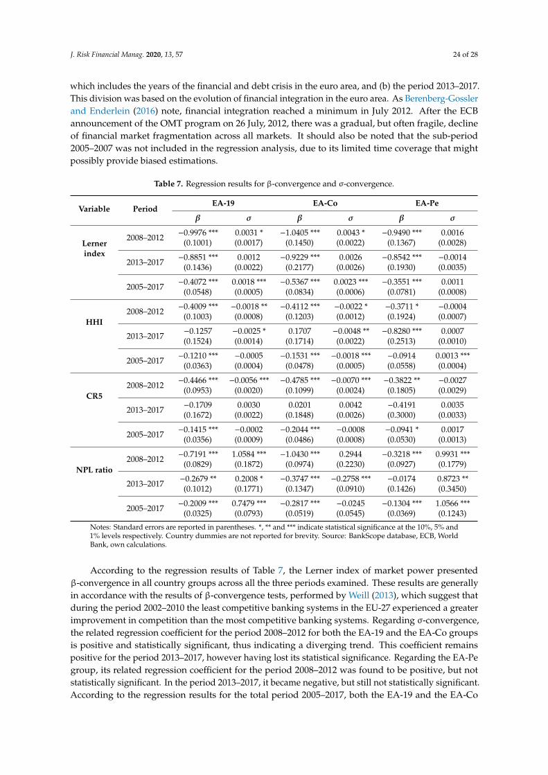
J. Risk Financial Manag. 2020, 13, 57 24 of 28
which includes the years of the financial and debt crisis in the euro area, and (b) the period 2013–2017.This division was based on the evolution of financial integration in the euro area. As Berenberg-Gosslerand Enderlein (2016) note, financial integration reached a minimum in July 2012. After the ECBannouncement of the OMT program on 26 July, 2012, there was a gradual, but often fragile, declineof financial market fragmentation across all markets. It should also be noted that the sub-period2005–2007 was not included in the regression analysis, due to its limited time coverage that mightpossibly provide biased estimations.
Table 7. Regression results for β-convergence and σ-convergence.
Variable PeriodEA-19 EA-Co EA-Pe
β σ β σ β σ
Lernerindex
2008–2012 −0.9976 ***(0.1001)
0.0031 *(0.0017)
−1.0405 ***(0.1450)
0.0043 *(0.0022)
−0.9490 ***(0.1367)
0.0016(0.0028)
2013–2017 −0.8851 ***(0.1436)
0.0012(0.0022)
−0.9229 ***(0.2177)
0.0026(0.0026)
−0.8542 ***(0.1930)
−0.0014(0.0035)
2005–2017 −0.4072 ***(0.0548)
0.0018 ***(0.0005)
−0.5367 ***(0.0834)
0.0023 ***(0.0006)
−0.3551 ***(0.0781)
0.0011(0.0008)
HHI2008–2012 −0.4009 ***
(0.1003)−0.0018 **(0.0008)
−0.4112 ***(0.1203)
−0.0022 *(0.0012)
−0.3711 *(0.1924)
−0.0004(0.0007)
2013–2017 −0.1257(0.1524)
−0.0025 *(0.0014)
0.1707(0.1714)
−0.0048 **(0.0022)
−0.8280 ***(0.2513)
0.0007(0.0010)
2005–2017 −0.1210 ***(0.0363)
−0.0005(0.0004)
−0.1531 ***(0.0478)
−0.0018 ***(0.0005)
−0.0914(0.0558)
0.0013 ***(0.0004)
CR52008–2012 −0.4466 ***
(0.0953)−0.0056 ***
(0.0020)−0.4785 ***
(0.1099)−0.0070 ***
(0.0024)−0.3822 **(0.1805)
−0.0027(0.0029)
2013–2017 −0.1709(0.1672)
0.0030(0.0022)
0.0201(0.1848)
0.0042(0.0026)
−0.4191(0.3000)
0.0035(0.0033)
2005–2017 −0.1415 ***(0.0356)
−0.0002(0.0009)
−0.2044 ***(0.0486)
−0.0008(0.0008)
−0.0941 *(0.0530)
0.0017(0.0013)
NPL ratio2008–2012 −0.7191 ***
(0.0829)1.0584 ***(0.1872)
−1.0430 ***(0.0974)
0.2944(0.2230)
−0.3218 ***(0.0927)
0.9931 ***(0.1779)
2013–2017 −0.2679 **(0.1012)
0.2008 *(0.1771)
−0.3747 ***(0.1347)
−0.2758 ***(0.0910)
−0.0174(0.1426)
0.8723 **(0.3450)
2005–2017 −0.2009 ***(0.0325)
0.7479 ***(0.0793)
−0.2817 ***(0.0519)
−0.0245(0.0545)
−0.1304 ***(0.0369)
1.0566 ***(0.1243)
Notes: Standard errors are reported in parentheses. *, ** and *** indicate statistical significance at the 10%, 5% and1% levels respectively. Country dummies are not reported for brevity. Source: BankScope database, ECB, WorldBank, own calculations.
According to the regression results of Table 7, the Lerner index of market power presentedβ-convergence in all country groups across all the three periods examined. These results are generallyin accordance with the results of β-convergence tests, performed by Weill (2013), which suggest thatduring the period 2002–2010 the least competitive banking systems in the EU-27 experienced a greaterimprovement in competition than the most competitive banking systems. Regarding σ-convergence,the related regression coefficient for the period 2008–2012 for both the EA-19 and the EA-Co groupsis positive and statistically significant, thus indicating a diverging trend. This coefficient remainspositive for the period 2013–2017, however having lost its statistical significance. Regarding the EA-Pegroup, its related regression coefficient for the period 2008–2012 was found to be positive, but notstatistically significant. In the period 2013–2017, it became negative, but still not statistically significant.According to the regression results for the total period 2005–2017, both the EA-19 and the EA-Co

J. Risk Financial Manag. 2020, 13, 57 25 of 28
groups experienced a diverging trend of market power, while the regression coefficient for the EA-Pegroup is positive, but not statistically significant.
The adverse evolution of the σ-convergence of market power during the period under examinationmay be attributed to the 2008 crisis, which led to distortions in competition created by the state aidgranted to banks, while mergers were allowed without taking into account their effects on marketpower (Maudos and Vives 2019).
The σ-convergence related regression coefficient of the HHI concentration measure for both theEA-19 and the EA-Co groups in the period 2008–2012 is negative and statistically significant; thus,indicating a converging trend. The corresponding regression coefficient for the EA-Pe group is alsonegative, but not statistically significant. Its sign turned to positive in the period 2013–2017, with thecoefficient remaining not statistically significant. In addition, the HHI concentration measure didnot present β-convergence in the case of both the EA-19 and the EA-Co groups during this period.Finally, the EA-Co group was the only one that experienced σ-convergence during the total period2005–2017. From 2008 to 2012, both the EA-19 and the EA-Co groups experienced σ-convergence ofthe CR5 concentration measure, in contrast to the EA-Pe group, the regression coefficient of which wasfound to be negative, but not statistically significant. The CR5 concentration measure did not presentβ-convergence during the period 2013–2017 in any of the three country groups under examination.The regression results also show that none of the three groups experienced σ-convergence during thetotal period 2005–2017, with the situation being worse in the case of EA-Pe group.
The observed diverging trends in concentration, measured by the HHI and CR5 concentrationindices, were caused by the global financial crisis of 2008, which accelerated the pace of bankconcentration in the countries that had been hit most severely by the crisis and whose banking systemshad been subject to restructuring (Maudos and Vives 2019). Concentration in Cyprus and Greece,which were already characterized by highly concentrated banking systems, increased further duringthe crisis period, widening the gap with Italy, which has the lowest bank concentration in the EA-Pegroup, including strong cooperative and savings banking sectors (ECB 2016). Regarding the EA-Cogroup, which was affected less than the EA-Pe group by the global financial crisis, the observeddiverging trends in concentration during the period 2013–2017 may be attributed to the fact that incountries, such as Austria, France, and Luxembourg, which were already characterized by very lowbank concentration, concentration decreased further, widening the gap with other more concentratedbanking systems in the EA-Co group.
During the period 2008–2012, both the EA-19 and the EA-Pe groups experienced lack ofσ-convergence with respect to the NPL ratio, while the related regression coefficient for the EA-Cogroup was found to be positive, but not statistically significant. The situation for the EA-Co groupchanged in the period 2013–2017, since the related regression coefficient not only changed to negativebut also became statistically significant; thus, suggesting a clear convergence. In the case of theEA-19 group, the related regression coefficient remained positive. Finally, the NPL ratio did notpresent β-convergence in the case of the EA-Pe group during the period 2013–2017. Regarding thetotal period 2005–2017, both the EA-19 and the EA-Pe groups experienced a clear divergence, incontrast to the EA-Co group, the regression coefficient of which was found to be negative, albeit notstatistically significant.
The convergence of the NPL ratio in the EA-Co group during the period 2013–2017 may beattributed to the fact that the countries of this group are characterized by low or relatively low levels ofNPLs. Although the NPL levels increased enormously in Latvia and Lithuania at the outburst of thecrisis, they entered into a very sharp decreasing path afterwards. On the contrary, the divergence ofthe NPL ratio in the EA-Pe countries may be attributed to the fact that these countries experiencedhigher levels of NPLs than the EA-Co countries during the crisis, which remain very high in the case ofCyprus and Greece.

J. Risk Financial Manag. 2020, 13, 57 26 of 28
8. Conclusions
In this study, we examined the evolution of competition (through market power and concentration)and credit risk (through non-performing loans) across euro area core (EA-Co), periphery (EA-Pe) andall 19 countries (EA-19) in the period 2005–2017, as well as in two sub-periods, 2008–2012 and 2013–2017.Furthermore, we tested two hypotheses with respect to competition, concentration and credit risk:(a) the existence of fragmentation in the euro area as a whole (EA-19), as well as in core countries(EA-Co) and periphery countries (EA-Pe), and (b) the presence of β-convergence and σ-convergenceamong the country-members of each of the three groups.
Our analysis extends beyond the period of financial crisis, thereby taking into account thenon-standard measures adopted by the ECB to support further integration. By using data from all the19 euro area countries, which have a common currency and a single bank supervisory mechanism,a possible bias that might stem from the use of either heterogeneous data or data coming from onlya subset of euro area countries was eliminated, allowing for robust testing of fragmentation andconverging or diverging trends. In addition to uncovering the evolution of bank competition and risk,providing substantiated clues to policy makers about the progress of integration was a major aim ofour research.
Competition (as expressed by the inverse of the Lerner index of market power) reached a minimumin 2015 and increased afterwards in all three country groups under examination (EA-19, EA-Co andEA-Pe), in line with a gradual but fragile post-crisis reintegration trend. This is supported by theTheil inequality index for market power, which reveals a decrease of the between-country inequalityfrom 2011 onwards in each of the three groups. This evolution was also confirmed by means ofβ-convergence and σ-convergence tests, which showed a decrease in divergence of competition.Another finding is that the global financial crisis reversed the advances in competitive pressure thathad been observed during the preceding few years.
With respect to concentration, as measured by the HHI and CR5 concentration indices, the averageconcentration in EA-19 and EA-Co started decreasing in 2015 and 2012, respectively, in contrast toEA-Pe, where concentration has followed a continuously increasing path since 2007. The progress thathad been made during the period 2008–2012 with the achievement of β-convergence and σ-convergencein the whole euro area and the core countries was reversed in the period 2013–2017. Periphery countriesdid not experience convergence of concentration in either of the two periods 2008–2012 and 2013–2017.
Regarding credit risk, NPL ratios have always been higher in EA-Pe. Moreover, while the weightedaverage of the NPL ratio in EA-Co peaked in 2013 at 3.38%, in EA-Pe the peak of 15.56% was in 2014. Thedecrease thereafter has not been proportional between the two groups, in line with the β-convergenceand σ-convergence tests, which indicate that the EA-Co group experienced β-convergence andσ-convergence in the period 2013–2017, while the EA-Pe group has been characterized by divergence.The Theil inequality index confirms the divergence between the two groups, indicating that theinequality between the EA-Co and the EA-Pe groups has been continuously increasing since 2008. Thisevolution suggests that the presence of persistent large stocks of NPLs remains a pressing challenge,which contributes to fragmentation between euro area countries. Hence, more effective measures, suchas the creation of asset management companies, NPL transaction platforms, securitization, or stateguarantees schemes, should be introduced in order not only to reduce the existing NPL volumes, butalso to prevent their increase in the future.
All in all, the persistence of fragmentation, in spite of some partial reintegration trends, suggeststhat policy measures accelerating convergence of our variables would not only strengthen financialintegration, but also help in establishing a real euro area banking union.
Author Contributions: Conceptualization, M.K. and H.L.; methodology, M.K. and H.L.; software, M.K.; validation,M.K.; formal analysis, M.K.; investigation, M.K.; resources, M.K.; data curation, M.K.; writing—original draftpreparation, M.K.; writing—review and editing, M.K. and H.L.; visualization, M.K. and H.L.; supervision, H.L.;project administration, H.L.; funding acquisition, H.L. All authors have read and agreed to the published versionof the manuscript.

J. Risk Financial Manag. 2020, 13, 57 27 of 28
Funding: Financial assistance from the Research Centre of the Athens University of Economics and Business.
Acknowledgments: The authors would like to thank participants at the ASSET Conference (Athens 2019), FEBSConferences (Athens 2019; Prague 2019), JIMF Conference (Marrakech 2019), and EBES Conference (Kuala Lumpur2020), for discussing and commenting on many of the research questions and approaches of this paper.
Conflicts of Interest: The authors declare no conflict of interest.
References
Al-Eyd, Ali, and Pelin Berkmen. 2013. Fragmentation and Monetary Policy in the Euro Area. Working Paper No.13/208, International Monetary Fund, Washington, DC, USA.
Anastasiou, Dimitrios, Helen Louri, and Mike Tsionas. 2019. Non-Performing Loans in the Euro-area: AreCore-Periphery Banking Markets Fragmented? International Journal of Finance and Economics 24: 97–112.[CrossRef]
Angelini, Paolo, and Nicola Cetorelli. 2003. The Effects of Regulatory Reform on Competition in the BankingIndustry. Journal of Money, Credit and Banking 35: 663–84. [CrossRef]
Apergis, Nicholas, Irene Fafaliou, and Michael L. Polemis. 2016. New evidence on assessing the level ofcompetition in the European Union banking sector: A panel data approach. International Business Review 25:395–407. [CrossRef]
Baele, Lieven, Annalisa Ferrando, Peter Hördahl, Elizaveta Krylova, and Cyril Monnet. 2004. Measuring FinancialIntegration in the Euro Area. Occasional Paper No. 14. Frankfurt: European Central Bank.
Barro, Robert J., and Xavier Sala-i-Martin. 1991. Convergence across states and regions. Brookings Papers onEconomic Activity 1: 107–82. [CrossRef]
Berenberg-Gossler, Paul, and Henrik Enderlein. 2016. Financial Market Fragmentation in the Euro Area: State of Play.Policy Paper No. 177. Berlin: Jacques Delors Institut.
Bikker, Jacob A., and Katharina Haaf. 2002. Competition, concentration and their relationship: An empiricalanalysis of the banking industry. Journal of Banking and Finance 26: 2191–214. [CrossRef]
Bikker, Jacob A., and Laura Spierdijk. 2008. How Banking Competition Changed over Time. Working Paper No.167, De Netherlandsche Bank, Amsterdam, The Netherlands.
Boone, Jan. 2008. A new way to measure competition. Economic Journal 118: 1245–61. [CrossRef]Casu, Barbara, and Claudia Girardone. 2009. Competition issues in European banking. Journal of Financial
Regulation and Compliance 17: 119–33. [CrossRef]Claessens, Stijn. 2019. Fragmentation in Global Financial Markets: Good or Bad for Financial Stability? BIS
Working Papers No. 815, Bank for International Settlements, Basel, Switzerland.Coccorese, Paolo. 2004. Banking competition and macroeconomic conditions: A disaggregate Analysis. Journal of
International Financial Markets, Institutions and Money 14: 203–19. [CrossRef]Cruz-Garcia, Paula, Juan Fernandez de Guevara, and Joaquin Maudos. 2017. The evolution of market power in
European banking. Finance Research Letters 23: 257–62. [CrossRef]De Bandt, Olivier, and E. Philip Davis. 2000. Competition, contestability and market structure in European
banking sectors on the eve of EMU. Journal of Banking and Finance 24: 1045–66. [CrossRef]De Sola Perea, Maite, and Christophe Van Nieuwenhuyze. 2014. Financial integration and fragmentation in the euro
area. Economic Review, 99-125, June. Brussels: National Bank of Belgium.ECB. 2003. The Integration of Europe’s Financial Markets. European Central Bank Monthly Bulletin. Frankfurt:
European Central Bank.ECB. 2016. Report on Financial Structures. Frankfurt: European Central Bank.ECB. 2018. Financial integration in Europe. Frankfurt: European Central Bank.ECB. 2019a. Statistical Data Warehouse: Balance Sheet Items Statistics. Available online: https://sdw.ecb.europa.
eu/browse.do?node=1491 (accessed on 3 September 2019).ECB. 2019b. Statistical Data Warehouse: Banking Structural Financial Indicators Statistics. Available online:
https://sdw.ecb.europa.eu/browseSelection.do?node=9689719 (accessed on 3 September 2019).ECB. 2020. Supervisory Banking Statistics—Third Quarter 2019. Frankfurt: European Central Bank.Fernandez de Guevara, Juan, Joaquin Maudos, and Francisco Perez. 2007. Integration and competition in the
European financial markets. Journal of International Money and Finance 26: 26–45. [CrossRef]FSB. 2019. FSB Report on Market Fragmentation. Basel: Financial Stability Board.

J. Risk Financial Manag. 2020, 13, 57 28 of 28
Gischer, Horst, and Mike Stiele. 2008. Competition Tests with a Non-Structural Model: The Panzar–Rosse MethodApplied to Germany’s Savings Banks. German Economic Review 10: 50–70. [CrossRef]
Goddard, John, Hong Liu, Phil Molyneux, and John O. S. Wilson. 2013. Do Bank Profits Converge? EuropeanFinancial Management 19: 345–65. [CrossRef]
Hondroyiannis, George, Sarantis Lolos, and Evangelia Papapetrou. 1999. Assessing competitive conditions in theGreek banking system. Journal of International Financial Markets, Institutions and Money 9: 377–91. [CrossRef]
Jondrow, James, C. A. Knox Lovell, Ivan S. Materov, and Peter Schmidt. 1982. On the estimation of technicalinefficiency in the stochastic frontier production function model. Journal of Econometrics 19: 233–38. [CrossRef]
Karadima, Maria, and Helen Louri. 2019. Non-Performing Loans in the Euro Area: Does Market Power Matter?Working Paper No. 271, Bank of Greece, Athens, Greece.
Kumbhakar, Subal C., Sjur Baardsen, and Gudbrand Lien. 2012. A new method for estimating market power withan application to Norwegian sawmilling. Review of Industrial Organization 40: 109–29. [CrossRef]
Lapteacru, Ion. 2018. Convergence of bank competition in Central and Eastern European countries: do foreignand domestic banks go hand in hand? Post-Communist Economies 30: 588–616. [CrossRef]
Lerner, Abba P. 1934. The concept of monopoly and the measurement of monopoly power. Review of EconomicStudies 1: 157–75. [CrossRef]
Louri, Helen, and Petros Migiakis. 2019. Bank lending margins in the euro area: Funding conditions, fragmentationand ECB’s policies. Review of Financial Economics 37: 482–505. [CrossRef]
Lucotte, Yannick. 2015. Euro area banking fragmentation in the aftermath of the crisis: A cluster analysis. AppliedEconomics Letters 22: 1046–50. [CrossRef]
Magnus, Marcel, Alienor Margerit, Benoit Mesnard, and Christina Katopodi. 2017. Non-Performing Loans inthe Banking Union—Stocktaking and Challenges. European Parliament Briefing, 13 July. Brussels: EuropeanParliament.
Maudos, Joaquin, and Xavier Vives. 2019. Competition Policy in Banking in the European Union. Review ofIndustrial Organization 55: 27–54. [CrossRef]
Moch, Nils. 2013. Competition in fragmented markets: New evidence from the German banking industry in thelight of the subprime crisis. Journal of Banking and Finance 37: 2908–19. [CrossRef]
Panzar, John C., and James N. Rosse. 1987. Testing for “monopoly” equilibrium. Journal of Industrial Economics 35:443–56. [CrossRef]
Phillips, Peter, and Donggyu Sul. 2007. Transition modeling and econometric convergence tests. Econometrica 75:1771–855. [CrossRef]
Staikouras, Christos K., and Anastasia Koutsomanoli-Filippaki. 2006. Competition and Concentration in the NewEuropean Banking Landscape. European Financial Management 12: 443–82. [CrossRef]
Sun, Yu. 2009. Recent Developments in European Bank Competition. Working Paper No. 11/146, InternationalMonetary Fund, Washington, DC, USA.
Weill, Laurent. 2013. Bank competition in the EU: How has it evolved? Journal of International Financial Markets,Institutions and Money 26: 100–12. [CrossRef]
World Bank. 2019a. World Development Indicators Database. Available online: https://databank.worldbank.org/
source/world-development-indicators (accessed on 28 October 2019).World Bank. 2019b. Global Financial Development Database. Available online: https://datacatalog.orldbank.org/
dataset/global-financial-development (accessed on 28 October 2019).
© 2020 by the authors. Licensee MDPI, Basel, Switzerland. This article is an open accessarticle distributed under the terms and conditions of the Creative Commons Attribution(CC BY) license (http://creativecommons.org/licenses/by/4.0/).