CEIS Tor Vergata RESEARCH PAPER SERIES

Vol. 10, Issue 8, No. 240 – July 2012

Can Portfolio Diversification increase

Systemic Risk? Evidence from the U.S

and European Mutual Funds Market

Claudio Dicembrino and Pasquale Lucio Scandizzo

Can Portfolio Diversification increase Systemic

Risk? Evidence from the U.S and European Mutual

Funds Market∗

Claudio Dicembrino

Enel SpA, Department of Strategic Planning andCenter for Economics and International Studies (CEIS)

University of Rome “Tor Vergata”claudio.dicembrino@enel.com

Pasquale Lucio Scandizzo

Center for Economics and International Studies (CEIS)University of Rome “Tor Vergata”scandizzo@economia.uniroma2.it

June 13, 2012

Abstract

This paper tests the hypothesis that portfolio diversification canincrease the threat of systemic financial risk. The paper provides firsta theoretical rationale for the possibility that systemic risk may beincreased by the proliferation of financial instruments that lead oper-ators to hold increasingly similar portfolios. Secondly, the paper teststhe hypothesis that diversification may result in increasing systematicrisk, by analyzing the portfolio dynamics of some of the major worldopen funds.

Keywords: portfolio diversification, financial stability, systemic risk,CAPM.

Jel Numbers: G01, G11, G32.

∗

The views expressed in this article are solely those of the authors and do not involve the

responsibility of the institutions of affiliation. All other usual disclaimers apply. Corresponding

author: Claudio Dicembrino. E-mail: claudio.dicembrino@enel.com.

1 Introduction

“I feel very strongly that we need a regulator that’s independent,got more muscle, and a number of other changes...

I also know people feel very strongly on both sides of this issue.I’ve never witnessed anything quite like this.

It’s the closest thing I’ve seen to a holy war.”

Paulson speech at the House of Representatives’ budget committee (7 February 2007).

This paper contributes to the growing literature on the link between port-folio diversification and its implications on the question of systemic risk. Wefirst show that the introduction of any contingent claim, whose value is cor-related with the value of the assets owned by a population of heterogeneousagents, causes an improvement of the agents expected utility. At the sametime, such an introduction will increase overall systemic risk. These effectsare due to the cumulative interaction of two distinct, but closely linked fac-tors:

(i) The gain obtained from diversifying one’s portfolio, thus reducing riskexposure through risk sharing;

(ii) The gain obtained through risk shifting from higher to lower riskaversion agents.

We test the hypothesis on the negative relationship between diversifica-tion and systemic risk by estimating a simultaneous equation model on apanel of the 226 largest mutual funds (based on size)1. In particular, weuse 162 funds to analyze the US market and 64 funds for the Europeanarea, exchanged in the market between January 2003 and March 2010. Theplan of the paper is as follows. In section 1, we review the basic conceptsand some of the recent literature on systemic risk. In section 2, we look inparticular at the relationship between diversification and systemic risk. InSection 3, we develop a theoretical model that captures the essence of thisrelationship, by analyzing the effects on both diversification and systemicrisks of the issuance of an additional security. In section 4 we describe thedata set. In section 5 we present the econometric analysis and the resultsobtained. In section 6 we discuss some conclusive remarks.

1The largest funds are chosen by size. Having our database comprised of 226 mutualfunds exchanged in n different countries, we divide these mutual funds into three widemacro-areas of affiliation. Europe = Austria, Belgium, Finland, France, Germany, Ireland,Italy, Luxembourg, Netherlands, Portugal, Spain, Sweden, Switzerland and the UnitedKingdom. North America = United States, Canada and Mexico

2

Figure 1: Interbank market spreads (basis points)

Author Elaborations on Bloomberg Database. Note: Spreads are the differences between3-month Euribor / Libor and Overnight Index Swap rates, in basis points

2 On the Meaning and the Measure of Systemic Risk

In the context of analysis of financial instability, an active debate hasemerged around how to define both a systemic event,systemic risk, and theireffects. Despite the considerable amount of literature on the topic, no sharedconsensus exists about the meaning, features and its policy implications ofthese concepts. Highlighting the complexity of this issue, Alan Greenspan(1994), as chair of the FED, has underlined that “the very definition of sys-temic risk is somewhat unsettled” [29].

Macro-level analyses of systemic risk can be found in several works ofthe past two decades. Kaufman 2003 [37] refers to systemic risk as riskor probability of collapse in an entire financial system. Bartholomew etal.(1995)[7] examine, within the systemic risk spreading mechanism, its ef-fect not only on the domestic economy but also on the entire internationalbanking, financial, or economic system. Mishkin (1995)[43] focuses on the in-vestment repercussions of such an important event. Allen and Gale (2000)[5]analyze the cause-effect process through which macro-shocks can spark con-tagion episodes and bank runs. Bordo et al. (1998)[10] define systemicrisk as a situation where “shocks to one part of the financial system leadto shocks elsewhere, in turn impinging on the stability of the real economy”(pp. 31). In their exhaustive review of the literature, De Bandt and Hart-mann (2000)[15] offer a similar view of a systemic event, saying that it takes

3

place when a shock affects “a considerable number of financial institutionsor markets in strong sense” (p. 11). De Nicolo and Kwast (2002)[16], andDow (2000)[22], define systemic risk as a mechanism that, at the same timeof the shock, affects the entire financial system while Lehar (2005) says thata “systemic crisis can be defined as an event in which a considerable numberof financial institutions default simultaneously”.

The search of micro foundations of systemic risk across shock-transmissionsand spillover effects on the entire financial system has given rise to anotherstrand of literature. The following contributions emphasize causation mech-anisms requiring close and direct connections among several institutions anddifferent markets. Kaufman (1995)[36] underlines that systemic risk is theprobability that cumulative losses originate from an event that, through acontagion effect, involves a chain of institutions belonging to a market. TheBoard of Governors of the FED (2001) provides a definition whereby sys-temic risk jeopardizes the solvency capacity of institutions 2. Kambhu et al.(2007)[35] define systemic risk as a situation where financial shocks “havethe potential to lead to substantial, adverse effects on the real economy, e.g.,a reduction in productive investment due to the reduction in credit provisionor a destabilization of economic activity”. This contribution has stressed thetransmission of financial events to the real economy, which represents the keyelement distinguishing it from a purely financial event. The contagion effectindiscriminately affects more or less the entire universe reflecting a generalloss of confidence in all the units (solvent and insolvent) involved in the sys-tem. Referring not only to bankruptcy but also to the default of all marketparticipants, the G-10 Report on Financial Consolidation (2001)[45] definessystemic risk as: “ . . . a risk that an event will trigger a loss of confidence ina substantial portion of the financial system that is serious enough to haveadverse consequences for the real economy”. In Bartram et al. (2005)[48],systemic risk affects the unexposed institutions not otherwise involved by acrisis given its economic fundamentals.

Overall, we can conclude that despite the vast literature on systemicrisk, a clear and shared view of these concepts underlying this term has notemerged. Nevertheless, the attempt to provide a general and unambiguousdefinition of systemic risk, both at a macro and micro level, three principalaspects must be recognized:

1: Impact on a “substantial portion” of the financial system;

2: Spillover from one institution to many others;

2“Private large-dollar payments network were unable or unwilling to settle its net debtposition. ( . . . ) Serious repercussions could, as a result, spread to other participants inthe private network, to other depository institutions not participating in the network, andto the nonfinancial economy generally.”[44]

4

3: Strong and adverse macroeconomic effects.

Turning again to the literature, we have carried out a review of systemicrisk measures according to two broad categories of indicators:

a) Traditional macroeconomic indicators of financial soundness and sta-bility ;

b) Indicators of interdependencies among financial institutions throughthe analysis of the financial institutions assets.

The first group of measures relies on bank capital ratios and bank liabil-ities to show that aggregate macroeconomic indicators can provide a validand useful instrument to predict systemic risk threats. Through the studyof macroeconomic fundamentals, Gonzalez-Hermosillo et al. (1997)[27],(1999)[26], Gorton (2005)[28] prove the evidence supporting the functioningof macro analysis to estimate systemic risk. More recently Bhansali et al.(2008)[9] derive a “systemic credit risk” variable from index credit deriva-tives finding the measure of systemic risk roughly doubles during the 2007- 2009 financial crisis as compared to May 2005. De Nicolo and Lucchetta(2010)[17] use a dynamic factor model to work out joint forecasts of indica-tors of systemic real risk and systemic financial risk, and then they elaboratestress-tests of these indicators as impulse responses to structurally identifi-able shocks.

The second group of measures quantifies the linkages among financialinstitutions as well as exposures among banks that through their businesscan influence each other in situations of financial distress. A more recentcontribution is provided by Lehar (2005)[39], assessing the probability thata certain number of banks within a specific arc of time go to bankrupt due toreduced asset value vis a vis a critical and well-defined liability value. Adrianand Brunnermeier (2009)[3] define CoVaR as the VaR of financial institu-tions conditional on other institutions that experience, at the same time,financial distress. De Nicolo and Lucchetta (2009)[17] investigate the trans-mission channels and contagion effects of certain shocks between the macroe-conomy, financial markets and intermediaries. Huang et al. (2010)[32] useas a proxy of systemic risk, the price of insuring a dozen of the major U.Sbanks against financial turmoil on the basis of both ex-ante bank defaultprobabilities and forecasted asset-returns correlations. The IMF (2009)[34]surveys four different methods to assess interlinkages among financial insti-tutions:

a) The network approach, here the interbank market spreads the trans-

5

mission of financial stress through the banking system (Allen et al. (2010)[4]).

b) The co-risk model (or co-movement risk model) whereby the probabil-ity default of one institution is directly linked to the default risk of anotherinstitution (Adrian et al. (2009, p.5)[3], de Vries et al. (2001)[20], Longinand Solnik (2001)[41] and Chan-Lau et al. (2004)[14]).

c) The distress dependence matrix based on the estimate of the proba-bility default of banks’ pairs, taking into account a panel of financial insti-tutions (Goodhart and Segoviano (2009)[50]).

d) The default intensity model based on the estimate of the probabilityof default of financial institutions (IMF 2009, p.75 [34]).

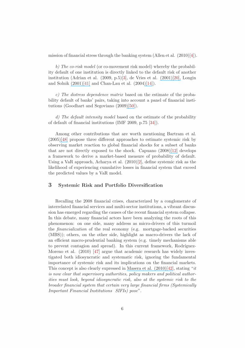
Among other contributions that are worth mentioning Bartram et al.(2005)[48] propose three different approaches to estimate systemic risk byobserving market reaction to global financial shocks for a subset of banksthat are not directly exposed to the shock. Capuano (2008)[12] developsa framework to derive a market-based measure of probability of default.Using a VaR approach, Acharya et al. (2010)[2], define systemic risk as thelikelihood of experiencing cumulative losses in financial system that exceedthe predicted values by a VaR model.

3 Systemic Risk and Portfolio Diversification

Recalling the 2008 financial crises, characterized by a conglomerate ofinterrelated financial services and multi-sector institutions, a vibrant discus-sion has emerged regarding the causes of the recent financial system collapse.In this debate, many financial actors have been analyzing the roots of thisphenomenon: on one side, many address as micro-drivers of this turmoilthe financialization of the real economy (e.g. mortgage-backed securities(MBS)); others, on the other side, highlight as macro-drivers the lack ofan efficient macro-prudential banking system (e.g. timely mechanisms ableto prevent contagion and spread). In this current framework, Rodrıguez-Moreno et al. (2010) [47] argue that academic research has widely inves-tigated both idiosyncratic and systematic risk, ignoring the fundamentalimportance of systemic risk and its implications on the financial markets.This concept is also clearly expressed in Masera et al. (2010)[42], stating “itis now clear that supervisory authorities, policy makers and political author-ities must look, beyond idiosyncratic risk, also at the systemic risk to thebroader financial system that certain very large financial firms (SystemicallyImportant Financial Institutions SIFIs) pose”.

6

Further, what appears to have been less investigated in the relevant lit-erature are the potential effects of portfolio diversification on systemic risk.While the benefits of diversification at a microeconomic level (in portfoliochoices theory) have been thoroughly examined in the economic literature(Allan and Gale, 2005[23]; Freixas et al., 2005[24]; and Wagner and Marsh,2006[55]), the macroeconomic side of the link between diversification andsystemic risk remains complex, multi-faceted, and not yet completely ex-plored (Lo, 2008[40]). In this regard, two different views, outlining boththe negative and positive effects of the relationship between diversificationand systemic risk have been characterizing this more controversial strandof the literature. Although portfolio diversification reduces risks at eachindividual institution, from the prospective of the entire financial system,it only reallocates these individual risks. (Wagner 2006) [54]. As argued inde Vries (2005)[19] “while diversification reduces the frequency of individualbank failures, since smaller shocks can be easily borne by the system, at thesame time diversification makes the bank sector prone to systemic break-downs in case of very large (non-macro) shocks, which otherwise would onlyhave isolated impact”.

Indeed, there is not any evidence to date, which would indicate thatportfolio diversification reduces the threat of systemic risk. Further diver-sification leads to sharing risks across institutions involved in contributingto make these positions similar to each other, with the effect of facilitatingfinancial contagion due to interlinked relationships among financial institu-tions. Nevertheless, it is crucial to include in these causes even the largefinancial conglomerates and the increasing presence of derivative instrumentsin the international financial system. In particular, derivative products havebeen indicated as both a responsible mechanism and perverse interaction ofrisk spreading and transferring from the banking to the insurance sector andvice versa (e.g. Originate-to-Distribute Model in banking and OTC deriva-tives).

In this regard, risk transfers between insurers and the banking sector rep-resent a widely used diversification instrument, allowing banks to transformliquid liabilities of depositors into illiquid assets (loans) (de Vries 2010[18]).Furthermore, and in particular during last decade, there are many contri-butions sustaining the contention that diversification has negative effects onthe financial system, including De Young and Roland (2001[21]), Stiroh(2004[52]), Acharya et al. (2006)[1], Stiroh (2006)[53] and Hirtle et al.(2007)[31]. In particular, Stiroh and Rumble (2006)[51] find that bene-fits stemming from diversification can be completely undermined by thevolatility effect of new exposures introduced into a portfolio. Sanya et al.(2010)[49] offers different kinds of mechanisms that can be detected to an-alyze the negative impact (or reduced benefits) of portfolio diversification

7

on systemic risk. The first, discussed in Froot and Stein (1998)[25] andCebenoyan and Strahan (2004)[13], indicates that gains obtained from port-folio diversification will be limited if the banks (managing the portfolio) donot have a risk efficient portfolio. The second argues that diversification canplay a negative role when banks expand their business into industries, withdifficulties emerging from loan-monitoring activities. Wegner (2006)[54] em-phasizes the role of diversification as an incentive for taking greater and newrisks in the international financial markets. De Vries (2010)[18] states that“diversification lowers the risk of isolated shocks for a financial entity, butmay simultaneously increase the systemic risk”. Allen et al. (2010)[4] claimthat the spread of credit default swaps and other credit derivative products,loan sales and collateralized loan obligations, has increased and improvedthe possibility for banks, mutual funds and financial institutions to diversifyrisk. But this possibility has, according to Allen et al. (2010)[4] “also ledto more overlap and more similarities among their portfolios. This has in-creased the probability that the failure of one institution is likely to coincidewith the failure of other similar institutions” (p.6).Conversely, there is an opposing strand of the relevant economic literaturewhich sustains the positive effects of diversification, first, from an efficiencygain point of view, and second, in increasing bank stability (Grossman(1994)[30], Wheelock (1995)[56], Hughes et al. (1996)[33], Berger et al.(1999)[8], Reichart and Wall (2000)[46], Campa and Kedia (2002)[11], andBaele et al. (2007)[6]).

4 The Model

Consider an economy formed by n agents. Each agent is endowed witha certain amount of wealth, whose rate of return varies stochastically fromone agent to the other. The satisfaction of the i-th agent is measured byexpected utility EUi(yi) where E is the expectation operator, Ui(.) denotesa well behaved utility function and yi is stochastic income. By projectingorthogonally the agents stochastic individual income y onto the stochastictotal agents’ revenue yi =

∑i yi, we can write the following identity:

yi − µi = βi(y − µ) + vi (1)

where:

8

∑

i

vi = 0; Evi = 0; Cov(vi, y) = 0;

Eyi = µi;1

n

∑

i

µi = µ and∑

i

βi = n(2)

Equation (1) decomposes individual risk into a systemic, diversifiablecomponent, correlated with total agents revenue, and into an independent,idiosyncratic component. The variance of individual income, assuming nocorrelation between diversifiable and idiosyncratic risk is:

V ar(yi) = β2i σ

2y + σ2

i (3)

By diversifying, each operator can bring her βi to unity, thus bringingher portfolio to coincide with the market portfolio, which by definition isthe most diversified, being an average of all portfolios, thereby achieving aminimum variance (i.e. the variance of the most diversified portfolio).

The distribution function (d.f.) of total revenue is F (y) and its supportis the compact interval [0, ymax], while the d.f of the idiosyncratic compo-nent is G(vi) over the support [vimin, vimax]. Assume now that a derivativeis introduced. In our context, a derivative is defined as a contingent claimwhose value depends on one of the assets, i.e. income sources in the mar-ket, more specifically, we will assume it depends on the average return ofall assets. The derivative corresponds to a contract between a issuer (i.e. ashort holder) and a buyer (a long holder), whereby each party promises topay the other a premium in different states of the world.

The i-th agent is confronted with the problem of choosing an optimalnumber of units of the derivative to hold long (i.e. to purchase) or short(i.e. to issue), so that total income for each agent will be equal in each stateof nature to the solution of the following optimization problem:

MaxqiEUi(xi), xi = yi + qip; i = 1, 2...n (4)

where qi denotes the number of units of the security in terms of sharesof the promised (random) payoff p, and is positive or negative accordingto whether the secutiry is bought or sold by the i-th agent. Using (1) andthe related assumptions, the expected utility in (4) can be written as follows:

9

EUi(xi) =

∫ vi,max

vi,min

∫ yi,max

0

Ui(µi + βi(y − µ)+

+ vi + qip(y))dF (y)dG(vi)

(5)

=

∫ ymax

0

Vi(mi + βi(y − µ) + qip(y))dF (y) (6)

where mi = µi − βiµ and Vi(.) is the indirect utility function defined as:

Vi(mi) =

∫ vi,max

vi,min

U(mi + vi)dG(vi) for all µi (7)

As shown by Kihlstrom, Romer and Williams (1981)[38], the indirectutility function in (7) is well behaved, i.e. it is increasing and concave in itsarguments. In order to show that the introduction of the security increasesthe income of the i-th subject, it is sufficient to show that the problem in(4) has a solution with a non zero value for the security in question. Thefirst order condition is obtained differentiating the (5) w.r.t. qi:

dEVi

dqi=

∫ ymax

0

(V ′

i p(y))dF (y) = E(V ′

i p) = 0 (8)

where primes indicate derivatives, while the second order condition re-quires:

d2EVi

dq2i

= E(V′′

i p2) < 0 (9)

which is always satisfied for a concave utility function. Applying thedefinition of covariance to (6), we obtain:

EV′

i Ey + Cov(V′

i p(y)) = 0 (10)

Differentiating totally with respect to the parameters yields:

EV′

i dEp+ [E(V′′

i p)Ep+ Cov(V′′

i p2)]dqi+

+ [E(V′′

i py)Ep+ Cov(V′′

i py)]dβi = 0(11)

which, by applying again the definition of covariance, can be also bewritten as:

EV′

i dEp+ E(V′′

i p2)dqi + E(V

′′

i p2y)dβi = 0 (12)

Since Θi = −E(V

′′

i p2)

EV′

i

≥ 0 and ψi =E(V

′′

i p2y)

EV′

i

≥ 0 (13)

10

are both positive measures of risk aversion, solving (10) for dqi yields:

dqi =dEp

Θi

+ψi

Θi

dβi (14)

Equation (14) establishes the fact that any increase in the expected pay-off and/or in the β will increase long positions while it will reduce shortpositions in the derivative asset. In a stable market equilibrium, we musthave∑n

i=1 dqi = 0, which implies:

dEp = −Θdβ (15)

where Θ = n(

m∑

i=1

(1

Θi

))−1; and; dβ =1

n

n∑

i=1

ψi

θi

βi (16)

Substituting (15) into (14) yields the equilibrium relationship:

dqi =ψi

θi

dβi −Θ

θi

dβi (17)

Expression (17) establishes the dependence of the quantities traded ofthe security on the difference between the individual incentive to diversify(through his beta and risk aversion) and the incentive to shift risk to or frommore risk adverse traders. Expression (17) could be integrated, assumingthat the utility function parameters are constant. A simpler way to proceed,however, is to expand V

′

i in (10) according to Mac Laurin formula:

V′

i = V′

i0 + V′′

i0(mi0 + βiy + qip(y)) +1

2V

′′′

iα (mi0 + βiy + qip(y))2 (18)

where the subscripts 0 and α denote the fact that the derivatives of theutility function are measured, respectively, at the origin and at α(yi + qip),with 0 ≤ α ≤ 1. Substituting into (10) and assuming that all the momentshigher than two of the joint distribution of y and p are zero, yields:

Ep− φi(βiσyp + qiσ2p) = 0 (19)

where φi = −V

′′

i,0

EV ii

is a measure of absolute risk aversion and coincides with

the Pratt coefficient for the family of constant risk aversion utility functions(CARA). Solving (19) for qi we obtain:

qi =Ep

φiσ2p

− βi

σyp

σ2p

(20)

Expression (20) shows that a solution to the maximization problem isthe result of two factors of agents’ heterogeneity: (i) the degree of risk

11

aversion and, (ii) the correlation between the security payoff and the agentincome. However, in order for the solutions for the different agents to bemutually compatible, the determination of the expected payoff Ep shouldbe completely determined, i.e.

∑i qi = 0, so that:

Ep = Φσyp (21)

where Φ = n(∑

11φi

)−1 is the harmonic average of the individual risk aver-

sion coefficients and we have used the property:∑n

i=1 βi = n.Substituting (21) into (20) yields:

qi = (Φ

φi

− βi)β = (Φ− φiβi

φi

)β (22)

where β =σyp

σ2p

, and

V ar∑

(qip(y)) = (n∑

i

(Φ− φiβi

φβ))2∑

j

(σ2p + 2σjp) (23)

In conclusion each agent will be able to improve her expected utility bydiversifying into a short or long position on an additional contingent claim,depending on two effects: (i) the difference between average and individualdemand for diversification (the beta) and, (ii) the difference between aver-age and individual risk aversion. The equilibrium level of long and shortpositions will be independent from the expected level of the pay off, but willdepend only on its variance. For example, in the special case of a deriva-tive that acts as an insurance (e.g. put option) and pays to long holdersp = R− y when yt ≤ R and p=-c otherwise, we have that σ2

p = σ2yF (R) and

σyp = −σ2yF (R), so that β = −1 and:

qi = (βi −Φ

φi

) (24)

and

xi = µi + βi(y − µ) + v + (Φ− φiβi

φi

)βp(y) (25)

so that:

V ar(xi) = β2i σ

2y + σ2

i + (Φ− φiβi

φi

)2β2(σ2p +∑

j

2σjp) (26)

Note that the introduction of the security has improved expected incomeof each agent, it has further diversified her portfolio, but, at the same time,has introduced a new source of variance (and, implicitly, risk), into thesystem. This new form of risk can be defined as “systemic”, because it

12

depends on the correlation between the yield of the derivative and the incomeof all agents in the system. In other words, a shock on the price of thederivative is transmitted to all agents. From equation (25), we can derive amodified version of the well known CAPM model, by subtracting from bothsides the risk free rate of return r :

xi − rf = (µi − βiµ) + βi(y − rf ) + vi + (Φ− φiβi

φi

)βp(y) (27)

5 Dataset

As noted in section 2, several methodologies have been implemented tomeasure systemic risk, based on different motivations and goals: we choosethe correlation among mutual funds showing lower performances comparedto the average level returns (threshold value) as a proxy of systemic risk(Systrsk). The choice of this approach is not novel in the literature (DeNicolo and Kwast (2002)[16] and Chan (2004)[14]), its advantage being thatcorrelation among fund returns are considered as a forward-looking variablemuch more suitable than balance sheet or company financial indicators tocapture systemic failures and the associated costs. Furthermore, the corre-lation between returns of different funds reflect fund values. Following theapproach by Chan et al. (2004)[14], we thus estimate this variable througha pairwise correlation approach between the return of the i-th and j-th fund:

Cov [RiRj ] =βiβjσ

2λ

√

β2i σ

2λ

+ σ2ǫ,i

√

β2j σ

2λ

+ σ2ǫ,i

(28)

As discussed above, we propose the systemic risk variable as the “pairwisecorrelation” within the subset of funds having lower than average perfor-mance:

Rij = xij − xij if xij < xij (29)

Rij = 0 otherwise (30)

We analyze a panel of the 226 largest mutual funds (based on size) fromthe Morningstar database. The U.S. market is analyzed through 162 fundsand through 64 funds for the European area, exchanged in the market be-tween January 2003 and March 2010 thereby amounting to 19662 monthly

13

Figure 2: U.S. Market performances

Source: Author Elaborations on Bloomberg Database. The “weighted” index is themarket index created on the other three index performances.

observations. We chose as the risk-free rate for the U.S market the 3-MonthsTreasury Bills from the Federal Reserve Bank of Saint Louis (FED of SaintLouis) database. For the European market, we use the 3-Months Germangovernment bond from the Bloomberg database (figure 2 and 3). Througha Return Based Style Analysis (RBSA), we create a return weighted indexable to capture the equity stocks, government bonds and corporate fundperformances. Bond, equity and cash compose the n-segments of any fundin the n-th portfolio.

In order to build up these two proxies (for both the U.S and Europeanmarket) we consider:

• The U.S and European Morgan Stanley (MSCI) index for governmentbonds;

• The U.S and European J.P Morgan (JPM EMBI) index for the stockexchange;

• The U.S and European Merry Lynch (ML-Corporate) index for thecorporate sector.

14

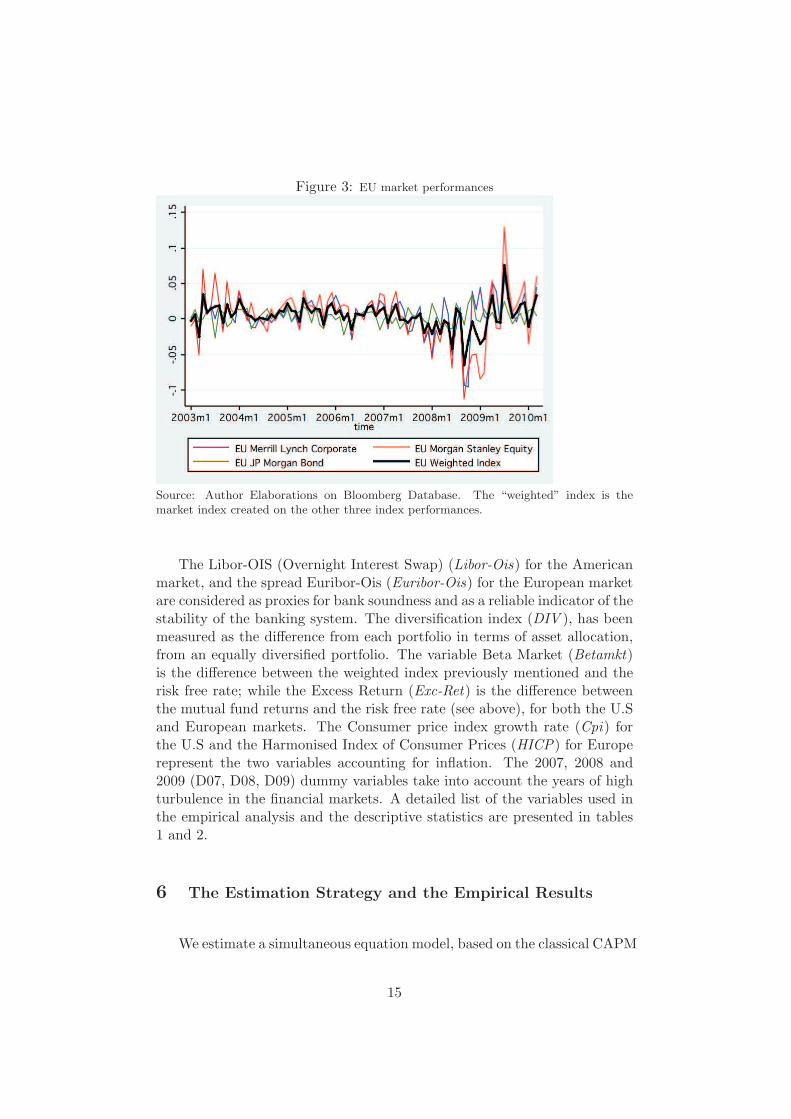
Figure 3: EU market performances

Source: Author Elaborations on Bloomberg Database. The “weighted” index is themarket index created on the other three index performances.

The Libor-OIS (Overnight Interest Swap) (Libor-Ois) for the Americanmarket, and the spread Euribor-Ois (Euribor-Ois) for the European marketare considered as proxies for bank soundness and as a reliable indicator of thestability of the banking system. The diversification index (DIV ), has beenmeasured as the difference from each portfolio in terms of asset allocation,from an equally diversified portfolio. The variable Beta Market (Betamkt)is the difference between the weighted index previously mentioned and therisk free rate; while the Excess Return (Exc-Ret) is the difference betweenthe mutual fund returns and the risk free rate (see above), for both the U.Sand European markets. The Consumer price index growth rate (Cpi) forthe U.S and the Harmonised Index of Consumer Prices (HICP) for Europerepresent the two variables accounting for inflation. The 2007, 2008 and2009 (D07, D08, D09) dummy variables take into account the years of highturbulence in the financial markets. A detailed list of the variables used inthe empirical analysis and the descriptive statistics are presented in tables1 and 2.

6 The Estimation Strategy and the Empirical Results

We estimate a simultaneous equation model, based on the classical CAPM

15

formulation augmented by a variable that represents the contribution thatdiversification through derivatives makes to systemic risk. In tables 3 and4, we show the result of the CAPM estimates in the two markets (U.S andEurope). In particular, using the CAPM specification presented in Famaet al. (2004) we regress individual (fund) excess returns, the diversificationindex and a series of dummy variables. In both markets, we find a positiverelation between Beta and excess returns. Although the two markets showa significant difference in their Beta coefficients, (approximately 1.16% inthe U.S and around 0.86% in the European market) there is not a sizeablevariation in intra-market differences (the U.S market ranges between 1.14%and 1.17%, while the European market varies between 0.84% and almost0.89%). In the U.S and European market, the diversification variable showsa positive value and a high significance coefficient, while the systemic riskvariable negatively impacts the excess returns (dependent variable).

Once we examined the CAPM analysis, in order to assess the impact ofthe diversification strategy on systemic risk, we specify a model in which themarket excess returns and the indicators of systemic risk are simultaneoslydetermined and depend on a series of key variables that, according to theliterature, play a fundamental role both in influencing the Beta market andas a possible factor impacting systemic risk. The model is estimated byusing two stages least squares. The first equation is given by:

U.S Market:

βmkti,t = Sistrski + Fcorri + Cpii

+ LiborOisi +D08i +D09i + ut

(31)

European Market:

βmkti = Sistrski + Fcorri +Hicpi

+ EuriborOisi +D08i +D09i + ut

(32)

Equations (31-32) test the hypothesis that the systemic risk variable hasa negative and significant impact on the market performances. In additionto the dependent variable βmkt, measured as the market monthly excessreturn, the independent variables are the systemic index measured as: thefund correlations (without any return threshold); the consumer price in-dex growth rate (for the American market) and the Harmonised Index ofConsumer Prices (for the European market); the spread Libor-Ois for the

16

American market; the spread Euribor-Ois for the European market as prox-ies of bank sector soundness; and the 2007, 2008 and 2009 dummy variableson the Beta Market variable, (defined as difference between market perfor-mance, created through the RBSA, and the risk free rate).

As tables 5 - 6 show, an increase in the correlation of mutual fundsreturns (Fcorr) has a negative impact on market excess returns (βmkt).This effect is strongly significant in both the U.S and EU markets. Thesefindings clearly emerge from the tests applied though the first hypothesis inany specification of the (31) (32) models. The Libor (Euribor) - OIS spreadrepresents the unsecured interest rate at which banks lend money to otherbanks which must satisfy certain criteria for creditworthiness. Libor andEuribor are not entirely credit risk free, because they reflect both liquidityrisk and the bank’s default risk over the following months. The OIS repre-sents the average of the overnight interest rates expected until maturity, sothe Libor (Euribor) - OIS reflects both the liquidity and default risks overthe next months. Then, during the period where the stock markets registera strong performance this spread should be subjected to a reduction. In thiscontext, our results confirm the negative relationship between market per-formance and the Libor (Euribor) - OIS spread indicator. The Cpi and Hicpnegative coefficients support the strand of the literature that attributes anegative relationship between inflation and stock performances in the shortrun. In the second equation of the simultaneous equation model, (31-32) weaim to test the second hypothesis, i.e. that an increase in the similarities ofthe diversification strategies of each fund can increase the threat of systemicrisk.

In this case the dependent variable is the systemic risk, while the inde-pendent variables are the three dummy variables for 2007, 2008, 2009, thefundsize and the cpi/hicp growth rate on the systemic risk variable.

U.S. Market:

Sistrski = βmkti + Fcorri +Divi + Cpii+

+ LiborOisi + Fsizei +D07i +D08i +D09i + u(33)

European Market:

Sistrski = βmkti + Fcorri +Divi +Hicpi+

+ EuriborOisi + Fsizei +D07i +D08i +D09i + u(34)

17

The results of the empirical analysis are contained in table 5 for the U.Smarket, and table 6 for the European market. In general, all these variablesshow high levels of significance, although the diversification index variableis weakly significant at 10%.

The strategy in the asset allocation investment choices is captured bythe diversification index (Div) variable. This index explains how portfoliodiversification can increase the threat of systemic risk showing a positivecoefficient when regressed on the systemic risk as dependent variable. Thesimilarities in fund returns for each portfolio are instead represented by theFcorr returns that also shows a positive and signifcant coefficient. Thissuggests that an increase of the correlation among funds can be interpretedas a warning for a distress situation in financial system. As already ex-plained in the first stage, in periods when the stock markets register goodperformances, this measure is subjected to a reduction, conversely in pe-riods of turmoil this spread should increase so as to capture the marketrisks. In the estimate of the second regression we find a that an increaseof this spread lead to an increase of the threat of systemic risk. Further inboth specifications (model 33− 34) we find a positive relation between thedummy variables, the Fund size and the Cpi (for the American market) orthe Hicp (for the European market) and the systemic risk variable. Theβmkt variable has a negative effect on systemic risk suggesting that deteri-orating market performances reverberates negatively on systemic risk.

7 Concluding Remarks

The theoretical and empirical motivation of this analysis is the ongo-ing debate which posits that derivative driven financial diversification, of-ten interpreted by professionals and academics as a fundamental benefit ofinvestment financial strategies can be undesirable and a driver of excessiveinstability. Our results provide insight into the connection between portfoliodiversification strategy and the impact on systemic risk. In this regard, wehave developed a model where the i-th agent diversification strategy inter-acts with the j-th agent diversification strategy, through the mutual purchaseand sale of derivatives thus increasing agent’s interdependence, the proba-bility of contagion from a systemic event and, ultimately systemic risk. Thebasic reason for this result is that derivatives provide an insidious instru-ment of diversification. While they appeal to risk managers because of theircapacity, as contingent claims, to provide insurance to individual investors,at the same time, they create a separate source of portfolio volatility whichmay be increasingly difficult to further diversify. Some of the implicationsof the theoretical model have been tested through a simultaneous equations

18

model, where we have hypothesized that systemic risk may increase the needto further diversify and, at the same time, further diversification, by increas-ing portfolio similarities, can boost systemic risk. Both hypotheses appearto be corroborated by our econometric tests, which show significant andmutual substantial impacts of the signs implied by the model, between di-versification and systemic risk variables. Our findings can be summarized asfollows: from the point of view of the individual agent, the portfolio diversi-fication strategy represents a valuable instrument of portfolio management.However, from the point of view of the financial system, when such a di-versification is pursued through a proliferation of derivative securities, theincrease in similarities and mutual interdependence among financial agentsmay result in an increase in aggregate risk. Such an increase has systemicnature since it is based on the loss of a diversified ensemble of financialagents as a key source of systemic resilience.

19

Table 1: Complete list of variables used in the empirical analysis

Variable Sample Frequency Source Acronym

Beta Market 1/01/2003 - Monthly Author elaborations on Bmkt

30/03/2010 Morningstar and Bloomberg data

Excess Market 1/01/2003 - Monthly Author elaborations Exc-ret

30/03/2010 Morningstar data

Systemic Risk 1/01/2003 - Monthly Bloomberg Sist-risk

30/03/2010

Fund Correlation 1/01/2003 - Monthly Bloomberg Fcorr

30/03/2010

Euribor OIS 1/01/2003 - Monthly FED St. Louis database Euribor-Ois

30/03/2010

Libor OIS 1/01/2003 - Monthly Bureau of LAbor Statistics Libor-Ois

30/03/2010

Consumer Price Index 1/01/2003 - Monthly ECB database Cpi

30/03/2010

Harmonised Index 30/03/2010 - Morningstar FED database Hicp

of Consumer Prices 30/03/2010

Fund Size 1/01/2003 - Monthly ECB database Fsize

30/03/2010

Rend Weighted Index 1/01/2003 - Monthly Bloomberg database Rend WI

30/03/2010

Diversification Index 1/01/2003 - Monthly Author elaborations on Div

30/03/2010 Morningstar data

Dummy 2007 1/01/2003 - Monthly Dummy variable D07

30/03/2010

Dummy 2008 1/01/2003 - Monthly Dummy variable D08

30/03/2010

Dummy 2009 1/01/2003 - Monthly Dummy variable D09

30/03/2010

Source: Authors elaborations

20

Table 2: Descriptive Statistics

min p1 p10 p25 p50 p75 p90 p99 max mean sd N

Bmkt US -0.66 -0.66 -0.18 -0.08 0.01 0.13 0.24 0.49 0.93 0.02 0.19 16502

Bmkt EU -0.65 -0.65 -0.22 -0.05 0.03 0.13 0.20 0.75 0.89 0.05 0.18 3160

Fcorr US -0.76 -0.58 -0.32 -0.30 0.14 0.19 0.38 0.55 0.93 0.03 0.71 14456

Fcorr EU -0.82 -0.74 -0.41 -0.019 0.09 0.23 0.34 0.59 0.87 0.01 0.41 3160

Sist rsk US -0.05 -0.04 -0.01 0.00 0.02 0.21 0.32 0.49 0.67 0.04 185.89 11225

Sist rsk EU -0.03 -0.04 -4.39 0.00 0.21 0.32 0.39 0.44 0.75 0.03 185.89 2770

Exc ret US -0.65 -0.65 -0.15 -0.06 0.04 0.16 0.25 0.49 0.49 0.04 0.19 16502

Exc ret EU -0.64 -0.64 -0.20 - 0.03 0.07 0.15 0.22 0.75 0.75 0.05 0.18 3160

Rend WI US -1.25 -0.39 -0.13 -0.03 0.21 0.26 0.31 0.48 0.61 0.25 0.09 16502

Rend WI EU -1.31 -0.63 -0.28 -0.17 0.10 0.15 0.21 0.30 0.58 0.13 0.13 3160

CPI -2.00 -2.00 -0.10 2.0 2.90 3.01 3.90 5.17 6.01 3.01 1.87 16502

HICP -1.76 -1.88 -0.10 1.50 2.80 3.60 4.20 5.50 5.50 2.55 1.56 3160

DIV US 1.49 11.86 26.90 33.26 38.57 44.72 53.20 68.60 214.61 38.26 11.06 10171

DIV EU 1.07 8.85 24.63 30.87 39.55 50.31 60.06 117.67 808.19 42.30 24.59 2770

Libor OIS 0.04 0.04 0.08 0.09 0.12 0.38 0.87 2.39 2.39 0.33 0.45 16052

Euribor OIS 0.04 0.04 0.05 0.06 0.07 0.45 0.79 1.86 1.86 0.29 0.37 3160

Fsize US 0.02 0.02 0.10 0.27 0.57 1.17 2.49 10.62 37.31 2.34 2.05 16502

Fsize EU 0.01 0.01 0.13 0.29 0.63 1.56 2.86 13.54 29.32 1.96 1.73 3160

Authors elaborations

21

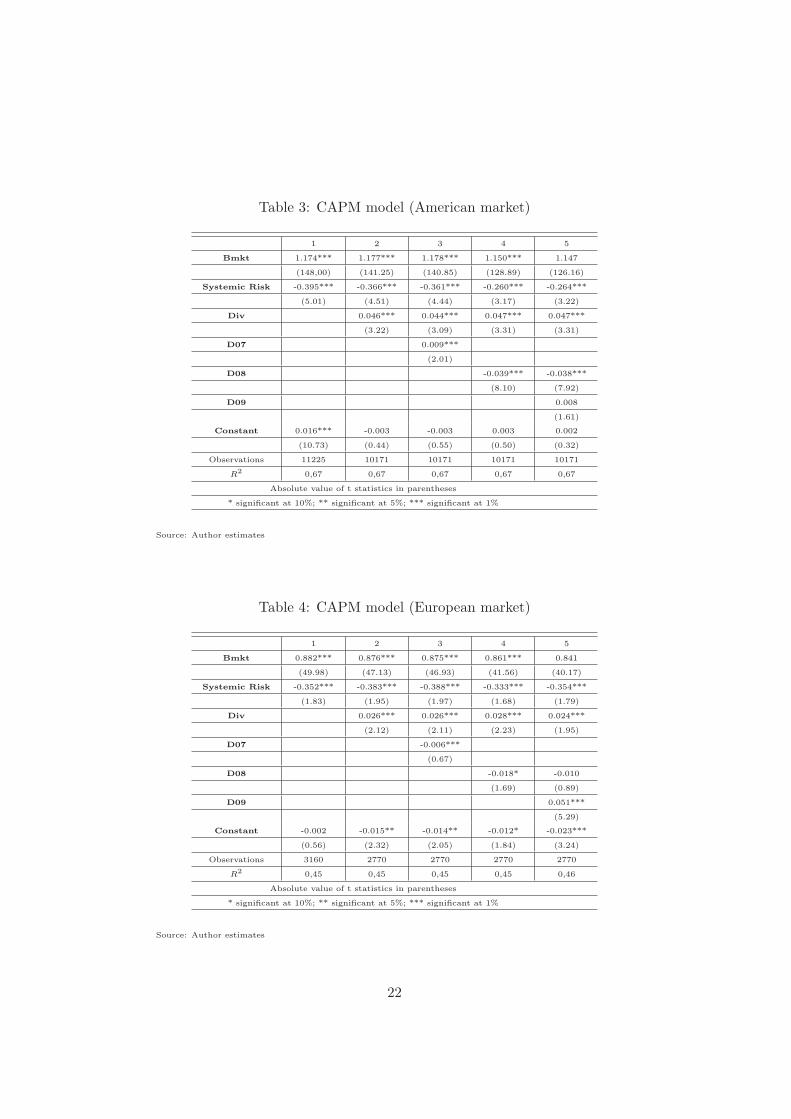
Table 3: CAPM model (American market)

1 2 3 4 5

Bmkt 1.174*** 1.177*** 1.178*** 1.150*** 1.147

(148,00) (141.25) (140.85) (128.89) (126.16)

Systemic Risk -0.395*** -0.366*** -0.361*** -0.260*** -0.264***

(5.01) (4.51) (4.44) (3.17) (3.22)

Div 0.046*** 0.044*** 0.047*** 0.047***

(3.22) (3.09) (3.31) (3.31)

D07 0.009***

(2.01)

D08 -0.039*** -0.038***

(8.10) (7.92)

D09 0.008

(1.61)

Constant 0.016*** -0.003 -0.003 0.003 0.002

(10.73) (0.44) (0.55) (0.50) (0.32)

Observations 11225 10171 10171 10171 10171

R2 0,67 0,67 0,67 0,67 0,67

Absolute value of t statistics in parentheses

* significant at 10%; ** significant at 5%; *** significant at 1%

Source: Author estimates

Table 4: CAPM model (European market)

1 2 3 4 5

Bmkt 0.882*** 0.876*** 0.875*** 0.861*** 0.841

(49.98) (47.13) (46.93) (41.56) (40.17)

Systemic Risk -0.352*** -0.383*** -0.388*** -0.333*** -0.354***

(1.83) (1.95) (1.97) (1.68) (1.79)

Div 0.026*** 0.026*** 0.028*** 0.024***

(2.12) (2.11) (2.23) (1.95)

D07 -0.006***

(0.67)

D08 -0.018* -0.010

(1.69) (0.89)

D09 0.051***

(5.29)

Constant -0.002 -0.015** -0.014** -0.012* -0.023***

(0.56) (2.32) (2.05) (1.84) (3.24)

Observations 3160 2770 2770 2770 2770

R2 0,45 0,45 0,45 0,45 0,46

Absolute value of t statistics in parentheses

* significant at 10%; ** significant at 5%; *** significant at 1%

Source: Author estimates

22

Table 5: Simultaneous Equations Model (American market)

I stage Y = Beta Market

1 2 3 4

Syst-Rsk -0.003*** -0.004*** -0.001*** -0.001***

(8.46) (7.67) (10.35) (14.49)

Fcorr -0.069*** -0.023*** -0.029*** -0.076***

(7.91) (2.77) (10.93) (20.31)

D08 0.187*** 0.276*** 0.052*** 0.027***

(4.90) (10.10) (5.81) (2.53)

Cpi -0.031***

(7.22)

Libor-OIS -0.072*** -0.029***

(2.77) (10.93)

D09 0.174*** 0.169*** 0.150***

(8.54) (27.60) (19.14)

Constant 0.136*** 0.042*** 0.052*** 0.034***

(11.11) (4.83) (20.53) (11.23)

II stage Y = Systemic risk

Fcorr 16.419** 37.284**

(4.94) (2.49)

Div 0.029* 0.030* 0.065* 0.029*

(1.27) (1.18) (0.73) (1.56)

Bmkt -1.286 -1.431** -1.882** -1.688*

(4.86) (5.26) (7.23) (3.70)

Libor-OIS 36.970*** 38.436***

(4.95) (4.56)

Cpi 5.951*** 28.373** 94.066***

(2.86) (15.82) (4.06)

D07 5.180**

(2.32)

D08 49.519*** 71.096*** 38.621*** 79.826***

(6.36) (7.37) (5.97) (2.62)

D09 45.340*** 117.786***

(5.65) (16.25)

Fsize 7.938*** 12.238***

(2.05) (1.84)

Constant -2.464 -15.204 -88.685*** -63.238***

(0.75) (2.43) (11.46) (4.13)

Observations 10168 10168 10168 10168

R2 0.141 0.153 0.156 0.147

Absolute value of t statistics in parentheses

* significant at 10%; ** significant at 5%; *** significant at 1%

Source: Author estimates

23

Table 6: Simultaneous Equations Model (European market)

I stage Y = Beta Market

1 2 3 4

Syst-Rsk -0.481*** -0.754*** -0.909*** -0.639***

(1.64) (1.44) (2.71) (1.19)

Fcorr -0.117*** -0.113*** -0.311*** -0.004***

(1.65) (11.61) (2.78) (1.18)

D08 0.205*** 0.074*** 0.087*** 0.196***

(12.95) (12.11) (4.05) (4.92)

Hicp -0.024***

(7.55)

Euribor-OIS -0.023*** -0.256***

(2.77) (10.93)

D09 0.044*** 0.625*** 0.261***

(8.54) (27.60) (19.14)

Constant 0.189*** 0.051*** 0.108*** 0.047***

(3.99) (0.78) (14.73) (6.13)

II stage Y = Systemic risk

Fcorr 7.079*** 14.071* 12.311* 20.246**

(12.06) (1.40) (2.78) (9.83)

Div 0.021* 0.038* 0.095* 0.114*

(1.26) (0.35) (0.37) (0.12)

Beta Market -0.241 -0.241** -0.231*

(5.47) (3.75) (3.77)

Libor-OIS 17.450*** 38.436***

(4.95) (4.56)

Hcpi 1.671*** 18.246** 13.176***

(1.29) (11.23) (2.16)

D07 0.007* 0.012*

(0.96) (1.42)

D08 0.106*** 0.209*** -0.217 0.057***

(6.42) (3.25) (3.24) (1.40)

D09 0.058*** 0.044

(3.75) (1.20)

Fsize 2.372* 1.918*

(0.03) (0.04)

Constant -0.052*** -0.051 -0.373*** -0.115***

(9.45) (7.06) (4.17) (0.89)

Observations 4484 4484 4484 4484

R2 0.112 0.116 0.123 0.119

Absolute value of t statistics in parentheses

* significant at 10%; ** significant at 5%; *** significant at 1%

Source: Author estimates

24

References

[1] V. Acharya, I. Hasan, and A. Saunders. Should banks be diversified?evidence from individual bank loan portfolios. Journal of Business,79(3):1355–1412, 2006.

[2] V. Acharya, H. Pedersen, L., T. Philippon, and P. Richardson, M.Measuring systemic risk. FRB of Cleveland Working Paper No. 10-02,2010.

[3] T. Adrian and M. Brunnermeier. Covar. Federal Reserve Bank of NewYork Staff Reports, 2009.

[4] F. Allen, Ana. Babus, and E. Carletti. Financial connections and sys-temic risk. European University Institute (EUI) - Working Papers,ECO 2010/30, 2010.

[5] F. Allen and D. Gale. Financial Contagion. Journal of Political Econ-omy, 2000.

[6] L. Baele, O. De Jonghe, and RV. Vennet. Does the stock market valuebank diversification? Journal of Banking and Finance, 31, 2007.

[7] P Bartholomew and W. Gary. Fundamentals of systemic risk. Researchin Financial Services: Banking, Financial Markets, and Systemic Risk,vol.7, edited by George G. Kaufman, 3 – 17, 1995.

[8] N. Berger, A, S. Demsetz, R, and E. Strahan, P. The consolidation offinancial services industry: Causes, consequences, and implications forthe future. Journal of Banking and Finance, 23:135–194, 1999.

[9] V. Bhansali, R. Gingrich, and A. Longstaff, F. Systemic credit risk:What is the market telling us? Financial Analysts Journal, 64(4):16–24, 2008.

[10] D. Bordo, M, B. Mizrach, and J. Schwartz, A. Real versus pseudo-international systemic risk: Some lessons from history. Review of PacificBasin Financial Markets and Policies, 1(1):31–58, 1998.

[11] J.M. Campa and Kedia S. Explaining the diversification discount. Jour-nal of Finance, 57(1731-1762), 2002.

[12] C. Capuano. The option-ipod. the probability of default implied byoption prices based on entropy. IMF Working Paper 08/194, 2008.

[13] S. Cebenoyan and E. Strahan P. Risk management, capital structureand lending at banks. Journal of Banking and Finance, 28:19–43, 2004.

25

[14] Chan-Lau, Jorge A., Donald J. Mathieson, and James Y.Yao. Extremecontagion in equity markets. IMF staff paper, 51(2):386–408, 2004.

[15] O. De Bandt and P. Hartmann. Systemic risk: A survey. Technicalreport, European Central Bank, 2000.

[16] G. De Nicolo and M.L. Kwast. Systemic risk and financial consolidation:Are they related? Journal of Banking and Finance, 2002.

[17] G. De Nicolo and M. Lucchetta. Systemic risk and macroeconomy.International Monetary Fund, 2010.

[18] Casper G. De Vries. Systemic risk and diversification across europeanbanks and issuers. In Presented at the conference: ”Beyond the Finan-cial Crisis: Systemic Risk, Spillovers and Regulation” Dresden, 28-29October 2010.

[19] Casper G. De Vries. The simple economics of bank fragility. Journalof Banking and Finance, 29(4):803–25, 2005.

[20] Casper G. de Vries, P. Hartmann, and S. Straetmans. Asset marketlinkages in crisis periods. C.E.P.R. Discussion Papers, 2001.

[21] R. De Young and K.R. Roland. Product mix and earnings volatilityat commercial banks: Evidence from a degree of total leverage model.Journal of Financial Intermediation, 10(54-84), 2001.

[22] J. Dow. What is systemic risk? moral hazard, initial shocks, andpropagation. Monetary and Economic Studies, pages 1–24, 2000.

[23] Allen F. and D. M. Gale. Systemic risk and regulation. WhartonFinancial Institutions Center Working Paper No. 95-24, 2005.

[24] X. Freixas, G. Loranth, and A. Morrison. Regulating financial conglom-erates. Oxford Financial Research Center Working Paper no.2005-FE-03, 2005.

[25] A. Froot, K and C. Stein, J. Risk management, capital budgeting,and capital structure policies for financial institutions: an integratedapproach. Journal of Financial Economics, 1998.

[26] B. Gonzalez-Hermosillo. Determinants of ex-ante banking system dis-tress: A macro-micro empirical exploration of some recent episodes.IMF Working Paper, 1999.

[27] B; Gonzlez-Hermosillo and Billings R. Pazarbasioglu, C. Banking sys-tem fragility: Likelihood versus timing of failure. an application to themexican financial crisis. IMF working paper, 1997.

26

[28] G. Gorton. Banking panics and business cycles. Oxford EconomicPapers, 05(21), 2005.

[29] A. Greenspan. Remarks at a conference on risk measurement and sys-temic risk. Board of Governors of the Federal Reserve System, Wash-ington, D.C., 1995.

[30] S. Grossman, R. The shoe that didn’t drop: Explaning banking stabilityduring the great depression. Journal of Economic History, 54(3):654–692, 1994.

[31] J. Hirtle and KJ Stiroh. The return to retail and the performance ofus banks. Journal of Banking and Finance, 21(1101-1133), 2007.

[32] X. Huang, H. Zhou, and H. Zhu. Assessing the systemic risk of aheterogeneous portfolio of banks during the recent financial crisis. 22ndAustralasian Finance and Banking Conference 2009, 2009.

[33] JP. Hughes, W. Lang, L.J. Mester, and C. Moon. Safety in numbers?geographic diversification and bank insolvency risk. Federal ReserveBank of Philadelphia, 14(96), 1996.

[34] IMF. Responding to the financial crisis and measuring systemic risk.Technical report, International Monetary Fund, 2009.

[35] J. Kambhu, T. Schuermann, and K.J. Stiroh. Hedge funds, financialintermediation, and systemic risk. Federal Reserve Bank of New YorkStaff Reports no. 291, 2007.

[36] G. Kaufman. Comment on systemic risk. Research in Financial Ser-vices, 1995.

[37] G. Kaufman and K. E. Scott. What is systemic risk and do bankregulators retard or contribute to it? Independent Review, 7:371–391,2003.

[38] R.E. Kihlstrom, D. Romer, and S. Williams. Risk aversion with randominitial wealth. Econometrica, 49(53-73), 1981.

[39] A. Lehar. Measuring systemic risk: A risk management approach. Tech-nical report, Journal of Banking and Finance, 2005.

[40] A. Lo, W. Hedge funds, systemic risk, and the financial crisis of 2007-2008. Technical report, Hearing on Hedge Funds, 2008.

[41] F. Longin and B. Solnik. Extreme correlation of international equitymarkets. Journal of Finance, 56(2):649–76, 2001.

27

[42] R. Masera, R. Maino, and G. Mazzoni. Reform of the risk capitalstandard (rcs) and systemically important financial institutions (sifis)in reform of the risk capital standard (rcs) and systemically importantfinancial institutions (sifis). Bancaria Editrice, 2010.

[43] F. Mishkin. Comment on systemic risk. in G. Kaufman (1995), pages31–45, 1995.

[44] Board of Governors of the Federal Reserve System Board of Governors.Technical report. 2, 2001.

[45] Group of Ten. Report on consolidation in the financial sector. Basel,2001.

[46] A. K. Reichart and L. D. Wall. The potential for portfolio diversificationin financial services. Federal Reserve Bank of Atlanta Economic Review,Third Quarter:31–51, 2000.

[47] M. Rodriguez-Moreno and J.I. Pena Sanchez de Rivera. Systemic riskmeasures: the simpler the better. Open Access publications from Uni-versidad Carlos III de Madrid., 2010.

[48] Bartram S. M., G. W. Brown, and J. E. Hund. Estimating systemicrisk in the international financial system. FDIC Center for FinancialResearch Working Paper, 2005.

[49] S. Sanya and S. Wolfe. Can banks in emerging economies benefit fromrevenue diversification. Journal of Financial Services Resources, 2010.

[50] M. Segoviano and C. Goodhart. Banking stability measures. IMFWorking Paper, 2009.

[51] K. Stiroh and A. Rumble. The dark side of diversification: The caseof us financial holding companies. Journal of Banking and Finance,30(2132-2161), 2006.

[52] K.J. Stiroh. Do community banks benefit from diversification? Journalof Financial Services Resources, 25(135-160), 2004.

[53] K.J. Stiroh. A portfolio view of banking with interest and noninterestactivities. Journal of Money Credit Bank, 38(5):1351–1361, 2006.

[54] W. Wagner. Diversification at financial institutions and systemic crises.Working Paper No. 2006-71, 2006.

[55] W. Wagner and I. Marsh. Credit risk transfer and financial sectorstability. Journal of Financial Stability, 2:173–193, 2006.

28

[56] D.C. Wheelock. Regulation, market structure, and the bank failuresof the great depression. Federal Reserve Bank of Saint Louis Review,27-38, 1995.

29