Journal of

Risk and FinancialManagement

Article

An Equilibrium-Based Measure of Systemic Risk

Katerina Ivanov 1, James Schulte 2, Weidong Tian 3,* and Kevin Tseng 4

�����������������

Citation: Ivanov, Katerina, James

Schulte, Weidong Tian, and Kevin

Tseng. 2021. An Equilibrium-Based

Measure of Systemic Risk. Journal of

Risk and Financial Management 14: 414.

https://doi.org/10.3390/jrfm14090414

Academic Editor: Shigeyuki Hamori

Received: 19 July 2021

Accepted: 24 August 2021

Published: 2 September 2021

Publisher’s Note: MDPI stays neutral

with regard to jurisdictional claims in

published maps and institutional affil-

iations.

Copyright: © 2021 by the authors.

Licensee MDPI, Basel, Switzerland.

This article is an open access article

distributed under the terms and

conditions of the Creative Commons

Attribution (CC BY) license (https://

creativecommons.org/licenses/by/

4.0/).

1 McColl School of Business, Queens University of Charlotte, Charlotte, NC 28274, USA; ivanovk@queens.edu2 Department of Economics, Florida State University, Tallahassee, FL 32306, USA; jtschulte@fsu.edu3 Belk College of Business, University of North Carolina at Charlotte, Charlotte, NC 28223, USA4 College of Management, National Taiwan University, Taipei 10617, Taiwan; kevintseng@ntu.edu.tw* Correspondence: wtian1@uncc.edu

Abstract: This paper develops and implements an equilibrium model of systemic risk. The modelderives a systemic risk measure, loss beta, in characterizing all too-big-to-fail banks using a capitalinsurance equilibrium. By constructing each bank’s loss portfolio with a recent accounting approach,we perform a comprehensive empirical study of this loss beta measure and document all TBTF banksfrom 2002 to 2019. Our empirical findings suggest a significant number of too-big-to-fail banks in2018–2019.

Keywords: systemic risk; too big to fail; capital insurance; loss beta

JEL Classification: G11; G12; G13

1. Introduction

The financial crisis of 2007–2009 generates a significant amount of interest in measuringsystemic risk and ensuring the health of the financial system. The most vivid response is thepassing of the Dodd-Frank Act. Measuring systemic risk has been at the center of academicresearch since 2008. For example, Acharya (2009), Acharya et al. (2012), and Brownlessand Engle (2016) show that time-varying correlation structure plays a crucial role in theirsystemic risk measurements and develop an expected shortfall measure approach. Adrianand Brunnermeier (2016) develop a CoVaR approach conditional on financial institutionsbeing in a state of financial distress. Acemoglu et al. (2015), and Elliott et al. (2014) developa network approach for systemic risk.1 While these quantitative and statistical metrics arestraightforward to apply, the precise economic channel to which the systemic risk enters themetrics is somewhat lacking. Moreover, Benoit et al. (2019) identify several shortcomingsin the systemic-risk scoring methodology.

From an insurance equilibrium perspective, Panttser and Tian (2013) and Ivanov (2017)present a capital insurance approach to address systemic risk and identify too-big-to-fail(TBTF) banks. Developing a rational expectation equilibrium model of the capital insurancemarket to address systemic risk was initially proposed in Kashyap et al. (2008). In theequilibrium model of capital insurance, a central player (regulator or insurer) sells aninsurance product, capital insurance, on the systemic risk of all banks. The insurer injectsthe guaranteed capital contingent upon a stressed period, while each bank pays insurancepremium upfront in exchange for an implicit guarantee subsidy. In equilibrium, each bankpredicts the optimal insured amount and the insurer determines the optimal pricingstructure. As a result, those banks purchasing capital insurance are characterized as TBTFbanks under this approach, so TBTF banks are identified endogenously. In characterizingthe equilibrium, this approach introduces a new equilibrium-based systemic risk measure,loss beta.

Compared with numerous systemic risk measures in previous literature, the equilibrium-based systemic risk measure, such as loss beta, is unique since it captures the perspectivefrom all banks together as well as an issuer about each bank’s systemic risk. Moreover,

J. Risk Financial Manag. 2021, 14, 414. https://doi.org/10.3390/jrfm14090414 https://www.mdpi.com/journal/jrfm

J. Risk Financial Manag. 2021, 14, 414 2 of 24

both the implicit guarantee subsidy and TBTF banks are determined endogenously andsimultaneously.2 Since the framework and its pricing structure are motivated by a clas-sical insurance setting, the capital insurance equilibrium is similar to classical insuranceequilibrium models such as Borch (1962), Arrow (1971), and Raviv (1979) for a new typeof insurance product on the systemic risk. Nevertheless, the strong law of large numbersis no longer satisfied for capital insurance because of the particular correlated feature ofsystemic risk among banks (Acharya et al. (2012) and Adrian and Brunnermeier (2016)).

This paper extends the equilibrium analysis in Panttser and Tian (2013) and Ivanov(2017) in several theoretical and empirical aspects. First, this paper characterizes theequilibrium for a general class of capital insurance. We focus on identifying TBTF banks,whereas Panttser and Tian (2013) study the welfare analysis of capital insurance as afinancial innovation. Second, and more importantly, we introduce a new methodology toconstruct an individual bank’s loss portfolio with systemic risk components consistent withBasel documentations.3 Building on the deposit insurance model developed in Diamondand Dybvig (1983) and Peck and Shell (2003), we construct an appropriate loss portfoliowith systemic risk exposure by modifying a recent accounting model in Atkeson et al. (2019)for commercial banks. Using deposit, loan, equity, and debt together, we construct a lossportfolio in every period and the time series of loss beta for each bank. In contrast, an asset-equity leverage ratio is used in Ivanov (2017) to construct the asset loss portfolio, but otherspecific information for commercial banks is not incorporated. Finally, we implement theproposed approach for U.S. banks and provide a comparison to the previously developedsystemic risk measures.

Specifically, there are three significant contributions in this paper. First, we characterizethe equilibrium of general capital insurance for the entire banking sector. This equilibriummodel helps us identify TBTF and how much premium TBTF banks should pay upfrontto hedge the systemic risk. Since our model is building on the insurance principle, itcomplements the equilibrium asset-pricing model of systemic risk in Allen and Gale (2000).At the same time, since our model focuses on the systemic risk only, we can construct anequilibrium-based systemic risk measure and identify TBTF simultaneously, which is notaddressed in Allen and Gale (2000).

Second, we propose a new methodology to construct the loss portfolio and use thisloss portfolio to develop an equilibrium systemic risk measure—bank loss beta. Giveneach bank’s loss portfolio, a bank’s loss beta is a ratio of the covariance between a bank’sloss portfolio with the aggregate loss portfolio in the entire banking sector to the varianceof the aggregate loss portfolio. The innovation of this methodology is to use all deposit,loan, and equity and debt information that is important to analyze a commercial bank’ssystemic risk exposure.

Third, we implement the equilibrium approach for U.S. banks.4 Using the “Call Report"of all U.S. banks with assets over $50 billion in each quarter from 2002 to 2019, we identifyTBTF banks in each quarter. Our empirical findings suggest highly concentrated TBTFbanks in the financial crises period and a significant number of TBTF banks starting from2019Q1. We also calculate CoVaR simultaneously and find a positive and significantrelationship between CoVaR and loss beta for a comparative purpose. As a comparison,we further implement the asset loss beta approach in Ivanov (2017) for all institutionswith a Standard Industrial Classification (SIC) code between 6000 and 6499 and assetsover $50 billion from quarter 1 of 2002 to quarter 2 of 2019. In our empirical findings,both approaches to constructing the loss portfolio generate a reasonably consistent groupof TBTF banks during the same period, but the accounting approach covers a muchlarger group of commercial banks. Overall, the empirical implementation and comparisonbetween these two approaches support the idea of using capital insurance to identifyTBTF banks.

The paper contributes to the literature on TBTF banks and identifies such banksthrough a new equilibrium approach. For instance, in the network approach to systemicrisk of Acemoglu et al. (2015) and Elliott et al. (2014), the connectedness amongst the banks

J. Risk Financial Manag. 2021, 14, 414 3 of 24

plays a key role. In other words, only the most relevant banks affect a bank’s systemic risk.By contrast, whether one bank is TBTF in our approach relies on all loss betas of financialinstitutions in the market. Therefore, the capital insurance approach highlights the relativeweight of loss beta in the whole financial system. In Acharya et al. (2012) and Adrian andBrunnermeier (2016), specific distribution-based measures are calculated and sorted, so allbanks’ systemic risks are compared with each other. In our approach, we use the loss beta asa criterion to measure and sort the systemic risk, so this approach provides an intuitive androbust way to measure the systemic risk in the spirit of CAPM. Eisenberg and Noe (2001)consider each bank’s cash flow and outflow and study the clearing payment to ensure eachsystem member clears the obligation (not default). We also use the deposit, loan, debt,and equity information in our approach, but this information is used to construct a lossportfolio with systemic risk exposure. Instead of examining the clearing payment vector(with a topology method) in Eisenberg and Noe (2001), we characterize the equilibrium ofsystemic risk based on economic and finance principles.

Since we study the appropriate amount of guarantee subsidy in exchange for a govern-ment bailout (injection), this paper also complements a recent paper by Berndt et al. (2021)on TBTF banks. Statistically speaking, it is impossible to estimate the government bailoutprobability since Lehman Brothers might be the only large bank that has not been bailedout. Therefore, Berndt et al. (2021) develop a structural model to compute a governmentbailout’s market-implied (risk-neutral) probabilities, and these authors find a significantpost-Lehman reduction in market-implied probabilities of government bailout for bothglobally systemically important banks (GSIBs) in the U.S. and other large banks that are notlarge enough to be classified as GSIBs.5 Kelly et al. (2016) also demonstrate the collectivegovernment guarantee for the financial sector using options data on the financial sectorindex and individual banks. Because Kelly et al. (2016) use the options data, the govern-ment guarantee is also interpreted under the risk-neutral probability measure. By contrast,our approach builds on the insurance principle to compute the insurance premium underthe real-world expectation of the loss portfolio. In our approach, we do not estimate thereal-world bailout probability directly. However, since the firm should pay a premium tobuy insurance from the government in exchange for the government bailout, the capitalinsurance premium is essentially the expected bailout amount, a product of the bailout ex-posure and the bailout probability under the real-world probability measure. Like Berndtet al. (2021), we find that the number of TBTF banks gradually decreases post-Lehmanuntil 2019.6

The paper proceeds as follows. Section 2 introduces a simple accounting model toconstruct each bank’s loss portfolio with a systemic risk component. In Section 3, wecharacterize the capital insurance equilibrium and derive a general property about the lossbeta measure. Finally, we report our empirical results in Section 4, and Section 5 concludes.Appendix A presents several properties of general capital insurance.

2. Bank’s Loss Portfolio

In this subsection, we explain bank’s loss portfolio in a Diamond-Dybvig frame-work (Diamond and Dybvig (1983) and Peck and Shell (2003)). We start with a motivatedexample. Then we present its formal description.

2.1. A Motivated Example

Consider a bank with equity investment $100 at time zero. There are two future timest = 1 and t = 2. There are identical households who are ex-ante identical and endowedwith $1 at time t = 0. We assume that there are in total 800 such households to deposit inthe bank, thus the bank has $800 of short-term debt (deposit) at time t = 0. In addition, thebank issues a subordinated debt of face value $100 at maturing time t = 2 and the couponrate is 5%.7 On the other hand, the bank loans $1000 to long-term borrowers with randomgross return R̃1 in the first time period (if liquid at t = 1) and random gross return R̃2 attime t = 2. Depositors have no risk because of deposit insurance issued by the Federal

J. Risk Financial Manag. 2021, 14, 414 4 of 24

Deposit Insurance Corporation (FDIC). For simplicity, we assume that the deposit cost(including the deposit insurance premium and operational cost) for the bank is zero, andthe deposit interest rate is also zero.

There are two types of depositors in the presence of idiosyncratic uncertainty. The firsttype of depositor needs to consume at time t = 1 while the second type of depositor onlywithdraws and consumes at t = 2. The depositor’s type is revealed in t = 1 in equilibrium.Since we focus on systemic risk in the banking system, we assume the withdraw probabilityis λ = 0.4 at time t = 1 in a good (Diamond-Dybvig) equilibrium, and there is no bank runequilibrium in the presence of deposit insurance.

At time t = 1, $320 (=λ × 800) are withdrawn and a $5 coupon payment for thesubordinated debt is paid. We assume that the prepaid probability is µ and no loandefaults; thus, the cash inflow is 1000µR̃1 from the loan (project). Let

Y1 = 1000µR̃1 + E1 − 325,

where E1 is the market price of the equity at time t = 1. Y1 presents a “profit and loss (P & L)portfolio” including the liquid common equity asset. If Y1 > 0, there exists sufficient cashinflow to cover the cash outflow, thus no systemic risk to the economy.

If, however, 1000µR̃1 + E1 ≤ 325 at time t = 1, the bank might sell the long-termilliquid asset (and could be subject to asset fire-sales) to avoid the default. In this situa-tion, the total sum of 1000µR̃1 and the fair value (at time t = 1) of the future payment1000(1− µ)R̃2 is the “fair value” of the long-term loan. Similarly, the subordinated debtobligation is represented by the market value of the debt. Therefore, we replace the P & Lportfolio Y1 by

Z1 = FL1 + E1 − FD1 − B1

where

• FL1 is the fair value of the long-term loan at time t = 1;• FD1 is the fair value of the deposit at time t = 1;• B1 is the market price of the subordinated debt.

If Z1 is positive, the bank does not generate systemic risk to the economy since thetotal asset value is greater than the total obligation to both short-term and long-term debtholders. On the other hand, if Z1 is negative, since the asset value is not sufficient to meetits obligation to both depositor (short-term debt holder) and long-term debt holder, thebank not only defaults but also generates systemic risk to the economy. Therefore, thebank’s loss portfolio is characterized as

L1 = max(−Z1, 0),

the maximum between negative Z1 and zero.Similarly, let

Y2 = 1000(1− µ)R̃2 + E2 − 580− (100 + 5),

where E2 is the market price of the equity at time t = 2. Conditional on no-default in theprevious time period, we notice that

Y2 = Z2 = FL2 + E2 − FD2 − B2

where FL2 = 1000(1− µ)R̃2 is the fair value of the loan, FD2 = $580 is the fair value of thedeposit and B2 = $105 is the market price of the subordinated debt at time t = 2. Hence,the banks’ loss portfolio at time 2 is

L2 = max(−Z2, 0).

J. Risk Financial Manag. 2021, 14, 414 5 of 24

2.2. Construction of Bank’s Loss Portfolio

In this subsection we define the bank’s loss portfolio by modifying a recent accountingmodel in Atkeson et al. (2019). The construction extends the idea in the last motivatedexample. For simplicity, we assume the Treasury interest rate is a constant r.

Specifically, D denotes the total face value (or the book value) of the deposit onthe bank’s balance sheet. In each time period, every dollar of deposits costs the bankcD, including the interest paid on deposit, the serving cost and the deposit insurancepremium paid to FDIC. The deposit is withdrawn with probability, µD, which dependson the depositor’s type in Diamond-Dybvig’s framework. Since a depositor’s withdrawaldecision relies on an idiosyncratic shock, his type is revealed upon new information, sothe probability µD is a random variable at each time period. The fair value of the debt isdenoted by FDt at time t. Following Atkeson et al. (2019), the fair value FDt is given by8

FDt =cD +EQ

t [µD,t+1]

r +EQt [µD,t+1]

D (1)

where EQt [·] denotes the conditional expectation operator under a risk-neutral probabil-

ity measure.On the other hand, L denotes the total face value of the loan. In every time period,

every dollar of loan pays a coupon cL, net of serving cost. The fair value of the loan dependson the prepaid probability µL, and the loan default probability δL on the face value. By asimilar derivation, the fair value of the loan at time t is 9

FLt =cL +EQ

t [µL]

r +EQt [µL] +EQ

t [δL]L. (2)

The bank issues a subordinated debt as well as the equity. At each time t, the commonequity’s market value is denoted by Et, and the market value of the subordinated debt iswritten as Bt. By the discussion in the motivated example, the bank’s P & L portfolio at timet is

Zt = FLt + Et − FDt − Bt, (3)

and the bank’s loss portfolio at time t is

Lt = max{FDt + Bt − FLt − Et, 0}. (4)

According to its definition, Lt represents the bank’s loss exposure to systemic risk. Tosee it, the loss exposure is positive if any only if

FDt + Bt > FLt + Et. (5)

There are two terms on the left side of the last formula, denoting the obligation toshort-term debt holders (depositor) and long-term debt holders, while the right side is asum of the (liquid asset) common equity and (illiquid asset) loan. Regardless depositors ordebt holders, as long as the bank’s obligation is greater than the total asset value, the bankendures a loss to the economy; thus a positive loss exposure Lt.

We notice that Atkeson et al. (2019) consider a representative bank with an additionalloan-making arm and the deposit-taking arm. Then the government guarantee is one com-ponent in the bank market-to-book ratio. In contrast, we consider a group of heterogenousbanks and we argue that the bank’s systemic risk and the government (implicit) guaranteeare driven by the “correlated structure” of all banks’ loss portfolios, in a theory of capitalinsurance below.

J. Risk Financial Manag. 2021, 14, 414 6 of 24

3. Loss Beta Measure

In this section, we introduce an equilibrium-based loss beta measure of a bank’ssystemic risk. We present an equilibrium model of a capital insurance market and char-acterize TBTF banks in this equilibrium approach. Our classification of TBTF relies onequilibrium-based loss beta measures of all banks simultaneously in the banking system.We further discuss several examples of the loss beta measures.

3.1. An Equilibrium Model

Following Panttser and Tian (2013) and Ivanov (2017), we present a model of capitalinsurance market.

There are N financial institutions, namely banks, indexed by i = 1, · · · , N, in afinancial sector. Each bank is endowed with a loss portfolio (or exposure, and we donot distinguish between these two concepts in this paper), L1, · · · , LN , respectively. Theaggregate loss portfolio is

L = L1 + · · ·+ LN . (6)

While our empirical results are based on the bank loss portfolio introduced in the lastsection, we highlight that the loss portfolios are merely inputs in the presented equilib-rium model.

To hedge the potential loss, each bank decides whether or not to purchase a capitalinsurance contract from an insurance company, which determines the insurance premium.The insurance contract is written on the aggregate loss portfolio L instead of individualloss to each bank. Specifically, the payoff of one unit of the insurance payoff is writtenas I(L), where I(·) is a continuous monotonic increasing function.10 Thus, the insurancecompany and all banks are the market participants in the capital insurance market, inwhich the equilibrium is obtained if all participants achieve their highest expected utilities,respectively.

Following the standard insurance equilibrium literature (Arrow (1971) and Raviv (1979)),the insurance premium for each unit is P = (1 + ρ)E[I(L)], where ρ is a load factor thatis determined by the issuer. Given the premium structure, each bank i decides how muchinsurance to purchase, namely, ai I(L), where ai ≥ 0, for a premium aiP accordingly. A bankdecides the percentage coefficient ai to optimize its expected utility. At the same time, theinsurance company determines the load factor, i.e., the premium structure, by the marketdemand ai I(L) from each bank i. Therefore, {ρ, ai, i = 1, · · · , N} are determined in thisequilibrium.

Specifically, we assume that each bank is risk-averse, and its risk preference is rep-resented entirely by the mean and the variance of the wealth with the reciprocal of riskaversion parameter A > 0.11 Given a premium structure ρ, bank i solves an optimalportfolio problem by choosing the best coinsurance coefficient:

max{ai≥0}

{E[W̃i]− 1

2AVar(W̃i)

}, (7)

where W̃i = Wi0 − Li + ai I(L)− (1 + ρ)E[ai I(L)] is the ex post terminal wealth for the bank

i after purchasing the capital insurance and Wi0 is the initial wealth of bank i. Similarly,

Wi = Wi0 − Li represents the ex ante wealth of bank i before buying capital insurance.

By the first-order condition in (7), the optimal coinsurance coefficient for bank i isgiven by

ai(ρ) = max(

Cov(Li, I(L))− ρE[I(L)]AVar(I(L))

, 0)

. (8)

The issuer is assumed to be risk-neutral.12 Therefore, the expected terminal wealth ofthe issuer is

Wr =N

∑i=1

(1 + ρ)E[ai I(L)]−N

∑i=1

ai I(L)−N

∑i=1

c(ai I(L)), (9)

J. Risk Financial Manag. 2021, 14, 414 7 of 24

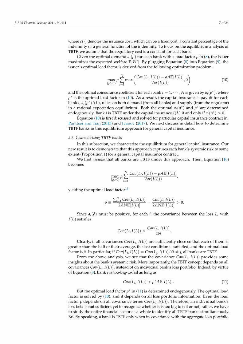
where c(·) denotes the issuance cost, which can be a fixed cost, a constant percentage of theindemnity or a general function of the indemnity. To focus on the equilibrium analysis ofTBTF, we assume that the regulatory cost is a constant for each bank.

Given the optimal demand ai(ρ) for each bank with a load factor ρ in (8), the issuermaximizes the expected welfare E[Wr]. By plugging Equation (8) into Equation (9), theissuer’s optimal load factor is derived from the following optimization problem:

max{ρ>0}

ρN

∑i=1

max(

Cov(Li, I(L))− ρAE[I(L)]Var(I(L))

, 0)

(10)

and the optimal coinsurance coefficient for each bank i = 1, · · · , N is given by ai(ρ∗), where

ρ∗ is the optimal load factor in (10). As a result, the capital insurance’s payoff for eachbank i, ai(ρ

∗)I(L), relies on both demand (from all banks) and supply (from the regulator)in a rational expectation equilibrium. Both the optimal ai(ρ

∗) and ρ∗ are determinedendogenously. Bank i is TBTF under the capital insurance I(L) if and only if ai(ρ

∗) > 0.Equation (10) is first discussed and solved for particular capital insurance contract in

Panttser and Tian (2013) and Ivanov (2017). We next discuss in detail how to determineTBTF banks in this equilibrium approach for general capital insurance.

3.2. Characterizing TBTF Banks

In this subsection, we characterize the equilibrium for general capital insurance. Ournew result is to demonstrate that this approach captures each bank’s systemic risk to someextent (Proposition 1) for a general capital insurance contract.

We first assume that all banks are TBTF under this approach. Then, Equation (10)becomes

max{ρ>0}

ρN

∑i=1

Cov(Li, I(L))− ρAE[I(L)]Var(I(L))

,

yielding the optimal load factor13

ρ̂ ≡ ∑Ni=1 Cov(Li, I(L))

2ANE[I(L)]=

Cov(L, I(L))2ANE[I(L)]

> 0.

Since ai(ρ̂) must be positive, for each i, the covariance between the loss Li withI(L) satisfies

Cov(Li, I(L)) >Cov(L, I(L))

2N.

Clearly, if all covariances Cov(Li, I(L)) are sufficiently close so that each of them isgreater than the half of their average, the last condition is satisfied, and the optimal loadfactor is ρ̂. In particular, if Cov(Li, I(L)) = Cov(Lj, I(L)), ∀i 6= j, all banks are TBTF.

From the above analysis, we see that the covariance Cov(Li, I(L)) provides someinsights about the bank’s systemic risk. More importantly, the TBTF concept depends on allcovariances Cov(Li, I(L)), instead of on individual bank’s loss portfolio. Indeed, by virtueof Equation (8), bank i is too-big-to-fail as long as

Cov(Li, I(L)) > ρ∗AE[I(L)]. (11)

But the optimal load factor ρ∗ in (11) is determined endogenously. The optimal loadfactor is solved by (10), and it depends on all loss portfolio information. Even the loadfactor ρ̂ depends on all covariance terms Cov(Li, I(L)). Therefore, an individual bank’sloss beta is not sufficient yet to recognize whether it is too big to fail or not; rather, we haveto study the entire financial sector as a whole to identify all TBTF banks simultaneously.Briefly speaking, a bank is TBTF only when its covariance with the aggregate loss portfolio

J. Risk Financial Manag. 2021, 14, 414 8 of 24

is relatively large compared with other banks’ corresponding covariances in the samefinancial sector.

Therefore, we introduce the loss beta of bank i with a capital insurance I(L),

βi =Cov(Li, I(L))

Var(I(L)), (12)

in analyzing systemic risk. We reorder {β1, · · · , βN} such that β1 ≥ · · · ≥ βN > 0. Weomit those banks with negative or zero loss betas. Clearly,

N

∑i=1

βi =Cov(L, I(L))

Var(I(L)). (13)

The total beta of all banks is the beta (regression) coefficient of the aggregate lossportfolio to the indemnity of the capital insurance. Appendix A presents an algorithmto characterize all TBTF banks. In particular, a bank with high loss beta is TBTF. Con-versely, the next result shows that all TBTF banks’s loss betas must be bounded belowby 1

2NCov(L,I(L))Var(I(L)) , regardless of the distribution of loss exposure of each bank. Therefore, a

TBTF must have a large loss beta, and vice versa to a certain extent. Proposition 1 thusjustifies our systemic risk measurement in terms of loss betas.

Proposition 1. For any capital insurance I(L), the loss beta of a TBTF bank must be greater thanor equal to 1

2NCov(L,I(L))Var(I(L)) .

Proof. See Appendix A.

We present two examples below to illustrate the equilibrium approach to identifyTBTF banks.

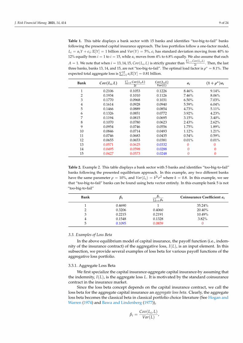
Example 1. We assume that N = 15. The loss portfolios follow a one-factor model, Li = αiY + εi;E[Y] = 1 billion and Var(Y) = 5%, εi has standard deviation moving from 40% to 12% equallyfrom i = 1 to i = 15, while αi moves from 4% to 6.8% equally. We also assume that A = 1 andI(L) = L.

Table 1 represents loss betas, ρ∗ and the optimal coinsurance ai(ρ∗). We note that when

i = 13, 14, 15, Cov(Li, L) >∑i

j=1 Cov(Lj ,L)2i for i = 13, 14, 15. Moreover, the first 12 banks

are TBTF. The optimal load factor is ρ∗ = 8.1%. The expected total aggregate loss is∑12

i=1 aiE[Y] = 0.81 billion. The coinsurance coefficient ai(ρ∗) increases with respect to the

loss beta.

Example 2. Assume that N = 5, and any two different banks’ loss portfolios have the samecorrelation coefficient ρ = 0.10. Var(Li) = k2iσ2 for 0 < k < 1.

Table 2 demonstrates that TBTF banks must have large betas, but the inverse statementis not completely valid. In fact, only the last bank has a small beta, but the first three banksare TBTF banks. Both examples provide a crucial insight into the equilibrium approach.Even though some banks contribute positively to systemic risk and banks are heavilycorrelated, those banks might still not be TBTF banks, as shown by the last example.The intuition is as follows. By insuring the bank with the most significant systemic riskexposure, other banks’ systemic risks can be insured to some extent. As a consequence,other banks are not TBTF anymore.

J. Risk Financial Manag. 2021, 14, 414 9 of 24

Table 1. This table displays a bank sector with 15 banks and identifies “too-big-to-fail” banksfollowing the presented capital insurance approach. The loss portfolios follow a one-factor model,Li = αiY + εi; E[Y] = 1 billion and Var(Y) = 5%, εi has standard deviation moving from 40% to12% equally from i = 1 to i = 15, while αi moves from 4% to 6.8% equally. We also assume that each

A = 1. We note that when i = 13, 14, 15, Cov(Li, L) is strictly greater than ∑ij=1 Cov(Lj ,L)

2i . Then, the lastthree banks, banks 13, 14, and 15, are not “too-big-to-fail”. The optimal load factor is ρ∗ = 8.1%. Theexpected total aggregate loss is ∑12

i=1 aiE[Y] = 0.81 billion.

Bank Cov(Li, L) ∑ij=1 Cov(Lj ,L)

2iCov(Li ,L)

Var(L)ai (1 + ρ∗)ai

1 0.2106 0.1053 0.1226 8.46% 9.14%2 0.1934 0.1010 0.1126 7.46% 8.06%3 0.1770 0.0968 0.1031 6.50% 7.03%4 0.1614 0.0928 0.0940 5.59% 6.04%5 0.1466 0.0889 0.0854 4.73% 5.11%6 0.1326 0.0851 0.0772 3.92% 4.23%7 0.1194 0.0815 0.0695 3.15% 3.40%8 0.1070 0.0780 0.0623 2.43% 2.62%9 0.0954 0.0746 0.0556 1.75% 1.89%

10 0.0846 0.0714 0.0493 1.12% 1.21%11 0.0746 0.0683 0.0435 0.54% 0.59%12 0.0655 0.0653 0.0381 0.01% 0.01%13 0.0571 0.0625 0.0332 0 014 0.0495 0.0598 0.0288 0 015 0.0427 0.0573 0.0248 0 0

Table 2. Example 2. This table displays a bank sector with 5 banks and identifies “too-big-to-fail”banks following the presented equilibrium approach. In this example, any two different bankshave the same parameter ρ = 10%, and Var(Li) = k2iσ2 where k = 0.8. In this example, we seethat “too-big-to-fail” banks can be found using beta vector entirely. In this example bank 5 is not“too-big-to-fail”

Bank βiβi

∑ik=1 βk

Coinsurance Coefficient ai

1 0.4690 1 35.24%2 0.3206 0.4060 20.40%3 0.2215 0.2191 10.49%4 0.1548 0.1328 3.82%5 0.1095 0.0859 0

3.3. Examples of Loss Beta

In the above equilibrium model of capital insurance, the payoff function (i.e., indem-nity of the insurance contract) of the aggregative loss, I(L), is an input element. In thissubsection, we provide several examples of loss beta for various payoff functions of theaggregative loss portfolio.

3.3.1. Aggregate Loss Beta

We first specialize the capital insurance-aggregate capital insurance-by assuming thatthe indemnity, I(L), is the aggregate loss L. It is motivated by the standard coinsurancecontract in the insurance market.

Since the loss beta concept depends on the capital insurance contract, we call theloss beta for the aggregate capital insurance an aggregate loss beta. Clearly, the aggregateloss beta becomes the classical beta in classical portfolio choice literature (See Hogan andWarren (1974) and Bawa and Lindenberg (1977)),

βi =Cov(Li, L)

Var(L),

J. Risk Financial Manag. 2021, 14, 414 10 of 24

and the total loss beta, ∑Ni=1 βi = 1. If each βi = 1

N , all banks are TBTF. In this case,Proposition 1 is proved in Ivanov (2017) that a TBTF bank’s aggregate loss beta is greaterthan 1

2N .

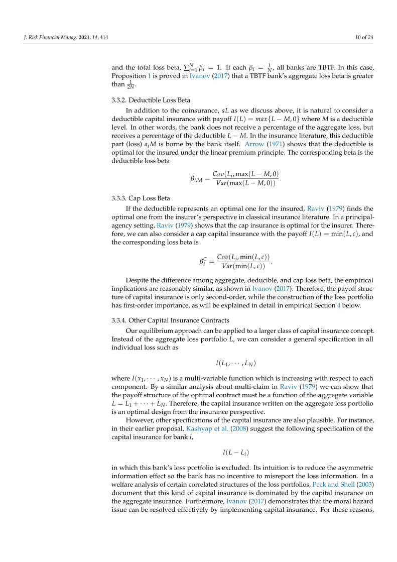
3.3.2. Deductible Loss Beta

In addition to the coinsurance, aL as we discuss above, it is natural to consider adeductible capital insurance with payoff I(L) = max{L−M, 0} where M is a deductiblelevel. In other words, the bank does not receive a percentage of the aggregate loss, butreceives a percentage of the deductible L−M. In the insurance literature, this deductiblepart (loss) ai M is borne by the bank itself. Arrow (1971) shows that the deductible isoptimal for the insured under the linear premium principle. The corresponding beta is thedeductible loss beta

βi,M =Cov(Li, max(L−M, 0)Var(max(L−M, 0))

.

3.3.3. Cap Loss Beta

If the deductible represents an optimal one for the insured, Raviv (1979) finds theoptimal one from the insurer’s perspective in classical insurance literature. In a principal-agency setting, Raviv (1979) shows that the cap insurance is optimal for the insurer. There-fore, we can also consider a cap capital insurance with the payoff I(L) = min(L, c), andthe corresponding loss beta is

βCi =

Cov(Li, min(L, c))Var(min(L, c))

.

Despite the difference among aggregate, deducible, and cap loss beta, the empiricalimplications are reasonably similar, as shown in Ivanov (2017). Therefore, the payoff struc-ture of capital insurance is only second-order, while the construction of the loss portfoliohas first-order importance, as will be explained in detail in empirical Section 4 below.

3.3.4. Other Capital Insurance Contracts

Our equilibrium approach can be applied to a larger class of capital insurance concept.Instead of the aggregate loss portfolio L, we can consider a general specification in allindividual loss such as

I(L1, · · · , LN)

where I(x1, · · · , xN) is a multi-variable function which is increasing with respect to eachcomponent. By a similar analysis about multi-claim in Raviv (1979) we can show thatthe payoff structure of the optimal contract must be a function of the aggregate variableL = L1 + · · ·+ LN . Therefore, the capital insurance written on the aggregate loss portfoliois an optimal design from the insurance perspective.

However, other specifications of the capital insurance are also plausible. For instance,in their earlier proposal, Kashyap et al. (2008) suggest the following specification of thecapital insurance for bank i,

I(L− Li)

in which this bank’s loss portfolio is excluded. Its intuition is to reduce the asymmetricinformation effect so the bank has no incentive to misreport the loss information. In awelfare analysis of certain correlated structures of the loss portfolios, Peck and Shell (2003)document that this kind of capital insurance is dominated by the capital insurance onthe aggregate insurance. Furthermore, Ivanov (2017) demonstrates that the moral hazardissue can be resolved effectively by implementing capital insurance. For these reasons,

J. Risk Financial Manag. 2021, 14, 414 11 of 24

we suggest the specification form I(L) as a capital insurance in studying the systemic riskthrough this presented insurance approach.

3.4. Analytical Expression of Loss Betas

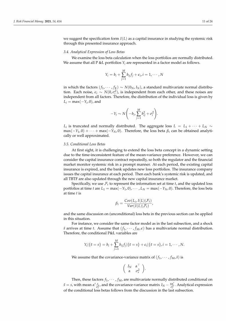
We examine the loss beta calculation when the loss portfolios are normally distributed.We assume that all P &L portfolios Yi are represented in a factor model as follows.

Yi = bi +M

∑j=1

bij f j + εi, i = 1, · · · , N

in which the factors ( f1, · · · , fK) ∼ N(0N , IN), a standard multivariate normal distribu-tion. Each noise, εi ∼ N(0, σ2

i ), is independent from each other, and these noises areindependent from all factors. Therefore, the distribution of the individual loss is given byLi = max(−Yi, 0), and

−Yi ∼ N

(−bi,

M

∑j=1

b2ij + σ2

i

).

Li is truncated and normally distributed. The aggregate loss L = L1 + · · · + LN ∼max(−Y1, 0) + · · · + max(−YN , 0). Therefore, the loss beta βi can be obtained analyti-cally or well approximated.

3.5. Conditional Loss Betas

At first sight, it is challenging to extend the loss beta concept in a dynamic settingdue to the time-inconsistent feature of the mean-variance preference. However, we canconsider the capital insurance contract repeatedly, so both the regulator and the financialmarket monitor systemic risk in a prompt manner. At each period, the existing capitalinsurance is expired, and the bank updates new loss portfolios. The insurance companyissues the capital insurance at each period. Then each bank’s systemic risk is updated, andall TBTF are also updated through the new capital insurance market.

Specifically, we use Ft to represent the information set at time t, and the updated lossportfolios at time t are L1 = max(−Y1, 0), · · · , LN = max(−YN , 0). Therefore, the loss betaat time t is

βi =Cov(Li, I(L)|Ft)

Var(I(L)|Ft),

and the same discussion on (unconditional) loss beta in the previous section can be appliedin this situation.

For instance, we consider the same factor model as in the last subsection, and a shocks̃ arrives at time t. Assume that ( f1, · · · , fM, ε) has a multivariate normal distribution.Therefore, the conditional P&L variables are

Yi|{s̃ = s} = bi +M

∑j=1

bij f j|{s̃ = s}+ εi|{s̃ = s}, i = 1, · · · , N.

We assume that the covariance-variance matrix of ( f1, · · · , fM, s̃) is(IN α>

α σ2s

).

Then, these factors f1, · · · , fM, are multivariate normally distributed conditional ons̃ = s, with mean α′ s

σ2s

, and the covariance-variance matrix IN − αα′

σ2s

. Analytical expressionof the conditional loss betas follows from the discussion in the last subsection.

J. Risk Financial Manag. 2021, 14, 414 12 of 24

3.6. Loss Betas with Tail Risks

Since our equilibrium approach is model-free, any profit and loss portfolio distributionand the loss portfolio can be used.14 Therefore, we can incorporate tail risk or the skewnessin the profit and loss portfolio, particularly for the portfolio with significant derivativepositions. Moreover, the correlation structure between these loss portfolios can calibratethe correlated structure in the market.

Specifically, we let Fi(x) denote the distribution of the loss variable Li, and the jointdistribution of {L1, · · · , LN} is written as

F(x1, · · · , xN) = C(F1(x1), · · · , FN(xN)), x1, · · · , xN ≥ 0

where C(u1, · · · , uN) is a copula function. Sklar’s theorem states that any joint distributioncan be written in this way, so the copula function C(·) measures the correlation struc-ture of the loss variables. In practice, the copula functions can be Gaussian copula andArchimedean copula. Those marginal distributions Fi(xi) can be chosen to capture thetail risk.

The loss beta in this setting can be calculated easily via a simulation method. Forinstance,

E[Li I(L)] =∫

xi I(x1 + · · ·+ xN)dC(F1(x1), · · · , FN(xN)).

4. Empirical Results

This section takes our model into the data to study the empirical implication of ourequilibrium-based measure of systemic risk. Our objective is to identify TBTF banks in theU.S. financial market over the period 2002 to 2019. We first construct the loss portfolio ofeach bank based on an empirically accessible proxy. Then we calculate the loss beta andidentify TBTF banks using the algorithm in Section 3.

We conduct two approaches in constructing the loss portfolio. In the first approach, wefollow the accounting-based methodology introduced in Section 2. In the second approach,we follow Ivanov (2017) to construct the loss portfolio. Moreover, we compare with theCoVaR approach in Adrian and Brunnermeier (2016).

4.1. Data and Sample

In our first approach to construct the loss portfolio, we use data from FFIEC 031 Forms,also called “Call Reports”. FEIEC 031 forms are the forms that every commercial bankor thrift institution must file quarterly, regardless of regulation by the Federal DepositInsurance Corporation (FDIC), Office of the Comptroller of the Currency (OCC), or FederalReserve. FFIEC 031 includes bank deposits, loans, and other bank characteristics of interest.

In our sample, we focus on all commercial U.S.banks with assets over $50 billion,which is the threshold to be classified as Large Banking Organization by the FederalReserve. Large Banking Organizations are subject to stricter examination for their systemicrisk, as evident by an additional layer of examination in annual stress testing. We chooseLarge Banking Organizations to be in our sample of interest since they are the candidatesfor higher systemic risk. The final sample contains 2821 bank-quarter observations over70 quarters, from the first quarter of 2002 to the second quarter of 2019. Since the data panelis unbalanced as banks exit and enter the sample throughout the sample period, there are67 unique banks in total.

In this section, we compare our loss beta with an established measure of systemic risk,CoVaR.15 To calculate CoVaR, we extend the measure from Adrian and Brunnermeier (2016)to the second quarter of 2019 based on stock return data from CRSP and macroeconomicvariables from the FRED.16 For tests on the correlation between loss beta and CoVaR, thesample is restricted to public banks since CoVaR requires stock return data that are onlyavailable to public firms. We use the CRSP-FRB link provided by the Federal Reserve Bankof New York to merge our loss data measures with the CoVaR measure.

J. Risk Financial Manag. 2021, 14, 414 13 of 24

Finally, in our second approach to construct the loss portfolio, we construct the bank’sloss portfolio based on information available in Compustat and CRSP, following Adrianand Brunnermeier (2016) and Ivanov (2017). Specifically, we obtain the bank total assetfrom Compustat and bank total equity from CRSP. Our sample is limited to publicly tradedfinancial institutions only in this approach.

4.2. Bank Loss Beta

Following the model provided in Section 2, we estimate the bank loss portfolio. Fromthe Call Reports, we gather the book value of the bank’s total loans, the book value ofthe bank’s total equity, the book value of the bank’s total deposits, and the book valueof the bank’s subordinated debt. We use these book values as proxies for the fair valueof the loans and deposits, and the market value of the equity and the subordinated debt.Then, we use these book values to calculate each bank’s loss portfolio for each quarter asexplained in Section 2. The aggregate loss portfolio is also calculated for each quarter inthe sample period.

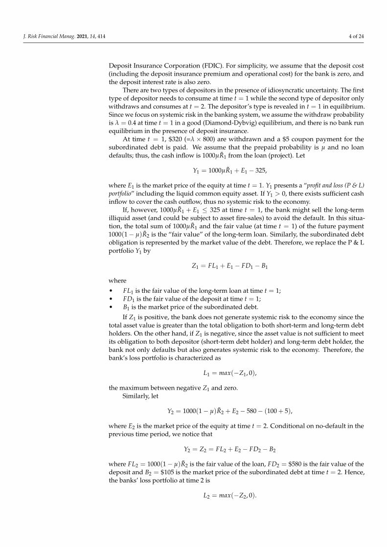
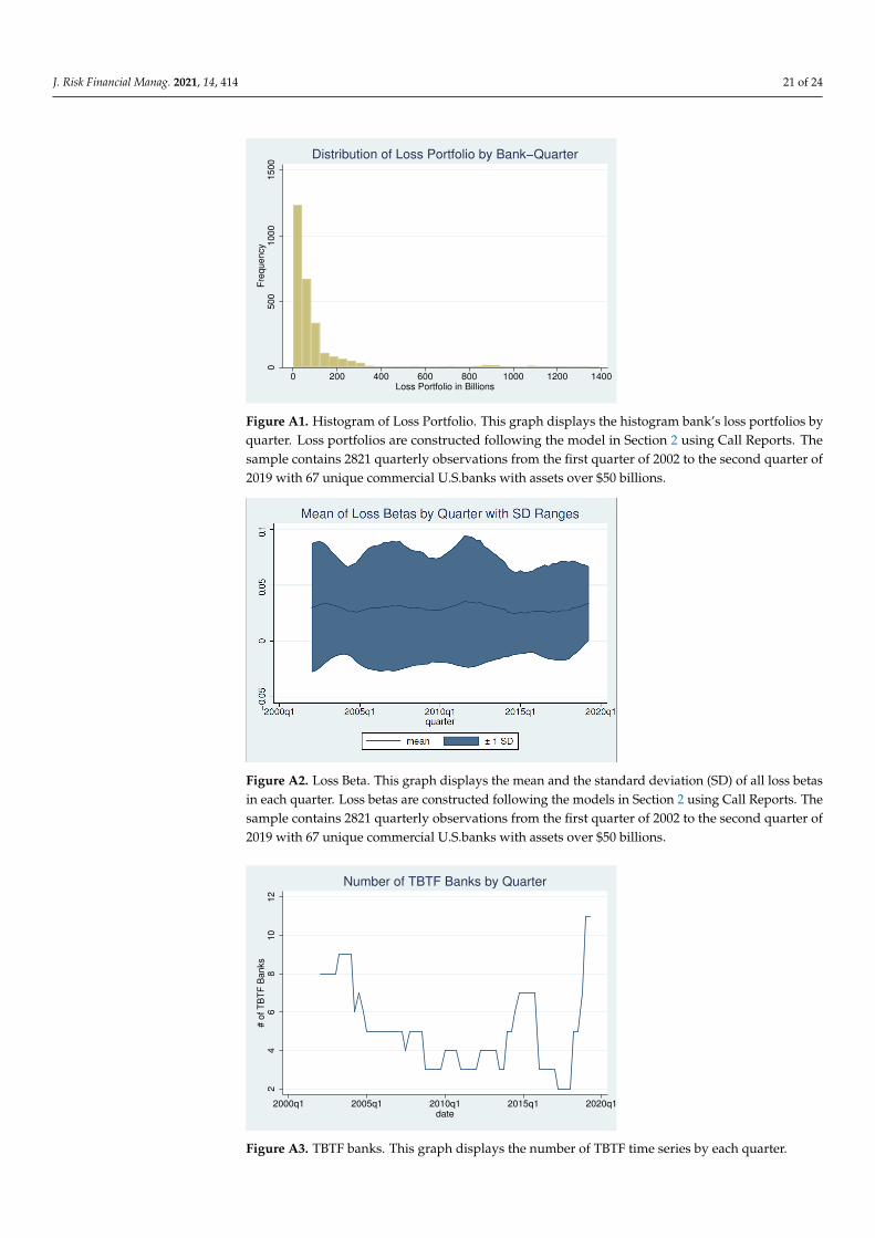
Figure A1 shows the histogram of all banks’ loss portfolios by quarter. As shown, thedistribution of loss portfolio across all banks is highly skewed. Moreover, the probabilityof a large loss, such as an over $800 billion loss, is not marginal, showing a clear tail risk inthe banks’ portfolios.

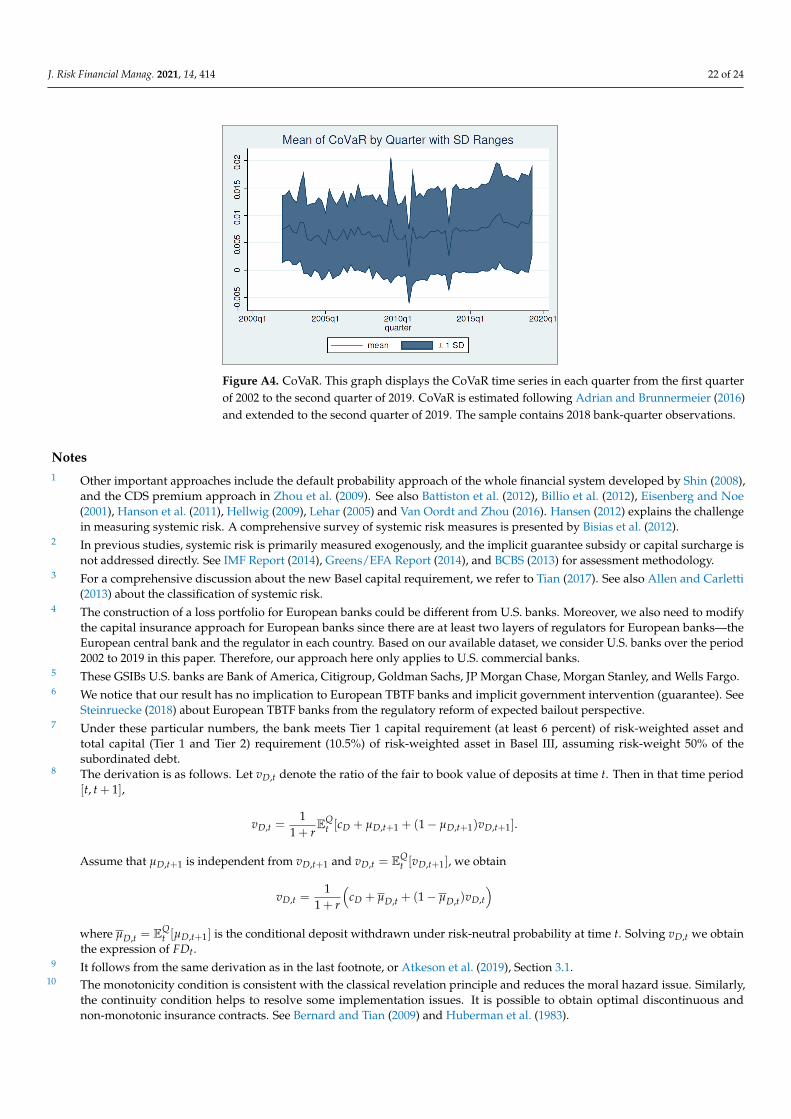
Given all loss portfolios and assuming that A = 1, we compute all aggregate lossbetas, Cov(Li ,L)

Var(L) , for each quarter. Figure A2 reports both mean and the standard deviationof all loss betas for each quarter. Since the total number of banks in our sample is N = 67,the mean of loss beta is close to 1/67. However, we observe a relatively high standarddeviation, meaning that some banks have substantial systemic risk components. Therefore,some banks are TBTF and some are not.

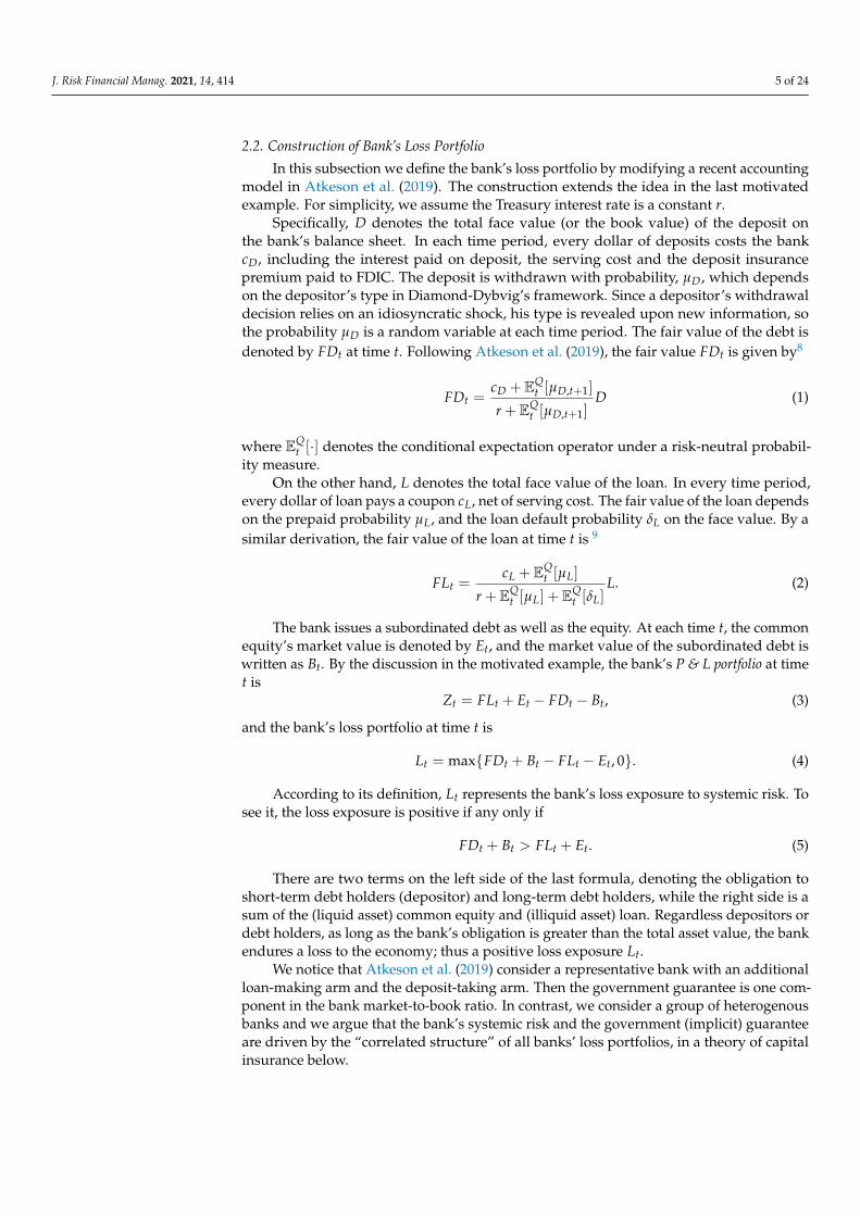
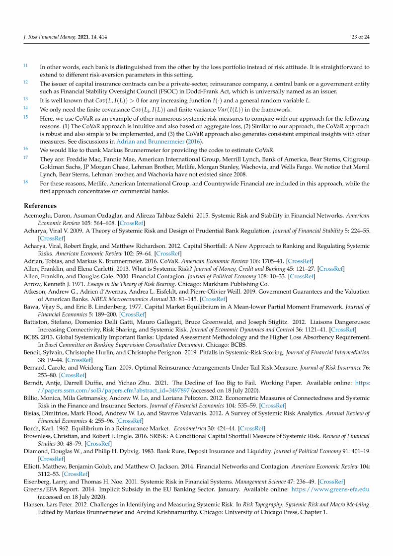
TBTF banks are identified in each quarter using the algorithm described in Appendix A.Figure A3 reports the number of TBTF in each quarter from 2002 to 2019. The number ofTBTF is time-varying. For example, there are 9 TBTF in 2004, then the number graduallydecreases. During the 2007–2008 financial crisis period, there are 3–5 TBTF, but each TBTF’ssystemic risk is substantial. As shown in Acharya et al. (2012), 5 firms provide 50% of theentire systemic risk in the U.S. financial markets, and 15 firms account for 92% of the sys-temic risk. This highly concentrated feature of TBTF banks is thus consistent with Acharyaet al. (2012). This finding is also confirmed by the second empirical approach below.

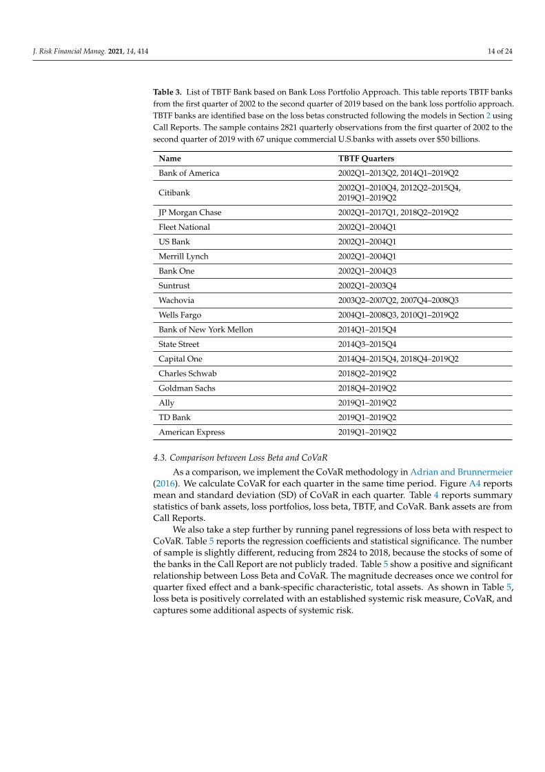
Table 3 reports all TBTF in a particular quarter. No bank is TBTF for the whole sampleperiod, but four banks are TBTF the vast majority of the time. Not surprisingly, those banksare the “Big Four”—Bank of America, JP Morgan Chase, Wells Fargo, and Citibank. Fromthe start of the data in 2001, the number of TBTF banks declined steadily even before thecrisis, dropping to just three TBTF banks in the fourth quarter of 2008 (JP Morgan Chase,Bank of America, and Citibank). Interestingly, Wachovia is identified as TBTF over theperiod 2007 Q4 to 2008 Q3. The number of TBTF banks stayed low until 2014, when BNYMellon, State Street, and Capital One briefly joined the Big Four before abruptly fallingout after 2015. The number of TBTF banks reached a sample low of two (Bank of Americaand Wells Fargo) TBTF banks from 2017Q2 to 2018Q1, before rapidly expanding to 2019Q2,with a sample high of 11 banks.

J. Risk Financial Manag. 2021, 14, 414 14 of 24

Table 3. List of TBTF Bank based on Bank Loss Portfolio Approach. This table reports TBTF banksfrom the first quarter of 2002 to the second quarter of 2019 based on the bank loss portfolio approach.TBTF banks are identified base on the loss betas constructed following the models in Section 2 usingCall Reports. The sample contains 2821 quarterly observations from the first quarter of 2002 to thesecond quarter of 2019 with 67 unique commercial U.S.banks with assets over $50 billions.

Name TBTF Quarters

Bank of America 2002Q1–2013Q2, 2014Q1–2019Q2

Citibank 2002Q1–2010Q4, 2012Q2–2015Q4,2019Q1–2019Q2

JP Morgan Chase 2002Q1–2017Q1, 2018Q2–2019Q2

Fleet National 2002Q1–2004Q1

US Bank 2002Q1–2004Q1

Merrill Lynch 2002Q1–2004Q1

Bank One 2002Q1–2004Q3

Suntrust 2002Q1–2003Q4

Wachovia 2003Q2–2007Q2, 2007Q4–2008Q3

Wells Fargo 2004Q1–2008Q3, 2010Q1–2019Q2

Bank of New York Mellon 2014Q1–2015Q4

State Street 2014Q3–2015Q4

Capital One 2014Q4–2015Q4, 2018Q4–2019Q2

Charles Schwab 2018Q2–2019Q2

Goldman Sachs 2018Q4–2019Q2

Ally 2019Q1–2019Q2

TD Bank 2019Q1–2019Q2

American Express 2019Q1–2019Q2

4.3. Comparison between Loss Beta and CoVaR

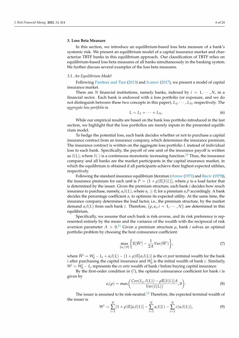
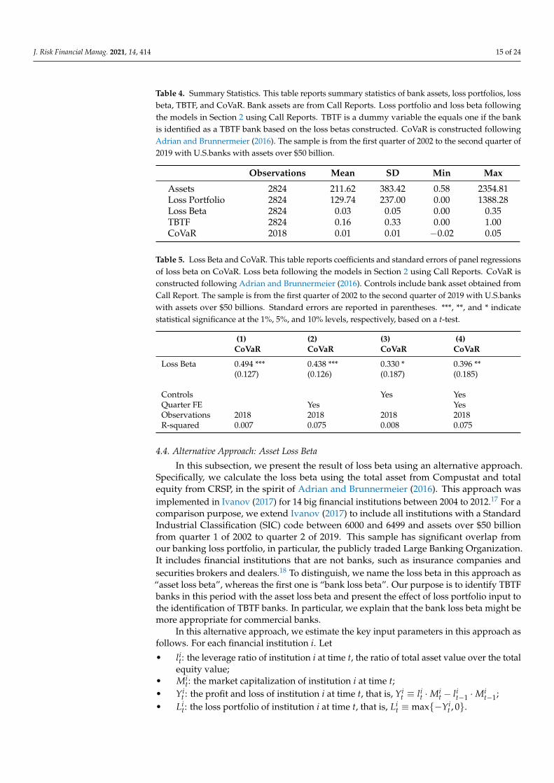
As a comparison, we implement the CoVaR methodology in Adrian and Brunnermeier(2016). We calculate CoVaR for each quarter in the same time period. Figure A4 reportsmean and standard deviation (SD) of CoVaR in each quarter. Table 4 reports summarystatistics of bank assets, loss portfolios, loss beta, TBTF, and CoVaR. Bank assets are fromCall Reports.

We also take a step further by running panel regressions of loss beta with respect toCoVaR. Table 5 reports the regression coefficients and statistical significance. The numberof sample is slightly different, reducing from 2824 to 2018, because the stocks of some ofthe banks in the Call Report are not publicly traded. Table 5 show a positive and significantrelationship between Loss Beta and CoVaR. The magnitude decreases once we control forquarter fixed effect and a bank-specific characteristic, total assets. As shown in Table 5,loss beta is positively correlated with an established systemic risk measure, CoVaR, andcaptures some additional aspects of systemic risk.

J. Risk Financial Manag. 2021, 14, 414 15 of 24

Table 4. Summary Statistics. This table reports summary statistics of bank assets, loss portfolios, lossbeta, TBTF, and CoVaR. Bank assets are from Call Reports. Loss portfolio and loss beta followingthe models in Section 2 using Call Reports. TBTF is a dummy variable the equals one if the bankis identified as a TBTF bank based on the loss betas constructed. CoVaR is constructed followingAdrian and Brunnermeier (2016). The sample is from the first quarter of 2002 to the second quarter of2019 with U.S.banks with assets over $50 billion.

Observations Mean SD Min Max

Assets 2824 211.62 383.42 0.58 2354.81Loss Portfolio 2824 129.74 237.00 0.00 1388.28Loss Beta 2824 0.03 0.05 0.00 0.35TBTF 2824 0.16 0.33 0.00 1.00CoVaR 2018 0.01 0.01 −0.02 0.05

Table 5. Loss Beta and CoVaR. This table reports coefficients and standard errors of panel regressionsof loss beta on CoVaR. Loss beta following the models in Section 2 using Call Reports. CoVaR isconstructed following Adrian and Brunnermeier (2016). Controls include bank asset obtained fromCall Report. The sample is from the first quarter of 2002 to the second quarter of 2019 with U.S.bankswith assets over $50 billions. Standard errors are reported in parentheses. ***, **, and * indicatestatistical significance at the 1%, 5%, and 10% levels, respectively, based on a t-test.

(1) (2) (3) (4)CoVaR CoVaR CoVaR CoVaR

Loss Beta 0.494 *** 0.438 *** 0.330 * 0.396 **(0.127) (0.126) (0.187) (0.185)

Controls Yes YesQuarter FE Yes YesObservations 2018 2018 2018 2018R-squared 0.007 0.075 0.008 0.075

4.4. Alternative Approach: Asset Loss Beta

In this subsection, we present the result of loss beta using an alternative approach.Specifically, we calculate the loss beta using the total asset from Compustat and totalequity from CRSP, in the spirit of Adrian and Brunnermeier (2016). This approach wasimplemented in Ivanov (2017) for 14 big financial institutions between 2004 to 2012.17 For acomparison purpose, we extend Ivanov (2017) to include all institutions with a StandardIndustrial Classification (SIC) code between 6000 and 6499 and assets over $50 billionfrom quarter 1 of 2002 to quarter 2 of 2019. This sample has significant overlap fromour banking loss portfolio, in particular, the publicly traded Large Banking Organization.It includes financial institutions that are not banks, such as insurance companies andsecurities brokers and dealers.18 To distinguish, we name the loss beta in this approach as“asset loss beta”, whereas the first one is “bank loss beta”. Our purpose is to identify TBTFbanks in this period with the asset loss beta and present the effect of loss portfolio input tothe identification of TBTF banks. In particular, we explain that the bank loss beta might bemore appropriate for commercial banks.

In this alternative approach, we estimate the key input parameters in this approach asfollows. For each financial institution i. Let

• lit: the leverage ratio of institution i at time t, the ratio of total asset value over the total

equity value;• Mi

t: the market capitalization of institution i at time t;• Yi

t : the profit and loss of institution i at time t, that is, Yit ≡ li

t ·Mit − li

t−1 ·Mit−1;

• Lit: the loss portfolio of institution i at time t, that is, Li

t ≡ max{−Yit , 0}.

J. Risk Financial Manag. 2021, 14, 414 16 of 24

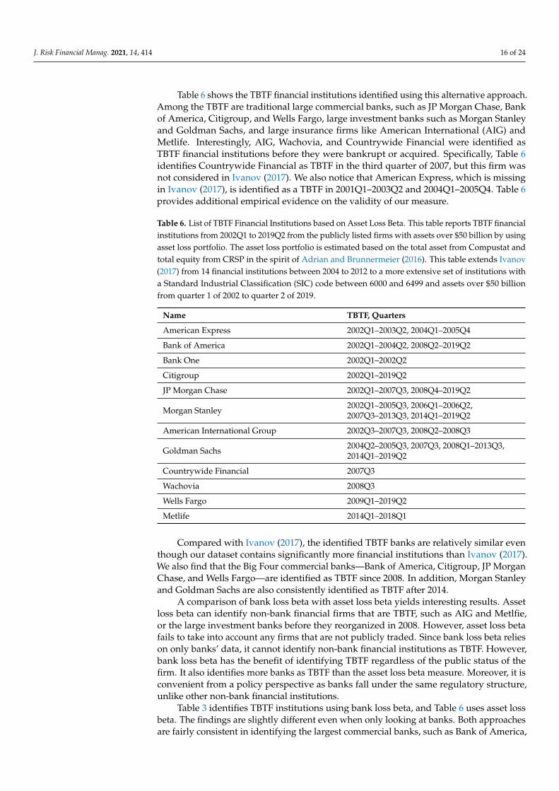
Table 6 shows the TBTF financial institutions identified using this alternative approach.Among the TBTF are traditional large commercial banks, such as JP Morgan Chase, Bankof America, Citigroup, and Wells Fargo, large investment banks such as Morgan Stanleyand Goldman Sachs, and large insurance firms like American International (AIG) andMetlife. Interestingly, AIG, Wachovia, and Countrywide Financial were identified asTBTF financial institutions before they were bankrupt or acquired. Specifically, Table 6identifies Countrywide Financial as TBTF in the third quarter of 2007, but this firm wasnot considered in Ivanov (2017). We also notice that American Express, which is missingin Ivanov (2017), is identified as a TBTF in 2001Q1–2003Q2 and 2004Q1–2005Q4. Table 6provides additional empirical evidence on the validity of our measure.

Table 6. List of TBTF Financial Institutions based on Asset Loss Beta. This table reports TBTF financialinstitutions from 2002Q1 to 2019Q2 from the publicly listed firms with assets over $50 billion by usingasset loss portfolio. The asset loss portfolio is estimated based on the total asset from Compustat andtotal equity from CRSP in the spirit of Adrian and Brunnermeier (2016). This table extends Ivanov(2017) from 14 financial institutions between 2004 to 2012 to a more extensive set of institutions witha Standard Industrial Classification (SIC) code between 6000 and 6499 and assets over $50 billionfrom quarter 1 of 2002 to quarter 2 of 2019.

Name TBTF, Quarters

American Express 2002Q1–2003Q2, 2004Q1–2005Q4

Bank of America 2002Q1–2004Q2, 2008Q2–2019Q2

Bank One 2002Q1–2002Q2

Citigroup 2002Q1–2019Q2

JP Morgan Chase 2002Q1–2007Q3, 2008Q4–2019Q2

Morgan Stanley 2002Q1–2005Q3, 2006Q1–2006Q2,2007Q3–2013Q3, 2014Q1–2019Q2

American International Group 2002Q3–2007Q3, 2008Q2–2008Q3

Goldman Sachs 2004Q2–2005Q3, 2007Q3, 2008Q1–2013Q3,2014Q1–2019Q2

Countrywide Financial 2007Q3

Wachovia 2008Q3

Wells Fargo 2009Q1–2019Q2

Metlife 2014Q1–2018Q1

Compared with Ivanov (2017), the identified TBTF banks are relatively similar eventhough our dataset contains significantly more financial institutions than Ivanov (2017).We also find that the Big Four commercial banks—Bank of America, Citigroup, JP MorganChase, and Wells Fargo—are identified as TBTF since 2008. In addition, Morgan Stanleyand Goldman Sachs are also consistently identified as TBTF after 2014.

A comparison of bank loss beta with asset loss beta yields interesting results. Assetloss beta can identify non-bank financial firms that are TBTF, such as AIG and Metlfie,or the large investment banks before they reorganized in 2008. However, asset loss betafails to take into account any firms that are not publicly traded. Since bank loss beta relieson only banks’ data, it cannot identify non-bank financial institutions as TBTF. However,bank loss beta has the benefit of identifying TBTF regardless of the public status of thefirm. It also identifies more banks as TBTF than the asset loss beta measure. Moreover, it isconvenient from a policy perspective as banks fall under the same regulatory structure,unlike other non-bank financial institutions.

Table 3 identifies TBTF institutions using bank loss beta, and Table 6 uses asset lossbeta. The findings are slightly different even when only looking at banks. Both approachesare fairly consistent in identifying the largest commercial banks, such as Bank of America,

J. Risk Financial Manag. 2021, 14, 414 17 of 24

JP Morgan Chase, Citigroup, Wachovia, and Wells Fargo, as TBTF. However, the bank lossbeta, by not taking into consideration non-bank financial institutions, is more informativewithin the banking sector as it much more consistently and frequently identifies relativelysmaller banks as TBTF, such as Bank One, Fleet National, US Bank, and Suntrust as TBTFbefore the 2008 Financial Crisis, and BNY Mellon and State Street after the crisis, andeven Capital One, Charles Schwab, Ally, and TD Bank in the most recent quarters of thedata sample. Notably, in the most recent quarter 2019Q2, using asset loss beta, only 6institutions, Bank of America, Citigroup, JP Morgan Chase, Morgan Stanley, GoldmanSachs, and Wells Fargo, were TBTF. However, using bank loss beta, 11 institutions areTBTF, the six under asset loss beta, and Capital One, Charles Schwab, Ally, TD Bank, andAmerican Express. Overall, the bank loss beta provides a more consistent and frequentsignal that a commercial bank should be considered TBTF.

5. Conclusions

In this paper, we provide an equilibrium approach based on economic theories to mea-sure the systemic risk of financial institutions and identify TBTF financial intermediariessuch as banks, insurance companies, or other types of intermediaries. This paper shedslight on why and how financial crises such as the 2007–2009 form and grow in magnitude.The recent episode of Covid-19 also sparks considerable interests on the systemic risk dueto unexpected shocks. By constructing each financial intermediary’s expected loss portfolioin a recent accounting model, we suggest a capital-based insurance approach to addressthe systemic risk that is crucial to the health of the entire financial market. We derive asystemic risk measure, termed loss beta, in a characterization of the capital-based insuranceequilibrium. We perform a comprehensive empirical implication and document U.S. TBTFfinancial intermediaries from 2002 to 2019. We demonstrate a time-series pattern of U.S.TBTF financial intermediaries, and a significant number of TBTF banks starting from 2019.

Compared with previous literature on systemic risk, our approach relies on an insur-ance equilibrium in which all banks with systemic risk exposures and a regulator withimplicit guarantee obligation maximize expected utility separably. Previous important stud-ies such as Acharya et al. (2012), Billio et al. (2012) and Adrian and Brunnermeier (2016)introduce some statistical measures that are easy to apply, but these measures are mostlyconstructed exogenously. On the other hand, other measures that provide specific channelssuch as liquidity mismatching or consumer/real property risk require future data, which isimpossible to implement ex-ante. Our proposed approach advances the literature by pro-viding a forward-looking systemic risk measure with an insurance equilibrium approachto determine the TBTF financial intermediaries endogenously. Moreover, since we developthis approach in an insurance framework, this approach can also be helpful to estimate theexpected bailout and bailout probability under the real-world probability measure.

Our results have policy implications and practical appeals. First, the implementationof this approach is straightforward. By using a loss portfolio for each bank (provided byeach bank or constructed by the regulator), the regulator can calculate each bank’s loss betaand identify TBTF banks with a simple algorithm in this conceptual framework. Second,the regulator is allowed to choose capital insurance contracts in the framework. In this way,various loss betas can be used to check the robustness of a bank’s systemic risk. Third, theregulator can use the capital insurance premium to assess the implied guarantee subsidyor another type of capital for TBTF banks. Finally, through the analysis of the loss portfolio,the bank can reduce the systemic risk exposure with this approach.

According to our theoretical and empirical study, a loss portfolio is a crucial input inour approach and affects the identification of TBTF banks. However, the construction of aloss portfolio is far from unique. While we suggest some accounting-based or asset-basedmethods, constructing the most appropriate loss portfolio with systemic risk exposure isnot resolved yet. In other words, we need to understand which bank factors/characteristicscontribute to the systemic risk before constricting the loss portfolio, and there are manystudies in the literature to identify those factors. This paper only compares the loss beta

J. Risk Financial Manag. 2021, 14, 414 18 of 24

approach with CoVaR, but it is also essential to compare it with numerous other systemicrisk measures to understand the loss beta measure better. More importantly, we do notconsider the availability of this approach to other regions, particularly European banks.We leave these topics to a future study.

Author Contributions: Writing—original draft, K.I., J.S., W.T. and K.T. All authors share first author-ship. All authors have read and agreed to the published version of the manuscript.

Funding: This research received no external funding.

Institutional Review Board Statement: Not applicable.

Informed Consent Statement: Not applicable.

Data Availability Statement: Data is available upon request.

Acknowledgments: We are grateful to Azamat Abdymomunov, Carole Bernard, Ethan Chiang,Atanas Mihov, Jeffrey Gerlach, Scott Frame, Christopher Kirby, Steven Zhu, and seminar participantsat Federal Reserve Bank of Richmond, Shanghai Jiaotong University, Xiamen University, and Uni-versity of North Carolina at Charlotte for very insightful and helpful comments. We thank MarkusBrunnermeier for providing the codes to estimate CoVaR. The authors thank the financial supportfrom the University of North Carolina at Charlotte, and Queens University of Charlotte. Both JamesSchulte and Kevin Tseng were working at the Federal Reserve Bank of Richmond while the projectwas developed. However, the views expressed in this paper are those of the authors and do notnecessarily represent those of the Federal Reserve Bank of Richmond or the Federal Reserve System.The authors would like to thank the editor and anonymous referees for their constructive commentsand insightful suggestions.

Conflicts of Interest: The authors declare no conflict of interest.

Appendix A. Properties of Capital Insurance

In this appendix, we present several properties of a general capital insurance, extend-ing Panttser and Tian (2013) and Ivanov (2017). Let Z = I(L), b = AE[Z]

Var(Z) > 0, and

f (ρ) =N

∑i=1

max(

βiρ− ρ2b, 0)

. (A1)

Without loss of generality, we assume that β1 > β2 > · · · > βN > 0. For eachm = 1, · · · , N, we define

gm(ρ) =m

∑i=1

ρ(βi − ρb), (A2)

and Im =[

βm+1b , βm

b

], m = 1, · · · , N − 1,

IN =[0, βN

b

].

(A3)

It can be shown that (see Ivanov (2017), Appendix A) the insurer’s optimizationproblem is reduced to

maxρ>0

f (ρ) = maxm=1,··· ,N

maxρ∈Im

gm(ρ). (A4)

Let Bm ≡ maxρ∈Im gm(ρ), m = 1, · · · , N, and τm = β1+···+βm2mb , m = 1, · · · , N.

Case 1. m = 1.In this case, A1 = g1(max(τ1, β2

b )). The function g1(·) is decreasing over I1 if and onlyif β2

b ≥ τ1, that is, β2 ≥ β12 .

Case 2. m = N.In this case, AN = gN(min(τN , βN

b )). The function gN(·) is increasing over IN ifand only if βN

b ≤ τN ; that is, βN ≤ β1+···+βN2N . Otherwise, if βN > β1+···+βN

2N , then

AN = gN(τN) =(β1+···+βN)2

4Nb .

J. Risk Financial Manag. 2021, 14, 414 19 of 24

Case 3. m = 2, · · · , N − 1.3.a. If βm+1

b < τm < βmb , then Am = gm(τm) =

(β1+···+βm)2

4mb .3.b. If τm ≤ βm+1

b , then gm(·) is decreasing over Im.3.c. If τm ≥ βm

b , then gm(·) is increasing over Im.Characterization of TBTF banks and ρ∗:Choose m∗ as argmax1≤m≤N Bm, and the least one if there are multiple solutions (see

Panttser and Tian (2013)). Then,

• Bank 1, · · · , m∗ − 1 are TBTF;• Bank m∗ + 1, · · · , N are NOT TBTF;

• Bank m∗ is TBTF if and only if τm∗ < βm∗ , that is, βm∗ >β1+···+βm∗

2m∗ .

Moreover, the optimal load factor is

ρ∗ =β1 + · · ·+ βm∗

2m∗. (A5)

The next three results follow from the above property of each function gm(ρ) overIm, 1 ≤ m ≤ N.

Proposition A1. Bank 1 is always a TBTF bank. If β1 is sufficiently large such that followingconditions hold,

β1 + · · ·+ βm

2m≥ βm, m = 2, · · · , N

then Bank 1 is the only one TBTF bank.

Proof. The first part follows from the above characterization of TBTF banks; see alsoPanttser and Tian (2013). By the above discussion, under the proposed condition, thefunction gm(ρ) is increasing over Im, m = 2, . . . , N. Therefore maxρ f (ρ) = g1(max(τ1, β2

b )),m∗ = 1. Since max(τ1, β2

b ) < β1b , Bank 1 is the only TBTF bank.

Proposition A2. Assume that for each m = 1, · · · , N − 1

βm+1 ≥β1 + · · ·+ βm

2m,

and

βN >β1 + · · ·+ βN

2N,

then all banks are TBTF.

Proof. Under the first condition, the function gm(ρ) is decreasing over Im, m = 1, · · · , N −1. Then m∗ = 1. If βN > β1+···+βN

2N , then all banks are TBTF. If βN is not large enough suchthat βN ≤ β1+···+βN

2N , then bank N is not TBTF, but all other banks are TBTF.

Proposition A3. Assume 2 ≤ m ≤ N − 1 and the following conditions holds,

βi ≤β1 + · · ·+ βi

2i, i = m + 1, · · · , N,

and

β j ≤β1 + · · ·+ β j

2j, j = 1, · · · , m− 1.

J. Risk Financial Manag. 2021, 14, 414 20 of 24

1. If β1+···+βm2m < βm, then all TBTF banks are banks 1, · · · , m.

2. If β1+···+βm2m ≥ βm, then all TBTF banks are banks 1, · · · , m− 1.

Proof. Given the condition we see that the function gi(·) is increasing over Ii fori = m+ 1, · · · , N, and the function gj(·) is decreasing over Ij for j = 1, · · · , m− 1. Therefore

m∗ = m, maxρ f (ρ) = maxρ∈Im gm(ρ). If τm < βmb , then maxρ f (ρ) = gm(max(τm, βm+1

b )).

Then all TBTF banks are 1, · · · , m. Otherwise, τm ≥ βmb implies that maxρ f (ρ) = gm(

βmb ).

Then all TBTF banks are 1, · · · , m− 1.

To prove Proposition 1, we need the following lemma that is shown in Ivanov (2017),Appendix A.

Lemma A1. Given N positive numbers such that b1 ≥ b2 ≥ · · · ≥ bN and ∑Ni=1 bi = 1. If there

exists an integer i such thatbi

∑ik=1 bi

>12i

, (A6)

then bi >1

2N . Moreover, if “>" is replaced by ≥ in (A6), then bi ≥ 12N .

Proof of Proposition 1. The proof is given for aggregate capital insurance in Ivanov (2017).We extend its proof as follows.

Case 1. Assume m∗ = m and τm < βmb .

In this case, βm > β1+···+βm2m . Then by Lemma A1 for bm = βm

Var(Z)Cov(L,Z) we obtain

bm > 12N . That is, βm > 1

2NCov(L,Z)Var(Z) . Here, all TBTF banks are 1, · · · , m. Hence the loss

betas of all TBTF banks are greater than 12N

Cov(L,Z)Var(Z) .

Case 2. Assume m∗ = m and τm ≥ βmb .

In this case, maxρ f (ρ) = maxρ∈Im g(ρ) = gm(βmb ). Therefore, the function gm−1(·)

must be decreasing over Im−1. Hence, βm−1b > βm

b ≥ τm−1. It can be written as

βm−1 >β1 + · · ·+ βm−1

2(m− 1).

Then by Lemma A1 again and similar to Case 1, we obtain βm−1 > 12N

Cov(L,Z)Var(Z) . In this

case, all TBTF banks are 1, · · · , m− 1. Hence, the loss betas of all TBTF banks are greaterthan 1

2NCov(L,Z)Var(Z) .

Finally, Ivanov (2017) Proposition 3 shows that the capital insurance market improvesthe market participants’ utilities. See also Panttser and Tian (2013) for more welfare analysisof capital insurance and its application to classical insurance market.

J. Risk Financial Manag. 2021, 14, 414 21 of 24

0500

1000

1500

Fre

quency

0 200 400 600 800 1000 1200 1400Loss Portfolio in Billions

Distribution of Loss Portfolio by Bank−Quarter

Figure A1. Histogram of Loss Portfolio. This graph displays the histogram bank’s loss portfolios byquarter. Loss portfolios are constructed following the model in Section 2 using Call Reports. Thesample contains 2821 quarterly observations from the first quarter of 2002 to the second quarter of2019 with 67 unique commercial U.S.banks with assets over $50 billions.

Figure A2. Loss Beta. This graph displays the mean and the standard deviation (SD) of all loss betasin each quarter. Loss betas are constructed following the models in Section 2 using Call Reports. Thesample contains 2821 quarterly observations from the first quarter of 2002 to the second quarter of2019 with 67 unique commercial U.S.banks with assets over $50 billions.

24

68

10

12

# o

f T

BT

F B

anks

2000q1 2005q1 2010q1 2015q1 2020q1date

Number of TBTF Banks by Quarter

Figure A3. TBTF banks. This graph displays the number of TBTF time series by each quarter.

J. Risk Financial Manag. 2021, 14, 414 22 of 24

Figure A4. CoVaR. This graph displays the CoVaR time series in each quarter from the first quarterof 2002 to the second quarter of 2019. CoVaR is estimated following Adrian and Brunnermeier (2016)and extended to the second quarter of 2019. The sample contains 2018 bank-quarter observations.

Notes1 Other important approaches include the default probability approach of the whole financial system developed by Shin (2008),

and the CDS premium approach in Zhou et al. (2009). See also Battiston et al. (2012), Billio et al. (2012), Eisenberg and Noe(2001), Hanson et al. (2011), Hellwig (2009), Lehar (2005) and Van Oordt and Zhou (2016). Hansen (2012) explains the challengein measuring systemic risk. A comprehensive survey of systemic risk measures is presented by Bisias et al. (2012).

2 In previous studies, systemic risk is primarily measured exogenously, and the implicit guarantee subsidy or capital surcharge isnot addressed directly. See IMF Report (2014), Greens/EFA Report (2014), and BCBS (2013) for assessment methodology.

3 For a comprehensive discussion about the new Basel capital requirement, we refer to Tian (2017). See also Allen and Carletti(2013) about the classification of systemic risk.

4 The construction of a loss portfolio for European banks could be different from U.S. banks. Moreover, we also need to modifythe capital insurance approach for European banks since there are at least two layers of regulators for European banks—theEuropean central bank and the regulator in each country. Based on our available dataset, we consider U.S. banks over the period2002 to 2019 in this paper. Therefore, our approach here only applies to U.S. commercial banks.

5 These GSIBs U.S. banks are Bank of America, Citigroup, Goldman Sachs, JP Morgan Chase, Morgan Stanley, and Wells Fargo.6 We notice that our result has no implication to European TBTF banks and implicit government intervention (guarantee). See

Steinruecke (2018) about European TBTF banks from the regulatory reform of expected bailout perspective.7 Under these particular numbers, the bank meets Tier 1 capital requirement (at least 6 percent) of risk-weighted asset and

total capital (Tier 1 and Tier 2) requirement (10.5%) of risk-weighted asset in Basel III, assuming risk-weight 50% of thesubordinated debt.

8 The derivation is as follows. Let vD,t denote the ratio of the fair to book value of deposits at time t. Then in that time period[t, t + 1],

vD,t =1

1 + rEQ

t [cD + µD,t+1 + (1− µD,t+1)vD,t+1].

Assume that µD,t+1 is independent from vD,t+1 and vD,t = EQt [vD,t+1], we obtain

vD,t =1

1 + r

(cD + µD,t + (1− µD,t)vD,t

)where µD,t = EQ

t [µD,t+1] is the conditional deposit withdrawn under risk-neutral probability at time t. Solving vD,t we obtainthe expression of FDt.

9 It follows from the same derivation as in the last footnote, or Atkeson et al. (2019), Section 3.1.10 The monotonicity condition is consistent with the classical revelation principle and reduces the moral hazard issue. Similarly,

the continuity condition helps to resolve some implementation issues. It is possible to obtain optimal discontinuous andnon-monotonic insurance contracts. See Bernard and Tian (2009) and Huberman et al. (1983).

J. Risk Financial Manag. 2021, 14, 414 23 of 24

11 In other words, each bank is distinguished from the other by the loss portfolio instead of risk attitude. It is straightforward toextend to different risk-aversion parameters in this setting.

12 The issuer of capital insurance contracts can be a private-sector, reinsurance company, a central bank or a government entitysuch as Financial Stability Oversight Council (FSOC) in Dodd-Frank Act, which is universally named as an issuer.

13 It is well known that Cov(L, I(L)) > 0 for any increasing function I(·) and a general random variable L.14 We only need the finite covariance Cov(Li, I(L)) and finite variance Var(I(L)) in the framework.15 Here, we use CoVaR as an example of other numerous systemic risk measures to compare with our approach for the following

reasons. (1) The CoVaR approach is intuitive and also based on aggregate loss, (2) Similar to our approach, the CoVaR approachis robust and also simple to be implemented, and (3) the CoVaR approach also generates consistent empirical insights with othermeasures. See discussions in Adrian and Brunnermeier (2016).

16 We would like to thank Markus Brunnermeier for providing the codes to estimate CoVaR.17 They are: Freddie Mac, Fannie Mae, American International Group, Merrill Lynch, Bank of America, Bear Sterns, Citigroup.

Goldman Sachs, JP Morgan Chase, Lehman Brother, Metlife, Morgan Stanley, Wachovia, and Wells Fargo. We notice that MerrilLynch, Bear Sterns, Lehman brother, and Wachovia have not existed since 2008.

18 For these reasons, Metlife, American International Group, and Countrywide Financial are included in this approach, while thefirst approach concentrates on commercial banks.

ReferencesAcemoglu, Daron, Asuman Ozdaglar, and Alireza Tahbaz-Salehi. 2015. Systemic Risk and Stability in Financial Networks. American

Economic Review 105: 564–608. [CrossRef]Acharya, Viral V. 2009. A Theory of Systemic Risk and Design of Prudential Bank Regulation. Journal of Financial Stability 5: 224–55.

[CrossRef]Acharya, Viral, Robert Engle, and Matthew Richardson. 2012. Capital Shortfall: A New Approach to Ranking and Regulating Systemic

Risks. American Economic Review 102: 59–64. [CrossRef]Adrian, Tobias, and Markus K. Brunnermeier. 2016. CoVaR. American Economic Review 106: 1705–41. [CrossRef]Allen, Franklin, and Elena Carletti. 2013. What is Systemic Risk? Journal of Money, Credit and Banking 45: 121–27. [CrossRef]Allen, Franklin, and Douglas Gale. 2000. Financial Contagion. Journal of Political Economy 108: 10–33. [CrossRef]Arrow, Kenneth J. 1971. Essays in the Theory of Risk Bearing. Chicago: Markham Publishing Co.Atkeson, Andrew G., Adrien d’Avernas, Andrea L. Eisfeldt, and Pierre-Olivier Weill. 2019. Government Guarantees and the Valuation

of American Banks. NBER Macroeconomics Annual 33: 81–145. [CrossRef]Bawa, Vijay S., and Eric B. Lindenberg. 1977. Capital Market Equilibrium in A Mean-lower Partial Moment Framework. Journal of

Financial Economics 5: 189–200. [CrossRef]Battiston, Stefano, Domenico Delli Gatti, Mauro Gallegati, Bruce Greenwald, and Joseph Stiglitz. 2012. Liaisons Dangereuses:

Increasing Connectivity, Risk Sharing, and Systemic Risk. Journal of Economic Dynamics and Control 36: 1121–41. [CrossRef]BCBS. 2013. Global Systemically Important Banks: Updated Assessment Methodology and the Higher Loss Absorbency Requirement.

In Basel Committee on Banking Supervision Consultative Document. Chicago: BCBS.Benoit, Sylvain, Christophe Hurlin, and Christophe Perignon. 2019. Pitfalls in Systemic-Risk Scoring. Journal of Financial Intermediation

38: 19–44. [CrossRef]Bernard, Carole, and Weidong Tian. 2009. Optimal Reinsurance Arrangements Under Tail Risk Measure. Journal of Risk Insurance 76:

253–80. [CrossRef]Berndt, Antje, Darrell Duffie, and Yichao Zhu. 2021. The Decline of Too Big to Fail. Working Paper. Available online: https:

//papers.ssrn.com/sol3/papers.cfm?abstract_id=3497897 (accessed on 18 July 2020).Billio, Monica, Mila Getmansky, Andrew W. Lo, and Loriana Pelizzon. 2012. Econometric Measures of Connectedness and Systemic

Risk in the Finance and Insurance Sectors. Journal of Financial Economics 104: 535–59. [CrossRef]Bisias, Dimitrios, Mark Flood, Andrew W. Lo, and Stavros Valavanis. 2012. A Survey of Systemic Risk Analytics. Annual Review of

Financial Economics 4: 255–96. [CrossRef]Borch, Karl. 1962. Equilibrium in a Reinsurance Market. Econometrica 30: 424–44. [CrossRef]Brownless, Christian, and Robert F. Engle. 2016. SRISK: A Conditional Capital Shortfall Measure of Systemic Risk. Review of Financial

Studies 30: 48–79. [CrossRef]Diamond, Douglas W., and Philip H. Dybvig. 1983. Bank Runs, Deposit Insurance and Liquidity. Journal of Political Economy 91: 401–19.

[CrossRef]Elliott, Matthew, Benjamin Golub, and Matthew O. Jackson. 2014. Financial Networks and Contagion. American Economic Review 104:

3112–53. [CrossRef]Eisenberg, Larry, and Thomas H. Noe. 2001. Systemic Risk in Financial Systems. Management Science 47: 236–49. [CrossRef]Greens/EFA Report. 2014. Implicit Subsidy in the EU Banking Sector. January. Available online: https://www.greens-efa.edu

(accessed on 18 July 2020).Hansen, Lars Peter. 2012. Challenges in Identifying and Measuring Systemic Risk. In Risk Topography: Systemic Risk and Macro Modeling.

Edited by Markus Brunnermeier and Arvind Krishnamurthy. Chicago: University of Chicago Press, Chapter 1.

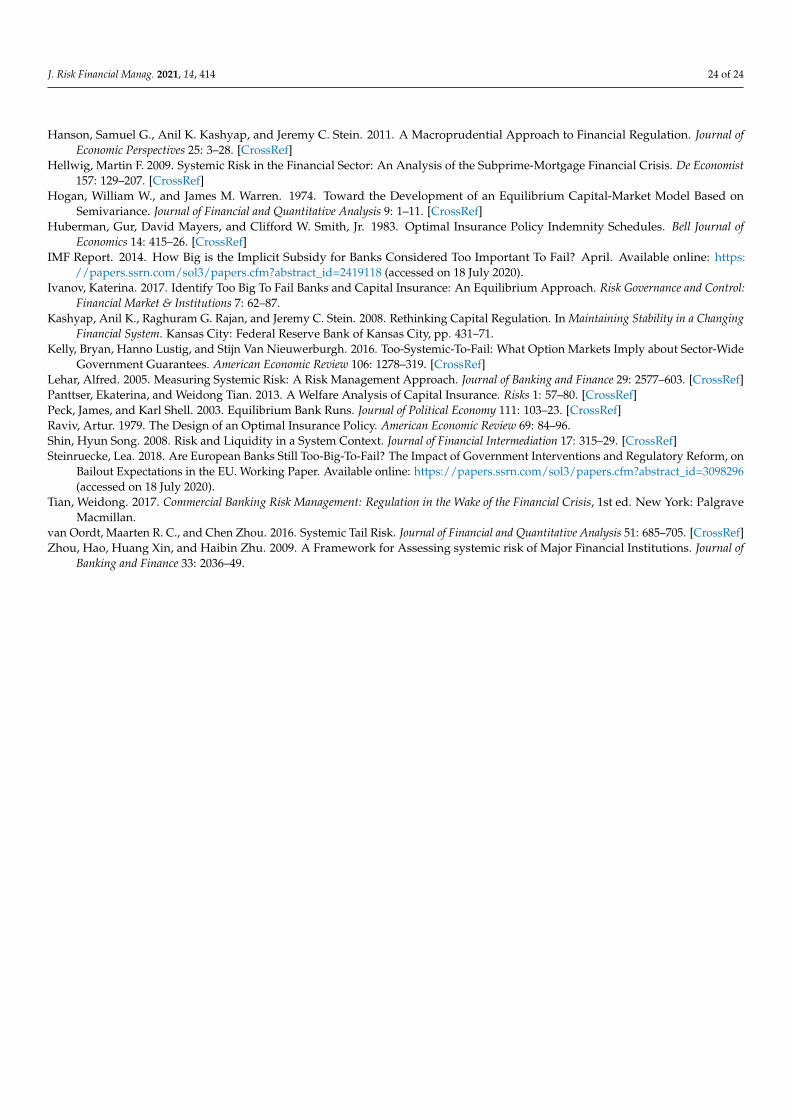
J. Risk Financial Manag. 2021, 14, 414 24 of 24

Hanson, Samuel G., Anil K. Kashyap, and Jeremy C. Stein. 2011. A Macroprudential Approach to Financial Regulation. Journal ofEconomic Perspectives 25: 3–28. [CrossRef]

Hellwig, Martin F. 2009. Systemic Risk in the Financial Sector: An Analysis of the Subprime-Mortgage Financial Crisis. De Economist157: 129–207. [CrossRef]

Hogan, William W., and James M. Warren. 1974. Toward the Development of an Equilibrium Capital-Market Model Based onSemivariance. Journal of Financial and Quantitative Analysis 9: 1–11. [CrossRef]

Huberman, Gur, David Mayers, and Clifford W. Smith, Jr. 1983. Optimal Insurance Policy Indemnity Schedules. Bell Journal ofEconomics 14: 415–26. [CrossRef]

IMF Report. 2014. How Big is the Implicit Subsidy for Banks Considered Too Important To Fail? April. Available online: https://papers.ssrn.com/sol3/papers.cfm?abstract_id=2419118 (accessed on 18 July 2020).

Ivanov, Katerina. 2017. Identify Too Big To Fail Banks and Capital Insurance: An Equilibrium Approach. Risk Governance and Control:Financial Market & Institutions 7: 62–87.

Kashyap, Anil K., Raghuram G. Rajan, and Jeremy C. Stein. 2008. Rethinking Capital Regulation. In Maintaining Stability in a ChangingFinancial System. Kansas City: Federal Reserve Bank of Kansas City, pp. 431–71.

Kelly, Bryan, Hanno Lustig, and Stijn Van Nieuwerburgh. 2016. Too-Systemic-To-Fail: What Option Markets Imply about Sector-WideGovernment Guarantees. American Economic Review 106: 1278–319. [CrossRef]

Lehar, Alfred. 2005. Measuring Systemic Risk: A Risk Management Approach. Journal of Banking and Finance 29: 2577–603. [CrossRef]Panttser, Ekaterina, and Weidong Tian. 2013. A Welfare Analysis of Capital Insurance. Risks 1: 57–80. [CrossRef]Peck, James, and Karl Shell. 2003. Equilibrium Bank Runs. Journal of Political Economy 111: 103–23. [CrossRef]Raviv, Artur. 1979. The Design of an Optimal Insurance Policy. American Economic Review 69: 84–96.Shin, Hyun Song. 2008. Risk and Liquidity in a System Context. Journal of Financial Intermediation 17: 315–29. [CrossRef]Steinruecke, Lea. 2018. Are European Banks Still Too-Big-To-Fail? The Impact of Government Interventions and Regulatory Reform, on

Bailout Expectations in the EU. Working Paper. Available online: https://papers.ssrn.com/sol3/papers.cfm?abstract_id=3098296(accessed on 18 July 2020).

Tian, Weidong. 2017. Commercial Banking Risk Management: Regulation in the Wake of the Financial Crisis, 1st ed. New York: PalgraveMacmillan.

van Oordt, Maarten R. C., and Chen Zhou. 2016. Systemic Tail Risk. Journal of Financial and Quantitative Analysis 51: 685–705. [CrossRef]Zhou, Hao, Huang Xin, and Haibin Zhu. 2009. A Framework for Assessing systemic risk of Major Financial Institutions. Journal of

Banking and Finance 33: 2036–49.