Risk-Based Integrity and Inspection Modeling (RBIIM) of Process Components/System
Upload
khangminh22Category
view
0download
0
Risk-Based Inspection Technology
API RECOMMENDED PRACTICE 581 SECOND EDITION, SEPTEMBER 2008
Copyright American Petroleum Institute Provided by IHS under license with API Licensee=Qatar Petroleum/5943408001
Not for Resale, 10/20/2008 01:51:29 MDTNo reproduction or networking permitted without license from IHS
--```,`,,`,`,,`,`,,,,,,``,```,`-`-`,,`,,`,`,,`---

Copyright American Petroleum Institute Provided by IHS under license with API Licensee=Qatar Petroleum/5943408001
Not for Resale, 10/20/2008 01:51:29 MDTNo reproduction or networking permitted without license from IHS
--```,`,,`,`,,`,`,,,,,,``,```,`-`-`,,`,,`,`,,`---
Risk-Based Inspection Technology
Downstream Segment
API RECOMMENDED PRACTICE 581 SECOND EDITION, SEPTEMBER 2008
Copyright American Petroleum Institute Provided by IHS under license with API Licensee=Qatar Petroleum/5943408001
Not for Resale, 10/20/2008 01:51:29 MDTNo reproduction or networking permitted without license from IHS
--```,`,,`,`,,`,`,,,,,,``,```,`-`-`,,`,,`,`,,`---

Special Notes
API publications necessarily address problems of a general nature. With respect to particular circumstances, local, state, and federal laws and regulations should be reviewed.
Neither API nor any of API's employees, subcontractors, consultants, committees, or other assignees make any warranty or representation, either express or implied, with respect to the accuracy, completeness, or usefulness of the information contained herein, or assume any liability or responsibility for any use, or the results of such use, of any information or process disclosed in this publication. Neither API nor any of API's employees, subcontractors, consultants, or other assignees represent that use of this publication would not infringe upon privately owned rights.
Classified areas may vary depending on the location, conditions, equipment, and substances involved in any given situation. Users of this publication should consult with the appropriate authorities having jurisdiction.
Users of this publication should not rely exclusively on the information contained in this document. Sound business, scientific, engineering, and safety judgment should be used in employing the information contained herein.
Work sites and equipment operations may differ. Users are solely responsible for assessing their specific equipment and premises in determining the appropriateness of applying the instructions. At all times users should employ sound business, scientific, engineering, and judgment safety when using this publication.
API is not undertaking to meet the duties of employers, manufacturers, or suppliers to warn and properly train and equip their employees, and others exposed, concerning health and safety risks and precautions, nor undertaking their obligations to comply with authorities having jurisdiction.
Information concerning safety and health risks and proper precautions with respect to particular materials and conditions should be obtained from the employer, the manufacturer or supplier of that material, or the material safety datasheet.
API publications may be used by anyone desiring to do so. Every effort has been made by the Institute to assure the accuracy and reliability of the data contained in them; however, the Institute makes no representation, warranty, or guarantee in connection with this publication and hereby expressly disclaims any liability or responsibility for loss or damage resulting from its use or for the violation of any authorities having jurisdiction with which this publication may conflict.
API publications are published to facilitate the broad availability of proven, sound engineering and operating practices. These publications are not intended to obviate the need for applying sound engineering judgment regarding when and where these publications should be utilized. The formulation and publication of API publications is not intended in any way to inhibit anyone from using any other practices.
Any manufacturer marking equipment or materials in conformance with the marking requirements of an API standard is solely responsible for complying with all the applicable requirements of that standard. API does not represent, warrant, or guarantee that such products do in fact conform to the applicable API standard.
All rights reserved. No part of this work may be reproduced, stored in a retrieval system, or transmitted by any means, electronic, mechanical, photocopying, recording, or otherwise, without prior written permission from the publisher. Contact the Publisher, API
Publishing Services, 1220 L Street, N.W., Washington, D.C. 20005.
Copyright © 2008 American Petroleum Institute
Copyright American Petroleum Institute Provided by IHS under license with API Licensee=Qatar Petroleum/5943408001
Not for Resale, 10/20/2008 01:51:29 MDTNo reproduction or networking permitted without license from IHS
--```,`,,`,`,,`,`,,,,,,``,```,`-`-`,,`,,`,`,,`---
Foreword
This publication provides quantitative procedures to establish an inspection program using risk-based methods for pressurized fixed equipment, including pressure vessel, piping, tankage, pressure relief devices, and heat exchanger tube bundles. This document is to be used in conjunction with API 580, which provides guidance on developing a risk-based inspection program for fixed equipment in the refining and petrochemical, and chemical process plants. The intent of these publications is for API 580 to introduce the principals and present minimum general guidelines for RBI while this publication provides quantitative calculation methods to determine an inspection plan using a risk-based methodology.
The API Risk-Based Inspection (API RBI) methodology may be used to manage the overall risk of a plant by focusing inspection efforts on the process equipment with the highest risk. API RBI provides the basis for making informed decisions on inspection frequency, the extent of inspection, and the most suitable type of NDE. In most processing plants, a large percent of the total unit risk will be concentrated in a relatively small percent of the equipment items. These potential high-risk components may require greater attention, perhaps through a revised inspection plan. The cost of the increased inspection effort may sometimes be offset by reducing excessive inspection efforts in the areas identified as having lower risk.
Shall: As used in a standard, “shall” denotes a minimum requirement in order to conform to the specification.
Should: As used in a standard, “should” denotes a recommendation or that which is advised but not required in order to conform to the specification.
May: As used in a standard, “may” indicates recommendations that are optional.
Nothing contained in any API publication is to be construed as granting any right, by implication or otherwise, for the manufacture, sale, or use of any method, apparatus, or product covered by letters patent. Neither should anything contained in the publication be construed as insuring anyone against liability for infringement of letters patent.
This document was produced under API standardization procedures that ensure appropriate notification and participation in the developmental process and is designated as an API standard. Questions concerning the interpretation of the content of this publication or comments and questions concerning the procedures under which this publication was developed should be directed in writing to the Director of Standards, American Petroleum Institute, 1220 L Street, N.W., Washington, D.C. 20005. Requests for permission to reproduce or translate all or any part of the material published herein should also be addressed to the director.
Generally, API standards are reviewed and revised, reaffirmed, or withdrawn at least every five years. A one-time extension of up to two years may be added to this review cycle. Status of the publication can be ascertained from the API Standards Department, telephone (202) 682-8000. A catalog of API publications and materials is published annually by API, 1220 L Street, N.W., Washington, D.C. 20005.
Suggested revisions are invited and should be submitted to the Standards Department, API, 1220 L Street, NW, Washington, D.C. 20005, [email protected].
Copyright American Petroleum Institute Provided by IHS under license with API Licensee=Qatar Petroleum/5943408001
Not for Resale, 10/20/2008 01:51:29 MDTNo reproduction or networking permitted without license from IHS
--```,`,,`,`,,`,`,,,,,,``,```,`-`-`,,`,,`,`,,`---

Copyright American Petroleum Institute Provided by IHS under license with API Licensee=Qatar Petroleum/5943408001
Not for Resale, 10/20/2008 01:51:29 MDTNo reproduction or networking permitted without license from IHS
--```,`,,`,`,,`,`,,,,,,``,```,`-`-`,,`,,`,`,,`---

API RP 581 RISK-BASED INSPECTION TECHNOLOGY
PART 1
INSPECTION PLANNING USING API RBI TECHNOLOGY
1-1 Copyright American Petroleum Institute Provided by IHS under license with API Licensee=Qatar Petroleum/5943408001
Not for Resale, 10/20/2008 01:51:29 MDTNo reproduction or networking permitted without license from IHS
--```,`,,`,`,,`,`,,,,,,``,```,`-`-`,,`,,`,`,,`---
API RP 581 RISK-BASED INSPECTION TECHNOLOGY
PART CONTENTS 1 SCOPE ........................................................................................................................................... 5
1.1 Purpose ................................................................................................................................. 5 1.2 Introduction ........................................................................................................................... 5 1.3 Risk Management ................................................................................................................. 5 1.4 Organization and Use ........................................................................................................... 6 1.5 Tables..................................................................................................................................... 7
2 REFERENCES ............................................................................................................................... 8 3 DEFINITIONS ................................................................................................................................. 8
3.1 Definitions ............................................................................................................................. 8 3.2 Acronyms ............................................................................................................................ 10
4 API RBI CONCEPTS ................................................................................................................... 11 4.1 Probability of Failure .......................................................................................................... 11
4.1.1 Overview ...................................................................................................................... 11 4.1.2 Generic Failure Frequency ........................................................................................ 11 4.1.3 Management Systems Factor .................................................................................... 11 4.1.4 Damage Factors .......................................................................................................... 11
4.2 Consequence of Failure ..................................................................................................... 12 4.2.1 Overview ...................................................................................................................... 12 4.2.2 Level 1 Consequence Analysis ................................................................................. 12 4.2.3 Level 2 Consequence Analysis ................................................................................. 13
4.3 Risk Analysis ...................................................................................................................... 14 4.3.1 Determination of Risk ................................................................................................. 14 4.3.2 Risk Matrix ................................................................................................................... 15
4.4 Inspection Planning Based on Risk Analysis .................................................................. 15 4.4.1 Overview ...................................................................................................................... 15 4.4.2 Risk Target .................................................................................................................. 15 4.4.3 Inspection Effectiveness – The Value of Inspection ............................................... 16 4.4.4 Inspection Effectiveness – Example ......................................................................... 17 4.4.5 Inspection Planning .................................................................................................... 17
4.5 Nomenclature ...................................................................................................................... 18 4.6 Tables................................................................................................................................... 19 4.7 Figures ................................................................................................................................. 21
5 PRESSURE VESSELS AND PIPING .......................................................................................... 26 5.1 Probability of Failure .......................................................................................................... 26 5.2 Consequence of Failure ..................................................................................................... 26 5.3 Risk Analysis ...................................................................................................................... 26 5.4 Inspection Planning Based on Risk Analysis .................................................................. 26
6 ATMOSPHERIC STORAGE TANKS ........................................................................................... 27 6.1 Probability of Failure .......................................................................................................... 27 6.2 Consequence of Failure ..................................................................................................... 27 6.3 Risk Analysis ...................................................................................................................... 27 6.4 Inspection Planning Based on Risk Analysis .................................................................. 27
7 PRESSURE RELIEF DEVICES ................................................................................................... 28 7.1 General ................................................................................................................................ 28
7.1.1 Overview ...................................................................................................................... 28 7.1.2 PRD Interdependence with Fixed Equipment .......................................................... 28 7.1.3 Failure Modes .............................................................................................................. 28 7.1.4 Use of Weibull Curves ................................................................................................ 29 7.1.5 PRD Testing, Inspection and Repair ......................................................................... 30 7.1.6 PRD Overhaul or Replacement Start Date ............................................................... 30 7.1.7 Risk Ranking of PRDs ................................................................................................ 30 7.1.8 Link to Fixed or Protected Equipment ...................................................................... 30
7.2 Probability of Failure .......................................................................................................... 31 7.2.1 Definition ..................................................................................................................... 31 7.2.2 Calculation of Probability of Failure to Open .......................................................... 31 7.2.3 PRD Demand Rate ...................................................................................................... 31
1-2 Copyright American Petroleum Institute Provided by IHS under license with API Licensee=Qatar Petroleum/5943408001
Not for Resale, 10/20/2008 01:51:29 MDTNo reproduction or networking permitted without license from IHS
--```,`,,`,`,,`,`,,,,,,``,```,`-`-`,,`,,`,`,,`---
API RP 581 RISK-BASED INSPECTION TECHNOLOGY
7.2.4 PRD Probability of Failure on Demand ..................................................................... 32 7.2.5 Protected Equipment Failure Frequency as a Function of Overpressure ............ 39 7.2.6 Calculation Procedure ................................................................................................ 40
7.3 Probability of Leakage ....................................................................................................... 41 7.3.1 Overview ...................................................................................................................... 41 7.3.2 Calculation of Probability of Leakage ....................................................................... 41 7.3.3 Calculation Procedure ................................................................................................ 43
7.4 Consequence of PRD Failure to Open .............................................................................. 44 7.4.1 General ......................................................................................................................... 44 7.4.2 Damage State of the Protected Equipment .............................................................. 44 7.4.3 Overpressure Potential for Overpressure Demand Cases ..................................... 44 7.4.4 Multiple Relief Device Installations ........................................................................... 45 7.4.5 Calculation of Consequence of Failure to Open ..................................................... 45 7.4.6 Calculation Procedure ................................................................................................ 46
7.5 Consequence of Leakage .................................................................................................. 46 7.5.1 General ......................................................................................................................... 46 7.5.2 Estimation of PRD Leakage Rate .............................................................................. 47 7.5.3 Estimation of Leakage Duration ................................................................................ 47 7.5.4 Credit for Recovery of Leaking Fluid ........................................................................ 47 7.5.5 Cost of Lost Inventory ................................................................................................ 47 7.5.6 Environmental Costs .................................................................................................. 48 7.5.7 Costs of Shutdown to Repair PRD ............................................................................ 48 7.5.8 Cost of Lost Production ............................................................................................. 48 7.5.9 Calculation of Leakage Consequence ...................................................................... 48 7.5.10 Calculation Procedure ................................................................................................ 49
7.6 Risk Analysis ...................................................................................................................... 49 7.6.1 Risk from Failure to Open .......................................................................................... 49 7.6.2 Risk from Leakage ...................................................................................................... 50 7.6.3 Total Risk ..................................................................................................................... 50 7.6.4 Calculation Procedure ................................................................................................ 50
7.7 Inspection Planning Based on Risk Analysis .................................................................. 50 7.7.1 Risk Based Inspection Intervals ................................................................................ 50 7.7.2 Effect of PRD Inspection, Testing and Overhaul on Risk Curve ........................... 50 7.7.3 Effect of PRD Testing without Overhaul on Risk Curve ......................................... 51
7.8 Nomenclature ...................................................................................................................... 52 7.9 Tables................................................................................................................................... 55 7.10 Figures ................................................................................................................................. 70
8 HEAT EXCHANGER TUBE BUNDLES ...................................................................................... 77 8.1 General ................................................................................................................................ 77
8.1.1 Overview ...................................................................................................................... 77 8.1.2 Background ................................................................................................................. 77 8.1.3 Basis of Model ............................................................................................................. 77 8.1.4 Required and Optional Data ...................................................................................... 77
8.2 Methodology Overview ...................................................................................................... 77 8.2.1 General ......................................................................................................................... 77
8.3 Probability of Failure .......................................................................................................... 78 8.3.1 Definition of Bundle Failure ....................................................................................... 78 8.3.2 Probability of Failure Using Weibull Distribution .................................................... 78 8.3.3 Exchanger Bundle Reliability Library or Seed Database........................................ 79 8.3.4 POF using the Owner-User Supplied Weibull Parameters ..................................... 81 8.3.5 POF using the User Supplied MTTF .......................................................................... 81 8.3.6 POF calculated using Specific Bundle History ........................................................ 81
8.4 Consequence of Failure ..................................................................................................... 81 8.4.1 Calculation Method ..................................................................................................... 81 8.4.2 Example ....................................................................................................................... 82
8.5 Risk Analysis ...................................................................................................................... 82 8.5.1 General ......................................................................................................................... 82
1-3 Copyright American Petroleum Institute Provided by IHS under license with API Licensee=Qatar Petroleum/5943408001
Not for Resale, 10/20/2008 01:51:29 MDTNo reproduction or networking permitted without license from IHS
--```,`,,`,`,,`,`,,,,,,``,```,`-`-`,,`,,`,`,,`---
API RP 581 RISK-BASED INSPECTION TECHNOLOGY
8.5.2 Risk Matrix ................................................................................................................... 82 8.6 Inspection Planning Based on Risk Analysis .................................................................. 83
8.6.1 Use of Risk Target in Inspection Planning ............................................................... 83 8.6.2 Example ....................................................................................................................... 83 8.6.3 Inspection Planning Without Inspection History (First Inspection Date) ............. 83 8.6.4 Inspection Planning with Inspection History ........................................................... 84 8.6.5 Effects of Bundle Life Extension Efforts .................................................................. 86 8.6.6 Future Inspection Recommendation ........................................................................ 87
8.7 Bundle Inspect/Replacement Decisions using Cost Benefit Analysis ......................... 87 8.7.1 General ......................................................................................................................... 87 8.7.2 Decision to Inspect or Replace at Upcoming Shutdown ........................................ 87 8.7.3 Decision for Type of Inspection ................................................................................ 88 8.7.4 Optimal Bundle Replacement Frequency................................................................. 88
8.8 Nomenclature ...................................................................................................................... 90 8.9 Tables................................................................................................................................... 92 8.10 Figures ............................................................................................................................... 102
1-4 Copyright American Petroleum Institute Provided by IHS under license with API Licensee=Qatar Petroleum/5943408001
Not for Resale, 10/20/2008 01:51:29 MDTNo reproduction or networking permitted without license from IHS
--```,`,,`,`,,`,`,,,,,,``,```,`-`-`,,`,,`,`,,`---
API RP 581 RISK-BASED INSPECTION TECHNOLOGY
1 SCOPE
1.1 Purpose This recommended practice provides quantitative procedures to establish an inspection program using risk-based methods for pressurized fixed equipment including pressure vessel, piping, tankage, pressure relief devices, and heat exchanger tube bundles. API RP 580 [1] provides guidance on developing a risk-based inspection program for fixed equipment in the refining and petrochemical, and chemical process plants. The intent of these publications is for API RP 580 to introduce the principles and present minimum general guidelines for RBI while this recommended practice provides quantitative calculation methods to determine an inspection plan.
1.2 Introduction The calculation of risk in the Risk-Based Inspection (API RBI) methodology involves the determination of a probability of failure combined with the consequence of failure. Failure in API RBI is defined as a loss of containment from the pressure boundary resulting in leakage to the atmosphere or rupture of a pressurized component. As damage accumulates in a pressurized component during in-service operation the risk increases. At some point, a risk tolerance or risk target is exceeded and an inspection is recommended of sufficient effectiveness to better quantify the damage state of the component. The inspection action itself does not reduce the risk; however, it does reduce uncertainty thereby allowing better quantification of the damage present in the component.
1.3 Risk Management In most situations, once risks have been identified, alternate opportunities are available to reduce them. However, nearly all major commercial losses are the result of a failure to understand or manage risk. API RBI takes the first step toward an integrated risk management program. In the past, the focus of risk assessment has been on on-site safety-related issues. Presently, there is an increased awareness of the need to assess risk resulting from: a) On-site risk to employees, b) Off-site risk to the community, c) Business interruption risks, and d) Risk of damage to the environment The API RBI approach allows any combination of these types of risks to be factored into decisions concerning when, where, and how to inspect equipment. The API RBI methodology may be used to manage the overall risk of a plant by focusing inspection efforts on the process equipment with the highest risk. API RBI provides the basis for managing risk by making an informed decision on inspection frequency, level of detail, and types of NDE. In most plants, a large percent of the total unit risk will be concentrated in a relatively small percent of the equipment items. These potential high-risk components may require greater attention, perhaps through a revised inspection plan. The cost of the increased inspection effort can sometimes be offset by reducing excessive inspection efforts in the areas identified as having lower risk. With an API RBI program in place, inspections will continue to be conducted as defined in existing working documents, but priorities and frequencies will be guided by the API RBI procedure. API RBI is flexible and can be applied on several levels. Within this document, API RBI is applied to pressurized equipment containing process fluids. However, it may be expanded to the system level and include additional equipment, such as instruments, control systems, electrical distribution, and critical utilities. Expanded levels of analyses may improve the payback for the inspection efforts. The API RBI approach can also be made cost-effective by integrating with recent industry initiatives and government regulations, such as Management of Process Hazards, Process Safety Management (OSHA 29 CFR 1910.119), or the proposed Environmental Protection Agency Risk Management Programs for Chemical Accident Release Prevention.
1-5 Copyright American Petroleum Institute Provided by IHS under license with API Licensee=Qatar Petroleum/5943408001
Not for Resale, 10/20/2008 01:51:29 MDTNo reproduction or networking permitted without license from IHS
--```,`,,`,`,,`,`,,,,,,``,```,`-`-`,,`,,`,`,,`---

API RP 581 RISK-BASED INSPECTION TECHNOLOGY
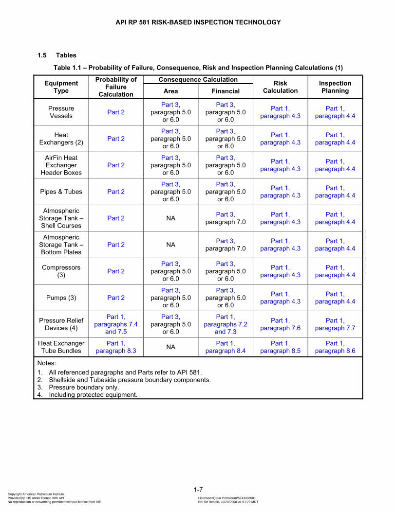
1.4 Organization and Use The API RBI methodology is presented in a three part volume. a) Part 1 – Inspection Planning Using API RBI Technology b) Part 2 – Determination of Probability of Failure in an API RBI Assessment c) Part 3 – Consequence Modeling in API RBI The methods used to obtain an inspection plan are provided in Part 1 for fixed equipment including pressure vessels, piping, atmospheric storage tanks, pressure relief devices and heat exchanger tube bundles. The pressure boundaries of rotating equipment may also be evaluated using this Part. The probability of failure for fixed equipment is covered in Part 2. The probability of failure is based on the component type and damage mechanisms present based on the process fluid characteristics, design conditions, materials of construction, and the original construction code. Part 3 provides methods for computing the consequence of failure. Two methods are provided. The first method, or Level 1, is based on closed form solutions generated for a limited set of reference fluids or fluid groups. The second method, Level 2, is a general, more rigorous method that can be used for any fluid stream composition. An overview of the probability of failure and consequence calculation procedures and the associated paragraph in this recommended practice for fixed equipment is provided in Table 1.1.
1-6 Copyright American Petroleum Institute Provided by IHS under license with API Licensee=Qatar Petroleum/5943408001
Not for Resale, 10/20/2008 01:51:29 MDTNo reproduction or networking permitted without license from IHS
--```,`,,`,`,,`,`,,,,,,``,```,`-`-`,,`,,`,`,,`---
API RP 581 RISK-BASED INSPECTION TECHNOLOGY
1.5 Tables
Table 1.1 – Probability of Failure, Consequence, Risk and Inspection Planning Calculations (1)
Equipment Type
Probability of Failure
Calculation
Consequence Calculation Risk Calculation
Inspection Planning Area Financial
Pressure Vessels Part 2
Part 3, paragraph 5.0
or 6.0
Part 3, paragraph 5.0
or 6.0
Part 1, paragraph 4.3
Part 1, paragraph 4.4
Heat Exchangers (2) Part 2
Part 3, paragraph 5.0
or 6.0
Part 3, paragraph 5.0
or 6.0
Part 1, paragraph 4.3
Part 1, paragraph 4.4
AirFin Heat Exchanger
Header Boxes Part 2
Part 3, paragraph 5.0
or 6.0
Part 3, paragraph 5.0
or 6.0
Part 1, paragraph 4.3
Part 1, paragraph 4.4
Pipes & Tubes Part 2
Part 3, paragraph 5.0
or 6.0
Part 3, paragraph 5.0
or 6.0
Part 1, paragraph 4.3
Part 1, paragraph 4.4
Atmospheric Storage Tank – Shell Courses
Part 2
NA Part 3, paragraph 7.0
Part 1, paragraph 4.3
Part 1, paragraph 4.4
Atmospheric Storage Tank – Bottom Plates
Part 2
NA Part 3, paragraph 7.0
Part 1, paragraph 4.3
Part 1, paragraph 4.4
Compressors (3) Part 2
Part 3, paragraph 5.0
or 6.0
Part 3, paragraph 5.0
or 6.0
Part 1, paragraph 4.3
Part 1, paragraph 4.4
Pumps (3) Part 2
Part 3, paragraph 5.0
or 6.0
Part 3, paragraph 5.0
or 6.0
Part 1, paragraph 4.3
Part 1, paragraph 4.4
Pressure Relief Devices (4)
Part 1, paragraphs 7.4
and 7.5
Part 3, paragraph 5.0
or 6.0
Part 1, paragraphs 7.2
and 7.3
Part 1, paragraph 7.6
Part 1, paragraph 7.7
Heat Exchanger Tube Bundles
Part 1, paragraph 8.3
NA Part 1, paragraph 8.4
Part 1, paragraph 8.5
Part 1, paragraph 8.6
Notes: 1. All referenced paragraphs and Parts refer to API 581. 2. Shellside and Tubeside pressure boundary components. 3. Pressure boundary only. 4. Including protected equipment.
1-7 Copyright American Petroleum Institute Provided by IHS under license with API Licensee=Qatar Petroleum/5943408001
Not for Resale, 10/20/2008 01:51:29 MDTNo reproduction or networking permitted without license from IHS
--```,`,,`,`,,`,`,,,,,,``,```,`-`-`,,`,,`,`,,`---
API RP 581 RISK-BASED INSPECTION TECHNOLOGY
2 REFERENCES 1. API, API RP 580 Recommended Practice for Risk-Based Inspection, American Petroleum Institute,
Washington, D.C. 2. API, API 579-1/ASME FFS-1 2007 Fitness-For-Service, American Petroleum Institute, Washington, D.C.,
2007. 3. CCPS, Guidelines for Consequence Analysis of Chemical Releases, ISBN 0-8169-0786-2, published by the
Center for Chemical Process Safety of the American Institute of Chemical Engineers, 1999. 4. TNO, Methods for Calculation of Physical Effects (TNO Yellow Book, Third Edition), Chapter 6: Heat Flux
from Fires, CPR 14E (ISSN 0921-9633/2.10.014/9110), Servicecentrum, The Hague, 1997. 5. CCPS, Guidelines for Evaluating the Characteristics of Vapor Cloud Explosions, Flash Fires, and BLEVEs,
ISBN 0-8169-0474-X, published by the Center for Chemical Process Safety of the American Institute of Chemical Engineers, 1994.
6. Lees, Frank P., Loss Prevention in the Process Industries: Hazard Identification, Assessment and Control, Butterworth-Heinemann, Second Edition, Reprinted 2001.
7. Baker, W.E., P.A. Cox, P.S. Westine, J.J. Kulesz, and R.A. Strelow, Explosion Hazards and Evaluation, New York: Elsevier, 1983.
8. OFCM, Directory of Atmospheric Transport and Diffusion Consequence Assessment Models (FC-I3-1999), published by the Office of the Federal Coordinator for Meteorological Services and Supporting Research (OFCM) with the assistance of SCAPA members, the document is available at http://www.ofcm.gov/atd_dir/pdf/frontpage.htm.
9. Cox, A.W., Lees, F. P., and Ang, M.L., Classification of Hazardous Locations, Rugby: Instn Chem. Engrs., 1990.
10. Osage, D.A., “API 579-1/ASME FFS-1 2006 – A Joint API/ASME Fitness-For-Service Standard for Pressurized Equipment”, ESOPE Conference, Paris, France, 2007.
11. API, API RP 521 Guide for Pressure-Relieving and Depressuring Systems, American Petroleum Institute, Washington, D.C.
12. API, API RP 520 Part 1 – Sizing, Selection, and Installation of Pressure–Relieving Devices in Refineries, American Petroleum Institute, Washington, D.C.
13. API, API RP 576 Inspection of Pressure Relieving Devices, American Petroleum Institute, Washington, D.C. 14. Abernethy, R.B., Ed., The New Weibull Handbook, 4th Edition, Published by Dr. Robert B. Abernethy, 2000. 15. CCPS, Guidelines for Pressure Relief and Effluent Handling Systems, Center for Chemical Process Safety
of the American Institute of Chemical Engineers, New York, 1998. 16. Lees, F. P., The Assessment of Human Reliability in Process Control, Institution of Chemical Engineers
Conference on Human Reliability in the Process Control Centre, London, 1983. 17. International Electrotechnical Commission (IEC), IEC 61511, Functional Safety: Safety Instrumented
Systems for the Process Sector, Geneva, Switzerland. 18. Trident, Report to the Institute of Petroleum on the “Development of Design Guidelines for Protection
Against Over-Pressures in High Pressure Heat Exchangers: Phase One”, Trident Consultants Ltd and Foster Wheeler Energy, Report J2572, known as “The Trident Report”, 1993.
19. Nelson, Wayne, Applied Life Data Analysis, John Wiley, 1982. 20. Mateshuki, R., “The Role of Information Technology in Plant Reliability”, P/PM Technology, June 1999. 21. Schulz, C.J., “Applications of Statistics to HF Alky Exchanger Replacement Decision Making”, presented at
the NPRA 2001 Annual Refinery & Petrochemical Maintenance Conference and Exhibition, 2001.
3 DEFINITIONS
3.1 Definitions 1. Components – Any part that is designed and fabricated to a recognized code or standard. For example a
pressure boundary may consist of components (cylindrical shell sections, formed heads, nozzles, tank shell courses, tank bottom plate, etc.)
1-8 Copyright American Petroleum Institute Provided by IHS under license with API Licensee=Qatar Petroleum/5943408001
Not for Resale, 10/20/2008 01:51:29 MDTNo reproduction or networking permitted without license from IHS
--```,`,,`,`,,`,`,,,,,,``,```,`-`-`,,`,,`,`,,`---
API RP 581 RISK-BASED INSPECTION TECHNOLOGY
2. Consequence – The outcome of an event or situation expressed qualitatively or quantitatively, being a loss, injury, disadvantage or gain.
3. Consequence analysis – performed to aid in establishing a relative ranking of equipment items on the basis of risk.
4. Consequence area – Reflects the area within which the results of an equipment failure will be evident. 5. Damage (or Deterioration) Mechanism – A process that induces deleterious micro and/or macro material
changes over time that are harmful to the material condition or mechanical properties. Damage mechanisms are usually incremental, cumulative and, in some instances unrecoverable. Common damage mechanisms include corrosion, chemical attack, creep, erosion, fatigue, fracture and thermal aging.
6. Damage Factor – An adjustment factor applied to the generic failure frequency to account for damage mechanisms that are active in a component.
7. Deterioration – The reduction in the ability of a component to provide its intended purpose of containment of fluids. This can be caused by various deterioration mechanisms (e.g., thinning, cracking, mechanical). Damage or degradation may be used in place of deterioration.
8. Equipment – An individual item that is part of a system, equipment is comprised of an assemblage of Components. Examples include pressure vessels, relief devices, piping, boilers and heaters.
9. Event – An incident or situation, which occurs in a particular place during a particular interval of time. 10. Event tree – Model used to depict the possible chain of events that lead to the probability of flammable
outcomes; used to show how various individual event probabilities should be combined to calculate the probability for the chain of events.
11. Event tree analysis – A technique which describes the possible range and sequence of the outcomes which may arise from an initiating event.
12. Failure – Termination of the ability of a system, structure, or component to perform its required function of containment of fluid (i.e., loss of containment). Failures may be unannounced and undetected until the next inspection (unannounced failure), or they may be announced and detected by any number of methods at the instance of occurrence (announced failure).
13. Fitness-for-Service Assessment – A methodology whereby damage or flaws/imperfections contained within a component or equipment item are assessed in order to determine acceptability for continued service.
14. Generic Failure Frequency – A probability of failure developed for specific component types based on a large population of component data that does not include the effects of specific damage mechanisms. The population of component data may include data from all plants within a company or from various plants within an industry, from literature sources, past reports, and commercial data bases.
15. Inspection – Activities performed to verify that materials, fabrication, erection, examinations, testing, repairs, etc. conform to applicable Code, engineering, and/or owner’s written procedure requirements.
16. Inspection Effectiveness – Is qualitatively evaluated by assigning the inspection methods to one of five descriptive categories ranging from Highly Effective to Ineffective.
17. Management Systems Factor – Adjusts the generic failure frequencies for differences in process safety management systems. The factor is derived from the results of an evaluation of a facility or operating unit’s management systems that affect plant risk.
18. Mitigation – Limitation of any negative consequence or reduction in probability of a particular event. 19. Probability – Extent to which an event is likely to occur within the time frame under consideration. The
mathematical definition of probability is a real number in the scale 0 to 1 attached to a random event. Probability can be related to a long-run relative frequency of occurrence or to a degree of belief that an event will occur. For a high degree of belief, the probability is near one. Frequency rather than probability may be used in describing risk. Degrees of belief about probability can be chosen as classes or ranks like; rare, unlikely, moderate, likely, almost certain, or incredible, improbable, remote, occasional, probable, frequent.
20. Process Unit – A group of systems arranged in a specific fashion to produce a product or service. Examples of processes include power generation, acid production, fuel oil production, and ethylene production.
1-9 Copyright American Petroleum Institute Provided by IHS under license with API Licensee=Qatar Petroleum/5943408001
Not for Resale, 10/20/2008 01:51:29 MDTNo reproduction or networking permitted without license from IHS
--```,`,,`,`,,`,`,,,,,,``,```,`-`-`,,`,,`,`,,`---

API RP 581 RISK-BASED INSPECTION TECHNOLOGY
21. Risk – The combination of the probability of an event and its consequence. In some situations, risk is a deviation from the expected. Risk is defined as the product of probability and consequence when probability and consequence are expressed numerically.
22. Risk Analysis – Systematic use of information to identify sources and to estimate the risk. Risk analysis provides a basis for risk evaluation, risk mitigation and risk acceptance. Information can include historical data, theoretical analysis, informed opinions and concerns of stakeholders.
23. Risk-Based Inspection – A risk assessment and management process that is focused on loss of containment of pressurized equipment in processing facilities, due to material deterioration. These risks are managed primarily through equipment inspection.
24. Risk Driver – An item affecting either the probability, consequence or both such that it constitutes a significant portion of the risk.
25. Risk Management – Coordinated activities to direct and control an organization with regard to risk. Risk management typically includes risk assessment, risk mitigation, risk acceptance and risk communication.
26. Risk Mitigation – Process of selection and implementation of measures to modify risk. The term risk mitigation is sometimes used for measures themselves.
27. Risk Target – Level of acceptable risk defined for inspection planning purposes. 28. System – A collection of equipment assembled for a specific function within a process unit. Examples of
systems include service water system, distillation systems and separation systems. 29. Toxic Chemical – Any chemical that presents a physical or health hazard or an environmental hazard
according to the appropriate Material Safety Data Sheet. These chemicals (when ingested, inhaled or absorbed through the skin) can cause damage to living tissue, impairment of the central nervous system, severe illness, or in extreme cases, death. These chemicals may also result in adverse effects to the environment (measured as ecotoxicity and related to persistence and bioaccumulation potential).
3.2 Acronyms API American Petroleum Institute ASME American Society of Mechanical Engineers BLEVE Boiling Liquid Expanding Vapor Explosion CCPS Center for Chemical Process Safety COF Consequence of Failure FFS Fitness-For-Service LOPA Layer of Protection Analysis MW Molecular weight MTBF Mean Time Between Failure NBP Normal boiling point NDE Non destructive examination NFPA National Fire Protection Association OSHA Occupational Safety and Health Administration POF Probability of Failure PRD Pressure Relief Device RBI Risk-Based Inspection TNO The Netherlands Organization for Applied Scientific Research VCE Vapor cloud explosion
1-10 Copyright American Petroleum Institute Provided by IHS under license with API Licensee=Qatar Petroleum/5943408001
Not for Resale, 10/20/2008 01:51:29 MDTNo reproduction or networking permitted without license from IHS
--```,`,,`,`,,`,`,,,,,,``,```,`-`-`,,`,,`,`,,`---
API RP 581 RISK-BASED INSPECTION TECHNOLOGY
4 API RBI CONCEPTS
4.1 Probability of Failure
4.1.1 Overview The probability of failure used in API RBI is computed from Equation (1.1).
( ) ( )f fP t gff D t F= ⋅ ⋅ MS (1.1)
The probability of failure, , is determined as the product of a generic failure frequency, , a damage
factor, , and a management systems factor,
( )fP t gff( )fD t MSF .
4.1.2 Generic Failure Frequency The generic failure frequency for different component types was set at a value representative of the refining and petrochemical industry’s failure data. The generic failure frequency is intended to be the failure frequency prior to any specific damage occurring from exposure to the operating environment, and are provided for several discrete hole sizes for various types of processing equipment (i.e. process vessels, drums, towers, piping systems, tankage, etc.). Discrete hole sizes and an associated failure frequency are introduced into the assessment to model release scenarios. API RBI uses four hole sizes to model the release scenarios covering a full range of events (i.e. small leak to rupture). Adjustment factors are applied to the generic failure frequencies to reflect departures from the industry data to account for damage mechanisms specific to the component’s operating environment and to account for reliability management practices within a plant. The damage factor is applied on a component and damage mechanism specific basis while the management systems factor is applied equally to all equipment within a plant. Damage factors with a value greater than 1.0 will increase the probability of failure, and those with a value less than 1.0 will decrease it. Both adjustment factors are always positive numbers.
4.1.3 Management Systems Factor The management systems adjustment factor, MSF , accounts for the influence of the facility’s management system on the mechanical integrity of the plant equipment. This factor accounts for the probability that accumulating damage which results in loss of containment will be discovered in time and is directly proportional to the quality of a facility’s mechanical integrity program. This factor is derived from the results of an evaluation of a facility’s or operating unit’s management systems that affect plant risk.
4.1.4 Damage Factors The damage factor is determined based on the applicable damage mechanisms (local and general corrosion, cracking, creep, etc.) relevant to the materials of construction and the process service, the physical condition of the component, and the inspection techniques used to quantify damage. The damage factor modifies the industry generic failure frequency and makes it specific to the component under evaluation. Damage factors do not provide a definitive Fitness-For-Service assessment of the component. Fitness-For-Service analyses for pressurized component are covered by API 579-1/ASME FFS-1 [2]. The basic function of the damage factor is to statistically evaluate the amount of damage that may be present as a function of time in service and the effectiveness of an inspection activity to quantify that damage. Methods for determining damage factors are provided in Part 2 for the following damage mechanisms: a) Thinning (both general and local) b) Component Linings c) External Damage (corrosion and stress corrosion cracking) d) Stress Corrosion Cracking (internal based on process fluid, operating conditions and materials of
construction) e) High Temperature Hydrogen Attack f) Mechanical Fatigue (Piping Only)
1-11 Copyright American Petroleum Institute Provided by IHS under license with API Licensee=Qatar Petroleum/5943408001
Not for Resale, 10/20/2008 01:51:29 MDTNo reproduction or networking permitted without license from IHS
--```,`,,`,`,,`,`,,,,,,``,```,`-`-`,,`,,`,`,,`---
API RP 581 RISK-BASED INSPECTION TECHNOLOGY
g) Brittle Fracture (including low-temperature brittle fracture, temper embrittlement, 885 embrittlement, and sigma phase embrittlement.)
If more than one damage mechanism is present, then the principal of superposition, with a special modification for general thinning and external damage, and component linings, is used to determine a total damage factor, see Part 2, paragraph 4.2.2.
4.2 Consequence of Failure
4.2.1 Overview Loss of containment of hazardous fluids from pressurized processing equipment may result in damage to surrounding equipment, serious injury to personnel, production losses, and undesirable environmental impacts. In API RBI, the consequences of loss of containment are determined using well established consequence analysis techniques [3], [4], [5], [6], [7] and are expressed as an affected impact area or in financial terms. Impact areas from such event outcomes as pool fires, flash fires, fireballs, jet fires and vapor cloud explosions are quantified based on the effects of thermal radiation and overpressure on surrounding equipment and personnel. Additionally, cloud dispersion analysis methods are used to quantify the magnitude of flammable releases and to determine the extent and duration of personnel exposure to toxic releases. Event trees are utilized to assess the probability of each of the various event outcomes and to provide a mechanism for probability-weighting the loss of containment consequences. An overview of the API RBI consequence analysis methodology is provided in Part 3, Figure 4.1. Methodologies for two levels of consequence analysis are provided in API RBI. A Level 1 consequence analysis provides a simplistic method to estimate the consequence area based on lookup tables for a limited number of generic or reference hazardous fluids. A Level 2 consequence analysis methodology has been added to API 581 that is more rigorous in that it incorporates a detailed calculation procedure that can be applied to a wider range of hazardous fluids.
4.2.2 Level 1 Consequence Analysis The Level 1 consequence analysis is a simplistic method for evaluating the consequences of hazardous releases for a limited number of reference fluids. The available reference fluids are shown in Part 3, Table 5.1. The reference fluid from Part 3, Table 5.1 that closely matches the normal boiling point and molecular weight of the fluid contained within the process equipment should be used. The flammable consequence area is then determined from a simple polynomial expression that is a function of the release magnitude. For each discrete hole size, release rates are calculated based on the phase of the fluid as described in Part 3, paragraph 5.3. These releases are then used in closed form equations to determine the flammable consequence. For the Level 1 analysis, a series of consequence analyses were performed to generate consequence areas as a function of the reference fluid and release magnitude. In these analyses, the major consequences were associated with pool fires for liquid releases and VCEs for vapor releases. Probabilities of ignition, probabilities of delayed ignition, and other probabilities in the Level 1 event tree were selected based on expert opinion for each of the reference fluids and release types (i.e. continuous or instantaneous). These probabilities were constant and independent of release rate or mass. Based on these analyses, closed form flammable consequence area equations of the form shown in Equation (1.2) were developed to compute consequence areas.
bCA a X= ⋅ (1.2)
The variables and in a b Equation (1.2) are provided for the reference fluids in Part 3, Tables 5.8 and 5.9. If the release is steady state and continuous such as the case for small hole sizes, then the release rate is substituted into Equation (1.2) for X . If the release is considered instantaneous, for example, as a result of a vessel or pipe rupture, then the release mass is substituted into Equation (1.2) for X . The transition between a continuous release and an instantaneous release in API RBI is defined as a release where more than 4,536 kgs [10,000 lbs] of fluid mass escapes in less than 3 minutes, see Part 3, paragraph 5.5.
1-12 Copyright American Petroleum Institute Provided by IHS under license with API Licensee=Qatar Petroleum/5943408001
Not for Resale, 10/20/2008 01:51:29 MDTNo reproduction or networking permitted without license from IHS
--```,`,,`,`,,`,`,,,,,,``,```,`-`-`,,`,,`,`,,`---

API RP 581 RISK-BASED INSPECTION TECHNOLOGY
The final flammable consequence areas are determined as a probability-weighted average of the individual consequence areas calculated for each release hole size. In API RBI, four hole sizes are used; the lowest hole size represents a small leak and the largest hole size represents a rupture or complete release of contents. This is performed for both the equipment damage and the personnel injury consequence areas. The probability weighting utilizes the hole size distribution and the generic frequencies of the release hole sizes selected. The equation for probability weighting of the flammable consequence areas is given by Equation (1.3).
4
1
flamn n
flam n
total
gff CACA
gff=
⎛ ⎞⋅⎜ ⎟⎜=⎜ ⎟⎜ ⎟⎝ ⎠
∑⎟ (1.3)
The total generic failure frequency, , in the above equation is determined using totalgff Equation (1.4).
4
1total n
n
gff gff=
=∑ (1.4)
The Level 1 consequence analysis procedure is a simplistic method for approximating the consequence area of a hazardous release. The only inputs required are basic fluid properties (such as MW, density and ideal gas specific heat ratio, ) and operating conditions. A calculation of the release rate or the available mass in the inventory group (i.e. the inventory of attached equipment that contributes fluid mass to a leaking equipment item) is also required. Once these terms are known, the flammable consequence area is determined from
k
Equations (1.2) and (1.3). A similar procedure is used for determining the consequences associated with releases of toxic chemicals such as H2S, ammonia or chlorine. Toxic impact areas are based on probit equations and can be assessed whether the stream is pure or a percentage of a hydrocarbon stream. One of the main limitations of the Level 1 consequence analysis is that it can only be used in cases where the fluid in the component can be represented by one of the reference fluids. The Level 1 consequence analysis has been used in the refining industry over the past 10 years. However, as international interest has grown in API RBI in the refining and petrochemical industries, as well as in the chemical industries, it became apparent that the limited number of reference fluids available in the consequence area tables was not sufficient. As a result, the Level 2 analysis was developed to calculate consequence areas for releases of hazardous fluids using a more rigorous approach. The Level 2 analysis also resolves inconsistencies in the Level 1 analysis related to release type and event probabilities.
4.2.3 Level 2 Consequence Analysis A detailed calculation procedure is provided for determining the consequences of loss of containment of hazardous fluids from pressurized equipment. The Level 2 consequence analysis was developed as a tool to use where the assumptions of the simplified Level 1 consequence analysis were not valid. Examples of where the more rigorous Level 2 calculations may be necessary are cited below: a) The specific fluid is not represented adequately within the list of reference fluids provided in Part 3, Table
4.1, including cases where the fluid is a wide-range boiling mixture or where the fluids toxic consequences are not represented adequately by any of the reference fluids.
b) The stored fluid is close to its critical point, in which case, the ideal gas assumptions for the vapor release equations are invalid.
c) The effects of two-phase releases, including liquid jet entrainment as well as rainout need to be included in the assessment.
d) The effects of BLEVEs are to be included in the assessment. e) The effects of pressurized non-flammable explosions, such as are possible when non-flammable
pressurized gases (e.g. air or nitrogen) are released during a vessel rupture, are to be included in the assessment.
f) The meteorological assumptions used in the dispersion calculations that form the basis for the Level 1 consequence analysis table lookups do not represent the site data.
1-13 Copyright American Petroleum Institute Provided by IHS under license with API Licensee=Qatar Petroleum/5943408001
Not for Resale, 10/20/2008 01:51:29 MDTNo reproduction or networking permitted without license from IHS
--```,`,,`,`,,`,`,,,,,,``,```,`-`-`,,`,,`,`,,`---
API RP 581 RISK-BASED INSPECTION TECHNOLOGY
The Level 2 consequence analysis procedures presented in Part 3, paragraph 6.0 provide equations and background information necessary to calculate consequence areas for several flammable and toxic event outcomes. A summary of these events are provided in Part 3, Table 4.1. To perform Level 2 consequence analysis calculations, the actual composition of the fluid stored in the equipment is modeled. Fluid property solvers are available which allow the analyst to calculate fluid physical properties more accurately. The fluid solver will also provide the ability to perform flash calculations to better determine the release phase of the fluid and to account for two-phase releases. In many of the consequence calculations, physical properties of the released fluid are required at storage conditions as well as conditions after release to the atmosphere. A cloud dispersion analysis must also be performed as part of a Level 2 consequence analysis to assess the quantity of flammable material or toxic concentration throughout vapor clouds that are generated after a release of volatile material. Modeling a release depends on the source term conditions, the atmospheric conditions, the release surroundings, and the hazard being evaluated. Employment of many commercially available models, including SLAB or DEGADIS [8], account for these important factors and will produce the desired data for the Level 2 RBI assessments. The event trees used in the Level 2 consequence analysis are shown in Part 3, Figures 6.2 and 6.3. Significant improvement in the calculations of the probabilities on the event trees have been made in the Level 2 analysis procedure. Unlike the Level 1 analysis, the probabilities of ignition on the event tree are not constant with release magnitude. Consistent with the work of Cox, Lee and Ang [9], the Level 2 event tree ignition probabilities are directly proportional to the release rate. The probabilities of ignition are also a strong function of the MW of the fluid. The probability that an ignition will be a delayed ignition is also a function of the release magnitude and how close the operating temperature is to the auto-ignition temperature (AIT) of the fluid. These improvements to the event tree will result in consequence impact areas that are more dependent on the size of release and the flammability and reactivity properties of the fluid being released.
4.3 Risk Analysis
4.3.1 Determination of Risk The calculation of risk can be determined as a function of time in accordance with Equation (1.5). This equation combines the probability of failure and the consequence of failure as described in paragraphs 4.1 and 4.2.
( ) ( ) ( )fR t P t C t= ⋅ (1.5)
Note that the probability of failure, , is a function of time since the damage factor as shown in ( )fP t Equation (1.1) increases as the damage in the component due to thinning, cracking, or other damage mechanisms accumulate with time. Figure 4.1 illustrates that the risk associated with individual damage mechanisms can be added together by superposition to provide the overall risk as a function of time. In API RBI, the consequence of failure, , is assumed to be invariant with time. Therefore,( )C t Equation (1.5) can be rewritten as shown in Equations (1.6) and (1.7) depending on whether the risk is expressed as an impact area or in financial terms.
( ) ( )fR t P t CA for Area Based Ris= ⋅ − k (1.6)
( ) ( )fR t P t FC for Financial Based Risk= ⋅ − (1.7)
In these equations, CA is the consequence impact area expressed in units of area and is the financial consequence expressed in economic terms. Note that in
FCEquations (1.6) and (1.7), the risk is varying with
time due only to the fact that the probability of failure is a function of time.
1-14 Copyright American Petroleum Institute Provided by IHS under license with API Licensee=Qatar Petroleum/5943408001
Not for Resale, 10/20/2008 01:51:29 MDTNo reproduction or networking permitted without license from IHS
--```,`,,`,`,,`,`,,,,,,``,```,`-`-`,,`,,`,`,,`---

API RP 581 RISK-BASED INSPECTION TECHNOLOGY
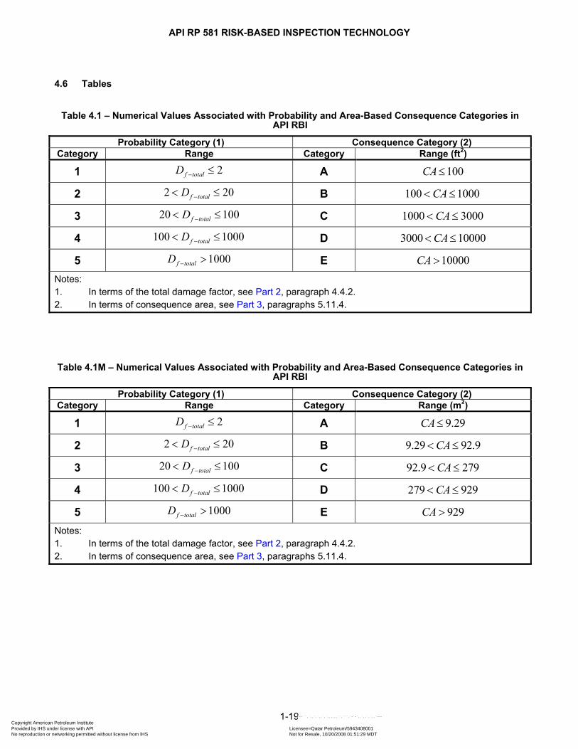
4.3.2 Risk Matrix Presenting the results in a risk matrix is an effective way of showing the distribution of risks for different components in a process unit without numerical values. In the risk matrix, the consequence and probability categories are arranged such that the highest risk components are toward the upper right-hand corner. The risk matrix used in API RBI is shown in Figure 4.2. The risk matrix may be expressed in terms of consequence area or financial consequence. Recommended numerical values associated with probability consequence categories are shown in Tables 4.1 and 4.2 for consequence categories expressed in terms of area or financial terms, respectively. Risk categories (i.e. High, Medium High, Medium, and Low) are assigned to the boxes on the risk matrix. In API RBI the risk categories are asymmetrical to indicate that the consequence category is given higher weighting than the probability category. Equipment items residing towards the upper right-hand corner of the risk matrix will most likely take priority for inspection planning because these items have the highest risk. Similarly, items residing toward the lower left-hand corner of the risk matrix tend to take lower priority because these items have the lowest risk. Once the plots have been completed, the risk matrix can then be used as a screening tool during the prioritization process.
4.4 Inspection Planning Based on Risk Analysis
4.4.1 Overview The premise of inspection planning using API RBI is based on the fact that at some point in time, the risk as defined in Equations (1.6) and (1.7) will reach a specified risk target. When or before the risk target is reached, an inspection of the equipment is recommended based on a ranking of the component damage mechanisms that have the highest calculated damage factors. Although inspection of a piece of equipment does not necessarily reduce the inherent risk associated with that piece of equipment, inspection does provide knowledge of the damage state of the vessel and reduces uncertainty. As a result, the probability that loss of containment will occur is directly related to the amount of information that is available from inspection and the ability to quantify that damage. In API RBI, reduction in uncertainty is a function of the effectiveness of the inspection in identifying and quantifying the type and extent of the damage. Some inspection techniques are better, for example, in detecting thinning (general corrosion) damage than others. On the other hand, an inspection technique appropriate for general corrosion may not be very effective in detecting and quantifying damage due to local thinning or cracking. From this discussion, the calculated risk as performed in API RBI is not only a function of time but it is also a function of the knowledge obtained on the condition or damage state of the component determined in an effective inspection program. When inspection effectiveness is introduced into the risk Equations (1.6) and (1.7), the equations can be rewritten as Equations (1.8) and (1.9):
( , ) ( , )E f ER t I P t I CA for Area Based Risk= ⋅ − (1.8)
( , ) ( , )E f ER t I P t I FC for Financial Based Risk= ⋅ − (1.9)
4.4.2 Risk Target The risk target is defined as the level of acceptable risk defined for inspection planning purposes. The risk target is in terms of area for area-based consequence analysis and in terms of financial limits for financial-based consequence analysis. Specification of the risk target is the responsibility of the Owner-User. A risk target may be developed based on Owner-Users internal guidelines for risk tolerance. Many companies have corporate risk criteria defining acceptable and prudent levels of safety, environmental and financial risks. These risk criteria should be used when making risk-based inspection decisions because each company may be different in terms of acceptable risk levels and risk management decisions can vary among companies.
1-15 Copyright American Petroleum Institute Provided by IHS under license with API Licensee=Qatar Petroleum/5943408001
Not for Resale, 10/20/2008 01:51:29 MDTNo reproduction or networking permitted without license from IHS
--```,`,,`,`,,`,`,,,,,,``,```,`-`-`,,`,,`,`,,`---
API RP 581 RISK-BASED INSPECTION TECHNOLOGY
4.4.3 Inspection Effectiveness – The Value of Inspection An estimate of the probability of failure for a component is dependent on how well the independent variables of the limit state are known [10]. In the models used for calculating the probability of failure, the flaw size (e.g. metal loss for thinning or crack size for environmental cracking) may have significant uncertainty especially when these parameters need to be projected into the future. An inspection program may be implemented to obtain a better estimate of the damage rate and associated flaw size. An inspection program is the combination of NDE methods (i.e. visual, ultrasonic, radiographic etc.), frequency of inspection, and the location and coverage of an inspection. Inspection programs vary in their effectiveness for locating and sizing damage, and thus for determining damage rates. Once the likely damage mechanisms have been identified, the inspection program should be evaluated to determine the effectiveness in finding the identified mechanisms. The effectiveness of an inspection program may be limited by: a) Lack of coverage of an area subject to deterioration, b) Inherent limitations of some inspection methods to detect and quantify certain types of deterioration, c) Selection of inappropriate inspection methods and tools, d) Application of methods and tools by inadequately trained inspection personnel, e) Inadequate inspection procedures, f) The damage rate under some conditions (e.g. start-up, shut-down, or process upsets) may increase the
likelihood or probability that failure may occur within a very short time; even if damage is not found during an inspection, failure may still occur as a result of a change or upset in conditions,
g) Inaccurate analysis of results leading to inaccurate trending of individual components, (problem with a statistical approach to trending), and
h) Probability of detection of the applied NDE technique for a given component type, metallurgy, temperature and geometry .
It is important to evaluate the benefits of multiple inspections and to also recognize that the most recent inspection may best reflect the current state of the component under the current operating conditions. If the operating conditions have changed, damage rates based on inspection data from the previous operating conditions may not be valid. Determination of inspection effectiveness should consider the following: a) Equipment or component type, b) Active and credible damage mechanism(s), c) Susceptibility to and rate of damage, d) NDE methods, coverage and frequency, and e) Accessibility to expected deterioration areas. Inspection effectiveness may be introduced into the probability of failure calculation by using Bayesian analysis or more directly by modifying the model for the independent variables, the distribution function, and/or the distribution function parameters. For example, if the model for metal loss is determined to be a lognormal distribution, the distribution parameters, mean and coefficient of variation, may be changed based on the NDE method and coverage used during an inspection. Extending this concept further, a series of standard inspection categories may be defined, and the distribution parameters adjusted based on the NDE method and coverage defined for each standard category. In API RBI, the inspection effectiveness categories and associated inspection recommended (i.e. NDE technique and coverage) for each damage mechanism are provided in Part 2. In addition, the rules for combining the benefits of multiple inspections are also provided in Part 2. By identifying credible damage mechanisms, determining the damage rate, and selecting an inspection effectiveness category based on a defined level of inspection, a probability of failure and associated risk may be determined using Equations (1.8) or (1.9). The probability of failure and risk may be determined using these equations for future time periods or conditions as well as current conditions by projecting the damage rate and associated flaw size into the future.
1-16 Copyright American Petroleum Institute Provided by IHS under license with API Licensee=Qatar Petroleum/5943408001
Not for Resale, 10/20/2008 01:51:29 MDTNo reproduction or networking permitted without license from IHS
--```,`,,`,`,,`,`,,,,,,``,```,`-`-`,,`,,`,`,,`---

API RP 581 RISK-BASED INSPECTION TECHNOLOGY
4.4.4 Inspection Effectiveness – Example In API RBI, the inspection effectiveness is graded A through E, with an A inspection providing the most effective inspection available (90% effective) and E representing no inspection. A description of the inspection effective levels for general thinning damage is provided in Part 2, Table 5.5. To illustrate the method in which different inspection levels effect the damage factor and probability of failure, consider the example of the general thinning damage mechanism (procedures for modifying damage factors based on inspection effectiveness are provided in API 581 for all damage mechanisms). For general thinning, API RBI utilizes an approach based on a metal loss parameter, rtA . The damage factor is calculated as a function of this parameter and is based on the premise that as a pressure vessel or piping wall corrodes below the construction Code minimum wall thickness plus the specified corrosion allowance, the damage factor will increase. An inspection program for general thinning will result in a reduction of the damage factor based on the effectiveness of the inspection to quantify the corrosion rate. As an example, the general thinning damage factor, thin
fD , for a component with an rtA equal to 0.5 is 1200 if there is no inspection (i.e. Inspection Effectiveness is E) as shown in Part 2, Table 5.5. If a B level inspection is performed, the damage factor is reduced to 600. If two B level inspections have been completed, the damage factor is further reduced to 200. When these damage factors are substituted into Equation (1.1), it becomes apparent that an effective inspection program can reduce the probability of failure of a component and the risk of loss of containment.
4.4.5 Inspection Planning In planning inspections using API RBI, a plan date is typically chosen far enough out into the future to include a time period covering one or several future maintenance turnarounds. Within this period, three cases are possible based on predicted risk and the specified risk target. a) Case 1 – Risk target is exceeded at a point in the future prior to the inspection plan date – This is the
classical case and is represented in Figure 4.3. In this case, the results of an inspection plan will be the number of inspections required, as well as the type or inspection effectiveness required, to reduce the risk at the future plan date down below the risk target. The target date is the date where the risk target is expected to be reached and is the date of the recommended inspection.
b) Case 2 – Risk already exceeds the risk target at the time the RBI analysis is performed – This case is shown in Figure 4.4 and indicates that the current risk at the time of the RBI analysis exceeds the risk target. An immediate inspection will be recommended at a level sufficient to reduce the risk at the future plan date down below the risk target.
c) Case 3 – Risk at the future plan date does not exceed the risk target – This case is shown in Figure 4.5 and indicates that the predicted future risk at the plan date will not exceed the risk target and therefore, no inspection is recommended during the plan period. In this case, the inspection due date for inspection scheduling purposes should be adjusted to the plan date indicating that an evaluation of the equipment for Inspection or re-analysis of risk should be performed by the plan end date.
The concept of how the different inspection techniques with different effectiveness levels can reduce risk is shown in Figure 4.3. In the example shown, a B Level inspection was recommended at the target date. This inspection level was sufficient since the risk predicted after the inspection was performed was determined to be below the risk target at the plan date. Note that in Figure 4.3, a D Level inspection at the target date would not have been sufficient to satisfy the risk target criteria. The projected risk at the plan date would have exceeded the risk target.
1-17 Copyright American Petroleum Institute Provided by IHS under license with API Licensee=Qatar Petroleum/5943408001
Not for Resale, 10/20/2008 01:51:29 MDTNo reproduction or networking permitted without license from IHS
--```,`,,`,`,,`,`,,,,,,``,```,`-`-`,,`,,`,`,,`---
API RP 581 RISK-BASED INSPECTION TECHNOLOGY
4.5 Nomenclature
nA is the cross sectional hole area associated with the release hole size, mm2 [in2] thn
rtA is the metal loss parameter
( )C t is the consequence of failure as a function of time
CA is the consequence impact area, m2 [ft2] ( )fD t is the damage factor as a function of time, equal to f totalD − evaluated at a specific time
thinfD is the damage factor for thinning
MSF is the management systems factor
FC is the financial consequence gff is the generic failure frequency
ngff are the generic failure frequencies for each of the release hole sizes selected for the type of equipment being evaluated
n
totalgff is the sum of the individual release hole size generic frequencies
k is the release fluid ideal gas specific heat capacity ratio, dimensionless
sP is the storage or normal operating pressure, kPa [psi]
( )fP t is the probability of failure as a function of time
( ),f EP t I is the probability of failure as a function of time and inspection effectiveness
R is the universal gas constant = 8,314 J/(kg-mol)K [1545 ft-lbf/lb-mol°R] ( )R t is the risk as a function of time
( ), ER t I is the risk as a function of time and inspection effectiveness
1-18 Copyright American Petroleum Institute Provided by IHS under license with API Licensee=Qatar Petroleum/5943408001
Not for Resale, 10/20/2008 01:51:29 MDTNo reproduction or networking permitted without license from IHS
--```,`,,`,`,,`,`,,,,,,``,```,`-`-`,,`,,`,`,,`---
API RP 581 RISK-BASED INSPECTION TECHNOLOGY
4.6 Tables
Table 4.1 – Numerical Values Associated with Probability and Area-Based Consequence Categories in API RBI
Probability Category (1) Consequence Category (2) Category Range Category Range (ft2)
1 2f totalD − ≤ A 100CA≤
2 2 2f totalD −< ≤ 0 B 100 1000CA< ≤
3 20 100f totalD −< ≤ C 1000 3000CA< ≤
4 100 1000f totalD −< ≤ D 3000 10000CA< ≤
5 1000f totalD − > E 10000CA >
Notes: 1. In terms of the total damage factor, see Part 2, paragraph 4.4.2. 2. In terms of consequence area, see Part 3, paragraphs 5.11.4.
Table 4.1M – Numerical Values Associated with Probability and Area-Based Consequence Categories in API RBI
Probability Category (1) Consequence Category (2) Category Range Category Range (m2)
1 2f totalD − ≤ A 9.29CA≤
2 2 2f totalD −< ≤ 0 B 9.29 92.9CA< ≤
3 20 100f totalD −< ≤ C 92.9 279CA< ≤
4 100 1000f totalD −< ≤ D 279 929CA< ≤
5 1000f totalD − > E 929CA >
Notes: 1. In terms of the total damage factor, see Part 2, paragraph 4.4.2. 2. In terms of consequence area, see Part 3, paragraphs 5.11.4.
1-19 Copyright American Petroleum Institute Provided by IHS under license with API Licensee=Qatar Petroleum/5943408001
Not for Resale, 10/20/2008 01:51:29 MDTNo reproduction or networking permitted without license from IHS
--```,`,,`,`,,`,`,,,,,,``,```,`-`-`,,`,,`,`,,`---
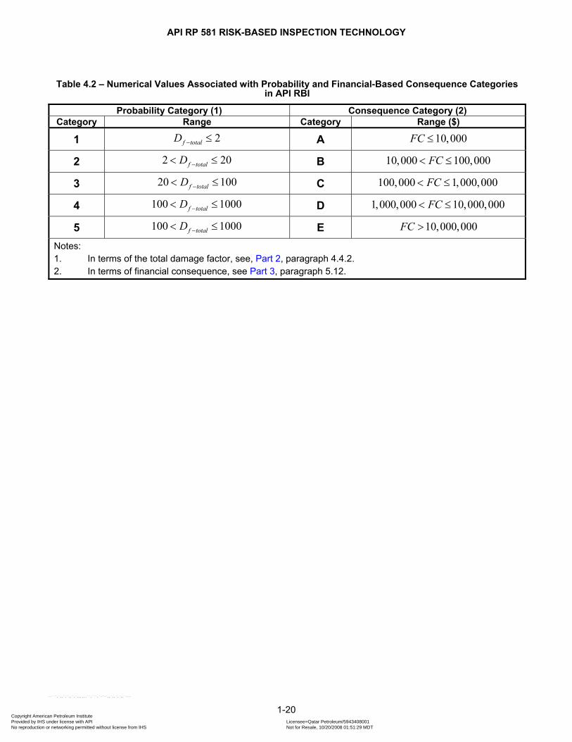
API RP 581 RISK-BASED INSPECTION TECHNOLOGY
Table 4.2 – Numerical Values Associated with Probability and Financial-Based Consequence Categories in API RBI
Probability Category (1) Consequence Category (2) Category Range Category Range ($)
1 2f totalD − ≤ A 10,000FC ≤
2 2 2f totalD −< ≤ 0 B 10,000 100,000FC< ≤
3 20 100f totalD −< ≤ C 100,000 1,000,000FC< ≤
4 100 1000f totalD −< ≤ D 1,000,000 10,000,000FC< ≤
5 100 1000f totalD −< ≤ E 10,000,000FC >
Notes: 1. In terms of the total damage factor, see, Part 2, paragraph 4.4.2. 2. In terms of financial consequence, see Part 3, paragraph 5.12.
1-20 Copyright American Petroleum Institute Provided by IHS under license with API Licensee=Qatar Petroleum/5943408001
Not for Resale, 10/20/2008 01:51:29 MDTNo reproduction or networking permitted without license from IHS
--```,`,,`,`,,`,`,,,,,,``,```,`-`-`,,`,,`,`,,`---
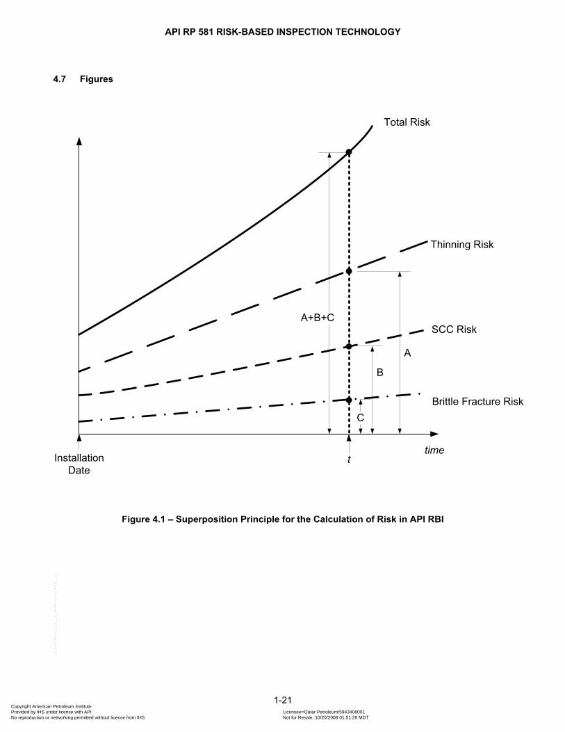
API RP 581 RISK-BASED INSPECTION TECHNOLOGY
4.7 Figures
Total Risk
Thinning Risk
SCC Risk
Brittle Fracture Risk
timeInstallation
Datet
C
B
A
A+B+C
Figure 4.1 – Superposition Principle for the Calculation of Risk in API RBI
1-21 Copyright American Petroleum Institute Provided by IHS under license with API Licensee=Qatar Petroleum/5943408001
Not for Resale, 10/20/2008 01:51:29 MDTNo reproduction or networking permitted without license from IHS
--```,`,,`,`,,`,`,,,,,,``,```,`-`-`,,`,,`,`,,`---
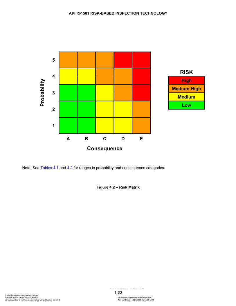
API RP 581 RISK-BASED INSPECTION TECHNOLOGY
Pr
obab
ility
5
4 RISK High
3 Medium High
Medium
2 Low
1
A B C D E
Consequence
Note: See Tables 4.1 and 4.2 for ranges in probability and consequence categories.
Figure 4.2 – Risk Matrix
1-22 Copyright American Petroleum Institute Provided by IHS under license with API Licensee=Qatar Petroleum/5943408001
Not for Resale, 10/20/2008 01:51:29 MDTNo reproduction or networking permitted without license from IHS
--```,`,,`,`,,`,`,,,,,,``,```,`-`-`,,`,,`,`,,`---

API RP 581 RISK-BASED INSPECTION TECHNOLOGY
Figure 4.3 – Case 1: Inspection Planning When the Risk Target is Exceeded Between the RBI Date and the Plan Date and the Impact of Inspection at Various Levels of Effectiveness
1-23 Copyright American Petroleum Institute Provided by IHS under license with API Licensee=Qatar Petroleum/5943408001
Not for Resale, 10/20/2008 01:51:29 MDTNo reproduction or networking permitted without license from IHS
--```,`,,`,`,,`,`,,,,,,``,```,`-`-`,,`,,`,`,,`---
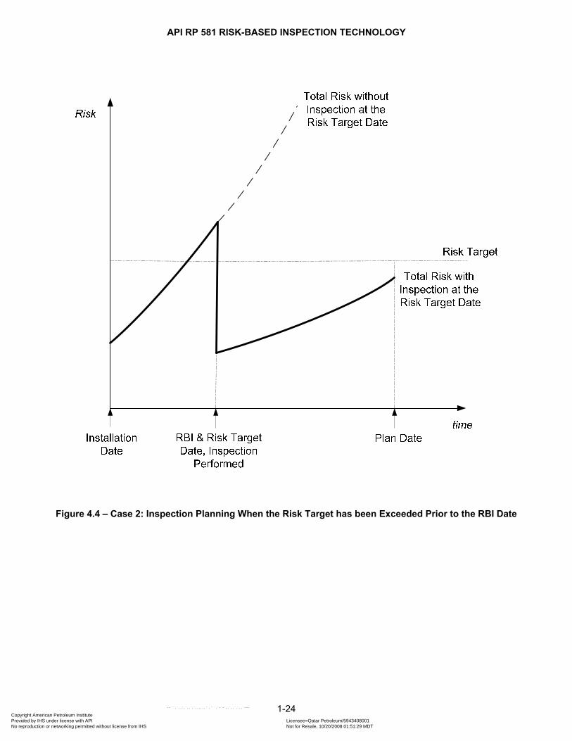
API RP 581 RISK-BASED INSPECTION TECHNOLOGY
Figure 4.4 – Case 2: Inspection Planning When the Risk Target has been Exceeded Prior to the RBI Date
1-24 Copyright American Petroleum Institute Provided by IHS under license with API Licensee=Qatar Petroleum/5943408001
Not for Resale, 10/20/2008 01:51:29 MDTNo reproduction or networking permitted without license from IHS
--```,`,,`,`,,`,`,,,,,,``,```,`-`-`,,`,,`,`,,`---

API RP 581 RISK-BASED INSPECTION TECHNOLOGY
time
Risk
InstallationDate
RBIDate
PlanDate
Risk Target
Total Risk withoutInspection
Figure 4.5 – Case 3: Inspection Planning When Risk Target is Not Exceeded Prior to the Plan Date
1-25 Copyright American Petroleum Institute Provided by IHS under license with API Licensee=Qatar Petroleum/5943408001
Not for Resale, 10/20/2008 01:51:29 MDTNo reproduction or networking permitted without license from IHS
--```,`,,`,`,,`,`,,,,,,``,```,`-`-`,,`,,`,`,,`---
API RP 581 RISK-BASED INSPECTION TECHNOLOGY
5 PRESSURE VESSELS AND PIPING
5.1 Probability of Failure The procedures for probability of failure calculations to be used in API RBI are provided in Part 2. The probability of failure as a function of time and inspection effectiveness is determined using a generic failure frequency, a management systems factor, and damage factors for the applicable active damage mechanisms as described in paragraph 4.1.
5.2 Consequence of Failure Consequence of failure calculation procedures to be used in API RBI is provided in Part 3. Methodologies for two levels of consequence analysis are provided in Part 2 as described in paragraph 4.2. In both methods, the consequence of failure may be determined in consequence area or in financial consequence. Consequences from flammable and explosive events, toxic releases, and nonflammable and non-toxic events are considered based on the process fluid and operating conditions are considered in both methods.
5.3 Risk Analysis In API RBI, the risk as a function of time is calculated in accordance with paragraph 4.3.1. The distribution of risks for different components may be displayed on a risk matrix in accordance with paragraph 4.3.2.
5.4 Inspection Planning Based on Risk Analysis The procedure to determine an inspection plan is provided in paragraph 4.4. This procedure may be used to determine both the time and type of inspection to be performed based on the process fluid and design conditions, component type and materials of construction, and the active damage mechanisms.
1-26 Copyright American Petroleum Institute Provided by IHS under license with API Licensee=Qatar Petroleum/5943408001
Not for Resale, 10/20/2008 01:51:29 MDTNo reproduction or networking permitted without license from IHS
--```,`,,`,`,,`,`,,,,,,``,```,`-`-`,,`,,`,`,,`---
API RP 581 RISK-BASED INSPECTION TECHNOLOGY
6 ATMOSPHERIC STORAGE TANKS
6.1 Probability of Failure Probability of failure calculation procedures to be used in API RBI for tank shell courses and bottom plates is provided in Part 2. The probability of failure as a function of time and inspection effectiveness is determined using a generic failure frequency and damage factors for the applicable active damage mechanisms as described in paragraph 4.1. Typically the damage factors for thinning in Part 2, paragraph 5 are utilized for tank components. However, damage factors for other active damage mechanisms may also be computed.
6.2 Consequence of Failure Consequence of failure calculation procedures to be used in API RBI is provided in Part 3, paragraph 7. Only the Level 1 consequence analysis in financial terms is used for the analysis of tank components. In addition, only consequences from component damage, product loss, and environmental penalties are considered.
6.3 Risk Analysis In API RBI, the risk as a function of time is calculated in accordance with paragraph 4.3.1. The distribution of risks for different components may be displayed on a risk matrix in accordance with paragraph 4.3.2. Only financial risk is used for atmospheric storage tank components.
6.4 Inspection Planning Based on Risk Analysis The procedure to determine an inspection plan is provided in paragraph 4.4. This procedure may be used to determine both the time and type of inspection to be performed based on the process fluid and design conditions, component type and materials of construction, and the active damage mechanisms.
1-27 Copyright American Petroleum Institute Provided by IHS under license with API Licensee=Qatar Petroleum/5943408001
Not for Resale, 10/20/2008 01:51:29 MDTNo reproduction or networking permitted without license from IHS
--```,`,,`,`,,`,`,,,,,,``,```,`-`-`,,`,,`,`,,`---
API RP 581 RISK-BASED INSPECTION TECHNOLOGY
7 PRESSURE RELIEF DEVICES
7.1 General
7.1.1 Overview The major concern with pressure relief devices (PRDs) and the main reason that routine PRD inspection and testing is required is that the device may fail to relieve overpressure events that can cause failure of the equipment protected by the device, leading to a loss of containment. There are also consequences associated with leakage of PRDs. A risk-based approach to evaluating pressure relief device criticality in order to set inspection/testing frequency is covered in this paragraph. Included in the scope are all spring-loaded and pilot-operated relief valves and rupture discs. Additional PRD types, such as atmospheric tank P/V vents and explosion hatches, may be analyzed provided reliability data in the form of Weibull parameters exists for the PRD type being considered. It is not the intention to perform or check PRD design or capacity calculations. It is assumed throughout that the devices have been designed in accordance with API 521 [11] and sized, selected and installed in accordance with API 520 [12]. It is also assumed that minimum inspection practices in accordance with API 576 [13] are in place. The fundamental approach is to use a demand rate for the device combined with a probability of failure on demand determined from plant specific data if available, or starting with default data. These inputs are used to generate a probability of failure as a function of time via a Weibull statistical approach. The consequences of device failure are determined based on methods outlined in Part 3 but modified to include overpressure demand cases, the amount of expected overpressure upon PRD failure and the additional consequences associated with device leakage. The combination of consequence with a time based probability of failure results in a risk value that increases with time between tests. This allows test intervals to be determined based on risk targets. The flow chart shown in Figure 7.1 illustrates the basic methodology, from basic data required to the determination of a risk-based inspection and test schedule. The basic data required for the evaluation is listed in Table 7.1.
7.1.2 PRD Interdependence with Fixed Equipment In API RBI, the risk of the PRD is directly related to the equipment that is protected by the PRD. The consequence analysis is performed as described in Part 3 for the protected equipment at an elevated pressure representing the estimated overpressure upon PRD failure to open upon demand.
7.1.3 Failure Modes There are several failure modes of significance when evaluating the risks associated with pressure relief device failure. For the PRD, the failure modes are grouped into two categories: a) Fail to Open (FAIL)
1) Stuck or fails to open (FTO) 2) Valve partially opens (VPO) 3) Opens above set pressure (OASP)
b) Leakage Failure (LEAK) 1) Leakage past valve (LPV), 2) Spurious/premature opening (SPO) 3) Valve stuck open (VSO)
1-28 Copyright American Petroleum Institute Provided by IHS under license with API Licensee=Qatar Petroleum/5943408001
Not for Resale, 10/20/2008 01:51:29 MDTNo reproduction or networking permitted without license from IHS
--```,`,,`,`,,`,`,,,,,,``,```,`-`-`,,`,,`,`,,`---
API RP 581 RISK-BASED INSPECTION TECHNOLOGY
The fail to open (FAIL) failure mode is the primary concern since this failure results in the potential of over-pressuring protected equipment and loss of containment. Included in this case is the instance when a valve only opens partially (VPO), where consequences are not as severe, but equipment may be over-pressured nonetheless. API RBI conservatively considers any data indicating a partially open valve as a failure to open as discussed in paragraph 7.2.2. Data that indicates a valve opened above set pressure (OASP) is included in the fail to open failure mode since the probability of failure curves are based on bench test data where a failure is defined as any test requiring a pressure greater than 1.3 times the set pressure. A test point that opens above set pressure but does not exceed 1.3 times the set pressure is considered a successful test and is not included in the fail to open (FAIL) case. Consequences associated with the failure to open failure mode include the effects of fires and explosions on personnel and equipment and the exposure of personnel to toxic fluids as a result of loss of containment. These consequences and their effect on personnel and equipment are further described in Part 3 of this document. A secondary concern is a failure of the PRD to contain the process while operating at normal conditions. The API RBI methodology groups the remaining three failure modes together into the LEAK category. Leakage past the valve (LPV), spurious or premature opening (SPO) and valves that stuck open (VSO) are failures that will not result in overpressure or loss of containment from the protected equipment, but will result in potential unacceptable leakage from the process system. The consequences of leakage through a PRD can range from a minor nuisance, causing some loss of product, to a more severe consequence resulting in a process shutdown to repair or replace the PRD. If the PRD discharges to atmosphere, additional consequences may be environmental impact and potential for fires, explosions and toxic exposure.
7.1.4 Use of Weibull Curves It is necessary to express the probability of failure to open and the probability of leakage as a function of time for risk-based planning of inspections and tests. Weibull functions are suitable for this task with the added advantage that they may be used to evaluate large populations of data points to seek trends. In the absence of large sets of failure data, the functions are still useful as a starting point since the parameters involved describe both the manner of failure and the time to failure. Using a two parameter Weibull distribution [14], the cumulative failure density function, , sometimes referred to as Unreliability, is expressed as:
( )F t
( ) 1 ( ) 1 exp tF t R tβ
η
⎡ ⎤⎛ ⎞= − = − −⎢ ⎜ ⎟
⎝ ⎠⎢ ⎥⎣ ⎦⎥ (1.10)
In Equation (1.10), the β parameter is the shape factor that is unit-less, the η parameter is the characteristic life that has units of years, and is the independent variable time in years. tThe Weibull η parameter or characteristic life is equivalent to the Mean Time Between Failure (MTBF) when the Weibull β parameter is equal to 1.0. Throughout this document, discussions are made related to the adjustment of the Weibull η parameter. Adjustments are made to the η parameter to increase or decrease the probability of failure on demand and leakage either as a result of environmental factors, PRD types or as a result of actual inspection data for a particular PRD. These adjustments may be veiwed as an adjustment to the Mean Time To Failure ( )MTTF for the PRD.
The assumption used to determine the default Weibull parameters is that PRDs in similar services will have a similar probability of failure on demand, fodP , and similar probability of leakage, . Therefore, industry failure rate data may be used as a basis for establishing the initial (or default) probabilities of failure for a specific device. The probability of failure on demand of the specific device is related to identifiable process and installation conditions. Such conditions may include process temperature, process corrosivity and the tendency of the process to foul, polymerize or otherwise block the PRD inlet or prevent the PRD from reseating during operation. Also associated with failure are conditions such as rough handling during transportation and installation and excessive piping vibration. Increased demand rates and improper installations that result in chatter may also increase the probability of failure on demand and leakage.
lP
1-29 Copyright American Petroleum Institute Provided by IHS under license with API Licensee=Qatar Petroleum/5943408001
Not for Resale, 10/20/2008 01:51:29 MDTNo reproduction or networking permitted without license from IHS
--```,`,,`,`,,`,`,,,,,,``,```,`-`-`,,`,,`,`,,`---
API RP 581 RISK-BASED INSPECTION TECHNOLOGY
7.1.5 PRD Testing, Inspection and Repair Inspection, testing, reconditioning, or replacement of PRDs is a recognized safe practice and serves to reduce the probability of failure on demand and leakage. One of the key assumptions of the API RBI methodology is that a bench test of a PRD performed in the as-received condition from a process unit will result in a true determination of the performance of the PRD on the unit. A good inspection program for PRDs will track the history of inspection and testing of each PRD. Based on this historical data, the API RBI method will adjust the probability of failure data for each PRD. The API RBI method also allows for varying degrees of inspection effectiveness. Where a shop bench pre-pop test is performed, the resulting Pass/Fail data is given the highest degree of confidence. On the other hand, if a valve is inspected and overhauled without a pre-test, a lower confidence level is associated with the inspection.
7.1.6 PRD Overhaul or Replacement Start Date When a PRD is overhauled in the shop, the basic assumption is made that the PRD is placed back into service in an as-new condition. The original install date for the PRD remains the same but the last inspection date is changed to reflect the date that the PRD was overhauled. In this way, the calculated inspection interval and subsequent new due date for the PRD is based on the last inspection date in which the PRD was overhauled. When a PRD is replaced in lieu of overhaul, the install date and last inspection date are identical. The calculated inspection interval and subsequent new due date for the PRD is based on the new install date. Often PRDs are pop-tested either in the field or in the shop without overhauling the PRD. In these instances the PRD has not been returned to service in an as-new condition. Without an overhaul, the assumption is made that the PRD remains in the condition that it was in prior to testing. In these cases, the probability of failure upon demand for the valve may be adjusted based on the results of the field test, however, the last inspection date remains unchanged and therefore the PRD will not get the full benefit of an overhaul.
7.1.7 Risk Ranking of PRDs The API RBI methodology allows a risk ranking to be made between individual PRDs and will also allow a risk ranking to be made between PRDs and other fixed equipment evaluated using the API RBI methodology. There are two key drivers for the effective risk ranking of PRDs with other PRDs. The first driver is in establishing the specific reliability for each PRD. This may be accomplished by selecting the severity of service of each PRD, establishing a default probability of failure and modifying the probability of failure on demand using the actual testing and inspection history of each PRD. The second key driver to ranking PRDs is in the relative importance or criticality of each PRD. This is accomplished through the relief system design basis and knowledge of the overpressure demand cases applicable for each PRD. The more demand placed on a PRD and the more critical the PRD application is, the higher the risk ranking should be.
7.1.8 Link to Fixed or Protected Equipment To effectively characterize the risk associated with PRD failure, the consequences associated with the failure of a PRD to open upon demand must be tied directly to the equipment that the PRD protects. This is accomplished using direct links to the fixed equipment RBI analysis as covered in Parts 2 and 3 of this document. The risk of loss of containment from fixed equipment increases proportionately with the amount of overpressure that occurs as a result of the PRD failing to open on demand. In addition, the calculated risk associated with damaged fixed equipment will be greater than for undamaged equipment since the actual damage states (i.e. damage factor, fD , see Part 2) are used in the calculations.
Although consequences associated with the PRD overpressure cases are greater than those associated with the fixed equipment operating at normal pressure, this is tempered by the fact that the use of realistic PRD demand rates and accurate PRD failure rate data results in a low frequency of occurrence.
1-30 Copyright American Petroleum Institute Provided by IHS under license with API Licensee=Qatar Petroleum/5943408001
Not for Resale, 10/20/2008 01:51:29 MDTNo reproduction or networking permitted without license from IHS
--```,`,,`,`,,`,`,,,,,,``,```,`-`-`,,`,,`,`,,`---
API RP 581 RISK-BASED INSPECTION TECHNOLOGY
7.2 Probability of Failure
7.2.1 Definition For a pressure relief device, it is important that the definition of failure be understood, since it is somewhat different than failure in terms of other types of equipment. In API RBI, failure is defined as a PRD failure to open during emergency situations causing an overpressure situation in the protected equipment resulting in loss of containment (failures/year). Leakage through a PRD is also a failure. This type of failure is discussed in paragraph 7.3.
7.2.2 Calculation of Probability of Failure to Open The fundamental approach applied to PRDs for the fail to open case is to estimate an overpressure demand case frequency (or Demand Rate) and multiply this by the probability of the PRD failing to open on demand and multiply this again by the probability that the protected equipment at higher overpressures will lose containment. A pressure relief device protects equipment components from multiple overpressure scenarios. Guidance on overpressure demand cases and pressure relieving system design is provided in API 521 [11]. Each of these scenarios (fire, blocked discharge, etc.) can result in a different overpressure, , if the PRD were to fail to
open upon demand. Additionally, each overpressure scenario has its own demand rate, . Demand cases are discussed in more detail in
,o jP
jDRparagraph 7.4.3 and Tables 7.2 and 7.3. The expression for probability of failure
for a PRD for a particular overpressure demand case is as shown in Equation (1.11).
, ,prd
,f j fod j j fP P DR P= ⋅ ⋅ j (1.11)
The subscript j in the above equation indicates that the probability of failure for the PRD, ,prd
f jP , needs to be calculated for each of the applicable overpressure demand cases associated with the PRD.
The probability of failure (loss of containment) of the equipment component that is protected by the PRD, ,f jP , is a function of time and the potential overpressure. API RBI recognizes that there is an increase in probability of loss of containment from the protected equipment due to the elevated overpressure, if the PRD fails to open during an emergency event. Each of the terms that make up the probability of failure for the PRD shown in Equation (1.11) are discussed in greater detail in the following paragraphs.
a) Paragraph 7.2.3 – Overpressure Scenario Demand Rate, jDR
b) Paragraph 7.2.4 – PRD Probability of Failure on Demand, ,fod j P
c) Paragraph 7.2.5 – Probability of Failure of Protected Equipment as a Result of Overpressure , ,f jP
7.2.3 PRD Demand Rate a) Default Initiating Event Frequencies
The first step in evaluating the probability of a PRD failure is to determine the demand rate (demands or events/year) placed on the device. API RBI provides estimates for the PRD initiating event frequencies,
based on the various relief overpressure demand cases that the device is providing protection. Examples of the initiating event frequencies are provided in
jEFTable 7.2. Additional background on the
default initiating event frequencies is provided in Table 7.3. b) Credit for Other Layers of Protection
It is recognized that the actual demand rate on a PRD is not necessarily equal to the initiating event frequency. The concept of a demand rate reduction factor, , is introduced here to account for the difference in the overpressure demand case event frequency and the demand rate on the PRD.
jDRRF
1-31 Copyright American Petroleum Institute Provided by IHS under license with API Licensee=Qatar Petroleum/5943408001
Not for Resale, 10/20/2008 01:51:29 MDTNo reproduction or networking permitted without license from IHS
--```,`,,`,`,,`,`,,,,,,``,```,`-`-`,,`,,`,`,,`---

API RP 581 RISK-BASED INSPECTION TECHNOLOGY
Many pressure vessel installations include control systems, high integrity protective instrumentation, shutdown systems and other layers of protection, to reduce the demand rate of a PRD. Credit can also be taken for operator intervention to reduce the probability of overpressure.
The demand rate reduction factor, , can be used to account for these additional layers of
protection. The may be determined rigorously for the installation as a result of a Layer of Protection Analysis (LOPA).
jDRRF
jDRRF
Another example of where credit may be taken using the demand rate reduction factor is for the fire overpressure demand case. A good estimate for the initiating event frequency of a fire on a specific pressure vessel is 1 every 250 years (0.004 events/year). However, due to many other factors, fire impingement from a pool directly on a pressure vessel rarely causes the pressure in the vessel to rise significantly enough to cause the PRD to open. Factors reducing the actual demand rate on the PRD include, fire proofing, availability of other escape paths for the process fluid as well as fire-fighting efforts at the facility to reduce the likelihood of overpressure
c) Calculation of Demand Rate The demand rate on the PRD is calculated as the product of the initiating event frequency and the demand rate reduction factor in accordance with Equation (1.12):
j jDR EF DRRF= ⋅ j (1.12)
The subscript j in Equation (1.12) signifies that the demand rate on a PRD is calculated for each applicable overpressure demand case. Typically, a PRD protects equipment for several overpressure demand cases and each overpressure case has a unique demand rate. Default initiating event frequencies for each of the overpressure cases are provided in Table 7.2. Additional guidance on overpressure demand cases and pressure relieving system design is provided in API 521 [11]. An overall demand rate on the PRD can be calculated as follows:
1
ndc
total jj
DR DR=
=∑ (1.13)
If the relief design basis of the PRD installation has not been completed, the list of applicable overpressure demand cases may not be available and it may be more appropriate to use a simple overall average value of the demand rate for a PRD. An overall demand rate for a particular PRD can usually be estimated from past operating experience for the PRD.
d) Owner-User Experience The initiating event frequencies for any or all of the overpressure demand cases as shown in Table 7.2 are default values that may not be applicable in all situations. Owner-Users may have operating experience with a particular process system that may warrant using other event frequencies. Additionally, a PRD that protects multiple pieces of equipment may legitimately see an increased demand for a particular overpressure scenario. For example, a PRD located on a crude distillation tower may also protect the desalted preheat exchanger train as well. Since the PRD protects equipment encompassing a much greater area of the unit, an increase in the event frequency for the fire case may be appropriate. In general, where a PRD protects multiple pieces of equipment, the initiating event frequencies should be evaluated to determine if an increase is justified.
7.2.4 PRD Probability of Failure on Demand a) General
The next step is to obtain the probability that the pressure relief device will fail to open upon demand in service. API RBI provides default failure on demand failure rates developed from industry data. These default values are expressed as default Weibull curves which are modified by several factors based on the following procedure:
1) Determine default Weibull parameters, β and defη , based on category of Service Severity and type of PRD, see paragraphs 7.2.4.b through 7.2.4.f.
1-32 Copyright American Petroleum Institute Provided by IHS under license with API Licensee=Qatar Petroleum/5943408001
Not for Resale, 10/20/2008 01:51:29 MDTNo reproduction or networking permitted without license from IHS
--```,`,,`,`,,`,`,,,,,,``,```,`-`-`,,`,,`,`,,`---

API RP 581 RISK-BASED INSPECTION TECHNOLOGY
2) Apply an adjustment factor, cF , for conventional valves discharging to closed system or to flare, see paragraph 7.2.4.g.
3) Apply an adjustment factor, opF , for overpressures higher than 1.3 times set pressure, see paragraph 7.2.4.h.
4) Apply an adjustment factor, envF , for environmental factors, see paragraph 7.2.4.i.
The result of the procedure outlined above will be a modified characteristic life, modη , as defined in Equation (1.14).
mod c op env defF F Fη η= ⋅ ⋅ ⋅ (1.14)
At this point, the modified characteristic life, modη , is updated based on the PRD’s inspection history, see
paragraph 7.2.4.l. This updated characteristic life, updη , is then used to calculate the probability of failure on demand for the specific PRD in accordance with Equation (1.15).
1 expfodupd
tPβ
η
⎡ ⎤⎛ ⎞⎢= − −⎜ ⎟⎜ ⎟⎢ ⎥⎝ ⎠⎣ ⎦
⎥ (1.15)
b) Categories of Service Severity The failure rates of pressure relief devices are related to the severity of service in which they are installed. Different fluid groups and categories of service are established in the PRD module as a function of the fluid tendency to induce PRD failure due to corrosion, fouling, plugging, or other effects. Temperature has also been found to be a factor in determining the severity of service. As a general rule of thumb, the categories of service severity (MILD, MODERATE or SEVERE) that are linked to specific failure tendencies (and default Weibull cumulative failure distribution curves) are described in Table 7.4. It is important to note that a fluid that is classified as being a MILD service group for the fail to open failure mode, is not necessarily a MILD service for the leakage failure mode. As an example, industry failure data shows that cooling water, which is known to be a dirty/scaling service, has one of the highest failure rates for the FAIL to open case and therefore may be classified as SEVERE for the FAIL case. Conversely, PRDs in cooling water service have not demonstrated a significant amount of leakage failures and therefore may be classified as MILD for the leak case. Another example is steam, where the database shows that steam should be classified as MILD for the fail to open case but should be classified as SEVERE for the leak case. Steam is known to be a leaking service due to the erosive nature of the high temperature steam.
c) Default Probability of Failure on Demand vs Time in Service Table 7.5 provides the default Weibull parameters for failure to open for conventional spring loaded pressure relief valves, balanced bellows pressure relief valves, pilot-operated pressure relief valves and rupture disks. These parameters were determined using industry failure rate data. The database includes approximately 4300 bench test data points where the majority of the data indicated successful performance during the interval that the PRD was in service. The successful test points are referred to as suspensions and were included with the failure data in determination of the Weibull parameters. Weibull parameters are provided for the three categories of PRD service severity; MILD, MODERATE and SEVERE, discussed in paragraph 7.2.4.b. These values, when substituted into the Weibull cumulative failure density function given by Equation (1.10), provides the default probability of failure on demand curves for each of the PRD types listed in the table. For example, Figure 7.2 provides the default Weibull cumulative failure distribution curves used in API RBI for spring-loaded conventional pressure relief valves using the Weibull function to describe the three categories of service severity; MILD, MODERATE, and SEVERE.
1-33 Copyright American Petroleum Institute Provided by IHS under license with API Licensee=Qatar Petroleum/5943408001
Not for Resale, 10/20/2008 01:51:29 MDTNo reproduction or networking permitted without license from IHS
--```,`,,`,`,,`,`,,,,,,``,```,`-`-`,,`,,`,`,,`---
API RP 581 RISK-BASED INSPECTION TECHNOLOGY
Note that the units for the failure to open upon demand data presented in Figure 7.2 are failures/demand as this data was established from bench tests of actual PRDs, not from continuous service data. When multiplied by the demand rate (see paragraph 7.2.3), a probability of failure (failures/year) may be determined as discussed in paragraph 7.2.2. The cumulative failure distribution curves shown in Figure 7.2 and the Weibull parameters presented in Table 7.5 are the default values based on the selected fluid severity (MILD, MODERATE, SEVERE) of the PRD being evaluated. These base values are defaults and should be overridden if the Owner-User provides site specific data as explained in paragraph 7.2.3.d.
d) Default Data for Balanced Bellows Pressure Relief Valves A balanced spring-loaded pressure relief valve utilizes a bellows to isolate the back side of the disc from the effects of superimposed and built-up back pressure. The bellows also isolates the internals of the PRD from the corrosive effects of the fluid in the discharge system. An analysis of the industry failure rate data shows that balanced bellows PRVs have the same probability of failure on demand rates as their conventional PRD counterparts, even though they typically discharge to dirty/corrosive closed systems. This is due to the isolation of the valve internals from the discharge fluid and the effects of corrosion and fouling. As shown in Table 7.5, the characteristic life (Weibull η parameter) is the same for bellows PRVs as it is for conventional PRVs.
e) Default Weibull Parameters for Pilot-Operated Pressure Relief Valves To date there is little data in the industry failure database (subject to change) available for pilot-operated PRVs. One source, [15] indicates that pilot-operated PRVs are 20 times more likely to fail than their spring-loaded counterparts. The Weibull parameters for the POFOD curves for conventional PRVs as shown in Table 7.5 are used as the basis for pilot-operated PRVs with adjustment factors applied to the characteristic life (η parameter). For MILD service, the η parameter for pilot-operated PRVs is reduced by a factor of 1.5; for MODERATE service, the reduction factor is 3.0; and for SEVERE service, the reduction factor is 5.0.
f) Default Weibull Parameters for Rupture Disks Currently, there is little failure rate data available for rupture disks. Rupture disks are simple, reliable devices which are not likely to fail to open at pressures significantly over their burst pressure (unless inlet or outlet plugging is a problem, or unless they are installed improperly). Typically, if a rupture disk were to fail, it would burst early. Therefore, in API RBI, the Weibull parameters for the failure to open upon demand case for rupture disks are based on the MILD severity curve for conventional PRVs. This makes the assumption that a rupture disk is at least as reliable as a conventional PRV. It also assumes that the rupture disc material has been properly selected to withstand the corrosive potential of the operating fluid. Where it is known that the rupture disc material is not properly selected for the corrosive service, the disk’s Weibull parameters should be adjusted accordingly.
g) Adjustment for Conventional PRVs Discharging to Closed System An adjustment is made to the base Weibull parameters for conventional valves that discharge to a closed system or to flare. Since a conventional valve does not have a bellows to protect the bonnet housing from the corrosive fluids in the discharge system, the characteristic life (represented by the η parameter) is reduced by 25%, using an adjustment factor of 0.75.
cF = 0.75 for conventional valves discharging to closed system or flare (1.16)
cF = 1.0 for all other cases (1.17)
1-34 Copyright American Petroleum Institute Provided by IHS under license with API Licensee=Qatar Petroleum/5943408001
Not for Resale, 10/20/2008 01:51:29 MDTNo reproduction or networking permitted without license from IHS
--```,`,,`,`,,`,`,,,,,,``,```,`-`-`,,`,,`,`,,`---

API RP 581 RISK-BASED INSPECTION TECHNOLOGY
h) Adjustment for Overpressures Higher than Set Pressure As discussed in paragraph 7.1.3, the probability of failure on demand curves are based on bench test data where a failure is defined as any test requiring a pressure greater than 1.3 times the set pressure. Intuitively, one would expect that at higher overpressures, the probability that the PRD would fail to open goes down dramatically. A review of the industry failure data supports this. Figure 7.4 shows that as the overpressure ratio (actual pressure/set pressure) increases, the PRD failure rate reduces significantly. A conservative approach is to assume that the failure rate is cut by a factor of 5 at 4.0 times the set pressure and to assume linear interpolation between 1.3 and 4.0 times the set pressure. A factor for overpressure,
, is introduced in opF Equation (1.18).
1 1.33.375
oop
PFMAWP
⎛ ⎞= ⋅ −⎜⎝ ⎠
⎟ (1.18)
The adjustment factor calculated above cannot be less than 0.0, nor greater than 1.0. i) Adjustment for Environmental Factors
There are several environmental/installation factors that can affect the reliability of pressure relief devices. These include the existence of vibration in the installed piping, a history of valve chatter and whether or not the device is located in pulsing flow or cyclical service, such as when the device is installed downstream of reciprocating rotating equipment. Other environmental factors which can significantly affect leakage probability are operating temperature and operating ratio. The operating ratio of a pressure relief device is the ratio of maximum system operating pressure to the set pressure. When the operating ratio is greater than 90% for spring-loaded PRVs, the system pressure is close to overcoming the closing force provided by the spring on the seating surface and the PRV will be more likely to leak (simmer). This increased potential for leakage is taken into account by applying an environmental factor to the default leakage curve. Similarly, an environmental factor is applied when the operating margin is greater than 95% for pilot-operated PRVs. Note that some pilot-operated PRVs can function at operating ratios up to 98%. An analysis of the industry failure rate data shows that PRDs installed in vibratory or cyclical service tend to have higher leakage rates. The analysis showed; however, that the Fail to Open failure rates remain about the same when a PRD is installed in these services. If a PRV has a history of chattering, the PRD installation should be modified/re-designed as soon as possible to eliminate the chatter, since the effects of chatter may be very detrimental to the protection provided by the PRD. An assumed adjustment factor of 0.5 is applied to the Weibull η parameters for the POFOD and POL curves of a PRD that has a history of chattering in service. Table 7.6 provides all of the environmental adjustment factors that API RBI applies to the default POFOD and POL Weibull curves.
API RBI uses the environmental factor, , to modify the Weibull envF η parameter for the PRD, effectively increasing the probability of failure on demand or leakage by reducing the curve’s characteristic life (Weibull η parameter). As shown in Figure 7.5, the modifier effectively shifts the probability curves to the left.
j) Presence of an Upstream Rupture Disk Rupture disks are often installed in combination with pressure relief valves to isolate the valve from process conditions and corrosive or fouling fluids that can reduce the probability that the valve will open upon demand. API RP 520 Parts 1 and 2 provide additional information related to the use and installation of rupture disks upstream of pressure relief valves. API RBI accounts for the presence of an upstream rupture disk by utilizing the probability of failure on demand curve for MILD service regardless of what fluid severity is selected. This assumes that the space between the rupture disk and the pressure relief valve is vented and monitored for leakage as required by Code and as recommended by API RP 520. If this is not the case, the upstream rupture disk should not be considered in the analysis (i.e. assume the disk is not present).
1-35 Copyright American Petroleum Institute Provided by IHS under license with API Licensee=Qatar Petroleum/5943408001
Not for Resale, 10/20/2008 01:51:29 MDTNo reproduction or networking permitted without license from IHS
--```,`,,`,`,,`,`,,,,,,``,```,`-`-`,,`,,`,`,,`---
API RP 581 RISK-BASED INSPECTION TECHNOLOGY
k) Use of Plant Specific Failure Data Data collected from specific plant testing programs can also be used to obtain probability of failure on demand and probability of leakage values. Different measures such as MTBF or failure per million operating hours may be converted into the desired form via simple conversion routines.
l) Modification of Failure on Demand Based on PRD Specific Testing Data 1) Tracking Historical Inspection and Testing Data
An inspection program should track each PRDs testing and inspection history from its initial installation. From this history, adjustments can be made to each device’s fodP and curves to take advantage of the knowledge gained by the testing of a particular relief device in a specific service.
lP
After actual testing data is obtained for a PRD, the probability functions of that device are adjusted up or down (modifying the Weibull parameters) depending upon the results (Pass/Fail/Leak) of the device’s specific inspection tests and the length of service since the last inspection. In this way, an increase or reduction in the recommended interval is obtained based on historical test data. In general, the adjustment of the probability of failure on demand is based on the results of the inspection of the PRD itself (e.g. bench test results). This could lead to non-conservative results if the inlet or outlet piping plugs during operation. Since the reliability of the PRD system can be affected by fouled piping, the API RBI methodology takes this into consideration. For each inspection date entered, the inspected condition of the piping should be documented. If the piping is determined to be plugged, the methodology will judge the inspection/test to be a FAIL, regardless of the results of the bench test or inspection method used on the PRD. Good engineering practice would suggest that if the piping is plugged by more than 25%, the piping should be defined as being plugged, since this would then drive down the inspection interval. This methodology adjusts the reliability of the PRD system to reflect excessive pipe plugging.
2) Determine the Effectiveness of Inspection Programs in Confirming Failure Rates Inspection programs vary in their effectiveness for determining failure rates. The definitions for inspection effectiveness used by API RBI are provided in Table 7.7. The inspection’s effectiveness is based on the inspection’s ability to adequately predict the failure (or pass) state of the PRD being inspected. Limitations in the ability of a program to improve confidence in the failure rate result from the inability of some test methods to detect and quantify damage. An inspection and testing program should track the effectiveness of the inspection and the testing performed for each pressure relief device. The concept of inspection effectiveness is similar to the concept that is described in paragraph 4.4.3 of this document for fixed equipment. With inspection effectiveness, a measure of confidence in the Pass/Fail/Leak result of the inspection effort is obtained. Default confidence values, based on expert opinion, are provided in Table 7.8, indicating the level of confidence each of the three levels of inspection effectiveness will accurately represent actual PRD performance in an overpressure demand case. For example, the 90% effectiveness associated with passing a “highly effective” bench test means that there is a 90% probability the valve would have opened upon demand in its installed service. Therefore, it also carries a 10% probability that the PRD would have failed upon demand during operation. The values shown in Table 7.8 are called conditional probabilities. The conditional probabilities listed reflect the confidence that an inspection result will predict the device’s performance upon demand. For passing PRDs, the highest confidence is assigned when the PRD is bench tested without any prior cleaning (i.e. as-received condition.) Bench testing where the devices are cleaned prior to testing, in-situ testing, and visual inspections provide some information about PRD performance, but are not considered as reliable as the as-received bench test. The philosophy is different for PRDs that fail an inspection. In the case of a “highly effective” bench test failure, the 95% confidence translates to a 95% chance that the PRD would have failed upon demand in actual service. Unlike the passing test case, the “usually effective” in-situ test, or bench test where the valve has been steamed out prior to testing, is assumed to have the same 95% confidence for failure upon demand in actual service.
1-36 Copyright American Petroleum Institute Provided by IHS under license with API Licensee=Qatar Petroleum/5943408001
Not for Resale, 10/20/2008 01:51:29 MDTNo reproduction or networking permitted without license from IHS
--```,`,,`,`,,`,`,,,,,,``,```,`-`-`,,`,,`,`,,`---

API RP 581 RISK-BASED INSPECTION TECHNOLOGY
An ineffective test does not provide any information to predict PRD performance upon demand and therefore the PRD does not receive any credit for the test/inspection date. The inspection still will get some credit if an overhaul was performed in that the valve is assumed to be returned to service in like-new condition, and the in-service duration is calculated from the ineffective inspection date.
3) Inspection Updating As previously discussed, Weibull parameters for the failure on demand curves have been determined based on the analysis of a sample set of data. Initially, these values are default (suggestions) parameters for the listed fluid services. As inspection data is collected for each PRD, these parameters may be adjusted for each device based on the inspection results. Applying a Bayesian updating approach to problems of this type is common to adjust probabilities as new information is collected. This approach assumes that the Weibull shape parameter (β parameter) remains constant based on the historical data, and adjusts the characteristic life (η parameter), as inspection data is collected. This is analogous to evaluating a one-parameter Weibull to update the PRD performance. Bayes’ Theorem works best when the error rates for a test are very small. This is not the case for PRDs. Test effectiveness, shown in Table 7.8, range from 50 to 90%. This uncertainty using Bayes’ Theorem results in an unrealistically high adjusted probability of failure, particularly for a passed bench test. Therefore, a similar inspection updating method was devised for API RBI to provide reasonable adjustments of characteristic life. Since the default Weibull parameters for a given PRD provide the probability of a failure on demand versus time, a default probability of failure on demand (modified as per paragraph 7.2.4) may be obtained for the device based on its in-service duration at the time of inspection. This is known as the prior probability of failure on demand and is calculated using Equation (1.19) as follows:
, 1 expprdf prior
mod
tPβ
η
⎡ ⎤⎛ ⎞⎢= − −⎜ ⎟⎢ ⎥⎝ ⎠⎣ ⎦
⎥
,
,
(1.19)
The prior probability that the valve will pass on demand is:
, 1prd prdp prior f priorP P= −
(1.20)
After the inspection, a second probability of failure on demand is calculated based upon the conditional probability factor, or confidence factor (CF) for the effectiveness of the inspection performed (see Table 7.8). This second, calculated probability is called the conditional probability of failure on demand and is calculated using Equations (1.21) or (1.22) depending on the result of the inspection: When the pressure relief valve passed the inspection the conditional probability of failure on demand is calculated as follows:
( ), 1prd prdf cond pass p priorP CF P= − ⋅ (1.21)
With a failed inspection, the conditional probability of failure on demand is calculated as follows:
( ), , 1prd prd prd,f cond fail f prior pass p priorP CF P CF P= ⋅ + − ⋅ (1.22)
A weighted probability of failure, ,prd
f wgtP , is then calculated, where the weighting factors have been formulated to give more credit to tests conducted later in the characteristic life. Using the prior and conditional probabilities and the weighting factors, an updated or posterior probability of failure on demand is calculated using the equations provided in Table 7.9. A revised characteristic life may be obtained using Equation (1.23) based on the in-service duration of the PRD, the known β parameter, and the posterior probability.
1-37 Copyright American Petroleum Institute Provided by IHS under license with API Licensee=Qatar Petroleum/5943408001
Not for Resale, 10/20/2008 01:51:29 MDTNo reproduction or networking permitted without license from IHS
--```,`,,`,`,,`,`,,,,,,``,```,`-`-`,,`,,`,`,,`---
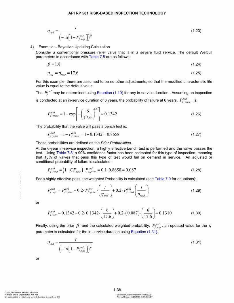
API RP 581 RISK-BASED INSPECTION TECHNOLOGY
( )1
,ln 1upd
prdf wgt
t
P β
η =⎡ ⎤− −⎣ ⎦
(1.23)
4) Example – Bayesian Updating Calculation Consider a conventional pressure relief valve that is in a severe fluid service. The default Weibull parameters in accordance with Table 7.5 are as follows:
1.8β = (1.24)
17.6def modη η= = (1.25)
For this example, there are assumed to be no other adjustments, so that the modified characteristic life value is equal to the default value.
The may be determined using prdfP Equation (1.19) for any in-service duration. Assuming an inspection
is conducted at an in-service duration of 6 years, the probability of failure at 6 years, ,prd
f priorP , is:
1.8
,61 exp 0.1342
17.6prd
f priorP⎡ ⎤⎛ ⎞= − − =⎢ ⎥⎜ ⎟⎝ ⎠⎢ ⎥⎣ ⎦
(1.26)
The probability that the valve will pass a bench test is:
, ,1 1 0.1342 0.8658prd prdp prior f priorP P= − = − = (1.27)
These probabilities are defined as the Prior Probabilities. At the 6-year in-service inspection, a highly effective bench test is performed and the valve passes the test. Using Table 7.8, a 90% confidence factor has been estimated for this type of inspection, meaning that 10% of valves that pass this type of test would fail on demand in service. An adjusted or conditional probability of failure is calculated:
( ), ,1 0.1 0.8658 0.087prd prdf cond pass p priorP CF P= − ⋅ = ⋅ = (1.28)
For a highly effective pass, the weighted Probability is calculated (see Table 7.9 for equations):
, , , ,0.2 0.2prd prd prd prdf wgt f prior f prior f cond
mod mod
t tP P P Pη η⎛ ⎞ ⎛ ⎞
= − ⋅ ⋅ + ⋅⎜ ⎟ ⎜⎝ ⎠ ⎝ ⎠
⎟ (1.29)
or
( ),6 60.1342 0.2 0.1342 0.2 0.087 0.1310
17.6 17.6prd
f wgtP ⎛ ⎞ ⎛ ⎞= − ⋅ ⋅ + ⋅ ⋅ =⎜ ⎟ ⎜ ⎟⎝ ⎠ ⎝ ⎠
(1.30)
Finally, using the prior β and the calculated weighted probability, ,prd
f wgtP , an updated value for the η parameter is calculated for the in-service duration using Equation (1.31).
( )1
,ln 1upd
prdf wgt
t
P β
η =⎡ ⎤− −⎣ ⎦
(1.31)
or
1-38 Copyright American Petroleum Institute Provided by IHS under license with API Licensee=Qatar Petroleum/5943408001
Not for Resale, 10/20/2008 01:51:29 MDTNo reproduction or networking permitted without license from IHS
--```,`,,`,`,,`,`,,,,,,``,```,`-`-`,,`,,`,`,,`---
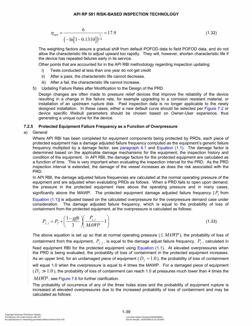
API RP 581 RISK-BASED INSPECTION TECHNOLOGY
[ ]( )1
1.8
6 17.9ln 1 0.1310
updη =− −
= (1.32)
The weighting factors assure a gradual shift from default POFOD data to field POFOD data, and do not allow the characteristic life to adjust upward too rapidly. They will, however, shorten characteristic life if the device has repeated failures early in its service. Other points that are accounted for in the API RBI methodology regarding inspection updating:
i) Tests conducted at less than one year do not get credit ii) After a pass, the characteristic life cannot decrease. iii) After a fail, the characteristic life cannot increase.
5) Updating Failure Rates after Modification to the Design of the PRD Design changes are often made to pressure relief devices that improve the reliability of the device resulting in a change in the failure rate, for example upgrading to a corrosion resistant material, or installation of an upstream rupture disk. Past inspection data is no longer applicable to the newly designed installation. In these cases, either a new default curve should be selected per Figure 7.2 or device specific Weibull parameters should be chosen based on Owner-User experience, thus generating a unique curve for the device.
7.2.5 Protected Equipment Failure Frequency as a Function of Overpressure a) General
Where API RBI has been completed for equipment components being protected by PRDs, each piece of protected equipment has a damage adjusted failure frequency computed as the equipment’s generic failure frequency multiplied by a damage factor, see paragraph 4.1 and Equation (1.1). The damage factor is determined based on the applicable damage mechanisms for the equipment, the inspection history and condition of the equipment. In API RBI, the damage factors for the protected equipment are calculated as a function of time. This is very important when evaluating the inspection interval for the PRD. As the PRD inspection interval is extended, the damage of the vessel increases as does the risk associated with the PRD. In API RBI, the damage adjusted failure frequencies are calculated at the normal operating pressure of the equipment and are adjusted when evalutating PRDs as follows. When a PRD fails to open upon demand, the pressure in the protected equipment rises above the operating pressure and in many cases, significantly above the MAWP. The protected equipment damage adjusted failure frequency [ fP from Equation (1.1)] is adjusted based on the calculated overpressure for the overpressure demand case under consideration. The damage adjusted failure frequency, which is equal to the probability of loss of containment from the protected equipment, at the overpressure is calculated as follows:
,,
1 13
o jf j f
PgfftP PMAWP
⎛ ⎞−⎛ ⎞= + −⎜⎜ ⎟⎝ ⎠⎝ ⎠
⎟ (1.33)
The above equation is set up so that at normal operating pressure ( MAWP≤ ), the probability of loss of containment from the equipment, ,f jP , is equal to the damage adjust failure frequency, fP , calculated in fixed equipment RBI for the protected equipment using Equation (1.1). At elevated overpressures when the PRD is being evaluated, the probability of loss of containment in the protected equipment increases. As an upper limit, for an undamaged piece of equipment ( 1.0fD = ), the probability of loss of containment will equal 1.0 when the overpressure is equal to 4 times the MAWP. For a damaged piece of equipment ( ), the probability of loss of containment can reach 1.0 at pressures much lower than 4 times the 1.0fDMAWP , see Figure 7.6 for further clarification. The probability of occurrence of any of the three holes sizes and the probability of equipment rupture is increased at elevated overpressures due to the increased probability of loss of containment and may be calculated as follows:
1-39 Copyright American Petroleum Institute Provided by IHS under license with API Licensee=Qatar Petroleum/5943408001
Not for Resale, 10/20/2008 01:51:29 MDTNo reproduction or networking permitted without license from IHS
--```,`,,`,`,,`,`,,,,,,``,```,`-`-`,,`,,`,`,,`---
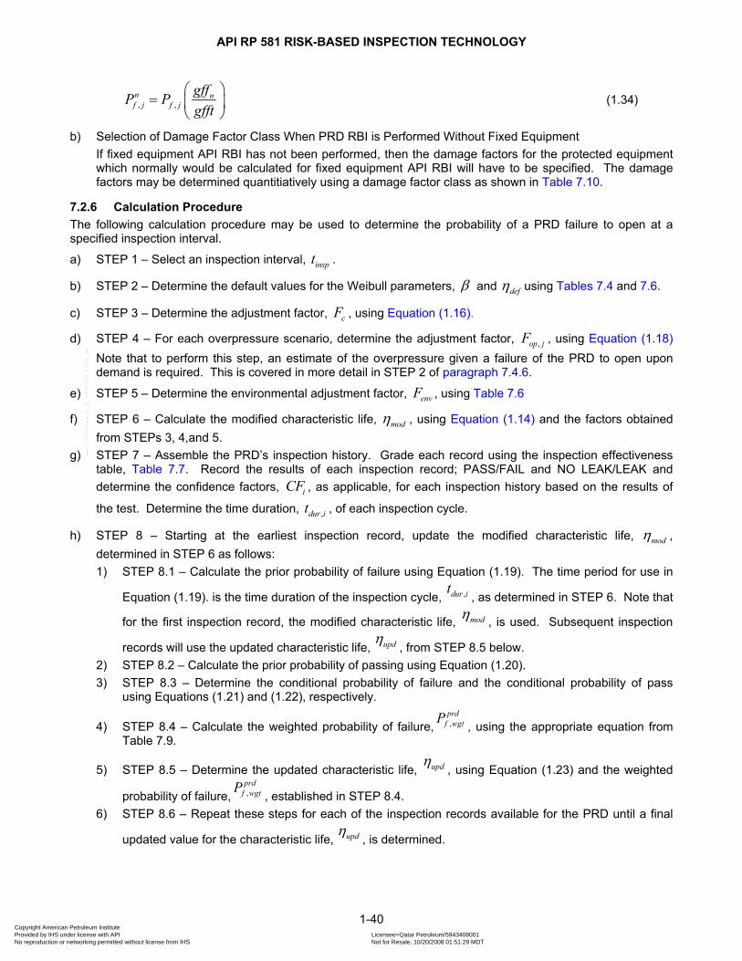
API RP 581 RISK-BASED INSPECTION TECHNOLOGY
, ,n nf j f j
gffP Pgfft
⎛ ⎞= ⎜
⎝ ⎠⎟ (1.34)
b) Selection of Damage Factor Class When PRD RBI is Performed Without Fixed Equipment If fixed equipment API RBI has not been performed, then the damage factors for the protected equipment which normally would be calculated for fixed equipment API RBI will have to be specified. The damage factors may be determined quantitiatively using a damage factor class as shown in Table 7.10.
7.2.6 Calculation Procedure The following calculation procedure may be used to determine the probability of a PRD failure to open at a specified inspection interval.
a) STEP 1 – Select an inspection interval, inspt .
b) STEP 2 – Determine the default values for the Weibull parameters, β and defη using Tables 7.4 and 7.6.
c) STEP 3 – Determine the adjustment factor, cF , using Equation (1.16).
d) STEP 4 – For each overpressure scenario, determine the adjustment factor, ,op jF , using Equation (1.18) Note that to perform this step, an estimate of the overpressure given a failure of the PRD to open upon demand is required. This is covered in more detail in STEP 2 of paragraph 7.4.6.
e) STEP 5 – Determine the environmental adjustment factor, envF , using Table 7.6
f) STEP 6 – Calculate the modified characteristic life, modη , using Equation (1.14) and the factors obtained from STEPs 3, 4,and 5.
g) STEP 7 – Assemble the PRD’s inspection history. Grade each record using the inspection effectiveness table, Table 7.7. Record the results of each inspection record; PASS/FAIL and NO LEAK/LEAK and determine the confidence factors, iCF , as applicable, for each inspection history based on the results of
the test. Determine the time duration, ,dur it , of each inspection cycle.
h) STEP 8 – Starting at the earliest inspection record, update the modified characteristic life, modη , determined in STEP 6 as follows: 1) STEP 8.1 – Calculate the prior probability of failure using Equation (1.19). The time period for use in
Equation (1.19). is the time duration of the inspection cycle, ,dur it, as determined in STEP 6. Note that
for the first inspection record, the modified characteristic life, modη , is used. Subsequent inspection
records will use the updated characteristic life, updη, from STEP 8.5 below.
2) STEP 8.2 – Calculate the prior probability of passing using Equation (1.20). 3) STEP 8.3 – Determine the conditional probability of failure and the conditional probability of pass
using Equations (1.21) and (1.22), respectively.
4) STEP 8.4 – Calculate the weighted probability of failure, ,prd
f wgtP, using the appropriate equation from
Table 7.9.
5) STEP 8.5 – Determine the updated characteristic life, updη, using Equation (1.23) and the weighted
probability of failure, ,prd
f wgtP, established in STEP 8.4.
6) STEP 8.6 – Repeat these steps for each of the inspection records available for the PRD until a final
updated value for the characteristic life, updη, is determined.
1-40 Copyright American Petroleum Institute Provided by IHS under license with API Licensee=Qatar Petroleum/5943408001
Not for Resale, 10/20/2008 01:51:29 MDTNo reproduction or networking permitted without license from IHS
--```,`,,`,`,,`,`,,,,,,``,```,`-`-`,,`,,`,`,,`---

API RP 581 RISK-BASED INSPECTION TECHNOLOGY
i) STEP 9 – For each overpressure demand case, determine the initiating event frequency, jEF , using Table 7.2 or based on Owner-User experience for the particular overpressure demand case.
j) STEP 10 – Determine the demand rate reduction factor, jDRRF , which accounts for any layers of protection in the process that may reduce the probability of overpressuring the protected piece of equipment, see paragraph 7.2.3.b for guidance.
k) STEP 11 – For each overpressure demand case, determine the demand rate placed on the PRD, jDR , using Equation (1.12).
l) STEP 12 – Determine the MAWP of the protected equipment. m) STEP 13 – If an RBI study has been completed for the protected equipment, calculate its damage adjusted
probability of failure, fP , using Equation (1.1). Since the damage factor for the protected equipment is a
function of time, the damage factor must be determined at the PRD inspection interval, inspt , specified in STEP 1. If an API RBI study has not been completed, a damage factor can be estimated using the values in Table 7.10.
n) STEP 14 – Calculate the probability of failure of the protected equipment at the elevated overpressure,
,f jP using Equation (1.33). Use the overpressure determined in STEP 2 of paragraph 7.4.6, the MAWP of the protected equipment and the probability of failure determined in STEP 13.
o) STEP 15 - Calculate the probability of failure, ,prd
f jP , using Equation (1.11).
p) STEP 16 – Repeat STEPs 1 through 15 for each piece of equipment protected by the PRD.
7.3 Probability of Leakage
7.3.1 Overview The leakage case is different than the fail to open case since the probability of failure is not a function of demand rate. It is based on failures during continuous operation. The industry data associated with the probability of leakage, , data is already in per year units (i.e. failures/year). No multiplication by any demand rate is necessary.
lP
7.3.2 Calculation of Probability of Leakage a) Overall Procedure
The probability of leakage for a PRD is determined using the following steps.
1) Determine default Weibull parameters, β and defη, based on category of Service Severity and type
of PRD, see paragraphs 7.3.2.b through 7.3.2.f
2) Apply an adjustment factor, sF , to account for the presence of soft seats, see paragraph 7.3.2.g
3) Apply an adjustment factor, envF , for environmental factors, see paragraph 7.3.2.h
The result of the procedure outlined above will be a modified characteristic life, modη , as defined in Equation (1.35).
mod s env defF Fη η= ⋅ ⋅ (1.35)
The modified characteristic life, modη , is updated based on the PRD’s inspection history, identical to the
method presented in paragraph 7.2.4.l for the failure to open case. This updated characteristic life, updη , is then used to calculate the probability of leakage for the specific PRD in accordance with Equation (1.36).
1-41 Copyright American Petroleum Institute Provided by IHS under license with API Licensee=Qatar Petroleum/5943408001
Not for Resale, 10/20/2008 01:51:29 MDTNo reproduction or networking permitted without license from IHS
--```,`,,`,`,,`,`,,,,,,``,```,`-`-`,,`,,`,`,,`---
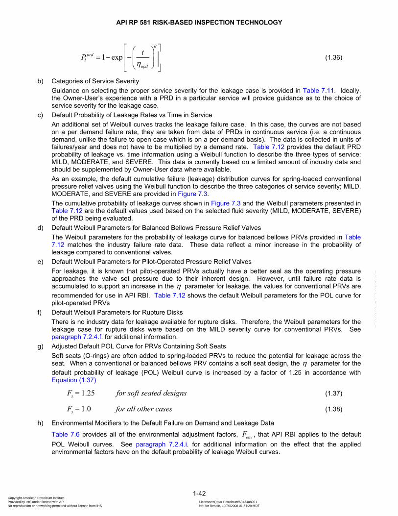
API RP 581 RISK-BASED INSPECTION TECHNOLOGY
1 expprdl
upd
tPβ
η
⎡ ⎤⎛ ⎞⎢= − −⎜ ⎟⎜ ⎟⎢ ⎥⎝ ⎠⎣ ⎦
⎥ (1.36)
b) Categories of Service Severity Guidance on selecting the proper service severity for the leakage case is provided in Table 7.11. Ideally, the Owner-User’s experience with a PRD in a particular service will provide guidance as to the choice of service severity for the leakage case.
c) Default Probability of Leakage Rates vs Time in Service An additional set of Weibull curves tracks the leakage failure case. In this case, the curves are not based on a per demand failure rate, they are taken from data of PRDs in continuous service (i.e. a continuous demand, unlike the failure to open case which is on a per demand basis). The data is collected in units of failures/year and does not have to be multiplied by a demand rate. Table 7.12 provides the default PRD probability of leakage vs. time information using a Weibull function to describe the three types of service: MILD, MODERATE, and SEVERE. This data is currently based on a limited amount of industry data and should be supplemented by Owner-User data where available. As an example, the default cumulative failure (leakage) distribution curves for spring-loaded conventional pressure relief valves using the Weibull function to describe the three categories of service severity; MILD, MODERATE, and SEVERE are provided in Figure 7.3. The cumulative probability of leakage curves shown in Figure 7.3 and the Weibull parameters presented in Table 7.12 are the default values used based on the selected fluid severity (MILD, MODERATE, SEVERE) of the PRD being evaluated.
d) Default Weibull Parameters for Balanced Bellows Pressure Relief Valves The Weibull parameters for the probability of leakage curve for balanced bellows PRVs provided in Table 7.12 matches the industry failure rate data. These data reflect a minor increase in the probability of leakage compared to conventional valves.
e) Default Weibull Parameters for Pilot-Operated Pressure Relief Valves For leakage, it is known that pilot-operated PRVs actually have a better seal as the operating pressure approaches the valve set pressure due to their inherent design. However, until failure rate data is accumulated to support an increase in the η parameter for leakage, the values for conventional PRVs are recommended for use in API RBI. Table 7.12 shows the default Weibull parameters for the POL curve for pilot-operated PRVs
f) Default Weibull Parameters for Rupture Disks There is no industry data for leakage available for rupture disks. Therefore, the Weibull parameters for the leakage case for rupture disks were based on the MILD severity curve for conventional PRVs. See paragraph 7.2.4.f. for additional information.
g) Adjusted Default POL Curve for PRVs Containing Soft Seats Soft seats (O-rings) are often added to spring-loaded PRVs to reduce the potential for leakage across the seat. When a conventional or balanced bellows PRV contains a soft seat design, the η parameter for the default probability of leakage (POL) Weibull curve is increased by a factor of 1.25 in accordance with Equation (1.37)
1.25 sF = for soft seated designs (1.37)
1.0 sF = for all other cases (1.38)
h) Environmental Modifiers to the Default Failure on Demand and Leakage Data
Table 7.6 provides all of the environmental adjustment factors, , that API RBI applies to the default POL Weibull curves. See
envFparagraph 7.2.4.i. for additional information on the effect that the applied
environmental factors have on the default probability of leakage Weibull curves.
1-42 Copyright American Petroleum Institute Provided by IHS under license with API Licensee=Qatar Petroleum/5943408001
Not for Resale, 10/20/2008 01:51:29 MDTNo reproduction or networking permitted without license from IHS
--```,`,,`,`,,`,`,,,,,,``,```,`-`-`,,`,,`,`,,`---
API RP 581 RISK-BASED INSPECTION TECHNOLOGY
i) Presence of an Upstream Rupture Disk When a rupture disk is installed upstream of the PRV, the API RBI methodology assumes that the probability of leakage is negligible (i.e. ) and does not calculate a consequence resulting from leakage.
0.0prdlP =
j) Modification of Leakage Rates Based on PRD Specific Testing Data The updating scheme for inspection history is identical to the scheme presented in paragraph 7.2.4.l for the failure to open case.
7.3.3 Calculation Procedure The following calculation procedure may be used to determine the probability of a PRD leakage at a specified inspection interval.
a) STEP 1 – Select an inspection interval, inspt .
b) STEP 2 – Determine the default values for the Weibull parameters, β and defη using Tables 7.4 and 7.6.
c) STEP 3 – Determine the adjustment factor, sF , using Equation (1.37).
d) STEP 4 – Determine the environmental adjustment factor, envF , using Table 7.6
e) STEP 5 – Calculate the modified characteristic life, modη , using Equation (1.35) and the factors obtained in STEPS 3 and 4.
f) STEP 6 – Assemble the PRD’s inspection history. Grade each record using the inspection effectiveness table, Table 7.7. Record the results of each inspection record; NO LEAK/LEAK and determine the confidence factors, iCF , as applicable, for each inspection history based on the results of the test.
Determine the time duration, ,dur it , of each inspection cycle.
g) STEP 7 – Starting at the earliest inspection record, update the modified characteristic life, modη , determined in STEP 5 as follows: 1) STEP 7.1 – Calculate the prior probability of leakage using Equation (1.19). Note that for the first
inspection record, the modified characteristic life, modη , is used. Subsequent inspection records will use the updated characteristic from STEP 7.5 below.
2) STEP 7.2 – Calculate the prior probability of passing using Equation (1.20). 3) STEP 7.3 – Determine the conditional probability of leakage and conditional probability of pass using
Equations (1.21) and (1.22), respectively.
4) STEP 7.4 – Calculate the weighted probability of leakage, , , using the appropriate equation from prd
l wgtPTable 7.9.
5) STEP 7.5 – Determine the updated characteristic life, updη, using Equation (1.23) and the weighted
probability of leakage, , , established in STEP 7.4 prd
l wgtP
6) STEP 7.6 – Repeat these steps for each of the inspection records available for the PRD until a final
updated value for the characteristic life, updη, is determined.
h) STEP 8 - Calculate the probability of leakage for the specific PRD in accordance with Equation (1.36).
1-43 Copyright American Petroleum Institute Provided by IHS under license with API Licensee=Qatar Petroleum/5943408001
Not for Resale, 10/20/2008 01:51:29 MDTNo reproduction or networking permitted without license from IHS
--```,`,,`,`,,`,`,,,,,,``,```,`-`-`,,`,,`,`,,`---

API RP 581 RISK-BASED INSPECTION TECHNOLOGY
7.4 Consequence of PRD Failure to Open
7.4.1 General The consequence calculations for event outcomes such as fires, explosions and toxic exposure are calculated as described in Part 3. For pressure relief devices, failures to open upon demand will likely result in the protected equipment being exposed to significantly higher pressures than during normal operations. The API RBI methodology calculates the consequences for each PRD failing to open at sometimes significantly higher overpressure than the normal operating pressure of the equipment. Table 7.13 shows the expected intermediate consequences of an overpressure event in a pressure vessel. Table 7.13 is only provided for a qualitative discussion of the potential risks to equipment due to overpressure and is not intended to indicate any specific event outcome. The API RBI method accounts for the effects of overpressure on protected equipment by increasing the probability of loss of containment. At an overpressure of 4 times the MAWP , the probability of loss of containment is conservatively assumed to be equal to 1.0, see paragraph 7.2.4.h.
7.4.2 Damage State of the Protected Equipment The advantage of linking the PRD consequence calculations to the protected equipment is that the existing damage state of the protected equipment may be determined. Damage for each protected vessel is measured by a damage factor, fD , which is calculated considering each of the damage mechanisms (corrosion, cracking, creep, etc.) that are applicable to the protected equipment. The higher the overall damage factor of the protected equipment, the more likely the equipment is to experience undesirable consequences as a result of a PRD that is in a failed state (stuck) upon demand. Part 2 of this document provides details on calculation of the damage factor and the probability of loss of containment from fixed equipment. A direct link to the current condition, or damage state, of the protected equipment is critical to the evaluation of the consequence of PRD failure. Where damage assessment has not been completed in conjunction with a RBI analysis of the PRD, then assumptions of the damage state of the protected equipment must be made as described in paragraph 7.2.5.b.
7.4.3 Overpressure Potential for Overpressure Demand Cases For API RBI to provide a relative ranking of risk between PRDs, the analysis must include an assessment of the overpressure demand cases (overpressure scenarios) that are applicable to each PRD. In other words, what process upsets is the device protecting against and how critical would the effect on the protected equipment be if the device were to fail to open upon demand. API RBI makes a clear distinction between criticality of the overpressure demand cases that the device is protecting against (i.e. why the device is there). For example, a PRD that protects equipment and piping for the blocked discharge demand case, downstream of a pump is considered to be less critical than a device that is protecting a reactor from a runaway chemical reaction since the amount of overpressure expected as a result of a PRD failure to open upon demand would be much less. Likewise, a device that is only protecting piping against thermal relief is much less critical than a device that is protecting low pressure equipment from gas breakthrough from a high pressure source due to control valve failure. For most of the overpressure demand cases, the potential overpressure that results when a PRD fails to open upon demand from an overpressure event may be calculated. The logic for determining the potential overpressure for each of the overpressure demand cases is provided in Table 7.3. In many situations, the potential overpressure will approach the burst pressure (assumed to be 4 times the MAWP ) of the protected equipment since the overpressure demand case is not self-limiting. In other overpressure scenarios, such as a blocked discharge downstream of a centrifugal pump, the potential overpressure will limit itself to the dead head pressure of the pump, which is typically 1.3 times the normal discharge pressure of the pump. This part of the API RBI analysis requires a thorough review of the unit Pressure Relief Study and P&IDs and should be performed by personnel qualified and experienced in the design and installation of pressure relief systems.
1-44 Copyright American Petroleum Institute Provided by IHS under license with API Licensee=Qatar Petroleum/5943408001
Not for Resale, 10/20/2008 01:51:29 MDTNo reproduction or networking permitted without license from IHS
--```,`,,`,`,,`,`,,,,,,``,```,`-`-`,,`,,`,`,,`---

API RP 581 RISK-BASED INSPECTION TECHNOLOGY
In general, the determination of the potential overpressure, , as a result of PRD failure to open upon demand is a function of the following:
oP
a) Type of Upstream Overpressure Source – For example, centrifugal pumps, steam supply headers, upstream pressure vessels, etc.
b) Upstream Source Pressures – These include the steam supply pressure, control valve upstream pressure, pressure from the high pressure side of a heat exchanger, deadhead pressure for centrifugal rotating equipment. Additionally, credit for pressure relief valves on upstream equipment can be assumed to be available to limit overpressure.
c) Heat Sources, Types and Temperatures – In cases of blocking-in equipment, the heat source supplying energy to the system has a significant impact on the potential overpressure. For example, solar heat/energy supplied in a thermal relief scenario will typically result in flange leaks and the overpressure ends up nominally being the normal operating pressure of the system. On the other hand, if the heat source is a fired heater, the overpressure can build until a rupture occurs (i.e. overpressure exceeding to four times the MAWP ). Other heat sources include steam reboilers to towers and the hot side of heat exchangers.
d) Fluid Bubble Point Pressure – In many overpressure scenarios, the pressure build-up is limited to the bubble point pressure of the contained fluid at the temperature of the heat/energy source being supplied to the process.
7.4.4 Multiple Relief Device Installations When the relief requirements for the process are such that multiple PRDs are needed to handle the required relief capacity, there is a reduction of risk, since the probability that all of the PRDs are in a failed state upon demand will be reduced. The protected equipment will have a higher probability that some of the PRD capacity is available on demand to minimize the amount of overpressure during an overpressure demand case. When a piece of equipment is protected by multiple PRDs, the calculated probability of failure on demand for any one specific PRD in the multiple device installation will remain the same. However, an adjustment is made to the potential overpressure as a result of the PRD failing to open on demand. This multiple valve installation adjustment, , takes into consideration common cause failures and also considers the likelihood that other PRDs of the multiple valve installation will be available to minimize the potential overpressure.
aF
prd
a prdtotal
AFA
= (1.39)
This multiple valve installation factor reduces the potential overpressure that is likely to occur by assuming that some of the installed PRD relief area will be available if the PRD under consideration fails to open upon demand. The presence of the square root takes into consideration that the PRDs in a multiple valve installation may have common failure modes. The reduction in overpressure as a result of multiple PRDs is in accordance with Equation
, ,o j a o jP F P= ⋅ (1.40)
For a multiple valve installation, the probability of leakage for any one specific PRD does not increase. However, since the number of valves increases, the probability of a leak and its associated consequences does increase in proportion to the number of valves protecting the system.
7.4.5 Calculation of Consequence of Failure to Open Consequence calculations are performed for each overpressure demand case that is applicable to the PRD. These consequence calculations are performed as described in Part 3 of this document for each piece of equipment that is protected by the PRD being evaluated and are performed at higher potential overpressures as described in paragraph 7.4.1.
1-45 Copyright American Petroleum Institute Provided by IHS under license with API Licensee=Qatar Petroleum/5943408001
Not for Resale, 10/20/2008 01:51:29 MDTNo reproduction or networking permitted without license from IHS
--```,`,,`,`,,`,`,,,,,,``,```,`-`-`,,`,,`,`,,`---
API RP 581 RISK-BASED INSPECTION TECHNOLOGY
The overpressure for each demand case that may result from a failure of a PRD to open upon demand has two effects. The probability of loss of containment from the protected equipment can go up significantly as discussed in paragraph 7.2.5. Secondly, the consequences of failure as a result of the higher overpressures increase also. The magnitude of the release increases in proportion to the overpressure, thus increasing the consequences of events such as jet fires, pool fires and vapor cloud explosions. Additionally, the amount of explosive energy released as a result of a vessel rupture increases in proportion to the amount of overpressure. Part 3 provides detail for the consequences associated with loss of containment from equipment components. The consequence calculations should be performed in accordance with Part 3 for each of the overpressure demand cases applicable to the PRD and for each piece of equipment that is protected by the PRD. The resultant consequence is ,
prdf jC .
7.4.6 Calculation Procedure The following calculation procedure may be used to determine the consequence of a PRD failure to open. a) STEP 1 – Determine the list of overpressure scenarios applicable to the piece of equipment being
protected by the PRD under evaluation. Table 7.2 provides a list of overpressure demand cases specifically covered in API RBI. Additional guidance on overpressure demand cases and pressure relieving system design is provided in API 521 [11].
b) STEP 2 – For each overpressure demand case, estimate the amount of overpressure, ,o jP , likely to occur during the overpressure event if the PRD were to fail to open. Paragraph 7.4.3 and Table 7.3 provide guidance in this area.
c) STEP 3 – For installations that have multiple pressure relief devices, determine the total amount of installed PRD orifice area, prd
totalA , including the area of the PRD being evaluated. Calculate the overpressure
adjustment factor, aF , in accordance with Equation (1.39).
d) STEP 4 – Reduce the overpressures determined in STEP 3 by the overpressure adjustment factor in accordance with Equation (1.40).
e) STEP 5 – For each overpressure demand case, calculate the financial consequences, ,prdf jC , of loss of
containment from the protected equipment using procedures developed in Part 3. Use the overpressures for the demand cases as determined in STEP 4 in lieu of the operating pressure, sP .
7.5 Consequence of Leakage
7.5.1 General Even though the consequences of PRD leakage are typically much less severe than that of a loss of containment from the protected equipment as a result of a PRD failure to open, the frequency of leakage may be high enough that the PRD may be ranked as a high priority on a leakage risk basis.
The calculation of the consequence of leakage from PRDs, , is estimated by summing the costs of several items. The cost of the lost inventory is based on the cost of fluid multiplied by the leakage rate (see
prdlC
paragraph 7.5.5.) and the number of days to discover the leak (see Table 7.14). Regulatory and environmental costs associated with leakage should be considered as well. Next, the cost of downtime to repair or replace the device is estimated if it is determined that continuous operation of the unit with a leaking or stuck open PRD cannot be tolerated. If a shutdown is required to repair the leaking PRD, then the cost associated with lost production will also be added.
The consequence of leakage, , is calculated using the following equation: prdlC
prdl inv env sdC Cost Cost Cost Cost= + + + prod (1.41)
1-46 Copyright American Petroleum Institute Provided by IHS under license with API Licensee=Qatar Petroleum/5943408001
Not for Resale, 10/20/2008 01:51:29 MDTNo reproduction or networking permitted without license from IHS
--```,`,,`,`,,`,`,,,,,,``,```,`-`-`,,`,,`,`,,`---

API RP 581 RISK-BASED INSPECTION TECHNOLOGY
7.5.2 Estimation of PRD Leakage Rate An analysis of industry bench test data shows that approximately 8.4% of the PRVs tested had some leakage on the bench stand between 70 and 90% of their set pressure. An additional 6.6% of the PRVs tested leaked at pressures below 70% of their set pressure. An additional 2.4% of the tested PRVs leaked significantly below 70% of their set pressure. The basis for the estimated leakage rates used for the consequence calculation in API RBI is provided in Table 7.15. As shown in Table 7.15, a leakage rate of 1% of the PRD capacity (calculated at normal operating conditions) is used in API RBI for mild and moderate leaks. For a stuck open PRD, the leakage rate is assumed to be 25% of the PRD capacity, as given in Equation (1.43).
In API RBI, two leak cases are evaluated. The first case handles minor or moderate leakage, , and represents 90% of all of the potential leakage cases, per
mildlC
Table 7.15. A stuck open case results in a leakage consequence, so
lC , and makes up 10% of all possible leakage cases.
For mild and moderate leaks, 1% of the rated capacity of the PRD, , is the basis for the leakage rate, see prdcW
Equation (1.42).
0.1 prdmild clrate W= ⋅ (1.42)
For the stuck open or spurious open case, the leakage rate is estimated per Equation (1.43).
0.25 prdso clrate W= ⋅ (1.43)
The rated capacity of the PRD, , can usually be found on the PRD datasheet. It can also be calculated using the methods presented in API 520 Part 1 [
prdcW
12].
7.5.3 Estimation of Leakage Duration
The leakage duration, , is estimated for the mild to moderate leakage case as shown in mildD Table 7.14. The durations shown make the assumption that moderate leakage from large PRDs will be discovered sooner than leakage from smaller PRDs. The stuck open category is handled differently. For the stuck open case, it is assumed that immediate repair to the PRD is required and that the time to isolate the PRD will be within 30 minutes. Therefore,
30 0.021 60 24 so
minD daysmin hr hr day
= =⋅
(1.44)
7.5.4 Credit for Recovery of Leaking Fluid API RBI recognizes that the cost of lost inventory is not as severe when the unit has a flare recovery system installed or the discharge from the relief devices is to a closed system. A recovery factor, , is applied to the leakage consequence as defined by
FEquations (1.45), (1.46), or (1.47).
0.5 rF if the PRD discharges to flare and a flare recovery system is installed = (1.45)
0.0 rF if the PRD discharges to a closed system = (1.46)
1.0 rF for all other cases = (1.47)
7.5.5 Cost of Lost Inventory
The cost of lost fluid inventory, , can be calculated using Equation invCost (1.48) or (1.49). Note that when
determining the consequence of leakage, the fluid costs, fluCost , in Equation (1.48) should be based on the fluid that exists in the protected equipment where the PRD is physically located.
24mildinv r flu mild mildCost F Cost D lrate= ⋅ ⋅ ⋅ ⋅ (1.48)
1-47 Copyright American Petroleum Institute Provided by IHS under license with API Licensee=Qatar Petroleum/5943408001
Not for Resale, 10/20/2008 01:51:29 MDTNo reproduction or networking permitted without license from IHS
--```,`,,`,`,,`,`,,,,,,``,```,`-`-`,,`,,`,`,,`---

API RP 581 RISK-BASED INSPECTION TECHNOLOGY
24soinv r flu so soCost F Cost D lrate= ⋅ ⋅ ⋅ ⋅ (1.49)
7.5.6 Environmental Costs The environmental costs, , are added when leakage through a PRD either to atmosphere or to a flare system could possibly result in cleanup costs or regulatory fines.
envCost
7.5.7 Costs of Shutdown to Repair PRD
API RBI adds the cost associated with repair and maintenance to a PRD, sdCost , if a leaking valve cannot be tolerated. API recommends using actual Owner-User work order costs associated with the maintenance, testing, inspection and repair of the PRD. However, the values provided in Equations (1.50) or (1.51) can be used.
$1,000 sdCost for PRDs < NPS 6 inlet size= (1.50)
$2,000 sdCost for PRDs NPS 6 inlet size= ≥ (1.51)
7.5.8 Cost of Lost Production The cost of lost production to repair a leaking PRD, , can be calculated using prodCost Equations (1.52) or (1.53). Where spare PRDs are installed in parallel or in cases where isolation valves underneath the PRD offer flexibility to repair without shutting down, production losses need not be considered. For the stuck open case, it is assumed that prolonged operation cannot be tolerated, in which case Equation (1.54) should be used.
0.0
mildprodCost if a leaking PRD can be tolerated or if the PRD can
be isolated and repaired without requiring a shutdown
= (1.52)
mildprod prod sdCost Unit D if a leaking PRD cannot be tolerated= ⋅ (1.53)
soprod prod sdC Unit D for a stuck open PRD= ⋅ (1.54)
7.5.9 Calculation of Leakage Consequence The consequence of leakage is calculated for two leaks cases. a) Mild to Moderate Leakage
The first case handles minor or moderate leakage, , and is used to represent 90% of all of the potential leakage cases, per
,prd
l leakCTable 7.15. In this case, the leakage rate is 1% of the PRD capacity and the
duration (or time to discover the leak) is a function of PRD inlet size and discharge location as shown in Table 7.14.
mild mild mildl flu env sd pC C C C C= + + + rod (1.55)
b) Stuck Open Leakage
The second case handles the spurious or stuck open leak case, , and is assumed to have a duration of 30 minutes. In this case, to determine the cost of lost fluid, 25% of the full capacity of the PRD (calculated at normal operating conditions) is used for the leakage rate and it is assumed that the PRD will be repaired immediately (within 30 minutes).
,prd
l soC
so so sol flu env sd prodC C C C C= + + +
(1.56)
1-48 Copyright American Petroleum Institute Provided by IHS under license with API Licensee=Qatar Petroleum/5943408001
Not for Resale, 10/20/2008 01:51:29 MDTNo reproduction or networking permitted without license from IHS
--```,`,,`,`,,`,`,,,,,,``,```,`-`-`,,`,,`,`,,`---
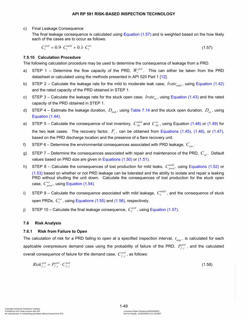
API RP 581 RISK-BASED INSPECTION TECHNOLOGY
c) Final Leakage Consequence The final leakage consequence is calculated using Equation (1.57) and is weighted based on the how likely each of the cases are to occur as follows:
0.9 0.1prd mild sol lC C= ⋅ + ⋅ lC (1.57)
7.5.10 Calculation Procedure The following calculation procedure may be used to determine the consequence of leakage from a PRD.
a) STEP 1 – Determine the flow capacity of the PRD, prdcW . This can either be taken from the PRD
datasheet or calculated using the methods presented in API 520 Part 1 [12].
b) STEP 2 – Calculate the leakage rate for the mild to moderate leak case, mildlrate , using Equation (1.42) and the rated capacity of the PRD obtained in STEP 1.
c) STEP 3 – Calculate the leakage rate for the stuck open case, solrate , using Equation (1.43) and the rated capacity of the PRD obtained in STEP 1.
d) STEP 4 – Estimate the leakage duration, leakD , using Table 7.14 and the stuck open duration, soD , using Equation (1.44).
e) STEP 5 – Calculate the consequence of lost inventory, mildfluC and so
fluC , using Equation (1.48) or (1.49) for
the two leak cases. The recovery factor, rF , can be obtained from Equations (1.45), (1.46), or (1.47), based on the PRD discharge location and the presence of a flare recovery unit.
f) STEP 6 – Determine the environmental consequences associated with PRD leakage, envC .
g) STEP 7 – Determine the consequences associated with repair and maintenance of the PRD, sdC . Default values based on PRD size are given in Equations (1.50) or (1.51).
h) STEP 8 – Calculate the consequences of lost production for mild leaks, mildprodC , using Equations (1.52) or
(1.53) based on whether or not PRD leakage can be tolerated and the ability to isolate and repair a leaking PRD without shutting the unit down. Calculate the consequences of lost production for the stuck open case, so
prodC , using Equation (1.54).
i) STEP 9 – Calculate the consequence associated with mild leakage, mildlC , and the consequence of stuck
open PRDs, solC , using Equations (1.55) and (1.56), respectively.
j) STEP 10 – Calculate the final leakage consequence, prdlC , using Equation (1.57).
7.6 Risk Analysis
7.6.1 Risk from Failure to Open The calculation of risk for a PRD failing to open at a specified inspection interval, , is calculated for each
applicable overpressure demand case using the probability of failure of the PRD, inspt
,prd
f jP , and the calculated
overall consequence of failure for the demand case, ,prdf jC , as follows:
, ,prd prd prd
,f j f j f jRisk P C= ⋅ (1.58)
1-49 Copyright American Petroleum Institute Provided by IHS under license with API Licensee=Qatar Petroleum/5943408001
Not for Resale, 10/20/2008 01:51:29 MDTNo reproduction or networking permitted without license from IHS
--```,`,,`,`,,`,`,,,,,,``,```,`-`-`,,`,,`,`,,`---
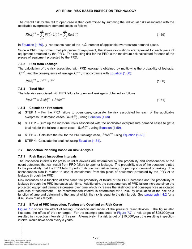
API RP 581 RISK-BASED INSPECTION TECHNOLOGY
The overall risk for the fail to open case is then determined by summing the individual risks associated with the applicable overpressure demand cases as follows:
, ,1 1
ndc ndcprd prd prd prd
,f f j f j f jj i
Risk P C Risk= =
= ⋅ =∑ ∑ (1.59)
In Equation (1.59), j represents each of the number of applicable overpressure demand cases. ndcSince a PRD may protect multiple pieces of equipment, the above calculations are repeated for each piece of equipment protected by the PRD. The resulting risk for the PRD is the maximum risk calculated for each of the pieces of equipment protected by the PRD.
7.6.2 Risk from Leakage The calculation of the risk associated with PRD leakage is obtained by multiplying the probability of leakage,
, and the consequence of leakage, , in accordance with prdlP prd
lC Equation (1.60):
prd prd prdl l lRisk P C= ⋅ (1.60)
7.6.3 Total Risk The total risk associated with PRD failure to open and leakage is obtained as follows:
prd prd prdf lRisk Risk Risk= + (1.61)
7.6.4 Calculation Procedure a) STEP 1 – For the PRD failure to open case, calculate the risk associated for each of the applicable
overpressure demand cases, ,prdf jRisk , using Equation (1.58).
b) STEP 2 – Sum up the individual risks associated with the applicable overpressure demand cases to get a total risk for the failure to open case, prd
fRisk , using Equation (1.59).
c) STEP 3 – Calculate the risk for the PRD leakage case, prdlRisk using Equation (1.60).
d) STEP 4 - Calculate the total risk using Equation (1.61).
7.7 Inspection Planning Based on Risk Analysis
7.7.1 Risk Based Inspection Intervals The inspection intervals for pressure relief devices are determined by the probability and consequence of the event outcomes that can result from PRD failure to open or leakage. The probability side of the equation relates to the probability that the PRD fails to perform its function, either failing to open upon demand or leaking. The consequence side is related to loss of containment from the piece of equipment protected by the PRD or to leakage through the PRD. Risk increases as a function of time since the probability of failure of the PRD increases and the probability of leakage through the PRD increases with time. Additionally, the consequences of PRD failure increase since the protected equipment damage increases over time which increases the likelihood and consequences associated with loss of containment. The recommended interval is determined for a PRD by calculation of the risk as a function of time and determining the time at which the risk is equal to the risk target. See paragraph 4.4.2 for a discussion of risk targets.
7.7.2 Effect of PRD Inspection, Testing and Overhaul on Risk Curve Figure 7.7 shows the effect of testing, inspection and repair of the pressure relief devices. The figure also illustrates the effect of the risk target. For the example presented in Figure 7.7, a risk target of $25,000/year resulted in inspection intervals of 5 years. Alternatively, if a risk target of $10,000/year, the resulting inspection interval would have been every 3 years.
1-50 Copyright American Petroleum Institute Provided by IHS under license with API Licensee=Qatar Petroleum/5943408001
Not for Resale, 10/20/2008 01:51:29 MDTNo reproduction or networking permitted without license from IHS
--```,`,,`,`,,`,`,,,,,,``,```,`-`-`,,`,,`,`,,`---
API RP 581 RISK-BASED INSPECTION TECHNOLOGY
Since devices are normally overhauled or replaced at the time of testing, the risk of failure goes to zero just after the test. This is a critical assumption; that the PRD is returned to an as-new condition upon overhaul.
7.7.3 Effect of PRD Testing without Overhaul on Risk Curve Typically, when a PRD is inspected and tested, the opportunity is taken to overhaul the PRD and return it to service in an as-new condition. This is one of the major assumptions of the RBI software. Occasionally, however, a PRD is inspected and/or tested without overhaul. An example would be performing a pop test in the shop in the as-received condition and returning the PRD to service without overhaul. Another example would be performing an in-situ pop test while the PRD remains on the unit. In these situations, confidence that the PRD is in working condition is gained, however, the PRD has not been restored to an as-new condition. API RBI credits for the inspection by adjusting the probability of failure and leakage curves (adjustment of Weibull η parameter). If the test was successful, the test interval will be increased, marginally. However, the risk does not drop back down to zero as would be the case if the PRD was overhauled. Therefore, the full benefit of the increased test interval will not be realized.
1-51 Copyright American Petroleum Institute Provided by IHS under license with API Licensee=Qatar Petroleum/5943408001
Not for Resale, 10/20/2008 01:51:29 MDTNo reproduction or networking permitted without license from IHS
--```,`,,`,`,,`,`,,,,,,``,```,`-`-`,,`,,`,`,,`---

API RP 581 RISK-BASED INSPECTION TECHNOLOGY
7.8 Nomenclature prdA is the orifice area of the PRD, mm2 [in2] prd
totalA is the total installed orifice area of a multiple valve installation, mm2 [in2]
β is the Weibull shape parameter η is the Weibull characteristic life parameter, years
defη is the Weibull characteristic life parameter based on the default service severity chosen for a specific PRD, years
modη is the Weibull characteristic life parameter modified to account for installation factors, design features, overpressure and environmental factors, years
updη is the Weibull characteristic life parameter updated to account for inspection history, years
CF is the confidence factor placed on the inspection effectiveness
iCF is the confidence factor placed on the inspection effectiveness associated with the historical inspection record
thi
failCF is the confidence factor that a failed test represents the true condition of the PRD at the time of the test
passCF is the confidence factor that a passed test represents the true condition of the PRD at the time of the test
,prdf jC is the PRD consequence of failure to open associated with the overpressure demand case, $ thjprd
lC is the PRD consequence of leakage, $ mildlC is the consequence of a mild to moderate leak through a PRD, $ solC is the consequence of a stuck open PRD, $
envCost is the environmental costs due to a PRD leak, $
invCost is the lost inventory or fluid costs due to a PRD leak, $
fluCost is the cost of the lost fluid, $/kg [$/lb] mildinvCost is the cost of lost inventory due to a mild or moderate PRD leak, $ soinvCost is the cost of lost inventory due to a stuck open PRD, $
prodCost is the production losses as a result of shutting down to repair a PRD, $ mildprodCost is the production losses as a result of shutting down to repair a mild or moderately leaking PRD, $ soprodCost is the production losses as a result of shutting down to repair a stuck open PRD, $
sdCost is the maintenance and repair costs associated with a PRD, $
fD is the damage factor as a function of time for equipment components protected by the PRD
jDR is the demand rate associated with the overpressure demand case, demands/year thj
totalDR is the total demand rate on a PRD, demands/year
jDRRF is the demand rate reduction factor associated with the overpressure demand case thj
mildD is the duration that a mild or moderate PRD leak will go undiscovered, days
soD is the duration of a stuck open PRD, days
sdD is the number of days required to shut a unit down to repair a leaking or stuck open PRD, days
1-52 Copyright American Petroleum Institute Provided by IHS under license with API Licensee=Qatar Petroleum/5943408001
Not for Resale, 10/20/2008 01:51:29 MDTNo reproduction or networking permitted without license from IHS
--```,`,,`,`,,`,`,,,,,,``,```,`-`-`,,`,,`,`,,`---

API RP 581 RISK-BASED INSPECTION TECHNOLOGY
jEF is the initiating event frequency associated with the overpressure demand case, demands/year
thj
aF is the multiple valve installation adjustment factor
cF is the adjustment factor for conventional valves
envF is the adjustment factor for environmental factors
opF is the adjustment factor for overpressure
rF is the recovery factor applied to lost inventory
sF is the adjustment factor for the presence of soft seats
ngff is the generic failure frequency for the protected equipment associated with the hole size thngfft is the total generic failure frequency for the protected equipment
mildlrate is the leakage rate of a mild or moderately leaking PRD, kg/hr [lb/hr]
solrate is the leakage rate for a stuck open PRD, kg/hr [lb/hr]
MAWP is the maximum allowable working pressure of the protected equipment, kPa [psig] ndc is the number of demand cases
oP is the overpressure likely to occur as a result of a PRD failing to open upon demand, kPa [psig]
,o jP is the overpressure likely to occur as a result of a PRD failing to open upon demand, associated
with the overpressure demand case, kPa [psig] thj
sP is the storage or operating pressure of the protected equipment, kPa [psig]
fP is the probability of failure (loss of containment) of the protected equipment, failures/year
,f jP is the probability of failure (loss of containment) of the protected equipment associated with the
overpressure demand case, failures/year thj
,nf jP is the probability of failure (loss of containment) of the protected equipment for the hole size
associated with the overpressure demand case, failures/year
thnthj
,prd
f jP is the probability of failure of a PRD associated with the overpressure demand case, failures/year
thj
,prd
f condP is the conditional probability of failure on demand, failures/demand
,prd
f priorP is the prior probability of failure on demand, failures/demand
,prd
f wgtP is the weighted probability of failure on demand, failures/demand
fodP is the PRD probability of failure on demand, failures/demand
,fod jP is the PRD probability of failure on demand associated with the overpressure demand case, failures/demand
thj
prdlP is the PRD probability of leakage, failures/year
,prd
l wgtP is the weighted probability of leakage, failures/demand
,prd
p priorP is the prior probability of passing on demand, failures/demand
,prdf jRisk is the risk of a PRD failure to open associated with the overpressure demand case, $/year thjprdfRisk is the risk of a PRD failure to open, $/year
1-53 Copyright American Petroleum Institute Provided by IHS under license with API Licensee=Qatar Petroleum/5943408001
Not for Resale, 10/20/2008 01:51:29 MDTNo reproduction or networking permitted without license from IHS
--```,`,,`,`,,`,`,,,,,,``,```,`-`-`,,`,,`,`,,`---
API RP 581 RISK-BASED INSPECTION TECHNOLOGY
prdlRisk is the risk of PRD leakage, $/year prdRisk is the total risk for a PRD, $/year
( )R t is the risk as a function of time t is time, years
,dur it is the actual duration between inspections associated with the historical inspection record, years
thi
inspt is the inspection interval, years
prodUnit is the daily production margin on the unit, $/day prd
cW is the rated capacity of a PRD, kg/hr [lb/hr]
1-54 Copyright American Petroleum Institute Provided by IHS under license with API Licensee=Qatar Petroleum/5943408001
Not for Resale, 10/20/2008 01:51:29 MDTNo reproduction or networking permitted without license from IHS
--```,`,,`,`,,`,`,,,,,,``,```,`-`-`,,`,,`,`,,`---

API RP 581 RISK-BASED INSPECTION TECHNOLOGY
7.9 Tables
Table 7.1 – Basic Data Needed for the PRD Module
Data Description Data Source
PRD Type
Type of Pressure Relief Device, (Drop Down Menu). • Conventional Spring Loaded PRV (Default) • Balanced Bellows PRV • Pilot-Operated PRV • PRV with Rupture Disk • Rupture Disk only
User Specified
Fluid Composition Process fluid mixture components, either mass or mole fraction. Limit of 10 components in mixture definition API RBI Fixed Equipment
Service Severity
Severity of process fluid. Choices are Mild, Moderate and Severe. The service severity provides the basis for the selection of the default probability of failure on demand and probability of leakage curves.
User Specified
FAIL TO OPEN • Mild • Moderate (Default) • Severe
LEAKAGE • Mild • Moderate (Default) • Severe
Overpressure Scenarios
Provide a listing of the applicable overpressure scenarios for each PRD. For each overpressure scenario, default values for the initiating event frequency and the PRD demand rate reduction factor (DRRF) are provided in Table 7.2. These two parameters when multiplied together provide an estimate of the demand rate on the PRD installation.
User Specified
PRD Discharge Location
• Atmosphere • Flare (Default) • Closed Process
User Specified
PRD Inspection History • Date of Testing • Install Date • Type of Test (Effectiveness)
• Results of Test/Inspection • Overhauled ? (Yes/No) • Piping Condition
User Specified
Protected Equipment Details
Operating conditions, Design conditions, dimensions, damage mechanisms, generic failure frequency and damage factors RBI Fixed Equipment
Fluid Inventory Fluid inventory associated with the protected equipment, (lbm) May be less than the RBI calculated inventory due to shut-in conditions, e.g. reactor discharge valve fails closed
RBI Fixed Equipment
Injury Costs Cost of serious injury, $ RBI Fixed Equipment
Environmental Costs Environmental fines and costs associated with PRD leakage or loss of equipment containment, $/event RBI Fixed Equipment
Production Costs Cost of Lost Production, $ RBI Fixed Equipment
Unit Costs Cost to replace unit, $/ft2 RBI Fixed Equipment
1-55 Copyright American Petroleum Institute Provided by IHS under license with API Licensee=Qatar Petroleum/5943408001
Not for Resale, 10/20/2008 01:51:29 MDTNo reproduction or networking permitted without license from IHS
--```,`,,`,`,,`,`,,,,,,``,```,`-`-`,,`,,`,`,,`---
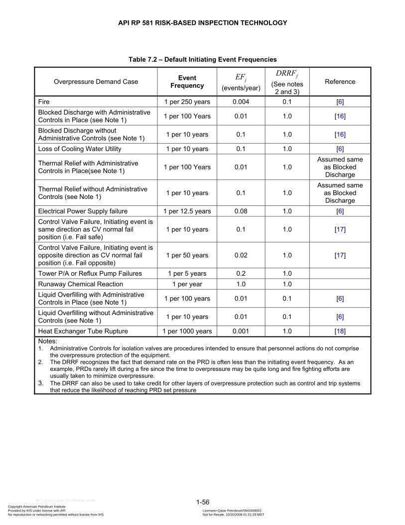
API RP 581 RISK-BASED INSPECTION TECHNOLOGY
1-56
Table 7.2 – Default Initiating Event Frequencies
Overpressure Demand Case Event Frequency
jEF (events/year)
fDRRF (See notes
2 and 3) Reference
Fire 1 per 250 years 0.004 0.1 [6] Blocked Discharge with Administrative Controls in Place (see Note 1) 1 per 100 Years 0.01 1.0 [16]
Blocked Discharge without Administrative Controls (see Note 1) 1 per 10 years 0.1 1.0 [16]
Loss of Cooling Water Utility 1 per 10 years 0.1 1.0 [6]
Thermal Relief with Administrative Controls in Place(see Note 1) 1 per 100 Years 0.01 1.0
Assumed same as Blocked Discharge
Thermal Relief without Administrative Controls (see Note 1) 1 per 10 years 0.1 1.0
Assumed same as Blocked Discharge
Electrical Power Supply failure 1 per 12.5 years 0.08 1.0 [6] Control Valve Failure, Initiating event is same direction as CV normal fail position (i.e. Fail safe)
1 per 10 years 0.1 1.0 [17]
Control Valve Failure, Initiating event is opposite direction as CV normal fail position (i.e. Fail opposite)
1 per 50 years 0.02 1.0 [17]
Tower P/A or Reflux Pump Failures 1 per 5 years 0.2 1.0 Runaway Chemical Reaction 1 per year 1.0 1.0 Liquid Overfilling with Administrative Controls in Place (see Note 1) 1 per 100 years 0.01 0.1 [6]
Liquid Overfilling without Administrative Controls (see Note 1) 1 per 10 years 0.01 0.1 [6]
Heat Exchanger Tube Rupture 1 per 1000 years 0.001 1.0 [18] Notes: 1. Administrative Controls for isolation valves are procedures intended to ensure that personnel actions do not comprise
the overpressure protection of the equipment. 2. The DRRF recognizes the fact that demand rate on the PRD is often less than the initiating event frequency. As an
example, PRDs rarely lift during a fire since the time to overpressure may be quite long and fire fighting efforts are usually taken to minimize overpressure.
3. The DRRF can also be used to take credit for other layers of overpressure protection such as control and trip systems that reduce the likelihood of reaching PRD set pressure
Copyright American Petroleum Institute Provided by IHS under license with API Licensee=Qatar Petroleum/5943408001
Not for Resale, 10/20/2008 01:51:29 MDTNo reproduction or networking permitted without license from IHS
--```,`,,`,`,,`,`,,,,,,``,```,`-`-`,,`,,`,`,,`---
API
RP
581
RIS
K-B
ASE
D IN
SPEC
TIO
N T
ECH
NO
LOG
Y
Tabl
e 7.
3 –
Ove
rpre
ssur
e Sc
enar
io L
ogic
Initi
atin
g Ev
ent
Freq
uenc
y Eq
uipm
ent
Type
PR
D D
eman
d R
ate
Red
uctio
n Fa
ctor
Q
ualif
ier
Ove
rpre
ssur
e Po
tent
ial
Bac
kgro
und
and
Com
men
ts
Ove
rpre
ssur
e Sc
enar
io –
Blo
cked
Dis
char
ge, M
anua
l Val
ve
1 pe
r 100
yea
rs
(adm
in c
ontro
ls)
1 pe
r 10
year
s (w
/o
adm
in c
ontro
ls
Mul
tiply
Eve
nt
Freq
uenc
y tim
es th
e #
of a
pplic
able
blo
ck
valv
es lo
cate
d in
pr
oces
s flo
w p
ath.
Le
es, 1
983
[16]
su
gges
ts a
n es
timat
ed ra
te o
f 0.
5 to
0.1
eve
nts
per y
ear f
or s
hutti
ng
man
ual v
alve
in
erro
r
Exc
hang
ers,
Fin
Fa
ns, R
eact
ors,
P
ipin
g, D
rum
s or
R
otat
ing
Equ
ipm
ent
1.0
Dow
nstre
am o
f ro
tatin
g eq
uipm
ent
othe
r tha
n po
sitiv
e di
spla
cem
ent t
ype
Dea
dhea
d P
ress
ure
or 1
.3 ti
mes
th
e no
rmal
dis
char
ge p
ress
ure
or B
ubbl
e P
oint
pre
ssur
e of
the
feed
stre
am a
t hea
t sou
rce
tem
pera
ture
(for
cas
es w
here
th
e eq
uipm
ent h
as in
tern
al o
r ex
tern
al h
eat s
ourc
es),
whi
chev
er is
gre
ates
t
Mos
t ce
ntrif
ugal
rot
atin
g eq
uipm
ent
will
dea
dhea
d at
30%
abo
ve th
e no
rmal
ope
ratin
g po
int.
Initi
atin
g ev
ent
frequ
ency
sh
ould
be
ad
just
ed
if th
e pr
otec
ted
equi
pmen
t is
rem
oved
fro
m s
ervi
ce f
or
mai
nten
ance
or
op
erat
iona
l ne
eds
(filte
r re
plac
emen
t or
cy
clic
pr
oces
s op
erat
ion)
at
a
frequ
ency
gr
eate
r th
an
the
unit
turn
arou
nd
frequ
ency
. E
quip
men
t w
ith i
nter
nal
or e
xter
nal
heat
sou
rces
m
ay h
ave
a si
gnifi
cant
pot
entia
l fo
r ov
erpr
essu
re
as a
res
ult
of v
apor
izat
ion
of t
he c
onta
ined
flu
id
stre
am.
1.0
Dow
nstre
am o
f po
sitiv
e di
spla
cem
ent t
ype
rota
ting
equi
pmen
t
4.0
X M
AW
P (R
uptu
re)
Dis
char
ge
pres
sure
fro
m
posi
tive
disp
lace
men
t pu
mps
w
ill
cont
inue
to
in
crea
se
pres
sure
. A
ssum
ptio
n is
mad
e th
at ru
ptur
e w
ill o
ccur
.
1.0
Dow
nstre
am o
f S
team
Tur
bine
s
Ste
am S
uppl
y P
ress
ure
or
Bub
ble
Poi
nt p
ress
ure
of th
e fe
ed s
tream
at s
team
sup
ply
tem
pera
ture
(for
cas
es w
here
th
e eq
uipm
ent h
as in
tern
al o
r ex
tern
al h
eat s
ourc
es),
whi
chev
er is
gre
ates
t
1.0
Dow
nstre
am o
f P
roce
ss U
nits
or
vess
els
1.1
X M
AW
P o
f Ups
tream
V
esse
l S
ourc
e P
ress
ure
Pro
cess
Tow
er w
ith
Fire
d H
eate
r he
at
sour
ce
1.0
Con
side
r LO
PA
or r
isk
redu
ctio
n an
alys
is
asso
ciat
ed w
ith lo
ss o
f flo
w c
ontro
ls o
n th
e fir
ed h
eate
r
Hea
t Sou
rce
to
tow
er is
a fi
red
heat
er
4.0
X M
AW
P (R
uptu
re)
Ass
umpt
ion
is m
ade
that
rup
ture
occ
urs.
Th
is
appl
ies
to t
he b
lock
ed v
apor
out
let
line
only
, se
e Li
quid
Ove
rfilli
ng C
ase
for
bloc
ked
liqui
d/bo
ttom
s ou
tlet
Pro
cess
To
wer
, al
l ot
her h
eat s
ourc
es
1.0
No
Ups
tream
Fire
d H
eate
r
Bub
ble
Poi
nt p
ress
ure
of th
e fe
ed s
tream
at h
eat s
ourc
e te
mpe
ratu
re
This
app
lies
to t
he b
lock
ed v
apor
out
let
line
only
, se
e Li
quid
O
verfi
lling
C
ase
for
bloc
ked
liqui
d/bo
ttom
s ou
tlet
Hea
ters
1.
0
4.0
X M
AW
P (R
uptu
re)
Add
ed
incr
ease
in
po
tent
ial
over
pres
sure
w
ith
fired
/radi
ant
heat
tra
nsfe
r. A
ssum
ptio
n is
mad
e th
at ru
ptur
e oc
curs
.
1-57
Copyright American Petroleum Institute Provided by IHS under license with API Licensee=Qatar Petroleum/5943408001
Not for Resale, 10/20/2008 01:51:29 MDTNo reproduction or networking permitted without license from IHS
--```,`,,`,`,,`,`,,,,,,``,```,`-`-`,,`,,`,`,,`---
API
RP
581
RIS
K-B
ASE
D IN
SPEC
TIO
N T
ECH
NO
LOG
Y
Tabl
e 7.
3 –
Ove
rpre
ssur
e Sc
enar
io L
ogic
Initi
atin
g Ev
ent
Freq
uenc
y Eq
uipm
ent
Type
PR
D D
eman
d R
ate
Red
uctio
n Fa
ctor
Q
ualif
ier
Ove
rpre
ssur
e Po
tent
ial
Bac
kgro
und
and
Com
men
ts
Ove
rpre
ssur
e Sc
enar
io –
Con
trol
Val
ve F
ail C
lose
at O
utle
t
1 pe
r 10
year
s [1
7]
for f
ail-c
lose
d C
ontro
l Val
ves
1 pe
r 50
year
s fo
r fa
il-op
en C
ontro
l V
alve
s M
ultip
ly E
vent
Fr
eque
ncy
times
the
# of
app
licab
le
cont
rol v
alve
s lo
cate
d in
pro
cess
flo
w p
ath.
Exc
hang
ers,
Fi
n Fa
ns,
Rea
ctor
s,
Pip
ing
or D
rum
s or
R
otat
ing
Equ
ipm
ent
1.0
Dow
nstre
am o
f ro
tatin
g eq
uipm
ent
othe
r tha
n po
sitiv
e di
spla
cem
ent t
ype
Dea
dhea
d P
ress
ure
or 1
.3 ti
mes
th
e no
rmal
dis
char
ge p
ress
ure
or B
ubbl
e P
oint
pre
ssur
e of
the
feed
stre
am a
t hea
t sou
rce
tem
pera
ture
(for
cas
es w
here
th
e eq
uipm
ent h
as in
tern
al o
r ex
tern
al h
eat s
ourc
es),
whi
chev
er is
gre
ates
t
Mos
t ce
ntrif
ugal
rot
atin
g eq
uipm
ent
will
dea
dhea
d at
30%
abo
ve th
e no
rmal
ope
ratin
g po
int.
Initi
atin
g ev
ent
frequ
ency
sh
ould
be
ad
just
ed
if th
e pr
otec
ted
equi
pmen
t is
rem
oved
fro
m s
ervi
ce f
or
mai
nten
ance
or
op
erat
iona
l ne
eds
(filte
r re
plac
emen
t or
cy
clic
pr
oces
s op
erat
ion)
at
a
frequ
ency
gr
eate
r th
an
the
unit
turn
arou
nd
frequ
ency
. E
quip
men
t w
ith i
nter
nal
or e
xter
nal
heat
sou
rces
may
hav
e a
sign
ifica
nt p
oten
tial
for
over
pres
sure
as
a re
sult
of v
apor
izat
ion
of t
he
cont
aine
d flu
id s
tream
.
1.0
Dow
nstre
am o
f po
sitiv
e di
spla
cem
ent t
ype
rota
ting
equi
pmen
t
4.0
X M
AW
P (R
uptu
re)
Dis
char
ge
pres
sure
fro
m
posi
tive
disp
lace
men
t pu
mps
w
ill
cont
inue
to
in
crea
se
pres
sure
. A
ssum
ptio
n is
mad
e th
at ru
ptur
e w
ill o
ccur
.
1.0
Dow
nstre
am o
f S
team
Tur
bine
s
Ste
am S
uppl
y P
ress
ure
or
Bub
ble
Poi
nt p
ress
ure
of th
e fe
ed s
tream
at s
team
sup
ply
tem
pera
ture
(for
cas
es w
here
th
e eq
uipm
ent h
as in
tern
al o
r ex
tern
al h
eat s
ourc
es),
whi
chev
er is
gre
ates
t
Pro
cess
Tow
er w
ith
Fire
d H
eate
r he
at
sour
ce
1.0
Dow
nstre
am o
f P
roce
ss U
nits
or
vess
els
1.1
X M
AW
P o
f Ups
tream
V
esse
l S
ourc
e P
ress
ure
1.0
Con
side
r LO
PA
or r
isk
redu
ctio
n an
alys
is
asso
ciat
ed w
ith lo
ss o
f flo
w c
ontro
ls o
n th
e fir
ed h
eate
r
Hea
t Sou
rce
to
tow
er is
a fi
red
heat
er
4.0
X M
AW
P (R
uptu
re)
Ass
umpt
ion
is m
ade
that
rup
ture
occ
urs.
Th
is
appl
ies
to t
he b
lock
ed v
apor
out
let
line
only
, se
e Li
quid
Ove
rfilli
ng C
ase
for
bloc
ked
liqui
d/bo
ttom
s ou
tlet
Pro
cess
To
wer
, al
l ot
her h
eat s
ourc
es
1.0
B
ubbl
e P
oint
pre
ssur
e of
the
feed
stre
am a
t hea
t sou
rce
tem
pera
ture
This
app
lies
to t
he b
lock
ed v
apor
out
let
line
only
, se
e Li
quid
O
verfi
lling
C
ase
for
bloc
ked
liqui
d/bo
ttom
s ou
tlet
Hea
ters
1.
0
4.0
X M
AW
P (R
uptu
re)
Add
ed
incr
ease
in
po
tent
ial
over
pres
sure
w
ith
fired
/radi
ant
heat
tra
nsfe
r. A
ssum
ptio
n is
mad
e th
at ru
ptur
e oc
curs
.
1-58
Copyright American Petroleum Institute Provided by IHS under license with API Licensee=Qatar Petroleum/5943408001
Not for Resale, 10/20/2008 01:51:29 MDTNo reproduction or networking permitted without license from IHS
--```,`,,`,`,,`,`,,,,,,``,```,`-`-`,,`,,`,`,,`---
API
RP
581
RIS
K-B
ASE
D IN
SPEC
TIO
N T
ECH
NO
LOG
Y
Tabl
e 7.
3 –
Ove
rpre
ssur
e Sc
enar
io L
ogic
Initi
atin
g Ev
ent
Freq
uenc
y Eq
uipm
ent
Type
PR
D D
eman
d R
ate
Red
uctio
n Fa
ctor
Q
ualif
ier
Ove
rpre
ssur
e Po
tent
ial
Bac
kgro
und
and
Com
men
ts
Ove
rpre
ssur
e Sc
enar
io –
Con
trol
Val
ve F
ail O
pen
at In
let,
incl
udin
g th
e H
P/LP
Gas
Bre
akth
roug
h C
ase
1 pe
r 10
year
s [1
7]
for f
ail-c
lose
d C
ontro
l Val
ves
1
per 5
0 ye
ars
for
fail-
open
Con
trol
Val
ves
M
ultip
ly E
vent
Fr
eque
ncy
times
the
# of
app
licab
le
cont
rol v
alve
s lo
cate
d in
pro
cess
flo
w p
ath.
All
Equ
ipm
ent
Type
s 1.
0 N
/A
Use
the
upst
ream
sou
rce
pres
sure
O
verp
ress
ure
Pot
entia
l is
a
func
tion
of
the
pres
sure
ratio
acr
oss
the
cont
rol v
alve
Ove
rpre
ssur
e Sc
enar
io –
Fire
1
per 2
50 y
ears
See
Lee
s [1
6] p
age
A7-
7, s
tate
s m
ajor
fir
e at
pla
nt 1
eve
ry
10 y
ears
All
Equ
ipm
ent
Type
s
0.1
Indu
stry
exp
erie
nce
just
ifies
this
val
ue
N/A
4.
0 X
MA
WP
(Rup
ture
)
Mod
ified
by
indu
stry
dat
a w
hich
indi
cate
s de
man
d ra
tes
on th
e or
der o
f 1 p
er 4
00 y
ears
Th
e D
RR
F fa
ctor
of
0.1
reco
gniz
es t
he i
ndus
try
expe
rienc
e th
at re
lativ
ely
few
ves
sels
exp
osed
to a
fir
e w
ill e
xper
ienc
e a
PR
D o
peni
ng.
Ass
umpt
ion
is
mad
e th
at
in
thos
e ra
re
case
s w
here
a P
RD
wou
ld o
pen
durin
g a
fire,
rupt
ure
will
oc
cur i
f the
PR
D fa
iled
to o
pen
upon
dem
and
1-59
Copyright American Petroleum Institute Provided by IHS under license with API Licensee=Qatar Petroleum/5943408001
Not for Resale, 10/20/2008 01:51:29 MDTNo reproduction or networking permitted without license from IHS
--```,`,,`,`,,`,`,,,,,,``,```,`-`-`,,`,,`,`,,`---
API
RP
581
RIS
K-B
ASE
D IN
SPEC
TIO
N T
ECH
NO
LOG
Y
Tabl
e 7.
3 –
Ove
rpre
ssur
e Sc
enar
io L
ogic
Initi
atin
g Ev
ent
Freq
uenc
y Eq
uipm
ent
Type
PR
D D
eman
d R
ate
Red
uctio
n Fa
ctor
Q
ualif
ier
Ove
rpre
ssur
e Po
tent
ial
Bac
kgro
und
and
Com
men
ts
Ove
rpre
ssur
e Sc
enar
io –
The
rmal
/Hyd
raul
ic E
xpan
sion
Rel
ief
1 pe
r 100
yea
rs
(man
ual v
alve
w
/adm
in c
ontro
ls)
1
per 1
0 ye
ars
(man
ual v
alve
w/o
ad
min
con
trols
or
cont
rol v
alve
Mul
tiply
initi
atin
g ev
ent f
requ
ency
tim
es th
e nu
mbe
r of
appl
icab
le b
lock
va
lves
loca
ted
in
proc
ess
flow
pat
h.
Pip
ing
or o
ther
liqu
id
fille
d eq
uipm
ent
1.0
N/A
O
pera
ting
Pre
ssur
e or
Bub
ble
Poi
nt p
ress
ure
of c
onta
ined
flui
d at
140
o F, w
hich
ever
is la
rger
Ass
umpt
ion
is m
ade
that
the
prob
abili
ty o
f a le
ak is
1.
0 (fl
ange
leak
s), m
odel
ed a
s a
¼ in
ch h
ole.
The
pr
obab
ility
of
rupt
ure
is a
ssum
ed t
o be
0.0
. F
or
fluid
s th
at
will
no
t bo
il,
sinc
e th
e pr
essu
re
is
relie
ved
imm
edia
tely
upo
n le
akag
e, t
he p
ress
ure
for
the
cons
eque
nce
calc
ulat
ion
will
be
the
norm
al
oper
atin
g pr
essu
re o
f the
pip
ing.
N
ot li
kely
to re
sult
in r
uptu
re, l
ikel
y to
cau
se fl
ange
le
aks/
smal
l lea
ks, h
eate
d on
ly
If th
e flu
id
can
boil
due
to
sola
r en
ergy
, th
e co
nseq
uenc
e pr
essu
re c
ould
be
mai
ntai
ned
at th
e bu
bble
poi
nt p
ress
ure
of th
e co
ntai
ned
fluid
. Le
ak
and
rupt
ure
prob
abili
ties
will
be
calc
ulat
ed a
s a
func
tion
of th
e bu
bble
poi
nt p
ress
ure.
Col
d si
de o
f Hea
t E
xcha
nger
s 1.
0 N
/A
Ope
ratin
g P
ress
ure
or B
ubbl
e P
oint
pre
ssur
e of
con
tain
ed fl
uid
at th
e ho
t sid
e flu
id in
let
tem
pera
ture
, whi
chev
er is
larg
er
Add
ed
incr
ease
in
po
tent
ial
over
pres
sure
w
ith
addi
tiona
l hea
t tra
nsfe
r fro
m h
ot s
ide.
Fo
r liq
uids
that
do
not b
oil,
the
assu
mpt
ion
is m
ade
that
the
pro
babi
lity
of l
eak
is 1
.0 (
flang
e le
aks)
, m
odel
ed a
s a
¼ in
ch h
ole,
and
the
pro
babi
lity
of
rupt
ure
is 0
.0.
If th
e co
ld s
ide
fluid
can
boi
l, th
e co
nseq
uenc
e pr
essu
re c
ould
rea
ch th
e bu
bble
poi
nt p
ress
ure
of
the
stor
ed
fluid
at
th
e ho
t si
de
fluid
in
let
tem
pera
ture
. Le
ak a
nd ru
ptur
e pr
obab
ilitie
s w
ill b
e ca
lcul
ated
as
a
func
tion
of
the
bubb
le
poin
t pr
essu
re.
Ove
rpre
ssur
e Sc
enar
io –
Los
s of
Coo
ling
1 pe
r 10
year
s
Pro
cess
Tow
er w
ith
Fire
d H
eate
r hea
t so
urce
1.0
Con
side
r LO
PA
or r
isk
redu
ctio
n an
alys
is
asso
ciat
ed w
ith lo
ss o
f flo
w c
ontro
ls o
n th
e fir
ed h
eate
r
Hea
t Sou
rce
to
tow
er is
a fi
red
heat
er
4.0
X M
AW
P (R
uptu
re)
Ass
umpt
ion
is m
ade
that
rupt
ure
occu
rs.
All
Oth
er E
quip
men
t w
ith in
tern
al o
r ex
tern
al h
eat
sour
ces
1.0
Bub
ble
Poi
nt p
ress
ure
of th
e fe
ed s
tream
at h
eat s
ourc
e te
mpe
ratu
re
1-60
Copyright American Petroleum Institute Provided by IHS under license with API Licensee=Qatar Petroleum/5943408001
Not for Resale, 10/20/2008 01:51:29 MDTNo reproduction or networking permitted without license from IHS
--```,`,,`,`,,`,`,,,,,,``,```,`-`-`,,`,,`,`,,`---
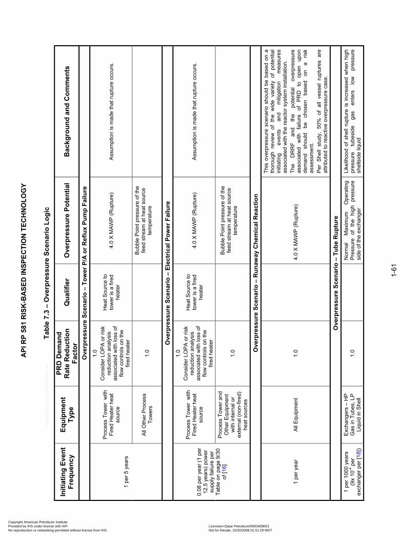
API
RP
581
RIS
K-B
ASE
D IN
SPEC
TIO
N T
ECH
NO
LOG
Y
Tabl
e 7.
3 –
Ove
rpre
ssur
e Sc
enar
io L
ogic
Initi
atin
g Ev
ent
Freq
uenc
y Eq
uipm
ent
Type
PR
D D
eman
d R
ate
Red
uctio
n Fa
ctor
Q
ualif
ier
Ove
rpre
ssur
e Po
tent
ial
Bac
kgro
und
and
Com
men
ts
Ove
rpre
ssur
e Sc
enar
io –
Tow
er P
/A o
r Ref
lux
Pum
p Fa
ilure
1 pe
r 5 y
ears
Pro
cess
Tow
er w
ith
Fire
d H
eate
r hea
t so
urce
1.0
Con
side
r LO
PA
or r
isk
redu
ctio
n an
alys
is
asso
ciat
ed w
ith lo
ss o
f flo
w c
ontro
ls o
n th
e fir
ed h
eate
r
Hea
t Sou
rce
to
tow
er is
a fi
red
heat
er
4.0
X M
AW
P (R
uptu
re)
Ass
umpt
ion
is m
ade
that
rupt
ure
occu
rs.
All
Oth
er P
roce
ss
Tow
ers
1.0
Bub
ble
Poi
nt p
ress
ure
of th
e fe
ed s
tream
at h
eat s
ourc
e te
mpe
ratu
re
Ove
rpre
ssur
e Sc
enar
io –
Ele
ctric
al P
ower
Fai
lure
0.08
per
yea
r (1
per
12.5
yea
rs) p
ower
su
pply
failu
re p
er
Tabl
e on
pag
e 9/
30
of [1
6]
Pro
cess
Tow
er w
ith
Fire
d H
eate
r hea
t so
urce
1.0
Con
side
r LO
PA
or r
isk
redu
ctio
n an
alys
is
asso
ciat
ed w
ith lo
ss o
f flo
w c
ontro
ls o
n th
e fir
ed h
eate
r
Hea
t Sou
rce
to
tow
er is
a fi
red
heat
er
4.0
X M
AW
P (R
uptu
re)
Ass
umpt
ion
is m
ade
that
rupt
ure
occu
rs.
Pro
cess
Tow
er a
nd
Oth
er E
quip
men
t w
ith in
tern
al o
r ex
tern
al (n
on-fi
red)
he
at s
ourc
es
1.0
Bub
ble
Poi
nt p
ress
ure
of th
e fe
ed s
tream
at h
eat s
ourc
e te
mpe
ratu
re
Ove
rpre
ssur
e Sc
enar
io –
Run
away
Che
mic
al R
eact
ion
1 pe
r yea
r A
ll E
quip
men
t 1.
0
4.0
X M
AW
P (R
uptu
re)
This
ove
rpre
ssur
e sc
enar
io s
houl
d be
bas
ed o
n a
thor
ough
rev
iew
of
the
wid
e va
riety
of
pote
ntia
l in
itiat
ing
even
ts
and
miti
gatio
n m
easu
res
asso
ciat
ed w
ith th
e re
acto
r sys
tem
inst
alla
tion.
Th
e D
RR
F an
d th
e po
tent
ial
over
pres
sure
as
soci
ated
w
ith
failu
re
of
PR
D
to
open
up
on
dem
and
shou
ld
be
chos
en
base
d on
a
risk
asse
ssm
ent.
Per
She
ll st
udy,
50%
of
all
vess
el r
uptu
res
are
attri
bute
d to
reac
tive
over
pres
sure
cas
e.
Ove
rpre
ssur
e Sc
enar
io –
Tub
e R
uptu
re
1 pe
r 100
0 ye
ars
(9x
10-4
per
ex
chan
ger p
er [1
8])
Exc
hang
ers
– H
P
Gas
in T
ubes
, LP
Li
quid
in S
hell
1.0
N
orm
al
Max
imum
O
pera
ting
Pre
ssur
e of
the
hig
h pr
essu
re
side
of t
he e
xcha
nger
Like
lihoo
d of
she
ll ru
ptur
e is
incr
ease
d w
hen
high
pr
essu
re
tube
side
ga
s en
ters
lo
w
pres
sure
sh
ells
ide
liqui
d
1-61
Copyright American Petroleum Institute Provided by IHS under license with API Licensee=Qatar Petroleum/5943408001
Not for Resale, 10/20/2008 01:51:29 MDTNo reproduction or networking permitted without license from IHS
--```,`,,`,`,,`,`,,,,,,``,```,`-`-`,,`,,`,`,,`---

API
RP
581
RIS
K-B
ASE
D IN
SPEC
TIO
N T
ECH
NO
LOG
Y
1-62
Tabl
e 7.
3 –
Ove
rpre
ssur
e Sc
enar
io L
ogic
Initi
atin
g Ev
ent
Freq
uenc
y Eq
uipm
ent
Type
PR
D D
eman
d R
ate
Red
uctio
n Fa
ctor
Q
ualif
ier
Ove
rpre
ssur
e Po
tent
ial
Bac
kgro
und
and
Com
men
ts
Ove
rpre
ssur
e Sc
enar
io –
Liq
uid
Ove
rfill
ing
1 pe
r 100
yea
rs
(adm
in c
ontro
ls)
1
per 1
0 ye
ars
(w/o
ad
min
con
trols
Mul
tiply
Eve
nt
Freq
uenc
y tim
es th
e nu
mbe
r of
appl
icab
le b
lock
va
lves
loca
ted
in
proc
ess
flow
pat
h.
All
Equ
ipm
ent
incl
udin
g P
roce
ss
Tow
er (B
lock
ed
Out
let o
f Liq
uid
Bot
tom
s)
1.0
Dow
nstre
am o
f ro
tatin
g eq
uipm
ent
othe
r tha
n po
sitiv
e di
spla
cem
ent t
ype
Dea
dhea
d P
ress
ure
or 1
.3 ti
mes
th
e no
rmal
dis
char
ge p
ress
ure
or B
ubbl
e P
oint
pre
ssur
e of
the
fe
ed
stre
am
at
heat
so
urce
te
mpe
ratu
re
(for
case
s w
here
th
e eq
uipm
ent
has
inte
rnal
or
ex
tern
al
heat
so
urce
s),
whi
chev
er is
gre
ates
t
Mos
t ce
ntrif
ugal
rot
atin
g eq
uipm
ent
will
dea
dhea
d at
30%
abo
ve th
e no
rmal
ope
ratin
g po
int.
Initi
atin
g ev
ent
frequ
ency
sh
ould
be
ad
just
ed
if th
e pr
otec
ted
equi
pmen
t is
rem
oved
fro
m s
ervi
ce f
or
mai
nten
ance
or
op
erat
iona
l ne
eds
(filte
r re
plac
emen
t or
cy
clic
pr
oces
s op
erat
ion)
at
a
frequ
ency
gr
eate
r th
an
the
unit
turn
arou
nd
frequ
ency
.
Equ
ipm
ent
with
int
erna
l or
ext
erna
l he
at s
ourc
es
may
hav
e a
sign
ifica
nt p
oten
tial
for
over
pres
sure
as
a r
esul
t of
vap
oriz
atio
n of
the
con
tain
ed f
luid
st
ream
.
1.0
Dow
nstre
am o
f po
sitiv
e di
spla
cem
ent t
ype
rota
ting
equi
pmen
t
4.0
X M
AW
P (R
uptu
re)
Dis
char
ge
pres
sure
fro
m
posi
tive
disp
lace
men
t pu
mps
w
ill
cont
inue
to
in
crea
se
pres
sure
. A
ssum
ptio
n is
mad
e th
at ru
ptur
e w
ill o
ccur
.
1.0
Dow
nstre
am o
f S
team
Tur
bine
s
Ste
am
Sup
ply
Pre
ssur
e or
B
ubbl
e P
oint
pr
essu
re
of
the
feed
st
ream
at
st
eam
su
pply
te
mpe
ratu
re
(for
case
s w
here
th
e eq
uipm
ent
has
inte
rnal
or
ex
tern
al
heat
so
urce
s),
whi
chev
er is
gre
ates
t
1.0
Dow
nstre
am o
f P
roce
ss U
nits
or
vess
els
1.1
X
MA
WP
of
U
pstre
am
Pre
ssur
e S
ourc
e V
esse
l
Copyright American Petroleum Institute Provided by IHS under license with API Licensee=Qatar Petroleum/5943408001
Not for Resale, 10/20/2008 01:51:29 MDTNo reproduction or networking permitted without license from IHS
--```,`,,`,`,,`,`,,,,,,``,```,`-`-`,,`,,`,`,,`---
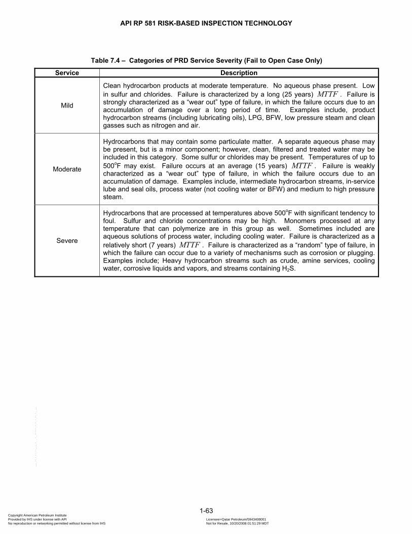
API RP 581 RISK-BASED INSPECTION TECHNOLOGY
Table 7.4 – Categories of PRD Service Severity (Fail to Open Case Only)
Service Description
Mild
Clean hydrocarbon products at moderate temperature. No aqueous phase present. Low in sulfur and chlorides. Failure is characterized by a long (25 years) MTTF . Failure is strongly characterized as a “wear out” type of failure, in which the failure occurs due to an accumulation of damage over a long period of time. Examples include, product hydrocarbon streams (including lubricating oils), LPG, BFW, low pressure steam and clean gasses such as nitrogen and air.
Moderate
Hydrocarbons that may contain some particulate matter. A separate aqueous phase may be present, but is a minor component; however, clean, filtered and treated water may be included in this category. Some sulfur or chlorides may be present. Temperatures of up to 500oF may exist. Failure occurs at an average (15 years) MTTF . Failure is weakly characterized as a “wear out” type of failure, in which the failure occurs due to an accumulation of damage. Examples include, intermediate hydrocarbon streams, in-service lube and seal oils, process water (not cooling water or BFW) and medium to high pressure steam.
Severe
Hydrocarbons that are processed at temperatures above 500oF with significant tendency to foul. Sulfur and chloride concentrations may be high. Monomers processed at any temperature that can polymerize are in this group as well. Sometimes included are aqueous solutions of process water, including cooling water. Failure is characterized as a relatively short (7 years) MTTF . Failure is characterized as a “random” type of failure, in which the failure can occur due to a variety of mechanisms such as corrosion or plugging. Examples include; Heavy hydrocarbon streams such as crude, amine services, cooling water, corrosive liquids and vapors, and streams containing H2S.
1-63 Copyright American Petroleum Institute Provided by IHS under license with API Licensee=Qatar Petroleum/5943408001
Not for Resale, 10/20/2008 01:51:29 MDTNo reproduction or networking permitted without license from IHS
--```,`,,`,`,,`,`,,,,,,``,```,`-`-`,,`,,`,`,,`---
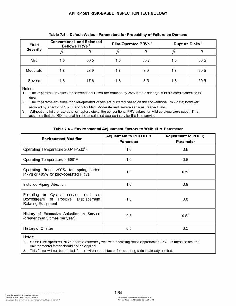
API RP 581 RISK-BASED INSPECTION TECHNOLOGY
Table 7.5 – Default Weibull Parameters for Probability of Failure on Demand
Fluid Severity
Conventional and Balanced Bellows PRVs 1 Pilot-Operated PRVs 2 Rupture Disks 3
β η β η β η
Mild 1.8 50.5 1.8 33.7 1.8 50.5
Moderate 1.8 23.9 1.8 8.0 1.8 50.5
Severe 1.8 17.6 1.8 3.5 1.8 50.5
Notes: 1. The η parameter values for conventional PRVs are reduced by 25% if the discharge is to a closed system or to
flare. 2. The η parameter values for pilot-operated valves are currently based on the conventional PRV data; however,
reduced by a factor of 1.5, 3, and 5 for Mild, Moderate and Severe services, respectively. 3. Without any failure rate data for rupture disks, the conventional PRV values for Mild services were used. This
assumes that the RD material has been selected appropriately for the fluid service.
Table 7.6 – Environmental Adjustment Factors to Weibull η Parameter
Environment Modifier Adjustment to POFOD η
Parameter Adjustment to POL η
Parameter
Operating Temperature 200<T<500oF 1.0 0.8
Operating Temperature > 500oF 1.0 0.6
Operating Ratio >90% for spring-loaded PRVs or >95% for pilot-operated PRVs 1.0 0.51
Installed Piping Vibration 1.0 0.8
Pulsating or Cyclical service, such as Downstream of Positive Displacement Rotating Equipment
1.0 0.8
History of Excessive Actuation in Service (greater than 5 times per year) 0.5 0.52
History of Chatter 0.5 0.5
Notes: 1. Some Pilot-operated PRVs operate extremely well with operating ratios approaching 98%. In these cases, the
environmental factor should not be applied. 2. This factor will not be applied if the environmental factor for operating ratio is already applied.
1-64 Copyright American Petroleum Institute Provided by IHS under license with API Licensee=Qatar Petroleum/5943408001
Not for Resale, 10/20/2008 01:51:29 MDTNo reproduction or networking permitted without license from IHS
--```,`,,`,`,,`,`,,,,,,``,```,`-`-`,,`,,`,`,,`---
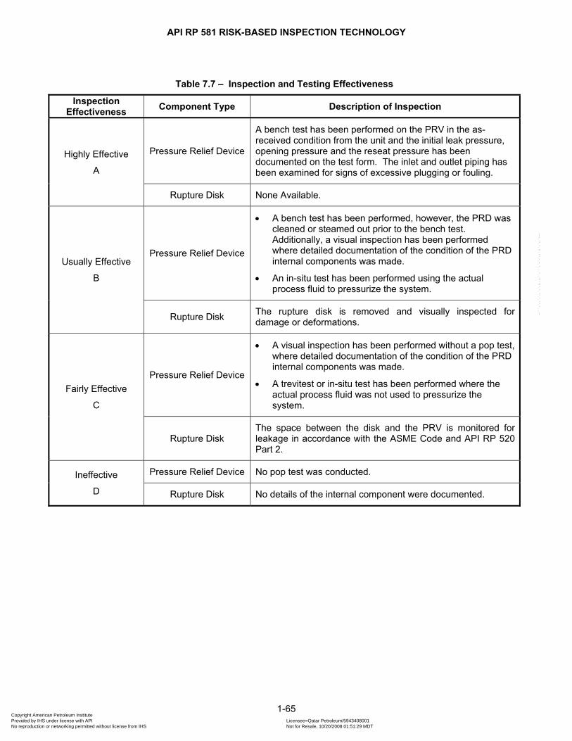
API RP 581 RISK-BASED INSPECTION TECHNOLOGY
Table 7.7 – Inspection and Testing Effectiveness
Inspection Effectiveness Component Type Description of Inspection
Highly Effective
A
Pressure Relief Device
A bench test has been performed on the PRV in the as-received condition from the unit and the initial leak pressure, opening pressure and the reseat pressure has been documented on the test form. The inlet and outlet piping has been examined for signs of excessive plugging or fouling.
Rupture Disk None Available.
Usually Effective
B
Pressure Relief Device
• A bench test has been performed, however, the PRD was cleaned or steamed out prior to the bench test. Additionally, a visual inspection has been performed where detailed documentation of the condition of the PRD internal components was made.
• An in-situ test has been performed using the actual process fluid to pressurize the system.
Rupture Disk The rupture disk is removed and visually inspected for damage or deformations.
Fairly Effective
C
Pressure Relief Device
• A visual inspection has been performed without a pop test, where detailed documentation of the condition of the PRD internal components was made.
• A trevitest or in-situ test has been performed where the actual process fluid was not used to pressurize the system.
Rupture Disk The space between the disk and the PRV is monitored for leakage in accordance with the ASME Code and API RP 520 Part 2.
Ineffective
D
Pressure Relief Device No pop test was conducted.
Rupture Disk No details of the internal component were documented.
1-65 Copyright American Petroleum Institute Provided by IHS under license with API Licensee=Qatar Petroleum/5943408001
Not for Resale, 10/20/2008 01:51:29 MDTNo reproduction or networking permitted without license from IHS
--```,`,,`,`,,`,`,,,,,,``,```,`-`-`,,`,,`,`,,`---

API RP 581 RISK-BASED INSPECTION TECHNOLOGY
Table 7.8 – Level of Inspection Confidence Factors
Inspection Result Confidence Factor That Inspection Result Determines the True Damage State, CFIneffective Fairly Effective Usually Effective Highly Effective
Pass, passCF No credit 0.5 0.70 0.9
Fail, failCF No Credit 0.70 0.95 0.95
No Leak, noleakCF No Credit 0.5 0.70 0.9
Leak, leakCF No Credit 0.70 0.95 0.95
Table 7.9 - Inspection Updating Equations
Inspection Effectiveness and Result Equation for Weighted Probability of Failure on Demand
Highly Effective Pass , ,, ,0.2 0.2
f prior f prior
prd prd prd prdf wgt f cond
t tP P P Pη η⎛ ⎞ ⎛ ⎞
= − ⋅ + ⋅⎜ ⎟ ⎜ ⎟⎝ ⎠ ⎝ ⎠
Usually Effective Pass , ,, ,0.2 0.2
f prior f prior
prd prd prd prdf wgt f cond
t tP P P Pη η⎛ ⎞ ⎛ ⎞
= − ⋅ + ⋅⎜ ⎟ ⎜ ⎟⎝ ⎠ ⎝ ⎠
Fairly Effective Pass , ,, ,0.2 0.2
f prior f prior
prd prd prd prdf wgt f cond
t tP P P Pη η⎛ ⎞ ⎛ ⎞
= − ⋅ + ⋅⎜ ⎟ ⎜ ⎟⎝ ⎠ ⎝ ⎠
Highly Effective Fail , ,prd prd
f wgt f condP P=
Usually Effective Fail , ,prd prd
f wgt f condP P=
Fairly Effective Fail , ,0.5 0.5prd prd prd,f wgt f prior f condP P P= ⋅ + ⋅
1-66 Copyright American Petroleum Institute Provided by IHS under license with API Licensee=Qatar Petroleum/5943408001
Not for Resale, 10/20/2008 01:51:29 MDTNo reproduction or networking permitted without license from IHS
--```,`,,`,`,,`,`,,,,,,``,```,`-`-`,,`,,`,`,,`---
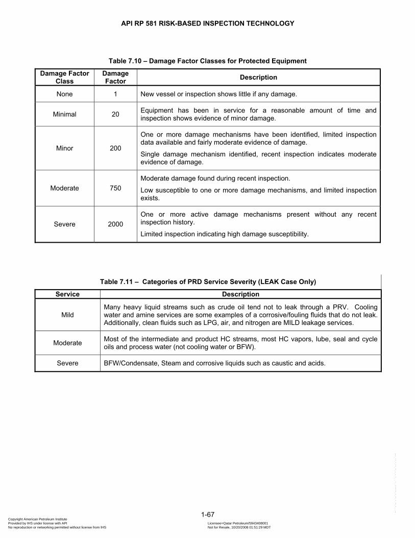
API RP 581 RISK-BASED INSPECTION TECHNOLOGY
Table 7.10 – Damage Factor Classes for Protected Equipment
Damage Factor Class
Damage Factor Description
None 1 New vessel or inspection shows little if any damage.
Minimal 20 Equipment has been in service for a reasonable amount of time and inspection shows evidence of minor damage.
Minor 200
One or more damage mechanisms have been identified, limited inspection data available and fairly moderate evidence of damage.
Single damage mechanism identified, recent inspection indicates moderate evidence of damage.
Moderate 750 Moderate damage found during recent inspection.
Low susceptible to one or more damage mechanisms, and limited inspection exists.
Severe 2000 One or more active damage mechanisms present without any recent inspection history.
Limited inspection indicating high damage susceptibility.
Table 7.11 – Categories of PRD Service Severity (LEAK Case Only)
Service Description
Mild Many heavy liquid streams such as crude oil tend not to leak through a PRV. Cooling water and amine services are some examples of a corrosive/fouling fluids that do not leak. Additionally, clean fluids such as LPG, air, and nitrogen are MILD leakage services.
Moderate Most of the intermediate and product HC streams, most HC vapors, lube, seal and cycle oils and process water (not cooling water or BFW).
Severe BFW/Condensate, Steam and corrosive liquids such as caustic and acids.
1-67 Copyright American Petroleum Institute Provided by IHS under license with API Licensee=Qatar Petroleum/5943408001
Not for Resale, 10/20/2008 01:51:29 MDTNo reproduction or networking permitted without license from IHS
--```,`,,`,`,,`,`,,,,,,``,```,`-`-`,,`,,`,`,,`---

API RP 581 RISK-BASED INSPECTION TECHNOLOGY
Table 7.12 – Default Weibull Parameters for Probability of Leakage (POL)
Fluid Severity
Conventional PRVs 1 Balanced Bellows PRVs 1 Pilot-Operated PRVs 2 Rupture Disks 3
β η β η β η β η
Mild 1.6 17.5 1.6 16.0 1.6 17.5 1.6 17.5
Moderate 1.6 15.5 1.6 14.0 1.6 15.5 1.6 17.5
Severe 1.6 13.1 1.6 11.5 1.6 13.1 1.6 17.5
Notes: 1. The η parameter values are increased by 25% for Conventional and Balanced PRVs that have soft seats. 2. The η parameter values for pilot-operated valves are currently based on the conventional PRV data, since there is
currently no failure rate data to support otherwise. 3. Without any failure rate data for rupture disks, the conventional PRV values for Mild service were used.
Table 7.13 – Potential Consequences of Pressure Vessel Overpressure
Accumulation (% over MAWP) Significance Potential Consequence
10% ASME code allowable accumulation for process upset cases (non-fire) protected by a single relief device
No expected consequence at this accumulation level.
16% ASME code allowable accumulation for process upset cases protected by multiple relief devices
No expected consequence at this accumulation level.
21% ASME code allowable accumulation for external fire relief cases regardless of the number of relief devices
No expected consequence at this accumulation level.
50% ASME standard hydrostatic test pressure (may be 30% on new designs)
Possible leaks in associated instrumentation, etc. Medium consequence.
90% Minimum yield strength (dependent on materials of construction)
Catastrophic vessel rupture, remote possibility. Significant leaks probable. Failure of damaged vessel areas (corrosion, cracks, blisters, etc. likely. High consequence.
300% Ultimate tensile strength (dependent on materials of construction)
Catastrophic vessel rupture predicted. Highest consequence.
1-68 Copyright American Petroleum Institute Provided by IHS under license with API Licensee=Qatar Petroleum/5943408001
Not for Resale, 10/20/2008 01:51:29 MDTNo reproduction or networking permitted without license from IHS
--```,`,,`,`,,`,`,,,,,,``,```,`-`-`,,`,,`,`,,`---
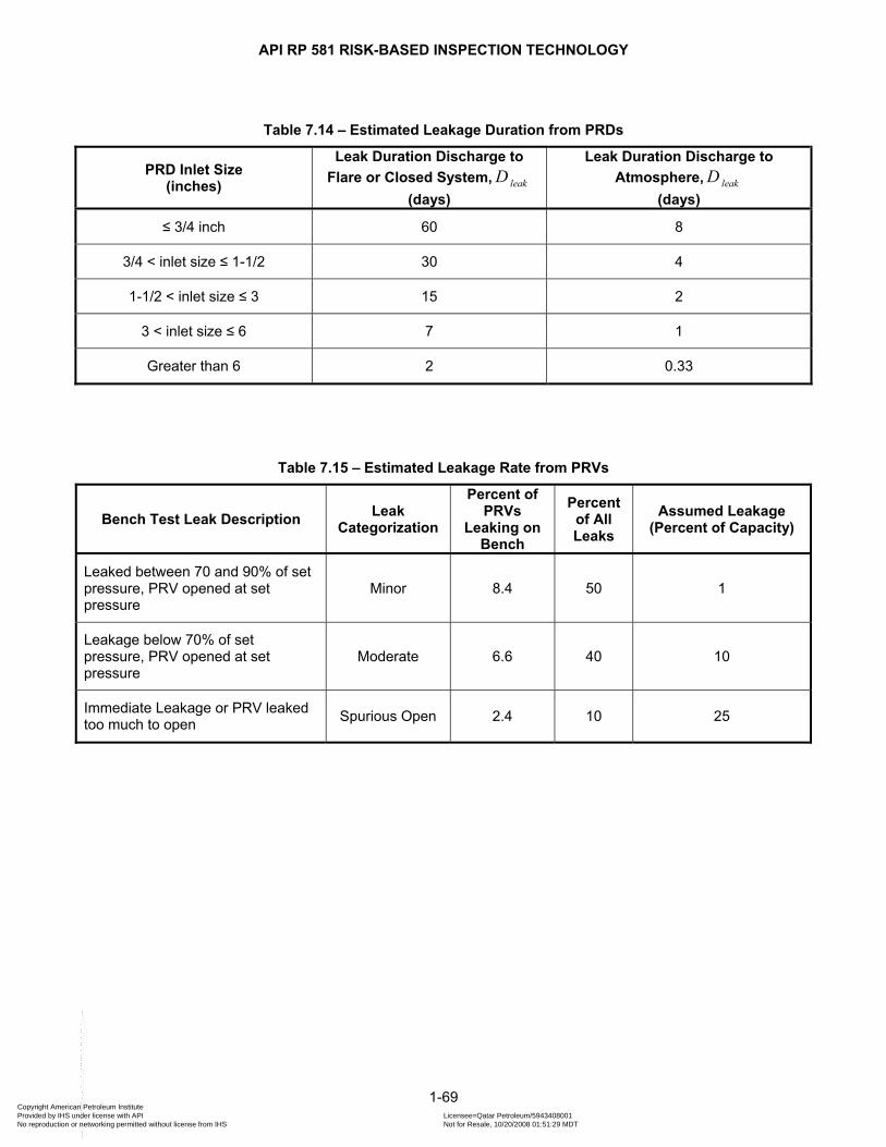
API RP 581 RISK-BASED INSPECTION TECHNOLOGY
Table 7.14 – Estimated Leakage Duration from PRDs
PRD Inlet Size (inches)
Leak Duration Discharge to Flare or Closed System, leakD
(days)
Leak Duration Discharge to Atmosphere, leakD
(days)
≤ 3/4 inch 60 8
3/4 < inlet size ≤ 1-1/2 30 4
1-1/2 < inlet size ≤ 3 15 2
3 < inlet size ≤ 6 7 1
Greater than 6 2 0.33
Table 7.15 – Estimated Leakage Rate from PRVs
Bench Test Leak Description Leak Categorization
Percent of PRVs
Leaking on Bench
Percent of All Leaks
Assumed Leakage (Percent of Capacity)
Leaked between 70 and 90% of set pressure, PRV opened at set pressure
Minor 8.4 50 1
Leakage below 70% of set pressure, PRV opened at set pressure
Moderate 6.6 40 10
Immediate Leakage or PRV leaked too much to open Spurious Open 2.4 10 25
1-69 Copyright American Petroleum Institute Provided by IHS under license with API Licensee=Qatar Petroleum/5943408001
Not for Resale, 10/20/2008 01:51:29 MDTNo reproduction or networking permitted without license from IHS
--```,`,,`,`,,`,`,,,,,,``,```,`-`-`,,`,,`,`,,`---
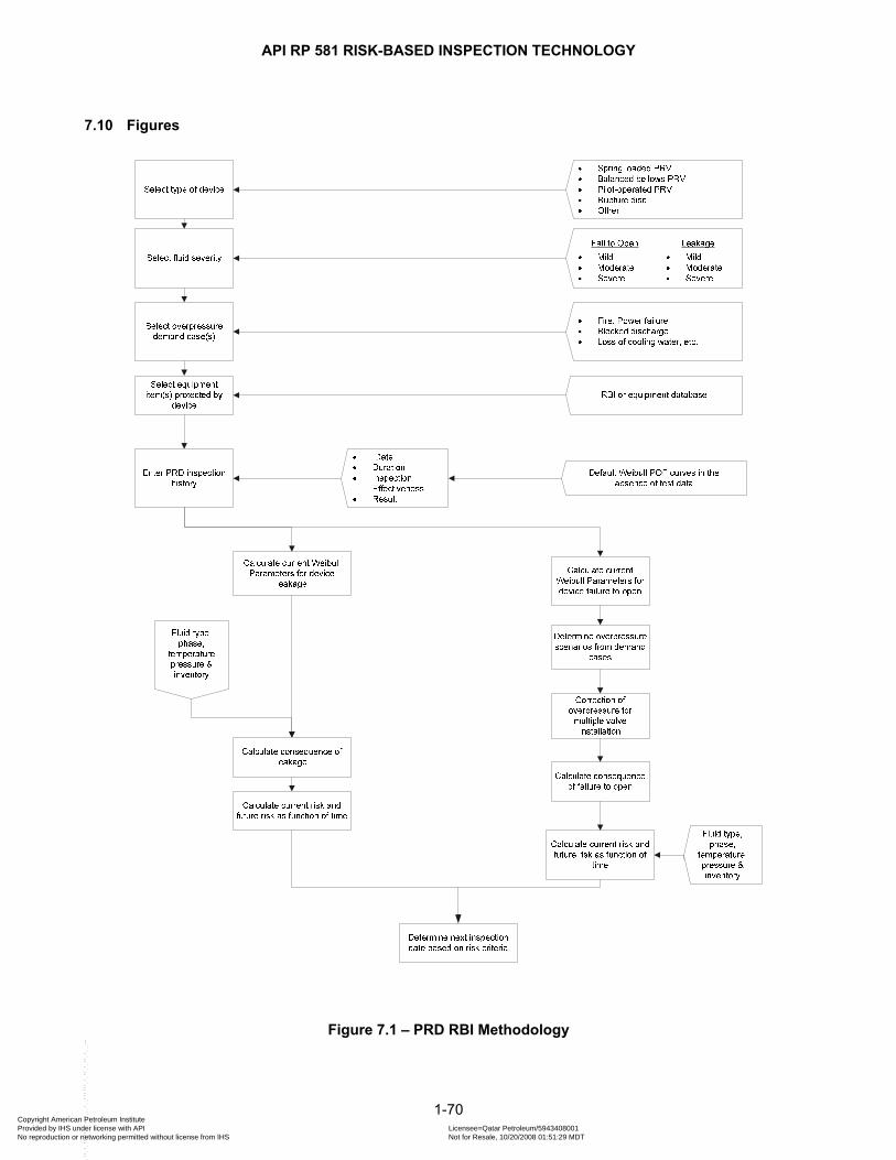
API RP 581 RISK-BASED INSPECTION TECHNOLOGY
7.10 Figures
Figure 7.1 – PRD RBI Methodology
1-70 Copyright American Petroleum Institute Provided by IHS under license with API Licensee=Qatar Petroleum/5943408001
Not for Resale, 10/20/2008 01:51:29 MDTNo reproduction or networking permitted without license from IHS
--```,`,,`,`,,`,`,,,,,,``,```,`-`-`,,`,,`,`,,`---

API RP 581 RISK-BASED INSPECTION TECHNOLOGY
.0000
.1000
.2000
.3000
.4000
.5000
.6000
.7000
.8000
0 2 4 6 8 10 12 14 16 18 20
Years
POFO
D MildModerateSevere
Figure 7.2 – Default Conventional PRV Fail to Open in Demand Weibull Curves
1-71 Copyright American Petroleum Institute Provided by IHS under license with API Licensee=Qatar Petroleum/5943408001
Not for Resale, 10/20/2008 01:51:29 MDTNo reproduction or networking permitted without license from IHS
--```,`,,`,`,,`,`,,,,,,``,```,`-`-`,,`,,`,`,,`---

API RP 581 RISK-BASED INSPECTION TECHNOLOGY
.0000
.1000
.2000
.3000
.4000
.5000
.6000
.7000
.8000
.9000
0 2 4 6 8 10 12 14 16 18 20
Years
POL
MildModerateSevere
Figure 7.3 – Default Leakage Failure Rate for Conventional PRVs
1-72 Copyright American Petroleum Institute Provided by IHS under license with API Licensee=Qatar Petroleum/5943408001
Not for Resale, 10/20/2008 01:51:29 MDTNo reproduction or networking permitted without license from IHS
--```,`,,`,`,,`,`,,,,,,``,```,`-`-`,,`,,`,`,,`---
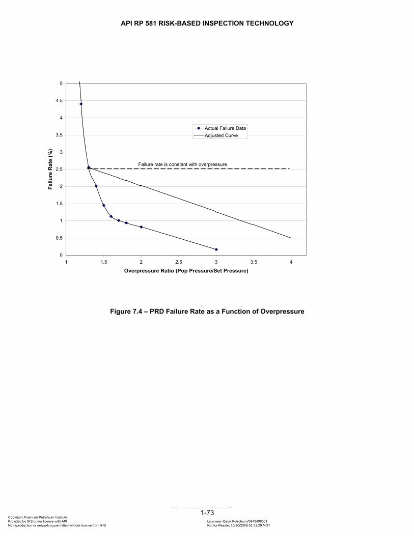
API RP 581 RISK-BASED INSPECTION TECHNOLOGY
0
0.5
1
1.5
2
2.5
3
3.5
4
4.5
5
1 1.5 2 2.5 3 3.5 4
Overpressure Ratio (Pop Pressure/Set Pressure)
Failu
re R
ate
(%)
Actual Failure DataAdjusted Curve
Failure rate is constant with overpressure
Figure 7.4 – PRD Failure Rate as a Function of Overpressure
1-73 Copyright American Petroleum Institute Provided by IHS under license with API Licensee=Qatar Petroleum/5943408001
Not for Resale, 10/20/2008 01:51:29 MDTNo reproduction or networking permitted without license from IHS
--```,`,,`,`,,`,`,,,,,,``,```,`-`-`,,`,,`,`,,`---

API RP 581 RISK-BASED INSPECTION TECHNOLOGY
.0000
.1000
.2000
.3000
.4000
.5000
.6000
0 1 2 3 4 5 6 7 8 9 10 11 12 13 14 15
Years In Service
POFO
D
SevereModified Severe
Default POFOD Curve
Modified POFOD Curve
Effect of Environmental Modifier
Figure 7.5 – Effect of Environmental Factors on PRD Weibull Curves
1-74 Copyright American Petroleum Institute Provided by IHS under license with API Licensee=Qatar Petroleum/5943408001
Not for Resale, 10/20/2008 01:51:29 MDTNo reproduction or networking permitted without license from IHS
--```,`,,`,`,,`,`,,,,,,``,```,`-`-`,,`,,`,`,,`---

API RP 581 RISK-BASED INSPECTION TECHNOLOGY
-0.5
0
0.5
1
1.5
2
0.5 1 1.5 2 2.5 3 3.5 4 4.5
Pressure Ratio (Pressure/MAWP)
Prob
abili
ty o
f Los
s of
Con
tain
men
t
DF=5000DF=2000DF=500DF=1.0
GFFT x DF
Figure 7.6 – Probability of Loss of Containment as a Function of Overpressure
1-75 Copyright American Petroleum Institute Provided by IHS under license with API Licensee=Qatar Petroleum/5943408001
Not for Resale, 10/20/2008 01:51:29 MDTNo reproduction or networking permitted without license from IHS
--```,`,,`,`,,`,`,,,,,,``,```,`-`-`,,`,,`,`,,`---

API RP 581 RISK-BASED INSPECTION TECHNOLOGY
0
5,000
10,000
15,000
20,000
25,000
30,000
0 2 4 6 8 10 12 14 16 18
Years
Cal
cula
ted
Ris
k, $
/yea
r
Risk Tolerance = $25,000/yearRisk Tolerance =$ 10,000/year
Figure 7.7 – Inspection Test Updating of Pressure Relief Devices
1-76 Copyright American Petroleum Institute Provided by IHS under license with API Licensee=Qatar Petroleum/5943408001
Not for Resale, 10/20/2008 01:51:29 MDTNo reproduction or networking permitted without license from IHS
--```,`,,`,`,,`,`,,,,,,``,```,`-`-`,,`,,`,`,,`---

API RP 581 RISK-BASED INSPECTION TECHNOLOGY
8 HEAT EXCHANGER TUBE BUNDLES
8.1 General
8.1.1 Overview This paragraph describes a methodology to assess the reliability and remaining life of heat exchanger bundles. It also provides a methodology for performing cost benefit analysis to assist in making risk-based inspection and replacement decisions and to determine the optimal replacement frequency of heat exchanger bundles. The purpose of the module is to optimize heat exchanger bundle inspection and replacement cycles and to minimize the annual operating and maintenance costs of heat exchanger bundles. These costs include bundle and installation costs, environmental impact costs and lost opportunity costs due to unit and plant unplanned shutdowns or unit rate reductions as a result of bundle failure.
8.1.2 Background Many companies currently predict bundle life by analyzing the history of each heat exchanger bundle since the service start date. These condition-based inspection programs do not, in general, consider the financial consequences associated with bundle failure. The problems with a condition-based approach for heat exchanger bundles is that many exchangers may experience few, if any bundle failures and some failures may not apply to current operating conditions or practices. In addition, these approaches are not based on a statistically significant data set to make an accurate prediction of future performance or probability of failure for the heat exchanger bundle. This philosophy also does not allow any predictions for newly installed bundles or for bundles where inspection information is not available.
8.1.3 Basis of Model The application of risk principles to exchanger bundle inspection allows decisions to be made based on the consequences of bundle failure, including costs associated with lost production and environmental impact costs associated with leakage into utility systems and the replacement and maintenance cost associated with bundle replacement. To facilitate a more accurate prediction of future performance, the combined experience of other heat exchanger bundles of similar design and in similar service may be combined and statistically analyzed. With this method, it is critical that the Owner-User maintains a heat exchanger bundle reliability library of failure data for exchanger bundles. The exchanger bundle being evaluated is matched to a subset of similar bundles from the reliability library and a Weibayes analysis is performed to estimate the future probability of failure of the bundle. The results from the analysis may be used to determine if the exchanger bundle will survive until the next scheduled maintenance shutdown. The advantage of using Weibayes analysis is that sound engineering decisions may be made with significantly fewer failure data points as would be needed with other statistical distributions [11]. The Weibayes approach is utilized as this method incorporates past experience of other similar bundles (Weibull library or seed database) with the specific data available for the bundle being evaluated.
8.1.4 Required and Optional Data The data listed in Table 8.1 shows the data requirements for each heat exchanger bundle. In addition to the required data, optional information can be supplied for the bundle being evaluated. The required and optional data are used as matching criteria for the reliability library to filter the database down to a subset of bundles with similar physical design and service. The more data that is used for a particular bundle, the better the ability the User has to filter down to a subset of bundles that are representative of the bundle being evaluated.
8.2 Methodology Overview
8.2.1 General Calculations for the risk and inspection benefit of the heat exchanger bundles are performed following the flow chart shown in Figure 8.1.
1-77 Copyright American Petroleum Institute Provided by IHS under license with API Licensee=Qatar Petroleum/5943408001
Not for Resale, 10/20/2008 01:51:29 MDTNo reproduction or networking permitted without license from IHS
--```,`,,`,`,,`,`,,,,,,``,```,`-`-`,,`,,`,`,,`---
API RP 581 RISK-BASED INSPECTION TECHNOLOGY
There are several steps involved in estimating the probability of failure, and the overall risks. The following steps describe the methodology: a) STEP 1 – Gather and input the bundle basic input data. b) STEP 2 – Gather and input inspection historical data.
c) STEP 3 – Determine consequences of bundle failure, tubefC .
d) STEP 4 – Determine the maximum acceptable POF based on the calculated tubefC and the Owner-User’s
risk target, tgtRisk .
e) STEP 5 – Provide MTTF or Weibull parameters for the bundle failure rate curve, if known. If supplied, go to STEP 12, otherwise proceed to STEP 6.
f) STEP 6 – Select a set of matching criteria and establish a cut-set of similar bundles from the reliability library.
g) STEP 7 – Generate a Weibull plot of the cut-set data h) STEP 8 – Assess the goodness of fit. Repeat cut-set selection (STEPs 6 and 7), if not acceptable. i) STEP 9 – Determine Weibull parameters for the library cut-set data (raw data). j) STEP 10 – Apply an uncertainty based on effectiveness of inspection to obtain the adjusted Weibull curve. k) STEP 11 – If the inspection history provides thickness measurements or some other estimate of the current
condition and/or the remaining life for the bundle, adjust the Weibull curve to account for the known condition of the bundle.
l) STEP 12 – Calculate the probability of failure at the current date using the adjusted Weibull curve. m) STEP 13 – Calculate the risk at the plan date with and without inspection. n) STEP 14 – Generate an inspection plan.
8.3 Probability of Failure
8.3.1 Definition of Bundle Failure
To be able to determine the bundle life (failure life) of bundles that are in the failure database and to predict the point in time at which an existing bundle will reach its end of life, a definition of bundle failure must be established. A failure for the purposes of RBI is defined as a tube leak. When the controlling damage mechanism for the bundle is general corrosion, the current condition or remaining life of a bundle can usually be quantified or expressed as a percent of the original wall thickness. Where inspection records document average remaining wall thickness, this data may be used to determine when failure occurred or to predict the point in the future where a failure is probable. Other damage mechanisms, such as local corrosion, erosion or vibration damage may not be easily predicted based on measurements taken during an inspection. In these cases, prediction of the bundle failure may need to be based on an estimation of remaining life of the bundle. Typically, bundles are replaced or repaired prior to failure due to a deteriorated condition. In these situations, one approach for estimating bundle failure is to assume that the bundle was replaced at 75% of the bundle life. A 75% bundle life assumption is a recommended default but may be modified, if desired. The degraded condition assumption allows consideration for remaining life of the bundle when replaced prior to actual tube failure. A degraded condition is a bundle that would not be expected to make another operating cycle without expected tube failures.
8.3.2 Probability of Failure Using Weibull Distribution
The probability of failure for a heat exchanger bundle may be expressed using a two parameter Weibull distribution using Equation (1.62) [12].
1 ( ) 1 exptubef
tP R tβ
η
⎡ ⎤⎛ ⎞= − = − −⎢ ⎜ ⎟
⎝ ⎠⎢ ⎥⎣ ⎦⎥ (1.62)
1-78 Copyright American Petroleum Institute Provided by IHS under license with API Licensee=Qatar Petroleum/5943408001
Not for Resale, 10/20/2008 01:51:29 MDTNo reproduction or networking permitted without license from IHS
--```,`,,`,`,,`,`,,,,,,``,```,`-`-`,,`,,`,`,,`---
API RP 581 RISK-BASED INSPECTION TECHNOLOGY
In Equation (1.62), is the probability of failure as a function of time or the fraction of bundles that have
failed at time t .
tubefP
β is the Weibull shape factor that is unitless and η is the Weibull characteristic life in years, and t is the independent variable time in years. The time to reach a desired probability of failure can be determined by rearranging Equation (1.62) as shown in Equation (1.63).
( )1
ln 1 tubeft P βη ⎡= ⋅ − −⎣ ⎤⎦ (1.63)
The calculation of probability of failure as a function of in-service duration may be performed using one of the methods shown below: a) Method 1 – Using matching criteria to filter on the reliability library, (see paragraph 8.3.3) – If a value of the
MTTF has not been specified, then the Weibull distribution is assumed and a Weibayes’ analysis is performed on the matching bundles in the reliability library.
b) Method 2 – Owner-User Specified Weibull Parameters (see paragraph 8.3.4) – This involves specification of the Weibull β and η parameters for the exchanger bundle being evaluated.
c) Method 3 – Owner-User Specified MTTF (see paragraph 8.3.5) – This involves the Owner-User providing the Mean Time to Failure ( MTTF ) for the bundle being evaluated. The method will convert the MTTF to a Weibull curve using a β value of 3.0. As an option, the Weibull β parameter in addition to the MTTF is specified.
d) Method 4 – Specific Bundle Inspection History (see paragraph 8.3.6) – Once enough inspection history is accumulated, the statistics could be determined for the bundle.
8.3.3 Exchanger Bundle Reliability Library or Seed Database a) General
A reliability database or Weibull library is extremely important to the evaluation of the risks associated with bundle failure. Certain exchanger details are required to be gathered for each bundle entry in the reliability database. Basic data required for the database are indicated in Table 8.1. Additional data is shown in Table 8.1 that could be collected to provide additional matching/filtering capability for the reliability library.
b) Weibayes Analysis If the assumption is made that similarly designed bundles in similar service will have the same failure mechanism, a Weibayes approach can be used. This approach assumes that the shape, or slope, of the Weibull curve for the cut-set of similar bundles will be identical to the bundle that is being evaluated. The Weibayes’ approach also allows an accurate statistical failure analysis to be performed without having a large amount of failure data for the specific bundle being evaluated.
c) Developing Matching Criteria or Cut-Set It is important to note that there are several different failure mechanisms that a heat exchanger bundle can experience such as: 1) Corrosion 2) Pitting 3) Cracking 4) Erosion/Corrosion 5) Vibration Damage 6) Mechanical Failure 7) Tube End Thinning The API RBI methodology involves filtering the bundle reliability database using the parameters listed in Table 8.1. The goal is to filter the database sufficiently enough to isolate the failure mechanism within the cut-set to one specific damage mechanism and to get the data to plot acceptably on a Weibull plot.
1-79 Copyright American Petroleum Institute Provided by IHS under license with API Licensee=Qatar Petroleum/5943408001
Not for Resale, 10/20/2008 01:51:29 MDTNo reproduction or networking permitted without license from IHS
--```,`,,`,`,,`,`,,,,,,``,```,`-`-`,,`,,`,`,,`---
API RP 581 RISK-BASED INSPECTION TECHNOLOGY
d) Goodness of fit test If a Weibull plot is created from too broad of a cut-set on the failure reliability database, the data will not properly plot on the Weibull plot. When this occurs, a likely reason is that multiple failure mechanisms are being plotted and a more specific list of matching criteria is required to isolate the failures to one mechanism. A goodness of fit test should be applied to determine whether or not the subset of data is correct. Once this is accomplished, there is added confidence that the Weibull distribution of the cut-set are applicable to the specific heat exchanger being evaluated.
Two approaches to the goodness of fit test for the data are the pve% and methods. The methodology for determining these values are given in the New Weibull Handbook [
2r14]. The closer the pve% is to 100,
the better the fit of the Weibull curve. In general a pve% of greater than 20 is considered adequate for small failure sample sizes (<20).
e) Determination of Weibull Curve Parameters from Matching Data After similar bundles have been matched from the database, the data has been plotted on a Weibull plot, and a goodness of fit test has been applied, the Weibull parameters, β and η , are obtained. In accordance with the Weibull Handbook [14], the standard method and best practice for estimating the Weibull parameters, β and η for small and moderate sized data sets is median rank regression curve fitting using the time-to-failure as the dependent variable (X onto Y). Note that failure data as well as “no-failure” data (suspensions) are used in the plotting of the Weibull curve.
f) Confidence Bounds Most statisticians will utilize confidence bounds on data of this nature to account for the statistical distribution in the data. For API RBI a 90% lower bound confidence interval is recommended using Fisher Matrix Bounds [19]. The 90% LBC provides a 90% confidence that the data point will fall to the right of the line.
g) Example Calculation of POF using Weibayes’ with Failure Database As an example of calculating a probability of failure as a function of time in service for a hypothetical heat exchanger bundle, a reliability database was searched to find bundles matching the following criteria: 1) Tubeside fluid category – Crude 2) Controlling Damage Mechanism – General Corrosion 3) Tubeside operating temperature range between 350 and 500 oF 4) TEMA Type AES 5) Exchanger type – Liquid/Liquid process exchanger 6) Sulfur content greater than 1% Nine bundles in the database were retrieved. Five failures and four suspensions (bundles in-service without failure reported) were found. The data is represented in Table 8.2. The first three records shown in Table 8.2, noted by the exchanger tag number 191-X-25A are data accumulated from the inspection records for the specific bundle that is being evaluated. The remaining data was obtained from similar bundles found in the reliability database. The data supplied in Table 8.2 for the matching bundles has been plotted as a Weibull distribution on Figure 8.2. The calculated Weibull parameters for this matching bundle set are:
2.568 slope parameterβ = (1.64)
20.45 characteristic life in yearsη = (1.65)
The goodness of fit parameter, pve% , is shown on Figure 8.2 to be 99.9 which implies that the data properly fits a Weibull distribution. For small samples (i.e. failures less than 20) a calculated greater than 20% is considered adequate.
pve
1-80 Copyright American Petroleum Institute Provided by IHS under license with API Licensee=Qatar Petroleum/5943408001
Not for Resale, 10/20/2008 01:51:29 MDTNo reproduction or networking permitted without license from IHS
--```,`,,`,`,,`,`,,,,,,``,```,`-`-`,,`,,`,`,,`---
API RP 581 RISK-BASED INSPECTION TECHNOLOGY
With the Weibull parameters defined, the probability of failure as a function of time is determined for the example problem using Equation (1.66).
2.568
1 exp20.45
tubef
tP⎡ ⎤⎛ ⎞= − −⎢ ⎜ ⎟⎝ ⎠⎢ ⎥⎣ ⎦
⎥ (1.66)
8.3.4 POF using the Owner-User Supplied Weibull Parameters As an option, the Owner-User can provide the β and η parameters for the exchanger bundle and utilize Equation (1.27) to determine the probability of failure for the bundle as a function of time.
8.3.5 POF using the User Supplied MTTF When sufficient inspection information exists for a bundle such that a Mean Time To Failure ( MTTF ) may be determined, the analyst can specify the bundle MTTF . A Weibull distribution can still be used. If the β parameter (slope) is known (API RBI assumes it to be 3.0), the η parameter (characteristic life) can be calculated using the gamma function as shown in Equation (1.67).
11MTTF ηβ
⎡ ⎤= ⋅Γ +⎢
⎣ ⎦⎥ (1.67)
8.3.6 POF calculated using Specific Bundle History Once the bundle has accumulated at least two life cycles with inspection data, a Weibayes’ analysis can be performed keeping the β parameter the same as determined from the matching bundle criteria. The η parameter (characteristic life) can be recalculated using Equation (1.68).
1
,
1
Ndur i
i
tr
β β
η=
⎛ ⎞= ⎜ ⎟⎜ ⎟⎝ ⎠∑ (1.68)
In Equation (1.68), is the number of past bundles, is the time in service for each bundle in years, r is
the number of failed bundles, and
N ,dur itβ is the Weibull slope parameter.
For the 191-X-25A exchanger in our example (see Table 8.2), there were failures recorded after 18 and 20 years. The current bundle (T3) has been in-service for 16 years without failure (suspension). The modified characteristic life may be recalculated using Equation (1.68) as demonstrated below:
( ) ( ) ( )1
2.568 2.568 2.568 2.56822 18 1622.16 years
2η
⎡ ⎤+ += ⎢ ⎥⎢ ⎥⎣ ⎦
= (1.69)
Note that this is slightly higher than the 20.45 year characteristic life calculated using the matching bundles from the reliability database, see Equation (1.65). The User should be cautioned that this method assumes that the bundle has not been redesigned over its life time. Changes in metallurgy, process conditions, or bundle design need to be considered before assuming that all of the past failure history is representative of the current bundle being evaluated.
8.4 Consequence of Failure
8.4.1 Calculation Method Failure for the bundle is defined as a tube leak and financial consequences are determined based on bundle criticality and include costs associated with lost opportunity due to production downtime, environmental impact costs and the costs associated with maintenance and replacement of the bundle. The consequence of an unplanned shutdown due to a bundle tube leak is determined using Equation (1.70).
1-81 Copyright American Petroleum Institute Provided by IHS under license with API Licensee=Qatar Petroleum/5943408001
Not for Resale, 10/20/2008 01:51:29 MDTNo reproduction or networking permitted without license from IHS
--```,`,,`,`,,`,`,,,,,,``,```,`-`-`,,`,,`,`,,`---
API RP 581 RISK-BASED INSPECTION TECHNOLOGY
tubef prod env bundle maintC Cost Cost Cost Cost= + + + (1.70)
The unit production or lost opportunity cost, , is determined using prodCost Equation (1.71).
100red
prod prod sdRateCost Unit D⎛ ⎞= ⋅ ⋅⎜ ⎟
⎝ ⎠ (1.71)
Consider the impact of a full unit/plant shutdown or rate cut when determining the lost opportunity cost, ($/day), for bundles that cannot be bypassed on-line. The default used in API RBI for the
environmental cost, , in cooling water service is $100,000. The days to repair the bundle during an
unplanned failure,
prodCost
envCost
sdD , should include the time it takes to purchase and install a new bundle at a future date.
Equation (1.34) may be used to estimate the bundle replacement costs, Costbundle. This equation assumes a typically sized carbon steel bundle, 800 mm [31.5 in] diameter x 6 m [20 ft] long bundle with a volume of 3.016 m3 [106.5 ft3], costs $22,000 to replace. Bundle costs are prorated as a function of size (volume) and tube material of construction. Tube material cost factors, fM , are provided in Table 8.3.
2
1
220004
shelltube f
bundle
D L MCost
C
π⎛ ⎞⋅ ⋅ ⋅⎜ ⎟⎝ ⎠= (1.72)
8.4.2 Example To illustrate the calculation for consequence of failure, the following data is supplied as an example: a) Unit Production Costs: $100,000/day b) Production Impact: Bypass with Rate Reduction of 25% if bundle failure occurs c) Planned Shutdown Days to Repair: 1 days d) Unplanned Shutdown Days to Repair: 4 days e) Bundle replacement costs: $25,000 f) Maintenance Cost associated with Bundle replacement: $25,000 g) Environmental Impact: $0.00 h) Corporate Financial Risk Target: $75,000 The consequence of an unplanned failure is calculated using Equation (1.70) as follows:
25100,000 4 0 25,000 25,000 $150,000100
tubefC ⎛ ⎞= ⋅ ⋅ + + + =⎜ ⎟
⎝ ⎠ (1.73)
8.5 Risk Analysis
8.5.1 General Risk as a function of time is the product of the probability of failure and the consequence of failure in financial terms.
tube tube tubef f fRisk P C= ⋅ (1.74)
8.5.2 Risk Matrix
The risk matrix is a valuable visual tool for identifying high risk bundles. The risk of each bundle is characterized by the probability and consequence of failure categories, shown in Tables 8.3 and 8.4, and this enables each bundle to be plotted on the risk matrix as shown in Figure 8.3.
1-82 Copyright American Petroleum Institute Provided by IHS under license with API Licensee=Qatar Petroleum/5943408001
Not for Resale, 10/20/2008 01:51:29 MDTNo reproduction or networking permitted without license from IHS
--```,`,,`,`,,`,`,,,,,,``,```,`-`-`,,`,,`,`,,`---
API RP 581 RISK-BASED INSPECTION TECHNOLOGY
The risk matrix is grouped into four areas: high risk, medium high risk, medium risk, and low risk. If an exchanger has been identified as high risk prior the turnaround it would require a more rigorous inspection than has been used on that bundle in the past. For example, if a bundle was determined to be a HIGH risk on the risk matrix and past inspections for that bundle were usually effective, it is very likely that a highly effective inspection would be required at the upcoming shutdown. The benefits of the different levels of inspection are discussed in paragraph 8.6.4.
8.6 Inspection Planning Based on Risk Analysis
8.6.1 Use of Risk Target in Inspection Planning
The risk target is a function of the Owner-User’s corporate philosophy for making risk decisions. Some companies are more risk adverse than others, and this will have a direct impact on the inspection planning results from API RBI. Rearranging Equation (1.74), the maximum acceptable probability of failure for any bundle as a function of the consequence of tube failure and the risk target specified by the User is as follows:
,maxtgttube
f tubef
RiskP
C= (1.75)
From this and the equation for probability of failure in time, see Equations (1.62) or (1.66), a target inspection date can be determined. This target date is the date at which the risk for the bundle meets the risk target specified by the User.
8.6.2 Example
Using the example risk target and tubefC calculated in paragraph 8.4.2, Equation (1.75) yields a maximum or
target probability of failure that may be used in inspection planning as follows:
75,000 0.5150,000
tubef,maxP = = (1.76)
8.6.3 Inspection Planning Without Inspection History (First Inspection Date)
a) General To plan inspections, the risk at any point in time must be calculated. Figure 8.2 provides the probability of failure curve for the example problem or paragraph 8.4.2 using the matching heat exchanger bundles from the reliability database. Using the value of that was calculated in ,max
tubefP Equation (1.75) and utilizing the
risk target, the risk as a function of time can be determined. b) Introduction of Uncertainty and its Effect on Risk
Without a large sampling of inspection data for the bundle, there is a degree of uncertainty associated with whether or not the matching set of exchanger bundles from the failure database accurately represents the bundle being evaluated. To account for inaccuracies and bias that are inherent in the failure database, additional uncertainty is introduced into the statistics. For API RBI, a default value for additional uncertainty of 50% is used. Figure 8.4 shows the curve from the example problem shifted to the left as a result of the addition of the 50% uncertainty. If the bundle has no inspection records and no knowledge exists as to the condition of the bundle, the 50% uncertainty curve is used to predict the probability of failure as a function of time for the bundle. The calculated risk for a bundle without any inspection knowledge will be higher than that for a bundle which has inspection records. Although, the action of inspection does not in itself reduce risk, this agrees with the governing RBI principals, that state that the more knowledge obtained for a piece of equipment, the less uncertainty exists, resulting in a reduction of the calculated risk. Without any inspection, the recommended length of service for the bundle in the example problem as a function of time may be determined using the 50% additional uncertainty (AU) curve on Figure 8.4 or may be obtained from Table 8.4.
1-83 Copyright American Petroleum Institute Provided by IHS under license with API Licensee=Qatar Petroleum/5943408001
Not for Resale, 10/20/2008 01:51:29 MDTNo reproduction or networking permitted without license from IHS
--```,`,,`,`,,`,`,,,,,,``,```,`-`-`,,`,,`,`,,`---
API RP 581 RISK-BASED INSPECTION TECHNOLOGY
In the example problem, the maximum acceptable probability of failure, , as calculated per ,maxtubefP Equation
(1.76), was determined to be 50%. Based on this, the recommended first inspection would be 7.1 years after installation. This compares to a predicted value of 14.7 years if the raw data (90% LBC) representing the matching set of bundles in the reliability database was used. This shows the direct effect that inspection uncertainty has on the calculated risk and the subsequent inspection plan.
8.6.4 Inspection Planning with Inspection History
a) Effect of Inspection on Probability of Failure The information gained from an inspection of the tube bundle can be used to assess the actual condition of the bundle and to make adjustments to the probability of failure rate curves as necessary. An inspection provides two things: 1) Reduction in uncertainty due to the effectiveness of the inspection resulting in the use of a more
accurate failure rate curve, e.g. moving from a 50% AU curve (no inspection history) to a curve 20% AU curve (Usually Effective Inspection), see paragraph 8.6.4.b for a discussion of inspection effectiveness.
2) Knowledge of the true condition of the bundle. This can result in a shift of the failure rate curve to the right or to the left. The current condition of the bundle could either be quantified by remaining wall thickness data or by an estimate of the remaining life that comes directly from an actual inspection, see paragraph 8.6.4.c.
b) Reduction in Uncertainty Due to Inspection Effectiveness If the tube bundle has been inspected, the uncertainty is reduced (probability of failure curve moves to the right) and the probability of failure at any time decreases. In this way, the API RBI methodology allows inspection knowledge to reduce probability of failure and the calculated risk. At this point the concept of inspection effectiveness is introduced, similar to the methodology used in other modules of API RBI. Table 8.5 provides the recommended default values for the uncertainty applied to the failure rate curve as a function of inspection effectiveness. As improved inspection techniques are used, the amount of uncertainty decreases and the Weibull plot shifts to the right. Using this concept will result in more rigorous inspection techniques being implemented as the bundle reaches end of life. In the example bundle problem, the impact of more rigorous inspection techniques can be seen by evaluating the predicted duration as a function of inspection effectiveness in Table 8.5.
c) Shift of POF Curve Due to Knowledge of True Bundle Condition 1) General
Not only does an inspection reduce the uncertainty in the data, it also provides knowledge of the current condition of the bundle. It may be determined that the bundle is in excellent condition and that the curve being used for the probability of failure is too conservative. It may also be determined that the bundle is in worse condition than what would be predicted using data from bundles in similar service. Where general corrosion is the controlling damage mechanism in the bundle, the average measured tube thickness data may be used to predict the future bundle failure date. For other damage mechanisms (vibration, tube end thinning, etc.) or where measured thickness data does not exist, a qualitative estimate of the remaining life can be used to predict the future bundle failure date. Whichever method is used to calculate a future failure date based on an inspection record, the predicted future failure data can be used to modify the base probability of failure curve.
2) Predicted Future Failure Date Based on Measured Thickness Data The thinning rate of the tube bundle may be determined using the average furnished wall thickness and the average wall thickness as measured at the last inspection as follows:
orig insprate
dur
t tt
t−
= (1.77)
1-84 Copyright American Petroleum Institute Provided by IHS under license with API Licensee=Qatar Petroleum/5943408001
Not for Resale, 10/20/2008 01:51:29 MDTNo reproduction or networking permitted without license from IHS
--```,`,,`,`,,`,`,,,,,,``,```,`-`-`,,`,,`,`,,`---
API RP 581 RISK-BASED INSPECTION TECHNOLOGY
With the failure point defined as a fraction of remaining wall thickness, fRWT , the predicted bundle life
adjusted for inspection, , can be calculated using adjPBL Equation (1.78).
f origadj
rate
RWT tPBL
t⋅
= (1.78)
As an example, let’s assume that the example bundle from paragraph 8.4.2 had the following inspection details
i) Installation Date – January 1992 with original wall thickness, origt , of 0.12 inches.
ii) June 2000 – Bundle had minor general corrosion throughout on OD, 10% of the tubes were sampled using Elliot gages/calipers and found to have an average wall thickness of 0.11 inches (8.5% wall loss). Bundle was hydro-tested without leaks. Inspection effectiveness graded as “C”
iii) September 2003 – Bundle showed minor wall loss to 0.104 inches average thickness (13% wall loss). Bundle was hydro-tested without leaks. Inspection effectiveness graded as “C”.
iv) A failure definition of 50% remaining wall thickness is used, i.e. 0.5f . RWT =
For the example problem, the bundle was inspected in September 2003 after 11-3/4 years in service. Over this time period, the average measured wall thickness went from 0.12 inches down to 0.104 inches. The thinning rate is calculated using Equation (1.77) as follows:
0.12 0.104 0.001362 11.75ratet inches/year−
= = (1.79)
The predicted bundle life adjusted for inspection, , is then calculated using adjPBL Equation (1.78).
0.5 0.12 44.1 years0.001362adjPBL ⋅
= = (1.80)
At this rate, the average wall thickness would reach 50% of the original wall thickness ( fRWT , Failure Definition) in 44.1 years, or in September of 2047. The bundle is obviously in much better shape than was originally predicted by bundles in similar service.
d) Predicted Future Failure Date Based on Estimated Remaining Life As an alternative, when tube wall thickness data is unavailable for calculation of a bundle tube thinning rate or when the damage mechanism is something other than general corrosion, the estimated remaining life (years) of the bundle from the last inspection can be used to calculate predicted bundle life.
adj durPBL t ERL= + (1.81)
e) Adjustment to Failure Rate Curve Based on Actual Condition of Bundle Once the predicted bundle life based on the last inspection has been determined using either Equation (1.78) or (1.81) a modified characteristic life (Weibull η parameter) for the bundle may be determined using Equation (1.82). It is modified by adding the adjusted predicted life of the bundle as an additional failure point as follows:
1
1
1 N
mod ii
tr
ββη
=
⎛ ⎞= ⎜⎝ ⎠∑ ⎟ (1.82)
For the example bundle with matching data of Table 8.2, a modified η parameter, modη , is calculated by adding the 44.1 year predicted failure life to the original data set as follows:
1-85 Copyright American Petroleum Institute Provided by IHS under license with API Licensee=Qatar Petroleum/5943408001
Not for Resale, 10/20/2008 01:51:29 MDTNo reproduction or networking permitted without license from IHS
--```,`,,`,`,,`,`,,,,,,``,```,`-`-`,,`,,`,`,,`---

API RP 581 RISK-BASED INSPECTION TECHNOLOGY
( ) ( ) ( ) ( ) ( )( ) ( ) ( ) ( )
12.568 2.568 2.568 2.568 2.568 2.568
2.568 2.568 2.568 2.568 2.568
18 22 16 10 121 27.2 years6 13 14 25 8 (44.1)
modη⎡ ⎤⎛ ⎞+ + + + +⎢ ⎥⎜ ⎟= =
⎜ ⎟⎢ ⎥+ + + +⎝ ⎠⎣ ⎦ (1.83)
Plotting this as the failure point on the Weibull diagram, results in a shift to the right as shown in Figure 8.5. Note that the β parameter (Weibull slope parameter) was kept the same as the original curves from data obtained from similar bundles. This is the basis of Weibaye’s analysis which assumes that similar failure mechanisms will produce similar slope values. The new probability of failure curve in Figure 8.5 (second from left) shows the impact of the September 2003 inspection. In the example problem, two adjustments to the right were made. The uncertainty was reduced from 50% (no inspection) to 30% (“C” Inspection) as a result of the Elliot gauging/calipers measurements taken to estimate the remaining wall thickness. Additionally, the base curve containing the raw data was shifted to the right of the original raw data curve as a result of the condition of the bundle not being in as poor of a condition as was expected using the initial curve. As a result, the recommended inspection interval at the maximum acceptable probability of failure of 50% for the bundle was increased from 7.1 years to 17.1 years or to February 2009. This calculation can be made using Equation (1.63) as follows:
( ) [ ]( )1 1
2.568ln 1 27.2 ln 1 0.5 17.1tubeint mod f,maxt P βη ⎡ ⎤= ⋅ − − = ⋅ − − =⎣ ⎦ years (1.84)
8.6.5 Effects of Bundle Life Extension Efforts
In general, during an inspection, only minor repairs and cleaning operations are performed on exchanger bundles. Bundles are not returned to an “as new” condition and therefore, the bundle probability of failure is typically calculated at a service duration (i.e. time in service) going back to the bundle’s original installation date. However, there are several life extension methods which may be made to a bundle during shutdowns which serve to return the bundle back into service in an improved (not as-new) condition. In these situations, it would be too conservative to calculate the future bundle probability of failure based on the original service date, so an adjustment is made to the start date for calculation purposes. Table 8.6 provides a list of life extension methods and the credit given as represented by the life extension factor, LEF. An adjusted service duration, , is
then calculated using the LEF in accordance with durtadj
Equation (1.85).
( )1dur durtadj LEF t= − (1.85)
In Equation (1.85), the actual service duration, , is calculated as the time period (years) calculated from the bundle original installation date to the inspection date when the life extension method was performed.
durt
durt Inspect Date Install Date= − (1.86)
The adjusted installation date from which all subsequent probability of failure calculations are made then is determined by subtracting the adjusted service duration, (years), from the date when the life extension method was performed as shown in
durtadjEquation (1.87).
durNew install date = Inspect Date tadj− (1.87)
1-86 Copyright American Petroleum Institute Provided by IHS under license with API Licensee=Qatar Petroleum/5943408001
Not for Resale, 10/20/2008 01:51:29 MDTNo reproduction or networking permitted without license from IHS
--```,`,,`,`,,`,`,,,,,,``,```,`-`-`,,`,,`,`,,`---
API RP 581 RISK-BASED INSPECTION TECHNOLOGY
8.6.6 Future Inspection Recommendation
With the inspection adjusted failure rate curve, as defined by the new Weibull parameters, the target date for the next inspection can be determined. This will be the date at which the risk calculated using Equation (1.74) exceeds the risk target, tgtRisk , specified by the User. An inspection will be required prior to this date. The question that needs to be answered is what level of inspection is required to ensure that the risk target will not be exceeded during operation of the equipment. This may best be illustrated using Figure 8.6. This figure shows the effect that inspections have had on the bundle of our example problem. With scheduled turnarounds of March 2008 and March 2012, inspection will be required at the March 2008 shutdown since the target risk (or tube
f,maxP ) will be exceeded in February 2009. If a “C” inspection is planned for the March 2008 shutdown, there is no guarantee that the slope of the curve will be modified enough to reduce the calculated risk below the target value by the March 2012 shutdown. Therefore, a level “B” inspection is recommended. Figure 8.7 shows the effect that the level “B” inspection has on the risk curve.
8.7 Bundle Inspect/Replacement Decisions using Cost Benefit Analysis
8.7.1 General
The Weibull statistics can also be utilized to predict the optimal replacement frequency for a bundle. It can also answer the question as to whether it makes economic sense to inspect or replace a bundle at an upcoming shutdown.
8.7.2 Decision to Inspect or Replace at Upcoming Shutdown
The methodology determines the risk reduction benefit obtained by mitigating actions including various levels of inspection or bundle replacement. The cost benefit calculation includes the mitigating action cost of performing the selected activity (inspection or replacement). In addition, an optional hurdle cost or a rate of return, , may be added to the cost of bundle replacement to encourage an inspection activity versus bundle replacement. Use of a hurdle cost can be used to avoid excessive bundle replacement for borderline risk determinations requiring action.
ROR
The decision to perform mitigating actions, such as bundle inspection or bundle replacement, at an upcoming turnaround can be made by comparing the incremental risk ($) associated with deferring the action to the cost associated with the action itself.
The expected incremental risk, 21ttEIR , associated with deferring the inspection or replacement of a bundle to a
subsequent shutdown can be calculated using Equation (1.88).
( )( )
221
1
11
1
tubeft tube
t f tubef
P tEIR C
P t
⎛ ⎞⎡ ⎤−= ⋅ −⎜ ⎢⎜ −⎢ ⎥⎣ ⎦⎝ ⎠
⎟⎥ ⎟ (1.88)
In Equation (1.88), is the service duration of the bundle at the upcoming shutdown (Turnaround Date 1) and
is the service duration of the bundle at the subsequent shutdown (Turnaround Date 2). 1t
2tThe decision to perform an action, whether to inspect or to replace a bundle, can be made by comparing the expected incremental cost of deferral of the action using Equation (1.88) to the cost of the action itself. If the cost of the action (inspect or replace) is greater than the expected incremental risk, the action should be taken. For example:
( ) ( ) 21 1 t
insp maint tIf Cost Cost ROR EIR then inspect+ ⋅ + < (1.89)
( ) ( ) 21 1 t
bundle maint tIf Cost Cost ROR EIR then replace the bundle+ ⋅ + < (1.90)
1-87 Copyright American Petroleum Institute Provided by IHS under license with API Licensee=Qatar Petroleum/5943408001
Not for Resale, 10/20/2008 01:51:29 MDTNo reproduction or networking permitted without license from IHS
--```,`,,`,`,,`,`,,,,,,``,```,`-`-`,,`,,`,`,,`---
API RP 581 RISK-BASED INSPECTION TECHNOLOGY
The equations provided above show a rate of return, , or hurdle rate that adds an economic incentive to the decision process.
ROR
Table 8.5 provides suggested values for inspection costs as a function of inspection effectiveness. If the Owner-User has actual inspection costs these should always be used. Note that the maintenance costs to pull the bundles and make them available for the inspection need to be added the inspection costs to obtain the total cost of inspection, see Equation (1.89).
8.7.3 Decision for Type of Inspection
Once a decision has been made to inspect per Equation (1.89), an economic decision can be made as to the appropriate level of inspection with similar techniques as described in paragraph 8.7.2; utilizing the cost of the various inspection techniques in accordance with Table 8.5, and comparing to the reduction in risk expected for the level of inspection.
8.7.4 Optimal Bundle Replacement Frequency
a) General Maintenance optimization helps to strike a balance between cost and reliability. Looking at cost per day of a "run to failure" strategy, shows low costs early in the life of the equipment but increasing costs as reliability decreases. By overlaying the costs of an associated preventative maintenance to address the failure mode, initial costs are high, but costs per unit time decrease as time progresses. This optimization occurs at a point where the total cost function (sum of the two cost functions) is at a minimum. The time at which the minimum occurs is the optimum time to perform maintenance [20]. For an exchanger bundle, the optimal replacement frequency can be determined by plotting the costs associated with bundle failure (increases with increasing replacement frequency) to the replacement costs associated with periodic planned shutdowns to replace the bundle (decreases with increasing replacement frequency). The replacement frequency at which these two costs when averaged over the expected bundle life reach a minimum value is the optimal replacement frequency. The methodology as described in Shultz, 2001 [21] are recommended for determining the optimal frequency for replacing bundles and is described below.
b) Increasing Risk Cost of Unplanned Outage If the planned replacement time frequency is defined by the variable, tr , the risk cost associated with an on-line failure (unplanned outage) to replace the bundle including business interruption and bundle replacement costs is in accordance with Equation (1.91).
( ) ( )tube tube tubef f fRisk tr C P tr= ⋅ (1.91)
where: tubef prod env bundle maintC Cost Cost Cost Cost= + + + (1.92)
The consequence of an unplanned outage due to a tube bundle failure, tubefC , is identical to Equation
(1.70) and includes any environmental impact, . The risk cost due to bundle failure increases with
time since the probability of failure, envCost
( )tubefP tr , as a function of replacement frequency increases with time.
c) Decreasing Cost of Bundle Replacement The bundle replacement costs as a function of planned replacement frequency, , is calculated using trEquation (1.93).
( ) ( ), 1tube tubepbr f plan fCost tr C P tr⎡= ⋅ −⎣ ⎤⎦ (1.93)
where:
, ,100tube redf plan prod sd plan env bundle maint
RateC Unit D Cost Cost Cost⎛ ⎞= ⋅ ⋅ + + +⎜ ⎟⎝ ⎠
(1.94)
1-88 Copyright American Petroleum Institute Provided by IHS under license with API Licensee=Qatar Petroleum/5943408001
Not for Resale, 10/20/2008 01:51:29 MDTNo reproduction or networking permitted without license from IHS
--```,`,,`,`,,`,`,,,,,,``,```,`-`-`,,`,,`,`,,`---
API RP 581 RISK-BASED INSPECTION TECHNOLOGY
Note that the cost of bundle replacement at a planned frequency includes downtime and business interruption, however, the number of days for a planned outage, ,sd planD , may be much less than if the outage was unplanned due to a bundle failure. An unplanned outage would require some additional lead time to get a replacement bundle on-site.
d) Optimization of Total Cost The total costs as a function of replacement time interval averaged over the service life of the bundle is computed using Equation (1.95).
( ) ( ) ( )365.24
tubef pb
totaln
rRisk tr Cost trCost tr
ESL+
=⋅
(1.95)
The estimated service life as a function of replacement time interval may be approximated using an integration technique using Equation (1.96).
,n fail n pass nESL ESL ESL= + , (1.96)
This approach adds the average life of the bundles that would have been expected to fail prior to the planned replacement time, failESL , to the average life of the bundles that would not have been expected
to fail prior to the planned replacement time, . passESLThe average life of the bundles that would have been expected to fail prior to the planned replacement time is:
(, , 1 , ,tube tube
f n f n n f n f nESL ESL tr P P−= + − )1−
),
(1.97)
The average life of the bundles that would not have been expected to fail prior to the planned replacement time is:
(, 1 tubep n n f nESL t P= − (1.98)
To optimize the total costs, a low planned replacement frequency is initially chosen, and the costs associated with this frequency are calculated. This frequency is increased in small increments and the costs are calculated for each increment step ( 1n n= + ). At some point the costs will reach a minimum, indicating that an optimal replacement frequency has been found. The following steps are recommended:
1) STEP 1 – Select an appropriate time step, st , in days. A value for st of 7 days should be sufficient.
The initial calculation will be at increment 1n = . Subsequent calculations will increase the increment by 1 or, ( 1n n= + ).
2) STEP 2 – Determine the planned replacement frequency, ntr , by multiplying the increment number,
n , by the time step, st as follows:
n str n t= ⋅ (1.99)
3) STEP 3 – Calculate the probability of failure at the planned replacement frequency at increment n , ( ),
tubef n n , using P tr Equation (1.62) and the updated Weibull parameters based on the latest inspection
of the bundle. Note that the time unit in Equation (1.62) is years. The time value to use in Equation (1.62) is ntr obtained in STEP 2.
4) STEP 4 – Calculate the average life of the bundles that would have been expected to fail prior to the planned replacement time, ,f nESL , using Equation (1.97).
5) STEP 5 – Calculate the average life of the bundles that would have not been expected to fail prior to the planned replacement time, ,p nESL , using Equation (1.98).
1-89 Copyright American Petroleum Institute Provided by IHS under license with API Licensee=Qatar Petroleum/5943408001
Not for Resale, 10/20/2008 01:51:29 MDTNo reproduction or networking permitted without license from IHS
--```,`,,`,`,,`,`,,,,,,``,```,`-`-`,,`,,`,`,,`---
API RP 581 RISK-BASED INSPECTION TECHNOLOGY
6) STEP 6 – Calculate the estimated service life, nESL , using Equation (1.96). Note that for the initial
increment (n = 1), when tr = st , , 1 0.0f nESL − = .
7) STEP 7 – Calculate the risk cost associated with bundle failure at the replacement frequency, ( )fRisk tr , using Equation (1.91). This value will increase with increasing replacement frequency,
tr .
8) STEP 8 – Calculate the bundle replacement cost at the replacement frequency, ( )pbr , using Cost trEquation (1.93). This value will decrease with increasing replacement frequency, tr .
9) STEP 9 – Calculate the total costs at the replacement frequency averaged over the expected life of the bundle, ( )totalCo , using st tr Equation (1.95).
10) STEP 10 – Increase the increment number by 1 ( 1n n= + ) and repeat STEPs 2 through 9 until a minimum value of ( )total in STEP 9 is obtained. Cost tr
11) STEP 11 – The optimal bundle replacement frequency, optt , will be that value of tr that minimizes
( )total . Cost tr
8.8 Nomenclature β is the Weibull shape parameter η is the Weibull characteristic life parameter, years
tubefC is the consequence of bundle failure, $
,tubef planC is the consequence of bundle failure based on a planned bundle replacement frequency, $
bundleCost is the replacement cost of the tube bundle, $
envCost is the environmental costs due to a bundle leak, $
maintCost is the cost of maintenance to pull the bundle and make it ready for inspection or replacement, $
( )prbCost tr is the cost per year of bundle replacement at a planned frequency, , $/year tr
prodCost is the production losses as a result of shutting down to repair or replace a tube bundle, $
( )totalCost tr is the total cost of a bundle replacement program at a planned frequency, tr , $/year
,sd planD is the number of days required to shut a unit down to repair a bundle during a planned shutdown, days
sdD is the number of days required to shut a unit down to repair a bundle during an unplanned shutdown, days
shellD is the heat exchanger shell inside diameter, mm [in]
ERL is the estimated remaining life of the bundle, years
nESL is the estimated service life of a bundle as a function of replacement time interval, years
,fail nESL is the average life of bundles that would have failed at the replacement time interval, years
,pass nESL is the average life of bundles that would not have failed at the replacement time interval, years 2
1ttEIR is the expected incremental risk between turnaround dates T1 and T2, $/year
( )xΓ is the Gamma function of x
LEF is the bundle life extension factor
1-90 Copyright American Petroleum Institute Provided by IHS under license with API Licensee=Qatar Petroleum/5943408001
Not for Resale, 10/20/2008 01:51:29 MDTNo reproduction or networking permitted without license from IHS
--```,`,,`,`,,`,`,,,,,,``,```,`-`-`,,`,,`,`,,`---

API RP 581 RISK-BASED INSPECTION TECHNOLOGY
fM is the material cost factor
MTTF is the mean time to failure, years N is the number of bundles in a heat exchangers past history
tubeL is the tube length of the bundle, m [ft]
adjPBL is the predicted bundle life adjusted based on inspection, years tubefP is the probability of bundle failure, failures/year
,tubef maxP is the maximum acceptable probability of bundle failure based on the Owner-User’s risk target,
failures/year pve is a measure of goodness of fit for the Weibull distribution. The P–value correlation for a
particular data set is the ranking of actual correlation among all the possible correlation values for the sample size of the data set and the model type selected.
r is the number of failed bundles in a heat exchangers past history 2r is a correlation coefficient us as a measure of goodness of fit for the Weibull distribution
redRate is the production rate reduction on a unit as a result of a bundle being out of service, %
ROR is the fractional rate of return
fRWT is the failure point defined as a fraction of remaining wall thickness tubefRisk is the risk of failure of the tube bundle, $/year
( )tubefRisk tr is the risk of failure of the tube bundle at a planned bundle replacement frequency, tr , $/year
tgtRisk is the risk target, $/year
ratet is the thinning rate for the tube bundle, mm/year [in/year] t is time, years
durt is the bundle duration or time in service, years
durtadj is the bundle duration or time in service adjusted for life extension activities, years tr is the bundle planned replacement frequency, year
,dur it is the time in service for the bundle in a heat exchanger, years thi
inspt is the average measured tube wall thickness, mm [in]
origt is the average furnished tube wall thickness, mm [in]
st is the time step used in the optimization routine for bundle replacement frequency, days
prodUnit is the daily production margin on the unit, $/day
bundleV is the volume of a typically sized carbon steel bundle = 3.016 m3 [106.5 ft3]
1-91 Copyright American Petroleum Institute Provided by IHS under license with API Licensee=Qatar Petroleum/5943408001
Not for Resale, 10/20/2008 01:51:29 MDTNo reproduction or networking permitted without license from IHS
--```,`,,`,`,,`,`,,,,,,``,```,`-`-`,,`,,`,`,,`---
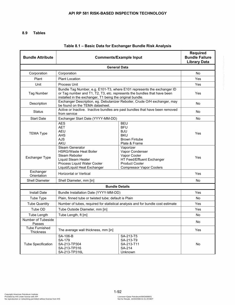
API RP 581 RISK-BASED INSPECTION TECHNOLOGY
8.9 Tables
Table 8.1 – Basic Data for Exchanger Bundle Risk Analysis
Bundle Attribute Comments/Example Input Required
Bundle Failure Library Data
General Data Corporation Corporation No
Plant Plant Location Yes Unit Process Unit Yes
Tag Number Bundle Tag Number, e.g. E101-T3, where E101 represents the exchanger ID or Tag number and T1, T2, T3, etc. represents the bundles that have been installed in the exchanger, T1 being the original bundle.
Yes
Description Exchanger Description, eg. Debutanizer Reboiler, Crude O/H exchanger, may be found on the TEMA datasheet. No
Status Active or Inactive. Inactive bundles are past bundles that have been removed from service No
Start Date Exchanger Start Date (YYYY-MM-DD) No
TEMA Type
AES AET AEU AHS AJS AKU
BEU BFU BJU BKU Brown Fintube Plate & Frame
Yes
Exchanger Type
Steam Generator HSRG/Waste Heat Boiler Steam Reboiler Liquid Steam Heater Process Liquid Water Cooler Liquid/Liquid Heat Exchanger
Vaporizer Vapor Condenser Vapor Cooler HT Feed/Effluent Exchanger Product Cooler Compressor Vapor Coolers
Yes
Exchanger Orientation Horizontal or Vertical Yes
Shell Diameter Shell Diameter, mm [in] No
Bundle Details
Install Date Bundle Installation Date (YYYY-MM-DD) Yes Tube Type Plain, finned tube or twisted tube; default is Plain No
Tube Quantity Number of tubes, required for statistical analysis and for bundle cost estimate Yes Tube OD Tube Outside Diameter, mm [in] Yes
Tube Length Tube Length, ft [m] No Number of Tubeside
Passes No
Tube Furnished Thickness The average wall thickness, mm [in] Yes
Tube Specification
SA-106-B SA-179 SA-213-TP304 SA-213-TP316 SA-213-TP316L
SA-213-T5 SA-213-T9 SA-213-T11 SA-214 Unknown
No
1-92 Copyright American Petroleum Institute Provided by IHS under license with API Licensee=Qatar Petroleum/5943408001
Not for Resale, 10/20/2008 01:51:29 MDTNo reproduction or networking permitted without license from IHS
--```,`,,`,`,,`,`,,,,,,``,```,`-`-`,,`,,`,`,,`---
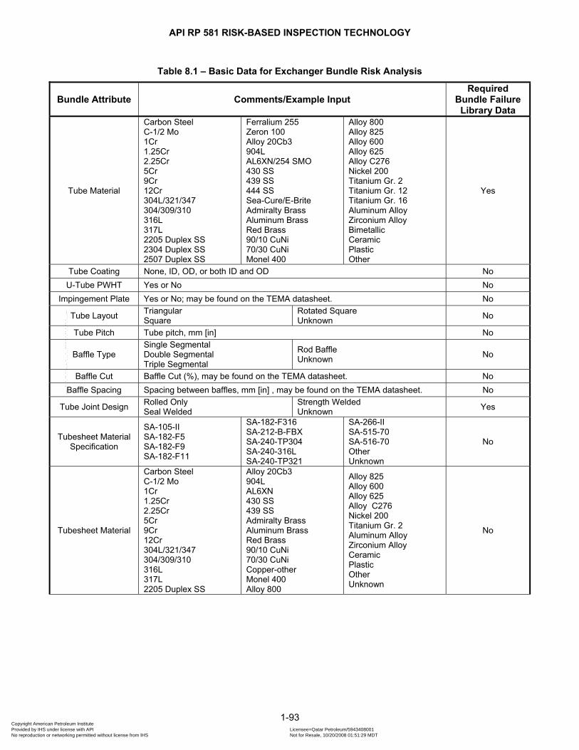
API RP 581 RISK-BASED INSPECTION TECHNOLOGY
Table 8.1 – Basic Data for Exchanger Bundle Risk Analysis
Bundle Attribute Comments/Example Input Required
Bundle Failure Library Data
Tube Material
Carbon Steel C-1/2 Mo 1Cr 1.25Cr 2.25Cr 5Cr 9Cr 12Cr 304L/321/347 304/309/310 316L 317L 2205 Duplex SS 2304 Duplex SS 2507 Duplex SS
Ferralium 255 Zeron 100 Alloy 20Cb3 904L AL6XN/254 SMO 430 SS 439 SS 444 SS Sea-Cure/E-Brite Admiralty Brass Aluminum Brass Red Brass 90/10 CuNi 70/30 CuNi Monel 400
Alloy 800 Alloy 825 Alloy 600 Alloy 625 Alloy C276 Nickel 200 Titanium Gr. 2 Titanium Gr. 12 Titanium Gr. 16 Aluminum Alloy Zirconium Alloy Bimetallic Ceramic Plastic Other
Yes
Tube Coating None, ID, OD, or both ID and OD No U-Tube PWHT Yes or No No
Impingement Plate Yes or No; may be found on the TEMA datasheet. No
Tube Layout Triangular Square
Rotated Square Unknown No
Tube Pitch Tube pitch, mm [in] No
Baffle Type Single Segmental Double Segmental Triple Segmental
Rod Baffle Unknown No
Baffle Cut Baffle Cut (%), may be found on the TEMA datasheet. No Baffle Spacing Spacing between baffles, mm [in] , may be found on the TEMA datasheet. No
Tube Joint Design Rolled Only Seal Welded
Strength Welded Unknown Yes
Tubesheet Material Specification
SA-105-II SA-182-F5 SA-182-F9 SA-182-F11
SA-182-F316 SA-212-B-FBX SA-240-TP304 SA-240-316L SA-240-TP321
SA-266-II SA-515-70 SA-516-70 Other Unknown
No
Tubesheet Material
Carbon Steel C-1/2 Mo 1Cr 1.25Cr 2.25Cr 5Cr 9Cr 12Cr 304L/321/347 304/309/310 316L 317L 2205 Duplex SS
Alloy 20Cb3 904L AL6XN 430 SS 439 SS Admiralty Brass Aluminum Brass Red Brass 90/10 CuNi 70/30 CuNi Copper-other Monel 400 Alloy 800
Alloy 825 Alloy 600 Alloy 625 Alloy C276 Nickel 200 Titanium Gr. 2 Aluminum Alloy Zirconium Alloy Ceramic Plastic Other Unknown
No
1-93 Copyright American Petroleum Institute Provided by IHS under license with API Licensee=Qatar Petroleum/5943408001
Not for Resale, 10/20/2008 01:51:29 MDTNo reproduction or networking permitted without license from IHS
--```,`,,`,`,,`,`,,,,,,``,```,`-`-`,,`,,`,`,,`---

API RP 581 RISK-BASED INSPECTION TECHNOLOGY
Table 8.1 – Basic Data for Exchanger Bundle Risk Analysis
Bundle Attribute Comments/Example Input Required
Bundle Failure Library Data
Tubesheet Cladding Material
Carbon Steel C-1/2 Mo 1Cr 1.25Cr 2.25Cr 5Cr 9Cr 12Cr 304L/321/347 304/309/310 316L 317L 2205 Duplex SS 2304 Duplex SS
2507 Duplex SS Alloy 20Cb3 904L AL6XN 430 SS 439 SS Sea-Cure/E-Brite Admiralty Brass Aluminum Brass Red Brass 90/10 CuNi 70/30 CuNi Copper-other Monel 400
Alloy 800 Alloy 825 Alloy 600 Alloy 625 Alloy C276 Nickel 200 Titanium Gr. 2 Titanium Gr. 12 Titanium Gr. 16 Aluminum Alloy Zirconium Alloy Non-metallic Coating Plastic Other Unknown
No
Process/Operating Conditions (Tubeside and Shellside)
Process Unit
Amine Regeneration Amine Treating Aromatics Recovery Catalytic Reforming (CCR) Catalytic Reforming (Fixed) Caustic Treating (Merox) Crude Distillation Unit Cumene Delayed Coker Distillate Fractionator Fluid Coker Dimersol Ether Plant (MTBE/TAME) Fluid Catalytic Cracking Sat Gas Plant Unsat Gas Plant Gas Separation HF Alkylation Hydrotreater/Hydrocracker
Hydrocracker (2nd Stage) Hydrogen Reforming Isomerization LPG Refrigeration Lube Plant Polymerization Partial Oxidation Selective Hydrogenation Sour Water Stripper Sulfolane Sulfur Recovery Unit Sulfuric Acid Alkylation Sulfuric Acid Plant Tail Gas Treater Thermal Cracking Vacuum Unit Cooling Tower Water Cooling Water – other
Yes
Fluid Name Generic Name, e.g. Crude, Effluent, HGO, etc. No
1-94 Copyright American Petroleum Institute Provided by IHS under license with API Licensee=Qatar Petroleum/5943408001
Not for Resale, 10/20/2008 01:51:29 MDTNo reproduction or networking permitted without license from IHS
--```,`,,`,`,,`,`,,,,,,``,```,`-`-`,,`,,`,`,,`---

API RP 581 RISK-BASED INSPECTION TECHNOLOGY
Table 8.1 – Basic Data for Exchanger Bundle Risk Analysis
Bundle Attribute Comments/Example Input Required
Bundle Failure Library Data
Fluid Category
Light Crude Feed Heavy Crude Feed Crude Tower O/H Hydrogen Fuel gas Ethylene Syngas LPG (C3/C4) Olefins Gasoline Ethers (MTBE/TAME) Alcohol Light Distillate Medium Distillate Heavy Distillate Atmospheric Resid. Lube oil (seal oil) Vacuum Residue Visbreaker Residue Sludge Rich Amine Lean Amine
Benfield or other acid gas treating Sour Water Tempered water/non-corrosive Steam/Condensate Caustic Solution Spent Caustic Acid Gas (Tail Gas) Sulfur Liquid H2S Hydrofluoric Acid Sulfuric Acid Phosphoric Acid Other Acid; Cooling Tower Water- corrosive Cooling Tower Water- non-corrosive River water Well water Brackish water Sea water Waste Water Inert Gas Air CO2
Yes
Operating Pressure Operating Pressure, kPa [psig] Yes
Inlet Temperature Inlet Temperature, oC [oF] Yes Outlet Temperature Outlet Temperature, oC [oF] Yes
Fluid Phase Gas, Liquid or Two-phase Yes
Fouling Severity Unknown None Mild
Moderate Severe Unknown
No
Flowrate Fluid Flowrate, kg/hr [lb/s] No
Design Velocity Enter the fluid design velocity from the TEMA datasheet, optional entry, consider entering for CW, amine, slurries or any other fluids where velocity is an important parameter for corrosion or erosion.
No
Process Fluid Damage Modifiers (Tubeside and Shellside)
Free Water Does the tubeside or shellside fluid have any free water, Yes/No Yes Sulfidation Is sulfidation a concern for the tubeside or shellside fluid, Yes/No Yes Dealloying Is dealloying is a concern for the tubeside or shellside fluid, Yes/No Yes
Naphthenic Acid Is naphthenic acid corrosion a concern for the tubeside or shellside fluid, Yes/No Yes
Ammonium Chloride Is ammonium chloride a concern for the tubeside or shellside fluid, Yes/No Yes CO2 Is CO2 corrosion a concern for the tubeside or shellside fluid, Yes/No Yes
Salt Deposits Are salt deposits likely on the tubeside or shellside, Yes/No Yes Weight % H2S If H2S is present in tubeside or shellside fluid, provide amount, (wt.%). Yes Mole % Sulfur If Sulfur is present in tubeside or shellside fluid, provide amount, (mole %). Yes Weight % Acid If Acid is present in tubeside or shellside fluid, provide amount, (wt.%). Yes
Weight % Caustic If Caustic is present in tubeside or shellside fluid, provide amount, (wt.%). Yes Weight %
Ammonium Bisulfide If Ammonium Bisulfide is present in tubeside or shellside fluid, provide amount, (mole %) Yes
Cyanides Are cyanides present in tubeside or shellside fluid, Yes/No Yes
1-95 Copyright American Petroleum Institute Provided by IHS under license with API Licensee=Qatar Petroleum/5943408001
Not for Resale, 10/20/2008 01:51:29 MDTNo reproduction or networking permitted without license from IHS
--```,`,,`,`,,`,`,,,,,,``,```,`-`-`,,`,,`,`,,`---
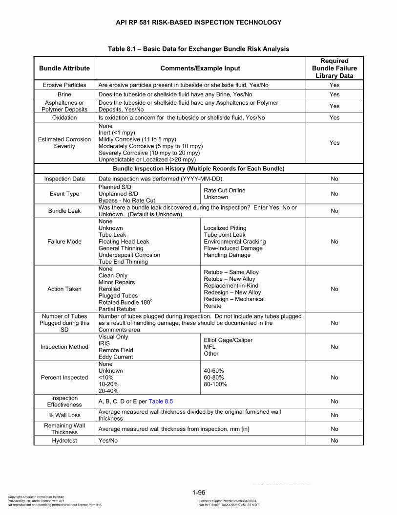
API RP 581 RISK-BASED INSPECTION TECHNOLOGY
Table 8.1 – Basic Data for Exchanger Bundle Risk Analysis
Bundle Attribute Comments/Example Input Required
Bundle Failure Library Data
Erosive Particles Are erosive particles present in tubeside or shellside fluid, Yes/No Yes Brine Does the tubeside or shellside fluid have any Brine, Yes/No Yes
Asphaltenes or Polymer Deposits
Does the tubeside or shellside fluid have any Asphaltenes or Polymer Deposits, Yes/No Yes
Oxidation Is oxidation a concern for the tubeside or shellside fluid, Yes/No Yes
Estimated Corrosion Severity
None Inert (<1 mpy) Mildly Corrosive (11 to 5 mpy) Moderately Corrosive (5 mpy to 10 mpy) Severely Corrosive (10 mpy to 20 mpy) Unpredictable or Localized (>20 mpy)
Yes
Bundle Inspection History (Multiple Records for Each Bundle)
Inspection Date Date inspection was performed (YYYY-MM-DD). No
Event Type Planned S/D Unplanned S/D Bypass - No Rate Cut
Rate Cut Online Unknown No
Bundle Leak Was there a bundle leak discovered during the inspection? Enter Yes, No or Unknown. (Default is Unknown) No
Failure Mode
None Unknown Tube Leak Floating Head Leak General Thinning Underdeposit Corrosion Tube End Thinning
Localized Pitting Tube Joint Leak Environmental Cracking Flow-Induced Damage Handling Damage
No
Action Taken
None Clean Only Minor Repairs Rerolled Plugged Tubes Rotated Bundle 180o
Partial Retube
Retube – Same Alloy Retube – New Alloy Replacement-in-Kind Redesign – New Alloy Redesign – Mechanical Rerate
No
Number of Tubes Plugged during this
SD
Number of tubes plugged during inspection. Do not include any tubes plugged as a result of handling damage, these should be documented in the Comments area
No
Inspection Method
Visual Only IRIS Remote Field Eddy Current
Elliot Gage/Caliper MFL Other
No
Percent Inspected
None Unknown <10% 10-20% 20-40%
40-60% 60-80% 80-100%
No
Inspection Effectiveness A, B, C, D or E per Table 8.5 No
% Wall Loss Average measured wall thickness divided by the original furnished wall thickness No
Remaining Wall Thickness Average measured wall thickness from inspection, mm [in] No
Hydrotest Yes/No No
1-96 Copyright American Petroleum Institute Provided by IHS under license with API Licensee=Qatar Petroleum/5943408001
Not for Resale, 10/20/2008 01:51:29 MDTNo reproduction or networking permitted without license from IHS
--```,`,,`,`,,`,`,,,,,,``,```,`-`-`,,`,,`,`,,`---
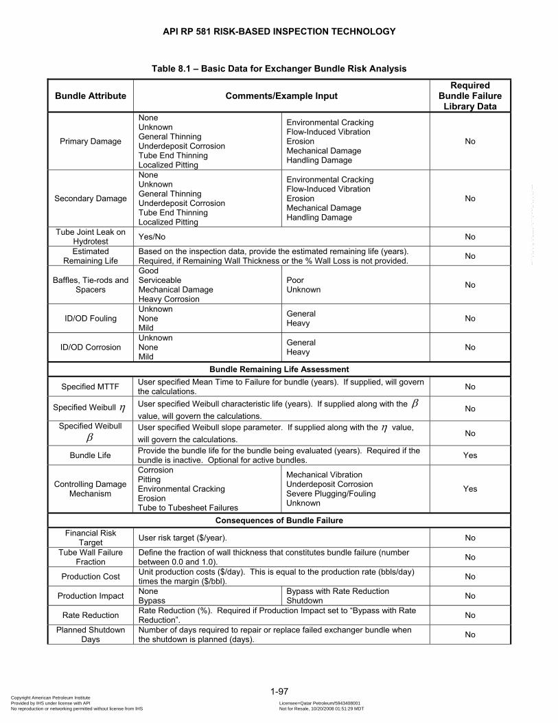
API RP 581 RISK-BASED INSPECTION TECHNOLOGY
Table 8.1 – Basic Data for Exchanger Bundle Risk Analysis
Bundle Attribute Comments/Example Input Required
Bundle Failure Library Data
Primary Damage
None Unknown General Thinning Underdeposit Corrosion Tube End Thinning Localized Pitting
Environmental Cracking Flow-Induced Vibration Erosion Mechanical Damage Handling Damage
No
Secondary Damage
None Unknown General Thinning Underdeposit Corrosion Tube End Thinning Localized Pitting
Environmental Cracking Flow-Induced Vibration Erosion Mechanical Damage Handling Damage
No
Tube Joint Leak on Hydrotest Yes/No No
Estimated Remaining Life
Based on the inspection data, provide the estimated remaining life (years). Required, if Remaining Wall Thickness or the % Wall Loss is not provided. No
Baffles, Tie-rods and Spacers
Good Serviceable Mechanical Damage Heavy Corrosion
Poor Unknown No
ID/OD Fouling Unknown None Mild
General Heavy No
ID/OD Corrosion Unknown None Mild
General Heavy No
Bundle Remaining Life Assessment
Specified MTTF User specified Mean Time to Failure for bundle (years). If supplied, will govern the calculations. No
Specified Weibull η User specified Weibull characteristic life (years). If supplied along with the β value, will govern the calculations.
No
Specified Weibull β
User specified Weibull slope parameter. If supplied along with the η value, will govern the calculations.
No
Bundle Life Provide the bundle life for the bundle being evaluated (years). Required if the bundle is inactive. Optional for active bundles. Yes
Controlling Damage Mechanism
Corrosion Pitting Environmental Cracking Erosion Tube to Tubesheet Failures
Mechanical Vibration Underdeposit Corrosion Severe Plugging/Fouling Unknown
Yes
Consequences of Bundle Failure Financial Risk
Target User risk target ($/year). No
Tube Wall Failure Fraction
Define the fraction of wall thickness that constitutes bundle failure (number between 0.0 and 1.0). No
Production Cost Unit production costs ($/day). This is equal to the production rate (bbls/day) times the margin ($/bbl). No
Production Impact None Bypass
Bypass with Rate Reduction Shutdown No
Rate Reduction Rate Reduction (%). Required if Production Impact set to “Bypass with Rate Reduction”. No
Planned Shutdown Days
Number of days required to repair or replace failed exchanger bundle when the shutdown is planned (days). No
1-97 Copyright American Petroleum Institute Provided by IHS under license with API Licensee=Qatar Petroleum/5943408001
Not for Resale, 10/20/2008 01:51:29 MDTNo reproduction or networking permitted without license from IHS
--```,`,,`,`,,`,`,,,,,,``,```,`-`-`,,`,,`,`,,`---
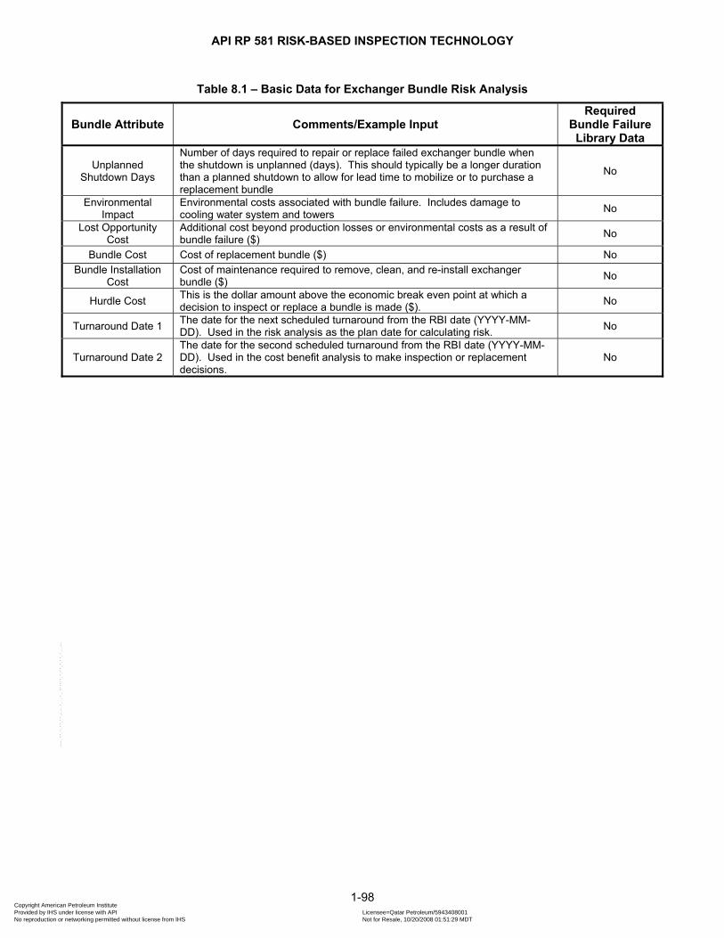
API RP 581 RISK-BASED INSPECTION TECHNOLOGY
Table 8.1 – Basic Data for Exchanger Bundle Risk Analysis
Bundle Attribute Comments/Example Input Required
Bundle Failure Library Data
Unplanned Shutdown Days
Number of days required to repair or replace failed exchanger bundle when the shutdown is unplanned (days). This should typically be a longer duration than a planned shutdown to allow for lead time to mobilize or to purchase a replacement bundle
No
Environmental Impact
Environmental costs associated with bundle failure. Includes damage to cooling water system and towers No
Lost Opportunity Cost
Additional cost beyond production losses or environmental costs as a result of bundle failure ($) No
Bundle Cost Cost of replacement bundle ($) No Bundle Installation
Cost Cost of maintenance required to remove, clean, and re-install exchanger bundle ($) No
Hurdle Cost This is the dollar amount above the economic break even point at which a decision to inspect or replace a bundle is made ($). No
Turnaround Date 1 The date for the next scheduled turnaround from the RBI date (YYYY-MM-DD). Used in the risk analysis as the plan date for calculating risk. No
Turnaround Date 2 The date for the second scheduled turnaround from the RBI date (YYYY-MM-DD). Used in the cost benefit analysis to make inspection or replacement decisions.
No
1-98 Copyright American Petroleum Institute Provided by IHS under license with API Licensee=Qatar Petroleum/5943408001
Not for Resale, 10/20/2008 01:51:29 MDTNo reproduction or networking permitted without license from IHS
--```,`,,`,`,,`,`,,,,,,``,```,`-`-`,,`,,`,`,,`---
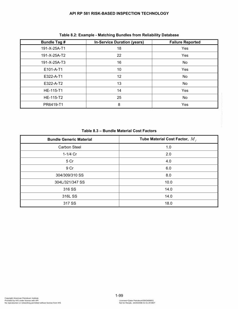
API RP 581 RISK-BASED INSPECTION TECHNOLOGY
Table 8.2: Example - Matching Bundles from Reliability Database
Bundle Tag # In-Service Duration (years) Failure Reported 191-X-25A-T1 18 Yes
191-X-25A-T2 22 Yes
191-X-25A-T3 16 No
E101-A-T1 10 Yes
E322-A-T1 12 No
E322-A-T2 13 No
HE-115-T1 14 Yes
HE-115-T2 25 No
PR6419-T1 8 Yes
Table 8.3 – Bundle Material Cost Factors
Bundle Generic Material Tube Material Cost Factor, fM
Carbon Steel 1.0
1-1/4 Cr 2.0
5 Cr 4.0
9 Cr 6.0
304/309/310 SS 8.0
304L/321/347 SS 10.0
316 SS 14.0
316L SS 14.0
317 SS 18.0
1-99 Copyright American Petroleum Institute Provided by IHS under license with API Licensee=Qatar Petroleum/5943408001
Not for Resale, 10/20/2008 01:51:29 MDTNo reproduction or networking permitted without license from IHS
--```,`,,`,`,,`,`,,,,,,``,```,`-`-`,,`,,`,`,,`---
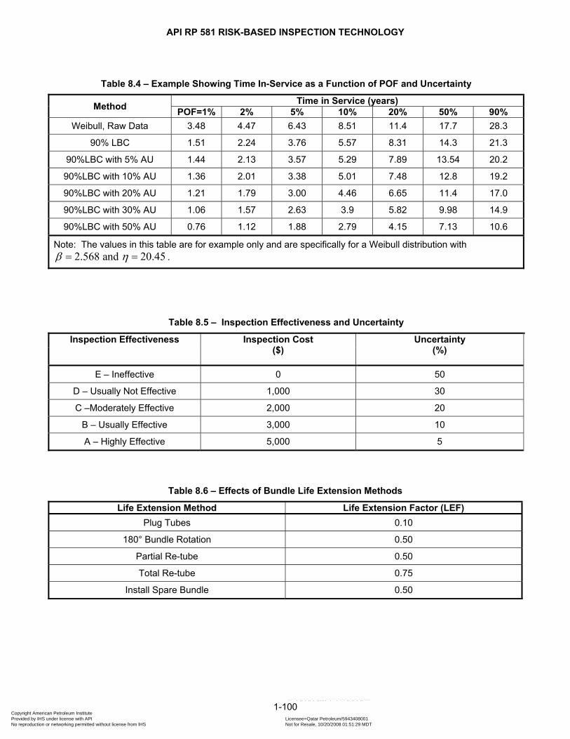
API RP 581 RISK-BASED INSPECTION TECHNOLOGY
Table 8.4 – Example Showing Time In-Service as a Function of POF and Uncertainty
Method Time in Service (years) POF=1% 2% 5% 10% 20% 50% 90%
Weibull, Raw Data 3.48 4.47 6.43 8.51 11.4 17.7 28.3
90% LBC 1.51 2.24 3.76 5.57 8.31 14.3 21.3
90%LBC with 5% AU 1.44 2.13 3.57 5.29 7.89 13.54 20.2
90%LBC with 10% AU 1.36 2.01 3.38 5.01 7.48 12.8 19.2
90%LBC with 20% AU 1.21 1.79 3.00 4.46 6.65 11.4 17.0
90%LBC with 30% AU 1.06 1.57 2.63 3.9 5.82 9.98 14.9
90%LBC with 50% AU 0.76 1.12 1.88 2.79 4.15 7.13 10.6
Note: The values in this table are for example only and are specifically for a Weibull distribution with 2.568 and 20.45β η= = .
Table 8.5 – Inspection Effectiveness and Uncertainty
Inspection Effectiveness Inspection Cost ($)
Uncertainty (%)
E – Ineffective 0 50
D – Usually Not Effective 1,000 30
C –Moderately Effective 2,000 20
B – Usually Effective 3,000 10
A – Highly Effective 5,000 5
Table 8.6 – Effects of Bundle Life Extension Methods
Life Extension Method Life Extension Factor (LEF) Plug Tubes 0.10
180° Bundle Rotation 0.50
Partial Re-tube 0.50
Total Re-tube 0.75
Install Spare Bundle 0.50
1-100 Copyright American Petroleum Institute Provided by IHS under license with API Licensee=Qatar Petroleum/5943408001
Not for Resale, 10/20/2008 01:51:29 MDTNo reproduction or networking permitted without license from IHS
--```,`,,`,`,,`,`,,,,,,``,```,`-`-`,,`,,`,`,,`---

API RP 581 RISK-BASED INSPECTION TECHNOLOGY
Table 8.7 – Numerical Values Associated with Probability and Area-Based Consequence Categories in API RBI for Heat Exchanger Bundles
Probability Category (1) Consequence Category (2) Category Range Category Range ($)
1 0.1POF ≤ A $10,000COF ≤
2 0.1 0.2POF< ≤ B $10,000 $50,000COF< ≤
3 0.2 0.3POF< ≤ C $50,000 $150,000COF< ≤
4 0.3 0.5POF< ≤ D $150,000 $1,000,000COF< ≤
5 0.5 1.0POF< ≤ E $1,000,000COF >
Notes: 1. In terms of the total damage factor, see Part 2, paragraph 2.3. 2. In terms of consequence area, see Part 3, paragraph 5.11.4.
1-101 Copyright American Petroleum Institute Provided by IHS under license with API Licensee=Qatar Petroleum/5943408001
Not for Resale, 10/20/2008 01:51:29 MDTNo reproduction or networking permitted without license from IHS
--```,`,,`,`,,`,`,,,,,,``,```,`-`-`,,`,,`,`,,`---

API RP 581 RISK-BASED INSPECTION TECHNOLOGY
8.10 Figures
Figure 8.1 – Flow Chart of Bundle Calculation Approach
1-102 Copyright American Petroleum Institute Provided by IHS under license with API Licensee=Qatar Petroleum/5943408001
Not for Resale, 10/20/2008 01:51:29 MDTNo reproduction or networking permitted without license from IHS
--```,`,,`,`,,`,`,,,,,,``,```,`-`-`,,`,,`,`,,`---

API RP 581 RISK-BASED INSPECTION TECHNOLOGY
Figure 8.2 – Weibull Plot of Similar Bundle Data
1-103 Copyright American Petroleum Institute Provided by IHS under license with API Licensee=Qatar Petroleum/5943408001
Not for Resale, 10/20/2008 01:51:29 MDTNo reproduction or networking permitted without license from IHS
--```,`,,`,`,,`,`,,,,,,``,```,`-`-`,,`,,`,`,,`---
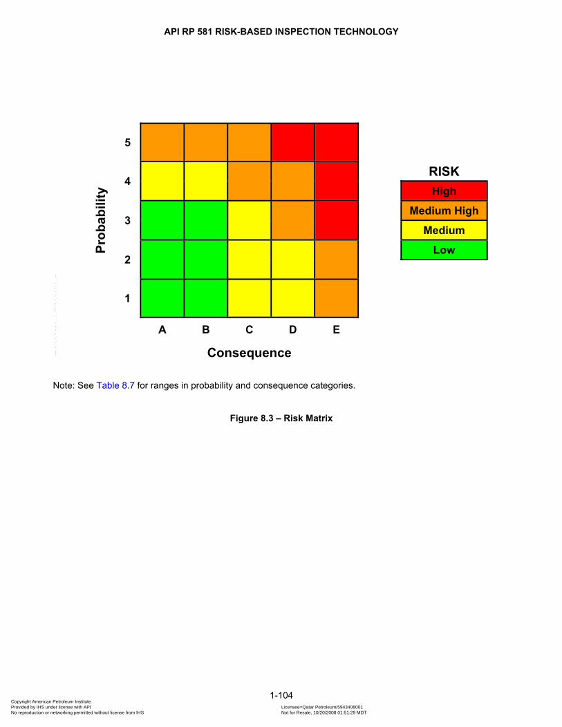
API RP 581 RISK-BASED INSPECTION TECHNOLOGY
Pr
obab
ility
5
4 RISK High
3 Medium High
Medium
2 Low
1
A B C D E
Consequence
Note: See Table 8.7 for ranges in probability and consequence categories.
Figure 8.3 – Risk Matrix
1-104 Copyright American Petroleum Institute Provided by IHS under license with API Licensee=Qatar Petroleum/5943408001
Not for Resale, 10/20/2008 01:51:29 MDTNo reproduction or networking permitted without license from IHS
--```,`,,`,`,,`,`,,,,,,``,```,`-`-`,,`,,`,`,,`---

API RP 581 RISK-BASED INSPECTION TECHNOLOGY
Figure 8.4 – Weibull Plot of Similar Bundle Data with 50% Additional Uncertainty
1-105 Copyright American Petroleum Institute Provided by IHS under license with API Licensee=Qatar Petroleum/5943408001
Not for Resale, 10/20/2008 01:51:29 MDTNo reproduction or networking permitted without license from IHS
--```,`,,`,`,,`,`,,,,,,``,```,`-`-`,,`,,`,`,,`---

API RP 581 RISK-BASED INSPECTION TECHNOLOGY
Figure 8.5 – Weibull Plot Shifted for Inspection
1-106 Copyright American Petroleum Institute Provided by IHS under license with API Licensee=Qatar Petroleum/5943408001
Not for Resale, 10/20/2008 01:51:29 MDTNo reproduction or networking permitted without license from IHS
--```,`,,`,`,,`,`,,,,,,``,```,`-`-`,,`,,`,`,,`---

API RP 581 RISK-BASED INSPECTION TECHNOLOGY
0
10
20
30
40
50
60
70
80
90
100
1992 1994 1996 1998 2000 2002 2004 2006 2008 2010 2012 2014
Years in Service
Prob
abili
ty o
f Fai
lure
Original curve with 50% UncertaintyModified, 2000 Inspection, 30% UncertaintyModified, 2003 Inspection, 30% Uncertainty
RBI Date, 6/2006
1st T/A, 3/2008
2nd T/A, 3/2012
Prior to Inspection
2000 Inspection
2003 Inspection
Target POF Line
Figure 8.6 – Example Problem Showing Effect of Inspection
1-107 Copyright American Petroleum Institute Provided by IHS under license with API Licensee=Qatar Petroleum/5943408001
Not for Resale, 10/20/2008 01:51:29 MDTNo reproduction or networking permitted without license from IHS
--```,`,,`,`,,`,`,,,,,,``,```,`-`-`,,`,,`,`,,`---
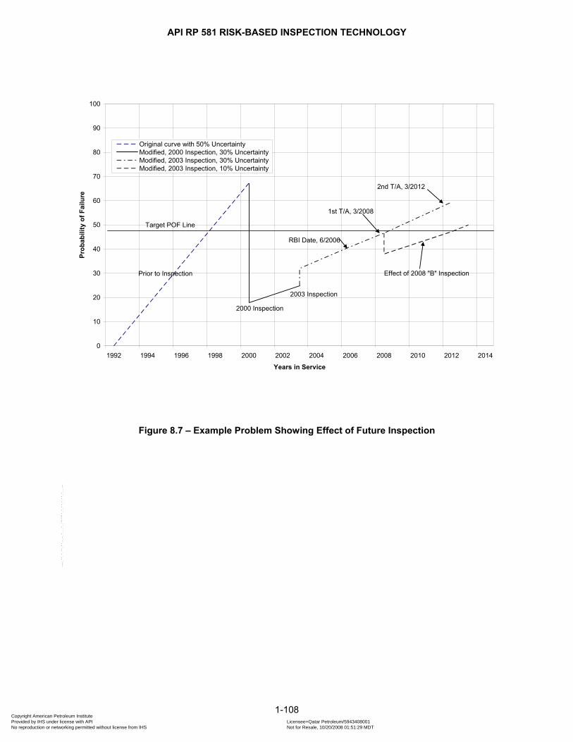
API RP 581 RISK-BASED INSPECTION TECHNOLOGY
1-108
0
10
20
30
40
50
60
70
80
90
100
1992 1994 1996 1998 2000 2002 2004 2006 2008 2010 2012 2014
Years in Service
Prob
abili
ty o
f Fai
lure
Original curve with 50% UncertaintyModified, 2000 Inspection, 30% UncertaintyModified, 2003 Inspection, 30% UncertaintyModified, 2003 Inspection, 10% Uncertainty
RBI Date, 6/2006
1st T/A, 3/2008
2nd T/A, 3/2012
Prior to Inspection
2000 Inspection
2003 Inspection
Effect of 2008 "B" Inspection
Target POF Line
Figure 8.7 – Example Problem Showing Effect of Future Inspection
Copyright American Petroleum Institute Provided by IHS under license with API Licensee=Qatar Petroleum/5943408001
Not for Resale, 10/20/2008 01:51:29 MDTNo reproduction or networking permitted without license from IHS
--```,`,,`,`,,`,`,,,,,,``,```,`-`-`,,`,,`,`,,`---

API RP 581 RISK-BASED INSPECTION TECHNOLOGY
PART 2
DETERMINATION OF PROBABILITY OF FAILURE IN AN API RBI ASSESSMENT
2-1 Copyright American Petroleum Institute Provided by IHS under license with API Licensee=Qatar Petroleum/5943408001
Not for Resale, 10/20/2008 01:51:29 MDTNo reproduction or networking permitted without license from IHS
--```,`,,`,`,,`,`,,,,,,``,```,`-`-`,,`,,`,`,,`---
API RP 581 RISK-BASED INSPECTION TECHNOLOGY
PART CONTENTS 1 SCOPE ........................................................................................................................................ 2-8 2 REFERENCES ............................................................................................................................ 2-8 3 DEFINTIONS ............................................................................................................................... 2-9 4 PROBABILITY OF FAILURE CALCULATIONS ........................................................................ 2-9
4.1 Overview ............................................................................................................................. 2-9 4.2 Calculation of Probability of Failure ................................................................................ 2-9 4.3 Generic Failure Frequency ............................................................................................. 2-10 4.4 Damage Factor ................................................................................................................. 2-10
4.4.1 Overview ................................................................................................................... 2-10 4.4.2 Damage Factor Combination for Multiple Damage Mechanisms ....................... 2-11 4.4.3 Inspection Effectiveness Category ........................................................................ 2-12
4.5 Management Systems Factor ......................................................................................... 2-12 4.5.1 General ...................................................................................................................... 2-12 4.5.2 Overview ................................................................................................................... 2-12 4.5.3 Auditing Technique ................................................................................................. 2-13 4.5.4 Calculation of the Management Systems Factor .................................................. 2-13
4.6 Nomenclature ................................................................................................................... 2-14 4.7 Tables................................................................................................................................ 2-16
5 THINNING DAMAGE FACTOR ................................................................................................ 2-20 5.1 Scope ................................................................................................................................ 2-20 5.2 Screening Criteria ............................................................................................................ 2-20 5.3 Required Data .................................................................................................................. 2-20 5.4 Basic Assumptions ......................................................................................................... 2-20 5.5 Determination of the Damage Factor ............................................................................. 2-20
5.5.1 Overview ................................................................................................................... 2-20 5.5.2 Inspection Effectiveness ......................................................................................... 2-20 5.5.3 Calculation of the Damage Factor .......................................................................... 2-21
5.6 Nomenclature ................................................................................................................... 2-23 5.7 Tables................................................................................................................................ 2-24 5.8 Figures .............................................................................................................................. 2-37
6 COMPONENT LINING DAMAGE FACTOR ............................................................................. 2-38 6.1 Scope ................................................................................................................................ 2-38 6.2 Screening Criteria ............................................................................................................ 2-38 6.3 Required Data .................................................................................................................. 2-38 6.4 Basic Assumptions ......................................................................................................... 2-38 6.5 Determination of the Damage Factor ............................................................................. 2-38
6.5.1 Overview ................................................................................................................... 2-38 6.5.2 Calculation of the Damage Factor .......................................................................... 2-38
6.6 Nomenclature ................................................................................................................... 2-39 6.7 Tables................................................................................................................................ 2-40 6.8 Figures .............................................................................................................................. 2-45
7 SCC DAMAGE FACTOR – CAUSTIC CRACKING ................................................................. 2-46 7.1 Scope ................................................................................................................................ 2-46 7.2 Description of Damage .................................................................................................... 2-46 7.3 Screening Criteria ............................................................................................................ 2-46 7.4 Required Data .................................................................................................................. 2-46 7.5 Basic Assumptions ......................................................................................................... 2-46 7.6 Determination of the Damage Factor ............................................................................. 2-47
7.6.1 Overview ................................................................................................................... 2-47 7.6.2 Inspection Effectiveness ......................................................................................... 2-47 7.6.3 Calculation of the Damage Factor .......................................................................... 2-47
7.7 Nomenclature ................................................................................................................... 2-48 7.8 References ....................................................................................................................... 2-48 7.9 Tables................................................................................................................................ 2-49 7.10 Figures .............................................................................................................................. 2-52
2-2 Copyright American Petroleum Institute Provided by IHS under license with API Licensee=Qatar Petroleum/5943408001
Not for Resale, 10/20/2008 01:51:29 MDTNo reproduction or networking permitted without license from IHS
--```,`,,`,`,,`,`,,,,,,``,```,`-`-`,,`,,`,`,,`---
API RP 581 RISK-BASED INSPECTION TECHNOLOGY
8 SCC DAMAGE FACTOR – AMINE CRACKING ...................................................................... 2-55 8.1 Scope ................................................................................................................................ 2-55 8.2 Description of Damage .................................................................................................... 2-55 8.3 Screening Criteria ............................................................................................................ 2-55 8.4 Required Data .................................................................................................................. 2-56 8.5 Basic Assumptions ......................................................................................................... 2-56 8.6 Determination of the Damage Factor ............................................................................. 2-56
8.6.1 Overview ................................................................................................................... 2-56 8.6.2 Inspection Effectiveness ......................................................................................... 2-56 8.6.3 Calculation of the Damage Factor .......................................................................... 2-56
8.7 Nomenclature ................................................................................................................... 2-57 8.8 References ....................................................................................................................... 2-57 8.9 Tables................................................................................................................................ 2-58 8.10 Figures .............................................................................................................................. 2-60
9 SCC DAMAGE FACTOR – SULFIDE STRESS CRACKING .................................................. 2-61 9.1 Scope ................................................................................................................................ 2-61 9.2 Description of Damage .................................................................................................... 2-61 9.3 Screening Criteria ............................................................................................................ 2-61 9.4 Required Data .................................................................................................................. 2-61 9.5 Basic Assumptions ......................................................................................................... 2-61 9.6 Determination of the Damage Factor ............................................................................. 2-62
9.6.1 Overview ................................................................................................................... 2-62 9.6.2 Inspection Effectiveness ......................................................................................... 2-62 9.6.3 Calculation of the Damage Factor .......................................................................... 2-62
9.7 Nomenclature ................................................................................................................... 2-63 9.8 References ....................................................................................................................... 2-63 9.9 Tables................................................................................................................................ 2-64 9.10 Figures .............................................................................................................................. 2-67
10 SCC DAMAGE FACTOR – HIC/SOHIC-H2S ............................................................................ 2-68 10.1 Scope ................................................................................................................................ 2-68 10.2 Description of Damage .................................................................................................... 2-68 10.3 Screening Criteria ............................................................................................................ 2-69 10.4 Required Data .................................................................................................................. 2-69 10.5 Basic Assumptions ......................................................................................................... 2-69 10.6 Determination of the Damage Factor ............................................................................. 2-69
10.6.1 Overview ................................................................................................................... 2-69 10.6.2 Inspection Effectiveness ......................................................................................... 2-69 10.6.3 Calculation of the Damage Factor .......................................................................... 2-69
10.7 Nomenclature ................................................................................................................... 2-70 10.8 References ....................................................................................................................... 2-70 10.9 Tables................................................................................................................................ 2-71 10.10 Figures .............................................................................................................................. 2-74
11 SCC DAMAGE FACTOR – CARBONATE CRACKING .......................................................... 2-75 11.1 Scope ................................................................................................................................ 2-75 11.2 Description of Damage .................................................................................................... 2-75 11.3 Screening Criteria ............................................................................................................ 2-75 11.4 Required Data .................................................................................................................. 2-75 11.5 Basic Assumptions ......................................................................................................... 2-76 11.6 Determination of the Damage Factor ............................................................................. 2-76
11.6.1 Overview ................................................................................................................... 2-76 11.6.2 Inspection Effectiveness ......................................................................................... 2-76 11.6.3 Calculation of the Damage Factor .......................................................................... 2-76
11.7 Nomenclature ................................................................................................................... 2-77 11.8 References ....................................................................................................................... 2-77 11.9 Tables................................................................................................................................ 2-78 11.10 Figures .............................................................................................................................. 2-80
2-3 Copyright American Petroleum Institute Provided by IHS under license with API Licensee=Qatar Petroleum/5943408001
Not for Resale, 10/20/2008 01:51:29 MDTNo reproduction or networking permitted without license from IHS
--```,`,,`,`,,`,`,,,,,,``,```,`-`-`,,`,,`,`,,`---
API RP 581 RISK-BASED INSPECTION TECHNOLOGY
12 SCC DAMAGE FACTOR – PTA CRACKING .......................................................................... 2-81 12.1 Scope ................................................................................................................................ 2-81 12.2 Description of Damage .................................................................................................... 2-81 12.3 Screening Criteria ............................................................................................................ 2-81 12.4 Required Data .................................................................................................................. 2-81 12.5 Basic Assumptions ......................................................................................................... 2-81 12.6 Determination of the Damage Factor ............................................................................. 2-82
12.6.1 Overview ................................................................................................................... 2-82 12.6.2 Inspection Effectiveness ......................................................................................... 2-82 12.6.3 Calculation of the Damage Factor .......................................................................... 2-82
12.7 Nomenclature ................................................................................................................... 2-82 12.8 References ....................................................................................................................... 2-83 12.9 Tables................................................................................................................................ 2-84 12.10 Figures .............................................................................................................................. 2-87
13 SCC DAMAGE FACTOR – CLSCC ......................................................................................... 2-88 13.1 Scope ................................................................................................................................ 2-88 13.2 Description of Damage .................................................................................................... 2-88 13.3 Screening Criteria ............................................................................................................ 2-88 13.4 Required Data .................................................................................................................. 2-88 13.5 Basic Assumptions ......................................................................................................... 2-89 13.6 Determination of the Damage Factor ............................................................................. 2-89
13.6.1 Overview ................................................................................................................... 2-89 13.6.2 Inspection Effectiveness ......................................................................................... 2-89 13.6.3 Calculation of the Damage Factor .......................................................................... 2-89
13.7 Nomenclature ................................................................................................................... 2-90 13.8 References ....................................................................................................................... 2-90 13.9 Tables................................................................................................................................ 2-91 13.10 Figures .............................................................................................................................. 2-94
14 SCC DAMAGE FACTOR – HSC-HF ........................................................................................ 2-95 14.1 Scope ................................................................................................................................ 2-95 14.2 Description of Damage .................................................................................................... 2-95 14.3 Screening Criteria ............................................................................................................ 2-95 14.4 Required Data .................................................................................................................. 2-95 14.5 Basic Assumptions ......................................................................................................... 2-95 14.6 Determination of the Damage Factor ............................................................................. 2-96
14.6.1 Overview ................................................................................................................... 2-96 14.6.2 Inspection Effectiveness ......................................................................................... 2-96 14.6.3 Calculation of the Damage Factor .......................................................................... 2-96
14.7 Nomenclature ................................................................................................................... 2-97 14.8 References ....................................................................................................................... 2-97 14.9 Tables................................................................................................................................ 2-98 14.10 Figures ............................................................................................................................ 2-100
15 SCC DAMAGE FACTOR – HIC/SOHIC-HF ........................................................................... 2-101
15.1 Scope .............................................................................................................................. 2-101 15.2 Description of Damage .................................................................................................. 2-101 15.3 Screening Criteria .......................................................................................................... 2-101 15.4 Required Data ................................................................................................................ 2-101 15.5 Basic Assumptions ....................................................................................................... 2-101 15.6 Determination of the Damage Factor ........................................................................... 2-102
15.6.1 Overview ................................................................................................................. 2-102 15.6.2 Inspection Effectiveness ....................................................................................... 2-102 15.6.3 Calculation of the Damage Factor ........................................................................ 2-102
2-4 Copyright American Petroleum Institute Provided by IHS under license with API Licensee=Qatar Petroleum/5943408001
Not for Resale, 10/20/2008 01:51:29 MDTNo reproduction or networking permitted without license from IHS
--```,`,,`,`,,`,`,,,,,,``,```,`-`-`,,`,,`,`,,`---

API RP 581 RISK-BASED INSPECTION TECHNOLOGY
15.7 Nomenclature ................................................................................................................. 2-103 15.8 References ..................................................................................................................... 2-103 15.9 Tables.............................................................................................................................. 2-104 15.10 Figures ............................................................................................................................ 2-107
16 EXTERNAL CORROSION DAMAGE FACTOR – FERRITIC COMPONENT ....................... 2-108 16.1 Scope .............................................................................................................................. 2-108 16.2 Description of Damage .................................................................................................. 2-108 16.3 Screening Criteria .......................................................................................................... 2-108 16.4 Required Data ................................................................................................................ 2-108 16.5 Basic Assumption ......................................................................................................... 2-108 16.6 Determination of the Damage Factor ........................................................................... 2-108
16.6.1 Overview ................................................................................................................. 2-108 16.6.2 Inspection Effectiveness ....................................................................................... 2-108 16.6.3 Calculation of the Damage Factor ........................................................................ 2-109
16.7 Nomenclature ................................................................................................................. 2-110 16.8 Tables.............................................................................................................................. 2-111 16.9 Figures ............................................................................................................................ 2-113
17 CUI DAMAGE FACTOR – FERRITIC COMPONENT ............................................................ 2-114 17.1 Scope .............................................................................................................................. 2-114 17.2 Description of Damage .................................................................................................. 2-114 17.3 Screening Criteria .......................................................................................................... 2-114 17.4 Required Data ................................................................................................................ 2-115 17.5 Basic Assumption ......................................................................................................... 2-115 17.6 Determination of the Damage Factor ........................................................................... 2-115
17.6.1 Overview ................................................................................................................. 2-115 17.6.2 Inspection Effectiveness ....................................................................................... 2-115 17.6.3 Calculation of the Damage Factor ........................................................................ 2-115
17.7 Nomenclature ................................................................................................................. 2-117 17.8 Tables.............................................................................................................................. 2-118 17.9 Figures ............................................................................................................................ 2-124
18 EXTERNAL CLSCC DAMAGE FACTOR – AUSTENITIC COMPONENT ............................ 2-125 18.1 Scope .............................................................................................................................. 2-125 18.2 Description of Damage .................................................................................................. 2-125 18.3 Screening Criteria .......................................................................................................... 2-125 18.4 Required Data ................................................................................................................ 2-125 18.5 Basic Assumption ......................................................................................................... 2-125 18.6 Determination of the Damage Factor ........................................................................... 2-125
18.6.1 Overview ................................................................................................................. 2-125 18.6.2 Inspection Effectiveness ....................................................................................... 2-125 18.6.3 Calculation of the Damage Factor ........................................................................ 2-126
18.7 Nomenclature ................................................................................................................. 2-126 18.8 Tables.............................................................................................................................. 2-127 18.9 Figures ............................................................................................................................ 2-129
19 EXTERNAL CUI CLSCC DAMAGE FACTOR – AUSTENITIC COMPONENT ..................... 2-130 19.1 Scope .............................................................................................................................. 2-130 19.2 Description of Damage .................................................................................................. 2-130 19.3 Screening Criteria .......................................................................................................... 2-130 19.4 Required Data ................................................................................................................ 2-130 19.5 Basic Assumption ......................................................................................................... 2-130 19.6 Determination of the Damage Factor ........................................................................... 2-130
19.6.1 Overview ................................................................................................................. 2-130 19.6.2 Inspection Effectiveness ....................................................................................... 2-131 19.6.3 Calculation of the Damage Factor ........................................................................ 2-131
19.7 Nomenclature ................................................................................................................. 2-132 19.8 Tables.............................................................................................................................. 2-133 19.9 Figures ............................................................................................................................ 2-136
2-5 Copyright American Petroleum Institute Provided by IHS under license with API Licensee=Qatar Petroleum/5943408001
Not for Resale, 10/20/2008 01:51:29 MDTNo reproduction or networking permitted without license from IHS
--```,`,,`,`,,`,`,,,,,,``,```,`-`-`,,`,,`,`,,`---

API RP 581 RISK-BASED INSPECTION TECHNOLOGY
20 HTHA DAMAGE FACTOR ...................................................................................................... 2-137 20.1 Scope .............................................................................................................................. 2-137 20.2 Description of Damage .................................................................................................. 2-137 20.3 Screening Criteria .......................................................................................................... 2-137 20.4 Required Data ................................................................................................................ 2-137 20.5 Basic Assumption ......................................................................................................... 2-138 20.6 Determination of the Damage Factor ........................................................................... 2-138
20.6.1 Overview ................................................................................................................. 2-138 20.6.2 Inspection Effectiveness ....................................................................................... 2-138 20.6.3 Calculation of the Damage Factor ........................................................................ 2-138
20.7 Nomenclature ................................................................................................................. 2-139 20.8 Tables.............................................................................................................................. 2-140 20.9 Figures ............................................................................................................................ 2-143
21 BRITTLE FACTURE DAMAGE FACTOR .............................................................................. 2-144 21.1 Scope .............................................................................................................................. 2-144 21.2 Description of Damage .................................................................................................. 2-144 21.3 Screening Criteria .......................................................................................................... 2-144 21.4 Required Data ................................................................................................................ 2-144 21.5 Basic Assumption ......................................................................................................... 2-144 21.6 Determination of the Damage Factor ........................................................................... 2-145
21.6.1 Overview ................................................................................................................. 2-145 21.6.2 Inspection Effectiveness ....................................................................................... 2-145 21.6.3 Calculation of the Damage Factor ........................................................................ 2-145
21.7 Nomenclature ................................................................................................................. 2-146 21.8 Tables.............................................................................................................................. 2-147 21.9 Figures ............................................................................................................................ 2-156
22 TEMPER EMBRITTLEMENT DAMAGE FACTOR ................................................................ 2-157 22.1 Scope .............................................................................................................................. 2-157 22.2 Description of Damage .................................................................................................. 2-157 22.3 Screening Criteria .......................................................................................................... 2-157 22.4 Required Data ................................................................................................................ 2-157 22.5 Basic Assumption ......................................................................................................... 2-157 22.6 Determination of the Damage Factor ........................................................................... 2-158
22.6.1 Overview ................................................................................................................. 2-158 22.6.2 Inspection Effectiveness ....................................................................................... 2-158 22.6.3 Calculation of the Damage Factor ........................................................................ 2-158
22.7 Nomenclature ................................................................................................................. 2-159 22.8 References ..................................................................................................................... 2-159 22.9 Tables.............................................................................................................................. 2-160 22.10 Figures ............................................................................................................................ 2-161
23 885 EMBRITTLEMENT DAMAGE FACTOR .......................................................................... 2-162 23.1 Scope .............................................................................................................................. 2-162 23.2 Description of Damage .................................................................................................. 2-162 23.3 Screening Criteria .......................................................................................................... 2-162 23.4 Required Data ................................................................................................................ 2-162 23.5 Basic Assumption ......................................................................................................... 2-162 23.6 Determination of the Damage Factor ........................................................................... 2-163
23.6.1 Overview ................................................................................................................. 2-163 23.6.2 Inspection Effectiveness ....................................................................................... 2-163 23.6.3 Calculation of the Damage Factor ........................................................................ 2-163
23.7 Nomenclature ................................................................................................................. 2-163 23.8 References ..................................................................................................................... 2-163 23.9 Tables.............................................................................................................................. 2-164 23.10 Figures ............................................................................................................................ 2-165
2-6 Copyright American Petroleum Institute Provided by IHS under license with API Licensee=Qatar Petroleum/5943408001
Not for Resale, 10/20/2008 01:51:29 MDTNo reproduction or networking permitted without license from IHS
--```,`,,`,`,,`,`,,,,,,``,```,`-`-`,,`,,`,`,,`---
API RP 581 RISK-BASED INSPECTION TECHNOLOGY
24 SIGMA PHASE EMBRITTLEMENT DAMAGE FACTOR ...................................................... 2-166 24.1 Scope .............................................................................................................................. 2-166 24.2 Description of Damage .................................................................................................. 2-166 24.3 Screening Criteria .......................................................................................................... 2-167 24.4 Required Data ................................................................................................................ 2-167 24.5 Basic Assumption ......................................................................................................... 2-167 24.6 Determination of the Damage Factor ........................................................................... 2-167
24.6.1 Overview ................................................................................................................. 2-167 24.6.2 Inspection Effectiveness ....................................................................................... 2-167 24.6.3 Calculation of the Damage Factor ........................................................................ 2-167
24.7 Nomenclature ................................................................................................................. 2-167 24.8 References ..................................................................................................................... 2-168 24.9 Tables.............................................................................................................................. 2-169 24.10 Figures ............................................................................................................................ 2-171
25 PIPING MECHANICAL FATIGUE DAMAGE FACTOR ......................................................... 2-172 25.1 Scope .............................................................................................................................. 2-172 25.2 Description of Damage .................................................................................................. 2-172 25.3 Screening Criteria .......................................................................................................... 2-172 25.4 Required Data ................................................................................................................ 2-172 25.5 Basic Assumption ......................................................................................................... 2-172 25.6 Determination of the Damage Factor ........................................................................... 2-173
25.6.1 Overview ................................................................................................................. 2-173 25.6.2 Inspection Effectiveness ....................................................................................... 2-173 25.6.3 Calculation of the Damage Factor ........................................................................ 2-173
25.7 Nomenclature ................................................................................................................. 2-175 25.8 Tables.............................................................................................................................. 2-176 25.9 Figures ............................................................................................................................ 2-178
2-7 Copyright American Petroleum Institute Provided by IHS under license with API Licensee=Qatar Petroleum/5943408001
Not for Resale, 10/20/2008 01:51:29 MDTNo reproduction or networking permitted without license from IHS
--```,`,,`,`,,`,`,,,,,,``,```,`-`-`,,`,,`,`,,`---
API RP 581 RISK-BASED INSPECTION TECHNOLOGY
1 SCOPE The calculation of the consequence of the probability of failure of a component for use in API RBI is covered in this document. This document is Part 2 of a three volume set presenting the API RBI methodology. The other two Parts are; Part 1 - Inspection Planning Using API RBI Technology [15], and Part 3 - Consequence Analysis in an API RBI Assessment [16]. The probability of failure calculated using the procedures of this Part are not intended to be used in a rigorous reliability analysis of a component. Alternatively, the probability of failure provided in the Part is intended to be used in API RBI methodology that provides a risk ranking and inspection plan for a component subject to process and environmental conditions typically found in the refining and petrochemical industry.
2 REFERENCES 1. Lees, F.P., Loss Control in the Process Industries, 1980. 2. Smith and Warwick, A Survey of Defects in Pressure Vessels, 1981. 3. US Nuclear Regulatory Commission, WASH-1400, 1970. 4. Thomas, H.M. Pipe and Vessel Failure Probability, Reliability Engineering Journal, 1981. 5. American Petroleum Institute report, Above Ground Storage Tank Survey, by Entropy Limited, 1989. 6. ENI Reliability Databook, Component Reliability Handbook, C. Galvanin, V. Columbari, G. Bellows, Italy,
1982. 7. Nuclear Plant Reliability Data System, Southwest Research Institute, 1981. 8. Krembs, J., Connolly, J., M&M Protection Consultants, Analysis of Large Property Losses in the
Hydrocarbon and Chemical Industries, Refinery and Petrochemical Plant Maintenance Conference, May 23-25, 1990
9. Process Safety Management of Highly Hazardous Chemicals. Code of Federal Regulations. Part 1910.119, Title 29
10. API, API 579-1/ASME FFS-1 2007 Fitness-For-Service, American Petroleum Institute, Washington, D.C., 20005, 2007
11. API, API STD 653 Tank Inspection, Repair, Alteration, And Reconstruction, American Petroleum Institute, Washington, D.C, 20005.
12. ASME Code, Boiler and Pressure Vessel Code, Section VIII, “Rules For Construction Of Pressure Vessels,” Division 1
13. API RP 571 Damage Mechanisms in the Refinery and Petrochemical Industry, American Petroleum Institute, Washington, D.C, 20005.
14. NACE, SP0169 Control of External Corrosion on Underground or Submerged Metallic Piping Systems, NACE International, Houston, TX.
15. API RP 581 Part 1 – Inspection Planning Using API RBI Technology, American Petroleum Institute, Washington, D.C, 20005.
16. API RP 581 Part 3 – Consequence Analysis in an API RBI Assessment, American Petroleum Institute, Washington, D.C, 20005.
17. NACE RP0472, Methods and Controls to Prevent In-Service Cracking of Carbon Steel Welds in Corrosive Petroleum Refining Environments, NACE International, Houston, TX.
18. NACE Publication 6H189, A State of the Art report on Protective Coatings for Carbon Steel and Austenitic Stainless Steel Surfaces under Thermal Insulation and Cementitious Fireproofing, NACE International, Houston, TX.
2-8 Copyright American Petroleum Institute Provided by IHS under license with API Licensee=Qatar Petroleum/5943408001
Not for Resale, 10/20/2008 01:51:29 MDTNo reproduction or networking permitted without license from IHS
--```,`,,`,`,,`,`,,,,,,``,```,`-`-`,,`,,`,`,,`---
API RP 581 RISK-BASED INSPECTION TECHNOLOGY
3 DEFINTIONS 1. Damage Factor – An adjustment factor applied to the generic failure frequency of a component to account
for damage mechanisms that are active in that component. 2. Generic Frequency of Failure – A probability of failure based on a large population of component data that
does not include the effects of specific damage mechanisms. 3. Management System Factor – An adjustment factor that accounts for the portions of the facility’s
management system that most directly impact the probability of failure of a component. 4. Process Safety Management (PSM) – Management procedures in accordance with OSHA 29 CFR
1910.119 for preventing or minimizing the consequences of catastrophic releases of toxic, reactive, flammable, or explosive chemicals.
4 PROBABILITY OF FAILURE CALCULATIONS
4.1 Overview The probability of failure used in API RBI is computed from Equation (2.1).
( ) ( )f fP t gff D t F= ⋅ ⋅ MS (2.1)
In this equation, the probability of failure, ( )fP t , is determined as the product of a generic failure frequency ,
, a damage factor, gff ( )fD t , and a management systems factor, MSF .
The adjustment factors on the generic frequency of failure reflect differences between damage mechanisms and the reliability management processes within a plant. The damage factor adjusts the generic failure frequency based on the active damage mechanisms the component is subject to and considers the susceptibility to the damage mechanism and/or the rate at which the damage accumulates. The damage factor also takes into consideration historical inspection data and the effectiveness of both past and future inspections, The management systems factor, adjusts for the influence of the facility’s management system on the mechanical integrity of the plant. The damage factor is applied on a component and damage mechanism specific basis while the management systems factor is applied equally to all components within a plant. Adjustment factors with a value greater than 1.0 will increase the probability of failure, and those with a value less than 1.0 will decrease it. Both adjustment factors are always positive numbers.
4.2 Calculation of Probability of Failure The probability of failure may be determined based on one, or a combination of the following methods. a) Structural reliability models – In this method, a limit state is defined based on a structural model that
includes all relevant damage mechanisms, and uncertainties in the independent variables of this model are defined in terms of statistical distributions. The resulting model is solved directly for the probability of failure.
b) Statistical models based on generic data – In this method, generic data is obtained for the component and damage mechanism under evaluation and a statistical model is used to evaluate the probability of failure.
c) Expert judgment – In this method, expert solicitation is used to evaluate the component and damage mechanism, a probability of failure can typically only be assigned on a relative basis using this method.
In API RBI, a combination of the above is used to evaluate the probability of failure in terms of a generic failure frequency and damage factor.
2-9 Copyright American Petroleum Institute Provided by IHS under license with API Licensee=Qatar Petroleum/5943408001
Not for Resale, 10/20/2008 01:51:29 MDTNo reproduction or networking permitted without license from IHS
--```,`,,`,`,,`,`,,,,,,``,```,`-`-`,,`,,`,`,,`---
API RP 581 RISK-BASED INSPECTION TECHNOLOGY
4.3 Generic Failure Frequency If enough data were available for a given component, true probabilities of failure could be calculated from actual observed failures. Even if a failure has not occurred in a component, the true probability of failure is likely to be greater than zero because the component may not have operated long enough to experience a failure. As a first step in estimating this non-zero probability, it is necessary to examine a larger set of data of similar components to find enough failures such that a reasonable estimate of a true probability of failure can be made. This generic component set of data is used to produce a generic failure frequency for the component. The generic failure frequency of a component type is estimated using records from all plants within a company or from various plants within an industry, from literature sources, and commercial reliability data bases. Therefore, these generic values typically represent an industry in general and do not reflect the true failure frequencies for a specific component subject to a specific damage mechanism. The generic failure frequency is intended to be the failure frequency representative of failures due to degradation from relatively benign service prior to accounting for any specific operating environment, and are provided for several discrete hole sizes for various types of processing equipment (i.e. process vessels, drums, towers, piping systems, tankage, etc.). A recommended list of generic failure frequencies is provided in Table 4.1 [1 through 8]. The generic failure frequencies are assumed to follow a log-normal distribution, with error rates ranging from 3% to 10%. Median values are given in Table 4.1. The data presented in the Table 4.1 is based on the best available sources and the experience of the API RBI Sponsor Group. The overall generic failure frequency for each component type was divided across the relevant hole sizes, i.e. the sum of the generic failure frequency for each hole size is equal to the total generic failure frequency for the component.
4.4 Damage Factor
4.4.1 Overview Damage factors are intended to support the API RBI methodology by providing a screening tool to determine inspection priorities and to optimize inspection efforts. Damage factors do not provide a definitive Fitness-for-Service assessment of the component. The basic function of the damage factor is to statistically evaluate the amount of damage that may be present as a function of time in service and the effectiveness of an inspection activity. Damage factors are calculated based on the techniques described in paragraph 4.2, but are not intended to reflect the actual probability of failure for the purposes of reliability analysis. Damage factors reflect a relative level of concern about the component based on the stated assumptions in each of the applicable paragraphs of the document. Damage factor estimates are currently provided for the following damage mechanisms.
a) Thinning – thinfD
b) Component Linings – elinfD
c) External Damage – extdfD
d) Stress Corrosion Cracking – sccfD
e) High Temperature Hydrogen Attack – hthafD
f) Mechanical Fatigue (Piping Only) – mfatfD
g) Brittle Fracture – britfD
2-10 Copyright American Petroleum Institute Provided by IHS under license with API Licensee=Qatar Petroleum/5943408001
Not for Resale, 10/20/2008 01:51:29 MDTNo reproduction or networking permitted without license from IHS
--```,`,,`,`,,`,`,,,,,,``,```,`-`-`,,`,,`,`,,`---

API RP 581 RISK-BASED INSPECTION TECHNOLOGY
4.4.2 Damage Factor Combination for Multiple Damage Mechanisms a) Total damage factor, f totalD − – If more than one damage mechanism is present, the following rules are
used to combine the damage factors. The total damage factor is given by Equation (2.2) when the thinning is local.
max ,thin extd scc htha brit mfatf total f gov f gov f gov f f gov fD D D D D D− − − − −⎡ ⎤= + + +⎣ ⎦ D+ (2.2)
If the thinning damage is general, then the total damage factor is given by Equation (2.3). thin extd scc htha brit mfat
f total f gov f gov f gov f f gov fD D D D D D D− − − − −= + + + + + (2.3)
When performing the summation of damage factors to determine the total damage factor using Equations (2.2) or (2.3), if a damage factor is less than or equal to one, then this damage factor shall be set to zero in the summation. For example, if , , , ,
and , the total damage factor is computed using Equation (
37.0thinf govD − = 1.0extd
f govD − = 15.0sccf govD − = 1.0htha
f govD − = 1.0britf govD − =
1.0mfatf govD − = 2.3), or:
37 0 15 0 0 0 52f totalD − = + + + + + = (2.4)
Finally, if f totalD − is computed as less than or equal to one, then f totalD − shall be set equal to one.
b) Governing Thinning Damage Factor, thinf govD − – The governing thinning damage factor is determined based
on the presence of an internal liner using Equations (2.5) and (2.6).
min ,thin thin elinf gov f fD D D when an internal liner is present− ⎡ ⎤= ⎣ ⎦ (2.5)
thin thinf gov fD D when an internal liner is not present− = (2.6)
c) Governing Stress Corrosion Cracking Damage Factor, sccf govD − – The governing stress corrosion cracking
damage factor is determine from Equation (2.7).
2/
/
, , , ,max
, , ,
HIC SOHIC H Scaustic amine ssc carbonatef f f f fscc
f gov PTA CLSCC HSC HF HIC SOHIC HFf f f f
D D D D DD
D D D D
−
− − −
⎡ ⎤= ⎢ ⎥
⎢ ⎥⎣ ⎦
, (2.7)
d) Governing External Damage Factor, extdf govD − – The governing external damage factor is determined from
Equation (2.8).
max , , ,extd extcor CUIF ext CLSCC CUI CLSCCf gov f f f fD D D D D− −− ⎡= ⎣ ⎤⎦ (2.8)
e) Governing Brittle Fracture Damage Factor, britf govD − – The governing brittle fracture damage factor is
determined from Equation (2.9). When performing the summation of damage factors in Equation (2.9), if a damage factor is less than or equal to one (i.e. the damage is inactive), then this damage factor shall be set to zero in the summation.
( )max , ,brit britfract tempe 885 sigmaf gov f f f fD D D D D−
⎡= +⎣⎤⎦ (2.9)
f) A description of the damage factors shown above and the associated paragraph number that contains the calculation procedures is provided in Table 4.2.
2-11 Copyright American Petroleum Institute Provided by IHS under license with API Licensee=Qatar Petroleum/5943408001
Not for Resale, 10/20/2008 01:51:29 MDTNo reproduction or networking permitted without license from IHS
--```,`,,`,`,,`,`,,,,,,``,```,`-`-`,,`,,`,`,,`---

API RP 581 RISK-BASED INSPECTION TECHNOLOGY
4.4.3 Inspection Effectiveness Category Damage factors are determined as a function of inspection effectiveness. The five inspection effectiveness categories used in API RBI are shown in Table 4.3. The inspection effectiveness categories presented are meant to be examples and provide a guideline for assigning actual inspection effectiveness. The actual effectiveness of any inspection technique depends on many factors such as the skill and training of inspectors, and the level of expertise used in selecting inspection locations. Inspections are ranked according to their expected effectiveness at detecting damage and correctly predicting the rate of damage. The actual effectiveness of a given inspection technique depends on the characteristics of the damage mechanism. The effectiveness of each inspection performed within the designated time period is characterized for each damage mechanism. The number of highest effectiveness inspections will be used to determine the damage factor. If multiple inspections of a lower effectiveness have been conducted during the designated time period, they can be approximated to an equivalent higher effectiveness inspection in accordance with the following relationships: a) 2 Usually Effective (B) Inspections = 1 Highly Effective (A) Inspection, or 2B = 1A b) 2 Fairly Effective (C) Inspections = 1 Usually Effective (B) inspection, or 2C = 1B c) 2 Poorly Effective (D) Inspections = 1 Fairly Effective (C) inspection, or 2D = 1C
Note that these equivalent higher inspection rules shall not be applied to No Inspections (E).
4.5 Management Systems Factor
4.5.1 General The effectiveness of a company’s process safety management system can have a pronounced effect on mechanical integrity. The API RBI procedure includes an evaluation tool to assess the portions of the facility’s management system that most directly impact the probability of failure of a component. This evaluation consists of a series of interviews with plant management, operations, inspection, maintenance, engineering, training, and safety personnel. The importance of an effective management system evaluation has long been recognized in preventing releases of hazardous materials and maintaining the mechanical integrity of process equipment. Compliance with PSM standards became mandatory in the United States in 1992 with the issue of OSHA 29 CFR 1910.119 [9].
4.5.2 Overview The API RBI procedure uses a management systems factor to adjust generic failure frequencies for differences in process safety management systems. This factor is derived from the results of an evaluation of a facility or operating unit’s management systems that affect plant risk. Different practices within units at a facility might create differences in the management systems factors between the units. However, within any one study, the management systems factor should be the same. The factor is applied equally to all components and, as a result, it does not change the order of the risk-based ranking of the components. The management systems factor can, however, have a pronounced effect on the total level of risk calculated for each item and for the summed risk for the study. This becomes important when risk levels of entire units are compared, or when risk values for similar components are compared between different units or plant sites. The management systems evaluation procedure developed for API RBI covers all areas of a plant’s PSM system that impact directly or indirectly on the mechanical integrity of process equipment. The management systems evaluation is based in large part on the requirements contained in API Recommended Practices and Inspection Codes. It also includes other proven techniques in effective safety management. A listing of the subjects covered in the management systems evaluation and the weight given to each subject is presented in Table 4.4.
2-12 Copyright American Petroleum Institute Provided by IHS under license with API Licensee=Qatar Petroleum/5943408001
Not for Resale, 10/20/2008 01:51:29 MDTNo reproduction or networking permitted without license from IHS
--```,`,,`,`,,`,`,,,,,,``,```,`-`-`,,`,,`,`,,`---
API RP 581 RISK-BASED INSPECTION TECHNOLOGY
It is not the intent of the management systems evaluation to measure overall compliance with all API recommendations or OSHA requirements, however. The emphasis is on mechanical integrity issues. Mechanical integrity is the largest single section, and most of the questions in the other subject areas are either closely related to mechanical integrity, or they have a bearing on total unit risk. The management systems evaluation is provided in Annex 2.A. It consists of numerous questions, most of which have multiple parts. Each possible answer to each question is given a weight, depending upon the appropriateness of the answer and the importance of the topic. This system provides a quantitative, reproducible score for the management systems evaluation. It also simplifies analysis of results, permitting the auditor to pinpoint areas of strength and weakness in the facility’s PSM system. The number of questions and the breadth of subject matter enable the management systems evaluation to differentiate between PSM systems of different effectiveness. There is no specific score that indicates compliance vs. noncompliance. A score of 1000 equates to achieving excellence in PSM issues that affect mechanical integrity, see Table 4.4. Many of the measured issues may be well beyond what is required for compliance with regulations.
4.5.3 Auditing Technique The management systems evaluation covers a wide range of topics and, as a result, requires input from several different disciplines within the facility to answer all questions. Ideally, representatives from the following plant functions should be interviewed: a) Plant Management b) Operations c) Maintenance d) Safety e) Inspection f) Training g) Engineering
The number of separate interviews required to complete the management systems evaluation will vary from application to application. In many cases, one individual can effectively answer the questions concerning two or more of the above functions. Normally, however, at least four interviews are required. The number of auditors involved is arbitrary, but there is some advantage in using more than one. With two or more auditors, the management systems evaluation team can compare notes and often avoid overlooking or misinterpreting important information. The persons to be interviewed should be designated, and then a subset of questions should be selected from the total management systems evaluation, to match the expertise of each person being interviewed. All audit questions should be answered by someone, of course, but there should be no hesitance to include some of the audit questions in more than one interview. This is sometimes important to provide continuity and clarity during the interview. In addition, it can be revealing to compare answers from different disciplines. Both parties probably answered the questions honestly and candidly, but perceptions can differ markedly. The intent of the management systems evaluation is to arrive at the single best answer for each question. In addition to comparing answers from different interviews, many of the responses should be verified by physical review of the appropriate written procedures, files and records. The auditor must ensure that the facts substantiate the answer, and that the intent of the question is met before credit is awarded for the answer.
4.5.4 Calculation of the Management Systems Factor The scale recommended for converting a management systems evaluation score to a management systems factor is based on the assumption that the “average” plant would score 50% (500 out of a possible score of 1000) on the management systems evaluation, and that a 100% score would equate to a one order-of-magnitude reduction in total unit risk. Based on this ranking, Equation (2.11) may be used to compute a management systems factor, MSF , for any management systems evaluation score, . Note that the management score must first be converted to a percentage (between 0 and 100) as follows:
Score
[100 unit is %1000Scorepscore = ⋅ ] (2.10)
2-13 Copyright American Petroleum Institute Provided by IHS under license with API Licensee=Qatar Petroleum/5943408001
Not for Resale, 10/20/2008 01:51:29 MDTNo reproduction or networking permitted without license from IHS
--```,`,,`,`,,`,`,,,,,,``,```,`-`-`,,`,,`,`,,`---

API RP 581 RISK-BASED INSPECTION TECHNOLOGY
( )0.02 110 pscoreMSF − ⋅ += (2.11)
The above assumptions can be modified and improved over time as more data become available on management systems evaluation results. It should be remembered that the management systems factor applies equally to all components and, therefore, does not change the risk ranking of components for inspection prioritization. The factor’s value is in comparing one operating unit or plant site to another.
4.6 Nomenclature Damage factors are defined in paragraph 4.1 and Table 4.2.
( )fD t is the damage factor as a function of time, equal to f totalD − evaluated at a specific time aminefD is the damage factor for amine cracking britf govD − is the governing damage factor for brittle fracture britfractfD is the damage factor for brittle fracture carbonatefD is the damage factor for carbonate cracking causticfD is the damage factor for caustic cracking CLSCCfD is the damage factor for chloride stress corrosion cracking CUIFfD is the damage factor for corrosion under insulation for ferritic components CUI CLSCCfD − is the damage factor for corrosion under insulation for austenitic stainless steel components
subject to external chloride stress corrosion extdf govD − is the governing damage factor for external damage extcorfD is the damage factor for external corrosion ext CLSCCfD − is the damage factor for external corrosion for uninsulated austenitic stainless steel components
subject to external chloride stress corrosion elinfD is the damage factor when an internal liner is present hthafD is the damage factor for high temperature hydrogen attack
/HIC SOHIC HFfD − is the damage factor for hydrogen-induced cracking and stress-oriented hydrogen Induced
cracking in hydrofluoric acid Services 2/HIC SOHIC H S
fD − is the damage factor for hydrogen-induced cracking and stress-oriented hydrogen induced cracking in hydrogen sulfide services
HSC HFfD − is the damage factor for hydrogen stress cracking mfatfD is the damage factor for mechanical fatigue PTAfD is the damage factor for polythionic acid cracking sigmafD is the damage factor for sigma phase embrittlement sccf govD − is the governing damage factor for stress corrosion cracking sscfD is the damage factor for sulfide stress cracking tempefD is the damage factor for Cr-Mo components subject to temper embrittlement
2-14 Copyright American Petroleum Institute Provided by IHS under license with API Licensee=Qatar Petroleum/5943408001
Not for Resale, 10/20/2008 01:51:29 MDTNo reproduction or networking permitted without license from IHS
--```,`,,`,`,,`,`,,,,,,``,```,`-`-`,,`,,`,`,,`---

API RP 581 RISK-BASED INSPECTION TECHNOLOGY
thinfD is the damage factor for thinning thinf govD − is the governing damage factor for thinning
f totalD − is the total damage factor for a component 885fD is the damage factor for 885 embrittlement
MSF is the management system factor adjustment
gff is the generic failure frequency pscore is the management systems evaluation score expressed as a percentage
( )fP t is the probability of failure as a function of time
Score is the score obtained from the management systems evaluation
2-15 Copyright American Petroleum Institute Provided by IHS under license with API Licensee=Qatar Petroleum/5943408001
Not for Resale, 10/20/2008 01:51:29 MDTNo reproduction or networking permitted without license from IHS
--```,`,,`,`,,`,`,,,,,,``,```,`-`-`,,`,,`,`,,`---
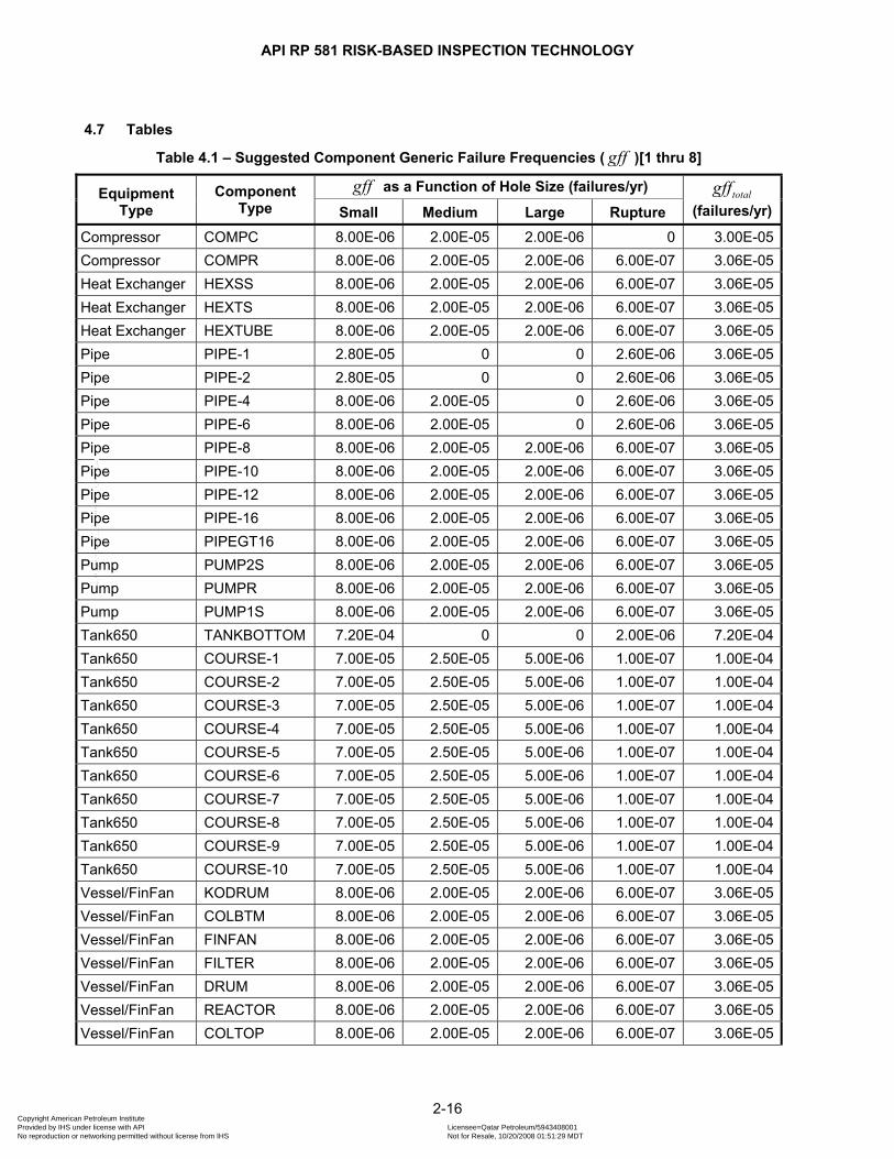
API RP 581 RISK-BASED INSPECTION TECHNOLOGY
4.7 Tables
Table 4.1 – Suggested Component Generic Failure Frequencies ( )[1 thru 8] gff
Equipment Type
Component Type
gff as a Function of Hole Size (failures/yr) totalgff (failures/yr) Small Medium Large Rupture
Compressor COMPC 8.00E-06 2.00E-05 2.00E-06 0 3.00E-05Compressor COMPR 8.00E-06 2.00E-05 2.00E-06 6.00E-07 3.06E-05Heat Exchanger HEXSS 8.00E-06 2.00E-05 2.00E-06 6.00E-07 3.06E-05Heat Exchanger HEXTS 8.00E-06 2.00E-05 2.00E-06 6.00E-07 3.06E-05Heat Exchanger HEXTUBE 8.00E-06 2.00E-05 2.00E-06 6.00E-07 3.06E-05Pipe PIPE-1 2.80E-05 0 0 2.60E-06 3.06E-05Pipe PIPE-2 2.80E-05 0 0 2.60E-06 3.06E-05Pipe PIPE-4 8.00E-06 2.00E-05 0 2.60E-06 3.06E-05Pipe PIPE-6 8.00E-06 2.00E-05 0 2.60E-06 3.06E-05Pipe PIPE-8 8.00E-06 2.00E-05 2.00E-06 6.00E-07 3.06E-05Pipe PIPE-10 8.00E-06 2.00E-05 2.00E-06 6.00E-07 3.06E-05Pipe PIPE-12 8.00E-06 2.00E-05 2.00E-06 6.00E-07 3.06E-05Pipe PIPE-16 8.00E-06 2.00E-05 2.00E-06 6.00E-07 3.06E-05Pipe PIPEGT16 8.00E-06 2.00E-05 2.00E-06 6.00E-07 3.06E-05Pump PUMP2S 8.00E-06 2.00E-05 2.00E-06 6.00E-07 3.06E-05Pump PUMPR 8.00E-06 2.00E-05 2.00E-06 6.00E-07 3.06E-05Pump PUMP1S 8.00E-06 2.00E-05 2.00E-06 6.00E-07 3.06E-05Tank650 TANKBOTTOM 7.20E-04 0 0 2.00E-06 7.20E-04Tank650 COURSE-1 7.00E-05 2.50E-05 5.00E-06 1.00E-07 1.00E-04Tank650 COURSE-2 7.00E-05 2.50E-05 5.00E-06 1.00E-07 1.00E-04Tank650 COURSE-3 7.00E-05 2.50E-05 5.00E-06 1.00E-07 1.00E-04Tank650 COURSE-4 7.00E-05 2.50E-05 5.00E-06 1.00E-07 1.00E-04Tank650 COURSE-5 7.00E-05 2.50E-05 5.00E-06 1.00E-07 1.00E-04Tank650 COURSE-6 7.00E-05 2.50E-05 5.00E-06 1.00E-07 1.00E-04Tank650 COURSE-7 7.00E-05 2.50E-05 5.00E-06 1.00E-07 1.00E-04Tank650 COURSE-8 7.00E-05 2.50E-05 5.00E-06 1.00E-07 1.00E-04Tank650 COURSE-9 7.00E-05 2.50E-05 5.00E-06 1.00E-07 1.00E-04Tank650 COURSE-10 7.00E-05 2.50E-05 5.00E-06 1.00E-07 1.00E-04Vessel/FinFan KODRUM 8.00E-06 2.00E-05 2.00E-06 6.00E-07 3.06E-05Vessel/FinFan COLBTM 8.00E-06 2.00E-05 2.00E-06 6.00E-07 3.06E-05Vessel/FinFan FINFAN 8.00E-06 2.00E-05 2.00E-06 6.00E-07 3.06E-05Vessel/FinFan FILTER 8.00E-06 2.00E-05 2.00E-06 6.00E-07 3.06E-05Vessel/FinFan DRUM 8.00E-06 2.00E-05 2.00E-06 6.00E-07 3.06E-05Vessel/FinFan REACTOR 8.00E-06 2.00E-05 2.00E-06 6.00E-07 3.06E-05Vessel/FinFan COLTOP 8.00E-06 2.00E-05 2.00E-06 6.00E-07 3.06E-05
2-16 Copyright American Petroleum Institute Provided by IHS under license with API Licensee=Qatar Petroleum/5943408001
Not for Resale, 10/20/2008 01:51:29 MDTNo reproduction or networking permitted without license from IHS
--```,`,,`,`,,`,`,,,,,,``,```,`-`-`,,`,,`,`,,`---

API RP 581 RISK-BASED INSPECTION TECHNOLOGY
Table 4.1 – Suggested Component Generic Failure Frequencies ( gff )[1 thru 8]
Equipment Type
Component Type
gff as a Function of Hole Size (failures/yr) totalgff (failures/yr) Small Medium Large Rupture
Vessel/FinFan COLMID 8.00E-06 2.00E-05 2.00E-06 6.00E-07 3.06E-05Note: See references [1] through [8] for discussion of failure frequencies for equipment
2-17 Copyright American Petroleum Institute Provided by IHS under license with API Licensee=Qatar Petroleum/5943408001
Not for Resale, 10/20/2008 01:51:29 MDTNo reproduction or networking permitted without license from IHS
--```,`,,`,`,,`,`,,,,,,``,```,`-`-`,,`,,`,`,,`---
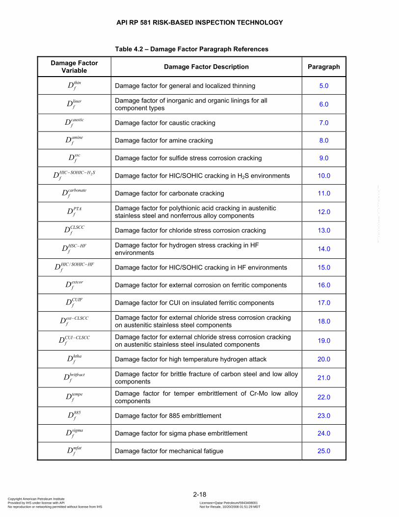
API RP 581 RISK-BASED INSPECTION TECHNOLOGY
Table 4.2 – Damage Factor Paragraph References
Damage Factor Variable Damage Factor Description Paragraph
thinfD Damage factor for general and localized thinning 5.0
linerfD Damage factor of inorganic and organic linings for all
component types 6.0
causticfD Damage factor for caustic cracking 7.0
aminefD Damage factor for amine cracking 8.0
sscfD Damage factor for sulfide stress corrosion cracking 9.0
2HIC SOHIC H SfD − − Damage factor for HIC/SOHIC cracking in H2S environments 10.0
carbonatefD Damage factor for carbonate cracking 11.0
PTAfD Damage factor for polythionic acid cracking in austenitic
stainless steel and nonferrous alloy components 12.0
CLSCCfD Damage factor for chloride stress corrosion cracking 13.0
HSC HFfD − Damage factor for hydrogen stress cracking in HF
environments 14.0
/HIC SOHIC HFfD − Damage factor for HIC/SOHIC cracking in HF environments 15.0
extcorfD Damage factor for external corrosion on ferritic components 16.0
CUIFfD Damage factor for CUI on insulated ferritic components 17.0
ext CLSCCfD − Damage factor for external chloride stress corrosion cracking
on austenitic stainless steel components 18.0
CUI CLSCCfD − Damage factor for external chloride stress corrosion cracking
on austenitic stainless steel insulated components 19.0
hthafD Damage factor for high temperature hydrogen attack 20.0
britfractfD Damage factor for brittle fracture of carbon steel and low alloy
components 21.0
tempefD Damage factor for temper embrittlement of Cr-Mo low alloy
components 22.0
885fD Damage factor for 885 embrittlement 23.0
sigmafD Damage factor for sigma phase embrittlement 24.0
mfatfD Damage factor for mechanical fatigue 25.0
2-18 Copyright American Petroleum Institute Provided by IHS under license with API Licensee=Qatar Petroleum/5943408001
Not for Resale, 10/20/2008 01:51:29 MDTNo reproduction or networking permitted without license from IHS
--```,`,,`,`,,`,`,,,,,,``,```,`-`-`,,`,,`,`,,`---
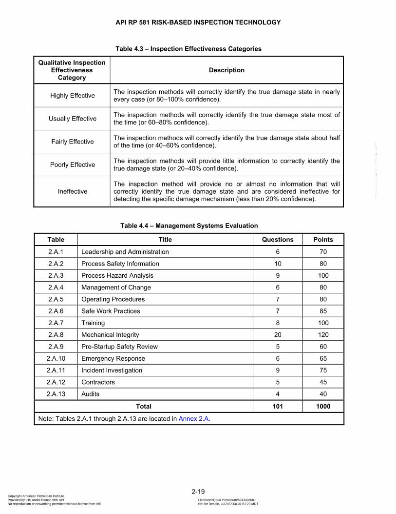
API RP 581 RISK-BASED INSPECTION TECHNOLOGY
Table 4.3 – Inspection Effectiveness Categories
Qualitative Inspection Effectiveness
Category Description
Highly Effective The inspection methods will correctly identify the true damage state in nearly every case (or 80–100% confidence).
Usually Effective The inspection methods will correctly identify the true damage state most of the time (or 60–80% confidence).
Fairly Effective The inspection methods will correctly identify the true damage state about half of the time (or 40–60% confidence).
Poorly Effective The inspection methods will provide little information to correctly identify the true damage state (or 20–40% confidence).
Ineffective The inspection method will provide no or almost no information that will correctly identify the true damage state and are considered ineffective for detecting the specific damage mechanism (less than 20% confidence).
Table 4.4 – Management Systems Evaluation
Table Title Questions Points
2.A.1 Leadership and Administration 6 70
2.A.2 Process Safety Information 10 80
2.A.3 Process Hazard Analysis 9 100
2.A.4 Management of Change 6 80
2.A.5 Operating Procedures 7 80
2.A.6 Safe Work Practices 7 85
2.A.7 Training 8 100
2.A.8 Mechanical Integrity 20 120
2.A.9 Pre-Startup Safety Review 5 60
2.A.10 Emergency Response 6 65
2.A.11 Incident Investigation 9 75
2.A.12 Contractors 5 45
2.A.13 Audits 4 40
Total 101 1000
Note: Tables 2.A.1 through 2.A.13 are located in Annex 2.A.
2-19 Copyright American Petroleum Institute Provided by IHS under license with API Licensee=Qatar Petroleum/5943408001
Not for Resale, 10/20/2008 01:51:29 MDTNo reproduction or networking permitted without license from IHS
--```,`,,`,`,,`,`,,,,,,``,```,`-`-`,,`,,`,`,,`---
API RP 581 RISK-BASED INSPECTION TECHNOLOGY
5 THINNING DAMAGE FACTOR
5.1 Scope The damage factor calculation for components subject to damage mechanisms that result in general or local thinning is covered in this paragraph.
5.2 Screening Criteria In an API RBI assessment, all components should be checked for thinning.
5.3 Required Data The basic component data required for analysis is given in Table 5.1. Component types and required geometry data are shown in Tables 5.2 and 5.3, respectively. The data required for determination of the thinning damage factor is provided in Table 5.4.
5.4 Basic Assumptions In the damage factor calculation, it is assumed that the thinning mechanism has resulted in an average rate of thinning over the time period defined in the basic data that is fairly constant. The probability of failure is estimated by examining the possibility that the rate of thinning is greater than what is expected. The probability of these higher rates is determined by the amount of inspection and on-line monitoring that has been performed. The more thorough the inspection, and the greater the number of inspections and continued use of on-line monitoring, the less likely is the chance that the rate of thinning is greater than anticipated. In the damage factor calculation, it is assumed that thinning damage would eventually result in failure by plastic collapse.
5.5 Determination of the Damage Factor
5.5.1 Overview A flow chart of the steps required to determine the damage factor for thinning is shown in Figure 5.1. The following paragraphs provide additional information and the calculation procedure. The corrosion rate should be calculated from thickness data available from equipment inspection(s). If corrosion rates have not been calculated from thickness inspection data, conservative estimates may be established using Annex 2.B or from expert opinion from knowledgeable materials or corrosion engineers. The results of inspections that have been performed on the component should be used to designate the type of thinning (i.e., general versus localized). If this information is not known, then the information in Annex 2.B may be used to determine the type of thinning (general or localized) expected for various thinning mechanisms. If both general and localized thinning mechanisms are possible, then designate the type of thinning as localized. The type of thinning designated will be used to determine the effectiveness of inspection performed.
5.5.2 Inspection Effectiveness Inspections are ranked according to their expected effectiveness at detecting thinning and correctly predicting the rate of thinning. The actual effectiveness of a given inspection technique depends on the characteristics of the thinning mechanism, (i.e., whether it is general or localized). Examples of inspection activities for general and localized thinning, respectively, that are both intrusive (requires entry into the equipment), non-intrusive (can be performed externally), and buried components are provided in Tables 5.5 through 5.7, respectively. Note that the effectiveness category assigned to the inspection activity differs depending on whether the thinning is general or localized. For localized thinning, selection of locations for examination must be based on a thorough understanding of the damage mechanism in the specific process.
2-20 Copyright American Petroleum Institute Provided by IHS under license with API Licensee=Qatar Petroleum/5943408001
Not for Resale, 10/20/2008 01:51:29 MDTNo reproduction or networking permitted without license from IHS
--```,`,,`,`,,`,`,,,,,,``,```,`-`-`,,`,,`,`,,`---

API RP 581 RISK-BASED INSPECTION TECHNOLOGY
The effectiveness of each inspection performed within the designated time period must be characterized in accordance with Tables 5.5 through 5.10, as applicable. The number and category of the highest effective inspection will be used to determine the damage factor. If multiple inspections of a lower effectiveness have been conducted during the designated time period, they can be equated to an equivalent higher effectiveness inspection in accordance with paragraph 4.4.3. Note that for tank bottoms, credit is given for only one inspection.
5.5.3 Calculation of the Damage Factor The following procedure may be used to determine the damage factor for thinning, see Figure 5.1. Note that this procedure makes the assumption that the cladding corrodes prior to any corrosion of the base metal. Where thinning due to external corrosion exists, this procedure will be conservative. a) STEP 1 – Determine the number of inspections, and the corresponding inspection effectiveness category
using paragraph 5.5.2 for all past inspections. Combine the inspections to the highest effectiveness performed using paragraph 4.4.3.
b) STEP 2 – Determine the time in-service, , since the last inspection thickness reading, . age rdt
c) STEP 3 – Determine the corrosion rate for the base metal, , based on the material of construction and
process environment, see ,r bmC
Annex 2.B. Where the component has cladding, a corrosion rate, , must also be obtained for the cladding.
,r cmC
d) STEP 4 – Determine the minimum required wall thickness, , per the original construction code or using API 579 [
mint10], Appendix A. If the component is a tank bottom, then in accordance with API 653 [11],
if the tank does not have a release prevention barrier and if the tank has a release prevention barrier.
min 0.1t = in inmin 0.05t =
e) STEP 5 – For clad components, calculate the time or age from the last inspection required to corrode away the clad material, , using Equation (rcage 2.12).
,
max , 0.0rdrc
r cm
t tageC
⎡ ⎤⎛ ⎞−= ⎢⎜ ⎟⎜ ⎟⎢ ⎥⎝ ⎠⎣ ⎦
⎥ (2.12)
f) STEP 6 – Determine the parameter using Equation (rtA 2.13) or (2.14), based on the age and from
STEP 2, from STEP 3, from STEP 4 and the age required to corrode away the cladding, , if applicable from STEP 5 .
rdtagerC mint rc
1) For components without cladding, and for components where the cladding is corroded away at the time of the last inspection (i.e. 0.0rcage = ), use Equation (2.13).
,
min
max 1 , 0.0rd r bmrt
t C ageA
t CA⎡ ⎤− ⋅⎛ ⎞
= −⎢⎜ +⎝ ⎠⎣ ⎦⎥⎟ (2.13)
2) For components that have cladding (i.e. ) at the time of the last inspection, use Equation (
0.0rcage ≥2.14) :
( ), ,
min
max 1 , 0.0rd r cm rc r bm rcrt
t C age C age ageA
t CA⎡ ⎤− ⋅ − ⋅ −
= −⎢ +⎣ ⎦⎥ (2.14)
g) STEP 7 – Determine the base damage factor for thinning, thinfBD , using Table 5.11 or Table 5.12, as
applicable, based on the number of, and highest effective inspection category from STEP 1, and the parameter from STEP 6.
rtA
2-21 Copyright American Petroleum Institute Provided by IHS under license with API Licensee=Qatar Petroleum/5943408001
Not for Resale, 10/20/2008 01:51:29 MDTNo reproduction or networking permitted without license from IHS
--```,`,,`,`,,`,`,,,,,,``,```,`-`-`,,`,,`,`,,`---
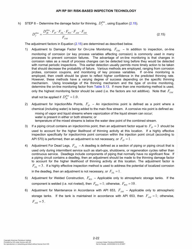
API RP 581 RISK-BASED INSPECTION TECHNOLOGY
h) STEP 8 – Determine the damage factor for thinning, thinfD , using Equation (2.15).
thinfB IP DL WD AM SMthin
fOM
D F F F F FD
F⋅ ⋅ ⋅ ⋅ ⋅
= (2.15)
The adjustment factors in Equation (2.15) are determined as described below.
1) Adjustment to Damage Factor for On-Line Monitoring, – In addition to inspection, on-line monitoring of corrosion (or key process variables affecting corrosion) is commonly used in many processes to prevent corrosion failures. The advantage of on-line monitoring is that changes in corrosion rates as a result of process changes can be detected long before they would be detected with normal periodic inspections. This earlier detection usually permits more timely action to be taken that should decrease the probability of failure. Various methods are employed, ranging from corrosion probes, corrosion coupons, and monitoring of key process variables. If on-line monitoring is employed, then credit should be given to reflect higher confidence in the predicted thinning rate. However, these methods have a varying degree of success depending on the specific thinning mechanism. Using knowledge of the thinning mechanism and the type of on-line monitoring, determine the on-line monitoring factor from
OMF
Table 5.13. If more than one monitoring method is used, only the highest monitoring factor should be used (i.e. the factors are not additive). Note that
shall not be applied if . OMF
1.0thinfbD =
2) Adjustment for Injection/Mix Points, – An injection/mix point is defined as a point where a chemical (including water) is being added to the main flow stream. A corrosive mix point is defined as:
IPF
mixing of vapor and liquid streams where vaporization of the liquid stream can occur; water is present in either or both streams; or temperature of the mixed streams is below the water dew point of the combined stream.
3) If a piping circuit contains an injection/mix point, then an adjustment factor equal to should be used to account for the higher likelihood of thinning activity at this location. If a highly effective inspection specifically for injection/mix point corrosion within the injection point circuit (according to API 570) is performed, then an adjustment is not necessary, or
3IPF =
1IPF = .
4) Adjustment For Dead Legs, DLF – A deadleg is defined as a section of piping or piping circuit that is used only during intermittent service such as start-ups, shutdowns, or regeneration cycles rather than continuous service. Deadlegs include components of piping that normally have no significant flow. If a piping circuit contains a deadleg, then an adjustment should be made to the thinning damage factor to account for the higher likelihood of thinning activity at this location. The adjustment factor is
. If a highly effective inspection method is used to address the potential of localized corrosion
in the deadleg, then an adjustment is not necessary, or
3DLF =1DLF = .
5) Adjustment for Welded Construction, – Applicable only to atmospheric storage tanks. If the
component is welded (i.e. not riveted), then WDF
1WDF = ; otherwise, 10WDF = .
6) Adjustment for Maintenance in Accordance with API 653, AMF – Applicable only to atmospheric
storage tanks. If the tank is maintained in accordance with API 653, then ; otherwise,
.
1AMF =5AMF =
2-22 Copyright American Petroleum Institute Provided by IHS under license with API Licensee=Qatar Petroleum/5943408001
Not for Resale, 10/20/2008 01:51:29 MDTNo reproduction or networking permitted without license from IHS
--```,`,,`,`,,`,`,,,,,,``,```,`-`-`,,`,,`,`,,`---
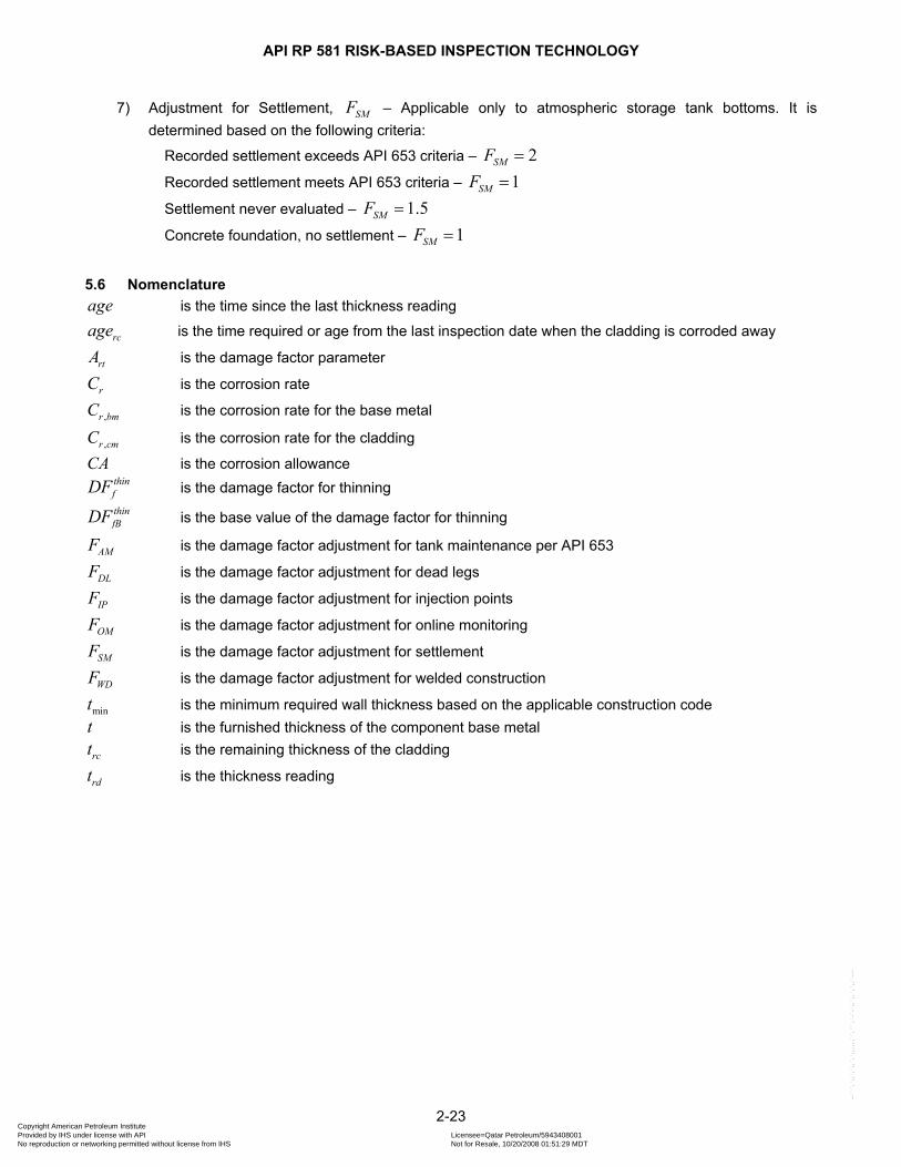
API RP 581 RISK-BASED INSPECTION TECHNOLOGY
7) Adjustment for Settlement, – Applicable only to atmospheric storage tank bottoms. It is determined based on the following criteria:
SMF
Recorded settlement exceeds API 653 criteria – 2SMF =
Recorded settlement meets API 653 criteria – 1SMF =
Settlement never evaluated – 1.5SMF =
Concrete foundation, no settlement – 1SMF =
5.6 Nomenclature age is the time since the last thickness reading
rcage is the time required or age from the last inspection date when the cladding is corroded away
rtA is the damage factor parameter
rC is the corrosion rate
,r bmC is the corrosion rate for the base metal
,r cmC is the corrosion rate for the cladding
CA is the corrosion allowance thinfDF is the damage factor for thinning thinfBDF is the base value of the damage factor for thinning
AMF is the damage factor adjustment for tank maintenance per API 653
DLF is the damage factor adjustment for dead legs
IPF is the damage factor adjustment for injection points
OMF is the damage factor adjustment for online monitoring
SMF is the damage factor adjustment for settlement
WDF is the damage factor adjustment for welded construction
mint is the minimum required wall thickness based on the applicable construction code t is the furnished thickness of the component base metal
rct is the remaining thickness of the cladding
rdt is the thickness reading
2-23 Copyright American Petroleum Institute Provided by IHS under license with API Licensee=Qatar Petroleum/5943408001
Not for Resale, 10/20/2008 01:51:29 MDTNo reproduction or networking permitted without license from IHS
--```,`,,`,`,,`,`,,,,,,``,```,`-`-`,,`,,`,`,,`---
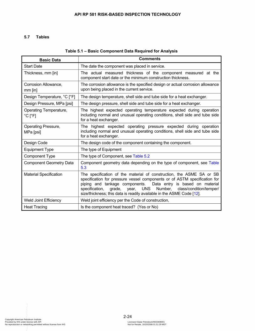
API RP 581 RISK-BASED INSPECTION TECHNOLOGY
5.7 Tables
Table 5.1 – Basic Component Data Required for Analysis
Basic Data Comments
Start Date The date the component was placed in service. Thickness, mm [in] The actual measured thickness of the component measured at the
component start date or the minimum construction thickness. Corrosion Allowance, mm [in]
The corrosion allowance is the specified design or actual corrosion allowance upon being placed in the current service.
Design Temperature, °C [°F] The design temperature, shell side and tube side for a heat exchanger. Design Pressure, MPa [psi] The design pressure, shell side and tube side for a heat exchanger. Operating Temperature, °C [°F]
The highest expected operating temperature expected during operation including normal and unusual operating conditions, shell side and tube side for a heat exchanger.
Operating Pressure, MPa [psi]
The highest expected operating pressure expected during operation including normal and unusual operating conditions, shell side and tube side for a heat exchanger.
Design Code The design code of the component containing the component. Equipment Type The type of Equipment Component Type The type of Component, see Table 5.2
Component Geometry Data Component geometry data depending on the type of component, see Table 5.3
Material Specification The specification of the material of construction, the ASME SA or SB specification for pressure vessel components or of ASTM specification for piping and tankage components. Data entry is based on material specification, grade, year, UNS Number, class/condition/temper/ size/thickness; this data is readily available in the ASME Code [12].
Weld Joint Efficiency Weld joint efficiency per the Code of construction, Heat Tracing Is the component heat traced? (Yes or No)
2-24 Copyright American Petroleum Institute Provided by IHS under license with API Licensee=Qatar Petroleum/5943408001
Not for Resale, 10/20/2008 01:51:29 MDTNo reproduction or networking permitted without license from IHS
--```,`,,`,`,,`,`,,,,,,``,```,`-`-`,,`,,`,`,,`---
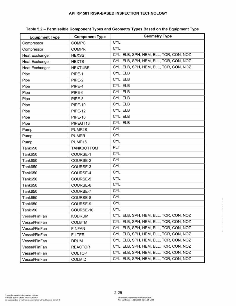
API RP 581 RISK-BASED INSPECTION TECHNOLOGY
Table 5.2 – Permissible Component Types and Geometry Types Based on the Equipment Type
Equipment Type Component Type Geometry Type
Compressor COMPC CYL
Compressor COMPR CYL
Heat Exchanger HEXSS CYL, ELB, SPH, HEM, ELL, TOR, CON, NOZ
Heat Exchanger HEXTS CYL, ELB, SPH, HEM, ELL, TOR, CON, NOZ
Heat Exchanger HEXTUBE CYL, ELB, SPH, HEM, ELL, TOR, CON, NOZ
Pipe PIPE-1 CYL, ELB
Pipe PIPE-2 CYL, ELB
Pipe PIPE-4 CYL, ELB
Pipe PIPE-6 CYL, ELB
Pipe PIPE-8 CYL, ELB
Pipe PIPE-10 CYL, ELB
Pipe PIPE-12 CYL, ELB
Pipe PIPE-16 CYL, ELB
Pipe PIPEGT16 CYL, ELB
Pump PUMP2S CYL
Pump PUMPR CYL
Pump PUMP1S CYL
Tank650 TANKBOTTOM PLT
Tank650 COURSE-1 CYL
Tank650 COURSE-2 CYL
Tank650 COURSE-3 CYL
Tank650 COURSE-4 CYL
Tank650 COURSE-5 CYL
Tank650 COURSE-6 CYL
Tank650 COURSE-7 CYL
Tank650 COURSE-8 CYL
Tank650 COURSE-9 CYL
Tank650 COURSE-10 CYL
Vessel/FinFan KODRUM CYL, ELB, SPH, HEM, ELL, TOR, CON, NOZ
Vessel/FinFan COLBTM CYL, ELB, SPH, HEM, ELL, TOR, CON, NOZ
Vessel/FinFan FINFAN CYL, ELB, SPH, HEM, ELL, TOR, CON, NOZ
Vessel/FinFan FILTER CYL, ELB, SPH, HEM, ELL, TOR, CON, NOZ
Vessel/FinFan DRUM CYL, ELB, SPH, HEM, ELL, TOR, CON, NOZ
Vessel/FinFan REACTOR CYL, ELB, SPH, HEM, ELL, TOR, CON, NOZ
Vessel/FinFan COLTOP CYL, ELB, SPH, HEM, ELL, TOR, CON, NOZ
Vessel/FinFan COLMID CYL, ELB, SPH, HEM, ELL, TOR, CON, NOZ
2-25 Copyright American Petroleum Institute Provided by IHS under license with API Licensee=Qatar Petroleum/5943408001
Not for Resale, 10/20/2008 01:51:29 MDTNo reproduction or networking permitted without license from IHS
--```,`,,`,`,,`,`,,,,,,``,```,`-`-`,,`,,`,`,,`---

API RP 581 RISK-BASED INSPECTION TECHNOLOGY
Table 5.3 – Geometry Data Based on the Geometry Type
Geometry Type
Geometry Description
Geometry Data
CYL Cylindrical Shell
• Diameter (OD for Component Types Pipe and Tube/NS Pipe, ID for all other Component Types)
• Length • Volume
ELB Elbow or Pipe Bend
• Diameter (OD for Component Types Pipe and Tube/NS Pipe, ID for all other Component Types)
• Bend Radius • Volume
SPH Spherical Shell • Diameter (ID) • Volume
HEM Hemispherical Head • Diameter (ID) • Volume
ELL Elliptical Head • Diameter (ID) • Major-to-Minor Axis Ratio • Volume
TOR Torispherical Head
• Diameter (ID) • Crown Radius (IR) • Knuckle (IR) • Volume
CON Conical Shell
• Diameter (ID) • Length • Cone Angle • Volume
NOZ Nozzle • Diameter (ID) • Length • Volume
2-26 Copyright American Petroleum Institute Provided by IHS under license with API Licensee=Qatar Petroleum/5943408001
Not for Resale, 10/20/2008 01:51:29 MDTNo reproduction or networking permitted without license from IHS
--```,`,,`,`,,`,`,,,,,,``,```,`-`-`,,`,,`,`,,`---

API RP 581 RISK-BASED INSPECTION TECHNOLOGY
Table 5.4 – Data Required for Determination of the Thinning Damage Factor
Basic Data Comments Thinning Type (General or Localized)
Determine whether the thinning is general or localized based on inspection results of effective inspections. General corrosion is defined as affecting more than 10% of the surface area and the wall thickness variation is less than 1.27 mm (50 mils). Localized corrosion is defined as affecting less than 10% of the surface area or a wall thickness variation greater than 1.27 mm (50 mils).
Corrosion Rate (mm/yr:mpy)
The current rate of thinning calculated from thickness data, if available. Corrosion rates calculated from thickness data typically vary from one inspection to another. These variations may be due to variations in the wall thickness, or they may indicate a change in the actual corrosion rate. If the short-term rate (calculated from the difference between the current thickness and the previous thickness) is significantly different from the long-term rate (calculated from the difference between the current thickness and the original thickness), then the component may be evaluated using the short term rate, but the appropriate time and thickness must be used.
Inspection Effectiveness Category
The effectiveness category of each inspection that has been performed on the component during the time period (specified above).
Number of Inspections The number of inspections in each effectiveness category that have been performed during the time period (specified above).
On-Line Monitoring
The types of proactive on-line monitoring methods or tools employed, such as corrosion probes, coupons, process variables (Coupons, Probes, Process Variables, or Combinations, etc.)
Thinning Mechanism If credit is to be taken for on-line monitoring, the potential thinning mechanisms must be known. A knowledgeable materials/corrosion engineer should be consulted for this information, also see API 571 [13].
Presence of Injection/Mix Point (Yes or No).
For piping, determine if there is an injection or mix point in the circuit.
Type of Injection/Mix Point Inspection
For piping circuits which contain an injection or mix point, determine whether not the inspection program is highly effective or not highly effective to detect local corrosion at these points.
Presence of a Deadleg (Yes or No).
For piping, determine if there is a deadleg in the circuit.
Type of Inspection for Deadleg Corrosion
For piping circuits which contain a deadleg, determine if the inspection program currently being used is highly effective or not highly effective to detect local corrosion in dead legs has been performed.
Welded Construction Applicable to Atmospheric Storage tanks only, tanks may be welded or riveted construction. Is the tank of welded construction? (Yes or No)
Maintained to API 653 Applicable to Atmospheric Storage tanks only. Is the tank maintained in accordance with API 653 [11]? (Yes or No)
Settlement Applicable to Atmospheric Storage tanks only, tanks may be welded or riveted construction. What is the settlement history of the tank
• Recorded settlement exceeds API 653 criteria • Recorded settlement meets API 653 criteria • Settlement never evaluated • Concrete foundation, no settlement
2-27 Copyright American Petroleum Institute Provided by IHS under license with API Licensee=Qatar Petroleum/5943408001
Not for Resale, 10/20/2008 01:51:29 MDTNo reproduction or networking permitted without license from IHS
--```,`,,`,`,,`,`,,,,,,``,```,`-`-`,,`,,`,`,,`---
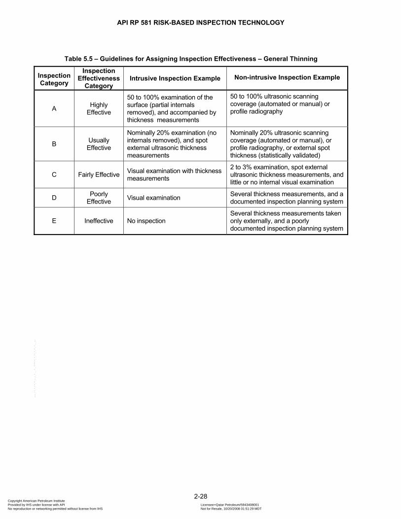
API RP 581 RISK-BASED INSPECTION TECHNOLOGY
Table 5.5 – Guidelines for Assigning Inspection Effectiveness – General Thinning
Inspection Category
Inspection Effectiveness
Category Intrusive Inspection Example Non-intrusive Inspection Example
A Highly Effective
50 to 100% examination of the surface (partial internals removed), and accompanied by thickness measurements
50 to 100% ultrasonic scanning coverage (automated or manual) or profile radiography
B Usually Effective
Nominally 20% examination (no internals removed), and spot external ultrasonic thickness measurements
Nominally 20% ultrasonic scanning coverage (automated or manual), or profile radiography, or external spot thickness (statistically validated)
C Fairly Effective Visual examination with thickness measurements
2 to 3% examination, spot external ultrasonic thickness measurements, and little or no internal visual examination
D Poorly Effective Visual examination Several thickness measurements, and a
documented inspection planning system
E Ineffective No inspection Several thickness measurements taken only externally, and a poorly documented inspection planning system
2-28 Copyright American Petroleum Institute Provided by IHS under license with API Licensee=Qatar Petroleum/5943408001
Not for Resale, 10/20/2008 01:51:29 MDTNo reproduction or networking permitted without license from IHS
--```,`,,`,`,,`,`,,,,,,``,```,`-`-`,,`,,`,`,,`---

API RP 581 RISK-BASED INSPECTION TECHNOLOGY
Table 5.6 – Guidelines for Assigning Inspection Effectiveness – Local Thinning
Inspection Category
Inspection Effectiveness
Category Intrusive Inspection Example Non-intrusive Inspection Example
A Highly Effective
100% visual examination (with removal of internal packing, trays, etc.) and thickness measurements
50 to 100% coverage using automated ultrasonic scanning, or profile radiography in areas specified by a corrosion engineer or other knowledgeable specialist.
B Usually Effective
100% visual examination (with partial removal of the internals) including manways, nozzles, etc. and thickness measurements.
20% coverage using automated ultrasonic scanning, or 50% manual ultrasonic scanning, or 50% profile radiography in areas specified by a corrosion engineer or other knowledgeable specialist.
C Fairly Effective
Nominally 50% visual examination and spot ultrasonic thickness measurements
Nominally 20% coverage using automated or manual ultrasonic scanning, or profile radiography, and spot thickness measurements at areas specified by a corrosion engineer or other knowledgeable specialist.
D Poorly Effective
Nominally 20% visual examination and spot ultrasonic thickness measurements
Spot ultrasonic thickness measurements or profile radiography without areas being specified by a corrosion engineer or other knowledgeable specialist.
E Ineffective
No inspection Spot ultrasonic thickness measurements without areas being specified by a corrosion engineer or other knowledgeable specialist.
2-29 Copyright American Petroleum Institute Provided by IHS under license with API Licensee=Qatar Petroleum/5943408001
Not for Resale, 10/20/2008 01:51:29 MDTNo reproduction or networking permitted without license from IHS
--```,`,,`,`,,`,`,,,,,,``,```,`-`-`,,`,,`,`,,`---

API RP 581 RISK-BASED INSPECTION TECHNOLOGY
Table 5.7 – Guidelines for Assigning Inspection Effectiveness – Buried Components
Inspection Category
Inspection Effectiveness Category
Intrusive Inspection Example
Non-intrusive Inspection Example
Non-intrusive Inspection Example
A Highly Effective
100% internal inspection via state-of-the-art pigging and in-line inspection technologies (UT, MFL, internal rotary UT, etc.) 100% external inspection of equipment that is only partially buried using an NDE crawler with circumferential inspection technology (MFL, lamb-wave UT)
Complete excavation, 100% external visual inspection, and 100% inspection with NDE technologies (UT thickness measurement such as handheld devices at close-interval grid locations, UT B-scan, automated ultrasonic scanning, guided-wave UT global search, crawler with circumferential inspection technology such as MFL or lamb-wave UT, digital radiography in more than one direction)
a. Cathodic Protection (CP) System maintained and managed by NACE certified personnel and complying with NACE SP0169 [14]– includes Stray current surveys on a regular basis
b. Close Interval Survey (at excavation sites) to assess the performance of the CP system locally
c. Sample soil and water resistivity and chemistry measurements along entire structure
B Usually Effective
Internal inspection via pigging and in-line inspection technologies (UT, MFL, internal rotary UT, etc.) of selected areas / sections, combined with statistical analysis or extreme value analysis (EVA). External inspection of equipment that is only partially buried using an NDE crawler with circumferential inspection technology (MFL, lamb-wave UT) on selected areas / sections, combined with statistical analysis or extreme value analysis (EVA).
Excavation at “Selected” locations, 100% external visual, and 100% inspection with NDE technologies (UT thickness measurement such as handheld devices at close-interval grid locations, UT B-scan, automated ultrasonic scanning, guided-wave UT global search, crawler with circumferential inspection technology such as MFL or lamb-wave UT, digital radiography in more than one direction)
a. CP System maintained and managed by NACE certified personnel and complying with NACE SP0169 [14] – includes Stray current surveys on a regular basis
b. Close Interval Survey (at excavation sites) to assess the performance of the CP system locally
c. Sample soil and water resistivity and chemistry measurements along entire structure
d. DC Voltage Gradient (DCVG) to determine coating damage
C Fairly Effective
Partly inspection by internal smart pig or specialized crawler device, including a representative portion of the buried pipe. (<25%)
Partial excavation guided-wave UT global search inspection in each direction of pipe. Corrosion Inspection and Maintenance managed by NACE certified and CP specialist, or equivalent
---
D Poorly Effective
Hydrostatic testing Spot check with conventional NDE equipment of local areas exposed by excavation
---
E Ineffective No inspection --- ---
2-30 Copyright American Petroleum Institute Provided by IHS under license with API Licensee=Qatar Petroleum/5943408001
Not for Resale, 10/20/2008 01:51:29 MDTNo reproduction or networking permitted without license from IHS
--```,`,,`,`,,`,`,,,,,,``,```,`-`-`,,`,,`,`,,`---
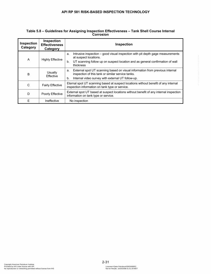
API RP 581 RISK-BASED INSPECTION TECHNOLOGY
Table 5.8 – Guidelines for Assigning Inspection Effectiveness – Tank Shell Course Internal Corrosion
Inspection Category
Inspection Effectiveness
Category Inspection
A Highly Effective
a. Intrusive inspection – good visual inspection with pit depth gage measurements at suspect locations.
b. UT scanning follow up on suspect location and as general confirmation of wall thickness
B Usually Effective
a. External spot UT scanning based on visual information from previous internal inspection of this tank or similar service tanks.
b. Internal video survey with external UT follow-up.
C Fairly Effective Eternal spot UT scanning based at suspect locations without benefit of any internal inspection information on tank type or service.
D Poorly Effective External spot UT based at suspect locations without benefit of any internal inspection information on tank type or service.
E Ineffective No inspection
2-31 Copyright American Petroleum Institute Provided by IHS under license with API Licensee=Qatar Petroleum/5943408001
Not for Resale, 10/20/2008 01:51:29 MDTNo reproduction or networking permitted without license from IHS
--```,`,,`,`,,`,`,,,,,,``,```,`-`-`,,`,,`,`,,`---

API RP 581 RISK-BASED INSPECTION TECHNOLOGY
Table 5.9 – Guidelines for Assigning Inspection Effectiveness – Tank Shell Course External Corrosion
Inspection Category
Inspection Effectiveness
Category Inspection
A Highly Effective
a. Insulated – >95% external visual inspection prior to removal of insulation b. Remove >90% of insulation at suspect locations, OR >90% pulse eddy current
inspection. c. Visual inspection of the exposed surface area with follow-up by UT or pit
gauge as required. a. Non-Insulated - >95% visual inspection of the exposed surface area with
follow-up by UT or pit gauge as required.
B Usually Effective
a. Insulated – >95% external visual inspection prior to removal of insulation b. Remove >30% of insulation at suspect locations, OR >30% pulse eddy current
inspection. c. Visual inspection of the exposed surface area with follow-up by UT or pit
gauge as required. a. Non-Insulated - >50% visual inspection of the exposed surface area with
follow-up by UT or pit gauge as required.
C Fairly Effective
a. Insulated – >95% external visual inspection prior to removal of insulation b. Remove >10% of insulation at suspect locations, OR >10% pulse eddy current
inspection. c. Visual inspection of the exposed surface area with follow-up by UT or pit
gauge as required. a. Non-Insulated - >25% visual inspection of the exposed surface area with
follow-up by UT or pit gauge as required.
D Poorly Effective
a. Insulated – >95% external visual inspection prior to removal of insulation b. Remove >5% of insulation at suspect locations, OR >5% pulse eddy current
inspection. c. Visual inspection of the exposed surface area with follow-up by UT or pit
gauge as required. a. Non-Insulated - >10% visual inspection of the exposed surface area with
follow-up by UT or pit gauge as required.
E Ineffective a. Insulated – No visual inspection of insulation surface area or removal of
insulation. a. Non-Insulated - <5% visual of the exposed surface area
2-32 Copyright American Petroleum Institute Provided by IHS under license with API Licensee=Qatar Petroleum/5943408001
Not for Resale, 10/20/2008 01:51:29 MDTNo reproduction or networking permitted without license from IHS
--```,`,,`,`,,`,`,,,,,,``,```,`-`-`,,`,,`,`,,`---

API RP 581 RISK-BASED INSPECTION TECHNOLOGY
Table 5.10 – Guidelines for Assigning Inspection Effectiveness – Tank Bottoms
Inspection Category
Inspection Effectiveness
Category Soil Side Product Side
A Highly Effective
a. Floor scan 90+% & UT follow-up
b. Include welds if warranted from the results on the plate scanning
c. Hand scan of the critical zone
a. Commercial blast b. Effective supplementary light c. Visual 100% (API 653) d. Pit depth gauge e. 100% vacuum box testing of suspect
welded joints Coating or Liner: a. Sponge test 100% b. Adhesion test c. Scrape test
B Usually Effective
a. Floor scan 50+% & UT follow-up
OR b. EVA or other statistical method
with Floor scan follow-up if warranted by the result
a. Brush blast b. Effective supplementary light c. Visual 100% (API 653) d. Pit depth gauge Coating or Liner: a. Sponge test >75% b. Adhesion test c. Scrape test
C Fairly Effective
a. Floor scan 5-10+% plates; supplement with scanning near Shell & UT follow-up; Scan circle and X pattern
b. Progressively increase if damage found during scanning
c. Helium/Argon test d. Hammer test e. Cut coupons
a. Broom swept b. Effective supplementary light c. Visual 100% d. Pit depth gauge Coating or Liner: a. Sponge test 50 – 75% b. Adhesion test c. Scrape test
D Poorly Effective a. Spot UT b. Flood test
a. Broom swept b. No effective supplementary lighting c. Visual 25-50% Coating or Liner: a. Sponge test <50
E Ineffective None None
2-33 Copyright American Petroleum Institute Provided by IHS under license with API Licensee=Qatar Petroleum/5943408001
Not for Resale, 10/20/2008 01:51:29 MDTNo reproduction or networking permitted without license from IHS
--```,`,,`,`,,`,`,,,,,,``,```,`-`-`,,`,,`,`,,`---
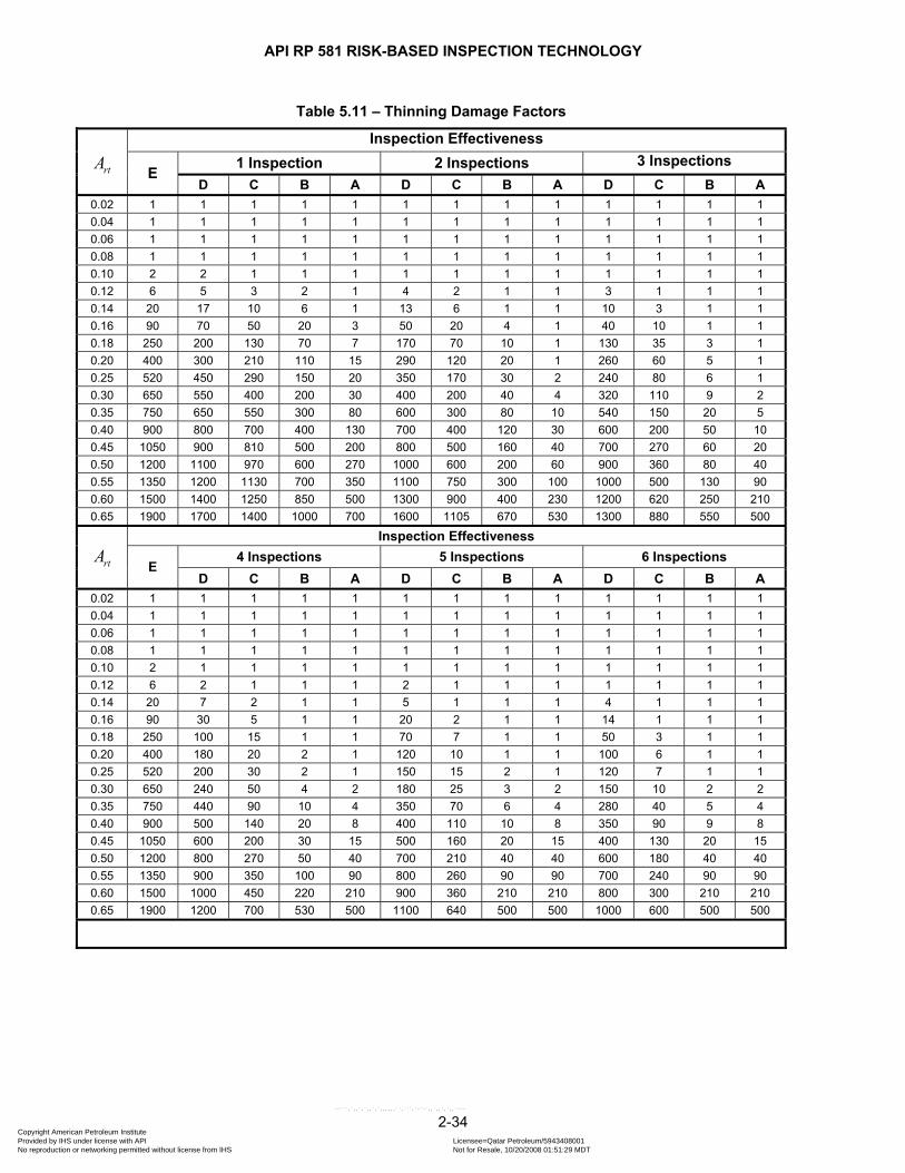
API RP 581 RISK-BASED INSPECTION TECHNOLOGY
Table 5.11 – Thinning Damage Factors
rtA Inspection Effectiveness
E 1 Inspection 2 Inspections 3 Inspections
D C B A D C B A D C B A 0.02 1 1 1 1 1 1 1 1 1 1 1 1 1 0.04 1 1 1 1 1 1 1 1 1 1 1 1 1 0.06 1 1 1 1 1 1 1 1 1 1 1 1 1 0.08 1 1 1 1 1 1 1 1 1 1 1 1 1 0.10 2 2 1 1 1 1 1 1 1 1 1 1 1 0.12 6 5 3 2 1 4 2 1 1 3 1 1 1 0.14 20 17 10 6 1 13 6 1 1 10 3 1 1 0.16 90 70 50 20 3 50 20 4 1 40 10 1 1 0.18 250 200 130 70 7 170 70 10 1 130 35 3 1 0.20 400 300 210 110 15 290 120 20 1 260 60 5 1 0.25 520 450 290 150 20 350 170 30 2 240 80 6 1 0.30 650 550 400 200 30 400 200 40 4 320 110 9 2 0.35 750 650 550 300 80 600 300 80 10 540 150 20 5 0.40 900 800 700 400 130 700 400 120 30 600 200 50 10 0.45 1050 900 810 500 200 800 500 160 40 700 270 60 20 0.50 1200 1100 970 600 270 1000 600 200 60 900 360 80 40 0.55 1350 1200 1130 700 350 1100 750 300 100 1000 500 130 90 0.60 1500 1400 1250 850 500 1300 900 400 230 1200 620 250 210 0.65 1900 1700 1400 1000 700 1600 1105 670 530 1300 880 550 500
rtA Inspection Effectiveness
E 4 Inspections 5 Inspections 6 Inspections
D C B A D C B A D C B A 0.02 1 1 1 1 1 1 1 1 1 1 1 1 1 0.04 1 1 1 1 1 1 1 1 1 1 1 1 1 0.06 1 1 1 1 1 1 1 1 1 1 1 1 1 0.08 1 1 1 1 1 1 1 1 1 1 1 1 1 0.10 2 1 1 1 1 1 1 1 1 1 1 1 1 0.12 6 2 1 1 1 2 1 1 1 1 1 1 1 0.14 20 7 2 1 1 5 1 1 1 4 1 1 1 0.16 90 30 5 1 1 20 2 1 1 14 1 1 1 0.18 250 100 15 1 1 70 7 1 1 50 3 1 1 0.20 400 180 20 2 1 120 10 1 1 100 6 1 1 0.25 520 200 30 2 1 150 15 2 1 120 7 1 1 0.30 650 240 50 4 2 180 25 3 2 150 10 2 2 0.35 750 440 90 10 4 350 70 6 4 280 40 5 4 0.40 900 500 140 20 8 400 110 10 8 350 90 9 8 0.45 1050 600 200 30 15 500 160 20 15 400 130 20 15 0.50 1200 800 270 50 40 700 210 40 40 600 180 40 40 0.55 1350 900 350 100 90 800 260 90 90 700 240 90 90 0.60 1500 1000 450 220 210 900 360 210 210 800 300 210 210 0.65 1900 1200 700 530 500 1100 640 500 500 1000 600 500 500
2-34 Copyright American Petroleum Institute Provided by IHS under license with API Licensee=Qatar Petroleum/5943408001
Not for Resale, 10/20/2008 01:51:29 MDTNo reproduction or networking permitted without license from IHS
--```,`,,`,`,,`,`,,,,,,``,```,`-`-`,,`,,`,`,,`---
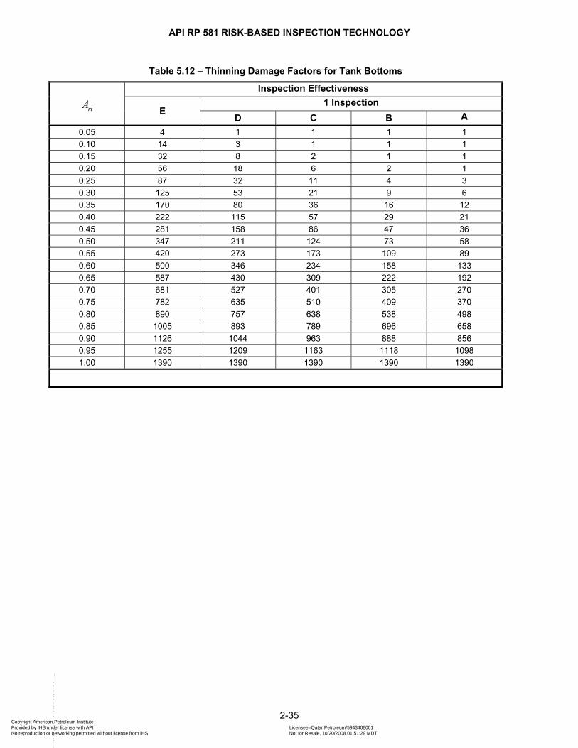
API RP 581 RISK-BASED INSPECTION TECHNOLOGY
Table 5.12 – Thinning Damage Factors for Tank Bottoms
rtA
Inspection Effectiveness
E 1 Inspection
D C B A 0.05 4 1 1 1 1 0.10 14 3 1 1 1 0.15 32 8 2 1 1 0.20 56 18 6 2 1 0.25 87 32 11 4 3 0.30 125 53 21 9 6 0.35 170 80 36 16 12 0.40 222 115 57 29 21 0.45 281 158 86 47 36 0.50 347 211 124 73 58 0.55 420 273 173 109 89 0.60 500 346 234 158 133 0.65 587 430 309 222 192 0.70 681 527 401 305 270 0.75 782 635 510 409 370 0.80 890 757 638 538 498 0.85 1005 893 789 696 658 0.90 1126 1044 963 888 856 0.95 1255 1209 1163 1118 1098 1.00 1390 1390 1390 1390 1390
2-35 Copyright American Petroleum Institute Provided by IHS under license with API Licensee=Qatar Petroleum/5943408001
Not for Resale, 10/20/2008 01:51:29 MDTNo reproduction or networking permitted without license from IHS
--```,`,,`,`,,`,`,,,,,,``,```,`-`-`,,`,,`,`,,`---
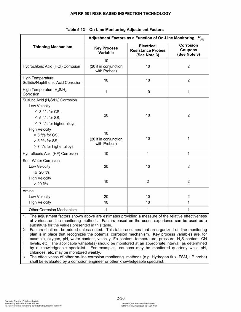
API RP 581 RISK-BASED INSPECTION TECHNOLOGY
Table 5.13 – On-Line Monitoring Adjustment Factors
Thinning Mechanism
Adjustment Factors as a Function of On-Line Monitoring, OMF
Key Process Variable
Electrical Resistance Probes
(See Note 3)
Corrosion Coupons
(See Note 3)
Hydrochloric Acid (HCI) Corrosion 10
(20 if in conjunction with Probes)
10 2
High Temperature Sulfidic/Naphthenic Acid Corrosion 10 10 2
High Temperature H2S/H2 Corrosion 1 10 1
Sulfuric Acid (H2S/H2) Corrosion Low Velocity
≤ 3 ft/s for CS, ≤ 5 ft/s for SS, ≤ 7 ft/s for higher alloys
20
10
2
High Velocity > 3 ft/s for CS, > 5 ft/s for SS, > 7 ft/s for higher alloys
10 (20 if in conjunction
with Probes) 10 1
Hydrofluoric Acid (HF) Corrosion 10 1 1
Sour Water Corrosion Low Velocity
≤ 20 ft/s 20 10 2
High Velocity > 20 ft/s 10 2 2
Amine Low Velocity
20
10
2
High Velocity 10 10 1
Other Corrosion Mechanism 1 1 1 1. The adjustment factors shown above are estimates providing a measure of the relative effectiveness
of various on-line monitoring methods. Factors based on the user’s experience can be used as a substitute for the values presented in this table.
2. Factors shall not be added unless noted. This table assumes that an organized on-line monitoring plan is in place that recognizes the potential corrosion mechanism. Key process variables are, for example, oxygen, pH, water content, velocity, Fe content, temperature, pressure, H2S content, CN levels, etc. The applicable variable(s) should be monitored at an appropriate interval, as determined by a knowledgeable specialist. For example: coupons may be monitored quarterly while pH, chlorides, etc. may be monitored weekly.
3. The effectivness of other on-line corrosion monitoring methods (e.g. Hydrogen flux, FSM, LP probe) shall be evaluated by a corrosion engineer or other knowledgeable specialist.
2-36 Copyright American Petroleum Institute Provided by IHS under license with API Licensee=Qatar Petroleum/5943408001
Not for Resale, 10/20/2008 01:51:29 MDTNo reproduction or networking permitted without license from IHS
--```,`,,`,`,,`,`,,,,,,``,```,`-`-`,,`,,`,`,,`---
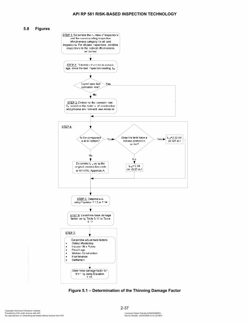
API RP 581 RISK-BASED INSPECTION TECHNOLOGY
5.8 Figures
Figure 5.1 – Determination of the Thinning Damage Factor
2-37 Copyright American Petroleum Institute Provided by IHS under license with API Licensee=Qatar Petroleum/5943408001
Not for Resale, 10/20/2008 01:51:29 MDTNo reproduction or networking permitted without license from IHS
--```,`,,`,`,,`,`,,,,,,``,```,`-`-`,,`,,`,`,,`---
API RP 581 RISK-BASED INSPECTION TECHNOLOGY
6 COMPONENT LINING DAMAGE FACTOR
6.1 Scope A general approach for computing the damage factor for a component that has a protective internal lining is covered in this paragraph. It is common practice to construct a component with a material that is known to be subject to damage in the operating environment, but to protect the material from the environment with a lining that is resistant as described in Table 6.1. The lining types covered in this paragraph are shown in Table 6.2. A general approach to using API RBI for lined component involves assessing the severity of damage that would be expected to occur on the base material, and then give credit for the existence of a lining. The degradation rate of the lining itself is not addressed. Evaluations of lining effectiveness at preventing damage are based on expert opinion.
6.2 Screening Criteria If the component has an inorganic or organic lining, then the component should be evaluated for lining damage.
6.3 Required Data The required data to determine the lining damage factor is shown in Tables 5.1 and 6.3.
6.4 Basic Assumptions All linings afford some degree of protection from the operating environment. Many linings will last for an indefinite period of time, essentially being immune to damage mechanisms that may otherwise occur. Other linings will slowly degrade with time, and have a finite life. In such cases, the age of the lining (or the years since the last inspection) becomes important in assigning a factor. Particularly in the case of organic linings, the assumption is made that the lining is compatible with the environment, operated within design temperature limits (including steam out), and properly applied with appropriate curing.
6.5 Determination of the Damage Factor
6.5.1 Overview A flow chart of the steps required to determine the damage factor for linings is shown in Figure 6.1. The following paragraphs provide additional information and the calculation procedure. The basic approach is that the type of lining and the age or years since last inspection determines a lining failure factor. This is adjusted for a qualitative description of the lining condition. It is further adjusted based on the probability of component failure upon lining failure (i.e. if the lining fails, does the component fail rapidly, or will it be expected to last for a considerable time?). A final credit is made for on-line monitoring that can provide early detection of a lining failure. After a lining damage factor is computed, it is then compared to the thinning damage factor determined for the base metal. The minimum of the two values is used. The basis for this is that if the thinning damage is small compared to the lining damage factor, then it does not yet matter if the lining has failed or not. This also provides a check that lining failure is not necessarily equated with a component.
6.5.2 Calculation of the Damage Factor The following procedure may be used to determine the damage factor for lining damage, see Figure 6.1. a) STEP 1 – Determine the lining type and time in-service, , of the lining. age
b) STEP 2 – Determine the base value of the lining damage factor, linerfBD , using Tables 6.4 and 6.5, as
applicable, based on the age and lining type from STEP 1.
c) STEP 3 – Determine the damage factor for lining damage, , is determined using Equation (linerfD 2.16).
liner linerf fB LC OMD D F F= ⋅ ⋅ (2.16)
2-38 Copyright American Petroleum Institute Provided by IHS under license with API Licensee=Qatar Petroleum/5943408001
Not for Resale, 10/20/2008 01:51:29 MDTNo reproduction or networking permitted without license from IHS
--```,`,,`,`,,`,`,,,,,,``,```,`-`-`,,`,,`,`,,`---
API RP 581 RISK-BASED INSPECTION TECHNOLOGY
The adjustment factors in Equation (2.16) are determined as described below.
1) Adjustment for Lining Condition, – The adjustment factors are given in LCF Table 6.6 based on a qualitative assessment of the lining condition.
2) Adjustment for On-Line Monitoring, – Some lined components have monitoring to allow early detection of a leak or other failure of the lining. The monitoring allows orderly shutdown of the component before failure occurs. If on-line monitoring is used, and it is known to be effective at detecting lining deterioration,
OMF
0.1OMF = ; otherwise 1.0OMF = . Examples of monitoring systems include thermography or heat sensitive paint (refractory linings), weep holes with detection devices (loose alloy linings), and electrical resistance detection (glass linings).
6.6 Nomenclature age is the time since the last thickness reading
linerfD is the damage factor for liners linerfBD is the base value of the damage factor for liners
LCF is the damage factor adjustment for lining condition
OMF is the damage factor adjustment for online monitoring
2-39 Copyright American Petroleum Institute Provided by IHS under license with API Licensee=Qatar Petroleum/5943408001
Not for Resale, 10/20/2008 01:51:29 MDTNo reproduction or networking permitted without license from IHS
--```,`,,`,`,,`,`,,,,,,``,```,`-`-`,,`,,`,`,,`---
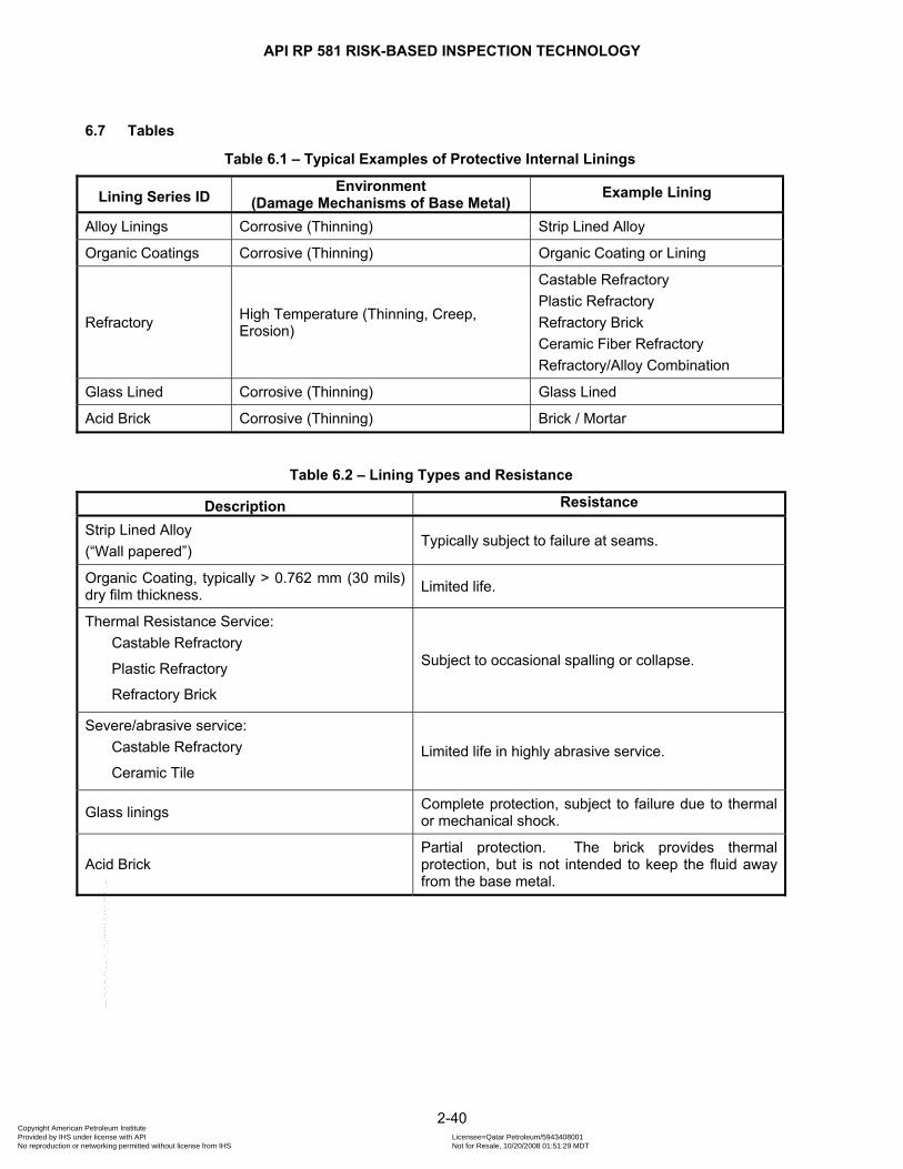
API RP 581 RISK-BASED INSPECTION TECHNOLOGY
6.7 Tables
Table 6.1 – Typical Examples of Protective Internal Linings
Lining Series ID Environment
(Damage Mechanisms of Base Metal) Example Lining
Alloy Linings Corrosive (Thinning) Strip Lined Alloy
Organic Coatings Corrosive (Thinning) Organic Coating or Lining
Refractory High Temperature (Thinning, Creep, Erosion)
Castable Refractory Plastic Refractory Refractory Brick Ceramic Fiber Refractory Refractory/Alloy Combination
Glass Lined Corrosive (Thinning) Glass Lined
Acid Brick Corrosive (Thinning) Brick / Mortar
Table 6.2 – Lining Types and Resistance
Description Resistance
Strip Lined Alloy (“Wall papered”)
Typically subject to failure at seams.
Organic Coating, typically > 0.762 mm (30 mils) dry film thickness. Limited life.
Thermal Resistance Service: Castable Refractory
Plastic Refractory
Refractory Brick
Subject to occasional spalling or collapse.
Severe/abrasive service: Castable Refractory
Ceramic Tile Limited life in highly abrasive service.
Glass linings Complete protection, subject to failure due to thermal or mechanical shock.
Acid Brick Partial protection. The brick provides thermal protection, but is not intended to keep the fluid away from the base metal.
2-40 Copyright American Petroleum Institute Provided by IHS under license with API Licensee=Qatar Petroleum/5943408001
Not for Resale, 10/20/2008 01:51:29 MDTNo reproduction or networking permitted without license from IHS
--```,`,,`,`,,`,`,,,,,,``,```,`-`-`,,`,,`,`,,`---
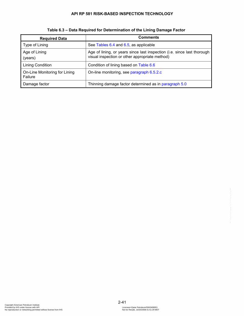
API RP 581 RISK-BASED INSPECTION TECHNOLOGY
Table 6.3 – Data Required for Determination of the Lining Damage Factor
Required Data Comments
Type of Lining See Tables 6.4 and 6.5, as applicable
Age of Lining (years)
Age of lining, or years since last inspection (i.e. since last thorough visual inspection or other appropriate method)
Lining Condition Condition of lining based on Table 6.6
On-Line Monitoring for Lining Failure
On-line monitoring, see paragraph 6.5.2.c
Damage factor Thinning damage factor determined as in paragraph 5.0
2-41 Copyright American Petroleum Institute Provided by IHS under license with API Licensee=Qatar Petroleum/5943408001
Not for Resale, 10/20/2008 01:51:29 MDTNo reproduction or networking permitted without license from IHS
--```,`,,`,`,,`,`,,,,,,``,```,`-`-`,,`,,`,`,,`---
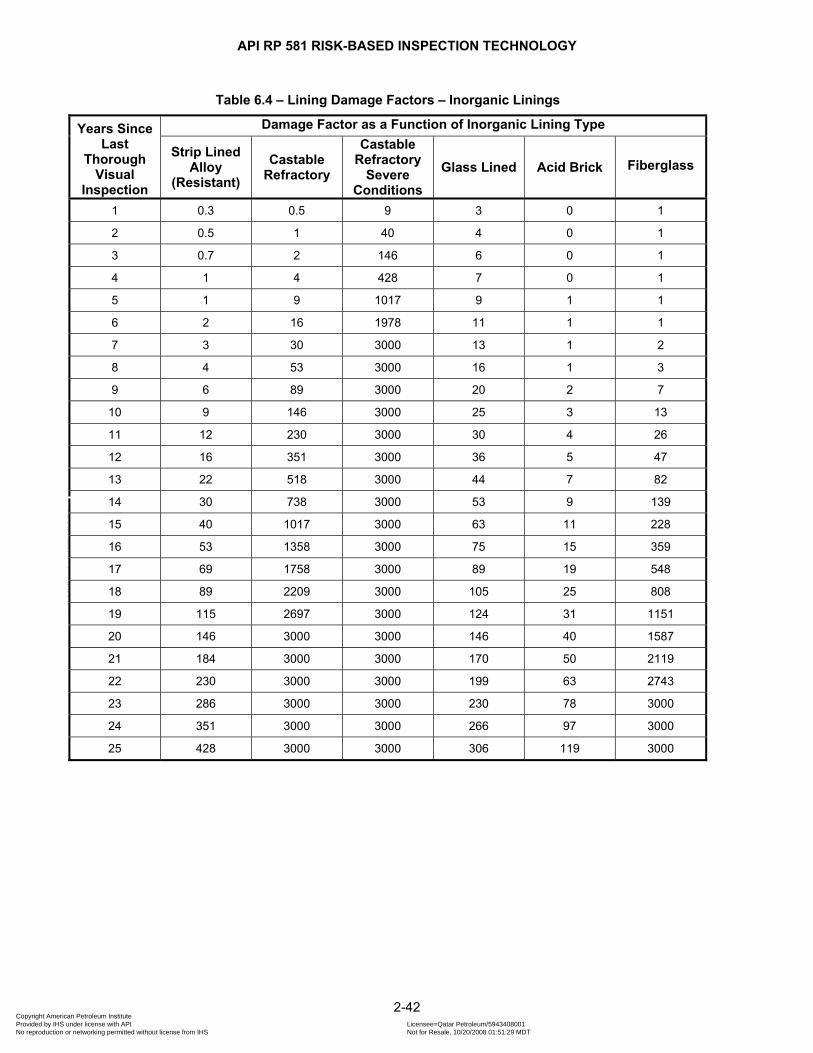
API RP 581 RISK-BASED INSPECTION TECHNOLOGY
Table 6.4 – Lining Damage Factors – Inorganic Linings
Years Since Last
Thorough Visual
Inspection
Damage Factor as a Function of Inorganic Lining Type
Strip Lined Alloy
(Resistant) Castable
Refractory
Castable Refractory
Severe Conditions
Glass Lined Acid Brick Fiberglass
1 0.3 0.5 9 3 0 1
2 0.5 1 40 4 0 1
3 0.7 2 146 6 0 1
4 1 4 428 7 0 1
5 1 9 1017 9 1 1
6 2 16 1978 11 1 1
7 3 30 3000 13 1 2
8 4 53 3000 16 1 3
9 6 89 3000 20 2 7
10 9 146 3000 25 3 13
11 12 230 3000 30 4 26
12 16 351 3000 36 5 47
13 22 518 3000 44 7 82
14 30 738 3000 53 9 139
15 40 1017 3000 63 11 228
16 53 1358 3000 75 15 359
17 69 1758 3000 89 19 548
18 89 2209 3000 105 25 808
19 115 2697 3000 124 31 1151
20 146 3000 3000 146 40 1587
21 184 3000 3000 170 50 2119
22 230 3000 3000 199 63 2743
23 286 3000 3000 230 78 3000
24 351 3000 3000 266 97 3000
25 428 3000 3000 306 119 3000
2-42 Copyright American Petroleum Institute Provided by IHS under license with API Licensee=Qatar Petroleum/5943408001
Not for Resale, 10/20/2008 01:51:29 MDTNo reproduction or networking permitted without license from IHS
--```,`,,`,`,,`,`,,,,,,``,```,`-`-`,,`,,`,`,,`---

API RP 581 RISK-BASED INSPECTION TECHNOLOGY
Table 6.5 – Lining Damage Factors – Organic Linings
Years in Service Damage Factor as a Function of Time Since the Last Inspection
Inspected More Than 6 years ago
Inspected Within Last 6 years
Inspected Within Last 3 years
1 30 1 0
2 89 4 0
3 230 16 0
4 518 53 0
5 1017 146 0.2
6 1758 351 1
7 2697 738 4
8 3000 1358 16
9 3000 2209 53
10 3000 3000 146
11 3000 3000 351
12 3000 3000 738
13 3000 3000 1358
14 3000 3000 2209
15 3000 3000 3000
16 3000 3000 3000
17 3000 3000 3000
18 3000 3000 3000
19 3000 3000 3000
20 3000 3000 3000
21 3000 3000 3000
22 3000 3000 3000
23 3000 3000 3000
24 3000 3000 3000
25 3000 3000 3000
2-43 Copyright American Petroleum Institute Provided by IHS under license with API Licensee=Qatar Petroleum/5943408001
Not for Resale, 10/20/2008 01:51:29 MDTNo reproduction or networking permitted without license from IHS
--```,`,,`,`,,`,`,,,,,,``,```,`-`-`,,`,,`,`,,`---
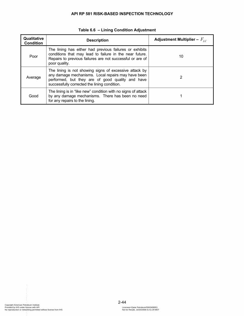
API RP 581 RISK-BASED INSPECTION TECHNOLOGY
Table 6.6 – Lining Condition Adjustment
Qualitative Condition
Description Adjustment Multiplier – LCF
Poor
The lining has either had previous failures or exhibits conditions that may lead to failure in the near future. Repairs to previous failures are not successful or are of poor quality.
10
Average
The lining is not showing signs of excessive attack by any damage mechanisms. Local repairs may have been performed, but they are of good quality and have successfully corrected the lining condition.
2
Good The lining is in “like new” condition with no signs of attack by any damage mechanisms. There has been no need for any repairs to the lining.
1
2-44 Copyright American Petroleum Institute Provided by IHS under license with API Licensee=Qatar Petroleum/5943408001
Not for Resale, 10/20/2008 01:51:29 MDTNo reproduction or networking permitted without license from IHS
--```,`,,`,`,,`,`,,,,,,``,```,`-`-`,,`,,`,`,,`---
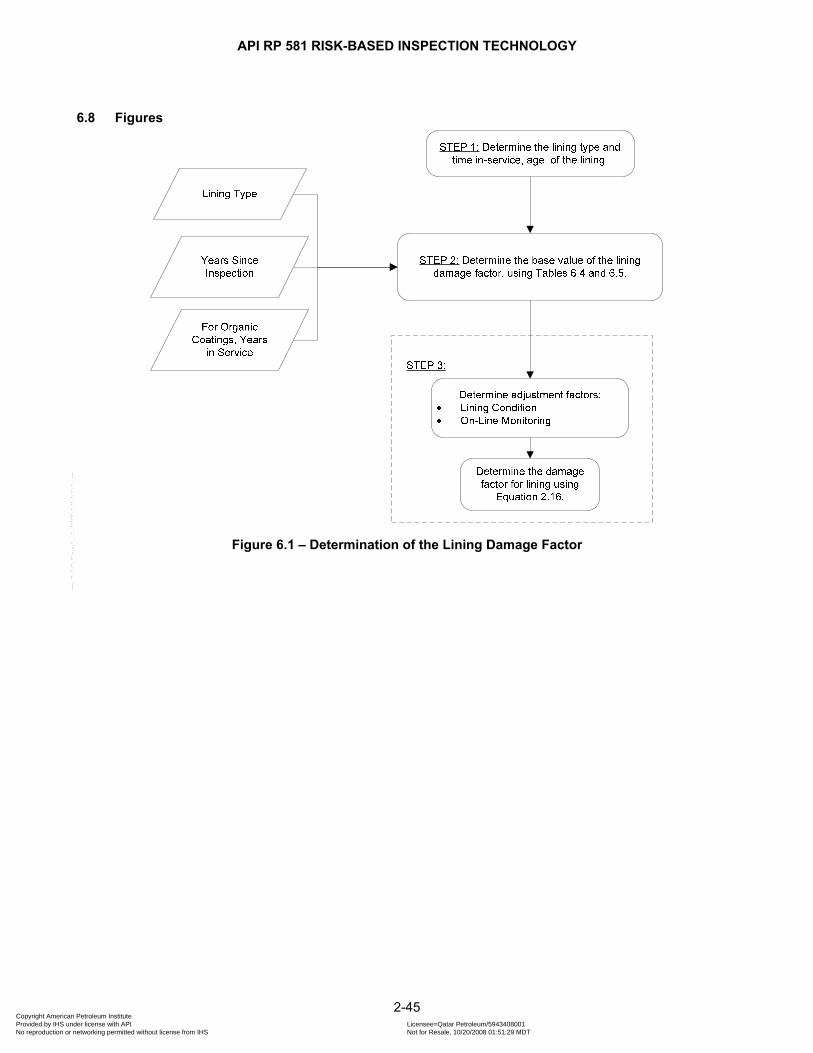
API RP 581 RISK-BASED INSPECTION TECHNOLOGY
6.8 Figures
Figure 6.1 – Determination of the Lining Damage Factor
2-45 Copyright American Petroleum Institute Provided by IHS under license with API Licensee=Qatar Petroleum/5943408001
Not for Resale, 10/20/2008 01:51:29 MDTNo reproduction or networking permitted without license from IHS
--```,`,,`,`,,`,`,,,,,,``,```,`-`-`,,`,,`,`,,`---

API RP 581 RISK-BASED INSPECTION TECHNOLOGY
7 SCC DAMAGE FACTOR – CAUSTIC CRACKING
7.1 Scope The damage factor calculation for components subject to caustic cracking is covered in this paragraph.
7.2 Description of Damage Caustic cracking is defined as cracking of a metal under the combined action of tensile stress and corrosion in the presence of sodium hydroxide (NaOH) at elevated temperature. The cracking is predominantly intergranular in nature, and typically occurs as a network of fine cracks in carbon steels. Low alloy ferritic steels have similar cracking susceptibility. There are three key parameters that determine susceptibility of steel fabrications to caustic cracking. They are caustic concentration, metal temperature, and level of tensile stress. Industry experience indicates that some caustic cracking failures occur in a few days, while many require prolonged exposure of one or more years. Increasing the caustic concentration or metal temperature accelerates the cracking rate. The susceptibility to caustic cracking of carbon steel is shown in Figures 7.1 and 7.1M (Metric). Caustic cracking of carbon steel is not anticipated at metal temperatures less than about 46°C [115°F]. In the 46°C to 82°C [115°F to 180°F] range, cracking susceptibility is a function of the caustic concentration. Above 82°C [180°F], cracking susceptibility is a function of the caustic concentration. Above 82°C [180°F] cracking is highly likely for all concentrations above about 5 wt %. Although cracking susceptibility is significantly lower in caustic solutions with less than 5% concentration, presence of high temperatures (approaching boiling) can cause locally higher concentrations which would increase cracking susceptibility. Notable case histories of this phenomenon include caustic cracking of distillation columns when caustic is added to the column for pH control, and caustic cracking of boiler feedwater components or piping bolts when gasket leaks expose the bolts to feedwater. With regard to temperature, the key consideration is the actual metal temperature, and not just the normal process temperature. There are many case histories of caustic cracking of components operating at ambient temperature that were heat traced or subject to a steam out while still containing caustic. As-welded or as-bent carbon and low alloy steel assemblies are susceptible to caustic cracking because of the high level of residual stress remaining after fabrication by these methods. Application of a post-fabrication stress-relieving heat treatment (e.g. postweld heat treatment) is a proven method of preventing caustic cracking. A heat treatment of about 621°C [1150°F] for one hour per inch of thickness (one hour minimum) is considered an effective stress-relieving heat treatment to prevent caustic cracking of carbon steel.
7.3 Screening Criteria If the component’s material of construction is carbon or low alloy steel and the process environment contains caustic in any concentration, then the component should be evaluated for susceptibility to caustic cracking.
7.4 Required Data The basic component data required for analysis is given in Table 5.1 and the specific data required for determination of the caustic cracking damage factor is provided in Table 7.1.
7.5 Basic Assumptions The main assumption in determining the damage factor for caustic cracking is that the damage can be characterized by a susceptibility parameter that is designated as high, medium, or low based on process environment, material of construction, and component fabrication variables (i.e. heat treatment). Based on a susceptibility, a Severity Index can be determined that is a measure of the susceptibility of the component cracking (or the probability of initiating cracks) and the probability of a crack resulting in a leak. If cracking is detected in the component during an inspection, the susceptibility is designated as High, and this will result in the maximum value for the Severity Index. Cracks or arrays of cracks that are found during an inspection should be evaluated using Fitness-For-Service methods in API 579 [10].
2-46 Copyright American Petroleum Institute Provided by IHS under license with API Licensee=Qatar Petroleum/5943408001
Not for Resale, 10/20/2008 01:51:29 MDTNo reproduction or networking permitted without license from IHS
--```,`,,`,`,,`,`,,,,,,``,```,`-`-`,,`,,`,`,,`---

API RP 581 RISK-BASED INSPECTION TECHNOLOGY
7.6 Determination of the Damage Factor
7.6.1 Overview A flow chart of the steps required to determine the damage factor for caustic cracking is shown in Figure 7.2. The following paragraphs provide additional information and the calculation procedure.
7.6.2 Inspection Effectiveness Inspections are ranked according to their expected effectiveness at detecting caustic cracking and correctly predicting the rate of damage. Examples of inspection activities for caustic cracking that are both intrusive (requires entry into the equipment) and non-intrusive (can be performed externally), are provided in Table 7.2. The effectiveness of each inspection performed within the designated time period must be characterized in accordance with Table 7.2. The number and category of the highest effective inspection will be used to determine the damage factor. If multiple inspections of a lower effectiveness have been conducted during the designated time period, they can be equated to an equivalent higher effectiveness inspection in accordance with paragraph 4.4.3.
7.6.3 Calculation of the Damage Factor The following procedure may be used to determine the damage factor for caustic cracking, see Figure 7.2. a) STEP 1 – Determine the number of inspections, and the corresponding inspection effectiveness category
using paragraph 7.6.2 for all past inspections. Combine the inspections to the highest effectiveness performed using paragraph 4.4.3.
b) STEP 2 – Determine the time in-service, , since the last Level A, B, C or D inspection was performed. agec) STEP 3 – Determine the susceptibility for cracking using Figure 7.2. Note that a HIGH susceptibility should
be used if cracking is known to be present.
d) STEP 4 – Based on the susceptibility in STEP 3, determine the severity index, , from VIS Table 7.3.
e) STEP 5 – Determine the base damage factor for caustic cracking, , using causticfBD Table 7.4 based on the
number of, and the highest inspection effectiveness determined in STEP 1, and the severity index, , from STEP 4.
VIS
f) STEP 6 – Calculate the escalation in the damage factor based on the time in-service since the last inspection using the from STEP 2 and Equation (age 2.17). In this equation, it is assumed that the probability for cracking will increase with time since the last inspection as a result of increased exposure to upset conditions and other non-normal conditions.
( )1.1caustic causticf fBD D age= (2.17)
2-47 Copyright American Petroleum Institute Provided by IHS under license with API Licensee=Qatar Petroleum/5943408001
Not for Resale, 10/20/2008 01:51:29 MDTNo reproduction or networking permitted without license from IHS
--```,`,,`,`,,`,`,,,,,,``,```,`-`-`,,`,,`,`,,`---
API RP 581 RISK-BASED INSPECTION TECHNOLOGY
7.7 Nomenclature age is the in-service time since the last inspection
causticfDF is the damage factor for caustic cracking causticfBDF is the base value of the damage factor for caustic cracking
VIS is the severity index
7.8 References 19. Corrosion Data Survey—Metals Section, NACE International, Houston, TX, Fifth Edition (March 1974), p.
274. 20. NACE-5, Stress Corrosion Cracking of Hydrogen Embrittlement of Iron Base Alloys, Edited by R.W.
Staehle, et. al., NACE International, Houston, TX, 1977, pp. 583-587. 21. P. Gegner, “Corrosion Resistance of Materials in Alkalies and Hypochlorites,” Process Industries Corrosion,
NACE International, Houston TX, 1975, pp. 296-305. 22. J. K. Nelson, “Materials of Construction for Alkalies and Hypochlorites,” Process Industries Corrosion—The
Theory and Practice, NACE International, Houston, TX, 1986, pp. 297-310.
2-48 Copyright American Petroleum Institute Provided by IHS under license with API Licensee=Qatar Petroleum/5943408001
Not for Resale, 10/20/2008 01:51:29 MDTNo reproduction or networking permitted without license from IHS
--```,`,,`,`,,`,`,,,,,,``,```,`-`-`,,`,,`,`,,`---

API RP 581 RISK-BASED INSPECTION TECHNOLOGY
7.9 Tables
Table 7.1 – Data Required for Determination of the Damage Factor – Caustic Cracking
Required Data Comments
Susceptibility (Low, Medium, High)
The susceptibility is determined by expert advice or using the procedures in this paragraph.
NaOH Concentration (%) Determine the concentration of the caustic solution being handled in this component. Take into account whether heating or flashing of water produces higher concentration.
Maximum Process Temperature, °C [°F]
Determine the maximum process temperature in this component. Consider local heating due to mixing if at a caustic injection point.
Steam out? (Yes or No)
Determine whether the component has been steamed out prior to water flushing to remove residual caustic.
Time since last SCC inspection (years)
Use inspection history to determine years since the last SCC inspection.
Inspection Effectiveness Category
The effectiveness category that has been performed on the component.
On-Line Monitoring (Hydrogen Probes, Process Variables, or Combination)
The type of proactive corrosion monitoring methods or tools employed, such as hydrogen probes and/or process variable monitoring.
Number of Inspections The number of inspections in each effectiveness category that have been performed.
2-49 Copyright American Petroleum Institute Provided by IHS under license with API Licensee=Qatar Petroleum/5943408001
Not for Resale, 10/20/2008 01:51:29 MDTNo reproduction or networking permitted without license from IHS
--```,`,,`,`,,`,`,,,,,,``,```,`-`-`,,`,,`,`,,`---
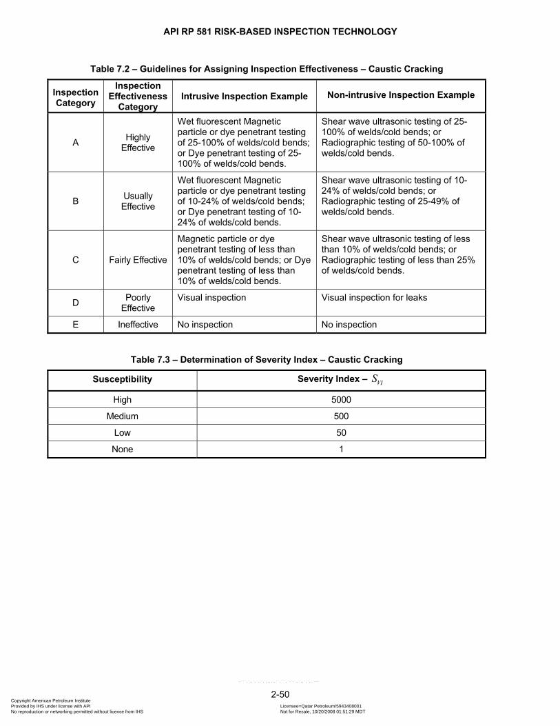
API RP 581 RISK-BASED INSPECTION TECHNOLOGY
Table 7.2 – Guidelines for Assigning Inspection Effectiveness – Caustic Cracking
Inspection Category
Inspection Effectiveness
Category Intrusive Inspection Example Non-intrusive Inspection Example
A Highly Effective
Wet fluorescent Magnetic particle or dye penetrant testing of 25-100% of welds/cold bends; or Dye penetrant testing of 25-100% of welds/cold bends.
Shear wave ultrasonic testing of 25-100% of welds/cold bends; or Radiographic testing of 50-100% of welds/cold bends.
B Usually Effective
Wet fluorescent Magnetic particle or dye penetrant testing of 10-24% of welds/cold bends; or Dye penetrant testing of 10-24% of welds/cold bends.
Shear wave ultrasonic testing of 10-24% of welds/cold bends; or Radiographic testing of 25-49% of welds/cold bends.
C Fairly Effective
Magnetic particle or dye penetrant testing of less than 10% of welds/cold bends; or Dye penetrant testing of less than 10% of welds/cold bends.
Shear wave ultrasonic testing of less than 10% of welds/cold bends; or Radiographic testing of less than 25% of welds/cold bends.
D Poorly Effective
Visual inspection Visual inspection for leaks
E Ineffective No inspection No inspection
Table 7.3 – Determination of Severity Index – Caustic Cracking
Susceptibility Severity Index – VIS
High 5000
Medium 500
Low 50
None 1
2-50 Copyright American Petroleum Institute Provided by IHS under license with API Licensee=Qatar Petroleum/5943408001
Not for Resale, 10/20/2008 01:51:29 MDTNo reproduction or networking permitted without license from IHS
--```,`,,`,`,,`,`,,,,,,``,```,`-`-`,,`,,`,`,,`---
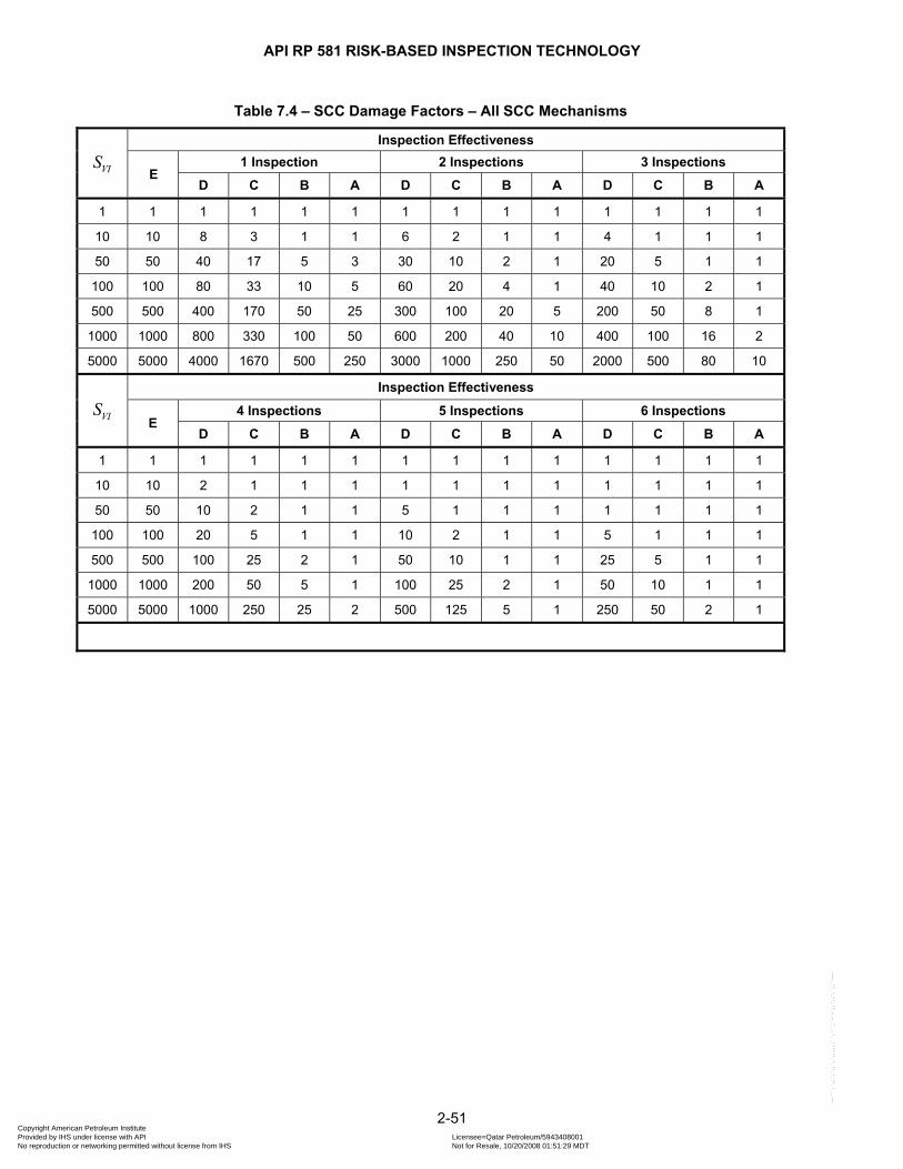
API RP 581 RISK-BASED INSPECTION TECHNOLOGY
Table 7.4 – SCC Damage Factors – All SCC Mechanisms
VIS
Inspection Effectiveness
E 1 Inspection 2 Inspections 3 Inspections
D C B A D C B A D C B A
1 1 1 1 1 1 1 1 1 1 1 1 1 1
10 10 8 3 1 1 6 2 1 1 4 1 1 1
50 50 40 17 5 3 30 10 2 1 20 5 1 1
100 100 80 33 10 5 60 20 4 1 40 10 2 1
500 500 400 170 50 25 300 100 20 5 200 50 8 1
1000 1000 800 330 100 50 600 200 40 10 400 100 16 2
5000 5000 4000 1670 500 250 3000 1000 250 50 2000 500 80 10
VIS
Inspection Effectiveness
E 4 Inspections 5 Inspections 6 Inspections
D C B A D C B A D C B A
1 1 1 1 1 1 1 1 1 1 1 1 1 1
10 10 2 1 1 1 1 1 1 1 1 1 1 1
50 50 10 2 1 1 5 1 1 1 1 1 1 1
100 100 20 5 1 1 10 2 1 1 5 1 1 1
500 500 100 25 2 1 50 10 1 1 25 5 1 1
1000 1000 200 50 5 1 100 25 2 1 50 10 1 1
5000 5000 1000 250 25 2 500 125 5 1 250 50 2 1
2-51 Copyright American Petroleum Institute Provided by IHS under license with API Licensee=Qatar Petroleum/5943408001
Not for Resale, 10/20/2008 01:51:29 MDTNo reproduction or networking permitted without license from IHS
--```,`,,`,`,,`,`,,,,,,``,```,`-`-`,,`,,`,`,,`---

API RP 581 RISK-BASED INSPECTION TECHNOLOGY
7.10 Figures
Concentration NAOH, % By Weight
0 10 20 30 40 50
Tem
pera
ture
, F
0
20
40
60
80
100
120
140
160
180
200
220
240
260
280
Application of Nickel Alloys to Be Considered in This Area
Area 'B'
Carbon SteelStress Relieve Welds & Bends
Area 'A'
Carbon SteelNo Stress Relief Necessary
Area 'C'
Nickel Alloy Trim for ValvesIn Areas 'B' & 'C'
Figure 7.1 – Susceptibility of Caustic Cracking in Carbon Steel
2-52 Copyright American Petroleum Institute Provided by IHS under license with API Licensee=Qatar Petroleum/5943408001
Not for Resale, 10/20/2008 01:51:29 MDTNo reproduction or networking permitted without license from IHS
--```,`,,`,`,,`,`,,,,,,``,```,`-`-`,,`,,`,`,,`---
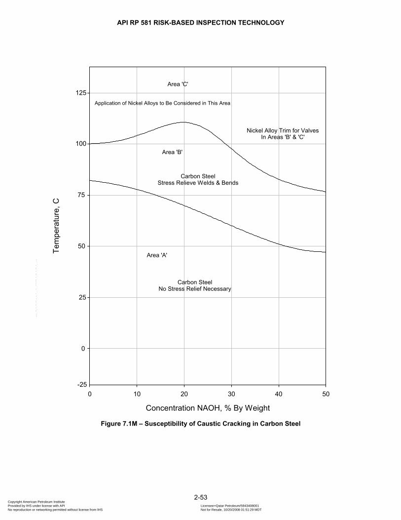
API RP 581 RISK-BASED INSPECTION TECHNOLOGY
Concentration NAOH, % By Weight
0 10 20 30 40 50
Tem
pera
ture
, C
Application of Nickel Alloys to Be Considered in This Area
Area 'B'
Carbon SteelStress Relieve Welds & Bends
Area 'A'
Carbon SteelNo Stress Relief Necessary
Area 'C'
Nickel Alloy Trim for ValvesIn Areas 'B' & 'C'
0
25
50
75
100
125
-25
Figure 7.1M – Susceptibility of Caustic Cracking in Carbon Steel
2-53 Copyright American Petroleum Institute Provided by IHS under license with API Licensee=Qatar Petroleum/5943408001
Not for Resale, 10/20/2008 01:51:29 MDTNo reproduction or networking permitted without license from IHS
--```,`,,`,`,,`,`,,,,,,``,```,`-`-`,,`,,`,`,,`---

API RP 581 RISK-BASED INSPECTION TECHNOLOGY
Figure 7.2 – Determination of the Caustic Cracking Damage Factor
2-54 Copyright American Petroleum Institute Provided by IHS under license with API Licensee=Qatar Petroleum/5943408001
Not for Resale, 10/20/2008 01:51:29 MDTNo reproduction or networking permitted without license from IHS
--```,`,,`,`,,`,`,,,,,,``,```,`-`-`,,`,,`,`,,`---

API RP 581 RISK-BASED INSPECTION TECHNOLOGY
8 SCC DAMAGE FACTOR – AMINE CRACKING
8.1 Scope The damage factor calculation for components subject to amine cracking is covered in this paragraph.
8.2 Description of Damage Amine cracking is defined as cracking of a metal under the combined action of tensile stress and corrosion in the presence of an aqueous alkanolamine solution at elevated temperature. The cracking is predominately intergranular in nature, and typically occurs in carbon steels as a network of very fine, corrosion product filled cracks. Low alloy ferritic steels are also susceptible to amine cracking. Amine cracking is typically observed in amine treating units which use aqueous alkanolamine solutions for removal of acid gases such as H2S and CO2 from various gas or liquid hydrocarbon streams. Four available parameters are used to assess the susceptibility of steel fabrications to amine cracking. They are the type of amine, amine solution composition, metal temperature, and level of tensile stress. Results of a NACE survey indicate that amine cracking is most prevalent in monoethanolamine (MEA) and disopropanolamine (DIPA) units, and to a somewhat lesser extent in diethanolamine (DEA) units. Cracking is much less prevalent in methyldiethanolamine (MDEA), Sulfinol, and diglycolamine (DGA) units. Studies have concluded that the cracking occurs in a narrow range of electrochemical potential, which is very dependent upon the amine solution composition. Carbonate is a critical solution contaminant, and other contaminants such as chlorides, cyanides, etc. have been shown to affect cracking susceptibility. Despite this mechanistic understanding, the electrochemical potential of in-service components may not be readily available. Amine concentration is a factor in cracking susceptibility in MEA solutions, where cracking susceptibility has been shown to be higher in the 15 to 35% concentration range. There is not sufficient understanding of this relationship in other amine solutions, but it is noteworthy that cracking susceptibility is lower in MDEA and Sulfinol units which typically utilize higher concentration amine solutions. With regard to the amine solution composition, cracking typically occurs in the lean alkanolamine solution which is alkaline and contains very low levels of acid gases. Amine cracking does not occur in fresh amine solutions, i.e., those that have not been exposed to acid gases. Amine cracking is not likely to occur in rich alkanolamine solutions, which contain high levels of acid gases. In rich amine solutions, other forms of cracking are far more prevalent. Amine cracking susceptibility is generally higher at elevated temperatures. A key consideration is the actual metal temperature, and not just the normal process temperature. Cracking has occurred in components that normally operate at low temperatures but were heat traced or steamed out prior to water washing to remove residual amine solution. As-welded or cold worked carbon and low alloy steel fabrications are susceptible to amine cracking because of the high level of residual stress remaining after fabrication by these methods. Application of a post-fabrication stress-relieving heat treatment (e.g., postweld heat treatment) is a proven method of preventing amine cracking. A heat treatment of about 621°C [1150°F] for one hour per inch of thickness (one hour minimum) is considered an effective stress-relieving heat treatment to prevent amine cracking of carbon steel. It should be noted that other forms of cracking have been reported in amine units. In most cases, cracking occurred in components exposed to rich alkanolamine solutions and have typically been forms of hydrogen damage such as sulfide stress cracking (SSC), hydrogen-induced cracking (HIC), and stress-oriented hydrogen-induced cracking (SOHIC). These are not included here, but are dealt with in other paragraphs of this Part.
8.3 Screening Criteria If the component’s material of construction is carbon or low alloy steel and the process environment contains acid gas treating amines (MEA, DEA, DIPA, MDEA, etc.) in any concentration, then the component should be evaluated for susceptibility to Amine cracking.
2-55 Copyright American Petroleum Institute Provided by IHS under license with API Licensee=Qatar Petroleum/5943408001
Not for Resale, 10/20/2008 01:51:29 MDTNo reproduction or networking permitted without license from IHS
--```,`,,`,`,,`,`,,,,,,``,```,`-`-`,,`,,`,`,,`---
API RP 581 RISK-BASED INSPECTION TECHNOLOGY
8.4 Required Data The basic component data required for analysis is given in Table 5.1 and the specific data required for determination of the amine cracking damage factor is provided in Table 8.1.
8.5 Basic Assumptions The main assumption in determining the damage factor for amine cracking is that the damage can be characterized by a susceptibility parameter that is designated as high, medium, or low based on process environment, material of construction, and component fabrication variables (i.e. heat treatment). Based on a susceptibility, a Severity Index can be determined that a measure of the susceptibility of the component cracking (or the probability of initiating cracks) and the probability of a crack resulting in a leak. If cracking is detected in the component during an inspection, the susceptibility is designated as High, and this will result in the maximum value for the Severity Index. Cracks or arrays of cracks that are found during an inspection should be evaluated using Fitness-For-Service methods in API 579 [10].
8.6 Determination of the Damage Factor
8.6.1 Overview A flow chart of the steps required to determine the damage factor for amine cracking is shown in Figure 8.1. The following paragraphs provide additional information and the calculation procedure.
8.6.2 Inspection Effectiveness Inspections are ranked according to their expected effectiveness at detecting amine cracking and correctly predicting the rate of damage. Examples of inspection activities for Amine cracking that are both intrusive (requires entry into the equipment) and non-intrusive (can be performed externally), are provided in Table 8.2. The effectiveness of each inspection performed within the designated time period must be characterized in accordance with Table 8.2. The number and category of the highest effective inspection will be used to determine the damage factor. If multiple inspections of a lower effectiveness have been conducted during the designated time period, they can be equated to an equivalent higher effectiveness inspection in accordance with paragraph 4.4.3.
8.6.3 Calculation of the Damage Factor The following procedure may be used to determine the damage factor for amine cracking, see Figure 8.1. a) STEP 1 – Determine the number of inspections, and the corresponding inspection effectiveness category
using paragraph 8.6.2 for all past inspections. Combine the inspections to the highest effectiveness performed using paragraph 4.4.3..
b) STEP 2 – Determine the time in-service, , since the last Level A, B, C or D inspection was performed. agec) STEP 3 – Determine the susceptibility for cracking using Figure 8.1. Note that a HIGH susceptibility should
be used if cracking is known to be present.
d) STEP 4 – Based on the susceptibility in STEP 3, determine the severity index, , from VIS Table 8.3.
e) STEP 5 – Determine the base damage factor for amine cracking, , using aminefBD Table 7.4 based on the
number of, and the highest inspection effectiveness determined in STEP 1, and the severity index, , from STEP 4.
VIS
f) STEP 6 – Calculate the escalation in the damage factor based on the time in-service since the last inspection using the from STEP 2 and Equation (age 2.18). In this equation, it is assumed that the probability for cracking will increase with time since the last inspection as a result of increased exposure to upset conditions and other non-normal conditions.
( )1.1amine aminef fBD D age= (2.18)
2-56 Copyright American Petroleum Institute Provided by IHS under license with API Licensee=Qatar Petroleum/5943408001
Not for Resale, 10/20/2008 01:51:29 MDTNo reproduction or networking permitted without license from IHS
--```,`,,`,`,,`,`,,,,,,``,```,`-`-`,,`,,`,`,,`---
API RP 581 RISK-BASED INSPECTION TECHNOLOGY
8.7 Nomenclature age is the in-service time since the last Level A, B, C or D inspection was performed
aminefD is the damage factor for amine cracking aminefBD is the base value of the damage factor for amine cracking
VIS is the severity index
8.8 References 23. API, API RP 945 Avoiding Environmental Cracking in Amine Units, 1st Edition, American Petroleum
Institute, Washington, D.C., 20005, August 1990. 24. Richert, Bagdasarian, and Shargay, “Stress Corrosion Cracking of Carbon Steel in Amine Systems,” NACE
paper #187, Corrosion/'87 (see also “Extent of Stress Corrosion Cracking in Amine Plants Revealed by Survey”, Oil & Gas Journal, June 5, 1989).
25. Parkins and Foroulis, “The Stress Corrosion Cracking of Mild Steel in Monoethanolamine Solutions,” NACE paper #188, Corrosion/87 (see also Materials Performance 25, 10 (1986), pp. 20-27).
26. Lenhart, Craig, and Howell, “Diethanolamine SCC of Mild Steel,” NACE paper #212, Corrosion/86. 27. Gutzeit and Johnson, “Stress Corrosion Cracking of Carbon Steel Welds in Amine Service,” NACE paper
#206, Corrosion/86. 28. Schutt, HU, “New Aspects of Stress Corrosion Cracking in Monoethanolamine Solutions,” NACE paper
#159, Corrosion/88 (see also Materials Performance 27, 12 (1988), pp. 53-58). 29. Bagdasarian, Shargay and Coombs, “Stress Corrosion Cracking of Carbon Steel in DEA and ADIP
Solutions,” Materials Performance 30, 5 (1991), pp. 63-67 (see also Oil & Gas Journal, Jan. 13, 1992, pp. 42-44).
2-57 Copyright American Petroleum Institute Provided by IHS under license with API Licensee=Qatar Petroleum/5943408001
Not for Resale, 10/20/2008 01:51:29 MDTNo reproduction or networking permitted without license from IHS
--```,`,,`,`,,`,`,,,,,,``,```,`-`-`,,`,,`,`,,`---

API RP 581 RISK-BASED INSPECTION TECHNOLOGY
8.9 Tables
Table 8.1 – Data Required for Determination of the Damage Factor – Amine Cracking
Required Data Comments
Susceptibility (Low, Medium, High)
The susceptibility is determined by expert advice or using the procedures in this paragraph.
Amine Solution Composition Determine what amine solution composition is being handled in this component. Fresh amine has not been exposed to H2S or CO2. Lean amine contains low levels of H2S or CO2. Rich amine contains high levels of H2S or CO2. For components exposed to both lean and rich amine solutions (i.e., amine contactors and regenerators), indicate lean.
Maximum Process Temperature, °C [°F] Determine the maximum process temperature in this component.
Steam out? (Yes or No)
Determine whether the component has been steamed out prior to water flushing to remove residual amine.
Age (years)
Use inspection history to determine the time since the last SCC inspection.
Inspection Effectiveness Category
The effectiveness category that has been performed on the component.
Number of Inspections The number of inspections in each effectiveness category that have been performed.
2-58 Copyright American Petroleum Institute Provided by IHS under license with API Licensee=Qatar Petroleum/5943408001
Not for Resale, 10/20/2008 01:51:29 MDTNo reproduction or networking permitted without license from IHS
--```,`,,`,`,,`,`,,,,,,``,```,`-`-`,,`,,`,`,,`---
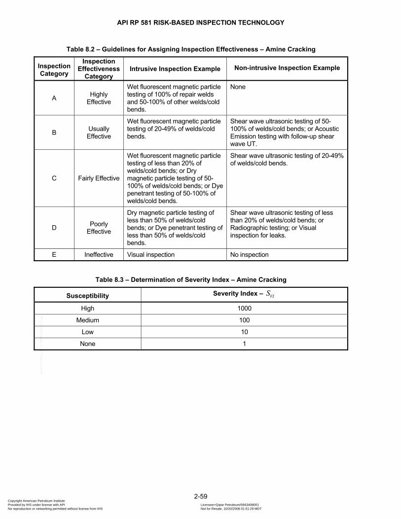
API RP 581 RISK-BASED INSPECTION TECHNOLOGY
Table 8.2 – Guidelines for Assigning Inspection Effectiveness – Amine Cracking
Inspection Category
Inspection Effectiveness
Category Intrusive Inspection Example Non-intrusive Inspection Example
A Highly Effective
Wet fluorescent magnetic particle testing of 100% of repair welds and 50-100% of other welds/cold bends.
None
B Usually Effective
Wet fluorescent magnetic particle testing of 20-49% of welds/cold bends.
Shear wave ultrasonic testing of 50-100% of welds/cold bends; or Acoustic Emission testing with follow-up shear wave UT.
C Fairly Effective
Wet fluorescent magnetic particle testing of less than 20% of welds/cold bends; or Dry magnetic particle testing of 50-100% of welds/cold bends; or Dye penetrant testing of 50-100% of welds/cold bends.
Shear wave ultrasonic testing of 20-49% of welds/cold bends.
D Poorly Effective
Dry magnetic particle testing of less than 50% of welds/cold bends; or Dye penetrant testing of less than 50% of welds/cold bends.
Shear wave ultrasonic testing of less than 20% of welds/cold bends; or Radiographic testing; or Visual inspection for leaks.
E Ineffective Visual inspection No inspection
Table 8.3 – Determination of Severity Index – Amine Cracking
Susceptibility Severity Index – VIS
High 1000
Medium 100
Low 10
None 1
2-59 Copyright American Petroleum Institute Provided by IHS under license with API Licensee=Qatar Petroleum/5943408001
Not for Resale, 10/20/2008 01:51:29 MDTNo reproduction or networking permitted without license from IHS
--```,`,,`,`,,`,`,,,,,,``,```,`-`-`,,`,,`,`,,`---
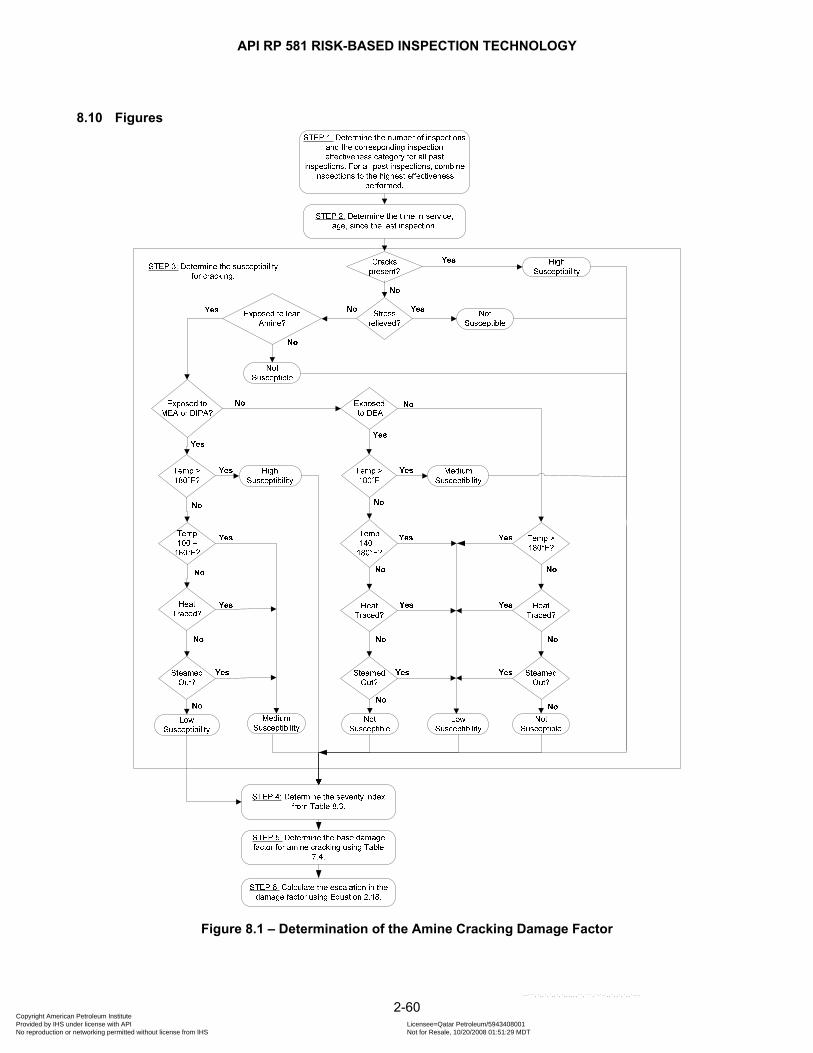
API RP 581 RISK-BASED INSPECTION TECHNOLOGY
8.10 Figures
Figure 8.1 – Determination of the Amine Cracking Damage Factor
2-60 Copyright American Petroleum Institute Provided by IHS under license with API Licensee=Qatar Petroleum/5943408001
Not for Resale, 10/20/2008 01:51:29 MDTNo reproduction or networking permitted without license from IHS
--```,`,,`,`,,`,`,,,,,,``,```,`-`-`,,`,,`,`,,`---
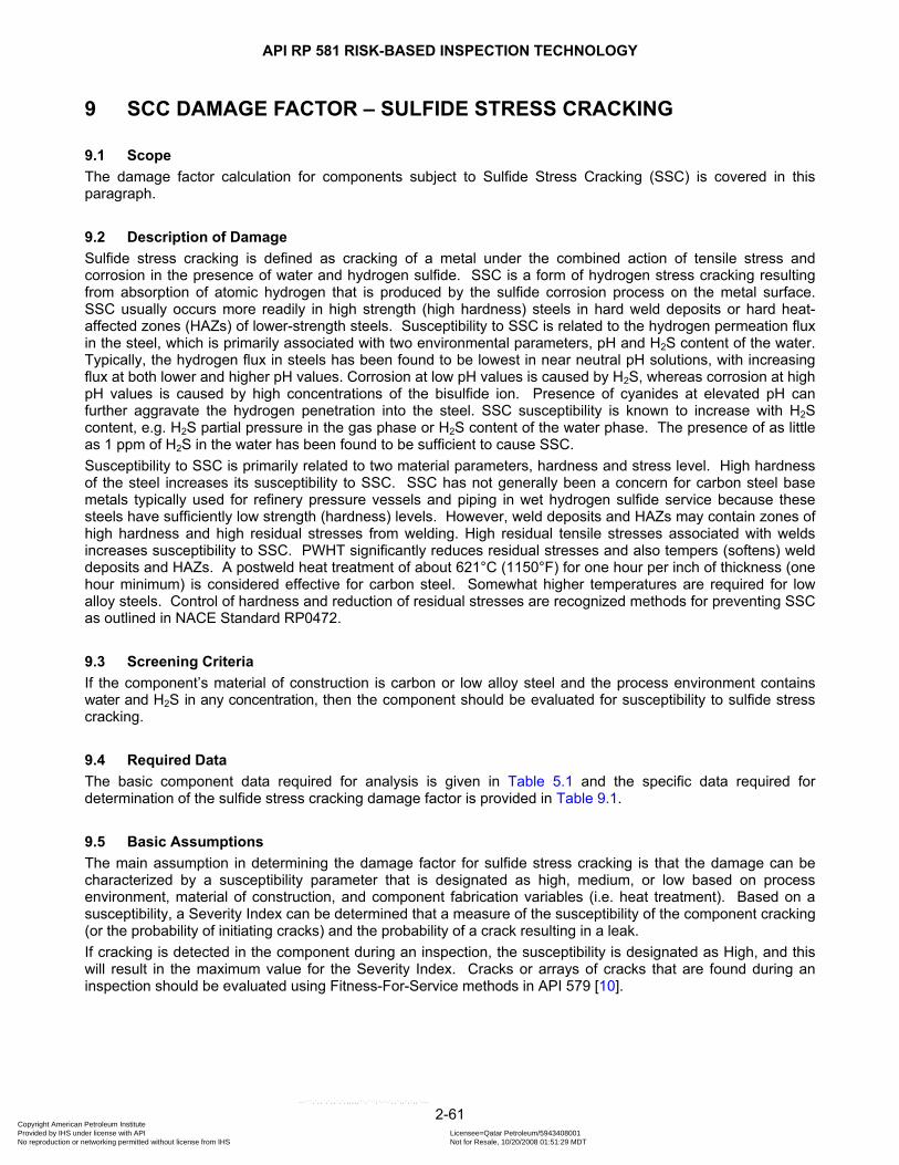
API RP 581 RISK-BASED INSPECTION TECHNOLOGY
9 SCC DAMAGE FACTOR – SULFIDE STRESS CRACKING
9.1 Scope The damage factor calculation for components subject to Sulfide Stress Cracking (SSC) is covered in this paragraph.
9.2 Description of Damage Sulfide stress cracking is defined as cracking of a metal under the combined action of tensile stress and corrosion in the presence of water and hydrogen sulfide. SSC is a form of hydrogen stress cracking resulting from absorption of atomic hydrogen that is produced by the sulfide corrosion process on the metal surface. SSC usually occurs more readily in high strength (high hardness) steels in hard weld deposits or hard heat-affected zones (HAZs) of lower-strength steels. Susceptibility to SSC is related to the hydrogen permeation flux in the steel, which is primarily associated with two environmental parameters, pH and H2S content of the water. Typically, the hydrogen flux in steels has been found to be lowest in near neutral pH solutions, with increasing flux at both lower and higher pH values. Corrosion at low pH values is caused by H2S, whereas corrosion at high pH values is caused by high concentrations of the bisulfide ion. Presence of cyanides at elevated pH can further aggravate the hydrogen penetration into the steel. SSC susceptibility is known to increase with H2S content, e.g. H2S partial pressure in the gas phase or H2S content of the water phase. The presence of as little as 1 ppm of H2S in the water has been found to be sufficient to cause SSC. Susceptibility to SSC is primarily related to two material parameters, hardness and stress level. High hardness of the steel increases its susceptibility to SSC. SSC has not generally been a concern for carbon steel base metals typically used for refinery pressure vessels and piping in wet hydrogen sulfide service because these steels have sufficiently low strength (hardness) levels. However, weld deposits and HAZs may contain zones of high hardness and high residual stresses from welding. High residual tensile stresses associated with welds increases susceptibility to SSC. PWHT significantly reduces residual stresses and also tempers (softens) weld deposits and HAZs. A postweld heat treatment of about 621°C (1150°F) for one hour per inch of thickness (one hour minimum) is considered effective for carbon steel. Somewhat higher temperatures are required for low alloy steels. Control of hardness and reduction of residual stresses are recognized methods for preventing SSC as outlined in NACE Standard RP0472.
9.3 Screening Criteria If the component’s material of construction is carbon or low alloy steel and the process environment contains water and H2S in any concentration, then the component should be evaluated for susceptibility to sulfide stress cracking.
9.4 Required Data The basic component data required for analysis is given in Table 5.1 and the specific data required for determination of the sulfide stress cracking damage factor is provided in Table 9.1.
9.5 Basic Assumptions The main assumption in determining the damage factor for sulfide stress cracking is that the damage can be characterized by a susceptibility parameter that is designated as high, medium, or low based on process environment, material of construction, and component fabrication variables (i.e. heat treatment). Based on a susceptibility, a Severity Index can be determined that a measure of the susceptibility of the component cracking (or the probability of initiating cracks) and the probability of a crack resulting in a leak. If cracking is detected in the component during an inspection, the susceptibility is designated as High, and this will result in the maximum value for the Severity Index. Cracks or arrays of cracks that are found during an inspection should be evaluated using Fitness-For-Service methods in API 579 [10].
2-61 Copyright American Petroleum Institute Provided by IHS under license with API Licensee=Qatar Petroleum/5943408001
Not for Resale, 10/20/2008 01:51:29 MDTNo reproduction or networking permitted without license from IHS
--```,`,,`,`,,`,`,,,,,,``,```,`-`-`,,`,,`,`,,`---

API RP 581 RISK-BASED INSPECTION TECHNOLOGY
9.6 Determination of the Damage Factor
9.6.1 Overview A flow chart of the steps required to determine the damage factor for sulfide stress cracking is shown in Figure 9.1. The following paragraphs provide additional information and the calculation procedure.
9.6.2 Inspection Effectiveness Inspections are ranked according to their expected effectiveness at detecting sulfide stress cracking and correctly predicting the rate of damage. Examples of inspection activities for sulfide stress cracking that are both intrusive (requires entry into the equipment) and non-intrusive (can be performed externally), are provided in Table 9.2. The effectiveness of each inspection performed within the designated time period must be characterized in accordance with Table 9.2 The number and category of the highest effective inspection will be used to determine the damage factor. If multiple inspections of a lower effectiveness have been conducted during the designated time period, they can be equated to an equivalent higher effectiveness inspection in accordance with paragraph 4.4.3.
9.6.3 Calculation of the Damage Factor The following procedure may be used to determine the damage factor for sulfide stress cracking, see Figure 9.1. a) STEP 1 – Determine the number of inspections, and the corresponding inspection effectiveness category
using paragraph 9.6.2 for all past inspections. Combine the inspections to the highest effectiveness performed using paragraph 4.4.3.
b) STEP 2 – Determine the time in-service, , since the last Level A, B, C or D inspection was performed. agec) STEP 3 – Determine the environmental severity (potential level of hydrogen flux) for cracking based on the
H2S content of the water and its pH using Table 9.3. Note that a HIGH environmental severity should be used if cracking is known to be present.
d) STEP 4 – Determine the susceptibility for cracking using Figure 9.1 and Table 9.4 based on the environmental severity from STEP 3, the maximum Brinnell hardness of weldments, and knowledge of whether the component was subject to PWHT.
e) STEP 5 – Based on the susceptibility in STEP 4, determine the severity index, , from VIS Table 9.5.
f) STEP 6 – Determine the base damage factor for sulfide stress cracking, sscfBD , using Table 7.4 based on
the number of, and the highest inspection effectiveness determined in STEP 1, and the severity index, , from STEP 5.
VIS
g) STEP 7 – Calculate the escalation in the damage factor based on the time in-service since the last inspection using the age from STEP 2 and Equation (2.19). In this equation, it is assumed that the probability for cracking will increase with time since the last inspection as a result of increased exposure to upset conditions and other non-normal conditions.
( )1.1ssc sscf fBD D age= (2.19)
2-62 Copyright American Petroleum Institute Provided by IHS under license with API Licensee=Qatar Petroleum/5943408001
Not for Resale, 10/20/2008 01:51:29 MDTNo reproduction or networking permitted without license from IHS
--```,`,,`,`,,`,`,,,,,,``,```,`-`-`,,`,,`,`,,`---

API RP 581 RISK-BASED INSPECTION TECHNOLOGY
9.7 Nomenclature age is the in-service time since the last Level A, B, C or D inspection was performed
sscfD is the damage factor for sulfide stress cracking sscfBD is the base value of the damage factor for sulfide stress cracking
VIS is the severity index
9.8 References 30. NACE RP0472, Methods and Controls to Prevent In-Service Cracking of Carbon Steel Welds in Corrosive
Petroleum Refining Environments, NACE International, Houston, TX 31. R. R. Petrie and E. M. Moore, Jr., “Determining the Suitability of Existing Pipelines and Producing Facilities
for Wet Sour Service,” Materials Performance 28, 6 (June 1989), pp. 59-65. 32. NACE Publication 8X294, Review of Published Literature on Wet H2S Cracking of Steels Through 1989 33. Stress Corrosion Cracking and Hydrogen Embrittlement of Iron Base Alloys, NACE-5, Edited by R. W.
Staehle, et. al., NACE International, Houston, TX, 1977, pp. 541-559. 34. C. M. Hudgins, et. al., “Hydrogen Sulfide Cracking of Carbon and Alloy Steels,” Corrosion, Vol. 22, pp. 238-
251. 35. NACE RP0296-96, Guidelines for Detection, Repair, and Mitigation of Existing Petroleum Refinery
Pressure Vessels in Wet H2S Environments, NACE International, Houston, TX.
2-63 Copyright American Petroleum Institute Provided by IHS under license with API Licensee=Qatar Petroleum/5943408001
Not for Resale, 10/20/2008 01:51:29 MDTNo reproduction or networking permitted without license from IHS
--```,`,,`,`,,`,`,,,,,,``,```,`-`-`,,`,,`,`,,`---

API RP 581 RISK-BASED INSPECTION TECHNOLOGY
9.9 Tables
Table 9.1 – Data Required for Determination of the Damage Factor – Sulfide Stress Cracking
Required Data Comments
Susceptibility (Low, Medium, High)
The susceptibility is determined by expert advice or using the procedures in this paragraph.
Presence of Water (Yes or No)
Determine whether free water is present in the component. Consider not only normal operating conditions, but also startup, shutdown, process upsets, etc.
H2S Content of Water Determine the H2S content of the water phase. If analytical results are not readily available, it can be estimated using the approach of Petrie & Moore (see Reference 17).
pH of Water Determine the pH of the water phase. If analytical results are not readily available, it should be estimated by a knowledgeable process engineer.
Presence of Cyanides (Yes or No)
Determine the presence of cyanide through sampling and/or field analysis. Consider primarily normal and upset operations but also startup and shutdown conditions.
Max Brinnell Hardness Determine the maximum Brinnell hardness actually measured at the weldments of the steel components. Report readings actually taken as Brinnell, not converted from finer techniques (e.g., Vickers, Knoop, etc.) If actual readings are not available, use the maximum allowable hardness permitted by the fabrication specification.
Age (years)
Use inspection history to determine the time since the last SCC inspection.
Inspection Effectiveness Category
The effectiveness category that has been performed on the component.
Number of Inspections The number of inspections in each effectiveness category that have been performed.
2-64 Copyright American Petroleum Institute Provided by IHS under license with API Licensee=Qatar Petroleum/5943408001
Not for Resale, 10/20/2008 01:51:29 MDTNo reproduction or networking permitted without license from IHS
--```,`,,`,`,,`,`,,,,,,``,```,`-`-`,,`,,`,`,,`---
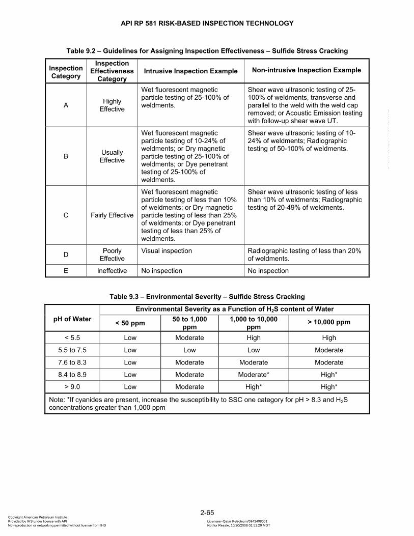
API RP 581 RISK-BASED INSPECTION TECHNOLOGY
Table 9.2 – Guidelines for Assigning Inspection Effectiveness – Sulfide Stress Cracking
Inspection Category
Inspection Effectiveness
Category Intrusive Inspection Example Non-intrusive Inspection Example
A Highly Effective
Wet fluorescent magnetic particle testing of 25-100% of weldments.
Shear wave ultrasonic testing of 25-100% of weldments, transverse and parallel to the weld with the weld cap removed; or Acoustic Emission testing with follow-up shear wave UT.
B Usually Effective
Wet fluorescent magnetic particle testing of 10-24% of weldments; or Dry magnetic particle testing of 25-100% of weldments; or Dye penetrant testing of 25-100% of weldments.
Shear wave ultrasonic testing of 10-24% of weldments; Radiographic testing of 50-100% of weldments.
C Fairly Effective
Wet fluorescent magnetic particle testing of less than 10% of weldments; or Dry magnetic particle testing of less than 25% of weldments; or Dye penetrant testing of less than 25% of weldments.
Shear wave ultrasonic testing of less than 10% of weldments; Radiographic testing of 20-49% of weldments.
D Poorly Effective
Visual inspection Radiographic testing of less than 20% of weldments.
E Ineffective No inspection No inspection
Table 9.3 – Environmental Severity – Sulfide Stress Cracking
pH of Water Environmental Severity as a Function of H2S content of Water
< 50 ppm 50 to 1,000 ppm
1,000 to 10,000 ppm
> 10,000 ppm
< 5.5 Low Moderate High High
5.5 to 7.5 Low Low Low Moderate
7.6 to 8.3 Low Moderate Moderate Moderate
8.4 to 8.9 Low Moderate Moderate* High*
> 9.0 Low Moderate High* High*
Note: *If cyanides are present, increase the susceptibility to SSC one category for pH > 8.3 and H2S concentrations greater than 1,000 ppm
2-65 Copyright American Petroleum Institute Provided by IHS under license with API Licensee=Qatar Petroleum/5943408001
Not for Resale, 10/20/2008 01:51:29 MDTNo reproduction or networking permitted without license from IHS
--```,`,,`,`,,`,`,,,,,,``,```,`-`-`,,`,,`,`,,`---
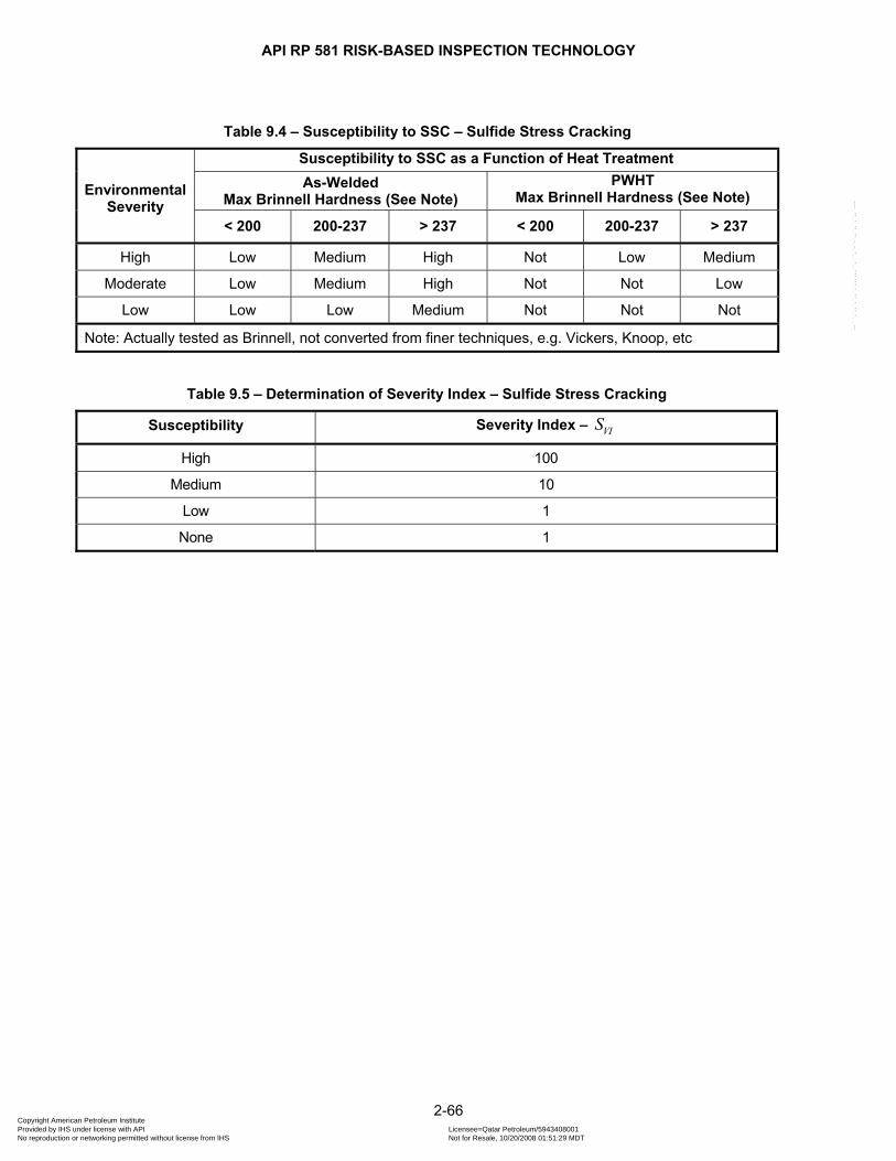
API RP 581 RISK-BASED INSPECTION TECHNOLOGY
Table 9.4 – Susceptibility to SSC – Sulfide Stress Cracking
Environmental Severity
Susceptibility to SSC as a Function of Heat Treatment As-Welded
Max Brinnell Hardness (See Note) PWHT
Max Brinnell Hardness (See Note)
< 200 200-237 > 237 < 200 200-237 > 237
High Low Medium High Not Low Medium
Moderate Low Medium High Not Not Low
Low Low Low Medium Not Not Not
Note: Actually tested as Brinnell, not converted from finer techniques, e.g. Vickers, Knoop, etc
Table 9.5 – Determination of Severity Index – Sulfide Stress Cracking
Susceptibility Severity Index – VIS
High 100
Medium 10
Low 1
None 1
2-66 Copyright American Petroleum Institute Provided by IHS under license with API Licensee=Qatar Petroleum/5943408001
Not for Resale, 10/20/2008 01:51:29 MDTNo reproduction or networking permitted without license from IHS
--```,`,,`,`,,`,`,,,,,,``,```,`-`-`,,`,,`,`,,`---

API RP 581 RISK-BASED INSPECTION TECHNOLOGY
9.10 Figures
STEP 2: Determine the time in-service, age, since the last inspection.
STEP 3: Determine the environmental severity using Table 9.3.
STEP 5: Determine the severity index from Table 9.5.
STEP 6: Determine the base damage factor for sulfide stress cracking using
Table 7.4.
STEP 7: Calculate the escalation in the damage factor using Equation 2.19.
STEP 4: Determine the susceptibility for cracking using Table 9.4.
pH of WaterH2S Content of Water
PWHT?Brinell Hardness
STEP 1: Determine the number of inspections and the corresponding inspection effectiveness category for all past
inspections. For all past inspections, combine inspections to the highest effectiveness
performed.
High Susceptibility
Cracks present?
No
Yes
Figure 9.1 – Determination of the Sulfide Stress Cracking Damage Factor
2-67 Copyright American Petroleum Institute Provided by IHS under license with API Licensee=Qatar Petroleum/5943408001
Not for Resale, 10/20/2008 01:51:29 MDTNo reproduction or networking permitted without license from IHS
--```,`,,`,`,,`,`,,,,,,``,```,`-`-`,,`,,`,`,,`---

API RP 581 RISK-BASED INSPECTION TECHNOLOGY
10 SCC DAMAGE FACTOR – HIC/SOHIC-H2S
10.1 Scope The damage factor calculation for components subject to hydrogen-induced cracking and stress-oriented hydrogen induced cracking in hydrogen sulfide services (HIC/SOHIC-H2S) is covered in this paragraph.
10.2 Description of Damage Hydrogen-induced cracking is defined as stepwise internal cracks that connect adjacent hydrogen blisters on different planes in the metal, or to the metal surface. An externally applied stress is not required for the formation of HIC. The driving force for the cracking is high stresses at the circumference of the hydrogen blisters caused by buildup of internal pressure in the blisters. Interactions between these high stress fields tend to cause cracks to develop that link blisters on different planes in the steel. The buildup of pressure in the blisters is related to the hydrogen permeation flux in the steel. The source of the hydrogen in the steel is the corrosion reaction with wet hydrogen sulfide. Water must be present for this corrosion reaction to occur, and the resultant hydrogen flux is primarily associated with two environmental parameters, pH and the H2S content of the water. Typically, the hydrogen flux in steels has been found to be lowest in near neutral pH solutions, with increasing flux at both lower and higher pH values. Corrosion at low pH values is caused by H2S, where as corrosion at high pH values, is caused by high concentrations of the bisulfide ion. Presence of cyanides at elevated pH can further aggravate the hydrogen penetration into the steel. Hydrogen permeation is known to increase with H2S content, e.g. H2S partial pressure in the gas phase or H2S content of the water phase. The presence of 50 ppm of H2S in the water has been sufficient to cause HIC. Hydrogen blisters are planar hydrogen-filled cavities formed at discontinuities in the steel (e.g. voids, inclusions, laminations, sulfide inclusions). Blisters most often occur in rolled plate steels, especially those with a banded microstructure resulting from elongated sulfide inclusions. Susceptibility to hydrogen blistering, and therefore HIC is primarily related to the quality of the plate steel, i.e., the number, size and shape of the discontinuities. In this regard, the sulfur content of the steel is a key material parameter. Reducing the sulfur content of the steel reduces the susceptibility to blistering and HIC. Additions of calcium or REMS (rare-earth elements) which control sulfide inclusion shape control is generally beneficial. The susceptibility of the steel to blistering is directly related to the cleanliness of the steel which is measured by sulfur content. It should be recognized that blistering is not a damage mechanism which will lead to a leak path unless it is accompanied by hydrogen-induced cracking leading to the surface. Blistering does pose a danger to mechanical integrity when it approaches a weld which contains sufficient residual stresses to drive the hydrogen-induced cracking to the surfaces. It is in this last case, the most severe situation that is considered when determining the susceptibility to HIC/SOHIC-H2S. SOHIC is defined as a stacked array of blisters joined by hydrogen-induced cracking that is aligned in the through-thickness direction of the steel as a result of high localized tensile stresses. SOHIC is a special form of HIC which usually occurs in the base metal, adjacent to the heat affected zone of a weld, where stresses are highest due to the additive effect of applied stress (from internal pressure) and the residual stresses from welding. As with HIC, plate steel quality is a key parameter for SOHIC susceptibility. In addition, reduction of residual stresses by PWHT can reduce, but may not eliminate, the occurrence and severity of SOHIC. The level of applied stress also influences the occurrence and severity of SOHIC. Although HIC/SOHIC is much more prominent in plate steel fabrications, it has been observed to a limited extent in steel pipe fabrications, usually in the more severe hydrogen charging environments.
2-68 Copyright American Petroleum Institute Provided by IHS under license with API Licensee=Qatar Petroleum/5943408001
Not for Resale, 10/20/2008 01:51:29 MDTNo reproduction or networking permitted without license from IHS
--```,`,,`,`,,`,`,,,,,,``,```,`-`-`,,`,,`,`,,`---
API RP 581 RISK-BASED INSPECTION TECHNOLOGY
10.3 Screening Criteria If the component’s material of construction is carbon or low alloy steel and the process environment contains water and H2S in any concentration, then the component should be evaluated for susceptibility to HIC/SOHIC-H2S cracking.
10.4 Required Data The basic component data required for analysis is given in Table 5.1 and the specific data required for determination of the HIC/SOHIC-H2S cracking damage factor is provided in Table 10.1.
10.5 Basic Assumptions The main assumption in determining the damage factor for HIC/SOHIC-H2S cracking is that the damage can be characterized by a susceptibility parameter that is designated as high, medium, or low based on process environment, material of construction, and component fabrication variables (i.e. heat treatment). Based on a susceptibility, a Severity Index can be determined that a measure of the susceptibility of the component cracking (or the probability of initiating cracks) and the probability of a crack resulting in a leak. If SOHIC is detected in the component during an inspection, the susceptibility is designated as High, and this will result in the maximum value for the Severity Index. Known blisters or cracks that are found during an inspection should be evaluated using Fitness-For-Service methods in API 579 [10].
10.6 Determination of the Damage Factor
10.6.1 Overview A flow chart of the steps required to determine the damage factor for HIC/SOHIC-H2S cracking is shown in Figure 10.1. The following paragraphs provide additional information and the calculation procedure.
10.6.2 Inspection Effectiveness Inspections are ranked according to their expected effectiveness at detecting HIC/SOHIC-H2S cracking and correctly predicting the rate of damage. Examples of inspection activities for HIC/SOHIC-H2S cracking that are both intrusive (requires entry into the equipment) and non-intrusive (can be performed externally), are provided in Table 10.2. The effectiveness of each inspection performed within the designated time period must be characterized in accordance with Table 10.2. The number and category of the highest effective inspection will be used to determine the damage factor. If multiple inspections of a lower effectiveness have been conducted during the designated time period, they can be equated to an equivalent higher effectiveness inspection in accordance with paragraph 4.4.3.
10.6.3 Calculation of the Damage Factor The following procedure may be used to determine the damage factor for HIC/SOHIC-H2S cracking, see Figure 10.1. a) STEP 1 – Determine the number of inspections, and the corresponding inspection effectiveness category
using paragraph 10.6.2 for all past inspections. Combine the inspections to the highest effectiveness performed using paragraph 4.4.3.
b) STEP 2 – Determine the time in-service, , since the last Level A, B, C or D inspection was performed. agec) STEP 3 – Determine the environmental severity (potential level of hydrogen flux) for cracking based on the
H2S content of the water and its pH using Table 10.3. Note that a HIGH environmental severity should be used if cracking is known to be present.
d) STEP 4 – Determine the susceptibility for cracking using Figure 10.1 and Table 10.4 based on the environmental severity from STEP 3, the sulfur content of the carbon steel, and knowledge of whether the component was subject to PWHT.
e) STEP 5 – Based on the susceptibility in STEP 4, determine the severity index, , from VIS Table 10.5.
2-69 Copyright American Petroleum Institute Provided by IHS under license with API Licensee=Qatar Petroleum/5943408001
Not for Resale, 10/20/2008 01:51:29 MDTNo reproduction or networking permitted without license from IHS
--```,`,,`,`,,`,`,,,,,,``,```,`-`-`,,`,,`,`,,`---

API RP 581 RISK-BASED INSPECTION TECHNOLOGY
f) STEP 6 – Determine the base damage factor for HIC/SOHIC-H2S cracking, 2/HIC SOHIC H SfBD − , using Table
7.4 based on the number of, and the highest inspection effectiveness determined in STEP 1, and the severity index, , from STEP 5. VIS
g) STEP 7 – Calculate the escalation in the damage factor based on the time in-service since the last inspection using the from STEP 2 and Equation (age 2.20). In this equation, it is assumed that the probability for cracking will increase with time since the last inspection as a result of increased exposure to upset conditions and other non-normal conditions.
( )2 21.1/ /HIC SOHIC H S HIC SOHIC H S
f fBD D age− −= (2.20)
10.7 Nomenclature age is the in-service time since the last Level A, B, C or D inspection was performed
2/HIC SOHIC H SfD − is the damage factor for HIC/SOHIC-H2S cracking
2/HIC SOHIC H SfBD − is the base value of the for HIC/SOHIC-H2S cracking
VIS is the severity index
10.8 References 36. R. R. Petrie and E. M. Moore, Jr., “Determining the Suitability of Existing Pipelines and Producing Facilities
for Wet Sour Service,” Materials Performance 28, 6 (June 1989), pp. 59-65. 37. R. D. Merrick, “Refinery Experiences with Cracking in Wet H2S Environments,” Materials Performance 27,
1 (January 1988), pp. 30. 38. R. D. Merrick and M.L. Bullen, “Prevention of Cracking in Wet H2S Environments,” NACE Corrosion/89,
paper no. 269. 39. NACE Publication 8X194, Materials and Fabrication Practices for New Pressure Vessels Used in Wet H2S
Refinery Service, NACE International, Houston, TX. 40. NACE Publication 8X294, Review of Published Literature on Wet H2S Cracking of Steels Through 1989,
NACE International, Houston, TX. 41. API Publication 939, Research Report on Characterization and Monitoring of Cracking in Wet H2S Service,
American Petroleum Institute, Washington, D.C., 20005, October 1994. 42. M. S. Cayard and R. D. Kane, “Characterization and Monitoring of Cracking of Steel Equipment in Wet H2S
Service,” NACE Corrosion/95, Paper no. 329. 43. NACE RP0296-96, Guidelines for Detection, Repair, and Mitigation of Existing Petroleum Refinery
Pressure Vessels in Wet H2S Environments, NACE International, Houston, TX.
2-70 Copyright American Petroleum Institute Provided by IHS under license with API Licensee=Qatar Petroleum/5943408001
Not for Resale, 10/20/2008 01:51:29 MDTNo reproduction or networking permitted without license from IHS
--```,`,,`,`,,`,`,,,,,,``,```,`-`-`,,`,,`,`,,`---
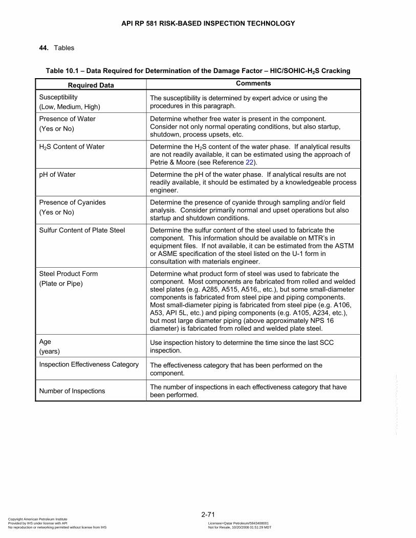
API RP 581 RISK-BASED INSPECTION TECHNOLOGY
44. Tables
Table 10.1 – Data Required for Determination of the Damage Factor – HIC/SOHIC-H2S Cracking
Required Data Comments
Susceptibility (Low, Medium, High)
The susceptibility is determined by expert advice or using the procedures in this paragraph.
Presence of Water (Yes or No)
Determine whether free water is present in the component. Consider not only normal operating conditions, but also startup, shutdown, process upsets, etc.
H2S Content of Water
Determine the H2S content of the water phase. If analytical results are not readily available, it can be estimated using the approach of Petrie & Moore (see Reference 22).
pH of Water
Determine the pH of the water phase. If analytical results are not readily available, it should be estimated by a knowledgeable process engineer.
Presence of Cyanides (Yes or No)
Determine the presence of cyanide through sampling and/or field analysis. Consider primarily normal and upset operations but also startup and shutdown conditions.
Sulfur Content of Plate Steel
Determine the sulfur content of the steel used to fabricate the component. This information should be available on MTR’s in equipment files. If not available, it can be estimated from the ASTM or ASME specification of the steel listed on the U-1 form in consultation with materials engineer.
Steel Product Form (Plate or Pipe)
Determine what product form of steel was used to fabricate the component. Most components are fabricated from rolled and welded steel plates (e.g. A285, A515, A516,, etc.), but some small-diameter components is fabricated from steel pipe and piping components. Most small-diameter piping is fabricated from steel pipe (e.g. A106, A53, API 5L, etc.) and piping components (e.g. A105, A234, etc.), but most large diameter piping (above approximately NPS 16 diameter) is fabricated from rolled and welded plate steel.
Age (years)
Use inspection history to determine the time since the last SCC inspection.
Inspection Effectiveness Category
The effectiveness category that has been performed on the component.
Number of Inspections The number of inspections in each effectiveness category that have been performed.
2-71 Copyright American Petroleum Institute Provided by IHS under license with API Licensee=Qatar Petroleum/5943408001
Not for Resale, 10/20/2008 01:51:29 MDTNo reproduction or networking permitted without license from IHS
--```,`,,`,`,,`,`,,,,,,``,```,`-`-`,,`,,`,`,,`---

API RP 581 RISK-BASED INSPECTION TECHNOLOGY
Table 10.2 – Guidelines for Assigning Inspection Effectiveness – HIC/SOHIC-H2S Cracking
Inspection Category
Inspection Effectiveness
Category Intrusive Inspection Example Non-intrusive Inspection Example
A Highly Effective
Wet fluorescent magnetic particle testing of 50-100% of weldments, plus additional shear wave UT for subsurface cracking.
None
B Usually Effective
Wet fluorescent magnetic particle testing of 20-49% of weldments.
Automated shear wave ultrasonic testing of 20-100% of weldments; or Acoustic Emission testing with follow-up shear wave UT.
C Fairly Effective
Wet fluorescent magnetic particle testing of less than 20% of weldments; or Dry magnetic particle testing of 50-100% of weldments; or Dye penetrant testing of 50-100% of weldments.
Automated shear wave ultrasonic testing of less than 20% of weldments; or Manual shear wave ultrasonic testing of 20-100% of weldments.
D Poorly Effective
Dye penetrant testing of less than 50% of weldments; Visual inspection for hydrogen blisters.
Manual shear wave ultrasonic testing of less than 20% of weldments.
E Ineffective No inspection Radiographic testing
Table 10.3 – Environmental Severity – HIC/SOHIC-H2S Cracking
pH of Water Environmental Severity as a Function of H2S content of Water
< 50 ppm 50 to 1,000 ppm
1,000 to 10,000 ppm
> 10,000 ppm
< 5.5 Low Moderate High High
5.5 to 7.5 Low Low Low Moderate
7.6 to 8.3 Low Moderate Moderate Moderate
8.4 to 8.9 Low Moderate Moderate* High*
> 9.0 Low Moderate High* High*
Note: *If cyanides are present, increase the susceptibility to HIC/SOHIC-H2S one category for pH > 8.3 and H2S concentrations greater than 1,000 ppm
2-72 Copyright American Petroleum Institute Provided by IHS under license with API Licensee=Qatar Petroleum/5943408001
Not for Resale, 10/20/2008 01:51:29 MDTNo reproduction or networking permitted without license from IHS
--```,`,,`,`,,`,`,,,,,,``,```,`-`-`,,`,,`,`,,`---

API RP 581 RISK-BASED INSPECTION TECHNOLOGY
Table 10.4 – Susceptibility to Cracking – HIC/SOHIC-H2S Cracking
Environmental Severity
Susceptibility to Cracking as a Function of Steel Sulfur Content High Sulfur Steel (1)
> 0.01% S Low Sulfur Steel (2)
0.002 to 0.01% S Ultra Low Sulfur (3)
< 0.002% S
As-Welded PWHT As-Welded PWHT As-Welded PWHT
High High High High Medium Medium Low
Moderate High Medium Medium Low Low Low
Low Medium Low Low Low Not Not 1. Typically includes A 70, A 201, A 212, A 285, A 515, and most A 516 before about 1990. 2. Typically includes early generations of HIC-resistant A 516 in 1980’s, with Ca additions. 3. Typically includes later generations of HIC-resistant A 516 in 1990’s.
Table 10.5 – Determination of Severity Index – HIC/SOHIC-H2S Cracking
Susceptibility Severity Index – VIS
High 100
Medium 10
Low 1
None 1
2-73 Copyright American Petroleum Institute Provided by IHS under license with API Licensee=Qatar Petroleum/5943408001
Not for Resale, 10/20/2008 01:51:29 MDTNo reproduction or networking permitted without license from IHS
--```,`,,`,`,,`,`,,,,,,``,```,`-`-`,,`,,`,`,,`---

API RP 581 RISK-BASED INSPECTION TECHNOLOGY
10.9 Figures
Figure 10.1 – Determination of the HIC/SOHIC-H2S Damage Factor
2-74 Copyright American Petroleum Institute Provided by IHS under license with API Licensee=Qatar Petroleum/5943408001
Not for Resale, 10/20/2008 01:51:29 MDTNo reproduction or networking permitted without license from IHS
--```,`,,`,`,,`,`,,,,,,``,```,`-`-`,,`,,`,`,,`---

API RP 581 RISK-BASED INSPECTION TECHNOLOGY
11 SCC DAMAGE FACTOR – CARBONATE CRACKING
11.1 Scope The damage factor calculation for components subject to carbonate cracking is covered in this paragraph.
11.2 Description of Damage Carbonate cracking is a common term applied to cracking of a metal under the combined action of tensile stress and corrosion in the presence of an alkaline sour water containing moderate to high concentrations of carbonate (CO3). The cracking is predominantly intergranular in nature, and typically occurs in as-welded carbon steel fabrications as a network of very fine, oxide-filled cracks. Carbonate cracking typically propagates parallel to the weld in adjacent base metal, but can also occur in the weld deposit or heat-affected zones. The pattern of cracking observed on the steel surface is sometimes described as a spider web of small cracks, which often initiate at or interconnect with weld-related flaws that serve as local stress risers. Carbonate cracking has been most prevalent in the catalytic cracking unit main fractionator overhead condensing and reflux system, the downstream wet gas compression system, and the sour water systems emanating from these areas. Assuming the presence of a sour water phase, three key parameters are used to assess the susceptibility of steel fabrications to carbonate cracking; pH of the sour water, carbonate concentration of the sour water, and level of tensile stress. Studies have concluded that the cracking occurs in a narrow range of electrochemical potential, which is very dependent upon the sour water composition. The presence of moderate to high levels of carbonates in alkaline sour water often produces an electrochemical potential of steel which is in this narrow range where carbonate cracking is likely to occur. Another common contaminant in these sour waters, cyanides, has been shown to influence cracking susceptibility. Despite this mechanistic understanding, the electrochemical potential of in-service components may not be readily available. Therefore, pH and carbonate concentration of the sour water are judged to be the key environmental parameters influencing the susceptibility of steel fabrications to carbonate cracking. Based on a survey of many process units reported in Reference [30], cracking susceptibility increases with increasing pH and carbonate concentration. With regard to the level of tensile stress, as-welded or as-bent carbon steel fabrications are susceptible to carbonate cracking because of the high level of residual stress remaining after fabrication by these methods. Application of a post fabrication stress-relieving heat treatment (e.g. postweld heat treatment) is a proven method of preventing carbonate cracking. A heat treatment of about 621°C [1150°F] for one hour per inch of thickness (one hour minimum) is considered an effective stress-relieving heat treatment to prevent carbonate cracking of carbon steel.
11.3 Screening Criteria If the component’s material of construction is carbon or low alloy steel and the process environment contains sour water at pH > 7.5 in any concentration, then the component should be evaluated for susceptibility to carbonate cracking.
11.4 Required Data The basic component data required for analysis is given in Table 5.1 and the specific data required for determination of the carbonate cracking damage factor is provided in Table 11.1.
2-75 Copyright American Petroleum Institute Provided by IHS under license with API Licensee=Qatar Petroleum/5943408001
Not for Resale, 10/20/2008 01:51:29 MDTNo reproduction or networking permitted without license from IHS
--```,`,,`,`,,`,`,,,,,,``,```,`-`-`,,`,,`,`,,`---

API RP 581 RISK-BASED INSPECTION TECHNOLOGY
11.5 Basic Assumptions The main assumption in determining the damage factor for carbonate cracking is that the damage can be characterized by a susceptibility parameter that is designated as high, medium, or low based on process environment, material of construction, and component fabrication variables (i.e. heat treatment). Based on a susceptibility, a Severity Index can be determined that a measure of the susceptibility of the component cracking (or the probability of initiating cracks) and the probability of a crack resulting in a leak. If cracks are detected in the component during an inspection, the susceptibility is designated as High, and this will result in the maximum value for the Severity Index. Cracks that are found during an inspection should be evaluated using Fitness-For-Service methods in API 579 [10].
11.6 Determination of the Damage Factor
11.6.1 Overview A flow chart of the steps required to determine the damage factor for carbonate cracking is shown in Figure 11.1. The following paragraphs provide additional information and the calculation procedure.
11.6.2 Inspection Effectiveness Inspections are ranked according to their expected effectiveness at detecting carbonate cracking and correctly predicting the rate of damage. Examples of inspection activities for carbonate cracking that are both intrusive (requires entry into the equipment) and non-intrusive (can be performed externally), are provided in Table 11.2. The effectiveness of each inspection performed within the designated time period must be characterized in accordance with Table 11.2. The number and category of the highest effective inspection will be used to determine the damage factor. If multiple inspections of a lower effectiveness have been conducted during the designated time period, they can be equated to an equivalent higher effectiveness inspection in accordance with paragraph 4.4.3.
11.6.3 Calculation of the Damage Factor The following procedure may be used to determine the damage factor for carbonate cracking, see Figure 11.1 a) STEP 1 – Determine the number of inspections, and the corresponding inspection effectiveness category
using paragraph 11.6.2 for all past inspections. Combine the inspections to the highest effectiveness performed using paragraph 4.4.3.
b) STEP 2 – Determine the time in-service, , since the last Level A, B, C or D inspection was performed. agec) STEP 3 – Determine the susceptibility for cracking using Figure 11.1 and Table 11.3 based on the pH of
the water and CO3 concentration, and knowledge of whether the component was subject to PWHT. Note that a HIGH susceptibility should be used if cracking is known to be present.
d) STEP 4 – Based on the susceptibility in STEP 3, determine the severity index, , from VIS Table 11.4.
e) STEP 5 – Determine the base damage factor for carbonate cracking, , using carbonatefBD Table 7.4 based on
the number of, and the highest inspection effectiveness determined in STEP 1, and the severity index, , from STEP 4.
VIS
2-76 Copyright American Petroleum Institute Provided by IHS under license with API Licensee=Qatar Petroleum/5943408001
Not for Resale, 10/20/2008 01:51:29 MDTNo reproduction or networking permitted without license from IHS
--```,`,,`,`,,`,`,,,,,,``,```,`-`-`,,`,,`,`,,`---
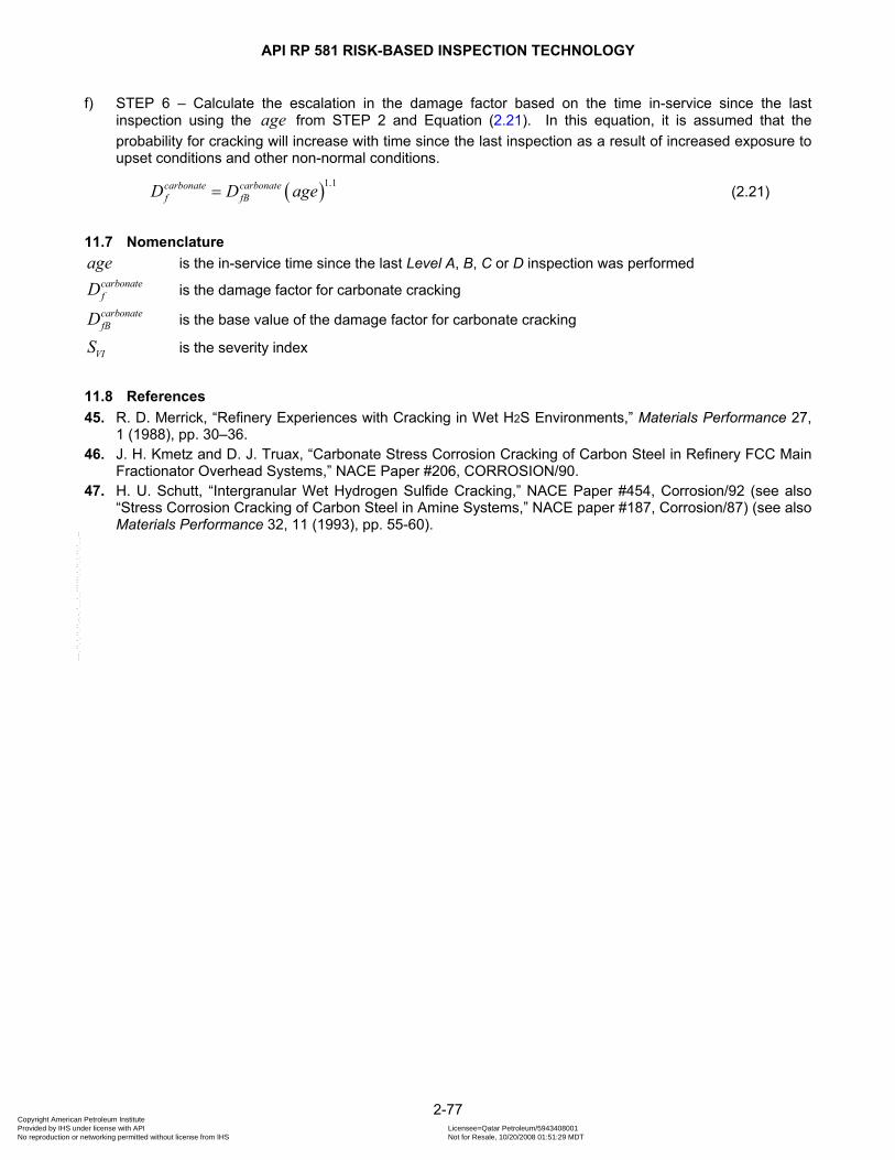
API RP 581 RISK-BASED INSPECTION TECHNOLOGY
f) STEP 6 – Calculate the escalation in the damage factor based on the time in-service since the last inspection using the age from STEP 2 and Equation (2.21). In this equation, it is assumed that the probability for cracking will increase with time since the last inspection as a result of increased exposure to upset conditions and other non-normal conditions.
( )1.1carbonate carbonatef fBD D ag= e (2.21)
11.7 Nomenclature age is the in-service time since the last Level A, B, C or D inspection was performed
carbonatefD is the damage factor for carbonate cracking carbonatefBD is the base value of the damage factor for carbonate cracking
VIS is the severity index
11.8 References 45. R. D. Merrick, “Refinery Experiences with Cracking in Wet H2S Environments,” Materials Performance 27,
1 (1988), pp. 30–36. 46. J. H. Kmetz and D. J. Truax, “Carbonate Stress Corrosion Cracking of Carbon Steel in Refinery FCC Main
Fractionator Overhead Systems,” NACE Paper #206, CORROSION/90. 47. H. U. Schutt, “Intergranular Wet Hydrogen Sulfide Cracking,” NACE Paper #454, Corrosion/92 (see also
“Stress Corrosion Cracking of Carbon Steel in Amine Systems,” NACE paper #187, Corrosion/87) (see also Materials Performance 32, 11 (1993), pp. 55-60).
2-77 Copyright American Petroleum Institute Provided by IHS under license with API Licensee=Qatar Petroleum/5943408001
Not for Resale, 10/20/2008 01:51:29 MDTNo reproduction or networking permitted without license from IHS
--```,`,,`,`,,`,`,,,,,,``,```,`-`-`,,`,,`,`,,`---
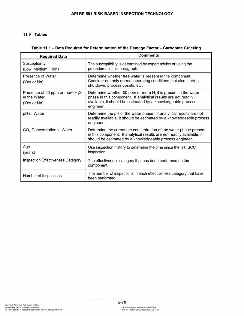
API RP 581 RISK-BASED INSPECTION TECHNOLOGY
11.9 Tables
Table 11.1 – Data Required for Determination of the Damage Factor – Carbonate Cracking
Required Data Comments
Susceptibility (Low, Medium, High)
The susceptibility is determined by expert advice or using the procedures in this paragraph.
Presence of Water (Yes or No)
Determine whether free water is present in the component. Consider not only normal operating conditions, but also startup, shutdown, process upsets, etc.
Presence of 50 ppm or more H2S in the Water (Yes or No)
Determine whether 50 ppm or more H2S is present in the water phase in this component. If analytical results are not readily available, it should be estimated by a knowledgeable process engineer.
pH of Water
Determine the pH of the water phase. If analytical results are not readily available, it should be estimated by a knowledgeable process engineer.
CO3 Concentration in Water
Determine the carbonate concentration of the water phase present in this component. If analytical results are not readily available, it should be estimated by a knowledgeable process engineer.
Age (years)
Use inspection history to determine the time since the last SCC inspection.
Inspection Effectiveness Category
The effectiveness category that has been performed on the component.
Number of Inspections The number of inspections in each effectiveness category that have been performed.
2-78 Copyright American Petroleum Institute Provided by IHS under license with API Licensee=Qatar Petroleum/5943408001
Not for Resale, 10/20/2008 01:51:29 MDTNo reproduction or networking permitted without license from IHS
--```,`,,`,`,,`,`,,,,,,``,```,`-`-`,,`,,`,`,,`---
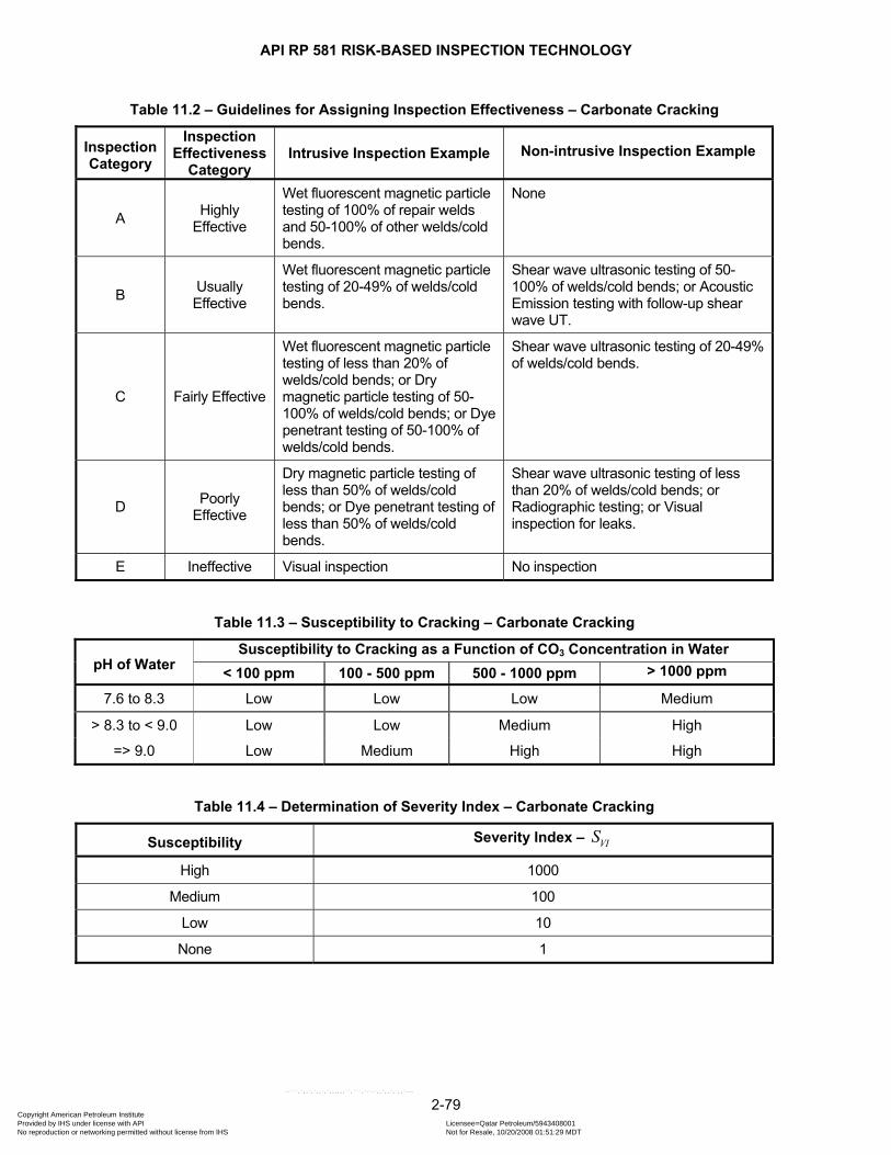
API RP 581 RISK-BASED INSPECTION TECHNOLOGY
Table 11.2 – Guidelines for Assigning Inspection Effectiveness – Carbonate Cracking
Inspection Category
Inspection Effectiveness
Category Intrusive Inspection Example Non-intrusive Inspection Example
A Highly Effective
Wet fluorescent magnetic particle testing of 100% of repair welds and 50-100% of other welds/cold bends.
None
B Usually Effective
Wet fluorescent magnetic particle testing of 20-49% of welds/cold bends.
Shear wave ultrasonic testing of 50-100% of welds/cold bends; or Acoustic Emission testing with follow-up shear wave UT.
C Fairly Effective
Wet fluorescent magnetic particle testing of less than 20% of welds/cold bends; or Dry magnetic particle testing of 50-100% of welds/cold bends; or Dye penetrant testing of 50-100% of welds/cold bends.
Shear wave ultrasonic testing of 20-49% of welds/cold bends.
D Poorly Effective
Dry magnetic particle testing of less than 50% of welds/cold bends; or Dye penetrant testing of less than 50% of welds/cold bends.
Shear wave ultrasonic testing of less than 20% of welds/cold bends; or Radiographic testing; or Visual inspection for leaks.
E Ineffective Visual inspection No inspection
Table 11.3 – Susceptibility to Cracking – Carbonate Cracking
pH of Water Susceptibility to Cracking as a Function of CO3 Concentration in Water
< 100 ppm 100 - 500 ppm 500 - 1000 ppm > 1000 ppm
7.6 to 8.3 Low Low Low Medium
> 8.3 to < 9.0 Low Low Medium High
=> 9.0 Low Medium High High
Table 11.4 – Determination of Severity Index – Carbonate Cracking
Susceptibility Severity Index – VIS
High 1000
Medium 100
Low 10
None 1
2-79 Copyright American Petroleum Institute Provided by IHS under license with API Licensee=Qatar Petroleum/5943408001
Not for Resale, 10/20/2008 01:51:29 MDTNo reproduction or networking permitted without license from IHS
--```,`,,`,`,,`,`,,,,,,``,```,`-`-`,,`,,`,`,,`---

API RP 581 RISK-BASED INSPECTION TECHNOLOGY
11.10 Figures
Figure 11.1 – Determination of the Carbonate Cracking Damage Factor
2-80 Copyright American Petroleum Institute Provided by IHS under license with API Licensee=Qatar Petroleum/5943408001
Not for Resale, 10/20/2008 01:51:29 MDTNo reproduction or networking permitted without license from IHS
--```,`,,`,`,,`,`,,,,,,``,```,`-`-`,,`,,`,`,,`---
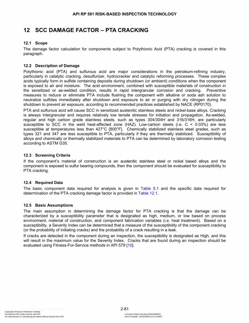
API RP 581 RISK-BASED INSPECTION TECHNOLOGY
12 SCC DAMAGE FACTOR – PTA CRACKING
12.1 Scope The damage factor calculation for components subject to Polythionic Acid (PTA) cracking is covered in this paragraph.
12.2 Description of Damage Polythionic acid (PTA) and sulfurous acid are major considerations in the petroleum-refining industry, particularly in catalytic cracking, desulfurizer, hydrocracker and catalytic reforming processes. These complex acids typically form in sulfide containing deposits during shutdown (or ambient) conditions when the component is exposed to air and moisture. The acid environment, combined with susceptible materials of construction in the sensitized or as-welded condition, results in rapid intergranular corrosion and cracking. Preventive measures to reduce or eliminate PTA include flushing the component with alkaline or soda ash solution to neutralize sulfides immediately after shutdown and exposure to air or purging with dry nitrogen during the shutdown to prevent air exposure, according to recommended practices established by NACE (RP0170). PTA and sulfurous acid will cause SCC in sensitized austenitic stainless steels and nickel-base alloys. Cracking is always intergranular and requires relatively low tensile stresses for initiation and propagation. As-welded, regular and high carbon grade stainless steels, such as types 304/304H and 316/316H, are particularly susceptible to SCC in the weld heat-affected zone (HAZ). Low-carbon steels (i.e. C < 0.03%) are less susceptible at temperatures less than 427°C [800°F]. Chemically stabilized stainless steel grades, such as types 321 and 347 are less susceptible to PTA, particularly if they are thermally stabilized. Susceptibility of alloys and chemically or thermally stabilized materials to PTA can be determined by laboratory corrosion testing according to ASTM G35.
12.3 Screening Criteria If the component’s material of construction is an austenitic stainless steel or nickel based alloys and the component is exposed to sulfur bearing compounds, then the component should be evaluated for susceptibility to PTA cracking.
12.4 Required Data The basic component data required for analysis is given in Table 5.1 and the specific data required for determination of the PTA cracking damage factor is provided in Table 12.1.
12.5 Basic Assumptions The main assumption in determining the damage factor for PTA cracking is that the damage can be characterized by a susceptibility parameter that is designated as high, medium, or low based on process environment, material of construction, and component fabrication variables (i.e. heat treatment). Based on a susceptibility, a Severity Index can be determined that a measure of the susceptibility of the component cracking (or the probability of initiating cracks) and the probability of a crack resulting in a leak. If cracks are detected in the component during an inspection, the susceptibility is designated as High, and this will result in the maximum value for the Severity Index. Cracks that are found during an inspection should be evaluated using Fitness-For-Service methods in API 579 [10].
2-81 Copyright American Petroleum Institute Provided by IHS under license with API Licensee=Qatar Petroleum/5943408001
Not for Resale, 10/20/2008 01:51:29 MDTNo reproduction or networking permitted without license from IHS
--```,`,,`,`,,`,`,,,,,,``,```,`-`-`,,`,,`,`,,`---
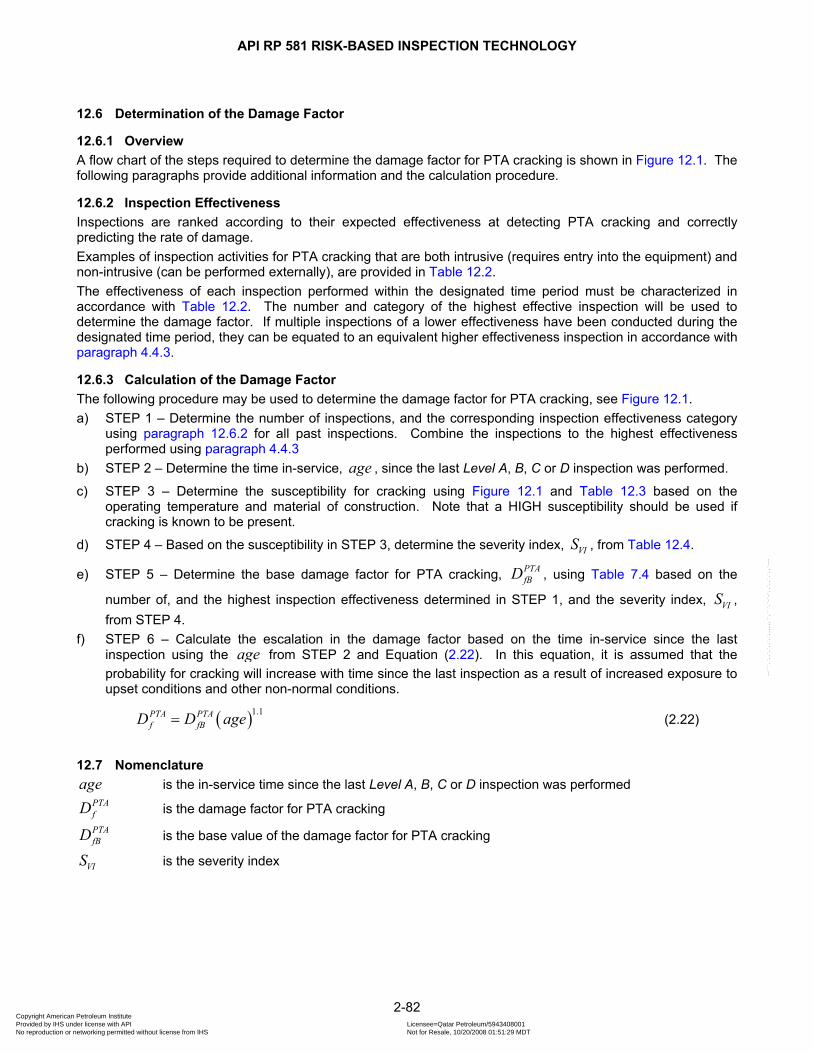
API RP 581 RISK-BASED INSPECTION TECHNOLOGY
12.6 Determination of the Damage Factor
12.6.1 Overview A flow chart of the steps required to determine the damage factor for PTA cracking is shown in Figure 12.1. The following paragraphs provide additional information and the calculation procedure.
12.6.2 Inspection Effectiveness Inspections are ranked according to their expected effectiveness at detecting PTA cracking and correctly predicting the rate of damage. Examples of inspection activities for PTA cracking that are both intrusive (requires entry into the equipment) and non-intrusive (can be performed externally), are provided in Table 12.2. The effectiveness of each inspection performed within the designated time period must be characterized in accordance with Table 12.2. The number and category of the highest effective inspection will be used to determine the damage factor. If multiple inspections of a lower effectiveness have been conducted during the designated time period, they can be equated to an equivalent higher effectiveness inspection in accordance with paragraph 4.4.3.
12.6.3 Calculation of the Damage Factor The following procedure may be used to determine the damage factor for PTA cracking, see Figure 12.1. a) STEP 1 – Determine the number of inspections, and the corresponding inspection effectiveness category
using paragraph 12.6.2 for all past inspections. Combine the inspections to the highest effectiveness performed using paragraph 4.4.3
b) STEP 2 – Determine the time in-service, , since the last Level A, B, C or D inspection was performed. agec) STEP 3 – Determine the susceptibility for cracking using Figure 12.1 and Table 12.3 based on the
operating temperature and material of construction. Note that a HIGH susceptibility should be used if cracking is known to be present.
d) STEP 4 – Based on the susceptibility in STEP 3, determine the severity index, , from VIS Table 12.4.
e) STEP 5 – Determine the base damage factor for PTA cracking, PTAfBD , using Table 7.4 based on the
number of, and the highest inspection effectiveness determined in STEP 1, and the severity index, , from STEP 4.
VIS
f) STEP 6 – Calculate the escalation in the damage factor based on the time in-service since the last inspection using the age from STEP 2 and Equation (2.22). In this equation, it is assumed that the probability for cracking will increase with time since the last inspection as a result of increased exposure to upset conditions and other non-normal conditions.
( )1.1PTA PTAf fBD D age= (2.22)
12.7 Nomenclature age is the in-service time since the last Level A, B, C or D inspection was performed
PTAfD is the damage factor for PTA cracking PTAfBD is the base value of the damage factor for PTA cracking
VIS is the severity index
2-82 Copyright American Petroleum Institute Provided by IHS under license with API Licensee=Qatar Petroleum/5943408001
Not for Resale, 10/20/2008 01:51:29 MDTNo reproduction or networking permitted without license from IHS
--```,`,,`,`,,`,`,,,,,,``,```,`-`-`,,`,,`,`,,`---
API RP 581 RISK-BASED INSPECTION TECHNOLOGY
12.8 References 48. Metals Handbook, Ninth Edition, ASM International, Metals Park, Ohio 44073, Volume 13 Corrosion, pp.
327. 49. D. R. McIntyre and C. P. Dillon, Guidelines for Preventing Stress Corrosion Cracking in the Chemical
Process Industries, Publication 15, Materials Technology Institute of the Chemical Process Industries, 1985, pp. 69.
50. The Role of Stainless Steels in Petroleum Refining, American Iron and Steel Institute, 1977, pp. 42-44. 51. NACE RP0170-93, Protection of Austenitic Stainless Steels and Other Austenitic Alloys from Polythionic
Acid Stress Corrosion Cracking During Shutdown of Refinery Equipment, NACE International, Houston, TX 52. D. V. Beggs, and R. W. Howe, “Effects of Welding and Thermal Stabilization on the Sensitization and
Polythionic Acid Stress Corrosion Cracking of Heat and Corrosion-Resistant Alloys,” NACE International Corrosion/93 Paper 541, NACE International, Houston, TX.
53. L. Scharfstein, “The Effect of Heat Treatments in the Prevention of Intergranular Corrosion Failures of AISI 321 Stainless Steel,” Materials Performance, September1983, pp. 22–24.
54. E. Lendvai-Linter, “Stainless Steel Weld Overlay Resistance to Polythionic acid Attack,” Materials Performance, Volume 18, No. 3, 1979, pp. 9.
55. K. Tamaki, S. Nakano, and M. Kimura, “Application of CrNi Stainless Steel Weld Metals to Polythionic Acid Environments,” Materials Performance, August 1987, pp. 9–13.
56. C. H. Samans, “Stress Corrosion Cracking Susceptibility of Stainless Steels and Nickel-Base Alloys in Polythionic Acids and Acid Copper Sulfate Solution,” Corrosion, Volume 20, No. 8, August 1964, pp. 256–262.
57. R. L. Piehl, “Stress Corrosion Cracking by Sulfur Acids,” Proceedings of API Division of Refining, Volume 44 (III), 1964, pp. 189–197.
58. S. Ahmad, M. L. Mehta, S. K. Saraf, and I. P. Saraswat, “Stress Corrosion Cracking of Sensitized 304 Austenitic Stainless Steel in Sulfurous Acid,” Corrosion, Volume 37, No. 7, July 1981, pp. 412–415.
59. S. Ahmad, M. L. Mehta, S. K. Saraf, and I. P. Saraswat, “Stress Corrosion Cracking of Sensitized 304 Austenitic Stainless Steel in Petroleum Refinery Environment,” Corrosion, Volume 38, No. 6, June 1982, p. 347– 353.
2-83 Copyright American Petroleum Institute Provided by IHS under license with API Licensee=Qatar Petroleum/5943408001
Not for Resale, 10/20/2008 01:51:29 MDTNo reproduction or networking permitted without license from IHS
--```,`,,`,`,,`,`,,,,,,``,```,`-`-`,,`,,`,`,,`---
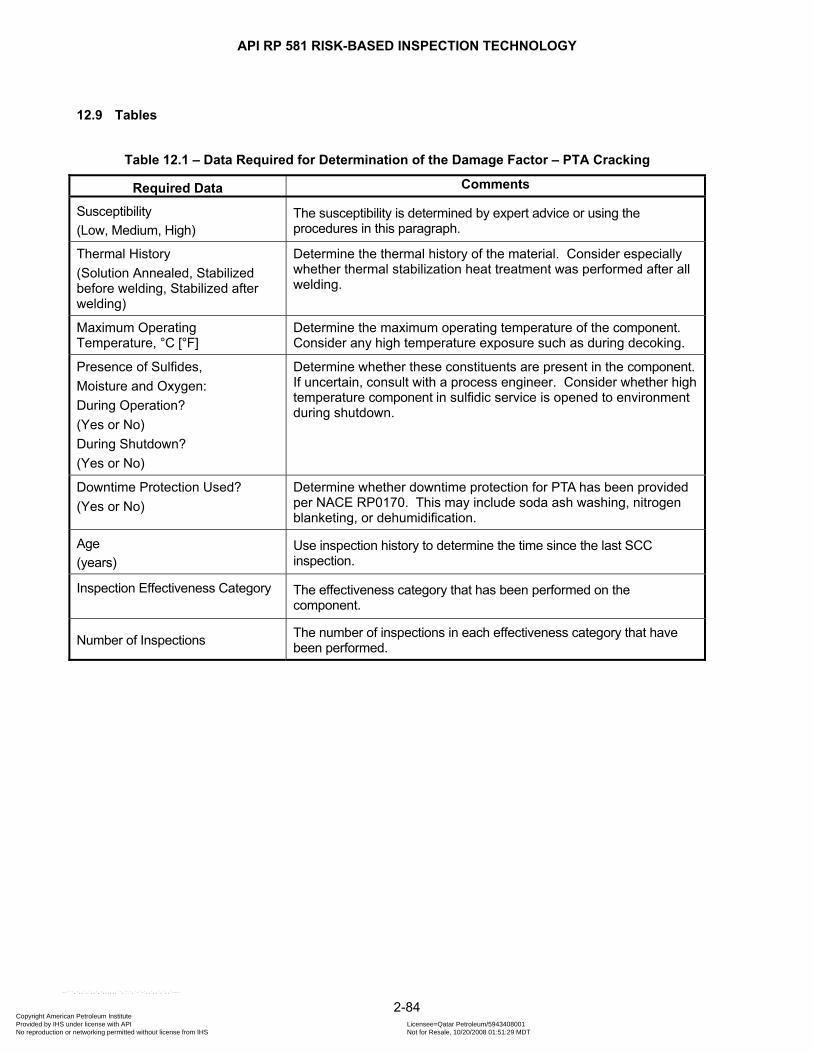
API RP 581 RISK-BASED INSPECTION TECHNOLOGY
12.9 Tables
Table 12.1 – Data Required for Determination of the Damage Factor – PTA Cracking
Required Data Comments
Susceptibility (Low, Medium, High)
The susceptibility is determined by expert advice or using the procedures in this paragraph.
Thermal History (Solution Annealed, Stabilized before welding, Stabilized after welding)
Determine the thermal history of the material. Consider especially whether thermal stabilization heat treatment was performed after all welding.
Maximum Operating Temperature, °C [°F]
Determine the maximum operating temperature of the component. Consider any high temperature exposure such as during decoking.
Presence of Sulfides, Moisture and Oxygen: During Operation? (Yes or No) During Shutdown? (Yes or No)
Determine whether these constituents are present in the component. If uncertain, consult with a process engineer. Consider whether high temperature component in sulfidic service is opened to environment during shutdown.
Downtime Protection Used? (Yes or No)
Determine whether downtime protection for PTA has been provided per NACE RP0170. This may include soda ash washing, nitrogen blanketing, or dehumidification.
Age (years)
Use inspection history to determine the time since the last SCC inspection.
Inspection Effectiveness Category
The effectiveness category that has been performed on the component.
Number of Inspections The number of inspections in each effectiveness category that have been performed.
2-84 Copyright American Petroleum Institute Provided by IHS under license with API Licensee=Qatar Petroleum/5943408001
Not for Resale, 10/20/2008 01:51:29 MDTNo reproduction or networking permitted without license from IHS
--```,`,,`,`,,`,`,,,,,,``,```,`-`-`,,`,,`,`,,`---
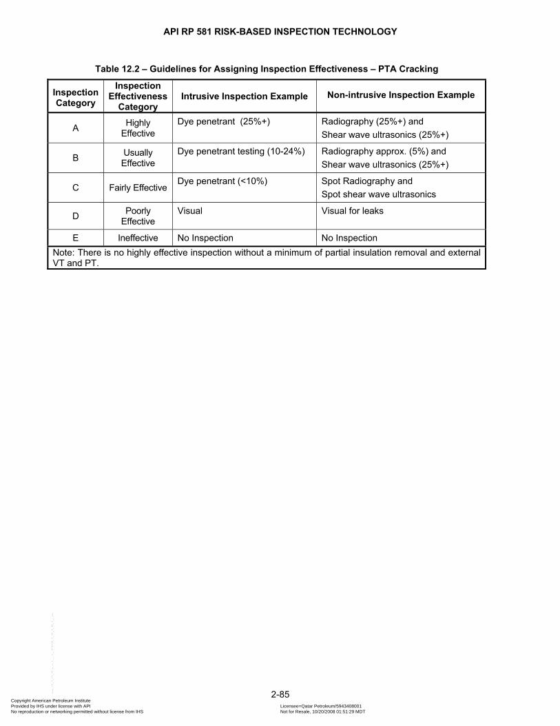
API RP 581 RISK-BASED INSPECTION TECHNOLOGY
Table 12.2 – Guidelines for Assigning Inspection Effectiveness – PTA Cracking
Inspection Category
Inspection Effectiveness
Category Intrusive Inspection Example Non-intrusive Inspection Example
A Highly Effective
Dye penetrant (25%+) Radiography (25%+) and Shear wave ultrasonics (25%+)
B Usually Effective
Dye penetrant testing (10-24%) Radiography approx. (5%) and Shear wave ultrasonics (25%+)
C Fairly Effective Dye penetrant (<10%) Spot Radiography and
Spot shear wave ultrasonics
D Poorly Effective
Visual Visual for leaks
E Ineffective No Inspection No Inspection Note: There is no highly effective inspection without a minimum of partial insulation removal and external VT and PT.
2-85 Copyright American Petroleum Institute Provided by IHS under license with API Licensee=Qatar Petroleum/5943408001
Not for Resale, 10/20/2008 01:51:29 MDTNo reproduction or networking permitted without license from IHS
--```,`,,`,`,,`,`,,,,,,``,```,`-`-`,,`,,`,`,,`---
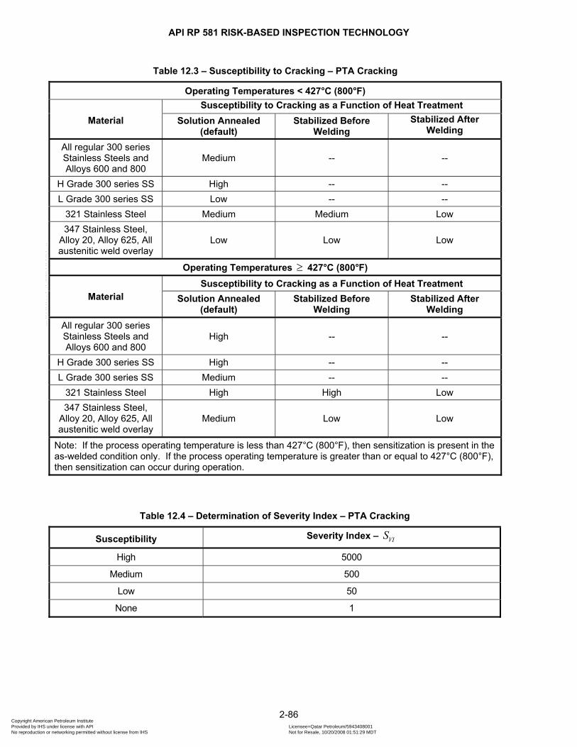
API RP 581 RISK-BASED INSPECTION TECHNOLOGY
Table 12.3 – Susceptibility to Cracking – PTA Cracking
Operating Temperatures < 427°C (800°F)
Material Susceptibility to Cracking as a Function of Heat Treatment
Solution Annealed (default)
Stabilized Before Welding
Stabilized After Welding
All regular 300 series Stainless Steels and Alloys 600 and 800
Medium -- --
H Grade 300 series SS High -- -- L Grade 300 series SS Low -- --
321 Stainless Steel Medium Medium Low 347 Stainless Steel,
Alloy 20, Alloy 625, All austenitic weld overlay
Low Low Low
Operating Temperatures 427°C (800°F) ≥
Material Susceptibility to Cracking as a Function of Heat Treatment
Solution Annealed (default)
Stabilized Before Welding
Stabilized After Welding
All regular 300 series Stainless Steels and Alloys 600 and 800
High -- --
H Grade 300 series SS High -- -- L Grade 300 series SS Medium -- --
321 Stainless Steel High High Low 347 Stainless Steel,
Alloy 20, Alloy 625, All austenitic weld overlay
Medium Low Low
Note: If the process operating temperature is less than 427°C (800°F), then sensitization is present in the as-welded condition only. If the process operating temperature is greater than or equal to 427°C (800°F), then sensitization can occur during operation.
Table 12.4 – Determination of Severity Index – PTA Cracking
Susceptibility Severity Index – VIS
High 5000
Medium 500
Low 50
None 1
2-86 Copyright American Petroleum Institute Provided by IHS under license with API Licensee=Qatar Petroleum/5943408001
Not for Resale, 10/20/2008 01:51:29 MDTNo reproduction or networking permitted without license from IHS
--```,`,,`,`,,`,`,,,,,,``,```,`-`-`,,`,,`,`,,`---
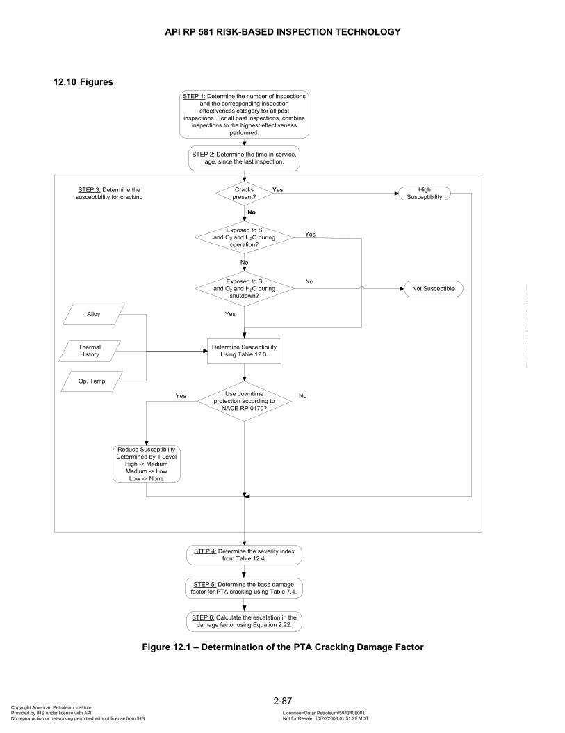
API RP 581 RISK-BASED INSPECTION TECHNOLOGY
12.10 Figures
STEP 2: Determine the time in-service, age, since the last inspection.
STEP 4: Determine the severity index from Table 12.4.
STEP 5: Determine the base damage factor for PTA cracking using Table 7.4.
STEP 6: Calculate the escalation in the damage factor using Equation 2.22.
Exposed to S and O2 and H2O during
operation?
Exposed to S and O2 and H2O during
shutdown?Not Susceptible
Determine Susceptibility Using Table 12.3.
Alloy
Op. Temp
Thermal History
Use downtime protection according to
NACE RP 0170?
No
STEP 3: Determine the susceptibility for cracking
Yes
No
Yes
Yes No
Reduce Susceptibility Determined by 1 Level
High -> MediumMedium -> Low
Low -> None
STEP 1: Determine the number of inspections and the corresponding inspection effectiveness category for all past
inspections. For all past inspections, combine inspections to the highest effectiveness
performed.
High Susceptibility
Cracks present?
No
Yes
Figure 12.1 – Determination of the PTA Cracking Damage Factor
2-87 Copyright American Petroleum Institute Provided by IHS under license with API Licensee=Qatar Petroleum/5943408001
Not for Resale, 10/20/2008 01:51:29 MDTNo reproduction or networking permitted without license from IHS
--```,`,,`,`,,`,`,,,,,,``,```,`-`-`,,`,,`,`,,`---

API RP 581 RISK-BASED INSPECTION TECHNOLOGY
13 SCC DAMAGE FACTOR – CLSCC
13.1 Scope The damage factor calculation for components subject to Chloride Stress Corrosion Cracking (CLSCC) is covered in this paragraph.
13.2 Description of Damage Chloride stress corrosion cracking (CLSCC) of austenitic stainless steels can occur in a chloride containing aqueous environment. The susceptibility to CLSCC is dependent on the concentration of the chloride ions, the temperature, and other factors outlined in the basic data Table 13.1. It should be emphasized that the chloride concentration in water within wetting and drying conditions can be higher than the concentration measured in the bulk solution due to partial water vaporization. Such vaporization can increase CLSCC susceptibility. CLSCC is more likely to occur at metal temperatures above 66°C [150°F]. Examples of common sources of chlorides in refineries and petrochemical plants are as follows: a) Chloride salts from crude oil, produced water, and ballast water b) Water condensed from a process stream (process water) c) Boiler feedwater and stripping system d) Catalyst e) Insulation f) Residue from hydrotest water and other manufacturing operations g) Fumes from chemicals containing either organic or inorganic chlorides
CLSCC may occur during service or shutdown periods, if chloride containing solutions are present, especially at temperatures above 66°C [150°F]. CLSCC can occur internally (for example, by wash-up water or fire water). CLSCC is typically transgranular and highly branched. The greatest susceptibility to CLSCC is exhibited by austenitic stainless steels with a nickel content of 8% (e.g. 300 series SS, 304, 316, etc.). Greater resistance is generally shown by alloys of either lower or higher nickel contents. Duplex stainless steels with low nickel contents are generally immune to CLSCC, as are alloys with greater than 42% nickel.
13.3 Screening Criteria If all of the following are true, then the component should be evaluated for susceptibility to CLSCC cracking. a) The component’s material of construction is an austenitic stainless steel, b) The component is exposed or potentially exposed to chlorides and water also considering upsets and
hydrotest water remaining in component, and cooling tower drift (consider both under insulation and process conditions, and
c) The operating temperature is above 38°C [100°F].
13.4 Required Data The basic component data required for analysis is given in Table 5.1 and the specific data required for determination of the CLSCC damage factor is provided in Table 13.1.
2-88 Copyright American Petroleum Institute Provided by IHS under license with API Licensee=Qatar Petroleum/5943408001
Not for Resale, 10/20/2008 01:51:29 MDTNo reproduction or networking permitted without license from IHS
--```,`,,`,`,,`,`,,,,,,``,```,`-`-`,,`,,`,`,,`---
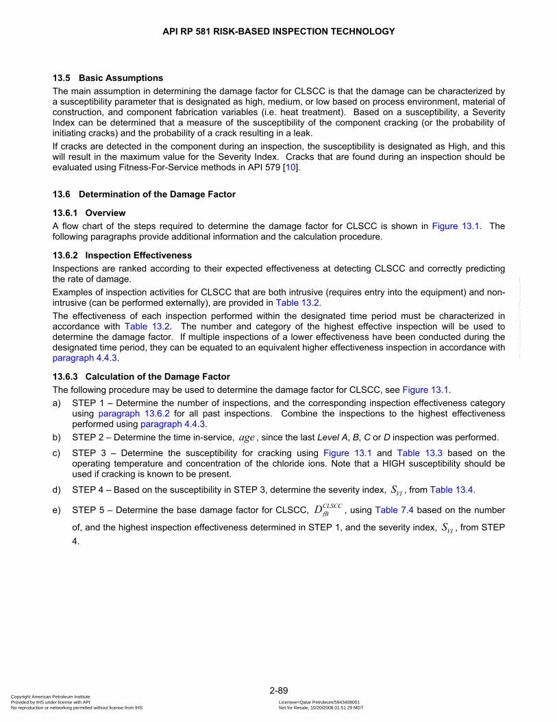
API RP 581 RISK-BASED INSPECTION TECHNOLOGY
13.5 Basic Assumptions The main assumption in determining the damage factor for CLSCC is that the damage can be characterized by a susceptibility parameter that is designated as high, medium, or low based on process environment, material of construction, and component fabrication variables (i.e. heat treatment). Based on a susceptibility, a Severity Index can be determined that a measure of the susceptibility of the component cracking (or the probability of initiating cracks) and the probability of a crack resulting in a leak. If cracks are detected in the component during an inspection, the susceptibility is designated as High, and this will result in the maximum value for the Severity Index. Cracks that are found during an inspection should be evaluated using Fitness-For-Service methods in API 579 [10].
13.6 Determination of the Damage Factor
13.6.1 Overview A flow chart of the steps required to determine the damage factor for CLSCC is shown in Figure 13.1. The following paragraphs provide additional information and the calculation procedure.
13.6.2 Inspection Effectiveness Inspections are ranked according to their expected effectiveness at detecting CLSCC and correctly predicting the rate of damage. Examples of inspection activities for CLSCC that are both intrusive (requires entry into the equipment) and non-intrusive (can be performed externally), are provided in Table 13.2. The effectiveness of each inspection performed within the designated time period must be characterized in accordance with Table 13.2. The number and category of the highest effective inspection will be used to determine the damage factor. If multiple inspections of a lower effectiveness have been conducted during the designated time period, they can be equated to an equivalent higher effectiveness inspection in accordance with paragraph 4.4.3.
13.6.3 Calculation of the Damage Factor The following procedure may be used to determine the damage factor for CLSCC, see Figure 13.1. a) STEP 1 – Determine the number of inspections, and the corresponding inspection effectiveness category
using paragraph 13.6.2 for all past inspections. Combine the inspections to the highest effectiveness performed using paragraph 4.4.3.
b) STEP 2 – Determine the time in-service, , since the last Level A, B, C or D inspection was performed. agec) STEP 3 – Determine the susceptibility for cracking using Figure 13.1 and Table 13.3 based on the
operating temperature and concentration of the chloride ions. Note that a HIGH susceptibility should be used if cracking is known to be present.
d) STEP 4 – Based on the susceptibility in STEP 3, determine the severity index, , from VIS Table 13.4.
e) STEP 5 – Determine the base damage factor for CLSCC, , using CLSCCfBD Table 7.4 based on the number
of, and the highest inspection effectiveness determined in STEP 1, and the severity index, , from STEP 4.
VIS
2-89 Copyright American Petroleum Institute Provided by IHS under license with API Licensee=Qatar Petroleum/5943408001
Not for Resale, 10/20/2008 01:51:29 MDTNo reproduction or networking permitted without license from IHS
--```,`,,`,`,,`,`,,,,,,``,```,`-`-`,,`,,`,`,,`---
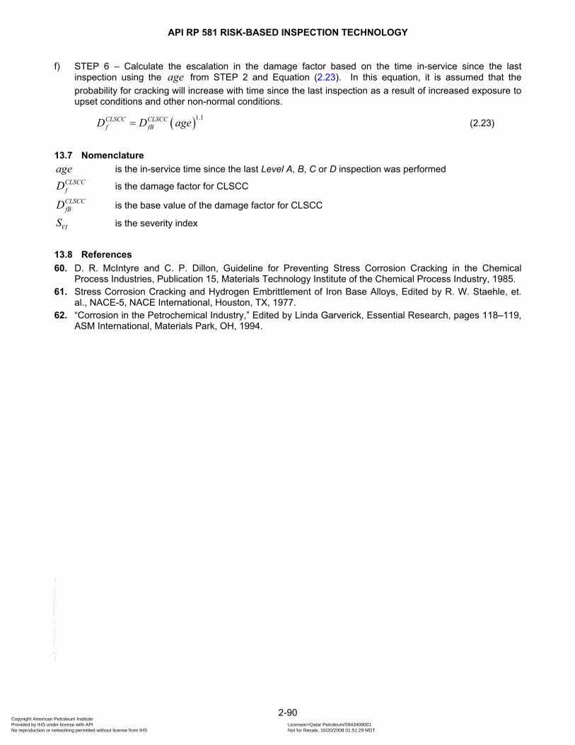
API RP 581 RISK-BASED INSPECTION TECHNOLOGY
f) STEP 6 – Calculate the escalation in the damage factor based on the time in-service since the last inspection using the age from STEP 2 and Equation (2.23). In this equation, it is assumed that the probability for cracking will increase with time since the last inspection as a result of increased exposure to upset conditions and other non-normal conditions.
( )1.1CLSCC CLSCCf fBD D age= (2.23)
13.7 Nomenclature age is the in-service time since the last Level A, B, C or D inspection was performed
CLSCCfD is the damage factor for CLSCC CLSCCfBD is the base value of the damage factor for CLSCC
VIS is the severity index
13.8 References 60. D. R. McIntyre and C. P. Dillon, Guideline for Preventing Stress Corrosion Cracking in the Chemical
Process Industries, Publication 15, Materials Technology Institute of the Chemical Process Industry, 1985. 61. Stress Corrosion Cracking and Hydrogen Embrittlement of Iron Base Alloys, Edited by R. W. Staehle, et.
al., NACE-5, NACE International, Houston, TX, 1977. 62. “Corrosion in the Petrochemical Industry,” Edited by Linda Garverick, Essential Research, pages 118–119,
ASM International, Materials Park, OH, 1994.
2-90 Copyright American Petroleum Institute Provided by IHS under license with API Licensee=Qatar Petroleum/5943408001
Not for Resale, 10/20/2008 01:51:29 MDTNo reproduction or networking permitted without license from IHS
--```,`,,`,`,,`,`,,,,,,``,```,`-`-`,,`,,`,`,,`---

API RP 581 RISK-BASED INSPECTION TECHNOLOGY
13.9 Tables
Table 13.1 – Data Required for Determination of the Damage Factor – CLSCC
Required Data Comments
Susceptibility (Low, Medium, High)
The susceptibility is determined by expert advice or using the procedures in this paragraph.
Cl- Concentration of Process Water (ppm)
Determine the bulk Cl- concentration of the water phase. If unknown, the default value for ppm is >1000. Consider Cl- content of any water present in system (i.e. hydrotest, boiler feed, steam) Also, consider the possibility of concentration of Cl- by evaporation or upset conditions.
Operating Temperature, °C [°F] Determine the highest operating temperature expected during operation (consider normal and non-normal operating conditions).
pH of Process Water
Determine pH of the process water. High pH solutions with high chlorides generally are not as susceptible to cracking as low pH solution with chlorides.
Age (years)
Use inspection history to determine the time since the last SCC inspection.
Inspection Effectiveness Category
The effectiveness category that has been performed on the component.
Number of Inspections The number of inspections in each effectiveness category that have been performed.
2-91 Copyright American Petroleum Institute Provided by IHS under license with API Licensee=Qatar Petroleum/5943408001
Not for Resale, 10/20/2008 01:51:29 MDTNo reproduction or networking permitted without license from IHS
--```,`,,`,`,,`,`,,,,,,``,```,`-`-`,,`,,`,`,,`---

API RP 581 RISK-BASED INSPECTION TECHNOLOGY
Table 13.2 – Guidelines for Assigning Inspection Effectiveness – CLSCC
Inspection Category
Inspection Effectiveness
Category Intrusive Inspection Example Non-intrusive Inspection Example
A Highly Effective
Dye penetrant testing of 50% to 100% of weldments
Shear wave ultrasonic testing of 25% to 100% of weldments, transverse and parallel to the weld with the weld cap removed
B Usually Effective
Dye penetrant testing of 25% to 50% of weldments
Shear wave ultrasonic testing of 10% to 24% of weldments, and radiographic testing of 50% to 100% of weldments. or AE test with partial insulation removal and PT
C Fairly Effective
Dye penetrant testing of less than 25% of weldments
Shear wave ultrasonic testing of less than 10% of weldments, and radiographic testing of 20% to 49% of weldments
D Poorly Effective
Visual Visual for Leaks
E Ineffective No Inspection No Inspection
Table 13.3 – Susceptibility to Cracking – CLSCC
pH ≤ 10
Temperature (°F)
Susceptibility to Cracking as a Function of Chloride ion (ppm) 1-10 11-100 101-1000 > 1000
100 – 150 Low Medium Medium High
>150 – 200 Medium Medium High High
>200 – 300 Medium High High High
pH > 10
Temperature (°F)
Susceptibility to Cracking as a Function of Chloride ion (ppm) 1-10 11-100 101-1000 > 1000
< 200 Low Low Low Low
200 – 300 Low Low Low Medium
2-92 Copyright American Petroleum Institute Provided by IHS under license with API Licensee=Qatar Petroleum/5943408001
Not for Resale, 10/20/2008 01:51:29 MDTNo reproduction or networking permitted without license from IHS
--```,`,,`,`,,`,`,,,,,,``,```,`-`-`,,`,,`,`,,`---
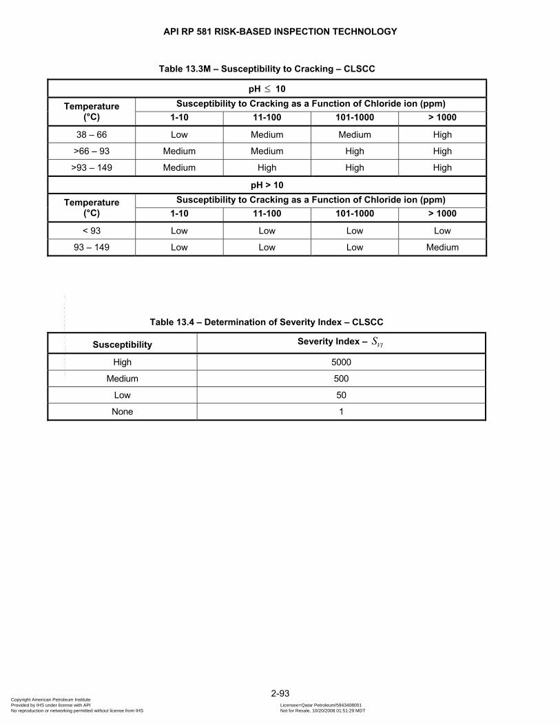
API RP 581 RISK-BASED INSPECTION TECHNOLOGY
Table 13.3M – Susceptibility to Cracking – CLSCC
pH ≤ 10
Temperature (°C)
Susceptibility to Cracking as a Function of Chloride ion (ppm) 1-10 11-100 101-1000 > 1000
38 – 66 Low Medium Medium High
>66 – 93 Medium Medium High High
>93 – 149 Medium High High High
pH > 10
Temperature (°C)
Susceptibility to Cracking as a Function of Chloride ion (ppm) 1-10 11-100 101-1000 > 1000
< 93 Low Low Low Low
93 – 149 Low Low Low Medium
Table 13.4 – Determination of Severity Index – CLSCC
Susceptibility Severity Index – VIS
High 5000
Medium 500
Low 50
None 1
2-93 Copyright American Petroleum Institute Provided by IHS under license with API Licensee=Qatar Petroleum/5943408001
Not for Resale, 10/20/2008 01:51:29 MDTNo reproduction or networking permitted without license from IHS
--```,`,,`,`,,`,`,,,,,,``,```,`-`-`,,`,,`,`,,`---

API RP 581 RISK-BASED INSPECTION TECHNOLOGY
13.10 Figures
Figure 13.1 – Determination of the CLSCC Damage Factor
2-94 Copyright American Petroleum Institute Provided by IHS under license with API Licensee=Qatar Petroleum/5943408001
Not for Resale, 10/20/2008 01:51:29 MDTNo reproduction or networking permitted without license from IHS
--```,`,,`,`,,`,`,,,,,,``,```,`-`-`,,`,,`,`,,`---
API RP 581 RISK-BASED INSPECTION TECHNOLOGY
14 SCC DAMAGE FACTOR – HSC-HF
14.1 Scope The damage factor calculation for components subject to Hydrogen Stress Cracking (HSC) covered in this paragraph.
14.2 Description of Damage Hydrogen stress cracking is defined as cracking of a metal under the combined action of tensile stress and a corrosion mechanism that produces hydrogen which may diffuse into the metal. HSC may result from exposure to hydrogen sulfide, see paragraph 9.0, or from exposure to hydrofluoric acid (HF). HSC-HF occurs in high-strength (high hardness) steels or in hard weld deposits or hard heat-affected zones (HAZs) of lower-strength steels. In addition, HSC-HF may occur in stressed Alloy 400 if oxygen or other oxidizers are present in the HF. Concentrated hydrofluoric acid (HF) is used as the acid catalyst in HF alkylation units. The usual HF-in-water concentrations are 96%–99+% and the temperatures are generally below 66°C [150°F]. Under these conditions a fully killed (deoxidized), low sulfur, clean soft carbon steel is the material of choice for most equipment except where close tolerances are required for operation (i.e., pumps, valves, instruments). Where close tolerances are required and at temperatures over 66°C [150°F] to approximately 178°C [350°F], Alloy 400 is used. Corrosion in 80% and stronger HF-in-water solutions is equivalent to corrosion in anhydrous hydrofluoric acid (AHF, <200 ppm H20) and reference to corrosion in AHF implies an HF-in-water concentration as low as 80%. HF acid with concentrations lower than 80% concentration HF in water are considered aqueous. Both aqueous and anhydrous HF can cause hydrogen embrittlement of hardened carbon and alloy steels. To prevent hydrogen embrittlement in welded steel structures, the requirements of NACE standard RP0472, Methods and Controls to Prevent In-Service Cracking of Carbon Steel Welds in Corrosive Petroleum Refining Environments should be followed. Welds produced by all welding methods should be hardness tested. Alloy steel fasteners have been a source of many failures in anhydrous HF service. ASTM A193 Grade B7, chromium molybdenum steel bolts are hard and will crack in the presence of HF. Grade B7M, the same steel tempered to a lower hardness of 201–235 Brinnell may be a better choice if contact by HF cannot be avoided. However, B7M bolts will also crack if stressed beyond their yield point in an HF environment. Bolt torque may be difficult to control in field flange make-up. In this case, B7 bolts may be specified and replacement of any bolt which may have contacted HF as a result of flange leaks would be required.
14.3 Screening Criteria If the component’s material of construction is carbon or low alloy steel and the component is exposed to hydrofluoric acid in any concentration, then the component should be evaluated for susceptibility to HSC-HF.
14.4 Required Data The basic component data required for analysis is given in Table 5.1 and the specific data required for determination of the HSC-HF damage factor is provided in Table 14.1.
14.5 Basic Assumptions The main assumption in determining the damage factor for HSC-HF is that the damage can be characterized by a susceptibility parameter that is designated as high, medium, or low based on process environment, material of construction, and component fabrication variables (i.e. heat treatment). Based on a susceptibility, a Severity Index can be determined that a measure of the susceptibility of the component cracking (or the probability of initiating cracks) and the probability of a crack resulting in a leak. If cracks are detected in the component during an inspection, the susceptibility is designated as High, and this will result in the maximum value for the Severity Index. Cracks that are found during an inspection should be evaluated using Fitness-For-Service methods in API 579 [10].
2-95 Copyright American Petroleum Institute Provided by IHS under license with API Licensee=Qatar Petroleum/5943408001
Not for Resale, 10/20/2008 01:51:29 MDTNo reproduction or networking permitted without license from IHS
--```,`,,`,`,,`,`,,,,,,``,```,`-`-`,,`,,`,`,,`---
API RP 581 RISK-BASED INSPECTION TECHNOLOGY
14.6 Determination of the Damage Factor
14.6.1 Overview A flow chart of the steps required to determine the damage factor for HSC-HF is shown in Figure 14.1. The following paragraphs provide additional information and the calculation procedure.
14.6.2 Inspection Effectiveness Inspections are ranked according to their expected effectiveness at detecting HSC-HF and correctly predicting the rate of damage. Examples of inspection activities for HSC-HF that are both intrusive (requires entry into the equipment) and non-intrusive (can be performed externally), are provided in Table 14.2. Note that the effectiveness category assigned to the inspection activity differs depending on whether the thinning is general or localized. The effectiveness of each inspection performed within the designated time period must be characterized in accordance with Table 14.2. The number and category of the highest effective inspection will be used to determine the damage factor. If multiple inspections of a lower effectiveness have been conducted during the designated time period, they can be equated to an equivalent higher effectiveness inspection in accordance with paragraph 4.4.3.
14.6.3 Calculation of the Damage Factor The following procedure may be used to determine the damage factor for HSC-HF, see Figure 14.1. a) STEP 1 – Determine the number of inspections, and the corresponding inspection effectiveness category
using paragraph 14.6.2 for all past inspections. Combine the inspections to the highest effectiveness performed using paragraph 4.4.3.
b) STEP 2 – Determine the time in-service, age , since the last Level A, B, C or D inspection was performed.
c) STEP 3 – Determine the susceptibility for cracking using Figure 14.1 and Table 14.3 based on the maximum Brinnell hardness of weldments, and knowledge of whether the component was subject to PWHT. Note that a HIGH susceptibility should be used if cracking is known to be present.
d) STEP 4 – Based on the susceptibility in STEP 3, determine the severity index, , from VIS Table 14.4.
e) STEP 5 – Determine the base damage factor for HSC-HF, HSC HFfBD − , using Table 7.4 based on the number
of, and the highest inspection effectiveness determined in STEP 1, and the severity index, , from STEP 4.
VIS
f) STEP 6 – Calculate the escalation in the damage factor based on the time in-service since the last inspection using the from STEP 2 and Equation (age 2.24). In this equation, it is assumed that the probability for cracking will increase with time since the last inspection as a result of increased exposure to upset conditions and other non-normal conditions.
( )1.1HSC HF HSC HFf fBD D age− −= (2.24)
2-96 Copyright American Petroleum Institute Provided by IHS under license with API Licensee=Qatar Petroleum/5943408001
Not for Resale, 10/20/2008 01:51:29 MDTNo reproduction or networking permitted without license from IHS
--```,`,,`,`,,`,`,,,,,,``,```,`-`-`,,`,,`,`,,`---

API RP 581 RISK-BASED INSPECTION TECHNOLOGY
14.7 Nomenclature age is the in-service time since the last Level A, B, C or D inspection was performed
HSC HFfD − is the damage factor for HSC-HF HSC HFfBD − is the base value of the damage factor for HSC-HF
VIS is the severity index
14.8 References 63. T. F. Degnan, “Material of Construction for Hydrofluoric Acid and Hydrogen Fluoride,” Process Industries
Corrosion, NACE, Houston, TX 1986. 64. Corrosion Resistance of Nickel-Containing Alloy in Hydrofluoric Acid, Hydrogen Fluoride and Fluorine,
Corrosion Engineering Bulletin CEB-5, The International Nickel Co., Inc., 1968.
2-97 Copyright American Petroleum Institute Provided by IHS under license with API Licensee=Qatar Petroleum/5943408001
Not for Resale, 10/20/2008 01:51:29 MDTNo reproduction or networking permitted without license from IHS
--```,`,,`,`,,`,`,,,,,,``,```,`-`-`,,`,,`,`,,`---
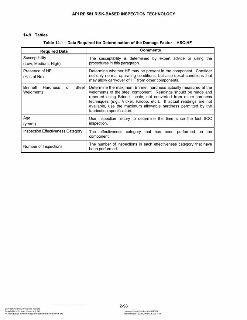
API RP 581 RISK-BASED INSPECTION TECHNOLOGY
14.9 Tables
Table 14.1 – Data Required for Determination of the Damage Factor – HSC-HF
Required Data Comments
Susceptibility (Low, Medium, High)
The susceptibility is determined by expert advice or using the procedures in this paragraph.
Presence of HF (Yes of No)
Determine whether HF may be present in the component. Consider not only normal operating conditions, but also upset conditions that may allow carryover of HF from other components.
Brinnell Hardness of Steel Weldments
Determine the maximum Brinnell hardness actually measured at the weldments of the steel component. Readings should be made and reported using Brinnell scale, not converted from micro-hardness techniques (e.g., Vicker, Knoop, etc.). If actual readings are not available, use the maximum allowable hardness permitted by the fabrication specification.
Age (years)
Use inspection history to determine the time since the last SCC inspection.
Inspection Effectiveness Category
The effectiveness category that has been performed on the component.
Number of Inspections The number of inspections in each effectiveness category that have been performed.
2-98 Copyright American Petroleum Institute Provided by IHS under license with API Licensee=Qatar Petroleum/5943408001
Not for Resale, 10/20/2008 01:51:29 MDTNo reproduction or networking permitted without license from IHS
--```,`,,`,`,,`,`,,,,,,``,```,`-`-`,,`,,`,`,,`---

API RP 581 RISK-BASED INSPECTION TECHNOLOGY
Table 14.2 – Guidelines for Assigning Inspection Effectiveness – HSC-HF
Inspection Category
Inspection Effectiveness
Category Intrusive Inspection Example Non-intrusive Inspection Example
A Highly Effective
Wet fluorescent magnetic particle testing of 25-100% of weldments.
Shear wave ultrasonic testing of 25-100% of weldments, transverse and parallel to the weld with the weld cap removed; or Acoustic Emission testing with follow-up shear wave UT.
B Usually Effective
Wet fluorescent magnetic particle testing of 10-24% of weldments; or Dry magnetic particle testing of 25-100% of weldments; or Dye penetrant testing of 25-100% of weldments.
Shear wave ultrasonic testing of 10-24% of weldments; and Radiographic testing of 50-100% of weldments.
C Fairly Effective
Wet fluorescent magnetic particle testing of less than 10% of weldments; or Dry magnetic particle testing of less than 25% of weldments; or Dye penetrant testing of less than 25% of weldments.
Shear wave ultrasonic testing of less than 10% of weldments; and Radiographic testing of 20-49% of weldments.
D Poorly Effective
Visual inspection Radiographic testing of less than 20% of weldments.
E Ineffective No inspection No inspection
Table 14.3 – Susceptibility to Cracking– HSC-HF
As-Welded Max Brinnell Hardness
PWHT Max Brinnell Hardness
< 200 200-237 > 237 < 200 200-237 > 237
Low Medium High Not Low High
Table 14.4 – Determination of Severity Index – HSC-HF
Susceptibility Severity Index – VIS
High 100
Medium 10
Low 1
None 1
2-99 Copyright American Petroleum Institute Provided by IHS under license with API Licensee=Qatar Petroleum/5943408001
Not for Resale, 10/20/2008 01:51:29 MDTNo reproduction or networking permitted without license from IHS
--```,`,,`,`,,`,`,,,,,,``,```,`-`-`,,`,,`,`,,`---
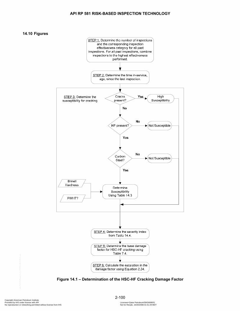
API RP 581 RISK-BASED INSPECTION TECHNOLOGY
14.10 Figures
Figure 14.1 – Determination of the HSC-HF Cracking Damage Factor
2-100 Copyright American Petroleum Institute Provided by IHS under license with API Licensee=Qatar Petroleum/5943408001
Not for Resale, 10/20/2008 01:51:29 MDTNo reproduction or networking permitted without license from IHS
--```,`,,`,`,,`,`,,,,,,``,```,`-`-`,,`,,`,`,,`---

API RP 581 RISK-BASED INSPECTION TECHNOLOGY
15 SCC DAMAGE FACTOR – HIC/SOHIC-HF
15.1 Scope The damage factor calculation for components subject to Hydrogen-Induced Cracking and Stress-Oriented Hydrogen Induced Cracking in Hydrofluoric Acid Services (HIC/SOHIC-HF) is covered in this paragraph.
15.2 Description of Damage Hydrogen-induced cracking is defined as stepwise internal cracks that connect adjacent hydrogen blisters on different planes in the metal, or to the metal surface. No externally applied stress is needed for the formation of HIC. The driving force for the cracking is high stress at the circumference of the hydrogen blisters caused by buildup of internal pressure in the blisters. Interaction between these high stress fields tends to cause cracks to develop that link blisters on different planes in the steel. The source of hydrogen in the steel is the corrosion reaction with either wet hydrogen sulfide (covered in paragraph 10) or hydrofluoric acid (HF). HF is used in HF alkylation units at concentrations in the range 96–99% and greater concentration of HF in water. Exposure of carbon steel to aqueous or anhydrous HF may result in HIC/SOHIC. Hydrogen blisters are planar hydrogen-filled cavities formed at discontinuities in the steel (i.e., voids, inclusions, laminations, sulfide inclusions). Blisters most often occur in rolled plate steels with a banded microstructure resulting from elongated sulfide inclusions. Susceptibility to hydrogen blistering, and therefore HIC, is primarily related to the quality of the plate steel (i.e., the number, size and shape of the discontinuities). In this regard, the sulfur content of the steel is a primary material parameter. Reducing the sulfur content of the steel reduces the susceptibility to blistering and HIC. Addition of calcium or REMS (rare-earth elements) for sulfide inclusion shape control is generally beneficial. SOHIC is defined as a stacked array of blisters joined by hydrogen-induced cracking that is aligned in the through-thickness direction of the steel as a result of high localized tensile stresses. SOHIC is a special form of HIC which usually occurs in the base metal adjacent to the heat-affected zone of a weld, where there are high residual stresses from welding. As with HIC, plate steel quality is a key parameter of SOHIC susceptibility. In addition, reduction of residual stresses by PWHT can reduce, but may not eliminate, the occurrence and severity of SOHIC.
15.3 Screening Criteria If the component’s material of construction is carbon or low alloy steel and the component is exposed to hydrofluoric acid in any concentration, then the component should be evaluated for susceptibility to HIC/SOHIC-HF.
15.4 Required Data The basic component data required for analysis is given in Table 5.1 and the specific data required for determination of the HIC/SOHIC-HF damage factor is provided in Table 15.1.
15.5 Basic Assumptions The main assumption in determining the damage factor for HIC/SOHIC-HF is that the damage can be characterized by a susceptibility parameter that is designated as high, medium, or low based on process environment, material of construction, and component fabrication variables (i.e. heat treatment). Based on a susceptibility, a Severity Index can be determined that a measure of the susceptibility of the component cracking (or the probability of initiating cracks) and the probability of a crack resulting in a leak. If cracks are detected in the component during an inspection, the susceptibility is designated as High, and this will result in the maximum value for the Severity Index. Cracks that are found during an inspection should be evaluated using Fitness-For-Service methods in API 579 [10].
2-101 Copyright American Petroleum Institute Provided by IHS under license with API Licensee=Qatar Petroleum/5943408001
Not for Resale, 10/20/2008 01:51:29 MDTNo reproduction or networking permitted without license from IHS
--```,`,,`,`,,`,`,,,,,,``,```,`-`-`,,`,,`,`,,`---
API RP 581 RISK-BASED INSPECTION TECHNOLOGY
15.6 Determination of the Damage Factor
15.6.1 Overview A flow chart of the steps required to determine the damage factor for HIC/SOHIC-HF is shown in Figure 15.1. The following paragraphs provide additional information and the calculation procedure.
15.6.2 Inspection Effectiveness Inspections are ranked according to their expected effectiveness at detecting HIC/SOHIC-HF and correctly predicting the rate of damage. Examples of inspection activities for HIC/SOHIC-HF that are both intrusive (requires entry into the equipment) and non-intrusive (can be performed externally), are provided in Table 15.2. The effectiveness of each inspection performed within the designated time period must be characterized in accordance with Table 15.2. The number and category of the highest effective inspection will be used to determine the damage factor. If multiple inspections of a lower effectiveness have been conducted during the designated time period, they can be equated to an equivalent higher effectiveness inspection in accordance with paragraph 4.4.3.
15.6.3 Calculation of the Damage Factor The following procedure may be used to determine the damage factor for HIC/SOHIC-HF, see Figure 15.1. a) STEP 1 – Determine the number of inspections, and the corresponding inspection effectiveness category
using paragraph 15.6.2 for all past inspections. Combine the inspections to the highest effectiveness performed using paragraph 4.4.3.
b) STEP 2 – Determine the time in-service, , since the last Level A, B, C or D inspection was performed. agec) STEP 3 – Determine the susceptibility for cracking using Figure 15.1 and Table 15.3 based on the material
of construction and knowledge of whether the component was subject to PWHT. Note that a HIGH susceptibility should be used if cracking is known to be present.
d) STEP 4 – Based on the susceptibility in STEP 3, determine the severity index, , from VIS Table 15.4. In determining the susceptibility, it should be noted that if HF is present in any concentration, then the component is potentially susceptible to HIC/SOHIC-HF. Piping fabricated from wrought components of conventional steels (i.e., A 53, A 106, API 5L [not including 5LX], A 234, A 105, etc.) should be considered to have a low susceptibility to HIC/SOHIC-HF. For components fabricated from rolled and welded plate steel, the susceptibility should be determined using Table 15.4. The susceptibility of the steel to blistering is directly related to the cleanliness of the steel which is measured by sulfur content. It should be recognized that blistering is not a damage mechanism which will lead to a leak path unless it is accompanied by hydrogen-induced cracking leading to the surface. Blistering does pose a danger to mechanical integrity when it approaches a weld which contains sufficient residual stresses to drive the hydrogen-induced cracking to the surfaces. It is in this last case, the most severe situation that is considered when determining the susceptibility to HIC/SOHIC-HF.
e) STEP 5 – Determine the base damage factor for HIC/SOHIC-HF, /HIC SOHIC HFfbD − , using Table 7.4 based on
the number of, and the highest inspection effectiveness determined in STEP 1, and the severity index, , from STEP 4.
VIS
f) STEP 5 – Calculate the escalation in the damage factor based on the time in-service since the last inspection using the from STEP 2 and Equation (age 2.25). In this equation, it is assumed that the probability for cracking will increase with time since the last inspection as a result of increased exposure to upset conditions and other non-normal conditions.
( )1.1/ /HIC SOHIC HF HIC SOHIC HFf fBD D− −= age (2.25)
2-102 Copyright American Petroleum Institute Provided by IHS under license with API Licensee=Qatar Petroleum/5943408001
Not for Resale, 10/20/2008 01:51:29 MDTNo reproduction or networking permitted without license from IHS
--```,`,,`,`,,`,`,,,,,,``,```,`-`-`,,`,,`,`,,`---
API RP 581 RISK-BASED INSPECTION TECHNOLOGY
15.7 Nomenclature age is the in-service time since the last Level A, B, C or D inspection was performed
/HIC SOHIC HFfD − is the damage factor for HIC/SOHIC-HF
/HIC SOHIC HFfBD − is the base value of the damage factor for HIC/SOHIC-HF
VIS is the severity index
15.8 References 65. T. F. Degnan, “Material of Construction for Hydrofluoric Acid and Hydrogen Fluoride,” Process Industries
Corrosion, NACE, Houston, TX 1986. 66. Corrosion Resistance of Nickel-Containing Alloy in Hydrofluoric Acid, Hydrogen Fluoride and Fluorine,
Corrosion Engineering Bulletin CEB-5, The International Nickel Co., Inc., 1968.
2-103 Copyright American Petroleum Institute Provided by IHS under license with API Licensee=Qatar Petroleum/5943408001
Not for Resale, 10/20/2008 01:51:29 MDTNo reproduction or networking permitted without license from IHS
--```,`,,`,`,,`,`,,,,,,``,```,`-`-`,,`,,`,`,,`---

API RP 581 RISK-BASED INSPECTION TECHNOLOGY
15.9 Tables
Table 15.1 – Data Required for Determination of the Damage Factor – HIC/SOHIC-HF
Required Data Comments
Susceptibility (Low, Medium, High)
The susceptibility is determined by expert advice or using the procedures in this paragraph.
Presence of HF (Yes of No)
Determine whether HF may be present in the component. Consider not only normal operating conditions, but also upset conditions that may allow carryover of HF from other components.
Sulfur Content of Plate Steel
Determine the sulfur content of the plate steel used to fabricate the component. This information should be available on the material test report (MTR) in the equipment files. If not available, it can be estimated from the ASTM or ASME specification of the steel listed on the U-1 form in consultation with a materials engineer.
Age (years)
Use inspection history to determine the time since the last SCC inspection.
Inspection Effectiveness Category
The effectiveness category that has been performed on the component.
Number of Inspections The number of inspections in each effectiveness category that have been performed.
2-104 Copyright American Petroleum Institute Provided by IHS under license with API Licensee=Qatar Petroleum/5943408001
Not for Resale, 10/20/2008 01:51:29 MDTNo reproduction or networking permitted without license from IHS
--```,`,,`,`,,`,`,,,,,,``,```,`-`-`,,`,,`,`,,`---

API RP 581 RISK-BASED INSPECTION TECHNOLOGY
Table 15.2 – Guidelines for Assigning Inspection Effectiveness – HIC/SOHIC-HF
Inspection Category
Inspection Effectiveness
Category Intrusive Inspection Example Non-intrusive Inspection Example
A Highly Effective
Wet fluorescent magnetic particle testing of 50-100% of weldments, plus additional shear wave UT for subsurface cracking.
None
B Usually Effective
Wet fluorescent magnetic particle testing of 20-49% of weldments.
Automated shear wave ultrasonic testing of 20-100% of weldments; or Acoustic Emission testing with follow-up shear wave UT.
C Fairly Effective
Wet fluorescent magnetic particle testing of less than 20% of weldments; or Dry magnetic particle testing of 50-100% of weldments; or Dye penetrant testing of 50-100% of weldments.
Automated shear wave ultrasonic testing of less than 20% of weldments; or Manual shear wave ultrasonic testing of 20-100% of weldments.
D Poorly Effective
Dye penetrant testing of less than 50% of weldments; or Visual inspection for hydrogen blisters.
Manual shear wave ultrasonic testing of less than 20% of weldments.
E Ineffective No inspection Radiographic testing
2-105 Copyright American Petroleum Institute Provided by IHS under license with API Licensee=Qatar Petroleum/5943408001
Not for Resale, 10/20/2008 01:51:29 MDTNo reproduction or networking permitted without license from IHS
--```,`,,`,`,,`,`,,,,,,``,```,`-`-`,,`,,`,`,,`---

API RP 581 RISK-BASED INSPECTION TECHNOLOGY
Table 15.3 – Susceptibility to Cracking – HIC/SOHIC-HF
High Sulfur Steel (1) > 0.01% S
Low Sulfur Steel (2) 0.002 – 0.01% S
Ultra Low Sulfur Steel (3) < 0.002% S
As-welded PWHT As-welded PWHT As-welded PWHT
High High High Medium Medium Low
Notes: 1. Typically includes A 70, A 201, A 212, A 285, A 515, and most A 516 before about 1990. 2. Typically includes early generations of HIC-resistant A 516 in 1980’s, with Ca additions. 3. Typically includes later generations of HIC-resistant A 516 in 1990s.
Table 15.4 – Determination of Severity Index – HIC/SOHIC-HF
Susceptibility Severity Index – VIS
High 100
Medium 10
Low 1
None 1
2-106 Copyright American Petroleum Institute Provided by IHS under license with API Licensee=Qatar Petroleum/5943408001
Not for Resale, 10/20/2008 01:51:29 MDTNo reproduction or networking permitted without license from IHS
--```,`,,`,`,,`,`,,,,,,``,```,`-`-`,,`,,`,`,,`---
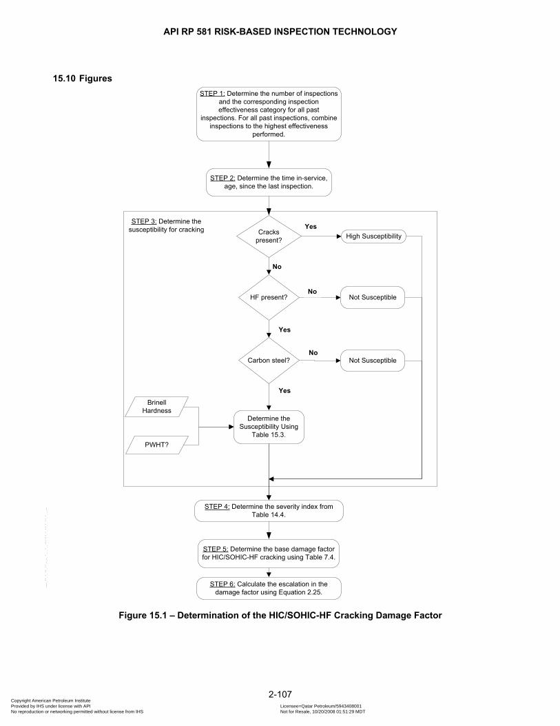
API RP 581 RISK-BASED INSPECTION TECHNOLOGY
15.10 Figures
STEP 2: Determine the time in-service, age, since the last inspection.
Carbon steel?
Brinell Hardness
PWHT?
Yes
No
No
Yes
HF present?
STEP 3: Determine the susceptibility for cracking
STEP 4: Determine the severity index from Table 14.4.
STEP 5: Determine the base damage factor for HIC/SOHIC-HF cracking using Table 7.4.
STEP 6: Calculate the escalation in the damage factor using Equation 2.25.
Not Susceptible
Not Susceptible
Determine the Susceptibility Using
Table 15.3.
STEP 1: Determine the number of inspections and the corresponding inspection effectiveness category for all past
inspections. For all past inspections, combine inspections to the highest effectiveness
performed.
High SusceptibilityCracks present?
No
Yes
Figure 15.1 – Determination of the HIC/SOHIC-HF Cracking Damage Factor
2-107 Copyright American Petroleum Institute Provided by IHS under license with API Licensee=Qatar Petroleum/5943408001
Not for Resale, 10/20/2008 01:51:29 MDTNo reproduction or networking permitted without license from IHS
--```,`,,`,`,,`,`,,,,,,``,```,`-`-`,,`,,`,`,,`---
API RP 581 RISK-BASED INSPECTION TECHNOLOGY
16 EXTERNAL CORROSION DAMAGE FACTOR – FERRITIC COMPONENT
16.1 Scope The damage factor calculation for ferritic components subject to external corrosion is covered in this paragraph.
16.2 Description of Damage As a general rule, plants located in areas with high annual rainfalls or warmer, marine locations are more prone to external corrosion than plants located in cooler, drier, mid-continent locations. Regardless of the climate, units located near cooling towers and steam vents are highly susceptible to external corrosion, as are units whose operating temperatures cycle through the dew point on a regular basis. Mitigation of external corrosion is accomplished through proper painting. A regular program of inspection for paint deterioration and repainting will prevent most occurrences of external corrosion.
16.3 Screening Criteria If the component is uninsulated and subject to any of the following, then the component should be evaluated for external damage from corrosion. a) Areas exposed to mist overspray from cooling towers, b) Areas exposed to steam vents, c) Areas exposed to deluge systems, d) Areas subject to process spills, ingress of moisture, or acid vapors. e) Carbon steel systems, operating between –23°C and 121°C (–10°F and 250°F). External corrosion is
particularly aggressive where operating temperatures cause frequent or continuous condensation and re-evaporation of atmospheric moisture,
f) Systems that do not normally operate between -12°C and 177°C (10°F and 350°F) but cool or heat into this range intermittently or are subjected to frequent outages,
g) Systems with deteriorated coating and/or wrappings, h) Cold service equipment consistently operating below the atmospheric dew point. i) Un-insulated nozzles or other protrusions components of insulated equipment in cold service conditions.
16.4 Required Data The basic component data required for analysis is given in Table 5.1 and the specific data required for determination of the damage factor for external corrosion is provided in Table 16.1.
16.5 Basic Assumption The damage factor for external corrosion is based on the method for general thinning covered in paragraph 5.0.
16.6 Determination of the Damage Factor
16.6.1 Overview A flow chart of the steps required to determine the damage factor for external corrosion is shown in Figure 16.1. The following paragraphs provide additional information and the calculation procedure.
16.6.2 Inspection Effectiveness Inspections are ranked according to their expected effectiveness at detecting external corrosion and correctly predicting the rate of damage. Examples of inspection activities for external corrosion are provided in Table 16.2.
2-108 Copyright American Petroleum Institute Provided by IHS under license with API Licensee=Qatar Petroleum/5943408001
Not for Resale, 10/20/2008 01:51:29 MDTNo reproduction or networking permitted without license from IHS
--```,`,,`,`,,`,`,,,,,,``,```,`-`-`,,`,,`,`,,`---

API RP 581 RISK-BASED INSPECTION TECHNOLOGY
The effectiveness of each inspection performed within the designated time period must be characterized in accordance with Table 16.2. The number and category of the highest effective inspection will be used to determine the damage factor. If multiple inspections of a lower effectiveness have been conducted during the designated time period, they can be equated to an equivalent higher effectiveness inspection in accordance with paragraph 4.4.3.
16.6.3 Calculation of the Damage Factor The following procedure may be used to determine the damage factor for external corrosion, see Figure 16.1. a) STEP 1 – Determine the number of inspections, and the corresponding inspection effectiveness category
using paragraph 16.6.2 for all past inspections. Combine the inspections to the highest effectiveness performed using paragraph 4.4.3.
b) STEP 2 – Determine the time in-service, , since the last inspection thickness reading, , taken either externally or internally.
tkage rdt
c) STEP 3 – Determine the in-service time, , since the coating has been determined to be ineffective using Equation (
coatage2.26).
[ ]max 0, coatage Calculation Date Date= − (2.26)
The parameter Date is determined based on the coating quality using Equations (2.27) through (2.29).
Date Component Installation Date No Coating or Poor Coating Quality= (2.27)
5Date Coating Installation Date years Medium Coating Quality= + (2.28)
15Date Coating Installation Date years High Coating Quality= + (2.29)
d) STEP 4 – Determine the in-service time, age , over which external corrosion may have occurred using Equation (2.30).
[ ]min , tk coatage age age= (2.30)
e) STEP 5 – Determine the base corrosion rate, , based on the driver and operating temperature using rBCTable 16.3.
f) STEP 6 – Compute the final corrosion rate using Equation (2.31).
[ ]max , r rB PS IPC C F F= ⋅ (2.31)
The adjustment factors are determined as follows.
1) Adjustment for Pipe Supports, PSF – If piping is supported directly on beams or other such
configuration that does not allow for proper coating maintenance, then ; otherwise, 2PSF = 1PSF = .
2) Adjustment for Interface, – If the piping has an interface where it enters either soil or water, then
; otherwise, . IPF
1=2IPF = IPF
g) STEP 7 – Determine the minimum required wall thickness, , per the original construction code or using API 579 [
mint10], Appendix A.
h) STEP 8 – Determine the parameter using Equation (rtA 2.32) , based on the age from STEP 4, the
from STEP 2, from STEP 6, and the from STEP 7. rdt
rC mint
min
max 1 , 0.0rd rrt
t C ageAt CA
⎡ ⎤⎛ ⎞− ⋅= −⎢⎜ ⎟+⎝ ⎠⎣ ⎦
⎥ (2.32)
2-109 Copyright American Petroleum Institute Provided by IHS under license with API Licensee=Qatar Petroleum/5943408001
Not for Resale, 10/20/2008 01:51:29 MDTNo reproduction or networking permitted without license from IHS
--```,`,,`,`,,`,`,,,,,,``,```,`-`-`,,`,,`,`,,`---
API RP 581 RISK-BASED INSPECTION TECHNOLOGY
i) STEP 9 – Calculate the damage factor for external corrosion, , using extcorfD Table 5.11 or Table 5.12, as
applicable, based on the number of, and highest effective inspection category from STEP 1, and the parameter from STEP 8.
rtA
16.7 Nomenclature
rtA is the damage factor parameter age is the in-service time
coatage is the in-service time since the coating has been determined to be ineffective
tkage is the in-service time since the last internal or external inspection measurement was taken
rC is the corrosion rate
rBC is the base value of the corrosion rate CA is the corrosion allowance
extcorfD is the damage factor for external corrosion
IPF is the corrosion rate adjustment factor for interface for soil and water
PSF is the corrosion rate adjustment factor for pipe supports
mint is the minimum required wall thickness based on the applicable construction code
rdt is the thickness reading
2-110 Copyright American Petroleum Institute Provided by IHS under license with API Licensee=Qatar Petroleum/5943408001
Not for Resale, 10/20/2008 01:51:29 MDTNo reproduction or networking permitted without license from IHS
--```,`,,`,`,,`,`,,,,,,``,```,`-`-`,,`,,`,`,,`---
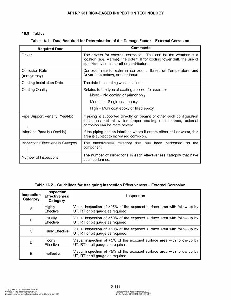
API RP 581 RISK-BASED INSPECTION TECHNOLOGY
16.8 Tables
Table 16.1 – Data Required for Determination of the Damage Factor – External Corrosion
Required Data Comments
Driver The drivers for external corrosion. This can be the weather at a location (e.g. Marine), the potential for cooling tower drift, the use of sprinkler systems, or other contributors.
Corrosion Rate (mm/yr:mpy)
Corrosion rate for external corrosion. Based on Temperature, and Driver (see below), or user input.
Coating Installation Date The date the coating was installed.
Coating Quality Relates to the type of coating applied, for example: None – No coating or primer only
Medium – Single coat epoxy
High – Multi coat epoxy or filled epoxy
Pipe Support Penalty (Yes/No) If piping is supported directly on beams or other such configuration that does not allow for proper coating maintenance, external corrosion can be more severe.
Interface Penalty (Yes/No) If the piping has an interface where it enters either soil or water, this area is subject to increased corrosion.
Inspection Effectiveness Category
The effectiveness category that has been performed on the component.
Number of Inspections The number of inspections in each effectiveness category that have been performed.
Table 16.2 – Guidelines for Assigning Inspection Effectiveness – External Corrosion
Inspection Category
Inspection Effectiveness
Category Inspection
A Highly Effective
Visual inspection of >95% of the exposed surface area with follow-up by UT, RT or pit gauge as required.
B Usually Effective
Visual inspection of >60% of the exposed surface area with follow-up by UT, RT or pit gauge as required.
C Fairly Effective Visual inspection of >30% of the exposed surface area with follow-up by UT, RT or pit gauge as required.
D Poorly Effective
Visual inspection of >5% of the exposed surface area with follow-up by UT, RT or pit gauge as required.
E Ineffective Visual inspection of <5% of the exposed surface area with follow-up by UT, RT or pit gauge as required.
2-111 Copyright American Petroleum Institute Provided by IHS under license with API Licensee=Qatar Petroleum/5943408001
Not for Resale, 10/20/2008 01:51:29 MDTNo reproduction or networking permitted without license from IHS
--```,`,,`,`,,`,`,,,,,,``,```,`-`-`,,`,,`,`,,`---
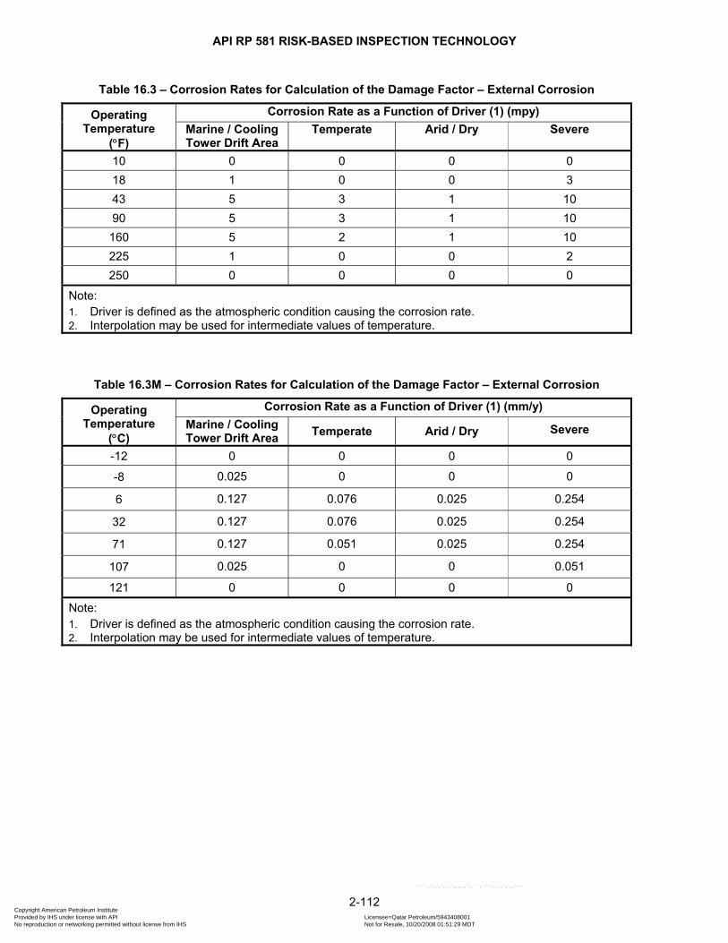
API RP 581 RISK-BASED INSPECTION TECHNOLOGY
Table 16.3 – Corrosion Rates for Calculation of the Damage Factor – External Corrosion
Operating Temperature
(°F)
Corrosion Rate as a Function of Driver (1) (mpy) Marine / Cooling Tower Drift Area
Temperate Arid / Dry Severe
10 0 0 0 0 18 1 0 0 3 43 5 3 1 10 90 5 3 1 10 160 5 2 1 10 225 1 0 0 2 250 0 0 0 0
Note: 1. Driver is defined as the atmospheric condition causing the corrosion rate. 2. Interpolation may be used for intermediate values of temperature.
Table 16.3M – Corrosion Rates for Calculation of the Damage Factor – External Corrosion
Operating Temperature
(°C)
Corrosion Rate as a Function of Driver (1) (mm/y) Marine / Cooling Tower Drift Area Temperate Arid / Dry Severe
-12 0 0 0 0
-8 0.025 0 0 0 6 0.127 0.076 0.025 0.254 32 0.127 0.076 0.025 0.254 71 0.127 0.051 0.025 0.254 107 0.025 0 0 0.051 121 0 0 0 0
Note: 1. Driver is defined as the atmospheric condition causing the corrosion rate. 2. Interpolation may be used for intermediate values of temperature.
2-112 Copyright American Petroleum Institute Provided by IHS under license with API Licensee=Qatar Petroleum/5943408001
Not for Resale, 10/20/2008 01:51:29 MDTNo reproduction or networking permitted without license from IHS
--```,`,,`,`,,`,`,,,,,,``,```,`-`-`,,`,,`,`,,`---
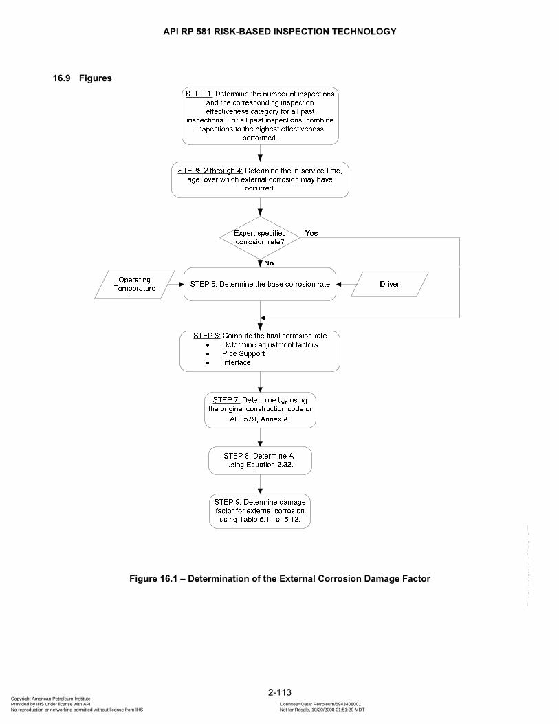
API RP 581 RISK-BASED INSPECTION TECHNOLOGY
16.9 Figures
Figure 16.1 – Determination of the External Corrosion Damage Factor
2-113 Copyright American Petroleum Institute Provided by IHS under license with API Licensee=Qatar Petroleum/5943408001
Not for Resale, 10/20/2008 01:51:29 MDTNo reproduction or networking permitted without license from IHS
--```,`,,`,`,,`,`,,,,,,``,```,`-`-`,,`,,`,`,,`---
API RP 581 RISK-BASED INSPECTION TECHNOLOGY
17 CUI DAMAGE FACTOR – FERRITIC COMPONENT
17.1 Scope The damage factor calculation for ferritic components subject to Corrosion Under Insulation (CUI) is covered in this paragraph.
17.2 Description of Damage Corrosion Under Insulation (CUI) results from the collection of water in the vapor space (or annulus space) between the insulation and the metal surface. Sources of water may include rain, water leaks, condensation, cooling water tower drift, deluge systems, and steam tracing leaks. CUI causes wall loss in the form of localized corrosion. CUI generally occurs in the temperature range between -12°C and 177°C [10°F and 350°F], with the temperature range of 49°C to 93°C [120°F to 200°F] being the most severe environment. As a general rule, plants located in areas with high annual rainfall or warmer, marine locations are more prone to CUI than plants located in cooler, drier, mid-continent locations. Regardless of the climate, units located near cooling towers and steam vents are highly susceptible to CUI, as are units whose operating temperatures cycle through the dew point on a regular basis. External inspection of insulated systems should include a review of the integrity of the insulation system for conditions that could lead to CUI and for signs of ongoing CUI, i.e. rust stains or bulging. However, external indicators of CUI are not always present. Mitigation of CUI is accomplished through good insulation practices and proper coatings. Proper installation and maintenance of insulation simply prevents ingress of large quantities of water. In recent years, a coating system is frequently specified for component operating in the CUI temperature range, and where CUI has been a problem. A high quality immersion grade coating, like those used in hot water tanks, is recommended. For guidance refer to NACE Publication 6H189. A good coating system should last a minimum of 15 years.
17.3 Screening Criteria Specific locations and/or systems, such as penetrations and visually damaged insulation areas, are highly suspect and should be considered during inspection program development. Examples of highly suspect areas include, but are not limited to, the following: a) Penetrations
1) All penetrations or breaches in the insulation jacketing systems, such as dead legs (vents, drains, and other similar items), hangers and other supports, valves and fittings, bolted-on pipe shoes, ladders, and platforms.
2) Steam tracer tubing penetrations. 3) Termination of insulation at flanges and other components. 4) Poorly designed insulation support rings. 5) Stiffener rings.
b) Damaged Insulation Areas 1) Damaged or missing insulation jacketing 2) Termination of insulation in a vertical pipe or piece of equipment 3) Caulking that has hardened, has separated, or is missing 4) Bulges, staining of the jacketing system or missing bands (bulges may indicate corrosion product
build-up) 5) Low points in systems that have a known breach in the insulation system, including low points in long
unsupported piping runs 6) Carbon or low alloy steel flanges, bolting, and other components under insulation in high alloy piping
The following are some examples of other suspect areas that should be considered when performing inspection for CUI: a) Areas exposed to mist overspray from cooling towers. b) Areas exposed to steam vents.
2-114 Copyright American Petroleum Institute Provided by IHS under license with API Licensee=Qatar Petroleum/5943408001
Not for Resale, 10/20/2008 01:51:29 MDTNo reproduction or networking permitted without license from IHS
--```,`,,`,`,,`,`,,,,,,``,```,`-`-`,,`,,`,`,,`---

API RP 581 RISK-BASED INSPECTION TECHNOLOGY
c) Areas exposed to deluge systems. d) Areas subject to process spills, ingress of moisture, or acid vapors. e) Insulation jacketing seams located on top of horizontal vessels or improperly lapped or sealed insulation
systems, f) Carbon steel systems, including those insulated for personnel protection, operating between -12°C and
177°C [10°F and 350°F]. CUI is particularly aggressive where operating temperatures cause frequent or continuous condensation and re-evaporation of atmospheric moisture.
g) Carbon steel systems that normally operate in services above 177°C [350°F] but are in intermittent service or are subjected to frequent outages.
h) Dead legs and attachments that protrude from the insulation and operate at a different temperature than the operating temperature of the active line, i.e. insulation support rings, piping/platform attachments.
i) Systems in which vibration has a tendency to inflict damage to insulation jacketing providing paths for water ingress.
j) Steam traced systems experiencing tracing leaks, especially at tubing fittings beneath the insulation. k) Systems with deteriorated coating and/or wrappings. l) Cold service equipment consistently operating below the atmospheric dew point. m) Inspection ports or plugs which are removed to permit thickness measurements on insulated systems
represent a major contributor to possible leaks in insulated systems. Special attention should be paid to these locations. Promptly replacing and resealing of these plugs is imperative.
17.4 Required Data The basic component data required for analysis is given in Table 5.1 and the specific data required for determination of the damage factor for CUI is provided in Table 17.1.
17.5 Basic Assumption The damage factor for CUI is based on the method for general thinning covered in paragraph 5.0.
17.6 Determination of the Damage Factor
17.6.1 Overview A flow chart of the steps required to determine the damage factor for CUI is shown in Figure 17.1. The following paragraphs provide additional information and the calculation procedure.
17.6.2 Inspection Effectiveness Inspections are ranked according to their expected effectiveness at detecting CUI and correctly predicting the rate of damage. Examples of inspection activities for detection of CUI are provided in Table 17.2. The effectiveness of each inspection performed within the designated time period must be characterized in accordance with Table 17.2. The number and category of the highest effective inspection will be used to determine the damage factor. If multiple inspections of a lower effectiveness have been conducted during the designated time period, they can be equated to an equivalent higher effectiveness inspection in accordance with paragraph 4.4.3.
17.6.3 Calculation of the Damage Factor The following procedure may be used to determine the damage factor for CUI, see Figure 17.1. a) STEP 1 – Determine the number of inspections, and the corresponding inspection effectiveness category
using paragraph 17.6.2 for all past inspections. Combine the inspections to the highest effectiveness performed using paragraph 4.4.3.
b) STEP 2 – Determine the time in-service, , since the last inspection thickness reading, , taken either externally or internally.
tkage rdt
2-115 Copyright American Petroleum Institute Provided by IHS under license with API Licensee=Qatar Petroleum/5943408001
Not for Resale, 10/20/2008 01:51:29 MDTNo reproduction or networking permitted without license from IHS
--```,`,,`,`,,`,`,,,,,,``,```,`-`-`,,`,,`,`,,`---
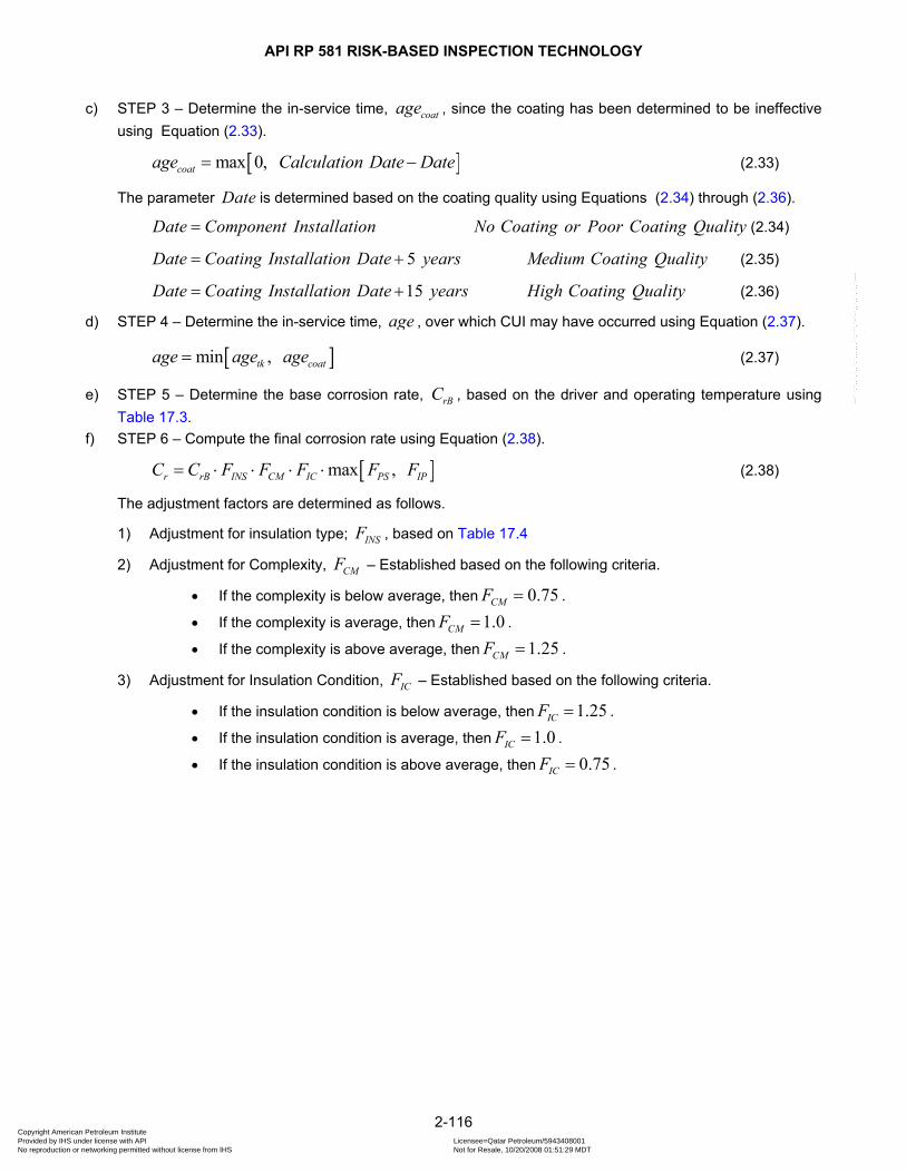
API RP 581 RISK-BASED INSPECTION TECHNOLOGY
c) STEP 3 – Determine the in-service time, , since the coating has been determined to be ineffective using Equation (
coatage2.33).
[ ]max 0, coatage Calculation Date Date= − (2.33)
The parameter Date is determined based on the coating quality using Equations (2.34) through (2.36).
Date Component Installation No Coating or Poor Coating Quality= (2.34)
5Date Coating Installation Date years Medium Coating Quality= + (2.35)
15Date Coating Installation Date years High Coating Quality= + (2.36)
d) STEP 4 – Determine the in-service time, age , over which CUI may have occurred using Equation (2.37).
[ ]min , tk coatage age age= (2.37)
e) STEP 5 – Determine the base corrosion rate, , based on the driver and operating temperature using rBCTable 17.3.
f) STEP 6 – Compute the final corrosion rate using Equation (2.38).
[ ]max , r rB INS CM IC PS IPC C F F F F F= ⋅ ⋅ ⋅ ⋅ (2.38)
The adjustment factors are determined as follows.
1) Adjustment for insulation type; , based on INSF Table 17.4
2) Adjustment for Complexity, – Established based on the following criteria. CMF
• If the complexity is below average, then 0.75CMF = .
• If the complexity is average, then 1.0CMF = .
• If the complexity is above average, then 1.25CMF = .
3) Adjustment for Insulation Condition, – Established based on the following criteria. ICF
• If the insulation condition is below average, then 1.25ICF = .
• If the insulation condition is average, then 1.0ICF = .
• If the insulation condition is above average, then 0.75ICF = .
2-116 Copyright American Petroleum Institute Provided by IHS under license with API Licensee=Qatar Petroleum/5943408001
Not for Resale, 10/20/2008 01:51:29 MDTNo reproduction or networking permitted without license from IHS
--```,`,,`,`,,`,`,,,,,,``,```,`-`-`,,`,,`,`,,`---

API RP 581 RISK-BASED INSPECTION TECHNOLOGY
4) Adjustment for Pipe Supports, PSF – If piping is supported directly on beams or other such
configuration that does not allow for proper coating maintenance, then ; otherwise, 2PSF = 1PSF = .
5) Adjustment for Interface, – If the piping has an interface where it enters either soil or water, then
; otherwise, . IPF
1=2IPF = IPF
g) STEP 7 – Determine the minimum required wall thickness, , per the original construction code or using API 579 [
mint10], Appendix A.
h) STEP 8 – Determine the parameter using Equation (rtA 2.39) , based on the from STEP 4, the
from STEP 2, from STEP 6, and the from STEP 7.
age rdt
rC mint
min
max 1 , 0.0rd rrt
t C ageAt CA
⎡ ⎤⎛ ⎞− ⋅= −⎢⎜ ⎟+⎝ ⎠⎣ ⎦
⎥ (2.39)
i) STEP 9 – Calculate the damage factor for CUI, , using CUIFfD Table 5.11 or Table 5.12, as applicable,
based on the number of, and highest effective inspection category from STEP 1, and the parameter from STEP 8.
rtA
17.7 Nomenclature
rtA is the damage factor parameter age is the in-service time
coatage is the in-service time since the coating has been determined to be ineffective
tkage is the in-service time since the last internal or external inspection measurement was taken
rC is the corrosion rate
rBC is the base value of the corrosion rate CA is the corrosion allowance
CUIFfD is the damage factor for CUI for ferritic components
CMF is the corrosion rate adjustment factor for insulation complexity
ICF is the corrosion rate adjustment factor for insulation condition
INSF the corrosion rate adjustment factor for insulation type
IPF is the corrosion rate adjustment factor for interface for soil and water
PSF is the corrosion rate adjustment factor for pipe supports
mint is the minimum required wall thickness based on the applicable construction code
rdt is the thickness reading
2-117 Copyright American Petroleum Institute Provided by IHS under license with API Licensee=Qatar Petroleum/5943408001
Not for Resale, 10/20/2008 01:51:29 MDTNo reproduction or networking permitted without license from IHS
--```,`,,`,`,,`,`,,,,,,``,```,`-`-`,,`,,`,`,,`---
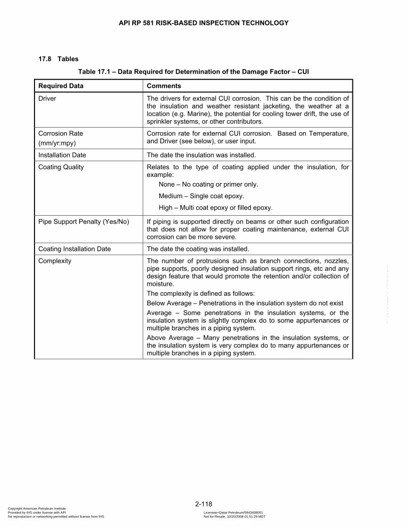
API RP 581 RISK-BASED INSPECTION TECHNOLOGY
17.8 Tables
Table 17.1 – Data Required for Determination of the Damage Factor – CUI
Required Data Comments
Driver The drivers for external CUI corrosion. This can be the condition of the insulation and weather resistant jacketing, the weather at a location (e.g. Marine), the potential for cooling tower drift, the use of sprinkler systems, or other contributors.
Corrosion Rate (mm/yr:mpy)
Corrosion rate for external CUI corrosion. Based on Temperature, and Driver (see below), or user input.
Installation Date The date the insulation was installed.
Coating Quality Relates to the type of coating applied under the insulation, for example:
None – No coating or primer only.
Medium – Single coat epoxy.
High – Multi coat epoxy or filled epoxy.
Pipe Support Penalty (Yes/No) If piping is supported directly on beams or other such configuration that does not allow for proper coating maintenance, external CUI corrosion can be more severe.
Coating Installation Date The date the coating was installed.
Complexity The number of protrusions such as branch connections, nozzles, pipe supports, poorly designed insulation support rings, etc and any design feature that would promote the retention and/or collection of moisture. The complexity is defined as follows: Below Average – Penetrations in the insulation system do not exist Average – Some penetrations in the insulation systems, or the insulation system is slightly complex do to some appurtenances or multiple branches in a piping system. Above Average – Many penetrations in the insulation systems, or the insulation system is very complex do to many appurtenances or multiple branches in a piping system.
2-118 Copyright American Petroleum Institute Provided by IHS under license with API Licensee=Qatar Petroleum/5943408001
Not for Resale, 10/20/2008 01:51:29 MDTNo reproduction or networking permitted without license from IHS
--```,`,,`,`,,`,`,,,,,,``,```,`-`-`,,`,,`,`,,`---
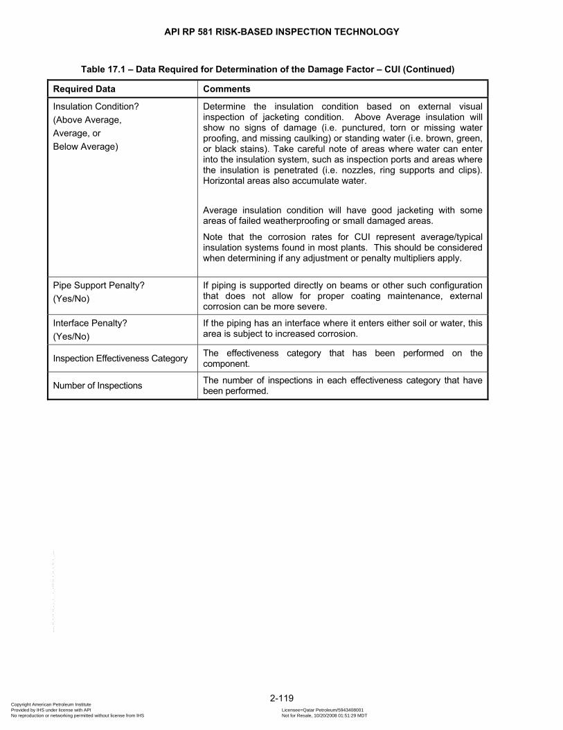
API RP 581 RISK-BASED INSPECTION TECHNOLOGY
Table 17.1 – Data Required for Determination of the Damage Factor – CUI (Continued)
Required Data Comments
Insulation Condition? (Above Average, Average, or Below Average)
Determine the insulation condition based on external visual inspection of jacketing condition. Above Average insulation will show no signs of damage (i.e. punctured, torn or missing water proofing, and missing caulking) or standing water (i.e. brown, green, or black stains). Take careful note of areas where water can enter into the insulation system, such as inspection ports and areas where the insulation is penetrated (i.e. nozzles, ring supports and clips). Horizontal areas also accumulate water.
Average insulation condition will have good jacketing with some areas of failed weatherproofing or small damaged areas.
Note that the corrosion rates for CUI represent average/typical insulation systems found in most plants. This should be considered when determining if any adjustment or penalty multipliers apply.
Pipe Support Penalty? (Yes/No)
If piping is supported directly on beams or other such configuration that does not allow for proper coating maintenance, external corrosion can be more severe.
Interface Penalty? (Yes/No)
If the piping has an interface where it enters either soil or water, this area is subject to increased corrosion.
Inspection Effectiveness Category The effectiveness category that has been performed on the component.
Number of Inspections The number of inspections in each effectiveness category that have been performed.
2-119 Copyright American Petroleum Institute Provided by IHS under license with API Licensee=Qatar Petroleum/5943408001
Not for Resale, 10/20/2008 01:51:29 MDTNo reproduction or networking permitted without license from IHS
--```,`,,`,`,,`,`,,,,,,``,```,`-`-`,,`,,`,`,,`---
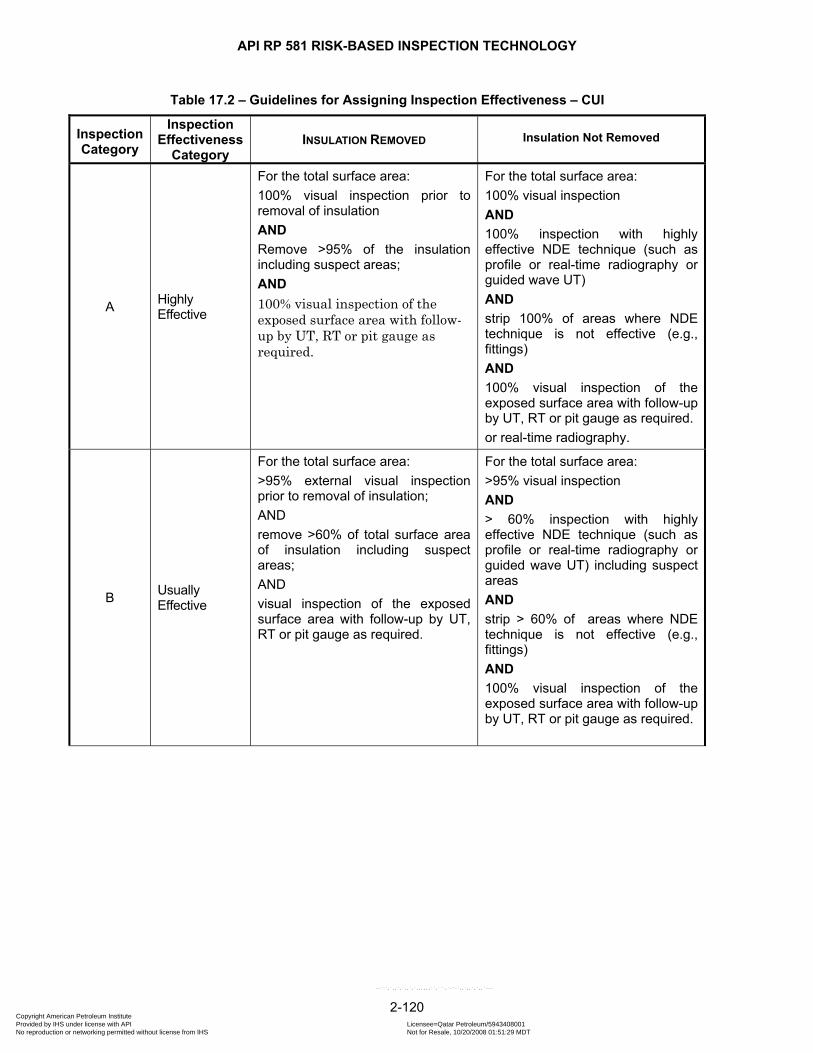
API RP 581 RISK-BASED INSPECTION TECHNOLOGY
Table 17.2 – Guidelines for Assigning Inspection Effectiveness – CUI
Inspection Category
Inspection Effectiveness
Category INSULATION REMOVED Insulation Not Removed
A Highly Effective
For the total surface area: 100% visual inspection prior to removal of insulation AND Remove >95% of the insulation including suspect areas; AND 100% visual inspection of the exposed surface area with follow-up by UT, RT or pit gauge as required.
For the total surface area: 100% visual inspection AND 100% inspection with highly effective NDE technique (such as profile or real-time radiography or guided wave UT) AND strip 100% of areas where NDE technique is not effective (e.g., fittings) AND 100% visual inspection of the exposed surface area with follow-up by UT, RT or pit gauge as required. or real-time radiography.
B Usually Effective
For the total surface area: >95% external visual inspection prior to removal of insulation; AND remove >60% of total surface area of insulation including suspect areas; AND visual inspection of the exposed surface area with follow-up by UT, RT or pit gauge as required.
For the total surface area: >95% visual inspection AND > 60% inspection with highly effective NDE technique (such as profile or real-time radiography or guided wave UT) including suspect areas AND strip > 60% of areas where NDE technique is not effective (e.g., fittings) AND 100% visual inspection of the exposed surface area with follow-up by UT, RT or pit gauge as required.
2-120 Copyright American Petroleum Institute Provided by IHS under license with API Licensee=Qatar Petroleum/5943408001
Not for Resale, 10/20/2008 01:51:29 MDTNo reproduction or networking permitted without license from IHS
--```,`,,`,`,,`,`,,,,,,``,```,`-`-`,,`,,`,`,,`---

API RP 581 RISK-BASED INSPECTION TECHNOLOGY
Table 17.2 – Guidelines for Assigning Inspection Effectiveness – CUI
Inspection Category
Inspection Effectiveness
Category INSULATION REMOVED Insulation Not Removed
C Fairly Effective
For the total surface area: >95% external visual inspection prior to removal of insulation; AND remove >30% of total surface area of insulation including suspect areas; AND visual inspection of the exposed surface area with follow-up by UT, RT or pit gauge as required.
For the total surface area: >95% visual inspection AND > 24% inspection with highly effective NDE technique (such as profile or real-time radiography or guided wave UT) including suspect areas AND strip > 24% of areas where NDE technique is not effective (e.g., fittings) AND 100% visual inspection of the exposed surface area with follow-up by UT, RT or pit gauge as required.
D Poorly Effective
>95% external visual inspection prior to removal of insulation; AND remove >5% of total surface area of insulation including suspect areas. AND visual inspection of the exposed surface area with follow-up by UT, RT or pit gauge as required.
For the total surface area: >95% visual inspection AND > 5% inspection with highly effective NDE technique (such as profile or real-time radiography or guided wave UT) including suspect areas AND strip > 5% of areas where NDE technique is not effective (e.g., fittings) AND 100% visual inspection of the exposed surface area with follow-up by UT, RT or pit gauge as required.
E Ineffective
<5% insulation removal and inspection; OR no inspection or ineffective inspection technique.
No inspection or ineffective inspection technique or <95% visual inspection.
2-121 Copyright American Petroleum Institute Provided by IHS under license with API Licensee=Qatar Petroleum/5943408001
Not for Resale, 10/20/2008 01:51:29 MDTNo reproduction or networking permitted without license from IHS
--```,`,,`,`,,`,`,,,,,,``,```,`-`-`,,`,,`,`,,`---
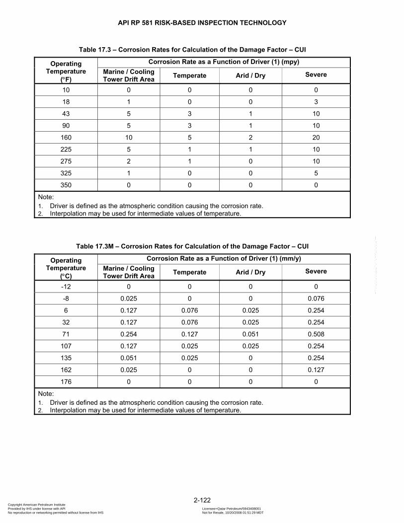
API RP 581 RISK-BASED INSPECTION TECHNOLOGY
Table 17.3 – Corrosion Rates for Calculation of the Damage Factor – CUI
Operating Temperature
(°F)
Corrosion Rate as a Function of Driver (1) (mpy) Marine / Cooling Tower Drift Area Temperate Arid / Dry Severe
10 0 0 0 0
18 1 0 0 3
43 5 3 1 10
90 5 3 1 10
160 10 5 2 20
225 5 1 1 10
275 2 1 0 10
325 1 0 0 5
350 0 0 0 0
Note: 1. Driver is defined as the atmospheric condition causing the corrosion rate. 2. Interpolation may be used for intermediate values of temperature.
Table 17.3M – Corrosion Rates for Calculation of the Damage Factor – CUI
Operating Temperature
(°C)
Corrosion Rate as a Function of Driver (1) (mm/y) Marine / Cooling Tower Drift Area Temperate Arid / Dry Severe
-12 0 0 0 0
-8 0.025 0 0 0.076
6 0.127 0.076 0.025 0.254
32 0.127 0.076 0.025 0.254
71 0.254 0.127 0.051 0.508
107 0.127 0.025 0.025 0.254
135 0.051 0.025 0 0.254
162 0.025 0 0 0.127
176 0 0 0 0
Note: 1. Driver is defined as the atmospheric condition causing the corrosion rate. 2. Interpolation may be used for intermediate values of temperature.
2-122 Copyright American Petroleum Institute Provided by IHS under license with API Licensee=Qatar Petroleum/5943408001
Not for Resale, 10/20/2008 01:51:29 MDTNo reproduction or networking permitted without license from IHS
--```,`,,`,`,,`,`,,,,,,``,```,`-`-`,,`,,`,`,,`---

API RP 581 RISK-BASED INSPECTION TECHNOLOGY
Table 17.4 – Corrosion Rate Adjustment Factor for Insulation Type
Insulation Type Adjustment Factor, INSF
None 1.0
Foamglass 0.75
Pearlite 1.0
Fiberglass 1.25
Mineral Wool 1.25
Calcium Silicate 1.25
Asbestos 1.25
2-123 Copyright American Petroleum Institute Provided by IHS under license with API Licensee=Qatar Petroleum/5943408001
Not for Resale, 10/20/2008 01:51:29 MDTNo reproduction or networking permitted without license from IHS
--```,`,,`,`,,`,`,,,,,,``,```,`-`-`,,`,,`,`,,`---
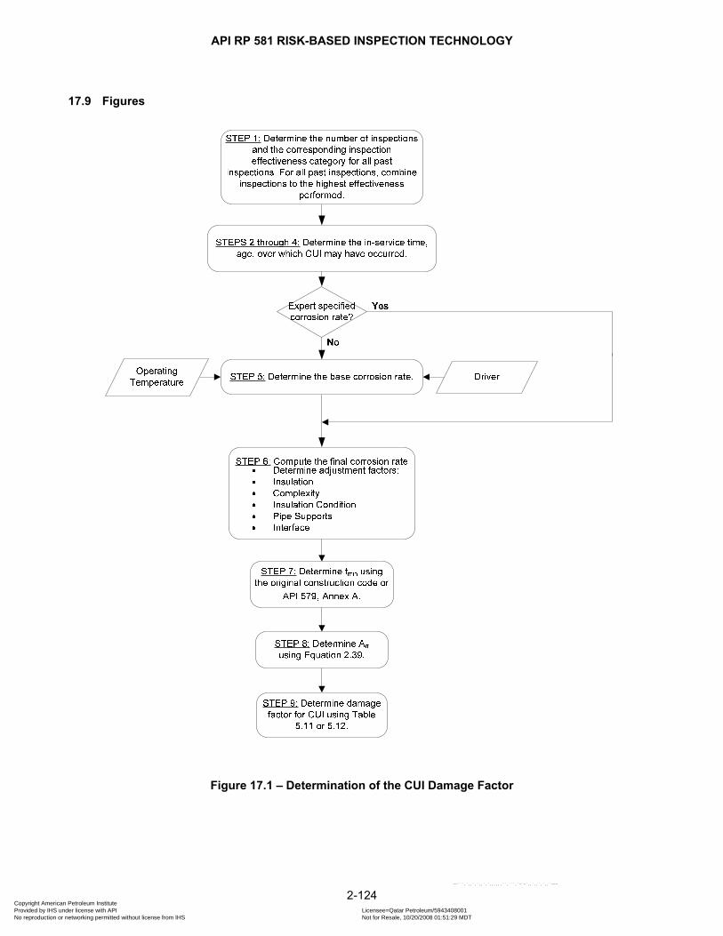
API RP 581 RISK-BASED INSPECTION TECHNOLOGY
17.9 Figures
Figure 17.1 – Determination of the CUI Damage Factor
2-124 Copyright American Petroleum Institute Provided by IHS under license with API Licensee=Qatar Petroleum/5943408001
Not for Resale, 10/20/2008 01:51:29 MDTNo reproduction or networking permitted without license from IHS
--```,`,,`,`,,`,`,,,,,,``,```,`-`-`,,`,,`,`,,`---
API RP 581 RISK-BASED INSPECTION TECHNOLOGY
18 EXTERNAL CLSCC DAMAGE FACTOR – AUSTENITIC COMPONENT
18.1 Scope The damage factor calculation for uninsulated austenitic stainless steel components subject to external chloride stress corrosion is covered in this paragraph.
18.2 Description of Damage Uninsulated austenitic stainless steel components located in process plants may be subject to external CLSCC, see paragraph 13.0, as a result chloride accumulation resulting from local atmospheric conditions that include chlorides. Mitigation of external CLSCC is best accomplished by preventing chloride accumulation on the stainless steel surface. On uninsulated surfaces, chloride containing fluids, mists, or solids should be prevented from contacting the surface. Markers, dyes, tape, etc. used on stainless steels should be certified suitable for such applications. In rare cases, uninsulated stainless steels could be protected externally by a coating. If intermittent conditions exist, then both normal operating and intermittent temperatures should be considered.
18.3 Screening Criteria If all of the following are true, then the component should be evaluated for susceptibility to external CLSCC. a) The component’s material of construction is an austenitic stainless steel, b) The component external surface is exposed to chloride containing fluids, mists, or solids. c) The operating temperature is between 49°C and 149°C [120°F and 300°F], or the system heats or cools
into this range intermittently.
18.4 Required Data The basic component data required for analysis is given in Table 5.1 and the specific data required for determination of the damage factor for external CLSCC is provided in Table 18.1.
18.5 Basic Assumption The damage factor for external CLSCC is based on the method in paragraph 13.0.
18.6 Determination of the Damage Factor
18.6.1 Overview A flow chart of the steps required to determine the damage factor for external CLSCC is shown in Figure 18.1. The following paragraphs provide additional information and the calculation procedure.
18.6.2 Inspection Effectiveness Inspections are ranked according to their expected effectiveness at detecting external CLSCC and correctly predicting the rate of damage. Examples of inspection activities for detection of external CLSCC are provided in Table 18.2. The effectiveness of each inspection performed within the designated time period must be characterized in accordance with Table 18.2. The number and category of the highest effective inspection will be used to determine the damage factor. If multiple inspections of a lower effectiveness have been conducted during the designated time period, they can be equated to an equivalent higher effectiveness inspection in accordance with paragraph 4.4.3.
2-125 Copyright American Petroleum Institute Provided by IHS under license with API Licensee=Qatar Petroleum/5943408001
Not for Resale, 10/20/2008 01:51:29 MDTNo reproduction or networking permitted without license from IHS
--```,`,,`,`,,`,`,,,,,,``,```,`-`-`,,`,,`,`,,`---

API RP 581 RISK-BASED INSPECTION TECHNOLOGY
18.6.3 Calculation of the Damage Factor The following procedure may be used to determine the damage factor for external CLSCC, see Figure 18.1. a) STEP 1 – Determine the number of inspections, and the corresponding inspection effectiveness category
using paragraph 18.6.2 for all past inspections. Combine the inspections to the highest effectiveness performed using paragraph 4.4.3.
b) STEP 2 – Determine the in-service time, age , over which external CLSCC may have occurred using Equation (2.40).
[ ]max 0, age Calculation Date Date= − (2.40)
The parameter Date is determined based on the coating quality using Equations (2.41) through (2.43).
Date Component Installation Date No Coating or Poor Coating Quality= (2.41)
5Date Coating Installation Date years Medium Coating Quality= + (2.42)
15Date Coating Installation Date years High Coating Quality= + (2.43)
c) STEP 3 – Determine the susceptibility using Table 18.3 based on the driver and the operating temperature.
d) STEP 4 – Determine the Severity Index, , using VIS Table 18.4 based on the susceptibility from STEP 3.
e) STEP 5 – Determine the base damage factor for external CLSCC, , using ext CLSCCfBD − Table 7.4 based on
the number of, and the highest inspection effectiveness determined in STEP 1, and the severity index, , from STEP 4.
VIS
f) STEP 6 – Calculate the escalation in the damage factor based on the time in-service since the last inspection using the age from STEP 2 and Equation (2.44). In this equation, it is assumed that the probability for cracking will increase with time since the last inspection as a result of increased exposure to upset conditions and other non-normal conditions.
( )1.1ext CLSCC extnal CLSCCf fBD D ag− −= e (2.44)
18.7 Nomenclature age is the in-service time
ext CLSCCfD − is the damage factor for external CLSCC ext CLSCCfBD − is the base value of the damage factor for external CLSCC
VIS is the severity index
2-126 Copyright American Petroleum Institute Provided by IHS under license with API Licensee=Qatar Petroleum/5943408001
Not for Resale, 10/20/2008 01:51:29 MDTNo reproduction or networking permitted without license from IHS
--```,`,,`,`,,`,`,,,,,,``,```,`-`-`,,`,,`,`,,`---

API RP 581 RISK-BASED INSPECTION TECHNOLOGY
18.8 Tables
Table 18.1 – Data Required for Determination of the Damage Factor – External CLSCC
Required Data Comments
Driver The drivers for external CLSCC. This can be the weather at a location (e.g. Marine), the potential for cooling tower drift, the use of sprinkler systems, or other contributors.
Crack Severity Crack severity based on susceptibility (Temperature, and Weather, see below).
Date The date the component was installed or the date of the last inspection where no damage was found
Coating Quality Relates to the type of coating applied, for example: None – No coating or primer only.
Medium – Single coat epoxy.
High – Multi coat epoxy or filled epoxy.
Coating Date Determine the age of the coating.
Inspection Effectiveness Category The effectiveness category that has been performed on the component.
Number of Inspections The number of inspections in each effectiveness category that have been performed.
Operating Temperature, °C [°F] Determine the expected operating temperature (consider normal and non-normal operating conditions).
Table 18.2 – Guidelines for Assigning Inspection Effectiveness – External CLSCC
Inspection Category
Inspection Effectiveness
Category Inspection
A Highly Effective
For the total surface area: greater than 95% dye penetrant or eddy current test with UT follow-up of relevant indications.
B Usually Effective
For the total surface area: greater than 60% dye penetrant or eddy current testing with UT follow-up of all relevant indications.
C Fairly Effective For the total surface area: greater than 30% dye penetrant or eddy current testing with UT follow-up of all relevant indications.
D Poorly Effective
For the total surface area: greater than 5% dye penetrant or eddy current testing with UT follow-up of all relevant indications.
E Ineffective Less than “D” effectiveness or no inspection or ineffective inspection technique used.
2-127 Copyright American Petroleum Institute Provided by IHS under license with API Licensee=Qatar Petroleum/5943408001
Not for Resale, 10/20/2008 01:51:29 MDTNo reproduction or networking permitted without license from IHS
--```,`,,`,`,,`,`,,,,,,``,```,`-`-`,,`,,`,`,,`---
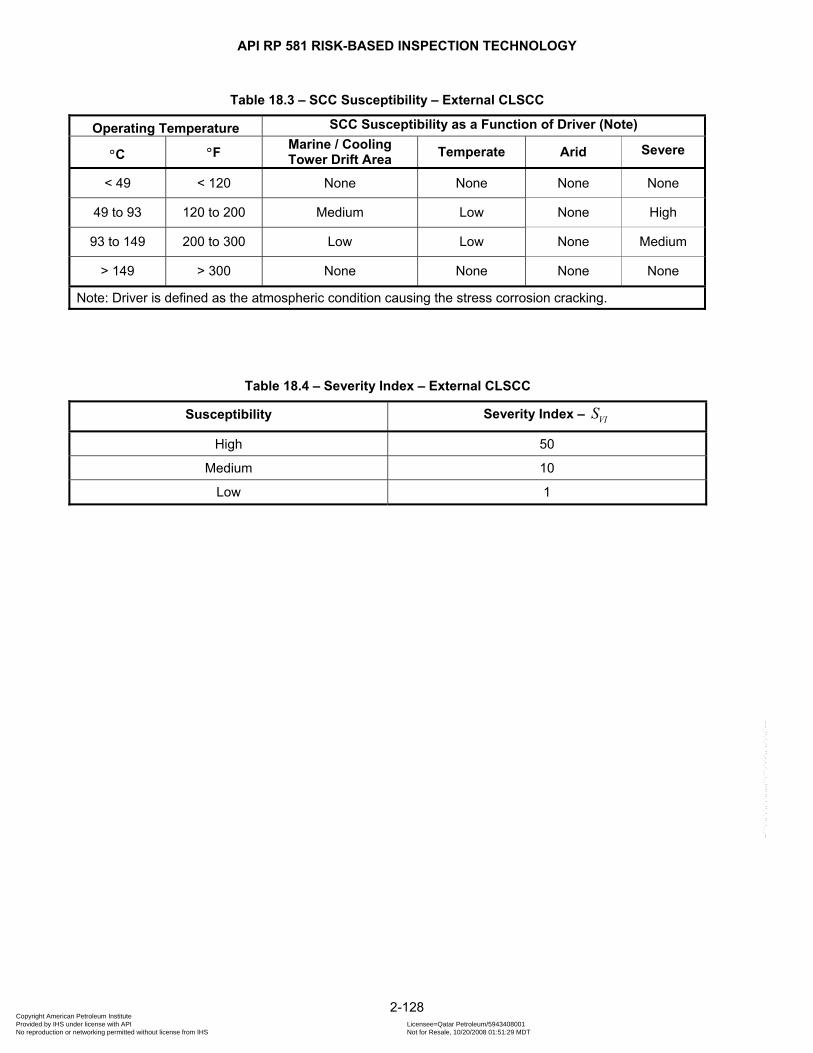
API RP 581 RISK-BASED INSPECTION TECHNOLOGY
Table 18.3 – SCC Susceptibility – External CLSCC
Operating Temperature SCC Susceptibility as a Function of Driver (Note)
°C °F Marine / Cooling Tower Drift Area Temperate Arid Severe
< 49 < 120 None None None None
49 to 93 120 to 200 Medium Low None High
93 to 149 200 to 300 Low Low None Medium
> 149 > 300 None None None None
Note: Driver is defined as the atmospheric condition causing the stress corrosion cracking.
Table 18.4 – Severity Index – External CLSCC
Susceptibility Severity Index – VIS
High 50
Medium 10
Low 1
2-128 Copyright American Petroleum Institute Provided by IHS under license with API Licensee=Qatar Petroleum/5943408001
Not for Resale, 10/20/2008 01:51:29 MDTNo reproduction or networking permitted without license from IHS
--```,`,,`,`,,`,`,,,,,,``,```,`-`-`,,`,,`,`,,`---
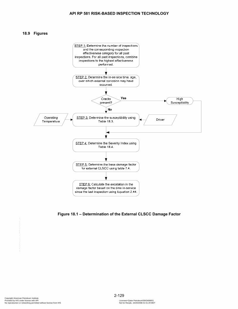
API RP 581 RISK-BASED INSPECTION TECHNOLOGY
18.9 Figures
Figure 18.1 – Determination of the External CLSCC Damage Factor
2-129 Copyright American Petroleum Institute Provided by IHS under license with API Licensee=Qatar Petroleum/5943408001
Not for Resale, 10/20/2008 01:51:29 MDTNo reproduction or networking permitted without license from IHS
--```,`,,`,`,,`,`,,,,,,``,```,`-`-`,,`,,`,`,,`---

API RP 581 RISK-BASED INSPECTION TECHNOLOGY
19 EXTERNAL CUI CLSCC DAMAGE FACTOR – AUSTENITIC COMPONENT
19.1 Scope The damage factor calculation for insulated austenitic stainless steel components subject to external chloride stress corrosion under insulation is covered in this paragraph.
19.2 Description of Damage Insulation can be a source of chlorides and/or cause the retention of water and chloride concentrating under the insulation. CUI CLSCC can be caused by the spray from sea water and cooling water towers carried by the prevailing winds. The spray soaks the insulation over the austenitic stainless steel components, the chloride concentrates by evaporation, and cracking occurs in the areas with residual stresses (e.g. weld and bends). Other cases of cracking under insulation have resulted from water dripping on insulated pipe and leaching chlorides from insulation. Mitigation of CLSCC under insulation is best accomplished by preventing chloride accumulation on the stainless steel surface. This is best accomplished by maintaining the integrity of the insulation and by preventing chloride ions from contacting the stainless steel surface with a protective coating. An immersion grade coating suitable for stainless steel is the most practical and proven method of protection. However, wrapping of the stainless steel with aluminum foil which serves as both a barrier coating and a cathodic protection anode has also proven to be effective.
19.3 Screening Criteria If all of the following are true, then the component should be evaluated for susceptibility to CUI CLSCC. a) The component’s material of construction is an austenitic stainless steel, b) The component is insulated, c) The component’s external surface is exposed to chloride containing fluids, mists, or solids, and d) The operating temperature is between 120°F and 300°F (50°C and 150°C) or cools or heats into this range
intermittently.
19.4 Required Data The basic component data required for analysis is given in Table 5.1 and the specific data required for determination of the damage factor for CUI CLSCC is provided in Table 19.1.
19.5 Basic Assumption The damage factor for external CUI CLSCC is based on the method in paragraph 13.0.
19.6 Determination of the Damage Factor
19.6.1 Overview A flow chart of the steps required to determine the damage factor for external CUI CLSCC is shown in Figure 19.1. The following paragraphs provide additional information and the calculation procedure.
2-130 Copyright American Petroleum Institute Provided by IHS under license with API Licensee=Qatar Petroleum/5943408001
Not for Resale, 10/20/2008 01:51:29 MDTNo reproduction or networking permitted without license from IHS
--```,`,,`,`,,`,`,,,,,,``,```,`-`-`,,`,,`,`,,`---
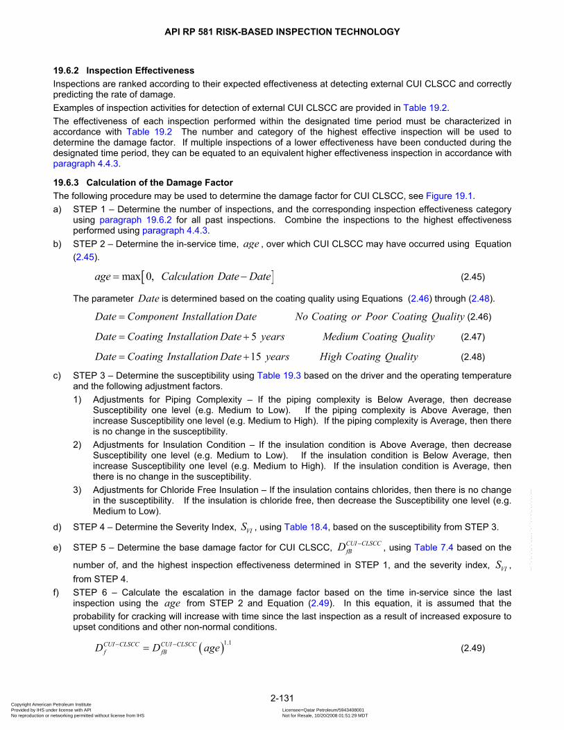
API RP 581 RISK-BASED INSPECTION TECHNOLOGY
19.6.2 Inspection Effectiveness Inspections are ranked according to their expected effectiveness at detecting external CUI CLSCC and correctly predicting the rate of damage. Examples of inspection activities for detection of external CUI CLSCC are provided in Table 19.2. The effectiveness of each inspection performed within the designated time period must be characterized in accordance with Table 19.2 The number and category of the highest effective inspection will be used to determine the damage factor. If multiple inspections of a lower effectiveness have been conducted during the designated time period, they can be equated to an equivalent higher effectiveness inspection in accordance with paragraph 4.4.3.
19.6.3 Calculation of the Damage Factor The following procedure may be used to determine the damage factor for CUI CLSCC, see Figure 19.1. a) STEP 1 – Determine the number of inspections, and the corresponding inspection effectiveness category
using paragraph 19.6.2 for all past inspections. Combine the inspections to the highest effectiveness performed using paragraph 4.4.3.
b) STEP 2 – Determine the in-service time, age , over which CUI CLSCC may have occurred using Equation (2.45).
[ ]max 0, age Calculation Date Date= − (2.45)
The parameter Date is determined based on the coating quality using Equations (2.46) through (2.48).
Date Component Installation Date No Coating or Poor Coating Quality= (2.46)
5 Date Coating Installation Date years Medium Coating Quality= + (2.47)
15 Date Coating Installation Date years High Coating Quality= + (2.48)
c) STEP 3 – Determine the susceptibility using Table 19.3 based on the driver and the operating temperature and the following adjustment factors. 1) Adjustments for Piping Complexity – If the piping complexity is Below Average, then decrease
Susceptibility one level (e.g. Medium to Low). If the piping complexity is Above Average, then increase Susceptibility one level (e.g. Medium to High). If the piping complexity is Average, then there is no change in the susceptibility.
2) Adjustments for Insulation Condition – If the insulation condition is Above Average, then decrease Susceptibility one level (e.g. Medium to Low). If the insulation condition is Below Average, then increase Susceptibility one level (e.g. Medium to High). If the insulation condition is Average, then there is no change in the susceptibility.
3) Adjustments for Chloride Free Insulation – If the insulation contains chlorides, then there is no change in the susceptibility. If the insulation is chloride free, then decrease the Susceptibility one level (e.g. Medium to Low).
d) STEP 4 – Determine the Severity Index, , using VIS Table 18.4, based on the susceptibility from STEP 3.
e) STEP 5 – Determine the base damage factor for CUI CLSCC, , using CUI CLSCCfBD − Table 7.4 based on the
number of, and the highest inspection effectiveness determined in STEP 1, and the severity index, , from STEP 4.
VIS
f) STEP 6 – Calculate the escalation in the damage factor based on the time in-service since the last inspection using the age from STEP 2 and Equation (2.49). In this equation, it is assumed that the probability for cracking will increase with time since the last inspection as a result of increased exposure to upset conditions and other non-normal conditions.
( )1.1CUI CLSCC CUI CLSCCf fBD D age− −= (2.49)
2-131 Copyright American Petroleum Institute Provided by IHS under license with API Licensee=Qatar Petroleum/5943408001
Not for Resale, 10/20/2008 01:51:29 MDTNo reproduction or networking permitted without license from IHS
--```,`,,`,`,,`,`,,,,,,``,```,`-`-`,,`,,`,`,,`---
API RP 581 RISK-BASED INSPECTION TECHNOLOGY
19.7 Nomenclature age is the in-service time
CUI CLSCCfD − is the damage factor for CUI CLSCC CUI CLSCCfBD − is the base value of the damage factor for CUI CLSCC
VIS is the severity index
2-132 Copyright American Petroleum Institute Provided by IHS under license with API Licensee=Qatar Petroleum/5943408001
Not for Resale, 10/20/2008 01:51:29 MDTNo reproduction or networking permitted without license from IHS
--```,`,,`,`,,`,`,,,,,,``,```,`-`-`,,`,,`,`,,`---
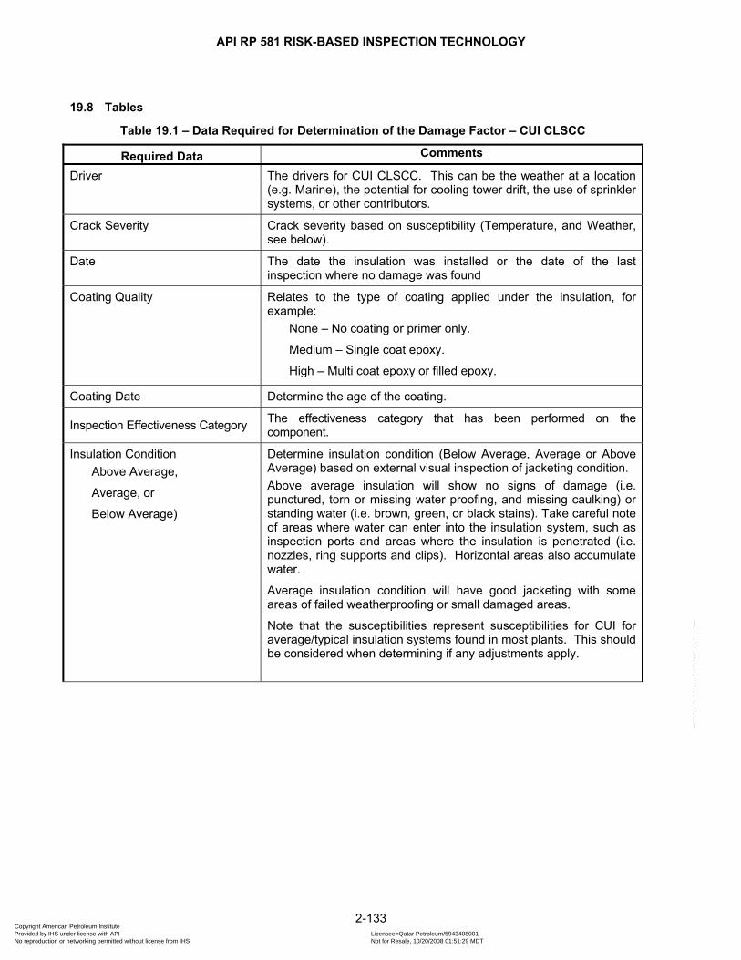
API RP 581 RISK-BASED INSPECTION TECHNOLOGY
19.8 Tables
Table 19.1 – Data Required for Determination of the Damage Factor – CUI CLSCC
Required Data Comments
Driver The drivers for CUI CLSCC. This can be the weather at a location (e.g. Marine), the potential for cooling tower drift, the use of sprinkler systems, or other contributors.
Crack Severity Crack severity based on susceptibility (Temperature, and Weather, see below).
Date The date the insulation was installed or the date of the last inspection where no damage was found
Coating Quality Relates to the type of coating applied under the insulation, for example:
None – No coating or primer only.
Medium – Single coat epoxy.
High – Multi coat epoxy or filled epoxy.
Coating Date Determine the age of the coating.
Inspection Effectiveness Category The effectiveness category that has been performed on the component.
Insulation Condition Above Average,
Average, or
Below Average)
Determine insulation condition (Below Average, Average or Above Average) based on external visual inspection of jacketing condition. Above average insulation will show no signs of damage (i.e. punctured, torn or missing water proofing, and missing caulking) or standing water (i.e. brown, green, or black stains). Take careful note of areas where water can enter into the insulation system, such as inspection ports and areas where the insulation is penetrated (i.e. nozzles, ring supports and clips). Horizontal areas also accumulate water.
Average insulation condition will have good jacketing with some areas of failed weatherproofing or small damaged areas.
Note that the susceptibilities represent susceptibilities for CUI for average/typical insulation systems found in most plants. This should be considered when determining if any adjustments apply.
2-133 Copyright American Petroleum Institute Provided by IHS under license with API Licensee=Qatar Petroleum/5943408001
Not for Resale, 10/20/2008 01:51:29 MDTNo reproduction or networking permitted without license from IHS
--```,`,,`,`,,`,`,,,,,,``,```,`-`-`,,`,,`,`,,`---
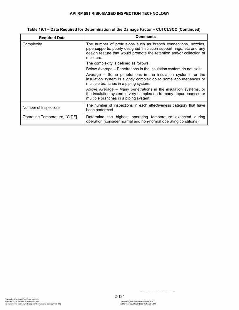
API RP 581 RISK-BASED INSPECTION TECHNOLOGY
Table 19.1 – Data Required for Determination of the Damage Factor – CUI CLSCC (Continued)
Required Data Comments
Complexity The number of protrusions such as branch connections, nozzles, pipe supports, poorly designed insulation support rings, etc and any design feature that would promote the retention and/or collection of moisture. The complexity is defined as follows: Below Average – Penetrations in the insulation system do not exist Average – Some penetrations in the insulation systems, or the insulation system is slightly complex do to some appurtenances or multiple branches in a piping system. Above Average – Many penetrations in the insulation systems, or the insulation system is very complex do to many appurtenances or multiple branches in a piping system.
Number of Inspections The number of inspections in each effectiveness category that have been performed.
Operating Temperature, °C [°F] Determine the highest operating temperature expected during operation (consider normal and non-normal operating conditions).
2-134 Copyright American Petroleum Institute Provided by IHS under license with API Licensee=Qatar Petroleum/5943408001
Not for Resale, 10/20/2008 01:51:29 MDTNo reproduction or networking permitted without license from IHS
--```,`,,`,`,,`,`,,,,,,``,```,`-`-`,,`,,`,`,,`---

API RP 581 RISK-BASED INSPECTION TECHNOLOGY
Table 19.2 – Guidelines for Assigning Inspection Effectiveness – CUI CLSCC
Inspection Category
Inspection Effectiveness
Category Insulation Removed Insulation Not Removed
A Highly Effective
For the total surface area: greater than 95% dye penetrant or eddy current test with UT follow-up of relevant indications.
No inspection techniques yet available meet requirements of "A".
B Usually Effective
For the total surface area: greater than 60% dye penetrant or eddy current testing with UT follow-up of all relevant indications.
For the total surface area: Greater then 95% automated or manual ultrasonic scanning from the internal surface OR AE testing with 100% follow-up of relevant indications.
C Fairly Effective
For the total surface area: greater than 30% dye penetrant or eddy current testing with UT follow-up of all relevant indications.
For the total surface area: Greater than 67% automated or manual ultrasonic scanning from the internal surface
D Poorly Effective
For the total surface area: greater than 5% dye penetrant or eddy current testing with UT follow-up of all relevant indications
For the total surface area: Greater than 30% automated or manual ultrasonic scanning from the internal surface OR Greater than 60% radiographic testing.
E Ineffective Less than “D” effectiveness or no inspection or ineffective inspection technique used
Less than “D” effectiveness or no inspection or ineffective inspection technique used
Table 19.3 – SCC Susceptibility – CUI CLSCC
Operating Temperature SCC Susceptibility as a Function of Driver (Note)
°C °F Marine / Cooling Tower Drift Area Temperate Arid Severe
< 49 < 120 None None None None
49 to 93 120 to 200 High Medium Low High
93 to 149 200 to 300 Medium Low None High
> 149 > 300 None None None None
Note: Driver is defined as the atmospheric condition causing the stress corrosion cracking.
2-135 Copyright American Petroleum Institute Provided by IHS under license with API Licensee=Qatar Petroleum/5943408001
Not for Resale, 10/20/2008 01:51:29 MDTNo reproduction or networking permitted without license from IHS
--```,`,,`,`,,`,`,,,,,,``,```,`-`-`,,`,,`,`,,`---
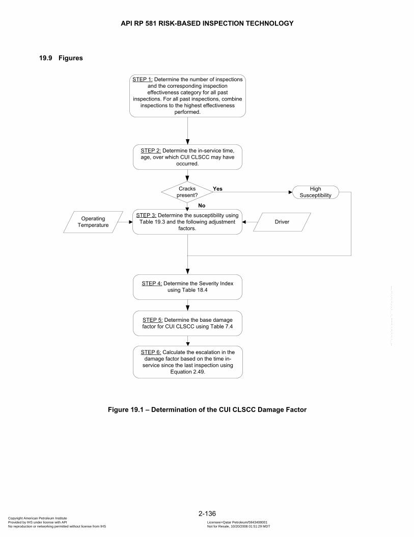
API RP 581 RISK-BASED INSPECTION TECHNOLOGY
19.9 Figures
DriverOperating Temperature
STEP 3: Determine the susceptibility using Table 19.3 and the following adjustment
factors.
STEP 4: Determine the Severity Index using Table 18.4
STEP 5: Determine the base damage factor for CUI CLSCC using Table 7.4
STEP 6: Calculate the escalation in the damage factor based on the time in-
service since the last inspection using Equation 2.49.
STEP 2: Determine the in-service time, age, over which CUI CLSCC may have
occurred.
STEP 1: Determine the number of inspections and the corresponding inspection effectiveness category for all past
inspections. For all past inspections, combine inspections to the highest effectiveness
performed.
High Susceptibility
Cracks present?
Yes
No
Figure 19.1 – Determination of the CUI CLSCC Damage Factor
2-136 Copyright American Petroleum Institute Provided by IHS under license with API Licensee=Qatar Petroleum/5943408001
Not for Resale, 10/20/2008 01:51:29 MDTNo reproduction or networking permitted without license from IHS
--```,`,,`,`,,`,`,,,,,,``,```,`-`-`,,`,,`,`,,`---

API RP 581 RISK-BASED INSPECTION TECHNOLOGY
20 HTHA DAMAGE FACTOR
20.1 Scope The damage factor calculation for carbon steel, C-0.5Mo, and Cr-Mo alloys components subject to High Temperature Hydrogen Attack (HTHA) is covered in this paragraph.
20.2 Description of Damage High Temperature Hydrogen Attack (HTHA) occurs in carbon and low alloy steels exposed to a high partial pressure of hydrogen at elevated temperatures. It is the result of atomic hydrogen diffusing through the steel and reacting with carbides in the microstructure. There are two reactions associated with HTHA. First the hydrogen molecule, , must dissociate to form atomic hydrogen, 2H H , which can diffuse through steel.
2 2 (H H hydrogen dissociation⇔ )The reaction to form atomic hydrogen occurs more readily at higher temperatures and higher hydrogen partial pressures. As a result, as both the temperature and hydrogen partial pressure are increased, the driving force for HTHA increases. The second reaction that occurs is between atomic hydrogen and the metal carbides.
44H MC CH M+ ⇔ +Damage due to the HTHA can possess two forms, internal decarburization and fissuring from the accumulation of methane gas at the carbide matrix interface and surface decarburization from the reaction of the atomic hydrogen with carbides at or near the surface where the methane gas can escape without causing fissures. Internal fissuring is more typically observed in carbon steel, C-0.5Mo steels and in Cr-Mo steels at higher hydrogen partial pressures, while surface decarburization is more commonly observed in Cr-Mo steels at higher temperatures and lower hydrogen partial pressures. HTHA can be mitigated by increasing the alloy content of the steel and, thereby, increasing the stability of the carbides in the presence of hydrogen. As a result, carbon steel that only contains Fe3C carbides has significantly less HTHA resistance than any of the Cr-Mo steels that contain Cr and Mo carbides that are more stable and resistant to HTHA. Historically, HTHA resistance has been predicted based on industry experience which has been plotted on a series of curves for carbon and low alloy steels showing the temperature and hydrogen partial pressure regime in which these steels have been successfully used without damage due to HTHA. These curves, which are commonly referred to as the Nelson curves, are maintained based on industry experience in API RP 941.
20.3 Screening Criteria If all of the following are true, then the component should be evaluated for susceptibility to HTHA. a) The material is carbon steel, C-0.5Mo, or a Cr-Mo low alloy steel b) The operating temperature is greater than 204°C [400°F] and the operating hydrogen partial pressure is
greater than 0.552 MPa [80 psia].
20.4 Required Data The basic component data required for analysis is given in Table 5.1 and the specific data required for determination of the damage factor for HTHA is provided in Table 20.1.
2-137 Copyright American Petroleum Institute Provided by IHS under license with API Licensee=Qatar Petroleum/5943408001
Not for Resale, 10/20/2008 01:51:29 MDTNo reproduction or networking permitted without license from IHS
--```,`,,`,`,,`,`,,,,,,``,```,`-`-`,,`,,`,`,,`---

API RP 581 RISK-BASED INSPECTION TECHNOLOGY
20.5 Basic Assumption The assessment of susceptibility to HTHA is based on the time the component has been exposed to high pressure hydrogen at elevated temperatures. A single parameter, , has been developed to relate time at temperature and a hydrogen partial pressure. This parameter is given by Equations (
vP2.50) and (2.51).
( ) ( ) [ ]( ) (2 4log 3.09 10 273 log 14 :0.0979
H ov
PP T age MPa C−⎡ ⎤= + ⋅ + ⋅ +⎢ ⎥
⎣ ⎦) (2.50)
( ) [ ]( ) (2 4 32log 3.09 10 273 log 14 :14.2 1.8
H ov
P TP age psia F−⎡ ⎤ ⎛ ⎞−⎡ ⎤= + ⋅ + ⋅ +⎢ ⎥ ⎜ ⎟⎢ ⎥⎣ ⎦⎝ ⎠⎣ ⎦) (2.51)
The variables in Equations (2.50) and (2.51) and the associated units are defined in Table 20.1. This parameter can be used to define the susceptibility of a material to damage from HTHA. In the technical basis of this paragraph, the susceptibility to damage from HTHA is based on 200,000 hours of service at a given combination of temperature and hydrogen partial pressure. If HTHA is detected in the component during an inspection, a Fitness-For-Service assessment should be performed in accordance with API 579 [10].
20.6 Determination of the Damage Factor
20.6.1 Overview A flow chart of the steps required to determine the damage factor for HTHA is shown in Figure 20.1. The following paragraphs provide additional information and the calculation procedure.
20.6.2 Inspection Effectiveness Inspections are ranked according to their expected effectiveness at detecting HTHA and correctly predicting the rate of damage. Examples of inspection activities for detection of HTHA are provided in Table 20.2. The effectiveness of each inspection performed within the designated time period must be characterized in accordance with Table 20.2. The number and category of the highest effective inspection will be used to determine the damage factor. If multiple inspections of a lower effectiveness have been conducted during the designated time period, they can be equated to an equivalent higher effectiveness inspection in accordance with paragraph 4.4.3. For HTHA, damage factors are only provided for two inspections. If more than two inspections are performed that conform to Table 20.2, then the damage factor for two inspections shall be used.
20.6.3 Calculation of the Damage Factor The following procedure may be used to determine the damage factor for HTHA, see Figure 20.1. a) STEP 1 – If the temperature is less than or equal to 204°C [400°F] or the hydrogen partial pressure is less
than or equal to 0.552 MPa [80 psia], the component is not susceptible to HTHA, proceed to STEP 6 to determine the damage factor.
b) STEP 2 – Determine the number of inspections, and the corresponding inspection effectiveness category using paragraph 20.6.2 for all past inspections. Combine the inspections to the highest effectiveness performed using paragraph 4.4.3.
c) STEP 3 – Determine the material of construction, exposure time, age , exposure temperature, T , and the
exposure hydrogen partial pressure, 2HP .
d) STEP 4 – Compute the factor using Equations (vP 2.50) and (2.51) based on the data in STEP 3.
2-138 Copyright American Petroleum Institute Provided by IHS under license with API Licensee=Qatar Petroleum/5943408001
Not for Resale, 10/20/2008 01:51:29 MDTNo reproduction or networking permitted without license from IHS
--```,`,,`,`,,`,`,,,,,,``,```,`-`-`,,`,,`,`,,`---

API RP 581 RISK-BASED INSPECTION TECHNOLOGY
e) STEP 5 – Determine the susceptibility using Table 20.3 based on the value of from STEP 4 and the material of construction from STEP 3.
vP
f) STEP 6 – Determine the damage factor for HTHA, HTHAfD , using Table 20.4 based on the susceptibility
from STEP 5. Note that if an inspection indicates the presence of HTHA, then the Damaged Observed category in Table 20.4 shall be used regardless of the number and type of inspection.
20.7 Nomenclature age is the in-service time, hours
HTHAfD is the damage factor for HTHA
2HP is the hydrogen partial pressure, MPa [psia]
vP is the factor vPT is the temperature, °C [°F]
2-139 Copyright American Petroleum Institute Provided by IHS under license with API Licensee=Qatar Petroleum/5943408001
Not for Resale, 10/20/2008 01:51:29 MDTNo reproduction or networking permitted without license from IHS
--```,`,,`,`,,`,`,,,,,,``,```,`-`-`,,`,,`,`,,`---
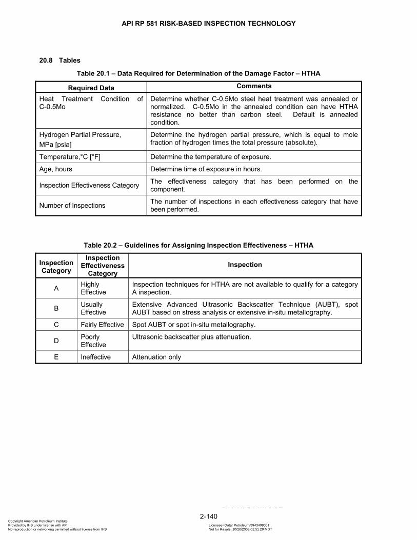
API RP 581 RISK-BASED INSPECTION TECHNOLOGY
20.8 Tables
Table 20.1 – Data Required for Determination of the Damage Factor – HTHA
Required Data Comments
Heat Treatment Condition of C-0.5Mo
Determine whether C-0.5Mo steel heat treatment was annealed or normalized. C-0.5Mo in the annealed condition can have HTHA resistance no better than carbon steel. Default is annealed condition.
Hydrogen Partial Pressure, MPa [psia]
Determine the hydrogen partial pressure, which is equal to mole fraction of hydrogen times the total pressure (absolute).
Temperature,°C [°F] Determine the temperature of exposure.
Age, hours Determine time of exposure in hours.
Inspection Effectiveness Category The effectiveness category that has been performed on the component.
Number of Inspections The number of inspections in each effectiveness category that have been performed.
Table 20.2 – Guidelines for Assigning Inspection Effectiveness – HTHA
Inspection Category
Inspection Effectiveness
Category Inspection
A Highly Effective
Inspection techniques for HTHA are not available to qualify for a category A inspection.
B Usually Effective
Extensive Advanced Ultrasonic Backscatter Technique (AUBT), spot AUBT based on stress analysis or extensive in-situ metallography.
C Fairly Effective Spot AUBT or spot in-situ metallography.
D Poorly Effective
Ultrasonic backscatter plus attenuation.
E Ineffective Attenuation only
2-140 Copyright American Petroleum Institute Provided by IHS under license with API Licensee=Qatar Petroleum/5943408001
Not for Resale, 10/20/2008 01:51:29 MDTNo reproduction or networking permitted without license from IHS
--```,`,,`,`,,`,`,,,,,,``,```,`-`-`,,`,,`,`,,`---
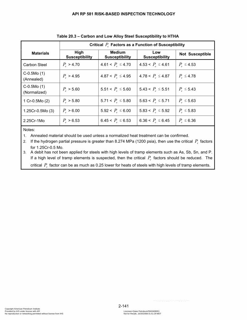
API RP 581 RISK-BASED INSPECTION TECHNOLOGY
Table 20.3 – Carbon and Low Alloy Steel Susceptibility to HTHA
Materials
Critical Factors as a Function of Susceptibility vPHigh
Susceptibility Medium
Susceptibility Low
Susceptibility Not Susceptible
Carbon Steel vP > 4.70 4.61 < ≤ 4.70 vP 4.53 < ≤ 4.61 vP vP ≤ 4.53
C-0.5Mo (1) (Annealed) vP > 4.95 4.87 < ≤ 4.95 vP 4.78 < ≤ 4.87 vP vP ≤ 4.78
C-0.5Mo (1) (Normalized) vP > 5.60 5.51 < ≤ 5.60 vP 5.43 < ≤ 5.51 vP vP ≤ 5.43
1 Cr-0.5Mo (2) vP > 5.80 5.71 < ≤ 5.80 vP 5.63 < ≤ 5.71 vP vP ≤ 5.63
1.25Cr-0.5Mo (3) vP > 6.00 5.92 < ≤ 6.00 vP 5.83 < ≤ 5.92 vP vP ≤ 5.83
2.25Cr-1Mo vP > 6.53 6.45 < ≤ 6.53 vP 6.36 < ≤ 6.45 vP vP ≤ 6.36
Notes: 1. Annealed material should be used unless a normalized heat treatment can be confirmed. 2. If the hydrogen partial pressure is greater than 8.274 MPa (1200 psia), then use the critical factors
for 1.25Cr-0.5 Mo. vP
3. A debit has not been applied for steels with high levels of tramp elements such as As, Sb, Sn, and P. If a high level of tramp elements is suspected, then the critical factors should be reduced. The
critical factor can be as much as 0.25 lower for heats of steels with high levels of tramp elements. vP
vP
2-141 Copyright American Petroleum Institute Provided by IHS under license with API Licensee=Qatar Petroleum/5943408001
Not for Resale, 10/20/2008 01:51:29 MDTNo reproduction or networking permitted without license from IHS
--```,`,,`,`,,`,`,,,,,,``,```,`-`-`,,`,,`,`,,`---

API RP 581 RISK-BASED INSPECTION TECHNOLOGY
Table 20.4 – Damage Factor - HTHA
Susceptibility No
Inspection
First Inspection Inspection Effectiveness
Second Inspection Inspection Effectiveness
D C B D C B
Damage Observed (2) --- 2000 2000 2000 2000 2000 2000
High Susceptibility 2000 1800 1200 800 1600 800 400
Medium Susceptibility 200 180 120 80 160 80 40
Low Susceptibility 20 18 12 8 16 8 4
Not Susceptible 1 1 1 1 1 1 1
Notes: 1. The HTHA damage factor has been provided for only two inspections. For a greater number of
inspections, the damage factor remains constant. 2. The category shall be used if HTHA is detected during an inspection.
2-142 Copyright American Petroleum Institute Provided by IHS under license with API Licensee=Qatar Petroleum/5943408001
Not for Resale, 10/20/2008 01:51:29 MDTNo reproduction or networking permitted without license from IHS
--```,`,,`,`,,`,`,,,,,,``,```,`-`-`,,`,,`,`,,`---

API RP 581 RISK-BASED INSPECTION TECHNOLOGY
20.9 Figures
Figure 20.1 – Determination of the HTHA Damage Factor
2-143 Copyright American Petroleum Institute Provided by IHS under license with API Licensee=Qatar Petroleum/5943408001
Not for Resale, 10/20/2008 01:51:29 MDTNo reproduction or networking permitted without license from IHS
--```,`,,`,`,,`,`,,,,,,``,```,`-`-`,,`,,`,`,,`---
API RP 581 RISK-BASED INSPECTION TECHNOLOGY
21 BRITTLE FACTURE DAMAGE FACTOR
21.1 Scope The damage factor calculation for ferritic components subject to brittle fracture due to low-temperature operation is covered in this paragraph.
21.2 Description of Damage Brittle fracture due to low temperature operating or low toughness is the sudden failure of a structural component, usually initiated at a crack or defect. This is an unusual occurrence, because design stresses are normally low enough to prevent such an occurrence. However, some older equipment with thick walls, equipment that might see low temperatures due to an upset, or equipment that has been modified could be susceptible to varying degrees. Low temperature/low toughness fracture of steel is affected by: a) The applied loads. Brittle fracture is less likely at low applied loads. b) The material specification. Some materials are manufactured to have good fracture properties or
toughness properties. Materials are often “qualified” for use by performing an impact test. This test measures the energy needed to break a notched specimen.
c) Temperature. Many materials (especially ferritic steels) become brittle below some temperature called the transition temperature. Brittle fracture is typically not a concern above 149°C [300°F].
d) Residual stresses and post-weld heat treatment e) Thickness
The goal of the low temperature/low toughness fracture assessment is to rank components with respect to their relative probability of failure with respect to fracture. This assessment will take into account the thickness, the material type, the post-weld heat treatment, and temperatures.
21.3 Screening Criteria If all of the following are true, then the component should be evaluated for susceptibility to brittle fracture. a) The material is carbon steel or a low alloy steel, see Table 21.1. b) The Minimum Design Metal Temperature (MDMT) is unknown, or the MDMT is known but the component may
operate at below the MDMT under normal or upset conditions.
21.4 Required Data The basic component data required for analysis is given in Table 5.1 and the specific data required for determination of the damage factor for brittle fracture is provided in Table 21.2.
21.5 Basic Assumption Brittle fracture requires the coincident presence of a sufficient size defect, application of sufficient stress, and a susceptible material. The susceptibility to failure by brittle fracture can change due to in-service conditions.
2-144 Copyright American Petroleum Institute Provided by IHS under license with API Licensee=Qatar Petroleum/5943408001
Not for Resale, 10/20/2008 01:51:29 MDTNo reproduction or networking permitted without license from IHS
--```,`,,`,`,,`,`,,,,,,``,```,`-`-`,,`,,`,`,,`---
API RP 581 RISK-BASED INSPECTION TECHNOLOGY
21.6 Determination of the Damage Factor
21.6.1 Overview A flow chart of the steps required to determine the damage factor for brittle fracture is shown in Figure 21.1. The following paragraphs provide additional information and the calculation procedure.
21.6.2 Inspection Effectiveness Low temperature/low toughness fracture is prevented by a combination of appropriate design and operating procedures. When low temperature/low toughness fracture does occur, it almost invariably initiates at some pre-existing crack-like defect. From the initiation point, a crack will grow quickly, resulting in a serious leak or sometimes complete rupture of the component. Theoretically, an inspection to locate and remove such pre-existing defects would reduce the probability of failure. However, the initiating defect can be very small, and need not be exposed to the surface where it could be found. For this reason, inspection for such defects is generally not considered to be an effective method for prevention of brittle fracture. If existing records of an component do not indicate if it is constructed of normalized plate, then a metallurgical examination may help resolve this. In some cases, it may be possible to remove samples of the material large enough for testing to determine the toughness, which can also improve the accuracy of the prediction of low temperature/low toughness fracture likelihood. For this damage mechanism, credit is not given for inspection. However, the results of metallurgical testing can be used to update the inputs to the damage factor calculation that may result in a change in this value.
21.6.3 Calculation of the Damage Factor The following procedure may be used to determine the damage factor for brittle fracture, see Figure 21.1. a) STEP 1 – Determine if administrative or process controls exist that will prevent the component from being
fully pressurized below some temperature. If so, use this temperature for and go to STEP 3. minT
b) STEP 2 – Determine the minimum temperature, , that the component may be subjected to during operation, use the lowest of the following:
minT
1) The minimum design temperature 2) The minimum temperature as estimated by the process engineer, including upsets 3) If the vessel or pipe is filled with a pressurized liquid, the boiling point of the liquid at atmospheric
pressure. For example liquid ammonia has a boiling point of –33°C [–28°F] and propane has a boiling point of –40°C [–40°F].
c) STEP 3 – Determine the reference temperature, , in accordance with API 579 [refT 10].
d) STEP 4 – Determine , is from STEP 1 or STEP 2, as applicable, is from STEP 3. min refT T− minT refT
e) STEP 5 – Determine the base damage factor, , using britfractfBD Table 21.4 if the component has not been
subject to PWHT or Table 21.5 is the component has been subject to PWHT based on min refT T− from STEP 4.
2-145 Copyright American Petroleum Institute Provided by IHS under license with API Licensee=Qatar Petroleum/5943408001
Not for Resale, 10/20/2008 01:51:29 MDTNo reproduction or networking permitted without license from IHS
--```,`,,`,`,,`,`,,,,,,``,```,`-`-`,,`,,`,`,,`---
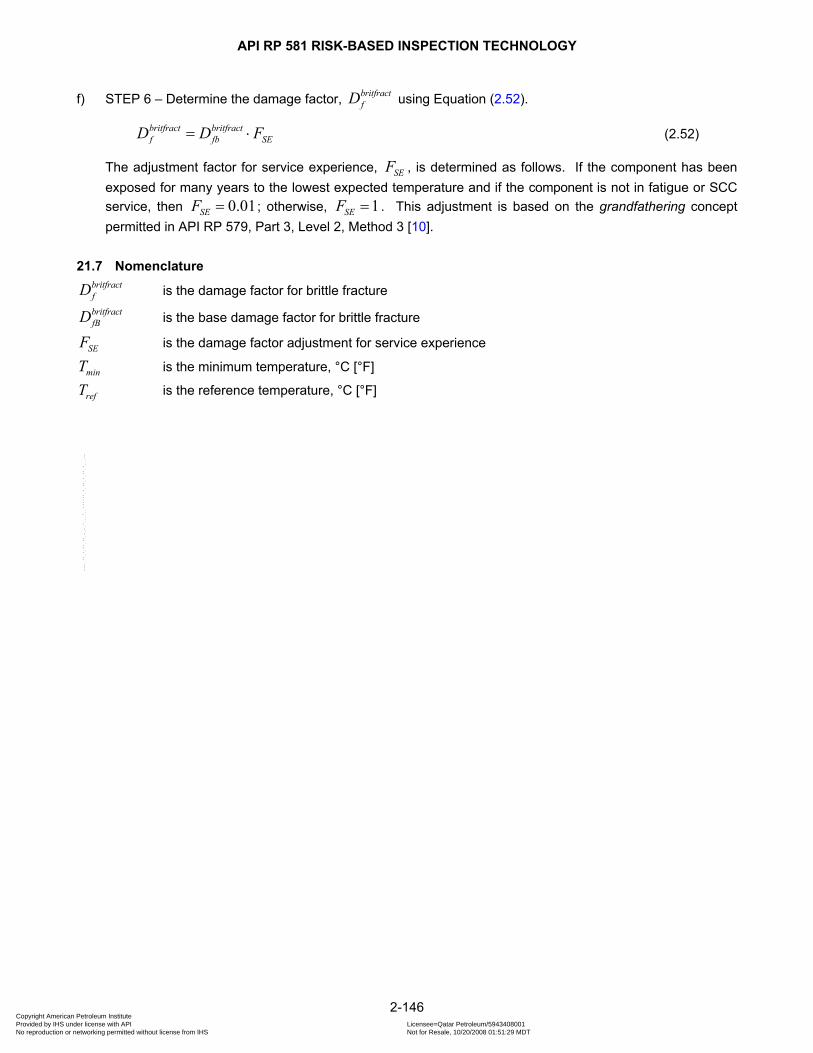
API RP 581 RISK-BASED INSPECTION TECHNOLOGY
f) STEP 6 – Determine the damage factor, using Equation (britfractfD 2.52).
britfract britfractf fb SED D F= ⋅ (2.52)
The adjustment factor for service experience, , is determined as follows. If the component has been exposed for many years to the lowest expected temperature and if the component is not in fatigue or SCC service, then ; otherwise,
SEF
0.01SEF = 1SEF = . This adjustment is based on the grandfathering concept permitted in API RP 579, Part 3, Level 2, Method 3 [10].
21.7 Nomenclature britfractfD is the damage factor for brittle fracture britfractfBD is the base damage factor for brittle fracture
SEF is the damage factor adjustment for service experience
minT is the minimum temperature, °C [°F]
refT is the reference temperature, °C [°F]
2-146 Copyright American Petroleum Institute Provided by IHS under license with API Licensee=Qatar Petroleum/5943408001
Not for Resale, 10/20/2008 01:51:29 MDTNo reproduction or networking permitted without license from IHS
--```,`,,`,`,,`,`,,,,,,``,```,`-`-`,,`,,`,`,,`---
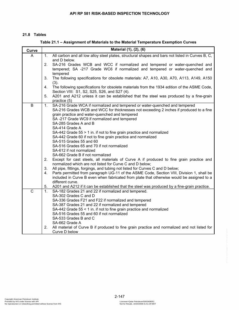
API RP 581 RISK-BASED INSPECTION TECHNOLOGY
21.8 Tables
Table 21.1 – Assignment of Materials to the Material Temperature Exemption Curves
Curve Material (1), (2), (6) A 1. All carbon and all low alloy steel plates, structural shapes and bars not listed in Curves B, C,
and D below. 2. SA-216 Grades WCB and WCC if normalized and tempered or water-quenched and
tempered; SA -217 Grade WC6 if normalized and tempered or water-quenched and tempered
3. The following specifications for obsolete materials: A7, A10, A30, A70, A113, A149, A150 (3).
4. The following specifications for obsolete materials from the 1934 edition of the ASME Code, Section VIII: S1, S2, S25, S26, and S27 (4).
5. A201 and A212 unless it can be established that the steel was produced by a fine-grain practice (5)
B 1. SA-216 Grade WCA if normalized and tempered or water-quenched and tempered SA-216 Grades WCB and WCC for thicknesses not exceeding 2 inches if produced to a fine
grain practice and water-quenched and tempered SA -217 Grade WC9 if normalized and tempered SA-285 Grades A and B SA-414 Grade A SA-442 Grade 55 > 1 in. if not to fine grain practice and normalized SA-442 Grade 60 if not to fine grain practice and normalized SA-515 Grades 55 and 60 SA-516 Grades 65 and 70 if not normalized SA-612 if not normalized SA-662 Grade B if not normalized 2. Except for cast steels, all materials of Curve A if produced to fine grain practice and
normalized which are not listed for Curve C and D below; 3. All pipe, fittings, forgings, and tubing not listed for Curves C and D below; 4. Parts permitted from paragraph UG-11 of the ASME Code, Section VIII, Division 1, shall be
included in Curve B even when fabricated from plate that otherwise would be assigned to a different curve.
5. A201 and A212 if it can be established that the steel was produced by a fine-grain practice. C
1. SA-182 Grades 21 and 22 if normalized and tempered. SA-302 Grades C and D SA-336 Grades F21 and F22 if normalized and tempered SA-387 Grades 21 and 22 if normalized and tempered SA-442 Grade 55 < 1 in. if not to fine grain practice and normalized SA-516 Grades 55 and 60 if not normalized SA-533 Grades B and C SA-662 Grade A 2. All material of Curve B if produced to fine grain practice and normalized and not listed for
Curve D below
2-147 Copyright American Petroleum Institute Provided by IHS under license with API Licensee=Qatar Petroleum/5943408001
Not for Resale, 10/20/2008 01:51:29 MDTNo reproduction or networking permitted without license from IHS
--```,`,,`,`,,`,`,,,,,,``,```,`-`-`,,`,,`,`,,`---
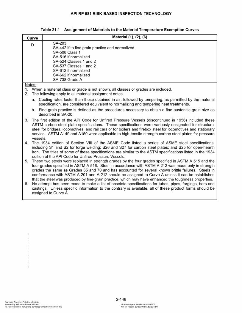
API RP 581 RISK-BASED INSPECTION TECHNOLOGY
Table 21.1 – Assignment of Materials to the Material Temperature Exemption Curves
Curve Material (1), (2), (6)
D
SA-203 SA-442 if to fine grain practice and normalized SA-508 Class 1 SA-516 if normalized SA-524 Classes 1 and 2 SA-537 Classes 1 and 2 SA-612 if normalized SA-662 if normalized SA-738 Grade A
Notes: 1. When a material class or grade is not shown, all classes or grades are included. 2. The following apply to all material assignment notes.
a. Cooling rates faster than those obtained in air, followed by tempering, as permitted by the material specification, are considered equivalent to normalizing and tempering heat treatments.
b. Fine grain practice is defined as the procedures necessary to obtain a fine austenitic grain size as described in SA-20.
3. The first edition of the API Code for Unfired Pressure Vessels (discontinued in 1956) included these ASTM carbon steel plate specifications. These specifications were variously designated for structural steel for bridges, locomotives, and rail cars or for boilers and firebox steel for locomotives and stationary service. ASTM A149 and A150 were applicable to high-tensile-strength carbon steel plates for pressure vessels.
4. The 1934 edition of Section VIII of the ASME Code listed a series of ASME steel specifications, including S1 and S2 for forge welding; S26 and S27 for carbon steel plates; and S25 for open-hearth iron. The titles of some of these specifications are similar to the ASTM specifications listed in the 1934 edition of the API Code for Unfired Pressure Vessels.
5. These two steels were replaced in strength grades by the four grades specified in ASTM A 515 and the four grades specified in ASTM A 516. Steel in accordance with ASTM A 212 was made only in strength grades the same as Grades 65 and 70 and has accounted for several known brittle failures. Steels in conformance with ASTM A 201 and A 212 should be assigned to Curve A unless it can be established that the steel was produced by fine-grain practice, which may have enhanced the toughness properties.
6. No attempt has been made to make a list of obsolete specifications for tubes, pipes, forgings, bars and castings. Unless specific information to the contrary is available, all of these product forms should be assigned to Curve A.
2-148 Copyright American Petroleum Institute Provided by IHS under license with API Licensee=Qatar Petroleum/5943408001
Not for Resale, 10/20/2008 01:51:29 MDTNo reproduction or networking permitted without license from IHS
--```,`,,`,`,,`,`,,,,,,``,```,`-`-`,,`,,`,`,,`---
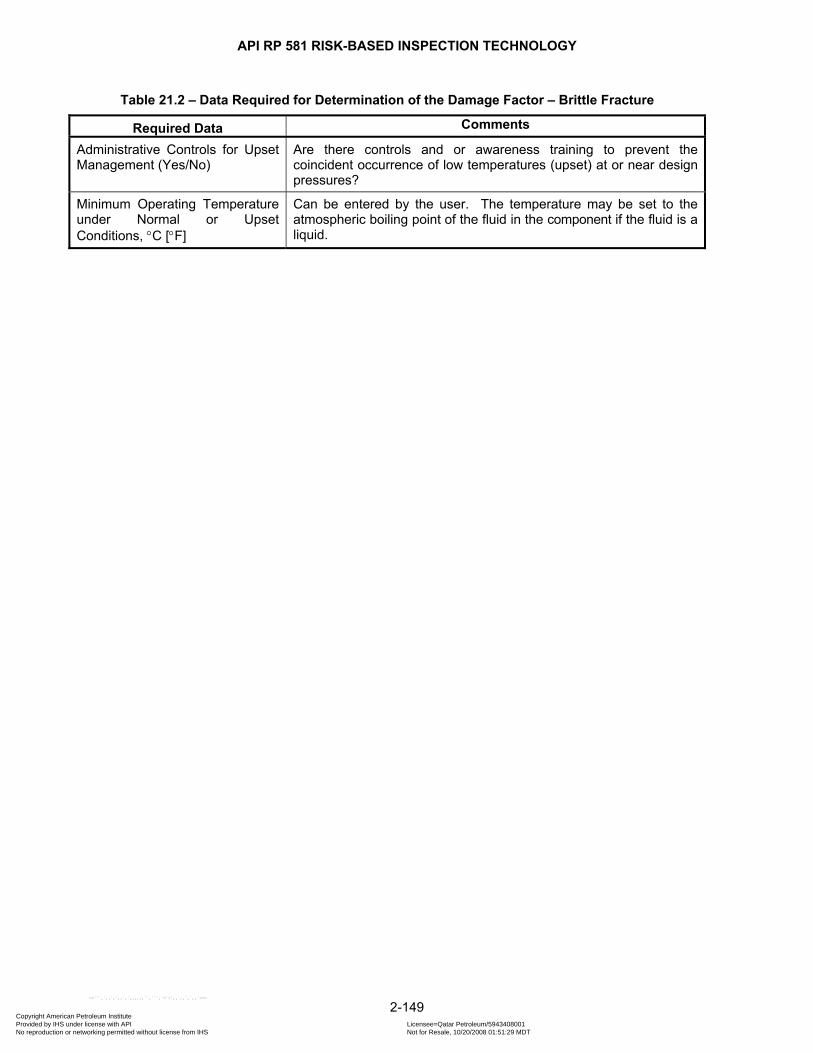
API RP 581 RISK-BASED INSPECTION TECHNOLOGY
Table 21.2 – Data Required for Determination of the Damage Factor – Brittle Fracture
Required Data Comments
Administrative Controls for Upset Management (Yes/No)
Are there controls and or awareness training to prevent the coincident occurrence of low temperatures (upset) at or near design pressures?
Minimum Operating Temperature under Normal or Upset Conditions, °C [°F]
Can be entered by the user. The temperature may be set to the atmospheric boiling point of the fluid in the component if the fluid is a liquid.
2-149 Copyright American Petroleum Institute Provided by IHS under license with API Licensee=Qatar Petroleum/5943408001
Not for Resale, 10/20/2008 01:51:29 MDTNo reproduction or networking permitted without license from IHS
--```,`,,`,`,,`,`,,,,,,``,```,`-`-`,,`,,`,`,,`---

API RP 581 RISK-BASED INSPECTION TECHNOLOGY
Table 21.3 – Impact Test Exemption Temperature
Component Thickness
(in)
Exemption Temperature as a Function of ASME Exemption Curve (°F)
Curve A Curve B Curve C Curve D
0.25 18.0 -20.0 -55.0 -55.0
0.3125 18.0 -20.0 -55.0 -55.0
0.375 18.0 -20.0 -55.0 -55.0
0.4375 24.2 -14.0 -40.5 -55.0
0.5 31.6 -6.9 -32.2 -55.0
0.5625 38.2 -0.6 -27.2 -51.0
0.625 44.0 5.2 -22.8 -47.5
0.6875 49.2 10.4 -18.7 -44.2
0.75 53.9 15.1 -15.0 -41.1
0.8125 58.2 19.5 -11.6 -38.1
0.875 62.1 23.5 -8.6 -35.3
0.9375 65.6 27.2 -5.7 -32.7
1 68.9 30.6 -3.1 -30.1
1.0625 71.9 33.8 -0.7 -27.8
1.125 74.6 36.7 1.6 -25.5
1.1875 77.2 39.4 3.7 -23.4
1.25 79.6 42.0 5.8 -21.4
1.3125 81.8 44.4 7.7 -19.5
1.375 83.8 46.6 9.6 -17.6
1.4375 85.8 48.7 11.4 -15.9
1.5 87.6 50.7 13.1 -14.3
1.5625 89.2 52.5 14.8 -12.7
1.625 90.8 54.3 16.4 -11.2
1.6875 92.3 55.9 17.9 -9.8
1.75 93.7 57.5 19.4 -8.5
1.8125 95.1 58.9 20.9 -7.2
1.875 96.3 60.3 22.3 -5.9
1.9375 97.5 61.7 23.7 -4.7
2 98.6 63.0 25.0 -3.6
2.0625 99.7 64.2 26.3 -2.5
2.125 100.7 65.3 27.5 -1.4
2.1875 101.7 66.4 28.7 -0.4
2.25 102.6 67.5 29.9 0.6
2-150 Copyright American Petroleum Institute Provided by IHS under license with API Licensee=Qatar Petroleum/5943408001
Not for Resale, 10/20/2008 01:51:29 MDTNo reproduction or networking permitted without license from IHS
--```,`,,`,`,,`,`,,,,,,``,```,`-`-`,,`,,`,`,,`---
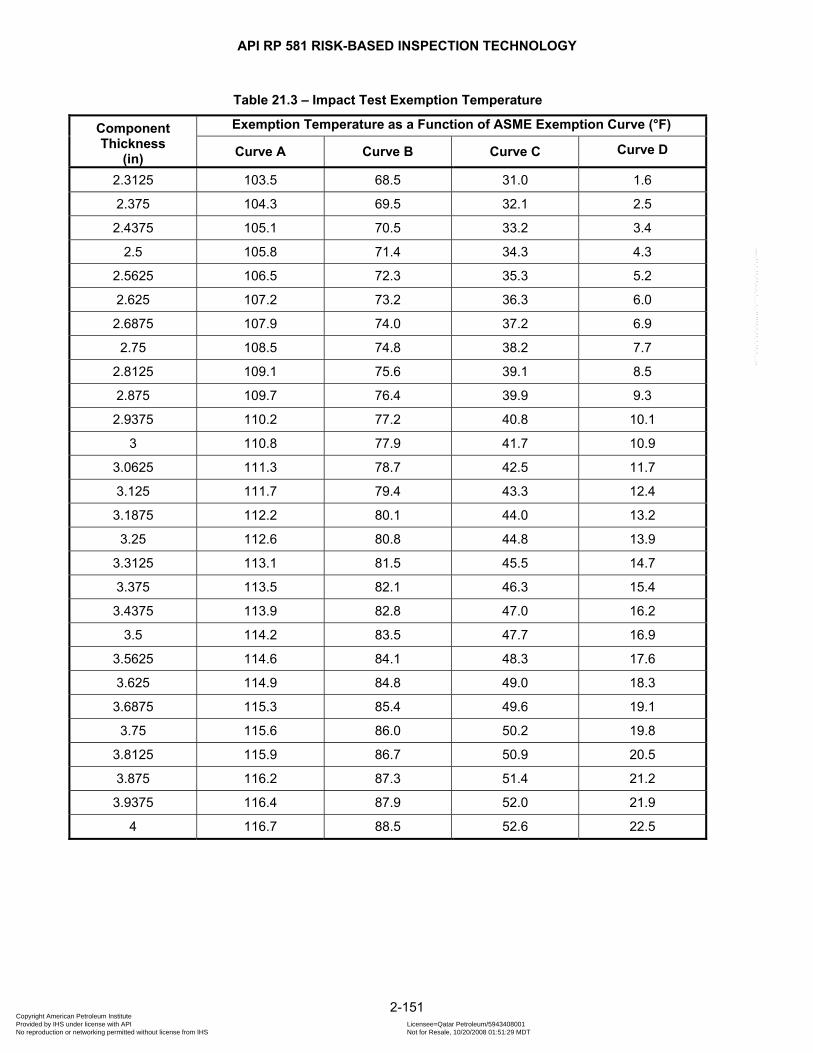
API RP 581 RISK-BASED INSPECTION TECHNOLOGY
Table 21.3 – Impact Test Exemption Temperature
Component Thickness
(in)
Exemption Temperature as a Function of ASME Exemption Curve (°F)
Curve A Curve B Curve C Curve D
2.3125 103.5 68.5 31.0 1.6
2.375 104.3 69.5 32.1 2.5
2.4375 105.1 70.5 33.2 3.4
2.5 105.8 71.4 34.3 4.3
2.5625 106.5 72.3 35.3 5.2
2.625 107.2 73.2 36.3 6.0
2.6875 107.9 74.0 37.2 6.9
2.75 108.5 74.8 38.2 7.7
2.8125 109.1 75.6 39.1 8.5
2.875 109.7 76.4 39.9 9.3
2.9375 110.2 77.2 40.8 10.1
3 110.8 77.9 41.7 10.9
3.0625 111.3 78.7 42.5 11.7
3.125 111.7 79.4 43.3 12.4
3.1875 112.2 80.1 44.0 13.2
3.25 112.6 80.8 44.8 13.9
3.3125 113.1 81.5 45.5 14.7
3.375 113.5 82.1 46.3 15.4
3.4375 113.9 82.8 47.0 16.2
3.5 114.2 83.5 47.7 16.9
3.5625 114.6 84.1 48.3 17.6
3.625 114.9 84.8 49.0 18.3
3.6875 115.3 85.4 49.6 19.1
3.75 115.6 86.0 50.2 19.8
3.8125 115.9 86.7 50.9 20.5
3.875 116.2 87.3 51.4 21.2
3.9375 116.4 87.9 52.0 21.9
4 116.7 88.5 52.6 22.5
2-151 Copyright American Petroleum Institute Provided by IHS under license with API Licensee=Qatar Petroleum/5943408001
Not for Resale, 10/20/2008 01:51:29 MDTNo reproduction or networking permitted without license from IHS
--```,`,,`,`,,`,`,,,,,,``,```,`-`-`,,`,,`,`,,`---
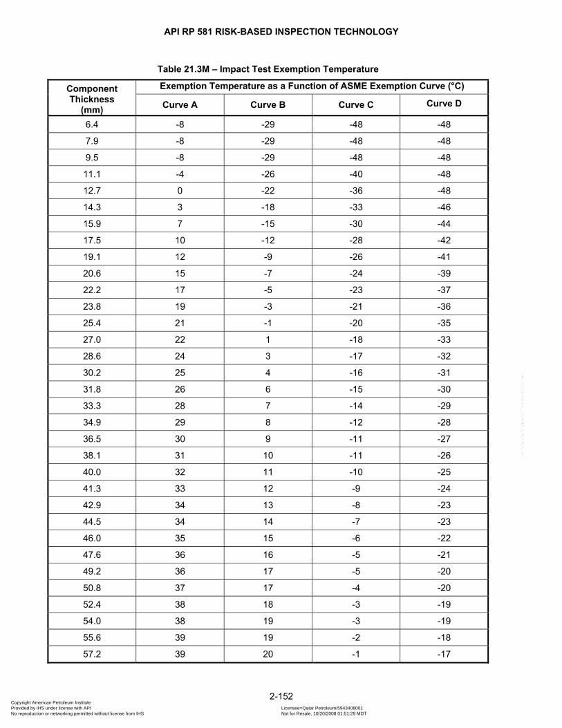
API RP 581 RISK-BASED INSPECTION TECHNOLOGY
Table 21.3M – Impact Test Exemption Temperature
Component Thickness
(mm)
Exemption Temperature as a Function of ASME Exemption Curve (°C)
Curve A Curve B Curve C Curve D
6.4 -8 -29 -48 -48
7.9 -8 -29 -48 -48
9.5 -8 -29 -48 -48
11.1 -4 -26 -40 -48
12.7 0 -22 -36 -48
14.3 3 -18 -33 -46
15.9 7 -15 -30 -44
17.5 10 -12 -28 -42
19.1 12 -9 -26 -41
20.6 15 -7 -24 -39
22.2 17 -5 -23 -37
23.8 19 -3 -21 -36
25.4 21 -1 -20 -35
27.0 22 1 -18 -33
28.6 24 3 -17 -32
30.2 25 4 -16 -31
31.8 26 6 -15 -30
33.3 28 7 -14 -29
34.9 29 8 -12 -28
36.5 30 9 -11 -27
38.1 31 10 -11 -26
40.0 32 11 -10 -25
41.3 33 12 -9 -24
42.9 34 13 -8 -23
44.5 34 14 -7 -23
46.0 35 15 -6 -22
47.6 36 16 -5 -21
49.2 36 17 -5 -20
50.8 37 17 -4 -20
52.4 38 18 -3 -19
54.0 38 19 -3 -19
55.6 39 19 -2 -18
57.2 39 20 -1 -17
2-152 Copyright American Petroleum Institute Provided by IHS under license with API Licensee=Qatar Petroleum/5943408001
Not for Resale, 10/20/2008 01:51:29 MDTNo reproduction or networking permitted without license from IHS
--```,`,,`,`,,`,`,,,,,,``,```,`-`-`,,`,,`,`,,`---

API RP 581 RISK-BASED INSPECTION TECHNOLOGY
Table 21.3M – Impact Test Exemption Temperature
Component Thickness
(mm)
Exemption Temperature as a Function of ASME Exemption Curve (°C)
Curve A Curve B Curve C Curve D
58.7 40 20 -1 -17
60.3 40 21 0 -16
61.9 41 21 1 -16
63.5 41 22 1 -15
65.1 41 22 2 -15
66.7 42 23 2 -14
68.3 42 23 3 -14
69.9 43 24 3 -14
71.4 43 24 4 -13
73.0 43 25 4 -13
74.6 43 25 5 -12
76.2 44 26 5 -12
77.8 44 26 6 -11
79.3 44 26 6 -11
81.0 45 27 7 -10
82.6 45 27 7 -10
84.1 45 28 8 -10
85.7 45 28 8 -9
87.3 46 28 8 -9
88.9 46 29 9 -8
90.5 46 29 9 -8
92.1 46 29 9 -8
93.7 46 30 10 -7
95.3 46 30 10 -7
96.8 47 30 11 -6
98.4 47 31 11 -6
100.0 47 31 11 -6
101.6 47 31 11 -5
2-153 Copyright American Petroleum Institute Provided by IHS under license with API Licensee=Qatar Petroleum/5943408001
Not for Resale, 10/20/2008 01:51:29 MDTNo reproduction or networking permitted without license from IHS
--```,`,,`,`,,`,`,,,,,,``,```,`-`-`,,`,,`,`,,`---
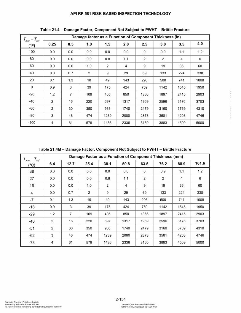
API RP 581 RISK-BASED INSPECTION TECHNOLOGY
Table 21.4 – Damage Factor, Component Not Subject to PWHT – Brittle Fracture
min refT T− (°F)
Damage factor as a Function of Component Thickness (in)
0.25 0.5 1.0 1.5 2.0 2.5 3.0 3.5 4.0
100 0.0 0.0 0.0 0.0 0.0 0 0.9 1.1 1.2
80 0.0 0.0 0.0 0.8 1.1 2 2 4 6
60 0.0 0.0 1.0 2 4 9 19 36 60
40 0.0 0.7 2 9 29 69 133 224 338
20 0.1 1.3 10 49 143 296 500 741 1008
0 0.9 3 39 175 424 759 1142 1545 1950
-20 1.2 7 109 405 850 1366 1897 2415 2903
-40 2 16 220 697 1317 1969 2596 3176 3703
-60 2 30 350 988 1740 2479 3160 3769 4310
-80 3 46 474 1239 2080 2873 3581 4203 4746
-100 4 61 579 1436 2336 3160 3883 4509 5000
Table 21.4M – Damage Factor, Component Not Subject to PWHT – Brittle Fracture
min refT T− (°C)
Damage Factor as a Function of Component Thickness (mm)
6.4 12.7 25.4 38.1 50.8 63.5 76.2 88.9 101.6
38 0.0 0.0 0.0 0.0 0.0 0 0.9 1.1 1.2 27 0.0 0.0 0.0 0.8 1.1 2 2 4 6 16 0.0 0.0 1.0 2 4 9 19 36 60 4 0.0 0.7 2 9 29 69 133 224 338 -7 0.1 1.3 10 49 143 296 500 741 1008
-18 0.9 3 39 175 424 759 1142 1545 1950 -29 1.2 7 109 405 850 1366 1897 2415 2903 -40 2 16 220 697 1317 1969 2596 3176 3703 -51 2 30 350 988 1740 2479 3160 3769 4310 -62 3 46 474 1239 2080 2873 3581 4203 4746 -73 4 61 579 1436 2336 3160 3883 4509 5000
2-154 Copyright American Petroleum Institute Provided by IHS under license with API Licensee=Qatar Petroleum/5943408001
Not for Resale, 10/20/2008 01:51:29 MDTNo reproduction or networking permitted without license from IHS
--```,`,,`,`,,`,`,,,,,,``,```,`-`-`,,`,,`,`,,`---

API RP 581 RISK-BASED INSPECTION TECHNOLOGY
Table 21.5 – Damage Factor, Component Subject to PWHT – Brittle Fracture
min refT T− (°F)
Damage Factor as a Function of Component Thickness (in)
0.25 0.5 1.0 1.5 2.0 2.5 3.0 3.5 4.0
100 0.0 0.0 0.0 0.0 0.0 0.0 0.0 0.0 0.0
80 0.0 0.0 0.0 0.0 0.0 0.0 0.0 0.0 0.2
60 0.0 0.0 0.0 0.0 0.0 0.5 0.9 1.1 1.3
40 0.0 0.0 0.0 0.5 1.1 1.3 2 3 4
20 0.0 0.0 0.6 1.2 2 4 7 13 23
0 0.0 0.0 1.1 2 6 14 29 53 88
-20 0.0 0.4 2 5 17 41 83 144 224
-40 0.0 0.9 3 12 38 90 171 281 416
-60 0.0 1.1 5 22 68 153 277 436 623
-80 0.0 1.2 7 34 102 219 382 582 810
-100 0.0 1.3 9 46 133 277 472 704 962
Table 21.5M – Damage Factor, Component Subject to PWHT – Brittle Fracture
min refT T− (°C)
Damage Factor as a Function of Component Thickness (mm)
6.4 12.7 25.4 38.1 50.8 63.5 76.2 88.9 101.6
38 0.0 0.0 0.0 0.0 0.0 0.0 0.0 0.0 0.0
27 0.0 0.0 0.0 0.0 0.0 0.0 0.0 0.0 0.2
16 0.0 0.0 0.0 0.0 0.0 0.5 0.9 1.1 1.3
4 0.0 0.0 0.0 0.5 1.1 1.3 2 3 4
-7 0.0 0.0 0.6 1.2 2 4 7 13 23
-18 0.0 0.0 1.1 2 6 14 29 53 88
-29 0.0 0.4 2 5 17 41 83 144 224
-40 0.0 0.9 3 12 38 90 171 281 416
-51 0.0 1.1 5 22 68 153 277 436 623
-62 0.0 1.2 7 34 102 219 382 582 810
-73 0.0 1.3 9 46 133 277 472 704 962
2-155 Copyright American Petroleum Institute Provided by IHS under license with API Licensee=Qatar Petroleum/5943408001
Not for Resale, 10/20/2008 01:51:29 MDTNo reproduction or networking permitted without license from IHS
--```,`,,`,`,,`,`,,,,,,``,```,`-`-`,,`,,`,`,,`---
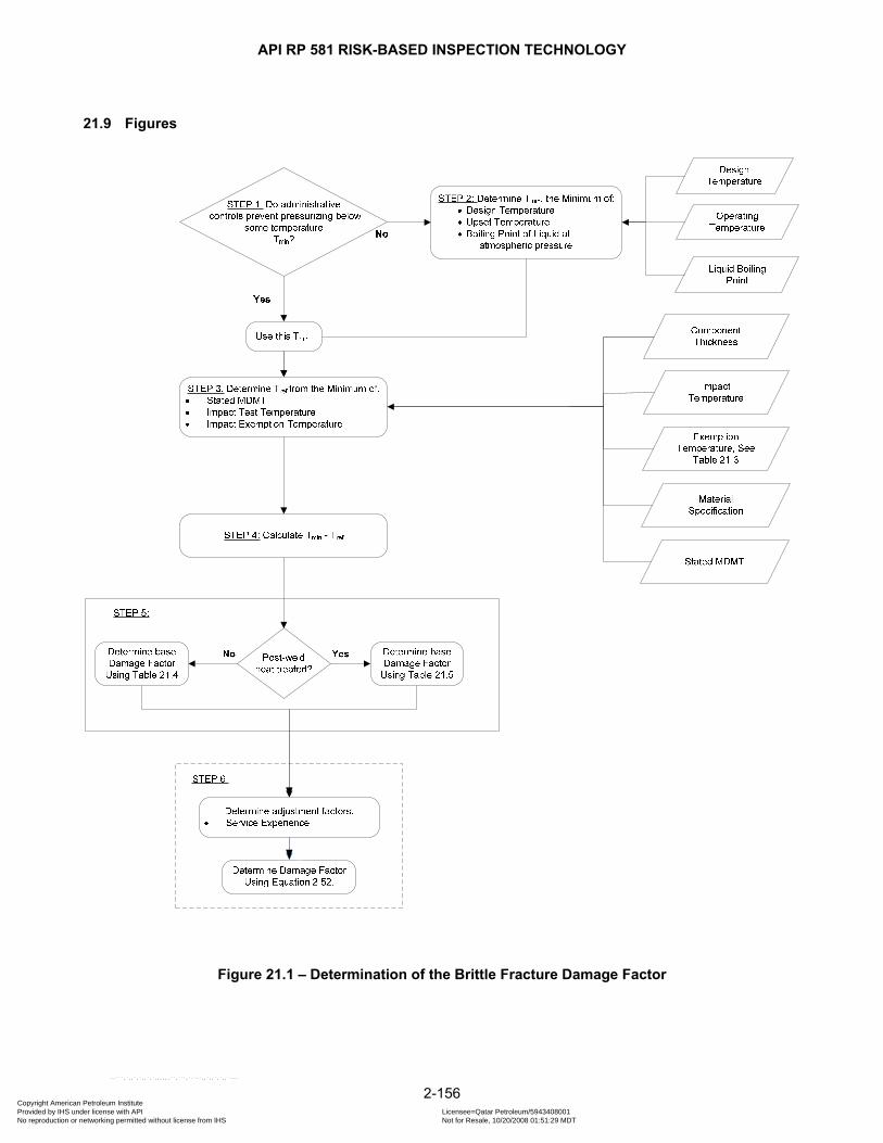
API RP 581 RISK-BASED INSPECTION TECHNOLOGY
21.9 Figures
Figure 21.1 – Determination of the Brittle Fracture Damage Factor
2-156 Copyright American Petroleum Institute Provided by IHS under license with API Licensee=Qatar Petroleum/5943408001
Not for Resale, 10/20/2008 01:51:29 MDTNo reproduction or networking permitted without license from IHS
--```,`,,`,`,,`,`,,,,,,``,```,`-`-`,,`,,`,`,,`---
API RP 581 RISK-BASED INSPECTION TECHNOLOGY
22 TEMPER EMBRITTLEMENT DAMAGE FACTOR
22.1 Scope The damage factor calculation for Cr-Mo components subject to temper embrittlement is covered in this paragraph.
22.2 Description of Damage The toughness of some steels is reduced by a phenomenon called temper embrittlement after extended exposure to temperatures in the range of 343°C to 577°C [650°F to 1070°F]. Of particular interest to the refining and petrochemical industries is the embrittlement of Cr-Mo steels used in operations within the temperature range for embrittlement. The reduction in fracture toughness only affects the material at the lower temperatures experienced during startup and shutdown of equipment. Industry practice to avoid brittle fracture has been to reduce the operating pressure to one-fourth of the design pressure when the vessel temperature is less than some minimum process temperature. Typical industry practice for this minimum temperature is 149°C to 177°C [300°F to 350°F] for older low alloy steels, or lower temperatures for more modern steels. Temper embrittlement is caused by segregation of tramp elements and alloying elements along grain boundaries in the steel. The phosphorous and tin content of the steel are of particular importance, and their effect is made worse by manganese and silicon, which are important alloying elements. A J-factor based on composition is typically specified to control the susceptibility to temper embrittlement. The J-factor is calculated using Equation (2.53). Laboratory and long-term field studies have confirmed fair correlation between the J-factor and the amount of temper embrittlement.
( ) (104 % % % %J Si Mn P= ⋅ + ⋅ + )Sn (2.53)
One very important aspect of temper embrittlement is the tendency of weld metal and heat affected zones to show increased susceptibility to embrittlement vs. the wrought base material. A few studies have shown that 2.25Cr-0.5Mo and 3Cr-1Mo are particularly susceptible. It is debatable whether or not 1.25Cr- 0.5Mo steels are also susceptible; however, these materials have been included in the damage factor calculation procedures in this paragraph.
22.3 Screening Criteria If all of the following are true, then the component should be evaluated for susceptibility to temper embrittlement. a) The material is 1.25Cr -0.5Mo, 2.25Cr -0.5Mo, or 3Cr-1 Mo low alloy steel. b) The operating temperature is between 343 and 577°C [650 and 1070°F].
22.4 Required Data The basic component data required for analysis is given in Table 5.1 and the specific data required for determination of the damage factor for temper embrittlement is provided in Table 22.1.
22.5 Basic Assumption Temper embrittlement is evaluated in the same way as brittle fracture, see paragraph 21.2, except that a shift in the reference temperature is made to account for embrittlement.
2-157 Copyright American Petroleum Institute Provided by IHS under license with API Licensee=Qatar Petroleum/5943408001
Not for Resale, 10/20/2008 01:51:29 MDTNo reproduction or networking permitted without license from IHS
--```,`,,`,`,,`,`,,,,,,``,```,`-`-`,,`,,`,`,,`---

API RP 581 RISK-BASED INSPECTION TECHNOLOGY
22.6 Determination of the Damage Factor
22.6.1 Overview A flow chart of the steps required to determine the damage factor for temper embrittlement is shown in Figure 22.1. The following paragraphs provide additional information and the calculation procedure.
22.6.2 Inspection Effectiveness For this damage mechanism, credit is not given for inspection. However, the results of metallurgical testing can be used to update the inputs to the damage factor calculation that may result in a change in this value.
22.6.3 Calculation of the Damage Factor The following procedure may be used to determine the damage factor for temper embrittlement, see Figure 22.1. a) STEP 1 – Determine if administrative or process controls exist that will prevent the component from being
fully pressurized below some temperature. If so, use this temperature for and go to STEP 3. minT
b) STEP 2 – Determine the minimum temperature, , that the component may be subjected to during operation, use the lowest of the following:
minT
1) The minimum design temperature. 2) The minimum temperature as estimated by the process engineer, including upsets.
c) STEP 3 – Determine the reference temperature, , in accordance with API 579 [refT 10].
d) STEP 4 – Determine and compute FATTΔ ( )refT FAT+ Δ T , is from STEP 3. If is not
known it may be estimated by one of the following methods, listed in decreasing order or accuracy. refT FATTΔ
1) Determined by engineering analysis or actual testing of metal samples. 2) Determined in a step cooling embrittlement (SCE) test. This can be related to the actual in-service
using Equation (FATTΔ 2.54) based on the operating time. In Equation (2.54), age is the operating time in hours and is the specified change in . SCE FATT
[ ](0.67 log 0.91FATT age SCEΔ = ⋅ − ⋅ ) (2.54)
3) Use the chemical composition to determine the J-factor using Equation (2.53). The J-factor may be correlated to the expected after long-term service. Based on long term exposures, this is conservatively correlated to the J-factor by Equation (
FATTΔ2.55).
0.6 20FATT JΔ = ⋅ − (2.55)
4) A conservative value of 66°C [150°F] can be assumed for the long term FATTΔ .
e) STEP 5 – Determine the damage factor, ,using tempefD
minT
Table 21.4 if the component has not been subject to PWHT and Table 21.5 if the component has been subject to PWHT. When determining the damage factor, use in place of ( )min refT T FATT− + Δ refT− where is from STEP 1 or STEP 2, as applicable,
and
minT
( )refT FATT+ Δ is from STEP 4.
2-158 Copyright American Petroleum Institute Provided by IHS under license with API Licensee=Qatar Petroleum/5943408001
Not for Resale, 10/20/2008 01:51:29 MDTNo reproduction or networking permitted without license from IHS
--```,`,,`,`,,`,`,,,,,,``,```,`-`-`,,`,,`,`,,`---
API RP 581 RISK-BASED INSPECTION TECHNOLOGY
22.7 Nomenclature age is the in-service operating time
tempefD is the damage factor for temper embrittlement
FATTΔ is the change in the fracture appearance transition temperature J is the J-factor SCE is the specified change in FATT
minT is the minimum temperature, °C [°F]
refT is the reference temperature, °C [°F]
22.8 References 67. Viswanathan, R., Damage Mechanisms and Life Assessment of High Temperature Components, ASM
International, 1989. 68. The Materials Properties Council, Inc., Meeting on MPC/ API Task Group on Materials for Pressure Vessel
Service with Hydrogen at High Temperatures and Pressures, HPV-51, Oct. 1990, Minutes. 69. T. Iwadate, J. Watanabe, Y. Tanaka; Prediction of the Remaining Life of High-Temperature/Pressure
Reactors Made of Cr-Mo Steels, Trans. of ASME, Vol.107, pp. 230, Aug.1985 70. T. Iwadate; Prediction of the Remaining Life of High-temperature/Pressure Reactors made of Cr-Mo Steels,
Maroran Research Laboratory, The Japan Steel Works Ltd., March1989. 71. T. Iwadate, M. Prager & M. J. Humphries; Reliability of new and older Chrome-Moly Steels for Hydrogen
Process Vessels, Part I: Degradation in Service, Part II: Enhanced Performance, The 1990 Pressure Vessel and Piping Conference, June, 1990 (PVP-Vol.201 or MPC-Vol.31)
72. G. Sangdahl and M. Semchyshen; Application of 2.25Cr-1Mo Steel for thick-wall Pressure Vessel ASTM STP 755, May 1980.
73. W. Erwin & J. Kerr; The Use of Quenched and tempered 2.25Cr-1Mo steel For Thick Wall Reactor Vessel in Petroleum Refinery Processes: An Interpretive Review of 25 Years of Research and Application, Bulletin 275, ISSN 0034-2326, Welding Research Council, New Yours, Feb 1982.
74. J. Barsom & S. Rolfe; Correlation Between KIC and Charpy V-Notch Test Results in the Transition Temperature Range, ASTM STP 466, Vol.2, No.4, 1970.
2-159 Copyright American Petroleum Institute Provided by IHS under license with API Licensee=Qatar Petroleum/5943408001
Not for Resale, 10/20/2008 01:51:29 MDTNo reproduction or networking permitted without license from IHS
--```,`,,`,`,,`,`,,,,,,``,```,`-`-`,,`,,`,`,,`---

API RP 581 RISK-BASED INSPECTION TECHNOLOGY
22.9 Tables
Table 22.1 – Data Required for Determination of the Damage Factor – Temper Embrittlement
Required Data Comments
Impact Test Temperature, °C [°F] If impact tested. If this is unknown, it should be assumed that impact tests were not done.
Administrative Controls for Upset Management (Yes/No)
Are there controls and or awareness training to prevent the coincident occurrence of low temperatures (upset) at or near design pressures?
Minimum Operating Temperature under Normal, Startup/Shutdown, or Upset Conditions, °C [°F]
For Temper Embrittlement, this may be the temperature below which the operating pressure is reduced for purposes of fracture control. If not known, the temperature should be set to the atmospheric boiling point of the fluid in the component if the fluid is a liquid.
Time in Service, Years The number of years in service within the temperature range
FATTΔ , °C [°F] The change in the Fracture Appearance transition temperature before and after temper embrittlement.
Chemical Composition of Steel (optional)
Specifically, the %Si, %Mn, %P, and %Sn which contribute to the susceptibility to Temper Embrittlement. If not known, a transition shift will be assumed.
Screening of Materials (Y/N) Was the material used for the component screened for susceptibility to Temper Embrittlement by such methods as specifications for steel composition, or specification of a transition temperature requirement in a Step Cooling Embrittlement (SCE) test.
SCE Specified delta Temperature, °C [°F]
The delta temperature specified for Step Cooling Embrittlement (SCE) tests.
2-160 Copyright American Petroleum Institute Provided by IHS under license with API Licensee=Qatar Petroleum/5943408001
Not for Resale, 10/20/2008 01:51:29 MDTNo reproduction or networking permitted without license from IHS
--```,`,,`,`,,`,`,,,,,,``,```,`-`-`,,`,,`,`,,`---
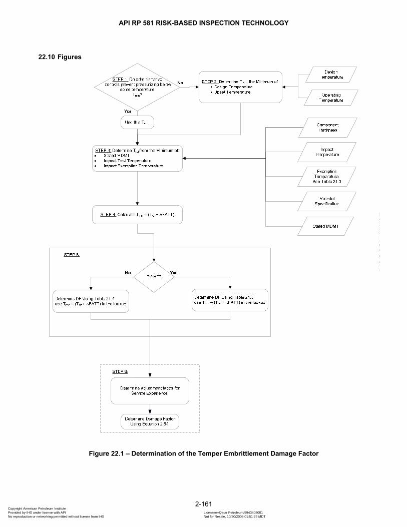
API RP 581 RISK-BASED INSPECTION TECHNOLOGY
22.10 Figures
Figure 22.1 – Determination of the Temper Embrittlement Damage Factor
2-161 Copyright American Petroleum Institute Provided by IHS under license with API Licensee=Qatar Petroleum/5943408001
Not for Resale, 10/20/2008 01:51:29 MDTNo reproduction or networking permitted without license from IHS
--```,`,,`,`,,`,`,,,,,,``,```,`-`-`,,`,,`,`,,`---
API RP 581 RISK-BASED INSPECTION TECHNOLOGY
23 885 EMBRITTLEMENT DAMAGE FACTOR
23.1 Scope The damage factor calculation for components subject to 885 embrittlement is covered in this paragraph.
23.2 Description of Damage 885 embrittlement is a reduction in toughness of ferritic stainless steels with a chromium content of greater than 13%, after exposure to temperatures between 371°C and 538°C [700°F and 1000°F]. The reduction in toughness is due to precipitation of a chromium-phosphorous intermetallic phase at elevated temperatures. As is the case with other mechanisms that result in a loss of toughness due to metallurgical changes, the effect on toughness is most pronounced not at the operating temperature, but at lower temperatures experienced during plant shutdowns or upsets. The precipitation of the intermetallic phase is believed to occur most readily at a temperature around 474°C [885°F], hence the name for this mechanism. Steels with more than 27% chromium are most severely affected, but these are not typically used in refinery or petrochemical processes. Martensitic stainless steels such as Type 410 are normally considered to be immune to this problem. Type 405 is a ferritic stainless steel that is subject to the problem if it contains chromium levels at the high end of its composition range. The existence of 885 embrittlement can reveal itself by an increase in hardness in affected areas. Physical testing of samples removed from service is the most positive indicator of a problem. 885 embrittlement is reversible by appropriate heat treatment to dissolve precipitates, followed by rapid cooling. Heat treatment temperature is typically in the range of 760°C to 816°C [1400°F to 1500°F], so this may not be practical for many components.
23.3 Screening Criteria If all of the following are true, then the component should be evaluated for susceptibility to 885 embrittlement. a) The material is a high chromium (>12% Cr) ferritic steel. b) The operating temperature is between 371°C and 566°C [700°F and 1050 °F].
23.4 Required Data The basic component data required for analysis is given in Table 5.1 and the specific data required for determination of the damage factor for 885 embrittlement is provided in Table 23.1.
23.5 Basic Assumption Since 885 embrittlement may occur in a relatively short period of time, it is assumed in the development of the damage factor that any of the ferritic materials listed in Table 23.2 that have been exposed to temperatures in the 371°C to 538°C [700°F to 1000°F] range are affected.
API RP 579 recommends that for embrittled materials, the toughness should be determined by the (fracture arrest) curves, truncated at 38°C [100°F]. It is further recommended that for severely embrittled materials, 50% of this value should be used. The ductile-to-brittle transition temperatures for ferritic stainless steels (400 series) typically are in the 10°C to 38°C [50°F to 100°F] range.
IrK
2-162 Copyright American Petroleum Institute Provided by IHS under license with API Licensee=Qatar Petroleum/5943408001
Not for Resale, 10/20/2008 01:51:29 MDTNo reproduction or networking permitted without license from IHS
--```,`,,`,`,,`,`,,,,,,``,```,`-`-`,,`,,`,`,,`---
API RP 581 RISK-BASED INSPECTION TECHNOLOGY
23.6 Determination of the Damage Factor
23.6.1 Overview A flow chart of the steps required to determine the damage factor for 885 embrittlement is shown in Figure 23.1. The following paragraphs provide additional information and the calculation procedure.
23.6.2 Inspection Effectiveness For this damage mechanism, credit is not given for inspection. However, the results of metallurgical testing can be used to update the inputs to the damage factor calculation that may result in a change in this value.
23.6.3 Calculation of the Damage Factor The following procedure may be used to determine the damage factor for 885 embrittlement, see Figure 23.1. a) STEP 1 – Determine if administrative or process controls exist that will prevent the component from being
fully pressurized below some temperature. If so, use this temperature for and go to STEP 3. minT
b) STEP 2 – Determine the minimum temperature, , that the component may be subjected to during operation, use the lowest of the following:
minT
1) The minimum design temperature. 2) The minimum temperature as estimated by the process engineer, including upsets.
c) STEP 3 – Determine the reference temperature, use 28 80o orefT C F⎡ ⎤= ⎣ ⎦ unless the actual ductile to
brittle transition temperature is known.
d) STEP 4 – Determine ; is from STEP 1 or STEP 2, as applicable, is from STEP 3. min refT T− minT refT
e) STEP 5 – Determine the damage factor, 885fD , using Table 23.3 based on from STEP 4. min refT T−
23.7 Nomenclature 885fD is the damage factor for 885 embrittlement
minT is the minimum temperature, °C [°F]
refT is the reference temperature, °C [°F]
23.8 References 75. Timmins, P. F., Predictive Corrosion and Failure Control in Process Operations, ASM International, 1996 76. Holt J. M., Mindlin H., and Ho C. Y., Structural Alloys Handbook, 1994 Edition, Purdue University, West
Lafayette, IN
2-163 Copyright American Petroleum Institute Provided by IHS under license with API Licensee=Qatar Petroleum/5943408001
Not for Resale, 10/20/2008 01:51:29 MDTNo reproduction or networking permitted without license from IHS
--```,`,,`,`,,`,`,,,,,,``,```,`-`-`,,`,,`,`,,`---
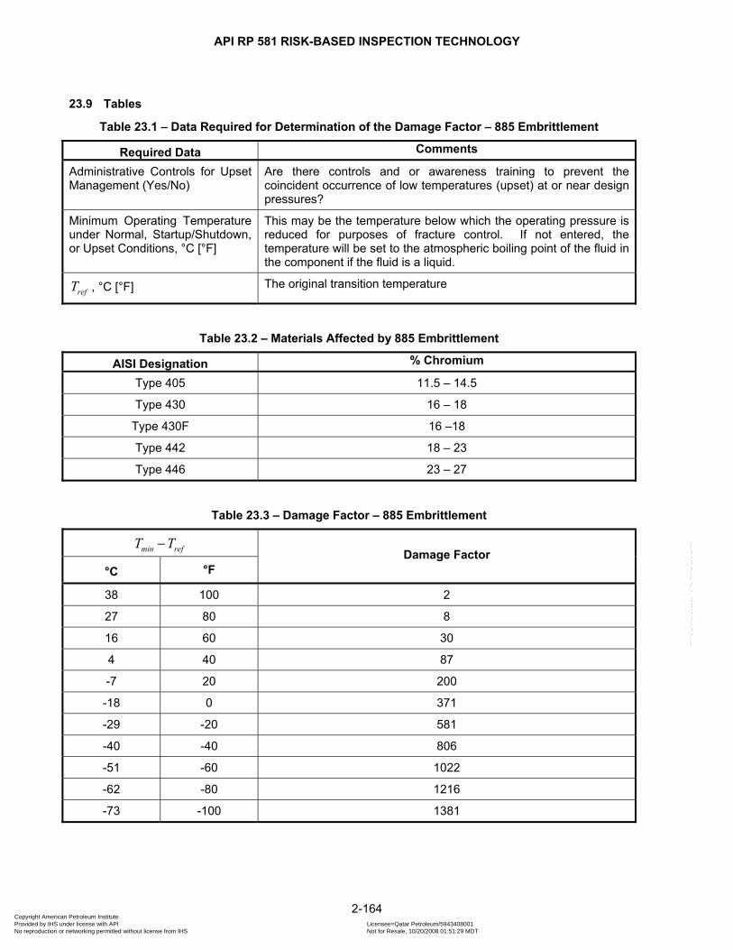
API RP 581 RISK-BASED INSPECTION TECHNOLOGY
23.9 Tables
Table 23.1 – Data Required for Determination of the Damage Factor – 885 Embrittlement
Required Data Comments
Administrative Controls for Upset Management (Yes/No)
Are there controls and or awareness training to prevent the coincident occurrence of low temperatures (upset) at or near design pressures?
Minimum Operating Temperature under Normal, Startup/Shutdown, or Upset Conditions, °C [°F]
This may be the temperature below which the operating pressure is reduced for purposes of fracture control. If not entered, the temperature will be set to the atmospheric boiling point of the fluid in the component if the fluid is a liquid.
refT , °C [°F] The original transition temperature
Table 23.2 – Materials Affected by 885 Embrittlement
AISI Designation % Chromium
Type 405 11.5 – 14.5
Type 430 16 – 18
Type 430F 16 –18
Type 442 18 – 23
Type 446 23 – 27
Table 23.3 – Damage Factor – 885 Embrittlement
min refT T− Damage Factor
°C °F
38 100 2
27 80 8
16 60 30
4 40 87
-7 20 200
-18 0 371
-29 -20 581
-40 -40 806
-51 -60 1022
-62 -80 1216
-73 -100 1381
2-164 Copyright American Petroleum Institute Provided by IHS under license with API Licensee=Qatar Petroleum/5943408001
Not for Resale, 10/20/2008 01:51:29 MDTNo reproduction or networking permitted without license from IHS
--```,`,,`,`,,`,`,,,,,,``,```,`-`-`,,`,,`,`,,`---

API RP 581 RISK-BASED INSPECTION TECHNOLOGY
23.10 Figures
Figure 23.1 – Determination of the 885 Embrittlement Damage Factor
2-165 Copyright American Petroleum Institute Provided by IHS under license with API Licensee=Qatar Petroleum/5943408001
Not for Resale, 10/20/2008 01:51:29 MDTNo reproduction or networking permitted without license from IHS
--```,`,,`,`,,`,`,,,,,,``,```,`-`-`,,`,,`,`,,`---

API RP 581 RISK-BASED INSPECTION TECHNOLOGY
24 SIGMA PHASE EMBRITTLEMENT DAMAGE FACTOR
24.1 Scope The damage factor calculation for components subject to sigma phase embrittlement is covered in this paragraph.
24.2 Description of Damage Sigma phase is a hard, brittle intermetallic compound of iron and chromium with an approximate composition of Fe0.6Cr0.4. It occurs in ferritic (Fe-Cr), martensitic (Fe-Cr), and austenitic (Fe-Cr-Ni) stainless steels when exposed to temperatures in the range of 593°C to 927°C [1100°F to 1700°F]. The rate of formation and the amount of sigma formed are dependent on chemical composition of the alloy and prior cold work history. Ferrite stabilizers (Cr, Si, Mo, Al, W, V, Ti, Nb) tend to promote sigma formation, while austenite stabilizers (C, Ni, N, Mn) tend to retard sigma formation. Austenitic stainless steel alloys typically exhibit a maximum of about 10% sigma phase, or less with increasing nickel. However, other alloys with a nominal composition of 60% Fe, 40% Cr (about the composition of sigma) can be transformed to essentially 100% sigma. A transformation vs. time curve for such a Fe-Cr alloy showed 100% conversion to sigma in 3 hours at 747°C [1377°F]. Conversion to sigma in austenitic stainless steels can also occur in a few hours, as evidenced by the known tendency for sigma to form if an austenitic stainless steel is subjected to a post-weld heat treatment at 691°C [1275°F]. Sigma is unstable at temperatures above 899°C [1650°F], and austenitic stainless steel components can be de-sigmatized by solution annealing at 1066°C [1950°F] for four hours followed by a water quench. Mechanical properties of sigmatized materials are affected depending upon both the amount of sigma present and the size and shape of the sigma particles. For this reason, prediction of mechanical properties of sigmatized material is difficult. The tensile and yield strength of sigmatized stainless steels increases slightly compared with solution annealed material. This increase in strength is accompanied by a reduction in ductility (measured by % elongation and reduction in area) and a slight increase in hardness. The property that is most affected by sigma formation is the toughness. Impact tests show decreased impact energy absorption, and decreased percent shear fracture sigmatized stainless steels vs. solution annealed material. The effect is most pronounced at temperatures below 538° C [1000° F] although there may be some reduction in impact properties at higher temperatures as well. However, because austenitic stainless steels exhibit such good impact properties in the solution annealed condition, then even with considerable degradation, the impact properties may be comparable to other steels used in the process industries. A draft fitness-for-service report from the Materials Properties Council recommends default fracture toughness values of 150 ksi in and 80 ksi in in for base metal and weld metal, respectively, for thermally embrittled austenitic stainless steels. Tests performed on sigmatized stainless steel samples from FCC regenerator internals showed that even with 10% sigma formation, the Charpy impact toughness was 53 joules at 649°C [39 ft-lbs at 1200°F]. This would be considered adequate for most steels, but is much less than the 258 joules [190 ft-lbs] obtained for solution annealed stainless steel. In this specimen, the impact toughness was reduced to 13 ft-lbs at room temperature, a marginal figure but still acceptable for many applications. The percent of shear fracture is another indicator of material toughness, indicating what percent of the Charpy impact specimen broke in a ductile fashion. For the 10% sigmatized specimen referenced above, the values ranged from 0% at room temperature to 100% at 649°C [1200°F]. Thus, although the impact toughness is reduced at high temperature, the specimens broke in a 100% ductile fashion, indicating that the material is still suitable. The lack of fracture ductility at room temperature indicates that care should be taken to avoid application of high stresses to sigmatized materials during shutdown, as a brittle fracture could result. Table 24.2 summarizes impact property data found for 304 and 321 stainless steels.
2-166 Copyright American Petroleum Institute Provided by IHS under license with API Licensee=Qatar Petroleum/5943408001
Not for Resale, 10/20/2008 01:51:29 MDTNo reproduction or networking permitted without license from IHS
--```,`,,`,`,,`,`,,,,,,``,```,`-`-`,,`,,`,`,,`---

API RP 581 RISK-BASED INSPECTION TECHNOLOGY
24.3 Screening Criteria If all of the following are true, then the component should be evaluated for susceptibility to sigma phase embrittlement. a) The material an austenitic stainless steel. b) The operating temperature between 593°C and 927°C [1100 and 1700 °F].
24.4 Required Data The basic component data required for analysis is given in Table 5.1 and the specific data required for determination of the damage factor for sigma phase embrittlement is provided in Table 24.1.
24.5 Basic Assumption Since data is scarce and exhibits considerable scatter, it is assumed that sigmatized austenitic stainless steels will behave in a brittle fashion similar to ferritic steels. The data available showed a reduction in properties, but not the original properties. It is assumed that in the calculation of the damage factor, the original impact toughness of austenitic stainless steels is about 330 [300 ]MPa m ksi in
The references were searched for additional test data, which was scarce and exhibited considerable scatter. The test data found is shown in Table 24.2. The data in this table was used to construct property trend lines of Low Sigma (1% and 2%), High Sigma (10%), and Medium Sigma (Average of Low and High).
24.6 Determination of the Damage Factor
24.6.1 Overview A flow chart of the steps required to determine the damage factor for sigma phase embrittlement is shown in Figure 24.1. The following paragraphs provide additional information and the calculation procedure.
24.6.2 Inspection Effectiveness For this damage mechanism, credit is not given for inspection. However, the results of metallurgical testing can be used to update the inputs to the damage factor calculation that may result in a change in this value.
24.6.3 Calculation of the Damage Factor The following procedure may be used to determine the damage factor for sigma phase embrittlement, see Figure 24.1.
a) STEP 1 – Determine the evaluation temperature, . The material may be evaluated at normal operating conditions, or at a lower temperature such as shutdown or upset temperature.
minT
b) STEP 2 – Determine the estimated % sigma in the material. This can be made through comparisons with materials in similar service, or via metallographic examination of a sample.
c) STEP 3 – Determine the damage factor, sigmafD , using Table 24.3 based on from STEP 1 and the
estimated % sigma from STEP 2. minT
24.7 Nomenclature sigmafD is the damage factor for sigma phase embrittlement
minT is the minimum temperature, °C [°F]
2-167 Copyright American Petroleum Institute Provided by IHS under license with API Licensee=Qatar Petroleum/5943408001
Not for Resale, 10/20/2008 01:51:29 MDTNo reproduction or networking permitted without license from IHS
--```,`,,`,`,,`,`,,,,,,``,```,`-`-`,,`,,`,`,,`---
API RP 581 RISK-BASED INSPECTION TECHNOLOGY
24.8 References 77. Viswanathan, R., Damage Mechanisms and Life Assessment of High Temperature Components , ASM
International, 1989. 78. Timmins, P. F., Predictive Corrosion and Failure Control in Process Operations, ASM International, 1996. 79. Kaieda Y. and Oguchi A., “Brittle Fracture Stress of an Fe-Cr Alloy (Sigma Phase) under High Hydrostatic
Pressure and High Temperature”, Trans. of the Japan Inst. of Metals, Vol. 22, No. 2 (1981), pp. 83 to 95. 80. Ohta S., Saori M., and Yoshida T., “Analysis and Prevention of Failure in Steam Reforming Furnace Tube”,
Kobe Steel Technical Bulletin 1059, Kobe Steel Engineering Reports, Vol. 33, No. 2, April 1983. 81. Gaertner D. J., “Metallurgical Characterization of Sigmatized Austenitic Stainless Steels in FCCU
Regenerator Cyclone Systems”, Paper #132, Corrosion '84, NACE, Houston TX. 82. Morris D., “The Influence of Sigma Phase on Creep Ductility in Type 316 Stainless Steel”, Scripta
Metallurgica, Vol. 13, pp. 1195-1196, 1979. 83. DeLong J. F., Bynum J. E., Ellis F. V., Rafiee M. H., Siddall W. F., Daikoku T., and Haneda H., “Failure
Investigation of Eddystone Main Steam Piping”, Welding Research Supplement, October 1985, AWS. 84. Tikhonov A. S., and Osipov V. G., “Sigma Phase in Wrought Fe-Cr Alloys”, Consultant’s Bureau, New York,
1971. 85. Sorokina N. A., Ullyanin E. A., Fedorova V. I., Kaputkin II, and Belyaeva V. A., “Structure and Properties of
Stainless Steel Alloyed with Molybdenum”, Plenum Publishing, New York, 1975. 86. “High Temperature Corrosion in Refinery ad Petrochemical Service”, High Temperature Engineering
Bulletin HTB-2, INCO, New York, 1960. 87. Peckner D., and Bernstein I. M., “Handbook of Stainless Steels,” McGraw-Hill, New York 1977.
2-168 Copyright American Petroleum Institute Provided by IHS under license with API Licensee=Qatar Petroleum/5943408001
Not for Resale, 10/20/2008 01:51:29 MDTNo reproduction or networking permitted without license from IHS
--```,`,,`,`,,`,`,,,,,,``,```,`-`-`,,`,,`,`,,`---
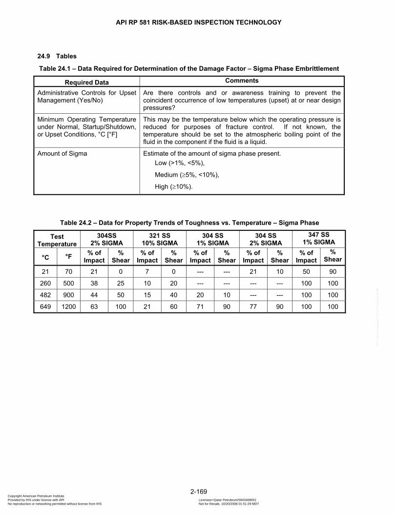
API RP 581 RISK-BASED INSPECTION TECHNOLOGY
24.9 Tables
Table 24.1 – Data Required for Determination of the Damage Factor – Sigma Phase Embrittlement
Required Data Comments
Administrative Controls for Upset Management (Yes/No)
Are there controls and or awareness training to prevent the coincident occurrence of low temperatures (upset) at or near design pressures?
Minimum Operating Temperature under Normal, Startup/Shutdown, or Upset Conditions, °C [°F]
This may be the temperature below which the operating pressure is reduced for purposes of fracture control. If not known, the temperature should be set to the atmospheric boiling point of the fluid in the component if the fluid is a liquid.
Amount of Sigma
Estimate of the amount of sigma phase present. Low (>1%, <5%),
Medium (≥5%, <10%),
High (≥10%).
Table 24.2 – Data for Property Trends of Toughness vs. Temperature – Sigma Phase
Test Temperature
304SS 2% SIGMA
321 SS 10% SIGMA
304 SS 1% SIGMA
304 SS 2% SIGMA
347 SS 1% SIGMA
°C °F % of Impact
% Shear
% of Impact
% Shear
% of Impact
% Shear
% of Impact
% Shear
% of Impact
% Shear
21 70 21 0 7 0 --- --- 21 10 50 90
260 500 38 25 10 20 --- --- --- --- 100 100
482 900 44 50 15 40 20 10 --- --- 100 100
649 1200 63 100 21 60 71 90 77 90 100 100
2-169 Copyright American Petroleum Institute Provided by IHS under license with API Licensee=Qatar Petroleum/5943408001
Not for Resale, 10/20/2008 01:51:29 MDTNo reproduction or networking permitted without license from IHS
--```,`,,`,`,,`,`,,,,,,``,```,`-`-`,,`,,`,`,,`---

API RP 581 RISK-BASED INSPECTION TECHNOLOGY
Table 24.3 – Damage Factor – Sigma Phase
minT Evaluation Temperature
Damage Factor as a Function of Sigma Content
(°C) (°F) Low Sigma Medium Sigma High Sigma
649 1200 0.0 0.0 18
538 1000 0.0 0.0 53
427 800 0.0 0.2 160
316 600 0.0 0.9 481
204 400 0.0 1.3 1333
93 200 0.1 3 3202
66 150 0.3 5 3871
38 100 0.6 7 4196
10 50 0.9 11 4196
-18 0 1.0 20 4196
-46 -50 1.1 34 4196
2-170 Copyright American Petroleum Institute Provided by IHS under license with API Licensee=Qatar Petroleum/5943408001
Not for Resale, 10/20/2008 01:51:29 MDTNo reproduction or networking permitted without license from IHS
--```,`,,`,`,,`,`,,,,,,``,```,`-`-`,,`,,`,`,,`---
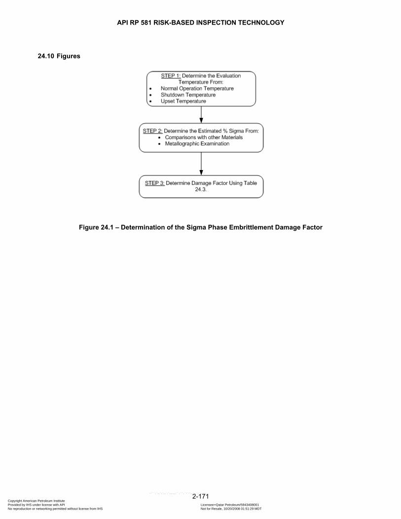
API RP 581 RISK-BASED INSPECTION TECHNOLOGY
24.10 Figures
Figure 24.1 – Determination of the Sigma Phase Embrittlement Damage Factor
2-171 Copyright American Petroleum Institute Provided by IHS under license with API Licensee=Qatar Petroleum/5943408001
Not for Resale, 10/20/2008 01:51:29 MDTNo reproduction or networking permitted without license from IHS
--```,`,,`,`,,`,`,,,,,,``,```,`-`-`,,`,,`,`,,`---
API RP 581 RISK-BASED INSPECTION TECHNOLOGY
25 PIPING MECHANICAL FATIGUE DAMAGE FACTOR
25.1 Scope The damage factor calculation for piping components subject to mechanical fatigue is covered in this paragraph.
25.2 Description of Damage Fatigue failures of piping systems present a very real hazard under certain conditions. Properly designed and installed piping systems should not be subject to such failures, but prediction of vibration in piping systems at the design stage is very difficult, especially if there are mechanical sources of cyclic stresses such as reciprocating pumps and compressors. In addition, even if a piping systems are not subject to mechanical fatigue in the as-built condition, changing conditions such as failure of pipe supports, increased vibration from out of balance machinery, chattering of relief valves during process upsets, changes in flow and pressure cycles or adding weight to unsupported branch connections (pendulum effect) can render a piping system susceptible to failure. Awareness of these influences incorporated into a management of change program can reduce the probability of failures.
25.3 Screening Criteria If all of the following are true, then the component should be evaluated for susceptibility to mechanical fatigue. a) The component is pipe. b) There have been past fatigue failures in this piping system or there is visible/audible shaking in this piping
system or there is a source of cyclic vibration within approximately 15.24 meters [50 feet] and connected to the piping (directly or indirectly via structure). Shaking and source of shaking can be continuous or intermittent. Transient conditions often cause intermittent vibration.
25.4 Required Data The basic component data required for analysis is given in Table 5.1 and the specific data required for determination of the damage factor for mechanical fatigue is provided in Table 25.1.
25.5 Basic Assumption Properly designed piping has a low tendency for mechanical fatigue failure due to the low period of vibration or low stress amplitude. The period is determined by the piping diameter, thickness, mass, support spacing, and support type. Based on input from plant engineers and inspectors from several disciplines, the following key indicators of a high l probability of failure were identified: a) Previous failures due to fatigue. b) Audible, visible, or otherwise noticeable piping vibration (including small branch connections) that is greater
than typical plant piping systems. c) Connection to reciprocating machinery, extreme cavitation through let-down or mixing valves, or relief valve
chatter. The presence of any or all of the above indicators determines the base susceptibility, which is then modified by various adjustment factors.
2-172 Copyright American Petroleum Institute Provided by IHS under license with API Licensee=Qatar Petroleum/5943408001
Not for Resale, 10/20/2008 01:51:29 MDTNo reproduction or networking permitted without license from IHS
--```,`,,`,`,,`,`,,,,,,``,```,`-`-`,,`,,`,`,,`---
API RP 581 RISK-BASED INSPECTION TECHNOLOGY
25.6 Determination of the Damage Factor
25.6.1 Overview A flow chart of the steps required to determine the damage factor for mechanical fatigue is shown in Figure 25.1. The following paragraphs provide additional information and the calculation procedure.
25.6.2 Inspection Effectiveness For this damage mechanism, credit is not given for inspection. However, the results of metallurgical testing can be used to update the inputs to the damage factor calculation that may result in a change in this value. Mechanical fatigue failures in piping are not that common. Unfortunately, when failures occur, they can be of high consequence. In addition and more unfortunately, traditional non-destructive testing techniques are of little value in preventing such failures. The reason that crack detection techniques are not by themselves adequate are several. a) Most of the time to failure in piping fatigue is in the initiation phase, where a crack in the process of forming
has formed but is so small that it is undetectable. b) By the time a crack has reached a detectable size, the crack growth rate is high, and failure will likely occur
in less than a typical inspection frequency. c) Cyclic stresses in vibrating piping tend to have a fairly high frequency, which increases the crack growth
rate. d) Cracks form and grow in locations that are typically difficult to inspect, such as at fillet weld toes, the first
unengaged thread root and defects in other welds. e) The initiation site for crack growth is not necessarily on the outside of the pipe; in fact, a crack can grow
from an embedded defect undetectable from either side without special techniques. Therefore, inspection for mechanical fatigue in piping systems depends heavily on detection and correction of the conditions that lead to susceptibility. Such techniques include: a) Visual examination of pipe supports to assure that all supports are functioning properly (i.e., they are
actually supporting the pipe). b) Visual examination of any cyclic motion of the pipe. If pipe can be seen to be vibrating or moving in a cyclic
manner, the pipe should be suspected of mechanical fatigue failure. c) Visual examination of all fillet welded supports and attachments to piping. Fillet welds are especially
susceptible to failure by fatigue, and these may provide an early warning of problems if cracks or failures are found.
d) As a general rule, small branch connections with unsupported valves or controllers on them are highly susceptible to failure. Examine these for signs of motion, and provide proper support for all such installations.
e) Surface inspection methods (PT, MT) can be effective in a focused and frequent inspection plan. f) Manually feeling the pipe to detect vibration. This requires experience, but normally process plant piping
will not vibrate any more severely than a car engine at idle speed. g) Measurement of piping vibration using special monitoring equipment. There are no set values of vibration
that will be acceptable or non acceptable under all conditions, so experience with using and interpreting vibration data is required.
h) Visual inspection of a unit during transient conditions and different operating scenarios (e.g., startups, shutdowns, upsets, etc.) looking for intermittent vibrating conditions.
i) Checking for audible sounds of vibration emanating from piping components such as control valves and fittings.
25.6.3 Calculation of the Damage Factor The following procedure may be used to determine the damage factor for mechanical fatigue, see Figure 25.1. a) STEP 1 – Determine the number of previous failures that have occurred, and determine the base damage
factor PFfBD based on the following criteria.
2-173 Copyright American Petroleum Institute Provided by IHS under license with API Licensee=Qatar Petroleum/5943408001
Not for Resale, 10/20/2008 01:51:29 MDTNo reproduction or networking permitted without license from IHS
--```,`,,`,`,,`,`,,,,,,``,```,`-`-`,,`,,`,`,,`---
API RP 581 RISK-BASED INSPECTION TECHNOLOGY
1) None – 1PFfBD =
2) One – 50PFfBD =
3) Greater than one – 500PFfBD =
b) STEP 2 – Determine the amount of visible/audible shaking or audible noise occurring in the pipe, and determine the base damage factor AS
fBD based on the following criteria.
1) Minor – 1ASfBD =
2) Moderate – 50ASfBD =
3) Severe – 500ASfBD =
c) STEP 3 – Determine the adjustment factor for visible/audible shaking based on the following criteria. This adjustment is based on observation that some piping systems may endure visible shaking for years. A repeated stress with a cycle of only 1 hertz (1/s) results in over 30 million cycles in a year. Most systems, if they were subject to failure by mechanical fatigue would be expected to fail before reaching tens or hundreds of million cycles. One should note that intermittent cycles are cumulative.
1) Shaking less than 2 weeks – 1ASfBF =
2) Shaking between 2 and 13 weeks – 0.2ASfBF =
3) Shaking between 13 and 52 weeks – 0.02ASfBF =
d) STEP 4 – Determine the type of cyclic loading connected directly or indirectly within approximately 15.24 meters (50 feet) of the pipe, and determine the base damage factor CF
fBD based on the following criteria.
1) Reciprocating Machinery – 50CFfBD =
2) PRV Chatter – 25CFfBD =
3) Valve with high pressure drop – 10CFfBD =
4) None – 1CFfBD =
e) STEP 5 – Determine the base damage factor using Equation (2.56).
( )max , ,mfat PF AS AS CFfB fB fB fB fBD D D F⎡= ⋅⎣ D ⎤
⎦ (2.56)
f) STEP 6 – Determine the final value of the damage factor using Equation (2.57). mfat mfatf fb CA PC CP JB BDD D F F F F F= ⋅ ⋅ ⋅ ⋅ ⋅ (2.57)
The adjustment factors are determined as follows.
1) Adjustment for Corrective Action, – Established based on the following criteria. CAF
• Modification based on complete engineering analysis – 0.002CAF =
• Modification based on experience – 0.2CAF =
• No modifications – 2CAF =
2) Adjustment for Pipe Complexity, PCF – Established based on the following criteria.
• 0 to 5 total pipe fittings – 0.5PCF =
2-174 Copyright American Petroleum Institute Provided by IHS under license with API Licensee=Qatar Petroleum/5943408001
Not for Resale, 10/20/2008 01:51:29 MDTNo reproduction or networking permitted without license from IHS
--```,`,,`,`,,`,`,,,,,,``,```,`-`-`,,`,,`,`,,`---
API RP 581 RISK-BASED INSPECTION TECHNOLOGY
• 6 to 10 total pipe fittings – 1PCF =
• Greater than 10 total pipe fittings – 2PCF =
3) Adjustment for Condition of Pipe, – Established based on the following criteria. CPF
• Missing or damaged supports, improper support – 2CPF =
• Broken gussets, gussets welded directly to the pipe – 2CPF =
• Good Condition – 1CPF =
4) Adjustment for Joint Type or Branch Design, JBF – Established based on the following criteria.
• Threaded, socketweld, saddle on – 2JBF =
• Saddle in fittings – 1JBF =
• Piping tee, Weldolets – 0.2JBF =
• Sweepolets – 0.02JBF =
5) Adjustment for Branch Diameter, – Established based on the following criteria. BDF
• All branches less than or equal to 2 NPS – 1BDF =
• Any branch greater than 2 NPS – 0.02BDF =
25.7 Nomenclature PFfBD is the base damage factor for previous failures ASfBD is the base damage factor for shaking CFfBD is the base damage factor for cyclic loading type mfatfD is the damage factor for mechanical fatigue mfatfBD is the base damage factor for mechanical fatigue
BDF is the damage factor adjustment for branch diameter
CAF is the damage factor adjustment for corrective action
CPF is the damage factor adjustment for condition of pipe
JBF is the damage factor adjustment for joint type
PCF is the damage factor adjustment for pipe complexity ASfBF is the adjustment factor for audible shaking
2-175 Copyright American Petroleum Institute Provided by IHS under license with API Licensee=Qatar Petroleum/5943408001
Not for Resale, 10/20/2008 01:51:29 MDTNo reproduction or networking permitted without license from IHS
--```,`,,`,`,,`,`,,,,,,``,```,`-`-`,,`,,`,`,,`---
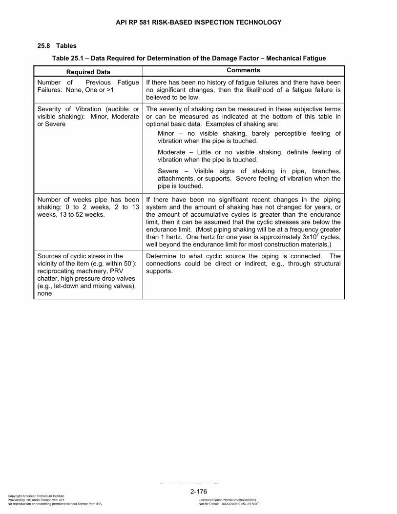
API RP 581 RISK-BASED INSPECTION TECHNOLOGY
25.8 Tables
Table 25.1 – Data Required for Determination of the Damage Factor – Mechanical Fatigue
Required Data Comments
Number of Previous Fatigue Failures: None, One or >1
If there has been no history of fatigue failures and there have been no significant changes, then the likelihood of a fatigue failure is believed to be low.
Severity of Vibration (audible or visible shaking): Minor, Moderate or Severe
The severity of shaking can be measured in these subjective terms or can be measured as indicated at the bottom of this table in optional basic data. Examples of shaking are:
Minor – no visible shaking, barely perceptible feeling of vibration when the pipe is touched.
Moderate – Little or no visible shaking, definite feeling of vibration when the pipe is touched.
Severe – Visible signs of shaking in pipe, branches, attachments, or supports. Severe feeling of vibration when the pipe is touched.
Number of weeks pipe has been shaking: 0 to 2 weeks, 2 to 13 weeks, 13 to 52 weeks.
If there have been no significant recent changes in the piping system and the amount of shaking has not changed for years, or the amount of accumulative cycles is greater than the endurance limit, then it can be assumed that the cyclic stresses are below the endurance limit. (Most piping shaking will be at a frequency greater than 1 hertz. One hertz for one year is approximately 3x10⁷ cycles, well beyond the endurance limit for most construction materials.)
Sources of cyclic stress in the vicinity of the item (e.g. within 50’): reciprocating machinery, PRV chatter, high pressure drop valves (e.g., let-down and mixing valves), none
Determine to what cyclic source the piping is connected. The connections could be direct or indirect, e.g., through structural supports.
2-176 Copyright American Petroleum Institute Provided by IHS under license with API Licensee=Qatar Petroleum/5943408001
Not for Resale, 10/20/2008 01:51:29 MDTNo reproduction or networking permitted without license from IHS
--```,`,,`,`,,`,`,,,,,,``,```,`-`-`,,`,,`,`,,`---
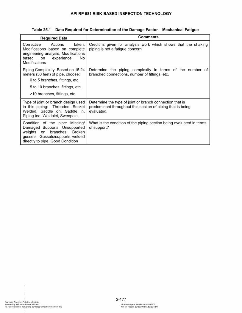
API RP 581 RISK-BASED INSPECTION TECHNOLOGY
Table 25.1 – Data Required for Determination of the Damage Factor – Mechanical Fatigue
Required Data Comments
Corrective Actions taken: Modifications based on complete engineering analysis, Modifications based on experience, No Modifications
Credit is given for analysis work which shows that the shaking piping is not a fatigue concern
Piping Complexity: Based on 15.24 meters (50 feet) of pipe, choose:
0 to 5 branches, fittings, etc.
5 to 10 branches, fittings, etc.
>10 branches, fittings, etc.
Determine the piping complexity in terms of the number of branched connections, number of fittings, etc.
Type of joint or branch design used in this piping: Threaded, Socket Welded, Saddle on, Saddle in, Piping tee, Weldolet, Sweepolet
Determine the type of joint or branch connection that is predominant throughout this section of piping that is being evaluated.
Condition of the pipe: Missing/ Damaged Supports, Unsupported weights on branches, Broken gussets, Gussets/supports welded directly to pipe, Good Condition
What is the condition of the piping section being evaluated in terms of support?
2-177 Copyright American Petroleum Institute Provided by IHS under license with API Licensee=Qatar Petroleum/5943408001
Not for Resale, 10/20/2008 01:51:29 MDTNo reproduction or networking permitted without license from IHS
--```,`,,`,`,,`,`,,,,,,``,```,`-`-`,,`,,`,`,,`---
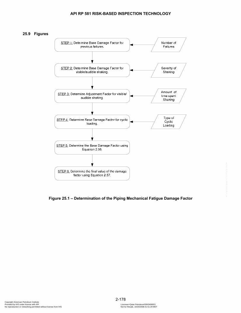
API RP 581 RISK-BASED INSPECTION TECHNOLOGY
2-178
25.9 Figures
Figure 25.1 – Determination of the Piping Mechanical Fatigue Damage Factor
Copyright American Petroleum Institute Provided by IHS under license with API Licensee=Qatar Petroleum/5943408001
Not for Resale, 10/20/2008 01:51:29 MDTNo reproduction or networking permitted without license from IHS
--```,`,,`,`,,`,`,,,,,,``,```,`-`-`,,`,,`,`,,`---
API RP 581 RISK-BASED INSPECTION TECHNOLOGY
API RP 581 PART 2
ANNEX 2.A – MANAGEMENT SYSTEMS WORK BOOK
2.A-1 Copyright American Petroleum Institute Provided by IHS under license with API Licensee=Qatar Petroleum/5943408001
Not for Resale, 10/20/2008 01:51:29 MDTNo reproduction or networking permitted without license from IHS
--```,`,,`,`,,`,`,,,,,,``,```,`-`-`,,`,,`,`,,`---

API RP 581 RISK-BASED INSPECTION TECHNOLOGY
PART CONTENTS TABLE 2.A.1 – LEADERSHIP AND ADMINISTRATION ............................................................... 2.A-3 TABLE 2.A.2 – PROCESS SAFETY INFORMATION .................................................................... 2.A-4 TABLE 2.A.3 – PROCESS HAZARD ANALYSIS ........................................................................... 2.A-6 TABLE 2.A.4 – MANAGEMENT OF CHANGE ............................................................................... 2.A-8 TABLE 2.A.5 – OPERATING PROCEDURES .............................................................................. 2.A-10 TABLE 2.A.6 – SAFE WORK PRACTICES .................................................................................. 2.A-12 TABLE 2.A.7 – TRAINING ............................................................................................................ 2.A-14 TABLE 2.A.8 – MECHANICAL INTEGRITY ................................................................................. 2.A-16 TABLE 2.A.9 – PRE-STARTUP SAFETY REVIEW...................................................................... 2.A-20 TABLE 2.A.10 – EMERGENCY RESPONSE ............................................................................... 2.A-21 TABLE 2.A.11 – INCIDENT INVESTIGATION .............................................................................. 2.A-22 TABLE 2.A.12 – CONTRACTORS ................................................................................................ 2.A-23 TABLE 2.A.13 – MANAGEMENT SYSTEMS ASSESSMENTS ................................................... 2.A-24
2.A-2 Copyright American Petroleum Institute Provided by IHS under license with API Licensee=Qatar Petroleum/5943408001
Not for Resale, 10/20/2008 01:51:29 MDTNo reproduction or networking permitted without license from IHS
--```,`,,`,`,,`,`,,,,,,``,```,`-`-`,,`,,`,`,,`---
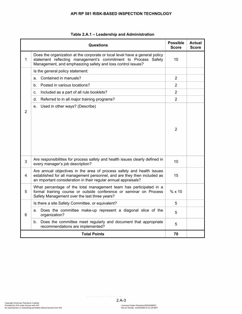
API RP 581 RISK-BASED INSPECTION TECHNOLOGY
Table 2.A.1 – Leadership and Administration
Questions Possible Score
Actual Score
1 Does the organization at the corporate or local level have a general policy statement reflecting management’s commitment to Process Safety Management, and emphasizing safety and loss control issues?
10
2
Is the general policy statement:
a. Contained in manuals? 2
b. Posted in various locations? 2
c. Included as a part of all rule booklets? 2
d. Referred to in all major training programs? 2
e. Used in other ways? (Describe)
2
3 Are responsibilities for process safety and health issues clearly defined in every manager’s job description? 10
4 Are annual objectives in the area of process safety and health issues established for all management personnel, and are they then included as an important consideration in their regular annual appraisals?
15
5 What percentage of the total management team has participated in a formal training course or outside conference or seminar on Process Safety Management over the last three years?
% x 10
6
Is there a site Safety Committee, or equivalent? 5
a. Does the committee make-up represent a diagonal slice of the organization? 5
b. Does the committee meet regularly and document that appropriate recommendations are implemented? 5
Total Points 70
2.A-3 Copyright American Petroleum Institute Provided by IHS under license with API Licensee=Qatar Petroleum/5943408001
Not for Resale, 10/20/2008 01:51:29 MDTNo reproduction or networking permitted without license from IHS
--```,`,,`,`,,`,`,,,,,,``,```,`-`-`,,`,,`,`,,`---
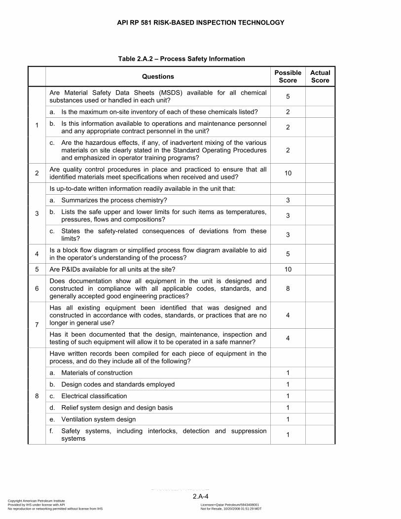
API RP 581 RISK-BASED INSPECTION TECHNOLOGY
Table 2.A.2 – Process Safety Information
Questions Possible Score
Actual Score
1
Are Material Safety Data Sheets (MSDS) available for all chemical substances used or handled in each unit? 5
a. Is the maximum on-site inventory of each of these chemicals listed? 2
b. Is this information available to operations and maintenance personnel and any appropriate contract personnel in the unit? 2
c. Are the hazardous effects, if any, of inadvertent mixing of the various materials on site clearly stated in the Standard Operating Procedures and emphasized in operator training programs?
2
2 Are quality control procedures in place and practiced to ensure that all identified materials meet specifications when received and used? 10
3
Is up-to-date written information readily available in the unit that:
a. Summarizes the process chemistry? 3
b. Lists the safe upper and lower limits for such items as temperatures, pressures, flows and compositions? 3
c. States the safety-related consequences of deviations from these limits? 3
4 Is a block flow diagram or simplified process flow diagram available to aid in the operator’s understanding of the process? 5
5 Are P&IDs available for all units at the site? 10
6 Does documentation show all equipment in the unit is designed and constructed in compliance with all applicable codes, standards, and generally accepted good engineering practices?
8
7
Has all existing equipment been identified that was designed and constructed in accordance with codes, standards, or practices that are no longer in general use?
4
Has it been documented that the design, maintenance, inspection and testing of such equipment will allow it to be operated in a safe manner? 4
8
Have written records been compiled for each piece of equipment in the process, and do they include all of the following?
a. Materials of construction 1
b. Design codes and standards employed 1
c. Electrical classification 1
d. Relief system design and design basis 1
e. Ventilation system design 1
f. Safety systems, including interlocks, detection and suppression systems 1
2.A-4 Copyright American Petroleum Institute Provided by IHS under license with API Licensee=Qatar Petroleum/5943408001
Not for Resale, 10/20/2008 01:51:29 MDTNo reproduction or networking permitted without license from IHS
--```,`,,`,`,,`,`,,,,,,``,```,`-`-`,,`,,`,`,,`---

API RP 581 RISK-BASED INSPECTION TECHNOLOGY
Table 2.A.2 – Process Safety Information
Questions Possible Score
Actual Score
9 Are procedures in place to ensure that each individual with responsibility for managing the process has a working knowledge of the process safety information appropriate to his or her responsibilities?
5
10
Is a documented compilation of all the above Process Safety Information maintained at the facility as a reference? The individual elements of the Information may exist in various forms and locations, but the compilation should confirm the existence and location of each element.
8
Total Points 80
2.A-5 Copyright American Petroleum Institute Provided by IHS under license with API Licensee=Qatar Petroleum/5943408001
Not for Resale, 10/20/2008 01:51:29 MDTNo reproduction or networking permitted without license from IHS
--```,`,,`,`,,`,`,,,,,,``,```,`-`-`,,`,,`,`,,`---

API RP 581 RISK-BASED INSPECTION TECHNOLOGY
Table 2.A.3 – Process Hazard Analysis
Questions Possible Score
Actual Score
1 What percentage of all process units that handle hazardous chemicals at the facility have had a formal Process Hazard Analysis (PHA) within the last five years?
% x 10
2
Has a priority order been established for conducting future PHAs? 5
Does the basis for the prioritization address the following factors?:
a. The quantity of toxic, flammable, or explosive material at the site 1
b. The level of toxicity or reactivity of the materials 1
c. The number of people in the immediate proximity of the facility, including both onsite and offsite locations 1
d. Process complexity 1
e. Severe operating conditions or conditions that can cause corrosion or erosion 1
3
Do the PHAs conducted to date address:
a. The hazards of the process? 2
b. A review of previous incident/accident reports from the unit being analyzed to identify any previous incidents that had a potential for catastrophic consequences?
2
c. Engineering and administrative controls applicable to the hazards and their interrelationships? 2
d. Consequences of failure of engineering and administrative controls? 2
e. Facilities siting? 2
f. Human factors? 2
g. A qualitative evaluation of the possible safety and health effects of failure 2
4
Based on the most recent PHA conducted:
a. Was the team leader experienced in the technique being employed? 3
b. Had the team leader received formal training in the method being employed? 3
c. Was at least one member of the team an expert on the process being analyzed? 3
d. Were all appropriate disciplines represented on the team or brought in as required during the analysis? 3
e. Was at least one member of the team a person who did not participate in the original design of the facility? 3
2.A-6 Copyright American Petroleum Institute Provided by IHS under license with API Licensee=Qatar Petroleum/5943408001
Not for Resale, 10/20/2008 01:51:29 MDTNo reproduction or networking permitted without license from IHS
--```,`,,`,`,,`,`,,,,,,``,```,`-`-`,,`,,`,`,,`---
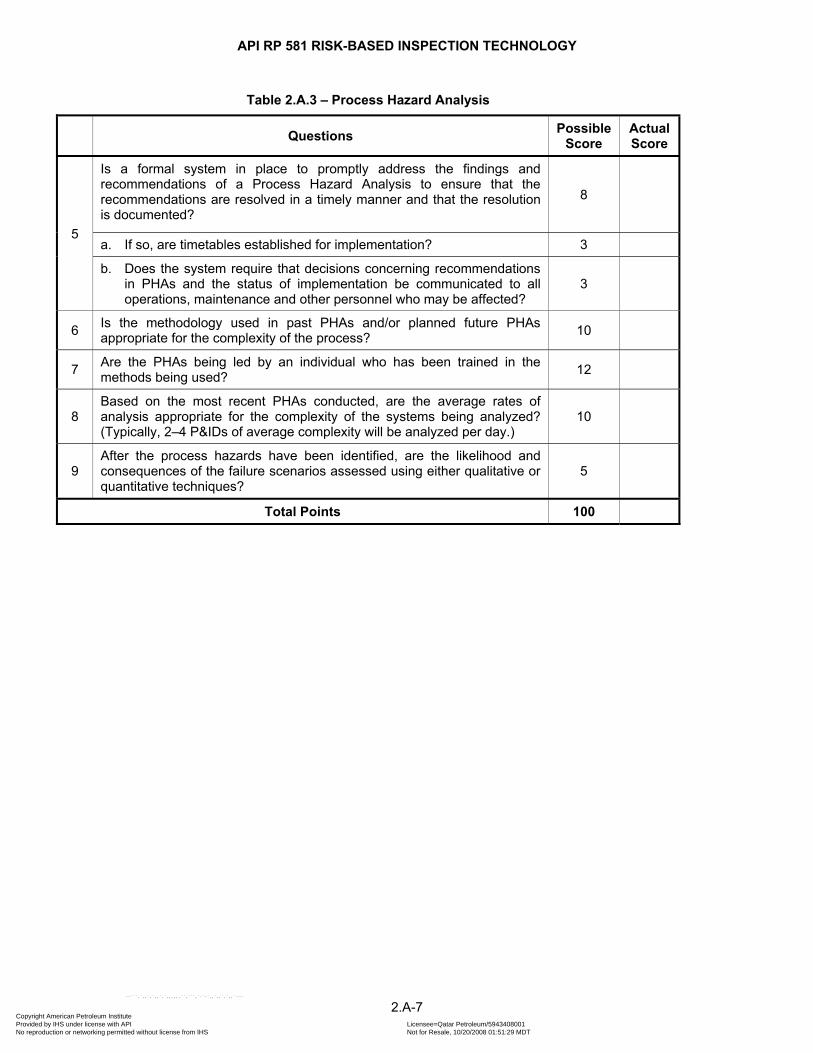
API RP 581 RISK-BASED INSPECTION TECHNOLOGY
Table 2.A.3 – Process Hazard Analysis
Questions Possible Score
Actual Score
5
Is a formal system in place to promptly address the findings and recommendations of a Process Hazard Analysis to ensure that the recommendations are resolved in a timely manner and that the resolution is documented?
8
a. If so, are timetables established for implementation? 3
b. Does the system require that decisions concerning recommendations in PHAs and the status of implementation be communicated to all operations, maintenance and other personnel who may be affected?
3
6 Is the methodology used in past PHAs and/or planned future PHAs appropriate for the complexity of the process? 10
7 Are the PHAs being led by an individual who has been trained in the methods being used? 12
8 Based on the most recent PHAs conducted, are the average rates of analysis appropriate for the complexity of the systems being analyzed? (Typically, 2–4 P&IDs of average complexity will be analyzed per day.)
10
9 After the process hazards have been identified, are the likelihood and consequences of the failure scenarios assessed using either qualitative or quantitative techniques?
5
Total Points 100
2.A-7 Copyright American Petroleum Institute Provided by IHS under license with API Licensee=Qatar Petroleum/5943408001
Not for Resale, 10/20/2008 01:51:29 MDTNo reproduction or networking permitted without license from IHS
--```,`,,`,`,,`,`,,,,,,``,```,`-`-`,,`,,`,`,,`---
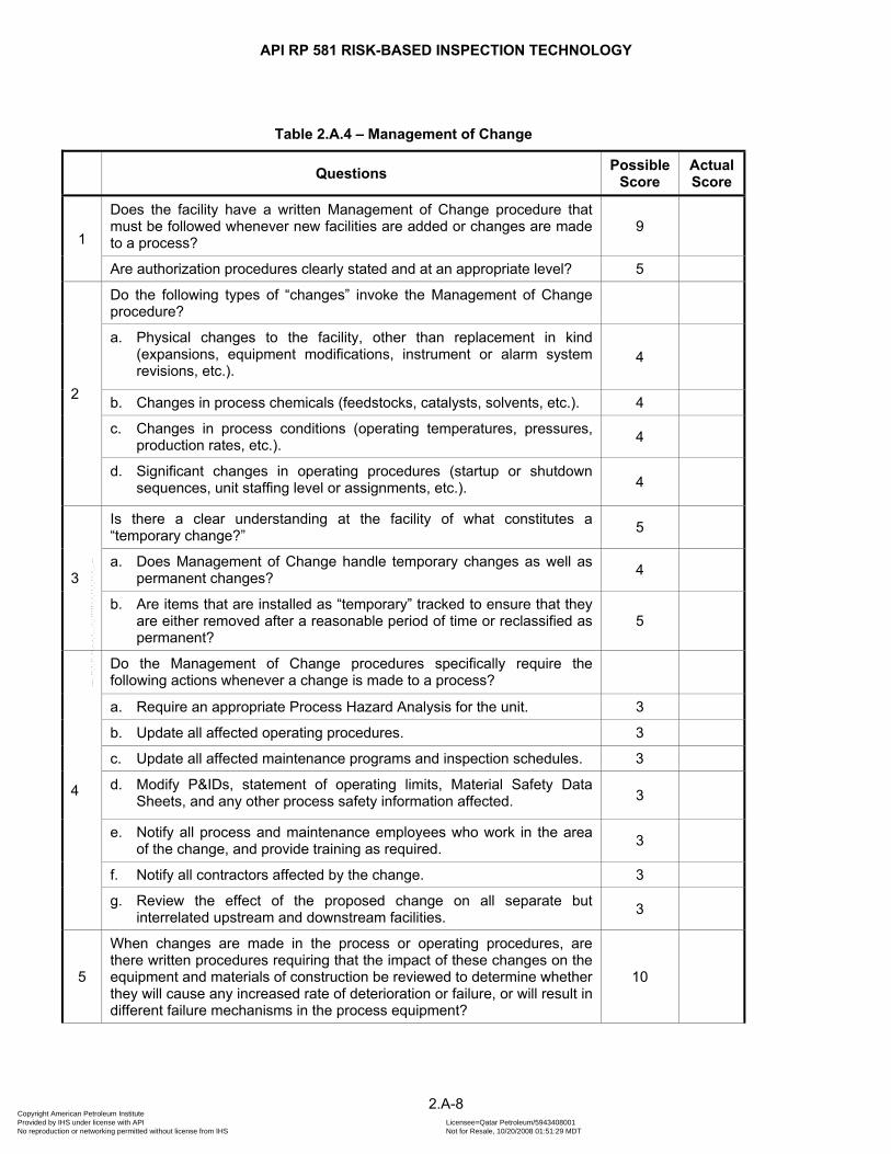
API RP 581 RISK-BASED INSPECTION TECHNOLOGY
Table 2.A.4 – Management of Change
Questions Possible Score
Actual Score
1
Does the facility have a written Management of Change procedure that must be followed whenever new facilities are added or changes are made to a process?
9
Are authorization procedures clearly stated and at an appropriate level? 5
2
Do the following types of “changes” invoke the Management of Change procedure?
a. Physical changes to the facility, other than replacement in kind (expansions, equipment modifications, instrument or alarm system revisions, etc.).
4
b. Changes in process chemicals (feedstocks, catalysts, solvents, etc.). 4
c. Changes in process conditions (operating temperatures, pressures, production rates, etc.). 4
d. Significant changes in operating procedures (startup or shutdown sequences, unit staffing level or assignments, etc.). 4
3
Is there a clear understanding at the facility of what constitutes a “temporary change?” 5
a. Does Management of Change handle temporary changes as well as permanent changes? 4
b. Are items that are installed as “temporary” tracked to ensure that they are either removed after a reasonable period of time or reclassified as permanent?
5
4
Do the Management of Change procedures specifically require the following actions whenever a change is made to a process?
a. Require an appropriate Process Hazard Analysis for the unit. 3
b. Update all affected operating procedures. 3
c. Update all affected maintenance programs and inspection schedules. 3
d. Modify P&IDs, statement of operating limits, Material Safety Data Sheets, and any other process safety information affected. 3
e. Notify all process and maintenance employees who work in the area of the change, and provide training as required. 3
f. Notify all contractors affected by the change. 3
g. Review the effect of the proposed change on all separate but interrelated upstream and downstream facilities. 3
5
When changes are made in the process or operating procedures, are there written procedures requiring that the impact of these changes on the equipment and materials of construction be reviewed to determine whether they will cause any increased rate of deterioration or failure, or will result in different failure mechanisms in the process equipment?
10
2.A-8 Copyright American Petroleum Institute Provided by IHS under license with API Licensee=Qatar Petroleum/5943408001
Not for Resale, 10/20/2008 01:51:29 MDTNo reproduction or networking permitted without license from IHS
--```,`,,`,`,,`,`,,,,,,``,```,`-`-`,,`,,`,`,,`---
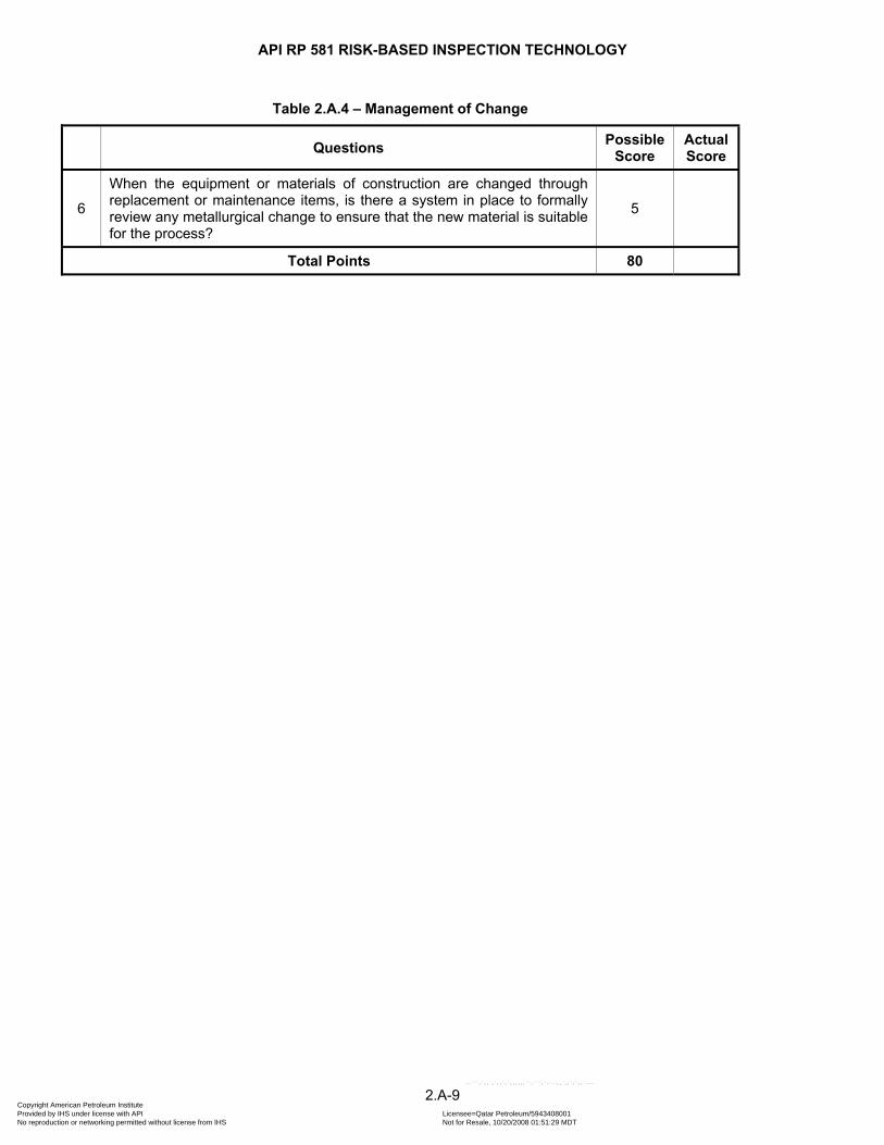
API RP 581 RISK-BASED INSPECTION TECHNOLOGY
Table 2.A.4 – Management of Change
Questions Possible Score
Actual Score
6
When the equipment or materials of construction are changed through replacement or maintenance items, is there a system in place to formally review any metallurgical change to ensure that the new material is suitable for the process?
5
Total Points 80
2.A-9 Copyright American Petroleum Institute Provided by IHS under license with API Licensee=Qatar Petroleum/5943408001
Not for Resale, 10/20/2008 01:51:29 MDTNo reproduction or networking permitted without license from IHS
--```,`,,`,`,,`,`,,,,,,``,```,`-`-`,,`,,`,`,,`---
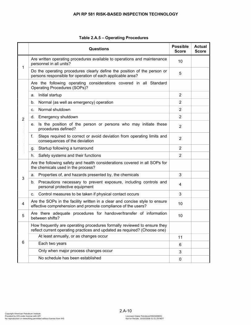
API RP 581 RISK-BASED INSPECTION TECHNOLOGY
Table 2.A.5 – Operating Procedures
Questions Possible Score
Actual Score
1
Are written operating procedures available to operations and maintenance personnel in all units? 10
Do the operating procedures clearly define the position of the person or persons responsible for operation of each applicable area? 5
2
Are the following operating considerations covered in all Standard Operating Procedures (SOPs)?
a. Initial startup 2
b. Normal (as well as emergency) operation 2
c. Normal shutdown 2
d. Emergency shutdown 2
e. Is the position of the person or persons who may initiate these procedures defined? 2
f. Steps required to correct or avoid deviation from operating limits and consequences of the deviation 2
g. Startup following a turnaround 2
h. Safety systems and their functions 2
3
Are the following safety and health considerations covered in all SOPs for the chemicals used in the process?
a. Properties of, and hazards presented by, the chemicals 3
b. Precautions necessary to prevent exposure, including controls and personal protective equipment 4
c. Control measures to be taken if physical contact occurs 3
4 Are the SOPs in the facility written in a clear and concise style to ensure effective comprehension and promote compliance of the users? 10
5 Are there adequate procedures for handover/transfer of information between shifts? 10
6
How frequently are operating procedures formally reviewed to ensure they reflect current operating practices and updated as required? (Choose one)
At least annually, or as changes occur 11 Each two years 6 Only when major process changes occur 3 No schedule has been established 0
2.A-10 Copyright American Petroleum Institute Provided by IHS under license with API Licensee=Qatar Petroleum/5943408001
Not for Resale, 10/20/2008 01:51:29 MDTNo reproduction or networking permitted without license from IHS
--```,`,,`,`,,`,`,,,,,,``,```,`-`-`,,`,,`,`,,`---
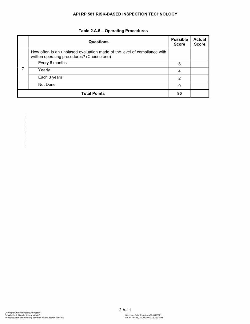
API RP 581 RISK-BASED INSPECTION TECHNOLOGY
Table 2.A.5 – Operating Procedures
Questions Possible Score
Actual Score
7
How often is an unbiased evaluation made of the level of compliance with written operating procedures? (Choose one)
Every 6 months 8 Yearly 4 Each 3 years 2 Not Done 0
Total Points 80
2.A-11 Copyright American Petroleum Institute Provided by IHS under license with API Licensee=Qatar Petroleum/5943408001
Not for Resale, 10/20/2008 01:51:29 MDTNo reproduction or networking permitted without license from IHS
--```,`,,`,`,,`,`,,,,,,``,```,`-`-`,,`,,`,`,,`---

API RP 581 RISK-BASED INSPECTION TECHNOLOGY
Table 2.A.6 – Safe Work Practices
Questions Possible Score
Actual Score
1
Have safe work practices been developed and implemented for employees and contractors to provide for the control of hazards during operation or maintenance, including:
a. Hot work 2
b. Line breaking procedures 2
c. Lockout/tagout 2
d. Confined space entry 2
e. Opening process equipment or piping 2
f. Entrance into a facility by maintenance, contract, laboratory, or other support personnel 2
g. Vehicle entry 2
h. Crane lifts 2
i. Handling of particularly hazardous materials (toxic, radioactive, etc.) 2
j. Inspection or maintenance of in-service equipment 2
2 Do all the safe work practices listed in Question 1 require a work authorization form or permit prior to initiating the activity? 10
3
If so, do the permit procedures include the following features?
a. Forms that adequately cover the subject area 1
b. Clear instructions denoting the number of copies issued and who receives each copy 1
c. Authority required for issuance 1
d. Sign-off procedure at completion of work 1
e. Procedure for extension or reissue after shift change 1
4 Is formal training provided to persons issuing each of the above permits? 10
5 Are the affected employees trained in the above permit and procedure requirements? 10
6
How often is an independent evaluation made (e.g., by Safety Department or similar group), with results communicated to appropriate management, to determine the extent of compliance with requirements for work permits and specialized procedures for major units within the organization? (Choose one)
Every 3 months 7 Every 6 months 4 Yearly 2 Not done 0
2.A-12 Copyright American Petroleum Institute Provided by IHS under license with API Licensee=Qatar Petroleum/5943408001
Not for Resale, 10/20/2008 01:51:29 MDTNo reproduction or networking permitted without license from IHS
--```,`,,`,`,,`,`,,,,,,``,```,`-`-`,,`,,`,`,,`---
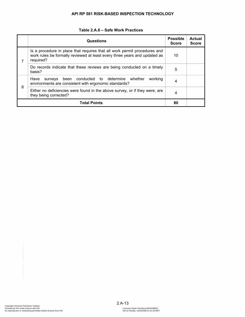
API RP 581 RISK-BASED INSPECTION TECHNOLOGY
Table 2.A.6 – Safe Work Practices
Questions Possible Score
Actual Score
7
Is a procedure in place that requires that all work permit procedures and work rules be formally reviewed at least every three years and updated as required?
10
Do records indicate that these reviews are being conducted on a timely basis? 5
8
Have surveys been conducted to determine whether working environments are consistent with ergonomic standards? 4
Either no deficiencies were found in the above survey, or if they were, are they being corrected? 4
Total Points 80
2.A-13 Copyright American Petroleum Institute Provided by IHS under license with API Licensee=Qatar Petroleum/5943408001
Not for Resale, 10/20/2008 01:51:29 MDTNo reproduction or networking permitted without license from IHS
--```,`,,`,`,,`,`,,,,,,``,```,`-`-`,,`,,`,`,,`---

API RP 581 RISK-BASED INSPECTION TECHNOLOGY
Table 2.A.7 – Training
Questions Possible Score
Actual Score
1 Is there a written procedure that defines the general training in site-wide safety procedures, work practices, etc., that a newly hired employee will receive?
10
2
Is there a written procedure that defines the amount and content of site-specific training, in addition to the general training provided in Question 1, that an employee newly assigned to an operations position will receive prior to assuming his duties?
10
3
Does the procedure described in Question 2 require that the training include the following?
a. An overview of the process and its specific safety and health hazards 3
b. Training in all operating procedures 3
c. Training on site-emergency procedures 3
d. Emphasis on safety-related issues such as work permits, importance of interlocks and other safety systems, etc. 3
e. Safe work practices 3
f. Appropriate basic skills 3
4
At the completion of formal training of operations personnel, what method is used to verify that the employee understands the information presented? (Choose one)
Performance test followed by documented observation 10 Performance test only 7 Opinion of instructor 3 No verification 0
5
How often are operations employees given formal refresher training? (Choose one)
At least once every three years 10 Only when major process changes occur 5 Never 0
6
What is the average amount of training given to each operations employee per year, averaged over all grades? (Choose one)
15 days/year or more 10 11 to 14 days/year 7 7 to 10 days/year 5 3 to 6 days/year 3 Less than 3 days/year 0
2.A-14 Copyright American Petroleum Institute Provided by IHS under license with API Licensee=Qatar Petroleum/5943408001
Not for Resale, 10/20/2008 01:51:29 MDTNo reproduction or networking permitted without license from IHS
--```,`,,`,`,,`,`,,,,,,``,```,`-`-`,,`,,`,`,,`---
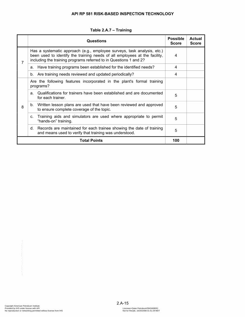
API RP 581 RISK-BASED INSPECTION TECHNOLOGY
Table 2.A.7 – Training
Questions Possible Score
Actual Score
7
Has a systematic approach (e.g., employee surveys, task analysis, etc.) been used to identify the training needs of all employees at the facility, including the training programs referred to in Questions 1 and 2?
4
a. Have training programs been established for the identified needs? 4
b. Are training needs reviewed and updated periodically? 4
8
Are the following features incorporated in the plant's formal training programs?
a. Qualifications for trainers have been established and are documented for each trainer. 5
b. Written lesson plans are used that have been reviewed and approved to ensure complete coverage of the topic. 5
c. Training aids and simulators are used where appropriate to permit “hands-on” training. 5
d. Records are maintained for each trainee showing the date of training and means used to verify that training was understood. 5
Total Points 100
2.A-15 Copyright American Petroleum Institute Provided by IHS under license with API Licensee=Qatar Petroleum/5943408001
Not for Resale, 10/20/2008 01:51:29 MDTNo reproduction or networking permitted without license from IHS
--```,`,,`,`,,`,`,,,,,,``,```,`-`-`,,`,,`,`,,`---
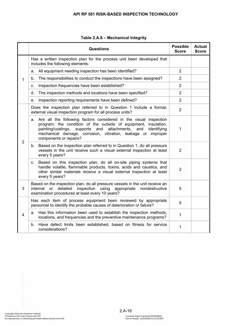
API RP 581 RISK-BASED INSPECTION TECHNOLOGY
Table 2.A.8 – Mechanical Integrity
Questions Possible Score
Actual Score
1
Has a written inspection plan for the process unit been developed that includes the following elements:
a. All equipment needing inspection has been identified? 2
b. The responsibilities to conduct the inspections have been assigned? 2
c. Inspection frequencies have been established? 2
d. The inspection methods and locations have been specified? 2
e. Inspection reporting requirements have been defined? 2
2
Does the inspection plan referred to in Question 1 include a formal, external visual inspection program for all process units? 2
a. Are all the following factors considered in the visual inspection program: the condition of the outside of equipment, insulation, painting/coatings, supports and attachments, and identifying mechanical damage, corrosion, vibration, leakage or improper components or repairs?
1
b. Based on the inspection plan referred to in Question 1, do all pressure vessels in the unit receive such a visual external inspection at least every 5 years?
2
c. Based on this inspection plan, do all on-site piping systems that handle volatile, flammable products, toxins, acids and caustics, and other similar materials receive a visual external inspection at least every 5 years?
2
3 Based on the inspection plan, do all pressure vessels in the unit receive an internal or detailed inspection using appropriate nondestructive examination procedures at least every 10 years?
5
4
Has each item of process equipment been reviewed by appropriate personnel to identify the probable causes of deterioration or failure? 5
a. Has this information been used to establish the inspection methods, locations, and frequencies and the preventive maintenance programs? 1
b. Have defect limits been established, based on fitness for service considerations? 1
2.A-16 Copyright American Petroleum Institute Provided by IHS under license with API Licensee=Qatar Petroleum/5943408001
Not for Resale, 10/20/2008 01:51:29 MDTNo reproduction or networking permitted without license from IHS
--```,`,,`,`,,`,`,,,,,,``,```,`-`-`,,`,,`,`,,`---
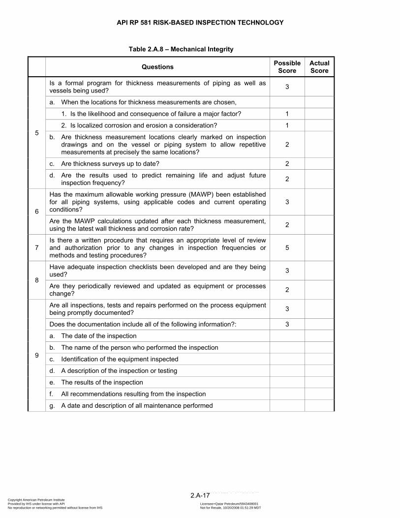
API RP 581 RISK-BASED INSPECTION TECHNOLOGY
Table 2.A.8 – Mechanical Integrity
Questions Possible Score
Actual Score
5
Is a formal program for thickness measurements of piping as well as vessels being used? 3
a. When the locations for thickness measurements are chosen,
1. Is the likelihood and consequence of failure a major factor? 1
2. Is localized corrosion and erosion a consideration? 1
b. Are thickness measurement locations clearly marked on inspection drawings and on the vessel or piping system to allow repetitive measurements at precisely the same locations?
2
c. Are thickness surveys up to date? 2
d. Are the results used to predict remaining life and adjust future inspection frequency? 2
6
Has the maximum allowable working pressure (MAWP) been established for all piping systems, using applicable codes and current operating conditions?
3
Are the MAWP calculations updated after each thickness measurement, using the latest wall thickness and corrosion rate? 2
7 Is there a written procedure that requires an appropriate level of review and authorization prior to any changes in inspection frequencies or methods and testing procedures?
5
8
Have adequate inspection checklists been developed and are they being used? 3
Are they periodically reviewed and updated as equipment or processes change? 2
9
Are all inspections, tests and repairs performed on the process equipment being promptly documented? 3
Does the documentation include all of the following information?: 3
a. The date of the inspection
b. The name of the person who performed the inspection
c. Identification of the equipment inspected
d. A description of the inspection or testing
e. The results of the inspection
f. All recommendations resulting from the inspection
g. A date and description of all maintenance performed
2.A-17 Copyright American Petroleum Institute Provided by IHS under license with API Licensee=Qatar Petroleum/5943408001
Not for Resale, 10/20/2008 01:51:29 MDTNo reproduction or networking permitted without license from IHS
--```,`,,`,`,,`,`,,,,,,``,```,`-`-`,,`,,`,`,,`---

API RP 581 RISK-BASED INSPECTION TECHNOLOGY
Table 2.A.8 – Mechanical Integrity
Questions Possible Score
Actual Score
10
Is there a written procedure requiring that all process equipment deficiencies identified during an inspection be corrected in a safe and timely manner and are they tracked and followed up to assure completion?
5
a. Is a system used to help determine priorities for action? 1
b. If defects are noted, are decisions to continue to operate the equipment based on sound engineering assessments of fitness for service?
2
11 Is there a complete, up-to-date, central file for all inspection program information and reports? 3
Is this file information available to everyone who works with the process? 2
12 Have all employees involved in maintaining and inspecting the process equipment been trained in an overview of the process and its hazards? 5
13
Have all employees involved in maintaining and inspecting the process equipment been trained in all procedures applicable to their job tasks to ensure that they can perform the job tasks in a safe and effective manner?
3
At completion of the training described above, are formal methods used to verify that the employee understands what he was trained on? 2
14 Are inspectors certified for performance in accordance with applicable industry codes and standards (e.g., API 510, 570 and 653)? 5
15 Are training programs conducted for contractors’ employees where special skills or techniques unique to the unit or plant are required for these employees to perform the job safely?
5
16
Has a schedule been established for the inspection or testing of all pressure relief valves in the unit? 3
a. Is the schedule being met? 1
b. Are all inspections and repairs fully documented? 1
c. Are all repairs made by personnel fully trained and experienced in relief valve maintenance? 1
2.A-18 Copyright American Petroleum Institute Provided by IHS under license with API Licensee=Qatar Petroleum/5943408001
Not for Resale, 10/20/2008 01:51:29 MDTNo reproduction or networking permitted without license from IHS
--```,`,,`,`,,`,`,,,,,,``,```,`-`-`,,`,,`,`,,`---
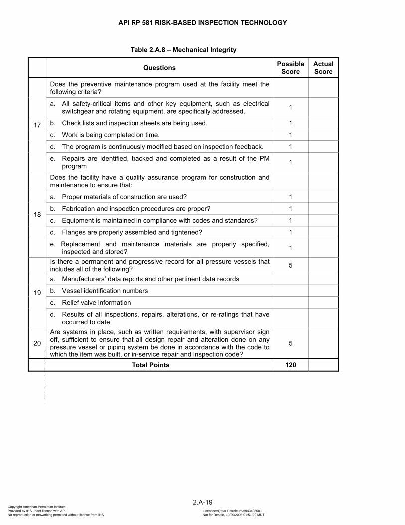
API RP 581 RISK-BASED INSPECTION TECHNOLOGY
Table 2.A.8 – Mechanical Integrity
Questions Possible Score
Actual Score
17
Does the preventive maintenance program used at the facility meet the following criteria?
a. All safety-critical items and other key equipment, such as electrical switchgear and rotating equipment, are specifically addressed. 1
b. Check lists and inspection sheets are being used. 1
c. Work is being completed on time. 1
d. The program is continuously modified based on inspection feedback. 1
e. Repairs are identified, tracked and completed as a result of the PM program 1
18
Does the facility have a quality assurance program for construction and maintenance to ensure that:
a. Proper materials of construction are used? 1
b. Fabrication and inspection procedures are proper? 1
c. Equipment is maintained in compliance with codes and standards? 1
d. Flanges are properly assembled and tightened? 1
e. Replacement and maintenance materials are properly specified, inspected and stored? 1
19
Is there a permanent and progressive record for all pressure vessels that includes all of the following? 5
a. Manufacturers’ data reports and other pertinent data records
b. Vessel identification numbers
c. Relief valve information
d. Results of all inspections, repairs, alterations, or re-ratings that have occurred to date
20
Are systems in place, such as written requirements, with supervisor sign off, sufficient to ensure that all design repair and alteration done on any pressure vessel or piping system be done in accordance with the code to which the item was built, or in-service repair and inspection code?
5
Total Points 120
2.A-19 Copyright American Petroleum Institute Provided by IHS under license with API Licensee=Qatar Petroleum/5943408001
Not for Resale, 10/20/2008 01:51:29 MDTNo reproduction or networking permitted without license from IHS
--```,`,,`,`,,`,`,,,,,,``,```,`-`-`,,`,,`,`,,`---

API RP 581 RISK-BASED INSPECTION TECHNOLOGY
Table 2.A.9 – Pre-Startup Safety Review
Questions Possible Score
Actual Score
1 Does company policy require a formal Process Hazard Analysis at the conception and/or design stages of all new development, construction, and major modification projects?
10
2
Is there a written procedure requiring that all of the following items have been accomplished before the startup of new or significantly modified facilities?
10
a. Written operating procedures have been issued.
b. Training has been completed for all personnel involved in the process.
c. Adequate maintenance, inspection, safety and emergency procedures are in place.
d. Any recommendations resulting from the formal PHA have been completed.
3
Is there a written procedure requiring that all equipment be inspected prior to startup to confirm that it has been installed in accordance with the design specifications and manufacturer’s recommendations?
10
a. Does the procedure require formal inspection reports at each appropriate stage of fabrication and construction? 5
b. Does the procedure define the corrective action and follow-up needed when deficiencies are found? 5
4
In the pre-startup safety review, is it required that physical checks be made to confirm:
a. Leak tightness of all mechanical equipment prior to the introduction of highly hazardous chemicals to the process? 5
b. Proper operation of all control equipment prior to startup? 5
c. Proper installation and operation of all safety equipment (relief valves, interlocks, leak detection equipment, etc.)? 5
5 Is there a requirement to formally document the completion of the items in Questions 1, 2, 3, and 4 prior to startup, with a copy of the certification going to facility management?
5
Total Points 60
2.A-20 Copyright American Petroleum Institute Provided by IHS under license with API Licensee=Qatar Petroleum/5943408001
Not for Resale, 10/20/2008 01:51:29 MDTNo reproduction or networking permitted without license from IHS
--```,`,,`,`,,`,`,,,,,,``,```,`-`-`,,`,,`,`,,`---
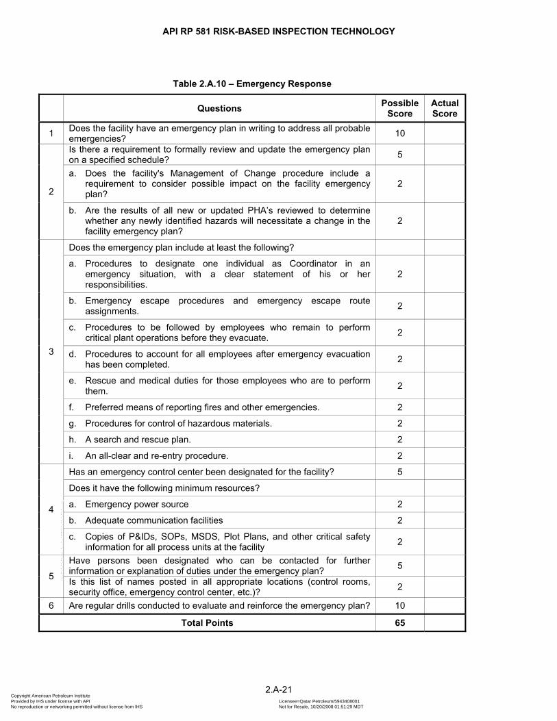
API RP 581 RISK-BASED INSPECTION TECHNOLOGY
Table 2.A.10 – Emergency Response
Questions Possible Score
Actual Score
1 Does the facility have an emergency plan in writing to address all probable emergencies? 10
2
Is there a requirement to formally review and update the emergency plan on a specified schedule? 5
a. Does the facility's Management of Change procedure include a requirement to consider possible impact on the facility emergency plan?
2
b. Are the results of all new or updated PHA’s reviewed to determine whether any newly identified hazards will necessitate a change in the facility emergency plan?
2
3
Does the emergency plan include at least the following?
a. Procedures to designate one individual as Coordinator in an emergency situation, with a clear statement of his or her responsibilities.
2
b. Emergency escape procedures and emergency escape route assignments. 2
c. Procedures to be followed by employees who remain to perform critical plant operations before they evacuate. 2
d. Procedures to account for all employees after emergency evacuation has been completed. 2
e. Rescue and medical duties for those employees who are to perform them. 2
f. Preferred means of reporting fires and other emergencies. 2
g. Procedures for control of hazardous materials. 2
h. A search and rescue plan. 2
i. An all-clear and re-entry procedure. 2
4
Has an emergency control center been designated for the facility? 5
Does it have the following minimum resources?
a. Emergency power source 2
b. Adequate communication facilities 2
c. Copies of P&IDs, SOPs, MSDS, Plot Plans, and other critical safety information for all process units at the facility 2
5
Have persons been designated who can be contacted for further information or explanation of duties under the emergency plan? 5
Is this list of names posted in all appropriate locations (control rooms, security office, emergency control center, etc.)? 2
6 Are regular drills conducted to evaluate and reinforce the emergency plan? 10
Total Points 65
2.A-21 Copyright American Petroleum Institute Provided by IHS under license with API Licensee=Qatar Petroleum/5943408001
Not for Resale, 10/20/2008 01:51:29 MDTNo reproduction or networking permitted without license from IHS
--```,`,,`,`,,`,`,,,,,,``,```,`-`-`,,`,,`,`,,`---

API RP 581 RISK-BASED INSPECTION TECHNOLOGY
Table 2.A.11 – Incident Investigation
Questions Possible Score
Actual Score
1
Is there a written incident/accident investigation procedure that includes both accidents and near misses? 10
Does the procedure require that findings and recommendations of investigations be addressed and resolved promptly? 5
2
Does the procedure require that the investigation team include:
a. A member trained in accident investigation techniques? 3
b. The line supervisor or someone equally familiar with the process? 3
3
Indicate whether the investigation procedure requires an investigation of the following items by the immediate supervisor with the results recorded on a standard form:
a. Fire and explosions 2
b. Property losses at or above an established cost base 2
c. All non-disabling injuries and occupational illnesses 2
d. Hazardous substance discharge 2
e. Other accidents/incidents (near-misses) 2
4
Is there a standard form for accident/incident investigation that includes the following information?
a. Date of incident 2
b. Date investigation began 2
c. Description of the incident 2
d. Underlying causes of the incident 2
e. Evaluation of the potential severity and probable frequency of recurrence 2
f. Recommendations to prevent recurrence 2
5 Based on a review of plant records, to what degree does it appear that the established incident investigation procedures are being followed? 5
6
If the incident/accident involved a failure of a component or piece of equipment, are appropriate inspection or engineering people required to be involved in a failure analysis to identify the conditions or practices that caused the failure?
10
7 Are incident investigation reports reviewed with all affected personnel whose job tasks are relevant to the incident findings, including contract employees, where applicable?
5
8 During the last 12-month period, have any incident or accident reports or report conclusions been transmitted to other sites that operate similar facilities within the company?
6
9 Do the procedures for incident reporting and/or process hazard analysis require that the findings from all applicable incident reports be reviewed and incorporated into future PHAs?
6
Total Points 75
2.A-22 Copyright American Petroleum Institute Provided by IHS under license with API Licensee=Qatar Petroleum/5943408001
Not for Resale, 10/20/2008 01:51:29 MDTNo reproduction or networking permitted without license from IHS
--```,`,,`,`,,`,`,,,,,,``,```,`-`-`,,`,,`,`,,`---
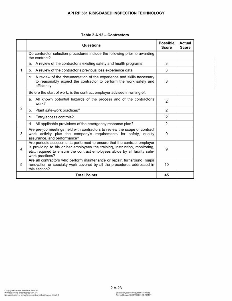
API RP 581 RISK-BASED INSPECTION TECHNOLOGY
Table 2.A.12 – Contractors
Questions Possible Score
Actual Score
1
Do contractor selection procedures include the following prior to awarding the contract?
a. A review of the contractor’s existing safety and health programs 3
b. A review of the contractor’s previous loss experience data 3
c. A review of the documentation of the experience and skills necessary to reasonably expect the contractor to perform the work safely and efficiently
3
2
Before the start of work, is the contract employer advised in writing of:
a. All known potential hazards of the process and of the contractor's work? 2
b. Plant safe-work practices? 2
c. Entry/access controls? 2
d. All applicable provisions of the emergency response plan? 2
3 Are pre-job meetings held with contractors to review the scope of contract work activity plus the company's requirements for safety, quality assurance, and performance?
9
4
Are periodic assessments performed to ensure that the contract employer is providing to his or her employees the training, instruction, monitoring, etc., required to ensure the contract employees abide by all facility safe-work practices?
9
5 Are all contractors who perform maintenance or repair, turnaround, major renovation or specialty work covered by all the procedures addressed in this section?
10
Total Points 45
2.A-23 Copyright American Petroleum Institute Provided by IHS under license with API Licensee=Qatar Petroleum/5943408001
Not for Resale, 10/20/2008 01:51:29 MDTNo reproduction or networking permitted without license from IHS
--```,`,,`,`,,`,`,,,,,,``,```,`-`-`,,`,,`,`,,`---
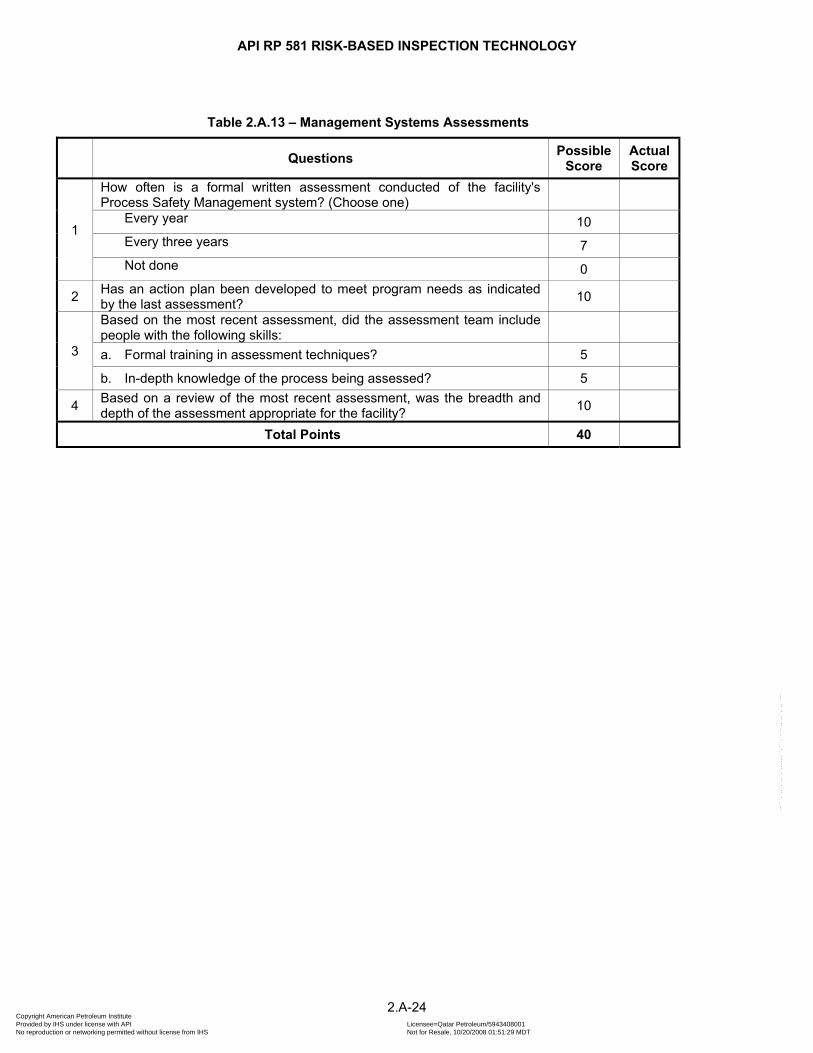
API RP 581 RISK-BASED INSPECTION TECHNOLOGY
2.A-24
Table 2.A.13 – Management Systems Assessments
Questions Possible Score
Actual Score
1
How often is a formal written assessment conducted of the facility's Process Safety Management system? (Choose one)
Every year 10 Every three years 7 Not done 0
2 Has an action plan been developed to meet program needs as indicated by the last assessment? 10
3
Based on the most recent assessment, did the assessment team include people with the following skills:
a. Formal training in assessment techniques? 5
b. In-depth knowledge of the process being assessed? 5
4 Based on a review of the most recent assessment, was the breadth and depth of the assessment appropriate for the facility? 10
Total Points 40
Copyright American Petroleum Institute Provided by IHS under license with API Licensee=Qatar Petroleum/5943408001
Not for Resale, 10/20/2008 01:51:29 MDTNo reproduction or networking permitted without license from IHS
--```,`,,`,`,,`,`,,,,,,``,```,`-`-`,,`,,`,`,,`---
API RP 581 RISK-BASED INSPECTION TECHNOLOGY
API RP 581 PART 2
ANNEX 2.B – DETERMINATION OF CORROSION RATES
2.B-1 Copyright American Petroleum Institute Provided by IHS under license with API Licensee=Qatar Petroleum/5943408001
Not for Resale, 10/20/2008 01:51:29 MDTNo reproduction or networking permitted without license from IHS
--```,`,,`,`,,`,`,,,,,,``,```,`-`-`,,`,,`,`,,`---
API RP 581 RISK-BASED INSPECTION TECHNOLOGY
PART CONTENTS 2.B.1 OVERVIEW ............................................................................................................... 2.B-5
2.B.1.1 Determination of Corrosion Rate ................................................................................ 2.B-5 2.B.1.2 Determination Thinning Type ..................................................................................... 2.B-5 2.B.1.3 Tables ............................................................................................................................ 2.B-6
2.B.2 HYDROCHLORIC ACID (HCL) CORROSION......................................................... 2.B-8 2.B.2.1 Description of Damage ................................................................................................ 2.B-8 2.B.2.2 Basic Data ..................................................................................................................... 2.B-8 2.B.2.3 Determination of Corrosion Rate ................................................................................ 2.B-8 2.B.2.4 References .................................................................................................................... 2.B-8 2.B.2.5 Tables ............................................................................................................................ 2.B-9 2.B.2.6 Figures ........................................................................................................................ 2.B-16
2.B.3 HIGH TEMPERATURE SULFIDIC AND NAPHTHENIC ACID CORROSION ...... 2.B-17 2.B.3.1 Description of Damage .............................................................................................. 2.B-17 2.B.3.2 Basic Data ................................................................................................................... 2.B-18 2.B.3.3 Determination of Corrosion Rate .............................................................................. 2.B-18 2.B.3.4 References .................................................................................................................. 2.B-18 2.B.3.5 Tables .......................................................................................................................... 2.B-19 2.B.3.6 Figures ........................................................................................................................ 2.B-38
2.B.4 HIGH TEMPERATURE H2S/H2 CORROSION ....................................................... 2.B-39 2.B.4.1 Description of Damage .............................................................................................. 2.B-39 2.B.4.2 Basic Data ................................................................................................................... 2.B-39 2.B.4.3 Determination of Corrosion Rate .............................................................................. 2.B-39 2.B.4.4 References .................................................................................................................. 2.B-39 2.B.4.5 Tables .......................................................................................................................... 2.B-40 2.B.4.6 Figures ........................................................................................................................ 2.B-50
2.B.5 SULFURIC ACID (H2SO4) CORROSION ............................................................... 2.B-51 2.B.5.1 Description of Damage .............................................................................................. 2.B-51 2.B.5.2 Basic Data ................................................................................................................... 2.B-51 2.B.5.3 Determination of Corrosion Rate .............................................................................. 2.B-51 2.B.5.4 References .................................................................................................................. 2.B-52 2.B.5.5 Tables .......................................................................................................................... 2.B-53 2.B.5.6 Figures ........................................................................................................................ 2.B-65
2.B.6 HYDROFLUORIC ACID (HF) CORROSION .......................................................... 2.B-66 2.B.6.1 Description of Damage .............................................................................................. 2.B-66 2.B.6.2 Basic Data ................................................................................................................... 2.B-66 2.B.6.3 Determination of Corrosion Rate .............................................................................. 2.B-66 2.B.6.4 References .................................................................................................................. 2.B-67 2.B.6.5 Tables .......................................................................................................................... 2.B-68 2.B.6.6 Figures ........................................................................................................................ 2.B-71
2.B.7 SOUR WATER CORROSION ................................................................................ 2.B-72 2.B.7.1 Description of Damage .............................................................................................. 2.B-72 2.B.7.2 Basic Data ................................................................................................................... 2.B-72 2.B.7.3 Determination of Corrosion Rate .............................................................................. 2.B-72 2.B.7.4 References .................................................................................................................. 2.B-72 2.B.7.5 Tables .......................................................................................................................... 2.B-73 2.B.7.6 Figures ........................................................................................................................ 2.B-74
2.B.8 AMINE CORROSION ............................................................................................. 2.B-75 2.B.8.1 Description of Damage .............................................................................................. 2.B-75 2.B.8.2 Basic Data ................................................................................................................... 2.B-75 2.B.8.3 Determination of Corrosion Rate .............................................................................. 2.B-76 2.B.8.4 References .................................................................................................................. 2.B-76 2.B.8.5 Tables .......................................................................................................................... 2.B-77 2.B.8.6 Figures ........................................................................................................................ 2.B-83
2.B.9 HIGH TEMPERATURE OXIDATION ..................................................................... 2.B-84 2.B.9.1 Description of Damage .............................................................................................. 2.B-84 2.B.9.2 Basic Data ................................................................................................................... 2.B-84
2.B-2 Copyright American Petroleum Institute Provided by IHS under license with API Licensee=Qatar Petroleum/5943408001
Not for Resale, 10/20/2008 01:51:29 MDTNo reproduction or networking permitted without license from IHS
--```,`,,`,`,,`,`,,,,,,``,```,`-`-`,,`,,`,`,,`---

API RP 581 RISK-BASED INSPECTION TECHNOLOGY
2.B.9.3 Determination of Corrosion Rate .............................................................................. 2.B-84 2.B.9.4 Tables .......................................................................................................................... 2.B-85 2.B.9.5 Figures ........................................................................................................................ 2.B-88
2.B.10 ACID SOUR WATER CORROSION ...................................................................... 2.B-89 2.B.10.1 Description of Damage ...................................................................................... 2.B-89
2.B.10.1.1 Overview ......................................................................................................... 2.B-89 2.B.10.1.2 Scope and Limitations ................................................................................... 2.B-89
2.B.10.2 Basic Data ........................................................................................................... 2.B-89 2.B.10.3 Determination of Corrosion Rate ...................................................................... 2.B-89 2.B.10.4 Nomenclature ..................................................................................................... 2.B-90 2.B.10.5 References .......................................................................................................... 2.B-90 2.B.10.6 Tables .................................................................................................................. 2.B-91 2.B.10.7 Figures ................................................................................................................ 2.B-93
2.B.11 COOLING WATER CORROSION .......................................................................... 2.B-94 2.B.11.1 Description of Damage ...................................................................................... 2.B-94
2.B.11.1.1 Overview ......................................................................................................... 2.B-94 2.B.11.1.2 Types of Cooling Water Systems ................................................................. 2.B-94 2.B.11.1.3 Once Through Systems ................................................................................. 2.B-94 2.B.11.1.4 Closed Recirculated Systems ...................................................................... 2.B-95 2.B.11.1.5 Open Recirculated Systems ......................................................................... 2.B-95 2.B.11.1.6 Factors Affecting Corrosion Rate ................................................................ 2.B-95 2.B.11.1.7 Types of Corrosion ........................................................................................ 2.B-96 2.B.11.1.8 Corrosion Monitoring and Control in Cooling Water Systems ................. 2.B-96 2.B.11.1.9 Indicators for Corrosion Issues and their Deterrence ............................... 2.B-97 2.B.11.1.10 Assumptions .............................................................................................. 2.B-98 2.B.11.1.11 Corrosion Rates for Copper Alloys Components .................................. 2.B-98
2.B.11.2 Basic Data ........................................................................................................... 2.B-99 2.B.11.2.1 Recirculating Cooling Water Systems ......................................................... 2.B-99 2.B.11.2.2 Once Through Cooling Water Systems ....................................................... 2.B-99
2.B.11.3 Determination of Corrosion Rate ...................................................................... 2.B-99 2.B.11.3.1 Recirculating Cooling Water Systems ......................................................... 2.B-99 2.B.11.3.2 Once Through Cooling Water Systems ..................................................... 2.B-101 2.B.11.3.3 Ground Water ............................................................................................... 2.B-103
2.B.11.4 Nomenclature ................................................................................................... 2.B-103 2.B.11.5 References ........................................................................................................ 2.B-104 2.B.11.6 Tables ................................................................................................................ 2.B-105 2.B.11.7 Figures .............................................................................................................. 2.B-114
2.B.12 SOIL-SIDE CORROSION ..................................................................................... 2.B-115 2.B.12.1 Description of Damage .................................................................................... 2.B-115
2.B.12.1.1 Overview ....................................................................................................... 2.B-115 2.B.12.1.2 Soil Corrosivity ............................................................................................ 2.B-115 2.B.12.1.3 Preventing Soil Corrosion........................................................................... 2.B-115
2.B.12.2 Description of Damage .................................................................................... 2.B-116 2.B.12.3 Basic Data ......................................................................................................... 2.B-117 2.B.12.4 Determination of Corrosion Rate .................................................................... 2.B-117
2.B.12.4.1 Corrosion Rate Equation ............................................................................. 2.B-117 2.B.12.4.2 Establishing the Base Corrosion Rate ...................................................... 2.B-117 2.B.12.4.3 Adjustment Factor for Soil Resistivity (Optional) .................................... 2.B-117 2.B.12.4.4 Adjustment Factor for Temperature .......................................................... 2.B-118 2.B.12.4.5 Adjustment Factor for ............................................................................................ Cathodic Protection and Stray Current Drainage ..................................... 2.B-118 2.B.12.4.6 Adjustment Factor for Coating Effectiveness........................................... 2.B-119
2.B.12.5 Nomenclature ................................................................................................... 2.B-119 2.B.12.6 References ........................................................................................................ 2.B-119 2.B.12.7 Tables ................................................................................................................ 2.B-120 2.B.12.8 Figures .............................................................................................................. 2.B-123
2.B.13 CO2 CORROSION ................................................................................................ 2.B-124
2.B-3 Copyright American Petroleum Institute Provided by IHS under license with API Licensee=Qatar Petroleum/5943408001
Not for Resale, 10/20/2008 01:51:29 MDTNo reproduction or networking permitted without license from IHS
--```,`,,`,`,,`,`,,,,,,``,```,`-`-`,,`,,`,`,,`---

API RP 581 RISK-BASED INSPECTION TECHNOLOGY
2.B.13.1 Description of Damage .................................................................................... 2.B-124 2.B.13.2 Basic Data ......................................................................................................... 2.B-124 2.B.13.3 Determination of Corrosion Rate .................................................................... 2.B-124
2.B.13.3.1 Calculation of the Corrosion Rate .............................................................. 2.B-124 2.B.13.3.2 Relative Humidity ......................................................................................... 2.B-124 2.B.13.3.3 Base Corrosion Rate ................................................................................... 2.B-125 2.B.13.3.4 Determining the pH ...................................................................................... 2.B-125 2.B.13.3.5 Determining the CO2 Fugacity .................................................................... 2.B-126 2.B.13.3.6 Determining the Flow Velocity ................................................................... 2.B-126 2.B.13.3.7 Adjustment for Inhibitors or Glycol ........................................................... 2.B-127
2.B.13.4 Nomenclature ................................................................................................... 2.B-128 2.B.13.5 Tables ................................................................................................................ 2.B-129 2.B.13.6 Figures .............................................................................................................. 2.B-131
2.B.14 ATMOSPHERIC STORAGE TANK BOTTOM CORROSION ............................. 2.B-132 2.B.14.1 Description of Damage .................................................................................... 2.B-132 2.B.14.2 Basic Data ......................................................................................................... 2.B-132
2.B.14.2.1 Soil-Side Corrosion Rate Equation ............................................................ 2.B-132 2.B.14.2.2 Product-Side Corrosion Rate Equation ..................................................... 2.B-132
2.B.14.3 Determination of Corrosion Rate .................................................................... 2.B-132 2.B.14.3.1 Soil-Side Corrosion Rate Equation ............................................................ 2.B-132 2.B.14.3.2 Product-Side Corrosion Rate Equation ..................................................... 2.B-133 2.B.14.3.3 Combined Tank Floor Corrosion Rate ....................................................... 2.B-134
2.B.14.4 Nomenclature ................................................................................................... 2.B-134 2.B.14.5 Tables ................................................................................................................ 2.B-135 2.B.14.6 Figures .............................................................................................................. 2.B-139
2.B-4 Copyright American Petroleum Institute Provided by IHS under license with API Licensee=Qatar Petroleum/5943408001
Not for Resale, 10/20/2008 01:51:29 MDTNo reproduction or networking permitted without license from IHS
--```,`,,`,`,,`,`,,,,,,``,```,`-`-`,,`,,`,`,,`---

API RP 581 RISK-BASED INSPECTION TECHNOLOGY
2.B.1 OVERVIEW
2.B.1.1 Determination of Corrosion Rate
The corrosion rate should be calculated from measured thickness data available from equipment inspection(s). However, if a calculated corrosion rate is not available, estimated corrosion rates may be determined for each potential thinning mechanism using this document or as estimated by a corrosion specialist.
Screening questions are used to determine which of the thinning mechanism sections apply. These applicable sections will be entered to determine conservative estimated corrosion rates for possible thinning mechanisms. The screening questions listed in Table 2.B.1.1 are used to select the applicable thinning mechanism.
2.B.1.2 Determination of Thinning Type
The results of effective inspections that have been performed on the equipment or piping should be used to designate the type of thinning (i.e., general versus localized). If this information is not known, then Table 2.B.1.2 lists the type of thinning (general or localized) expected for various thinning mechanisms. If both general and localized thinning mechanisms are possible, then the type of thinning should be designated as localized. The type of thinning designated will be used to determine the effectiveness of inspection performed.
2.B-5 Copyright American Petroleum Institute Provided by IHS under license with API Licensee=Qatar Petroleum/5943408001
Not for Resale, 10/20/2008 01:51:29 MDTNo reproduction or networking permitted without license from IHS
--```,`,,`,`,,`,`,,,,,,``,```,`-`-`,,`,,`,`,,`---

API RP 581 RISK-BASED INSPECTION TECHNOLOGY
2.B.1.3 Tables
Table 2.B.1.1 - Screening Questions for Corrosion Rate Calculations
Screening Questions Action
Hydrochloric Acid (HCl) Corrosion 1. Does the process contain HCl? 2. Is free water present in the process stream (including initial
condensing condition)? 3. Is the pH < 7.0?
If Yes to all, proceed to 2.B.2
High Temperature Sulfidic/Naphthenic Acid Corrosion 1. Does the process contain oil with sulfur compounds? 2. Is the operating temperature > 204°C [400°F]?
If Yes to both, proceed to 2.B.3
High Temperature H2S/H2 Corrosion 1. Does the process contain H2S and hydrogen? 2. Is the operating temperature > 204°C [400°F]?
If Yes to both, proceed to 2.B.4
Sulfuric Acid (H2SO4) Corrosion Does the process contain H2SO4?
If Yes, proceed to 2.B.5
Hydrofluoric Acid (HF) Corrosion Does the process stream contain HF?
If Yes, proceed to 2.B.6
Sour Water Corrosion Is free water with H2S present? If Yes, proceed to 2.B.7
Amine Corrosion Is equipment exposed to acid gas treating amines (MEA, DEA, DIPA, or MDEA)?
If Yes, proceed to 2.B.8
High Temperature Oxidation 1. Is the temperature ≥ 482°C [900°F]? 2. Is there oxygen present?
If Yes to both, proceed to 2.B.9
Acid Sour Water
1. Is free water with H2S present and pH <7.0? 2. Does the process contain <50 ppm Chlorides?
If Yes, proceed to 2.B.10
Cooling Water
Is equipment in cooling water service? If Yes, proceed to 2.B.11
Soil Side Corrosion
1. Is equipment in contact with soil (buried or partially buried)? 2. Is the material of construction carbon steel?
If Yes, proceed to 2.B.12
CO2 Corrosion 1. Is free water with CO2 present (including consideration for dew
point condensation)? 2. Is the material of construction carbon steel or < 13% Cr?
If Yes, proceed to 2.B.13
Atmospheric storage tank bottom Is the equipment item an atmospheric storage tank bottom?
If Yes, proceed to 2.B.14
2.B-6 Copyright American Petroleum Institute Provided by IHS under license with API Licensee=Qatar Petroleum/5943408001
Not for Resale, 10/20/2008 01:51:29 MDTNo reproduction or networking permitted without license from IHS
--```,`,,`,`,,`,`,,,,,,``,```,`-`-`,,`,,`,`,,`---

API RP 581 RISK-BASED INSPECTION TECHNOLOGY
Table 2.B.1.2 Type of Thinning
Thinning Mechanism Condition Type of Thinning
Hydrochloric Acid (HCl) Corrosion --- Local
High Temperature Sulfidic/Naphthenic Acid Corrosion
TAN ≤ 0.5 General
TAN > 0.5 Local
High Temperature H2S/H2 Corrosion --- General
Sulfuric Acid (H2SO4) Corrosion
Low Velocity < 0.61 m/s (2 ft/s) for carbon steel, < 1.22 m/s (4 ft/s) for SS, and < 1.83 m/s (6 ft/s) for higher alloys
General
High Velocity > 0.61 m/s (2 ft/s) for carbon steel, > 1.22 m/s (4 ft/s) for SS, and > 1.83 m/s (6 ft/s) for higher alloys
Local
Hydrofluoric Acid (HF) Corrosion --- Local
Sour Water Corrosion Low Velocity: ≤ 6.1 m/s (20 ft/s) General
High Velocity: > 6.1 m/s (20 ft/s) Local
Amine Corrosion
Low Velocity < 1.5 m/s (5 ft/s) rich amine < 6.1 m/s (20 ft/s) lean amine
General
High Velocity > 1.5 m/s (5 ft/s) rich amine > 6.1 m/s (20 ft/s) lean amine
Local
High Temperature Oxidation --- General
Acid Sour Water Corrosion < 1.83 m/s (6 ft/s) > 1.83 m/s (6 ft/s)
General Local
Cooling Water Corrosion < 0.91 m/s (3 ft/s)
0.91-2.74 m/s (3-9 ft/s) > 2.74 m/s (9 ft/s)
Local General
Local
Soil Side Corrosion --- Local
CO2 Corrosion --- Local
Atmospheric Storage Tank Bottom Product Side
Soil Side Local Local
2.B-7 Copyright American Petroleum Institute Provided by IHS under license with API Licensee=Qatar Petroleum/5943408001
Not for Resale, 10/20/2008 01:51:29 MDTNo reproduction or networking permitted without license from IHS
--```,`,,`,`,,`,`,,,,,,``,```,`-`-`,,`,,`,`,,`---
API RP 581 RISK-BASED INSPECTION TECHNOLOGY
2.B.2 HYDROCHLORIC ACID (HCL) CORROSION
2.B.2.1 Description of Damage
Hydrochloric acid (HCl) corrosion is a concern in some of the most common refining process units. HCl is aggressive to many common materials of construction across a wide range of concentrations and is often localized in nature, particularly when it is associated with localized or shock condensation or the deposition of chloride containing ammonia or amine salts. Austenitic stainless steels will often suffer pitting attack and may experience crevice corrosion and/or chloride stress corrosion cracking. Some of the nickel-based alloys may experience accelerated corrosion if oxidizing agents are present or if the alloys are not in the solution annealed heat treatment condition.
The primary refining units where HCl corrosion is a concern are crude distillation, hydrotreating, and catalytic reforming. HCl forms in crude units by the hydrolysis of magnesium and calcium chloride salts and results in dilute HCl in the overhead system. In hydrotreating units, HCl may form by hydrogenation of organic chlorides in the feed or can enter the unit with hydrocarbon feed or hydrogen and condense with water in the effluent train. In catalytic reforming units, chlorides may be stripped off of the catalyst and hydrogenate resulting in HCl corrosion in the effluent train or regeneration systems.
2.B.2.2 Basic Data
The data listed in Table 2.B.2.1 are required to estimate the rate of corrosion in dilute hydrochloric acid. More concentrated acid is outside the scope of this section. If precise data have not been measured, a knowledgeable process specialist should be consulted.
2.B.2.3 Determination of Corrosion Rate
The steps required to determine the corrosion rate are shown in Figure 2.B.2.1. The hydrochloric acid corrosion rate may be determined using the basic data in Table 2.B.2.1 in conjunction with Tables 2.B.2.3 through 2.B.2.6.
2.B.2.4 References
1. Metals Handbook , Vol. 13, “Corrosion,” ASM International. 2. T. S. Lee, III, and F.G. Hodge, Resistance of Hastelloy Alloys to Corrosion by Inorganic Acids, Materials
Performance, September 1976, pp. 29. 3. Corrosion Resistance of Hastelloy Alloys, Haynes International, Inc., 1984. 4. Resistance to Corrosion, Inco Alloys International, Inc. 5. “Resistance of Nickel and High Nickel Alloys to Corrosion by Hydrochloric Acid, Hydrogen Chloride and
Chlorine,” Corrosion Engineering Bulletin CEB-3, The International Nickel Company, Inc., 1969. 6. L. Colombier and J. Hochmann, Stainless and Heat Resisting Steels, St. Martins Press, New York, NY.
2.B-8 Copyright American Petroleum Institute Provided by IHS under license with API Licensee=Qatar Petroleum/5943408001
Not for Resale, 10/20/2008 01:51:29 MDTNo reproduction or networking permitted without license from IHS
--```,`,,`,`,,`,`,,,,,,``,```,`-`-`,,`,,`,`,,`---

API RP 581 RISK-BASED INSPECTION TECHNOLOGY
2.B.2.5 Tables
Table 2.B.2.1 – Hydrochloric Acid Corrosion – Basic Data Required for Analysis
Material of Construction
Determine the Material of Construction of the Equipment Item
pH or Cl- Concentration
pH is preferred for estimating the corrosion rate at dilute concentrations for carbon steel and 300 series stainless steels. Table 2.B.2.2 may be used to estimate pH from the Cl- concentration if it is known. Note that the presence of neutralizing agents may elevate the pH however. For high alloy materials, Cl- concentration is used to estimate the corrosion rate. Note: The pH used should be of the separated acid phase within this equipment or nearest equipment downstream, e.g. the overhead accumulator boot water downstream of the overhead condenser.
Maximum Temperature, °C [°F]
Determine the maximum temperature present in this equipment/piping. This may be the maximum process temperature, but local heating condition such as effect of the sun or heat tracing should be considered.
Presence of Air or Oxidants (Yes or No)
Presence of air (oxygen) may increase corrosion rates, particularly for Alloy 400 and Alloy B-2. Other oxidants such as ferric and cupric ions will have a similar effect on these alloys.
Table 2.B.2.2 – Hydrochloric Acid Corrosion – Determination of pH from Cl- Concentration
Cl- Concentration
(wppm) pH
3,601 - 12,000 0.5
1,201 – 3600 1.0
361 - 1,200 1.5
121 – 360 2.0
36 – 120 2.5
16 – 35 3.0
6 – 15 3.5
3 – 5 4.0
1 – 2 4.5
< 1 5.0
Note: Assumes no alkaline agent present (NH3, neutralizing amines or caustic)
2.B-9 Copyright American Petroleum Institute Provided by IHS under license with API Licensee=Qatar Petroleum/5943408001
Not for Resale, 10/20/2008 01:51:29 MDTNo reproduction or networking permitted without license from IHS
--```,`,,`,`,,`,`,,,,,,``,```,`-`-`,,`,,`,`,,`---

API RP 581 RISK-BASED INSPECTION TECHNOLOGY
Table 2.B.2.3 – Hydrochloric Acid Corrosion – Estimated Corrosion Rates for Carbon Steel (mpy)
pH Temperature (°F)
100 125 175 200
0.5 999 999 999 999
0.80 900 999 999 999
1.25 400 999 999 999
1.75 200 700 999 999
2.25 100 300 400 560
2.75 60 130 200 280
3.25 40 70 100 140
3.75 30 50 90 125
4.25 20 40 70 100
4.75 10 30 50 70
5.25 7 20 30 40
5.75 4 15 20 30
6.25 3 10 15 20
6.80 2 5 7 10
2.B-10 Copyright American Petroleum Institute Provided by IHS under license with API Licensee=Qatar Petroleum/5943408001
Not for Resale, 10/20/2008 01:51:29 MDTNo reproduction or networking permitted without license from IHS
--```,`,,`,`,,`,`,,,,,,``,```,`-`-`,,`,,`,`,,`---
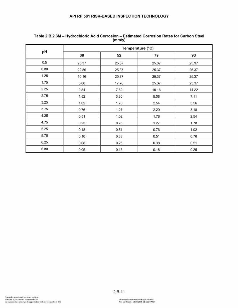
API RP 581 RISK-BASED INSPECTION TECHNOLOGY
Table 2.B.2.3M – Hydrochloric Acid Corrosion – Estimated Corrosion Rates for Carbon Steel (mm/y)
pH Temperature (°C)
38 52 79 93
0.5 25.37 25.37 25.37 25.37
0.80 22.86 25.37 25.37 25.37
1.25 10.16 25.37 25.37 25.37
1.75 5.08 17.78 25.37 25.37
2.25 2.54 7.62 10.16 14.22
2.75 1.52 3.30 5.08 7.11
3.25 1.02 1.78 2.54 3.56
3.75 0.76 1.27 2.29 3.18
4.25 0.51 1.02 1.78 2.54
4.75 0.25 0.76 1.27 1.78
5.25 0.18 0.51 0.76 1.02
5.75 0.10 0.38 0.51 0.76
6.25 0.08 0.25 0.38 0.51
6.80 0.05 0.13 0.18 0.25
2.B-11 Copyright American Petroleum Institute Provided by IHS under license with API Licensee=Qatar Petroleum/5943408001
Not for Resale, 10/20/2008 01:51:29 MDTNo reproduction or networking permitted without license from IHS
--```,`,,`,`,,`,`,,,,,,``,```,`-`-`,,`,,`,`,,`---
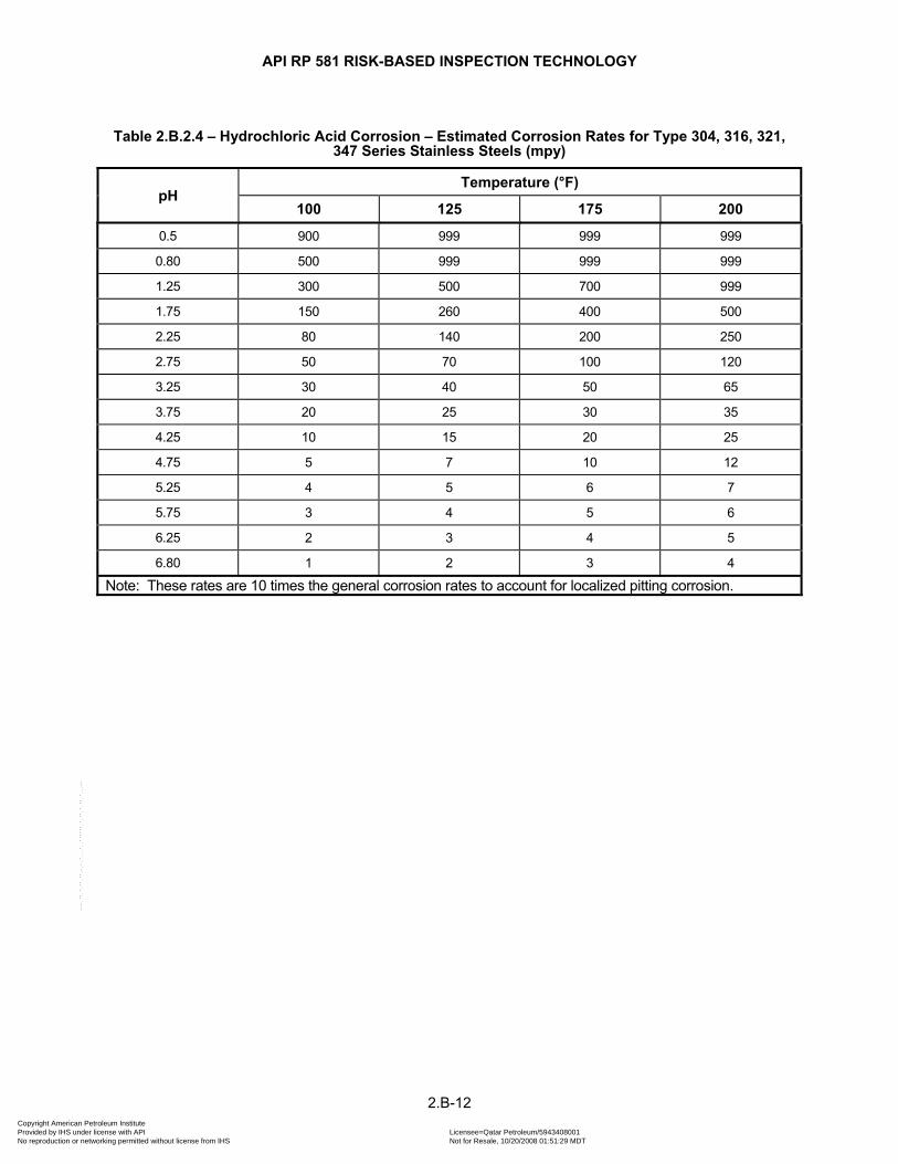
API RP 581 RISK-BASED INSPECTION TECHNOLOGY
Table 2.B.2.4 – Hydrochloric Acid Corrosion – Estimated Corrosion Rates for Type 304, 316, 321, 347 Series Stainless Steels (mpy)
pH Temperature (°F)
100 125 175 200
0.5 900 999 999 999
0.80 500 999 999 999
1.25 300 500 700 999
1.75 150 260 400 500
2.25 80 140 200 250
2.75 50 70 100 120
3.25 30 40 50 65
3.75 20 25 30 35
4.25 10 15 20 25
4.75 5 7 10 12
5.25 4 5 6 7
5.75 3 4 5 6
6.25 2 3 4 5
6.80 1 2 3 4
Note: These rates are 10 times the general corrosion rates to account for localized pitting corrosion.
2.B-12 Copyright American Petroleum Institute Provided by IHS under license with API Licensee=Qatar Petroleum/5943408001
Not for Resale, 10/20/2008 01:51:29 MDTNo reproduction or networking permitted without license from IHS
--```,`,,`,`,,`,`,,,,,,``,```,`-`-`,,`,,`,`,,`---
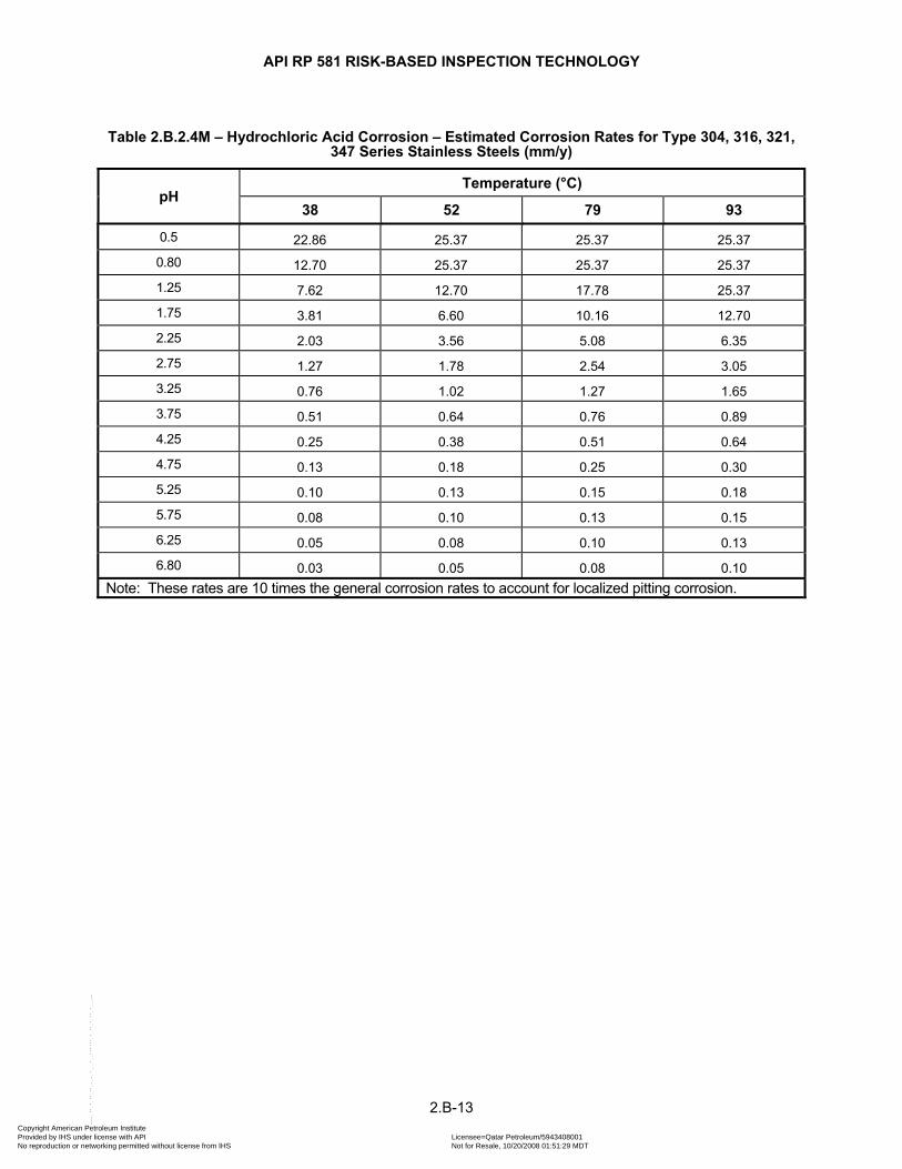
API RP 581 RISK-BASED INSPECTION TECHNOLOGY
Table 2.B.2.4M – Hydrochloric Acid Corrosion – Estimated Corrosion Rates for Type 304, 316, 321, 347 Series Stainless Steels (mm/y)
pH Temperature (°C)
38 52 79 93
0.5 22.86 25.37 25.37 25.37
0.80 12.70 25.37 25.37 25.37
1.25 7.62 12.70 17.78 25.37
1.75 3.81 6.60 10.16 12.70
2.25 2.03 3.56 5.08 6.35
2.75 1.27 1.78 2.54 3.05
3.25 0.76 1.02 1.27 1.65
3.75 0.51 0.64 0.76 0.89
4.25 0.25 0.38 0.51 0.64
4.75 0.13 0.18 0.25 0.30
5.25 0.10 0.13 0.15 0.18
5.75 0.08 0.10 0.13 0.15
6.25 0.05 0.08 0.10 0.13
6.80 0.03 0.05 0.08 0.10 Note: These rates are 10 times the general corrosion rates to account for localized pitting corrosion.
2.B-13 Copyright American Petroleum Institute Provided by IHS under license with API Licensee=Qatar Petroleum/5943408001
Not for Resale, 10/20/2008 01:51:29 MDTNo reproduction or networking permitted without license from IHS
--```,`,,`,`,,`,`,,,,,,``,```,`-`-`,,`,,`,`,,`---

API RP 581 RISK-BASED INSPECTION TECHNOLOGY
Table 2.B.2.5 – Hydrochloric Acid Corrosion – Estimated Corrosion Rates for Alloys 825, 20, 625, C-276 (mpy)
Alloy Cl-
Concentration Temperature (°F)
(wt%) 100 125 175 200
Alloy 825 and
Alloy 20
0.50 1 3 40 200
0.75 2 5 80 400
1.0 10 70 300 999
Alloy 625
0.50 1 2 15 75
0.75 1 5 25 125
1.0 2 70 200 400
Alloy C-276
0.50 1 2 8 30
0.75 1 2 15 75
1.0 2 10 60 300
Table 2.B.2.5M – Hydrochloric Acid Corrosion – Estimated Corrosion Rates for Alloys 825, 20, 625, C-276 (mm/y)
Alloy Cl-
Concentration Temperature (°C)
(wt%) 38 52 79 93
Alloy 825 and
Alloy 20
0.50 0.03 0.08 1.02 5.08 0.75 0.05 0.13 2.03 10.16 1.0 0.25 1.78 7.62 25.37
Alloy 625
0.50 0.03 0.05 0.38 1.91 0.75 0.03 0.13 0.64 3.18 1.0 0.05 1.78 5.08 10.16
Alloy C-276
0.50 0.03 0.05 0.20 0.76 0.75 0.03 0.05 0.38 1.91 1.0 0.05 0.25 1.52 7.62
2.B-14 Copyright American Petroleum Institute Provided by IHS under license with API Licensee=Qatar Petroleum/5943408001
Not for Resale, 10/20/2008 01:51:29 MDTNo reproduction or networking permitted without license from IHS
--```,`,,`,`,,`,`,,,,,,``,```,`-`-`,,`,,`,`,,`---
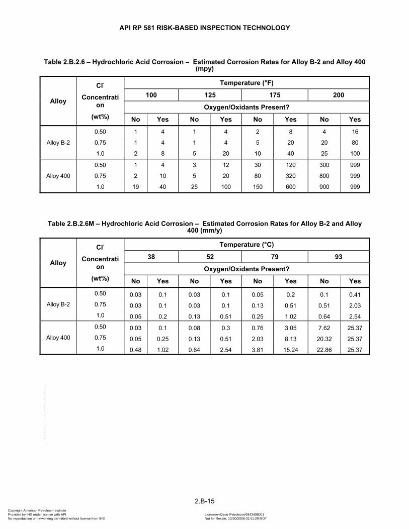
API RP 581 RISK-BASED INSPECTION TECHNOLOGY
Table 2.B.2.6 – Hydrochloric Acid Corrosion – Estimated Corrosion Rates for Alloy B-2 and Alloy 400 (mpy)
Alloy
Cl-
Concentration
(wt%)
Temperature (°F)
100 125 175 200
Oxygen/Oxidants Present?
No Yes No Yes No Yes No Yes
Alloy B-2
0.50 1 4 1 4 2 8 4 16
0.75 1 4 1 4 5 20 20 80
1.0 2 8 5 20 10 40 25 100
Alloy 400
0.50 1 4 3 12 30 120 300 999
0.75 2 10 5 20 80 320 800 999
1.0 19 40 25 100 150 600 900 999
Table 2.B.2.6M – Hydrochloric Acid Corrosion – Estimated Corrosion Rates for Alloy B-2 and Alloy 400 (mm/y)
Alloy
Cl-
Concentration
(wt%)
Temperature (°C)
38 52 79 93
Oxygen/Oxidants Present?
No Yes No Yes No Yes No Yes
Alloy B-2
0.50 0.03 0.1 0.03 0.1 0.05 0.2 0.1 0.41 0.75 0.03 0.1 0.03 0.1 0.13 0.51 0.51 2.03 1.0 0.05 0.2 0.13 0.51 0.25 1.02 0.64 2.54
Alloy 400
0.50 0.03 0.1 0.08 0.3 0.76 3.05 7.62 25.37 0.75 0.05 0.25 0.13 0.51 2.03 8.13 20.32 25.37 1.0 0.48 1.02 0.64 2.54 3.81 15.24 22.86 25.37
2.B-15 Copyright American Petroleum Institute Provided by IHS under license with API Licensee=Qatar Petroleum/5943408001
Not for Resale, 10/20/2008 01:51:29 MDTNo reproduction or networking permitted without license from IHS
--```,`,,`,`,,`,`,,,,,,``,```,`-`-`,,`,,`,`,,`---
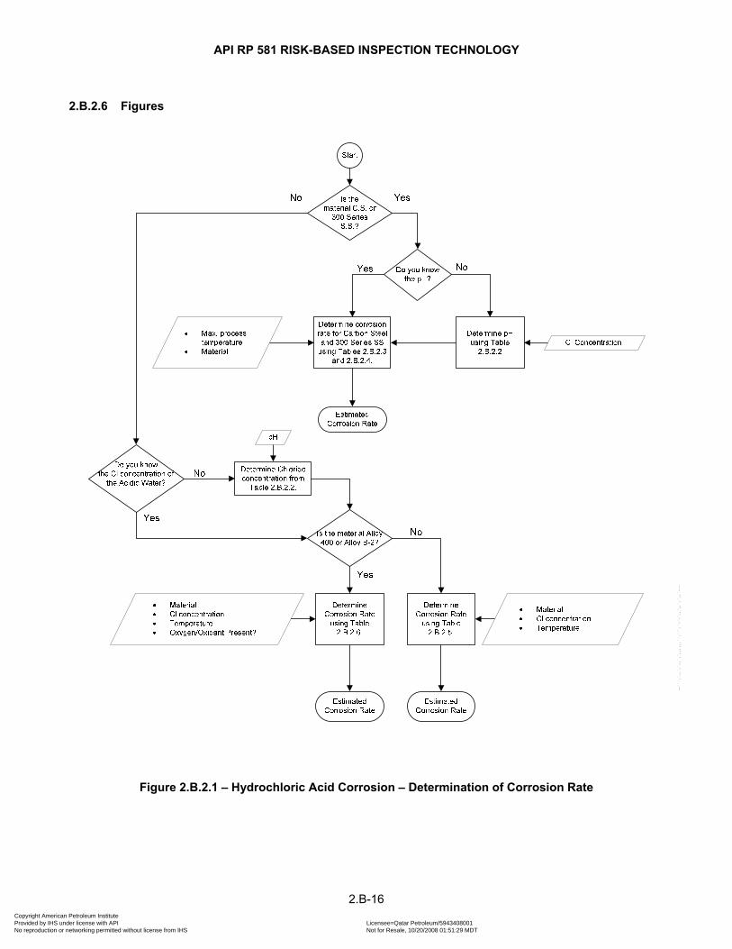
API RP 581 RISK-BASED INSPECTION TECHNOLOGY
2.B.2.6 Figures
Figure 2.B.2.1 – Hydrochloric Acid Corrosion – Determination of Corrosion Rate
2.B-16 Copyright American Petroleum Institute Provided by IHS under license with API Licensee=Qatar Petroleum/5943408001
Not for Resale, 10/20/2008 01:51:29 MDTNo reproduction or networking permitted without license from IHS
--```,`,,`,`,,`,`,,,,,,``,```,`-`-`,,`,,`,`,,`---
API RP 581 RISK-BASED INSPECTION TECHNOLOGY
2.B.3 HIGH TEMPERATURE SULFIDIC AND NAPHTHENIC ACID CORROSION
2.B.3.1 Description of Damage
High temperature sulfidic corrosion is a form of normally uniform corrosion which can occur at temperatures typically above about 204°C (400°F). This form of corrosion sometimes occurs along with naphthenic acid corrosion depending on the oil being processed. Naphthenic acid corrosion, when it occurs, is normally localized. Sulfur species occur naturally in most crude oils but their concentrations vary from crude-to-crude. These naturally occurring compounds may be corrosive themselves as well as when they are converted to hydrogen sulfide through thermal decomposition. Catalytic conversion of sulfur compounds to 2S occurs in the presence of hydrogen and a catalyst bed in hydroprocessing units. Corrosion in vapor streams containing both H2S and hydrogen is covered in paragraph 2.B.4. As with sulfur compounds, naphthenic acids occur naturally in some crude oils. During distillation, these acids tend to concentrate in higher boiling point fractions such as heavy atmospheric gas oil, atmospheric resid, and vacuum gas oils. The acids may also be present in vacuum resid, but often many of the more corrosive ones will have distilled into the vacuum side streams. Lower boiling point streams are usually low in naphthenic acids. Corrosion may appear either as pitting, more common at lower acid levels, or grooving and gouging at higher acid levels and, particularly, at higher velocities. Naphthenic acids may modify or destabilize protective films (sulfides or oxides) on the material and thus allow a high sulfidation corrosion rate to continue or it may itself directly attack the base material.
The corrosion rate in high temperature sulfidic environments is a function of the material, temperature, and the concentration of the sulfur compound(s) present. The presence of naphthenic acid in sufficient amounts, however, can dramatically decrease a material’s corrosion resistance where it might otherwise have suitable corrosion resistance. The following summarize the key variables in corrosion:
a) In high temperature sulfidic environments, materials such as carbon and low alloy steels form sulfide corrosion products. The extent to which these are protective depends on the environmental factors mentioned. At high enough temperatures and/or sulfur levels, the corrosion products may become less protective so corrosion can occur at an accelerated rate.
b) Moderate additions of chromium to carbon steel increase the material’s corrosion resistance. Alloys containing 5Cr-0.5Mo, 7Cr-1Mo and 9Cr-1Mo are often sufficient to provide acceptable material performance in these environments. Lower alloys such as 1.25Cr-0.5Mo and 2.25Cr-1Mo generally do not offer sufficient benefits over carbon steel to justify their use. Stainless steels such as 12Cr (Type 405, 410, 410S) and Type 304 may be required at higher sulfur levels and temperatures.
c) Sulfidation corrosion is related to the amount of sulfur present in the stream and is usually reported simply as wt% sulfur. Corrosion generally increases with increasing sulfur content.
d) High temperature sulfidic corrosion occurs at temperatures greater than about 204°C (400°F). Naphthenic acid corrosion typically has been observed in the 204°C to 399°C (400°F to 750°F) temperature range although corrosion which exhibits naphthenic acid characteristics has been reported outside this temperature range. Above 399°C (750°F), the naphthenic acids either break down or distill into the vapor phase. While sulfidation will occur in both liquid and vapor phases, naphthenic acid corrosion occurs only where liquid phase is present.
e) The materials most vulnerable to naphthenic acid corrosion are carbon steel and the iron-chrome (5–12% Cr) alloys commonly used in corrosive refining services. 12Cr may experience corrosion rates greater than that of carbon steel. Type 304 stainless steel offers some resistance to naphthenic acid corrosion at lower acid levels but normally the molybdenum containing austenitic stainless steels (Type 316 or Type 317 SS) are required for resistance to greater acid concentrations. It has been found that a minimum Mo content of 2.5% is required in Type 316 SS to provide the best resistance to naphthenic acids.
2.B-17 Copyright American Petroleum Institute Provided by IHS under license with API Licensee=Qatar Petroleum/5943408001
Not for Resale, 10/20/2008 01:51:29 MDTNo reproduction or networking permitted without license from IHS
--```,`,,`,`,,`,`,,,,,,``,```,`-`-`,,`,,`,`,,`---
API RP 581 RISK-BASED INSPECTION TECHNOLOGY
f) The amount of naphthenic acid present is most commonly indicated by a neutralization number or total acid number (TAN). The various acids which comprise the naphthenic acid family can have distinctly different corrosivities. The TAN is determined by an ASTM standard titration and is reported in mg KOH/g which is the amount of potassium hydroxide (KOH) required to neutralize the acidity of one gram of oil sample. While both colorimetric and potentiometric titration methods are available, the potentiometric method covered by ASTM D664 is the more commonly used method. It should be noted that the titration neutralizes all of the acids present and not just the naphthenic acids. For example, dissolved hydrogen sulfide will be represented in the TAN of a sample. From a corrosion standpoint, the TAN of the liquid hydrocarbon stream being evaluated rather than the TAN of the whole crude is the important parameter in determining susceptibility to naphthenic acid corrosion.
g) Another important factor in corrosion is the stream velocity, particularly where naphthenic acid is a factor in corrosion. Increased velocity increases the corrosivity by enhancing removal of protective sulfides. This effect is most pronounced in mixed liquid-vapor phase systems where velocities may be high.
h) At particularly low sulfur levels, naphthenic acid corrosion may be more severe, even at low TAN since protective sulfides may not readily form.
The process units where sulfidic and naphthenic acid corrosion is most commonly observed are atmospheric and vacuum crude distillation as well as the feed systems of downstream units such as hydrotreaters, catalytic crackers, and cokers. In hydrotreaters, naphthenic acid corrosion has not been reported downstream of the hydrogen addition point, even upstream of the reactor. Catalytic crackers and cokers thermally decompose naphthenic acids so this form of corrosion is also not normally reported in the fractionation sections of these units unless uncracked feed is carried in. Naphthenic acids can appear in high concentrations in lube extract oil streams when naphthenic acid containing feeds are processed. It should be noted that, where naphthenic acids may thermally decompose, lighter organic acids or carbon dioxide may form which can affect the corrosivity of condensed waters.
2.B.3.2 Basic Data
The data listed in Table 2.B.3.1 are required to determine the estimated rate of corrosion in high temperature sulfidic and naphthenic acid service. If precise data have not been measured, a knowledgeable process specialist should be consulted.
2.B.3.3 Determination of Corrosion Rate
The steps required to determine the corrosion rate are shown in Figure 2.B.3.1. The corrosion rate may be determined using the basic data in Table 2.B.3.1 in conjunction with Tables 2.B.3.2 through 2.B.3.10.
The corrosion rate in high temperature sulfidic environments in the absence of a naphthenic acid influence is based upon the modified McConomy curves. While various papers have been presented on naphthenic acid corrosion, no widely accepted correlations have yet been developed between corrosion rate and the various factors influencing it. Consequently, the corrosion rate to be used when naphthenic acid is a factor is only an order-of-magnitude estimate of the corrosion rate. Once a corrosion rate is selected from the appropriate table, it should be multiplied by a factor of 5 if the velocity is > 30.48 m/s (100 ft/s).
2.B.3.4 References
7. F. McConomy, High-Temperature Sulfidic Corrosion in Hydrogen-Free Environment, API Division of Refining, Vol. 43 (III), 1963.
8. J. Gutzeit, High Temperature Sulfidic Corrosion of Steels, Process Industries Corrosion, NACE, Appendix 3, pg. 367.
9. API Publication 943, High Temperature Crude Oil Corrosivity Studies, American Petroleum Institute, Washington, D.C, 20005, September 1974.
2.B-18 Copyright American Petroleum Institute Provided by IHS under license with API Licensee=Qatar Petroleum/5943408001
Not for Resale, 10/20/2008 01:51:29 MDTNo reproduction or networking permitted without license from IHS
--```,`,,`,`,,`,`,,,,,,``,```,`-`-`,,`,,`,`,,`---
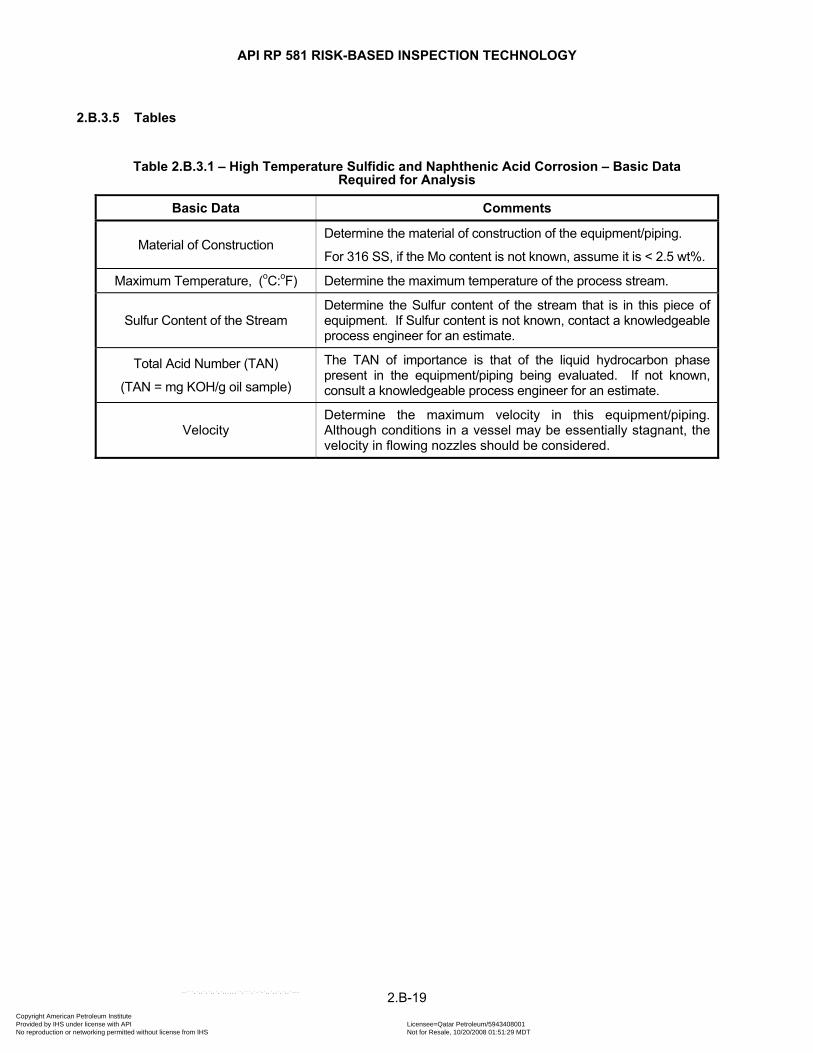
API RP 581 RISK-BASED INSPECTION TECHNOLOGY
2.B.3.5 Tables
Table 2.B.3.1 – High Temperature Sulfidic and Naphthenic Acid Corrosion – Basic Data Required for Analysis
Basic Data Comments
Material of Construction Determine the material of construction of the equipment/piping.
For 316 SS, if the Mo content is not known, assume it is < 2.5 wt%.
Maximum Temperature, (oC:oF) Determine the maximum temperature of the process stream.
Sulfur Content of the Stream Determine the Sulfur content of the stream that is in this piece of equipment. If Sulfur content is not known, contact a knowledgeable process engineer for an estimate.
Total Acid Number (TAN)
(TAN = mg KOH/g oil sample)
The TAN of importance is that of the liquid hydrocarbon phase present in the equipment/piping being evaluated. If not known, consult a knowledgeable process engineer for an estimate.
Velocity Determine the maximum velocity in this equipment/piping. Although conditions in a vessel may be essentially stagnant, the velocity in flowing nozzles should be considered.
2.B-19 Copyright American Petroleum Institute Provided by IHS under license with API Licensee=Qatar Petroleum/5943408001
Not for Resale, 10/20/2008 01:51:29 MDTNo reproduction or networking permitted without license from IHS
--```,`,,`,`,,`,`,,,,,,``,```,`-`-`,,`,,`,`,,`---
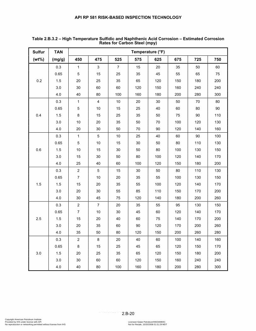
API RP 581 RISK-BASED INSPECTION TECHNOLOGY
Table 2.B.3.2 – High Temperature Sulfidic and Naphthenic Acid Corrosion – Estimated Corrosion Rates for Carbon Steel (mpy)
Sulfur
(wt%)
TAN
(mg/g)
Temperature (°F)
450 475 525 575 625 675 725 750
0.2
0.3 1 3 7 15 20 35 50 60
0.65 5 15 25 35 45 55 65 75
1.5 20 25 35 65 120 150 180 200
3.0 30 60 60 120 150 160 240 240
4.0 40 80 100 160 180 200 280 300
0.4
0.3 1 4 10 20 30 50 70 80
0.65 5 10 15 25 40 60 80 90
1.5 8 15 25 35 50 75 90 110
3.0 10 20 35 50 70 100 120 130
4.0 20 30 50 70 90 120 140 160
0.6
0.3 1 5 10 25 40 60 90 100
0.65 5 10 15 30 50 80 110 130
1.5 10 15 30 50 80 100 130 150
3.0 15 30 50 80 100 120 140 170
4.0 25 40 60 100 120 150 180 200
1.5
0.3 2 5 15 30 50 80 110 130
0.65 7 10 20 35 55 100 130 150
1.5 15 20 35 55 100 120 140 170
3.0 20 30 55 85 110 150 170 200
4.0 30 45 75 120 140 180 200 260
2.5
0.3 2 7 20 35 55 95 130 150
0.65 7 10 30 45 60 120 140 170
1.5 15 20 40 60 75 140 170 200
3.0 20 35 60 90 120 170 200 260
4.0 35 50 80 120 150 200 260 280
3.0
0.3 2 8 20 40 60 100 140 160
0.65 8 15 25 45 65 120 150 170
1.5 20 25 35 65 120 150 180 200
3.0 30 60 60 120 150 160 240 240
4.0 40 80 100 160 180 200 280 300
2.B-20 Copyright American Petroleum Institute Provided by IHS under license with API Licensee=Qatar Petroleum/5943408001
Not for Resale, 10/20/2008 01:51:29 MDTNo reproduction or networking permitted without license from IHS
--```,`,,`,`,,`,`,,,,,,``,```,`-`-`,,`,,`,`,,`---

API RP 581 RISK-BASED INSPECTION TECHNOLOGY
Table 2.B.3.2M – High Temperature Sulfidic and Naphthenic Acid Corrosion – Estimated Corrosion Rates for Carbon Steel (mm/y)
Sulfur
(wt%)
TAN
(mg/g)
Temperature (°C)
232 246 274 302 329 357 385 399
0.2
0.3 0.03 0.08 0.18 0.38 0.51 0.89 1.27 1.52 0.65 0.13 0.38 0.64 0.89 1.14 1.40 1.65 1.91 1.5 0.51 0.64 0.89 1.65 3.05 3.81 4.57 5.08 3.0 0.76 1.52 1.52 3.05 3.81 4.06 6.10 6.10 4.0 1.02 2.03 2.54 4.06 4.57 5.08 7.11 7.62
0.4
0.3 0.03 0.10 0.25 0.51 0.76 1.27 1.78 2.03 0.65 0.13 0.25 0.38 0.64 1.02 1.52 2.03 2.29 1.5 0.20 0.38 0.64 0.89 1.27 1.91 2.29 2.79 3.0 0.25 0.51 0.89 1.27 1.78 2.54 3.05 3.30 4.0 0.51 0.76 1.27 1.78 2.29 3.05 3.56 4.06
0.6
0.3 0.03 0.13 0.25 0.64 1.02 1.52 2.29 2.54 0.65 0.13 0.25 0.38 0.76 1.27 2.03 2.79 3.30 1.5 0.25 0.38 0.76 1.27 2.03 2.54 3.30 3.81 3.0 0.38 0.76 1.27 2.03 2.54 3.05 3.56 4.32 4.0 0.64 1.02 1.52 2.54 3.05 3.81 4.57 5.08
1.5
0.3 0.05 0.13 0.38 0.76 1.27 2.03 2.79 3.30 0.65 0.18 0.25 0.51 0.89 1.40 2.54 3.30 3.81 1.5 0.38 0.51 0.89 1.40 2.54 3.05 3.56 4.32 3.0 0.51 0.76 1.40 2.16 2.79 3.81 4.32 5.08 4.0 0.76 1.14 1.91 3.05 3.56 4.57 5.08 6.60
2.5
0.3 0.05 0.18 0.51 0.89 1.40 2.41 3.30 3.81 0.65 0.18 0.25 0.76 1.14 1.52 3.05 3.56 4.32 1.5 0.38 0.51 1.02 1.52 1.91 3.56 4.32 5.08 3.0 0.51 0.89 1.52 2.29 3.05 4.32 5.08 6.60 4.0 0.89 1.27 2.03 3.05 3.81 5.08 6.60 7.11
3.0
0.3 0.05 0.20 0.51 1.02 1.52 2.54 3.56 4.06 0.65 0.20 0.38 0.64 1.14 1.65 3.05 3.81 4.32 1.5 0.51 0.64 0.89 1.65 3.05 3.81 4.57 5.08 3.0 0.76 1.52 1.52 3.05 3.81 4.06 6.10 6.10 4.0 1.02 2.03 2.54 4.06 4.57 5.08 7.11 7.62
2.B-21 Copyright American Petroleum Institute Provided by IHS under license with API Licensee=Qatar Petroleum/5943408001
Not for Resale, 10/20/2008 01:51:29 MDTNo reproduction or networking permitted without license from IHS
--```,`,,`,`,,`,`,,,,,,``,```,`-`-`,,`,,`,`,,`---

API RP 581 RISK-BASED INSPECTION TECHNOLOGY
Table 2.B.3.3 – High Temperature Sulfidic and Naphthenic Acid Corrosion – Estimated Corrosion Rates for 1 Cr-0.2 Mo, 1 Cr-0.5 Mo, 1.25Cr-0.5Mo, 2.25Cr-1Mo, and 3Cr-1Mo (mpy)
Sulfur
(wt%)
TAN
(mg/g)
Temperature (°F)
450 475 525 575 625 675 725 750
0.2
0.3 1 1 4 7 13 21 25 30
0.65 3 8 15 20 25 30 35 40
1.5 10 15 20 30 60 75 90 100
3.0 15 30 30 60 75 85 120 120
4.0 20 40 50 80 100 120 140 160
0.4
0.3 1 2 5 10 20 30 35 40
0.65 3 5 8 15 20 30 40 45
1.5 4 8 15 20 25 40 45 55
3.0 5 10 20 25 35 50 60 65
4.0 10 15 25 35 45 60 70 80
0.8
0.3 1 3 6 15 25 40 45 50
0.65 3 5 8 20 30 45 55 60
1.5 5 8 15 25 40 50 65 75
3.0 7 15 25 40 50 60 70 85
4.0 12 20 30 50 60 75 90 100
1.5
0.3 2 3 8 15 30 50 55 65
0.65 4 5 10 20 40 55 65 75
1.5 6 10 20 30 50 65 70 80
3.0 10 15 30 45 60 75 85 100
4.0 15 20 35 60 75 90 100 130
2.5
0.3 2 4 9 20 35 55 65 75
0.65 4 5 15 25 40 60 70 80
1.5 7 10 20 30 45 70 80 100
3.0 10 15 30 45 60 80 100 120
4.0 15 25 40 60 80 100 120 140
3.0
0.3 2 4 10 20 35 60 70 80
0.65 5 8 15 25 40 70 75 85
1.5 10 15 20 30 60 75 90 100
3.0 15 30 30 60 75 85 120 120
4.0 20 40 50 80 100 120 140 160
2.B-22 Copyright American Petroleum Institute Provided by IHS under license with API Licensee=Qatar Petroleum/5943408001
Not for Resale, 10/20/2008 01:51:29 MDTNo reproduction or networking permitted without license from IHS
--```,`,,`,`,,`,`,,,,,,``,```,`-`-`,,`,,`,`,,`---

API RP 581 RISK-BASED INSPECTION TECHNOLOGY
Table 2.B.3.3M – High Temperature Sulfidic and Naphthenic Acid Corrosion – Estimated Corrosion Rates for 1 Cr-0.2 Mo, 1 Cr-0.5 Mo, 1.25Cr-0.5Mo, 2.25Cr-1Mo, and 3Cr-1Mo (mm/y)
Sulfur
(wt%)
TAN
(mg/g)
Temperature (°C)
232 246 274 302 329 357 385 399
0.2
0.3 0.03 0.03 0.10 0.18 0.33 0.53 0.64 0.76 0.65 0.08 0.20 0.38 0.51 0.64 0.76 0.89 1.02 1.5 0.25 0.38 0.51 0.76 1.52 1.91 2.29 2.54 3.0 0.38 0.76 0.76 1.52 1.91 2.16 3.05 3.05 4.0 0.51 1.02 1.27 2.03 2.54 3.05 3.56 4.06
0.4
0.3 0.03 0.05 0.13 0.25 0.51 0.76 0.89 1.02 0.65 0.08 0.13 0.20 0.38 0.51 0.76 1.02 1.14 1.5 0.10 0.20 0.38 0.51 0.64 1.02 1.14 1.40 3.0 0.13 0.25 0.51 0.64 0.89 1.27 1.52 1.65 4.0 0.25 0.38 0.64 0.89 1.14 1.52 1.78 2.03
0.8
0.3 0.03 0.08 0.15 0.38 0.64 1.02 1.14 1.27 0.65 0.08 0.13 0.20 0.51 0.76 1.14 1.40 1.52 1.5 0.13 0.20 0.38 0.64 1.02 1.27 1.65 1.91 3.0 0.18 0.38 0.64 1.02 1.27 1.52 1.78 2.16 4.0 0.30 0.51 0.76 1.27 1.52 1.91 2.29 2.54
1.5
0.3 0.05 0.08 0.20 0.38 0.76 1.27 1.40 1.65 0.65 0.10 0.13 0.25 0.51 1.02 1.40 1.65 1.91 1.5 0.15 0.25 0.51 0.76 1.27 1.65 1.78 2.03 3.0 0.25 0.38 0.76 1.14 1.52 1.91 2.16 2.54 4.0 0.38 0.51 0.89 1.52 1.91 2.29 2.54 3.30
2.5
0.3 0.05 0.10 0.23 0.51 0.89 1.40 1.65 1.91 0.65 0.10 0.13 0.38 0.64 1.02 1.52 1.78 2.03 1.5 0.18 0.25 0.51 0.76 1.14 1.78 2.03 2.54 3.0 0.25 0.38 0.76 1.14 1.52 2.03 2.54 3.05 4.0 0.38 0.64 1.02 1.52 2.03 2.54 3.05 3.56
3.0
0.3 0.05 0.10 0.25 0.51 0.89 1.52 1.78 2.03 0.65 0.13 0.20 0.38 0.64 1.02 1.78 1.91 2.16 1.5 0.25 0.38 0.51 0.76 1.52 1.91 2.29 2.54 3.0 0.38 0.76 0.76 1.52 1.91 2.16 3.05 3.05 4.0 0.51 1.02 1.27 2.03 2.54 3.05 3.56 4.06
2.B-23 Copyright American Petroleum Institute Provided by IHS under license with API Licensee=Qatar Petroleum/5943408001
Not for Resale, 10/20/2008 01:51:29 MDTNo reproduction or networking permitted without license from IHS
--```,`,,`,`,,`,`,,,,,,``,```,`-`-`,,`,,`,`,,`---

API RP 581 RISK-BASED INSPECTION TECHNOLOGY
Table 2.B.3.4 – High Temperature Sulfidic and Naphthenic Acid Corrosion – Estimated Corrosion Rates for 5Cr-0.5Mo (mpy)
Sulfur
(wt%)
TAN
(mg/g)
Temperature (°F)
450 475 525 575 625 675 725 750
0.2
0.7 1 1 2 4 6 8 10 15
1.1 2 3 4 6 10 10 15 20
1.75 7 10 15 20 25 35 45 50
3.0 10 15 20 30 40 45 50 60
4.0 15 20 30 40 50 60 70 80
0.4
0.7 1 2 3 5 8 10 15 20
1.1 2 3 4 6 10 15 20 25
1.75 2 4 6 8 15 20 25 30
3.0 4 6 8 10 15 20 30 35
4.0 6 8 10 10 20 25 35 40
0.75
0.7 1 2 4 6 10 15 23 25
1.1 2 4 6 8 15 20 25 30
1.75 4 6 8 10 15 20 30 35
3.0 6 8 10 10 20 25 35 40
4.0 8 10 10 15 20 30 40 50
1.5
0.7 1 2 5 8 15 20 30 35
1.1 3 5 10 15 20 30 35 40
1.75 5 10 15 20 30 35 40 45
3.0 10 15 20 30 35 40 45 50
4.0 15 20 30 35 40 50 60 70
2.5
0.7 1 3 6 9 15 20 35 40
1.1 5 7 10 15 20 25 40 45
1.75 7 10 15 20 25 35 45 50
3.0 10 15 20 30 40 45 50 60
4.0 15 20 30 40 50 60 70 80
3.0
0.7 2 3 6 10 15 25 35 40
1.1 5 7 10 15 20 30 40 45
1.75 7 10 15 20 25 35 45 50
3.0 10 15 20 30 40 45 50 60
4.0 15 20 30 40 50 60 70 80
2.B-24 Copyright American Petroleum Institute Provided by IHS under license with API Licensee=Qatar Petroleum/5943408001
Not for Resale, 10/20/2008 01:51:29 MDTNo reproduction or networking permitted without license from IHS
--```,`,,`,`,,`,`,,,,,,``,```,`-`-`,,`,,`,`,,`---

API RP 581 RISK-BASED INSPECTION TECHNOLOGY
Table 2.B.3.4M – High Temperature Sulfidic and Naphthenic Acid Corrosion – Estimated Corrosion Rates for 5Cr-0.5Mo (mm/y)
Sulfur
(wt%)
TAN
(mg/g)
Temperature (°C)
232 246 274 302 329 357 385 399
0.2
0.7 0.03 0.03 0.05 0.10 0.15 0.20 0.25 0.38 1.1 0.05 0.08 0.10 0.15 0.25 0.25 0.38 0.51
1.75 0.18 0.25 0.38 0.51 0.64 0.89 1.14 1.27 3.0 0.25 0.38 0.51 0.76 1.02 1.14 1.27 1.52 4.0 0.38 0.51 0.76 1.02 1.27 1.52 1.78 2.03
0.4
0.7 0.03 0.05 0.08 0.13 0.20 0.25 0.38 0.51 1.1 0.05 0.08 0.10 0.15 0.25 0.38 0.51 0.64
1.75 0.05 0.10 0.15 0.20 0.38 0.51 0.64 0.76 3.0 0.10 0.15 0.20 0.25 0.38 0.51 0.76 0.89 4.0 0.15 0.20 0.25 0.25 0.51 0.64 0.89 1.02
0.75
0.7 0.03 0.05 0.10 0.15 0.25 0.38 0.58 0.64 1.1 0.05 0.10 0.15 0.20 0.38 0.51 0.64 0.76
1.75 0.10 0.15 0.20 0.25 0.38 0.51 0.76 0.89 3.0 0.15 0.20 0.25 0.25 0.51 0.64 0.89 1.02 4.0 0.20 0.25 0.25 0.38 0.51 0.76 1.02 1.27
1.5
0.7 0.03 0.05 0.13 0.20 0.38 0.51 0.76 0.89 1.1 0.08 0.13 0.25 0.38 0.51 0.76 0.89 1.02
1.75 0.13 0.25 0.38 0.51 0.76 0.89 1.02 1.14 3.0 0.25 0.38 0.51 0.76 0.89 1.02 1.14 1.27 4.0 0.38 0.51 0.76 0.89 1.02 1.27 1.52 1.78
2.5
0.7 0.03 0.08 0.15 0.23 0.38 0.51 0.89 1.02 1.1 0.13 0.18 0.25 0.38 0.51 0.64 1.02 1.14
1.75 0.18 0.25 0.38 0.51 0.64 0.89 1.14 1.27 3.0 0.25 0.38 0.51 0.76 1.02 1.14 1.27 1.52 4.0 0.38 0.51 0.76 1.02 1.27 1.52 1.78 2.03
3.0
0.7 0.05 0.08 0.15 0.25 0.38 0.64 0.89 1.02 1.1 0.13 0.18 0.25 0.38 0.51 0.76 1.02 1.14
1.75 0.18 0.25 0.38 0.51 0.64 0.89 1.14 1.27 3.0 0.25 0.38 0.51 0.76 1.02 1.14 1.27 1.52 4.0 0.38 0.51 0.76 1.02 1.27 1.52 1.78 2.03
2.B-25 Copyright American Petroleum Institute Provided by IHS under license with API Licensee=Qatar Petroleum/5943408001
Not for Resale, 10/20/2008 01:51:29 MDTNo reproduction or networking permitted without license from IHS
--```,`,,`,`,,`,`,,,,,,``,```,`-`-`,,`,,`,`,,`---
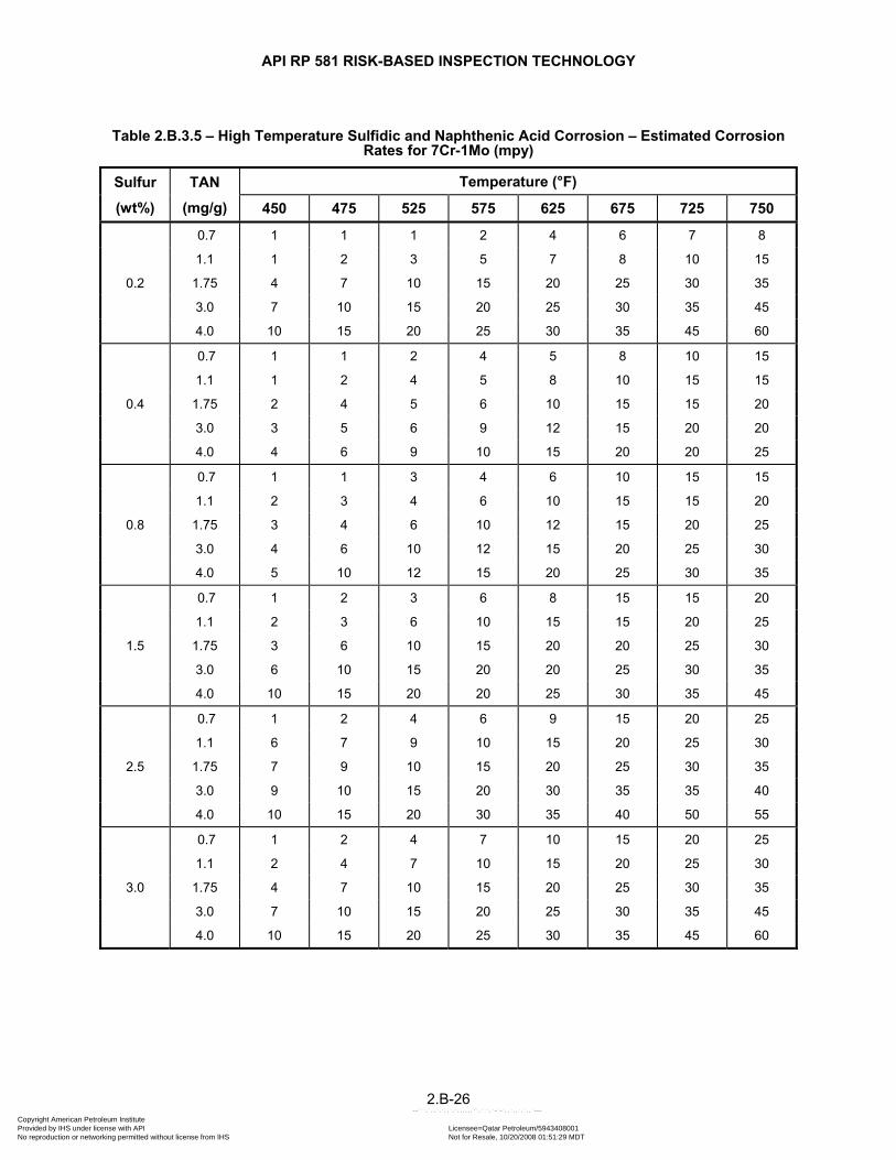
API RP 581 RISK-BASED INSPECTION TECHNOLOGY
Table 2.B.3.5 – High Temperature Sulfidic and Naphthenic Acid Corrosion – Estimated Corrosion Rates for 7Cr-1Mo (mpy)
Sulfur
(wt%)
TAN
(mg/g)
Temperature (°F)
450 475 525 575 625 675 725 750
0.2
0.7 1 1 1 2 4 6 7 8
1.1 1 2 3 5 7 8 10 15
1.75 4 7 10 15 20 25 30 35
3.0 7 10 15 20 25 30 35 45
4.0 10 15 20 25 30 35 45 60
0.4
0.7 1 1 2 4 5 8 10 15
1.1 1 2 4 5 8 10 15 15
1.75 2 4 5 6 10 15 15 20
3.0 3 5 6 9 12 15 20 20
4.0 4 6 9 10 15 20 20 25
0.8
0.7 1 1 3 4 6 10 15 15
1.1 2 3 4 6 10 15 15 20
1.75 3 4 6 10 12 15 20 25
3.0 4 6 10 12 15 20 25 30
4.0 5 10 12 15 20 25 30 35
1.5
0.7 1 2 3 6 8 15 15 20
1.1 2 3 6 10 15 15 20 25
1.75 3 6 10 15 20 20 25 30
3.0 6 10 15 20 20 25 30 35
4.0 10 15 20 20 25 30 35 45
2.5
0.7 1 2 4 6 9 15 20 25
1.1 6 7 9 10 15 20 25 30
1.75 7 9 10 15 20 25 30 35
3.0 9 10 15 20 30 35 35 40
4.0 10 15 20 30 35 40 50 55
3.0
0.7 1 2 4 7 10 15 20 25
1.1 2 4 7 10 15 20 25 30
1.75 4 7 10 15 20 25 30 35
3.0 7 10 15 20 25 30 35 45
4.0 10 15 20 25 30 35 45 60
2.B-26 Copyright American Petroleum Institute Provided by IHS under license with API Licensee=Qatar Petroleum/5943408001
Not for Resale, 10/20/2008 01:51:29 MDTNo reproduction or networking permitted without license from IHS
--```,`,,`,`,,`,`,,,,,,``,```,`-`-`,,`,,`,`,,`---

API RP 581 RISK-BASED INSPECTION TECHNOLOGY
Table 2.B.3.5M – High Temperature Sulfidic and Naphthenic Acid Corrosion – Estimated Corrosion Rates for 7Cr-1Mo (mm/y)
Sulfur
(wt%)
TAN
(mg/g)
Temperature (°C)
232 246 274 302 329 357 385 399
0.2
0.7 0.03 0.03 0.03 0.05 0.10 0.15 0.18 0.20 1.1 0.03 0.05 0.08 0.13 0.18 0.20 0.25 0.38
1.75 0.10 0.18 0.25 0.38 0.51 0.64 0.76 0.89 3.0 0.18 0.25 0.38 0.51 0.64 0.76 0.89 1.14 4.0 0.25 0.38 0.51 0.64 0.76 0.89 1.14 1.52
0.4
0.7 0.03 0.03 0.05 0.10 0.13 0.20 0.25 0.38 1.1 0.03 0.05 0.10 0.13 0.20 0.25 0.38 0.38
1.75 0.05 0.10 0.13 0.15 0.25 0.38 0.38 0.51 3.0 0.08 0.13 0.15 0.23 0.30 0.38 0.51 0.51 4.0 0.10 0.15 0.23 0.25 0.38 0.51 0.51 0.64
0.8
0.7 0.03 0.03 0.08 0.10 0.15 0.25 0.38 0.38 1.1 0.05 0.08 0.10 0.15 0.25 0.38 0.38 0.51
1.75 0.08 0.10 0.15 0.25 0.30 0.38 0.51 0.64 3.0 0.10 0.15 0.25 0.30 0.38 0.51 0.64 0.76 4.0 0.13 0.25 0.30 0.38 0.51 0.64 0.76 0.89
1.5
0.7 0.03 0.05 0.08 0.15 0.20 0.38 0.38 0.51 1.1 0.05 0.08 0.15 0.25 0.38 0.38 0.51 0.64
1.75 0.08 0.15 0.25 0.38 0.51 0.51 0.64 0.76 3.0 0.15 0.25 0.38 0.51 0.51 0.64 0.76 0.89 4.0 0.25 0.38 0.51 0.51 0.64 0.76 0.89 1.14
2.5
0.7 0.03 0.05 0.10 0.15 0.23 0.38 0.51 0.64 1.1 0.15 0.18 0.23 0.25 0.38 0.51 0.64 0.76
1.75 0.18 0.23 0.25 0.38 0.51 0.64 0.76 0.89 3.0 0.23 0.25 0.38 0.51 0.76 0.89 0.89 1.02 4.0 0.25 0.38 0.51 0.76 0.89 1.02 1.27 1.40
3.0
0.7 0.03 0.05 0.10 0.18 0.25 0.38 0.51 0.64 1.1 0.05 0.10 0.18 0.25 0.38 0.51 0.64 0.76
1.75 0.10 0.18 0.25 0.38 0.51 0.64 0.76 0.89 3.0 0.18 0.25 0.38 0.51 0.64 0.76 0.89 1.14 4.0 0.25 0.38 0.51 0.64 0.76 0.89 1.14 1.52
2.B-27 Copyright American Petroleum Institute Provided by IHS under license with API Licensee=Qatar Petroleum/5943408001
Not for Resale, 10/20/2008 01:51:29 MDTNo reproduction or networking permitted without license from IHS
--```,`,,`,`,,`,`,,,,,,``,```,`-`-`,,`,,`,`,,`---
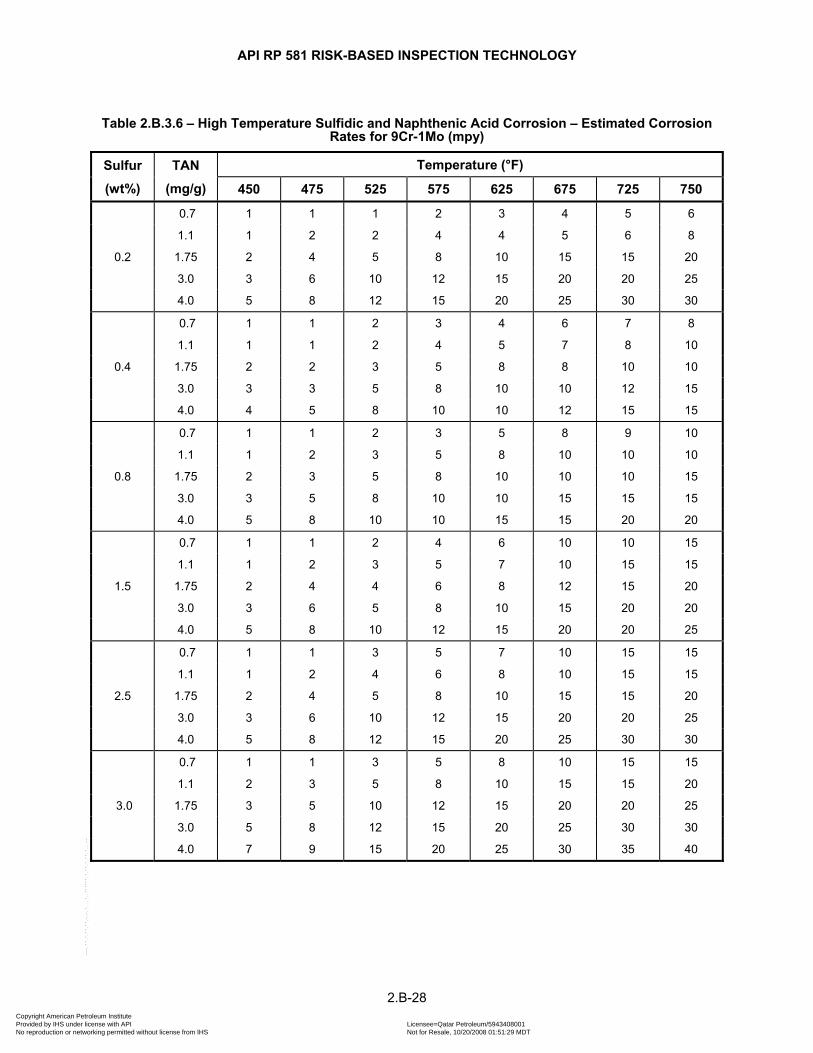
API RP 581 RISK-BASED INSPECTION TECHNOLOGY
Table 2.B.3.6 – High Temperature Sulfidic and Naphthenic Acid Corrosion – Estimated Corrosion Rates for 9Cr-1Mo (mpy)
Sulfur
(wt%)
TAN
(mg/g)
Temperature (°F)
450 475 525 575 625 675 725 750
0.2
0.7 1 1 1 2 3 4 5 6
1.1 1 2 2 4 4 5 6 8
1.75 2 4 5 8 10 15 15 20
3.0 3 6 10 12 15 20 20 25
4.0 5 8 12 15 20 25 30 30
0.4
0.7 1 1 2 3 4 6 7 8
1.1 1 1 2 4 5 7 8 10
1.75 2 2 3 5 8 8 10 10
3.0 3 3 5 8 10 10 12 15
4.0 4 5 8 10 10 12 15 15
0.8
0.7 1 1 2 3 5 8 9 10
1.1 1 2 3 5 8 10 10 10
1.75 2 3 5 8 10 10 10 15
3.0 3 5 8 10 10 15 15 15
4.0 5 8 10 10 15 15 20 20
1.5
0.7 1 1 2 4 6 10 10 15
1.1 1 2 3 5 7 10 15 15
1.75 2 4 4 6 8 12 15 20
3.0 3 6 5 8 10 15 20 20
4.0 5 8 10 12 15 20 20 25
2.5
0.7 1 1 3 5 7 10 15 15
1.1 1 2 4 6 8 10 15 15
1.75 2 4 5 8 10 15 15 20
3.0 3 6 10 12 15 20 20 25
4.0 5 8 12 15 20 25 30 30
3.0
0.7 1 1 3 5 8 10 15 15
1.1 2 3 5 8 10 15 15 20
1.75 3 5 10 12 15 20 20 25
3.0 5 8 12 15 20 25 30 30
4.0 7 9 15 20 25 30 35 40
2.B-28 Copyright American Petroleum Institute Provided by IHS under license with API Licensee=Qatar Petroleum/5943408001
Not for Resale, 10/20/2008 01:51:29 MDTNo reproduction or networking permitted without license from IHS
--```,`,,`,`,,`,`,,,,,,``,```,`-`-`,,`,,`,`,,`---

API RP 581 RISK-BASED INSPECTION TECHNOLOGY
Table 2.B.3.6M – High Temperature Sulfidic and Naphthenic Acid Corrosion – Estimated Corrosion Rates for 9Cr-1Mo (mm/y)
Sulfur
(wt%)
TAN
(mg/g)
Temperature (°C)
232 246 274 302 329 357 385 399
0.2
0.7 0.03 0.03 0.03 0.05 0.08 0.10 0.13 0.15 1.1 0.03 0.05 0.05 0.10 0.10 0.13 0.15 0.20
1.75 0.05 0.10 0.13 0.20 0.25 0.38 0.38 0.51 3.0 0.08 0.15 0.25 0.30 0.38 0.51 0.51 0.64 4.0 0.13 0.20 0.30 0.38 0.51 0.64 0.76 0.76
0.4
0.7 0.03 0.03 0.05 0.08 0.10 0.15 0.18 0.20 1.1 0.03 0.03 0.05 0.10 0.13 0.18 0.20 0.25
1.75 0.05 0.05 0.08 0.13 0.20 0.20 0.25 0.25 3.0 0.08 0.08 0.13 0.20 0.25 0.25 0.30 0.38 4.0 0.10 0.13 0.20 0.25 0.25 0.30 0.38 0.38
0.8
0.7 0.03 0.03 0.05 0.08 0.13 0.20 0.23 0.25 1.1 0.03 0.05 0.08 0.13 0.20 0.25 0.25 0.25
1.75 0.05 0.08 0.13 0.20 0.25 0.25 0.25 0.38 3.0 0.08 0.13 0.20 0.25 0.25 0.38 0.38 0.38 4.0 0.13 0.20 0.25 0.25 0.38 0.38 0.51 0.51
1.5
0.7 0.03 0.03 0.05 0.10 0.15 0.25 0.25 0.38 1.1 0.03 0.05 0.08 0.13 0.18 0.25 0.38 0.38
1.75 0.05 0.10 0.10 0.15 0.20 0.30 0.38 0.51 3.0 0.08 0.15 0.13 0.20 0.25 0.38 0.51 0.51 4.0 0.13 0.20 0.25 0.30 0.38 0.51 0.51 0.64
2.5
0.7 0.03 0.03 0.08 0.13 0.18 0.25 0.38 0.38 1.1 0.03 0.05 0.10 0.15 0.20 0.25 0.38 0.38
1.75 0.05 0.10 0.13 0.20 0.25 0.38 0.38 0.51 3.0 0.08 0.15 0.25 0.30 0.38 0.51 0.51 0.64 4.0 0.13 0.20 0.30 0.38 0.51 0.64 0.76 0.76
3.0
0.7 0.03 0.03 0.08 0.13 0.20 0.25 0.38 0.38 1.1 0.05 0.08 0.13 0.20 0.25 0.38 0.38 0.51
1.75 0.08 0.13 0.25 0.30 0.38 0.51 0.51 0.64 3.0 0.13 0.20 0.30 0.38 0.51 0.64 0.76 0.76 4.0 0.18 0.23 0.38 0.51 0.64 0.76 0.89 1.02
2.B-29 Copyright American Petroleum Institute Provided by IHS under license with API Licensee=Qatar Petroleum/5943408001
Not for Resale, 10/20/2008 01:51:29 MDTNo reproduction or networking permitted without license from IHS
--```,`,,`,`,,`,`,,,,,,``,```,`-`-`,,`,,`,`,,`---
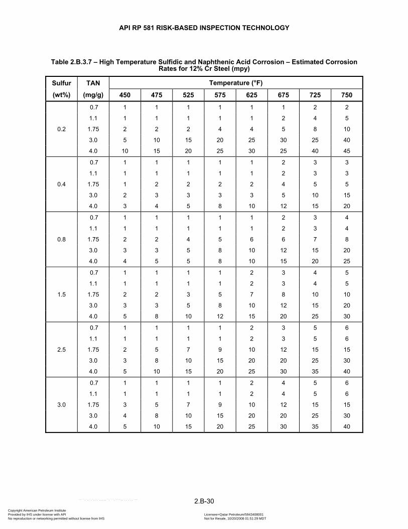
API RP 581 RISK-BASED INSPECTION TECHNOLOGY
Table 2.B.3.7 – High Temperature Sulfidic and Naphthenic Acid Corrosion – Estimated Corrosion Rates for 12% Cr Steel (mpy)
Sulfur
(wt%)
TAN
(mg/g)
Temperature (°F)
450 475 525 575 625 675 725 750
0.2
0.7 1 1 1 1 1 1 2 2
1.1 1 1 1 1 1 2 4 5
1.75 2 2 2 4 4 5 8 10
3.0 5 10 15 20 25 30 25 40
4.0 10 15 20 25 30 25 40 45
0.4
0.7 1 1 1 1 1 2 3 3
1.1 1 1 1 1 1 2 3 3
1.75 1 2 2 2 2 4 5 5
3.0 2 3 3 3 3 5 10 15
4.0 3 4 5 8 10 12 15 20
0.8
0.7 1 1 1 1 1 2 3 4
1.1 1 1 1 1 1 2 3 4
1.75 2 2 4 5 6 6 7 8
3.0 3 3 5 8 10 12 15 20
4.0 4 5 5 8 10 15 20 25
1.5
0.7 1 1 1 1 2 3 4 5
1.1 1 1 1 1 2 3 4 5
1.75 2 2 3 5 7 8 10 10
3.0 3 3 5 8 10 12 15 20
4.0 5 8 10 12 15 20 25 30
2.5
0.7 1 1 1 1 2 3 5 6
1.1 1 1 1 1 2 3 5 6
1.75 2 5 7 9 10 12 15 15
3.0 3 8 10 15 20 20 25 30
4.0 5 10 15 20 25 30 35 40
3.0
0.7 1 1 1 1 2 4 5 6
1.1 1 1 1 1 2 4 5 6
1.75 3 5 7 9 10 12 15 15
3.0 4 8 10 15 20 20 25 30
4.0 5 10 15 20 25 30 35 40
2.B-30 Copyright American Petroleum Institute Provided by IHS under license with API Licensee=Qatar Petroleum/5943408001
Not for Resale, 10/20/2008 01:51:29 MDTNo reproduction or networking permitted without license from IHS
--```,`,,`,`,,`,`,,,,,,``,```,`-`-`,,`,,`,`,,`---
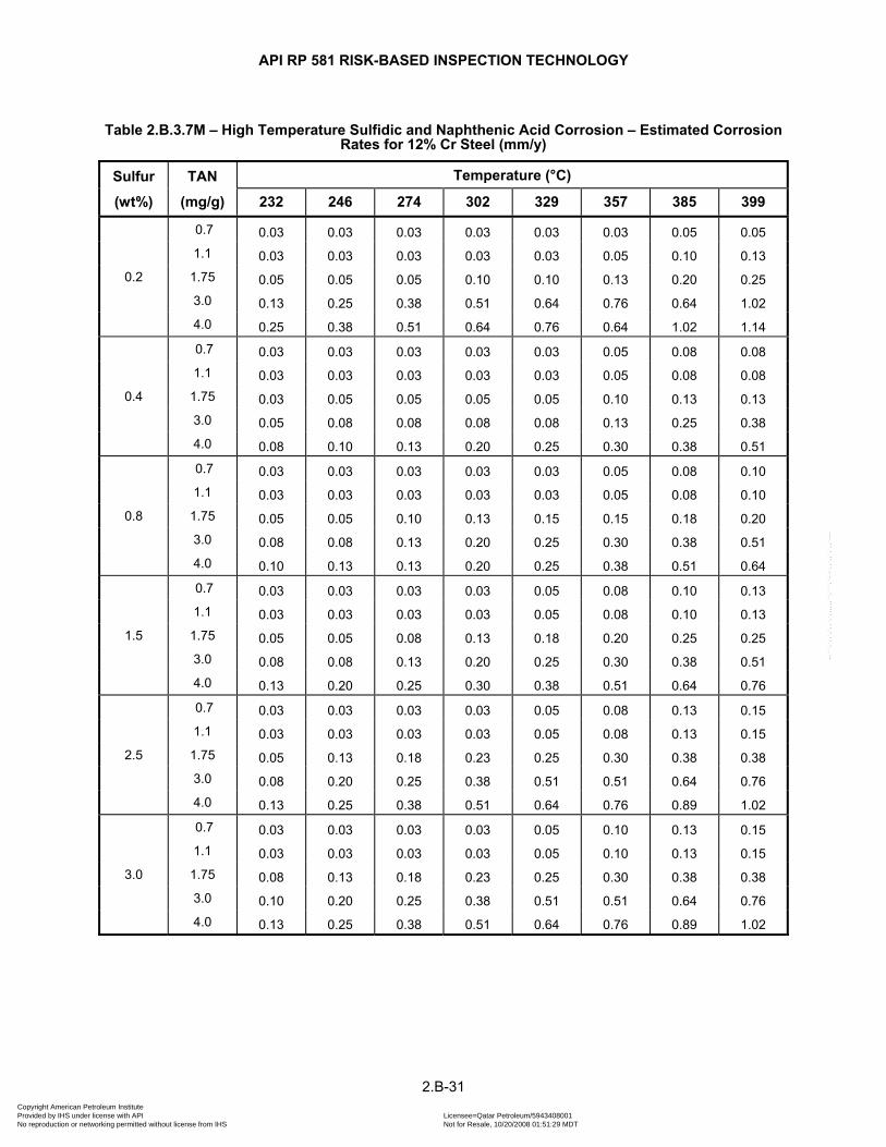
API RP 581 RISK-BASED INSPECTION TECHNOLOGY
Table 2.B.3.7M – High Temperature Sulfidic and Naphthenic Acid Corrosion – Estimated Corrosion Rates for 12% Cr Steel (mm/y)
Sulfur
(wt%)
TAN
(mg/g)
Temperature (°C)
232 246 274 302 329 357 385 399
0.2
0.7 0.03 0.03 0.03 0.03 0.03 0.03 0.05 0.05 1.1 0.03 0.03 0.03 0.03 0.03 0.05 0.10 0.13
1.75 0.05 0.05 0.05 0.10 0.10 0.13 0.20 0.25 3.0 0.13 0.25 0.38 0.51 0.64 0.76 0.64 1.02 4.0 0.25 0.38 0.51 0.64 0.76 0.64 1.02 1.14
0.4
0.7 0.03 0.03 0.03 0.03 0.03 0.05 0.08 0.08 1.1 0.03 0.03 0.03 0.03 0.03 0.05 0.08 0.08
1.75 0.03 0.05 0.05 0.05 0.05 0.10 0.13 0.13 3.0 0.05 0.08 0.08 0.08 0.08 0.13 0.25 0.38 4.0 0.08 0.10 0.13 0.20 0.25 0.30 0.38 0.51
0.8
0.7 0.03 0.03 0.03 0.03 0.03 0.05 0.08 0.10 1.1 0.03 0.03 0.03 0.03 0.03 0.05 0.08 0.10
1.75 0.05 0.05 0.10 0.13 0.15 0.15 0.18 0.20 3.0 0.08 0.08 0.13 0.20 0.25 0.30 0.38 0.51 4.0 0.10 0.13 0.13 0.20 0.25 0.38 0.51 0.64
1.5
0.7 0.03 0.03 0.03 0.03 0.05 0.08 0.10 0.13 1.1 0.03 0.03 0.03 0.03 0.05 0.08 0.10 0.13
1.75 0.05 0.05 0.08 0.13 0.18 0.20 0.25 0.25 3.0 0.08 0.08 0.13 0.20 0.25 0.30 0.38 0.51 4.0 0.13 0.20 0.25 0.30 0.38 0.51 0.64 0.76
2.5
0.7 0.03 0.03 0.03 0.03 0.05 0.08 0.13 0.15 1.1 0.03 0.03 0.03 0.03 0.05 0.08 0.13 0.15
1.75 0.05 0.13 0.18 0.23 0.25 0.30 0.38 0.38 3.0 0.08 0.20 0.25 0.38 0.51 0.51 0.64 0.76 4.0 0.13 0.25 0.38 0.51 0.64 0.76 0.89 1.02
3.0
0.7 0.03 0.03 0.03 0.03 0.05 0.10 0.13 0.15 1.1 0.03 0.03 0.03 0.03 0.05 0.10 0.13 0.15
1.75 0.08 0.13 0.18 0.23 0.25 0.30 0.38 0.38 3.0 0.10 0.20 0.25 0.38 0.51 0.51 0.64 0.76 4.0 0.13 0.25 0.38 0.51 0.64 0.76 0.89 1.02
2.B-31 Copyright American Petroleum Institute Provided by IHS under license with API Licensee=Qatar Petroleum/5943408001
Not for Resale, 10/20/2008 01:51:29 MDTNo reproduction or networking permitted without license from IHS
--```,`,,`,`,,`,`,,,,,,``,```,`-`-`,,`,,`,`,,`---
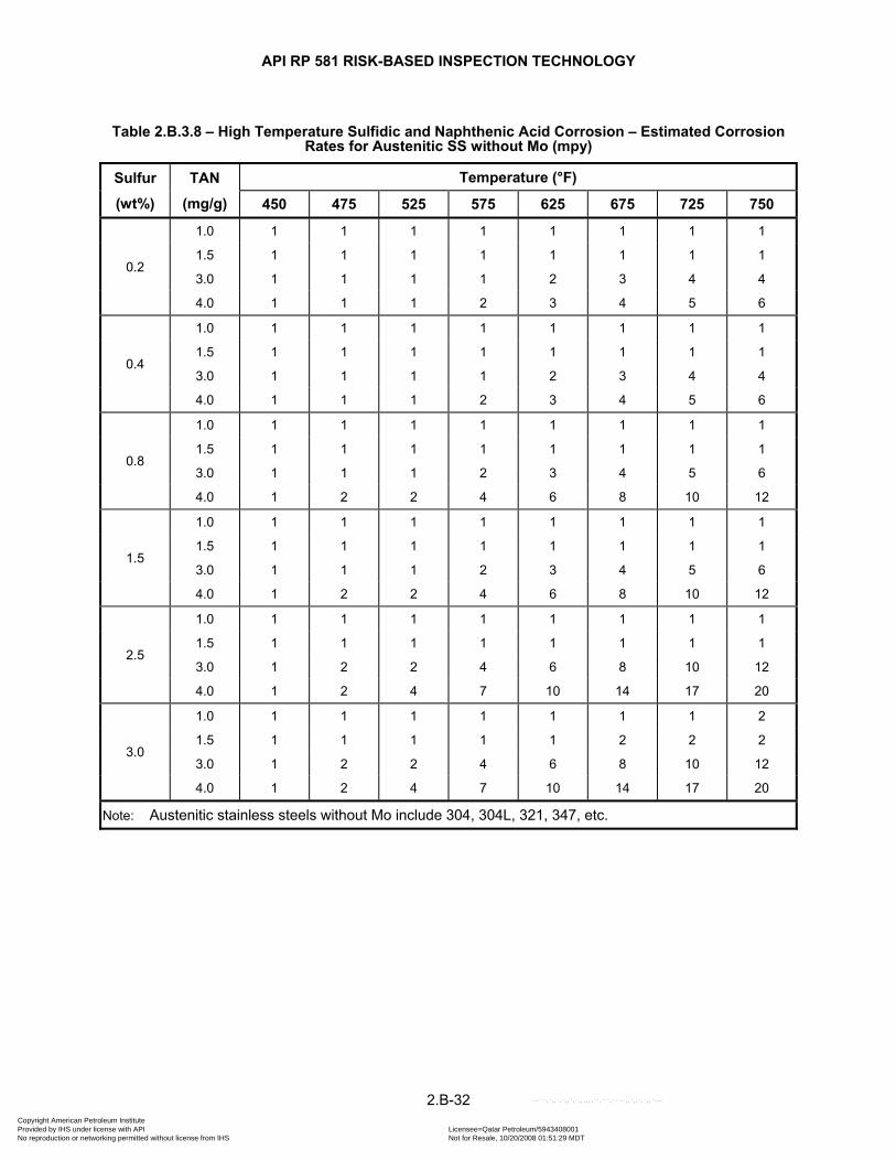
API RP 581 RISK-BASED INSPECTION TECHNOLOGY
Table 2.B.3.8 – High Temperature Sulfidic and Naphthenic Acid Corrosion – Estimated Corrosion Rates for Austenitic SS without Mo (mpy)
Sulfur
(wt%)
TAN
(mg/g)
Temperature (°F)
450 475 525 575 625 675 725 750
0.2
1.0 1 1 1 1 1 1 1 1
1.5 1 1 1 1 1 1 1 1
3.0 1 1 1 1 2 3 4 4
4.0 1 1 1 2 3 4 5 6
0.4
1.0 1 1 1 1 1 1 1 1
1.5 1 1 1 1 1 1 1 1
3.0 1 1 1 1 2 3 4 4
4.0 1 1 1 2 3 4 5 6
0.8
1.0 1 1 1 1 1 1 1 1
1.5 1 1 1 1 1 1 1 1
3.0 1 1 1 2 3 4 5 6
4.0 1 2 2 4 6 8 10 12
1.5
1.0 1 1 1 1 1 1 1 1
1.5 1 1 1 1 1 1 1 1
3.0 1 1 1 2 3 4 5 6
4.0 1 2 2 4 6 8 10 12
2.5
1.0 1 1 1 1 1 1 1 1
1.5 1 1 1 1 1 1 1 1
3.0 1 2 2 4 6 8 10 12
4.0 1 2 4 7 10 14 17 20
3.0
1.0 1 1 1 1 1 1 1 2
1.5 1 1 1 1 1 2 2 2
3.0 1 2 2 4 6 8 10 12
4.0 1 2 4 7 10 14 17 20
Note: Austenitic stainless steels without Mo include 304, 304L, 321, 347, etc.
2.B-32 Copyright American Petroleum Institute Provided by IHS under license with API Licensee=Qatar Petroleum/5943408001
Not for Resale, 10/20/2008 01:51:29 MDTNo reproduction or networking permitted without license from IHS
--```,`,,`,`,,`,`,,,,,,``,```,`-`-`,,`,,`,`,,`---
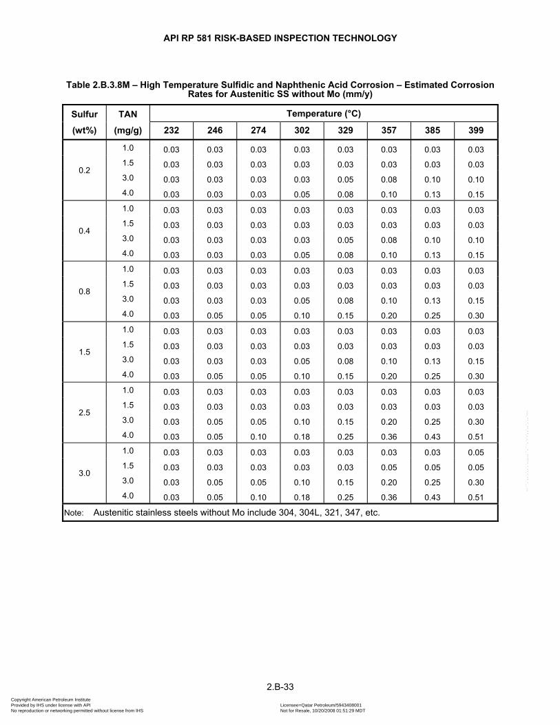
API RP 581 RISK-BASED INSPECTION TECHNOLOGY
Table 2.B.3.8M – High Temperature Sulfidic and Naphthenic Acid Corrosion – Estimated Corrosion Rates for Austenitic SS without Mo (mm/y)
Sulfur
(wt%)
TAN
(mg/g)
Temperature (°C)
232 246 274 302 329 357 385 399
0.2
1.0 0.03 0.03 0.03 0.03 0.03 0.03 0.03 0.03 1.5 0.03 0.03 0.03 0.03 0.03 0.03 0.03 0.03 3.0 0.03 0.03 0.03 0.03 0.05 0.08 0.10 0.10 4.0 0.03 0.03 0.03 0.05 0.08 0.10 0.13 0.15
0.4
1.0 0.03 0.03 0.03 0.03 0.03 0.03 0.03 0.03 1.5 0.03 0.03 0.03 0.03 0.03 0.03 0.03 0.03 3.0 0.03 0.03 0.03 0.03 0.05 0.08 0.10 0.10 4.0 0.03 0.03 0.03 0.05 0.08 0.10 0.13 0.15
0.8
1.0 0.03 0.03 0.03 0.03 0.03 0.03 0.03 0.03 1.5 0.03 0.03 0.03 0.03 0.03 0.03 0.03 0.03 3.0 0.03 0.03 0.03 0.05 0.08 0.10 0.13 0.15 4.0 0.03 0.05 0.05 0.10 0.15 0.20 0.25 0.30
1.5
1.0 0.03 0.03 0.03 0.03 0.03 0.03 0.03 0.03 1.5 0.03 0.03 0.03 0.03 0.03 0.03 0.03 0.03 3.0 0.03 0.03 0.03 0.05 0.08 0.10 0.13 0.15 4.0 0.03 0.05 0.05 0.10 0.15 0.20 0.25 0.30
2.5
1.0 0.03 0.03 0.03 0.03 0.03 0.03 0.03 0.03 1.5 0.03 0.03 0.03 0.03 0.03 0.03 0.03 0.03 3.0 0.03 0.05 0.05 0.10 0.15 0.20 0.25 0.30 4.0 0.03 0.05 0.10 0.18 0.25 0.36 0.43 0.51
3.0
1.0 0.03 0.03 0.03 0.03 0.03 0.03 0.03 0.05 1.5 0.03 0.03 0.03 0.03 0.03 0.05 0.05 0.05 3.0 0.03 0.05 0.05 0.10 0.15 0.20 0.25 0.30 4.0 0.03 0.05 0.10 0.18 0.25 0.36 0.43 0.51
Note: Austenitic stainless steels without Mo include 304, 304L, 321, 347, etc.
2.B-33 Copyright American Petroleum Institute Provided by IHS under license with API Licensee=Qatar Petroleum/5943408001
Not for Resale, 10/20/2008 01:51:29 MDTNo reproduction or networking permitted without license from IHS
--```,`,,`,`,,`,`,,,,,,``,```,`-`-`,,`,,`,`,,`---

API RP 581 RISK-BASED INSPECTION TECHNOLOGY
Table 2.B.3.9 – High Temperature Sulfidic and Naphthenic Acid Corrosion – Estimated Corrosion Rates for 316 SS with < 2.5% Mo (mpy)
Sulfur
(wt%)
TAN
(mg/g)
Temperature (°F)
450 475 525 575 625 675 725 750
0.2
0.2 1 1 1 1 1 1 1 1
3.0 1 1 1 1 1 2 2 2
4.0 1 1 1 2 4 5 7 10
0.4
0.2 1 1 1 1 1 1 1 1
3.0 1 1 1 1 2 2 2 2
4.0 1 1 2 3 4 5 7 10
0.8
0.2 1 1 1 1 1 1 1 1
3.0 1 1 1 1 2 2 2 3
4.0 1 1 2 3 5 5 7 10
1.5
0.2 1 1 1 1 1 1 1 1
3.0 1 1 1 1 3 3 3 4
4.0 1 1 3 5 5 5 7 10
2.5
0.2 1 1 1 1 1 1 1 1
3.0 1 1 1 2 3 3 4 5
4.0 1 1 3 5 5 6 8 10
3.0
0.2 1 1 1 1 1 1 1 2
3.0 1 1 1 2 4 5 5 6
4.0 1 2 3 5 5 6 8 10
Note: Includes stainless steels with < 2.5% Mo, for example 316, 316L, 316H, etc.
2.B-34 Copyright American Petroleum Institute Provided by IHS under license with API Licensee=Qatar Petroleum/5943408001
Not for Resale, 10/20/2008 01:51:29 MDTNo reproduction or networking permitted without license from IHS
--```,`,,`,`,,`,`,,,,,,``,```,`-`-`,,`,,`,`,,`---
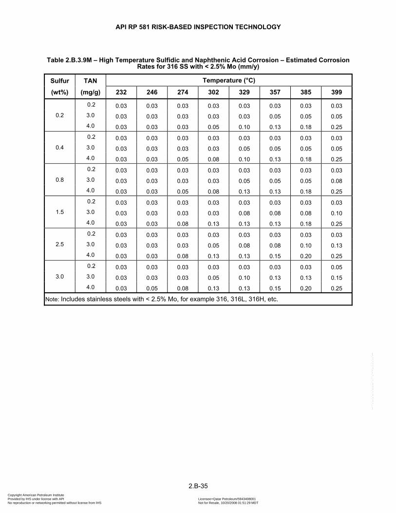
API RP 581 RISK-BASED INSPECTION TECHNOLOGY
Table 2.B.3.9M – High Temperature Sulfidic and Naphthenic Acid Corrosion – Estimated Corrosion Rates for 316 SS with < 2.5% Mo (mm/y)
Sulfur
(wt%)
TAN
(mg/g)
Temperature (°C)
232 246 274 302 329 357 385 399
0.2
0.2 0.03 0.03 0.03 0.03 0.03 0.03 0.03 0.03 3.0 0.03 0.03 0.03 0.03 0.03 0.05 0.05 0.05 4.0 0.03 0.03 0.03 0.05 0.10 0.13 0.18 0.25
0.4
0.2 0.03 0.03 0.03 0.03 0.03 0.03 0.03 0.03 3.0 0.03 0.03 0.03 0.03 0.05 0.05 0.05 0.05 4.0 0.03 0.03 0.05 0.08 0.10 0.13 0.18 0.25
0.8
0.2 0.03 0.03 0.03 0.03 0.03 0.03 0.03 0.03 3.0 0.03 0.03 0.03 0.03 0.05 0.05 0.05 0.08 4.0 0.03 0.03 0.05 0.08 0.13 0.13 0.18 0.25
1.5
0.2 0.03 0.03 0.03 0.03 0.03 0.03 0.03 0.03 3.0 0.03 0.03 0.03 0.03 0.08 0.08 0.08 0.10 4.0 0.03 0.03 0.08 0.13 0.13 0.13 0.18 0.25
2.5
0.2 0.03 0.03 0.03 0.03 0.03 0.03 0.03 0.03 3.0 0.03 0.03 0.03 0.05 0.08 0.08 0.10 0.13 4.0 0.03 0.03 0.08 0.13 0.13 0.15 0.20 0.25
3.0
0.2 0.03 0.03 0.03 0.03 0.03 0.03 0.03 0.05 3.0 0.03 0.03 0.03 0.05 0.10 0.13 0.13 0.15 4.0 0.03 0.05 0.08 0.13 0.13 0.15 0.20 0.25
Note: Includes stainless steels with < 2.5% Mo, for example 316, 316L, 316H, etc.
2.B-35 Copyright American Petroleum Institute Provided by IHS under license with API Licensee=Qatar Petroleum/5943408001
Not for Resale, 10/20/2008 01:51:29 MDTNo reproduction or networking permitted without license from IHS
--```,`,,`,`,,`,`,,,,,,``,```,`-`-`,,`,,`,`,,`---

API RP 581 RISK-BASED INSPECTION TECHNOLOGY
Table 2.B.3.10 – High Temperature Sulfidic and Naphthenic Acid Corrosion – Estimated Corrosion Rates for 316 SS with ≥ 2.5% Mo and 317 SS (mpy)
Sulfur
(wt%)
TAN
(mg/g)
Temperature (°F)
450 475 525 575 625 675 725 750
0.2
4.0 1 1 1 1 1 1 1 1
5.0 1 1 1 1 1 2 4 5
6.0 1 1 1 2 4 5 7 10
0.4
4.0 1 1 1 1 1 1 1 1
5.0 1 1 1 1 2 4 4 5
6.0 1 1 2 3 4 5 7 10
0.8
4.0 1 1 1 1 1 1 1 1
5.0 1 1 1 1 2 4 4 5
6.0 1 1 2 3 4 5 7 10
1.5
4.0 1 1 1 1 1 1 1 1
5.0 1 1 1 1 2 3 5 7
6.0 1 1 3 5 5 5 7 10
2.5
4.0 1 1 1 1 1 1 1 1
5.0 1 1 1 2 3 4 5 7
6.0 1 1 3 5 5 6 8 10
3.0
4.0 1 1 1 1 1 1 1 2
5.0 1 1 1 2 3 4 5 7
6.0 1 2 3 5 5 6 8 10
2.B-36 Copyright American Petroleum Institute Provided by IHS under license with API Licensee=Qatar Petroleum/5943408001
Not for Resale, 10/20/2008 01:51:29 MDTNo reproduction or networking permitted without license from IHS
--```,`,,`,`,,`,`,,,,,,``,```,`-`-`,,`,,`,`,,`---

API RP 581 RISK-BASED INSPECTION TECHNOLOGY
Table 2.B.3.10M – High Temperature Sulfidic and Naphthenic Acid Corrosion – Estimated Corrosion Rates for 316 SS with ≥ 2.5% Mo and 317 SS (mm/y)
Sulfur
(wt%)
TAN
(mg/g)
Temperature (°C)
232 246 274 302 329 357 385 399
0.2
4.0 0.03 0.03 0.03 0.03 0.03 0.03 0.03 0.03 5.0 0.03 0.03 0.03 0.03 0.03 0.05 0.10 0.13 6.0 0.03 0.03 0.03 0.05 0.10 0.13 0.18 0.25
0.4
4.0 0.03 0.03 0.03 0.03 0.03 0.03 0.03 0.03 5.0 0.03 0.03 0.03 0.03 0.05 0.10 0.10 0.13 6.0 0.03 0.03 0.05 0.08 0.10 0.13 0.18 0.25
0.8
4.0 0.03 0.03 0.03 0.03 0.03 0.03 0.03 0.03 5.0 0.03 0.03 0.03 0.03 0.05 0.10 0.10 0.13 6.0 0.03 0.03 0.05 0.08 0.10 0.13 0.18 0.25
1.5
4.0 0.03 0.03 0.03 0.03 0.03 0.03 0.03 0.03 5.0 0.03 0.03 0.03 0.03 0.05 0.08 0.13 0.18 6.0 0.03 0.03 0.08 0.13 0.13 0.13 0.18 0.25
2.5
4.0 0.03 0.03 0.03 0.03 0.03 0.03 0.03 0.03 5.0 0.03 0.03 0.03 0.05 0.08 0.10 0.13 0.18 6.0 0.03 0.03 0.08 0.13 0.13 0.15 0.20 0.25
3.0
4.0 0.03 0.03 0.03 0.03 0.03 0.03 0.03 0.05 5.0 0.03 0.03 0.03 0.05 0.08 0.10 0.13 0.18 6.0 0.03 0.05 0.08 0.13 0.13 0.15 0.20 0.25
2.B-37 Copyright American Petroleum Institute Provided by IHS under license with API Licensee=Qatar Petroleum/5943408001
Not for Resale, 10/20/2008 01:51:29 MDTNo reproduction or networking permitted without license from IHS
--```,`,,`,`,,`,`,,,,,,``,```,`-`-`,,`,,`,`,,`---

API RP 581 RISK-BASED INSPECTION TECHNOLOGY
2.B.3.6 Figures
Is Velocity < 30.48 m/s (100 ft/s)?
Yes No
MaterialMaximum Process Temp.
Sulfur ConcentrationTAN
Determine Corrosion Rate using Tables 2.B.3.2 through 2.B.3.10.
Start
Estimated Corrosion Rate
Estimated Corrosion Rate
Use Corrosion Rates
from Tables
Maximum Corrosion Rate X 5
Figure 2.B.3.1 – High Temperature Sulfidic and Naphthenic Acid Corrosion – Determination of Corrosion Rate
2.B-38 Copyright American Petroleum Institute Provided by IHS under license with API Licensee=Qatar Petroleum/5943408001
Not for Resale, 10/20/2008 01:51:29 MDTNo reproduction or networking permitted without license from IHS
--```,`,,`,`,,`,`,,,,,,``,```,`-`-`,,`,,`,`,,`---

API RP 581 RISK-BASED INSPECTION TECHNOLOGY
2.B.4 HIGH TEMPERATURE H2S/H2 CORROSION
2.B.4.1 Description of Damage
High temperature H2S/H2 corrosion is a form of normally uniform corrosion which can occur at temperatures typically above about 204°C (400°F). This form of sulfidation corrosion differs from high temperature sulfidic and naphthenic corrosion described in paragraph 2.B.3. H2S/H2 corrosion occurs in hydroprocessing units, e.g., hydrodesulfurizers and hydrocrackers, once sulfur compounds are converted to hydrogen sulfide via catalytic reaction with hydrogen. Conversion of sulfur compounds to H2S/H2 typically does not occur to a significant extent in the presence of hydrogen, even at elevated temperatures, unless a catalyst is present. The corrosion rate is a function of the material of construction, temperature, nature of the process stream and the concentration of H2S.
In H2S/H2 environments, low levels of chromium (e.g., 5 to 9% Cr) provide only a modest increase the corrosion resistance of steel. A minimum of 12% Cr is needed to provide a significant decrease in corrosion rate. Further addition of chromium and nickel provides a substantial increase in corrosion resistance. The nature of the process stream is a factor in determining the corrosion rate. In H2S/H2 environments alone (all vapor), corrosion rates may be as much as 50% greater than in the presence of hydrocarbons as suggested by the referenced NACE committee report. Nevertheless, the correlations developed by Cooper and Gorman are used for estimating corrosion rates in both hydrocarbon free and hydrocarbon containing services. The predicted rates in both services are very high at high H2S levels and temperatures and the one set of data are satisfactory for risk-based inspection assessment purposes of either situation.
2.B.4.2 Basic Data
The data listed in Table 2.B.4.1 are required to determine the rate of corrosion in high temperature H2S/H2 service. If precise data have not been measured, a knowledgeable process specialist should be consulted.
2.B.4.3 Determination of Corrosion Rate
The steps required to determine the corrosion rate are shown in Figure 2.B.4.1. The corrosion rate may be determined using the basic data in Table 2.B.4.1 in conjunction with Tables 2.B.4.2 through 2.B.4.7.
The estimated corrosion rate in H2S/H2 environments in these tables were determined using data from the correlations developed by Cooper and Gorman.
2.B.4.4 References
10. “High Temperature Hydrogen Sulfide Corrosion of Stainless Steel,” NACE Technical Committee Report, Corrosion, January 1958.
11. “Iso-Corrosion Rate Curves for High Temperature Hydrogen-Hydrogen Sulfide,” NACE Technical Committee Report, Corrosion, Vol. 15, March 1959.
2.B-39 Copyright American Petroleum Institute Provided by IHS under license with API Licensee=Qatar Petroleum/5943408001
Not for Resale, 10/20/2008 01:51:29 MDTNo reproduction or networking permitted without license from IHS
--```,`,,`,`,,`,`,,,,,,``,```,`-`-`,,`,,`,`,,`---
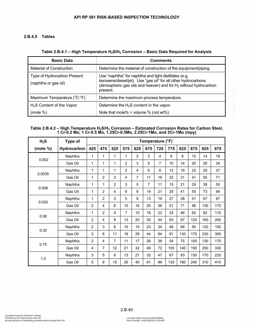
API RP 581 RISK-BASED INSPECTION TECHNOLOGY
2.B.4.5 Tables
Table 2.B.4.1 – High Temperature H2S/H2 Corrosion – Basic Data Required for Analysis
Basic Data Comments
Material of Construction Determine the material of construction of the equipment/piping.
Type of Hydrocarbon Present
(naphtha or gas oil)
Use “naphtha” for naphtha and light distillates (e.g. kerosene/diesel/jet). Use “gas oil” for all other hydrocarbons (atmospheric gas oils and heavier) and for H2 without hydrocarbon present.
Maximum Temperature (oC:°F) Determine the maximum process temperature.
H2S Content of the Vapor
(mole %)
Determine the H2S content in the vapor.
Note that mole% = volume % (not wt%)
Table 2.B.4.2 – High Temperature H2S/H2 Corrosion – Estimated Corrosion Rates for Carbon Steel, 1 Cr-0.2 Mo, 1 Cr-0.5 Mo, 1.25Cr-0.5Mo, 2.25Cr-1Mo, and 3Cr-1Mo (mpy)
H2S
(mole %)
Type of
Hydrocarbon
Temperature (°F)
425 475 525 575 625 675 725 775 825 875 925 975
0.002 Naphtha 1 1 1 1 2 3 4 6 8 10 14 18
Gas Oil 1 1 1 2 3 5 7 10 14 20 26 34
0.0035 Naphtha 1 1 1 2 4 6 8 12 16 22 29 37
Gas Oil 1 2 3 4 7 11 16 22 31 41 55 71
0.008 Naphtha 1 1 2 3 5 7 11 15 21 29 38 50
Gas Oil 1 2 4 6 9 14 21 29 41 55 73 94
0.035 Naphtha 1 2 3 5 9 13 19 27 38 51 67 87
Gas Oil 2 4 6 10 16 25 36 51 71 96 130 170
0.08 Naphtha 1 2 4 7 10 16 23 33 46 62 82 110
Gas Oil 2 4 8 13 20 30 44 63 87 120 160 200
0.30 Naphtha 2 3 6 10 15 23 34 48 66 90 120 150
Gas Oil 3 6 11 18 29 44 64 91 130 170 230 300
0.75 Naphtha 2 4 7 11 17 26 38 54 75 100 130 170
Gas Oil 4 7 12 21 32 49 72 100 140 190 250 330
1.0 Naphtha 3 5 8 13 21 32 47 67 93 130 170 220
Gas Oil 5 9 15 26 40 61 89 130 180 240 310 410
2.B-40 Copyright American Petroleum Institute Provided by IHS under license with API Licensee=Qatar Petroleum/5943408001
Not for Resale, 10/20/2008 01:51:29 MDTNo reproduction or networking permitted without license from IHS
--```,`,,`,`,,`,`,,,,,,``,```,`-`-`,,`,,`,`,,`---

API RP 581 RISK-BASED INSPECTION TECHNOLOGY
Table 2.B.4.2M – High Temperature H2S/H2 Corrosion – Estimated Corrosion Rates for Carbon Steel, 1 Cr-0.2 Mo, 1 Cr-0.5 Mo, 1.25Cr-0.5Mo, 2.25Cr-1Mo, and 3Cr-1Mo (mm/y)
H2S
(mole %)
Type of
Hydrocarbon
Temperature (°C)
218 246 274 302 329 357 385 413 441 468 496 524
0.002 Naphtha 0.03 0.03 0.03 0.03 0.05 0.08 0.1 0.15 0.2 0.25 0.36 0.46
Gas Oil 0.03 0.03 0.03 0.05 0.08 0.13 0.18 0.25 0.36 0.51 0.66 0.86
0.0035 Naphtha 0.03 0.03 0.03 0.05 0.1 0.15 0.2 0.3 0.41 0.56 0.74 0.94
Gas Oil 0.03 0.05 0.08 0.1 0.18 0.28 0.41 0.56 0.79 1.04 1.4 1.8
0.008 Naphtha 0.03 0.03 0.05 0.08 0.13 0.18 0.28 0.38 0.53 0.74 0.97 1.27
Gas Oil 0.03 0.05 0.1 0.15 0.23 0.36 0.53 0.74 1.04 1.4 1.85 2.39
0.035 Naphtha 0.03 0.05 0.08 0.13 0.23 0.33 0.48 0.69 0.97 1.3 1.7 2.21
Gas Oil 0.05 0.1 0.15 0.25 0.41 0.64 0.91 1.3 1.8 2.44 3.3 4.32
0.08 Naphtha 0.03 0.05 0.1 0.18 0.25 0.41 0.58 0.84 1.17 1.57 2.08 2.79
Gas Oil 0.05 0.1 0.2 0.33 0.51 0.76 1.12 1.6 2.21 3.05 4.06 5.08
0.30 Naphtha 0.05 0.08 0.15 0.25 0.38 0.58 0.86 1.22 1.68 2.29 3.05 3.81
Gas Oil 0.08 0.15 0.28 0.46 0.74 1.12 1.63 2.31 3.3 4.32 5.84 7.62
0.75 Naphtha 0.05 0.1 0.18 0.28 0.43 0.66 0.97 1.37 1.91 2.54 3.3 4.32
Gas Oil 0.1 0.18 0.3 0.53 0.81 1.24 1.83 2.54 3.56 4.83 6.35 8.38
1.0 Naphtha 0.08 0.13 0.2 0.33 0.53 0.81 1.19 1.7 2.36 3.3 4.32 5.59
Gas Oil 0.13 0.23 0.38 0.66 1.02 1.55 2.26 3.3 4.57 6.1 7.87 10.41
2.B-41 Copyright American Petroleum Institute Provided by IHS under license with API Licensee=Qatar Petroleum/5943408001
Not for Resale, 10/20/2008 01:51:29 MDTNo reproduction or networking permitted without license from IHS
--```,`,,`,`,,`,`,,,,,,``,```,`-`-`,,`,,`,`,,`---
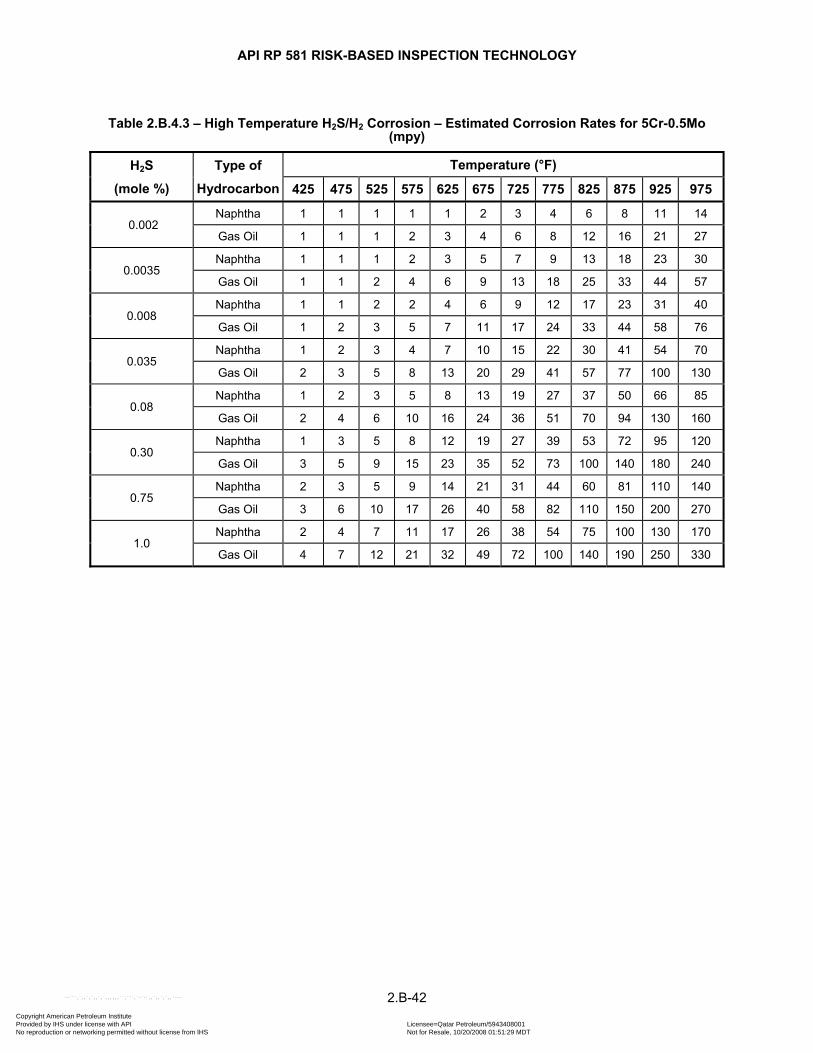
API RP 581 RISK-BASED INSPECTION TECHNOLOGY
Table 2.B.4.3 – High Temperature H2S/H2 Corrosion – Estimated Corrosion Rates for 5Cr-0.5Mo (mpy)
H2S
(mole %)
Type of
Hydrocarbon
Temperature (°F)
425 475 525 575 625 675 725 775 825 875 925 975
0.002 Naphtha 1 1 1 1 1 2 3 4 6 8 11 14
Gas Oil 1 1 1 2 3 4 6 8 12 16 21 27
0.0035 Naphtha 1 1 1 2 3 5 7 9 13 18 23 30
Gas Oil 1 1 2 4 6 9 13 18 25 33 44 57
0.008 Naphtha 1 1 2 2 4 6 9 12 17 23 31 40
Gas Oil 1 2 3 5 7 11 17 24 33 44 58 76
0.035 Naphtha 1 2 3 4 7 10 15 22 30 41 54 70
Gas Oil 2 3 5 8 13 20 29 41 57 77 100 130
0.08 Naphtha 1 2 3 5 8 13 19 27 37 50 66 85
Gas Oil 2 4 6 10 16 24 36 51 70 94 130 160
0.30 Naphtha 1 3 5 8 12 19 27 39 53 72 95 120
Gas Oil 3 5 9 15 23 35 52 73 100 140 180 240
0.75 Naphtha 2 3 5 9 14 21 31 44 60 81 110 140
Gas Oil 3 6 10 17 26 40 58 82 110 150 200 270
1.0 Naphtha 2 4 7 11 17 26 38 54 75 100 130 170
Gas Oil 4 7 12 21 32 49 72 100 140 190 250 330
2.B-42 Copyright American Petroleum Institute Provided by IHS under license with API Licensee=Qatar Petroleum/5943408001
Not for Resale, 10/20/2008 01:51:29 MDTNo reproduction or networking permitted without license from IHS
--```,`,,`,`,,`,`,,,,,,``,```,`-`-`,,`,,`,`,,`---

API RP 581 RISK-BASED INSPECTION TECHNOLOGY
Table 2.B.4.3M – High Temperature H2S/H2 Corrosion – Estimated Corrosion Rates for 5Cr-0.5Mo (mm/y)
H2S
(mole %)
Type of
Hydrocarbon
Temperature (°C)
218 246 274 302 329 357 385 413 441 468 496 524
0.002 Naphtha 0.03 0.03 0.03 0.03 0.03 0.05 0.08 0.1 0.15 0.2 0.28 0.36
Gas Oil 0.03 0.03 0.03 0.05 0.08 0.1 0.15 0.2 0.3 0.41 0.53 0.69
0.0035 Naphtha 0.03 0.03 0.03 0.05 0.08 0.13 0.18 0.23 0.33 0.46 0.58 0.76
Gas Oil 0.03 0.03 0.05 0.1 0.15 0.23 0.33 0.46 0.64 0.84 1.12 1.45
0.008 Naphtha 0.03 0.03 0.05 0.05 0.1 0.15 0.23 0.3 0.43 0.58 0.79 1.02
Gas Oil 0.03 0.05 0.08 0.13 0.18 0.28 0.43 0.61 0.84 1.12 1.47 1.93
0.035 Naphtha 0.03 0.05 0.08 0.1 0.18 0.25 0.38 0.56 0.76 1.04 1.37 1.78
Gas Oil 0.05 0.08 0.13 0.2 0.33 0.51 0.74 1.04 1.45 1.96 2.54 3.3
0.08 Naphtha 0.03 0.05 0.08 0.13 0.2 0.33 0.48 0.69 0.94 1.27 1.68 2.16
Gas Oil 0.05 0.1 0.15 0.25 0.41 0.61 0.91 1.3 1.78 2.39 3.3 4.06
0.30 Naphtha 0.03 0.08 0.13 0.2 0.3 0.48 0.69 0.99 1.35 1.83 2.41 3.05
Gas Oil 0.08 0.13 0.23 0.38 0.58 0.89 1.32 1.85 2.54 3.56 4.57 6.1
0.75 Naphtha 0.05 0.08 0.13 0.23 0.36 0.53 0.79 1.12 1.52 2.06 2.79 3.56
Gas Oil 0.08 0.15 0.25 0.43 0.66 1.02 1.47 2.08 2.79 3.81 5.08 6.86
1.0 Naphtha 0.05 0.1 0.18 0.28 0.43 0.66 0.97 1.37 1.91 2.54 3.3 4.32
Gas Oil 0.1 0.18 0.3 0.53 0.81 1.24 1.83 2.54 3.56 4.83 6.35 8.38
2.B-43 Copyright American Petroleum Institute Provided by IHS under license with API Licensee=Qatar Petroleum/5943408001
Not for Resale, 10/20/2008 01:51:29 MDTNo reproduction or networking permitted without license from IHS
--```,`,,`,`,,`,`,,,,,,``,```,`-`-`,,`,,`,`,,`---
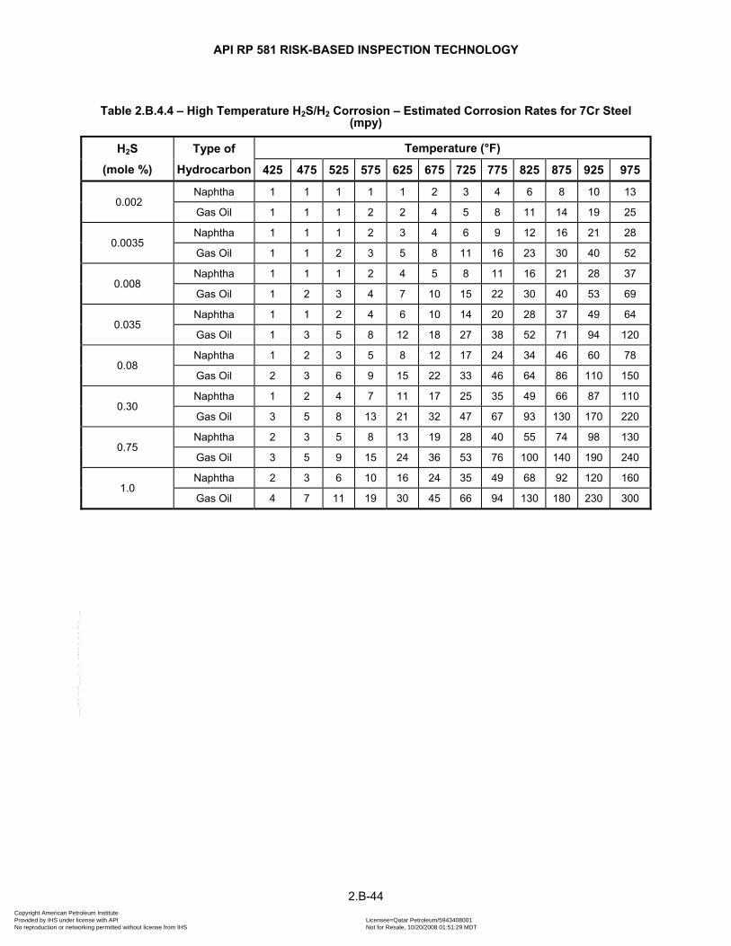
API RP 581 RISK-BASED INSPECTION TECHNOLOGY
Table 2.B.4.4 – High Temperature H2S/H2 Corrosion – Estimated Corrosion Rates for 7Cr Steel (mpy)
H2S
(mole %)
Type of
Hydrocarbon
Temperature (°F)
425 475 525 575 625 675 725 775 825 875 925 975
0.002 Naphtha 1 1 1 1 1 2 3 4 6 8 10 13
Gas Oil 1 1 1 2 2 4 5 8 11 14 19 25
0.0035 Naphtha 1 1 1 2 3 4 6 9 12 16 21 28
Gas Oil 1 1 2 3 5 8 11 16 23 30 40 52
0.008 Naphtha 1 1 1 2 4 5 8 11 16 21 28 37
Gas Oil 1 2 3 4 7 10 15 22 30 40 53 69
0.035 Naphtha 1 1 2 4 6 10 14 20 28 37 49 64
Gas Oil 1 3 5 8 12 18 27 38 52 71 94 120
0.08 Naphtha 1 2 3 5 8 12 17 24 34 46 60 78
Gas Oil 2 3 6 9 15 22 33 46 64 86 110 150
0.30 Naphtha 1 2 4 7 11 17 25 35 49 66 87 110
Gas Oil 3 5 8 13 21 32 47 67 93 130 170 220
0.75 Naphtha 2 3 5 8 13 19 28 40 55 74 98 130
Gas Oil 3 5 9 15 24 36 53 76 100 140 190 240
1.0 Naphtha 2 3 6 10 16 24 35 49 68 92 120 160
Gas Oil 4 7 11 19 30 45 66 94 130 180 230 300
2.B-44 Copyright American Petroleum Institute Provided by IHS under license with API Licensee=Qatar Petroleum/5943408001
Not for Resale, 10/20/2008 01:51:29 MDTNo reproduction or networking permitted without license from IHS
--```,`,,`,`,,`,`,,,,,,``,```,`-`-`,,`,,`,`,,`---
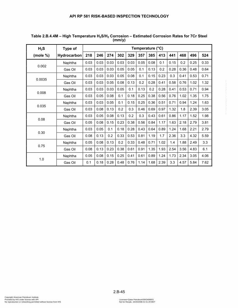
API RP 581 RISK-BASED INSPECTION TECHNOLOGY
Table 2.B.4.4M – High Temperature H2S/H2 Corrosion – Estimated Corrosion Rates for 7Cr Steel (mm/y)
H2S
(mole %)
Type of
Hydrocarbon
Temperature (°C)
218 246 274 302 329 357 385 413 441 468 496 524
0.002 Naphtha 0.03 0.03 0.03 0.03 0.03 0.05 0.08 0.1 0.15 0.2 0.25 0.33
Gas Oil 0.03 0.03 0.03 0.05 0.05 0.1 0.13 0.2 0.28 0.36 0.48 0.64
0.0035 Naphtha 0.03 0.03 0.03 0.05 0.08 0.1 0.15 0.23 0.3 0.41 0.53 0.71
Gas Oil 0.03 0.03 0.05 0.08 0.13 0.2 0.28 0.41 0.58 0.76 1.02 1.32
0.008 Naphtha 0.03 0.03 0.03 0.05 0.1 0.13 0.2 0.28 0.41 0.53 0.71 0.94
Gas Oil 0.03 0.05 0.08 0.1 0.18 0.25 0.38 0.56 0.76 1.02 1.35 1.75
0.035 Naphtha 0.03 0.03 0.05 0.1 0.15 0.25 0.36 0.51 0.71 0.94 1.24 1.63
Gas Oil 0.03 0.08 0.13 0.2 0.3 0.46 0.69 0.97 1.32 1.8 2.39 3.05
0.08 Naphtha 0.03 0.05 0.08 0.13 0.2 0.3 0.43 0.61 0.86 1.17 1.52 1.98
Gas Oil 0.05 0.08 0.15 0.23 0.38 0.56 0.84 1.17 1.63 2.18 2.79 3.81
0.30 Naphtha 0.03 0.05 0.1 0.18 0.28 0.43 0.64 0.89 1.24 1.68 2.21 2.79
Gas Oil 0.08 0.13 0.2 0.33 0.53 0.81 1.19 1.7 2.36 3.3 4.32 5.59
0.75 Naphtha 0.05 0.08 0.13 0.2 0.33 0.48 0.71 1.02 1.4 1.88 2.49 3.3
Gas Oil 0.08 0.13 0.23 0.38 0.61 0.91 1.35 1.93 2.54 3.56 4.83 6.1
1.0 Naphtha 0.05 0.08 0.15 0.25 0.41 0.61 0.89 1.24 1.73 2.34 3.05 4.06
Gas Oil 0.1 0.18 0.28 0.48 0.76 1.14 1.68 2.39 3.3 4.57 5.84 7.62
2.B-45 Copyright American Petroleum Institute Provided by IHS under license with API Licensee=Qatar Petroleum/5943408001
Not for Resale, 10/20/2008 01:51:29 MDTNo reproduction or networking permitted without license from IHS
--```,`,,`,`,,`,`,,,,,,``,```,`-`-`,,`,,`,`,,`---
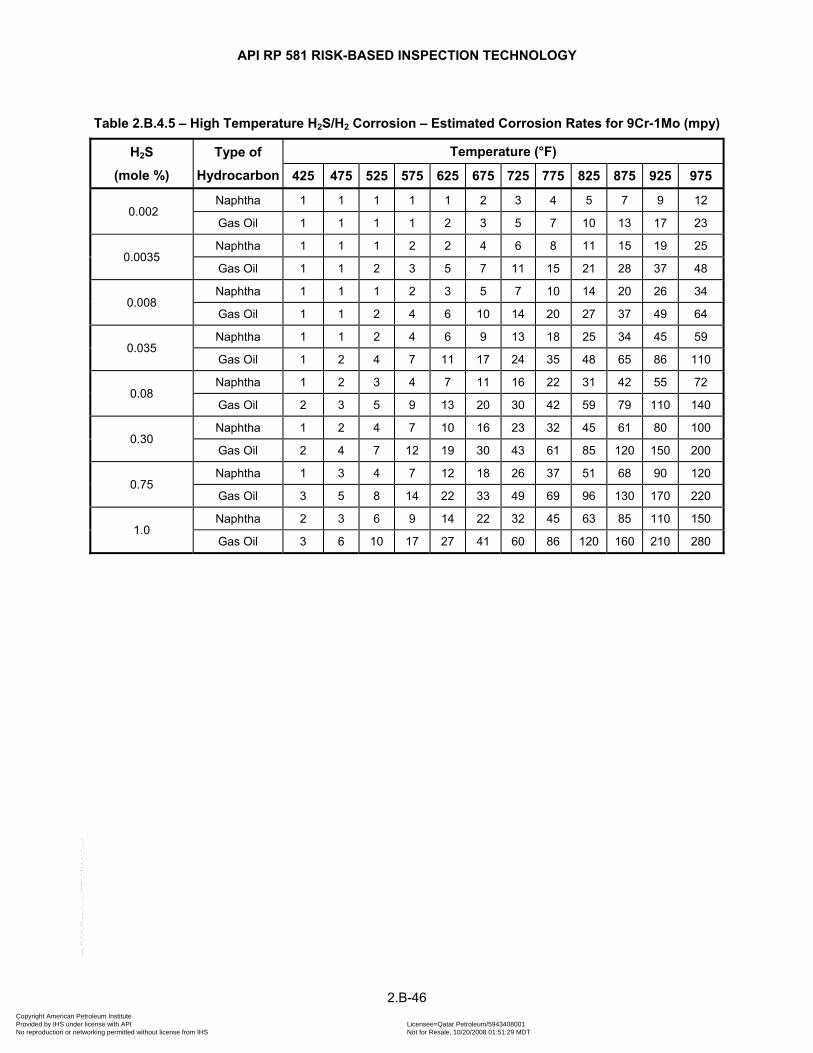
API RP 581 RISK-BASED INSPECTION TECHNOLOGY
Table 2.B.4.5 – High Temperature H2S/H2 Corrosion – Estimated Corrosion Rates for 9Cr-1Mo (mpy)
H2S
(mole %)
Type of
Hydrocarbon
Temperature (°F)
425 475 525 575 625 675 725 775 825 875 925 975
0.002 Naphtha 1 1 1 1 1 2 3 4 5 7 9 12
Gas Oil 1 1 1 1 2 3 5 7 10 13 17 23
0.0035 Naphtha 1 1 1 2 2 4 6 8 11 15 19 25
Gas Oil 1 1 2 3 5 7 11 15 21 28 37 48
0.008 Naphtha 1 1 1 2 3 5 7 10 14 20 26 34
Gas Oil 1 1 2 4 6 10 14 20 27 37 49 64
0.035 Naphtha 1 1 2 4 6 9 13 18 25 34 45 59
Gas Oil 1 2 4 7 11 17 24 35 48 65 86 110
0.08 Naphtha 1 2 3 4 7 11 16 22 31 42 55 72
Gas Oil 2 3 5 9 13 20 30 42 59 79 110 140
0.30 Naphtha 1 2 4 7 10 16 23 32 45 61 80 100
Gas Oil 2 4 7 12 19 30 43 61 85 120 150 200
0.75 Naphtha 1 3 4 7 12 18 26 37 51 68 90 120
Gas Oil 3 5 8 14 22 33 49 69 96 130 170 220
1.0 Naphtha 2 3 6 9 14 22 32 45 63 85 110 150
Gas Oil 3 6 10 17 27 41 60 86 120 160 210 280
2.B-46 Copyright American Petroleum Institute Provided by IHS under license with API Licensee=Qatar Petroleum/5943408001
Not for Resale, 10/20/2008 01:51:29 MDTNo reproduction or networking permitted without license from IHS
--```,`,,`,`,,`,`,,,,,,``,```,`-`-`,,`,,`,`,,`---
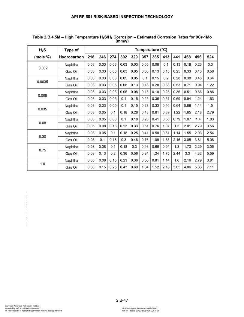
API RP 581 RISK-BASED INSPECTION TECHNOLOGY
Table 2.B.4.5M – High Temperature H2S/H2 Corrosion – Estimated Corrosion Rates for 9Cr-1Mo (mm/y)
H2S
(mole %)
Type of
Hydrocarbon
Temperature (°C)
218 246 274 302 329 357 385 413 441 468 496 524
0.002 Naphtha 0.03 0.03 0.03 0.03 0.03 0.05 0.08 0.1 0.13 0.18 0.23 0.3
Gas Oil 0.03 0.03 0.03 0.03 0.05 0.08 0.13 0.18 0.25 0.33 0.43 0.58
0.0035 Naphtha 0.03 0.03 0.03 0.05 0.05 0.1 0.15 0.2 0.28 0.38 0.48 0.64
Gas Oil 0.03 0.03 0.05 0.08 0.13 0.18 0.28 0.38 0.53 0.71 0.94 1.22
0.008 Naphtha 0.03 0.03 0.03 0.05 0.08 0.13 0.18 0.25 0.36 0.51 0.66 0.86
Gas Oil 0.03 0.03 0.05 0.1 0.15 0.25 0.36 0.51 0.69 0.94 1.24 1.63
0.035 Naphtha 0.03 0.03 0.05 0.1 0.15 0.23 0.33 0.46 0.64 0.86 1.14 1.5
Gas Oil 0.03 0.05 0.1 0.18 0.28 0.43 0.61 0.89 1.22 1.65 2.18 2.79
0.08 Naphtha 0.03 0.05 0.08 0.1 0.18 0.28 0.41 0.56 0.79 1.07 1.4 1.83
Gas Oil 0.05 0.08 0.13 0.23 0.33 0.51 0.76 1.07 1.5 2.01 2.79 3.56
0.30 Naphtha 0.03 0.05 0.1 0.18 0.25 0.41 0.58 0.81 1.14 1.55 2.03 2.54
Gas Oil 0.05 0.1 0.18 0.3 0.48 0.76 1.09 1.55 2.16 3.05 3.81 5.08
0.75 Naphtha 0.03 0.08 0.1 0.18 0.3 0.46 0.66 0.94 1.3 1.73 2.29 3.05
Gas Oil 0.08 0.13 0.2 0.36 0.56 0.84 1.24 1.75 2.44 3.3 4.32 5.59
1.0 Naphtha 0.05 0.08 0.15 0.23 0.36 0.56 0.81 1.14 1.6 2.16 2.79 3.81
Gas Oil 0.08 0.15 0.25 0.43 0.69 1.04 1.52 2.18 3.05 4.06 5.33 7.11
2.B-47 Copyright American Petroleum Institute Provided by IHS under license with API Licensee=Qatar Petroleum/5943408001
Not for Resale, 10/20/2008 01:51:29 MDTNo reproduction or networking permitted without license from IHS
--```,`,,`,`,,`,`,,,,,,``,```,`-`-`,,`,,`,`,,`---

API RP 581 RISK-BASED INSPECTION TECHNOLOGY
Table 2.B.4.6 – High Temperature H2S/H2 Corrosion – Estimated Corrosion Rates for 12Cr Steels (mpy)
H2S
(mole %)
Temperature (°F)
425 475 525 575 625 675 725 775 825 875 925 975
0.002 1 1 1 1 2 3 4 5 6 9 11 14
0.0035 1 1 1 1 2 3 4 6 8 11 14 18
0.008 1 1 1 2 2 4 5 7 9 12 15 19
0.035 1 1 1 2 3 4 6 9 12 15 19 25
0.08 1 1 1 2 3 5 7 10 13 17 22 27
0.30 1 1 2 3 4 6 9 12 16 21 27 34
0.75 1 1 2 3 5 7 10 13 18 23 30 38
1.0 1 2 3 4 7 10 13 18 25 32 42 53
Table 2.B.4.6M – High Temperature H2S/H2 Corrosion – Estimated Corrosion Rates for 12Cr Steels (mm/y)
H2S
(mole %)
Temperature (°C)
218 246 274 302 329 357 385 413 441 468 496 524
0.002 0.03 0.03 0.03 0.03 0.05 0.08 0.1 0.13 0.15 0.23 0.28 0.36
0.0035 0.03 0.03 0.03 0.03 0.05 0.08 0.1 0.15 0.2 0.28 0.36 0.46
0.008 0.03 0.03 0.03 0.05 0.05 0.1 0.13 0.18 0.23 0.3 0.38 0.48
0.035 0.03 0.03 0.03 0.05 0.08 0.1 0.15 0.23 0.3 0.38 0.48 0.64
0.08 0.03 0.03 0.03 0.05 0.08 0.13 0.18 0.25 0.33 0.43 0.56 0.69
0.30 0.03 0.03 0.05 0.08 0.1 0.15 0.23 0.3 0.41 0.53 0.69 0.86
0.75 0.03 0.03 0.05 0.08 0.13 0.18 0.25 0.33 0.46 0.58 0.76 0.97
1.0 0.03 0.05 0.08 0.1 0.18 0.25 0.33 0.46 0.64 0.81 1.07 1.35
2.B-48 Copyright American Petroleum Institute Provided by IHS under license with API Licensee=Qatar Petroleum/5943408001
Not for Resale, 10/20/2008 01:51:29 MDTNo reproduction or networking permitted without license from IHS
--```,`,,`,`,,`,`,,,,,,``,```,`-`-`,,`,,`,`,,`---
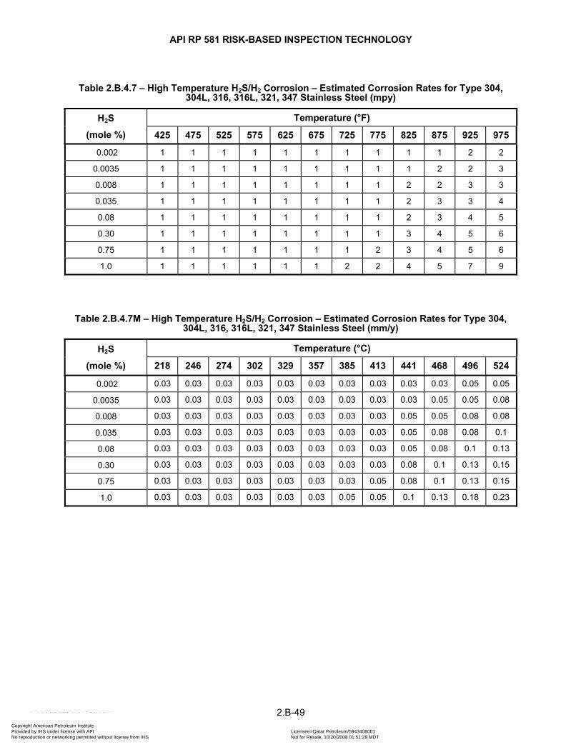
API RP 581 RISK-BASED INSPECTION TECHNOLOGY
Table 2.B.4.7 – High Temperature H2S/H2 Corrosion – Estimated Corrosion Rates for Type 304, 304L, 316, 316L, 321, 347 Stainless Steel (mpy)
H2S
(mole %)
Temperature (°F)
425 475 525 575 625 675 725 775 825 875 925 975
0.002 1 1 1 1 1 1 1 1 1 1 2 2
0.0035 1 1 1 1 1 1 1 1 1 2 2 3
0.008 1 1 1 1 1 1 1 1 2 2 3 3
0.035 1 1 1 1 1 1 1 1 2 3 3 4
0.08 1 1 1 1 1 1 1 1 2 3 4 5
0.30 1 1 1 1 1 1 1 1 3 4 5 6
0.75 1 1 1 1 1 1 1 2 3 4 5 6
1.0 1 1 1 1 1 1 2 2 4 5 7 9
Table 2.B.4.7M – High Temperature H2S/H2 Corrosion – Estimated Corrosion Rates for Type 304, 304L, 316, 316L, 321, 347 Stainless Steel (mm/y)
H2S
(mole %)
Temperature (°C)
218 246 274 302 329 357 385 413 441 468 496 524
0.002 0.03 0.03 0.03 0.03 0.03 0.03 0.03 0.03 0.03 0.03 0.05 0.05
0.0035 0.03 0.03 0.03 0.03 0.03 0.03 0.03 0.03 0.03 0.05 0.05 0.08
0.008 0.03 0.03 0.03 0.03 0.03 0.03 0.03 0.03 0.05 0.05 0.08 0.08
0.035 0.03 0.03 0.03 0.03 0.03 0.03 0.03 0.03 0.05 0.08 0.08 0.1
0.08 0.03 0.03 0.03 0.03 0.03 0.03 0.03 0.03 0.05 0.08 0.1 0.13
0.30 0.03 0.03 0.03 0.03 0.03 0.03 0.03 0.03 0.08 0.1 0.13 0.15
0.75 0.03 0.03 0.03 0.03 0.03 0.03 0.03 0.05 0.08 0.1 0.13 0.15
1.0 0.03 0.03 0.03 0.03 0.03 0.03 0.05 0.05 0.1 0.13 0.18 0.23
2.B-49 Copyright American Petroleum Institute Provided by IHS under license with API Licensee=Qatar Petroleum/5943408001
Not for Resale, 10/20/2008 01:51:29 MDTNo reproduction or networking permitted without license from IHS
--```,`,,`,`,,`,`,,,,,,``,```,`-`-`,,`,,`,`,,`---
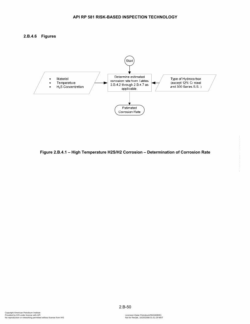
API RP 581 RISK-BASED INSPECTION TECHNOLOGY
2.B.4.6 Figures
Figure 2.B.4.1 – High Temperature H2S/H2 Corrosion – Determination of Corrosion Rate
2.B-50 Copyright American Petroleum Institute Provided by IHS under license with API Licensee=Qatar Petroleum/5943408001
Not for Resale, 10/20/2008 01:51:29 MDTNo reproduction or networking permitted without license from IHS
--```,`,,`,`,,`,`,,,,,,``,```,`-`-`,,`,,`,`,,`---
API RP 581 RISK-BASED INSPECTION TECHNOLOGY
2.B.5 SULFURIC ACID (H2SO4) CORROSION
2.B.5.1 Description of Damage
Sulfuric acid (H2SO4) is one of the most widely used industrial chemicals. One common use of concentrated sulfuric acid is as a catalyst for the alkylation process. Sulfuric acid is a very strong acid that can be extremely corrosive under certain conditions. The corrosiveness of sulfuric acid varies widely, and depends on many factors. Acid concentration and temperature are the foremost factors that influence corrosion. In addition, velocity effects and presence of impurities in the acid, especially oxygen or oxidants, can have a significant impact on corrosion.
Although sulfuric acid corrodes carbon steel, it is the material typically chosen for equipment and piping handling concentrated sulfuric acid at near ambient temperatures. The corrosion rate of steel by sulfuric acid as a function of acid concentration and temperature under stagnant conditions is provided in NACE Publication 5A151 [ 12]. Stagnant or low flow (< 0.91 m/s or 3 ft/s) conditions typically cause general thinning of carbon steel. The ferrous sulfate corrosion product film is somewhat protective, and as it builds on the metal surface the corrosion rate decreases. The mass transfer of ferrous sulfate away from the corroding steel surface is the rate-limiting step for the corrosion. Acid solution velocity above approximately 0.91 m/s (3 ft/s) (turbulent flow) has a significant impact on this mass transfer rate and thus the corrosion rate. Corrosion rates for steel pipelines carrying sulfuric acid at various conditions and velocities have been calculated from a well-established mathematical model [ 13]. The calculated rates were based on pure sulfuric acid solutions with no ferrous sulfate present in the acid solution. These rates for turbulent flow in straight pipes were then multiplied by a factor of 3 (based on experience cited in [ 13] to account for the enhanced localized corrosion that occurs at elbows, tees, valves, and areas of internal surface roughness such as protuberances at welded joints. This provides maximum estimated corrosion rates. Actual corrosion rates could be 20 to 50% of these estimated maximum corrosion rates.
Although the performance of many alloys in sulfuric acid service is primarily related to the acid concentration and temperature, velocity and the presence of an oxidant can play a significant role as well. This is because these alloys often depend upon formation of a protective oxide film to provide passivity, and therefore corrosion resistance. The presence of an oxidant usually improves the corrosion performance in sulfuric acid service of alloys such as stainless steel and many nickel alloys. This is not the case with Alloy B-2, which can suffer drastically high corrosion rates if an oxidant is present in the acid. The corrosion rates provided in these tables are from published literature, and the corrosion rates for non-aerated acid services are used to provide conservatism, except for Alloy B-2. This conservatism is appropriate because other acid contaminants and velocity can affect the material’s passivity. The effect of velocity on corrosion rates is assumed to hold over a wide range of conditions for very little information on the effect of velocity is published.
2.B.5.2 Basic Data
The data listed in Table 2.B.5.1 are required to determine the estimated corrosion rate for sulfuric acid service. If precise data have not been measured, a knowledgeable process specialist should be consulted.
2.B.5.3 Determination of Corrosion Rate
The steps required to determine the corrosion rate are shown in Figure 2.B.5.1. The corrosion rate may be determined using the basic data in Table 2.B.5.1 in conjunction with Tables 2.B.5.2 through 2.B.5.7.
Note that the corrosion rates of Alloy B-2 can increase drastically in the presence of an oxidant (e.g., oxygen or ferric ions), which is not reflected in Table 2.B.5.7. For this environment, a corrosion engineer should be consulted to establish an estimated corrosion rate.
2.B-51 Copyright American Petroleum Institute Provided by IHS under license with API Licensee=Qatar Petroleum/5943408001
Not for Resale, 10/20/2008 01:51:29 MDTNo reproduction or networking permitted without license from IHS
--```,`,,`,`,,`,`,,,,,,``,```,`-`-`,,`,,`,`,,`---
API RP 581 RISK-BASED INSPECTION TECHNOLOGY
2.B.5.4 References
12. Materials of Construction for Handling Sulfuric Acid, NACE Publication 5A151 (1985 Revision). 13. Sheldon W. Dean and George D. Grab, “Corrosion of Carbon Steel by Concentrated Sulfuric Acid,” NACE
paper #147, CORROSION/84. 14. S. K. Brubaker, Materials of Construction for Sulfuric Acid, Process Industries Corrosion—The Theory and
Practice, NACE, Houston TX, pp. 243-258. 15. The Corrosion Resistance of Nickel-Containing Alloys in Sulfuric Acid and Related Compounds, Corrosion
Engineering Bulletin CEB-1, The International Nickel Company, Inc. (INCO), 1983. 16. Corrosion Resistance of Hastelloy Alloys, Haynes International, Inc., 1984.
2.B-52 Copyright American Petroleum Institute Provided by IHS under license with API Licensee=Qatar Petroleum/5943408001
Not for Resale, 10/20/2008 01:51:29 MDTNo reproduction or networking permitted without license from IHS
--```,`,,`,`,,`,`,,,,,,``,```,`-`-`,,`,,`,`,,`---

API RP 581 RISK-BASED INSPECTION TECHNOLOGY
2.B.5.5 Tables
Table 2.B.5.1 – Sulfuric Acid (H2SO4) Corrosion – Basic Data Required for Analysis
Basic Data Comments
Material of Construction Determine the material of construction of the equipment/piping.
Acid Concentration (wt %) Determine the concentration of the sulfuric acid present in this equipment/piping. If analytical results are not readily available, it should be estimated by a knowledgeable process engineer.
Maximum Temperature (°C:°F) Determine the maximum temperature present in this equipment/piping. This may be the maximum process temperature, but local heating conditions such as effect of the sun or heat tracing should be considered.
Velocity of Acid (m/s: ft/s) Determine the maximum velocity of the acid in this equipment/piping. Although conditions in a vessel may be essentially stagnant, the acid velocity in flowing nozzles (inlet, outlet, etc.) should be considered.
Oxygen/Oxidant Present?
(Yes or No)
Determine whether the acid contains oxygen or some other oxidant. If in doubt, consult a knowledgeable process engineer. This data is only necessary if the material of construction is Alloy B-2. For carbon steel and other alloys, the corrosion rates in the tables assume the acid does not contain oxygen/oxidants.
2.B-53 Copyright American Petroleum Institute Provided by IHS under license with API Licensee=Qatar Petroleum/5943408001
Not for Resale, 10/20/2008 01:51:29 MDTNo reproduction or networking permitted without license from IHS
--```,`,,`,`,,`,`,,,,,,``,```,`-`-`,,`,,`,`,,`---

API RP 581 RISK-BASED INSPECTION TECHNOLOGY
Table 2.B.5.2 – Sulfuric Acid (H2SO4) Corrosion – Estimated Corrosion Rate for Carbon Steel (mpy)
Acid Conc
(wt%)
Acid Temp
(°F)
Acid Velocity (ft/s)
0 1 2 3 4.5 6.5 8.5 11.5 12
100
42 5 7 9 12 45 60 75 95 120
59.5 12 14 17 20 65 85 110 140 170
91 50 55 60 70 270 360 450 580 720
122.5 100 150 200 300 999 999 999 999 999
98
42 4 6 8 10 35 45 60 75 90
59.5 5 10 15 20 80 110 140 180 220
91 15 25 40 60 290 390 490 640 780
122.5 40 80 120 250 999 999 999 999 999
96
42 8 10 12 15 60 80 110 130 160
59.5 15 20 25 40 170 220 270 350 430
91 25 40 60 100 500 650 820 999 999
122.5 50 100 200 500 999 999 999 999 999
93.5
42 10 15 20 25 120 160 200 260 330
59.5 20 25 40 70 340 450 570 740 910
91 30 40 75 130 640 850 999 999 999
122.5 60 120 250 600 999 999 999 999 999
91
42 15 25 45 70 320 430 540 710 870
59.5 25 40 80 120 700 940 999 999 999
91 35 60 100 200 940 999 999 999 999
122.5 70 150 300 800 999 999 999 999 999
87
42 20 30 50 80 380 500 630 810 999
59.5 30 160 300 420 690 920 999 999 999
91 45 450 850 999 999 999 999 999 999
122.5 80 999 999 999 999 999 999 999 999
83
42 20 25 35 45 210 280 350 460 570
59.5 30 50 100 150 680 910 999 999 999
91 40 100 200 400 999 999 999 999 999
122.5 80 200 400 999 999 999 999 999 999
78
42 15 20 20 25 110 150 190 250 300
59.5 20 40 70 120 570 760 950 999 999
91 30 60 120 250 999 999 999 999 999
122.5 60 120 300 900 999 999 999 999 999
2.B-54 Copyright American Petroleum Institute Provided by IHS under license with API Licensee=Qatar Petroleum/5943408001
Not for Resale, 10/20/2008 01:51:29 MDTNo reproduction or networking permitted without license from IHS
--```,`,,`,`,,`,`,,,,,,``,```,`-`-`,,`,,`,`,,`---
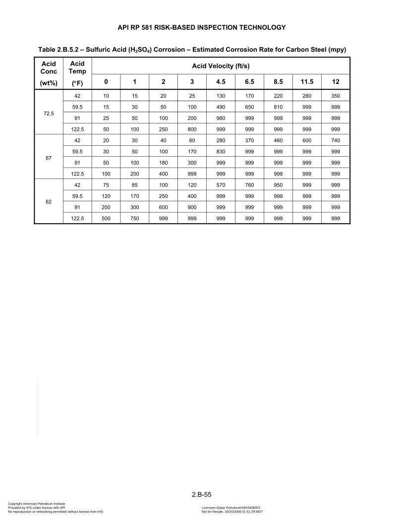
API RP 581 RISK-BASED INSPECTION TECHNOLOGY
Table 2.B.5.2 – Sulfuric Acid (H2SO4) Corrosion – Estimated Corrosion Rate for Carbon Steel (mpy)
Acid Conc
(wt%)
Acid Temp
(°F)
Acid Velocity (ft/s)
0 1 2 3 4.5 6.5 8.5 11.5 12
72.5
42 10 15 20 25 130 170 220 280 350
59.5 15 30 50 100 490 650 810 999 999
91 25 50 100 200 980 999 999 999 999
122.5 50 100 250 800 999 999 999 999 999
67
42 20 30 40 60 280 370 460 600 740
59.5 30 50 100 170 830 999 999 999 999
91 50 100 180 300 999 999 999 999 999
122.5 100 200 400 999 999 999 999 999 999
62
42 75 85 100 120 570 760 950 999 999
59.5 120 170 250 400 999 999 999 999 999
91 200 300 600 900 999 999 999 999 999
122.5 500 750 999 999 999 999 999 999 999
2.B-55 Copyright American Petroleum Institute Provided by IHS under license with API Licensee=Qatar Petroleum/5943408001
Not for Resale, 10/20/2008 01:51:29 MDTNo reproduction or networking permitted without license from IHS
--```,`,,`,`,,`,`,,,,,,``,```,`-`-`,,`,,`,`,,`---

API RP 581 RISK-BASED INSPECTION TECHNOLOGY
Table 2.B.5.2M – Sulfuric Acid (H2SO4) Corrosion – Estimated Corrosion Rate for Carbon Steel (mm/y)
Acid Conc
(wt%)
Acid Temp
(°C)
Acid Velocity (m/s)
0 1 2 3 4.5 6.5 8.5 11.5 12
100
6 0.13 0.18 0.23 0.3 1.14 1.52 1.91 2.41 3.05
15 0.3 0.36 0.43 0.51 1.65 2.16 2.79 3.56 4.32
33 1.27 1.4 1.52 1.78 6.86 9.14 11.43 14.73 18.29
50 2.54 3.81 5.08 7.62 25.37 25.37 25.37 25.37 25.37
98
6 0.1 0.15 0.2 0.25 0.89 1.14 1.52 1.91 2.29
15 0.13 0.25 0.38 0.51 2.03 2.79 3.56 4.57 5.59
33 0.38 0.64 1.02 1.52 7.37 9.91 12.45 16.26 19.81
50 1.02 2.03 3.05 6.35 25.37 25.37 25.37 25.37 25.37
96
6 0.2 0.25 0.3 0.38 1.52 2.03 2.79 3.3 4.06
15 0.38 0.51 0.64 1.02 4.32 5.59 6.86 8.89 10.92
33 0.64 1.02 1.52 2.54 12.7 16.51 20.83 25.37 25.37
50 1.27 2.54 5.08 12.7 25.37 25.37 25.37 25.37 25.37
93.5
6 0.25 0.38 0.51 0.64 3.05 4.06 5.08 6.6 8.38
15 0.51 0.64 1.02 1.78 8.64 11.43 14.48 18.8 23.11
33 0.76 1.02 1.91 3.3 16.26 21.59 25.37 25.37 25.37
50 1.52 3.05 6.35 15.24 25.37 25.37 25.37 25.37 25.37
91
6 0.38 0.64 1.14 1.78 8.13 10.92 13.72 18.03 22.1
15 0.64 1.02 2.03 3.05 17.78 23.88 25.37 25.37 25.37
33 0.89 1.52 2.54 5.08 23.88 25.37 25.37 25.37 25.37
50 1.78 3.81 7.62 20.32 25.37 25.37 25.37 25.37 25.37
87
6 0.51 0.76 1.27 2.03 9.65 12.7 16 20.57 25.37
15 0.76 4.06 7.62 10.67 17.53 23.37 25.37 25.37 25.37
33 1.14 11.43 21.59 25.37 25.37 25.37 25.37 25.37 25.37
50 2.03 25.37 25.37 25.37 25.37 25.37 25.37 25.37 25.37
83
6 0.51 0.64 0.89 1.14 5.33 7.11 8.89 11.68 14.48
15 0.76 1.27 2.54 3.81 17.27 23.11 25.37 25.37 25.37
33 1.02 2.54 5.08 10.16 25.37 25.37 25.37 25.37 25.37
50 2.03 5.08 10.16 25.37 25.37 25.37 25.37 25.37 25.37
78
6 0.38 0.51 0.51 0.64 2.79 3.81 4.83 6.35 7.62
15 0.51 1.02 1.78 3.05 14.48 19.3 24.13 25.37 25.37
33 0.76 1.52 3.05 6.35 25.37 25.37 25.37 25.37 25.37
50 1.52 3.05 7.62 22.86 25.37 25.37 25.37 25.37 25.37
2.B-56 Copyright American Petroleum Institute Provided by IHS under license with API Licensee=Qatar Petroleum/5943408001
Not for Resale, 10/20/2008 01:51:29 MDTNo reproduction or networking permitted without license from IHS
--```,`,,`,`,,`,`,,,,,,``,```,`-`-`,,`,,`,`,,`---

API RP 581 RISK-BASED INSPECTION TECHNOLOGY
Table 2.B.5.2M – Sulfuric Acid (H2SO4) Corrosion – Estimated Corrosion Rate for Carbon Steel (mm/y)
Acid Conc
(wt%)
Acid Temp
(°C)
Acid Velocity (m/s)
0 1 2 3 4.5 6.5 8.5 11.5 12
72.5
6 0.25 0.38 0.51 0.64 3.3 4.32 5.59 7.11 8.89
15 0.38 0.76 1.27 2.54 12.45 16.51 20.57 25.37 25.37
33 0.64 1.27 2.54 5.08 24.89 25.37 25.37 25.37 25.37
50 1.27 2.54 6.35 20.32 25.37 25.37 25.37 25.37 25.37
67
6 0.51 0.76 1.02 1.52 7.11 9.4 11.68 15.24 18.8
15 0.76 1.27 2.54 4.32 21.08 25.37 25.37 25.37 25.37
33 1.27 2.54 4.57 7.62 25.37 25.37 25.37 25.37 25.37
50 2.54 5.08 10.16 25.37 25.37 25.37 25.37 25.37 25.37
62
6 1.91 2.16 2.54 3.05 14.48 19.3 24.13 25.37 25.37
15 3.05 4.32 6.35 10.16 25.37 25.37 25.37 25.37 25.37
33 5.08 7.62 15.24 22.86 25.37 25.37 25.37 25.37 25.37
50 12.7 19.05 25.37 25.37 25.37 25.37 25.37 25.37 25.37
2.B-57 Copyright American Petroleum Institute Provided by IHS under license with API Licensee=Qatar Petroleum/5943408001
Not for Resale, 10/20/2008 01:51:29 MDTNo reproduction or networking permitted without license from IHS
--```,`,,`,`,,`,`,,,,,,``,```,`-`-`,,`,,`,`,,`---

API RP 581 RISK-BASED INSPECTION TECHNOLOGY
Table 2.B.5.3 – Sulfuric Acid (H2SO4) Corrosion – Estimated Corrosion Rates for Type 304 SS (mpy)
Acid
Concentration
(wt%)
Temperature
86°F 104.5°F 140.5°F
2
ft/s
6
ft/s
7
ft/s
2
ft/s
6
ft/s
7
ft/s
2
ft/s
6
ft/s
7
ft/s
98 5 10 15 20 40 60 200 400 600
92.5 20 40 60 40 80 120 500 999 999
87 40 80 120 80 160 240 999 999 999
82 100 200 300 500 999 999 999 999 999
75 500 999 999 999 999 99 999 999 999
65 999 999 999 999 999 999 999 999 999
50 999 999 999 999 999 999 999 999 999
30 999 999 999 999 999 999 999 999 999
15 400 800 999 999 999 999 999 999 999
8 200 400 600 800 999 999 999 999 999
3.5 50 100 150 200 400 600 500 999 999
2 20 40 60 70 140 210 200 400 600
2.B-58 Copyright American Petroleum Institute Provided by IHS under license with API Licensee=Qatar Petroleum/5943408001
Not for Resale, 10/20/2008 01:51:29 MDTNo reproduction or networking permitted without license from IHS
--```,`,,`,`,,`,`,,,,,,``,```,`-`-`,,`,,`,`,,`---
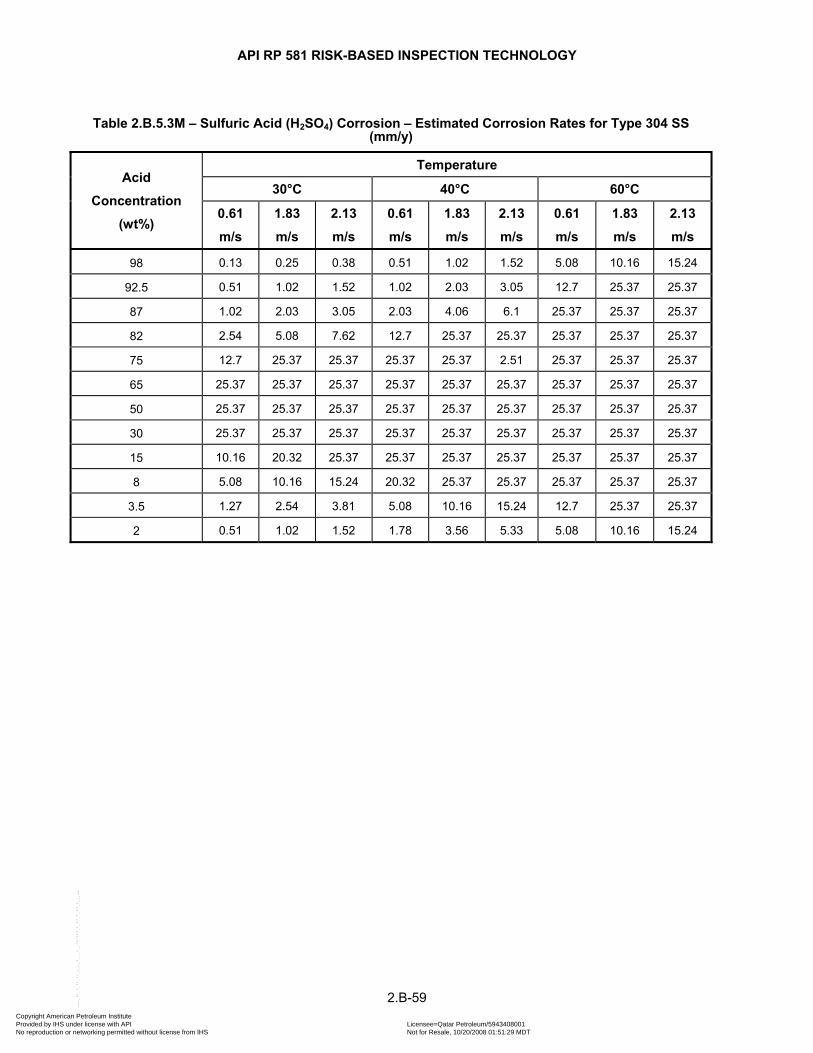
API RP 581 RISK-BASED INSPECTION TECHNOLOGY
Table 2.B.5.3M – Sulfuric Acid (H2SO4) Corrosion – Estimated Corrosion Rates for Type 304 SS (mm/y)
Acid
Concentration
(wt%)
Temperature
30°C 40°C 60°C
0.61
m/s
1.83
m/s
2.13
m/s
0.61
m/s
1.83
m/s
2.13
m/s
0.61
m/s
1.83
m/s
2.13
m/s
98 0.13 0.25 0.38 0.51 1.02 1.52 5.08 10.16 15.24
92.5 0.51 1.02 1.52 1.02 2.03 3.05 12.7 25.37 25.37
87 1.02 2.03 3.05 2.03 4.06 6.1 25.37 25.37 25.37
82 2.54 5.08 7.62 12.7 25.37 25.37 25.37 25.37 25.37
75 12.7 25.37 25.37 25.37 25.37 2.51 25.37 25.37 25.37
65 25.37 25.37 25.37 25.37 25.37 25.37 25.37 25.37 25.37
50 25.37 25.37 25.37 25.37 25.37 25.37 25.37 25.37 25.37
30 25.37 25.37 25.37 25.37 25.37 25.37 25.37 25.37 25.37
15 10.16 20.32 25.37 25.37 25.37 25.37 25.37 25.37 25.37
8 5.08 10.16 15.24 20.32 25.37 25.37 25.37 25.37 25.37
3.5 1.27 2.54 3.81 5.08 10.16 15.24 12.7 25.37 25.37
2 0.51 1.02 1.52 1.78 3.56 5.33 5.08 10.16 15.24
2.B-59 Copyright American Petroleum Institute Provided by IHS under license with API Licensee=Qatar Petroleum/5943408001
Not for Resale, 10/20/2008 01:51:29 MDTNo reproduction or networking permitted without license from IHS
--```,`,,`,`,,`,`,,,,,,``,```,`-`-`,,`,,`,`,,`---
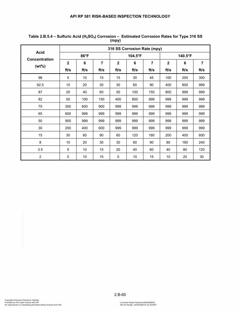
API RP 581 RISK-BASED INSPECTION TECHNOLOGY
Table 2.B.5.4 – Sulfuric Acid (H2SO4) Corrosion – Estimated Corrosion Rates for Type 316 SS (mpy)
Acid
Concentration
(wt%)
316 SS Corrosion Rate (mpy)
86°F 104.5°F 140.5°F
2
ft/s
6
ft/s
7
ft/s
2
ft/s
6
ft/s
7
ft/s
2
ft/s
6
ft/s
7
ft/s
98 5 10 15 15 30 45 100 200 300
92.5 10 20 30 30 60 90 400 800 999
87 20 40 60 50 100 150 800 999 999
82 50 100 150 400 800 999 999 999 999
75 300 600 900 999 999 999 999 999 999
65 600 999 999 999 999 999 999 999 999
50 900 999 999 999 999 999 999 999 999
30 200 400 600 999 999 999 999 999 999
15 30 60 90 60 120 180 200 400 600
8 10 20 30 30 60 90 80 160 240
3.5 5 10 15 20 40 60 40 80 120
2 5 10 15 5 10 15 10 20 30
2.B-60 Copyright American Petroleum Institute Provided by IHS under license with API Licensee=Qatar Petroleum/5943408001
Not for Resale, 10/20/2008 01:51:29 MDTNo reproduction or networking permitted without license from IHS
--```,`,,`,`,,`,`,,,,,,``,```,`-`-`,,`,,`,`,,`---

API RP 581 RISK-BASED INSPECTION TECHNOLOGY
Table2.B.5.4M – Sulfuric Acid (H2SO4) Corrosion – Estimated Corrosion Rates for Type 316 SS (mm/y)
Acid
Concentration
(wt%)
Temperature
30°C 40°C 60°C
0.61
m/s
1.83
m/s
2.13
m/s
0.61
m/s
1.83
m/s
2.13
m/s
0.61
m/s
1.83
m/s
2.13
m/s
98 0.13 0.25 0.38 0.38 0.76 1.14 2.54 5.08 7.62
92.5 0.25 0.51 0.76 0.76 1.52 2.29 10.16 20.32 25.37
87 0.51 1.02 1.52 1.27 2.54 3.81 20.32 25.37 25.37
82 1.27 2.54 3.81 10.16 20.32 25.37 25.37 25.37 25.37
75 7.62 15.24 22.86 25.37 25.37 25.37 25.37 25.37 25.37
65 15.24 25.37 25.37 25.37 25.37 25.37 25.37 25.37 25.37
50 22.86 25.37 25.37 25.37 25.37 25.37 25.37 25.37 25.37
30 5.08 10.16 15.24 25.37 25.37 25.37 25.37 25.37 25.37
15 0.76 1.52 2.29 1.52 3.05 4.57 5.08 10.16 15.24
8 0.25 0.51 0.76 0.76 1.52 2.29 2.03 4.06 6.1
3.5 0.13 0.25 0.38 0.51 1.02 1.52 1.02 2.03 3.05
2 0.13 0.25 0.38 0.13 0.25 0.38 0.25 0.51 0.76
2.B-61 Copyright American Petroleum Institute Provided by IHS under license with API Licensee=Qatar Petroleum/5943408001
Not for Resale, 10/20/2008 01:51:29 MDTNo reproduction or networking permitted without license from IHS
--```,`,,`,`,,`,`,,,,,,``,```,`-`-`,,`,,`,`,,`---
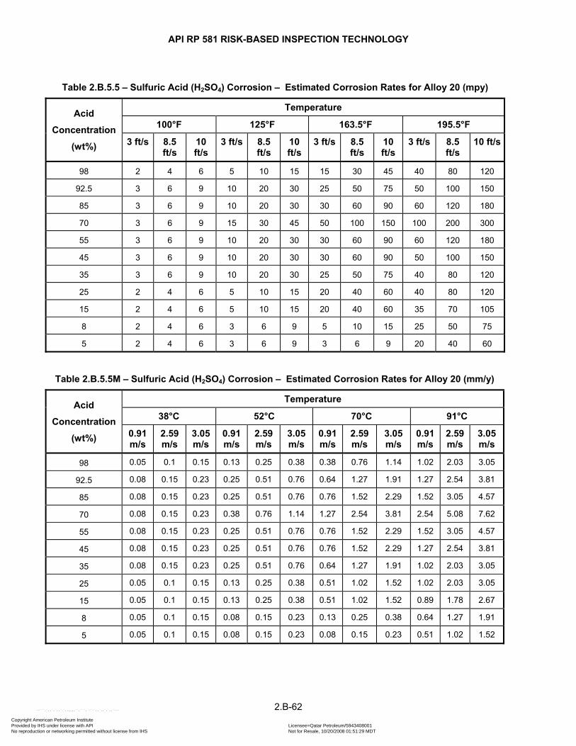
API RP 581 RISK-BASED INSPECTION TECHNOLOGY
Table 2.B.5.5 – Sulfuric Acid (H2SO4) Corrosion – Estimated Corrosion Rates for Alloy 20 (mpy)
Acid
Concentration
(wt%)
Temperature
100°F 125°F 163.5°F 195.5°F
3 ft/s 8.5 ft/s
10 ft/s
3 ft/s 8.5 ft/s
10 ft/s
3 ft/s 8.5 ft/s
10 ft/s
3 ft/s 8.5 ft/s
10 ft/s
98 2 4 6 5 10 15 15 30 45 40 80 120
92.5 3 6 9 10 20 30 25 50 75 50 100 150
85 3 6 9 10 20 30 30 60 90 60 120 180
70 3 6 9 15 30 45 50 100 150 100 200 300
55 3 6 9 10 20 30 30 60 90 60 120 180
45 3 6 9 10 20 30 30 60 90 50 100 150
35 3 6 9 10 20 30 25 50 75 40 80 120
25 2 4 6 5 10 15 20 40 60 40 80 120
15 2 4 6 5 10 15 20 40 60 35 70 105
8 2 4 6 3 6 9 5 10 15 25 50 75
5 2 4 6 3 6 9 3 6 9 20 40 60
Table 2.B.5.5M – Sulfuric Acid (H2SO4) Corrosion – Estimated Corrosion Rates for Alloy 20 (mm/y)
Acid
Concentration
(wt%)
Temperature
38°C 52°C 70°C 91°C
0.91 m/s
2.59 m/s
3.05 m/s
0.91 m/s
2.59 m/s
3.05 m/s
0.91 m/s
2.59 m/s
3.05 m/s
0.91 m/s
2.59 m/s
3.05 m/s
98 0.05 0.1 0.15 0.13 0.25 0.38 0.38 0.76 1.14 1.02 2.03 3.05
92.5 0.08 0.15 0.23 0.25 0.51 0.76 0.64 1.27 1.91 1.27 2.54 3.81
85 0.08 0.15 0.23 0.25 0.51 0.76 0.76 1.52 2.29 1.52 3.05 4.57
70 0.08 0.15 0.23 0.38 0.76 1.14 1.27 2.54 3.81 2.54 5.08 7.62
55 0.08 0.15 0.23 0.25 0.51 0.76 0.76 1.52 2.29 1.52 3.05 4.57
45 0.08 0.15 0.23 0.25 0.51 0.76 0.76 1.52 2.29 1.27 2.54 3.81
35 0.08 0.15 0.23 0.25 0.51 0.76 0.64 1.27 1.91 1.02 2.03 3.05
25 0.05 0.1 0.15 0.13 0.25 0.38 0.51 1.02 1.52 1.02 2.03 3.05
15 0.05 0.1 0.15 0.13 0.25 0.38 0.51 1.02 1.52 0.89 1.78 2.67
8 0.05 0.1 0.15 0.08 0.15 0.23 0.13 0.25 0.38 0.64 1.27 1.91
5 0.05 0.1 0.15 0.08 0.15 0.23 0.08 0.15 0.23 0.51 1.02 1.52
2.B-62 Copyright American Petroleum Institute Provided by IHS under license with API Licensee=Qatar Petroleum/5943408001
Not for Resale, 10/20/2008 01:51:29 MDTNo reproduction or networking permitted without license from IHS
--```,`,,`,`,,`,`,,,,,,``,```,`-`-`,,`,,`,`,,`---

API RP 581 RISK-BASED INSPECTION TECHNOLOGY
Table 2.B.5.6 – Sulfuric Acid (H2SO4) Corrosion – Estimated Corrosion Rates for Alloy C-276 (mpy)
Acid
Concentration
(wt%)
Temperature
125°F 137.5°F 162.5°F 187.5°F
3 ft/s 8.5 ft/s
10 ft/s
3 ft/s 8.5 ft/s
10 ft/s
3 ft/s 8.5 ft/s
10 ft/s
3 ft/s 8.5 ft/s
10 ft/s
98 3 6 9 4 8 12 5 10 15 20 40 60
92.5 4 8 12 5 10 15 20 40 60 50 100 150
85 5 10 15 10 20 30 20 40 60 60 120 180
75 5 10 15 10 20 30 20 40 60 50 100 150
55 5 10 15 10 20 30 15 30 45 40 80 120
20 4 8 12 5 10 15 15 30 45 40 80 120
8 4 8 12 5 10 15 10 20 30 30 60 90
5 3 6 9 4 8 12 5 10 15 15 30 45
Table 2.B.5.6M – Sulfuric Acid (H2SO4) Corrosion – Estimated Corrosion Rates for Alloy C-276 (mm/y)
Acid
Concentration
(wt%)
Temperature
52°C 59°C 73°C 86°C
0.91 m/s
2.59 m/s
3.05 m/s
0.91 m/s
2.59 m/s
3.05 m/s
0.91 m/s
2.59 m/s
3.05 m/s
0.91 m/s
2.59 m/s
3.05 m/s
98 0.08 0.15 0.23 0.1 0.2 0.3 0.13 0.25 0.38 0.51 1.02 1.52
92.5 0.1 0.2 0.3 0.13 0.25 0.38 0.51 1.02 1.52 1.27 2.54 3.81
85 0.13 0.25 0.38 0.25 0.51 0.76 0.51 1.02 1.52 1.52 3.05 4.57
75 0.13 0.25 0.38 0.25 0.51 0.76 0.51 1.02 1.52 1.27 2.54 3.81
55 0.13 0.25 0.38 0.25 0.51 0.76 0.38 0.76 1.14 1.02 2.03 3.05
20 0.1 0.2 0.3 0.13 0.25 0.38 0.38 0.76 1.14 1.02 2.03 3.05
8 0.1 0.2 0.3 0.13 0.25 0.38 0.25 0.51 0.76 0.76 1.52 2.29
5 0.08 0.15 0.23 0.1 0.2 0.3 0.13 0.25 0.38 0.38 0.76 1.14
2.B-63 Copyright American Petroleum Institute Provided by IHS under license with API Licensee=Qatar Petroleum/5943408001
Not for Resale, 10/20/2008 01:51:29 MDTNo reproduction or networking permitted without license from IHS
--```,`,,`,`,,`,`,,,,,,``,```,`-`-`,,`,,`,`,,`---
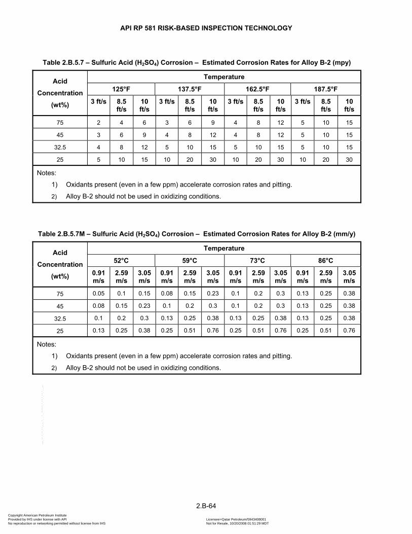
API RP 581 RISK-BASED INSPECTION TECHNOLOGY
Table 2.B.5.7 – Sulfuric Acid (H2SO4) Corrosion – Estimated Corrosion Rates for Alloy B-2 (mpy)
Acid
Concentration
(wt%)
Temperature
125°F 137.5°F 162.5°F 187.5°F
3 ft/s 8.5 ft/s
10 ft/s
3 ft/s 8.5 ft/s
10 ft/s
3 ft/s 8.5 ft/s
10 ft/s
3 ft/s 8.5 ft/s
10 ft/s
75 2 4 6 3 6 9 4 8 12 5 10 15
45 3 6 9 4 8 12 4 8 12 5 10 15
32.5 4 8 12 5 10 15 5 10 15 5 10 15
25 5 10 15 10 20 30 10 20 30 10 20 30
Notes:
1) Oxidants present (even in a few ppm) accelerate corrosion rates and pitting.
ons. 2) Alloy B-2 should not be used in oxidizing conditi
Table 2.B.5.7M – Sulfuric Acid (H2SO4) Corrosion – Estimated Corrosion Rates for Alloy B-2 (mm/y)
Acid
Concentration
(wt%)
Temperature
52°C 59°C 73°C 86°C
0.91 m/s
2.59 m/s
3.05 m/s
0.91 m/s
2.59 m/s
3.05 m/s
0.91 m/s
2.59 m/s
3.05 m/s
0.91 m/s
2.59 m/s
3.05 m/s
75 0.05 0.1 0.15 0.08 0.15 0.23 0.1 0.2 0.3 0.13 0.25 0.38
45 0.08 0.15 0.23 0.1 0.2 0.3 0.1 0.2 0.3 0.13 0.25 0.38
32.5 0.1 0.2 0.3 0.13 0.25 0.38 0.13 0.25 0.38 0.13 0.25 0.38
25 0.13 0.25 0.38 0.25 0.51 0.76 0.25 0.51 0.76 0.25 0.51 0.76
Notes:
1) Oxidants present (even in a few ppm) accelerate corrosion rates and pitting.
ions. 2) Alloy B-2 should not be used in oxidizing condit
2.B-64 Copyright American Petroleum Institute Provided by IHS under license with API Licensee=Qatar Petroleum/5943408001
Not for Resale, 10/20/2008 01:51:29 MDTNo reproduction or networking permitted without license from IHS
--```,`,,`,`,,`,`,,,,,,``,```,`-`-`,,`,,`,`,,`---
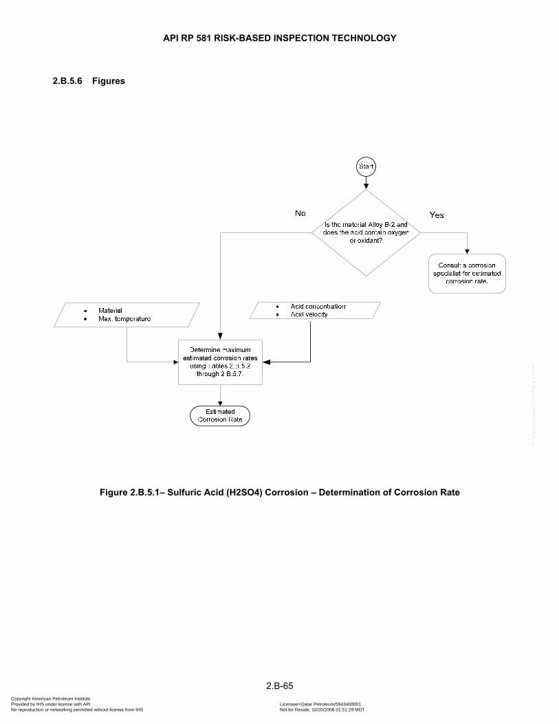
API RP 581 RISK-BASED INSPECTION TECHNOLOGY
2.B.5.6 Figures
Figure 2.B.5.1– Sulfuric Acid (H2SO4) Corrosion – Determination of Corrosion Rate
2.B-65 Copyright American Petroleum Institute Provided by IHS under license with API Licensee=Qatar Petroleum/5943408001
Not for Resale, 10/20/2008 01:51:29 MDTNo reproduction or networking permitted without license from IHS
--```,`,,`,`,,`,`,,,,,,``,```,`-`-`,,`,,`,`,,`---

API RP 581 RISK-BASED INSPECTION TECHNOLOGY
2.B.6 HYDROFLUORIC ACID (HF) CORROSION
2.B.6.1 Description of Damage
Concentrated hydrofluoric acid (HF) is used as the acid catalyst in HF alkylation units. The alkylation reaction chemically combines an alkane (usually isobutane) with an olefin (butylene, propylene, amylene) in the presence of the acid catalyst. HF presents severe health hazards as both a liquid and vapor. If spilled, HF may form a dense, low lying, toxic cloud. Extreme caution should be exercised when using HF.
Corrosion of materials in HF primarily depends on the HF-in-water concentration and the temperature. Other variables, such as velocity, turbulence, aeration, impurities, etc., can strongly influence corrosion. Some metals will form a protective fluoride film or scale which protects the surface. Loss of this protective film, especially through high velocity or turbulence, will likely result in greatly accelerated corrosion rates. Corrosion in 80% and stronger HF-in-water solutions is equivalent to corrosion in anhydrous hydrofluoric acid (AHF, 200 ppm H2O). Below 80% HF, the acid is considered aqueous and metal corrosion is highly temperature and velocity dependent and usually accelerated. The usual HF-in-water concentrations in typical HF alkylation units are 96%–99+% and the temperatures are generally below 66°C (150°F). Under these conditions carbon steel is widely used for all equipment except where close tolerances are required for operation (i.e., pumps, valves, instruments). Where close tolerances are required and at temperatures over 66°C (150°F) to approximately 149°C (300°F), Alloy 400 is typically used.
Accelerated corrosion from water dilution of the acid is often encountered in low points (bleeders, line pockets, etc.) if unit dry out leaves residual free water in these areas.
2.B.6.2 Basic Data
The data listed in Table 2.B.6.1 are required to determine the estimated corrosion rate for sulfuric acid service. If precise data have not been measured, a knowledgeable process specialist should be consulted.
2.B.6.3 Determination of Corrosion Rate
The steps required to determine the corrosion rate are shown in Figure 2.B.6.1. The corrosion rate may be determined using the basic data in Table 2.B.6.1 in conjunction with Tables 2.B.6.2 through 2.B.6.3.
It is important to note that the corrosion rate is very high in the initial stages of exposure to HF as the protective fluoride scale is being established. Once established, the fluoride scale protects the steel resulting in low corrosion rates unless the scale is disturbed or removed.
Alloy steels have been found to exhibit higher corrosion rates than mild carbon steel in both dilute and concentrated HF and generally are not specified for this service. Higher alloys are sometimes used in HF service and corrosion rates, if unknown, should be obtained from published literature or from the manufacturer [20]. It is important to consider the galvanic effects of welding carbon steel to Alloy 400 or other corrosion resistant alloys. Accelerated and localized attack of the carbon steel may result from galvanic coupling. Increased rates of corrosion have also been reported in carbon steels which contain high levels of residual elements, notably Cu, Ni, and Cr [ 22].
Corrosion caused by HF results in general thinning except in the event of potential galvanic attack. The presence of HF may also result in hydrogen stress cracking and blistering. These degradation modes are considered in Part 2, paragraph 14.1.
2.B-66 Copyright American Petroleum Institute Provided by IHS under license with API Licensee=Qatar Petroleum/5943408001
Not for Resale, 10/20/2008 01:51:29 MDTNo reproduction or networking permitted without license from IHS
--```,`,,`,`,,`,`,,,,,,``,```,`-`-`,,`,,`,`,,`---
API RP 581 RISK-BASED INSPECTION TECHNOLOGY
2.B.6.4 References
17. T. F. Degnan, Material of Construction for Hydrofluo-ric Acid and Hydrogen Fluoride, Process Industries Corrosion, NACE, Houston, TX 1986.
18. Materials for Receiving, Handling and Storing Hydro-fluoric Acid, NACE Publication 5A171 (1995 Revision). 19. Corrosion Resistance of Nickel-Containing Alloys in Hydrofluoric Acid, Hydrogen Fluoride and Fluorine,
Corrosion Engineering, Bulletin CEB-5, The International Nickel Co., Inc., 1968. 20. W. K. Blanchard and N.C. Mack, “Corrosion Results of Alloys and Welded Couples Over a Range of
Hydroflu-oric Acid Concentrations at 125°F,” NACE Paper 452, Corrosion/92. 21. J. Dobis, D. Clarida and J. Richert, “A Survey of Plant Practices and Experience in HF Alkylation Units,”
NACE Paper 511, Corrosion/94. 22. H. Hashim and W. Valerioti, “Effect of Residual Copper, Nickel, and Chromium on the Corrosion Resistance
of Carbon Steel in Hydrofluoric Acid Alkylation Service,” NACE Paper 623, Corrosion/93.
2.B-67 Copyright American Petroleum Institute Provided by IHS under license with API Licensee=Qatar Petroleum/5943408001
Not for Resale, 10/20/2008 01:51:29 MDTNo reproduction or networking permitted without license from IHS
--```,`,,`,`,,`,`,,,,,,``,```,`-`-`,,`,,`,`,,`---
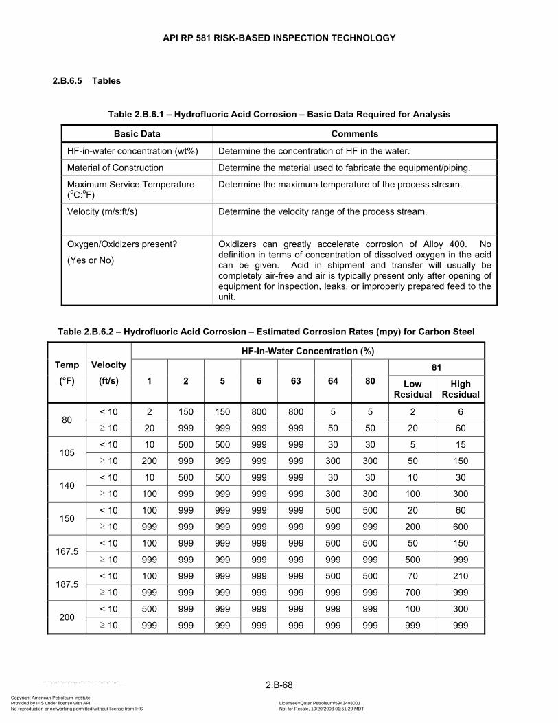
API RP 581 RISK-BASED INSPECTION TECHNOLOGY
2.B.6.5 Tables
Table 2.B.6.1 – Hydrofluoric Acid Corrosion – Basic Data Required for Analysis
Basic Data Comments
HF-in-water concentration (wt%) Determine the concentration of HF in the water.
Material of Construction Determine the material used to fabricate the equipment/piping.
Maximum Service Temperature (oC:oF)
Determine the maximum temperature of the process stream.
Velocity (m/s:ft/s)
Determine the velocity range of the process stream.
Oxygen/Oxidizers present?
(Yes or No)
Oxidizers can greatly accelerate corrosion of Alloy 400. No definition in terms of concentration of dissolved oxygen in the acid can be given. Acid in shipment and transfer will usually be completely air-free and air is typically present only after opening of equipment for inspection, leaks, or improperly prepared feed to the unit.
Table 2.B.6.2 – Hydrofluoric Acid Corrosion – Estimated Corrosion Rates (mpy) for Carbon Steel
Temp
(°F)
Velocity
(ft/s)
HF-in-Water Concentration (%)
1 2 5 6 63 64 80 81
Low Residual
High Residual
80 < 10 2 150 150 800 800 5 5 2 6
≥ 10 20 999 999 999 999 50 50 20 60
105 < 10 10 500 500 999 999 30 30 5 15
≥ 10 200 999 999 999 999 300 300 50 150
140 < 10 10 500 500 999 999 30 30 10 30
≥ 10 100 999 999 999 999 300 300 100 300
150 < 10 100 999 999 999 999 500 500 20 60
≥ 10 999 999 999 999 999 999 999 200 600
167.5 < 10 100 999 999 999 999 500 500 50 150
≥ 10 999 999 999 999 999 999 999 500 999
187.5 < 10 100 999 999 999 999 500 500 70 210
≥ 10 999 999 999 999 999 999 999 700 999
200 < 10 500 999 999 999 999 999 999 100 300
≥ 10 999 999 999 999 999 999 999 999 999
2.B-68 Copyright American Petroleum Institute Provided by IHS under license with API Licensee=Qatar Petroleum/5943408001
Not for Resale, 10/20/2008 01:51:29 MDTNo reproduction or networking permitted without license from IHS
--```,`,,`,`,,`,`,,,,,,``,```,`-`-`,,`,,`,`,,`---
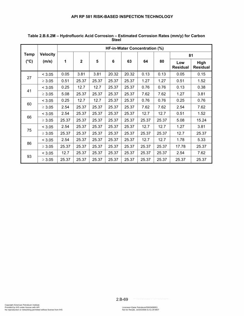
API RP 581 RISK-BASED INSPECTION TECHNOLOGY
Table 2.B.6.2M – Hydrofluoric Acid Corrosion – Estimated Corrosion Rates (mm/y) for Carbon Steel
Temp
(°C)
Velocity
(m/s)
HF-in-Water Concentration (%)
1 2 5 6 63 64 80 81
Low Residual
High Residual
27 < 3.05 0.05 3.81 3.81 20.32 20.32 0.13 0.13 0.05 0.15
≥ 3.05 0.51 25.37 25.37 25.37 25.37 1.27 1.27 0.51 1.52
41 < 3.05 0.25 12.7 12.7 25.37 25.37 0.76 0.76 0.13 0.38
≥ 3.05 5.08 25.37 25.37 25.37 25.37 7.62 7.62 1.27 3.81
60 < 3.05 0.25 12.7 12.7 25.37 25.37 0.76 0.76 0.25 0.76
≥ 3.05 2.54 25.37 25.37 25.37 25.37 7.62 7.62 2.54 7.62
66 < 3.05 2.54 25.37 25.37 25.37 25.37 12.7 12.7 0.51 1.52
≥ 3.05 25.37 25.37 25.37 25.37 25.37 25.37 25.37 5.08 15.24
75 < 3.05 2.54 25.37 25.37 25.37 25.37 12.7 12.7 1.27 3.81
≥ 3.05 25.37 25.37 25.37 25.37 25.37 25.37 25.37 12.7 25.37
86 < 3.05 2.54 25.37 25.37 25.37 25.37 12.7 12.7 1.78 5.33
≥ 3.05 25.37 25.37 25.37 25.37 25.37 25.37 25.37 17.78 25.37
93 < 3.05 12.7 25.37 25.37 25.37 25.37 25.37 25.37 2.54 7.62
≥ 3.05 25.37 25.37 25.37 25.37 25.37 25.37 25.37 25.37 25.37
2.B-69 Copyright American Petroleum Institute Provided by IHS under license with API Licensee=Qatar Petroleum/5943408001
Not for Resale, 10/20/2008 01:51:29 MDTNo reproduction or networking permitted without license from IHS
--```,`,,`,`,,`,`,,,,,,``,```,`-`-`,,`,,`,`,,`---
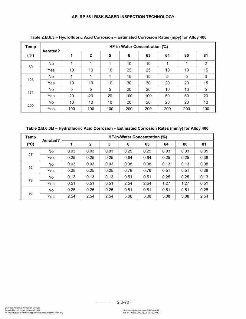
API RP 581 RISK-BASED INSPECTION TECHNOLOGY
Table 2.B.6.3 – Hydrofluoric Acid Corrosion – Estimated Corrosion Rates (mpy) for Alloy 400
Temp
(°F) Aerated?
HF-in-Water Concentration (%)
1 2 5 6 63 64 80 81
80 No 1 1 1 10 10 1 1 2 Yes 10 10 10 25 25 10 10 15
125 No 1 1 1 15 15 5 5 3 Yes 10 10 10 30 30 20 20 15
175 No 5 5 5 20 20 10 10 5 Yes 20 20 20 100 100 50 50 20
200 No 10 10 10 20 20 20 20 10 Yes 100 100 100 200 200 200 200 100
Table 2.B.6.3M – Hydrofluoric Acid Corrosion – Estimated Corrosion Rates (mm/y) for Alloy 400
Temp
(°C) Aerated?
HF-in-Water Concentration (%)
1 2 5 6 63 64 80 81
27 No 0.03 0.03 0.03 0.25 0.25 0.03 0.03 0.05
Yes 0.25 0.25 0.25 0.64 0.64 0.25 0.25 0.38
52 No 0.03 0.03 0.03 0.38 0.38 0.13 0.13 0.08
Yes 0.25 0.25 0.25 0.76 0.76 0.51 0.51 0.38
79 No 0.13 0.13 0.13 0.51 0.51 0.25 0.25 0.13
Yes 0.51 0.51 0.51 2.54 2.54 1.27 1.27 0.51
93 No 0.25 0.25 0.25 0.51 0.51 0.51 0.51 0.25
Yes 2.54 2.54 2.54 5.08 5.08 5.08 5.08 2.54
2.B-70 Copyright American Petroleum Institute Provided by IHS under license with API Licensee=Qatar Petroleum/5943408001
Not for Resale, 10/20/2008 01:51:29 MDTNo reproduction or networking permitted without license from IHS
--```,`,,`,`,,`,`,,,,,,``,```,`-`-`,,`,,`,`,,`---
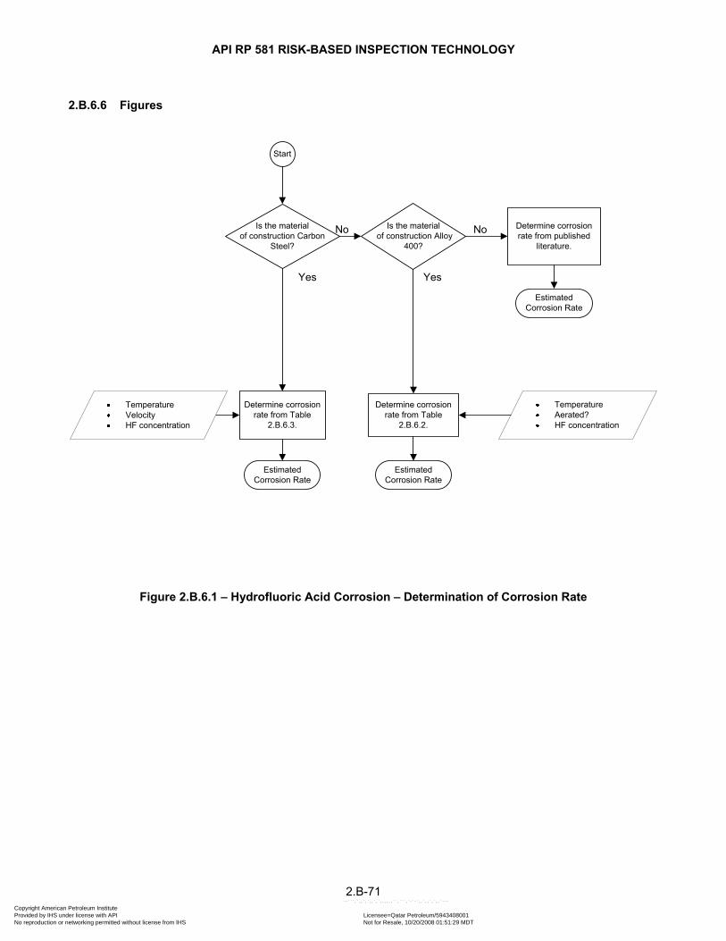
API RP 581 RISK-BASED INSPECTION TECHNOLOGY
2.B.6.6 Figures
Start
Is the material of construction Carbon
Steel?
Is the material of construction Alloy
400?
Determine corrosion rate from Table
2.B.6.3.
Determine corrosion rate from Table
2.B.6.2.
Determine corrosion rate from published
literature.
Estimated Corrosion Rate
Estimated Corrosion Rate
Estimated Corrosion Rate
Yes Yes
No No
TemperatureVelocityHF concentration
TemperatureAerated?HF concentration
Figure 2.B.6.1 – Hydrofluoric Acid Corrosion – Determination of Corrosion Rate
2.B-71 Copyright American Petroleum Institute Provided by IHS under license with API Licensee=Qatar Petroleum/5943408001
Not for Resale, 10/20/2008 01:51:29 MDTNo reproduction or networking permitted without license from IHS
--```,`,,`,`,,`,`,,,,,,``,```,`-`-`,,`,,`,`,,`---
API RP 581 RISK-BASED INSPECTION TECHNOLOGY
2.B.7 SOUR WATER CORROSION
2.B.7.1 Description of Damage
Sour water corrosion is broadly defined as corrosion by water containing hydrogen sulfide and ammonia, and it is typically a concern for carbon steel above neutral pH. This corrosion is caused by aqueous ammonium disulfide
(NH4HS) is also known as ammonium hydrosulfide. The primary variables which influence sour water corrosion rates are the NH4HS concentration of the water and the stream velocity. Secondary variables are the pH, cyanide, and oxygen contents of the water. Sour water corrosion is of concern across a broad range of the most common refining process units, notably hydrotreating, hydrocracking, coking, catalytic cracking, light ends, amine treating and sour water stripping. Hydrogen sulfide is typically formed by thermal or catalytic conversion of sulfur compounds. Ammonia is similarly formed from nitrogen compounds. To some extent, sour water corrosion can be of importance in crude distillation depending on water pH.
Below neutral pH, HCl is generally the controlling corrosion mechanism in crude distillation, naphtha hydrotreating, and catalytic reforming water condensates. Small amounts of ammonia may also be formed in some distillate hydrotreaters, depending on operating conditions.
2.B.7.2 Basic Data
The data listed in Table 2.B.7.1 are required to determine the estimated corrosion rate for sulfuric acid service. If precise data have not been measured, a knowledgeable process specialist should be consulted.
2.B.7.3 Determination of Corrosion Rate
The steps required to determine the corrosion rate are shown in Figure 2.B.7.1. The corrosion rate may be determined using the basic data in Table 2.B.7.1 in conjunction with Table 2.B.7.2.
2.B.7.4 References
23. R. L. Piehl, “Survey of Corrosion in Hydrocracker Effluent Air Coolers,” Materials Protection, January, 1976. 24. E. F. Ehmke, “Corrosion Correlation with Ammonia and Hydrogen Sulfide in Air Coolers,” Materials
Protection, July, 1975. 25. D. G. Damin and J. D. McCoy, “Prevention of Corrosion in Hydrodesulfurizer Air Coolers and Condensers,”
Materials Performance, December, 1978, pp. 23–26 (See also NACE Corrosion/78 paper #131). 26. C. Scherrer, M. Durrieu, and G. Jarno, “Distillate and Resid Hydroprocessing: Coping with High
Concentrations of Ammonium Bisulfide in the Process Water,” Materials Performance, November, 1980, pp 25–31 (See also NACE Corrosion/79 paper #27).
2.B-72 Copyright American Petroleum Institute Provided by IHS under license with API Licensee=Qatar Petroleum/5943408001
Not for Resale, 10/20/2008 01:51:29 MDTNo reproduction or networking permitted without license from IHS
--```,`,,`,`,,`,`,,,,,,``,```,`-`-`,,`,,`,`,,`---
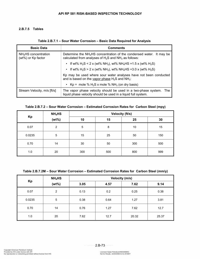
API RP 581 RISK-BASED INSPECTION TECHNOLOGY
2.B.7.5 Tables
Table 2.B.7.1 – Sour Water Corrosion – Basic Data Required for Analysis
Basic Data Comments
NH4HS concentration (wt%) or Kp factor
Determine the NH4HS concentration of the condensed water. It may be calculated from analyses of H2S and NH3 as follows:
• If wt% H2S < 2 x (wt% NH3), wt% NH4HS =1.5 x (wt% H2S)
• If wt% H2S > 2 x (wt% NH3), wt% NH4HS =3.0 x (wt% H2S)
Kp may be used where sour water analyses have not been conducted and is based on the vapor phase H2S and NH3:
• Kp = mole % H2S x mole % NH3 (on dry basis)
Stream Velocity, m/s [ft/s] The vapor phase velocity should be used in a two-phase system. The liquid phase velocity should be used in a liquid full system.
Table 2.B.7.2 – Sour Water Corrosion – Estimated Corrosion Rates for Carbon Steel (mpy)
Kp NH4HS
(wt%)
Velocity (ft/s)
10 15 25 30
0.07 2 5 8 10 15
0.0235 5 15 25 50 150
0.70 14 30 50 300 500
1.0 20 300 500 800 999
Table 2.B.7.2M – Sour Water Corrosion – Estimated Corrosion Rates for Carbon Steel (mm/y)
Kp NH4HS
(wt%)
Velocity (m/s)
3.05 4.57 7.62 9.14
0.07 2 0.13 0.2 0.25 0.38
0.0235 5 0.38 0.64 1.27 3.81
0.70 14 0.76 1.27 7.62 12.7
1.0 20 7.62 12.7 20.32 25.37
2.B-73 Copyright American Petroleum Institute Provided by IHS under license with API Licensee=Qatar Petroleum/5943408001
Not for Resale, 10/20/2008 01:51:29 MDTNo reproduction or networking permitted without license from IHS
--```,`,,`,`,,`,`,,,,,,``,```,`-`-`,,`,,`,`,,`---

API RP 581 RISK-BASED INSPECTION TECHNOLOGY
2.B.7.6 Figures
Start
Determine corrosion rate using Table
2.B.7.2.
Estimated corrosion rate
NH4HS Concentration or Kp FactorVelocity
Figure 2.B.7.1 – Sour Water Corrosion – Determination of Corrosion Rate
2.B-74 Copyright American Petroleum Institute Provided by IHS under license with API Licensee=Qatar Petroleum/5943408001
Not for Resale, 10/20/2008 01:51:29 MDTNo reproduction or networking permitted without license from IHS
--```,`,,`,`,,`,`,,,,,,``,```,`-`-`,,`,,`,`,,`---
API RP 581 RISK-BASED INSPECTION TECHNOLOGY
2.B.8 AMINE CORROSION
2.B.8.1 Description of Damage
Amine corrosion is a form of often-localized corrosion which occurs principally on carbon steel in some gas treating processes. Carbon steel is also vulnerable to stress corrosion cracking in gas treating amines if it is not postweld heat treated (see H.6). Gas treating amines fall into two major categories—chemical solvents and physical solvents. This supplement deals with corrosion in the most common chemical solvents, monoethanolamine (MEA), diethanolamine (DEA), and methyldiethanolamine (MDEA). These amines are used to remove acid gases, primarily H2S, from plant streams. MEA and DEA will also remove CO2, but MDEA is selective to H2S and will remove little CO2 if it is present. Generally, corrosion in MDEA is less than in MEA and DEA when contaminants are well controlled.
Carbon steel corrosion in amine treating processes is a function of a number of inter-related factors, the primary ones being the concentration of the amine solution, the acid gas content of the solution (“loading”), and the temperature. The most commonly used amine concentrations are 20 wt% MEA, 30 wt% DEA, and 40 to 50 wt% MDEA. At greater concentrations, corrosion rates increase.
Acid gas loading is reported in terms of moles of acid gas per mole of active amine. “Rich” solution is amine of higher acid gas loading and “lean” solution has lower acid gas loading (typically < 0.1 mole/mole). Corrosion in poorly regenerated amine with high lean loadings is not an uncommon problem, particularly because lean solution temperatures are often greater than rich solution temperatures. Both H2S and CO2 must be measured to determine the acid gas loading. In addition, only the amount of available or “active” amine should be considered when calculating the loading. In H2S only systems, rich amine loadings up to 0.70 mole/mole have been satisfactory. In H2S + CO2 systems, rich loading is often limited to 0.35 to 0.45 mole/mole. In MDEA units, and particularly those used for selective H2S removal in sulfur plant tail gas cleanup, rich loadings are often below these levels. As with most corrosion mechanisms, higher temperature increases the corrosion rate.
Another important factor in amine corrosion is the presence of amine degradation products, usually referred to as “Heat Stable Amine Salts” or HSAS. These amine degradation products act in two ways. On the one hand, they reduce the amount of active amine available to absorb acid gas, resulting in higher acid gas loadings. In addition, some amine degradation products themselves are corrosive. In MEA and DEA systems, heat stable amine salts above 0.5 wt% can begin to increase corrosion although a common operating limit is 2 wt%. Corrosion can be particularly significant, even at low acid gas loadings, at > 2.0 wt% HSAS. MDEA will also form heat stable amine salts, but the primary influence on corrosion in these units is organic acid contaminants (for-mate, oxalate, and acetate). Thermal reclaimers are often provided in MEA units to reduce HSAS, but DEA and MDEA salts are more stable and can not be thermally reclaimed. DEA degrades less readily than MEA and MDEA. Velocity or turbulence also influences amine corrosion. In the absence of high velocities and turbulence, amine corrosion can be fairly uniform. Higher velocities and turbulence can cause acid gas to evolve from solution, particularly at elbows and where pressure drops occur such as valves, resulting in more localized corrosion. Higher velocity and turbulence may also disrupt protective iron sulfide films that may form. Where velocity is a factor, corrosion may appear either as pitting or grooving. For carbon steel, common velocity limits are about 1.52 m/s (5 ft/s) for rich amine and about 6.01 m/s (20 ft/s) for lean amine.
Austenitic stainless steels are commonly used in areas which are corrosive to carbon steel with good success unless temperatures, amine concentration and degradation product levels are particularly high. Common applications for stainless steels are reboiler, reclaimer, and hot rich-lean exchanger tubes as well as pressure let-down valves and downstream piping/equipment. 12% Cr steels have been used for scrubber (absorber) tower internals successfully. Copper alloys are subject to accelerated corrosion and stress corrosion cracking and are normally avoided.
2.B.8.2 Basic Data
The data listed in Table 2.B.8.1 are required to determine the estimated corrosion rate for amine service. If precise data have not been measured, a knowledgeable process specialist should be consulted.
2.B-75 Copyright American Petroleum Institute Provided by IHS under license with API Licensee=Qatar Petroleum/5943408001
Not for Resale, 10/20/2008 01:51:29 MDTNo reproduction or networking permitted without license from IHS
--```,`,,`,`,,`,`,,,,,,``,```,`-`-`,,`,,`,`,,`---
API RP 581 RISK-BASED INSPECTION TECHNOLOGY
2.B.8.3 Determination of Corrosion Rate
The steps required to determine the corrosion rate are shown in Figure 2.B.8.1. The corrosion rate may be determined using the basic data in Table 2.B.8.1 in conjunction with Tables 2.B.8.2 through 2.B.8.5.
The estimated corrosion rate for carbon steel should be obtained from Table 2.B.8.2 for 20 wt% MEA and 30 wt% DEA and from Table 2.B.8.3 for 50 wt% MDEA. If higher amine concentrations are used, the corrosion rate obtained should be multiplied by the appropriate factor from Table 2.B.8.4.
The estimated corrosion rate for stainless steel may be obtained from Table 2.B.8.5. Note that at extreme conditions of amine concentrations, temperatures, and levels of degradation products, the corrosion rate of stainless steel can be as much as 200 times the value in the Table 2.B.8.5.
2.B.8.4 References
27. API RP 945, Avoiding Environmental Cracking in Amine Units, First Edition, August 1990, Appendix B – “Considerations for Corrosion Control”, American Petroleum Institute, Washington, D.C, 20005
28. L. Pearce, S. Grosso, D. C. Gringle, “Amine Gas Treating Solution Analysis a Tool in Problem Solving,” Presentation at the 59th Annual GPA Convention, March 17-19, 1990, Houston, TX.
29. P. Liebermann, “Amine Appearance Signals Condition of System,” Oil and Gas Journal, May 12, 1980, pp. 115.
30. M. S. DuPart, T. R. Bacon, and D. J. Edwards, “Understanding Corrosion in Alkanolamine Gas Treating Plants,” Hydrocarbon Processing, April 1993, pp. 75.
31. R. Abry and M. S. DuPart, “Amine Plant Troubleshooting and Optimization,” Hydrocarbon Processing, April 1995, pp. 41-50
32. H. L. Craig and B. D. McLaughlin, “Corrosive Amine Characterization,” NACE Paper No. 394, Corrosion/96. 33. R. Hays, and C. J. Schulz, “Corrosion and Fouling of a Refinery MDEA System,” NACE Paper No. 447,
Corrosion/92. 34. A. Keller, B. Scott, D. Tunnell, E. Wagner, and M. Zacher, “How Efficient are Refinery Amine Units?,”
Hydrocarbon Processing, April 1995, pp. 91-92. 35. C. Rooney, T. R. Bacon, and M. S. DuPart, “Effect of Heat Stable Salts on MDEA Solution Corrosivity,”
Hydrocarbon Processing, March 1996, pp. 95. 36. G. McCullough and R. B. Nielsen, “Contamination and Purification of Alkaline Gas Treating Solutions,”
NACE Paper No. 396, Corrosion/96. 37. M.J. Litschewski, “More Experiences With Corrosion and Fouling in a Refinery Amine System,” NACE Paper
No. 391, Corrosion/96.
2.B-76 Copyright American Petroleum Institute Provided by IHS under license with API Licensee=Qatar Petroleum/5943408001
Not for Resale, 10/20/2008 01:51:29 MDTNo reproduction or networking permitted without license from IHS
--```,`,,`,`,,`,`,,,,,,``,```,`-`-`,,`,,`,`,,`---

API RP 581 RISK-BASED INSPECTION TECHNOLOGY
2.B.8.5 Tables
Table 2.B.8.1 – Amine Corrosion – Basic Data Required for Analysis
Basic Data Comments
Material of Construction
(CS or SS) Determine the material of construction of equipment/piping.
Amine Concentration (wt%)
Determine the amine concentration in the equipment/piping. Due to vaporization of water, a local increase in amine concentration may need to be considered in evaluating the corrosion of some reboilers and reclaimers.
Maximum Process Temperature
(°C :°F)
Determine the maximum process temperature. In reboilers and reclaimers, tube metal temperatures may be higher than the bulk process temperature.
Acid Gas Loading
(mole acid gas/mole active amine)
Determine the acid gas loading in the amine. If analytical results are not available, it should be estimated by a knowledgeable process engineer.
Velocity (m/s:ft/s) Determine the maximum velocity of the amine in this equipment/piping.
Heat Stable Amine Salt (HSAS) Concentration:
MEA and DEA
( 2 wt%, 2-4 wt%, > 4 wt%) ≤In MEA and DEA, “HSAS” represents the normal family of amine degradation products
MDEA
(<500, 500-4000, >4000, wppm) In MDEA “HSAS” refers to organic acid contaminants, mainly formate, oxalate, and acetate
2.B-77 Copyright American Petroleum Institute Provided by IHS under license with API Licensee=Qatar Petroleum/5943408001
Not for Resale, 10/20/2008 01:51:29 MDTNo reproduction or networking permitted without license from IHS
--```,`,,`,`,,`,`,,,,,,``,```,`-`-`,,`,,`,`,,`---
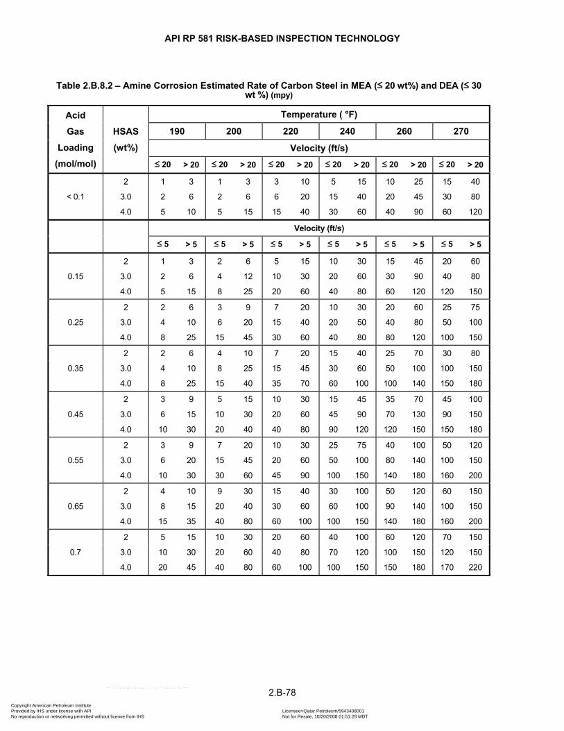
API RP 581 RISK-BASED INSPECTION TECHNOLOGY
Table 2.B.8.2 – Amine Corrosion Estimated Rate of Carbon Steel in MEA (≤ 20 wt%) and DEA (≤ 30 wt %) (mpy)
Acid
Gas
Loading
(mol/mol)
HSAS
(wt%)
Temperature ( °F)
190 200 220 240 260 270
Velocity (ft/s) ≤ 20 > 20 ≤ 20 > 20 ≤ 20 > 20 ≤ 20 > 20 ≤ 20 > 20 ≤ 20 > 20
< 0.1
2 1 3 1 3 3 10 5 15 10 25 15 40
3.0 2 6 2 6 6 20 15 40 20 45 30 80
4.0 5 10 5 15 15 40 30 60 40 90 60 120
Velocity (ft/s)
≤ 5 > 5 ≤ 5 > 5 ≤ 5 > 5 ≤ 5 > 5 ≤ 5 > 5 ≤ 5 > 5
0.15
2 1 3 2 6 5 15 10 30 15 45 20 60
3.0 2 6 4 12 10 30 20 60 30 90 40 80
4.0 5 15 8 25 20 60 40 80 60 120 120 150
0.25
2 2 6 3 9 7 20 10 30 20 60 25 75
3.0 4 10 6 20 15 40 20 50 40 80 50 100
4.0 8 25 15 45 30 60 40 80 80 120 100 150
0.35
2 2 6 4 10 7 20 15 40 25 70 30 80
3.0 4 10 8 25 15 45 30 60 50 100 100 150
4.0 8 25 15 40 35 70 60 100 100 140 150 180
0.45
2 3 9 5 15 10 30 15 45 35 70 45 100
3.0 6 15 10 30 20 60 45 90 70 130 90 150
4.0 10 30 20 40 40 80 90 120 120 150 150 180
0.55
2 3 9 7 20 10 30 25 75 40 100 50 120
3.0 6 20 15 45 20 60 50 100 80 140 100 150
4.0 10 30 30 60 45 90 100 150 140 180 160 200
0.65
2 4 10 9 30 15 40 30 100 50 120 60 150
3.0 8 15 20 40 30 60 60 100 90 140 100 150
4.0 15 35 40 80 60 100 100 150 140 180 160 200
0.7
2 5 15 10 30 20 60 40 100 60 120 70 150
3.0 10 30 20 60 40 80 70 120 100 150 120 150
4.0 20 45 40 80 60 100 100 150 150 180 170 220
2.B-78 Copyright American Petroleum Institute Provided by IHS under license with API Licensee=Qatar Petroleum/5943408001
Not for Resale, 10/20/2008 01:51:29 MDTNo reproduction or networking permitted without license from IHS
--```,`,,`,`,,`,`,,,,,,``,```,`-`-`,,`,,`,`,,`---
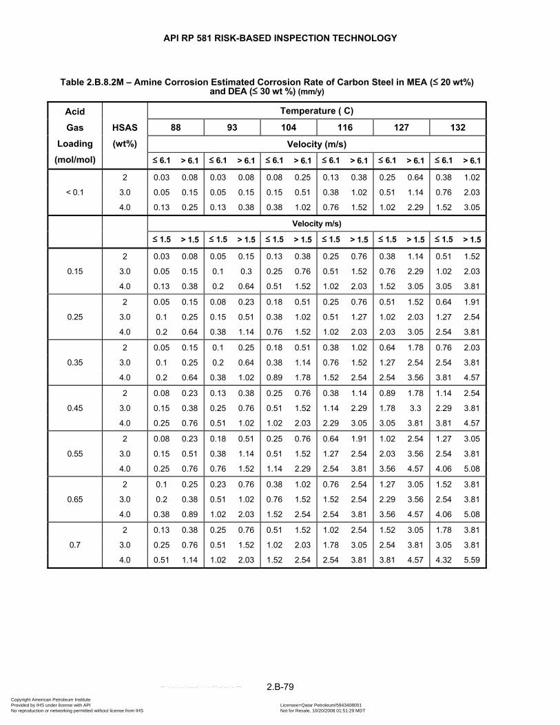
API RP 581 RISK-BASED INSPECTION TECHNOLOGY
Table 2.B.8.2M – Amine Corrosion Estimated Corrosion Rate of Carbon Steel in MEA (≤ 20 wt%) and DEA (≤ 30 wt %) (mm/y)
Acid
Gas
Loading
(mol/mol)
HSAS
(wt%)
Temperature ( C)
88 93 104 116 127 132
Velocity (m/s) ≤ 6.1 > 6.1 ≤ 6.1 > 6.1 ≤ 6.1 > 6.1 ≤ 6.1 > 6.1 ≤ 6.1 > 6.1 ≤ 6.1 > 6.1
< 0.1
2 0.03 0.08 0.03 0.08 0.08 0.25 0.13 0.38 0.25 0.64 0.38 1.02
3.0 0.05 0.15 0.05 0.15 0.15 0.51 0.38 1.02 0.51 1.14 0.76 2.03
4.0 0.13 0.25 0.13 0.38 0.38 1.02 0.76 1.52 1.02 2.29 1.52 3.05
Velocity m/s)
≤ 1.5 > 1.5 ≤ 1.5 > 1.5 ≤ 1.5 > 1.5 ≤ 1.5 > 1.5 ≤ 1.5 > 1.5 ≤ 1.5 > 1.5
0.15
2 0.03 0.08 0.05 0.15 0.13 0.38 0.25 0.76 0.38 1.14 0.51 1.52
3.0 0.05 0.15 0.1 0.3 0.25 0.76 0.51 1.52 0.76 2.29 1.02 2.03
4.0 0.13 0.38 0.2 0.64 0.51 1.52 1.02 2.03 1.52 3.05 3.05 3.81
0.25
2 0.05 0.15 0.08 0.23 0.18 0.51 0.25 0.76 0.51 1.52 0.64 1.91
3.0 0.1 0.25 0.15 0.51 0.38 1.02 0.51 1.27 1.02 2.03 1.27 2.54
4.0 0.2 0.64 0.38 1.14 0.76 1.52 1.02 2.03 2.03 3.05 2.54 3.81
0.35
2 0.05 0.15 0.1 0.25 0.18 0.51 0.38 1.02 0.64 1.78 0.76 2.03
3.0 0.1 0.25 0.2 0.64 0.38 1.14 0.76 1.52 1.27 2.54 2.54 3.81
4.0 0.2 0.64 0.38 1.02 0.89 1.78 1.52 2.54 2.54 3.56 3.81 4.57
0.45
2 0.08 0.23 0.13 0.38 0.25 0.76 0.38 1.14 0.89 1.78 1.14 2.54
3.0 0.15 0.38 0.25 0.76 0.51 1.52 1.14 2.29 1.78 3.3 2.29 3.81
4.0 0.25 0.76 0.51 1.02 1.02 2.03 2.29 3.05 3.05 3.81 3.81 4.57
0.55
2 0.08 0.23 0.18 0.51 0.25 0.76 0.64 1.91 1.02 2.54 1.27 3.05
3.0 0.15 0.51 0.38 1.14 0.51 1.52 1.27 2.54 2.03 3.56 2.54 3.81
4.0 0.25 0.76 0.76 1.52 1.14 2.29 2.54 3.81 3.56 4.57 4.06 5.08
0.65
2 0.1 0.25 0.23 0.76 0.38 1.02 0.76 2.54 1.27 3.05 1.52 3.81
3.0 0.2 0.38 0.51 1.02 0.76 1.52 1.52 2.54 2.29 3.56 2.54 3.81
4.0 0.38 0.89 1.02 2.03 1.52 2.54 2.54 3.81 3.56 4.57 4.06 5.08
0.7
2 0.13 0.38 0.25 0.76 0.51 1.52 1.02 2.54 1.52 3.05 1.78 3.81
3.0 0.25 0.76 0.51 1.52 1.02 2.03 1.78 3.05 2.54 3.81 3.05 3.81
4.0 0.51 1.14 1.02 2.03 1.52 2.54 2.54 3.81 3.81 4.57 4.32 5.59
2.B-79 Copyright American Petroleum Institute Provided by IHS under license with API Licensee=Qatar Petroleum/5943408001
Not for Resale, 10/20/2008 01:51:29 MDTNo reproduction or networking permitted without license from IHS
--```,`,,`,`,,`,`,,,,,,``,```,`-`-`,,`,,`,`,,`---

API RP 581 RISK-BASED INSPECTION TECHNOLOGY
Table 2.B.8.3 – Amine Corrosion Estimated Corrosion Rate of Carbon Steel in MDEA (≤ 50 wt%) (mpy)
Acid
Gas
Loading
(mol/mol)
HSAS
(wt%)
Temperature ( F)
190 200 220 240 260 270
Velocity (ft/s) ≤ 20 > 20 ≤ 20 > 20 ≤ 20 > 20 ≤ 20 > 20 ≤ 20 > 20 ≤ 20 > 20
< 0.1
0.5 1 3 1 3 3 10 5 15 10 25 15 40
2.25 2 6 2 6 6 20 15 40 20 45 30 80
4.0 5 10 5 15 15 40 30 60 40 90 60 120
Velocity (ft/s)
≤ 5 > 5 ≤ 5 > 5 ≤ 5 > 5 ≤ 5 > 5 ≤ 5 > 5 ≤ 5 > 5
0.15
0.5 1 3 2 6 5 15 10 30 15 45 20 60
2.25 2 6 4 12 10 30 20 60 30 90 40 80
4.0 5 15 8 25 20 60 40 80 60 120 120 150
0.25
0.5 2 6 3 9 7 20 10 30 20 60 25 75
2.25 4 10 6 20 15 40 20 50 40 80 50 100
4.0 8 25 15 45 30 60 40 80 80 120 100 150
0.35
0.5 2 6 4 10 7 20 15 40 25 70 30 80
2.25 4 10 8 25 15 45 30 60 50 100 100 150
4.0 8 25 15 40 35 70 60 100 100 140 150 180
0.45
0.5 3 9 5 15 10 30 15 45 35 70 45 100
2.25 6 15 10 30 20 60 45 90 70 130 90 150
4.0 10 30 20 40 40 80 90 120 120 150 150 180
0.55
0.5 3 9 7 20 10 30 25 75 40 100 50 120
2.25 6 20 15 45 20 60 50 100 80 140 100 150
4.0 10 30 30 60 45 90 100 150 140 180 160 200
0.65
0.5 4 10 9 30 15 40 30 100 50 120 60 150
2.25 8 15 20 40 30 60 60 100 90 140 100 150
4.0 15 35 40 80 60 100 100 150 140 180 160 200
0.7
0.5 5 15 10 30 20 60 40 100 60 120 70 150
2.25 10 30 20 60 40 80 70 120 100 150 120 150
4.0 20 45 40 80 60 100 100 150 150 180 170 220
2.B-80 Copyright American Petroleum Institute Provided by IHS under license with API Licensee=Qatar Petroleum/5943408001
Not for Resale, 10/20/2008 01:51:29 MDTNo reproduction or networking permitted without license from IHS
--```,`,,`,`,,`,`,,,,,,``,```,`-`-`,,`,,`,`,,`---
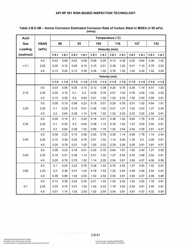
API RP 581 RISK-BASED INSPECTION TECHNOLOGY
Table 2.B.8.3M – Amine Corrosion Estimated Corrosion Rate of Carbon Steel in MDEA (≤ 50 wt%) (mm/y)
Acid
Gas
Loading
(mol/mol)
HSAS
(wt%)
Temperature ( C)
88 93 104 116 127 132
Velocity (m/s) ≤ 6.1 > 6.1 ≤ 6.1 > 6.1 ≤ 6.1 > 6.1 ≤ 6.1 > 6.1 ≤ 6.1 > 6.1 ≤ 6.1 > 6.1
< 0.1
0.5 0.03 0.08 0.03 0.08 0.08 0.25 0.13 0.38 0.25 0.64 0.38 1.02
2.25 0.05 0.15 0.05 0.15 0.15 0.51 0.38 1.02 0.51 1.14 0.76 2.03
4.0 0.13 0.25 0.13 0.38 0.38 1.02 0.76 1.52 1.02 2.29 1.52 3.05
Velocity (m/s)
≤ 1.5 > 1.5 ≤ 1.5 > 1.5 ≤ 1.5 > 1.5 ≤ 1.5 > 1.5 ≤ 1.5 > 1.5 ≤ 1.5 > 1.5
0.15
0.5 0.03 0.08 0.05 0.15 0.13 0.38 0.25 0.76 0.38 1.14 0.51 1.52
2.25 0.05 0.15 0.1 0.3 0.25 0.76 0.51 1.52 0.76 2.29 1.02 2.03
4.0 0.13 0.38 0.2 0.64 0.51 1.52 1.02 2.03 1.52 3.05 3.05 3.81
0.25
0.5 0.05 0.15 0.08 0.23 0.18 0.51 0.25 0.76 0.51 1.52 0.64 1.91
2.25 0.1 0.25 0.15 0.51 0.38 1.02 0.51 1.27 1.02 2.03 1.27 2.54
4.0 0.2 0.64 0.38 1.14 0.76 1.52 1.02 2.03 2.03 3.05 2.54 3.81
0.35
0.5 0.05 0.15 0.1 0.25 0.18 0.51 0.38 1.02 0.64 1.78 0.76 2.03
2.25 0.1 0.25 0.2 0.64 0.38 1.14 0.76 1.52 1.27 2.54 2.54 3.81
4.0 0.2 0.64 0.38 1.02 0.89 1.78 1.52 2.54 2.54 3.56 3.81 4.57
0.45
0.5 0.08 0.23 0.13 0.38 0.25 0.76 0.38 1.14 0.89 1.78 1.14 2.54
2.25 0.15 0.38 0.25 0.76 0.51 1.52 1.14 2.29 1.78 3.3 2.29 3.81
4.0 0.25 0.76 0.51 1.02 1.02 2.03 2.29 3.05 3.05 3.81 3.81 4.57
0.55
0.5 0.08 0.23 0.18 0.51 0.25 0.76 0.64 1.91 1.02 2.54 1.27 3.05
2.25 0.15 0.51 0.38 1.14 0.51 1.52 1.27 2.54 2.03 3.56 2.54 3.81
4.0 0.25 0.76 0.76 1.52 1.14 2.29 2.54 3.81 3.56 4.57 4.06 5.08
0.65
0.5 0.1 0.25 0.23 0.76 0.38 1.02 0.76 2.54 1.27 3.05 1.52 3.81
2.25 0.2 0.38 0.51 1.02 0.76 1.52 1.52 2.54 2.29 3.56 2.54 3.81
4.0 0.38 0.89 1.02 2.03 1.52 2.54 2.54 3.81 3.56 4.57 4.06 5.08
0.7
0.5 0.13 0.38 0.25 0.76 0.51 1.52 1.02 2.54 1.52 3.05 1.78 3.81
2.25 0.25 0.76 0.51 1.52 1.02 2.03 1.78 3.05 2.54 3.81 3.05 3.81
4.0 0.51 1.14 1.02 2.03 1.52 2.54 2.54 3.81 3.81 4.57 4.32 5.59
2.B-81 Copyright American Petroleum Institute Provided by IHS under license with API Licensee=Qatar Petroleum/5943408001
Not for Resale, 10/20/2008 01:51:29 MDTNo reproduction or networking permitted without license from IHS
--```,`,,`,`,,`,`,,,,,,``,```,`-`-`,,`,,`,`,,`---
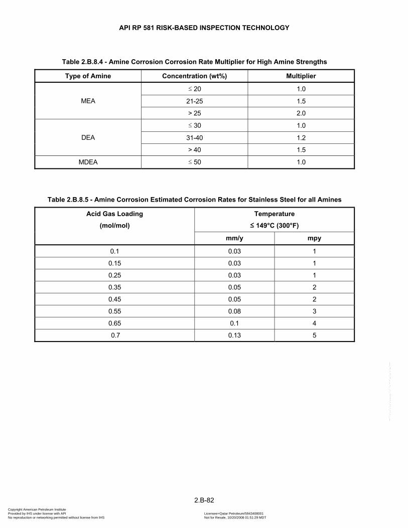
API RP 581 RISK-BASED INSPECTION TECHNOLOGY
Table 2.B.8.4 - Amine Corrosion Corrosion Rate Multiplier for High Amine Strengths
Type of Amine Concentration (wt%) Multiplier
MEA
≤ 20 1.0
21-25 1.5
> 25 2.0
DEA
≤ 30 1.0
31-40 1.2
> 40 1.5
MDEA ≤ 50 1.0
Table 2.B.8.5 - Amine Corrosion Estimated Corrosion Rates for Stainless Steel for all Amines
Acid Gas Loading
(mol/mol)
Temperature
≤ 149°C (300°F)
mm/y mpy
0.1 0.03 1
0.15 0.03 1
0.25 0.03 1
0.35 0.05 2
0.45 0.05 2
0.55 0.08 3
0.65 0.1 4
0.7 0.13 5
2.B-82 Copyright American Petroleum Institute Provided by IHS under license with API Licensee=Qatar Petroleum/5943408001
Not for Resale, 10/20/2008 01:51:29 MDTNo reproduction or networking permitted without license from IHS
--```,`,,`,`,,`,`,,,,,,``,```,`-`-`,,`,,`,`,,`---
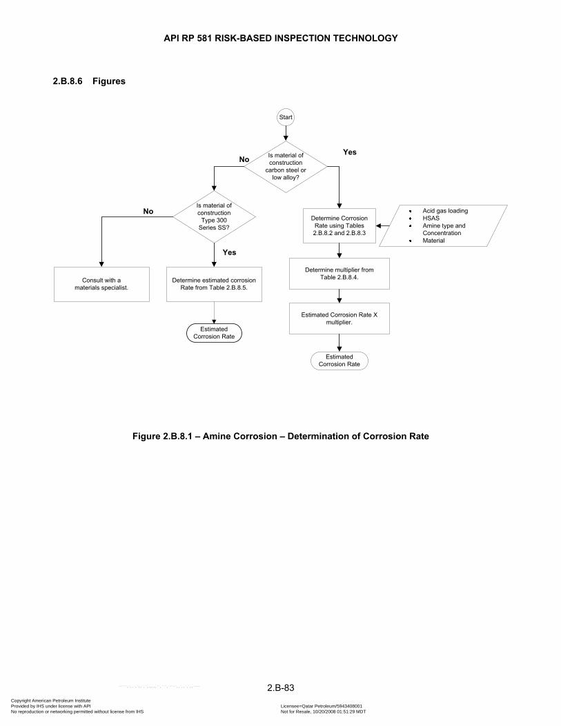
API RP 581 RISK-BASED INSPECTION TECHNOLOGY
2.B.8.6 Figures
Start
Determine Corrosion Rate using Tables 2.B.8.2 and 2.B.8.3
Estimated Corrosion Rate
Determine multiplier from Table 2.B.8.4.
YesNo Is material of
constructioncarbon steel or
low alloy?
Is material of construction
Type 300 Series SS?
Determine estimated corrosionRate from Table 2.B.8.5.
No
Estimated Corrosion Rate X multiplier.
Yes
Consult with amaterials specialist.
Acid gas loadingHSASAmine type and ConcentrationMaterial
Estimated Corrosion Rate
Figure 2.B.8.1 – Amine Corrosion – Determination of Corrosion Rate
2.B-83 Copyright American Petroleum Institute Provided by IHS under license with API Licensee=Qatar Petroleum/5943408001
Not for Resale, 10/20/2008 01:51:29 MDTNo reproduction or networking permitted without license from IHS
--```,`,,`,`,,`,`,,,,,,``,```,`-`-`,,`,,`,`,,`---

API RP 581 RISK-BASED INSPECTION TECHNOLOGY
2.B.9 HIGH TEMPERATURE OXIDATION
2.B.9.1 Description of Damage
Corrosion due to high temperature oxidation occurs at temperatures above about 482°C (900°F) for carbon steel and increasing higher temperatures for alloys. The metal loss occurs as a result of the reaction of metal with oxygen in the environment. Typically, at temperatures just above the temperature where oxidation begins to occur, a dense comparatively protective oxide forms on the surface that reduces the metal loss rate. The oxide scale tends to be significantly more protective as the chromium concentration in the metal increases.
2.B.9.2 Basic Data
The data listed in Table 2.B.9.1 are required to determine the estimated corrosion rate for high temperature oxidation service. If precise data have not been measured, a knowledgeable process specialist should be consulted.
2.B.9.3 Determination of Corrosion Rate
The steps required to determine the corrosion rate are shown in Figure 2.B.9.1. The corrosion rate may be determined using the basic data in Table 2.B.9.1 in conjunction with Tables 2.B.9.2 through 2.B.9.3.
2.B-84 Copyright American Petroleum Institute Provided by IHS under license with API Licensee=Qatar Petroleum/5943408001
Not for Resale, 10/20/2008 01:51:29 MDTNo reproduction or networking permitted without license from IHS
--```,`,,`,`,,`,`,,,,,,``,```,`-`-`,,`,,`,`,,`---
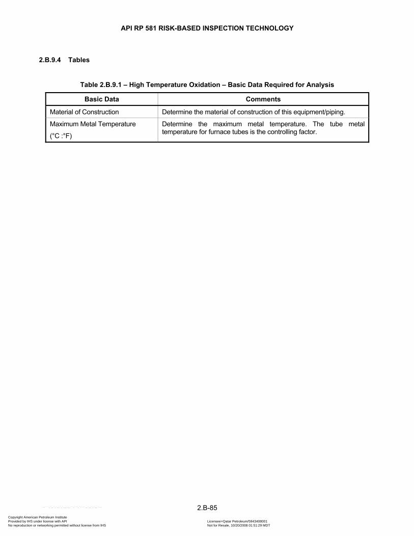
API RP 581 RISK-BASED INSPECTION TECHNOLOGY
2.B.9.4 Tables
Table 2.B.9.1 – High Temperature Oxidation – Basic Data Required for Analysis
Basic Data Comments
Material of Construction Determine the material of construction of this equipment/piping.
Maximum Metal Temperature
(°C :°F)
Determine the maximum metal temperature. The tube metal temperature for furnace tubes is the controlling factor.
2.B-85 Copyright American Petroleum Institute Provided by IHS under license with API Licensee=Qatar Petroleum/5943408001
Not for Resale, 10/20/2008 01:51:29 MDTNo reproduction or networking permitted without license from IHS
--```,`,,`,`,,`,`,,,,,,``,```,`-`-`,,`,,`,`,,`---
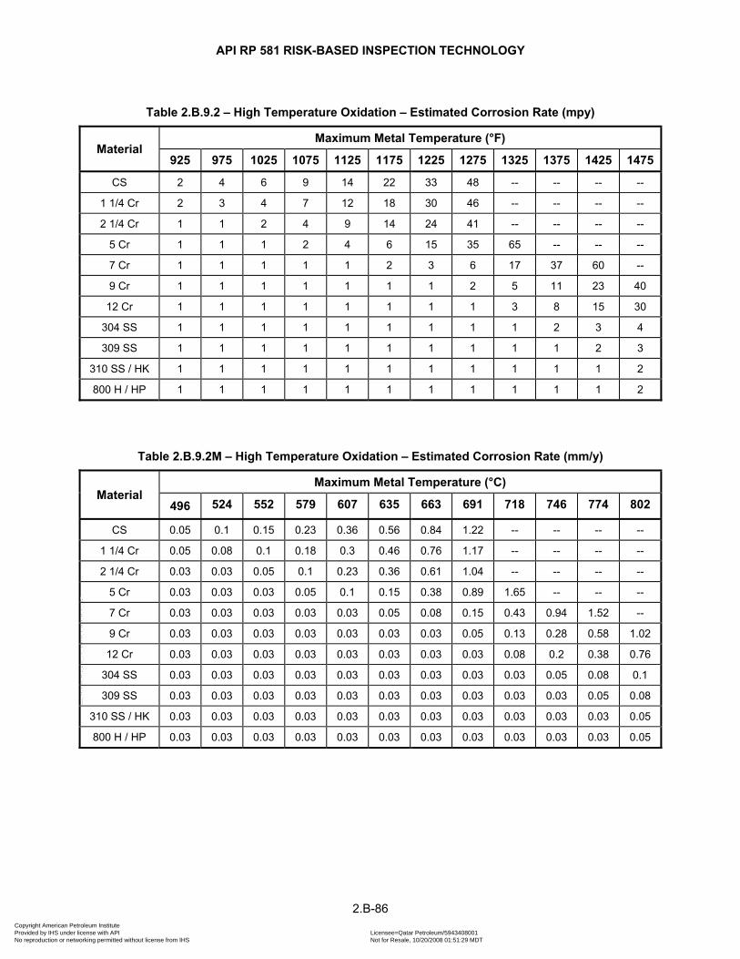
API RP 581 RISK-BASED INSPECTION TECHNOLOGY
Table 2.B.9.2 – High Temperature Oxidation – Estimated Corrosion Rate (mpy)
Material Maximum Metal Temperature (°F)
925 975 1025 1075 1125 1175 1225 1275 1325 1375 1425 1475
CS 2 4 6 9 14 22 33 48 -- -- -- --
1 1/4 Cr 2 3 4 7 12 18 30 46 -- -- -- --
2 1/4 Cr 1 1 2 4 9 14 24 41 -- -- -- --
5 Cr 1 1 1 2 4 6 15 35 65 -- -- --
7 Cr 1 1 1 1 1 2 3 6 17 37 60 --
9 Cr 1 1 1 1 1 1 1 2 5 11 23 40
12 Cr 1 1 1 1 1 1 1 1 3 8 15 30
304 SS 1 1 1 1 1 1 1 1 1 2 3 4
309 SS 1 1 1 1 1 1 1 1 1 1 2 3
310 SS / HK 1 1 1 1 1 1 1 1 1 1 1 2
800 H / HP 1 1 1 1 1 1 1 1 1 1 1 2
Table 2.B.9.2M – High Temperature Oxidation – Estimated Corrosion Rate (mm/y)
Material Maximum Metal Temperature (°C)
496 524 552 579 607 635 663 691 718 746 774 802
CS 0.05 0.1 0.15 0.23 0.36 0.56 0.84 1.22 -- -- -- --
1 1/4 Cr 0.05 0.08 0.1 0.18 0.3 0.46 0.76 1.17 -- -- -- --
2 1/4 Cr 0.03 0.03 0.05 0.1 0.23 0.36 0.61 1.04 -- -- -- --
5 Cr 0.03 0.03 0.03 0.05 0.1 0.15 0.38 0.89 1.65 -- -- --
7 Cr 0.03 0.03 0.03 0.03 0.03 0.05 0.08 0.15 0.43 0.94 1.52 --
9 Cr 0.03 0.03 0.03 0.03 0.03 0.03 0.03 0.05 0.13 0.28 0.58 1.02
12 Cr 0.03 0.03 0.03 0.03 0.03 0.03 0.03 0.03 0.08 0.2 0.38 0.76
304 SS 0.03 0.03 0.03 0.03 0.03 0.03 0.03 0.03 0.03 0.05 0.08 0.1
309 SS 0.03 0.03 0.03 0.03 0.03 0.03 0.03 0.03 0.03 0.03 0.05 0.08
310 SS / HK 0.03 0.03 0.03 0.03 0.03 0.03 0.03 0.03 0.03 0.03 0.03 0.05
800 H / HP 0.03 0.03 0.03 0.03 0.03 0.03 0.03 0.03 0.03 0.03 0.03 0.05
2.B-86 Copyright American Petroleum Institute Provided by IHS under license with API Licensee=Qatar Petroleum/5943408001
Not for Resale, 10/20/2008 01:51:29 MDTNo reproduction or networking permitted without license from IHS
--```,`,,`,`,,`,`,,,,,,``,```,`-`-`,,`,,`,`,,`---

API RP 581 RISK-BASED INSPECTION TECHNOLOGY
Table 2.B.9.3 – High Temperature Oxidation – Estimated Corrosion Rate (mpy)
Material Maximum Metal Temperature (°F)
1525 1575 1625 1675 1725 1775 1825 1875 1925 1975 2025 2075
CS -- -- -- -- -- -- -- -- -- -- -- --
1 1/4 Cr -- -- -- -- -- -- -- -- -- -- -- --
2 1/4 Cr -- -- -- -- -- -- -- -- -- -- -- --
5 Cr -- -- -- -- -- -- -- -- -- -- -- --
7 Cr -- -- -- -- -- -- -- -- -- -- -- --
9 Cr 60 -- -- -- -- -- -- -- -- -- -- --
12 Cr 50 -- -- -- -- -- -- -- -- -- -- --
304 SS 6 9 13 18 25 35 48 -- -- -- -- --
309 SS 4 6 8 10 13 16 20 30 40 50 -- --
310 SS / HK 3 4 5 7 8 10 13 15 19 23 27 31
800 H / HP 3 4 6 8 10 13 17 21 27 33 41 50
Table 2.B.9.3M – High Temperature Oxidation – Estimated Corrosion Rate (mm/y)
Material Maximum Metal Temperature (°C)
829 857 885 913 941 968 996 1024 1052 1079 1107 1135
CS -- -- -- -- -- -- -- -- -- -- -- --
1 1/4 Cr -- -- -- -- -- -- -- -- -- -- -- --
2 1/4 Cr -- -- -- -- -- -- -- -- -- -- -- --
5 Cr -- -- -- -- -- -- -- -- -- -- -- --
7 Cr -- -- -- -- -- -- -- -- -- -- -- --
9 Cr 1.52 -- -- -- -- -- -- -- -- -- -- --
12 Cr 1.27 -- -- -- -- -- -- -- -- -- -- --
304 SS 0.15 0.23 0.33 0.46 0.64 0.89 1.22 -- -- -- -- --
309 SS 0.1 0.15 0.2 0.25 0.33 0.41 0.51 0.76 1.02 1.27 -- --
310 SS / HK 0.08 0.1 0.13 0.18 0.2 0.25 0.33 0.38 0.48 0.58 0.69 0.79
800 H / HP 0.08 0.1 0.15 0.2 0.25 0.33 0.43 0.53 0.69 0.84 1.04 1.27
2.B-87 Copyright American Petroleum Institute Provided by IHS under license with API Licensee=Qatar Petroleum/5943408001
Not for Resale, 10/20/2008 01:51:29 MDTNo reproduction or networking permitted without license from IHS
--```,`,,`,`,,`,`,,,,,,``,```,`-`-`,,`,,`,`,,`---
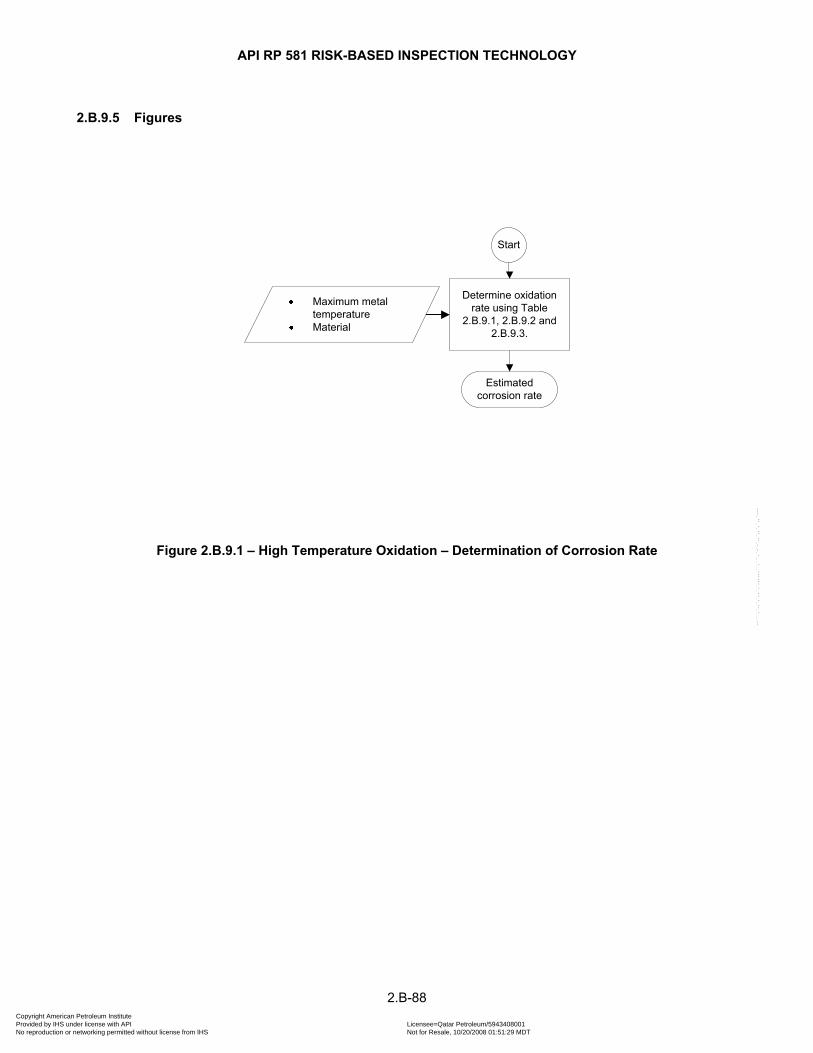
API RP 581 RISK-BASED INSPECTION TECHNOLOGY
2.B.9.5 Figures
Start
Determine oxidation rate using Table
2.B.9.1, 2.B.9.2 and 2.B.9.3.
Estimated corrosion rate
Maximum metal temperatureMaterial
Figure 2.B.9.1 – High Temperature Oxidation – Determination of Corrosion Rate
2.B-88 Copyright American Petroleum Institute Provided by IHS under license with API Licensee=Qatar Petroleum/5943408001
Not for Resale, 10/20/2008 01:51:29 MDTNo reproduction or networking permitted without license from IHS
--```,`,,`,`,,`,`,,,,,,``,```,`-`-`,,`,,`,`,,`---
API RP 581 RISK-BASED INSPECTION TECHNOLOGY
2.B.10 ACID SOUR WATER CORROSION
2.B.10.1 Description of Damage
2.B.10.1.1 Overview
Acid sour water is defined as water containing H2S and with pH below neutral pH (7). The primary refining units or gas fractionator plants where acid sour water corrosion is a concern are sour distillation overhead systems in gas fractionation plants. Most other refining distillation units contain chlorides or ammonia and are covered in paragraphs 2.B.2 and 2.B.7, respectively.
Corrosion damage from acid sour water is typically general thinning. Above pH of about 4.5, a protective thin iron sulfide layer limits the corrosion rate. In some instances at pH above 4.5, a thicker porous sulfide film layer can form. This can promote pitting under sulfide deposits yet generally this does not affect the general corrosion rate. Sour water condensates in equilibrium with a vapor containing H2S at a partial pressure below 1 atm will usually have a pH between 4.5 and 7. At H2S partial pressures greater than 1 atm a pH < 4.5 can be achieved, and are outside the scope of this paragraph.
2.B.10.1.2 Scope and Limitations
The scope of this paragraph is to give guidance in determining a conservatively estimated corrosion rate driven by acid sour water, under the following conditions and assumptions.
a) Primary corrosive is H2S. Assuming no significant amounts of ammonia, carbon dioxide, chlorides, or cyanides are present.
b) The corrosion mechanism is general corrosion, with some occurrence of pitting in the presence of oxygen.
c) This paragraph contains guidance for estimating corrosion rates of carbon steel. Copper alloys and nickel alloys (not containing chromium) can be used and are generally not susceptible to acid sour water corrosion in the refinery applications where acid sour water is found. Stainless steel can be used where the temperature is low enough that chloride stress corrosion cracking (ClSCC) is not likely. Where the material of construction is other than carbon steel, it is assumed that the selected material is suitable for the service and that the corrosion rates will not exceed 0.05 mm/y (2 mpy).
d) Cracking is not considered. Wet H2S cracking mechanisms are addressed elsewhere in this document.
e) Presence of air or oxidants may increase the corrosion. It is assumed that the normal concentration of oxygen is less than 8 ppm.
f) A high flow velocity can have an adverse effect on the corrosion. It is assumed that the effect is negligible for velocities less than 1.83 m/s (6 ft/s). When velocities exceed 1.83 m/s (6 ft/s), higher corrosion rates and possible localized corrosion should be considered.
The base corrosion rate is estimated from the pH level and temperature. An adjustment is made for oxygen content. Other factors, such as content of chlorides, cyanides, etc. are relevant, but are considered less significant for the end result in this context. The result is a conservative value for the estimated corrosion rate.
2.B.10.2 Basic Data
The data listed in Table 2.B.10.1 is required to estimate the rate of corrosion rate in acid sour water. If precise data have not been measured, a knowledgeable process specialist should be consulted.
2.B.10.3 Determination of Corrosion Rate
The steps required to determine the corrosion rate are shown in Figure 2.B.10.1. If the pH is less than 4.5, then the corrosion rate shall be calculated using paragraph 2.B.2. If the pH is greater than 7, then the corrosion rate is calculated using paragraph 2.B.7. Otherwise, the corrosion rate of carbon steel exposed to acid sour water is computed using Equation (2.B.1).
2.B-89 Copyright American Petroleum Institute Provided by IHS under license with API Licensee=Qatar Petroleum/5943408001
Not for Resale, 10/20/2008 01:51:29 MDTNo reproduction or networking permitted without license from IHS
--```,`,,`,`,,`,`,,,,,,``,```,`-`-`,,`,,`,`,,`---

API RP 581 RISK-BASED INSPECTION TECHNOLOGY
= ⋅ ⋅ph O VCR CR F F (2.B.1)
The base corrosion rate, , of carbon steel exposed to acid sour water as a function of pH is provided in pHCTable 2.B.10.2. The corrosion rate can vary significantly with level of dissolved oxygen. The modification factor for the corrosion rate as a function of the oxygen content factor, , is provided in OF Table 2.B.10.3. The corrosion rate also varies with fluid velocity. The modification factor for fluid velocity is given by the following equations.
For SI units, use Equations (2.B.2) through (2.B.4),
1.0VF = when velocity < 1.83 m/s (2.B.2)
0.82 0.5VF velocity= ⋅ − when 1.83 m/s < velocity < 6.10 m/s (2.B.3)
5.0VF = when velocity > 6.10 m/s (2.B.4)
For US Customary units, use Equations (2.B.5) through (2.B.7),
1.0VF = when velocity < 6 ft/s (2.B.5)
0.25 0.5VF velocity= ⋅ − when 6 ft/s < velocity < 20 ft/s (2.B.6)
5.0VF = when velocity > 20 ft/s (2.B.7)
2.B.10.4 Nomenclature CR is the corrosion rate
phCR is the base corrosion rate as a function of pH
OF is the corrosion rate correction for oxygen
VF is the corrosion rate correction for velocity
velocity is the fluid velocity, m/s [ft/s]
2.B.10.5 References
38. Joerg Gutzeit, ”Corrosion of Steel by Sulfides and Cyanides in Refinery Condensate Water”, Materials Protection, December 1968, p. 17-23.
39. R.H. Hausler and N.D. Coble, “Corrosion Control in Crude Unit Overhead Systems”, paper 42-72 at API 37th Midyear Meeting, May 10, 1972.
40. Bruce D. Craig, “The Nature of Sulfides Formed on Steel in an H2S-O2 Environment”, Corrosion Vol. 35, No. 3, March 1979, p. 136-138.
41. Dillon, C.P., Corrosion Control in the Chemical Process Industries, MTI Publication No. 45, Second Edition, NACE International. Houston, TX (1994).
42. Jones, Denny A., Principles and Prevention of Corrosion, Prentice-Hall, Inc. (1996).
2.B-90 Copyright American Petroleum Institute Provided by IHS under license with API Licensee=Qatar Petroleum/5943408001
Not for Resale, 10/20/2008 01:51:29 MDTNo reproduction or networking permitted without license from IHS
--```,`,,`,`,,`,`,,,,,,``,```,`-`-`,,`,,`,`,,`---
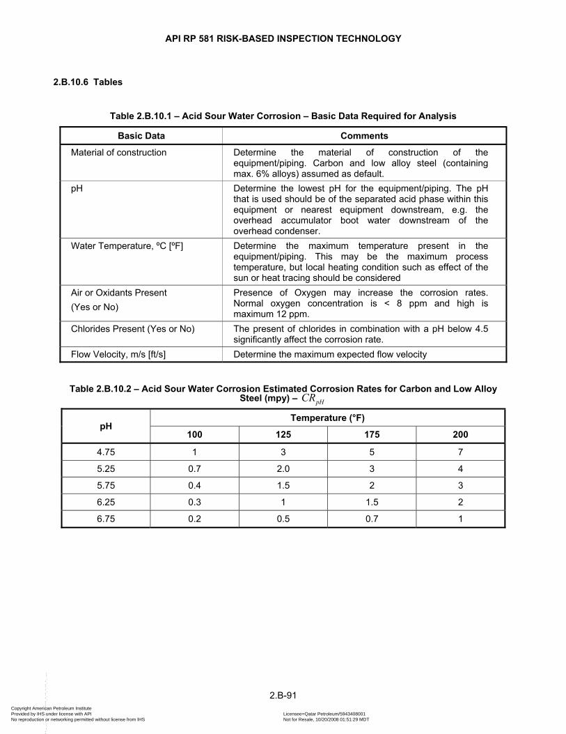
API RP 581 RISK-BASED INSPECTION TECHNOLOGY
2.B.10.6 Tables
Table 2.B.10.1 – Acid Sour Water Corrosion – Basic Data Required for Analysis
Basic Data Comments
Material of construction Determine the material of construction of the equipment/piping. Carbon and low alloy steel (containing max. 6% alloys) assumed as default.
pH Determine the lowest pH for the equipment/piping. The pH that is used should be of the separated acid phase within this equipment or nearest equipment downstream, e.g. the overhead accumulator boot water downstream of the overhead condenser.
Water Temperature, ºC [ºF] Determine the maximum temperature present in the equipment/piping. This may be the maximum process temperature, but local heating condition such as effect of the sun or heat tracing should be considered
Air or Oxidants Present (Yes or No)
Presence of Oxygen may increase the corrosion rates. Normal oxygen concentration is < 8 ppm and high is maximum 12 ppm.
Chlorides Present (Yes or No) The present of chlorides in combination with a pH below 4.5 significantly affect the corrosion rate.
Flow Velocity, m/s [ft/s] Determine the maximum expected flow velocity
Table 2.B.10.2 – Acid Sour Water Corrosion Estimated Corrosion Rates for Carbon and Low Alloy Steel (mpy) – pHCR
pH Temperature (°F)
100 125 175 200
4.75 1 3 5 7
5.25 0.7 2.0 3 4
5.75 0.4 1.5 2 3
6.25 0.3 1 1.5 2
6.75 0.2 0.5 0.7 1
2.B-91 Copyright American Petroleum Institute Provided by IHS under license with API Licensee=Qatar Petroleum/5943408001
Not for Resale, 10/20/2008 01:51:29 MDTNo reproduction or networking permitted without license from IHS
--```,`,,`,`,,`,`,,,,,,``,```,`-`-`,,`,,`,`,,`---
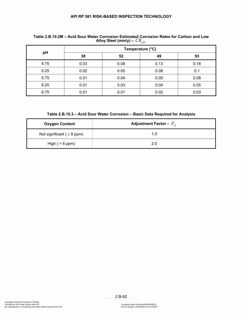
API RP 581 RISK-BASED INSPECTION TECHNOLOGY
Table 2.B.10.2M – Acid Sour Water Corrosion Estimated Corrosion Rates for Carbon and Low Alloy Steel (mm/y) – pHCR
pH Temperature (°C)
38 52 49 93
4.75 0.03 0.08 0.13 0.18
5.25 0.02 0.05 0.08 0.1
5.75 0.01 0.04 0.05 0.08
6.25 0.01 0.03 0.04 0.05
6.75 0.01 0.01 0.02 0.03
Table 2.B.10.3 – Acid Sour Water Corrosion – Basic Data Required for Analysis
Oxygen Content Adjustment Factor – OF
Not significant ( ≤ 8 ppm) 1.0
High ( > 8 ppm) 2.0
2.B-92 Copyright American Petroleum Institute Provided by IHS under license with API Licensee=Qatar Petroleum/5943408001
Not for Resale, 10/20/2008 01:51:29 MDTNo reproduction or networking permitted without license from IHS
--```,`,,`,`,,`,`,,,,,,``,```,`-`-`,,`,,`,`,,`---
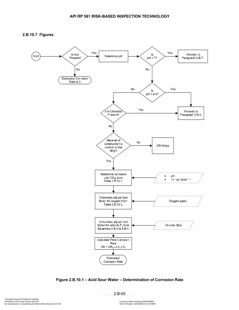
API RP 581 RISK-BASED INSPECTION TECHNOLOGY
2.B.10.7 Figures
Figure 2.B.10.1 – Acid Sour Water – Determination of Corrosion Rate
2.B-93 Copyright American Petroleum Institute Provided by IHS under license with API Licensee=Qatar Petroleum/5943408001
Not for Resale, 10/20/2008 01:51:29 MDTNo reproduction or networking permitted without license from IHS
--```,`,,`,`,,`,`,,,,,,``,```,`-`-`,,`,,`,`,,`---

API RP 581 RISK-BASED INSPECTION TECHNOLOGY
2.B.11 COOLING WATER CORROSION
2.B.11.1 Description of Damage
2.B.11.1.1 Overview
The objective for this paragraph is to describe a conservative approach for estimating corrosion rates of carbon steel components in cooling water systems. In fresh water systems, a model uses the Ryznar Stability Index (RSI), chloride content, temperature, and flow velocity to calculate a corrosion rate. For seawater systems, a simple correlation of corrosion rate and velocity is used. Many other factors influence corrosion of the typical modern cooling water system, and this paragraph also describes qualitatively some of these considerations.
This paragraph does not attempt to account for degradation of alloys other than carbon steel or to quantify the effectiveness of water treatment. Many other alloys are used in cooling water systems. Some of these alloys and the threats that they may face are described qualitatively, but corrosion rates of these alloys are assumed to be very low. While low alloy steels are rarely used in cooling water systems, the corrosion rates given by this methodology would be reasonably accurate for low alloy steels.
The best way to assess corrosion in cooling water systems is to use a variety of monitoring techniques, but detailed use of those techniques is not described here. Most cooling water corrosion monitoring begins with the use of corrosion coupons. Other techniques have been used to monitor cooling water corrosion in-situ, but they are not described. Microbiologically-Induced Corrosion (MIC) is another common degradation mechanism in cooling water systems, and coupons are not always a reliable way to monitor this corrosion or other corrosion where there are deposits or stagnant areas. Direct monitoring and control of the microorganisms is recommended.
2.B.11.1.2 Types of Cooling Water Systems
There are three types of cooling water systems typically found in industrial operations such as refineries:
a) Once through cooling – Does not reuse the heated water, which normally is pumped from a fresh water or seawater source
b) Closed recirculating cooling – Continuously reuses water that is captive in the system. No make-up after the initial water charge (except to replace accidental leakage).
c) Open recirculating cooling (cooling tower) – Reuses water from which the heat is rejected into a cooling reservoir (tower or pond), needs continual make-up water to compensate for evaporation, blowdown, windage, and drift losses, and needs a blow-down facility to limit the concentration of impurities that are typically introduced with the make-up water.
2.B.11.1.3 Once Through Systems
Usually, the water source must be presumed corrosive since the surface waters are open to the atmosphere and contain dissolved oxygen. In a general way, corrosion of iron and steel is proportional to the chloride content when dissolved oxygen is constant, and vice versa. For seawater in particular, the flow velocity has a significant impact on the corrosion rate.
Because once through cooling water is not reused, the volume of water circulated through such a system effectively precludes chemical inhibition from a cost-effective standpoint. In some cases, a small amount of scale inhibitor is added to the influent water. However, chlorination is usually necessary to control biological growth (e.g., bacteria, slime, marine organisms).
Both fresh and saline waters are sufficiently corrosive to carbon steel that more corrosion-resistant materials must be employed. In fresh water, galvanized steel is often adequate but brackish or salt water requires more resistant materials (e.g., copper or nickel alloys; titanium; super-austenitic stainless steels (such as 6-Mo stainless steels); plastic; FRP or plastic-lined steel; concrete, etc.).
2.B-94 Copyright American Petroleum Institute Provided by IHS under license with API Licensee=Qatar Petroleum/5943408001
Not for Resale, 10/20/2008 01:51:29 MDTNo reproduction or networking permitted without license from IHS
--```,`,,`,`,,`,`,,,,,,``,```,`-`-`,,`,,`,`,,`---

API RP 581 RISK-BASED INSPECTION TECHNOLOGY
2.B.11.1.4 Closed Recirculated Systems
Recirculated cooling water systems are applied where water is in short supply or when the water chemistry must be rigorously controlled. Closed Recirculated Systems may be treated either by rendering them sterile and anaerobic or by use of inhibitors. The cost of treatment is minimal, including softening and pH control, if required or desirable. The heat is removed either in air-cooled heat exchangers or water-to-water exchangers cooled by an external cooling water system. Bactericidal treatment may be required, using non-oxidizing biocide, such as hexamethylene biguanide. If no treatment is applied sulfate-reducing bacteria would otherwise be a potential problem.
A successfully used strategy for preventing problems in the closed cooling water systems is to charge the system with condensate quality water and then add an effective corrosion inhibitor to prevent corrosion. Given the controlled environment, the material of construction is usually carbon steel, unless otherwise required for process reasons.
2.B.11.1.5 Open Recirculated Systems
These types of cooling systems involve constant air saturation as well as some concentration of water-borne solids in the circulating water. Such systems are corrosive to steel (unless suitably inhibited) and potentially scaling unless the hardness, pH and alkalinity are also controlled.
In a cooling tower system, the total amount of water actually used is limited to that lost by evaporation plus the blow-down established to limit the build-up of salts and solids in the system. The extent of soluble salt concentration is expressed as cycles of concentration, which is the ratio of hardness in the blow-down to that in the make-up. Water treatment chemicals need only be replaced in accordance with the blow-down rate. In most systems (water chemistry permitting), the optimum balance between water savings and salt concentration is effected at four to six cycles of concentration. The additional water savings from a higher number of cycles are usually offset by the increasing difficulty of coping with higher dissolved salt and hardness concentrations.
Because of the warm temperature and constant air scrubbing in the tower, the water is not only corrosive, but also a breeding ground for slime and algae introduced from air-borne spores. Unless corrosion resistant materials are used, open recirculated systems must usually be corrosion inhibited, treated with biocides to control biological growths, and chemically treated to control scale and deposits. The cost of such treatment must be balanced against the obvious savings in water consumption. The choice between corrosion inhibition versus resistant materials of construction is one of economics and pollution abatement considerations.
Typical corrosion resistant materials for components in fresh-water type open recirculated systems are stainless steel, copper alloys, nickel alloys, titanium, cement lined carbon steel, FRP lined or coated steel (for vessels), etc.
2.B.11.1.6 Factors Affecting Corrosion Rate
There are several factors that affect the rate of corrosion in cooling systems. Depending on the type of system and water source, the main concerns are related to the following:
a) Impurities in make-up water – Calcium, Chlorides, Alkalinity, Silica, etc.
b) Scale formation – When the process side temperature is greater than 140°F (60°C) a scaling potential exists. The scales are minerals formed by high concentration of specific impurities, for example calcite (CaCO3) formed by calcium salts and dissolved CO2 species. Temperature, pH and alkalinity influence the solubility limit of most minerals found in cooling water systems. Unfortunately, high temperature reduces the solubility of many important minerals, causing scale most often to appear on the hottest surfaces in the entire cooling system, which are the heat exchangers. Phosphates and zinc are two of the most common minerals used as corrosion inhibitors in water treatment programs, and can form mineral scale if not properly controlled.
c) Deposits
1) Mud and silt – Enters the cooling tower in make-up water or scrubbed from the air.
2) Corrosion Products (iron oxide) – Formed as a result of corrosion. Forms a porous deposit that is frequently the site for pitting corrosion.
2.B-95 Copyright American Petroleum Institute Provided by IHS under license with API Licensee=Qatar Petroleum/5943408001
Not for Resale, 10/20/2008 01:51:29 MDTNo reproduction or networking permitted without license from IHS
--```,`,,`,`,,`,`,,,,,,``,```,`-`-`,,`,,`,`,,`---
API RP 581 RISK-BASED INSPECTION TECHNOLOGY
3) Bio-Mass – A mixture of bacterial slime and other material. Typically mud and iron oxide accumulate in low flow regions, causing a favorable environment for microorganisms to form colonies on the surface that potentially can promote accelerated pitting corrosion. Process leaks of hydrocarbon can often accelerate bacterial growth and lead to rapid formation of bio-mass.
2.B.11.1.7 Types of Corrosion
Corrosion of carbon steel in cooling water systems is dominated by pitting. The following are other more common types of corrosion that can be seen:
a) Underdeposit corrosion – A form of pitting corrosion that occurs beneath deposits.
b) Crevice corrosion – Pitting and preferential attack at a crevice such as at the tube to tubesheet crevice, etc.
c) Galvanic corrosion – The enhanced corrosion of one metal in electrical contact with another kind of metal in an electrolyte. This form of corrosion depends on the metals having a dissimilar corrosion potential that causes one metal to be polarized into a potential region where it corrodes more quickly. As an example, copper alloy tubes in a carbon steel tubesheet may cause more rapid corrosion of the tubesheet.
d) Dealloying – Corrosion process that appears to selectively dissolve one of the constituents of an alloy. When admiralty brass experiences dealloying, zinc is removed leaving copper (referred to as dezincification).
e) MIC – Microbiologically Influenced Corrosion (MIC) is a complex issue. Strictly speaking, MIC is not a specific type of corrosion. Rather, it consists of both direct and indirect effects on materials by bacteria, fungi, algae, and yeasts. Many types of bacteria can be implicated involved in MIC processes. Perhaps the best known type of MIC attack is the corrosion process involving sulfate reducing bacteria (SRB). These organisms are anaerobic (cannot tolerate oxygen), and thrive beneath deposits. They metabolize sulfate creating a highly acidic local environment that leads to metal corrosion. Other types of bacteria that contribute to MIC include slime forming bacteria, nitrifying bacteria, manganese reducing bacteria, and iron reducing bacteria.
f) Stress Corrosion Cracking – Stress Corrosion Cracking (SCC) mechanisms require the coming together of three things – a tensile stress, a susceptible alloy, and an environment that promotes SCC in that alloy. The tensile stress may be either applied or residual, and residual stresses from welding commonly contribute to SCC. Many alloys can be susceptible to SCC in at least one environment with 300-series stainless steels and copper alloys being the most common susceptible materials used in cooling water systems. The environments most associated with SCC of these alloys are aqueous chloride environments for 300-series stainless steels and ammonia for specific copper alloys.
2.B.11.1.8 Corrosion Monitoring and Control in Cooling Water Systems
The largest potential for problems in the cooling system is associated with scaling, deposition of suspended solids and MIC. Usually, under conditions with controlled water treatment and operating parameters, only negligible corrosion is expected. However, even with these parameters in control, MIC or build-up of solids may cause unsuspected corrosion. This fact emphasizes the need for an effective corrosion monitoring program in addition to the water treatment and process control programs.
There are several strategies for controlling corrosion. These include:
a) Keep metal surfaces free from deposits.
b) Create and maintain an environment that is not conducive to corrosion.
c) Incorporate corrosion inhibitors into the treatment program.
d) Pre-passivate new and recently cleaned equipment.
In practice it is common to simultaneously employ several of the above strategies. For example, an effective treatment program frequently incorporates corrosion inhibitors, maintenance of a benign environment, and steps to keep metal surfaces clean by using dispersants and side-stream filtration.
2.B-96 Copyright American Petroleum Institute Provided by IHS under license with API Licensee=Qatar Petroleum/5943408001
Not for Resale, 10/20/2008 01:51:29 MDTNo reproduction or networking permitted without license from IHS
--```,`,,`,`,,`,`,,,,,,``,```,`-`-`,,`,,`,`,,`---
API RP 581 RISK-BASED INSPECTION TECHNOLOGY
Many variations of basic cooling water treatment programs are being practiced. In general they all include fouling control, corrosion control and microbiological control. The most common method to control the microbiological population in a cooling system is to treat the system with one or more biocides. Biocides can be classified into oxidizing and non-oxidizing.
2.B.11.1.9 Indicators for Corrosion Issues and their Deterrence
The following parameters might be used as indicators for potential issues in the cooling system, depending on the water treatment program in place.
a) If process side temperature is greater than 60°C (140°F) then a scaling potential exists. However, note that at the measured pH, one can calculate the temperature at which the water begins to scale, by solving for the value of 2C in equation (2.B.11) using the coefficients provided in Table 2.B.11.3.
b) Dissolved solids – the higher the level of dissolved solids, typically an indicator of chlorides, the higher the corrosion rate.
c) Velocity should be maintained at minimum 1 m/s (3 ft/s) through all parts of the system. For example, if cooling water is on the shellside of a shell-and-tube exchanger, some regions within the shell will have a low velocity.
d) Iron levels greater than 5 ppm in the recirculating water could be an indication that the applied dispersants and flocculating agents are insufficient to keep the formation of deposits at an acceptable level. Other means of deposit control may be required.
e) In open recirculated systems, suspended solids above 100 ppm will cause settlement in heat exchanger equipment and become a site for underdeposit corrosion.
f) Chlorine content: May be dissolved intentionally in water as a biocide. It has little effect on carbon steel if pH is maintained above 7 to suppress formation of acid hydrolysis products by Cl2+H2O → HCLO+HCL. However, chlorine will attack copper alloys, even at higher pH, presumably by reaction with the Cu2O surface film.
g) Ammonia content: Results primarily from contamination by process leaks. Could also be present if NH4OH is used as an acid neutralizer, however, this is not recommended due to the volatility of ammonia and its use as a food source by microorganisms. It has little effect on iron and steel but has a strong effect on copper alloys. Ammonia forms complexes with copper that can cause rapid general corrosion and/or stress corrosion cracking of copper alloys. For example, admiralty brass is very susceptible to ammonia SCC and might experience SCC with only trace amount of ammonia present.
With fresh waters, corrosion of steel is governed by dissolved oxygen over a broad pH range (4.5 to 9.5) at relatively low temperatures. Below pH 4.5, the corrosion is controlled by hydrogen evolution under acid conditions. Above pH 9.5 an insoluble film of ferric hydroxide suppresses corrosion. In buffered solutions, where ionic concentrations are high without a corresponding drop in pH (as with carbonic and other weakly ionized acids), corrosion with hydrogen evolution may occur in the pH 5.0 to 5.5 range. In the intermediate pH range of 4.5 through 9.5, a loose, porous, ferrous-oxide deposit shelters the surface and maintains the steel surface pH at about 9.5. The corrosion rate remains nearly constant and is determined by uniform diffusion of dissolved oxygen through the deposit. At the metal surface under the deposit, oxygen is reduced cathodically. Cathodic reduction of dissolved oxygen produces a slightly alkaline surface condition, which precipitates calcium carbonate (CaCO3). These precipitates in turn inhibit further cathodic reduction and corrosion.
The corrosive effect from the water in closed recirculating cooling water systems is easily mitigated. These systems may be treated either by rendering them sterile and anaerobic or by either oxidizing or non-oxidizing inhibitors.
Corrosion control in open recirculating cooling water systems can be achieved through the continuous use of treatment chemicals containing scale and corrosion inhibitors and polymeric dispersants. The regular use of broad spectrum microbiocides is typically used for controlling microbiological populations.
2.B-97 Copyright American Petroleum Institute Provided by IHS under license with API Licensee=Qatar Petroleum/5943408001
Not for Resale, 10/20/2008 01:51:29 MDTNo reproduction or networking permitted without license from IHS
--```,`,,`,`,,`,`,,,,,,``,```,`-`-`,,`,,`,`,,`---
API RP 581 RISK-BASED INSPECTION TECHNOLOGY
Once through cooling water systems present special problems because chemical treatment of the water may not be possible or practical. In addition, such systems often use seawater or other inherently corrosive water. Corrosion control in once through systems is principally achieved by proper alloy selection, cathodic protection, and/or the use of epoxy-phenolic coatings.
2.B.11.1.10 Assumptions
Cooling water systems can be very complex, and this risk-based inspection model does not attempt to address every issue that must be considered. For the purposes of this model, the following assumptions have been made.
a) Low alloy steels are rarely used in cooling water systems and will not be addressed in the remainder of this paragraph. However, most of the content for carbon steel applies to low alloy steels.
b) This model does not consider degradation of alloys other than carbon steel. Beyond some general comments, SCC and pitting of stainless steels and dealloying of copper alloys is not considered.
c) If coupon measurement results are available, these should be used instead of this model. As a rule of thumb for carbon steel, the pitting rate is a factor of 5 to 10 times the coupon general corrosion rate, (calculated by weight loss).
d) If corrosion inhibitors are being used, it is assumed that the program is designed and operated to adequately control corrosion of carbon steel and alloy materials.
e) An effective microbiological control program is in place, and corrosion driven by MIC is negligible, i.e., can be set to < 0.13 mm/y (5 mpy), pitting.
f) Water pH is kept within the range 6.5 to 9.5. Outside this pH range, the corrosion is assumed caused by other means than what is covered in this paragraph.
g) In the event the RSI value is < 6, it is assumed that corrosion is retarded by scale formation, but can still be estimated on the basis of the chloride content, temperature and flow velocity.
h) There is no deposition and no local low flow areas.
2.B.11.1.11 Corrosion Rates for Copper Alloys Components
This paragraph is not intended to cover material of construction other than carbon steel. The introduction of other materials such as stainless steel, Copper, Nickel, Zinc or Aluminum based alloys etc., might introduce other types of degradation mechanisms. It is virtually impossible to model the complexity of the various materials and interrelation with various chemical and contaminants in the water. Thus, it has been assumed that, in general, the selection of appropriate alloy material combined with “correct” chemical treatment and process control will render a negligible corrosion rate in the cooling water system.
In general, copper and its alloys are the most reliable and cost effective alloys for many water services, although dezincification needs to be specifically inhibited for brasses containing more than 15% zinc. Copper, red brass, inhibited admiralty brasses, aluminum brass, aluminum bronze, and cupronickels, in that order, are used for water of increasing salinity and/or velocity. In the presence of dissolved oxygen, soft waters can be highly corrosive to copper alloys. Also copper can suffer pitting under some conditions, which for fresh waters can be described as three types of pitting:
a) Type 1 pitting is apparently caused by residual carbonaceous films from the manufacturing process;
b) Type 2 pitting is associated with hot soft waters [>60°C (140°F)], and
c) Type 3 pitting may occur in cold water or high pH and low salt concentrations, for unknown reasons.
Another issue related to copper alloys is cracking. Admiralty brass is very susceptible to ammonia SCC and might experience SCC with only a trace amount of ammonia present.
An important factor for copper-based alloys is maintaining operation within design velocity limits. Velocities under the lower limit can lead to increased deposition and underdeposit corrosion, and velocities exceeding the upper limit can cause damage to the protective surface film resulting in impingement attack.
2.B-98 Copyright American Petroleum Institute Provided by IHS under license with API Licensee=Qatar Petroleum/5943408001
Not for Resale, 10/20/2008 01:51:29 MDTNo reproduction or networking permitted without license from IHS
--```,`,,`,`,,`,`,,,,,,``,```,`-`-`,,`,,`,`,,`---
API RP 581 RISK-BASED INSPECTION TECHNOLOGY
2.B.11.2 Basic Data
2.B.11.2.1 Recirculating Cooling Water Systems
The data listed in Table 2.B.11.1 is required for determining the estimated corrosion rate for recirculating cooling water service. If precise data have not been measured, a knowledgeable process specialist should be consulted.
2.B.11.2.2 Once Through Cooling Water Systems
The data listed in Table 2.B.11.2 is required for determining the estimated corrosion rate for once through cooling water service. If precise data have not been measured, a knowledgeable process specialist should be consulted.
2.B.11.3 Determination of Corrosion Rate
2.B.11.3.1 Recirculating Cooling Water Systems
2.B.11.3.1.1 Corrosion Rate Equation
The steps required to determine the corrosion rate are shown in Figure 2.B.11.1. The corrosion rate is computed using Equation (2.B.8). In this equation, the base corrosion rate, , is adjusted for temperature and flow velocity for each component in the system to calculate a final representative corrosion rate.
BCR
= ⋅ ⋅B T VCR CR F F (2.B.8)
The estimated corrosion rates need further adjustments in case construction material is other than carbon steel. This has not been addressed within this paragraph.
2.B.11.3.1.2 Base Corrosion Rate
The Base Corrosion Rate, , is an estimated corrosion rate that is determined from the water scale tendency, chloride concentration, and a threshold for flow velocity (i.e., higher or lower than 2.44 m/s [8 ft/s]).
BCR
The concept of Ryznar stability indices is used to predict whether water variables in the pH range of 6.5 to 9.5 will produce conditions that are scaling or corrosive to carbon steel. The expected tendencies are increased scaling conditions at higher temperatures, higher Ca hardness and higher MO Alkalinity and seeing corrosive conditions at lower temperatures, lower Ca hardness or lower MO Alkalinity. MO Alkalinity refers to the Methyl Orange and the test used to measure the total alkalinity of water.
For given values of calcium hardness, MO Alkalinity and total dissolved salt concentration, a value of pH ,
spH , exists at which the water is in equilibrium with solid CaCO3. The deposit of CaCO3 is thermodynamically
possible when the pH of water is higher than spH , i.e., higher than the pH at saturation of calcium
carbonate. The difference between the actual pH , apH , of a sample of water and the pH for CaCO3
saturated water, spH , is called the Langelier Saturation Index (LSI) and is computed using Equation (2.B.9).
sa pHpHLSI −= (2.B.9)
The Langelier Saturation Index is used to predict the tendency for CaCO3 to either dissolve or precipitate and provide corrosion resistance in fresh water, under varying conditions.
2.B-99 Copyright American Petroleum Institute Provided by IHS under license with API Licensee=Qatar Petroleum/5943408001
Not for Resale, 10/20/2008 01:51:29 MDTNo reproduction or networking permitted without license from IHS
--```,`,,`,`,,`,`,,,,,,``,```,`-`-`,,`,,`,`,,`---
API RP 581 RISK-BASED INSPECTION TECHNOLOGY
While the concept of the Langelier index is correct and helpful; however, it should be emphasized that a positive value of the index can result from waters of totally different quality. As the pH increases, the Ca2+ concentration decreases drastically. The corrosion protection characteristics of the resulting CaCO3 film differ accordingly. In other words, waters of different pH , Ca hardness, and MO Alkalinity that give the same value of the index have different corrosivity.
The Langelier index alone cannot be used to do any quantitative assessment. However when used along with the Ryznar Stability Index (RSI) determined using Equation (2.B.10), a relatively good prediction of the scaling or corrosive tendencies of a water is obtained.
2= ⋅ −s aRSI pH pH (2.B.10)
This Ryznar Stability Index was developed based on actual operating results for waters with different Saturation Indexes, and is used in practice for estimating corrosivity of water. The value of spH in Equation (2.B.10) is calculated using Equation (2.B.11) and the parameters in Table 2.B.11.3.
( ) (1 2 3 49.3s )pH C C C= + + − +C (2.B.11)
All values of the Stability Index can be expected to be positive. At the value of 6 the CaCO3 is in equilibrium. The deposition of CaCO3 increases proportionally (increased tendency of forming scale) as the index drops to below 6, and corrosivity increases as the index rises above 6. Values of 10 or above indicate extreme corrosivity. Note that corrosion can still take place with < 6 RSI. However, in general, low corrosion rates are obtained in scale-forming waters.
Even though the RSI indicates that CaCO3 precipitation takes place, the corrosion rate may remain high if the water contains colloidal silica or organic particles, such as algae, because CaCO3 precipitates on them instead of on the steel surface. For waters high in dissolved salt (such as seawater) or at high temperature, the CaCO3 film is less protective.
Once the Ryznar Stability Index has been determined, the base corrosion rate is calculated based on the chloride concentration and flow velocity of the water using Table 2.B.11.4. In case where the velocity is larger than 8 ft/s, the effect from scaling is assumed not protective against corrosion.
Corrosion of steel increases with chloride content of the water, and reaches a maximum at approximately 6000 ppm. Above that level the chloride effect is offset by diminishing solubility of dissolved oxygen.
2.B.11.3.1.3 Temperature Factor
The corrosion rate of carbon steel has shown to increase almost linearly with temperature from 27ºC to 79ºC (80ºF to 175ºF). This classical correlation has been used to adjust the calculated corrosion rates. Therefore, to calculate the temperature adjustment, the ΔT is calculated by subtracting 24°C (75°F) from the actual metal temperature , or: OPT
OP adjustT T TΔ = − (2.B.12)
This is used to determine the temperature correction factor, , using ΔT TF Table 2.B.11.5. Note that the values are different between open and closed systems at high temperatures. In an open system, heating above room temperature initially increases corrosion rate for steel, but also reduces solubility of dissolved oxygen which allows oxygen to escape. Therefore, at temperatures of 79°C (175°F) and greater, the corrosion rate decreases. However, in a closed system, the corrosion rate increases with temperature because of retention of small amounts of dissolved oxygen under pressure.
TF
2.B-100 Copyright American Petroleum Institute Provided by IHS under license with API Licensee=Qatar Petroleum/5943408001
Not for Resale, 10/20/2008 01:51:29 MDTNo reproduction or networking permitted without license from IHS
--```,`,,`,`,,`,`,,,,,,``,```,`-`-`,,`,,`,`,,`---
API RP 581 RISK-BASED INSPECTION TECHNOLOGY
2.B.11.3.1.4 Flow Velocity Factor
Velocity is one of the prime variables influencing waterside corrosion. At very low velocity, bio-fouling or deposit build up can occur promoting under deposit type of attack or microbiologically-induced corrosion (MIC). Even if fouling deposits do not occur, low velocity encourages higher metal temperatures that results in an increase in the corrosion rate. For carbon steel there is a range of flow velocities (see Equation (2.B.14)) where temperature does not have an affect on the corrosion rate. If flow velocities are outside these limits the velocity factor may be determined from Table 2.B.11.6 or calculated using the following equations where is the actual velocity.
aV
For SI units, use Equations (2.B.13) through (2.B.15),
1 1.64 (0.914 )VF = + ⋅ − aV for Va < 0.914 m/s (2.B.13)
1VF = for 0.914 m/s < Va < 2.44 m/s (2.B.14)
1 0.82 ( 2.44)V aF V= + ⋅ − for Va > 2.44 m/s (2.B.15)
For US Customary units, use Equations (2.B.16) through (2.B.18),
1 0.50 (3 )V aF V= + ⋅ − for Va < 3 ft/s (2.B.16)
1VF = for 3 ft/s < Va < 8 ft/s (2.B.17)
1 0.25 ( 8)V aF V= + ⋅ − for Va > 8 ft/s (2.B.18)
This represents a fairly coarse and conservative way of factoring in the velocity effect in the corrosion rate prediction model. In reality this effect is a product of a much more sophisticated interrelation between temperature, dissolved oxygen, pH and velocity. However, the trend shown in Table 2.B.11.6 does comply with actual testing described in [52] for velocities up to 2.13 m/s (7 ft/s). Note that for carbon steel in seawater, the velocity is even more a governing factor for the corrosion rate.
2.B.11.3.2 Once Through Cooling Water Systems
2.B.11.3.2.1 Overview
The steps required to determine the corrosion rate are shown in Figure 2.B.11.1. Once through cooling water systems are much less common in the US refinery industry than recirculation systems. Once through systems may be economical where there is an abundance of surface water, but the effects of thermal pollution may be too great to allow their use in some locations. Chemical treatment is normally environmentally unacceptable and/or uneconomical. These systems rarely use anything but chlorination which controls biological growth.
It is assumed in this paragraph that chemical treatment is not applied and that the material of construction is carbon steel. In practice, the materials of construction in once through systems may be copper alloys, titanium alloys, stainless steels, PVC, cement-lined, or coated (organic) steel, or even galvanized carbon steel where the supply source is know to be fairly clean fresh water.
The main concern for a once through cooling water system is the quality of the supply water, i.e., type of water (sea or salt, brackish or fresh water) and level of contaminants (such as solids, phosphates, iron, ammonia, bugs and bacteria, etc.). In total there are a large number of factors that ultimately affect the deterioration of the equipment in a once through cooling water system.
For simplicity of this corrosion model for once through systems, these systems are considered either as seawater systems or fresh water systems, and the corrosion rates are determined as a function of temperature, water flow velocity, dissolved oxygen and content of chlorides.
2.B-101 Copyright American Petroleum Institute Provided by IHS under license with API Licensee=Qatar Petroleum/5943408001
Not for Resale, 10/20/2008 01:51:29 MDTNo reproduction or networking permitted without license from IHS
--```,`,,`,`,,`,`,,,,,,``,```,`-`-`,,`,,`,`,,`---
API RP 581 RISK-BASED INSPECTION TECHNOLOGY
2.B.11.3.2.2 Fresh Water Once Through System
Fresh water comprises natural surface water with chloride content less than 1000 ppm. The corrosion rate is estimated in the same manner as an open recirculating system, with no chemical treatment or corrosion inhibition, except for biocide.
2.B.11.3.2.3 Seawater Once Through Systems
Seawater comprises brackish or seawater with a chloride content of more than 1000 ppm. The salts found in seawater do not appreciably alter the pH value when dissolved in water. The main type of dissolved salt in seawater is sodium chloride (NaCl).
Seawater typically contains about 3% sodium chloride with approximately 19,000 ppm chloride ion (and 11,000 ppm sodium). The chloride ions comprise about 55% of the Total Dissolved Solids (TDS). Dissolved Oxygen (DO) is typically present at normal saturated values of 6 to 8 ppm at 24°C to 29°C (75°F to 85°F). The pH of seawater is usually 7.7 to 8.3 in surface waters [44]. Seawater always contains SRB and a level of sulfate ion concentration (2 to 3,000 ppm) conductive to SRB growth under anaerobic conditions. Anaerobic conditions will exist under deposits (organic or inorganic), in crevices, and under the influence of BOD (biological oxygen demand) or COD (chemical oxygen demand). One of the most important properties of seawater is its ratios of concentrations of the major constituents are remarkably constant worldwide, including the level of chloride and oxygen.
The temperatures encountered in once through seawater systems usually preclude scale formation by inverse solubility effects, which normally would initiate at about 88°C (190°F). Obviously deposits can occur under extreme conditions of temperature in condensers, but this is an exceptional circumstance. Deposition of sand and silt is primarily controlled by establishing a minimum flow and by mechanical cleaning as required. Biofouling can be caused by soft organisms (slimes, algae and hydroids) and hard organisms (barnacles, mussels, oysters, tubeworms and seasquirts). The degree of fouling depends to some extent on the material of construction. Metals and alloys that produce toxic salts (e.g., copper, lead, and zinc) are more resistant. Both fouling and bacterial effects are controlled largely by chlorination.
Corrosion of carbon steel in seawater is controlled by the availability of oxygen to the metal surface. Under static conditions (zero velocity), carbon steel corrodes at rates between 0.10 and 0.20 mm/y (4 and 8 mpy), depending on the local oxygen and temperature variations. As the velocity causes a mass flow of oxygen to the metal surface, corrosion is very dependent on flow rate and can increase by a factor of 100 in moving from static condition to a velocity of about 39.6 m/s (130 ft/s). Galvanizing confers only limited benefit under flow conditions, as corrosion of zinc also increases with velocity. For the thickness normally used in seawater piping, it will extend the life of the pipe for about 6 months only.
Thus, velocity is the most important single factor influencing design of carbon steel components in seawater systems. The chosen design velocity controls the dimensions of many components, such as piping and valves. When the corrosion rate is subject to mass transfer control, flow velocity at the metal surface becomes the rate-determining factor.
Based on test results reported in [45,50,51]; Equations (2.B.19) and (2.B.20) may be used to compute the corrosion rates on carbon steel in seawater systems as a function of the velocity, . Values for the corrosion rate as a function of velocity using this equation are shown in
aVTable 2.B.11.7.
For SI Units, use Equation (2.B.19),
20.1318 0.3108 0.0579 .01208a aCR V V V= + ⋅ − ⋅ + ⋅ 2.5a
2.5a
(2.B.19)
For US Customary units, use Equation (2.B.20).
25.1885 3.7293 0.21181 0.02439a aCR V V V= + ⋅ − ⋅ + ⋅ (2.B.20)
Equations (2.B.19) and (2.B.20) were developed based on the data specified in [50], assuming seawater temperature of about 21°C (70°F) and an oxygen concentration of 6-8 ppm.
2.B-102 Copyright American Petroleum Institute Provided by IHS under license with API Licensee=Qatar Petroleum/5943408001
Not for Resale, 10/20/2008 01:51:29 MDTNo reproduction or networking permitted without license from IHS
--```,`,,`,`,,`,`,,,,,,``,```,`-`-`,,`,,`,`,,`---
API RP 581 RISK-BASED INSPECTION TECHNOLOGY
With high flow rates, the corrosion rate increases up to around 12.2 m/s (40 ft/s), where the attack changes to erosion-corrosion. However, it is assumed that cooling water systems in the refining industry will not experience water flow velocities in excess of 6.1 m/s (20 ft/s).
2.B.11.3.3 Ground Water
Ground waters are not specifically addressed in this paragraph. However, the following can be a quick guideline for determining the level of corrosivity for such waters. The assessment needs to be made by a competent person for water corrosivity issues.
Ground waters may contain well water, geothermal springs, or produced water (i.e., waters of brines co-produced with oil or gas). Although ground waters can be considered one category, they might vary largely in chemistry. Ground waters are often characterized in terms of total key species (TKS), which is a sum of chloride, sulfate, dissolved CO2, bicarbonate, carbonate, sulfide, and ammonia concentrations. TKS is a measure of corrosivity. Depending on the TKS value, the corrosivity towards steel can be rated as:
a) Low [< 0.03 mm/y (1 mpy)] corrosion rate
b) Medium [0.03 to 0.25 mm/y (1 to 10 mpy)]
c) High [0.25 to 1.27 mm/y (10 to 50 mpy)]
d) Very High [> 1.27 mm/y (50 mpy]
The subject of specific TKS values versus corrosivity has not been addressed in this paragraph.
2.B.11.4 Nomenclature CR is the corrosion rate, mm/yr [mpy]
BCR is the base corrosion rate, mm/yr [mpy]
1 4C C→ are the spH calculation parameters
TΔ is the temperature difference, °C [°F]
VF is the corrosion rate velocity correction
TF is the corrosion rate temperature correction
LSI is the Langelier Saturation Index
apH is the actual pH
spH is the pH of the sample
RSI is the Ryznar Stability Index
opT is the corrosion operating temperature, °C [°F]
adjustT is used to calculate the temperature adjustment = 24°C [75°F]
aV is the actual velocity, m/s [ft/s]
2.B-103 Copyright American Petroleum Institute Provided by IHS under license with API Licensee=Qatar Petroleum/5943408001
Not for Resale, 10/20/2008 01:51:29 MDTNo reproduction or networking permitted without license from IHS
--```,`,,`,`,,`,`,,,,,,``,```,`-`-`,,`,,`,`,,`---
API RP 581 RISK-BASED INSPECTION TECHNOLOGY
2.B.11.5 References
43. Material Selection for the Chemical Process Industries, C. P. Dillon, McGraw-Hill, 1992. 44. Materials of Construction for Once Through Water Systems, C. P. Dillon, MTI Publication No. 43, 1995. 45. Corrosion of Metals in Deaerated Seawater, J.W. Oldfield et al., presented at Bahrain Society of
Engineers/NACE Conference, in Bahrain, January, 1981. 46. NACE Corrosion Engineer’s Reference Book, Second Edition, NACE, Houston, 1991. 47. Principles and Prevention of Corrosion, Jones, A. Denny Mc Millan Publishing Co. (1992). 48. Cooling Water Treatment Manual, 3rd Edition, NACE Publication TPC1. 1990 49. Cooling Water Systems, Puckorius & Associates, Inc., paper presented by T.J. Tvedt, Jr. at Corrosion in
the Oil Refinery Industry Conference in Phoenix, Arizona September 17, 1998. 50. Stop Corrosion of Carbon and Lo-Alloy Steels, Kirby, N. Gary Kirby Corrosion Control, Inc., Chemical
Engineering Progress, June 1995. 51. Handbook of Corrosion Engineering, Pierre R. Roberge, McGraw-Hill 1999.
2.B-104 Copyright American Petroleum Institute Provided by IHS under license with API Licensee=Qatar Petroleum/5943408001
Not for Resale, 10/20/2008 01:51:29 MDTNo reproduction or networking permitted without license from IHS
--```,`,,`,`,,`,`,,,,,,``,```,`-`-`,,`,,`,`,,`---
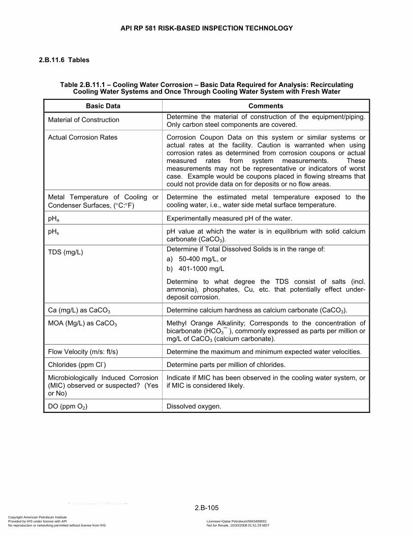
API RP 581 RISK-BASED INSPECTION TECHNOLOGY
2.B.11.6 Tables
Table 2.B.11.1 – Cooling Water Corrosion – Basic Data Required for Analysis: Recirculating Cooling Water Systems and Once Through Cooling Water System with Fresh Water
Basic Data Comments
Material of Construction Determine the material of construction of the equipment/piping. Only carbon steel components are covered.
Actual Corrosion Rates Corrosion Coupon Data on this system or similar systems or actual rates at the facility. Caution is warranted when using corrosion rates as determined from corrosion coupons or actual measured rates from system measurements. These measurements may not be representative or indicators of worst case. Example would be coupons placed in flowing streams that could not provide data on for deposits or no flow areas.
Metal Temperature of Cooling or Condenser Surfaces, (°C:°F)
Determine the estimated metal temperature exposed to the cooling water, i.e., water side metal surface temperature.
pHa Experimentally measured pH of the water.
pHs pH value at which the water is in equilibrium with solid calcium carbonate (CaCO3).
TDS (mg/L) Determine if Total Dissolved Solids is in the range of: a) 50-400 mg/L, or b) 401-1000 mg/L
Determine to what degree the TDS consist of salts (incl. ammonia), phosphates, Cu, etc. that potentially effect under-deposit corrosion.
Ca (mg/L) as CaCO3 Determine calcium hardness as calcium carbonate (CaCO3).
MOA (Mg/L) as CaCO3 Methyl Orange Alkalinity; Corresponds to the concentration of bicarbonate (HCO3¯ ), commonly expressed as parts per million or mg/L of CaCO3 (calcium carbonate).
Flow Velocity (m/s: ft/s) Determine the maximum and minimum expected water velocities.
Chlorides (ppm Cl-) Determine parts per million of chlorides.
Microbiologically Induced Corrosion (MIC) observed or suspected? (Yes or No)
Indicate if MIC has been observed in the cooling water system, or if MIC is considered likely.
DO (ppm O2) Dissolved oxygen.
2.B-105 Copyright American Petroleum Institute Provided by IHS under license with API Licensee=Qatar Petroleum/5943408001
Not for Resale, 10/20/2008 01:51:29 MDTNo reproduction or networking permitted without license from IHS
--```,`,,`,`,,`,`,,,,,,``,```,`-`-`,,`,,`,`,,`---

API RP 581 RISK-BASED INSPECTION TECHNOLOGY
Table 2.B.11.2 – Cooling Water Corrosion – Basic Data Required for Analysis: Once Through Cooling Water System with Salt Water
Basic Data Comments
Material of Construction Determine the material of construction of the equipment/piping. Only carbon steel components are covered.
Actual Corrosion Rates Corrosion Coupon Data on this system or similar systems or actual rates at the facility.
Flow Velocity (m/s:ft/s) Determine the maximum and minimum expected water velocities.
2.B-106 Copyright American Petroleum Institute Provided by IHS under license with API Licensee=Qatar Petroleum/5943408001
Not for Resale, 10/20/2008 01:51:29 MDTNo reproduction or networking permitted without license from IHS
--```,`,,`,`,,`,`,,,,,,``,```,`-`-`,,`,,`,`,,`---

API RP 581 RISK-BASED INSPECTION TECHNOLOGY
Table 2.B.11.3 – pH Calculation Parameters
1C Factor 3C Factor 4C Factor
Total Solids (mg/L) 1C
Calcium Hardness
(mg/L CaCO3) 3C M.O. Alkalinity
(mg/L CaCO3) 4C
50-400 0.1 10.5 0.6 10.5 10.5 > 400-1000 0.2 12.5 0.7 12.5 12.5
2C Factor 15.5 0.8 15.5 1.2
20 0.9 20 1.3
Temperature (ºC)
Temperature (ºF) 2C
25 1.0 25 1.4 31 1.1 31 1.5
1 33 2.6 39 1.2 40 1.6 4 39 2.5 49.5 1.3 50 1.7 8 46 2.4 62.5 1.4 62.5 1.8 12 53 2.3 78.5 1.5 79 1.9 16 60 2.2 99 1.6 99.5 2.0 19 67 2.1 124.5 1.7 125 2.1 24 76 2.0 156.5 1.8 158 2.2 29 85 1.9 197.5 1.9 197.5 2.3 34 94 1.8 250 2.0 250 2.4 41 105 1.7 310 2.1 315 2.5 47 117 1.6 390 2.2 400 2.6 53 128 1.5 495 2.3 500 2.7 60 140 1.4 625 2.4 625 2.8 68 154 1.3 785 2.5 790 2.9 77 170 1.2 940 2.6 945 3.0
2.B-107 Copyright American Petroleum Institute Provided by IHS under license with API Licensee=Qatar Petroleum/5943408001
Not for Resale, 10/20/2008 01:51:29 MDTNo reproduction or networking permitted without license from IHS
--```,`,,`,`,,`,`,,,,,,``,```,`-`-`,,`,,`,`,,`---
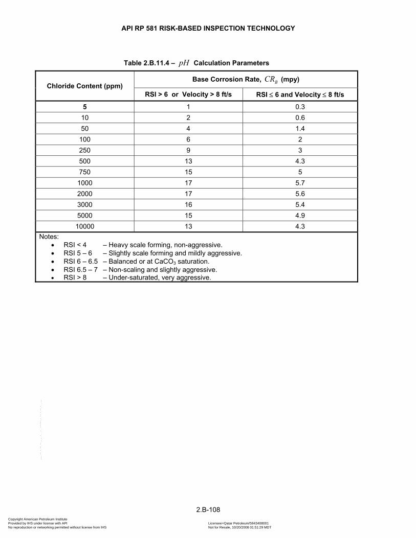
API RP 581 RISK-BASED INSPECTION TECHNOLOGY
Table 2.B.11.4 – pH Calculation Parameters
Chloride Content (ppm) Base Corrosion Rate, (mpy) BCR
RSI > 6 or Velocity > 8 ft/s RSI ≤ 6 and Velocity ≤ 8 ft/s
5 1 0.3 10 2 0.6 50 4 1.4
100 6 2 250 9 3 500 13 4.3 750 15 5 1000 17 5.7 2000 17 5.6 3000 16 5.4 5000 15 4.9 10000 13 4.3
Notes: • RSI < 4 – Heavy scale forming, non-aggressive. • RSI 5 – 6 – Slightly scale forming and mildly aggressive. • RSI 6 – 6.5 – Balanced or at CaCO3 saturation. • RSI 6.5 – 7 – Non-scaling and slightly aggressive. • RSI > 8 – Under-saturated, very aggressive.
2.B-108 Copyright American Petroleum Institute Provided by IHS under license with API Licensee=Qatar Petroleum/5943408001
Not for Resale, 10/20/2008 01:51:29 MDTNo reproduction or networking permitted without license from IHS
--```,`,,`,`,,`,`,,,,,,``,```,`-`-`,,`,,`,`,,`---
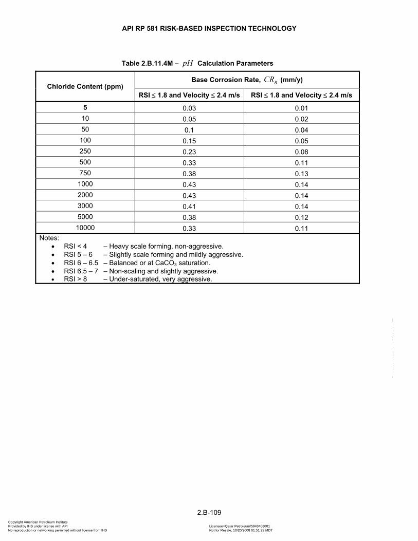
API RP 581 RISK-BASED INSPECTION TECHNOLOGY
Table 2.B.11.4M – pH Calculation Parameters
Chloride Content (ppm) Base Corrosion Rate, (mm/y) BCR
RSI ≤ 1.8 and Velocity ≤ 2.4 m/s RSI ≤ 1.8 and Velocity ≤ 2.4 m/s
5 0.03 0.01 10 0.05 0.02 50 0.1 0.04
100 0.15 0.05 250 0.23 0.08 500 0.33 0.11 750 0.38 0.13 1000 0.43 0.14 2000 0.43 0.14 3000 0.41 0.14 5000 0.38 0.12 10000 0.33 0.11
Notes: • RSI < 4 – Heavy scale forming, non-aggressive. • RSI 5 – 6 – Slightly scale forming and mildly aggressive. • RSI 6 – 6.5 – Balanced or at CaCO3 saturation. • RSI 6.5 – 7 – Non-scaling and slightly aggressive. • RSI > 8 – Under-saturated, very aggressive.
2.B-109 Copyright American Petroleum Institute Provided by IHS under license with API Licensee=Qatar Petroleum/5943408001
Not for Resale, 10/20/2008 01:51:29 MDTNo reproduction or networking permitted without license from IHS
--```,`,,`,`,,`,`,,,,,,``,```,`-`-`,,`,,`,`,,`---
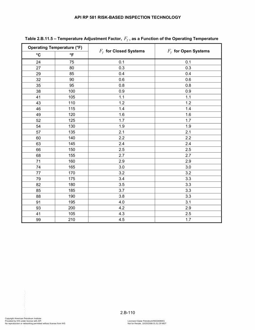
API RP 581 RISK-BASED INSPECTION TECHNOLOGY
Table 2.B.11.5 – Temperature Adjustment Factor, , as a Function of the Operating Temperature TF
Operating Temperature (°F) TF for Closed Systems TF for Open Systems
°C °F 24 75 0.1 0.1 27 80 0.3 0.3 29 85 0.4 0.4 32 90 0.6 0.6 35 95 0.8 0.8 38 100 0.9 0.9 41 105 1.1 1.1 43 110 1.2 1.2 46 115 1.4 1.4 49 120 1.6 1.6 52 125 1.7 1.7 54 130 1.9 1.9 57 135 2.1 2.1 60 140 2.2 2.2 63 145 2.4 2.4 66 150 2.5 2.5 68 155 2.7 2.7 71 160 2.9 2.9 74 165 3.0 3.0 77 170 3.2 3.2 79 175 3.4 3.3 82 180 3.5 3.3 85 185 3.7 3.3 88 190 3.8 3.3 91 195 4.0 3.1 93 200 4.2 2.9 41 105 4.3 2.5 99 210 4.5 1.7
2.B-110 Copyright American Petroleum Institute Provided by IHS under license with API Licensee=Qatar Petroleum/5943408001
Not for Resale, 10/20/2008 01:51:29 MDTNo reproduction or networking permitted without license from IHS
--```,`,,`,`,,`,`,,,,,,``,```,`-`-`,,`,,`,`,,`---

API RP 581 RISK-BASED INSPECTION TECHNOLOGY
Table 2.B.11.6 – Flow Velocity Adjustment Factor ( ) as a Function of the Flow Velocity VF
Flow Velocity VF – Flow Velocity Factor
m/s ft/s
0.15 0.5 2.25
0.3 1 2
0.61 2 1.5
0.91 3 1
1.22 4 1
1.52 5 1
1.83 6 1
2.13 7 1
2.44 8 1
2.74 9 1.25
3.05 10 1.5
3.35 11 1.75
3.66 12 2
3.96 13 2.25
4.27 14 2.5
4.57 15 2.75
4.88 16 3
5.18 17 3.25
5.49 18 3.5
5.79 19 3.75
6.1 20 4
2.B-111 Copyright American Petroleum Institute Provided by IHS under license with API Licensee=Qatar Petroleum/5943408001
Not for Resale, 10/20/2008 01:51:29 MDTNo reproduction or networking permitted without license from IHS
--```,`,,`,`,,`,`,,,,,,``,```,`-`-`,,`,,`,`,,`---
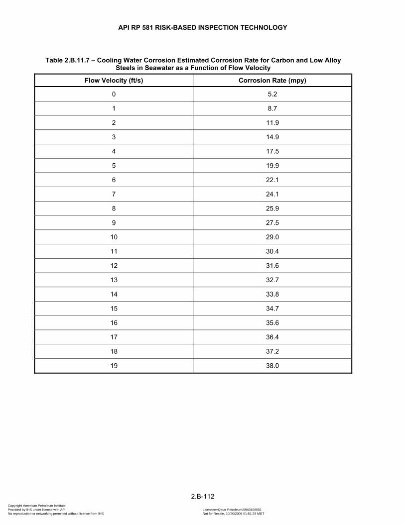
API RP 581 RISK-BASED INSPECTION TECHNOLOGY
Table 2.B.11.7 – Cooling Water Corrosion Estimated Corrosion Rate for Carbon and Low Alloy Steels in Seawater as a Function of Flow Velocity
Flow Velocity (ft/s) Corrosion Rate (mpy)
0 5.2
1 8.7
2 11.9
3 14.9
4 17.5
5 19.9
6 22.1
7 24.1
8 25.9
9 27.5
10 29.0
11 30.4
12 31.6
13 32.7
14 33.8
15 34.7
16 35.6
17 36.4
18 37.2
19 38.0
2.B-112 Copyright American Petroleum Institute Provided by IHS under license with API Licensee=Qatar Petroleum/5943408001
Not for Resale, 10/20/2008 01:51:29 MDTNo reproduction or networking permitted without license from IHS
--```,`,,`,`,,`,`,,,,,,``,```,`-`-`,,`,,`,`,,`---
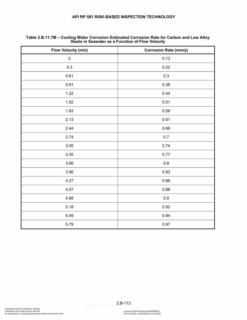
API RP 581 RISK-BASED INSPECTION TECHNOLOGY
Table 2.B.11.7M – Cooling Water Corrosion Estimated Corrosion Rate for Carbon and Low Alloy Steels in Seawater as a Function of Flow Velocity
Flow Velocity (m/s) Corrosion Rate (mm/y)
0 0.13
0.3 0.22
0.61 0.3
0.91 0.38
1.22 0.44
1.52 0.51
1.83 0.56
2.13 0.61
2.44 0.66
2.74 0.7
3.05 0.74
3.35 0.77
3.66 0.8
3.96 0.83
4.27 0.86
4.57 0.88
4.88 0.9
5.18 0.92
5.49 0.94
5.79 0.97
2.B-113 Copyright American Petroleum Institute Provided by IHS under license with API Licensee=Qatar Petroleum/5943408001
Not for Resale, 10/20/2008 01:51:29 MDTNo reproduction or networking permitted without license from IHS
--```,`,,`,`,,`,`,,,,,,``,```,`-`-`,,`,,`,`,,`---
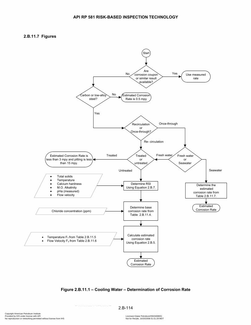
API RP 581 RISK-BASED INSPECTION TECHNOLOGY
2.B.11.7 Figures
Start
Are corrosion coupon or similar result
available?
Carbon or low-alloy steel?
Recirculationor
Once-through?
Fresh wateror
Seawater
Treatedor
untreated
Determine RSIUsing Equation 2.B.7.
Determine basecorrosion rate from
Table 2.B.11.4.
Calculate estimatedcorrosion rate
Using Equation 2.B.5.
Determine the estimated
corrosion rate from Table 2.B.11.7.
YesNo
No
Yes
Fresh water
SeawaterUntreated
Treated
Total solidsTemperatureCalcium hardnessM.O. AlkalinitypHa (measured)Flow velocity
Temperature FT from Table 2.B.11.5 Flow Velocity FV from Table 2.B.11.6
Chloride concentration (ppm)
Use measuredrate
Once-through
Re- circulation
Estimated Corrosion Rate
Estimated Corrosion Rate
Estimated Corrosion Rate is 0.5 mpy
Estimated Corrosion Rate isless than 3 mpy and pitting is less
than 15 mpy.
Figure 2.B.11.1 – Cooling Water – Determination of Corrosion Rate
2.B-114 Copyright American Petroleum Institute Provided by IHS under license with API Licensee=Qatar Petroleum/5943408001
Not for Resale, 10/20/2008 01:51:29 MDTNo reproduction or networking permitted without license from IHS
--```,`,,`,`,,`,`,,,,,,``,```,`-`-`,,`,,`,`,,`---
API RP 581 RISK-BASED INSPECTION TECHNOLOGY
2.B.12 SOIL SIDE CORROSION
2.B.12.1 Description of Damage
2.B.12.1.1 Overview
The objective for this supplement is to give a conservative approach for assessing the potential for soil corrosion and determining appropriate mitigation measures, while taking the most significant factors for soil corrosion into account.
This supplement pertains to any carbon steel equipment or structure having surface metal exposed to soil, with the exception of the soil side of Above Ground Storage Tanks, which are covered in paragraph 2.B.14. The most typical equipment exposed to soil corrosion, is buried or partly buried carbon steel vessels / drums and piping, with some type of coating.
The method described in this paragraph may be used to establish an estimate of the corrosion rate that would be expected in a given environment. If actual corrosion rates are known for particular pieces of equipment or other similar equipment in similar service, that data may be used in lieu of this method.
2.B.12.1.2 Soil Corrosivity
The deterioration of the exterior of metals exposed to soils is usually referred to as soil corrosion, and is often attributed to soil characteristics. Soils having high moisture content, high dissolved salt concentrations, and high acidity are expected to be the most corrosive. However, soil composition alone has been found to have little correlation with soil corrosivity.
There is no single easily-measured soil parameter that can be used to determine soil corrosivity. Instead, a number of characteristics must be combined to estimate the corrosion that may be expected on a steel structure from a particular soil. According to ASTM STP 741, Soil Corrosivity Classes can be characterized by total acidity, resistivity, conductivity, drainage (soil texture) and aeration (water-air permeability). The most significant causes for soil corrosion are described in paragraph 2.B.12.2.
Soils frequently have characteristics, of which some indicate that the soil is corrosive and others indicate just the opposite. By virtue of water and related water-soluble salts being present, soil becomes an effective electrolyte for completing the corrosion circuit between anode and cathode. This can be true even if the soil is fairly dry and nonconductive (high resistivity). The water content in the soils relates to drainage, which is defined as the ability to allow water percolation. In the long term, the residence time for water or moisture on the metal surface will control the degree of corrosion in soil. Measuring this residence time is difficult or impossible in practice. Therefore, it becomes necessary to use more easily measured soil characteristics, which have a less certain correlation with soil corrosivity. The parameters usually considered include soil resistivity, pH, chloride content, redox potential and type of soil.
Soil resistivity is frequently used to estimate soil corrosivity, mainly because it is easy to measure (commonly measured by the 4-pin Werner technique as described in ASME G 57, or electromagnetic non-contacting methods, Geonics). In practice, the conditions around the equipment surface are likely to be different than in the surrounding native soil, due to different compaction and possibly also different soil type and texture (especially where sand is used for backfill). Furthermore, the conditions probably vary along the equipment surface as well. These variations will cause local effects that are not easily predicted by bulk resistivity measurements, and these local effects again make a direct correlation solely between soil resistivity and soil corrosivity of questionable value.
2.B.12.1.3 Preventing Soil Corrosion
The common prevention methods for soil corrosion of carbon steel equipment are special backfill, coating, and cathodic protection (CP). The most effective corrosion protection is achieved by a combination of a corrosion resistant coating and an effective CP system. With an effective CP system in place, the corrosion rate can be maintained at a level close to zero. However, maintaining and managing an effective CP system can be complex and should involve personnel competent in this field. An effective CP system will normally be maintained in compliance with a recognized standard, such as NACE RP0169.
2.B-115 Copyright American Petroleum Institute Provided by IHS under license with API Licensee=Qatar Petroleum/5943408001
Not for Resale, 10/20/2008 01:51:29 MDTNo reproduction or networking permitted without license from IHS
--```,`,,`,`,,`,`,,,,,,``,```,`-`-`,,`,,`,`,,`---

API RP 581 RISK-BASED INSPECTION TECHNOLOGY
Partially buried equipment must be handled in three ways. The portion under the soil will be treated as a piece of buried equipment. The portion exposed to air will be treated as any other outdoor equipment and often requires little attention. The soil-to-air interface is unique for the location and alloy, and soil-to-air interface corrosion may present a higher corrosion concern than underground corrosion.
Equipment that is fully encased in concrete is not normally in need of additional corrosion protection provided that a chloride-free concrete mix is used and moisture content is stable, and it is not subject to chloride intrusion.
2.B.12.2 Description of Damage
The soil corrosion damage morphology is generally expected to be localized external corrosion, i.e. pitting at the anode. The severity of corrosion depends on the local soil conditions and changes in the immediate environment along the equipment metal surface. The following are the main theoretical causes of soil and underground corrosion:
a) Equipment Temperature – For a moist environment containing dissolved oxygen, an increase in the equipment temperature (operating temperature for piping or pipelines) can significantly increase the external corrosion rate. Theoretically corrosion by oxygen (Oxidation) ceases when all the dissolved oxygen is consumed. Oxygen can be replenished by drain water, or from the air (especially at the soil-to-air interface). The corrosion reaction is primarily controlled by diffusion of oxygen to the corroding surface. Any process that slows oxygen diffusion slows the reaction, and ultimately reduce the corrosion rate. As corrosion products accumulate on the corroding surface, oxygen diffusion is slowed. Corrosion due to oxidation of steel doubles for every 20-30°C (35-55°F) rise in temperature, beginning at room temperature. Corrosion is nearly proportional to temperature up to about 80°C (180°F) when oxygen is replenished unrestricted to the corroding surface. With the increase in temperature, dissolved oxygen is driven from the water solution, resulting in a decrease in the rate of corrosion by oxygen.
b) Galvanic Corrosion (Dissimilar Metal Corrosion) – This occurs when two different metals are joined in the soil, such as steel and copper. Electrical current will flow from the steel into the soil and back into the copper resulting in corrosion of the steel. A less recognized, but similar phenomenon occurs when new steel is connected to old steel in the soil, such as when replacing a section of corroded pipe. The new steel that is not cathodically protected will frequently experience a higher corrosion rate.
c) Corrosion Resulting from Dissimilar Soils – In much the same manner as dissimilar metals, a structure that contacts two or more different types of soil will have different electrical potentials between the metal and each respective soil. Hence, variations in soil density and porosity can be a common cause of corrosion in buried equipment, with more dense soil areas promoting an anodic reaction and lighter soil cover promoting a cathodic reaction. The resultant pitting at the anode can lead to swift penetration of the wall. The phenomena can occur even over long distances. For example, on a buried pipeline, the anodic areas and cathodic areas may be considerable distances apart, for example where a pipeline crosses a marshy area near a river and then runs through much drier sandy soil. The differences in the native pipe-to-soil potential can be sufficient to set up a corrosion cell with anode and cathode many hundreds of yards apart.
d) Corrosion by Stray Current Drainage – This corrosion differs from other corrosion damage types in that the current, which causes the corrosion, has a source external to the affected structure. The stray current source can be AC power lines, telephone lines, adjacent cathodic protection systems, or any electrically driven equipment, most notably rail systems. Stray currents flow from an external source onto a pipeline or structure and then flow along it to some other area(s) where they leave to reenter the earth causing localized corrosion. Where stray current corrosion is a factor, CP may not be the best method of controlling corrosion. The majority of stray current corrosion problems result from the interacting cathodic protection systems where nearby equipment provides the low-resistance paths for the current from the impressed-current cathodic protection system to pass before returning to the protected equipment. This disturbance in current distribution makes the CP system incomplete and causes localized corrosion on the interfering equipment. One solution to stray current problems is electrical bonding of nearby equipment. However, the appropriate solution needs to be evaluated on a case by case basis.
2.B-116 Copyright American Petroleum Institute Provided by IHS under license with API Licensee=Qatar Petroleum/5943408001
Not for Resale, 10/20/2008 01:51:29 MDTNo reproduction or networking permitted without license from IHS
--```,`,,`,`,,`,`,,,,,,``,```,`-`-`,,`,,`,`,,`---
API RP 581 RISK-BASED INSPECTION TECHNOLOGY
e) Differential Aeration Corrosion Cells – Local differences in the packing of the soil and in its moisture content may develop oxygen concentration cells where the area with the least oxygen is anodic to the area in which oxygen is more readily available. Aeration corrosion cells are similar to the corrosion cells that produce pitting in waters, when one area of the metal has more ready access to oxygen than other areas. The areas with less access to oxygen will corrode preferentially. This sometimes occurs when a pipe passes beneath a roadbed or crosses deep underneath a river.
f) Microbiologically Induced Corrosion – Microbacterial action can also promote local corrosion. Corrosion enhanced by sulfate reducing bacteria is well documented. These microbes reduce the commonly available sulfate ions in the soil to produce hydrogen sulfide. This, in turn, results in increased acidity and acceleration of anodic dissolution. Coating types, age and condition are significant factors in preventing microbiologically influenced corrosion.
2.B.12.3 Basic Data
The data listed in Table 2.B.12.1 are required to determine the estimated corrosion rate for soil side corrosion. If precise data have not been measured, a knowledgeable process specialist should be consulted.
2.B.12.4 Determination of Corrosion Rate
2.B.12.4.1 Corrosion Rate Equation
The steps required to determine the corrosion rate are shown in Figure 2.B.12.1. The corrosion rate may be determined using the basic data in Table 2.B.12.1 in conjunction with Equation. (2.B.21)
B SR T CP CECR CR F F F F= ⋅ ⋅ ⋅ ⋅ (2.B.21)
In this equation, the base corrosion rate, , is adjusted for soil resistivity, , temperature, , cathodic
protection, , and coating effectiveness, . Determination of the base corrosion rate and each of these factors is discussed in the following paragraphs.
BCR
CEFSRF TF
CPF
2.B.12.4.2 Establishing the Base Corrosion Rate
The base corrosion rate is the expected or observed corrosion rate for the buried equipment or structure. Estimating a corrosion rate based on soil properties is difficult without extensive physical and chemical analyses. Corrosion rates will be estimated based on rather easily established general characteristics, as shown in Table 2.B.12.2. There are numerous possible combinations of these variables, with possible offsetting or compounding effects on the expected corrosion rate. The user should use a corrosion rate that is based on the actual conditions of the soil in contact with the structure. Corrosion rates should be extrapolated between those values shown in the table to account for the expected effects of the various factors. For example, if a soil had all the characteristics of those in row 2 of the table, then a corrosion rate of 0.13 mm/y (5 mpy) would be estimated. If however, the soil was primarily clay, in an industrial setting (moderate chemical contaminants), with a mixture of some other soil types and sizes and the soil is normally saturated, a corrosion rate between 0.13 and 0.25 mm/y (5 and 10 mpy), or as an average 0.178 mm/y (7 mpy) would be estimated. If actual corrosion rates are known for the particular piece of equipment or other similar equipment in similar service, that data should be used.
2.B.12.4.3 Adjustment Factor for Soil Resistivity (Optional)
The soil resistivity factor might be considered as input information when estimating the base corrosion, and as such discarded as an adjustment factor. However, for a couple of cases, the soil resistivity factor should be included as an adjustment factor for the base corrosion rate, i.e. where:
a) Estimation of the base corrosion rate is determined by intuitive settings for the sub-factors in Table 2.B.12.2, and
2.B-117 Copyright American Petroleum Institute Provided by IHS under license with API Licensee=Qatar Petroleum/5943408001
Not for Resale, 10/20/2008 01:51:29 MDTNo reproduction or networking permitted without license from IHS
--```,`,,`,`,,`,`,,,,,,``,```,`-`-`,,`,,`,`,,`---

API RP 581 RISK-BASED INSPECTION TECHNOLOGY
b) Regular measurements of soil resistivity are part of the inspection program and variation in soil resistivity might be the only indicative variable for monitoring changes in the soil characteristics (an example would be monitoring soil resistivity around a cooling tower basin with adjacent chemical treating facilities).
Soil resistivity gives a composite measure of moisture content of soil and dissolved electrolytes in the soil water, i.e. an indication for soil condition. Soil resistivity has often been used as a broad indicator of soil corrosivity. Because ionic current flow is associated with soil corrosion reactions, high resistivity will arguably slow down corrosion reactions although a high soil resistivity alone will not guarantee absence of serious corrosion. Soil resistivity generally decreases with increasing water content and concentration of ionic species. Variations in soil resistivity along the length of the structure are highly undesirable, as this will lead to the formation of macro corrosion cells. Thus, the merit of a corrosion risk classification based on an absolute value of soil resistivity is limited.
Resistivity of native undisturbed earth and the soil adjacent to the pipe (looser) may be very different. However, over time the less compacted and possibly higher resistivity soil near the structure will assume the characteristics of the native soil, i.e. the high resistivity soil might become contaminated by capillary action. While the soil resistivity against the pipe or structure cannot be measured accurately, bulk measurements can be taken for soil resistivity in the vicinity of the buried equipment. Given the above theory and assuming several measurements will be taken, these resistivity measurements can be considered representative for the soil adjacent to the structure.
Normal soil resistivity is 3,000-5,000 Ω·cm, although 20,000 Ω·cm is not uncommon. Corrosion rate adjustment factors for soil resistivities are provided in Table 2.B.12.3. The ranges in this table are consistent with API 651 (general classification of resistivity, based on NACE 51011). API 570 (1997) only stipulates 3 ranges (<2000; 2000-10000; >10000) for determining the recommended inspection frequencies of 5, 10 and 15 years, respectively, for buried piping without cathodic protection.
2.B.12.4.4 Adjustment Factor for Temperature
The base corrosion rate is adjusted for the operating temperature in accordance with Table 2.B.12.4. See ASM Handbook 13 (Corrosion) for temperature effect on external corrosion.
2.B.12.4.5 Adjustment Factor for Cathodic Protection and Stray Current Drainage
Cathodic protection is the primary method used to avoid corrosion of buried structures from the soil corrosion. However, the system must be installed and maintained properly. In Table 2.B.12.5 corrosion rate adjustment factors are given for CP system coverage and expected efficiency of protection. “Hot Spot” protection is the practice of installing sacrificial anodes (aluminum, zinc or magnesium) at locations of suspected anodic activity, as determined by surveys of structure-to-soil potential. Complete protection is achieved by installation of sacrificial anodes or impressed current protection systems sufficient to cover the entire surface of the buried equipment. Anodic protection is not an applicable method for protection of buried equipment. NACE Standard RP0169 establishes three criteria for protection. One common reference level is a structure-to-soil potential measurement of –0.85 volts with reference to a copper/copper sulfate reference electrode. This criterion is considered less effective than the other two criteria commonly known as: a) 100mV polarization and b) –0.85 Volt polarized structure-to-soil potential.
As discussed earlier, stray current can originate from various external sources such as power lines, electrically driven equipment and impressed current cathodic protection systems in the environs. Except for the few cases where AC stray currents is present from inductively coupled situations such as paralleling high tension lines, stray current would not occur if electrical systems were entirely insulated from earth. At the same time, proper grounding of electrical power circuits is necessary to reduce electric shock hazards. Hence the stray current corrosion problem will probably never be eliminated.
A low level, steady state current may be controlled with CP systems. But a larger stray current that may be dynamic would require special analysis and corrective measures. The corrosion potential from these larger stray current problems is of a much higher magnitude than the other corrosion causes discussed. Therefore, they should be addressed first before considering any other effects on the corrosion potential of the equipment or structure being addressed. An effective Cathodic Protection system will include testing and mitigating the effect of stray currents on a routine basis.
2.B-118 Copyright American Petroleum Institute Provided by IHS under license with API Licensee=Qatar Petroleum/5943408001
Not for Resale, 10/20/2008 01:51:29 MDTNo reproduction or networking permitted without license from IHS
--```,`,,`,`,,`,`,,,,,,``,```,`-`-`,,`,,`,`,,`---
API RP 581 RISK-BASED INSPECTION TECHNOLOGY
Adjustment factors for CP systems, based on the effectiveness of the system, are provided in Table 2.B.12.5. It shall be noted that the effectiveness of the CP system depends on the continuity of operation of impressed current sources, the system complies to NACE RP0169 and managed by NACE certified personal.
For structures which are only partly protected by a cathodic protection system, the unprotected areas will have corrosion rates that are determined by the prevailing conditions.
2.B.12.4.6 Adjustment Factor for Coating Effectiveness
The primary effect that a coating has on the corrosion rate is related to the potential for the coating to shield the cathodic protection current in the event that the coating becomes disbonded from the structure. This is a complicated relationship between many factors, but is primarily related to how well coating adheres to the pipe and how age, temperature extremes, and maintenance practices affect the dielectric properties of the coating. Each factor is considered to be independent of each other. All of multiplying factors that apply to the coating in question should be used to determine the total coating effectiveness factor, . CEF
Table 2.B.12.6 is used for calculating the adjustment factor for a coating. When the multiplying factors criterion does not apply, substitute factor with 1.0. For example, for a mill applied PE tape that is 30 years old, has been occasionally subjected to temperatures over the maximum and there is never any coating inspection or maintenance, the total coating effectiveness factor would be:
1.5 1.2 3.0 1.5 13.5CEF = ⋅ ⋅ ⋅ = (2.B.22)
For a bare pipe or structure, . For a pipe that does not have cathodic protection, the coating effectiveness factors should still be used since holidays in the coating may allow concentrated corrosion to occur in the damaged area.
1.0CEF =
2.B.12.5 Nomenclature CR is the corrosion rate
BCR is the base corrosion rate
CEF is the corrosion rate correction factor for coating effectiveness
CPF is the corrosion rate correction factor for cathodic protection
SRF is the corrosion rate correction factor for soil resistivity
TF is the corrosion rate correction factor for temperature
2.B.12.6 References
52. Control of Pipeline Corrosion, A.W. Peabody, NACE, Houston, TX (1967). 53. Cathodic Protection, Morgan, John, NACE, Houston, TX (1987). 54. AWWA Journal,O’Day, D. Kelly, “External Corrosion in Distribution Systems”, October 1989. 55. Pipe Line Corrosion and Cathodic Protection, Marshall E. Parker, Gulf Publishing Company, Houston, TX
(1954). 56. Underground Corrosion, M. Romanoff, NACE, Houston, TX (1997). 57. Principles and Prevention of Corrosion, Jones, A. Denny, McMillan Publishing Co. (1992). 58. Corrosion Handbook, Herbert H. Uhlig, John Wilkey & Sons, Inc. (1948). 59. Handbook of Corrosion Engineering, Pierre R. Roberge, McGraw-Hill 1999.
2.B-119 Copyright American Petroleum Institute Provided by IHS under license with API Licensee=Qatar Petroleum/5943408001
Not for Resale, 10/20/2008 01:51:29 MDTNo reproduction or networking permitted without license from IHS
--```,`,,`,`,,`,`,,,,,,``,```,`-`-`,,`,,`,`,,`---

API RP 581 RISK-BASED INSPECTION TECHNOLOGY
2.B.12.7 Tables
Table 2.B.12.1 – Soil Side Corrosion – Basic Data Required for Analysis
Basic Data Comments
Base Corrosion Rate, mm/yr [mpy] The expected or observed corrosion rate for the buried structure, or a “similar” structure under “similar” service and conditions.
Equipment Temperature, °C [°F] Equipment temperature (operating temperature for piping and pipelines)
Soil Resistivity, cmΩ− Soil characteristics in the vicinity of the buried structure.
Cathodic Protection Specify whether or not a cathodic protection system is installed, and how effective it is.
Coating Type of coating, age, temperature abuse and inspection and maintenance history, if a coating is installed.
Equipment Age, years The time since installation of the buried equipment – used to determine accumulated corrosion over time since buried.
Table 2.B.12.2 – Base Corrosion Rate
Factors Affecting Base Corrosion Rate Base Corrosion Rate
Primary Soil Type Level of
Chemical Contaminants
Particle Size and Uniformity Moisture Level mm/y mpy
Sand Low Chlorides (Inland, non-
industrial)
Homogeneous, fine silt or sand Dry, Desert-like 0.03 1
Silt Moderate (Industrial) Mixed Variable moisture 0.13 5
Clay High Chlorides (Coastal Areas) > 50% Gravel Normally saturated 0.25 10
Table 2.B.12.3 – Soil Resistivity Adjustment
Resistivity (Ω cm) Corrosiveness Multiplying Factor
<500 Very Corrosive 1.50 500-1000 Corrosive 1.25
1000-2000 Moderately Corrosive 1.00 2000-10000 Mildly Corrosive 0.83
>10000 Progressively less corrosive 0.60
2.B-120 Copyright American Petroleum Institute Provided by IHS under license with API Licensee=Qatar Petroleum/5943408001
Not for Resale, 10/20/2008 01:51:29 MDTNo reproduction or networking permitted without license from IHS
--```,`,,`,`,,`,`,,,,,,``,```,`-`-`,,`,,`,`,,`---
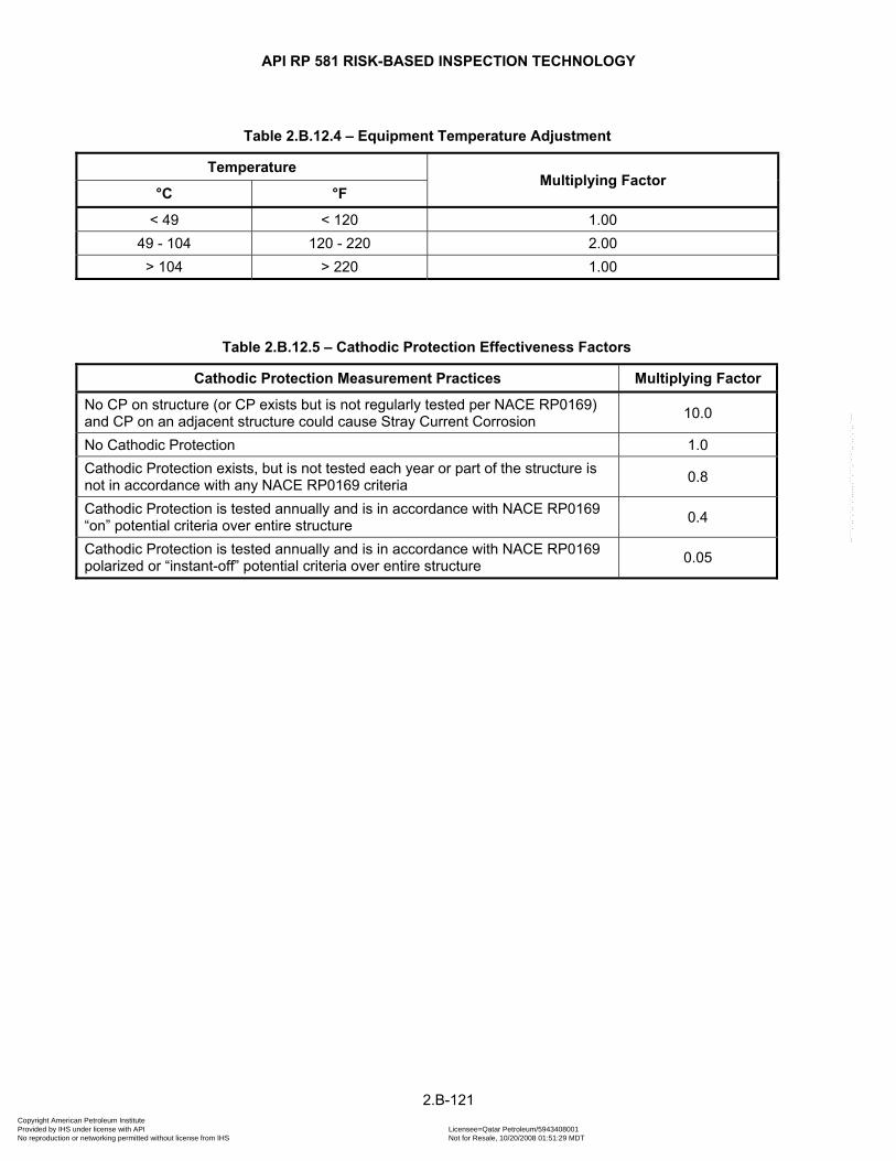
API RP 581 RISK-BASED INSPECTION TECHNOLOGY
Table 2.B.12.4 – Equipment Temperature Adjustment
Temperature Multiplying Factor
°C °F
< 49 < 120 1.00 49 - 104 120 - 220 2.00
> 104 > 220 1.00
Table 2.B.12.5 – Cathodic Protection Effectiveness Factors
Cathodic Protection Measurement Practices Multiplying Factor
No CP on structure (or CP exists but is not regularly tested per NACE RP0169) and CP on an adjacent structure could cause Stray Current Corrosion 10.0
No Cathodic Protection 1.0 Cathodic Protection exists, but is not tested each year or part of the structure is not in accordance with any NACE RP0169 criteria 0.8
Cathodic Protection is tested annually and is in accordance with NACE RP0169 “on” potential criteria over entire structure 0.4
Cathodic Protection is tested annually and is in accordance with NACE RP0169 polarized or “instant-off” potential criteria over entire structure 0.05
2.B-121 Copyright American Petroleum Institute Provided by IHS under license with API Licensee=Qatar Petroleum/5943408001
Not for Resale, 10/20/2008 01:51:29 MDTNo reproduction or networking permitted without license from IHS
--```,`,,`,`,,`,`,,,,,,``,```,`-`-`,,`,,`,`,,`---

API RP 581 RISK-BASED INSPECTION TECHNOLOGY
Table2.B.12.6 – Calculating the Total Coating Effectiveness Factor
COATING TYPE Base Factor for Coating Type
Multiplying Factors
Age > 20 yrs Maximum Rated Temperature is Occasionally
Exceeded
Coating Maintenance is Rare or None
Fusion Bonded Epoxy
1.0 1.1 1.5 1.1 Liquid Epoxy Asphalt Enamel Asphalt Mastic
Coal Tar Enamel 1.0 1.2 2.0 1.5 Extruded
Polyethylene with mastic or rubber
1.0 1.2 3.0 1.5
Mill Applied PE Tape with mastic 1.5 1.2 3.0 1.5
Field Applied PE Tape with mastic 2.0 2.0 3.0 1.5
Three-Layer PE or PP 1.0 1.2 2.0 1.2
2.B-122 Copyright American Petroleum Institute Provided by IHS under license with API Licensee=Qatar Petroleum/5943408001
Not for Resale, 10/20/2008 01:51:29 MDTNo reproduction or networking permitted without license from IHS
--```,`,,`,`,,`,`,,,,,,``,```,`-`-`,,`,,`,`,,`---

API RP 581 RISK-BASED INSPECTION TECHNOLOGY
2.B.12.8 Figures
Determine Base Corrosion Rate using Table 2.B.12.2.
Soil Resistivityconsidered for Base
CR ?
Calculate Soil ResistivityFactor using Table 2.B.12.3.
Determine Operating Temperature factor using Table 2.B.12.4.
Determine Cathodic Protection System effectiveness using Table 2.B.12.5.
Determine Coating Effectiveness FactorUsing Table 2.B.12.6.
Set Coating Effectiveness Factor to 1.0
Yes
No
Start
Is there a coating?
YesNo
Calculate estimatedcorrosion rate
Using Equation 2.B.21.
Estimated Corrosion Rate
Figure 2.B.12.1 – Soil Side Corrosion – Determination of Corrosion Rate
2.B-123 Copyright American Petroleum Institute Provided by IHS under license with API Licensee=Qatar Petroleum/5943408001
Not for Resale, 10/20/2008 01:51:29 MDTNo reproduction or networking permitted without license from IHS
--```,`,,`,`,,`,`,,,,,,``,```,`-`-`,,`,,`,`,,`---

API RP 581 RISK-BASED INSPECTION TECHNOLOGY
2.B.13 CO2 CORROSION
2.B.13.1 Description of Damage
Carbon Dioxide is a weakly acidic gas which is corrosive when dissolved in water becoming carbonic acid (H2CO3). CO2 is commonly found in upstream sections before treatment. CO2 corrosion requires the presence of water in order to produce the Carbonic acid. The primary variables, which influence CO2 corrosion rates, are the CO2 concentration, operating pressure, operating temperature, application of inhibitors, flow rate, and presence of hydrocarbon fluids and contaminants in the system.
Aqueous CO2 corrosion of carbon and low alloy steels is an electrochemical process involving the anodic dissolution of iron and the cathodic evolution of hydrogen. The electrochemical reactions are often accompanied by the formation of films of FeCO3 (and/or Fe3O4) which can be protective or non-protective depending on the conditions under which these are formed.
2.B.13.2 Basic Data
The data listed in Table 2.B.13.1 are required to determine the estimated corrosion rate for carbonic acid service. If precise data have not been measured, a knowledgeable process specialist should be consulted. Entering only the data marked required will result in a conservative estimate of the corrosion rate. The calculation for the corrosion rate is more refined as more optional data is entered.
2.B.13.3 Determination of Corrosion Rate
2.B.13.3.1 Calculation of the Corrosion Rate
The steps required to determine the corrosion rate are shown in Figure 2.B.13.1. The corrosion rate may be determined using the basic data in Table 2.B.13.1 in conjunction with Equation (2.B.23).
min ,B glycol inhibCR CR F F⎡= ⋅ ⎣ ⎤⎦ (2.B.23)
The calculation of the base corrosion rate, , is most complex; it depends on the temperature, the partial pressure of CO2, the fluid flow velocity and the pH of the fluid. The following paragraphs detail how these can be estimated for RBI purposes for some simple mixtures of crude oil, water, and natural gas mixtures. In order to estimate corrosion rates for situations outside this simple mixture, the analyst should refer to the NORSOK standard M-506. In cases where the equipment is not associated with upstream production, the analyst should also be prepared to adjust or estimate corrosion rates for fluids that are not mixtures of crude, water and natural gas.
BCR
2.B.13.3.2 Relative Humidity
In order for corrosion to occur, there must be liquid water present in the equipment. In a system transporting gas, liquid water exists only if the temperature is below the dew point and the relative humidity in the stream is greater than 100%. When a mixture of water vapor and natural gas behaves approximately as ideal gases, the relative humidity in a gas is 100% when the partial pressure of the water vapor is equal to the saturation pressure. This result in the simplified formula for the relative humidity,
( )1
0.622sat
x PRHP T x
⎛ ⎞⋅ ⎛ ⎞= ⎜ ⎟⎜⎜ ⎟ +⎝ ⎠⎝ ⎠⎟ (2.B.24)
2.B-124 Copyright American Petroleum Institute Provided by IHS under license with API Licensee=Qatar Petroleum/5943408001
Not for Resale, 10/20/2008 01:51:29 MDTNo reproduction or networking permitted without license from IHS
--```,`,,`,`,,`,`,,,,,,``,```,`-`-`,,`,,`,`,,`---

API RP 581 RISK-BASED INSPECTION TECHNOLOGY
In Equation (2.B.24), x is the ratio of the mass of water to the mass of dry gas, or ( )% 100 %w − w , where
is the percent water by weight in the stream. The parameter is the pressure and is the
saturation pressure for water at temperature T , which can be obtained from steam tables. The 0.622 is the ratio of the molecular weight of water (≈18) to the average molecular weight of air (≈29). Using Equation (
%w P ( )satP T
dT2.B.24) and standard steam tables, an approximate equation for the dew point temperature (°F) can be derived, see Equation (2.B.25).
[ ]10 10 10%log 2.0866 0.2088 log 0.2242 log100d
wT ⎡ ⎤= + ⋅ + ⋅⎢ ⎥⎣ ⎦P (2.B.25)
In Equation (2.B.25), is the pressure in psia, % is the percent water by weight in the stream (lbm/100lbm), between 0 and 30.
P w
2.B.13.3.3 Base Corrosion Rate
The base corrosion rate in mm/y is calculated from Equation (2.B.26) To obtain mpy, multiply the result in mm/y by 39.4.
( )2
2
0.146 0.03240.62,
19
COf
base COSCR f T pH f
+⎛ ⎞= ⋅ ⋅⎜ ⎟⎝ ⎠
(2.B.26)
In Equation (2.B.26), ( , )f T pH is the temperature-pH function that is tabulated in Table 2.B.13.2. This tabulated function was calculated by combining the M-506 temperature and temperature dependent function pH function into a single quantity. It should be noted that the ( , )f T pH function jumps sharply between 80°C and 90°C (176°F and 194°F.).
The CO2 fugacity, 2COf in bar, pH, and the shear stress from the flow in Pa needed to calculate the basic
corrosion rate are discussed in the following paragraphs. S
2.B.13.3.4 Determining the pH
For RBI purposes, the pH term in temperature-pH function tabulated in Table 2.B.13.2 may be calculated using one of the following approximations. For condensation,
[ ]210 102.8686 0.7931 log 0.57 log COpH T p⎡ ⎤= + ⋅ − ⋅ ⎣ ⎦ (2.B.27)
for Fe++ saturated water,
[ ]210 102.5907 0.8668 log 0.49 log COpH T p⎡ ⎤= + ⋅ − ⋅ ⎣ ⎦ (2.B.28)
and for water with salinity slightly greater than seawater (salinity = 46 g/l),
[ ]210 102.7137 0.8002 log 0.57 log COpH T p⎡ ⎤= + ⋅ − ⋅ ⎣ ⎦ (2.B.29)
In Equations (2.B.27), (2.B.28), and (2.B.29), T is the temperature in °F and 2COp is the CO2 partial pressure
in psi. These approximations were developed from Monte Carlo simulations. These simulation studies used the equilibrium equations recommended and by M-506 to calculate the concentration of hydrogen cation and then the pH for a wide range of temperatures, pressures, and CO2 mole fractions.
2.B-125 Copyright American Petroleum Institute Provided by IHS under license with API Licensee=Qatar Petroleum/5943408001
Not for Resale, 10/20/2008 01:51:29 MDTNo reproduction or networking permitted without license from IHS
--```,`,,`,`,,`,`,,,,,,``,```,`-`-`,,`,,`,`,,`---
API RP 581 RISK-BASED INSPECTION TECHNOLOGY
Equations (2.B.27), (2.B.28), and (2.B.29) apply to water, seawater and Fe++ saturated water and do not account for the buffering action of bicarbonate ions or for the increase acidity caused by salinity levels higher than 45 g/l. In cases where these factors are significant, the analyst should consider using an alternative analysis such as direct application of the provisions in M-506 for salinity and dissolved bicarbonate.
2.B.13.3.5 Determining the CO2 Fugacity
Fugacity has units of pressure. It is used in place of the pressure – or partial pressure – in calculations concerning the equilibrium of real gas mixtures. When the fugacity is used in place of the pressure, real gases can be modeled using the equations for ideal gases. M-506 uses the following equation for modeling the fugacity,
2COf .
2 2 210 101.4log log min 250, 0.0031
273CO CO COf p pT
⎛ ⎞⎡ ⎤ ⎡ ⎤ ⎡ ⎤= + ⋅ −⎜⎣ ⎦ ⎣ ⎦ ⎣ ⎦ +⎝ ⎠⎟ (2.B.30)
[ ]2 210 10 10log log logCO COf p⎡ ⎤ ⎡ ⎤= +⎣ ⎦ ⎣ ⎦ a (2.B.31)
In Equations (2.B.30) and (2.B.31), 2COp is the CO2 partial pressure in bar and T is the temperature in °C.
Note that the fugacity coefficient, , is the ratio between CO2 fugacity and the partial pressure, or: a
2 2CO COf p a= ⋅ (2.B.32)
2.B.13.3.6 Determining the Flow Velocity
M-506 uses the fluid flow shear stress to model the effect of flow velocity on the base corrosion rate. M-506 recommends the Equation (2.B.33) to calculate the stress, , in units of Pa. In the calculation for the corrosion rate, the shear stress need not exceed 150 Pa.
S
2
2m mf uS ρ⋅ ⋅
= (2.B.33)
In Equation (2.B.33), f is the friction factor, is the mixture flow velocity in m/s, and mu mρ is the mixture mass density in kg/m3. The friction coefficient may be approximated for turbulent flow (Re > 2300) by using Equation (2.B.34).
0.336100.001375 1 20000 efD Re
⎡ ⎤⎛ ⎞⎛ ⎞= + +⎢ ⎜ ⎜ ⎟⎝ ⎠⎢ ⎥⎝ ⎠⎣ ⎦
⎥⎟ (2.B.34)
The term e D is the relative roughness and Re is the Reynolds Number of the mixture given by Equation (2.B.35).
mm
mm
ADmuDReμμ
ρ== (2.B.35)
In Equation (2.B.35), is the diameter in meters, and D mμ is viscosity of the mixture in Pa·s (0.001cP = Pa·s).
This equation also shows that the Reynolds number can be calculated using the mass flux, , and the cross sectional area, .
mA
2.B-126 Copyright American Petroleum Institute Provided by IHS under license with API Licensee=Qatar Petroleum/5943408001
Not for Resale, 10/20/2008 01:51:29 MDTNo reproduction or networking permitted without license from IHS
--```,`,,`,`,,`,`,,,,,,``,```,`-`-`,,`,,`,`,,`---
API RP 581 RISK-BASED INSPECTION TECHNOLOGY
M-506 gives some guidance on the calculation of the two-phase viscosity, density, and fluid velocity. These factors depend on the volumetric ratio of the liquid flow to the flow, sometimes known as the liquid hold up, the amount of water in the liquid fraction, the gas water and oil viscosities at the temperature and pressure. These calculations are complex and go beyond the scope of an RBI study. If required, the analyst can refer to the recommendations in NORSOK or use the software provided by NORSOK to perform the calculations recommended in M-506 to approximate the two-phase flow characteristics. While M-506 provides some guidelines for the calculation of bulk fluid properties, they do not explicitly account for the solubility of natural gas in oil, which can also affect the all of these properties.
2.B.13.3.7 Adjustment for Inhibitors or Glycol
The addition of glycol reduces the CO2 corrosion rate. M-506 accounts for this by simply reducing the corrosion rate by applying a factor of the form:
[ ](10log 1.6 log 100 2glycolF⎡ ⎤ = ⋅ − −⎣ ⎦ )G (2.B.36)
In Equation (2.B.36), G is the percent weight of glycol as a percent of water in the system. glycolF is limited to a
minimum value of 0.008. The base corrosion rate is multiplied by the factor glycolF to account for the corrosion reduction due to glycol.
For other types of corrosion inhibitors added to the stream, M-506 requires that its effectiveness must be independently determined and used directly as a reduction factor, . If both glycol and an inhibitor are
used, the minimum of and inhibF
inhibF glycolF should be used as shown in Equation (2.B.23).
2.B-127 Copyright American Petroleum Institute Provided by IHS under license with API Licensee=Qatar Petroleum/5943408001
Not for Resale, 10/20/2008 01:51:29 MDTNo reproduction or networking permitted without license from IHS
--```,`,,`,`,,`,`,,,,,,``,```,`-`-`,,`,,`,`,,`---
API RP 581 RISK-BASED INSPECTION TECHNOLOGY
2.B.13.4 Nomenclature a is the fugacity coefficient A is the pipe cross sectional area, m2 [ft2] CR is the corrosion rate
BCR is the base corrosion rate
D is the pipe diameter, m [ft] e D is the relative roughness f is the fraction factor
2COf is the CO2 fugacity, bar
( , )f T pH is the temperature-pH function
glycolF is the corrosion rate correction factor for glycol
inhibF is the corrosion rate correction factor for the inhibitor
G is the percent weight of glycol as a percent of water in the system m is the calculated using the mass flux, kg/m2-s [lb/ft2-s] P is the pressure, psia
( )satP T is the saturation pressure for water at temperature , psia T
2COp is the CO2 partial pressure, bar [psi]
%w is the percent water by weight in the stream Re is the Reynolds Number RH is the relative humidity
mρ is the mixture mass density, kg/m3
S is the shear stress, Pa T is the temperature, °C [°F]
dT is dew point temperature, °C [°F]
mu is the mixture flow velocity, m/s
mμ is the viscosity of the mixture, cp x is the ratio of the mass of water to the mass of dry gas
2.B-128 Copyright American Petroleum Institute Provided by IHS under license with API Licensee=Qatar Petroleum/5943408001
Not for Resale, 10/20/2008 01:51:29 MDTNo reproduction or networking permitted without license from IHS
--```,`,,`,`,,`,`,,,,,,``,```,`-`-`,,`,,`,`,,`---
API RP 581 RISK-BASED INSPECTION TECHNOLOGY
2.B.13.5 Tables
Table 2.B.13.1 – CO2 Corrosion – Basic Data Required for Analysis
Basic Data Comments
Temperature – Required The corrosion phenomenon is highly temperature dependent. The maximum temperature of the process is required. Temperatures above 140°C (284°F) are not considered.
Pressure – Required Total pressure of the system. The total pressure of the gas is a big contributor in the corrosion rate up to about 250 psig.
CO2 concentration (mole %) – Required
Determine the CO2 partial pressure (pCO2) = (mol fraction of CO2 × total pressure), a maximum 4 MPa (580 psi) partial CO2 pressure is considered.
pCO2 – Required, if CO2 concentration is not given
CO2 partial pressure, which is converted to CO2 fugacity to account for non-ideal behavior.
Material of Construction – Required Determine the material of construction of equipment/piping. Stainless steels and copper alloys are assumed to be resistant to CO2 corrosion
pH – Required
If known explicitly, the pH of the stream should be used; otherwise Equations(2.B.27), (2.B.28), and (2.B.29), can be used to estimate the pH based on the CO2 partial pressure, whether the water in the stream is Fe++ saturated or water with salinity slightly larger than seawater.
Stream properties: bulk density, ρm, viscosity, μm, gas to liquid ratios –Required
Guidance with respect to typical values properties expected in natural gas-oil mixtures (i.e. reservoir fluids) is provided. Estimation of densities can be made on the basis of the oil density (°API), gas oil ratio (GOR) and pressure, P and temperature, T. For other streams, a process engineer should assess these parameters.
For systems with liquids: Water Cut – Optional
Determine the percentage of water in the system. The default for this field is 30%
For gas systems: Relative humidity, RH or the dew point temperature, – Optional
dT
Determine the dew point temperature, based on the water content. Equation (
dT2.B.25) is provided for guidance, but should
not be assumed to be accurate within ±10°F. If not provided the gas stream temperature is assumed to below the dew point.
Glycol/Water mix - Optional Water content of glycol/water mix in %weight (%water in the total glycol/water mix). The default value would assume no glycol added in the system.
Inhibition efficiency - Optional Requires %efficiency of the inhibitor. No inhibitor injected as a default value.
2.B-129 Copyright American Petroleum Institute Provided by IHS under license with API Licensee=Qatar Petroleum/5943408001
Not for Resale, 10/20/2008 01:51:29 MDTNo reproduction or networking permitted without license from IHS
--```,`,,`,`,,`,`,,,,,,``,```,`-`-`,,`,,`,`,,`---

API RP 581 RISK-BASED INSPECTION TECHNOLOGY
Table 2.B.13.2 – pH Temperature function
Temperature
(°F)
pH
3.5 4.0 4.5 5.0 5.5 6.0 6.5
68 6.00 5.45 4.9 3.72 2.55 1.55 0.72 86 8.52 7.77 7.02 5.16 3.40 2.00 0.91 104 10.98 10.06 9.13 6.49 4.08 2.30 1.02 122 11.92 10.96 10.01 6.86 4.10 2.20 0.94 140 12.83 11.86 10.89 7.18 4.05 2.03 0.84 158 13.42 12.01 10.6 6.58 3.61 1.86 0.87 176 13.93 12.12 10.31 6.01 3.20 1.70 0.90 194 9.37 7.91 6.45 2.44 0.82 0.49 0.32 212 9.23 8.04 6.38 2.19 0.94 0.62 0.42 230 8.96 8.09 6.22 1.87 1.07 0.77 0.53 248 8.55 8.06 5.98 1.48 1.20 0.92 0.65 266 7.38 6.39 3.98 0.96 0.80 0.63 0.47 284 6.26 4.91 2.31 0.53 0.46 0.39 0.32 302 5.20 3.62 0.98 0.19 0.19 0.19 0.19
Table 2.B.13.2M – pH Temperature function
Temperature
(°C)
pH
3.5 4.0 4.5 5.0 5.5 6.0 6.5
20 6.00 5.45 4.9 3.72 2.55 1.55 0.72 30 8.52 7.77 7.02 5.16 3.40 2.00 0.91 40 10.98 10.06 9.13 6.49 4.08 2.30 1.02 50 11.92 10.96 10.01 6.86 4.10 2.20 0.94 60 12.83 11.86 10.89 7.18 4.05 2.03 0.84 70 13.42 12.01 10.6 6.58 3.61 1.86 0.87 80 13.93 12.12 10.31 6.01 3.20 1.70 0.90 90 9.37 7.91 6.45 2.44 0.82 0.49 0.32 100 9.23 8.04 6.38 2.19 0.94 0.62 0.42 110 8.96 8.09 6.22 1.87 1.07 0.77 0.53 120 8.55 8.06 5.98 1.48 1.20 0.92 0.65 130 7.38 6.39 3.98 0.96 0.80 0.63 0.47 140 6.26 4.91 2.31 0.53 0.46 0.39 0.32 150 5.20 3.62 0.98 0.19 0.19 0.19 0.19
2.B-130 Copyright American Petroleum Institute Provided by IHS under license with API Licensee=Qatar Petroleum/5943408001
Not for Resale, 10/20/2008 01:51:29 MDTNo reproduction or networking permitted without license from IHS
--```,`,,`,`,,`,`,,,,,,``,```,`-`-`,,`,,`,`,,`---
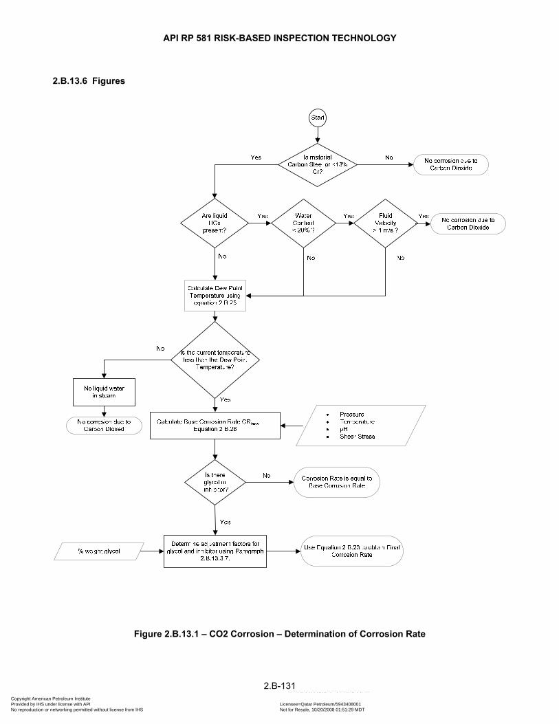
API RP 581 RISK-BASED INSPECTION TECHNOLOGY
2.B.13.6 Figures
Figure 2.B.13.1 – CO2 Corrosion – Determination of Corrosion Rate
2.B-131 Copyright American Petroleum Institute Provided by IHS under license with API Licensee=Qatar Petroleum/5943408001
Not for Resale, 10/20/2008 01:51:29 MDTNo reproduction or networking permitted without license from IHS
--```,`,,`,`,,`,`,,,,,,``,```,`-`-`,,`,,`,`,,`---
API RP 581 RISK-BASED INSPECTION TECHNOLOGY
2.B.14 ATMOSPHERIC STORAGE TANK BOTTOM CORROSION
2.B.14.1 Description of Damage
Corrosion occurs from the product side (internal corrosion) and soil side (external corrosion) of atmospheric storage tank bottoms constructed of carbon steel. Product side corrosion can result in general or localized thinning. Factors affecting product side corrosion is the stored product corrosivity characteristics, operating temperature, steam coil practices and the presence of water in the tank. Soil side corrosion results in localized thinning. Factors affecting soil side corrosion are soil type, pad type, water draining, cathodic protection, tank bottom design and operating temperature of the process stored.
2.B.14.2 Basic Data
2.B.14.2.1 Soil-Side Corrosion Rate Equation
The data listed in Table 2.B.14.1 are required to determine the estimated corrosion rate for soil side service. If precise data have not been measured, a knowledgeable corrosion specialist should be consulted.
2.B.14.2.2 Product-Side Corrosion Rate Equation
The data listed in Table 2.B.14.2 are required to determine the estimated corrosion rate for product side service. If precise data have not been measured, a knowledgeable process specialist should be consulted.
2.B.14.3 Determination of Corrosion Rate
2.B.14.3.1 Soil-Side Corrosion Rate Equation
The steps required to determine the corrosion rate are shown in Figure 2.B.14.1. The corrosion rate may be determined using the basic data in Table 2.B.14.1 in conjunction with Equation (2.B.37).
S SB SR PA TD CP TB STCR CR F F F F F F= ⋅ ⋅ ⋅ ⋅ ⋅ ⋅ (2.B.37)
The base soil side base corrosion rate, , should be determined based on actual inspection data. If this data is not available, then the base soil side corrosion rate may be assumed to be 0.13 mm/y (5 mpy). This base corrosion rate is the expected or observed corrosion rate for a typical tank under average conditions (see
SBCR
Table 2.B.14.3) neither highly susceptible to corrosion nor especially resistant to corrosion.
The adjustment factors in Equation (2.B.37) are determined as described below.
a) Adjustment Factor for Soil Conditions, SRF – The corrosion rate adjustment factor is given in Table 2.B.14.4. The resistivity of the native soil beneath the tank pad can affect the corrosion rate of the tank bottom. The resistivity of the tank pad material may be higher than the existing surrounding soil. However, corrosive soil beneath the high resistivity tank pad material may contaminate the tank pad fill by capillary action (See API RP 651, 1997 Section 5.3.1). Therefore, resistivity of the surrounding native soil may be used to determine the likelihood of corrosion on the tank bottom. A common method of measuring soil resistivity is described in ASTM G 57. If the soil resistivity is not known, then assume Moderately Corrosive soil (adjustment factor equals 1). Note that an adjustment factor of 1 is used for tanks with Release Prevention Barriers (RPBs), since RPBs effectively prevent the contamination of the tank pad material by the native soil.
b) Adjustment Factor for Tank Pad, PAF – The corrosion rate adjustment factor is given in Table 2.B.14.5. The type of pad or foundation that the tank rests upon will influence the corrosion rate. The adjustment factors are assigned in a similar manner to those for the native soil beneath the tank pad.
2.B-132 Copyright American Petroleum Institute Provided by IHS under license with API Licensee=Qatar Petroleum/5943408001
Not for Resale, 10/20/2008 01:51:29 MDTNo reproduction or networking permitted without license from IHS
--```,`,,`,`,,`,`,,,,,,``,```,`-`-`,,`,,`,`,,`---
API RP 581 RISK-BASED INSPECTION TECHNOLOGY
c) Adjustment Factor for Drainage, TDF – The corrosion rate adjustment factor is given in Table 2.B.14.6. Rainwater collecting around the base of the tank can greatly increase corrosion. The adjustment is made so that storm water collecting around a tank will cause the base corrosion rate to increase by a factor of 2. If the drainage is so poor that more than one-third of the circumference of the bottom edge of the tank is underwater for extended periods of time then the base corrosion rate is increased by a factor of 3. Good drainage is considered normal, so the multiplier is set to 1 if water does not normally collect around the base of the tank.
d) Adjust for Cathodic Protection, CPF – The corrosion rate adjustment factor is given in Table 2.B.14.7. Cathodic protection is one of the primary methods used to avoid corrosion of tank bottoms from the soil side. However, the system must be installed and maintained properly. The factor is established so that the most credit is given for a properly functioning cathodic protection (CP) system in accordance with API 651, but no penalty is assessed for lack of CP. This assumes that the base corrosion rate is for systems without cathodic protection. Note that unless a High Level inspection can verify that the CP system is effective (verified by inspection in compliance with NACE RP0169 or equivalent), no credit is obtained for the CP system.
e) Adjust for Tank Bottom Type, TBF – The corrosion rate adjustment factor is given in Table 2.B.14.8. Tanks with properly installed release prevention barriers (RPB) tend to have bottom corrosion rates comparable to those with a single bottom.
f) Adjustment for Operating Temperature, STF – The corrosion rate adjustment factor is given in Table 2.B.14.9. The operating temperature of the tank may influence external corrosion.
2.B.14.3.2 Product Side Corrosion Rate Equation
The steps required to determine the corrosion rate are shown in Figure 2.B.14.1. The corrosion rate may be determined using the basic data in Table 2.B.14.2 in conjunction with Equation (2.B.38).
P PB PC PT SC WDCR CR F F F F= ⋅ ⋅ ⋅ ⋅ (2.B.38)
The product side base corrosion rate, PBCR , should be determined based on actual inspection data. If this data is not available, then the base product side corrosion rate may be assumed to be 0.05 mm/y (2 mpy). The base corrosion rate is founded on the conditions stated in Table 2.B.14.10.
The adjustment factors in Equation (2.B.38) are determined as described below.
a) Adjustment for Product Condition, PCF – The corrosion rate adjustment factor is given in Table 2.B.14.11. Wet conditions should be used if significant bottom sediments and water are present.
b) Adjustment for Operating temperature, PTF – The corrosion rate adjustment factor is given in Table 2.B.14.12.
c) Adjustment for Steam Coil, SCF – The corrosion rate adjustment factor is given in Table 2.B.14.13. If a steam coil heater is present, the internal corrosion rate is adjusted upwards slightly due to extra heat, and the possibility of steam leaks from the internal coil
d) Adjustment for Water Draw-off, WDF – The corrosion rate adjustment factor is given in Table 2.B.14.14. Water draws, when consistently used, can greatly reduce the damaging effects of water at the bottom of the tank. To receive the full benefit, water must be drawn weekly or after every receipt.
2.B-133 Copyright American Petroleum Institute Provided by IHS under license with API Licensee=Qatar Petroleum/5943408001
Not for Resale, 10/20/2008 01:51:29 MDTNo reproduction or networking permitted without license from IHS
--```,`,,`,`,,`,`,,,,,,``,```,`-`-`,,`,,`,`,,`---
API RP 581 RISK-BASED INSPECTION TECHNOLOGY
2.B.14.3.3 Combined Tank Floor Corrosion Rate
The internal and external corrosion rates are estimated by multiplying the base corrosion rate by the respective adjustment factors. This will produce two separate corrosion rates that are combined as described below. It is assumed that the soil side corrosion will be localized in nature while the product side corrosion will be either generalized or localized. Note that in order to avoid understating the risk, it is recommended that the combined corrosion rate should not be set lower than 2 mils per year.
a) Option 1 – If the internal corrosion is generalized in nature, the corrosion areas will likely overlap such that the bottom thickness is simultaneously reduced by both internal and external influences. In this case, the internal and external rates are additive.
b) Option 2 – For pitting and localized corrosion, the chances are low that internal and external rates can combine to produce an additive effect on wall loss. In this case, the user chooses the greater of the two corrosion rates as the governing rate for the proceeding step.
2.B.14.4 Nomenclature
PCR is the product side corrosion rate
PBCR is the product side base corrosion rate
SCR is the soil side corrosion rate
SBCR is the soil side base corrosion rate
CPF is the soil side corrosion rate correction factor for cathodic protection
PAF is the soil side corrosion rate correction factor for tank pad type
PCF is the product side corrosion rate correction factor for product condition
PTF is the product side corrosion rate correction factor for temperature
SCF is the soil side corrosion rate correction factor for temperature
SRF is the soil side corrosion rate correction factor for soil conditions
STF is the product side corrosion rate correction factor for temperature
TBF is the soil side corrosion rate correction factor for tank bottom type
TDF is the soil side corrosion rate correction factor for drainage
WDF is the product side corrosion rate correction factor for water draw-off
2.B-134 Copyright American Petroleum Institute Provided by IHS under license with API Licensee=Qatar Petroleum/5943408001
Not for Resale, 10/20/2008 01:51:29 MDTNo reproduction or networking permitted without license from IHS
--```,`,,`,`,,`,`,,,,,,``,```,`-`-`,,`,,`,`,,`---
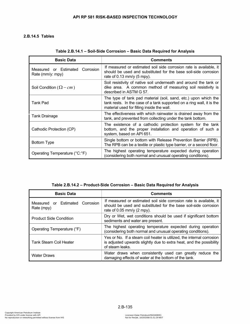
API RP 581 RISK-BASED INSPECTION TECHNOLOGY
2.B.14.5 Tables
Table 2.B.14.1 – Soil-Side Corrosion – Basic Data Required for Analysis
Basic Data Comments
Measured or Estimated Corrosion Rate (mm/y: mpy)
If measured or estimated soil side corrosion rate is available, it should be used and substituted for the base soil-side corrosion rate of 0.13 mm/y (5 mpy).
Soil Condition ( ) cmΩ−Soil resistivity of native soil underneath and around the tank or dike area. A common method of measuring soil resistivity is described in ASTM G 57.
Tank Pad The type of tank pad material (soil, sand, etc.) upon which the tank rests. In the case of a tank supported on a ring wall, it is the material used for filling inside the wall.
Tank Drainage The effectiveness with which rainwater is drained away from the tank, and prevented from collecting under the tank bottom.
Cathodic Protection (CP) The existence of a cathodic protection system for the tank bottom, and the proper installation and operation of such a system, based on API 651.
Bottom Type Single bottom or bottom with Release Prevention Barrier (RPB). The RPB can be a textile or plastic type barrier, or a second floor.
Operating Temperature (°C:°F) The highest operating temperature expected during operation (considering both normal and unusual operating conditions).
Table 2.B.14.2 – Product-Side Corrosion – Basic Data Required for Analysis
Basic Data Comments
Measured or Estimated Corrosion Rate (mpy)
If measured or estimated soil side corrosion rate is available, it should be used and substituted for the base soil-side corrosion rate of 0.05 mm/y (2 mpy).
Product Side Condition Dry or Wet, wet conditions should be used if significant bottom sediments and water are present.
Operating Temperature (°F) The highest operating temperature expected during operation (considering both normal and unusual operating conditions).
Tank Steam Coil Heater Yes or No. If a steam coil heater is utilized, the internal corrosion is adjusted upwards slightly due to extra heat, and the possibility of steam leaks.
Water Draws Water draws when consistently used can greatly reduce the damaging effects of water at the bottom of the tank.
2.B-135 Copyright American Petroleum Institute Provided by IHS under license with API Licensee=Qatar Petroleum/5943408001
Not for Resale, 10/20/2008 01:51:29 MDTNo reproduction or networking permitted without license from IHS
--```,`,,`,`,,`,`,,,,,,``,```,`-`-`,,`,,`,`,,`---
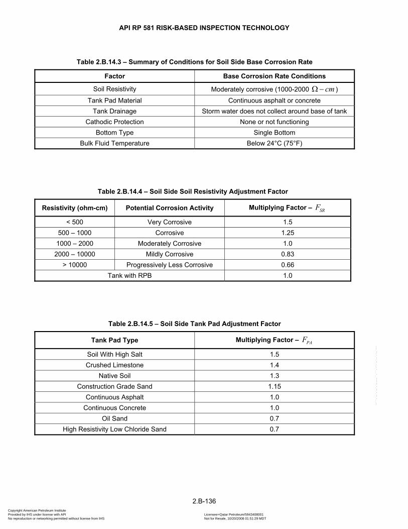
API RP 581 RISK-BASED INSPECTION TECHNOLOGY
Table 2.B.14.3 – Summary of Conditions for Soil Side Base Corrosion Rate
Factor Base Corrosion Rate Conditions
Soil Resistivity Moderately corrosive (1000-2000 ) cmΩ−Tank Pad Material Continuous asphalt or concrete
Tank Drainage Storm water does not collect around base of tank Cathodic Protection None or not functioning
Bottom Type Single Bottom Bulk Fluid Temperature Below 24°C (75°F)
Table 2.B.14.4 – Soil Side Soil Resistivity Adjustment Factor
Resistivity (ohm-cm) Potential Corrosion Activity Multiplying Factor – SRF
< 500 Very Corrosive 1.5 500 – 1000 Corrosive 1.25 1000 – 2000 Moderately Corrosive 1.0 2000 – 10000 Mildly Corrosive 0.83
> 10000 Progressively Less Corrosive 0.66 Tank with RPB 1.0
Table 2.B.14.5 – Soil Side Tank Pad Adjustment Factor
Tank Pad Type Multiplying Factor – PAF
Soil With High Salt 1.5 Crushed Limestone 1.4
Native Soil 1.3 Construction Grade Sand 1.15
Continuous Asphalt 1.0 Continuous Concrete 1.0
Oil Sand 0.7 High Resistivity Low Chloride Sand 0.7
2.B-136 Copyright American Petroleum Institute Provided by IHS under license with API Licensee=Qatar Petroleum/5943408001
Not for Resale, 10/20/2008 01:51:29 MDTNo reproduction or networking permitted without license from IHS
--```,`,,`,`,,`,`,,,,,,``,```,`-`-`,,`,,`,`,,`---
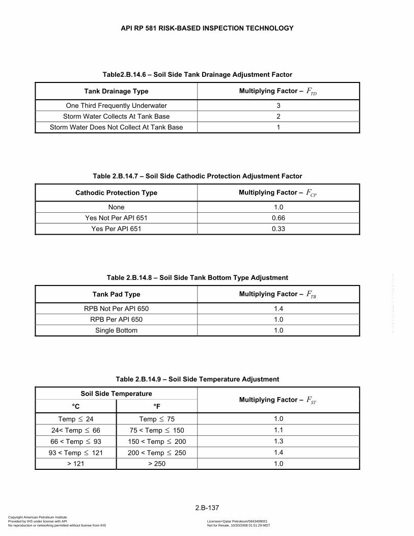
API RP 581 RISK-BASED INSPECTION TECHNOLOGY
Table2.B.14.6 – Soil Side Tank Drainage Adjustment Factor
Tank Drainage Type Multiplying Factor – TDF
One Third Frequently Underwater 3 Storm Water Collects At Tank Base 2
Storm Water Does Not Collect At Tank Base 1
Table 2.B.14.7 – Soil Side Cathodic Protection Adjustment Factor
Cathodic Protection Type Multiplying Factor – CPF
None 1.0 Yes Not Per API 651 0.66
Yes Per API 651 0.33
Table 2.B.14.8 – Soil Side Tank Bottom Type Adjustment
Tank Pad Type Multiplying Factor – TBF
RPB Not Per API 650 1.4 RPB Per API 650 1.0
Single Bottom 1.0
Table 2.B.14.9 – Soil Side Temperature Adjustment
Soil Side Temperature Multiplying Factor – STF
°C °F
Temp ≤ 24 Temp ≤ 75 1.0
24< Temp ≤ 66 75 < Temp 150 ≤ 1.1
66 < Temp 93 ≤ 150 < Temp ≤ 200 1.3
93 < Temp 121 ≤ 200 < Temp ≤ 250 1.4 > 121 > 250 1.0
2.B-137 Copyright American Petroleum Institute Provided by IHS under license with API Licensee=Qatar Petroleum/5943408001
Not for Resale, 10/20/2008 01:51:29 MDTNo reproduction or networking permitted without license from IHS
--```,`,,`,`,,`,`,,,,,,``,```,`-`-`,,`,,`,`,,`---
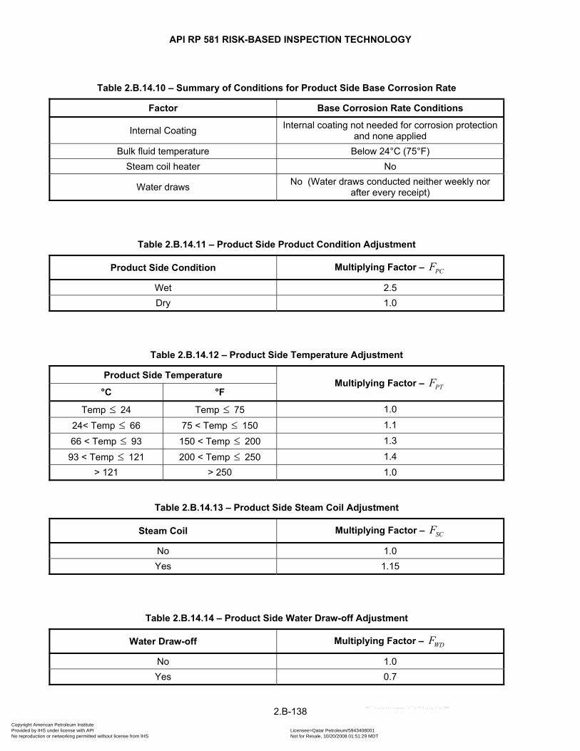
API RP 581 RISK-BASED INSPECTION TECHNOLOGY
Table 2.B.14.10 – Summary of Conditions for Product Side Base Corrosion Rate
Factor Base Corrosion Rate Conditions
Internal Coating Internal coating not needed for corrosion protection and none applied
Bulk fluid temperature Below 24°C (75°F) Steam coil heater No
Water draws No (Water draws conducted neither weekly nor after every receipt)
Table 2.B.14.11 – Product Side Product Condition Adjustment
Product Side Condition Multiplying Factor – PCF
Wet 2.5 Dry 1.0
Table 2.B.14.12 – Product Side Temperature Adjustment
Product Side Temperature Multiplying Factor – PTF
°C °F
Temp ≤ 24 Temp ≤ 75 1.0
24< Temp ≤ 66 75 < Temp 150 ≤ 1.1
66 < Temp 93 ≤ 150 < Temp ≤ 200 1.3
93 < Temp 121 ≤ 200 < Temp ≤ 250 1.4 > 121 > 250 1.0
Table 2.B.14.13 – Product Side Steam Coil Adjustment
Steam Coil Multiplying Factor – SCF
No 1.0 Yes 1.15
Table 2.B.14.14 – Product Side Water Draw-off Adjustment
Water Draw-off Multiplying Factor – WDF
No 1.0 Yes 0.7
2.B-138 Copyright American Petroleum Institute Provided by IHS under license with API Licensee=Qatar Petroleum/5943408001
Not for Resale, 10/20/2008 01:51:29 MDTNo reproduction or networking permitted without license from IHS
--```,`,,`,`,,`,`,,,,,,``,```,`-`-`,,`,,`,`,,`---
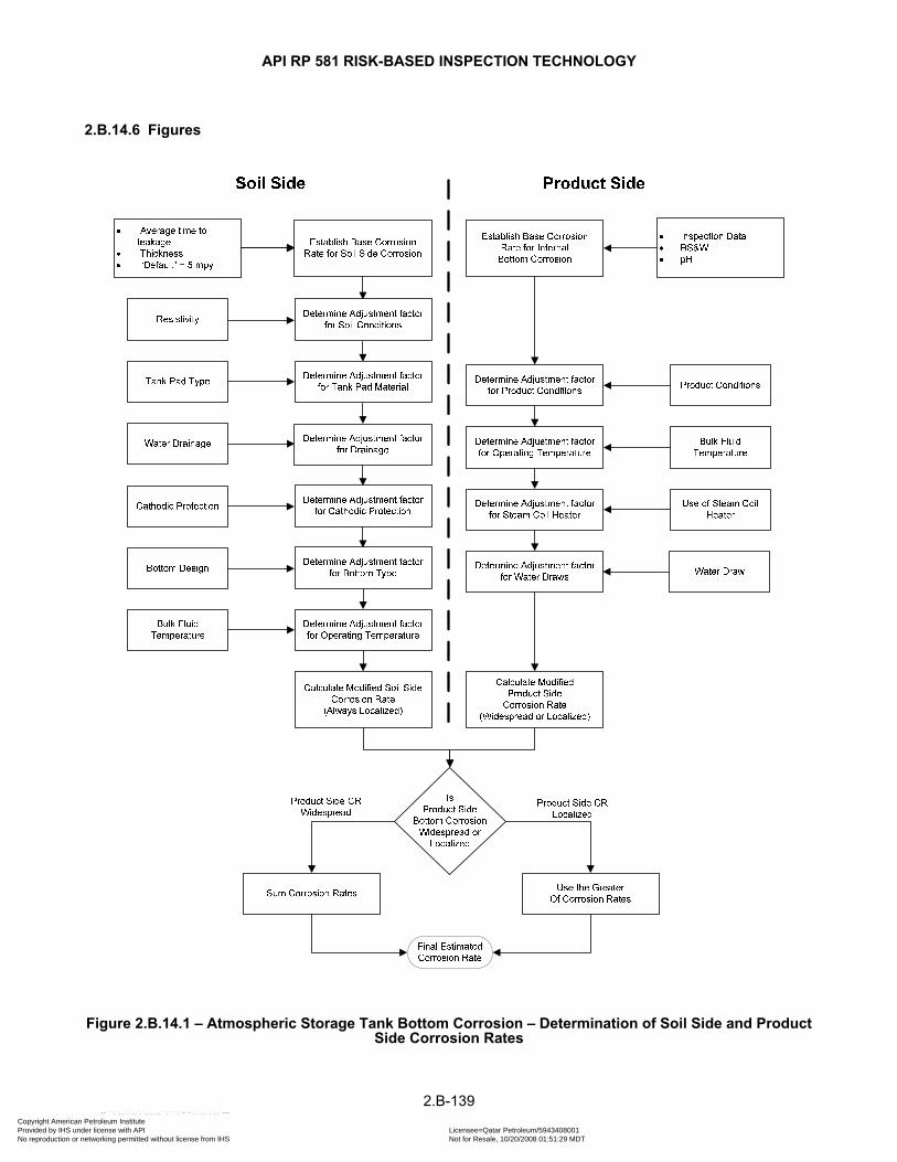
API RP 581 RISK-BASED INSPECTION TECHNOLOGY
2.B-139
2.B.14.6 Figures
Figure 2.B.14.1 – Atmospheric Storage Tank Bottom Corrosion – Determination of Soil Side and Product Side Corrosion Rates
Copyright American Petroleum Institute Provided by IHS under license with API Licensee=Qatar Petroleum/5943408001
Not for Resale, 10/20/2008 01:51:29 MDTNo reproduction or networking permitted without license from IHS
--```,`,,`,`,,`,`,,,,,,``,```,`-`-`,,`,,`,`,,`---

Copyright American Petroleum Institute Provided by IHS under license with API Licensee=Qatar Petroleum/5943408001
Not for Resale, 10/20/2008 01:51:29 MDTNo reproduction or networking permitted without license from IHS
--```,`,,`,`,,`,`,,,,,,``,```,`-`-`,,`,,`,`,,`---
API RP 581 RISK-BASED INSPECTION TECHNOLOGY
3-1
API RP 581 PART 3
CONSEQUENCE ANALYSIS IN AN API RBI ASSESSMENT
Copyright American Petroleum Institute Provided by IHS under license with API Licensee=Qatar Petroleum/5943408001
Not for Resale, 10/20/2008 01:51:29 MDTNo reproduction or networking permitted without license from IHS
--```,`,,`,`,,`,`,,,,,,``,```,`-`-`,,`,,`,`,,`---
API RP 581 RISK-BASED INSPECTION TECHNOLOGY
3-2
PART CONTENTS 1 SCOPE ........................................................................................................................................ 3-6 2 REFERENCES ............................................................................................................................ 3-6 3 DEFINITIONS.............................................................................................................................. 3-7 4 GENERAL ................................................................................................................................. 3-10
4.1 Overview........................................................................................................................... 3-10 4.1.1 Consequence Categories........................................................................................ 3-10 4.1.2 Collateral Damage.................................................................................................... 3-10
4.2 Overview of Consequence Analyses in API RBI .......................................................... 3-10 4.2.1 Level 1 Consequence Analysis .............................................................................. 3-10 4.2.2 Level 2 Consequence Analysis .............................................................................. 3-11
4.3 Consequence Analysis for Storage Tank Bottoms and Shell Courses ..................... 3-11 4.4 Consequence Analysis Calculation Procedure............................................................ 3-11 4.5 Area and Financial Based Consequence Analyses ..................................................... 3-11 4.6 Use of Atmospheric Dispersion Modeling .................................................................... 3-12 4.7 Tables................................................................................................................................ 3-13 4.8 Figures.............................................................................................................................. 3-15
5 CONSEQUENCE ANALYSIS – LEVEL 1 ................................................................................ 3-16 5.1 Determine the Representative Fluid and Associated Properties ............................... 3-16
5.1.1 Representative Fluids.............................................................................................. 3-16 5.1.2 Fluid Properties........................................................................................................ 3-16 5.1.3 Choice of Representative Fluids for Acids and Caustic Fluids .......................... 3-16 5.1.4 Estimation of Ideal Gas Specific Heat Capacity Ratio ......................................... 3-16 5.1.5 Flammable Fluid Types ........................................................................................... 3-17 5.1.6 Release Phase.......................................................................................................... 3-17 5.1.7 Calculation Procedure............................................................................................. 3-17
5.2 Release Hole Size Selection ........................................................................................... 3-18 5.2.1 General...................................................................................................................... 3-18 5.2.2 Calculation Procedure............................................................................................. 3-18
5.3 Release Rate Calculation................................................................................................ 3-18 5.3.1 Overview ................................................................................................................... 3-18 5.3.2 Liquid Release Rate Calculation ............................................................................ 3-19 5.3.3 Vapor Release Rate Equations............................................................................... 3-19 5.3.4 Calculation Procedure............................................................................................. 3-20
5.4 Estimate the Fluid Inventory Available for Release ..................................................... 3-20 5.4.1 Overview ................................................................................................................... 3-20 5.4.2 Maximum Mass Available for Release (Available Mass)...................................... 3-20 5.4.3 Calculation Procedure............................................................................................. 3-21
5.5 Determine the Release Type (Continuous or Instantaneous)..................................... 3-21 5.5.1 Release Type – Instantaneous or Continuous...................................................... 3-21 5.5.2 Calculation Procedure............................................................................................. 3-22
5.6 Estimate the Impact of Detection and Isolation Systems on Release Magnitude .... 3-22 5.6.1 Overview ................................................................................................................... 3-22 5.6.2 Assessing Detection and Isolation Systems ........................................................ 3-22 5.6.3 Impact on Release Magnitude ................................................................................ 3-22 5.6.4 Impact on Release Duration ................................................................................... 3-22 5.6.5 Releases to the Environment ................................................................................. 3-23 5.6.6 Calculation Procedure............................................................................................. 3-23
5.7 Determine the Release Rate and Mass for Consequence Analysis ........................... 3-23 5.7.1 Continuous Release Rate ....................................................................................... 3-23 5.7.2 Instantaneous Release Mass.................................................................................. 3-23 5.7.3 Calculation Procedure............................................................................................. 3-24
5.8 Determine Flammable and Explosive Consequences ................................................. 3-24 5.8.1 Overview ................................................................................................................... 3-24 5.8.2 Consequence Area Equations................................................................................ 3-24 5.8.3 Limit Liquid Release Consequence Area to 929 m2 [10,000 ft2] .......................... 3-25 5.8.4 Adjustment of Consequence Areas to Account for Mitigation Systems ........... 3-26
Copyright American Petroleum Institute Provided by IHS under license with API Licensee=Qatar Petroleum/5943408001
Not for Resale, 10/20/2008 01:51:29 MDTNo reproduction or networking permitted without license from IHS
--```,`,,`,`,,`,`,,,,,,``,```,`-`-`,,`,,`,`,,`---
API RP 581 RISK-BASED INSPECTION TECHNOLOGY
3-3
5.8.5 Adjustment of Consequence Areas for Energy Efficiencies............................... 3-26 5.8.6 Blending of Results Based on Release Type........................................................ 3-26 5.8.7 Blending of Results Based on AIT ......................................................................... 3-27 5.8.8 Determination of Final Flammable Consequence Areas ..................................... 3-27 5.8.9 Calculation Procedure............................................................................................. 3-28
5.9 Determine Toxic Consequences .................................................................................... 3-33 5.9.1 General...................................................................................................................... 3-33 5.9.2 Common Refining Toxic Materials......................................................................... 3-33 5.9.3 Common Chemical Industry Toxic Materials........................................................ 3-33 5.9.4 Representative Fluids for Toxic Mixtures ............................................................. 3-33 5.9.5 Determination of the Toxic Release Rate and Mass ............................................ 3-33 5.9.6 Estimation of Toxic Consequence Area for HF Acid and H2S............................. 3-34 5.9.7 Estimation of Toxic Consequence Area for Ammonia and Chlorine ................. 3-34 5.9.8 Estimation of Toxic Consequence Area for Additional Common Chemicals.... 3-35 5.9.9 Material Concentration Cut-Off .............................................................................. 3-35 5.9.10 Release Duration...................................................................................................... 3-35 5.9.11 Toxic Outcome Probabilities .................................................................................. 3-36 5.9.12 Consequences of Releases Containing Multiple Toxic Chemicals .................... 3-36 5.9.13 Effects of Mitigation Measures on Toxic Releases .............................................. 3-36 5.9.14 Determination of Final Toxic Consequence Areas............................................... 3-36 5.9.15 Calculation Procedure............................................................................................. 3-37
5.10 Determine Non-Flammable Non-Toxic Consequences................................................ 3-37 5.10.1 General...................................................................................................................... 3-37 5.10.2 Consequences of Steam Leaks.............................................................................. 3-37 5.10.3 Consequences of Acid and Caustic Leaks ........................................................... 3-38 5.10.4 Blending of Results Based on Release Type........................................................ 3-38 5.10.5 Determination of Final Non-Flammable, Non-Toxic Consequence Areas ......... 3-39 5.10.6 Calculation Procedure............................................................................................. 3-39
5.11 Determine the Component Damage and Personnel Injury Consequence Areas...... 3-39 5.11.1 Overview ................................................................................................................... 3-39 5.11.2 Final Component Damage Consequence Area..................................................... 3-40 5.11.3 Final Personnel Injury Consequence Area ........................................................... 3-40 5.11.4 Final Consequence Area......................................................................................... 3-40 5.11.5 Calculation Procedure............................................................................................. 3-40
5.12 Determine the Financial Consequences ....................................................................... 3-40 5.12.1 Overview ................................................................................................................... 3-40 5.12.2 Component Damage Cost....................................................................................... 3-41 5.12.3 Damage Costs to Surrounding Equipment in Affected Area .............................. 3-42 5.12.4 Business Interruption Costs................................................................................... 3-42 5.12.5 Potential Injury Costs.............................................................................................. 3-43 5.12.6 Environmental Cleanup Costs................................................................................ 3-43 5.12.7 Calculation Procedure............................................................................................. 3-44
5.13 Nomenclature................................................................................................................... 3-46 5.14 Tables................................................................................................................................ 3-50 5.15 Figures.............................................................................................................................. 3-76
6 CONSEQUENCE ANALYSIS – LEVEL 2 ................................................................................ 3-78 6.1 Determine the Fluid Composition and Associated Properties ................................... 3-78
6.1.1 General...................................................................................................................... 3-78 6.1.2 Required Properties at Storage Conditions.......................................................... 3-78 6.1.3 Required Properties at Flashed Conditions.......................................................... 3-79 6.1.4 Calculation Procedure............................................................................................. 3-79
6.2 Release Hole Size Selection ........................................................................................... 3-80 6.2.1 General...................................................................................................................... 3-80 6.2.2 Calculation Procedure............................................................................................. 3-80
6.3 Release Rate Calculation................................................................................................ 3-80 6.3.1 Source Term Modeling ............................................................................................ 3-80 6.3.2 Determining the Release Phase ............................................................................. 3-80
Copyright American Petroleum Institute Provided by IHS under license with API Licensee=Qatar Petroleum/5943408001
Not for Resale, 10/20/2008 01:51:29 MDTNo reproduction or networking permitted without license from IHS
--```,`,,`,`,,`,`,,,,,,``,```,`-`-`,,`,,`,`,,`---
API RP 581 RISK-BASED INSPECTION TECHNOLOGY
3-4
6.3.3 Vapor Release Source............................................................................................. 3-81 6.3.4 Two-Phase Release Source .................................................................................... 3-81 6.3.5 Liquid Release Source ............................................................................................ 3-81 6.3.6 Calculation Procedure............................................................................................. 3-81
6.4 Estimate the Fluid Inventory Available for Release ..................................................... 3-82 6.4.1 General...................................................................................................................... 3-82 6.4.2 Calculation Procedure............................................................................................. 3-82
6.5 Determine Release Type ................................................................................................. 3-82 6.5.1 General...................................................................................................................... 3-82 6.5.2 Calculation Procedure............................................................................................. 3-82
6.6 Estimate the Impact of Detection and Isolation Systems on Release Magnitude .... 3-82 6.6.1 General...................................................................................................................... 3-82 6.6.2 Calculation Procedure............................................................................................. 3-82
6.7 Determine the Release Rate and Mass for Consequence Analysis ........................... 3-82 6.7.1 General...................................................................................................................... 3-82 6.7.2 Aerosol and Rainout Modeling............................................................................... 3-82 6.7.3 Calculation of Jet Release Rate and Pool Release Rate...................................... 3-83 6.7.4 Vapor Sources from Boiling or Non-Boiling Pools .............................................. 3-83 6.7.5 Cloud Dispersion Modeling .................................................................................... 3-84 6.7.6 Calculation Procedure............................................................................................. 3-84
6.8 Determine Flammable and Explosive Consequences ................................................. 3-85 6.8.1 Event Tree Calculations .......................................................................................... 3-85 6.8.2 Pool Fires.................................................................................................................. 3-90 6.8.3 Jet Fires .................................................................................................................... 3-93 6.8.4 Fireballs .................................................................................................................... 3-94 6.8.5 Vapor Cloud Explosions (VCEs) ............................................................................ 3-96 6.8.6 Flash Fires ................................................................................................................ 3-99 6.8.7 Determination of Flammable Consequence for Each Release Case (Hole Size)3-99 6.8.8 Determination of Final Flammable Consequence Areas ..................................... 3-99 6.8.9 Calculation Procedure........................................................................................... 3-100
6.9 Determine Toxic Consequences .................................................................................. 3-105 6.9.1 General.................................................................................................................... 3-105 6.9.2 Toxic Impact Criteria Used in Level 2 .................................................................. 3-106 6.9.3 Release Duration.................................................................................................... 3-107 6.9.4 Toxic Event Probabilities ...................................................................................... 3-107 6.9.5 Consequences of Releases Containing Multiple Toxic Chemicals .................. 3-107 6.9.6 Toxic Consequence Area...................................................................................... 3-107 6.9.7 Determination of Final Toxic Consequence Areas............................................. 3-108 6.9.8 Calculation Procedure........................................................................................... 3-108
6.10 Determine Non-Flammable Non-Toxic Consequences.............................................. 3-109 6.10.1 General.................................................................................................................... 3-109 6.10.2 Physical Explosions .............................................................................................. 3-109 6.10.3 BLEVEs ................................................................................................................... 3-110 6.10.4 Steam Leaks and Chemical Spills........................................................................ 3-110 6.10.5 Determination of Final Non-Flammable, Non-Toxic Consequence Areas ....... 3-110 6.10.6 Calculation Procedure........................................................................................... 3-111
6.11 Determine the Component Damage and Personnel Injury Consequence Areas.... 3-113 6.11.1 Overview ................................................................................................................. 3-113 6.11.2 Final Component Damage Consequence Area................................................... 3-113 6.11.3 Final Personnel Injury Consequence Area ......................................................... 3-113 6.11.4 Final Consequence Area....................................................................................... 3-113 6.11.5 Calculation Procedure........................................................................................... 3-114
6.12 Determine the Financial Consequence ....................................................................... 3-114 6.12.1 General.................................................................................................................... 3-114 6.12.2 Calculation Procedure........................................................................................... 3-114
6.13 Nomenclature................................................................................................................. 3-115 6.14 Tables.............................................................................................................................. 3-122
Copyright American Petroleum Institute Provided by IHS under license with API Licensee=Qatar Petroleum/5943408001
Not for Resale, 10/20/2008 01:51:29 MDTNo reproduction or networking permitted without license from IHS
--```,`,,`,`,,`,`,,,,,,``,```,`-`-`,,`,,`,`,,`---
API RP 581 RISK-BASED INSPECTION TECHNOLOGY
3-5
6.15 Figures............................................................................................................................ 3-125 7 CONSEQUENCE ANALYSIS – ATMOSPHERIC STORAGE TANKS.................................. 3-133
7.1 Determine the Representative Fluid and Associated Properties ............................. 3-133 7.1.1 Representative Fluids............................................................................................ 3-133 7.1.2 Liquid Density and Dynamic Viscosity................................................................ 3-133 7.1.3 Hydraulic Conductivity.......................................................................................... 3-133 7.1.4 Fluid Seepage Velocity.......................................................................................... 3-133 7.1.5 Calculation Procedure........................................................................................... 3-133
7.2 Release Hole Size Selection ......................................................................................... 3-134 7.2.1 Overview ................................................................................................................. 3-134 7.2.2 Calculation Procedure........................................................................................... 3-134
7.3 Release Rate Calculation.............................................................................................. 3-134 7.3.1 Overview ................................................................................................................. 3-134 7.3.2 Tank Shell Course.................................................................................................. 3-134 7.3.3 Tank Bottom........................................................................................................... 3-135 7.3.4 Calculation Procedure – Tank Shell Course ....................................................... 3-135 7.3.5 Calculation Procedure – Tank Bottom................................................................. 3-135
7.4 Estimate the Inventory Volume Available for Release............................................... 3-136 7.4.1 Overview ................................................................................................................. 3-136 7.4.2 Calculation Procedure – Tank Shell Course ....................................................... 3-136 7.4.3 Calculation Procedure – Tank Floor .................................................................... 3-136
7.5 Determine the Type of Release .................................................................................... 3-137 7.6 Estimate the Impact of Detection and Isolation Systems on Release Magnitude .. 3-137 7.7 Determine the Release Rate and Volume for the Consequence Analysis............... 3-137
7.7.1 Overview ................................................................................................................. 3-137 7.7.2 Calculation Procedure – Tank Shell Course ....................................................... 3-137 7.7.3 Calculation Procedure – Tank Bottom................................................................. 3-138
7.8 Determine Flammable and Explosive Consequences ............................................... 3-138 7.9 Determine Toxic Consequences .................................................................................. 3-138 7.10 Determine Non-Flammable Non-toxic Consequences............................................... 3-138 7.11 Determine Component damage and Personnel Injury Consequences.................... 3-139 7.12 Determine the Financial Consequences ..................................................................... 3-139
7.12.1 Overview ................................................................................................................. 3-139 7.12.2 Calculation Procedure – Tank Shell Course ....................................................... 3-139 7.12.3 Calculation procedures – Tank Bottom............................................................... 3-141
7.13 Nomenclature................................................................................................................. 3-143 7.14 Tables.............................................................................................................................. 3-146 7.15 Figures............................................................................................................................ 3-151
Copyright American Petroleum Institute Provided by IHS under license with API Licensee=Qatar Petroleum/5943408001
Not for Resale, 10/20/2008 01:51:29 MDTNo reproduction or networking permitted without license from IHS
--```,`,,`,`,,`,`,,,,,,``,```,`-`-`,,`,,`,`,,`---
API RP 581 RISK-BASED INSPECTION TECHNOLOGY
3-6
1 SCOPE The calculation of the consequence of a leak or rupture of a component for use in API RBI is covered in this document. This document is Part 3 of a three volume set presenting the API RBI methodology. The other two Parts are; Part 1 - Inspection Planning Using API RBI Technology [1], and Part 2 - Probability of Failure in API RBI [2].
The consequences calculated using the procedures of this Part are not intended to be used in a rigorous consequence analysis of a component, such as might be employed during unit design, equipment siting and for other safety purposes. However, the methods provided for the Level 2 Consequence Analysis are consistant with these approaches. Instead, the consequence methods provided in this Part are intended to be used in API RBI methodology that provides a risk ranking and inspection plan for a component subject to process and environmental conditions typically found in the refining and petrochemical industry.
2 REFERENCES 1. API RP 581 Part 1 – Inspection Planning Using API RBI Technology, American Petroleum Institute,
Washington, D.C, 20005. 2. API RP 581 Part 2 – Determination of Probability of Failure in an API RBI Assessment, American Petroleum
Institute, Washington, D.C, 20005. 3. Crowl, D.A. and J.F. Louvar, Chemical Process Safety: Fundamentals with Applications, ISBN 0-13-129701-
5, Prentice Hall, Inc., 1990. 4. API RP 520 Part 1 – Sizing, Selection, and Installation of Pressure–Relieving Devices in Refineries,
American Petroleum Institute, Washington, D.C, 20005. 5. Leung, J.C., “Easily Size Relief Devices and Piping for Two-Phase Flow”, Chemical Engineering Progress,
December, 1996, pp 28-50. 6. Kletz, T.A., “Unconfined Vapor Cloud Explosions”, AICHE Loss Prevention, 11, p.50, 1977. 7. Center for Chemical Process Safety, Estimating the Flammable Mass of a Vapor Cloud, ISBN 0-8169-0778-
1, published by the American Institute of Chemical Engineers, 1999. 8. Davenport, J.A., “A Study of Vapor Cloud Explosions,” Chem. Eng. Progress, 73(9), September 1977. Also
AICHE Loss Prevention, 11, p.39, 1977. 9. Prugh, R.W. and Johnson, R.W., Guidelines for Vapor Release Mitigation, Center for Chemical Process
Safety of the American Institute of Chemical Engineers, New York, 1988. 10. Mudan, K.S., “Evaluation of Fire and Flammability Hazards,” Encyclopedia of Environmental Control
Technology, Vol. 1, Chapter 14, p. 416, Gulf Publishing Co., Houston, TX, 1989. 11. Shaw, P. and Briscoe, F., Vaporization of Spills of Hazardous Liquids on Land and Water, SRD R 100,
Safety and Reliability Directorate, United Kingdom Atomic Energy Authority, Wigshaw Lane, Culcheth Warrington, WA3 4NE, May 1978.
12. Cremer and Warner, Ltd., Risk Analysis of Six Potentially Hazardous Industrial Objects in the Rijnmond Area, A Pilot Study: A Report to the Rijnmond Public Authority, ISBN 90-277-1393-6, D. Reidel Publishing Company, P.O. Box 17, 3300 AA Dordrecht, Holland, sold and distributed in the U.S.A. and Canada by Kluwer Boston, Inc., 190 Old Derby Street, Hingham, MA 02043, 1982.
13. Directory of Atmospheric Transport and Diffusion Consequence Assessment Models (FC-I3-1999), published by the Office of the Federal Coordinator for Meteorological Services and Supporting Research (OFCM) with the assistance of SCAPA members, the document is available at http://www.ofcm.gov/atd_dir/pdf/frontpage.htm.
14. Hanna, S.R. and Drivas, P.J., Guidelines for Use of Vapor Cloud Dispersion Models, Center for Chemical Process Safety of the American Institute of Chemical Engineers, New York, 1987.
15. CCPS, Guidelines for Chemical Process Quantitative Risk Analysis, Second Edition, Center for Chemical Process Safety of the American Institute of Chemical Engineers, New York, 2000.
Copyright American Petroleum Institute Provided by IHS under license with API Licensee=Qatar Petroleum/5943408001
Not for Resale, 10/20/2008 01:51:29 MDTNo reproduction or networking permitted without license from IHS
--```,`,,`,`,,`,`,,,,,,``,```,`-`-`,,`,,`,`,,`---
API RP 581 RISK-BASED INSPECTION TECHNOLOGY
3-7
16. Cox, A., Lees, F., and Ang, M., “Classification of Hazardous Locations,” a report of the Inter-Institutional Group Classification of Hazardous Locations (HGCHL), 1990.
17. Ignition Probability Review, Model Development and Look-up Correlations, First Edition, Energy Institute, London, ISBN 978 0 85293 454 8, 2006.
18. CCPS, Guidelines for Consequence Analysis of Chemical Releases, ISBN 0-8169-0786-2, published by the Center for Chemical Process Safety of the American Institute of Chemical Engineers, 1999.
19. TNO, Methods for calculation of Physical Effects (TNO Yellow Book, Third Edition), Chapter 6: Heat Flux from Fires, CPR 14E (ISSN 0921-9633/2.10.014/9110), Servicecentrum, The Hague, 1997."
20. SFPE, The SPFE Handbook for Fire Protection (second Edition), Society of Fire Protection Engineering and the National Fire Protection Association, ISBN 0-87765-354-2 (NFPA No. HFPE-95), 1995.
21. Pietersen, C. M., and S. C. Huerta. TNO 84-0222: “Analysis of the LPG Incident in San Juan Ixhuatepec, Mexico City, 19 Nov 1984”, Apeldoorn, The Netherlands: Netherlands Organization for Applied Scientific Research.
22. Mudan, K. S., and P. A. Croce. “Fire Hazard Calculations for Large Open Hydrocarbon Fires.” SFPE Handbook of Fire Protection Engineering. Boston, MA: Society of Fire Protection Engineers.
23. Mudan, K.S., “Geometric View Factors for Thermal Radiation Hazard Assessment,” Fire Safety Journal, Vol. 12, pp 89-96, 1987.
24. Roberts, A.F., “Thermal Radiation Hazards from Releases of LPG from Pressurized Storage”, Fire Safety Journal, Volume 4, pp. 197-212, 1981-82.
25. Lees, F.P., Loss Prevention in the Process Industries, Butterworths, London, 1986. 26. Zebetakis, M.G., “Flammability Characteristics of Combustible Gases and Vapors,” Bulletin 627, U.S.
Department of Interior, Bureau of Mines, Washington, D. C., 1965. 27. Baker, W.E., P.A. Cox, P.S. Westine, J.J. Kulesz, and R.A. Strelow, Explosion Hazards and Evaluation,
New York: Elsevier, 1983. 28. Eisenberg, N.A., C.J. Lynch and R.J.Breeding, "Vulnerability Model - A Simulation System for Assessing
Damage Resulting from Marine Spills, CG-D-136-75 (NTIS ADA-015-245), Prepared by Enviro Control, Inc. for the U.S. Coast Guard, Office of Research and Development, June 1975.
29. Finney, D. J., Probit Analysis, Third Edition, ISBN 0-51-080-41, Cambridge University Press, Cambridge, 1971.
30. EPA, RMP Off-site Consequence Analysis Guidance, 1996. 31. Brode, H. L., “Blast Wave from a Spherical Charge.” Phys. Fluids, Vol 2, p. 217, 1959. 32. CCPS, Guidelines for Evaluating the Characteristics of Vapor Cloud Explosions, Flash Fires, and BLEVEs,
ISBN 0-8169-0474-X, published by the Center for Chemical Process Safety of the American Institute of Chemical Engineers, 1994.
33. American Gas Association, “LNG Safety Research Program,” Report IS 3-1, 1974. 34. R. Kerry Rowe, Geotechnical and Geoenviornmental Engineering Handbook, Kulware Academic Publishers,
2000, page 808. 35. Process Safety Institute, Hazard Evalaution: Consequence Anlysis Method, ABSG Consulting Inc., 2001.
3 DEFINITIONS 1. Aerosol – Lliquid droplets small enough to be entrained in a vapor stream. 2. Atmospheric Dispersion – The low momentum mixing of a gas or vapor with air. The mixing is the result of
turbulent energy exchange, which is a function of wind (mechanical eddy formation) and atmospheric temperature profile (thermal eddy formation.)
3. Auto-Ignition Temperature – The lowest temperature for which a fluid mixture can ignite without a source of ignition.
4. BLEVE – A “Boiling Liquid Expanding Vapor Explosion,” which occurs from the sudden release of a large mass of pressurized liquid to the atmosphere. A primary cause is an external flame impinging on the shell of a vessel above the liquid level, weakening the shell and resulting in sudden rupture.
Copyright American Petroleum Institute Provided by IHS under license with API Licensee=Qatar Petroleum/5943408001
Not for Resale, 10/20/2008 01:51:29 MDTNo reproduction or networking permitted without license from IHS
--```,`,,`,`,,`,`,,,,,,``,```,`-`-`,,`,,`,`,,`---

API RP 581 RISK-BASED INSPECTION TECHNOLOGY
3-8
5. Business Interruption Costs (Financial Consequence) – Includes the costs which are associated with any failure of equipment in a process plant. These include, but are not limited to; the cost of equipment repair and replacement, downtime associated with equipment repair and replacement, costs due to potential injuries associated with a failure, and environmental cleanup costs.
6. Consequence – The outcome of an event or situation expressed qualitatively or quantitatively, being a loss, injury, disadvantage or gain.
7. Consequence Analysis – The analysis of the expected effects of incident outcome cases independent of frequency or probability.
8. Consequence Area – Reflects the area within which the results of an equipment failure will be evident. 9. Consequence Modeling – Prediction of failure consequences based on a set of empirical equations, using
release rate (for continuous releases) or mass (for instantaneous releases) as input. 10. Continuous Release – A release that occurs over a longer period of time, allowing the fluid to disperse in
the shape of an elongated ellipse. 11. Critical Point - The thermodynamic state in which liquid and gas phases of a substance coexist in
equilibrium at the highest possible temperature. At higher temperatures than the critical no liquid phase can exist.
12. Deflagration – The chemical reaction of a substance in which the reaction front advances into the unreacted substance at less than sonic velocity. Where a blast wave is produced that has the potential to cause damage, the term explosive deflagration may be used.
13. Dense Gas – a gas with density exceeding that of air at ambient temperature. 14. Detonation – A release of energy caused by the extremely rapid chemical reaction of a substance in which
reaction front advances into the unreacted substance at greater than sonic velocity . 15. Dispersion – Vapor cloud will be formed after the release of vapor or volatile liquid in the environment. The
vapor cloud is dispersed through mixing with air until the concentration eventually reaches a safe level or is ignited.
16. Entrainment – the suspension of liquid as an aerosol in the atmospheric dispersion of a two-phase release or the aspiration of air into a jet discharge.
17. Event Tree – Visually depicts the possible chain of events that lead to the probability of flammable outcomes; used to show how various individual event probabilities should be combined to calculate the probability for the chain of events.
18. Fireball – The atmospheric burning of a fuel-air cloud in which the energy is mostly emitted in the form of radiant heat. The inner core of the fuel release consists of almost pure fuel whereas the outer layer in which ignition first occurs is a flammable fuel-air mixture. As buoyancy forces of the hot gases begin to dominate, the burning cloud rises and becomees more spherical in shape.
19. Flammability Range – Difference between upper and lower flammability limits. 20. Flammable Consequence – Result of the release of a flammable liquid in the environment. 21. Flash Fire – The combustion of a flammable vapor and air mixture in which flame passes through that
mixture at less the sonic velocity, such that negligible damaging overpressure is generated. 22. Flashpoint Temperature – Temperature above which a material can ignite given a source of ignition. 23. Hazard And Operability Study (HAZOP) – A structured brainstorming exercise that utilizes a list of guide
words to stimulate team discussions. The guidewords focus on process parameters, such as flow, level, temperature, and pressure, and then branch out to include other concerns, such as human factors, and operating outside normal parameters.
24. IDLH Value – Immediately Dangerous to Life or Health value. 25. Instantaneous Release – A release that occurs so rapidly that the fluid disperses as a single large cloud or
pool. 26. Inventory Group – Inventory of attached equipment that can realistically contribute fluid mass to a leaking
equipment item. 27. Jet Fire – Results when a high-momentum gas, liquid, or two-phase release is ignited. 28. Loss Of Containment – Occurs only when the pressure boundary is breached.
Copyright American Petroleum Institute Provided by IHS under license with API Licensee=Qatar Petroleum/5943408001
Not for Resale, 10/20/2008 01:51:29 MDTNo reproduction or networking permitted without license from IHS
--```,`,,`,`,,`,`,,,,,,``,```,`-`-`,,`,,`,`,,`---
API RP 581 RISK-BASED INSPECTION TECHNOLOGY
3-9
29. Mitigation Systems – Are designed to detect, isolate and reduce the effects of a release of hazardous materials.
30. Neutral Buoyant Gas – A gas with density approximately equal to that of air at ambient temperature. 31. Physical Explosion – the catastrophic rupture of a pressurized gas-filled vessel. 32. Pool Fire – Caused when liquid pools of flammable materials ignite. 33. Probit – the random variable with a mean of 5 and a variance of 1, which is used in vaious effect models. 34. Rainout – When a superheated liquid is relased to the atmosphere, a fraction of it will flash into vapor.
Another fraction may remain suspended as an aerosol. The remaining liquid, as well as portions of aerosol, may “rain out” on the ground.
35. Release Mass – Amount of material which will be released during an instantaneous release. 36. Safe Dispersion – Occurs when a non-toxic, flammable fluid is released and then disperses without
ignition. 37. Side-on Pressure – The pressure that would be recorded on the side of a structure parallel to the blast. 38. Source Model or Term – A model use to determine the rate of discharge, the total quantity released (or
total time) of a discharge of material froma process, and the physical state of the discharged material. 39. TNO Multi-energy Model – A blast model based on the theory that the energy of explosion is highly
dependent on the level of congestion and less dependent on the fuel in the cloud. 40. TNT equivalency Model – An explosion model based on the explosion of a thermodynamically equivalent
mass of TNT. 41. Transmissivity – The fraction of radiant energy that is transmitted from the radiating object through the
atmosphere to a target, the transmittivity is reduced due to the absorption and scattering of energy by the atmosphere itself.
42. Vapor Cloud Explosion – When a flammable vapor is released, its mixture with air will form a flammable vapor cloud. If ignited, the flame speed may accelerate to high velocities and produce significant blast overpressure.
Copyright American Petroleum Institute Provided by IHS under license with API Licensee=Qatar Petroleum/5943408001
Not for Resale, 10/20/2008 01:51:29 MDTNo reproduction or networking permitted without license from IHS
--```,`,,`,`,,`,`,,,,,,``,```,`-`-`,,`,,`,`,,`---

API RP 581 RISK-BASED INSPECTION TECHNOLOGY
3-10
4 GENERAL
4.1 Overview
The consequence analysis in an API RBI assessment is performed to aid in establishing a ranking of equipment items on the basis of risk. The consequence measures presented in this Part are intended to be used for establishing priorities for inspection programs. Methodologies for two levels of analysis are provided. A Level 1 consequence analysis which is intended to be a simplified workbook method is detailed in paragraph 5.0 for a limited number of hazardous fluids. A Level 2 consequence analysis methodology is provided in paragraph 6.0 which is intended to be much more rigorous and can be applied to a wider range of hazardous fluids. A special consequence analysis methodology is provided for atmospheric storage tanks and is covered in paragraph 7.0.
4.1.1 Consequence Categories
The major consequence categories are analyzed using different techniques.
a) Flammable and explosive consequences are calculated using event trees to determine the probabilities of various outcomes (e.g., pool fires, flash fires, vapor cloud explosions), combined with computer modeling to determine the magnitude of the consequence. Consequence areas can be determined based on serious personnel injuries and component damage from thermal radiation and explosions. Financial losses are also determined based on the area affected by the release.
b) Toxic consequences are calculated using computer modeling to determine the magnitude of the consequence area as a result of overexposure of personnel to toxic concentrations within a vapor cloud. Where fluids are flammable and toxic, the toxic event probability assumes that if the release is ignited, the toxic consequence is negligible (i.e. toxics are consumed in the fire). Financial losses are also determined based on the area affected by the release.
c) Non-flammable, non-toxic releases are also considered since they can still result in serious consequences. Consequences from chemical splashes and high temperature steam burns are determined based on serious injuries to personnel. Physical explosions and BLEVEs can also cause serious personnel injuries and component damage.
d) Financial Consequences includes losses due to business interruption and costs associated with environmental releases. Business interruption consequences are estimated as a function of the flammable and non-flammable consequence area results. Environmental consequences are determined directly from the mass available for release or from the release rate.
4.1.2 Collateral Damage
In the API RBI methodology, collateral damage such as exposure of electrical, instrumentation and control equipment to hazardous releases is not considered. As an example, serious delayed consequences can occur when control instrumentation is exposed to releases of chlorine.
4.2 Overview of Consequence Analyses in API RBI
Two levels of assessment are available in API RBI for consequence analysis.
4.2.1 Level 1 Consequence Analysis
The Level 1 consequence analysis can be used for a limited number of representative fluids. This simplified method contains table lookups and graphs that can readily be used to calculate the consequence of releases without the need of specialized consequence modeling software or techniques. A series of consequence modeling analyses were performed for these reference fluids using dispersion modeling software, the results of which have been incorporated into lookup tables. The following simplifying assumptions are made in the Level 1 consequence analysis.
Copyright American Petroleum Institute Provided by IHS under license with API Licensee=Qatar Petroleum/5943408001
Not for Resale, 10/20/2008 01:51:29 MDTNo reproduction or networking permitted without license from IHS
--```,`,,`,`,,`,`,,,,,,``,```,`-`-`,,`,,`,`,,`---
API RP 581 RISK-BASED INSPECTION TECHNOLOGY
3-11
a) The fluid phase upon release can only be either a liquid or a gas, depending on the storage phase and the phase expected to occur upon release to the atmosphere, in general, no consideration is given to the cooling effects of flashing liquid, rainout, jet liquid entrainment or two-phase.
b) Fluid properties for representative fluids containing mixtures are based on average values (e.g. MW, NBP, density, specific heats, AIT)
c) Probabilities of ignition, as well as the probabilities of other release events (VCE, pool fire, jet fire, etc.) have been pre-determined for each of the representative fluids as a function of temperature, fluid AIT and release type. These probabilities are constants, totally independent of the release rate.
4.2.2 Level 2 Consequence Analysis
The Level 2 consequence analysis may be used in cases where the assumptions of the Level 1 consequence analysis are not valid. Examples of where the more rigorous calculations may be necessary are cited below.
a) The specific fluid is not represented adequately within the list of reference fluid groups provided in the Level 1 analysis, including cases where the fluid is a wide-range boiling mixture or where the fluids toxic consequences are not represented adequately by any of the reference fluid groups.
b) The stored fluid is close to its critical point, in which case, the ideal gas assumptions for the vapor release equations are invalid.
c) The effects of two-phase releases, including liquid jet entrainment as well as rainout need to be included in the assessment.
d) The effects of BLEVES are to be included in the assessment (not included in the Level 1 analysis).
e) The effects of pressurized non-flammable explosions, such as possible when non-flammable pressurized gases (e.g. air or nitrogen) are released during a vessel rupture are to be included in the assessment (not included in the Level 1 analysis).
f) The meteorological assumptions (see Annex 3.A) used in the dispersion calculations that form the basis for the Level 1 consequence analysis table lookups do not represent the site data.
4.3 Consequence Analysis for Storage Tank Bottoms and Shell Courses
The consequences associated with atmospheric storage tanks is concerned primarily with the financial losses due to loss of containment and leakage through the tank floor as well as leakage and/or rupture of a tank shell course. Detailed procedures for calculating these consequences are provided in paragraph 7.0.
4.4 Consequence Analysis Calculation Procedure
The consequence analysis of releasing a hazardous fluid is determined in 12 steps. A description of these steps and a cross reference to the associated paragraph of this document for the Level 1 and Level 2 consequence analyses are provided in Table 4.1. Figure 4.1 provides a flowchart of the methodology.
For both the Level 1 and Level 2 analyses, the methodology and a detailed calculation procedure for each of the 12 steps are provided. For the Level 2 consequence analysis, calculations for several of the steps are identical to the Level 1 analysis, and references are made to those paragraphs. The special requirements and a step-by-step procedure for atmospheric storage tanks are provide in paragraphs 7.1 through 7.12.
4.5 Area and Financial Based Consequence Analyses
The consequence analysis results in this Part are presented in terms of either area or financial loss. Financial based consequence analysis is provided for all components in API RBI, while area based consequence analysis is provided for pressure vessels, heat exchangers, piping, and pressure containing components of rotating equipment, see Table 4.2.
Copyright American Petroleum Institute Provided by IHS under license with API Licensee=Qatar Petroleum/5943408001
Not for Resale, 10/20/2008 01:51:29 MDTNo reproduction or networking permitted without license from IHS
--```,`,,`,`,,`,`,,,,,,``,```,`-`-`,,`,,`,`,,`---
API RP 581 RISK-BASED INSPECTION TECHNOLOGY
3-12
4.6 Use of Atmospheric Dispersion Modeling
Calculation of the consequence areas associated with several event outcomes (flash fires, VCEs) associated with releases of flammable and toxic fluids require the use of hazards analysis software capable of performing atmospheric dispersion analysis (cloud modeling). Assumptions and additional background for the Level 1 API RBI dispersion modeling calculations are provided in Annex 3.A. Additional information on the use of cloud dispersion modeling is provided in paragraph 6.7.5.
Copyright American Petroleum Institute Provided by IHS under license with API Licensee=Qatar Petroleum/5943408001
Not for Resale, 10/20/2008 01:51:29 MDTNo reproduction or networking permitted without license from IHS
--```,`,,`,`,,`,`,,,,,,``,```,`-`-`,,`,,`,`,,`---

API RP 581 RISK-BASED INSPECTION TECHNOLOGY
3-13
4.7 Tables
Table 4.1 – Analysis Steps in an API RBI Consequence Analysis
Paragraph in this Part
Step Description Level 1 Consequence
Analysis
Level 2 Consequence
Analysis
1 Determine the released fluid and its properties, including the release phase. 5.1 6.1
2 Select a set of release hole sizes to determine the possible range of consequences in the risk calculation. 5.2
3 Calculate the theoretical release rate. 5.3 6.3 4 Estimate the total amount of fluid available for release. 5.4
5 Determine the type of release, continuous or instantaneous, to determine the method used for modeling the dispersion and consequence.
5.5
6 Estimate the impact of detection and isolation systems on release magnitude. 5.6
7 Determine the Release Rate and Mass for the Consequence Analysis 5.7 6.7
8 Calculate Flammable/Explosive Consequences 5.8 6.8 9 Calculate Toxic Consequences 5.9 6.9 10 Calculate Non-flammable, non-toxic consequences 5.10 6.10
11 Determine the final probability weighted component damage and personnel injury consequence areas 5.11
12 Calculate Financial Consequences 5.12
Copyright American Petroleum Institute Provided by IHS under license with API Licensee=Qatar Petroleum/5943408001
Not for Resale, 10/20/2008 01:51:29 MDTNo reproduction or networking permitted without license from IHS
--```,`,,`,`,,`,`,,,,,,``,```,`-`-`,,`,,`,`,,`---

API RP 581 RISK-BASED INSPECTION TECHNOLOGY
3-14
Table 4.2 – Consequence Calculation Type Based on Equipment and Component Type
Consequence Calculation Type Equipment Type Component Type
Area Based Financial Based
Compressor COMPC Yes Yes Compressor COMPR Yes Yes Heat Exchanger HEXSS Yes Yes Heat Exchanger HEXTS Yes Yes Heat Exchanger HEXTUBE No Yes Pipe PIPE-1 Yes Yes Pipe PIPE-2 Yes Yes Pipe PIPE-4 Yes Yes Pipe PIPE-6 Yes Yes Pipe PIPE-8 Yes Yes Pipe PIPE-10 Yes Yes Pipe PIPE-12 Yes Yes Pipe PIPE-16 Yes Yes Pipe PIPEGT16 Yes Yes Pump PUMP2S Yes Yes Pump PUMPR Yes Yes Pump PUMP1S Yes Yes Tank650 TANKBOTTOM No Yes Tank650 COURSE-1 No Yes Tank650 COURSE-2 No Yes Tank650 COURSE-3 No Yes Tank650 COURSE-4 No Yes Tank650 COURSE-5 No Yes Tank650 COURSE-6 No Yes Tank650 COURSE-7 No Yes Tank650 COURSE-8 No Yes Tank650 COURSE-9 No Yes Tank650 COURSE-10 No Yes Vessel/FinFan KODRUM Yes Yes Vessel/FinFan FINFAN Yes Yes Vessel/FinFan FILTER Yes Yes Vessel/FinFan DRUM Yes Yes Vessel/FinFan REACTOR Yes Yes Vessel/FinFan COLTOP Yes Yes Vessel/FinFan COLMID Yes Yes Vessel/FinFan COLBTM Yes Yes
Copyright American Petroleum Institute Provided by IHS under license with API Licensee=Qatar Petroleum/5943408001
Not for Resale, 10/20/2008 01:51:29 MDTNo reproduction or networking permitted without license from IHS
--```,`,,`,`,,`,`,,,,,,``,```,`-`-`,,`,,`,`,,`---

API RP 581 RISK-BASED INSPECTION TECHNOLOGY
3-15
4.8 Figures
Calculate Theoretical
Release Rate See 5.3 or 6.3
Estimate the Amount of Fluid Available for Release
See 5.4 or 6.4
Determine if Release is Continuous or Instantaneous
See 5.5 or 6.5
Assess the Impact of Detection and Isolation
SystemsSee 5.6 or 6.6
Calculate Flammable Consequence Area
See 5.8 or 6.8
Calculate Toxic Consequence AreaSection 5.9 or 6.9
Calcualte Final Probability-Weighted Consequence Areas
See 5.11 or 6.11
Fluid Properties at Storage and
Ambient Conditions
See 5.1 or 6.1
Range of Hole Sizes
See 5.2 or 6.2
Calculate Non-Flammable, Non-Toxic Consequence Area, See 5.10 or 6.10
Determine the Release Rate and the Release Mass
See 5.7 or 6.7
Calculate Financial Consequences
Section 5.12 or 6.12
Figure 4.1 – Consequence Analysis Procedure
Copyright American Petroleum Institute Provided by IHS under license with API Licensee=Qatar Petroleum/5943408001
Not for Resale, 10/20/2008 01:51:29 MDTNo reproduction or networking permitted without license from IHS
--```,`,,`,`,,`,`,,,,,,``,```,`-`-`,,`,,`,`,,`---
API RP 581 RISK-BASED INSPECTION TECHNOLOGY
3-16
5 CONSEQUENCE ANALYSIS – LEVEL 1
5.1 Determine the Representative Fluid and Associated Properties
5.1.1 Representative Fluids
In the Level 1 Consequence Analysis, a representative fluid that most closely matches the fluid contained in the pressurized system being evaluated is selected from the representative fluids shown in Table 5.1. Because very few refinery and chemical plant streams are pure materials, the selection of a representative fluid almost always involves making some assumptions. Annex 3.A provides guidance on selecting a representative fluid when an obvious match in Table 5.1 cannot be found or when the fluid is a mixture with or without toxic components.
5.1.2 Fluid Properties
In a Level 1 Consequence Analysis, the required properties have been estimated for each of the representative fluids and are provided in Table 5.2. The fluid properties needed for the Level 1 analysis are dependent on the stored phase of the fluid and are identified below:
a) Stored Liquid
1) Normal Boiling Point, NBP
2) Density, lρ
3) Auto-Ignition Temperature, AIT
b) Stored Vapor or gas
1) Normal Boiling Point, NBP
2) Molecular Weight, MW
3) Ideal Gas Specific Heat Capacity Ratio, k
4) Constant Pressure Specific Heat, pC
5) Auto-Ignition Temperature, AIT
The properties of fluids (or individual components of mixtures) can typically be found in standard chemical reference books. In the Level 1 consequence analysis, the normal boiling point is used in determining the phase of the material following the release to atmosphere and either the molecular weight or density is used in determining the release rate, depending on whether a liquid or gas, respectively, is released.
5.1.3 Choice of Representative Fluids for Acids and Caustic Fluids
In the Level 1 Consequence Analysis, the appropriate choice of reference fluid for acids and caustics is ACID. ACID should be chosen whenever the fluid is non-flammable and non-toxic but still would present a hazard to personnel that may come in contact with the release. ACID is modeled as a liquid spray, see paragraph 5.10.3.
5.1.4 Estimation of Ideal Gas Specific Heat Capacity Ratio
If the value of the ideal gas specific heat capacity ratio is unknown, an estimate can be made provided a value of the constant pressure specific heat capacity, pC , is available, using Equation (3.1).
p
p
Ck
C R=
− (3.1)
Copyright American Petroleum Institute Provided by IHS under license with API Licensee=Qatar Petroleum/5943408001
Not for Resale, 10/20/2008 01:51:29 MDTNo reproduction or networking permitted without license from IHS
--```,`,,`,`,,`,`,,,,,,``,```,`-`-`,,`,,`,`,,`---
API RP 581 RISK-BASED INSPECTION TECHNOLOGY
3-17
The constant specific heat capacity, pC , may be evaluated using the equations provided in Table 5.2.
5.1.5 Flammable Fluid Types
In the initial development of the API RBI methodology, the consequence analysis was performed and the results were correlated in to simplified equations for the analyst and presented in lookup tables. As the results of these initial consequence analyses were studied, it became clear that adjustments had to be made to limit the consequence areas to reasonable values and to smooth out the results for instantaneous versus continuous releases and whether or not the release was going to auto-ignite, see paragraphs 5.8.6 and 5.8.7.
a) Type 0 Fluids – For the initial set of reference fluids, the consequence area equations were not smoothed and there remained step changes in the equations. Instead, adjustment factors and blending factors were applied to the consequence area equations. These initial fluids are designated here as TYPE 0 and can be found in Table 5.1.
b) Type 1 Fluids – As subsequent reference fluids were added to the API RBI Level 1 consequence analysis methodology, the adjustments described above were made during the consequence analysis and the resulting consequence area equations accounted for these adjustments. Subsequently, blending factors need not be applied to TYPE 1 fluids.
5.1.6 Release Phase
The dispersion characteristics of a fluid and the probability of consequence outcomes (events) after release are strongly dependent on the phase (i.e., gas, liquid or two-phase) of the fluid after it is released into the environment. Most releases from pressurized units are two-phase releases, especially if the fluid is viscous or has a tendency to foam. Released fluids operating under pressure above their boiling points will flash and produce a two-phase release. Guidelines for determining the phase of the released fluid when utilizing the Level 1 consequence analysis are provided in Table 5.3, if more sophisticated methods are not available. Consultation with process or operations personnel is appropriate in this determination. For STEAM, the release phase is gas/vapor. For the representative fluid, ACID, the release phase is always liquid, see paragraph 5.1.3.
Where more rigorous calculations are desired in order to include the effect of two-phase flashing releases as described in paragraph 6.3.4, a Level 2 consequence analysis should be performed. This analysis requires a fluid property package to isentropically flash (isenthalpic is acceptable) the stored fluid from its normal operating conditions to atmospheric conditions. The effects of flashing on the fluid temperature as well as the phase of the fluid at atmospheric conditions should also be evaluated. Liquid entrainment in the jet release as well as rainout effects could be evaluated to get a more representative evaluation of the release consequences (see paragraph 6.7.2).
5.1.7 Calculation Procedure
a) STEP 1.1 – Select a representative fluid group from Table 5.1.
b) STEP 1.2 – Determine the stored fluid phase; Liquid or Vapor. If two-phase, a Level 2 consequence analysis should be performed.
c) STEP 1.3 – Determine the stored fluid properties.
1) For a stored liquid
• lρ – Stored liquid density, kg/m3 [lb/ft3], can be estimated from Table 5.2
• AIT – Auto-ignition temperature, K [°R], can be estimated from Table 5.2
2) For a stored vapor
• MW – Molecular weight, kg/kg-mol [lb/lb-mol], can be estimated from Table 5.2
• k – Ideal gas specific heat ratio, can be estimated using Equation (3.1) and the PC values as determined using Table 5.2
• AIT – Auto-ignition temperature, K [°R], can be estimated from Table 5.2
Copyright American Petroleum Institute Provided by IHS under license with API Licensee=Qatar Petroleum/5943408001
Not for Resale, 10/20/2008 01:51:29 MDTNo reproduction or networking permitted without license from IHS
--```,`,,`,`,,`,`,,,,,,``,```,`-`-`,,`,,`,`,,`---

API RP 581 RISK-BASED INSPECTION TECHNOLOGY
3-18
d) STEP 1.4 – Determine the steady state phase of the fluid after release to the atmosphere, using Table 5.3 and the phase of the fluid stored in the equipment as determined in STEP 1.2.
5.2 Release Hole Size Selection
5.2.1 General
A discrete set of release events or release hole sizes are used in the Level 1 (and Level 2) consequence analysis. It would be impractical to perform the consequence calculations for a continuous spectrum of release hole sizes. Limiting the number of release hole sizes allows for an analysis that is manageable yet still reflects the range of possible outcomes.
The release hole sizes shown in Table 5.4 are used in the Level 1 (and Level 2) consequence analysis. The use of these release hole sizes is based on the component type and geometry as described in Annex 3.A. In addition, the release hole sizes are limited to a maximum diameter of 16 inches. This diameter represents a practical maximum value for a release calculation because catastrophic failures of components generally do not involve disintegration of the equipment item.
5.2.2 Calculation Procedure
The following steps are repeated for each release hole size, typically four release hole sizes are evaluated.
a) STEP 2.1 – Based on the component type and Table 5.4, determine the release hole size diameters, nd .
b) STEP 2.2 – Determine the generic failure frequency, ngff , for the thn release hole size from Part 2, Table 4.1, and the total generic failure frequency from this table or from Equation (3.2).
4
1total n
ngff gff
=
= ∑ (3.2)
5.3 Release Rate Calculation
5.3.1 Overview
Release rates depend upon the physical properties of the material, the initial phase, the process operating conditions, and the assigned release hole sizes. The correct release rate equation must be chosen, based on the phase of the material when it is inside the equipment item, and its discharge regime (sonic or subsonic), as the material is released. Two-phase flow equations have been omitted in the interest of simplicity. A conservative assumption for a two-phase release is to utilize the liquid release equation. Note that this assumption does not intend to imply that the consequence area calculation would be conservative if a two-phase release was modeled as a liquid release. The analyst should consider a Level 2 analysis if the release is a two-phase release.
In the Level 1 Consequence Analysis, the initial phase or state of the fluid inside the equipment is required to be defined as either liquid or vapor. The initial phase of the hazardous material is the phase of the stored fluid prior to coming into contact with the atmosphere (i.e., flashing and aerosolization is not included at this point). For two-phase systems (condensers, phase separators, evaporators, reboilers, etc.), some judgment as to the handling of the model needs to be taken into account. In most cases, choosing liquid as the initial state inside the equipment is more conservative, but may be preferred. One exception may be for two-phase piping systems. Here, the upstream spill inventory should be considered such that if a majority of the upstream material could be released as vapor, then vapor should be selected. The results should also be checked accordingly for conservatism. It is also suggested that items containing two-phases have a closely approximated potential spill inventory; this should assist in preventing the over prediction of results. The release rate equations are provided in the following paragraphs. The initial phase within the equipment can be determined using a fluid property solver and this eliminates assumptions on the release rate calculations.
Copyright American Petroleum Institute Provided by IHS under license with API Licensee=Qatar Petroleum/5943408001
Not for Resale, 10/20/2008 01:51:29 MDTNo reproduction or networking permitted without license from IHS
--```,`,,`,`,,`,`,,,,,,``,```,`-`-`,,`,,`,`,,`---

API RP 581 RISK-BASED INSPECTION TECHNOLOGY
3-19
5.3.2 Liquid Release Rate Calculation
Discharges of liquids through a sharp-edged orifice is discussed in the work by Crowl and Louvar [3] and may be calculated using Equation (3.3).
( ),
1
2 c s atmnn d v n l
l
g P PAW C KC
ρρ
⋅ ⋅ −= ⋅ ⋅ ⋅ (3.3)
In Equation (3.3), the discharge coefficient, dC , for fully turbulent liquid flow from sharp-edged orifices is in the
range of 0.60 0.65dC≤ ≤ . A conservative value of 0.61dC = is recommended. Equation (3.3) is used for both flashing and non-flashing liquids.
The viscosity correction factor, ,v nK , can be determined from Figure 5.1 or approximated using Equation (3.4), both of which have been reprinted from API RP 520, Part 1 [4]. As a conservative assumption, a value of 1.0 may be used.
1.0
, 0.5 1.5
2.878 342.750.9935v nn n
KRe Re
−⎛ ⎞
= + +⎜ ⎟⎝ ⎠
(3.4)
5.3.3 Vapor Release Rate Equations
There are two regimes for flow of gases or vapors through an orifice; sonic (or choked) for higher internal pressures, and subsonic flow for lower pressures (nominally, 103.4 kPa [15 psig] or less). Therefore, vapor release rates are calculated in a two-step process. In the first step, the flow regime is determined and in the second step the release rate is computed using the equation for the specific flow regime. The transition pressure at which the flow regime changes from sonic to subsonic is defined by Equation (3.5).
112
kk
trans atmkP P
−+⎛ ⎞= ⎜ ⎟⎝ ⎠
(3.5)
The two equations used to calculate vapor flowrate are shown below.
a) If the storage pressure, sP , within the equipment item is greater than the transition pressure, transP , computed using Equation (3.5), then the release rate is computed using Equation (3.6.) This equation is based on discharges of gases and vapors at sonic velocity through an orifice, see Crowl and Louvar [3].
11
2
21
kk
d cn n s
s
C k MW gW A PC R T k
+−⎛ ⎞⋅ ⋅ ⎛ ⎞= ⋅ ⋅ ⎜ ⎟⎜ ⎟⋅ +⎝ ⎠⎝ ⎠
(3.6)
b) If the storage pressure is less than or equal to transP , computed using Equation (3.5), then the release rate is computed using Equation (3.7.) This equation is based on the discharge of a gas or vapor at subsonic velocity through an orifice, see Crowl and Louvar [3].
2 1
2
2 11
kk k
d c atm atmn n s
s s s
C MW g P PkW A PC R T k P P
−⎛ ⎞⎛ ⎞ ⎛ ⎞ ⎛ ⎞⋅ ⋅⎛ ⎞ ⎜ ⎟= ⋅ ⋅ −⎜ ⎟ ⎜ ⎟ ⎜ ⎟⎜ ⎟ ⎜ ⎟⋅ −⎝ ⎠⎝ ⎠ ⎝ ⎠ ⎝ ⎠⎜ ⎟
⎝ ⎠
(3.7)
Copyright American Petroleum Institute Provided by IHS under license with API Licensee=Qatar Petroleum/5943408001
Not for Resale, 10/20/2008 01:51:29 MDTNo reproduction or networking permitted without license from IHS
--```,`,,`,`,,`,`,,,,,,``,```,`-`-`,,`,,`,`,,`---

API RP 581 RISK-BASED INSPECTION TECHNOLOGY
3-20
c) In this Equations (3.6) and (3.7), the discharge coefficient, dC , for fully turbulent gas or vapor flow from
sharp-edged orifices is typically in the range of 0.85 1.0dC≤ ≤ . A conservative value of 0.90dC = is recommended.
5.3.4 Calculation Procedure
a) STEP 3.1 – Select the appropriate release rate equation as described above using the stored fluid phase determined in STEP 1.2.
b) STEP 3.2 – For each release hole size, compute the release hole size area, nA , using Equation (3.8)
based on nd .
2
4n
ndA π
= (3.8)
c) STEP 3.3 – For liquid releases, for each release hole size, calculate the viscosity correction factor, ,v nK , using Figure 5.1 or Equation (3.4).
d) STEP 3.4 – For each release hole size, calculate the release rate, nW , for each release area, nA , determined in STEP 2.2.
5.4 Estimate the Fluid Inventory Available for Release
5.4.1 Overview
When the consequences of loss of containment from an equipment item is evaluated, API RBI recognizes that fluid inventory beyond the component being evaluated is available for release. The leaking component’s inventory is combined with inventory from other attached components that can contribute fluid mass. Additional background on the development of the inventory group concept is provided in Annex 3.A.
5.4.2 Maximum Mass Available for Release (Available Mass)
In API RBI, the available mass for release is estimated for each release hole size as the lesser of two quantities:
a) Inventory Group Mass – The component being evaluated is part of a larger group of components that can be expected to provide fluid inventory to the release. These equipment items together form an Inventory Group. Additional guidance for creating logical inventory groups is provided in Annex 3.A. The Inventory Group calculation as presented here is used as an upper limit on the mass of fluid available for a release and does not indicate that this amount of fluid would be released in all leak scenarios. The inventory group mass can be calculated using Equation (3.9).
,1
N
inv comp ii
mass mass=
= ∑ (3.9)
b) Component Mass – In API RBI, it is assumed that for large leaks operator intervention will occur within three minutes, thereby limiting the amount of released material (see Annex 3.A for additional background). Therefore, the amount of available mass for the release is limited to the mass of the component plus an additional mass, ,add nmass , that is computed based on three minutes of leakage from the component’s Inventory Group. This additional mass is calculated assuming the same flow rate from the leaking component, but is limited to a 203 mm [8 in.] release hole size. The additional mass can be calculated for each release hole size using Equation (3.10).
[ ], 8180 min , add n n maxmass W W= ⋅ (3.10)
Copyright American Petroleum Institute Provided by IHS under license with API Licensee=Qatar Petroleum/5943408001
Not for Resale, 10/20/2008 01:51:29 MDTNo reproduction or networking permitted without license from IHS
--```,`,,`,`,,`,`,,,,,,``,```,`-`-`,,`,,`,`,,`---
API RP 581 RISK-BASED INSPECTION TECHNOLOGY
3-21
In Equation (3.10), the maximum flow rate to be added to the release from the surrounding components,
max8W , (limited by a 203 mm [8 in] diameter leak) can be calculated using Equations (3.3), (3.6) or (3.7), as
applicable, with the hole area, nA = 32,450 mm2 [50.3 in2].
The maximum mass available for release is computed using Equation (3.11).
, ,min , avail n comp add n invmass mass mass mass⎡ ⎤= +⎣ ⎦ (3.11)
Plant detection, isolation and mitigation techniques, as described in paragraph 5.6, will limit the duration of the release such that the actual mass released to atmosphere can be significantly less than the available mass as determined above.
Further guidance on the basis of the above methodology for calculating the available mass and the inventory grouping is provided in Annex 3.A.
5.4.3 Calculation Procedure
a) STEP 4.1 – Group components and equipment items into inventory groups (see Annex 3.A).
b) STEP 4.2 – Calculate the fluid mass, compmass , in the component being evaluated.
c) STEP 4.3 – Calculate the fluid mass in each of the other components that are included in the inventory group, ,comp imass .
d) STEP 4.4 – Calculate the fluid mass in the inventory group, invmass , using Equation (3.9).
e) STEP 4.5 – Calculate the flow rate from a 203 mm [8 in] diameter hole, max8W , using Equations (3.3), (3.6)
or (3.7), as applicable, with 8 32,450nA A= = mm2 [50.3 in2]. This is the maximum flow rate that can be added to the equipment fluid mass from the surrounding equipment in the inventory group.
f) STEP 4.6 – For each release hole size, calculate the added fluid mass, ,add nmass , resulting from three
minutes of flow from the inventory group using Equation (3.10) where nW is the leakage rate for the
release hole size being evaluated and max8W is from STEP 4.5.
g) STEP 4.7 – For each release hole size, calculate the available mass for release using Equation (3.11).
5.5 Determine the Release Type (Continuous or Instantaneous)
5.5.1 Release Type – Instantaneous or Continuous
In API RBI, the release is modeled as one of two following types:
a) Instantaneous Release – An instantaneous or puff release is one that occurs so rapidly that the fluid disperses as a single large cloud or pool.
b) Continuous Release – A continuous or plume release is one that occurs over a longer period of time, allowing the fluid to disperse in the shape of an elongated ellipse (depending on weather conditions).
The process for determining the appropriate type of release to model requires determining the time required to release 4,536 kgs [10,000 lbs] of fluid, nt , through each of the release hole sizes. This has been determined to be the transition point between continuous and instantanteous release types. Further guidance on the background and importance of selecting the proper type of release is provided in Annex 3.A.
Copyright American Petroleum Institute Provided by IHS under license with API Licensee=Qatar Petroleum/5943408001
Not for Resale, 10/20/2008 01:51:29 MDTNo reproduction or networking permitted without license from IHS
--```,`,,`,`,,`,`,,,,,,``,```,`-`-`,,`,,`,`,,`---
API RP 581 RISK-BASED INSPECTION TECHNOLOGY
3-22
5.5.2 Calculation Procedure
a) STEP 5.1 – For each release hole size, calculate the time required to release 4,536 kgs [10,000 lbs] of fluid.
3n
n
CtW
= (3.12)
b) STEP 5.2 – For each release hole size, determine if the release type is instantaneous or continuous using the following criteria.
1) If the release hole size is 6.35 mm [0.25 inches] or less, then the release type is continuous.
2) If 180nt sec≤ or the release mass is greater than 4,536 kgs [10,000 lbs], then the release is instantaneous; otherwise, the release is continuous.
5.6 Estimate the Impact of Detection and Isolation Systems on Release Magnitude
5.6.1 Overview
Petrochemical processing plants typically have a variety of detection, isolation and mitigation systems that are designed to reduce the effects of a release of hazardous materials. A simplified methodology for assessing the effectiveness of various types of detection, isolation and mitigation systems is included in API RBI. These systems affect a release in different ways. Some systems reduce magnitude and duration of the release by detecting and isolating the leak. Other systems reduce the consequence area by minimizing the chances for ignition or limiting the spread of material.
In API RBI, detection, isolation, and mitigation systems are assumed to affect the release in two ways:
a) Detection and Isolation Systems – These systems are designed to detect and isolate a leak, and tend to reduce the magnitude and duration of the release, (see paragraph 5.6.2).
b) Mitigation Systems – These systems are designed to mitigate or reduce the consequence of a release (see paragraph 5.8.4).
5.6.2 Assessing Detection and Isolation Systems
Detection and isolation systems that are present in the unit can have a significant impact on the magnitude and duration of the hazardous fluid release. Guidance for assigning a qualitative letter rating (A, B, or C) to the unit’s detection and isolation systems is provided in Table 5.5. Detection System A is usually found only in specialty chemical applications and is not often used in refineries.
The information presented in Table 5.5 is used only when evaluating the consequences of continuous releases, see paragraph 5.7.1.
5.6.3 Impact on Release Magnitude
Detection and Isolation systems can reduce the magnitude of the release. For the release of both flammable and toxic materials, isolation valves serve to reduce the release rate or mass by a specified amount, depending on the quality of these systems. The reduction values presented in Table 5.6 are used in API RBI.
5.6.4 Impact on Release Duration
Detection and Isolation systems can also reduce the duration of the release, which is extremely important when calculating the consequences of toxic releases, since toxic consequences are a function of concentration and exposure duration. The duration is used as direct input to the estimation of flammable and toxic consequences.
Copyright American Petroleum Institute Provided by IHS under license with API Licensee=Qatar Petroleum/5943408001
Not for Resale, 10/20/2008 01:51:29 MDTNo reproduction or networking permitted without license from IHS
--```,`,,`,`,,`,`,,,,,,``,```,`-`-`,,`,,`,`,,`---

API RP 581 RISK-BASED INSPECTION TECHNOLOGY
3-23
The quality ratings of the detection and isolation systems have been translated into an estimate of leak duration. Total leak duration, max,nld , presented in Table 5.7, is the sum of the following times:
a) Time to detect the leak.
b) Time to analyze the incident and decide upon corrective action.
c) Time to complete appropriate corrective actions.
Note that there is no total leak duration provided in Table 5.7 for the rupture case (largest release hole size, if greater than 102 mm [4 in.] diameter).
5.6.5 Releases to the Environment
Environmental consequences are mitigated in two ways: physical barriers act to contain leaks on-site, and detection and isolation systems limit the duration of the leak. In API RBI, the volume contained on-site is accounted for directly in the spill calculation. Detection and isolation systems serve to reduce the duration of the leak and, thus, the final spill volume.
5.6.6 Calculation Procedure
a) STEP 6.1 – Determine the detection and isolation systems present in the unit.
b) STEP 6.2 – Using Table 5.5, select the appropriate classification (A, B, C) for the detection system.
c) STEP 6.3 – Using Table 5.5, select the appropriate classification (A, B, C) for the isolation system.
d) STEP 6.4 – Using Table 5.6 and the classifications determined in STEPs 6.2 and 6.3, determine the release reduction factor, difact .
e) STEP 6.5 – Using Table 5.7 and the classifications determined in STEPs 6.2 and 6.3, determine the total leak durations for each of the selected release hole sizes, ,max nld .
5.7 Determine the Release Rate and Mass for Consequence Analysis
5.7.1 Continuous Release Rate
For continuous releases, the release is modeled as a steady state plume; therefore, the release rate (units are lb/s) is used as the input to the consequence analysis. The release rate that is used in the consequence analysis is the theoretical release as discussed in paragraph 5.3 adjusted for the presence of unit detection and isolations as discussed in paragraph 5.6; see Equation (3.13).
( )1n n dirate W fact= − (3.13)
5.7.2 Instantaneous Release Mass
For transient instantaneous puff releases, the release mass is required to perform the analysis. The available release mass as determined in paragraph 5.4.2 for each release hole size, ,avail nmass , is used as an upper
bound for the release mass, nmass as shown in Equation (3.14).
,min ,n n n avail nmass rate ld mass⎡ ⎤= ⋅⎣ ⎦ (3.14)
In this equation, the leak duration, nld , cannot exceed the maximum duration ,max nld established in paragraph 5.6.4 based on the detection and isolation systems present. Equation (3.15) can be used to calculate the actual duration of the release, nld .
Copyright American Petroleum Institute Provided by IHS under license with API Licensee=Qatar Petroleum/5943408001
Not for Resale, 10/20/2008 01:51:29 MDTNo reproduction or networking permitted without license from IHS
--```,`,,`,`,,`,`,,,,,,``,```,`-`-`,,`,,`,`,,`---
API RP 581 RISK-BASED INSPECTION TECHNOLOGY
3-24
,,min , 60avail n
n max nn
massld ld
rate⎡ ⎤⎧ ⎫
= ⋅⎨ ⎬⎢ ⎥⎩ ⎭⎣ ⎦
(3.15)
5.7.3 Calculation Procedure
a) STEP 7.1 – For each release hole size, calculate the adjusted release rate, nrate , using Equation (3.13)
where the theoretical release rate, nW , is from STEP 3.2. Note that the release reduction factor, difact , determined in STEP 6.4 accounts for any detection and isolation systems that are present.
b) STEP 7.2 – For each release hole size, calculate the leak duration, nld , of the release using Equation
(3.15), based on the available mass, ,avail nmass , from STEP 4.6 and the adjusted release rate, nrate , from
STEP 7.1. Note that the leak duration cannot exceed the maximum duration, ,max nld , determined in STEP 6.5.
c) STEP 7.3 – For each release hole size, calculate the release mass, nmass , using Equation (3.14) based
on the release rate, nrate , from STEP 3.2, the leak duration, nld , from STEP 7.2, and the available mass,
,avail nmass , from STEP 4.6.
5.8 Determine Flammable and Explosive Consequences
5.8.1 Overview
In the Level 1 consequence analysis for the representative fluids presented in Table 5.1, equations to compute flammable and explosive consequence areas have been developed. Consequence areas are estimated from a set of equations using release rate (for continuous releases) or release mass (for instantaneous releases) as input. Technical background information pertaining to the development of the empirical equations for the flammable consequences areas used in the Level 1 consequence analysis is provided in Annex 3.A.
5.8.2 Consequence Area Equations
5.8.2.1 Generic Equations
In the Level 1 consequence analysis, the following equations are used to determine the flammable consequence areas for component damage and personnel injury. The background for development of these generic equations is provided in Annex 3.A.
a) Continuous Release – For a continuous release, Equation (3.16) is used. Coefficients for this equation for component damage areas and personnel injury areas are provided in Tables 5.8 and 5.9, respectively.
( )bCONTn nCA a rate= (3.16)
b) Instantaneous Release – For an instantaneous release, Equation (3.17) is used. Coefficients for this equation for component damage areas and personnel injury areas are provided in Tables 5.8 and 5.9, respectively.
( )bINSTn nCA a mass= (3.17)
Copyright American Petroleum Institute Provided by IHS under license with API Licensee=Qatar Petroleum/5943408001
Not for Resale, 10/20/2008 01:51:29 MDTNo reproduction or networking permitted without license from IHS
--```,`,,`,`,,`,`,,,,,,``,```,`-`-`,,`,,`,`,,`---

API RP 581 RISK-BASED INSPECTION TECHNOLOGY
3-25
5.8.2.2 Development of Generic Equations
Equations (3.16) and (3.17) were employed to calculate overall consequence areas following a 3-step process:
a) An event tree analysis was performed by listing possible events or outcomes and providing estimates for the probabilities of each event. The two main factors that define the paths on the event tree for the release of flammable material are the probability of ignition and the timing of ignition. The event trees that were used in the Level 1 consequence analysis is provided in Figure 5.2. Probabilities of events were preset in the Level 1 assessment procedure as a function of release type (continuous or instantaneous) and temperature (proximity to the AIT ). These probabilities are provided in Annex 3.A.
b) The consequence areas as a result of each event were calculated using appropriate analysis techniques, including cloud dispersion modeling. Additional background on the methods used for these consequence calculations are provided in Annex 3.A.
c) The consequence areas of each individual event were combined into a single probability weighted empirical equation representing the overall consequence area of the event tree (see Annex 3.A).
5.8.2.3 Threshold Limits
To calculate these consequence areas for a particular event outcome (pool fire, VCE, etc.), the Level 1 analysis used threshold limits for thermal radiation and overpressure, sometimes referred as impact criteria.
a) Component damage Criteria:
1) Explosion Overpressure – 34.5 kPa [5 psig].
2) Thermal Radiation – 37.8 kW/m2 [12,000 Btu/hr-ft2] (jet fire, pool fire and fireball).
3) Flash Fire – 25% of the area within the lower flammability limits (LFL) of the cloud when ignited.
b) Personnel Injury Criteria
1) Explosion Overpressure – 20.7 kPa [3 psig].
2) Thermal Radiation – 12.6 kW/m2 [4,000 Btu/hr-ft2] (jet fire, fireball, and pool fire).
3) Flash Fire – the LFL limits of the cloud when ignited.
The predicted results using the above threshold limits were intended to produce a relative risk ranking, which, while being considered to be reasonably accurate, are not the highest levels of consequence that could be estimated for a given accident sequence. As are most effects data, the component damage and personnel injury criteria listed above are subject to intensive scientific debate, and values other than those used in this methodology could be suggested.
5.8.3 Limit Liquid Release Consequence Area to 929 m2 [10,000 ft2]
The consequences of releases of flammable materials are not strongly dependent on the duration of the release since most fluids reach a steady state size or footprint within a short period of time when dispersed in the atmosphere. The only exception to this generalization is a pool fire resulting from the continuous release of a liquid. If flammable liquids are released in a continuous manner, the consequences associated with a pool fire will depend on the duration and the total mass of the release.
For pool fires (resulting from continuous and instantaneous liquid releases), the API RBI method assumes a maximum size of 30.5 meters by 30.5 meters (929 m2) [100 feet by 100 feet (10,000 ft2)] and limits the flammable consequence area, flam
cmdCA , for component damage to a maximum area of this size.
As discussed in paragraph 5.1.5, for many of the reference fluids shown in Table 5.1, this limit on pool size and consequence area of 929 m2 [10,000 ft2] must be applied. These are designated as TYPE 0 fluids in Table 5.1. The consequence area equations for liquid releases of TYPE 1 fluids already account for the 929 m2 [10,000 ft2] limit, and therefore need no adjustment.
Copyright American Petroleum Institute Provided by IHS under license with API Licensee=Qatar Petroleum/5943408001
Not for Resale, 10/20/2008 01:51:29 MDTNo reproduction or networking permitted without license from IHS
--```,`,,`,`,,`,`,,,,,,``,```,`-`-`,,`,,`,`,,`---
API RP 581 RISK-BASED INSPECTION TECHNOLOGY
3-26
If the 929 m2 [10,000 ft2] limit for a liquid is applied, then an effective release rate, neffrate , is computed based
on this area and subsequently used in the injury consequence area, flaminjCA , calculation. Note that for gases
and vapors, the 929 m2 [10,000 ft2] limit on consequence area does not apply.
5.8.4 Adjustment of Consequence Areas to Account for Mitigation Systems
5.8.4.1 Evaluating Post-Leak Mitigation of Consequence
Evaluating post-leak response is an important step in the consequence analysis. In this step, the various mitigation systems in place are evaluated for their effectiveness in limiting the consequence areas. Toxic releases are typically characterized as a prolonged buildup, then reduction, in cloud concentration, with accumulated exposure throughout. Flammable events more often are releases that are either ignited quickly, or the material is quickly dispersed below its lower flammability limit. For these reasons, different approaches are necessary for evaluating the post-leak response for the types of consequences accounted for in API RBI. Mitigations systems and their effect on flammable release consequences are presented here.
5.8.4.2 Effects of Mitigation Measures on Flammable Consequence Magnitudes
The adjustments to the magnitude of the consequence for flammable releases based on unit mitigation systems are provided in Table 5.10. These values are based on engineering judgment, utilizing experience in evaluating mitigation measures in quantitative risk analyses. The consequence area reduction factor, mitfact , to account for the presence of mitigation systems is provided in Table 5.10.
5.8.5 Adjustment of Consequence Areas for Energy Efficiencies
Comparison of calculated consequences with those of actual historical releases indicates that there is a need to correct large instantaneous releases for energy efficiency. In API RBI, this correction is made for instantaneous events exceeding a release mass of 4536 kgs [10,000 lbs] by dividing the calculated consequence areas by the adjustment factor, neneff , given by Equation.(3.18).
[ ]10 44 log 15n neneff C mass= ⋅ ⋅ − (3.18)
Note that the adjustment defined by Equation (3.18) is not applied to continuous releases.
5.8.6 Blending of Results Based on Release Type
The Level 1 consequence area calculations yield significantly different results depending on whether the continuous area equations are used or the instantaneous area equations are used. The blending factor is determined as follows based on the release type.
a) For Continuous Releases – To smooth out the results for releases that are near the continuous to instantaneous transition point (4,536 kgs [10,000 lbs] in 3 minutes, or a release rate of 25.2 kg/s [55.6 lb/s]), the blending factor given by Equation (3.19) is used.
5
min , 1.0IC nn
ratefactC
⎡ ⎤⎧ ⎫= ⎨ ⎬⎢ ⎥
⎩ ⎭⎣ ⎦ (3.19)
If instantaneous equation constants are not provided in Tables 5.8 and 5.9 for the reference fluid, then the blending factor is given by Equation (3.20).
0.0ICnfact = (3.20)
Copyright American Petroleum Institute Provided by IHS under license with API Licensee=Qatar Petroleum/5943408001
Not for Resale, 10/20/2008 01:51:29 MDTNo reproduction or networking permitted without license from IHS
--```,`,,`,`,,`,`,,,,,,``,```,`-`-`,,`,,`,`,,`---

API RP 581 RISK-BASED INSPECTION TECHNOLOGY
3-27
b) For Instantaneous Releases – Blending is not required. Since the definition of an instantaneous release is one with a adjusted release rate, nrate , greater than 25.2 kg/s [55.6 lb/s] (4536 kg [10,000 lbs] in 3
minutes), the blending factor, ICnfact , using Equation (3.19) will always be equal to 1.0.
1.0ICnfact = (3.21)
The blended release area is computed using Equation (3.20). Note that this area is proportionate to how close the actual release rate, nrate , is to the continuous/instantaneous transition rate of 25.2 kg/s [55.6 lb/s].
( )1IC blend INST IC CONT ICn n n n nCA CA fact CA fact− = ⋅ + − (3.22)
5.8.7 Blending of Results Based on AIT
Consequence area calculations also yield significantly different results depending on whether the auto-ignition not likely consequence equations are used or the auto-ignition likely consequence area equations are used. In the Level 1 consequence analysis, the consequence areas are blended using Equation (3.23).
( )1AIT blend AIL AIT AINL AITCA CA fact CA fact− = + − (3.23)
The AIT blending factor, AITfact , is determined using the following equations.
60AITsfact for T C AIT= + ≤ (3.24)
( )66 6
62sAIT
s s
T AIT Cfact for T C AIT T C
C− +
= + > > −⋅
(3.25)
61AITsfact for T C AIT= − ≥ (3.26)
5.8.8 Determination of Final Flammable Consequence Areas
The final flammable consequence areas are determined as a probability weighted average of the individual (blended) flammable consequence areas calculated for each release hole size. This is performed for both the component damage and the personnel injury consequence areas. The probability weighting utilizes the generic frequencies of the release hole sizes selected per paragraph 5.2.
The equation for probability weighting of the component damage consequence areas is given by Equation (3.27).
4
,1
flamn cmd n
flam ncmd
total
gff CACA
gff=
⎛ ⎞⋅⎜ ⎟⎜ ⎟=⎜ ⎟⎜ ⎟⎝ ⎠
∑ (3.27)
The equation for probability weighting of the personnel injury consequence areas is given by Equation (3.28).
Copyright American Petroleum Institute Provided by IHS under license with API Licensee=Qatar Petroleum/5943408001
Not for Resale, 10/20/2008 01:51:29 MDTNo reproduction or networking permitted without license from IHS
--```,`,,`,`,,`,`,,,,,,``,```,`-`-`,,`,,`,`,,`---

API RP 581 RISK-BASED INSPECTION TECHNOLOGY
3-28
4
,1
flamn inj n
flam ninj
total
gff CACA
gff=
⎛ ⎞⋅⎜ ⎟⎜ ⎟=⎜ ⎟⎜ ⎟⎝ ⎠
∑ (3.28)
In Equations (3.27) and (3.28), the total generic failure frequency is as computed in Equation (3.2).
5.8.9 Calculation Procedure
a) STEP 8.1 – Select the consequence area mitigation reduction factor, mitfact , from Table 5.10.
b) STEP 8.2 – For each release hole size, calculate the energy efficiency correction factor, neneff , using Equation (3.18).
c) STEP 8.3 – Determine the fluid type, either TYPE 0 or TYPE 1 from Table 5.1.
d) STEP 8.4 – For each release hole size, compute the component damage consequence areas for Auto-ignition Not Likely, Continuous Release (AINL-CONT), ,
AINL CONTcmd nCA − .
1) Determine the appropriate constants a and b from the Table 5.8. The release phase as determined in STEP 1.4 will be needed to assure selection of the correct constants.
AINL CONTcmda a −= (3.29)
AINL CONTcmdb b −= (3.30)
2) If the release type is a liquid and the fluid type is TYPE 0, then use Equation (3.31) for the consequence area, see paragraph 5.8.3, and Equation (3.32) for the release rate.
( ) ( ), 7min , 1bAINL CONTcmd n n mitCA a rate C fact− ⎡ ⎤= ⋅ −
⎣ ⎦ (3.31)
, 110
4 8
1 exp logAINL CONTcmd nAINL CONT
n
CAeffrate b
C C a
−− −
⎡ ⎤⎡ ⎤= ⋅ ⋅⎢ ⎥⎢ ⎥⋅⎢ ⎥⎣ ⎦⎣ ⎦
(3.32)
3) If the release is a gas or vapor and the fluid type is TYPE 0, or the fluid type is TYPE 1, then use Equation (3.33) for the consequence area and Equation (3.34) for the effective release rate.
( ) ( ), 1bAINL CONTcmd n n mitCA a rate fact− = ⋅ − (3.33)
AINL CONTn neffrate rate− = (3.34)
e) STEP 8.5 – For each release hole size, compute the component damage consequence areas for Auto-ignition Likely, Continuous Release (AIL-CONT), ,
AIL CONTcmd nCA −
1) Determine the appropriate constants, a and b . The release phase as determined in STEP 1.4 will be needed to assure selection of the correct constants.
AIL CONTcmda a −= (3.35)
Copyright American Petroleum Institute Provided by IHS under license with API Licensee=Qatar Petroleum/5943408001
Not for Resale, 10/20/2008 01:51:29 MDTNo reproduction or networking permitted without license from IHS
--```,`,,`,`,,`,`,,,,,,``,```,`-`-`,,`,,`,`,,`---

API RP 581 RISK-BASED INSPECTION TECHNOLOGY
3-29
AIL CONTcmdb b −= (3.36)
2) If the release type is liquid, Type 0 or Type 1, then use Equation (3.37) to compute the consequence area and Equation (3.38) to compute the effective release rate.
( ) ( ), 7min , 1bAIL CONTcmd n n mitCA a rate C fact− ⎡ ⎤= ⋅ −
⎣ ⎦ (3.37)
, 1
4 8
1 exp logAIL CONTcmd nAIL CONT
n
CAeffrate b
C C a
−− −
⎡ ⎤⎡ ⎤= ⋅ ⋅⎢ ⎥⎢ ⎥⋅⎢ ⎥⎣ ⎦⎣ ⎦
(3.38)
3) If the release type is gas or vapor, Type 0 or Type 1, then use Equation (3.39) to compute the consequence area and Equation (3.40) to compute the effective release rate.
( ) ( ), 1bAIL CONTcmd n n mitCA a rate fact− = ⋅ − (3.39)
AIL CONTn neffrate rate− = (3.40)
f) STEP 8.6 – For each release hole size, compute the component damage consequence areas for Auto-ignition Not Likely, Instantaneous Release (AINL-INST), ,
AINL INSTcmd nCA − .
1) Determine the appropriate constants a and b . The release phase as determined in STEP 1.4 will be needed to assure selection of the correct constants.
AINL INSTcmda a −= (3.41)
AINL INSTcmdb b −= (3.42)
2) If the release type is a liquid and the fluid type is TYPE 0, then use Equation (3.43) for the consequence area, see paragraph 5.8.3, and Equation (3.44) for the release rate.
( ) , 71min , bAINL INST mit
cmd n nn
factCA a mass Ceneff
− ⎛ ⎞−⎡ ⎤= ⋅⎜ ⎟⎣ ⎦ ⎝ ⎠ (3.43)
, 110
4 8
1 exp logAINL INSTcmd nAINL INST
n
CAeffmass b
C C a
−− −
⎡ ⎤⎡ ⎤= ⋅ ⋅⎢ ⎥⎢ ⎥⋅⎢ ⎥⎣ ⎦⎣ ⎦
(3.44)
3) If the release is a gas or vapor and the fluid type is TYPE 0, or the fluid type is TYPE 1, then use Equation (3.45) for the consequence area and Equation (3.46) for the effective release rate.
( ),1bAINL INST mit
cmd n nn
factCA a masseneff
− ⎛ ⎞−= ⋅⎜ ⎟
⎝ ⎠ (3.45)
AINL INSTn neffmass mass− = (3.46)
g) STEP 8.7 – For each release hole size, compute the component damage consequence areas for Auto-ignition Likely, Instantaneous Release (AIL-INST), ,
AIL INSTcmd nCA − .
Copyright American Petroleum Institute Provided by IHS under license with API Licensee=Qatar Petroleum/5943408001
Not for Resale, 10/20/2008 01:51:29 MDTNo reproduction or networking permitted without license from IHS
--```,`,,`,`,,`,`,,,,,,``,```,`-`-`,,`,,`,`,,`---
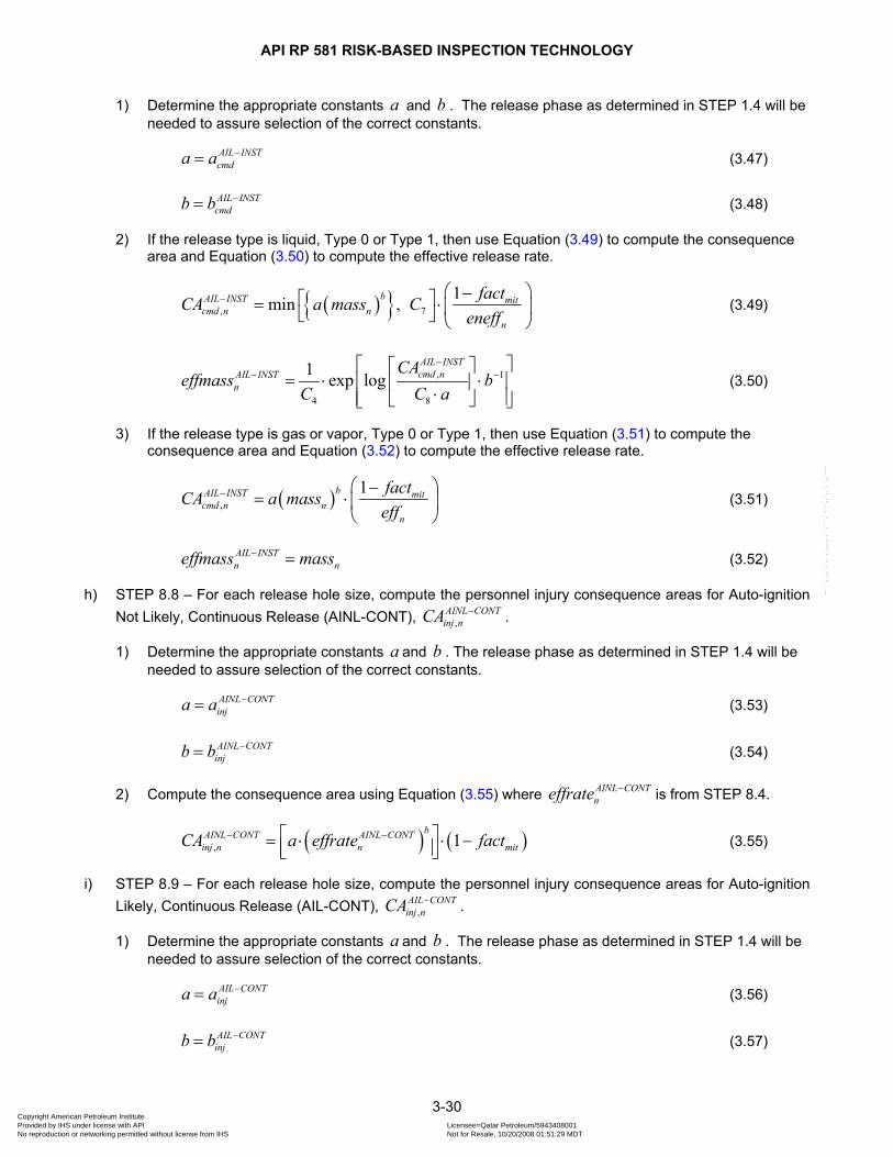
API RP 581 RISK-BASED INSPECTION TECHNOLOGY
3-30
1) Determine the appropriate constants a and b . The release phase as determined in STEP 1.4 will be needed to assure selection of the correct constants.
AIL INSTcmda a −= (3.47)
AIL INSTcmdb b −= (3.48)
2) If the release type is liquid, Type 0 or Type 1, then use Equation (3.49) to compute the consequence area and Equation (3.50) to compute the effective release rate.
( ) , 71min , bAIL INST mit
cmd n nn
factCA a mass Ceneff
− ⎛ ⎞−⎡ ⎤= ⋅⎜ ⎟⎣ ⎦ ⎝ ⎠ (3.49)
, 1
4 8
1 exp logAIL INSTcmd nAIL INST
n
CAeffmass b
C C a
−− −
⎡ ⎤⎡ ⎤= ⋅ ⋅⎢ ⎥⎢ ⎥⋅⎢ ⎥⎣ ⎦⎣ ⎦
(3.50)
3) If the release type is gas or vapor, Type 0 or Type 1, then use Equation (3.51) to compute the consequence area and Equation (3.52) to compute the effective release rate.
( ),1bAIL INST mit
cmd n nn
factCA a masseff
− ⎛ ⎞−= ⋅⎜ ⎟
⎝ ⎠ (3.51)
AIL INSTn neffmass mass− = (3.52)
h) STEP 8.8 – For each release hole size, compute the personnel injury consequence areas for Auto-ignition Not Likely, Continuous Release (AINL-CONT), ,
AINL CONTinj nCA − .
1) Determine the appropriate constants a and b . The release phase as determined in STEP 1.4 will be needed to assure selection of the correct constants.
AINL CONTinja a −= (3.53)
AINL CONTinjb b −= (3.54)
2) Compute the consequence area using Equation (3.55) where AINL CONTneffrate − is from STEP 8.4.
( ) ( ), 1bAINL CONT AINL CONT
inj n n mitCA a effrate fact− −⎡ ⎤= ⋅ ⋅ −⎢ ⎥⎣ ⎦ (3.55)
i) STEP 8.9 – For each release hole size, compute the personnel injury consequence areas for Auto-ignition Likely, Continuous Release (AIL-CONT), ,
AIL CONTinj nCA − .
1) Determine the appropriate constants a and b . The release phase as determined in STEP 1.4 will be needed to assure selection of the correct constants.
AIL CONTinja a −= (3.56)
AIL CONTinjb b −= (3.57)
Copyright American Petroleum Institute Provided by IHS under license with API Licensee=Qatar Petroleum/5943408001
Not for Resale, 10/20/2008 01:51:29 MDTNo reproduction or networking permitted without license from IHS
--```,`,,`,`,,`,`,,,,,,``,```,`-`-`,,`,,`,`,,`---

API RP 581 RISK-BASED INSPECTION TECHNOLOGY
3-31
2) Compute the consequence area using Equation (3.58) where AIL CONTneffrate − is from STEP 8.5.
( ) ( ), 1bAIL CONT AIL CONT
inj n n mitCA a effrate fact− −⎡ ⎤= ⋅ ⋅ −⎢ ⎥⎣ ⎦ (3.58)
j) STEP 8.10 – For each release hole size, compute the personnel injury consequence areas for Auto-ignition Not Likely, Instantaneous Release (AINL-INST), ,
AINL INSTinj nCA − .
1) Determine the appropriate constants a and b . The release phase as determined in STEP 1.4 will be needed to assure selection of the correct constants.
AINL INSTinja a −= (3.59)
AINL INSTinjb b −= (3.60)
2) Compute the consequence area using Equation (3.61) where AINL INSTneffrate − is from STEP 8.6.
( ),1bAINL INST AINL INST mit
inj n nn
factCA a effrateeneff
− − ⎛ ⎞−⎡ ⎤= ⋅ ⋅⎜ ⎟⎢ ⎥⎣ ⎦ ⎝ ⎠ (3.61)
k) STEP 8.11 – For each release hole size, compute the personnel injury consequence areas for Auto-ignition Likely, Instantaneous Release (AIL-INST), ,
AIL INSTinj nCA − .
1) Determine the appropriate constants a and b . The release phase as determined in STEP 1.4 will be needed to assure selection of the correct constants.
AIL INSTinja a −= (3.62)
AIL INSTinjb b −= (3.63)
2) Compute the consequence area using Equation (3.64) where AIL INSTneffrate − is from STEP 8.7.
( ),1bAIL INST AIL INST mit
inj n nn
factCA a effrateeneff
− − ⎛ ⎞−⎡ ⎤= ⋅ ⋅⎜ ⎟⎢ ⎥⎣ ⎦ ⎝ ⎠ (3.64)
l) STEP 8.12 – For each release hole size, calculate the instantaneous/continuous blending factor, ICnfact ,
using Equation (3.19), (3.20), or (3.21), as applicable.
m) STEP 8.13 – Calculate the AIT blending factor, AITfact , using Equations (3.24), (3.25), or (3.26), as applicable.
n) STEP 8.14 – Compute the continuous/instantaneous blended consequence areas for the component using Equations (3.65) through (3.68) based on the consequence areas computed in STEPs 8.4, 8.5, 8.6, 8.7, 8.8, 8.9, 8.10 and 8.11, and the continuous/instantaneous blending factor, IC
nfact , from STEP 8.12.
( ), , , 1AIL AIL CONT IC AIL INST ICcmd n cmd n n cmd n nCA CA fact CA fact− −= ⋅ + ⋅ − (3.65)
( ), , , 1AIL AIL CONT IC AIL INST ICinj n inj n n inj n nCA CA fact CA fact− −= ⋅ + ⋅ − (3.66)
Copyright American Petroleum Institute Provided by IHS under license with API Licensee=Qatar Petroleum/5943408001
Not for Resale, 10/20/2008 01:51:29 MDTNo reproduction or networking permitted without license from IHS
--```,`,,`,`,,`,`,,,,,,``,```,`-`-`,,`,,`,`,,`---
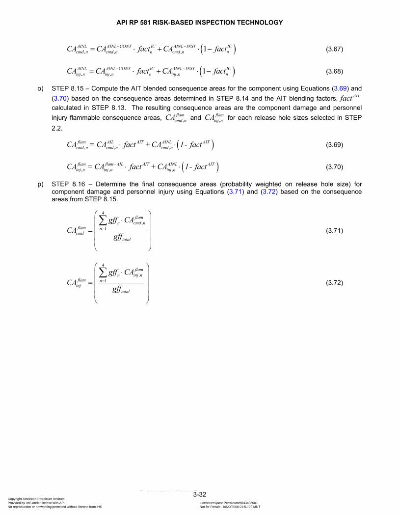
API RP 581 RISK-BASED INSPECTION TECHNOLOGY
3-32
( ), , , 1AINL AINL CONT IC AINL INST ICcmd n cmd n n cmd n nCA CA fact CA fact− −= ⋅ + ⋅ − (3.67)
( ), , , 1AINL AINL CONT IC AINL INST ICinj n inj n n inj n nCA CA fact CA fact− −= ⋅ + ⋅ − (3.68)
o) STEP 8.15 – Compute the AIT blended consequence areas for the component using Equations (3.69) and (3.70) based on the consequence areas determined in STEP 8.14 and the AIT blending factors, AITfact calculated in STEP 8.13. The resulting consequence areas are the component damage and personnel injury flammable consequence areas, ,
flamcmd nCA and ,
flaminj nCA for each release hole sizes selected in STEP
2.2.
( ), , ,flam AIL AIT AINL AIT
cmd n cmd n cmd nCA = CA fact +CA 1- fact⋅ ⋅ (3.69)
( ), , ,flam flam AIL AIT AINL AIT
inj n inj n inj nCA = CA fact +CA 1- fact− ⋅ ⋅ (3.70)
p) STEP 8.16 – Determine the final consequence areas (probability weighted on release hole size) for component damage and personnel injury using Equations (3.71) and (3.72) based on the consequence areas from STEP 8.15.
4
,1
flamn cmd n
flam ncmd
total
gff CACA
gff=
⎛ ⎞⋅⎜ ⎟⎜ ⎟=⎜ ⎟⎜ ⎟⎝ ⎠
∑ (3.71)
4
,1
flamn inj n
flam ninj
total
gff CACA
gff=
⎛ ⎞⋅⎜ ⎟⎜ ⎟=⎜ ⎟⎜ ⎟⎝ ⎠
∑ (3.72)
Copyright American Petroleum Institute Provided by IHS under license with API Licensee=Qatar Petroleum/5943408001
Not for Resale, 10/20/2008 01:51:29 MDTNo reproduction or networking permitted without license from IHS
--```,`,,`,`,,`,`,,,,,,``,```,`-`-`,,`,,`,`,,`---
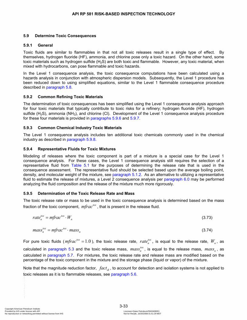
API RP 581 RISK-BASED INSPECTION TECHNOLOGY
3-33
5.9 Determine Toxic Consequences
5.9.1 General
Toxic fluids are similar to flammables in that not all toxic releases result in a single type of effect. By themselves, hydrogen fluoride (HF), ammonia, and chlorine pose only a toxic hazard. On the other hand, some toxic materials such as hydrogen sulfide (H2S) are both toxic and flammable. However, any toxic material, when mixed with hydrocarbons, can pose flammable and toxic hazards.
In the Level 1 consequence analysis, the toxic consequence computations have been calculated using a hazards analysis in conjunction with atmospheric dispersion models. Subsequently, the Level 1 procedure has been reduced down to using simplified equations, similar to the Level 1 flammable consequence procedure described in paragraph 5.8.
5.9.2 Common Refining Toxic Materials
The determination of toxic consequences has been simplified using the Level 1 consequence analysis approach for four toxic materials that typically contribute to toxic risks for a refinery; hydrogen fluoride (HF), hydrogen sulfide (H2S), ammonia (NH3), and chlorine (Cl). Development of the Level 1 consequence analysis procedure for these four materials is provided in paragraphs 5.9.6 and 5.9.7.
5.9.3 Common Chemical Industry Toxic Materials
The Level 1 consequence analysis includes ten additional toxic chemicals commonly used in the chemical industry as described in paragraph 5.9.8.
5.9.4 Representative Fluids for Toxic Mixtures
Modeling of releases where the toxic component is part of a mixture is a special case for the Level 1 consequence analysis. For these cases, the Level 1 consequence analysis still requires the selection of a representative fluid from Table 5.1 for the purposes of determining the release rate that is used in the consequence assessment. The representative fluid should be selected based upon the average boiling point, density, and molecular weight of the mixture, see paragraph 5.1.2. As an alternative to utilizing a representative fluid to estimate the release of mixtures, a Level 2 consequence analysis per paragraph 6.0 may be performed analyzing the fluid composition and the release of the mixture much more rigorously.
5.9.5 Determination of the Toxic Release Rate and Mass
The toxic release rate or mass to be used in the toxic consequence analysis is determined based on the mass fraction of the toxic component, toxmfrac , that is present in the release fluid.
tox toxn nrate mfrac W= ⋅ (3.73)
tox toxn nmass mfrac mass= ⋅ (3.74)
For pure toxic fluids ( 1.0toxmfrac = ), the toxic release rate, toxnrate , is equal to the release rate, nW , as
calculated in paragraph 5.3 and the toxic release mass, toxnmass , is equal to the release mass, nmass , as
calculated in paragraph 5.7. For mixtures, the toxic release rate and release mass are modified based on the percentage of the toxic component in the mixture and the storage phase (liquid or vapor) of the mixture.
Note that the magnitude reduction factor, difact , to account for detection and isolation systems is not applied to toxic releases as it is to flammable releases, see paragraph 5.6.
Copyright American Petroleum Institute Provided by IHS under license with API Licensee=Qatar Petroleum/5943408001
Not for Resale, 10/20/2008 01:51:29 MDTNo reproduction or networking permitted without license from IHS
--```,`,,`,`,,`,`,,,,,,``,```,`-`-`,,`,,`,`,,`---

API RP 581 RISK-BASED INSPECTION TECHNOLOGY
3-34
5.9.6 Estimation of Toxic Consequence Area for HF Acid and H2S
a) The background for the development of the toxic consequence equations for HF Acid and H2S is provided in Annex 3.A. For determination of the toxic consequence areas, the assumption was made that the release phase would always be a gas or vapor.
b) The toxic consequence areas for continuous releases of HF or H2S as a function of the release rate may be computed using Equation (3.75).
( )10 4log, 8 10
toxnc C rate dtox
inj nCA C⎡ ⎤⋅ ⋅ +⎣ ⎦= ⋅ (3.75)
Note that for continuous releases, the toxic release rate, toxnrate , is used as the input to Equation (3.75).
The constants c and d to be used in Equation (3.75) are provided in Table 5.11 as a function of release duration. Interpolation between curves using the actual duration (defined in paragraph 5.9.10) is acceptable.
c) The toxic consequence areas for instantaneous releases of HF or H2S as a function of the release rate may be computed using Equation (3.76).
( )10 4log, 8 10
toxnc C mass dtox
inj nCA C⎡ ⎤⋅ ⋅ +⎣ ⎦= ⋅ (3.76)
Note that for instantaneous releases, the toxic release mass, toxnmass , is used as the input to Equation
(3.76). The constants c and d to be used in Equation (3.76) are provided in Table 5.11.
5.9.7 Estimation of Toxic Consequence Area for Ammonia and Chlorine
a) The background for the development of the toxic consequence equations for Ammonia and Chlorine are provided in Annex 3.A. For determination of the consequence areas, the assumption was made that the release phase would always be a gas or vapor.
b) The toxic consequence areas for continuous releases of Ammonia or Chlorine as a function of the release rate may be computed using Equation (3.77).
( ),
ftox toxinj n nCA e rate= (3.77)
Note that for continuous releases, the toxic release rate, toxnrate , is used as the input to Equation (3.77).
The constants e and f for Equation (3.77) are provided in Table 5.12 as a function of release duration. Interpolation between curves using the actual duration is acceptable.
c) The toxic consequence areas for instantaneous releases of Ammonia or Chlorine as a function of the release rate may be computed using Equation (3.78).
( ),
ftox toxinj n nCA e mass= (3.78)
Note that for instantaneous releases, the toxic release mass, toxnmass , is used as the input to Equation
(3.78). The constants e and f for Equation (3.78) are provided in Table 5.12.
Copyright American Petroleum Institute Provided by IHS under license with API Licensee=Qatar Petroleum/5943408001
Not for Resale, 10/20/2008 01:51:29 MDTNo reproduction or networking permitted without license from IHS
--```,`,,`,`,,`,`,,,,,,``,```,`-`-`,,`,,`,`,,`---
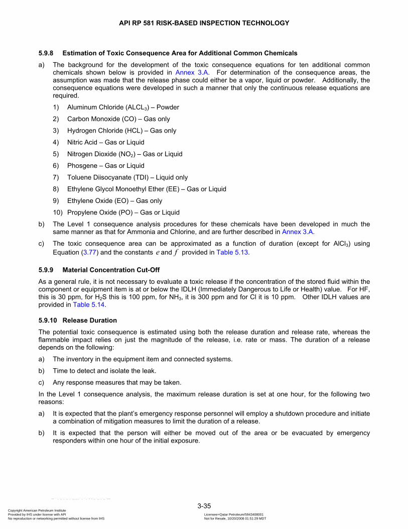
API RP 581 RISK-BASED INSPECTION TECHNOLOGY
3-35
5.9.8 Estimation of Toxic Consequence Area for Additional Common Chemicals
a) The background for the development of the toxic consequence equations for ten additional common chemicals shown below is provided in Annex 3.A. For determination of the consequence areas, the assumption was made that the release phase could either be a vapor, liquid or powder. Additionally, the consequence equations were developed in such a manner that only the continuous release equations are required.
1) Aluminum Chloride (ALCL3) – Powder
2) Carbon Monoxide (CO) – Gas only
3) Hydrogen Chloride (HCL) – Gas only
4) Nitric Acid – Gas or Liquid
5) Nitrogen Dioxide (NO2) – Gas or Liquid
6) Phosgene – Gas or Liquid
7) Toluene Diisocyanate (TDI) – Liquid only
8) Ethylene Glycol Monoethyl Ether (EE) – Gas or Liquid
9) Ethylene Oxide (EO) – Gas only
10) Propylene Oxide (PO) – Gas or Liquid
b) The Level 1 consequence analysis procedures for these chemicals have been developed in much the same manner as that for Ammonia and Chlorine, and are further described in Annex 3.A.
c) The toxic consequence area can be approximated as a function of duration (except for AlCl3) using Equation (3.77) and the constants e and f provided in Table 5.13.
5.9.9 Material Concentration Cut-Off
As a general rule, it is not necessary to evaluate a toxic release if the concentration of the stored fluid within the component or equipment item is at or below the IDLH (Immediately Dangerous to Life or Health) value. For HF, this is 30 ppm, for H2S this is 100 ppm, for NH3, it is 300 ppm and for Cl it is 10 ppm. Other IDLH values are provided in Table 5.14.
5.9.10 Release Duration
The potential toxic consequence is estimated using both the release duration and release rate, whereas the flammable impact relies on just the magnitude of the release, i.e. rate or mass. The duration of a release depends on the following:
a) The inventory in the equipment item and connected systems.
b) Time to detect and isolate the leak.
c) Any response measures that may be taken.
In the Level 1 consequence analysis, the maximum release duration is set at one hour, for the following two reasons:
a) It is expected that the plant’s emergency response personnel will employ a shutdown procedure and initiate a combination of mitigation measures to limit the duration of a release.
b) It is expected that the person will either be moved out of the area or be evacuated by emergency responders within one hour of the initial exposure.
Copyright American Petroleum Institute Provided by IHS under license with API Licensee=Qatar Petroleum/5943408001
Not for Resale, 10/20/2008 01:51:29 MDTNo reproduction or networking permitted without license from IHS
--```,`,,`,`,,`,`,,,,,,``,```,`-`-`,,`,,`,`,,`---

API RP 581 RISK-BASED INSPECTION TECHNOLOGY
3-36
The release duration can be estimated as the inventory in the system divided by the initial release rate. While the calculated duration may exceed one hour, there may be systems in place that will significantly shorten this time, such as isolation valves and rapid-acting leak detection systems. Times should be determined on a case-by-case basis. The leak duration, tox
nld , should be calculated for each release hole size as the minimum of:
a) One hour.
b) Inventory mass (mass available) divided by release rate (see paragraph 5.7).
c) Maximum leak duration, max,nld listed in Table 5.7
,min 3600, , 60tox nn max n
n
massld ldW
⎛ ⎞⎧ ⎫= ⋅⎜ ⎟⎨ ⎬⎜ ⎟⎩ ⎭⎝ ⎠
(3.79)
5.9.11 Toxic Outcome Probabilities
In the event the release can involve both toxic and flammable outcomes, it is assumed that either the flammable outcome consumes the toxic material, or the toxic materials are dispersed and flammable materials have insignificant consequences. In this case, the probability for the toxic event is the remaining non-ignition frequency for the event (i.e., the probability of safe dispersion).
5.9.12 Consequences of Releases Containing Multiple Toxic Chemicals
Consequence results for releases of multi-component toxic chemicals are uncommon but can be handled in API RBI. In this instance, the consequence areas are determined for each of the individual toxic components within the mixture. The overall toxic consequence area is the largest of the individual toxic areas.
5.9.13 Effects of Mitigation Measures on Toxic Releases
To this point, isolation and detection capabilities have been taken into account in calculating the quantity of material that may be released during a loss-of-containment event, see paragraph 5.7.1. However, there may be additional systems, such as water sprays, in place that can mitigate a release once the material has reached the atmosphere.
The effectiveness of mitigating systems can be simply accounted for in API RBI by reducing the release rate and duration for continuous releases, or by reducing the release mass for instantaneous releases. The RBI analyst will need to provide his or her own reduction factors, based on the effectiveness of their particular spray-system design or passive mitigation technology.
Where mitigation is a major issue, specialists should be consulted to get an accurate input to the API RBI analysis. As an example, it is possible to mitigate HF releases with a water spray. However, the fraction of HF that is removed by a water spray may vary from near 0% to near 100% depending on the size of the release, the droplet size, flow rate and orientation of the spray, and several other variables.
5.9.14 Determination of Final Toxic Consequence Areas
The final toxic consequence areas are determined as a probability weighted average of the individual toxic consequence areas calculated for each release hole size. This is only performed for the personnel injury consequence areas, since toxic releases result in no component damage. The probability weighting utilizes the generic frequencies of the release hole sizes obtained in STEP 2.3. Equation (3.80) is used to compute the probability weighted toxic consequence area.
4
,1
toxn inj n
tox ninj
total
gff CACA
gff=
⎛ ⎞⋅⎜ ⎟⎜ ⎟=⎜ ⎟⎜ ⎟⎝ ⎠
∑ (3.80)
Copyright American Petroleum Institute Provided by IHS under license with API Licensee=Qatar Petroleum/5943408001
Not for Resale, 10/20/2008 01:51:29 MDTNo reproduction or networking permitted without license from IHS
--```,`,,`,`,,`,`,,,,,,``,```,`-`-`,,`,,`,`,,`---

API RP 581 RISK-BASED INSPECTION TECHNOLOGY
3-37
5.9.15 Calculation Procedure
a) STEP 9.1 – For each release hole size selected in STEP 2.2, calculate the effective duration of the toxic release using Equation (3.79).
b) STEP 9.2 – Determine the toxic percentage of the toxic component, toxmfrac , in the release material. If
the release fluid is a pure fluid, 1.0toxmfrac = . Note that if there is more than one toxic component in the released fluid mixture, this procedure can be repeated for each toxic component.
c) STEP 9.3 – For each release hole size, calculate the release rate, toxnrate , and release mass, tox
nxmass , to be used in the toxic consequence analysis using Equations (3.73) and (3.74).
d) STEP 9.4 – For each release hole size, calculate the toxic consequence area for each of the release hole sizes
1) HF Acid and H2S – Compute ,toxinj nCA using Equation (3.75) for a continuous release or Equation (3.76)
for an instantaneous release, the constants used in these equations are from Table 5.11.
2) Ammonia and Chlorine – Compute ,toxinj nCA using Equation (3.77) for a continuous release or Equation
(3.78) for an instantaneous release, the constants used in these equations are from Table 5.12.
3) For all other Level 1 Fluids – Compute ,toxinj nCA using Equation (3.78) for either a continuous or
instantaneous release, the constants used in these equations are from Table 5.13.
e) STEP 9.5 – If there are additional toxic components in the released fluid mixture, the STEPs 9.2 through 9.4 should be repeated for each toxic component.
f) STEP 9.6 - Determine the final toxic consequence areas for personnel injury in accordance with Equation (3.80).
5.10 Determine Non-Flammable Non-Toxic Consequences
5.10.1 General
Consequences associated with the release of non-flammable, non-toxic materials are not as severe as with other materials, however, they can still result in serious injury to personnel and damage to equipment.
5.10.2 Consequences of Steam Leaks
Steam represents a hazard to personnel who are exposed to steam at high temperatures. Steam leaks do not result in a component damage consequence. In general, steam is at 100°C [212°F] immediately after exiting a hole in an equipment item. Within a few feet, depending upon its pressure, steam will begin to mix with air, cool and condense. At a concentration of about 20%, the steam/air mixture cools to about 60°C [140°F]. The approach used here is to assume that injury occurs only above 60°C [140°F]. This temperature was selected as the threshold for injury to personnel, as this is the temperature above which OSHA requires that hot surfaces be insulated to protect against personnel burns.
To determine an equation for the consequence area of a continuous release of steam, four release cases (0.25 in., 1 in., 4 in., and 16 in.) were run through atmospheric dispersion software for varying steam pressures. A plot of the release rate vs. the area covered by a 20% concentration of steam shows a linear relationship in accordance with Equation (3.81).
, 9CONTinj n nCA C rate= ⋅ (3.81)
For instantaneous release cases, four masses of steam were modeled; 4.5 kgs, 45.4 kgs, 454.0 kgs, 4,540 kgs [10 lbs, 100 lbs, 1,000 lbs, and 10,000 lbs], and the relationship between release mass and consequence area to 20% concentration was found to be in accordance with Equation (3.82).
Copyright American Petroleum Institute Provided by IHS under license with API Licensee=Qatar Petroleum/5943408001
Not for Resale, 10/20/2008 01:51:29 MDTNo reproduction or networking permitted without license from IHS
--```,`,,`,`,,`,`,,,,,,``,```,`-`-`,,`,,`,`,,`---
API RP 581 RISK-BASED INSPECTION TECHNOLOGY
3-38
( )0.6384, 10
INSTinj n nCA C mass= (3.82)
For non-flammable releases of steam, the continuous/instantaneous blending of results should be performed as described in paragraph 5.8.6. The blending factor, IC
nfact , for steam leaks is calculated using Equation (3.83).
5
min , 1.0IC nn
ratefactC
⎡ ⎤⎧ ⎫= ⎨ ⎬⎢ ⎥
⎩ ⎭⎣ ⎦ (3.83)
5.10.3 Consequences of Acid and Caustic Leaks
For caustics/acids that have only splash type consequences, water was chosen as a representative fluid to determine the personnel consequence area. Acid or caustic leaks do not result in a component damage consequence. The consequence area was defined at the 180° semi-circular area covered by the liquid spray, or rainout. Modeling was performed at three pressures; 103.4 kPa, 206.8 kPa, and 413.7 kPa [15 psig, 30 psig, and 60 psig] for four release hole sizes (0.25 in, 1 in, 4 in, and 16 in). Only continuous releases were modeled, as instantaneous releases are assumed not to produce rainout. The results were analyzed to obtain a correlation between release rate and consequence area, and were divided by 5 since it is believed that serious injuries to personnel are only likely to occur within about 20% of the total splash area as calculated by the above method.
The resulting consequence area for non-flammable releases of acids and caustics is computed using Equations (3.84) and (3.85).
( ), 8 40.2 hCONTinj n nCA C g C rate= ⋅ ⋅ ⋅ (3.84)
, 0.0INSTinj nCA = (3.85)
The constants g and h shown in Equation (3.84), are functions of pressure and can be calculated using Equations (3.86) and (3.87), respectively.
( ) ( ) 211 112696.0 21.9 1.474s atm s atmg C P P C P P= − ⋅ − + −⎡ ⎤⎣ ⎦ (3.86)
( ) 2110.31 0.00032 40s atmh C P P= − − −⎡ ⎤⎣ ⎦ (3.87)
Since there are no consequences associated with an instantaneous release of acid or caustic, the instantaneous/continuous blending factor, IC
nfact , is equal to 0.0.
5.10.4 Blending of Results Based on Release Type
The Level 1 consequence area calculations yield significantly different results depending on whether the continuous area equations are used or the instantaneous area equations are used. The non-flammable, non-toxic personnel injury consequence area for steam or acid leaks can be calculated for each hole size using Equation (3.88).
( ), , , 1leak INST IC CONT ICinj n inj n n inj n nCA CA fact CA fact= ⋅ + − (3.88)
Note that there is no need to calculate a component damage area for the Level 1 non-flammable releases of steam or acid/caustic.
, 0.0leakcmd nCA = (3.89)
Copyright American Petroleum Institute Provided by IHS under license with API Licensee=Qatar Petroleum/5943408001
Not for Resale, 10/20/2008 01:51:29 MDTNo reproduction or networking permitted without license from IHS
--```,`,,`,`,,`,`,,,,,,``,```,`-`-`,,`,,`,`,,`---
API RP 581 RISK-BASED INSPECTION TECHNOLOGY
3-39
5.10.5 Determination of Final Non-Flammable, Non-Toxic Consequence Areas
The final non-flammable, non-toxic consequence areas are determined as a probability weighted average of the individual consequence areas calculated for each release hole size. This is only performed for the personnel injury consequence areas, since these releases result in no component damage. The probability weighting utilizes the generic frequencies of the release hole sizes as provided in Table 4.1 of Part 2. Equation (3.90) is used to compute the probability weighted non-flammable, non-toxic consequence area for steam, caustic or acid releases.
4
,1
leakn inj n
nfnt ninj
total
gff CACA
gff=
⎛ ⎞⋅⎜ ⎟⎜ ⎟=⎜ ⎟⎜ ⎟⎝ ⎠
∑ (3.90)
The term ,leakinj nCA in Equation (3.90) represents the personnel injury areas for each of the holes sizes either due to
steam or acid releases as described in paragraph 5.10.2 and 5.10.3.
5.10.6 Calculation Procedure
a) STEP 10.1 – For each release hole size, calculate the non-flammable, non-toxic consequence area.
1) For Steam – Compute ,CONTinj nCA using Equation (3.81) and ,
INSTinj nCA using Equation (3.82).
2) For Acids or Caustics – Compute ,CONTinj nCA using Equations (3.84), (3.86), and (3.87). Note that data
is not provided for an instantaneous release; therefore, , 0.0INSTinj nCA = .
b) STEP 10.2 – For each release hole size, calculate the Instantaneous/Continuous blending factor, ICnfact .
For steam, use Equation (3.83). For Acids or Caustics, 0.0ICnfact = .
c) STEP 10.3 – For each release hole size, compute the blended non-flammable, non-toxic personnel injury consequence area for steam or acid leaks, ,
leakinj nCA , using Equation (3.88) based on the consequence areas
from STEP 10.1 and the blending factor, ICnfact , from STEP 10.2. Note that there is no need to calculate
a component damage area for the Level 1 non-flammable releases (steam or acid/caustic):
, 0.0leakcmd nCA = (3.91)
d) STEP 10.4 - Determine the final non-flammable, non-toxic consequence areas for personnel injury, nfntinjCA ,
using Equation (3.90) based on consequence areas calculated for each release hole size in STEP 10.3. Note that there is no need to calculate a final non-flammable, non-toxic consequence area for component damage area for the Level 1 non-flammable releases (steam or acid/caustic), or:
0.0nfntcmdCA = (3.92)
5.11 Determine the Component Damage and Personnel Injury Consequence Areas
5.11.1 Overview
The final consequence areas for component damage and personnel injury are the maximum areas of those calculated for:
a) Flammable Consequences, see paragraph 5.8
Copyright American Petroleum Institute Provided by IHS under license with API Licensee=Qatar Petroleum/5943408001
Not for Resale, 10/20/2008 01:51:29 MDTNo reproduction or networking permitted without license from IHS
--```,`,,`,`,,`,`,,,,,,``,```,`-`-`,,`,,`,`,,`---

API RP 581 RISK-BASED INSPECTION TECHNOLOGY
3-40
b) Toxic Consequences, see paragraph 5.9.
c) Non-flammable, Non-toxic Consequences, see paragraph 5.10
5.11.2 Final Component Damage Consequence Area
The final component damage consequence area is:
max , , flam tox nfntcmd cmd cmd cmdCA CA CA CA⎡ ⎤= ⎣ ⎦ (3.93)
Note that since the component damage consequence areas for toxic releases, toxcmdCA , and non-flammable, non-
toxic releases, nfntcmdCA , are both equal to zero, the final component damage consequence area is equal to the
consequence area calculated for flammable releases, flamcmdCA .
flamcmd cmdCA CA= (3.94)
5.11.3 Final Personnel Injury Consequence Area
The final personnel injury consequence area is:
max , , flam tox nfntinj inj inj injCA CA CA CA⎡ ⎤= ⎣ ⎦ (3.95)
5.11.4 Final Consequence Area
The final consequence area is:
max ,cmd injCA CA CA⎡ ⎤= ⎣ ⎦ (3.96)
5.11.5 Calculation Procedure
a) STEP 11.1 – Compute the final component damage consequence area, cmdCA , using Equation (3.94).
b) STEP 11.2 – Compute the final personnel injury consequence area, injCA , using Equation (3.95).
5.12 Determine the Financial Consequences
5.12.1 Overview
There are many costs associated with any failure of equipment in a process plant. These include, but are not limited to:
a) Cost of equipment repair and replacement
b) Cost of damage to surrounding equipment in affected areas
c) Costs associated with production losses and business interruption as a result of downtime to repair or replace damaged equipment
d) Costs due to potential injuries associated with a failure
e) Environmental cleanup costs
Copyright American Petroleum Institute Provided by IHS under license with API Licensee=Qatar Petroleum/5943408001
Not for Resale, 10/20/2008 01:51:29 MDTNo reproduction or networking permitted without license from IHS
--```,`,,`,`,,`,`,,,,,,``,```,`-`-`,,`,,`,`,,`---
API RP 581 RISK-BASED INSPECTION TECHNOLOGY
3-41
The approach used in API RBI is to consider all of these costs on both an equipment specific basis and an affected area basis. Thus, any failure (loss of containment) has costs associated with it, even when the release of the hazardous material does not result in damage to other equipment in the unit or serious injury to personnel. Recognizing and using this fact presents a more realistic value of the consequences associated with a failure. Since the costs include more than just business interruption, the approach used for quantitative API RBI analysis is called the financial consequence approach.
The financial consequence of a loss of containment and subsequent release of hazardous materials can be determined by adding up the individual costs discussed above:
cmd affa prod inj environFC FC FC FC FC FC= + + + + (3.97)
The basic method of risk analysis as presented in API RBI is not changed for the financial risk analysis. The risk is still calculated as the consequence of failure (now expressed as cost in dollars) times the probability of failure. For a rigorous and flexible analysis, the consequences (costs) are evaluated at the hole size level. Risk is also evaluated at the release hole size level by using the probability of failure associated with each release hole size. The total risk is calculated as the sum of the risks of each release hole size.
5.12.2 Component Damage Cost
The method chosen for these calculations operates under the presumption that there is a specific cost associated with each possible leak scenario (release hole size), and that these are unique to each component type. This approach was chosen based on the inherent differences in the costs associated with repairing components having small hole damage to that of component that has had extreme damage such as would be the case if the equipment were to rupture.
A small hole in a piping system can sometimes be repaired with little or no impact on production by use of a temporary clamp until a permanent repair can be scheduled during normal maintenance shutdowns. Larger holes usually do not allow this option, and shutdown plus repair costs are greatly increased.
The component damage costs, holecost , for different release hole sizes for each component are shown in Table 5.15. Actual failure cost data for component should be used if available. The sources cited were used to estimate the relative installed costs of the equipment. Since repair or replacement of a component usually does not involve replacement of all supports, foundations, etc., the repair and replacement costs presented do not reflect actual installed cost.
The cost estimates shown in Table 5.15 are based on carbon steel prices. It is suggested for the quantitative API RBI analysis approach that these costs be multiplied by a material cost factor, matcost , for other materials. Table 5.16 shows the suggested values for these material cost factors. These factors are based on a variety of sources from manufacturer’s data and cost quotations.
The consequence cost to repair or replace the component that has been damaged is a probability weighted average of the individual repair costs determined for each release hole size, and is computed using Equation (3.98). The probability weighting utilizes the generic frequencies of the release hole sizes provided in Table 4.1 of Part 2 [2].
4
1n n
ncmd
total
gff holecostFC matcost
gff=
⎛ ⎞⋅⎜ ⎟⎜ ⎟= ⋅⎜ ⎟⎜ ⎟⎝ ⎠
∑ (3.98)
Copyright American Petroleum Institute Provided by IHS under license with API Licensee=Qatar Petroleum/5943408001
Not for Resale, 10/20/2008 01:51:29 MDTNo reproduction or networking permitted without license from IHS
--```,`,,`,`,,`,`,,,,,,``,```,`-`-`,,`,,`,`,,`---
API RP 581 RISK-BASED INSPECTION TECHNOLOGY
3-42
5.12.3 Damage Costs to Surrounding Equipment in Affected Area
It is necessary to calculate the component damage costs to other equipment components in the vicinity of the failure, if the failure results in a flammable (or explosive) event. Toxic releases do not result in damage to surrounding equipment. Typically, a constant value of the process unit replacement cost, equipcost , is used in the quantitative API RBI analysis approach. In other words, as a starting point the average cost of other equipment components surrounding any given component is about the same regardless of location within the process unit. This could be refined for individual components by allowing the default value to be overridden with a higher or lower value where appropriate.
The consequence cost to repair or replace surrounding components that have become damaged in the affected area, is a probability weighted average of the affected area costs determined for each release hole size, and is computed using Equation (3.99). The probability weighting utilizes the generic frequencies of the release hole sizes provided in Table 4.1 of Part 2.
affa cmdFC CA equipcost= ⋅ (3.99)
5.12.4 Business Interruption Costs
The costs associated with business interruption is determined based on the amount of downtime (and lost production) associated with repairing damage to the specific piece of equipment that has had loss of containment (due to holes or rupture) as well as the downtime associated with repairing surrounding equipment in the area of the plant affected by the release (consequence area).
a) For each release hole size, an estimated downtime for each equipment type, nOutage is presented in Table 5.17. Centrifugal pumps are assumed to have on-line spares, so the assumption is made that there is no downtime associated with the failure of these equipment types. The probability weighting of the downtime required to repair damage for a specific equipment item is given by Equation (3.100). The probability weighting utilizes the generic frequencies of the release hole sizes provided in Table 4.1 of Part 2.
4
1n n
ncmd mult
total
gff OutageOutage Outage
gff=
⎛ ⎞⋅⎜ ⎟⎜ ⎟= ⋅⎜ ⎟⎜ ⎟⎝ ⎠
∑ (3.100)
b) If a component has a failure (loss of containment through hole or rupture) resulting in an affected area (consequence area), the cost of downtime for replacement and repair of surrounding equipment in the affected area must also be considered. The downtime associated with repairing the surrounding equipment in the affected area is computed using Equation (3.101).
( ) 6101.242 0.585 log 10
10 affaFC
affaOutage−⎡ ⎤+ ⋅ ⋅⎢ ⎥⎣ ⎦= (3.101)
c) The cost of the business interruption associated with repairing damaged equipment is equal to the cost associated with lost production due to the shutdown of the facility.
( )( )prod cmd affaFC Outage Outage prodcost= + (3.102)
Copyright American Petroleum Institute Provided by IHS under license with API Licensee=Qatar Petroleum/5943408001
Not for Resale, 10/20/2008 01:51:29 MDTNo reproduction or networking permitted without license from IHS
--```,`,,`,`,,`,`,,,,,,``,```,`-`-`,,`,,`,`,,`---

API RP 581 RISK-BASED INSPECTION TECHNOLOGY
3-43
5.12.5 Potential Injury Costs
Another cost to consider when a failure occurs is the potential injury costs. When a business takes injury costs into account in a risk management scheme, then appropriate resources can be spent to prevent these injuries from happening. Just as failure to consider the business cost of a zero affected area event can lead to under ranking this event with respect to risk, if injury costs are not considered, then a risk could be present that is not considered in allocating inspection resources.
In the Level 1 consequence analysis, a constant population density, popdens , is used as a default for all equipment in the unit. This default value can be overridden by higher or lower values depending on specific equipment location with respect to controls rooms, walkways, roads, etc. In addition to the population density, the cost per individual, injcost , affected must also be entered. This value must be sufficiently high to adequately represent typical costs to businesses of an injury up to and including fatal injuries. When assigning this value, consideration should be given to the following:
a) Any existing company standards for such calculations,
b) Local medical/compensation costs associated with long-term disability,
c) Legal/settlement costs,
d) Indirect costs such as increased regulatory scrutiny, loss of reputation, etc.
The costs associated with personnel injury are computed using Equation (3.103)
inj injFC CA popdens injcost= ⋅ ⋅ (3.103)
5.12.6 Environmental Cleanup Costs
Environmental consequences as a result of loss of containment can be a significant cost and should be added to the other costs including fines and other financial penalties. The methods presented here are based on the amount of material spilled to the ground, the number of days to clean up the spill and the environmental hazards associated with the properties of the fluid released.
The cost of cleanup depends on where the release is likely to be spilled. Spills into waterways for instance will be much more costly than spills above ground. Spills that work their way below ground will also be more costly than those above ground. The environmental cost, envcost , in $/Bbl, must be provided as an estimate by the analyst.
Cleanup costs are only applied to fluids that are released as a liquid per paragraph 5.1.6. Only liquids are considered to have the potential for environmental costs. Additionally, it is assumed that any liquid with a normal boiling point less than 93oC [200oF] will readily evaporate and environmental costs will be negligible. Also, if the release is likely to auto-ignite, the environmental costs should not be included since the release will probably ignite and burn.
The amount of material released during the release event for each of the release hole sizes being evaluated,
nxmass , has already been determined in paragraph 5.7. The fraction of the release fluid that needs to be cleaned up is a function of how likely the fluid is to evaporate. Estimates of the fraction of material to evaporate, evapfrac , as a function of the NBP is given in Table 5.18. As an alternative the following equation
can be used to estimate, evapfrac :
Copyright American Petroleum Institute Provided by IHS under license with API Licensee=Qatar Petroleum/5943408001
Not for Resale, 10/20/2008 01:51:29 MDTNo reproduction or networking permitted without license from IHS
--```,`,,`,`,,`,`,,,,,,``,```,`-`-`,,`,,`,`,,`---

API RP 581 RISK-BASED INSPECTION TECHNOLOGY
3-44
( )
( )
312
2612
212 12
7.1408 8.5827(10)
3.5594(10)2331.1 203545
evap
C NBP
frac C NBP
C NBP C NBP
−
−
⎡ ⎤⎢ ⎥− + ⋅ ⋅⎢ ⎥⎢ ⎥= − ⋅ ⋅⎢ ⎥⎢ ⎥+ −⎢ ⎥⋅ ⋅⎣ ⎦
(3.104)
The spill volume of fluid that requires cleanup can be is computed using Equation (3.105) for each release hole size using the fluid liquid density, lρ (see Table 5.1), and the fraction of release that does not evaporate.
( )13 1n evapenvn
l
C mass fracvol
ρ⋅ −
= (3.105)
The final spill volume to be cleaned up is a probability weighted average of the spill volumes for each of the release hole sizes. The probability weighting utilizes the generic frequencies of the release hole sizes provided in Table 4.1 of Part 2 [2]. The environmental cost to clean up the weighted spill volume is calculated using Equation (3.106).
4
1
envn n
nenviron
total
gff volFC envcost
gff=
⎛ ⎞⋅⎜ ⎟⎜ ⎟= ⋅⎜ ⎟⎜ ⎟⎝ ⎠
∑ (3.106)
5.12.7 Calculation Procedure
a) STEP 12.1 – Calculate the cost (consequence in $) to repair the specific piece of equipment, cmdFC , using Equation (3.98) with the release hole size damage costs from Table 5.15 and generic failure frequencies for the release hole sizes from STEP 2.2. The material cost factor, matcost , is obtained from Table 5.16.
b) STEP 12.2 – Calculate the cost of damage to surrounding equipment in the affected area, affaFC , using
Equation (3.99) and the probability weighted component damage consequence area, cmdFC , calculated in STEP 11.1. The equipment cost factor, equipcost , is the unit equipment replacement cost in $/m2 [$/ft2].
c) STEP 12.3 – For each release hole size, calculate the cost of business interruption due to the outage days required to repair the damage to equipment.
1) Calculate the probability weighted repair the specific piece of equipment using Equation (3.100) and the downtime for each release hole size, nOutage , from Table 5.17.
2) Calculate the downtime required to repair the surrounding equipment in the affected area, affaOutage , using Equation (3.101) and the cost of damage to the surrounding equipment in the affected area,
affaFC , calculated in STEP 12.2 .
3) Calculate the cost of business interruption, prodFC , using Equation (3.102). The production costs,
prodcost , is the cost of loss production on the unit, $/day.
Copyright American Petroleum Institute Provided by IHS under license with API Licensee=Qatar Petroleum/5943408001
Not for Resale, 10/20/2008 01:51:29 MDTNo reproduction or networking permitted without license from IHS
--```,`,,`,`,,`,`,,,,,,``,```,`-`-`,,`,,`,`,,`---

API RP 581 RISK-BASED INSPECTION TECHNOLOGY
3-45
d) STEP 12.4 – Calculate the costs associated with personnel injury using Equation (3.103) and the personnel injury consequence area calculated in STEP 11.2. The unit population density, popdens , is the average number of personnel on the unit per m2[personnel/ft2]. The personnel injury cost, injcost , is the cost incurred by the company as a result serious injury or fatality of personnel.
e) STEP 12.5 – Calculate the costs associated with environmental cleanup.
1) Estimate the spill volume from each release hole size, using Equation (3.105), the release mass from STEP 7.3 and the fluid liquid density and evaporation fraction obtained from Table 5.18.
2) Calculate the probability weighted environmental cleanup costs, environFC , using Equation (3.106)
and the spill volume calculated for each release hole size, ,env nvol . The environmental costs, envcost , are the environmental cleanup costs, $/bbl
f) STEP 12.6 – Calculate the total financial consequence using Equation (3.97), which is the sum of the costs determined in STEPs 12.1 through 12.5.
Copyright American Petroleum Institute Provided by IHS under license with API Licensee=Qatar Petroleum/5943408001
Not for Resale, 10/20/2008 01:51:29 MDTNo reproduction or networking permitted without license from IHS
--```,`,,`,`,,`,`,,,,,,``,```,`-`-`,,`,,`,`,,`---

API RP 581 RISK-BASED INSPECTION TECHNOLOGY
3-46
5.13 Nomenclature
The following lists the nomenclature used in paragraph 5.0. The coefficients 1C through 36C which provide the metric and U.S conversion factors for the equations are provided in Annex 3.B.
AIT is the auto-ignition temperature of the released fluid, K [°R]
nA is the hole area associated with the thn release hole size, mm2 [in2]
dC is the release hole coefficient of discharge, unitless
pC is the specific heat of the released fluid, J/kg-K [Btu/lb-oR]
CA is the final consequence area, m2 [ft2] AILCA is the flammable consequence area where auto-ignition is likely to occur, m2 [ft2] AINLCA is the flammable consequence area where auto-ignition is not likely to occur, m2 [ft2] AIT blendCA − is the AIT blended flammable consequence area, m2 [ft2] INSTnCA is the consequence area for an instantaneous release, m2 [ft2]
CONTnCA is the consequence area for a continuous release, m2 [ft2]
IC blendnCA − is the continuous/instantaneous blended flammable consequence area, m2 [ft2]
,AINL CONTcmd nCA − is the component damage flammable consequence area for continuous releases that are not
likely to auto-ignite, associated with the thn release hole size, m2 [ft2]
,AIL CONTcmd nCA − is the component damage flammable consequence area for continuous releases that are likely to
auto-ignite, associated with the thn release hole size, m2 [ft2]
,AINL INSTcmd nCA − is the component damage flammable consequence area for instantaneous releases that are not
likely to auto-ignite, associated with the thn release hole size, m2 [ft2]
,AIL INSTcmd nCA − is the component damage flammable consequence area for instantaneous releases that are likely
to auto-ignite, associated with the thn release hole size, m2 [ft2]
,flam
cmd nCA is the blended component damage flammable consequence area, associated with the thn release hole size, m2 [ft2]
flamcmdCA is the final probability weighted component damage flammable consequence area, ft2
cmdCA is the final component damage consequence area, m2 [ft2]
,AINL CONT
inj nCA − is the personnel injury flammable consequence area for continuous releases that are not likely to
auto-ignite, associated with the thn release hole size, m2 [ft2]
,AIL CONT
inj nCA − is the personnel injury flammable consequence area for continuous releases that are likely to
auto-ignite, associated with the thn release hole size, m2 [ft2]
,AINL INST
inj nCA − is the personnel injury flammable consequence area for instantaneous releases that are not likely
to auto-ignite, associated with the thn release hole size, m2 [ft2]
,AIL INST
inj nCA − is the personnel injury flammable consequence area for instantaneous releases that are likely to
auto-ignite, associated with the thn release hole size, m2 [ft2]
,flam
inj nCA is the blended personnel injury flammable consequence area, associated with the thn release hole size, m2 [ft2]
Copyright American Petroleum Institute Provided by IHS under license with API Licensee=Qatar Petroleum/5943408001
Not for Resale, 10/20/2008 01:51:29 MDTNo reproduction or networking permitted without license from IHS
--```,`,,`,`,,`,`,,,,,,``,```,`-`-`,,`,,`,`,,`---

API RP 581 RISK-BASED INSPECTION TECHNOLOGY
3-47
flaminjCA is the final probability weighted personnel injury flammable consequence area, m2 [ft2]
,toxinj nCA is the personnel injury toxic consequence area, associated with the thn release hole size, m2 [ft2]
,stminj nCA is the personnel injury consequence areafor steam leaks, associated with the thn release hole
size, m2 [ft2]
,acidinj nCA is the personnel injury consequence areafor caustic and acid leaks, associated with the thn
release hole size, m2 [ft2]
,leakinj nCA is the personnel injury nonflammable, non-toxic consequence area for steam or acid leaks,
associated with the thn release hole size, m2 [ft2]
,nfntinj nCA is the personnel injury nonflammable, non-toxic consequence area, associated with the thn
release hole size, m2 [ft2] toxinjCA is the final probability weighted personnel injury toxic consequence area, m2 [ft2]
nfntinjCA is the final probability weighted personnel injury consequence area for non-flammable, non-toxic
releases such as steam or acids, m2 [ft2] nfntinjCA is the final probability weighted personnel injury consequence area for non-flammable, non-toxic
releases such as steam or acids, m2 [ft2]
cmdCA is the final component damage consequence area, m2 [ft2]
injCA is the final personnel injury consequence area, m2 [ft2]
maxCA is the final maximum consequence area, m2 [ft2]
nd is the diameter of the thn release hole size, mm [in] AIL INSTneffmass − is the effective release rate for instantaneous releases that are likely to auto-ignite, associated
with the thn release hole size, kg/s [lb/s]
neffrate is the effective release rate that provides the maximum liquid pool component damage
consequence area of 929 m2 [10,000 ft2], associated with the thn release hole size, lb/s
neneff is the energy efficiency adjustment factor for large instantaneous releases, associated with the thn release hole size
envcost is the environmental clean-up costs, $/bbl equipcost is the process unit replacement costs for component, $/m2 [$/ft2]
AITfact is the auto-ignition temperature (AIT) consequence area blending factor
difact is the release magnitude reduction factor, based on the detection and isolations systems present in the unit.
ICnfact is the continuous/instantaneous consequence area blending factor determined for each release
hole size, associated with the thn release hole size
mitfact is the consequence area reduction factor, based on the mitigation systems present in the unit.
evapfrac is the fraction of the released liquid pool that evaporates, needed to estimated the volume of material for environmental clean-up
FC is the final financial consequence, $
affaFC is the financial consequence of damage to surrounding equipment on the unit, $
environFC is the financial consequence of environmental clean-up, $
cmdFC is the financial consequence of component damage, $
Copyright American Petroleum Institute Provided by IHS under license with API Licensee=Qatar Petroleum/5943408001
Not for Resale, 10/20/2008 01:51:29 MDTNo reproduction or networking permitted without license from IHS
--```,`,,`,`,,`,`,,,,,,``,```,`-`-`,,`,,`,`,,`---
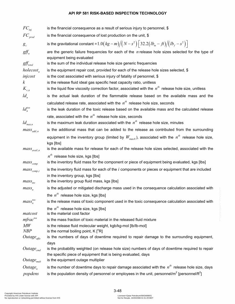
API RP 581 RISK-BASED INSPECTION TECHNOLOGY
3-48
injFC is the financial consequence as a result of serious injury to personnel, $
prodFC is the financial consequence of lost production on the unit, $
cg is the gravitational constant = ( ) ( )21.0 kg m N s− − ( ) ( )232.2 m flb ft lb s⎡ ⎤− −⎣ ⎦
ngff are the generic failure frequencies for each of the n release hole sizes selected for the type of equipment being evaluated
totalgff is the sum of the individual release hole size generic frequencies
nholecost is the equipment repair cost, provided for each of the release hole sizes selected, $ injcost is the cost associated with serious injury of fatality of personnel, $ k is the release fluid ideal gas specific heat capacity ratio, unitless
,v nK is the liquid flow viscosity correction factor, associated with the thn release hole size, unitless
nld is the actual leak duration of the flammable release based on the available mass and the
calculated release rate, associated with the thn release hole size, seconds toxnld is the leak duration of the toxic release based on the available mass and the calculated release
rate, associated with the thn release hole size, seconds
max,nld is the maximum leak duration associated with the thn release hole size, minutes
,add nmass is the additional mass that can be added to the release as contributed from the surrounding
equipment in the inventory group (limited by max8W ), associated with the thn release hole size, kgs [lbs]
,avail nmass is the available mass for release for each of the release hole sizes selected, associated with the thn release hole size, kgs [lbs]
compmass is the inventory fluid mass for the component or piece of equipment being evaluated, kgs [lbs]
,comp imass is the inventory fluid mass for each of the i components or pieces or equipment that are included in the inventory group, kgs [lbs]
invmass is the inventory group fluid mass, kgs [lbs]
nmass is the adjusted or mitigated discharge mass used in the consequence calculation associated with
the thn release hole size, kgs [lbs] toxnmass is the release mass of toxic component used in the toxic consequence calculation associated with
the thn release hole size, kgs [lbs] matcost is the material cost factor
toxmfrac is the mass fraction of toxic material in the released fluid mixture MW is the release fluid molecular weight, kgb/kg-mol [lb/lb-mol] NBP is the normal boiling point, K [oR]
affaOutage is the numbers of days of downtime required to repair damage to the surrounding equipment, days
cmdOutage is the probability weighted (on release hole size) numbers of days of downtime required to repair the specific piece of equipment that is being evaluated, days
multOutage is the equipment outage multiplier
nOutage is the number of downtime days to repair damage associated with the thn release hole size, days
popdens is the population density of personnel or employees in the unit, personnel/m2 [personnel/ft2]
Copyright American Petroleum Institute Provided by IHS under license with API Licensee=Qatar Petroleum/5943408001
Not for Resale, 10/20/2008 01:51:29 MDTNo reproduction or networking permitted without license from IHS
--```,`,,`,`,,`,`,,,,,,``,```,`-`-`,,`,,`,`,,`---

API RP 581 RISK-BASED INSPECTION TECHNOLOGY
3-49
atmP is the atmospheric pressure, kPa [psia]
sP is the storage or normal operating pressure, kPa [psia]
transP is the transition back pressure, kPa [psia]. Higher back pressures will result in subsonic vapor flow through the release hole, lower back pressures will cause choked or sonic flow across the release hole.
prodcost is the cost of lost production due to downtime to repair equipment, $/day R is the universal gas constant = 8,314 J/(kg-mol)K [1545 ft-lbf/lb-mol°R]
nRe is the Reynolds Number for flow through the release, associated with the thn release hole size, unitless
nrate is the adjusted or mitigated discharge rate used in the consequence calculation associated with
the thn release hole size, kg/s [lb/s] toxnrate is the release mass rate of toxic component used in the consequence calculation, associated with
the thn release hole size, kg/s [lb/s]
atmρ is the atmospheric air density, kg/m3 [lb/ft3]
lρ is the liquid density at storage or normal operating conditions, kg/m3 [lb/ft3]
sT is the storage or normal operating temperature, K [oR]
nt is the time to release 10,000 lbs of fluid mass, calculated for each of the n release hole sizes selected, seconds
envnvol is the spill volume to be cleaned up, used to determine environmental clean-up costs, calculated
for each of the n release hole sizes selected, barrels
nW is the theoretical release rate associated with the thn release hole size, kg/s [lb/s]
max8W is the maximum flowrate of additional mass that can be added to the release as contributed from the surrounding equipment in the inventory group, kg/s [lb/s]
ix is the mole fraction of the component and iProperty may be the NBP, MW, or density of the individual components in the fluid mixture
Copyright American Petroleum Institute Provided by IHS under license with API Licensee=Qatar Petroleum/5943408001
Not for Resale, 10/20/2008 01:51:29 MDTNo reproduction or networking permitted without license from IHS
--```,`,,`,`,,`,`,,,,,,``,```,`-`-`,,`,,`,`,,`---

API RP 581 RISK-BASED INSPECTION TECHNOLOGY
3-50
5.14 Tables
Table 5.1 – List of Representative Fluids Available for Level 1 Analysis
Representative Fluid Fluid TYPE (see 5.1.5) Examples of Applicable Materials C1 – C2 TYPE 0 methane, ethane, ethylene, LNG, fuel gas
C3 – C4 TYPE 0 propane, butane, isobutane, LPG
C5 TYPE 0 pentane
C6 – C8 TYPE 0 gasoline, naptha, light straight run, heptane
C9 – C12 TYPE 0 diesel, kerosene
C13 – C16 TYPE 0 jet fuel, kerosene, atmospheric gas oil
C17 – C25 TYPE 0 gas oil, typical crude
C25+ TYPE 0 residuum, heavy crude, lube oil, seal oil
H2 TYPE 0 hydrogen only
H2S TYPE 0 hydrogen sulfide only
HF TYPE 0 hydrogen fluoride water TYPE 0 water steam TYPE 0 steam
Acid (low) TYPE 0 Acid, caustic Aromatics TYPE 1 Benzene, Toluene, Xylene, Cumene
AlCl3 TYPE 0 Aluminum Chloride Pyrophoric TYPE 0 Pyrophoric Materials Ammonia TYPE 0 Ammonia Chlorine TYPE 0 Chlorine
CO TYPE 1 Carbon Monoxide DEE TYPE 1 (see Note 2) Diethyl Ether HCL TYPE 0 (see Note 1) Hydrogen Chloride
Nitric Acid TYPE 0 (see Note 1) Nitric Acid NO2 TYPE 0 (see Note 1) Nitrogen Dioxide
Phosgene TYPE 0 Phosgene TDI TYPE 0 (see Note 1) Toluene Diisocyanate
Methanol TYPE 1 Methanol PO TYPE 1 Propylene Oxide
Styrene TYPE 1 Styrene EEA TYPE 1 Ethylene Glycol Monoethyl Ether Acetate EE TYPE 1 Ethylene Glycol Monoethyl Ether EG TYPE 1 Ethylene Glycol EO TYPE 1 Ethylene Oxide
Notes: 1. HCL, Nitric Acid, NO2 and TDI are TYPE 1 toxic fluids 2. DEE is a TYPE 0 toxic fluid
Copyright American Petroleum Institute Provided by IHS under license with API Licensee=Qatar Petroleum/5943408001
Not for Resale, 10/20/2008 01:51:29 MDTNo reproduction or networking permitted without license from IHS
--```,`,,`,`,,`,`,,,,,,``,```,`-`-`,,`,,`,`,,`---

API RP 581 RISK-BASED INSPECTION TECHNOLOGY
3-51
Table 5.2 – Properties of the Representative Fluids Used in Level 1 Analysis
Cp
Fluid MW Liquid
Density
(lb/ft3)
NBP
(°F) Ambient
State
Ideal Gas
Specific Heat Eq.
Ideal Gas
Constant A
Ideal Gas
Constant B
Ideal Gas
Constant C
Ideal Gas
Constant D
Ideal Gas
Constant E
Auto-Ignition Temp.
(°F)
C1-C2 23 15.639 -193 Gas Note 1 12.3 1.150E-01 -2.87E-05 -1.30E-09 N/A 1036
C3-C4 51 33.61 -6.3 Gas Note 1 2.632 0.3188 -1.347E4 1.466E-8 N/A 696
C5 72 39.03 97 Liquid Note 1 -3.626 0.4873 -2.6E-4 5.3E-8 N/A 544
C6-C8 100 42.702 210 Liquid Note 1 -5.146 6.762E-01 -3.65E-04 7.658E-08 N/A 433
C9-C12 149 45.823 364 Liquid Note 1 -8.5 1.01E+00 -5.56E-04 1.180E-07 N/A 406
C13-C16 205 47.728 502 Liquid Note 1 -11.7 1.39E+00 -7.72E-04 1.670E-07 N/A 396
C17-C25 280 48.383 651 Liquid Note 1 -22.4 1.94E+00 -1.12E-03 -2.53E-07 N/A 396
C25+ 422 56.187 981 Liquid Note 1 -22.4 1.94E+00 -1.12E-03 -2.53E-07 N/A 396
Water 18 62.3 212 Liquid Note 3 2.76E+05 -2.09E+03 8.125 -1.41E-02 9.37E-06 N/A
Steam 18 62.3 212 Gas Note 3 3.34E+04 2.68E+04 2.61e+03 8.90E+03 1.17E+03 N/A
Acid 18 62.3 212 Liquid Note 3 2.76E+05 -2.09E+03 8.125 -1.41E-02 9.37E-06 N/A
H2 2 4.433 -423 Gas Note 1 27.1 9.270E-03 -1.38E-05 7.650E-09 N/A 752
H2S 34 61.993 -75 Gas Note 1 31.9 1.440E-03 2.430E-05 -1.18E-08 N/A 500
HF 20 60.37 68 Gas Note 1 29.1 6.610E-04 -2.03E-06 2.500E-09 N/A 32000
CO 28 50 -312 Gas Note 2 2.91E+04 8.77E+03 3.09E+03 8.46E+03 1.54E+03 1128
DEE 74 45 95 Liquid Note 2 8.62E+04 2.55E+05 1.54E+03 1.44E+05 -6.89E+02 320
HCL 36 74 -121 Gas --- --- --- --- --- --- N/A
Nitric Acid 63 95 250 Liquid --- --- --- --- --- --- N/A
ALCL3 133.5 152 382 Powder Note 1 4.34E+04 3.97E+04 4.17E+02 2.40E+04 N/A 1036
NO2 90 58 275 Liquid --- --- --- --- --- --- N/A
Phosgene 99 86 181 Liquid --- --- --- --- --- --- N/A
TDI 174 76 484 Liquid --- --- --- --- --- --- 1148
Methanol 32 50 149 Liquid Note 2 3.93E+04 8.79E+04 1.92E+03 5.37E+04 8.97E+02 867
PO 58 52 93 Liquid Note 2 4.95E+04 1.74E+05 1.56E+03 1.15E+05 7.02E+02 840
Copyright American Petroleum Institute Provided by IHS under license with API Licensee=Qatar Petroleum/5943408001
Not for Resale, 10/20/2008 01:51:29 MDTNo reproduction or networking permitted without license from IHS
--```,`,,`,`,,`,`,,,,,,``,```,`-`-`,,`,,`,`,,`---

API RP 581 RISK-BASED INSPECTION TECHNOLOGY
3-52
Table 5.2 – Properties of the Representative Fluids Used in Level 1 Analysis
Cp
Fluid MW Liquid
Density
(lb/ft3)
NBP
(°F) Ambient
State
Ideal Gas
Specific Heat Eq.
Ideal Gas
Constant A
Ideal Gas
Constant B
Ideal Gas
Constant C
Ideal Gas
Constant D
Ideal Gas
Constant E
Auto-Ignition Temp.
(°F)
Styrene (Aromatic)
104 42.7 293 Liquid Note 2 8.93E+04 2.15E+05 7.72E+02 9.99E+04 2.44E+03 914
EEA 132 61 313 Liquid Note 2 1.06E+05 2.40E+05 6.59E+02 1.50E+05 1.97E+03 715
EE 90 58 275 Liquid Note 2 3.25E+04 3.00E+05 1.17E+03 2.08E+05 4.73E+02 455
EG 62 69 387 Liquid Note 2 6.30E+04 1.46E+05 1.67E+03 9.73E+04 7.74E+02 745
EO 44 55 51 Gas Note 2 3.35E+04 1.21E+05 1.61E+03 8.24E+04 7.37E+02 804
Pyrophoric 149 45.823 364 Liquid Note 1 -8.5 1.01E+00 -5.56E-04 1.180E-07 N/A Note 3
Notes:
1. 2 3pC A BT CT DT= + + + with T in K, units for pC are J/kmol-K
2.
2 2
sinh coshp
C ET TC A B D
C ET T
⎛ ⎞ ⎛ ⎞⎜ ⎟ ⎜ ⎟⎜ ⎟ ⎜ ⎟= + +
⎡ ⎤ ⎡ ⎤⎜ ⎟ ⎜ ⎟⎜ ⎟ ⎜ ⎟⎢ ⎥ ⎢ ⎥⎣ ⎦ ⎣ ⎦⎝ ⎠ ⎝ ⎠
with T in K, units for pC are J/kmol-K
3. 2 3 4pC A BT CT DT ET= + + + + with T in K, units for pC are J/kmol-K
4. Pyrophoric materials, by definition, auto-ignite and therefore, a very low value for the AIT is assumed. 5. Conversion factor for units of pC is 1 J/kmol-K = 5.27x10⁻⁴ Btu/kmol-oR
Copyright American Petroleum Institute Provided by IHS under license with API Licensee=Qatar Petroleum/5943408001
Not for Resale, 10/20/2008 01:51:29 MDTNo reproduction or networking permitted without license from IHS
--```,`,,`,`,,`,`,,,,,,``,```,`-`-`,,`,,`,`,,`---

API RP 581 RISK-BASED INSPECTION TECHNOLOGY
3-53
Table 5.2M – Properties of the Representative Fluids Used in Level 1 Analysis
Cp
Fluid MW Liquid
Density
(kg/m3)
NBP
(°C) Ambient
State
Ideal Gas
Specific Heat Eq.
Ideal Gas
Constant A
Ideal Gas
Constant B
Ideal Gas
Constant C
Ideal Gas
Constant D
Ideal Gas
Constant E
Auto-Ignition Temp.
(°C)
C1-C2 23 250.512 -125 Gas Note 1 12.3 1.15E-01 -2.87E-05 -1.30E-09 N/A 558
C3-C4 51 538.379 -21 Gas Note 1 2.632 0.3188 -1.35E+04 1.47E-08 N/A 369
C5 72 625.199 36 Liquid Note 1 -3.626 0.4873 -2.60E-04 5.30E-08 N/A 284
C6-C8 100 684.018 99 Liquid Note 1 -5.146 6.76E-01 -3.65E-04 7.66E-08 N/A 223
C9-C12 149 734.012 184 Liquid Note 1 -8.5 1.01E+00 -5.56E-04 1.18E-07 N/A 208
C13-C16 205 764.527 261 Liquid Note 1 -11.7 1.39E+00 -7.72E-04 1.67E-07 N/A 202
C17-C25 280 775.019 344 Liquid Note 1 -22.4 1.94E+00 -1.12E-03 -2.53E-07 N/A 202
C25+ 422 900.026 527 Liquid Note 1 -22.4 1.94E+00 -1.12E-03 -2.53E-07 N/A 202
Water 18 997.947 100 Liquid Note 3 2.76E+05 -2.09E+03 8.125 -1.41E-02 9.37E-06 N/A
Steam 18 997.947 100 Gas Note 3 3.34E+04 2.68E+04 2.61E+03 8.90E+03 1.17E+03 N/A
Acid 18 997.947 100 Liquid Note 3 2.76E+05 -2.09E+03 8.125 -1.41E-02 9.37E-06 N/A
H2 2 71.010 -253 Gas Note 1 27.1 9.27E-03 -1.38E-05 7.65E-09 N/A 400
H2S 34 993.029 -59 Gas Note 1 31.9 1.44E-03 2.43E-05 -1.18E-08 N/A 260
HF 20 967.031 20 Gas Note 1 29.1 6.61E-04 -2.03E-06 2.50E-09 N/A 17760
CO 28 800.920 -191 Gas Note 2 2.91E+04 8.77E+03 3.09E+03 8.46E+03 1.54E+03 609
DEE 74 720.828 35 Liquid Note 2 8.62E+04 2.55E+05 1.54E+03 1.44E+05 -6.89E+02 160
HCL 36 1185.362 -85 Gas --- --- --- --- --- --- N/A
Nitric Acid 63 1521.749 121 Liquid --- --- --- --- --- --- N/A
ALCL3 133.5 2434.798 194 Powder Note 1 4.34E+04 3.97E+04 4.17E+02 2.40E+04 N/A 558
NO2 90 929.068 135 Liquid --- --- --- --- --- --- N/A
Phosgene 99 1377.583 83 Liquid --- --- --- --- --- --- N/A
TDI 174 1217.399 251 Liquid --- --- --- --- --- --- 620
Methanol 32 800.920 65 Liquid Note 2 3.93E+04 8.79E+04 1.92E+03 5.37E+04 8.97E+02 464
PO 58 832.957 34 Liquid Note 2 4.95E+04 1.74E+05 1.56E+03 1.15E+05 7.02E+02 449
Copyright American Petroleum Institute Provided by IHS under license with API Licensee=Qatar Petroleum/5943408001
Not for Resale, 10/20/2008 01:51:29 MDTNo reproduction or networking permitted without license from IHS
--```,`,,`,`,,`,`,,,,,,``,```,`-`-`,,`,,`,`,,`---
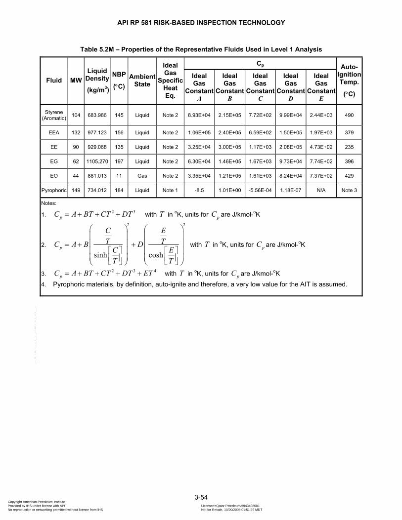
API RP 581 RISK-BASED INSPECTION TECHNOLOGY
3-54
Table 5.2M – Properties of the Representative Fluids Used in Level 1 Analysis
Cp
Fluid MW Liquid
Density
(kg/m3)
NBP
(°C) Ambient
State
Ideal Gas
Specific Heat Eq.
Ideal Gas
Constant A
Ideal Gas
Constant B
Ideal Gas
Constant C
Ideal Gas
Constant D
Ideal Gas
Constant E
Auto-Ignition Temp.
(°C)
Styrene (Aromatic) 104 683.986 145 Liquid Note 2 8.93E+04 2.15E+05 7.72E+02 9.99E+04 2.44E+03 490
EEA 132 977.123 156 Liquid Note 2 1.06E+05 2.40E+05 6.59E+02 1.50E+05 1.97E+03 379
EE 90 929.068 135 Liquid Note 2 3.25E+04 3.00E+05 1.17E+03 2.08E+05 4.73E+02 235
EG 62 1105.270 197 Liquid Note 2 6.30E+04 1.46E+05 1.67E+03 9.73E+04 7.74E+02 396
EO 44 881.013 11 Gas Note 2 3.35E+04 1.21E+05 1.61E+03 8.24E+04 7.37E+02 429
Pyrophoric 149 734.012 184 Liquid Note 1 -8.5 1.01E+00 -5.56E-04 1.18E-07 N/A Note 3
Notes:
1. 2 3pC A BT CT DT= + + + with T in oK, units for pC are J/kmol-oK
2.
2 2
sinh coshp
C ET TC A B D
C ET T
⎛ ⎞ ⎛ ⎞⎜ ⎟ ⎜ ⎟⎜ ⎟ ⎜ ⎟= + +
⎡ ⎤ ⎡ ⎤⎜ ⎟ ⎜ ⎟⎜ ⎟ ⎜ ⎟⎢ ⎥ ⎢ ⎥⎣ ⎦ ⎣ ⎦⎝ ⎠ ⎝ ⎠
with T in oK, units for pC are J/kmol-oK
3. 2 3 4pC A BT CT DT ET= + + + + with T in oK, units for pC are J/kmol-oK
4. Pyrophoric materials, by definition, auto-ignite and therefore, a very low value for the AIT is assumed.
Copyright American Petroleum Institute Provided by IHS under license with API Licensee=Qatar Petroleum/5943408001
Not for Resale, 10/20/2008 01:51:29 MDTNo reproduction or networking permitted without license from IHS
--```,`,,`,`,,`,`,,,,,,``,```,`-`-`,,`,,`,`,,`---
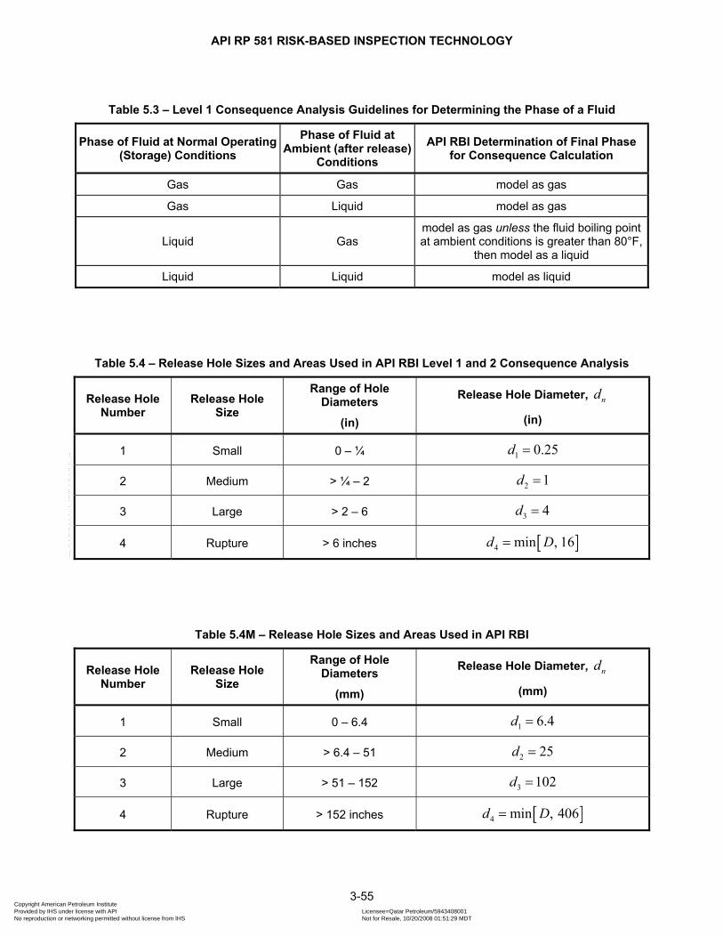
API RP 581 RISK-BASED INSPECTION TECHNOLOGY
3-55
Table 5.3 – Level 1 Consequence Analysis Guidelines for Determining the Phase of a Fluid
Phase of Fluid at Normal Operating (Storage) Conditions
Phase of Fluid at Ambient (after release)
Conditions API RBI Determination of Final Phase
for Consequence Calculation
Gas Gas model as gas
Gas Liquid model as gas
Liquid Gas model as gas unless the fluid boiling point at ambient conditions is greater than 80°F,
then model as a liquid
Liquid Liquid model as liquid
Table 5.4 – Release Hole Sizes and Areas Used in API RBI Level 1 and 2 Consequence Analysis
Release Hole Number
Release Hole Size
Range of Hole Diameters
(in)
Release Hole Diameter, nd
(in)
1 Small 0 – ¼ 1 0.25d =
2 Medium > ¼ – 2 2 1d =
3 Large > 2 – 6 3 4d =
4 Rupture > 6 inches [ ]4 min , 16d D=
Table 5.4M – Release Hole Sizes and Areas Used in API RBI
Release Hole Number
Release Hole Size
Range of Hole Diameters
(mm)
Release Hole Diameter, nd
(mm)
1 Small 0 – 6.4 1 6.4d =
2 Medium > 6.4 – 51 2 25d =
3 Large > 51 – 152 3 102d =
4 Rupture > 152 inches [ ]4 min , 406d D=
Copyright American Petroleum Institute Provided by IHS under license with API Licensee=Qatar Petroleum/5943408001
Not for Resale, 10/20/2008 01:51:29 MDTNo reproduction or networking permitted without license from IHS
--```,`,,`,`,,`,`,,,,,,``,```,`-`-`,,`,,`,`,,`---

API RP 581 RISK-BASED INSPECTION TECHNOLOGY
3-56
Table 5.5 – Detection and Isolation System Rating Guide
Type of Detection System Detection Classification
Instrumentation designed specifically to detect material losses by changes in operating conditions (i.e., loss of pressure or flow) in the system.
A
Suitably located detectors to determine when the material is present outside the pressure-containing envelope.
B
Visual detection, cameras, or detectors with marginal coverage. C
Type of Isolation System Isolation Classification
Isolation or shutdown systems activated directly from process instrumentation or detectors, with no operator intervention.
A
Isolation or shutdown systems activated by operators in the control room or other suitable locations remote from the leak.
B
Isolation dependent on manually-operated valves C
Copyright American Petroleum Institute Provided by IHS under license with API Licensee=Qatar Petroleum/5943408001
Not for Resale, 10/20/2008 01:51:29 MDTNo reproduction or networking permitted without license from IHS
--```,`,,`,`,,`,`,,,,,,``,```,`-`-`,,`,,`,`,,`---

API RP 581 RISK-BASED INSPECTION TECHNOLOGY
3-57
Table 5.6 – Adjustments to Release Based on Detection and Isolation Systems
System Classifications
Detection Isolation Release Magnitude Adjustment Reduction Factor, difact
A A Reduce release rate or mass by 25% 0.25
A B Reduce release rate or mass by 20% 0.20
A or B C Reduce release rate or mass by 10% 0.10
B B Reduce release rate or mass by 15% 0.15
C C No adjustment to release rate or mass 0.00
Table 5.7 – Leak Durations Based on Detection and Isolation Systems
Detection System Rating Isolation System Rating
Maximum Leak Duration, maxld
A A 20 minutes for 1/4 inch leaks 10 minutes for 1 inch leaks 5 minutes for 4 inch leaks
A B 30 minutes for 1/4 inch leaks 20 minutes for 1 inch leaks 10 minutes for 4 inch leaks
A C 40 minutes for 1/4 inch leaks 30 minutes for 1 inch leaks 20 minutes for 4 inch leaks
B A or B 40 minutes for 1/4 inch leaks 30 minutes for 1 inch leaks 20 minutes for 4 inch leaks
B C 1 hour for 1/4 inch leaks
30 minutes for 1 inch leaks 20 minutes for 4 inch leaks
C A, B or C 1 hour for 1/4 inch leaks
40 minutes for 1 inch leaks 20 minutes for 4 inch leaks
Copyright American Petroleum Institute Provided by IHS under license with API Licensee=Qatar Petroleum/5943408001
Not for Resale, 10/20/2008 01:51:29 MDTNo reproduction or networking permitted without license from IHS
--```,`,,`,`,,`,`,,,,,,``,```,`-`-`,,`,,`,`,,`---

API RP 581 RISK-BASED INSPECTION TECHNOLOGY
3-58
Table 5.7M – Leak Durations Based on Detection and Isolation Systems
Detection System Rating Isolation System Rating
Maximum Leak Duration, maxld
A A 20 minutes for 6.4 mm leaks 10 minutes for 25 mm leaks 5 minutes for 102 mm leaks
A B 30 minutes for 6.4 mm leaks 20 minutes for 25 mm leaks
10 minutes for 102 mm leaks
A C 40 minutes for 6.4 mm leaks 30 minutes for 25 mm leaks
20 minutes for 102 mm leaks
B A or B 40 minutes for 6.4 mm leaks 30 minutes for 25 mm leaks
20 minutes for 102 mm leaks
B C 1 hour for 6.4 mm leaks
30 minutes for 25 mm leaks 20 minutes for 102 mm leaks
C A, B or C 1 hour for 6.4 mm leaks
40 minutes for 25 mm leaks 20 minutes for 102 mm leaks
Copyright American Petroleum Institute Provided by IHS under license with API Licensee=Qatar Petroleum/5943408001
Not for Resale, 10/20/2008 01:51:29 MDTNo reproduction or networking permitted without license from IHS
--```,`,,`,`,,`,`,,,,,,``,```,`-`-`,,`,,`,`,,`---

API RP 581 RISK-BASED INSPECTION TECHNOLOGY
3-59
Table 5.8 – Component Damage Flammable Consequence Equation Constants
Continuous Releases Constants Instantaneous Releases Constants
Auto-Ignition Not Likely
(CAINL)
Auto-Ignition Likely
(CAIL)
Auto-Ignition Not Likely
(IAINL)
Auto-Ignition Likely
(IAIL) Gas Liquid Gas Liquid Gas Liquid Gas Liquid
Fluid
a b a b a b a b a b a b a b a b
C1-C2 43.0 0.98 280.0 0.95 41.0 0.67 1079 0.62
C3-C4 49.48 1.00 313.6 1.00 27.96 0.72 522.9 0.63
C5 25.17 0.99 536.0 0.89 304.7 1.00 13.38 0.73 1.49 0.85 275.0 0.61
C6-C8 29.0 0.98 182.0 0.89 312.4 1.00 525.0 0.95 13.98 0.66 4.35 0.78 275.7 0.61 57.0 0.55
C9-C12 12.0 0.98 130.0 0.90 391.0 0.95 560.0 0.95 7.1 0.66 3.3 0.76 281.0 0.61 6.0 0.53
C13-C16 64.0 0.90 1023 0.92 0.46 0.88 9.2 0.88
C17-C25 20.0 0.90 861.0 0.92 0.11 0.91 5.6 0.91
C25 + 11.0 0.91 544.0 0.90 0.03 0.99 1.4 0.99
H2 64.5 0.992 420.0 1.00 61.5 0.657 1430 0.618
H2S 32.0 1.00 203.0 0.89 148.0 0.63 357.0 0.61
HF
Aromatics 17.87 1.097 103.0 1.00 374.5 1.055 11.46 0.667 70.12 1.00 512.6 0.713 701.2 1.00
Styrene 17.87 1.097 103.0 1.00 374.5 1.055 11.46 0.667 70.12 1.00 512.6 0.713 701.2 1.00
CO 0.107 1.752 69.68 0.667
DEE 39.84 1.134 737.4 1.106 320.7 1.033 6289 0.649 155.7 0.667 5.105 0.919 5.672 0.919
Methanol 0.026 0.909 1751 0.934 28.11 0.667 1.919 0.900
PO 14.62 1.114 1295 0.960 65.58 0.667 3.404 0.869
EEA 0.002 1.035 117.0 1.00 8.014 0.667 69.0 1.00
EE 12.62 1.005 173.1 1.00 38.87 0.667 72.21 1.00
EG 7.721 0.973 108.0 1.00 6.525 0.667 69.0 1.00
EO 31.03 1.069 136.3 0.667
Pyrophoric 12.0 0.98 130.0 0.90 391.0 0.95 560.0 0.95 7.1 0.66 3.3 0.76 281.0 0.61 6.0 0.53
Copyright American Petroleum Institute Provided by IHS under license with API Licensee=Qatar Petroleum/5943408001
Not for Resale, 10/20/2008 01:51:29 MDTNo reproduction or networking permitted without license from IHS
--```,`,,`,`,,`,`,,,,,,``,```,`-`-`,,`,,`,`,,`---

API RP 581 RISK-BASED INSPECTION TECHNOLOGY
3-60
Table 5.8M – Component Damage Flammable Consequence Equation Constants
Continuous Releases Constants Instantaneous Releases Constants
Auto-Ignition Not Likely
(CAINL)
Auto-Ignition Likely
(CAIL)
Auto-Ignition Not Likely
(IAINL)
Auto-Ignition Likely
(IAIL) Gas Liquid Gas Liquid Gas Liquid Gas Liquid
Fluid
a b a b a b a b a b a b a b a b
C1-C2 8.669 0.98 55.13 0.95 6.469 0.67 163.7 0.62
C3-C4 10.13 1.00 64.23 1.00 4.590 0.72 79.94 0.63
C5 5.115 0.99 100.6 0.89 62.41 1.00 2.214 0.73 0.271 0.85 41.38 0.61
C6-C8 5.846 0.98 34.17 0.89 63.98 1.00 103.4 0.95 2.188 0.66 0.749 0.78 41.49 0.61 8.180 0.55
C9-C12 2.419 0.98 24.60 0.90 76.98 0.95 110.3 0.95 1.111 0.66 0.559 0.76 42.28 0.61 0.848 0.53
C13-C16 12.11 0.90 196.7 0.92 0.086 0.88 1.714 0.88
C17-C25 3.785 0.90 165.5 0.92 0.021 0.91 1.068 0.91
C25 + 2.098 0.91 103.0 0.90 0.006 0.99 0.284 0.99
H2 13.13 0.992 86.02 1.00 9.605 0.657 216.5 0.618
H2S 6.554 1.00 38.11 0.89 22.63 0.63 53.72 0.61
HF
Aromatics 3.952 1.097 21.10 1.00 80.11 1.055 1.804 0.667 14.36 1.00 83.68 0.713 143.6 1.00
Styrene 3.952 1.097 21.10 1.00 80.11 1.055 1.804 0.667 14.36 1.00 83.68 0.713 143.6 1.00
CO 0.040 1.752 10.97 0.667
DEE 9.072 1.134 164.2 1.106 67.42 1.033 976.0 0.649 24.51 0.667 0.981 0.919 1.090 0.919
Methanol 0.005 0.909 340.4 0.934 4.425 0.667 0.363 0.900
PO 3.277 1.114 257.0 0.960 10.32 0.667 0.629 0.869
EEA 0 1.035 23.96 1.00 1.261 0.667 14.13 1.00
EE 2.595 1.005 35.45 1.00 6.119 0.667 14.79 1.00
EG 1.548 0.973 22.12 1.00 1.027 0.667 14.13 1.00
EO 6.712 1.069 21.46 0.667
Pyrophoric 2.419 0.98 24.60 0.90 76.98 0.95 110.3 0.95 1.111 0.66 0.559 0.76 42.28 0.61 0.848 0.53
Copyright American Petroleum Institute Provided by IHS under license with API Licensee=Qatar Petroleum/5943408001
Not for Resale, 10/20/2008 01:51:29 MDTNo reproduction or networking permitted without license from IHS
--```,`,,`,`,,`,`,,,,,,``,```,`-`-`,,`,,`,`,,`---
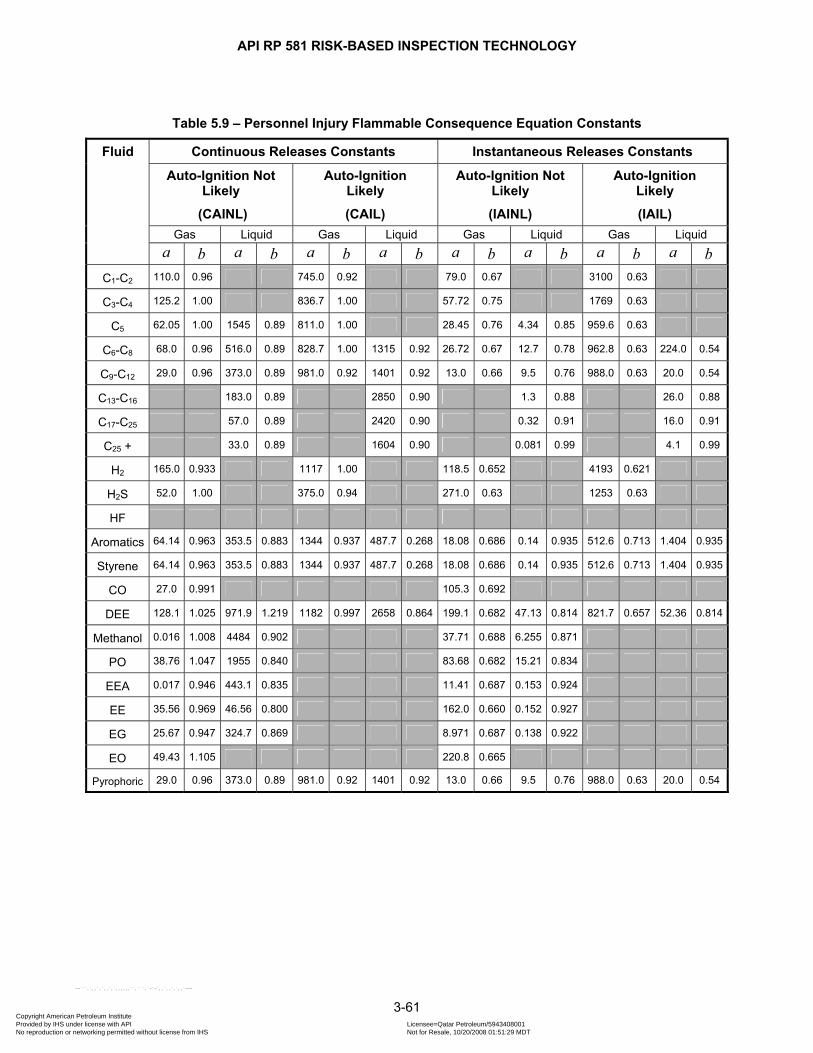
API RP 581 RISK-BASED INSPECTION TECHNOLOGY
3-61
Table 5.9 – Personnel Injury Flammable Consequence Equation Constants
Continuous Releases Constants Instantaneous Releases Constants
Auto-Ignition Not Likely
(CAINL)
Auto-Ignition Likely
(CAIL)
Auto-Ignition Not Likely
(IAINL)
Auto-Ignition Likely
(IAIL) Gas Liquid Gas Liquid Gas Liquid Gas Liquid
Fluid
a b a b a b a b a b a b a b a b
C1-C2 110.0 0.96 745.0 0.92 79.0 0.67 3100 0.63
C3-C4 125.2 1.00 836.7 1.00 57.72 0.75 1769 0.63
C5 62.05 1.00 1545 0.89 811.0 1.00 28.45 0.76 4.34 0.85 959.6 0.63
C6-C8 68.0 0.96 516.0 0.89 828.7 1.00 1315 0.92 26.72 0.67 12.7 0.78 962.8 0.63 224.0 0.54
C9-C12 29.0 0.96 373.0 0.89 981.0 0.92 1401 0.92 13.0 0.66 9.5 0.76 988.0 0.63 20.0 0.54
C13-C16 183.0 0.89 2850 0.90 1.3 0.88 26.0 0.88
C17-C25 57.0 0.89 2420 0.90 0.32 0.91 16.0 0.91
C25 + 33.0 0.89 1604 0.90 0.081 0.99 4.1 0.99
H2 165.0 0.933 1117 1.00 118.5 0.652 4193 0.621
H2S 52.0 1.00 375.0 0.94 271.0 0.63 1253 0.63
HF
Aromatics 64.14 0.963 353.5 0.883 1344 0.937 487.7 0.268 18.08 0.686 0.14 0.935 512.6 0.713 1.404 0.935
Styrene 64.14 0.963 353.5 0.883 1344 0.937 487.7 0.268 18.08 0.686 0.14 0.935 512.6 0.713 1.404 0.935
CO 27.0 0.991 105.3 0.692
DEE 128.1 1.025 971.9 1.219 1182 0.997 2658 0.864 199.1 0.682 47.13 0.814 821.7 0.657 52.36 0.814
Methanol 0.016 1.008 4484 0.902 37.71 0.688 6.255 0.871
PO 38.76 1.047 1955 0.840 83.68 0.682 15.21 0.834
EEA 0.017 0.946 443.1 0.835 11.41 0.687 0.153 0.924
EE 35.56 0.969 46.56 0.800 162.0 0.660 0.152 0.927
EG 25.67 0.947 324.7 0.869 8.971 0.687 0.138 0.922
EO 49.43 1.105 220.8 0.665
Pyrophoric 29.0 0.96 373.0 0.89 981.0 0.92 1401 0.92 13.0 0.66 9.5 0.76 988.0 0.63 20.0 0.54
Copyright American Petroleum Institute Provided by IHS under license with API Licensee=Qatar Petroleum/5943408001
Not for Resale, 10/20/2008 01:51:29 MDTNo reproduction or networking permitted without license from IHS
--```,`,,`,`,,`,`,,,,,,``,```,`-`-`,,`,,`,`,,`---

API RP 581 RISK-BASED INSPECTION TECHNOLOGY
3-62
Table 5.9M – Personnel Injury Flammable Consequence Equation Constants
Continuous Releases Constants Instantaneous Releases Constants
Auto-Ignition Not Likely
(CAINL)
Auto-Ignition Likely
(CAIL)
Auto-Ignition Not Likely
(IAINL)
Auto-Ignition Likely
(IAIL) Gas Liquid Gas Liquid Gas Liquid Gas Liquid
Fluid
a b a b a b a b a b a b a b a b
C1-C2 21.83 0.96 143.2 0.92 12.46 0.67 473.9 0.63
C3-C4 25.64 1.00 171.4 1.00 9.702 0.75 270.4 0.63
C5 12.71 1.00 290.1 0.89 166.1 1.00 4.820 0.76 0.790 0.85 146.7 0.63
C6-C8 13.49 0.96 96.88 0.89 169.7 1.00 252.8 0.92 4.216 0.67 2.186 0.78 147.2 0.63 31.89 0.54
C9-C12 5.755 0.96 70.03 0.89 188.6 0.92 269.4 0.92 2.035 0.66 1.609 0.76 151.0 0.63 2.847 0.54
C13-C16 34.36 0.89 539.4 0.90 0.242 0.88 4.843 0.88
C17-C25 10.70 0.89 458.0 0.90 0.061 0.91 3.052 0.91
C25 + 6.196 0.89 303.6 0.90 0.016 0.99 0.833 0.99
H2 32.05 0.933 228.8 1.00 18.43 0.652 636.5 0.621
H2S 10.65 1.00 73.25 0.94 41.43 0.63 191.5 0.63
HF
Aromatics 12.76 0.963 66.01 0.883 261.9 0.937 56.00 0.268 2.889 0.686 0.027 0.935 83.68 0.713 0.273 0.935
Styrene 12.76 0.963 66.01 0.883 261.9 0.937 56.00 0.268 2.889 0.686 0.027 0.935 83.68 0.713 0.273 0.935
CO 5.491 0.991 16.91 0.692
DEE 26.76 1.025 236.7 1.219 241.5 0.997 488.9 0.864 31.71 0.682 8.333 0.814 128.3 0.657 9.258 0.814
Methanol 0 1.008 849.9 0.902 6.035 0.688 1.157 0.871
PO 8.239 1.047 352.8 0.840 13.33 0.682 2.732 0.834
EEA 0 0.946 79.66 0.835 1.825 0.687 0.030 0.924
EE 7.107 0.969 8.142 0.800 25.36 0.660 0.029 0.927
EG 5.042 0.947 59.96 0.869 1.435 0.687 0.027 0.922
EO 11.00 1.105 34.70 0.665
Pyrophoric 5.755 0.96 70.03 0.89 188.6 0.92 269.4 0.92 2.035 0.66 1.609 0.76 151.0 0.63 2.847 0.54
Copyright American Petroleum Institute Provided by IHS under license with API Licensee=Qatar Petroleum/5943408001
Not for Resale, 10/20/2008 01:51:29 MDTNo reproduction or networking permitted without license from IHS
--```,`,,`,`,,`,`,,,,,,``,```,`-`-`,,`,,`,`,,`---
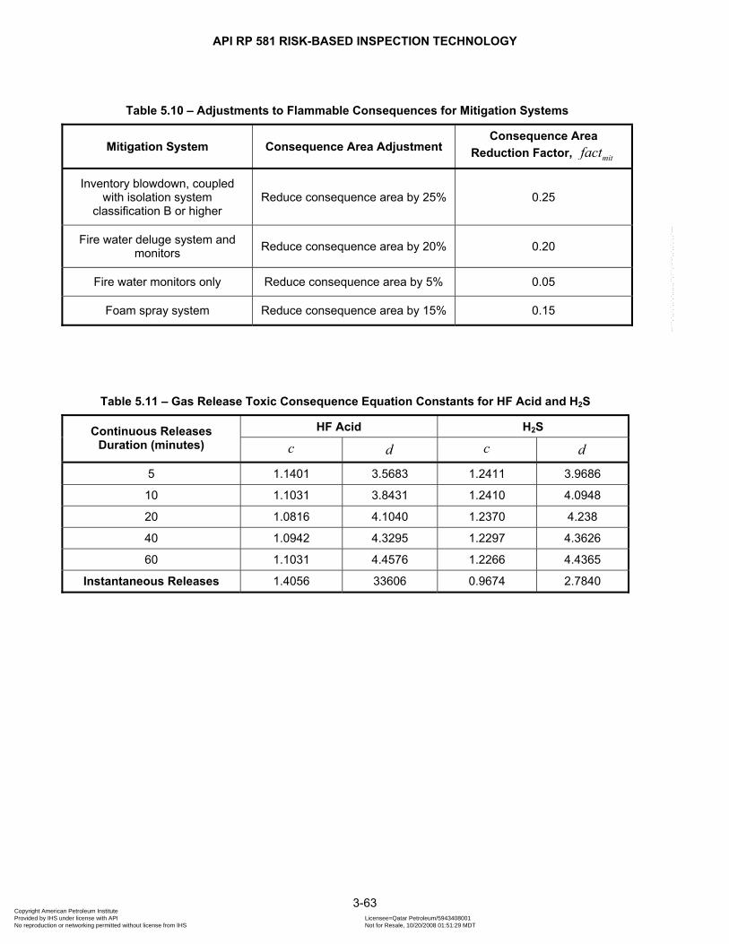
API RP 581 RISK-BASED INSPECTION TECHNOLOGY
3-63
Table 5.10 – Adjustments to Flammable Consequences for Mitigation Systems
Mitigation System Consequence Area Adjustment Consequence Area
Reduction Factor, mitfact
Inventory blowdown, coupled with isolation system
classification B or higher Reduce consequence area by 25% 0.25
Fire water deluge system and monitors Reduce consequence area by 20% 0.20
Fire water monitors only Reduce consequence area by 5% 0.05
Foam spray system Reduce consequence area by 15% 0.15
Table 5.11 – Gas Release Toxic Consequence Equation Constants for HF Acid and H2S
HF Acid H2S Continuous Releases Duration (minutes) c d c d
5 1.1401 3.5683 1.2411 3.9686
10 1.1031 3.8431 1.2410 4.0948
20 1.0816 4.1040 1.2370 4.238
40 1.0942 4.3295 1.2297 4.3626
60 1.1031 4.4576 1.2266 4.4365
Instantaneous Releases 1.4056 33606 0.9674 2.7840
Copyright American Petroleum Institute Provided by IHS under license with API Licensee=Qatar Petroleum/5943408001
Not for Resale, 10/20/2008 01:51:29 MDTNo reproduction or networking permitted without license from IHS
--```,`,,`,`,,`,`,,,,,,``,```,`-`-`,,`,,`,`,,`---
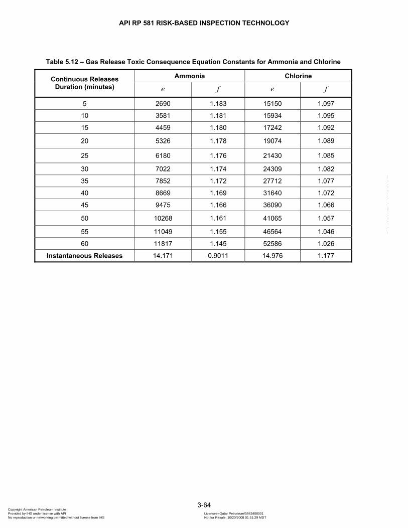
API RP 581 RISK-BASED INSPECTION TECHNOLOGY
3-64
Table 5.12 – Gas Release Toxic Consequence Equation Constants for Ammonia and Chlorine
Ammonia Chlorine Continuous Releases Duration (minutes) e f e f
5 2690 1.183 15150 1.097
10 3581 1.181 15934 1.095
15 4459 1.180 17242 1.092
20 5326 1.178 19074 1.089
25 6180 1.176 21430 1.085
30 7022 1.174 24309 1.082
35 7852 1.172 27712 1.077
40 8669 1.169 31640 1.072
45 9475 1.166 36090 1.066
50 10268 1.161 41065 1.057
55 11049 1.155 46564 1.046
60 11817 1.145 52586 1.026
Instantaneous Releases 14.171 0.9011 14.976 1.177
Copyright American Petroleum Institute Provided by IHS under license with API Licensee=Qatar Petroleum/5943408001
Not for Resale, 10/20/2008 01:51:29 MDTNo reproduction or networking permitted without license from IHS
--```,`,,`,`,,`,`,,,,,,``,```,`-`-`,,`,,`,`,,`---
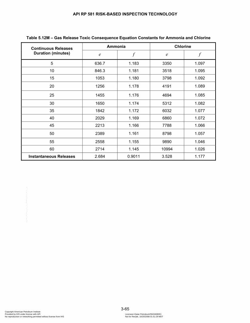
API RP 581 RISK-BASED INSPECTION TECHNOLOGY
3-65
Table 5.12M – Gas Release Toxic Consequence Equation Constants for Ammonia and Chlorine
Ammonia Chlorine Continuous Releases Duration (minutes) e f e f
5 636.7 1.183 3350 1.097
10 846.3 1.181 3518 1.095
15 1053 1.180 3798 1.092
20 1256 1.178 4191 1.089
25 1455 1.176 4694 1.085
30 1650 1.174 5312 1.082
35 1842 1.172 6032 1.077
40 2029 1.169 6860 1.072
45 2213 1.166 7788 1.066
50 2389 1.161 8798 1.057
55 2558 1.155 9890 1.046
60 2714 1.145 10994 1.026
Instantaneous Releases 2.684 0.9011 3.528 1.177
Copyright American Petroleum Institute Provided by IHS under license with API Licensee=Qatar Petroleum/5943408001
Not for Resale, 10/20/2008 01:51:29 MDTNo reproduction or networking permitted without license from IHS
--```,`,,`,`,,`,`,,,,,,``,```,`-`-`,,`,,`,`,,`---
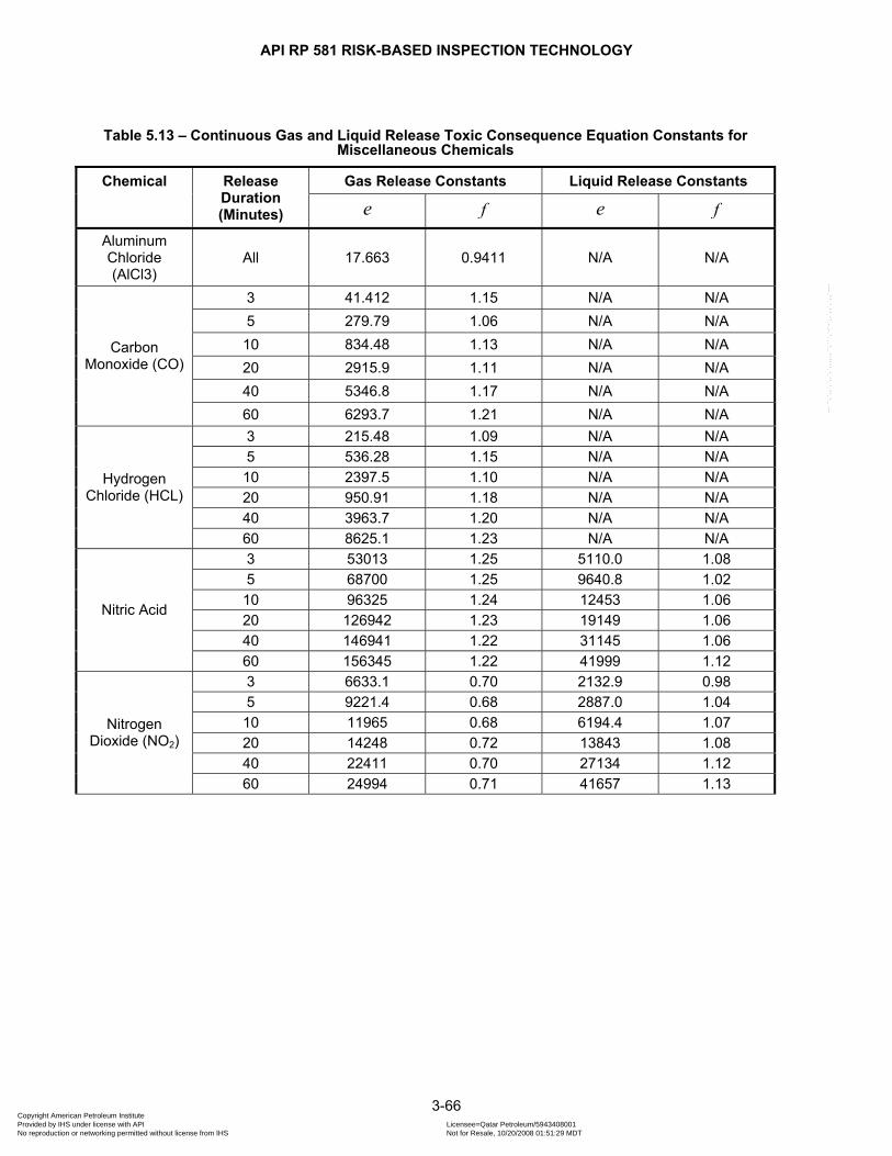
API RP 581 RISK-BASED INSPECTION TECHNOLOGY
3-66
Table 5.13 – Continuous Gas and Liquid Release Toxic Consequence Equation Constants for Miscellaneous Chemicals
Gas Release Constants Liquid Release Constants Chemical Release Duration (Minutes) e f e f
Aluminum Chloride (AlCl3)
All 17.663 0.9411 N/A N/A
3 41.412 1.15 N/A N/A 5 279.79 1.06 N/A N/A 10 834.48 1.13 N/A N/A 20 2915.9 1.11 N/A N/A 40 5346.8 1.17 N/A N/A
Carbon Monoxide (CO)
60 6293.7 1.21 N/A N/A 3 215.48 1.09 N/A N/A 5 536.28 1.15 N/A N/A 10 2397.5 1.10 N/A N/A 20 950.91 1.18 N/A N/A 40 3963.7 1.20 N/A N/A
Hydrogen Chloride (HCL)
60 8625.1 1.23 N/A N/A 3 53013 1.25 5110.0 1.08 5 68700 1.25 9640.8 1.02 10 96325 1.24 12453 1.06 20 126942 1.23 19149 1.06 40 146941 1.22 31145 1.06
Nitric Acid
60 156345 1.22 41999 1.12 3 6633.1 0.70 2132.9 0.98 5 9221.4 0.68 2887.0 1.04 10 11965 0.68 6194.4 1.07 20 14248 0.72 13843 1.08 40 22411 0.70 27134 1.12
Nitrogen Dioxide (NO2)
60 24994 0.71 41657 1.13
Copyright American Petroleum Institute Provided by IHS under license with API Licensee=Qatar Petroleum/5943408001
Not for Resale, 10/20/2008 01:51:29 MDTNo reproduction or networking permitted without license from IHS
--```,`,,`,`,,`,`,,,,,,``,```,`-`-`,,`,,`,`,,`---
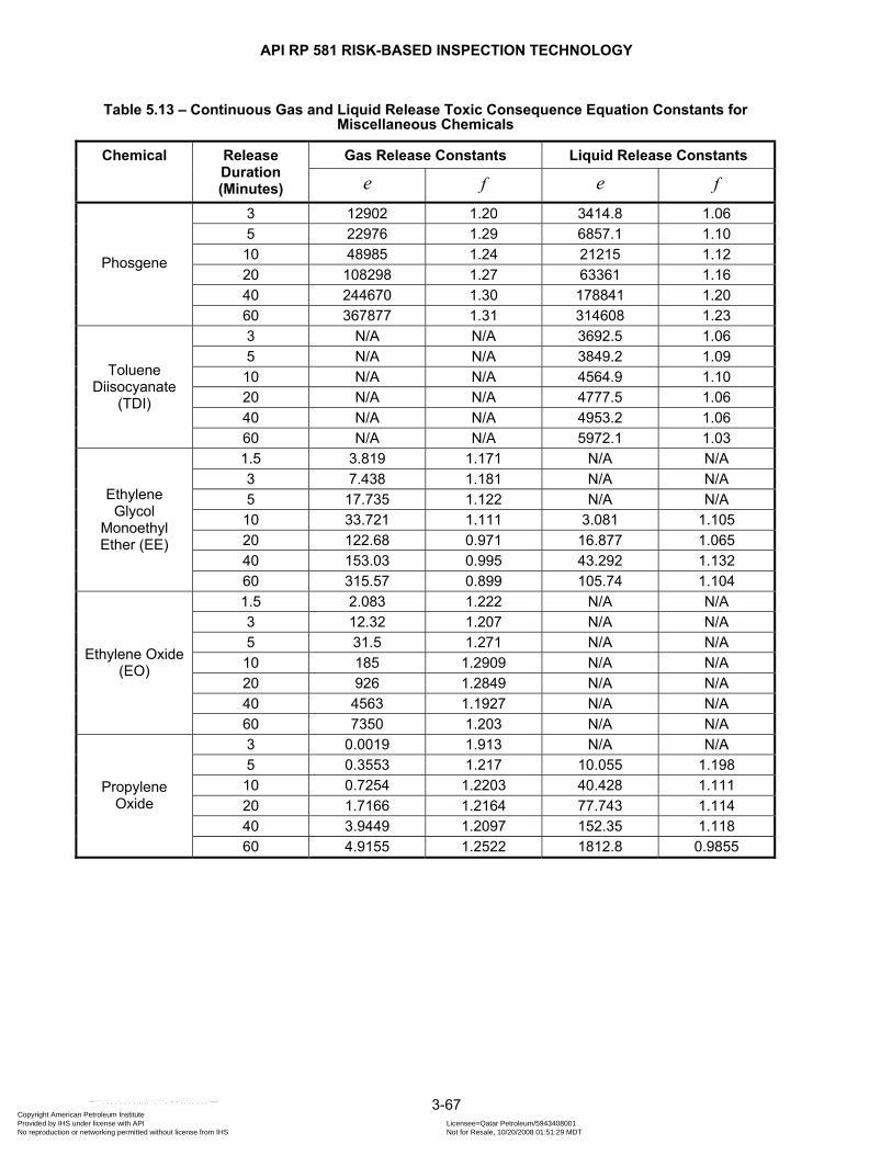
API RP 581 RISK-BASED INSPECTION TECHNOLOGY
3-67
Table 5.13 – Continuous Gas and Liquid Release Toxic Consequence Equation Constants for Miscellaneous Chemicals
Gas Release Constants Liquid Release Constants Chemical Release Duration (Minutes) e f e f
3 12902 1.20 3414.8 1.06 5 22976 1.29 6857.1 1.10 10 48985 1.24 21215 1.12 20 108298 1.27 63361 1.16 40 244670 1.30 178841 1.20
Phosgene
60 367877 1.31 314608 1.23 3 N/A N/A 3692.5 1.06 5 N/A N/A 3849.2 1.09 10 N/A N/A 4564.9 1.10 20 N/A N/A 4777.5 1.06 40 N/A N/A 4953.2 1.06
Toluene Diisocyanate
(TDI)
60 N/A N/A 5972.1 1.03 1.5 3.819 1.171 N/A N/A 3 7.438 1.181 N/A N/A 5 17.735 1.122 N/A N/A 10 33.721 1.111 3.081 1.105 20 122.68 0.971 16.877 1.065 40 153.03 0.995 43.292 1.132
Ethylene Glycol
Monoethyl Ether (EE)
60 315.57 0.899 105.74 1.104 1.5 2.083 1.222 N/A N/A 3 12.32 1.207 N/A N/A 5 31.5 1.271 N/A N/A 10 185 1.2909 N/A N/A 20 926 1.2849 N/A N/A 40 4563 1.1927 N/A N/A
Ethylene Oxide (EO)
60 7350 1.203 N/A N/A 3 0.0019 1.913 N/A N/A 5 0.3553 1.217 10.055 1.198 10 0.7254 1.2203 40.428 1.111 20 1.7166 1.2164 77.743 1.114 40 3.9449 1.2097 152.35 1.118
Propylene Oxide
60 4.9155 1.2522 1812.8 0.9855
Copyright American Petroleum Institute Provided by IHS under license with API Licensee=Qatar Petroleum/5943408001
Not for Resale, 10/20/2008 01:51:29 MDTNo reproduction or networking permitted without license from IHS
--```,`,,`,`,,`,`,,,,,,``,```,`-`-`,,`,,`,`,,`---
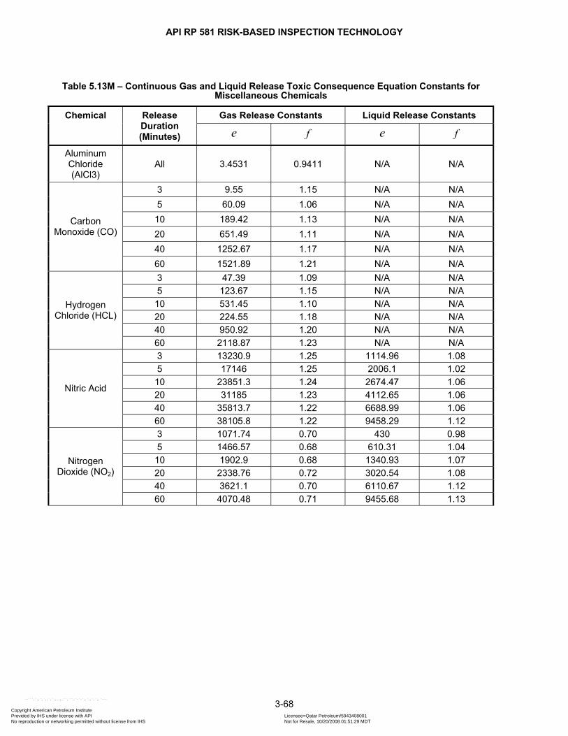
API RP 581 RISK-BASED INSPECTION TECHNOLOGY
3-68
Table 5.13M – Continuous Gas and Liquid Release Toxic Consequence Equation Constants for Miscellaneous Chemicals
Gas Release Constants Liquid Release Constants Chemical Release Duration (Minutes) e f e f
Aluminum Chloride (AlCl3)
All 3.4531 0.9411 N/A N/A
3 9.55 1.15 N/A N/A 5 60.09 1.06 N/A N/A 10 189.42 1.13 N/A N/A 20 651.49 1.11 N/A N/A 40 1252.67 1.17 N/A N/A
Carbon Monoxide (CO)
60 1521.89 1.21 N/A N/A 3 47.39 1.09 N/A N/A 5 123.67 1.15 N/A N/A 10 531.45 1.10 N/A N/A 20 224.55 1.18 N/A N/A 40 950.92 1.20 N/A N/A
Hydrogen Chloride (HCL)
60 2118.87 1.23 N/A N/A 3 13230.9 1.25 1114.96 1.08 5 17146 1.25 2006.1 1.02 10 23851.3 1.24 2674.47 1.06 20 31185 1.23 4112.65 1.06 40 35813.7 1.22 6688.99 1.06
Nitric Acid
60 38105.8 1.22 9458.29 1.12 3 1071.74 0.70 430 0.98 5 1466.57 0.68 610.31 1.04 10 1902.9 0.68 1340.93 1.07 20 2338.76 0.72 3020.54 1.08 40 3621.1 0.70 6110.67 1.12
Nitrogen Dioxide (NO2)
60 4070.48 0.71 9455.68 1.13
Copyright American Petroleum Institute Provided by IHS under license with API Licensee=Qatar Petroleum/5943408001
Not for Resale, 10/20/2008 01:51:29 MDTNo reproduction or networking permitted without license from IHS
--```,`,,`,`,,`,`,,,,,,``,```,`-`-`,,`,,`,`,,`---

API RP 581 RISK-BASED INSPECTION TECHNOLOGY
3-69
Table 5.13M – Continuous Gas and Liquid Release Toxic Consequence Equation Constants for Miscellaneous Chemicals
Gas Release Constants Liquid Release Constants Chemical Release Duration (Minutes) e f e f
3 3095.33 1.20 733.39 1.06 5 5918.49 1.29 1520.02 1.10 10 12129.3 1.24 4777.72 1.12 20 27459.6 1.27 14727.5 1.16 40 63526.4 1.30 42905 1.20
Phosgene
60 96274.2 1.31 77287.7 1.23 3 N/A N/A 793.04 1.06 5 N/A N/A 846.54 1.09 10 N/A N/A 1011.9 1.10 20 N/A N/A 1026.06 1.06 40 N/A N/A 1063.8 1.06
Toluene Diisocyanate
(TDI)
60 N/A N/A 1252.57 1.03 1.5 0.8954 1.171 N/A N/A 3 1.7578 1.181 N/A N/A 5 4.0002 1.122 N/A N/A 10 7.5400 1.111 0.6857 1.105 20 24.56 0.971 3.6389 1.065 40 31.22 0.995 9.8422 1.132
Ethylene Glycol
Monoethyl Ether (EE)
60 59.67 0.899 23.513 1.104 1.5 0.5085 1.222 N/A N/A 3 2.9720 1.207 N/A N/A 5 7.9931 1.271 N/A N/A 10 47.69 1.2909 N/A N/A 20 237.57 1.2849 N/A N/A 40 1088.4 1.1927 N/A N/A
Ethylene Oxide (EO)
60 1767.5 1.203 N/A N/A 3 0.0008 1.913 N/A N/A 5 0.0864 1.217 2.4084 1.198 10 0.1768 1.2203 9.0397 1.111 20 0.4172 1.2164 17.425 1.114 40 0.9537 1.2097 34.255 1.118
Propylene Oxide
60 1.2289 1.2522 367.06 0.9855
Copyright American Petroleum Institute Provided by IHS under license with API Licensee=Qatar Petroleum/5943408001
Not for Resale, 10/20/2008 01:51:29 MDTNo reproduction or networking permitted without license from IHS
--```,`,,`,`,,`,`,,,,,,``,```,`-`-`,,`,,`,`,,`---
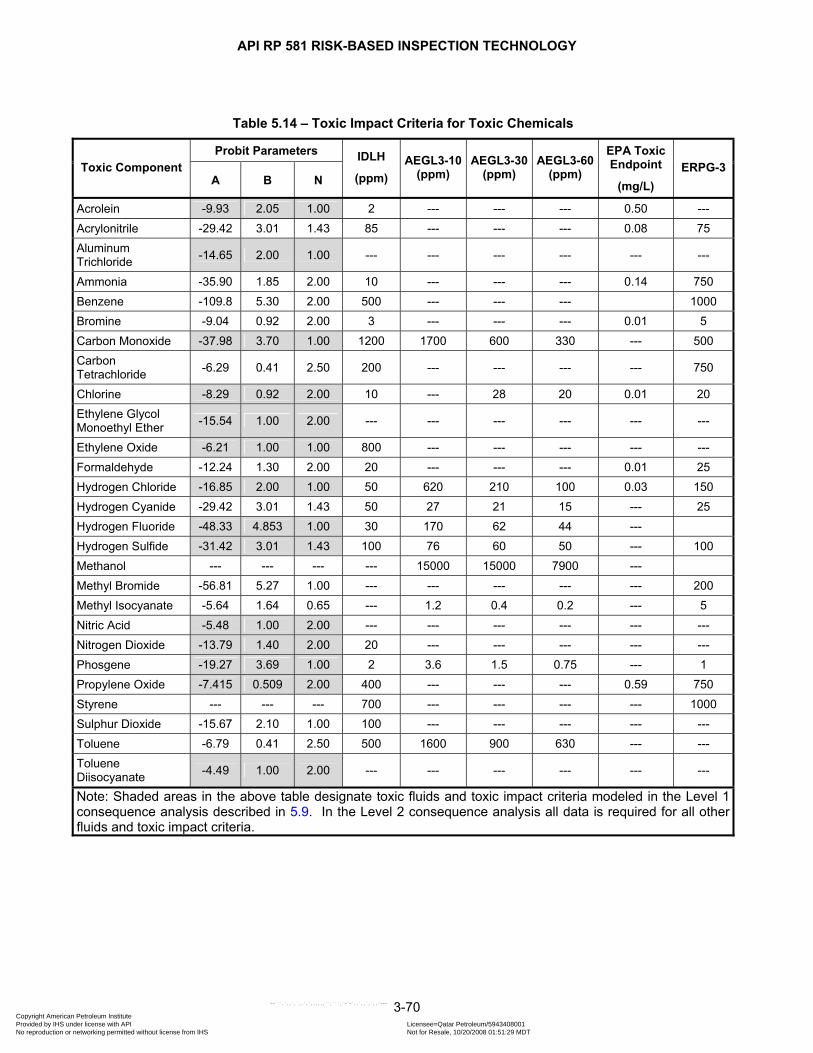
API RP 581 RISK-BASED INSPECTION TECHNOLOGY
3-70
Table 5.14 – Toxic Impact Criteria for Toxic Chemicals
Probit Parameters Toxic Component
A B N
IDLH
(ppm) AEGL3-10
(ppm) AEGL3-30
(ppm) AEGL3-60
(ppm)
EPA Toxic Endpoint
(mg/L) ERPG-3
Acrolein -9.93 2.05 1.00 2 --- --- --- 0.50 --- Acrylonitrile -29.42 3.01 1.43 85 --- --- --- 0.08 75 Aluminum Trichloride -14.65 2.00 1.00 --- --- --- --- --- ---
Ammonia -35.90 1.85 2.00 10 --- --- --- 0.14 750 Benzene -109.8 5.30 2.00 500 --- --- --- 1000 Bromine -9.04 0.92 2.00 3 --- --- --- 0.01 5 Carbon Monoxide -37.98 3.70 1.00 1200 1700 600 330 --- 500 Carbon Tetrachloride -6.29 0.41 2.50 200 --- --- --- --- 750
Chlorine -8.29 0.92 2.00 10 --- 28 20 0.01 20 Ethylene Glycol Monoethyl Ether -15.54 1.00 2.00 --- --- --- --- --- ---
Ethylene Oxide -6.21 1.00 1.00 800 --- --- --- --- --- Formaldehyde -12.24 1.30 2.00 20 --- --- --- 0.01 25 Hydrogen Chloride -16.85 2.00 1.00 50 620 210 100 0.03 150 Hydrogen Cyanide -29.42 3.01 1.43 50 27 21 15 --- 25 Hydrogen Fluoride -48.33 4.853 1.00 30 170 62 44 --- Hydrogen Sulfide -31.42 3.01 1.43 100 76 60 50 --- 100 Methanol --- --- --- --- 15000 15000 7900 --- Methyl Bromide -56.81 5.27 1.00 --- --- --- --- --- 200 Methyl Isocyanate -5.64 1.64 0.65 --- 1.2 0.4 0.2 --- 5 Nitric Acid -5.48 1.00 2.00 --- --- --- --- --- --- Nitrogen Dioxide -13.79 1.40 2.00 20 --- --- --- --- --- Phosgene -19.27 3.69 1.00 2 3.6 1.5 0.75 --- 1 Propylene Oxide -7.415 0.509 2.00 400 --- --- --- 0.59 750 Styrene --- --- --- 700 --- --- --- --- 1000 Sulphur Dioxide -15.67 2.10 1.00 100 --- --- --- --- --- Toluene -6.79 0.41 2.50 500 1600 900 630 --- --- Toluene Diisocyanate -4.49 1.00 2.00 --- --- --- --- --- ---
Note: Shaded areas in the above table designate toxic fluids and toxic impact criteria modeled in the Level 1 consequence analysis described in 5.9. In the Level 2 consequence analysis all data is required for all other fluids and toxic impact criteria.
Copyright American Petroleum Institute Provided by IHS under license with API Licensee=Qatar Petroleum/5943408001
Not for Resale, 10/20/2008 01:51:29 MDTNo reproduction or networking permitted without license from IHS
--```,`,,`,`,,`,`,,,,,,``,```,`-`-`,,`,,`,`,,`---
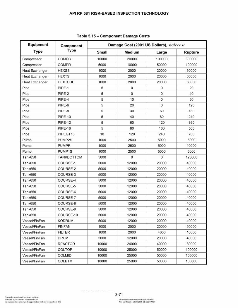
API RP 581 RISK-BASED INSPECTION TECHNOLOGY
3-71
Table 5.15 – Component Damage Costs
Damage Cost (2001 US Dollars), holecost Equipment
Type Component
Type Small Medium Large Rupture Compressor COMPC 10000 20000 100000 300000 Compressor COMPR 5000 10000 50000 100000 Heat Exchanger HEXSS 1000 2000 20000 60000 Heat Exchanger HEXTS 1000 2000 20000 60000 Heat Exchanger HEXTUBE 1000 2000 20000 60000 Pipe PIPE-1 5 0 0 20 Pipe PIPE-2 5 0 0 40 Pipe PIPE-4 5 10 0 60 Pipe PIPE-6 5 20 0 120 Pipe PIPE-8 5 30 60 180 Pipe PIPE-10 5 40 80 240 Pipe PIPE-12 5 60 120 360 Pipe PIPE-16 5 80 160 500 Pipe PIPEGT16 10 120 240 700 Pump PUMP2S 1000 2500 5000 5000 Pump PUMPR 1000 2500 5000 10000 Pump PUMP1S 1000 2500 5000 5000 Tank650 TANKBOTTOM 5000 0 0 120000 Tank650 COURSE-1 5000 12000 20000 40000 Tank650 COURSE-2 5000 12000 20000 40000 Tank650 COURSE-3 5000 12000 20000 40000 Tank650 COURSE-4 5000 12000 20000 40000 Tank650 COURSE-5 5000 12000 20000 40000 Tank650 COURSE-6 5000 12000 20000 40000 Tank650 COURSE-7 5000 12000 20000 40000 Tank650 COURSE-8 5000 12000 20000 40000 Tank650 COURSE-9 5000 12000 20000 40000 Tank650 COURSE-10 5000 12000 20000 40000 Vessel/FinFan KODRUM 5000 12000 20000 40000 Vessel/FinFan FINFAN 1000 2000 20000 60000 Vessel/FinFan FILTER 1000 2000 4000 10000 Vessel/FinFan DRUM 5000 12000 20000 40000 Vessel/FinFan REACTOR 10000 24000 40000 80000 Vessel/FinFan COLTOP 10000 25000 50000 100000 Vessel/FinFan COLMID 10000 25000 50000 100000 Vessel/FinFan COLBTM 10000 25000 50000 100000
Copyright American Petroleum Institute Provided by IHS under license with API Licensee=Qatar Petroleum/5943408001
Not for Resale, 10/20/2008 01:51:29 MDTNo reproduction or networking permitted without license from IHS
--```,`,,`,`,,`,`,,,,,,``,```,`-`-`,,`,,`,`,,`---

API RP 581 RISK-BASED INSPECTION TECHNOLOGY
3-72
Table 5.16 – Material Cost Factors
Material Cost Factor, matcost
Material Cost Factor, matcost
Carbon Steel 1.0 90/10 Cu/Ni 6.8 1.25Cr-0.5Mo 1.3 Clad Alloy 600 7.0 2.25Cr-1Mo 1.7 CS “Teflon” Lined 7.8 5Cr-0.5Mo 1.7 Clad Nickel 8.0 7Cr-0.5Mo 2.0 Alloy 800 8.4
Clad 304 SS 2.1 70/30 Cu/Ni 8.5 Polypropylene Lined (pp) 2.5 904L 8.8
9Cr-1Mo 2.6 Alloy 20 11 405 SS 2.8 Alloy 400 15 410 SS 2.8 Alloy 600 15 304 SS 3.2 Nickel 18
Clad 316 SS 3.3 Alloy 625 26 CS “Saran” Lined 3.4 Titanium 28 CS Rubber Lined 4.4 Alloy “C” 29
316 SS 4.8 Zirconium 34 CS Glass Lined 5.8 Alloy “B” 36 Clad Alloy 400 6.4 Tantalum 535
Copyright American Petroleum Institute Provided by IHS under license with API Licensee=Qatar Petroleum/5943408001
Not for Resale, 10/20/2008 01:51:29 MDTNo reproduction or networking permitted without license from IHS
--```,`,,`,`,,`,`,,,,,,``,```,`-`-`,,`,,`,`,,`---
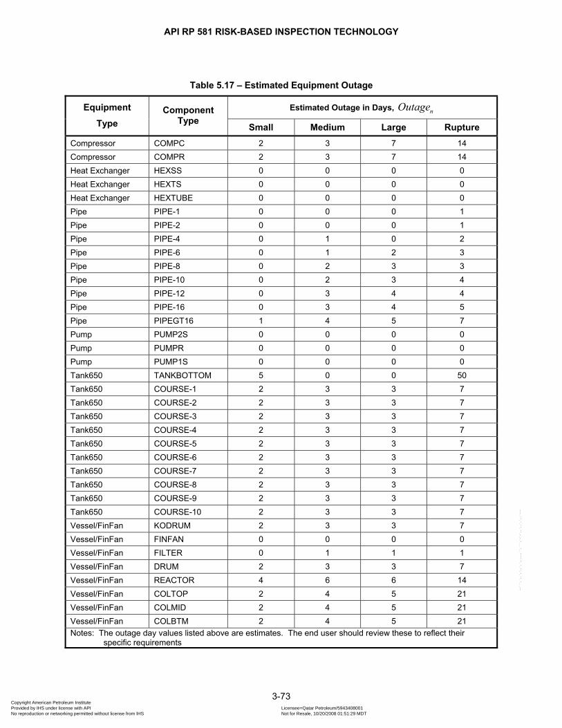
API RP 581 RISK-BASED INSPECTION TECHNOLOGY
3-73
Table 5.17 – Estimated Equipment Outage
Estimated Outage in Days, nOutage Equipment
Type Component
Type Small Medium Large Rupture
Compressor COMPC 2 3 7 14 Compressor COMPR 2 3 7 14 Heat Exchanger HEXSS 0 0 0 0 Heat Exchanger HEXTS 0 0 0 0 Heat Exchanger HEXTUBE 0 0 0 0 Pipe PIPE-1 0 0 0 1 Pipe PIPE-2 0 0 0 1 Pipe PIPE-4 0 1 0 2 Pipe PIPE-6 0 1 2 3 Pipe PIPE-8 0 2 3 3 Pipe PIPE-10 0 2 3 4 Pipe PIPE-12 0 3 4 4 Pipe PIPE-16 0 3 4 5 Pipe PIPEGT16 1 4 5 7 Pump PUMP2S 0 0 0 0 Pump PUMPR 0 0 0 0 Pump PUMP1S 0 0 0 0 Tank650 TANKBOTTOM 5 0 0 50 Tank650 COURSE-1 2 3 3 7 Tank650 COURSE-2 2 3 3 7 Tank650 COURSE-3 2 3 3 7 Tank650 COURSE-4 2 3 3 7 Tank650 COURSE-5 2 3 3 7 Tank650 COURSE-6 2 3 3 7 Tank650 COURSE-7 2 3 3 7 Tank650 COURSE-8 2 3 3 7 Tank650 COURSE-9 2 3 3 7 Tank650 COURSE-10 2 3 3 7 Vessel/FinFan KODRUM 2 3 3 7 Vessel/FinFan FINFAN 0 0 0 0 Vessel/FinFan FILTER 0 1 1 1 Vessel/FinFan DRUM 2 3 3 7 Vessel/FinFan REACTOR 4 6 6 14 Vessel/FinFan COLTOP 2 4 5 21 Vessel/FinFan COLMID 2 4 5 21 Vessel/FinFan COLBTM 2 4 5 21 Notes: The outage day values listed above are estimates. The end user should review these to reflect their
specific requirements
Copyright American Petroleum Institute Provided by IHS under license with API Licensee=Qatar Petroleum/5943408001
Not for Resale, 10/20/2008 01:51:29 MDTNo reproduction or networking permitted without license from IHS
--```,`,,`,`,,`,`,,,,,,``,```,`-`-`,,`,,`,`,,`---

API RP 581 RISK-BASED INSPECTION TECHNOLOGY
3-74
Table 5.18 – Fluid Leak Properties
Fluid Molecular Weight
Density
(lb/ft3)
NBP
(oF)
Fraction Evaporated in 24 Hours (Note 1)
evapfract
C1-C2 23 15.639 -193 1.00
C3-C5 58 36.209 31 1.00
C6-C8 100 42.702 210 0.90
C9-C12 149 45.823 364 0.50
C13-C16 205 47.728 502 0.10
C17-C25 280 48.383 651 0.05
C25+ 422 56.187 981 0.02
Acid 18 62.3 212 0.90
H2 2 4.433 -423 1.00
H2S 34 61.993 -75 1.00
HF 20 60.37 68 1.00
CO 28 50 -312 1.00
DEE 74 45 95 1.00
HCL 36 74 -121 1.00
Nitric Acid 63 95 250 0.80
NO2 90 58 275 0.75
Phosgene 99 86 181 1.00
TDI 174 76 484 0.15
Methanol 32 50 149 1.00
PO 58 52 93 1.00
Styrene 104 42.7 293 0.60
EEA 132 61 313 0.65
EE 90 58 275 0.75
EG 62 69 387 0.45
EO 44 55 51 1.00
Note 1: Estimated values.
Copyright American Petroleum Institute Provided by IHS under license with API Licensee=Qatar Petroleum/5943408001
Not for Resale, 10/20/2008 01:51:29 MDTNo reproduction or networking permitted without license from IHS
--```,`,,`,`,,`,`,,,,,,``,```,`-`-`,,`,,`,`,,`---
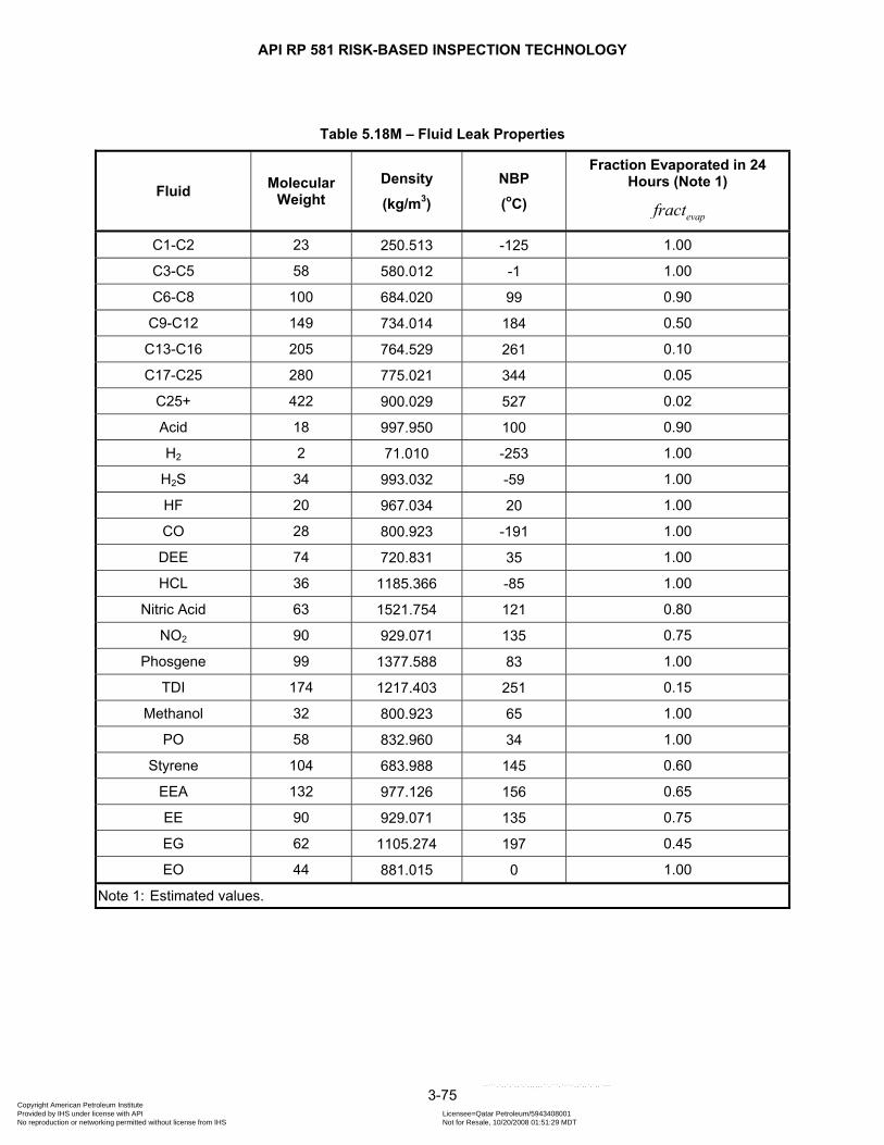
API RP 581 RISK-BASED INSPECTION TECHNOLOGY
3-75
Table 5.18M – Fluid Leak Properties
Fluid Molecular Weight
Density
(kg/m3)
NBP
(oC)
Fraction Evaporated in 24 Hours (Note 1)
evapfract
C1-C2 23 250.513 -125 1.00
C3-C5 58 580.012 -1 1.00
C6-C8 100 684.020 99 0.90
C9-C12 149 734.014 184 0.50
C13-C16 205 764.529 261 0.10
C17-C25 280 775.021 344 0.05
C25+ 422 900.029 527 0.02
Acid 18 997.950 100 0.90
H2 2 71.010 -253 1.00
H2S 34 993.032 -59 1.00
HF 20 967.034 20 1.00
CO 28 800.923 -191 1.00
DEE 74 720.831 35 1.00
HCL 36 1185.366 -85 1.00
Nitric Acid 63 1521.754 121 0.80
NO2 90 929.071 135 0.75
Phosgene 99 1377.588 83 1.00
TDI 174 1217.403 251 0.15
Methanol 32 800.923 65 1.00
PO 58 832.960 34 1.00
Styrene 104 683.988 145 0.60
EEA 132 977.126 156 0.65
EE 90 929.071 135 0.75
EG 62 1105.274 197 0.45
EO 44 881.015 0 1.00
Note 1: Estimated values.
Copyright American Petroleum Institute Provided by IHS under license with API Licensee=Qatar Petroleum/5943408001
Not for Resale, 10/20/2008 01:51:29 MDTNo reproduction or networking permitted without license from IHS
--```,`,,`,`,,`,`,,,,,,``,```,`-`-`,,`,,`,`,,`---
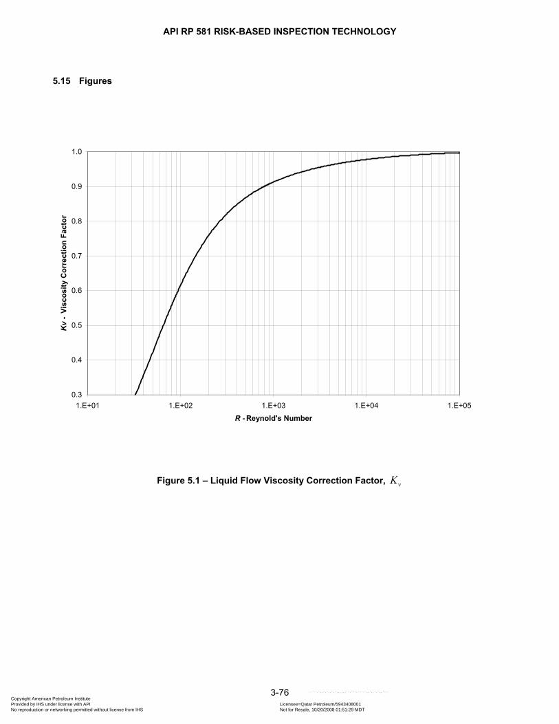
API RP 581 RISK-BASED INSPECTION TECHNOLOGY
3-76
5.15 Figures
0.3
0.4
0.5
0.6
0.7
0.8
0.9
1.0
1.E+01 1.E+02 1.E+03 1.E+04 1.E+05
R - Reynold's Number
Kv
- Vi
scos
ity C
orre
ctio
n Fa
ctor
Figure 5.1 – Liquid Flow Viscosity Correction Factor, vK
Copyright American Petroleum Institute Provided by IHS under license with API Licensee=Qatar Petroleum/5943408001
Not for Resale, 10/20/2008 01:51:29 MDTNo reproduction or networking permitted without license from IHS
--```,`,,`,`,,`,`,,,,,,``,```,`-`-`,,`,,`,`,,`---

API RP 581 RISK-BASED INSPECTION TECHNOLOGY
3-77
Instantaneous-Type Release
Continuous-Type Release
VCE
Flash Fire
Fireball
Fireball
Safe Dispersion
Pool Fire
Safe Dispersion
Late Ignition
Early Ignition
Above AIT
No Ignition
Final State Gas
Final State Liquid
Final State Gas
Final State Liquid
No Ignition
No Ignition
Ignition
Above AIT
Late Ignition
Early Ignition
VCE
Flash Fire
Jet Fire
Jet Fire
Safe Dispersion
Pool Fire
Jet Fire
Safe Dispersion
No Ignition
Ignition
Figure 5.2 – API RBI Level 1 Consequence Analysis Release Event Tree
Copyright American Petroleum Institute Provided by IHS under license with API Licensee=Qatar Petroleum/5943408001
Not for Resale, 10/20/2008 01:51:29 MDTNo reproduction or networking permitted without license from IHS
--```,`,,`,`,,`,`,,,,,,``,```,`-`-`,,`,,`,`,,`---
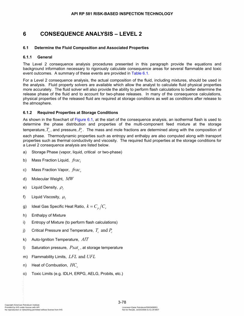
API RP 581 RISK-BASED INSPECTION TECHNOLOGY
3-78
6 CONSEQUENCE ANALYSIS – LEVEL 2
6.1 Determine the Fluid Composition and Associated Properties
6.1.1 General
The Level 2 consequence analysis procedures presented in this paragraph provide the equations and background information necessary to rigorously calculate consequence areas for several flammable and toxic event outcomes. A summary of these events are provided in Table 6.1.
For a Level 2 consequence analysis, the actual composition of the fluid, including mixtures, should be used in the analysis. Fluid property solvers are available which allow the analyst to calculate fluid physical properties more accurately. The fluid solver will also provide the ability to perform flash calculations to better determine the release phase of the fluid and to account for two-phase releases. In many of the consequence calculations, physical properties of the released fluid are required at storage conditions as well as conditions after release to the atmosphere.
6.1.2 Required Properties at Storage Conditions
As shown in the flowchart of Figure 6.1, at the start of the consequence analysis, an isothermal flash is used to determine the phase distribution and properties of the multi-component feed mixture at the storage temperature, sT , and pressure, sP . The mass and mole fractions are determined along with the composition of each phase. Thermodynamic properties such as entropy and enthalpy are also computed along with transport properties such as thermal conductivity and viscosity. The required fluid properties at the storage conditions for a Level 2 consequence analysis are listed below.
a) Storage Phase (vapor, liquid, critical or two-phase)
b) Mass Fraction Liquid, lfrac
c) Mass Fraction Vapor, vfrac
d) Molecular Weight, MW
e) Liquid Density, lρ
f) Liquid Viscosity, lµ
g) Ideal Gas Specific Heat Ratio, p vk C C=
h) Enthalpy of Mixture
i) Entropy of Mixture (to perform flash calculations)
j) Critical Pressure and Temperature, and c cT P
k) Auto-Ignition Temperature, AIT
l) Saturation pressure, sPsat , at storage temperature
m) Flammability Limits, and LFL UFL
n) Heat of Combustion, sHC
o) Toxic Limits (e.g. IDLH, ERPG, AELG, Probits, etc.)
Copyright American Petroleum Institute Provided by IHS under license with API Licensee=Qatar Petroleum/5943408001
Not for Resale, 10/20/2008 01:51:29 MDTNo reproduction or networking permitted without license from IHS
--```,`,,`,`,,`,`,,,,,,``,```,`-`-`,,`,,`,`,,`---
API RP 581 RISK-BASED INSPECTION TECHNOLOGY
3-79
6.1.3 Required Properties at Flashed Conditions
This is followed by an isentropic flash calculation (requiring the entropy to remain equal to its value computed at the storage conditions) to atmospheric pressure, atmP , that simulates the release of the fluid from a leaking or
ruptured storage container. The resulting flash temperature, fT , is determined along with the phase distribution and properties of each phase at these conditions. The released mixture can either be a single-phase liquid, a single-phase vapor or a two-phase mixture of both as shown in Figure 6.1. The required fluid properties at the flashed conditions for a Level 2 consequence analysis are listed below.
a) Flashed Phase (vapor, liquid, or two-phase)
b) Flash Temperature, fT
c) Flash Fraction, fshfrac
d) Density of the liquid, lρ
e) Density of the vapor, vρ
f) Specific Heat of the Liquid, lCp
g) Heat of Combustion of Liquid, lHC
h) Heat of Combustion of Vapor, vHC
i) Latent Heat of Vaporization of Liquid, vH∆
j) Bubble Pont Temperature of Liquid, bT
k) Dew Point Temperature of Vapors, dT
As shown in Figure 6.1, where a fluid is flashed to a single-phase liquid, a bubble-point temperature calculation is performed at atmospheric pressure to find the temperature, bT , at which vapor bubbles first appear. Similarly, in the single-phase vapor case, a dew-point calculation is performed at atmospheric pressure to find the temperature, dT , at which liquid drops first start condensing.
For fluids that flash to two-phase, flash calculations at both the bubble point and the dew point of the flashed mixture, may be required depending on the composition of the fluid.
a) For pure fluids or binary mixtures, (two components in mixture), additional calculations are not necessary because in these cases the bubble-point and dew-point temperatures are the same and equal to the isentropic flash temperature, i.e. b d fT T T= = .
b) For multi-component mixtures, both the bubble point and the dew point calculations are required.
6.1.4 Calculation Procedure
a) STEP 1.1 – Obtain the stored fluid composition. For mixtures, concentrate on the major components within the fluid mixture and attempt to get at least 90% of the mixture identified and quantified. A more detailed breakdown of the composition is not warranted, unless there is small quantities of toxic materials that are in the mixture.
Copyright American Petroleum Institute Provided by IHS under license with API Licensee=Qatar Petroleum/5943408001
Not for Resale, 10/20/2008 01:51:29 MDTNo reproduction or networking permitted without license from IHS
--```,`,,`,`,,`,`,,,,,,``,```,`-`-`,,`,,`,`,,`---
API RP 581 RISK-BASED INSPECTION TECHNOLOGY
3-80
b) STEP 1.2. – Using a fluid propery solver, determine the fluid properties as specificed in 6.1.2.a for the fluid at storage conditions. Some of the fluid properties required for the analysis, such as LFL, UFL, Heat of Combustion and toxic limits may require research to determine. The analyst may need to utilize Material Safety Data Sheets (MSDS) or other fluid databases, such as DIPPR, to determine these properties. Mixing rules (e.g. LaChatalier’s mixing principle for LFL and UFL) are available to determine propetires of mixtures but, in general, a mole weighted method may be used as an estimate.
c) STEP 1.3. – Using a fluid property solver, perform an isentropic flash (isenthalpic is acceptable) and deterrmine the flash temperature, fT , the phase of the flashed fluid and the fraction of fluid flashed,
fshfrac .
d) STEP 1.4. – Determine the bubble point or dew point temperature of the flashed fluid, as necessary.
1) For flashed liquid, determine the bubble point temperature, bT , at atmospheric pressure.
2) For flashed vapors, determine the dew point temperature, dT , at atmospheric pressure.
3) For fluids that flash to two-phase, the bubble point temperature, bT , at atmospheric pressure and the
dew point temperature, dT , at atmospheric pressure should be determined. Note that for pure fluids and binary mixtures, no calculation is required since the bubble point temperature and the dew point temperature are equal to the flash temperature, fT , as determined in STEP 1.3.
6.2 Release Hole Size Selection
6.2.1 General
As with the Level 1 approach, a discrete set of release events or release hole sizes are used in the Level 2 consequence analysis. The release hole sizes shown in Table 5.4 are used in the Level 2 consequence analysis.
6.2.2 Calculation Procedure
The step-by-step procedure for selecting the release hole sizes are in accordance with the Level 1 consequence analysis, see paragraph 5.2.2.
6.3 Release Rate Calculation
6.3.1 Source Term Modeling
Quantification of the consequence of a release event requires calculations of the release amount (or rate of release), the duration of the release, and the state (e.g., gas, liquid or two-phase) of the material released. The terminology used for determining these parameters is source term modeling. The source term is used as an input to the various consequence models as well as the cloud dipersion analysis.
6.3.2 Determining the Release Phase
Estimation of the release amount or rate is covered for liquids and vapors (gases) adequately in paragraph 5.3. For calculating the release rate, the release phase must be determined. Note that the release phase is different then the phase of the fluid at storage conditions or the phase of the fluid after flashing to atmosphere as described in paragraphs 6.1.2 and 6.1.3. This is the phase immediately downstream of the release point and is used for selecting the proper equation for calcuating the release rate through the hole or crack opening.
Copyright American Petroleum Institute Provided by IHS under license with API Licensee=Qatar Petroleum/5943408001
Not for Resale, 10/20/2008 01:51:29 MDTNo reproduction or networking permitted without license from IHS
--```,`,,`,`,,`,`,,,,,,``,```,`-`-`,,`,,`,`,,`---

API RP 581 RISK-BASED INSPECTION TECHNOLOGY
3-81
To determine the release phase, the saturation pressure of the stored fluid at the storage temperature, sPsat , must be determined.
if release phase is vapors s atmPsat P P≥ ≥ ⇒ (3.107)
if release phase is two-phases s atmP Psat P≥ > ⇒ (3.108)
if release phase is liquids atm sP P Psat≥ > ⇒ (3.109)
6.3.3 Vapor Release Source
As shown in Equation (3.107), if the saturation pressure of the fluid at storage temperature, sPsat , is greater
than or equal to the storage pressure, sP , the fluid will be stored as a gas or vapor and released as a gas or
vapor. In this case, calculation of the theoretical release rate, nW , can be in accordance with equations (3.6) or (3.7). Most gases will cool as they are depressured through an orifice, so in some cases condensation will occur and liquid rainout needs to be considered as presented in paragraph 6.7.2.
For supercritical fluids (stored above critical pressure or temperature), the release rate can be estimated using Equation (3.6), however, in this case the specific heat ratio, k , should be evaluated at the normal boiling point of the fluid mixture or at standard conditions. This will result in a conservative release rate. More rigorous methods, such as the HEM Omega [5] method can be used to calculate the release rate of a supercritical fluid. In some cases, supercritical fluids will condense upon release, and liquid rainout needs to be considered as presented in paragraph 6.7.2.
6.3.4 Two-Phase Release Source
As shown in Equation (3.108), if the saturation pressure of the fluid at the storage temperature, sPsat , is less
than or equal to the storage pressure, sP , but greater than atmospheric pressure, atmP , the fluid will be stored as a liquid and will be released as a two-phase mixture. In this case, the release rate can be conservatively estimated using the liquid Equation (3.3). Alternatively, a more accurate two-phase flow calculation procedure may be used. For this case, the effect of liquid entrainment in the released jet needs to be considered as well as rainout. Methods for evaluating these effects are presented in paragraph 6.7.2.
6.3.5 Liquid Release Source
Finally, as shown in Equation (3.109), if the saturation pressure of the fluid at the storage temperature, sPsat , is
less than atmospheric pressure, atmP , the fluid will be stored as a liquid and will be released as a liquid. In this case, the release rate can be determined using Equation (3.3).
6.3.6 Calculation Procedure
a) STEP 3.1 – Determine the stored fluid’s saturation pressure, sPsat , at the storage temperature.
b) STEP 3.2 – Determine the release phase using Equations (3.107), (3.108), or (3.109).
c) STEP 3.3 – For each release hole size selected in STEP 2.1, compute the release hole size area, nA ,
using Equation (3.8) based on nd .
d) STEP 3.4 – For each release hole size, calculate the release rate, nW , for each release area, nA , determined in STEP 3.3.
1) For liquid releases, use Equation (3.3).
Copyright American Petroleum Institute Provided by IHS under license with API Licensee=Qatar Petroleum/5943408001
Not for Resale, 10/20/2008 01:51:29 MDTNo reproduction or networking permitted without license from IHS
--```,`,,`,`,,`,`,,,,,,``,```,`-`-`,,`,,`,`,,`---
API RP 581 RISK-BASED INSPECTION TECHNOLOGY
3-82
2) For vapor releases, use Equations (3.6) or (3.7), as applicable.
3) For two-phase releases, use Equation (3.3), for a conservative approximation. As an alternative, a two-phase method, such as the HEM Omega method [5], may be utilized.
6.4 Estimate the Fluid Inventory Available for Release
6.4.1 General
The total amount of fluid inventory available for release is estimated in accordance with the Level 1 consequence analysis, see paragraph 5.4.
6.4.2 Calculation Procedure
The step-by-step procedure for estimated the available fluid inventory mass is in accordance with paragraph 5.4.3.
6.5 Determine Release Type
6.5.1 General
The type of release is established in accordance with the Level 1 consequence analysis, see paragraph 5.5.
6.5.2 Calculation Procedure
The step-by-step procedure for determining if the release is classified ans continuous or instantaneous is in accordance with paragraph 5.5.2.
6.6 Estimate the Impact of Detection and Isolation Systems on Release Magnitude
6.6.1 General
The effects of detection and isolation systems are established in accordance with the Level 1 consequence analysis, see paragraph 5.6.
6.6.2 Calculation Procedure
The step-by-step procedure for estimating the impact of detection and isolation systems is in accordance with paragraph 5.6.6.
6.7 Determine the Release Rate and Mass for Consequence Analysis
6.7.1 General
Unlike the Level 1 analysis, the Level 2 analysis takes into account two-phase releases and distinguishes between the amount of the theoretical release rate that releases to the atmosphere as vapor or as an aerosol (vapor with entrained liquid) in the form of a jet and the amount of the release that drops to the ground as liquid to form a pool.
6.7.2 Aerosol and Rainout Modeling
When a release is two-phase, there is an amount of liquid entrained in the jet (vapor) portion of the release (aerosol). The remaining liquid portion of the release, or rainout, can be estimated by the following correlation recommended by Kletz [6].
1 2 0.5ro fsh fshfrac frac for frac= − ⋅ < (3.110)
Copyright American Petroleum Institute Provided by IHS under license with API Licensee=Qatar Petroleum/5943408001
Not for Resale, 10/20/2008 01:51:29 MDTNo reproduction or networking permitted without license from IHS
--```,`,,`,`,,`,`,,,,,,``,```,`-`-`,,`,,`,`,,`---

API RP 581 RISK-BASED INSPECTION TECHNOLOGY
3-83
0.0 0.5ro fshfrac for frac= ≥ (3.111)
Other liquid rainout correlations are available from CCPS [7], Davenport [8], Prugh [9] and Mudan [10].
The fraction that flashes, fshfrac , as it is released to the atmosphere can be determined using fluid property software by isentropically (isenthalpically is acceptable) expanding the release fluid from the storage conditions to the atmospheric conditions.
6.7.3 Calculation of Jet Release Rate and Pool Release Rate
Once the release rate is determined and the rainout fraction is estimated, the release rate for modeling pool type consequences, pool
nW , and for modeling jet type consequences, jetnW , can be determined as follows:
pooln n roW rate frac= ⋅ (3.112)
( )1jetn n roW rate frac= − (3.113)
Note that the jet release rate may include entrained liquid. To calculate the mass fraction of liquid entrained in the jet, use Equation (3.114).
( )( )1
l fshentl
ro
frac fracfrac
frac⋅
=−
(3.114)
6.7.4 Vapor Sources from Boiling or Non-Boiling Pools
6.7.4.1 General
Vapors evaporating off of the surface of liquid pools, if not ignited immediately can be the source of vapor clouds that could result in flash fires or vapor cloud explosions. Quantifying these vapor rates are necessary when determining the impact of thse event outcomes. The vapor source rate is dependent on whether the pool is a boiling or a non-boiling pool. The bubble-point temperature bT of the liquid is required to determine the type of analysis to be used for liquid pools on the ground.
6.7.4.2 Boiling Liquid Pools
If b gT T< , where gT is the ground temperature, then we have the boiling liquid pool case. The temperature of
the liquid will remain at its boiling-point temperature bT (at least near the liquid-vapor interface) while vapor will be rapidly evaporating at a rate that is only limited by how fast heat energy can be supplied to the liquid-vapor interface. The partial pressure of the vapor right above the liquid pool will be equal to the atmospheric pressure.
The vapor rate generated off of the surface of a boiling pool, berate , can be estimated using Equation (3.115) as provided by Shaw and Briscoe [11].
( ) ( )0.51.5, ,
14
2surf surf g bn p n p n
v surf
X k T Terate g V t
C Hπ
π α
⎡ ⎤⋅ ⋅ −⎢ ⎥= ⋅ ⋅
⋅∆ ⋅⎢ ⎥⎣ ⎦ (3.115)
The surface interaction parameters, surfX , surfk and surfα in the above equation account for the liquid interaction with the surface on which the pool forms. These can be obtained from Table 6.2 repeated from Cremer and Warner [12].
Copyright American Petroleum Institute Provided by IHS under license with API Licensee=Qatar Petroleum/5943408001
Not for Resale, 10/20/2008 01:51:29 MDTNo reproduction or networking permitted without license from IHS
--```,`,,`,`,,`,`,,,,,,``,```,`-`-`,,`,,`,`,,`---
API RP 581 RISK-BASED INSPECTION TECHNOLOGY
3-84
The size of the boiling pool reaches a steady state, when the evaporation rate, berate , is equal to the pool
release rate, poolnW as discussed in paragraph 6.7.3. At this point the radius of the evaporating pool can be
determined using Equation (3.116) as provided by Shaw and Briscoe [11].
.25
, 0.75, ,
823
p np n p n
g Vr t
π⎛ ⎞⋅
= ⎜ ⎟⎜ ⎟⎝ ⎠
(3.116)
6.7.4.3 Non-Boiling Liquid Pools
If b gT T> , then we have the case of a non-boiling (evaporating) liquid pool, where the liquid temperature will be nearly equal to the ground temperature (after some initial transient period), and the vapor pressure right above the pool will be less than atmospheric pressure and equal to the bubble-point pressure, ,b gP , corresponding to
the ground temperature. Thus, an additional thermodynamic calculation is required to determine ,b gP . The evaporation rate in this case is primarily limited by how fast the newly-generated vapor can be carried away from the interface by diffusion or convection.
The vapor rate generated off of the surface of a non-boiling pool, nberate , can be estimated using Equation (3.117) as provided by Shaw and Briscoe [11].
, 0.78 1.8915 ,
b gn w p n
s
P MWerate C u r
RT⋅⎛ ⎞
= ⋅ ⋅⎜ ⎟⎝ ⎠
(3.117)
The size of the non-boiling pool reaches a steady state, when the evaporation rate, ,b nerate , is equal to the pool
release rate, poolnW as discussed in paragraph 6.7.3.
6.7.5 Cloud Dispersion Modeling
The ability to perform cloud dispersion analysis is a key component to performing the Level 2 consequence analyses. Modeling a release depends on the source term conditions, the atmospheric conditions, the release surroundings, and the hazard being evaluated. Employment of many commercially available models, including SLAB, account for these important factors and will produce the desired data for the Level 2 RBI assessments [13]. Annex 3.A provides background on performing these studies and provides some guidance on available software. Additional guidance is provided by Hanna and Drivas [14].
The dispersion analysis is needed to determine several things. For flammable releases, such as flash fires, this will typically entail determination of the portion of the cloud area (area footprint, ft2, at grade) where the air to fuel mixture is between the Lower Flammability Limit (LFL) and the Upper Flammability Limit (UFL). For VCEs, the amount of flammable mass in the cloud is required. In this case, the amount of flammable material (lbs) is required and therefore the cloud dispersion model must be able to predict the volumetric portion within the cloud that is above the LFL of the mixture.
For toxic releases, the cloud dispersion model must be able to calculate the concentration (ppm or vol%) of the toxic component of the release throughout the cloud. The portion of the cloud in terms of plant area that has a higher concentration than the relevant toxic impact criteria may then be determined. The toxic criteria may be based on a probit value, EPA toxic endpoint, IDLH, or ERPG.
6.7.6 Calculation Procedure
a) STEP 7.1 – For each release hole size, calculate the adjusted release rate, nrate , using Equation (3.13)
where the theoretical release rate, nW , is from STEP 3.2. Note that the release reduction factor, difact , determined in STEP 6.4 accounts for any detection and isolation systems that are present.
Copyright American Petroleum Institute Provided by IHS under license with API Licensee=Qatar Petroleum/5943408001
Not for Resale, 10/20/2008 01:51:29 MDTNo reproduction or networking permitted without license from IHS
--```,`,,`,`,,`,`,,,,,,``,```,`-`-`,,`,,`,`,,`---
API RP 581 RISK-BASED INSPECTION TECHNOLOGY
3-85
b) STEP 7.2 – For each release hole size, calculate the leak duration, nld , of the release using Equation
(3.15), based on the available mass, ,avail nmass , from STEP 4.6 and the adjusted release rate, nrate , from
STEP 7.1. Note that the leak duration cannot exceed the maximum duration, ,max nld , determined in STEP 6.5.
c) STEP 7.3 – Determine the rainout mass fraction from the released fluid using Equation (3.110) or (3.111), based on the flash fraction calculated in STEP 1.3.
d) STEP 7.4 – For each hole size selected in STEP 2.1, calculate the release rate of liquid that settles to the ground for the pool calculations, pool
nW , using Equation (3.112).
e) STEP 7.5 – For each hole size selected, calculate the release rate of vapor (including entrained liquid remaining in the jet, jet
nW , using Equation (3.113).
f) STEP 7.6 – Calculate the mas fraction of entrained liquid, entlfrac , within the jet portion of the release using Equation (3.114).
g) STEP 7.7 – Determine the vapor source rate and source area for the vapor cloud and flash fire dispersion analysis.
1) For a vapor releases, use the jet release rate, jetnW , established in STEP 7.5.
2) For liquid releases, determine whether the pool is boiling or non-boiling in accordance with paragraph 6.7.4. For boiling pools, calculate the evaporation rate, nerate and the pool radius, ,p nr using
Equations (3.115) and (3.116). For non-boiling pools, calculate the evaporation rate, nerate and the
pool radius, ,p nr using Equation (3.117).
6.8 Determine Flammable and Explosive Consequences
6.8.1 Event Tree Calculations
6.8.1.1 Overview
Event tree analysis determines the probabilities of various outcomes as a result of release of hazardous fluids to the atmosphere. These probabilities are then used to weight the overall consequences of release.
The CCPS [15] defines an event tree as “a graphical logic model that identifies and quantifies possible outcomes following an initiating event. The event tree provides systematic coverage of the time sequence of event propagation, either through a series of protective system actions, normal plant functions, and operator interventions (a preincident application), or where loss of containment has occurred, through the range of consequences possible (a postincident application).”
An overall event tree for the API RBI methodology is presented in Figure 6.2. The consequence analysis portion of API RBI fits within the overall RBI methodology as shown in Figure 6.2. Probabilities of loss of containment ( POL for leakage or POR for Rupture) are a function of the generic failure frequencies for particular pieces of equipment and the calculated damage state (damage factors) of the piece of equipment or component being evaluated. The determination of the probabilities of loss of containment is covered in Part 2 [2] of this document.
The probabilities of loss of containment are then multiplied by the event probabilities as determined from the consequence analysis. Similar to trees employed by the CCPS [15] to evaluate consequences of releases in process units, the event trees presented in Figures 6.2 through 6.4 display the potential outcomes that could occur from the initiating event (a release). The event tree for the leakage cases, which corresponds to the small, medium and large release hole sizes as discussed in paragraph 5.2 is shown in Figure 6.3. The event tree for the rupture case is shown in Figure 6.4.
Copyright American Petroleum Institute Provided by IHS under license with API Licensee=Qatar Petroleum/5943408001
Not for Resale, 10/20/2008 01:51:29 MDTNo reproduction or networking permitted without license from IHS
--```,`,,`,`,,`,`,,,,,,``,```,`-`-`,,`,,`,`,,`---

API RP 581 RISK-BASED INSPECTION TECHNOLOGY
3-86
6.8.1.2 Probability of Ignition Given a Release
For a release of a hazardous fluid, the two main factors that define the event outcome is the probability of ignition and the timing of ignition, in other words, immediate versus delayed ignition. For the Level 1 consequence analysis, the assumption is made that the probability of ignition for a continuous release is constant and is only a function of the material released and whether or not the fluid is at or above its auto-ignition temperature. The probability does not increase as a function of release rate. In general, the lower the molecular weight of the release the higher the probability of ignition. For an instantaneous release, the probability of ignition goes up significantly (The probabilities of ignition for the Level 1 consequence analysis are presented in Annex 3.A). As a result, there is an abrupt change in the Level 1 consequence results between a continuous release and an instantaneous release. An instantaneous release is defined as any release larger than 4,536 kgs [10,000 lbs] in 3 minutes which is equivalent to a release rate of 25.2 kg/s [55.6 lb/s]. A continuous release of 24.5 kg/s would have a much lower consequence than an instantaneous release at 25.2 kg/s of the same material. Therefore, the Level 1 consequence analysis includes a blending of the calculated results of the continuous and instantaneous releases (see paragraph 5.8.7).
A study by Cox, Lee, and Ang in 1990 [16] indicates that the probability that a flammable release will ignite is proportional to the release rate of flammable material. Additional research on probabilities of ignition is provided in [17]. The curve fit for the Cox, Lee and Ang work can be seen as the lowest curves in Figures 6.5. Figures 6.5 and 6.5M apply to liquids and Figures 6.6 and 6.6M apply to vapors.. The additional curves provided in these figures, are extrapolated to match the constant values assumed in the Level 1 consequence analysis provided in Tables A.3.3 through A.3.6 of Annex 3.A. These curves take into consideration release rate and molecular weight. Using these curves eliminates the need to blend results between the continuous and instantaneous results as required in the Level 1 consequence analysis.
For the Level 2 consequence analysis, the mass fraction of flammable fluid in the release fluid mixture, flammfrac , must be known to calculate the release rate of flammable material:
flam flamn nrate rate mfrac= ⋅ (3.118)
The liquid and vapor portions of the flammable release rate are determined using Equations (3.119) and (3.120).
( ), 1flam flaml n n fshrate rate frac= ⋅ − (3.119)
,flam flam
v n n fshrate rate frac= ⋅ (3.120)
As an alternative to using Figures 6.5 and 6.6, the probability of ignition at ambient conditions of a flammable liquid or vapor release may be computed from Equation (3.121) or Equation (3.122), respectively. Since these are a function of release rate, the probabilities of ignition are calculated for each of the release hole sizes selected. Note that when the flammable liquid or vapor release rate, exceeds a rate that would indicate an instantaneous release (4,535.9 kgs [10,000 lbs] release in three minuters or less), a maximum value of 25.22 kg/s [55.6 lb/s] should be used for ,
flaml nrate or ,
flamv nrate in Equations (3.121) and (3.122).
[ ]
[ ][ ] [ ]
4 ,
224 ,
3, 4 ,
3
4 ,
1.00982 0.70372 ln 0.013045 ln
0.18554 ln 0.0014619 ln
0.022131 ln ln 0.016572 ln
0.00011281 ln 0.00050697
flaml n
flaml n
amb flaml n l n
flaml n
MW C rate
MW C rate
poi MW C rate MW
C rate
⎡ ⎤− ⋅ − ⋅ ⋅ +⎣ ⎦
⎡ ⎤⋅ − ⋅ ⋅ +⎣ ⎦
⎡ ⎤= ⋅ ⋅ ⋅ − ⋅ +⎣ ⎦
⎡ ⎤⋅ ⋅ +⎣ ⎦ [ ][ ]
2
4 ,
24 ,
ln ln
0.0035535ln ln
flaml n
flaml n
MW C rate
MW C rate
⎛ ⎞⎜ ⎟⎜ ⎟⎜ ⎟⎜ ⎟⎜ ⎟⎜ ⎟
⎡ ⎤⋅ ⋅ ⋅ −⎜ ⎟⎣ ⎦⎜ ⎟⎜ ⎟⎡ ⎤⋅ ⋅⎣ ⎦⎝ ⎠
(3.121)
Copyright American Petroleum Institute Provided by IHS under license with API Licensee=Qatar Petroleum/5943408001
Not for Resale, 10/20/2008 01:51:29 MDTNo reproduction or networking permitted without license from IHS
--```,`,,`,`,,`,`,,,,,,``,```,`-`-`,,`,,`,`,,`---
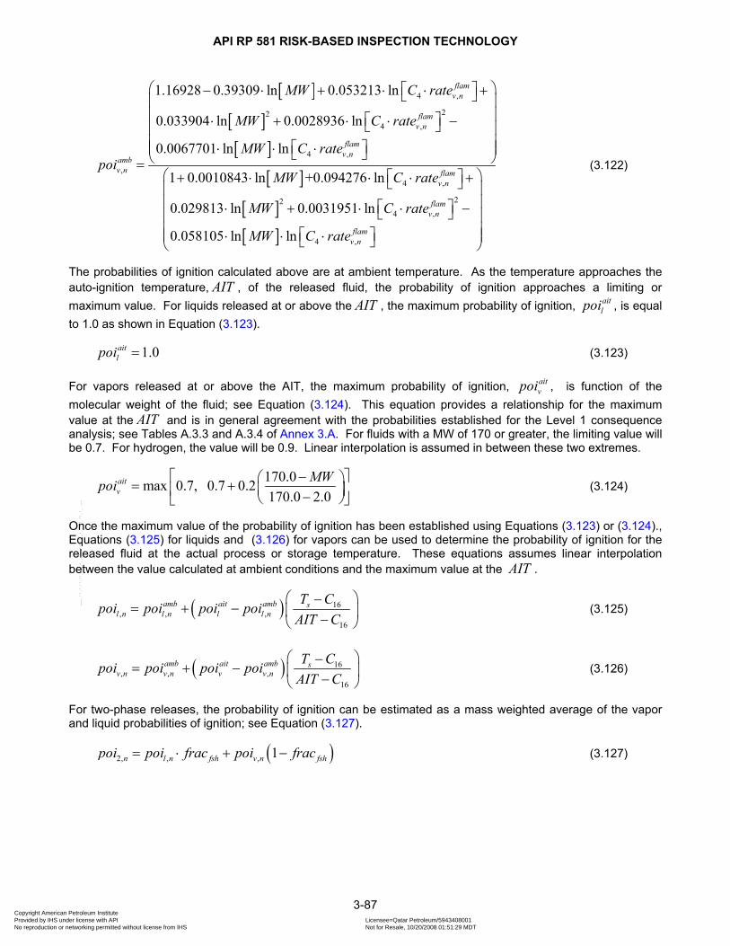
API RP 581 RISK-BASED INSPECTION TECHNOLOGY
3-87
[ ]
[ ][ ]
[ ]
4 ,
224 ,
4 ,
,4 ,
1.16928 0.39309 ln 0.053213 ln
0.033904 ln 0.0028936 ln
0.0067701 ln ln
1 0.0010843 ln +0.094276 ln
flamv n
flamv n
flamv n
ambv n flam
v n
MW C rate
MW C rate
MW C ratepoi
MW C rate
⎛ ⎞⎡ ⎤− ⋅ + ⋅ ⋅ +⎣ ⎦⎜ ⎟⎜ ⎟⎡ ⎤⋅ + ⋅ ⋅ −⎣ ⎦⎜ ⎟⎜ ⎟⎡ ⎤⋅ ⋅ ⋅⎜ ⎟⎣ ⎦⎝ ⎠=
⎡+ ⋅ ⋅ ⋅
[ ][ ]
224 ,
4 ,
0.029813 ln 0.0031951 ln
0.058105 ln ln
flamv n
flamv n
MW C rate
MW C rate
⎛ ⎞⎤ +⎣ ⎦⎜ ⎟⎜ ⎟⎡ ⎤⋅ + ⋅ ⋅ −⎣ ⎦⎜ ⎟⎜ ⎟⎡ ⎤⋅ ⋅ ⋅⎜ ⎟⎣ ⎦⎝ ⎠
(3.122)
The probabilities of ignition calculated above are at ambient temperature. As the temperature approaches the auto-ignition temperature, AIT , of the released fluid, the probability of ignition approaches a limiting or maximum value. For liquids released at or above the AIT , the maximum probability of ignition, ait
lpoi , is equal to 1.0 as shown in Equation (3.123).
1.0aitlpoi = (3.123)
For vapors released at or above the AIT, the maximum probability of ignition, aitvpoi , is function of the
molecular weight of the fluid; see Equation (3.124). This equation provides a relationship for the maximum value at the AIT and is in general agreement with the probabilities established for the Level 1 consequence analysis; see Tables A.3.3 and A.3.4 of Annex 3.A. For fluids with a MW of 170 or greater, the limiting value will be 0.7. For hydrogen, the value will be 0.9. Linear interpolation is assumed in between these two extremes.
170.0max 0.7, 0.7 0.2170.0 2.0
aitv
MWpoi ⎡ − ⎤⎛ ⎞= + ⎜ ⎟⎢ ⎥−⎝ ⎠⎣ ⎦ (3.124)
Once the maximum value of the probability of ignition has been established using Equations (3.123) or (3.124)., Equations (3.125) for liquids and (3.126) for vapors can be used to determine the probability of ignition for the released fluid at the actual process or storage temperature. These equations assumes linear interpolation between the value calculated at ambient conditions and the maximum value at the AIT .
( ) 16, , ,
16
amb ait amb sl n l n l l n
T Cpoi poi poi poiAIT C
⎛ ⎞−= + − ⎜ ⎟−⎝ ⎠
(3.125)
( ) 16, , ,
16
amb ait amb sv n v n v v n
T Cpoi poi poi poiAIT C
⎛ ⎞−= + − ⎜ ⎟−⎝ ⎠
(3.126)
For two-phase releases, the probability of ignition can be estimated as a mass weighted average of the vapor and liquid probabilities of ignition; see Equation (3.127).
( )2, , , 1n l n fsh v n fshpoi poi frac poi frac= ⋅ + − (3.127)
Copyright American Petroleum Institute Provided by IHS under license with API Licensee=Qatar Petroleum/5943408001
Not for Resale, 10/20/2008 01:51:29 MDTNo reproduction or networking permitted without license from IHS
--```,`,,`,`,,`,`,,,,,,``,```,`-`-`,,`,,`,`,,`---
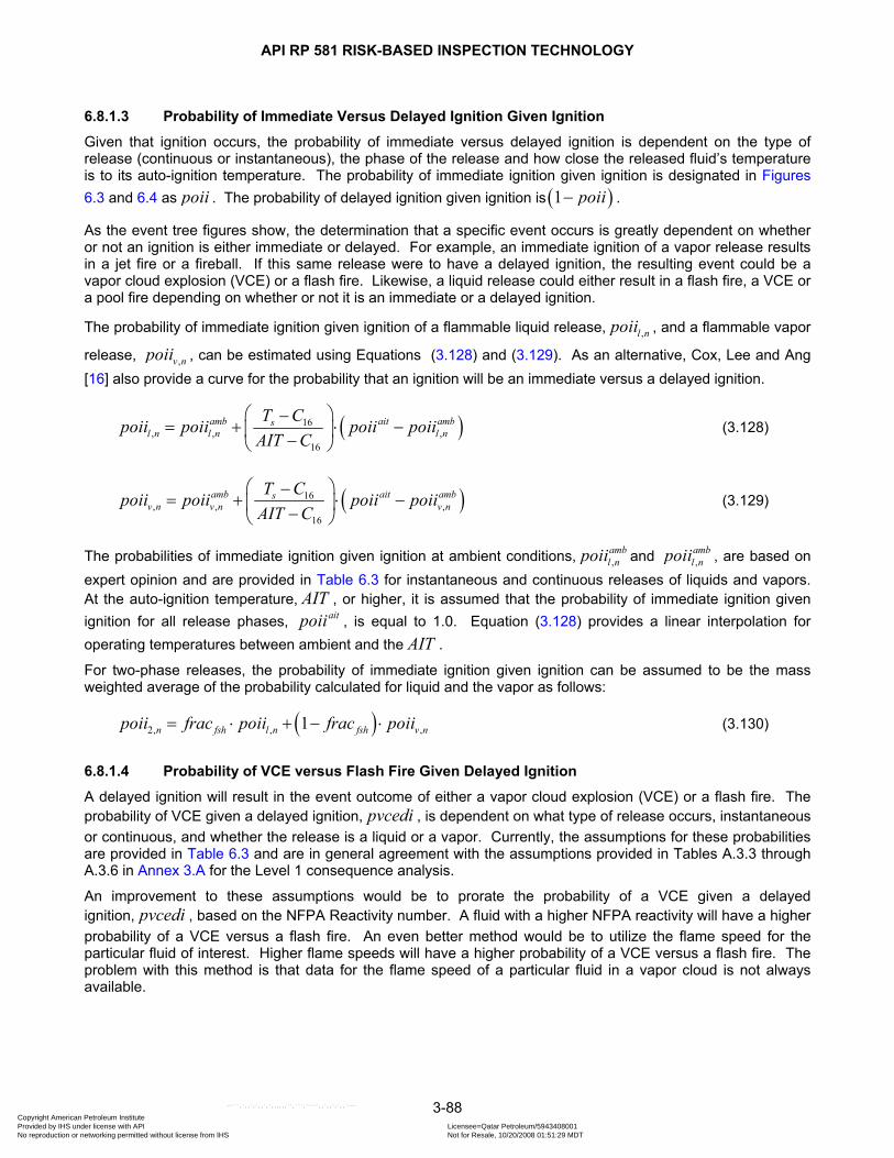
API RP 581 RISK-BASED INSPECTION TECHNOLOGY
3-88
6.8.1.3 Probability of Immediate Versus Delayed Ignition Given Ignition
Given that ignition occurs, the probability of immediate versus delayed ignition is dependent on the type of release (continuous or instantaneous), the phase of the release and how close the released fluid’s temperature is to its auto-ignition temperature. The probability of immediate ignition given ignition is designated in Figures 6.3 and 6.4 as poii . The probability of delayed ignition given ignition is ( )1 poii− .
As the event tree figures show, the determination that a specific event occurs is greatly dependent on whether or not an ignition is either immediate or delayed. For example, an immediate ignition of a vapor release results in a jet fire or a fireball. If this same release were to have a delayed ignition, the resulting event could be a vapor cloud explosion (VCE) or a flash fire. Likewise, a liquid release could either result in a flash fire, a VCE or a pool fire depending on whether or not it is an immediate or a delayed ignition.
The probability of immediate ignition given ignition of a flammable liquid release, ,l npoii , and a flammable vapor
release, ,v npoii , can be estimated using Equations (3.128) and (3.129). As an alternative, Cox, Lee and Ang [16] also provide a curve for the probability that an ignition will be an immediate versus a delayed ignition.
( )16, , ,
16
amb ait ambsl n l n l n
T Cpoii poii poii poiiAIT C
⎛ ⎞−= + ⋅ −⎜ ⎟−⎝ ⎠
(3.128)
( )16, , ,
16
amb ait ambsv n v n v n
T Cpoii poii poii poiiAIT C
⎛ ⎞−= + ⋅ −⎜ ⎟−⎝ ⎠
(3.129)
The probabilities of immediate ignition given ignition at ambient conditions, ,ambl npoii and ,
ambl npoii , are based on
expert opinion and are provided in Table 6.3 for instantaneous and continuous releases of liquids and vapors. At the auto-ignition temperature, AIT , or higher, it is assumed that the probability of immediate ignition given ignition for all release phases, aitpoii , is equal to 1.0. Equation (3.128) provides a linear interpolation for operating temperatures between ambient and the AIT .
For two-phase releases, the probability of immediate ignition given ignition can be assumed to be the mass weighted average of the probability calculated for liquid and the vapor as follows:
( )2, , ,1n fsh l n fsh v npoii frac poii frac poii= ⋅ + − ⋅ (3.130)
6.8.1.4 Probability of VCE versus Flash Fire Given Delayed Ignition
A delayed ignition will result in the event outcome of either a vapor cloud explosion (VCE) or a flash fire. The probability of VCE given a delayed ignition, pvcedi , is dependent on what type of release occurs, instantaneous or continuous, and whether the release is a liquid or a vapor. Currently, the assumptions for these probabilities are provided in Table 6.3 and are in general agreement with the assumptions provided in Tables A.3.3 through A.3.6 in Annex 3.A for the Level 1 consequence analysis.
An improvement to these assumptions would be to prorate the probability of a VCE given a delayed ignition, pvcedi , based on the NFPA Reactivity number. A fluid with a higher NFPA reactivity will have a higher probability of a VCE versus a flash fire. An even better method would be to utilize the flame speed for the particular fluid of interest. Higher flame speeds will have a higher probability of a VCE versus a flash fire. The problem with this method is that data for the flame speed of a particular fluid in a vapor cloud is not always available.
Copyright American Petroleum Institute Provided by IHS under license with API Licensee=Qatar Petroleum/5943408001
Not for Resale, 10/20/2008 01:51:29 MDTNo reproduction or networking permitted without license from IHS
--```,`,,`,`,,`,`,,,,,,``,```,`-`-`,,`,,`,`,,`---

API RP 581 RISK-BASED INSPECTION TECHNOLOGY
3-89
For liquids and vapors the probability of VCE given a delayed ignition, ,v npvcedi or ,v npvcedi , can be obtained from Table 6.3. For two-phase releases, the probability of VCE given a delayed ignition can be assumed to be the mass weighted average of the probability for liquid and the vapor as shown in Equation (3.131):
( )2, , ,1n fsh l n fsh v npvcedi frac pvcedi frac pvcedi= ⋅ + − ⋅ (3.131)
Since either a VCE or a flash fire occurs as a result of a delayed ignition, the probability of a flash fire given a delayed ignition of a liquid or a vapor release are in accordance with Equations (3.132) and (3.133).
, ,1l n l npffdi pvcedi= − (3.132)
, ,1v n v npffdi pvcedi= − (3.133)
For two-phase releases, the probability of flash fire given a delayed ignition can be assumed to be the mass weighted average of the probability calculated for liquid and the vapor as shown in Equation (3.134).
( )2, , ,1n fsh l n fsh v npffdi frac pffdi frac pffdi= ⋅ + − ⋅ (3.134)
6.8.1.5 Probability of Fireball Given Immediate Ignition
Fireballs occur as a result of an immediate ignition of an instantaneous vapor or two-phase release upon rupture of a component. The probability can be determined using Equations (3.135) and (3.136).
1.0 pfbii for instantaneous vapor or two - phase releases= (3.135)
0.0 pfbii for all other cases= (3.136)
6.8.1.6 Event Outcome Probabilities
Event trees are used to calculate the probability of every possible event or outcome (even safe outcomes) as a result of a hazardous release. The probability of a particular event outcome after a release can be determined by multiplication of all of the individual probabilities along the path of the event tree being taken. For example, the probability of a VCE given leakage of a vapor can be determined from Figure 6.3 using Equation (3.137).
( ) ( ), , , ,1 1v n v n v n v npvce poi poii pvcedi= ⋅ − ⋅ − (3.137)
The probability of safe release of a leaking two-phase release is given by Equation (3.138).
( )2, 2,1n npsafe poi= − (3.138)
The probability of a pool fire given a rupture of a vessel containing liquid per Figure 6.4 is given by Equation (3.139).
, , ,l n l n l nppool poi poii= ⋅ (3.139)
Copyright American Petroleum Institute Provided by IHS under license with API Licensee=Qatar Petroleum/5943408001
Not for Resale, 10/20/2008 01:51:29 MDTNo reproduction or networking permitted without license from IHS
--```,`,,`,`,,`,`,,,,,,``,```,`-`-`,,`,,`,`,,`---

API RP 581 RISK-BASED INSPECTION TECHNOLOGY
3-90
6.8.2 Pool Fires
6.8.2.1 Overview
When a flammable liquid is released from a piece of equipment or pipeline, a liquid pool may form. As the pool forms, some of the liquid will evaporate and, if the vaporizing flammable materials find an ignition source while it is above its Lower Flammability Limit (LFL), a pool fire can occur. For API RBI, pool fires are considered to occur as a result of immediate ignition of a flammable liquid from a pressurized process vessel or pipe that develops a hole or ruptures.
Important characteristics of pools fires include its burning velocity, rate of heat release, flame height, flame plume deflection, and radiative heat flux. To model a pool fire correctly, necessary data for the calculations include the extent of the pool surface, the physical properties of the burning fluid, the physical and thermal properties of the substrate, and the ambient conditions.
A method for calculating the consequences associated with a pool fire is provided by CCPS [18]. This method entails calculating the burning rate off the surface of the pool which is a function of the pool area and the heat of combustion, the latent heat of vaporization and the specific heat of the flammable liquid. The maximum size of the pool is determined at that point where the burning rate off the surface of the pool is equal to the release rate calculated through the hole or rupture from the protected piece of equipment (see paragraph 6.8.2.3).
The API RBI consequence area is estimated by considering the potential for personnel injury and component damage due to the effects of exposure to thermal radiation in the vicinity of the fire.
6.8.2.2 Pool Fire Burning Rate
The burning rate off of the surface of a pool fire is the rate at which the flammable material is evaporated during the fire is given in TNO [19] and can be determined using the following equations.
For non-boiling pools:
( )17 l
bl b atm v
C HCmCp T T H
⋅=
− + ∆ (3.140)
For boiling pools, such as cryogenic liquids or LPGs:
17 lb
v
C HCmH⋅
=∆
(3.141)
Note that for liquid mixtures (such as gasoline), the burning rate can be approximated by calculating the burning rate for each component in the mixture, ,b im , and summing as follows:
, ,1
N
b mole i b ii
m frac m=
= ⋅∑ (3.142)
6.8.2.3 Pool Fire Size
The ultimate size of the pool fire is then determined to be the size where the liquid portion (rainout) of the release rate from the pressurized system, pool
nW , is equal to the burning rate off the surface of the pool, bm , or:
,
pooln
pf nb
WAburnm
= (3.143)
Copyright American Petroleum Institute Provided by IHS under license with API Licensee=Qatar Petroleum/5943408001
Not for Resale, 10/20/2008 01:51:29 MDTNo reproduction or networking permitted without license from IHS
--```,`,,`,`,,`,`,,,,,,``,```,`-`-`,,`,,`,`,,`---

API RP 581 RISK-BASED INSPECTION TECHNOLOGY
3-91
For instantaneous releases of the flammable liquid inventory to the ground, a practical limit to the amount of pool spread should be used in the consequence calculations. The maximum size of the pool can be determined based on assuming a circle with depth of 5 mm [0.0164 ft], in accordance with The Netherlands Organization (TNO Yellow Book), 1997 [19], recommendations.
,,
18
avail npf n
ro l
massAmax
C frac ρ=
⋅ ⋅ (3.144)
The pool fire area to be used in the consequence area calculation is then:
, , , 7min , , 929.1pf n pf n pf nA Aburn Amax C⎡ ⎤= ⋅⎣ ⎦ (3.145)
Note that the pool size is also limited to a maximum of 929.1 m2 [10,000 ft2], as discussed in paragraph 5.8.3. From this area, the radius of the pool fire can be determined:
,,
pf npf n
AR
π= (3.146)
6.8.2.4 Flame Length and Flame Tilt
The SPFE Fire Protection Handbook [20] provides a correlation from Thomas that can be used for calculating the flame length of a pool fire, pfL .
0.67
0.21, ,
,
1102
bpf n pf n s
atm pf n
mL R ug Rρ
−⎡ ⎤⎢ ⎥= ⋅
⋅ ⋅⎢ ⎥⎣ ⎦ (3.147)
The non-dimensional wind velocity, su , cannot be less than 1.0 and is dependent on the wind speed as follows:
0.333
,,
max 1.0 , 2
vs n w
b pf n
u ug m R
ρ⎡ ⎤⎛ ⎞⎢ ⎥= ⋅⎜ ⎟⎜ ⎟⋅ ⋅ ⋅⎢ ⎥⎝ ⎠⎣ ⎦
(3.148)
The American Gas Association provides the following correlation for estimating the flame tilt:
,,
1cos pf ns nu
θ = (3.149)
6.8.2.5 Pool Fire Radiated Energy
The amount of energy radiated by the pool fire (often referred to as surface emitted heat flux) is a fraction of the total combustion power of the flame [19]. The fraction of the total combustion power that is radiated, β , is often quoted in the range of 0.15 – 0.35. A conservative value of 0.35 can be chosen. Therefore:
214 ,
2, , ,2
b l pf npooln
pf n pf n pf n
C m HC RQrad
R L Rβ π
π π⋅ ⋅ ⋅ ⋅ ⋅
=⋅ ⋅ ⋅ + ⋅
(3.150)
The amount of the radiated energy that actually reaches a target at some location away from the pool fire is a function of the atmospheric conditions as well as the radiation view factor between the pool and the target. The received thermal flux can be calculated as follows:
Copyright American Petroleum Institute Provided by IHS under license with API Licensee=Qatar Petroleum/5943408001
Not for Resale, 10/20/2008 01:51:29 MDTNo reproduction or networking permitted without license from IHS
--```,`,,`,`,,`,`,,,,,,``,```,`-`-`,,`,,`,`,,`---
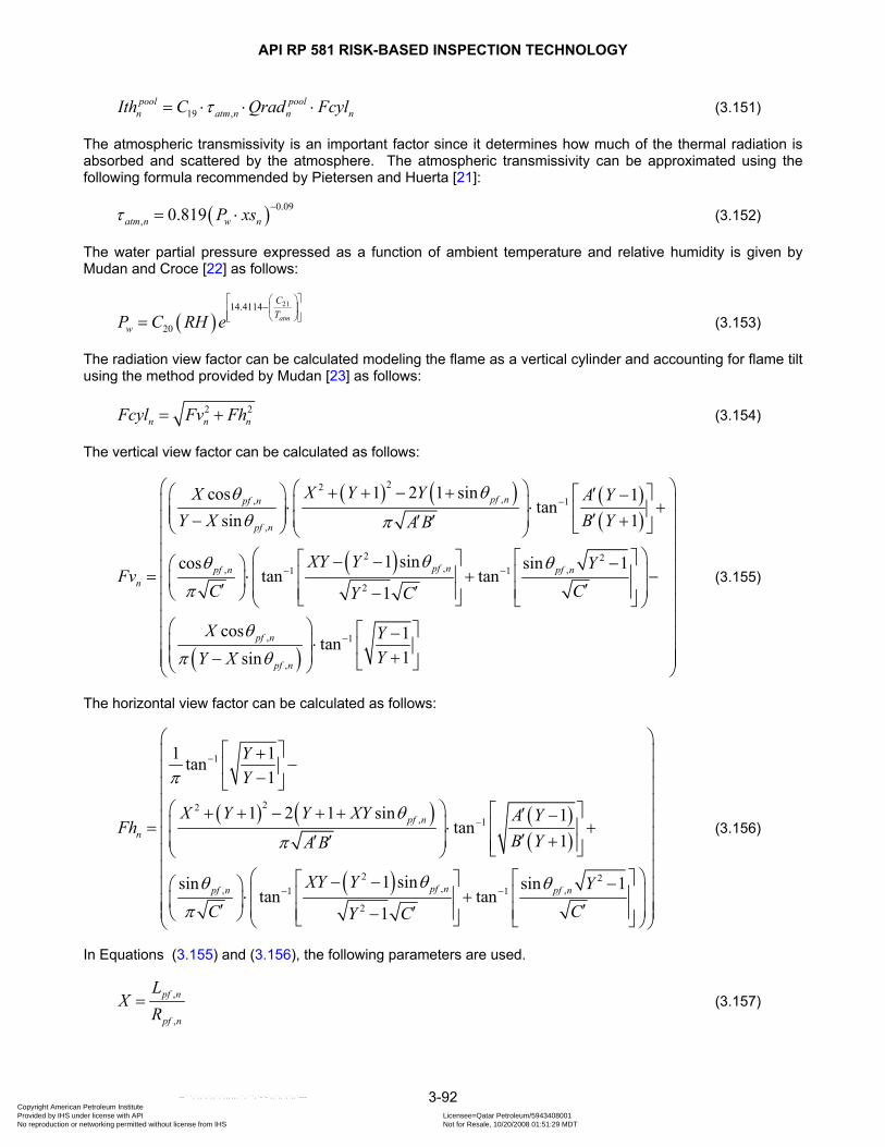
API RP 581 RISK-BASED INSPECTION TECHNOLOGY
3-92
19 ,pool pool
n atm n n nIth C Qrad Fcylτ= ⋅ ⋅ ⋅ (3.151)
The atmospheric transmissivity is an important factor since it determines how much of the thermal radiation is absorbed and scattered by the atmosphere. The atmospheric transmissivity can be approximated using the following formula recommended by Pietersen and Huerta [21]:
( ) 0.09, 0.819atm n w nP xsτ −= ⋅ (3.152)
The water partial pressure expressed as a function of ambient temperature and relative humidity is given by Mudan and Croce [22] as follows:
( )2114.4114
20atm
CT
wP C RH e⎡ ⎤⎛ ⎞
−⎢ ⎥⎜ ⎟⎢ ⎥⎝ ⎠⎣ ⎦= (3.153)
The radiation view factor can be calculated modeling the flame as a vertical cylinder and accounting for flame tilt using the method provided by Mudan [23] as follows:
2 2n n nFcyl Fv Fh= + (3.154)
The vertical view factor can be calculated as follows:
( ) ( ) ( )( )
( )
( )
22,, 1
,
2 2,, ,1 1
2
,
,
1 2 1 sincos 1tan
sin 1
1 sincos sin 1tan tan
1
cossin
pf npf n
pf n
pf npf n pf nn
pf n
pf n
X Y YX A YY X B YA B
XY Y YFv
C CY C
XY X
θθθ π
θθ θπ
θπ θ
−
− −
⎛ ⎞+ + − +⎛ ⎞ ⎡ ⎤′ −⎜ ⎟⋅ ⋅ +⎜ ⎟ ⎢ ⎥⎜ ⎟ ′⎜ ⎟− +′ ′ ⎣ ⎦⎝ ⎠ ⎝ ⎠⎛ ⎞⎡ ⎤⎡ ⎤− − −⎛ ⎞ ⎜ ⎟⎢ ⎥⎢ ⎥= ⋅ + −⎜ ⎟ ⎜ ⎟′ ′⎢ ⎥′⎢ ⎥−⎝ ⎠ ⎣ ⎦ ⎣ ⎦⎝ ⎠
⎛
−1 1tan
1YY
−
⎛ ⎞⎜ ⎟⎜ ⎟⎜ ⎟⎜ ⎟⎜ ⎟⎜ ⎟⎜ ⎟⎜ ⎟⎞ ⎡ ⎤−⎜ ⎟⎜ ⎟ ⋅ ⎢ ⎥⎜ ⎟⎜ ⎟ +⎜ ⎟⎣ ⎦⎝ ⎠⎝ ⎠
(3.155)
The horizontal view factor can be calculated as follows:
( ) ( ) ( )( )
( )
1
22, 1
2 2,, ,1 1
2
1 1tan1
1 2 1 sin 1tan
1
1 sinsin sin 1tan tan
1
pf nn
pf npf n pf n
YY
X Y Y XY A YFh
B YA B
XY Y YC CY C
π
θ
π
θθ θπ
−
−
− −
⎛ ⎞⎡ ⎤+⎜ ⎟−⎢ ⎥⎜ ⎟−⎣ ⎦⎜ ⎟
⎜ ⎟⎛ ⎞ ⎡ ⎤+ + − + + ′ −⎜ ⎟⎜ ⎟= ⋅ +⎢ ⎥⎜ ⎟′⎜ ⎟ +′ ′ ⎢ ⎥⎣ ⎦⎝ ⎠⎜ ⎟⎜ ⎟⎛ ⎞⎡ ⎤⎡ ⎤− − −⎛ ⎞⎜ ⎟⎜ ⎟⎢ ⎥⎢ ⎥⋅ +⎜ ⎟⎜ ⎟⎜ ⎟′ ′⎜ ⎟⎢ ⎥′⎢ ⎥−⎝ ⎠ ⎣ ⎦ ⎣ ⎦⎝ ⎠⎝ ⎠
(3.156)
In Equations (3.155) and (3.156), the following parameters are used.
,
,
pf n
pf n
LX
R= (3.157)
Copyright American Petroleum Institute Provided by IHS under license with API Licensee=Qatar Petroleum/5943408001
Not for Resale, 10/20/2008 01:51:29 MDTNo reproduction or networking permitted without license from IHS
--```,`,,`,`,,`,`,,,,,,``,```,`-`-`,,`,,`,`,,`---
API RP 581 RISK-BASED INSPECTION TECHNOLOGY
3-93
,
n
pf n
xsYR
= (3.158)
( ) ( )22,1 2 1 sin pf nA X Y X Y θ′ = + + − + (3.159)
( ) ( )22,1 2 1 sin pf nB X Y X Y θ′ = + − − − (3.160)
( )2 2,1 1 cos pf nC Y θ′ = + − (3.161)
6.8.2.6 Pool Fire Safe Distance and Consequence Area
The procedure used in API RBI for determining the consequence area associated with a pool fire consists of calculating the distance away from the pool fire where the radiated energy from the pool fire is equal to the exposure limits (impact criteria) for thermal radiation as provided in paragraph 5.8.2. For serious personnel injury, API RBI uses a maximum permissible radiation of 12.6 kW/m2 [4,000 Btu/hr-ft2]. For component damage the maximum permissible radiation is 37.8 kW/m2 [12,000 Btu/hr-ft2].
Note that the atmospheric transmissivity and the source view factor are functions of the distance from the flame source to the target. These are the two parameters which account for the fact that the received thermal radiation at any point away from the fire goes down as the distance increases. An iterative approach is required to determine the acceptable or safe distance away from the pool fire.
This procedure is carried out for personnel injury as well as component damage for each of the release hole sizes selected as described in paragraph 5.2. Once the safe distances, ,
poolcmd nxs and ,
poolinj nxs , are determined,
Equations (3.162) and (3.163) are used to calculate the pool fire consequence areas.
( )2
, ,pool pool
cmd n cmd nCA xsπ= ⋅ (3.162)
( )2
, ,pool pool
inj n inj nCA xsπ= ⋅ (3.163)
6.8.3 Jet Fires
6.8.3.1 General
Jet fires occur as a result of immediate ignition of a flammable fluid from a pressurized process vessel or pipe that develops a hole. Jet fires do not occur as a result of an immediate ignition from a loss of containment due to a rupture, see Figure 6.4. Similar to pool fires, the main deleterious effect is the heat flux produced by the jet fire.
One method for calculating the consequences from a jet fire is provided in CCPS [18]. The method involves calculating the flame length of the jet fire and the radiative heat flux at distances away from the jet source. The distance at which the calculated thermal radiation from the jet fire equals the thermal radiation limit specified by the risk analyst (for API RBI, limit is 12.6 kW/m2 [4,000 Btu/hr-ft2] for personnel and 37.8 kW/m2 [12,000 Btu/hr-ft2] for equipment), provides the radius for the consequence area.
A conservative assumption is made that the jet fire arises vertically at a point located at grade since this will provide the largest effected area that exceeds the thermal radiation limit.
6.8.3.2 Jet Fire Radiated Energy
The amount of energy radiated by the jet (often referred to as surface emitted heat flux) is a fraction of the total combustion power of the flame. The fraction of the total combustion power that is radiated,β , is often quoted in the range of 0.15 – 0.35. A conservative value of 0.35 can be chosen. Therefore:
Copyright American Petroleum Institute Provided by IHS under license with API Licensee=Qatar Petroleum/5943408001
Not for Resale, 10/20/2008 01:51:29 MDTNo reproduction or networking permitted without license from IHS
--```,`,,`,`,,`,`,,,,,,``,```,`-`-`,,`,,`,`,,`---

API RP 581 RISK-BASED INSPECTION TECHNOLOGY
3-94
14jet jet
n n vQrad C W HCβ= ⋅ ⋅ ⋅ (3.164)
For mixtures, the heat of combustion can be evaluated using a mole weighted average of the individual component heats of combustion.
6.8.3.3 Jet Fire Safe Distance and Consequence Area
The amount of the radiated energy that actually reaches a target at some location away from the jet fire is a function of the atmospheric conditions as well as the radiation view factor between the source and the target. The received thermal flux can be calculated as follows:
,jet jet
n atm n n nIth Qrad Fpτ= ⋅ ⋅ (3.165)
If a point source model is used then the radiation view factor between the source flame and the target can be approximated as follows:
2
14n
n
Fpxsπ
=⋅
(3.166)
The point source view factor provides a reasonable estimate of received flux at distances far from the flame. More rigorous formulas that are based on specific flame shapes [e.g. cylinders, see Equation (3.154)] or that assume a solid plume radiation model may be used as alternatives to the simplified calculation shown above.
Note that the atmospheric transmissivity and the point source view factor are functions of the distance from the flame source to the target. An iterative approach is required to determine the acceptable distance away from the jet fire, and the resultant consequence area.
This procedure is carried out for personnel injury as well as component damage for each of the release hole sizes selected as described in paragraph 5.2. Once the safe distances, ,
jetcmd nxs and ,
jetinj nxs , are determined,
Equations (3.167) and (3.168) are used to calculate the jet fire consequence areas.
2, ,
jetcmd n cmd nCA xsπ= ⋅ (3.167)
2, ,
jetinj n inj nCA xsπ= ⋅ (3.168)
6.8.4 Fireballs
6.8.4.1 General
Fireballs result from the immediate ignition of a flammable, superheated liquid/vapor. Fireballs always occur in combination with a physical explosion or a BLEVE. The effects of fireballs need to be evaluated for instantaneous releases (or ruptures) only. Continuous releases do not result in fireballs.
CCPS [18] provides a suitable methodology for determining the effects of fireballs. Four factors have to be considered to determine the heat flux of a fireball: the mass of the flammable fluid and the fireball’s diameter, duration, and thermal emissive power. The main parameter needed is the mass of flammable fluid in the stored equipment prior to rupture. In API RBI, the flammable mass for the fireball, fbmass is the fraction of the released mass that contains flammable material and can be determined using Equation (3.169).
,flam
fb avail nmass mfrac mass= ⋅ (3.169)
The maximum mass available for release, ,avail nmass , is defined in paragraph 5.4.2; see Equation (3.11).
Copyright American Petroleum Institute Provided by IHS under license with API Licensee=Qatar Petroleum/5943408001
Not for Resale, 10/20/2008 01:51:29 MDTNo reproduction or networking permitted without license from IHS
--```,`,,`,`,,`,`,,,,,,``,```,`-`-`,,`,,`,`,,`---

API RP 581 RISK-BASED INSPECTION TECHNOLOGY
3-95
Once the flammable mass of the fireball is known, the diameter, duration and height of the fireball can be readily calculated. The effects of thermal radiation on personnel and equipment can be determined in much the same way as has been previously done for jet fires and pool fires.
6.8.4.2 Fireball Size and Duration
The diameter of the fireball is a function of the flammable mass as follows:
0.33322fb fbDmax C mass= ⋅ (3.170)
The center height of the fireball is assumed to be:
0.75fb fbH Dmax= ⋅ (3.171)
The duration of the fireball is also a function of the flammable mass as follows:
0.33323 29,937 [66,000 ]fb fb fbt C mass for mass kgs lbs= ⋅ ≤ (3.172)
0.16724 29,937 [66,000 ]fb fb fbt C mass for mass kgs lbs= ⋅ > (3.173)
6.8.4.3 Fireball Radiated Energy
The amount of energy radiated by the fireball (often referred to as surface emitted heat flux) is a fraction of its total combustion power. The fraction of the total combustion power that is radiated, fbβ , is often quoted in the range of 0.25 – 0.4, see Equation (3.175).
142
fb fb lfball
fb fb
C mass HCQrad
Dmax tβπ⋅ ⋅ ⋅
=⋅ ⋅
(3.174)
The fraction of combustion power that is radiated from a fireball can be calculated from a correlation by [24]:
0.3225fb BC Pβ = ⋅ (3.175)
The burst pressure used above for determining the radiation fraction depends on the consequence being calculated. If the calculation is for pressurized fixed equipment where the concern is for rupture during normal operation, the normal operating pressure is used. When the calculation is to be performed at elevated pressures such as the case when the consequences of failure of pressure relief devices are being evaluated, the likely overpressure that results from the failure to open upon demand should be used.
6.8.4.4 Fireball Safe Distance and Consequence Area
The amount of the radiated energy that actually reaches a target at some location away from the fireball is a function of the atmospheric conditions as well as the radiation view factor between the source and the target. The received thermal flux can be determined as before:
fball fballatmIth Qrad Fsphτ= ⋅ ⋅ (3.176)
For a fireball, the spherical model for the geometric view factor is used:
( )2
24fb
fb
DmaxFsph
C= (3.177)
where:
Copyright American Petroleum Institute Provided by IHS under license with API Licensee=Qatar Petroleum/5943408001
Not for Resale, 10/20/2008 01:51:29 MDTNo reproduction or networking permitted without license from IHS
--```,`,,`,`,,`,`,,,,,,``,```,`-`-`,,`,,`,`,,`---

API RP 581 RISK-BASED INSPECTION TECHNOLOGY
3-96
2 2
2.0 2.0
fballfb
fb
Dmax xsC⎛ ⎞ ⎛ ⎞
= +⎜ ⎟ ⎜ ⎟⎝ ⎠⎝ ⎠
(3.178)
Note that the atmospheric transmissivity and the geometric view factor are functions of the distance from the flame source to the target, fballxs . An iterative approach is required to determine the acceptable distance away from the fireball.
This procedure is carried out for personnel injury as well as component damage for the rupture case only. Once the safe distances, fball
cmdxs and fballinjxs , are determined, Equations (3.179) and (3.180) are used to calculate the
fireball consequence areas.
( )2fball fballcmd cmdCA xsπ= ⋅ (3.179)
( )2fball fballinj injCA xsπ= ⋅ (3.180)
6.8.5 Vapor Cloud Explosions (VCEs)
6.8.5.1 General
When a sizable amount of flammable fluid is suddenly released into the air and is not immediately ignited, three things can happen: the cloud can encounter an ignition source and explode, producing a vapor cloud explosion (VCE); the cloud can encounter an ignition source and flash back, producing a flash fire (paragraph 6.8.6); or the cloud can safely disperse. For a VCE or flash fire to occur, the released material must form a partially mixed vapor cloud that contains vapor concentrations above the lower flammability limit. The cloud then encounters an ignition source and either explodes or flashes back. Since VCEs produce devastating effects on plants if they occur, significant research on their causes has been performed. From research on VCEs that have occurred, Lees [25] has identified several parameters that affect VCE behavior:
a) Quantity of material released
b) Fraction of material vaporized
c) Probability of ignition of the cloud
d) Distance traveled by the cloud
e) Time delay before ignition of the cloud
f) Probability of explosion rather than fire
g) Existence of a threshold quantity of material
h) Efficiency of the explosion
i) Location of ignition source with respect to the release
Vapor Cloud Explosions (VCEs) can occur as a result of a delayed ignition of a vapor cloud. The source of the vapor cloud could either be from a vapor or two-phase jet release or evaporation off the surface of an un-ignited liquid flammable pool. Dispersion modeling of the cloud is required to evaluate the extent of a vapor cloud since the amount of flammable material in the cloud is needed. See the general discussion on cloud modeling presented in paragraph 6.7.4. A vapor cloud explosion is a deflagration (not detonation) that produces significant overpressure (blast wave) and occurs when the flame propagation through the cloud travels at extremely high velocities. If the flame propogates at a relatively slow velocity, a VCE, with the resulting overpressure, does not occur. In this case, a relatively low consequence, low energy, flash fire is the outcome (see paragraph 6.8.6).
Copyright American Petroleum Institute Provided by IHS under license with API Licensee=Qatar Petroleum/5943408001
Not for Resale, 10/20/2008 01:51:29 MDTNo reproduction or networking permitted without license from IHS
--```,`,,`,`,,`,`,,,,,,``,```,`-`-`,,`,,`,`,,`---
API RP 581 RISK-BASED INSPECTION TECHNOLOGY
3-97
6.8.5.2 Source of Vapor
The source of flammable vapor for the vapor cloud explosion could either be from a jet release or from an evaporating liquid pool release. For the jet release case, the source rate is simply the jet release rate as discussed in paragraph 6.7.3.
For an evaporating pool, the vapor rate used as the source for the vapor cloud explosion is dependent on whether the pool is a boiling or non-boiling, as discussed in paragraph 6.7.4 and shown in Figure 6.1.
6.8.5.3 Amount of Flammable Material
The first step in evaluating the effects of a VCE, is to determine the amount of flammable material that is in the source cloud. The mass is a function of the release rate, the atmospheric dispersion of the cloud and the time of ignition. A suitable cloud dispersion model that can handle plumes (continuous release with steady state analysis) as well as puffs (instantaneous releases that required a transient model) should be used to evaluate the amount of flammable material that exists in the cloud at the time of ignition.
6.8.5.4 Explosion Yield Factor
An important parameter in the evaluation of the vapor cloud is the explosion yield factor, η . This is an empirical value that determines how much of the combustion power in the cloud is released into the pressure wave. Where the flammable mass in the cloud is calculated as the portion of the cloud between the LFL and the UFL of the flammable material, a conservative value for the explosion yield factor of 1.0 should be used.
Where the flammable mass is based on the total amount of flammable fluid released, than a yield factor, η , with a range of between 0.03 0.19η≤ ≤ is typically used and this is a function of the material released. For example, typical hydrocarbons have a yield factor of 0.03, while highly reactive fluids, such as ethylene oxide have yield factors up around 0.19. Additional yield factors are provided by Zebetakis [26].
6.8.5.5 Determination of Blast Overpressure
a) General – There are several approaches to estimating the overpressure that results from a VCE. The first method, used by API RBI and detailed in paragraph 6.8.5.5.b, is the TNT equivalency method, explained in [27]. In this method, the source of the explosion is assumed to be at a point (point source model) and the characteristics of the explosion are similar to that of a TNT explosion. This approach will likely result in conservative estimates of the damage at locations closest to the source of the explosion.
Another model that will not be presented here is more complicated and will provide more accurate (less conservative) results in the near field of the explosion. This method is known as the TNO Multi-energy Method and it focuses on the characteristics of the site, rather than on the size of the release. This method recognizes the fact that primarily only those portions of the vapor cloud that are obstructed or partially confined could undergo blast-generating combustion.
Yet another model is the Baker-Strelow-Tang Energy Model [27] which also looks at the characteristics of site. The key parameter to calculate in this method is the volume associated with the congested/confined region of the site this takes a great deal of subjectivity and experience to accurately identify and to compare this with the stoichiometic volume produced in the cloud.
b) TNT Equivalency Method – The TNT equivalency method, also presented in CCPS [18], determines the amount of available energy in the cloud and relates this to an equivalent amount of TNT using Equation (3.181).
vce sTNT
TNT
mass HCWHC
η ⋅ ⋅= (3.181)
For mixtures, a mole weighting of the individual component heats of combustions can be used to estimate the heat of combustion for the mixture in the cloud. The heat of combustion of TNT, TNTHC , is approximately 4,648 J/kg [2,000 Btu/lb].
Copyright American Petroleum Institute Provided by IHS under license with API Licensee=Qatar Petroleum/5943408001
Not for Resale, 10/20/2008 01:51:29 MDTNo reproduction or networking permitted without license from IHS
--```,`,,`,`,,`,`,,,,,,``,```,`-`-`,,`,,`,`,,`---

API RP 581 RISK-BASED INSPECTION TECHNOLOGY
3-98
c) Use of Blast Curves – To determine the blast effect, the side-on blast wave overpressure can be calculated using blast curves. An acceptable curve for estimating the overpressure is the Hopkinson-scaled curved which is reproduced by CCPS [18]. Equation (3.182) is a curve fit of the Hopkinson-scaled data which provide a closed form solution for determining the side-on overpressure (units are bar):
( )
( ) ( ) ( )
( ) ( ) ( )
2, ,
, 26 3 4 5
, , ,
6 7 8
, , ,
1.1288697 7.96252160.059965896ln ln
25.106738 30.396707 19.399862
ln ln ln
6.8853477 1.2825511 0.097705789
ln ln ln
HS n HS n
SO n
HS n HS n HS n
HS n HS n HS n
R R
P CR R R
R R R
⎛− + − +
⎡ ⎤ ⎡ ⎤⎣ ⎦ ⎣ ⎦
= ⋅ − + −⎡ ⎤ ⎡ ⎤ ⎡ ⎤⎣ ⎦ ⎣ ⎦ ⎣ ⎦
+ −⎡ ⎤ ⎡ ⎤ ⎡ ⎤⎣ ⎦ ⎣ ⎦ ⎣ ⎦
⎞⎜ ⎟⎜ ⎟⎜ ⎟⎜ ⎟⎜ ⎟⎜ ⎟⎜ ⎟⎜ ⎟⎜ ⎟⎜ ⎟⎝ ⎠
(3.182)
For use in Equation (3.182), the Hopkinson-scaled distance, ,HS nR , presented above requires units of m/kg1/3 and is calculated from the actual distance from the blast center as follows:
, 27 1 3
vcen
HS nTNT
xsR CW
= ⋅ (3.183)
6.8.5.6 VCE Safe Distance and Consequence Area
The consequence areas for serious injury to personnel and component damage can be determined once the overpressure as a function of distance from the blast is known. For serious injuries to personnel, the consequence area can be based on the following Probit equation provided by Eisenberg [28].
28 ,23.8 2.92 ln SO nPr C P⎡ ⎤= − + ⋅ ⋅⎣ ⎦ (3.184)
This probit equation provides the probability of process building collapse due to structural damage as a result of overpressure. Data shows that personnel can withstand much higher overpressures (15 to 30 psi overpressure for lung hemmorage) when out in the open and that typical serious injury occurs as a result of the collapse of buildings.
For component damage, an overpressure of 34.5 kPa [5.0 psi] has proven to be a good value to use when evaluating the consequence area to equipment as a result of overpressures from explosions.
Note that the side-on overpressure is a function of the distance from the blast source to the target. An iterative approach is required to determine the acceptable distance away from the explosion.
This procedure is carried out for personnel injury as well as component damage for each of the release hole sizes selected as described in paragraph 5.2. Once the safe distances, ,
vcecmd nxs and ,
vceinj nxs , are determined,
Equations (3.185) and (3.186) are used to calculate the VCE consequence areas.
( )2
, ,vce vcecmd n cmd nCA xsπ= ⋅ (3.185)
( )2
, ,vce vceinj n inj nCA xsπ= ⋅ (3.186)
Copyright American Petroleum Institute Provided by IHS under license with API Licensee=Qatar Petroleum/5943408001
Not for Resale, 10/20/2008 01:51:29 MDTNo reproduction or networking permitted without license from IHS
--```,`,,`,`,,`,`,,,,,,``,```,`-`-`,,`,,`,`,,`---
API RP 581 RISK-BASED INSPECTION TECHNOLOGY
3-99
6.8.6 Flash Fires
6.8.6.1 General
Flash fires, like VCEs, can occur as a result of a delayed ignition of a vapor cloud. The source of the vapor cloud could either be from a vapor or two-phase jet release or evaporation off the surface of an un-ignited liquid flammable pool. Dispersion modeling of the cloud is required to evaluate the extent of a vapor cloud since the amount of flammable material and the area covered by the flammable portion in the cloud is needed. See the general discussion on cloud modeling presented in Annex 3.A.
6.8.6.2 Flash Fire Consequence Area
A flash fire is a deflagration (not detonation), however, unlike VCEs, the flame speed is relatively slow and overpressures (blast waves) do not occur. Flash fires are much more common than VCEs and last for no more a few tenths of a second. Unlike pool or jet fires (immediate ignition), flash fires need not consider radiation effects away from the fire boundary, since the combustion process is of short duration and relatively low intensity. The consequence area for personnel from a flash fire, ,
flashinj nCA , is merely the flammable cloud
boundary and no further.
As with VCEs, a suitable cloud dispersion model that can handle plumes (continuous release with steady state analysis) as well as puffs (instantaneous releases that required a transient model) should be used. The cloud dispersion model is used to determine the boundary area of the vapor cloud that contains flammable material that is at or above the lower flammability limit (LFL) of the mixture in the cloud. The resultant boundary area will equal the consequence area for serious injury to personnel. As a general rule of the thumb, the consequence area associated with damage to an equipment component from flash fires, ,
flashcmd nCA , is limited to 25% of the area
for serious injury to personnel.
, ,0.25flash flashcmd n inj nCA CA= ⋅ (3.187)
6.8.7 Determination of Flammable Consequence for Each Release Case (Hole Size)
For each hole size or release case selected, the flammable consequence area is calculated as a probability weighted consequence area of all of the potential event outcomes on the event tree as shown in Equations (3.188) and (3.189). For component damage, use Equation (3.188); for personnel injury, use Equation (3.189)
, ,,
, , ,
pool jet fballn cmd n n cmd n n cmdflam
cmd n vce flash safen cmd n n cmd n n cmd n
ppool CA pjet CA pfball CACA
pvce CA pflash CA psafe CA
⎛ ⎞⋅ + ⋅ + ⋅ += ⎜ ⎟⎜ ⎟⋅ + ⋅ + ⋅⎝ ⎠
(3.188)
, ,,
, , ,
pool jet fballn inj n n inj n n injflam
inj n vce flash safen inj n n inj n n inj n
ppool CA pjet CA pfball CACA
pvce CA pflash CA psafe CA
⎛ ⎞⋅ + ⋅ + ⋅ +⎜ ⎟=⎜ ⎟⋅ + ⋅ + ⋅⎝ ⎠
(3.189)
Note that a safe release is a legitimate event outcome from the event trees. Although the consequence area of a safe release, ,
safecmd nCA and ,
safeinj nCA , are equal to 0.0, they have been presented in Equations (3.188) and (3.189)
for completeness.
6.8.8 Determination of Final Flammable Consequence Areas
The final flammable consequence areas are determined as a probability weighted average of the individual flammable consequence areas calculated for each release hole size. This is performed for both the component damage and the personnel injury consequence areas. The probability weighting utilizes the generic frequencies of the release hole sizes selected per paragraph 5.2.
Copyright American Petroleum Institute Provided by IHS under license with API Licensee=Qatar Petroleum/5943408001
Not for Resale, 10/20/2008 01:51:29 MDTNo reproduction or networking permitted without license from IHS
--```,`,,`,`,,`,`,,,,,,``,```,`-`-`,,`,,`,`,,`---
API RP 581 RISK-BASED INSPECTION TECHNOLOGY
3-100
The equation for probability weighting of the component damage consequence areas is given by Equation (3.190).
4
,1
flamn cmd n
flam ncmd
total
gff CACA
gff=
⎛ ⎞⋅⎜ ⎟⎜ ⎟=⎜ ⎟⎜ ⎟⎝ ⎠
∑ (3.190)
The equation for probability weighting of the personnel injury consequence areas is given by Equation (3.191).
4
,1
flamn inj n
flam ninj
total
gff CACA
gff=
⎛ ⎞⋅⎜ ⎟⎜ ⎟=⎜ ⎟⎜ ⎟⎝ ⎠
∑ (3.191)
In Equations (3.190) and (3.191), the total generic failure frequency is as computed in STEP 2.2
6.8.9 Calculation Procedure
a) STEP 8.1 – Determine the mass fraction of the release rate that contains a flammable component, flammfrac . This can be determined by adding the mass fractions of all flammable components in the
mixture.
b) STEP 8.2 – For each hole size, calculate the flammable release rate, flamnrate , using Equation (3.118).
Also calculate the liquid portion, ,flam
l nrate , and the vapor portion, ,flam
v nrate , of the flammable release rate using (3.119) and/or (3.120), as applicable. Note that for two-phase releases both values should be calculated.
c) STEP 8.3 – For each hole size, select the appropriate event tree using Figures 6.2 and 6.3 and the phase of the fluid after flashing to atmosphere in STEP 1.3. For the leak cases (small, medium and large hole sizes), utilize Figure 6.2. For the rupture case, use Figure 6.3.
d) STEP 8.4 – For each hole size, including the rupture case, calculate the probability of ignition of the release.
1) Determine the probability of ignition at ambient temperature for the liquid portion of the release,
,ambl npoi , using Equation (3.121) and the value of ,
flaml nrate obtained in STEP 8.2. Note that for the
rupture case or some of the larger hole sizes a maximum value of 25.2 kg/s [55.6 lb/s] should be used.
2) Determine the probability of ignition at ambient temperature for the vapor portion of the release,
,ambv npoi , using Equation (3.122) and the value of ,
flamv nrate obtained in STEP 8.2. Note that for the
rupture case and some of the larger hole sizes a maximum value of 25.2 kg/s [55.6 lb/s] should be used.
3) Determine the maximum probability of ignition for the liquid, aitlpoi , and the vapor, ait
vpoi at the AIT using Equations (3.123) and (3.124).
4) Calculate the probability of ignition for the liquid, ,l npoi , and the vapor, ,v npoi , at normal storage temperatures using Equation (3.125) and (3.126), respectively.
5) For two-phase releases, calculate the probability of ignition, 2,npoi , at normal storage temperatures using Equation (3.127).
Copyright American Petroleum Institute Provided by IHS under license with API Licensee=Qatar Petroleum/5943408001
Not for Resale, 10/20/2008 01:51:29 MDTNo reproduction or networking permitted without license from IHS
--```,`,,`,`,,`,`,,,,,,``,```,`-`-`,,`,,`,`,,`---

API RP 581 RISK-BASED INSPECTION TECHNOLOGY
3-101
e) STEP 8.5 – For each hole size, determine the probability of Immediate Ignition given ignition.
1) Obtain the probabilities of immediate ignition at ambient conditions for the liquid portion and the vapor portions of the release, ,
ambl npoii and ,
ambv npoii from Table 6.3, based on whether the release is an
instantaneous or continuous liquid or vapor release.
2) Calculate the probability of immediate ignition given ignition at storage conditions for the liquid portion of the release, ,l npoii , and the vapor portion of the release, ,v npoii , using Equations (3.128) and
(3.129). Use a value for the probability of immediate ignition at the AIT, aitpoii =1.0.
3) For two-phase releases, calculate the probability of immediate ignition given ignition, 2,npoii , at
normal storage temperatures using Equation (3.130) and the flash fraction, fshfrac calculated in STEP 1.3.
f) STEP 8.6 – Determine the probability of VCE given a delayed ignition
1) Determine the probability of VCE given delayed ignition, pvcedi from Table 6.3 as a function of the release type and phase of release. The probability of a VCE given delayed ignition for a liquid release is ,l npvcedi ; for a vapor it is ,v npvcedi .
2) For two-phase releases, calculate the probability of VCE, given delayed ignition, 2,npvcedi , using
Equation (3.131) and the flash fraction, fshfrac calculated in STEP 1.3.
g) STEP 8.7 – Determine the probability of flash fire given delayed ignition
1) Determine the probability of flash fire given delayed ignition, pffdi from Table 6.3 as a function of the release type and phase of release. Alternatively, Equations (3.132) and (3.133) can be used to obtain these values.
2) For two-phase releases, calculate the probability of flash fire given delayed ignition, 2,npffdi , using
Equation (3.134) and the flash fraction, fshfrac calculated in STEP 1.3.
h) STEP 8.8 – Determine the probability of a fireball given an immediate release, pfbii , using Equations (3.135) or (3.136).
i) STEP 8.9 – Select the appropriate event tree. For small, medium and large hole sizes select the event tree from Figure 6.3 based on whether the release is a liquid, vapor or two-phase release. For the rupture case, select the event tree from Figure 6.4 based on whether the release is a liquid, vapor or two-phase release.
j) STEP 8.10 – For each hole size, determine the probability of each of the possible event outcomes on the event tree selected in STEP 8.9. As an example, the probability of each of the event outcomes for leakage of a vapor from a small, medium or large hole size is shown below. All other event tree outcomes can be calculated in a similar manner.
1) Probability of a pool fire given a release:
, 0.0v nppool = (3.192)
2) Probability of a jet fire given a release (Continuous releases only):
, , ,v n v n v npjet poi poii= ⋅ (3.193)
Copyright American Petroleum Institute Provided by IHS under license with API Licensee=Qatar Petroleum/5943408001
Not for Resale, 10/20/2008 01:51:29 MDTNo reproduction or networking permitted without license from IHS
--```,`,,`,`,,`,`,,,,,,``,```,`-`-`,,`,,`,`,,`---

API RP 581 RISK-BASED INSPECTION TECHNOLOGY
3-102
3) Probability of a VCE given a release:
( ) ( ), , , ,1 1v n v n v n v npvce poi poii pvcedi= ⋅ − ⋅ − (3.194)
4) Probability of a flash fire given a release (Instantaneous releases only):
, , ,v n v n v npflash poi poii= ⋅ (3.195)
5) Probability of a fireball:
, 0.0v npfball = (3.196)
6) Probabiltiy of safe dispersion given a release:
, ,1v n v npsafe poi= − (3.197)
k) STEP 8.11 – For each hole size, calculate the component damage consequence area of a pool fire,
,pool
cmd nCA , and the personnel injury consequence area, ,pool
inj nCA , of a pool fire.
1) Determine the pool type, i.e.non-boiling or boiling per the procedure described in paragraph 6.8.2.2.
2) Calculate the burning rate off the pool surface, bm , using either Equation (3.140), (3.141) or (3.142), based on whether the pool is a non-boiling or a boiling pool.
3) Calculate the burning pool fire size, ,pf nAburn , using Equation (3.143). Use the pool release rate, pool
nW , established in STEP 7.4.
4) Determine the pool fire size to be used in the consequence analysis, ,pf nA using Equation (3.145).
Note that the pool size will in general be equal to the burning pool fire size, ,pf nAburn , calculated using Equation (3.143) but cannot exceed the maximum value calculated using Equation (3.144).
5) Calculate the radius of the pool fire, ,pf nR , using Equation (3.146) and the lenghth of the pool fire
,pf nL , using Equation (3.147). Also, calculate the pool flame tilt, ,pf nθ , using Equation (3.149).
6) Calculate the amount of heat radiated from the pool fire, poolnQrad , using Equation (3.150).
7) For the component damage consequence area, API RBI uses a radiation limit of 37.8 kW/m2 [12,000 Btu/hr-ft2]. For personnel injury 12.6 kW/m2 [4,000 Btu/hr-ft2] is used. These radiation limits are used to determine the safe distances, ,
poolcmd nxs and ,
poolinj nxs , from the pool fire using the following 4-step
iterative procedure:
i) Guess at an acceptable distance from the pool fire, poolnxs .
ii) Calculate the atmospheric transmissivity, ,atm nτ , and the view factor, nFcyl , using Equations (3.152) and (3.154). Both of these parameters are functions of the distance from the pool fire chosen above, pool
nxs .
iii) Calculate the received thermal heat flux, poolnIth , at the distance chosen using Equation (3.151)
and compare it to the acceptable radiation limit (37.8 kW/m2 [12,000 Btu/hr-ft2] for component damge and 12.6 kW/m2 [4,000 Btu/hr-ft2] for personnel injury).
Copyright American Petroleum Institute Provided by IHS under license with API Licensee=Qatar Petroleum/5943408001
Not for Resale, 10/20/2008 01:51:29 MDTNo reproduction or networking permitted without license from IHS
--```,`,,`,`,,`,`,,,,,,``,```,`-`-`,,`,,`,`,,`---
API RP 581 RISK-BASED INSPECTION TECHNOLOGY
3-103
iv) Adjust the distance, poolnxs , accordingly, and repeat the above steps until the calculated received
thermal heat flux equals the allowable limit.
8) Calculate the component damage consequence area, ,pool
cmd nCA , and the personnel injury consequence
area, ,pool
inj nCA using Equations (3.162) and (3.163).
l) STEP 8.12 – For each hole size, calculate the component damage consequence area of a jet fire, ,jet
cmd nCA ,
and the personnel injury consequence area, ,jet
inj nCA , of a jet fire.
1) Calculate the amount of heat radiated from the jet fire, jetnQrad , using Equation (3.164). Use the jet
release rate, jetnW , established in STEP 7.5.
2) For the component damage consequence area, API RBI uses a radiation limit of 37.8 kW/m2 [12,000 Btu/hr-ft2]. For personnel injury 12.6 kW/m2 [4,000 Btu/hr-ft2] is used. These radiation limits are used to determine the safe distances, ,
jetcmd nxs and ,
jetinj nxs , from the jet fire using the following 4-step iterative
procedure:
i) Guess at an acceptable distance from the jet fire, jetnxs .
ii) Calculate the atmospheric transmissivity, ,atm nτ , and the view factor, nFp , using Equations (3.152) and (3.166). Both of these parameters are functions of the distance from the jet fire chosen above, jet
nxs .
iii) Calculate the received thermal heat flux, jetnIth , at the distance chosen using Equation (3.165)
and compare it to the acceptable radiation limit (37.8 kW/m2 [12,000 Btu/hr-ft2] for component damge and 12.6 kW/m2 [4,000 Btu/hr-ft2] for personel injury).
iv) Adjust the distance, jetnxs , accordingly, and repeat the above steps until the calculated received
thermal heat flux equals the allowable limit.
3) Calculate the component damage consequence area, ,jet
cmd nCA , and the personnel injury consequence
area, ,jet
inj nCA using Equations (3.167) and (3.168).
m) STEP 8.13 – For the rupture case only, calculate the component damage consequence area , ,fball
cmd nCA , and
the personnel injury consequence area, ,fball
inj nCA , of a fireball.
1) Detemine the flammable mass of the fluid contained in the equipment using Equation (3.169), the mass fraction of flammable material, flammfrac , obtained in STEP 8.1, and the inventory mass
available for release, ,avail nmass , determined in STEP 4.7.
2) Calculate the maximum diameter, fbDmax , and the center height, fbH , of the fireball using Equations (3.170) and (3.171), respectively.
3) Calculate the duration of the fireball, fbt , using Equation (3.172) or (3.173) based on the mass of the fireball.
4) Calculate the amount of energy radiated by the fireball, fballQrad , using Equation (3.174).
Copyright American Petroleum Institute Provided by IHS under license with API Licensee=Qatar Petroleum/5943408001
Not for Resale, 10/20/2008 01:51:29 MDTNo reproduction or networking permitted without license from IHS
--```,`,,`,`,,`,`,,,,,,``,```,`-`-`,,`,,`,`,,`---

API RP 581 RISK-BASED INSPECTION TECHNOLOGY
3-104
5) For the component damage consequence area, API RBI uses a radiation limit of 37.8 kW/m2 [12,000 Btu/hr-ft2]. For personnel injury 12.6 kW/m2 [4,000 Btu/hr-ft2] is used. These radiation limits are used to determine the safe distances, fball
cmdxs and fballinjxs , from the fireball using the following 4-step
iterative procedure:
i) Guess at an acceptable distance from the fireball, fballxs .
ii) Calculate the atmospheric transmissivity, atmτ , and the spherical view factor, Fsph , using Equations (3.152) and (3.177). Both of these parameters are functions of the distance from the fireball chosen above, fballxs .
iii) Calculate the received thermal heat flux, fballIth , at the distance chosen using Equation (3.176) and compare it to the acceptable radiation limit (37.8 kW/m2 [12,000 Btu/hr-ft2] for component damge and 12.6 kW/m2 [4,000 Btu/hr-ft2] for personnel injury).
iv) Adjust the distance, fballxs , accordingly, and repeat the above steps until the calculated received thermal heat flux equals the allowable limit.
6) Calculate the component damage consequence area, fballcmdCA , and the personnel injury consequence
area, fballinjCA using Equations (3.179) and (3.180).
n) STEP 8.14 – For each of the hole sizes, calculate the component damage consequence area, ,vcecmd nCA ,
and the personnel injury consequence area, ,vceinj nCA , of a vapor cloud explosion.
Using the vapor source rate and source area determined in STEP 7.7, perform a cloud dispersion analysis in accordance with paragraph 6.7.4 and determine the mass of flammable material, vcemass , in the vapor cloud. This is the portion of the cloud that has concentrations between the LFL and the UFL of the fluid being released. The LFL and UFL were obtained in STEP 1.2.
1) Determine the amount of potential energy in the vapor cloud expressed as an equivalent amount of TNT, TNTW , using Equation (3.181). Note that the energy yield factor, η , is equal to 1.0 when the mass used in this step is based on the flammable mass of the cloud between the LFL and the UFL.
2) For the component damage consequence area, API RBI uses an overpressure limit of 34.5 kPa [5.0 psi]. This overpressure limit is used to determine the safe distance, ,
vcecmd nxs , from the VCE using the
following 4-step iterative procedure:
i) Guess at an acceptable component damage distance from the VCE, ,vcecmd nxs .
ii) Calculate the Hopkinson-scaled distance, ,HS nR , using Equation (3.183). This parameter is a
function of the distance from the VCE chosen above, ,vcecmd nxs .
iii) Calculate the side-on overpressure, ,SO nP , at the Hopkinson-scaled distance, ,HS nR using Equation (3.182).
iv) Adjust the distance, ,vcecmd nxs , accordingly, and repeat the above steps until the side-on
overpressure, ,SO nP , is equal to 34.5 kPa [5.0 psi].
3) Calculate the component damage consequence area, ,vcecmd nCA , using Equation (3.185).
Copyright American Petroleum Institute Provided by IHS under license with API Licensee=Qatar Petroleum/5943408001
Not for Resale, 10/20/2008 01:51:29 MDTNo reproduction or networking permitted without license from IHS
--```,`,,`,`,,`,`,,,,,,``,```,`-`-`,,`,,`,`,,`---

API RP 581 RISK-BASED INSPECTION TECHNOLOGY
3-105
4) For the personnel injury consequence area, API RBI uses a probit equation based on building collapse, see paragraph 6.8.5.5. This probit equaiton is used to determine the safe distance, ,
vceinj nxs ,
from the VCE using the following 5-step iterative procedure:
i) Guess at an acceptable personnel injury distance from the VCE, ,vceinj nxs .
ii) Calculate the Hopkinson-scaled distance, ,HS nR , using Equation (3.183). This parameter is a
function of the distance from the vce chosen above, ,vceinj nxs .
iii) Calculate the side-on overpressure, ,SO nP , at the Hopkinson-scaled distance, ,HS nR using Equation (3.182). .
iv) Calculate the probit value, Pr , using Equation (3.184).
v) Adjust the distance, ,vcecmd nxs , accordingly, and repeat the above steps until the probit value is
equal to 5.0.
5) Calculate the personal injury consequence area, ,vceinj nCA , using Equation (3.186).
o) STEP 8.15 – For each of the hole sizes, calculate the component damage consequence area, ,flash
cmd nCA ,
and the personnel injury consequence area, ,flash
inj nCA , of a flash fire.
1) Using the vapor source rate and source area determined in STEP 7.7, perform a cloud dispersion analysis in accordance with paragraph 6.7.4 and determine the grade level area or boundary of the cloud that is at or above the lower flammability limit (LFL) of the mixture in the cloud. This grade level area is equal to the personnel injury consequence area, ,
flashinj nCA .
2) The component damage consequence area for the flash fire, ,flash
cmd nCA , is 25% of personnel injury
consequence area ,flash
inj nCA , in accordance with Equation (3.187).
p) STEP 8.16 – For each hole size, determine the component damage and personnel injury flammable consequence areas, ,
flamcmd nCA and ,
flaminj nCA , using Equations (3.188) and (3.189), respectively. Use the
probability of each event outcome, as determined in STEP 8.10 and the consequence area of each of the event outcomes, as determined in STEPS 8.11 through 8.15.
q) STEP 8.17 – Determine the final consequence areas (probability weighted on release hole size) for component damage, flam
cmdCA , and personnel injury, flaminjCA using Equations (3.190) and (3.191),
respectively.
6.9 Determine Toxic Consequences
6.9.1 General
The Level 1 consequence analysis for evaluation of toxic releases described in paragraph 5.9 is limited to 14 toxic fluids. The only impact criteria for these fluids are the probit equation. To evaluate additional fluids or to make use of other published toxic criteria (IDLH, EPA Toxic Endpoints, ERPG, AEGL), a Level 2 consequence analysis is required.
Copyright American Petroleum Institute Provided by IHS under license with API Licensee=Qatar Petroleum/5943408001
Not for Resale, 10/20/2008 01:51:29 MDTNo reproduction or networking permitted without license from IHS
--```,`,,`,`,,`,`,,,,,,``,```,`-`-`,,`,,`,`,,`---
API RP 581 RISK-BASED INSPECTION TECHNOLOGY
3-106
The Level 2 consequence analysis consists of performing a cloud dispersion analysis (see paragraph 6.7.4) to determine the extent and duration of the portions of the cloud which remain above the toxic impact criteria acceptable for the particular toxin being evaluated. The vapor source rate to be used as an input to a cloud dispersion analysis either from a jet release or from evaporation off of a liquid pool, as discussed in paragraph 6.7.4.
6.9.2 Toxic Impact Criteria Used in Level 2
Table 5.14 provides toxic impact criteria for specific toxic fluids modeled in API RBI. For the Level 2 analysis, consequence areas are determined for toxic releases by comparing the cloud concentration to various published toxic impact criteria. A Level 1 analysis only uses probit data for determining the consequence areas. In addition to probit equations, a Level 2 analysis could use any published criteria available for any fluid under consideration. API RBI calculates the consequence area for each criteria available for a particular fluid and uses the largest consequence area (most conservative).
6.9.2.1 Probit Analysis
Probit equations [29] provide a simple way of expressing probability of fatality due to exposure of personnel to concentrations and dosages of toxic releases. Coefficients for Probit equations are provided for common toxic in Table 5.14. The probit equation and some background into its use is provided in Annex 3.A.
6.9.2.2 Immediately Dangerous to Life or Health – IDLH
The immediately Dangerous to Life or Health air concentration values (IDLHs) used by the National Institute for Occupational Safety and Health (NIOSH) as respirator selection criteria were first developed in the mid-1970's. The Documentation for Immediately Dangerous to Life or Health Concentrations (IDLHs) is a compilation of the rationale and sources of information used by NIOSH during the original determination of 387 IDLHs and their subsequent review and revision in 1994.
The IDLH is a 30 minute exposure limit. The cloud dispersion model should determine areas in the cloud that have time-weighted average concentrations exceeding the IDLH for a period of 30 minutes or longer.
6.9.2.3 Emergency Response Planning Guidelines – ERPG3
ERPGs have been developed for toxic chemicals by the American Industrial Hygiene Association (AIHA), for three levels of increasing danger to exposed personnel. API RBI uses the ERPG-3 criteria which represents the maximum concentration (ppm) below which it is believed nearly all individuals could be exposed for up to one hour without experiencing or developing life-threatening effects.
The cloud dispersion model should determine areas in the cloud that have time-weighted average concentrations exceeding the ERPG-3 limit for a period of one hour or longer.
6.9.2.4 Acute Exposure Guideline Limit 3 – AEGL3
AEGLs represent ceiling exposure values for the general public and are published for emergency periods of 10 minutes, 30 minutes, 1 hour, 4 hours and 8 hours. API RBI checks the concentration in the toxic cloud against exposure durations of 10 minutes, 30 minutes and 1 hour, since it is assumed that the release will be detected and mitigated within that time frame.
AEGLs are published for three levels of exposure, AEGL-1, AEGL-2 and AEGL-3, each one representing increasing levels of danger to the exposed personnel. API RBI utilizes the most life-threatening level, AEGL-3, when comparing it against the concentrations as calculated by the cloud dispersion model. The AEGL-3 limit is the airborne concentration (ppm) of a substance at or above which it is predicted that the general population, including susceptible but excluding hypersusceptible individuals, could experience life-threatening effects or even death. Airborne concentrations below AEGL-3 but at or above AEGL-2 represent exposure levels which may cause irreversible or other serious, long-lasting effects or impaired ability to escape.
Copyright American Petroleum Institute Provided by IHS under license with API Licensee=Qatar Petroleum/5943408001
Not for Resale, 10/20/2008 01:51:29 MDTNo reproduction or networking permitted without license from IHS
--```,`,,`,`,,`,`,,,,,,``,```,`-`-`,,`,,`,`,,`---

API RP 581 RISK-BASED INSPECTION TECHNOLOGY
3-107
6.9.2.5 EPA Toxic Endpoint
EPA Toxic Endpoints are published in the EPA RMP Guidance document [30]. These endpoints are used for air dispersion modeling to estimate the consequence distance for a release of toxic gas and are provided for all EPA regulated gases.
6.9.3 Release Duration
As with the Level 1 analysis, the potential toxic consequence in API RBI is estimated using both the release duration and release rate, see paragragh 5.9.10 for a discussion of determination of the duration used in API RBI. In general, the toxic leak duration, tox
nld , should be calculated per Equation (3.198) for each release hole size as the minimum of:
a) One hour.
b) Inventory mass (mass available) divided by release rate (see paragraph 5.7).
c) Maximum leak duration, max,nld listed in Table 5.7
,min 3600, , 60tox nn max n
n
massld ldW
⎡ ⎤⎧ ⎫= ⋅⎨ ⎬⎢ ⎥
⎩ ⎭⎣ ⎦ (3.198)
6.9.4 Toxic Event Probabilities
In the event the release can involve both toxic and flammable outcomes, it is assumed that either the flammable outcome consumes the toxic material, or the toxic materials are dispersed and flammable materials have insignificant consequences. In this case, the probability for the toxic event is the remaining non-ignition frequency for the event (i.e., the probability of safe dispersion).
n nptox psafe= (3.199)
6.9.5 Consequences of Releases Containing Multiple Toxic Chemicals
Consequence results for releases of multi-component toxic chemicals are uncommon but can be handled in API RBI. In this instance, the consequence areas are determined for each of the individual toxic components within the mixture. The overall toxic consequence area is the largest of the individual toxic areas.
6.9.6 Toxic Consequence Area
The results of a cloud dispersion analysis will provide a ground level area or boundary where the concentration of the toxic material exceeds the toxic criteria for the duration of interest, cloud
nCA . The cloud dispersion analysis will be performed for each of the release hole sizes with the resulting area when multiplied by the toxic probability, nptox , is equal to the personnel injury toxic consequence area, ,
toxinj nCA .
,tox cloudinj n n nCA ptox CA= ⋅ (3.200)
This area will be calculated for each toxic component that is part of the release stream (see paragraph 6.9.5) and for each toxic limit is available for the toxic component being modeled.
The component damage toxic consequence area, ,toxcmd nCA , is equal to 0.0.
Most cloud simulators treat the released fluid mixture as a homogeneous mixture and the release rate used in the analysis is equal to the full rate of the release, not just the fraction of the toxic material. Most process stream are not pure fluids and typically the toxic portion is a small fraction of the total. Therefore, a modified toxic criteria is used to check against the concentrations predicted for the cloud as shown in Equation (3.201).
Copyright American Petroleum Institute Provided by IHS under license with API Licensee=Qatar Petroleum/5943408001
Not for Resale, 10/20/2008 01:51:29 MDTNo reproduction or networking permitted without license from IHS
--```,`,,`,`,,`,`,,,,,,``,```,`-`-`,,`,,`,`,,`---

API RP 581 RISK-BASED INSPECTION TECHNOLOGY
3-108
mod limlim tox
toxtoxmolfrac
= (3.201)
For example, a hydrocarbon stream contains 5 mole% H2S. H2S has an AEGL-3 10 minute duration toxic limit of 100 ppm. Since the stream is not a pure stream a modified toxic limit can be established as follows:
100 ppm 2000 ppm0.05
modlimtox = = (3.202)
When the cloud dispersion analysis is performed, the consequence area would be based on that portion of the the cloud at grade level which exceeded 2000 ppm for a duration of 10 minutes or more.
6.9.7 Determination of Final Toxic Consequence Areas
The final toxic consequence areas are determined as a probability weighted average of the individual toxic consequence areas calculated for each release hole size. The probability weighting utilizes the generic frequencies of the release hole sizes selected per paragraph 5.2.
The equation for probability weighting of the personnel injury consequence areas is given by Equation (3.203).
4
,1
toxn inj n
tox ninj
total
gff CACA
gff=
⎛ ⎞⋅⎜ ⎟⎜ ⎟=⎜ ⎟⎜ ⎟⎝ ⎠
∑ (3.203)
In Equation (3.203), the total generic failure frequency is as computed in STEP 2.2.
6.9.8 Calculation Procedure
a) STEP 9.1 – Determine the mole fraction of the release rate that contains a toxic component, toxmolefrac .
b) STEP 9.2 – Calculation the release duration, toxnld , using Equation (3.198).
c) STEP 9.3 – Determine the toxic impact criteria, limtox , and the time durations associated with each. For example, an AEGL-3 toxic criteria can be based on a 10 minute, 30 minute or 1 hour duration.
d) STEP 9.4 – Determine the modified toxic limt, modlimtox , using Equation (3.201).
e) STEP 9.5 – For each hole size and for each toxic criteria available for the fluid, use the vapor source rate and source area determined in STEP 7.7, and perform a cloud dispersion analysis in accordance with paragraph 6.7.4. The leak duration, tox
nld , from STEP 9.2 is also used as an input into this analysis. Note that the concentration averaging time used in the dispersion analysis should be equal to the time duration applicable to the toxic criteria being evalauted.
f) STEP 9.6 – From the cloud dispersion analysis, determine the grade level area or boundary of the cloud that is at or above the modified toxic exposure criteria established in STEP 9.4. This area is the toxic cloud area, cloud
nCA .
g) STEP 9.7 – For each hole size, determine the probability of toxic release, nptox , using Equation (3.199) and the results from STEP 8.10.
h) STEP 9.8 – For each hole size, calculate the personnel injury toxic consequence area, ,toxinj nCA , using
Equation (3.200).
Copyright American Petroleum Institute Provided by IHS under license with API Licensee=Qatar Petroleum/5943408001
Not for Resale, 10/20/2008 01:51:29 MDTNo reproduction or networking permitted without license from IHS
--```,`,,`,`,,`,`,,,,,,``,```,`-`-`,,`,,`,`,,`---
API RP 581 RISK-BASED INSPECTION TECHNOLOGY
3-109
i) STEP 9.9 – Calculate the probability weighted or final toxic personnel injury consequence area, toxinjCA ,
using Equation (3.203).
6.10 Determine Non-Flammable Non-Toxic Consequences
6.10.1 General
Many non-flammable non-toxic fluids will still result in a consequence area as a result of loss of containment. These include steam, acids and other fluids where the concern is for personnel being sprayed or splashed. Other non-flammable gases such as air an nitrogen, although not flammable, can have siginifcant consequences if the equipment ruptures under excessive pressure.
6.10.2 Physical Explosions
6.10.2.1 General
A physical explosion occurs when a pressurized piece of equipment containing a vapor or two-phase fluid ruptures. An explosion or blast wave occurs as the contained energy is released into the atmosphere. A physical explosion can result with ruptures of equipment containing flammable or non-flammable materials. If the contained fluid is flammable, the pressure wave can be followed by other events, such as fireballs, pool fires, flash fires or VCEs, depending on whether or not the release ignites and whether or not there is an immediate or delayed ignition.
6.10.2.2 TNT Equivalency Method
As with a VCE, a conservative method for calculating the effects of physical explosions is to utilize the TNT Equivalency method. The energy associated with the rupture of a gas-filled vessel can be estimated using Equation (3.204) which is provided by Brode [30] and modified here to convert to an equivalent TNT.
29 1s atm
TNT sP PW C V
k−⎛ ⎞= ⋅ ⋅⎜ ⎟−⎝ ⎠
(3.204)
6.10.2.3 Physical Explosion Safe Distance and Consequence Area
At this point, the calculation of the consequence area as a result of the release of energy from a gas-filled vessel rupture is identical to that described earlier for VCEs. The calculation of the blast overpressure utilizes blast curves as described in paragraph 6.8.5.5.c. The calculation of the consequence area is identical to paragraph 6.8.5.5.
In general, the calculation procedure results in a safe distance for both component damage, pexpcmdxs , and
personnel injury, pexpinjxs , from which a consequence area can be calculated per Equations (3.205) and (3.206).
( )2pexp pexpcmd cmdCA xsπ= ⋅ (3.205)
( )2pexp pexpinj injCA xsπ= ⋅ (3.206)
Copyright American Petroleum Institute Provided by IHS under license with API Licensee=Qatar Petroleum/5943408001
Not for Resale, 10/20/2008 01:51:29 MDTNo reproduction or networking permitted without license from IHS
--```,`,,`,`,,`,`,,,,,,``,```,`-`-`,,`,,`,`,,`---
API RP 581 RISK-BASED INSPECTION TECHNOLOGY
3-110
6.10.3 BLEVEs
6.10.3.1 General
A boiling liquid expansion vapor explosion (BLEVE) can occur upon rupture of a vessel containing a superheated but pressurized liquid that flashes to vapor upon release to atmosphere. The classic example of a BLEVE is when an LPG storage vessel is exposed to fire. As a vapor space is created in the vessel, the vessel metal in the vapor space, if it is exposed to flame impingement, can fail at a pressure well below the MAWP of the vessel. If the vessel ruptures, the remaining superheated liquid will expand significantly causing an overpressure blast wave. Quite often, a BLEVE will be followed by a fireball (see paragraph 6.8.4).
BLEVEs can also occur for non-flammable fluids, such as high temperature pressurized water.
6.10.3.2 TNT Equivalency Method
Similar to VCEs (paragraph 6.8.5) and physical ruptures (paragraph 6.10.2) of gas-filled vessels, the TNT Equivalency method can conservatively be used to estimate the blast pressure wave and the resultant consequence area. The energy associated with the BLEVE of a vessel containing superheated liquid can be estimated using Equation (3.207).
30 ln sTNT v s
atm
PW C n RTP⎡ ⎤
= ⋅ ⋅ ⎢ ⎥⎣ ⎦
(3.207)
For cases where the vessel contains liquid and vapor just prior to the rupture, the released energy can be calculated by using Equation (3.204) to calculated the energy released from the vapor portion stored in the vessel and adding to that the energy released as calculated using Equation (3.207) for the expanding liquid portion.
6.10.3.3 BLEVE Safe Distance and Consequence Area
At this point, the calculation of the consequence area as a result of a BLEVE from a vessel rupture is identical to that described earlier for VCEs. The calculation of the blast overpressure utilizes blast curves as described in paragraph 6.8.5.5.c. The calculation of the consequence area is identical to paragraph 6.8.5.5.
In general, the calculation procedure results in a safe distance for both component damage, blevecmdxs , and
personnel injury, bleveinjxs , from which a consequence area can be calculated per Equations (3.208) and (3.209) .
( )2bleve blevecmd cmdCA xsπ= ⋅ (3.208)
( )2bleve bleveinj injCA xsπ= ⋅ (3.209)
6.10.4 Steam Leaks and Chemical Spills
The consequence calculations for steam leaks or chemical burns, such as mild acids or caustic, are calculated in the same way as performed in the Level 1 consequence analysis, see paragraph 5.10.
6.10.5 Determination of Final Non-Flammable, Non-Toxic Consequence Areas
For each hole size, the component damage and personnel injury consequence area for each of the non-flammable, non-toxic events can be added up using Equations (3.210) and (3.211).
( ), ,max , nfnt pexp blevecmd n inj,n inj nCA CA CA= (3.210)
Copyright American Petroleum Institute Provided by IHS under license with API Licensee=Qatar Petroleum/5943408001
Not for Resale, 10/20/2008 01:51:29 MDTNo reproduction or networking permitted without license from IHS
--```,`,,`,`,,`,`,,,,,,``,```,`-`-`,,`,,`,`,,`---
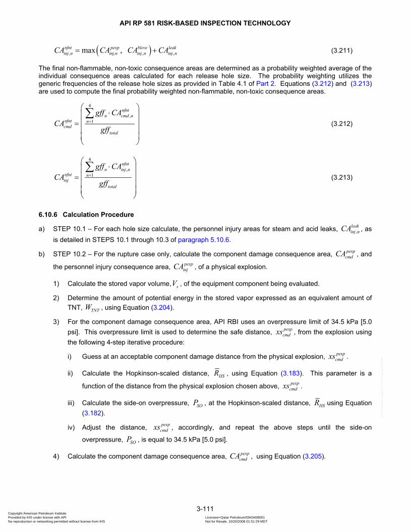
API RP 581 RISK-BASED INSPECTION TECHNOLOGY
3-111
( ), , ,max , nfnt pexp bleve leakinj n inj,n inj n inj nCA CA CA CA= + (3.211)
The final non-flammable, non-toxic consequence areas are determined as a probability weighted average of the individual consequence areas calculated for each release hole size. The probability weighting utilizes the generic frequencies of the release hole sizes as provided in Table 4.1 of Part 2. Equations (3.212) and (3.213) are used to compute the final probability weighted non-flammable, non-toxic consequence areas.
4
,1
nfntn cmd n
nfnt ncmd
total
gff CACA
gff=
⎛ ⎞⋅⎜ ⎟⎜ ⎟=⎜ ⎟⎜ ⎟⎝ ⎠
∑ (3.212)
4
,1
nfntn inj n
nfnt ninj
total
gff CACA
gff=
⎛ ⎞⋅⎜ ⎟⎜ ⎟=⎜ ⎟⎜ ⎟⎝ ⎠
∑ (3.213)
6.10.6 Calculation Procedure
a) STEP 10.1 – For each hole size calculate, the personnel injury areas for steam and acid leaks, ,leakinj nCA , as
is detailed in STEPS 10.1 through 10.3 of paragraph 5.10.6.
b) STEP 10.2 – For the rupture case only, calculate the component damage consequence area, pexpcmdCA , and
the personnel injury consequence area, pexpinjCA , of a physical explosion.
1) Calculate the stored vapor volume, sV , of the equipment component being evaluated.
2) Determine the amount of potential energy in the stored vapor expressed as an equivalent amount of TNT, TNTW , using Equation (3.204).
3) For the component damage consequence area, API RBI uses an overpressure limit of 34.5 kPa [5.0 psi]. This overpressure limit is used to determine the safe distance, pexp
cmdxs , from the explosion using the following 4-step iterative procedure:
i) Guess at an acceptable component damage distance from the physical explosion, pexpcmdxs .
ii) Calculate the Hopkinson-scaled distance, HSR , using Equation (3.183). This parameter is a
function of the distance from the physical explosion chosen above, pexpcmdxs .
iii) Calculate the side-on overpressure, SOP , at the Hopkinson-scaled distance, HSR using Equation (3.182).
iv) Adjust the distance, pexpcmdxs , accordingly, and repeat the above steps until the side-on
overpressure, SOP , is equal to 34.5 kPa [5.0 psi].
4) Calculate the component damage consequence area, pexpcmdCA , using Equation (3.205).
Copyright American Petroleum Institute Provided by IHS under license with API Licensee=Qatar Petroleum/5943408001
Not for Resale, 10/20/2008 01:51:29 MDTNo reproduction or networking permitted without license from IHS
--```,`,,`,`,,`,`,,,,,,``,```,`-`-`,,`,,`,`,,`---
API RP 581 RISK-BASED INSPECTION TECHNOLOGY
3-112
5) For the personnel injury consequence area, API RBI uses a probit equation based on building collapse, see paragraph 6.8.5.5. This probit equation is used to determine the safe distance, pexp
injxs , from the VCE using the following 5-step iterative procedure:
i) Guess at an acceptable personnel injury distance from the VCE, pexpinjxs .
ii) Calculate the Hopkinson-scaled distance, HSR , using Equation (3.183). This parameter is a
function of the distance from the vce chosen above, pexpinjxs .
iii) Calculate the side-on overpressure, SOP , at the Hopkinson-scaled distance, HSR using Equation (3.182).
iv) Calculate the probit value, Pr , using Equation (3.184).
v) Adjust the distance, pexpinjxs , accordingly, and repeat the above steps until the probit value is
equal to 5.0.
6) Calculate the personal injury consequence area, pexpinjCA , using Equation (3.186).
c) STEP 10.3 – For the rupture case only, calculate the component damage consequence area , blevecmdCA , and
the personnel injury consequence area, bleveinjCA , of a BLEVE.
1) Calculate the number of moles of stored liquid that flash to vapor upon release to atmosphere, vn .
2) Determine the amount of potential energy in the flashed liquid expressed as an equivalent mount of TNT, TNTW , using Equation (3.207).
3) For two-phase cases, add to this value the equivalent amount of TNT for the stored vapor energy using Equation (3.204).
4) For the component damage consequence area, API RBI uses an overpressure limit of 5.0 psig. This overpressure limit is used to determine the safe distance, bleve
cmdxs , from the BLEVE using the following 4-step iterative procedure:
i) Guess at an acceptable component damage distance from the BLEVE, blevecmdxs .
ii) Calculate the Hopkinson-scaled distance, HSR , using Equation (3.183). This parameter is a
function of the distance from the BLEVE chosen above, blevecmdxs .
iii) Calculate the side-on overpressure, SOP , at the Hopkinson-scaled distance, HSR using Equation (3.182).
iv) Adjust the distance, blevecmdxs , accordingly, and repeat the above steps until the side-on
overpressure, SOP , is equal to 34.5 kPa [5.0 psi].
5) Calculate the component damage consequence area, blevecmdCA , using Equation (3.208).
6) For the personnel injury consequence area, API RBI uses a probit equation based on building collapse, see paragraph 6.8.5.5. This probit equaiton is used to determine the safe distance, bleve
injxs , from the BLEVE using the following 5-step iterative procedure:
Copyright American Petroleum Institute Provided by IHS under license with API Licensee=Qatar Petroleum/5943408001
Not for Resale, 10/20/2008 01:51:29 MDTNo reproduction or networking permitted without license from IHS
--```,`,,`,`,,`,`,,,,,,``,```,`-`-`,,`,,`,`,,`---
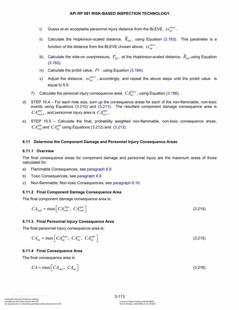
API RP 581 RISK-BASED INSPECTION TECHNOLOGY
3-113
i) Guess at an acceptable personnel injury distance from the BLEVE, bleveinjxs .
ii) Calculate the Hopkinson-scaled distance, HSR , using Equation (3.183). This parameter is a
function of the distance from the BLEVE chosen above, bleveinjxs .
iii) Calculate the side-on overpressure, SOP , at the Hopkinson-scaled distance, HSR using Equation (3.182).
iv) Calculate the probit value, Pr , using Equation (3.184).
v) Adjust the distance, bleveinjxs , accordingly, and repeat the above steps until the probit value is
equal to 5.0.
7) Calculate the personal injury consequence area, bleveinjCA , using Equation (3.186).
d) STEP 10.4 – For each hole size, sum up the consequence areas for each of the non-flammable, non-toxic events using Equations (3.210) and (3.211). The resultant component damage consequence area is
,nfntcmd nCA , and personnel injury area is ,
nfntinj nCA .
e) STEP 10.5 – Calculate the final, probability weighted non-flammable, non-toxic consequence areas, nfntcmdCA and nfnt
injCA using Equations (3.212) and (3.213).
6.11 Determine the Component Damage and Personnel Injury Consequence Areas
6.11.1 Overview
The final consequence areas for component damage and personnel injury are the maximum areas of those calculated for:
a) Flammable Consequences, see paragraph 6.8
b) Toxic Consequences, see paragraph 6.9
c) Non-flammable, Non-toxic Consequences, see paragraph 6.10.
6.11.2 Final Component Damage Consequence Area
The final component damage consequence area is:
max , flam nfntcmd cmd cmdCA CA CA⎡ ⎤= ⎣ ⎦ (3.214)
6.11.3 Final Personnel Injury Consequence Area
The final personnel injury consequence area is:
max , , flam tox nfntinj inj inj injCA CA CA CA⎡ ⎤= ⎣ ⎦ (3.215)
6.11.4 Final Consequence Area
The final consequence area is:
max , cmd injCA CA CA⎡ ⎤= ⎣ ⎦ (3.216)
Copyright American Petroleum Institute Provided by IHS under license with API Licensee=Qatar Petroleum/5943408001
Not for Resale, 10/20/2008 01:51:29 MDTNo reproduction or networking permitted without license from IHS
--```,`,,`,`,,`,`,,,,,,``,```,`-`-`,,`,,`,`,,`---
API RP 581 RISK-BASED INSPECTION TECHNOLOGY
3-114
6.11.5 Calculation Procedure
a) STEP 11.1 – Compute the final component damage consequence area, cmdCA , using Equation (3.214).
b) STEP 11.2 – Compute the final personnel injury consequence area, injCA , using Equation (3.215).
6.12 Determine the Financial Consequence
6.12.1 General
The financial consequence is determined accordance with the Level 1 consequence analysis, see paragraph 5.12.
6.12.2 Calculation Procedure
The step-by-step procedure for estimating the impact of detection and isolation systems is in accordance with paragraph 5.12.2.
Copyright American Petroleum Institute Provided by IHS under license with API Licensee=Qatar Petroleum/5943408001
Not for Resale, 10/20/2008 01:51:29 MDTNo reproduction or networking permitted without license from IHS
--```,`,,`,`,,`,`,,,,,,``,```,`-`-`,,`,,`,`,,`---
API RP 581 RISK-BASED INSPECTION TECHNOLOGY
3-115
6.13 Nomenclature
The following lists the nomenclature used in paragraph 6.0. The coefficients 1C through 36C which provide the metric and U.S conversion factors for the equations are provided in Annex 3.B.
surfα is the thermal diffusivity of the surface under the liquid pool, m2/s [ft2/s]
,pf nAburn is the pool fire area based on burning rate, associated with the thn release hole size, m2 [ft2]
AIT is the auto-ignition temperature of the released fluid, K [°R]
,pf nAmax is the maximum pool fire area based on a pool depth of 5 mm (0.0164 ft), associated with the thn release hole size, m2 [ft2]
,pf nA is the pool fire surface area, associated with the thn release hole size, m2 [ft2]
β is the fraction of combustion power radiated from a flame
fbβ is the fraction of combustion power radiated from a fireball
sBP is the boiling point temperature of the stored fluid at normal operating conditions, K [°R]
CA is the final consequence area, m2 [ft2] blevecmdCA is the component damage consequence area for a BLEVE associated with the rupture cae only,
m2 [ft2] bleveinjCA is the personnel injury consequence area for a BLEVE associated with the rupture cae only, m2
[ft2] fball
cmdCA is the component damage consequence area for a fireball associated with the rupture cae only, m2 [ft2]
fballinjCA is the personnel injury consequence area for a fireball associated with the rupture case only, m2
[ft2]
,flam
cmd nCA is the component damage flammable consequence area associated with the thn release hole size, m2 [ft2]
,flam
inj nCA is the personnel injury flammable consequence area associated with the thn release hole size, m2 [ft2]
flamcmdCA is the final overall component damage flammable consequence area, m2 [ft2] flam
injCA is the final overall personnel injury flammable consequence area, m2 [ft2]
,flash
cmd nCA is the component damage consequence area for a flash fire associated with the thn release hole size, m2 [ft2]
,flash
inj nCA is the personnel injury consequence area for a flash fire associated with the thn release hole size, m2 [ft2]
,jet
cmd nCA is the component damage consequence area for a jet fire associated with the thn release hole size, m2 [ft2]
,jet
inj nCA is the personnel injury consequence area for a jet fire associated with the thn release hole size, m2 [ft2]
,leakinj nCA is the personnel injury non-flammable, non-toxic consequence area for steam or acid leaks,
associated with the thn release hole size, m2 [ft2]
,nfntinj nCA is the personnel injury non-flammable, non-toxic consequence area, associated with the thn
release hole size, m2 [ft2]
Copyright American Petroleum Institute Provided by IHS under license with API Licensee=Qatar Petroleum/5943408001
Not for Resale, 10/20/2008 01:51:29 MDTNo reproduction or networking permitted without license from IHS
--```,`,,`,`,,`,`,,,,,,``,```,`-`-`,,`,,`,`,,`---
API RP 581 RISK-BASED INSPECTION TECHNOLOGY
3-116
nfntcmdCA is the final probability weighted component damage consequence area for non-flammable, non-
toxic releases, m2 [ft2] nfntinjCA is the final probability weighted personnel injury consequence area for non-flammable, non-toxic
releases, m2 [ft2] pexp
cmdCA is the component damage consequence area for a physical explosion associated with the rupture cae only, m2 [ft2]
pexpinjCA is the personnel injury consequence area for a physical explosion associated with the rupture cae
only, m2 [ft2]
,pool
cmd nCA is the component damage consequence area for a pool fire associated with the thn release hole size, m2 [ft2]
,pool
inj nCA is the personnel injury consequence area for a pool fire associated with the thn release hole size, m2 [ft2]
,safecmd nCA is the component damage consequence area for a safe release associated with the thn release
hole size, m2 [ft2]
,safeinj nCA is the personnel injury consequence area for a safe release associated with the thn release hole
size, m2 [ft2] cloudnCA is the footprint at grade level of the portion of the vapor cloud that exceeds the toxic exposure
limit of the toxic component being evaluated, associated with the thn release hole size, m2 [ft2]
,toxinj nCA is the personnel injury toxic consequence area associated with the thn release hole size, m2 [ft2]
toxinjCA is the final overall personnel injury toxic consequence area, m2 [ft2]
,vcecmd nCA is the component damage consequence area for a vapor cloud explosion associated with the thn
release hole size, m2 [ft2]
,vceinj nCA is the personnel injury consequence area for a vapor cloud explosion associated with the thn
release hole size, m2 [ft2]
fbC is the distance from the center of the fireball to the target, m [ft]
lCp is the specific heat of the pool liquid, J/kg-K [Btu/lb-oR]
fbDmax is the maximum diameter of the fireball, m [ft]
nerate is the liquid pool mass evaporation rate associated with the thn release hole size, kg/s [lb/s]
difact is the release magnitude reduction factor, based on the detection and isolations systems present in the unit
fshfrac is the mass fraction of the stored fluid that flashes to vapor upon release to the atmosphere
lfrac is the mass fraction liquid of the stored fluid under storage conditions
vfrac is the mass fraction vapor of the stored fluid under storage conditions
rofrac is the rainout mass fraction
,mole ifrac is the mole fractions for the thi component in the fluid mixture
nFcyl is the radiation view factor for a cylindrical shape, unitless
nFh is the horizontal radiation view factor for a cylindrical shape associated with the thn release hole size, unitless
nFp is the radiation view factor for a point source associated with the thn release hole size, m-2 [ft-2]
Copyright American Petroleum Institute Provided by IHS under license with API Licensee=Qatar Petroleum/5943408001
Not for Resale, 10/20/2008 01:51:29 MDTNo reproduction or networking permitted without license from IHS
--```,`,,`,`,,`,`,,,,,,``,```,`-`-`,,`,,`,`,,`---

API RP 581 RISK-BASED INSPECTION TECHNOLOGY
3-117
Fsph is the view factor for a spherical shape, unitless
nFv is the vertical radiation view factor for a cylindrical shape associated with the thn release hole size, unitless
g is the acceleration due to gravity on earth at sea level = 9.81 m/s2 [32.2 ft/s2]
cg is the gravitational constant = ( ) ( )21.0 kg m N s− − ( ) ( )232.2 m flb ft lb s⎡ ⎤− −⎣ ⎦
ngff are the generic failure frequencies for each of the n release hole sizes selected for the type of equipment being evaluated
totalgff is the sum of the individual release hole size generic frequencies
lHC is the heat of combustion of the liquid fuel for the pool fire calculations, J/kg [Btu/lb]
vHC is the heat of combustion of the vapor fuel for the jet fire calculations, J/kg [Btu/lb]
sHC is the heat of combustion of the stored fluid or mixture, J/kg [Btu/lb]
TNTHC is the heat of combustion of TNT ≈ 2000, J/kg [Btu/lb]
vH∆ is the latent heat of vaporization of the liquid in the pool, J/kg [Btu/lb]
fbH is the center height of the fireball, m [ft] fballIth is the radiant heat flux received at a distant receiver location from a fireball associated with the
rupture case only, W/m2 [Btu/hr-ft2] jet
nIth is the radiant heat flux received at a distant receiver location from a jet fire associated with the thn release hole size, W/m2 [Btu/hr-ft2]
poolnIth is the radiant heat flux received at a distant receiver location from a pool fire associated with the
thn release hole size, W/m2 [Btu/hr-ft2] k is the release fluid ideal gas specific heat capacity ratio, unitless
surfk is the thermal conductivity of the surface for liquid pools, W/m-K [Btu/hr-ft-oR]
nld is the actual leak duration of the flammable release based on the available mass and the
calculated release rate, associated with the thn release hole size, seconds toxnld is the actual leak duration of the toxic release based on the available mass and the calculated
release rate, associated with the thn release hole size, seconds
max,nld is the maximum leak duration associated with the thn release hole size, minutes
,pf nL is the pool fire flame length, associated with the thn release hole size, m [ft]
LFL is the lower flammability limit for the fluid
,avail nmass is the available mass for release for each of the release hole sizes selected, associated with the thn release hole size, kgs [lbs]
fbmass is the flammable mass of the stored liquid used in the fireball calculation, kgs [lbs]
vcemass is the mass of flammable material in the vapor cloud used in the VCE calculation, kgs [lbs]
bm is the burning flux rate of a pool fire fire, kg/m2-s [lb/ft2-s]
,b im is the burning flux rate of a pool fire for the thi component in the fluid mixture in the pool fire, kg/m2-s [lb/ft2-s]
flammfrac is the flammable mass fraction of the released fluid mixture
Copyright American Petroleum Institute Provided by IHS under license with API Licensee=Qatar Petroleum/5943408001
Not for Resale, 10/20/2008 01:51:29 MDTNo reproduction or networking permitted without license from IHS
--```,`,,`,`,,`,`,,,,,,``,```,`-`-`,,`,,`,`,,`---

API RP 581 RISK-BASED INSPECTION TECHNOLOGY
3-118
toxmfrac is the toxic mass fraction of the released fluid mixture toxmolfrac is the toxic mole fraction of the released fluid mixture
MW is the release fluid molecular weight, kg/kg-mol [lb/lb-mol]
vn is the moles that flash from liquid to vapor upon release to atmosphere, kg-mol [lb-mol]
npfball is the probability of a fireball given a release associated with the thn release hole size
,v npfball is the probability of a fireball given a vapor release associated with the thn release hole size
pfbii is the probability of fireball given a immediate ignition of a vapor or two-phase instantaneous release
npflash is the probability of a flash fire given a release associated with the thn release hole size
,v npflash is the probability of a flash fire given a vapor release associated with the thn release hole size
pffdi is the probability of flash fire given a delayed ignition
,l npffdi is the probability of flash fire given a delayed ignition of a release of a flammable liquid
associated with the thn release hole size
,v npffdi is the probability of flash fire given a delayed ignition of a release of a flammable vapor
associated with the thn release hole size
,ambl npoi is the probability of ignition given a liquid release at ambient temperature associated with the thn
release hole size
,ambv npoi is the probability of ignition given a vapor release at ambient temperature associated with the thn
release hole size aitlpoi is the maximum probability of ignition for a liquid release at or above the AIT aitvpoi is the maximum probability of ignition for a vapor release at or above the AIT
poi is the probability of ignition given a release
,l npoi is the probability of ignition given a liquid release associated with the thn release hole size
,v npoi is the probability of ignition given a vapor release associated with the thn release hole size
2,npoi is the probability of ignition given a two-phase release associated with the thn release hole size
poii is the probability of immediate ignition given ignition
,l npoii is the probability of immediate ignition given ignition of a liquid release associated with the thn release hole size
,v npoii is the probability of immediate ignition given ignition of a vapor release associated with the thn release hole size
2,npoii is the probability of immediate ignition given ignition of a two-phase release associated with the thn release hole size
,ambl npoii is the probability of immediate ignition given ignition if a liquid were to be released at ambient
temperature associated with the thn release hole size
,ambv npoii is the probability of immediate ignition given ignition if a vapor were to be released at ambient
temperature associated with the thn release hole size aitpoii is the probability of immediate ignition given ignition if the fluid were to be released at or above its
AIT , assumed = 1.0
Copyright American Petroleum Institute Provided by IHS under license with API Licensee=Qatar Petroleum/5943408001
Not for Resale, 10/20/2008 01:51:29 MDTNo reproduction or networking permitted without license from IHS
--```,`,,`,`,,`,`,,,,,,``,```,`-`-`,,`,,`,`,,`---
API RP 581 RISK-BASED INSPECTION TECHNOLOGY
3-119
npjet is the probability of a jet fire given a release associated with the thn release hole size
,v npjet is the probability of a jet fire given a vapor release associated with the thn release hole size
nppool is the probability of a pool fire given a release associated with the thn release hole size
,l nppool is the probability of a pool fire given a release of a flammable liquid associated with the thn release hole size
,v nppool is the probability of a pool fire given a release of a flammable vapor associated with the thn release hole size
npsafe is the probability of a safe release given a release associated with the thn release hole size
,v npsafe is the probability of a safe release given a vapor release associated with the thn release hole size
2,npsafe is the probability of a safe release given a release of a flammable two-phase fluid associated with
the thn release hole size
nptox is the probability of a toxic release given a release associated with the thn release hole size
npvce is the probability of a vapor cloud explosion given a release associated with the thn release hole size
,v npvce is the probability of a vapor cloud explosion given a vapor release associated with the thn release hole size
pvcedi is the probability of VCE given a delayed ignition
,l npvcedi is the probability of VCE given a delayed ignition of a release of a flammable liquid associated
with the thn release hole size
,v npvcedi is the probability of VCE given a delayed ignition of a release of a flammable vapor associated
with the thn release hole size
,v npvce is the probability of a VCE given a release of a flammable vapor associated with the thn release hole size
,b gP is the bubble-point pressure of the released fluid at the ground temperature, kPa [psia]
BP is the component or equipment burst pressure, kPa [psia]
atmP is the atmospheric pressure, kPa [psia]
Pr is the probit value, typically set at 5 (50% probability)
sP is the storage or normal operating pressure, kPa [psia]
,SO nP is the side-on overpressure associated with the thn release hole size, kPa [psia]
sPsat is the saturation pressure of the stored fluid at operating (storage) temperature, kPa [psia]
wP is the atmospheric water partial pressure, kPa [psia] fballQrad is the total energy flux radiated from a fireball, W/m2 [Btu/hr-m2] jet
nQrad is the total energy radiated from a jet fire associated with the thn release hole size, W [Btu/hr] pool
nQrad is the total energy flux radiated from a pool fire associated with the thn release hole size, W/m2 [Btu/hr-ft2]
,p nr is the pool radius, calculated for each of the n release hole sizes selected, m [ft]
R is the universal gas constant = 8,314 J/(kg-mol)K [1545 ft-lbf/lb-mol°R]
,pf nR is the pool fire radius, calculated for each of the n release hole sizes selected, m [ft]
Copyright American Petroleum Institute Provided by IHS under license with API Licensee=Qatar Petroleum/5943408001
Not for Resale, 10/20/2008 01:51:29 MDTNo reproduction or networking permitted without license from IHS
--```,`,,`,`,,`,`,,,,,,``,```,`-`-`,,`,,`,`,,`---

API RP 581 RISK-BASED INSPECTION TECHNOLOGY
3-120
RH is the atmospheric relative humidity, %
nrate is the adjusted or mitigated discharge rate used in the consequence calculation associated with
the thn release hole size, kg/s [lb/s] flam
nrate is the flammable portion of the adjusted or mitigated discharge rate used in the consequence
calculation associated with the thn release hole size, kg/s [lb/s]
,flam
l nrate is the flammable liquid portion of the adjusted or mitigated discharge rate used in the
consequence calculation associated with the thn release hole size, kg/s [lb/s]
,flam
v nrate is the flammable vapor portion of the adjusted or mitigated discharge rate used in the
consequence calculation associated with the thn release hole size, kg/s [lb/s] toxnrate is the toxic portion of the adjusted or mitigated discharge rate used in the consequence
calculation associated with the thn release hole size, kg/s [lb/s]
,HS nR is the Hopkinson’s scaled distance used in the blast calculations associated with the thn release hole size, m/kg1/3]
atmρ is the atmospheric air density, kg/m3 [lb/ft3]
lρ is the liquid density at storage or normal operating conditions, kg/m3 [lb/ft3]
vρ is the vapor density at storage or normal operating conditions, kg/m3 [lb/ft3]
,pf nθ is the pool fire flame tilt associated with the thn release hole size, radians
atmT is the atmospheric temperature, K [oR]
bT is the bubble pont temperature of released liquid, K [oR]
dT is the dew point temperature of released vapor, K [oR]
fT is the flash temperature of the released fluid, K [oR]
gT is the ground temperature, K [oR]
sT is the storage or normal operating temperature, K [oR]
,p nt is the time it takes for the liquid pool to reach steady state, seconds
fbt is the fireball duration, seconds
limtox is the toxic exposure limit for a toxic component in the released stream (e.g. IDLH, AEGL-3, ERPG), usually expressed in ppm.
modlimtox is the modified toxic exposure limit to account for cloud modeling of mixtures, ppm
atmτ is the atmospheric transmitivity, unitless
,atm nτ is the atmospheric transmitivity associated with the thn release hole size, unitless
UFL is the upper flammability limit for the fluid
,s nu is the non-dimensional wind speed associated with the thn release hole size, unitless
wu is the wind speed measured at 6 feet off of grade, m/s [ft/s]
sV is the equipment stored vapor volume, m3 [ft3]
,p nV is the volumetric vapor rate leaving the pool surface associated with the thn release hole size, m3/s [ft3/s]
nW is the theoretical release rate associated with the thn release hole size, kg/s [lb/s]
Copyright American Petroleum Institute Provided by IHS under license with API Licensee=Qatar Petroleum/5943408001
Not for Resale, 10/20/2008 01:51:29 MDTNo reproduction or networking permitted without license from IHS
--```,`,,`,`,,`,`,,,,,,``,```,`-`-`,,`,,`,`,,`---
API RP 581 RISK-BASED INSPECTION TECHNOLOGY
3-121
jetnW is the portion of the release rate that forms a jet associated with the thn release hole size, kg/s
[lb/s] pool
nW is the portion of the release rate that forms a pool on the ground associated with the thn release hole size, kg/s [lb/s]
TNTW is the energy released in an explosion expressed as and equivalent mass of TNT, kg [lb]
nxs is the safe distance from the flame surface to the target location associated with the thn release hole size, m [ft]
blevecmdxs is the safe distance from a BLEVE for component damage associated with the rupture case only,
m [ft] bleveinjxs is the safe distance from a BLEVE for personnel injury associated with the rupture case only, m
[ft] fballxs is the safe distance from the flame surface of a fireball, m [ft] fball
cmdxs is the safe distance from a fireball for component damage associated with the rupture case only, m [ft]
fballinjxs is the safe distance from a fireball for personnel injury associated with the rupture case only, m [ft] jet
nxs is the safe distance from the jet fire flame surface associated with the thn release hole size, m [ft]
,jet
cmd nxs is the safe distance from the jet fire flame surface for component damage associated with the thn release hole size, m [ft]
,jet
inj nxs is the safe distance from the jet fire flame surface for personnel injury associated with the thn release hole size, m [ft]
poolnxs is the safe distance from the pool fire flame surface associated with the thn release hole size, m
[ft] pexpcmdxs is the safe distance from a physical explosion for component damage associated with the rupture
case only, m [ft] pexp
injxs is the safe distance from a physical explosion for personnel injury associated with the rupture case only, m [ft]
,poolcmd nxs is the safe distance from the pool fire flame surface for component damage associated with the
thn release hole size, m [ft]
,pool
inj nxs is the safe distance from the pool fire flame surface for personnel injury associated with the thn release hole size, m [ft]
vcenxs is the safe distance from the vapor cloud explosion associated with the thn release hole size, m
[ft]
,vcecmd nxs is the safe distance from the vapor cloud explosion for component damage associated with the
thn release hole size, m [ft]
,vceinj nxs is the safe distance from the vapor cloud explosion for personnel injury associated with the thn
release hole size, m [ft] vcenxs is the safe distance from the vapor cloud explosion associated with the thn release hole size, m
[ft]
surfX is the surface roughness factor, unitless η is the explosion yield factor, unitless
Copyright American Petroleum Institute Provided by IHS under license with API Licensee=Qatar Petroleum/5943408001
Not for Resale, 10/20/2008 01:51:29 MDTNo reproduction or networking permitted without license from IHS
--```,`,,`,`,,`,`,,,,,,``,```,`-`-`,,`,,`,`,,`---
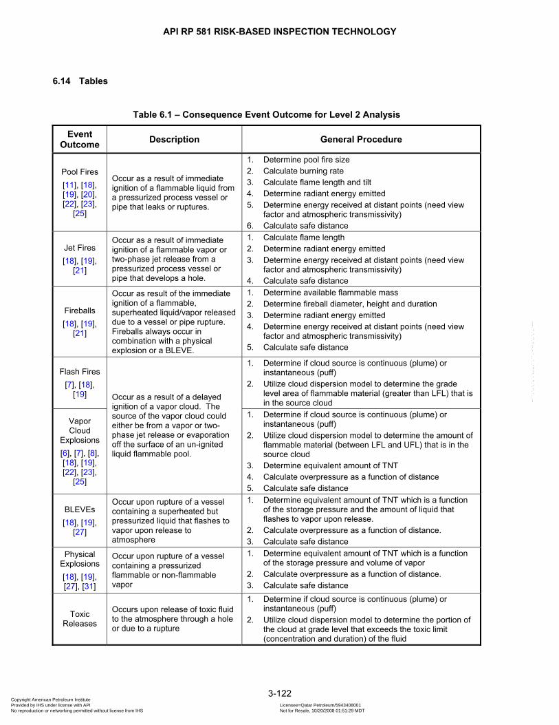
API RP 581 RISK-BASED INSPECTION TECHNOLOGY
3-122
6.14 Tables
Table 6.1 – Consequence Event Outcome for Level 2 Analysis
Event Outcome Description General Procedure
Pool Fires [11], [18], [19], [20], [22], [23],
[25]
Occur as a result of immediate ignition of a flammable liquid from a pressurized process vessel or pipe that leaks or ruptures.
1. Determine pool fire size 2. Calculate burning rate 3. Calculate flame length and tilt 4. Determine radiant energy emitted 5. Determine energy received at distant points (need view
factor and atmospheric transmissivity) 6. Calculate safe distance
Jet Fires [18], [19],
[21]
Occur as a result of immediate ignition of a flammable vapor or two-phase jet release from a pressurized process vessel or pipe that develops a hole.
1. Calculate flame length 2. Determine radiant energy emitted 3. Determine energy received at distant points (need view
factor and atmospheric transmissivity) 4. Calculate safe distance
Fireballs [18], [19],
[21]
Occur as result of the immediate ignition of a flammable, superheated liquid/vapor released due to a vessel or pipe rupture. Fireballs always occur in combination with a physical explosion or a BLEVE.
1. Determine available flammable mass 2. Determine fireball diameter, height and duration 3. Determine radiant energy emitted 4. Determine energy received at distant points (need view
factor and atmospheric transmissivity) 5. Calculate safe distance
Flash Fires [7], [18],
[19]
1. Determine if cloud source is continuous (plume) or instantaneous (puff)
2. Utilize cloud dispersion model to determine the grade level area of flammable material (greater than LFL) that is in the source cloud
Vapor Cloud
Explosions [6], [7], [8], [18], [19], [22], [23],
[25]
Occur as a result of a delayed ignition of a vapor cloud. The source of the vapor cloud could either be from a vapor or two-phase jet release or evaporation off the surface of an un-ignited liquid flammable pool.
1. Determine if cloud source is continuous (plume) or instantaneous (puff)
2. Utilize cloud dispersion model to determine the amount of flammable material (between LFL and UFL) that is in the source cloud
3. Determine equivalent amount of TNT 4. Calculate overpressure as a function of distance 5. Calculate safe distance
BLEVEs [18], [19],
[27]
Occur upon rupture of a vessel containing a superheated but pressurized liquid that flashes to vapor upon release to atmosphere
1. Determine equivalent amount of TNT which is a function of the storage pressure and the amount of liquid that flashes to vapor upon release.
2. Calculate overpressure as a function of distance. 3. Calculate safe distance
Physical Explosions [18], [19], [27], [31]
Occur upon rupture of a vessel containing a pressurized flammable or non-flammable vapor
1. Determine equivalent amount of TNT which is a function of the storage pressure and volume of vapor
2. Calculate overpressure as a function of distance. 3. Calculate safe distance
Toxic Releases
Occurs upon release of toxic fluid to the atmosphere through a hole or due to a rupture
1. Determine if cloud source is continuous (plume) or instantaneous (puff)
2. Utilize cloud dispersion model to determine the portion of the cloud at grade level that exceeds the toxic limit (concentration and duration) of the fluid
Copyright American Petroleum Institute Provided by IHS under license with API Licensee=Qatar Petroleum/5943408001
Not for Resale, 10/20/2008 01:51:29 MDTNo reproduction or networking permitted without license from IHS
--```,`,,`,`,,`,`,,,,,,``,```,`-`-`,,`,,`,`,,`---
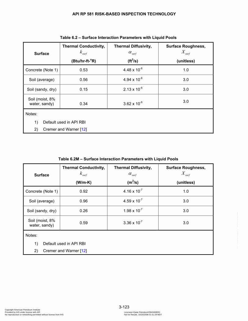
API RP 581 RISK-BASED INSPECTION TECHNOLOGY
3-123
Table 6.2 – Surface Interaction Parameters with Liquid Pools
Surface
Thermal Conductivity, surfk
(Btu/hr-ft-oR)
Thermal Diffusivity, surfα
(ft2/s)
Surface Roughness, surfX
(unitless)
Concrete (Note 1) 0.53 4.48 x 10⁻⁶ 1.0
Soil (average) 0.56 4.94 x 10⁻⁶ 3.0
Soil (sandy, dry) 0.15 2.13 x 10⁻⁶ 3.0
Soil (moist, 8% water, sandy) 0.34 3.62 x 10⁻⁶ 3.0
Notes:
1) Default used in API RBI
2) Cremer and Warner [12]
Table 6.2M – Surface Interaction Parameters with Liquid Pools
Surface
Thermal Conductivity, surfk
(W/m-K)
Thermal Diffusivity, surfα
(m2/s)
Surface Roughness, surfX
(unitless)
Concrete (Note 1) 0.92 4.16 x 10⁻⁷ 1.0
Soil (average) 0.96 4.59 x 10⁻⁷ 3.0
Soil (sandy, dry) 0.26 1.98 x 10⁻⁷ 3.0
Soil (moist, 8% water, sandy) 0.59 3.36 x 10⁻⁷ 3.0
Notes:
1) Default used in API RBI
2) Cremer and Warner [12]
Copyright American Petroleum Institute Provided by IHS under license with API Licensee=Qatar Petroleum/5943408001
Not for Resale, 10/20/2008 01:51:29 MDTNo reproduction or networking permitted without license from IHS
--```,`,,`,`,,`,`,,,,,,``,```,`-`-`,,`,,`,`,,`---

API RP 581 RISK-BASED INSPECTION TECHNOLOGY
3-124
Table 6.3 – Event Probabilities
Probability of Immediate Ignition, Given Ignition
Probability of VCE or Flash Fire, Given Delayed Ignition
Release Type Fluid Phase
At Ambient Temperature
ambnpoii
At AIT
aitpoii
VCE,
,l npvcedi or ,v npvcedi
Flash Fire,
,l npffdi or ,v npffdi
Continuous Liquid 0.80 1.00 0.25 0.75
Continuous Vapor 0.50 1.00 0.50 0.50
Instantaneous Liquid 0.80 1.00 0.125 0.875
Instantaneous Vapor 0.10 1.00 0.25 0.75
Copyright American Petroleum Institute Provided by IHS under license with API Licensee=Qatar Petroleum/5943408001
Not for Resale, 10/20/2008 01:51:29 MDTNo reproduction or networking permitted without license from IHS
--```,`,,`,`,,`,`,,,,,,``,```,`-`-`,,`,,`,`,,`---

API RP 581 RISK-BASED INSPECTION TECHNOLOGY
3-125
6.15 Figures
Figure 6.1 – Source Term Modeling – Thermodynamic Modeling
Copyright American Petroleum Institute Provided by IHS under license with API Licensee=Qatar Petroleum/5943408001
Not for Resale, 10/20/2008 01:51:29 MDTNo reproduction or networking permitted without license from IHS
--```,`,,`,`,,`,`,,,,,,``,```,`-`-`,,`,,`,`,,`---

API RP 581 RISK-BASED INSPECTION TECHNOLOGY
3-126
Figure 6.2 – API RBI Overall Event Tree
Copyright American Petroleum Institute Provided by IHS under license with API Licensee=Qatar Petroleum/5943408001
Not for Resale, 10/20/2008 01:51:29 MDTNo reproduction or networking permitted without license from IHS
--```,`,,`,`,,`,`,,,,,,``,```,`-`-`,,`,,`,`,,`---
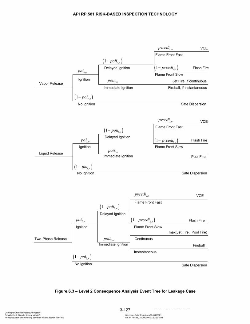
API RP 581 RISK-BASED INSPECTION TECHNOLOGY
3-127
Safe DispersionNo Ignition
Vapor Release
( ),1 v npoi−
,v npoi
Ignition
Flash Fire
Jet Fire, if continuous,v npoii
( ),1 v npoii−
Delayed Ignition
Flame Front Slow
( ),1 v npvcedi−
VCE
Immediate Ignition
Flame Front Fast
Fireball, if instantaneous
Safe DispersionNo Ignition
Liquid Release
( ),1 l npoi−
,l npoiIgnition
Flash Fire
Pool Fire,l npoii
( ),1 l npoii−Delayed Ignition
Flame Front Slow( ),1 l npvcedi−
VCE
Immediate Ignition
Flame Front Fast,l npvcedi
Two-Phase Release
No Ignition
Delayed Ignition
VCE
Flash Fire
Safe Dispersion
( )2,1 npoi−
2,npoi
Ignition
2,npoiiImmediate Ignition
( )2,1 npoii−
2,npvcedi
Flame Front Fast
Flame Front Slow
( )2,1 npvcedi−
max(Jet Fire, Pool Fire)
Fireball
,v npvcedi
Continuous
Instantaneous
Figure 6.3 – Level 2 Consequence Analysis Event Tree for Leakage Case
Copyright American Petroleum Institute Provided by IHS under license with API Licensee=Qatar Petroleum/5943408001
Not for Resale, 10/20/2008 01:51:29 MDTNo reproduction or networking permitted without license from IHS
--```,`,,`,`,,`,`,,,,,,``,```,`-`-`,,`,,`,`,,`---
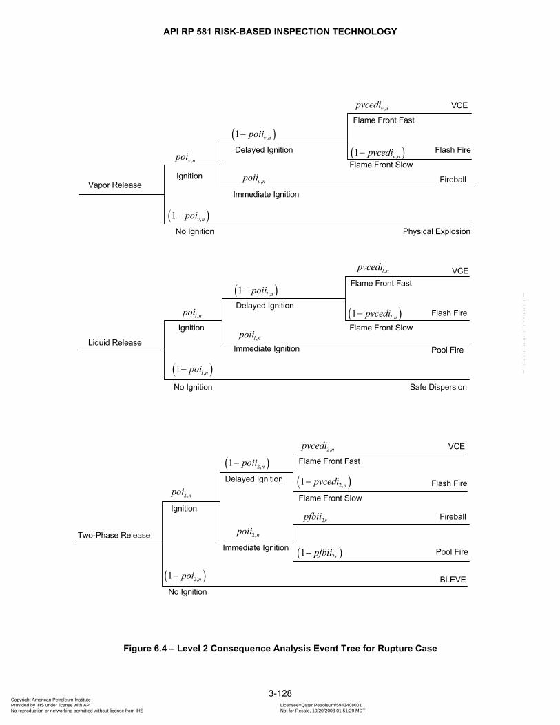
API RP 581 RISK-BASED INSPECTION TECHNOLOGY
3-128
Physical ExplosionNo Ignition
Vapor Release
( ),1 v npoi−
,v npoi
Ignition
Flash Fire
,v npoii
( ),1 v npoii−
Delayed Ignition
Flame Front Slow( ),1 v npvcedi−
VCE
Immediate Ignition
Flame Front Fast
Safe DispersionNo Ignition
Liquid Release
( ),1 l npoi−
,l npoiIgnition
Flash Fire
Pool Fire
( ),1 l npoii−Delayed Ignition
Flame Front Slow( ),1 l npvcedi−
VCE
Immediate Ignition
Flame Front Fast,l npvcedi
Two-Phase Release
No Ignition
Delayed Ignition
VCE
Flash Fire
BLEVE( )2,1 npoi−
2,npoi
Ignition
2,npoiiImmediate Ignition
( )2,1 npoii−2,npvcedi
Flame Front Fast
Flame Front Slow
( )2,1 npvcedi−
Fireball
,v npvcedi
,l npoii
Fireball
2rpfbii
Pool Fire( )21 rpfbii−
Figure 6.4 – Level 2 Consequence Analysis Event Tree for Rupture Case
Copyright American Petroleum Institute Provided by IHS under license with API Licensee=Qatar Petroleum/5943408001
Not for Resale, 10/20/2008 01:51:29 MDTNo reproduction or networking permitted without license from IHS
--```,`,,`,`,,`,`,,,,,,``,```,`-`-`,,`,,`,`,,`---
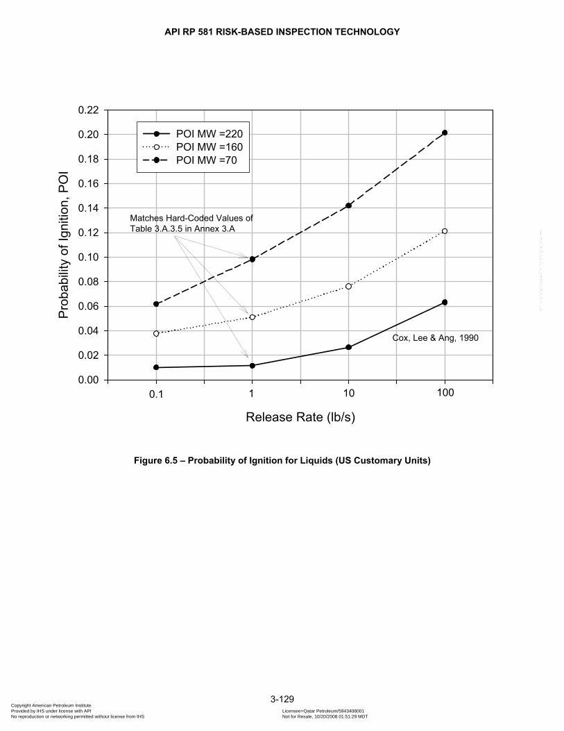
API RP 581 RISK-BASED INSPECTION TECHNOLOGY
3-129
Release Rate (lb/s)
Pro
babi
lity
of Ig
nitio
n, P
OI
0.00
0.02
0.04
0.06
0.08
0.10
0.12
0.14
0.16
0.18
0.20
0.22
POI MW =220POI MW =160POI MW =70
0.1 1 10 100
Cox, Lee & Ang, 1990
Matches Hard-Coded Values ofTable 3.A.3.5 in Annex 3.A
Figure 6.5 – Probability of Ignition for Liquids (US Customary Units)
Copyright American Petroleum Institute Provided by IHS under license with API Licensee=Qatar Petroleum/5943408001
Not for Resale, 10/20/2008 01:51:29 MDTNo reproduction or networking permitted without license from IHS
--```,`,,`,`,,`,`,,,,,,``,```,`-`-`,,`,,`,`,,`---
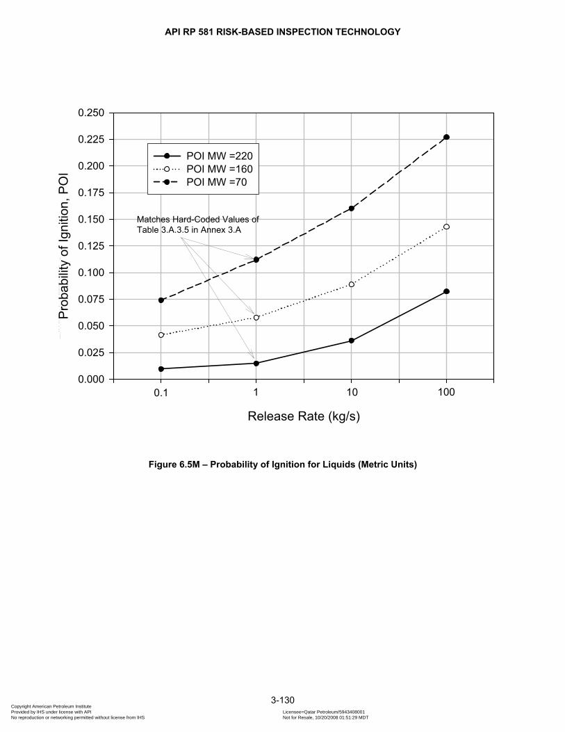
API RP 581 RISK-BASED INSPECTION TECHNOLOGY
3-130
Release Rate (kg/s)
Pro
babi
lity
of Ig
nitio
n, P
OI
0.000
0.025
0.050
0.075
0.100
0.125
0.150
0.175
0.200
0.225
0.250
POI MW =220POI MW =160POI MW =70
0.1 1 10 100
Matches Hard-Coded Values ofTable 3.A.3.5 in Annex 3.A
Figure 6.5M – Probability of Ignition for Liquids (Metric Units)
Copyright American Petroleum Institute Provided by IHS under license with API Licensee=Qatar Petroleum/5943408001
Not for Resale, 10/20/2008 01:51:29 MDTNo reproduction or networking permitted without license from IHS
--```,`,,`,`,,`,`,,,,,,``,```,`-`-`,,`,,`,`,,`---

API RP 581 RISK-BASED INSPECTION TECHNOLOGY
3-131
Release Rate (lb/s)
Pro
babi
lity
of Ig
nitio
n, P
OI
0.00
0.05
0.10
0.15
0.20
0.25
0.30
0.35
0.40
0.45
0.50
POI MW=160POI MW=70POI MW=30
10 1001 0.1
Cox, Lee & Ang, 1990
Matches Hard-Coded Values ofTable 3.A.3.6 in Annex 3.A
Figure 6.6 – Probability of Ignition for Vapors (US Customary Units)
Copyright American Petroleum Institute Provided by IHS under license with API Licensee=Qatar Petroleum/5943408001
Not for Resale, 10/20/2008 01:51:29 MDTNo reproduction or networking permitted without license from IHS
--```,`,,`,`,,`,`,,,,,,``,```,`-`-`,,`,,`,`,,`---

API RP 581 RISK-BASED INSPECTION TECHNOLOGY
3-132
Release Rate (kg/s)
Pro
babi
lity
of Ig
nitio
n, P
OI
0.00
0.05
0.10
0.15
0.20
0.25
0.30
0.35
0.40
0.45
0.50
0.55
0.60
POI MW=160POI MW=70POI MW=30
0.1 1 10 100
Matches Hard-Coded Values ofTable 3.A.3.6 in Annex 3.A
Figure 6.6M – Probability of Ignition for Vapors (Metric Units)
Copyright American Petroleum Institute Provided by IHS under license with API Licensee=Qatar Petroleum/5943408001
Not for Resale, 10/20/2008 01:51:29 MDTNo reproduction or networking permitted without license from IHS
--```,`,,`,`,,`,`,,,,,,``,```,`-`-`,,`,,`,`,,`---
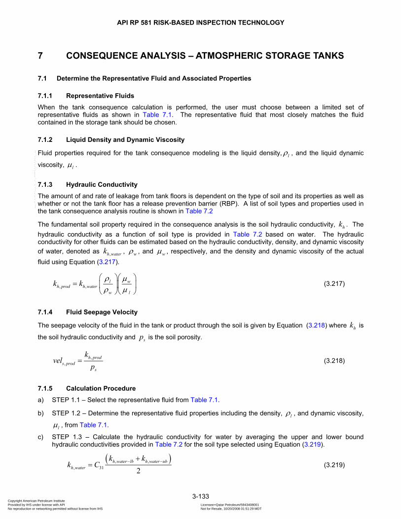
API RP 581 RISK-BASED INSPECTION TECHNOLOGY
3-133
7 CONSEQUENCE ANALYSIS – ATMOSPHERIC STORAGE TANKS
7.1 Determine the Representative Fluid and Associated Properties
7.1.1 Representative Fluids
When the tank consequence calculation is performed, the user must choose between a limited set of representative fluids as shown in Table 7.1. The representative fluid that most closely matches the fluid contained in the storage tank should be chosen.
7.1.2 Liquid Density and Dynamic Viscosity
Fluid properties required for the tank consequence modeling is the liquid density, lρ , and the liquid dynamic
viscosity, lµ .
7.1.3 Hydraulic Conductivity
The amount of and rate of leakage from tank floors is dependent on the type of soil and its properties as well as whether or not the tank floor has a release prevention barrier (RBP). A list of soil types and properties used in the tank consequence analysis routine is shown in Table 7.2
The fundamental soil property required in the consequence analysis is the soil hydraulic conductivity, hk . The hydraulic conductivity as a function of soil type is provided in Table 7.2 based on water. The hydraulic conductivity for other fluids can be estimated based on the hydraulic conductivity, density, and dynamic viscosity of water, denoted as ,h waterk , wρ , and wµ , respectively, and the density and dynamic viscosity of the actual fluid using Equation (3.217).
, ,l w
h prod h waterw l
k k ρ µρ µ
⎛ ⎞⎛ ⎞= ⎜ ⎟⎜ ⎟
⎝ ⎠⎝ ⎠ (3.217)
7.1.4 Fluid Seepage Velocity
The seepage velocity of the fluid in the tank or product through the soil is given by Equation (3.218) where hk is
the soil hydraulic conductivity and sp is the soil porosity.
,,
h prods prod
s
kvel
p= (3.218)
7.1.5 Calculation Procedure
a) STEP 1.1 – Select the representative fluid from Table 7.1.
b) STEP 1.2 – Determine the representative fluid properties including the density, lρ , and dynamic viscosity,
lµ , from Table 7.1.
c) STEP 1.3 – Calculate the hydraulic conductivity for water by averaging the upper and lower bound hydraulic conductivities provided in Table 7.2 for the soil type selected using Equation (3.219).
( ), ,, 31 2
h water lb h water ubh water
k kk C − −+
= (3.219)
Copyright American Petroleum Institute Provided by IHS under license with API Licensee=Qatar Petroleum/5943408001
Not for Resale, 10/20/2008 01:51:29 MDTNo reproduction or networking permitted without license from IHS
--```,`,,`,`,,`,`,,,,,,``,```,`-`-`,,`,,`,`,,`---
API RP 581 RISK-BASED INSPECTION TECHNOLOGY
3-134
d) STEP 1.4 – Calculate the fluid hydraulic conductivity, ,h prodk , for the fluid stored in the tank using Equation
(3.217) based on the density, lρ , and dynamic viscosity, lµ , from STEP 1.2 and the hydraulic conductivity
for water, ,h waterk , from STEP 1.3.
e) STEP 1.5 – Calculate the product seepage velocity, ,s prodvel , for the fluid stored in the tank using Equation
(3.218) based on fluid hydraulic conductivity, ,h prodk , from STEP 1.4 and the soil porosity provided in Table 7.2.
7.2 Release Hole Size Selection
7.2.1 Overview
A discrete set of release events or release hole sizes are used in the Level 1 consequence analysis.
7.2.2 Calculation Procedure
The following calculation procedure may be used to determine the release hole size and the associated generic failure frequencies.
a) STEP 2.1 – Determine the release hole size, nd , from Table 7.3 for tank shell courses and from Table 7.4 for tank bottoms.
b) STEP 2.2 – Determine the generic failure frequency, ngff , for the thn release hole size from Part 2, Table 4.1, and the total generic failure frequency from this table or from Equation (3.220).
4
1tot n
n
gff gff=
= ∑ (3.220)
7.3 Release Rate Calculation
7.3.1 Overview
Release rate calculations are provided for a leak in a tank shell course and a leak in the tank bottom plate. For the leak in the shell course, the liquid head of the product is assumed to be constant in time, and the leak is to atmospheric pressure. For the leak in the tank bottom, the liquid head is assumed to be constant in time, and the leak is into the ground that is modeled as a continuous porous media approximated by soil properties typically used for tank foundations.
7.3.2 Tank Shell Course
The discharge of a liquid through a sharp-edged orifice in a tank with a liquid height above the orifices may be calculated using Equation (3.221).
32 2n d n liqW C C A g h= ⋅ ⋅ ⋅ ⋅ (3.221)
In Equation (3.221), the discharge coefficient, dC , for fully turbulent liquid flow from sharp-edged orifices is in
the range of 0.60 0.65dC≤ ≤ . A value of 0.61dC = is recommended in Level 1 consequence analysis.
Copyright American Petroleum Institute Provided by IHS under license with API Licensee=Qatar Petroleum/5943408001
Not for Resale, 10/20/2008 01:51:29 MDTNo reproduction or networking permitted without license from IHS
--```,`,,`,`,,`,`,,,,,,``,```,`-`-`,,`,,`,`,,`---

API RP 581 RISK-BASED INSPECTION TECHNOLOGY
3-135
7.3.3 Tank Bottom
The product leakage flow rate through a small hole in the tank floor is a function of the soil and fluid properties as well as the liquid head (fill height) above the floor. The flow rate equations can be found in Rowe [34]. The flow rate through a tank bottom into a porous media is calculated using the Bernoulli equation, Equation (3.222), or the Giroud equation, Equation (3.223), based on the hydraulic conductivity, hk , and release hole size, nd .
233 , 342n n liq rh n h nW C d g h n for k C dπ= ⋅ ⋅ ⋅ ⋅ ⋅ > ⋅ (3.222)
0.2 0.9 0.74 235 , 34n qo n liq h rh n h nW C C d h k n for k C d= ⋅ ⋅ ⋅ ⋅ ⋅ ≤ ⋅ (3.223)
In Equation (3.223), the parameter qoC is an adjustment factor for degree of contact with soil and ranges from
0.21qoC = for good contact to 1.15qoC = for poor contact. In the consequence analysis, 0.21qoC = .
If the tank bottom has a release prevention barrier (RBP), then the liquid height, liqh , to be used in the flow rate calculations is set to .0762 m [0.25 ft]. If the tank does not have a release prevention barrier, the liquid height,
liqh , to be used in the flow rate calculations is the actual height of the stored product.
The number of release holes, ,rh nn , for each release hole size is a function of the tank diameter and is shown in Table 7.5.
7.3.4 Calculation Procedure – Tank Shell Course
a) STEP 3.1 – For each release hole size, determine the height of the liquid, liqh , above the release hole size,
nd .
b) STEP 3.2 – For each release hole size, determine the hole area, nA , using Equation (3.224).
2
4n
ndA π
= (3.224)
c) STEP 3.3 – For each release hole size, determine the flow rate, nW , using Equation (3.222) based on liqh
from STEP 3.1 and nA from STEP 3.2.
7.3.5 Calculation Procedure – Tank Bottom
a) STEP 3.1 – For each release hole size, determine the height of the liquid, liqh , above the release hole size,
nd .
b) STEP 3.2 – For each release hole size, determine the number of release holes, ,rh nn , from Table 7.5.
c) STEP 3.3 – Determine the hydraulic conductivity of the stored liquid, hk , from STEP 1.3.
d) STEP 3.4 – For each release hole size, determine the flow rate, nW , using Equation (3.222) or Equation
(3.223), as applicable. The liquid height, liqh , to use in this calculation is determined as follows:
1) The Tank has an RPB – 0.0762 [.25 ]liqh m ft=
Copyright American Petroleum Institute Provided by IHS under license with API Licensee=Qatar Petroleum/5943408001
Not for Resale, 10/20/2008 01:51:29 MDTNo reproduction or networking permitted without license from IHS
--```,`,,`,`,,`,`,,,,,,``,```,`-`-`,,`,,`,`,,`---

API RP 581 RISK-BASED INSPECTION TECHNOLOGY
3-136
2) The Tank does not have an RPB – liqh Actual Product Height=
7.4 Estimate the Inventory Volume Available for Release
7.4.1 Overview
The amount of inventory in the storage tank available for release depends on the component being evaluated. For tank floors the available inventory is the entire contents of the tank. For the tank shell courses, the available inventory is a function of the location of the release hole and is computed as the volume of fluid above the release hole.
7.4.2 Calculation Procedure – Tank Shell Course
The amount of fluid inventory used in the shell course consequence analysis is only the amount of fluid that is above the lower elevation of the course under evaluation.
a) STEP 4.1 – Determine the liquid height above the thi shell course where cN is the total number of shell
courses and CHT is the height of each shell course.
( ), 1above i liqLHT h i CHT⎡ ⎤= − − ⋅⎣ ⎦ (3.225)
b) STEP 4.2 – Determine the volume above the course in question.
2
, ,4tank
above i above iDLvol LHTπ⎛ ⎞
= ⎜ ⎟⎝ ⎠
(3.226)
c) STEP 4.3 – For each release hole size, determine the location of the hole on the tank shell. Based on this location determine the available volume of the release. Note that the release hole should be assumed to be at the bottom of the course.
, ,avail n above iLvol Lvol= (3.227)
d) STEP 4.4 – Calculate the tank volume in barrels using Equation (3.228).
,,
13
avail navail n
LvolBbl
C= (3.228)
7.4.3 Calculation Procedure – Tank Floor
The amount of fluid available for release through tank floors is the fluid level up to the tank design fill height or the operating fill height.
a) STEP 4.1 – Calculate liquid volume in the tank in m3 [ft3] using Equation (3.229).
2
4tank
total liqDLvol hπ⎛ ⎞
= ⋅⎜ ⎟⎝ ⎠
(3.229)
b) STEP 4.2 – Calculate the total tank volume in barrels using Equation (3.230).
13
totaltotal
LvolBblC
= (3.230)
Copyright American Petroleum Institute Provided by IHS under license with API Licensee=Qatar Petroleum/5943408001
Not for Resale, 10/20/2008 01:51:29 MDTNo reproduction or networking permitted without license from IHS
--```,`,,`,`,,`,`,,,,,,``,```,`-`-`,,`,,`,`,,`---
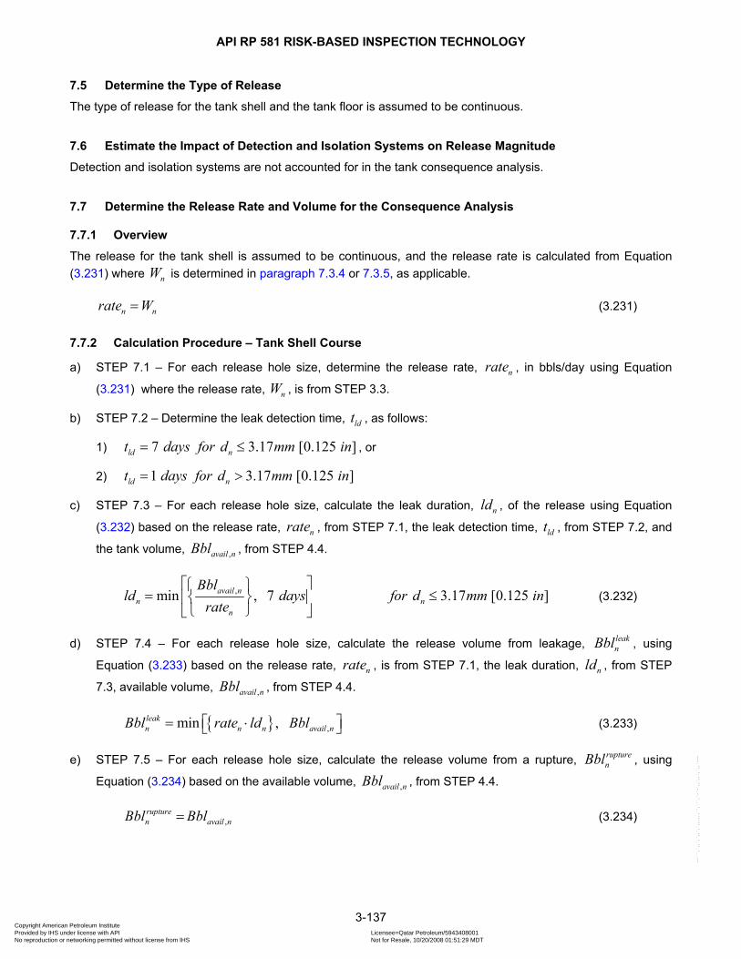
API RP 581 RISK-BASED INSPECTION TECHNOLOGY
3-137
7.5 Determine the Type of Release
The type of release for the tank shell and the tank floor is assumed to be continuous.
7.6 Estimate the Impact of Detection and Isolation Systems on Release Magnitude
Detection and isolation systems are not accounted for in the tank consequence analysis.
7.7 Determine the Release Rate and Volume for the Consequence Analysis
7.7.1 Overview
The release for the tank shell is assumed to be continuous, and the release rate is calculated from Equation (3.231) where nW is determined in paragraph 7.3.4 or 7.3.5, as applicable.
n nrate W= (3.231)
7.7.2 Calculation Procedure – Tank Shell Course
a) STEP 7.1 – For each release hole size, determine the release rate, nrate , in bbls/day using Equation
(3.231) where the release rate, nW , is from STEP 3.3.
b) STEP 7.2 – Determine the leak detection time, ldt , as follows:
1) 7 3.17 [0.125 ]ld nt days for d mm in= ≤ , or
2) 1 3.17 [0.125 ]ld nt days for d mm in= >
c) STEP 7.3 – For each release hole size, calculate the leak duration, nld , of the release using Equation
(3.232) based on the release rate, nrate , from STEP 7.1, the leak detection time, ldt , from STEP 7.2, and
the tank volume, ,avail nBbl , from STEP 4.4.
,min , 7 3.17 [0.125 ]avail nn n
n
Bblld days for d mm in
rate⎡ ⎤⎧ ⎫
= ≤⎨ ⎬⎢ ⎥⎩ ⎭⎣ ⎦
(3.232)
d) STEP 7.4 – For each release hole size, calculate the release volume from leakage, leaknBbl , using
Equation (3.233) based on the release rate, nrate , is from STEP 7.1, the leak duration, nld , from STEP
7.3, available volume, ,avail nBbl , from STEP 4.4.
,min ,leakn n n avail nBbl rate ld Bbl⎡ ⎤= ⋅⎣ ⎦ (3.233)
e) STEP 7.5 – For each release hole size, calculate the release volume from a rupture, rupturenBbl , using
Equation (3.234) based on the available volume, ,avail nBbl , from STEP 4.4.
,rupturen avail nBbl Bbl= (3.234)
Copyright American Petroleum Institute Provided by IHS under license with API Licensee=Qatar Petroleum/5943408001
Not for Resale, 10/20/2008 01:51:29 MDTNo reproduction or networking permitted without license from IHS
--```,`,,`,`,,`,`,,,,,,``,```,`-`-`,,`,,`,`,,`---

API RP 581 RISK-BASED INSPECTION TECHNOLOGY
3-138
7.7.3 Calculation Procedure – Tank Bottom
a) STEP 7.1 – For each release hole size, determine the release rate, nrate , using Equation (3.231) where
the release rate, nW , is from STEP 3.5.
b) STEP 7.2 – Determine the leak detection time, ldt , as follows:
1) 7ldt days= for a tank on a concrete or asphalt foundation, or
2) 30ldt days= for a tank with a release prevention barrier, or
3) 360ldt days= for a tank without a release prevention barrier.
c) STEP 7.3 – For each release hole size, calculate the leak duration, nld , of the release using Equation
(3.235) based on the release rate, nrate , from STEP 7.1, the leak detection time, ldt , from STEP 7.2, and
the total volume, totalBbl , from STEP 4.2
min ,totaln ld
n
Bblld trate
⎡ ⎤⎧ ⎫= ⎨ ⎬⎢ ⎥
⎩ ⎭⎣ ⎦ (3.235)
d) STEP 7.4 – For each release hole size, calculate the release volume from leakage, leaknBbl , using
Equation (3.236) based on the release rate, nrate , from STEP 7.1, the leak duration, nld , from STEP 7.3,
and the total volume, totalBbl , from STEP 4.2.
,min ,leakn n n avail nBbl rate ld Bbl⎡ ⎤= ⋅⎣ ⎦ (3.236)
e) STEP 7.5 – For each release hole size, calculate the release volume from a rupture, rupturenBbl , using
Equation (3.237) based on the total volume, totalBbl , from STEP 4.2.
rupturen totalBbl Bbl= (3.237)
7.8 Determine Flammable and Explosive Consequences
Flammable and explosive consequences are not included in the consequence analysis for atmospheric storage tanks.
7.9 Determine Toxic Consequences
Toxic consequences are not included in the consequence analysis for atmospheric storage tanks.
7.10 Determine Non-Flammable Non-toxic Consequences
Non-flammable non-toxic consequences are not included in the consequence analysis for atmospheric storage tanks.
Copyright American Petroleum Institute Provided by IHS under license with API Licensee=Qatar Petroleum/5943408001
Not for Resale, 10/20/2008 01:51:29 MDTNo reproduction or networking permitted without license from IHS
--```,`,,`,`,,`,`,,,,,,``,```,`-`-`,,`,,`,`,,`---
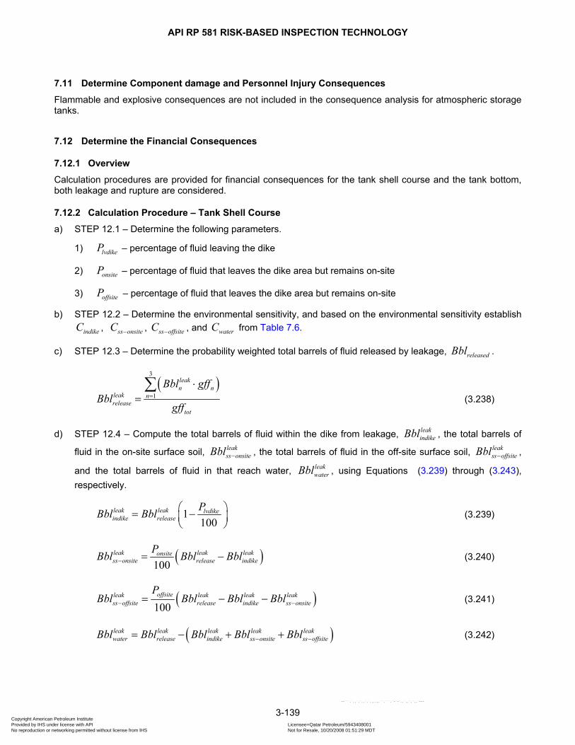
API RP 581 RISK-BASED INSPECTION TECHNOLOGY
3-139
7.11 Determine Component damage and Personnel Injury Consequences
Flammable and explosive consequences are not included in the consequence analysis for atmospheric storage tanks.
7.12 Determine the Financial Consequences
7.12.1 Overview
Calculation procedures are provided for financial consequences for the tank shell course and the tank bottom, both leakage and rupture are considered.
7.12.2 Calculation Procedure – Tank Shell Course
a) STEP 12.1 – Determine the following parameters.
1) lvdikeP – percentage of fluid leaving the dike
2) onsiteP – percentage of fluid that leaves the dike area but remains on-site
3) offsiteP – percentage of fluid that leaves the dike area but remains on-site
b) STEP 12.2 – Determine the environmental sensitivity, and based on the environmental sensitivity establish
indikeC , ss onsiteC − , ss offsiteC − , and waterC from Table 7.6.
c) STEP 12.3 – Determine the probability weighted total barrels of fluid released by leakage, releasedBbl .
( )3
1
leakn n
leak nrelease
tot
Bbl gffBbl
gff=
⋅=∑
(3.238)
d) STEP 12.4 – Compute the total barrels of fluid within the dike from leakage, leakindikeBbl , the total barrels of
fluid in the on-site surface soil, leakss onsiteBbl − , the total barrels of fluid in the off-site surface soil, leak
ss offsiteBbl − ,
and the total barrels of fluid in that reach water, leakwaterBbl , using Equations (3.239) through (3.243),
respectively.
1100
leak leak lvdikeindike release
PBbl Bbl ⎛ ⎞= −⎜ ⎟⎝ ⎠
(3.239)
( )100leak leak leakonsitess onsite release indike
PBbl Bbl Bbl− = − (3.240)
( )100offsiteleak leak leak leak
ss offsite release indike ss onsite
PBbl Bbl Bbl Bbl− −= − − (3.241)
( )leak leak leak leak leakwater release indike ss onsite ss offsiteBbl Bbl Bbl Bbl Bbl− −= − + + (3.242)
Copyright American Petroleum Institute Provided by IHS under license with API Licensee=Qatar Petroleum/5943408001
Not for Resale, 10/20/2008 01:51:29 MDTNo reproduction or networking permitted without license from IHS
--```,`,,`,`,,`,`,,,,,,``,```,`-`-`,,`,,`,`,,`---
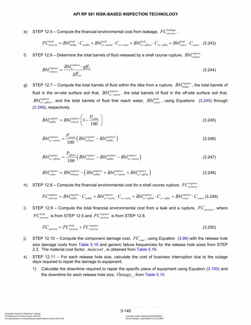
API RP 581 RISK-BASED INSPECTION TECHNOLOGY
3-140
e) STEP 12.5 – Compute the financial environmental cost from leakage, leakageenvironFC .
leak leak leak leak leakenviron indike indike ss onsite ss onite ss offsite ss offite water waterFC Bbl C Bbl C Bbl C Bbl C− − − −= ⋅ + ⋅ + ⋅ + ⋅ (3.243)
f) STEP 12.6 – Determine the total barrels of fluid released by a shell course rupture, rupturereleaseBbl .
4rupture
rupture nrelease
tot
Bbl gffBblgff
⋅= (3.244)
g) STEP 12.7 – Compute the total barrels of fluid within the dike from a rupture, ruptureindikeBbl , the total barrels of
fluid in the on-site surface soil that, rupturess onsiteBbl − , the total barrels of fluid in the off-site surface soil that,
rupturess offsiteBbl − , and the total barrels of fluid that reach water, leak
waterBbl , using Equations (3.245) through (3.248), respectively.
1100
rupture rupture lvdikeindike release
PBbl Bbl ⎛ ⎞= −⎜ ⎟⎝ ⎠
(3.245)
( )100rupture rupture ruptureonsitess onsite release indike
PBbl Bbl Bbl− = − (3.246)
( )100offsiterupture rupture rupture rupture
ss offsite release indike ss onsite
PBbl Bbl Bbl Bbl− −= − − (3.247)
( )rupture rupture rupture rupture rupturewater release indike ss onsite ss offsiteBbl Bbl Bbl Bbl Bbl− −= − + + (3.248)
h) STEP 12.8 – Compute the financial environmental cost for a shell course rupture, ruptureenvironFC .
rupture rupture rupture rupture ruptureenviron indike indike ss onsite ss onite ss offsite ss offite water waterFC Bbl C Bbl C Bbl C Bbl C− − − −= ⋅ + ⋅ + ⋅ + ⋅ (3.249)
i) STEP 12.9 – Compute the total financial environmental cost from a leak and a rupture, environFC , where leakenvironFC is from STEP 12.5 and rupture
environFC is from STEP 12.8.
leak ruptureenviron environ environFC FC FC= + (3.250)
j) STEP 12.10 – Compute the component damage cost, cmdFC , using Equation (3.98) with the release hole size damage costs from Table 5.15 and generic failure frequencies for the release hole sizes from STEP 2.3. The material cost factor, matcost , is obtained from Table 5.16.
k) STEP 12.11 – For each release hole size, calculate the cost of business interruption due to the outage days required to repair the damage to equipment.
1) Calculate the downtime required to repair the specific piece of equipment using Equation (3.100) and the downtime for each release hole size, nOutage , from Table 5.15.
Copyright American Petroleum Institute Provided by IHS under license with API Licensee=Qatar Petroleum/5943408001
Not for Resale, 10/20/2008 01:51:29 MDTNo reproduction or networking permitted without license from IHS
--```,`,,`,`,,`,`,,,,,,``,```,`-`-`,,`,,`,`,,`---
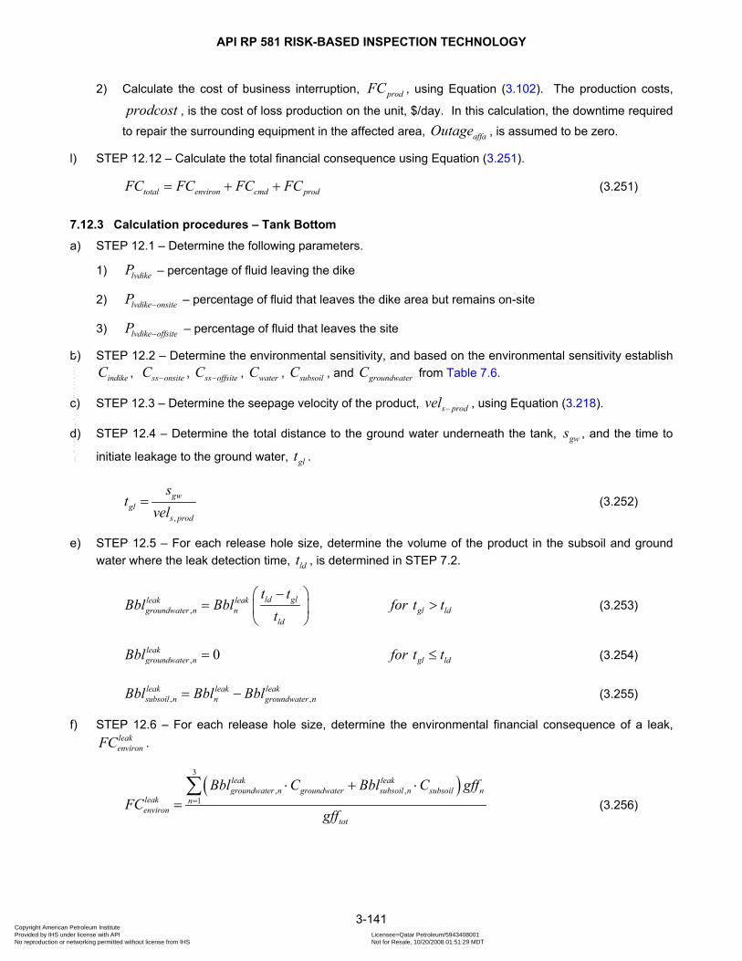
API RP 581 RISK-BASED INSPECTION TECHNOLOGY
3-141
2) Calculate the cost of business interruption, prodFC , using Equation (3.102). The production costs,
prodcost , is the cost of loss production on the unit, $/day. In this calculation, the downtime required
to repair the surrounding equipment in the affected area, affaOutage , is assumed to be zero.
l) STEP 12.12 – Calculate the total financial consequence using Equation (3.251).
total environ cmd prodFC FC FC FC= + + (3.251)
7.12.3 Calculation procedures – Tank Bottom
a) STEP 12.1 – Determine the following parameters.
1) lvdikeP – percentage of fluid leaving the dike
2) lvdike onsiteP − – percentage of fluid that leaves the dike area but remains on-site
3) lvdike offsiteP − – percentage of fluid that leaves the site
b) STEP 12.2 – Determine the environmental sensitivity, and based on the environmental sensitivity establish
indikeC , ss onsiteC − , ss offsiteC − , waterC , subsoilC , and groundwaterC from Table 7.6.
c) STEP 12.3 – Determine the seepage velocity of the product, s prodvel − , using Equation (3.218).
d) STEP 12.4 – Determine the total distance to the ground water underneath the tank, gws , and the time to
initiate leakage to the ground water, glt .
,
gwgl
s prod
st
vel= (3.252)
e) STEP 12.5 – For each release hole size, determine the volume of the product in the subsoil and ground water where the leak detection time, ldt , is determined in STEP 7.2.
,ld glleak leak
groundwater n n gl ldld
t tBbl Bbl for t t
t−⎛ ⎞
= >⎜ ⎟⎝ ⎠
(3.253)
, 0leakgroundwater n gl ldBbl for t t= ≤ (3.254)
, ,leak leak leaksubsoil n n groundwater nBbl Bbl Bbl= − (3.255)
f) STEP 12.6 – For each release hole size, determine the environmental financial consequence of a leak, leakenvironFC .
( )3
, ,1
leak leakgroundwater n groundwater subsoil n subsoil n
leak nenviron
tot
Bbl C Bbl C gffFC
gff=
⋅ + ⋅=∑
(3.256)
Copyright American Petroleum Institute Provided by IHS under license with API Licensee=Qatar Petroleum/5943408001
Not for Resale, 10/20/2008 01:51:29 MDTNo reproduction or networking permitted without license from IHS
--```,`,,`,`,,`,`,,,,,,``,```,`-`-`,,`,,`,`,,`---

API RP 581 RISK-BASED INSPECTION TECHNOLOGY
3-142
g) STEP 12.7 – Determine the total barrels of fluid released by a tank bottom rupture, rupturereleaseBbl .
4rupture totalrelease
tot
Bbl gffBblgff
⋅= (3.257)
h) STEP 12.8 – Compute the total barrels of fluid within the dike from a rupture, ruptureindikeBbl , the total barrels of
fluid in the on-site surface soil, rupturess onsiteBbl − , the total barrels of fluid in the off-site surface soil, rupture
ss offsiteBbl − ,
and the total barrels of fluid that reach water, leakwaterBbl , using Equations (3.245) through (3.248),
respectively.
i) STEP 12.9 – Compute the financial environmental cost for a tank bottom rupture, ruptureenvironFC , using Equation
(3.249) where ruptureindikeBbl , rupture
ss onsiteBbl − , rupturess offsiteBbl − , and leak
waterBbl are from STEP 12.8.
j) STEP 12.10 – Compute the total financial environmental cost from a leak and a rupture, environFC , using
Equation (3.250) where leakenvironFC is from STEP 12.6 and rupture
environFC is from STEP 12.8.
k) STEP 12.11 – Compute the component damage cost, cmdFC , using Equation (3.258) with the release hole size damage costs from Table 5.15 and generic failure frequencies for the release hole sizes from STEP 2.3. The material cost factor, matcost , is obtained from Table 5.16.
23
1 36
tankn n 4
ncmd
total
Dgff holecost holecostC
FC matcostgff
=
⎛ ⎞⎛ ⎞⎜ ⎟⋅ + ⎜ ⎟⎜ ⎟⎝ ⎠= ⋅⎜ ⎟⎜ ⎟⎜ ⎟⎝ ⎠
∑ (3.258)
The parameter, ( )236tankD C , is a cost adjustment factor for a tank bottom replacement. The cost factor
included in Table 5.15 is normalized for a tank with a diameter of 30.5 m [100 ft], and this factor corrects the cost for other tank diameters.
l) STEP 12.12 – For each release hole size, calculate the cost of business interruption due to the outage days required to repair the damage to equipment.
1) Calculate the downtime required to repair the specific piece of equipment using Equation (3.100) and the downtime for each release hole size, nOutage , from Table 5.17.
2) Calculate the cost of business interruption, prodFC , using Equation (3.102). The production costs,
prodcost , is the cost of loss production on the unit, $/day. Note that in this calculation, the downtime
required to repair the surrounding equipment in the affected area, affaOutage , is assumed to be zero.
m) STEP 12.13 – Calculate the total financial consequence using Equation (3.259).
total environ cmd prodFC FC FC FC= + + (3.259)
Copyright American Petroleum Institute Provided by IHS under license with API Licensee=Qatar Petroleum/5943408001
Not for Resale, 10/20/2008 01:51:29 MDTNo reproduction or networking permitted without license from IHS
--```,`,,`,`,,`,`,,,,,,``,```,`-`-`,,`,,`,`,,`---
API RP 581 RISK-BASED INSPECTION TECHNOLOGY
3-143
7.13 Nomenclature
The following lists the nomenclature used in paragraph 7.0. The coefficients 1C through 36C which provide the metric and U.S conversion factors for the equations are provided in Annex 3.B.
nA is the hole area associated with the thn release hole size, mm2 [in2]
totalBbl is the product volume in the tank, barrels
,avail nBbl is the available product volume for the thn release hole size due to a leak, barrels
,leakgroundwater nBbl is the product volume for the thn release hole size due to a leak in the groundwater, barrels
,leaksubsoil nBbl is the product volume for the thn release hole size due to a leak in the subsoil, barrels leaknBbl is the product volume for the thn release hole size due to a leak, barrels leakgroundwaterBbl is the total product volume in the groundwater due to a leak, barrels leakindikeBbl is the total product volume in the dike due to a leak, barrels leakreleaseBbl is the total product volume released due to a leak, barrels leakssoffsiteBbl is the total product volume released on the surface located on-site due to a leak, barrels leakssonsiteBbl is the total product volume released on the surface located off-site due to a leak, barrels leaksubsoilBbl is the total product volume in the subsoil due to a leak, barrels leakwaterBbl is the total product volume in the water due to a leak, barrels rupturenBbl is the product volume for the thn release hole size due to a rupture, barrels ruptureindikeBbl is the product volume in the dike due to a rupture, barrels rupturereleaseBbl is the product volume in released due to a rupture, barrels rupturessonsiteBbl is the product volume on the surface located on-site due to a rupture, barrels rupturessoffsiteBbl is the product volume on the surface located off-site due to a rupture, barrels rupturewaterBbl is the total product volume in the water due to a rupture, barrels
CHT is the course height of the tank, m [ft]
dC is the discharge coefficient
indikeC is the environmental cost for product in the dike area, $/bbl
ss onsiteC − is the environmental cost for product on the surface located on-site, $/bbl
ss offsiteC − is the environmental cost for product on the surface located off-site, $/bbl
waterC is the environmental cost for product in water, $/bbl
subsoilC is the environmental cost for product in the subsoil, $/bbl
groundwaterC is the environmental cost for product in the groundwater, $/bbl
qoC is the adjustment factor for degree of contact with soil
nd is the diameter of the thn release hole, mm [in]
tankD is the tank diameter, m [ft]
environFC is the financial consequence of environmental clean-up, $
cmdFC is the financial consequence of component damage, $
Copyright American Petroleum Institute Provided by IHS under license with API Licensee=Qatar Petroleum/5943408001
Not for Resale, 10/20/2008 01:51:29 MDTNo reproduction or networking permitted without license from IHS
--```,`,,`,`,,`,`,,,,,,``,```,`-`-`,,`,,`,`,,`---

API RP 581 RISK-BASED INSPECTION TECHNOLOGY
3-144
prodFC is the financial consequence of lost production on the unit, $
totalFC is the total financial consequence, $ leakenvironFC is the financial consequence of environmental cleanup for leakage, $ ruptureenvironFC is the financial consequence of environmental cleanup for leakage, $
g is the acceleration due to gravity on earth at sea level = 9.81 m/s2 [32.2 ft/s2]
ngff are the generic failure frequencies for each of the n release hole sizes selected for the type of equipment being evaluated
totalgff is the sum of the individual release hole size generic frequencies
liqh is the maximum fill height in the tank, m [ft]
hk is the soil hydraulic conductivity, m/day [ft/day]
,h prodk is the soil hydraulic conductivity based on the tank product, m/day [ft/day]
,h waterk is the soil hydraulic conductivity based on water, m/day [ft/day]
,h water lbk − is the lower bound soil hydraulic conductivity based on water, cm/s [in/s]
,h water ubk − is the upper bound soil hydraulic conductivity based on water, cm/s [in/s]
nld is the actual leak duration of the release based on the available mass and the calculated release
rate, associated with the thn release hole size, day
,above nLvol is the total liquid volume for the thn release hole size, m3 [ft3]
,avail nLvol is the available liquid volume for the thn release hole size, m3 [ft3]
,above iLvol is the total liquid volume above the thi tank shell course, m3 [ft3]
totalLvol is the total liquid volume in the tank, m3 [ft3]
,above iLHT is the liquid height above the thi tank shell course, m [ft] matcost is the material cost factor
cN is the total number of tank shell courses
lµ is the dynamic viscosity, N-s/m2 [lbf-s/ft2]
affaOutage is the numbers of days of downtime required to repair damage to the surrounding equipment, days
nOutage is the number of downtime days to repair damage associated with the thn release hole size, days
sp is the soil porosity
lvdikeP is the percentage of fluid leaving the dike
onsiteP is the percentage of fluid that leaves the dike area but remains on-site
offsiteP is the percentage of fluid that leaves the dike area but remains off-site
lρ is the liquid density at storage or normal operating conditions, kg/m3 [lb/ft3]
wρ is the density of water at storage or normal operating conditions, kg/m3 [lb/ft3]
nrate is the adjusted or mitigated discharge rate used in the consequence calculation associated with
the thn release hole size, bbl/day
gws is the distance to the groundwater underneath the tank, m [ft]
Copyright American Petroleum Institute Provided by IHS under license with API Licensee=Qatar Petroleum/5943408001
Not for Resale, 10/20/2008 01:51:29 MDTNo reproduction or networking permitted without license from IHS
--```,`,,`,`,,`,`,,,,,,``,```,`-`-`,,`,,`,`,,`---

API RP 581 RISK-BASED INSPECTION TECHNOLOGY
3-145
glt is the time required for the product to reach the groundwater through a leak in the tank bottom, day
ldt is the leak detection time, day
,s prodvel is the seepage velocity, m/day [ft/day]
nW is the discharge rate of the tank product through a hole in the shell course, bbl/day
Copyright American Petroleum Institute Provided by IHS under license with API Licensee=Qatar Petroleum/5943408001
Not for Resale, 10/20/2008 01:51:29 MDTNo reproduction or networking permitted without license from IHS
--```,`,,`,`,,`,`,,,,,,``,```,`-`-`,,`,,`,`,,`---
API RP 581 RISK-BASED INSPECTION TECHNOLOGY
3-146
7.14 Tables
Table 7.1 – Fluids and Fluid Properties for Atmospheric Storage Tank Consequence Analysis
Fluid
Level 1 Consequence
Analysis Representative
Fluid
Molecular Weight Liquid Density
(lb/ft3)
Liquid Dynamic Viscosity
(lbf-s/ft2)
Gasoline C6-C8 100 42.702 8.383E-5
Light Diesel Oil C9-C12 149 45.823 2.169E-5
Heavy Diesel Oil C13-C16 205 47.728 5.129E-5
Fuel Oil C17-C25 280 48.383 7.706E-4
Crude Oil C17-C25 280 48.383 7.706E-4
Heavy Fuel Oil C25+ 422 56.187 9.600E-4
Heavy Crude Oil C25+ 422 56.187 9.600E-4
Table 7.1M – Fluids and Fluid Properties for Atmospheric Storage Tank Consequence Analysis
Fluid
Level 1 Consequence
Analysis Representative
Fluid
Molecular Weight Liquid Density
(kg/m3)
Liquid Dynamic Viscosity
(N-s/m2)
Gasoline C6-C8 100 684.018 4.01E-3
Light Diesel Oil C9-C12 149 734.011 1.04E-3
Heavy Diesel Oil C13-C16 205 764.527 2.46E-3
Fuel Oil C17-C25 280 775.019 3.69E-2
Crude Oil C17-C25 280 775.019 3.69E-2
Heavy Fuel Oil C25+ 422 900.026 4.60E-2
Heavy Crude Oil C25+ 422 900.026 4.60E-2
Copyright American Petroleum Institute Provided by IHS under license with API Licensee=Qatar Petroleum/5943408001
Not for Resale, 10/20/2008 01:51:29 MDTNo reproduction or networking permitted without license from IHS
--```,`,,`,`,,`,`,,,,,,``,```,`-`-`,,`,,`,`,,`---

API RP 581 RISK-BASED INSPECTION TECHNOLOGY
3-147
Table 7.2 – Soil Types and Properties for Atmospheric Storage Tank Consequence Analysis
Soil Type
Hydraulic Conductivity for Water
Lower Bound
(in/s)
Hydraulic Conductivity for Water
Upper Bound
(in/s)
Soil Porosity
Coarse Sand 3.94E-2 3.94E-3 0.33
Fine Sand 3.94E-3 3.94E-4 0.33
Very Fine Sand 3.94E-4 3.94E-6 0.33
Silt 3.94E-6 3.94E-7 0.41
Sandy Clay 3.94E-7 3.94E-8 0.45
Clay 3.94E-8 3.94E-9 0.50
Concrete-Asphalt 3.94E-11 3.94E-12 0.99
Table 7.2M – Soil Types and Properties for Atmospheric Storage Tank Consequence Analysis
Soil Type
Hydraulic Conductivity for Water
Lower Bound
(cm/s)
Hydraulic Conductivity for Water
Upper Bound
(cm/s)
Soil Porosity
Coarse Sand 1E-1 1E-2 0.33
Fine Sand 1E-2 1E-3 0.33
Very Fine Sand 1E-3 1E-5 0.33
Silt 1E-5 1E-6 0.41
Sandy Clay 1E-6 1E-7 0.45
Clay 1E-7 1E-8 0.50
Concrete-Asphalt 1E-10 1E-11 0.99
Copyright American Petroleum Institute Provided by IHS under license with API Licensee=Qatar Petroleum/5943408001
Not for Resale, 10/20/2008 01:51:29 MDTNo reproduction or networking permitted without license from IHS
--```,`,,`,`,,`,`,,,,,,``,```,`-`-`,,`,,`,`,,`---
API RP 581 RISK-BASED INSPECTION TECHNOLOGY
3-148
Table 7.3 – Release Hole Sizes and Areas – Tank Shell Courses
Release Hole Number
Release Hole Size
Range of Hole Diameters
(in)
Release Hole Diameter
(in)
1 Small 0 – 1/8 1 0.125d =
2 Medium > 1/8 – ¼ 2 0.5d =
3 Large > ¼ – 2 3 2d =
4 Rupture > 2 4 124tankDd ⎛ ⎞= ⎜ ⎟
⎝ ⎠
Table 7.3M – Release Hole Sizes and Areas – Tank Shell Courses
Release Hole Number
Release Hole Size
Range of Hole Diameters
(mm)
Release Hole Diameter
(mm)
1 Small 0 – 3.175 1 3.175d =
2 Medium > 3.175 – 6.35 2 6.35d =
3 Large > 6.35 – 50.8 3 50.8d =
4 Rupture > 50.8 4 10004tankDd ⎛ ⎞= ⎜ ⎟
⎝ ⎠
Copyright American Petroleum Institute Provided by IHS under license with API Licensee=Qatar Petroleum/5943408001
Not for Resale, 10/20/2008 01:51:29 MDTNo reproduction or networking permitted without license from IHS
--```,`,,`,`,,`,`,,,,,,``,```,`-`-`,,`,,`,`,,`---
API RP 581 RISK-BASED INSPECTION TECHNOLOGY
3-149
Table 7.4 – Release Hole Sizes and Areas – Tank Bottoms
Release Hole Number
Release Hole Size
Release Prevention
Barrier?
Range of Hole Diameters
(in)
Release Hole Diameter
(in)
Yes 0 – 1/8 1 0.125d = 1 Small
No 0 – 1/2 1 0.50d =
NA 0 2 Medium
NA 0 2 0d =
NA 0 3 Large
NA 0 3 0d =
Yes > 1/8 4 Rupture
No > 1/2 4 12
4tankDd ⎛ ⎞= ⎜ ⎟
⎝ ⎠
Table 7.4M – Release Hole Sizes and Areas – Tank Bottoms
Release Hole Number
Release Hole Size
Release Prevention
Barrier?
Range of Hole Diameters
(mm)
Release Hole Diameter
(mm)
Yes 0 – 3.175 1 3.175d = 1 Small
No 0 – 12.7 1 12.7d =
NA 0 2 Medium
NA 0 2 0d =
NA 0 3 Large
NA 0 3 0d =
4 Rupture Yes > 3.175 4 10004tankDd ⎛ ⎞= ⎜ ⎟
⎝ ⎠
Copyright American Petroleum Institute Provided by IHS under license with API Licensee=Qatar Petroleum/5943408001
Not for Resale, 10/20/2008 01:51:29 MDTNo reproduction or networking permitted without license from IHS
--```,`,,`,`,,`,`,,,,,,``,```,`-`-`,,`,,`,`,,`---

API RP 581 RISK-BASED INSPECTION TECHNOLOGY
3-150
Table 7.5 – Number of Release Holes as a Function of Tank Diameter
Number of Release Holes With or Without a Release Prevention Barrier Tank Diameter (m [ft])
Small Medium Large
30.5 [100] 1 0 0
61.0 [200] 4 0 0
91.4 [300] 9 0 0
Note: For intermediate tank diameters, the number of small release holes may be computed using the following equation where the function nint[] is defined as the nearest integer. For example, nint[3.2]=3, nint[3.5]=4, and nint[3.7]=4.
2
,136
Dmax nint , 1Crhn
⎡ ⎤⎡ ⎤⎛ ⎞⎢ ⎥⎢ ⎥= ⎜ ⎟⎢ ⎥⎢ ⎥⎝ ⎠⎣ ⎦⎣ ⎦
Table 7.6 – Cost Parameters Based on Environmental Sensitivity
Environmental Sensitivity Location
(1) Description Low
(US$/bbl)
Medium
(US$/bbl)
High
(US$/bbl)
1 indikeC – Environmental cost for product located in the dike area
10 10 10
2 ss onsiteC − – Environmental cost for product located in surface soil located on-site
50 50 50
3 ss offsiteC − – Environmental cost for product located in surface soil located off-site
100 250 500
4 subsoilC – Environmental cost for product located in subsoil
500 1500 3000
5 groundwaterC – Environmental cost for product located in groundwater
1000 5000 10000
6 waterC – Environmental cost for product in surface water
500 1500 5000
Notes: 1. See Figure 7.1 2. The values shown above are estimates. The end user should decide if these values are
appropriate for the specific application.
Copyright American Petroleum Institute Provided by IHS under license with API Licensee=Qatar Petroleum/5943408001
Not for Resale, 10/20/2008 01:51:29 MDTNo reproduction or networking permitted without license from IHS
--```,`,,`,`,,`,`,,,,,,``,```,`-`-`,,`,,`,`,,`---

API RP 581 RISK-BASED INSPECTION TECHNOLOGY
3-151
7.15 Figures
Subsurface Soil
Surface Water
OnsiteOffsite
1
Ground Water
Tank
Dike Area
6
32
4
5
Figure 7.1 – Tank Consequence
Copyright American Petroleum Institute Provided by IHS under license with API Licensee=Qatar Petroleum/5943408001
Not for Resale, 10/20/2008 01:51:29 MDTNo reproduction or networking permitted without license from IHS
--```,`,,`,`,,`,`,,,,,,``,```,`-`-`,,`,,`,`,,`---

Copyright American Petroleum Institute Provided by IHS under license with API Licensee=Qatar Petroleum/5943408001
Not for Resale, 10/20/2008 01:51:29 MDTNo reproduction or networking permitted without license from IHS
--```,`,,`,`,,`,`,,,,,,``,```,`-`-`,,`,,`,`,,`---
API RP 581 RISK-BASED INSPECTION TECHNOLOGY
API RP 581 PART 3
ANNEX 3.A – BASIS FOR CONSEQUENCE ANALYSIS
3.A-1 Copyright American Petroleum Institute Provided by IHS under license with API Licensee=Qatar Petroleum/5943408001
Not for Resale, 10/20/2008 01:51:29 MDTNo reproduction or networking permitted without license from IHS
--```,`,,`,`,,`,`,,,,,,``,```,`-`-`,,`,,`,`,,`---
API RP 581 RISK-BASED INSPECTION TECHNOLOGY
PART CONTENTS 3.A.1 GENERAL ........................................................................................................................ 3.A-4 3.A.2 REFERENCES ................................................................................................................. 3.A-4 3.A.3 LEVEL 1 CONSEQUENCE ANALYSIS ........................................................................... 3.A-5
3.A.3.1 Representative Fluid and Associated Properties .................................................. 3.A-5 3.A.3.1.1 Overview ........................................................................................................... 3.A-5 3.A.3.1.2 Choice of Representative Fluids for Mixtures .............................................. 3.A-5
3.A.3.1.2.1 General ...................................................................................................... 3.A-5 3.A.3.1.2.2 Example ..................................................................................................... 3.A-5 3.A.3.1.2.3 Example with a Mixture ............................................................................ 3.A-6 3.A.3.1.2.4 Toxic Mixture ............................................................................................. 3.A-6
3.A.3.1.3 Fluid Properties ................................................................................................ 3.A-6 3.A.3.2 Release Hole Size Selection .................................................................................... 3.A-6
3.A.3.2.1 Overview ........................................................................................................... 3.A-6 3.A.3.2.2 Piping ................................................................................................................ 3.A-6 3.A.3.2.3 Pressure Vessels ............................................................................................. 3.A-6 3.A.3.2.4 Pumps ............................................................................................................... 3.A-7 3.A.3.2.5 Compressors .................................................................................................... 3.A-7
3.A.3.3 Estimating the Fluid Inventory Available for Release ........................................... 3.A-7 3.A.3.3.1 Overview ........................................................................................................... 3.A-7 3.A.3.3.2 Equipment Items .............................................................................................. 3.A-7 3.A.3.3.3 Liquid Systems ................................................................................................ 3.A-8 3.A.3.3.4 Vapor Systems ................................................................................................. 3.A-8 3.A.3.3.5 Two-Phase Systems ........................................................................................ 3.A-8
3.A.3.4 Determination of the Release Type (Instantaneous or Continuous) ................... 3.A-8 3.A.3.5 Determination of Flammable and Explosive Consequences ............................... 3.A-9
3.A.3.5.1 Overview ........................................................................................................... 3.A-9 3.A.3.5.2 Assumptions and Limitations ........................................................................ 3.A-9 3.A.3.5.3 Basis for Flammable Consequence Area Tables ......................................... 3.A-9
3.A.3.5.3.1 General ...................................................................................................... 3.A-9 3.A.3.5.3.2 Predicting Probabilities of Flammable Outcomes .............................. 3.A-10 3.A.3.5.3.3 Calculating Consequences for Each Outcome ................................... 3.A-10 3.A.3.5.3.4 Calculation of the Combined Consequence Area ............................... 3.A-10 3.A.3.5.3.5 Consequence Analysis Dispersion Modeling ...................................... 3.A-11
3.A.3.6 Determination of Toxic Consequences ................................................................ 3.A-11 3.A.3.6.1 Overview ......................................................................................................... 3.A-11 3.A.3.6.2 Background for Calculation of Toxic Consequences ................................ 3.A-12 3.A.3.6.3 Toxic Continuous Releases .......................................................................... 3.A-12 3.A.3.6.4 Toxic Instantaneous Releases ..................................................................... 3.A-12 3.A.3.6.5 Development of Toxic Consequence Areas for HF Acid ........................... 3.A-12
3.A.3.6.5.1 General .................................................................................................... 3.A-12 3.A.3.6.5.2 Continuous Releases ............................................................................. 3.A-13 3.A.3.6.5.3 Instantaneous Releases ......................................................................... 3.A-13
3.A.3.6.6 Development of Toxic Consequence Areas for H2S ................................... 3.A-13 3.A.3.6.6.1 General .................................................................................................... 3.A-13 3.A.3.6.6.2 Continuous Releases ............................................................................. 3.A-14 3.A.3.6.6.3 Instantaneous Releases ......................................................................... 3.A-14
3.A.3.6.7 Development of Toxic Consequence Areas for Ammonia ........................ 3.A-14 3.A.3.6.7.1 General .................................................................................................... 3.A-14 3.A.3.6.7.2 Continuous Releases ............................................................................. 3.A-14 3.A.3.6.7.3 Instantaneous Releases ......................................................................... 3.A-14
3.A.3.6.8 Development of Toxic Consequence Areas for Chlorine .......................... 3.A-14 3.A.3.6.8.1 General .................................................................................................... 3.A-14 3.A.3.6.8.2 Continuous Releases ............................................................................. 3.A-15 3.A.3.6.8.3 Instantaneous Releases ......................................................................... 3.A-15
3.A.3.6.9 Development of Toxic Consequence Areas for Common Chemicals ...... 3.A-15 3.A.3.6.9.1 General .................................................................................................... 3.A-15
3.A-2 Copyright American Petroleum Institute Provided by IHS under license with API Licensee=Qatar Petroleum/5943408001
Not for Resale, 10/20/2008 01:51:29 MDTNo reproduction or networking permitted without license from IHS
--```,`,,`,`,,`,`,,,,,,``,```,`-`-`,,`,,`,`,,`---
API RP 581 RISK-BASED INSPECTION TECHNOLOGY
3.A.3.6.9.2 Continuous Releases ............................................................................. 3.A-15 3.A.3.6.9.3 Instantaneous Releases ......................................................................... 3.A-15
3.A.3.7 Nomenclature .......................................................................................................... 3.A-16 3.A.3.8 Tables....................................................................................................................... 3.A-17 3.A.3.9 Figures ..................................................................................................................... 3.A-27
3.A.4 LEVEL 2 CONSEQUENCE ANALYSIS ......................................................................... 3.A-30 3.A.4.1 General .................................................................................................................... 3.A-30 3.A.4.2 Cloud Dispersion Analysis .................................................................................... 3.A-30
3.A.5 CONSEQUENCE ANALYSIS FOR ATMOSPHERIC STORAGE TANKS ................... 3.A-31 3.A.5.1 Overview .................................................................................................................. 3.A-31 3.A.5.2 Representative Fluid and Associated Properties ................................................ 3.A-31 3.A.5.3 Generic Failure Frequencies and Release Holes Sizes ...................................... 3.A-31
3.A.5.3.1 Tank Bottom ................................................................................................... 3.A-31 3.A.5.3.2 Shell Courses ................................................................................................. 3.A-31
3.A.5.4 Estimating the Fluid Inventory Available for Release ......................................... 3.A-32 3.A.5.5 Determination of the Release Type (Instantaneous or Continuous) ................. 3.A-32 3.A.5.6 Determination of Flammable and Explosive Consequences ............................. 3.A-32 3.A.5.7 Determination of Toxic Consequences ................................................................ 3.A-32 3.A.5.8 Determination of Environmental Consequences ................................................ 3.A-33 3.A.5.9 Tables....................................................................................................................... 3.A-35
3.A-3 Copyright American Petroleum Institute Provided by IHS under license with API Licensee=Qatar Petroleum/5943408001
Not for Resale, 10/20/2008 01:51:29 MDTNo reproduction or networking permitted without license from IHS
--```,`,,`,`,,`,`,,,,,,``,```,`-`-`,,`,,`,`,,`---

API RP 581 RISK-BASED INSPECTION TECHNOLOGY
3.A.1 GENERAL The consequence analysis in an API RBI program is performed to aid in establishing a relative ranking of equipment items on the basis of risk. The consequence measures presented in Part 3 of this document are intended as simplified methods for establishing relative priorities for inspection programs. If more accurate consequence estimates are needed, the analyst should refer to more rigorous analysis techniques, such as those used in quantitative risk analysis.
This Annex provides background and supplemental information to the specific procedures for conducting the consequence analysis provided in Part 3.
3.A.2 REFERENCES 1. API RP 581 Part 1 – Inspection Planning Using API RBI Technology, American Petroleum Institute,
Washington, D.C, 20005 2. API RP 581 Part 3 – Consequence Analysis in an API RBI Assessment, American Petroleum Institute,
Washington, D.C, 20005. 3. API, A Survey of API Members’ Aboveground Storage Tank Facilities, 1994. 4. Directory of Atmospheric Transport and Diffusion Consequence Assessment Models (FC-I3-1999),
published by the Office of the Federal Coordinator for Meteorological Services and Supporting Research (OFCM) with the assistance of SCAPA members, the document is available at http://www.ofcm.gov/atd_dir/pdf/frontpage.htm.
3.A-4 Copyright American Petroleum Institute Provided by IHS under license with API Licensee=Qatar Petroleum/5943408001
Not for Resale, 10/20/2008 01:51:29 MDTNo reproduction or networking permitted without license from IHS
--```,`,,`,`,,`,`,,,,,,``,```,`-`-`,,`,,`,`,,`---
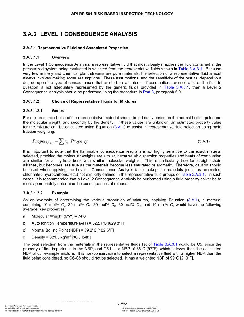
API RP 581 RISK-BASED INSPECTION TECHNOLOGY
3.A.3 LEVEL 1 CONSEQUENCE ANALYSIS
3.A.3.1 Representative Fluid and Associated Properties
3.A.3.1.1 Overview
In the Level 1 Consequence Analysis, a representative fluid that most closely matches the fluid contained in the pressurized system being evaluated is selected from the representative fluids shown in Table 3.A.3.1. Because very few refinery and chemical plant streams are pure materials, the selection of a representative fluid almost always involves making some assumptions. These assumptions, and the sensitivity of the results, depend to a degree upon the type of consequences that are to be evaluated. If assumptions are not valid or the fluid in question is not adequately represented by the generic fluids provided in Table 3.A.3.1, then a Level 2 Consequence Analysis should be performed using the procedure in Part 3, paragraph 6.0.
3.A.3.1.2 Choice of Representative Fluids for Mixtures
3.A.3.1.2.1 General
For mixtures, the choice of the representative material should be primarily based on the normal boiling point and the molecular weight, and secondly by the density. If these values are unknown, an estimated property value for the mixture can be calculated using Equation (3.A.1) to assist in representative fluid selection using mole fraction weighting.
mix i iProperty x Property= ⋅∑ (3.A.1)
It is important to note that the flammable consequence results are not highly sensitive to the exact material selected, provided the molecular weights are similar, because air dispersion properties and heats of combustion are similar for all hydrocarbons with similar molecular weights. This is particularly true for straight chain alkanes, but becomes less true as the materials become less saturated or aromatic. Therefore, caution should be used when applying the Level 1 Consequence Analysis table lookups to materials (such as aromatics, chlorinated hydrocarbons, etc.) not explicitly defined in the representative fluid groups of Table 3.A.3.1. In such cases, it is recommended that a Level 2 Consequence Analysis be performed using a fluid property solver be to more appropriately determine the consequences of release.
3.A.3.1.2.2 Example
As an example of determining the various properties of mixtures, applying Equation (3.A.1), a material containing 10 mol% C3, 20 mol% C4, 30 mol% C5, 30 mol% C6, and 10 mol% C7 would have the following average key properties:
a) Molecular Weight (MW) = 74.8
b) Auto Ignition Temperature (AIT) = 322.1°C [629.8°F]
c) Normal Boiling Point (NBP) = 39.2°C [102.6°F]
d) Density = 621.5 kg/m3 [38.8 lb/ft3]
The best selection from the materials in the representative fluids list of Table 3.A.3.1 would be C5, since the property of first importance is the NBP, and C5 has a NBP of 36oC [97oF], which is lower than the calculated NBP of our example mixture. It is non-conservative to select a representative fluid with a higher NBP than the fluid being considered, so C6-C8 should not be selected. It has a weighted NBP of 99oC [210oF].
3.A-5 Copyright American Petroleum Institute Provided by IHS under license with API Licensee=Qatar Petroleum/5943408001
Not for Resale, 10/20/2008 01:51:29 MDTNo reproduction or networking permitted without license from IHS
--```,`,,`,`,,`,`,,,,,,``,```,`-`-`,,`,,`,`,,`---
API RP 581 RISK-BASED INSPECTION TECHNOLOGY
3.A.3.1.2.3 Example with a Mixture
If a mixture contains inerts such as CO2, water, etc., the choice of representative fluid should be based on the flammable/toxic materials of concern, excluding these materials. This is a somewhat crude assumption that will result in slightly conservative results, but it is a fair enough estimation for this process. For instance, if the material is 93 mol% water and 7 mol% C20, simply model it as C20, using the corresponding inventory of the hydrocarbon. This may result in an overly conservative answer. A Level 2 Consequence Analysis may be used to more accurately model the release.
3.A.3.1.2.4 Toxic Mixture
If the mixture contains toxic components and a toxic consequence calculation is desired, the choice of reference fluid is still required, even if the toxic component only makes up a small fraction of the mixture. In this situation, the reference fluid group should be chosen as described in paragraph 3.A.3.1.2.2.
3.A.3.1.3 Fluid Properties
Average fluid properties for the Level 1 Consequence Analysis are provided in Table 3.A.3.1. The properties of fluids (or individual components of mixtures) can typically be found in standard chemical reference books.
3.A.3.2 Release Hole Size Selection
3.A.3.2.1 Overview
Part 2 of this document defines release hole sizes that represent small, medium, large, and rupture cases for various components or types of equipment. This predefined set of release hole sizes are based on failure size distributions observed in piping and pressure vessels. The range of release hole sizes is chosen to address potential onsite and offsite consequences. For onsite effects, small and medium hole-size cases usually dominate the risk because of their much higher likelihood and potential for onsite consequences.
For offsite effects, medium and large hole-size cases will dominate the risk. To address both onsite and offsite consequences, and to provide good resolution between equipment items, four release hole sizes per equipment item is typically used. The following paragraphs provide a discussion of how the release hole sizes are selected for specific pieces of equipment.
3.A.3.2.2 Piping
Piping uses the standard four release hole sizes: 1/4-inch, 1-inch, 4-inch, and rupture, provided the diameter of the leak is less than, or equal to, the diameter of the pipe itself. For example, an NPS 1 pipe can have only two release hole sizes, 1/4-inch and rupture, because the largest possible choice is equivalent to the 1-inch release hole size. An NPS 4 pipe can have three release hole sizes: 1/4-inch, 1-inch, and rupture, for the same reason.
3.A.3.2.3 Pressure Vessels
For pressure vessels, the same standard four release hole sizes are assumed for all sizes and types of vessels. Equipment types included in this general classification are:
a) Vessel – standard pressure vessels such as KO drums, accumulators, and reactors
b) Filter – standard types of filters and strainers
c) Column – distillation columns, absorbers, strippers, etc.
d) Heat Exchanger Shell – shell side of reboilers, condensers, heat exchangers
e) Heat Exchanger Tube – tube side of reboilers, condensers, heat exchangers
f) Fin/Fan Coolers – fin/fan-type heat exchangers
3.A-6 Copyright American Petroleum Institute Provided by IHS under license with API Licensee=Qatar Petroleum/5943408001
Not for Resale, 10/20/2008 01:51:29 MDTNo reproduction or networking permitted without license from IHS
--```,`,,`,`,,`,`,,,,,,``,```,`-`-`,,`,,`,`,,`---

API RP 581 RISK-BASED INSPECTION TECHNOLOGY
3.A.3.2.4 Pumps
Pumps are assumed to have three possible release hole sizes: 1/4-inch, 1-inch, and 4-inch. If the suction line is less than NPS 4, the last possible release hole size will be the full suction line diameter. Ruptures are not modeled for pumps, and the use of three release hole sizes for pumps is consistent with historical failure data.
3.A.3.2.5 Compressors
Both centrifugal and reciprocating compressors use two release hole sizes: 1-inch and 4-inch (or suction line full bore rupture, whichever is the smaller diameter). The selection of only two release hole sizes is consistent with historical failure data.
3.A.3.3 Estimating the Fluid Inventory Available for Release
3.A.3.3.1 Overview
The consequence calculation requires an upper-limit for the amount of fluid, or fluid inventory that is available for release from an equipment item. In theory, the total amount of fluid that can be released is the amount that is held within pressure containing equipment between isolation valves that can be quickly closed. In reality, emergency operations can be performed over time to close manual valves, de-inventory sections, or otherwise stop a leak. In addition, piping restrictions and differences in elevation can serve to effectively slow or stop a leak. The inventory calculation as presented here is used as an upper limit and does not indicate that this amount of fluid would be released in all leak scenarios.
The Level 1 Consequence Model in this Part is not based on detailed fluid hydraulic modeling. Rather, a simple procedure is used to determine the mass of fluid that could realistically be released in the event of a leak. When a component or piece of equipment is evaluated, its inventory is combined with inventory from other attached equipment that can realistically contribute fluid mass to the component that is leaking. These items together form an Inventory Group. The procedure estimates available mass as the lesser of two quantities:
a) The mass within the component being evaluated plus the mass that can be added to it within three minutes from the surrounding Inventory Group, assuming the same flow rate from the leaking equipment item, but limited to an 8-inch leak in the case of ruptures.
b) The total mass of the fluid in the Inventory Group associated with the component being evaluated.
The three-minute time limit for the added fluid from the surrounding inventory group is based on the dynamics of a large leak scenario. In a large leak, the leaking vessel will begin to de-inventory, while the secondary vessel provides makeup to feed the leak. Large leaks are expected to last for only a few minutes, because of the many cues given to operators that a leak exists. The amount of time that a large leak or rupture will be fed is expected to range from 1 to 5 minutes. Three minutes was chosen since it is the midpoint of this range.
The three-minute assumption is not as applicable to small leaks, since it is far less likely that small leaks will persist long enough to empty the inventory from the leaking vessel and additional inventory from other vessels in the inventory group. In these situations, plant detection, isolation and mitigation techniques will limit the duration of the release such that the actual mass released to atmosphere will be significantly less than the available mass as determined above.
Estimating the inventories for equipment and piping can be done using the guidelines provided in 3.A.3.3.2 through 3.A.3.3.5:
3.A.3.3.2 Equipment Items
Liquid inventories within components can be calculated. In line with coarse risk methodology, the assumptions presented in Table 3.A.3.2 can be used (note that normal operating levels should be used, if known):
3.A-7 Copyright American Petroleum Institute Provided by IHS under license with API Licensee=Qatar Petroleum/5943408001
Not for Resale, 10/20/2008 01:51:29 MDTNo reproduction or networking permitted without license from IHS
--```,`,,`,`,,`,`,,,,,,``,```,`-`-`,,`,,`,`,,`---

API RP 581 RISK-BASED INSPECTION TECHNOLOGY
3.A.3.3.3 Liquid Systems
For liquid systems, define the representative equipment groups which, given a certain failure within that group, could result in similar consequences. Examples of liquid systems may include:
a) The bottom half of a distillation column, its reboiler, and the associated piping
b) An accumulator and its outlet piping
c) A long feed pipeline
d) A storage tank and its outlet piping
e) A series of heat exchangers and the associated piping
Once the liquid piping and equipment groups are established, the inventories for each item are added to obtain the group inventory. This liquid inventory determined in this manner is used for each equipment item modeled from that group.
3.A.3.3.4 Vapor Systems
For vapor systems, common equipment and piping groups for vapor systems include:
a) The top half of the distillation column, its overhead piping, and the overhead condenser.
b) A vent header line, its knock-out pot, and its exit line.
For vapor systems, however, the inventory is not likely to be governed by the amount of vapor in the equipment items, but rather the flow rate, or charge rate, through the system. One method to determine the inventory would be to use this flow rate for a given period of time (say, 60 minutes) and determine the resulting mass. If this rate is not known and, since flashing may also occur from the liquid system, it may be preferable to simply use the upstream group’s liquid inventory. This, however, is likely to lead to a somewhat more conservative inventory.
3.A.3.3.5 Two-Phase Systems
For two-phase systems, such as separators, the potential spill inventory of the liquid is most likely to be used, as it is the assumption that the release occurs at the base of the equipment item. Again, some conservatism may occur. For two-phase pipes, the upstream spill inventory can be a consideration such that, if a majority is liquid, then the liquid spill inventory should be determined. Conversely, if upstream inventory is primarily two-phase or gaseous, then the vapor inventory can be calculated with an allowance for the liquid portion.
3.A.3.4 Determination of the Release Type (Instantaneous or Continuous)
Different analytical models and methods are used to estimate the effects of an instantaneous versus a continuous type of release. The calculated consequences can differ greatly, depending on the type of analytical model chosen to represent the release. Therefore, it is very important that a release is properly categorized into one of the two release types.
As an example of the importance of proper model selection is the case for vapor cloud explosions, VCEs. A review of historical data on fires and explosions shows that unconfined vapor cloud explosions are more likely to occur for instantaneous vapor releases than they are for continuous releases. For API RBI a threshold for the instantaneous release model is if more than 4,536 kilograms [10,000 pounds] of fluid are released in a short period of time. Using this threshold to define continuous releases reflects the tendency for amounts released in a short period of time, less than 4,536 kilograms [10,000 pounds], to result in a flash fire rather than a VCE.
In a Level 1 Consequence Analysis, the modeling of continuous releases uses a lower probability for a vapor cloud explosion (VCE) following a leak and the probability is not a function of release rate, only release type. Level 1 Consequence Analysis event probabilities are provided in Tables 3.A.3.3 through 3.A.3.6. A Level 2 analysis calculates event probabilities not only as a function of release type but also as a function of release mass rate, see Part 3, paragraph 6.8.1 for determining event probabilities for a Level 2 Consequence Analysis.
3.A-8 Copyright American Petroleum Institute Provided by IHS under license with API Licensee=Qatar Petroleum/5943408001
Not for Resale, 10/20/2008 01:51:29 MDTNo reproduction or networking permitted without license from IHS
--```,`,,`,`,,`,`,,,,,,``,```,`-`-`,,`,,`,`,,`---

API RP 581 RISK-BASED INSPECTION TECHNOLOGY
3.A.3.5 Determination of Flammable and Explosive Consequences
3.A.3.5.1 Overview
For flammable materials, consequences are measured in terms of the area affected by the ignition of a release. There are several potential consequence outcomes for any release involving a flammable material; however, a single combined result is determined as the average of all possible consequence outcomes, weighted according to probability. The probability of a consequence outcome is different from, and should not be confused with, the probability of a release or probability of loss of containment (see Part 2), which involves evaluation of the damage state of the piece of equipment, and is a function of equipment integrity.
The probability of a consequence outcome represents the probability that a specific physical phenomenon (outcome) will be observed after the release has occurred. Potential release consequence outcomes for flammable materials are:
a) Safe Dispersion
b) Jet Fire
c) Vapor Cloud Explosion (VCE)
d) Flash Fire
e) Fireball
f) Liquid Pool Fire
g) Boiling Liquid Expanding Vapor Explosion (BLEVE)
A description of each event outcome has been provided in Part 3, paragraph 6.8.
3.A.3.5.2 Assumptions and Limitations
The consequence modeling procedure for API RBI is a greatly simplified approach to a relatively complex discipline. A large number of assumptions are implicit in the procedure in addition to the assumptions that would be part of a more in-depth analysis. This section is intended to highlight a few of the more important assumptions related to the simplified approach, but does not attempt a comprehensive discussion.
a) The consequence area does not reflect where the damage occurs. Jet and pool fires tend to have damage areas localized around the point of the release, but vapor cloud explosions and flash fires may result in damage far from the release point.
b) The use of a fixed set of conditions for meteorology and release orientations is a great simplification over detailed consequence calculations because these factors can have a significant impact on the results.
c) The use of the standardized event trees for consequence outcomes and standardized ignition probabilities is a limitation of the API RBI Level 1 Consequence Analysis method. These factors are very site-specific, and the user needs to realize that they are chosen to reflect representative conditions for the petrochemical industry. The Level 2 Consequence Analysis does a little better, since ignition probabilities and probabilities of other consequence outcome have been correlated as a function of release rate, release type and fluid molecular weight.
3.A.3.5.3 Basis for Flammable Consequence Area Tables
3.A.3.5.3.1 General
For representative fluids shown in Table 3.A.3.1, the determination of flammable consequences has been simplified with the Level 1 Consequence Analysis approach by reducing the calculation down to simplified equations presented in lookup tables. This allows the RBI analyst to determine approximate consequence measures using only the following information:
a) The representative material and its associated properties.
b) The type (continuous or instantaneous) and phase of dispersion.
3.A-9 Copyright American Petroleum Institute Provided by IHS under license with API Licensee=Qatar Petroleum/5943408001
Not for Resale, 10/20/2008 01:51:29 MDTNo reproduction or networking permitted without license from IHS
--```,`,,`,`,,`,`,,,,,,``,```,`-`-`,,`,,`,`,,`---
API RP 581 RISK-BASED INSPECTION TECHNOLOGY
c) The release rate or mass, depending on the type of dispersion and the effects of detection, isolation and mitigation measures.
3.A.3.5.3.2 Predicting Probabilities of Flammable Outcomes
Each flammable event outcome is the result of a chain of events. Event trees, as shown in Figure 3.A.3.1, are used to visually depict the possible chain of events that lead to each outcome. The event trees also are used to show how various individual event probabilities should be combined to calculate the probability for the chain of events.
For a given release type, the two main factors that define the outcome of the release of flammable material is the probability of ignition and the timing of ignition. The three possibilities depicted in the outcome event trees were: no ignition, early ignition, and late ignition. The event tree outcome probabilities used in the Level 1 Consequence Analysis for all release types are presented in Tables 3.A.3.3 through 3.A.3.6 according to the release type and material. Each row within the tables contains probabilities for each potential outcome, according to the representative fluid group. Event trees developed for standard risk analyses were used to develop the relative outcome probabilities. Ignition probabilities were based on previously developed correlations. In general, ignition probabilities are found as a function of the following parameters for the fluid:
a) Auto Ignition Temperature (AIT).
b) Flash temperature.
c) NFPA Flammability Index.
d) Flammability Range (difference between upper and lower flammability limits).
Fluids released well above their auto ignition temperatures will have markedly different ignition probabilities (Tables 3.A.3.3 and 3.A.3.4) than those released near or below their auto ignition temperatures (Tables 3.A.3.5 and 3.A.3.6).
3.A.3.5.3.3 Calculating Consequences for Each Outcome
A set of representative materials was run through the hazards analysis screening program to determine the consequence areas for all potential outcomes. The consequence areas were then plotted as a function of release rate or mass to generate graphs. When plotted on a log/log scale, the consequence curves formed straight lines that were fit to an equation relating consequence area to the release rate or mass. The consequence equations are presented in the following generic form:
( ) yCA x rate for a continuous release= (3.A.2)
( ) yCA x mass for an instantaneous release= (3.A.3)
The consequences of releases of flammable materials are not strongly dependent on the duration of the release, since most fluids reach a steady state size, or footprint, within a short period of time when dispersed in the atmosphere. The only exception to this generalization is a pool fire resulting from the continuous release of a liquid. If flammable liquids are released in a continuous manner, the consequences associated with a pool fire will depend on the duration and the total mass of the release.
For pool fires, the API RBI method assumes a dike size of 30.5 meters by 30.5 meters (929 m2) [100 feet by 100 feet (10,000 ft2)] and estimates the flammable consequences due to a maximum pool fire of that size.
3.A.3.5.3.4 Calculation of the Combined Consequence Area
An equation that represents a single consequence area for the combination of possible outcomes can be derived for each of the four combinations of release types and final phase cases. The combined consequence area is determined by a two-step process:
3.A-10 Copyright American Petroleum Institute Provided by IHS under license with API Licensee=Qatar Petroleum/5943408001
Not for Resale, 10/20/2008 01:51:29 MDTNo reproduction or networking permitted without license from IHS
--```,`,,`,`,,`,`,,,,,,``,```,`-`-`,,`,,`,`,,`---

API RP 581 RISK-BASED INSPECTION TECHNOLOGY
a) STEP 1 – Multiply the consequence area for each outcome (computed from Equation (3.A.2) by the associated event tree probabilities (taken from the appropriate Tables 3.A.3.3 through 3.A.3.6). If the impact criterion uses only a portion of the consequence area (for instance, flash fires use only 25% of the area within the LFL for equipment damage) include this in the probability equation.
b) STEP 2 – Sum all of the consequence-probability products found in STEP 1.
The equation that summarizes the result of the process is as follows:
comb i iCA p CA=∑ (3.A.4)
The procedure for combining consequence equations for all of the potential outcomes was performed for a set of representative materials (see Table 3.A.3.1). The results of this exercise were the equations given in Tables 5.8 and 5.9 of Part 3.
3.A.3.5.3.5 Consequence Analysis Dispersion Modeling
The computer modeling necessary to determine consequence areas associated with cloud dispersion (flash fires, VCEs, toxic releases) require specific input regarding meteorological and release conditions. For the Level 1 Consequence Analysis, meteorological conditions representative of the Gulf Coast annual averages were used. These conditions can also be used when performing a Level 2 Consequence Analysis. The meteorological input assumptions were as follows:
a) Atmospheric Temperature 70°F [21°C]
b) Relative Humidity 75%
c) Wind Speed 8 mph [12.9 km/h]
d) Stability Class D
e) Surface Roughness Parameter 30.5 mm [1.2 in] (typical for processing plants)
Further simplifications were made as part of the inputs to the Level 1 Consequence Analysis as follows:
a) Initial pressure typical of medium-pressure processing conditions with a refinery 0.69 MPa [100 psig]
b) Initial temperatures representing a range from low temperature (below auto-ignition, i.e. 20°C [68°F]) to high temperature (near auto-ignition) conditions
c) Range of release hole sizes from 6.35 mm to 406 mm [0.25 in to 16 in] diameter for continuous events
d) Range of release masses from 45.4 kgs to 453,592 kgs [100 lbs to 100,000 lbs].
e) Both vapor and liquid releases from a vessel containing saturated liquid, with release orientation horizontal downwind at an elevation of ten feet over a concrete surface
Analysis has shown that these assumptions are satisfactory for a wide variety of plant conditions. Where these assumptions are not suitable, the analyst should consider performing a Level 2 Consequence Analysis.
3.A.3.6 Determination of Toxic Consequences
3.A.3.6.1 Overview
As with the flammable consequence procedure, dispersion analysis has been performed to evaluate the consequence areas associated with the release of toxic fluids to the atmosphere. The assumptions made for the cloud dispersion modeling are as described in paragraph 3.A.3.5.3.5. The Level 1 Consequence Analysis procedure has been reduced down to using simplified equations presented in lookup tables, similar to the Level 1 flammable consequence procedure described in paragraph 3.A.3.5.
3.A-11 Copyright American Petroleum Institute Provided by IHS under license with API Licensee=Qatar Petroleum/5943408001
Not for Resale, 10/20/2008 01:51:29 MDTNo reproduction or networking permitted without license from IHS
--```,`,,`,`,,`,`,,,,,,``,```,`-`-`,,`,,`,`,,`---

API RP 581 RISK-BASED INSPECTION TECHNOLOGY
3.A.3.6.2 Background for Calculation of Toxic Consequences
The development of the toxic consequence area equations for the Level 1 Consequence Analysis considers two components: exposure time and concentration. These two components combine to result in an exposure that is referred to as the toxic dose. In API RBI, the degree of injury from a toxic release is directly related to the toxic dose. Level 1 Consequence Analysis relates dose to injury using probits.
For toxic vapor exposure, the probit (a shortened form of probability unit) is represented as follows:
ln nPr A B C t⎡= + ⋅ ⎣ ⎤⎦
b
(3.A.5)
Example constants for the probit equation are provided in Part 3, Table 5.14 for various toxic fluids. API RBI uses a single fixed probability of fatality (50% probability of fatality) to determine the toxic impact. This level corresponds to a probit value of 5.0.
3.A.3.6.3 Toxic Continuous Releases
A cloud dispersion model is used to analyze a continuous release (plume model) to the atmosphere. The cloud footprint or plan area is approximated as the shape of an ellipse, as shown in Figure 3.A.3.2, and is calculated using Equation (3.A.6).
A aπ= (3.A.6)
3.A.3.6.4 Toxic Instantaneous Releases
For instantaneous releases (puff model), the dispersion of the cloud over time is shown in Figure 3.A.3.3. The plan area covered by the cloud is conservatively assumed to be an ellipse, except that the y- distance (a) is taken as one-half of the maximum cloud width as determined from the dispersion results. As part of a Level 2 Consequence Analysis, cloud dispersion modeling software exists that provides a more accurate plot area as a function of concentration than the elliptical area assumptions made above.
3.A.3.6.5 Development of Toxic Consequence Areas for HF Acid
3.A.3.6.5.1 General
Hydrogen fluoride (HF) is typically stored, transferred, and processed in liquid form. However, the toxic impact associated with a release of liquid HF to the atmosphere is due to the dispersion of the toxic vapor cloud. A toxic vapor cloud of HF can be produced by flashing of the liquid upon release or evaporation from a liquid pool. For the Level 1 Consequence Analysis, the initial state of HF is assumed to be liquid; the models for calculating the toxic impact areas for HF liquid releases take into account the possibility of flashing and pool evaporation. For HF releases, the Level 1 Consequence Analysis uses the following guidelines to determine the release rate or mass of mixtures containing HF:
a) If the released material contains HF as a component in a mixture, the mass fraction of HF is obtained, and
b) The liquid rate (or mass) of only the HF component is used to calculate the toxic impact area.
c) For continuous releases, the discharge rate should be calculated for the mixture (using a closely matching representative fluid) using the equations presented in paragraph 5.3 of Part 3. The Level 1 Consequence Analysis uses a simplified approach for modeling releases of mixtures. If a release material is a mixture, the resulting toxic material release rate should then be calculated by multiplying the mass fraction of the toxic component by the previously-calculated discharge rate for the mixture.
For the Level 1 Consequence Analysis, a consequence analysis tool was used for a range of release rates and durations to obtain graphs of toxic consequence areas. Release durations of instantaneous (less than 3 minutes), 5 minutes (300 sec), 10 minutes (600 sec), 30 minutes (1800 sec), 40 minutes (2400 sec), and 1 hour (3600 sec) were evaluated to obtain toxic consequence areas for varying release rates. Toxic impact criteria used was for a probit value of 5.0 using the probit Equation (3.A.5) and probit values listed in Table 5.14 of Part 3 for HF.
3.A-12 Copyright American Petroleum Institute Provided by IHS under license with API Licensee=Qatar Petroleum/5943408001
Not for Resale, 10/20/2008 01:51:29 MDTNo reproduction or networking permitted without license from IHS
--```,`,,`,`,,`,`,,,,,,``,```,`-`-`,,`,,`,`,,`---
API RP 581 RISK-BASED INSPECTION TECHNOLOGY
3.A.3.6.5.2 Continuous Releases
The results of the dispersion analyses showed that the clouds modeled in accordance with the approximated shapes of 3.A.3.6.3 could be correlated as functions of release rate for continuous releases in accordance with Equation (3.A.7).
[ ]( )10 4log8 10 c C rate dCA C ⋅ ⋅ += ⋅ (3.A.7)
For continuous releases, the values of the constants are functions of the release duration and provided for HF in Table 5.11 of
and c dPart 3.
3.A.3.6.5.3 Instantaneous Releases
The results of the dispersion analyses showed that the clouds modeled in accordance with the approximated shapes of 3.A.3.6.4 could be correlated as functions of release mass for instantaneous releases in accordance with Equation (3.A.8).
[ ]( )10 4log8 10 c C mass dCA C ⋅ ⋅ += ⋅ (3.A.8)
For instantaneous releases, the values of the constants are provided for HF and H2S in Table 5.11 of and c dPart 3.
3.A.3.6.6 Development of Toxic Consequence Areas for H2S
3.A.3.6.6.1 General
Hydrogen sulfide, due to its low boiling point, is processed as a vapor or, when processed under high pressures, quickly flashes upon release. In either case, the release of H2S to the atmosphere results in the quick formation of a toxic vapor cloud. For H2S releases, the Level 1 Consequence Analysis uses the following guidelines to determine the release rate or mass of mixtures containing H2S:
1) If the released material contains H2S as a component in a mixture, the mass fraction of H2S is obtained, and
2) If the initial state of the material is a vapor, the mass fraction of H2S is used to obtain the vapor discharge rate (or mass) of only H2S; this rate (or mass) is used to determine the impact area, or
If the initial state of the material is a liquid, the mass fraction of H2S is used to obtain the vapor flash rate (or mass) of only the H2S; this rate (or mass) is used to determine the impact.
If the initial phase of a material being released is 1 wt% H2S in gas oil, the material has the potential for both toxic and flammable outcomes from the vapor, and flammable outcomes from the liquid. Therefore, the following procedure is followed, using C17-C25 as the representative material:
a) Calculate the liquid discharge rate for C17-C25 as described in paragraph 5.3 of Part 3.
b) When estimating flammable consequences, calculate the potential flammable consequence areas as in paragraph 5.3 of Part 3 and take the worst case between:
1) The flammable effects of C17-C25 using 100% of the release rate
2) The flammable effects of H2S based on 1% of the release rate
c) Calculate the toxic effects of H2S, using 1% of the release rate.
For instantaneous releases, use the above procedure, substituting inventory mass for release rate
The release durations used to model the consequences of the H2S release were identical to those assumed for HF Acid as discussed in paragraph 3.A.3.6.5.2.
3.A-13 Copyright American Petroleum Institute Provided by IHS under license with API Licensee=Qatar Petroleum/5943408001
Not for Resale, 10/20/2008 01:51:29 MDTNo reproduction or networking permitted without license from IHS
--```,`,,`,`,,`,`,,,,,,``,```,`-`-`,,`,,`,`,,`---
API RP 581 RISK-BASED INSPECTION TECHNOLOGY
3.A.3.6.6.2 Continuous Releases
The results of the dispersion analyses showed that the clouds modeled in accordance with the approximated shapes of 3.A.3.6.3 could be correlated as functions of release rate for continuous releases in accordance with Equation (3.A.7).
The values of the constants are functions of the release duration and provided for H2S in Table 5.11 of and c d
d
Part 3.
3.A.3.6.6.3 Instantaneous Releases
The results of the dispersion analyses showed that the clouds modeled in accordance with the approximated shapes of 3.A.3.6.4 could be correlated as functions of release mass for instantaneous releases in accordance with Equation (3.A.8).
For instantaneous releases, the values of the constants are provided for H2S in Table 5.11 of and c Part 3.
3.A.3.6.7 Development of Toxic Consequence Areas for Ammonia
3.A.3.6.7.1 General
To estimate the consequence area for ammonia, the dispersion analyses was performed using a saturated liquid at ambient temperature (24°C [75°F]), with liquid being released from a low pressure storage tank. The tank head was set at 3.05 meters [10 feet].
3.A.3.6.7.2 Continuous Releases
To determine an equation for the continuous area of a release of ammonia, four release hole sizes (0.25 in, 1 in., 4 in., and 16 in.) were run for various release durations (10, 30, and 60 minutes). Again, toxic consequence computations were calculated using a software package containing atmospheric dispersion routines.
Toxic impact criteria used was for a probit value of 5.0 using the probit Equation (3.A.5) and probit values listed in Table 5.17 of Part 3 for ammonia. The results showed that the clouds modeled in accordance with the approximated shapes of 3.A.3.6.3 could be correlated as functions of release rate for continuous releases in accordance with Equation (3.A.9) .
( ) fCA e rate= (3.A.9)
For continuous releases, the values of the constants are functions of the release duration and provided for Ammonia in Table 5.12 of
and e fPart 3.
3.A.3.6.7.3 Instantaneous Releases
For instantaneous release cases, four release masses of ammonia were modeled (10, 100, 1,000, and 10,000 lb), and the relationship between release mass and consequence area to a probit value of 5.0 were correlated. The results in ft2 for Ammonia are provided in Equation (3.A.10).
( )0.901114.17CA mass= (3.A.10)
3.A.3.6.8 Development of Toxic Consequence Areas for Chlorine
3.A.3.6.8.1 General
To estimate the consequence area for chlorine, the dispersion analyses were performed using the identical procedure for ammonia as described in 3.A.3.6.7.1 and 3.A.3.6.7.2.
3.A-14 Copyright American Petroleum Institute Provided by IHS under license with API Licensee=Qatar Petroleum/5943408001
Not for Resale, 10/20/2008 01:51:29 MDTNo reproduction or networking permitted without license from IHS
--```,`,,`,`,,`,`,,,,,,``,```,`-`-`,,`,,`,`,,`---
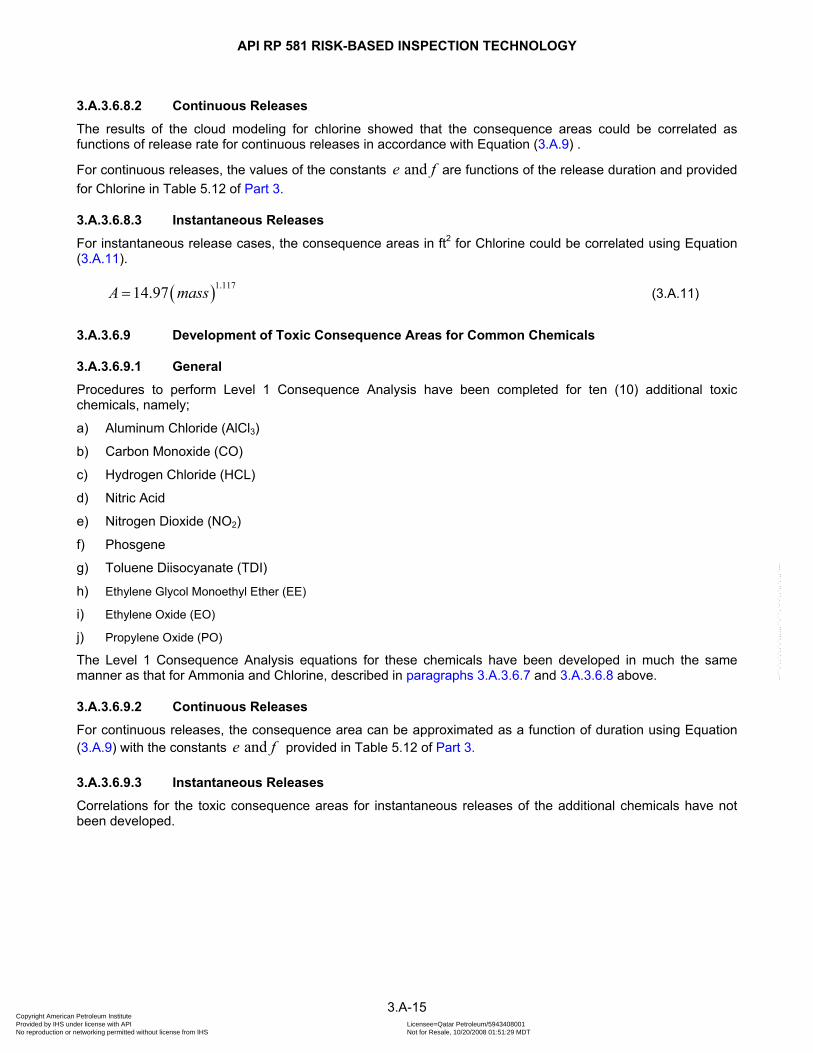
API RP 581 RISK-BASED INSPECTION TECHNOLOGY
3.A.3.6.8.2 Continuous Releases
The results of the cloud modeling for chlorine showed that the consequence areas could be correlated as functions of release rate for continuous releases in accordance with Equation (3.A.9) .
For continuous releases, the values of the constants are functions of the release duration and provided for Chlorine in Table 5.12 of
and e f
f
Part 3.
3.A.3.6.8.3 Instantaneous Releases
For instantaneous release cases, the consequence areas in ft2 for Chlorine could be correlated using Equation (3.A.11).
( )1.11714.97A mass= (3.A.11)
3.A.3.6.9 Development of Toxic Consequence Areas for Common Chemicals
3.A.3.6.9.1 General
Procedures to perform Level 1 Consequence Analysis have been completed for ten (10) additional toxic chemicals, namely;
a) Aluminum Chloride (AlCl3)
b) Carbon Monoxide (CO)
c) Hydrogen Chloride (HCL)
d) Nitric Acid
e) Nitrogen Dioxide (NO2)
f) Phosgene
g) Toluene Diisocyanate (TDI)
h) Ethylene Glycol Monoethyl Ether (EE)
i) Ethylene Oxide (EO)
j) Propylene Oxide (PO)
The Level 1 Consequence Analysis equations for these chemicals have been developed in much the same manner as that for Ammonia and Chlorine, described in paragraphs 3.A.3.6.7 and 3.A.3.6.8 above.
3.A.3.6.9.2 Continuous Releases
For continuous releases, the consequence area can be approximated as a function of duration using Equation (3.A.9) with the constants provided in Table 5.12 of and e Part 3.
3.A.3.6.9.3 Instantaneous Releases
Correlations for the toxic consequence areas for instantaneous releases of the additional chemicals have not been developed.
3.A-15 Copyright American Petroleum Institute Provided by IHS under license with API Licensee=Qatar Petroleum/5943408001
Not for Resale, 10/20/2008 01:51:29 MDTNo reproduction or networking permitted without license from IHS
--```,`,,`,`,,`,`,,,,,,``,```,`-`-`,,`,,`,`,,`---

API RP 581 RISK-BASED INSPECTION TECHNOLOGY
3.A.3.7 Nomenclature
The following lists the nomenclature used in paragraph 3.A.3. The coefficients through which provide the metric and U.S conversion factors for the equations are provided in
1C 36CAnnex 3.B.
a is one-half of the cloud width (minor axis), taken at its largest point (within the 50% probability of fatality dose level)
b is one-half of the downwind dispersion distance (major axis), taken at the 50% probability of fatality dose level
A is a constant for the probit equation CA is the consequence area, m2 [ft2]
combCA is the combined/probability weighted consequence area, m2 [ft2]
iCA is the individual outcome consequence area for the event outcome, m2 [ft2] thiB is a constant for the probit equation c is a constant for the specific consequence area equations for HF Acid and H2S C is the toxic concentration in the probit equation, ppm d is a constant for the specific consequence area equations for HF Acid and H2S e is the constant for the specific consequence area equations for Ammonia and Chlorine f is the exponent for the specific consequence area equations for Ammonia and Chlorine mass is the release mass, kgs [lbs] n is the exponent in the probit equation
ip is the specific event probability for the event outcome, see thi Tables 3.A.3.3, 3.A.3.4, 3.A.3.5 or 3.A.3.6
Pr is the probit value, typically 5.0 which is defined as 50% probability rate is the release rate, kg/s [lb/s] t is the toxic dosage in the probit equation, seconds x is the constant for the generic consequence area equation y is the exponent for the generic consequence area equation
3.A-16 Copyright American Petroleum Institute Provided by IHS under license with API Licensee=Qatar Petroleum/5943408001
Not for Resale, 10/20/2008 01:51:29 MDTNo reproduction or networking permitted without license from IHS
--```,`,,`,`,,`,`,,,,,,``,```,`-`-`,,`,,`,`,,`---
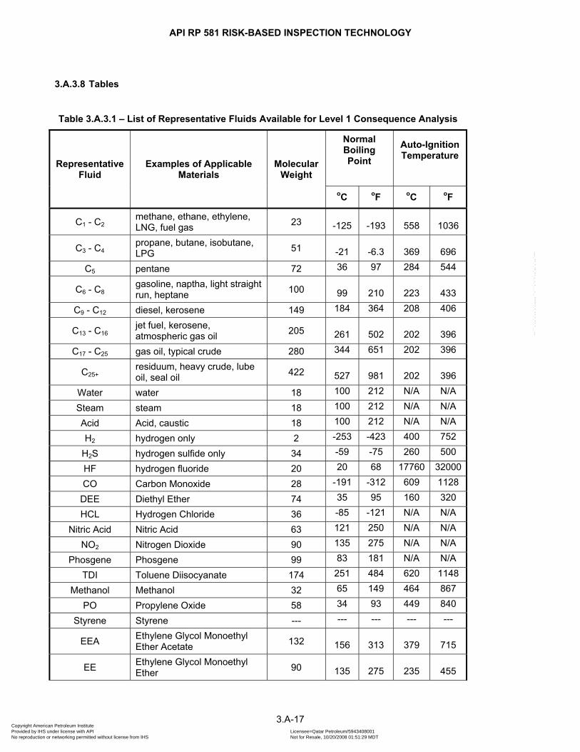
API RP 581 RISK-BASED INSPECTION TECHNOLOGY
3.A.3.8 Tables
Table 3.A.3.1 – List of Representative Fluids Available for Level 1 Consequence Analysis
Representative Fluid
Examples of Applicable Materials
Molecular Weight
Normal Boiling Point
Auto-Ignition Temperature
oC oF oC oF
C1 - C2 methane, ethane, ethylene, LNG, fuel gas 23 -125 -193 558 1036
C3 - C4 propane, butane, isobutane, LPG 51 -21 -6.3 369 696
C5 pentane 72 36 97 284 544
C6 - C8 gasoline, naptha, light straight run, heptane 100 99 210 223 433
C9 - C12 diesel, kerosene 149 184 364 208 406
C13 - C16 jet fuel, kerosene, atmospheric gas oil 205 261 502 202 396
C17 - C25 gas oil, typical crude 280 344 651 202 396
C25+ residuum, heavy crude, lube oil, seal oil 422 527 981 202 396
Water water 18 100 212 N/A N/A
Steam steam 18 100 212 N/A N/A
Acid Acid, caustic 18 100 212 N/A N/A
H2 hydrogen only 2 -253 -423 400 752
H2S hydrogen sulfide only 34 -59 -75 260 500
HF hydrogen fluoride 20 20 68 17760 32000
CO Carbon Monoxide 28 -191 -312 609 1128
DEE Diethyl Ether 74 35 95 160 320
HCL Hydrogen Chloride 36 -85 -121 N/A N/A
Nitric Acid Nitric Acid 63 121 250 N/A N/A
NO2 Nitrogen Dioxide 90 135 275 N/A N/A
Phosgene Phosgene 99 83 181 N/A N/A
TDI Toluene Diisocyanate 174 251 484 620 1148
Methanol Methanol 32 65 149 464 867
PO Propylene Oxide 58 34 93 449 840
Styrene Styrene --- --- --- --- ---
EEA Ethylene Glycol Monoethyl Ether Acetate 132 156 313 379 715
EE Ethylene Glycol Monoethyl Ether 90 135 275 235 455
3.A-17 Copyright American Petroleum Institute Provided by IHS under license with API Licensee=Qatar Petroleum/5943408001
Not for Resale, 10/20/2008 01:51:29 MDTNo reproduction or networking permitted without license from IHS
--```,`,,`,`,,`,`,,,,,,``,```,`-`-`,,`,,`,`,,`---
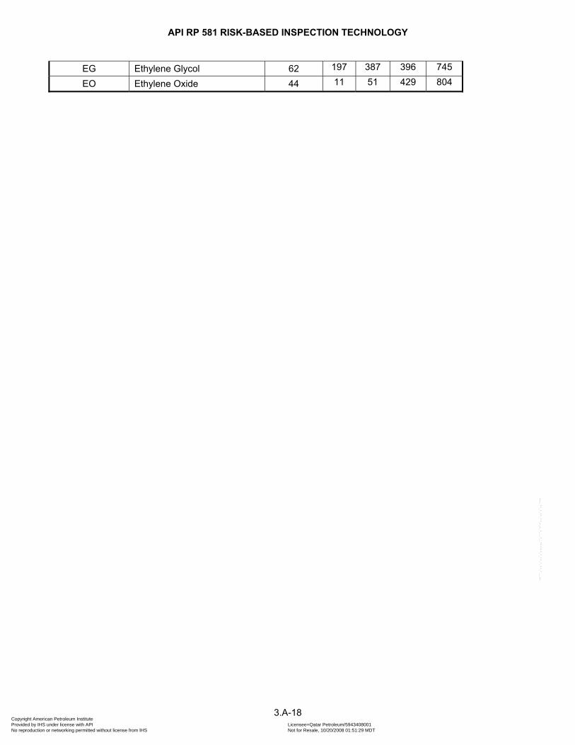
API RP 581 RISK-BASED INSPECTION TECHNOLOGY
EG Ethylene Glycol 62 197 387 396 745
EO Ethylene Oxide 44 11 51 429 804
3.A-18 Copyright American Petroleum Institute Provided by IHS under license with API Licensee=Qatar Petroleum/5943408001
Not for Resale, 10/20/2008 01:51:29 MDTNo reproduction or networking permitted without license from IHS
--```,`,,`,`,,`,`,,,,,,``,```,`-`-`,,`,,`,`,,`---

API RP 581 RISK-BASED INSPECTION TECHNOLOGY
Table 3.A.3.2 -– Assumptions Used When Calculating Liquid Inventories Within Equipment
Equipment Description
Component Type
Examples Default Liquid Volume Percent
Process Columns (may be treated as two or three items)
- top half
- middle section
- bottom half
COLTOP
COLMID
COLBTM
Distillation Columns, FCC Main Fractionator, Splitter
Tower, Debutanizer, Packed Columns (see note 1), Liquid/Liquid
Columns (see Note 2),
25%
25%
37%
These default values are typical of trayed distillation columns and
consider liquid holdup at the bottom of the vessel as well as the
presence of chimney trays in the upper sections
Accumulators and Drums
DRUM OH Accumulators, Feed Drums, HP/LP Separators, Nitrogen Storage drums,
Steam Condensate Drums, 3-Phase
Separators (see note 3)
50% liquid
Typically, 2-phase drums are liquid level controlled at 50%
Knock-out Pots and Dryers
KODRUM Compressor Knock-outs, Fuel Gas KO Drums (see note 4), Flare Drums, Air
Dryers (see note 4),
10% liquid
Much less liquid inventory expected in knock-out drums
Compressors COMPC
COMPR
Centrifugal and Reciprocating Compressors
Negligible, 0%
Pumps PUMP1S
PUMP2S
PUMPR
Pumps 100% liquid
Heat Exchangers HEXSS
HEXTS
Shell and Tube exchangers
50% shell-side, 25% tube-side
Fin Fan Air Coolers FINFAN Total Condensers, Partial Condensers, Vapor Coolers and Liquid
Coolers
(see note 5)
25% liquid
Filters FILTER 100% full
Piping PIPE-xx 100% full, calculated for Level 2 Analysis
Reactors REACTOR Fluid Reactors (see note 6), Fixed-Bed Reactors
(see note 7), mole-sieves
15% liquid
3.A-19 Copyright American Petroleum Institute Provided by IHS under license with API Licensee=Qatar Petroleum/5943408001
Not for Resale, 10/20/2008 01:51:29 MDTNo reproduction or networking permitted without license from IHS
--```,`,,`,`,,`,`,,,,,,``,```,`-`-`,,`,,`,`,,`---

API RP 581 RISK-BASED INSPECTION TECHNOLOGY
NOTES: 1. Packed Columns will typically contain much less liquid traffic than trayed columns. Typical liquid volumes
percents for packed columns are 10-15%. 2. For liquid/liquid columns, such as Amine Contactors, Caustic Contactors and Lube or Aromatics Extractors,
where a solvent or other fluid is brought into direct contact with the process fluid (eg. TEG and BTX in an Aromatics Extractor), the LV % will be much higher. Consideration should be given to the amount of each fluid in the vessel and whether or not the fluid composition includes both fluids in the mixture composition.
3. For 3-phase separators, such as Desalters and OH drums with water boots, the LV% may be lower than 50%, depending on how much of the second liquid phase (typically water) is present and whether or not the fluid composition includes both liquid phases in the mixture composition.
4. Most air coolers are two-phase and only partially condense vapors. Even A/Cs that totally condense the vapor stream require the majority of the heat transfer area (and volume) to cool the vapors to their dew point and condense to liquid. Typically, only the final pass (less rows of tubes than other passes), will be predominately liquid. A LV of 25% should still be conservative for all A/Cs except liquid coolers.
5. For Flue Gas Knock-out drums and Air Dryers, the LV% is typically negligible. Consideration should be given to reducing the LV% to 0%.
6. Fluidized reactors can have up to 15-25% of the available vessel volume taken up by catalyst. The remaining available volume is predominately vapor. A LV of 15% should still be conservative.
7. Fixed-Bed reactors can have up to 75% of the available vessel volume taken up by hardware and catalyst. The remaining volume will typically be 50% liquid and 50% vapor. An assumed LV of 15% of the overall available vessel volume should still be conservative
3.A-20 Copyright American Petroleum Institute Provided by IHS under license with API Licensee=Qatar Petroleum/5943408001
Not for Resale, 10/20/2008 01:51:29 MDTNo reproduction or networking permitted without license from IHS
--```,`,,`,`,,`,`,,,,,,``,```,`-`-`,,`,,`,`,,`---

API RP 581 RISK-BASED INSPECTION TECHNOLOGY
Table 3.A.3.3 – Specific Event Probabilities – Continuous Release Auto Ignition Likely
Final Liquid State – Processed Above AIT
Fluid Probability of Ignition
Probabilities of Outcome
VCE Fireball Flash Fire Jet Fire Pool Fire
C1 – C2
C3 – C4
C5
C6 – C8 1 1
C9 – C12 1 1
C13 – C16 1 0.5 0.5
C17 – C25 1 0.5 0.5
C25 + 1 1
H2
H2S
Styrene 1 1
Final Gas State – Processed Above AIT
Fluid Probability of Ignition
Probabilities of Outcome
VCE Fireball Flash Fire Jet Fire Pool Fire
C1 – C2 0.7 0.7
C3 – C4 0.7 0.7
C5 0.7 0.7
C6 – C8 0.7 0.7
C9 – C12 0.7 0.7
C13 – C16
C17 – C25
C25 +
H2 0.9 0.9
H2S 0.9 0.9
Styrene 1 1
Notes: 1. Shaded area represent outcomes that are not possible 2. Must be processed at least 27°C [80°F] above AIT
3.A-21 Copyright American Petroleum Institute Provided by IHS under license with API Licensee=Qatar Petroleum/5943408001
Not for Resale, 10/20/2008 01:51:29 MDTNo reproduction or networking permitted without license from IHS
--```,`,,`,`,,`,`,,,,,,``,```,`-`-`,,`,,`,`,,`---
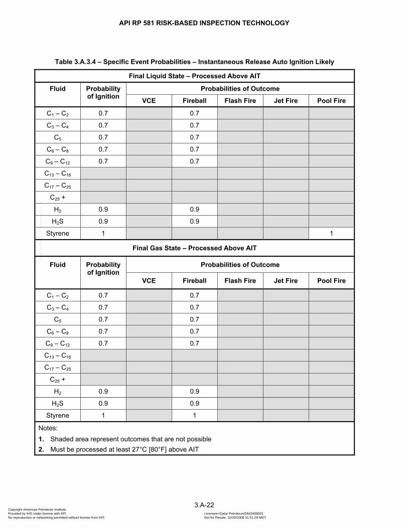
API RP 581 RISK-BASED INSPECTION TECHNOLOGY
Table 3.A.3.4 – Specific Event Probabilities – Instantaneous Release Auto Ignition Likely
Final Liquid State – Processed Above AIT
Fluid Probability of Ignition
Probabilities of Outcome
VCE Fireball Flash Fire Jet Fire Pool Fire
C1 – C2 0.7 0.7
C3 – C4 0.7 0.7
C5 0.7 0.7
C6 – C8 0.7 0.7
C9 – C12 0.7 0.7
C13 – C16
C17 – C25
C25 +
H2 0.9 0.9
H2S 0.9 0.9
Styrene 1 1
Final Gas State – Processed Above AIT
Fluid Probability of Ignition
Probabilities of Outcome
VCE Fireball Flash Fire Jet Fire Pool Fire
C1 – C2 0.7 0.7
C3 – C4 0.7 0.7
C5 0.7 0.7
C6 – C8 0.7 0.7
C9 – C12 0.7 0.7
C13 – C16
C17 – C25
C25 +
H2 0.9 0.9
H2S 0.9 0.9
Styrene 1 1
Notes: 1. Shaded area represent outcomes that are not possible 2. Must be processed at least 27°C [80°F] above AIT
3.A-22 Copyright American Petroleum Institute Provided by IHS under license with API Licensee=Qatar Petroleum/5943408001
Not for Resale, 10/20/2008 01:51:29 MDTNo reproduction or networking permitted without license from IHS
--```,`,,`,`,,`,`,,,,,,``,```,`-`-`,,`,,`,`,,`---

API RP 581 RISK-BASED INSPECTION TECHNOLOGY
Table 3.A.3.5 – Specific Event Probabilities – Continuous Release Auto Ignition Not Likely
Final Liquid State – Processed Below AIT
Fluid Probability of Ignition
Probabilities of Outcome
VCE Fireball Flash Fire Jet Fire Pool Fire
C1 – C2
C3 – C4 0.1
C5 0.1 0.02 0.08
C6 – C8 0.1 0.02 0.08
C9 – C12 0.05 0.01 0.04
C13 – C16 0.05 0.01 0.04
C17 – C25 0.02 0.005 0.0015
C25 + 0.005 0.0015
H2
H2S
DEE 1.0 0.18 0.72
Methanol 0.4 0.08 0.32
PO 0.4 0.08 0.32
Styrene 0.1 0.02 0.08
EEA 0.10 0.02 0.08
EE 0.10 0.02 0.08
EG 0.10 0.02 0.08
3.A-23 Copyright American Petroleum Institute Provided by IHS under license with API Licensee=Qatar Petroleum/5943408001
Not for Resale, 10/20/2008 01:51:29 MDTNo reproduction or networking permitted without license from IHS
--```,`,,`,`,,`,`,,,,,,``,```,`-`-`,,`,,`,`,,`---
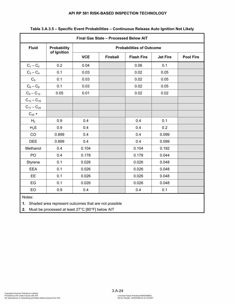
API RP 581 RISK-BASED INSPECTION TECHNOLOGY
Table 3.A.3.5 – Specific Event Probabilities – Continuous Release Auto Ignition Not Likely
Final Gas State – Processed Below AIT
Fluid Probability of Ignition
Probabilities of Outcome
VCE Fireball Flash Fire Jet Fire Pool Fire
C1 – C2 0.2 0.04 0.06 0.1
C3 – C4 0.1 0.03 0.02 0.05
C5 0.1 0.03 0.02 0.05
C6 – C8 0.1 0.03 0.02 0.05
C9 – C12 0.05 0.01 0.02 0.02
C13 – C16
C17 – C25
C25 +
H2 0.9 0.4 0.4 0.1
H2S 0.9 0.4 0.4 0.2
CO 0.899 0.4 0.4 0.099
DEE 0.899 0.4 0.4 0.099
Methanol 0.4 0.104 0.104 0.192
PO 0.4 0.178 0.178 0.044
Styrene 0.1 0.026 0.026 0.048
EEA 0.1 0.026 0.026 0.048
EE 0.1 0.026 0.026 0.048
EG 0.1 0.026 0.026 0.048
EO 0.9 0.4 0.4 0.1
Notes: 1. Shaded area represent outcomes that are not possible 2. Must be processed at least 27°C [80°F] below AIT
3.A-24 Copyright American Petroleum Institute Provided by IHS under license with API Licensee=Qatar Petroleum/5943408001
Not for Resale, 10/20/2008 01:51:29 MDTNo reproduction or networking permitted without license from IHS
--```,`,,`,`,,`,`,,,,,,``,```,`-`-`,,`,,`,`,,`---

API RP 581 RISK-BASED INSPECTION TECHNOLOGY
Table 3.A.3.6 – Specific Event Probabilities – Instantaneous Release Auto Ignition Not Likely
Final Liquid State – Processed Above AIT
Fluid Probability of Ignition
Probabilities of Outcome
VCE Fireball Flash Fire Jet Fire Pool Fire
C1 – C2
C3 – C4
C5 0.1 0.1
C6 – C8 0.1 0.1
C9 – C12 0.05 0.05
C13 – C16 0.05 0.05
C17 – C25 0.02 0.02
C25 + 0.02 0.02
H2
H2S
DEE 0.9 0.9
Methanol 0.4 0.4
PO 0.4 0.4
Styrene 0.1 0.1
EEA 0.1 0.1
EE 0.1 0.1
EG 0.1 0.1
3.A-25 Copyright American Petroleum Institute Provided by IHS under license with API Licensee=Qatar Petroleum/5943408001
Not for Resale, 10/20/2008 01:51:29 MDTNo reproduction or networking permitted without license from IHS
--```,`,,`,`,,`,`,,,,,,``,```,`-`-`,,`,,`,`,,`---

API RP 581 RISK-BASED INSPECTION TECHNOLOGY
Table 3.A.3.6 – Specific Event Probabilities – Instantaneous Release Auto Ignition Not Likely
Final Gas State – Processed Above AIT
Fluid Probability of Ignition
Probabilities of Outcome
VCE Fireball Flash Fire Jet Fire Pool Fire
C1 – C2 0.2 0.04 0.01 0.15
C3 – C4 0.1 0.02 0.01 0.07
C5 0.1 0.02 0.01 0.07
C6 – C8 0.1 0.02 0.01 0.07
C9 – C12 0.04 0.01 0.005 0.025
C13 – C16
C17 – C25
C25 +
H2 0.9 0.4 0.1 0.4
H2S 0.9 0.4 0.1 0.4
CO 0.899 0.4 0.099 0.4
DEE 0.899 0.4 0.099 0.4
Methanol 0.4 0.099 0.038 0.263
PO 0.4 0.178 0.044 0.178
Styrene 0.101 0.025 0.01 0.066
EEA 0.101 0.01 0.066 0.025
EE 0.101 0.01 0.066 0.025
EG 0.101 0.01 0.066 0.025
EO 0.9 0.4 0.1 0.4
Notes: 1. Shaded area represent outcomes that are not possible 2. Must be processed at least 27°C [80°F] above AIT
3.A-26 Copyright American Petroleum Institute Provided by IHS under license with API Licensee=Qatar Petroleum/5943408001
Not for Resale, 10/20/2008 01:51:29 MDTNo reproduction or networking permitted without license from IHS
--```,`,,`,`,,`,`,,,,,,``,```,`-`-`,,`,,`,`,,`---
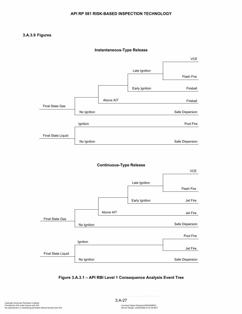
API RP 581 RISK-BASED INSPECTION TECHNOLOGY
3.A.3.9 Figures
Instantaneous-Type Release
Continuous-Type Release
VCE
Flash Fire
Fireball
Fireball
Safe Dispersion
Pool Fire
Safe Dispersion
Late Ignition
Early Ignition
Above AIT
No Ignition
Final State Gas
Final State Liquid
Final State Gas
Final State Liquid
No Ignition
No Ignition
Ignition
Above AIT
Late Ignition
Early Ignition
VCE
Flash Fire
Jet Fire
Jet Fire
Safe Dispersion
Pool Fire
Jet Fire
Safe Dispersion
No Ignition
Ignition
Figure 3.A.3.1 – API RBI Level 1 Consequence Analysis Event Tree
3.A-27 Copyright American Petroleum Institute Provided by IHS under license with API Licensee=Qatar Petroleum/5943408001
Not for Resale, 10/20/2008 01:51:29 MDTNo reproduction or networking permitted without license from IHS
--```,`,,`,`,,`,`,,,,,,``,```,`-`-`,,`,,`,`,,`---
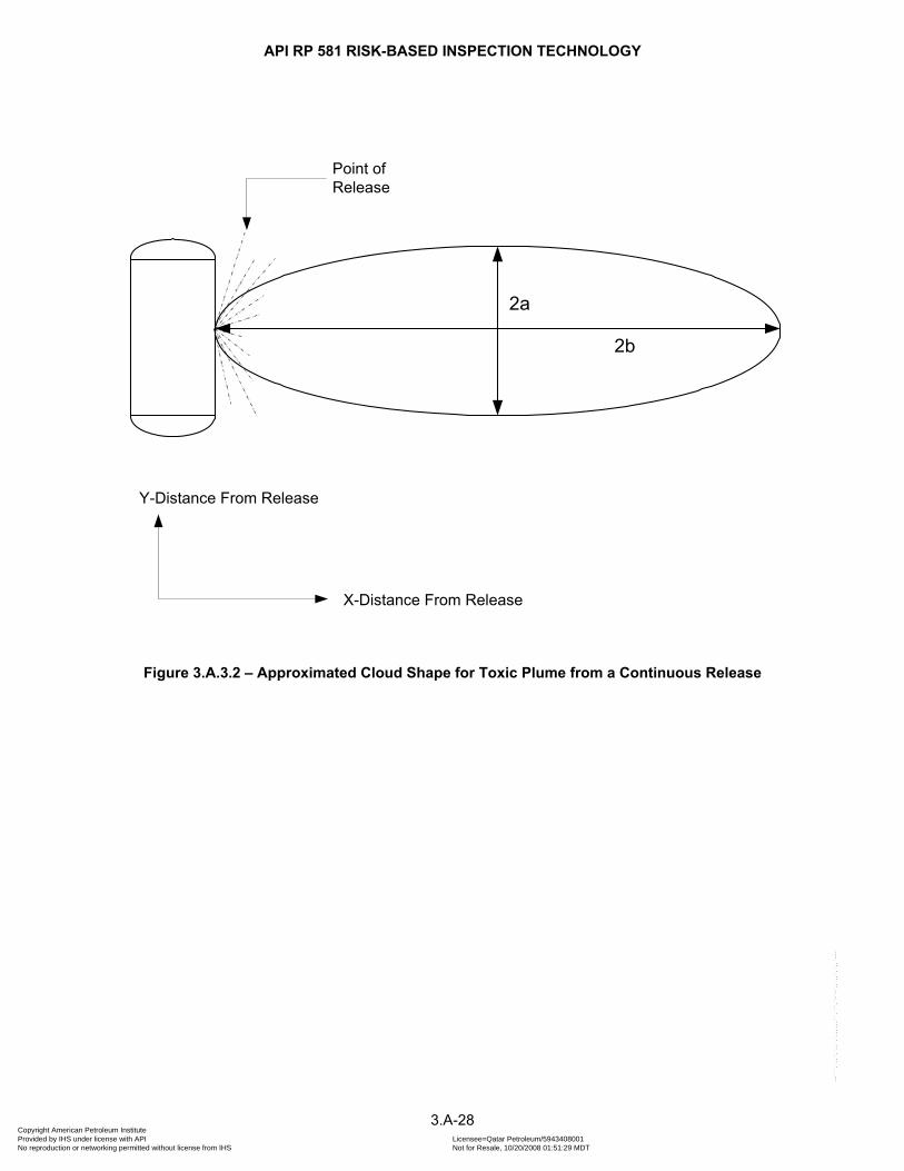
API RP 581 RISK-BASED INSPECTION TECHNOLOGY
Y-Distance From Release
X-Distance From Release
2a
2b
Point of Release
Figure 3.A.3.2 – Approximated Cloud Shape for Toxic Plume from a Continuous Release
3.A-28 Copyright American Petroleum Institute Provided by IHS under license with API Licensee=Qatar Petroleum/5943408001
Not for Resale, 10/20/2008 01:51:29 MDTNo reproduction or networking permitted without license from IHS
--```,`,,`,`,,`,`,,,,,,``,```,`-`-`,,`,,`,`,,`---
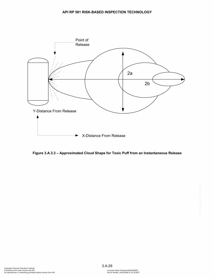
API RP 581 RISK-BASED INSPECTION TECHNOLOGY
2b
2a
Y-Distance From Release
X-Distance From Release
Point of Release
Figure 3.A.3.3 – Approximated Cloud Shape for Toxic Puff from an Instantaneous Release
3.A-29 Copyright American Petroleum Institute Provided by IHS under license with API Licensee=Qatar Petroleum/5943408001
Not for Resale, 10/20/2008 01:51:29 MDTNo reproduction or networking permitted without license from IHS
--```,`,,`,`,,`,`,,,,,,``,```,`-`-`,,`,,`,`,,`---
API RP 581 RISK-BASED INSPECTION TECHNOLOGY
3.A.4 LEVEL 2 CONSEQUENCE ANALYSIS
3.A.4.1 General
The use of event trees and quantitative effects analysis forms the basis for the Level 2 Consequence Analysis procedures presented in Paragraph 6.0 of Part 3. Part 3 provides the details for calculating the event tree probabilities and the effects of pool fires, jet fires, flash fires, fireballs, VCEs and BLEVEs. The impact of most of these events can be determined with closed-form equations as presented in Part 3.
3.A.4.2 Cloud Dispersion Analysis
However, some of these events, such as VCEs and flash fires require the use of sophisticated dispersion analysis software to model how the flammable or toxic releases mix and disperse with air as they are released to the atmosphere.
There are several commercially available software packages that will allow the user to perform dense gas dispersion consequence modeling. Examples include, SLAB, DEGADIS and PHAST, some of which are available in the public domain, others are commercially available. A study contracted by the United States Department of Energy provides a comparison of many different software packages, and recommendations are provided to help select the appropriate package for a particular application.
In general, packages that perform dense gas dispersion modeling should be chosen as opposed to neutrally buoyant models since hazardous releases will typically be materials with molecular weights heavier than air. Even light hydrocarbons can be typically modeled accurately using dense gas modeling since the temperature of the releases will result in releases with densities heavier than air.
Dispersion models will provide a cloud concentration profile. For flammables releases, the concentration profile is used to assess which portions of the cloud are in the flammable range. For flash fires, the impact area at grade is determined to be that area in the cloud that has flammable concentrations between the released fluid’s LFL and UFL. For vapor cloud explosions, a volumetric calculation is required since the total amount of flammable volume and mass is required to assess the magnitude of the explosion.
3.A-30 Copyright American Petroleum Institute Provided by IHS under license with API Licensee=Qatar Petroleum/5943408001
Not for Resale, 10/20/2008 01:51:29 MDTNo reproduction or networking permitted without license from IHS
--```,`,,`,`,,`,`,,,,,,``,```,`-`-`,,`,,`,`,,`---

API RP 581 RISK-BASED INSPECTION TECHNOLOGY
3.A.5 CONSEQUENCE ANALYSIS FOR ATMOSPHERIC STORAGE TANKS
3.A.5.1 Overview
The consequence model for atmospheric storage tanks is based on a modification of the Level 1 Consequence Analysis. Only a financial consequence analysis is provided for the tank bottom and tank shell courses.
3.A.5.2 Representative Fluid and Associated Properties
A representative fluid that most closely matches the fluid contained in the atmospheric storage tank system being evaluated is selected from the representative fluids shown in Part 3, Table 7.1. The required fluid properties for the consequence analysis are also contained in this table.
In addition to selecting a fluid, a soil type must also be specified because the consequence model depends on soil properties. Representative soil conditions and the associated soil properties required or the consequence analysis is provided in Part 3, Table 7.2.
3.A.5.3 Generic Failure Frequencies and Release Holes Sizes
3.A.5.3.1 Tank Bottom
The base failure frequency for the leak of a tank bottom was derived primarily from an analysis of a portion of the American Petroleum Institute publication A Survey of API Members’ Aboveground Storage Tank Facilities, published in July 1994. The survey included refining, marketing, and transportation storage tanks, each compiled separately. The survey included the years 1983 to 1993. The base failure frequencies obtained from this survey are shown in Part 2 Table 4.1 One of the most significant findings of the survey was that tank bottom leaks contributing to soil contamination had been cut in half in the last five years compared to the first five years covered by the survey. This was attributed to an increased awareness of the seriousness of the problem and to the issuance of the API 653 standard for aboveground storage tank inspection.
A bottom leak frequency of 7.2E-3 leaks per year was chosen as the base leak frequency for an atmospheric storage tank bottom. Although the leak frequency data in Part 2 Table 4.1 indicates that tanks less than 5 years old had a much lower leak frequency, it was decided to use the whole survey population in setting the base leak frequency. The age of the tank was accounted for elsewhere in the model since the percent wall loss in the model is a function of the tank age, corrosion rate, and original wall thickness. The percent wall loss was selected as the basis of the modifier on the base leak frequency; thus, a very young tank with minimal corrosion would have a frequency modifier less than one, which lowers the leak frequency accordingly.
It should be noted that the damage factor for atmospheric storage tank bottoms in Part 2 was originally developed based on a generic failure frequency of equal to 7.2E-3, which equates to a range in damage factors from less than 1 to 139. In order to be consistent with the other components in Part 2, the range of damage factors was adjusted to a range of 1 to 1390. This adjustment in the damage factor required a corresponding change of the generic failure frequency to a value of 7.2E-4, and this is the value shown in Part 2, Table 4.1.
The survey did not report the size of leaks, but a survey of the sponsors for the AST RAP project indicated that leak sizes of less than or equal to ½ inch in diameter would adequately describe the vast majority of tank bottom leaks. In API RBI a 1/8 inch release hole size is used if a release prevention barrier is present and ½ inch hole size is used for tank bottom without a release prevention barrier. A generic failure frequency of 7.2E-4 is assigned to this hole size in the consequence analysis. In addition, the number of release holes in a tank bottom is determined as a function of the tank bottom area, see Part 3, Table 7.3.
3.A.5.3.2 Shell Courses
The generic failure rate for rapid shell failures was determined based on actual incidents. A review of literature produced reports of two rapid shell failures in the petroleum industry in the United States in the last thirty years.
a) 1971 (location unknown), brittle fracture caused loss of 66,000 bbl crude oil
3.A-31 Copyright American Petroleum Institute Provided by IHS under license with API Licensee=Qatar Petroleum/5943408001
Not for Resale, 10/20/2008 01:51:29 MDTNo reproduction or networking permitted without license from IHS
--```,`,,`,`,,`,`,,,,,,``,```,`-`-`,,`,,`,`,,`---

API RP 581 RISK-BASED INSPECTION TECHNOLOGY
b) 1988 Ashland Oil, PA, brittle fracture caused loss of 96,000 bbl diesel
The number of tanks that provided the basis for the two failures was estimated from literature to be about 33,300 large storage tanks. This value was based on a 1989 study carried out for API by Entropy Ltd. Large, in this case, is defined as having a capacity greater than 10,000 barrels. The number of tanks represents the total in the Unites States for the refining, marketing, transportation, and production sectors; thus, the total number of tank years was found to be approximately 1,000,000. Dividing the number of failures by the number of tank years yields a rapid shell failure frequency of 2E-6 per tank year. API Standard 653 requires an evaluation of tanks for susceptibility to brittle fracture and hydrostatic testing or re-rating of the tank may be required for continued service; thus, API 653 provides considerable protection against brittle fracture. Assuming that one-half of the tanks are not maintained to API 653, then the base leak frequencies for rapid shell failures would be 4E-6 per tank year. Because the committee team members had no available documented cases of rapid shell failures for a tank that was operated, maintained, inspected and altered in accordance with API 653, the failure frequency was believed to be significantly better than the calculated average result and the committee selected a frequency of 1E-7 per tank year.
The total generic failure frequency for leakage events in tank shell courses is set at 1E-4. The generic failure frequencies for the small, medium and large holes size is determined by allocating the total generic failure frequency for leakage on a 70%, 25%, 5% basis for these release hole sizes, respectively. The resulting generic failure requires are shown in Part 2 Table 4.1.
3.A.5.4 Estimating the Fluid Inventory Available for Release
The consequence calculation requires an upper-limit for the amount of fluid, or fluid inventory that is available for release from a component. The total amount of fluid that available for release is taken as the amount of product located above the release hole size being evaluated. Flow into and out of the storage tank is not considered in the consequence analysis.
3.A.5.5 Determination of the Release Type (Instantaneous or Continuous)
The release type for the tank bottom and tank shell courses is assumed to be continuous.
3.A.5.6 Determination of Flammable and Explosive Consequences
Flammable and explosive consequences are not included in the atmospheric storage tank consequence analysis.
3.A.5.7 Determination of Toxic Consequences
Toxic consequences are not included in the atmospheric storage tank consequence analysis.
3.A-32 Copyright American Petroleum Institute Provided by IHS under license with API Licensee=Qatar Petroleum/5943408001
Not for Resale, 10/20/2008 01:51:29 MDTNo reproduction or networking permitted without license from IHS
--```,`,,`,`,,`,`,,,,,,``,```,`-`-`,,`,,`,`,,`---

API RP 581 RISK-BASED INSPECTION TECHNOLOGY
3.A.5.8 Determination of Environmental Consequences
Environmental consequences are driven by the volume and type of product spilled, the media impacted, and the cost associated with cleanup. The consequence analysis includes the potential environmental impact to the locations shown below, see Part 3, Figure 7.1.
a) Diked Area – A release of petroleum products is contained within a diked area or other secondary containment system such as a Release Prevention Barrier (RPB), spill catch basin or spill tank. The “diked area” impacted media assumes the spill is of a size and physical characteristics to be contained within a system that is sufficiently impermeable to prevent migration of the spill offsite, prevent contamination of groundwater and surface water, and that minimizes the volume of impacted onsite soil. Minimal onsite soil impact is defined as less than 0.30 m [1 ft] depth of soil contamination in a 72 hour period. An earthen secondary containment system that contains a release of petroleum may be considered a “Diked Area” if the soil permeability and stored material properties are sufficient to meet the above definition. For example, a secondary containment system constructed from a uniform sandy soil which is containing asphalt or other heavy petroleum products would be considered “diked” because a release into the containment is not expected to impact other media (e.g., limited onsite soil impact, no offsite soil, no groundwater or surface water impacts). Conversely, the same system containing gasoline may not meet this definition.
b) Onsite Soil – A release of petroleum products is limited to contaminating onsite surficial soils. Onsite refers to the area within the physical property boundary limits of the facility. Surface soils refer to the upper 0.61 m [2 ft] of soil that could be readily removed in the event of a spill. The volume spilled, location of spill, site grade, size of the property, soil permeability and stored material properties are important in determining whether a spill will be contained onsite. For example, a flange leak on a section of aboveground piping may be limited to impacting a small section of onsite soils.
c) Offsite Soil – A release of petroleum products contaminates offsite surface soils. Offsite refers to the property outside of the physical property boundary limits of the facility. Surface soils refer to the upper 0.61 m [2 ft] of soil that could be readily removed in the event of a spill. The volume released location of spill, site grade, land use of the offsite impacted property, soil permeability and stored material properties are important in determining the impacts to offsite property.
d) Subsurface Soil – A release of petroleum products contaminates subsurface soils. Subsurface impacts may or may not be contained within the physical property boundary limits of the facility. Subsurface soils refer to soils deeper than 0.61 m [2 ft] in depth or those soils that cannot be readily removed in the event of a spill, such as soils beneath a field erected tank or building slab. The soil permeability, stored material properties and location of the spill are important in determining the extent of the environmental consequences associated with subsurface soil impacts. For example, a release of petroleum from an AST bottom that rests on native clay soils will have minor subsurface impacts relative to the same tank which is located on native sand soil.
e) Groundwater – A release of petroleum products contaminates groundwater. Groundwater refers to the first encountered phreatic water table that may exist subsurface at a facility. Groundwater elevation may fluctuate seasonally and different groundwater tables may exist at a site (e.g., possible shallow soil water table and a deep bedrock water table). The soil permeability, stored material properties and location of the spill are important in determining the extent of the environmental consequences associated with groundwater impacts. The nature of the subsurface soils will dictate the time required for a spill to impact the groundwater and the severity of the impact.
f) Surface Water – A release of petroleum products contaminates offsite surface water. Conveyance of spilled product to surface waters is primarily by overland flow, but may also occur through subsurface soils. Surface water refers to non-intermittent surficial waters from canals, lakes, streams, ponds, creeks, rivers, seas, or oceans and includes both fresh and salt water. Surface waters may or may not be navigable. The stored material properties, type of surface water and response capabilities are important in determining the extent of the environmental consequences associated with surface water impacts.
3.A-33 Copyright American Petroleum Institute Provided by IHS under license with API Licensee=Qatar Petroleum/5943408001
Not for Resale, 10/20/2008 01:51:29 MDTNo reproduction or networking permitted without license from IHS
--```,`,,`,`,,`,`,,,,,,``,```,`-`-`,,`,,`,`,,`---

API RP 581 RISK-BASED INSPECTION TECHNOLOGY
The cleanup costs associated with these environmental impacts are provided in Part 3, Table 7.6 as a function of environmental sensitivity. The environmental sensitivity is given as Low, Medium or High, and determines the expected cost factor per barrel of spilled fluid for environmental clean-up in a worst-case scenario.
3.A-34 Copyright American Petroleum Institute Provided by IHS under license with API Licensee=Qatar Petroleum/5943408001
Not for Resale, 10/20/2008 01:51:29 MDTNo reproduction or networking permitted without license from IHS
--```,`,,`,`,,`,`,,,,,,``,```,`-`-`,,`,,`,`,,`---
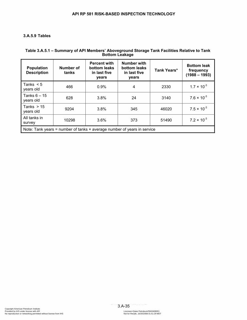
API RP 581 RISK-BASED INSPECTION TECHNOLOGY
3.A-35
3.A.5.9 Tables
Table 3.A.5.1 – Summary of API Members’ Aboveground Storage Tank Facilities Relative to Tank Bottom Leakage
Population Description
Number of tanks
Percent with bottom leaks
in last five years
Number with bottom leaks
in last five years
Tank Years* Bottom leak frequency
(1988 – 1993)
Tanks < 5 years old 466 0.9% 4 2330 1.7 × 10⁻³
Tanks 6 – 15 years old 628 3.8% 24 3140 7.6 × 10⁻³
Tanks > 15 years old 9204 3.8% 345 46020 7.5 × 10⁻³
All tanks in survey 10298 3.6% 373 51490 7.2 × 10⁻³
Note: Tank years = number of tanks × average number of years in service
Copyright American Petroleum Institute Provided by IHS under license with API Licensee=Qatar Petroleum/5943408001
Not for Resale, 10/20/2008 01:51:29 MDTNo reproduction or networking permitted without license from IHS
--```,`,,`,`,,`,`,,,,,,``,```,`-`-`,,`,,`,`,,`---

Copyright American Petroleum Institute Provided by IHS under license with API Licensee=Qatar Petroleum/5943408001
Not for Resale, 10/20/2008 01:51:29 MDTNo reproduction or networking permitted without license from IHS
--```,`,,`,`,,`,`,,,,,,``,```,`-`-`,,`,,`,`,,`---

API RP 581 RISK-BASED INSPECTION TECHNOLOGY
API RP 581 PART 3
ANNEX 3.B – SI AND US CUSTOMARY CONVERSION FACTORS
3.B-1 Copyright American Petroleum Institute Provided by IHS under license with API Licensee=Qatar Petroleum/5943408001
Not for Resale, 10/20/2008 01:51:29 MDTNo reproduction or networking permitted without license from IHS
--```,`,,`,`,,`,`,,,,,,``,```,`-`-`,,`,,`,`,,`---
API RP 581 RISK-BASED INSPECTION TECHNOLOGY
PART CONTENTS 3.B.1 GENERAL ........................................................................................................................... 3.B-3 3.B.2 TABLES .............................................................................................................................. 3.B-4
3.B-2 Copyright American Petroleum Institute Provided by IHS under license with API Licensee=Qatar Petroleum/5943408001
Not for Resale, 10/20/2008 01:51:29 MDTNo reproduction or networking permitted without license from IHS
--```,`,,`,`,,`,`,,,,,,``,```,`-`-`,,`,,`,`,,`---

API RP 581 RISK-BASED INSPECTION TECHNOLOGY
3.B.1 GENERAL The SI and US Customary unit conversion factors for equations that appear throughout Part 3 of this document are provided in Table 3.B.1 of this Annex.
3.B-3 Copyright American Petroleum Institute Provided by IHS under license with API Licensee=Qatar Petroleum/5943408001
Not for Resale, 10/20/2008 01:51:29 MDTNo reproduction or networking permitted without license from IHS
--```,`,,`,`,,`,`,,,,,,``,```,`-`-`,,`,,`,`,,`---
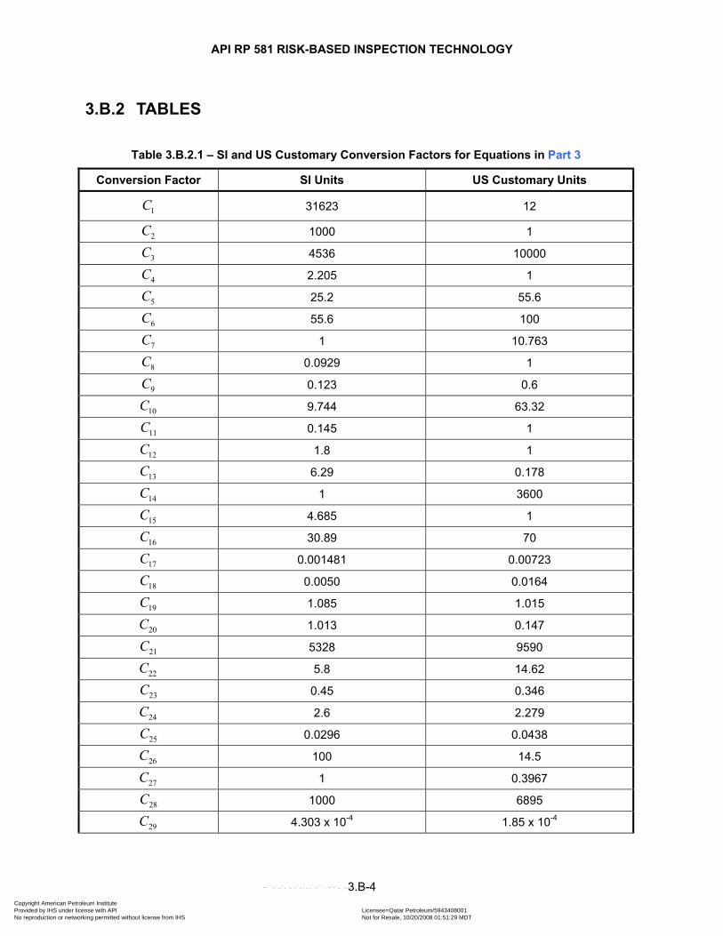
API RP 581 RISK-BASED INSPECTION TECHNOLOGY
3.B.2 TABLES
Table 3.B.2.1 – SI and US Customary Conversion Factors for Equations in Part 3
Conversion Factor SI Units US Customary Units
1C 31623 12
2C 1000 1
3C 4536 10000
4C 2.205 1
5C 25.2 55.6
6C 55.6 100
7C 1 10.763
8C 0.0929 1
9C 0.123 0.6
10C 9.744 63.32
11C 0.145 1
12C 1.8 1
13C 6.29 0.178
14C 1 3600
15C 4.685 1
16C 30.89 70
17C 0.001481 0.00723
18C 0.0050 0.0164
19C 1.085 1.015
20C 1.013 0.147
21C 5328 9590
22C 5.8 14.62
23C 0.45 0.346
24C 2.6 2.279
25C 0.0296 0.0438
26C 100 14.5
27C 1 0.3967
28C 1000 6895
29C 4.303 x 10⁻⁴ 1.85 x 10⁻⁴
3.B-4 Copyright American Petroleum Institute Provided by IHS under license with API Licensee=Qatar Petroleum/5943408001
Not for Resale, 10/20/2008 01:51:29 MDTNo reproduction or networking permitted without license from IHS
--```,`,,`,`,,`,`,,,,,,``,```,`-`-`,,`,,`,`,,`---
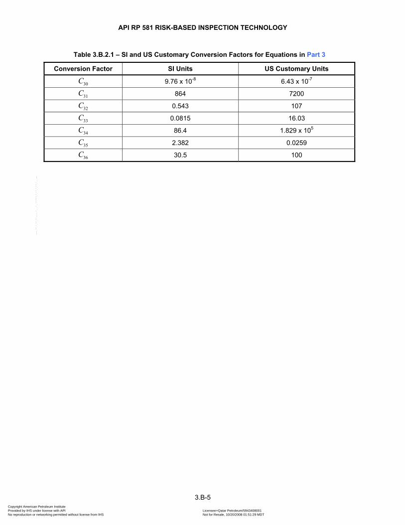
API RP 581 RISK-BASED INSPECTION TECHNOLOGY
3.B-5
Table 3.B.2.1 – SI and US Customary Conversion Factors for Equations in Part 3
Conversion Factor SI Units US Customary Units
30C 9.76 x 10⁻⁸ 6.43 x 10⁻⁷
31C 864 7200
32C 0.543 107
33C 0.0815 16.03
34C 86.4 1.829 x 10⁵
35C 2.382 0.0259
36C 30.5 100
Copyright American Petroleum Institute Provided by IHS under license with API Licensee=Qatar Petroleum/5943408001
Not for Resale, 10/20/2008 01:51:29 MDTNo reproduction or networking permitted without license from IHS
--```,`,,`,`,,`,`,,,,,,``,```,`-`-`,,`,,`,`,,`---

Copyright American Petroleum Institute Provided by IHS under license with API Licensee=Qatar Petroleum/5943408001
Not for Resale, 10/20/2008 01:51:29 MDTNo reproduction or networking permitted without license from IHS
--```,`,,`,`,,`,`,,,,,,``,```,`-`-`,,`,,`,`,,`---
Invoice To ( Check here if same as “Ship To”)
Name:
Title:
Company:
Department:
Address:
City: State/Province:
Zip/Postal Code: Country:
Telephone:
Fax:
Email:
Payment Enclosed P.O. No. (Enclose Copy)
Charge My IHS Account No.
VISA MasterCard American Express Diners Club Discover
Credit Card No.:
Print Name (As It Appears on Card):
Expiration Date:
Signature:
Quantity Title Total
Subtotal
Applicable Sales Tax (see below)
Rush Shipping Fee (see below)
Shipping and Handling (see below)
Total (in U.S. Dollars)
To be placed on Standing Order for future editions of this publication, place a check mark in the SO column and sign here:
Pricing and availability subject to change without notice.
Date:
SO Unit Price
API Member (Check if Yes)
Ship To (UPS will not deliver to a P.O. Box)
Name:
Title:
Company:
Department:
Address:
City: State/Province:
Zip/Postal Code: Country:
Telephone:
Fax:
Email:
Mail Orders – Payment by check or money order in U.S. dollars is required except for established accounts. State and local taxes, $10 processing fee, and 5% shipping must be added.Send mail orders to: API Publications, IHS, 15 Inverness Way East, c/o Retail Sales, Englewood, CO 80112-5776, USA.
Purchase Orders – Purchase orders are accepted from established accounts. Invoice will include actual freight cost, a $10 processing fee, plus state and local taxes.Telephone Orders – If ordering by telephone, a $10 processing fee and actual freight costs will be added to the order.Sales Tax – All U.S. purchases must include applicable state and local sales tax. Customers claiming tax-exempt status must provide IHS with a copy of their exemption certificate.Shipping (U.S. Orders) – Orders shipped within the U.S. are sent via traceable means. Most orders are shipped the same day. Subscription updates are sent by First-Class Mail. Other options, including next-day service, air service, and fax transmission are available at additional cost. Call 1-800-854-7179 for more information.Shipping (International Orders) – Standard international shipping is by air express courier service. Subscription updates are sent by World Mail. Normal delivery is 3-4 days fromshipping date.Rush Shipping Fee – Next Day Delivery orders charge is $20 in addition to the carrier charges. Next Day Delivery orders must be placed by 2:00 p.m. MST to ensure overnight delivery.Returns – All returns must be pre-approved by calling the IHS Customer Service Department at 1-800-624-3974 for information and assistance. There may be a 15% restocking fee.Special order items, electronic documents, and age-dated materials are non-returnable.
Effective January 1, 2008.API Members receive a 30% discount where applicable.The member discount does not apply to purchases made for the purpose of resale or for incorporation into commercial products, training courses, workshops, or othercommercial enterprises.
Available through IHS:Phone Orders: 1-800-854-7179 (Toll-free in the U.S. and Canada)
303-397-7956 (Local and International)Fax Orders: 303-397-2740Online Orders: global.ihs.com
2008 PublicationsOrder Form
Copyright American Petroleum Institute Provided by IHS under license with API Licensee=Qatar Petroleum/5943408001
Not for Resale, 10/20/2008 01:51:29 MDTNo reproduction or networking permitted without license from IHS
--```,`,,`,`,,`,`,,,,,,``,```,`-`-`,,`,,`,`,,`---

API provides additional resources and programs to the oil and natural gas industry which arebased on API Standards. For more information, contact:
API MONOGRAM® LICENSINGPROGRAMPhone: 202-962-4791Fax: 202-682-8070Email: [email protected]
API QUALITY REGISTRAR(APIQR®)> ISO 9001 Registration> ISO/TS 29001 Registration> ISO 14001 Registration> API Spec Q1® RegistrationPhone: 202-962-4791Fax: 202-682-8070Email: [email protected]
API PERFORATOR DESIGNREGISTRATION PROGRAMPhone: 202-682-8490Fax: 202-682-8070Email: [email protected]
API TRAINING PROVIDERCERTIFICATION PROGRAM(API TPCPTM)Phone: 202-682-8490Fax: 202-682-8070Email: [email protected]
API INDIVIDUAL CERTIFICATIONPROGRAMS (ICP®)Phone: 202-682-8064Fax: 202-682-8348Email: [email protected]
API ENGINE OIL LICENSING ANDCERTIFICATION SYSTEM (EOLCS)Phone: 202-682-8516Fax: 202-962-4739Email: [email protected]
API PETROTEAM (TRAINING,EDUCATION AND MEETINGS)Phone: 202-682-8195Fax: 202-682-8222Email: [email protected]
API UNIVERSITYTM
Phone: 202-682-8195Fax: 202-682-8222Email: [email protected]
Check out the API Publications, Programs,and Services Catalog online at www.api.org.
Copyright 2008 – API, all rights reserved. API, API monogram, APIQR, API Spec Q1,API TPCP, ICP, API University and the API logo are either trademarks or registeredtrademarks of API in the United States and/or other countries.
THERE’S MOREWHERE THIS CAME FROM.
Copyright American Petroleum Institute Provided by IHS under license with API Licensee=Qatar Petroleum/5943408001
Not for Resale, 10/20/2008 01:51:29 MDTNo reproduction or networking permitted without license from IHS
--```,`,,`,`,,`,`,,,,,,``,```,`-`-`,,`,,`,`,,`---

Copyright American Petroleum Institute Provided by IHS under license with API Licensee=Qatar Petroleum/5943408001
Not for Resale, 10/20/2008 01:51:29 MDTNo reproduction or networking permitted without license from IHS
--```,`,,`,`,,`,`,,,,,,``,```,`-`-`,,`,,`,`,,`---

Additional copies are available through IHSPhone Orders: 1-800-854-7179 (Toll-free in the U.S. and Canada)
303-397-7956 (Local and International)Fax Orders: 303-397-2740Online Orders: global.ihs.com
Information about API Publications, Programs and Servicesis available on the web at www.api.org
1220 L Street, NWWashington, DC 20005-4070USA
202.682.8000
Product No. C58102Copyright American Petroleum Institute Provided by IHS under license with API Licensee=Qatar Petroleum/5943408001
Not for Resale, 10/20/2008 01:51:29 MDTNo reproduction or networking permitted without license from IHS
--```,`,,`,`,,`,`,,,,,,``,```,`-`-`,,`,,`,`,,`---
Copyright © 2022 FDOKUMEN