Risk Assessment and Management for
358
Risk Assessment and Management for Interconnected and Interactive Critical Flood Defense Systems By Hamed Hamedifar A dissertation submitted in partial satisfaction of the requirements for the degree of Doctor of Philosophy in Civil and Environmental Engineering in the Graduate Division of the University of California, Berkeley Committee in charge: Professor Juan M. Pestana, Co-Chair Professor Robert G. Bea, Co-Chair Professor Raymond B. Seed Professor Ronald Amundson Fall 2012
-
Upload
khangminh22 -
Category
Documents
-
view
3 -
download
0
Transcript of Risk Assessment and Management for

Risk Assessment and Management for Interconnected and Interactive Critical Flood Defense Systems
By
Hamed Hamedifar
A dissertation submitted in partial satisfaction of the
requirements for the degree of
Doctor of Philosophy
in
Civil and Environmental Engineering
in the
Graduate Division
of the
University of California, Berkeley
Committee in charge:
Professor Juan M. Pestana, Co-Chair Professor Robert G. Bea, Co-Chair
Professor Raymond B. Seed Professor Ronald Amundson
Fall 2012


Risk Assessment and Management for Interconnected and Interactive Critical Flood Defense Systems
Copyright © 2012
By
Hamed Hamedifar

1
Abstract
Risk Assessment and Management
for Interconnected and Interactive Critical Flood Defense Systems
By
Hamed Hamedifar
Doctor of Philosophy in Civil and Environmental Engineering
University of California, Berkeley
Juan M. Pestana-Nascimento, Co-Chair
Robert G. Bea, Co-Chair
The current State-of-the-Practice relies heavily in the deterministic characterization and assessment of performance of civil engineering infrastructure. In particular, flood defense systems, such as levees, have been evaluated within the context of Factor of Safety where the capacity of the system is compared with the expected demand. Uncertainty associated with the capacity and demand render deterministic modeling inaccurate. In particular, two structures with the same Factor of Safety can have vastly different probabilities of failure. While efforts have been made to assess levee vulnerability, results from these more traditional engineering approaches are questionable because they do not more fully account for uncertainties included in modeling, natural variability, or human and organization factors.
This study develops and documents a probabilistic Risk Assessment Methodology that explicitly addresses levee resilience and sustainability by explicitly incorporating uncertainty in the Capacity and Demand components. In this research, we have categorized uncertainties into four different categories: Type I- Inherent (or aleatory) variability; Type II- Analytical/ Model (epistemic) variability; Type III- Human and Organizational Performance Uncertainty; and Type IV- Knowledge integration uncertainty.
The complete infrastructure system in the Delta is very complex with many components integrally correlated. These include large-scale water supplies that supply over 20 million residents; a flood protection and levee system that past research has shown to be at great risk; an electricity transmission grid key to California and western North America; and a multimodal transportation system (roads, rail and shipping) that extends throughout the Pacific Rim. Delta’s levees are among of the most unstable engineering systems, with several major hazards threatening the stability of the approximately 1100 miles of its levees. Flood, sea level rise, and aging infrastructure all contribute to this risk. It is this potential levee failure that could cause the greatest damage, particularly with respect to the security of freshwater exports.
This thesis validates the proposed methodology by evaluating the probability of failure for an interconnected flood defense system in the California Sacramento-San Joaquin Delta. The study focuses on the behavior of the levee system protecting Sherman Island. Sherman island is of

2
critical importance to California because of the critical infrastructures that pass under, on and over it, including: natural gas pipelines: regional and inter-regional electricity transmission lines; two deepwater shipping channels that run alongside the island; and the presence of State Highway 160, a link between major expressways. The work evaluates current (year 2010) and future conditions (year 2100) and incorporates variations in capacity and demand arising from human activities and global climate change. Specifically, the work evaluates the uncertainties for three potential failure modes: underseepage, slope (or levee) instability and overtopping/erosion through the use of Monte Carlo simulations that correctly capture the probability distribution of capacity and demand measures.
Finally, the work incorporates Human and Organizational Factors including interconnections and uncertainties into the Risk Assessment Model as they account for the largest contribution of major engineered system failures.
With this approach, probability of failure was determined and uncertainties were explicitly stated in every step of the method. By doing so decision makers and engineers can quickly identify where the uncertainty lies and decrease the probability of failure by increasing their understanding of the engineered system.
3
Dedication
To memory of those who lost their lives because of vulnerable flood defense systems all around the world.
Everywhere you look you see infinite pain,
High water lines,
Mold infested basements,
Missing neighbors,
Tears in the eyes,
Broken voices…

i
CONTENTS
1 INTRODUCTION ................................................................................................................... 1
1.1 General Approach ............................................................................................................ 1
1.2 Research Focus ................................................................................................................. 2
1.3 Sherman Island Infrastructure Systems ............................................................................ 4
1.4 Sherman Island Levee System ......................................................................................... 6
1.4.1 Sherman Island Levee System History ..................................................................... 7
1.4.2 Sherman Island Levee System Vulnerability ............................................................ 9
1.5 Scope of Project ............................................................................................................... 9
2 BACKGROUND ................................................................................................................... 10
2.1 Defining Metrics for Quality .......................................................................................... 10
2.2 Reliability ....................................................................................................................... 11
2.3 Classification of Uncertainties ....................................................................................... 13
2.4 Quantification of Uncertainty......................................................................................... 14
2.4.1 Uncertainty Distributions ........................................................................................ 14
2.4.2 Probability of Failure .............................................................................................. 14
2.5 System Failure Mechanisms .......................................................................................... 15
2.5.1 Surface sloughing.................................................................................................... 15
2.5.2 Shear failure ............................................................................................................ 16
2.5.3 Liquefaction ............................................................................................................ 16
2.5.4 Seepage, and Piping ................................................................................................ 16
2.5.5 Other Failure Mechanisms ...................................................................................... 16
3 ASSESSMENT OF LEVEE FAILURE DUE TO SEEPAGE .............................................. 18
3.1 Seepage Mechanism ....................................................................................................... 18
3.2 Metric of Failure for Seepage Mechanism ..................................................................... 20
3.3 Site Selection .................................................................................................................. 22
3.3.1 Location to Analyze Effective Stress ...................................................................... 22
3.4 Site Characterization ...................................................................................................... 24
3.5 Uncertainty Characterization.......................................................................................... 26

ii
3.5.1 Demands ................................................................................................................. 27
3.5.2 Capacity .................................................................................................................. 32
3.6 Probabilistic Analyses (Monte Carlo Simulations) ........................................................ 33
3.6.1 Probability Distribution for Capacity and Demand ................................................ 33
3.6.2 Probability of Failure .............................................................................................. 34
3.7 Type II Uncertainty (Model Bias) .................................................................................. 36
3.8 Probability of Failure over Time .................................................................................... 37
4 ASSESSMENT OF LEVEE FAILURE DUE SLOPE INSTABILITY ................................ 40
4.1 Lateral Slope Instability Mechanism.............................................................................. 40
4.1.1 Surface Sloughing ................................................................................................... 40
4.1.2 Shear Failure ........................................................................................................... 40
4.1.3 Liquefaction and Other Types of Slope Instability ................................................. 42
4.2 Sherman Island Levee System ....................................................................................... 42
4.2.1 System Definition ................................................................................................... 42
4.2.2 Hazard Characterization .......................................................................................... 42
4.2.3 Site Geology Characterization ................................................................................ 43
4.2.4 Soil Properties ......................................................................................................... 44
4.2.5 Site Selection .......................................................................................................... 44
4.3 Probability of Levee Failure Due to Sliding Considering Type I (Aleatory) Uncertainties.............................................................................................................................. 45
4.3.1 Type I Uncertainty Evaluation ................................................................................ 45
4.3.2 Southern Site ........................................................................................................... 47
4.3.3 Northern Site ........................................................................................................... 55
4.4 Probability of Levee Failure Due to Sliding with Additional Consideration of Type II (Epistemic) Uncertainties: ......................................................................................................... 60
4.4.1 Type II Uncertainty Evaluation .............................................................................. 60
4.4.2 Determination of Type II Uncertainties (Bias) for Slope Stability Models ............ 60
4.4.3 Bias Mean Value and Standard Deviation .............................................................. 67
4.4.4 Analysis of Probability of Levee Failure Due to Sliding with Additional Consideration of Type II (Epistemic) Uncertainties .............................................................. 70
4.4.5 Probability of Levee Failure Due to Sliding ........................................................... 73
5 OVERTOPPING AND EROSION ....................................................................................... 76
iii
5.1 Background .................................................................................................................... 76
5.2 Previous Laboratory Experiments .................................................................................. 77
5.3 Failure Mechanism ......................................................................................................... 78
5.4 Natural Uncertainty (Type I) Evaluation ....................................................................... 79
5.4.1 Demands (Rivers Data) ........................................................................................... 79
5.4.2 Capacity (Levee Height) ......................................................................................... 85
5.5 Overtopping, Probability of Failure 2010 ...................................................................... 95
5.6 Hazard Adjustment (Projection to the Year 2100) ......................................................... 96
5.6.1 Sea Level Rise......................................................................................................... 96
5.6.2 Sea Level Rise Adjustment ..................................................................................... 97
5.6.3 Levee Crest Adjustment .......................................................................................... 99
5.7 Overtopping, Probability of Failure 2100 .................................................................... 101
5.8 Probability of Failure for Series Element System ........................................................ 102
5.8.1 Overtopping Probability of Failure for Levee System of Sherman Island ........... 102
5.9 Levee Erosion ............................................................................................................... 104
5.9.1 Erosion of levee’s Inner Slope by Wave Overtopping ......................................... 106
5.9.2 Erosion Rate (ε) .................................................................................................... 111
5.10 Final Probability of Levee Failure Due to Erosion considering Type I, & II .............. 113
5.10.1 Time for Levee Erosion, Time of Breaching (Capacity) ...................................... 113
5.10.2 Time for Grass Turf Erosion ................................................................................. 113
5.10.3 Time for Levee Fill Erosion .................................................................................. 116
5.10.4 Time for Overtopping (Demands) ........................................................................ 118
5.10.5 Likelihood of Failure (Breach) ............................................................................. 118
6 INCORPORATING HUMAN AND ORGANIZATIONAL FACTORS INTO PROBABILTY OF FAILURE ANALYSIS ............................................................................... 120
6.1 Flood fighting ............................................................................................................... 122
6.2 System definition.......................................................................................................... 123
6.2.1 General .................................................................................................................. 123
6.2.2 Sherman Island System Definition Illustration ..................................................... 125
6.3 Conceptual Model ........................................................................................................ 128
6.3.1 General .................................................................................................................. 128

iv
6.3.2 Sherman Island Conceptual Model Illustration .................................................... 131
6.4 Event Tree .................................................................................................................... 133
6.4.1 General .................................................................................................................. 133
6.4.2 Sherman Island Event Tree Illustration ................................................................ 134
6.5 Create Task Structure Map ........................................................................................... 136
6.5.1 General .................................................................................................................. 136
6.5.2 Sherman Island Task Structure Map Illustration .................................................. 137
6.6 Perform QMAS+ Assessment ...................................................................................... 138
6.6.1 General .................................................................................................................. 138
6.6.2 Adapt QMAS to QMAS+ ..................................................................................... 143
6.6.3 Sherman Island QMAS Illustration ...................................................................... 144
6.7 Probability of Failure Computation ............................................................................. 149
6.7.1 General .................................................................................................................. 149
6.7.2 Sherman Island Probability of Failure Computation Illustration .......................... 155
6.8 Discussion .................................................................................................................... 158
6.8.1 Risk management strategies .................................................................................. 158
6.8.2 Method Limitations and Proposed Refinements ................................................... 161
6.8.3 Integrating Human Intervention in Risk Assessment and Management and to Refine the Sherman Island ................................................................................................... 163
7 ASSESSMENT OF CONSEQUENCES OF FAILURE ..................................................... 164
7.1 Introduction .................................................................................................................. 164
7.2 Consequence of Sherman Island Levee Failure ........................................................... 165
7.2.1 Loss of Life ........................................................................................................... 166
7.2.2 Water Quality ........................................................................................................ 168
7.2.3 State Highways and Bridges ................................................................................. 168
7.2.4 Natural Gas Pipeline ............................................................................................. 169
7.2.5 Transmission Lines ............................................................................................... 171
7.2.6 Ecosystem (Fishes) ............................................................................................... 172
7.3 Target Reliabilities ....................................................................................................... 172
7.3.1 Probability of Failure (Pf) vs. Consequence of Failure (Cf) Curves .................... 172
7.3.2 Concept of ALARP (as low as reasonably practicable): ...................................... 173
v
7.4 Level of Risk for Sherman Island Levee System ......................................................... 175
8 SUMMARY AND CONCLUSIONS .................................................................................. 176
8.1 Probability of Failure ................................................................................................... 176
8.2 Consequences of Failure .............................................................................................. 177
8.3 Sherman Island Levee System Risk Level ................................................................... 178
8.4 Concluding Remarks .................................................................................................... 180
9 REFERENCES .................................................................................................................... 182
APPENDICES ............................................................................................................................ 198

vi
Figure 1-1: The Sacramento-San Joaquin River Delta Map of the Delta showing islands, waterways, and significant infrastructure. (Source: DWR) ............................................................ 3
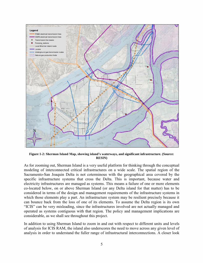
Figure 1-2: Sherman Island Map, showing island’s waterways, and significant infrastructure. (Source: RESIN) ............................................................................................................................. 5
Figure 1-3: Aerial view of Sherman Island's North site, San Joaquin River (below) the Sacramento (above). (Source: flickr) .............................................................................................. 7
Figure 1-4: Chinese laborers built many of the early levees in the Delta. (Source: Overland Monthly, 1896) ............................................................................................................................... 8
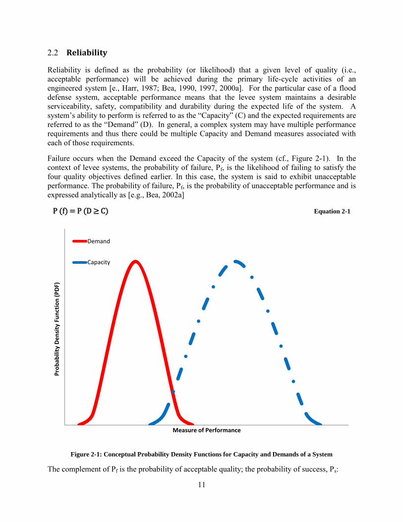
Figure 2-1: Conceptual Probability Density Functions for Capacity and Demands of a System . 11
Figure 2-2: Definition of Probability of Failure ........................................................................... 12
Figure 2-3: Different Levee Failure Mechanisms (after Zina Deretsky, National Science Foundation) ................................................................................................................................... 17
Figure 3-1: Levee Through-Seepage Failure Mechanism (after Zina Deretsky, NSF) ................ 19
Figure 3-2: Levee Under-Seepage, Piping Failure Mechanism (after Zina Deretsky, NSF) ........ 19
Figure 3-3: Example of Equipotential & Flow lines –Flownet (Holtz & Kovacs, 1981) ............. 21
Figure 3-4: Sherman Island Site Locations ................................................................................... 23
Figure 3-5: Total Head for Vertical Effective Stress Calculation................................................. 23
Figure 3-6: Classification of Soil Units Used in the Sherman Island Pilot Project ...................... 24
Figure 3-7: Interface Situation in Flownet (after DM 7.01) ......................................................... 30
Figure 3-8: Effects of Varying Topography ................................................................................. 33
Figure 3-9: Capacity PDF 100 year event-current conditions (year 2010) ................................... 34
Figure 3-10: Demand PDF for 100 year event-Current conditions (year 2010) ........................... 34
Figure 3-11: Overlap of Demand and Capacity PDF for 100 year event in year 2010 ................ 35
Figure 3-12: Probability of Failure vs. Time (2010).................................................................... 39
Figure 4-1: Levee Surface Sloughing Failure Mechanism (after Zina Deretsky, NSF) ............... 41
Figure 4-2: Levee Rotational Shear Failure Mechanism (after Zina Deretsky, NSF) .................. 41
Figure 4-3: Schematic of Embankment Strength Failure ............................................................ 46
Figure 4-4: Southern Site Location ............................................................................................... 47
Figure 4-5: Best and Worst Case Levee Cross Section Interpolation, Sherman Island South Section........................................................................................................................................... 48
Figure 4-6: Driving and Resisting Forces on the Blocks (The subscripts A and P denote active and passive wedges) ...................................................................................................................... 49
Figure 4-7: Driving and Resisting Forces on the Blocks in Ordinary Method of Slices Method. 50
Figure 4-8: Driving and Resisting Forces on the Blocks in Bishop's Simplified Method ............ 50
Figure 4-9: Calculating fo Factor for Janbu's Generalized Procedure of Slices ............................ 51
Figure 4-10: Deep Levee Slope Failure, Southern Portion of Sherman Island (Best Case Scenario) ....................................................................................................................................... 53
Figure 4-11: Deep Levee Slope Failure, Southern Portion of Sherman Island (Worst Case Scenario) ....................................................................................................................................... 54
Figure 4-12: Northern Site Location ............................................................................................. 55

vii
Figure 4-13: Best and Worst Case Levee Cross Section Interpolation, Sherman Island North Section........................................................................................................................................... 56
Figure 4-14: Shallow Levee Slope Failure, Northern Portion of Sherman Island (Best Case Scenario) ....................................................................................................................................... 58
Figure 4-15: Shallow Levee Slope Failure, Northern Portion of Sherman Island (Best Case Scenario) ....................................................................................................................................... 59
Figure 4-16: Test Fill Embankment over Soft Peat on Bouldin Island (“Performance of Test Fill Constructed on Soft Peat”, by Kevin Tillis, Michael Meyer, and Edwin Hultgren, 1992) .......... 62
Figure 4-17: Replication of the Field Condition from Test Fill Embankment over Soft Peat on Bouldin Island in the Stability Analytical Model (“Performance of Test Fill Constructed on Soft Peat”, by Kevin Tillis, Michael Meyer, and Edwin Hultgren, 1992) ........................................... 62
Figure 4-18: Atchafalaya levees located on plains of the Mississippi River “Stability of Atchafalaya Levees”, by Robert Kaufman, and Frank Weaver, 1967 .......................................... 63
Figure 4-19: Replication of the Field Condition from Test Fill Embankment over Atchafalaya levee in the Stability Analytical Model. (“Stability of Atchafalaya Levees”, by Kaufman, and Weaver, 1967) ............................................................................................................................... 63
Figure 4-20: James Bay Project levees “Design of Single- or Multi-stage Construction of Embankment Dams for the James Bay Project”, Ladd et al. (1983) ............................................ 65
Figure 4-21: Replication of the Field Condition from James Bay Project levees in the Stability Analytical Model (“Design of Single- or Multi-stage Construction of Embankment Dams for the James Bay Project”, Ladd et al. 1983) .......................................................................................... 65
Figure 4-22: Instrumentation for the Bergambacht test “Monitoring of the Test on the Dike at Bergambacht”, by A.R. Koelewijn, and Meindert Van, 2003 ...................................................... 66
Figure 4-23: Replication of the Field Condition from Bergambacht Dike in the Stability Analytical Model. (“Monitoring of the Test on the Dike at Bergambacht”, by A.R. Koelewijn, and Meindert Van, 2003) .............................................................................................................. 66
Figure 4-24: Probability-Lognormal, Mean Value and Standard Deviation of Bias Points (OMS Method) ......................................................................................................................................... 68
Figure 4-25: Probability-Lognormal, Mean Value and Standard Deviation of Bias Points (Simplified Bishop) ....................................................................................................................... 68
Figure 4-26: Probability-Lognormal, Mean Value and Standard Deviation of Bias Points (Simplified Janbu) ......................................................................................................................... 69
Figure 4-27: Probability-Lognormal, Mean Value and Standard Deviation of Bias Points (Spencer) ....................................................................................................................................... 69
Figure 4-28: Annual Probability Failure for South Side Sherman Island in the Best Case Scenario....................................................................................................................................................... 74
Figure 4-29: Annual Probability Failure for South Side Sherman Island in the Worst Case Scenario......................................................................................................................................... 74
Figure 4-30: Annual Probability Failure for North Side Sherman Island in the Best Case Scenario....................................................................................................................................................... 75

viii
Figure 4-31: Annual Probability Failure for North Side Sherman Island in the Worst Case Scenario......................................................................................................................................... 75
Figure 5-1: Experimental Set-up Developed and Described by Pachnio (2005) .......................... 77
Figure 5-2: Schematic of Levee Overtopping (after Zina Deretsky, NSF) ................................... 78
Figure 5-3: 2010 Hydrograph (Antioch Station) .......................................................................... 80
Figure 5-4: 2010 Hydrograph (Rio Vista Station) ........................................................................ 80
Figure 5-5: Lognormal Distribution of Water Level Annual Extremes for “Sacramento River” 84
Figure 5-6: Lognormal Distribution of Water Level Annual Extremes for “San Joaquin River” 85
Figure 5-7: Southern Site, Location of each Section .................................................................... 86
Figure 5-8: levee Height Uncertainty in Southern Site Section 6 through 10 ............................. 89
Figure 5-9: Northern Site, Location of each Section .................................................................... 90
Figure 5-10: levee Height Uncertainty in Northern Site Section 1 through 5 and Section 11 ..... 94
Figure 5-11: Levee Sections ........................................................................................................ 95
Figure 5-12: Likelihood of Overtopping, for the each of 11 levee sections ................................. 96
Figure 5-13: Regional Trends in Sea Level Rise .......................................................................... 97
Figure 5-14: Lognormal Distribution of Water Level Annual Extremes for “San Joaquin River” with MSLR Adjustment ................................................................................................................ 98
Figure 5-15: Lognormal Distribution of Water Level Annual Extremes for “Sacramento River” with MSLR.................................................................................................................................... 99
Figure 5-16: levee Cross Sections for Adjustments to the Year 2100 ........................................ 100
Figure 5-17: Projected Likelihood of Overtopping, for the each of 11 Levee Sections ............. 101
Figure 5-18: Schematic Illustration of Series System................................................................. 102
Figure 5-19: Schematic Illustration of Two Different Sets of Erosion Mechanisms (Source: Seed et al, 2008a) ................................................................................................................................. 104
Figure 5-20: Southern Part of Sherman Island Levee System Protected with Rip-rap Armor along the San Joaquin River ................................................................................................................. 105
Figure 5-21: Schematic Illustration of Lands Side Erosion due to Levee Over topping ............ 106
Figure 5-22: Lognormal Distribution of Overtopping Flow Velocity ........................................ 110
Figure 5-23: Critical Shear Stress vs. Erodibility Coefficient, by Hanson and Simon (2001) .. 111
Figure 5-24: Normal Distribution of Grass Cover Quality ........................................................ 115
Figure 5-25: Normal Distribution of Turf Thickness Data ........................................................ 115
Figure 6-1: Sand bag ring around a sand boil. (Source: Department of Water Resources, 2011)..................................................................................................................................................... 123
Figure 6-2: Sack topping on a levee (Source: Department of Water Resources, 2010) ............. 123
Figure 6-3: System Components ................................................................................................. 124
Figure 6-4: Sherman Island Flood Protection System Components ........................................... 127
Figure 6-5: Framework for Conceptual Model ........................................................................... 129
Figure 6-6: Variables and Values in Conceptual Model ............................................................. 130
Figure 6-7: An Event Sequence. Photos courtesy of DWR ........................................................ 132

ix
Figure 6-8: Conceptual Model of Sherman Island Flood Fighting System Including System Variables and Values .................................................................................................................. 133
Figure 6-9: Event Tree for Flood Protection on Sherman Island ................................................ 135
Figure 6-10: OODA Loop. Inspired from Boyd, J.R. (1996) .................................................... 136
Figure 6-11: Task Structure Map for Anticipatory Flood Fighting ........................................... 137
Figure 6-12: Task Structure Map for Interactive Flood Fighting .............................................. 138
Figure 6-13: The QMAS process. Inspired from [Hee, 1997] .................................................... 140
Figure 6-14: QMAS structure of the data [from Bea, 2002] ....................................................... 141
Figure 6-15: QMAS grading scale. Taken from [Bea, R.G. (2002);] ......................................... 142
Figure 6-16: Factors and Attributes for Interactive Flood Fighting ........................................... 145
Figure 6-17: South Site at Sherman Island ................................................................................. 147
Figure 6-18: Sherman Island’s Levee Overlooking Mayberry (Photographer: Rich Fletcher) .. 147
Figure 6-19: QMAS+ average grades for Sherman Island's flood protection system. For illustration purposes only and does not represent the result of a field application of the QMAS+ instrument ................................................................................................................................... 149
Figure 6-20: Nominal Human Performance Task Reliability. (Source: Williams, J.C. 1988) ... 151
Figure 6-21: QMAS Qualitative Scale Translation into Performance Shaping Factors. (Source: Bea, 2000) ................................................................................................................................... 153
Figure 6-22: Event Space for a Sequence of Four Linear Tasks ................................................ 154
Figure 6-23: Annual Probability for Seepage Events Under a 100 Year Storm, with Human Intervention ................................................................................................................................. 157
Figure 6-24: Annual Probability for Seepage Events Under a 100 Year Storm, Without Human Intervention ................................................................................................................................. 158
Figure 6-25: OODA loop for Interactive Flood Fighting with Procedures ................................ 159
Figure 6-26: Event Space with QA/QC ..................................................................................... 161
Figure 7-1: Risk Assessment Schematics ................................................................................... 165
Figure 7-2: Consequences of Sherman Island levee failure ........................................................ 166
Figure 7-3: The San Joaquin River flows towards the San Francisco Bay beneath the Antioch Bridge (Route 160), (RESIN Sherman Island Pilot Project 2009) ............................................. 170
Figure 7-4: Underground Natural Gas Pipelines cross Sherman Island, (RESIN SIPP, 2009) .. 170
Figure 7-5: Transmission lines greater then 500kV cross Sherman Island. RESIN Sherman Island Pilot Project 2009 ........................................................................................................................ 171
Figure 7-6: Fitness for purpose reliability evaluation guideline (Bea 2005) .............................. 174
Figure 7-7: Infrastructure Journal ‘inputs’ to address the Sherman Island ‘water protection’ infrastructure – levees – analyses of probabilities of failure. Bea, 2012 .................................... 175
Figure 8-1: Probability of Failure (Pf) vs. Consequence of failure (Cf) curve, showing the level of risk for Shearman Island Levees South side, 2010 ..................................................................... 178
Figure 8-2: Probability of Failure (Pf) vs. Consequence of failure (Cf) curve, showing the level of risk for Shearman Island Levees North side, 2010 ..................................................................... 179

x
Table 3-1: Exit Gradient Conditions (USACE) ............................................................................ 19
Table 3-2: Saturated Unit Weight of Soil (pcf) ............................................................................ 25
Table 3-3: Hydraulic Conductivity of Soil Units .......................................................................... 25
Table 3-4: Qualitative Uncertainty Breakdown ............................................................................ 26
Table 3-5: Quantitative Uncertainty Breakdown .......................................................................... 27
Table 3-6: Measured pore pressures versus predicted pore pressures .......................................... 37
Table 4-1: Southern Site, Material Properties and Uncertainty which is associating with each layer............................................................................................................................................... 46
Table 4-2: Calculated Probability of Failure for the South Section (Best Case Scenario) ........... 52
Table 4-3: Calculated probability of failure for the South section (Worst Case Scenario) .......... 52
Table 4-4: Calculated probability of failure for the North Section (Best Case Scenario) ........... 57
Table 4-5: Calculated probability of failure for the North Section (Worst Case Scenario) ......... 57
Table 4-6: Summary of the Final Result of Bias Point Calculation ............................................. 67
Table 4-7: Bmean value and standard deviation σ .......................................................................... 67
Table 4-8: C Mean/ D Mean, σ ln C Mean/ D Mean, C 50/ D50 for South & North Site in the Best & Worst Cross-section Conditions .............................................................................................................. 71
Table 4-9: Summary of Final Probability of Failures, Final Safety Indexes, and Standard Normal Distribution probabilities for the Levees of Sherman Island ........................................................ 72
Table 5-1: Analyses to be Included (Bulletin 17B, 1982) ............................................................ 81
Table 5-2: Probability of Non-Exceedance (PNE) ....................................................................... 82
Table 5-3: Standard Deviations (σ) of Levee Height in Southern Part ......................................... 87
Table 5-4: Standard Deviations (σ) of Levee Height in Northern Part ......................................... 91
Table 5-5: 2100, Sacramento and San Joaquin River Stages Uncertainties ................................. 98
Table 5-6: Probability of Failure of Sherman Island Levee system due to Overtopping using both Equations 6-3 and 6-4 ......................................................................................................... 103
Table 5-7: Mean and Standard Deviation Values for Critical Shear Stresses on Levees ........... 107
Table 5-8: Manning coefficient (n) values (By: Christopher Trevor) ....................................... 109
Table 5-9: Mean and Standard Deviation Values for Hydraulic Shear Stresses ........................ 109
Table 5-10: Mean and Standard Deviation Values for Levee’s Soils Erodibility Coefficient ... 111
Table 5-11: Mean and Standard Deviation Values of Erosion Rate .......................................... 112
Table 5-12: Mean and Standard Deviation Values of Grass Cover Quality, and Turf Thickness..................................................................................................................................................... 114
Table 5-13: Sherman Island Levee Width .................................................................................. 116
Table 5-14: Mean and Standard Deviation Values for Levee Erosion Time ............................. 117
Table 5-15: Mean and Standard Deviation Values for Total time required for Levee Erosion . 117
Table 5-16: Mean and Standard Deviation Values for Time of Overtopping ........................... 118
Table 5-17: Safety Index ............................................................................................................. 119
Table 5-18: Final Annual Probability of Failure......................................................................... 119
Table 6-1: List of Organizations potentially involved in protecting Sherman Island from flooding, by activity .................................................................................................................... 126

xi
Table 6-2 : System Definition Concepts ..................................................................................... 127
Table 6-3: Information requested from the organization ............................................................ 142
Table 6-4: Recommended literature on QMAS .......................................................................... 143
Table 6-5: QMAS+ Coarse Assessment ..................................................................................... 148
Table 6-6: Human Failure Rates (Source: Gertman, D. I. 1997) ................................................ 150
Table 6-7: Base Error Rates for Interactive Flood Fighting ....................................................... 155
Table 6-8: Results from QMAS+ and SYRAS PSF ................................................................... 156
Table 8-1: Summary of Failure Probabilities (annual probabilities of failure for year 2010) .... 176
Table 8-2: Summary of damage estimates (106US$) and information for Sherman Island infrastructure failures. ................................................................................................................. 177

xii
Acknowledgements
The thesis would not have been written in this form without Prof. Juan M. Pestana and Prof. Robert G. Bea. Prof. Pestana introduced me into numerical modeling in geomechanics and through our numerous discussions provided superior guides for my research activities; Prof. Bea originated my interest in Geotechnical Risk Assessment and Management of engineering systems and they particularly, managed to create perfect conditions for research at University of California Berkeley.
I was lucky to work with many wise people who all left their traces in my research presented in the thesis. Particularly I would like to thank Prof. Raymond B. Seed. He was a source of inspiration for me from the beginning to the end of my academic career at University of California Berkeley. I truly appreciate the support provided by Dr. Emery Roe, Prof. Paul Schulman, Dr. Bas Jonkman, Dr. Howard Foster, Dr. Rune Storesund, Mr. Miles Brodsky, and Mr. Henri de Corn, whom I met during my research in Resilient and Sustainable Infrastructure Networks (RESIN) team. I must mention three individuals in particular, Mr. Richard Short who was my supervisor for a different project. In many senses, he has been a mentor and a friend; I have learned enormously from him. I truly appreciate the support provided by Prof. Michael Riemer during the course of my experimental studies in the Laboratory, and Prof. Garrison Sposito for guiding me into environmental geotechnics.
I would like to thank my parents, Forugh Razaghi Khamsi and Frahad Hamedifar for their support during the course of my research. This work would have not been possible without their unconditional support and love. Special thanks to my sisters Dr. Haleh Hamedifar, and Mrs. Hoda Hamedifar, whose supports were invaluable. Also, thanks to Rosy and Frank Hamedi-Fard, who helped me take a major step toward achieving my goals.
So to the personnel acknowledgements, life in college runs parallel to life outside, and established friendships helped deal with stresses arising in both parts of my life, so thanks to Dr. Roozbeh Geraili Mikola, Mr. Justin Hollenback, Mr. Tonguc Deger, and Mr. Joseph Weber.
The National Science Foundation (NSF) generously provided funding for this research under the grant number EFRI-083604.
Any opinions, findings, and conclusions or recommendations expressed in this material are those of the author(s) and do not necessarily reflect the views of the National Science Foundation.

1
1 INTRODUCTION
1.1 General Approach
With good reason, engineers and the engineering professions have viewed interconnected technical systems positively. History is full of advanced technologies and structures that benefit humankind. In the past, many people (and not just engineers) felt that these benefits exceed the costs of unexpected disruptions and failures emerging from increasingly complex and sophisticated systems. There has been growing concern, however, that vulnerabilities arising in what society considers strategically interconnected infrastructures pose new threats to those demonstrated benefits. Critical infrastructures are defined as assets and systems essential for the provision of vital societal services and include large engineered supplies for water, electricity, telecommunications, transportation and financial services [National Research Council (2009)].
Engineering communities have responded to the challenge of interconnected critical infrastructures in two related ways: Many primarily focus on better approaches to design out vulnerabilities, while others recognize vulnerabilities missed at the design or construction stages must be mitigated in subsequent operations and redesign. This research initiative takes up the challenge in the following way. We seek to develop improved risk assessment and management (RAM) strategies for use by engineers throughout all stages of the any infrastructure’s life cycle (from design to decommission) so as to reduce inter-infrastructural vulnerabilities and optimize the benefits of cross-system interconnectivity. If vulnerability reduction and interconnectivity optimization are promoted through better RAM strategies, the resilience and sustainability of the infrastructures’ critical services will be enhanced.
Why do engineers need improved risk assessment and management approaches for resilient and sustainable critical infrastructures? First, risk analysis is typically the charge of specific units within individual infrastructures; fewer approaches deal with explicit risk (that is, the probabilities and consequences of failure) at “the system of systems” scale, that is, the level of interconnected critical infrastructure systems (ICIS). A major feature of our research has been to take RAM methods proven at the infrastructure level and modify/extend them to the ICIS level. Second, numbers of existing RAM methodologies are limited by their assumptions about and estimation of the various types of uncertainties that pervade infrastructural development and we see methods that correct for that (more below). Last, key terms, including “resilience” and “sustainability,” are under-conceptualized and rarely operationalized within infrastructures, let alone the ICIS level. The National Science Foundation’s Directorate of Engineering seeks to address these issues explicitly.
The specific goal of this project has been to develop and validate approaches and strategies for risk assessment and management of interconnected infrastructure systems operating in the California Sacramento-San Joaquin Delta and beyond. Practically, this has meant the development of RAM methods that better address four general categories of uncertainties of major concern to engineers as risk assessors of infrastructures:

2
I. Natural variabilities (Type 1)
II. Modeling uncertainties (Type 2)
III. Human/organizational factors (Type 3)
IV. Informational uncertainties related to data utilization in all stages of an infrastructure's life cycle (Type 4)
The first two types of uncertainties can be treated as intrinsic. The last two are grouped as extrinsic in nature. This study has focused on the emerging methodological importance of modeling (Type 2) uncertainties, while underscoring the ongoing need to better understand, reduce or otherwise accommodate the extrinsic (Types 3 and 4) uncertainties in any RAM focused at the ICIS level.
This ambitious aim led to a set of project activities that seek to better integrate human and organizational factors into risk analysis, assess connected networks of critical infrastructures, and develop new approaches for incorporating and modeling a wide range of uncertainties in risk assessments. This mandate, in turn, required an interdisciplinary approach from the outset. By mid-2011, our interdisciplinary team had involved more than 20 researchers from five disciplines: engineering, social sciences, environmental sciences, city and regional planning (most important, geographical information system specialists), and law. The interdisciplinary activities and research methods enabled us to develop and use the ICIS perspective as a unique platform to zoom in, out and across levels of analysis in terms of how infrastructures, their components, and their services interconnect. Our research to date has undertaken analyses of specific levees as well as site visits, discussions and a tabletop exercise with key decision makers, including state and federal infrastructure managers, emergency response officials, and support staff. As part of the methodological development of RAM approaches appropriate for the ICIS level of analysis, our research has also focused on the development of Geographical Information System (GIS) databases and their use in risks assessments and simulations.
This report focuses on one of several themes emerging across Project activities as well as those activities. The connecting theme—the importance of assessing and managing modeling (Type 2) uncertainties better—is drawn out as we discuss Project’s site, regional and infrastructure-wide activities. We appreciate that improved risk assessment and management across critical infrastructures is of interest to more than engineers. However, this report centers on the engineering communities.
1.2 Research Focus
The area focus of Project research is the Sacramento-San Joaquin Delta, which has been called California’s “infrastructure crossroads.” The interconnections at the crossroads are live policy and management issues for counties, state agencies and the U.S. federal government. The infrastructures of research interest are those, which public and private entities uniformly acknowledge as of manifest importance. These include large-scale water supplies that supply over 20 million residents; a flood protection and levee system that past research has shown to be at great risk; an electricity transmission grid key to California and western North America; and a

3
multimodal transportation system (roads, rail and shipping) that extends throughout the Pacific Rim (Figure 1-1). In the process of undertaking the research, we also found telecommunications, like electricity, to be a key infrastructure. These critical infrastructures take on added importance because the Delta itself is a one-of-a-kind aquatic-terrestrial ecosystem of international significance that could be harmed were the infrastructures to fail in major ways.
Figure 1-1: The Sacramento-San Joaquin River Delta Map of the Delta showing islands, waterways, and
significant infrastructure. (Source: DWR)
4
1.3 Sherman Island Infrastructure Systems
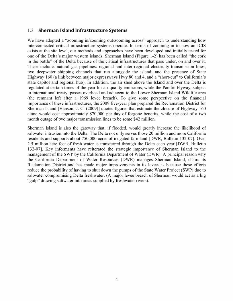
We have adopted a “zooming in/zooming out/zooming across” approach to understanding how interconnected critical infrastructure systems operate. In terms of zooming in to how an ICIS exists at the site level, our methods and approaches have been developed and initially tested for one of the Delta’s major western islands. Sherman Island (Figure 1-2) has been called “the cork in the bottle” of the Delta because of the critical infrastructures that pass under, on and over it. These include: natural gas pipelines: regional and inter-regional electricity transmission lines; two deepwater shipping channels that run alongside the island; and the presence of State Highway 160 (a link between major expressways Hwy 80 and 4, and a “short-cut” to California’s state capitol and regional hub). In addition, the air shed above the Island and over the Delta is regulated at certain times of the year for air quality emissions, while the Pacific Flyway, subject to international treaty, passes overhead and adjacent to the Lower Sherman Island Wildlife area (the remnant left after a 1969 levee breach). To give some perspective on the financial importance of these infrastructures, the 2009 five-year plan prepared the Reclamation District for Sherman Island [Hanson, J. C. (2009)] quotes figures that estimate the closure of Highway 160 alone would cost approximately $70,000 per day of forgone benefits, while the cost of a two month outage of two major transmission lines to be some $42 million.
Sherman Island is also the gateway that, if flooded, would greatly increase the likelihood of saltwater intrusion into the Delta. The Delta not only serves those 20 million and more California residents and supports about 750,000 acres of irrigated farmland [DWR, Bulletin 132-07]. Over 2.5 million-acre feet of fresh water is transferred through the Delta each year [DWR, Bulletin 132-07]. Key informants have reiterated the strategic importance of Sherman Island to the management of the SWP by the California Department of Water (DWR). A principal reason why the California Department of Water Resources (DWR) manages Sherman Island, chairs its Reclamation District and has made major improvements in its levees is because these efforts reduce the probability of having to shut down the pumps of the State Water Project (SWP) due to saltwater compromising Delta freshwater. (A major levee breach of Sherman would act as a big “gulp” drawing saltwater into areas supplied by freshwater rivers).
5
Figure 1-2: Sherman Island Map, showing island’s waterways, and significant infrastructure. (Source:
RESIN)
As for zooming out, Sherman Island is a very useful platform for thinking through the conceptual modeling of interconnected critical infrastructures on a wide scale. The spatial region of the Sacramento-San Joaquin Delta is not coterminous with the geographical area covered by the specific infrastructure systems that cross the Delta. This is important, because water and electricity infrastructures are managed as systems. This means a failure of one or more elements co-located below, on or above Sherman Island (or any Delta island for that matter) has to be considered in terms of the design and management requirements of the infrastructure systems in which those elements play a part. An infrastructure system may be resilient precisely because it can bounce back from the loss of one of its elements. To assume the Delta region is its own “ICIS” can be very misleading, since the infrastructures involved are not actually managed and operated as systems contiguous with that region. The policy and management implications are considerable, as we shall see throughout this project.
In addition to using Sherman Island to zoom in and out with respect to different units and levels of analysis for ICIS RAM, the island also underscores the need to move across any given level of analysis in order to understand the fuller range of infrastructural interconnections. A closer look
N

6
at Sherman Island in Figure 1-2 shows that an ICIS extends beyond a site of co-located elements of multiple critical infrastructures. For there are stretches of the Sherman Island levees that are not just elements in a Delta-wide flood protection system but also elements in other critical infrastructures. The very same structure serves multiple infrastructure functions. There is a stretch of Sherman Island levee over which part of Highway 160 runs; other stretches serve as the waterside banks of the deepwater shipping channels. There is another stretch that serves to protect a large wetland berm providing ecosystem services in terms of fishing and habitat. Moreover, any stretch of levee breaching on Sherman Island would directly increase the probability of DWR’s State Water Project failing, given the intrusion of saltwater following the loss of the island. If such stretches of levee fail, so too by definition do the same structural elements fail in the deepwater shipping channel, Highway 160, the state’s water supply, or the Delta’s endangered habitat.
Consequently, an incompletely specified model or models of how the ICIS starts from the ground up and operates at different scales during different time periods adds considerable uncertainty to engineer-based RAM analyses. What is needed is a suite of methods and approaches that zoom in, out and across multiple level of risk analysis. This has significant repercussions for the calculation of the probability and consequences of interinfrastructural failure (Pf and Cf respectively).
1.4 Sherman Island Levee System
The Sacramento and the San Joaquin Rivers supply water to most of the state of California, collecting and rainfall and snow form the Sierra Nevada and transporting it toward San Francisco Bay. On the western side of the northern California, the two rivers flow together into a delta before ending up into the bay. A major function of the two rivers extends beyond water supply; they also transport sediment in the Sacramento and San Joaquin Valleys, collectively known as the Central Valley. This sediment transportation system is one reason why the soils are so rich in nutrient and why farming is so productive in the valley. Although the Delta is a rich agricultural area, its most important value remains as a source of freshwater for the rest of the State. The Delta is the center of north to south water delivery system. Much of this water is pumped southward for use in the San Joaquin Valley and elsewhere in central and southern California. Pumping stations and river canals deliver Sacramento Delta water to farms and cities across the Central Valley. The levees and islands help to protect water-export facilities in the southern Delta from saltwater intrusion by maintaining freshwater fraction.
Delta’s levees are among of the most unstable engineering systems, with several major hazards threatening the stability of the approximately 1100 miles of its levees. To repeat: Not only do the levees help to defend the agricultural, recreational, urban, and environmental land that lies behind them (Figure 1-3), but they also protect the freshwater supplies for more than 23 million Californians which consider being two-thirds of the population of this state. Flood, sea level rise, and aging infrastructure all contribute to this risk. It is this potential levee failure that could cause the greatest damage, particularly with respect to the security of freshwater exports.

7
Figure 1-3: Aerial view of Sherman Island's North site, San Joaquin River (below) the Sacramento (above).
(Source: flickr)
Sherman Island lies at the western limit of the Sacramento-San Joaquin Delta, 35 miles south-southwest of Sacramento, bounded by the San Joaquin River on the east and the Sacramento River on the west as shown on Figure 1-2. Both rivers are also formally deepwater shipping channels at this point to Sacramento and Stockton, respectively. Like most Delta islands, Sherman is predominantly below sea level and protected by perimeter levee built over vulnerable foundation soils.
Today, Sherman Island is protected by approximately 18-miles of levee that encompass approximately 9,937 acres of land, according to the 1995 Sacramento Delta San Joaquin Atlas. Approximately 9 miles of levee are project levee, constructed by the US Army Corps of Engineers, and approximately 9 miles of levee are non-project levee. The entire levee system is maintained by the Sherman Island Reclamation District, RD 341.
1.4.1 Sherman Island Levee System History
In the late-1800s, large-scale agricultural development in the Delta required levee-building to prevent frequent flooding. The marshland had to be drained, cleared of wetland vegetation, and tilled. Levees and drainage systems were largely complete by 1930, with the Delta taking on its current appearance of mostly a, 1,150-squaremile area reclaimed for agricultural use [Thompson,

8
2006]. The levees were constructed over the past 150 to 160 years primarily by farmers. These levees made out of un-compacted sediments and organics. Farmers did little or no foundation preparation for the levees. Foundations are composed of a complex river sediments and organic materials with overlapping zones of widely varying compositions and consistencies. Materials range from coarse-grained sediments, including gravels and loose, clean sands, to soft, fine-grained materials such as silts, clays, and organics, including fibrous peat.
Figure 1-4: Chinese laborers built many of the early levees in the Delta. (Source: Overland Monthly, 1896)
By the end of the 1860s, “substantial” levees had been built by the hands of Chinese laborers (Figure 1-4) on Twitchell and Sherman Islands, and by the 1870s, small reclamation projects had begun on Rough and Ready and Roberts Islands. In the early 1870s, however, it became apparent that these first levees would be insufficient to protect the Delta as islands such as Sherman and Twitchell continued to flood annually. By 1874, the costs for reclamation and preservation of Sherman Island’s levees alone totaled 500,000 [California Department of Water Resources, 1995], approximately 8-9 billion in 2007 dollars. Sherman Island was chosen as the target island for this study because it is one of the first leveed islands in Delta, it is currently being managed by RD 341 in close coordination with DWR, and its failure can lead to failure of neighboring islands and the change of the salt water balance in Delta. Accordingly, Sherman Island is one of the most critical Islands in the Western Delta and within the entire Delta basin.
9
1.4.2 Sherman Island Levee System Vulnerability
A variety of hazards including storms, earthquakes, and floods threaten levees in the Sherman Island. Given the increasing human populations and local, regional, and national critical infrastructures dependent on these structures, levee reliability is a crucial component to averting social, ecological, and economic disaster.
While efforts have been made to assess levee vulnerability, results from these more traditional engineering approaches are questionable because they do not more fully account for uncertainties included in modeling, natural variability, or human and organization factors [Duncan, S.J. (2007)]. Such a probabilistic approach to analysis is overlooked or neglected likely because geotechnical engineers are unfamiliar with the procedures for both identifying and quantifying uncertainty [Duncan, S.J. (2007)]. Not incorporating the full range of uncertainties into an analysis and ultimately into decision making, however, could actually lead to levee failure and ultimately, worsened consequences because of a false understanding of the engineered system. It could appear safer that it really is. Therefore, in the face an uncertain yet changing climate likely to exacerbate the effects of climate-related hazards, new methods for assessing levee safety and reliability are of increasing importance.
1.5 Scope of Project
The reliability of any risk estimate is increased if the uncertainty associated with the results is offered with its estimation are explicitly accounted for. It is often the case in traditional engineering that only one estimate solution is presented as the “correct” answer. The capacity to enhance the reliability of results is often neglected or overlooked because engineers have not been properly trained to handle the variety of different uncertainties affecting any risk estimate. This study aims to provide an example of how traditional methods for analyzing levees can be approached probabilistically so that the variety of uncertainty within the results is understood and areas or recommendations for improvement are readily identified. Furthermore, the study aims to show how human and organizational factors (HOF) within the system affect the probability of failure (Appendix A)
This study develops, validates, and documents a probabilistic RAM method that explicitly addresses levee resilience and sustainability, using a case example from Sherman Island. In doing so, the activity examines performance now (2010) and projected future performance (2100) under a various water-level conditions, including forecasted variations in regional global climate change. The goals of the Sherman Island Pilot Project (SIPP) are to
1) Provide an example of how probability of failure could be determined for three different failure modes:
I. Seepage II. Slope stability
III. Overtopping
Given flood events with 2, 50 and 100 year return periods in the years 2010 and 2100 and
2) Show how the HOF within the system can be accounted for and how its effects on the probability of failure can be determined.

10
2 BACKGROUND
The current State-of-the-Practice relies heavily in the deterministic characterization and assessment of performance of civil engineering infrastructure. In particular, flood defense systems, such as levees, have been evaluated within the context of Factor of Safety where the capacity of the system is compared with the expected demand. Uncertainty has been qualitatively accounted for by requiring a minimum Factor of Safety, with larger values required when uncertainty is large. Nevertheless, this procedure seems arbitrary and lacks the rigor than a proper probabilistic analysis brings to bear on the problem. If more robust methods for determining the probability of failure are to be developed, engineers will need to move towards stochastic modeling and away from deterministic modeling. Uncertainty associated with the capacity and demand render deterministic modeling inaccurate. In particular, two structures with the same Factor of Safety can have vastly different probabilities of failure.
This chapter briefly introduces the concept of Quality and Failure in a broad sense as related to civil engineering infrastructure with particular application to flood defense systems. A brief discussion of the concept of reliability and probability of failure for levee systems is presented. Estimation of system reliability requires the evaluation of intrinsic and extrinsic capacity and demand uncertainties. Finally, a brief discussion of the failure mechanisms for levee systems is presented while full details of reliability analyses are presented in subsequent chapters.
2.1 Defining Metrics for Quality
For the purposes of risk assessment and management of any civil engineering infrastructure, we require the definition of quality metrics. Quality is defined as freedom from unanticipated defects. For a civil engineering system, quality is associated with acceptable performance and it implies that the system satisfies the requirements of those that own, design, construct, operate and regulate the system. These requirements are composed of the following components:
I. Serviceability
II. Safety
III. Compatibility
IV. Durability
Serviceability is suitability of the system for the proposed application and it is intended to guarantee the performance for the agreed purpose and conditions of use. Safety is the freedom from excessive danger/threat to human life, the environment, and property damage. Compatibility implies that the system does not have unnecessary or excessive negative impacts on the environment and society. Finally, durability requires that the serviceability, safety and environmental compatibility are maintained during the intended life of the system [Bea, 2007]. The metric by which a component of quality is measured varies from system to system. For this study serviceability and sustainability (with regards to serviceability) was the quality component chosen for analysis.
11
2.2 Reliability
Reliability is defined as the probability (or likelihood) that a given level of quality (i.e., acceptable performance) will be achieved during the primary life-cycle activities of an engineered system [e., Harr, 1987; Bea, 1990, 1997, 2000a]. For the particular case of a flood defense system, acceptable performance means that the levee system maintains a desirable serviceability, safety, compatibility and durability during the expected life of the system. A system’s ability to perform is referred to as the “Capacity” (C) and the expected requirements are referred to as the “Demand” (D). In general, a complex system may have multiple performance requirements and thus there could be multiple Capacity and Demand measures associated with each of those requirements.
Failure occurs when the Demand exceed the Capacity of the system (cf., Figure 2-1). In the context of levee systems, the probability of failure, Pf, is the likelihood of failing to satisfy the four quality objectives defined earlier. In this case, the system is said to exhibit unacceptable performance. The probability of failure, Pf, is the probability of unacceptable performance and is expressed analytically as [e.g., Bea, 2002a]
P (f) = P (D ≥ C) Equation 2-1
Figure 2-1: Conceptual Probability Density Functions for Capacity and Demands of a System
The complement of Pf is the probability of acceptable quality; the probability of success, Ps:
Pro
bab
ility
De
nsi
ty F
un
ctio
n (
PD
F)
Measure of Performance
Demand
Capacity

12
P(s) = P(C ≥ D) = 1 – P (f) Equation 2-2
In broad terms, the probability of failure for a levee system depends on the balance between demands imposed on the system (water levels, wind waves, seismic loading) and the capacity of the system to resist those demands (height of levees, side slopes of levees, etc.). Both demands and capacities have uncertainty associated with them. In this framework, the overlap between the demands and capacities is proportional to the probability of failure
As shown in Figure 2-2, uncertainty influences the shape of the demand and capacity probability density functions (pdfs). The larger the uncertainty, the wider the distributions become relative to their central tendencies. With other things being equal, larger uncertainty results in a larger overlap between distributions thus a higher probability of failure. The more uncertain one must be with respect to demand and capacity, the greater is the estimated total value of Pf. As a result, the magnitude of uncertainty plays a major factor in the calculated total probability of failure.
This study focuses primarily on the probability of failure. Assessment of failure consequences is outside the scope of this work and is the subject of future research.
Figure 2-2: Definition of Probability of Failure
Pro
bab
ility
De
nsi
ty F
un
ctio
n
Measure of Performance
Demand
Capacity
Uncertainty in Demand
Uncertainty in Capacity
Probability of Failure: Overlap Between Demand & Capacity

13
2.3 Classification of Uncertainties
Uncertainties associated with the Demand and Capacity of an engineered structure or system can be Intrinsic or Extrinsic. Based on past research of flood defense systems, we have classified uncertainties into four different types [i.e., Bea, 2006]:
Type I: Natural or inherent variability.
Type II: Engineering/analytical model and parametric uncertainty.
Type III: Human and organizational factors (affecting performance) uncertainty.
Type IV: Information, knowledge, understanding uncertainties
Types I and II fall under the general category of Intrinsic uncertainty, while Type III and IV fall under the category of Extrinsic uncertainty. Human and organizational factors (HOF) uncertainty is associated with how individuals perform, act (or react) and how organizations influence this performance. Information, knowledge, understanding uncertainty is associated with the general understanding of system performance and can be further classified into two subcategories: a) unknown knowable and b) unknown unknowable.
This work focuses primarily on the estimation of Type I and II uncertainties for Flood Defense systems and it is presented in chapters 3, 4 and 5. A discussion of Type III uncertainty is presented in chapter 6. Type IV uncertainty is outside the scope of this work.
There are four primary approaches that should be used in an integrated and complimentary way in order to characterize Type I and II uncertainties.
I. Simulation
II. Experiment (field, laboratory)
III. Process reviews (analysis of relevant past failures and successes)
IV. Judgment
All of these approaches represent viable means of providing quantitative characterization of uncertainty. It is uncommon to find a structured and consistent use of these four approaches in current risk assessment studies. Simulation (analytical or numerical experiments) can provide significant insights into how and when uncertainties are developed- and their characterizations. Field and laboratory experiments are an important way to gather information on uncertainties. They represent samplings of the more general situation being studied, and must be carefully designed to avoid bias in the result. Studies of past failures and successes involving relevant engineered systems also are a significant source of information if carefully done. A forensic study is a particular case of process review concentrating on the explanation of past failures. Finally, judgment is perhaps the most important source of quantitative information on uncertainties. Judgment has a primary and rightful place because available data is always deficient for the evaluation of a particular situation.
14
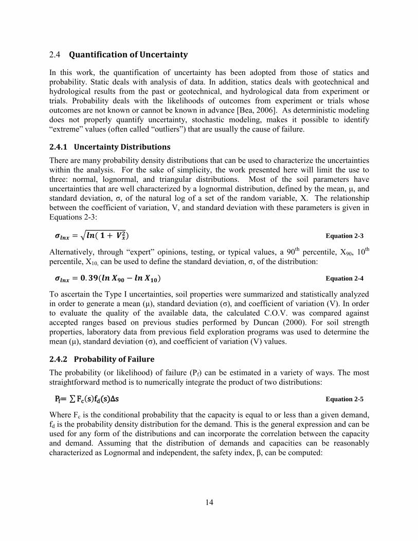
2.4 Quantification of Uncertainty
In this work, the quantification of uncertainty has been adopted from those of statics and probability. Static deals with analysis of data. In addition, statics deals with geotechnical and hydrological results from the past or geotechnical, and hydrological data from experiment or trials. Probability deals with the likelihoods of outcomes from experiment or trials whose outcomes are not known or cannot be known in advance [Bea, 2006]. As deterministic modeling does not properly quantify uncertainty, stochastic modeling, makes it possible to identify “extreme” values (often called “outliers”) that are usually the cause of failure.
2.4.1 Uncertainty Distributions
There are many probability density distributions that can be used to characterize the uncertainties within the analysis. For the sake of simplicity, the work presented here will limit the use to three: normal, lognormal, and triangular distributions. Most of the soil parameters have uncertainties that are well characterized by a lognormal distribution, defined by the mean, μ, and standard deviation, σ, of the natural log of a set of the random variable, X. The relationship between the coefficient of variation, V, and standard deviation with these parameters is given in Equations 2-3:
= √ ( ) Equation 2-3
Alternatively, through “expert” opinions, testing, or typical values, a 90th percentile, X90, 10th percentile, X10, can be used to define the standard deviation, σ, of the distribution:
= ( ) Equation 2-4
To ascertain the Type I uncertainties, soil properties were summarized and statistically analyzed in order to generate a mean (μ), standard deviation (σ), and coefficient of variation (V). In order to evaluate the quality of the available data, the calculated C.O.V. was compared against accepted ranges based on previous studies performed by Duncan (2000). For soil strength properties, laboratory data from previous field exploration programs was used to determine the mean (μ), standard deviation (σ), and coefficient of variation (V) values.
2.4.2 Probability of Failure
The probability (or likelihood) of failure (Pf) can be estimated in a variety of ways. The most straightforward method is to numerically integrate the product of two distributions:
Pf= ∑ (s)f (s) s Equation 2-5
Where Fc is the conditional probability that the capacity is equal to or less than a given demand, fd is the probability density distribution for the demand. This is the general expression and can be used for any form of the distributions and can incorporate the correlation between the capacity and demand. Assuming that the distribution of demands and capacities can be reasonably characterized as Lognormal and independent, the safety index, β, can be computed:

15
= (
⁄ )
√
Equation 2-6
C50 and D50 are the median (i.e., 50th percentile) values of the capacity and demand, respectively. The ratio of C50/D50 is the traditional definition of the deterministic “unbiased” factor of safety (FS). The values of are the standard deviations of the log-normal distribution of the capacity and demand. If the demands and capacities are correlated, with correlation DC, then the safety index can be determined from:
= (
⁄ )
√
Equation 2-7
The probability of failure, Pf, can then be determined from the safety index:
Pf = 1 – Φ ( ) Equation 2-8
Where Φ ( ) is the standard cumulative normal probability function for the safety index. When the safety index ranges between 1 and 3 (common in civil engineering infrastructure applications), the probability of failure, Pf, can be approximated as:
Pf ≈ 0.475 exp(– β1.6 ) Equation 2-9
Pf ≈ 10– β (rough approximation) Equation 2-10
As the factor of safety increases, the safety index increases, and the likelihood of failure decreases. As the uncertainty in the demand and capacity increases which can be represented either as type I or type II uncertainties, the likelihood of failure increases. In this way, probabilistic analyses give more information than a single value of the factor of safety. It also allows assessment of the importance of uncertainties associated with each parameter in the reliability of the levee system.
2.5 System Failure Mechanisms
Experience with the behavior of levees, and often with their catastrophic failure, has led to the identification of at least a dozen different failure mechanisms (Figure 2-3). These failure mechanisms are result of change in one or several parameters in the levee system associating, with either capacity or demand, which in turn subsequently results in flooding. A complete discussion of all of these mechanisms is outside the scope of this work and only a few of them will be briefly discusses as related to the research work presented here.
2.5.1 Surface sloughing
A shear failure in which a surficial portion of the levee moves down slope is termed a surface slough. If such failures are not monitored at the first sign of occurrence and repaired, they can become progressively larger, and may then represent a threat to levee safety.

16
2.5.2 Shear failure
A shear failure involves sliding of a portion of a levee, or a levee and its foundation and they occurs along weaker soil strata within the soil profile. Failure surfaces are generally nonlinear and frequently they are approximated by circular arcs.
2.5.3 Liquefaction
The phenomenon of soil liquefaction, or significant reduction in soil strength and stiffness as a result of shear-induced increase in pore water pressure, is a major cause of earthquake damage to embankments and levees (e.g., Youd et al. 1984). Although most instances of liquefaction have been associated with saturated loose sandy or silty soils, loose gravelly soil deposits are also vulnerable to liquefaction (e.g., Coulter and Migliaccio 1966; Chang 1978; Youd et al. 1984; Harder, 1988).
2.5.4 Seepage, and Piping
Seepage and piping can occur when hydraulic gradients at the landside of a levee are large enough to move soil particles. For piping to occur, a layer with low hydraulic, such as cohesive layer must overlay a layer with high hydraulic conductivity such as cohesionless soil.
2.5.5 Other Failure Mechanisms
Several types of levee failure, including wave impacts, structural impacts, jetting, tree and animal damage, lateral spreading, and combinations of these factor may also cause levee failure. These types of failure mechanisms are not discussed in this study, but the possibility of their occurrence should not be ignored.
The probability of failure of a system would ideally account for all possible failure scenarios. The Sherman Island Pilot Project (SIPP) chose to analyze three possible scenarios specifically: seepage, slope stability and overtopping. The probability of failure of the system will be a function of each individual probability of failure. By choosing only three failure modes the entire probability of failure of the system may not be fully captured. Therefore it is termed P*
f
system, where the asterisk denotes that the probability of failure of the system is conditional on only three failure modes and not all possible failure mechanisms. For the remainder of this work, we will simply refer to the probability of failure.
The failure modes for the Sherman Island levee system are linked in series, because if one failure occurs from any one of these failure modes at any location on the levees, the entire system fails. Therefore the probability of failure of the system can be determined with Equation 2-11
Pf s s = 1-(1 - Pf )(1-Pf s ) (1-Pf ) Equation 2-11
Where: P*f, System – probability of failure of the system (conditional upon previously mentioned failure modes), and Pf, Seepage, Pf, Overtopping, Pf, Slope stability are the probability of failures due to seepage, slope stability and overtopping, respectively. The probability of failure for each failure mode is determined through the proper quantification of demands and capacities for each failure mode along with the uncertainty associated with them. A distribution of results can be used if uncertainty is associated with it (as explained in pervious section). Chapters 3, 4, and 5 of this

17
study focuses on those first two categories of intrinsic uncertainties associating with the seepage, overtopping, and lateral stability of any engineering levee systems.
Figure 2-3: Different Levee Failure Mechanisms (after Zina Deretsky, National Science Foundation)

18
3 ASSESSMENT OF LEVEE FAILURE DUE TO SEEPAGE
3.1 Seepage Mechanism
Seepage is the movement of water through porous soils and can be detrimental to any type of earth foundation including levees because of its ability to erode soil, due to high seepage velocities, and result in detrimental seepage forces leading to very small effective stresses, due to high porewater pressure (cf., Figure 3-1). Seepage is an ongoing problem for many islands in the Delta. Levees in the Sacramento-San Joaquin Delta were originally built in an ad-hoc manner and consist of fill material, with sands, silts, and clays, while their foundations are typically a layer of silty clay, peat, another silty clayey layer, and sand.
A type of seepage is termed through-seepage which is the seepage through the body of the levee itself that could lead to a full levee collapse. The levee and subsurface cross sections from Sherman Island show that through seepage may be more of a problem than under-seepage. This is also confirmed by the SEEP/W results that are presented in subsequent sections. The occurrence of seepage in itself does not indicate the inevitable failure of the levee. If seepage flow is limited, human and organizational factors can intervene to ensure that the water is removed with temporary pumps and drainage ditches.
Another type of seepage is referred to as under-seepage that occurs through the foundation soil. The main concern that arises from under-seepage is piping, which involves the erosion of sandy and silty soils underneath the levee. As the material is carried away due to high seepage velocity, it creates a hollow space or “pipe” downstream that could potential propagate upstream thus progressively increasing the hydraulic gradient and thus increase seepage velocities even further. Cohesive materials can sustain the position for a short time, but eventually will collapse causing failure of the levee as illustrated in Figure 3-2. For piping to occur, a low hydraulic conductivity layer, such as clay must overlay a cohesionless soil such as sandy soil. If these conditions exist, piping may a concern. An extensive analysis can be done using the erodibility of soil and it is described in detail in “Road and Hydraulic Engineering Institute’s Technical Report on Sand Boils (Piping)” (1999, 2002) where a method is developed for determining whether or not piping will occur given different water levels.
A variety of metrics can be used to measure seepage. Initially, this study chose to use exit gradient as the metric for seepage because it allows for a closed form solution to be developed in order to determine a probability of failure. The exit gradient, i, is defined as:
= Equation 3-1
Where Δh and L are the difference in energy head and the distance between two locations, respectively. The US Army Corps of Engineers has classified seepage conditions as a function of exit gradients (cf., Table 3-1). This classification is rather ambiguous when it comes to describing certain exit gradients. For instance, an exit gradient at the toe of a levee of 0.5 could indicate conditions ranging from “no seepage” all the way to “sand boils.” For this reason another metric, effective stress, was used to assess seepage failure in this analysis.
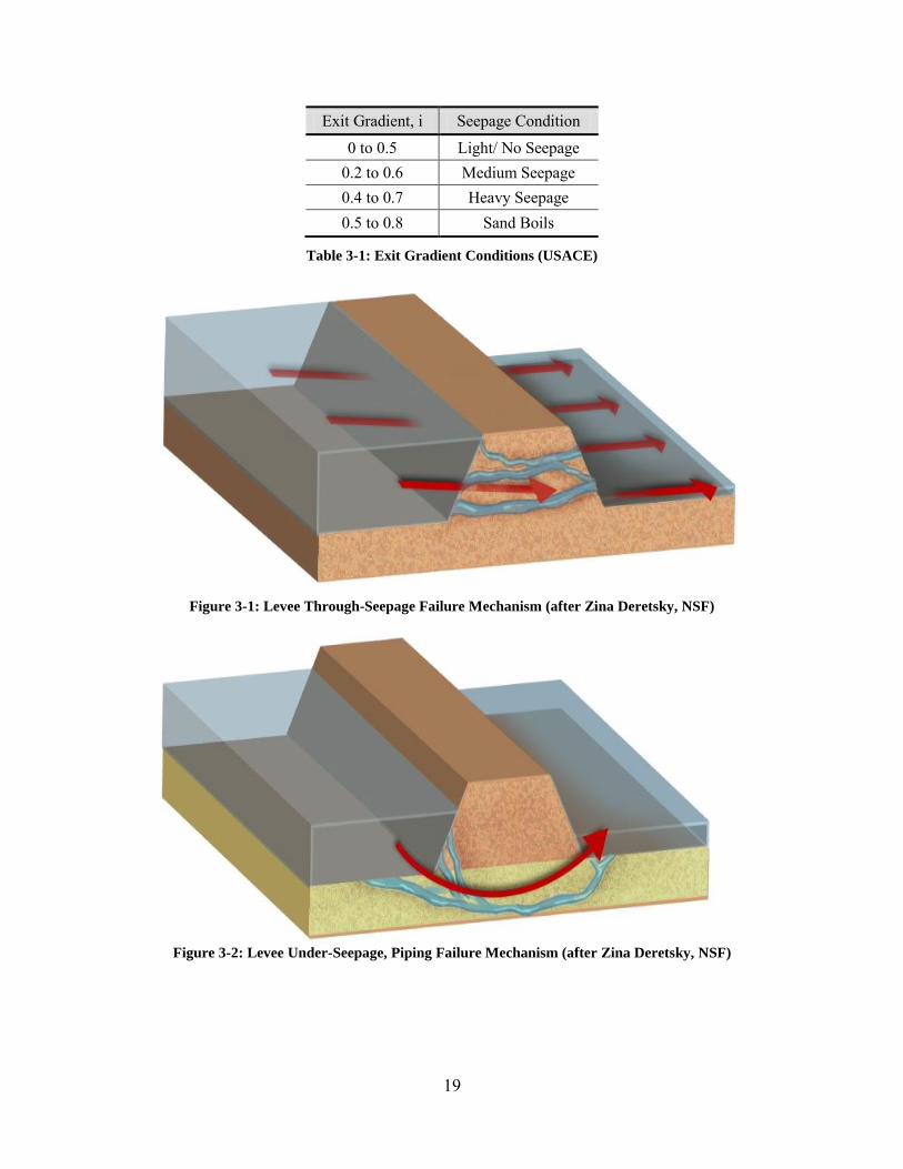
19
Exit Gradient, i Seepage Condition
0 to 0.5 Light/ No Seepage 0.2 to 0.6 Medium Seepage 0.4 to 0.7 Heavy Seepage 0.5 to 0.8 Sand Boils
Table 3-1: Exit Gradient Conditions (USACE)
Figure 3-1: Levee Through-Seepage Failure Mechanism (after Zina Deretsky, NSF)
Figure 3-2: Levee Under-Seepage, Piping Failure Mechanism (after Zina Deretsky, NSF)

20
3.2 Metric of Failure for Seepage Mechanism
Acceptable performance of a levee system has been traditionally assessed by computing a deterministic factor of safety, F.S., which is the ratio of Capacity to Demand. A factor of safety larger than one implies that the Capacity is larger than the Demand and the system will not fail. In reality, there is uncertainty associated with each of these parameters (capacity and demand), thus the FS cannot be given as one value, but a distribution of different values. The ratio of C50/D50 is the traditional definition of the deterministic “unbiased” factor of safety (FS), with C50 and D50 being the median (i.e., 50th percentile) values of the capacity and demand, respectively. The probability of failure is then defined as the probability that the FS < 1.
Effective stress is used for many geotechnical engineering applications. The effective stress is determined by subtracting u, pore pressure, from σ, the total stress. Porewater pressure may increase drastically under flow conditions, although the total stress, σ, may remain constant. This leads to a reduction in effective stress, which may mean partial or total loss of solid particle contacts in the physical sense, causing quicksand conditions and other instabilities [e.g., Reddi, 2003]. The vertical effective stress, σ’v, can be obtained as:
’ = - Equation 3-2
Where σv is the total vertical stress and u is the porewater pressure. In a situation where there is upward seepage, the pore pressure will be a function of the vertical hydraulic gradient. The vertical effective stress can then be written as:
’ = ( s - ) - Equation 3-3
Where γsat is the unit weight of the saturated soil, w is the unit weight of water, i is the exit gradient at the selected point, and z is the depth below the surface the point of interest is. Equation 3-3 can be reworked to more accurately represent effective stress in terms of capacity and demand as shown in Equation 3-4.
’ = s - (1 ) Equation 3-4
Failure state is then defined as:
’ Equation 3-5
Combining Equation 3-4 and Equation 3-5, we obtain:
- (1 ) Equation 3-6
Thus, failure occurs when, γsat γw(1 i). The capacity, C, and the demand, D, are defined by:
Capacity, C= Equation 3-7
Demand, D= (1 ) Equation 3-8
The exit gradient can be determined with the traditional method of flownet assuming steady-state condition. For cases where high water elevations occur for a limited time, steady state conditions may not be achieved. Although non-steady conditions can be readily analyzed, it is not generally

21
done in practice for routine work and it is not discussed further in this work. Flownets involve hand drawing (or computing) flow lines and perpendicular equipotential lines. Flowlines represent the direction of water flow through the soil and the equipotential lines represent constant energy head conditions as shown in Figure 3-3. The exit gradient at any point can then be described using Equation 3-9:
=
Equation 3-9
Where hL is total head above point of interest, b is the distance between equipotential lines at this location and Nd is number of equipotential drops for the entire mesh (i.e., flownet). Please note that the product “b. Nd” is fully a geometric property and it is a constant for a given soil profile and hydraulic conductivity of the soil units, so the parameters b and Nd are not independent parameters, only one of them is.
Figure 3-3: Example of Equipotential & Flow lines –Flownet (Holtz & Kovacs, 1981)

22
The probability of failure can be determined using a Monte Carlo simulation of the capacities and demands of the system independently sampling from the random variables (input parameters) of the equation. The overlap of their probability density functions will be proportional to the probability of failure.
The use of Monte Carlo simulation allows the problem to be approached probabilistically. To run a Monte Carlo simulation, each of the random variables, must be defined with a distribution and associated properties of the distribution. For example, if the parameter was defined using a normal distribution this parameter needs to have a mean and standard deviation associated with it so that the distribution can be created. The Monte Carlo starts with a generation of random variables for the input parameters with prescribed probability distributions. In any Monte Carlo simulation the sample size or number of random numbers generated is determined by the user [e.g., Ang and Tank, 2007].
3.3 Site Selection
The site selection for this analysis was purposive, arising out of the availability of data and need to focus on levees facing each of the deep-water shipping channels. Three sites were selected for evaluation: 1) Southern Site, 2) Piezometer Site and 3) the Northern Site. The locations of these sites are shown in Figure 3-4. The Northern site analysis with respect the seepage failure mode was delayed and will thus not be presented in this work. The Southern site and Piezometer site analysis will be discussed in detail in the following sections. The procedure used to evaluate these sites can be applied to any site location throughout the Island.
3.3.1 Location to Analyze Effective Stress
To maximize the timeliness of the analysis, the study used SEEP/W to determine where maximum seepage occurred on the landside section of the levee. For every evaluation, this point was held as the point of concern. The depth that was analyzed, z, for effective stress was half way down a flow net “box” as shown in Figure 3-5.
In these models, it is shown that the phreatic surface is at the surface of the soil, meaning that the soils is saturated completely and the depth used to define the weight of the water is the same as the depth used for the pore pressure. This was the case for all the models analyzed and for use of an example, it works.

23
Figure 3-4: Sherman Island Site Locations
0
5
10
-5
-10
-15
-20
-25
-30
-35
40 80 120 160 200 240 280 320 360 400 440 480 520 560 600 640 680 720
h
10
Point of interestb/2
Figure 3-5: Total Head for Vertical Effective Stress Calculation
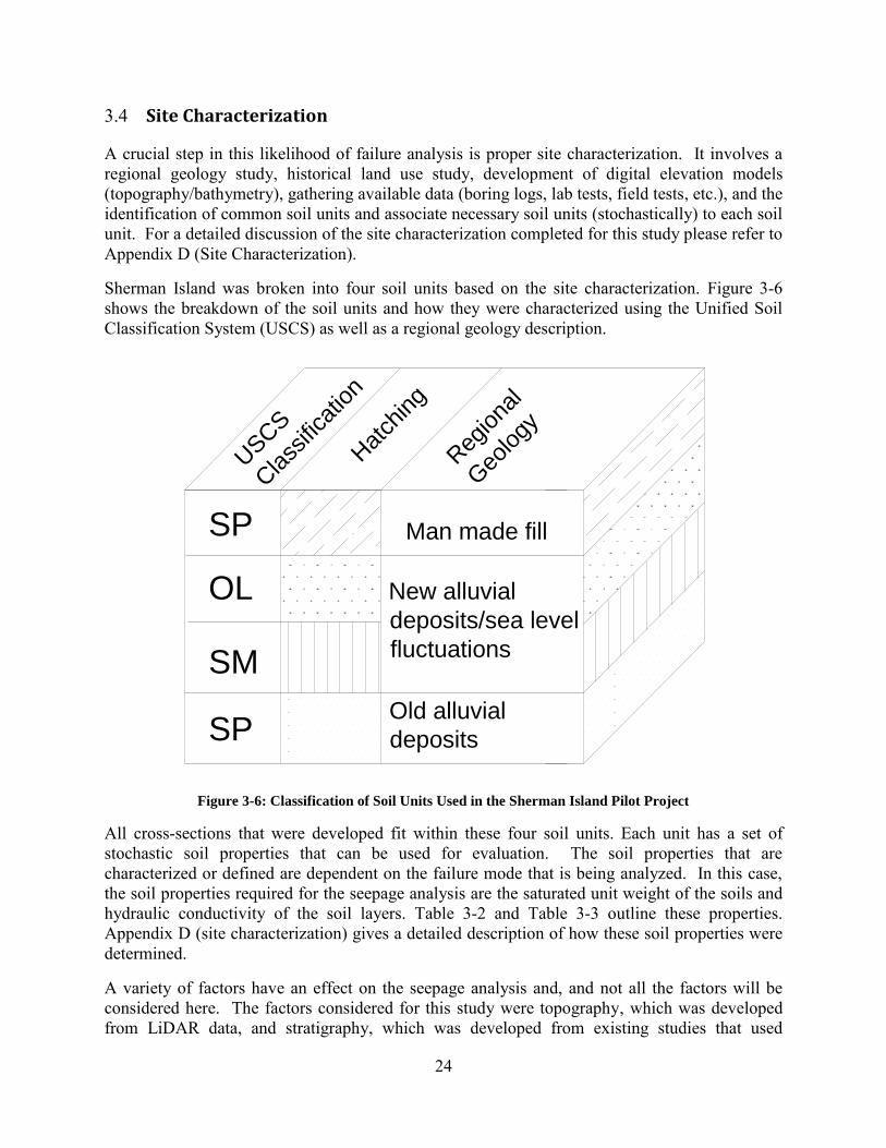
24
3.4 Site Characterization
A crucial step in this likelihood of failure analysis is proper site characterization. It involves a regional geology study, historical land use study, development of digital elevation models (topography/bathymetry), gathering available data (boring logs, lab tests, field tests, etc.), and the identification of common soil units and associate necessary soil units (stochastically) to each soil unit. For a detailed discussion of the site characterization completed for this study please refer to Appendix D (Site Characterization).
Sherman Island was broken into four soil units based on the site characterization. Figure 3-6 shows the breakdown of the soil units and how they were characterized using the Unified Soil Classification System (USCS) as well as a regional geology description.
Figure 3-6: Classification of Soil Units Used in the Sherman Island Pilot Project
All cross-sections that were developed fit within these four soil units. Each unit has a set of stochastic soil properties that can be used for evaluation. The soil properties that are characterized or defined are dependent on the failure mode that is being analyzed. In this case, the soil properties required for the seepage analysis are the saturated unit weight of the soils and hydraulic conductivity of the soil layers. Table 3-2 and Table 3-3 outline these properties. Appendix D (site characterization) gives a detailed description of how these soil properties were determined.
A variety of factors have an effect on the seepage analysis and, and not all the factors will be considered here. The factors considered for this study were topography, which was developed from LiDAR data, and stratigraphy, which was developed from existing studies that used
SP
OL
SM
SP
Man made fill
New alluvial
deposits/sea level
fluctuations
Old alluvial
deposits
USCS
Class
ifica
tion
Hat
ching
Reg
iona
l
Geo
logy

25
Standard Penetration Tests (SPT). For a detailed discussion of the development of the stratigraphy refer to Appendix D (Site Characterization). Other factors that could possibly exist at the site, but were not examined include pipe penetrations, animal burrows, vegetation, riprap, gas fields and groundwater.
On the demands portion of the analysis, water level is a key factor which affects seepage. The main influence from water level arises from tidal fluctuations and river inflow. For a detailed discussion of the hazard characterization refer to Appendix B (Hazard Characterization).
Material (UCSC) Description Mean STD COV
SP Sandy fill 102.2 10.4 0.10
OL Organics (peat) 91.7 20.3 0.22
SM Silty sand 106 15.9 0.15
SP Deep sands 118 7.7 0.07
Table 3-2: Saturated Unit Weight of Soil (pcf)
Material (UCSC) Description kh (cm/s) ft/day kh/kv*
Wor
st C
ase
SP Fill 3.50E-02 99.21 1
OL Peat 0.001 2.83 0.5
SM Silt/sand 1.76E-03 4.99 1
SP Sand 3.50E-02 99.21 1
Expe
cted
(med
ian)
SP Fill 1.00E-03 2.83 3
OL Peat 0.0001 0.28 10
SM Silt/sand 1.00E-05 0.03 1.5
SP Sand 1.00E-03 2.83 3
Bes
t Cas
e
SP Fill 1.00E-04 0.28 4
SM Peat 1.00E-05 0.03 100
OL Silt/sand 0.000001 0.00 2
SP Sand 1.00E-04 0.28 4
Table 3-3: Hydraulic Conductivity of Soil Units

26
3.5 Uncertainty Characterization
This study chose to categorize uncertainty of each parameter as Type I, II, III and/or IV. This classification attempts to identify where uncertainty lies for each parameter and the contribution of each parameters to the probability of failure. This allows decisions makers and engineers to make better decisions on where money and resources should be spent in order to decrease the probability of failure.
For each random variable (or model in cases of type II uncertainty) in the demand and capacity, a distribution, and associated parameters of that distribution should be used to properly characterize it. The aim of this study, however, is not an exposition of the proper selection of distributions to fit data, which is the subject of many probability theory studies elsewhere. This study used three common distributions to define the parameters:
1. Normal distribution (or Gaussian distribution) 2. Lognormal distribution 3. Triangular distribution
Between the three of these distributions our random variables could be characterized. There may have been distributions that better fit the random variables, however these three probability distributions perform well enough and simple enough to warrant their use.
The normal and lognormal distributions are characterized by the mean, and standard deviation of the available data on the random variable of interest (Appendix O). For the normal and lognormal distributions to be used enough data must have been gathered so that a mean and standard deviation could be determined.
To properly capture uncertainty in the analysis, parameters used in both the demand and the capacity closed form solutions were decomposed and categorized as Type I, II, III or IV uncertainty. Table 3-4 outlines how this can be done qualitatively. This table is helpful from a management stand-point because it encourages the user to identify where uncertainty lies within each parameter. It also encourages decision makers to make informed decision about how the uncertainty of a parameter can be reduced.
Parameter Symbol Units Type I Type II Type III Type IV
Demand
Water Level hL ft √ √ √ Head Drops Nh - √ √
Equipotential Distance b ft √ Unit Weight of Water γW pcf √
Bias Correction B - √
Capacity
Saturated Unit Weight γSAT pcf √ Topography - ft √ √ Bathymetry - ft √ √
Soil Stratigraphy - - √ √ √
Table 3-4: Qualitative Uncertainty Breakdown
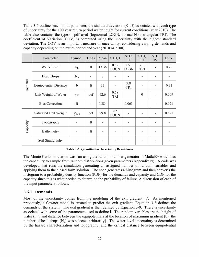
27
Table 3-5 outlines each input parameter, the standard deviation (STD) associated with each type of uncertainty for the 100 year return period water height for current conditions (year 2010). The table also contains the type of pdf used (lognormal-LOGN, normal-N or triangular-TRI). The coefficient of Variation (COV) is computed using the uncertainty with the highest standard deviation. The COV is an important measure of uncertainty, considering varying demands and capacity depending on the return period and year (2010 or 2100).
Parameter Symbol Units Mean STD, I STD, II
STD, III
STD, IV COV
Dem
and
Water Level hL ft 13.36 0.82 LOGN
2.51 LOGN
3.38 TRI - 0.25
Head Drops Nh - 8 - - - - -
Equipotential Distance b ft 32 - 9.8 TRI - - 0.31
Unit Weight of Water γW pcf 62.6 0.58 TRI 0 - 0.009
Bias Correction B - 0.884 - 0.063 - - 0.071
Cap
acity
Saturated Unit Weight γSAT pcf 99.8 62 LOGN - - - 0.621
Topography - ft - - - - - -
Bathymetry - ft - - - - - -
Soil Stratigraphy - - - - - - - -
Table 3-5: Quantitative Uncertainty Breakdown
The Monte Carlo simulation was run using the random number generator in Matlab® which has the capability to sample from random distributions given parameters (Appendix N). A code was developed that runs the simulation generating an assigned number of random variables and applying them to the closed form solution. The code generates a histogram and then converts the histogram to a probability density function (PDF) for the demands and capacity and CDF for the capacity since this is what needed to determine the probability of failure. A discussion of each of the input parameters follows.
3.5.1 Demands
Most of the uncertainty comes from the modeling of the exit gradient ‘i’. As mentioned previously, a flownet model is created to predict the exit gradient. Equation 3-8 defines the demands of the system. The exit gradient is then defined by Equation 3-9. There is uncertainty associated with some of the parameters used to define i. The random variables are the height of water (hL), and distance between the equipotentials at the location of maximum gradient (b) [the number of head drops (Nd) was selected arbitrarily]. The water level uncertainty is determined by the hazard characterization and topography, and the critical distance between equipotential

28
lines (b) is obtained from a seepage analyses. Parameter b is a function of geometry and flow properties given by:
= f(s ⁄ ) Equation 3-10
However the relationship between b, stratigraphy, kh, kh/kv, is not explicit, meaning there is no closed form solution that relates b to these random variables. Stratigraphy is a major source of uncertainty which was discussed previously in this report. To attempt at characterizing the uncertainty, three interpreted cross sections were made with the available boring logs. These three interpretations represented the worst, best and most likely scenarios. The stratigraphy is only one source of uncertainty out of the three with respect to seepage. The hydraulic conductivity and ratio of hydraulic conductivity present another source of uncertainty. By using the proper combination of these parameters, the uncertainty for b can be characterized. The discussion of each of these parameters as well as the combination of the three will be discussed in this section.
3.5.1.1 Unit Weight of Water
The unit weight of water is usually held constant in most geotechnical analyses. The unit weight of water can vary depending on the salinity of the water and its temperature. In this location of Sherman Island the water is not always fresh due to tidal fluctuations. The mean value for the unit weight of water was the unit weight of fresh water. The uncertainty for this input parameter was categorized as Type I since differences in measured unit weights of water are a result of inherent randomness (Appendix O).
3.5.1.2 Total Head (hL)
The total head is the water elevation over the point of interest, where we are calculating effective stress. Therefore the total head is affected by the topography, the water level, and how deep the point of interest is. Figure 3-5 illustrates how the total head is calculated and can be determined by the following equation:
= Equation 3-11
The water level in this example refers to the 100 year water level in the year 2010. Possible combinations of inputs from the topography and water levels were used to determine high, low and most likely values (Appendix K).
The mean water level due to the storm event was determined using the regression line from the 60 previous maximum values. For a more detailed discussion of the 100 year water level and the uncertainties associated with it, refer to Appendix B, Hazard Characterization.
Type I uncertainty is present in the water level due to the natural skew. The standard deviation from Type I uncertainty was determined from the available data over the past 60 years. Since these are field measurements that reflect actual water levels these are categorized as Type I uncertainty. Type I was represented with a lognormal distribution.
29
Type II uncertainty is dominant in this parameter since a regression model is being used to extrapolate beyond observed values. Therefore the uncertainty of this type is expected to be large. To determine this uncertainty, confidence intervals from the regression of the 60 year data analysis back calculated to determine the standard deviation at the 100 year level. As the regression extends beyond observed values, the confidence intervals become more spaced and from this a standard deviation could be back calculated at any point along the regression line. Type II was defined using a lognormal distribution.
Type III is also present because the total head is dependent on topography which is left to the interpretation of the engineer. This was characterized with a triangular distribution to represent best, worst and expected conditions.
3.5.1.3 Flownet Model
The flownet model is a crucial aspect of the seepage analysis. However, a large amount of uncertainty can be associated with the model that must be accounted for. From the flow net model the values for head drops (ND) as well as the length between flow lines (b). These are difficult to obtain an accurate distribution for because so much variation can be created within the flow net model. To properly understand the possible variations within the model, it must be understood how the model is created. The steps are outlined by NAVFAC DM 7.01 and are as follows:
a. When materials are isotropic with respect to hydraulic conductivity, the pattern of flow lines and equipotentials intersect at right angles. Draw a pattern in which square figures are formed between flow lines and equipotentials
b. Divide total head by a whole number and draw flowlines to conform to these equipotentials. The shape of rectangles (ratio B/L) must be constant.
c. The upper boundary of a flownet that is at atmospheric pressure is a “free water surface”. Integer equipotentials intersect the free water surface at points spaced equal vertical intervals
d. A discharge face through which seepage passes is an equipotential line if the discharge is submerged, or a free surface if the discharge is not submerged. If it is free water surface, the flow net figures adjoining the discharge face will not be squares.
e. In a stratified soil profile where ratio of hydraulic conductivity of layers exceeds 10, the flow in the more permeable layer controls. That is, the flow net may be drawn for more permeable to be impervious. The head on the interface thus obtained is imposed on the less pervious layer for construction of the flow net within it.
f. In a stratified soil profile where ratio of hydraulic conductivity of layers is less than 10, flow is deflected at the interface of layers
g. When materials are anisotropic with respect to hydraulic conductivity, the cross section may be transformed by changing scale as shown in Figure 3-7. In computing quantity of seepage, the differential head is not altered for the transformation.
h. Where only the quantity of seepage is to be determined, an approximate flow net suffices. If pore pressures are to be determined, the flow net must be accurate.
The steps outlined above are used for hand drawn flow net models. To obtain the “bounds” of the input models taken from the model, two “extreme” models were created (best case and worst case) using the information available. By bounding the problem like this, it is expected that the

30
true answer will fall somewhere between them. The two extreme models were developed using SEEP/W to obtain the flow net model only. These extremes were created using specific combinations of variables.
Figure 3-7: Interface Situation in Flownet (after DM 7.01)
3.5.1.3.1 Hydraulic conductivity
Hydraulic conductivity has a large range of value over small spatial extents even within the same soil classification. Lab testing could be done to determine what the hydraulic conductivity is, but even then it could vary throughout the stratigraphy a great deal. For this reason hydraulic conductivity has a large amount of uncertainty associated with it (Appendix L).
The hydraulic conductivity of materials has already been discussed previously. Each soil unit had a low range and high range. These values were adjusted for each soil unit and run with the SEEP/W software. The uncertainty associated with hydraulic conductivity can be characterized as Type I.

31
3.5.1.3.2 Head Drops (ND)
The number of head drops throughout a flow net is assumed constant. This value is an arbitrary value that the creator of the flownet decides. What is affected by the number of head drops is the equipotential distance between each head drop. For this reason the number of head drops is not modeled as a random variable.
3.5.1.3.3 Equipotential Distance (b)
The mean value for the equipotential distance is a complex function of stratigraphy and hydraulic conductivity of the soil strata. For this reason the cross sections and hydraulic conductivity coefficients were combined in such a way as to give a low, high and median bound for the variable b so that it may be characterized with a triangular distribution. The mean value for the equipotential distance was determined using the most likely case for the stratigraphy, the mean hydraulic conductivities of each of the soil layers, and the mean hydraulic conductivity ratio. By using the mean values and most likely cross section the “most likely” b parameters was defined. The low and high bounds for b were determined using the worst and best case interpretation of the cross section along with the lower bound of hydraulic conductivity and the higher bound respectively.
Because of the complexity of the stratigraphy, the flow net models are not a “simple” model. The nature of how water flows through the material affects the equipotential lines (or head drops) and these head drops can become “distorted” due to how the water flows through different stratum. This makes determining the b variable a difficult task because there is even variation in each of the three models themselves. To handle this, a spread of b values was determined by measuring the distances in each of the three models and combining the data sets. These parameters were modeled with a triangular distribution. The results of the Seep W/® models used to determine the uncertainty can be found in Appendix O.
3.5.1.4 Bias Correction Factor (B)
There is another source of uncertainty that arises from the flow net model used to determine the exit gradient. It is a Type II uncertainty that needs to be explicitly accounted for with a Bias Correction, B that has yet to be discussed. The results of this analysis were actually adjusted by a Bias Correction factor to account for Bias of the model. The results presented account for Model Bias (Type II) uncertainty as discussed later. Type II modeling uncertainties on the estimation of Pf is that they affect the central tendency and distribution characteristics of the probabilistic descriptions used to define the demands and capacities for the infrastructure concerned.

32
3.5.2 Capacity
The capacity of a system for this seepage analysis is defined by Equation 3-7. Each one of the random variables associated with this closed form solution will be discussed here and decomposed into its particular uncertainties.
3.5.2.1 Saturated Unit Weight
The total unit weight varies depending on what soil type. Laboratory tests were done throughout Sherman Island for saturated unit weight on a variety of different soil types in the area. From these tests the saturated unit weight of the soil could be determined.
Because of how this problem is structured only one soil type will be overlying the point of interest and thus only one saturated unit weight value is needed. Since it is uncertain exactly what soil type overlies it because there is uncertainty within the stratigraphy, the populations was looked at as a whole rather than breaking it up into soil units. From the high COV, this is a variable of concern. The high COV is due to the fact that we do not understand the stratigraphy and must therefore sample the entire population of soil units (Appendix O).
This is an excellent example of how a simple exploration in the area of interest can help reduce the uncertainty in this parameter. If a boring was done exactly at the point of interest, we would understand what soil unit we were working with and reduce the sampling to that single soil unit rather than all of them.
3.5.2.2 Topography/Bathymetry
The topography for the selected sites was developed using available data from U.S. Geological Survey. USGS Western Region Geographic Science Center, in conjunction with the USGS Western Branch of Regional Research, developed a high-resolution elevation dataset covering the Sacramento/San Joaquin Delta region. The dataset has a 10-meter horizontal resolution grid of elevation values, with a vertical accuracy of 1m. No information is given as to the accuracy of the bathymetry data. For this reason, the site cross section elevations were varied 1.5 meters (4.9 ft). The chosen value of 1.5 was somewhat arbitrary, and more research is required to quantify the accuracy of the bathymetry data.
Varying topography will have the greatest effect on the difference in head between the water level and the point of interest. The limiting factor for how much total head overlies the point of interest is the height of the levee. If the levee crest is higher, the water is allowed to rise higher and increase the total head in the system; this is assuming that the 100 year water level is possibly as high as or higher than the levee crest.
From the varying topography, bounds of the possible total head over the point of interest were identified. Figure 3-8 outlines how the bounds were created by using the highest possible crest and lowest possible inland topography, the largest potential total head condition is possible. Similarly, by using the lowest bound of the levee crest and the highest possible inland topography, the smallest potential situation for total head is possible. The varying topography used in the south site analysis and be found in Appendix K.
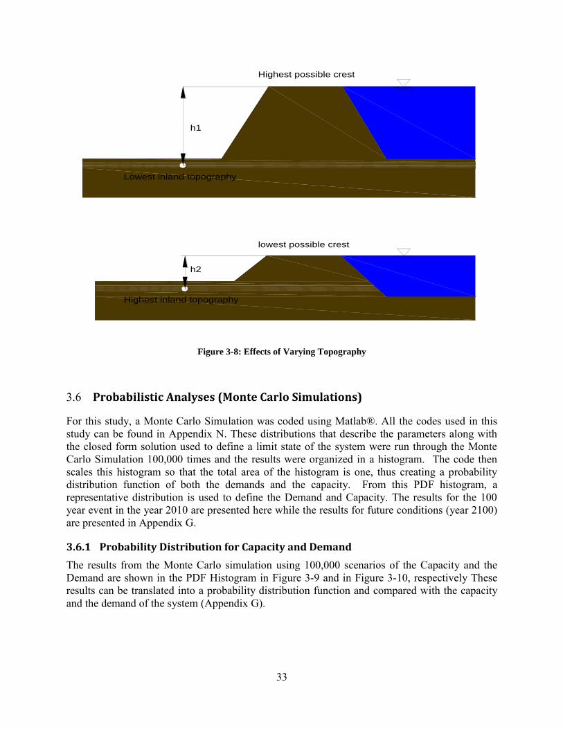
33
Figure 3-8: Effects of Varying Topography
3.6 Probabilistic Analyses (Monte Carlo Simulations)
For this study, a Monte Carlo Simulation was coded using Matlab®. All the codes used in this study can be found in Appendix N. These distributions that describe the parameters along with the closed form solution used to define a limit state of the system were run through the Monte Carlo Simulation 100,000 times and the results were organized in a histogram. The code then scales this histogram so that the total area of the histogram is one, thus creating a probability distribution function of both the demands and the capacity. From this PDF histogram, a representative distribution is used to define the Demand and Capacity. The results for the 100 year event in the year 2010 are presented here while the results for future conditions (year 2100) are presented in Appendix G.
3.6.1 Probability Distribution for Capacity and Demand
The results from the Monte Carlo simulation using 100,000 scenarios of the Capacity and the Demand are shown in the PDF Histogram in Figure 3-9 and in Figure 3-10, respectively These results can be translated into a probability distribution function and compared with the capacity and the demand of the system (Appendix G).
66.9955
h1
28.0328 h2
Highest possible crest
Lowest inland topography
Highest inland topography
lowest possible crest

34
Figure 3-9: Capacity PDF 100 year event-current conditions (year 2010)
Figure 3-10: Demand PDF for 100 year event-Current conditions (year 2010)
3.6.2 Probability of Failure
The probability of failure is proportional to the area of overlap between the Capacity and Demand curves as shown in Figure 3-11. The probability of this occurring can be determined using Equation 3-12, presented earlier in this report. However the Matlab® that was developed determines the probability by counting the number of times a failure occurs during the sampling and dividing it by the total number of simulations.
0 50 100 150 200 250 3000
0.002
0.004
0.006
0.008
0.01
0.012
0.014
0.016
0.018
0.02
Unit Weight (pcf)
Pro
bability D
ensity
65 70 75 80 85 900
0.05
0.1
0.15
0.2
0.25
0.3
0.35
Unit Weight (pcf)
Pro
bability D
ensity
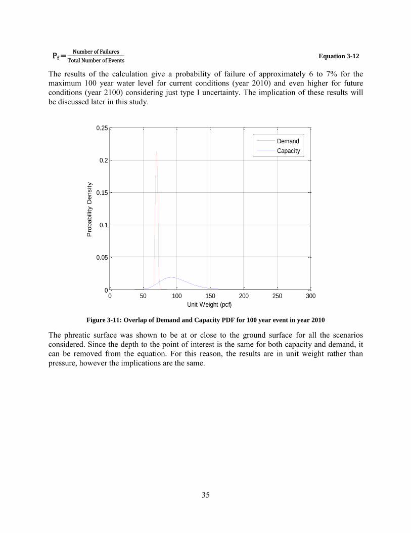
35
P f = f s
f s Equation 3-12
The results of the calculation give a probability of failure of approximately 6 to 7% for the maximum 100 year water level for current conditions (year 2010) and even higher for future conditions (year 2100) considering just type I uncertainty. The implication of these results will be discussed later in this study.
Figure 3-11: Overlap of Demand and Capacity PDF for 100 year event in year 2010
The phreatic surface was shown to be at or close to the ground surface for all the scenarios considered. Since the depth to the point of interest is the same for both capacity and demand, it can be removed from the equation. For this reason, the results are in unit weight rather than pressure, however the implications are the same.
0 50 100 150 200 250 3000
0.05
0.1
0.15
0.2
0.25
Unit Weight (pcf)
Pro
bability D
ensity
Demand
Capacity
36
3.7 Type II Uncertainty (Model Bias)
One aspect of engineering that is often overlooked is the accuracy of models used in the analysis. In some cases models are accepted to be accurate without any proof or justification of the model. Typically biased values are used in traditional engineering processes, procedures, codes, and guidelines since the engineer wants to be conservative. Biases are frequently “hidden” in the design codes and guidelines. Problems develop due to the compounding different levels of conservatism and a lack of knowledge of how conservative the results really are. In addition, what is conservative for one set may not be conservative for another set of conditions [Bea, 2006]
The best way to identify magnitudes of the Bias is to compare the results from any analytical models that will be employed by engineers in determining demands and capacities associated with a given system during a point in its life cycle with “measured” or observed results. However extreme care must be taken with measured and observed results. Laboratory results generally are different from those in the field – it is extremely difficult to simulate all of these realities of the field laboratory or laboratory experiments can introduce effects that are not present in the field. [Bea, Robert (2006)]
For these reasons, it is crucial if engineers are to properly design and evaluate engineered systems that Bias must be accounted for. In this method for Risk Assessment any engineering model that is used must be corrected for bias. To apply this correction measured field values should be compared with predicted values, experts should verify the results, and the results can be compared to results from other system. The Bias correction is measured as follows:
= s
P Equation 3-13
This correction can then be applied to the results of the model by which the engineer is using to predict components of either the capacity or demands of the system. However, there is a spread to this value, meaning the Bias correction itself acts as a random variable with its own source of uncertainty. It can be treated like any other parameter within the limit state analysis.
A bias correction was applied to this analysis and all the results account for it. The Bias correction was determined using a third site (deemed the “Piezometer Site”) where piezometers were placed to measure pore pressure. Pore pressure is defined by Equation 3-14.
= (1 ) Equation 3-14
This is the equation for demands on the system in our limit state analysis. A model is used to derive parameters for pore pressures; those models are flow nets used to determine ‘i’, the exit gradient.
The predicted values were compared with the measured values and a variety of Bias Correction values were determined that could be sampled from. This Bias Correction was applied to the Capacity side of the model, and thus the actual Capacity closed form solution that was being used in the Monte Carlo Simulations is shown by Equation 3-15.
= (1 ) Equation 3-15

37
Where: B is the Bias Correction term that was applied to the model.
For more details of how this method was applied, refer to Appendix F of this report. Table 3-6 summarizes the results of the Bias correction analysis conducted on 9 piezometers (Appendix F).
Piezometer No.
Measured Pore Pressure, (psi)
Avg Predicted Pore Pressure, (psi) Bias
1 3.15 3.28 0.96
2 5.13 5.47 0.94
3 5.13 5.46 0.94
4 7.21 7.86 0.92
5 16.18 19.41 0.83
6 21.11 26.59 0.79
7 7.4 8.09 0.92
8 13.49 15.74 0.86
9 20.44 25.59 0.80
Table 3-6: Measured pore pressures versus predicted pore pressures
3.8 Probability of Failure over Time
In some cases, such as this study, it is necessary to account for time dependent scenarios. In the Sacramento San Joaquin delta, the rising waters to the 2, 50 or 100 year event happen quickly and the water level is not sustained for long, in historical situations sometimes a matter of hours. The levee system reacts differently to a load like this versus a static load, especially when it comes to seepage. Therefore it is important to consider this in the risk assessment.
To explore the performance of the Sherman Island levees as a flood protection system, and just considering seepage mode, and three annual storm return periods (i.e., 2, 50 and 100 years) are being analyzed, along with an explicit characterization of uncertainties involved: namely, those related to analytical modeling, human performance, and information development (Types II, III and IV, respectively).
As the water rises, there is another factor of uncertainty with respect to time. How fast it is rising has an effect on the results of the analysis. The hydrograph developed in Appendix B (Hazard Characterization) offer different scenarios with uncertainty bounds about how the water will rise based on historical water events in the area. This makes the water level a time-dependent factor. To get a better understanding of how the probability of failure is changing over time, it can be

38
graphed versus time. For this study, three points in time were chosen, at each of these points there would be a different water level (with uncertainty bounds that could be characterized by a distribution). This change in both the water level and the uncertainty with that water level at that specific point in time will change the probability of failure. The goal is to map the progression of the probability of failure throughout the event to the maximum probability of failure.
The reason for approaching the probability of failure like this is so that the influence of HOF can be recognized at certain time steps along the progression of the flood event. However certain changes were made in the input parameters at each step. For changes to input parameters at each step refer to Appendix M. The resultant probability of failures at each step were graphed and shown in Figure 3-12 for the 2, 50 and 100 year event in the year 2010, the maximum values are drawn on the graph. These results and calculation inputs to the Monte Carlo Simulation can also be found in Appendix M.
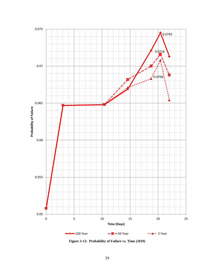
39
Figure 3-12: Probability of Failure vs. Time (2010)
0.0745
0.0716
0.0708
0.05
0.055
0.06
0.065
0.07
0.075
0 5 10 15 20 25
Pro
bab
ility
of
Failu
re
Time (Days)
100 Year 50 Year 2 Year
40
4 ASSESSMENT OF LEVEE FAILURE DUE SLOPE INSTABILITY
The reliability of a levee is the computed probability that a levee will not fail and considers explicitly the uncertainties involved in estimating the failure conditions. The next sections address the assessment of the probability of failure (and thus the complement of reliability) considering slope instability. Levee stability calculations provide an illustration for evaluating the combined effects of both type I, and type II uncertainties.
4.1 Lateral Slope Instability Mechanism
Levee slope sliding hazard is customarily evaluated based on the comparison of two variables: Driving Force and/or Moment (Demand) and the Resisting Force and/ or Moment (Capacity). Calculation of these variables allows a factor of safety value to be calculated for a given levee system and consequently the Sliding hazard can be characterized (e.g., Seed et al, 2007). However, for these analyses to be useful, they must capture the correct failure mechanism. In general, this requires: a) mastery of soil mechanic principles, b) knowledge of the geology and site conditions, c) knowledge of the properties of the soil at the site, d) assessment of uncertainties associating with important properties in capacity, demand, and more important model, and e) accurate identification of the potential failure mechanism which causes an unsatisfactory levee stability performance.
Over the past several years, experience with the behavior of levees, and often with their catastrophic failure, has led to identification of different failure mechanisms caused by lateral instability. These failure mechanisms (listed below) are result of change in one or several parameters in the levee system associating with either capacity or demand which subsequently results in levee failure and thus flooding.
4.1.1 Surface Sloughing
A shear failure in which a surficial portion of the levee moves down slope is termed a surface slough. In this particular case, failure occurs when the levee soil material had insufficient resistance to erosion or low strength. Typically, after few days of high water, the surface layers of the levee (by phreatic water movement) will become saturated making them heavier and potentially weaker due to lower effective strength than the underlying layers. The heavier and weaker surficial layers start yielding resulting in the surface layer sliding down the slope of the levee. If such failures are not monitored and addressed as they occur and repaired, they can become progressively larger, and may then represent a threat to levee safety.
4.1.2 Shear Failure
A shear failure involves sliding of a portion of a levee, or a levee and its foundation. Although failure surfaces are typically nonlinear, they are frequently approximated as circular in shape (in 2D cross-sections) and they occur where weak strata exist within a soil deposits. Figure 4-2 illustrates water side rotation shear failure of a levee. In these cases, localized failure (yielding) begins at some point at depth within the slope and progresses upslope and/or downslope until the failure surface is expressed at the surface. When soft soils are present in the foundation, slope failure tends to manifest themselves as deeper rotational failures. For frictional materials like sand and silt, slope failures tend to be surficial failures [e.g., Terzaghi and Peck, 1967]. Since

41
cohesive soils have a relative low Φ and high cohesion in terms of total stress, it makes it relatively strong at shallow depths and weak at deep depths. Peat is especially prone to rotational failure of failure by spreading, particularly under the action of horizontal flood forces [e.g., Bell, 2000].
Figure 4-1: Levee Surface Sloughing Failure Mechanism (after Zina Deretsky, NSF)
Figure 4-2: Levee Rotational Shear Failure Mechanism (after Zina Deretsky, NSF)

42
4.1.3 Liquefaction and Other Types of Slope Instability
The phenomenon of soil liquefaction, or significant reduction in soil strength and stiffness as a result of shear-induced increase in pore water pressure, is a major cause of earthquake damage to embankments and levees (Youd et al. 1984). Most instances of liquefaction have been associated with saturated loose sandy or silty soils. Loose gravelly soil deposits are also vulnerable to liquefaction (e.g., Coulter and Migliaccio 1966; Chang 1978; Youd et al. 1984; and Harder 1988). In addition several types of levee failure, including wave impacts, structural impacts, jetting, tree and animal damage, lateral spreading, and combinations of these factor may cause levee failure. Liquefaction and these other types of failure mechanisms are not discussed in this study, but the possibility of their occurrence should not be ignored.
4.2 Sherman Island Levee System
4.2.1 System Definition
For the purpose of this study, the Sherman Island levee system was selected. For simplicity of the analyses, the only element considered here is the perimeter levee surrounding the island. Although there are more elements in the system than simply the levee, this simplified system definition will be used here.
4.2.2 Hazard Characterization
The Sherman Island levee system was completed in 1869 and from that point on, Sherman Island suffered from several floods. Historical data shows Sherman Island levees failed during the winters of 1871-72, 1874-75, 1876, and 1878. As a result, the new levee reconstruction featured a 12-foot high peat levee with 120 feet widths at the base. Even so, the 1876 event broke the levee and flood covered the western portion of the island again. In August of 1880, high waters collapsed a levee section and although an effort was made for levee repair following the 1880 break, most of the land remained under water until 1894 when reclamation efforts were renewed.
During the first decade of the twentieth century, reclamation district conducted frequent levee upgrading and restoration projects on Sherman Island. “Flooding occurred in some section of the Delta almost annually during the period from 1900 to 1910, and serious levee breaks and major flooding occurred during 1904 when a crevasse opened on Mayberry Slough, and in 1906 and 1909, when water again inundated the island.”(U.S. Army Corps of Engineers. 1982. Sacramento-San Joaquin Delta, California - Draft Feasibility).
The southern levee on the San Joaquin River side failed and flooded the Island on January 20, 1969. After finding the break, a large quantity of rock was placed on the upstream and downstream ends of the levee to protect against further erosion from high velocities into and out of the break due to tide. The Corps of Engineers spent approximately $600,000 in emergency funds to repair, re-slope, and re-grade the levee break area after the 1969 break. Seepage and settlement in the area of the break have been ongoing issues requiring constant levee improvements.
Sea level rise directly affects the probability of levee failure on Sherman Island through higher normal tide levels and therefore higher flood stages during winter storm and spring snowmelt. The indirect effect of sea level rise is that it can increase the chance of occurrence of 100 year
43
flood. Consequently, it is important to include sea level rise data into the reliability analysis. Since elevated water levels would result in increased hydrostatic loads acting on the water side of levees, the Sea level rise is a major factor for levee stability. A variety of estimates exist for predicted sea level rise between now and 2150. The Intergovernmental Panel on Climate Change has predicted an increase in sea level of 0.1m to 0.65m by 2150 (URS, 2005) over 1990 levels. In contrast, a more recent analysis has predicted a sea level rise of 0.5m to 1.4m by 2150 (Rahmstorf, 2007).
For this study, the hazard was chosen before the completion of the system definition to provide an example of how a complete reliability analysis could be completed. Storm events were chosen because failures have occurred during storm events in the Sacramento San Joaquin Delta before. This also allows the analysis to account for human interactions during the event. At this point in time, there is no previous warning for an earthquake event and people reaction occurs after the fact. Thanks to advances in meteorology, atmospheric models and global weather monitoring, it is possible to have a larger lead time before a storm event (sometimes 10 days in advance). This study selected to evaluate the 2, 50 and 100 year flood event for the current conditions (year 2010). To this end, previous studies were used (mainly the Delta Risk Management Strategy, DRMS), to determine the 100 year water level at Sherman Island. Once this was determined, a representative river stage hydrograph can be created based on past events (Appendix B).
4.2.3 Site Geology Characterization
The Sacramento-San Joaquin Delta region has been an area of ground subsidence and soil deposition for over 140 million years. During that time, thousands of feet of sediments were deposited in marine, brackish and freshwater conditions. The sediments of primary importance for evaluating delta levees occur at relatively shallow depths and were deposited in the last 70,000 years (Late Quaternary era). The geologic history during this period and the resulting sediments were strongly influenced by changes in sea level due to glaciations. During lower sea level periods (glacial periods), the delta was characterized by river systems. When glaciers melted, higher sea levels occurred, and deltaic and estuarine environments existed.
During the period from 70,000 to 100,000 years ago (the last glacial period at the end of the Pleistocene era) sea level was as much as 365 ft below present sea level. The delta area was then a fluvial and alluvial system, with fast flowing rivers typically depositing course grained sediments (predominantly sand) in alluvial fans and channels.
At the end of this glacial period, sea level rose in the Holocene (10,000 years ago to present), progressively flooding the San Francisco Bay and Delta. The topography at the time of flooding had a strong influence on the thickness of the deposits that covered the Pleistocene sand deposits. During initial flooding, silty sands and clayey silts were deposited in shallow bays. As conditions became conducive to plant growth, organic sediments (peat and organic soils) started to accumulate above the silts. Once vegetation was established, growth led to deposition of peat at a rate which kept pace with the rising sea level and basin subsidence. The thickest peat accumulation appears to be in areas that had the lowest elevation during the last sea level low stand (i.e., the location of the major Pleistocene drainages). Sherman Island is within one of these low areas. The process of peat formation led to the development of peat islands, with river channels and sloughs established around them and within some of the larger islands. During
44
floods, rivers would overflow their banks to form natural levees of sand and silt along the edges of the islands. Many of the current levees are founded on these natural levees. The levees on Sherman Island appear to be founded mostly on an old river channel consisting of relatively thin deposits of clay and silty clay underlain by sands. At the landside of the levees, however, there are thick deposits of peat, clay, and sands (Appendix D).
4.2.4 Soil Properties
There is approximately 125,000 feet (20 miles) of levees that protect Sherman Island (GEI Consultants database). The South levee on Sherman Island consists of dredged loose to medium sand and silt. Beneath the levee there is a thick layer of peat/organic soil. This peat/organic soil layer is typically 35 feet thick in the fields away from the levee but it has been consolidated under the weight of the levee. Underlying the peat/organic is an approximately 20-foot-thick layer of soft clay, under which is a dense sand stratum. A total of 67 soil borings were analyzed to determine the soil properties on Sherman Island (Data gathered from: DWR, URS, GEI, USACE, Roger Foott Associates, Department of Civil Engineering Texas A&M University, and Department of Civil Engineering UC Berkeley). Of these borings, 42 had enough data and were considered reliable enough to conduct a full calculation about soil properties. Other borings were tossed out because of a lack of Standard Penetration Test (SPT) blow counts (N), limitations of testing equipment, unreliable or missing soil parameters, or limited depth. The remaining 42 borings all extended to layers of dense to very dense sand and had enough information to make reliable calculations. From these borings and Standard Penetration Test (SPT) blow counts values it can be observed that the levee section is mainly built by sand with some clay layers (Few locations). Low Standard Penetration Test (SPT) N values in the layer 0 to 30 feet below levee’s crown show that soil strength is relatively low and is an indication of Organics material sliding hazard in case of an extreme demand loads (Appendix H).
4.2.5 Site Selection
The site selection for this analysis was somewhat arbitrary. Two sites were selected for evaluation: a) Southern Site and b) Northern Site and their locations are shown in Figure 3-4. The procedure used to evaluate these sites can be applied to any site location throughout Sherman Island.
45
4.3 Probability of Levee Failure Due to Sliding Considering Type I (Aleatory) Uncertainties
4.3.1 Type I Uncertainty Evaluation
The first general category of uncertainties is addressed. Type I (also referred to as Aleatory) uncertainties are those that are inherent or natural variable. To ascertain Type I uncertainties, soil properties were summarized and statistically analyzed in order to generate a mean (μ), standard deviation (σ), and coefficient of variation (COV, the ratio of standard deviation to mean value of variable). Laboratory data was obtained from previous field exploration programs by the Department of Water Resources (DWR), URS, GEI Consultants, US Army Corps of Engineers, Roger Foott Associates, Department of Civil Engineering Texas A&M University, and Department of Civil Engineering UC Berkeley. A discussion of the uncertainty for each parameter is presented below.
4.3.1.1 Unit Weight (γ)
Uncertainty in the unit weight (weight of soil per unit volume) is a result of heterogeneous soil matrix and deposition history, as well as sample disturbance during field collection (e.g., Das, 1998). A coefficient of variation was calculated based on the available laboratory test data and falls within the established acceptable range for this parameter. Uncertainty for this parameter is primarily a Type I (natural) uncertainty (Appendix O).
4.3.1.2 Undrained Shear Strength (Su)
Undrained shear strength is defined as the maximum value of shear stress that the soil can withstand under undrained (i.e., no change in volume) conditions (e.g., Duncan and Wright, 2005). For a levee shear failure, the shear stress along the failure surface reaches the shear strength (cf., Figure 4-3). The two most important factors affecting uncertainty in the strength of soils in levees are magnitude of loading and the density of soil. A series of laboratory tests and field tests including Unconsolidated Undrained (UU) Tests, Triaxial Compression, Triaxial Extension, and Direct Simple Shear tests, Field vane shear tests, Cone Penetration tests (CPT), and Standard Penetration tests (SPT) were performed on both levee and foundation soils by multiple organizations mentioned earlier to develop shear strength parameters for soils for the Sherman Island Project. Shear strength uncertainty is usually the largest involved in slope stability analyses (e.g., Duncan and Wright, 2005).

46
Figure 4-3: Schematic of Embankment Strength Failure
4.3.1.3 Stress History
The stress history was assessed for the virgin conditions outside the original levee fill area, and for the consolidated condition beneath the levee embankment. The vertical effective stresses for the virgin condition (free field conditions) are relatively low and the vertical stress vs. depth profile has a steep slope, reflecting the very low unit weight of these peaty soils. The maximum past pressure data in the peat are seen to be equal to, or very slightly higher than the effective stress profile, which indicates that the soil is nearly normally consolidated. Much higher vertical effective stress profiles have been estimated in the location with about 30 ft of fill. This information suggests that some areas in the foundation soils had been heavily pre-stressed long before the levee fills were placed. The next stage in the stability assessment was the development of strength contours within the foundation soil for this section. The following table show the material properties and uncertainty which is associating with each layers.
Material Property Distribution Mean Std. Dev. Rel. Min Rel. Max
Peat 1 su (psf) Normal, Log Normal 700 100 600 800
Peat 1 Unit Weight (pcf)
Normal, Log Normal 85 5 80 90
Silt 1 su (psf) Normal, Log Normal 700 100 600 800
Peat 2 su (psf) Normal, Log Normal 300 141.4 200 400
Peat 2 Unit Weight (pcf)
Normal, Log Normal 72.5 3.52 70 75
Silt 2 su (psf) Normal, Log Normal 433.33 152.75 300 600
Table 4-1: Southern Site, Material Properties and Uncertainty which is associating with each layer
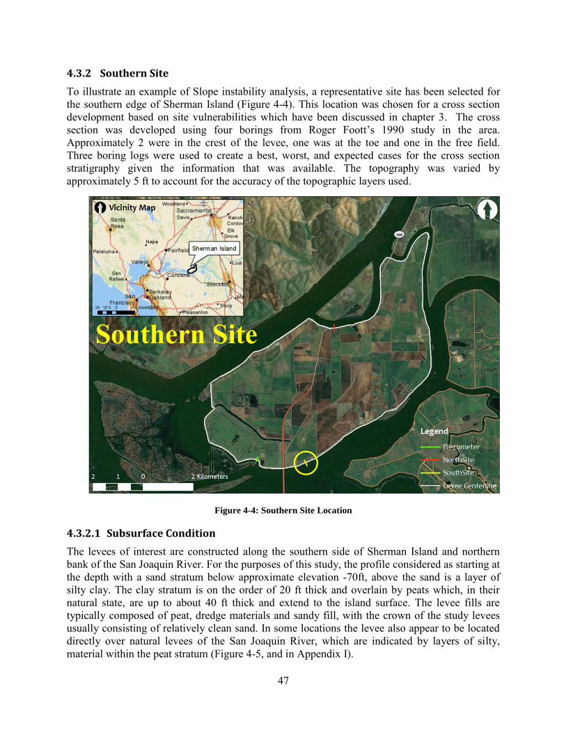
47
4.3.2 Southern Site
To illustrate an example of Slope instability analysis, a representative site has been selected for the southern edge of Sherman Island (Figure 4-4). This location was chosen for a cross section development based on site vulnerabilities which have been discussed in chapter 3. The cross section was developed using four borings from Roger Foott’s 1990 study in the area. Approximately 2 were in the crest of the levee, one was at the toe and one in the free field. Three boring logs were used to create a best, worst, and expected cases for the cross section stratigraphy given the information that was available. The topography was varied by approximately 5 ft to account for the accuracy of the topographic layers used.
Figure 4-4: Southern Site Location
4.3.2.1 Subsurface Condition
The levees of interest are constructed along the southern side of Sherman Island and northern bank of the San Joaquin River. For the purposes of this study, the profile considered as starting at the depth with a sand stratum below approximate elevation -70ft, above the sand is a layer of silty clay. The clay stratum is on the order of 20 ft thick and overlain by peats which, in their natural state, are up to about 40 ft thick and extend to the island surface. The levee fills are typically composed of peat, dredge materials and sandy fill, with the crown of the study levees usually consisting of relatively clean sand. In some locations the levee also appear to be located directly over natural levees of the San Joaquin River, which are indicated by layers of silty, material within the peat stratum (Figure 4-5, and in Appendix I).

48
Figure 4-5: Best and Worst Case Levee Cross Section Interpolation, Sherman Island South Section
4.3.2.2 Analysis
The methodology selected for modeling capacity and demand acting on the levee systems is based on the most widely used and most generally useful definition of factor of safety for embankment stability analysis. The factor of safety against sliding is computed base of the various forces acting on each block. Components for each of the active, passive and neutral blocks are D as the driving force and R as the resisting force. For each of these blocks, D and R can be obtained by constructing the force polygon which consists of the weight of the block W, the normal force N on the slide plane, and the shear strength of soil being mobilized along the sliding plane. The uplift force U can also be considered in the polygon of forces when the effective strength parameters are used for freely draining material (Figure 4-6). The factor of safety with respect to the shear strength of soil can then be expressed as
=
⁄ Equation 4-1
Since the probability of failure Pf is function of the safety index, β, and given that the distributions of demands and capacities can be reasonably characterized as Lognormal, then β can be computed directly from Equation 2-7 (cf., section 2.4.1). In equation 2-7 the embedded ratio of C50/D50 is the equivalent of the median Factor of Safety, defined as the ratio of the mean, median, or mode capacity to the median demand. As the factor of safety increases, the safety
SILTS & CLAYS
SILTS & CLAYS
SANDS
SANDS
PEATS
PEATS
LEVEE FILL
FILL
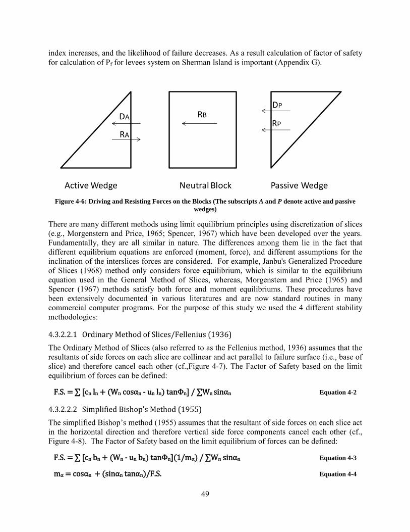
49
index increases, and the likelihood of failure decreases. As a result calculation of factor of safety for calculation of Pf for levees system on Sherman Island is important (Appendix G).
Figure 4-6: Driving and Resisting Forces on the Blocks (The subscripts A and P denote active and passive
wedges)
There are many different methods using limit equilibrium principles using discretization of slices (e.g., Morgenstern and Price, 1965; Spencer, 1967) which have been developed over the years. Fundamentally, they are all similar in nature. The differences among them lie in the fact that different equilibrium equations are enforced (moment, force), and different assumptions for the inclination of the interslices forces are considered. For example, Janbu's Generalized Procedure of Slices (1968) method only considers force equilibrium, which is similar to the equilibrium equation used in the General Method of Slices, whereas, Morgenstern and Price (1965) and Spencer (1967) methods satisfy both force and moment equilibriums. These procedures have been extensively documented in various literatures and are now standard routines in many commercial computer programs. For the purpose of this study we used the 4 different stability methodologies:
4.3.2.2.1 Ordinary Method of Slices/Fellenius (1936)
The Ordinary Method of Slices (also referred to as the Fellenius method, 1936) assumes that the resultants of side forces on each slice are collinear and act parallel to failure surface (i.e., base of slice) and therefore cancel each other (cf.,Figure 4-7). The Factor of Safety based on the limit equilibrium of forces can be defined:
F.S. = ∑ [ n ln + (Wn sαn - un ln) Φn] ∑Wn s αn Equation 4-2
4.3.2.2.2 Simplified Bishop's Method (1955)
The simplified Bishop’s method (1955) assumes that the resultant of side forces on each slice act in the horizontal direction and therefore vertical side force components cancel each other (cf., Figure 4-8). The Factor of Safety based on the limit equilibrium of forces can be defined:
F.S. = ∑ [ n bn + (Wn - un bn) Φn](1/mα) ∑Wn s αn Equation 4-3
mα = cosαn + (sinαn tanαn)/F.S. Equation 4-4
RB
DP
RPDA
RA
Active Wedge Neutral Block Passive Wedge

50
Figure 4-7: Driving and Resisting Forces on the Blocks in Ordinary Method of Slices Method
Figure 4-8: Driving and Resisting Forces on the Blocks in Bishop's Simplified Method

51
4.3.2.2.3 Spencer (1967)
The Spencer method is a general method of slices developed on the basis of limit equilibrium. It requires satisfying equilibrium of forces and moments acting on individual blocks. The method assumes that the angle for the interslice forces is constant and it simultaneously satisfies that the Factor of Safety obtained from the force equilibrium is the same as the one obtained by using moment equilibrium.
4.3.2.2.4 Janbu's Generalized Procedure of Slices (1968)
Janbu is a general method of slices which also developed on the basis of limit equilibrium. It requires satisfying equilibrium of forces acting on individual blocks which is applicable to circular and noncircular failure surfaces. The factor of safety FS is determined by employing the following equation:
F = fo ∑ {[cn bn + (Wn - un bn) tanΦn](1/ cosαnmα)} / ∑Wn tanαn Equation 4-5
Where fo is a correction factor that varies with depth to length ratio of sliding mass and type of soil (f = 0, c, Φ, or c = 0). Step-by-step process to calculate fo illustrated in Figure 4-9:
Figure 4-9: Calculating fo Factor for Janbu's Generalized Procedure of Slices
The software Slide (from Rocscience) can perform Monte Carlo simulations with the help of a random number generator. The program has the capability to sample from random distributions given the correct parameters from both shear strength of the soil and driving forces in the demand side. This software develops a simulation generating an assigned number of random variables and applying them to the closed form solution. The software generates a histogram and then converts the histogram to a PDF for the demands and capacity and CDF for the capacity and demand since the probability of failure calculation is proportional to the overlapping area of capacity and demand PDF histograms (Appendix G). The low and high bounds for soil layers were determined using the worst and best case interpretation of the cross section along with the lower bound of soil’s parameters and the higher bound respectively.
Factor, fo
Ratio, d/L
c, soil
c = 0
L
d
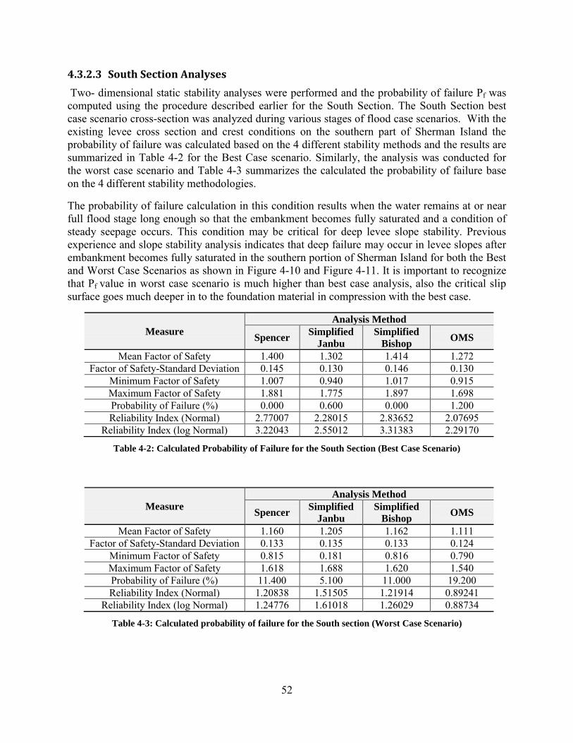
52
4.3.2.3 South Section Analyses
Two- dimensional static stability analyses were performed and the probability of failure Pf was computed using the procedure described earlier for the South Section. The South Section best case scenario cross-section was analyzed during various stages of flood case scenarios. With the existing levee cross section and crest conditions on the southern part of Sherman Island the probability of failure was calculated based on the 4 different stability methods and the results are summarized in Table 4-2 for the Best Case scenario. Similarly, the analysis was conducted for the worst case scenario and Table 4-3 summarizes the calculated the probability of failure base on the 4 different stability methodologies.
The probability of failure calculation in this condition results when the water remains at or near full flood stage long enough so that the embankment becomes fully saturated and a condition of steady seepage occurs. This condition may be critical for deep levee slope stability. Previous experience and slope stability analysis indicates that deep failure may occur in levee slopes after embankment becomes fully saturated in the southern portion of Sherman Island for both the Best and Worst Case Scenarios as shown in Figure 4-10 and Figure 4-11. It is important to recognize that Pf value in worst case scenario is much higher than best case analysis, also the critical slip surface goes much deeper in to the foundation material in compression with the best case.
Measure
Analysis Method
Spencer Simplified
Janbu
Simplified
Bishop OMS
Mean Factor of Safety 1.400 1.302 1.414 1.272 Factor of Safety-Standard Deviation 0.145 0.130 0.146 0.130
Minimum Factor of Safety 1.007 0.940 1.017 0.915 Maximum Factor of Safety 1.881 1.775 1.897 1.698 Probability of Failure (%) 0.000 0.600 0.000 1.200 Reliability Index (Normal) 2.77007 2.28015 2.83652 2.07695
Reliability Index (log Normal) 3.22043 2.55012 3.31383 2.29170
Table 4-2: Calculated Probability of Failure for the South Section (Best Case Scenario)
Measure
Analysis Method
Spencer Simplified
Janbu
Simplified
Bishop OMS
Mean Factor of Safety 1.160 1.205 1.162 1.111 Factor of Safety-Standard Deviation 0.133 0.135 0.133 0.124
Minimum Factor of Safety 0.815 0.181 0.816 0.790 Maximum Factor of Safety 1.618 1.688 1.620 1.540 Probability of Failure (%) 11.400 5.100 11.000 19.200 Reliability Index (Normal) 1.20838 1.51505 1.21914 0.89241
Reliability Index (log Normal) 1.24776 1.61018 1.26029 0.88734
Table 4-3: Calculated probability of failure for the South section (Worst Case Scenario)

53
Figure 4-10: Deep Levee Slope Failure, Southern Portion of Sherman Island (Best Case Scenario)
SAN
DS
SILTS & C
ALY
PEA
TS
FILL

54
Figure 4-11: Deep Levee Slope Failure, Southern Portion of Sherman Island (Worst Case Scenario)
FILL
SAN
DS
PEATS
SILTS & C
ALY

55
4.3.3 Northern Site
To illustrate an example of Slope instability analysis, for the northern edge of the Island a representative site has been chosen to run the analyses on (Figure 4-12). This location was chosen for a cross section development base on site vulnerabilities which have been discussed in chapter 3. Three boring logs were used to create a best, worst, and expected cases for the cross section stratigraphy given the information that was available. The topography was varied by approximately 2 ft to almost 20 ft in peat layer because of the accuracy of the topographic layers used.
Figure 4-12: Northern Site Location
4.3.3.1 Subsurface Condition
The levees of interest are constructed along the northern side of Sherman Island and southern bank of the Sacramento River. For the purposes of this study, the profile considered as starting at the depth with a sand stratum below approximate elevation -20ft, above the sand is a layer of peat. The peat stratum is on the order of 20 ft thick and overlain by levee fills. Peat in their natural state, are up to about 40 ft thick and extend under the river’s bed. The levee fills are typically composed of peat, dredge materials and sandy fill, with the crown of the study levees usually consisting of relatively clean sand. In some locations the levee also appear to be located

56
directly over natural levees of the sacrament River, which are indicated by layers of silty material (very rare) within the peat stratum (Figure 4-13).
Figure 4-13: Best and Worst Case Levee Cross Section Interpolation, Sherman Island North Section
Based on the pervious investigation by Brodsky et al. (2011), the low and high bounds for soil layers were determined using the worst and best case interpretation of the cross section along with the lower bound of soil’s parameters and the higher bound respectively. Levee stability for northern site analysis has been done for two different possible Levee profile: Best Case and Worst Case Scenarios. Seepage through or under this levee is the main potential concern only during a possible flood cases on the Sacramento River which is the subject of Chapter 3. In addition, for this analysis unsaturated soil conditions did not consider above the water table in a levee analysis. Unsaturated shear strength properties will have the effect of raising the calculated factors of safety which would be unrealistic. It should be noted that in the reasonable operation of levee structure there may be fluctuations in the water table and arguably the groundwater table may not be at steady-state conditions. Fluctuations in the water table should be considered in the probabilistic analyses of levee stability (both northern and southern levee analysis).
SANDS
FILL
PEAT

57
4.3.3.2 North Section Analyses
Two- dimensional static stability analyses were performed and the probability of failure Pf was computed using the procedure described earlier for the North Section. Similarly to the South Section, the North Section best and worst case scenarios was analyzed for various flood stages. The probability of failure was calculated based on the 4 different stability methods and the results are summarized in Table 4-4 for the Best Case scenario. Similarly, the analysis was conducted for the worst case scenario and Table 4-5 summarizes the calculated the probability of failure for this case.
The Probability of failure calculation in this condition occurs when the water remains at or near full flood stage long enough so that the embankment becomes fully saturated and a condition of steady seepage occurs. Experience and slope stability analysis indicates that shallow failure may occur in levee slopes in this section after heavy rainfall, or fluctuations in the water table. Failure generally occurs in these very plastic peat slopes. They are probably the result of shrinkage during dry weather and moisture gain during wet weather or fluctuations in the water table with a resulting loss in shear strength due to a net increase in water content, plus additional driving force from water in cracks. Figure 4-14 and Figure 4-15 show the best and worst case scenarios. It is important to recognize that Pf value in worst case scenario is much higher than best case analysis, also the critical slip surface goes much shallower in to the levee fill material in compression with the best case (Appendix G).
Measure
Analysis Method
Spencer Simplified
Janbu
Simplified
Bishop OMS
Mean Factor of Safety 1.343 1.263 1.318 1.310 Factor of Safety-Standard Deviation 0.097 0.092 0.099 0.094
Minimum Factor of Safety 1.023 0.959 0.995 1.008 Maximum Factor of Safety 1.642 1.540 1.632 1.609 Probability of Failure (%) 0.000 0.300 0.100 0.000 Reliability Index (Normal) 3.52832 2.84732 3.19040 3.30256
Reliability Index (log Normal) 4.04403 3.16042 3.61937 3.73846
Table 4-4: Calculated probability of failure for the North Section (Best Case Scenario)
Measure
Analysis Method
Spencer Simplified
Janbu
Simplified
Bishop OMS
Mean Factor of Safety 1.0999 1.055226 1.095953 1.082766 Factor of Safety-Standard Deviation 0.042126 0.039343 0.042688 0.036118
Minimum Factor of Safety 0.940379 0.906254 0.934860 0.947139 Maximum Factor of Safety 1.201230 1.149790 1.199510 1.170090 Probability of Failure (%) 2.000 8.100 2.100 2.000 Reliability Index (Normal) 2.37267 1.40369 2.24778 2.29153
Reliability Index (log Normal) 2.46925 1.42362 2.33375 2.36784
Table 4-5: Calculated probability of failure for the North Section (Worst Case Scenario)

58
Figure 4-14: Shallow Levee Slope Failure, Northern Portion of Sherman Island (Best Case Scenario)
SAN
DS
PEATS
FILL

59
Figure 4-15: Shallow Levee Slope Failure, Northern Portion of Sherman Island (Best Case Scenario)
SAN
DS
PEATS
FILL

60
4.4 Probability of Levee Failure Due to Sliding with Additional Consideration of Type II (Epistemic) Uncertainties:
4.4.1 Type II Uncertainty Evaluation
Type II uncertainties are those that are due to modeling, observation errors, statistical, and measurement. This type of uncertainty is also known as epistemic, since this category of uncertainty is information sensitive in that data gathering, improved modeling, or measurement will reduce the uncertainties (Robert Bea, 1989). Type II (Epistemic) uncertainty, which is related to the modeling of the problem is often ignored. It can be characterized by two parameters:
Bias Value Coefficient of variation
Determination of Central tendency measurement of the bias, (B median, B50, B mean); and a dispersion measurement of the bias, the coefficient of variation for Levee slope stability is not easy. Several approaches should be utilized to compute these estimations. Some of them include field and laboratory measurements, comparison of the results among different analytical and numerical models, model testing (real size or scaled) and expert judgment (Bea, 2003; Vick, 2002; Baecher and Christian, 2003).
4.4.2 Determination of Type II Uncertainties (Bias) for Slope Stability Models
Determination of Bias is one of the most critical parts of determining Margins of Quality. Analytical results derived from mathematical models are similarly different from those in the field. All analytical models have flaws due to the assumptions. The best way to identify the magnitude of the Bias is to compare the results from the analytical models that will be employed by the engineers with observed filed test data. Bias is defined as the ratio of the true or measured value of a parameter to the predicted value of the same parameter by a model (Equation 4-6).
( ) = Equation 4-6
For the purpose of this study the author used the field test data from four different full scale test sites. Data for these four different test sections are presented in the following technical papers:
1. “Performance of Test Fill Constructed on Soft Peat”, by Tillis et al. (1992) 2. “Stability of Atchafalaya Levees”, by Kaufman and Weaver (1967) 3. “Design of Single- or Multi-stage Construction of Embankment Dams for the James Bay
Project”, Ladd et al. (1983) 4. “Monitoring of the Test on the Dike at Bergambacht”, by Koelewijn and Van (2003)
These four cases were used as the true or measured values. Then replicate the field test condition in our computer model with its associating stability methodologies and predict the factor of safety. By comparing the results from the analytical models that will be employed by the engineers with observed field test data we can calculate the Bias (Appendix F). After calculation of Bias value of desired stability model base on these four cases. We can imply dispersion measurement of the bias, which is the coefficient of variation for Levee slope stability model in
61
software or hand calculation for the stability consideration of the Sherman island‘s levees due to sliding and correct the final Pf result by applying σII value to it.
4.4.2.1 “Performance of Test Fill Constructed on Soft Peat”, by Tillis et al. (1992)
A test fill embankment was constructed over soft peat on Bouldin Island in the Sacramento- San Joaquin River delta. The site is underlined by 10 to 12 feet of peat the peat layer has an average undrained shear strengths of 244 psf. A test fill approximately 350 feet long and 200 feet wide at the base was constructed. The reason for construction of embankment was to simulate plane strain conditions during loading and wide enough to permit failing one slope rapidly in an undrained condition. As a result, this embankment was rapidly loaded to failure (Figure 4-16).
In order to replicate the field test condition in the desire model for slope stability analysis, the result of past laboratory and filed program included tests to determine unconsolidated undrained (UU) triaxial strength, consolidated undrained (CU) Triaxial strength, direct shear strength, organic contents, moisture density, and cone penetration probes were assembled from Hultgren - Tillis Engineers. After replicating the field condition in the stability numerical model (Figure 4-17) and by comparing the results of safety factor from the analytical models with the field result the first set of Bias points were calculated.
4.4.2.2 “Stability of Atchafalaya Levees”, by Kaufman, and Weaver (1992)
The Atchafalaya levees of interest for this case are located on the alluvial and deltaic plains of the Mississippi River. In the southern part of the basin, soils consist of a thick, fine-grained top stratum of soft clay containing peat and organic matter overlaying a sand substratum. For the purpose of Bias calculation, the result of test section 1 which is a narrow-crown levee enlargement simulating protection that might be provide in an emergency were used. The narrow-crown levee was built to a height of 6 ft on top of the existing levee without constructing berm and has a length of 1000 ft (Figure 4-18).
In order to replicate the field test condition in the desired model for slope stability analysis, results of the past soil boring and laboratory tests (Unconfined compression and Triaxial shear tests) have been used. After replicating the field condition of Atchafalaya levees in the stability numerical model (Figure 4-19) and by comparing the results of safety factor from the analytical models with the field result the second set of Bias points were calculated.

62
Figure 4-16: Test Fill Embankment o er Soft Peat on Bouldin Island (“Performance of Test Fill Constructed
on Soft Peat”, by Ke in Tillis, Michael Meyer, and Edwin Hultgren, 1992)
Figure 4-17: Replication of the Field Condition from Test Fill Embankment over Soft Peat on Bouldin Island
in the Stability Analytical Model (“Performance of Test Fill Constructed on Soft Peat”, by Ke in Tillis,
Michael Meyer, and Edwin Hultgren, 1992)
Fill
Peat
Stiff Silt

63
Figure 4-18: Atchafalaya le ees located on plains of the Mississippi Ri er “Stability of Atchafalaya Le ees”,
by Robert Kaufman, and Frank Weaver, 1967
Figure 4-19: Replication of the Field Condition from Test Fill Embankment over Atchafalaya levee in the
Stability Analytical Model. (“Stability of Atchafalaya Le ees”, by Kaufman, and Weaver, 1967)
Existing LeveePeat & Soft Organic Clay
Medium & Soft Organic Clay
FS (deterministic) = 1.164FS (mean) = 1.167
Max Height of 6ft3:1 Slope
Medium Clay
Sand

64
4.4.2.3 “Design of Single- or Multi-stage Construction of Embankment Dams for the James Bay Project”, Ladd et al. (1983)
Figure 4-20 shows the cross section for the single construction of dikes for the James Bay project (Ladd et al. 1983). The first part which used for bias calculation was the construction of the embankment in a single stage, either to a height of 6 or 12 m with one berm. The foundation is composed of 4 m of crust underlain by 8 m of highly sensitive marine clay underlain in turn by 6.5 m of Lacustrine clay, for a total thickness of clay of 18.5 m. Undrained shear strength values were obtained from field vane tests, and the stability analyses were done by the simplified Bishop circular and method of slices. Methods stability analyses, simplified Bishop circular and method of slices are important since they are part of desired stability analyses methods of the analytical models. To replicate the field test condition, the undrained shear strength would be obtained from consolidated undrained shear tests combined with knowledge of the initial and consolidated stress histories were used for the slope stability analysis. After replicating the field condition of James Bay Project levees in the desire stability models (Figure 4-21) and by comparing the results of safety factor from the analytical models with the field result the third set of Bias points were calculated.
4.4.2.4 “Monitoring of the Test on the Dike at Bergambacht”, by Koelewijn, and Van, 2003
A large-scale field test has been carried out on an old river dike, to determine its actual strength and to study the uplift mechanism. The test location is on an 800 years old river dike near the village of Bergambacht, about 30 kilometers east of Rotterdam, along the river Lek.
The uplift failure mechanism, which is a special case of a slope stability problem, is primarily caused by the loss of shear strength at the bottom of the soft layers as a result of high pore pressures in the sand layer. The uplift is part our analytical model analysis and having the Bergambacht case as one the point to comparison is very beneficial. In order to study uplift mechanism in this test a sheet pile wall with a length of 50 meters has been placed at the river side of the old dike. This has been filled six weeks in advance of the actual test, to raise the phreatic line in the dike. In addition, the upper two meters have been excavated over a length of 70 meters about four weeks before the test, to facilitate the uplift mechanism (Figure 4-22).
In order to replicate the field test condition in the desire model for slope stability analysis, the result of past laboratory and filed program included tests to determine unconsolidated undrained (UU) triaxial strength, consolidated undrained (CU) Triaxial strength, direct shear strength, organic contents, moisture density, cone penetration probes, piezometers, surface deformation readers, and subsoil deformation were assembled from GeoDelft/Delft Cluster, Delft, Netherlands. After replicating the field condition in the stability numerical model (Figure 4-23) and by comparing the results of safety factor from the analytical models with the field result the last Bias point were calculated
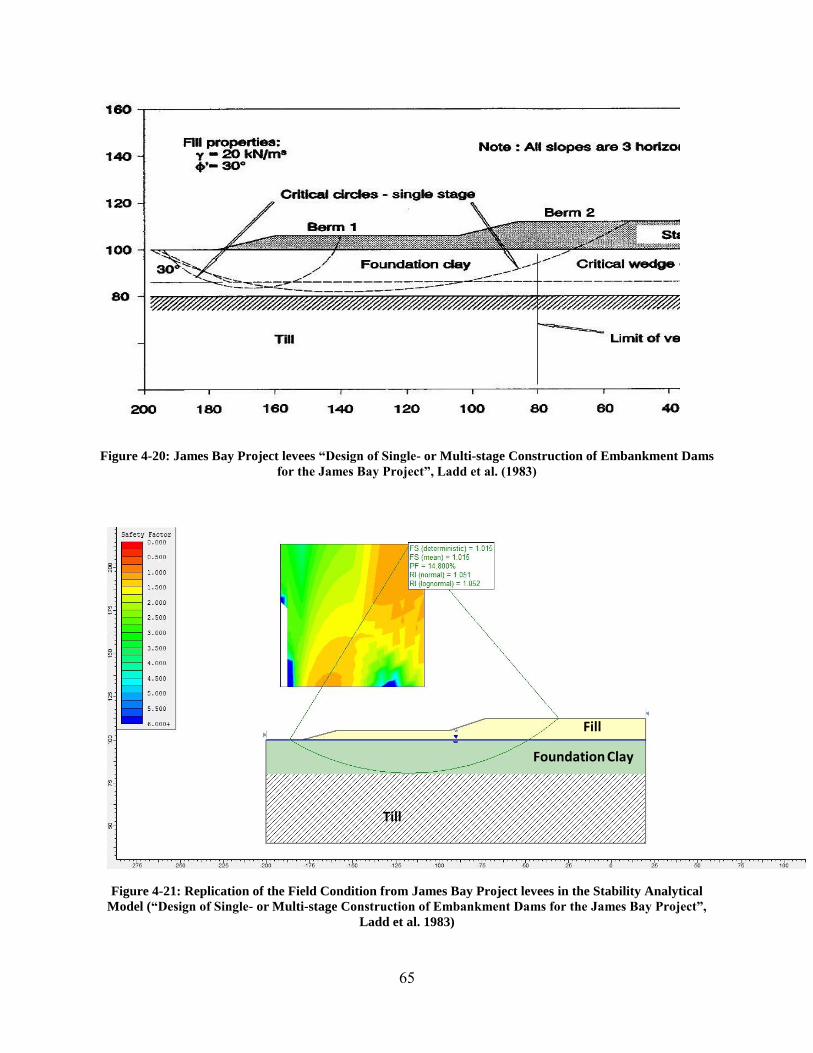
65
Figure 4-20: James Bay Project levees “Design of Single- or Multi-stage Construction of Embankment Dams
for the James Bay Project”, Ladd et al. (1983)
Figure 4-21: Replication of the Field Condition from James Bay Project levees in the Stability Analytical
Model (“Design of Single- or Multi-stage Construction of Embankment Dams for the James Bay Project”,
Ladd et al. 1983)
Fill
Foundation Clay
Till

66
Figure 4-22: Instrumentation for the Bergambacht test “Monitoring of the Test on the Dike at Bergambacht”,
by A.R. Koelewijn, and Meindert Van, 2003
Figure 4-23: Replication of the Field Condition from Bergambacht Dike in the Stability Analytical Model.
(“Monitoring of the Test on the Dike at Bergambacht”, by A.R. Koelewijn, and Meindert Van, 2003)
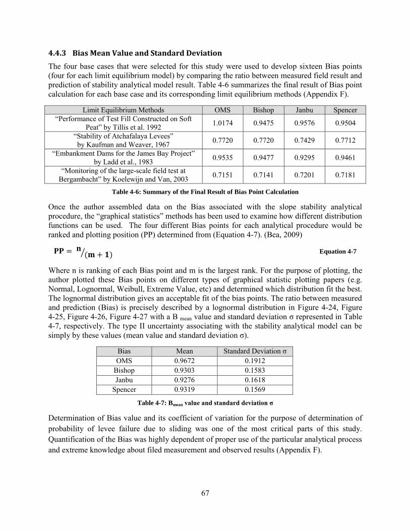
67
4.4.3 Bias Mean Value and Standard Deviation
The four base cases that were selected for this study were used to develop sixteen Bias points (four for each limit equilibrium model) by comparing the ratio between measured field result and prediction of stability analytical model result. Table 4-6 summarizes the final result of Bias point calculation for each base case and its corresponding limit equilibrium methods (Appendix F).
Limit Equilibrium Methods OMS Bishop Janbu Spencer “Performance of Test Fill Constructed on Soft
Peat” by Tillis et al. 1992 1.0174 0.9475 0.9576 0.9504
“Stability of Atchafalaya Levees” by Kaufman and Weaver, 1967 0.7720 0.7720 0.7429 0.7712
“Embankment Dams for the James Bay Project” by Ladd et al., 1983 0.9535 0.9477 0.9295 0.9461
“Monitoring of the large-scale field test at Bergambacht” by Koelewijn and Van, 2003 0.7151 0.7141 0.7201 0.7181
Table 4-6: Summary of the Final Result of Bias Point Calculation
Once the author assembled data on the Bias associated with the slope stability analytical procedure, the “graphical statistics” methods has been used to examine how different distribution functions can be used. The four different Bias points for each analytical procedure would be ranked and plotting position (PP) determined from (Equation 4-7). (Bea, 2009)
= ( )⁄ Equation 4-7
Where n is ranking of each Bias point and m is the largest rank. For the purpose of plotting, the author plotted these Bias points on different types of graphical statistic plotting papers (e.g. Normal, Lognormal, Weibull, Extreme Value, etc) and determined which distribution fit the best. The lognormal distribution gives an acceptable fit of the bias points. The ratio between measured and prediction (Bias) is precisely described by a lognormal distribution in Figure 4-24, Figure 4-25, Figure 4-26, Figure 4-27 with a B mean value and standard deviation σ represented in Table 4-7, respectively. The type II uncertainty associating with the stability analytical model can be simply by these values (mean value and standard deviation σ).
Bias Mean Standard Deviation σ OMS 0.9672 0.1912
Bishop 0.9303 0.1583 Janbu 0.9276 0.1618
Spencer 0.9319 0.1569
Table 4-7: Bmean alue and standard de iation
Determination of Bias value and its coefficient of variation for the purpose of determination of probability of levee failure due to sliding was one of the most critical parts of this study. Quantification of the Bias was highly dependent of proper use of the particular analytical process and extreme knowledge about filed measurement and observed results (Appendix F).

68
Figure 4-24: Probability-Lognormal, Mean Value and Standard Deviation of Bias Points (OMS Method)
Figure 4-25: Probability-Lognormal, Mean Value and Standard Deviation of Bias Points (Simplified Bishop)
ReliaSoft Weibull++ 7 - www.ReliaSoft.com
Probability - Lognormal
Time, (t)
Unre
liabi
lity,
F(t)
0.100 2.0001.00010.000
50.000
99.000Probability-Lognormal
Data 1Lognormal-2PRRX SRM MED FMF=4/S=0
Data PointsProbability Line
Hamed HamediBerkeley2/8/20129:06:08 PM
Bias
ReliaSoft Weibull++ 7 - www.ReliaSoft.com
Probability - Lognormal
Time, (t)
Unre
liabi
lity,
F(t)
0.100 2.0001.00010.000
50.000
99.000Probability-Lognormal
Data 1Lognormal-2PRRX SRM MED FMF=4/S=0
Data PointsProbability Line
Hamed HamediBerkeley2/8/20129:18:30 PM
Bias
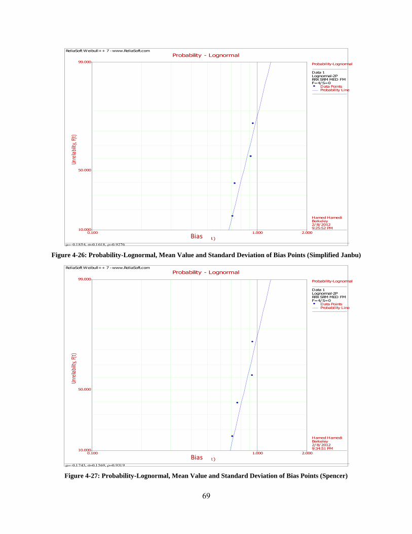
69
Figure 4-26: Probability-Lognormal, Mean Value and Standard Deviation of Bias Points (Simplified Janbu)
Figure 4-27: Probability-Lognormal, Mean Value and Standard Deviation of Bias Points (Spencer)
ReliaSoft Weibull++ 7 - www.ReliaSoft.com
Probability - Lognormal
Time, (t)
Unre
liabi
lity,
F(t)
0.100 2.0001.00010.000
50.000
99.000Probability-Lognormal
Data 1Lognormal-2PRRX SRM MED FMF=4/S=0
Data PointsProbability Line
Hamed HamediBerkeley2/8/20129:25:52 PM
Bias
ReliaSoft Weibull++ 7 - www.ReliaSoft.com
Probability - Lognormal
Time, (t)
Unre
liabi
lity,
F(t)
0.100 2.0001.00010.000
50.000
99.000Probability-Lognormal
Data 1Lognormal-2PRRX SRM MED FMF=4/S=0
Data PointsProbability Line
Hamed HamediBerkeley2/8/20129:34:51 PM
Bias
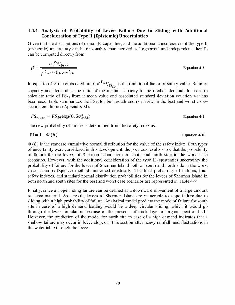
70
4.4.4 Analysis of Probability of Levee Failure Due to Sliding with Additional Consideration of Type II (Epistemic) Uncertainties
Given that the distributions of demands, capacities, and the additional consideration of the type II (epistemic) uncertainty can be reasonably characterized as Lognormal and independent, then Pf can be computed directly from:
= (
⁄ )
√
Equation 4-8
In equation 4-8 the embedded ratio of ⁄ is the traditional factor of safety value. Ratio of capacity and demand is the ratio of the median capacity to the median demand. In order to calculate ratio of FS50 from it mean value and associated standard deviation equation 4-9 has been used, table summarizes the FS50 for both south and north site in the best and worst cross-section conditions (Appendix M).
= ( ) Equation 4-9
The new probability of failure is determined from the safety index as:
Pf = 1 – Φ ( ) Equation 4-10
Φ ( ) is the standard cumulative normal distribution for the value of the safety index. Both types of uncertainty were considered in this development, the previous results show that the probability of failure for the levees of Sherman Island both on south and north side in the worst case scenarios. However, with the additional consideration of the type II (epistemic) uncertainty the probability of failure for the levees of Sherman Island both on south and north side in the worst case scenarios (Spencer method) increased drastically. The final probability of failures, final safety indexes, and standard normal distribution probabilities for the levees of Sherman Island in both north and south sites for the best and worst case scenarios are represented in Table 4-9.
Finally, since a slope sliding failure can be defined as a downward movement of a large amount of levee material .As a result, levees of Sherman Island are vulnerable to slope failure due to sliding with a high probability of failure. Analytical model predicts the mode of failure for south site in case of a high demand loading would be a deep circular sliding, which it would go through the levee foundation because of the presents of thick layer of organic peat and silt. However, the prediction of the model for north site in case of a high demand indicates that a shallow failure may occur in levee slopes in this section after heavy rainfall, and fluctuations in the water table through the levee.

71
C Mean/ D Mean σ ln C Mean/ D Mean C 50/ D50 South Worst
1.161 0.133 1.150 Spencer
1.115 0.125 1.107 Janbu
1.162 0.133 1.152 Bishop
1.111 0.124 1.102 OMS
C Mean/ D Mean σ ln C Mean/ D Mean C 50/ D50 South Best
1.400 0.145 1.386 Spencer
1.301 0.132 1.290 Janbu
1.414 0.146 1.399 Bishop
1.272 0.131 1.261 OMS
C Mean/ D Mean σ ln C Mean/ D Mean C 50/ D50 North Worst
1.099 0.042 1.099 Spencer
1.055 0.039 1.054 Janbu
1.096 0.042 1.095 Bishop
1.083 0.036 1.082 OMS
C Mean/ D Mean σ ln C Mean/ D Mean C 50/ D50 North Best
1.343 0.108 1.335 Spencer
1.263 0.106 1.256 Janbu
1.318 0.110 1.311 Bishop
1.310 0.104 1.303 OMS
Table 4-8: C Mean/ D Mean, ln C Mean/ D Mean, C 50/ D50 for South & North Site in the Best & Worst Cross-section
Conditions
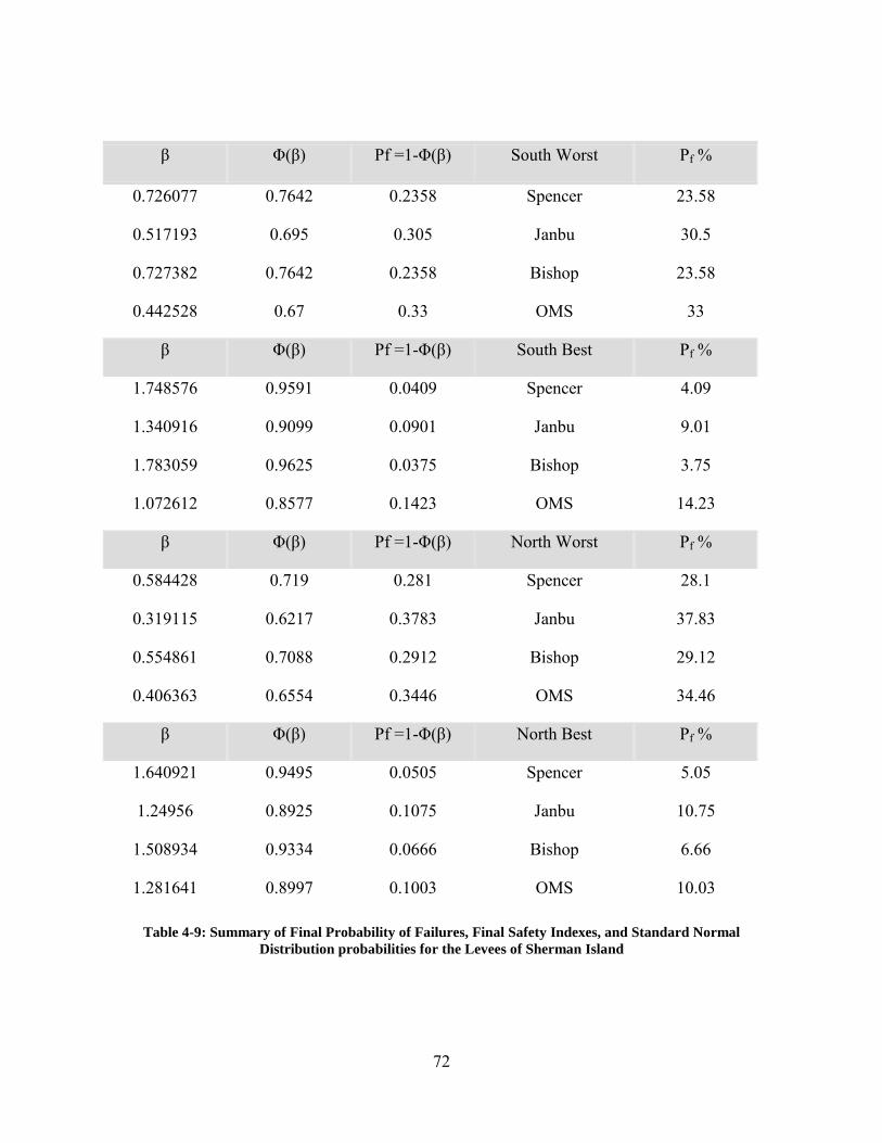
72
β Φ(β) Pf =1-Φ(β) South Worst Pf %
0.726077 0.7642 0.2358 Spencer 23.58
0.517193 0.695 0.305 Janbu 30.5
0.727382 0.7642 0.2358 Bishop 23.58
0.442528 0.67 0.33 OMS 33
β Φ(β) Pf =1-Φ(β) South Best Pf %
1.748576 0.9591 0.0409 Spencer 4.09
1.340916 0.9099 0.0901 Janbu 9.01
1.783059 0.9625 0.0375 Bishop 3.75
1.072612 0.8577 0.1423 OMS 14.23
β Φ(β) Pf =1-Φ(β) North Worst Pf %
0.584428 0.719 0.281 Spencer 28.1
0.319115 0.6217 0.3783 Janbu 37.83
0.554861 0.7088 0.2912 Bishop 29.12
0.406363 0.6554 0.3446 OMS 34.46
β Φ(β) Pf =1-Φ(β) North Best Pf %
1.640921 0.9495 0.0505 Spencer 5.05
1.24956 0.8925 0.1075 Janbu 10.75
1.508934 0.9334 0.0666 Bishop 6.66
1.281641 0.8997 0.1003 OMS 10.03
Table 4-9: Summary of Final Probability of Failures, Final Safety Indexes, and Standard Normal
Distribution probabilities for the Levees of Sherman Island
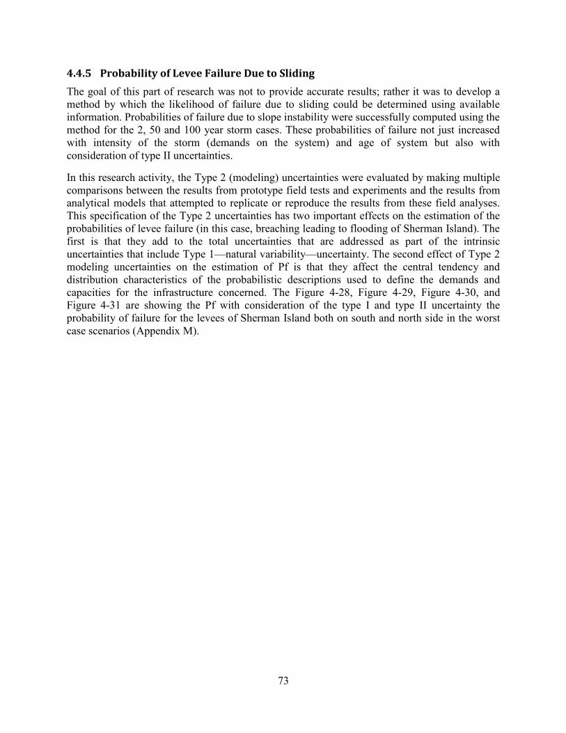
73
4.4.5 Probability of Levee Failure Due to Sliding
The goal of this part of research was not to provide accurate results; rather it was to develop a method by which the likelihood of failure due to sliding could be determined using available information. Probabilities of failure due to slope instability were successfully computed using the method for the 2, 50 and 100 year storm cases. These probabilities of failure not just increased with intensity of the storm (demands on the system) and age of system but also with consideration of type II uncertainties.
In this research activity, the Type 2 (modeling) uncertainties were evaluated by making multiple comparisons between the results from prototype field tests and experiments and the results from analytical models that attempted to replicate or reproduce the results from these field analyses. This specification of the Type 2 uncertainties has two important effects on the estimation of the probabilities of levee failure (in this case, breaching leading to flooding of Sherman Island). The first is that they add to the total uncertainties that are addressed as part of the intrinsic uncertainties that include Type 1—natural variability—uncertainty. The second effect of Type 2 modeling uncertainties on the estimation of Pf is that they affect the central tendency and distribution characteristics of the probabilistic descriptions used to define the demands and capacities for the infrastructure concerned. The Figure 4-28, Figure 4-29, Figure 4-30, and Figure 4-31 are showing the Pf with consideration of the type I and type II uncertainty the probability of failure for the levees of Sherman Island both on south and north side in the worst case scenarios (Appendix M).

74
Figure 4-28: Annual Probability Failure for South Side Sherman Island in the Best Case Scenario
Figure 4-29: Annual Probability Failure for South Side Sherman Island in the Worst Case Scenario
4.09
9.01
3.75
14.23
0 10 20 30 40 50 60 70 80 90 100
Spencer
Janbu
Bishop
OMS
Annual Pf
South Side Best Case
Spencer
Janbu
Bishop
OMS
23.58
30.5
23.58
33
0 10 20 30 40 50 60 70 80 90 100
Spencer
Janbu
Bishop
OMS
Annual Pf
South Side Worst Case
Spencer
Janbu
Bishop
OMS
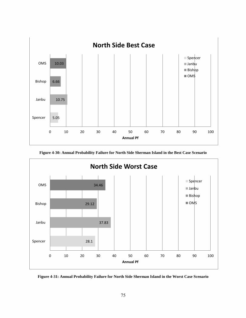
75
Figure 4-30: Annual Probability Failure for North Side Sherman Island in the Best Case Scenario
Figure 4-31: Annual Probability Failure for North Side Sherman Island in the Worst Case Scenario
5.05
10.75
6.66
10.03
0 10 20 30 40 50 60 70 80 90 100
Spencer
Janbu
Bishop
OMS
Annual Pf
North Side Best Case
Spencer
Janbu
Bishop
OMS
28.1
37.83
29.12
34.46
0 10 20 30 40 50 60 70 80 90 100
Spencer
Janbu
Bishop
OMS
Annual Pf
North Side Worst Case
Spencer
Janbu
Bishop
OMS

76
5 OVERTOPPING AND EROSION
The primary objective of this section is to assess risk associated with levee overtopping mechanism for vulnerable earthen levees of Sherman Island. In addition, to establish a probabilistic failure criteria for embankment erosion by studying flow overtopping of levees on Sherman Island. The reliability of any solution can be made evident if the uncertainty associated with the results is offered with it. It is often the case in traditional engineering that only one solution is presented as the “correct” answer. The reliability of the results are often neglected or overlooked because engineers have not been properly trained to handle uncertainty specifically in the fields that analysis deals with flow and hydrology. This section of study aims to provide an example of how traditional methods for analyzing levees overtopping can be approached probabilistically so that inherent uncertainty within the results is understood and areas or recommendations for improvement are readily identified. Finally, gaps in knowledge should be identified, and review all the suggestions for improving the flow overtopping analysis to add greater confidence to risk assessment of the Sherman Island levee system.
5.1 Background
Levee overtopping has been responsible for many levee failures, levee breaches and severe flooding in the past including erosion aspect of the New Orleans levees as they were overtopped by flow. Countries bordering the North Sea like the Netherlands, Germany, Belgium, Denmark, and UK share a long history in fighting against levee overtopping threats from the sea. Earthen levees are used extensively also in the United States to protect populations and infrastructure from periodic floods and high water due to storm surges. Overtopping of levees and dikes produces fast-flowing, turbulent water velocities on the landward-side slope that can damage the protective grass covering and expose the underlying soil to erosion. If overtopping continues long enough, the erosion may eventually result in loss of levee crest elevation and perhaps breaching of the protective structure. Overtopping can be separated in 3 processes:
1. Wave motion and wave run-up on the waterside of levees 2. Wave overtopping on the levee crest 3. Wave overtopping on the landside slope
Earthen levees on Sherman Island constructed mostly without slope protection or armoring at the landside. Specifically, the levees of interest which were constructed along the southern side of Sherman Island and northern bank of the San Joaquin River must rely on the erosion resistance of the outer soil layer during episodes of wave and/or storm surge overtopping. Usually erosion resistance for wave or surge overtopping is most needed on the levee crown and down the rear slope on the protected side of the levee. Levees which were constructed with a top layer of good clay and well-established vegetation with a healthy root system have much better erosion resistance. However, the levees of interest for this research have top layers of sandy soil with sparse or unhealthy vegetation.
77
5.2 Previous Laboratory Experiments
Several laboratory experiments were conducted over the years on the subject of wave impact and soil erosion. The main purpose of these tests is to gain knowledge on the surface erosion processes of the soil subject to a series of impact pressures caused by overtopping. Some of these tests are Führböter (1966), Wu et al. (1979), Woolhiser et al. (1990), and finally In order to investigate the effects of impact pressure acting on the soil with a water-filled crack the laboratory tests were performed at the Leichtweiß-Institute. This experimental set-up developed and described by Pachnio (2005), which is a wooden boxes of dimensions 900x900x600mm, as described by Pachnio (2005) are used in the experiment. The clay is placed into a box in six layers with a 10cm thickness. Each layer is compacted using a force generating constant pressure of about 100 kPa. After all layers have been compacted, a crack is artificially induced in the middle of the sample, at the location where the falling water mass hits the soil. The crack is 150mm deep, 10mm wide and 100mm long. In Figure 5-1 the side and top views of the crack are shown. The crack is filled up with water, and the automatically released mass of water is used to produce an impact pressure in the crack at the surface of the sample. No pressure measurements are needed, as the dependency of pressure on the drop height and after an impact event for which shear failure occurred, a picture of the crack development is taken Figure 5-1 , then the angle of shear failure α between the failure plane and the surface of the soil sample is measured.
Figure 5-1: Experimental Set-up Developed and Described by Pachnio (2005)

78
The main purpose of these laboratory experiments is to investigate the shear failure that may occur when a crack has no cover is subject to impact pressures. Essentially the same procedure as in the case of clay with grass cover is applied. However, as the shear strength of the grass cover is significantly larger that the shear strength of the clay without cover.
5.3 Failure Mechanism
This section will focus predominantly on the likelihood of failure. Capacity and its required Demands for the purpose of the levee overtopping probability of failure analysis can be expressed as:
Capacity (C): Sherman Island‘s levee heights
Demands (D): Sacramento and San Joaquin River stages around Sherman Island
System’s ability to perform is called the “Capacity” (C) and the expectation requirements are called the “Demands” (D). The criteria for failure are met when the Demands exceed the Capacity of the levee system. In this levee system with defined “Capacity” (C) and its required “Demands” (D), the criteria for failure are met when the Demands exceed the Capacity of the levee system (Figure 5-2). For an overtopping failure to occur the river stage must exceed the top of the lowest point of the levee segment before initial erosion occurs.
The probability is estimated based on the information compiled on flood flow and stage and associated uncertainties, levee embankment and associated structure geometry uncertainties. For levee systems that have high probability of flood water to overtop of the levee, capacity has to be lower than demands which will result in high overtopping probability.
Figure 5-2: Schematic of Levee Overtopping (after Zina Deretsky, NSF)
Levee
Capacity
Flood
Demand

79
5.4 Natural Uncertainty (Type I) Evaluation
Natural uncertainties from the projection arise from models and future predictions that often have a large possible range. This study projected two major changes in the system: 1) River stages changes and to sea level rise, and 2) Topography (levee height) change due to subsidence, levee crest raising and sediment deposits.
5.4.1 Demands (Rivers Data)
Collection of resources and data for water level annual extremes in both San Joaquin and Sacramento River was accomplished by using various state and federal agency websites, water level reports from various data coalitions, and other hard copy reports. Most of the water level annual extremes information came from existing reports. Because this existing conditions report covers such a large geographical area (Appendix C).
Many types of data for water level annual extremes analysis are available from government agencies (e.g., NOAA, DWR, USGS, Reclamation) that routinely measure river flow, temperature, salinity, and other water quality parameters. Different agencies have collected data during various time periods, at different stations and with different parameters. These data are stored in various public and private databases. For the purpose of this analysis, data has been collected from The National Oceanic and Atmospheric Administration (NOAA) (http://www.noaa.gov/) which maintained by DWR, through the Division of Flood Management. It contains current and historical flow, water quality, and meteorological datasets for all of California.
5.4.1.1 Hydrograph
A hydrograph shows how the river level changes over time at a specific location. Forecast hydrographs are displayed when flooding is expected, otherwise the hydrograph for the past few months is provided, if the data are available. At key river gages, such as along navigable rivers, daily forecast hydrographs are provided, whether or not flooding is anticipated. For some locations, probabilistic outlooks for extended periods of up to 90 days are provided. Also In cold regions, the hydrograph may seasonally show the effects of the formation of an ice cover. The critical stage is the stage; which hydrographs show rising stream, lake, or reservoir represents the level capacity.
To determine uncertainty associated with high water level in the Sacramento and San Joaquin Rivers, daily extremes hydrographs of water level data measured at Rio Vista Bridge and Antioch gage stations were examined Figure 5-3and Figure 5-4 (Appendix C).

80
Figure 5-3: 2010 Hydrograph (Antioch Station)
Figure 5-4: 2010 Hydrograph (Rio Vista Station)
-4
-2
0
2
4
6
8
10
12
0 50 100 150 200 250 300 350 400 450 500
Riv
er
Stag
e (
NA
VD
88
ft)
Time (hours)
2010 Hydrograph (Antioch Station)
2 Year Storm 50 Year Storm 100 Year Storm
0
2
4
6
8
10
12
14
0 50 100 150 200 250 300 350 400 450 500
Riv
er
Stag
e (
NA
VD
88
ft)
Time (hours)
2010 Hydrograph (Rio Vista Bridge )
2 Year Storm 50 Year Storm 100 Year Storm

81
5.4.1.2 Flood Severity
Flood severity is usually stated in terms of:
Probability of Exceedance, or Frequency of Recurrence.
Modern concepts tend to define a flood in terms of probability. Probability of exceedance, the statistical odds or chance of a flood of given magnitude being exceeded in any year, is generally expressed as a percentage. Frequency of recurrence is expressed in years, on the average, that a flood of given magnitude would be predicted. Modern hydrologists tend to define floods in terms of probability, as expressed in percentage rather than in terms of return period (recurrence interval). Return period, the "T-year flood", and probability (p) are reciprocals, that is, PE = 1/T. Therefore, a flood having a 50-year return frequency (Flood50) is now commonly expressed as a flood with the probability of recurrence of 0.02 (2% chance of being exceeded) in any given year.
River stage measures the height of water in the river channel at any location in the Delta. River stage is a function of river discharge and tidal fluctuations. River stage is used to evaluate the levee system since this is what is applying the actual demands. DRMS developed a method for calculating river stage at a variety of gage stations throughout the Delta given certain discharges from key reservoirs located throughout the Delta, however their method is only one of many that exist in determining river stage.
River stage is directly related to river discharges (or inflows). These are calculated using a combination of different approaches depending on the amount of data available. Most gage stations throughout the Delta measure flow, however the length of data collection is variable.
The three approaches are statistical analysis, comparisons with similar watersheds and flood estimates from precipitation. Table 5-1 outlines what methods should be used with available data (Bulletin #17B, 1982).
Analyses to Include Length of Available Record (years) 10 to 24 25 to 50 50 or more
Statistical Analysis x x x Comparison with similar watersheds x x Flood estimates from precipitation x
Table 5-1: Analyses to be Included (Bulletin 17B, 1982)
A statistical analysis uses available data with a Log Pearson III (LPIII) distribution to predict return periods. A statistical analysis should always be included in a hydrologic study, but can only be the sole analysis if the available record is 50 or more years long. The LPIII distribution should be the distribution of choice unless it can be shown otherwise that alternate distribution fits the given data better than the LPIII (Bulletin 17B, 1982). If the record is limited in length a comparison can be done using data from a similar watershed.
This is especially useful when the alternate watershed has a long unbroken data record. Mathematical procedures have been developed to adjust short term records if a long record exists on a similar watershed (Bulletin 17b, 1982).
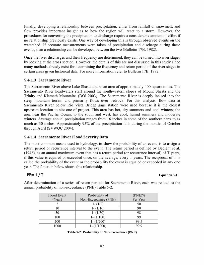
82
Finally, developing a relationship between precipitation, either from rainfall or snowmelt, and flow provides important insight as to how the region will react to a storm. However, the procedures for converting the precipitation to discharge require a considerable amount of effort if no relationship previously exists. One way of developing this is through observed events on the watershed. If accurate measurements were taken of precipitation and discharge during these events, than a relationship can be developed between the two (Bulletin 17B, 1982).
Once the river discharges and their frequency are determined, they can be turned into river stages by looking at the cross section. However, the details of this are not discussed in this study since many methods already exist for determining the frequency and return period of the river stages in certain areas given historical data. For more information refer to Bulletin 17B, 1982.
5.4.1.3 Sacramento River
The Sacramento River above Lake Shasta drains an area of approximately 400 square miles. The Sacramento River headwaters start around the southwestern slopes of Mount Shasta and the Trinity and Klamath Mountains (DOI 2003). The Sacramento River is deeply incised into the steep mountain terrain and primarily flows over bedrock. For this analysis, flow data at Sacramento River below Rio Vista Bridge gage station were used because it is the closest upstream location to site one of project. This area has hot, dry summers and cool winters; the area near the Pacific Ocean, to the south and west, has cool, humid summers and moderate winters. Average annual precipitation ranges from 16 inches in some of the southern parts to as much as 30 inches. Approximately 95% of the precipitation falls during the months of October through April (SVWQC 2004).
5.4.1.4 Sacramento River Flood Severity Data
The most common means used in hydrology, to show the probability of an event, is to assign a return period or recurrence interval to the event. The return period is defined by Bedient et al. (1948), as an annual maximum event that has a return period (or recurrence interval) of T years, if this value is equaled or exceeded once, on the average, every T years. The reciprocal of T is called the probability of the event or the probability the event is equaled or exceeded in any one year. The function below shows this relationship.
PE= 1 / T Equation 5-1
After determination of a series of return periods for Sacramento River, each was related to the annual probability of non-exceedance (PNE) Table 5-2.
Flood Event (Year)
Probability of Non-Exceedance (PNE)
(PNE)% Per Year
2 1- (1/2) 50 10 1- (1/10) 90 50 1- (1/50) 98
100 1- (1/100) 99 200 1- (1/200) 99.5 1000 1- (1/1000) 99.9
Table 5-2: Probability of Non-Exceedance (PNE)

83
Once the plotting positions have been determined, the exceedance probability and stage coordinates plotted on the several appropriate probability paper. The U.S. Interagency Advisory Committee on Water Data (IACWD, 1981) recommends that the log type distribution, In addition, Morris (1982) suggests the log-normal distribution.
For the purpose of plotting, the author plotted these data points on different types of graphical statistic plotting papers (e.g. Normal, Lognormal, Weibull, Extreme Value, etc) and determined which distribution fits the best. The lognormal distribution gives an acceptable fit of the data points. The uncertainties in Sacramento River stages are precisely described by a lognormal distribution in Figure 5-5, with a standard deviation σ equal to 0.2576, respectively.
5.4.1.5 San Joaquin River
The mainstream of the San Joaquin River is 330 miles long from its headwaters in the Sierra Nevada Mountains to its confluence with the Sacramento River and drains an area of approximately 15,550 square miles. Construction of storage infrastructure (dams) and diversions have vastly altered the natural flow regime of the San Joaquin River (SJR) and its major tributaries (McBain and Trush 2000; Kondolf et al. 2001; Cain et. al 2003, Brown and Bauer 2009). For the purpose of water level annual extremes, analysis has describes how the magnitude, frequency, duration, timing, and rate of change of the flows in the San Joaquin River and its major tributaries have been altered within the project area site 2.
5.4.1.6 San Joaquin River Flood Severity Data
The most common means used in hydrology, to show the probability of an event, is to assign a return period or recurrence interval to the event. The return period is defined by Bedient et al. (1948), as an annual maximum event that has a return period (or recurrence interval) of T years, if this value is equaled or exceeded once, on the average, every T years. The reciprocal of T is called the probability of the event or the probability the event is equaled or exceeded in any one year.
After determination of a series of return periods for San Joaquin River, each was related to the annual probability of non-exceedance (PNE) Table 5-2. Once the plotting positions have been determined, the exceedance probability and stage coordinates plotted on the several appropriate probability paper. The U.S. Interagency Advisory Committee on Water Data (IACWD, 1981) recommends that the log type distribution, In addition, Morris (1982) suggests the log-normal distribution. For the purpose of plotting, the author plotted these data points on different types of graphical statistic plotting papers (e.g. Normal, Lognormal, Weibull, Extreme Value, etc) and determined which distribution fits the best. The lognormal distribution gives an acceptable fit of the data points. The uncertainties in San Joaquin River stages are precisely described by a lognormal distribution in Figure 5-6, with a standard deviation σ equal to 0.2963, respectively.

84
Figure 5-5: Lognormal Distribution of Water Le el Annual Extremes for “Sacramento Ri er”
ReliaSoft Weibull++ 7 - www.ReliaSoft.com
Probability- Lognormal, Demand (Without MSLR)
F lood Stages Sacramento River (ft) North
% U
nd
er
1.000 20.00010.00010.000
50.000
99.900
6.890;50.000
8.090;90.000
11.460;98.000
12.120;99.000
12.910;99.500
13.530;99.900
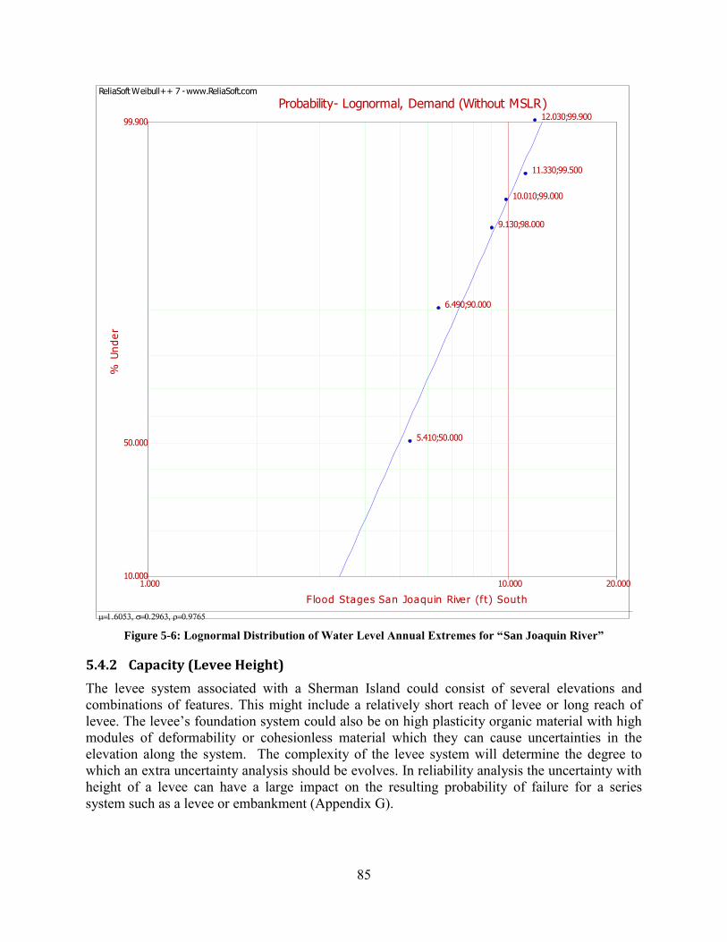
85
Figure 5-6: Lognormal Distribution of Water Le el Annual Extremes for “San Joaquin Ri er”
5.4.2 Capacity (Levee Height)
The levee system associated with a Sherman Island could consist of several elevations and combinations of features. This might include a relatively short reach of levee or long reach of levee. The levee’s foundation system could also be on high plasticity organic material with high modules of deformability or cohesionless material which they can cause uncertainties in the elevation along the system. The complexity of the levee system will determine the degree to which an extra uncertainty analysis should be evolves. In reliability analysis the uncertainty with height of a levee can have a large impact on the resulting probability of failure for a series system such as a levee or embankment (Appendix G).
ReliaSoft Weibull++ 7 - www.ReliaSoft.com
Probability- Lognormal, Demand (Without MSLR)
F lood Stages San Joaquin River (ft) South
% U
nd
er
1.000 20.00010.00010.000
50.000
99.900
5.410;50.000
6.490;90.000
9.130;98.000
10.010;99.000
11.330;99.500
12.030;99.900

86
5.4.2.1 Southern Site
To illustrate an example of over topping analysis, the southern edge of the Island was divided into 5 smaller pieces, or sections. These representative sections have been chosen to run the overtopping analyses on (Figure 5-7). Selection of start and ending point of each section was a function of relative levee height, soil type, access road, maintenance arrangements, location of interior and exterior infrastructure, and a range of similar considerations.
Sample of the levee heights data from surveying done by Dr. Howard Foster Analyst of Geographic Information Science Center in UC Berkeley was used to determine uncertainty associated with proposed design levee height (http://www.arcgis.com/apps/Identify/Chrome/index.html?webmap=3ce1e9a55cea4a01b20468cdda4d0d18). Uncertainty in levee height comes from levee exposure to the environment, Vegetation, wind and wave erosion, foundation soil consolidation, and inhomogeneous soil properties, all contribute to this uncertainty. The levee height was varied by approximately minimum of 5 ft at each section.
Figure 5-7: Southern Site, Location of each Section

87
The “graphical statistics” method has been used to examine how different distribution functions can be used. The data would be ranked and plotting position (PP) determined from (Equation 4-7). (Bea, 2009)
For the purpose of plotting, the author plotted these data points on different types of graphical statistic plotting papers (e.g. Normal, Lognormal, Weibull, Extreme Value, etc) and determined which distribution fits the best. The lognormal distribution gives an acceptable fit of the data points. The levee height uncertainty in southern site for each section is precisely described by a lognormal distribution in Figure 5-8, with a standard deviations σ, represented in Table 5-3.
Sections Levee Height Uncertainty (standard deviations σ)
6 0.0331 7 0.0372 8 0.0293 9 0.0810 10 0.1103
Table 5-3: Standard De iations ( ) of Le ee Height in Southern Part
ReliaSoft Weibull++ 7 - www.ReliaSoft.com
Typy I Uncertainties Capacity (Crown)
Levee Hight
% U
nder
14.000 20.0001.000
5.000
10.000
50.000
99.000Probability-Lognormal
Data 6Lognormal-2PRRX SRM MED FMF=25/S=0
Data PointsProbability Line
Hamed HamedifarUC Berkeley5/10/20123:13:04 PM
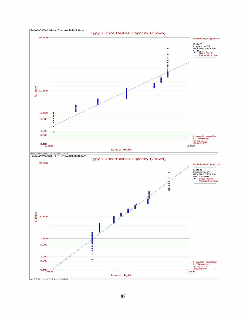
88
ReliaSoft Weibull++ 7 - www.ReliaSoft.com
Typy I Uncertainties Capacity (Crown)
Levee Hight
% U
nder
13.000 15.0000.100
0.500
1.000
5.000
10.000
50.000
99.900
0.100
Probability-Lognormal
Data 7Lognormal-2PRRX SRM MED FMF=89/S=0
Data PointsProbability Line
Hamed HamedifarUC Berkeley5/10/20123:26:24 PM
ReliaSoft Weibull++ 7 - www.ReliaSoft.com
Typy I Uncertainties Capacity (Crown)
Levee Hight
% U
nder
10.000 12.0000.100
0.500
1.000
5.000
10.000
50.000
99.900
0.100
Probability-Lognormal
Data 8Lognormal-2PRRX SRM MED FMF=122/S=0
Data PointsProbability Line
Hamed HamedifarUC Berkeley5/10/20123:33:46 PM
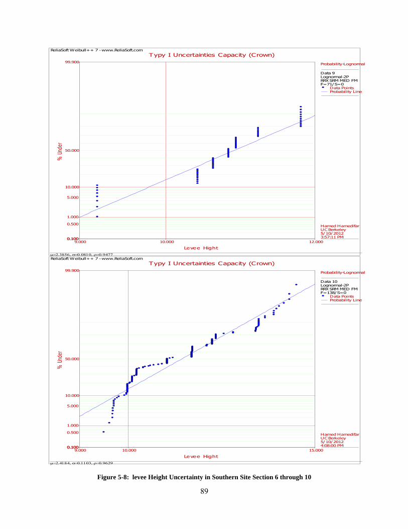
89
Figure 5-8: levee Height Uncertainty in Southern Site Section 6 through 10
ReliaSoft Weibull++ 7 - www.ReliaSoft.com
Typy I Uncertainties Capacity (Crown)
Levee Hight
% U
nder
9.000 12.00010.0000.100
0.500
1.000
5.000
10.000
50.000
99.900
0.100
Probability-Lognormal
Data 9Lognormal-2PRRX SRM MED FMF=71/S=0
Data PointsProbability Line
Hamed HamedifarUC Berkeley5/10/20123:57:11 PM
ReliaSoft Weibull++ 7 - www.ReliaSoft.com
Typy I Uncertainties Capacity (Crown)
Levee Hight
% U
nder
9.000 15.00010.0000.100
0.500
1.000
5.000
10.000
50.000
99.900
0.100
Probability-Lognormal
Data 10Lognormal-2PRRX SRM MED FMF=138/S=0
Data PointsProbability Line
Hamed HamedifarUC Berkeley5/10/20124:08:00 PM
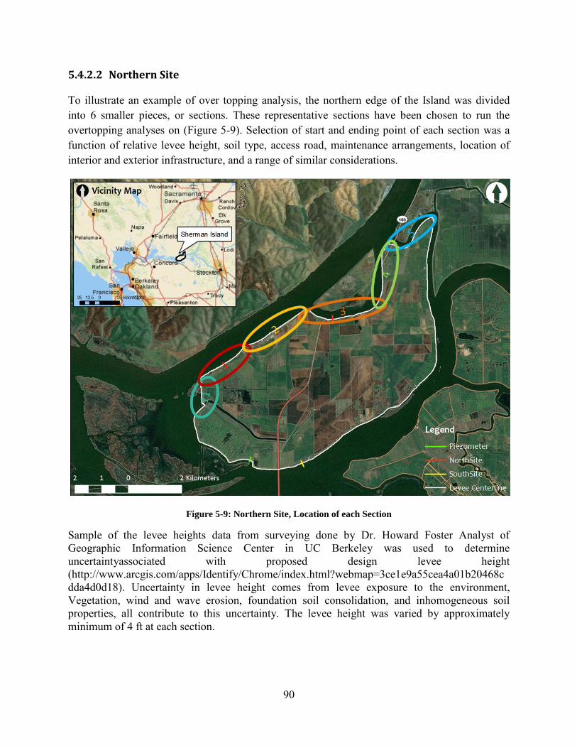
90
5.4.2.2 Northern Site
To illustrate an example of over topping analysis, the northern edge of the Island was divided into 6 smaller pieces, or sections. These representative sections have been chosen to run the overtopping analyses on (Figure 5-9). Selection of start and ending point of each section was a function of relative levee height, soil type, access road, maintenance arrangements, location of interior and exterior infrastructure, and a range of similar considerations.
Figure 5-9: Northern Site, Location of each Section
Sample of the levee heights data from surveying done by Dr. Howard Foster Analyst of Geographic Information Science Center in UC Berkeley was used to determine uncertaintyassociated with proposed design levee height (http://www.arcgis.com/apps/Identify/Chrome/index.html?webmap=3ce1e9a55cea4a01b20468cdda4d0d18). Uncertainty in levee height comes from levee exposure to the environment, Vegetation, wind and wave erosion, foundation soil consolidation, and inhomogeneous soil properties, all contribute to this uncertainty. The levee height was varied by approximately minimum of 4 ft at each section.

91
The “graphical statistics” method has been used to examine how different distribution functions can be used. The data would be ranked and plotting position (PP) determined from (Equation 4-7). (Bea, 2009)
For the purpose of plotting, the author plotted these data points on different types of graphical statistic plotting papers (e.g. Normal, Lognormal, Weibull, Extreme Value, etc) and determined which distribution fits the best. The lognormal distribution gives an acceptable fit of the data points. The levee height uncertainty in southern site for each section is precisely described by a lognormal distribution in Figure 5-10, with a standard deviations σ, represented in Table 5-4.
Sections Levee Height Uncertainty (standard deviations σ)
1 0.0450 2 0.0405 3 0.1200 4 0.0789 5 0.1115 11 0.0472
Table 5-4: Standard De iations ( ) of Le ee Height in Northern Part

92
ReliaSoft Weibull++ 7 - www.ReliaSoft.com
Typy I Uncertainties Capacity (Crown)
Levee Hight
% U
nder
12.000 15.5000.100
0.500
1.000
5.000
10.000
50.000
99.900
0.100
Probability-Lognormal
Data 1Lognormal-2PRRX SRM MED FMF=67/S=0
Data PointsProbability Line
Hamed HamedifarUC Berkeley5/10/20122:18:35 PM
ReliaSoft Weibull++ 7 - www.ReliaSoft.com
Typy I Uncertainties Capacity (Crown)
Levee Hight
% U
nder
14.000 17.0000.100
0.500
1.000
5.000
10.000
50.000
99.900
0.100
Probability-Lognormal
Data 2Lognormal-2PRRX SRM MED FMF=80/S=0
Data PointsProbability Line
Hamed HamedifarUC Berkeley5/10/20122:36:26 PM

93
ReliaSoft Weibull++ 7 - www.ReliaSoft.com
Typy I Uncertainties Capacity (Crown)
Levee Hight
% U
nder
14.000 22.0000.100
0.500
1.000
5.000
10.000
50.000
99.900
0.100
Probability-Lognormal
Data 3Lognormal-2PRRX SRM MED FMF=94/S=0
Data PointsProbability Line
Hamed HamedifarUC Berkeley5/10/20122:43:22 PM
ReliaSoft Weibull++ 7 - www.ReliaSoft.com
Typy I Uncertainties Capacity (Crown)
Levee Hight
% U
nder
10.000 30.0000.100
0.500
1.000
5.000
10.000
50.000
99.900
0.100
Probability-Lognormal
Data 4Lognormal-2PRRX SRM MED FMF=72/S=0
Data PointsProbability Line
Hamed HamedifarUC Berkeley5/10/20122:53:37 PM

94
Figure 5-10: levee Height Uncertainty in Northern Site Section 1 through 5 and Section 11
ReliaSoft Weibull++ 7 - www.ReliaSoft.com
Typy I Uncertainties Capacity (Crown)
Levee Hight
% U
nder
10.000 20.0000.100
0.500
1.000
5.000
10.000
50.000
99.900
0.100
Probability-Lognormal
Data 5Lognormal-2PRRX SRM MED FMF=156/S=0
Data PointsProbability Line
Hamed HamedifarUC Berkeley5/10/20123:06:40 PM
ReliaSoft Weibull++ 7 - www.ReliaSoft.com
Typy I Uncertainties Capacity (Crown)
Levee Hight
% U
nder
9.000 12.00010.0001.000
5.000
10.000
50.000
99.000Probability-Lognormal
Data 11Lognormal-2PRRX SRM MED FMF=18/S=0
Data PointsProbability Line
Hamed HamedifarUC Berkeley5/10/20124:14:40 PM
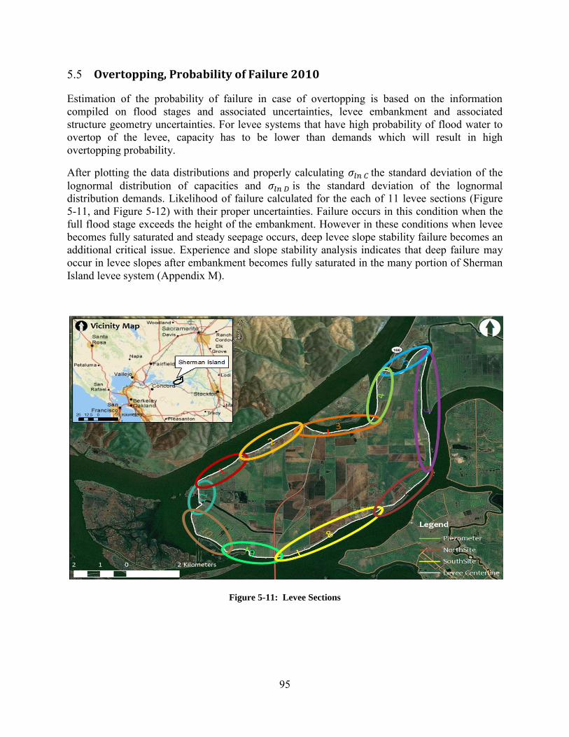
95
5.5 Overtopping, Probability of Failure 2010
Estimation of the probability of failure in case of overtopping is based on the information compiled on flood stages and associated uncertainties, levee embankment and associated structure geometry uncertainties. For levee systems that have high probability of flood water to overtop of the levee, capacity has to be lower than demands which will result in high overtopping probability.
After plotting the data distributions and properly calculating the standard deviation of the lognormal distribution of capacities and is the standard deviation of the lognormal distribution demands. Likelihood of failure calculated for the each of 11 levee sections (Figure 5-11, and Figure 5-12) with their proper uncertainties. Failure occurs in this condition when the full flood stage exceeds the height of the embankment. However in these conditions when levee becomes fully saturated and steady seepage occurs, deep levee slope stability failure becomes an additional critical issue. Experience and slope stability analysis indicates that deep failure may occur in levee slopes after embankment becomes fully saturated in the many portion of Sherman Island levee system (Appendix M).
Figure 5-11: Levee Sections

96
Figure 5-12: Likelihood of Overtopping, for the each of 11 levee sections
5.6 Hazard Adjustment (Projection to the Year 2100)
To test the system for sustainability the analysis needed to be projected to the year 2100. This system will be no means remain static over the years, especially with projected sea level rise. For this reason the cross section needed to be adjusted for the 2100 conditions. To do this, different aspects were considered including erosion of the levee, sedimentation in the river channel and subsidence of peat materials within the levee itself (Appendix E)
5.6.1 Sea Level Rise
Global sea level rose by about 120 m during the several millennia that followed the end of the last ice age (approximately 21,000 years ago), and stabilized between 3,000 and 2,000 years ago. Sea level indicators suggest that global sea level did not change significantly from then until the late 19th century. The instrumental record of modern sea level change shows evidence for onset of sea level rise during the 19th century. Estimates for the 20th century show that global average sea level rose at a rate of about 1.7 mm yr–1 (IPCC, 2007). Global sea level is projected to rise during the 21st century at a greater rate than during 1961 to 2003. Under the IPCC Special Report on Emission Scenarios (SRES) A1B scenario by the mid-2090s, for instance, global sea level reaches 0.22 to 0.44 m above 1990 levels, and is rising at about 4 mm yr–1. The Figure 5-13 illustrates regional trends in sea level, with arrows representing the direction and magnitude of
0 0.5 1 1.5 2 2.5 3 3.5 4 4.5 5
South 9
North 1
South 8
South 7
South 6
North 5
North 4
North 3
North 2
North 11
South 10
Annual Pf% Without MSLR

97
mean sea level rise in the United States of America. The data has been collected from The National Oceanic and Atmospheric Administration (NOAA) (http://www.noaa.gov/).
Figure 5-13: Regional Trends in Sea Level Rise
5.6.2 Sea Level Rise Adjustment
In the projection of the year 2100, sea level rise was accounted for. A range of sea level rise was used based on a number of models. This adjusted the 2, 10, 50, 100, 200, and 1000 year flood levels. After determination of adjustment, for series of return periods of Sacramento, and San Joaquin River, each was related to the annual probability of non-exceedance (PNE). Once the plotting positions have been determined, the exceedance probability and stage coordinates plotted on the several appropriate probability paper. For the purpose of plotting, the author plotted these data points on different types of graphical statistic plotting papers (e.g. Normal, Lognormal, Weibull, Extreme Value, etc) and determined which distribution fits the best. The lognormal distribution gives an acceptable fit of the data points. The uncertainties in both San Joaquin and Sacramento River stages are precisely described by a lognormal distribution in Figure 5-14, and Figure 5-15, with standard deviations σ represented in Table 5-5.

98
2100 conditions (Demand) Standard Deviations σ
Sacramento River 0.1554
San Joaquin River 0.1595
Table 5-5: 2100, Sacramento and San Joaquin River Stages Uncertainties
Figure 5-14: Lognormal Distribution of Water Le el Annual Extremes for “San Joaquin Ri er” with MSLR
Adjustment
ReliaSoft Weibull++ 7 - www.ReliaSoft.com
Probability- Lognormal Demand (With MSLR)
F lood Stages San Joaquin River (ft) South
% U
nd
er
1.000 20.00010.00010.000
50.000
99.900
8.858;50.000
10.305;90.000
11.752;98.000
12.375;99.000
12.998;99.500
14.445;99.900
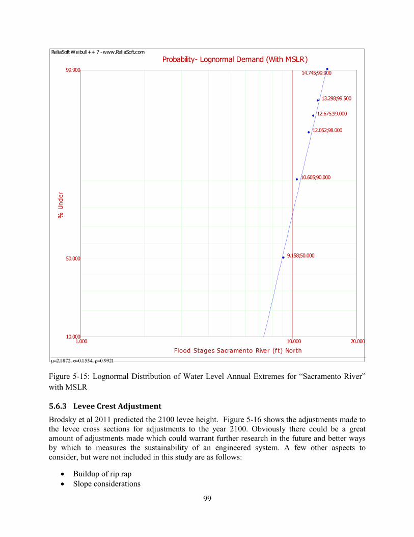
99
Figure 5-15: Lognormal Distribution of Water Level Annual Extremes for “Sacramento River” with MSLR
5.6.3 Levee Crest Adjustment
Brodsky et al 2011 predicted the 2100 levee height. Figure 5-16 shows the adjustments made to the levee cross sections for adjustments to the year 2100. Obviously there could be a great amount of adjustments made which could warrant further research in the future and better ways by which to measures the sustainability of an engineered system. A few other aspects to consider, but were not included in this study are as follows:
Buildup of rip rap Slope considerations
ReliaSoft Weibull++ 7 - www.ReliaSoft.com
Probability- Lognormal Demand (With MSLR)
F lood Stages Sacramento River (ft) North
% U
nd
er
1.000 20.00010.00010.000
50.000
99.900
9.158;50.000
10.605;90.000
12.052;98.000
12.675;99.000
13.298;99.500
14.745;99.900

100
Unexposed peats because of application of levee fill may affect oxidation rates
Figure 5-16: levee Cross Sections for Adjustments to the Year 2100

101
5.7 Overtopping, Probability of Failure 2100
Estimation of the projected probability of failure in case of overtopping is based on the adjusted information compiled on flood stages and associated uncertainties, levee embankment and associated structure geometry uncertainties for the year 2100.
After plotting the data distributions and properly calculating the standard deviation of the lognormal distribution of capacities and adjusted which is the standard deviation of the lognormal distribution demands. Likelihood of failure calculated for the each of 11 levee sections (Figure 5-17) with their 2100 adjusted uncertainties. After plotting the Likelihood of failure calculated for the each of 11 levee sections in year 2100 (Figure 5-11), date shows that chance of failure occurs in each section increase this condition when the full flood stage exceeds the height of the embankment (Appendix M).
Figure 5-17: Projected Likelihood of Overtopping, for the each of 11 Levee Sections
0 0.5 1 1.5 2 2.5 3 3.5
South 9
North 1
South 8
South 7
South 6
North 5
North 4
North 3
North 2
North 11
South 10
Annual Pf% With MSLR

102
5.8 Probability of Failure for Series Element System
Series systems function properly only when all their components function properly. A good examples is chains made out of links (Figure 5-18), the reliability of a series system is easily calculated from the reliability of its components.
Figure 5-18: Schematic Illustration of Series System
A series system fails when any single element fails. In probabilistic terms, the probability of failure of a series system can be expressed in terms of the probabilities of failure of its N elements as:
= ( ) ( ) ( ) Equation 5-2
For a series system comprised of N elements, if the components fail or survive independently of one another, then the probability of failure of the system can be expressed as:
= ∏ ( ) Equation 5-3
If the elements (independent) have different failure probabilities:
= ∑ ( ) Equation 5-4
And finally, if the elements are perfectly correlated then:
= ( ) Equation 5-5
5.8.1 Overtopping Probability of Failure for Levee System of Sherman Island
Levees are predominantly series systems; if one section of a levee fails the system has failed. In order to calculate the probability of failure for the whole system, the calculated probability of failure each section has to consider using either of the original equations 5-3 or 5-4. Table 5-6 illustrates the annual probability of failure of each levee section for year 2010 and 2100; also the probability of failure of Sherman Island levee system due to overtopping using both Equations 5-3 or 5-4 has been calculated. There results indicate that since = ( ) in this case section 11, the elements of this levee system are not perfectly but highly correlated.
1 2 ... i ... n n+1

103
2010:
= ∑ ( ) = 6.6098%
= 1 ∏ (1 ) = 6.5061%
2100:
= ∑ ( ) = 6.3985%
= 1 ∏ (1 ) = 6.2631%
Section %Pf (2010) %Pf (2100) South 9 0.557878 1.251741
North 1 0.208619 0.027311
South 8 0.394081 0.563004
South 7 0.030064 0.009544
South 6 0.008523 0.001035
North 5 0.127513 0.035859
North 4 0.003275 7.1E-05
North 3 0.032546 0.006209
North 2 0.043371 0.002022
North 11 4.693297 3.147173 Equations
6-3 and 6-4 System %Pf
(2010) System %Pf (2100)
=∑( )
6.6098 6.3985
=
1 ∏(1 )
6.50616 6.26311
Table 5-6: Probability of Failure of Sherman Island Levee system due to Overtopping using both Equations
6-3 and 6-4

104
5.9 Levee Erosion
Ideally, all earthen levees should have a crown elevation with enough freeboard to prevent wave and/or surge overtopping for any conceivable storm scenario. However, poor engineering judgment and economic constraints dictate a levee designs with a lower crown elevations, but with the high risk of some wave/surge overtopping will occur during flood events. As a result, wave over topping depends mainly on the geometry of the embankment and the incoming waves.
Figure 5-19 shows a schematic illustration of two different sets of erosion mechanisms for the levees. The first figure shows simple “sheet flow” overtopping. This is a common mode of concern for many river levees, and also for many earth dams. In this mode, as the water flows over the top and then flows like a sheet down the rear-side slope of the levee embankment, the velocity of flow down the rear slope face accelerates and the shear stresses (erosive forces) induced by the flow increase with this increased velocity. “Accordingly, erosion is most pronounced low on the back slope face, and the embankment is eroded from the back side until the crest is breached” (Investigation of the Performance of the New Orleans Flood Protection Systems in Hurricane Katrina, 2006)
Figure 5-19: Schematic Illustration of Two Different Sets of Erosion Mechanisms (Source: Seed et al, 2008a)
The second figure illustrates additional potential set of erosion mode. This is the attack of the outboard side (water side) face of the levee by storm waves. These high energy waves can scallop and erode the outboard face. They can also rush up the face toward the crest, and can erode “notches” in the crest from the front side. Subsequent waves can then pass through these notches, especially as the storm surge continues to rise, and the flow can widen the notches and also erode the back face levee slope.

105
The majority of Sherman Island Levee system protected with rip-rap armor both along the Sacramento, and San Joaquin River (Figure 5-20). As a result for the goal of this report, analysis was conducted on the landward slope of the levees. On the previous section, the probability of the water flows over the top and then flows like a sheet down the rear-side slope of the levee embankment has been calculated.
Evaluating the Sherman island levee vulnerability in term of erosion depends on the layer thickness and overtopping velocity at the end of the levee crest, slope of levee, and roughness of the surface. In addition, the velocity of flow which goes down the rear slope face is an important factor for this analysis. Since, it accelerates and the shear stresses (erosive forces) induced by the flow increase with this increased velocity. This mechanism is the principal concern of flood control management teams for levees in any region, because of its scale and difficulties from the perspective of post failure management. Levees are not generally designed for overtopping and as a result, if overtopping does occur, they are can be highly susceptible to catastrophic failure.
Figure 5-20: Southern Part of Sherman Island Levee System Protected with Rip-rap Armor along the San
Joaquin River
A central concept in assessment of levees overtopping is a linear “Miner’s fatigue damage accumulation”. This equation links the performance target to the processes that lead to failure to fulfill that target. This study stared with a proper definition of the flood defense function and flood defense failure is therefore essential for meaningful results. The defense can fail in

106
different ways, referred to as failure modes. The reliability of the levee in this approach represented by a combination between the strength of the levee materials and the loading of the defense structure in the form of the following equation:
D = R / S (when D = 1 failure occurs) Equation 5-6
In which S expresses the loading and can for example be a function of the hydraulic loading conditions or the ground pressures behind a vertical wall. R represents the strength the levee defense System and can be a function of e.g. the thickness of the embankment, or the crest elevation.
5.9.1 Erosion of levee’s Inner Slope by Wave Overtopping
In this case levee system fails when water overtops the crest of the levee. Overtopping can be caused when flood waters simply exceed the lowest crest of the levee system or if high winds begin to generate significant storm surge in the river water to bring waves crashing over the levee (previous cases reported in Sherman Island). Overtopping in this case can lead to a significant landside erosion of the levee or even be the mechanism for complete breach in this case. In this case levee is overtopped and the land side of the levee is not armored or reinforced, the waters can undercut the levee and cause it to collapse or breach Figure 5-21.
Figure 5-21: Schematic Illustration of Lands Side Erosion due to Levee Over topping
In this case, the back of the levee can be attacked by overtopping flow. Back erosion of the levees depends on the hydraulic shear stress that is calculated from velocity. The response of this surface will depend on the magnitude and duration characteristics of the flow, regional geometry material characteristics, vegetation, and armoring, if present. This response can be in terms of a scour depth or an erosion rate. The velocity may be a function of water elevation (flood stage or storm surge). The probability of failure is then determined by comparing the erosion rate

107
multiplied by time of an event to an existing volume that must be eroded. An equation for erosion rate (Hanson and Temple, 2002, Hanson and Cook, 2004) is:
= ( ) Equation 5-7
Where = ( ) ,
= ( )
= (
⁄ )
5.9.1.1 Critical Shear Stress ( )
Critical shear stress values are highly dependent on the local soil properties. The best method to estimate erosion rate as a function of shear stress, and critical shear stress, is to perform an analysis of shear stress and sediment erodibility using a mobile erosion flume and site-specific sediment cores that are as undisturbed as possible. The sediment samples are subjected to various flow conditions to evaluate erosion rate as a function of imposed shear stress (Briaud et al. 2001).
The design procedure and requirements for levee design are established by U.S. Army Corps of Engineers (EC 1110-2-6066), outlined and provides guidance for the typical range of values for critical shear stresses on levees. Table 5-7 shows mean and standard deviation of values for critical shear stresses on levees. Fine grained represents cohesive material (silts and clays) and coarse grained represents sands and gravels.
Fill Material Mean COV STD 50th
Fine Compacted 0.221 1.09 0.2409 0.2146
Fine Un-Compacted 0.035 0.7 0.0245 0.0349
Coarse Compacted 0.134 0.74 0.0992 0.1333
Coarse Un-Compacted 0.006 0.74 0.0044 0.006
Table 5-7: Mean and Standard Deviation Values for Critical Shear Stresses on Levees
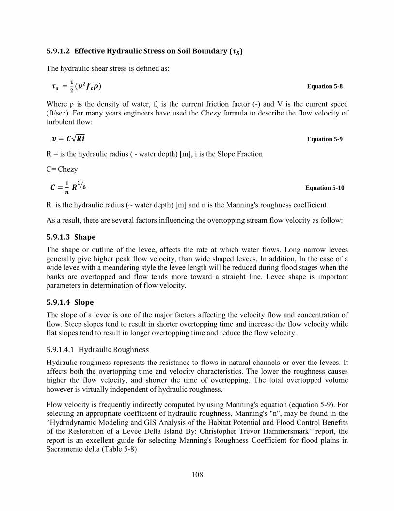
108
5.9.1.2 Effective Hydraulic Stress on Soil Boundary ( )
The hydraulic shear stress is defined as:
=
( ) Equation 5-8
Where is the density of water, fc is the current friction factor (-) and V is the current speed (ft/sec). For many years engineers have used the Chezy formula to describe the flow velocity of turbulent flow:
= √ Equation 5-9
R = is the hydraulic radius (~ water depth) [m], i is the Slope Fraction
C= Chezy
=
⁄ Equation 5-10
R is the hydraulic radius (~ water depth) [m] and n is the Manning's roughness coefficient
As a result, there are several factors influencing the overtopping stream flow velocity as follow:
5.9.1.3 Shape
The shape or outline of the levee, affects the rate at which water flows. Long narrow levees generally give higher peak flow velocity, than wide shaped levees. In addition, In the case of a wide levee with a meandering style the levee length will be reduced during flood stages when the banks are overtopped and flow tends more toward a straight line. Levee shape is important parameters in determination of flow velocity.
5.9.1.4 Slope
The slope of a levee is one of the major factors affecting the velocity flow and concentration of flow. Steep slopes tend to result in shorter overtopping time and increase the flow velocity while flat slopes tend to result in longer overtopping time and reduce the flow velocity.
5.9.1.4.1 Hydraulic Roughness
Hydraulic roughness represents the resistance to flows in natural channels or over the levees. It affects both the overtopping time and velocity characteristics. The lower the roughness causes higher the flow velocity, and shorter the time of overtopping. The total overtopped volume however is virtually independent of hydraulic roughness.
Flow velocity is frequently indirectly computed by using Manning's equation (equation 5-9). For selecting an appropriate coefficient of hydraulic roughness, Manning's "n", may be found in the “Hydrodynamic Modeling and GIS Analysis of the Habitat Potential and Flood Control Benefits of the Restoration of a Levee Delta Island By: Christopher Trevor Hammersmark” report, the report is an excellent guide for selecting Manning's Roughness Coefficient for flood plains in Sacramento delta (Table 5-8)
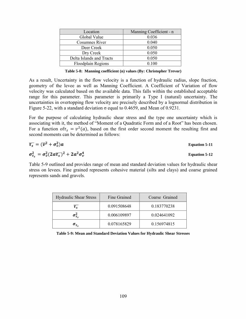
109
Location Manning Coefficient - n Global Value 0.036
Cosumnes River 0.040 Deer Creek 0.050 Dry Creek 0.050
Delta Islands and Tracts 0.050 Floodplain Regions 0.100
Table 5-8: Manning coefficient (n) values (By: Christopher Trevor)
As a result, Uncertainty in the flow velocity is a function of hydraulic radius, slope fraction, geometry of the levee as well as Manning Coefficient. A Coefficient of Variation of flow velocity was calculated based on the available data. This falls within the established acceptable range for this parameter. This parameter is primarily a Type I (natural) uncertainty. The uncertainties in overtopping flow velocity are precisely described by a lognormal distribution in Figure 5-22, with a standard deviation σ equal to 0.4659, and Mean of 0.9231.
For the purpose of calculating hydraulic shear stress and the type one uncertainty which is associating with it, the method of “Moment of a Quadratic Form and of a Root” has been chosen. For a function of = ( ), based on the first order second moment the resulting first and second moments can be determined as follows:
= (
) Equation 5-11
=
( )
Equation 5-12
Table 5-9 outlined and provides range of mean and standard deviation values for hydraulic shear stress on levees. Fine grained represents cohesive material (silts and clays) and coarse grained represents sands and gravels.
Hydraulic Shear Stress Fine Grained Coarse Grained
0.091508648 0.183770238
0.006109897 0.024641092
0.078165829 0.156974815
Table 5-9: Mean and Standard Deviation Values for Hydraulic Shear Stresses

110
Figure 5-22: Lognormal Distribution of Overtopping Flow Velocity
5.9.1.5 Erodibility Coefficient (k)
The Erodibility Coefficients (k) of the levee and embankment soils were measured in the Sacramento delta using a submerged jet test device (ASTM, 1999). An inverse relationship between and k exists , where soils exhibiting a low have a high k and soils having a high tend to have a low k. Hanson and Simon (2001) provide a graph for the inverse relationship between critical shear stress and erodibility coefficient (Figure 5-23)
ReliaSoft Weibull++ 7 - www.ReliaSoft.com
Probability Density Function
Velocity (ft/sec)
f(t)
0.000 8.0001.600 3.200 4.800 6.4000.000
0.400
0.080
0.160
0.240
0.320
Data 2Lognormal-2PRRX SRM MED FMF=39/S=0
Pdf Line
Hamed HamedifarUC Berkeley6/1/201211:56:54 AM
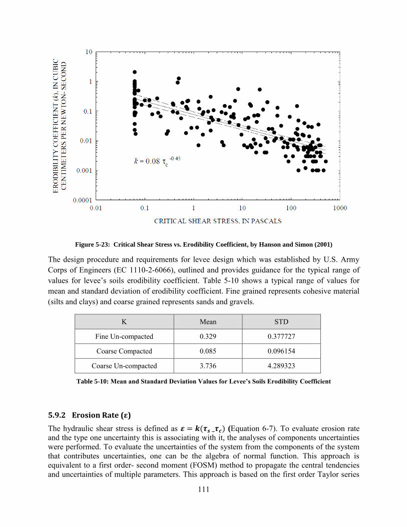
111
Figure 5-23: Critical Shear Stress vs. Erodibility Coefficient, by Hanson and Simon (2001)
The design procedure and requirements for levee design which was established by U.S. Army Corps of Engineers (EC 1110-2-6066), outlined and provides guidance for the typical range of values for levee’s soils erodibility coefficient. Table 5-10 shows a typical range of values for mean and standard deviation of erodibility coefficient. Fine grained represents cohesive material (silts and clays) and coarse grained represents sands and gravels.
K Mean STD
Fine Un-compacted 0.329 0.377727
Coarse Compacted 0.085 0.096154
Coarse Un-compacted 3.736 4.289323
Table 5-10: Mean and Standard De iation Values for Le ee’s Soils Erodibility Coefficient
5.9.2 Erosion Rate (ε)
The hydraulic shear stress is defined as = ( ) (Equation 6-7). To evaluate erosion rate and the type one uncertainty this is associating with it, the analyses of components uncertainties were performed. To evaluate the uncertainties of the system from the components of the system that contributes uncertainties, one can be the algebra of normal function. This approach is equivalent to a first order- second moment (FOSM) method to propagate the central tendencies and uncertainties of multiple parameters. This approach is based on the first order Taylor series
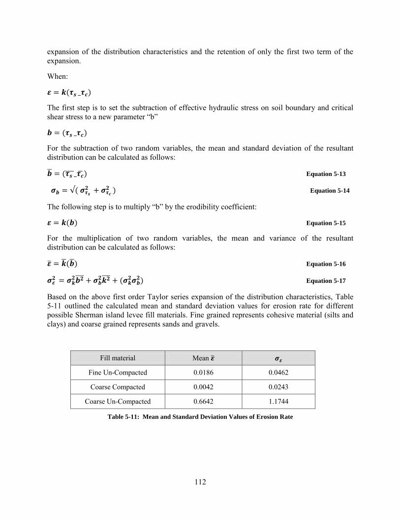
112
expansion of the distribution characteristics and the retention of only the first two term of the expansion.
When:
= ( )
The first step is to set the subtraction of effective hydraulic stress on soil boundary and critical shear stress to a new parameter “b”
= ( )
For the subtraction of two random variables, the mean and standard deviation of the resultant distribution can be calculated as follows:
= ( ) Equation 5-13
= √(
) Equation 5-14
The following step is to multiply “b” by the erodibility coefficient:
= ( ) Equation 5-15
For the multiplication of two random variables, the mean and variance of the resultant distribution can be calculated as follows:
= ( ) Equation 5-16
=
(
) Equation 5-17
Based on the above first order Taylor series expansion of the distribution characteristics, Table 5-11 outlined the calculated mean and standard deviation values for erosion rate for different possible Sherman island levee fill materials. Fine grained represents cohesive material (silts and clays) and coarse grained represents sands and gravels.
Fill material Mean
Fine Un-Compacted 0.0186 0.0462
Coarse Compacted 0.0042 0.0243
Coarse Un-Compacted 0.6642 1.1744
Table 5-11: Mean and Standard Deviation Values of Erosion Rate

113
5.10 Final Probability of Levee Failure Due to Erosion considering Type I, & II
The breaching of Sherman Island Levee system occurs as a result of a complex interaction between fluid and soil structure. In the case of breaching initiated from the inside usually the breaching process begins with the erosion of the grass cover and the under laying soil layer, followed by the erosion of the uncovered core which leads to the overflow and the final breach. However, the analysis has been done in terms of time both for capacity and demand.
5.10.1 Time for Levee Erosion, Time of Breaching (Capacity)
The total time of levee breaching can be given as a sum of the following phases:
1. Time of grass failure: time between the incipient erosion end the time of grass failure expressed in terms of erosion depth;
2. Time of cover failure: time between the incipient erosion end the time when the revetment fails and the core becomes unprotected;
3. Time of core failure: time between the incipient erosion end the time when the erosion reaches the inner soil and the erosion progress becomes irreversible;
4. Breach initiation time: time between the incipient erosion and the initiation of the breach described in terms of erosion depth;
5. Breach formation time: time between end of the breach initiation and the end of the breach formation;
6. Core wash-out time: time between the end of the breach development and the time when the water level on the landside becomes equal to the one on the waterside (final breach).
This time calculated in 2 different phase time for grass turf erosion and time for levee erosion.
5.10.2 Time for Grass Turf Erosion
The following equation was developed by Seijffert and Verheij (1998), established by results and observations from Dutch large scalewave tank experiments involving wave conditions, levee slopes, and a range of turf/substrate conditions similar to conditions in Sherman Island. The time required to remove grass turf is computed as:
=
Equation 5-18
Where d is the turf thickness (m), Hs is the Height of water (m) and CE is the grass cover quality (m-1 s-1).
5.10.2.1 Grass Cover Quality and Turf Thickness
In previous studies, grass cover quality was measured based on the in situ root pull-out test, laboratory root tensile test, and shear test of soil blocks reinforced with roots or artificial fibers. Root pull-out tests conducted in the field provide data of root tensile strength and root−soil interactions (Burroughs and Thomas, 1977; Ziemer, 1978; Wu et al., 1979; Riestenberg and Sovonick-Dunford, 1983; Riestenberg, 1994; Watson et al., 1997, 1999; Schmidt et al., 2001; Norris, 2005; Pollen and Simon, 2005; Pollen, in press). Riestenberg (1994) and Norris (2005)

114
concluded that the number and morphology of root branches influences the stress−strain relationship and ultimate resistance to failure. Burroughs and Thomas (1977), Watson et al. (1999) and Schmidt et al. (2001) show that the tensile strength of living roots is significantly larger than that of decaying roots. However, data derived from tests may only have a local value because of spatial variations in vegetation and tensile force (Burroughs and Thomas, 1977; Schmidt et al., 2001) and differences in the season when the test was carried out (Hathaway and Penny, 1975; Wasterlund, 1989; Makarova et al., 1998). Laboratory tests (Riestenberg and Sovonick- Dunford, 1983; Abe and Iwamoto, 1986; Riestenberg, 1994) may only provide data on root strength of a single specimen. In addition, previous studies indicated exponential (Abe and Iwamoto, 1986) and linear (Riestenberg, 1994) relationships between the tensile force and root diameter.
As a result, For the purpose of understanding influence of root and vegetation on the reliability of Sherman island levee system, the result of research program done by Douglas Shields, and Donald H. Gray was used. The investigators used field data in seepage and slope stability analyses. Field data were collected from selected sites within a 10-km segment of a channel levee on the Sacramento River near Elkhorn, California. Root architecture and distribution were determined using the profile-wall method in which root cross sections were exposed in the vertical wall of an excavated trench. Figure 5-24 and Figure 5-25 summarize the Botanical data needed for the analysis of Sherman Island Overtopping erosion in terms of grass cover quality, and turf thickness. Table 5-12 outlined the mean and standard deviation values for grass cover quality, and turf thickness
Parameter Mean σ
( ) 2.2308E-006 9.4601E-007
( ) 0.0240 0.0035
Table 5-12: Mean and Standard Deviation Values of Grass Cover Quality, and Turf Thickness
The first step is to set the nominator of time for grass turf erosion’s equation (Equation 6-18) equal to a new parameter “A”
= Equation 5-19
The second step is to set equal to another parameter “B”, for:
= Equation 5-20
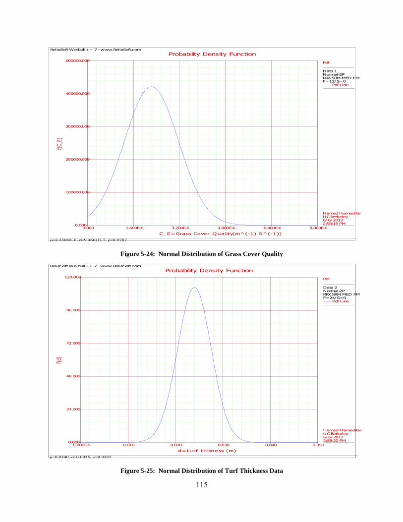
115
Figure 5-24: Normal Distribution of Grass Cover Quality
Figure 5-25: Normal Distribution of Turf Thickness Data
ReliaSoft Weibull++ 7 - www.ReliaSoft.com
Probability Density Function
C_E=Grass Cover Quality(m^(-1) S^(-1))
f(C_
E)
0.000 8.000E-61.600E-6 3.200E-6 4.800E-6 6.400E-60.000
500000.000
100000.000
200000.000
300000.000
400000.000
Data 1Normal-2PRRX SRM MED FMF=13/S=0
Pdf Line
Hamed HamedifarUC Berkeley6/6/20122:58:15 PM
ReliaSoft Weibull++ 7 - www.ReliaSoft.com
Probability Density Function
d=turf thikness (m)
f(d)
6.000E-5 0.0500.010 0.020 0.030 0.0400.000
120.000
24.000
48.000
72.000
96.000
Data 2Normal-2PRRX SRM MED FMF=24/S=0
Pdf Line
Hamed HamedifarUC Berkeley6/6/20122:58:22 PM
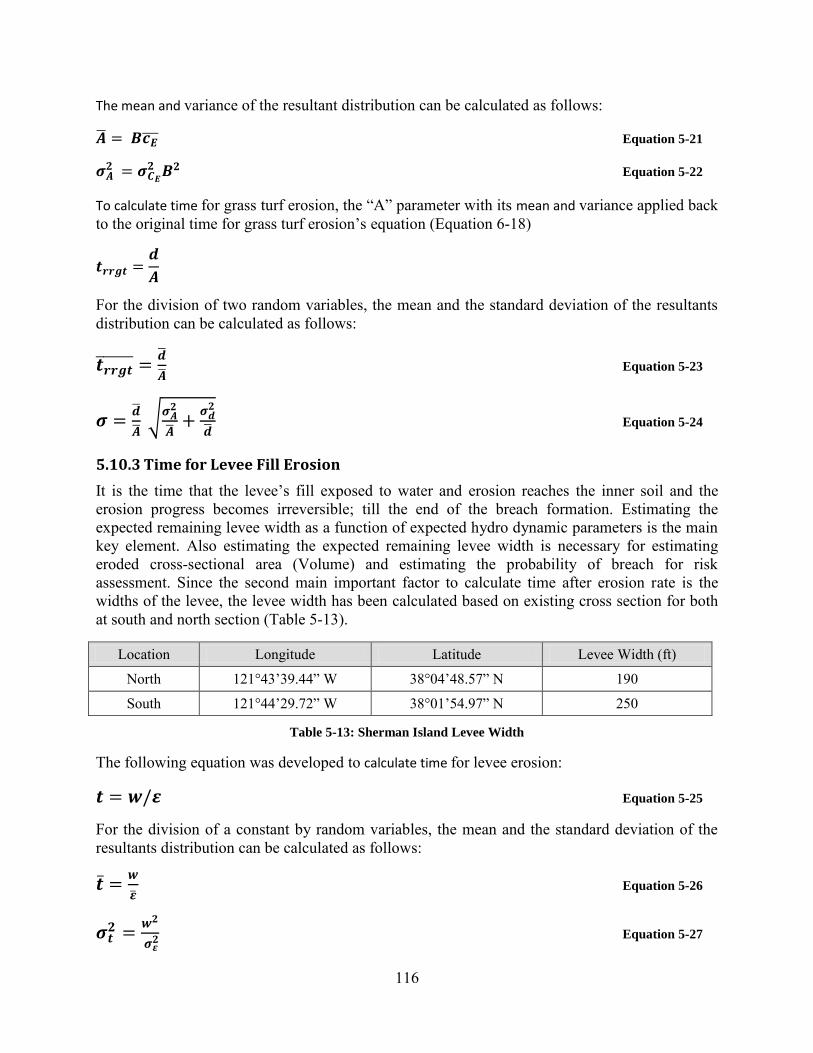
116
The mean and variance of the resultant distribution can be calculated as follows:
= Equation 5-21
=
Equation 5-22
To calculate time for grass turf erosion, the “A” parameter with its mean and variance applied back to the original time for grass turf erosion’s equation (Equation 6-18)
=
For the division of two random variables, the mean and the standard deviation of the resultants distribution can be calculated as follows:
=
Equation 5-23
=
√
Equation 5-24
5.10.3 Time for Levee Fill Erosion
It is the time that the levee’s fill exposed to water and erosion reaches the inner soil and the erosion progress becomes irreversible; till the end of the breach formation. Estimating the expected remaining levee width as a function of expected hydro dynamic parameters is the main key element. Also estimating the expected remaining levee width is necessary for estimating eroded cross-sectional area (Volume) and estimating the probability of breach for risk assessment. Since the second main important factor to calculate time after erosion rate is the widths of the levee, the levee width has been calculated based on existing cross section for both at south and north section (Table 5-13).
Location Longitude Latitude Levee Width (ft)
North 121°43’39.44” W 38°04’48.57” N 190
South 121°44’29.72” W 38°01’54.97” N 250
Table 5-13: Sherman Island Levee Width
The following equation was developed to calculate time for levee erosion:
= Equation 5-25
For the division of a constant by random variables, the mean and the standard deviation of the resultants distribution can be calculated as follows:
=
Equation 5-26
=
Equation 5-27
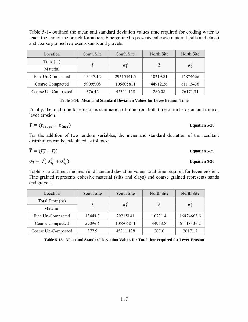
117
Table 5-14 outlined the mean and standard deviation values time required for eroding water to reach the end of the breach formation. Fine grained represents cohesive material (silts and clays) and coarse grained represents sands and gravels.
Location South Site South Site North Site North Site
Time (hr)
Material
Fine Un-Compacted 13447.12 29215141.3 10219.81 16874666
Coarse Compacted 59095.08 105805811 44912.26 61113436
Coarse Un-Compacted 376.42 45311.128 286.08 26171.71
Table 5-14: Mean and Standard Deviation Values for Levee Erosion Time
Finally, the total time for erosion is summation of time from both time of turf erosion and time of levee erosion:
= ( ) Equation 5-28
For the addition of two random variables, the mean and standard deviation of the resultant distribution can be calculated as follows:
= ( ) Equation 5-29
= √(
) Equation 5-30
Table 5-15 outlined the mean and standard deviation values total time required for levee erosion. Fine grained represents cohesive material (silts and clays) and coarse grained represents sands and gravels.
Location South Site South Site North Site North Site
Total Time (hr)
Material
Fine Un-Compacted 13448.7 29215141 10221.4 16874665.6
Coarse Compacted 59096.6 105805811 44913.8 61113436.2
Coarse Un-Compacted 377.9 45311.128 287.6 26171.7
Table 5-15: Mean and Standard Deviation Values for Total time required for Levee Erosion

118
5.10.4 Time for Overtopping (Demands)
The overtopping time is the time that an individual wave passes a certain location on the levee section, till the wave or water stage goes back to its original positions. The larger the volume of an overtopping event has been, the longer the overtopping time will be. The maximum overtopping time is useful when one wants to describe Probability of the system.
This time is calculated for the 'hydrographs' plots (Figure 6-3 and 6-4). In the plots of water elevation versus time for the different return periods, when the water elevation exceeds the elevation of the levee crest the time starts and when the water elevation becomes less than the elevation of the levee crest the time stops. This time difference is the time based demand of overtopping. Table 5-16 outlined the mean and standard deviation values this demand time for 2, 50, and 100 year flood both for year 2010 and 2100.
Flood Events ∆t = 2010 ∆t = 2100
2 16 414
50 112 608
100 329 624
Mean 4.215 414
σ 101.4 91
Table 5-16: Mean and Standard Deviation Values for Time of Overtopping
5.10.5 Likelihood of Failure (Breach)
Given that the distributions of demands and capacities can be reasonably characterized as Lognormal and independent, then Pf can be computed directly from:
=
√
Equation 5-31
Where β is defined as the safety index, is the mean capacity, is the mean demand, the standard deviation of the normal distribution of capacities and is the standard deviation of the normal distribution demands. If the demands and capacities are correlated, then the safety index can be determined from:
=
√
Equation 5-32
The probability of failure is determined from the safety index equation (Equation 4-10). It is important to notice, as the uncertainty in the demand and capacity increases which can be represented as type I uncertainties, the likelihood of failure increases. The probabilistic analyses give more information than the simpler factor of safety. It also allows determining the importance and uncertainties associated with each parameter in the reliability of the levee system. Type II uncertainty value for this failure mechanism is = , which has been

119
calculated by Professor. Robert Bea, and Dr. Rune Storesund in a technical paper “Validations of Levee Wave Induced Breaching Characteristics”.
Finally, ( ) which is the safety index has been evaluated for both types of uncertainty and for the levees of Sherman Island both on south and north side for year 2010 and 2100. As a result, the final annual probability of failure for the levees of Sherman Island in both north and south sites for the best and worst case scenarios are represented in Table 5-17 and Table 5-18.
These high probabilities of failure numbers indicate that levees of Sherman Island are venerable to breach due to overtopping. However, this venerability becomes more hazardous for the Un-compacted coarse material, which the dominating material exists in the body of levees of Sherman Island both in north and south side. The probabilities of failure determined during this project for both current and future conditions (base on type I and II uncertainties) are clearly not acceptable, and intolerable when compared with acceptability guidelines for other U.S. infrastructure systems.
Location South Site South Site North Site North Site
Safety index β 2100 β 2010 β 2100 β 2010
Material
Fine Un-Compacted 2.41113626 2.4869264 2.38677013 2.486451
Coarse Compacted 5.70472836 5.74454934 5.69188968 5.744264
Coarse Un-Compacted -0.1568386 1.58507678 -0.6808809 1.484253
Table 5-17: Safety Index
Location South Site South Site North Site North Site
Annual Probability of Failure Pf 2100 Pf 2010 Pf 2100 Pf 2010
Material
Fine Un-Compacted 0.8 0.66 0.87 0.66
Coarse Compacted 0.01 0.01 0.01 0.01
Coarse Un-Compacted 55.96 5.71 75.17 6.94
Table 5-18: Final Annual Probability of Failure

120
6 INCORPORATING HUMAN AND ORGANIZATIONAL FACTORS INTO PROBABILTY OF FAILURE ANALYSIS
Critical infrastructures not only enable the flow of products and services essential to the welfare, defense and economic security of the United States, but they also help ensure the smooth functioning of governments and society as a whole [National Since Foundation, 2009]. In the aftermath of Hurricane Katrina, the following questions remain unanswered: Why did this happen again after the city was flooded in 1965 in the wake of Hurricane Betsy? Was this event predictable and were its consequences preventable? The surge hazards had been known for years and the early warnings of potential weaknesses in the flood defense system were identified in the exercise dubbed Hurricane Pam [Davis, 2006]. What had not been identified then but is widely acknowledged now is how important relationships among organizations, society, the economy, and technologies are to understanding and managing the risks of critical infrastructure. It is now obvious that continuing to use the same risk assessment framework is not the answer.
The main element of improvement is to explicitly incorporate human and organizational factors (HOF) including interconnections and uncertainties into our risk evaluation conceptual model. Human and organizational factors contribute to roughly 80% of major engineered system failures [Bea, 2000]. Generally, these factors are omitted in analytical conceptual models and by extension, in reliability evaluations. By incorporating these factors, risk assessments will more accurately reflect the risk of a system and the factors that drive it. Furthermore, risk assessments that account for HOF will also empower risk managers by offering them a more complete set of system variables by which to mitigate and manage risks. The core and fundamental positive features of HOF to the high reliability management of critical infrastructures are discussed elsewhere. Here we focus on the contribution of HOFs to infrastructure failure.
The difficulties in incorporating human, organizational, and societal interconnections with the physical infrastructure reliability evaluations are numerous, and it is probably for this reason that they have been traditionally left out of the analysis. The range of human and organizational responses to changes in physical and social environments is extremely large, and because these behaviors are less than adequately understood, it is difficult to characterize and measure the numerous uncertainties. Furthermore, data sets by which to quantify the associated uncertainties are either extremely limited or unavailable. This makes the classical analytical approaches to infrastructure risk assessment, let alone management, daunting and often intractable with respect to human factors.
Human and organizational factors have been incorporated in the reliability evaluation of a variety of engineered systems including marine terminals, offshore platforms, and nuclear power plants [e.g., Bea, 2002, 1997; Swain, 1983]. To our knowledge, human and organizational factors have not been applied to the flood control sector.
One possible explanation of this relative lack of attention could be that the human role in operation and maintenance of these infrastructure systems is less obvious than the human role in marine, offshore, and nuclear systems. For example, in the case of a nuclear power plant, performance of the plant is highly correlated with that of the engineers and technicians who monitor and make adjustments at the second-to-minute temporal resolution. By misinterpreting information or failing to communicate information to those who need it, operators can

121
unknowingly degrade the system’s performance very quickly with the consequences being quite severe [Meshkati, 1991]. As a result, managers and regulators have become well aware of the importance people play in these systems.
In contrast, levees could be seen as “unassuming piles of dirt” adjacent to tranquil rivers and sloughs. Operators commonly interact with the system at a weekly-to-monthly temporal resolution while during emergency flood fighting and recovery operations, they interact hourly. The societal perception of risk seems to be relatively low and the contribution people and their organizations make to the system’s margin of quality is largely unknown.
A major challenge to incorporating human and organizational factors into decision-making is methodological. Human behavior frequently is not predictable, and therefore we cannot develop deterministic models. We can however develop more robust methods that aide in the assessment, communication, and management of the risks to the suite of stakeholders involved.
There is no better place to illustrate the application of the new methods than on Sherman Island, in the Sacramento-San Joaquin Delta. Humans were and are a critical component of designing, building, and maintaining the entire system. In fact, it is difficult to imagine how these complex systems could be managed reliably without humans doing that management in real time, given humans stand to be significantly impacted by any failure of the system. As such and as part of the Sherman Island Pilot Project (SIPP), this work builds on existing risk assessment instruments, principally the Quality Management Assessment System ® (QMAS) and the System Risk Assessment System ® (SYRAS), to develop an approach suitable for incorporating human and organizational factors in flood protection reliability evaluations.
This work has two important contributions to the state of the art: (1) In a field where human factors are traditionally not considered, the SIPP integrates a panel of several instruments to compute the probability of failure of the Sherman Island flood protection system given human intervention, and (2) by showing how to adapt the QMAS and SYRAS processes to a new system, this project underscores their relevance to the field of Risk Assessment and Management.
The background section presents contextual elements on risk, system failure, Sherman Island, and flood fighting. Thereafter, the method is presented and the results described.
The approach presented in this study has six key steps:
1. System definition 2. Conceptual Model 3. Event tree 4. Task structure map 5. QMAS+ assessment 6. Estimation of probability of failure
At each step, we detail a general approach and illustrate it through flood protection illustration. In the discussion section, we examine the benefits of this method on a risk management perspective and discuss its limitations and points of improvements.

122
6.1 Flood fighting
Flood fighting refers to the set of activities performed in order to prevent levees from breaching. There are three main causes of levee failure during high flows [California Department of Water Resources, 2003]:
Seepage through or under the levee heavy enough to cause a boil Erosion of the levee due to swift moving water of wave action Overtopping resulting from river water-surface elevations higher than the levee
We have examined each mode of failure in other chapters of this thesis. For each cause of failure, the California Department of Water Resources (DWR) recommends an appropriate response.
Flood fighting generally begins with the state Flood Operations Center, staffed by the Department of Water Resources and the National Weather Service, alerting local reclamation districts of potentially high river stages. The local reclamation district, the organization responsible for maintaining the levees, will then typically activate teams to walk on top of or “patrol” vulnerable levee segments to detect signs that the levee might fail [Fong, 2010; Matsunaga, 2010]. Warning signs include sand boils, cracks, or erosion of the levee crest. An appropriate response may include filling sand bags, staging materials, or creating a sack ring around a sand boil. (Figure 6-1). Other common form of flood control work is the use of sandbags for construction of temporary walls. The use of sandbag walls to increase the height of a levee section is called “sack topping” (Figure 6-2). In this study, flood fighting begins when a storm approaches, and flood fighting ends when the levee breaches or when high river discharges have declined from threatening levels.
In the Delta, DWR is an authority in flood fighting methods – ‘The flood fighting methods described in this booklet have proven effective during many years’ [DWR, 2003]. DWR has offered free flood fighting training sessions [Burnett, 2010]. Reclamation Districts and individuals receive both theoretical and hands-on training in basic flood fighting methods.

123
Figure 6-1: Sand bag ring around a sand boil. (Source: Department of Water Resources, 2011)
Figure 6-2: Sack topping on a levee (Source: Department of Water Resources, 2010)
6.2 System definition
6.2.1 General
System definition is the first step of any analysis. The goal, scope, and limitations of the study are specified at this step. In general, the system definition ascertains how the concepts of ‘system’, ‘goal’, ‘scope’, and ‘assumptions’ apply to the particular study.
The way we define the system captures both the physical elements and the role of people in the system. An engineered system can be separated into seven components as shown in Figure 6-3 [Bea, 2009]:
Operators: People who take action in the system Organization: Unit for whom the operators work

124
Environment: Conditions (external, internal, social) in which operators activities are performed
Structure and Hardware: Physical facilities and equipment involved in the activities of the operators
Procedure: Procedures (formal, informal, software) that the operators use to perform their activities
Interfaces: Interaction between the system operators and the previous components
Figure 6-3: System Components
The first step of this method is to define the seven components of the system that is studied. A precise definition of each component clarifies to the analyses and will shape the scope of the study. Once the system is defined, the actual problem resolved in the study should be exposed. The problem needs to be stated as the computation of the probability of failure of the system. Computing the probability of failure of the system requires knowing how the following concepts apply to the system:
Failure: Inability to achieve or maintain a desired level of quality Hazard: Event that may lead to failure Geographical boundary: Geographical scope of the study Time boundary: Temporal scope of the study
Interfaces
Operator
Organization
Structure
Procedures
Environment
Hardware

125
Limitations in the analyses may force revision of the system definition. As a result, the system definition step and analyses step may be iterative. Generally, the sources of information for the system definition are:
The purpose of the study (reason to carry out the study, intended audience) Discussions with operators of the system or experts Literature review studies on the system or on similar systems
6.2.2 Sherman Island System Definition Illustration
The goal of this study is: ‘quantify the probability of failure of the Flood protection system on Sherman Island’ with human intervention. Given that the operating team is the group of people that take action in the system, in this example the operators are those charged with protecting Sherman Island from flooding. To identify Sherman Island system operators, then, we conducted discussions [Fong, 2010; Matsunaga, 2010; Burnett, 2010] and reviewed flood fighting manuals [DWR, 2003] and emergency procedures [DWR, 2002; Hanson, 2009].
Table 6-1 summarizes the number of operators and organizations that may be involved in protecting Sherman Island from flooding and describes their respective roles. Additional organizations may be involved in a Sherman Island flood fight depending on the scenario including its time, location and size. In this way, the geographical scope of the study impacts the definition of the operating team.
In this illustration and out of all the possible operators, we selected the flood fighting team as being the operators. Specifically, the flood fighting team is the group of people on Sherman Island actively trying to prevent a flood. RD 341 is the organization for which the operators work. Though other organizations are involved in providing information and resources to the flood fighting team such as DWR or the California Conservation Corps, in this simple example they have been excluded from the “flood fighting team.”

126
Activity Organization Role
Observation DWR Monitor and disseminate weather and hydrologic forecasts/advisories in conjunction with the NWS
Perceive Warning National Weather Service
Monitor and disseminate weather and hydrologic forecasts/advisories in conjunction with DWR
NOAA Monitor weather Local
Meteorologist Monitor weather patterns, notify the public
RD341 Notified of forecasted storm conditions USBR Reservoir operators upstream are notified of forecasted storm
conditions
DWR Reservoir operators upstream are notified of forecasted storm conditions
RD341 Acknowledge that the warning is a legitimate threat to levee integrity
RD341 Activate and organize levee patrols RD341 Initiate and facilitate staging of flood fighting materials DWR Assist RD341 with patrols DWR Operate the Flood Operations Center. USACE Assist RD341 with patrols The Dutra Group Notified of potential need of rock USBR Reservoir operators adjust release schedules and storage
capacities
DWR Reservoir operators adjust release schedules and storage capacities
Detection RD341 Patrols identify, mark, and monitor problems including but not limited to: wave wash/erosion, boils/seepage, cracking,
sloughing, or noticeable settling.
DWR Assist RD341 with patrols
USACE Assist RD341 with patrols
CHP RD341 Notify CHP of possible road closures Local residents
Correct RD341 Take action to prevent failure of the levee system from happening
Implement DWR Assist RD341 with action Corrective Action USACE Assist RD341 with action
Table 6-1: List of Organizations potentially involved in protecting Sherman Island from flooding, by activity

127
In Figure 6-4 assembled the definitions of the six other system components based around our definition of the operating team. The organization was determined to be RD 341 since it is the organization in charge of maintaining the entire Sherman Island Levee system, patrolling during case of high waters [Hanson, 2009], and reinforcing the levees if necessary.
Figure 6-4: Sherman Island Flood Protection System Components
This definition of the system includes the levees as the “structure” component. However, this definition also shows that there is a great deal more that comes into play for flood protection than just the levees. We also defined the concepts form which we compute the probability of failure. The results are presented in Table 6-2.
Concept Flood Protection Illustration
Failure Sherman Island flooded
Hazard Water elevation due to storm
Geographical Boundary Sherman Island
Time Boundary From notification of hazard to failure
Table 6-2 : System Definition Concepts
During discussions, system operators stated that the definition of failure in the case of Sherman Island is equivalent to a levee breach since this will undoubtedly lead to the entire island being
Interfaces
Flood Fighting
Team
RD 341
Levee
Flood Fighting
Procedures
Environment
Flood Fighting
Equipment

128
flooded based on the island’s current configuration and emergency operation procedures [Matsunaga, 2010].
Failure and quality are closely related. As previously mentioned, the level of quality of a flood protection system depends upon its ability to meet system requirements, the most important of which is to protect land, people, or infrastructure from flooding. A low level of quality would indicate that the Sherman Island flood protection system could not protect Sherman Island from flooding. Since failure is the inability to achieve quality, failure for this system is defined as the state in which Sherman Island is flooded.
Note: DWR = Department of Water Resources, NOAA = National Oceanic and Atmospheric Administration, RD341 = Reclamation District 341, USBR = United States Bureau of Reclamation, USACE = United States Army Corps of Engineers, CHP = California Highway Patrol
6.3 Conceptual Model
6.3.1 General
In order to assess the probability of failure of an engineered system it is necessary to understand how the operating team and the physical system interact. A conceptual model is a problem formulation that expresses concepts and relationships between systems components, as identified above. It can either be a written description or a visual representation, and it aims to describe the system. This section explains how to build a conceptual model that describes the particular engineered system and that can be useful later in the analyses.
The conceptual model is based on a variety of scenarios, each illustrating different ways in which the system of interest can fail. These scenarios are described in a sequence of events, some events involving human intervention and coordination, and some involving the system’s response to a hazard or to human intervention. For each scenario, the event that initiates the sequence is called a triggering event. It is also commonly referred to as a hazard or a threat to a system. The sequence of events triggered ends with either survival or failure of the system of interest. In between, the system is described as a sequence of human interventions and system’s response to those interventions. Figure 6-5 presents a diagram that describes the framework for building the conceptual model. The iterative nature of the box in the middle permits for a range of situations to be captured. At that stage, it is important to assign a precise meaning to each box of the conceptual model.
The way to define precisely each box in Figure 6-5 is to assign a list of possible values to each step of the sequence. For example, the initiating event can be an earthquake of a certain magnitude or a storm of certain return period. These may vary in magnitude and frequency. Given pertaining constrains; the set of possible events is finite. Analytical constraints restrict this set to a limited number of events carefully chosen to be representative of the system’s behavior. The way to capture relevant events from a probabilistic standpoint is to consider events with respect to their likelihoods of occurring. That means for example, looking at three events that have a high, medium and low annual probability of occurring. This way the analysis will capture the system’s response to common hazards as well as more severe (and therefore infrequent)
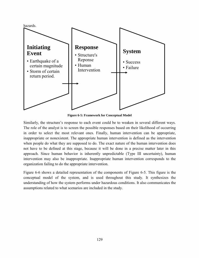
129
hazards.
Figure 6-5: Framework for Conceptual Model
Similarly, the structure’s response to each event could be to weaken in several different ways. The role of the analyst is to screen the possible responses based on their likelihood of occurring in order to select the most relevant ones. Finally, human intervention can be appropriate, inappropriate or nonexistent. The appropriate human intervention is defined as the intervention when people do what they are supposed to do. The exact nature of the human intervention does not have to be defined at this stage, because it will be done in a precise matter later in this approach. Since human behavior is inherently unpredictable (Type III uncertainty), human intervention may also be inappropriate. Inappropriate human intervention corresponds to the organization failing to do the appropriate intervention.
Figure 6-6 shows a detailed representation of the components of Figure 6-5. This figure is the conceptual model of the system, and is used throughout this study. It synthesizes the understanding of how the system performs under hazardous conditions. It also communicates the assumptions related to what scenarios are included in the study.
Initiating Event
• Earthquake of a certain magnitude
• Storm of certain return period.
Response
• Structure's Reponse
• Human Intervention
System • Success • Failure

130
Figure 6-6: Variables and Values in Conceptual Model
The sources for assembling the conceptual model include:
Discussions with operators of the system or experts Literature review studies on the system or on similar systems Judgment to make simplifications
With the conceptual model established as in Figure 6-6, it is possible to study separately the different boxes. Characterizing the different types of initiating events should be done first. The study of the initiating events should determine: (1) the number and nature of the types of initiating events, (2) the annual likelihood of each event occurring, and (3) the characteristics of the events that impact the structure’s response and the human intervention. Though different studies will require different characteristics (item 3), time from the initiating event to the next structure’s response has to be determined in most cases. This duration corresponds to the time before the next structure’s response happens if there is no human intervention. This piece of data is a required entry for the further analyses.
Similarly, the study of the structure’s response should determine: (1) the number and nature of the types of structure’s response, (2) the conditional probability of each response occurring, and (3) the characteristics of the response that impact the structure’s response and the human intervention later in the sequence. The study of the structure’s response requires in general all the appropriate human interventions and structure’s response prior to it to be known.
Finally, the study of the human intervention should determine: (1) the conditional probability of the intervention being ‘appropriate’, ‘inappropriate’ and ‘none’ given prior events, and (2) the characteristics of the response that impact the structure’s response and the human intervention
Intiating Event
• Earthquake of a certain magnitude
• Storm of certain return period
• Extream impact from large ships or explosion
Structure's Response
• Type1 • Type2 • Type3
Human Intervention
• None • Appropriate • Inappropriate
System • Success • Failure

131
later in the sequence. The study of human intervention requires, in general, all the appropriate human interventions and structural responses prior to it to be known.
The study that determines whether or not the system will fail is very similar to the study of the structure’s response. The only difference is that it is imposed on the outcome of the ‘system’ study that the type of structure’s response is either success or failure.
Caution: for consistency, make sure that the conditional probabilities in the ‘structure’s response’ and ‘system’ boxes add up to exactly one. This ensures that all the events are covered and that there is no overlap (i.e. independent).
The study of characterizing ‘initiating events’ and ‘structural responses’ is specific to each system and for that reason is not part of this report. The approach to determine the characteristics of ‘human intervention’, however, is detailed in the later steps.
6.3.2 Sherman Island Conceptual Model Illustration
For the flood protection example on Sherman Island we developed the conceptual model based on the following sequence:
1. Storm forms 2. Flood fighting takes place, or not (human intervention) 3. Problem occurs on the levee, or not (structure’s response) 4. Flood fighting takes place, or not (human intervention) 5. Levee breaches, or not (failure or success)
The storm forming is the event that initiates the scenario (1). Then, human intervention takes place (2) and it leads to a particular response from the levee (3) to which human intervention can react (4). Finally the levee may or may not breach (5), depending what happened during this previous sequence. Figure 6-7 shows the sequence for an extreme event.
The scope of the study, expressed in the system definition step, defined the triggering event to be a storm scenario. Though the flood protection system could also fail due to an earthquake or a terrorist action, this example commences with a storm of three different return intervals as the triggers. The rationale behind the possible values for the initiating event (here 2, 50 and 100-year return period storms) is developed in the hazard characterization appendix (Appendix B). The reason for including three storms is to capture the central tendency and the extremes of the distribution of possible storms. The 2 year storm is a likely event and is not too much of a threat for the levees. The 50 and 100 years storms are less likely and represent a bigger threat for the levees.

132
Figure 6-7: An Event Sequence. Photos courtesy of DWR
It is interesting to notice that most events following the formation of a storm are captured in this sequence. For example, if overtopping or seepage begins and the flood fighting team does not have time to react, that is represented by ‘no flood fighting’ at step (4). Similarly, if RD 341 is not informed that there is a storm coming, that is also represented by ‘no flood fighting’ at step (2). On the other hand, steps (1), (3) and (5) are happening even if there is no failure. Figure 6-8 is our conceptual model based on the method and on the sequence above.
The “integrity indicator” in Figure 6-8 is the “structure’s response” for the Sherman Island situation. It refers to the different mechanisms that may cause failure when water surface elevations are high [DWR, 2003].
At this step in constructing the conceptual model, it is possible to divide the work into the study of the different pieces of the Figure 6-8. “Storm” should determine the characteristics of the 2, 50, and 100 years return period necessary to understand “integrity indicator” and “levee”. Also, it should state how much time there is before an integrity indicator occurs on the levee. In this Sherman Island example, this was done in the “hazard characterization” Appendix B.
“Integrity indicator” should determine the likelihoods of ‘seepage’, ‘overtopping’, ‘slope stability’ and ‘none’ occurring conditional on the nature of the storm and the nature of anticipatory flood fighting. It should also state the time available between the moments when “integrity indicator” starts and when the levee fails. In other words, this duration is a time to failure.
“Anticipatory flood fighting” and “interactive flood fighting” are detailed in subsequent sections.
Storm Flood
Defense Integrity Indicator
Interactive Flood
Fighting
Levee System
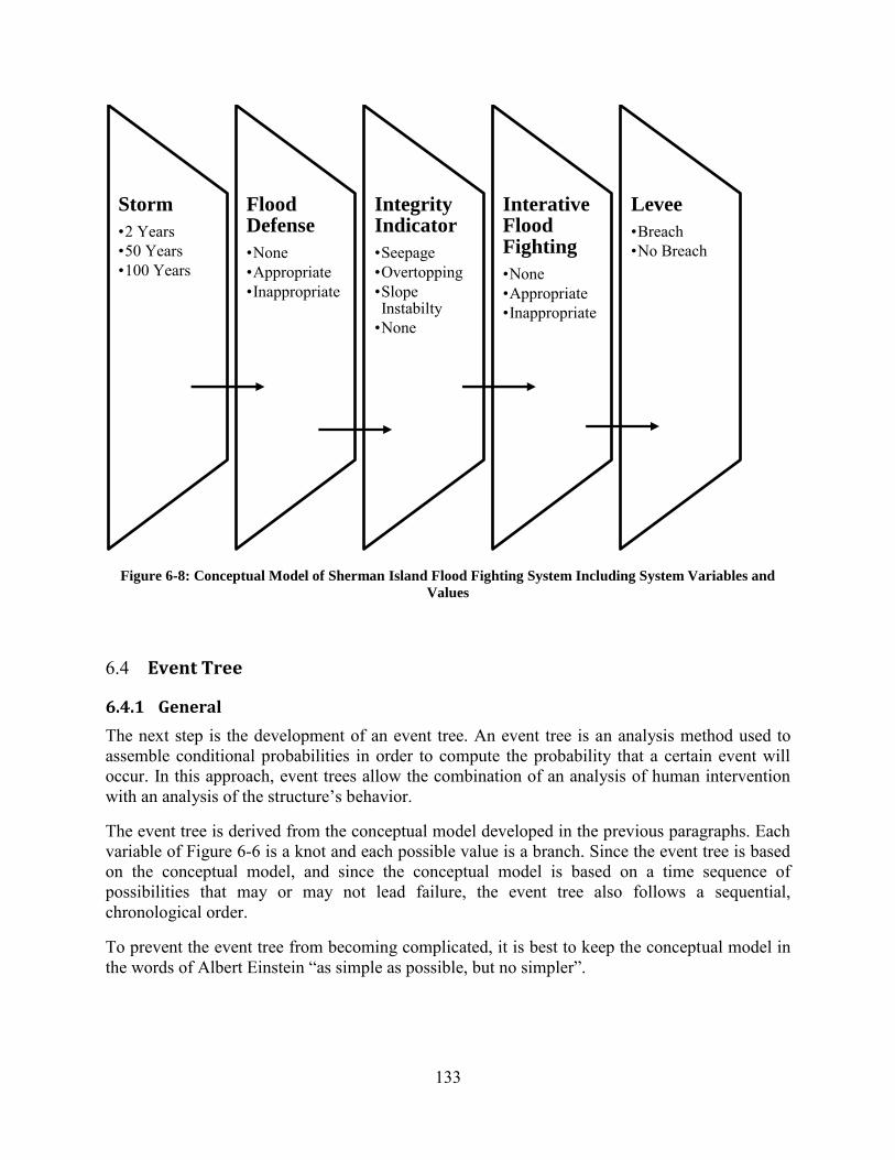
133
Figure 6-8: Conceptual Model of Sherman Island Flood Fighting System Including System Variables and
Values
6.4 Event Tree
6.4.1 General
The next step is the development of an event tree. An event tree is an analysis method used to assemble conditional probabilities in order to compute the probability that a certain event will occur. In this approach, event trees allow the combination of an analysis of human intervention with an analysis of the structure’s behavior.
The event tree is derived from the conceptual model developed in the previous paragraphs. Each variable of Figure 6-6 is a knot and each possible value is a branch. Since the event tree is based on the conceptual model, and since the conceptual model is based on a time sequence of possibilities that may or may not lead failure, the event tree also follows a sequential, chronological order.
To prevent the event tree from becoming complicated, it is best to keep the conceptual model in the words of Albert Einstein “as simple as possible, but no simpler”.
Storm
•2 Years •50 Years •100 Years
Flood Defense
•None •Appropriate •Inappropriate
Integrity Indicator
•Seepage •Overtopping •Slope Instabilty
•None
Interative Flood Fighting
•None •Appropriate •Inappropriate
Levee
•Breach •No Breach

134
6.4.2 Sherman Island Event Tree Illustration
The event tree for the flood protection system on Sherman Island is a system which is applied to analyze all the combinations (and the associated probability of occurrence) of the parameters that affect the system under analysis. In this case, all the analyzed events are linked to each other and all possible states of the system are considered at each node and each state (branch of the event tree) is characterized by a defined value of probability of occurrence. For the flood protection system on Sherman Island, the event tree is Figure 6-9, the sequence in red ink Figure 6-9 corresponds to the following scenario:
“Under a storm with a 50 years return period, slope instability started occurring at a site where no flood fighting had occurred yet. The flood fighting team detected the problem, took the appropriate corrective actions but that didn’t prevent the levee from failing.”
In order to explain how the proposed approach can be applied, it is necessary to take the scheme shown in Figure 6-9 as a reference, where the various probabilities of each branch can be evaluated by means of different approaches.
In this illustration the number of branches to the event tree can be enumerated as:
Nb =3*3*4*3*2 =216 Equation 6-1
Nevertheless, by looking into the details of each variable, some branches can be excluded. For instance, if no problem occurs on the levee, then there will not be interactive flood fighting or a levee breach. In other words, and using the conceptual model, if the value the ‘integrity indicator’ is ‘none,’ then the value of ‘interactive flood fighting’ is ‘none’ and the value of ‘levee’ is ‘no breach’.
Reminder: since ‘levee breach’ and ‘island flooded’ are equivalent in our example because the first statement leads to the second, this event tree captures scenarios that describe failure of the system as they are defined in the system definition. The two are inextricably linked.
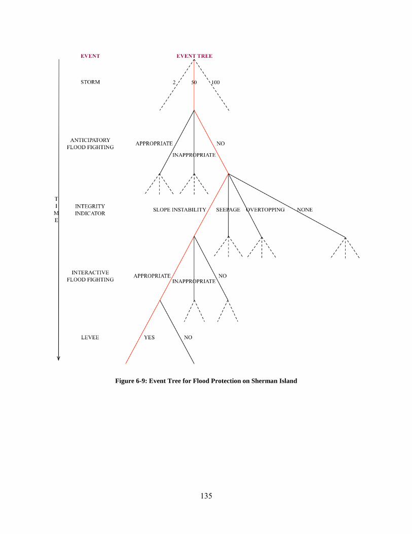
135
Figure 6-9: Event Tree for Flood Protection on Sherman Island
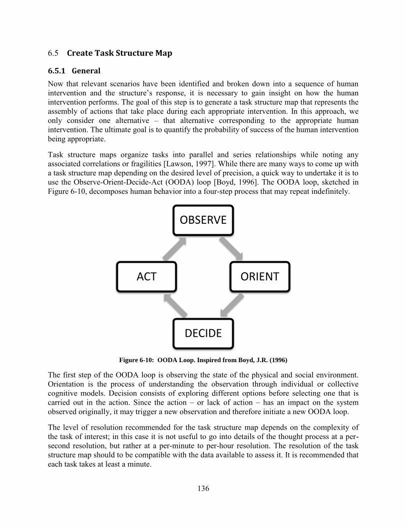
136
6.5 Create Task Structure Map
6.5.1 General
Now that relevant scenarios have been identified and broken down into a sequence of human intervention and the structure’s response, it is necessary to gain insight on how the human intervention performs. The goal of this step is to generate a task structure map that represents the assembly of actions that take place during each appropriate intervention. In this approach, we only consider one alternative – that alternative corresponding to the appropriate human intervention. The ultimate goal is to quantify the probability of success of the human intervention being appropriate.
Task structure maps organize tasks into parallel and series relationships while noting any associated correlations or fragilities [Lawson, 1997]. While there are many ways to come up with a task structure map depending on the desired level of precision, a quick way to undertake it is to use the Observe-Orient-Decide-Act (OODA) loop [Boyd, 1996]. The OODA loop, sketched in Figure 6-10, decomposes human behavior into a four-step process that may repeat indefinitely.
Figure 6-10: OODA Loop. Inspired from Boyd, J.R. (1996)
The first step of the OODA loop is observing the state of the physical and social environment. Orientation is the process of understanding the observation through individual or collective cognitive models. Decision consists of exploring different options before selecting one that is carried out in the action. Since the action – or lack of action – has an impact on the system observed originally, it may trigger a new observation and therefore initiate a new OODA loop.
The level of resolution recommended for the task structure map depends on the complexity of the task of interest; in this case it is not useful to go into details of the thought process at a per-second resolution, but rather at a per-minute to per-hour resolution. The resolution of the task structure map should to be compatible with the data available to assess it. It is recommended that each task takes at least a minute.
OBSERVE
ORIENT
DECIDE
ACT
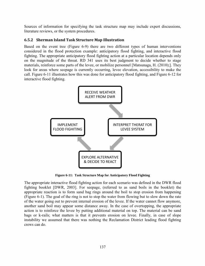
137
Sources of information for specifying the task structure map may include expert discussions, literature reviews, or the system procedures.
6.5.2 Sherman Island Task Structure Map Illustration
Based on the event tree (Figure 6-9) there are two different types of human interventions considered in the flood protection example: anticipatory flood fighting, and interactive flood fighting. The appropriate anticipatory flood fighting action at a particular location depends only on the magnitude of the threat. RD 341 uses its best judgment to decide whether to stage materials, reinforce some parts of the levee, or mobilize personnel [Matsunaga, H. (2010);]. They look for areas where seepage is currently occurring, levee elevation, accessibility to make the call. Figure 6-11 illustrates how this was done for anticipatory flood fighting, and Figure 6-12 for interactive flood fighting.
Figure 6-11: Task Structure Map for Anticipatory Flood Fighting
The appropriate interactive flood fighting action for each scenario was defined in the DWR flood fighting booklet [DWR, 2003]. For seepage, (referred to as sand boils in the booklet) the appropriate reaction is to form sand bag rings around the boil to stop erosion from happening (Figure 6-1). The goal of the ring is not to stop the water from flowing but to slow down the rate of the water going out to prevent internal erosion of the levee. If the water cannot flow anymore, another sand boil may appear some distance away. In the case of overtopping, the appropriate action is to reinforce the levee by putting additional material on top. The material can be sand bags or k-rails; what matters is that it prevents erosion on levee. Finally, in case of slope instability we assumed that there was nothing the Reclamation District leading flood fighting crews can do.
RECEIVE WEATHER ALERT FROM DWR
INTERPRET THERAT FOR LEVEE SYSTEM
EXPLORE ALTERNATIVE & DECIDE TO REACT
IMPLEMENT FLOOD FIGHITING

138
Figure 6-12: Task Structure Map for Interactive Flood Fighting
6.6 Perform QMAS+ Assessment
6.6.1 General
QMAS+ is part of the overall method to help identify human and organizational factors that drive the performance of the system. QMAS+ is an adaptation of the QMAS instrument to the engineered system of concern. Even though it was designed to assess offshore structures, QMAS was intended to be flexible and has been applied to a variety of systems (offshore platforms, tanker loading and discharge terminals, US Navy diving operations and ship operations).
This section outlines the main steps of the QMAS process and explains how to adapt QMAS to a specific system of concern. QMAS is comprised of three components:
1. An assessor qualification protocol and a training program 2. A computer-based instrument and its documentation 3. An assessment process
6.6.1.1 Assessment team
The assessment team is the most important element in the QMAS system. It may be comprised of operators, engineers, managers or regulators. The team members are chosen by the organization being assessed and the criteria for selection are as follows:
Experience with the system Motivation Integrity
PATROL DETECTS INTEGRITY INDICATOR
OPERATOR & ORGANIZATION INTERPRET
THREAT
EXPLORE ALTERNATIVE & DECIDE TO REACT
REINFORCE LEVEE

139
Sensitivity to quality hazards
Experience with the system assures acute knowledge of how the system actually works as opposed to how it is supposed to work. Motivation, integrity and sensitivity to quality hazards ensure that the assessor’s input to QMAS will be useful and complete.
The assessors are trained prior to making the assessment. Training has two parts:
I. Informational Background information on QMAS process and instrument Failures involving offshore structures and other types of engineered structures Human and organizational performance factors
II. Practical exercises Hands-on use of the computer software Cases studies The assessors perform their own assessment
6.6.1.2 Instrument
The instrument component of QMAS is a computer-based tool. It is a web application that guides assessors through the process by raising issues about the operating team, the funding, the environmental conditions etc. The tool automatically records and archives assessors’ responses for future analysis.
6.6.1.3 Assessment process
The assessment process is illustrated in Figure 6-13. The first step is to select the system to study and to select and train the assessors. The first phase of the actual assessment is coarse, and it is done usually in an office (phase 1). Having first been introduced to the system in a controlled environment, the site visit for the assessors are more effective and generally leads to a deeper knowledge of the system (phase 2). Finally the assessment team communicates the results through a summary and a report (phase 3).

140
Figure 6-13: The QMAS process. Inspired from [Hee, 1997]
Throughout the assessment, the assessors grade the system based on a set of criteria referred to as the QMAS ‘data’. The data structure is based on a conception of any engineered system identical to Figure 6-13. The system is made of seven components: the operators, an organization, equipment, structure, environment, procedures and interfaces. Each component is divided into several factors that may also be divided into attributes to best capture the specificity of each component. The data is organized in a pyramid (Figure 6-15), where factors describe the components, and attributes describe the factors.
During Phase 1, the assessment team grades the attributes. More precisely, they grade how well a statement synthesized by the name of the attribute matches the system of concern. They grade all the attributes using the Likert scale [Likert, 1974] with values ranging from one (excellent/best) to seven (very poor/worst) shown in Figure 6-15. In order to capture uncertainty and potential disagreement in the assessment team, the instrument requires entering three grades for each attribute: the best, the worst, and the most likely. For example, when the assessment team focuses on attribute 1.1.2, they will consider the accuracy of the communications within the
Pre-Assessment
Phase
• Select System • Select Assessors
• Train Assessors
Phase 1 (at office)
• Input pre-assessment data into the QMAS instrument • Coarse qualitative evaluation of attributes
• Select Cutoff for Factors of Concern (FOC) • Assessors create scenarios that incorporate the FOCs
Phase 2 (at system)
• Detailed qualitative evaluation of attributes within the context of the scenarios. Data input into the instrument
Phase 3 (at office)
• Assessors write up an overall summery of the assessment • Instrument outputs summery reports of the assessment

141
operating team (Figure 6-14). This means the assessors would agree that the best scenario for accuracy of the communications between operators would be “excellent,” the worst would be “below average,” and the most likely would be “very good.” With this process carried out on the seven components, QMAS brings up all potential flaws of the system.
Figure 6-14: QMAS structure of the data [from Bea, 2002]
COMPONENTS 1-operators,
2-organization, 3-procedures, 4-equipment, 5-structure,
6-environments, 7-interfaces
FACTORS(graded) 1.0-operators
1.1-communicatons, 1.2-selection,1.3-knowledge,
1.4-training, 1.5-skills, 1.6-limitation/impairments,
1.7-organization/coordiantion
ATTRIBUTES (reason for grades) 1.1.0-communicatons
1.1.1-clarity, 1.1.2-accuracy, 1.1.3-freguency, 1.1.4-openess/honesty, 1.1.5-verifying,
1.1.6-encouraging
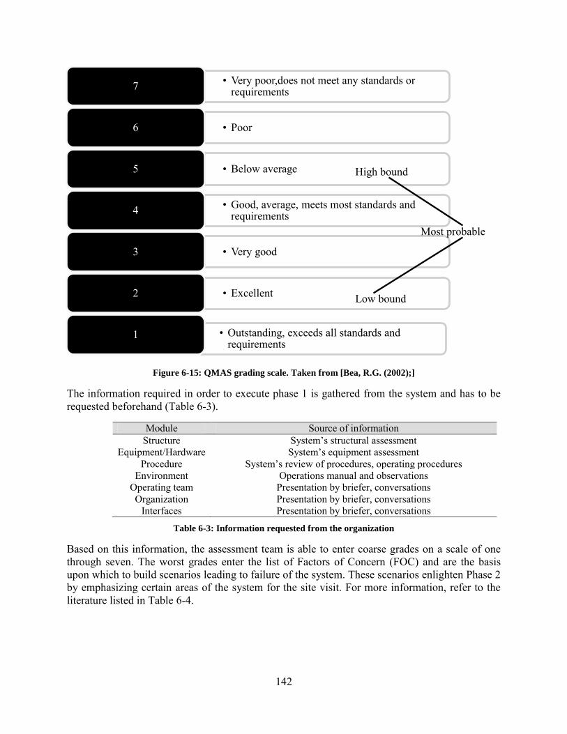
142
Figure 6-15: QMAS grading scale. Taken from [Bea, R.G. (2002);]
The information required in order to execute phase 1 is gathered from the system and has to be requested beforehand (Table 6-3).
Module Source of information Structure System’s structural assessment
Equipment/Hardware System’s equipment assessment Procedure System’s review of procedures, operating procedures
Environment Operations manual and observations Operating team Presentation by briefer, conversations Organization Presentation by briefer, conversations
Interfaces Presentation by briefer, conversations
Table 6-3: Information requested from the organization
Based on this information, the assessment team is able to enter coarse grades on a scale of one through seven. The worst grades enter the list of Factors of Concern (FOC) and are the basis upon which to build scenarios leading to failure of the system. These scenarios enlighten Phase 2 by emphasizing certain areas of the system for the site visit. For more information, refer to the literature listed in Table 6-4.
• Very poor,does not meet any standards or requirements 7
• Poor 6
• Below average 5
• Good, average, meets most standards and requirements 4
• Very good 3
• Excellent 2
• Outstanding, exceeds all standards and requirements
1
High bound
Low bound
Most probable
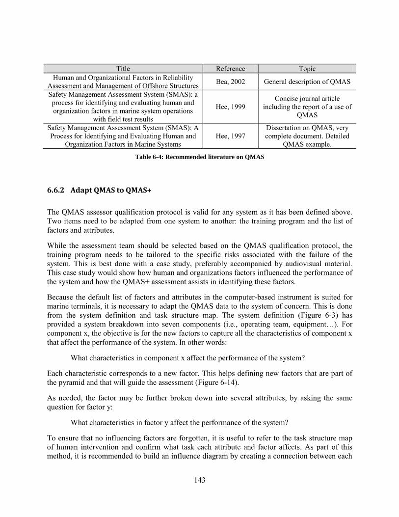
143
Title Reference Topic Human and Organizational Factors in Reliability
Assessment and Management of Offshore Structures Bea, 2002 General description of QMAS
Safety Management Assessment System (SMAS): a process for identifying and evaluating human and organization factors in marine system operations
with field test results
Hee, 1999 Concise journal article
including the report of a use of QMAS
Safety Management Assessment System (SMAS): A Process for Identifying and Evaluating Human and
Organization Factors in Marine Systems Hee, 1997
Dissertation on QMAS, very complete document. Detailed
QMAS example.
Table 6-4: Recommended literature on QMAS
6.6.2 Adapt QMAS to QMAS+
The QMAS assessor qualification protocol is valid for any system as it has been defined above. Two items need to be adapted from one system to another: the training program and the list of factors and attributes.
While the assessment team should be selected based on the QMAS qualification protocol, the training program needs to be tailored to the specific risks associated with the failure of the system. This is best done with a case study, preferably accompanied by audiovisual material. This case study would show how human and organizations factors influenced the performance of the system and how the QMAS+ assessment assists in identifying these factors.
Because the default list of factors and attributes in the computer-based instrument is suited for marine terminals, it is necessary to adapt the QMAS data to the system of concern. This is done from the system definition and task structure map. The system definition (Figure 6-3) has provided a system breakdown into seven components (i.e., operating team, equipment…). For component x, the objective is for the new factors to capture all the characteristics of component x that affect the performance of the system. In other words:
What characteristics in component x affect the performance of the system?
Each characteristic corresponds to a new factor. This helps defining new factors that are part of the pyramid and that will guide the assessment (Figure 6-14).
As needed, the factor may be further broken down into several attributes, by asking the same question for factor y:
What characteristics in factor y affect the performance of the system?
To ensure that no influencing factors are forgotten, it is useful to refer to the task structure map of human intervention and confirm what task each attribute and factor affects. As part of this method, it is recommended to build an influence diagram by creating a connection between each

144
influencing factor and the corresponding task that the factor influences. This clarifies both the task structure maps and the influences taken into account in the QMAS assessment.
It is important have a general approach to the system at this step. One way to do so is to make sure that the QMAS+ tool newly developed could help assessing a system similar but distinct from the system of concern. In fact, all factors that could influence a similar system should be included, not only those that negatively affect the performance. This ensures that the QMAS assessment will (1) accurately reflect the state of the system, (2) inform decision-makers of what is being done will, and (3) identify where system improvements could be made. Refer to the original QMAS attributes for the HOF.
Expert discussions and document review (operating manuals, regulations, standards etc.) provides an excellent basis for building a new set of relevant factors and attributes. The analyst should generate a list of factors and attributes and present it to the assessment team for review prior to the assessment.
6.6.3 Sherman Island QMAS Illustration
6.6.3.1 Assessment Team
While this study did not select members to form a formal assessment team, this research identified individuals who would be appropriate to assess the flood protection system on Sherman Island. The organization in charge of flood protection is Reclamation District (RD) 341 (Figure 6-3). Therefore, the assessment team should be comprised of a flood fighter (system operator) with the requisite background, experience, and character. Also, the assessment team should include someone who has a broader vision of the current flood practices in the Sacramento-San Joaquin Delta. Mr. Sonny Fong meets the criteria for assessor selection based on the exchanges we had with him. He has more than thirty years of experience with flood fighting and management. He has experience as field engineer, as supervisor levee patrol/inspect/repair team, and as emergency manager for DWR [Fong, 2010].
Assessor training should include an example of levee failure in the Delta. The After Action Report from the levee failure on Jones Tract (also in the Delta) in 2004 is a relevant document to increase awareness of assessors with respect to the consequences of a levee failure [DWR, 2004], as it accounts for the events during and after the failure.

145
6.6.3.2 Flood Fighting Factors and Attributes
Creating new factors and attributes for the assessors to grade is the most intricate part of adapting QMAS to flood protection. From discussions and on the flood fighting training, we identified the most important influencing factors on the performance of the flood fighting action. Figure 6-16 is the influence diagram based upon the task structure map and the list of factors and attributes.
Figure 6-16: Factors and Attributes for Interactive Flood Fighting
The inner circle contains the factors, and the outer circle contains the attributes. When a factor doesn’t need to be more clearly defined, then the QMAS web application asks the assessment team to grade the factor directly.
During our discussions, it came up several times that visibility on the levees is crucial for detecting problems. At night, if it is foggy, or if the vegetation has not been properly maintained, patrollers have greater difficulty detecting seepage. So we identified “visibility” as an environmental factor that affects the performance of flood fighting.
A recurring theme at the flood fighting training was the difference between knowing what to do in the case of a sand boil, and actually doing it. This is why experience is such a critical factor for both the operating team and the organization. Experience influences the ability to understand a situation (Orient) and make the appropriate decision (Decide).

146
Another important factor is the availability of material. Sometimes overtopping would warrant immediately raising the levees, but often resources are not available at the critical moment and location due to financial, time, and labor constraints. However, Memorandums of Understanding were identified as tools that could help improve resource availability.
6.6.3.3 Grading of the Attributes
The assessment team grades the attributes. However, as a knowledgeable person in QMAS, risk assessment, and human and organizational factors, the analyst will facilitate the assessment. This facilitator guides the assessors through to the assessment and answers questions relative to the QMAS+ tool. If necessary, the facilitator may need to explain the meaning of an attribute. For this example the exact grading process is illustrated for one attribute: vegetation.
As stated earlier, vegetation is a performance attribute of visibility. The assessment would grade whether vegetation is ‘performance degrading.’ The scale they would use is:
1 - Always taken into consideration 2 - Always enhances performance 3 - Sometimes enhances performance 4 - Adequate for performance 5 - Sometimes hinders performance 6 - Always hinders performance 7 - Not considered
Depending on the assessment team’s knowledge and understanding of the vegetation on Sherman Island, this attribute would ideally capture how the vegetation affects the performance of flood fighting on Sherman Island.
Figure 6-17 was taken at the South Site at Sherman Island. Based on our field visit to the island, the existing vegetation does not block visibility and therefore appears to be adequate for performance. However, vegetation may sometimes hinder performance during some periods of the year (e.g. when it grows in spring, Figure 6-18) or if it is not maintained frequently enough. For this reason, an assessment team may assign the following grades: 3 (low bound), 4 (most likely) and 5 (high bound). There is little uncertainty in the grading because the picture provides detailed information on the state of the vegetation.
A similar process should be used for all of the attributes of concern. In this illustration we did not actually perform the QMAS+ assessment, and we put together the numbers. Table 6-5 summarizes a plausible result of a QMAS+ assessment. This information will be used in the later sections if this report.
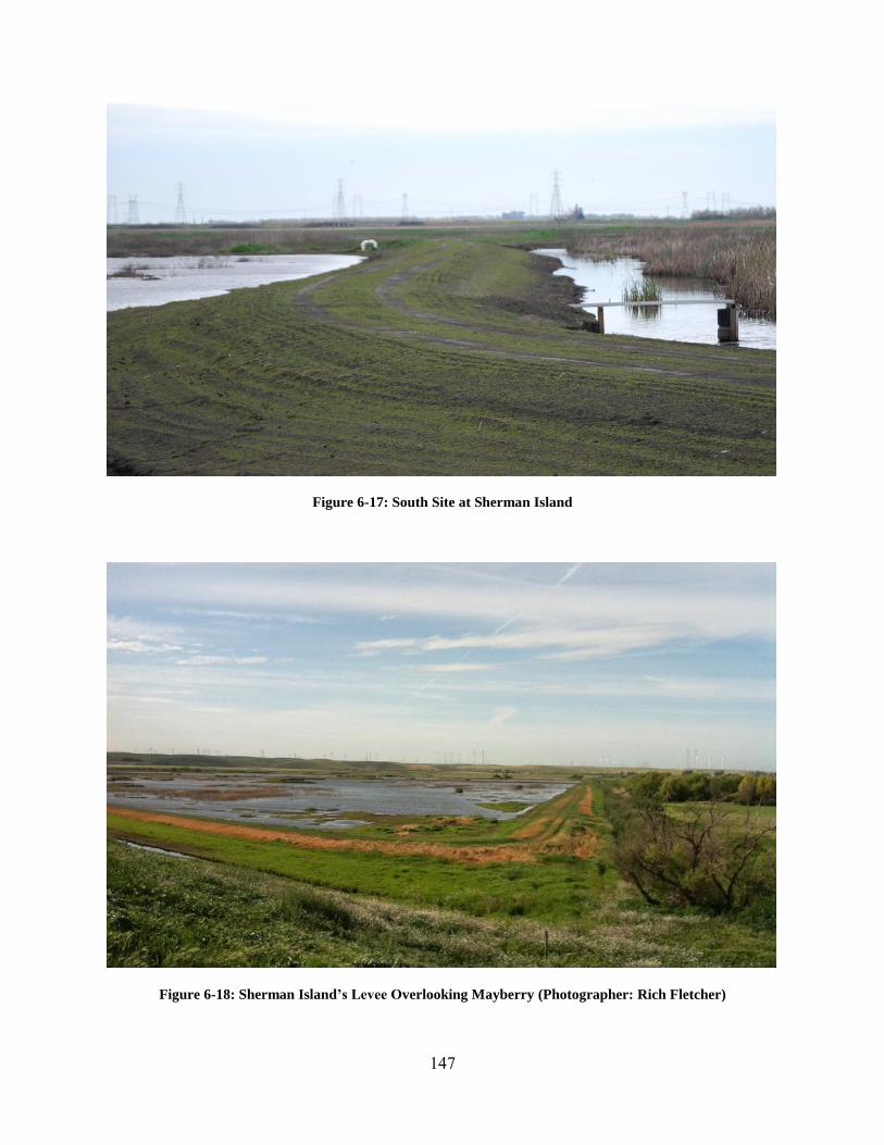
147
Figure 6-17: South Site at Sherman Island
Figure 6-18: Sherman Island’s Le ee Overlooking Mayberry (Photographer: Rich Fletcher)

148
Component Factor Attribute Low bound Most probable High bound
Operators
Education
2 4 5
Training 3 4 4
Experience 4 4 5
Organization
Education 4 4 5
Training 3 4 5
Experience 4 5 6
Communications 4 4 7
Command and control 4 4 4
Procedure Procedures 4 4 5
Equipment Availability Contracts 4 4 5
MOU 3 3 5
Environment Visibility
Fog 3 5 6
Time of day 3 5 6
Vegetation 3 4 5
Interface Access
Barges 4 5 6
Vehicle 3 4 4
Roads 4 5 6
Note: MOU = Memorandum of Understanding. This information is for illustration purposes only and does not represent the result of a field application of the QMAS+ instrument
Table 6-5: QMAS+ Coarse Assessment
For each attribute, we utilized the aforementioned triangular distribution to represent the uncertainty in the grading. The grade of a factor is the average of the mean grades of each associated attribute. The overall grade of a component is the average of the mean grades of the factors that are part of this component.
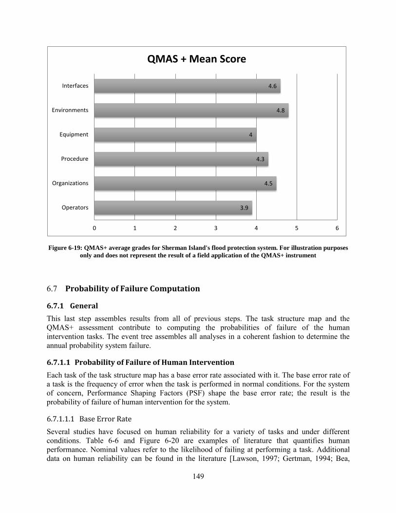
149
Figure 6-19: QMAS+ average grades for Sherman Island's flood protection system. For illustration purposes
only and does not represent the result of a field application of the QMAS+ instrument
6.7 Probability of Failure Computation
6.7.1 General
This last step assembles results from all of previous steps. The task structure map and the QMAS+ assessment contribute to computing the probabilities of failure of the human intervention tasks. The event tree assembles all analyses in a coherent fashion to determine the annual probability system failure.
6.7.1.1 Probability of Failure of Human Intervention
Each task of the task structure map has a base error rate associated with it. The base error rate of a task is the frequency of error when the task is performed in normal conditions. For the system of concern, Performance Shaping Factors (PSF) shape the base error rate; the result is the probability of failure of human intervention for the system.
6.7.1.1.1 Base Error Rate
Several studies have focused on human reliability for a variety of tasks and under different conditions. Table 6-6 and Figure 6-20 are examples of literature that quantifies human performance. Nominal values refer to the likelihood of failing at performing a task. Additional data on human reliability can be found in the literature [Lawson, 1997; Gertman, 1994; Bea,
3.9
4.5
4.3
4
4.8
4.6
0 1 2 3 4 5 6
Operators
Organizations
Procedure
Equipment
Environments
Interfaces
QMAS + Mean Score

150
1997]. Each task of the task map previously developed is assigned a base error rate. The information required to do so is the time available to perform the task, the data on human performance, and the judgment to select the appropriate data.
The time available is a very important piece of information. One hour or ten hours to react before a system failure may radically change the probability of the appropriate action being taken. The time available to react is provided by the study of the physical system prior to human intervention. This should state that the average time before failure will be five hours; this is the time used to determine the stress under which the appropriate response happens.
Individual base error rates are combined depending on the configuration of the task structure map (series, parallel, or mixed). In our example, the task structure map is modeled as a series of tasks.
Nature of activity Data Source Nominal Value Simulated Process
Monitoring Marshall and Owre 0.0190
Simulated process Modeling Verhagen 0.1800
Vigilance Task Lanzetta et al. 0.1500
Mirocircuit inspection Schoonard 0.1500
Check reading dials Dashevsky 0.0800
Simulated process monitoring Verhagen 0.0800
Meter reading Horst et al. 0.0700
Check reading dial Oatman 0.0600
Check reading dials (2) White et al. 0.0250
Check reading dials (3) Mital and Ramanan 0.0600
Simulator control actions Beare et al. 0.0032
Identify correct controls Osborne and Ellingstad 0.0030
Close valve Peters 0.0018
Operate pump Luckas and Hall 0.0010
Align manual valve Luckas and Hall 0.0015
Operate remote valve Luckas and Hall 0.0004
Table 6-6: Human Failure Rates (Source: Gertman, D. I. 1997)

151
Figure 6-20: Nominal Human Performance Task Reliability. (Source: Williams, J.C. 1988)
The probability of a series of N tasks failing relates to the individual probabilities of errors:
n
i
basef EPP1
, )(11 Equation 6-2
Literature provides additional resources on series and parallel systems [Bea, 2006].
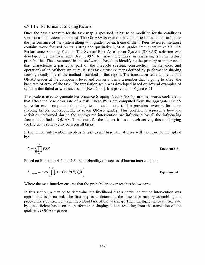
152
6.7.1.1.2 Performance Shaping Factors
Once the base error rate for the task map is specified, it has to be modified for the conditions specific to the system of interest. The QMAS+ assessment has identified factors that influence the performance of the system along with grades for each one of them. Peer-reviewed literature contains work focused on translating the qualitative QMAS grades into quantitative SYRAS Performance Shaping Factors. The System Risk Assessment System (SYRAS) software was developed by Lawson and Bea (1997) to assist engineers in assessing system failure probabilities. The assessment in this software is based on identifying the primary or major tasks that characterize a particular part of the lifecycle (design, construction, maintenance, and operation) of an offshore structure. It uses task structure maps defined by performance shaping factors, exactly like in the method described in this report. The translation scale applies to the QMAS grades at the component level and converts it into a number that is going to affect the base rate of error of the task. The translation scale was developed based on several examples of systems that failed or were successful [Bea, 2000]. It is provided in Figure 6-21.
This scale is used to generate Performance Shaping Factors (PSFs), in other words coefficients that affect the base error rate of a task. These PSFs are computed from the aggregate QMAS score for each component (operating team, equipment…). This provides seven performance shaping factors corresponding to seven QMAS grades. This coefficient represents how the activities performed during the appropriate intervention are influenced by all the influencing factors identified in QMAS. To account for the impact it has on each activity this multiplying coefficient is split evenly between all tasks.
If the human intervention involves N tasks, each base rate of error will therefore be multiplied by:
N
i
iPSFC
7
1
Equation 6-3
Based on Equations 4-2 and 4-3, the probability of success of human intervention is:
0,)(1max1
N
i
isuccess EPCP Equation 6-4
Where the max function ensures that the probability never reaches below zero.
In this section, a method to determine the likelihood that a particular human intervention was appropriate is discussed. The first step is to determine the base error rate by assembling the probabilities of error for each individual task of the task map. Then, multiply the base error rate by a coefficient based on the performance shaping factors resulting from the translation of the qualitative QMAS+ grades.

153
Figure 6-21: QMAS Qualitative Scale Translation into Performance Shaping Factors. (Source: Bea, 2000)
6.7.1.1.3 Probabilities of ‘appropriate’, ‘inappropriate’, and ‘no human intervention’
It is also necessary to determine the likelihoods of human intervention being ‘inappropriate’ or ‘none’. This is done by distinguishing whether or not the system’s response was detected (the first step of the OODA loop). If the system’s response is detected, but people make a mistake in the subsequent tasks, then the human intervention is considered ‘inappropriate’. On the other hand, if the system’s response is not detected, then the human intervention is ‘none’. The distinction between ‘none’ and ‘inappropriate’ is useful because the ways to manage a team to improve its detection of the hazard is different than to improve its ability to perform the appropriate action. In other words the measures to improve the system are different whether the hazard is mostly undetected or whether it is mostly inappropriately fought.
This study provides the mathematical treatment in case of a linear sequence of four steps initiated by the detection activity (one run through the OODA loop – Figure 6-10).
Let Ti be the event ‘Task i completed successfully’. Figure 6-22 shows to which events correspond the ‘appropriate’, ‘inappropriate’ and ‘none’ human interventions.
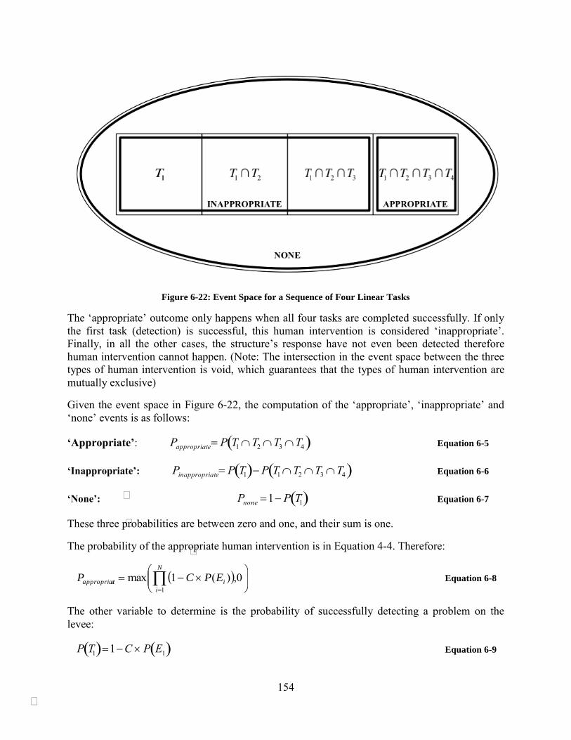
154
Figure 6-22: Event Space for a Sequence of Four Linear Tasks
The ‘appropriate’ outcome only happens when all four tasks are completed successfully. If only the first task (detection) is successful, this human intervention is considered ‘inappropriate’. Finally, in all the other cases, the structure’s response have not even been detected therefore human intervention cannot happen. (Note: The intersection in the event space between the three types of human intervention is void, which guarantees that the types of human intervention are mutually exclusive)
Given the event space in Figure 6-22, the computation of the ‘appropriate’, ‘inappropriate’ and ‘none’ events is as follows:
‘Appropriate’:
Pappropriate P T1T2T3T4 Equation 6-5
‘Inappropriate’:
Pinappropriate P T1 P T1T2T3T4 Equation 6-6
‘None’:
Pnone 1P T1 Equation 6-7
These three probabilities are between zero and one, and their sum is one.
The probability of the appropriate human intervention is in Equation 4-4. Therefore:
0,)(1max1
N
i
ieappropriat EPCP Equation 6-8
The other variable to determine is the probability of successfully detecting a problem on the levee:
P T1 1C P E1 Equation 6-9
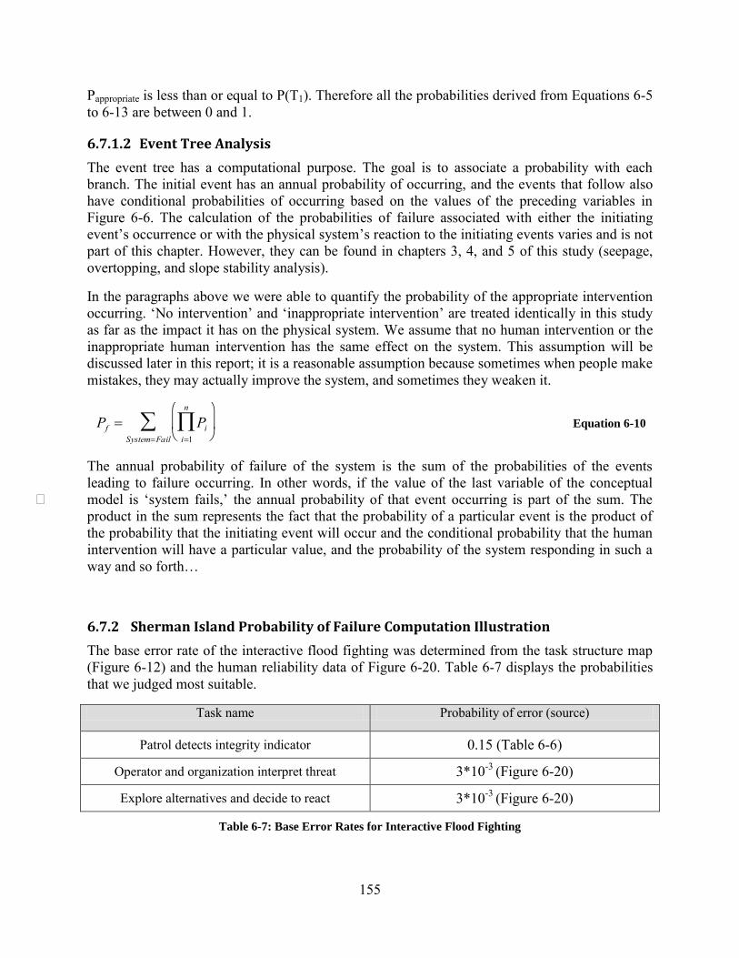
155
Pappropriate is less than or equal to P(T1). Therefore all the probabilities derived from Equations 6-5 to 6-13 are between 0 and 1.
6.7.1.2 Event Tree Analysis
The event tree has a computational purpose. The goal is to associate a probability with each branch. The initial event has an annual probability of occurring, and the events that follow also have conditional probabilities of occurring based on the values of the preceding variables in Figure 6-6. The calculation of the probabilities of failure associated with either the initiating event’s occurrence or with the physical system’s reaction to the initiating events varies and is not part of this chapter. However, they can be found in chapters 3, 4, and 5 of this study (seepage, overtopping, and slope stability analysis).
In the paragraphs above we were able to quantify the probability of the appropriate intervention occurring. ‘No intervention’ and ‘inappropriate intervention’ are treated identically in this study as far as the impact it has on the physical system. We assume that no human intervention or the inappropriate human intervention has the same effect on the system. This assumption will be discussed later in this report; it is a reasonable assumption because sometimes when people make mistakes, they may actually improve the system, and sometimes they weaken it.
Pf Pii1
n
SystemFail
Equation 6-10
The annual probability of failure of the system is the sum of the probabilities of the events leading to failure occurring. In other words, if the value of the last variable of the conceptual model is ‘system fails,’ the annual probability of that event occurring is part of the sum. The product in the sum represents the fact that the probability of a particular event is the product of the probability that the initiating event will occur and the conditional probability that the human intervention will have a particular value, and the probability of the system responding in such a way and so forth…
6.7.2 Sherman Island Probability of Failure Computation Illustration
The base error rate of the interactive flood fighting was determined from the task structure map (Figure 6-12) and the human reliability data of Figure 6-20. Table 6-7 displays the probabilities that we judged most suitable.
Task name Probability of error (source)
Patrol detects integrity indicator 0.15 (Table 6-6)
Operator and organization interpret threat 3*10-3 (Figure 6-20)
Explore alternatives and decide to react 3*10-3 (Figure 6-20)
Table 6-7: Base Error Rates for Interactive Flood Fighting

156
To select the likelihoods of error we assumed that the time to failure was 48 hours. The rationale behind this duration is explained in the seepage, overtopping and slope stability analysis chapters of this study. We had very little insight on the durations associated with each activity, in particular the detection one. This is a limitation of this method.
Naturally, the detection activity is the one most likely to fail. It has 15% chance of failing according to Table 6-6. The other activities are tasks performed with training, and procedure. Based on Equation 6-1, the base error rate for interactive flood fighting is:
1Pf , base 10.15 1 3103 1 3103 15 104 Equation 6-11
Hence:
Pf , base 1 10.15 1 3103 1 3103 15 104 0.16 Equation 6-12
This assumes that there is no correlation between the tasks. This assumption is reasonable because correlation would mean that the magnitude of the value of one task (success or failure) is related to the magnitude of the value of another task, or – if one task is successful, then the other is also successful. In the list of tasks, it seems reasonable that the success of one task does not necessarily presume the success of another task, and therefore they are not correlated.
With the results of the QMAS+ assessment assembled in Table 6-5, we took the average of the total scores to get the scores at the component level. Then we used the translation scale to ascertain the PSFs. Table 6-8 synthesizes the results of our calculations.
System Components Operators Organizations Procedure Equipment Environments Interfaces
QMAS Mean Score 3.9 4.5 4.3 4 4.8 4.6
PSF 0.8 2.9 2.2 1 6 3.6
Table 6-8: Results from QMAS+ and SYRAS PSF
Therefore we can modify the base error rate for interactive flood fighting by multiplying the result by the overall PSF (100).
C 1004 3.2 Equation 6-13
In the end, for the flood fighting illustration the probability of success of interactive flood fighting is:
Pappropriatemax 1 3.2 .15 1 3.2 .003 1 3.2 .003 1 3.2 .0005 , 0 0.5Equation 6-14
For the flood protection example in Sherman Island, our computations lead to the conclusion that interactive flood fighting has a 0.5 probability of being successful. Using equations 6-5, 6-6, and 6-7. We also found:
Pinappropriate 1 3.2 .15 0.5 .01 Equation 6-15

157
Pnone 1 1 3.2 .15 .49 Equation 6-16
It is important to note that in the illustration, interactive flood fighting is not specific to a particular type of problem detected on the levee. To refine this illustration, it would be useful to study the nature of human intervention with respect to each failure mechanism – seepage, slope instability or overtopping. Detecting overtopping, for example, is straightforward because one can see when water spills or splashes over the top of the levee. Slope instability on the other hand may only appear through cracks that can be difficult to detect. There is room for additional refinement in this approach, and if time is available virtually all the steps of the method can be improved. Methodological improvements are discussed in the end of this report.
Integrating the structural analysis and the human analysis is the very last part of the method. In the event tree (Figure 6-9), simply associate each branch with its conditional likelihood. Figure 6-23 illustrates how this method assembles the annual probability of the initiating event with the conditional probabilities of the structure’s response and human intervention.
All the events that lead to failure are in bold in Figure 6-23. In this example, the probabilities for ‘integrity indicator’ and ‘levee’ can be found in the ‘seepage and slope stability analysis’ appendix of this report.
According to the figures above, the annual probability of the flood protection system failing given human intervention during a hundred year storm and due to seepage is:
Pf 06 106 3104 3104 Equation 6-17
On the other hand, when there is no human intervention the event tree is as illustrated in Figure 6-24. According to this, the annual probability of the flood protection system failing given no human intervention during a hundred year storm and due to seepage is:
Pf 6 104
Equation 6-18
An interesting point to notice in this example is that the scenario that controls the likelihood of failure in this example is when there is no human intervention. The system should focus on improving its detection capabilities to decrease its probability of failure.
Figure 6-23: Annual Probability for Seepage Events Under a 100 Year Storm, with Human Intervention
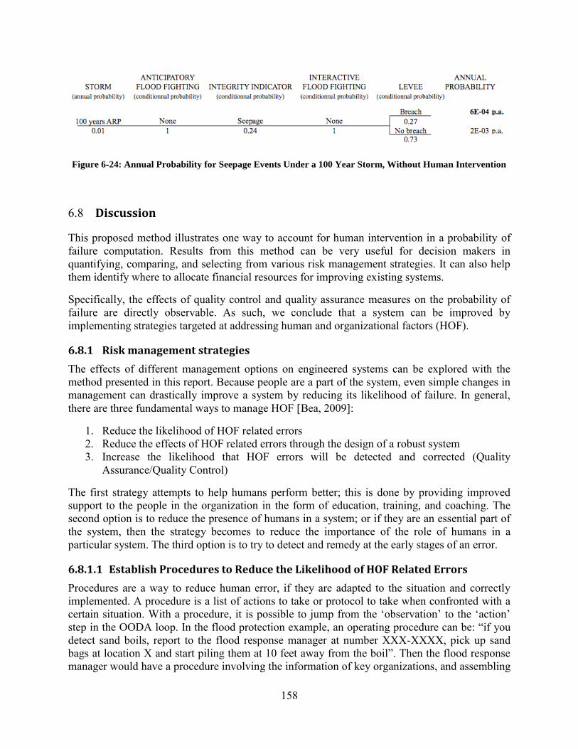
158
Figure 6-24: Annual Probability for Seepage Events Under a 100 Year Storm, Without Human Intervention
6.8 Discussion
This proposed method illustrates one way to account for human intervention in a probability of failure computation. Results from this method can be very useful for decision makers in quantifying, comparing, and selecting from various risk management strategies. It can also help them identify where to allocate financial resources for improving existing systems.
Specifically, the effects of quality control and quality assurance measures on the probability of failure are directly observable. As such, we conclude that a system can be improved by implementing strategies targeted at addressing human and organizational factors (HOF).
6.8.1 Risk management strategies
The effects of different management options on engineered systems can be explored with the method presented in this report. Because people are a part of the system, even simple changes in management can drastically improve a system by reducing its likelihood of failure. In general, there are three fundamental ways to manage HOF [Bea, 2009]:
1. Reduce the likelihood of HOF related errors 2. Reduce the effects of HOF related errors through the design of a robust system 3. Increase the likelihood that HOF errors will be detected and corrected (Quality
Assurance/Quality Control)
The first strategy attempts to help humans perform better; this is done by providing improved support to the people in the organization in the form of education, training, and coaching. The second option is to reduce the presence of humans in a system; or if they are an essential part of the system, then the strategy becomes to reduce the importance of the role of humans in a particular system. The third option is to try to detect and remedy at the early stages of an error.
6.8.1.1 Establish Procedures to Reduce the Likelihood of HOF Related Errors
Procedures are a way to reduce human error, if they are adapted to the situation and correctly implemented. A procedure is a list of actions to take or protocol to take when confronted with a certain situation. With a procedure, it is possible to jump from the ‘observation’ to the ‘action’ step in the OODA loop. In the flood protection example, an operating procedure can be: “if you detect sand boils, report to the flood response manager at number XXX-XXXX, pick up sand bags at location X and start piling them at 10 feet away from the boil”. Then the flood response manager would have a procedure involving the information of key organizations, and assembling
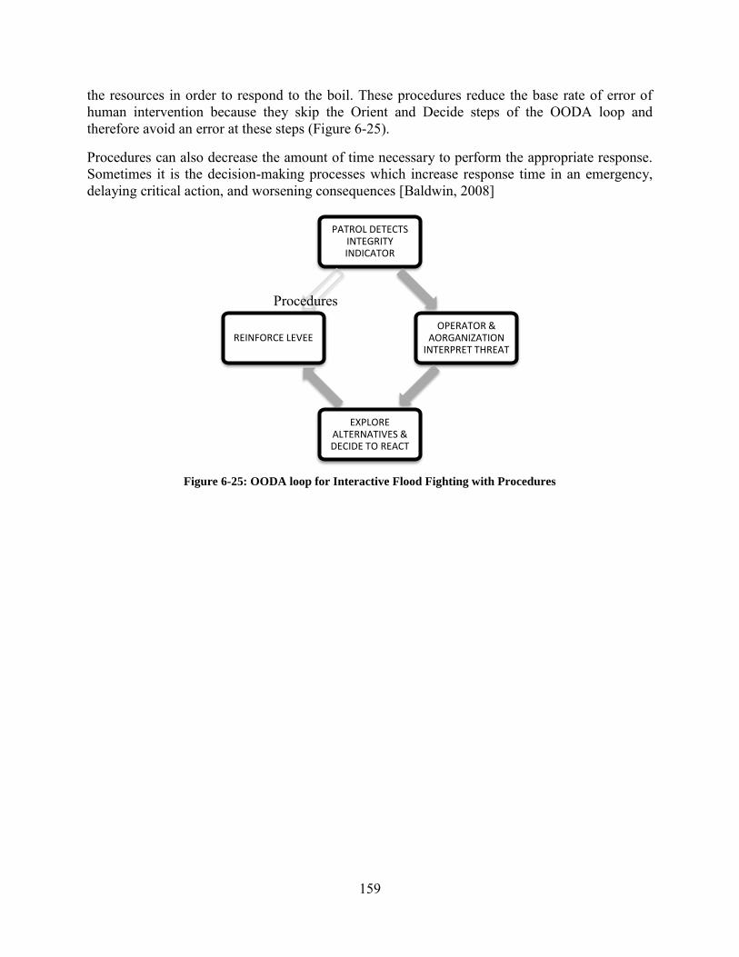
159
the resources in order to respond to the boil. These procedures reduce the base rate of error of human intervention because they skip the Orient and Decide steps of the OODA loop and therefore avoid an error at these steps (Figure 6-25).
Procedures can also decrease the amount of time necessary to perform the appropriate response. Sometimes it is the decision-making processes which increase response time in an emergency, delaying critical action, and worsening consequences [Baldwin, 2008]
Figure 6-25: OODA loop for Interactive Flood Fighting with Procedures
PATROL DETECTS INTEGRITY INDICATOR
OPERATOR & AORGANIZATION
INTERPRET THREAT
EXPLORE ALTERNATIVES & DECIDE TO REACT
REINFORCE LEVEE
Procedures

160
6.8.1.2 Improve the Performance of the Organization and Operating Team to Reduce Likelihood of HOF Related Errors
Another way to improve the system is to improve the performance of the organization and the operating team itself. The QMAS tool identifies ‘factors of concern’ and possible remediation measures. In the probability of failure computation, the organization and operating team’s performance intervenes when the base error rate is shaped by Performance Shaping Factors (PSF). The logarithmic scale that translate QMAS+ scores into PSFs highlights the importance of having a team that performs at least at the current standards. (Table 6-8)
With respect to the Sherman Island flood protection system, we identified experience, training, and education of both the operating team and the organization as elements that influenced the performance of flood fighting. High QMAS+ assessment scores of these elements for RD341 would drastically reduce the probability of failure of the system. For example, someone with flood fighting experience is more likely to know where to look for a sand boil. Additionally, he or she would be able to interpret the overall threat with better judgment than someone less experienced. Similarly, for those without direct experience, education can provide a basis for a more thorough understanding of what might occur during an emergency.
6.8.1.3 Implement Quality Assurance/Quality Control to Increase Likelihood that HOF Related Errors will be Detected and Corrected
Quality assurance and quality control (QA/QC) are measurements aimed at ensuring that a given system will perform at the desired level of quality. QA/QC is the activity of preventing, controlling, inspecting, and testing, detecting errors. In the flood protection example, one QA/QC measure would be to have people inspect the Reclamation District to make sure they have appropriate resources, procedure, etc... Another QA/QC measure would be to make sure to have someone on site when there is flood fighting simply to make sure that everything is done properly. This person is not active apparently, but simply monitoring the situation. This improves the likelihood of detecting an error. In the event space, this translates as shown in Figure 6-26.
The shaded area represents the sequence of events that started with detection and that, without QA/QC, would have been inappropriate intervention. However the team was able to detect, assess and correct the error, and therefore ended up responding appropriately. Mathematically, QA/QC increases the probability of the human intervention being appropriate:
PappropriateQA /QC PappropriatePinappropriate P D P A P C Equation 6-19
Where
Pappropriate and
Pinappropriate correspond to the probability of the human intervention being respectively ‘appropriate’ and ‘inappropriate’;
P D ,
P A ,
P C correspond to the likelihood of the detection, assessment and correction of the QA/QC to be successful.
By explicitly accounting for human intervention, the method described in this report accentuates the fact that the flood protection system can be improved not only by reinforcing the levee structure but also by improving the organization responsible for managing the flood protection system.

161
Figure 6-26: Event Space with QA/QC
6.8.2 Method Limitations and Proposed Refinements
While this method has opened a path for integrating structures and HOF into a single probabilistic model, like any method, it has constraints. We have identified here limitations to the method and recommend refinements and future work.
6.8.2.1 Translation from Qualitative to Quantitative Results
An essential step of the proposed method is to translate qualitative grades from the QMAS+ assessment into quantitative grades (performance shaping factors, Figure 6-21) in order to reflect how QMAS+ attributes affect the probability of failure of the system.
Bea (2000b) calibrated the QMAS qualitative scale to the SYRAS quantitative scale by using several reference cases utilizing the original set of attributes and factors [Bea, R.G. (2000);]. The scale’s relevance was demonstrated by applying QMAS to five cases of offshore structures that failed or succeeded. An evaluation of the QMAS grades for each case was carried out, to verify that the probability of failure was of either unity (1) for the cases of failure or close to zero (0). This method of calibration exposes two weaknesses.
Calibration of the scale ensures sense making but is not sufficient to validate the center of the translation scale and it’s rapidity of increase. To prove that the scale is valid, it necessary to show that it is supported by objective truth or generally accepted authority, and based on flawless reasoning [Campbell, 1963]. This requires proving that the scale also matches systems that have a likelihood of failure between zero and one. For example, right now a QMAS average grade of five translates into a PSF of ten (Figure 6-21). Therefore a system that performs overall worse than average has a high probability of failure. But we would get the same results with a QMAS grade of 5 that translates into a PSF of one hundred. The current calibration method doesn’t justify why the chosen scale is better than the one in which five translates into one hundred.

162
Another point of concern is whether it is accurate to have an exponential scale. For an increase of one on the QMAS grade, the PSF is multiplied by ten. Why is it not linear? Finally, for the same reason the center of the scale (QMAS grade that translates into a PSF of one) cannot be certain.
Secondly, a calibration should be done every time the set of factors and attributes are changed to match a different system. The calibration depends upon the nature of the attributes and the nature of the system of concern. Further, if the attributes are not equally accounting for factors that can both improve and worsen the system, the QMAS+ grade that translate into a PSF of one may not be four. Calibration can be done similar to the way in which it was done for the original instrument [Bea, 2000]. It is best to find systems comparable to the one in question, and then look at them across a variety of successes and failures. For the flood fighting example this means finding documented examples of flood fighting that preventing flooding from happening, and flood fighting that failed. Then, apply the method described in this report to determine whether the scale still accurately anticipates failure or success of flood protection systems.
6.8.2.2 Base Error Rate
The selection of the base error rate for the task structure maps is a step of the method that is both crucial and difficult. First, data across different tables may have been gathered under different conditions that are not explicitly included in the summary table. It is critical that these assumptions are made clear in order to appropriately select the task. Additionally, time is an underlying influence of the base error rate that is hard to explicitly and rigorously include, as discussed in section 6.8.1.1.1. A way to better account for the time available in the analysis would be to gain more insight on the duration of the tasks of the appropriate human intervention.
6.8.2.3 Performance Shaping Factors Weighting
The Performance Shaping Factors (PSF) intervenes in the probability of failure computation by shaping the likelihoods of the human intervention being appropriate. The higher the PSF would be, the lower the likelihood of the appropriate intervention. However, the method is not currently refined because all the influencing factors have the same influence (there is no weighting of the factors) and they influence equally all the tasks of the OODA loop.
Figure 6-16 illustrates how all the QMAS+ factors and attributes related to the tasks of the appropriate human intervention. Some factors, for example the operators’ experience with flood fighting, influence all activities in the OODA loop. Others, for example the availability of material, influence only one activity (here, the action task of the OODA loop). It would be natural to give more importance to influencing factors in relation with how many tasks they impact. However, currently all the factors are given the same weight, no matter how important they are.
One way to remedy this could be to be more specific about what factors influence each task and, for the probability of error computation, account for those influencing factors only. For example, the assessment team could determine the exhaustive set of factors that influence the detection activity of interactive flood fighting. In Figure 6-16, the factors visibility, operators’ training and education, and operators’ experience point directly to the task ‘patrol detects integrity indicator’. Then, the average QMAS score of these factors could translate into a PSF to shape the probability of error.
163
6.8.3 Integrating Human Intervention in Risk Assessment and Management and to Refine the Sherman Island
We recommend the following steps to refine the proposed method for integrating human intervention in risk assessment and management and to refine the Sherman Island illustration used in the study.
1. Select and train assessors to actually run through a QMAS+ assessment of the flood protection system on Sherman Island. Assessors are very knowledgeable on the system and can provide useful results.
2. Run actual experiments to determine the bias introduced by our modeling of human intervention. Compare the anticipated probability of failure with the one observed.
3. Validate the translation scale in Figure 6-21, from QMAS to SYRAS. In particular, explore for which engineered systems it is most appropriate.

164
7 ASSESSMENT OF CONSEQUENCES OF FAILURE
7.1 Introduction
Sherman Island Levee system is exposed to both natural and human-induced risks, and while the risk can never be eliminated, the engineer's task is to reduce the risk to levels that are acceptable or tolerable. Coordinated, local/federal, and multi-disciplinary efforts are required to develop effective to reduce the risk to levels that are acceptable or tolerable for Sherman Island levee system. As a result, risk management is effectively decision-making under uncertainty. Risk is conventionally defined as the possibility of loss or injury. There are two important elements in this definition for the purpose Sherman Island Levee System risk assessment:
1. Possibility of loss 2. Injury
The element of possibility introduces the concept of uncertainty which is important to recognize that there are different types of uncertainties that determine the resultant uncertainties associated with demands and capacities. Failures in a levee system can develop from Intrinsic or Extrinsic uncertainties. For the purpose of this research, we have categorized uncertainties into four categories:
1. Natural or inherent variability (Intrinsic). 2. Engineering analytical model and parametric (Intrinsic). 3. Human and organizational performance (Extrinsic). 4. Information development, knowledge understanding uncertainties (Extrinsic). [Bea
(2006)]
The element of injury introduces the concept of consequences that could develop from an action or activity. This potential ‘consequences’ associated with a levee failure is important. It is at this point that the very sensitive and difficult issues associated with potential environmental impacts must be addressed including potential human impacts as result of Sherman Island Levee failure (injuries, fatalities). Figure 7-1 shows schematics of risk assessment for Sherman island levee failure as a result of seepage, over-topping, and slope stability mechanism. This approach defines risk as a set of scenarios, each of which has a probability failure and a consequence failure. It is important to understand that this analysis is considering a full set of uncertainties since the system and its associating hazard is something that it is not known definitely. In general two main types of uncertainty (Type I and II uncertainty) considered in order to calculate likelihood of failure for the Sherman island levee system.
However, in many contexts knowing the accurate likelihood of failure and its associating consequences cannot solve the issue. A multi-disciplinary approach is heavily underlined by all organizations working in this field. A deciding factor on whether an extreme event turns into a disaster is the social vulnerability of the population at risk, i.e. the capacity to prepare for, respond to and recover from the extreme event. Policy-makers and affected parties are recognizing that traditional expert-based decision-making processes are insufficient in controversial risk contexts.

165
This section describes the approaches taken to estimate the economic consequences of lost use of facilities and resources caused by Sherman island levee failure. Moreover, this section will summarize the annual probability of failure of Sherman Island Levee system which would result that Cfs and finalizing the risk analysis for the system.
Figure 7-1: Risk Assessment Schematics
7.2 Consequence of Sherman Island Levee Failure
Many factors complicate the consequence of failure analysis. Urbanization and changes in demography are increasing the exposure of vulnerable population. Climate change is altering the geographic distribution, frequency and intensity of hydro-meteorological hazards and threatens to undermine the resilience of vulnerable flood defense system and peoples who absorb loss and recover from disaster impacts.
The levees in the Sherman Island protect number of residences and their living places, business space, public buildings, agricultural, local assets, non-local assets, and recreational services in the island and beyond (natural gas pipeline from Canada). Moreover, failure of these flood protection systems will cause the failure of water, electricity, and natural gas, petroleum, and transportation services to the entire state of California (Figure 7-2). Consequences of Sherman Island levee failure due to seepage, over-topping, and slope stability were analyzed base on comprehension with Delta Risk Management Strategy (DRMS) study. The DRMS report provides detailed descriptions of types of failures possible and economic consequences of such failures.
Risk
Annual Probability of
Levee Failure Pf
Slope Stability Overtopping Seepage
Consequence of Failure Cf
Sherman Island Infrastructures &
Residents

166
Figure 7-2: Consequences of Sherman Island levee failure
Consequences of Sherman Island levee failure (breach) as a result of seepage, over-topping, and slope stability for local and non-local assets described briefly below.
7.2.1 Loss of Life
It is not the concern of this thesis to estimate the loss of human life within the context of (quantitative) risk assessment, with a focus on applications to the field of flood protection. However, the subject of loss of human life is the most important section of levee failure consequences estimation. The scarcely available information regarding loss of life in historical floods has been evaluated by different researchers [Jonkman et al., 2003, Walker et al., 1994]. Analysis of global data on natural disasters shows that the impacts of floods on a global scale are enormous. Coastal and river floods that affect low elevation areas protected by flood defenses can cause many fatalities.
The loss of life because of flooding is affected by the number of people that are present in the flooded area, the flood conditions, and the extent to which these flood conditions result in loss of life. The factors are represented in Equation 7-1 (Jonkman et al. 2009), and this is used for analyses
Consequences of Levee Failure
Water Quality
State Highways &
Bridges
Loss of life or Injury
Transmission Lines &
Natural Gas Pipeline
Ecosystem

167
N = FD (h) (1-FE) NPAR (h) Equation 7-1
Where N is the number of fatalities, FD is the mortality fraction, FE is the fraction of the population that evacuates to a safe location, NPAR is the number of people at risk in the area affected by flooding and h is a measure of flood conditions, such as flood depth and flow velocity
Because flood risk depends on uncertain conditions, including water level and evacuation fraction, this study focuses on bandwidths for the elements in Equation 7-1. As an implication, the estimates of consequences and risk levels are presented as ranges. Especially in the Sherman Island, where the whole island is below mean sea level or the high water levels in the rivers, floods can have disastrous consequences.
In terms of NPAR, base on to the 2000 census approximately 233 people live on Sherman Island with 110 dwelling units. Majority Sherman Island‘s population residing in a small residential area along the Sacramento River.
Because no specific information was available regarding the differences in evacuation effectiveness at various locations in the Sherman Island, constant evacuation fractions have been assumed for all locations within the system. Because of noncompliance to warnings, a full evacuation (100%) will never be achieved (Jonkman 2007). For the flood scenario an evacuation fraction between 50 and 90% is assumed, which is consistent with the 80% evacuation effectiveness from the DRMS (URS 2009b). A similar evacuation fraction was observed in New Orleans prior to Hurricane Katrina (Wolshon et al. 2006). Sunny-day and seismic failures are typically characterized by unexpected levee breaches. It is therefore expected that the evacuation fraction will be low, and a range of 0–20% has been adopted.
Based on observed mortality near breaches in New Orleans, an additional criterion has been defined to account for the loss of life in high-velocity flood zones, that is, mostly near breaches. When the combination of flood depth [d (m)] which is about 10 -15ft (3 – 5m) in this site and flow velocity [v (m/s)] is larger than dv=5 m2/s, the mortality rate will be approximately between 0.02 and 0.056. There is a necessity to add a “penalty” for cold-water in this location a factor 2; this will change the mortality fraction (FD) to 0.04 and 0.112.
The existing models for loss of life, estimate a number of fatalities between 10 to 25 for Sherman Island in case of Levee failure In general there is limited insight in the consequences of accidents. Especially loss of life estimates is uncertain, while loss of life is a very important factor in risk evaluation and decision-making. In addition, the general principles of life estimation methods and their application to risk quantification require further attention in the following areas:
1. Variety of factors involved in estimating loss of life 2. Complexity of underlying processes 3. Improvement of existing models in different sectors (mainly on numerical risk
calculations). 4. Analysis of possible consequences for the different scenarios which result in loss of life.
168
In addition, these is a lot of discussion in literature about how risk estimates can be properly adjusted for loss of human life [see e.g. Bennet, (1970); Vrijling et al. (1998); Evans and Verlander, (1997); Rackwitz, (2002); Pandey and Nathwani, (2004); Bedford, (2005)].
7.2.2 Water Quality
The security of water resources in the Sacramento-San Joaquin Delta, upon which over 23 million Californians rely on for freshwater, is under severe threat. The levee systems that were built to protect the numerous islands that were reclaimed from the wetlands during the California Gold Rush of the late 1800s are vulnerable to seepage, flooding and earthquake induced failures. It is the latter of these that poses the greatest hazard to the Delta [Seed et al., (2006)]. Sherman Island levees provide high water quality and water supply for cities and farms in the San Francisco Bay area, San Joaquin Valley, and Southern California. Sherman Island is located where fresh river waters (Sacramento River, and San Joaquin River) and salty bay water meet and mix. As a result, Sherman Island levees are critical in controlling salinity intrusion to the Sacramento Delta. If one of the levees breaks the saline bay water moves further upstream, mixing with the fresh water.
Freshwater inflows used by upstream dams, water canals, the farms, and cities in bay area and southern California. There is a balance exist between the Delta’s freshwater and the San Francisco Bay saltwater. Failure of Sherman Island levees would change this balance in favor of more saltwater intrusion, which can ruin the water for agriculture and municipal uses. Any reductions in the Delta fresh water could face water deficiency in many parts of the state of California. In other hand, the timing of levee breaks and flooding is critical. Most flooding occurs in High-flow (winter and spring), when major saltwater intrusion is less likely. However, there are levee failures under low-flow conditions. History shows these failures can cause major short-term freshwater-quality problems, in summer of 1972, the Andrus Island levee failed, flooding an area approximately same size as Sherman Island. As a result, Salt concentrations in the Delta quickly showed an increase. Similar situation could occur if one of Sherman Island’s levees were to fail under low flow conditions. The Department of Water Resources modeled (DWRSIM1) salinity impacts of levee breaches in the Sherman Island with the DWR Delta Simulation. The situation is very critical on Sherman Island because of the Island’s size is approximately 1000 acres and interior elevation of island is 20 feet below sea level. The DWR model predicted that un-repaired levee breaches on Sherman Island would nearly double salinity near the Contra Costa Water District intakes [DWR, (1999)].The DWR model (DWRSIM1) concluded that if one of the levees in Sherman Island were to break and not be repaired, causes a long-term degradation of Delta water quality (Note: DWR model did not consider engineering analytical model and parametric uncertainties, Type II). Moreover, this would affect fish and wildlife, municipal and industrial, and agricultural uses in delta and bay area.
7.2.3 State Highways and Bridges
The first priority to protect the lives of those trapped by the flood, search and rescue teams initially transported people from attics and flood waters to higher grounds, such as elevated highways and bridges. However, Sherman Island levees are protecting these elevated highways and bridges including State Highway 160. The Antioch Bridge is located on State Highway 160 extending across the San Joaquin River onto Sherman Island in Sacramento County to the north and Contra Costa County to the south. Failure of the Sherman Island levee system and resulting

169
loss of State Route 160 and access to the Antioch Bridge (Figure 7-3) would severely impact the traffic on this roadway. In addition to the high traffic load for the general public caused by the loss of a major state highway, since the truck traffic along State Route 160 is significant, and loss of the roadway would hurt the commerce of the state of California. The loss of such infrastructure may have economic consequences to the state as a whole, rather than just in the Sherman Island.
7.2.4 Natural Gas Pipeline
The Natural gas pipeline traverses the Sherman Island from north to south, a distance of about 27 miles. Information provided by DWR indicates that the Natural gas pipeline is a buried steel 10-inch diameter pipeline [URS, (2005)]. In addition to this pipeline, other Natural gas pipelines cross Sherman Island, although their locations are not in the GIS database for DRMS. In addition, Sherman Island has more than 55 natural gas and oil wells, and approximately 1000 acres of gas and oil production fields. In addition, the levees protect 27.5 miles of a natural gas pipeline which crosses Sherman Island (Figure 7-4. Failure of the Sherman Island levee system would cause disruption of gasoline supplies crossing the Delta and might lead to an increase in gasoline prices. Impacts of flooding on natural gas production also damage the wells and loss of storage occurring on Sherman Island.

170
Figure 7-3: The San Joaquin River flows towards the San Francisco Bay beneath the Antioch Bridge (Route
160), (RESIN Sherman Island Pilot Project 2009)
Figure 7-4: Underground Natural Gas Pipelines cross Sherman Island, (RESIN SIPP, 2009)

171
7.2.5 Transmission Lines
The analysis of consequences arising from failure of electric transmission assets in the Sherman Island is as equally important as other cases. Three major electric transmission lines greater then 500kV cross Sherman Island [RD341 Sherman Island 5 Year Plan, (2009)]. The total length of these major power lines on Sherman Island equals about 30km. The transmission lines in the western side of Sherman Island were installed in 1910 and 1952. These lines work mainly to interconnect California loads and generation with loads and generation in the Pacific Northwest. The three lines through the Delta are operated as a coordinated grouping, with maximum imports or exports limited to provide some joint redundancy to help ensure reliability (California Public Utilities Commission) <http://www.cpuc.ca.gov/static/energy/index.htm>. These lines are approximately ten percent of statewide summer loads. PG&E also operates two other lines with less than 500kV capacity to provide local service to Sherman Island. Failure of the Sherman Island levee system would impact the ability of PG&E to serve the local delta community.
Figure 7-5: Transmission lines greater then 500kV cross Sherman Island. RESIN Sherman Island Pilot
Project 2009

172
7.2.6 Ecosystem (Fishes)
Perhaps the most important species is the delta smelt which is listed as threatened by both the federal and state governments. These are native to the Delta, and have a unique one-year life span dynamic. They spawn in freshwater but grow and nurture in saltwater [Moyle, (2002)]. The Sherman Island region has been ideal for supporting the delta smelt living patterns, as the Delta provides the freshwater, while Suisun Bay provides the saltwater.
In the event of multiple levee breaches in Sherman Island, large numbers of delta smelt will likely be sucked into the rapidly filling islands. The DRMS study predicts that many, if not all, of the fish sucked into the flooding islands will die of stress due to high turbidity and the existence of particulate matter in the water, which can harm gills [DWR, (2007)].On the other hand however, if the delta smelt can survive the more immediate dangers of flooding, the lagoons formed can become a good habitat for the fish. The flooding could isolate the fish from predators and toxic algae blooms. In addition to this, it is likely that in the immediate aftermath pumping projects will be shut down [Bennett, (2005)]. In addition to the aforementioned delta smelt, many other fish species are at threat from levee failures in the Sherman Island. These include Long-fin smelt, Striped Bass, Sacramento Split-tail, and Chinook salmon just to name a few. These species all suffer in a similar way to the delta smelt and it is clear that the implications for all species will be severe.
7.3 Target Reliabilities
Risk assessment for Sherman Island Levee failure in this study was based on the economics or utility based approach. The key component of such models is the consequence of failure, which includes potential human impacts (injuries, fatalities). It must be remembered that the objective of the entire Target Reliability process is an attempt to identify the tolerable or intolerable risks for the Sherman Island Levee system. However, it is a difficult task in risk management to establish risk acceptance criteria. Who should define acceptable and tolerable risk level: the potentially affected population, government, or the design engineer? Acceptable risk refers to the level of risk requiring no further reduction. It is the level of risk society desires to achieve.
Tolerable risk presents the risk level reached by compromise in order to gain certain benefits. A construction with a tolerable risk level requires no action/expenditure for risk reduction, but it would be desirable to control and reduce the risk if the economic and/or technological means for doing so are available. A number of investigators have developed tolerable or intolerable risks criteria including Bea, et al (1998) which would be the bases of this study analysis.
7.3.1 Probability of Failure (Pf) vs. Consequence of Failure (Cf) Curves
The overall risk depends on both the probability and consequence of the event. To estimate the level of risk, determination of the follow:
The consequences of failure for events The probability of failure of the asset The probability of the event occurring
At a simple level, the risk can be assessed using a probability of failure (Pf) vs. consequence of failure (Cf) curves. The Pf vs. Cf curves relate the annual probability of causing number of injury

173
or fatalities. The term Cf can be replaced by other quantitative measure of consequences, such as costs. The curves are used to express societal risk and to describe the safety levels of particular facilities. Figure 7-6 presents an example of Pf vs. Cf curve. In addition, consequences of failure for Levees in Sherman Island are linked to the asset types and should be considered in terms of how they are related to economic, social and environmental factors. Such factors should include:
1. Economic Factors Repair cost Loss of income Damage to property Third party loses
2. Social Factors Loss of life or injury Loss of service Health impacts
3. Environmental Factors Environmental damage Failure to meet statutory requirements
7.3.2 Concept of ALARP (as low as reasonably practicable):
ALARP is a boundary which the safety risk could be defined by equating the slope of optimum target probability of failure. For a risk to be ALARP it must be possible to demonstrate that the cost involved in reducing the risk further would be increasingly grater to the benefit gained. It should not be understood as simply a quantities measure of benefit against damage. It is more a best common practice of judgment of the balance of risk and societal benefit.
As a result, for the mater of calculating optimum target probability of failure the following equation can be used (Bea 2005):
=
( )
Equation 7-2
Where CF is the Cost of failure, Ci is the Incremental cost, pvf is the Present value function
= [ ( ) ] ⁄ Equation 7-3
ALARP is the boundary of risk that are 'definitely acceptable' or 'definitely not acceptable' are established as shown in the Figure 6. The basic idea behind ALARP line concept is that risk should be reduced to a reasonable level below the ALARP line for Sherman Island. And this can be achieved by reducing both probability of and the consequents levee failure in the Island. In Figure 7-6, the line indicated as ALARP is the same as determined based on Pfo. ALARP is taken to be ‘As Low as Reasonably Practicable’. The dashed line indicates the marginal Pf.
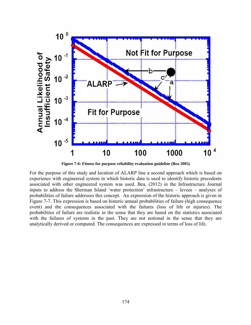
174
Figure 7-6: Fitness for purpose reliability evaluation guideline (Bea 2005)
For the purpose of this study and location of ALARP line a second approach which is based on experience with engineered system in which historic data is used to identify historic precedents associated with other engineered system was used. Bea, (2012) in the Infrastructure Journal inputs to address the Sherman Island ‘water protection’ infrastructure – levees – analyses of probabilities of failure addresses this concept. An expression of the historic approach is given in Figure 7-7. This expression is based on historic annual probabilities of failure (high consequence event) and the consequences associated with the failures (loss of life or injuries). The probabilities of failure are realistic in the sense that they are based on the statistics associated with the failures of systems in the past. They are not notional in the sense that they are analytically derived or computed. The consequences are expressed in terms of loss of life.
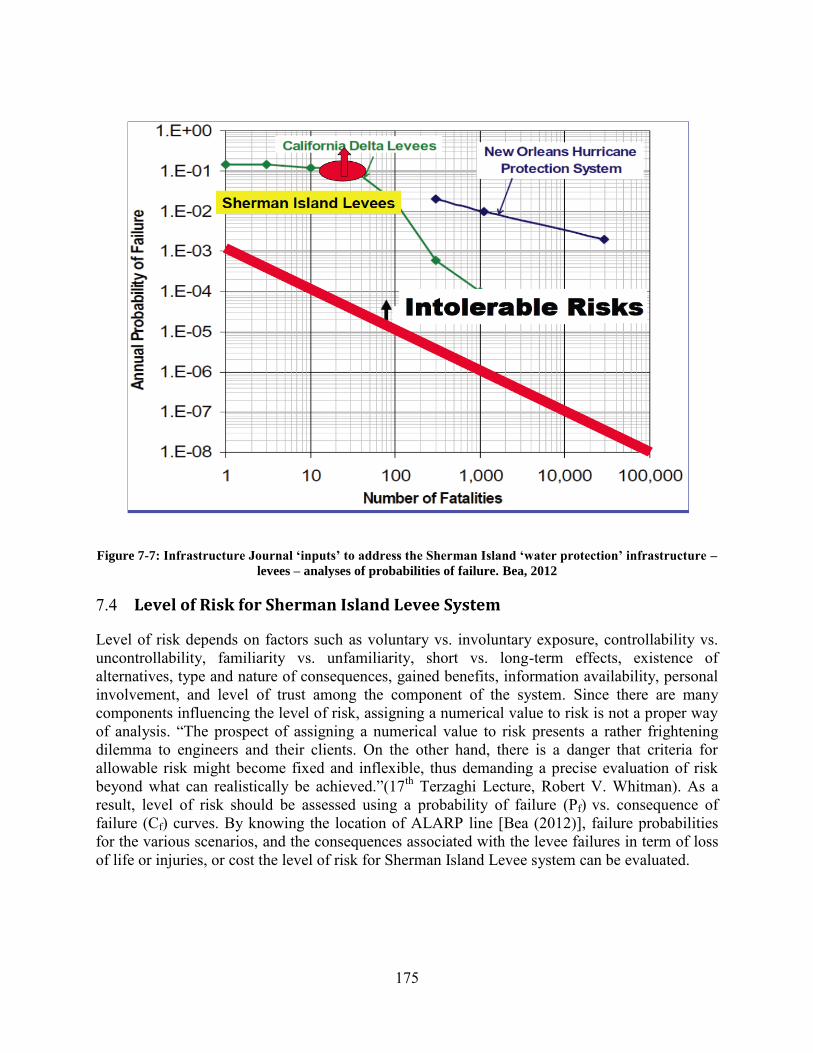
175
Figure 7-7: Infrastructure Journal ‘inputs’ to address the Sherman Island ‘water protection’ infrastructure –
levees – analyses of probabilities of failure. Bea, 2012
7.4 Level of Risk for Sherman Island Levee System
Level of risk depends on factors such as voluntary vs. involuntary exposure, controllability vs. uncontrollability, familiarity vs. unfamiliarity, short vs. long-term effects, existence of alternatives, type and nature of consequences, gained benefits, information availability, personal involvement, and level of trust among the component of the system. Since there are many components influencing the level of risk, assigning a numerical value to risk is not a proper way of analysis. “The prospect of assigning a numerical value to risk presents a rather frightening dilemma to engineers and their clients. On the other hand, there is a danger that criteria for allowable risk might become fixed and inflexible, thus demanding a precise evaluation of risk beyond what can realistically be achieved.”(17th Terzaghi Lecture, Robert V. Whitman). As a result, level of risk should be assessed using a probability of failure (Pf) vs. consequence of failure (Cf) curves. By knowing the location of ALARP line [Bea (2012)], failure probabilities for the various scenarios, and the consequences associated with the levee failures in term of loss of life or injuries, or cost the level of risk for Sherman Island Levee system can be evaluated.

176
8 SUMMARY AND CONCLUSIONS
8.1 Probability of Failure
This research addressed three major modes of failure of the Sherman Island ‘water protection’ infrastructure represented by its levees when they are exposed to extreme storms from the Pacific Ocean. The first failure mode was associated with the levee soil hydraulic conductivity – seepage- effects. The second mode was associated with the levee soil lateral instability, including seepage effects. Finally, third mode of failure was overtopping and soil erosion. The choice of the intense storm hazard and identification of the three failure modes was based on the long-term history of performance of the Sherman Island and similar water protection infrastructure systems in the California Delta and results from previous analyses of the risks associated with the Delta’s levees.
As described earlier in this work, a primary objective was to address categories of uncertainties not normally incorporated by engineers into their traditional risk analyses. In this research in addition to Type 1 uncertainties which has been identified as natural or inherent randomness of data, the Type 2 uncertainties were evaluated by making multiple comparisons between the results from prototype field ‘experiments’ and tests and the results from analytical models that attempted to ‘replicate’ or reproduce the results from the field experiments and tests. The general effect of including Type 2 uncertainties has been to increase the probabilities of failure of ‘components’ that comprise ‘systems’. This is not always the case, because the changes in the central tendencies of the probabilistic distributions introduced by inclusion of Type 2 uncertainties can lead to reductions in the calculated probabilities of failure.
Results of annual probabilities of failure associating with analyses of hydraulic conductivity – seepage – effects, lateral stability, and overtopping have been presented in Table 8-1. The annual probabilities of failure determined during this project for both current and future conditions are clearly ‘not acceptable’ – intolerable - when compared with acceptability guidelines for other U.S. infrastructure systems.
Failure Probabilities Pf, Seepage Pf, O ertopping Pf, Slope stability
South Side 7.45% 6.60% 4.09% - 23.58%
North Side 7.08% 6.60% 5.05% - 28.1%
Table 8-1: Summary of Failure Probabilities (annual probabilities of failure for year 2010)
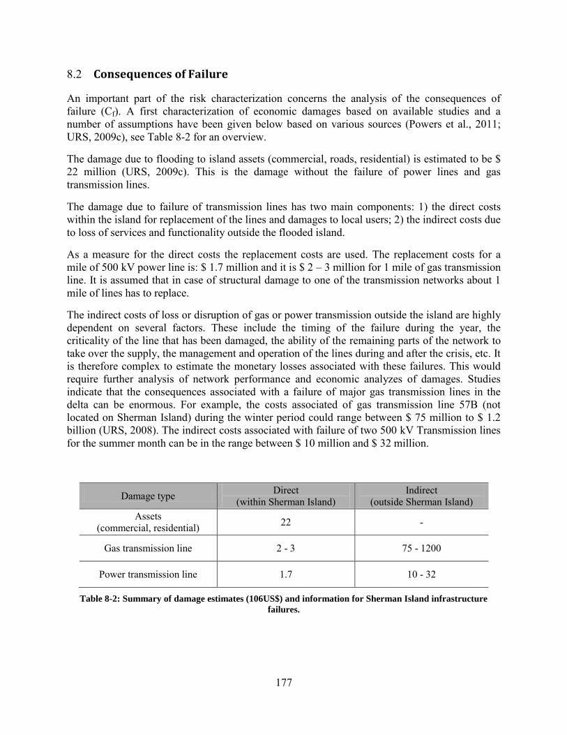
177
8.2 Consequences of Failure
An important part of the risk characterization concerns the analysis of the consequences of failure (Cf). A first characterization of economic damages based on available studies and a number of assumptions have been given below based on various sources (Powers et al., 2011; URS, 2009c), see Table 8-2 for an overview.
The damage due to flooding to island assets (commercial, roads, residential) is estimated to be $ 22 million (URS, 2009c). This is the damage without the failure of power lines and gas transmission lines.
The damage due to failure of transmission lines has two main components: 1) the direct costs within the island for replacement of the lines and damages to local users; 2) the indirect costs due to loss of services and functionality outside the flooded island.
As a measure for the direct costs the replacement costs are used. The replacement costs for a mile of 500 kV power line is: $ 1.7 million and it is $ 2 – 3 million for 1 mile of gas transmission line. It is assumed that in case of structural damage to one of the transmission networks about 1 mile of lines has to replace.
The indirect costs of loss or disruption of gas or power transmission outside the island are highly dependent on several factors. These include the timing of the failure during the year, the criticality of the line that has been damaged, the ability of the remaining parts of the network to take over the supply, the management and operation of the lines during and after the crisis, etc. It is therefore complex to estimate the monetary losses associated with these failures. This would require further analysis of network performance and economic analyzes of damages. Studies indicate that the consequences associated with a failure of major gas transmission lines in the delta can be enormous. For example, the costs associated of gas transmission line 57B (not located on Sherman Island) during the winter period could range between $ 75 million to $ 1.2 billion (URS, 2008). The indirect costs associated with failure of two 500 kV Transmission lines for the summer month can be in the range between $ 10 million and $ 32 million.
Damage type Direct (within Sherman Island)
Indirect (outside Sherman Island)
Assets (commercial, residential) 22 -
Gas transmission line 2 - 3 75 - 1200
Power transmission line 1.7 10 - 32
Table 8-2: Summary of damage estimates (106US$) and information for Sherman Island infrastructure
failures.
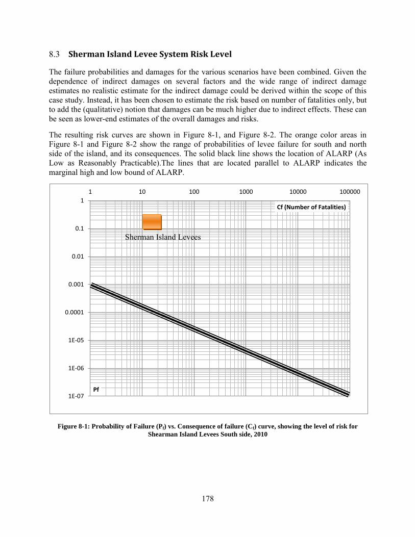
178
8.3 Sherman Island Levee System Risk Level
The failure probabilities and damages for the various scenarios have been combined. Given the dependence of indirect damages on several factors and the wide range of indirect damage estimates no realistic estimate for the indirect damage could be derived within the scope of this case study. Instead, it has been chosen to estimate the risk based on number of fatalities only, but to add the (qualitative) notion that damages can be much higher due to indirect effects. These can be seen as lower-end estimates of the overall damages and risks.
The resulting risk curves are shown in Figure 8-1, and Figure 8-2. The orange color areas in Figure 8-1 and Figure 8-2 show the range of probabilities of levee failure for south and north side of the island, and its consequences. The solid black line shows the location of ALARP (As Low as Reasonably Practicable).The lines that are located parallel to ALARP indicates the marginal high and low bound of ALARP.
Figure 8-1: Probability of Failure (Pf) vs. Consequence of failure (Cf) curve, showing the level of risk for
Shearman Island Levees South side, 2010
1E-07
1E-06
1E-05
0.0001
0.001
0.01
0.1
1
1 10 100 1000 10000 100000
Pf
Cf (Number of Fatalities)
Sherman Island Levees

179
Figure 8-2: Probability of Failure (Pf) vs. Consequence of failure (Cf) curve, showing the level of risk for
Shearman Island Levees North side, 2010
1E-07
1E-06
1E-05
0.0001
0.001
0.01
0.1
1
1 10 100 1000 10000 100000
Pf
Cf (Number of Fatalities)
Sherman Island Levees

180
8.4 Concluding Remarks
This research has contributed to the development of a framework and methods for the quantitative analysis of risks (probabilities and consequences) for interconnected infrastructures. For a complete characterization of the system environmental hazards, physical systems characteristics and human and organizational factors need to be taken into account. This risk models mainly focus on factors, engineered parts of the system and the hazards.
Risk analysis of interconnected systems requires a combination of various modeling approaches, such as engineering models to estimate the strength of structures such as levees, physical effect models and methods to incorporate effects of human and organizational factors [e.g. QMAS (Bea, 2002)]. As a result, a number of techniques and approaches for assessing risks in interconnected systems have been explored and applied to case studies in this report.
The case study for Sherman Island demonstrated the use of the proposed methods and techniques for cascading failures. The probability of levee failure for this island is estimated to be relatively high. In the presented analyzes for Sherman Island several simplifying assumptions have been used. For a better estimate of the risk it would be necessary to improve estimates of failure probabilities of levees and other infrastructures and to get a better understanding of the consequences within and outside Sherman Island of failure of various systems. This requires a further analysis of the effects of flooding of an island on power and gas transmission networks throughout the delta and California. In addition a broader range of event scenarios (various types of floods, storms and earthquakes) has to be considered to generate a better estimate of the risk.
The quantitative analyzes in the case study focused on the infrastructures within Sherman Island. However, these infrastructures are part of a larger system in and around the Sacramento – San Joaquin delta. The effects of flooding of an island can extend to infrastructure elements and systems outside the island. In addition, the functioning of systems outside the island (power, and gas operation, emergency management) will affect the probabilities and damages of the events that are associated with flooding within the (Sherman) Island boundaries. It is therefore recommended to further apply the methods and approaches (influence diagrams, maps showing zones with effects due to failure of an infrastructure) that have been used for the island case study at a wider delta scale for various hazard and flood scenarios (earthquake, storm, single island failure, multiple island failure).

181

182
9 REFERENCES
Allsop, N.W.H. (2000) Wave forces on vertical and composite walls Chapter 4 in Handbook of Coastal Engineering, pages 4.1-4.47, Editor J. Herbich, ISBN 0-07-134402-0, publn. McGraw-Hill, New York.
Ang, A. and Wilson H. Tank (2007). “Probability Concepts in Engineering, Emphasis on Applications to Civil and Environmental Engineering”. 2nd Edition. John Wiley & Sons, Inc.'
ASCE National Convention, Boston, 1979, Reliability Analysis and Geotechnical Engineering (Preprint 3600).
Apostolakis G. (1990) Th e concept of probability in safety assessment of technological systems, Science Vol. 250, pp. 1359-1364
Apostolakis G.E. (2004) How useful is quantitative risk assessment? Risk Analysis Vol. 24 No. 3, pp. 515-520
Atwater, BF (1982). “Geological Maps of the Sacramento-San Joaquin Delta, California” USGS Surv Map MF-1401. 1982
Aubeny, C.P. and Lytton, R.L. “Shallow slides in compacted high plasticity clay slopes,” ASCE
J. Geotech. and Geoenv. Engrg., pp. 717-727, 2004.
Baecher, G. and J. Christian (2003). “Reliability and Statistics in Geotechnical Engineering.” John Wiley & Sons Ltd. West Sussex, England
Bay-Delta Programmatic Environmental Impact Report Coordinated Proceedings 43 Cal.4th 1143, 1168 (2008).
Bea, R. G. (1974). Selection of environmental criteria for offshore platform design, Journal of Petroleum Technology, Society of Petroleum Engineers, Richardson, Texas, pp. 1206–1214.
Bea, R. G. (1975). Development of safe environmental criteria for offshore structures, Proceedings Oceanology International Conference, Brighton, UK.
Bea, R. G. (1990). Reliability Based Design Criteria for Coastal and Ocean Structures, Institution of Engrs. Australia, Barton ACT.
Bea, R. G. (1992). Marine structural integrity programs (MSIP), Ship Structure Committee, SSC-365, Washington, DC.

183
Bea, R. G. (1996a). Human and organisation errors in reliability of offshore structures, Journal of Offshore Mechanics and Arctic Engineering, American Society of Mechanical Engineers, New York, Nov.–Dec. 1996.
Bea, R. G. (1996b). Quantitative and qualitative risk analyses – the safety of offshore platforms, Proceedings of the Offshore Technology Conference, OTC 8037, Society of Petroleum Engineers, Richardson, Texas.
Bea, R. G. (1997). "Human and Organization Errors in Reliability of Offshore Structures," J.
Offshore Mech. and Arctic Engrg., Trans. ASME, 119, 46-52.
Bea, R. G. (1998). "Reliability Characteristics of a Platform in the Mississippi River Delta," J. Geotech. and Geoenv. Engrg., ASCE 124 (8) 729-738.
Bea, R.G. (2000a). Achieving Step Change in Risk Assessment & Management (RAM), Centre for Oil and Gas Engineering, University of Western Australia Press, Nedlands, Western
Australia; also Human & Organizational Factors in Design & Reliability of Offshore
Structures, Doctor of Philosophy Thesis, Centre for Oil and Gas Engineering, the University of Western Australia.
Bea, R. G. (2000b). "Performance Shaping Factors in Reliability Analysis of Design of Offshore Structures," J. Offshore Mech. and Arctic Engrg., Trans ASME, 122, 163-172.
Bea, R. G. (2001). "Risk Assessment and Management of Offshore Structures," Prog. Struct.
Engrg. & Materials, 3, John Wiley & Sons, Ltd., 180-187.
Bea, R. G. (2000a). Achieving step change in risk assessment and management (RAM), Centre for Oil and Gas Engineering, http://www.oil-gas.uwa.edu.au, University of Western Australia, Nedlands, WA.
Bea, R. G. (2002a). "Human and Organizational Factors in Reliability Assessment and Management of Offshore Structures," Risk Analysis, 22 (1), Soc. for Risk Analysis, New York, 29-45.
Bea, R. G. (2002b). "Human & Organizational Factors in design and Operation of Deepwater Structures," OTC 14293, Proc. Offshore Technology Conference, Society of Petroleum Engrs., Richardson, TX, 1 - 19.
Bea, R. G. (2000b). Performance shaping factors in reliability analysis of design of offshore structures, Journal of Offshore Mechanics and Arctic
Bea, R. G. (2001). "Risk Assessment and Management of Offshore Structures," Prog. Struct.
Engrg. & Materials, 3, John Wiley & Sons, Ltd., 180-187.

184
Bea, R.G. (2006). “Reliability and Human Factors in Geotechnical Engineering.” ASCE J.
Geotechnical and Geoenvironmental Engineering, 132 (5), 631-643.
Bea, R.G. (2007a). “Reliability Assessment & Management Lessons from Hurricane Katrina,”
Bea, R.G. (2008b) “Failure of the New Orleans 17th Street Canal Levee & Floodwall During Hurricane Katrina,” Proceedings Schmertmann Symposium, GeoCongress 08, ASCE, pp 574-593.
Bea, R.G. (2008b) “Failure of the New Orleans 17th Street Canal Levee & Floodwall During Hurricane Katrina,” Proceedings Schmertmann Symposium, GeoCongress 08, ASCE, pp 574-593.
Bea, R.G. (2008a). “Robinson v. United States. Expert Report of Dr. Robert Glenn Bea. Engineering Forensic Studies of Performance of the Man-Made Features Bordering the Mississippi River-Gulf Outlet (MR-GO) during Hurricane Katrina.” Dated July 11, 2008.
Bea, R. G. (2008b). “Robinson v. United States. Expert Report of Dr. Robert Glenn Bea. Engineering Forensic Studies of Performance of the Man-Made Features Bordering the Mississippi River-Gulf Outlet (MR-GO) during ‘Neutral’ MR-GO Hurricane Katrina Conditions.” Dated July 11, 2008.
Bea, R., (2009). Lecture, UC Berkeley. CE 205B (Margins of Quality for Engineered Systems), Fall 2009.
Bea, Robert (2010). “Human & Organizational Factors: Risk Assessment & Management Engineered Systems” Volume 1. UC Berkeley Class Reader.
Bea, R. G., Bernard, H. A., Arnold, P., Doyle, E. H. (1975). "Soil Movements and Forces Developed by Wave-Induced Slides in the Mississippi Delta," J. Petroleum Tech., Soc. of Petroleum Engrs., Richardson, TX. 599-514.
Bea, R. G., Wright, S. G., Sircar, P. Niedoroda, A. W. (1983). "Wave-Induced Slides in South Pass Block 70, Mississippi Delta," J. Geotech. Engrg., 109 (4), ASCE. 619-644.
Bea, R. G. and Audibert, J. M. E. (1980). "Offshore Platforms and Pipelines in Mississippi River Delta," J. Geotech. Engrg., 106 (8), 853-869.
Bedford T. (2005) Keynote lecture: Multi-attribute utility theory and FN-criteria, in: Proc.
OfESREL 2005, Tri City, Poland, pp. 157-166
Bedford T. Cooke R. (2002) Probabilistic risk analysis: foundations and methods, Cambridge University Press.

185
Bear, J (1972). “Dynamics in Fluids in Porous Media”. Department of Civil Engineering, Israel Institute of Technology. Haifa, Israel.
Bennet, G.(1970) Bristol Floods 1968 – Controlled Survey of Eff ects on Health of Local Community Disaster, British Medical Journal Vol. 3, pp.454-458.
Bick, A., et al. California Environmental Law Handbook. 11th ed. R. Denney et al., eds. Government Institutes: Rochester, MD, 1999.
Bishop, A.W. (1954) "The Use of Pore Pressure Coefficients in Practice," Geotechnique, Vol. IV, No. 4, pp. 148-152.
Bishop, A.W. (1955) "The Use of the Slip Circle in the Stability Analysis of Slopes," Geotechnique, Great Britain, Vol. 5, No. 1, Mar., pp. 7-17.
Bishop, A.W. and Morgenstern, Norbert (1960) "Stability Coefficients for Earth Slopes," Geotechnique, Vol. 10, No. 4, December, pp. 129-150.
Bjerrum, L. (1955) "Stability of Natural Slopes in Quick Clay," Geotechnique, Vol. 5, No. 1, pp. 101-119.
Bjerrum L. (1967) "Progressive Failure in Slopes of Overconsolidated Plastic Clay and Clay Shales," Journal of the Soil Mechanics and Foundations Division, ASCE, Vol. 93, No. SM5, pp. 1-49.
Bjerrum, L. and Kjaernsli, B. (1957) "Analysis of the Stability of Some Norwegian Natural Clay Slopes," Geotechnique, Vol. 7, No. 1, March, pp. 1-16.
Boyd, J.R. 1976. An Organic Design for Command and Control. In BOYD, J.R. 1976. Discourse on Winning and Losing. Unpublished lecture notes
Boyd, J.R. 1987a. Organic Design for C2. Unpublished lecture notes.
Boyd, J.R. 1987b. A Discourse on Winning and Losing. Maxwell Air Force Base, AL: Air University Library Document No. M-U 43947 (Briefing slides).
Boyd, J.R. 1996. The Essence of Winning and Losing. Unpublished lecture notes BRETON, R., AND ROUSSEAU, R. 2003. Modelling approach for Team Decision
Brauns, Josef (1980), "Safety Against Slip in Inclined Base of Toe Slopes," Technical Note, " Journal of the Geotechnical Engineering Division, ASCE, Vol. 106, No. GT10, Oct., pp. 1158-1162.
Brown, Rendall L. (1999). Department of Water Resources. http://www.water.ca.gov/iep/newsletters/1999/1999fall.txt

186
Burcharth, H. F., and Hughes, S. A. (2002). “Fundamentals of Design.” In: Hughes (editor), Coastal Engineering Manual, Part VI, Design of Coastal Project Elements, Chapter VI-5, Engineer Manual 1110-2-1100, U.S. Army Corps of Engineers, Washington, D.C.
California Department of Water Resources, Bulletin 132-07 accessed online at http://www.water.ca.gov/swpao/bulletin.cfm.
Campbell, D.T. and Stanley, J.C. (1963). Experimental and quasi-experimental designs for
research. Chicago: Rand McNally.
Casagrande, A. (1960) "An Unsolved Problem of Embankment Stability on Soft Ground," Proceedings, First Pan-American Conf. on Soil Mech. and Found. Engrg., Vol. 2, pp. 721-746.
Chang, C-J., Chen, W. and Yao, J. T. P., "Seismic Displacements in Slopes by Limit Analysis," American Society of Civil Engineers, Journal of Geotechnical Engineering, Vol. 110, No. GT7, pp. 860-874, 1984.
Christian, J. T. (2004). "Geotechnical Engineering Reliability: How Well Do We Know What We Are Doing?" J. Geotechnical and Geoenvrionmental Engineering, ASCE, Oct, 985-1003.
Christian, J. T. (2005). "Geotechnical Engineering Reliability: The Observational Method." Presentation at 2005 Distinguished Lecture Program, UC Berkeley Geoengineering Society, University of California, Berkeley, May.
Christian, J.T., Ladd, C.C. and Baecher, G.B. (1994). Reliability and Probability in Stability
Analysis, Journal of Geotechnical Engineering, ASCE, Vol. 120, pp. 1071-1111.
Coastal Engineering Research Center (1984). Shore Protection Manual. U.S. Army Corps of Engineers, Waterways Experiment Station, Vicksburg Mississippi.
Coastal Engineering Manual (2001). Scour and Scour Protection. Chapter VI-5-6, Engineer Manual EM 1110-2-1100, Headquarters, U.S. Army Corps of Engineers, Washington D.C.
Conard, S.G., MacDonald, R.L. and Holland, R.F., 1977. Riparian vegetation and flora of the Sacramento Valley. In: A. Sands (ed.). Riparian Forests in California. University of California, Davis.
Coons, Tom, Christopher Soulard and Noah Knowles. (2008). “High-Resolution Digital Terrain Models of the Sacramento/San Joaquin Delta Region, California”. USGS Data Series 359 V.1
187
Coulter, H. W., and Migliaccio, R. R., "Effects of the Earthquake of March 27, 1964, at Valdez, Alaska," U.S. Geological Survey Professional Paper 542-C, U.S. Department of the Interior, 1966.
Das, Braja M 2006. “Principles of Geotechnical Engineering”. England: THOMSON LEARNING (KY).
Delta Protection Commission. (1994) .Background report on Levees., <http://www.delta.ca.gov/bkgreports.PDF> (Nov. 12, 2005)
Department of Water Resources. (1976) .Sacramento . San Joaquin Delta Levees Study., California Department of Water Resources. Sacramento
Department of Water Resources. (1993). Sacramento San Joaquin Delta atlas”. California Department of Water Resources.Sacramento
Department of Water Resources. (2005) “Flood warnings: Responding to California’s flood crisis. California Department of Water Resources, http://www.publicaffairs.water.ca.gov (Dec. 1, 2005)
Department of Water Resources and Department of Food and Agriculture. Current Water Use
Efficiency Policy and Programs and Estimate of Agricultural and Urban Water Use.
Report prepared for the Delta Vision Task Force, October 10, 2008.
Duncan, M. J. (2000). "Factors of Safety and Reliability in Geotechnical Engineering," J. Geotech. and Geoenv. Engrg, 126 (4), ASCE, 307-316.
Duncan, J.M. & Wright, S.G. 2005. “Soil Strength and Slope Stability”, John Wiley, Hoboken\ NJ.
Duncan, S., Paredis, C. J. J., and Bras, B. (2007). "Applying Info-Gap Theory To Remanufacturing Process Selection Affected By Severe Uncertainty." 2007 ASME International Mechanical Engineering Congress and Exposition (IMECE). November 11-15, 2007, Seattle, WA, USA. Paper#: DETC2007-43608
Evans A.W., Verlander N.Q. (1997) What is wrong with criterion FN-lines for judging the tolerability of risk, Risk Analysis Vol. 17 No. 2 pp. 157–168.
Foott, R., and Ladd, C. C. (1973). The behavior of Atchafalaya test embankments during
construction. Research report R73-27, Dept. of Civil Engineering, Massachusetts Institute of Technology, Cambridge MA.
Foott, R., and Ladd, C. C. (1977). “Behaviour of Atchafalaya levees during construction.” Geotechnique, 27(2), 137-160.
188
Roger Foott Associates, Inc., Threatened Levees on Sherman Island, Berkeley, California, 1992
Geostudio 2007a. “SEEP/W Student Edition Workbook”,
Geostudio 2007b. “SLOPE/W Student Edition Workbook”
Gertman, D. I., and Blackman, H.S. (1994). Human Reliability and Safety Analysis Data Handbook, John Wiley & Sons, Chicester, UK.
Gray, D.H., Leiser, A.T., 1982. Biotechnical Slope Protection and Erosion Control. Van Nostrand Reinhold Co., New York.
Gray, D.H., Sotir, R.B., 1996. Biotechnical and Soil Bioengineering Slope Stabilization. A Practical Guide for Erosion Control. John Wiley and Sons, New York.
Gwynne, S., Galea, E. R., Owen, M., Lawrence, P. J., and Filippidis, L. (1999). “A review of the methodologies used in computer simulation of evacuation from the built environment.” Build. Environ., 34(6), 741–749.
Hanak, E., et al. (2011). Managing California’s water from conflict to reconciliation, Public Policy Institute of California, San Francisco.
Hanson, J. C. (2009). Reclamation District 341 Sherman Island Five-Year Plan (SH 08-3.0. Five-Year Plan). California Department of Water Resources. Sacramento, CA.
Harder, L. F., Jr., "Use of Penetration Tests to Determine the Cyclic Loading Resistance of Gravelly Soils During Earthquake Shaking," Ph.D. Dissertation, University of California, Berkeley, CA, 1988.
Harder, L.F. Jr., "Performance of Earth Dams during Loma Prieta Earthquake," Proceedings 2nd
International Conference on Recent Advances in Geotechnical Earthquake Engineering
and Soil Dynamics, St. Louis, MO, pp. 1673-1690, 1991.
Harr, M. E. (1987). Reliability-Based Design in Civil Engineering, McGraw-Hill, New York.
Hee DD, Bea RG. Safety management assessment system (SMAS). Marine Technology and Management Group, University of California, Berkeley, CA, 1997.
Hewlett, H.W.M., L. A. Boorman, and M. E. Bramley. “Design of Reinforced Grass Waterways.” Construction Industry Research and Information Association. London. 1987.
Holtz, R. and W. Kovacs (1981). “An Introduction to Geotechnical Engineering.” Civil and Environmental Engineering Mechanics Series. Prentice Hall Inc. New Jersey
Hunrichs, R.A 1998. Magnitude and Frequency of the Floods of January 1997 in Northern and
Central California. U.S. Geological Survey open-file report; 98-626

189
Janbu, N. (1954) "Application of Composite Slip Surface for Stability Analysis," Proceedings, European Conference on Stability of Earth Slopes, Stockholm, 3:43-49.
Janbu, N. (1957) "Earth Pressures and Bearing Capacity Calculations by Generalized Procedure of Slices," Proceedings, Fourth International Conference on Soil Mechanics and Foundation Engineering, Vol. 2, London, pp. 207-212.
Jonkman S.N., van Gelder P.H.A.J.M., Vrijling J.K. (2003) An overview of quantitative risk measures for loss of life and economic damage, Journal of Hazardous Materials. A99, pp.1-30
Jonkman, S. N. (2007). “Loss of life estimation in flood risk assessment: Theory and applications.” Ph.D. dissertation, Delft Univ. of Technology, Delft, Netherlands.
Jonkman, S. N., Maaskant, B., Boyd, E., and Levitan, M. L. (2009). “Loss of life caused by the flooding of New Orleans after Hurricane Katrina: Analysis of the relationship between flood characteristics and mortality.” Risk Anal., 29(5), 676–698.
Jonkman, S. N., Vrijling, J. K., and Vrouwenvelder, A. C. W. M. (2008). “Methods for the estimation of loss of life due to floods: A literature review and a proposal for a new method.” Nat. Hazards, 46(3), 353–389.
Kaufman, R. I., and Weaver, F. J., “Stability of Atchafalaya Levees,” Journal of Soil Mechanics Foundations, ASCE, Vol. 93, No. SM4, July, 1967, pp. 157–176.
Koelewijn A.R., M.A. Van (2003): Monitoring of the test on the dike at Bergambacht: Design and practice – Proceedings XIII ECSMGE
Kulhawy, F. (1996). "From Casagrande's Calculated Risk to Reliability-Based Design in Foundation Engineering," Civil Engrg. Practice, BSCE, 11(2), 43-56.
Kulhawy, F. H. and Phoon, K. K. (1996). "Engineering Judgment in the Evolution from Deterministic to Reliability-Based Foundation Design," Uncertainty in the Geologic Environment, Shackelford, C. D., Nelson, P. P., Roth, J.J.S., eds., ASCE, Vol. 1, 29-48
Lacasse, S. (2004). "Risk Assessment for Geotechnical Solutions Offshore," Proc. 23rd Int. Conf. Offshore Mechanics and Arctic Engrg., OMAE2004-51144, ASME.
Lacasse, S. and Nadim, F. (1994). "Reliability Isses and Future Challenges in Geotechnical Engineering for Offshore Structures", Proc. 7th Int. Conf on Behaviour of Offshore Structures, MIT, Cambridge, MA, 9-38.
Ladd, C.C. (1983). Geotechnical Exploration in Clay Deposits with Emphasis on Recent
Advances in Laboratory and In Situ Testing and Analysis of Data Scatter, Journal of Civil and Hydraulic Engineering, Taiwan, 10(3), pp. 3-35.

190
Ladd, C.C. (1991). Stability Evaluation during Staged Construction, Journal of Geotechnical Engineering, ASCE, 117 (4) pp. 540-615.
Lawson, RB, and Bea, RG 1997. Stage-II Analysis of Human and Organizational Factors, Report to JIP on Comparative Evaluation of Minimum Structures and Jackets, Marine Technology & Development Group, University of California at Berkeley.
Leenknecht, David A., Andre Szuwalski and Ann R. Sherlock. Automated Coastal Engineering
System Technical Reference. September 1992. Coastal Engineering Research Center.
Lematire, J. and Desmorat, R. (2005). Engineering Damage Mechanics, Springer Verlag, New York.
Likert R., (1974). The method of constructing an attitude scale. In: Marannell, G.M. (Ed.), Scales: A Sourcebook for behavioral scientist. Aldine Publishing Company, Chicago, IL, 21-43.
Meshkati, N. (1991). Human Factors in Large-Scale Technological Systems' Accidents: Three Mile Island, Bhopal, Chernobyl. Industrial Crisis Quarterly, 5, 133-154.
Meyerhoff, G.G. (1957) "The Mechanism of Flow Slides in Cohesive Soils," Geotechnique, Vol. VII, No. 1, pp. 41-49.
Morgenstern, Norbert (1963), "Stability Charts for Earth Slopes During Rapid Drawdown," Geotechnique, Great Britain, Vol. 13, No. 2, June, 1963, pp. 121-131.
Morgenstern, N. R., and V. E. Price (1965), "The Analysis of the Stability of General Slip Surfaces," Geotechnique, Great Britain, Vol. 15, No. 1, Mar., pp. 79-93.
Morgenstern, N.R. and Price, V.E. (1967) "A Numerical Method for Solving the Equations of Stability of General Slip Surfaces," The Computer Journal, Great Britain, Vol. 9, No. 4, February, pp. 388-393.
Munson, Bruce R., Donald Young and Theodore Okiishi (2006). “Fundamentals of Fluid Mechanics 5e.” John Wiley & Sons Inc.
National Research Council (2009). Science and Decisions: Advancing Risk Assessment. Committee on Improving Risk Analysis Approaches Used by the U.S. EPA
Pandey M.D., Nathwani J.S. (2004) Life quality index for the estimation of societal willingness-to-pay for safety, Structural Safety Vol. 26 No. 2 pp.181-199
Peck, R.B. (1967) "Stability of Natural Slopes," Journal of the Soil Mechnaics and
Foundations Division, ASCE, Vol. 93, No. SM4, pp. 403-418.
191
Perdikis, H. S. (1967). “Hurricane Flood Protection in the United States.” J. Waterways and
Harbors Div., ASCE, Reston, VA.
Petroski, H. (1985). To Engineer is Human: The Role of Failure in Successful Design, St. Martins Press, New York, NY.
Petroski, H. (1994). Design Paradigms, Case Histories of Error and Judgment in Engineering, Cambridge University Press, Cambridge, UK.
Powers J, Hanson E, Myslewski C (2011) Critical Infrastructure Interdepencies Within the California Delta. UC Berkeley. CE268k working paper.
Rackwitz R. (2002) Optimization and risk acceptability based on the life quality index, Structural Safety Vol. 24, pp. 297-331
Rantz, S.E 1963a. Floods of December 1955-January 1956 in far Western States. Geological Survey water-supply paper; 1650-B.
Rantz, S.E 1963b. Floods of January-February 1963 in California and Nevada. U.S Geological Survey.
Reddi, Lakshmi N. (2003) “Seepage in Soils”. John Wiley, Hoboken, NJ.
Reed, D.J., 2002. Understanding tidal marsh sedimentation in the SacramentoeSan Joaquin Delta, California. Journal of Coastal Research Special Issue 36, 605e611.
Resource Management Inc.(2005), “Flooded Island Study” http://www.rmanet.com/Projects/SFBay-Delta/SFBay_FloodedIslands.htm
Road and Hydraulic Engineering Institute (RHEI) 1999. “Technical Report on Sand Boils (Piping)” Technical Advisory Committee on Flood Defenses. The Netherlands
Roberts, K. H. (1993). New Challenges to Understanding Organizations, McMillan Pub., New York.
Roberts, K. H. (1989). "New Challenges in Organizational Research: High Reliability Organizations," Industrial Crisis Quarterly, Elsevier Sciences Pub. B.V., Amsterdam, Netherlands, 20-26.
Roberts, K. H. and Bea, R. G. (2001a). "Must Accidents Happen? Lessons from High-Reliability Organizations," Academy of Management Executive, 15(3), Academy of Management, New York, 1-9.
Roberts, K. H. and Bea, R. G. (2001b). "When Systems Fail," Organizational Dynamics, 29 (3) 179-191, Elsevier Science, Inc., New York.

192
Ronold, K.O. and Bjerager, P. (1992). "Model Uncertainty Representation in Geotechnical Reliability Analyses," J. Geotech.Engrg, ASCE, 118 (3), 363-376.
Sanders B.F., Katapodes N.D., 1999b. Active flood hazard mitigation. II:omnidirectional wave control. Journal of hydraulic engineering, October 1999. 125(10). p. 1071-1083.
Santamarina, J.C., and Turkstra, C. J. (1990). "Human Factors and Communication Problems in Foundation Engineering," Foundation Engineering: Current Principles and Practices, Kulhawy, F.H. , ed., Vol 2, ASCE.
Santos, B., A. Antunes, and E. Miller, E. (2010). “Interurban road network planning model with accessibility and robustness objectives.” Transportation Planning Technology 33(3), pp. 297-313.
Sasou, K. and Reason, J. (1999). "Team Errors: Definition and Taxonomy," Reliability Engineering and System Safety, 65, Elsevier Science Ltd., 1-9.
Seed R.B., Bea R.G., Abdelmalak R.I., Athanasopoulos A.G., Boutwell G.P., Bray J.D., Briaud J.-L., Cheung C., Cobos-Roa D., Cohen-Waeber J., Collins B. D., Ehrensing L., Farber D., Hanemann M., Harder L. F., Inkabi K. S., Kammerer A.M., Karadeniz D., Kayen R.E., Moss R.E.S., Nicks J., Nimmala S., Pestana J.M., Porter J., Rhee K., Riemer M.F., Robert K., Rogers J. D., Storesund R., Govindasamy A.V., Vera-Grunauer X., Wartman J.E., Watkins C.M., Wenk Jr. E., Yim S.C. (2006) Investigation of the performance of the New
Orleans fl ood protection systems in hurricane Katrina on august 29, 2005, Final report. Independent Levee Investigation team, July 31 2006
Seed R.B., Nicholson P.G., Dalrymple R.A., Battjes J.A., Bea R.G., Boutwell G.P., Bray J.D., Collins B.D., Harder L.F., Headland J.R., Inamine M.S., Kayen R.E., Kuhr R.A., Pestana J. M., Silva-Tulla F., Storesund R., Tanaka S., Wartman J., Wolff T.F., Wooten R.L., Zimmie T.F. (2005) Preliminary Report on the Performance of the New Orleans Levee Systems in
Hurricane Katrina on August 29, 2005. Report No. UCB/CITRIS – 05/01
Seed, R. B., L. F. Harder. 1990. “SPT-Based Analysis of Cyclic Pore Pressure Generation and Undrained Residual Strength”, Proceedings of the H. Bolton Seed Memorial Symposium, University of California, Berkeley, May 10-11, 1990, pp. 351-376.
Shapira, Z. (1995). Risk Taking, A Managerial Perspective, Russell Sage Foundation, New York.
Shields, F. D., Jr., and N. R. Nunnally. 1984. Environmental aspects of clearing and snagging. ASCE Journal of Environmental Engineering 110:152-165.
Smith, G. M. (1994). “Grasdijken” (Dutch), ”Grass dikes,” Delft Hydraulics report H1565, Delft, The Netherlands.
193
Sowers, G. F. (1993). "Human Factors in Civil and Geotechnical Engineering Failures," J.
Geotech. Engrg., 119 (2), 238-256.
Spencer, E. (1967) "A Method of Analysis of the Stability of Embankments Assuming Parallel Inter-Slice Forces," Geotechnique, Great Britain, Vol. 17, No. 1, March, pp. 11-26.
Spencer, E. (1968), "Stability of Earth Embankments," Civil Engineering and Public Works
Review, Vol. 63, No. 745, Aug., 1968, pp. 869-872.
Spencer, E. (1968) "Effect of Tension on Stability of Embankments," Journal of the Soil
Mechanics and Foundations Division, ASCE, Vo. 94, No. SM5, September, pp. 1159-1173.
Spencer, Eric (1969), "Circular and Logarithmic Spiral Slip Surfaces," Journal of the Soil Mechanics and Foundations Division, ASCE, Vol. 95, No. SM1, Jan., pp. 227-234.
Spencer, E. (1973), "Thrust Line Criterion in Embankment Stability Analysis," Geotechnique, Vol. 23, No. 1, Mar., pp. 85-100.
Spencer, E. (1969) "Circular and Logarithmic Spiral Slip Surfaces," Journal of the Soil
Mechanics and Foundations Division, ASCE, Vol. 95, No. SM1, January, pp. 227-234.
Stoelsnes, R. R. and Bea, R. G. (2005). "Uncertainty Management of General Conditions in a Project." Risk Management: An International Journal, 7 (2), Perpetuity Press Ltd., London.
Swain, A. D. & Guttman, H. E. (1983). Handbook of human reliability analysis with emphasis
on nuclear power plant operations (NUREG/CR-1278). Washington D.C: Nuclear Regulatory Commission.
Tang, W. H., Stark, T.D. Angulo, M. (1999). "Reliability in Back Analysis of Slope Failures," J. Soil Mech. and Found., Tokyo, Oct.
Terzaghi, Karl V. (1936), "Stability of Slopes of Natural Clay," Proceedings of the First
International Conference on Soil Mechanics and Foundation Engineering, Harvard, Vol.1, pp. 161-165.
Terzaghi, K., Peck, R.B. Mesri, G. (1996). Soil Mechanics in Engineering Practice, 3rd Ed., Wiley, New York.
Thompson, R (2006) "Early Reclamation and Abandonment of the Central Sacramento – San Joaquin Delta," Sacramento History Journal 6:1-4 (2006), 41-72.
Tillis, R. Kevin, Michael Meyers and Edwin M. Hultgren; Proceedings - Stability and Performance of Slopes and Embankments, ASCE Specialty Conference, Berkeley, California; June 1992.

194
United Research Services (URS Corporation). 2003b. In-Delta Storage Program Embankment Design Analysis. Prepared for Department of Water Resources. April.
United Research Services (URS). (2009a). “Delta risk management strategy, Phase 1: Section 4, risk analysis methodology.” Rep. Prepared for California Department of Water Resources. United Research Services, Oakland, CA.
United Research Services URS (2009). Delta Risk Management Strategy. Multiple volumes prepared for California Department of Water Resources.
United States Army Corps of Engineers, 1968. Levee Maintenance Standards and Procedures. Engineer Manual 1130-2-335, Washington, D.C.
United States Army Corps of Engineers, 1978. Design and Construction of Levees. Engineer Manual 1110-2-19 13, Washington, D.C.
United States Army Corps of Engineers, 1991. Mokelumne River and tributaries, California: Reconnaissance Report. Sacramento: 93.
United States Army Corps of Engineers, 1999. Sacramento and San Joaquin River Basins post-flood assessment. Sacramento, U.S. Army Corps of Engineers, Sacramento District.
United States Army Corps of Engineers, Sacramento District & Sacramento Area Flood Control Agency, 1998. San Joaquin River Basin South Sacramento County streams investigation, California: Final Feasibility Report: Main Report, U. S. Army Corps of Engineers.
United States Army Corps of Engineers, Sacramento District & Sacramento Area Flood Control Agency, 1996. South Sacramento County Streams Investigation, California: Final Feasibility Report: Appendicies-Feasibiliy Level Hydrology, U. S. Army Corps of Engineers.
United States Army Corps of Engineers, Sacramento District, 1996. South Sacramento County Streams: Morrison Creek Stream Group, California: Feasibility-Level Hydrology, U. S. Army Corps of Engineers.
United States Army Corps of Engineers, Sacramento District, 1988. Downstream flood impacts for the proposed Lambert Road outlet facility, office report.
United States Army Corps of Engineers (USACE) (1999). “Emergency Management and Assistance.” Code of Federal Regulations, Title 44, Vol. 1, Part 65, CITE: 44CFR65.10, 338-340.
United States Army Corps of Engineers (USACE) (2000). “Engineering and Design – Design and Construction of Levees.” Engineering Manual EM1110-2-1913, Chapters 1, 4-7.

195
United States Army Corps of Engineers and Reclamation Board of California. (2002). .Sacramento and San Joaquin River Basins. California. Interim report.. The Sacramento
and San Joaquin River Basins Comprehensive Study, <www.compstudy.org> (Oct. 20, 2005)
United States Department of the Interior, 1979. Cosumnes River division reformulation study Central Valley Project, California concluding report, U.S. Department of the Interior Bureau of Reclamation, Mid-Pacific Region: 42.
USGS (2007). Sacramento – San Joaquin Delta Ecosystem Restoration Implementation, Ecosystem Conceptual Model, Sedimentation. November 13, 2007
USGS. Delta Subsidence in California, The Sacramento - San Joaquin River Delta Subsidence. April 2000.
USGS, 1911. Topographical map of the Sacramento Valley, California. U.S. Geological Survey Atlas Sheets.
Van Gent, M. R. (2001). “Wave run-up on dikes with shallow foreshores,” Journal of Waterway, Port, Coastal and Ocean Engineering, American Society of Civil Engineers, Vol 127, No. 5, pp 254-262
Van Gent, M. R. (2002). “Wave overtopping events at dikes,” Proceedings of the 28th International Coastal Engineering Conference, World Scientific, Vol 2, pp 2203-2215. Vanmarcke, E. H., "Probabilistic Modeling of Soil Profiles," Journal of the Geotechnical Engineering Division, ASCE, Vol. 103, No. GT11, 1977, pp. 1227-1246.
Vanmarcke, E. H., "Reliability of Earth Slopes," Journal of the Geotechnical Engineering Division, ASCE, Vol. 103, No. GT11, 1977, pp. 1247-1266.
Versteeg, M.F. (1988). “External Safety Policy in the Netherlands: an Approach to Risk Management.” J. of Hazardous Materials, Elsevier 17, Amsterdam, The Netherlands.
Vick, S. G. (2002). Degrees of Belief, Subjective Probability and Engineering Judgment, ASCE Press, Reston, VA.
Vicuna, Sebastian, Michael Hanemann, and Larry Dale. Economic Impact of Delta’s Levee’s
Failure Due to Climate Change. January, 1995. California Climate Center at UC Berkeley.
Vrijling, J.K., Hengel, W. van, Houben, R.J. (1998) Acceptable risk as a basis for design, Reliability Engineering and System Safety Vol. 59 pp. 141-150
Walker, W., Abrahamse, A., Bolten, J., Kahan, J.P., Van de Riet, O., Kok, M. & Den Braber, M. (1994) A Policy Analysis of Dutch River Dike Improvements: Trading off safety, cost and environmental impacts. Operations Research Vol. 42 No. 5 pp. 823-836

196
Weick, K. E., and Sutcliffe, K. M. (2001). Managing the Unexpected, Jossey-Bass, San Francisco, CA.
Wenk, E., Jr. (1986). Tradeoffs, Imperatives of Choice in a High- Tech World, Johns Hopkins University Press, Baltimore, MD.
Whitman, R.V. and Moore, P.J. (1963) "Thoughts Concerning the Mechanics of Slope Stability Analysis," Proceedings, Second Pan American Conference on Soil Mechanics and Foundation Engineering, Brazil, Vol. 1, pp. 391-411.
Whitman, R.V. and Bailey, W.A. (1967) "The Use of Computers for Slope Stability Analysis," Journal of the Soil Mechanics and Foundations Division, ASCE, Vol. 93, No. SM4, pp. 475-498.
Whitman, R.V. (1984). "Evaluating Calculated Risk in Geotechnical Engineering," J. Geotech. Engrg, ASCE, 110 (2), 145-188.
Whitman, R. V. (2000). "Organizing and Evaluating Uncertainty in Geotechnical Engineering," J. Geotech. Engrg, ASCE, 126 (7), 583-592.
Williams, J. C. (1988). A Data-based method for assessing and reducing Human Error to improve operational experience. In Proceedings of IEEE 4th. Conference on Human Factors in power Plants, Monterey, California, -9 June 1988, pp. 436-450.
Wolff, T. (2005). “Factors of Safety for Levee Design”, Personal Communication.
Wolshon, B., Catarella, M. A., and Lambert, L. (2006). “Louisiana highway evacuation plan for Hurricane Katrina: Proactive management of a regional evacuation.” J. Transp. Eng., 132(1), 1–10.
Woods, D. D. (1990) "Risk and Human Performance: Measuring the Potential for Disaster," Reliability Engrg. and System Safety, 29, Elsevier Science Pub. Ltd, London, 22-36.
Wu, T. H., Kjekstad, O., Lee, I.M Lacasse, S. (1989). "Reliability Analysis of Foundation Stability for Gravity Platforms in the North Sea," Can. Geotech J., 26, 359-368.
Wu, T.H. (1974). "Uncertainty, Safety and Decision in Civil Engineering," J. of Geotech. Engrg., ASCE, 100 (GT3), 329-348.
Xiao, Ming et al. (2009). “Experimental Study on Subsurface Erosion of Peats”. American Society of Civil Engineers. State University, Fresno California.
Youd, T. L., 1984. Recurrence of liquefaction at the same site, Proceedings of 8th World
Conference on Earthquake Engineering, San Francisco, pp. 231–238.

197
Youd, T. L., andWieczorek, G. F., 1984. Liquefaction during the 1981 and previous earthquakes near Westmorland, CA, USGS Open-File Report 84-680, U.S. Geological Survey, Menlo Park, CA.
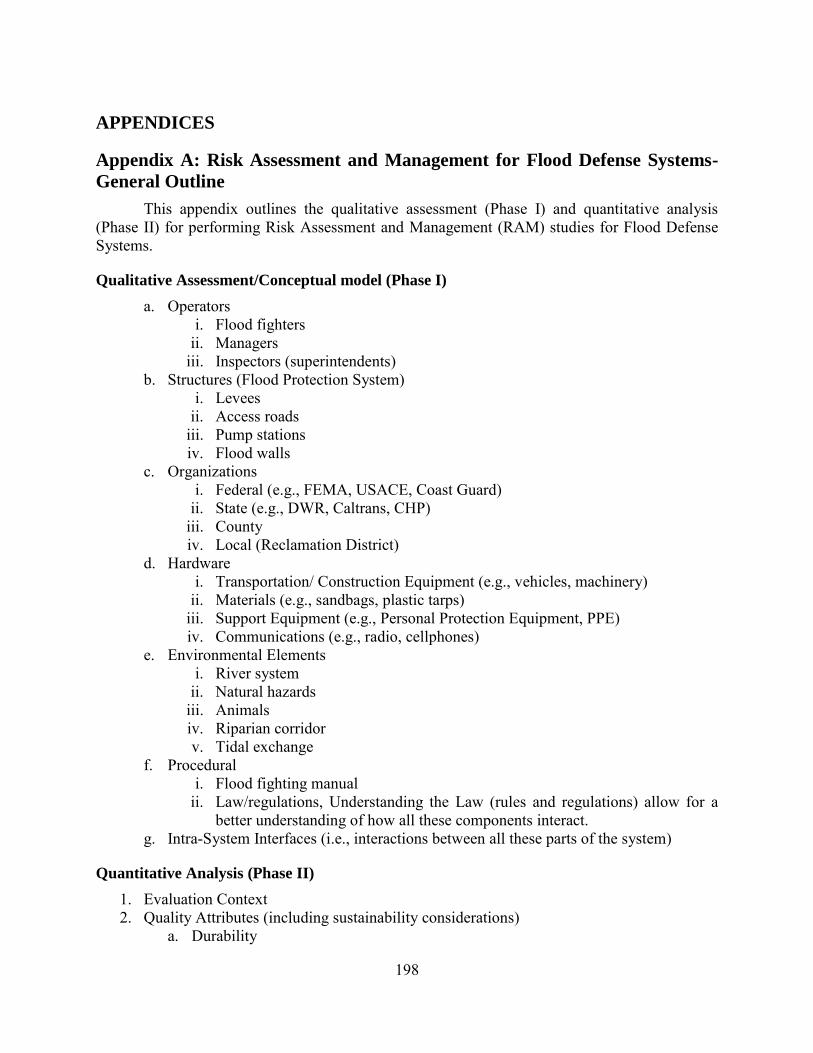
198
APPENDICES
Appendix A: Risk Assessment and Management for Flood Defense Systems-
General Outline
This appendix outlines the qualitative assessment (Phase I) and quantitative analysis (Phase II) for performing Risk Assessment and Management (RAM) studies for Flood Defense Systems.
Qualitative Assessment/Conceptual model (Phase I)
a. Operators i. Flood fighters
ii. Managers iii. Inspectors (superintendents)
b. Structures (Flood Protection System) i. Levees
ii. Access roads iii. Pump stations iv. Flood walls
c. Organizations i. Federal (e.g., FEMA, USACE, Coast Guard)
ii. State (e.g., DWR, Caltrans, CHP) iii. County iv. Local (Reclamation District)
d. Hardware i. Transportation/ Construction Equipment (e.g., vehicles, machinery)
ii. Materials (e.g., sandbags, plastic tarps) iii. Support Equipment (e.g., Personal Protection Equipment, PPE) iv. Communications (e.g., radio, cellphones)
e. Environmental Elements i. River system
ii. Natural hazards iii. Animals iv. Riparian corridor v. Tidal exchange
f. Procedural i. Flood fighting manual
ii. Law/regulations, Understanding the Law (rules and regulations) allow for a better understanding of how all these components interact.
g. Intra-System Interfaces (i.e., interactions between all these parts of the system)
Quantitative Analysis (Phase II)
1. Evaluation Context 2. Quality Attributes (including sustainability considerations)
a. Durability

199
b. Safety c. Compatibility d. Resilience e. Serviceability (focus of this work)
3. Definition of Failure Modes a. Identify dominant failure modes for evaluation
i. Historical failures ii. Hazards of interest
b. Failure metrics (closed form solutions to represent failure) i. Demand
ii. Capacity 4. Quantitative system definition (per failure modes)
a. Historical land use (e.g., Historical maps, topographic maps, air photos) b. Digital elevation models (i.e., Topography, Bathymetry) c. Soil Stratigraphy for Analyses
i. Regional Geology/Geomorphology 1. Deposit Age (i.e., Pleistocene, Quaternary, Holocene) 2. Features (i.e., abandoned channel courses, faults, crevasse splays)
ii. Fluvial Geomorphology 1. River channel changes 2. Scour holes 3. Sediment transport
iii. Geotechnical investigations 1. Soundings (i.e., Soil borings/Cone Penetration Testing) 2. Material characterization (i.e., In-situ and laboratory testing)
iv. Spatial Data Plotting (GIS), All jurisdictions and important information can be mapped on ArcGIS
v. Representative cross sections 1. Levee crest
a. Surface elevation from DEM b. Subsurface profile from geotechnical investigation c. Stratigraphic grouping
2. Cross sections a. Best case interpretation b. Worst case interpretation c. Most likely
vi. Representative material properties (by groups) 1. Group data per stratum 2. Uncertainty Characterization of Capacity Parameters
a. Identify uncertainty types b. Distribution type for each uncertainty type c. Median (50th percentile value) d. Std Type I, II, III, IV e. COV
5. Hazard Characterization (i.e., Quantify return periods for analyses) 6. Probabilistic Analysis. Development of Demand and Capacity (PDFs)
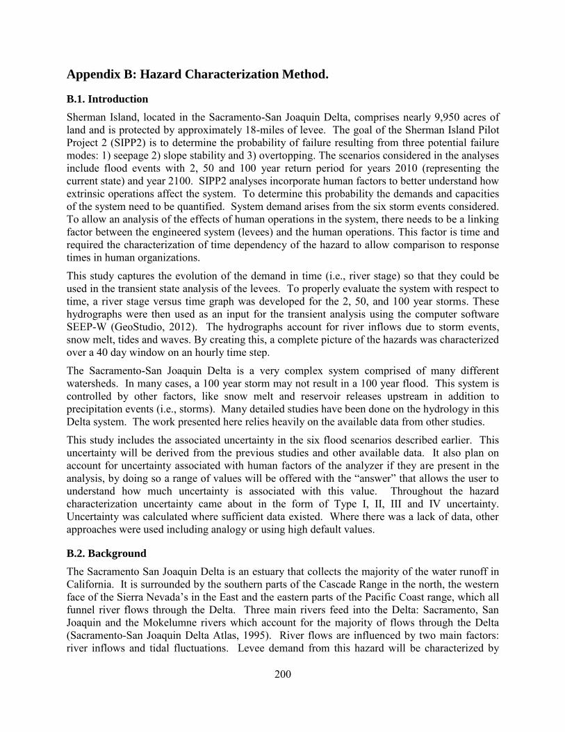
200
Appendix B: Hazard Characterization Method.
B.1. Introduction
Sherman Island, located in the Sacramento-San Joaquin Delta, comprises nearly 9,950 acres of land and is protected by approximately 18-miles of levee. The goal of the Sherman Island Pilot Project 2 (SIPP2) is to determine the probability of failure resulting from three potential failure modes: 1) seepage 2) slope stability and 3) overtopping. The scenarios considered in the analyses include flood events with 2, 50 and 100 year return period for years 2010 (representing the current state) and year 2100. SIPP2 analyses incorporate human factors to better understand how extrinsic operations affect the system. To determine this probability the demands and capacities of the system need to be quantified. System demand arises from the six storm events considered. To allow an analysis of the effects of human operations in the system, there needs to be a linking factor between the engineered system (levees) and the human operations. This factor is time and required the characterization of time dependency of the hazard to allow comparison to response times in human organizations.
This study captures the evolution of the demand in time (i.e., river stage) so that they could be used in the transient state analysis of the levees. To properly evaluate the system with respect to time, a river stage versus time graph was developed for the 2, 50, and 100 year storms. These hydrographs were then used as an input for the transient analysis using the computer software SEEP-W (GeoStudio, 2012). The hydrographs account for river inflows due to storm events, snow melt, tides and waves. By creating this, a complete picture of the hazards was characterized over a 40 day window on an hourly time step.
The Sacramento-San Joaquin Delta is a very complex system comprised of many different watersheds. In many cases, a 100 year storm may not result in a 100 year flood. This system is controlled by other factors, like snow melt and reservoir releases upstream in addition to precipitation events (i.e., storms). Many detailed studies have been done on the hydrology in this Delta system. The work presented here relies heavily on the available data from other studies.
This study includes the associated uncertainty in the six flood scenarios described earlier. This uncertainty will be derived from the previous studies and other available data. It also plan on account for uncertainty associated with human factors of the analyzer if they are present in the analysis, by doing so a range of values will be offered with the “answer” that allows the user to understand how much uncertainty is associated with this value. Throughout the hazard characterization uncertainty came about in the form of Type I, II, III and IV uncertainty. Uncertainty was calculated where sufficient data existed. Where there was a lack of data, other approaches were used including analogy or using high default values.
B.2. Background
The Sacramento San Joaquin Delta is an estuary that collects the majority of the water runoff in California. It is surrounded by the southern parts of the Cascade Range in the north, the western face of the Sierra Nevada’s in the East and the eastern parts of the Pacific Coast range, which all funnel river flows through the Delta. Three main rivers feed into the Delta: Sacramento, San Joaquin and the Mokelumne rivers which account for the majority of flows through the Delta (Sacramento-San Joaquin Delta Atlas, 1995). River flows are influenced by two main factors: river inflows and tidal fluctuations. Levee demand from this hazard will be characterized by

201
river stage which is a function of inflows to the Delta from rainfall, runoff and/or snowmelt runoff, tidal fluctuations, and channel conveyance characteristics (e.g., cross-section, roughness).
The scenarios considered in this study include three flood events with 2, 50 and 100 year return periods for the year 2010 (current conditions) and year 2100 (future conditions). Due to time and budget constraints, this study relied heavily on previous studies, supported by a limited statistical analysis.
River Inflows
Inflows from the river are controlled primarily by upstream releases. These releases are typically larger during storm events because as the reservoirs fill, more water needs to be released. Storms are not the only phenomena that cause high flows; one of the main concerns, especially in California, is snow melt (Bulletin #17B, 1982). A combination of storms and snow melt cause floods with different return periods. The goal of this study is to quantify the demand for each return period, regardless of the cause (and relative contribution from the different factors) of the flood.
Tidal Fluctuations
Tidal fluctuations vary in magnitude throughout the delta because of geometry, geography and natural dampening effects that occur (Topical Area: Flood Hazard, 2008). The tidal fluctuations occur on a smaller time scale (hours) unlike large river inflow which occurs over hours or days.
Wind
The main concern in this area is wind induced wave generation. These waves, if large enough, can cause overtopping and backside erosion. Wind induced waves are used extensively in overtopping analysis. They are also used to develop and adjust hydrographs used as input into seepage and slope stability analyses. In our work, the influence of wind induced waves on seepage was negligible due to their relatively short duration. Most of the information used in this study derived from the DRMS Wind-Wave Technical Memorandum (Topical Area: Wind-Wave Hazard 2008).
Historical Events
One of the most important resources for this study was historical events, which offer important insight into the system. During flood situations, readings are usually taken on a regular basis throughout the Delta. Three important events were examined: 1955, 1963 and 1997, all of which occurred in the months of December and January. All three events caused extensive flooding due of the associated warm front brought to the Sierras that accelerated snow melt. This coupled with extensive precipitation caused the floods and, in some cases, breaches in levee systems.
Using these historical events and the data previously discussed a better understanding of how river inflows are adjusted from storm events was achieved. In all cases, the start of the storm did not result in an instantaneous increase of river inflow. It takes time for water to move down stream, which means that the location of the storm’s centering is important to determine the response of the associated water ways around the point of interest.
Rather than spend extensive time determining where, when and how the storm hits and whether or not it brings about a warm front, this study focused on the magnitude of flows. Once the 2, 50
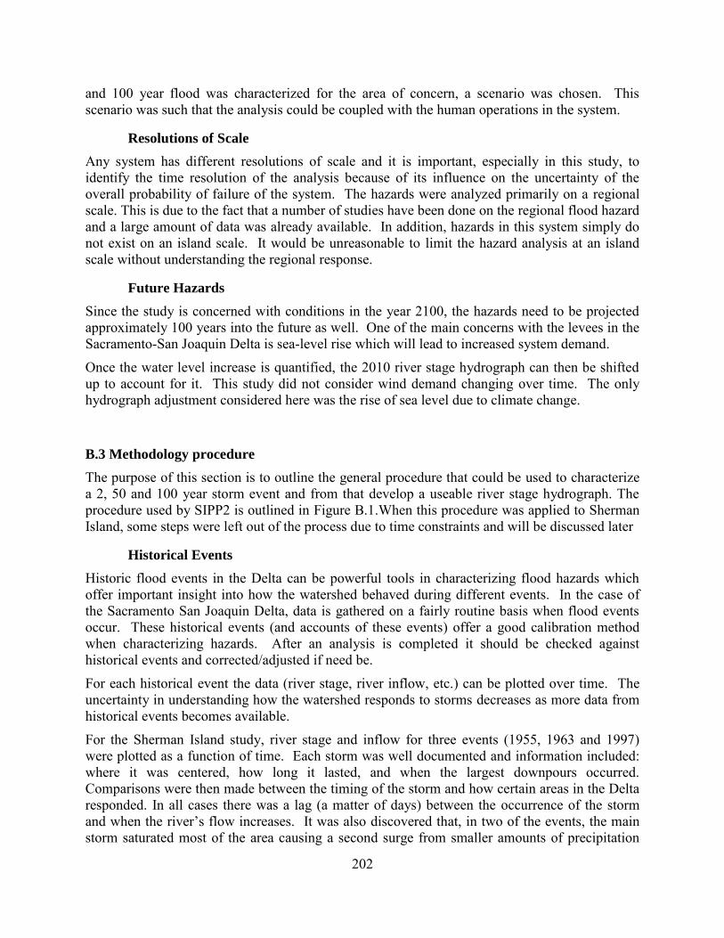
202
and 100 year flood was characterized for the area of concern, a scenario was chosen. This scenario was such that the analysis could be coupled with the human operations in the system.
Resolutions of Scale
Any system has different resolutions of scale and it is important, especially in this study, to identify the time resolution of the analysis because of its influence on the uncertainty of the overall probability of failure of the system. The hazards were analyzed primarily on a regional scale. This is due to the fact that a number of studies have been done on the regional flood hazard and a large amount of data was already available. In addition, hazards in this system simply do not exist on an island scale. It would be unreasonable to limit the hazard analysis at an island scale without understanding the regional response.
Future Hazards
Since the study is concerned with conditions in the year 2100, the hazards need to be projected approximately 100 years into the future as well. One of the main concerns with the levees in the Sacramento-San Joaquin Delta is sea-level rise which will lead to increased system demand.
Once the water level increase is quantified, the 2010 river stage hydrograph can then be shifted up to account for it. This study did not consider wind demand changing over time. The only hydrograph adjustment considered here was the rise of sea level due to climate change.
B.3 Methodology procedure
The purpose of this section is to outline the general procedure that could be used to characterize a 2, 50 and 100 year storm event and from that develop a useable river stage hydrograph. The procedure used by SIPP2 is outlined in Figure B.1.When this procedure was applied to Sherman Island, some steps were left out of the process due to time constraints and will be discussed later
Historical Events
Historic flood events in the Delta can be powerful tools in characterizing flood hazards which offer important insight into how the watershed behaved during different events. In the case of the Sacramento San Joaquin Delta, data is gathered on a fairly routine basis when flood events occur. These historical events (and accounts of these events) offer a good calibration method when characterizing hazards. After an analysis is completed it should be checked against historical events and corrected/adjusted if need be.
For each historical event the data (river stage, river inflow, etc.) can be plotted over time. The uncertainty in understanding how the watershed responds to storms decreases as more data from historical events becomes available.
For the Sherman Island study, river stage and inflow for three events (1955, 1963 and 1997) were plotted as a function of time. Each storm was well documented and information included: where it was centered, how long it lasted, and when the largest downpours occurred. Comparisons were then made between the timing of the storm and how certain areas in the Delta responded. In all cases there was a lag (a matter of days) between the occurrence of the storm and when the river’s flow increases. It was also discovered that, in two of the events, the main storm saturated most of the area causing a second surge from smaller amounts of precipitation
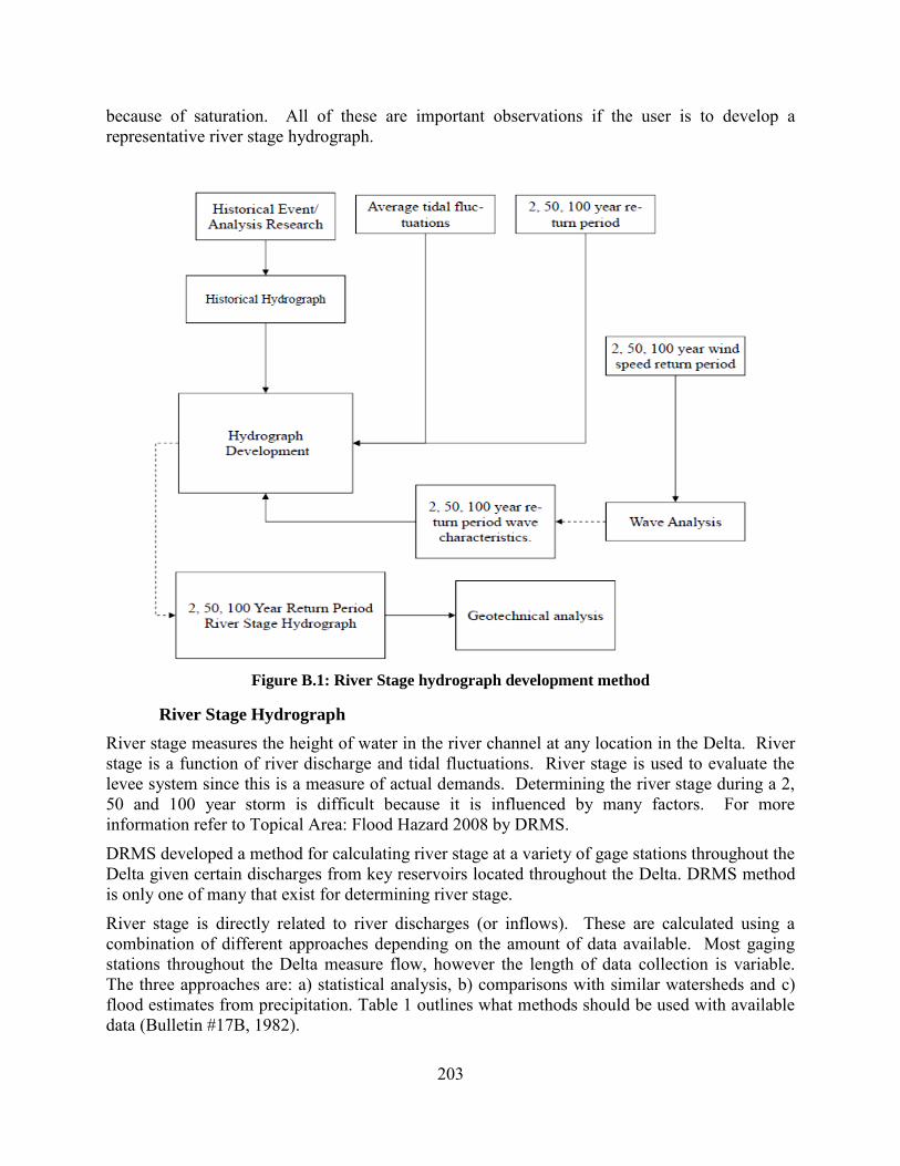
203
because of saturation. All of these are important observations if the user is to develop a representative river stage hydrograph.
Figure B.1: River Stage hydrograph development method
River Stage Hydrograph
River stage measures the height of water in the river channel at any location in the Delta. River stage is a function of river discharge and tidal fluctuations. River stage is used to evaluate the levee system since this is a measure of actual demands. Determining the river stage during a 2, 50 and 100 year storm is difficult because it is influenced by many factors. For more information refer to Topical Area: Flood Hazard 2008 by DRMS.
DRMS developed a method for calculating river stage at a variety of gage stations throughout the Delta given certain discharges from key reservoirs located throughout the Delta. DRMS method is only one of many that exist for determining river stage.
River stage is directly related to river discharges (or inflows). These are calculated using a combination of different approaches depending on the amount of data available. Most gaging stations throughout the Delta measure flow, however the length of data collection is variable. The three approaches are: a) statistical analysis, b) comparisons with similar watersheds and c) flood estimates from precipitation. Table 1 outlines what methods should be used with available data (Bulletin #17B, 1982).

204
A statistical analysis uses available data with a Log Pearson III (LPIII) distribution to predict return periods. A statistical analysis should always be included in a hydrologic study, but can only be the sole analysis if the available record is 50 or more years long. The LPIII distribution should be the distribution of choice unless it can be shown otherwise that alternate distribution fits the given data better than the LPIII (Bulletin 17B, 1982). If the record is limited in length a comparison can be done using data from a similar watershed. This is especially useful when the alternate watershed has a long unbroken data record. Mathematical procedures have been developed to adjust short term records if a long record exists on a similar watershed (Bulletin 17b, 1982).
Finally, developing a relationship between precipitation, either from rainfall or snowmelt, and flow provides important insight as to how the region will react to a storm. However, the procedures for converting the precipitation to discharge require a considerable amount of effort if no relationship previously exists. One way of developing this is through observed events on the watershed. If accurate measurements were taken of precipitation and discharge during these events, than a relationship can be developed between the two (Bulletin 17B, 1982).
Once the river discharges and their frequency are determined, they can be turned into river stages by looking at the cross section. However, the details of this are not discussed in this study since many methods already exist for determining the frequency and return period of the river stages in certain areas given historical data. For more information refer to Bulletin 17B, 1982.
Analyses to Include Length of Available Record (years)
10 to 24 25 to 50 50 or more
Statistical Analysis x x x
Comparison with similar watersheds x x
Flood estimates from precipitation x Table B.1: Analyses to be Included (Bulletin 17B, 1982)
Tidal Fluctuation
Tidal fluctuations vary throughout the Delta. It is important however to understand how tidal fluctuations affect the river stage and discharge at areas of interest in the study. To calculate the magnitude of the fluctuation of tides, historical data can be collected from a gage station closer to the bay or open water. These gage stations are affected less by river flows and vary mainly due to tidal influences during most parts of the year (Topical Area: Flood Hazard, 2008).
If tides will be used in a statistical analysis, the data needs to be normalized to a chosen height to account for sea level rise. Throughout a collection of tidal data, there is an upward trend that should be adjusted so present day conditions can be evaluated (Topical Area: Flood Hazard, 2008).
The alternate method for determining tidal fluctuations involves the observed river stage or river flow changes through time during a “low flow” period. Historically on any watershed there are
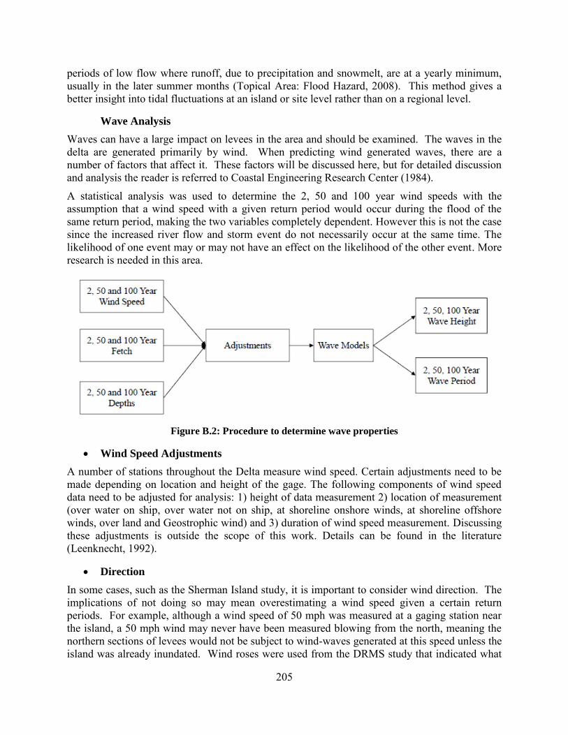
205
periods of low flow where runoff, due to precipitation and snowmelt, are at a yearly minimum, usually in the later summer months (Topical Area: Flood Hazard, 2008). This method gives a better insight into tidal fluctuations at an island or site level rather than on a regional level.
Wave Analysis
Waves can have a large impact on levees in the area and should be examined. The waves in the delta are generated primarily by wind. When predicting wind generated waves, there are a number of factors that affect it. These factors will be discussed here, but for detailed discussion and analysis the reader is referred to Coastal Engineering Research Center (1984).
A statistical analysis was used to determine the 2, 50 and 100 year wind speeds with the assumption that a wind speed with a given return period would occur during the flood of the same return period, making the two variables completely dependent. However this is not the case since the increased river flow and storm event do not necessarily occur at the same time. The likelihood of one event may or may not have an effect on the likelihood of the other event. More research is needed in this area.
Figure B.2: Procedure to determine wave properties
Wind Speed Adjustments
A number of stations throughout the Delta measure wind speed. Certain adjustments need to be made depending on location and height of the gage. The following components of wind speed data need to be adjusted for analysis: 1) height of data measurement 2) location of measurement (over water on ship, over water not on ship, at shoreline onshore winds, at shoreline offshore winds, over land and Geostrophic wind) and 3) duration of wind speed measurement. Discussing these adjustments is outside the scope of this work. Details can be found in the literature (Leenknecht, 1992).
Direction
In some cases, such as the Sherman Island study, it is important to consider wind direction. The implications of not doing so may mean overestimating a wind speed given a certain return periods. For example, although a wind speed of 50 mph was measured at a gaging station near the island, a 50 mph wind may never have been measured blowing from the north, meaning the northern sections of levees would not be subject to wind-waves generated at this speed unless the island was already inundated. Wind roses were used from the DRMS study that indicated what
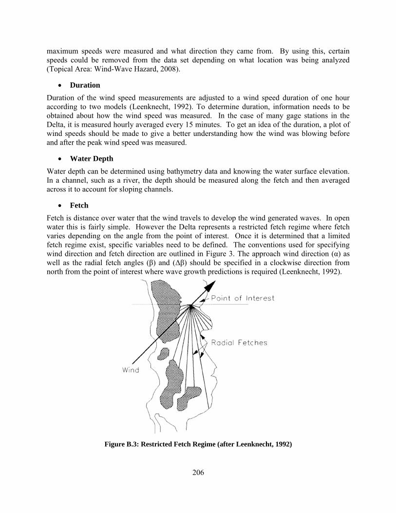
206
maximum speeds were measured and what direction they came from. By using this, certain speeds could be removed from the data set depending on what location was being analyzed (Topical Area: Wind-Wave Hazard, 2008).
Duration
Duration of the wind speed measurements are adjusted to a wind speed duration of one hour according to two models (Leenknecht, 1992). To determine duration, information needs to be obtained about how the wind speed was measured. In the case of many gage stations in the Delta, it is measured hourly averaged every 15 minutes. To get an idea of the duration, a plot of wind speeds should be made to give a better understanding how the wind was blowing before and after the peak wind speed was measured.
Water Depth
Water depth can be determined using bathymetry data and knowing the water surface elevation. In a channel, such as a river, the depth should be measured along the fetch and then averaged across it to account for sloping channels.
Fetch
Fetch is distance over water that the wind travels to develop the wind generated waves. In open water this is fairly simple. However the Delta represents a restricted fetch regime where fetch varies depending on the angle from the point of interest. Once it is determined that a limited fetch regime exist, specific variables need to be defined. The conventions used for specifying wind direction and fetch direction are outlined in Figure 3. The approach wind direction (α) as well as the radial fetch angles (β) and (Δβ) should be specified in a clockwise direction from north from the point of interest where wave growth predictions is required (Leenknecht, 1992).
Figure B.3: Restricted Fetch Regime (after Leenknecht, 1992)
207
Wave Characteristics
The USACE’s Shore Protection Manual offers two ways to predict wave height and period: one for shallow or transitional waters and one for deep waters. Deep water is used for more open ocean environments. Because of the transitional bank near the levees, it is better to use the shallow water predictions. The models used to predict wave height and period of shallow water conditions are shown in Equation 3-39 and 3-40 in the USACE Shore Protection Manual.
Vegetation Effects
The presence of vegetation affects the wave loading on the levee system. The USACE Shore Protection Manual offers an approximate method for estimating the growth or decay of wind waves passing over areas with high values of bottom friction. Their model assumes that the high bottom friction can be accounted for by adjusting the fetch length. The procedure is outlined in the USACE Shore Protection Manual and will not be discussed here (Shore Protection Manual, 1984). There is however a great deal of uncertainty associated with this model that should be quantified for the analysis.
Statistical Analysis
Wave analysis needs to be completed for different return periods. In order to do this correctly, the inputs into the wave analysis need to be adjusted for the 2, 50 and 100 year return periods. Therefore, fetch, wind speed and water depth will vary depending on the return period. This can be done in a variety of ways. For wind, it is assumed that a 50 year wind will occur at the same time as a 50 year storm thus making the two events concurrent. The fetch and water depths are affected by the river stage, so the 50 year fetch needs to be analyzed at the 50 year flood. To account for Type I uncertainty, a Monte Carlo simulation should be run with the model and given inputs, because each parameter will have uncertainty associated with it. A Monte Carlo simulation will then provide a distribution of wave heights and periods.
River Stage Hydrograph Development
Once information is gathered on the historical events, river stage levels, tidal fluctuation, wave height and period, a river stage hydrograph that incorporates all these factors can be created. The following steps can be used to determine a conditional river stage hydrograph:
1. Determine the time duration of the hydrograph (e.g., hours, days, weeks) 2. Based on historical hydrograph determine when the peak of the storm will occur. 3. Determine the approximate duration of the peak river stage based on historical events. 4. Make the storms peak equal to the river stage of interest, for example the 100 year river
stage hydrograph will have a peak with magnitude of the 100 year river stage that was determined.
5. Add tidal fluctuations by adding and subtracting to every step the difference in water level due to tidal fluctuations
6. If river stage hydrograph resolution is small enough to capture the influence of waves, then add the effect of waves.
208
B.4. Application to Sherman Island study
This section outlines how the SIPP2 study developed the 2, 50 and 100 year river stage hydrographs. The method is relatively simple and some steps were omitted due to time and budget limitations. Nevertheless the results and conclusions are believed to realistically capture the key elements of the problem. SIPP2 relied primarily on past studies’ results for river stages, historical hydrographs and sea level rise studies. Integrating all this information with tidal fluctuation data in the area, river stage hydrographs were developed.
For this study, three historical events were studied: the December 1955-January 1956 event, the January 1963 event and the January 1997 Event. For each of these events data was collected on river flows and stage heights throughout the delta during the flood and documented in reports by Rantz (Rantz, 1963a, 1963b).
December 1955 – January 1956 Event
These floods were caused be a series of storms from December 15 to January 27; three occurring between December 15 and 27 and three more from January 2 to 27. In all but a few areas, the storm from December 21 to 24 was the most severe. The storms were accompanied by high wind velocities and high temperatures. This warm front caused large amounts of snow melt and record-breaking runoff (Rantz, 1963a). Saturation from the first set of storms that came from the event caused larger river inflow from smaller precipitation events.
January 1963 Event
The first rainfall of this event occurred on January 28, 1963 to terminate a record-breaking 42-day winter drought. This event involved two warm front systems. The first crossed California on January 30 and was centered over the Yuba, American and Truckee River basins. The second was centered about 150 miles to the south over the Kweah, Tule, and Kern River basins and crossed the state on January 31. Almost all the precipitation was concentrated in a 72-hour period between January 29 and February 1 (Rantz, 1963b). The primary difference between this and the 1955-1956 event was the volume of storm runoff produced. Because the 1963 event occurred over a relatively short time period, the runoff was not particularly notable. Nevertheless, reservoir storage attained a high level. Figure B.4 shows the area of flooding in California (Rantz, 1963b).
Hydrograph of Historical Events
Flow information from the Sacramento River and San Joaquin River was gathered on each of these events. Using descriptions of the storm, time ‘0’ was defined as 8 days before the beginning of each of the events. The river inflow, measured in cfs (cubic feet per second) was than plotted on the same graph to compare the storm events as shown on Figure B.5.

209
Figure B.4: Flood affected area during the 1963 event
Figure B.5: Historical Hydrographs

210
River Stage Hydrographs
In order to create a representative river stage hydrograph for the 2, 50 and 100 year flood levels, these levels must first be determined. Bulletin 17B offers the formal procedure and it was briefly outlined earlier. Due to time and budget constraints this study relied on results from the Delta Risk Management Study (DRMS, 2012). DRMS used a statistical regression combining possible river flows and tidal levels to develop a river stage versus return period graph. There were nearly a million runs (over 900,000) with each event having its own probability of occurrence.
SIPP2 used results presented by DRMS at the Venice Island station. Figure B.6 shows the return period versus river stage based both on the model developed by DRMS and a logarithmic regression run on available river stage data. The 20%, 50% and 80% confidence intervals are also given. Since the regression and model values are within fractions of a foot of each other, the regression equation was used to determine the river stage at a given time interval.
Figure B.6: River stage at Venice station from DRMS study
River Stage, feet NAVD
Return Period 20% CL 50% CL 80% CL
2 7.82 7.86 7.9
50 10.2 10.75 11.3
100 10.76 11.38 12 NAVD- North American Vertical Datum, 1988
Table B.2: River stage return periods

211
Tidal Considerations
The river stage in the previous section accounts for tidal influences. However the method did not determine how long this river stage will be at this level. The time factor is crucial in this study. To determine the length of a tidal influence, a tidal cycle was analyzed over a 30 day period during a low inflow season in 2010. A low inflow season occurs during the late summer months when the snow has melted and runoff is minimal. By looking at a low inflow the effects on river stage are mostly due to tidal fluctuations. At each time step, the difference from the mean river stage to the actual measured value was calculated, the magnitude of this difference was called delta. Figure B.7 shows an example of what delta looks like on the river stage hydrograph during a low inflow season. The average, or river stage is represented by the dotted line, the distance from the average value to the measured value at time step ‘n’ is the magnitude of the tidal influence at that time step. This delta value represents the change in river stage due to tide and is now factored into the hypothetical river stage hydrograph.
Figure B.8 shows an actual river stage hydrograph during late August at the Antioch Gaging station near the southern site. The fluctuations are due to tidal effects. The difference at every hour (since this is when measurements were taken) between the average value and the measured value are the delta values that were added to the river stage hydrograph to account for tide. Figure B.9 shows the average river stage hydrograph corresponding to the current conditions (2010).
Figure B.7: Example of tidal fluctuations
Figure B.8: Tidal fluctuations at Antioch station during low inflow season
0
1
2
3
4
5
6
7
0 100 200 300 400
Riv
er
Stag
e (
NA
VD
88
ft)
Time (hours)
River Stage Data
average

212
Future Adjustments
For the 2100 hydrograph adjustments were made to the 2010 hydrograph to account for sea level rise. A number of studies and models were used to estimate sea level rise and they are summarized in Table B.3. There was a wide range of predictions of sea level rise (from 2.3 to 6.5 feet), the average of all these studies was used (4.1 feet). During the Monte Carlo simulation for the geotechnical analysis, this value will be sampled to determine possible water heights and capture uncertainty. To adjust the river stage hydrograph, the average value was used. The results of the adjustment are shown in Figure B.10.
Source Rise (ft)
CALFED Independent Science Board 2.3
CALFED Independent Science Board 3.0
Healey, 2007 6.5
Noble Consultants,2009 4.8 Table B.3: Summary of sea level rise predictions
Discussion
The purpose of the hazard characterization was to provide three possible scenarios for the 2, 50 and 100 year events. These scenarios are based on tidal fluctuations, a known river stage and historical events. These values are not meant to be strictly accurate as far as predicting how the water shed will respond to this event; rather it is to provide a useable situation where the water level reaches the maximum height for a duration similar to those of historical events in the area. One shortcoming of this study is the wind generated wave analysis. The effect of these waves on the seepage analysis very limited, but they are significant for the overtopping and slope stability analysis. The wind-wave characterization is outside the scope of this work.
Results
Using the historical events, a known river stage and tidal fluctuations, three river stage hydrographs are presented in Figures B.9 and B.10 for the current and future conditions, respectively. Time zero, is assumed as eight days prior to the start of the storm. This time gap is important so that Human-Organizational Factors (HOF) can be considered during the buildup to the maximum water level. The peak water levels and their durations were based entirely on historical events. In these scenarios, a large storm will cause the maximum peak, then there is a decline in river stage followed by another smaller rainfall that causes a quicker peak due to the saturation of the ground from the previous storm. This was seen in many historical events and was therefore replicated in the development of the scenarios. Figure B.10 shows the river stage hydrographs for the year 2100, which were adjusted only for sea level rise. Increased inflow was considered, but the DRMS report concluded that increased inflow from climate change would not be significant enough, therefore was not considered in this study. These hydrographs, along with their upper and lower bounds, were used in the geotechnical analysis. The study considers upper and lower bounds for the 2, 50 and 100 year river stages and the ranges of possible sea level rise. These different possibilities will be accounted for using Monte Carlo simulation and other methods used in the probabilistic geotechnical analysis.
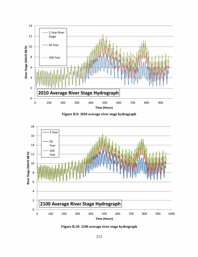
213
Figure B.9: 2010 average river stage hydrograph
Figure B.10: 2100 average river stage hydrograph
0
2
4
6
8
10
12
14
0 100 200 300 400 500 600 700 800 900
Riv
er
Stag
e (
NA
VD
88
ft)
Time (Hours)
2010 Average River Stage Hydrograph
2 Year RiverStage
50 Year
100 Year
0
2
4
6
8
10
12
14
16
18
0 100 200 300 400 500 600 700 800 900 1000
Riv
er
Stag
e (
NA
VD
88
ft)
Time (Hours)
2100 Average River Stage Hydrograph
2 Year
50Year
100Year

214
APPENDIX C: River Stage Hydrographs
Figure C.1. Average River Stage Hydrographs for Current (2010) Conditions.
0
2
4
6
8
10
12
14
0 200 400 600 800 1000
Riv
er
Stag
e (
NA
VD
88
ft)
Time (Hours)
2010 100-Year Average River Stage Hydrograph
0
2
4
6
8
10
12
14
0 200 400 600 800 1000
Riv
er
Stag
e (
NA
VD
88
ft)
Time (Hours)
2010, 50-Year Average River Stage Hydrograph
0
2
4
6
8
10
0 200 400 600 800 1000
Riv
er
Stag
e (
NA
VD
88
ft)
Time (Hours)
2010, 2-Year Average River Stage Hydrograph
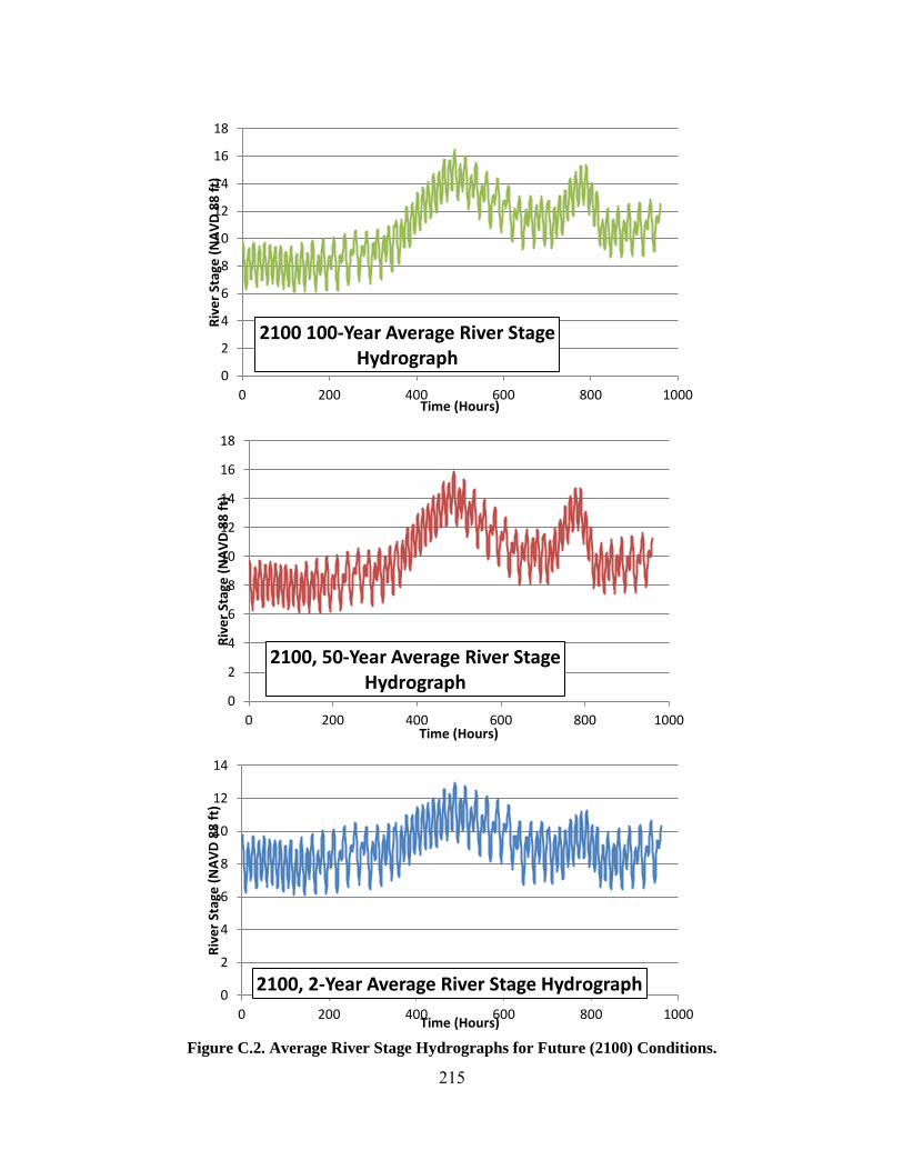
215
Figure C.2. Average River Stage Hydrographs for Future (2100) Conditions.
0
2
4
6
8
10
12
14
16
18
0 200 400 600 800 1000
Riv
er
Stag
e (
NA
VD
88
ft)
Time (Hours)
2100 100-Year Average River Stage Hydrograph
0
2
4
6
8
10
12
14
16
18
0 200 400 600 800 1000
Riv
er
Stag
e (
NA
VD
88
ft)
Time (Hours)
2100, 50-Year Average River Stage Hydrograph
0
2
4
6
8
10
12
14
0 200 400 600 800 1000
Riv
er
Stag
e (
NA
VD
88
ft)
Time (Hours)
2100, 2-Year Average River Stage Hydrograph

216
APPENDIX D: SITE CHARACTERIZATION
Introduction
Due to subsidence and the non-engineered design and construction of many of the levees in the Delta, islands are at risk from flooding due to a variety of failure modes. Sherman Island lies near the mouth of the Delta, and so it is subject to tidal fluctuations as well as river flows. The Sherman Island Pilot Project 2 (SIPP2) aims to develop a method to quantify uncertainty at all levels of risk calculation in the flood protection structures (levees) of Sherman Island, located in the Sacramento-San Joaquin River Delta. This study aims to improve upon the procedures employed by URS in their Delta Risk Management Study (DRMS) by focusing on a less-emphasized aspect of their study: storm-based flood risk.
The study is resource-constrained, so the study will be conducted using two cross sections of the levee ring and will consider two failure modes: seepage and slope stability. A probability of failure (Pf) versus time curve will be developed for each failure mode, and the Pf will be assessed for two different conditions: current conditions as they exist (2010) and in the future (2100). At every analysis step, uncertainty will be accounted for and quantified to the extent possible.
The first step in risk assessment and management (RAM) is to define the system, or in the case of SIPP2, characterize the study site. The single levee cross-section is on the southern portion of the island, adjacent to the San Joaquin River, and not far from the historic (1964) failure at Maybury Slough. Multiple scales of resolution are addressed in the site characterization, moving from regional, to island-wide, to site-level scale. The various components of the system are defined and accounted for, and this information contributes to the construction of a cross-section of the levee ring. This profile, complete with above ground and subsurface characteristics, is then loaded into the methods for the various failure modes.
This appendix outlines the method used in this study to develop the cross section for the northern, southern and piezometer (used for Bias correction) site locations on Sherman Island and account for uncertainty in the interpolation and extrapolation of the available boring logs. It also outlines how soil properties were determined and how uncertainty was characterized in the properties. The cross section and soil properties along with their associated uncertainty were used in the seepage, slope stability and overtopping analysis.
Background
Traditional Methods/State of Practice
The current state of practice for geotechnical engineering is to develop a cross section for the site of interest after a certain amount of exploration is done at the site. However, what is lacking is the ability to account for more “accurate” cross sections from more thorough field investigations. For example, for a certain site one engineer may use ten borings to create a cross section while another engineer uses only two. The result is two cross sections that are used for analysis; however one is more “accurate” than the other. Standard of practice does not currently have a method to account for uncertainty created by field investigations when developing cross sections.

217
Site Selection
SIPP2 chose two site locations to run the analyses on, one on the Southern edge of the island, slightly to the east of the Antioch Bridge, and the other in the Northern part of the island, across the channel from the Southern edge of Decker Island, as shown in Figures D.1 through D.4.
The Sherman Island levee system is comprised of much more than these two sites; in fact it is comprised of an infinite number of sites. To properly analyze the system, a cross section would be developed at every location around the entire levee ring. As this is not realistic; a more practical approach is to strategically select locations that are representative of long segments on the ring. The more locations selected, the smaller the uncertainty. This work aims at proof-of concept, so only three sites were selected.
Stratigraphy
Soil Stratigraphy is the depth and thickness of each soil type in the cross section. The stratigraphy is developed by plotting the elevation of the surface, and on that placing the boring logs. The different soil layers are then interpolated from one boring to the next based on regional site characterization. When trying to work with regions outside of the soil borings, extrapolating, the uncertainty is much greater since there is no real understanding of what could be happening beyond the boring logs. This creates a complex type of uncertainty that will be addressed in the next section.
Uncertainty
A great deal of uncertainty is present in the Site Characterization for a risk assessment, especially when it involves developing stratigraphy. This process is very much information dependent and, since a model is being developed, Type II (model uncertainty) is present. However, no matter how much information is available, it still requires human interpretation, thus Type III is also present. This study has developed methods by which this uncertainty can be accounted for through the use of bounding the problem with best/worst case scenarios.
Topography/Bathymetry
Obtaining the topography at the desired cross section is the first step in its development. Methods do exist to obtain highly accurate topography data. However, sometimes the available data sets are limited. For this study high resolution digital terrain models done by USGS were used for cross section development. Figure D.5 shows a regional location of where the terrain models are available. The files are available for use with ArcGIS® and from the program, the topography can be developed. All elevations were taken with respect to the 1988 North American Vertical Datum (NAVD88). All vertical measurements for this study are with respect to NAVD88.
The digital terrain models were developed on a 10m by 10m grid and the elevations within that were averaged. If elevations were not accurate to 1m they were adjusted (Coons, 2008). Bathymetry data has a different accuracy since these elevations are under water and less easy to acquire. Again, methods do exist today that allow for more accurate measurements, but they were not available for use in this study. There was also no available information on the accuracy of the Bathymetry data. For this reason, both the topography and Bathymetry used in this study were assumed to have a vertical accuracy of 1.5 m (4.9 ft). This is somewhat of an arbitrary number. If this was found to be crucial to the study, it could be researched in more detail.

218
Figure D.11: Site Locations for Study
Figure D.12: South Site Cross Section Location
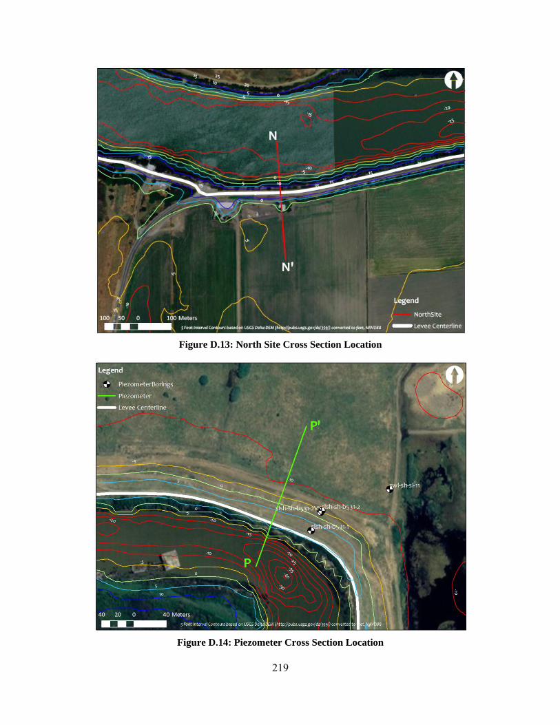
219
Figure D.13: North Site Cross Section Location
Figure D.14: Piezometer Cross Section Location

220
To account for this uncertainty, bounds were used on the topography. This is not to say that the entire cross section was lowered by 5 ft and rose by 5 ft, this would not create the “worst” and “best” case scenario. These scenarios are directly related to what failure mode is being examined. For example the best case scenario for seepage (having a low levee crest so head levels are low) is not the best case for overtopping, where a high levee crest is favorable. This is where it is important to have understanding of how the failure modes work as an engineer. The site characterization will be geared entirely for seepage since this is the only failure mode that has been analyzed at this point.
Figure D.6 shows how the lowest inland topography and the highest possible levee crest that can be created given the accuracy of the topographical data will result in the worst case situation for seepage. Appendix K shows the bounded topography and bathymetry for both the South Site location (year 2010 and 2100) and Piezometer Site Location.
Figure D15: Location of Digital Terrain Maps

221
66.9955
h1
28.0328 h2
Highest possible crest
Lowest inland topography
Highest inland topography
lowest possible crest
Figure D.16: Topography Variation
Boring Logs
A major factor of uncertainty associated with site characterization is the amount of field investigation done. For this study, only traditional Standard Penetration Tests (SPT) investigations will be discussed. There are other methods of investigation including Cone Penetration Test (CPT) which has a much different approach. The SPT requires a boring to be made in the ground and samples are retrieved by pushing a sampler through the soil. The sample is pushed by dropping a hammer on a sampling tube, forcing the tube through the soil. The blow counts used to push the tube through the soil also gives insight into the type of soil and its properties.
In general, the more borings (or soundings) completed, the more accurate the developed cross section. If, for example, a boring was taken every foot across the cross section, this cross section would be much more accurate than one created using borings every 10 feet.
Besides horizontal interpolation and extrapolation uncertainty, there is also uncertainty associated with the boring logs themselves. The rate of sampling and logging greatly influences the uncertainty associated with the cross section. As the boring is drilled, the depth and type of material is logged. However the exact depth and exact type of material is never for certain, especially when a young inexperienced engineer is logging. Therefore there is uncertainty associated with where exactly one soil type ends and another begins.
The frequency of sampling from SPT samplers is also another factor that affects uncertainty. The more frequent the samples, the more accurate the vertical stratigraphy. For example, if
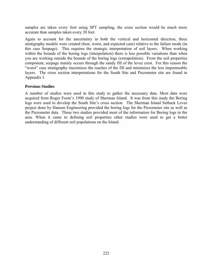
222
samples are taken every foot using SPT sampling, the cross section would be much more accurate than samples taken every 20 feet.
Again to account for the uncertainty in both the vertical and horizontal direction, three stratigraphy models were created (best, worst, and expected case) relative to the failure mode (in this case Seepage). This requires the strategic interpretation of soil layers. When working within the bounds of the boring logs (interpolation) there is less possible variations than when you are working outside the bounds of the boring logs (extrapolation). From the soil properties component, seepage mainly occurs through the sandy fill of the levee crest. For this reason the “worst” case stratigraphy maximizes the reaches of the fill and minimizes the less impermeable layers. The cross section interpretations for the South Site and Piezometer site are found in Appendix I.
Previous Studies
A number of studies were used in this study to gather the necessary data. Most data were acquired from Roger Foote’s 1990 study of Sherman Island. It was from this study the Boring logs were used to develop the South Site’s cross section. The Sherman Island Setback Levee project done by Hanson Engineering provided the boring logs for the Piezometer site as well as the Piezometer data. These two studies provided most of the information for Boring logs in the area. When it came to defining soil properties other studies were used to get a better understanding of different soil populations on the Island.
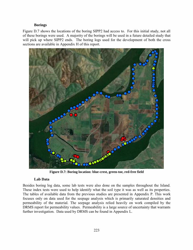
223
Borings
Figure D.7 shows the locations of the boring SIPP2 had access to. For this initial study, not all of these borings were used. A majority of the borings will be used in a future detailed study that will pick up where SIPP2 ends. The boring logs used for the development of both the cross sections are available in Appendix H of this report.
Figure D.7: Boring location: blue-crest, green-toe, red-free field
Lab Data
Besides boring log data, some lab tests were also done on the samples throughout the Island. These index tests were used to help identify what the soil type it was as well as its properties. The tables of available data from the previous studies are presented in Appendix P. This work focuses only on data used for the seepage analysis which is primarily saturated densities and permeability of the material. The seepage analysis relied heavily on work compiled by the DRMS report for permeability values. Permeability is a large source of uncertainty that warrants further investigation. Data used by DRMS can be found in Appendix L.

224
Stratigraphy
The stratigraphy of Sherman Island is dependent on the regional geology of the area. A regional geology study was done first to categorize main soil layers. From here the soil borings were used to develop the cross section for the South Site and Piezometer Site using these general soil layers. By breaking the stratigraphy into general soil layers, the properties for these layers can be determined and used throughout the island if the regional geology agrees. The process is outlined in Figure D.8. The soil units are defined using Unified Soil Classification System (USCS), and the soil properties can be characterized statistically to account for uncertainty both within the soil unit itself and variations throughout the Island.
Figure D.8: Site Study Process
Regional Geology
The regional geology studies of the area offer important insight into the cross sections that are developed. For the Sacramento San Joaquin Delta, Brian Atwater Geological Maps of 1982 were used to develop an understanding of the geological history of Sherman Island. Figure D.9 shows a scaled redrawn version of the Atwater map of Sherman Island.
The Sacramento San Joaquin Delta overlies 5 to 10 km of sedimentary deposits. Most of this material, including natural gas deposits, accumulated during a time when the area was a marine environment about 175 million to 25 million years ago. Younger deposits are usually described as non-marine, as some were formed in shallow seas and estuaries (Atwater, 1982). The deposits in the area have been laid down over the past one million years (late Quaternary time) through cycles of deposition, no deposition and erosion.
One important cycle to the delta is the rise and fall in sea level relative to the land. The result of this in the Delta is soft peat and mud that have accumulated during the past 7,000 years. This material was deposited between major ice ages when sea level was high enough for tidewater to invade the Central Valley and create extensive wetlands that covered most of the Delta before agricultural reclamation.
Another important cycle to consider is the waxing and waning of glaciers in the Sierra Nevada. These glaciers have been used to explain a widespread sequence of alluvial fan deposits throughout the Delta. The glaciation of the Sierra Nevada is also the cause of windblown (eolian) sand, which extends southwestward from an area between Antioch and the Bradford Island. Deposits of tidal waterways are chiefly clay and silt with low organic content. Locally they are sandy, particularly along a major prehistoric channel at Sherman Island.
Figure D.9 outlines the map units on the Atwater maps. The ones’ of interest for Sherman Island are the “man-made and tidal deposits” as well as the “Antioch and vicinity.” Sherman Island is shown covered by Qpm which represents peats and mud of tidal wetlands and waterways from the Holocene. Underlying that is Qia which is intermediate alluvium of Antioch and vicinity
Regional Geology Study
General Soil Units (USCS)
Statistic Soil Properties per Soil
Units

225
from the upper Pleistocene. The deeper layers are described as Qoa which are the oldest alluvium of Antioch and vicinity, still part of the upper Pleistocene.
More recently, there have been issues of sediment transport in the waterways. Dredging has taken place to reduce the sediment in the channel, but the dredging is not done on a regular basis. For this reason, there is a large amount of uncertainty surrounding the base of the channel as the sediment that exists there.
Figure D.9: Regional Geology at Sherman Island (Atwater, 1982)
Soil Units
After the regional geology study and examination of the borings, four distinct soil strata were used in characterizing the sites. Figure D.10 also outlines the representative hatching that will be used for each layer. These are also how the soil units exist relative to each other as far as depositional history. The boring logs do not specify these exact strata, rather the Unified Soil Classification System (USCS) was used to describe the soil layers. It was up to the engineer to determine what strata each of the soil layers belonged. The levee fill is described as the man made fill used to create the levees and is not found throughout the entire site. The same is true for the other layers, the relative deposition will remain, but the thickness varies throughout the site.
Each layer and each location will also have its own set of engineering soil properties. Each will have an average and standard deviation. These values are determined using various borings throughout the island as specified in Figure D.7. Note that a majority of borings were taken at the crest, which means the uncertainty in the crest values will be less than the uncertainty of the free field which has fewer samples. This is important because some engineering properties, such as strength, change relative to where they are on the levee (beneath the crest, toe or free field).

226
SP
OL
SM
SP
Man made fill
New alluvial
deposits/sea level
fluctuations
Old alluvial
deposits
USCS
Class
ifica
tion
Hat
ching
Reg
iona
l
Geo
logy
Figure D.10: Sherman Island Soil Units
Cross Section Development
Three locations were chosen for a cross section development. Only two will be discussed in full: the South Site cross section and the Piezometer Site cross section. To develop these cross sections the boring logs were uploaded to the gINT® software. These were then exported out to AutoCAD® where the cross sections were drawn. This study uses four borings from Roger Foote’s 1990 study in the area to develop the south site cross-section. Approximately 2 were in the crest of the levee, one was in the toe and one in the free field.
The Piezometer site is to the west of the South Site. This site was used to develop a Bias correction for the models used in the method being developed. This site was chosen because of the available piezometer data in the area. Three borings were used to characterize this site.
Soil properties
For the soil characterization, the soil properties will focus on those pertaining to the seepage analysis. This process will be followed for overtopping and slope stability as well, and in the process the necessary soil properties required for the analysis will be determined.
For this risk assessment, the soil properties need to be characterized with uncertainty. To do so, they need to be given a mean (or some form of central tendency) along with a standard deviation that will be determined from the available data around the island. Through this form of soil properties characterization, a proper stochastic risk assessment can be performed.
Saturated Unit Weight
The saturated unit weight of a soil is determined from a variety of laboratory tests done on the soil units throughout the island. Each soil unit was identified within the available soil borings (all of the borings throughout the island) and the average and standard deviation was determined (cf., Table D.1). The entire dataset can be found in Appendix P.

227
Hydraulic Conductivity
Hydraulic conductivity is perhaps the most difficult soil parameters to quantify properly because of the great amount of variation that can occur within such close space. This property can vary over magnitudes within the same soil unit. It must be noted that very few tests were available. For these reasons not a great amount of time was spent trying to determine what proper permeability values should be used in the site characterization. All values were determined from DRMS’ Levee Vulnerability Technical Memorandum. Because of the nature of the risk assessment, permeability values needed to be categorized into lowest, highest and expected ranges. This is because hydraulic conductivity was not used directly in the metric for failure; rather it altered the model that was used to obtain parameters for the closed form solution. Table D.2 outlines the values used for the analysis. It is important to note the extreme variations within the same soil units. The uncertainty behind permeability constants is difficult to characterize and is an excellent topic for future research. These values used however are within the DRMS’s studies as well as within the ranges given by Weber 1969 in his study of permeability of peat materials in the Sacramento San Joaquin Delta.
Unit Weight (pcf)
Material (UCSC) Description Mean STD COV
SP Sandy fill 102.2 10.4 0.10
OL Organics (peat) 91.7 20.3 0.22
SM Silty sand 106 15.9 0.15
SP Deep sands 118 7.7 0.07 Table D.1: Saturated Unit Weights of Soil Units
Material Description kh (cm/s) kh (ft/day) kh/kv*
Wor
st C
ase
SP Fill 3.50E-02 99.21 1
OL Peat 0.001 2.83 0.5
SM Silt/sand 1.76E-03 4.99 1
SP Sand 3.50E-02 99.21 1
Expe
cted
(m
edia
n)
SP Fill 1.00E-03 2.83 3
OL Peat 0.0001 0.28 10
SM Silt/sand 1.00E-05 0.03 1.5
SP Sand 1.00E-03 2.83 3
Bes
t Cas
e
SP Fill 1.00E-04 0.28 4
SM Peat 1.00E-05 0.03 100
OL Silt/sand 0.000001 0.00 2
SP Sand 1.00E-04 0.28 4 Table D.2: Hydraulic Conductivity of Soil Units

228
APPENDIX E: 2100 South Site Adjustments
Introduction
Due to subsidence and the non-engineered design and construction of many of the levees in the Delta, islands are at risk from flooding due to a variety of failure modes. Sherman Island lies near the mouth of the Delta, and so it is subject to tidal fluctuations as well as river flows. The Sherman Island Pilot Project 2 (SIPP) aims to develop a method to quantify uncertainty at all levels of risk calculation in the flood protection structures (levees) of Sherman Island, located in the Sacramento-San Joaquin River Delta. This study aims to improve upon the procedures employed by URS in their Delta Risk Management Study (DRMS) by focusing on a less-emphasized aspect of their study: storm-based flood risk.
The study is resource-constrained, so the study will be conducted using two cross sections of the levee ring and will consider two failure modes: seepage and slope stability. A probability of failure (Pf) versus time curve will be developed for each failure mode, and the Pf will be assessed for current conditions (i.e., 2010) and future conditions (i.e., 2100). At every step, uncertainty will be accounted for and quantified to the extent possible.
To test the system for sustainability the analysis needed to be projected to the year 2100. This system will not remain static, especially with projected sea level rise. For this reason the cross section needed to be adjusted for the 2100 conditions. Different aspects were considered including erosion of the levee, sedimentation in the river channel and subsidence of peat materials within the levee itself.
This appendix will discuss how the South Site cross section was projected to the year 2100 and how these considerations resulted in further sources of uncertainty that were accounted for in the analysis.
Background
Sustainability
Sustainability is one aspect by which the Quality of the system can be measured. Sustainability for this study refers to the system’s ability to provide the mains aspects of Quality (durability, safety, compatibility, resilience and serviceability) over the lifespan of the system. In this study, the focus will be on the ability of the system to provide serviceability on through the year 2100. It will be assumed that guidelines and regulations that are currently in place will be followed correctly.
Sedimentation, Subsidence, Levee Crest Raising
For this study, three aspects will be considered when projecting the cross section into the future: sedimentation, erosion and subsidence. Although more considerations may exist, they are outside the scope of this work and can be a subject for further study.
Sedimentation in the Delta has been an area of concern. Dredging activities in the area make this element difficult to properly quantify in current conditions, and even more difficult to project to the future. Previous studies done by the Department of Water Resources (DWR) were used to obtain a range of values used for this study. Drivers that affect sedimentation include bed particle size, geomorphic change, suspended sedimentation concentration and character, water

229
column light, bio-flocculation among others. Full study of these elements is outside the scope of this work and ranges from previous studies will be used (USGS, 2007).
Subsidence occurs on the landside of the levee due to oxidization of the organic material. This can potentially decrease the topography on the landside of the levee. Finally, the levee crest elevation will be raised as the overall sea level rises. It was assumed that the levee crest would be continually raised as needed to maintain a given freeboard.
Effect on Seepage
The main concern for seepage analysis is the increased total head values. If the landside elevation of the levee is decreased, and the crest is rising, this allows for the difference in head between the location of concern (landside) and the total water level. Rather than spilling over the crest of the levee, the water level will now be able to rise to a level that could cause dangerous amounts of seepage.
Uncertainty
One of the most important parts of the risk assessment process, as outlined in this study, is the proper classification and presentation of the uncertainty. The uncertainty from this projection comes mainly in the form of Type IV, knowledge based. A more advanced study may find that Type II will be the main driving force for uncertainty, but this limited study did not rely on models. Given more time and resources, the procedure for risk assessment and management outlined in this report can be, and should be, applied to this projection of the cross section. However, for this limited study, the uncertainty was entirely categorized as type IV. This means that more knowledge (or investigation) is needed to decrease the uncertainty.
2100 Adjustments
Topography
The topography for the cross section was adjusted based on previous studies of sedimentation, subsidence and levee crest rising. These adjustments will be presented in ranges so that the uncertainty within them can be accounted for.
Sedimentation
The adjustments to topography were made because of sedimentation, subsidence and levee crest rising as described before. A range of possible values was assigned to each component. It was assumed that these components could be characterized using a triangular PDF distribution. Although it could be argued that a continuous distribution should be used (e.g., normal), the triangular PDF distribution is justified given the limited information available.
A DWR study estimates long-term sedimentation rates between 8 and 9 mm/year (Randall, 1999). According to another study, surface accretion rates in tidal marshes located in the northern, western, and southern Delta were in excess of 10 mm/year (study, 2004). These rates were primarily a function of inorganic sediment accumulation (Reed, 2002). From these two studies, the sedimentation rates are somewhere between 8 to 10 mm/yr (0.02624 to 0.0328 ft/year). Since it is characterized as a triangular distribution, the mean was taken between the two values and was used as the mode to characterize the distribution.
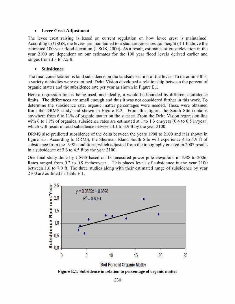
230
Levee Crest Adjustment
The levee crest raising is based on current regulation on how levee crest is maintained. According to USGS, the levees are maintained to a standard cross section height of 1 ft above the estimated 100-year flood elevation (USGS, 2000). As a result, estimates of crest elevation in the year 2100 are dependent on our estimates for the 100 year flood levels derived earlier and ranges from 3.3 to 7.5 ft.
Subsidence
The final consideration is land subsidence on the landside section of the levee. To determine this, a variety of studies were examined. Delta Vision developed a relationship between the percent of organic matter and the subsidence rate per year as shown in Figure E.1.
Here a regression line is being used, and ideally, it would be bounded by different confidence limits. The differences are small enough and thus it was not considered further in this work. To determine the subsidence rate, organic matter percentages were needed. These were obtained from the DRMS study and shown in Figure E.2. From this figure, the South Site contains anywhere from 6 to 11% of organic matter on the surface. From the Delta Vision regression line with 6 to 11% of organics, subsidence rates are estimated at 1 to 1.3 cm/year (0.4 to 0.5 in/year) which will result in total subsidence between 3.1 to 3.9 ft by the year 2100.
DRMS also predicted subsidence of the delta between the years 1998 to 2100 and it is shown in figure E.3. According to DRMS, the Sherman Island South Site will experience 4 to 4.9 ft of subsidence from the 1998 conditions, which adjusted from the topography created in 2007 results in a subsidence of 3.6 to 4.5 ft by the year 2100.
One final study done by USGS based on 13 measured power pole elevations in 1988 to 2006. Rates ranged from 0.2 to 0.9 inches/year. This places levels of subsidence in the year 2100 between 1.6 to 7.0 ft. The three studies along with their estimated range of subsidence by year 2100 are outlined in Table E.1.
Figure E.1: Subsidence in relation to percentage of organic matter

231
Figure E.2: Organic matter content: Sacramento San Joaquin Delta (DRMS, 2007)
Figure E.3: DRMS Subsidence prediction (DRMS, 2007)
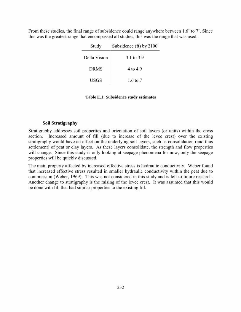
232
From these studies, the final range of subsidence could range anywhere between 1.6’ to 7’. Since this was the greatest range that encompassed all studies, this was the range that was used.
Study Subsidence (ft) by 2100
Delta Vision 3.1 to 3.9
DRMS 4 to 4.9
USGS 1.6 to 7
Table E.1: Subsidence study estimates
Soil Stratigraphy
Stratigraphy addresses soil properties and orientation of soil layers (or units) within the cross section. Increased amount of fill (due to increase of the levee crest) over the existing stratigraphy would have an effect on the underlying soil layers, such as consolidation (and thus settlement) of peat or clay layers. As these layers consolidate, the strength and flow properties will change. Since this study is only looking at seepage phenomena for now, only the seepage properties will be quickly discussed.
The main property affected by increased effective stress is hydraulic conductivity. Weber found that increased effective stress resulted in smaller hydraulic conductivity within the peat due to compression (Weber, 1969). This was not considered in this study and is left to future research. Another change to stratigraphy is the raising of the levee crest. It was assumed that this would be done with fill that had similar properties to the existing fill.

233
Results
Figure E.4 shows the adjustments made to the levee cross sections for adjustments to the year 2100. Obviously there could be a great amount of adjustments made which could warrant further research in the future and better ways by which to measures the sustainability of an engineered system. A few other aspects to consider, but were not included in this study are as follows: Buildup of rip rap, change of side slopes, unexposed peats due to additional levee fill may affect oxidation rates. These are all more areas in uncertainty and if sustainability was a crucial aspect of quality to the engineered system, additional research would be needed to predict what changes would be made as the system is projected into the future.
3.3' to 7.5' Levee crest
raising to account for
sea level rise 2.36' to 2.95' of
sedimentation
-1.6' to -7' of subsidence
due to oxidation of peat
Figure E.4: Summary of adjustments made to 2010 cross section

234
APPENDIX F: BIAS
Introduction
This appendix outlines the process that can be used to handle the second category of uncertainty known as analytical modeling or professional uncertainty (Type II uncertainty) modeling or professional uncertainty (Type II uncertainty = “modeling’). This type of uncertainty applies to deterministic, but unknown values of parameters (parameter uncertainty); to modeling uncertainty (imperfect understanding of problems, simplified analytical models used in practice); and to the actual state of the system (imprecise knowledge of properties and characteristics). This category of uncertainty is “information sensitive” – gathering additional data and information can have an important effect on our characterizations for the uncertainties (Bea, 2006).
Background
Bias
One of the objectives of this study was to illustrate how Type II uncertainties (model uncertainties) can be accounted for in a risk assessment of an engineered system. It is often much easier to do when dealing with engineered concepts that can be explicitly measured in the laboratory, such as tensile strength of steel wire, or compressive strength of concrete. This is more difficult to do when dealing with something as non-homogeneous as in-situ soil. None the less, this uncertainty needs to be accounted for.
Uncertainty of this kind can be characterized through the use of a Bias correction which is a ratio of the actual (or measured) to the predicted value. The procedure involves comparing predictive measures to field or measured data. Once the comparison is made, future predictions can be adjusted to account for the Bias within the process. This appendix outlines the results of the Bias correction applied to the Seepage Analysis for the Sherman Island study.
Bias is determined by comparing model results with measured values (cf., Equation F.1) and it is given by:
F.1
Not only does the model need to be adjusted for Bias, but the uncertainty within the Bias value must be considered as well. It will be uncommon that no Bias exists for a given model. The uncertainty within the Bias can be reduced with more available measured data that can be used to compare with the predictive model. Bias uncertainty is characterized through the development of a collection of Bias values. From the Bias population, we can develop a representative PDF distribution. This distribution can then be sampled from in a Monte Carlo simulation and will act as a random variable so as to “adjust” the results of the model. An example of how this is done for Seepage will be discussed in a subsequent section.
Traditional Methods/State of Practice
Typically biased values are used in traditional engineering processes, procedures, codes, and guidelines. This is because the engineer wants to be “conservative.” Biases are often times hidden in design codes and guidelines in an attempt to be conservative. Problems develop due to the compounding of these drivers to be conservative and lack of knowledge of how conservative
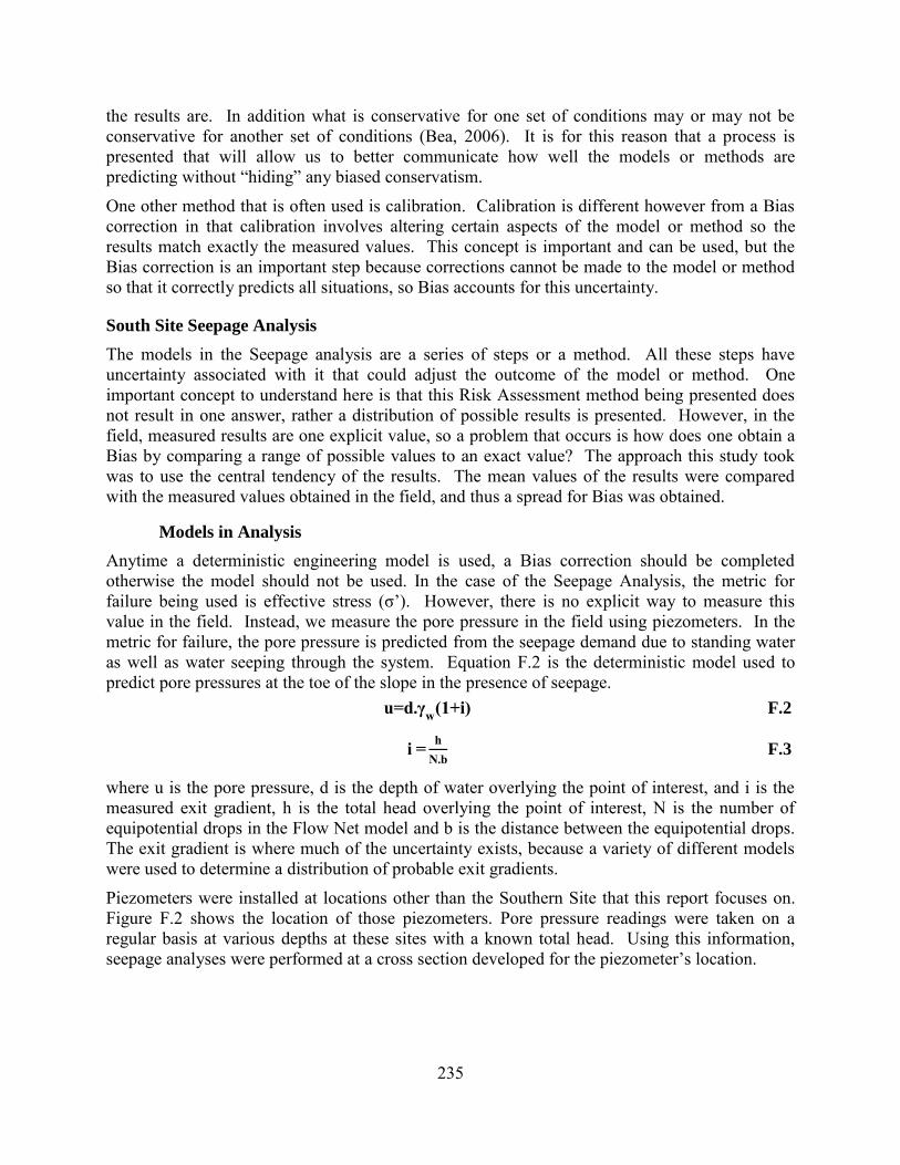
235
the results are. In addition what is conservative for one set of conditions may or may not be conservative for another set of conditions (Bea, 2006). It is for this reason that a process is presented that will allow us to better communicate how well the models or methods are predicting without “hiding” any biased conservatism.
One other method that is often used is calibration. Calibration is different however from a Bias correction in that calibration involves altering certain aspects of the model or method so the results match exactly the measured values. This concept is important and can be used, but the Bias correction is an important step because corrections cannot be made to the model or method so that it correctly predicts all situations, so Bias accounts for this uncertainty.
South Site Seepage Analysis
The models in the Seepage analysis are a series of steps or a method. All these steps have uncertainty associated with it that could adjust the outcome of the model or method. One important concept to understand here is that this Risk Assessment method being presented does not result in one answer, rather a distribution of possible results is presented. However, in the field, measured results are one explicit value, so a problem that occurs is how does one obtain a Bias by comparing a range of possible values to an exact value? The approach this study took was to use the central tendency of the results. The mean values of the results were compared with the measured values obtained in the field, and thus a spread for Bias was obtained.
Models in Analysis
Anytime a deterministic engineering model is used, a Bias correction should be completed otherwise the model should not be used. In the case of the Seepage Analysis, the metric for failure being used is effective stress (σ’). However, there is no explicit way to measure this value in the field. Instead, we measure the pore pressure in the field using piezometers. In the metric for failure, the pore pressure is predicted from the seepage demand due to standing water as well as water seeping through the system. Equation F.2 is the deterministic model used to predict pore pressures at the toe of the slope in the presence of seepage.
F.2
F.3
where u is the pore pressure, d is the depth of water overlying the point of interest, and i is the measured exit gradient, h is the total head overlying the point of interest, N is the number of equipotential drops in the Flow Net model and b is the distance between the equipotential drops. The exit gradient is where much of the uncertainty exists, because a variety of different models were used to determine a distribution of probable exit gradients.
Piezometers were installed at locations other than the Southern Site that this report focuses on. Figure F.2 shows the location of those piezometers. Pore pressure readings were taken on a regular basis at various depths at these sites with a known total head. Using this information, seepage analyses were performed at a cross section developed for the piezometer’s location.

236
Figure F.1: Location of Piezometers (blue circles)
Piezometer Site Cross Section
The cross section and stratigraphy for this site was developed similarly to the stratigraphy of the South Site. Three boring logs were used to create a best, worst, and expected cases for the cross section stratigraphy given the available information. The topography was varied by approximately 5 ft because of the accuracy of the topographic layers used. The cross sections used, along with the depths and locations of the piezometers can be found in Appendix I (Cross Section Auto-Cad Drawings). The models were run in SEEPW/® to determine bounds of random variables in predicting exit gradient just as it was done in determining bounds for the Southern Site exit gradient.
Measuring Bias
Although a large amount of data was gathered from the piezometers and ideally a Bias correction could be determined for each one, only nine were selected at different depths and times so that a variety of different total head values could be examined. Table F.1 contains the location and depth of the piezometers chosen to measure Bias for this model.
Results
Once the model was created, a probability density distribution was assigned for the exit gradient (i). A Monte Carlo simulation was then run by varying the total head depending on what piezometer location was being evaluated. The code developed to run the Monte Carlo Simulation in Matlab® can be found in Appendix N of this report. Table F.1 contains model predictions and the associated Bias. Figure 3 to Figure 5 are the results of the models run on the different piezometers.
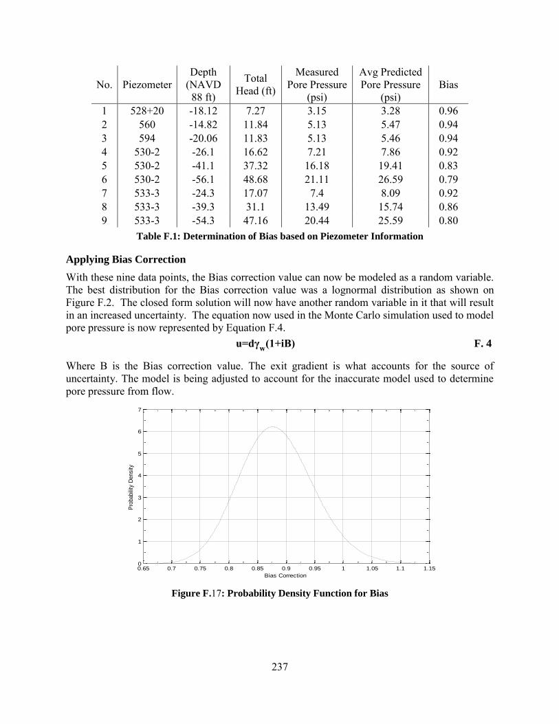
237
No. Piezometer Depth
(NAVD 88 ft)
Total Head (ft)
Measured Pore Pressure
(psi)
Avg Predicted Pore Pressure
(psi) Bias
1 528+20 -18.12 7.27 3.15 3.28 0.96 2 560 -14.82 11.84 5.13 5.47 0.94 3 594 -20.06 11.83 5.13 5.46 0.94 4 530-2 -26.1 16.62 7.21 7.86 0.92 5 530-2 -41.1 37.32 16.18 19.41 0.83 6 530-2 -56.1 48.68 21.11 26.59 0.79 7 533-3 -24.3 17.07 7.4 8.09 0.92 8 533-3 -39.3 31.1 13.49 15.74 0.86 9 533-3 -54.3 47.16 20.44 25.59 0.80
Table F.1: Determination of Bias based on Piezometer Information
Applying Bias Correction
With these nine data points, the Bias correction value can now be modeled as a random variable. The best distribution for the Bias correction value was a lognormal distribution as shown on Figure F.2. The closed form solution will now have another random variable in it that will result in an increased uncertainty. The equation now used in the Monte Carlo simulation used to model pore pressure is now represented by Equation F.4.
F. 4
Where B is the Bias correction value. The exit gradient is what accounts for the source of uncertainty. The model is being adjusted to account for the inaccurate model used to determine pore pressure from flow.
Figure F.17: Probability Density Function for Bias
0.65 0.7 0.75 0.8 0.85 0.9 0.95 1 1.05 1.1 1.150
1
2
3
4
5
6
7
Bias Correction
Pro
babili
ty D
ensity

238
Figure F.3: Pore Pressure Predictions for Piezometer Cross Section.
3.1 3.15 3.2 3.25 3.3 3.35 3.4 3.45 3.5 3.55 3.60
1
2
3
4
5
6
7
Pore Pressure (psi)
Pro
babili
ty D
ensity
Piezometer 1 Results
mean = 3.28
5 5.2 5.4 5.6 5.8 6 6.2 6.40
0.5
1
1.5
2
2.5
3
Pore Pressure (psi)
Pro
babili
ty D
ensity F
unction
Piezometer 2 Results
mean =5.47
5 5.2 5.4 5.6 5.8 6 6.2 6.40
0.5
1
1.5
2
2.5
3
3.5
Pore Pressure (psi)
Pro
babili
ty D
ensity
Piezometer 3 Results
mean = 5.46

239
Figure F.4: Pore Pressure Predictions for Piezometer Cross Section (continued).
7 7.5 8 8.5 9 9.50
0.2
0.4
0.6
0.8
1
1.2
1.4
1.6
1.8
Pore Pressure (psi)
Pro
babili
ty D
ensity
Piezometer 4 Results
mean = 7.86
17 18 19 20 21 22 23 24 25 26 270
0.05
0.1
0.15
0.2
0.25
0.3
0.35
0.4
Pore Pressure (psi)
Pro
babili
ty D
ensity
Piezometer 5 Results
mean = 19.41
22 24 26 28 30 32 34 36 38 400
0.05
0.1
0.15
0.2
0.25
Pore Pressure (psi)
Pro
babili
ty D
ensity
Piezometer 6 Results
mean = 26.59

240
Figure F.5: Pore Pressure Predictions for Piezometer Cross Section (continued)
7.5 8 8.5 9 9.5 100
0.2
0.4
0.6
0.8
1
1.2
1.4
1.6
1.8
Pore Pressure (psi)
Pro
babili
ty D
ensity
Piezometer 7 Results
mean =8.09
14 15 16 17 18 19 20 210
0.1
0.2
0.3
0.4
0.5
0.6
0.7
Pore Pressure (psi)
Pro
babili
ty D
ensity
Piezometer 8 Results
mean = 15.74
20 22 24 26 28 30 32 34 36 380
0.05
0.1
0.15
0.2
0.25
Pore Pressure (psi)
Pro
babili
ty D
ensity
Piezometer 9 Results
mean = 25.59
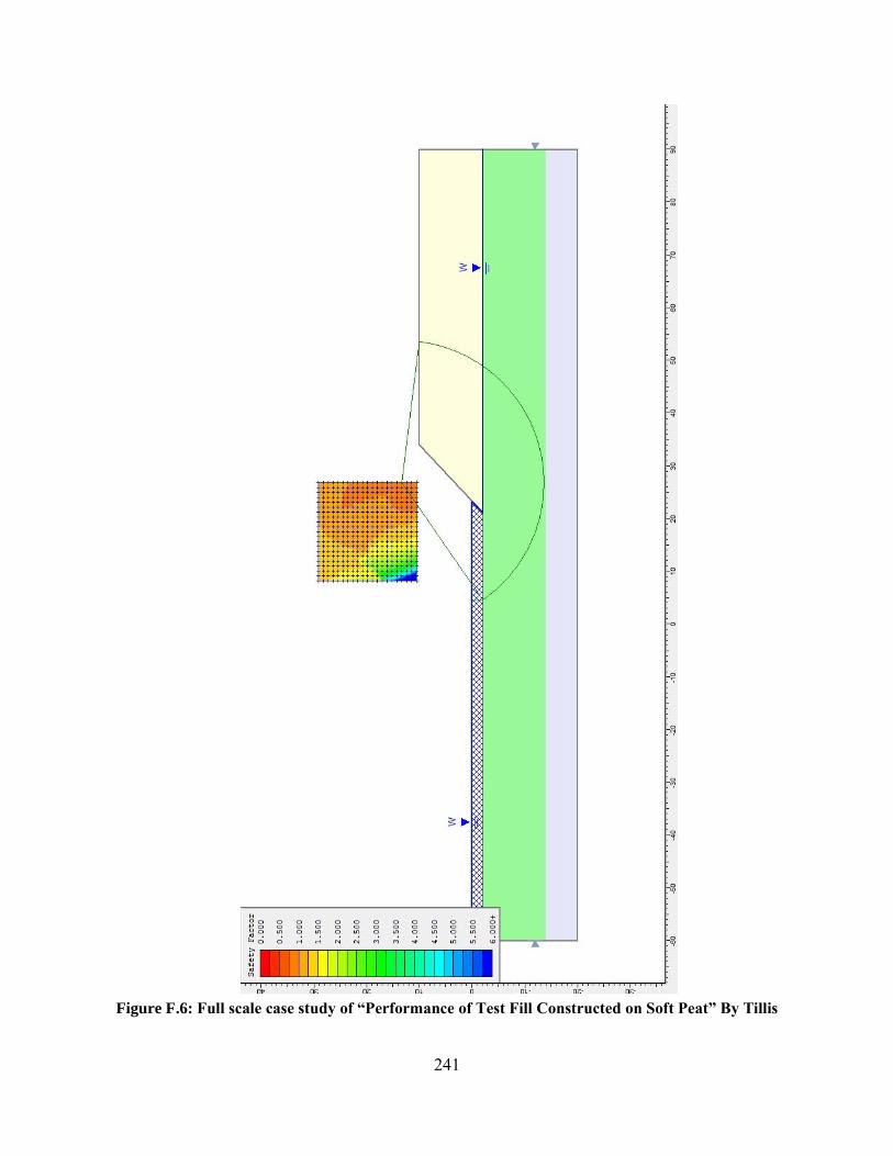
241
Figure F.6: F y f “ f f F C S f ” y
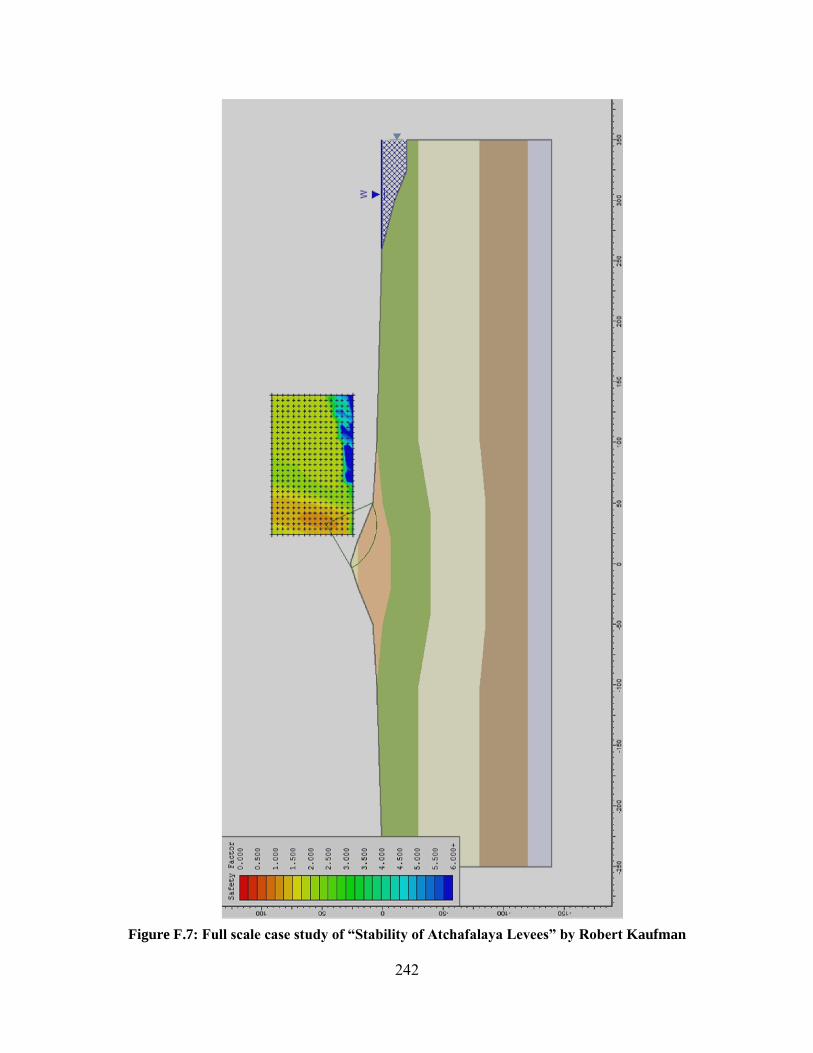
242
Figure F.7: F y f “S y f A f y L v ” y R Kaufman

243
Figure F.8: F y f “RELIA ILI Y A LIED O SLO E S A ILI Y
A ALYSIS” y C L
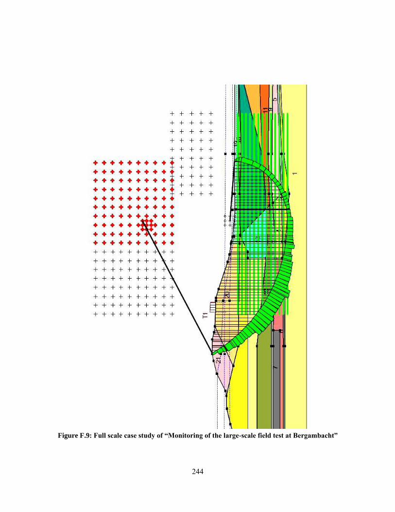
244
Figure F.9: F y f “ g f g - f g ”
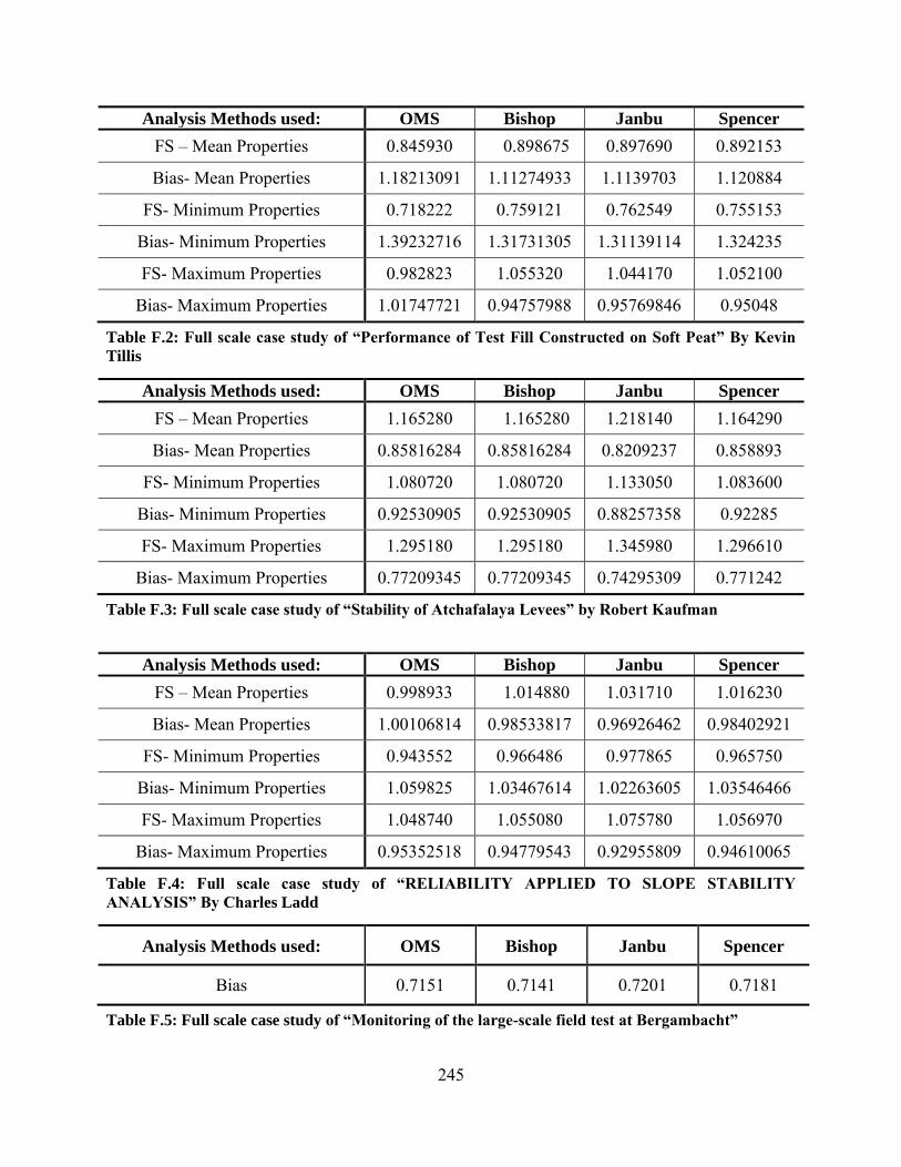
245
Analysis Methods used: OMS Bishop Janbu Spencer
FS – Mean Properties 0.845930 0.898675 0.897690 0.892153
Bias- Mean Properties 1.18213091 1.11274933 1.1139703 1.120884
FS- Minimum Properties 0.718222 0.759121 0.762549 0.755153
Bias- Minimum Properties 1.39232716 1.31731305 1.31139114 1.324235
FS- Maximum Properties 0.982823 1.055320 1.044170 1.052100
Bias- Maximum Properties 1.01747721 0.94757988 0.95769846 0.95048
Table F.2: F y f “ f f F C S f ” y K v
Tillis
Analysis Methods used: OMS Bishop Janbu Spencer
FS – Mean Properties 1.165280 1.165280 1.218140 1.164290
Bias- Mean Properties 0.85816284 0.85816284 0.8209237 0.858893
FS- Minimum Properties 1.080720 1.080720 1.133050 1.083600
Bias- Minimum Properties 0.92530905 0.92530905 0.88257358 0.92285
FS- Maximum Properties 1.295180 1.295180 1.345980 1.296610
Bias- Maximum Properties 0.77209345 0.77209345 0.74295309 0.771242
Table F.3: F y f “S y f A f y L v ” y R K f
Analysis Methods used: OMS Bishop Janbu Spencer
FS – Mean Properties 0.998933 1.014880 1.031710 1.016230
Bias- Mean Properties 1.00106814 0.98533817 0.96926462 0.98402921
FS- Minimum Properties 0.943552 0.966486 0.977865 0.965750
Bias- Minimum Properties 1.059825 1.03467614 1.02263605 1.03546466
FS- Maximum Properties 1.048740 1.055080 1.075780 1.056970
Bias- Maximum Properties 0.95352518 0.94779543 0.92955809 0.94610065
Table F.4: F y f “RELIA ILI Y A LIED O SLO E S A ILI Y
A ALYSIS” y C rles Ladd
Analysis Methods used: OMS Bishop Janbu Spencer
Bias 0.7151 0.7141 0.7201 0.7181
Table F.5: Full scale case study f “ g f g - f g ”

246
Mean Properties
Minimum Properties
Maximum Properties Figure F.10: Evaluation of Bias for Slope Stability Analyses: Ordinary Method of Slices (OMS)
ReliaSoft Weibull++ 7 - www.ReliaSoft.com
Probability - Lognormal
Time, (t)
Unre
liabil
ity, F
(t)
0.100 2.0001.00010.000
50.000
99.000Probability-Lognormal
Data 1Lognormal-2PRRX SRM MED FMF=4/S=0
Data PointsProbability Line
Hamed HamediBerkeley2/8/20128:52:10 PM
Bias
ReliaSoft Weibull++ 7 - www.ReliaSoft.com
Probability - Lognormal
Time, (t)
Unre
liabil
ity, F
(t)
0.100 2.0001.00010.000
50.000
99.000Probability-Lognormal
Data 1Lognormal-2PRRX SRM MED FMF=4/S=0
Data PointsProbability Line
Hamed HamediBerkeley2/8/20129:04:02 PM
Bias
ReliaSoft Weibull++ 7 - www.ReliaSoft.com
Probability - Lognormal
Time, (t)
Unre
liabil
ity, F
(t)
0.100 2.0001.00010.000
50.000
99.000Probability-Lognormal
Data 1Lognormal-2PRRX SRM MED FMF=4/S=0
Data PointsProbability Line
Hamed HamediBerkeley2/8/20129:06:08 PM
Bias

247
Mean Properties
Minimum Properties
Maximum Properties Figure F.11: Evaluation of Bias for Slope Stability Analyses: Simplified Bishop
ReliaSoft Weibull++ 7 - www.ReliaSoft.com
Probability - Lognormal
Time, (t)
Unre
liabi
lity, F
(t)
0.100 2.0001.00010.000
50.000
99.000Probability-Lognormal
Data 1Lognormal-2PRRX SRM MED FMF=4/S=0
Data PointsProbability Line
Hamed HamediBerkeley2/8/20129:14:24 PM
Bias
ReliaSoft Weibull++ 7 - www.ReliaSoft.com
Probability - Lognormal
Time, (t)
Unre
liabil
ity, F
(t)
0.100 2.0001.00010.000
50.000
99.000Probability-Lognormal
Data 1Lognormal-2PRRX SRM MED FMF=4/S=0
Data PointsProbability Line
Hamed HamediBerkeley2/8/20129:16:28 PM
Bias
ReliaSoft Weibull++ 7 - www.ReliaSoft.com
Probability - Lognormal
Time, (t)
Unre
liabi
lity,
F(t)
0.100 2.0001.00010.000
50.000
99.000Probability-Lognormal
Data 1Lognormal-2PRRX SRM MED FMF=4/S=0
Data PointsProbability Line
Hamed HamediBerkeley2/8/20129:18:30 PM
Bias
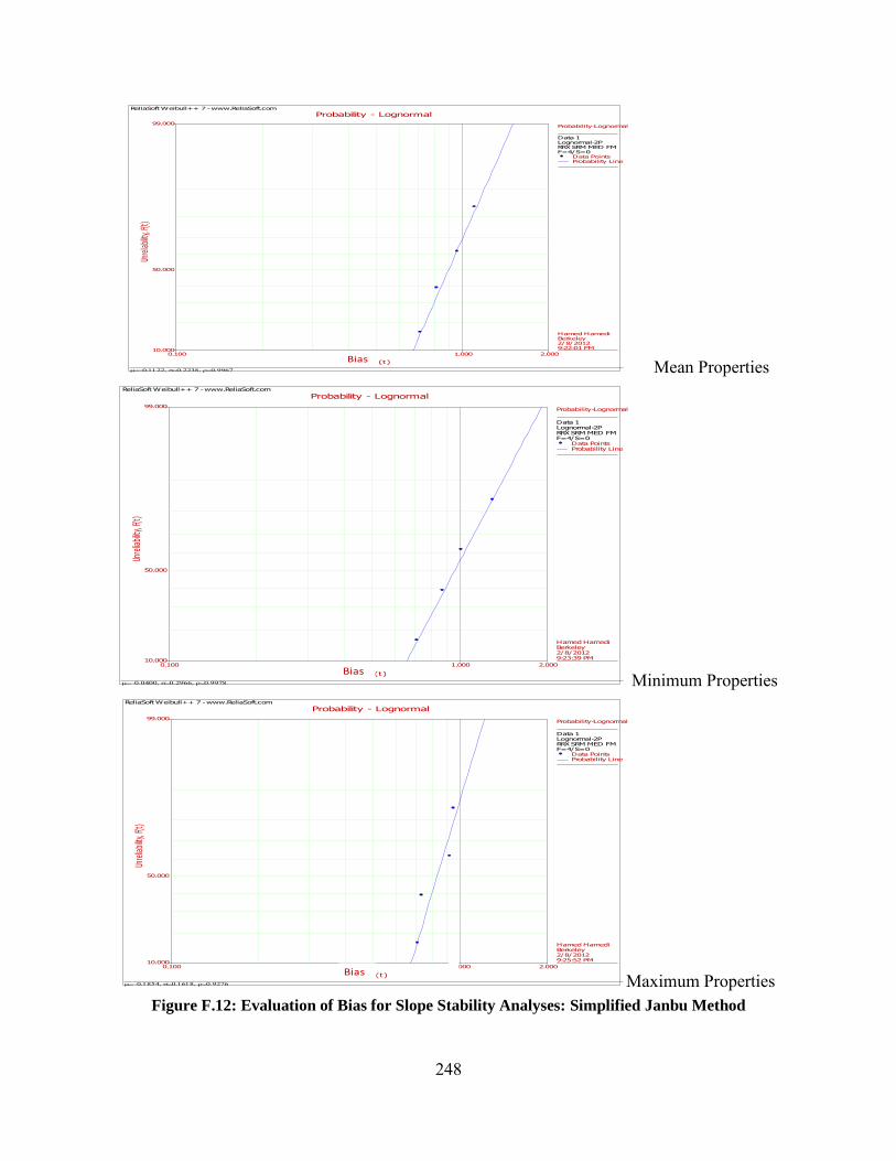
248
Mean Properties
Minimum Properties
Maximum Properties Figure F.12: Evaluation of Bias for Slope Stability Analyses: Simplified Janbu Method
ReliaSoft Weibull++ 7 - www.ReliaSoft.com
Probability - Lognormal
Time, (t)
Unre
liabil
ity, F
(t)
0.100 2.0001.00010.000
50.000
99.000Probability-Lognormal
Data 1Lognormal-2PRRX SRM MED FMF=4/S=0
Data PointsProbability Line
Hamed HamediBerkeley2/8/20129:22:01 PM
Bias
ReliaSoft Weibull++ 7 - www.ReliaSoft.com
Probability - Lognormal
Time, (t)
Unre
liabi
lity,
F(t)
0.100 2.0001.00010.000
50.000
99.000Probability-Lognormal
Data 1Lognormal-2PRRX SRM MED FMF=4/S=0
Data PointsProbability Line
Hamed HamediBerkeley2/8/20129:23:39 PM
Bias
ReliaSoft Weibull++ 7 - www.ReliaSoft.com
Probability - Lognormal
Time, (t)
Unre
liabi
lity, F
(t)
0.100 2.0001.00010.000
50.000
99.000Probability-Lognormal
Data 1Lognormal-2PRRX SRM MED FMF=4/S=0
Data PointsProbability Line
Hamed HamediBerkeley2/8/20129:25:52 PM
Bias

249
Mean Properties
Minimum Properties
Maximum Properties Figure F.13: Evaluation of Bias for Slope Stability Analyses: Spencer Method
ReliaSoft Weibull++ 7 - www.ReliaSoft.com
Probability - Lognormal
Time, (t)
Unre
liabi
lity,
F(t)
0.100 2.0001.00010.000
50.000
99.000Probability-Lognormal
Data 1Lognormal-2PRRX SRM MED FMF=4/S=0
Data PointsProbability Line
Hamed HamediBerkeley2/8/20129:29:02 PM
Bias
ReliaSoft Weibull++ 7 - www.ReliaSoft.com
Probability - Lognormal
Time, (t)
Unre
liabi
lity, F
(t)
0.100 2.0001.00010.000
50.000
99.000Probability-Lognormal
Data 1Lognormal-2PRRX SRM MED FMF=4/S=0
Data PointsProbability Line
Hamed HamediBerkeley2/8/20129:32:21 PM
Bias
ReliaSoft Weibull++ 7 - www.ReliaSoft.com
Probability - Lognormal
Time, (t)
Unre
liabil
ity, F
(t)
0.100 2.0001.00010.000
50.000
99.000Probability-Lognormal
Data 1Lognormal-2PRRX SRM MED FMF=4/S=0
Data PointsProbability Line
Hamed HamediBerkeley2/8/20129:34:51 PM
Bias

250
APPENDIX G: Capacity and Demand Probability Density Functions
This Appendix shows the results of the Monte Carlo Simulations for the 2, 50 and 100 year water levels in the year 2010 and 2100. The x-axis represents Unit Weight (pcf) and the y-axis is the probability density. Unit weight was used as a metric because the depth for both the demand and capacity was considered equal (i.e the phreatic surface was at the ground surface).
The figure below shows the results of the calculation of the overlap between the Demand and Capacity, which represents the probability that the Capacity is less than the Demand.
0.0708 0.0716 0.0745
0.0962 0.1009 0.1025
0
0.02
0.04
0.06
0.08
0.1
0.12
2 50 100
Pro
bab
ility
of
Failu
re
Return Period
2010
2100
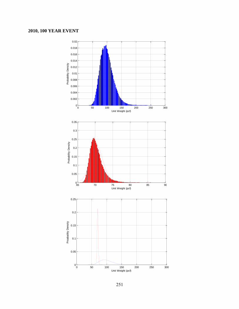
251
2010, 100 YEAR EVENT
0 50 100 150 200 250 3000
0.002
0.004
0.006
0.008
0.01
0.012
0.014
0.016
0.018
0.02
Unit Weight (pcf)
Pro
babili
ty D
ensity
65 70 75 80 85 900
0.05
0.1
0.15
0.2
0.25
0.3
0.35
Unit Weight (pcf)
Pro
babili
ty D
ensity
0 50 100 150 200 250 3000
0.05
0.1
0.15
0.2
0.25
Unit Weight (pcf)
Pro
abaili
ty D
ensity
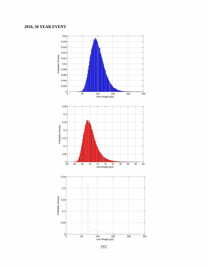
252
2010, 50 YEAR EVENT
0 50 100 150 200 2500
0.002
0.004
0.006
0.008
0.01
0.012
0.014
0.016
0.018
0.02
Untit Weight (pcf)
Pro
babili
ty D
ensity
64 66 68 70 72 74 76 78 80 82 840
0.05
0.1
0.15
0.2
0.25
0.3
0.35
Unit Weight (pcf)
Pro
babili
ty D
ensity
0 50 100 150 200 2500
0.05
0.1
0.15
0.2
0.25
Unit Weight (pcf)
Pro
babiit
y D
ensity

253
2010, 2 YEAR EVENT
0 50 100 150 200 250 300 3500
0.002
0.004
0.006
0.008
0.01
0.012
0.014
0.016
0.018
0.02
Unit Weight
Pro
babili
ty D
ensity
64 66 68 70 72 74 76 78 80 820
0.05
0.1
0.15
0.2
0.25
0.3
0.35
Unit Weight (pcf)
Pro
babili
ty D
ensity
0 50 100 150 200 250 300 3500
0.05
0.1
0.15
0.2
0.25
0.3
0.35
Unit Weight (pcf)
Pro
babilt
y D
ensity

254
2100, 100 YEAR EVENT
0 50 100 150 200 250 3000
0.002
0.004
0.006
0.008
0.01
0.012
0.014
0.016
0.018
0.02
65 70 75 80 85 90 95 1000
0.02
0.04
0.06
0.08
0.1
0.12
0.14
0.16
0.18
0 50 100 150 200 250 3000
0.02
0.04
0.06
0.08
0.1
0.12
0.14
0.16
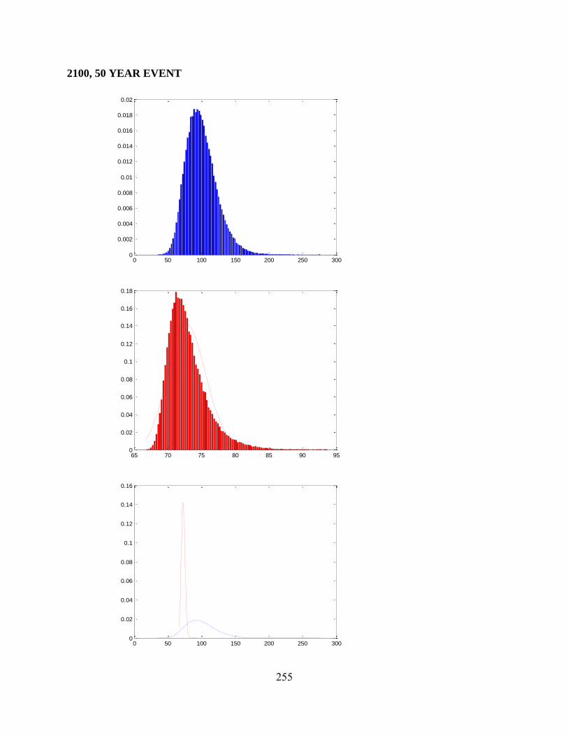
255
2100, 50 YEAR EVENT
0 50 100 150 200 250 3000
0.002
0.004
0.006
0.008
0.01
0.012
0.014
0.016
0.018
0.02
65 70 75 80 85 90 950
0.02
0.04
0.06
0.08
0.1
0.12
0.14
0.16
0.18
0 50 100 150 200 250 3000
0.02
0.04
0.06
0.08
0.1
0.12
0.14
0.16

256
2100, 2 YEAR EVENT
0 50 100 150 200 250 3000
0.002
0.004
0.006
0.008
0.01
0.012
0.014
0.016
0.018
0.02
65 70 75 80 85 90 950
0.02
0.04
0.06
0.08
0.1
0.12
0.14
0.16
0.18
0.2
0 50 100 150 200 250 3000
0.02
0.04
0.06
0.08
0.1
0.12
0.14
0.16

257
SLOPE STABILITY
MEAN VALUES OF CAPACITY & DEMAND
Values from Analyses
Method Used Resisting Force
(103 lb)
Driving Force
(103 lb)
Resisting Moment
(107 lb-ft)
Driving Moment
(107 lb-ft)
Ordinary Method of Slices - - 1.2562 1.0007
Simplified Bishop Method 1.3976 1.0007
Simplified Janbu Method 107.125 85.454 - -
Spencer Method 106.903 77.286 1.3842 1.0007
Factor of Safety, FS
Case Mean Standard Deviation 50% Method of Analysis
South Site-Worst Case
1.160567 0.132878 1.150366 Spencer
1.11543 0.125477 1.106684 Simplified Janbu
1.162173 0.133022 1.151936 Simplified Bishop
1.111121 0.124517 1.102541 Ordinary Method of Slices
South Site-Best Case
1.400993 0.144759 1.386391 Spencer
1.301914 0.132409 1.290551 Simplified Janbu
1.41423 0.146035 1.39923 Simplified Bishop
1.272079 0.131 1.261211 Ordinary Method of Slices
North Site-Worst Case
1.099951 0.042126 1.098975 Spencer
1.055226 0.039343 1.05441 Simplified Janbu
1.095953 0.042688 1.094955 Simplified Bishop
1.082766 0.036118 1.08206 Ordinary Method of Slices
North Site-Best Case
1.343527 0.108578 1.335631 Spencer
1.263023 0.10664 1.255862 Simplified Janbu
1.318645 0.11002 1.310688 Simplified Bishop
1.3107 0.103955 1.303637 Ordinary Method of Slices

258
Factor of Safety, F.S. Obtained
Method Used Mean Standard Dev. Minimum Maximum
Ordinary Method of Slices 1.3089 0.1039 0.9381 1.6808
Simplified Bishop Method 1.3161 0.1100 0.9333 1.7061
Simplified Janbu Method 1.2615 0.1066 0.8951 1.6316
Spencer Method 1.3413 0.1086 0.9817 1.7248 Results for North Site Best Case Conditions
Factor of Safety, F.S. Obtained
Method Used Mean Standard Dev. Minimum Maximum
Ordinary Method of Slices 1.0828 0.0361 0.9471 1.1701
Simplified Bishop Method 1.0959 0.0427 0.9349 0.1995
Simplified Janbu Method 1.0552 0.0393 0.9063 1.1497
Spencer Method 1.0999 0.0421 0.9404 1.2012 Results for North Site Worst Case Conditions
Factor of Safety, F.S. Obtained
Method Used Mean Standard Dev. Minimum Maximum
Ordinary Method of Slices 1.3089 0.1039 0.9381 1.6808
Simplified Bishop Method 1.3161 0.1100 0.9333 1.7061
Simplified Janbu Method 1.2615 0.1066 0.8951 1.6316
Spencer Method 1.3413 0.1086 0.9817 1.7248 Results for South Site Best Case Conditions
Factor of Safety, F.S. Obtained
Method Used Mean Standard Dev. Minimum Maximum
Ordinary Method of Slices 1.111 0.1245 0.7899 1.5405
Simplified Bishop Method 1.1621 0.1330 0.8157 1.6204
Simplified Janbu Method 1.1152 0.1255 0.7876 1.5621
Spencer Method 1.1605 0.1329 0.8154 1.6183 Results for South Site Worst Case Conditions

259
OVERTOPPING CAPACITY
Section 1
ReliaSoft Weibull++ 7 - www.ReliaSoft.com
Typy I Uncertainties Capacity (Crown)
Levee Hight
% U
nder
12.000 15.5000.100
0.500
1.000
5.000
10.000
50.000
99.900
0.100
Probability-Lognormal
Data 1Lognormal-2PRRX SRM MED FMF=67/S=0
Data PointsProbability Line
Hamed HamedifarUC Berkeley5/10/20122:18:35 PM

260
Section 2
ReliaSoft Weibull++ 7 - www.ReliaSoft.com
Typy I Uncertainties Capacity (Crown)
Levee Hight
% U
nder
14.000 17.0000.100
0.500
1.000
5.000
10.000
50.000
99.900
0.100
Probability-Lognormal
Data 2Lognormal-2PRRX SRM MED FMF=80/S=0
Data PointsProbability Line
Hamed HamedifarUC Berkeley5/10/20122:36:26 PM

261
Section 3
ReliaSoft Weibull++ 7 - www.ReliaSoft.com
Typy I Uncertainties Capacity (Crown)
Levee Hight
% U
nder
14.000 22.0000.100
0.500
1.000
5.000
10.000
50.000
99.900
0.100
Probability-Lognormal
Data 3Lognormal-2PRRX SRM MED FMF=94/S=0
Data PointsProbability Line
Hamed HamedifarUC Berkeley5/10/20122:43:22 PM

262
Section 4
ReliaSoft Weibull++ 7 - www.ReliaSoft.com
Typy I Uncertainties Capacity (Crown)
Levee Hight
% U
nder
10.000 30.0000.100
0.500
1.000
5.000
10.000
50.000
99.900
0.100
Probability-Lognormal
Data 4Lognormal-2PRRX SRM MED FMF=72/S=0
Data PointsProbability Line
Hamed HamedifarUC Berkeley5/10/20122:53:37 PM

263
Section 5
ReliaSoft Weibull++ 7 - www.ReliaSoft.com
Typy I Uncertainties Capacity (Crown)
Levee Hight
% U
nder
10.000 20.0000.100
0.500
1.000
5.000
10.000
50.000
99.900
0.100
Probability-Lognormal
Data 5Lognormal-2PRRX SRM MED FMF=156/S=0
Data PointsProbability Line
Hamed HamedifarUC Berkeley5/10/20123:06:40 PM

264
Section 6
ReliaSoft Weibull++ 7 - www.ReliaSoft.com
Typy I Uncertainties Capacity (Crown)
Levee Hight
% U
nder
14.000 20.0001.000
5.000
10.000
50.000
99.000Probability-Lognormal
Data 6Lognormal-2PRRX SRM MED FMF=25/S=0
Data PointsProbability Line
Hamed HamedifarUC Berkeley5/10/20123:13:04 PM

265
Section 7
ReliaSoft Weibull++ 7 - www.ReliaSoft.com
Typy I Uncertainties Capacity (Crown)
Levee Hight
% U
nder
13.000 15.0000.100
0.500
1.000
5.000
10.000
50.000
99.900
0.100
Probability-Lognormal
Data 7Lognormal-2PRRX SRM MED FMF=89/S=0
Data PointsProbability Line
Hamed HamedifarUC Berkeley5/10/20123:26:24 PM

266
ReliaSoft Weibull++ 7 - www.ReliaSoft.com
Typy I Uncertainties Capacity (Crown)
Levee Hight
% U
nder
10.000 12.0000.100
0.500
1.000
5.000
10.000
50.000
99.900
0.100
Probability-Lognormal
Data 8Lognormal-2PRRX SRM MED FMF=122/S=0
Data PointsProbability Line
Hamed HamedifarUC Berkeley5/10/20123:33:46 PM

267
Section 8
ReliaSoft Weibull++ 7 - www.ReliaSoft.com
Typy I Uncertainties Capacity (Crown)
Levee Hight
% U
nder
9.000 12.00010.0000.100
0.500
1.000
5.000
10.000
50.000
99.900
0.100
Probability-Lognormal
Data 9Lognormal-2PRRX SRM MED FMF=71/S=0
Data PointsProbability Line
Hamed HamedifarUC Berkeley5/10/20123:57:11 PM

268
Section 9
Section 10
ReliaSoft Weibull++ 7 - www.ReliaSoft.com
Typy I Uncertainties Capacity (Crown)
Levee Hight
% U
nder
9.000 15.00010.0000.100
0.500
1.000
5.000
10.000
50.000
99.900
0.100
Probability-Lognormal
Data 10Lognormal-2PRRX SRM MED FMF=138/S=0
Data PointsProbability Line
Hamed HamedifarUC Berkeley5/10/20124:08:00 PM

269
Section 11
ReliaSoft Weibull++ 7 - www.ReliaSoft.com
Typy I Uncertainties Capacity (Crown)
Levee Hight
% U
nder
9.000 12.00010.0001.000
5.000
10.000
50.000
99.000Probability-Lognormal
Data 11Lognormal-2PRRX SRM MED FMF=18/S=0
Data PointsProbability Line
Hamed HamedifarUC Berkeley5/10/20124:14:40 PM
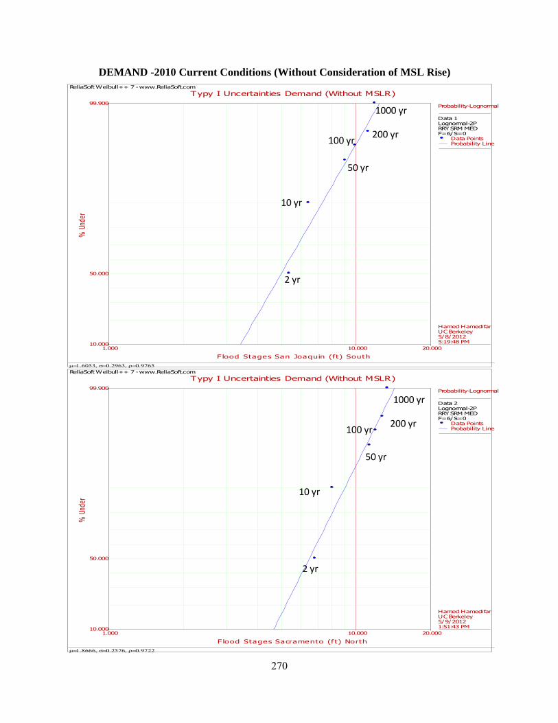
270
DEMAND -2010 Current Conditions (Without Consideration of MSL Rise)
ReliaSoft Weibull++ 7 - www.ReliaSoft.com
Typy I Uncertainties Demand (Without MSLR)
F lood Stages San Joaquin (ft) South
% U
nder
1.000 20.00010.00010.000
50.000
99.900Probability-Lognormal
Data 1Lognormal-2PRRY SRM MED F=6/S=0
Data PointsProbability Line
Hamed HamedifarUC Berkeley5/8/20125:19:48 PM
50 yr
10 yr
2 yr
200 yr
1000 yr
100 yr
ReliaSoft Weibull++ 7 - www.ReliaSoft.com
Typy I Uncertainties Demand (Without MSLR)
F lood Stages Sacramento (ft) North
% U
nder
1.000 20.00010.00010.000
50.000
99.900Probability-Lognormal
Data 2Lognormal-2PRRY SRM MED F=6/S=0
Data PointsProbability Line
Hamed HamedifarUC Berkeley5/9/20121:51:43 PM
50 yr
10 yr
2 yr
200 yr
1000 yr
100 yr

271
DEMAND – 2100- Future Conditions(With Consideration of Mean Sea Level Rise)
ReliaSoft Weibull++ 7 - www.ReliaSoft.com
Typy I Uncertainties Demand (With MSLR)
F lood Stages San Joaquin (ft) South
% U
nder
1.000 20.00010.00010.000
50.000
99.900Probability-Lognormal
Data 3Lognormal-2PRRY SRM MED F=6/S=0
Data PointsProbability Line
Hamed HamedifarUC Berkeley5/8/20125:26:23 PM
50 yr
10 yr
2 yr
200 yr
1000 yr
100 yr
ReliaSoft Weibull++ 7 - www.ReliaSoft.com
Typy I Uncertainties Demand (With MSLR)
F lood Stages Sacramento (ft) North
% U
nder
1.000 20.00010.00010.000
50.000
99.900Probability-Lognormal
Data 4Lognormal-2PRRY SRM MED F=6/S=0
Data PointsProbability Line
Hamed HamedifarUC Berkeley5/9/20121:52:42 PM
50 yr
10 yr
2 yr
200 yr
1000 yr
100 yr

272
Overtopping Current Velocity(ft/sec) Mean=0.9231 σ=0.4659

273
Page intentionally left blank

274
APPENDIX H: Boring Logs

275

276
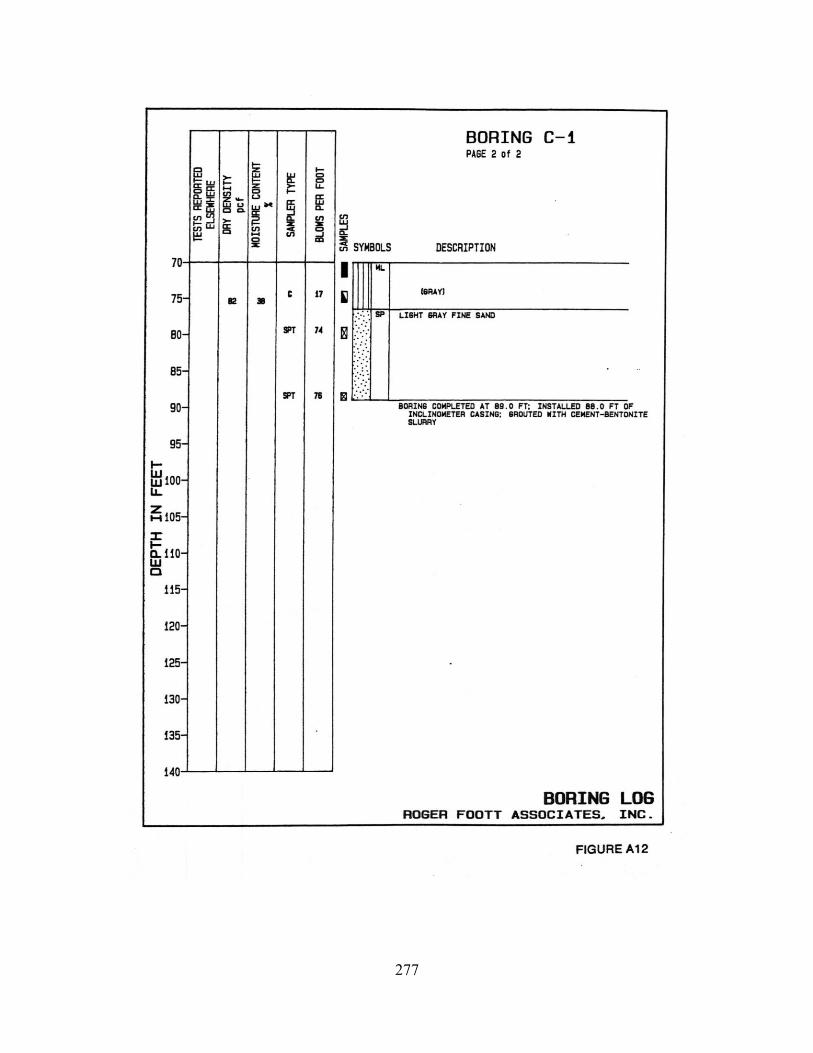
277

278

279

280
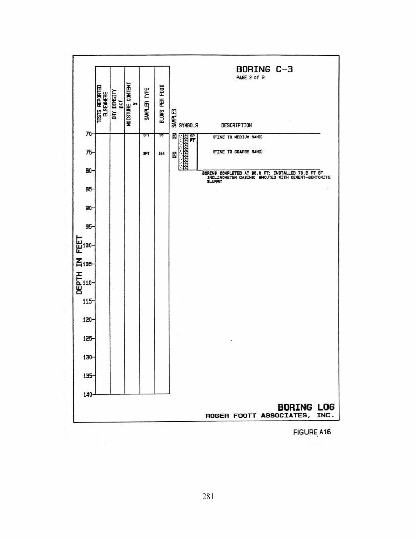
281
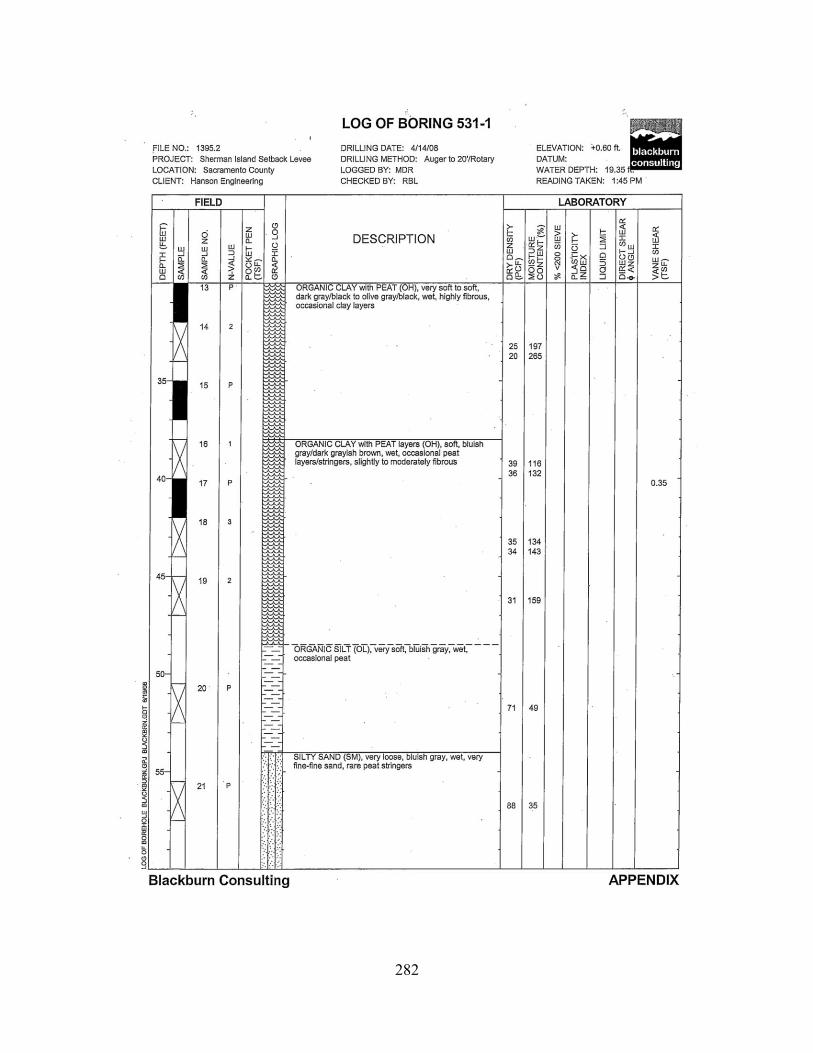
282

283

284

285

286
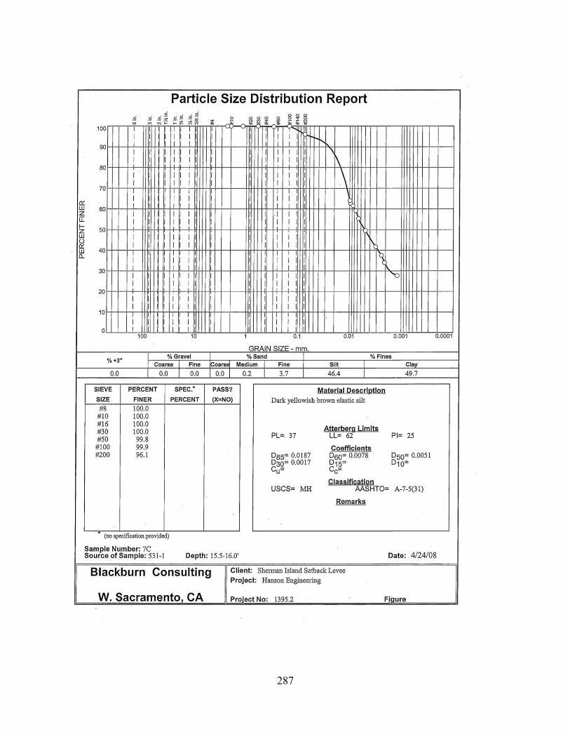
287

288

289

290
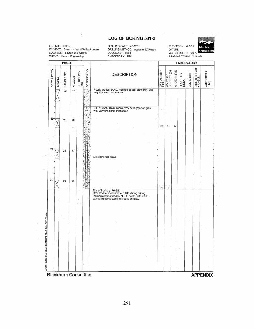
291
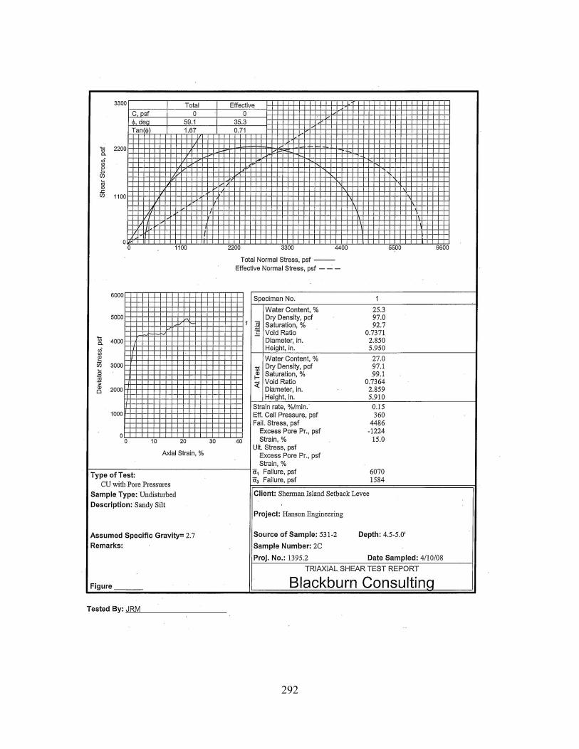
292

293
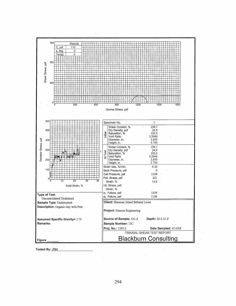
294

295

296

297

298

299
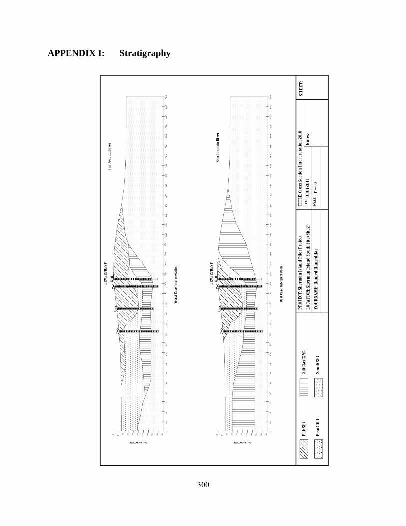
300
APPENDIX I: Stratigraphy
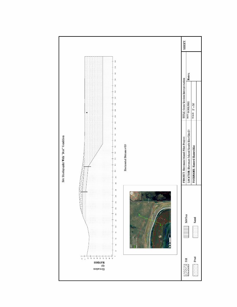
301

302

303

304

305
Page intentionally left blank

306
APPENDIX J: Piezometer Locations

307
APPENDIX K: Topography Variation
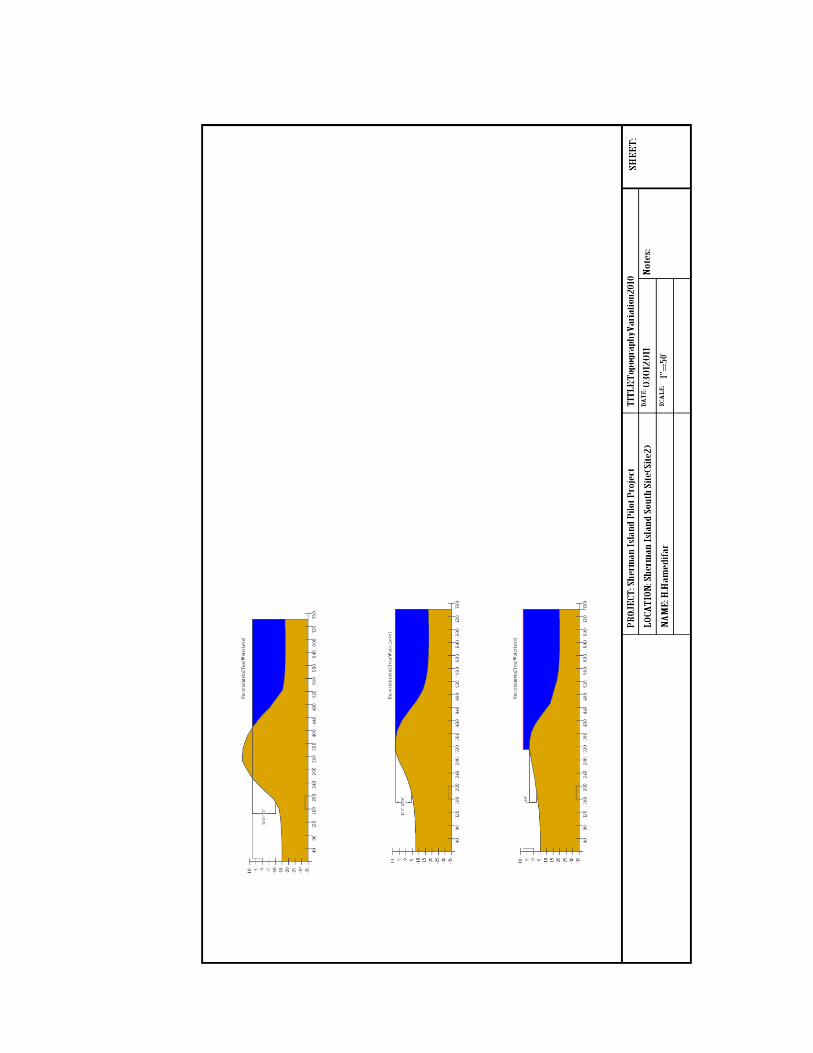
308

309

310

311
APPENDIX L: Delta Risk Management Strategy, Permeability Data
Table L.1: Reported Permeability Data for Organic Soils (Source: HLA 1989, 1992)
Soil Type kh (cm/s) kv(cm/s) Test Type Location Sampling
detail
Black peat (PT) with fat clay 2.4 x 10⁻⁷ - Lab test Levee, Bacon
Island 1988, Sample depth = 22 ft
Black peat (PT) with fat clay 7.2 x 10⁻⁷ - Lab test Levee, Web Tract 1988, Sample
depth = 25 ft
Black Peat (PT) 4.7 x 10⁻⁶ 1.3 x 10⁻⁶
Falling head
lab test
Wilkerson Dam- Test-fill Bouldin
Island
1989, Sample depth = 9 ft
Black Peat (PT) 5.5 x 10⁻⁶ 7.6 x 10⁻⁶
Falling head
lab test
Wilkerson Dam- Test-fill Bouldin
Island
1989, Sample depth = 4 ft
Black Silty Peat (PT) 1.5 x 10⁻⁶ 2.1 x 10⁻⁶
Falling head
lab test Wilkerson Dam- Bouldin Island
1989, Sample depth = 4 ft
Black Silty Peat (PT) - 7.5x 10⁻⁶
Falling head lab test
Wilkerson Dam- Bouldin Island
1989, Sample depth = 5 ft
Black Silty Peat (PT) 1.9 x 10⁻⁶ 9.7 x 10⁻⁷
Falling head
lab test Wilkerson Dam- Bouldin Island
1989, Sample depth = 11 ft
Black Silty Peat (PT) 2.6 x 10⁻⁶ 1.8 x 10⁻⁷
Falling head
lab test Wilkerson Dam- Bouldin Island
1989, Sample depth = 10 ft
Black Silty Peat (PT) 8.8 x 10⁻⁷ 1.5 x 10⁻⁶
Falling head
lab test Wilkerson Dam- Bouldin Island
1989, Sample depth = 5 ft
Brown elastic silt w/ peat (MH) 1.2 x 10⁻⁶
3.2 x 10⁻⁷ Falling head lab test
Wilkerson Dam- Bouldin Island
1989, Sample depth = 8 ft
Black organic silt (OH) contains peat
5.7 x 10⁻⁷
Falling head lab test
Wilkerson Dam- Bouldin Island
1989, Sample depth = 15 ft
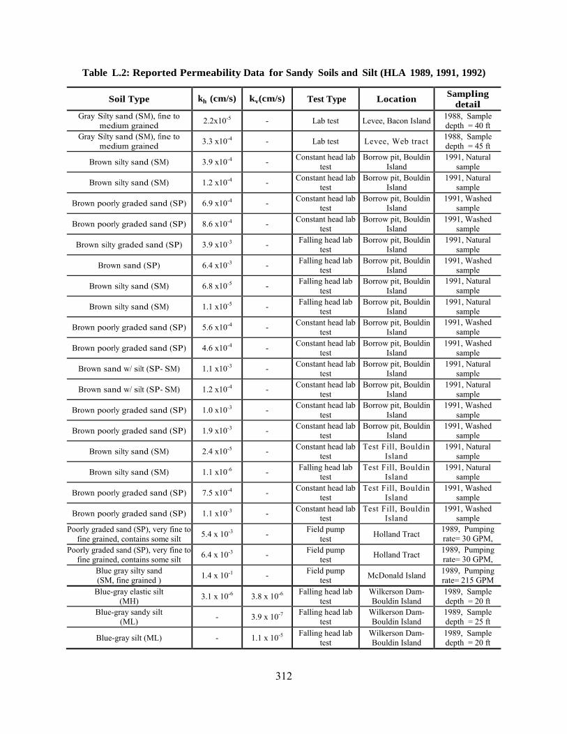
312
Table L.2: Reported Permeability Data for Sandy Soils and Silt (HLA 1989, 1991, 1992)
Soil Type kh (cm/s) kv(cm/s) Test Type Location Sampling
detail
Gray Silty sand (SM), fine to medium grained 2.2x10⁻⁵ - Lab test Levee, Bacon Island 1988, Sample
depth = 40 ft Gray Silty sand (SM), fine to
medium grained 3.3 x10⁻⁴ - Lab test Levee, Web tract 1988, Sample depth = 45 ft
Brown silty sand (SM) 3.9 x10⁻⁴ - Constant head lab test
Borrow pit, Bouldin Island
1991, Natural sample
Brown silty sand (SM) 1.2 x10⁻⁴ - Constant head lab test
Borrow pit, Bouldin Island
1991, Natural sample
Brown poorly graded sand (SP) 6.9 x10⁻⁴ - Constant head lab test
Borrow pit, Bouldin Island
1991, Washed sample
Brown poorly graded sand (SP) 8.6 x10⁻⁴ - Constant head lab test
Borrow pit, Bouldin Island
1991, Washed sample
Brown silty graded sand (SP) 3.9 x10⁻³ - Falling head lab test
Borrow pit, Bouldin Island
1991, Natural sample
Brown sand (SP) 6.4 x10⁻³ - Falling head lab test
Borrow pit, Bouldin Island
1991, Washed sample
Brown silty sand (SM) 6.8 x10⁻⁵ - Falling head lab test
Borrow pit, Bouldin Island
1991, Natural sample
Brown silty sand (SM) 1.1 x10⁻⁵ - Falling head lab
test Borrow pit, Bouldin
Island 1991, Natural
sample
Brown poorly graded sand (SP) 5.6 x10⁻⁴ - Constant head lab test
Borrow pit, Bouldin Island
1991, Washed sample
Brown poorly graded sand (SP) 4.6 x10⁻⁴ - Constant head lab
test Borrow pit, Bouldin
Island 1991, Washed
sample
Brown sand w/ silt (SP- SM) 1.1 x10⁻³ - Constant head lab test
Borrow pit, Bouldin Island
1991, Natural sample
Brown sand w/ silt (SP- SM) 1.2 x10⁻⁴ - Constant head lab test
Borrow pit, Bouldin Island
1991, Natural sample
Brown poorly graded sand (SP) 1.0 x10⁻³ - Constant head lab test
Borrow pit, Bouldin Island
1991, Washed sample
Brown poorly graded sand (SP) 1.9 x10⁻³ - Constant head lab test
Borrow pit, Bouldin Island
1991, Washed sample
Brown silty sand (SM) 2.4 x10⁻⁵ - Constant head lab test
Test Fill, Bouldin Island
1991, Natural sample
Brown silty sand (SM) 1.1 x10⁻⁶ - Falling head lab test
Test Fill, Bouldin Island
1991, Natural sample
Brown poorly graded sand (SP) 7.5 x10⁻⁴ - Constant head lab test
Test Fill, Bouldin Island
1991, Washed sample
Brown poorly graded sand (SP) 1.1 x10⁻³ - Constant head lab test
Test Fill, Bouldin Island
1991, Washed sample
Poorly graded sand (SP), very fine to fine grained, contains some silt 5.4 x 10⁻³ - Field pump
test Holland Tract 1989, Pumping rate= 30 GPM, Depth =20 ft Poorly graded sand (SP), very fine to
fine grained, contains some silt 6.4 x 10⁻³ - Field pump test Holland Tract 1989, Pumping
rate= 30 GPM, Depth =30 ft Blue gray silty sand
(SM, fine grained ) 1.4 x 10⁻¹ - Field pump test McDonald Island 1989, Pumping
rate= 215 GPM Blue-gray elastic silt
(MH) 3.1 x 10⁻⁶ 3.8 x 10⁻⁶ Falling head lab test
Wilkerson Dam- Bouldin Island
1989, Sample depth = 20 ft
Blue-gray sandy silt (ML) - 3.9 x 10⁻⁷ Falling head lab
test Wilkerson Dam- Bouldin Island
1989, Sample depth = 25 ft
Blue-gray silt (ML) - 1.1 x 10⁻⁵ Falling head lab test
Wilkerson Dam- Bouldin Island
1989, Sample depth = 20 ft

313
Table L.3 Permeability Coefficients Used for Initial Seepage Analysis
Material kh (cm/s)
kh/kv Mean - σ Mean Mean + σ
Fill
CL-ML (fill) - 1 x 10⁻⁵ - 4
SM (fill) - 1 x 10⁻³ - 4
Peats & Organics
Free Field 1 x 10⁻⁵ 1 x 10⁻⁴ 1 x 10⁻³ 10
Under Levee 1 x 10⁻⁶ 1 x 10⁻⁵ 1 x 10⁻⁴ 10
Other Foundation Soils
Sand (SM/SP) 5 x 10⁻⁴ 1 x 10⁻³ 5 x 10⁻³ 4
ML - 1 x 10⁻⁴ - 4
CL - 1 x 10⁻⁶ - 4
Sediment
(at slough bottom) - 1 x 10⁻⁵ - 1
Table L.4 Evaluated Permeability Coefficients Used for Model Analyses
Material kh (cm/s)
kh/kv Mean - σ Mean Mean + σ
Fill
SM (fill) - 1 x 10⁻³ - 4
Peats & Organics
Free Field 1 x 10⁻⁵ 1 x 10⁻⁴ 1 x 10⁻³ 100
Under Levee 1 x 10⁻⁶ 1 x 10⁻⁵ 1 x 10⁻⁴ 100
Other Foundation Soils
Sand (SM/SP) - 1 x 10⁻³ - 4
CL - 1 x 10⁻⁶ - 4
Sediment
(at slough bottom) - 1 x 10⁻⁵ - 1

314
Table L.5 Initial Analysis Results for Terminus Tract
Slough
Water
Elevation
(ft)
[NAVD88]
Analysis Case-
Permeability
Ditch No Ditch
Remarks iy below
ditch
(Point A)
Ave. iy @
Point B
iy
(near toe )
Ave. iy
@Point B
0 4 7
kmean kmean kmean
0.46 0.64 0.75
0.17 0.24 0.29
0.22 0.30 0.36
0.178 0.249 0.301
model with sediment model with sediment model with sediment
0 4 7
k(mean-cr)peat k(mean-cr)peat k(mean-cr)peat
0.57 0.82
1
0.25 0.38 0.47
-
-
model with sediment model with sediment model with sediment
0 4 7
k(mean+cr)peat k(mean+cr)peat k(mean+cr)peat
0.26 0.36 0.42
0.05 0.07 0.08
-
-
model with sediment model with sediment model with sediment
0 4 7
k(mean-cr) sand k(mean-cr) sand k(mean-cr) sand
0.44 0.6 0.7
0.14 0.20 0.24
-
-
model with sediment model with sediment model with sediment
0 4 7
k(mean+cr) sand k(mean+cr) sand k(mean+cr) sand
0.25 0.41 0.52
0.07 0.15 0.21
-
-
model with sediment model with sediment model with sediment
0 4 7
kmean kmean kmean
0.58 0.79 0.94
0.22 0.31 0.38
-
-
model without sediment model without sediment model without sediment
Table L.6: Estimated Vertical Gradients for Grand Island Under-seepage Problem
(kh/kv)peat Analysis Case: No Ditch & No Sediment
Ave. iy near toe Ave. iy at Point B
10 0.42 0.26
100 0.59 0.50
1000 0.63 0.56
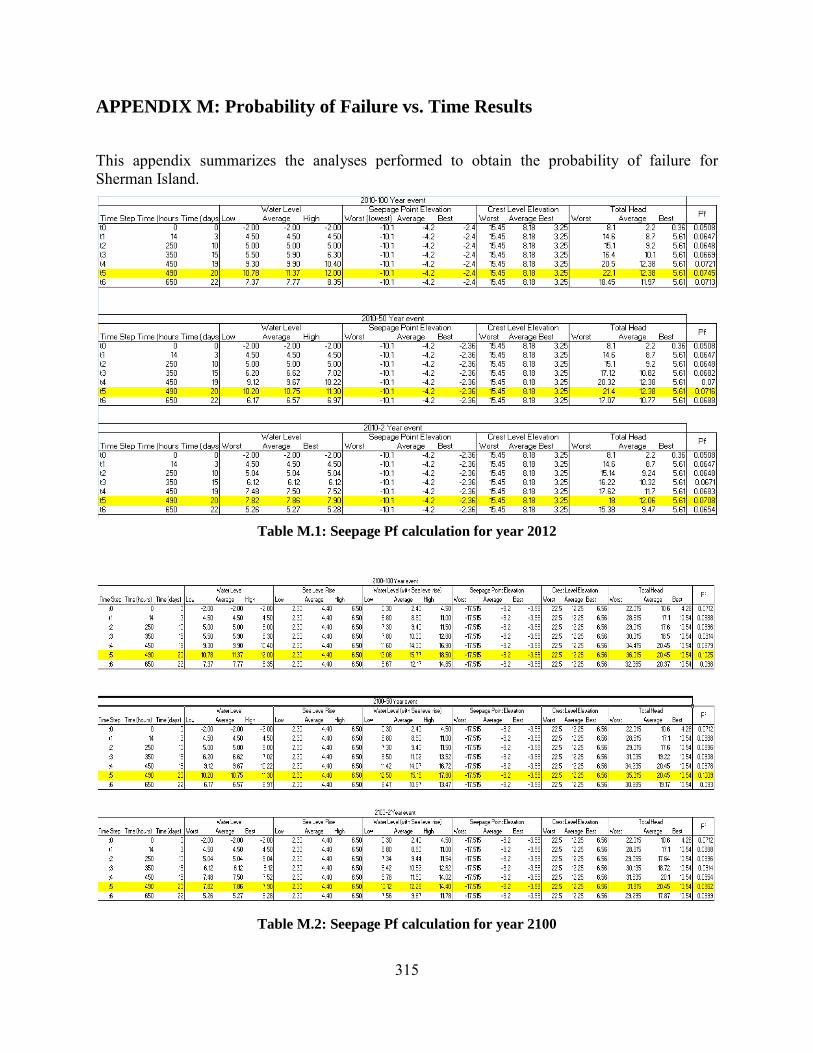
315
APPENDIX M: Probability of Failure vs. Time Results
This appendix summarizes the analyses performed to obtain the probability of failure for Sherman Island.
Table M.1: Seepage Pf calculation for year 2012
Table M.2: Seepage Pf calculation for year 2100

316
Figure M.3: Probability of Failure as a Function of Time for the Seepage Analyses
0.05
0.055
0.06
0.065
0.07
0.075
0 5 10 15 20 25
Pro
bab
ility
of
Failu
re
Time (Days)
2010 Pf vs. Time
100 Year
50 Year
2 Year
0.07
0.075
0.08
0.085
0.09
0.095
0.1
0.105
0 5 10 15 20 25
Pro
bab
ility
of
Failu
re
Time (Days)
2100 Pf vs. Time
100 Year
50 Year
2 Year

317
Figure M.4: Seepage Pf vs. Time with application of ODAA loop
0.05
0.055
0.06
0.065
0.07
0.075
0 5 10 15 20 25
Pro
bab
ility
of
Failu
re
Time (Days)
Seepage is Noticed (observe)
Orient
Decide
Action is taken (i.e Sandbag Ring)
System reevaluated
Alternate path of system due to human intervention
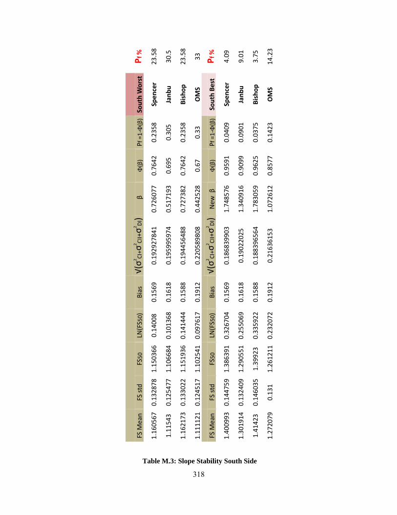
318
Table M.3: Slope Stability South Side
FS M
ean
FS s
td
FS5
0
LN(F
S 50)
Bia
s √(σ
2C
I+σ
2C
II+σ
2D
I)
β
Φ(β)
Pf
=1- Φ
(β) S
ou
th W
ors
t P
f %
1.1
60
56
7
0.1
32
87
8
1.1
50
36
6
0.1
40
08
0.1
56
9
0.1
92
92
78
41
0.7
26
07
7
0.7
64
2
0.2
35
8
Spe
nce
r 2
3.5
8
1.1
15
43
0.1
25
47
7
1.1
06
68
4
0.1
01
36
8
0.1
61
8
0.1
95
99
59
74
0.5
17
19
3
0.6
95
0.3
05
Jan
bu
30
.5
1.1
62
17
3
0.1
33
02
2
1.1
51
93
6
0.1
41
44
4
0.1
58
8
0.1
94
45
64
88
0.7
27
38
2
0.7
64
2
0.2
35
8
Bis
ho
p
23
.58
1.1
11
12
1
0.1
24
51
7
1.1
02
54
1
0.0
97
61
7
0.1
91
2
0.2
20
58
98
08
0.4
42
52
8
0.6
7
0.3
3
OM
S 3
3
FS M
ean
FS s
td
FS5
0
LN(F
S 50)
Bia
s √(σ
2C
I+σ
2C
II+σ
2D
I)
New
β
Φ(β)
Pf
=1- Φ
(β)
Sou
th B
est
Pf
%
1.4
00
99
3
0.1
44
75
9
1.3
86
39
1
0.3
26
70
4
0.1
56
9
0.1
86
83
99
03
1.7
48
57
6
0.9
59
1
0.0
40
9
Spe
nce
r 4
.09
1.3
01
91
4
0.1
32
40
9
1.2
90
55
1
0.2
55
06
9
0.1
61
8
0.1
90
22
02
5
1.3
40
91
6
0.9
09
9
0.0
90
1
Jan
bu
9.0
1
1.4
14
23
0.1
46
03
5
1.3
99
23
0.3
35
92
2
0.1
58
8
0.1
88
39
65
64
1.7
83
05
9
0.9
62
5
0.0
37
5
Bis
ho
p
3.7
5
1.2
72
07
9
0.1
31
1.2
61
21
1
0.2
32
07
2
0.1
91
2
0.2
16
36
15
3
1.0
72
61
2
0.8
57
7
0.1
42
3
OM
S 1
4.2
3
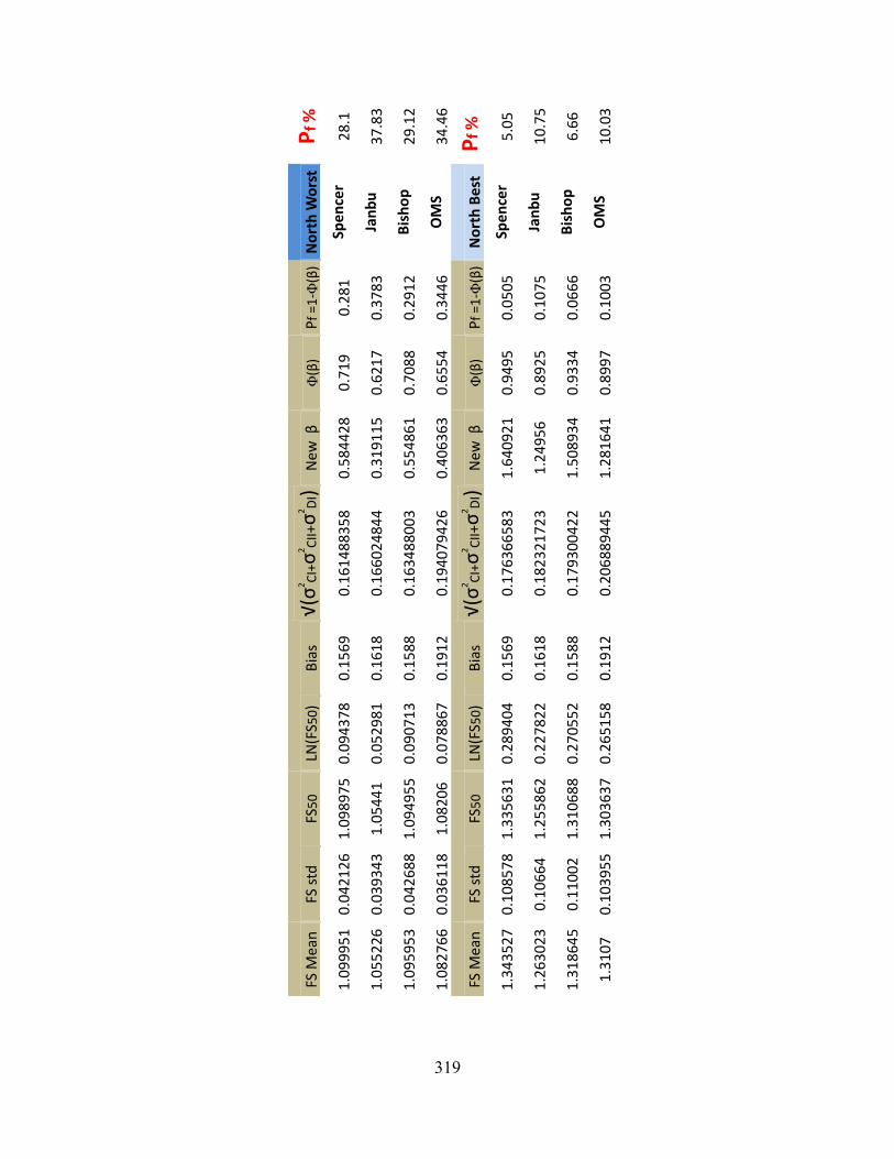
319
FS M
ean
FS s
td
FS5
0
LN(F
S 50)
Bia
s √(σ
2C
I+σ
2C
II+σ
2D
I)
New
β
Φ(β)
Pf
=1- Φ
(β) N
ort
h W
ors
t P
f %
1.0
99
95
1
0.0
42
12
6
1.0
98
97
5
0.0
94
37
8
0.1
56
9
0.1
61
48
83
58
0.5
84
42
8
0.7
19
0.2
81
Spe
nce
r 2
8.1
1.0
55
22
6
0.0
39
34
3
1.0
54
41
0.0
52
98
1
0.1
61
8
0.1
66
02
48
44
0.3
19
11
5
0.6
21
7
0.3
78
3
Jan
bu
37
.83
1.0
95
95
3
0.0
42
68
8
1.0
94
95
5
0.0
90
71
3
0.1
58
8
0.1
63
48
80
03
0.5
54
86
1
0.7
08
8
0.2
91
2
Bis
ho
p
29
.12
1.0
82
76
6
0.0
36
11
8
1.0
82
06
0.0
78
86
7
0.1
91
2
0.1
94
07
94
26
0.4
06
36
3
0.6
55
4
0.3
44
6
OM
S 3
4.4
6
FS M
ean
FS s
td
FS5
0
LN(F
S 50)
Bia
s √(σ
2C
I+σ
2C
II+σ
2D
I)
New
β
Φ(β)
Pf
=1- Φ
(β)
No
rth
Be
st
Pf
%
1.3
43
52
7
0.1
08
57
8
1.3
35
63
1
0.2
89
40
4
0.1
56
9
0.1
76
36
65
83
1.6
40
92
1
0.9
49
5
0.0
50
5
Spe
nce
r 5
.05
1.2
63
02
3
0.1
06
64
1.2
55
86
2
0.2
27
82
2
0.1
61
8
0.1
82
32
17
23
1.2
49
56
0.8
92
5
0.1
07
5
Jan
bu
10
.75
1.3
18
64
5
0.1
10
02
1.3
10
68
8
0.2
70
55
2
0.1
58
8
0.1
79
30
04
22
1.5
08
93
4
0.9
33
4
0.0
66
6
Bis
ho
p
6.6
6
1.3
10
7
0.1
03
95
5
1.3
03
63
7
0.2
65
15
8
0.1
91
2
0.2
06
88
94
45
1.2
81
64
1
0.8
99
7
0.1
00
3
OM
S 1
0.0
3
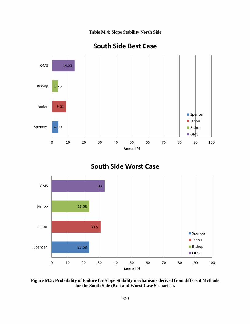
320
Table M.4: Slope Stability North Side
Figure M.5: Probability of Failure for Slope Stability mechanisms derived from different Methods
for the South Side (Best and Worst Case Scenarios).
4.09
9.01
3.75
14.23
0 10 20 30 40 50 60 70 80 90 100
Spencer
Janbu
Bishop
OMS
Annual Pf
South Side Best Case
Spencer
Janbu
Bishop
OMS
23.58
30.5
23.58
33
0 10 20 30 40 50 60 70 80 90 100
Spencer
Janbu
Bishop
OMS
Annual Pf
South Side Worst Case
Spencer
Janbu
Bishop
OMS
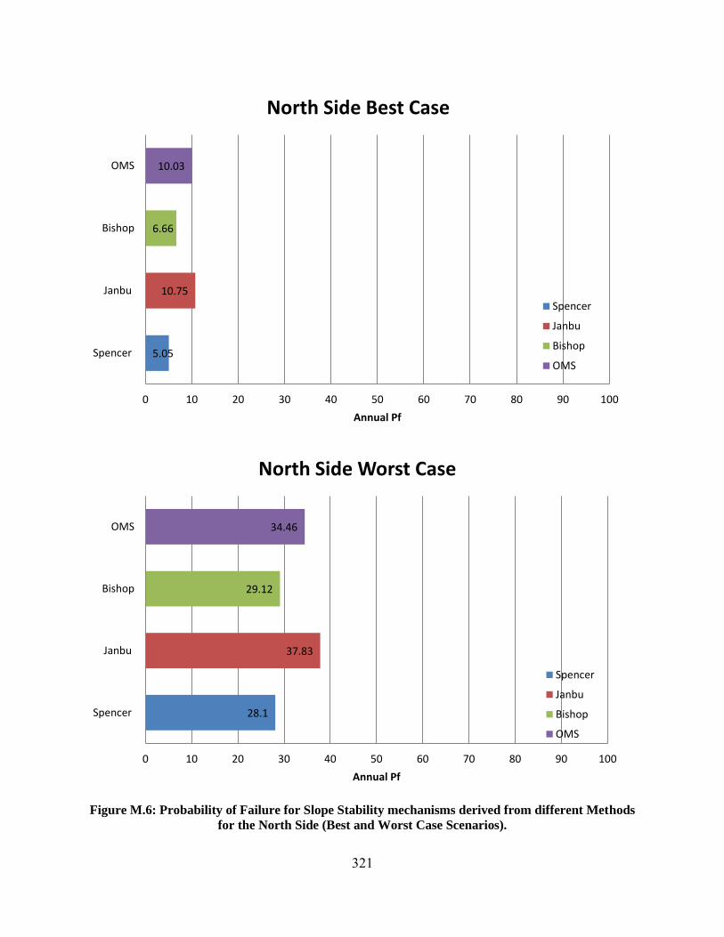
321
Figure M.6: Probability of Failure for Slope Stability mechanisms derived from different Methods
for the North Side (Best and Worst Case Scenarios).
5.05
10.75
6.66
10.03
0 10 20 30 40 50 60 70 80 90 100
Spencer
Janbu
Bishop
OMS
Annual Pf
North Side Best Case
Spencer
Janbu
Bishop
OMS
28.1
37.83
29.12
34.46
0 10 20 30 40 50 60 70 80 90 100
Spencer
Janbu
Bishop
OMS
Annual Pf
North Side Worst Case
Spencer
Janbu
Bishop
OMS

322
Table M.5: Probability of Failure due to Overtopping for Current and Future Conditions
Current Conditions-2010 Future Conditions-2100
Sections Pf =1-Φ(β) Pf (%) Pf =1-Φ(β) Pf (%)
South 9 0.005579 0.557878 0.012517 1.251741
North 1 0.002086 0.208619 0.000273 0.027311
South 8 0.003941 0.394081 0.00563 0.563004
South 7 0.000301 0.030064 9.54E-05 0.009544
South 6 8.52E-05 0.008523 1.03E-05 0.001035
North 5 0.001275 0.127513 0.000359 0.035859
North 4 3.27E-05 0.003275 7.1E-07 7.1E-05
North 3 0.000325 0.032546 6.21E-05 0.006209
North 2 0.000434 0.043371 2.02E-05 0.002022
North 11 0.046933 4.693297 0.031472 3.147173
South 10 0.005106 0.510631 0.013545 1.354524

323
Figure M.7: Probability of Overtopping for sections along the levee protecting Sherman Island for
Current Conditions
0 0.5 1 1.5 2 2.5 3 3.5 4 4.5 5
South 9
North 1
South 8
South 7
South 6
North 5
North 4
North 3
North 2
North 11
South 10
Anuual Pf%
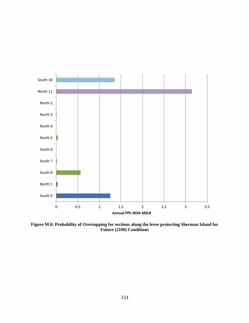
324
Figure M.8: Probability of Overtopping for sections along the levee protecting Sherman Island for
Future (2100) Conditions
0 0.5 1 1.5 2 2.5 3 3.5
South 9
North 1
South 8
South 7
South 6
North 5
North 4
North 3
North 2
North 11
South 10
Annual Pf% With MSLR

325
APPENDIX N: Matlab® Code
N.1 EFFECTIVE STRESS MONTE CARLO SIMULATION
function pf = effectivestress(nnumber)
%Failure will be defined when effective stress is less than or equal to 0
%sigma' = d(g_soil - g_water) - i*d*g_water
%Monte Carlo Simulation for Sigma'
%Number of samples = 'nnumber'
%Define Random Variables
%d - depth
%g_soil - saturated unit weight of soil
%g_water - unit weight of water
% i - exit gradient at point of interest
% i=h/(N*b)
% Random Variable Input Parameters
b_min = 10;
b_mode = 28;
b_max = 53;
gw_min =61.3;
gw_mode =62.4;
gw_max = 64.1;
h_min = 10.54;
h_mode = 20.5;
h_max = 31.915;
gs_mean =4.579991;
gs_std = 0.223878;
% Bias term for pore pressure model
b_mean = -0.12514;
b_std = 0.07308;
D=[];
C=[];
i=[];
tic
for j = 1:nnumber
b = trirnd(b_min,b_mode,b_max,1);
gamma_water = trirnd(gw_min,gw_mode,gw_max,1);
gamma_sat = lognrnd(gs_mean,gs_std);
h = trirnd(h_min,h_mode,h_max,1);
Nd = 7;
i(j) = (h+b/2)/(Nd*b);

326
d=b/2;
beta = lognrnd(b_mean,b_std);
C(j) = (gamma_sat);
D(j) = (i(j)*beta+1)*gamma_water;
end
toc
%Scale histogram to PDF of D
[t,y]=hist(D,100);
w=abs(y(2)-y(1));
area=sum(w.*t);
scale_factor=1/(w*nnumber);
pdf_D=t*scale_factor;
bar(y,pdf_D,'r');
new_area_D=w*sum(pdf_D)
hold
%Develop a continuous PDF for D (Lognormal)
mu_D = mean(log(D));
s_D = std(log(D));
pdf = lognpdf(sort(D),mu_D,s_D);
plot(sort(D),pdf,'r-')
figure
%Scale histogram of PDF of C
[t,y]= hist(C,100);
w=abs(y(2)-y(1));
area = sum(w.*t);
scale_factor = 1/(w*nnumber);
pdf_C = t*scale_factor;
bar(y,pdf_C,'b')
new_area_C = w*sum(pdf_C)
hold
%Develop a continuous PDF for C (Lognormal)
mu_C = mean(log(C));
s_C = std(log(C));
pdf_C = lognpdf(sort(C),mu_C,s_C);
plot(sort(C),pdf_C,'b-');
Mean_c = mean(C);
S_c = std(C);
v_c = var(C);
Mean_d = mean(D);
S_d = std(D);
v_d = var(D);
%plot
figure
plot(sort(D),pdf,'r')
hold
plot(sort(C),pdf_C,'b-')

327
%Determining Probability of Failure counts the number of times effective
stress was less than zero and divides it by the number of samples.
m1 = polyfit([x1 x2],[y1 y2],1);
m2 = polyfit([x2 x3],[y2 y3],1);
pf = length(find(D>C))/nnumber

328
N. 2 PORE PRESSURE MONTE CARLO SIMULATION (FOR MODEL BIAS
CORRECTION)
function u = pore(nnumber,h)
%Failure will be defined when effective stress is less than or equal to 0
%sigma' = d(g_soil - g_water) - i*d*g_water
%Monte Carlo Simulation for Sigma'
%Number of samples = 'nnumber'
%Define Random Variables
%d - depth
%g_soil - saturated unit weight of soil
%g_water - unit weight of water
% i - exit gradient at point of interest
% i=h/(N*b)
% Random Variable Input Parameters
b_min = 9;
b_mode = 16;
b_max = 76;
gw_min =61.3;
gw_mode =62.4;
gw_max = 64.1;
Nd=7;
U=[];
for j = 1:nnumber
b = trirnd(b_min,b_mode,b_max,1);
gamma_water = trirnd(gw_min,gw_mode,gw_max,1);
i(j) = h/(Nd*b);
d=b/2;
U(j) = ((i(j)+1)*gamma_water*h)/144;
end
%Scale histogram to PDF of D
[t,y]=hist(U,100);
w=abs(y(2)-y(1));
area=sum(w.*t);
scale_factor=1/(w*nnumber);
pdf_U=t*scale_factor;
bar(y,pdf_U,'r');
new_area_U=w*sum(pdf_U)
hold
u=mean(U);

329
APPENDIX O: Soil Statistical Boring Log Data
102
103
104
0.0050.01
0.05
0.1
0.25
0.5
0.75
0.9
0.95
0.990.995
Data
Pro
babili
ty
Probability plot for Lognormal distribution
500 1000 1500 20000
0.2
0.4
0.6
0.8
1
1.2x 10
-3

330
102
103
104
0.0050.01
0.05
0.1
0.25
0.5
0.75
0.9
0.95
0.990.995
Data
Pro
babili
tyProbability plot for Lognormal distribution
0 500 1000 15000
0.2
0.4
0.6
0.8
1
1.2
1.4
1.6
1.8
2x 10
-3
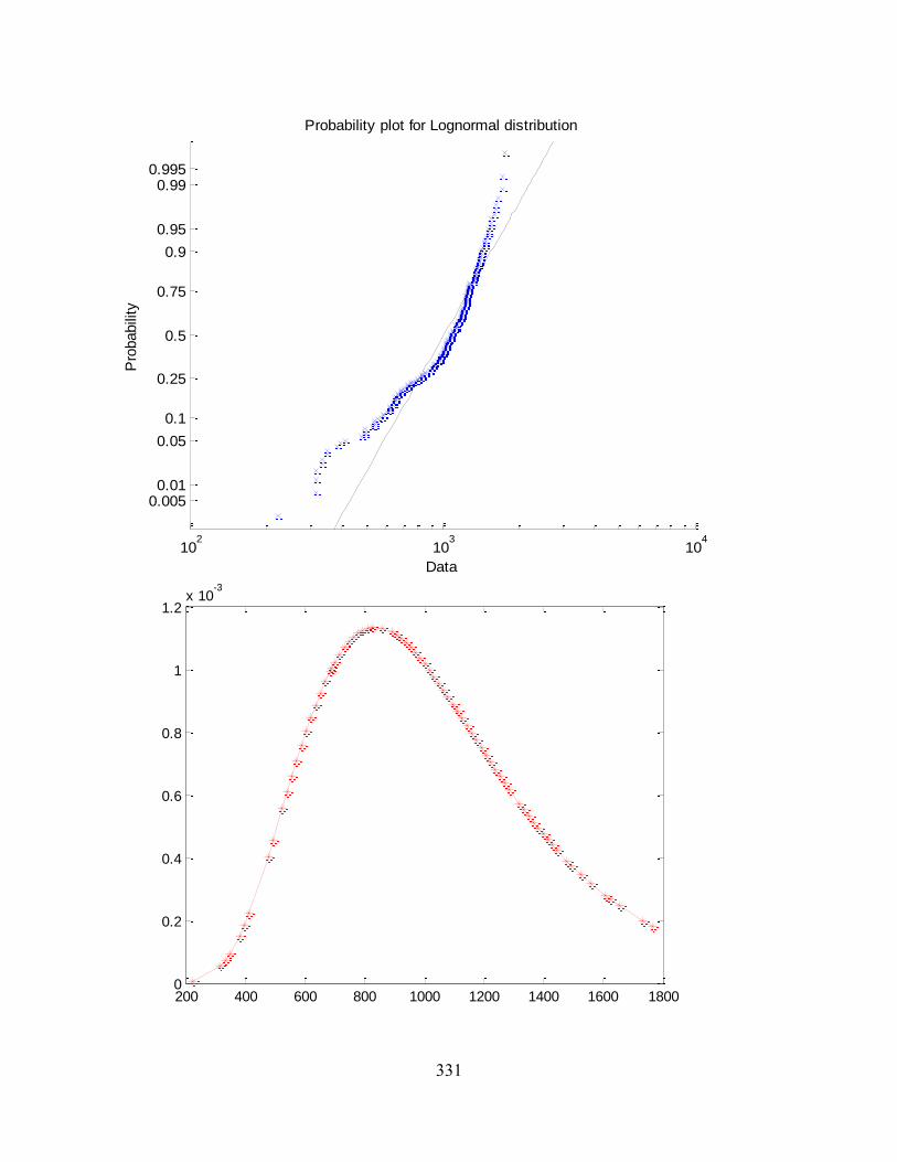
331
102
103
104
0.0050.01
0.05
0.1
0.25
0.5
0.75
0.9
0.95
0.990.995
Data
Pro
babili
tyProbability plot for Lognormal distribution
200 400 600 800 1000 1200 1400 1600 18000
0.2
0.4
0.6
0.8
1
1.2x 10
-3

332
103
0.0050.01
0.05
0.1
0.25
0.5
0.75
0.9
0.95
0.990.995
Data
Pro
babili
tyProbability plot for Lognormal distribution
1000 1200 1400 1600 1800 2000 22000
0.2
0.4
0.6
0.8
1
1.2
1.4
1.6
1.8
2x 10
-3

333
APPENDIX P: Photos of Storm Events
Figure P.1: Overtopping of levee, taken on Jan. 1, 2006 on Sherman Island levee adjacent to the
San Joaquin River during high winds and High tide.
Figure P.2 Overtopping of levee, taken on Jan. 1, 2006 on Sherman Island levee adjacent to the San
Joaquin River during high winds and High tide.

334
Figure P.3 Overtopping of levee, taken on Jan. 1, 2006 on Sherman Island levee adjacent to the San
Joaquin River during high winds and High tide.
Figure P.4: Overtopping of levee, taken on Jan. 1, 2006 on Sherman Island levee adjacent to the
San Joaquin River during high winds and High tide (land side)

335
Figure P.5: Overtopping of levee, taken on Jan. 1, 2006 on Sherman Island levee adjacent to the
San Joaquin River during high winds and High tide (land side)

336
Figure P.6: Overtopping of levee, taken on Feb. 7, 1998 on Sherman Island levee adjacent to the
San Joaquin River during high winds and High tide

337
Figure P.7: Overtopping and Water side erosion of levee, taken on Feb. 7, 1998 on Sherman Island
levee adjacent to the San Joaquin River during high winds and High tide.

338
Figure P.8: Overtopping and Water side erosion of levee, taken on Feb. 7, 1998 on Sherman Island
levee adjacent to the San Joaquin River during high winds and High tide

339
APPENDIX Q: Table of Standard Normal Probabilities
( ) ( ) ∫ ( )
β (+) 0 0.01 0.02 0.03 0.04 0.05 0.06 0.07 0.08 0.09 0 0.5 0.504 0.508 0.512 0.516 0.5199 0.5239 0.5279 0.5319 0.5359
0.1 0.5398 0.5438 0.5478 0.5517 0.5557 0.5596 0.5636 0.5675 0.5714 0.5753 0.2 0.5793 0.5832 0.5871 0.591 0.5948 0.5987 0.6026 0.6064 0.6103 0.6141 0.3 0.6179 0.6217 0.6255 0.6293 0.6331 0.6368 0.6406 0.6443 0.648 0.6517 0.4 0.6554 0.6591 0.6628 0.6664 0.67 0.6736 0.6772 0.6808 0.6844 0.6879 0.5 0.6915 0.695 0.6985 0.7019 0.7054 0.7088 0.7123 0.7157 0.719 0.7224 0.6 0.7257 0.7291 0.7324 0.7357 0.7389 0.7422 0.7454 0.7486 0.7517 0.7549 0.7 0.758 0.7611 0.7642 0.7673 0.7704 0.7734 0.7764 0.7794 0.7823 0.7852 0.8 0.7881 0.791 0.7939 0.7967 0.7995 0.8023 0.8051 0.8078 0.8106 0.8133 0.9 0.8159 0.8186 0.8212 0.8238 0.8264 0.8289 0.8315 0.834 0.8365 0.8389
1 0.8413 0.8438 0.8461 0.8485 0.8508 0.8531 0.8554 0.8577 0.8599 0.8621 1.1 0.8643 0.8665 0.8686 0.8708 0.8729 0.8749 0.877 0.879 0.881 0.883 1.2 0.8849 0.8869 0.8888 0.8907 0.8925 0.8944 0.8962 0.898 0.8997 0.9015 1.3 0.9032 0.9049 0.9066 0.9082 0.9099 0.9115 0.9131 0.9147 0.9162 0.9177 1.4 0.9192 0.9207 0.9222 0.9236 0.9251 0.9265 0.9279 0.9292 0.9306 0.9319 1.5 0.9332 0.9345 0.9357 0.937 0.9382 0.9394 0.9406 0.9418 0.9429 0.9441 1.6 0.9452 0.9463 0.9474 0.9484 0.9495 0.9505 0.9515 0.9525 0.9535 0.9545 1.7 0.9554 0.9564 0.9573 0.9582 0.9591 0.9599 0.9608 0.9616 0.9625 0.9633 1.8 0.9641 0.9649 0.9656 0.9664 0.9671 0.9678 0.9686 0.9693 0.9699 0.9706 1.9 0.9713 0.9719 0.9726 0.9732 0.9738 0.9744 0.975 0.9756 0.9761 0.9767
2 0.9772 0.9778 0.9783 0.9788 0.9793 0.9798 0.9803 0.9808 0.9812 0.9817 2.1 0.9821 0.9826 0.983 0.9834 0.9838 0.9842 0.9846 0.985 0.9854 0.9857 2.2 0.9861 0.9864 0.9868 0.9871 0.9875 0.9878 0.9881 0.9884 0.9887 0.989 2.3 0.9893 0.9896 0.9898 0.9901 0.9904 0.9906 0.9909 0.9911 0.9913 0.9916 2.4 0.9918 0.992 0.9922 0.9925 0.9927 0.9929 0.9931 0.9932 0.9934 0.9936 2.5 0.9938 0.994 0.9941 0.9943 0.9945 0.9946 0.9948 0.9949 0.9951 0.9952 2.6 0.9953 0.9955 0.9956 0.9957 0.9959 0.996 0.9961 0.9962 0.9963 0.9964 2.7 0.9965 0.9966 0.9967 0.9968 0.9969 0.997 0.9971 0.9972 0.9973 0.9974 2.8 0.9974 0.9975 0.9976 0.9977 0.9977 0.9978 0.9979 0.9979 0.998 0.9981 2.9 0.9981 0.9982 0.9982 0.9983 0.9984 0.9984 0.9985 0.9985 0.9986 0.9986
3 0.9987 0.9987 0.9987 0.9988 0.9988 0.9989 0.9989 0.9989 0.999 0.999
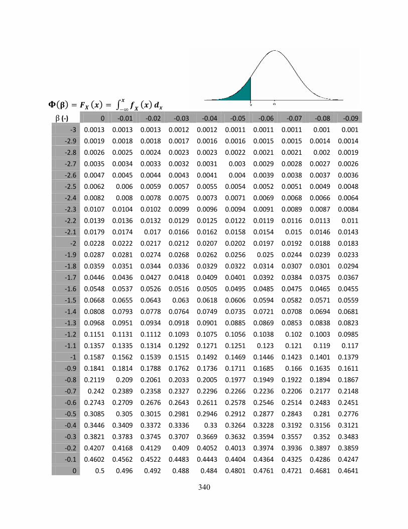
340
( ) ( ) ∫ ( )
β (-) 0 -0.01 -0.02 -0.03 -0.04 -0.05 -0.06 -0.07 -0.08 -0.09
-3 0.0013 0.0013 0.0013 0.0012 0.0012 0.0011 0.0011 0.0011 0.001 0.001
-2.9 0.0019 0.0018 0.0018 0.0017 0.0016 0.0016 0.0015 0.0015 0.0014 0.0014
-2.8 0.0026 0.0025 0.0024 0.0023 0.0023 0.0022 0.0021 0.0021 0.002 0.0019
-2.7 0.0035 0.0034 0.0033 0.0032 0.0031 0.003 0.0029 0.0028 0.0027 0.0026
-2.6 0.0047 0.0045 0.0044 0.0043 0.0041 0.004 0.0039 0.0038 0.0037 0.0036
-2.5 0.0062 0.006 0.0059 0.0057 0.0055 0.0054 0.0052 0.0051 0.0049 0.0048
-2.4 0.0082 0.008 0.0078 0.0075 0.0073 0.0071 0.0069 0.0068 0.0066 0.0064
-2.3 0.0107 0.0104 0.0102 0.0099 0.0096 0.0094 0.0091 0.0089 0.0087 0.0084
-2.2 0.0139 0.0136 0.0132 0.0129 0.0125 0.0122 0.0119 0.0116 0.0113 0.011
-2.1 0.0179 0.0174 0.017 0.0166 0.0162 0.0158 0.0154 0.015 0.0146 0.0143
-2 0.0228 0.0222 0.0217 0.0212 0.0207 0.0202 0.0197 0.0192 0.0188 0.0183
-1.9 0.0287 0.0281 0.0274 0.0268 0.0262 0.0256 0.025 0.0244 0.0239 0.0233
-1.8 0.0359 0.0351 0.0344 0.0336 0.0329 0.0322 0.0314 0.0307 0.0301 0.0294
-1.7 0.0446 0.0436 0.0427 0.0418 0.0409 0.0401 0.0392 0.0384 0.0375 0.0367
-1.6 0.0548 0.0537 0.0526 0.0516 0.0505 0.0495 0.0485 0.0475 0.0465 0.0455
-1.5 0.0668 0.0655 0.0643 0.063 0.0618 0.0606 0.0594 0.0582 0.0571 0.0559
-1.4 0.0808 0.0793 0.0778 0.0764 0.0749 0.0735 0.0721 0.0708 0.0694 0.0681
-1.3 0.0968 0.0951 0.0934 0.0918 0.0901 0.0885 0.0869 0.0853 0.0838 0.0823
-1.2 0.1151 0.1131 0.1112 0.1093 0.1075 0.1056 0.1038 0.102 0.1003 0.0985
-1.1 0.1357 0.1335 0.1314 0.1292 0.1271 0.1251 0.123 0.121 0.119 0.117
-1 0.1587 0.1562 0.1539 0.1515 0.1492 0.1469 0.1446 0.1423 0.1401 0.1379
-0.9 0.1841 0.1814 0.1788 0.1762 0.1736 0.1711 0.1685 0.166 0.1635 0.1611
-0.8 0.2119 0.209 0.2061 0.2033 0.2005 0.1977 0.1949 0.1922 0.1894 0.1867
-0.7 0.242 0.2389 0.2358 0.2327 0.2296 0.2266 0.2236 0.2206 0.2177 0.2148
-0.6 0.2743 0.2709 0.2676 0.2643 0.2611 0.2578 0.2546 0.2514 0.2483 0.2451
-0.5 0.3085 0.305 0.3015 0.2981 0.2946 0.2912 0.2877 0.2843 0.281 0.2776
-0.4 0.3446 0.3409 0.3372 0.3336 0.33 0.3264 0.3228 0.3192 0.3156 0.3121
-0.3 0.3821 0.3783 0.3745 0.3707 0.3669 0.3632 0.3594 0.3557 0.352 0.3483
-0.2 0.4207 0.4168 0.4129 0.409 0.4052 0.4013 0.3974 0.3936 0.3897 0.3859
-0.1 0.4602 0.4562 0.4522 0.4483 0.4443 0.4404 0.4364 0.4325 0.4286 0.4247
0 0.5 0.496 0.492 0.488 0.484 0.4801 0.4761 0.4721 0.4681 0.4641